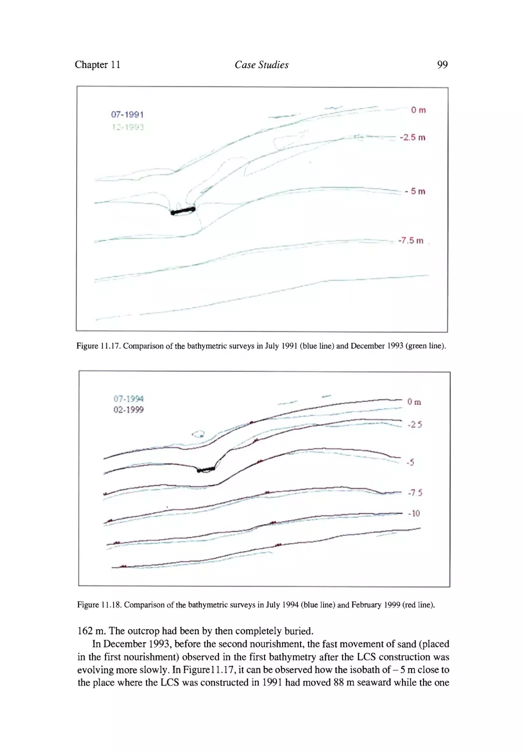
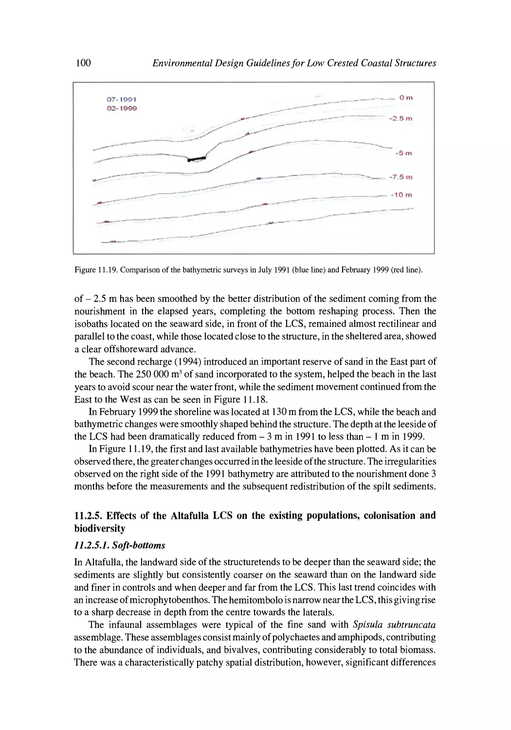
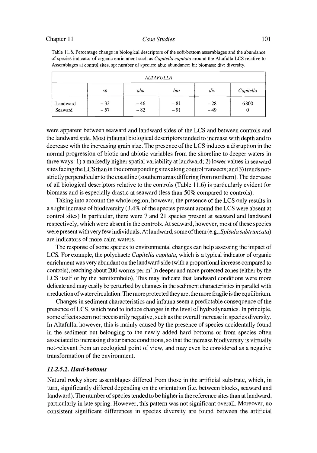
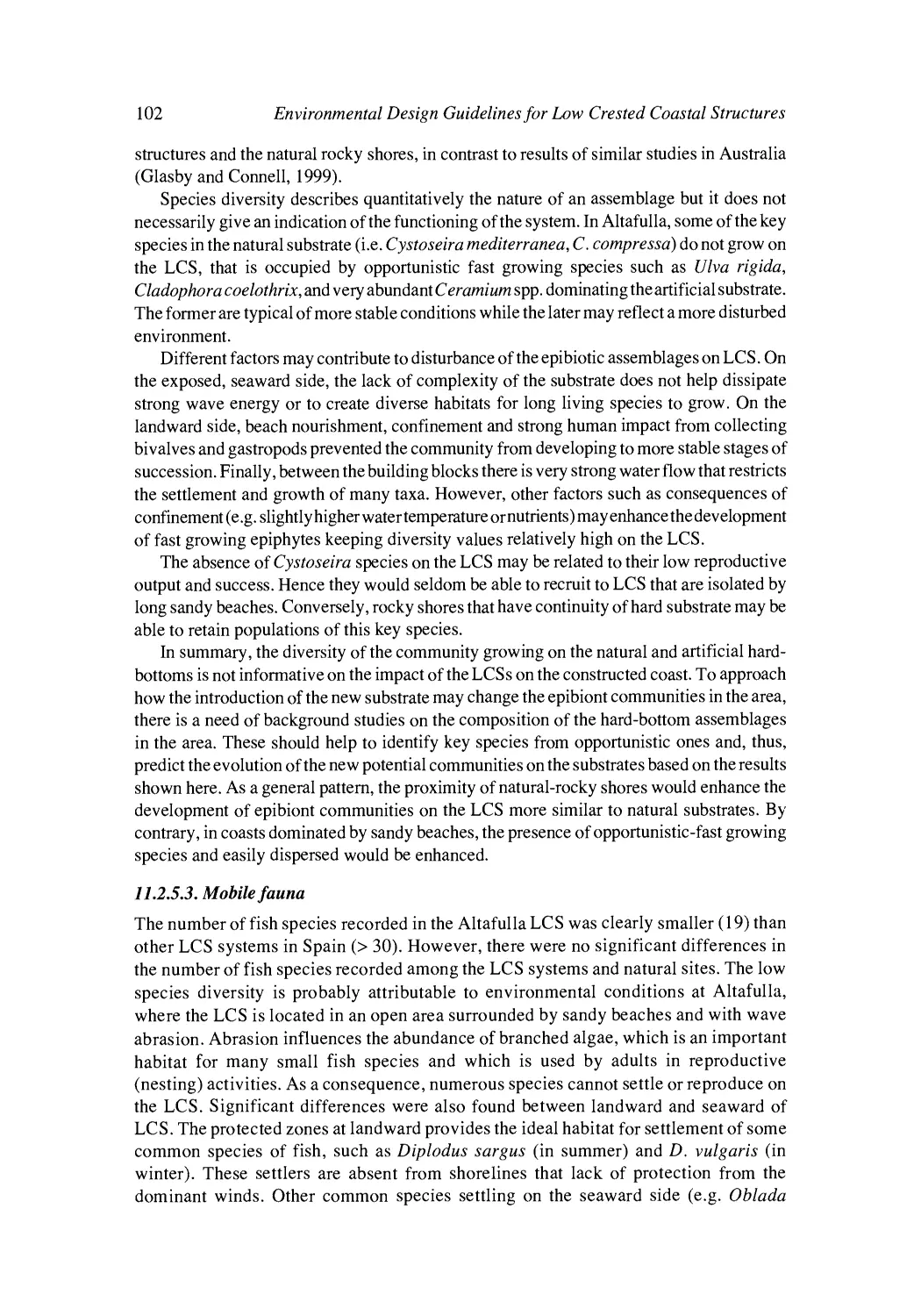
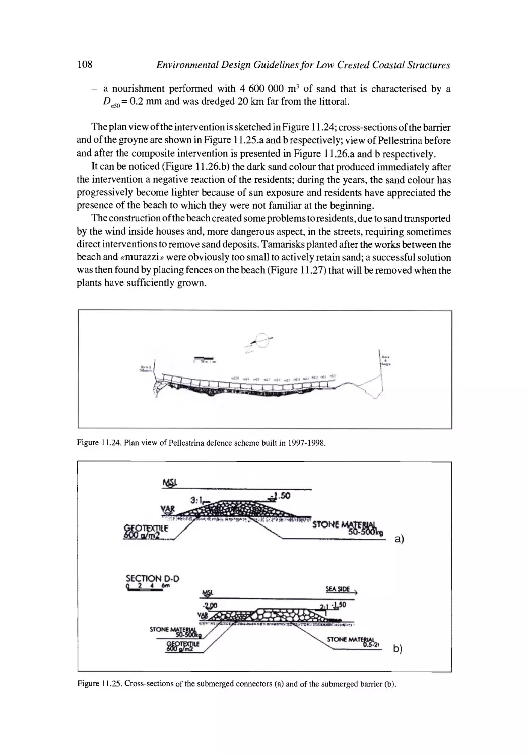
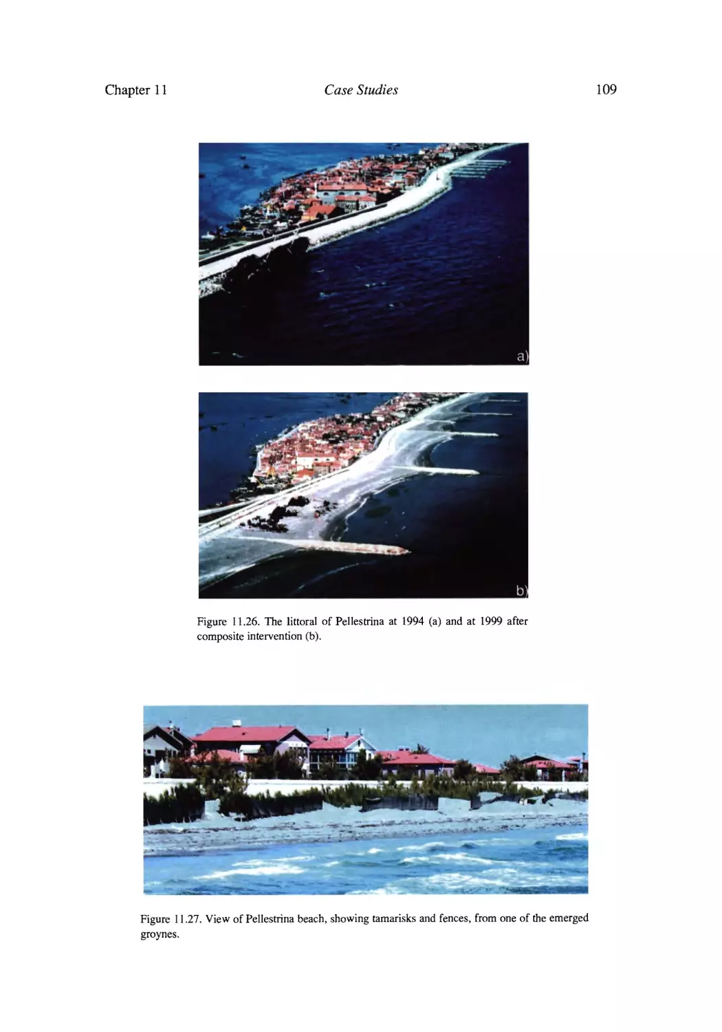
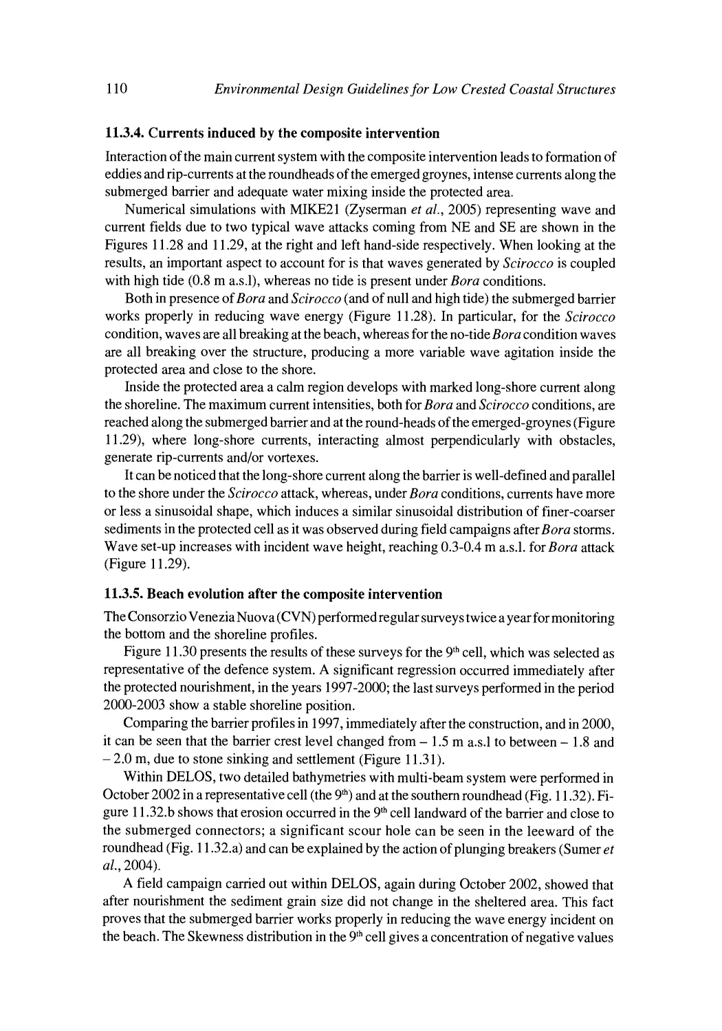
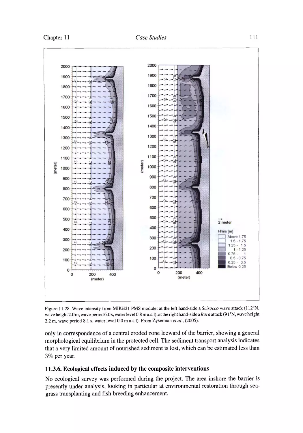
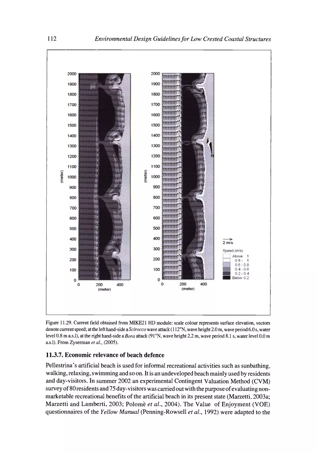
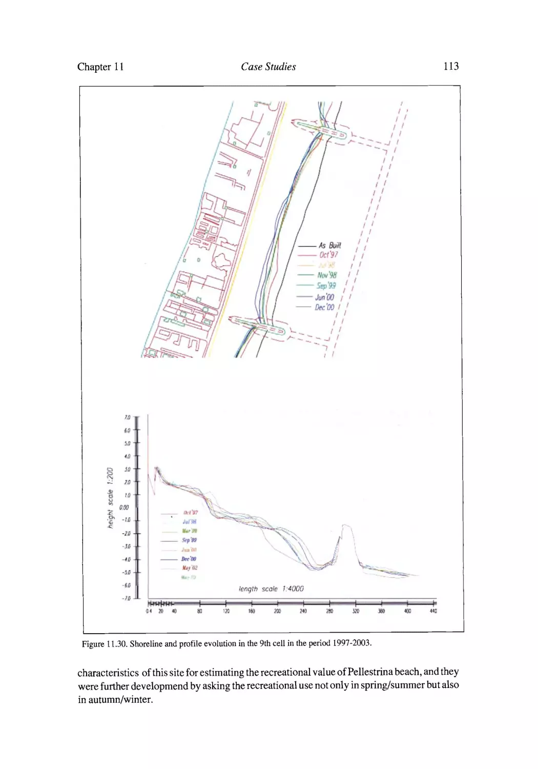
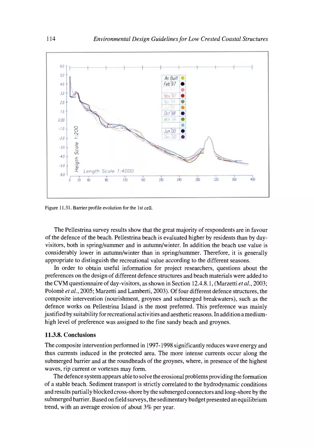
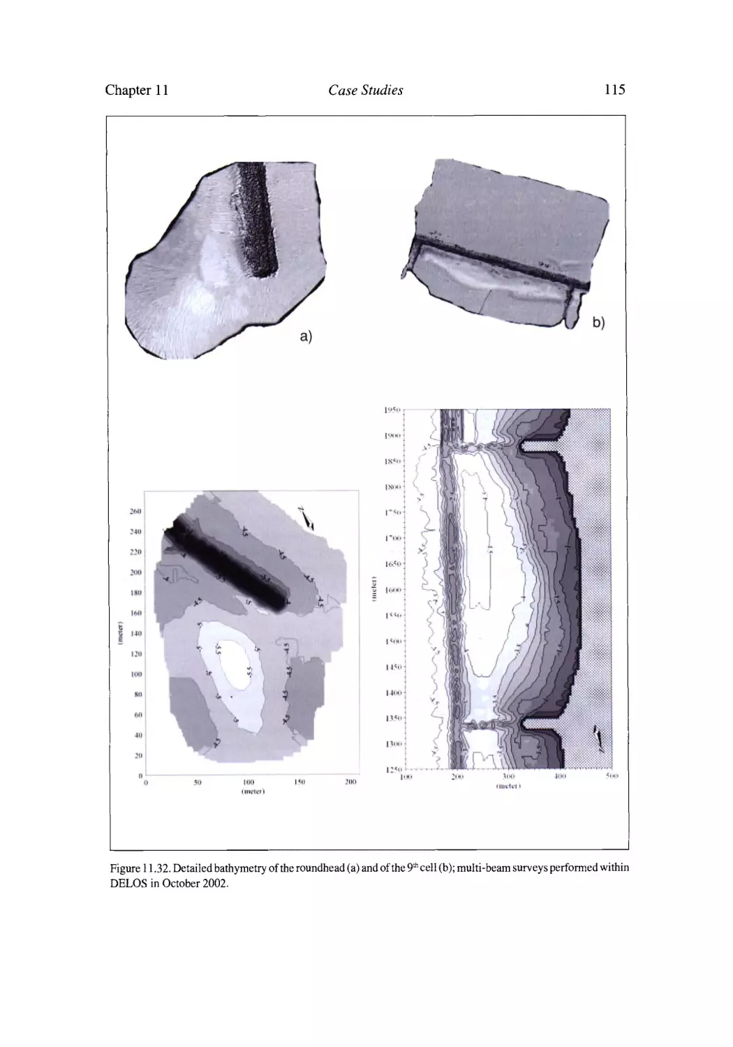
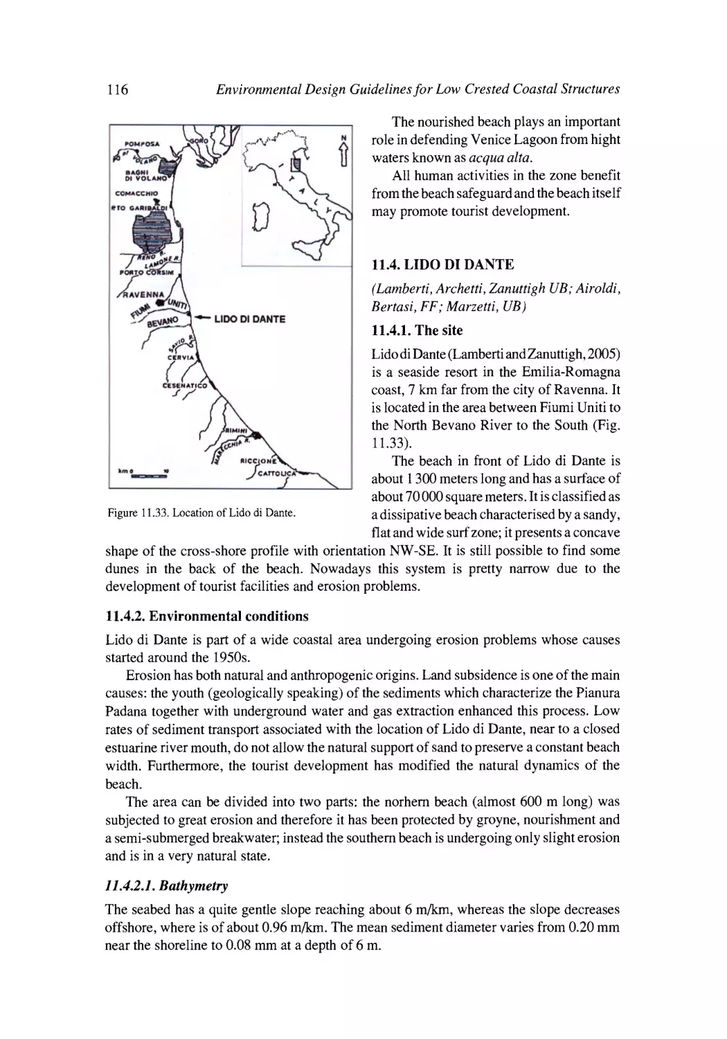
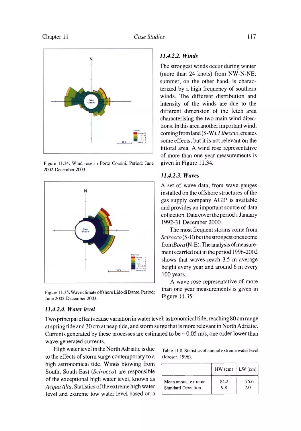
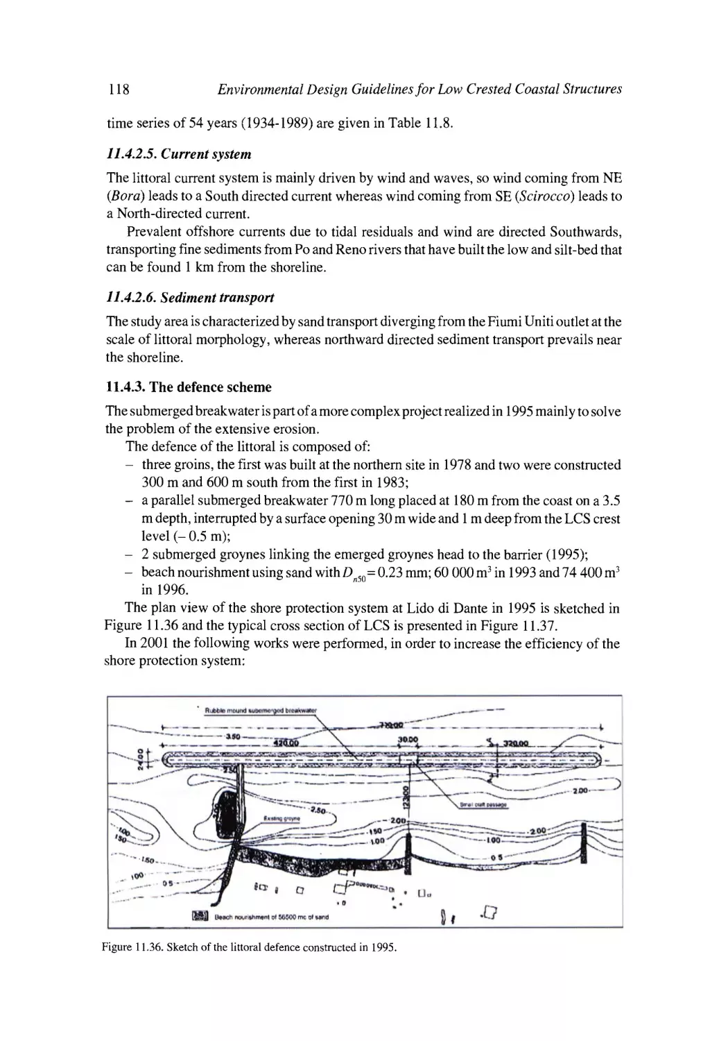
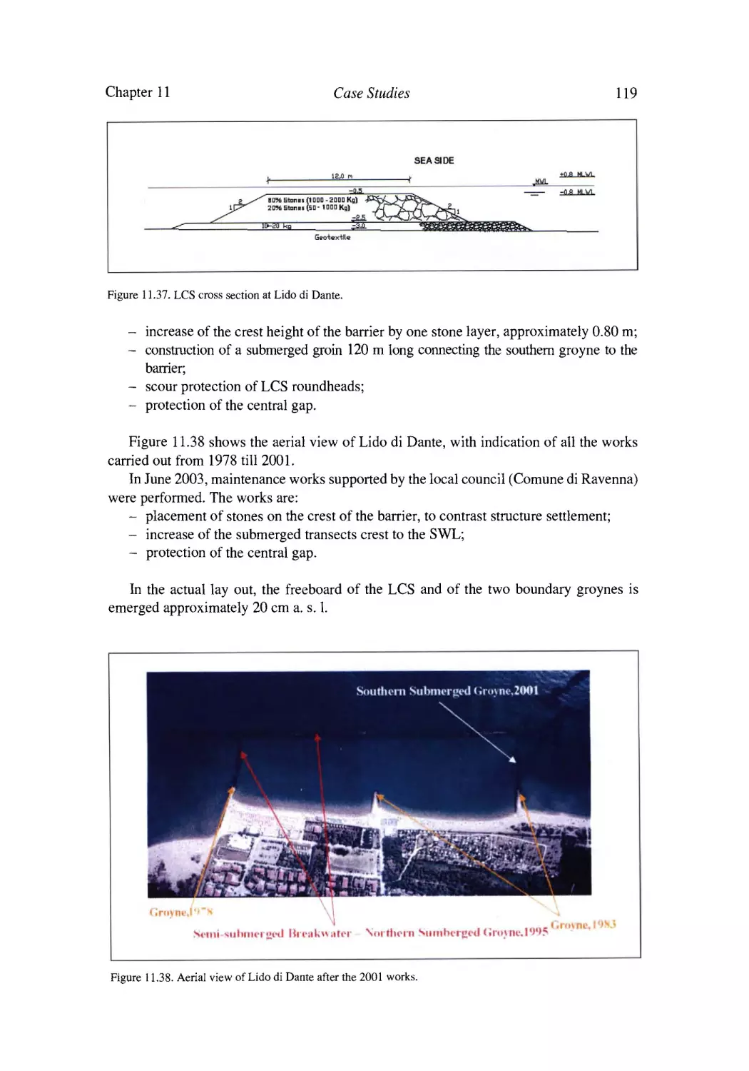
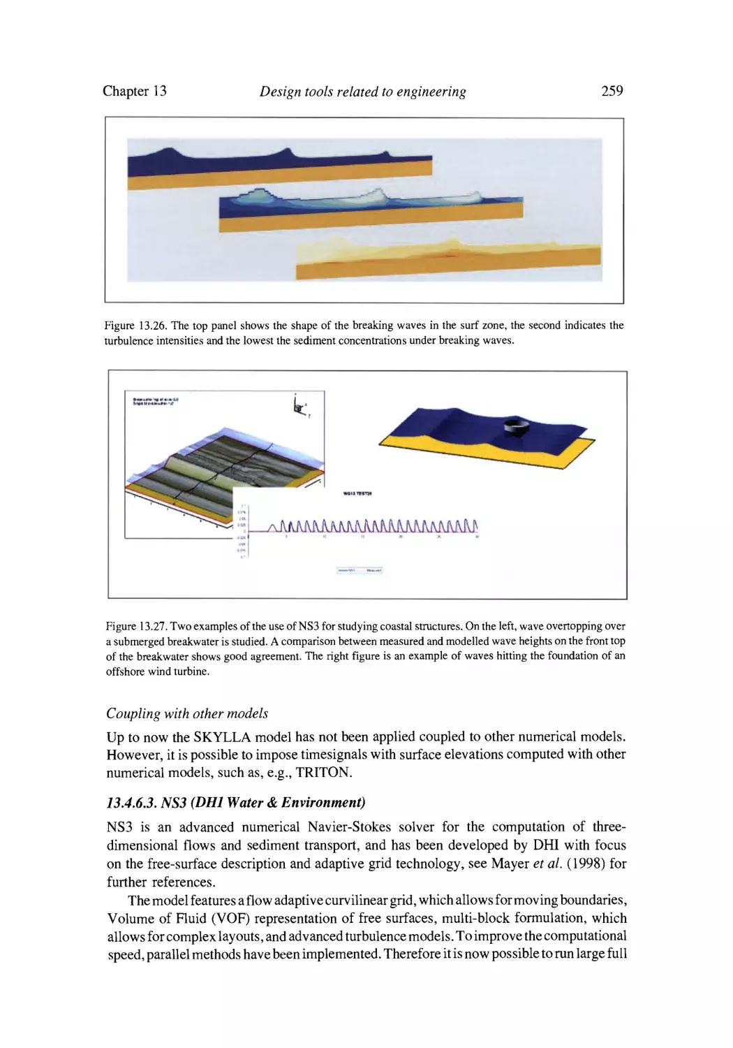
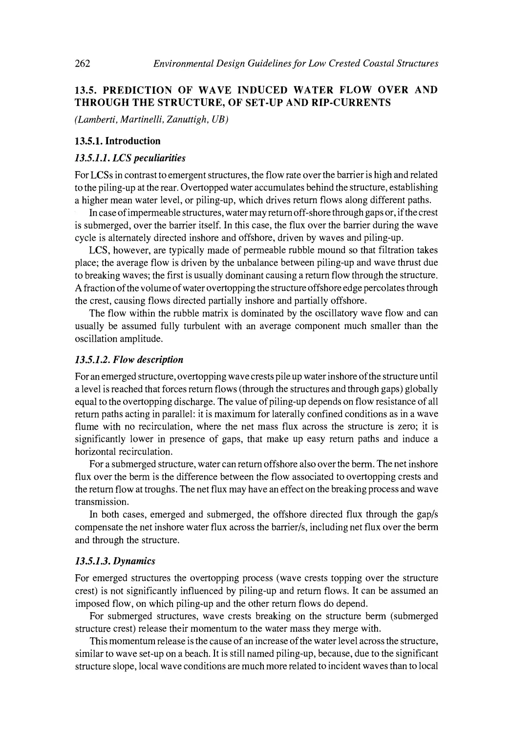
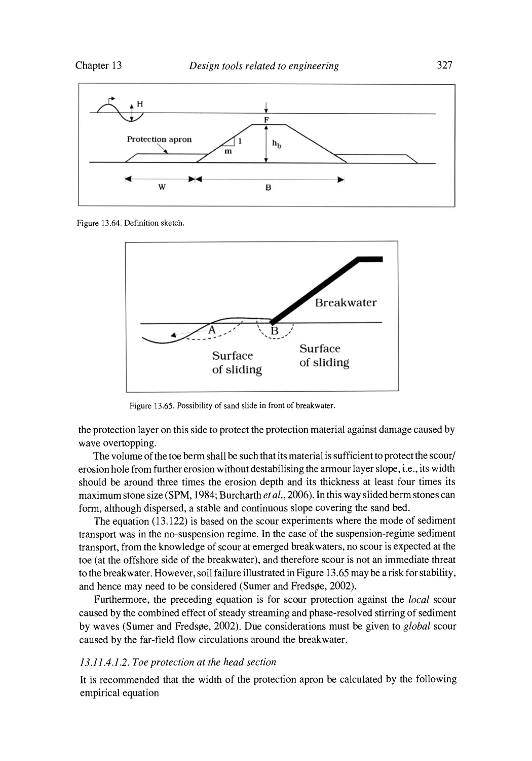
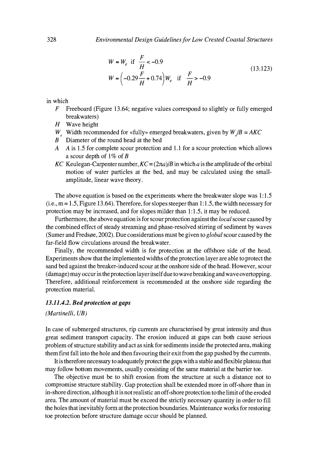
/


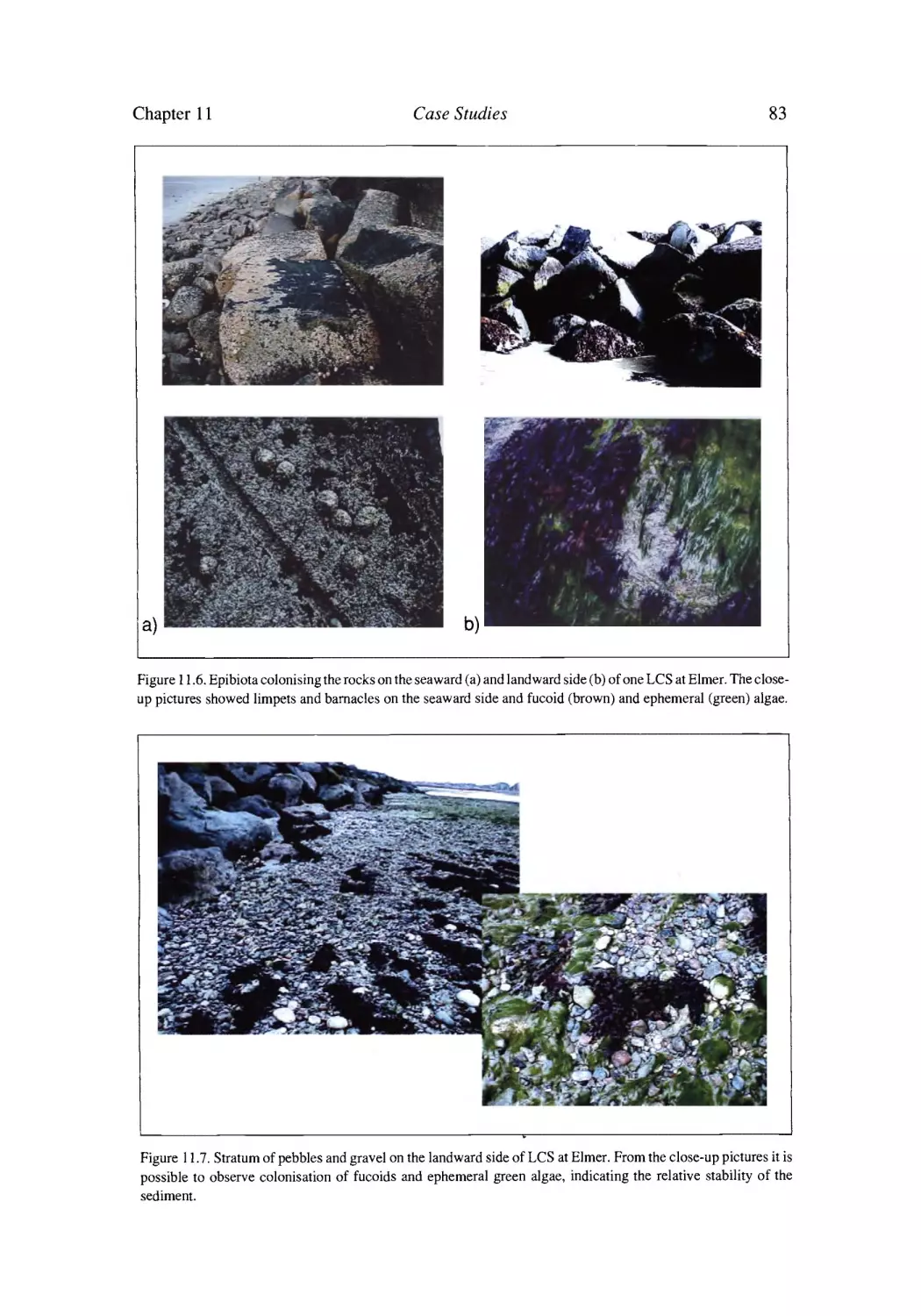
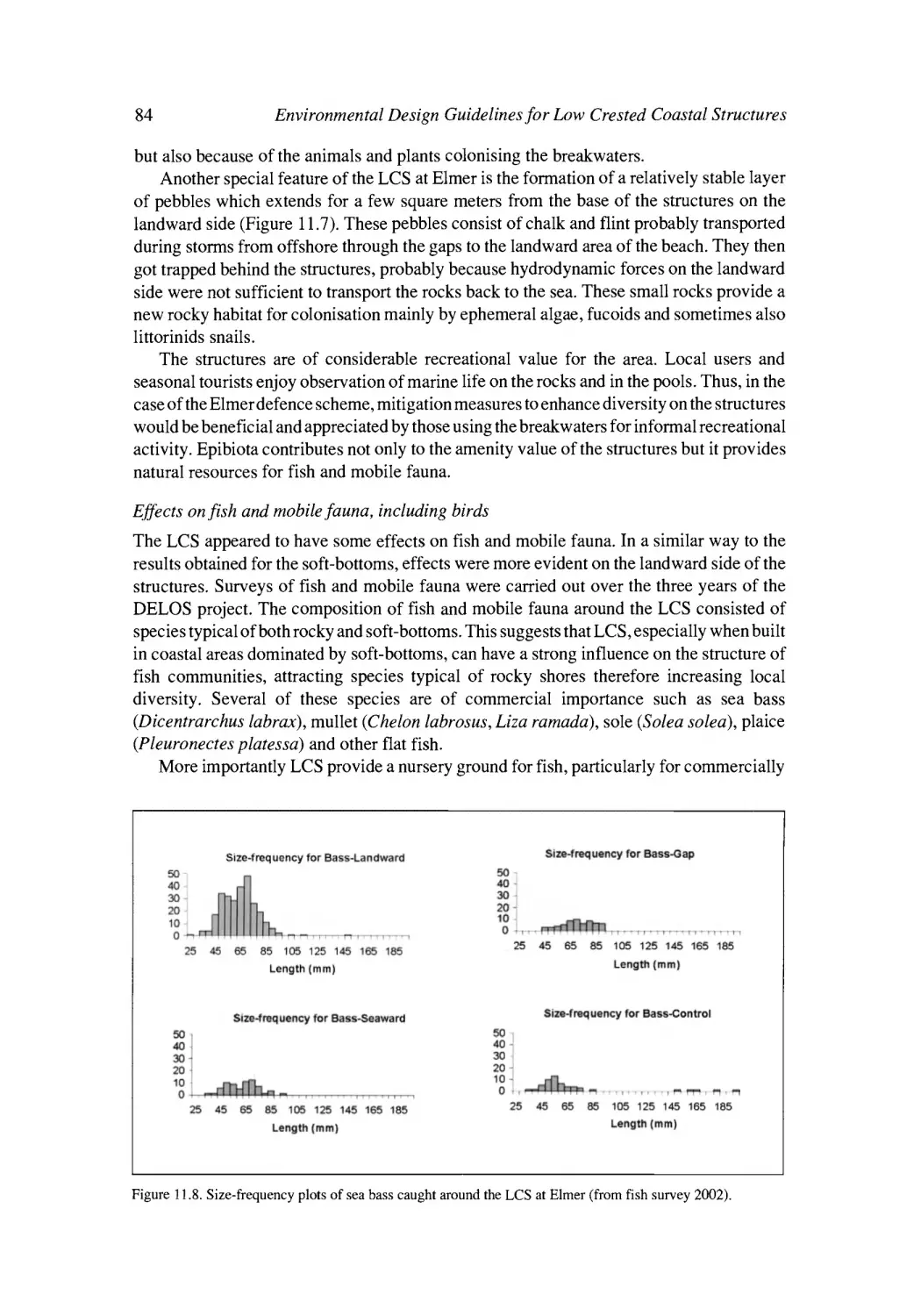
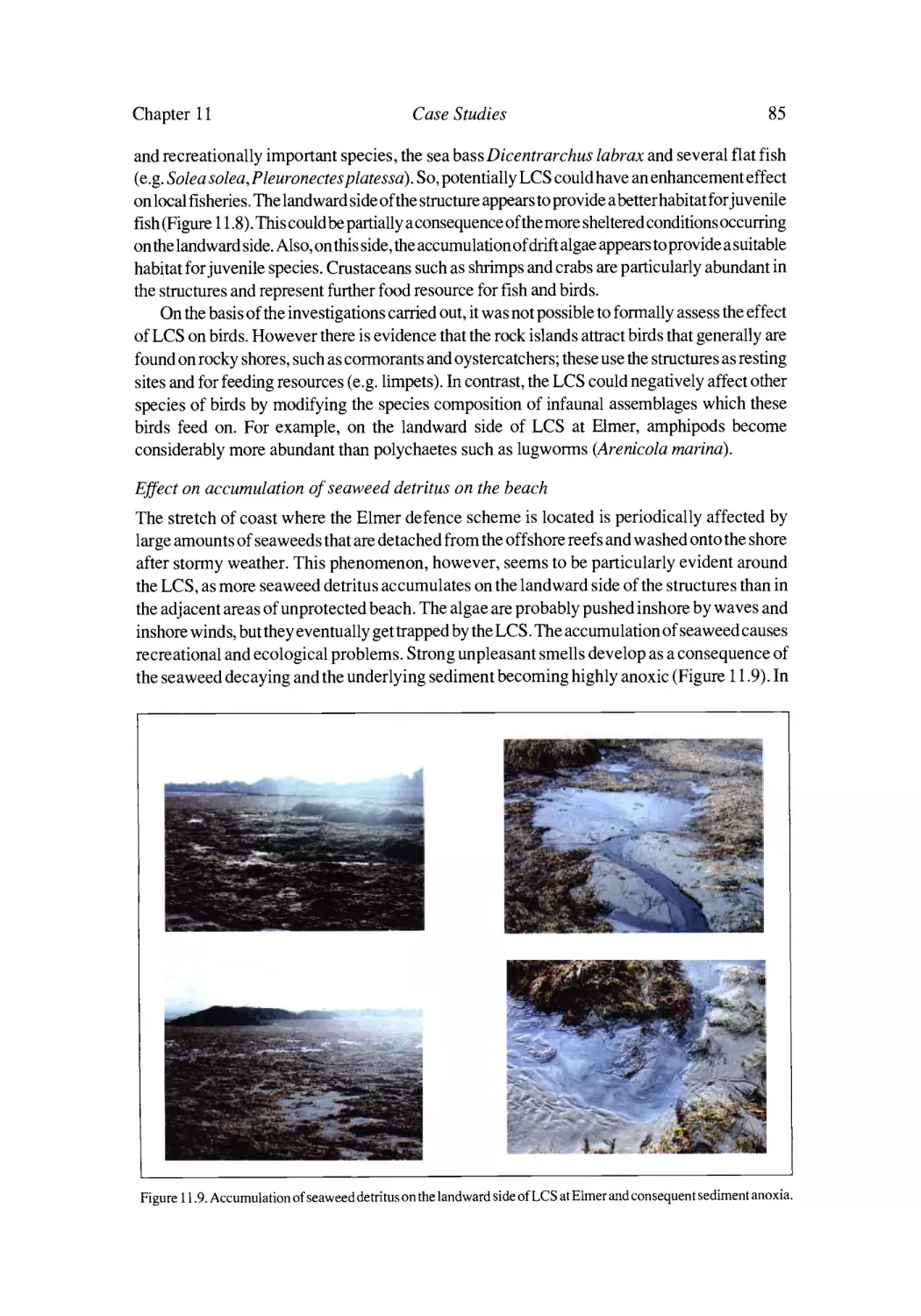
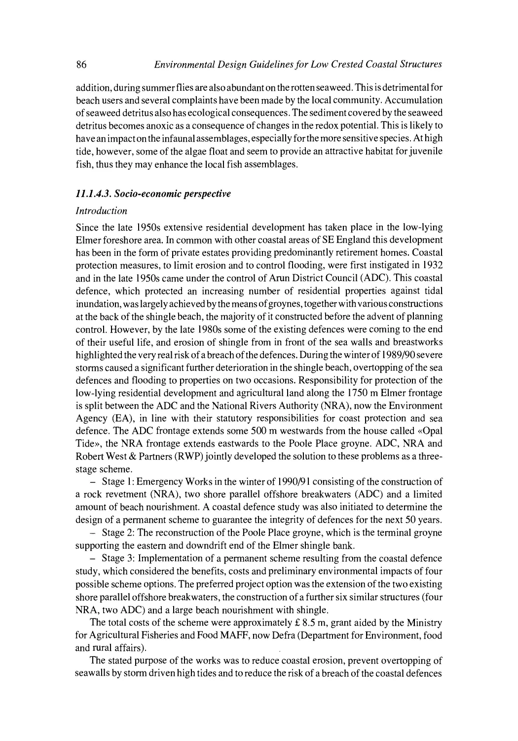


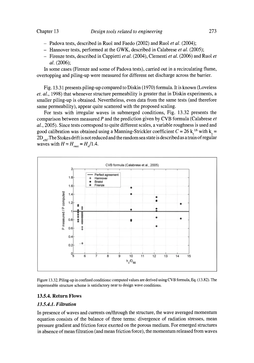


Text
Prologue
H.F. Burcharth, A. Lamberti
The effect of human activities is primarily local but can extend far away from the location of
intervention. This underlines the importance of establishing coastal zone management plans covering
large stretches of coastlines.
The interaction of wave climate, beach erosion, beach defence, habitat changes and beach value,
which clearly exists based on EC research experiences and particularly on results obtained by DELOS
Project (www.delos.unibo.it) for Low Crested Structures (LCSs), suggests the necessity of integrated
approaches and thus the relevance of design guidelines covering: structure stability and construction
problems, hydro and morphodynamic effects, environmental effects (colonisation of the structure and
water quality), societal and economic impacts (recreational benefits, swimming safety, beach quality).
The present guidelines are specifically dedicated to LCSs to provide methodological tools both for
the engineering design of structures and for prediction of performance and environmental impacts of
such structures. It is anticipated that the guidelines will provide valuable inputs to coastal zone
management plans.
The target audience for this set of guidelines is consulting engineers or engineering officers and
officials of local authorities dealing with coastal protection schemes. The guidelines are also of
relevance in providing a briefing of current best practice for local and national planning authorities,
statutory agencies and other stakeholders in the coastal zone. The guidelines have been drafted in a
generic way to be appropriate throughout the European Union taking into regard current European
Commission policy and directives to promote sustainable development and integrated coastal zone
management.
The guidelines are composed of three main parts.
The first part (Chapters 1-10) contains the description of the design methodology, from the
preliminary identification of design alternatives till the selection of the sustainable scheme and its
construction.
The second part presents:
the analysis of the performance of beach defences in DELOS study sites, which were selected to
represent a variety of environmental conditions (Chapter 11);
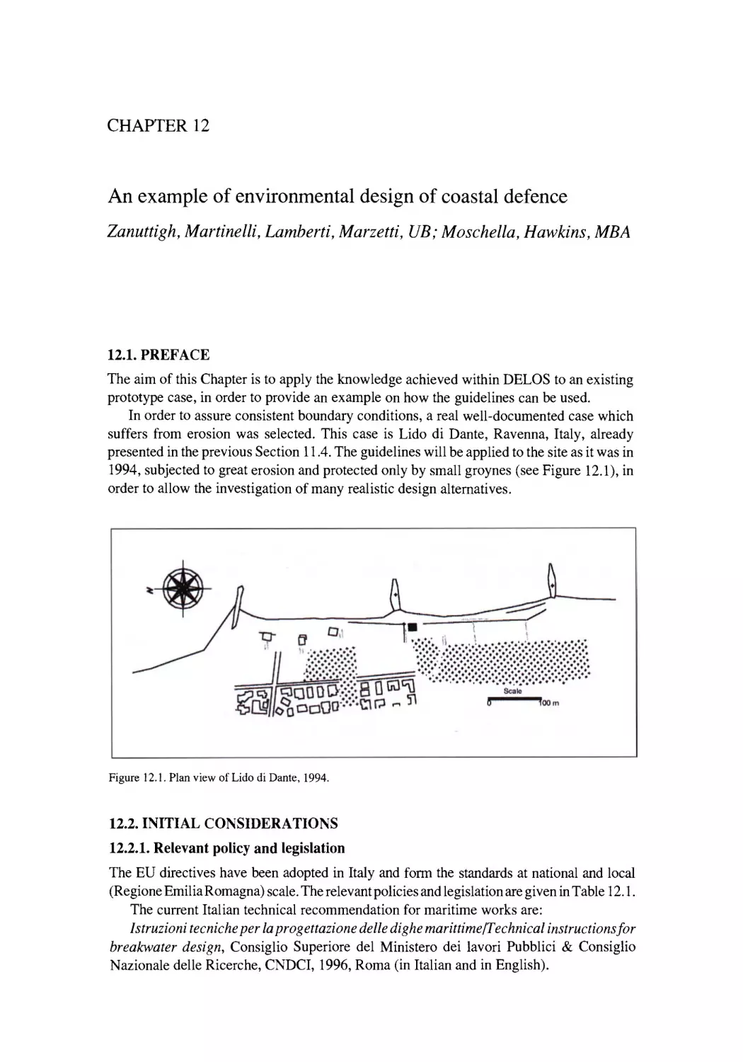
the application of the proposed methodology to a real prototype case, in order to give a practical
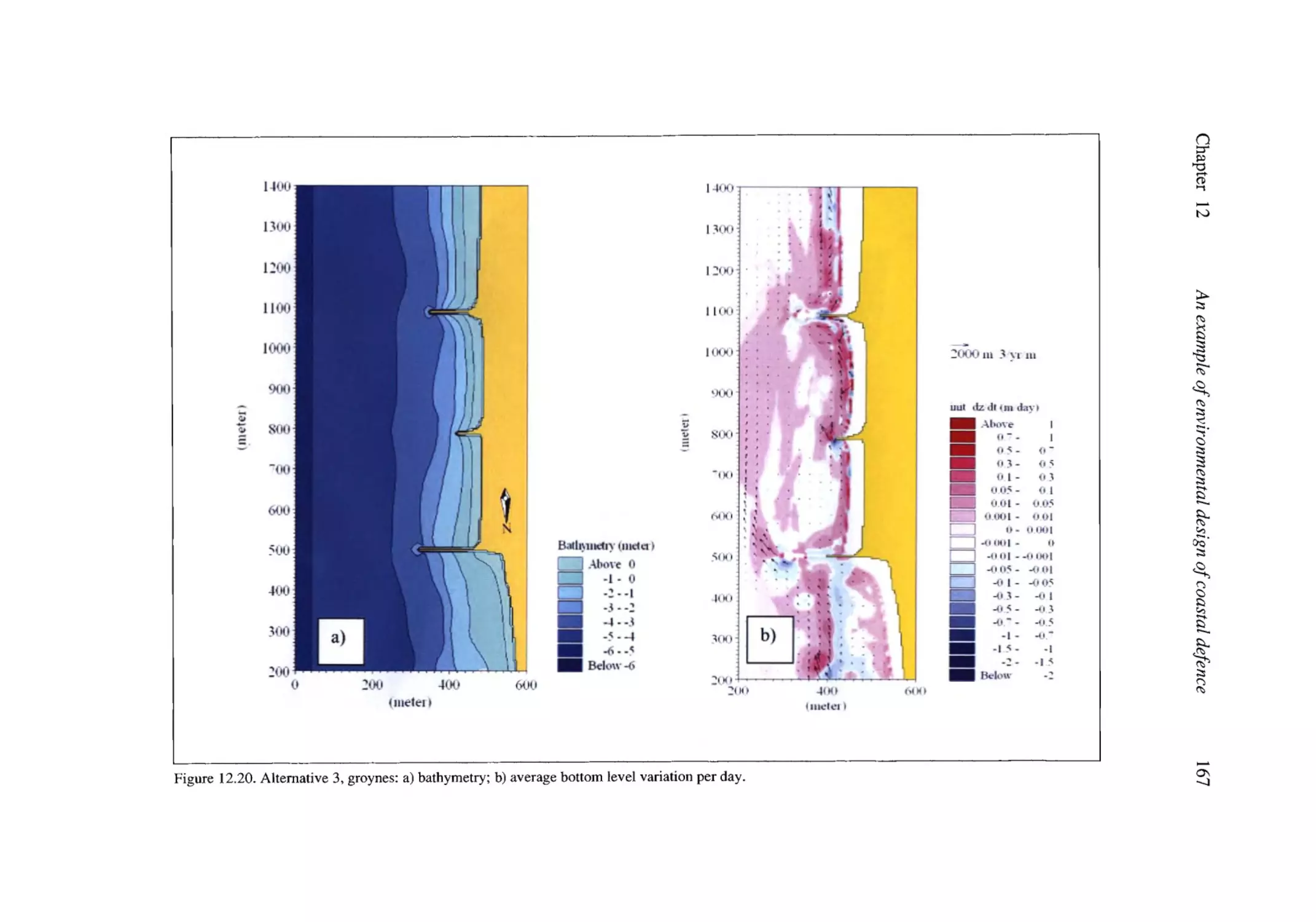
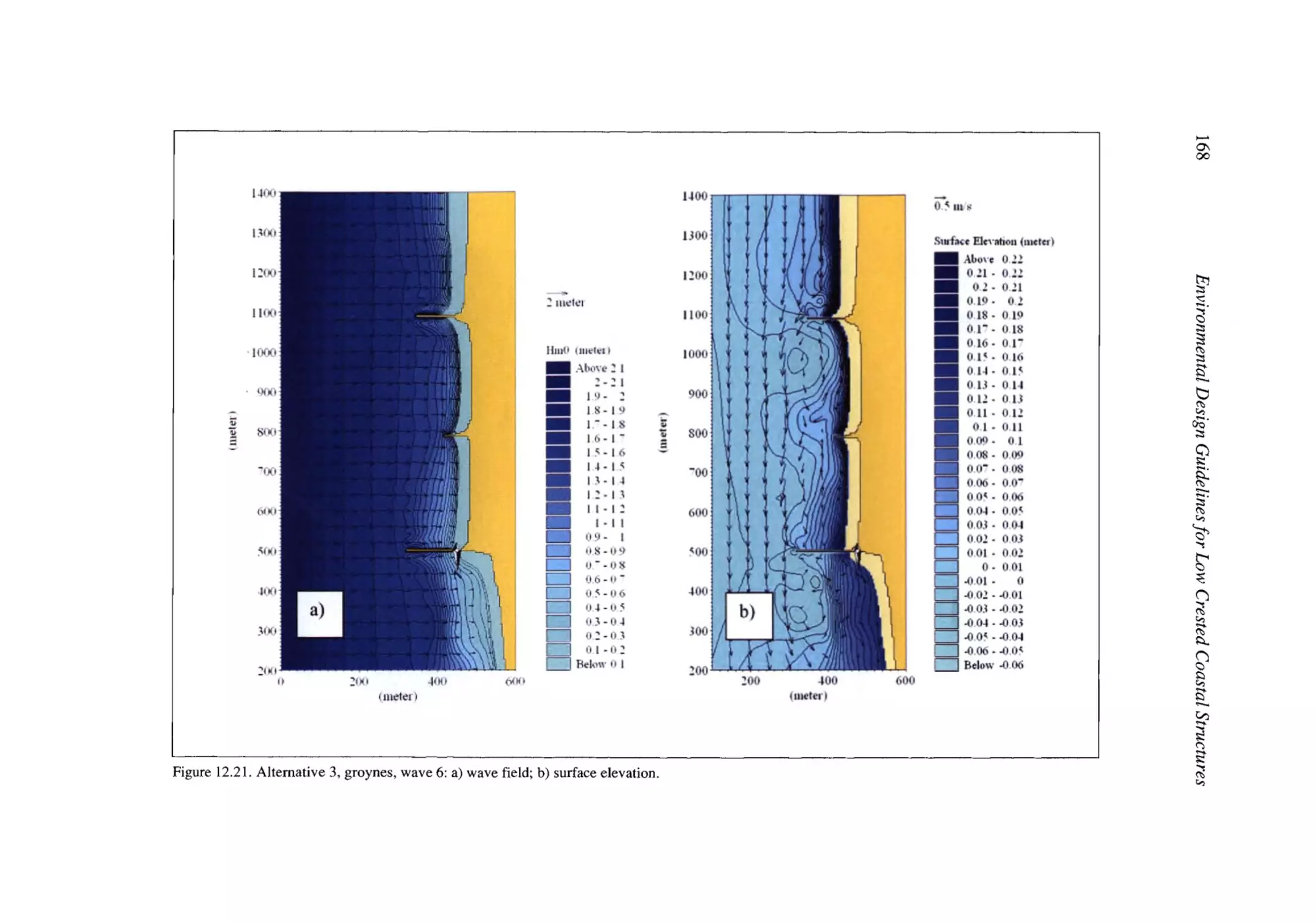
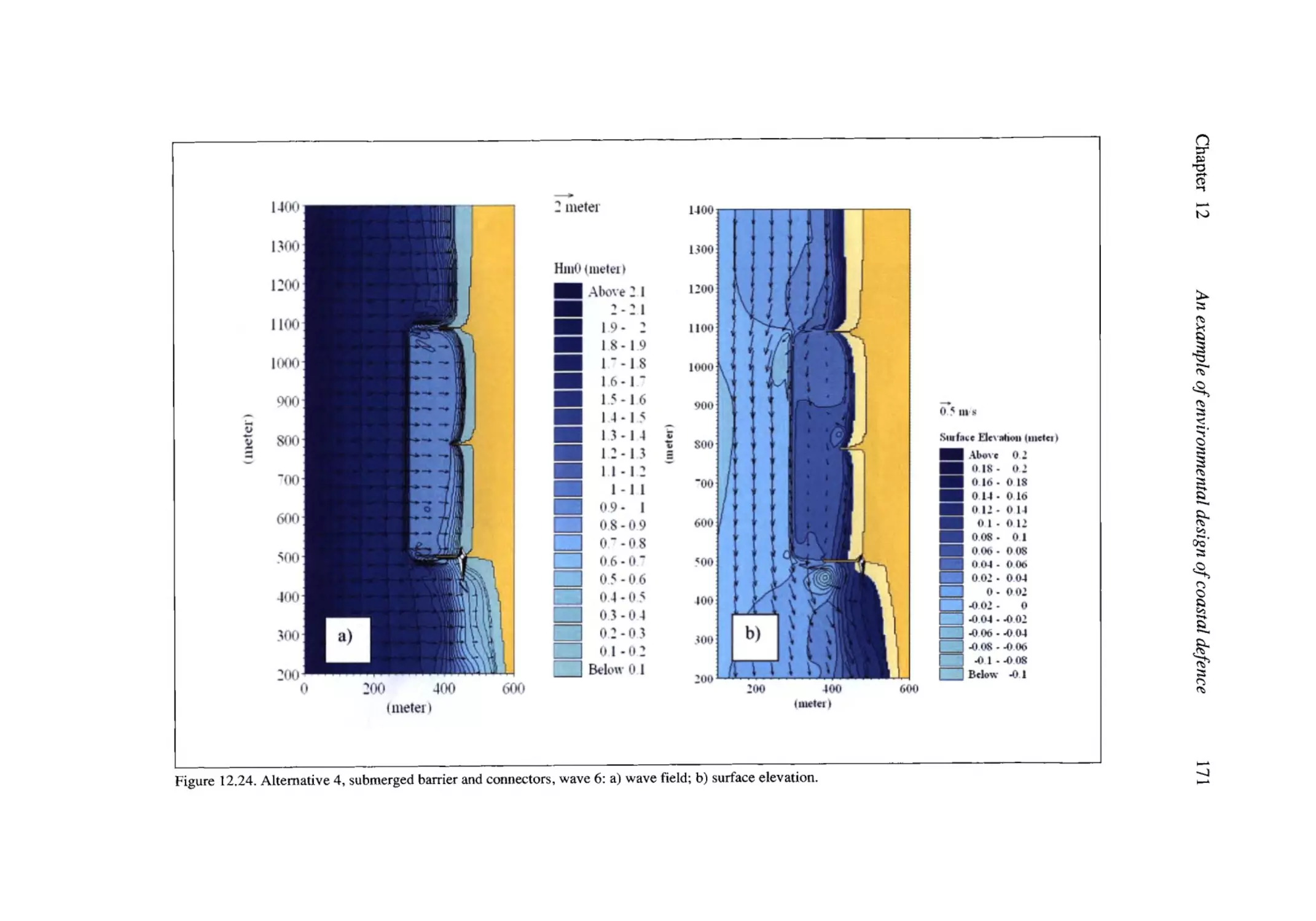
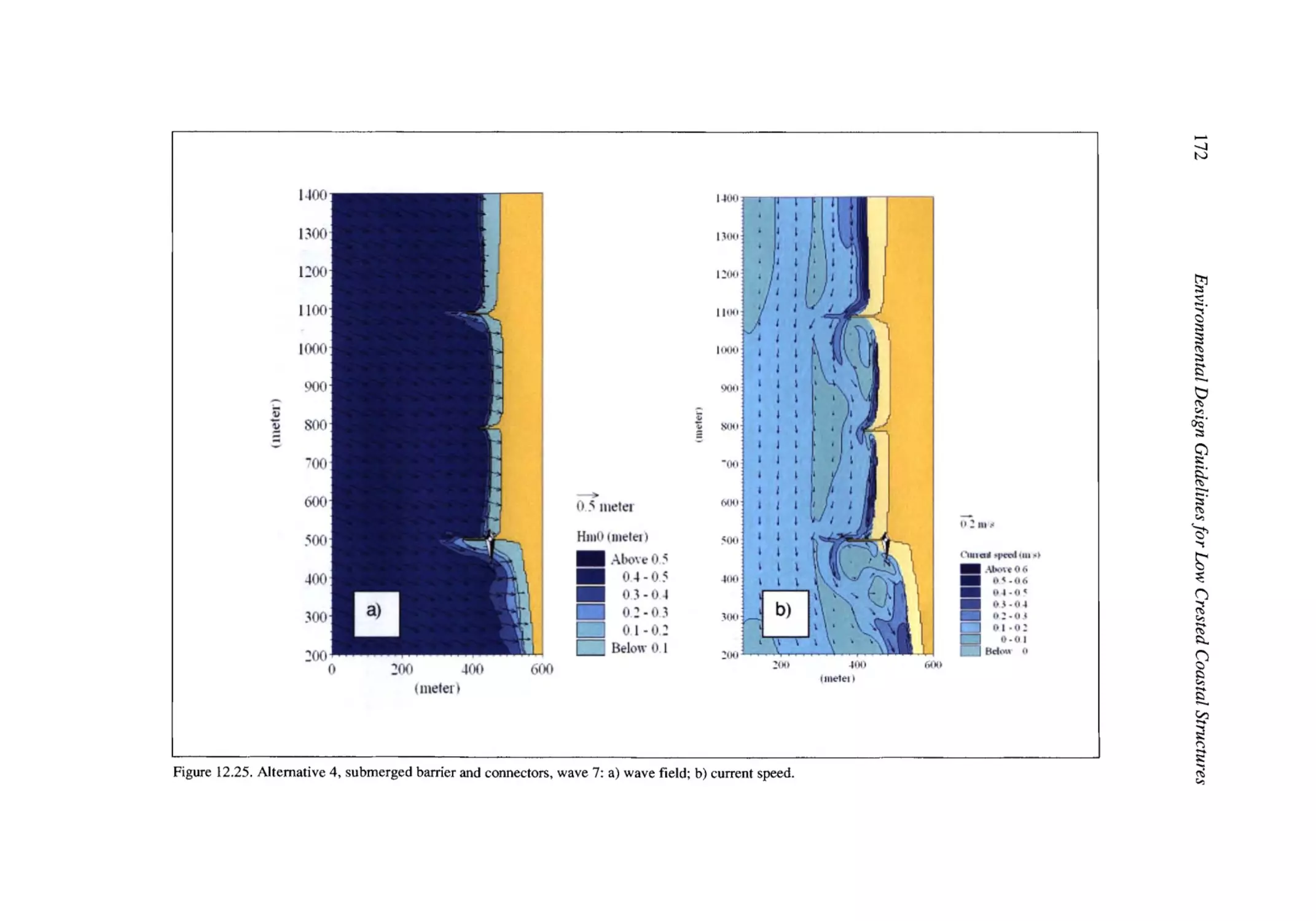
example to designers (Chapter 12).
The third part contains all the formulae and tools to help engineers (Chapter 13), ecologists
(Chapter 14) and economists (Chapter 15) during the design procedure.
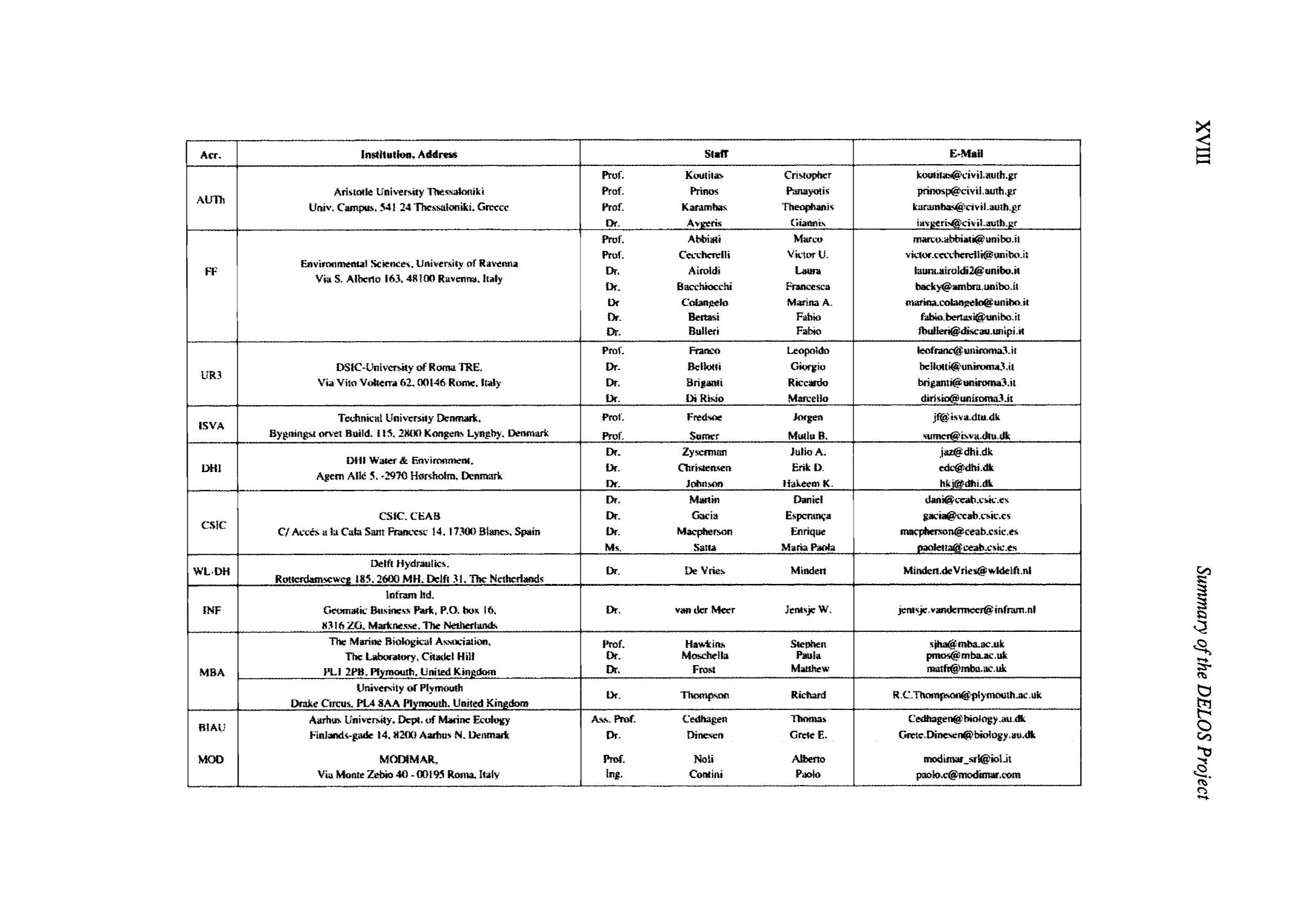
These Guidelines are a product of DELOS Consortium; for each section the main authors and
their institution are mentioned, whose contact information can be found in the list reported in DELOS
Consortium section.
Summary of the DELOS Project
The overall objective of DELOS was to promote effective and environmentally compatible design
of low crested structures (LCSs) to defend European shores against erosion and to preserve the littoral
environment and economic development of the coast.
Specific objectives and methods were:
9 to provide an inventory of existing LCS and a literature based description of their effects;
9 to analyse LCS hydrodynamics, stability and effects on beach morphology by surveys on sites,
laboratory experiments and numerical modelling;
9 to investigate the impacts of LCS on biodiversity and functioning of coastal ecosystems by
observations and field experiments;
9 to develop a general methodology to quantify benefits to enable implementation of Integrated
Coastal Zone Management based on Contingent Valuation methodologies in different European
countries;
9 to provide local authorities with validated operational guidelines for the design of LCS based on
the achieved knowledge of LCS hydrodynamics and stability, water circulation, beach morphology,
impacts on coastal assemblages, human perception and related economic effects.
DELOS offered the possibility to achieve these aims through integrated collaboration among
engineers, coastal oceanographers, marine ecologists, economists and political institutions, involving
18 partners from 7 European countries and end users.
The work necessary to meet the overall goal of DELOS was grouped in five integrated Research
Tasks:
~' Research Task 1: to provide an overview of the different types of structure, how effective they
are in the different coastal situations, and to identify which parameters may characterise each
structure and its effects on the coastal environment.
~, Research Task 2: to analyse the hydrodynamics around stability of structure, to provide
relationships among water level, discharge and wave characteristics at both sides of the structure,
to analyse currents induced by breaking over the structures and their effects on beach morphology,
both near to the structure and over the protected beach, up to the swash limit. This shall be done
by observation on sites, by laboratory experiments in wave channel and wave basin and by
numerical modelling.
~' Research Task 3: to identify, quantify and forecast the impacts (perceived as positive or negative)
of low-crested breakwaters on the biodiversity and functioning of coastal assemblages of animals
and plants at a range of spatial (local, regional and European) and temporal scales (months to years)
and in relation to different environmental conditions (including meteorological conditions, tidal
range, wave action, human usage, surrounding habitats).
~' Research Task 4: to develop a general methodology for Integrated Coastal Zone Management
linking economic and environmental components, based on Contingent Valuation values obtained
by Contingent Valuation in different countries in Europe and on criteria for transferring them from
one country to the other, accounting for the effects of situations specific to each country.
~' Research Task 5: to provide guidelines for an environmental design of such structures, based on
practical experience, on the most recent scientific results regarding the hydrodynamics around
structures and stability of them, water circulation and beach morphology, impacts on coastal
assemblages, and accounting for human perception and related economic effects; guidelines will
be verified by application to the study sites and selected case studies.
~' Research Task 6: to establish communication among partners and with end-users.
Summary of the DELOS Project
KVI
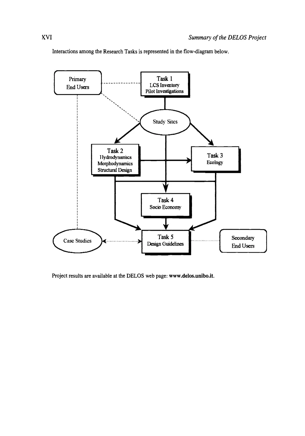
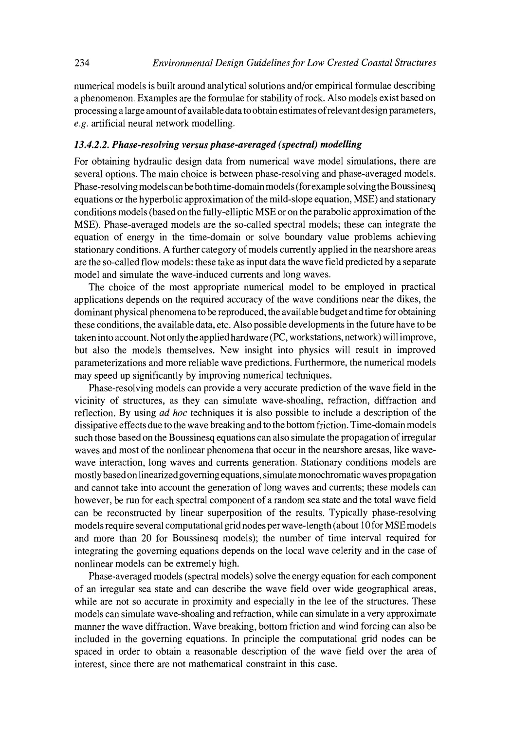
Interactions among the Research Tasks is represented in the flow-diagram below.
f
Primary
i
Task1
1
LCS lnvento~
Pilot Investigations
+~s+
Study Sites
............++++-"
.
I
Morphodynmmcs ]
straea"+al~
n I
+++++++~++++~++|!i++++!+ii
++++++!I
+,,-+++++.,,
Task 3
I.......... +L
: "--++:+++~+'-+::~
...........
Ecology
"
I
I "l
~Task4
sock, Economy
Task 5
Design Guidelines
Project results are available at the DELOS web page: www.delos.unibo.it.
Secondary
End Users
~
~
,
"
6
,~
.-'i ~"
-
~
. - - . .
~
CJ
~1
i
~ ~ ~ l~ ~ ~ ~
=
~.~_~
~
Summary of the DELOS Project
,'~
_~-
"
-
~.~
_
<
<<~
~
,!
2
"~
6
~
,'.
,,
.~
~
r
-
.~ ~
.
~~
~ ~
~~
~~ ~~ ~
~,~ ~i ~. ~i~, ~ ~
XVII
XVIII
~
~
~~ ~~ ~ i
!i
r~
~.
i
.<
?
~! ~i~ ~ii ~ ~"
Summary of the DELOS Project
"r/:
IIII
CHAPTER 1
Definition of LCSs covered by the guidelines
(Burcharth, AA U)
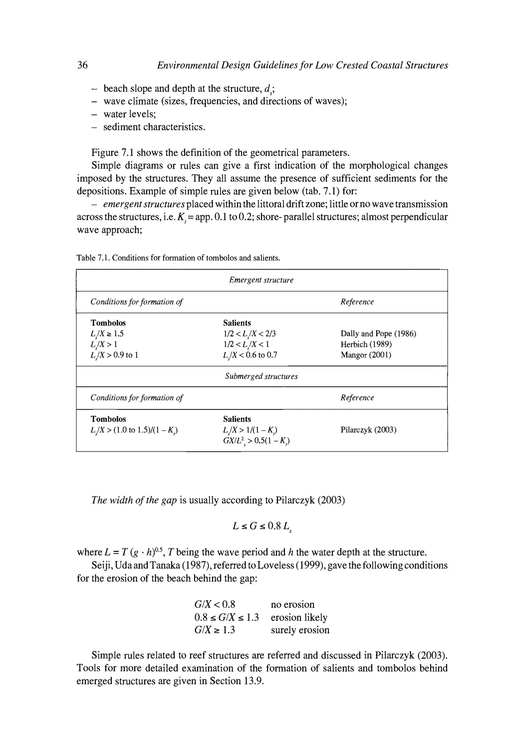
The guidelines cover shore-parallel low crested and submerged structures such as regularly
overtopped emergent and submerged detached breakwaters. Whilst LCSs share engineering
and ecological features with artificial reefs, these are considered as a separate issue as they
are very wide crested, deeply submerged and deployed mainly to enhance fisheries.
The structures reduce the amount of wave energy reaching the shore behind them and as
a consequence also influence sediment transport and impose shoreline changes.
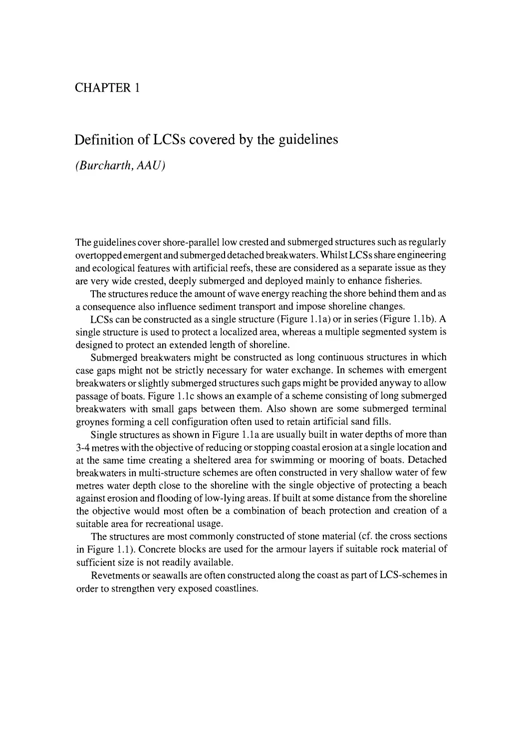
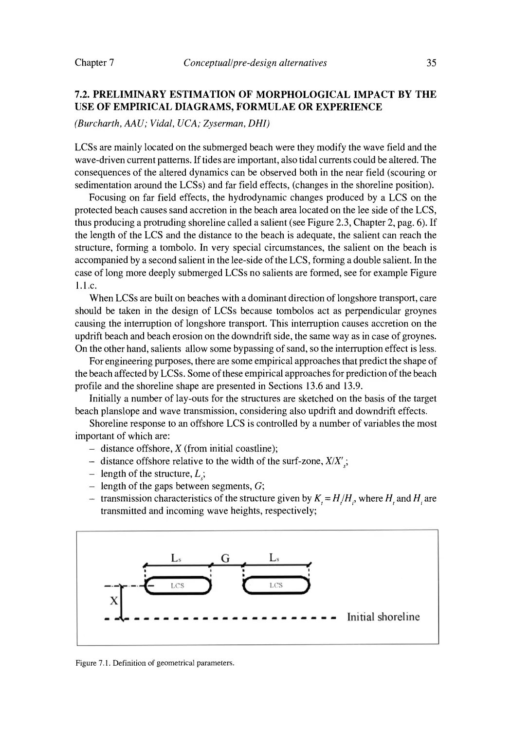
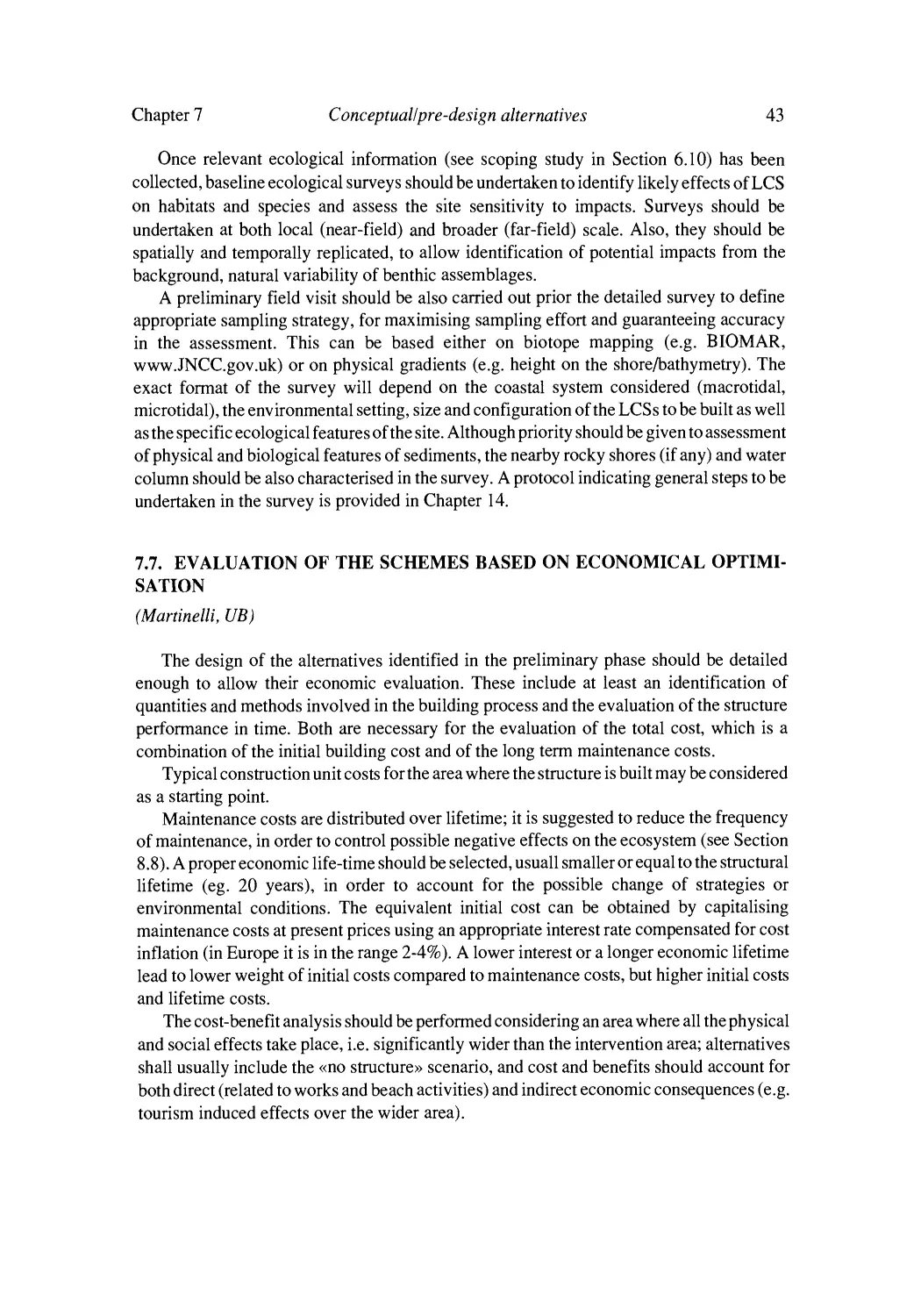
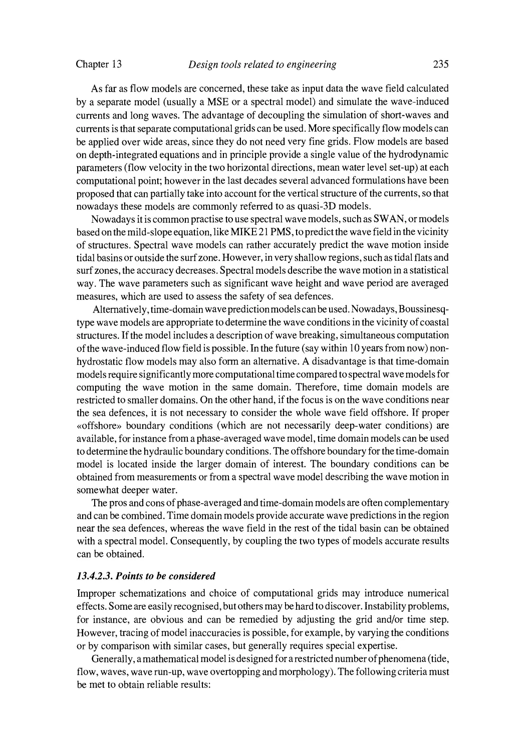
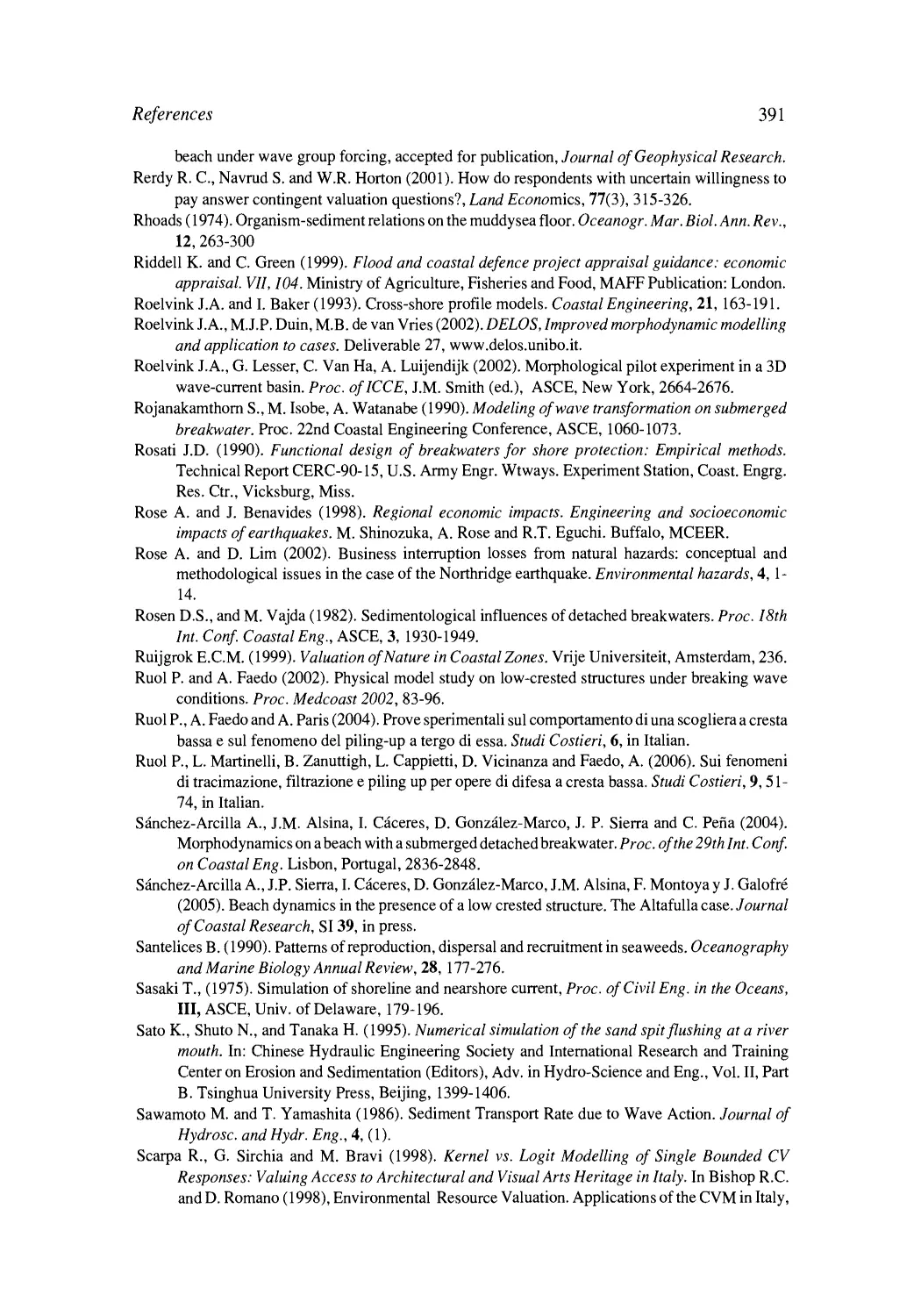
LCSs can be constructed as a single structure (Figure 1.1 a) or in series (Figure 1.1 b). A
single structure is used to protect a localized area, whereas a multiple segmented system is
designed to protect an extended length of shoreline.
Submerged breakwaters might be constructed as long continuous structures in which
case gaps might not be strictly necessary for water exchange. In schemes with emergent
breakwaters or slightly submerged structures such gaps might be provided anyway to allow
passage of boats. Figure 1.1 c shows an example of a scheme consisting of long submerged
breakwaters with small gaps between them. Also shown are some submerged terminal
groynes forming a cell configuration often used to retain artificial sand fills.
Single structures as shown in Figure 1.1a are usually built in water depths of more than
3-4 metres with the objective of reducing or stopping coastal erosion at a single location and
at the same time creating a sheltered area for swimming or mooring of boats. Detached
breakwaters in multi-structure schemes are often constructed in very shallow water of few
metres water depth close to the shoreline with the single objective of protecting a beach
against erosion and flooding of low-lying areas. If built at some distance from the shoreline
the objective would most often be a combination of beach protection and creation of a
suitable area for recreational usage.
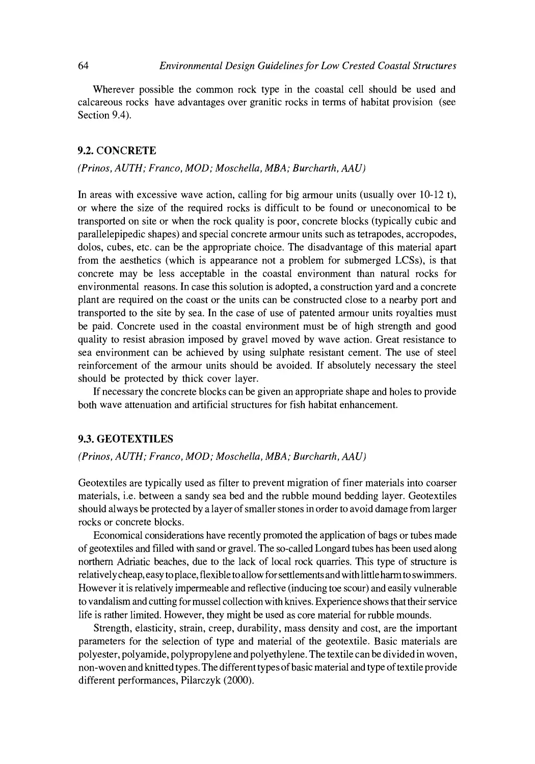
The structures are most commonly constructed of stone material (cf. the cross sections
in Figure 1.1). Concrete blocks are used for the armour layers if suitable rock material of
sufficient size is not readily available.
Revetments or seawalls are often constructed along the coast as part of LCS-schemes in
order to strengthen very exposed coastlines.
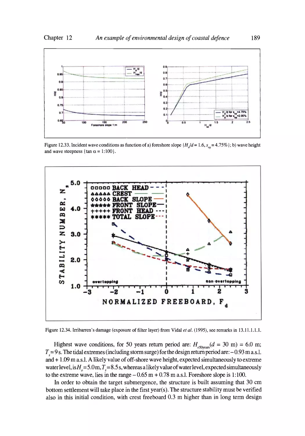
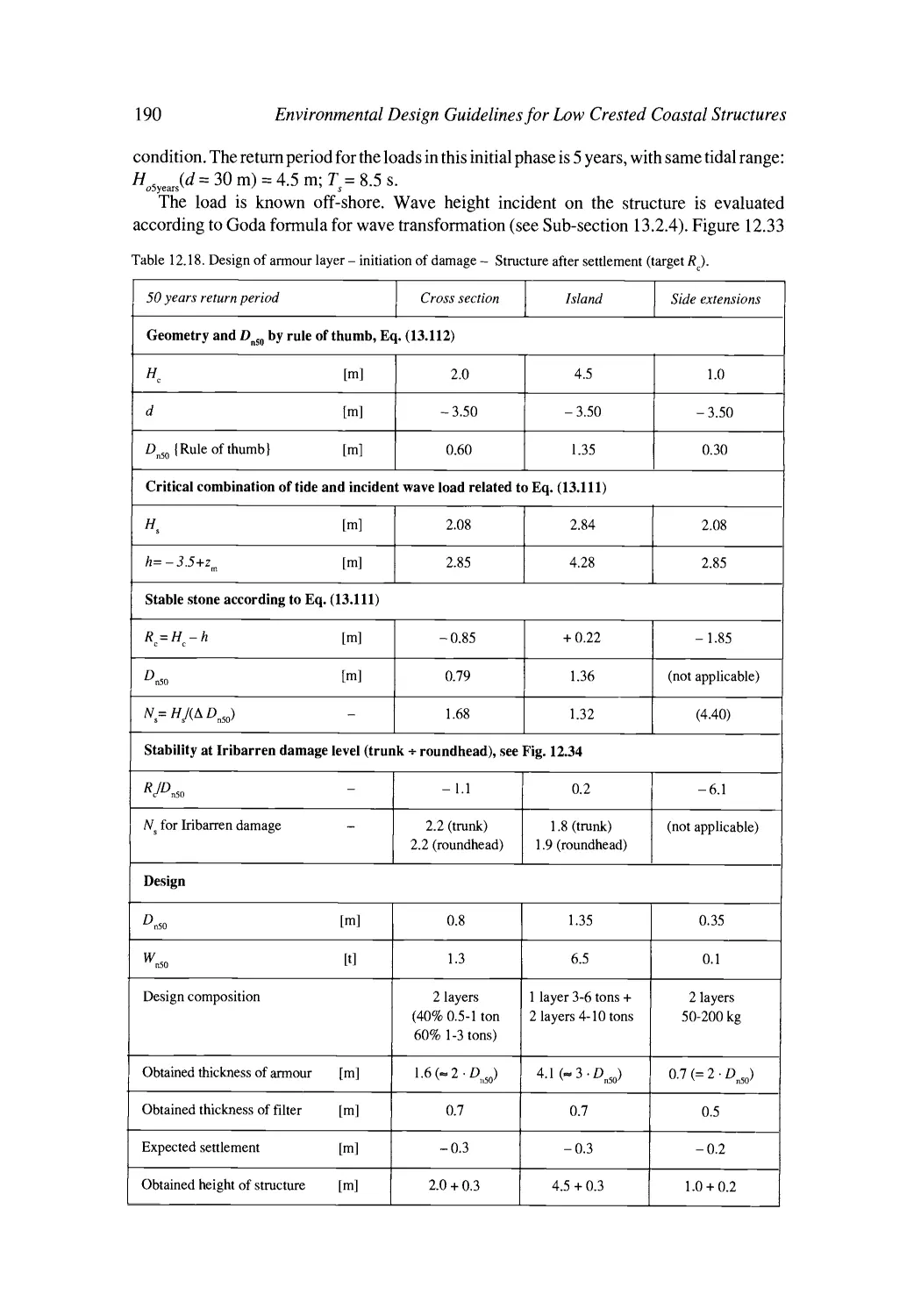
Environmental Design Guidelines for Low Crested Coastal Structures
Single LCS structure
-*~_~
,,
~
.
t--
""
"~.'Ir"~',~,rB"~
a'
,11,"',,,"
~"
"-~,b
~,
,,
tll.~
a,
~,
,,
Approximate length scale
t ............
A L.
'1
I
|
5om
~/////////////////~
Emerg ~t~struCtu~
m
4,1
Approximate length scale
.
MWL Section A-A
.
1,
.
.
.
0 ....
~m
to be used on san~, sea b ~
Nearshore detached LCSs in multistructure scheme
|~,.:2~_ .~ .. q'~-'.,.'},~:~,.,.,) ~ ....... ~ = _, r,,-r . . . . . . .
-.-..,-:~ ~._~._a, Initial coastline
B 4"3
~il/H/A
7/////Z
9"//i/iiA
.~proximate length scale
9
rfllllllh
~Emergent structure
..................
50m
B ~]
|
'
Approximate length ~ l e
M3,VL
S~on
P,-B
Offshore submerged LCSs in cell-scheme with low crest groynes
,
~.~-"~ ~.a.t,,E .~.~.*,
~'~'~'~iit;z,t,.,~
Initial coastline ti~,,--_~.;.tx, ......, ~ , : - ~ t
.'zc.,j.:-~'..,_
Approx~ate length scale
1 .............
,.i
~
'
t
u
r
.
.
.
e
.
.
c(J
~mximate
length scale
9
Section C-C
MWL ,,
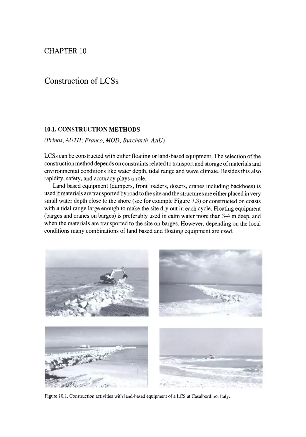
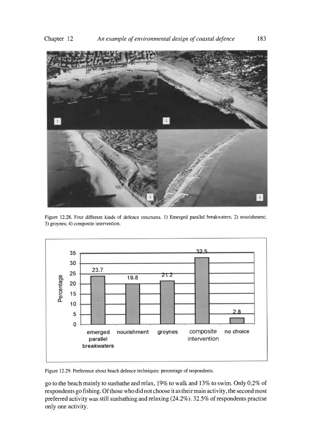
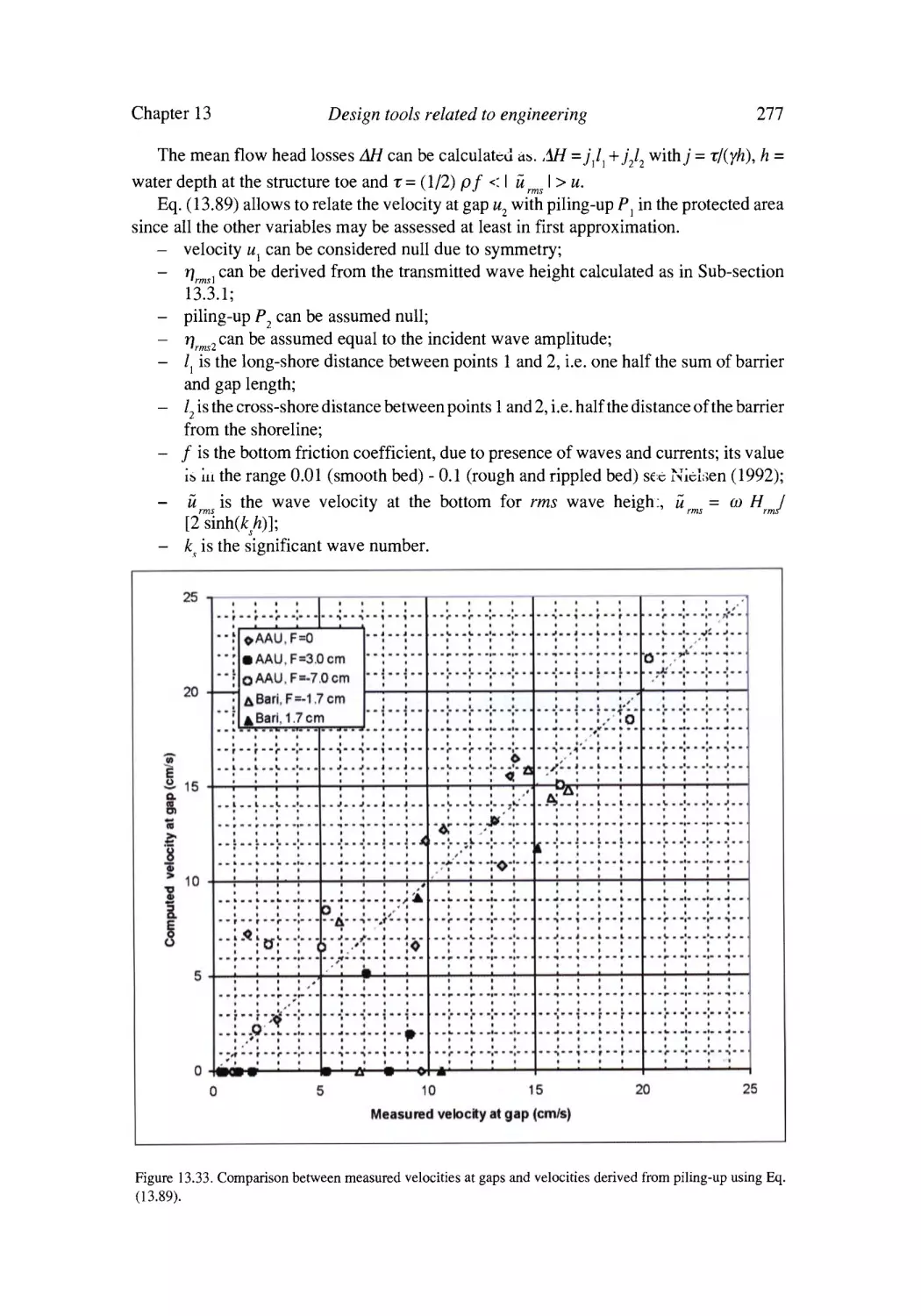
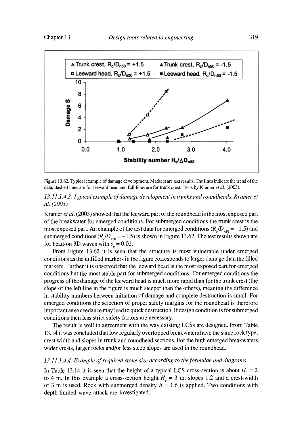
Figure 1.1. Examples of layouts and cross sections of LCSs.
]
i
i
O ....
a
i
i
~Sm
.:~
CHAPTER 2
Function of LCSs
2.1. LCSs I N T E R A C T I O N W I T H W A V E S , C U R R E N T S AND S E D I M E N T
TRANSPORT
(Burcharth, AA U)
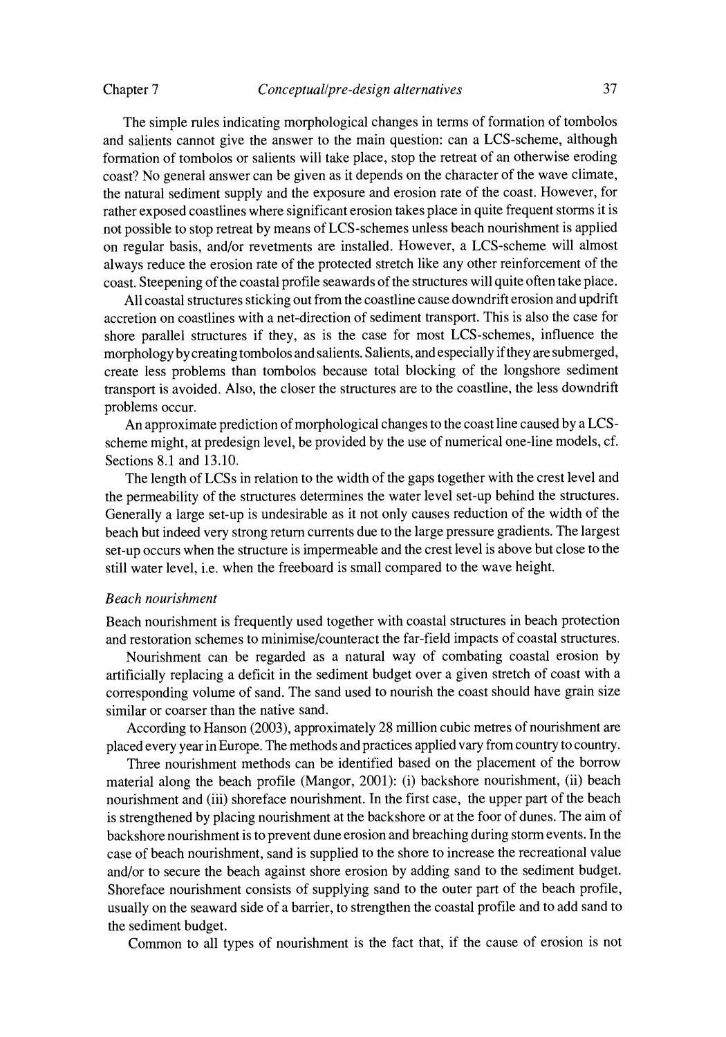
When used for beach stabilization the function of LCSs is to reduce wave energy in their lee
and thereby reducing the sediment carrying capacity of the waves to the shoreward. They can
be designed to reduce or prevent the erosion of an existing beach or a beach fill, or to
encourage natural sediment accumulation to form a new beach.
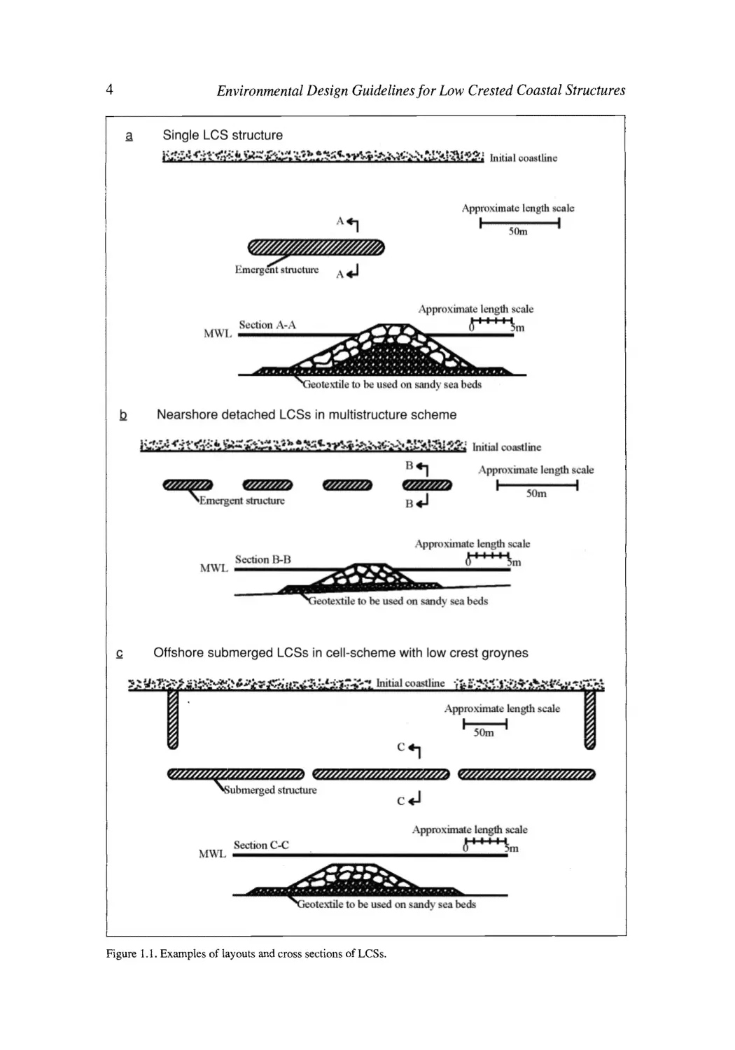
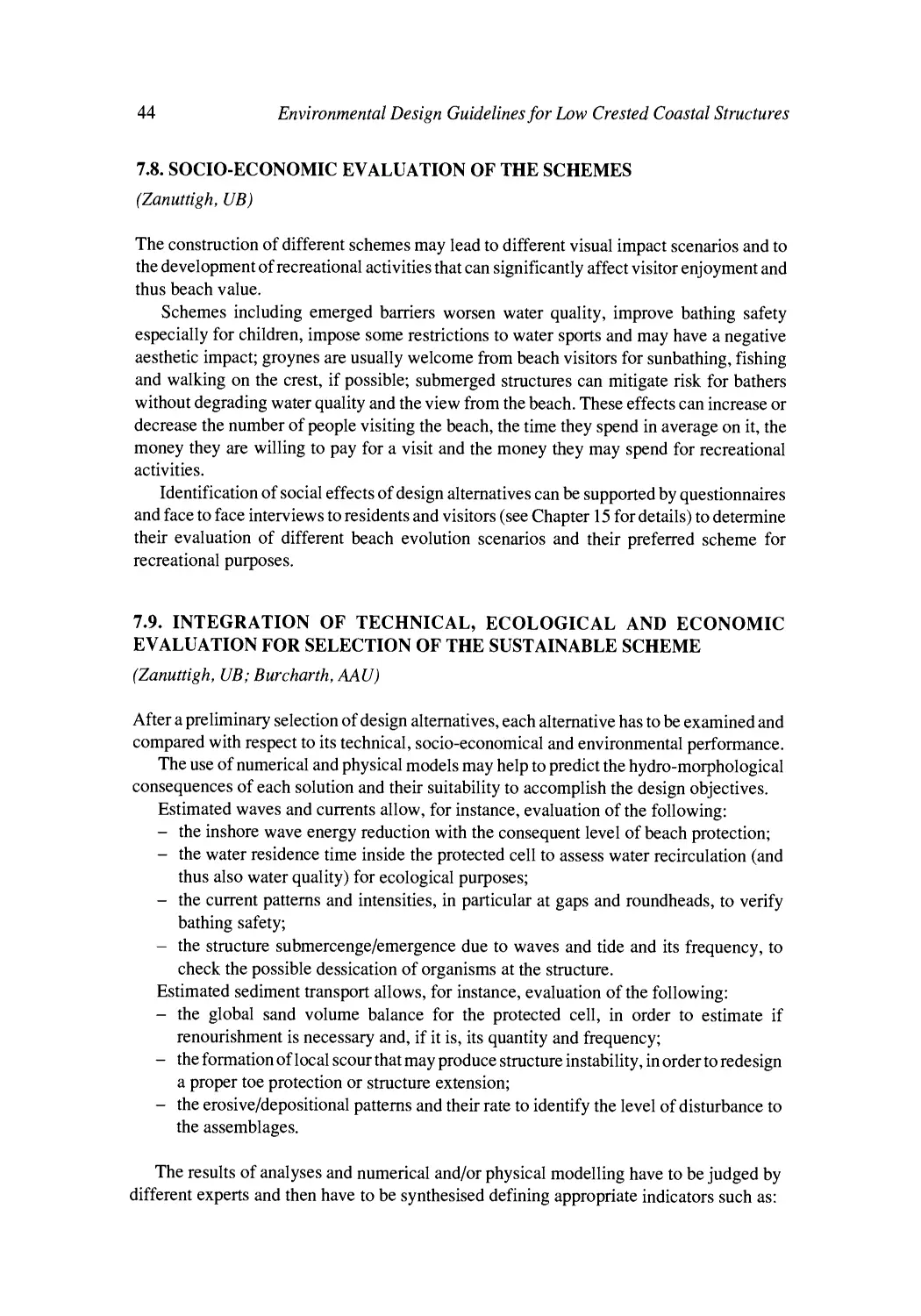
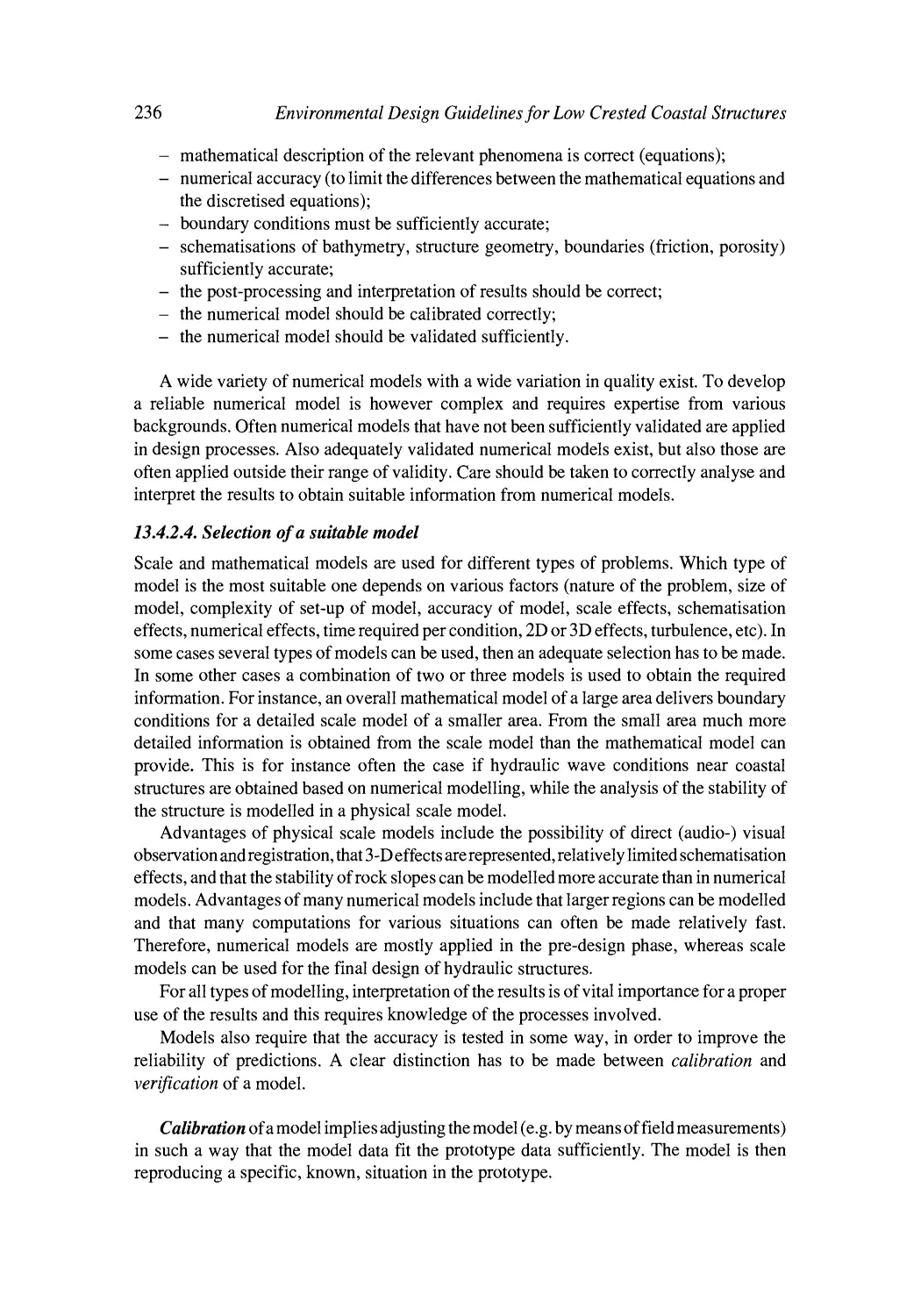
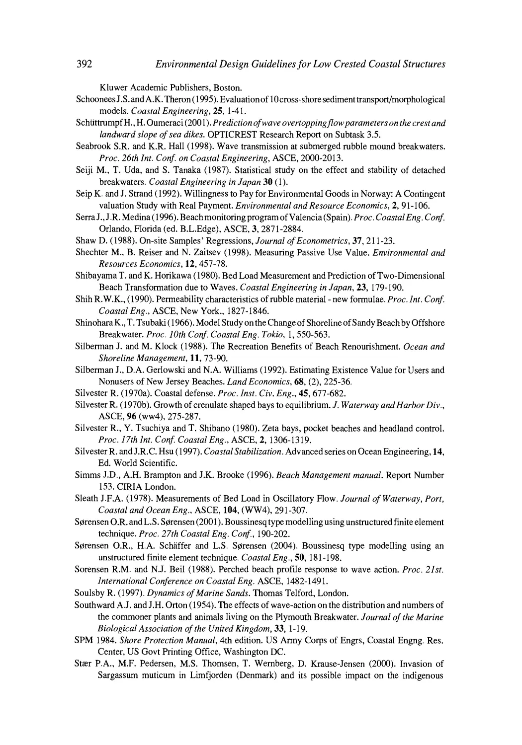
The structures reduce the incoming wave energy across the structure by triggering wave
breaking at and on the structure, by partially reflecting the waves and by dissipation related
to the wave induced porous flow in the structure. This is illustrated for an emergent structure
in Figure 2.1.
Wave breaking accounts for the largest part of the energy reduction, reflection for the
second largest part and porous flow for the smallest part. Wave energy is also transmitted
BRI'~AK IN{; WAVE
~,,,,,,,,,.,-'~ ~
Small Ba'~r caused In.' '~a%e { ~ert{ I I ing
RI(FI.I!C'rF, I} WAVE
Ver~, small ',~a~es cattsed h~ ~a',r i~.nelraiion
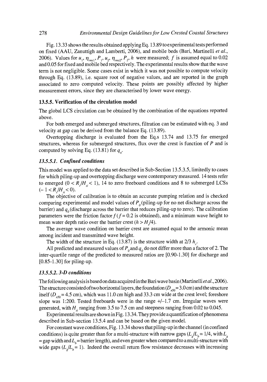
Figure 2.1. Illustration of the sheltering effect of an emergent LCS by reduction in shorewards transmitted wave
energy by wave breaking, wave reflection and porous flow.
6
Environmental Design Guidelines for Low Crested Coastal Structures
tI
_,.~.~i~:.,,--~-.~'-~
,
--
"" :,. ,-,, ,~-;-.~.
I
,~,,,
;:~:~r ~"~:~.~ ~
:-.lrlrJ9..,"~,e /t"
~
9 ,1~'.
~
q ~
..
9
~
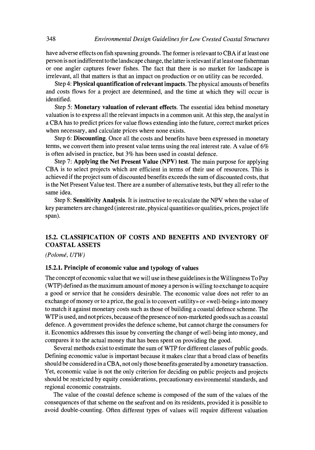
.
y
9
~ . ~ _ . . ~ h o r e h n e / o r m a t x o n tollo,~mg
%.
~...c'&~_.~,6thewave breaker line
N, T'~eTr~,.",,
-.-.
iiiiiiiiiiiiiiiii----'_
" )
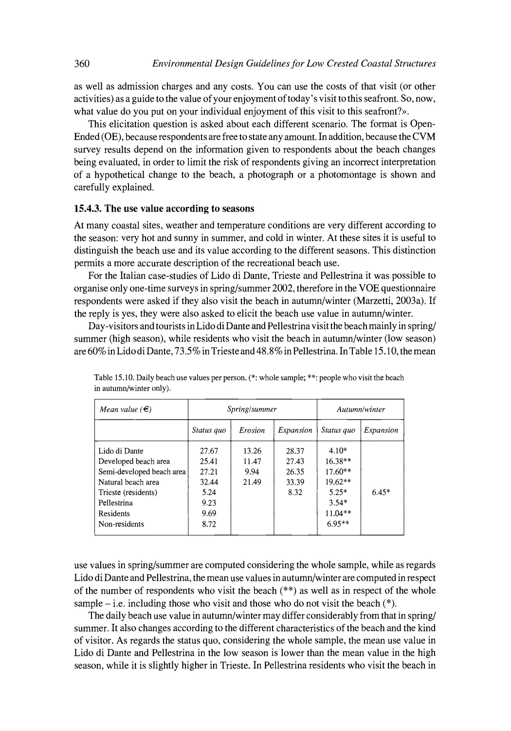
.
.
.
)
.
'
.
.
.
.
.
.
.
.
I
. . . . . . . . . .
I
'(ii;.....il
I
.
.
.
.
.
.
.
.
.
.
.
.
.
.
.
.
.
.
.
.
.
.
.
.
.
.
.
.
.
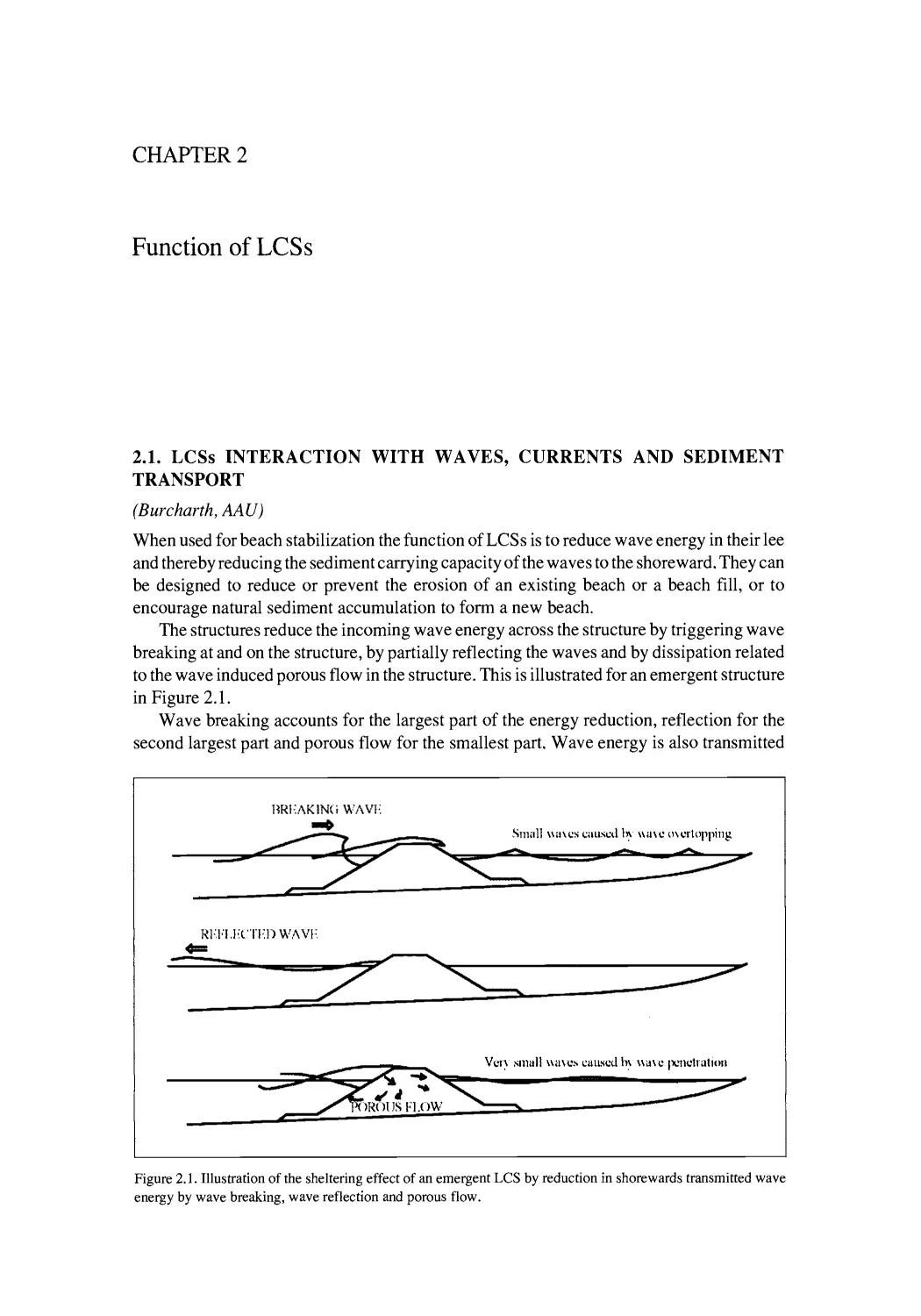
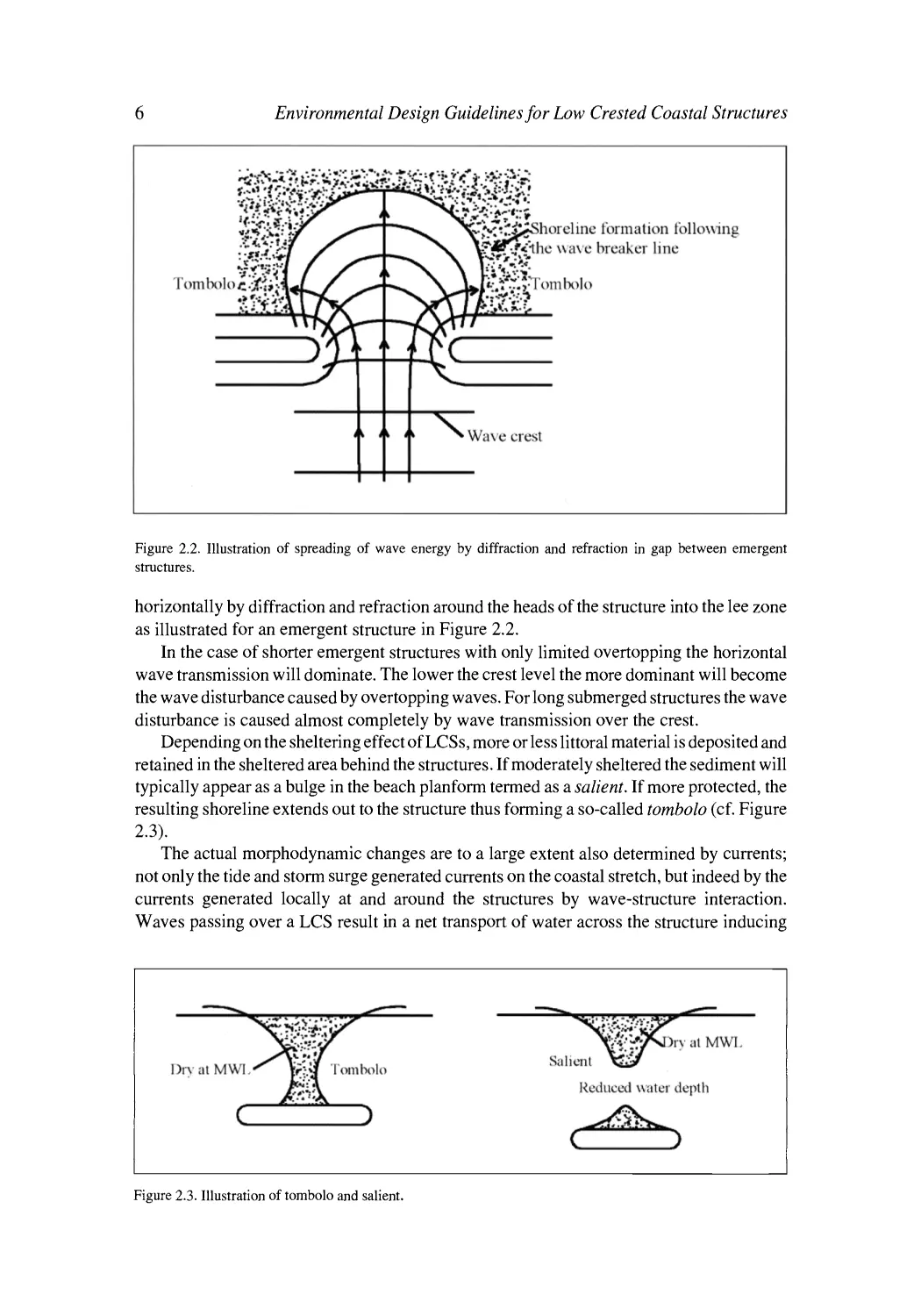
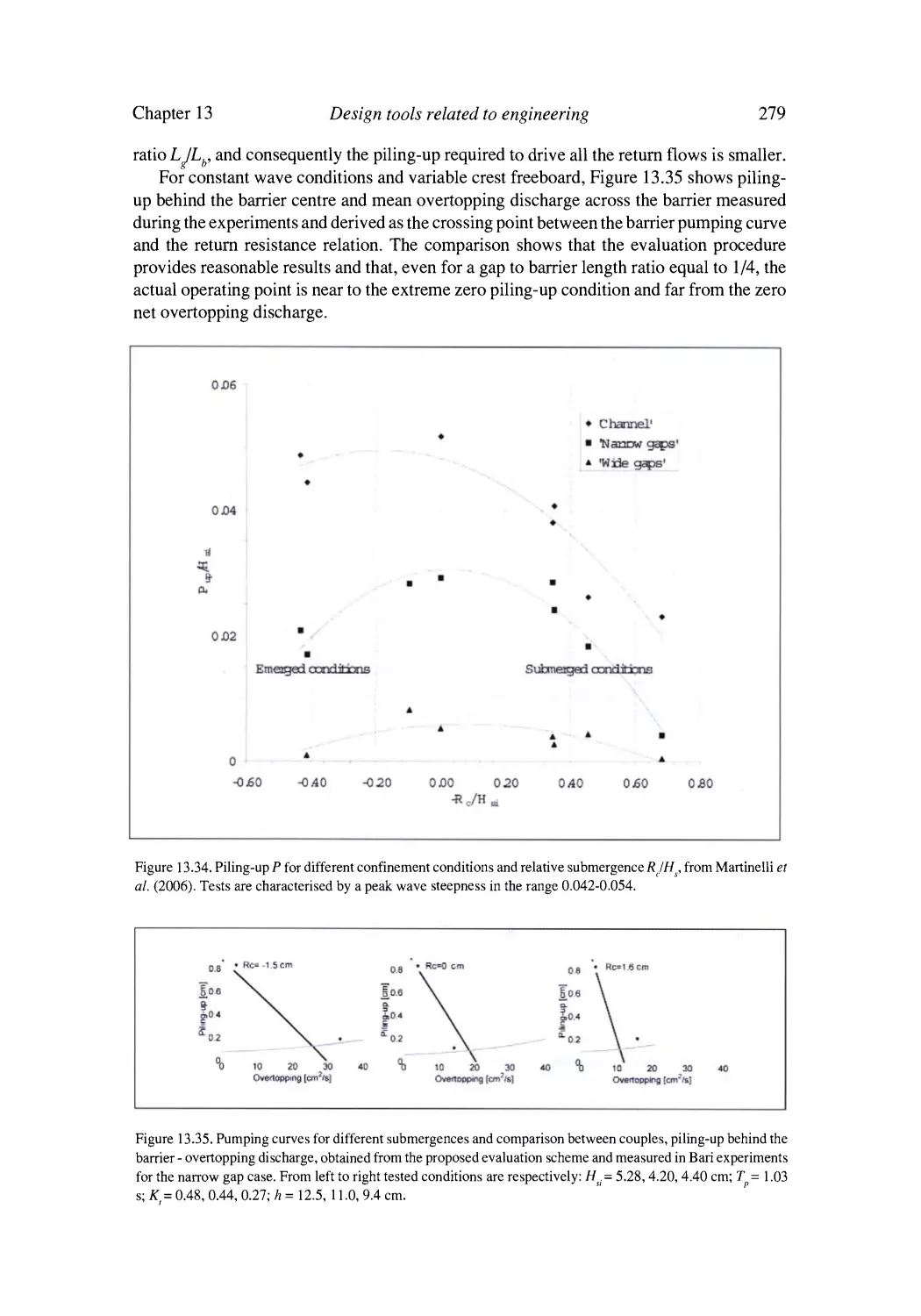
Figure 2.2. Illustration of spreading of wave energy by diffraction and refraction in gap between emergent
structures.
horizontally by diffraction and refraction around the heads of the structure into the lee zone
as illustrated for an emergent structure in Figure 2.2.
In the case of shorter emergent structures with only limited overtopping the horizontal
wave transmission will dominate. The lower the crest level the more dominant will become
the wave disturbance caused by overtopping waves. For long submerged structures the wave
disturbance is caused almost completely by wave transmission over the crest.
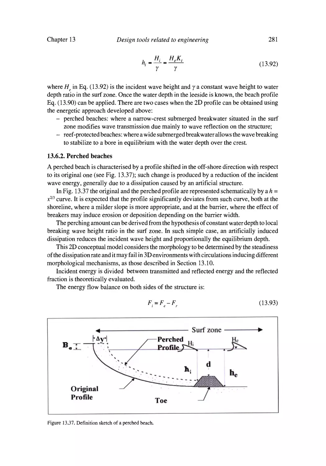
Depending on the sheltering effect of LCSs, more or less littoral material is deposited and
retained in the sheltered area behind the structures. If moderately sheltered the sediment will
typically appear as a bulge in the beach planform termed as a salient. If more protected, the
resulting shoreline extends out to the structure thus forming a so-called tombolo (cf. Figure
2.3).
The actual morphodynamic changes are to a large extent also determined by currents;
not only the tide and storm surge generated currents on the coastal stretch, but indeed by the
currents generated locally at and around the structures by wave-structure interaction.
Waves passing over a LCS result in a net transport of water across the structure inducing
~Vg'~7~Drv at M~q....
"~',;~
Dr3'at M W l ~ . ~ U o m b o l o
ReducM x~ater depth
C
)
Figure 2.3. Illustration of tombolo and salient.
C
)
Function of LCSs
Chapter 2
. . . . . . . . . .
'~,.Z,~."
' . . . . . . . . . . . . . . . . . . .
;~
"'"
. . . . . . . . . . . . . . . . . . . . . . .
2
''C
........... ) ' ' ' (
t
"'"
"
-'d
- ..........
t _,
.................. Z ' ' - (
)''
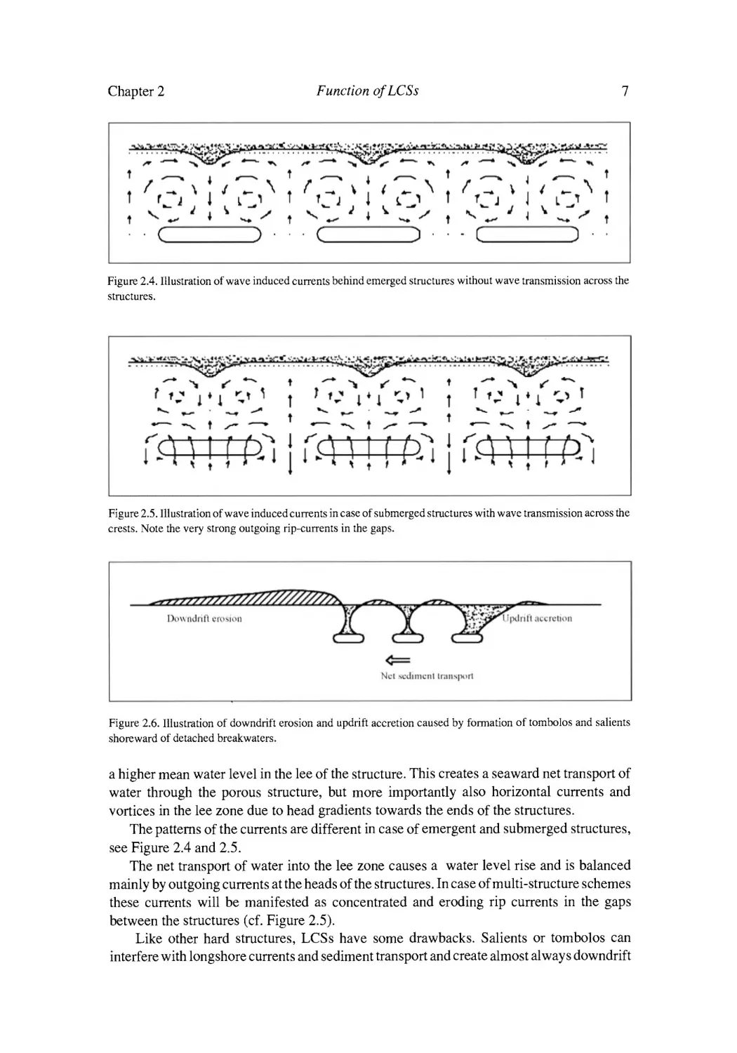
Figure 2.4. Illustration of wave induced currents behind emerged structures without wave transmission across the
structures.
. . . . . . .
_- . .
-'-"
t-s
t,
~
.
- ~
t
.
,
.,-
,,
f
.
.
.
.
.
.
.
.
.
~ "
~
.
.
.
.
.
.
.
.
-'-"
~
~
.r"
.
.
.
.~
?
-'~
. . . . . . . . . . . . . . . . . . . . .
i.
~
~ ................
- .............- ...............,,........ ~
~-"~
"~
~
-~
-~
t
. . . . . . . . . .
I"
.,
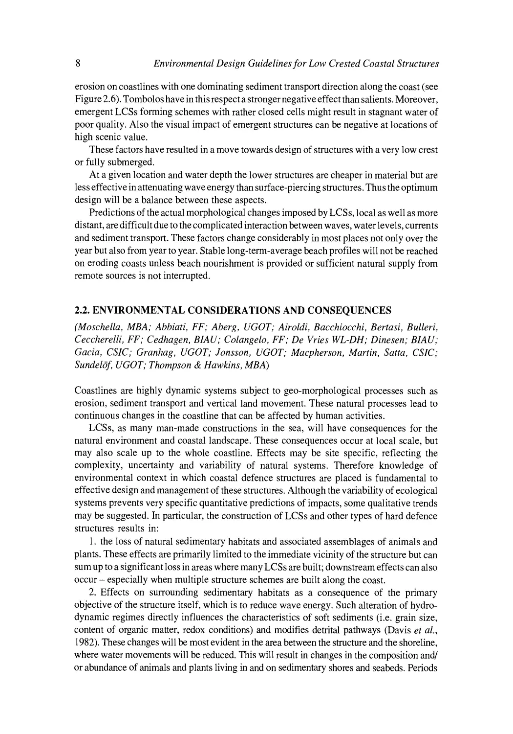
Figure 2.5. Illustration of wave induced currents in case of submerged structures with wave transmission across the
crests. Note the very strong outgoing rip-currents in the gaps.
t[
]
I[
{
(
]
N r | scd i m c n I transpol"l
Figure 2.6. Illustration of downdrift erosion and updrift accretion caused by formation of tombolos and salients
shoreward of detached breakwaters.
a higher mean water level in the lee of the structure. This creates a seaward net transport of
water through the porous structure, but more importantly also horizontal currents and
vortices in the lee zone due to head gradients towards the ends of the structures.
The patterns of the currents are different in case of emergent and submerged structures,
see Figure 2.4 and 2.5.
The net transport of water into the lee zone causes a water level rise and is balanced
mainly by outgoing currents at the heads of the structures. In case of multi-structure schemes
these currents will be manifested as concentrated and eroding rip currents in the gaps
between the structures (cf. Figure 2.5).
Like other hard structures, LCSs have some drawbacks. Salients or tombolos can
interfere with longshore currents and sediment transport and create almost always downdrift
8
Environmental Design Guidelinesfor Low Crested Coastal Structures
erosion on coastlines with one dominating sediment transport direction along the coast (see
Figure 2.6). Tombolos have in this respect a stronger negative effect than salients. Moreover,
emergent LCSs forming schemes with rather closed cells might result in stagnant water of
poor quality. Also the visual impact of emergent structures can be negative at locations of
high scenic value.
These factors have resulted in a move towards design of structures with a very low crest
or fully submerged.
At a given location and water depth the lower structures are cheaper in material but are
less effective in attenuating wave energy than surface-piercing structures. Thus the optimum
design will be a balance between these aspects.
Predictions of the actual morphological changes imposed by LCSs, local as well as more
distant, are difficult due to the complicated interaction between waves, water levels, currents
and sediment transport. These factors change considerably in most places not only over the
year but also from year to year. Stable long-term-average beach profiles will not be reached
on eroding coasts unless beach nourishment is provided or sufficient natural supply from
remote sources is not interrupted.
2.2. ENVIRONMENTAL CONSIDERATIONS AND CONSEQUENCES
(Moschella, MBA; Abbiati, FF; Aberg, UGOT; Airoldi, Bacchiocchi, Bertasi, Bulleri,
Ceccherelli, FF; Ceclhagen, BIAU; Colangelo, FF; De Vries WL-DH; Dinesen; BIAU;
Gacia, CSIC; Granhag, UGOT; Jonsson, UGOT; Macpherson, Martin, Satta, CSIC;
Sundel6f, UGOT; Thompson & Hawkins, MBA)
Coastlines are highly dynamic systems subject to geo-morphological processes such as
erosion, sediment transport and vertical land movement. These natural processes lead to
continuous changes in the coastline that can be affected by human activities.
LCSs, as many man-made constructions in the sea, will have consequences for the
natural environment and coastal landscape. These consequences occur at local scale, but
may also scale up to the whole coastline. Effects may be site specific, reflecting the
complexity, uncertainty and variability of natural systems. Therefore knowledge of
environmental context in which coastal defence structures are placed is fundamental to
effective design and management of these structures. Although the variability of ecological
systems prevents very specific quantitative predictions of impacts, some qualitative trends
may be suggested. In particular, the construction of LCSs and other types of hard defence
structures results in:
1. the loss of natural sedimentary habitats and associated assemblages of animals and
plants. These effects are primarily limited to the immediate vicinity of the structure but can
sum up to a significant loss in areas where many LCSs are built; downstream effects can also
occur- especially when multiple structure schemes are built along the coast.
2. Effects on surrounding sedimentary habitats as a consequence of the primary
objective of the structure itself, which is to reduce wave energy. Such alteration of hydrodynamic regimes directly influences the characteristics of soft sediments (i.e. grain size,
content of organic matter, redox conditions) and modifies detrital pathways (Davis et al.,
1982). These changes will be most evident in the area between the structure and the shoreline,
where water movements will be reduced. This will result in changes in the composition and/
or abundance of animals and plants living in and on sedimentary shores and seabeds. Periods
Chapter 2
Function of LCSs
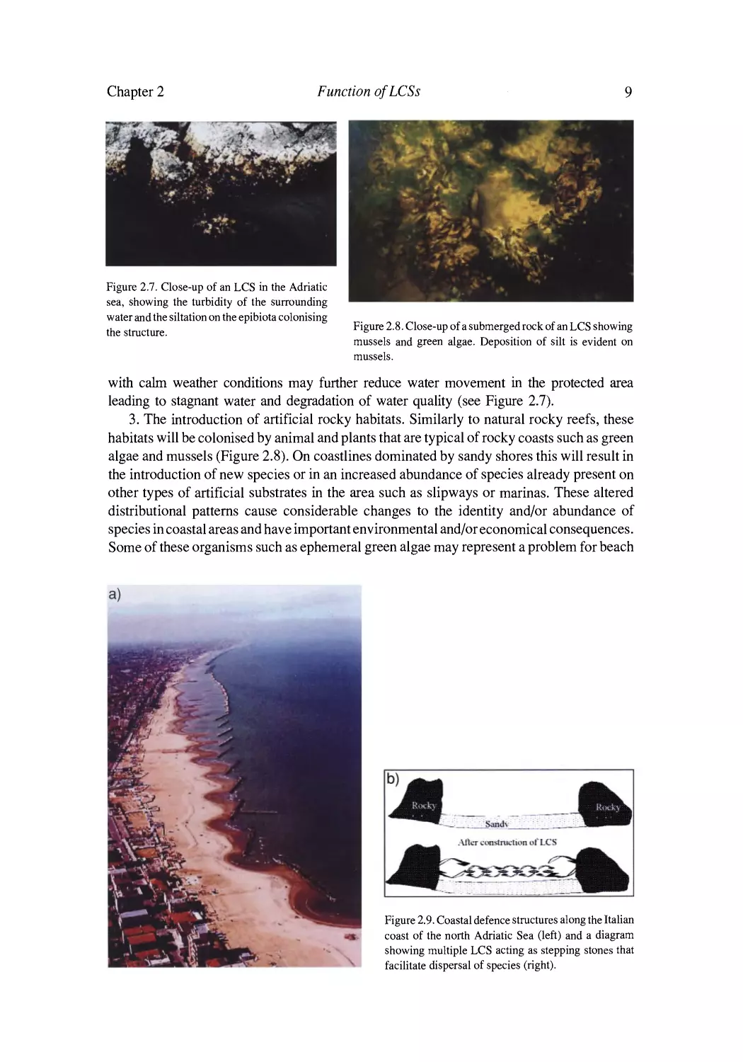
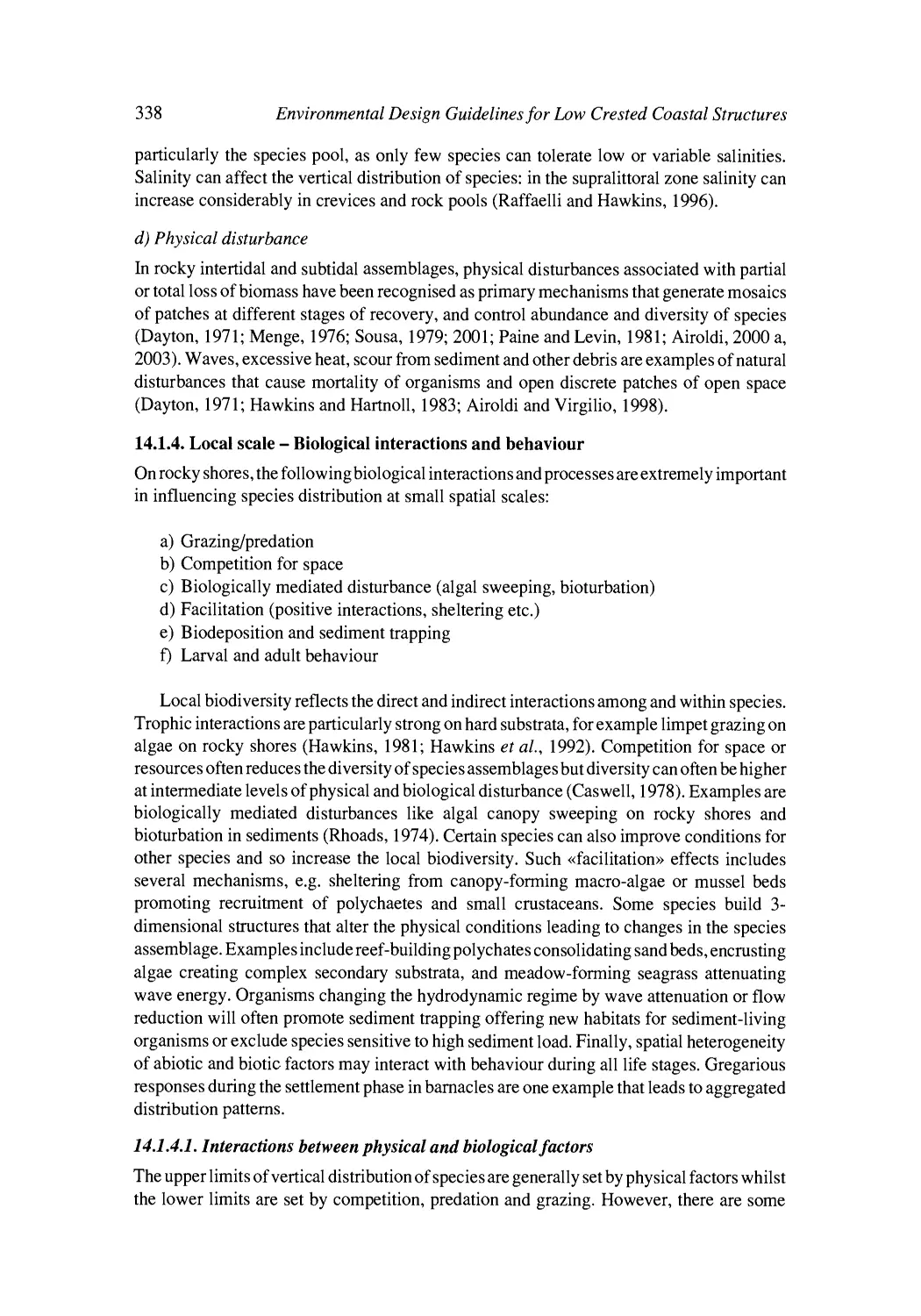
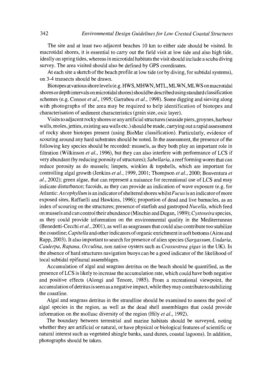
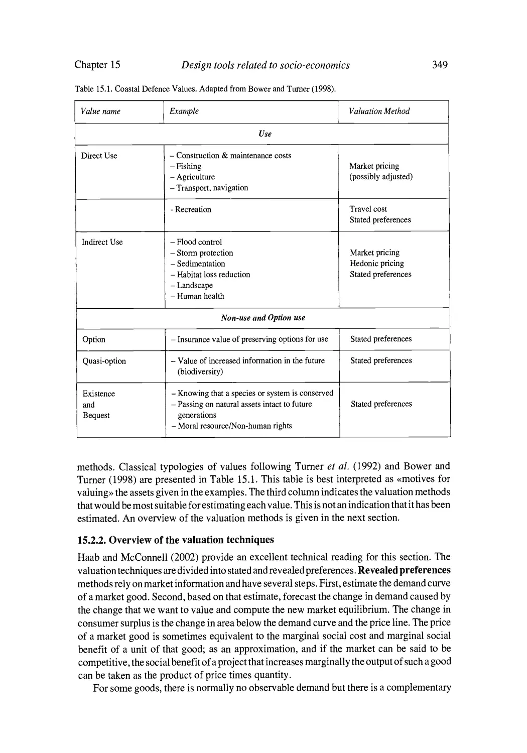
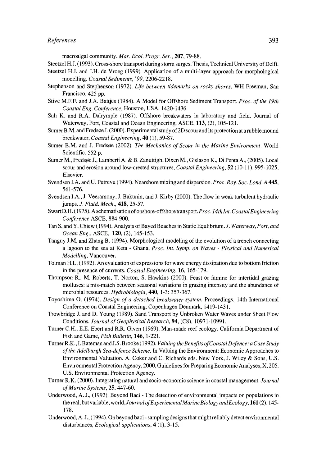
Figure 2.7. Close-up of an LCS in the Adriatic
sea, showing the turbidity of the surrounding
water and the siltation on the epibiota colonising
the structure.
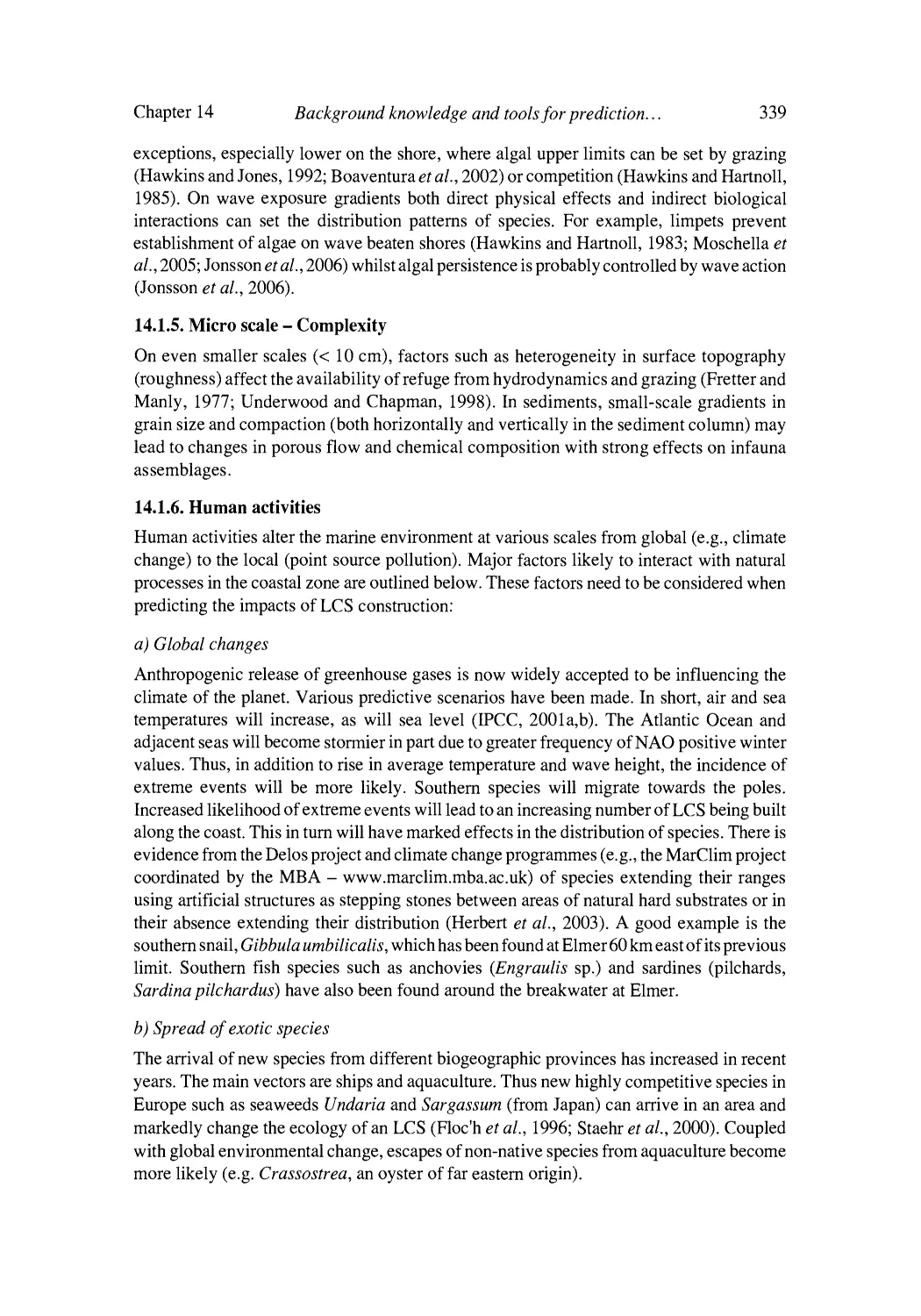
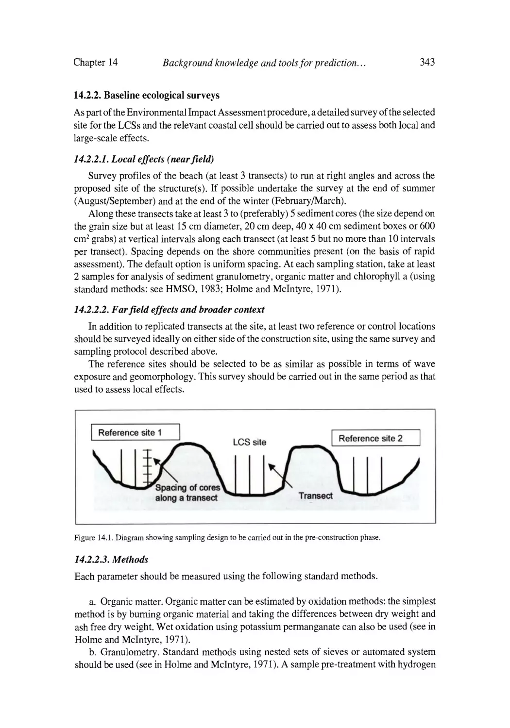
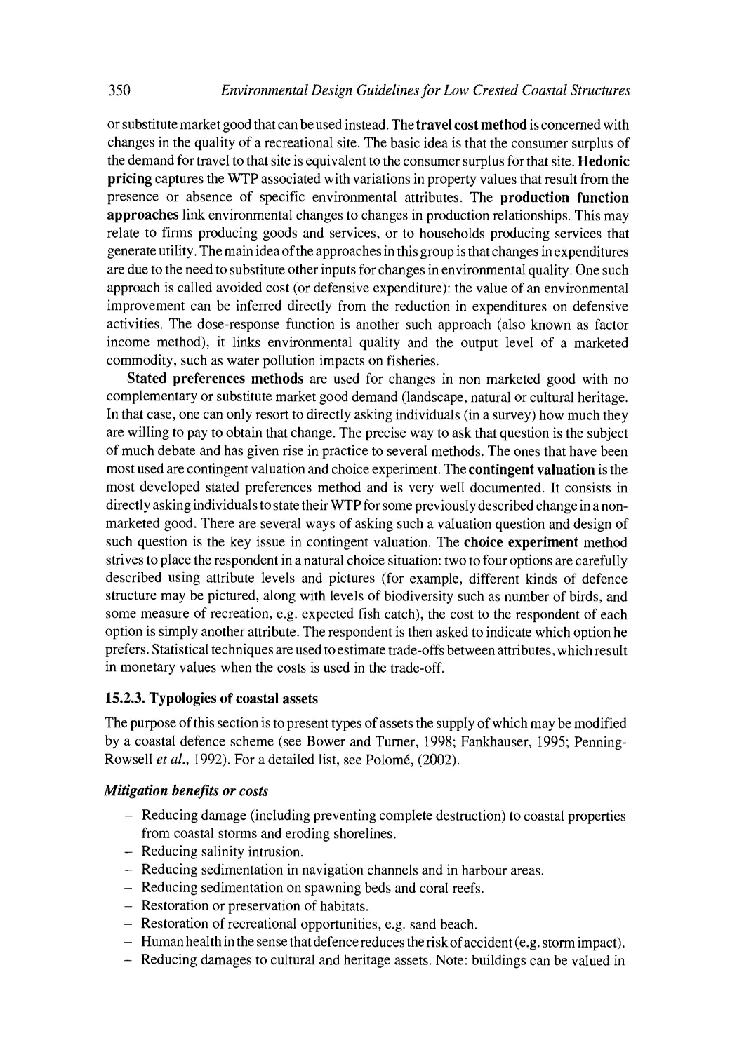
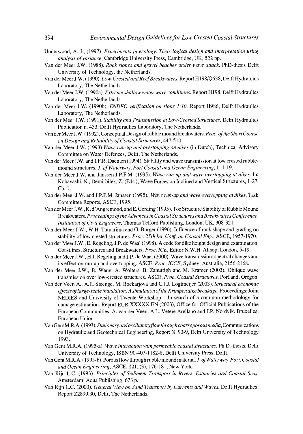
Figure 2.8. Close-up of a submergedrock of an LCS showing
mussels and green algae. Deposition of silt is evident on
mussels.
with calm weather conditions may further reduce water movement in the protected area
leading to stagnant water and degradation of water quality (see Figure 2.7).
3. The introduction of artificial rocky habitats. Similarly to natural rocky reefs, these
habitats will be colonised by animal and plants that are typical of rocky coasts such as green
algae and mussels (Figure 2.8). On coastlines dominated by sandy shores this will result in
the introduction of new species or in an increased abundance of species already present on
other types of artificial substrates in the area such as slipways or marinas. These altered
distributional patterns cause considerable changes to the identity and/or abundance of
species in coastal areas and have important environmental and/or economical consequences.
Some of these organisms such as ephemeral green algae may represent a problem for beach
a)
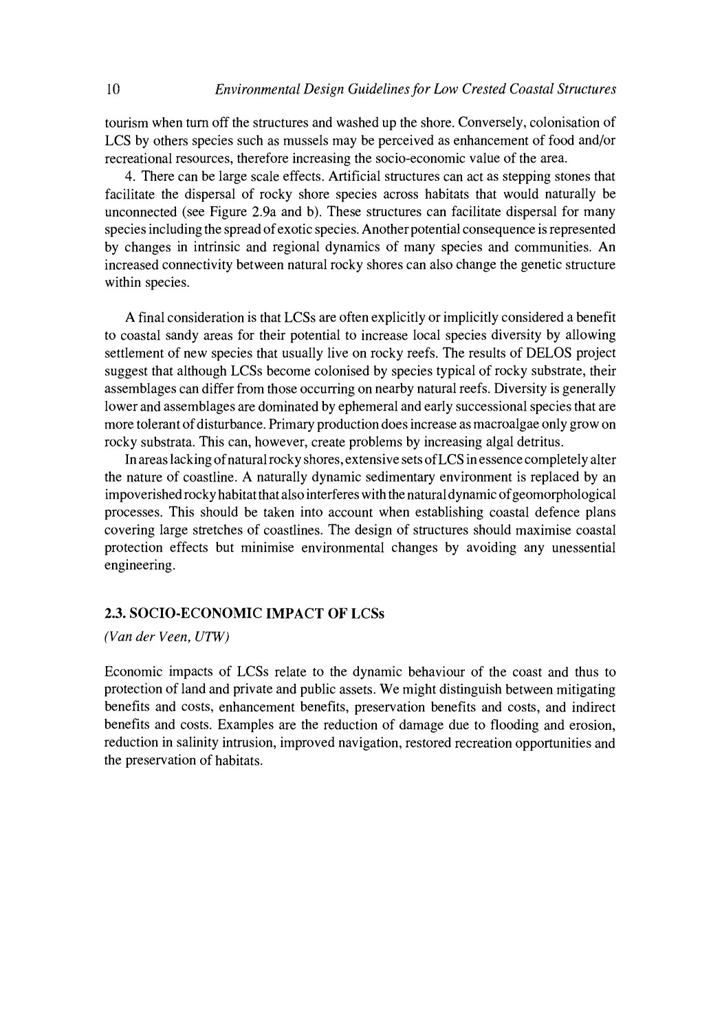
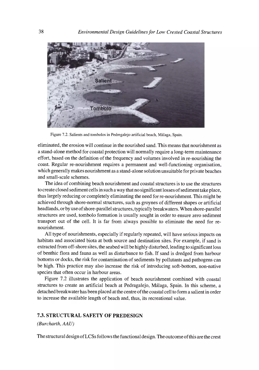
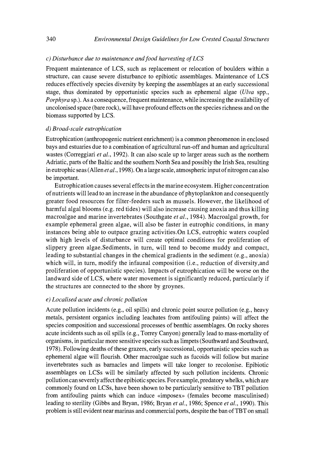
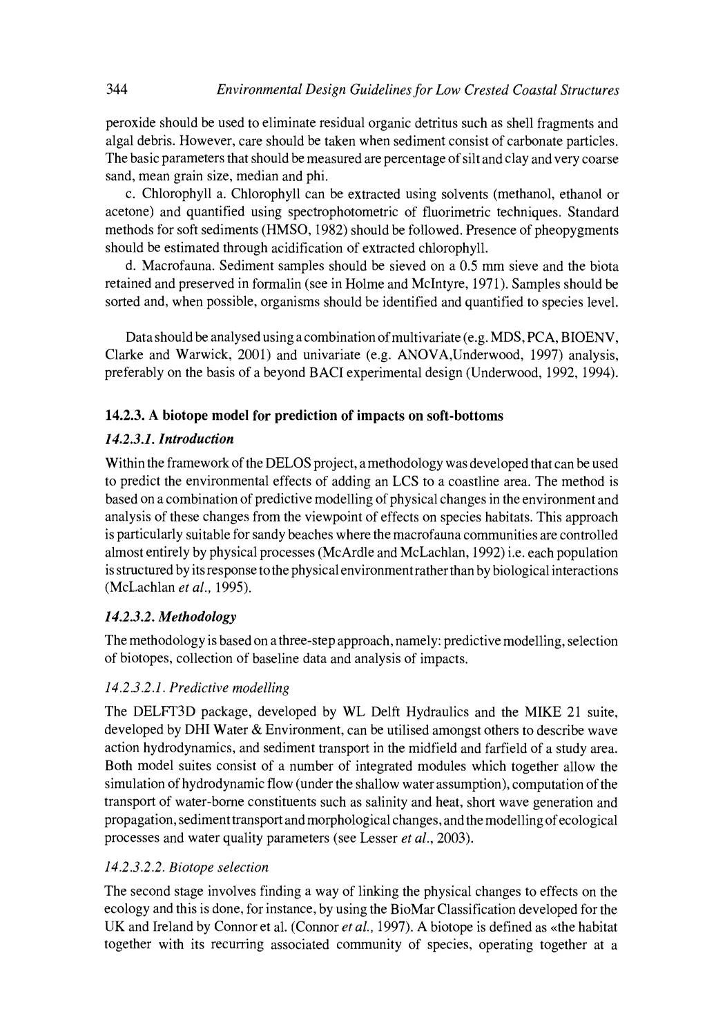
Figure 2.9. Coastal defence structures along the Italian
coast of the north Adriatic Sea (left) and a diagram
showing multiple LCS acting as stepping stones that
facilitate dispersal of species (right).
10
Environmental Design Guidelines for Low Crested Coastal Structures
tourism when tum off the structures and washed up the shore. Conversely, colonisation of
LCS by others species such as mussels may be perceived as enhancement of food and/or
recreational resources, therefore increasing the socio-economic value of the area.
4. There can be large scale effects. Artificial structures can act as stepping stones that
facilitate the dispersal of rocky shore species across habitats that would naturally be
unconnected (see Figure 2.9a and b). These structures can facilitate dispersal for many
species including the spread of exotic species. Another potential consequence is represented
by changes in intrinsic and regional dynamics of many species and communities. An
increased connectivity between natural rocky shores can also change the genetic structure
within species.
A final consideration is that LCSs are often explicitly or implicitly considered a benefit
to coastal sandy areas for their potential to increase local species diversity by allowing
settlement of new species that usually live on rocky reefs. The results of DELOS project
suggest that although LCSs become colonised by species typical of rocky substrate, their
assemblages can differ from those occurring on nearby natural reefs. Diversity is generally
lower and assemblages are dominated by ephemeral and early successional species that are
more tolerant of disturbance. Primary production does increase as macroalgae only grow on
rocky substrata. This can, however, create problems by increasing algal detritus.
In areas lacking of natural rocky shores, extensive sets of LCS in essence completely alter
the nature of coastline. A naturally dynamic sedimentary environment is replaced by an
impoverished rocky habitat that also interferes with the natural dynamic of geomorphological
processes. This should be taken into account when establishing coastal defence plans
covering large stretches of coastlines. The design of structures should maximise coastal
protection effects but minimise environmental changes by avoiding any unessential
engineering.
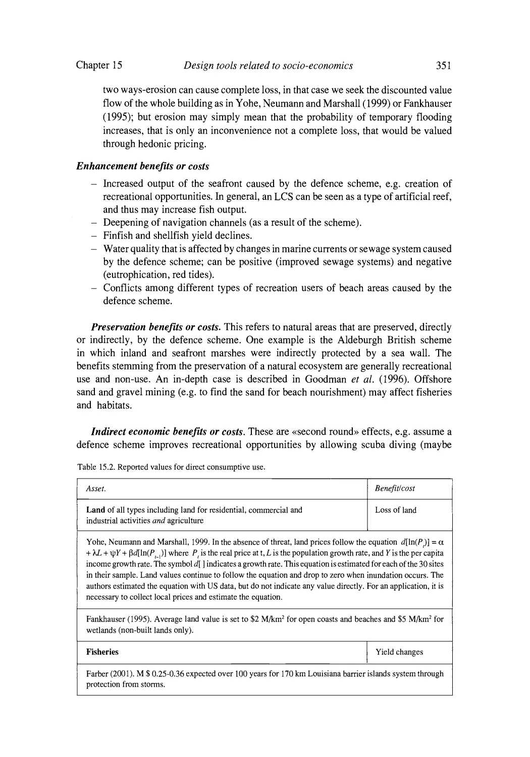
2.3. SOCIO-ECONOMIC IMPACT OF LCSs
(Van der Veen, UTW)
Economic impacts of LCSs relate to the dynamic behaviour of the coast and thus to
protection of land and private and public assets. We might distinguish between mitigating
benefits and costs, enhancement benefits, preservation benefits and costs, and indirect
benefits and costs. Examples are the reduction of damage due to flooding and erosion,
reduction in salinity intrusion, improved navigation, restored recreation opportunities and
the preservation of habitats.
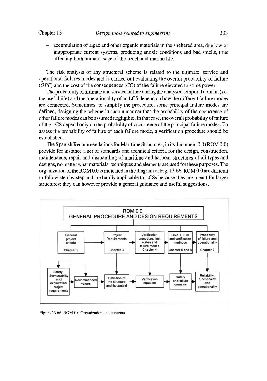
CHAPTER 3
Objectives and target effects of LCSs
(Moschella, MBA; Burcharth, AA U)
3.1. PROTECTION OF LAND AND INFRASTRUCTURE BY PREVENTION OR
REDUCTION OF COASTAL EROSION
(Moschella & Hawkins, MBA)
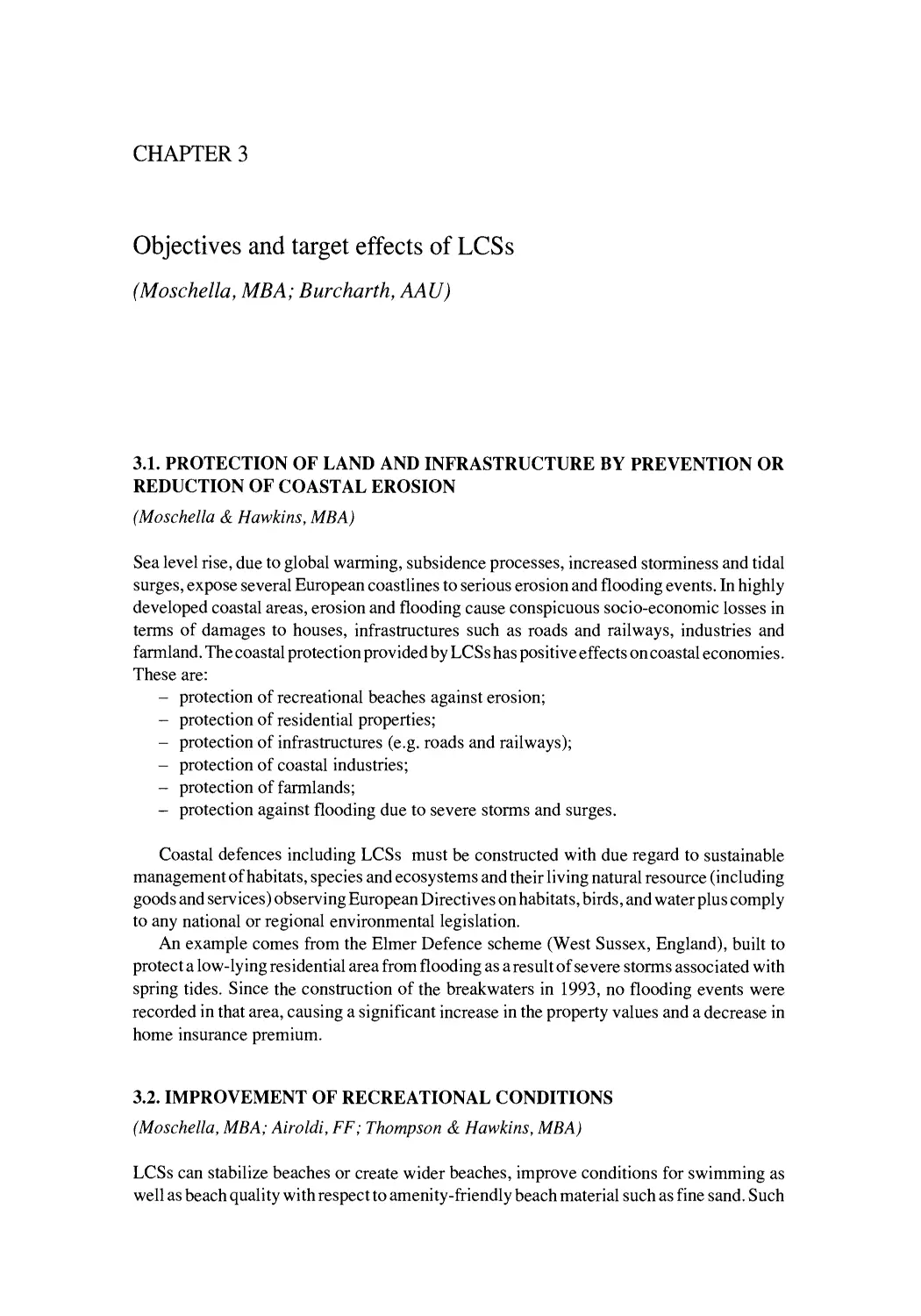
Sea level rise, due to global warming, subsidence processes, increased storminess and tidal
surges, expose several European coastlines to serious erosion and flooding events. In highly
developed coastal areas, erosion and flooding cause conspicuous socio-economic losses in
terms of damages to houses, infrastructures such as roads and railways, industries and
farmland. The coastal protection provided by LCSs has positive effects on coastal economies.
These are:
protection of recreational beaches against erosion;
protection of residential properties;
protection of infrastructures (e.g. roads and railways);
protection of coastal industries;
- protection of farmlands;
protection against flooding due to severe storms and surges.
-
-
-
-
-
Coastal defences including LCSs must be constructed with due regard to sustainable
management of habitats, species and ecosystems and their living natural resource (including
goods and services) observing European Directives on habitats, birds, and water plus comply
to any national or regional environmental legislation.
An example comes from the Elmer Defence scheme (West Sussex, England), built to
protect a low-lying residential area from flooding as a result of severe storms associated with
spring tides. Since the construction of the breakwaters in 1993, no flooding events were
recorded in that area, causing a significant increase in the property values and a decrease in
home insurance premium.
3 . 2 .
IMPROVEMENT OF RECREATIONAL CONDITIONS
(Moschella, MBA; Airoldi, FF; Thompson & Hawkins, MBA)
LCSs can stabilize beaches or create wider beaches, improve conditions for swimming as
well as beach quality with respect to amenity-friendly beach material such as fine sand. Such
Environmental Design Guidelinesfor Low Crested Coastal Structures
12
development should also observe relevant environmental legislation, guidance and emerging
best practice in order to ensure sustainable usage of the coastal zone.
LCSs have significant influence on the recreational conditions for beach users. Some
influences are regarded as positive, while others are considered as negative. The influence
is either direct due to the physical presence of the structure in the nearshore zone, or indirect
due to the consequent effects on the local hydro-morphodynamics (eg. rip currents).
Sea conditions behind LCSs are generally calmer than on open beaches and this can
improve bathing conditions, especially for children. The improved safety of bathing and
swimming in a calm sheltered zone (probably excluding for boat traffic) is a very positive
effect since this is the most common recreational activity taking place in the nearshore area.
However the possible formation of strong rip currents at gaps and/or ends of the LCS
shore protection system during rough seas may endanger the safety of bathing.
The presence of organisms that grow on the structures or colonise the sheltered habitats
behind LCSs can be a nuisance for beach tourism, leading to expensive beach cleaning or
removal of the organisms. Examples of these negative effects on the recreational value of
the beach come from the Italian shores of the North Adriatic Sea, where the ephemeral green
algae that extensively colonise LCSs (also favoured by local eutrophic conditions) are torn
off the structures and washed up the shore, where they decay. In the UK, large amounts of
drift algae are trapped on the landward side of the structures and eventually decompose
leading to unpleasant smells due to formation of anoxic conditions and increase in number
of flies. Further, periods with calm weather conditions may lead to stagnant water and
degradation of bathing water quality.
Boating with various craft and surfing may be negatively affected by the presence of the
LCS if the crest elevation is not clearly visible, due to the risk of collision. Even more
dangerous could be diving into the sea from a boat and hitting on the hard structure.
Conversely, activities like snorkelling or sport fishing can be positively enhanced if the
structure provides a new attractive habitat for marine life. If the structure is emergent it
favours access for fishermen.
3.3. P R O T E C T AND MINIMISE IMPACTS ON CULTURAL AND NATURAL
HERITAGE OF THE COASTLINE
(Moschella, MBA; Airoldi, FF; Gacia, CSIC; Thompson & Hawkins, MBA)
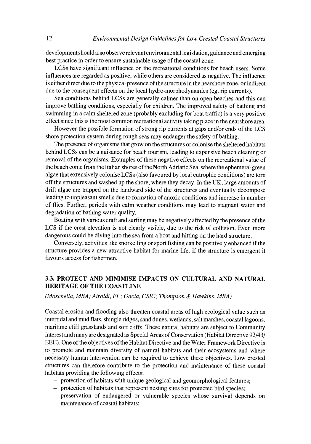
Coastal erosion and flooding also threaten coastal areas of high ecological value such as
intertidal and mud flats, shingle ridges, sand dunes, wetlands, salt marshes, coastal lagoons,
maritime cliff grasslands and soft cliffs. These natural habitats are subject to Community
interest and many are designated as Special Areas of Conservation (Habitat Directive 92/43/
EEC). One of the objectives of the Habitat Directive and the Water Framework Directive is
to promote and maintain diversity of natural habitats and their ecosystems and where
necessary human intervention can be required to achieve these objectives. Low crested
structures can therefore contribute to the protection and maintenance of these coastal
habitats providing the following effects:
protection of habitats with unique geological and geomorphological features;
protection of habitats that represent nesting sites for protected bird species;
- preservation of endangered or vulnerable species whose survival depends on
maintenance of coastal habitats;
-
-
Chapter 3
Objectives and target effects of LCSs
13
- preservation of coastal plant and animal species of scientific interest.
In addition, special features of natural heritage importance (e.g., saline lagoons,
saltmarshes, vegetated shingle banks and sand dunes) or special sectors of interest (bird
reserves) may be threatened by coastal erosion. Therefore circumstances may occur where
a coastal defence structure is proposed to expressly protect endangered habitats or species.
For example, in the coastal area between Happisburgh and Winterton-on-sea in Norfolk
(East Anglia, UK), a system of LCS and a seawall were built to protect The Broads wetlands.
In Tuscany sea defence structures were built to protect the maritime pine tree forest in
the national park of San Rossore endangered by coastal erosion. Sometimes habitats or
species protected by conservation legislation such as the vegetated shingles (habitat listed
on Annex 1 of the EC Habitats Directive) can indirectly benefit from coastal defence
schemes that were built with the only purpose of protecting properties. For example, the
Elmer defence schemes in West Sussex (South of England) also protects the vegetated
shingle ridge which host species of special national conservation interest such as little robin
Geranium purpureum, a rare plant in West Sussex, the toadflax brocade moth Calophasia
lunula, a Biodiversity Action Plan species and many birds which nest in this zone. Elmer
defence scheme has been designated as an SSSI (Site of Special Scientific Interest). In Poole
Bay (south of England), the recently built rock groyne system not only protects residential
properties and the beach from erosion but also helps restoration of native vegetated sand
dunes. If protected, these will in turn provide additional natural protection against erosion.
LCSs can be used to protect areas of cultural heritage value such as archaeological and
historic sites, monuments, churches and buildings threatened by coastal erosion. Nonvisible LCSs are probably preferable; if necessary combined with a revetment or a seawall
to strengthen the shore. For example, on the Adriatic coast, along the promontory of Conero,
a system consisting of LCS and rocks were deployed to protect historic buildings from
erosion.
3.4. ENHANCEMENT OF NATURAL LIVING RESOURCES FOR FOOD AND
R E C R E A T I O N
(Moschella, MBA; Airoldi & Bulleri, FF; Thompson & Hawkins, MBA)
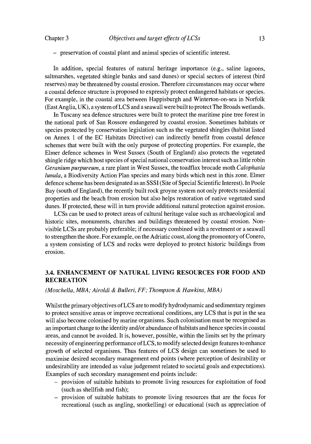
Whilst the primary objectives of LCS are to modify hydrodynamic and sedimentary regimes
to protect sensitive areas or improve recreational conditions, any LCS that is put in the sea
will also become colonised by marine organisms. Such colonisation must be recognised as
an important change to the identity and/or abundance of habitats and hence species in coastal
areas, and cannot be avoided. It is, however, possible, within the limits set by the primary
necessity of engineering performance of LCS, to modify selected design features to enhance
growth of selected organisms. Thus features of LCS design can sometimes be used to
maximise desired secondary management end points (where perception of desirability or
undesirability are intended as value judgement related to societal goals and expectations).
Examples of such secondary management end points include:
provision of suitable habitats to promote living resources for exploitation of food
(such as shellfish and fish);
provision of suitable habitats to promote living resources that are the focus for
recreational (such as angling, snorkelling) or educational (such as appreciation of
-
-
Environmental Design Guidelines for Low Crested Coastal Structures
14
marine wildlife, ~(rock-pooling>> and omithology) activities;
provision of suitable habitats to promote endangered or rare species;
- provision of suitable habitats to promote diverse rocky substrate assemblages for
conservation or mitigation purposes.
-
CHAPTER 4
Outline of design procedure
(Burcharth, AA U; Lamberti UB)
The design procedure is usually divided into a preliminary (or conceptual) design phase and
a detailed design phase. The objective of the preliminary design phase is to explore the
project feasibility with respect to economy, technical performance, and societal and
environmental impacts. This usually involves conceptual design of alternative LCSschemes. The preferred scheme is then selected for detailed design which basically consists
of optimizing the scheme with respect to impacts, structural performance and costs.
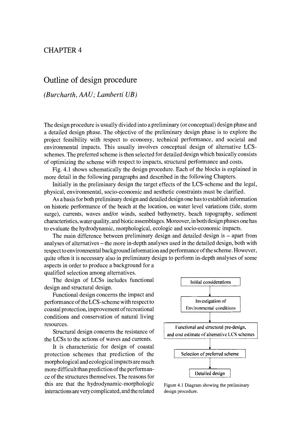
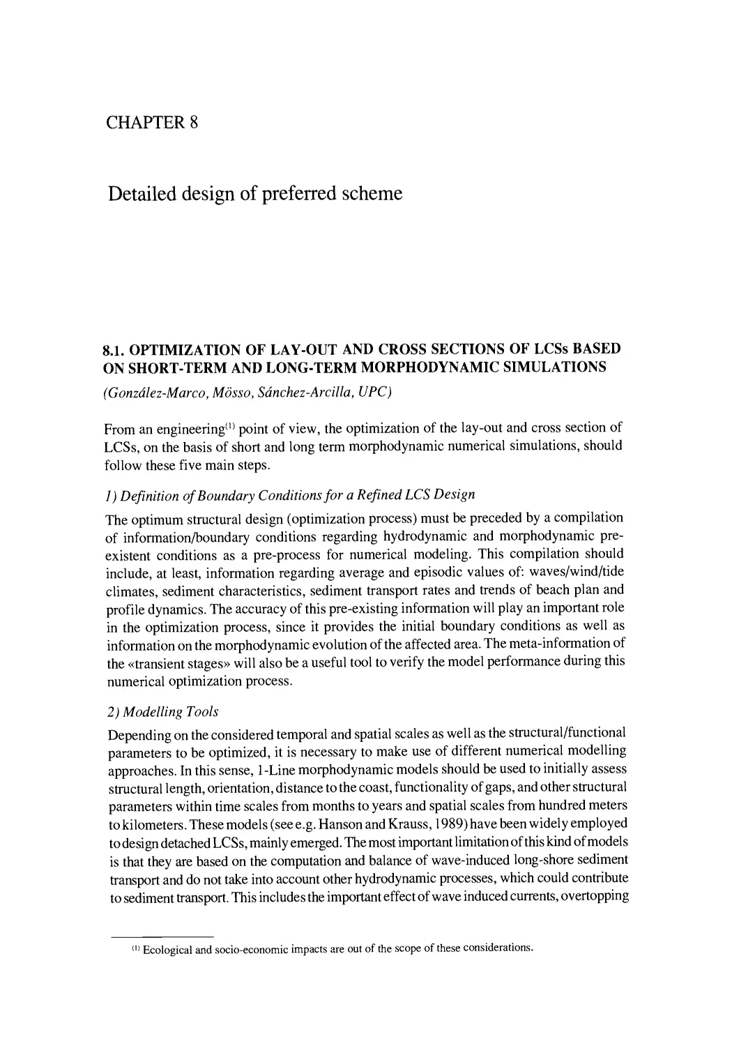
Fig. 4.1 shows schematically the design procedure. Each of the blocks is explained in
more detail in the following paragraphs and described in the following Chapters.
Initially in the preliminary design the target effects of the LCS-scheme and the legal,
physical, environmental, socio-economic and aesthetic constraints must be clarified.
As a basis for both preliminary design and detailed design one has to establish information
on historic performance of the beach at the location, on water level variations (tide, storm
surge), currents, waves and/or winds, seabed bathymetry, beach topography, sediment
characteristics, water quality, and biotic assemblages. Moreover, in both design phases one has
to evaluate the hydrodynamic, morphological, ecologic and socio-economic impacts.
The main difference between preliminary design and detailed design is - apart from
analyses of alternatives - the more in-depth analyses used in the detailed design, both with
respect to environmental background information and performance of the scheme. However,
quite often it is necessary also in preliminary design to perform in-depth analyses of some
aspects in order to produce a background for a
qualified selection among alternatives.
The design of LCSs includes functional
design and structural design.
Functional design concerns the impact and
Investigation of
performance of the LCS-scheme with respect to
Environmental conditions
coastal protection, improvement of recreational
conditions and conservation of natural living
.............................. i ...............
resources.
i
I:unctlonaland structural pre-design.
Structural design concerns the resistance of
and ost estimate of alternative LCS schemes
the LCSs to the actions of waves and currents.
It is characteristic for design of coastal
i ...............................
.i. Sd;ciioi;o(PreferrCd sd~e,n~ ]
protection schemes that prediction of the
morphological and ecological impacts are much
more difficult than prediction of the performance of the structures themselves. The reasons for
this are that the hydrodynamic-morphologic
Figure 4.1 Diagram showing the preliminary
design procedure.
interactions are very complicated, and the related
~
16
Environmental Design Guidelines for Low Crested Coastal Structures
predictive tools are either indicative simple rules of thumb or complex numerical models.
For reliable prediction of the morphological development the latter needs to be run for longterm simulations, not only covering the local areas around the structure but also the sediment
cell. To establish the necessary boundary conditions and hydrodynamic input, and to run
such models is all together very costly and time consuming. As a consequence they are
generally used only for finer tuning of larger schemes. In most cases only more simple
numerical models are used locally, and then only for short-term simulations. It follows that
the uncertainty related to the long-term prediction of the morphological response will be
large.
The tools for structural design are quite reliable formulae for the stability of the various
parts of the structures, and/or performance of model tests. The major part of the uncertainty
of the structural response is related to the estimation of the design wave climate and, if scour
is critical, also to the local currents at the structures.
Because the structure should preserve its shape for the whole project period and because
repair cannot take place immediately after damage, it is common practice in structural design
to consider the most severe environmental conditions in structure lifetime.
In functional design with respect to impact on beach morphology and ecosystems it is
necessary to analyse the long-term effect of all environmental conditions accounting for the
variations in intensity and duration that affect the function of the structure.
Most LCSs are located where wave heights are depth limited. As water depth depends
both on the water level and the sea bed level, both have to be examined with respect to
statistics and variations.
It follows that it is difficult to give more specific guidance with respect to design
procedure and selection of design tools. A general statement could be that the marginal costs
of further detailed analyses in preliminary and detailed design stages should be compensated
by the added value of the certainty of the performance (or reduced risk of failure) of the
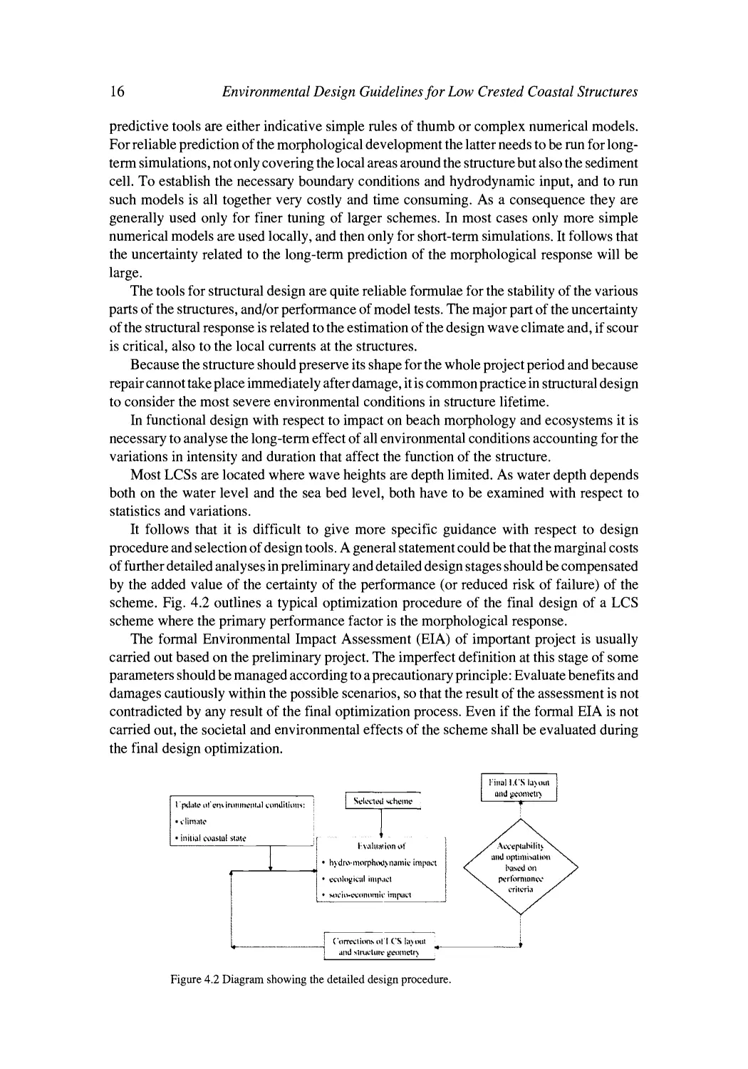
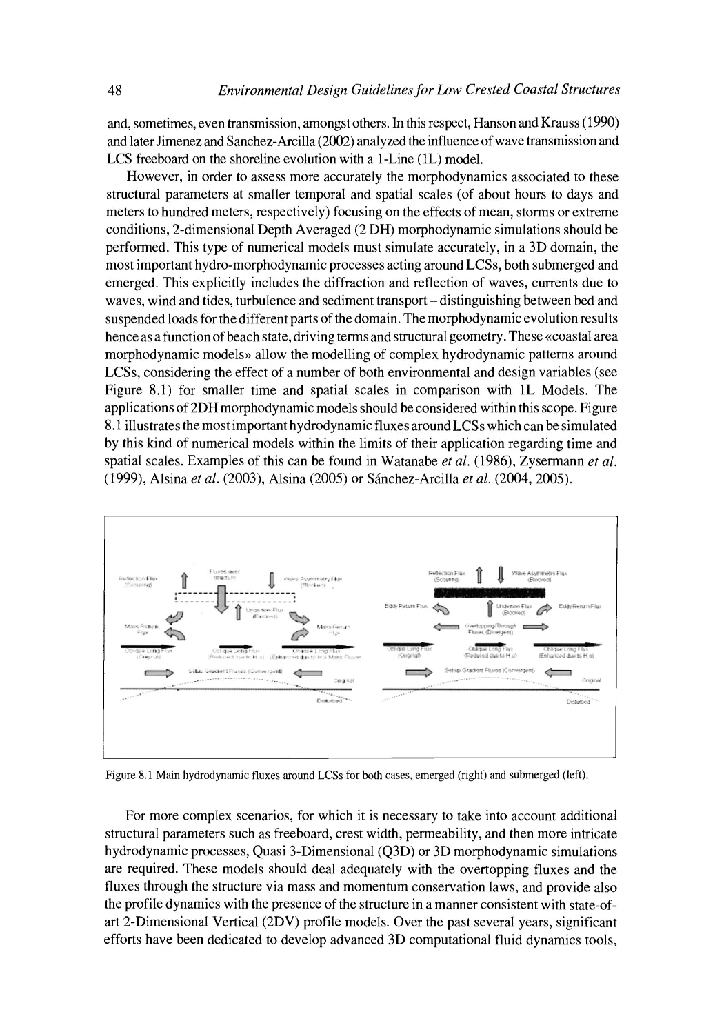
scheme. Fig. 4.2 outlines a typical optimization procedure of the final design of a LCS
scheme where the primary performance factor is the morphological response.
The formal Environmental Impact Assessment (EIA) of important project is usually
carried out based on the preliminary project. The imperfect definition at this stage of some
parameters should be managed according to a precautionary principle: Evaluate benefits and
damages cautiously within the possible scenarios, so that the result of the assessment is not
contradicted by any result of the final optimization process. Even if the formal EIA is not
carried out, the societal and environmental effects of the scheme shall be evaluated during
the final design optimization.
[ i~i,,~iii:s=~;,,,, I
I
I ~::!:~!_~d
~ :o,l,,,~ ,,,'~,. i~,,.,,,~,,,.,~ .-,,.di,i,,,,~:
'
initial coastal st~le
l- .......... i
and ~eome~,
~-"~'"~
i!,,'ahl;~tion o f
/
;
j
9
t~vdro-morpht~namic imp,act
ecolot~.icul ill|p~tcl
i" .~ocit1-r
1
imp~wl
('orrr
o1' i CS layout
and .~ll'tlr
~t-g't.llllelr% r
i
Figure 4.2 Diagramshowing the detailed design procedure.
I
CHAPTER 5
Initial considerations
5.1. CONSIDERATION OF LEGAL, PHYSICAL, ENVIRONMENTAL, SOCIOE C O N O M I C AND AESTHETIC CONSTRAINTS
(Burcharth, AAU; Vidal, UCA; Moschella, MBA; Airoldi, Bulleri, Ceccherelli, Colangelo,
FF; Thompson & Hawkins, MBA)
5.1.1. Relevant policy and legislation
Both coastal protection (protection from erosion) and sea defence (defence from inundation)
are influenced by EU policy and legislation and by the translation of these at the national
level. Other legal issues relate to directives and legislation regarding the procedural steps to
obtain the necessary planning permissions and licences for any defence scheme (such as
consultation and freedom of access to environmental information).
These approaches and their translation vary across Europe but the overarching EU
legislative requirements are the same. Table 5.1 identifies the relevant Directives that will
need to be considered when developing proposals for coastal protection and sea defence
measures, including LCSs. These directives have been divided into the vertical and
horizontal controls impacting on the process. Horizontal directives are the EIA Directive
(coastal defence works) and the Strategic Environmental Assessment (SEA) Directive
(coastal works to combat erosion and works that alter the coastline). SEA will be required
where plans and programmes are from particular sectors or otherwise from those which have
significant environmental effects, and set the framework for future development consent of
EIA projects (under Directive 85/337/EEC as amended), or any plan which requires an
appropriate assessment under the provisions of the Habitats Directive (92/43/EEC).
The SEA Directive had to be translated into national legislation by 21 st July 2004. Many
of the datasets relevant to implementation of the SEA Directive at the strategic level are also
relevant at the individual project level (the EIA Directive level) and will therefore be relevant
to individual coast defence project assessments. Sustainability Appraisals (SA), which have
been increasingly used at plan and programme level are essentially non-statutory and
overlap with many of the requirements of the SEA Directive. Usually SA has a wider remit
within the social and economic appraisal than does SEA with its stronger focus on
sustainable environment, but SA also has a lower baseline information demand and less
analytical approach than SEA.
There are also proposed EU directives and conventions relevant to the development of
defences that have been included here since there is already wide adoption of the principles
at national level even without the weight of European legislation. A number of the Directives
18
Environmental Design Guidelines for Low Crested Coastal Structures
that h a v e i n f l u e n c e d the d e v e l o p m e n t or that h a v e b e e n active during the d e v e l o p m e n t o f
existing coastal d e f e n c e structures h a v e since b e e n m o d i f i e d and or a m e n d e d . T h e s e c h a n g e s
h a v e r e s u l t e d u n i v e r s a l l y in a s t r e n g t h e n i n g o f the controls and i n f o r m a t i o n r e q u i r e m e n t s to
s u p p o r t projects.
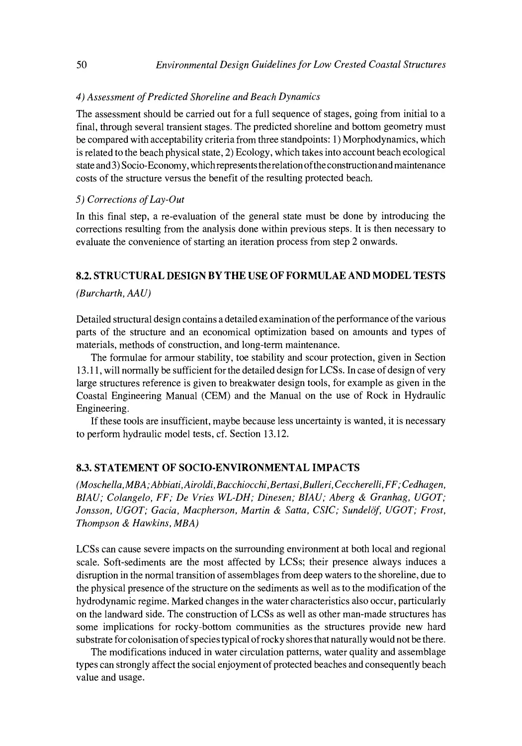
Table 5.1. Relevant policies and legislations at international and European level Directives relevant to proposals
for coastal protection and sea defence measures.
Directive
Date
Horizontal
Environmental Impact Assessment Directive
1985
Strategic Environmental Assessment (SEA) Directive
Water Framework Directive
2001
2000
Environmental Quality
Bathing Water Directive
1976 (modified)
Shellfish Waters Directive
1979
Waste Water Treatment Directive
Nitrates Directive for Protection of water
against pollution caused by nitrates
from agricultural sources
Dangerous substances
1991
Information
Access to Environmental Information Directive
Directive No.
85/337/EEC amended by
Directive 97/11/EC
2001/42/EC
2000/60/EC
76/160/EEC modified
90/656/EEC and 91/692/EEC
79/923/EEC amended by
91/692/EEC
91/271/EEC
1991
91/676/EEC
76/464/EEC amended by
Directives 90/656/EEC
and 91/692/EEC
1990
90/313/EEC replaced by
2003/4/EC
Nature Conservation
Conservation of Wild Birds
Conservation of Natural Habitats and
Wild Flora and Fauna (Habitats Directive)
1979
79/409/EEC
1992
92/43/EEC
Conventions and proposed Directives
Aarhus Convention on access to information
and participation in decision making
2000
Integrated Coastal Zone Management (ICZM)
2000
Implemented through
Directives.
Currently a recommendation
COM/2000/547
OSPAR Oslo and Paris Convention for the
protection of the Marine Environment
of the North East Atlantic.
HELCOM Helsinki Convention for the
Protection of the Marine Environment
of the Baltic Sea Area.
Barcelona Convention for the Protection of the
Marine Environment and the Coastal Region
of the Mediterranean.
Ramsar Convention (Wetlands of International
Importance).
1992
1974 revised 1992
1995
1971
Chapter 5
Initial consideration
19
In addition, there are a number of other international conventions to which the majority
of the member states are signatories and are treated alongside the EU legislation. These
conventions relate both to horizontal and thematic initiatives.
Two relatively new Directives have a wider role in the strategic assessment of defence
projects and for which member states are developing approaches to implementation.
Specifically, the Strategic Environmental Assessment Directive and the Water Framework
Directive are seen as providing the scope for integrated management of resources, including
those on the coast. The Water Framework Directive in particular will provide a new strategic
framework for the development of defence plans as part of the overall development of River
Basin Management Plans (RBMP) and through these the potential for nationally consistent
approaches. Within the UK the RBMPs are likely to act as an overarching framework into
which the strategic management of coastal defence will have to be developed. Whether the
RBMP can integrate the existing non-statutory approach to Shoreline Management Plans
through which strategic defence management is developed is yet to be decided. However,
it is likely that any non-statutory plan would be subservient to the objectives developed
within any RBMP, which will also cover coastal waters. It is also likely that the objectives
of the WFD will influence coastal defence proposals. Defence structures are almost certainly
significant modifications to the natural environment and mitigation procedures are therefore
likely to be required within LCS scheme to contribute to achieving good ecological status
for relevant waterbodies.
The integration of activities along the EU shoreline is also influenced by conventions
that target regional seas and consider issues of erosion and water quality. The EU
has also considered the requirements for an integrated approach to management of
the coastal zone with the adoption of a resolution for the development of an EU strategy
for coastal zones (1992). This has lead to the draft strategy for Integrated Coastal Zone
Management (ICZM) and a three-year demonstration programme from 1996. The
development of ICZM will affect existing legislation and is likely to reinforce the
integration of existing Directives and national legislation as well as non-statutory
planning guidance.
The development of enhanced integration within spatial planning is also relevant to
the coastal zone and the development of the European Spatial Development Perspective
(ESDP) offers insight into spatial approaches within integrated coastal zone management
planning.
The legislative requirements and policy implementation at member state level for coastal
defence planning and management have not been individually assessed here, although it is
clear that the approach to Directive implementation and spatial planning differs widely
around Europe. In many countries the planning is managed as much by guidance notes and
non-statutory plans as they are through legislative provisions.
Many of the member states are also looking more closely at the integration of coastal
zone management in advance of any EU ICZM Directive. The complexity of the current
administrative and legal system suggests at a national scale (at least in UK) that no EU
wide ICZM Directive will be immediately forthcoming. It seems more likely that the
ICZM will be implemented through a Council resolution, procedural guidance and best
practice.
For example, in England and Wales many of the non-statutory plans focusing on flood
and coastal defence would however fall within the assessment of the SEA Directive. These
are likely to include Shoreline Management Plans (SMP), Water Level Management Plans
20
Environmental Design Guidelines for Low Crested Coastal Structures
(WLMP), Coastal Habitat Management Plans (CHaMPs). B iodiversity (through B iodiversity
Action Plans) will also need to be considered within the scope of defence approaches
(DEFRA, 2001). For example, whilst LCSs may develop diverse epibiotic communities,
these may not be typical of the area and therefore they may not form appropriate mitigation
for significant environmental effects of a flood defence action. However, the development
and maintenance of flood and coastal defence may also form integral part of the defence of
freshwater sites (e.g. grazing marshes and lagoons) and hence the maintenance of site
integrity. The conservation benefits of these LCSs will therefore need careful consideration
balancing the environmental losses against the maintenance of biodiversity and potential for
enhancement, even where sites are not under international conservation designations.
There are clearly strong overlapping requirements between SEA, EIA, WFD and
sectorial Directives. At least there is the potential for the environmental as well as social and
economic baseline datasets to be shared between the national implementations of these
Directives requirements and also on into non-statutory planning processes- such as
shoreline management plans (specifically targeting sea defence and coast protection). Such
approaches will help to avoid duplication, provide consistent data and allow national and
international status reports to be generated. Further duplication may occur where there is the
requirement for multiple assessments (such as where both SEA and Appropriate Assessment
under the Habitats Directive would be required). Promotion of the integration of assessments
will be important in considering the different objectives of the Directive but also in
integrating the findings when applied to coastal planning.
5.1.2. Physical constraints
Physical constraints are mainly given by the bathymetry, the character of neighbouring
stretches and by material supply possibilities.
In case of a steep seabed it will be expensive to place the structures at some distance to
the shore.
Sedimentary neighbouring coasts vulnerable to erosion cause serious constraints with
respect to the tolerable impact of the LCS-scheme on the coastal development. Down-drift
erosion is the most serious problem in this respect.
The use of natural rock as building material depends on the availability, size, quality,
quantity and costs for quarrying and transport. If not available then concrete blocks is an
alternative solution. The choice of material should, however, take into account environmental
constraints and desired ecological effects of LCSs.
5.1.3. Ecological constraints (including ecosystems, natural heritage and living
resources)
A variety of constraints should be considered in the design and construction procedures of
LCS. Environmental constraints should be clearly identified through the EIA and current
practice, following also the requirements of the European Commission Environmental
Directive 85/337/EEC. Environmental constraints may include cultural and natural heritage,
state and sensitivity of habitats, ecosystems and water quality.
1. Cultural heritage:
-
The presence of historic sites.
The presence of archaeological sites, both land and marine based.
The presence of listed buildings.
Initial consideration
Chapter 5
21
2. Natural heritage:
-
-
-
The presence of marine and coastal natural heritage areas (NHAs), with designated sites
of special interest containing important wildlife habitats, endangered species or unique
geological or geomorphological features.
The presence of special areas of protection and conservation at intemational (e.g. Ramsar
convention), European (e.g. SACs under Habitat Directive), national (e.g. SSSI, and
SPAs in the UK, PEIN in Spain) and local (voluntary, statutory or private nature reserves)
level.
The presence of national parks, wildlife sanctuaries and marine protected areas (MPAs).
3. Habitats and associated ecosystems:
-
-
-
The vulnerability of surrounding habitats and associated biota (benthic fauna, fish,
birds). For example, subtidal rocky habitats and boulder fields can be severely affected
by alteration of sediment regime and deposition (Airoldi 2003). Similarly seagrass
meadows (such as Posidonia, Zostera, Cymodocea) are sensitive to changes in sediment
and nutrient dynamics (Pergent-Martini et al., 1996; Vermaat et al., 1997).
The presence of rare or endangered species which could be threatened by the construction
of LCS. For example, rare species such as the coarse sand requiring Branchiostoma
lanceolatum which can be threatened by changes in granulometry (Desprez, 2000).
The presence of species that are important for the local economy (e.g. Chamelea gallina,
Solen vagina) and that could be replaced by non-native and not edible species introduced
by the new structures.
Indirect effects should be also taken into account, such as the presence of birds that rely on
feeding on certain infaunal species in the area affected by LCSs.
4. Water quality:
-
-
5.1.4.
The presence of estuaries, as LCSs could affect the distribution and characteristics of
sediment and organic load on the coast.
The presence of source of contaminants such as heavy metals, and persistant organic
compounds. LCSs might have a trapping effect, leading to accumulation of these
pollutants in finer deposits especially on the landward, sheltered side.
The eutrophic state and nutrients load. The presence of LCSs leading to greater residence
time could trigger macroalgal growth and harmful microalgal blooms including potential
toxic species (dinoflagellates) by increasing the eutrophic state of the surrounding waters.
Aesthetic
constraints
Coastal defences, especially multiple structure defence schemes, represent one very often
significant visual impact on the coastal landscape. This is particularly true for emerging
shore-parallel structures that tend to block the view from both land to sea and sea to land.
Visual impacts need therefore to be taken in consideration in the choice of LCS layout,
design and building material. Spoiling the view from beach and seafront restaurants could
also have a negative socio-economic effect, as well as the selection of construction material
which is in contrast with the surrounding natural landscape. For example, in most cases rock
material is preferred instead of concrete.
Aesthethic constraints include considerations for:
Environmental Design Guidelines for Low Crested Coastal Structures
22
- National Parks or Coastal Reserves of particular landscape or scenic beauty.
Specially designated Areas of Outstanding Natural Beauty (AONBs).
- Heritage Coasts, primarily designated for the quality of their coastal landscape.
- Historic landscapes, such as coastal monuments or terrestrial archaeological sites.
- Residential houses, hotels and leisure infrastructures on the top of the beach.
-
5.2. D E F I N I T I O N O F T H E P R I M A R Y O B J E C T I V E S
(Moschella, MBA; Airoldi, FF; Thompson & Hawkins, MBA)
5.2.1. T e c h n i c a l objectives
The engineering objectives for the specific project must be specified, reference is given to
Section 3.1.
5.2.2. E n v i r o n m e n t a l objectives
a. Geology-geomorphology
One of the environmental aims of LCSs should be to limit the target changes in the
geomorphological processes (e.g. from erosional to accreting beach) to the designated area
of influence of these structures. Changes in the sediment transport, usually causing
downdrift erosion, should be avoided.
b. Ecology
There are no direct natural heritage benefits which derive from construction of LCSs, except
when these structures are built with the clear objective of protecting terrestrial or freshwater
ecosystems of high natural value such as freshwater or brackish lagoons, wetlands and
saltmarshes. Even in this case there will be concomitant impacts on coastal and marine
systems.
Ecological objectives can be incorporated into design to maximise specific management
goals. Management goals may include minimising specific impacts on the environment (e.g.
minimising changes to the characteristics of surrounding soft-bottom sediments, or spread
of exotic species) and/or enhancing specific natural resources (e.g. enhancing species
biodiversity for recreational purposes, or recruitment to fisheries).
5.2.3. S o c i o - e c o n o m i c objectives
The socio-economic objectives constructing LCSs relate to the question <<what is it we are
protecting?>> and secondly, how are we going to protect it? The first question refers to the
basic societal need for safety and protection, and consequently economic growth and
welfare. However, currently environmental quality aspects of coastal protection receive
more and more attention and are being incorporated into a measure of welfare. The second
question also refers to an environmental problem: the design of a LCS may disrupt or
enhance landscape quality or habitat quality. In conclusion the socio-economic objective
of constructing a LCS is one of sustainability.
Chapter 5
Initial consideration
23
5.3. CONSIDERATION OF LCSs AS A POSSIBLE C O N T R I B U T I O N TO A
FUNCTIONAL AND E C O N O M I C A L SOLUTION
(Burcharth, AA U)
The most common use of LCSs is in coastal protection schemes. The conventional elements
in coastal protection schemes are dikes, seawalls, revetments, groynes, beach nourishment,
and shore-parallel breakwaters. The LCSs dealt with in this book belong to the last category.
A coastal protection scheme very often contains combinations of some of the mentioned
elements. The selection of the optimal scheme has to be based on analyses of a number of
possible combinations. It is beyond the scope of the present book to discuss schemes not
containing shore parallel breakwaters.
5.4. CONSIDERATION OF P R O J E C T SERVICE L I F E T I M E AND STRUCTURE
SAFETY CLASSIFICATION
(Moschella, MBA; Burcharth, AAU; Airoldi, FF; Lamberti, UB; Thompson & Hawkins,
MBA)
Where LCSs are part of a coastal protection scheme the service lifetime for the
structures will be as long as protection is required, provided that the structures are
functioning satisfactorily. It can be said that the structure service lifetime should equal
to the functional lifetime of the LCS scheme. A 50 years lifetime or more is common
for coastal structures. However, due to the dynamic character of many sedimentary
coasts it can be foreseen that in some places adjustments to the LCSs have to be made
maybe several times within such span of years. This means that the structure lifetime
is shorter than the functional lifetime of the LCS-scheme.
It is not important related to design to define a specific service lifetime for the LCSs
themselves because LCSs are built close to the shore in shallow water and consequently
structurally designed for depth limited waves, the sizes of which will be practically
independent of the service lifetime.
Internationally accepted safety classes for coastal structures do not exist. However,
LCSs will surely belong to a low safety class as the damage that might occur to the structures
will not cause human injury or immediate large economic losses. Moreover, repair can
normally be done fairly quickly. However, because maximum waves occur frequently in
depth limited conditions and because the extra costs needed for increasing the strength of the
structure is very small, the economical optimum corresponds to a very safe structure with
marginal probability of damage. More details on safety aspects are given in the section on
structural design.
From an environmental viewpoint the project lifetime and required maintenance is one
of the most crucial factors affecting composition, abundance and composition of species that
colonise the structures themselves. For instance, results of DELOS project have shown that
along the Italian coasts of the North Adriatic Sea, frequent maintenance of structures by
adding new blocks to the crest has dramatic effects on epibiota. Such frequent and severe
disturbance effectively reduces biodiversity to an early stage of succession, with few species
compared to those on structures which have not been maintained, and facilitate the
development of green ephemeral algae with consequent negative effects on the quality of the
beach. On any new LCS it will take time for the biological assemblage to reach a diverse
24
Environmental Design Guidelinesfor Low Crested Coastal Structures
community that is most likely to resemble that of a natural shore. For mature biological
communities to develop, LCSs need to be stable and built in such a way that maintenance
will be minimal.
Marine life also can influence the lifetime and the functioning of the system, for instance
by impact of mussel growth on sediment trapping and porosity. In Mediterranean regions,
rock boring organisms such as the date mussel Lithophaga lithophaga can in the long-term
undermine the integrity and reduce the lifetime of structures. In addition, service lifetime can
be limited by impacts in the surrounding areas, for example increased siltation or water
quality problems. Safety of structures for navigation should be also considered using current
legislation and best practice. The design of structures should also minimise risks for
recreational use. These include falling into deep gaps between the rocks, sinking in soft sand
and mud forming around the structures, swimming in rip and tidal currents.
5.5. C O N S I D E R A T I O N OF E N V I R O N M E N T A L C O N T E X T I N C L U D I N G
ECOSYSTEM, NATURAL H E R I T A G E AND NATURAL RESOURCES
(Moschella, MBA; Airoldi, FF; Thompson & Hawkins, MBA)
It is important to be aware that the complexity, uncertainty and diversity of natural
ecosystems cause a high degree of spatial variability, and that every system and location may
respond differently to the construction of an LCS. Thus while generic suggestions can be
made, spatial variability precludes standardised designs but solutions should be site specific.
The status, vulnerability and sensitivity and resilience of the coastal ecosystems involved
should be carefully assessed prior construction of LCSs. The different compartments of the
ecosystems that can be directly and indirectly affected should be considered, including
terrestrial and marine habitats.
5.6. SYNTHESIS OF ~Go / No Go>> DECISION
(Moschella, MBA; De Vries WL-DH; Thompson & Hawkins, MBA)
Initial considerations should function as a preliminary screening phase to address specific
issues such as objectives, environmental constraints and socio-economic evaluation. These
considerations should then be summarised and integrated to enable decision on whether or
not to proceed (Go / No Go) to the environmental assessment, planning and construction of
a LCS.
CHAPTER 6
Investigation of environmental conditions
This chapter describes the investigations of environmental conditions recommended for
design of LCSs. Instruments and procedures should comply with ISO standards where
applicable.
6.1. BATHYMETRY AND TOPOGRAPHY INCLUDING SEASONAL AND LONGTERM VARIATIONS
(Burcharth, AAU; Martinelli, UB)
The bathymetry, the topography and the coastline must be known at the location of the LCSscheme.
LCSs are usually placed in the active zone for sediment transport where almost
continuous changes in seabed levels take place. Seabed level changes can be characterized
as short-term fluctuations if caused by single events like storms; as mid-term variations if
caused by seasonal changes in the meteomarine climate; or as long-term variations if caused
by climatic changes or changes in the sediment budget along the coastline, for example
changes in discharge from rivers, sand mining, etc.
In order to decide the position of LCSs and their foundation level it is necessary to know
the expected range of seabed level variations at the actual location of the LCS-scheme, i.e.
the observed range of variations before placement of the structures plus the influence on the
seabed levels caused by the presence of the structures. A foundation level not higher than
the lowest expected seabed level should be chosen.
Historic information on coastline position and seabed bathymetry is often available and
should be supplemented by surveys of the actual situation. If no historic information is
available it is strongly recommended to carry out bathymetric surveys several times over a
year in order to cover seasonal variations and situations after significant storms. The
bathymetric surveys can be carried out with cable or echo-sounder. Use of differential GPS
installed directly over the sonar is the state of the art, allowing for centimetric precision.
Remote sensing techniques do not provide for the moment a bathymetry with sufficient
reliability. Older methods, like manual soundings and tide corrections can be used as well.
Series of cross shore profiles spaced 15 m to 25 m with few long-shore profiles for crosschecking is sufficient for design purpose.
If the mean sea level is not given at nearby fixpoints the mean sea level should be
estimated from measured water surface levels over a sufficiently long period.
26
Environmental Design Guidelinesfor Low Crested Coastal Structures
6.2. G E O L O G Y INCLUDING C H A R A C T E R I Z A T I O N OF SURFACE LAYERS
(SEDIMENTS)
(Burcharth, AA U; Martinelli, UB)
Information on seabed soil conditions is necessary both for the design of the LCS foundation
and for the prediction of the morphological changes caused by the structures.
Settlement and subsidence are critical for the proper function of LCSs because the crest
level is one of the most important design parameters. Expected consolidation of the seabed
due to the weight of the structure must be estimated from mechanical characterisation of the
subsoil. Settlement due to consolidation is a problem only in case of very soft and weak
subsoils as the foundation load of LCSs is usually small due to the limited height of the
structure.
The levels of more solid soil or rock formations underlying relatively thin loose
sedimentary surface layers should be identified in order to investigate the possibility of
direct foundation of LCSs on the more solid bed.
Subsidence of parts of LCSs into the seabed sediments will take place only if proper filter
layers and scour protection are not provided, or if the sediments are very sensible to
liquefaction caused by wave action or earthquakes. Information for the evaluation of such
conditions can be obtained by conventional geotechnical surveying techniques and soil
characterization methods. The spacing of sampling positions should account for the
variability in the soil formations.
For the prediction of morphological changes it is necessary to analyze the seabed as well
as the beach surface layer sediments with respect to grain size distribution, mass density and
fall velocity. Samples should be taken from several locations covering the whole LCSscheme and adjacent stretches (sediment cell).
Extraction of liquids or gas from the underground may be responsible of settlement in
the coastal zone and should be accounted for in the design of the structure crest levels.
6.3. WATER LEVEL VARIATIONS
(Burcharth, AAU; Lamberti, UB)
Water levels are of outmost importance in structural and functional design of LCS schemes
by determining both the maximum wave heights in shallow water (due to depth limitations)
and the freeboard of the structures. Together they basically control wave transmission.
Variations in water level are due to astronomical tides, storm surges and climatic
changes. Tidal variations follow the cycles of the moon and the sun, and are generally very
well predicted at almost all coastal locations by various institutes.
The small uncertainty makes it acceptable to model tides as a deterministic cyclic
process.
Storm surges are related to stormy weather which causes the water level to rise due to
barometric low pressures, wind stress (wind set-up) and breaking of waves approaching the
coast (wave set-up). Storm surge must be regarded as a stochastic variable due to the
unpredictability of meteorological variables.
More information on storm surge is given in Subsection 13.1.1.
Sea level rise due to climatic changes is a long-term effect, at the moment predicted with
Chapter 6
Investigation of environmental conditions
27
large uncertainty to be in the order of 0.5 m within 100 years. This is significant with respect
to consequences for erodible coasts and coastal protection works.
Sea level rise might be modelled as a linear rise with time having a coefficient ofvariation
in the order of 30%.
The relative importance of tides and storm surges varies with location. In general tides
will dominate on coasts with relatively steep foreshores facing an ocean (e.g. west coasts of
France, Ireland, U.K.), whereas storm surges dominate on shallow water coasts of more
confined seas (e.g. coastlines of the Baltic Sea).
The statistics of water levels is needed for the design. For structural design extreme
values are needed. For functional design with respect to morphological and ecological
impacts the more frequent water levels are needed. The correlation between wave heights
and wave periods is important in both cases.
If maximum water levels at or near the actual location have been recorded over many
years on a daily or monthly basis, it is possible to fit a statistical distribution from which
extreme values as well as frequent values can be extracted corresponding to any return period
(exceedence probability). If only annual extreme values are recorded then solely extreme
value statistics can be established, see Sub-section 13.1.3 for description of standard
methodology. If water level maxima throughout the year in a period of approximately ten
years or more are recorded then a Peak Over Threshold (POT) analysis can be used.
If water level records are not available it might be possible to establish an extreme
distribution based on synthetic data consisting ofhindcasted storm surges and the simultaneous
tide given by charged institutes.
For LCS schemes, compared for instance to sea dikes, it is less important to obtain
accurate statistics of extreme water levels for the structural design, because structures are
frequently overtopped and a high water level will often result in greater protection of the
armour layer against wave impacts. Accurate statistics of extremes is however important to
assess beach response to storm events.
The joint statistics of water levels and waves are dealt with in Section 6.4.
6.4. WAVE STATISTICS
(Burcharth, AAU; Lamberti & Archetti, UB)
The most important environmental loading parameters for the design of LCS schemes are
waves and water levels as they fully determine, together with tidal currents, the hydrodynamic
load. As most LCS schemes are built on coasts with limited tidal range, tidal currents are not
discussed further in this section.
Because the combined effect of water level and waves determine the impact on structure
and morphology, it is necessary to deal with the joint statistics of the two.
Statistics of waves and water levels very seldom exist at the nearshore locations usually
selected for LCS schemes. Available information on waves usually relates to deeper water
off the coast. However, such information, given as frequencies of wave heights, wave
periods and direction of waves, is readily available for almost all locations through
hydrographic service institutes.
As wind generated waves are irregular some statistical parameters are used to characterise
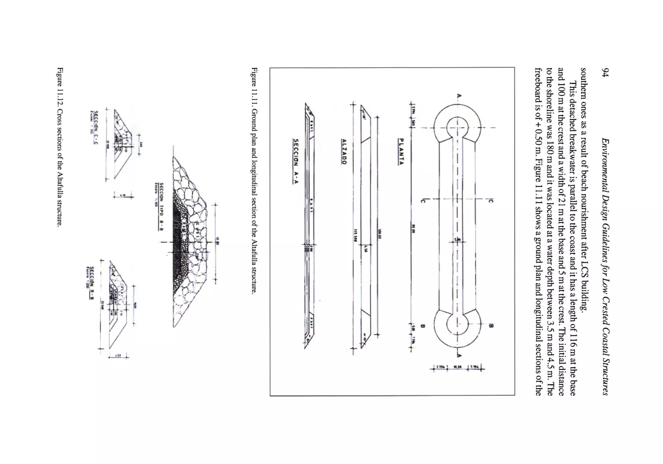
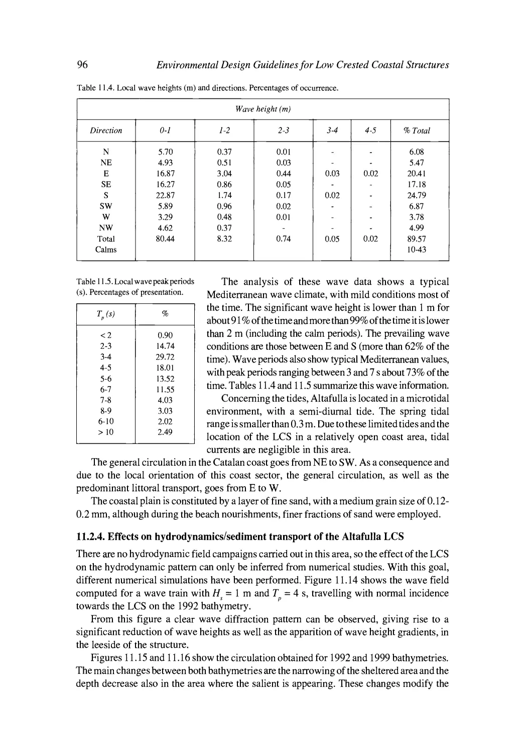
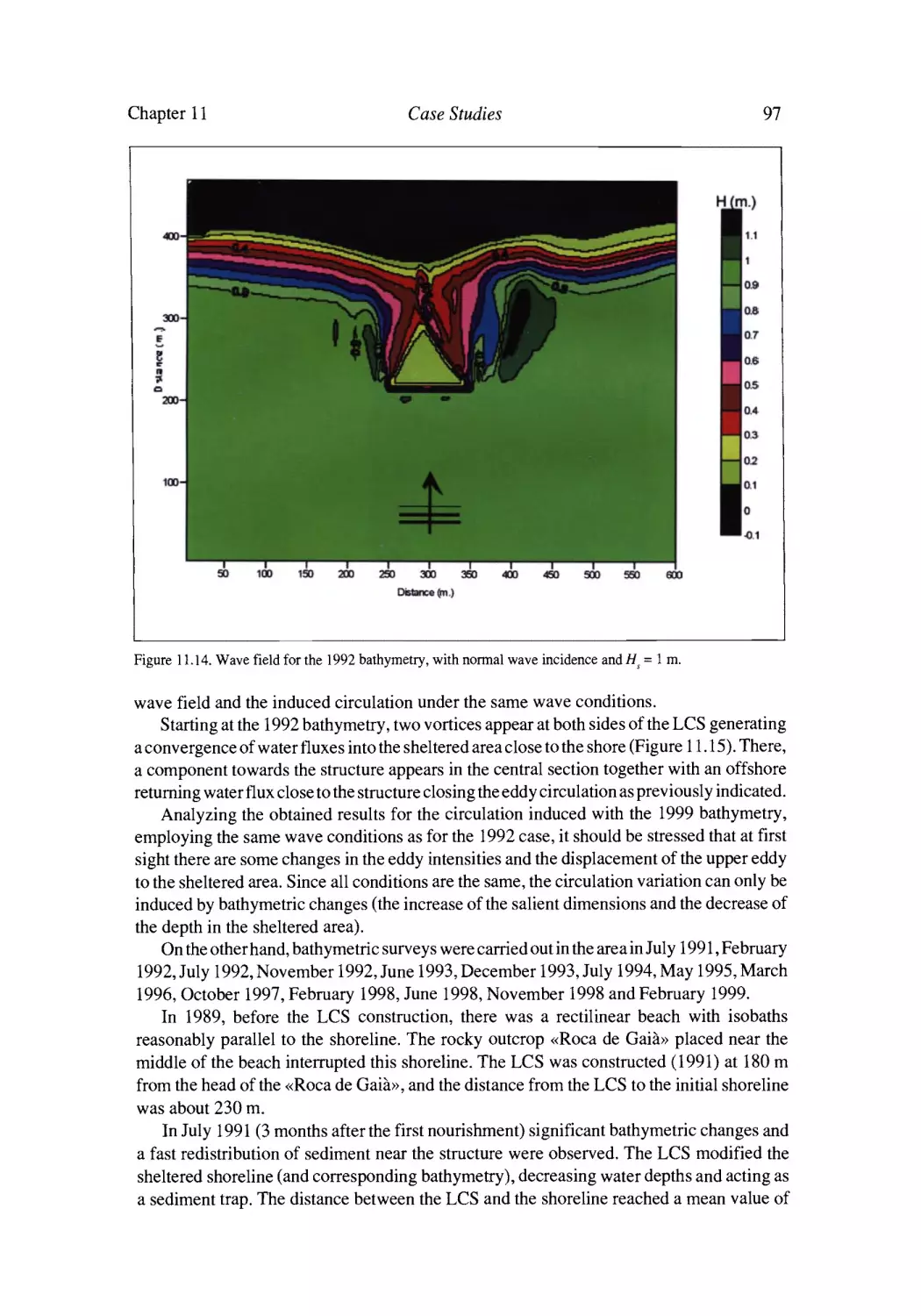
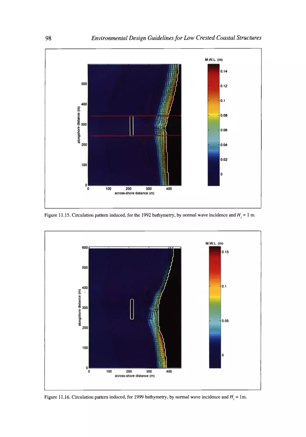
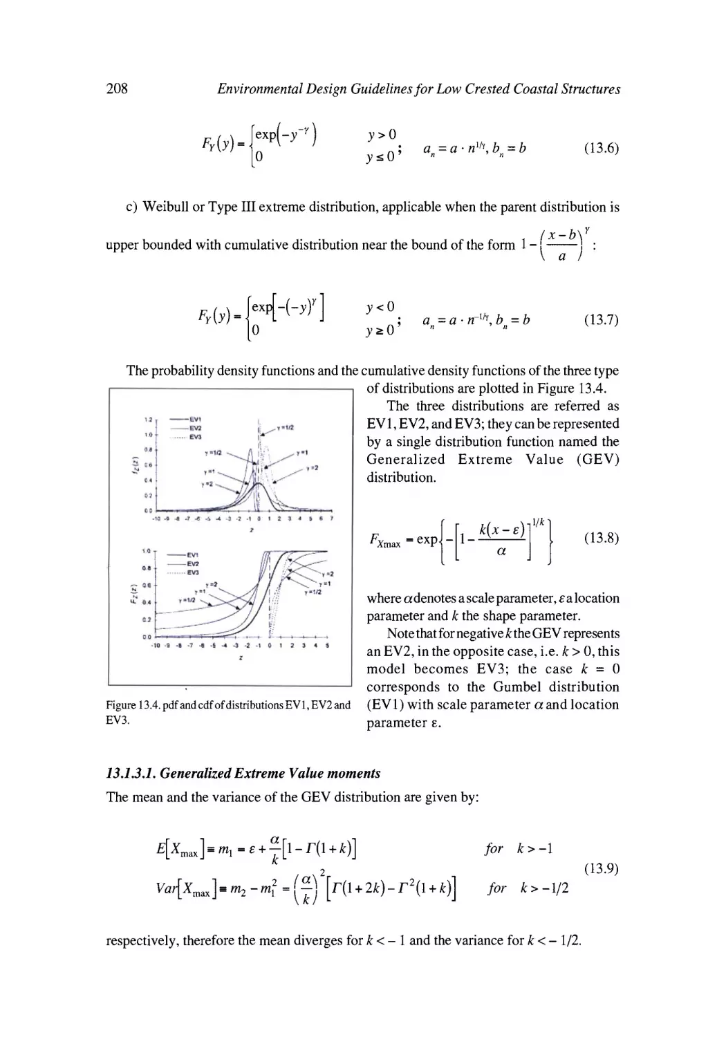
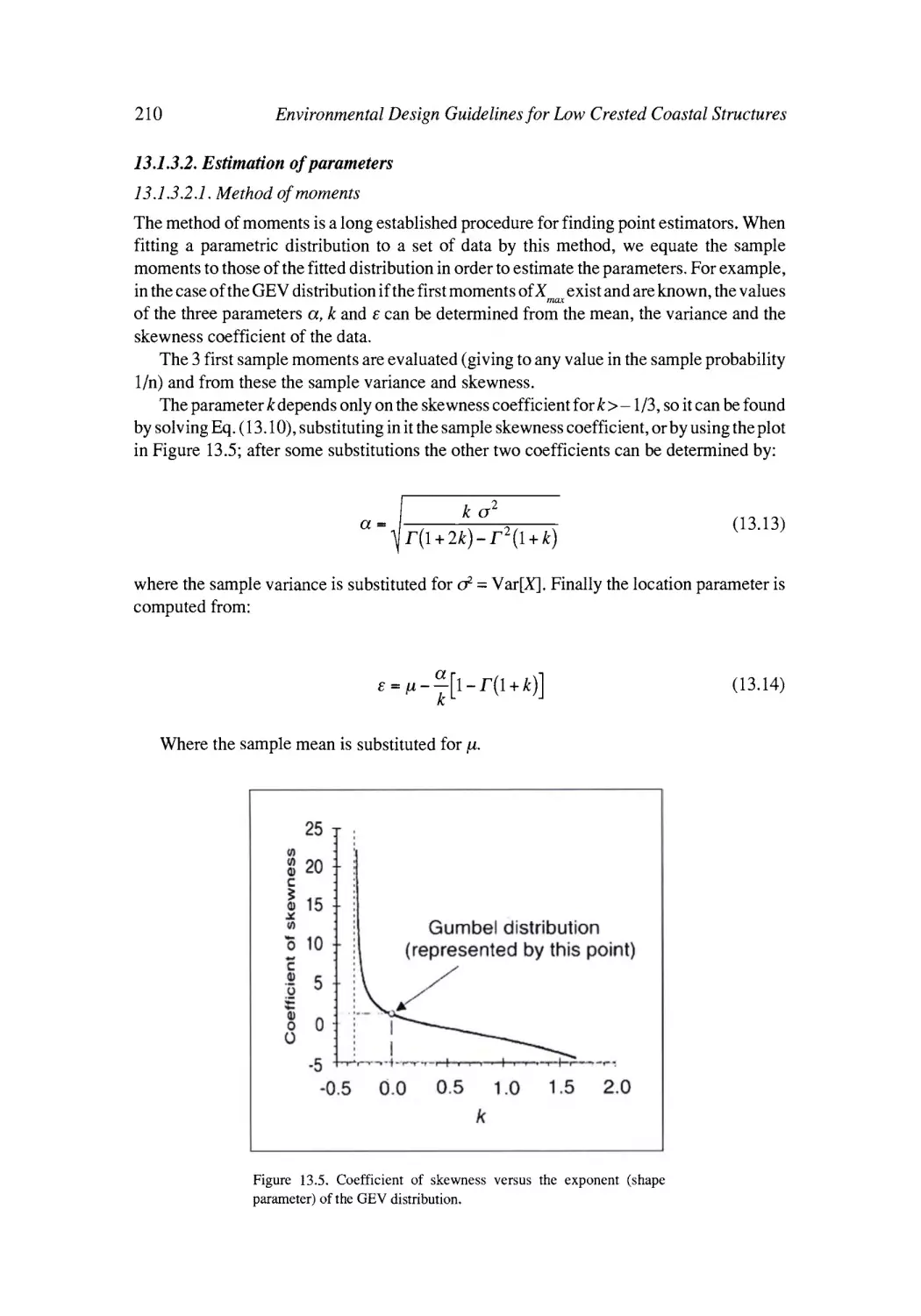
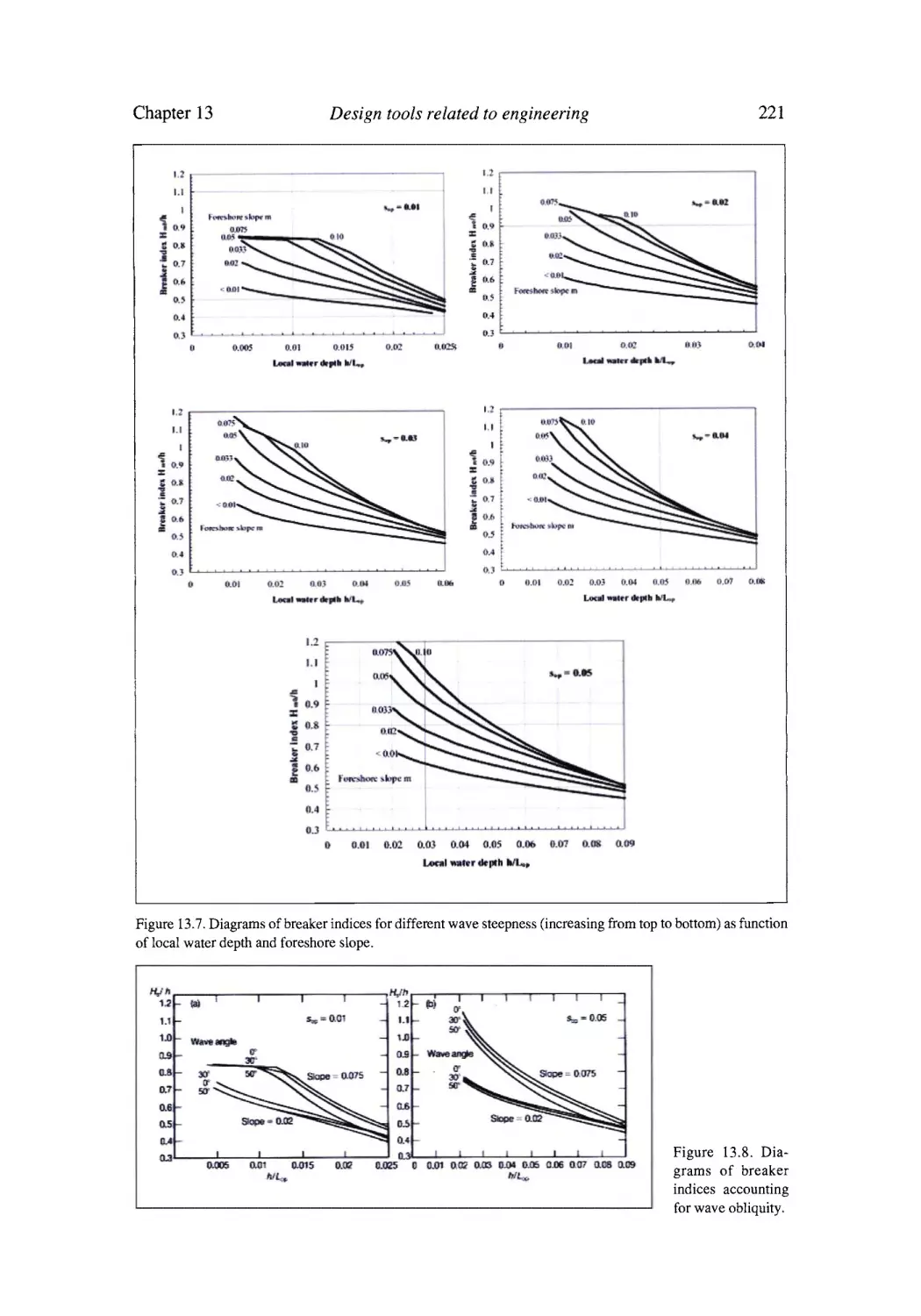
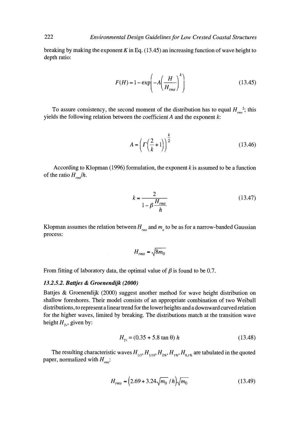
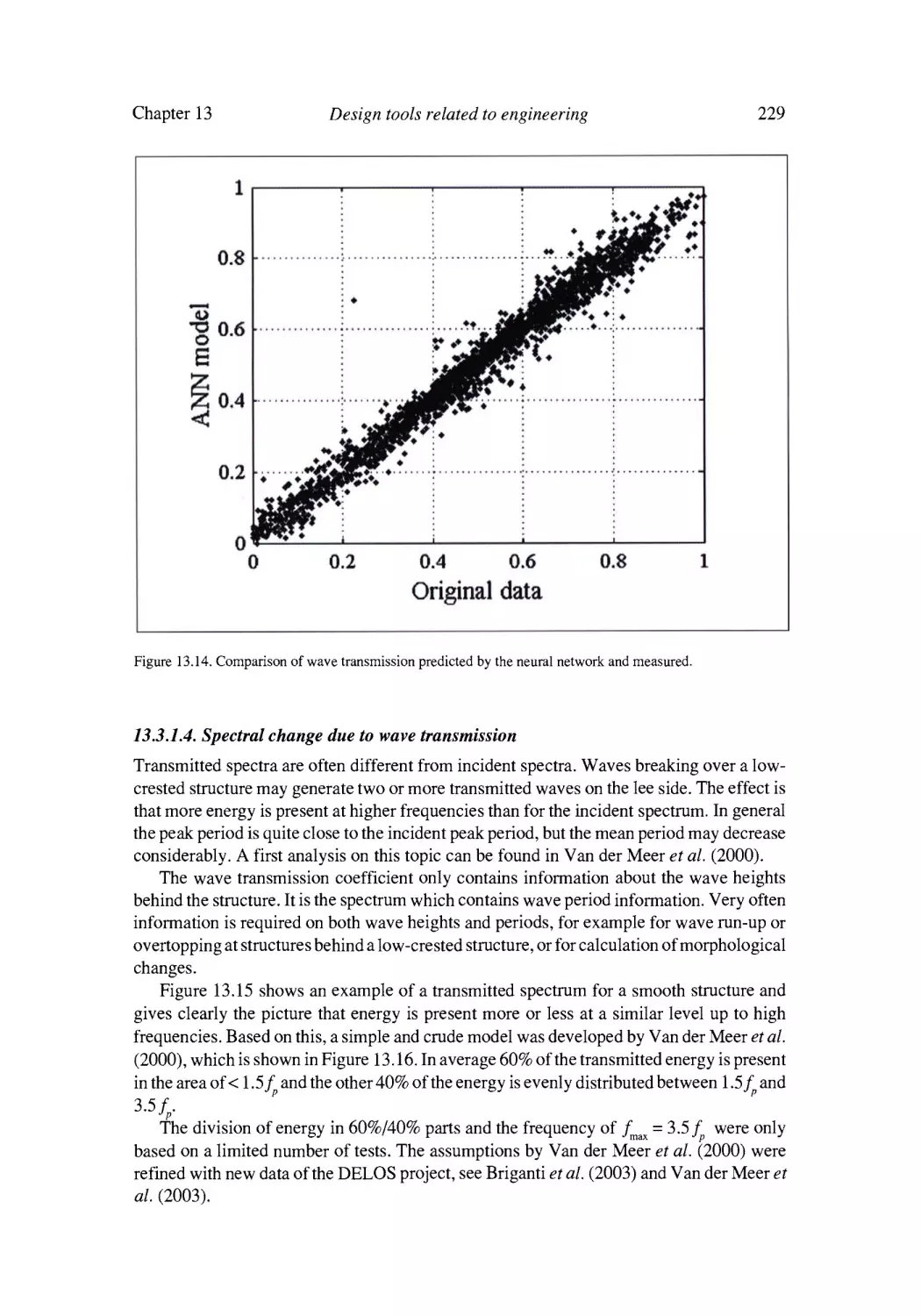
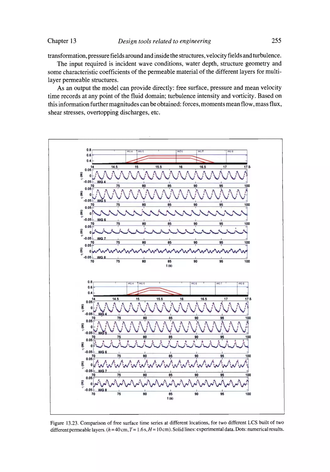
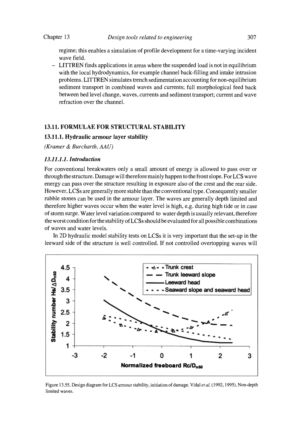
the sea state. The most important are listed below (see Section 13.2 for other parameters).
Significant wave height, H = H1/3,defined as the average of the highest one third of
the waves during the peak of the storm usually 1- 3 hours long. H corresponds closely
-
Environmental Design Guidelinesfor Low Crested Coastal Structures
28
to the visual estimate of wave height in a sea state.
-R~176
I 1 ~ H2 whereNis the number
and H i is the height of a single wave i.
- A typical wave period, T.
- Wave direction.
H and T are used as input in formulae for structure design, overtopping and wave
transmission, whereas Hrms is often used as input parameter in numerical modelling of
morphodynamics. The distribution of wave heights in a sea state with constant H follows a
specific distribution (Rayleigh) for which reason ratios of wave heights of different
exceedence probabilities are always the same, like e.g. the ratio between H and Hrms ( n =
1.416 Hms). However, the Rayleigh distribution does not apply in shallow water where wave
heights are limited due to forced wave breaking when the height exceeds approximately 0.8
times water depth. Consequently also the significant wave height H is restricted by the water
depth. For example, on a flat sloping sea bed the maximum H will be approximately 0.6
times the water depth.
The transformation of waves from deep to shallow water with respect to distribution of
heights and to directions is explained in Section 13.2.
Where waves are limited by water depth it is necessary to consider changes in seabed
levels in front of the structure together with water level variations. Seabed level changes can
be considerable on barred coasts with large longshore sediment transport. Such conditions
will modify the otherwise almost full correlation (linear relationship) between design wave
heights and water levels. Larger changes in wave period with wave height might cause minor
deviations from the linear relationship.
It is important to notice that in shallow water it is not possible to extrapolate wave height
statistics without consideration of the physical constraint given by depth limitation of the
waves.
Where LCSs are built in deeper water, the joint statistics of waves and water levels must
be based either on long term recordings, or synthetic data as described in Section 6.3. The
latter could also be composed by real time simulation of storms in accordance with the
statistics supplied by hydrographic service institutes combined with real time inclusion of
tides (variations are known) and estimated storm surges linked to the height of waves with
onshore directions.
6.5. CURRENT STATISTICS INCLUDING TIDAL, BATHYMETRIC AND WAVE
GENERATED CURRENTS, RESIDUAL LARGE-SCALE CURRENTS
(Lamberti & Archetti, UB)
Currents can be distinguished in offshore currents and littoral currents. Offshore tidal
currents have usually a modest velocity, with exception of shallow seas with high tidal range.
Offshore wind currents due to storms lasting one or two days have an intensity equal to 23% of the wind intensity and deviate about 10-20 ~ from the wind following earth rotation
(clockwise in Northern hemisphere). Density currents do not exceed some cm/s. All the
currents mentioned above intensify in the vicinity of the coasts.
Tidal currents are very important with respect to sediment transport on littoral coast with
Chapter 6
Investigation of environmental conditions
29
high tides. Otherwise in the Mediterranean Sea, currents due to tide are of the order of
magnitude of 0.10 m/s, smaller than wave-generated currents. In countries where tidal
excursion is large (i.e. UK) these currents are strong and are markedly influenced by the local
bathymetry, significantly contributing to the sediment transport processes (see for instance
Elmer site in Chapter 11).
Littoral currents develop in the surf zone, forced by momentum released by breaking
waves. Their intensity can exceed lm/s with direction linked to wave obliquity. Their main
effect is longshore sediment transport. In general their intensity does not affect directly the
stability of LCSs, but they may have to be taken into account with respect to the scour they
can cause around LCS heads.
Current measurements can be carried out with current meters (e.g. propellers, acoustics)
installed at a fixed position in the study site, or alternatively the movement in time of a mass
of water can be recorded by tracers or drifters. In general, current measurements are useful
to describe velocity fields and for calibration of hydrodynamic models.
6.6. WIND STATISTICS, SOLAR EXPOSURE AND PRECIPITATION
(Lamberti & Archetti, UB)
Winds are measured from fixed stations on land and on ships. Wind data are mainly used as
input for estimation of waves. Observed wind data have to be normalized to the wind
blowing over the sea at the anemometric standard level (10 m a.m.s.1.).
In absence or to substitute for wind observations, information on atmospheric pressure
gradients (isobar maps) can be used for prediction of wind fields over open seas.
Standard analysis of wind data time series provides:
- statistics of wind with respect to velocity and direction (wind rose);
- identification of storms: i.e. of events where a certain wind velocity threshold is
exceeded.
Solar exposure, temperature and precipitation are data often available at local
environmental offices and can be useful in extreme climate environments. At high latitudes
the knowledge of periods with very cold weather can be useful for the estimation of
degradation of stones due to frost (Norway, Iceland, Canada etc). The knowledge of
precipitation is important where salinity concentration is very high (i.e. Red Sea). Also solar
radiation can influence the stone durability in tropical climates. These data are usually given
as time-series and statistics.
6.7. SEDIMENT TRANSPORT BY WAVES AND WIND
(Zyserman, DHI)
A detailed understanding of the local sediment transport processes is of large importance
when designing LCSs and when assessing the expected impact on sediment transport and
coastal morphology of the planned intervention.
This understanding should not be limited to the local area where the structure(s) will be
built, but should encompass at least the involved sediment sub-cell or, preferably, the whole
sediment cell. The term sediment cell refers to the length of coastline that is relatively self-
30
Environmental Design Guidelinesfor Low Crested Coastal Structures
contained as far as movement of sand and other sediments is concerned, and where
interruption of such movements will not have significant effect on neighbouring sediment
cells. The boundary of a sediment cell generally coincides with larger estuaries or prominent
headlands (Mangor, 2001). By extending the analysis of sediment transport processes to the
entire cell, undesired impacts on coastal morphology of the scheme being designed can be
avoided.
In order to quantify the sediment transport processes, it is necessary to establish a
sediment budget for the investigated coast. Such a budget quantifies the variability of the
total longshore drift along the coast and helps in the identification of areas of potential coastal
erosion or shoreline advance. Adjustment of beach profile to gradients in cross-shore
transport takes place on a significantly shorter time scale than shoreline response, and can
thus be left out from this analysis.
Known sources of sediment (e.g. discharge from rivers, nourishment schemes, etc.) and
sinks (e.g. sand mining for construction purposes, removal of wind-blown sand from the
coastal system, etc.) must be taken into account when the sediment budget is established. The
same applies to spatial changes in the characteristics of coastal morphology and sediment
properties (granulometry).
In some cases, it is possible to define the sediment budget for a given coast on the basis
of recorded long-term changes in shoreline position, e.g. from aerial photographs. However,
sediment transport models are frequently used for this purpose, since they also provide
useful additional information for the design of LCSs.
Output from transport models will typically include gross and net rates of sediment
transport (on a yearly and seasonal basis) and their variation along the coast. Other
parameters are the distribution of the transport along the beach profile, the equilibrium
alignment of the coastline (which corresponds to zero net transport on a yearly-averaged
basis), etc.
Input to the models normally includes information about the local hydrographic
conditions (winds, waves and tides), coastal morphology (bathymetry, beach profiles,
shoreline position) and sediment characteristics (granulometry, density, etc.).
6.8. SEDIMENT CHARACTERISTICS
(Moschella, MBA; Bertasi, Ceccherelli, Colangelo, FF; Frost, Gacia, Martin, CSIC;
Thompson & Hawkins, MBA)
One of the major environmental impacts of coastal defence structures is on the surrounding
sediments. Sediment characteristics should be therefore fully investigated. The following
sediment descriptors should be considered: geological composition, grain size and other
granulometric parameters, redox potential and compactation, organic content, nutrient
content and chlorophyll content (to quantify abundance ofmicrophytobenthos). In particular,
it is important to quantify sediment features that are more likely to worsen after the
construction of LCSs, such as anoxic or organic rich sediments.
Chapter 6
Investigation of environmental conditions
31
6.9. HYDROGRAPHIC PARAMETERS INCLUDING WATER QUALITY
(Moschella, MBA; Airoldi, FF; Thompson & Hawkins, MBA)
Hydrographic parameters include salinity, temperature density and other parameters related
to water quality. Water quality refers to the use of a water body for a defined purpose. It is
a concept which overlaps with ecological characteristics but is primarily geared to suitability
for amenity, recreation, immersion water sports, collection of shellfish or other living
resources. The relevant water quality parameters include total suspended solids, clarity
(measurable by advanced instrumentation or simple field devices such as Secchi disc),
dissolved oxygen and biochemical oxygen demand, nutrients and chlorophyll concentration.
In addition, presence of pollutants (e.g. organic compounds, heavy metals) and pathogens
(e.g. Escherichia coli, total number of streptococci) should be also assessed. These
parameters must comply with the European Bathing Water Directive (76/160/EEC) and
local legislation.
Aesthetic data on the amount of seaweed detritus and non-biodegradable waste material
could also be of relevant importance for water quality (see Section 6.10).
6.10. ECOLOGICAL CONDITIONS (ECOSYSTEMS, HABITAT AND SPECIES)
(Moschella, MBA ; B ulleri, Airoldi, FF ; Gacia, Martin, CSIC ; Frost, Thompson & Hawkins,
MBA)
A scoping study (mainly desk based, but supplemented by a site visit) of ecological
conditions of the site and coastal cell should be carried out to identify the factors likely to
affect the biota and to inform design of environmental impact assessment.
To assess the ecological status of the site and coastal cell both physico-chemical and
ecological data should be collected. All the information described in Section 6.1-6.9
(particularly Sections 6.8 and 6.9) is also relevant to the investigation of ecological
conditions. The physical and geomorphological information can also be used in Delft
biotope prediction model (see Chapter 14) of prior conditions, which need to be verified by
site visit and to simulate post-construction impacts.
The following ecological data should be gathered:
-
-
any available information for onshore (maritime) habitats (dunes, lagoons, shingle banks
and their vegetation) and associated fauna and flora and geological features likely to be
influenced (protected/impacted) including downstream effects.
Any published information for soft shores in the region (e.g. for UK, Marine Nature
Conservation review).
Any published information for rocky shores in the region (e.g., for UK, Lewis 1964;
Marine Nature Conservation Review Mermaid database, MARLIN website).
Any available information from existing artificial structures (especially jetties, moles,
harbour walls, stone groynes, sea walls etc.) in the nearby areas.
Marine biogeographic province and likely species pool: available from general literature
(Lewis 1964; Stephenson & Stephenson 1972; Hawkins & Jones 1992) by broad region
32
-
-
-
-
Environmental Design Guidelines for Low Crested Coastal Structures
(e.g., Atlantic west coasts; Iberian coasts; French coasts; British and Irish coasts; North
Sea coasts; west and east Mediterranean coasts; west and north Baltic coasts). In
particular, regional species pool and potential source populations of hard-substrate
assemblages.
Any knowledge on recruitment regimes, for species of particular local interest such as
mussels and other shellfish.
Basic knowledge of the ecology and life histories of soft and hard-substrate species to
predict dispersal capability, successional patterns and distribution (e.g. between the
landward and seawards sides of the LCSs) of assemblages that will result as a
consequence of the construction of LCSs.
Existing information on pest or nuisance species.
Identification of exploitable natural resources, including fish, shellfish and crustaceans.
Distribution of fisheries nursery grounds.
In the absence of relevant information data on i-iv can also be gathered by a site visit.
Information on conservation and natural heritage legislation for the site should also be
collected (see Sub-section 5.1.3).
The desk-based study should be combined with a rapid field assessment of the site and
adjacent coastal areas to verify and integrate the information collected during the desk study
(see Chapter 14 for a protocol). The field assessment should include a stretch of coast
extending at least 10 km either side of the selected site for the proposed LCS.
CHAPTER 7
Conceptual/pre-design alternatives
A preliminary design has to demonstrate satisfactory functional performance and
environmental impact at a level high enough for the objective comparison of several
alternatives.
7.1. PROPOSALS FOR LAY-OUT AND CROSS SECTIONS OF POTENTIAL LCS
SCHEMES
(Burcharth, AA U)
At the pre-design stage a number of alternatives, all meeting the functional objectives and
legislative, environmental and economical restrictions, have to be worked out in such detail
that an objective comparison can be performed.
As for lay-out and cross sections no single LCS-scheme geometry can be generally
recommended since its performance varies with each coastal site, depending on wave
climate and required attenuation, on beach morphology (e.g. slope, grain size), use
(recreational bathing, boating, surfing, fishing, etc.) and scope of work. However, some
guidance to the initial choice of scheme can be given.
Figure 1.1 (Chapter 1, pag. 4) shows examples of typical lay-outs and cross-sections of
three different schemes. At pre-design level the choice with respect to lay-out is more or less
shown in this figure.
If the objective is to protect a very limited coastal stretch against severe wave action and
at the same time to create a sheltered area for mooring of boats then a single-structure
solution is often used with a LCS placed at some distance from the shore in order to have
enough space for moorings. The length of the structure is determined by the needed space
for moorings and the tolerated wave agitation. The demand for water depth and space usually
results in water depths of more than 3-5 metre (LWL) at the structure. The structure will
normally be emerging with crest-level high enough to prevent significant wave transmission
by overtopping and penetration. Thus the wave agitation in the lee of the structure is mainly
caused by diffraction and refraction of waves at the heads of the structure. The tidal range
and the water level due to storm surge influences the crest level very much. If of some size
the structure will certainly be visible as it emerges several metres above MSL. The high
structures are economically built as a multilayer rubble mound breakwater. Figure 1.1.a
shows an example. The distance to the shore should be large enough to prevent formation
of tombolos and salients of some size as the area for moorings will be reduced and down drift
erosion will occur. The problems are, however, difficult to avoid in case of significant
34
Environmental Design Guidelines for Low Crested Coastal Structures
sediment transport along the coastline unless the structure is built in deep water.
LCS-schemes with the primary objective of coastal protection and improvement of
recreational conditions normally cover a longer stretch of the coastline. Two main types of
schemes with dependence on the range of water level variations can be identified.
Schemes with submerging structures or structures with crest levels close to MSL can
effectively dampen waves on coastlines with small tidal range and rare storm surge events
like in the Mediterranean Sea. Such structures are invisible or only sporadic visible for which
reason they can be large (continuous) structures without spoiling the sea view. Distinct
openings, often made just as lowering of the crest, can be provided for the access of small
vessels. Figure 1.1.c illustrates such a scheme. The net-inflow of water across the structures
can generate very strong outflow currents in the openings and their surroundings thus
creating scour. Dimensions and number of openings should be determined with due
consideration of these problems. The larger the submergence the wider the crest should be
in order to reduce transmitted wave energy sufficiently. On the other hand problems with
return flow currents will be less. The height of the submerged structures is often so small that
a homogeneous rubble mound structure is cheaper than a layered rubble mound structure.
Appropriate filter layers and/or geotextiles should be used anyway to prevent penetration of
finer materials into coarser materials and vice versa.
The other main type of scheme relates to coasts with frequent larger water level
variations, such as coasts with significant tidal range and/or frequent storm surge water level
set-up. Relatively high structures with crest elevation well above MSL are necessary in order
to reduce the wave action on the coast sufficiently. Such emergent structures are blocking
the sea view for which reason large gaps between the structures are required. Creation of
pocket beaches (see Figure 2.6) by formation of tombolos or salients (see Figure 2.3) are
generally also wanted. This leads to detached shorter structures placed relatively close to the
shoreline. The width of the gaps relative to the length of the structures influences the total
cost of the scheme significantly, especially in case of high emergent structures. For this
reason, and in order to avoid concentrated rip currents, the gap width should be as large as
possible considering the necessary protection of the coast.
Land-connection of the longitudinal LCS's by means of groynes is beneficial to avoid
strong longshore currents. Moreover, they can provide access to the LCSs and thus serve
additional recreational value. However, water movement on the landward side is considerably
reduced, often negatively affecting water quality.
Also, by blocking the longshore sediment transport usually serious downdrift erosion
problems occur. In this respect formation of salients are less damaging than tombolos as
the interference with longshore sediment transport is smaller.
The lower the crest level of the LCSs, the greater the wave transmission, with consequent
smaller morphological impacts of the structures. This generally means less protective effect
but also less downdrift erosion.
From an environmental viewpoint, LCS design should balance the need for engineering
performance in terms of coastal protection with the necessity of minimising impacts on
surrounding habitats and associated fauna and flora. For example, if structures are built in
such a way that considerable water movement on the landward side is maintained (e.g. by
frequent wave overtopping or water penetration through the pores), sediment and water
characteristics will be less altered and consequently impacts on the sediment fauna and flora
will be limited. Design recommendations for minimising impacts on habitats and ecosystems
are provided in Sections 8.3, 8.4.
Conceptual/pre-design alternatives
Chapter 7
35
7.2. P R E L I M I N A R Y E S T I M A T I O N OF M O R P H O L O G I C A L I M P A C T BY
OR EXPERIENCE
O F E M P I R I C A L DIAGRAMS, F O R M U L A E
THE
USE
(Burcharth, AAU; Vidal, UCA; Zyserman, DHI)
LCSs are mainly located on the submerged beach were they modify the wave field and the
wave-driven current patterns. If tides are important, also tidal currents could be altered. The
consequences of the altered dynamics can be observed both in the near field (scouring or
sedimentation around the LCSs) and far field effects, (changes in the shoreline position).
Focusing on far field effects, the hydrodynamic changes produced by a LCS on the
protected beach causes sand accretion in the beach area located on the lee side of the LCS,
thus producing a protruding shoreline called a salient (see Figure 2.3, Chapter 2, pag. 6). If
the length of the LCS and the distance to the beach is adequate, the salient can reach the
structure, forming a tombolo. In very special circumstances, the salient on the beach is
accompanied by a second salient in the lee-side of the LCS, forming a double salient. In the
case of long more deeply submerged LCSs no salients are formed, see for example Figure
1.1.c.
When LCSs are built on beaches with a dominant direction of longshore transport, care
should be taken in the design of LCSs because tombolos act as pe~endicular groynes
causing the interruption of longshore transport. This interruption causes accretion on the
updrift beach and beach erosion on the downdrift side, the same way as in case of groynes.
On the other hand, salients allow some bypassing of sand, so the interruption effect is less.
For engineering pu~oses, there are some empirical approaches that predict the shape of
the beach affected by LCSs. Some of these empirical approaches for prediction of the beach
profile and the shoreline shape are presented in Sections 13.6 and 13.9.
Initially a number of lay-outs for the structures are sketched on the basis of the target
beach planslope and wave transmission, considering also updrift and downdrift effects.
Shoreline response to an offshore LCS is controlled by a number of variables the most
important of which are:
- distance offshore, X (from initial coastline);
- distance offshore relative to the width of the surf-zone, X/X's;
- length of the structure, Ls;
- length of the gaps between segments, G;
- transmission characteristics of the structure given by K = H/H i, where H and H i are
transmitted and incoming wave heights, respectively;
i
i ~ m
i
;9
-;
,;
I
i
II
......
i
i
i
i
i
I
t
i
I
i
i
i
Figure 7.1. Definition of geometricalparameters.
,;
I
I
i
i
I
i
i
i
i
~itial shoreline
Environmental Design Guidelines for Low Crested Coastal Structures
36
- beach slope and depth at the structure, d;
wave climate (sizes, frequencies, and directions of waves);
- water levels;
sediment characteristics.
-
-
Figure 7.1 shows the definition of the geometrical parameters.
Simple diagrams or rules can give a first indication of the morphological changes
imposed by the structures. They all assume the presence of sufficient sediments for the
depositions. Example of simple rules are given below (tab. 7.1) for:
emergent structures placed within the littoral drift zone; little orno wave transmission
across the structures, i.e. K t = app. 0.1 to 0.2; shore- parallel structures; almost perpendicular
wave approach;
-
Table 7.1. Conditions for formation of tombolos and salients.
Emergent structure
Reference
Conditionsfor formation of
Tombolos
Ls/X > 1.5
L]X > 1
Ls/X > 0.9 to
1
Salients
1/2 < Ls/X < 2/3
1/2 <Ls/X < 1
Ls/X < 0.6 to 0.7
Dally and Pope (1986)
Herbich (1989)
Mangor (2001)
Submerged structures
Reference
Conditionsfor formation of
Tombolos
(1.0 to 1.5)/(1 - K)
Ls/X >
Salients
Ls/X > 1/(1 - K)
GX/L2s > 0.5(1 -
Pilarczyk (2003)
K)
The width of the gap is usually according to Pilarczyk (2003)
L <G~O.8L
s
where L = T (g 9h) ~ T being the wave period and h the water depth at the structure.
Seiji, Uda and Tanaka (1987), referred to Loveless (1999), gave the following conditions
for the erosion of the beach behind the gap:
G/X < 0.8
0.8 < G/X ~ 1.3
G/X > 1.3
no erosion
erosion likely
surely erosion
Simple rules related to reef structures are referred and discussed in Pilarczyk (2003).
Tools for more detailed examination of the formation of salients and tombolos behind
emerged structures are given in Section 13.9.
Chapter 7
Conceptual/pre-design alternatives
37
The simple rules indicating morphological changes in terms of formation of tombolos
and salients cannot give the answer to the main question: can a LCS-scheme, although
formation of tombolos or salients will take place, stop the retreat of an otherwise eroding
coast? No general answer can be given as it depends on the character of the wave climate,
the natural sediment supply and the exposure and erosion rate of the coast. However, for
rather exposed coastlines where significant erosion takes place in quite frequent storms it is
not possible to stop retreat by means of LCS-schemes unless beach nourishment is applied
on regular basis, and/or revetments are installed. However, a LCS-scheme will almost
always reduce the erosion rate of the protected stretch like any other reinforcement of the
coast. Steepening of the coastal profile seawards of the structures will quite often take place.
All coastal structures sticking out from the coastline cause downdrift erosion and updrift
accretion on coastlines with a net-direction of sediment transport. This is also the case for
shore parallel structures if they, as is the case for most LCS-schemes, influence the
morphology by creating tombolos and salients. Salients, and especially if they are submerged,
create less problems than tombolos because total blocking of the longshore sediment
transport is avoided. Also, the closer the structures are to the coastline, the less downdrift
problems occur.
An approximate prediction of morphological changes to the coast line caused by a LCSscheme might, at predesign level, be provided by the use of numerical one-line models, cf.
Sections 8.1 and 13.10.
The length of LCSs in relation to the width of the gaps together with the crest level and
the permeability of the structures determines the water level set-up behind the structures.
Generally a large set-up is undesirable as it not only causes reduction of the width of the
beach but indeed very strong return currents due to the large pressure gradients. The largest
set-up occurs when the structure is impermeable and the crest level is above but close to the
still water level, i.e. when the freeboard is small compared to the wave height.
Beach nourishment
Beach nourishment is frequently used together with coastal structures in beach protection
and restoration schemes to minimise/counteract the far-field impacts of coastal structures.
Nourishment can be regarded as a natural way of combating coastal erosion by
artificially replacing a deficit in the sediment budget over a given stretch of coast with a
corresponding volume of sand. The sand used to nourish the coast should have grain size
similar or coarser than the native sand.
According to Hanson (2003), approximately 28 million cubic metres of nourishment are
placed every year in Europe. The methods and practices applied vary from country to country.
Three nourishment methods can be identified based on the placement of the borrow
material along the beach profile (Mangor, 2001): (i) backshore nourishment, (ii) beach
nourishment and (iii) shoreface nourishment. In the first case, the upper part of the beach
is strengthened by placing nourishment at the backshore or at the foor of dunes. The aim of
backshore nourishment is to prevent dune erosion and breaching during storm events. In the
case of beach nourishment, sand is supplied to the shore to increase the recreational value
and/or to secure the beach against shore erosion by adding sand to the sediment budget.
Shoreface nourishment consists of supplying sand to the outer part of the beach profile,
usually on the seaward side of a barrier, to strengthen the coastal profile and to add sand to
the sediment budget.
Common to all types of nourishment is the fact that, if the cause of erosion is not
Environmental Design Guidelines for Low Crested Coastal Structures
38
Figure 7.2. Salients and tombolos in Pedregalejo artificial beach, M~ilaga,Spain.
eliminated, the erosion will continue in the nourished sand. This means that nourishment as
a stand-alone method for coastal protection will normally require a long-term maintenance
effort, based on the definition of the frequency and volumes involved in re-nourishing the
coast. Regular re-nourishment requires a permanent and well-functioning organisation,
which generally makes nourishment as a stand-alone solution unsuitable for private beaches
and small-scale schemes.
The idea of combining beach nourishment and coastal structures is to use the structures
to create closed sediment cells in such a way that no significant losses of sediment take place,
thus largely reducing or completely eliminating the need for re-nourishment. This might be
achieved through shore-normal structures, such as groynes of different shapes or artificial
headlands, or by use of shore-parallel structures, typically breakwaters. When shore-parallel
structures are used, tombolo formation is usually sought in order to ensure zero sediment
transport out of the cell. It is far from always possible to eliminate the need for renourishment.
All type of nourishments, especially if regularly repeated, will have serious impacts on
habitats and associated biota at both source and destination sites. For example, if sand is
extracted from off-shore sites, the seabed will be highly disturbed, leading to significant loss
of benthic flora and fauna as well as disturbance to fish. If sand is dredged from harbour
bottoms or docks, the risk for contamination of sediments by pollutants and pathogens can
be high. This practice may also increase the risk of introducing soft-bottom, non-native
species that often occur in harbour areas.
Figure 7.2 illustrates the application of beach nourishment combined with coastal
structures to create an artificial beach at Pedragalejo, M~ilaga, Spain. In this scheme, a
detached breakwater has been placed at the centre of the coastal cell to form a salient in order
to increase the available length of beach and, thus, its recreational value.
7.3. STRUCTURAL SAFETY OF PREDESIGN
(Burcharth, AA U)
The structural design of LCSs follows the functional design. The outcome of this are the crest
Chapter 7
Conceptual/pre-design alternatives
39
level of the structure, the sea bed level at the structure, and the length of the structure (and
width of gaps in case of multi-structure schemes). Apart form drawing trunk cross sections
and head sections defining the composition of materials to be used obeying filter criteria etc,
the structural design consists of determining the size of stone (blocks) in armour, toe and
scour protection, see Section 13.11. For this it is necessary to define safety levels if not given
in a national standard or design recommendation. If given, they usually relate to larger
structures and not to very small structures such as LCSs built close to the foreshore.
Typically is safety implemented by definition of a maximum allowable damage, e.g. 5% of
the armour blocks displaced, when exposed to the 50-years return period sea state. This
implies that a certain return period sea state has to be extracted from the combined
information (joint statistics) on water levels and waves. However, as this is very complicated
because of several dimensions (water depth, freeboard, wave height, wave direction) it is
recommended to establish the statistics on the effect of the various sea states in terms of
necessary size of the armour units, and extract from this the size corresponding to the 50years event.
Economical optimization of rubble mound breakwaters shows very flat minima for
lifetime costs as function of armour unit size (Burcharth and Sorensen, 2005). This means
that no money is saved by minimizing the armour size, unless at the limit where size of
armour units is a supply or a construction problem. If this is not the case and if the waves are
depth limited there is no need at predesign level to perform detailed statistical analyses of
the sea states as stone size can be based on conservative use of water depth statistics alone.
In shallow water there will most often be very small differences between wave heights
related to for example the 5-years and the 50-years return period sea states.
If in a standard the demanded safety level is given as a maximum probability PI~
exceedence of a certain damage within service lifetime TLof the structure, then the structure
should as a minimum be designed for a sea state with return period TR given as
The formula expresses the encounter probability which does not include uncertainties
related to the parameters and to the formulae. A probabilistic design approach is necessary
for the inclusion of these uncertainties, but this is not used for conceptual design of small
simple LCS structures.
If no standards or recommendation covering the actual location exist, or if these apply
to breakwaters in deeper water, it is recommended to design the main armour of LCSs in
shallow water for practically no damage applying a conservative value of wave height, cf.
the discussion in Sections 7.5 and 13.11.1. Where toe berms consist offew stones they should
also be designed for practically no damage. In case of wide toe berms and scour protection
layers consisting of many stones placed in two layers or more, some displacement can
normally be tolerated when exposed to the largest depth limited waves.
7.4. IDENTIFICATION OF ENVIRONMENTAL CONDITIONS FOR PREDESIGN
(Burcharth, AA U)
Fundamental understanding of the historic performance of the actual coastal stretch
including responses to man made interventions is of outmost importance for drafting of
40
Environmental Design Guidelines for Low Crested Coastal Structures
realistic alternatives at predesign level. To obtain such understanding it is necessary to seek
historic information and combine it with knowledge about seabed and sediment characteristics,
wave climate, water level variations and currents.
The understanding of the morphodynamic processes must cover not only the project area
but the whole of the sediment cell. Also, to ensure that the project will not impose
unacceptable environmental conditions it is necessary to know the ecological conditions and
identify constraints related to conservation and natural heritage.
Chapter 6 describes how the environmental conditions can be investigated. The
environmental data needed at predesign level does not need to be very detailed as long as the
main characteristics are given. For meteormarine data it means that slightly conservative
parameter values are sufficient. This is because calculations related to conceptual designs
will normally be deterministic. Stochastic analyses usually await detailed design stages.
The first phase of predesign deals with lay-out and main dimensions of alternative
schemes and their tuning to fulfil the set target performances. In most cases the focus is on
morphodynamic and recreational performances. The meteormarine input to be used for
estimation of the morphodynamic performance of a scheme should reflect the typical
conditions at the site including seasonal variations. For this is used simplified time series of
combined values of water levels wave height, wave period and direction of waves. The
values will typically be chosen to reflect average conditions for each season, but storm
conditions might be included as well. Only conditions which cause movement of sediments
should be included when defining average conditions. If tidal currents are significant they
should be included in a simplified manner.
If there is risk of stagnant water etc. it is important to include time series reflecting also
quiet conditions for the study of recreational and environmental performances of the
predesign schemes.
7.5. S T R U C T U R A L DESIGN OF LCSs BASED ON M A T E R I A L S U P P L Y
FORMULAE
FOR STABILITY,
AND S E M I - E M P I R I C A L
INFORMATION
O N SCOUR
POSSIBILITIES,
(Kramer & Burcharth, AA U)
In general a LCS consists of the following parts:
- an outer armour layer of large stones or concrete blocks (Sub-section 13.11.1).
- a bedding layer of smaller stones and/or geotextile between the bottom of the
structure and the sea bed (Sub-section 13.11.2).
- a toe protection of armour layer stones or smaller stones (Sub-section 13.11.3).
At almost all locations in Europe suitable rock and stone material for LCSs is economically
available due to the rather limited costs of long distance shipping materials by barge.
However, nearby land-based sources with sufficient quality and sizes of stone and rock
materials are also used. Concrete blocks are used only if costs for rock materials are very
high.
The fact that finer rock and stone materials generally are cheaper than larger size
materials leads to preference for layered designs instead of more homogeneous designs
based on very few sizes or classes of materials. In any case, sufficient filter layers must be
provided between sandy seabed and the coarser structure materials. Geotextiles are often
Conceptual/pre-design alternatives
Chapter 7
41
................ Quart2,,,stone
1000 - 1800 kg
............... Cobble. 150-200 mm
,,
tduarry stone .,,1
3(~) - 600 kg
. . . .
~
./
I i~0
r--
Quart7 stone
/
I
3(]~) - 6 0 0 kg
i
Geotcxtiic
g~'l~i"l--
..4,,,,,,K.,f"V-"~,r
. . . . . . .
~2' . . . .
.
):~:.~_[,~2.s0 § 2.~,.7~_e - 2.~0 §
.
.
.
.
.
.
.
.
.
.
.
.
.
.
~.~c]~,
Figure 7.3. Cross-section of breakwaters at LCnstrup, Denmark (Laustrup & Madsen, 1994).
used for this purpose.
For structures of limited height it is not possible to have several layers of different grain/
block sizes due to the large size of the armour blocks compared to the total height of the
structure. In such cases similar sized blocks will be used for the main body resulting in a very
permeable structure as opposed to structures with a core of finer materials. In the case of
deeper water there is a choice between homogeneous structures and layered more impermeable
structures. The target wave penetration and exchange of water through the structure then
determines the type of design.
A toe protection of a certain width must be provided; this is usually made flexible by the
use of stone and geotextiles to allow for some sea bed scour close to the structure. Toe
protection is necessary both on the front and the rear side of the structure.
Various designs of cross-section composition and shape are possible. A sketch of a
characteristic cross-section built to prevent coastal erosion in Denmark is shown in Figure
7.3. The level of the crest is seen to be 1.3 m above MSL indicating that the structure is not
low-crested under normal wave conditions. However, storm surge can be around 1.5 m
above MSL making the breakwater heavily overtopped. In Figure 7.4 a typical cross-section
ocadm1:100
mmu,~(w.-Imoo~
.~
I
mmmo
pro,k).mmoom~n,~ v~o
!
9
__
-__
--:.----i:,~-.
Figure 7.4. Cross-section of a submerged breakwater along Emilia Romagna coast, Italy.
42
Environmental Design Guidelines for Low Crested Coastal Structures
of a submerged breakwater along the Emilia Romagna coast (North Adriatic coast) in Italy
is shown.
The cross-section shown in Figure 7.3 is narrow-crested and relatively high compared
to the submerged wide-crested breakwater in Figure 7.4. Typically also the leeward side of
LCSs are exposed to direct wave action due to overtopping waves and it is therefore
necessary to design a toe berm on both sides of the breakwater. If the breakwaters are very
high and/or wide, then overtopping will be reduced and the toe berm on the leeward side of
the breakwater can be designed using smaller stones.
Stones used in the armour layer of a LCS must be sufficiently large to avoid undesirable
displacements caused by the wave action against the structure. As LCSs are built in shallow
water the highest waves will often be depth limited. As a consequence the structures will
typically be exposed to design waves numerous times during the lifetime. Because damage
is cumulative it is important to design such structures with criteria based on a very low
damage per storm criteria. Moreover, because narrow-crested breakwaters built in shallow
water are only a few stone-sizes high and wide, one stone removed from the edge of the crest
will cause a relatively large hole in the cross-section leading to increased wave transmission.
Consequently it is recommended to use the limit between the no damage and initiation of
damage for the design and to use at the same time a safety factor which compensates for the
uncertainties.
For the determination of the armour block size the armour stability formulae given in
Sub-section 13.11.1 can be used with a safety factor of 1.1 on the nominal diameter.
Generally there are differences in the exposure of armour blocks of the various parts of the
structure (heads, trunk crest, trunk seaward and leeward sides). However, for preliminary/
conceptual design it is recommended to use the same armour size for the whole structure,
corresponding to the most exposed part. The armour stability formulae are in case of depthlimited waves valid only for 1:2 slopes. For LCSs exposed to non-depth limited waves also
slopes of 1:1.5 are covered by the formulae. For structures in larger water depth reference
can be given to armour stability formulae given in CEM (2003).
Determination of the toe block sizes and scour protection can be based on the formulae
given in Sub-section 13.11.3. The extent of the scour protection is given by formulae
covering the seaward side of the trunk and the head. The toe berm stability formula can be
used for the determination of the size of the scour protection material if the width of the
protected area is not too wide. In case of wide areas the stone size should be determined by
theory for the transport of granular materials in waves and currents.
Bedding layers and stone filters must fulfil accepted filter criteria, e.g. as given in Subsection 13.11.2.
7.6. ASSESSMENT OF E N V I R O N M E N T A L I M P A C T S (EIA) AT L O C A L AND
R E G I O N A L SCALE
(Moschella, MBA; De Vries WL-DH; Frost, Thompson, Hawkins, MBA)
An EIA should be performed at this stage to identify and evaluate the potential impacts (or
effects) of construction of a LCS in relation to physical, chemical, biological and cultural
components of the environment. This should enable environmental issues to be integrated
at the planning and decision making phase and hence promote design alternatives that are
environmentally sound.
Chapter 7
Conceptual/pre-design
alternatives
43
Once relevant ecological information (see scoping study in Section 6.10) has been
collected, baseline ecological surveys should be undertaken to identify likely effects of LCS
on habitats and species and assess the site sensitivity to impacts. Surveys should be
undertaken at both local (near-field) and broader (far-field) scale. Also, they should be
spatially and temporally replicated, to allow identification of potential impacts from the
background, natural variability of benthic assemblages.
A preliminary field visit should be also carried out prior the detailed survey to define
appropriate sampling strategy, for maximising sampling effort and guaranteeing accuracy
in the assessment. This can be based either on biotope mapping (e.g. B IOMAR,
www.JNCC.gov.uk) or on physical gradients (e.g. height on the shore/bathymetry). The
exact format of the survey will depend on the coastal system considered (macrotidal,
microtidal), the environmental setting, size and configuration of the LCSs to be built as well
as the specific ecological features of the site. Although priority should be given to assessment
of physical and biological features of sediments, the nearby rocky shores (if any) and water
column should be also characterised in the survey. A protocol indicating general steps to be
undertaken in the survey is provided in Chapter 14.
7.7. EVALUATION OF THE SCHEMES BASED ON E C O N O M I C A L OPTIMISATION
(Martinelli, UB)
The design of the alternatives identified in the preliminary phase should be detailed
enough to allow their economic evaluation. These include at least an identification of
quantities and methods involved in the building process and the evaluation of the structure
performance in time. Both are necessary for the evaluation of the total cost, which is a
combination of the initial building cost and of the long term maintenance costs.
Typical construction unit costs for the area where the structure is built may be considered
as a starting point.
Maintenance costs are distributed over lifetime; it is suggested to reduce the frequency
of maintenance, in order to control possible negative effects on the ecosystem (see Section
8.8). A proper economic life-time should be selected, usuall smaller or equal to the structural
lifetime (eg. 20 years), in order to account for the possible change of strategies or
environmental conditions. The equivalent initial cost can be obtained by capitalising
maintenance costs at present prices using an appropriate interest rate compensated for cost
inflation (in Europe it is in the range 2-4%). A lower interest or a longer economic lifetime
lead to lower weight of initial costs compared to maintenance costs, but higher initial costs
and lifetime costs.
The cost-benefit analysis should be performed considering an area where all the physical
and social effects take place, i.e. significantly wider than the intervention area; alternatives
shall usually include the <<nostructure>> scenario, and cost and benefits should account for
both direct (related to works and beach activities) and indirect economic consequences (e.g.
tourism induced effects over the wider area).
Environmental Design Guidelines for Low Crested Coastal Structures
44
7.8. SOCIO-ECONOMIC EVALUATION OF THE SCHEMES
(Zanuttigh, UB)
The construction of different schemes may lead to different visual impact scenarios and to
the development of recreational activities that can significantly affect visitor enjoyment and
thus beach value.
Schemes including emerged barriers worsen water quality, improve bathing safety
especially for children, impose some restrictions to water sports and may have a negative
aesthetic impact; groynes are usually welcome from beach visitors for sunbathing, fishing
and walking on the crest, if possible; submerged structures can mitigate risk for bathers
without degrading water quality and the view from the beach. These effects can increase or
decrease the number of people visiting the beach, the time they spend in average on it, the
money they are willing to pay for a visit and the money they may spend for recreational
activities.
Identification of social effects of design alternatives can be supported by questionnaires
and face to face interviews to residents and visitors (see Chapter 15 for details) to determine
their evaluation of different beach evolution scenarios and their preferred scheme for
recreational purposes.
7.9. I N T E G R A T I O N OF T E C H N I C A L , E C O L O G I C A L AND E C O N O M I C
EVALUATION FOR SELECTION OF THE SUSTAINABLE SCHEME
(Zanuttigh, UB; Burcharth, AA U)
After a preliminary selection of design alternatives, each alternative has to be examined and
compared with respect to its technical, socio-economical and environmental performance.
The use of numerical and physical models may help to predict the hydro-morphological
consequences of each solution and their suitability to accomplish the design objectives.
Estimated waves and currents allow, for instance, evaluation of the following:
- the inshore wave energy reduction with the consequent level of beach protection;
the water residence time inside the protected cell to assess water recirculation (and
thus also water quality) for ecological purposes;
- the current patterns and intensities, in particular at gaps and roundheads, to verify
bathing safety;
the structure submercenge/emergence due to waves and tide and its frequency, to
check the possible dessication of organisms at the structure.
Estimated sediment transport allows, for instance, evaluation of the following:
- the global sand volume balance for the protected cell, in order to estimate if
renourishment is necessary and, if it is, its quantity and frequency;
- the formation of local scour that may produce structure instability, in order to redesign
a proper toe protection or structure extension;
the erosive/depositional patterns and their rate to identify the level of disturbance to
the assemblages.
-
-
-
The results of analyses and numerical and/or physical modelling have to be judged by
different experts and then have to be synthesised defining appropriate indicators such as:
Chapter 7
Conceptual/pre-design
alternatives
45
- performance of the scheme for beach protection;
initial and maintenance costs;
impact on habitats, species, ecosystem and their living natural resources;
cultural heritage of the coastline;
- recreational value.
-
-
-
A proper weight has to be assigned to each indicator and a mark for each altemative is
derived from the weighted sum of all indicators, providing an objective selection of the
~optimum~ scheme.
An example of selection of the sustainable scheme starting from several different
alternatives is given in details in Chapter 12. Tab. 12.17 shows the selection of the scheme
among design alternatives by means of representative weighted indicators; in this case, the
intervention is judged based on four main objectives: beach protection, intervention total
costs, ecological and social effects; to each objective an equal weight of 1 is assigned and
specific indicators within each area are equally weighted; the selected alternative is
characterised by the greatest mark, which means a compromise among the judgements
achieved for each specific design objective.
CHAPTER 8
Detailed design of preferred scheme
8.1. O P T I M I Z A T I O N OF LAY-OUT AND CROSS SECTIONS OF LCSs BASED
ON SHORT-TERM AND LONG-TERM MORPHODYNAMIC SIMULATIONS
(Gonzfilez-Marco, Mrsso, S(mchez-Arcilla, UPC)
From an engineering (~ point of view, the optimization of the lay-out and cross section of
LCSs, on the basis of short and long term morphodynamic numerical simulations, should
follow these five main steps.
1) Definition of Boundary Conditions for a Refined LCS Design
The optimum structural design (optimization process) must be preceded by a compilation
of information/boundary conditions regarding hydrodynamic and morphodynamic preexistent conditions as a pre-process for numerical modeling. This compilation should
include, at least, information regarding average and episodic values of: waves/wind/tide
climates, sediment characteristics, sediment transport rates and trends of beach plan and
profile dynamics. The accuracy of this pre-existing information will play an important role
in the optimization process, since it provides the initial boundary conditions as well as
information on the morphodynamic evolution of the affected area. The meta-information of
the <<transient stages>~ will also be a useful tool to verify the model performance during this
numerical optimization process.
2) Modelling Tools
Depending on the considered temporal and spatial scales as well as the structural/functional
parameters to be optimized, it is necessary to make use of different numerical modelling
approaches. In this sense, 1-Line morphodynamic models should be used to initially assess
structural length, orientation, distance to the coast, functionality of gaps, and other structural
parameters within time scales from months to years and spatial scales from hundred meters
to kilometers. These models (see e.g. Hanson and Krauss, 1989) have been widely employed
to design detached LCSs, mainly emerged. The most important limitation of this kind of models
is that they are based on the computation and balance of wave-induced long-shore sediment
transport and do not take into account other hydrodynamic processes, which could contribute
to sediment transport. This includes the important effect of wave induced currents, overtopping
(!) Ecological and socio-economic impacts are out of the scope of these considerations.
48
Environmental Design Guidelines for Low Crested Coastal Structures
and, sometimes, even transmission, amongst others. In this respect, Hanson and Krauss (1990)
and later Jimenez and Sanchez-Arcilla (2002) analyzed the influence of wave transmission and
LCS freeboard on the shoreline evolution with a 1-Line (1L) model.
However, in order to assess more accurately the morphodynamics associated to these
structural parameters at smaller temporal and spatial scales (of about hours to days and
meters to hundred meters, respectively) focusing on the effects of mean, storms or extreme
conditions, 2-dimensional Depth Averaged (2 DH) morphodynamic simulations should be
performed. This type of numerical models must simulate accurately, in a 3D domain, the
most important hydro-morphodynamic processes acting around LCSs, both submerged and
emerged. This explicitly includes the diffraction and reflection of waves, currents due to
waves, wind and tides, turbulence and sediment transport-distinguishing between bed and
suspended loads for the different parts of the domain. The morphodynamic evolution results
hence as a function of beach state, driving terms and structural geometry. These <<coastal area
morphodynamic models>> allow the modelling of complex hydrodynamic patterns around
LCSs, considering the effect of a number of both environmental and design variables (see
Figure 8.1) for smaller time and spatial scales in comparison with 1L Models. The
applications of 2DH morphodynamic models should be considered within this scope. Figure
8.1 illustrates the most important hydrodynamic fluxes around LCSs which can be simulated
by this kind of numerical models within the limits of their application regarding time and
spatial scales. Examples of this can be found in Watanabe et al. (1986), Zysermann et al.
(1999), Alsina et al. (2003), Alsina (2005) or Sdnchez-Arcilla et al. (2004, 2005).
A
l
l
p
~
1
Figure 8.1 Main hydrodynamicfluxes around LCSs for both cases, emerged (right) and submerged(left).
For more complex scenarios, for which it is necessary to take into account additional
structural parameters such as freeboard, crest width, permeability, and then more intricate
hydrodynamic processes, Quasi 3-Dimensional (Q3D) or 3D morphodynamic simulations
are required. These models should deal adequately with the overtopping fluxes and the
fluxes through the structure via mass and momentum conservation laws, and provide also
the profile dynamics with the presence of the structure in a manner consistent with state-ofart 2-Dimensional Vertical (2DV) profile models. Over the past several years, significant
efforts have been dedicated to develop advanced 3D computational fluid dynamics tools,
Chapter 8
Detailed design of preferred scheme
49
mainly centred on the solution of the three-dimensional Navier-Stokes equations (see e.g.
Mayer et al. 1998). This level of numerical simulations allows an accurate description of the
hydrodynamics acting both around and inside (in case of permeable structures) LCSs.
Nowadays the applicability of these models is limited due to the complex process of model
calibration, as well as the high computational costs required to run them. For this reason,
their use is mainly centred on the solution of very specific problems in small computational
regions.
In addition, as a complement to numerical simulations, physical modelling both in
flumes and wave tanks should be carried out in order to reduce uncertainties in the
hydrodynamic and morphodynamic processes simulated around LCSs.
3) Predictions with Error Bounds
The final objective of numerical simulations must be to improve the knowledge of expected
shoreline and beach morphodynamic behaviour (both 2DH and Q3D or 3D) with its
corresponding error bounds. These morphological changes will be a function of meteooceanographic characteristics (waves, tide, wind, currents), sediment characteristics and
structural and geometrical aspects (structure length, orientation and distance to coast, gaps,
freeboard, crest width and permeability).
The level of uncertainty of hydro-morphodynamic parameters is well known and described
Table 8.1. Estimateduncertainties intervalsfor someusual
variables in coastal engineering projects (From Soulsby,
1997).
Input Parameter
Uncertainty
Density of water, p
Kinematic viscosityof water, v
Sediment density Ps
Grain diameters, dl0,ds0,dg0,etc.
Water depth, h
Current speed, U
Current direction
Significant wave height, Hs
Wave period, T
Wave direction, 0
+_0.2%
_ 10%
__.2%
__.20%
_ 5%
+_10%
__.1 0 ~
__.10%
__.10%
+_.15~
(see e.g. Soulsby, 1997). The most important error typical values are compiled in Table 1.
These uncertainties, together with those intrinsic to numerical models, have to be taken
into account in order to evaluate and interpret numerical results. Then, when making
predictions, it is prudent to perform a priori a sensitivity analysis of the models in order to
estimate differences between prediction methods and errors in the output as a result of the
uncertainties in the input parameters. In this respect, in van Rijn et al. (2003) there is an
intercomparison exercise in which several models (prediction methods) are evaluated for the
same scenarios. In the same way, in Mrsso (2004) there is an exhaustive sensitivity analysis
of a hydromorphodynamic suite of models, in which an extensive number of input
parameters has been evaluated.
50
Environmental Design Guidelines for Low Crested Coastal Structures
4) Assessment of Predicted Shoreline and Beach Dynamics
The assessment should be carried out for a full sequence of stages, going from initial to a
final, through several transient stages. The predicted shoreline and bottom geometry must
be compared with acceptability criteria from three standpoints: 1) Morphodynamics, which
is related to the beach physical state, 2) Ecology, which takes into account beach ecological
state and 3) Socio-Economy, which represents the relation of the construction and maintenance
costs of the structure versus the benefit of the resulting protected beach.
5) Corrections of Lay-Out
In this final step, a re-evaluation of the general state must be done by introducing the
corrections resulting from the analysis done within previous steps. It is then necessary to
evaluate the convenience of starting an iteration process from step 2 onwards.
8.2. STRUCTURAL DESIGN BY THE USE OF FORMULAE AND MODEL TESTS
(Burcharth, AA U)
Detailed structural design contains a detailed examination of the performance of the various
parts of the structure and an economical optimization based on amounts and types of
materials, methods of construction, and long-term maintenance.
The formulae for armour stability, toe stability and scour protection, given in Section
13.11, will normally be sufficient for the detailed design for LCSs. In case of design of very
large structures reference is given to breakwater design tools, for example as given in the
Coastal Engineering Manual (CEM) and the Manual on the use of Rock in Hydraulic
Engineering.
If these tools are insufficient, maybe because less uncertainty is wanted, it is necessary
to perform hydraulic model tests, cf. Section 13.12.
8.3. STATEMENT OF SOCIO-ENVIRONMENTAL IMPACTS
(Moschella, MBA ;Abbiati, Airoldi, Bacchiocchi, Bertasi, B ulleri, Ceccherelli, FF ; Cedhagen,
BIAU; Colangelo, FF; De Vries WL-DH; Dinesen; BIAU; Aberg & Granhag, UGOT;
Jonsson, UGOT; Gacia, Macpherson, Martin & Satta, CSIC; Sundelgf, UGOT; Frost,
Thompson & Hawkins, MBA)
LCSs can cause severe impacts on the surrounding environment at both local and regional
scale. Soft-sediments are the most affected by LCSs; their presence always induces a
disruption in the normal transition of assemblages from deep waters to the shoreline, due to
the physical presence of the structure on the sediments as well as to the modification of the
hydrodynamic regime. Marked changes in the water characteristics also occur, particularly
on the landward side. The construction of LCSs as well as other man-made structures has
some implications for rocky-bottom communities as the structures provide new hard
substrate for colonisation of species typical of rocky shores that naturally would not be there.
The modifications induced in water circulation patterns, water quality and assemblage
types can strongly affect the social enjoyment of protected beaches and consequently beach
value and usage.
Chapter 8
Detailed design of preferred scheme
51
8.3.1. Impacts on soft-bottoms (habitats and associated biota)
Unavoidable large scale changes in sedimentation patterns of the coastal cell due to the
presence of the LCSs may impact not only immediate sea bottoms but also nearby updrift/
downdrift areas affected by changed erosion/sedimentation processes with major negative
consequences for the associated fauna and flora. The construction of one or more LCSs have
two direct consequences: habitat loss and habitat fragmentation. The construction of LCSs
leads to loss of sandy areas and the associated infaunal communities.
Where coastlines are defended by a series of LCSs, habitat loss becomes important and
can lead to severe disruption of soft-bottoms at large scale. Impacts of LCS on infaunal
communities, however, are mainly indirect, through modification of the local hydrodynamics
and sediment regime including physical and chemical characteristics of the water column
and sediment. Changes to the physical environment are particularly evident on the landward
side of the LCS and include reduced water movement, increased scour in proximity of the
structures, increase of silt/clay fraction, organic matter and anoxic layer in the sediments,
and trapping of coarse material (i.e. pebbles, shells, algal detritus). These modifications of
the sedimentary habitat surrounding the structures will in turn affect the associated biota.
The main effects are:
-
-
-
changes in the structure (composition and abundance) of the assemblages. Certain
species are more sensitive to changes under the new habitat conditions and can decrease
in abundance or in some cases disappear. Others will take advantage of the new
environmental conditions and from reduced interspecific competition. As a result, the
relative abundance of species in the infaunal assemblages could permanently change as
well as diversity being altered.
In extremely altered conditions the composition of the infaunal community can change
completely, leading to replacement of all the local species with others typical of other
ecosystems (from an open beach to a lagoon).
Increased risk of spread of non-native species. The modified habitat can also provide an
opportunity for non-native, invasive species to expand their range of distribution.
The presence of soft-sediments vegetation should also be taken into account. Seagrass
meadows are important engineering species in the coastal zone providing sediment stability
and refugee for associated species. Vegetated soft-bottoms are richer in terms of diversity
than unvegetated areas; thus, LCSs should not be built in such areas. This is particularly
critical when in the area there are endangered species such as Posidonia oceanica in the
Mediterranean.
8.3.2. Implications for hard-substrate assemblages
LCSs provide new rocky habitats for colonization by species typical of natural rocky shores.
The type of habitat can vary depending on a series of natural factors and processes (see
Ecological Tools) but is also influenced by LCSs design features, including the layout of
structures and the building material used. Also, the sheltered and exposed side of the
structures increases the variety of habitats provided. The main ecological implication is that
LCSs can function as <<stepping stones>> in coastal areas lacking of rocky shores, promoting
the expansion of hard bottom species beyond the limits set by the availability of suitable
natural habitats. For example, in the UK two species of grazers (Gibbula umbilicalis and
52
Environmental Design Guidelines for Low Crested Coastal Structures
Melaraphe neritoides) have extended their distribution along the south east of England by
colonizing the LCSs at Elmer. In Italy, the alga Codiumfragile ssp tomentosoides has much
of spread along the north Adriatic coast, colonizing the sheltered side of LCSs. This has
serious implications for the identity of rocky shore communities, as the composition and
dynamics of assemblages can change considerably after the introduction of non-native
species and the detrimental effects of invasive species on native assemblages have already
been demonstrated (e.g. Sargassum muticum, see review in Rueness, 1989).
8.3.3. Impacts on water quality
Emerged and rarely overtopped structures significantly reduce water movement and mixing
on the landward side of the structures, thus oxygen exchange is often minimal and nutrients
tend to accumulate. This can lead to hypoxia and increase the risk of algal blooms,
particularly in shallow, eutrophic waters such as in the Adriatic Sea. Reduction of water
movement on the landward side may also enhance accumulation of algal detritus, leading
to anoxic sediments, proliferation of flies and unpleasant odours.
The worsening of water quality, the presence of algae and stagnant enclosed waters will
reduce the quality of recreational activities such as swimming and sunbathing.
LCS due to frequent overtopping allow greater water movement and mixing thereby avoiding
stagnant conditions. Thus water quality is minimally affected as are recreational activities.
8.3.4. Impacts on safety issues
LCSs partially reduce wave kinetic energy in the protected area and thus increase safety for
beach visitors in general. Nevertheless, rip currents at gaps (in case of multiple structures,
see Fig. 2.5) and roundheads may occur and be very risky for bathers; moreover, the location
of submerged structures has to be marked not to be dangerous for boating and water sports.
8.4. DESIGN MITIGATION MEASURES
(Moschella, MBA ;Abbiati, Airoldi, Bacchiocchi, Bertasi, B ulleri, Colangelo & Ceccherelli,FF ;
Cedhagen, BIAU; De Vries WL-DH; Dinesen; BIAU; Granhag & Jonsson, UGOT; Gacia,
Macpherson, Martin & Satta, CSIC; Sundel6f, UGOT; Frost, Thompson & Hawkins, MBA)
LCS are designed to modify hydrodynamics and geo-morphological coastal processes and,
inevitably, these changes will have ecological consequences (see Chapter 2). It is therefore
important to ensure that adequate measures are considered in the design procedure of LCS
to minimise environmental impacts.
The following LCS design features influence the type and magnitude of impacts on the
surrounding habitats and associated biota:
a) Extensively defended coastlines
Results of DELOS project have shown that proliferation of LCSs causes broad-scale
alteration of the whole coastline, resulting in important changes on habitats and species (see
Sub-Section 8.3.2). Along the coasts of the North Adriatic Sea, for example, the proliferation
of defence structures has substantially changed the identity and nature of the coastal
landscape of this region (see Sub-section 11.4.6 and Chapter 12). Local coastal defence
planning should also take into account regional environmental conditions, and avoid any
unnecessary overengineering.
Chapter 8
Detailed design of preferred scheme
53
b) Spatial arrangement of structures
Spatial arrangement (i.e. location, relative proximity to natural reefs and other artificial
structures) of coastal defence structures is of great importance in influencing the type of
hard-bottom species that will colonise any novel structure, including the dispersal of
invasive species.
c) Distance from the shore
In microtidal systems distance from the shore can be important in determining the degree of
impacts on water quality (e.g. sediment suspension, eutrophication, turbidity) on the
landward side, especially in shallow waters. In this case, LCSs should not be built too close
to the shoreline. In microtidal systems distance from the shore can be important in
determining the degree of impacts on water quality (etc., sediment suspension, eutrophication,
turbidity) on the landward side, especially in shallow waters.
d) Tombolo and salient formation
Tombolo formation can cause burial of assemblages colonising the lower part of the
structures on the landward side. The extent of the zone affected can vary depending on the
height of tombolo from the sediment level.
e) Shore connectors, groynes
The addition of perpendicular rock groynes connected or unconnected to the structures
significantly decreases water mixing on the landward side, thus worsening impacts on
sedimentary habitat and the associated biota and water quality. These additional structures
should not be considered in the design of LCSs unless strictly necessary.
f) Length of structures
At a local scale length of structures might affect hydrodynamics, particularly on the
landward side. In case of emerged structures, shorter structures should be preferred, as long
structures create more sheltered conditions on the landward side to the detriment of water
quality and sedimentary habitat. In addition, the very sheltered habitats that are likely to be
created by longer structures increase the risk for spread of non-native species such as the
invasive species Codiumfragile ssp tomentosoides along the Adriatic coast.
g) Submerged versus emerged barriers
Height of the structure affects the hydrodynamics at the landward side of the structure. This
has important consequences for both soft-bottom and hard-bottom assemblages. Reducing
the height of structures allows greater water movement on the landward side thus mitigate
impacts on soft-bottom habitats and the water column. Greater water movement also reduces
the effects of siltation that negatively affect hard-substrate species. Submerged structures
should therefore be preferred, recreational value is lower, however, since the structures can
be accessed only by diving or snorkelling as they also minimise aesthetic impacts.
h) Distance between structures
In case of high emerged structures, currents at gaps are usually of low intensity and thus gap
width is not a critical design parameter. Conversely, for moderately submerged structures,
due to the great velocities that rip currents may reach, wide gaps have to be preferred both
54
Environmental Design Guidelines for Low Crested Coastal Structures
for safety issues and ecological reasons. Slower currents will reduce erosion at gaps and
hence risk of structure instability and disturbance of colonising organisms.
i) Type of material (see also Section 9.4)
The physical and chemical attributes of materials used to build LCSs will affect the
development of the epibiota. In particular, ifLCSs are built with materials that are not typical
of the area (e.g., granite in an area of limestone bedrock or concrete blocks) this may affect
the local distribution of species, providing suitable substrata for species that would normally
be rare or absent in the area, including invasive species. For example certain type of smooth
geotextiles may be colonised only be ephemeral algae which can represent a nuisance for the
local community. Therefore the same or similar stone materials typical of the area should be
used. Carbonate rocks used for construction of LCS are softer and are more easily weathered
and bioeroded, leading to a more complex topography (crevices, small pits) which enhance
colonisation and growth by algae and marine invertebrates.
j) Porosity
Large pores between blocks allow greater water flow through the structures and increase
water mixing on the landward side, thus reducing impacts on sediments and water quality
(see Sub-Sections 8.3.1 and 8.3.3). In addition, small pores can be easily filled blocked by
growth of marine organisms such as mussels and polychaetes (Sabellaria), which facilitate
sediment trapping thus further reducing porosity.
k) Scouring and abrasion
Scour at the base of the structures causes high level of disturbance to communities, leading
to increased mortality, especially for filter feeders such as barnacles and algae. This effect
can be minimised by building a berm around the structures, particularly on the seaward side
or by providing more refugia such as crevices and holes.
l) Maintenance works
Frequent maintenance of LCSs leads to greater disturbance of epibiotic assemblages. These
will remain at a permanent pioneer stage, characterised by abundance of ephemeral green
algae (Ulva spp.) that are often considered a nuisance for recreational activities. Stability of
the structure should be increased to allow development of assemblages and succession of
species leading to a more diverse community.
8.5. IDENTIFICATION OF DESIGN OPTIONS THAT MAXIMISE SPECIFIC
SECONDARY MANAGEMENT GOALS
(Moschella,MBA ;Abbiati, Airoldi, Bacchiocchi, Bertasi, Bulleri, Colangelo & Ceccherelli,
FF; Cedhagen, BIAU; Colangelo, FF; De Vries WL-DH; Dinesen; BIAU; Granhag &
Jonsson, UGOT; Gacia, Macpherson, Martin & Satta, CSIC; Aberg; Frost, Thompson &
Hawkins, MBA)
8.5.1. Tools to maximise recreational activities
Appropriate LCS design can also provide suitable habitat for living resources for exploitation
of food (usually non-commercial or recreational) or act as the focus for recreational
Chapter 8
Detailed design of preferred scheme
55
activities, primarily angling but also snorkelling, appreciation of marine wildlife such as
~rock-pooling~ and ornithology. In some cases such activities have been an accidental byproduct of the building of LCS and other sea defence structures. For example, in some
Mediterranean countries such as Italy, shellfish harvesting (mussels, oysters) is a very
popular recreational activity on LCS, particularly during summer. In the UK, where the
structures can be easily reached at low tide, many people consider LCS as sites of natural
interest for observation of marine life. This effect can also have a potential educational value
particularly on coastal areas lacking of natural rocky shores. Some recreational activities
can, however, compromise the ecological value of the structures. For example, frequent
trampling on the rocks and intense mussel harvesting have a negative effect on the diversity
and dynamics of epibiotic communities.
8.5.2. Tools to maximise diversity of species (e.g. for recreational or commercial
purposes)
Some species are generally perceived as benefits in coastal environments because they
represent a resource to exploit for commercial and recreational activities. Other species can
also contribute in ameliorating environmental conditions (e.g. bivalves filtering the water,
see Allen et al., 1995; Wilkinson et al., 1996).
1) A general rule is that location of structure is one of the most important factors
influencing the species that will colonise the structures. Further, for any new LCS introduced
into the marine environment it will take time for the biological assemblage to reach a diverse
community that is most likely to resemble that of a natural shores. For mature biological
communities to develop, LCSs need to be stable and built in such a way that maintenance
will be minimal. Unless LCSs meet these criteria, there is little point in introducing
additional features to enhance diversity (for example by enhancing complexity), as attempts
to repair the structure will result in considerable degradation of developing communities.
2) Surfaces that are complex on different spatial scales enhance settlement of a wide
variety of sessile species. Many larvae and algal propagules prefer to settle in small pits or
crevices as they provide protection from desiccation, wave exposure and refuges from
grazing. The surface of the blocks can be made rougher by chiselling grooves or drilling
small pits and deeper holes. The choice of building material can also significantly contribute
to increase diversity of microhabitats. Rough or complex surfaces can be easily cast in
concrete units, although similar features can be naturally created by weathering and
bioerosion when using limestone blocks. Much more time (5-10 years), however, is needed
to obtain complex and heterogeneous surfaces on the natural rock.
3) Rock pools can also be incorporated into design of LCSs to increase diversity on
blocks located above mean tidal level and to provide suitable habitats for recruitment and
settlement of lower shore species and mobile animals such as limpets, winkles (littorinids)
and crabs. Artificial rock pools can be created either by pre-cast units or by modification of
drainage patterns on the blocks.
4) On macrotidal systems, location of LCS on the shore is also important to determine
the number of epibiotic species that will colonise the structure. Structures built lower on the
shore will have greater diversity than those built above mean tidal level.
56
Environmental Design Guidelinesfor Low Crested Coastal Structures
5) Large mobile species (crabs, lobsters, octopuses) need small-medium size (10-20 cm
diameter) refuges and the interstices between boulders/blocks provide them. The design
should avoid large crevices and cavities where scouring can be exaggerated.
6) Living resources will regenerate if exploited in a sustainable manner. Therefore
fishing and shellfish collection may need to be managed. There are a variety of methods
(closed seasons, licenses, quotas) to limit these activities. Artificial structures are particularly
suitable for management by defining areas open or closed to access to be interspersed along
the structures.
8.5.3. Tools for minimising growth of ephemeral green algae
1) Minimising disturbance. The high macroalgal growth on LCS is generally perceived
as negative. Along the shores of the North Adriatic, for example, the banks of ephemeral
green algae that are torn off the structures and washed up on the shore is a major problem
for beach tourism, and leads to major costs to clean the beach. Green ephemeral algae are
opportunistic species that flourish on disturbed habitats and they are the first colonisers when
a new bare substrate becomes available. Maintenance of LCSs significantly increases
disturbance to the epibiotic assemblages, and remove later colonisers. Minimal maintenance
should be carried out on LCSs. The stability of the structures should also be ameliorated, in
order to minimize translocation and overturning of the blocks, which can provide new
substratum for colonisation by early stage colonisers.
2) Increasing recruitment of grazers. Promoting settlement of limpets can be a very
useful, cost-effective and environ-mentally sensitive tool for drastically reducing the
abundance of nuisance green on LCSs. Settlement of limpets generally occurs in rock pools.
Therefore building blocks should be included features such as artificial pools and small pits
which retain water during low tide.
Table 8.2. Design parameters for emerged LCS.
Reference is given to the scheme in Fig. 12.9.
Water depth (m)
Crest elevation (m MSL)
Crest width (m)
Shoreward slope
Seaward slope
Armour rock weight ( k g )
Stones for bedding layer (kg)
Thickness of bedding layer (m)
h = 3.0
Rc = + 1.5
B=4
1:2
1:2
3000-6000
0-200
1.0
Table 8.3. Design parameters for submerged LCS.
Reference is given to the scheme in Fig. 12.7.
Water depth (m)
Crest elevation (m MSL)
Crest width (m)
Shoreward slope
Seaward slope
Armour rock weight ( k g )
Stones for bedding layer (kg)
Thickness of bedding layer (m)
h = 3.5
Rc = - 1.5
B = 16
1:2
1:2
500-1000
0-200
0.7
8.6. E V A L U A T I O N O F I N I T I A L AND
MAINTENANCE COSTS
(Franco, MOD; Lamberti, UB)
Preliminary analysis of construction costs is
carried outas an example for two typical LCS
geometries, namely emerged and submerged
rubble mounds, assuming unit costs and other
typical constraints (wave climate, foreshore
slope, sediment characteristics, construction
material and technology) of the Italian North
East regions.
Table 8.4. Design parameters for gap bed protection.
Water depth (m)
Crown width (m)
Stones for bedding layer (kg)
Thickness of bedding layer (m)
h = 3.5
B = 30
0-200
0.7
Chapter 8
D e t a i l e d design o f p r e f e r r e d s c h e m e
57
Table 8.5. Unit costs for emerged LCS.
Item
Unit cost
Amount
Cost
Armour
40 ~ / m 3
38,50 m3/m
1.540 ~/m
Bedding
37 ~/m3
28,00 m3/m
1.036 ~/m
Geotextile
12 ~/m2
34,00 m2/m
408 ~/m
2.984 ~/m
Total
Table 8.6. Unit costs for submerged LCS.
Item
Unit cost
Amount
Cost
Armour
39 ~ / m 3
24,18 m3/m
943 ~/m
Bedding
37 ~/m 3
21,42 m3/m
792 ~/m
Geotextile
12 ~/m 2
38,00 m2[m
456 ~/m
2.191 ~/m
Total
Table 8.7. Unit costs for gap protection among LCS.
Item
Unit cost
Amount
Cost
Bedding
37 ~/m3
22,00 m3/m
813 ~/m
Geotextile
12 ~/m 2
38,00 m2/m
456 ~/m
Total
1.269 ~/m
The construction costs include material supply (the material is supposed to be imported
from Croatia) and placement with floating equipment.
Geometric-structural characteristics are given in Table 8.2 (emerged LCS), Table 8.3
(submerged LCS), Table 8.4 (gap protection), while corresponding unit costs (per metre
length) are given in Tables 8.5-8.6-8.7.
Structure design is provided in Chapter 12, figs. 12.7 and 12.9.
It is obvious that construction costs are proportional to the LCS volume.
Maintenance costs could be determined with reference to the expected damage
during LCS lifetime as predicted by stability formulae (see Section 13.11), though the total
costs will increase due to the higher mobilization costs of the equipment for a small volume
of rock to be placed.
LCS maintenance is relatively expensive and causes disturbance to local ecology and
recreational activities and should therefore be reduced to a minimum or avoided with a more
conservative and careful design. Significant and rare (every 10 years, once in economic
lifetime) maintenance interventions should be preferred to small and frequent ones (twice
or more in economic lifetime).
58
r~
9
=
9
=
=
0
f2~
9
[-
b
r~
~D
~D
9
9
,=N
~.~. ~
9
9
9
Z
. ,..~
=
9
.=.
C~
-
0
z
9
o
9
~
awltaftl lVUO!Xsun~4
9
.~
~ ~~-~ ~
O
9
alW~ aw!~ paJvlaJ uo!lsnJl~uo D
uo!lsn.tt~uoD
9
e:~
=
9
9
Environmental Design Guidelines for Low Crested Coastal Structures
9
~o
~
,=
aJd
Chapter 8
Detailed design of preferred scheme
59
8.7. FORMULATION OF MONITORING PROGRAMMES
(Paphitis, Plomaritis & Collins, UoS; Moschella, Thompson & Hawkins, MBA)
The monitoring programme should incorporate information about beach levels, sediment
distributions, tidal information (i.e. tidal currents and levels), wave and wind conditions. The
exact techniques used for collection of the data can be decided on the degree of accuracy that
each measurement requires and on the monitoring costs. For the case of the beach and
intertidal zone the best method is beach profiling that provides both high accuracy and low
cost (Serra and Medina, 1997). The spacing between beach profiles (or any beach levelling
technique) is very important since it will determine the accuracy of any derived calculation
(i.e. sediment budget, beach volume, etc.) (Irish et al., 1997). Where data exist, these can be
used for estimating the optimum beach profile sampling interval (Philips, 1985). Beach
profiles should extend, in the offshore direction, down to the estimated closure depth for the
area. Sediment sampling/analysis should be undertaken following standard techniques
(grabs, shallow cores, mechanical sieving, settling towers, microscopy, etc.); care should be
taken for the collections of an appropriate number of samples and spatial density for the
proper representation of the sedimentary environment. Hydrodynamic information can be
collected using various methods (i.e. pressure transducers, current meters, etc.); these will
depend upon the required accuracy and frequency of measurements.
When dealing with defence schemes, involving LCSs, the programme for monitoring the
structures and assessing the environmental impacts must be comprised of methods and
techniques that are referring to different spatial and temporal scales. For an integrated
investigation on the performance and impact of the structures, measurements have to be
undertaken in the vicinity of individual breakwaters, scheme-wide and on a regional scale
(see Table 8.8). Furthermore, especially in the assessment of the impacts, information about
the pre-construction environment, together with post-construction information is required.
An outline of the methods proposed for the monitoring, is presented in Table 8.8. The
different monitoring programmes that can be used will be explored in relation to the timing
of the construction.
In the pre-construction period the main task of the monitoring programme should be a
desk study; the purpose of this is to identify all the available information which is related to
the geological and historical development of the area. Existing monitoring programmes in
the area should be evaluated with regards to the collected information. Both on a regional
scale and in the area of the future scheme, beach level data and their accuracy should be
established. In situations were an ongoing beach level programme is not established by the
local authorities, a baseline study must be undertaken before the beginning of the construction
works. Superficial sediment samples have to be collected from the area for the determination
of seasonal or long-term changes in beach composition and possibly for the identification of
sediment transport trends. A combined study of beach profiles and grain parameters can give
an indication of beach stability (Mohan and Kana, 1997). Hydrodynamic measurements have
to be undertaken to establish the current and wave regime prior to the construction. All the
above information can be used to investigate the performance and impact of the proposed
scheme by means of numerical and physical models.
During the actual construction of the scheme the monitoring procedures (i.e. beach level,
hydrodynamic measurement) may be compromised by the high level of activity in the area.
Some construction process necessitates a great amount of excavation work which, in turn,
60
Environmental Design Guidelines for Low Crested Coastal Structures
results in unusually high levels of suspended sediment concentrations. In such circumstances
the plume development must be monitored. In cases of soft bottom substrate compaction/
subsidence should be monitored, during and after the construction.
The careful monitoring of the early post-construction period is of the utmost importance.
Beach level measurements need to be intensified, both in spatial and temporal scales, in order
to capture the immediate response of the beach system. Such measurements will also provide
information for the sediment budget and the morphodynamic evolution; for this reason an
accurate evaluation of the volume changes close to the scheme is important. Irish et al.
(1997) demonstrated that the error in computing beach volumes from beach profiles is
increased with increasing profile spacing. The recommended spacing, in the literature, both
for pre and post-construction monitoring seems to be 30 m; in practice 300 m spacing is used
from the majority of Local Authorities in their monitoring programmes (Kana and Andrassy,
1995). However, a certain level of flexibility in the spacing of beach profiles was to be
adopted, especially in the area of the scheme, as all of the major features of the system (i.e
tombolos, salients) have to be monitored. Such flexibility is rather difficult in beach profiling
procedures, whereas a 3D beach level measurement, using a total station or kinematic GPS
systems, can provide faster beach coverage and better accuracy in the morphological
representation. The time interval between successive measurements needs to be more
frequent (more often than seasonal measurements), incorporating fast response monitoring
after storm events. Offshore bathymetric surveys also have to be undertaken in order to
investigate the offshore morphodynamic influence of the scheme. Standard field measurements
of sediment distribution, hydrodynamic condition and sediment transport have to be
continued as in the pre-construction period. Furthermore, these measurements have to be
intensified closer to the LCS for the identification of specific processes taking place (i.e.
wave diffraction reflection at the structures, wave energy behind the structures) and the
evaluation of their performance. Again the data can be used for the calibration ofhydrodynamic
and morphodynamic models.
In the vicinity of the breakwater scour measurements at the head and the trunk sections
of the structures have to be performed. Although a considerable amount of research has been
undertaken in laboratories considering scour development and prediction, field measurements
of scour are very rare and difficult. For the long time monitoring of the scour around coastal
structures the most common method is the use of scour rods (Dean et al., 1997). Rods are
tubes with relatively small diameter and long enough so they can be placed firmly in the study
area. A movable disk is placed around the tube on the sand surface and when erosion takes
place the disk follows the sands elevation; then the sand is excavated down to the disk and
the maximum scour depth is obtained. The disadvantage of this method is that only the
maximum scour depth is obtained with no information on the time scale of the process or the
shape of the scour hole.
On the regional scale, following construction, the monitoring programme should provide
data for the evaluation of significant changes in the adjacent coastlines. These can be done
in terms of accretion/erosion and sediment budget calculations. The spatial spacing of beach
profiling in the adjacent coastlines should be kept low for a more accurate estimation of
sediment volume changes (Irish et al., 1997); such estimations will provide evidence on the
probable blockage of longshore sediment transport. For better understanding of the sediment
dynamics of the area the regional transport pathways have to be established.
LCSs would be expected to have environmental impacts on short (largely associated with
construction) and immediate responses to altered sediment regimes. Thus detailed monitoring
Chapter 8
Detailed design of preferred scheme
61
needs to be made for 1-2 years. Subsequent ecological effects are likely to be long term and
to date have not been measured. Thus programme of biannual survey of sediment infauna
(early spring, early autumn) needs to be run around the structure using sample locations
selected on the basis of hydrodynamics/sediment modelling. Particular attention should be
given to the sampling at various distances to the seaward/landward side of the structure, at
least two control areas outside the influence of the structure (ideally on either side). Samples
should also be located at the round heads (simple structures) or gaps (multiple structures).
At the end of the 2nd year the number of station can be minimised on the basis of experience.
Within the sediments granulometry, organic matter and chlorophyll are the minimum
environmental data required. The infauna should be sampled on 0.5 mm sieve and identified
to highest taxonomic level possible. Data can be processed using appropriate univariate,
bivariate and multivariate statistics.
Depending on resource value surveys of fish and shellfish can be made around the
structures using appropriate methods (nets, traps, visual transects). Such survey should be
made at least four times per year to allow for seasonal variation.
The ecology of the hard substrates can be monitored using broad-scale rapid assessment
methods (biotope mapping) compiled with more detailed stratified random non-destructive
sampling of major species and categories (percentage cover of canopy forming algae,
ephemeral algae, algal turfs, barnacles, mussels, number of grazers and predators (especially
winkles, limpets and whelks). In addition where mussels occur biomass can be evaluated.
If there are exploitable resources, then yields should be estimated by recording fishing
activities. Structures should be censused 1, 3, 6, 12, 18, 24 months after construction
bioannually for at least 5 years. Each survey is estimated to take 2 people times 2 days for
a single structure.
8.8
M A I N T E N A N C E
P L A N
(Lamberti, Zanuttigh & Martinelli, UB; Burcharth, AA U)
Structures built for local shore protection and the accompanying beach fill must be
maintained to preserve the project functionality. The maintenance plan should be part of the
design procedure and should include periodic scheduled interventions (ordinary maintenance)
as well as sporadic interventions after exceptional storms (extraordinary maintenance).
It is necessary to identify:
- possible ~failure modes>> of the intervention;
state indicators to monitor the first signs of these ~failure modes>>;
threshold values of these state indicators to trigger maintenance actions;
- the type of maintenance to be performed.
The plan is site specific and based on the information obtained from preliminary surveys
of the site (see Section 8.7):
- historical records of natural shoreline evolution (regression) and of shore response to
similar defense schemes;
general environmental conditions of the littoral (tide, wind, waves, ecology);
- records of subsidence of the coastal zone including the submerged beach;
sediment characterization and sediment budget of the protected cell;
coast vulnerability to sea ingression.
The use of morphological/morphodynamic simulations allows:
Environmental Design Guidelines for Low Crested Coastal Structures
62
to quantify the frequency and the sand volume for re-nourishment;
to anticipate local erosions close to the structures that may require reinforcement of
toe protection.
The necessity of structure/beach maintenance is made evident by comparison of the state
indicators with the threshold values.
For instance a failure mode may be beach erosion beyond a limit that cause damage to
landward structures (dunes, seawall, buildings .... ). Beach width or beach volume are
appropriate indicators; they can be evaluated from surveys of the shoreline position or from
bathymetric and topographic surveys of the submerged and emerged beach; the volume
might be preferred because it is insensitive to temporary displacement of sand from the
emerged beach to submerged bars and therefore less noisy than the beach width. A target and
a threshold value of the beach width can be defined; if erosion continues so that the beach
width falls below the threshold value a nourishment has to be carried out and the necessary
sand volume can be estimated from the difference between the target and actual beach width
(or from the loss of beach volume).
If scour holes of the order of twice the stone diameter are shown by bathymetric surveys,
toe berm stability may be compromised and toe protection should be reinforced and
widened.
In the Mediterranean Sea, cross-shore profiles of the structures frequently documented
structure settlement. Field observations in Ostia, Pellestrina and Lido di Dante (see the
description of the sites in Chapter 11) show a barrier settlement variable in the range 3 to 15
cm/year, with the greatest values occurring immediately after the works on fine sandy
bottoms. Since LCS effectiveness is very sensitive to submergence, settlement can easily
bring the structure out of the acceptable functioning domain and rock recharge has thus to
be planned.
In case of flooding, dune maintenance (planting and fertilizing dune stabilizing vegetation
and/or installing proper sand fences) should be performed.
If beach recreational value is affected by organic deposits on the beach (for instance,
algae grown on the structure and drifted during storms), periodic removal of these deposits
has to be done, even daily in the holiday season.
Attention has to be paid to the fact that maintenance of water and sediment quality is
extremely difficult and costly compared to a design that avoids this negative effects of the
intervention.
Maintenance works produce disturbance to the surrounding ecosystem; it is therefore
suggested to moderate the maintenance frequency. Re-nourishment should hence be
planned with a frequency not greater than once every 3rd year and the maintenance of a rocky
structure is suggested to be even more rare, i.e. once every 10-20 years.
-
-
CHAPTER 9
Materials for LCSs
Materials used to construct coastal engineering projects are critically important for the
success and longevity of the project.
The selection of materials for LCSs comes from knowledge of the following
characteristics:
- specific gravity (self-weight of the structure to resist applied loads) and strength
(determines the size, shape, and stability of component structural members);
durability (ability to resist abrasion, chemical attack and corrosion, marine biodegradation,
wet/dry cycles, freeze/thaw cycles, and temperature extremes);
costs and availability (eg. related to quantities of material needed, construction and
transportation costs);
handling requirements;
maintenance requirements;
environmental impacts.
-
-
-
For LCS construction the following materials are generally used:
natural rocks;
- concrete blocks;
- geotextiles (plastic filaments or fibres woven or needlepunched).
-
Material selection is mainly dictated by availability and cost, and execution methods.
9.1.
N A T U R A L
R O C K
(Prinos, AUTH; Franco, MOD; Moschella & Hawkins, MBA; Burcharth, AAU)
The vast majority of LCSs is built as rubble mounds armoured with quarried natural rock,
since this material is generally available from nearby quarries and it is suitable for structures
subjected to waves.
Rock quality is another important consideration, especially for the primary armour layers
since they are subjected to severe wave action, thus requiring high strength and durability
characteristics. According to current practice, when selecting suitable rock material properties
such as density, water absorption, porosity, shape, discontinuities, weathering grade and
intact strength should be carefully examined.
64
Environmental Design Guidelinesfor Low Crested Coastal Structures
Wherever possible the common rock type in the coastal cell should be used and
calcareous rocks have advantages over granitic rocks in terms of habitat provision (see
Section 9.4).
9.2. CONCRETE
(Prinos, AUTH; Franco, MOD; Moschella, MBA; Burcharth, AAU)
In areas with excessive wave action, calling for big armour units (usually over 10-12 t),
or where the size of the required rocks is difficult to be found or uneconomical to be
transported on site or when the rock quality is poor, concrete blocks (typically cubic and
parallelepipedic shapes) and special concrete armour units such as tetrapodes, accropodes,
dolos, cubes, etc. can be the appropriate choice. The disadvantage of this material apart
from the aesthetics (which is appearance not a problem for submerged LCSs), is that
concrete may be less acceptable in the coastal environment than natural rocks for
environmental reasons. In case this solution is adopted, a construction yard and a concrete
plant are required on the coast or the units can be constructed close to a nearby port and
transported to the site by sea. In the case of use of patented armour units royalties must
be paid. Concrete used in the coastal environment must be of high strength and good
quality to resist abrasion imposed by gravel moved by wave action. Great resistance to
sea environment can be achieved by using sulphate resistant cement. The use of steel
reinforcement of the armour units should be avoided. If absolutely necessary the steel
should be protected by thick cover layer.
If necessary the concrete blocks can be given an appropriate shape and holes to provide
both wave attenuation and artificial structures for fish habitat enhancement.
9.3. GEOTEXTILES
(Prinos, AUTH; Franco, MOD; Moschella, MBA; Burcharth, AAU)
Geotextiles are typically used as filter to prevent migration of finer materials into coarser
materials, i.e. between a sandy sea bed and the rubble mound bedding layer. Geotextiles
should always be protected by a layer of smaller stones in order to avoid damage from larger
rocks or concrete blocks.
Economical considerations have recently promoted the application of bags or tubes made
of geotextiles and filled with sand or gravel. The so-called Longard tubes has been used along
northern Adriatic beaches, due to the lack of local rock quarries. This type of structure is
relatively cheap, easy to place, flexible to allow for settlements and with little harm to swimmers.
However it is relatively impermeable and reflective (inducing toe scour) and easily vulnerable
to vandalism and cutting for mussel collection with knives. Experience shows that their service
life is rather limited. However, they might be used as core material for rubble mounds.
Strength, elasticity, strain, creep, durability, mass density and cost, are the important
parameters for the selection of type and material of the geotextile. Basic materials are
polyester, polyamide, polypropylene and polyethylene. The textile can be divided in woven,
non-woven and knitted types. The different types of basic material and type of textile provide
different performances, Pilarczyk (2000).
Chapter 9
Materials for LCSs
65
9.4. ENVIRONMENTAL CONSIDERATIONS
(Moschella, Thompson, Hawkins, MBA)
It is known that the type of substratum plays an important role in the colonisation and
development of benthic organisms (Richmond and Seed, 1991; Callow and Fletcher, 1994).
The main feature of the substratum affecting the composition, abundance and spatial
distribution of epibiota is the topographic complexity (Crisp, 1974; Holmes et al., 1997;
Johnson et al., 2003). A rough surface with crevices and small pits provides marine
organisms a better protection from wave action, desiccation and insolation stresses and
refuges from predators and grazers. As a result, a higher number of species can settle and
survive. In general, the rougher is the surface the greater is diversity and abundance of
epibiotic species.
Natural rocks generally are characterised by these complex features, especially those that
are more easily weathered, such as carbonate rock (e.g. limestone). These are subject to
bioerosion, if boring species are present in the area (e.g. the date mussel Lithophaga
lithophaga in the Mediterranean), thus further increasing complexity. The rock material
used for construction should be (where possible) the same of similar to the coastal geology
of the area.
Colonisation of epibiota on concrete can be very different depending on the surface
roughness. Very smooth concrete blocks are poorly colonised and very few species settle on
them. Results from DELOS showed that when the concrete is rough there are no differences
in the epibiota between this material and the natural rock. If concrete is used, a rougher
surface texture should be preferred. Cast concrete can also integrate features such as small
rock pools or holes that can promote colonisation by epibiotic species, crustaceans and
fishes.
Geotextiles do not offer a suitable substratum for colonisation by marine life unless they
are very textured. Results from DELOS showed that organisms such as barnacles and
mussels are not able to colonise smooth surfaces, and ephemeral green algae are generally
the only species present. This can have an important impact also on the recreational value
of LCSs such as shellfish harvesting, sport fishing and observation of marine life.
CHAPTER 10
Construction of LCSs
10.1. C O N S T R U C T I O N M E T H O D S
(Prinos, AUTH; Franco, MOD; Burcharth, AAU)
LCSs can be constructed with either floating or land-based equipment. The selection of the
construction method depends on constraints related to transport and storage of materials and
environmental conditions like water depth, tidal range and wave climate. Besides this also
rapidity, safety, and accuracy plays a role.
Land based equipment (dumpers, front loaders, dozers, cranes including backhoes) is
used if materials are transported by road to the site and the structures are either placed in very
small water depth close to the shore (see for example Figure 7.3) or constructed on coasts
with a tidal range large enough to make the site dry out in each cycle. Floating equipment
(barges and cranes on barges) is preferably used in calm water more than 3-4 m deep, and
when the materials are transported to the site on barges. However, depending on the local
conditions many combinations of land based and floating equipment are used.
Figure 10.1. Constructionactivities with land-based equipment of a LCS at Casalbordino, Italy.
68
Environmental Design Guidelines for Low Crested Coastal Structures
Many beaches are generally highly exposed to wave activity and therefore a crane on a
barge cannot operate safely and accurately for long periods. This is the case on many coasts
in Italy, for which reason LCSs are generally executed with land based equipment by
dumping rock material from lorries and placing armour with cranes. If the structure is to be
submerged the emergent crest of the mound is lowered at the end of the works when the crane
is retreating and dumped at the sides of the mound. Access for the equipment to the LCSs
are provided by interim access causeways, which are removed at the end of the works (see
Figure 10.1).
In Italy, the water depth is generally low (2-4 m MSL) and tides are negligible. Water
turbidity due to provisional causeway construction and demolition can recover quickly.
Only if stringent environmental constraints exist, floating equipment may be recommended.
In any case severe regulations are enforced to preserve the environment (e.g., by regulations
limiting dust emissions in air and sea, and recovering of any material from demolitions and
dredging operations).
In Greece, despite similar microtidal regime as in Italy, LCSs are constructed from
offshore using floating cranes and barges for placement of materials, as wave activity is often
moderate. Thus direct dumping from barges with the assistance of floating cranes for rock
placement is the most common construction method. The material supply is from land by
barges. The crane barge for placement of individual units and the material haul are usually
separate, allowing the crane barge to remain on station while a material shuttle operates.
Several types of self-unloading barges can be used, differing only by the method of
unloading, i.e. split barges, bottom-door barges, tilting barges and side-unloading barges.
Commonly available self-unloading types have load capacities of the order of 500-800 t. The
first three types do not allow great precision in placing materials but are generally adequate
for core construction. For bedding layers, scour protections and berms, flat-deck barges with
a bulldozer for discharge can also be used. Capacities of such barges can be much higher,
typically reaching 5000 t. For all types of barges, strengthening of the surfaces in contact
with rock material is normally required.
The maximum construction elevation for barge-dumped core material is governed by
the maximum draught of the barges plus a safety clearance for heave (vertical motion)
of the barge. In exposed sites it is important to plan the construction procedure in such
a way that finer materials are not left unprotected in longer periods with high risk of
erosion in stormy seas.
Conveyor systems, trucks or cranes can load the barges. It is preferable to have a
stockyard at the loading area in order to make the barge transport less dependent on the
supply from the quarry.
For quantification of the material placed by barge, weight measurement after loading is
preferred to volume measurement, because soundings cannot account for bed settlements,
scour or filling of scour holes at the placement area.
For placement of filter layers only side-unloading or flat-deck barges can offer good
precision. In general if the barges do not operate with a high precision positioning system
it is not possible to place thin layers (0.50 m) on the seabed or on the core. Thin layers can
be laid by multiple passages of the dumping barge. Alternatively the material can be placed
by a clamshell or front-end loader working from a barge.
Placing of gravel-size materials can be carried out using modem trailing suction hopper
dredgers. Such hoppers are equipped with a system for pumping the material through the
suction pipe with the drag head suspended only a few meters above the seabed.
Chapter 10
Construction of LCSs
69
Stone blankets can also be placed by crane. It is normally both convenient and economic
to use containers (rock trays or skips) in order to reduce crane time.
For construction of an armour layer of relatively small rock, a side-unloading barge may
still be used, but often specifications do not allow dumping because of the required accuracy
of placing. The alternative method for rocks or concrete units is the use of derrick barges or
pontoon-mounted cranes. The armour units have to be placed piece by piece in order to form
a proper two-layer cover. For controlling the placement a positioning system has to be
installed in the crane. Critical fall velocities for both rock and especially concrete armour
units should be considered. For most applications where cranes are necessary, rock is mainly
handled with grabs, and concrete armour units by wire slings. The latter has the advantage
of adding little to the crane payload, while the former has a self-weight of about half that of
the rock lifted.
The construction tolerances are related to the functional requirements of the structure and
the working method. The stricter the requirements, the more sophisticated the working
method. The accuracy of LCSs built by floating equipment is generally less than if built by
land-based equipment, and the risk of damage to concrete armour units during placement
is greater when floating equipment is used.
Generally in sheltered water (no severe currents and waves) a horizontal accuracy of
1 m can be achieved. In exposed conditions this accuracy will be less and the accuracy will
also decrease with increasing water depth.
For operations the following site conditions will have to be considered: current, wind and
wave, available water depth and manoeuvring space, seasonal effects, tidal variation and
visibility.
Currents, waves and wind conditions obviously control any working conditions.
Positioning of floating equipment is achieved by a roundabout anchoring system (usually 6
~,~.
Figure 10.2. Constructionactivities with floatingequipmentof a LCS at Alaminos,Cyprus.
70
Environmental Design Guidelinesfor Low Crested Coastal Structures
anchors). Dynamic positioning systems using computerized thruster propulsion is generally
not used for LCS construction.
Down-time caused by waves and wind is often determined by the influence on the
positioning accuracy of the stone-dumping vessel and the accuracy of the armour placement
rather than on operational limitations of the equipment.
Seasonal effects are essential. Construction may not be allowed during the winter season
working when severe wave conditions prevail. In case construction time has to be split across
several seasons, temporary protection layers may to be applied to prevent erosion of exposed
materials.
Locally generated waves having a short period (2 to 6 s) and subsequent small wave
length, have less impact on the floating equipment stone dumping process from than swell
conditions, having longer periods. Generally wind waves should not exceed 1 to 1.5 m,
whereas swell conditions beyond 0.5 m can already impose restrictions on the dumping.
The critical limits are even lower for cranes, when barge mounted, as the maximum wave
height is limited by the effect on the ringer mechanisms and the derricks. Cranes are normally
not designed to take any lateral forces caused by swinging loads due to barge motions. For
this reason maximum allowable tilts should not exceed a few degrees.
10.2. ENVIRONMENTAL IMPACTS DURING CONSTRUCTION OPERATIONS
(Moschella & Frost, MBA; Gacia & Martin, CSIC; Thompson & Hawkins, MBA)
During construction there will be considerable environmental impacts due to plant, machinery
and the deployment of materials. These will have direct effects on the sediment structure and
the associated biota. Indirect effects will occur due to suspended material. The construction
impact should be significantly mitigated if the works are carried out from the sea instead of
a land-based construction. This (frequent and cheap) procedure results in a severe threat to
the fringe communities that are crucial to the stability of the whole coastal cell. Underwater,
this construction procedure results in great disturbance infaunal assemblages and seagrass
meadows due to suspended materials and accumulation of fine sediments on the seabed.
After construction phase, maintenance of LCSs should be kept to minimum, to facilitate
recolonisation and development of infaunal assemblages.
CHAPTER 11
Case Studies
11.1. ELMER
(Moschella, MBA; Paphitis, Plomaritis & Collins, UoS; Aberg, Granhag & Jonsson,
UGOT; UoS; Frost, Thompson & Hawkins, MBA)
11.1.1. Introduction
The Elmer study site (West Sussex, south coast of U.K.), lies on an approximately straight
stretch of coastline, between Bognor Regis and Littlehampton (Figure 11.1). Elmer bulges
slightly, beyond the average coastal alignment; within this context, it has been referred to
as a small headland (Green, 1992). The breakwater scheme extends along 1.75 km of
coastline. The first 1.25 km from west are under the responsibility of the Environment
Agency (EA, formerly National Rivers Authority) and 500 m under the responsibility of
Arun District Council.
11.1.1.1. Selection of Elmer defence scheme as case study for the DELOS project
Case studies for DELOS were selected to represent different coastal systems across
European countries and Elmer represented the case study for macrotidal shores. Although
detached breakwaters have been used as a form of coastal protection for more than four
decades (King et al., 2000) their use was restricted to micro- and meso-tidal. In macro-tidal
areas (tidal range > 4 m), such as the UK, their use is still uncommon. The study of interaction
between tidal currents and waves in the vicinity of low crested structures is important for
identification of processes driving the sediment transport. Such conditions (high tidal range
and wave energy) are exemplified in the scheme at Elmer, which was investigated in terms
of: a field measurement programme of sediment, waves and currents (at high frequency);
and the development and use of a 2-D numerical modelling approaches. Furthermore,
specific engineering choices (i.e. the unusually high permeability) make Elmer an interesting
study site.
Technically, the location of the scheme in the intertidal zone also allowed easy access
to the structures as they are completely uncovered at low tide. Ecological investigations and
experimental studies could therefore be carried out by accessing the structures on foot. The
relative proximity of Elmer (South of England) to University of Southampton and Plymouth
also allowed frequent field visits to the breakwaters. Furthermore, the system consists of 8
similar islands that represent ideal replicate sites for statistical comparisons.
11.1.1.2. Problems that led to decision of building a sea defence
Historically, the Elmer sea frontage suffered from fairly rapid coastal erosion (Roger
Environmental Design Guidelines for Low Crested Coastal Structures
74
:.,.
Lll-ILEHAMPTON
BOGNOR
_
R E a , S
~
....
'
.
!
o
km
S
ELMER
N
ELMER BREAKWATER SCHEME
t
RoOKGroyne
~SEAWALL
."
............................~WM
.................."Y
.......................
.~ \ C : ~ ~ "
~
~
,,.__=_--\
ADC
\
Offshore
Breakwaters
NRA
..
,~m
Figure 11.1.Locationmap of the studyarea, showingits regional setting,togetherwith a sectorof the coastline and
the breakwater scheme.
Spencer, Borough Engineer, Arun District Council, personal communication). The area
experiences substantial wave focusing and this, along with other environmental factors,
produces a regime of increased wave height and potential for flooding (Green, 1992). Thus,
Elmer has long been affected by wave overtopping and consequent flooding of the low-lying
hinterland; most recently, in the winter of 1989/90, severe flooding occurred on two separate
occasions, causing large-scale damage to the existing defences. The starvation of this part
of the coastline, from littoral material, was considered to be one of the main reasons for the
continued coastal problems. Following the later flooding events, a plan was conceived as a
form of emergency works, to overcome the immediate problems of the area and provide
coastal protection over the impending winters. These emergency works included the
construction of two rock breakwaters 90 m long, with a gap of 80 m between them at
approximately 120 m from the coast (to reduce incoming wave energy) and of a rock
revetment on the National Rivers Authority (now EA) frontage (to provide storm
protection).
Chapter 11
Case Studies
75
11.1.1.3. Selection of shore parallel low crested structure
The defence scheme at Elmer was selected after a variety of alternative options were
considered and evaluated from both engineering and socio-economic perspectives.
Erosion problems in that area were well known since 1986 and protection options were
already considered at that time. The first solution of building a secondary sea wall proposed
by Posford consultants was rejected by the local community, as the wall would have required
the destruction of private seaward gardens. Although a timber groyne field pattern,
consisting of long and short groynes for the retention of sand and shingle respectively, was
historically adopted over the Elmer frontage, under the new circumstances this type of sea
defences was not considered, as it was unlikely to be successful in retaining shingle. Timber
groynes had periodically required a modest amount of replenished material that was
deposited on the foreshore, to provide additional protection.
Alternatively, a scheme was designed, consisting of four elements: new timber groynes,
restoration of seawalls, (where necessary) a rock revetment parallel to the shore and a pump
to return overtopping water back to the sea, for additional protection against erosion and
flooding. However, HR Wallingford modelled the revetment and contrasting outcomes in
the performance were obtained. Whilst the performance at low energies was good, in extreme
conditions it was actually worse - probably due to wave grouping - the first wave filled the
gap between the revetment and the seawall and the second rolled over the top of the first, the
beach not having time to drain. The distance from the shore was therefore set at 130 m.
Due to the pressing need to build a coastal and sea defence before the winter storms, it was
decided to build a wider frontage. The first two islands were planned to be built with rock by
sea delivery, but due to risks related to sea delivery companies refused to carry out the
construction work in winter, thus land delivery was adopted to build the defence structures
using a simple mound approach. The same approach was used for the remaining 6 rock islands.
As a result, a system of eight shore-parallel offshore breakwaters was constructed, and
the area between these and the coast nourished with sediment. This scheme was considered
as being the most suitable, in both environmental and engineering terms in comparison to
the other scheme options: (i) Minor improvements to the existing groyne field; (ii) Minor
improvements to the emergency works; (iii) Construction of fishtailed breakwaters (Robert
West & Partners, 1991).
11.1.2. The defence scheme
A system of eight (incorporating the two emergency breakwaters, with only a small
relocation and expansion of their initial size) shore-parallel offshore breakwaters was
constructed, and the area between these and the coast nourished with sediment (Holland and
Coughlan, 1994). The construction of the scheme (budgeted at s 6.5 million) commenced
in 1991 and was phased over the next few years, reaching completion in August 1993.
The eight breakwaters at Elmer come under the joint jurisdiction of Arun District Council
and the Environment Agency, being responsible for breakwaters 1-4 (including the beach
to the left of the structures) and 5-8 (including the beach to right of the structures)
respectively (King et al., 2000). Arun District Council erected two emergency offshore
breakwaters (3 & 4) close to low water mark and at the same time the Environment Agency
constructed a rock revetment to the east in order to prevent an earth bank from being breached
(King et al., 2000). The emergency breakwaters were constructed from 6-8 tonnes limestone
blocks transported by road from the Mendips, West England (Pope, 2001). During the
Environmental Design Guidelines for Low Crested Coastal Structures
76
following summer 11 000 m 3 of natural sand and shingle built up in the lee of the
breakwaters. In the final scheme, completed in 1993, the initial emergency breakwaters were
extended and a further 6 rock islands added, as well as a terminal rock groyne at the downdrift end, (King et al., 2000). For this purpose a 600 mm layer of 350-650 mm graded
bedstone was placed on exposed bedrock, to provide the foundation of the breakwaters' main
rock armouring (Cooper et al., 1996; Pope, 2001) and 33000 tonnes of Norwegian syenite
(an igneous rock) in form of blocks of 6-10 ton each were used to build the main breakwater
body construction (~ 95%), although some French quartzite was also used as a bedstone.
The eight breakwaters vary in size (Table 11.1, see also Figure 11.2), depending upon
their location, and extended, overall, along 2 km of the coastline. Towards the east, the gaps
are larger and the length of the breakwaters shorter; this reduction in protection was
intentional, in order to produce a smoother transition between the scheme and the open beach
downdrift (King et al., 2000). A terminal rock groyne to the east of the system (downdrift
end) acts as the beach level regulator. The high tidal range over the area created difficulties
in the original location of the breakwaters, with respect to the coastline, since there was a
need for scheme efficiency (towards protection) during the whole of the tidal cycle. The
offshore structures are exposed completely at low tide and during high water they do not
become completely submerged.
Table 11.1. Breakwater dimensions and design parameters of the Elmer **finab~ scheme 1.
Breakwater
Crest Elevation
(m) AOD 2
Breakwater Length
Gap length
(m)
(m)
4.5
4.5
4.5
4.5
4.5
4.5
3.0
3.0
90
90
140
140
140
80
80
80
80
60
60
44
1003
140
80
Distance Offshore
(m)
85
79
75
77
88
54
68
38
l For locations, see Figure 11.1.
2 Above Ordnance Datum.
3 Opposite this particular gap is the area of the revetment.
SEAWARD
LANDWARD
4.5m O 0
4
4m
iP,b
1 , ~
...
qzaam
-n
Figure 11.2. The positioning and size of the 4.5 m breakwater at Elmer with respect to different water levels.
Chapter 11
Case Studies
77
The breakwaters are round-headed with a slope of 1:2.5 at the head, each breakwater is
approximately 6 m high with a slope of 1:1.5 on the landward side and 1:2 on the seaward
side with a 4 m wide crest (see Table 11.1).
11.1.3. Environmental setting
A physical and ecological description of the area where the LCS were built is provided
below.
11.1.3.1. Hydrodynamics and sediment regime
Waves
The dominant wave direction is the Southwest; with 65% of the waves approaching from
within the segment 180 ~ to 220 ~ but with some 15 % of the waves approach from the 100 ~
to 160 ~ (Southeast). Waves come from the sector of 180 ~ to 200 ~ with a significant wave
height of up to 5.5 m and a wave period of about 7.5 sec (Hydraulic Research, 1994). The
sheltering effect of the Isle of Wight limits waves arriving from 220 ~ to 260 ~. In response
to the gently sloping bathymetry at Elmer, the waves reach the coastline with very small
angles of approach; this is especially characteristic of waves arriving from the southeast
direction, which are more normally aligned to the shore.
Figure 11.3. Typical high water spring tidal currents in the upper intertidal zone of Elmer.
78
Environmental Design Guidelines for Low Crested Coastal Structures
Tides
Elmer is located within a macrotidal environment, with a semi-diurnal tide. The mean spring
tidal range is approximately 5.3 m, whereas the mean neap tidal range does not exceed
2.9 m maximum. Spring tidal ranges can reach up to 6 m. Near bottom (approximately
30 cm above the bed) tidal currents over the area do not exceed 1 m/s (on spring tides); they
run in a general east-west direction in the offshore areas. Tidal currents in the intertidal zone
almost always flow in a westerly direction in this coastal cell (Figure 11.3).
Superficial Sediment
The coastal plain generally comprises a poorly-consolidated layer of sand, exposed during
low tides, with a 115 ~tm median grain size. Shingle occurs on the upper part of the beach,
on top of the thin sand veneer, median diameter of 20 mm (King et al., 2000). The longshore
sediment transport in the area is to the east, with possible temporal reversal during long
periods of Southeast winds and associated waves (Bray et al., 1995).
11.1.3.2. Ecology of the surrounding area
The area around the LCS at Elmer can be divided in three zones: the vegetated shingle beach,
the intertidal zone and the subtidal zone. The vegetated shingle is located at the top of the
shore and is characterised by a wide variety of wild plants, some of them being artificially
seeded as mitigation measure soon after the construction of the rock islands. The plants
living on the shingle ridge are generally typical of this habitat and include babington' s orache
Atriplex glabriuscula, sea kale Crambe maritima, yellow homed poppy Glaucium flavum
and tree mallow Lavatera arborea and other common coastal species. Apparently the
vegetated shingle backing the structures is the only site in West Sussex where little robin
Geranium purpureum, a rare plant, can be found. These plants attract invertebrates of
particular scientific or conservation interest such as the toadflax brocade moth Calophasia
lunula, which is included in the B iodiversity Action Plan and is also a Data Book species.
This zone is also used as a nesting site by birds such as the ringed plover. The intertidal zone
is typical of moderately exposed sandy shores. Polychaeta and amphipods dominate the
infaunal assemblages. In particular, the most common species are the lugworm Arenicola
marina and the amphipod Bathyporeia spp. In the lower intertidal natural boulder fields and
rocky outcrops are colonised by ephemeral algae (Ulva lactuca, Enteromorpha spp.),
gastropods (slipper limpets, Gibbula cineraria), crustaceans such as amphipods, shrimps
and crabs, and benthic fish (gobids). The subtidal is a mixture of sand, shingle and rocky
areas, probably hosting a variety of organisms.
11.1.4. Environmental effects of Elmer defence scheme
11.1.4.1. Effects on hydrodynamics~sediment transport
Numerous studies, using a range of techniques, have been undertaken in the area mainly after
the construction of the offshore breakwater scheme. The main focus of the studies was the
investigation of hydrodynamic processes introduced by the scheme and the associate
sediment dynamics.
The general wave-induced circulation pattern observed inshore of the breakwaters is
characterised by a clockwise pattern, with its core inshore of the gap (Sterlini, 1997). The
magnitude of the wave-induced currents depends upon the direction of wave approach and
Chapter 11
79
Case Studies
N
Rock'Grv,/ne
w~ac~
~
S w ~ --4S% of the ~
_..,,,~..~._
/
/
- J
_..~ .., ~
_
--
9,000 m'/yC~r
:~,~
(sh~nele to ~
..
t.;m)
O.m,ct Cour~a
9J ~
f.... ! ~
Figure 11.4. Localised sediment transport in the vicinity of the Elmer (offshore breakwater) scheme (adopted from
various sources).
their characteristics. As mentioned earlier tidal currents in the upper part of the intertidal
zone i.e. in the area of the scheme are flowing mainly in a westerly direction (Figure 11.3).
The magnitude of spring current in the area is low at the beginning of the tidal cycle,
increasing before high water and degreasing slowly again, during the ebb phase of the tide.
However, the flow appears to reverse under high-energy wave conditions (Pope, 1997), this
flow reversal is an important factor controlling mainly the net sediment transport close to the
breakwaters. The tidal currents accelerate in the lee of the breakwater as they flow over the
salient feature enhancing the sediment mobility (Figure 11.3); this mechanism probably is
controlling the salient growth behind the structures.
Fluorescent pebble tracer studies have revealed that sediment in the immediate lee of the
breakwaters remained immobile during storm conditions, highlighting the degree of
protection afforded by the structures; likewise, their ability to maintain the beach. In
addition, these experiments revealed that, under calm conditions, movement from the west
into the scheme was negligible; however, movement out of the scheme at the eastern end did
occur (King, 1996a; Cooper et al., 1996). Notwithstanding these observations, the terminal
rocky groyne at the eastern end (Figure 11.4) is proving to be somewhat successful in
retaining the sediment along the defended frontage. Beach profile analysis, undertaken after
completion of the scheme (King, 1996b), for the evaluation of longshore sediment transport,
has revealed accretion to the west of the scheme (an increase in beach volume of around 5 000
m3/year), and in the area controlled by Arun District Cancel (approximately 9000 m3/year).
Throughout the remaining of the scheme (area controlled by the Environment Agency), the
beach volume was reduced by 3 500 m3/year. Down-drift of the scheme, after the terminal
groyne, a reduction in the beach volume of 10000 m3/year has been estimated.
Aluminium tracer experiments revealed that with predominant waves from the southwest,
net transport directions recorded were from west to east, with recorded rates of up to 2 m 3/
day, under the most typical wave conditions. The maximum rate of transport recorded in the
lee of the breakwater was 57 m3/tide (for shingle), during a storm (King et al., 2000).
80
Environmental Design Guidelines for Low Crested Coastal Structures
However, this rate of transport, as opposed to that on natural beaches under the same
conditions, is an order of magnitude lower; this demonstrates the efficiency of breakwaters
in reducing the wave energy that reaches the beach. Under mild wave conditions the net
sediment transport pathways, in the close vicinity of the structures, were inferred using grain
size trend methods. Offshore of the structures the pathways had clearly onshore direction.
Between the structures and the coastline the direction of transport was diverted East and
West feeding the salient features.
In the offshore areas of the breakwaters, over the inner continental shelf, sand was found
to be mobile for approximately 40-50% of the time over a typical year (Velegrakis, personal
communication). The mobility of gravel for the same area is around 10% of the time, over
a year.
All experimental, literature and morphological evidence on the sediment transport in the
area of Elmer is suggesting littoral drift from West to East; which is consistence with the general
trend observed in this coastal cell. However, tidal currents in the upper part of the intertidal
zone (i.e. in the area of the scheme) are flowing mainly in a westerly direction (Figure 11.3).
That difference in the direction of the peak tidal currents and the net long-shore transport is
due to the effect of the incoming waves (dominant direction Southeast-South-southeast)
creating, as mention earlier, a flow reversal that is driving the sediment transport to the East.
11.1.4.2. Effects on the ecology
Introduction
The construction of the defence scheme at Elmer has produced a series of changes to the
surrounding environment. Environmental impacts include aesthetic effects on the landscape,
recreational value, ecological effects on soft- and rocky bottoms, fish assemblages and other
mobile fauna and birds. Many of these were investigated and assessed over the 3 years
activities of the DELOS project. The structures were built with the sole purpose ofprotecting
that part of the shore from beach erosion and flooding of the residential area located behind
the beach. There were no primary ecological objectives set up for the construction of the
LCS, therefore the ecological effects observed must be considered only as a bi-product of
the construction of these structures. Some effects, although negative from the ecological
viewpoint, can have positive consequences from a socio-economic perspective.
Effects on sediment infauna
The effect on sediment-dwelling biota surrounding the LCSs at Elmer was investigated
during two studies, in summer 2001 and 2002. The first study was restricted to the effects
of LCS on infauna and sediment characteristics, whilst the second investigated the extent of
these effects along the shore and the effect of tidal level.
Results from the two studies were consistent. All the areas investigated were characterised
by a high degree of spatial variability that affected both sediment descriptors and biotic
features. This variability made it difficult to detect small changes in the sediment descriptors
(chlorophyll, organic matter, granulometry, anoxic layer), and may explain why no significant
differences were detected. However, some changes in the sediment features could be
observed on the landward side. Chlorophyll in sediment was generally less on the landward
side than in the surrounding area. Organic matter was evenly distributed in the locations
investigated, except for the landward where a slightly higher value was recorded. On this
side of the structures sediment was also finer, including a small amount of silt/clay.
Case Studies
Chapter 11
,
~:0'1,
a
**
81
&
SEAWARD
V
LANDWARD
9
CONTROL
2
:po~
&
D
*
DO
$
TV
9
T
LW
...........
,.~,A~N~ID
9
, .....
LN~WARD
,
,'
COI~'ROL - ~
9
( X / d l ~ L - ~.W
b)
A~r'~le
m~mb~f ~ I i l : m : l e s
Aver~tlp numlztr m( Inelvldum
lt~O
~
2(]
Q
SEA~,RD
c)
U
~
-
~'Yd
.
.
.
.
.
.
,
OON3~OL- LW
d)
Figure 11.5. a: nMDSplots of infaunal communitiesat Elmer showingdifferencesbetweenthe landward, seaward
and control areas, b, c and d: comparisonof diversity, expressedas Shannon index (b), meannumberof species (c)
and total abundance, expressed as number of individuals (b) and (c) on the seaward, landward and control areas
sampled.
The absence of clear patterns in the sediments surrounding the breakwaters and in control
areas along the coastline can be attributed to two factors: the characteristics of the beach
where the structures are located and the porosity of the structures. The beach at Elmer is a
typical sandy shore with moderate exposure to waves and moderately reflective. This is a
much more dynamic system than more dissipative, sheltered beaches. For example, the
investigations conducted on LCS located on a sandflat in the Wirral, showed less variability
and stronger effects on the landward side. The peculiar design of the LCS at Elmer, lacking
a central core and having a high porosity allows greater water flow from the seaward to the
landward side of the structures. Therefore the hydrodynamics is not so strongly reduced, thus
also the effect on sediments is not severe. The multiple structure scheme also probably
contributes to create zones of turbulence and local currents on the landward side.
As a result, sediment characteristics on the landward and on the seaward side and control
areas are relatively similar providing therefore similar habitats. More clear patterns were
shown in the infaunal assemblages present and the LCSs had apparent effects on the
composition and abundance of infaunal communities. There were significant differences in
infaunal assemblages between the landward and the seaward side and control (Figure
11.5.a). Crustaceans dominated the infaunal communities at all locations considered. On the
landward side of the structure, the average abundance of amphipods was approximately ten
times higher than that ofpolychaetes. The main dissimilarity between landward and seaward
and control areas was attributed to the amphipod Bathyporeia spp., which was 5 times more
abundant on the landward side than the other locations. Although not statistically significant,
diversity (indicated by Shannon's index and total number of species) tended to be lower
whilst abundance was higher than in other locations (Figure 11.5.b,d).
82
Environmental Design Guidelines for Low Crested Coastal Structures
The effect of LCSs on the soft-bottom community appeared to be evident only on the
landward side, as the seaward side and the other control areas along the coast were very
similar in diversity and abundance of organisms and sediment characteristics. Also, the
effect appeared localised within 100 m or so around the structures as no effect was detected
at increasing distances. On the landward side of the structures the formation of tombolos and
salients, which can alter considerably the tidal level between the two sides of the structures,
appeared to have only a minor effect on the soft bottom communities as minimal differences
where observed in control areas at similar tidal elevations.
These studies showed that the environmental setting is extremely important in determining
the magnitude of impacts on the soft-bottom habitat and communities. On relatively
reflective and exposed beaches such as Elmer, LCSs seem to have a minor but significant
impact on sediments and infaunal communities. On dissipative shores, such as on the Wirral
(West England), the impact of LCS on surrounding soft-bottoms was more apparent, and the
effects on sediment characteristics and infaunal communities were similar to those observed
at Elmer but markedly amplified. Also changes in sediment characteristics and infaunal
assemblages still occur at Elmer but are probably less evident and often obscured by the
natural variation. Design features of LCSs, however, can partially reduce the effects, for
example through increased porosity.
Provision of rocky habitats
A major effect of LCSs at Elmer is the creation of artificial habitats for species naturally
living on rocky shores. Elmer is located on a stretch of coastline which lacks of natural rocky
shores With only patchy boulder fields and small rocky outcrops. The area is also
characterised by low recruitment of common rocky shore species such as mussels. The
epibiota colonising the blocks of the structures is relatively poor in terms of diversity (21
species). The most common organisms observed are fucoids, ephemeral algae, limpets,
littorinids snails and barnacles. Distinct differences between landward and seaward side
were observed on all the structures. On the seaward side limpets and barnacles were
dominant whilst on the landward side permanent patches of fucoid and ephemeral algae were
present (Figure 11.6.a and b). The absence of algae on the seaward side was probably the
combined result of physical factors (strong exposure to waves, higher dislodgement forces)
and biological interactions (higher grazing pressure). Rock pools were also present at the
base of the structures on the seaward side. These had extremely high diversity (72 species),
with numerous species typically found on the lower intertidal/subtidal zone. One of the
reasons for the significantly lower diversity on the structures than in the rock pools is
probably the low complexity of the blocks and their freely draining nature, which does not
provide enough micro-habitat diversity as on a natural rocky shores. Experiments that was
carried out on the structures showed that more complex surfaces with holes and pits
significantly increased species diversity, particularly for species that are more sensitive to
desiccation and insolation stresses occurring at low tide. A more complex topography also
promotes settlement of juvenile marine invertebrates and provides algae and refuges for
mobile fauna. Several south-western species that reach their limits in the English Channel
have been able to colonise further east by using the breakwaters at Elmer. These include the
snakelock anemone Anemonia viridis, the periwinkle Melaraphe neritoides and the purple
top shell Gibbula umbilicalis.
The conservation value of the Elmer site has been recognised by the proposed designation
as a Site of Special Scientific Interest (SISI). This is largely because of the vegetated shingle
Chapter 11
.
a)
Case Studies
.
.
83
.
b)
Figure 11.6. Epibiota colonising the rocks on the seaward (a) and landward side (b) of one LCS at Elmer. The closeup pictures showed limpets and barnacles on the seaward side and fucoid (brown) and ephemeral (green) algae.
Figure 11.7. Stratum of pebbles and gravel on the landward side of LCS at Elmer. From the close-up pictures it is
possible to observe colonisation of fucoids and ephemeral green algae, indicating the relative stability of the
sediment.
Environmental Design Guidelines for Low Crested Coastal Structures
84
but also because of the animals and plants colonising the breakwaters.
Another special feature of the LCS at Elmer is the formation of a relatively stable layer
of pebbles which extends for a few square meters from the base of the structures on the
landward side (Figure 11.7). These pebbles consist of chalk and flint probably transported
during storms from offshore through the gaps to the landward area of the beach. They then
got trapped behind the structures, probably because hydrodynamic forces on the landward
side were not sufficient to transport the rocks back to the sea. These small rocks provide a
new rocky habitat for colonisation mainly by ephemeral algae, fucoids and sometimes also
littorinids snails.
The structures are of considerable recreational value for the area. Local users and
seasonal tourists enjoy observation of marine life on the rocks and in the pools. Thus, in the
case of the Elmer defence scheme, mitigation measures to enhance diversity on the structures
would be beneficial and appreciated by those using the breakwaters for informal recreational
activity. Epibiota contributes not only to the amenity value of the structures but it provides
natural resources for fish and mobile fauna.
Effects on fish and mobile fauna, including birds
The LCS appeared to have some effects on fish and mobile fauna. In a similar way to the
results obtained for the soft-bottoms, effects were more evident on the landward side of the
structures. Surveys of fish and mobile fauna were carried out over the three years of the
DELOS project. The composition of fish and mobile fauna around the LCS consisted of
species typical of both rocky and soft-bottoms. This suggests that LCS, especially when built
in coastal areas dominated by soft-bottoms, can have a strong influence on the structure of
fish communities, attracting species typical of rocky shores therefore increasing local
diversity. Several of these species are of commercial importance such as sea bass
(Dicentrarchus labrax), mullet (Chelon labrosus, Liza ramada), sole (Solea solea), plaice
(Pleuronectes platessa) and other flat fish.
More importantly LCS provide a nursery ground for fish, particularly for commercially
Size-frequency for Bass-Landward
50-.
Size-frequency for Bass.Gap
5040.-30
20
.~
20-
,o
0
25
45
65
85
~ , ,
T~ ~ ,
25
105 125 145 165 185
,
45
~
65
85
Size-frequency for Bass-Seaward
-
~
-
~
T
,
,
-
~
-
,
-
~
-
~
v
~
Size-frequency for Bass-Control
50.
4030
20-
20 i
25
,
105 125 145 165 185
Leng~ (ram)
Length (ram)
50 ~
40 i.
30 4
~
45
65
85
t05 125 145 165 185
Length (ram)
25
45
65
85
105 125 145 165 185
Length (mm)
Figure 11.8. Size-frequency plots of sea bass caught around the LCS at Elmer (from fish survey 2002).
Chapter 11
Case Studies
85
and recreationally important species, the sea bass Dicentrarchus labrax and several flat fish
(e.g. Solea solea, Pleuronectesplatessa). So, potentially LCS could have an enhancement effect
on local fisheries. The landward side of the structure appears to provide a better habitat for juvenile
fish (Figure 11.8). This could be partially a consequence ofthe more sheltered conditions occurring
on the landward side. Also, on this side, the accumulation ofdrift algae appears to provide a suitable
habitat for juvenile species. Crustaceans such as shrimps and crabs are particularly abundant in
the structures and represent further food resource for fish and birds.
On the basis of the investigations carried out, it was not possible to formally assess the effect
of LCS on birds. However there is evidence that the rock islands attract birds that generally are
found on rocky shores, such as cormorants and oystercatchers; these use the structures as resting
sites and for feeding resources (e.g. limpets). In contrast, the LCS could negatively affect other
species of birds by modifying the species composition of infaunal assemblages which these
birds feed on. For example, on the landward side of LCS at Elmer, amphipods become
considerably more abundant than polychaetes such as lugworms (Arenicola marina).
Effect on accumulation of seaweed detritus on the beach
The stretch of coast where the Elmer defence scheme is located is periodically affected by
large amounts of seaweeds that are detached from the offshore reefs and washed onto the shore
after stormy weather. This phenomenon, however, seems to be particularly evident around
the LCS, as more seaweed detritus accumulates on the landward side of the structures than in
the adjacent areas of unprotected beach. The algae are probably pushed inshore by waves and
inshore winds, but they eventually get trapped by the LCS. The accumulation of seaweed causes
recreational and ecological problems. Strong unpleasant smells develop as a consequence of
the seaweed decaying and the underlying sediment becoming highly anoxic (Figure 11.9). In
Figure 11.9.Accumulationof seaweeddetrituson the landwardsideof LCS at Elmerandconsequentsedimentanoxia.
Environmental Design Guidelines for Low Crested Coastal Structures
86
addition, during summer flies are also abundant on the rotten seaweed. This is detrimental for
beach users and several complaints have been made by the local community. Accumulation
of seaweed detritus also has ecological consequences. The sediment covered by the seaweed
detritus becomes anoxic as a consequence of changes in the redox potential. This is likely to
have an impact on the infaunal assemblages, especially for the more sensitive species. At high
tide, however, some of the algae float and seem to provide an attractive habitat for juvenile
fish, thus they may enhance the local fish assemblages.
11.1.4.3. Socio-economic perspective
Introduction
Since the late 1950s extensive residential development has taken place in the low-lying
Elmer foreshore area. In common with other coastal areas of SE England this development
has been in the form of private estates providing predominantly retirement homes. Coastal
protection measures, to limit erosion and to control flooding, were first instigated in 1932
and in the late 1950s came under the control of Arun District Council (ADC). This coastal
defence, which protected an increasing number of residential properties against tidal
inundation, was largely achieved by the means of groynes, together with various constructions
at the back of the shingle beach, the majority of it constructed before the advent of planning
control. However, by the late 1980s some of the existing defences were coming to the end
of their useful life, and erosion of shingle from in front of the sea walls and breastworks
highlighted the very real risk of a breach of the defences. During the winter of 1989/90 severe
storms caused a significant further deterioration in the shingle beach, overtopping of the sea
defences and flooding to properties on two occasions. Responsibility for protection of the
low-lying residential development and agricultural land along the 1750 m Elmer frontage
is split between the ADC and the National Rivers Authority (NRA), now the Environment
Agency (EA), in line with their statutory responsibilities for coast protection and sea
defence. The ADC frontage extends some 500 m westwards from the house called <<Opal
Tide>>, the NRA frontage extends eastwards to the Poole Place groyne. ADC, NRA and
Robert West & Partners (RWP) jointly developed the solution to these problems as a threestage scheme.
Stage 1: Emergency Works in the winter of 1990/91 consisting of the construction of
a rock revetment (NRA), two shore parallel offshore breakwaters (ADC) and a limited
amount of beach nourishment. A coastal defence study was also initiated to determine the
design of a permanent scheme to guarantee the integrity of defences for the next 50 years.
- Stage 2: The reconstruction of the Poole Place groyne, which is the terminal groyne
supporting the eastern and downdrift end of the Elmer shingle bank.
Stage 3: Implementation of a permanent scheme resulting from the coastal defence
study, which considered the benefits, costs and preliminary environmental impacts of four
possible scheme options. The preferred project option was the extension of the two existing
shore parallel offshore breakwaters, the construction of a further six similar structures (four
NRA, two ADC) and a large beach nourishment with shingle.
The total costs of the scheme were approximately s 8.5 m, grant aided by the Ministry
for Agricultural Fisheries and Food MAFF, now Defra (Department for Environment, food
and rural affairs).
The stated purpose of the works was to reduce coastal erosion, prevent overtopping of
seawalls by storm driven high tides and to reduce the risk of a breach of the coastal defences
-
-
.,.~
Chapter 11
~
o
~.
~
~
~
;~
0
Case Studies
r,.;
X
~
~
X
9.~
~
~
o
Z
=
~
o
~
.,,,~
&
~ , ~
87
88
..
~D
[..,
~
m
,,,,a
:~
~
~
=
~
9
9
.,..~
"~
o
xx
.~
0
o
g
0
~ a z
o
~=
.o .o
,<
9
,<
Environmental Design Guidelines for Low Crested Coastal Structures
~=
.,..~
0
,<
-g
~
"~
~
~
.~
~
~
.0 . . .
0
"'~
~
.~
~
~
~
s
s
Ghapter 11
o
~.
. .
~
0
~
~
0
0
~= ~
0
"t=
c~
0
~
O ~
9'~
Case Studies
0
~
~
~
o~
~
9~
r.~
.o
o
89
Environmental Design Guidelines for Low Crested Coastal Structures
90
on the Elmer frontage. The works would also protect adjacent properties and highways from
damage by flooding.
Cost Benefit Analysis
The following documents form the basis of this review of the BCA for the Elmer scheme:
- DELOS Work Package 4.1 <<Extracting a Benefit Transfer Function from CV
studies>>, www.delos.unibo.it;
the Environmental Statement (ES), prepared for the NRA Sea Defences at Elmer,
West Sussex, by Environmental Assessment Services Ltd in April 1992. This covered the
stage 3 works along the NRA frontage;
the <<JointEngineer's Report for the Elmer Coastal Defences - Stage 3>>,prepared by
RWP in April 1992.
-
-
Coastal Defence Impacts
A coastal defence scheme has many kinds of consequences on the seafront and on its
residents. For example, on top of changing erosion patterns and flood risk, a breakwater will
change the appearance of the landscape, offer some recreational opportunities and modify
the local biodiversity. Therefore the value of the coastal defence scheme is composed of the
sum of the values for each of these changes.
DELOS Work Package 4.1 identified a comprehensive list of coastal assets and their
benefit/cost values. These relate to mitigation, enhancement, preservation and other indirect
benefits or costs that may, or may not, have value at a particular location. The perceived
impacts of the Elmer scheme are considered within this framework (Table 11.2).
Perceived Impacts of the Elmer Scheme
The ES for the EA frontage perceived a number of long-term impacts of the stage 3
permanent scheme (Table 11.2) and a number of short-term impacts relating to the
construction of the scheme, which are not considered in this report. Planning procedure
covered the ADC works; an ES was not required at the time as no SSSI was impacted. The
T a b l e 11.3. E s t i m a t e d benefits of the E l m e r scheme.
Impact
Flooding: V a l u e of properties ~p e r m a n e n t l y
Flooding: D a m a g e to other properties 3
Erosion: N P V of properties lost 4
Total Benefit
Benefit
lost to habitation 2
s
14.9m
s
m
s
2.17 m
s 17.15 m
Property was valued based on average property values in Elmer in 1992. These ranged from
s 50 000 (Flat) to s 115 000 (Detached House).
2 An assessment of the value of property that would be flooded more often than once in two years
and therefore assumed to be rendered uninhabitable. Comparison made between the 1 in 2 year flood
level (3 375 m OD) and the upper ground floor level of each property.
3 An assessment of the flood damage to properties that would be flooded less often than once in two
years.
4 An assessment of the value of property that would be lost to erosion over the 50 year design life
of the scheme. The assumption was made that two key segments of the existing coastal defences
were at the end of their useful life and would provide no further defence against erosion and that
erosion would radiate from these locations at the historical rate of retreat of 2.6 m per year.
Chapter 11
Case Studies
91
ES concluded that the permanent works would have very few adverse environmental effects.
The most severe impact would be that of the rock islands on the sea views. However, when
balanced against the impacts of flooding, it was concluded that overall the proposals would
be of benefit to Elmer and its locality.
Economic Benefit Analysis
The Joint Engineers Report, 1992 estimated that the total discounted benefits of the scheme
(Table 11.3) ranged from s 17.15 m, assuming an immediate breach of the NRA frontage,
reducing to s 10.5 m in the unlikely event of the breach not occurring for 10 years. Details
of this benefit calculation are shown in Chapter 15 of the tools. Compared to the total costs
of the scheme of s 8.5 m, these benefits indicated a benefit cost ratio for the overall scheme
of between 2.1 and 1.3.
Benefits Assessed
Benefits of the scheme were calculated based (only) on the positive impacts shown in bold
italics (Table 11.3). The methodology adopted was that presented in Middlesex Polytechnic
Flood Hazard Research Centre (1987) and supported by detailed methodologies presented
in Penning-Rowsell et al. (1987) and Parker et al. (1987).
Limitations of the Elmer BCA
The economic value of a significant number of the impacts identified in the ES (Table 11.2)
was not assessed. These included:
the agricultural benefits of preventing flooding to land adjoining the eastern part of
the frontage; this was considered insignificant in comparison with the residential flooding
benefits;
the indirect benefit of removing property development constraints. There is evidence
of recent development of high value property at Elmer;
ecological benefits, such as the creation of a new inter tidal habitat;
tourism and leisure related benefits. In the case of Elmer this is probably justified, as
there is little visible attempt to encourage visitors to the area. Public access is limited; there
is a lack of parking and nowhere for visitors to spend money.
-
-
-
-
Monitoring
The Elmer ES called for monitoring of the following potential impacts (Table 11.2) of the scheme:
- [M1 ] the supply of littoral material to Climping beach, which is downdrift of the scheme;
[M2] the impact of beach nourishment on the launching and landing of small boats;
[M3] all aspects of the environment and coastal engineering issues;
[M4] predicted patterns of seaweed transport and deposition.
-
-
-
Key elements of the monitoring programme implemented and managed by ADC, as part
of a District monitoring scheme, included:
monitoring of the Elmer frontage and 1 km updrift (west) and 2 km downdrift (east),
based on 69 shore normal profiles and 4 shore parallel profiles;
- profiling updated monthly for the first 15 months, then every 3 months since 1994/5;
- profiles derived from 1:3000 scale stereoscopic aerial photography.
This monitoring programme focussed on the physical performance of the scheme. ADC
considers that it addresses the first three of the ES monitoring requirements. No environmental
-
92
Environmental Design Guidelines for Low Crested Coastal Structures
monitoring or specific monitoring of seaweed transportation/deposition has been carried
out, but the ADC view is that construction of the breakwaters has made the problem slightly
worse. There has been no monitoring or substantiation of the perceived impacts on
recreational activity.
ADC is no longer directly responsible for the monitoring programme, as the scheme is
now covered by the SE England Regional Monitoring programme, operated by the Channel
Coastal Observatory, based in Southampton University. However this scheme of monitoring
is solely physical parameters and does not cover other areas of benefit.
11.1.5. Conclusions
11.1.5.1. Hydrodynamics~sediment transport
In terms of hydrodynamic regime, two significantly different hydrodynamic conditions
were revealed in response to differences in the incident wave energy. Under low wave energy
the tidal currents are dominant; however, flow reversal appears under higher energy
conditions (Pope, 1997).
The wave-induced circulation pattern observed inshore of the breakwaters (Sterlini,
1997) are characteristic of surface piercing breakwaters with a clockwise pattern, with its
core inshore of the gap (Pechon et al., 1997).
The sediment mobility behind the structures was found to be reduced in comparison with
natural unprotected beaches.
The scheme appears to be successful in protecting the low-lying areas from flooding.
However the increasing gap dimensions and the decreasing length of the breakwaters to the
east led to the need for further scour protection at the revetment. Further, the cast part of the
scheme undergoes a net loss of material of 3 500 m3/year.
Downdrift erosion is estimated to be 10 000 m3/year significantly different from the
updrift accession rate of 5 000 m3/year.
11.1.5.2. Environmental considerations
The LCS showed several effects on the surrounding environment, including changes in the
composition and abundance sediment infaunal assemblages, increased diversity of epibiotic
species and enhancement of juvenile fish. These effects, however, were localised on the
landward side of the structures and seem of reduced magnitude in comparison with other
case studies such as Lido di Dante (Italy). This might be due to the high permeability of the
structures and the increase in gap length, which allows a higher level of water movement and
sediment transport on the landward side. The geographical location and the type of shore,
however, are likely to influence the magnitude of these impacts.
The main effect of the Elmer defence scheme is probably represented by the accumulation
of seaweed detritus on the landward side. This has a negative effect on the recreational value
of the area but could also severely impact the sediment characteristics and the associated
infaunal assemblages.
The Elmer defence scheme is apparently a success in terms of protecting from flooding
and coastal erosion. From a socio-economic perspective, the impacts of the Elmer scheme
seem to be compensated by the high amenity value of its structures.
11.1.5.3. Elmer scheme benefits
The Elmer scheme has been successful, in that there have been no breaches of the sea
Chapter 11
Case Studies
93
defences, or flooding of the residential areas, since its inception in 1992. It can therefore be
considered to have met its socio-economic objectives. In addition maintenance costs of the
scheme have been lower than anticipated. The monitoring programme has identified that
further beach nourishment is now required, whereas It was originally thought that this would
be necessary after 5 years, thereby delaying expenditure over 6 years.
11.2. ALTAFULLA
(Sierra, UPC ; Martin, Satta Gacia, Mc Pherson, CSIC)
11.2.1. Introduction and background
Altafulla is a typical Mediterranean beach located on the tourist coast of Tarragona (Spanish
Mediterranean), 70 km south of Barcelona. The beach of Altafulla is facing South and
surrounded by two rocky salients enclosing the considered morphodynamic system. The
length of the beach is about 2 300 m and it has an average slope of 1.6%. In 1965 a defence
concrete seawall with a length of 250 m was constructed, being extended to 450 m in 1972.
In 1983 the seawall suffered from increasing scour and failed. The failure area was then
protected with a conventional rubble mound.
However, and due to the high tourism value of the place, in 1991 a LCS was built,
complemented with a 160000 m 3 sand nourishment to increase the width of the emerged
beach. The LCS was placed in the middle of the coastal cell, in front of the <<Rocade Gai?~>>
which splits the beach (Figure 11.10) in two parts. The structure was located between- 4 and
- 5 m water depth and it is 110 m long, 5 m wide and the stillwater freeboard is less than 1
m. The nourishment took place at the East of the coastal cell (right part of Figure 11.10)
where there was a lower amount of sand due to the E-W (right to left in Figure 11.10) net
sediment transport pattern. Due to the lack of precise knowledge on the actual hydrodynamic
conditions, the nourishment did not behave as expected and two years later, in 1994, another
recharge was required to maintain the sub-aerial beach surface. This time 250000 m 3of sand
were fed at the East side of the beach. The cost of the structure and the first nourishment was
of 1002934 ~. The second beach fill cost 1681649 ~.
11.2.2. Description of the defence scheme
The LCS in Altafulla is a simple, single structure, unclosed by lateral groins and built to
protect a single large beach, which joined the two previously separated northern and
Figure 11.10. Aerial view of the Altafulla beach in 1983 (above) and 2001 (below).
94
t
:,
l
.
Environmental Design Guidelines for Low Crested Coastal Structures
.
. . ...........
.
.
PLANT&
.
.
............
ALZADO
".A-A
.
lc
Ic
.
.
.
"'"
.
--$.:~
1/ --
~e
e
?i i- .......... "--/ . . . .
;
'.~
,F----
i
southern ones as a result of beach nourishment after LCS building.
This detached breakwater is parallel to the coast and it has a length of 116 m at the base
and 100 m at the crest and a width of 21 m at the base and 5 m at the crest. The initial distance
to the shoreline was 180 m and it was located at a water depth between 3.5 m and 4.5 m. The
freeboard is of + 0.50 m. Figure 11.11 shows a ground plan and longitudinal sections of the
-'1'
.
SECClON
J
Figure 11.11. Ground plan and longitudinal section of the Altafulla structure.
stccto, lseo s- e
Figure 11.12. Cross sections of the Altafulla structure.
Case Studies
Chapter 11
95
structure, while in Figure 11.12, different cross-sections are plotted.
The breakwater is round-headed with a slope of 1:1.6 along all the structure. The cross
section is constituted by a core of quarry run, a filter layer with stones of 0.5 T (nominal
diameter of 0.57 m) and a width of 1 m and, finally, by a armour layer with stones of 6 T
(nominal diameter of 1.31 m) and a width of 2.5 m. The employed material is granite with
a density of 2.65 T/m 3.
The stones were placed with barges and, since its construction, no structural problems were
observed. Other problems such as structure settlement or scour were not observed either.
11.2.3. Hydrodynamics and sediment regime
No wind or currents have been measured, although wind data are available from a
meteorological station located at the Tarragona harbour (about 15 km to the SW). Data
recorded from January 1st 2002 to March 6 th 2003 are summarized in Figure 11.13.
Wind climate shows that the most frequent winds are those from the N (18%) followed
by WNW (8.4%), NW (8.1%) y SW (7.5%). The strongest winds are those from the W-NW,
with speeds greater than 11.6 m/s. Winds from the N rarely exceed 5.4 m/s. This pattern is
the usual one during all the year, although in summer winds from the NW increase and those
from the SW decrease. In autumn, winds between NE and S are almost nonexistent. In
winter, winds from the E are the most frequent and strong, exceeding many times velocities
of 11.6 m/s. In spring, winds from the W-NW decrease their frequency while those from the
SW and E increase, with few episodes of strong winds.
The local wave climate has been studied from forecasted data (1996 to 2003) supplied
by the Spanish Ministry of Public Works (~Puertos del Estado>>), obtaining the distribution
of significant wave heights and directions.
I
I'
IJ
4.
ilm
Figure 11.13. Wind distribution in Tarragonaharbour.
.
96
Environmental Design Guidelines f o r Low Crested Coastal Structures
Table 11.4. Local wave heights (m) and directions. Percentages of occurrence.
Wave height (m)
Direction
0-1
1-2
2-3
3-4
N
NE
E
SE
S
SW
W
NW
Total
Calms
5.70
4.93
16.87
16.27
22.87
5.89
3.29
4.62
80.44
0.37
0.51
3.04
0.86
1.74
0.96
0.48
0.37
8.32
0.01
0.03
0.44
0.05
0.17
0.02
0.01
0.74
0.03
0.02
0.05
-
4-5
-
0.02
0.02
% Total
6.08
5.47
20.41
17.18
24.79
6.87
3.78
4.99
89.57
10-43
Table 11.5.Local wavepeakperiods
(s). Percentages of presentation.
The analysis of these wave data shows a typical
Mediterranean wave climate, with mild conditions most of
the time. The significant wave height is lower than 1 m for
r (s)
about 91% ofthe time and more than 99% ofthe time it is lower
than 2 m (including the calm periods). The prevailing wave
<2
0.90
2-3
14.74
conditions are those between E and S (more than 62% of the
3-4
29.72
time). Wave periods also show typical Mediterranean values,
4-5
18.01
with peak periods ranging between 3 and 7 s about 73% of the
13.52
5-6
time. Tables 11.4 and 11.5 summarize this wave information.
11.55
6-7
Concerning the tides, Altafulla is located in a microtidal
4.03
7-8
8-9
3.03
environment, with a semi-diurnal tide. The spring tidal
6-10
2.02
range is smaller than 0.3 m. Due to these limited tides and the
>10
2.49
location of the LCS in a relatively open coast area, tidal
currents are negligible in this area.
The general circulation in the Catalan coast goes from NE to SW. As a consequence and
due to the local orientation of this coast sector, the general circulation, as well as the
predominant littoral transport, goes from E to W.
The coastal plain is constituted by a layer of fine sand, with a medium grain size of 0.120.2 mm, although during the beach nourishments, finer fractions of sand were employed.
11.2.4. Effects on h y d r o d y n a m i c s / s e d i m e n t t r a n s p o r t of the Altafulla L C S
There are no hydrodynamic field campaigns carried out in this area, so the effect of the LCS
on the hydrodynamic pattern can only be inferred from numerical studies. With this goal,
different numerical simulations have been performed. Figure 11.14 shows the wave field
computed for a wave train with H s = 1 m and Tp = 4 s, travelling with normal incidence
towards the LCS on the 1992 bathymetry.
From this figure a clear wave diffraction pattern can be observed, giving rise to a
significant reduction of wave heights as well as the apparition of wave height gradients, in
the leeside of the structure.
Figures 11.15 and 11.16 show the circulation obtained for 1992 and 1999 bathymetries.
The main changes between both bathymetries are the narrowing of the sheltered area and the
depth decrease also in the area where the salient is appearing. These changes modify the
Chapter 11
Case Studies
97
t~ame (m.)
Figure 11.14. Wave field for the 1992 bathymetry, with normal wave incidence and H s = 1 m.
wave field and the induced circulation under the same wave conditions.
Starting at the 1992 bathymetry, two vortices appear at both sides of the LCS generating
a convergence of water fluxes into the sheltered area close to the shore (Figure 11.15). There,
a component towards the structure appears in the central section together with an offshore
returning water flux close to the structure closing the eddy circulation as previously indicated.
Analyzing the obtained results for the circulation induced with the 1999 bathymetry,
employing the same wave conditions as for the 1992 case, it should be stressed that at first
sight there are some changes in the eddy intensities and the displacement of the upper eddy
to the sheltered area. Since all conditions are the same, the circulation variation can only be
induced by bathymetric changes (the increase of the salient dimensions and the decrease of
the depth in the sheltered area).
On the other hand, bathymetric surveys were carried out in the area in July 1991, February
1992, July 1992, November 1992, June 1993, December 1993, July 1994, May 1995, March
1996, October 1997, February 1998, June 1998, November 1998 and February 1999.
In 1989, before the LCS construction, there was a rectilinear beach with isobaths
reasonably parallel to the shoreline. The rocky outcrop ~Roca de Gai~> placed near the
middle of the beach interrupted this shoreline. The LCS was constructed (1991) at 180 m
from the head of the ~Roca de Gaiety>,and the distance from the LCS to the initial shoreline
was about 230 m.
In July 1991 (3 months after the first nourishment) significant bathymetric changes and
a fast redistribution of sediment near the structure were observed. The LCS modified the
sheltered shoreline (and corresponding bathymetry), decreasing water depths and acting as
a sediment trap. The distance between the LCS and the shoreline reached a mean value of
Environmental Design Guidelinesfor Low Crested Coastal Structures
98
M.W.L (m)
0.14
500
0.12
0.1
4OO
0.08
0.06
l
1200
0.04
0.02
100
0
0
t00
200
300
across-shore distance (m)
400
Figure 11.15. Circulation pattern induced, for the 1992 bathymetry, by normal wave incidence and H = 1 m.
MW.L. (m)
6O0
0.15
500
0.1
4OO
A
,oo
1
0.05
2OO
100
0
0
100
200
300
across-shore distance (m)
400
Figure 11.16. Circulation pattern induced, for 1999 bathymetry, by normal wave incidence and H s = lm.
Chapter 11
Case
99
Studies
0 m
07-1991
2.5 m
................................
- 5m
.........
....
......
....
.......
.
.
.
.
.
, o
.
.
.
.
.
.
7.5 rn
.......................
Figure 11.17. Comparison of the bathymetric surveys in July 1991 (blue line) and December 1993 (green line).
0 .m
02-1999
_
..................................................
r
Figure 11.18. Comparison of the bathymetric surveys in July 1994 (blue line) and February 1999 (red line).
162 m. The outcrop had been by then completely buried.
In December 1993, before the second nourishment, the fast movement of sand (placed
in the first nourishment) observed in the first bathymetry after the LCS construction was
evolving more slowly. In Figure 11.17, it can be observed how the isobath o f - 5 m close to
the place where the LCS was constructed in 1991 had moved 88 m seaward while the one
1O0
Environmental Design Guidelines for Low Crested Coastal Structures
..........
0 7 - i 991
02-1999
. v .....
9
~--
..................
0
J~ ~
-2.5
m
7.5
m
-10
m
....--
._.,f,"
_~
. . . .
. . . .
.. . . . . . . .
- . . . . .
....
Figure
11.19. Comparison
of
.
.
.
.
.
--,,: -
-
..e.~ o - ~ - - ~
the bathymetric surveys in July 1991 (blue line) and February 1999 (red line).
o f - 2.5 m has been smoothed by the better distribution of the sediment coming from the
nourishment in the elapsed years, completing the bottom reshaping process. Then the
isobaths located on the seaward side, in front of the LCS, remained almost rectilinear and
parallel to the coast, while those located close to the structure, in the sheltered area, showed
a clear offshoreward advance.
The second recharge (1994) introduced an important reserve of sand in the East part of
the beach. The 250 000 m 3 of sand incorporated to the system, helped the beach in the last
years to avoid scour near the water front, while the sediment movement continued from the
East to the West as can be seen in Figure 11.18.
In February 1999 the shoreline was located at 130 m from the LCS, while the beach and
bathymetric changes were smoothly shaped behind the structure. The depth at the leeside of
the LCS had been dramatically reduced f r o m - 3 m in 1991 to less than- 1 m in 1999.
In Figure 11.19, the first and last available bathymetries have been plotted. As it can be
observed there, the greater changes occurred in the leeside of the structure. The irregularities
observed on the right side of the 1991 bathymetry are attributed to the nourishment done 3
months before the measurements and the subsequent redistribution of the spilt sediments.
11.2.5. Effects of the Altafulla LCS on the existing populations, colonisation and
biodiversity
11.2.5.1. Soft-bottoms
In Altafulla, the landward side of the structuretends to be deeper than the seaward side; the
sediments are slightly but consistently coarser on the seaward than on the landward side
and finer in controls and when deeper and far from the LCS. This last trend coincides with
an increase ofmicrophytobenthos. The hemitombolo is narrow near the LCS, this giving rise
to a sharp decrease in depth from the centre towards the laterals.
The infaunal assemblages were typical of the fine sand with Spisula subtruncata
assemblage. These assemblages consist mainly ofpolychaetes and amphipods, contributing
to the abundance of individuals, and bivalves, contributing considerably to total biomass.
There was a characteristically patchy spatial distribution, however, significant differences
Case Studies
Chapter 11
101
Table 11.6. Percentage change in biological descriptors of the soft-bottom assemblages and the abundance
of species indicator of organic enrichment such as Capitella capitata around the Altafulla LCS relative to
Assemblages at control sites, sp: number of species; abu: abundance; bi: biomass; div: diversity.
ALTAFULLA
sp
Landward
Seaward
33
57
abu
bio
div
46
82
81
91
28
49
Capitella
6800
0
were apparent between seaward and landward sides of the LCS and between controls and
the landward side. Most infaunal biological descriptors tended to increase with depth and to
decrease with the increasing grain size. The presence of the LCS induces a disruption in the
normal progression of biotic and abiotic variables from the shoreline to deeper waters in
three ways: 1) a markedly higher spatial variability at landward; 2) lower values in seaward
sites facing the LCS than in the corresponding sites along control transects; and 3) trends notstrictly perpendicular to the coastline (southern areas differing from northern). The decrease
of all biological descriptors relative to the controls (Table 11.6) is particularly evident for
biomass and is especially drastic at seaward (less than 50% compared to controls).
Taking into account the whole region, however, the presence of the LCS only results in
a slight increase of biodiversity (3.4% of the species present around the LCS were absent at
control sites) In particular, there were 7 and 21 species present at seaward and landward
respectively, which were absent in the controls. At seaward, however, most of these species
were present with very few individuals. At landward, some of them (e.g., Spisula subtruncata)
are indicators of more calm waters.
The response of some species to environmental changes can help assessing the impact of
LCS. For example, the polychaete Capitella capitata, which is a typical indicator of organic
enrichment was very abundant on the landward side (with a proportional increase compared to
controls), reaching about 200 worms per m 2 in deeper and more protected zones (either by the
LCS itself or by the hemitombolo). This may indicate that landward conditions were more
delicate and may easily be perturbed by changes in the sediment characteristics in parallel with
a reduction of water circulation. The more protected they are, the more fragile is the equilibrium.
Changes in sediment characteristics and infauna seem a predictable consequence of the
presence of LCS, which tend to induce changes in the level of hydrodynamics. In principle,
some effects seem not necessarily negative, such as the overall increase in species diversity.
In Altafulla, however, this is mainly caused by the presence of species accidentally found
in the sediment but belonging to the newly added hard bottoms or from species often
associated to increasing disturbance conditions, so that the increase biodiversity is virtually
not-relevant from an ecological point of view, and may even be considered as a negative
transformation of the environment.
11.2.5.2. Hard-bottoms
Natural rocky shore assemblages differed from those in the artificial substrate, which, in
turn, significantly differed depending on the orientation (i.e. between blocks, seaward and
landward). The number of species tended to be higher in the reference sites than at landward,
particularly in late spring. However, this pattern was not significant overall. Moreover, no
consistent significant differences in species diversity are found between the artificial
102
Environmental Design Guidelines for Low Crested Coastal Structures
structures and the natural rocky shores, in contrast to results of similar studies in Australia
(Glasby and Connell, 1999).
Species diversity describes quantitatively the nature of an assemblage but it does not
necessarily give an indication of the functioning of the system. In Altafulla, some of the key
species in the natural substrate (i.e. Cystoseira mediterranea, C. compressa) do not grow on
the LCS, that is occupied by opportunistic fast growing species such as Ulva rigida,
Cladophora coelothrix, and very abundant Ceramium spp. dominating the artificial substrate.
The former are typical of more stable conditions while the later may reflect a more disturbed
environment.
Different factors may contribute to disturbance of the epibiotic assemblages on LCS. On
the exposed, seaward side, the lack of complexity of the substrate does not help dissipate
strong wave energy or to create diverse habitats for long living species to grow. On the
landward side, beach nourishment, confinement and strong human impact from collecting
bivalves and gastropods prevented the community from developing to more stable stages of
succession. Finally, between the building blocks there is very strong water flow that restricts
the settlement and growth of many taxa. However, other factors such as consequences of
confinement (e.g. slightly higher water temperature or nutrients) may enhance the development
of fast growing epiphytes keeping diversity values relatively high on the LCS.
The absence of Cystoseira species on the LCS may be related to their low reproductive
output and success. Hence they would seldom be able to recruit to LCS that are isolated by
long sandy beaches. Conversely, rocky shores that have continuity of hard substrate may be
able to retain populations of this key species.
In summary, the diversity of the community growing on the natural and artificial hardbottoms is not informative on the impact of the LCSs on the constructed coast. To approach
how the introduction of the new substrate may change the epibiont communities in the area,
there is a need of background studies on the composition of the hard-bottom assemblages
in the area. These should help to identify key species from opportunistic ones and, thus,
predict the evolution of the new potential communities on the substrates based on the results
shown here. As a general pattern, the proximity of natural-rocky shores would enhance the
development of epibiont communities on the LCS more similar to natural substrates. By
contrary, in coasts dominated by sandy beaches, the presence of opportunistic-fast growing
species and easily dispersed would be enhanced.
11.2.5.3. Mobile fauna
The number of fish species recorded in the Altafulla LCS was clearly smaller (19) than
other LCS systems in Spain (> 30). However, there were no significant differences in
the number of fish species recorded among the LCS systems and natural sites. The low
species diversity is probably attributable to environmental conditions at Altafulla,
where the LCS is located in an open area surrounded by sandy beaches and with wave
abrasion. Abrasion influences the abundance of branched algae, which is an important
habitat for many small fish species and which is used by adults in reproductive
(nesting) activities. As a consequence, numerous species cannot settle or reproduce on
the LCS. Significant differences were also found between landward and seaward of
LCS. The protected zones at landward provides the ideal habitat for settlement of some
common species of fish, such as Diplodus sargus (in summer) and D. vulgaris (in
winter). These settlers are absent from shorelines that lack of protection from the
dominant winds. Other common species settling on the seaward side (e.g. Oblada
Chapter 11
Case Studies
103
melanura, Thalassoma pavo, Chromis chromis) do not show this pattern.
The LCS does not provide habitats that maintain structured fish populations, because of
the small size of the structure but, also, because of the intense sport fishing activities around
the LCS. The populations of the different species mainly consist of juveniles no older than
two years. The presence of the LCS in Altafulla does not increase the biodiversity of the area,
allowing only the development of local assemblages that remain at early stages of succession.
None of the species occurring on the LCS are different to those of the local fish fauna. In this
particular area of the Mediterranean, other factors such as eutrophication or proximity to
major boat traffic are more relevant in terms of a potential enhancement of introduced
species than the creation of artificial habitats in areas near to natural rocky shores.
Figure 11.20.Aerial imageof Venice Lagoonwithpositionand viewof Pellestrina Island.
Environmental Design Guidelines for Low Crested Coastal Structures
104
11.3. P E L L E S T R I N A
(Lamberti, Zanuttigh, Archetti, Marzetti, UB)
11.3.1. The site
The island of Pellestrina is the southernmost barrier dividing Venice Lagoon from the
Adriatic sea; it is separated from the mainland by Chioggia lagoon inlet southwards and from
Lido Island by Malamocco inlet northwards (Figure 11.20).
Pellestrina is about 13 800 m long in N-S direction and has a minimum width of 25 m
and a maximum one of 210 m.
11.3.2. Environmental conditions
11.3.2.1. Bathymetry
Pellestrina littoral is characterised by a closure depth of 5 m. The average steepness of the
beach is about 1:60 and becomes milder (1:90) southwards due to sedimentation caused by
the maritime dike of Chioggia.
Natural grain size dimension between the shoreline a n d - 3 m depth is Dnso= 0.175 mm,
with greater values northwards and finer southwards.
11.3.2.2. Winds
The major winds blowing in front of Pellestrina are: Bora (NE), which is the strongest in
frequency and velocity during autumn and winter rising up to 70 knots; Scirocco (SE) that
dominates during spring and summer with maximum intensity of 55 knots. Figure 11.21
shows the wind-rose for data acquired in about 15 years of measurements at the CNR tower.
N
Vv (Knots)
1
0<Vv<7
7~Vv< 17
17 r
<28
Vv ~---28
I
4%
3%
==~?~
~
3%
2%
J
S
Figure 11.21. Wind rose at CNR tower (Venice). Period: October 1987-December2002.
4%
Case Studies
Chapter 11
105
11.3.2.3. Waves
The most frequent waves are induced by Scirocco winds, come from 130 ~ 140 ~ N and reach
in average 1 m; higher waves (up to 3 m high) come from 110 ~ 120 ~ N. The highest waves
are due to Bora, come from 800-90 ~ N and rise up to 3.5 m.
The typical annual wave climate, expressed by significant wave heights and frequencies,
is summarised in Table 11.7. Figure 11.22 shows the wave-rose for data acquired in about
15 years of measurements at the CNR tower.
11.3.2.4. Water level
Venice Lagoon is frequently flooded, particularly during winter, due to the phenomenon of
acqua alta, which occurs whenever sea level exceeds 0.8 m above datum (-0.23 m a.s.1).
Spring tidal range is about 1 m, however the highest water levels are due to storm surges
caused by Scirocco.
The closed and narrow shape of the lagoon allows the rising of seiches that are usually
characterised by an oscillation period slightly shorter than tide (11 and 22 hours).
11.3.2.5. Current system
The littoral current system is mainly driven by wind and waves, so wind coming from NE
(Bora) leads to a southwards directed current whereas wind coming from SE (Scirocco)
leads to a northwards directed current.
Table 11.7. Annual wave climate at CNR tower. Wave frequencies with varying wave height
and direction.
Significant Wave heights Hs [m]
0.125 0.375 0.75
1.25
1.75
2.25
2.75 i 3.25 0.25/4.0
Direction from North
50 ~
0.45
60 ~
0.54
0.30
0.30
0.10
70 ~
0.64
2.10
1.30
0.60
0.20
0.10
80 ~
0.64
3.50
1.40
0.80
0.40
0.10
0.30
7.14%
90 ~
1.74
1.60
0.70
0.30
0.20 0 . 1 0
0.10
4.74%
100 ~
0.85
1.80 0.70
0.30
0.10
110 ~
0.97
1.80 0.60
0.20
0.10
0.05
3.72%
120 ~
1.44
2.00
0.80
0.30
0.10
0.05
4.69%
130 ~
5.05
3.50
0.90
0.30
0.10
140 ~
5.31 3.40
0.90
0.30
150 ~
0.84
0.30
0.10
160 ~
0.44
0.10
TOTAL
0.45%
1.24%
4.94%
3.75%
8.85%
9.91%
1.24%
0.54%
48.2% 18.9% 20.4% 7.70% 3.20% 1.20% 0.40%10.40% 100%
Environmental Design Guidelines for Low Crested Coastal Structures
106
N
Hs (m)
F$55q 0,5 < Hs < !,0
1,0 < its ,r 2,0
gr/~ 2,0 < Hs <~ 3,0
l
Hs > 3,0
9
~ L..I
~-- 84149
='Sg
~E
W
1%
2%
3%
4 %.
.!
S
Figure 11.22. W a v e rose at C N R tower (Venice). Period: October 1 9 8 7 - D e c e m b e r 2002.
11.3.2.6. Sediment transport
Before the 1997 works, the littoral of Pellestrina was typified by a strong long-shore
sediment transport of about 13 000-15 0000 m3/year, directed from North to South, and by
a significant cross-shore transport due to reflection caused by stone walls (Murazzi).
11.3.3. The defenee scheme
Pellestrina is one of the most evocative examples of the combined effects of erosive wave
forces and subsidence in absence of sediment feeding.
About 6 000 years ago, long submerged bars were formed and developed into bar islands
separating Venice Lagoon from the Adriatic Sea.
After the Middle Age, several anthropogenic interventions (the diversion of rivers
Brenta, Sile and Piave outside the lagoon and the protection of Chioggia, Malamocco and
Lido inlets) caused an important loss of sediments.
The coastline was so seriously exposed to the risk of being submerged that the Venetian
Water Authority decided in 1751 to construct the <<Murazzi>> system, which are 5 m high
massive Istrian stone sea walls. This kind of defence reduced sea ingressions but did not stop
erosion of the submerged beach (Figure 11.23).
~Murazzb~ became inadequate around 1900, when long jetties, reaching depth around
- 8 m, were built to defend the Malamocco and Chioggia inlets. These dikes interrupted the
natural long-shore sediment transport provoking a small recession of the northern coastline
and a strong accretion southwards.
Chapter 11
Case Studies
107
BEFORE XH CENTURY
BEFORE XY CENTURY
XVH CENTI :RY
MURAZZI - XI'III-XIX CENTURY
AFI'ER NOURISHMENT
Figure 11.23. Historical evolution of Pellestrina cross-shore profile.
An exceptional storm surge in 1966 provided clear evidence of the fragility of Pellestrina
defence system: severe overtopping occurred and the sea walls were damaged in several
points. After this storm, the toe defence was significantly reinforced and a new protection
system was finally designed.
The works done in Pellestrina in 1996-1998 (Brotto and La Terza 1996) were aimed at
protecting the island from coastal erosion and, at the same time, at creating a sheltered wide
beach.
The composite intervention covered 9 km and consisted of:
a submerged barrier, parallel to the coastline, placed 290 m far from the shore on a
- 4 m depth, with crest l e v e l - 1.5 m a.s.1; 50-500 kg stones compose the leeward side
of the barrier and bigger 500-2 000 kg stones the seaward side, lying on a geotextile;
- 18 emerged groynes, forming 17 cells, each of which is 500 m long;
18 submerged groynes, 150-210 m long, that connect the barrier to the emerged
groynes; the groynes are made of 50-500 kg stones lying on a geotextile;
-
-
108
Environmental Design Guidelines for Low Crested Coastal Structures
- a nourishment performed with 4 600 000 m 3 of sand that is characterised by a
D50 = 0.2 mm and was dredged 20 km far from the littoral.
The plan view of the intervention is sketched in Figure 11.24; cross-sections of the barrier
and of the groyne are shown in Figure 11.25.a and b respectively; view of Pellestrina before
and after the composite intervention is presented in Figure 11.26.a and b respectively.
It can be noticed (Figure 11.26.b) the dark sand colour that produced immediately after
the intervention a negative reaction of the residents; during the years, the sand colour has
progressively become lighter because of sun exposure and residents have appreciated the
presence of the beach to which they were not familiar at the beginning.
The construction of the beach created some problems to residents, due to sand transported
by the wind inside houses and, more dangerous aspect, in the streets, requiring sometimes
direct interventions to remove sand deposits. Tamarisks planted after the works between the
beach and ~murazzi~ were obviously too small to actively retain sand; a successful solution
was then found by placing fences on the beach (Figure 11.27) that will be removed when the
plants have sufficiently grown.
Figure 11.24. Plan view of Pellestrina defence scheme built in 1997-1998.
~ E j " ' : ~ - : ~ ' e ' ~ ~ ' ~ ~.~..~'~"~.~ ~ ' , . , , ~ o ~
$~NE ...............
M ~ ~
a)
SECTION D-D
,
.,.,.,,,
. . . . . . . . .
,
.
.
.
.
.
.
.
.
.
.
b)
Figure 11.25. Cross-sections of the submergedconnectors (a) and of the submergedbarrier (b).
C h a p t e r 11
Case Studies
Figure 11.26. The littoral of Pellestrina at 1994 (a) and at 1999 after
composite intervention (b).
Figure 11.27. View of Pellestrina beach, showing tamarisks and fences, from one of the emerged
groynes.
109
110
Environmental Design Guidelines for Low Crested Coastal Structures
11.3.4. Currents induced by the composite intervention
Interaction of the main current system with the composite intervention leads to formation of
eddies and rip-currents at the roundheads of the emerged groynes, intense currents along the
submerged barrier and adequate water mixing inside the protected area.
Numerical simulations with MIKE21 (Zyserman et al., 2005) representing wave and
current fields due to two typical wave attacks coming from NE and SE are shown in the
Figures 11.28 and 11.29, at the right and left hand-side respectively. When looking at the
results, an important aspect to account for is that waves generated by Scirocco is coupled
with high tide (0.8 m a.s.1), whereas no tide is present under Bora conditions.
Both in presence of Bora and Scirocco (and of null and high tide) the submerged barrier
works properly in reducing wave energy (Figure 11.28). In particular, for the Scirocco
condition, waves are all breaking at the beach, whereas for the no-tide Bora condition waves
are all breaking over the structure, producing a more variable wave agitation inside the
protected area and close to the shore.
Inside the protected area a calm region develops with marked long-shore current along
the shoreline. The maximum current intensities, both for Bora and Scirocco conditions, are
reached along the submerged barrier and at the round-heads of the emerged-groynes (Figure
11.29), where long-shore currents, interacting almost perpendicularly with obstacles,
generate rip-currents and/or vortexes.
It can be noticed that the long-shore current along the barrier is well-defined and parallel
to the shore under the Scirocco attack, whereas, under Bora conditions, currents have more
or less a sinusoidal shape, which induces a similar sinusoidal distribution of finer-coarser
sediments in the protected cell as it was observed during field campaigns after Bora storms.
Wave set-up increases with incident wave height, reaching 0.3-0.4 m a.s.1, for Bora attack
(Figure 11.29).
11.3.5. Beach evolution after the composite intervention
The Consorzio Venezia Nuova (CVN) performed regular surveys twice a year for monitoring
the bottom and the shoreline profiles.
Figure 11.30 presents the results of these surveys for the 9 th cell, which was selected as
representative of the defence system. A significant regression occurred immediately after
the protected nourishment, in the years 1997-2000; the last surveys performed in the period
2000-2003 show a stable shoreline position.
Comparing the barrier profiles in 1997, immediately after the construction, and in 2000,
it can be seen that the barrier crest level changed f r o m - 1.5 m a.s.1 to between- 1.8 and
- 2.0 m, due to stone sinking and settlement (Figure 11.31).
Within DELOS, two detailed bathymetries with multi-beam system were performed in
October 2002 in a representative cell (the 9th) and at the southern roundhead (Fig. 11.32). Figure 11.32.b shows that erosion occurred in the 9th cell landward of the barrier and close to
the submerged connectors; a significant scour hole can be seen in the leeward of the
roundhead (Fig. 11.32.a) and can be explained by the action of plunging breakers (Sumer et
al., 2004).
A field campaign carried out within DELOS, again during October 2002, showed that
after nourishment the sediment grain size did not change in the sheltered area. This fact
proves that the submerged barrier works properly in reducing the wave energy incident on
the beach. The Skewness distribution in the 9thcell gives a concentration of negative values
Chapter 11
Case Studies
111
2000
1900
1900
1800
1700
1600
----:-.-.-.;
----, ---,,-~ . . . .
1600
'~
1500
1500
1400
1400
1300
1300
1200
1100
---.
1100
1000
900
700 ~-'--.-'-" .'~-- -- ~
700
6o0 4 - - - , . - - - - - 4 - - - -
coo
2
meter
H~ms
~oo <
~---
2oo...t-~----* 4 ~ ! ~ I
{-- - - ~ .-4
"
100:].~o
0 '
0
~
"
~
200
(meter)
........
400
.,
100
0
0
200
i
1.5-!.75
~_~--~
lzs-
I
1 - '~25
075"
1
I
I
05.o75
o.25. o.5
Beov,, 0.25
zoo
" I ~ ~ J
Ira]
T:::iiii,.",t.~,,e 175
3oo
15
400
(meter)
Figure 11.28. Wave intensity from MIKE21 PMS module: at the left hand-side a Scirocco wave attack (112~
wave height 2.0 m, wave period 6.0 s, water level 0.8 m a.s.1), at the right hand-side aBora attack (91 ~ wave height
2.2 m, wave period 8.1 s, water level 0.0 m a.s.1). From Zyserman et al., (2005).
only in correspondence of a central eroded zone leeward of the barrier, showing a general
morphological equilibrium in the protected cell. The sediment transport analysis indicates
that a very limited amount of nourished sediment is lost, which can be estimated less than
3% per year.
11.3.6. Ecological effects induced by the composite interventions
No ecological survey was performed during the project. The area inshore the barrier is
presently under analysis, looking in particular at environmental restoration through seagrass transplanting and fish breeding enhancement.
Environmental Design Guidelines for Low Crested Coastal Structures
112
.j
2000
2000
1900
1900
1800
1800
1700
1700
1600
1600
1500
1500
1400
1400
1300
1300
1200
1200
11o0
1100
c,-
C"
,ooo
......
90O
900
800
8OO
700
700
60O
6OO
50O
5OO
40O
I
4OO
------31,
2 m;rs
3O0
3OO
200
200
Speed (mis)
!
Abo,ve 1
~
o8- I
o6-0.+
100
100
0
200
(meter)
400
0
200
(meter)
ll
ll
04-0.6
02-0.4
I
~io,,.o.2
400
Figure 11.29. Current field obtained from MIKE21 HD module: scale colour represents surface elevation, vectors
denote current speed; at the left hand-side a Scirocco wave attack (112~ wave height 2.0 m, wave period 6.0 s, water
level 0.8 m a.s.1), at the right hand-side a Bora attack (91 ~ wave height 2.2 m, wave period 8.1 s, water level 0.0 m
a.s.1). From Zyserman et al., (2005).
11.3.7. Economic relevance of beach defence
Pellestrina's artificial beach is used for informal recreational activities such as sunbathing,
walking, relaxing, swimming and so on. It is an undeveloped beach mainly used by residents
and day-visitors. In summer 2002 an experimental Contingent Valuation Method (CVM)
survey of 80 residents and 75 day-visitors was carried out with the purpose of evaluating nonmarketable recreational benefits of the artificial beach in its present state (Marzetti, 2003a;
Marzetti and Lamberti, 2003; Polom~ et al., 2004). The Value of Enjoyment (VOE)
questionnaires of the Yellow Manual (Penning-Rowsell et al., 1992) were adapted to the
Chapter
Case Studies
11
/
:
113
//'
~,{
"'-:~-~-."W'"--.: ',
/r
.
-~'-~
-..............
--.; r
/t/~
t,
f
5 7 i ?~
11
~'~...... ~ "<~........ 7
,,/ . _ ~ , . ~ - . ~
/
,"
/,,;'
,f tz2..-t~'7:~/_.
;
'
:'
,',,'
i
."IC~L?;:~;-.-2 z ...... ':/'
As ~;!!
~
......................
:'
" "
. ........
,/
/
,
/
r
....... J~n'O0
,," '
I ,"
............t,bv'98
...............,.,:
Dec'O0
._
i
..
,
;t
........
/,e..
--.-:-- --/
/
[
:
'
7
,~
,
7.O
6.#
A..#
3.8
'"
~.8
r2
t,,.
4,_
.~:.
.~
\
(7,00
,,..~
.t.~
-ZO
-I0
/~.'0~
-~0
-5.6
lenqth scale 1>4000
-ZO
04
~0
40
t~
~
l~
~
240
~
J20
YeO
400
4r
Figure 11.30. Shorelineand profile evolution in the 9th cell in the period 1997-2003.
characteristics of this site for estimating the recreational value of Pellestrina beach, and they
were further developmend by asking the recreational use not only in spring/summer but also
in autumn/winter.
114
Environmental Design Guidelines for Low Crested Coastal Structures
5.!'';,
Fe~'97 0
L
|
-50 [I
l
r
T
I'
T
T. . . . . . . . . . . . . . . .
-'-3
Figure 11.31. Barrierprofile evolutionfor the 1st cell.
The Pellestrina survey results show that the great majority of respondents are in favour
of the defence of the beach. Pellestrina beach is evaluated higher by residents than by dayvisitors, both in spring/summer and in autumn/winter. In addition the beach use value is
considerably lower in autumn/winter than in spring/summer. Therefore, it is generally
appropriate to distinguish the recreational value according to the different seasons.
In order to obtain useful information for project researchers, questions about the
preferences on the design of different defence structures and beach materials were added to
the CVM questionnaire of day-visitors, as shown in Section 12.4.8.1, (Marzetti et al., 2003;
Polomb et al., 2005; Marzetti and Lamberti, 2003). Of four different defence structures, the
composite intervention (nourishment, groynes and submerged breakwaters), such as the
defence works on Pellestrina Island is the most preferred. This preference was mainly
justified by suitability for recreational activities and aesthetic reasons. In addition a mediumhigh level of preference was assigned to the fine sandy beach and groynes.
11.3.8. Conclusions
The composite intervention performed in 1997-1998 significantly reduces wave energy and
thus currents induced in the protected area. The more intense currents occur along the
submerged barrier and at the roundheads of the groynes, where, in presence of the highest
waves, rip current or vortexes may form.
The defence system appears able to solve the erosional problems providing the formation
of a stable beach. Sediment transport is strictly correlated to the hydrodynamic conditions
and results partially blocked cross-shore by the submerged connectors and long-shore by the
submerged barrier. Based on field surveys, the sedimentary budget presented an equilibrium
trend, with an average erosion of about 3% per year.
Chapter 11
Case Studies
115
l!ar
IS~,,
I Xl.,
I
"q'
241!
j "111,
22n
1 ,'iS0:,
2o~i
[ J',l
~I
141!
~'
121.1
'~
~,b
I.Ir
l~Ii.,
~"
:~ii ~
~
135,,
_e'
12~','
fl
0
5f
IIH}
i.I1~,~1r1 ii
150
2tK}
L0 iii
21 It,
}1 ,it
'
I lllt4Jt'l t
-1~1~t
"~1~1.',
"
Figure 11.32. Detailed bathymetry of the roundhead (a) and of the 9 thcell (b); multi-beam surveys performed within
DELOS in October 2002.
116
Environmental Design Guidelines for Low Crested Coastal Structures
,,,j...~ .....~'*-,e
r162
N
The nourished beach plays an important
role in defending Venice Lagoon from hight
waters known as acqua alta.
All human activities in the zone benefit
from the beach safeguard and the beach itself
may promote tourist development.
11.4. LIDO DI DANTE
(Lamberti, Archetti, Zanuttigh UB ; Airoldi,
Bertasi, FF; Marzetti, UB)
" * " LIDO DI DANTE
11.4.1. The site
Lido di Dante (Lamberti and Zanuttigh, 2005)
is a seaside resort in the Emilia-Romagna
r
coast, 7 km far from the city of Ravenna. It
s
is located in the area between Fiumi Uniti to
the North Bevano River to the South (Fig.
11.33).
The beach in front of Lido di Dante is
about 1300 meters long and has a surface of
about 70 000 square meters. It is classified as
Figure 11.33. Location of Lido di Dante.
a dissipative beach characterised by a sandy,
flat and wide surf zone; it presents a concave
shape of the cross-shore profile with orientation NW-SE. It is still possible to find some
dunes in the back of the beach. Nowadays this system is pretty narrow due to the
development of tourist facilities and erosion problems.
11.4.2. Environmental conditions
Lido di Dante is part of a wide coastal area undergoing erosion problems whose causes
started around the 1950s.
Erosion has both natural and anthropogenic origins. Land subsidence is one of the main
causes: the youth (geologically speaking) of the sediments which characterize the Pianura
Padana together with underground water and gas extraction enhanced this process. Low
rates of sediment transport associated with the location of Lido di Dante, near to a closed
estuarine river mouth, do not allow the natural support of sand to preserve a constant beach
width. Furthermore, the tourist development has modified the natural dynamics of the
beach.
The area can be divided into two parts: the norhern beach (almost 600 m long) was
subjected to great erosion and therefore it has been protected by groyne, nourishment and
a semi-submerged breakwater; instead the southern beach is undergoing only slight erosion
and is in a very natural state.
11.4.2.1. Bathymetry
The seabed has a quite gentle slope reaching about 6 m/km, whereas the slope decreases
offshore, where is of about 0.96 m/km. The mean sediment diameter varies from 0.20 mm
near the shoreline to 0.08 mm at a depth of 6 m.
Chapter 11
Case Studies
117
11.4.2.2. Winds
Figure 11.34. Wind rose in Porto Corsini. Period: June
2002-December 2003.
The strongest winds occur during winter
(more than 24 knots) from NW-N-NE;
summer, on the other hand, is characterized by a high frequency of southern
winds. The different distribution and
intensity of the winds are due to the
different dimension of the fetch area
characterising the two main wind directions. In this area another important wind,
coming from land (S-W),Libeccio, creates
some effects, but it is not relevant on the
littoral area. A wind rose representative
of more than one year measurements is
given in Figure 11.34.
11.4.2.3. Waves
Figure 11.35. Wave climate offshore Lido di Dante. Period:
June 2002-December 2003.
A set of wave data, from wave gauges
installed on the offshore structures of the
gas supply company AGIP is available
and provides an important source of data
collection. Data cover the period 1 January
1992-31 December 2000.
The most frequent storms come from
Scirocco (S-E) but the strongest ones come
fromBora (N-E). The analysis of measurements carried out in the period 1996-2002
shows that waves reach 3.5 m average
height every year and around 6 m every
100 years.
A wave rose representative of more
than one year measurements is given in
Figure 11.35.
11.4.2.4. Water level
Two principal effects cause variation in water level: astronomical tide, reaching 80 cm range
at spring tide and 30 cm at neap tide, and storm surge that is more relevant in North Adriatic.
Currents generated by these processes are estimated to be -- 0.05 m/s, one order lower than
wave-generated currents.
High water level in the North Adriatic is due Table 11.8. Statistics of annual extreme water level
to the effects of storm surge contemporary to a (Idroser, 1996).
high astronomical tide. Winds blowing from
HW (cm) LW (cm)
South, South-East (Scirocco) are responsible
of the exceptional high water level, known as
84.2
- 75.6
Mean annual extreme
Acqua Alta. Statistics of the extreme high water
9.8
7.0
Standard Deviation
level and extreme low water level based on a
Environmental Design Guidelines for Low Crested Coastal Structures
118
time series of 54 years (1934-1989) are given in Table 11.8.
11.4.2.5. Current system
The littoral current system is mainly driven by wind and waves, so wind coming from NE
(Bora) leads to a South directed current whereas wind coming from SE (Scirocco) leads to
a North-directed current.
Prevalent offshore currents due to tidal residuals and wind are directed Southwards,
transporting fine sediments from Po and Reno rivers that have built the low and silt-bed that
can be found 1 km from the shoreline.
11.4.2.6. Sediment transport
The study area is characterized by sand transport diverging from the Fiumi Uniti outlet at the
scale of littoral morphology, whereas northward directed sediment transport prevails near
the shoreline.
11.4.3.
The
defence
scheme
The submerged breakwater is part of a more complex project realized in 1995 mainly to solve
the problem of the extensive erosion.
The defence of the littoral is composed of:
three groins, the first was built at the northern site in 1978 and two were constructed
300 m and 600 m south from the first in 1983;
- a parallel submerged breakwater 770 m long placed at 180 m from the coast on a 3.5
m depth, interrupted by a surface opening 30 m wide and 1 m deep from the LCS crest
level ( - 0 . 5 m);
2 submerged groynes linking the emerged groynes head to the barrier (1995);
beach nourishment using sand with D s0= 0.23 mm; 60 000 m 3in 1993 and 74 400 m 3
in 1996.
The plan view of the shore protection system at Lido di Dante in 1995 is sketched in
Figure 11.36 and the typical cross section of LCS is presented in Figure 11.37.
In 2001 the following works were performed, in order to increase the efficiency of the
shore protection system:
Rui~l~io mound I~l)eme~lod bieilkwaCer
I.
"" . . . . . .
_ ~oo
t.-
_
I-:
;-
" .... ....
"- .....
~
. . . . . . ~-,~. . . . . . . . , . . _ . /- , , ~ L
....
.....
................
._._~..~_.---.
..............
/
,...,-i
!
- - . ,
--
~
"
"
-
-
"
....
- ~
Jl'-.._'>-.~
......
r
io
........
=
Figure 11.36. Sketch of the littoral defence constructed in 1995.
u~
Case Studies
Chapter 11
119
SEA $I DE
~,
.I't
1•t•
12,0
m
aO% 5tone' (I ODD- 2ODDKg) ~
20~ st,,.,,. (so- tooo Kg) T2.5"
_
.....
Geo'l:ex'~lt,e
Figure 11.37. LCS cross section at Lido di Dante.
increase of the crest height of the barrier by one stone layer, approximately 0.80 m;
- construction of a submerged groin 120 m long connecting the southern groyne to the
barrier;
- scour protection of LCS roundheads;
protection of the central gap.
-
-
Figure 11.38 shows the aerial view of Lido di Dante, with indication of all the works
carried out from 1978 till 2001.
In June 2003, maintenance works supported by the local council (Comune di Ravenna)
were performed. The works are:
placement of stones on the crest of the barrier, to contrast structure settlement;
increase of the submerged transects crest to the SWL;
protection of the central gap.
-
-
-
In the actual lay out, the freeboard of the LCS and of the two boundary groynes is
emerged approximately 20 cm a. s. 1.
x~.,)1~i~lq).:r~2.~d liie~;ik~iiter h~lflwrl~ hlil:ilb~,l,;Z(,(i
iil'~,)}ne.|9',.}5
Figure 11.38. Aerial view of Lido di Dante after the 2001 works.
120
Environmental Design Guidelines for Low Crested Coastal Structures
11.4.4. Currents induced by LCS
Interaction of the main current system with the LCS and groyne system of the area leads to
formation of eddy circulation at both heads of the LCS, and rip-current towards the gap in
the middle of the LCS (Zyserman et al., 2005). Due to this current pattern, several changes
in the bottom morphology occurred since the LCS was built, above all erosion at both heads
of the structure caused by the eddy circulation.
Numerical simulations carried out with MIKE21 represent in the Figures 11.39 and
11.40 the typical wave and current system during a wave attack from SE in presence of
different works.
Comparison of the flow fields in Figure 11.40 to the surveys (to be discussed in the next
section) of June and October 2001 (see Figure 11.41) indicates that the crescent-shaped
erosion holes observed around the southern roundhead can be linked to blocking of the
northward longshore current by the southern connector under Scirocco wave events. The
presence of the barrier further concentrates the deflected flow at its roundhead, which results
in locally increased transport capacity and consequent erosion. Eddy formation and flow
concentration behind the northern roundhead of the barrier under Scirocco waves results in
far-field erosion shaped as shown in Figure 4 for the surveys of June and October 2001. The
analysis and these surveys are consistent with the fact that Scirocco is predominant during
spring and summer.
In a similar way, erosion patterns like the ones shown in Figure 11.41 for the June 2002 and
January 2004 surveys can be linked to Bora events, which predominate during autumn and winter.
The generalised erosion observed behind the submerged barrier in the June 2001
bathymetry can be linked to the significant flow that existed behind the structure before
construction of the southern connector. This flow accelerated towards the northernmost
groin, resulting in increasing transport capacity and erosion leeward of the barrier. Figure
11.40 shows that the current behind the barrier was largely eliminated following construction
of the southernmost connector, which in turn reduced the erosional trend along the protected
beach, as shown in Figure 11.41. Following recharge of the barrier, return flow is concentrated
at the gap, which explains the erosion shown in Figure 11.41 for the January 2004 survey.
Currents have been monitored in Lido di Dante (Drei et al., 2001; Archetti et al., 2003)
using an ADCP, which provides the punctual (Eulerian) measurements of waves and
currents, and dropping floating drifters (Langragian) at the edge of the study area and
following their patterns with several techniques. Both methodologies appeared to be
essential to obtain a reliable representation of velocity fields and for the calibration of the
numerical models.
11.4.5. Beach evolution
From a very detailed bathymetry carried out with the multi-beam system (June 2002), a
deeply eroded area at about 70 m from the two roundheads is recognisable. This is due to the
strong vortexes that are induced at the roundheads during strong storms from Scirocco (at
the southern roundhead) and Bora (at the northern roundhead).
In Figure 11.41 (the bathymetry in 2004), the erosion at the heads and at the gap is more
evident. It is interesting also the accumulation on the seaward side of the LCS.
The topography and bathymetry of the site have been monitored before and after the
construction of the structures, in order to study the changes and the evolution of the beach.
Figure 11.41 compares four bathymetries carried out in the years 2001-2004.
Chapter 11
Case Studies
(Jeletu)
8
~
llllllllMtlltllilllllllllll/Ittlllllllllt/lllllllllllllllllllllllilll
I
lllllllllllllllllltlllllllltlllllllllltlllllllllttllllllllllllltllllll[
tlllllllt/ll!!llliltlllll!lll!t!!lll!It!ll!!.ll!lltlllll!llll!!lllll!l~
B
MMMM/MMMMM~MtMtt~MtM~MM/MtMM/tMttZ/M/MMt~/M//M
~/?/~I/II/~IIIIIItlIIII(IIIIIIIMII/I~IIIIIN~IIII/~II/I/~.IIIHN~t
/lltl/I//I//ltl/lll/llttlltlll/t/Itllt/llt/lltlll/ll////t/lllllltl/?ll
~IlIIlIMIIIIIIMIIIIIIM/IIIIIIIIMIMIIIIIIIIIMIIIIIIIIIIIIIIIIMII
~M!!!!M!!~!!!I!!!!!M!!M!!!!!!!!!M!I!!!!!I!!I!!!I!!M!!I!!I 8
121
#
.Ib
oo
I-Ta
Cr
~D
-&
E
r~
9
o<
LC
122
u~
.~ ,~ ~-.~ ~
g<
~
~, .~ ~,.~
t~ ~.~ .;_r[jDIIIlili
Or
Q ~8
Oe,~
8
8
E
.,,,~
~D
z~
o,I
@
E
@
rae~
o
z
@
.,..~
@
5
s
E
N
~D
Environmental Design Guidelines for Low Crested Coastal Structures
O~|oLa)
(Jele~u)
,{Jel~)
Chapter 11
123
Case Studies
1200
1200
1100
II00
1000
1000
O00
O00
800
800
700
700
O00
600
500
500
400
400
300
300
..,,~
E
200
200
400
000
(meter)
800
1200
i 200
1100
I 1O0
1000
1000
O00
000
800
800
400
600
!meter)
800
400
600
(nleter)
800
700
700
.,,I
600
600
500
500
400
400
300
300
200
200
400
600
(meter)
800
Figure 11.41. Bathymetry maps derived from surveys carried out, from top to bottom and from left to right: in June
2001, October 2001, June 2002 (multi-beam) and January 2004 (multi-beam). From Zyserman et al. (2005).
124
Environmental Design Guidelines for Low Crested Coastal Structures
Two bathymetric surveys performed in 2001 are presented, one month before (Figure
11.41, top, left-handside) and three months after (Figure 11.41, top, right-hand-side) the
works carried out in July 2001. The bathymetry of June 2001 shows an intense erosive
process at the North of the protected area, with a shoreline retreat between 12 and 17 m; an
erosive trend is clear also at the Southern beach. Inside the protected area, the behaviour of
the northern and the Southern cell is different. The Northern cell seems to be in equilibrium,
erosion inside the barrier stopped and minor sedimentation took place, whereas the southern
cell is still under erosion due to the high currents flowing between the barrier and the shore.
From the second survey of October 2001, it appears that the southern submerged groyne
works properly in the reduction of the erosion trend in the southern cell; this is confirmed
by also by the following surveys in 2002 and 2004 (bottom of Figure 11.41).
From the first multi-beam bathymetry carried out in June 2002 (Figure 11.41, bottom,
left-handside) a deep erosion at the two barrier roundheads is recognisable, due to the
vortexes induced during strong storms from Scirocco at the southern andBora at the northern
roundhead.
From the bathymetry carried out on January 2004 (Figure 11.41, bottom, fight-handside), a reduction of erosive trend is visible in the northern hole and in the southern cell, while
erosion is increasing seaward the central gap that is now the only way for water inside the
cell to flow offshore. Inside the protected cells, the sedimentation process is appreciable.
11.4.6. Ecological effects induced by LCSs
From an ecological viewpoint, the Italian coast of the north Adriatic Sea represents a
particularly interesting case study, both for the environmental peculiarities of the area (a sandy
flat coastal system almost uninterrupted except for one isolated rocky promontory, the mouths
of rivers, channels and lagoon systems and for human-made structures) and for the dramatic
proliferation of LCSs and groynes that has affected the whole coastline. The ecological
consequences of these constructions can be seen on a local scale at each single site, but have
also propagated up to affecting coastal assemblages at a regional scale (Bacchiocchi & Airoldi,
2003). For this reason, the analysis of the ecological implications ofLCS s cannot be restricted
to the site of the case study alone, but needs to be expanded to cover the whole geographical
area (i.e. about 400 km of coast from Trieste south to Ancona).
The main ecological consequences of the construction of LCSs along the Italian coast of
the north Adriatic sea can be summarized as follows.
1) The loss ofnatural soft bottom habitats and associated assemblages of animals and plants
as a direct consequence of the construction of LCSs. Although the surface covered by any
individual structure or schemes of structures is limited, in some areas, such as the coasts of
Emilia Romagna, construction of LCSs has affected over 60% of the natural landscape in
intertidal and shallow subtidal habitats. Thus the losses sum up to a significant surface-area.
2) Changes in the surrounding soft bottom habitats and associated assemblages as a
consequence of the reduction of wave energy on the landward side of LCSs and in some cases
of the enhanced sediment loads due to beach nourishment. Specifically for Lido di Dante,
such alterations have directly influenced the characteristics of the sedimentary habitats (i.e.
grain size, percentage of silt/clay, content of organic matter). This has resulted in changes
in the composition and/or abundance of animal assemblages living in the sediments. These
changes reflected both the peculiarity of the benthic biocenoses typical of the North Adriatic
Sea and the design of the defence scheme at Lido di Dante, where the presence of groynes
in addition to the LCS creates a water enclosure that approximates to a lagoon system (this
Chapter 11
Case Studies
125
is also indicated by the presence of species typical of lagoon habitats (e.g. Musculista
senhousia, Hediste diversicolor), coupled with large numbers of opportunistic worms (e.g.
Capitella capitata, Spio decoratus) and species from deeper waters (e.g. Corbula gibba,
Owenia fusiformis) as a consequence of an increased abundance of fine sediments and
reduced water flow on the landward side of the LCS). Overall, natural communities
inhabiting the surf zone of the Adriatic coast were relatively species poor. Conversely, a
more structured community, characterized by a higher richness and diversity of species than
the natural assemblages, was present on the landward side of the LCS up to the shoreline
(Figure 11.42).
3) The extensive introduction of LCSs, providing hard substrata as well as sheltered
habitats, has considerably changed the identity, abundance and distribution of hard bottom
species within the region. LCSs have become colonised by animals and plants that are typical
of natural rocky coasts. The composition and distribution of these assemblages is largely
influenced by location of the LCSs (with a trend of increasing species richness from North
to South) and by the orientation within structures. Overall, assemblages on LCSs, and
particularly along the coasts of Emilia Romagna, were structurally simple, dominated by
only few species and with a large amount of unoccupied space (Figure 11.43). Most LCSs
in this region were colonised by extensive beds of the mussel Mytilus galloprovincialis. This
species is also abundant in coastal lagoons of the region as well as on other types of artificial
coastal structures (Ceccherelli & Rossi, 1984; Bombace et al., 1995; Relini et al., 1998), and
is a species intensively harvested. Green ephemeral algae (i.e. Ulva spp.), that are also
common in coastal lagoons, and filamentous algae were the only other abundant species, and
their growth is a major problem for local tourism, as these fragile algae are torn off of the
LCSs and washed up along the shoreline, where they accumulate and begin to decompose.
The accompanying smell reduces the amenity value of the beaches, hence they need to be
periodically removed. Although LCSs were colonised by rocky bottom species, the
assemblages differed from those on nearby natural reefs (Figure 11.44), and their composition
was not related to the age of the LCSs. These differences are probably related to the frequent
disturbances of LCSs by maintenance works. Maintenance of structures by adding new
blocks to the crest has dramatic effects on epibiota, effectively reducing biodiversity to an
early stage of succession, with few species compared to that on structures which have not
been maintained, and favouring the development of green ephemeral algae.
4) Considering large scale effects, the proliferation of LCSs, by providing extensive new
habitats for colonisation of rocky-shore species, has allowed the dispersal of hard bottom
species using LCS as stepping stones to areas where they would not previously have occurred
because of the unavailability of suitable natural habitats and failure to disperse. One of the
consequences of these corridor effects is that in this area LCSs and other man-made structures
have acted as a vector for the spread ofexotic species (e.g. Codiumfragile ssp. Tomentosoides).
Spatially explicit population dynamic models have been developed that predict the rates and
pathways of dispersal and persistence of hard-bottom species that can result as a consequence
of the proliferation of LCSs over large stretches of coasts. The model developed for the
sedentary gastropod Patella caerulea showed approximately 60% occupation of the available
habitat for this particular species in this region. Changing the spatial distribution of habitat
patches by either adding or removing breakwaters is bound to change the dynamics. Adding
virtual breakwaters to the area between Cesenatico and Lido di Savio has in principle little
effect more than increasing the proportion of occupied habitat. Removing breakwaters show
non-linear results depending on the specific location of each breakwater.
Environmental Design Guidelines for Low Crested Coastal Structures
126
T
0
~'
0
V
0
0
e
9
9
9
T
T
9
0
T
T
0
V
T
9
T
12
Figure 11.42. nMDS plot of macrobenthic communities based on fourth-root transformed abundance data C =
control site; L = landward site; S = seaward site; 1 = 1.0 m depth; 2.5 = 2.5 m depth.
40
A
el
10
D
.,~
o
x
|
=SI N
uSI A
=GA N
AGA A
eNU N
oNU A
9
0
9
-10
U
|
-
o
,=,=
.=.
B
B
"0
=,. -20
0
.==
U
-30
o
-40
-,~
=60
l
-50
,
=
-40-30
9
9
-20-10
,
0
|
10
9
, ,#,,
~,
30
40
20
,
50
,
60
Coordinate Axis 1
Figure 11.43. Plot of the analysis of the principal coordinates (PCCOORD, or metric MDS) showing centroids of
areas sampled on coastal defence structures (labelled A) and on natural rocky reefs (labelled N) at 3 different
locations along the Italian shores of the North Adriatic sea (SI = S istiana, GA = Gabicce and NU = Numana). Results
show how assemblages on natural reefs and defence works were notably different at each of the 3 locations.
Overall, two main considerations emerge from the evaluation of the ecological impacts
o f L C S s a l o n g t h e s h o r e s o f t h e N o r t h A d r i a t i c sea:
Chapter 11
Case Studies
127
Figure11.44.BenthicassemblagesgrowingontheLCSatLidodiDante.
1) For any new LCS introduced into the marine environment it will take time for the
biological assemblage to reach a stable climax community that is most likely to resemble that
of a natural shores. For mature biological communities to develop, LCSs need to be stable
and built in such a way that maintenance will be minimal. Unless LCSs meet these criteria,
there is little point in introducing additional features to enhance diversity, as attempts to
repair the structure will result in considerable degradation of developing communities.
2) The Italian coast of the North Adriatic Sea represents an example of poor management
particularly at a regional scale. By piecemeal local defence interventions, planned without
an overall consideration of the regional environmental conditions, erosion problems have
been extended to other parts of coast, and in some cases have magnified the original problem
which defence works set out to resolve. The proliferation of defence structures has
substantially changed the identity and nature of the coastal landscape of this region. Only by
taking an holistic approach, and treating the whole coast as a natural unit, can successful
management ever occur.
11.4.7. Economic relevance of beach defence
The Lido di Dante beach is visited by local residents, day-visitors and tourists mainly for
informal recreational activities. Tourism is well developed and foreign tourists are numerous,
mainly attracted by the natural state of the Southern beach. Within the Cost-Benefit Analysis
framework, a contingent valuation method (CVM) survey of 600 interviews was carried out
in Summer 2002 (Marzetti et al., 2003a; Marzetti and Zanuttigh, 2003; Polomb et al., 2005)
which main aims were i) to estimate the Value of Enjoyment (VOE) of a daily visit to the
beach in the status quo, after a hypothetical erosion of the beach, and after a hypothetical
protection of the beach; ii) to find out whether in these two hypothetical situations of the
beach respondents would change their number of visits and would go to another beach.
The basic structure of the VOE questionnaire used for the Lido di Dante case-study is the
standard site user questionnaire published in the Yellow Manual (Penning-Rowsell et
a/.,1992). It was adapted to the specific characteristics of this site, and innovated by
including specific questions about the VOE in autumn/winter.
The results show that, compared with the mean economic value of the present beach state,
in spring/summer the change in the mean value of enjoyment due to erosion is considerable
(from 27.67 to 13.26 ~), while there is little change as regards the situation of protection
(from 27.67 to 28.37 ~). In particular, as regards the different areas of the Lido di Dante
128
Environmental Design Guidelines for Low Crested Coastal Structures
beach, the undeveloped or natural area is also evaluated highly in the hypothetical situation
of erosion. Foreigners were also interviewed, and the majority of them elicit higher values
than Italian visitors. In addition, the daily use value of the Lido di Dante beach in the low
season is considerably lower than in the high season, justifying in this way the seasonal
distinction of the beach use value for this beach. These results, contingent to the specific
scenarios described in the Lido di Dante survey, confirm the conviction that beach visitors
are very sensitive to the defence of beaches from erosion: not only is the daily reduction of
enjoyment for the hypothetical situation of erosion fairly high, but also the percentage of
visitors who would reduce the number of visits because of erosion is high; while, in condition
of beach protection very few respondents would go to another beach (Marzetti, 2003a).
Finally, in order to design defence projects which also satisfy beach visitors' preferences,
some specific questions about respondents' opinion on four different defence projects were
included in the survey questionnaire. Among the different defence techniques, respondents
prefer the composite intervention, consisting of nourishment, groynes and submerged
breakwaters; aesthetic reasons mainly justify their preference (Marzetti et al., 2003;
Marzetti and Zanuttigh, 2003).
11.4.8. Conclusions
The protection built in Lido di Dante in 1995 seems to have produced benefit almost only
to the northern cell, while the southern cell and littoral remained exposed to the erosive
power of currents induced by overtopping and flowing out the southern gap. Current
circulation around the structures was active and complicated, causing a strong mixing of
water, erosion near the roundheads and apparently a positive effect on water quality.
The rocky barrier induced a change of assemblages in the area, increasing biodiversity
of the littoral zone. Wave energy reduction in the protected area and the higher sediment
loads due to periodic beach nourishment have directly influenced the characteristics
(composition and/or abundance of assemblages) of the sedimentary habitats.
The construction of the southern submerged connector in 2001 has produced the
stabilisation of beach bottom inside the northern cell and a progressive sedimentation in the
southern one. Water mixing appears sufficient to guarantee an adequate water quality.
A contingent valuation method survey on beach visitors, carried out during summer
2002, showed that the users did appreciate the beach defence system in use at the time.
The latest evolution of the beach defence, mainly due to the strong pressure exerted by the
owners of the bathing facilities, has produced an almost complete closure of the system in 2003,
which has perhaps reached an excessive defence level. The water enclosure, approximating to
a lagoon system, presently affects both water quality and habitat characteristics.
11.5. OSTIA
(Franco, UR3 ; Marzetti, UB)
11.5.1. Introduction
The shallow (1% slope) sandy beaches ofLido di Ostia stretch along the southem delta cusp
of the fiver Tiber, some 25 km from Rome on the Tyrrhenian Sea, and represent a very
popular holiday resort for the Roman community for a long time. It is exposed to waves from
West to South (Figure 11.45). The tidal range is very small (+/-0.2 m) with setup up to 0.5
m. The depth of closure is 7.0 m MSL.
Chapter 11
Case Studies
129
The cuspated delta was formed by alluvial sediments carried by the river, producing a
progressive coastline advance of more than 4 km from the Roman age until the last century.
Then, particularly in the last 35 years, a severe erosional process has been taking place
reverting the evolution trend to a recession rate of 1.7 m/year. The main cause has been the
strong reduction of river sediment supply (due to upstream dams and extraction of building
material from the river bed) with a consequent deficit in the coastal budget and a trend
towards the cusp straightening and smoothing out, due to the gradient of alongshore
sediment transport to the southeast. Coastal protection works, such as the system of detached
breakwaters constructed near the river mouth, have shifted erosion downdrift, mainly
affecting the southern beach between the Vittoria Pier and the Pescatori Canal, causing
damage to the beach clubs and to the littoral road during storm events.
11.5.2. The perched beach project
An innovative beach nourishment project was then designed in 1988 by the competent
Authority, the Office of Civil Engineers for Maritime Works of Rome (Ministry of Public
Works) with the support of 2D model stability tests and one-line shoreline evolution
modelling, both performed at DH (Ferrante et al. 1993). The aim of the project was to
recreate a wide protective beach with an efficient technical defence solution complying with
the economical, managing, political and environmental requirements. In fact the local
community rejected any traditional emerging coastal structure to favour tourism, aesthetics
and ecology. Indeed the project represented a new approach of the administration toward a
global view in coastal defence, also taking account the environmental aspects. Given the
existing high deficit of the littoral sand budget, the proposed beach nourishment needed to
be protected by some coastal structure able to dissipate part of the wave energy and reduce
the littoral transport, and to retain the new fill material. The most suitable solution then
included an offshore underwater rock barrier fixing the natural dynamics sandy bar, as a
perched beach scheme. The submerged bar should hold the artificial beach at a shallower
slope, reducing both offshore sand losses and longshore transport, enhancing the development
of marine fauna, without endangering bathing and leisure navigation. Important constraints
were also resulting from the scarcity of marine sand for nourishment. The dark native beach
sediments have a fine grain size with D50 = 0.15-0.3 mm. Fill material needed to be quarried
inland on the alluvial Tiber delta at 20 km distance from the beach: the available material
is a poorly sorted mix of well rounded sands and gravels. The works were carried out in 1990
by means of land-based equipment.
The protection scheme covers a beach length of 2.8 km and basically consists of:
- a sill made with a submerged rubble mound parallel to the shoreline at a distance of some
150 m, with toe level at about M S L - 4.0 m, a 15 m wide crest berm a t - 1.5 m, seaward
slope of 1:5, a multilayer rock mound (maximum stone weight of 1 t) placed above a
geotextile and a 5 m wide rock toe protection in a 1 m deep trench. The material required
was about 300 000 m 3of rock (basalt and limestone from different quarries). The barrier
crest was actually built a t - 1.8 m MSL and settled rapidly a t - 2.0 m MSL and later at
- 2.3 m MSL.
- A fill with a double layer of quarry material: a lower layer of mixed sand with grading
of 0.08-120 mm, and a 1 m thick upper layer of yellowish sand with grading 0.3-1.3 mm;
the underlayer also acts as a 5 m thick filter between the sand and the rock bar; the beach
equilibrium slope is 2.5% and the berm crest located at MSL + 1.0m. The average design
shoreline advance is about 60 m. The material quantities were about 1360000 m 3of sand
Environmental Design Guidelines for Low Crested Coastal Structures
130
I / / M t! R I A
-r o
s (;
::,
A N A
" .....
~.,~,,.,~
,~
,x~, ~ X . L >
.
CAMP.~N!
!
Figure 11.45. Lido di Ostia location and wave climate (from Ferrante et al. 1993).
and selected mixed sandy-gravel.
Later on additional works were performed as described in Figure 11.46. In 1998 a
235 000 m3 beach nourishment (Ds0= 0.2 mm supplied from land quarries) was placed from
Repubbliche Marinare Way to Lido (1 220 m), in 2000 a new 70 000 m 3 sand backpassing
fill (dredged from Pescatori Canal inlet) was added onto the beach from Magellano Square
to Belsito (680 m), in 2003 further 366 000 m 3 beach nourishment (grey fine sands from
offshore quarries) were delivered from Vittoria Pier to Belsito. Also maintenance works
have been made by 1-3 t rock recharging over the barrier along partial stretches (2001 and
2003/4) raising the crest up to - 1.0 and - 0.5 m MSL.
11.5.3. Monitoring programme
Given the innovation of this technical solution and the unusual length of nourished beach
without groynes, the Supreme Council of the Ministry of Public Works attributed an
experimental character to the works and imposed the setup of a monitoring programme since
the construction start in 1990. More recently the monitoring surveys are carried out by the
Centro di Monitoraggio of the Osservatorio dei Litorali of Regione Lazio now in charge of
the coastal defences. The periodic acquisition of field data includes: aerial photographs,
beach profile surveys, sediment sample analysis and, just for first 3 years, directional wave
recordings (see Table 11.9).
Chapter 11
Case Studies
131
m e r g ~ b r e a k w a t e r section
,.~ '.,' ,,,~--~,%
,~,,
Ul:h~'1" layer: O.S m m
'
Lowerlayer:0.08-~30 m m
:=_,.
lOG Kg
tO01 SD[
1990
- SAND
FILL
. LENGTH = 2.800 m
DC--~]GN AREA = I(~B.DOD rr6
9 C)ES|GN SHCREL]NE
ADVANCE - 60 m
, MEA/~ BEACH NCtJR1SHME~T
' ~ . U M E = 495 rr~.tm
, TOTAL I~.ACH NC)URIS,"tME~T
~OLUME = t.360.000 m"
MI
0
200
400
m
Figure 11.46. Planimetric view and submergedbreakwater section scheme.
11.5.4. Analysis and observations on beach morphology and rock mound
Figure 11.47 shows the aerial photo of 1944 with superimposed retreated shorelines of
1955 and 1967 and a double bar system under the transparent water (at 70 and 300 m distance
from shore).
Historically reconstructed shorelines have been diachronically analysed to derive the
aerial variations of the emerged beach compared to the 1944 reference situation (Figure
11.48). Before the 1990 works the 2.8 km long dry beach had lost nearly 60 000 m 2 as
compared to the 1944 condition. After the works of 1990 an erosion rate of some 16 m2/m
was observed in the next 8 years.
The analysis of the topographical beach surveys has shown a marked rotation of the
shoreline with shoreline advance (at southern end) and retreat (at northern end), due to the
southbound littoral drift. In 2003, after the last fill, the emerged beach area is almost equal
to that of 1944.
Historical beach profiles were compared for 6 representative sections at 500 m spacing
(Figure 11.49), where the rock barrier position is also indicated. The disappearance of the
offshore bar is noted.
Volumetric computations carried out with Beach Morphology Analysis Package (BMAP)
by Coastal Engineering Research Center (CERC) show the beach reduction in the first
period 1992-96 with an erosion peak of 234 m3/m at pl 1 (Figure 11.50), while accretion
obviously occurred after additional recent fills, particularly at the downdrift sections (due
to the expected deposit against the Canal groyne) and at the most updrift section (due to the
LCS raising a t - 0.5 m MSL).
132
Environmental Design Guidelines f o r Low Crested Coastal Structures
Table 11.9. Summary of work and monitoring activities.
Year
Works
Beach Profile
survey
Shoreline survey
1944
RAF photo (may)
1955
IGM (photo)
1967
SARA photo (april)
1990
Construction of the submerged
breakwater up to -1.8 m below
m.l.w, and 1 300 000 m 3beach
nourishment from <<Vittoria Pier>>
to <@escatori Canab> (2 700 m)
CTR
1992
May to -4 m
RILTER photo
1994
July to -4 m
VOLO ITALIA
1995
September t o - 7 m
Foto RILTER
1996
February t o - 8 m
AIMA
Grain size data
Design data
28 sections (each 100 m).
Samples at elev. +1; 0; -1;
both barrier toes
1997
1998
235 000 m 3 beach nourishment
from <<Repubbliche Marinare
Way>> to <~Lido>>(1 220 m)
CGR
SIDRA photo
1999
2000
2001
2002
70 000 m 3 beach nourishment
form Magellano square to
Belsito (680 m)
October to -10
Submerged breakwater rock
recharge up to -0.5 m below
m.l.w, from <<Vittoria Pier>> to
<~Lido>>(340 m)
Submerged breakwater rock
May to -10 m
recharge up to-1 below m.l.w.
December to -10 m
from <<Lido>>to <<Belsito>>
(1 000 m)
2003
366 000 m 3 beach nourishment
from <<Vittoria Pier>> to
<<Belsito>> (1 300 m)
2004
Submerged breakwater rock
recharge up t o - 1 m.l.w, from
Belsito to Pescatori Canal
(1 150m)
February. to -10 m
May to -10 m
Aeroplane Photo
(May)
CM (July) local
survey (October)
7 sect. samples
at el. 0; 2.5; 5;7.5 m
AGEA photo
7 sect. samples
at el. 0; 2.5; 5;7.5m
Satellite photo
Case Studies
Chapter 11
S y s t e m bar
1944
1955 shorelines
........ 1967
133
I
0
411
D
I
Figure 11.47. 1944 p h o t o g r a p h with bar system and 1944, 1955, 1967 shorelines.
Grain size analysis confirms the migration of sands both offshore and downdrift, only
reduced after the rock recharges of the submerged barrier. The LCS has been reshaped in time
by both settlements and wave action, with an average crest lowering of 0.5 m in a decade. A
computation of the actual damage was made by comparing negative differences (eroded areas)
"~2234
~
..................~--,--<..................... I ~ g ~ . 2zs
!
"-..
I,~ n,
ax~o ..................r ............................-
ooo
m~ )~ ........................... ?12000.7o
IX,
/ l,-a m
ooo m ~
..... : ........................ ..............\.........................../-I
~a-~o ............... r .......................................... " ~ ~ ................... ~.................. ! ...............................
01
I
~"
~B
iw
i"lXm
.
.
.
i~(~P
.
1992
~99B
............. ~...... : : ' "~!' - 1 i 9 8 ~ - 1 3 0 0 ~
I
~.
.
~99:
m 3 $ina
I
,4"-----
'
~
'
~
"
~xjrj4
, Ii ............... ~,4 .......................... / v:....................
[
//
lllllprotectedbysubmerged
!...........i ............
'
~"
~le
.
.
.
.
.
.
.
.
.
.
.
I........................................
/
/
!
..........................
-31X'JI:]O .............
I ..............................................................................................................................................
/ .........................................
I
2001+2
.4t~o0
1.................................................................
.........
I
I
~0000
ouomeql~
....................................
brnlwvatir rock
recharge up to -1 m
. . . . . . . . . . . . . . . . . . . . . . . . . . . . . . . . . . . . . . . . . . . . . . . . . . . . . . . . . . . . . . . . . . . . . . . . . . . . . . . . . . . . . . . . . . . . . . . . . . . . . . . . . . .
!
Figure 11.48. T e m p o r a l evolution of the beach area with respect to 1944 situation.
Environmental Design Guidelines for Low Crested Coastal Structures
134
!7o,..1"i?,n1
4
4
3
2
i
3
2
.............
I~
~"::~&
....................
"---'
. . . . . ' - - : . . . . . . . -. . . . . . . . . . . . . . . . . . . . . . . . . . . . . . . . . . . . . . . . . . . . . .
!t
0. 4
1
2000, October
.....
~
t:~
-~.ooz O+=+mb+~
st+
. . . .
~
.....
i,~ . . . .
,'~e;
~
<4o~ " ' '~.,,.-.
....
:
i
~o" ' ' '~4f,e; ' ' ' bd ' + '~:,d ' ' '4n~' ' ' '~,~
P r o g r e s s i v e D i s t a n c e Ira]
. . .
Orlzzontal Scale i :1.000
Vertical Scale 1:100
Sect=r
' ' '
";c<
6
31
a
,j
-t
'dD---
. . . . . . . . . . . . . .
~o
~'oo
-I
7~o
~,o~
"
"
~
"
"
~ o
Odzzonlal Scale 1:1 .OOO
Verlical Scale 1:100
. . . .
~+~
"
"
Pmglssive
~ect~on
i 0 6
"
" ~'~
" "
-~oo
"
"
4 ~
" + "
D i s t a n c e Ira]
16
4!
___20_0 D, 0 c i o b e r
t~-S
"
-2ore, ,~,,
. . . .
~,~ . . . . . .
i':6
'
'
9
75d
'
"
,t .........._............ -
"jG6
'
"
'j~'
"
'
'
~,~
~.~
~:;
'
"
'~t~6
'
'
' N d
'
'
'1.~::
'
'~o6
+
'
"
~.,~J
"
"
"
+,m
C,',rizz orlal Scale 1 1 003
P r o g r e s s i v e D i s t a n c e [m]
...... _".r
................................................................................................................................................
...........................................................................................................................................................................................................................
' ~ .r.rlC:,rl <'(~
I+
-- 2000, October
---2002, December
Ortzzonlal Scale 1:1.000
Vedk:~l Scale 1:100
Progressive
D i s t a n c e [m]
Figure 11.49. B e a c h profile surveys c o m p a r i s o n .
of barrier cross sections with the <<asbuilt>> geometry of 1992 survey. The average damage
over the 6 representative sections is plotted in Figure 11.51. There is an obvious tendency to
equilibrium with a maximum mean damage of 12.5%. The most damaged section is p 1 with
25%, while p 11 and p 16 only show a 4% damage. This damage is well predicted by Van der
Meer formulae, assuming Ds0 = 0.5 m (Ws0= 0.35 t) and depth-limited breaking waves. The
Chapter 11
Case Studies
135
progressive barrier siltation from both shoreward and offshore transport reduces the rock barrier
porosity and efficiency, and increases its reflectivity.
In conclusion the original rock LCS has a weak protection effect due to its low crest
elevation, (average o f - 2.3 m MSL) after settlement (despite geotextile) and erosion due to
direct wave action and scour; the size of the rock also appears to be underdesigned. The old
barrier only provides a transmission coefficient of about 0.6 under typical storm conditions.
The strong wave obliquity still produces a significant drift, which is now being slowed
by few semi-submerged groynes.
2 2 7 84
~"~176
.........
/I
........................
i 0t D/ ........ iiiiiii iiiiiiiiiiiiiiiiiiiii.......'iiiii iiI
p01
.........0,, ..........011................jl .......::::o:t ......[
Figure 11.50. Sand unitary volumetric variations at six transversal sections.
12 ..............................................................................
g~
11 . . . . . . . . . . . . . . . . . . . . . . . . . . . . . .
Figure 11.51. Submerged breakwater mean damage.
136
Environmental Design Guidelines for Low Crested Coastal Structures
11.5.5. Socio-economic investigations
In order to perform a Contingent Valuation Method (CVM) survey about the use value of
Ostia beach, similarly to Lido di Dante and Pellestrina (Marzetti et al., 2003a; Marzetti and
Franco 2003; Polom6 et al., 2005) a questionnaire (with 40 questions including photos and
figures) was created. A few technical questions related to the preference about coastal
protection works and sediment type have been added with the aim to find out users'
preferences, Marzetti et al., 2003.
Some 100 interviews were made at Ostia Beach in summer 2002 with good responses:
50% of the approached people accepted the interview and generally showed interest and
good understanding (especially the more sensitive residents). Ostia is a popular beach town
just 25 km from Rome (3 million people) from where most beach visitors come (67% of
interviewed people). In general the residents showed more concern for the overall sea
defence issue, while the summer visitors from Rome paid more attention to visual impacts
and water quality. With regards to the preferred type of beach protection scheme nearly 50%
favoured the inclusion of some kind of rigid structure (14% emerged detached breakwaters,
22% submerged barriers, 6% groynes, 5% a mixed box-type system) since they believe they
last longer and are more effective for the beach defence. However the remaining 50% prefers
a pure soft option as sand nourishment, especially for aesthetical reasons, but also to favour
recreation activities.
With regards to the preference about sediment characteristics it is noted that nearly 80%
of users prefer fine light-coloured sands and just 14% like the dark sand which was the
original one at Ostia beaches. Some 10% prefers coarse sand and no one likes a gravel beach.
This quite obvious response can be useful for nourishment projects. With regards to the
fundamental question about the amount of money users would spend for one day at the
replenished beach the average value was around 23 euros in developed areas and just over
6 euros within free undeveloped areas, but this drops to only 1-2 euros in case of severely
eroded beach. This analysis can quantify the loss of enjoyment due to erosion problems and
thus can be used to quantify the benefits of coastal protection works.
Finally, as regards a hypothetical beach change because of erosion, 39% of respondents
would reduce the number of visits and 36% would never visit the beach.
11.5.6. Ecological aspects
Specific biologic studies were started only recently by the Central Institute for Marine
Research (ICRAM). Various diving inspections and two video films (Nov 2003 and Feb
2004) were carried out. Observations show that the rock barrier has lost its porosity and is
mostly filled with sand (also coming from the new artificial fill) and well naturalized with
the seabed, resembling a natural reef with active marine life (fishes, octopuses, vegetation,
mussels, etc.). However the existing fine sand beach did not experience hard bottom
structures before. In general the water quality at Ostia Beach is improved in the last years
and the general attitude towards the rock barrier is positive.
CHAPTER
12
An example of environmental design of coastal defence
Zanuttigh, Martinelli, Lamberti, Marzetti, UB ; Moschella, Hawkins, MBA
12.1. PREFACE
The aim of this Chapter is to apply the knowledge achieved within DELOS to an existing
prototype case, in order to provide an example on how the guidelines can be used.
In order to assure consistent boundary conditions, a real well-documented case which
suffers from erosion was selected. This case is Lido di Dante, Ravenna, Italy, already
presented in the previous Section 11.4. The guidelines will be applied to the site as it was in
1994, subjected to great erosion and protected only by small groynes (see Figure 12.1), in
order to allow the investigation of many realistic design alternatives.
;
i;.;-.": .'.;. .'
Figure 12.1. Plan view of Lido di Dante, 1994.
12.2. INITIAL CONSIDERATIONS
12.2.1. Relevant policy and legislation
The EU directives have been adopted in Italy and form the standards at national and local
(Regione Emilia Romagna) scale. The relevant policies and legislation are given in Table 12.1.
The current Italian technical recommendation for maritime works are:
lstruzioni tecnicheper laprogettazione delle dighe mar#time/Technical instructionsfor
breakwater design, Consiglio Superiore del Ministero dei lavori Pubblici & Consiglio
Nazionale delle Ricerche, CNDCI, 1996, Roma (in Italian and in English).
138
Environmental Design Guidelines f o r Low Crested Coastal Structures
Table 12.1. Relevant legislation.
National and~or regional Main subject of Italian
legislation (modifications legislation (in italian)
are not quoted)
Code of directive
Directive~Convention
85/337/EEC and
97/11/EC
EIA (Environmental D.P.R. 12.04.96 (technical Procedura di v alutazione
standards);
Impact Assessment
dell'impatto ambientale
D.Lgs. 31.05.1998, n. 112,
L. 31.10.2003 n. 306
(application of most recent
directives)
L.R. 18.05.1999, n. 9,
L.R. 16.11.2000, n. 35
(for regional implications)
2001/42/EC
SEA (coastal works PROGETTO DI
against erosion and works LEGGE REGIONALE
that alter the coastline)
(under discussion)
2000/60/EC
Water framework
D.Lgs. 11.05.1999, n. 152;
D.Lgs. 18.08.2000, n. 258
Tutela delle acque dall'inquinamento
76/160/EEC and
91/692/EEC
Bathing water
D.P.R. 26.07.1082, n. 470;
L. 29.12.2000, n. 422
Qualit~t delle acque di
balneazione
79/409/CEE 92/43/EEC
Conservation of wild L.R. 15.02.1994, n. 8;
birds; Habitat;
L.R. 21.04.1999, n. 3;
L.R. 16.02.2000, n. 6
91/271/EEC and
91/676/EEC
Waste water treatment; REGOLAMENTO REGIO- Regolamento per la disciNALE 20.11.2001, n. 41; plina del procedimento di
Pollution by nitrates
D.Lgs 11.04.1999, n. 152
concessione di acqua pubblica
90/313/EEC
Access to environmental D.Lgs. 24.02.1997, n. 39
information
Libert?t di accesso alle informazioni in materia di ambiente
79/923/EEC
Shellfish water directive D.Lgs. 27.01.1992, n. 131
Requisiti di qualit~ delle acque
destinate
alia
molluschicoltura
Disciplina della programmazione energetica territoriale
ed altre disposizioni in materia di energia
Protezione della fauna selvatica e per l'esercizio dell' attivit?~venatoria; Riforma
del Sistema Regionale e
Locale;
Barcelona Convention Protection of the marine L. 25.01.1979, n. 30 L. Prevenzione ed eliminazio(1976, revised in 1995) e n v i r o n m e n t and the 29.05.99, n. 175
ne dell'inquinamento del
coastal region of the
mar Mediterraneo
Mediterranean
RAMSAR Convention
(1972)
Wetlands of international D.P.R. 13.03.1976, n. 448
importance
Zone umide di importanza
internazionale, in particolare come habitat di uccelli
acquatici
Chapter 12
An example of environmental design of coastal defence
139
Regional coastal plans are available (IDROSER, 1996 and ARPA, 2001) with a
description of the coast at regional scale, individuation of critical points and suggestion of
preliminary designs.
12.2.2. EIA Constraints
Social preferences led to motivate the choice of fine yellow sand (based on the results of the
CVM survey carried out in Lido di Dante during Summer 2002, see Marzetti et al., 2003;
Marzetti and Zanuttigh, 2003; Polom~ et al., 2005).
In the surrounding area, natural rock is extensively used, whereas no artificial blocks are
present and this constitutes a technological constraint.
12.2.3. Definition of technical, environmental, and socio-economic objectives
The main objective of the design is the maintenance of an adequate beach for recreational
activities; desired features for the resort include:
- sufficient length of the beach (50 m is generally required in the region);
- use ofmaterial which is typical ofthe surrounding areas (yellow sand ofmedium grain
size, approx. 0.2 mm, and natural rock);
- appropriate swimming conditions (reduce risk to swimmers of possible injuries or
drowning);
- small visual impact (structure should not be such as to obscure the horizon);
- good water quality (avoid colonisation of the sheltered habitats by organisms such as
ephemeral green algae, which also cause a drift algae on the beach).
The achievement of this objective also provides a proper protection of land and
infrastructures. It is indeed necessary to avoid possible floodings, to protect the residential
properties and streets; the northern part in correspondence of the urban area is more critical
than the southern, where the dune system is more consistent.
It
-
is also desired that the intervention:
minimise impact on cultural heritage;
minimise impact on ecosystem, habitat and species;
if possible, enhance natural living resources for food and recreation.
12.2.4. Project service lifetime and safety classification
Although the functional lifetime may be considered to be 30-60 years, the expected
economic lifetime may be assumed to be much smaller, since a proper maintenance
programme is foreseen and scheduled. A lifetime L of 15 years is more appropriate.
Possible damages to the structure are not likely to cause human injury or immediate large
economic losses, and therefore a structural failure probability Pi of 25% or more may be
tolerated.
The return period of the design wave load becomes:
-
L
Trp - - l n ( 1 - Pf)
- 52 = 50 years
The main design load is then characterised by a 50 years return period. The actual load
140
Environmental Design Guidelines for Low Crested Coastal Structures
on the structure is due to a combination of wave height, wave period, wave direction, water
level and tidal currents. The probability of occurrence of the combination of all these factors
together is of course higher than the occurrence probability of each single load, and the joint
statistics should be referred to. It is seen in the next sections, however, that knowledge of the
joint statistics of waves and water level is absent.
When both such rare loads contrast the stability, two cases are analysed, for simplicity:
100% probability of the first rare load (waves or tide) plus 70% of the second rare loads (tide
or waves), plus 100% of all other permanent or very frequent loads.
In some cases it is not known a priori the effects of water level on submerged structure
stability. In this case the rare load effect should be investigated in more detail considering all
possible effects of water level ranging from a 70% of minimum to 70% of maximum.
An initial phase of 1-2 years will also be considered, relative to a particular configuration
in which the structure has not yet reached a final settlement; with similar structural failure
probability, a return period of 5 years should be assumed.
12.2.5. Consideration of environmental context
Lido di Dante is a small seaside resort in the Northern Adriatic Sea, 7 km far from the town
of Ravenna, between the mouth of the rivers Fiumi Uniti Northwards and Bevano Southwards. The two rivers drain basins of very different size and characteristics: Fiumi Uniti
basin is much wider and contains an important mountainous part contributing to a significant
sediment load in the past; Bevano river is essentially a natural drainage channel of the plain
with little sediment transport.
The Adriatic Sea in this area is characterised by a maximum depth around 50 meters and
normally eutrophic conditions caused by waters drained by the Po river from the highly
inhabited and cultivated Po plain.
The sandy beach of Lido di Dante has a concave shape and is more than 2500 m long.
It can be divided into two parts: the Northern beach (almost 600 m long) was subjected to
much erosion and therefore it has been protected by groynes, nourishment and semisubmerged breakwater; the Southern beach instead has undergone slight erosion and is in a
very natural state.
Shore protection in Lido di Dante was the result of several successive interventions
aiming to stop littoral regression starting around 1960. The first work was carried out in
1978, when a single Northern groyne was constructed to retain sediment transport due to
littoral drift. In 1983, other two groynes were constructed South of the previous one,
forming two cells; a beach nourishment protected by a submerged barrier made of sand
bags completed the intervention (many bags were destroyed and found on the beach
during the following years). Erosion however continued: the greatest erosion occurred
North of the defence system (90 m), but it was significant also in the Northern cell (40
m) and in the Southern one (30 m), requiting a further intervention in 1994 (the start year
of this exercise) before the nourishment protected by a semi-submerged barrier.
Present shoreline retreat is mainly caused by the low sediment transport rates of the rivers
in the last decades and by the anthropogenic and natural subsidence, which justifies recent
beach recession rate of 3 m/year. Erosion has disrupted beach equilibrium, with major
damage when storm surges are coupled with high tides. Littoral recession, such as erosion
of dunes and land subsidence, together with building of tourism facilities, has altered and
partially destroyed the maritime pinewoods behind the dunes.
Chapter 12
An example of environmental design of coastal defence
141
12.2.6. Status, vulnerability, sensitivity and resilience of coastal ecosystem
The results of the Coast Project on indicators/indices for monitoring and assessment of
European coastline/marine eutrophication showed that the North Adriatic, in particular the
Emilia-Romagna region, is characterised by the highest sensitivity to eutrophication.
Surveys carried out within DELOS on the Emilia Romagna coasts demonstrate that in
general chlorophyll a content landward of rocky structures was higher than in outside/
seward the protected areas, indicating increased eutrophic conditions in presence of such
defence structures.
Based on surveys carried out in 2002, the Emilia Romagna coast is typified by artificial
rocky bottoms provide additional habitat for species.
In Lido di Dante, marked differences occurred in the structure ofmacrofaunal communities.
A significant increase in the number of species occurred landward the barrier at 1.0 m depth.
Moreover, a gradual change of the community structure was observed following a progressive decrease of the hydrodynamic stress on the sediments.
,1 ii iiii
-
Sensitivitv _.Index
Hioh
i
lo.s-o,9 !I
~:,, o.7--o,e I
IiO.S-I.
:::
M,~lium
-"
.
0,.6---0. ? I
O.S.,.,o,e I
0.4-0,5 I
lo. -o.,I
o.2.-o,~ !
~o.~-o,z !
,.o, I1o.-o., [
Figure 12.2. Eutrophication in the Adriatic Sea.
From a qualitative standpoint, the increased biodiversity on the landward side was due
to colonisation by species commonly living in lagoons or saltmarsh habitats (e.g. Musculista
senhousia, Neanthes succinea, Cirriformia tentaculata). Moreover, the polychaete Capitella
capitata typically associated with organically enriched environments, where low
hydrodynamics tend to lead to the accumulation of muddy sediments, showed significantly
higher abundance landward than in the control, where it was only occasionally detected.
These results cannot be considered as an improvement of the benthic environment, but
rather as a substantial modification of the natural characteristics of the biotope. The presence
of species typical of the lagoon fauna, coupled with large numbers of opportunistic worms
and specimens coming from deeper environments indicates a substantial transformation of
the benthic communities in the protected site. Most of these species are known to be
indicative of increasing disturbance (e.g., organic enrichment, presence of stagnant or
brackish waters).
Environmental Design Guidelines for Low Crested Coastal Structures
142
o
o
~
o[ .
~-
-- I
O~
I
~w
I
1
I
0
=
e-t ?
YT
J
I
i
I
! I
il
I
i
1
[
I
I
I
I
t
l
1
I
I
I
!
!
I
I
I
I
1
I
I
i
Ii
tl
It
tl
,
,
o~
coco
en
,.n
~=.
--
o
(jtJ
t~
o
g
i
0
m
r'- 1949
i
f
1
I
i
!
I I
f 1
I I
I I
I I
I t
I
I
i
I
I
tO tO
tO
I
I
I
o
3O
!
I
,L|
L_Ig77
2 5 84
i
1972
!
!
.'~
TT
TT
T
T'
r
T
T
T
5O
0
IS
t
I IT
7O
75
8O
15
I o0
I
I
I
I
I
0
!
Ill
I
I . . . . . .
5 Km
,,I
Figure 12.3. Subsidence data collected in the period 1949-1993.
12.3. E N V I R O N M E N T A L
CONDITIONS
12.3.1. Bathymetry, topology and geology
Several bottom surveys, described in Section 11.4, are available.
From a geological viewpoint, compaction of deeper layers due to liquid extraction is an
important issue that must be considered with special attention. The subsidence in the site is
Chapter 12
An example of environmental design of coastal defence
143
the combination of a small natural contribution, of the order of 3 mm/year, and an additional
term mainly due to extractions of liquids from the subsoil. The regimentation of water extraction
in Ravenna area, started in the 1980s, succeeded in reducing the anthropogenic components
in many areas along the cost, but not in Lido di Dante. The subsidence is therefore assumed
to be 20 mm/year, which determines, assuming a 1:100 mean slope (from shoreline to depth
of closure), a mean shoreline retreat of 4 m/year. In order to compensate subsidence, the
necessary volume is approximately 20 000 m3/year, e.g. a 20 mm/year multiplied by the active
profile length, 1.1 km long, and by the width the beach requiring more protection (0.9 km).
The nourishment compensating the apparent erosion due to subsidence can be reduced by
limiting the causes which determine the subsidence and by reducing the active profile length,
like for instance by use of coarser sand or by defending the beach with parallel barriers.
12.3.2. Wind and Wave climate
The climate data are derived from information and measurements taken after 1983; by
assuming the statistic to be stationary, these data can still apply to the beach.
The meteorological climate ofLido di Dante (Ravenna) is characterised by hot summers
with occasional heavy storms, persistent high pressure and thermal inversion, cold winters
with possibly some snow, rainy springs and even more rainy autumns characterised by low
pressure (cyclonic circulations).
Metereological and wave observations were carried out on the numerous gas platforms
just in front of Lido di Dante beach. The analysis of measurements from years 1996-2002
shows that most intense events come from Bora and Scirocco with similar intensity; waves
reach 3.5 m average height every year and around 6 m every 100 years. Wind intensity is
stronger from the shorter fetch sector of Bora (NE) where it reaches frequently 35 knots
intensity, whereas from the long fetch sector of Scirocco it seldom exceeds 30 knots. The
waves resulting from Bora winds are steeper and break far offshore than waves from
Scirocco winds.
Frequency of occurrence of Bora and Scirocco winds range from 20 to 30%. Thermal
gradient winds characterise the summer.
The representative wind and wave climate is given in Table 12.2; Table 12.3 gives the
extreme wave conditions.
The design wave height (50 years return period) is given for different sectors, in order
to define the critical conditions for the structure stability (refraction reduces waves
approaching obliquely).
Table 12.2. Representativeclimate.
Condition
n ~
Wave direction
[~
m
[ml
T
Is/
Wind velocity
[m/sl
Frequency
[%1
45~
45~
90~
90~
135~
135~
120~
1.5
4.0
1.5
3.5
1.5
3.5
0.3
5.0
8.0
5.0
8.0
5.0
8.0
3.0
12
20
12
18
12
18
5
4.74
0.53
5.86
0.81
4.80
0.47
40.00
n s
144
Environmental
Design Guidelines for Low Crested Coastal Structures
Table 12.3. Extreme wave values.
TR
1y
2y
5y
Hs
T
Hs
Ts
Hs
60 ~
3.6
7.4
900o
3.5
2.8
8.4
7.8
4.0
3.9
3.3
7.8
8.7
8.4
4.5
4.4
3.8
Dir
lOy
8.1
9.1
8.9
50y
25 y
Hs
Ts
4.9
4.9
4.2
8.3
9.6
9.4
5.4
5.4
4.7
100 y
L
Hs
Ts
Hs
Ts
8.7
10.1
9.9
5.8
5.8
5.1
9.0
10.5
10.3
6.2
6.2
5.5
9.2
10.7
10.8
The coast is approximately aligned in the North-South direction, facing East, and the
structure is exposed to waves coming from direction 90 ~.
The critical off-shore conditions, relative to 50 years return wave load, marginal over
direction, is only a little higher than H = 5.8 m, of the order of H s = 6.0. Location of the
measurement is at depth of 30 m, which are indeed deep water conditions ( h / L ~ = 0.17).
In practice such wave in the beach is depth limited, of the order of 50%-70% of depth,
with lower values associated to flat foreshores; since the foreshore slope is mild, the mean
value, 60%, may be considered. For simple considerations the details of wave climate may
be abandoned and 60% of depth may be assumed as the highest wave condition.
12.3.3. Currents
Currents generated by tide are estimated to be small in comparison to the site dynamics.
12.3.4. Water level
The area under study is subject to small astronomical tide. Water level statistics is given in
Table 12.4. Depths are usually described with reference to the mean level of low water at
spring tide.
Table 12.4. Water Level Variations.
Parameter
MHWS
MWL
MLWS
Description
Level [m]
Extreme high level (50 years return period)
Extreme high level (10 years return period)
Expected maximum annual level
1.09
0.97
0.80
Mean high water springs
0.40
Mean water level
Mean low water springs (most frequently used chart datum)
Expected minimum annual level
Extreme low level (10 years return period)
Extreme low level (50 years return period)
-0.40
-0.72
- 0.84
-0.93
12.3.5. Sediment transport by winds and waves
The study area is characterised by sand transport diverging from the Fiumi Uniti outlet at the
scale of littoral morphology, whereas northwards directed sand transport prevail near the
Chapter 12
An example of environmental design of coastal defence
145
shoreline, specifically in the first 1-200 m from the coast, where breaking of the long and
frequent waves due to Scirocco winds takes place.
In the more off-shore region, up to a depth of 6 m, the neat sediment transport is southdirected, due to a combination of the currents driven by the more intense and steep Bora wind
waves. In total, the sediment transport in the area is still south directed, of the order of
100 000 m3/year (assessment based on wave climate and valid for a free beach configuration,
IDROSER, 1996).
From comparison of cross profiles 7 years distant, cross-shore sediment transport
appears limited to the depth o f - 8 m, which is placed 1.1 km far from the shore.
12.3.6. Water quality
Periodic surveys in the area are carried out by Agenzia Regionale per l'Ambiente (ARPA)
Ravenna, by monitoring different indicators of organic (Coliform, Streptococci) and factory
pollution (pH, phenol, mineral oils), oxygen, colour and transparency that can be related to
eutrophication phenomena. Based on the data collected in the last ten years, it can be deduced
that the values of dissolved oxygen few times per year are lower than the limits fixed by DPR
470/82; moreover, few cases of too high microbiological parameters are usually identified
Table 12.5. Information obtained on the basis of 25 surveys between 2002 and 2004 (ARPA ER).
Investigated property
150 m South of
2,15 km South of
Fiumi Uniti mouth Fiumi Uniti mouth
Total coliforms, n~
(max 2000/100 ml)
ml
Minimum value
Median
Maximum value
0
0
500
0
0
250
Faecal coliforms n~
(max 100/100 ml)
ml
Minimum value
Median
Maximum value
0
0
95
0
0
80
Streptococcifaecali UFC/100 ml
(max 100/100 ml)
Minimum value
Median
Maximum value
Dissolved oxygen [%]
Minimum value
Median
Maximum value
77.9
106
129
38
107
141
pH
Minimum value
Median
Maximum value
7.8
8.1
8.7
7.8
8.1
8.7
Colour [Pt/Co scale]
Same for all samples
Turbidity by Secchi depth [m]
Same for all samples
Mineral oils [mg/l]
Same for all samples
Surface actives agents
Same for all samples
Absent
Absent
Phenols [mg/1]
Same for all samples
0
0
10
146
Environmental Design Guidelines f o r Low Crested Coastal Structures
during the bathing season, but insufficient for bathing prohibition. In both cases water hyperoxygenation is usually found out together with algae hyper-trophication.
Result of 25 surveys between April 2002 and April 2004, in the beach of Lido di Dante
are presented in Table 12.5. The limits associated with the organic indicators are fixed by
DPR 470/82.
The presence of the Po fiver to the North, with its load of nutrients, determines a NorthSouth gradient of most water quality parameters along the Coast of Emilia Romagna. There
is a general tendency to eutrophication, extended to 10 km from shore, in winter conditions.
The winter euthrophic state is usually suddenly removed by the water recirculation induced
by storms. During summer the euthrophic conditions are confined closer to shore and from
the Po River to Ravenna. The discharge of the Savio River is concentrated over only a few
days and has some influence on Lido di Dante. The chlorophyll -a>> and the algal biomass
is found in average below 10 ~tg/1 (data from 1992 to 2002 from Ravenna to Cesenatico).
12.3.7. Ecosystems, habitat and species
Data on ecosystems, habitat and species are derived from the field monitoring carried out by
FF during DELOS project. Data to be used for the design (1994) are assumed to be the same
collected in the period 2001-2003 in the Lido di Dante control site, which is located outside
the boundaries of the protected area (data from Bacchiocchi et al., 1999; Bacchiocchi and
Airoldi, 2003).
A total of 106 species were identified and were grouped into 17 major taxa (Table 12.6).
Control site is almost completely dominated by Lentidium mediterraneum (96% and
Table 12.6.Totalcontributionto the abundance,biomassand numberof speciesof the majortaxonomictaxain each
treatment.
Abundance [ind/m2]
Biomass [mg/me]
N. of species
Anthozoa
Turbellaria
Nemertea
Sipunculida
Gastropoda
Bivalvia
Polychaeta
Clitellata
Amphipoda
Anisopoda
Isopoda
Cumacea
Mysidacea
Thoracica
Decapoda
Insecta
Echinodermata
0
0
26
3
52
49508
598
0
65
0
7
95
0
0
13
0
0
0
0
32
8
1 807
4 995
945
0
11
0
0
0
1
1
15
0
0
623
0
0
4
0
0
3
0
0
TOTAL
50367
8436
62
TAXON
1
1
4
14
24
0
10
0
Chapter 12
An example of environmental design of coastal defence
147
86%, respectively), a species known to be well adapted to energetically dynamic habitats.
This suggests that the environment is mainly structured by physical factors and, therefore,
characterized by simplified macrobenthic assemblages.
12.4. CONCEPTUAL PRE-DESIGN ALTERNATIVES
12.4.1. Definition of local conditions and constraints
A plan view of the site is given in Figure 11.1.
Main physical constraints are the Northern and Southern river, the urbanised area and a
pinewood in the rear. The dune system is generally poor, almost absent in the north.
The constraints are detailed in the following list.
- A urban area in further expansion is located behind the northern part of the beach.
Some bathing establishment are placed very close to the shore and their change of
position is not practical.
- A pine forest is present in the southern part of the area, just behind the dunes; it has
some natural heritage interest (the pine is the symbol of Ravenna) and has a well
developed undergrowth.
- Fiumi Uniti River in the north discharges mainly during spring, with a significant
amount of sediment transport (fine sand).
- Bevano River, in the south, is on the contrary very short, the outlet branch migrating
toward North, thus eroding the natural dune, not having sufficient energy to clear the
natural sand bar at the mouth.
Biological and socio-economic constraints are typical of the region and given in the
previous chapters.
12.4.2. Identification of alternatives
The following alternatives for beach defence can be considered:
- nourishment (no intervention);
- nourishment with gravel or pebbles;
- revetment;
- submerged structure;
- submerged multi-structure;
- emerged structure;
- emerged multi-structure;
- groynes.
It is immediately seen that the use of pebbles or gravel contrasts with one of the
requirements, which is the use of sand of small grain size. Similarly, the revetment does not
provide a beach for recreational use. Finally, a single or multiple high crested structures will
be not accepted by the local community for aesthetic and ecological reasons.
Based on these simple observations, five design alternatives can be selected from the list
above:
- sand nourishment (Alternative 0);
- submerged single structure (Alternative 1);
- emerged multi-structure (Alternative 2);
148
Environmental Design Guidelines for Low Crested Coastal Structures
- prolongation of existent groynes (Alternative 3);
- composite intervention, with submerged barrier and connectors to existent groynes
(Alternative 4).
All the Alternatives suggesting the construction of structures also include a beach
nourishment with sand.
12.4.3. Preliminary investigation of design alternatives
The basic design and the morphological response of the five alternatives selected in the
previous section is outlined below:
0) no intervention solution (see Figure 11.1);
1) submerged continuous barrier, 670 m long; depth at barrier (axis) is 3.5 m, mean
distance from shore is 185 m; the single structure is meant to uniformly reduce wave action;
the typology is suited in case currents in the protected area remain small;
2) emerged barriers parallel to the coast, made of 4 sections 150 m long and separated
by small gaps. The barrier is continuous at level- 2.0, providing a protection to the toe and
to the gaps. Depth at barrier (axis) is 3.0 m, mean distance from shore is 125 m; the type is
suited in case of strong waves, associated to high tide;
3) northern and southern groyne extension (80 and 40 m, respectively); this option is
suitable where there is large long-shore sediment transport and where the reduction of
transport toward adjacent beaches is not critical;
4) submerged barrier 530 m long, connected to the beach by submerged groynes; depth
at barrier (axis) is 3.5 m, mean distance from shore is 185 m; the configuration is similar to
n. 1, except land connections to the longitudinal LCS are planned; this option is appropriate
where strong long-shore currents are induced by overtopping and aims at reducing the loss
of material from the protected area.
12.4.3.1. Preliminary investigation on sediment transport
The following simple considerations are used to preliminarily investigate the sediment
transport in the area.
As an example the simple CERC formula is applied to the series of waves representative
of the wave climate defined in Table 12.2:
11= ciK/16 (9w gl"5/YbO'5)Hb,rms2"5sin(2~Xb)
Q,= I~/((Ps- Pw) g(1 - n))
In practice the formula does not account for the complexity of the phenomenon, and the
uncertainty of the result is so high that it may be used only as a very preliminary investigation.
The immersed weight transport rate 11and volume transport rate Q~, given in Table 12.7,
are obtained with the following parameters"
9s = mass density of the quartz sand (2 650 kg/m3);
9w = mass density of water (1 030 kg/m3);
n = in-place sediment porosity (0.4);
~'b = breaking condition for Hms= 0.78;
cI = conversion factor for use of H instead of Hms = 32~
K = coefficient based on utilizing the rms breaking wave height (H b. . . . ) = 0.92.
An example of environmental design of coastal defence
C h a p t e r 12
, , ,
~670
..~,~ ,..,m,,..-~.,~,.,,-'-'~''''F'm
~
185
J
-••..z_z•
12~
36
_-.
80
J
~'
~,.~__.....
/
~ 530 ~
........
~:,"---_-..: . . . . . . . . . . . . .
Figure 12.4. Plan view of four alternatives (dashed line = submerged).
]
-..~,',,.~
~'~
--1.
/
1
/
149
Environmental Design Guidelines for Low Crested Coastal Structures
150
Table 12.7. Potential Sediment trans )ort evaluated with CERC formula.
Hs
[ml
[deg normal
to the beach]
[kgf/s]
al
Frequency
Transport
[m31s]
[%1
north directed
[m3/year]
1.5
_41 ~
- 2352
0.2459
4.74%
- 367 628
4
_41 ~
- 27316
2.8559
0.53%
- 477 340
1.5
4~
330
0.0346
5.86%
63 849
3.5
4~
2748
0.2873
0.81%
73398
1.5
49 ~
2353
0.2460
4.80%
372365
3.5
49 ~
19568
2.0458
0.47%
303 2 2 6
0.3
34 ~
39
0.0041
40.00%
51954
19824
The choice of K = 0.92 is, according to Del Valle et al. (1993), the best value for sand
of diameter of 0.2 mm.
12.4.3.2. Submerged single structure
Submerged structures are in general less efficacious than emerged structures, and their wide
adoption is justified by the water quality constraint, which requires that some fraction (30%40%) of the incoming wave energy enters the protected area.
A submerged single structure, parallel to shore, is designed as first alternative. The main
design variables are the distance from shore (i.e. the depth at the structure), the crest
freeboard and the crest width.
The cross section is designed in resemblance of the design of Pellestrina (described in
Chapter 11.3), subjected to wave conditions and constraints similar to Lido di Dante:
- depth at the structure = 3.5 m, which determines a distance from shore of 185 m;
- crest freeboard = - 1.5 m;
- berm width = 16 m.
The assumed cross section is presented in Figure 12.7, including the stone dimensions.
In this preliminary phase we will assume for simplicity that extreme waves are depth
limited, with H i = 0.6 h = 2.1 m, and absence of tide. The investigated phenomena are: setup (or piling-up), overtopping and transmission.
Experimental studies in wave flumes give some indications of overtopping (although not
for submerged structures) in absence of piling-up, and piling up in completely confined
conditions (absence of return flow). The actual piling up and overtopping depends on the degree
of conf'mement of the structure (gap to barrier length ratio and friction), see Section 13.5.
Lamberti et al. (2003) showed that Van der Meer and Janssen (1995) formula, designed
for high crested structures, may be extrapolated up to null freeboard. In conditions of null
piling up and therefore in absence of a return flow over the structure, discharge for negative
freeboards, at least until waves break on the barrier, is assumed similar to discharge in case
of null freeboard, and the overtopping is assessed by using the available formula (Van der
Meer & Janssen, 1995). The following input values are used:
- R c = 0 (although actual crest freeboard is R c = - 1.5 m);
- ~op= 0 . 5 N 0 . 0 4 = 2.5;
An example of environmental design of coastal defence
Chapter 12
yb= 1.0 (influence
- y/= 0.6 (reduction
- yb= 1.0 (reduction
- yv = 1.0 (reduction
151
of the berm is small for low berms);
factor for rough slope);
factor for oblique wave attack);
factor for presence of vertical wall on the slope).
-
The assessed overtopping is QMa=2.0 m3/m/s, associated to a null set up (frictionless
return flow). For a 670 m long barrier, total discharge is approximately 1340 m3/s, that in
stationary conditions must return off-shore. Gaps are absent, the barrier is distant 185 m from
shore, and the only return paths are lateral, on a mean water depth of 1.2 m, for a total section
of 450 m 2. The rip current velocity is therefore of the order of 3.0 m/s.
Next step is the evaluation of set-up induced in absence of recirculation. Such value
depends from the permeability of the structure, and therefore details of the structure cross
section are needed (see Figure 12.5). From experimental data (Debski and Loveless, 1997)
3 , 5 ~i
.
,...-,
.
.
.
.
.
.
.
.
.
E
2,5 ..............
I
9
=
2~-i . . . . . . . . . . . . .
1.1
.
.
.
.
.
.
.
.
.
.
.
.
.
.
.
.
.
.
.
.
.......,t ........ current dri,,en b y set-up
.....i
.
.
.
-
.
.
.
.
.
.
.
.
.
.
-
.
.
.
.
.
.
.
.
.
.
.
.
.
O~,aopping
.
.
.
.
.
.
.
.
.
.
!
.
.
.
.
.
.
.
.
...........................
....i
0,5 ....~
,, ......
/
!
'
0
I
!
:
*
0,05
!
!
~
0,1
0,15
Set-up [m]
Figure 12.5. Total overtopping and rip current as function of set-up.
o.7~ ............
0.65 -
i ............
i ...........
0 . 6 ............. ; ..................
i ............
i ...........
i ...........
T ...........
i ............
' . . . . . . . . :-............ ; ............ :............ ; ............ i
0.55
o.~
............
0.45 .
0.4
4
.
i ............
.
.
i ...........
.
.
i .............
i .....................................
.
.
.
,
,
,
,
6
8
10
12
.
.
i4
.
.
16
i ............
.
i
":
,
,
18
20
Berm width
Figure 12.6. Effect of berm width on transmission (geometry relative to submerged structure, Fig. 12.7).
152
Environmental Design Guidelines for Low Crested Coastal Structures
a set-up (or piling-up) of 15 cm is associated to a structure in similar conditions (very
submerged). According to Bellotti (2004) formula, piling-up results 32 cm (a slight
overestimation is a consequence of the postulation of impermeability).
Total overtopping and return flow, which are strongly dependent on piling-up, must be
equal in stationary conditions. The actual piling up is indeed found imposing the mass
balance. Figure 12.5 tentatively describes the two functions with a simple approach: 1) the
rip current velocity is driven by set-up as through a weir; 2) the equivalent velocity due to
overtopping is the difference between a constant shoreward component, determined above,
and filtration return flow, proportional to piling up, with zero discharge associated to a piling
up of 15 cm.
The complex effect of lateral confinement is not accurate and should be considered,
accounting for the appropriate head loss. In Figure 12.5 the overtopping discharge per meter
of barrier is converted into rip current velocity using as conversion factor the ratio between
barrier length and (contracted) gap section area. From Figure 12.5 the resulting actual setup in the area is 9 cm, with rip currents of 1.2 m/s.
Transmission is presented in Figure 12.6, where the effect of the berm width is pointed
out. In order to allow only 30% of incident wave height, the transmission coefficient k = 0.55
based on Eq. (13.50) and (13.51) in Section 13.3.
A submerged single structure, parallel to shore, is designed.
The main design variables are the distance from shore (i.e. the depth at the structure), the
crest freeboard and the crest width. The optimal parameters allow for the desired amount of
wave transmission, overtopping, set-up and currents.
Cross section (depth at the structure, crest freeboard) is similar to the design of Pellestrina,
a resort in Venice subjected to wave conditions and constraints similar to Lido di Dante, see
Section 11.3
The optimal design should avoid big currents and reduce high waves. High mean currents
are induced by high overtopping rates and very strong currents may be expected in case of
high piling-up. It is therefore desired to reduce both these effects together with incident wave
energy.
The design is carried out in order to have currents of 0.5 m/sec, piling-up of 10 cm,
transmission of 0.63 (allow 40% of energy in the protected area):
Extreme conditions are depth limited, e.g. H = 0.6 93.5 m - 2.1 m. No-tide conditions
are assumed for simplicity.
U = mean long-shore current;
A = lateral area where the current exits the protected zone;
L s = length of the barrier;
Q - overtopping discharge;
~op= breaker parameter = tan(c~)/qSop= 0.5/0.03 = 2.9.
According to Van der Meer formula (1988):
yb= 0.95 (influence of the berm is small for low berms);
~,i= 0.5 (reduction factor for rough slope, presence of 2 rubble mound layers);
~'b= 1.0 (reduction factor for oblique wave attack);
~,v= 1.0 (vertical wall on the slope).
12.4.3.3. Emerged multi-structure
Emerged structures are typical along the nearby coast.
Chapter 12
An example of environmental design of coastal defence
153
The main design variables are the distance from shore (i.e. the depth at the structure), the
crest freeboard and width, the gap extension and the number of gaps.
The distance from shore should be as small as possible, in order to minimise impact to
the adjacent beach. On the other hand, depth should be sufficient to allow normal bathing
activity and extend to the sediment active region. A depth of 3.0 m is therefore assumed.
The crest freeboard is designed in order to be always emergent even in high tide, Rc = 1.5 m.
Small gaps are desired, in order to reduce the part of the shore directly exposed to the
waves and thus possibly subjected to erosion. The gap length L g should on the other hand
allow for passage of boats. A value of L g = 36 m agrees with the guidelines indications,
according to which the gap width is generally in the range L - 0.8 L s, where:
L = T-(~,- d)~
37-43 m 1T=5-8
s,d=3.0m};
0.8 L s = 96 m {L s = barrier length = 120 m}.
Supposing the overtopping has little relevance, (Kt for emerged LCS is null for small
waves and tend to 0.2 for high waves), the total energy enters only from the gaps and is totally
dissipated at the beach. The amount energy in the protected area is therefore given by the
length to gap ratio. The design ratio is (4 barriers of length Ls= 120 m, 3 gaps 36 m long) equal
to 18%.
The amount of energy allowed in the protected area should be sufficient to keep in
suspension the fine material in the deeper parts behind the barriers, thus avoiding deposition
of the silty fraction. In the following, the minimum necessary wave energy that avoids such
deposition is assessed.
The condition that should be fulfilled is that the friction velocity due to waves at the
bottom Umo*exceeds the falling velocity of small material w:
Uo*(H) >w
From Table 12.2 it can be observed that wave height of 0.3 m is exceeded 57 % of the time.
We require that for such wave the silty fraction should be re-suspended.
Input (in brackets) and results are:
w = 0.005 m/s for {Ds0= 0.0625 mm, silt }
Uo=(YtH)/(Tsinh(kd))=O.12 m/s {H = 0.3 m , T = 3 s , d = 3.5 m , L = 13 m}
a = UoT/(2p)= 0.058 m
fw = 0.04 (a/k) -1/4 0.026 {k = 0.01 m}
U no *= U no ~/(fw/2) = 0.014 m/s
and therefore Umo ~t H 8/7.
The bottom friction velocity condition results:
Umo*(I-I ) =
0.014(H/0.3) 8/7 > w
which requires H to be higher than 0.10 m.
In conclusion, where the wave exceeds 0.1 m, the silty fraction remain in suspension. It
is therefore enough that 9 - 10% of the incident energy (with H > 0.3 m) is allowed in the
sheltered area in order to avoid deposition for most of the time (note that energy is
Environmental Design Guidelines for Low Crested Coastal Structures
154
Table 12.8. Conditions for formation of tombolos (c 1 > c2) and salients (c 1 < c3 or c4 > c5).
Parameter
Ref.
Parameter characterising single structure
Condition for tombolos
Condition for salients
Parameter characterising multi-structures
Condition for salients
cl
c2
c3
c4
c5
Expression
Value
L/X
( 1+ 1,5)/( 1 - K t)
1/(1 -/r
0,96
1.25+ 1.875
1.25
0.3125
0.625
s
G X/Ls2
0.5(1 - Kt)
proportional to the square of wave height).
In practice, the energy is not constant in the sheltered area, and although some reflection
of the beach may contribute in increasing the waves, some stagnation points (and formation
of salients) are expected. Salients of some relevance are indeed expected to develop
according to the guidelines present some expressions which can be used to predict the
formation of salients and tombolos in case of small transmission (Table 12.8). Tombolos are
expected if c 1 > c2 (see the tag in column 1 of Table 12.8), whereas for smaller values of c 1,
the expected coastline projection has dimension that increases with the ratio c 1/c3, so that
when cl = c3 salients may look almost like tombolos, and when cl/c3 is smaller than 0.10.3 no shoreline response is expected.
12.4.3.4. Groynes
The groynes are intended to trap a significant percentage of the long-shore sediment
transport, to reduce long-shore currents and to stabilise the nourished beach.
As indicated in Sub-section 12.3.5, the transport closer to the beach is north directed,
whereas in a fore-shore region the transport is south-directed. This depends on the fact that
waves coming from south are more frequent, longer and generally less intense than waves
coming from north; the breaking process is then concentrated closer to shore.
The length of the groyne is designed in order to trap a fraction of the transport. The
northern groyne, 40 m long, is therefore extended of 80 m. Also the Southern groyne is
extended, just 40 m, with the aim of stabilising the coast orientation.
Table 12.9. Potential sediment transport trapped by a 120 groyne.
Hs
T
lml
lsl
lrr?/year]
1.5
4
1.5
3.5
1.5
3.5
0.3
12
20
12
18
12
18
5
- 367628
-477340
63849
73398
372365
303226
51954
Sediment transport Off-shore limit
derived in
of transport1
Table 12.7
(depth)
Off-shore limit
of transporte
(depth)
Assumed off-shore
limit of transport
(distance from shore)
Trapped
transport
lm/
lml
lm/
lm3/year]
3.3
8.8
3.3
7.7
3.3
7.7
0.7
2.4
6.3
2.4
5.5
2.4
5.5
0.5
250
1000
250
800
250
800
50
- 264704
190692
45973
29102
268114
123716
51954
Value assessed applying Hallermeier(1978, 1981)
2 Value assessed applying Birkemeier(1985)
Chapter 12
An example of environmental design of coastal defence
155
The groynes should reflect as little as possible, and have an appropriate roundhead to
prevent scour. A 1:3 slope is designed in order to reduce reflection, with the same crest
freeboard of Alternative 2 (Rc= 1.5 m).
The preliminary design may benefit from a simplified representation of the sediment
transport distribution. In first approximation we imagine that, during a single storm, the
transport takes place between the shore and the breaking point, or in a region slightly wider.
The breaking point can be assessed using a ratio between depth and significant incident wave
height of the order of 1.8 - 2. A confirm that this is the area where the transport takes placed
is found observing that similar coefficients relate the depth of closure to the significant wave
height of a characteristic storm, according to Hallermeier (1978, 1981) or Birkemeier
(1985).
For each wave condition presented in Table 12.9, the transport is assumed to be
parabolically and symmetrically distributed; the groyne is supposed to trap all the sediment
occurring between shore and the roundhead, 120 m off-shore.
12.4.3.5. Submerged cell
In this case, the cross section of Alternative 1 is completed by two submerged groynes
connecting the structure to shore. This should increase piling up and reduce the rip
currents.
12.4.4. Structural design
Only rock and stone material is considered for design as it is available, widely used in the
area and environmentally acceptable.
For the actual conditions of the site the simple rule of thumb for armour layer design
(Dn50= 0.3 H csee Subsection 13.11.1) is applicable and has been used, cf. Table 12.10.
In practice structures receive much damage, due to toe collapse, even for stability number
N = HJ(A D s0) < 1, which, in shallow water (typical of LCS) corresponds to big stones
Dns0> 0.37 d; note that where the toe is not firm, the bigger the armour stones the quicker they
sink in the sand.
Design of alternative cross sections are given in Figures 12.7, 12.8, 12.9 and 12.10. For
the groyne with 1"3 slope (Alternative 3), the designed size of armour stone is slightly
smaller, than for the groyne with 1:2 slope (Alternative 2).
Table 12.10. List of relevant designed parameters.
Alternatives
Parameter
Distance of structure from shore
Length of the barrier
Length of the groyne
Length of the gaps
Depth at the structure
Freeboard
Structure height
Armour (30% H)
Transmission
X [m]
Ls [m]
Ls [m]
G [m]
<
Rc[m]
n [m]
Dns0[m]
r
185
670
125
120
3.5
1.5
2.0
0.60
0.55
36
3.0
1.5
4.5
1.35
0.18
185
530
80/40
2.5-3
1.5
4.0-4.5
1.35
1
3.5
1.5
2.0
0.60
0.55
156
Environmental Design Guidelines for Low Crested Coastal Structures
t_
_J
JIL
.-d'"
-t.r.ut
,............
"
~
ha
L
~
,Lmn_
!_- z m . . . . .
~
I I ~ W l l ~ mtlJ 0m - O , S ~
Figure 12.7. Cross section of submerged barrier, Alternatives 1 and 4.
~"-'~*-'1
.........
Mw~(~
_x.,.............
9
Qnm~mtlh
~ O m Ooo
, .....
m O.2 mm
Figure 12.8. Cross section of emerged barrier, armour slope 1:2, Alternative 2.
]*stem
i•....•'-
=U.E~
__3.O
-
~
. , h o..
,
. . . . . .
oaR.
Figure 12.9. Cross section of emerged groyne, armour slope 1:3, Alternative 3.
-_2.11
Oooq~h w1111000- 0,2 nm
Figure 12.10. Cross section of submerged transverse connectors, Alternative 4.
...............
Chapter 12
An example of environmental design of coastal defence
157
12.4.5. Analysis of waves, currents and sediment transport induced by each design
alternative by means of 2DH numerical simulations
12.4.5.1. Numerical model: settings and results
Numerical simulations presented here were performed with MIKE 21, a 2DH numerical
modelling suite developed by DHI Water & Environment. In particular, the Near-shore
Spectral Waves (NSW), the Parabolic Mild Slope (PMS), the Hydrodynamic (HD) and the
Quasi-3D Sediment Transport (ST-Q3) modules of MIKE 21 were applied.
The NSW model is a wind-wave model, which describes the growth, decay and
transformation of wind-generated waves and swell in near-shore areas. The model is a
stationary, directionally decoupled parametric model and takes into account the effects of
refraction and shoaling, local wind generation, energy dissipation due to bottom friction and
wave breaking, wave-current interaction. The basic equations in the model are derived from
the conservation equation for the spectral wave action density and are solved using an
Eulerian finite difference technique. The PMS module is based on the parabolic approximation
to the mild-slope equation of Kirby (1986) which assumes a predominant wave direction and
neglects wave diffraction and back-scattering in the direction of wave propagation. The HD
module solves the full time-dependent non-linear equations of mass and momentum
balance. The solution is obtained using an implicit ADI finite-difference second-order
accurate scheme, see e.g. Abbott et al. (1973) for details.
The ST-Q3 module calculates the rates of non-cohesive sediment sand transport for both
pure current and combined waves and current situations, on the basis of the hydrodynamic
conditions that correspond to a given bathymetry. No feedback is given of the bed level
change rates on the waves and the hydrodynamics, as in the case for a full morphological
model. Hence, the results provided by ST-Q3 can be used to identify potential areas of
erosion or deposition and to get an indication of the initial rate at which bed level changes
will take place, but not to determine an updated bathymetry at the end of the simulation
period.
Offshore wave conditions in Table 12.2 were tested for each design alternative. In
particular, waves from 1 to 6 reconstruct the typical wave attacks during a year, whereas
Wave 7 is representative more or less of calm periods, with low waves coming from Scirocco
that have been documented to induce sediment transport close to the shore-line from South
to North. Wave 7 was also chosen to look in details at stagnant zone formation for ecological
purposes.
Simulations account both for a sinusoidal tide variation in the range _+0.5m and for wind
as it is reported in Table 12.2.
Bottom bathymetry was reconstructed following field observations and detailed multibeam surveys performed during DELOS (see Fig. 11.41). Based on sediment samples
collected within Lido di Dante monitoring, bottom Ds0 was assumed to be equal to 0.28 mm
inshore the structures and 0.22 mm offshore; structure Ds0 was fixed as 0.8 m.
NSW and PMS boundaries were assumed to be <<symmetrical>>(i.e., uniform conditions),
whereas at HD boundaries fluxes and levels derived from radiation stresses were imposed.
Wave breaking was evaluated both in NSW and PMS modules according to Battjes &
Janssen (1976) model, with default suggested values: ~'1= 1.0 (controls steepness breaking),
~'2= 0.8 (controls depth limited breaking) and a = 1.0 (controls breaking dissipation rate).
In the HD module, eddy viscosity was imposed to be constant with dissipation coefficient
equal to 0.8.
158
9
! ~ , ~ ' ~
..... . ~ :
i
=.
t-,',
=
--
,1~
'
.i
_+
r+.','+ +,-+
_.
_
+,
,..
~
'
,,e,
-.+
,. ....
.
--
~+
..
+~..~
-.
--
"+51.+;
:
--
+~.
P"
i
,+',
- ~ ......
--++
3
~:
+ IIIII|M+[
:~:~
=
+
.++
, t +,
~
--,
+~
P.'-.
~
t~.
I
-.-
*~'
~,
+~,
!
~+
,..,
..........
.....
I
rt
t+,"
r+l
~
=
~'i
9,
~~,~+~
'
...,,
,~,
-
.....
+[I-I|IIIIII
--+
--
~'.
--,
~+i~:
_~,+~
i.-~--
......
i++
",' "~ "~ ~,. "~
-..
.v
=_
w
<
.,..+
E
9,,,.i
,0
0
0
..Q
,i,-,
E
0
1,,,.i
0
0
0
0
.i,-+
0
.,..,+
.+.+
=
<D
Environmental Design Guidelines for Low Crested Coastal Structures
++ .........
~ ~ -
-+
SOMIi///o.
..,,,.
++_.+,
,,...,i
e:~
. ,..,+
Chapter 12
=
-
....
- .
-,:~
~:~
~-~
~
~ : ' .' ~
. .'.~. .~. . .
. . . .~
~
~
~:~
~
~..
"P
-~.~
~ ' ~ ~ -~
~"
I W
; ~
. . . . . . . . . . . . . . . .
" ~ ' ~. '.
~
An example of environmental design of coastal defence
.: ~ ' ' .
i~ ~" ~.'., ~.-.~.,.-.~. . . . .
~
IIIIIIIIIIIIIIIII
~=~
~a
//I///I/II/II INNNNNN
,i.
159
p,
0
q)
(D
(L)
(D
p,
=0
.,=~
0
.=,
cE
E
<
(q
e:~
160
.-#.
sI I m ~
"I"
~
i<I
? ~ IIIINN
i'.
i
0
.o
~D
Environmental Design Guidelines for Low Crested Coastal Structures
(.t|I~ m)
e,i
.,..~
~',
, .....
"_~_: . .
j!Ji![.~
.....
!~. . . . . .
Chapter 12
.......
1. . . . . . . . . .
"1"
'.
"
_.,
~
.
,
~.~
,,.,,
,,.,
r+",
el
.
. . . . . .
.
.
.....
~
v
.
o
: co
o
I
v
.
o
n
__'.--.
!:;ii~i : j ~
"
......
~:~
m
,
~,
n
|
~ ~
;
,
i
~1
a
a
i
.....................
m
"-r
~
,
.
o
e~,
,
,-.,
o, NIIIItlIIIIi
--.~-
G
..... ~'~i~~,.......................
~
i illlii|++++++lliHlll
t
, .......
I. + I + | + t t l
~0
n
~
I"~ t
rl
~ S
[ ~
An example of environmental design of coastal defence
:i
~.~j
_
~
--.,
, ................
~ !
161
t-i
0
o,..i
;>
;>.
0
0
e:xC)
I-i
;>
E
.<
r,,i
;::S
I;~C)
.,,-i
162
I '~,
'" ? ~ .... '~
~
I
I
I
I
"i
I
I
~e'"~ ~ , I
I
I
~.=~ v ,
I
I
I
"~" e~'~ P-I i i
i !84~
I
m~ @,
I
~
I
I.
I
~,~ ~
i
I
I
-'1" ,'~, ~-.I , i i
'
A
"I"
..-.,
f!
o
0
--..
~g
<
E
~D
~D
~0
~D
~D
~D
cD
~D
O
Environmental Design Guidelines for Low Crested Coastal Structures
,=.,
N)
~
i !
lllllIlilnIlii
TI 84 84184 I',~IT 84!~ i.... i
{.1atom)
Chapter 12
I
5 <
,
m
~l
An example of environmental design of coastal defence
i i~|~lLl
163
=
=
,.Q
~D
~D
9
E
9
ct~
,.Q
=
~D
;>
E
<
~D
=
164
'
.......
" ; ; ~+
'
~
i ~:.;,~
+ + ~ + ...............
+,:'
.
=
Z
T~
.
.
.
.:+;++++7+.,
.
.
.
+~
..,--., - . ,
<
I
t.#+, r ,~, - -
++++++
~<
:
+-..+ .-+
+~''
.+~, ~
.... +++:. . . . .
.........
--
~.
pr-"--'--
+
/+:
~
="
. . . .
9
--++
--
l~,
~+
i
i
Ir
P l
z
+ ,,~,
+++++++++
:++:+.+< +
.............. ++++++; + + ~ +
_
l,+r+
--
-~t +-,
~
F<i
=
;:
m
.=1
.+..,
+-...+
~ + "+++
; !! ++i++++:++++
" +
+:
+
++IIIIII+M++++]+ I +IIIIIII
++
.......... "~,i+;.+-;+,:-..?+ i + i + 2 . : + i +2.+.?+..;............................. : ..................... ;+,~i...........
+
++ +??:'+ ++++~7+~
"......
, i l
~,r
........ :+..... !++...... ....
.:++:::+++"++::.++~:++. .
r--?
.
.
+i
G
?_.,
o=oM M M | I H i
,,,i.
<~,
i'-il
,:~,+
e,i
<
B
B
9
=
,.Q
eD
,.xl
0
0
,_+
9
=
0
+.+
Environmental Design Guidelines for Low Crested Coastal Structures
++
.
0
.
-__
.
+
.
-_
.
.+-
.
<'+ I
,...,.+
.
++
.
~+P,
+..,,
.
'~
t .
1
-I"
--
~.lalatu
i !+|~ttt)
Chapter 12
,-,
.', ~
~
:
,'_, m
'-r _'2" .",
,= .-,
IIIIIIIIIIIII|NNNNNINN
~
~"I I I I I I I I | ~ ~ ~
..=
=
An example of environmental design of coastal defence
~
165
o
9
r
r
r
9
r
9
r
<
o6
166
D
.-. :_~,~ .,-~..~_-..
,~ ,.-_;
|
~
N
IIIIIIIIIIIII NWDB
,v.
E
.>
9
9
0
9
0
i
Environmental Design Guidelines for Low Crested Coastal Structures
=
i
o<
9
Chapter 12
~'
o" N N N H I I I I
u
...
nnnnnn
An example of environmental design of coastal defence
=.
] nnnunu
i84i!'84iiiiii!i::ii~i;il
167
9
. ~0
9
0
9
9
9
0
.~
168
r.~
9
~D
cD
O
Environmental Design Guidelines for Low Crested Coastal Structures
~
iIBBIIIIBIIBIIBBilImNNNNNNNNN
-
IIIIIIIIIIIII|NNNNNNNN
~D
~g
9
O
9
.,..~
E
,<
(",4
~D
t"q
. ,...~
Chapter 12
r
rl
-=I
..I-,
f7
,,.,,
b-
if',
-..- ~, : . ~
-.~
~
e,,', ~ !
-III
,r
-T"
~ . . . ~ ,.~
r
0
~ I
An example of environmental design of coastal defence
( .I~l~l.tT)
169
~D
~D
>
/z
O
~D
.,..~
<
e,i
e,i
170
i i, i,,~i~,i, i:i;i ::!:i
~
o
~,~
.,
:
=
,
v~
:~=~
.,_,.
i~., ! ~!
~,~
~-T,,-,~,~.
o
|IIII
o
,-, . . . .
. . ,. . ,
i, :,
. ~,~r~.--~
9 J--" .....
~ i
.......~ % ~ ~:~
D
~._ o ~
i .................
................ ,,~:~
..4
<
E
,,-q
9
,.0
e~
.i
"0
0
0
0
,.0
,.0
9
C
C
E
;>
9
;>
0
t~
9
Environmental Design Guidelines for Low Crested Coastal Structures
.....................................
-
o~
Chapter 12
,~
I'
,C,
~.
,~
=
:-
~
~
~
# I ,~
~
-~:~
of,, !
'@
C,
~f,
"I*
~
~
~
.~,
~ ~ r
~
~
~ | --.4
0
-~
,~
~>
~.
C~
~ c ,
(~.
~>
6#3 1-..
C,
~
,~
~
~
C ~
e!
~
~.
~ , ~ -
t~,
C,
~~~
,.~ ~. I I I l I I B I I I | | W ~ ~
~
~
C.
~I
-~
~,,..'
~.
~.,
d~
An example of environmental design of coastal defence
.~
~
-~
,3~
iIIIIIIIIIIIIU
.~,
{ .r~l~m )
=.
171
0
>
d
0
=
0
E
E
<
~q
=
172
._
m.
,,--
.....
._
u
.--
( .r,~l~
ut )
.,.,.
M
17
--I=
,'.',
r
I
-- ,
)mmmmm ))
,.~
IIIHNN
r
~a
.....
E
..Q
0
0
~g
~D
Environmental Design Guidelines for Low Crested Coastal Structures
.--
9- = .
,<
t"q
e,i
Chapter 12
An example of environmental design of coastal defence
173
Figures 12.11 to 12.25 present, for each design alternative, the following plots in the
order:
Bathymetry of the intervention, see Figures 12.11.a, 12.14.a, 12.17.a, 12.20.a,
12.23.a;
- Average bottom level variation per day (erosion/deposition intensity in blue/red scale
and sediment fluxes denoted by vectors). The deposition/erosion trend is obtained by
a weighted integration (weights in Table 12.2) of all tested conditions, see Figures
12.11.b, 12.14.b, 12.17.b, 12.20.b, 12.23.b;
- Wave field (wave height intensity in both colour scale and vectors) for the most severe
condition identified by Wave 6 (waves breaking at the submerged barrier, highest
wave height around 1.55 m in front of the structure itself), see Figures 12.12.a,
12.15.a, 12.18.a, 12.21.a, 12.24.a, 12.12;
Current field (set-up in colour scale; current speed intensity and direction as vectors)
again for Wave 6, see Figures 12.12.b, 12.15.b, 12.18.b, 12.21.b, 12.24.b;
- Wave field (wave height intensity in both colour scale and vectors) for the lowest
wave, Wave 7, to show the residual water agitation level inshore the structures in the
worst conditions, see Figures 12.13.a, 12.16.a, 12.19.a, 12.22.a, 12.25.a;
- Current field (speed intensity in both colour scale and vectors) for the lowest wave,
Wave 7, to identify areas interested by worst circulation conditions, see Figures
12.13.b, 12.16.b, 12.19.b, 12.22.b, 12.25.b.
A summary of numerical results useful for ecological purposes is reported in Table
12.11. which presents extreme values of wave agitation and water residence time inside the
protected area. These values are obtained as average values of wave height and hydrodynamic
flux to water volume ratio over the protected area in correspondence of Waves 6 and 7. These
values can be regarded as indicators of the intensity of residual agitation in the protected area
and water exchanges with the adjacent areas, factors that can strongly affect the existing
habitat.
Effects of the design alternatives on sediment fluxes are summarised in the Table 12.12,
which contains long-shore and cross-shore average fluxes in correspondence of the boundaries
of the protected areas and in the neighbour beaches, North and South of the two extreme
groynes. Cross-shore fluxes are positive if directed inshore and long-shore fluxes are
positive if directed Southwards.
12.4.5.2. Comments on numerical
results
Wave
agitation.
Both in Alternative 0 and 3 waves propagate inshore undisturbed. In
the protected cell, wave energy is reduced more or less of 50% both by Alternative 1 and 4.
In Alternative 2, wave agitation is almost null behind the barriers, whereas is still of
importance at gaps (separated values in Table 12.3). Reduction of incident wave height on
the shore is responsible of two opposite effects: one, positive, the reduction of offshore sand
transport from the emergent beach; another, negative, the landward reduction of wave
agitation, inhibiting deposition of fine sediments.
Currents. Current intensities induced by the Alternatives is similar, except for Alternative 2 were they are lower. Current speeds landward the structures are in the range 0.1-0.3
m/s with peaks of 0.5 m/s at the shoreline for all the Alternatives except for Alternative 2
where the maximum is 0.3 m/s. Currents in correspondence of the groyne roundheads are
174
Environmental Design Guidelines for Low Crested Coastal Structures
in the range 0.4-0.5 m/s for all alternatives except for Alternative 3, for which are in the range
0.3-0.4 m/s. These currents are directed offshore in Alternative 0 and this effect is moved
more offshore in Alternative 3 by the groyne prolongation; in Alternatives 1,4 and in a more
marked way in Alternative 2 they appear to be redirected towards the beach. In Alternative
1, vortexes are induced at the submerged barrier roundheads.
Set-up. Set-up at the beach, compared to the no-structure case (Alternative 0)
increases with increasing the beach protection level, in ascendant order, from Alternative
3 to 4 and 1. The only case for which set-up decreases is in presence of emerged barriers
(Alternative 2).
Water mixing. Considering the values of the residence time
in Table 12.11, all the
interventions with hard-structures imply the growth of t r with respect to the existing
situation. Alternatives 1 and 4 are the only designs that allow to maintain the range of t r very
close to the one computed for Alternative 0: t for lower waves (Wave 7) is nearly not affected
at all, whereas for higher waves (Wave 6) is about 1.5 times the t r for Alternative 0. In
Alternative 3, the prolongation of the groynes break currents northwards directed and
induced a very calm area; Alternative 2 is likely to produce the strongest effects on water
circulation due to the very close environment produced by the emerged barriers.
tr
Sediment transport. The erosion inside the protected cell, which is very high for the nostructure case (Alternative 0), is strongly reduced by the introduction of hard structures.
Alternative 1 shows a deposition tendency landward the submerged barrier, with still
some shoreline erosion; seaward the barrier there is in average a deposition process whereas
at the roundheads erosion takes place.
In Alternative 2, deposition occurs in average along te coastline, although erosion takes
place inside gaps. The mixture of erosion and deposition patterns that seems to characterise
the protected cell has to be interpreted on the basis of the more or less calm conditions
produced by Wave 7 that lasts the 40% of the year (Figure 12.19.a): the global tendency is
an accumulation process that can be responsible of salients/tombolos as in other places
defended by breakwaters in Emilia Romagna coast, like Igea Marina, or in Marche coast, like
Gabicce. The salient formation is also confirmed by applying to this design alternative the
formula by Herbich (2000).
Both in Alternative 3 and 4 the deposition process is more marked near the shoreline and
in the Southern part than in the Northern part of the protected area. In Alternative 4,
deposition takes place both landward and seaward the submerged barrier, whereas erosion
occurs in vicinity of the roundheads and of the submerged connectors.
Erosion at the groyne roundheads is present in all the alternatives.
Considering the effects on the adjacent beaches, all the alternatives induce erosion, in
particular at the Northern beach.
Alternative 0 produces the highest erosion; by introducing hard structures, the erosion
process is strongly reduced especially near the shore close to the Southern groyne, where
some deposition takes place for Alternatives 2, 3 and 4. In Alternative 3, the sediment flux
from the Northern beach is deviated far off-shore by the groyne prolongation.
Quantitative comments can be derived from Table 12.12. Alternative 2 guarantees the
highest entrapment of sediments inside the protected area, followed in descendent order by
Alternative 1, 4 and 3.
An example of environmental design of coastal defence
Chapter 12
175
Table 12.11. Extreme value of wave agitation H s and residence time tr inside the protected
cell; values are obtained as average over the cell in correspondence of Wave 6 and 7
respectively.
Alternative
0
1
2 (gaps)
3
4
W a v e agitation
Residence time t
H s
Wave 6 [m]
Wave 7 [m]
Wave 6 [s]
Wave 7 [s]
0.92
0.84
0.31 (1.30)
0.92
0.78
0.44
0.40
0.05 (0.40)
0.44
0.35
1043
1438
2667
2143
1667
5 760
5833
9 600
9130
5676
Table 12.12. Sediment transport for each design alternative.
Protected Area
Alternative
Long-shore flux Cross-shore flux
(mqy)
(m~/y)
+ 51856
+ 26 896
+ 33 527
+ 7 283
+ 5 285
-82320
+ 3 284
+ 4 960
+ 3 985
+9180
Inside the cell
(m3/y)
+
+
+
+
30 464
30180
38 487
11268
14465
i i
L97..8 . . . . . . . . .
~ : . ' .
~': ~"',~"
:.:
ti
--f"
..........
'..~"'"i.T~--~-, ~"--'~ ':;":' .......
' .... J
Figure 12.26. Evolution of shoreline in Lido di Dante, 1978-1993.
Alternative 0 is the only one that produces a sand loss, as expected on the basis of
historical data. This sand loss for the examined cell (600 m long x 5m deep) is equivalent
to 10 m/year. Data on shoreline retreat collected from 1978 (construction of the first groyne)
to 1993 show an average recession of about 35 m in the protected area. Moreover, the
nourishment performed in 1983 (after the shoreline survey presented in Figure 12.26) should
have produced a shoreline advancement of 25 m. Surveyed shorelines in Figure 12.26 shows
that shoreline retreat in the protected area is about 12 m in the period 1978-1983 and 23 m
in the period 1983-1993, to which the 25 m of beach advancement have to be added. This
proves that immediately after the nourishment the erosion rate is higher and the shoreline
176
Environmental Design Guidelines f o r Low Crested Coastal Structures
recession can be estimated as 5 m/year, corresponding to an offshore flux of 15 000 m3/year.
The overestimation of about twice in numerical simulations can be explained - even if not
completely j u s t i f i e d - by two considerations: first, simulations are carried out on a nourished
and advanced profile, which was derived from a detailed 2001 bathymetry of the area; then,
other nourishment of smaller entities, a part from the intervention in 1983, were perhaps
performed but not recorded. In conclusion, an overestimation of about 50% shall be
considered when interpreting values in Table 12.12.
12.4.6. C o n s t r u c t i o n c o s t s
12.4.6.1. I n i t i a l costs
The building costs are evaluated in a simple way, considering a tentative unit cost
for the supply (from Croatia) and the placing (with a floating equipment) of each part
of the structure (armour 17-21 ~ / m 3, dense filter 17 <~/m3, geotextile 12 g / m 2) multiplied
by the actual volumes. A detailed analysis is indeed behind the scope of the example.
An initial nourishment of 100 m 3 per metre of beach (40-50 m of beach advancement),
giving a total of 110 000 m 3 equal for all alternatives, is also foreseen. The cost for the
initial nourishment, assuming 12 ~ / m 3 is 1 320000 ~ and exceeds the building costs for
all the alternatives.
Results of the calculations are reported in Table 12.13.
Table 12.13. Construction costs.
Alternative I
Quantity
Unit Cost
Total
Structure (cross section Figure 12.7)
Roundhead with radius increased of 4 m
Total cost
641 m
n. 2 (r = 14.5 m)
1231.20 ~/m
21850.00~/n
789199.20
43700.00 ~
832 899.20
Alternative 2
Quantity
Unit Cost
Total
Structure (cross section Figure 12.9)
Gaps (no armour)
External roundhead (radius increased of 4 m)
Roundhead at gaps (radius increased of 4 m)
Total cost
376 m
108 m
n. 2 (r= 13.0 m)
n. 6 (r = 13.0 m)
1644.50 ~/m
836.00 ~/m
33177.00~/n
16 989.00 ~/n
618 332.00
90 288.00
66354.00~
101934.00
Alternative 3
Quantity
Unit Cost
Total
Structure (cross section Figure 12.10)
Additional toe protection
Roundhead (radius increased of 4 m)
Total cost
87 m
400 m3
n. 2 (r= 16.5 m)
2 054.00 ~/m
17 ~/m 3
56222:00~/n
178 698.00
6 800.00
112444.00~
Alternative 4
Quantity
Unit Cost
Total
Structure (cross section Figure 12.7)
Submerged groynes (cross section Figure 12.8)
Additional toe protection
Total cost
600 m
140 m
400 m3
1231.20 ~/m
823.20 ~/m
17 ~ / m 3
738 720.00
115 248.00
6 800.00
876 908.00
297 942.00
860.768.00
Chapter 12
An example of environmental design of coastal defence
177
12.4.6.2. Total Costs (including maintenance)
Maintenance for a reasonable period should also be considered for a proper analysis. The
historical information suggests that the site is subjected to constant shoreline regression:
the part of the beach included within the existing groynes requires a nourishment of 15 000
m3]year in order to maintain a stable shoreline, whereas the adjacent beaches to the North
and South require approximately 9000 and 1000 m3/year, respectively. This fixes the
maintenance plan for Alternative 0.
It is suggested to moderate the frequency of maintenance, which negatively affects the
development of the ecosystem, reducing the development of mussels and enhancing the
ephemeral green algae. The nourishment is therefore planned every 3 years. For Alternative
0 a nourishment of 45 000 m3/3 years for the protected areas and 30000 m3/3 years for the
South and North beaches are planned.
On the basis of comparisons between the numerical simulations and on the basis of
experience on similar sites a specific nourishment plan is formulated for all alternatives.
Maintenance is distributed in time in order to obtain an equivalent initial cost, after
applying a proper interest rate. The applied interest rate (free from inflation) is 4%. Lower
Table 12.14. Initial and maintaining costs.
30 years lifetime
(4% interest)
Alternative 0
Building costs [g]
Initial
nourishment [m3]
110000 m 3
Alternative 1
(submerged)
Alternative 2
(emerged)
Alternative 3
(groynes)
832 899.00
911756.00
296 898.00
110000 m 3
110000 m 3
110000 m 3
Alternative 4
(multistructure )
860 768.00
110000 m 3
Costs of initial
nourishment
(12 ~/m 3)
1320000.00
1320000.00
1320000.00
1320000.00
1320000.00
Initial cost [~]
1320 000.00
2153 000.00
2197 000.00
1618000.00 4g
2181000.00 ~
Periodic
nourishment
(beach between
groynes)
40000 m3/3years 20000 m3/3years 10000 m3/3years 30000 m3/3years 15 000 m3/3years
Periodic
nourishment
(South and North
30000 m3/3years 25 000 m3/3years 35 000 m3/3years 40000 m3/3years 25 000 m3/3years
beaches)
Structure
maintenance
6 700 m3/9years
5 880 m3/9years
1200 m3/9years
7 400 m3/9years
Maintenance
costs
(anticipated) [~]
4 394 000.00 4g
2 883 000.00
2 876 000.00
4 405 000.00
2 575 000.00
Total costs [~]
5 714000.00 ~g
5 036 000.00 4g
5 073 000.00
6 023 000.00 4g
4 756 000.00 4E
178
Environmental Design Guidelines for Low Crested Coastal Structures
values may also be reasonable, leading to higher equivalent initial costs.
The period considered is 30 years, which can appear a long time if compared to the usual
political horizon, but is actually very short if compared to the existing structures in Emilia
Romagna Region, some of them built more than 90 years ago and still under periodic
maintenance.
The maintenance of the rocky structure is supposed to be rare (once every 10 years, i.e.
3 times in the considered period) and quantified in a tentative value of 10 m 3 per metre of
structure (for a cost of 20 ~/m3).
It is assumed that the value of the structure at the end of the 30 years is zero. Indeed the
building cost is small compared to the total and it is difficult to know whether at the end of
the period the structures are still efficient or whether it will be necessary to remove them,
causing additional costs.
The periodic nourishment (planned every 3 years, i.e. 9 times in the considered period)
results the main cost entry in terms of equivalent initial costs. Cost for damage to adjacent
beaches is not included and is similar for the different alternatives. Note that the beaches
immediately adjacent to the protected area are included in the simulation and their
maintenance is considered. The cost for maintenance dominates for Alternatives 0 and 3,
which would appear cheaper judging on the basis of the initial costs.
Results are in Table 12.14.
12.4.7. Ecological comments to design alternatives
12.4.7.1. Preliminary considerations
Every type of LCS that is built on the coast will change the surrounding environment. Results
from DELOS have shown that the severity and extent of the impacts on the habitats and
associated biota depend on the physical and biological features of the coastal environment
as well as the design of the LCS scheme (Martin et al., 2005; Moschella et al., 2005).
In Lido di Dante, the relatively shallow seabed, the eutrophic state of water and the
considerable input of organic material and sediments from the nearby rivers make the area
more sensitive to changes in the environmental conditions (Correggiari et al., 1992). For
example, under such conditions, a reduction in water circulation could indirectly facilitate
the formation of toxic algal blooms and anoxic bottom sediments via nutrient retention on
the lee of the structure.
The proposed design alternatives will all produce some modifications in the physical
environment. These will in turn change the type of habitats present in the area, with likely
consequences on species and ecosystem function. Biological responses to physical changes
in the coastal environment are not linear, but can vary in time and space. Predicting
ecological impacts of design alternatives with high level of confidence is therefore difficult.
It is possible to forecast, however, in qualitative terms, the relative magnitude of impacts
caused by each type of LCS scheme on the various components of the ecosystem (epibiota,
sediment infauna, fish and shellfish) and water quality. These can be assessed on the basis
of the degree of changes in the physical conditions predicted by the model, results from
DELOS and the background knowledge on the ecology of sandy and rocky shores.
12.4.7.2. Forecast environmental impacts of structures
Scores indicating the magnitude of changes (from 1 being no changes to 4 being marked
changes) in water movement (waves, residence time), currents and sediment transport are
Chapter 12
An example of environmental design of coastal defence
179
assigned to each design alternative (Table 12.15). Changes are assessed using the Alternative 0 as reference situation, where no intervention to hydrodynamic conditions was made.
The ecological considerations of each design alternative described below are only indicative and should be verified by studies and monitoring of real design applications. It seems
clear however, that at local scale design options can induce very different ecological effects.
12.4.7.3. Alternative 2 - Emerged barriers with gaps
This design option is likely to cause the strongest changes in the surrounding environment,
particularly on the landward side. The reduction in hydrodynamics on this side of the
structures will markedly affect the sediments and water quality, which will in turn influence
the abundance and diversity of the sediment infauna.
Water movement is considerably reduced during most of the year, leading to periods of
stagnant water in summer. This will also result in deposition of very fine sediments (silt/clay)
with likely increase in organic matter and decrease in oxygen. These features are not
characteristic of an open beach but reflect typical lagoonal conditions, thus the species
assemblages will change accordingly. In contrast, water circulation in the gaps between the
structures is not affected, independently of wave conditions (summer or winter situation).
The landward side is therefore characterised by areas of fine, muddy sediments with areas
of coarser sand, particularly in proximity of the roundheads. The habitat patchiness is likely
to increase species diversity, although this effect will depend also on the temporal stability
and disturbance of these areas. For example, erosion is higher in the gaps than in normal open
beach conditions, resulting in higher disturbance for infaunal species.
The presence of emerged portions of the barriers increases the diversity of rocky habitats.
In respect of Alternatives 1 and 4, where only subtidal habitats are created, this design option
include the intertidal zone, thus a higher number of species can colonise the barriers, including
mussels and oysters. Also, different types of epibiotic assemblages will colonise the different
areas of the barriers, ranging from species typical of exposed shore (seaward side, ends) to
species of more sheltered habitats (landward side). On a microtidal system such as the Adriatic
coast, however, the intertidal zone is very narrow, thus the increase in species diversity will
be minimal. The increase in habitat diversity will also raise the risk for invasion of non-native
species, which can permanently change the identity of the native species assemblages.
The lack of water mixing will also affect water quality, as turbidity will increase as
consequence of sediment suspension and trapping of organic material. More importantly,
the limited water circulation will facilitate formation of algal blooms, particularly during
summer, when water temperature and nutrient concentration increase considerably. This
will in turn cause anoxia and light depletion in the water columns with detrimental
consequences for the soft-bottom benthic fauna and flora.
Potential mitigation effects of this design option might include the increase of habitat and
species diversity (for appreciation of marine life), promotion of natural resources such as
mussels and oysters and mobile fauna (for leisure food harvesting and fishing), and easy
accessibility to the structures by beach users.
12.4.7.4. Alternative 4 - Submerged barriers with connectors
The reduction in wave transmission of almost 50% produced by this LCS design and the cell
system created by the connectors and the shore-parallel barrier will create a fairly stable and
homogenous sedimentary habitat on the landward side, despite the structures being submerged.
Sediments on the landward side will have similar characteristic to those already observed in
180
Environmental Design Guidelines for Low Crested Coastal Structures
Alternative 2, with fine, muddy sediment accumulating the behind the barrier. Under these
conditions, diversity is likely to increase in comparison with adjacent more exposed sandy
beaches, but species more sensitive to environmental changes will disappear. Siltation will
also increase and hence disturbance to epibiotic species on the building blocks located in
proximity of the seabed.
The submerged barriers will provide new rocky habitats for colonisation by epibiotic
species, and in particular shellfish, for example mussels. The barriers will also attract fish
and crustaceans by providing food resources and refuges in the cavities and gaps between
the rocks. The semi-enclosed system created on the landward side can, however, prevent fish
moving into this area, taking also in consideration the reduction in water depth on this side
of the barriers.
Turbidity of waters will probably increase, as a consequence of sediment resuspension
and siltation. Water quality can be negatively affected as nutrients, pathogens and pollutants
are likely to be retained and hence accumulate on the landward side due to lack of water
mixing.
The likely increase in fish and mobile fauna can be seen as a positive effect for leisure
fishing and food harvesting. However, as the structures are only subtidal, appreciation of
marine life will be possible only by divers or snorkellers. Furthermore, the increased siltation
on the landward side can significantly reduce visibility and thus make it more difficult
visiting the structures.
12.4.7.5. Alternative 3 - Extended groynes
Sediment processes appear markedly affected near the northern groyne and the southern
groyne. Similarly to the landward areas of shore-parallel barriers, the habitat behind the
northern groyne will be characterised by accumulation of fine grained and organic-rich
sediments. In the southern groyne, erosion of sediment creates a more disturbed environment
for the infaunal assemblages. The central sedimentary area between the two main groynes
Table 12.15. Magnitude of environmental changes from the reference
situation (Alternative 0) induced by each design option. Both Wave 6
(winter conditions) and Wave 7 (summer conditions) simulations were
considered when scoring wave agitation, residence time and currents.
Scores represent degree of effects: 1 = minor, 2 = medium, 3 = marked
and 4 = very marked.
Alternative
Physical changes
Waves
Residence time
Currents
Sediment processes
1
2
3
4
2
2
3
3
4
4
2
4
1
4
2
3
2
2
3
4
2
2
3
2
4
4
4
4
3
1
2
3
4
2
2
2
Environmental effects
Sediment infauna
Epibiota
Shellfish & mobile fauna
Water quality
Chapter 12
An example of environmental design of coastal defence
181
seems less affected, as frontal waves are not stopped by offshore barriers and wave energy
is still high. Similarly, water quality will be less affected than in option 2 and 4, as water
movement is mainly reduced in the sheltered areas behind the groynes.
The impacts of this design option appear to be more localised than with respect of the
design Alternatives 2 and 4. In contrast, erosion of the adjacent beaches outside the protected
coastal cell is considerably high. This defence scheme seems to produce more important
large-scale effects than the other design alternatives.
The extended groynes also provide additional rocky habitats that can be colonised by
both subtidal and intertidal epibiotic species, crustaceans, fish and birds. The habitat and
species diversity and the easier access to the structures by beach users and in particular by
children increases the recreational value of this defence scheme.
12.4.7.6. Alternative 1 - Submerged barrier
This design option seems to cause the least impacts on the surrounding environment. The
ecological effects, although very similar to those of Alternative 4, are much reduced in
magnitude. The absence of shore connectors makes the landward area a less enclosed
environment, thus reducing problems of water quality and sedimentation. As a result,
differences in the infaunal assemblages between the landward area and the adjacent beaches
should be relatively smaller.
Similarly to Alternative 4, mitigation effects are limited, as the structure cannot be easily
accessed by people. However, the structures still provide new habitats for fish and mobile
fauna, thus promoting natural resources.
12.4.7.7. Concluding comments
The first, a priori environmental consideration would be to avoid any change from the
original, natural conditions of the site. This is, however, a rather unrealistic option, as several
engineering interventions to prevent coastal erosion had already been made in Lido di Dante
since 1978, before our reference situation (Alternative 0). Therefore a more appropriate
approach for such modified environment should be adopted, identifying the LCS design
alternative that represents the best trade-offbetween engineering performance, conservation
of ecological conditions and socio-economic value.
The choice of an LCS scheme should include design criteria that minimise and mitigate
ecological impacts. Mitigation effects (e.g. LCS design promoting shellfish resources) can
be considered as byproducts of the construction of LCS and their importance in the
evaluation of design alternatives will depend on the management goals. From an ecological
viewpoint, however, minimisation of impacts should be given the highest priority in the final
choice of LCS design (see Table 12.17). Furthermore, any potential impacts and mitigation
effects of design alternatives should be considered in a geographically broader context rather
than the single coastal cell where the LCS is being built. This is particularly important on the
Adriatic coast, where local environmental impacts are amplified at a regional scale, due to
the extensive coastal defence protection (Colantoni et al., 1997; Airoldi et al., 2005). Also,
mitigation effects become negligible in respect of the cumulative impacts caused by the
proliferation of coastal defence structures, thus overengineering should always be avoided.
All the design alternatives proposed here could be improved by modifying selected
design features, as shown in several ecological studies and experiments carried out during
DELOS. These include:
making the structures more stable, thus reducing disturbance by frequent maintenance
-
Environmental Design Guidelines for Low Crested Coastal Structures
182
works. On the Adriatic coast, this causes great disturbance to epibiotic assemblages,
which are kept at an early successional stage characterised by low diversity and
patchiness. Reducing maintenance works will therefore increase diversity in
epibiotic assemblages.
- Creating or increasing gaps between barriers, to facilitate hydrodynamics around the
structures. Increasing porosity of the barriers, perhaps by reducing or eliminating the
core. This will reduce water stagnation on the landward side.
- Increasing habitat and surface complexity, for example by creating pits and small
holes or creating rock pools.
- Using limestone as building material. This is more easily weathered than other types
of rocks offering therefore a rougher surface that promotes settlement of epibiotic
species.
12.4.8. Soeio-eeonornie eomrnents to design alternatives
Lido di Dante beach is characterised by a significant development of tourism facilities, due
to the widespread availability of rented accommodation and the existence of campsites. Data
collected during the period 1978-2001 from the Tourism Office of Ravenna show that the
mean annual night stays of tourists in the area is about 90000, with a minimum of about
51000 in 1989. This reduction may be related to the severe algal blooms caused by water
eutrophication in that year (see Drei, 1996). For this reason, particular attention shall be paid
to the impact of design alternatives on water quality and eutrophication risk.
In summer 2002 a Contingent Valuation Method (CVM) survey (600 face-to-face
interviews) was carried out here (Marzetti et al., 2003, Marzetti and Zanuttigh, 2003). To the
specific question about the main activities on the beach (as shown in Figure 12.27), the data
about the beach use value are presented in section 11.4.7; 47.5% ofrespondents said that they
Pe~m~
of responden~ according to their main
activity ~ the beach
50
40
.~ 30
~.
47.5
t ...........
.......
........
.................. i i
' ......
....
.... ....
. . . . . . . . . . . . . . . . . . . . . . . . . . . . . . . . . . . . . . . . . . . . . . . . . . . . . . . . . . . . . . . . . . . . . . . . . . . . . . . . . . . . . . . . . . . . . . . . . . . . . . . . . . . . . . . . . . . . . . . . . . . . . . . . . . . . . . . . . .
20
is ~
130
..............
..............
==
. . . .
y:o
0
Ac~viti~
Figure 12.27. Percentage of respondents.
. . . . . . . . . . . . . .
!
i
An example of environmental design of coastal defence
Chapter 12
183
Figure 12.28. Four different kinds of defence structures. 1) Emerged parallel breakwaters; 2) nourishment;
3) groynes; 4) composite intervention.
35
30
25
IZD
1
,, ................2 3 . 7 ..........................
[
.......................................................... i - 9 , 8
.........................................................................................
~!NNN!........................................................................
..............................................2 i - ~ 2
.................................................................................................................
20
15
t0
......
5 .........
~
~
.............................................................
z 8
. . . . . . . . .
.......................
......
0
emerged nour~hment
parallel
breakwatem
gro~es
~m~site
i~ewention
no dloice
Figure 12.29. Preference about beach defence techniques: percentage of respondents.
go to the beach mainly to sunbathe and relax, 19% to walk and 13% to swim. Only 0.2% of
respondents go fishing. Of those who did not choose it as their main activity, the second most
preferred activity was still sunbathing and relaxing (24.2%). 32.5% of respondents practise
only one activity.
Environmental Design Guidelines for Low Crested Coastal Structures
184
12.4.8.1. Visitors' preferences regarding different kinds of defence structures and beach
materials
To save time and money a CVM questionnaire is also a good opportunity to collect
information other than the economic data (Marzetti et al., 2003). In order to design
sustainable LCS to satisfy beach visitors' preferences, some specific questions about
respondents' preferences for different kinds of beach defence structures were added to the
CVM questionnaire of Lido di Dante (Marzetti et al., 2003):
- <<Thebeach can be protected from erosion with different techniques. Which of these
techniques do you prefer?>>. The photomontage presented in Figure 12.28 was shown
to respondents. It shows four kinds of LCS: parallel breakwaters nourishment,
groynes, and composite intervention (submerged breakwaters + groynes + nourishment).
- <<Whydid you choose this technique?>>
- <<Couldyou indicate a second technique together with the first one?>>
- <<Howdo you rate the presence of groynes on a beach?>>.
Amongst the defence techniques, as first choice, 32.5% of respondents prefer composite
intervention, 23.7% emerged parallel breakwaters, 21.2% groynes (longer than those in
Table 12.16. Number of respondents according to their preferences and motives for preference.
Aesthetic
impact
Nourishment
Emerged breakwaters
Groynes
Composite intervention
70.
~
Recreational
use
7
82
71
71
141
12
15
2
Best
solution
Water
quality
Suitable for
children
23
32
36
31
7
7
13
6
2
27
Other
reason
11
2
6
5
8
19
66.0
. . . . . . . . . . . . . . . . . . . . . . . . . . . . . . . . . . . . . . . . . . . . . . . . . . . . . . . . .
-. . . . .
40
~ ,00
~~1
,I
:~!
................ .....~~ . .i...~. .l, . . '.............~. .
9
Aesthetic reasons
I
i
e|
i
i
[
~"
i Water qual~ would improve
Figure 12.30. Aesthetic reasons and water quality -percentage of respondents distinguished into residents, dayvisitors and tourists.
An example of environmental design of coastal defence
Chapter 12
185
Percentages of mpondents according to the groyne
rating
~0
12.
l
15.0
15.0
I
4a9
1 1 /
c
10.0
5.0
/
0.0
I
2
3
4
5
/
6
(very
7
m
l
8
a ..../
9
10
(very
bad)
Groyne rating
Figure 12.31.Percentageof respondents accordingto the groynerating.
photo 4) and 19.8% nourishment (see Figure 12.29). Only 2.8% of respondents claim they
are not able to express a preference.
As second choice, the majority (62.4%) of interviewees did not give a second preferred
technique. As regards those who did, 13.4% prefer <<composite intervention>> and 12.9%
<<groynes>>. In addition, 25.4% of people preferring <<nourishment>> and 21.3% of people
preferring <<groynes>>choose <<composite intervention>> as second option.
12.4.8.2. Motives for preference
As regards the main motives of preference according to the different defence
structures,Table 12.16 highlights that aesthetic motives prevail for all the defence structures.
The second motive of preference is <<water quality>> for all the different structures.
Figure 12.30 shows the different percentage of residents, tourists and day-visitors and
their preferred protection technique for <<aesthetic reasons>> or <<waterquality>>respectively.
Residents are less interested in aesthetic characteristics than other groups of people and more
interested in water quality. The majority of tourists (60.4%) and day-visitors (66.0%),
instead, declared that their choice was dictated mainly by aesthetic reasons.
Finally, to the question <<Howdo you rate the presence of groynes on a beach?>> the mean
rating is 5.91 on a scale from 1 to 10. More specifically, the mean rating for residents is 5.30;
for day-visitors 5.62 and for tourists 6.17. Figure 12.31 shows that 64.0% of respondents
expressed a rating equal to or higher than 6.
12.5. SELECTION OF THE SUSTAINABLE SCHEME
In the selection of the design alternative, each aspect presented in the previous section is
accounted for and is evaluated with an appropriate weight (see Table 12.17).
Environmental Design Guidelines for Low Crested Coastal Structures
186
Table 12.17. Evaluation rank of design alternatives.
Beach protection
Alternative
Partial Weight
Ecological effects
Social effects
Ecological Mitigation Recreational
impacts
effects
Aesthetic Swimming
impact
safety
Shoreline
Effects on
maintenance
adjacent
littoral
1
4
5
2
3
3
5
2
1
4
5
4
1
3
2
1
2
3
3
2
3
2
4
5
2
4
5
2
3
5
1
2
5
4
3
1/2
1/2
3/4
1/4
1/3
1/3
1/3
Total
costs
Global
Mark
2
4
3
1
5
10.67
15.00
11.92
9.50
13.83
use
Global Weight
~Beach protectiom> weight is equal to 2 (twice the weight for ecological and social
effects) as this is the main aim of the intervention. Moreover, ~beach protection>> is divided
into two tasks. ~Shoreline maintenance>> refers to the results obtained with numerical
simulations on sediment transport fluxes inside the protected cell. ~Effects on adjacent
littorals>> considers the erosion/deposition effects induced in the areas close to the protected
one and is based both on numerical simulations and on the experience on effects due to
different defence types (as breakwaters, emergent barriers, nourishment) all along the
Emilia Romagna coasts where several protection works have been built during the last 50
years. In particular, the prolongation of harbour defences like Porto Garibaldi, Rimini and
Cesenatico appeared to produce strong and negative effects on the littoral zone downdrift.
~Ecological effects~ have weight equal to 1 and ranking of the design options is based on
the lowest ecological impact and highest mitigation effects. Ecological impacts refer to
sediment infauna, epibiota and water quality; values in Table 12.17 increase with decreasing
impact on present conditions. Mitigation effects refer to promotion of natural resources, habitat
and species diversity with respect to the existing situation, Alternative 0. In the composite
ranking, different partial weights are given to impact and mitigation effects (3 to 1 respectively).
~Social effects>> are weighted as the ecological ones and again include three tasks:
recreational use, aesthetic impact and swimming safety. Recreational use and aesthetic
impact have been ranked in Table 12.17 on the basis of the results of the socio-economic
survey. In particular, beach ~recreational use>> is mainly related to sunbathing and relaxing,
walking and swimming (in order of importance); for this reason, this rank is strictly related
both to ~beach protection~ and ~water quality~ ranks. Alternatives 1 and 4 are considered
as having the same aesthetic impact and recreational use. ~Swimming safety>> has been
evaluated looking at current intensities and directions (offshore or inshore) close to the
shoreline and in some critical points as the breakwater/barriers trunks and roundheads.
Finally, ~Total costs~> are again weighted 1. Although not listed in the project objectives,
some economic optimisation is implicit in any significant work. Indeed no particular budget
restriction was indicated in the constraints and the weight of the economical aspects avoid
a priori exclusions. Moreover, this term represents only building costs; maintenance costs
are not considered as a separate item because it would have rather been a duplication of the
~beach protection>> term.
Chapter 12
An example of environmental design of coastal defence
187
The sum of each weighted item in Table 12.17 indicates that the scheme to be preferred
is Alternative 1.
12.6. D E T A I L E D DESIGN
The detail design phase is applied to the preferred alternative.
The following aspects are considered:
optimisation of functional design;
- structural design (including toe protections, bottom protections, roundhead);
- construction phases;
maintenance plan;
- monitoring plan.
12.6.1.
Optimisation
of functional
design
The weak points of Alternative 1 that need special care for optimisation are:
- biodiversity: the structure is characterised by a too homogenous design, with the same
crest level, which does not enhance habitat and species biodiversity;
- bathing security: eddies at the barrier roundheads may be unsafe for bathers and
dangerous for rescue boats;
- recreational usage: bathers can not take advantage of the structure as it is everywhere
submerged without special facilities for boats;
- water quality: water circulation close to the barrier and the groynes can be improved
to avoid stagnation zones;
- effects on adjacent beaches: erosion, in particular at the South of the protected cell,
is enhanced by the sediment flux paths.
In order to answer to these disadvantages, the design is modified by:
- extending the barrier at the roundheads with two very low crest long aisles;
- building two small emerged islands just in front of the two external groynes
roundheads;
enlarging the width of the existing groynes to provide a walking path on them.
The following improvements are expected, with reference to the above aspects:
both subtidal and intertidal epibiota can colonise the structure;
- the presence of the emerged islands is a clear sign of the extension of the submerged
barrier and of the limits of the aisles, with increasing human safety;
- the two aisles become a secure passage for boats with clear limits and advantage to
navigation;
- both islands and existing groynes can be 'colonised' by people for sunbathing and
walking respectively;
- diffraction induced by the islands should generate long-shore fluxes in presence of
small waves;
- negative effects on adjacent beaches can be reduced by extending the submerged
defence at the sides of the protected area.
-
Figure 12.32 presents the final design of the structure (as built) that accounts for a
foreseen 30 cm settlement. A detached barrier 800 m long is placed at 185 m from the
Environmental Design Guidelinesfor Low Crested Coastal Structures
188
...... J
=.=..=,-_=_Zl~~
=--="-
....,,,.=..
=-
I
loo
=F . . . . . .
!
+1 . U U /
t
LONGITUDINAL SECTION A-A
~-.-o.o----.~
S
"o...o~,,'
.......
:aa
"
...........
t:t,'r.
"~
--o-mob= t ~
'
:M
~
-=,. . . . . . . .
....
-;a~-,T
=u
~,'um
~
CROSS SECTION B - B
I ! ~ - 1,1ram
~ ~ O m
-Umm
Figure 12.32. From up to down: plan view of the optimised design; longitudinal barrier section A-A; cross section
of the small emerged island B-B.
shoreline on a 3.5 m depth. The structure is symmetrical and formed by three different cross
sections: a central submerged part with height Hc= 2 m, crest level - 1.2 m, crest width
B = 6.0 m, length Lc= 588 m; two emerged islands with height H = 4.5 m, crest level + 1.3
m and diameter equal to 6 m; two side extensions with height Hc= 2 m, crest l e v e l - 2.3 m
and length 100 m each; armour slope is 1"2 in all cases.
12.6.2. Structural design
The load conditions are determined by an unknown combination of water levels and waves,
whose joint return period is 50 years (see Sub-section 12.2.4).
An example of environmental design of coastal defence
Chapter 12
0el
......
|
:
..!
H
:
:
~
06[ ............
ii.....
i ...........!...............
!
,
*..i ..................
! .......
:
0il /
/4
i
061 ............... i .........
:
189
~............
i .............
: ...........
~
i ............. !................"I
0.3[
,~ . . . ~ . . - . ,
~
. . . . . . . . ~........................ t
ForQShO~ UDINI* 'I :m
..........
, J d ~ , %2.~'r,
H.oM
F i g u r e 12.33. Incident w a v e c o n d i t i o n s as f u n c t i o n of a) foreshore slope {H/d = 1.6, Sop= 4 . 7 5 % }" b) w a v e h e i g h t
and w a v e steepness {tan a = 1:100 }.
........
- ooooo
m
,++++
*****
3.0
~
2.0
I
0 O 0 0 o BA~I[ W ~ O P E - - - ,
, - J r * * * FIION'Y S L O P E - - ,
~l.O
~
BACK H E A l ) - - - ,
AAAAA C]IBST
To'rAL
SLOPZ'-":
!
over topplnil
',......i " . " " ' V " "w " ' ~ I
I
9
~t
N.
l ~ O l ~ BrAD ---,
eK
..,
",~,
"
\
"
'~
.
"
1
1.0
-3
-2
'""
~ -'
-1
NORMALIZED
~ ; .....I ~ , - .
I l-,
0
1
uon-overtopplng
', ~' I .... . - " i i ' i
FREEBOARD,
2
F
"
$
d
F i g u r e 12.34. I r r i b a r r e n ' s d a m a g e ( e x p o s u r e of filter layer) f r o m Vidal et al. (1995), see r e m a r k s in 13.11.1.1.I.
Highest wave conditions, for 50 years remm period a r e : nos0years(d = 30 m) = 6.0 m;
T = 9 s. The tidal extremes (including storm surge) for the design return period are:-0.93 m a.s.1.
and + 1.09 m a.s.1. A likely value of off-shore wave height, expected simultaneously to extreme
water level, is H = 5.0m, T = 8.5 s, whereas a likely value of water level, expected simultaneously
to the extreme wave, lies in the range- 0.65 m + 0.78 m a.s.1. Foreshore slope is 1"100.
In order to obtain the target submergence, the structure is built assuming that 30 cm
bottom settlement will take place in the first year(s). The structure stability must be verified
also in this initial condition, with crest freeboard 0.3 m higher than in long term design
Environmental Design Guidelines f o r Low Crested Coastal Structures
190
c o n d i t i o n . T h e r e t u r n p e r i o d for the l o a d s in this initial p h a s e is 5 years, w i t h s a m e tidal range:
Hosyears(d = 30 m) = 4.5 m; T = 8.5 s.
T h e l o a d is k n o w n off-shore. W a v e h e i g h t i n c i d e n t on the structure is e v a l u a t e d
a c c o r d i n g to G o d a f o r m u l a for w a v e t r a n s f o r m a t i o n (see S u b - s e c t i o n 13.2.4). F i g u r e 12.33
Table 12.18. Design of armour layer - initiation of damage - Structure after settlement (target Rc).
50 years return period
Cross section
Island
Side extensions
4.5
1.0
Geometry and Dn50 by rule of thumb, Eq. (13.112)
Hc
[m]
2.0
d
[m]
- 3.50
Dn5o {Rule of thumb }
[m]
0.60
3.50
1.35
- 3.50
0.30
Critical combination of tide and incident wave load related to Eq. (13.111)
Hs
h= - 3 . 5 + Z
m
[m]
2.08
2.84
2.08
[m]
2.85
4.28
2.85
Stable stone according to Eq. (13.111)
Rc= H c - h
[m]
-0.85
+ 0.22
- 1.85
D50
[m]
0.79
1.36
(not applicable)
1.68
1.32
(4.40)
Ns= Hs](A Dn5o)
Stability at Iribarren damage level (trunk + roundhead), see Fig. 12.34
Rc/Dnso
N s for Iribarren damage
-1.1
0.2
-6.1
2.2 (trunk)
2.2 (roundhead)
1.8 (trunk)
1.9 (roundhead)
(not applicable)
Design
Dn50
[m]
0.8
1.35
0.35
Wso
[t]
1.3
6.5
0.1
2 layers
(40% 0.5-1 ton
60% 1-3 tons)
1 layer 3-6 tons +
2 layers 4-10 tons
2 layers
50-200 kg
Design composition
Obtained thickness of armour
[m]
1.6 (-- 2 9D 50)
4.1 (,~ 3 9Dnso)
0.7 (=2-Ds0)
Obtained thickness of filter
[m]
0.7
0.7
0.5
Expected settlement
[m]
Obtained height of structure
[m]
0.3
2.0 + 0.3
-0.3
4.5 + 0.3
0.2
1.0 + 0.2
Chapter 12
An example of environmental design of coastal defence
191
Table 12.19. Verification of armour layer stability - initiation of d a m a g e - structure <<asbuilt>> (H c 30 cm) higher
than target in view of possible settlement.
5 years return p eri o d
Cross section
Island
Side extensions
H c (0.3 m)
[m]
(2.3)
4.5 (4.8)
(1.3)
Dnso
[m]
0.69
1.44
0.39
Rule of thumb
Critical combination of tide and incident wave load related to Eq. (13.111)
Hs
[m]
1.96
2.72
1.96
h = - 3.5 + z m
[m]
2.85
4.28
2.85
Stable stone according to Eq. (13.111)
Rc = H c - h
[m]
-0.55
0.52
- 1.55
D50
[m]
0.81
1.35
0.36
shows the result of the transformation and shows the sensitivity to the foreshore slope and
to the off-shore wave conditions.
12.6.2.1. Design of Armour layer
Table 12.18 gives details of the armour stone design, carried out with Eq. (13.111) given in
Sub-section 13.11.1.2.2, with A = 1.57, ps = 2.65 t/m 3, pw = 1.03 t/m 3. The rule of thumb
(13.112) used for the preliminary design is basically confirmed. Table 12.19 verifies the
stability immediately after construction, before settlement occurs.
For the permanently submerged parts of the structure, the most extreme condition occurs
for low water levels, since the presence of a water cover shelters the structure from the wave
impact. On the contrary, for the parts of structures always emerged, high water levels are
more critical, since the most important effect of mean water level is to limit by breaking the
incident waves and, in case of high water level, waves transferred form offshore to the
structure are higher.
The suggested safety factor of 1.1 on the diameter (i.e. 1.3 on weight), expresses the
uncertainty level for armour stability, provided that the toe is stable. In this example, like in
many other cases, the crest level is a design requirement, and further security on stone
geometry involve thicker armour layer, which requires a significant bottom excavation.
When bottom excavation is not desired, over-design of stones is not geometrically possible,
and the risk of structure damages should be accounted for in the maintenance plan.
For design optimisation, it may sometimes be convenient to differentiate the trunk
section from the roundhead. Figure 12.34 shows the stability number in different parts of the
structure: the trunk section damage is indicated by the <<total slope curve>>, whereas the
roundhead is the minimum between <<crest>>,<<back head>> and <<front head>>. In the present
design the stability number for trunk section or roundhead is similar, so that in such
conditions a differentiation of the armour along the barrier is not suggested.
The selected armour is a combination of different classes of stones, available on the
market. The final grading has ratio DsJD~5 lower than 2 (as recommended in van der Meer
et al., 1996). The armour stone size designed for the emerged structure (4-10 tons) is not
192
Environmental Design Guidelines for Low Crested Coastal Structures
easily available in the area. In order to use stones of smaller dimensions, the emerged islands
may be built with a milder slope of the armour. This shape requires bigger volumes of
material and is advantageous with respect to reflection. The beneficial effects of a milder
slope can be roughly assessed by computing the ratio between the stable armour layer stone
(based on van der Meer, 1992) for the 1:3 and the 1:2 slopes. The reduction factor results to
be 82%.
12.6.2.2. Design of toe berm
For the sake of construction simplicity, the filter layer and the toe berm are formed by the
same material. The compatibility with the foundation is investigated in the following, when
filter design is investigated.
The stability criterion for toe berm is given by Eq. (13.120), Sub-section 13.11.3.1.
The berm is 4.0 m wide, and therefore formed by many stones in order to tolerate some
damage. A wide berm is also useful to support possible stones displaced from the armour.
Should this happen, the berm will retain the removed stones, reducing the effective slope of
the armour layer which then becomes more resistant.
Different tide conditions are investigated. In high tide, since waves are depth limited, the
load on the structure increases. It is seen that the stability number, representing the structure
resistance, also increases, but not so much. The critical conditions are indeed found in this
design for high water levels.
12.6.2.3. Design of filter layer
The median stone designed in the previous paragraph can be adopted only as filter layer.
According to the filter role this layer is compatible with the armour.
In the following, the toe berm/filter compatibility with the underlying sand is investigated,
considering that only one layer is geometrically feasible.
For the filter-bottom interface the filter rule (D15F< 4D858; D508= 0.2 mm) results in a
condition which is not internally stable. Design practice suggests that internal stability
condition is D60dO 10F< 10 (with no further requirements). Actually the internal stability rule
can be obtained, at least conceptually, applying repeatedly the filter rule, if the amount of
Table 12.20. Design of toe berm for start of damage (Nd-, 2).
Emerged
Submerged
H
[m]
2.0
4.5
ht
[m]
0.7
1.0
h
[m]
2.85
(low tide)
3.50
(no tide)
4.26
(high tide)
2.35
(low tide)
3.00
(no tide)
3.76
(high tide)
2.08
2.42
2.82
1.91
2.16
2.56
Hs
Dnsov
[m]
0.42
0.45
0.48
0.48
0.47
0.50
W5o F
[kg]
196
241
293
293
275
331
Ns= Hs/(ADns0)
[m]
3.13
3.45
3.77
2.52
2.90
3.24
An example of environmental design of coastal defence
Chapter 12
193
fine material in the bedding layer is sufficiently controlled. This is suggested for instance in
Pilarczyk (2000), where, for the internal stability, it is suggested 4D05 > D~0, 4D10 > D20,
4D20> D40, etc., which can produce a compact material with small pore size D e (~ DoJ5, e.g.
1 mm) compared to the larger stones (D80= 250. D05 > 1 m).
A small advantage in the design of the filter-foundation interface, when the bottom is
made of non-cohesive fine material, relies in the application of hydraulic stability conditions.
The shear stress in the fluid flowing in the filter layer is induced by hydraulic gradient and
its intensity is conditioned by the pore diameter. It is desired that such shear stress is not
sufficient to move the material of the foundation, possibly present in the pores (hydraulic
filter condition for the bottom material). Such requirements is less strict than the geometrical
filter rule.
Table 12.21 shows the characteristics of the designed filter.
Table 12.21. Design of filter layer.
Armour and foundation geometry
DnSOA
{Table 12.18}
[m]
0.80+ 1.35
[mm]
0.2
1pcr {see for instance Pilarczyk, 2000 }
[-]
0.06
Hso
[m]
5.0
Zm
[m]
1.09
H,i
[m]
2.9
kt
[m]
~0.5
B
[m]
30
DsoB
Hydraulic condition for interface with bottom
j {~ Hsi( 1+kt)/(2B))
0.07
A {= (Ps-Pw)IPs}
1.57
Dp {-- 4 'q)crA DsoB/ j }
[mm]
1.03
Design of filter (DsoFis chosen in order to be stable also as toe berm)
DSOF{DSOF> DSOA/4}
[mm]
480
D25F{=DsoF/4}
[mm]
120
D10F{=D25F/6.25}
[mm]
20
D05F{'~D10F/4}
[mm]
Dp {=D05d5}
[mm]
194
Environmental Design Guidelinesfor Low Crested Coastal Structures
12.6.2.4. Design of geotextile
Placement of geotexile is planned for additional security. The geotextile is designed in
HDPE (polyethylene) non woven (flexible and permeable, resistant to punctures) for 09o=
D508= 0.2 mm, 600 g/m 2. It is placed by rolling it down across the section by divers, assuring
a 50 cm overlapping, and anchoring it to the toe berm.
12.6.2.5. Design of roundhead
The roundhead is designed with a radius 4 m wider than the barried, in order to ensure
stability and reduce the currents.
12.6.2.6. Design of details
The submerged barrier must be properly signalled to navigation. Although the structure has
nominal crest level of Rc=- 1.1 m with respect to MLWS, a controlled path o f - 1.40 m is
foreseen and signalled, whereas the remaining part can not be crossed. The passage is
relevant with regards to bathing safety, surface.
In order to increase the recreational use of the site, the existing groynes should be
maintained, providing a smooth surface.
12.6.3. Verification of expected optimisations
The expected improvements, already identified two sections above, have been verified
through numerical simulations carried out with MIKE 21 as already done previously for each
design alternatives. By comparing the results obtained for the optimised design (Figures
12.35 to 12.37) with simulations for Alternative 1 (Figures 12.14 to 12.16), it can be seen
that in the optimised design:
- sediment fluxes produce everywhere sedimentation close to the shoreline and a strong
reduction in erosion induced at the Northern beach;
- erosion persists at the barrier and groyne roundheads;
- erosion is present also landward the barrier and inside the protected cell far from the shore;
- wave heights are reduced ( H = 0.2 - 0.8 m);
- eddies at the barrier roundheads, in particular in presence of Wave 6, are characterized
by lower intensity;
- currents inside the protected cell are characterised by lower intensities, especially
close to the Southern groyne and to the shoreline. Maximum values are reached close
to the groyne roundheads and rise up to 0.4 m/s.
In conclusions, numerical results confirm the desired improvements and enhance an
additional improvement in deposition trends close to the shoreline.
12.6.4. Maintenance plan
Possible failure modes of the works are beach erosion and structure damage and settlement.
A suitable state indicator for beach erosion is the beach width. Accounting for tidal
excursion, wave climate and beach slope, the beach shall be at least 35 m wide up to the first
infrastructures or the dunes, whereas its target value is 40 m. The maintenance action is
renourishment aiming to obtain the target width; since the beach is approximately 5 m high
and 700 m long, the necessary sand volume is 16.500 m 3and numerical modeling shows that
intervention should be scheduled every 3 years.
The breakwater performance is strictly related to its crest height and width, whose target
Chapter 12
" "
-'
.=
~.
~
~!q
'
;
'~"
......
'~
!
~
:'1
~
~
'-
~
0
-~ ~,' ~,' ~ ~,, '~
"~
IIIIIlI~!][]L[]~IlIIII
s,
.~;
;!7~i!~it,,~:i< ......~ .....~
~
it
~
-"
o-o N N N I N U
~..-~
~9
,
-
I<
?;
R y
An example of environmental design of coastal defence
...................
"~
;.
7~
;~.'
~'
~........."~''~
...............
9~'
I ,l~ l~lii
(;1t1111)
9
9
195
i
0
0
E
E
<
9
&
196
w
|
|
,
o
.
.
.
~
,
,
ilIIIIIIilH M
,
.
.
.o
Environmental Design Guidelines for Low Crested Coastal Structures
,..,,
I
=.,
l"'
4 .T~l~ ttr )
~D
~D
~D
~D
E
. ,...~
,<
r~
. ,...~
.E
9
,,6
e,i
Chapter 12
I l,+l,~tll
I
~7
!,~
~
I',',
~
~
'
IIIlm
-"
+•
r,
4.,
An example of environmental design of coastal defence
I
197
9
cD
~D
cD
/z
,<
.E
9
t<
,,,,~
Environmental Design Guidelines for Low Crested Coastal Structures
198
values are provided in Fig.s 12.7 and 12.32. Considering also stone size, a significant loss
of functionality and possible reintegration is foreseen when any cross-section is reduced
more than 6.4 m 2(half stone size times crest width). Stones shall be placed in the most eroded
part of the profile.
In order to avoid regressive erosion from the structure toe, if scour holes exceed twice
the berm stone size along the trunk, i.e. 1 m, and twice as much at the roundheads, toe design
profile shall be restored.
The global stone reintegration volume is estimated to be around 7.000 m 3, and the
maintenance frequency is once every 10 years approximately (after 50 significant storms).
12.6.5.
Monitoring
plan
A monitoring plan includes:
evaluation of transmission, piling up and rip currents during first significant storms.
This can be achieved by a set of instruments measuring simultaneously waves and
currents at both sides of the barrier and at the gaps;
continuous monitoring of direction and intensity of waves. Available ondametric
buoys in the North Adriatic do not cover the Emilia Romagna region. The set up of
an off-shore buoy is to be considered;
- shoreline evolution (4 times per year). This can be achieved by means of a DGPS
survey along the shellfish line;
annual bathymetry with investigation of structural integrity. Suited technology are the
multi-beam bathymetry or a net of bathymetric profiles spaced 20 m cross shore and
intersecting 5 long-shore profiles, at least one of which crossing the barrier; gaps
should be accurately monitored;
annual characterisation of sediment distribution.
The collected information should provide a feedback to the maintenance programme.
Evaluation of the annual loss in the protected area, related to the sediment distribution, gives
sufficient information of the amount of required nourishment and of the morphological
behaviour of the defence structure, also in view of possible design modification.
12.6.6. Recommendations
for
construction
phase
The structure can be built by pontoon. Bottom should be preliminary flattened, in order to
supply sufficient depth to allow the placement of both armour and filter.
The filter should be accurately mixed, and in absence of a proper technology, the bigger
fraction (> 100 mm) may be placed separately in three layers, on top of the mix.
Both the filter and the geotextile are not entirely reliable due to construction problems:
during placement of the filter the fine material may be washed out or may not be sufficiently
mixed to the coarser part; conversely the geotextile may be removed or folded by waves
before being anchored by the stones.
Waves should be Hrms< 0.10 m (maximum 0.25 m) during placing of geotextile and of
first part of filter layer. Stability is much dependent on a proper realisation of the filter and
geotextile. Possible over dimension of the armour (Dns0a) is not dangerous provided that Dnsoa
< 4 Dnssr where subscript ~f>>refer to the filter.
Chapter 12
An example of environmental design of coastal defence
199
12.7. CONCLUSIONS
This Chapter presented the application of integrated design approach for the selection of a
coastal defence scheme in Lido di Dante. In the example application it is assumed that at the
initial (hypothetical) design stage the coast was defended only by three groynes, and as a
consequence subject to great erosion which justify an intervention for better protection of
the beach and the related human activities.
The preliminary investigation of European directives, environmental constraints and site
characteristics allowed identification five design alternatives: pure nourishment; a submerged
barrier; emerged barriers parallel to the shore; prolongation of the two external existing
groynes; a submerged barrier with submerged connectors to the existing groynes.
The inputs for the integrated design consisted of available data on climate, environmental
conditions, habitat and species, preferences of visitors; tools (see Chapter 13) for establishment
of design wave climate, selection structure type and their lay-out and geometries; tools for
simulating waves and currents induced by the structures and the consequent morphological
changes.
Engineers would have selected emerged barriers or submerged barrier with connectors
as preferred schemes for beach defence; ecologists would have preferred submerged barriers
for minimising ecological impacts or the prolongation of groynes for maximising species
biodiversity and natural resources; socio-economists would have chosen submerged structures
mainly for aesthetic reasons but also for water quality. The global evaluation of design
alternatives resulted in the selection of the submerged barrier which was then optimised
accounting for general multidisciplinary perspectives achieved within DELOS.
The analysis performed and the results presented for this site emphasized the strict
interactions among LCS construction, habitat changes, hydrodynamics, beach erosion,
water quality and thus beach value; it appears therefore necessary to follow general LCS
design guidelines to account for the multiple effects of LCS on the littoral environment and
thus promote an effective and environmentally sustainable defence scheme.
CHAPTER
13
Design tools related to engineering
13.1. SITE CONDITION PARAMETERS
This Section provides a description of the most important site condition parameters related
to the design of LCSs.
13.1.1. Bathymetry and morphology
(Burcharth, AA U)
The bathymetry of the sea bed, the beach and the adjacent coastal land formations must be
known, not only at the location of the LCS scheme but also for the neighbouring stretches
along the coast because of potential distant effects of the structures. On charts for navigation
purposes the sea bed level is most often defined relative to the chart datum, commonly taken
as the lowest astronomic spring tide level. The coastal profile is very important for the
assessment of the wave regime and its impact on morphology and the structure itself.
Morphological impact due to seabed erosion and sedimentation causes the bathymetry
to vary with time. One storm can impose significant changes as can seasonal variations in
storm intensities. On eroding coasts such short-term bathymetric modifications appear as
fluctuations on top of the long-term retreat of the coastal profile. For the design of LCSs it
is important to know the lowest seabed level at the position of the structure, bearing in mind
that the structure impose local changes if scour occurs.
The rate of seabed morphological changes depends on the divergence of the sediment
transport. Large gradients are generally related to situations with high sediment transport,
i.e. under conditions of storm waves and strong currents. With the exception of tidal currents,
there is a strong correlation between waves and currents, which again under storm conditions
in shallow water are correlated to the local water depth due to depth limitation of the waves.
The water depth is determined not only by the seabed level but also by the water level, which,
with respect to the storm surge component, is strongly correlated to the waves.
The complicated interaction between the morphological changes and the hydrographic
conditions makes prediction of changes in coastal profiles difficult and rather uncertain (see
Section 13.10). Historical data on seabed and shoreline changes therefore becomes of great
importance for the understanding of coast dynamics as a basis for design of LCS schemes.
204
Environmental Design Guidelinesfor Low Crested Coastal Structures
13.1.2. W a t e r levels, w a v e s a n d c u r r e n t s
(Burcharth, AA U)
Prediction of water level is very important in shallow water as it determines the water depth
and thereby the upper limit for wave heights. Changes in water level are due to astronomical
tide and storm surge, the latter being the effect of barometric pressure variations and set-up
caused by wind and waves.
Most LCSs are constructed in shallow water on coasts with mildly sloping seabeds. For
such coastlines, the storm surge can be significant, say a rise in water level up to
approximately 2-3 metres. Tropical storms can generate much higher storm surges. Storm
surge is then dominating on coasts with small astronomic tide as for example in the
Mediterranean Sea. Storm surge is strongly correlated to wind and waves.
Water level changes are of importance for the design of LCSs. Generally it is easier to
optimize LCSs with respect to crest level when only small water level variations occur,
because the distance from the crest to the still water table determines largely the wave energy
that can be transmitted over the structure. Very few LCSs are built on coasts with large tidal
ranges although it is certainly possible to design for such conditions.
Large water level variations give high exchange of the water which helps maintaining
good water quality. On coasts with small tidal range, long periods with warm and calm
weather and consequently no storm surge conditions might result in stagnant water of poor
quality. Closed-cell LCS-schemes should then be avoided.
The mean water level (MWL) is known with high accuracy on European coastlines.
It can be determined with good accuracy by measurements over a period of some
months.
The change in water level, Za, caused by atmospheric pressure variations can be
estimated at equilibrium as:
Za = 0.01 (1013 -pa)
(13.1)
where pa is the pressure at sea level in mbar or hPa. Za is water level change in metres,
positive for rise in water level. A common low pressure of 960 mbar causes a rise of 0.53 m.
Wind generated shear stress on the water surface causes a tilt of the water surface in
shallow water in the continental shelf. Onshore winds then generate a rise in water level on
the coast termed wind set-up. For long straight coasts with a mild sloping seabed with shoreparallel depth contours and a constant onshore wind field the rise in sea level S at a distance
F from deep water can be roughly estimated as:
s=Paf
U?~
In( D1 ) F
Pw g(D1 - D - S )
D +S
(13.2)
where f is the air-water friction coefficient (1.10-3 3.10-3), [3a and 9ware the mass density
of air and water respectively (pa/ pw ~ 1/800), and U~0 is the average onshore directed wind
velocity at 10 m height. D1, D, S and F are explained in Figure 13.1.
Wind set-up is sensitive to the alignment of the coastline. Bays result in relatively large
set-up at the shoreline whereas wind set-up is usually marginal on convex coastlines.
_
Chapter 13
Design tools related to engineering
S
205
SWI.
1)1
Figure 13.1. Definition of geometrical parameters for calculation of wind set-up.
Waves impose the largest impacts on open coasts. Related to evaluation of the
morphological effect of LCS-schemes it is important to know the yearly average nearshore
wave climate in terms of combined statistics of wave heights, wave periods, and wave
direction as well as the correlation to water levels and currents. For the structural design of
the LCSs the waves imposing the most damaging effect on the location of the structures must
be identified.
LCS-schemes are generally located in shallow water where the larger waves break before
reaching the coastline. Open littoral coasts with limited tidal range have bars on which the
storm waves break. The number and the positions of the bars changes with time resulting in
changes in waves as well as in currents at given locations. However, the yearly average
conditions at a location vary only slowly.
As the waves approaches from deeper water into shallow they are refracted resulting in
a turn of the wave crest to be parallel to the seabed depth contours. As water depth
diminishes, shoaling (steepening) of the waves takes place resulting in wave breaking when
the wave height exceeds approximately 80% of the water depth. The wave height reduces
as energy is dissipated by breaking. The shoaling process is influenced by the seabed slope.
The wave breaking and wave transformation is described in detail in Section 13.2.
Breaking waves approaching the coastline cause a raise in water level termed wave setup due to changes in the radiation stress (wave thrust). For waves approaching perpendicular
to a straight coastline with a plane sloping seabed, the water level set-up at the shoreline can
be approximated in excess by
S --- 3 H2 1 ~ 0.25H b
8
Db
(13.3)
where H b and D b are wave height and water depth, respectively, at the breaker line.
This value, which is the theoretical maximum, is practically never reached as irregularities
in coastline alignment and seabed topography cause generation of compensating return
flows. For oblique waves, only the coast-perpendicular component of the radiation stress
generates wave set-up.
Astronomical tide water level variations are well known along practically all coastlines
as they can be calculated. Astronomical tide is not correlated to storm surge. Storm surges
are normally correlated to large offshore waves whereas tide is uncorrelated to offshore
waves. However, in the shallow water coastal zone both types of water level variations
influences the nearshore waves due to depth limitation of wave heights.
206
Environmental Design Guidelines for Low Crested Coastal Structures
9-.,..
Wa~e breaking
I
~
.,,,."? . . . . . . . . . . .
_.v_-.__%
~_
~'~'/1111
---<._~-~
~
~
/
4-/
I///"'
t
r
/
l
/
/
H
_
/
.
5 ~ / , , .....
..~.--~!!/
"
"
/ """
Figure 13.2. Sketch of net circulation patterns due to wave breaking.
/-Current.
_ _ J
i
"-
~
/
,
v
Beach
............... ............ .....
Figure 13.3. Wave induced currents in case of oblique waves.
Coastal currents are generated by tides, by changes in water levels due to storm surge and
by breaking waves. Tidal currents in the nearshore zone are mainly shore parallel on straight
coastlines, but more complex patterns are generated around, and especially in the lee of,
protruding headlands or structures or other irregularities along the coastline. This includes
estuaries. Tidal currents can be predicted quite accurately if the seabed topography is known.
Longshore storm surge generated currents are caused by water level gradients along the
coast and can be predicted if the gradients are known. Like for tidal currents, more complex
local patterns are caused by irregularities along the coastline. Storm surge also generate cross
shore currents which together with wave generated currents can result in complex patterns.
The most dominant wave generated currents are those caused by breaking waves. On a
plane coast with shore parallel depth contours and perpendicular waves, the seaward
undertow is the most significant current, see Figure 13.2.
Design tools related to engineering
Chapter 13
207
Oblique waves on a barred coast create complicated patterns as illustrated on Figure 13.3,
dominated by strong longshore currents in the breaker zone on the bars and return flows as
rip-currents to compensate for the net-inflow of water over the bars.
13.1.3. Extreme events analysis
(Lamberti, Archetti, UB)
Extreme value theory is used in storm, flood, wind, sea waves and earthquake estimation,
according to the theory of extreme values: the largest or smallest value from a set of
independent identically distributed random variables, tends to an asymptotic distribution
form that only depends on the tail of the distribution of the parent variable.
Obviously if the sign of the variable is changed, the order of the order statistics is
reversed, maximum is changed into minimum and the distribution function values are
changed into their complement to 1. The theory of extreme distributions is normally
presented for the maxima but can be easily translated to minima.
Let X be a random variable and X 1,X 2, X 3..... X an independent sample from it, i.e. a set
of n random variates with a common distribution Fx(x ), where x is the current value of the
variable and n is the sample size. Let also X~I ), X~2)..... X~n) represent the ordered set of the
same variables, or order statistics, with X~I)< X~2) < .... < X~n), the distribution of X~i) (or X~i;n)
when the sample size is emphasised)is given by:
Fx(i;n) (X) ~
In particular for i =
n,
~=l(j)[l- Fx(x)]n-J[Fx(x)] j
(13.4)
Fx(i;n)provides the distribution of the maximum as:
Fx(i;n)(X ) "~ [Fx(x)]n"
As n increases indefinitely, the distribution of the standardized maximum Y = (X(n) - bn)/a n
converges to a limit distribution, where a n > 0 denotes a scale parameter and b n a location
parameters both of which may depend on sample size n but in a very simple way.
The limiting distribution must be one of the following types" where y denotes a positive
constant and Y is the asymptote of Y.
a) Gumbel or Type I extreme distribution, applicable when the parent cumulative
distribution has an exponential upper tail of asymptotic form 1 - exp {- x - b ~.
a)"
Fr(y) = exp(- e-Y)
- ~, < y < +~;
an =
a,
b n = b + a In n
(13.5)
b) Frechet or Type II extreme distribution, applicable when the parent cumulative
distribution has an upper tail of the form 1 - ~ x - b ~ -~ .
kaJ
Environmental Design Guidelines for Low Crested Coastal Structures
208
{;xp(-y,t
y~O;
a = a. n lh, b = b
n
(13.6)
n
c) Weibull or Type III extreme distribution, applicable when the parent distribution is
upper bounded with cumulative distribution near the bound of the form 1 -/' x - b) Y.
~a]
y<0
Fr(y)={~xP[ -(-y)~' ]
y~0;
an = a. n-1/v, b n = b
(13.7)
The probability density functions and the cumulative density functions of the three type
of distributions are plotted in Figure 13.4.
The three distributions are referred as
1;
. . v 11g2
EV
1, EV2, and EV3; they can be represented
1.0 ,EV3
by
a
single distribution function named the
. = I Q "-~
~I i!,",
.~=1
Generalized
E x t r e m e Value (GEV)
~'~i
, .
i k;i~
__.,.2
distribution.
........
z
fxmax - exp{-
~
1- k(xa-~') 1/kt
(13.8)
.......... ..
""
.'./'i" II .,?
oo . . . . . . . . . .
,=,a
........!:!................
z
Figure 13.4. pdf and cdf of distributions EV 1, EV2 and
EV3.
13.1.3.1. Generalized Extreme
where a denotes a scale parameter, e a location
parameter and k the shape parameter.
Note that for negative k the GEV represents
an EV2, in the opposite case, i.e. k > 0, this
model becomes EV3; the case k = 0
corresponds to the Gumbel distribution
(EV 1) with scale parameter a and location
parameter e.
Value moments
The mean and the variance of the GEV distribution are given by:
1
E[Xmax]=ml=6+k[-/-'(1
+ k)]
for
k>-I
(13.9)
2
Var[Xmax]-m2-m2--(~k)
[ F ( I + 2 k ) - F 2 ( l + k)]
for
k > - 1/2
respectively, therefore the mean diverges for k < - 1 and the variance for k < - 1/2.
Design tools related to engineering
Chapter 13
209
The coefficient of skewness is given by:
~tl,Xmax
--
sign(k)-F(1
3/'(1 + k)/'(1 + 2 k ) - 2/'3(1 + k)
[r,(1 + 2k)_/_,2 (1 + k)]3/2
+ 3k)+
fork>-l/3
(13.10)
13.1.3.1.1. GEV L-moments
Moments are very sensitive to extreme values of the distribution and to outliers, that with
high probability will fall among extremes; the L moments, here described are expected to be
less prone to adverse sampling effects (introducing outliers).
Let Xi," be the ith largest observation in a sample of size n, then the second and third L
moments are defined as:
L,- E(x)
L2=
L3=
(13.11)
2
E(X3:3 - 2X2:3 + XI: 3)
3
The first L moment is the mean; the second and third are measures of dispersion and
skewness.
For any distribution, the L moments can be given in terms of the probability-weighted
moments:
L1 = M 0
L 2 - 2M 1 - M 0
L 3 - 6M 2 - 6M 1 + M 0
wh~re
Mn
-fx[1- FIx)JndFIx)''~
" " is a probability weighted average.
The parameter of the GEV distribution are related to the first three L moments as follows:
a[1-r(l+k)]
L 1 = e +-~(13.12)
_
210
Environmental Design Guidelines for Low Crested Coastal Structures
13.1.3.2. Estimation of parameters
13.1.3.2.1. Method of moments
The method of moments is a long established procedure for finding point estimators. When
fitting a parametric distribution to a set of data by this method, we equate the sample
moments to those of the fitted distribution in order to estimate the parameters. For example,
in the case of the GEV distribution if the first moments of X exist and are known, the values
of the three parameters a, k and e can be determined from the mean, the variance and the
skewness coefficient of the data.
The 3 first sample moments are evaluated (giving to any value in the sample probability
I/n) and from these the sample variance and skewness.
The parameter k depends only on the skewness coefficient for k > - 1/3, so it can be found
by solving Eq. (13.10), substituting in it the sample skewness coefficient, or by using the plot
in Figure 13.5; after some substitutions the other two coefficients can be determined by:
max
I
k
0 -2
a = r(1 + 2 k ) - r2(1+ k)
(13.13)
where the sample variance is substituted for o a = Var[X]. Finally the location parameter is
computed from"
a [1-r(1 +k)]
(13.14)
e = ~t ---k--
Where the sample mean is substituted for/~.
25
20
c
Gumbel distribution
(represented by this point)
c
I1
~9
5
1=
-5
-0.5
0.0
0.5
1.0
1.5
2.0
Figure 13.5. Coefficient of skewness versus the exponent (shape
parameter) of the GEV distribution.
Chapter 13
Design tools related to engineering
211
13.1.3.2.2. Method of maximum likelihood
A consistent estimator for the parameters of the GEV distribution is given by Maximum
Likelihood (ML) method.
The maximum likelihood procedure, or ML, is an alternative to the method of moments.
For a random variable X with a known pdffx(X) and observed values xl, X2, X 3. . . . . Xn, in a
random sample of size n, the likely function of the set of unknown parameters O, is defined
asi
/'/
L(L~)-" i~= fx(xilO)dxi
(13.15)
The objective is to maximize L(0) with respect to 0 for a given data set. This is easily
done by taking m partial derivatives of L(0), where m is the number of parameters, and
equating them to zero. We then obtain the maximum likelihood (ML) estimators of the
parameter set 0from the solution of the equations. In this way the greatest probability is given
to the observed set of events, provided that we know the true form of the probability
distribution (Kottegoda and Rosso, 1997).
The ML is the only presented method that can easily provide through Fisher' s information
matrix (defined as the expected value of the squared gradient of minus the log-likelihood
function) the estimation of the errors, see Ibragimov & Has'minskii (1981) and for
applications the Matlab Statistics Toolbox.
13.1.3.2.3. Method of L moments
As moment and ML estimators perform poorly when the distributions of the observations
deviates significantly from the fitted distributions, the alternative method of L-moments is
suggested (LM). The LM are expected to be less prone to adverse sampling effects (presence
of outlyers) as they give a probability weight to the moments.
After the sample values of L 1, L 2 and L 3 a r e estimated from the data, associating to each
ordered variate probability 1/n the cdf value provided by a proper formula (Hazen formula
Fi(i - 0.5)/n is appropriate) one can solve for k the last equation.
An approximate solution of Eq. (13.12) (3 ra equation) is:
7859(2L2 ln )
L3 + 3L2
In
(2L2 ln )
2
+2.95554
L3 + 3L2
(13.16)
In
Then, the estimate of a is obtained as:
a
(1- 2 -k )F(1 + k)
(13.17)
finally the location parameter is:
e=L 1- ~-[1- r'(1 + k)]
(13.18)
212
Environmental Design Guidelines f o r Low Crested Coastal Structures
13.1.3.3. Suggestions
Among the methods presented for the estimation of the parameters all are valid. When we
are sure of the data source and we are sure that the data set has been cleaned from outliers
or erroneous data, the method of moments (Eq. (13.10), Eq. (13.13) and Eq. (13.14)) is the
simplest to use with hand calculation.
When some outliers can be present in the data set we suggest to use the method of L
moments because the parameters are easily estimated through Eq. (13.16), Eq. (13.17) and
Eq. (13.18).
The ML method is the only one that gives an estimate of the parameter error. It requires
automatic computation and the absence of outliers should be checked.
Whenever estimates provided by the three methods are significantly divergent the guess
made on the parent distribution is probably wrong, for instance because of the presence of
erroneous data in the data set.
13.2. TRANSFORMATION OF WAVES FROM DEEP TO SHALLOW WATER
(Martinelli, Zanuttigh, Clementi, UB)
This Section briefly describes the wave transformation processes, such as shoaling,
refraction, diffraction, breaking and energy dissipation, and presents consolidated models
to be solved, in the general case, by means of numerical modelling. For coastlines with
straight and parallel isobaths, simplified equations (e.g. Snell's law) or diagrams (Goda,
1985; CUR/CIRIA, 1991) are reported.
Notations
b = distance between adjacent wave rays
b ~ = rays distance in deep water
C = wave celerity (L/T=co/k)
C O= wave celerity in deep water
Cg= group wave celerity
Cgo= group wave celerity in deep water
E - wave energy density
f = bottom friction coefficient
g = gravitational acceleration
H = wave height
H b - breaking wave height
H d = diffracted wave height
Hi=incident wave height
Hm0= spectral wave height
H = wave height in deep water
H r m s = root mean square wave height
H = significant wave height
HTr= transitional wave height
H ~ = wave height of percentile x%
h ~ - offshore water depth
K d - diffraction coefficient
K r - refraction coefficient
K s = shoaling coefficient
k = wave number (2yt/L)
L = wave length
L b - breaking wave length
L o - wave length in deep water
L o p - L o related to the peak frequency
m = beach slope
m o = zero spectral moment
n - energy flux parameter
R c = crest freeboard (positive if structure
is submerged)
T - wave period
u b = wave velocity at the bottom
a - wave amplitude
q - wave direction
r - water density
Chapter 13
213
Design tools related to engineering
co = wave angular frequency (2~t/T)
rl = surface elevation
l-Iv3 = average of 1/3 higher waves
h = water depth
hb = breaking water depth
13.2.1. Basic concepts
The simplest way to describe a wave, propagating along the x direction is:
~/(x, t) = a cos ( k x - cot)
(13.19)
In linear theory, wave length L - 2rt/k is related to the local water depth, h, and period,
T = 2~/co, by the dispersion relationship"
6o2 = gk tanh kh = gk o
(13.20)
Period and water depth are usually given and wave numbers (or length) is obtained.
Wave length decreases as the wave propagates from deep tn shallc~w water, assuming the
value ofLo= gTZ/2~t= 1.56 T 2 ( S I units) is deep water aad L = ~ T
celerity is defined as C = L/T.
in shallow water. Wave
If the wave is propagating in an arbitrary direction, water elevation is expressed by:
t/(x, y, t) = a cos [(k cos O)x + (k sin 0)y - cot + Xo] = a cos ;~(x, y, t)
(13.21)
where X(x, y, t) is the phase function for given L, T and ;~o"The wave crest is the line formed
by points with maximum elevation (where ;~ = 2mr, n - 0, 1, 2,..).
Wave energy is proportional to the square of wave amplitude and travels in wave
direction at group celerity Cg which may differ from wave celerity C:
Cg=nC=I
2
2kh
1 + ~
C
sinh 2kh }
(13.22)
n is defined by Eq. (13.22) itself and is 1/2 in deep water and 1 in shallow water, where the
group and wave celerity become function of depth only (not dispersive conditions).
Waves at sea can be considered as the superposition of many (infinite) small waves with
different period and direction and random phase. A time history of real waves appears indeed
as an irregular record, with elevation crossing a mean value (zero) alternatively downward
and upward. Single waves may be identified extracting the record between two consecutive
zero up- or down-crossing, and the set of periods and heights may be statistically described
in an easy way: periods are usually concentrated around a mean value; the statistical
distribution of wave heights in deep water tends to the Rayleigh one, which is function of
a single parameter, e.g. Hrms or H .
13.2.2. Energy conservation
Conservation of wave energy in stationary conditions and in absence of currents is expressed
by:
V(ECg) = 0
(13.23)
214
Environmental Design Guidelines f o r Low Crested Coastal Structures
where E _ ng,..oH2 for regular waves aad E = not_Hrms
.e, 2 for irregular waves.
8
8
During propagation in absence of energy dissipation, three physical phenomenon may be
recognised: shoaling, refraction and diffraction, which are described by separate factors K:
H
(13.24)
- KsKrK d
Ho
Directional spreading has usually a significant effect on refraction and diffraction. In the
following, waves are considered to be long-crested (i.e. monodirectional) for sake of
simplicity, but influence of spreading must be considered in practice. This can be easily done
by subdividing the spectrum in different directional classes and applying wave transformation
to each class.
13.2.2.1. Wave shoaling
Shoaling is the modification of the wave specific energy E induced by group celerity
variations. Eq. (13.25) describes the shoaling effect when waves propagate along a straight
line and gives:
Ho
~Cg
2ntanhkh
=Ks
(13.25)
K(h) is equal to 1 in deep waters, it has a minimum of 0.91 in intermediate waters and then
rises to infinity as the water depth approaches zero. In practice waves do not grow to infinity
since they are limited by breaking.
13.2.2.2. Wave refraction
Refraction is a change of wave direction associated to the modification of celerity. It is
encountered typically by waves approaching obliquely a sloping beach, in which case water
depth, and therefore wave celerity, decreases along the front, and the wave bends toward the
shore. By simple geometrical considerations, it is seen that:
sin0
sin0 o
m
C
- constant (Snell's law for a long-shore uniform bathymetry)
(13.26)
CO
Refraction on non-uniform bathymetries may be obtained solving numerically:
V x f: = O(k sin 0) _ O(k cos 0) = 0
Ox
(13.27)
As effect of refraction, the distance among wave rays changes and the wave height varies
Design tools related to engineering
Chapter 13
215
accordingly (decreases). The wave height variation which may be specifically attributed to
refraction is given by the conservation of energy flux in case of constant group celerity:
H ~-Z = ~ c~176
gr- k -
~
COSO
(for a large-shore uniform bathymetry)
(13.28)
In general, offshore contours are irregular and vary along the coast, so that a solution for
0 and b can not be found as easily as in Eq. (13.26) and Eq. (13.28) and numerical modelling
is required. Ray tracing techniques, described for instance in Dean and Dalrymple (1992),
were specifically developed to solve refraction and shoaling following wave-path.
13.2.2.3. Wave diffraction
Wave diffraction is the process by which wave energy spreads perpendicularly to the
dominant direction of wave propagation.
Wave diffraction is specifically concerned with sudden changes in boundary conditions
such as at breakwater roundheads, where wave energy is transferred into the shadow zone
by diffraction. For uniform water depth, Helmholtz equation can be used to describe
diffraction and obtain Kd:
AS - k25 = 0
(13.29)
where ~(x, y) is the unknown horizontal variation in velocity potential ~, i.e. ~(x, y, z, t) =
d~(x, y) Z(z) cos (cot).
The above equation is obtained solving the Laplace condition over the wave field
A~ = 0 considering Z(z) a known exponentially decreasing function of uniform depth.
In general a different equation, instead of Eq. (13.29), is used, which is valid for (mild)
sloping bottoms and accounts for diffraction, shoaling and refraction:
V'(CCgV~)+ o)2(-'~)(I)= 0 (Berkhoff, 1972)
(13.30)
For irregular waves, Eq. (13.30) is evaluated for each class of the directional spectrum.
The diffraction coefficient Kd is found in literature for typical cases also in presence of
directional spreading (Goda, 2000).
13.2.3. Wave energy dissipation
During wave propagation, in particular approaching the shoreline, some dissipative
phenomena occur, such as wave breaking and bottom dissipation. In these cases the energy
flux convergence is equal to the energy dissipation rate D:
V.(ECg) = - D
(13.31)
216
Environmental Design Guidelines for Low Crested Coastal Structures
13.2.3.1. Wave breaking criteria
Breaking conditions occur when the horizontal particle velocity u at the crest of the wave
equals or exceeds the wave celerity C, or when the vertical acceleration of the particles at
the surface exceeds gravity, causing an instable free surface. In practice we can predict
breaking when wave height exceeds a certain fraction of water depth or of wave length. In
these cases the wave breaks, producing turbulence, dissipating energy and causing a rapid
reduction in wave height.
Breaking position or point is defined as where the wave front becomes vertical and it is
determined when weves in their propagation reach breaking wave height (H b, see below).
Breakers have different shapes, which are usually grouped into 3 classes (a 4 th class,
~collapsing>>, refers to conditions between surging and plunging) and may be predicted on
the basis of the surf similarity parameter:
m
---
~b
[~b > 3.3
Surging
~0.5 < ~b < 3.3 Plunging breakers
4Hb/Lo [~b > 0.5
Spilling breakers
The following subparagraphs present consolidated models for the evaluation of breaking
wave height and the consequent energy dissipation in case of regular and irregular waves.
13.2.3.1.1. Breaking wave height
Waves break when they reach the upper wave height limit, H b, which is function of depth
h, wave length L and bottom slope m.
In the following, 5 models to estimate H b are presented. Models 1 to 3 are related to
regular waves, models 4 and 5 are related to irregular waves.
1) McCowan (1894) introduces the breaker depth index Yb:
Hb =0.78
Yb= hb
(13.32)
to be applied in shallow water conditions (depth limited waves).
2) Miche criterion (1944):
Hb - 0.14 tanh(kh) or kH b -- 0.88 tanh(kh)
Lb
(13.33)
which becomes: H b= O.14Lb in deep water and H o= 0.88h b in shallow water.
3) Weggel (1972) introduces the influence of the foreshore slope m:
nb
(13.34)
Chapter 13
Design tools related to engineering
217
where:
1.56
C1 -
l+e
-19.5m
C2 - 4 3 . 7 5 ( 1 -
e -19m)
Note that for long waves as the beach slope approaches zero, the breaker index tends to
0.78; as the beach slope approaches infinity this index tends to 1.56 (sum of the incident and
perfectly reflected wave component).
4) Kamphuis (1991) proposes the following extensions to the practical case of irregular
waves; the limit shall be imposed to H " H < H b where:
H b = 0.095e4"~ tanh 12~hb
Lb, JLbp for steepness limited breaking
H b - 0.56e3"5mhb for depth limited breaking
(13.35)
5) Hur et al. (2003) describe the breaking over a submerged permeable breakwater, far
from the edges breaking limit is:
Hb
Los
= (0.095 + 0.106) tanh( 2~Rc )
Los
(13.36)
withLosbeing thre off-shore wave height relative to the significant wave period. It was found
that multidirectionality of waves has little effect.
13.2.3.1.2. Energy loss due to breaking
Three models are summarised in the following.
1) Battjes and Janssen (1978) describe the energy dissipation per wave on the basis of
the bore analogy:
1
2
D -- ~ aQbpgH b f
(13.37)
where: a ~- 1 is the dissipation coefficient, Qbis the fraction of breaking waves and f is wave
arrival frequency.
If waves are Rayleigh distributed, Qb can be derived from:
(1 - Qb)/ln(Qb) = (/-/ s]Hb)2
where H b is obtained by kH b = 0.88 tanh(~lbkh/0.88) with ~'b = 0.5 + 0.4 tanh(33 HrmJLop).
2) Dally, Dean and Dalrymple (1985) describe the dissipation in shallow water,
218
Environmental Design Guidelines for Low Crested Coastal Structures
assuming that beyond the breaking point breaking waves continue to dissipate energy until
a stable wave height is reached:
D = x---(ECg-(ECg)s)
h
(13.38)
(ECg)s
where: k expresses the rate at which wave height decays,
is the energy flux associated
with a stable wave height, He= yeh. For regular waves, 0.1 < to< 0.275 and 0.35 < Ye< 0.475;
for irregular waves, tr = 0.15 and ~/e= 0.4. Different values of the coefficients are suggested
in the case wave set up is not considered: tr = 0.17 and Ye= 0.5.
Wave height in the surf zone can be predicted on the basis of this model for dissipation
D, by solving equation Eq. (13.31).
3) Goda (1985) defines indirectly a criterion for evaluation of energy decay giving the
wave height distribution after the breaking process.
Waves with height from H 2 to H~ have a probability to break which varies linearly from
zero to 1, so that no wave higher than H~ may exist. After breaking, waves are assumed to
be distributed in the range of wave heights 0 - H 1, with a probability proportional to the
distribution of unbroken waves.
For given wave period water depth and foreshore slope, the various breaking wave
heights are provided by:
Lo
0.17
where A - ]0.18
[0.12
All expf1 (115m4/31)
-~o
(13.39)
for the unique limit in case of regular waves
for the upper breaking limit in case of irregular waves
(H1)
for the lower breaking limit in case of irregular waves
(H2)
13.2.3.2. Energy dissipation over rough bottom
The energy rate dissipated by bottom friction in absence of currents is
where < .. > denotes time averaging. When the boundary layer is turbulent (high waves and/
or rough bottom) the dissipation becomes:
O _. [of ( Ubmax ) 3
6~
-
[9f [
Boo
~3
6~ ~,2 sinh kh ]
(13.40)
The decay with distance of a regular wave height can be obtained from the energy
balance:
Chapter 13
Design tools related to engineering
d(Ecg)
dx -
D
--->
1
DH2
-~ pgCg dx
219
Pf
w3 H 3
- 48---psinh3k--------~
=
(13.41)
and therefore assuming constant friction along a flat bottom (starting from x = 0, where H
is given), integration of Eq. (13.41) gives"
H(x) -
H~
1+ f
k2H~
3:r (2kh + sinh 2 kh)sinh kh
-
- KfH o
-
o
(13.42)
X
13.2.4. Technical methods for irregular wave decay
13.2.4.1. Goda (2000)
This consolidated method accounts for shoaling and breaking under the hypothesis of
Rayleigh distributed waves. Refraction and diffraction, if present, should be assessed
separately considering the directional spreading.
Figure 13.6 presents the non-linear shoaling factor K. The dotted lines in the figure for
the different bed slope separate the regions of breaking and non-breaking waves. When the
intersection of the relative water depth (h/Lo) and the equivalent deepwater steepness
(H'/Lo) falls in the region of the dotted lines, the structure is subjected to the action of
breaking waves.
3.o~
O,I
0,15
h/I. o
0.2
O,3
O,4
11.6
0.03
0.04
0,0~
:tilIt:t
Nskt:t_i:]i
-
0.8
! I
I.t'~
I
z.5
K,=,-~-
1.51.0,!~ 6
0,004
0,006 0.0080.01
0.0Lb
0.02
A/L t
Figure 13.6. Diagram of non linear wave shoaling.
0.0a 0.I
L.O
Environmental Design Guidelines for Low Crested Coastal Structures
220
Wave height within the surf zone can be expressed as follows:
H1/3
Hmax - H1/25~
=[KsH' o
h/Lo>0.2
~min{ (floH'o o + fllh),/~maxn~o , g s n ' o } h / L o < 0.2
1.8 K~H' o
h / L o > 0.2
min{ (boll' o o + b 1h),bmax H o, 1.8 KsH' o } h / L o < 0.2
(13.43)
(13.44)
where H' ~ = g f g d g r ( n l / 3 )
~ n / g is the equivalent deep water wave height corresponding
(in a wave flume) to the local significant wave height and the coefficient flo, fll .... are listed
in Table 13.1.
- - -
Table 13.1. Coefficients for approximate estimation of
wave heights within the surf zone.
Coefficients for H1/3
/8o = 0.028(H'o/Lo )-~ exp[20 tan 1"50]
~1 = 0.52 exp[4.2 tan 0]
flmax = max {0.92, 0.32(H'o/Lo)-~ exp[2.4 tan 0] }
Coefficients for Hmax
= 0.052(H'o/Lo) -~ exp[20 tan 1"50]
= 0.63 exp[3.8 tan 0]
flmax = max{ 1.65, 0.53(H'o/Lo )-~ exp[2.4 tan 0]}
13.2.4.2. CUR/CIRIA (1991)
This method is based on design curves for the combined effect of shoaling and breaking on
uniform foreshore slopes. These graphs were obtained from the ENDEC model (Van der
Meer, 1990a,b), which makes use of the Battjes and Janssen (1978) energy dissipation
model.
Input data are off-shore peak wave length and steepness, local water depth and foreshore
slope; the output consists of the local ratio Hmo/h.
The graphs (Fig. 13.7) are provided for wave steepnesses in the range 0.01 - 0.05; a
couple of similar graphs are available accounting also for the obliquity of the incident wave
(Fig. 13.8).
13.2.5. Wave height distribution in shallow water
13.2.5.1. Glukhovskiy (1966)
In shallow water, the Rayleigh distribution significantly underestimates the lower wave
heights, and overestimates the highest. Several works deals with semiempirical adaptation
to the Rayleigh distribution to allow for the effect of shallow water and breaking.
Glukhovskiy (1966) proposed a Weibull type distribution that accounts for depth-limited
Chapter 13
221
Design tools related to engineering
1,2 . . . . . . . . . . . . . . . . . . . . . . . . . . . . . . . . . . . . . . . . . . . . . . . . . . . . . . . . . . . . . . . .
,, [:iii--: -,
-ii,
711:~ :-?ii 7111~~ ii!
,= tkOI
1.2 f
,,,
i
f
0,6
O.5
0,~. ,,,~._
Fot,z~l,~re ~,
0.6
lX~
o.
~ = ItlZ
.
0,:~
...................
0
0.3
O.Oi
0.~
I. I
i
0.015
0.02
o
s~.
~
0.5
0,4
0.4 1
0:02
0.03
total w m o
o.04
0.~6
0.05
~o.9
0
0.01
0.02
0.0:~
~. o.s
0.7
0.B4
'
0 l:O
'
0,~
0.05
0.ii~
0.07
o.olt
~:
~
i
~,
ii
o.~
i
i
.-:o.o
I
i
0.03
I0.6
m
. . . . . . .
~,1,- O,IBMI
i
==
'
0.t)2
Lecd water =kl~k
I
-
. . . .
oo,: \ ' - \
dtl~l= I=/L~
!, I
J=
'
tetc,~b~r
0,5
o.oi
'
0,01
~ o.~ ::
=~
~
'
i
IklU
-,,\~~\
l~olerd~m~~d~pem
'
0
"' I
0.05
=Io.9
"
0.0"~
Fowsh,..~ ~lope m
0,5
0.4
~,.
J
0.3 t
0.0!
0.~
0.03
0.04
0.05
0.06
0.0"/
o.og
0.09
Local vnlter depth it/L,p
Figure 13.7. Diagrams of breaker indices for different wave steepness (increasing from top to bottom) as function
of local water depth and foreshore slope.
H~
~
I
:
1
T
Sop = (~01
1.11
1.11:
Wave a c ~ e
:
-
o"
31r
ur
0.7
0.6
O.5
, 0.4
0.40.3
-
I
I
0,01
.,,
I
0015
l
01.0~
:l 0.3
0.0~5
O
l
t
!
t
i
z _x_
0.01 0~02 0,013 004 0.05 0.06 0 0 7
~t<o
0.08 0,09
Figure 13.8. Diagrams of breaker
indices accounting
for wave obliquity.
222
Environmental Design Guidelines for Low Crested Coastal Structures
breaking by making the exponent K in Eq. (13.45) an increasing function of wave height to
depth ratio:
(13.45)
To assure consistency, the second moment of the distribution has to equal
yields the following relation between the coefficient A and the exponent k:
Hrms2;this
k
(13.46)
According to Klopman (1996) formulation, the exponent k is assumed to be a function
of the ratio HmJh.
2
k --
(13.47)
1- fl Hrms
h
Klopman assumes the relation between H rms and m to be as for a narrow-banded Gaussian
process:
o
HFms ~
From fitting of laboratory data, the optimal value of fl is found to be 0.7.
13.2.5.2. Battjes & Groenendijk (2000)
Battjes & Groenendijk (2000) suggest another method for wave height distribution on
shallow foreshores. Their model consists of an appropriate combination of two Weibull
distributions, to represent a linear trend for the lower heights and a downward curved relation
for the higher waves, limited by breaking. The distributions match at the transition wave
height Hrr, given by:
Hrr = (0.35 + 5.8 tan 0) h
The resulting characteristic
paper, normalized with Hms"
waves
(13.48)
Hi~3,H,/lO,H2~, H,,~, H0,,% are tabulated in the quoted
Hrms = (2.69 + 3 . 2 4 ~ 0 / h ) ~ 0
(13.49)
Chapter
Design tools related to engineering
13
223
Table 13.2. Characteristic dimensionless wave heights.
G/n,,s
Hl/3/nrms
H2%/Hrms
0.05
0.50
1.279
1.280
1.324
1.371
1.395
1.406
1.413
1.415
1.416
1.416
1.548
1.549
1.603
1.662
1.717
1.778
1.884
1.985
1.978
1.978
1.00
1.20
1.35
1.50
1.75
2.00
2.50
3.00
.
.
.
.
.
.
.
.
.
,
.
.
.
.
.
.
,
,, - i i i - i - " i i ! i i - i - i i i [ - i - i i i
....
:
:
:
:.
::.
',.-':
[
.
: ....
.
.
.
.
.
.
.
.
,
.
'
.....
'
'
', ....
',
:
'
l
;r_r
'
"
'
"
I
]
"
:
"
'
~ ~ ~..:
:
'
: : :
:
..... [..[..]..'...1..'......'..:..
-
"
~
:
-
-
'
-
'...:...:..-.:..:...'~'~.-i
I
,
....
..~:::::::':~~~~-.~.i..~..l..[..[..[..[
1';
,
~..:._~._.: . . . . :..i..- i ~
[ :" ~ [ r _ r
: :~
: : : I : : : [ I :
,
.... i i i J ~ ~ H o . ~ , 6 ' H r ~ .
,.
: . . . i ! i . . ' . . ! . i . . : . . . . . . .~.: : . . . i - . . i . . . . i..-..i..:
,
,
: Ht;3H.-,-,s
..... i..i..i..i..!..i..:..,..,..,...~..:..~..~
!~ i
. . . . . . . . . . . .
.
.
.
.
,
.
,
,
,
,
.
,
,
.
.
9-:-:-:-:-r::--::-~
.............
9--i---?--!--!--i.................................
_:
~..... ~. . . . . . . . ,,. . .,,. . .,,. . .:. . . . . .,,,,
. . . . . .":.
........... .........!
!
.
: : " :
..... i . . i . . i . ' . ,
.
,
,
,
I
. . . : . . . , . . : . . , . . . . . : . . : . . : . . ~ . . ' . . - - : . . t . - ~ - - : - - , . - : - - , ~ - - ; - - :
--;.-,.-'
-, ...... , . - ; - - , . . ;
] ,
...4...~..~..~
..L..~..~.
, - ~. - - , -. - i - -. ; - - .
0..*
.
-~.
-~.
- - i .- - i - .- i - - .i
!. . . . .
. . . . .
~..:..;..,,
. . . . .
,,..,..~-.,,
...... " . - ; - . ; . - : . - i . - ' . - ; - . : . - : . . ~ . . : . . ' . - ' . - : . . , . . ' - . : . . ~ . . :
-~.
.
- ~ . . i . . t . .
-k
~.
, .
,
- -~ - -.~ - - ~ - .t.
-1
.
.
- -~..
,
A..
,
A..
t . . | . .
,
*..
.
.
.
.
i ' ;
.
.
.
.
, " ' , " - ; " : " ;
0
0.5
. . . .
,..
J..J..
J...
..... "-.~..'-.~--
.
J...
t.-4"
" A..
J..
~..
~..
.....i--i--i--i--!--i--';--~--~.... ~--i--i--~--l-4--i--i--i--l--i-.~--i--i.
:
,
,
,
,
,
,
,
:
: ; : :
' i--.:---i-- i i i i
!
.
.
.
. . . . . . . . . . . . .
1
,
: .....
.
; " ~ " : " :
1.5
.
. . . . .
.
.
.
: " : " : " :
2
.
:
!
',
,
,
,
,
: : ', : '--i-.i--'.-i
,
.
.
A..
.
.
.....
2.5
,
,
,
.
: " : " 1 " , "
. . . .
: " 1 " : " : ' "
3
3.5
HT~Hrms
Figure 13.9. Characteristic waves
Groenendijk (2000) distribution.
HI/3, HI/10, H2%, H ~ ,
Tab. 13.2 reports some normalised
HoA,o, for given Hrms and nTr , according to Battjes &
values of
H1/3 a n d
H2~ c o r r e s p o n d i n g
to
H~r in
the
r a n g e 0 . 0 5 - 3 . 0 0 . A p l o t o f c h a r a c t e r i s t i c w a v e d i s t r i b u t i o n s is g i v e n in F i g . 13.9.
13.3.
WAVE
TRANSFORMATION
BY
STRUCTURES
(Van der Meer, INF)
Waves coming from deep water may reach a structure after refraction and breaking, see the
previous
section on wave transformation.
A s s o o n as w a v e s r e a c h a s t r u c t u r e , s u c h as a n
Environmental Design Guidelines for Low Crested Coastal Structures
224
LCS, a lot of processes start. The waves may break on the structure, overtop it, generate
waves behind the structure and reflect from the structure. Another effect is wave penetration
through openings between structures and diffraction around the head of structures. Both
wave penetration and diffraction do not depend on the fact whether the structure is lowcrested or not and, therefore, one is referred to handbooks for these items (CEM, 2001;
Massie, 1986).
13.3.1. Wave transmission
The main effect of an LCS is that energy can pass over the crest and generate waves behind
the structure. The main parameters describing wave transmission are given in Figure 13.10,
here for a rubble mound structure. These are:
incident significant wave height, preferably nm0i, at the toe of the structure
transmitted significant wave height, preferably Hm0'
peak period
wave steepness, s op = 2:tni/(gT:)
crest freeboard
structure height
transmission coefficient H / H i
breaker parameter ~op = tancz/(Sop)~
n. !
I-I=
TP=
S
op
"-
R=
c
H=
r
Kt=
~op =
H, Ot mo ocH ~)
~'
~_-
"
w
Htt Hmo or Hs)
"
~j'd---/c'k'~'s JIJl[ J
" ~
I
U
1,3
Figure 13.10. Governing parameters for wave transmission.
13.3.1.1. Rubble mound low-crested structures
An extensive database on wave transmission was gathered in the DELOS project. This
database was analysed to come up with the best formulae describing wave transmission. The
full analysis is given in Briganti et al. (2003). The gathered database, made up of 2337 tests,
include the data by Van der Meer and Daemen (1994) and by d'Angremond et al. (1996) on
rock and tetrapod structures (old database); Calabrese et al. (2002) with large scale tests on
shallow foreshores (GWK); Seabrook and Hall (1998) on submerged structures with very
wide crests; Hirose et al. (2000) on Aquareef blocks with very wide crests; and Melito and
Melby (2000) on structures with corelocs. Within the DELOS project, tests were performed
at the University of Cantabria (UCA) and the Polytechnic University of Catalonia (UPC),
both in Spain. Table 13.3 gives the datasets with the number of tests and ranges tested.
The main conclusion by Briganti et al. (2003) is that, if submerged rubble mound
structures with very wide crests are considered, two formulae should be considered, one for
relatively narrow crested structures and one for very wide and submerged structures. The
formulae are given by:
Design tools related to engineering
Chapter 13
225
Table 13.3. Overall view of extensive database on wave transmission at rubble mound structures.
Database
Armour type
Rc/Hi
B/Hi
B/Lop
~op
H/Dn5o
H/h
Sop
Test #
Old database
various
- 8.7
4.0
0.37
43.48
0.009
0.51
0.7
8.26
0.3
6.62
0.03
0.62
2.10 .4
0.06
398
UCA
rubble mound
- 1.5
1.53
2.67
30.66
0.04
0.4
3.97
12.98
0.84
2.42
0.1
0.37
0.002
0.02
53
UPC
rubble mound
-0.37
0.88
2.66
8.38
0.07
0.24
2.69
3.56
2.65
4.36
0.17
0.33
0.02
0.034
24
GWK
rubble mound
- 0.76
0.66
1.05
8.13
0.02
0.21
3
5.21
1.82
3.84
0.31
0.61
0.01
0.03
45
M&M
core locks
- 8.2
8.9
1.02
7.21
0.02
0.13
2.87
6.29
0.68
4.84
0.05
0.5
0.01
0.054
122
Seabrook
rubble mound
- 3.9
0
1.38
74.47
0.04
1.66
0.8
8.32
0.78
3.2
0.11
0.58
0.01
0.06
632
Aquareef
aquareef
-4.77
-0.09
1.24
102.12
0.02
2.1
1.78
5.8
0.59
4.09
0.1
0.87
0.01
0.08
1063
-0.31
Kt =-o'4 Rci + 0"64( B
(1 - e -~
),
B / H i < 10
(13.50)
B/H i >
(13.51)
-0.65
K t --0.35
Rc
Hsi
+0.5
l(~si )
( 1 - e-~
),
10
Eq. (13.50) is the original formula of D'Angremond et al. (1996), which proved to be
applicable to the dataset with the restriction given on crest width. For wider crests, Eq.
(13.51) was derived with a similar structure. Both formulae shall be limited by plausible
lower and upper bounds. These are 0.07 and 0.80 for narrow crests; for wide crests, 0.05 and:
Ktu = -0.006 ~B
+ 0.93
(13.52)
Hi
the transition between Eq. (13.50) and (13.51) is not continuous. If a continuous transition
is required, it is suggested to use Eq. (13.50) for B / H i < 8 and Eq. (13.51) for B / H i > 12. For
8 < B/Hi< 12 one should interpolate between the values for B / H i = 8 and 12.
A comparison of calculated and measured transmission coefficients is given in Figure
13.11. The results show quite some scatter. The performance of Eq. (13.50) and Eq. ( 13.51)
+ Eq. (13.52) may be evaluated in terms of root mean square error (RMSE) and R 2. They
show an RMSE of 0.072 and 0.082 and R 2 equal to 0.91 and 0.90, respectively.
The DELOS project gave also results with regard to oblique wave attack and transmission,
see Van der Meer et al. (2003). The main conclusion on the effect of angle of wave attack
Environmental Design Guidelines for Low Crested Coastal Structures
226
...............
, ............................
9
, .........................
, .......................
,
......................
, ................
, ..................
,
....................
,
.........~ ~
_//1
t~t1<5
0.9
o
oo~
0.8
0.7
g
9
o
. 9
~
0.6
0
A ~O "
0.3
~
C
o v ..~
~.~^o
o:,
o:~
+," ~ x ' - c , t a ~ . . '
--~_ .2,o
_
l
qp~165
P
~
~--~
0.2
0.1
01~
0
Z
oi,
o:,
o;
o;
oi,
o:.
o:,
,
Kt (measured)
Figure 13.11. Calculated (Eq.s (13.50), (13.51), (13.52)) and measured transmission coefficients on rubble mound
structures (Briganti et al. 2003).
was that there was none to marginal influence on wave transmission up to a wave angle of
70 ~ (0 ~ is perpendicular wave attack). This conclusion means that Eq. (13.50) to Eq. (13.52),
developed for perpendicular wave attack, can also be used for oblique wave attack, up to 70 ~.
Another question with regard to oblique wave attack is whether the transmitted wave
angle is similar to the incident wave angle. The same research showed that this was not the
case, the transmitted wave angle is consequently smaller than the incident one:
~t = 0.80 ~i for rubble mound s t r u c t u r e s
(13.53)
where 13, = the angle of transmitted waves and 131= the incident wave angle.
13.3.1.2. Smooth low-crested structures
Not all low-crested structures are of the rubble mound type. Sometimes smooth and
impermeable structures exist, for example low-crested structures covered with asphalt or
armoured with a block revetment. Often the slope angles of the structure are gentler (1:3 or
1:4) than for rubble mound structures, mainly for construction reasons.
Wave transmission over smooth low-crested structures is completely different from
rubble mound structures. First of all, the wave transmission is larger for the same crest
height, simply because there is no energy dissipation by friction and porosity of the structure.
Furthermore, the crest width has less or even no influence on transmission, as also on the
crest there is no energy dissipation, which is completely different from rubble mound
structures. Only for very wide (submerged) structures there could be some influence of the
crest width, but this is not a case that will often be present in reality as asphalt and block
Chapter 13
227
Design tools related to engineering
revetments are mainly constructed in the dry and not under water. The presence of tide or
storm surges make it possible to construct these kind of structures above water.
As smooth structures are different from rubble mound structures, also different formulae
will be given for the transmission coefficient and the influence of oblique wave attack. The
wave transmission can be calculated by, see Van der Meer et al. (2003):
(13.54)
K = [, 0.3 Rc/H i + 0.75[ 1 - exp(- 0.5~op)]] cos2/313
with as minimum K = 0.075 and maximum K - 0.8 and limitations:
1 < ~op < 3
0 ~ < ~ < 70 ~
1 < B/H i < 4
Eq. (13.54) already includes the effect of oblique wave transmission by the term cos2/313.
It was very clear from the experiments that wave transmission decreases with increasing
obliquity. Figure 13.12 show this dependency, where on the vertical axis the measured
transmission coefficient is given as a ratio to Eq. (13.54), without the cosine part.
Oblique wave attack has also influence on the transmitted wave angle and in a different
way than for rubble mound structures. Up to 45 ~ the transmitted wave angle is similar to the
incident one. Beyond 45 ~ the waves jump along the structure and generate consequently a
transmitted wave angle of 45 ~ regardless of the incident angle. Thus:
for ~i ~ 45~
for ~i > 45~
~ t - ~i
~t-" 45~
for smooth structures
(13.55)
,~, ]'4 I
1.2_
. t * __
1.0
COS -J32/3
plq
--" 0.8
U--
q
.+, 0.6
,-,.,._.
.%
0,4
0.2
0.0
0
10
20
30
40
50
60
70
80
I n c i d e n t w a v e angle ~ ( d e g r e e s )
Figure 13.12. Influence of angle of wave attack on wave transmission for smooth structures.
90
Environmental Design Guidelines for Low Crested Coastal Structures
228
13.3.1.3. Application of a neural network
It is clear in Figure 13.11 that quite some scatter still exists if formulae are based on various
investigations and a large dataset. One of the main drawbacks of empirical formulae is that,
in order to keep the application fairly simple, a reduced number of parameters are taken into
account.
A neural network is a tool which has proven its usefulness if a process is difficult to
describe and if a large dataset is available. In fact this is the case for wave transmission at
rubble mound low-crested structures. In Panizzo et al. (2003) a neural network was made
with the DELOS dataset as described in Table 13.3. Figure 13.13 gives the structure of the
neural network and also the input parameters. The number of input parameters is larger than
in Eq. (13.50)-Eq. (13.52). The parameters in the formulae are Rc/Hi; B/Hi; and ~op(in Figure
13.13 given as Ir). For the neural network also Hi/On5o;B/Lop, and Hi/h were added. This gives
the added effect of the rock size, another effect of the wave length than only the breaker
parameter, and the effect of wave height to water depth.
Input layer
Hidden layer
Output layer
R~/H~
Hj D,,o
B/H,
K,
B/Lo
Ir
njh
Figure 13.13. Structure of the neural network with the input parameters used.
The results of the neural network are given in Figure 13.14 as predicted versus measured
wave transmission coefficients. This should be compared with Figure 13.11 and it is clear
that, due to the presence of an extensive dataset, the neural network performs much better
than the empirical Eq. (13.50)-Eq. (13.52).
The drawback of a neural network is that an equation is not available. The method can
only be used with direct access to the neural network, which is not publicly available for the
wave transmission prediction.
Chapter 13
229
Design tools related to engineering
9
!
!
,
0.8
. . . . . . . . . . . . . .
r
-
~
.- . . . . . . . . . . . . . . . . . . . . . . . . . . . . . . . .
~ . . . . . . .
9
~
0
.
!
"~
0
~
~, "
"O0
..............
0.6
: .....................
~
I
|
,
9 "~
~
:
,N
1,
~
0.4
.........
,...
~0,~
0.2
,F~
0
,r
,
0.2
0.4
0.6
0.8
1
Original data
Figure 13.14. Comparison of wave transmission predicted by the neural network and measured.
13.3.1.4. Spectral change due to wave transmission
Transmitted spectra are often different from incident spectra. Waves breaking over a lowcrested structure may generate two or more transmitted waves on the lee side. The effect is
that more energy is present at higher frequencies than for the incident spectrum. In general
the peak period is quite close to the incident peak period, but the mean period may decrease
considerably. A first analysis on this topic can be found in Van der Meer et al. (2000).
The wave transmission coefficient only contains information about the wave heights
behind the structure. It is the spectrum which contains wave period information. Very often
information is required on both wave heights and periods, for example for wave run-up or
overtopping at structures behind a low-crested structure, or for calculation of morphological
changes.
Figure 13.15 shows an example of a transmitted spectrum for a smooth structure and
gives clearly the picture that energy is present more or less at a similar level up to high
frequencies. Based on this, a simple and crude model was developed by Van der Meer et al.
(2000), which is shown in Figure 13.16. In average 60% of the transmitted energy is present
in the area of < 1.5fp and the other 40% of the energy is evenly distributed between 1.5fp and
3.5 fp.
The division of energy in 60%/40% parts and the frequency of Lax : 3.5 Up were only
based on a limited number of tests. The assumptions by Van der Meer et al. (2000) were
refined with new data of the DELOS project, see Briganti et al. (2003) and Van der Meet et
al. (2003).
230
Environmental Design Guidelines for Low Crested Coastal Structures
0.5
N
;~ 0,4
('4
g
.~o,3
c
-~ 0.2
L_
ro0.1
la.I
0.0
0.1
0.0
0,2
0.3
0.4
0,5
Frequency (Hz)
0.6
0.7
Figure 13.15. Example of transmitted spectrum with energy at high frequencies.
0.12
~ 0.10
.......~
t'N
E
reduced incident spectrum
[
Pr0~sed~t ransmitte d "spectrum ....
1
0.08
1.5 fp
0.06
fm.x = 3.5 fp
~~j; 0.04
0.02
0.00
0.0
0.1
0.2
0.3
0.4
0.5
0.6
0.7
0.8
frequency (Hz)
Figure 13.16. Proposed method by Van der Meer et al. (2000) for transmitted spectrum.
The conclusion was that overall results are similar to the proposed method in Figure
13.16, although rubble mound structures give a little smaller values than smooth structures.
Briganti et al. (2003) analyzed this a little further and concluded that rubble mound and
smooth structures do not give a similar behaviour. The method is also applicable to
submerged rubble mound structures, but not to emerged ones. In the latter case much less
energy goes to the higher frequencies and fmaxmay become close to 2 . 0 f . More research is
needed to improve the method as described above.
Design tools related to engineering
Chapter 13
231
13.3.2. Wave reflection
As far as wave transformation over low-crested structures is concerned, the DELOS project
focused on wave transmission only. Wave reflection was not considered to be an important
aspect and was only treated at the end of the project. Preliminary results are given here for
rubble-mound structures.
Wave reflection at non-overtopped structures is described in the Rock Manual (CUR/
CIRIA, 1991). For rock structures the data source is: Van der Meer (1988) and Allsop and
Channel (1989). The most simple prediction formula given in the Rock Manual is:
K = 0.14 ~op0"73for ~op < 10
(13.56)
This formula, together with the original data, is shown in Figure 13.17. A more
elaborated formula for rock slopes in the Rock Manual is:
K = 0.071 p-0.82 cot~-0.62 S -0.46
r
(13.57)
op
In this formula the slope angle has a little larger influence than the steepness, compared
to the relationship in the breaker parameter ~op"Also the permeability has a small influence,
see Van der Meer (1988). In the case of overtopped structures, the P-value will often be close
to P = 0.4-0.6 and the influence of the slope angle will reduce if the structure becomes more
submerged. Therefore the simple Eq. (13.56) was taken for comparison.
0.8
0.7
o8
8
0 0.6
*Wmml
U
0
0.5
)
4)
U
= 0.4
o
~I 0.3
r
0.2
f
0.i
8
'
o
* Van der Meer 1988
l
i
. . . . . . . . . . . . . . . . . . . . . . . . . . . . . . . . . . . . . .
0.0
0
1
2
3
4
5
6
7
Breakerparameter ~p
Figure 13.17. Reflection on non-overtopped rock slopes, CUR/CIRIA (1991).
8
9
10
Environmental Design Guidelines for Low Crested Coastal Structures
232
It is expected that (very) submerged structures will have smaller reflection than nonovertopped, due to the fact that more energy will go over the structure. It is also expected that
the relative crest height Rc/H has the main influence on a possible reduction of the reflection
coefficient. The crest width will have no influence as waves reflect from the seaward side only.
Within the DELOS project there are 4 data sets with low-crested structures:
- UPC: Large scale 2D tests at the Polytechnic University of Catalonia, Spain. In total
63 tests.
- UCA: Small scale 2D tests at University of Cantabria, Spain. In total 53 tests.
- UB: 3D tests at Aalborg University, Denmark by University of Bologna. In total 28
tests (random waves, lay-out 1).
- INF: 3D tests at Aalborg University by Infram. In total 19 tests (rubble mound
structure, perpendicular attack).
Comparison of reflection coefficients with Figure 13.17 showed, for various reasons,
quite some scatter. But it was clear that lower structures gave indeed lower reflection. In
order to reduce the scatter and to come to a conclusion about the reduction in reflection by
low-crested structures, the averages of groups of similar data points were taken. Furthermore,
it was assumed that for the highest structures tested (Rc]Hi > 0.5), the influence on the
reflection would be very small or not existing.
Based on these assumptions a reduction in average reflection coefficients was determined
for data groups of the four mentioned data sets. Figure 13.18 gives the final graph, which still
must be considered as a preliminary result.
1.2
P-'l
1.0
A
IIIIII
A
o
~
0.8
I
BI
.E 0.6
Q
= 0.4
0.2
0.0
-1.5
-1.0
-0.5
0.0
0.5
1.0
A v e r a g e o f group o f Rc/Hs
Figure 13.18. Reduction in reflection coefficient for low-crested rubble mound structures.
1.5
Chapter 13
Design tools related to engineering
233
The reduction factor fr on K for LCSs is:
fr = 0.2 R J H + 0.9
fr = 1
for R J H < 0.5
for RJH s e 0.5
(13.58)
The reduction factorfr in Eq. (13.58) can be applied to reflection coefficients determined
by Eq. (13.56) or by other existing equations for wave reflection. Eq. (13.58) is valid for
rubble mound structures. There is no method for smooth structures other than using also Eq.
(13.58), but now applied to a prediction formula for smooth non-overtopped structures. Such
prediction formulae can be found in the Rock Manual.
13.4. H Y D R O D Y N A M I C N U M E R I C A L M O D E L S TO P R E D I C T L O C A L
HYDRODYNAMICS IN THE VICINITY OF THE STRUCTURES
(de Vries, WL-DH; Zyserman, DHI; Losada, UCA; Gonzalez-Marco & Arcilla, UPC)
13.4.1. Introduction and concepts
For the design of hydraulic structures, the hydraulic design data (e.g., water levels, waves
and currents) need to be assessed. To achieve this, use is often made of measurements and
numerical modelling. The hydraulic design data are used as input for the design of the coastal
protection structures. The conceptual design of these structures is often based on empirical
formulae. These formulae have a limited range of validity, and for some cases do not provide
sufficiently accurate estimates. For instance, the geometry of the structure may be different
from those structures on which the empirical formulae were based, leading to unacceptable
uncertainties in the predictions of hydraulic interactions and structural response. For this
reason, there is a need for additional information that can be obtained from measurements
or numerical modelling. In this section, some basic aspects of numerical modelling related
to hydraulic structures consisting of rock are discussed. The numerical models provide a
useful tool in the pre-design phase, but for the final design of the coastal protection
structures, verification in physical scale models are in some cases indispensable.
13.4.2. Types of models and modelling
Hydraulic phenomena can be represented physically, in physical or scale models, or
numerically, in numerical or mathematical models. The latter type of modelling is discussed
in this Section. For a discussion of physical or scale models, the reader is referred to Section
13.12. Processes and phenomena relevant to low-crested structures which may be subject to
modelling are water levels, currents, waves, wave reflection, wave run-up, wave overtopping,
wave transmission. Scour, forces and the stability of stones is typically a topic for study in
physical models.
13.4.2.1. Mathematical models
Mathematical models are based upon descriptions of physical phenomena through (a set of)
mathematical equations. The equations are then solved numerically for the parameters of
interest by a numerical model, usually in a computer program.
In many numerical models for hydraulic applications, such programs solve the equations
of continuity and momentum or energy. These numerical models simulate for instance the
motion of water, or the interaction of water with hydraulic structures. Another type of
234
Environmental Design Guidelines for Low Crested Coastal Structures
numerical models is built around analytical solutions and/or empirical formulae describing
a phenomenon. Examples are the formulae for stability of rock. Also models exist based on
processing a large amount of available data to obtain estimates of relevant design parameters,
e.g. artificial neural network modelling.
13.4.2.2. Phase-resolving versus phase-averaged (spectral) modelling
For obtaining hydraulic design data from numerical wave model simulations, there are
several options. The main choice is between phase-resolving and phase-averaged models.
Phase-resolving models can be both time-domain models (for example solving the Boussinesq
equations or the hyperbolic approximation of the mild-slope equation, MSE) and stationary
conditions models (based on the fully-elliptic MSE or on the parabolic approximation of the
MSE). Phase-averaged models are the so-called spectral models; these can integrate the
equation of energy in the time-domain or solve boundary value problems achieving
stationary conditions. A further category of models currently applied in the nearshore areas
are the so-called flow models: these take as input data the wave field predicted by a separate
model and simulate the wave-induced currents and long waves.
The choice of the most appropriate numerical model to be employed in practical
applications depends on the required accuracy of the wave conditions near the dikes, the
dominant physical phenomena to be reproduced, the available budget and time for obtaining
these conditions, the available data, etc. Also possible developments in the future have to be
taken into account. Not only the applied hardware (PC, workstations, network) will improve,
but also the models themselves. New insight into physics will result in improved
parameterizations and more reliable wave predictions. Furthermore, the numerical models
may speed up significantly by improving numerical techniques.
Phase-resolving models can provide a very accurate prediction of the wave field in the
vicinity of structures, as they can simulate wave-shoaling, refraction, diffraction and
reflection. By using ad hoc techniques it is also possible to include a description of the
dissipative effects due to the wave breaking and to the bottom friction. Time-domain models
such those based on the Boussinesq equations can also simulate the propagation of irregular
waves and most of the nonlinear phenomena that occur in the nearshore aresas, like wavewave interaction, long waves and currents generation. Stationary conditions models are
mostly based on linearized governing equations, simulate monochromatic waves propagation
and cannot take into account the generation of long waves and currents; these models can
however, be run for each spectral component of a random sea state and the total wave field
can be reconstructed by linear superposition of the results. Typically phase-resolving
models require several computational grid nodes per wave-length (about 10 for MSE models
and more than 20 for Boussinesq models); the number of time interval required for
integrating the governing equations depends on the local wave celerity and in the case of
nonlinear models can be extremely high.
Phase-averaged models (spectral models) solve the energy equation for each component
of an irregular sea state and can describe the wave field over wide geographical areas,
while are not so accurate in proximity and especially in the lee of the structures. These
models can simulate wave-shoaling and refraction, while can simulate in a very approximate
manner the wave diffraction. Wave breaking, bottom friction and wind forcing can also be
included in the governing equations. In principle the computational grid nodes can be
spaced in order to obtain a reasonable description of the wave field over the area of
interest, since there are not mathematical constraint in this case.
Chapter 13
Design tools related to engineering
235
As far as flow models are concerned, these take as input data the wave field calculated
by a separate model (usually a MSE or a spectral model) and simulate the wave-induced
currents and long waves. The advantage of decoupling the simulation of short-waves and
currents is that separate computational grids can be used. More specifically flow models can
be applied over wide areas, since they do not need very fine grids. Flow models are based
on depth-integrated equations and in principle provide a single value of the hydrodynamic
parameters (flow velocity in the two horizontal directions, mean water level set-up) at each
computational point; however in the last decades several advanced formulations have been
proposed that can partially take into account for the vertical structure of the currents, so that
nowadays these models are commonly referred to as quasi-3D models.
Nowadays it is common practise to use spectral wave models, such as SWAN, or models
based on the mild-slope equation, like MIKE 21 PMS, to predict the wave field in the vicinity
of structures. Spectral wave models can rather accurately predict the wave motion inside
tidal basins or outside the surf zone. However, in very shallow regions, such as tidal flats and
surf zones, the accuracy decreases. Spectral models describe the wave motion in a statistical
way. The wave parameters such as significant wave height and wave period are averaged
measures, which are used to assess the safety of sea defences.
Alternatively, time-domain wave prediction models can be used. Nowadays, Boussinesqtype wave models are appropriate to determine the wave conditions in the vicinity of coastal
structures. If the model includes a description of wave breaking, simultaneous computation
of the wave-induced flow field is possible. In the future (say within 10 years from now) nonhydrostatic flow models may also form an alternative. A disadvantage is that time-domain
models require significantly more computational time compared to spectral wave models for
computing the wave motion in the same domain. Therefore, time domain models are
restricted to smaller domains. On the other hand, if the focus is on the wave conditions near
the sea defences, it is not necessary to consider the whole wave field offshore. If proper
<<offshore>> boundary conditions (which are not necessarily deep-water conditions) are
available, for instance from a phase-averaged wave model, time domain models can be used
to determine the hydraulic boundary conditions. The offshore boundary for the time-domain
model is located inside the larger domain of interest. The boundary conditions can be
obtained from measurements or from a spectral wave model describing the wave motion in
somewhat deeper water.
The pros and cons of phase-averaged and time-domain models are often complementary
and can be combined. Time domain models provide accurate wave predictions in the region
near the sea defences, whereas the wave field in the rest of the tidal basin can be obtained
with a spectral model. Consequently, by coupling the two types of models accurate results
can be obtained.
13.4.2.3. Points to be considered
Improper schematizations and choice of computational grids may introduce numerical
effects. Some are easily recognised, but others may be hard to discover. Instability problems,
for instance, are obvious and can be remedied by adjusting the grid and/or time step.
However, tracing of model inaccuracies is possible, for example, by varying the conditions
or by comparison with similar cases, but generally requires special expertise.
Generally, a mathematical model is designed for a restricted number of phenomena (tide,
flow, waves, wave run-up, wave overtopping and morphology). The following criteria must
be met to obtain reliable results:
236
-
-
-
-
Environmental Design Guidelines for Low Crested Coastal Structures
mathematical description of the relevant phenomena is correct (equations);
numerical accuracy (to limit the differences between the mathematical equations and
the discretised equations);
boundary conditions must be sufficiently accurate;
schematisations of bathymetry, structure geometry, boundaries (friction, porosity)
sufficiently accurate;
the post-processing and interpretation of results should be correct;
the numerical model should be calibrated correctly;
the numerical model should be validated sufficiently.
A wide variety of numerical models with a wide variation in quality exist. To develop
a reliable numerical model is however complex and requires expertise from various
backgrounds. Often numerical models that have not been sufficiently validated are applied
in design processes. Also adequately validated numerical models exist, but also those are
often applied outside their range of validity. Care should be taken to correctly analyse and
interpret the results to obtain suitable information from numerical models.
13.4.2.4. Selection of a suitable model
Scale and mathematical models are used for different types of problems. Which type of
model is the most suitable one depends on various factors (nature of the problem, size of
model, complexity of set-up of model, accuracy of model, scale effects, schematisation
effects, numerical effects, time required per condition, 2D or 3D effects, turbulence, etc). In
some cases several types of models can be used, then an adequate selection has to be made.
In some other cases a combination of two or three models is used to obtain the required
information. For instance, an overall mathematical model of a large area delivers boundary
conditions for a detailed scale model of a smaller area. From the small area much more
detailed information is obtained from the scale model than the mathematical model can
provide. This is for instance often the case if hydraulic wave conditions near coastal
structures are obtained based on numerical modelling, while the analysis of the stability of
the structure is modelled in a physical scale model.
Advantages of physical scale models include the possibility of direct (audio-) visual
observation and registration, that 3-D effects are represented, relatively limited schematisation
effects, and that the stability of rock slopes can be modelled more accurate than in numerical
models. Advantages of many numerical models include that larger regions can be modelled
and that many computations for various situations can often be made relatively fast.
Therefore, numerical models are mostly applied in the pre-design phase, whereas scale
models can be used for the final design of hydraulic structures.
For all types of modelling, interpretation of the results is of vital importance for a proper
use of the results and this requires knowledge of the processes involved.
Models also require that the accuracy is tested in some way, in order to improve the
reliability of predictions. A clear distinction has to be made between calibration and
verification of a model.
Calibration of a model implies adjusting the model (e.g. by means of field measurements)
in such a way that the model data fit the prototype data sufficiently. The model is then
reproducing a specific, known, situation in the prototype.
Chapter 13
Design tools related to engineering
237
Verification of a model implies hindcasting of another known situation without
adjusting the model parameters anymore. In fact, verification is a must because calibration
alone is not a sufficient guarantee for reliability.
A calibrated and verified model can be considered operational for delivering forecasts
of future changes as a result of hydraulic engineering works. However, it will never represent
all physical phenomena exactly, but only the most important aspects selected by the
designer.
It leaves the designer with the responsibility to select the suitable model for the problem
to be solved. The availability of accurate field data also plays a role in the process of the
ultimate selection of a model. Selection is based on (and thus requires knowledge of) data
on for instance:
- the phenomena to be quantified (including possible interactions between the structure
and the phenomena of concern);
- data (boundary conditions), which are available or to be acquired (from existing files
or from measurements);
- the limitations of available tools ranging from simple design formulae to existing
models;
- the accuracy of available tools (range of validity, and uncertainties within the range
of validity);
- extent and accuracy of information needed for the purpose of design and
construction.
Finally, the designer should be capable to make a good interpretation of the model results
to be used in the design process.
13.4.3. Numerical m o d e l l i n g s y s t e m s available for e n g i n e e r i n g a p p l i c a t i o n s
Mathematical modelling tools are nowadays available as commercial software from major
hydraulic laboratories and universities. In the following Sub-sections, model tools are
divided into tree groups, namely (a) flow models, (b) wave models and (c) fluid dynamics
(CFD) models. The main characteristics of these models are summarised in the Tables 13.4
and 13.5, which provide information on the output quantities generated by different type of
numerical models and their limitations and suitability for different applications.
13.4.4. F l o w m o d e l l i n g tools
13.4.4.1. Delft3D modelling framework (Delft Hydraulics)
Delft3D-FLOW is applied to simulation of 2- and 3D hydraulics in lakes, estuaries, bays,
coastal areas and seas. WL Delft Hydraulics has developed a fully integrated modelling
framework for a multi-disciplinary approach and 3D computations for coastal, river, lake
and estuarine areas. It can carry out simulations of flows, sediment transports, waves, water
quality, morphological developments and ecology. It has been designed for experts and
non-experts alike. The Delft3D framework is composed of several modules, grouped
around a mutual interface, while being capable to interact with one another.
Delft3D can switch between the 2D vertically averaged and 3D mode simply by
changing the number of layers. This feature enables to set up and investigate the model
behaviour in 2D mode before going into full 3D simulations.
238
Environmental Design Guidelines f o r L o w Crested Coastal Structures
Table 13.4. Functionalities of models (a).
Model
Dim.
Spatial
scale
[ml
Time scale
Output quantities
Engineering
parameters ~*)
Impact
parameters
H
[m]
T
[s]
q
[m21s]
H2~
[ml
x
x
x
x
x
x
x
x
X
X
X
X
X
x
x
Velocity at
bottom
[m/sl
Flow
COPLA
D3D-FLOW
MIKE 21 HD
SHORECIRC
LIMCIR
O( 102-106)
2DH
2DH/3D
2DH
2DH/3D
Q3D
hours-months
hours-months
hours-months
O(102-104) hours -months
O( 102-106) hours-months
BMV
DELFT- TRITON
MIKE 21 BW
MIKE 21 PMS
OLUCA-SP
1DH
1-2DH
2DH
2DH
2DH
REF-DIF
2DH
LIMWAVE
2DH
minutes
O(101-103)
O(102-10 3) minutes-hours
O(102-103) minutes-hours
O(102-103)
days-months
O(102-103)
stationary
conditions
O( 102-103 )
stationary
conditions
O(102-103 )
stationary
conditions
O(103-107 )
O(102-106)
Wave
X
x
x
CFD
COBRAS
DELFT-SKYLLA
NS3
2DV
2DV
3D
O(101-102)
O( 101-102)
O(101-102)
minutes
minutes
minutes
x
x
x
x
x
x
x
x
x
x
x
x
X
X
x
x
x
Other
Breakwat
LIMORPH
-
Q3D
-
O(101-103) minutes-weeks
~*)Engineering parameters indicated in the columns are wave height, wave period, wave overtopping discharge
per unit length and wave run-up (expressed, e.g. in terms of H2~).
M o d u l a r setup
D e l f t 3 D is c o m p o s e d o f a n u m b e r o f m o d u l e s , e a c h a d d r e s s i n g a s p e c i f i c d o m a i n o f
interest, s u c h as f l o w , n e a r - f i e l d a n d f a r - f i e l d w a t e r q u a l i t y , w a v e g e n e r a t i o n a n d
propagation, morphology and sediment transport, together with pre-processing and postp r o c e s s i n g m o d u l e s . A l l m o d u l e s are d y n a m i c a l l y i n t e r f a c e d to e x c h a n g e data and r e s u l t s
w h e r e p r o c e s s f o r m u l a t i o n s r e q u i r e . In the f o l l o w i n g c h a p t e r s t h e s e m o d u l e s are d e s c r i b e d
in m o r e detail.
Chapter 13
Design tools related to engineering
239
Table 13.5. Functionalities of models (b).
Model
Available for
end
users
Suitability for
pre-or detailed
design
Limitations
Pre- Detailed
design design
COPLA
D3D-FLOW
M I K E 21 HD
SHORECIRC
DELFT-TRITON
offshore nearshore
depth-averaged flow velocities
and set-up
yes
(**)
yes
(*)
no
x
x
near
structure
X
X
X
X
depth-averaged flow velocities
only
X
X
Quasi 3D flow velocities and
surface elevation
X
X
accuracy decreases for
very short waves
X
X
waves only in combination with
WAVE module
yes
yes
Geographical
domain of application
X
M I K E 21 BW
yes
x
computing time
X
X
M I K E 21 PMS
yes
x
stationary conditions
X
X
yes (**)
(free)
Stationary conditions
X
X
yes
(free)
Stationary conditions
X
X
OLUCA-SP
REF-DIF
BMV
no
x
Suitable for nearshore
hydrodynamics (shallow
waters waves)
COBRAS
no
x
computing time
DELFT-SKYLLA
no
x
computing time
x
I
NS3
no
x
computing time
Breakwat
yes
x
only suitable for design of
structure; no computation of
wave propagation
LIMCIR
no
x
short boundary conditions
LIMWAVE
no
x
energic model with only first
reflection considered
LIMORPH
no
x
short boundary conditions for
water and sediment fluxes
x
x
x
x
x
x
x
(*) Commercial license. (**) Spanish and French version available. English version to be completed. Userfriendly interface included with permission of the Spanish Ministry of the Environment granted through UC.
240
Environmental Design Guidelines for Low Crested Coastal Structures
Delft3d-FLOW
The hydrodynamic module, Delft3D-FLOW, is a multi-dimensional hydrodynamic simulation
program that calculates non-steady flow and transport phenomena resulting from tidal and
meteorological forcing on a curvilinear, boundary-fitted grid. In 3D simulations, the
hydrodynamic module applies the so-called sigma co-ordinate transformation in the
vertical, which results in a smooth representation of the bottom topography. It also results
in a high computing efficiency because of the constant number of vertical layers over the
whole computational domain.
Module description
The hydrodynamic module is based on the full Navier-Stokes equations with the shallow
water approximation applied. The equations are solved with a highly accurate unconditionally
stable solution procedure. The supported features are:
three co-ordinate systems, i.e. rectilinear, curvilinear and spherical in the horizontal
directions and a sigma co-ordinate transformation in the vertical;
domain decomposition both in the horizontal and vertical direction;
tide generating forces (only in combination with spherical grids);
simulation of drying and flooding of inter-tidal fiats (moving boundaries);
density gradients due to a non-uniform temperature and salinity concentration
distribution (density driven flows);
- for 2D horizontal large eddy simulations the horizontal exchange coefficients due to
circulation's on a sub-grid scale (Smagorinsky concept);
turbulence model to account for the vertical turbulent viscosity and diffusivity based
on the eddy viscosity concept;
- selection from four turbulence closure models: k-e, k-L, algebraic and constant
coefficient;
- shear stresses exerted by the turbulent flow on the bottom based on a Ch6zy, Manning
or White-Colebrook formulation;
enhancement of the bottom stresses due to waves;
automatic conversion of the 2D bottom-stress coefficient into a 3D coefficient;
wind stresses on the water surface modelled by a quadratic friction law;
- space varying wind and barometric pressure (specified on the flow grid or on a
coarser meteo grid), including the hydrostatic pressure correction at open boundaries
(optional);
simulation of the thermal discharge, effluent discharge and the intake of cooling water
at any location and any depth in the computational field (advection-diffusion
module);
- the effect of the heat flux through the free surface;
online analysis of model parameters in terms of Fourier amplitudes and phases
enabling the generation of co-tidal maps;
- drogue tracks;
advection-diffusion of substances with a first order decay rate;
online simulation of the transport of sediment (silt or sand) including formulations for
erosion and deposition and feedback to the flow by the baroclinic pressure term, the
turbulence closure model and the bed changes;
the influence of spiralling motion in the flow (i.e. in river bends). This phenomenon
-
-
-
-
-
-
-
-
-
-
-
-
-
-
Chapter 13
Design tools related to engineering
241
is especially important when sedimentation and erosion studies are performed;
modelling of obstacles like 2D spillways, weirs, 3D gates, porous plates and floating
structures;
wave-current interaction, taking into account the distribution over the vertical;
- many options for boundary conditions, such as water level, velocity, discharge and
weakly reflective conditions;
- several options to define boundary conditions, such as time series, harmonic and
astronomical constituents;
online visualisation of model parameters enabling the production of animations.
-
-
-
Applications
Delft3D-FLOW is for example applied to the following related problems:
harbours-wave disturbance, seiches, breakwater alignment, ship motion;
sediment erosion, transport and deposition;
salt intrusion in estuaries;
- fresh water river discharges in bays;
thermal stratification in lakes and seas;
cooling water intakes, heat and salt recirculation and waste water outlets;
sediment transport including feedback on the flow;
transport of dissolved material and pollutants;
- storm surges, combined effect of tide and wind/typhoon;
- bottom vanes, spurs, groynes, bridges, weirs and levees.
-
-
-
-
-
-
-
More references to Delft3D models: http://www.wldelft.nl/soft/d3d
13.4.4.2. MIKE 21 Modelling System (DHI Water & Environment)
MIKE 21 is a professional engineering software package containing a comprehensive
modeling system for 2D free-surface flows. MIKE 21 is applicable to the simulation of
hydraulic and related phenomena in lakes, estuaries, bays, coastal areas and seas where
stratification can be neglected.
MIKE 21 provides the design engineer with a unique and flexible modeling environment
using techniques which have set the standard in 2D modeling. It is provided with a modem
user-friendly interface facilitating the application of the system. A wide range of support
software for use in data preparation, analysis of simulation results and graphical presentation
is included.
MIKE 21 utilises some of the most modem computer hardware and software and is
available for PCs. MIKE 21 is compiled as a true 32-bit application implying that it can only
be executed under Windows 98, NT, 2000 and XP.
MIKE 21 is the result of more than 20 years of continuous development and is tuned
through the experience gained from thousands of applications worldwide. DHI continues to
use MIKE 21 in its own studies, thus giving a valuable symbiosis between development and
application.
Modular Construction
MIKE 21 is constructed in a modular manner around the four main application areas:
- coastal hydraulics and oceanography
- environmental hydraulics
242
Environmental Design Guidelines f o r L o w Crested Coastal Structures
sediment processes
- waves
-
Applications
MIKE 21 can be used to study a wide range of phenomena related to hydraulics. Examples
are:
- tidal exchange and currents
- storm surge
heat and salt recirculation
water quality
harbours-wave disturbance, seiche, breakwater alignment, ship motion, sediment
erosion, transport and deposition.
-
-
-
For additional references on MIKE 21, see http://www.dhisoftware.com/mike21/
M I K E 21 H D
MIKE 21 HD is the basic module of the entire MIKE 21 system. It provides the
hydrodynamic basis for the computations performed in most other modules, for example the
Advection-Dispersion and Sediment Transport modules.
MIKE 21 HD simulates the water level variations and flows in response to a variety
of forcing functions in lakes, estuaries, bays and coastal areas. The water levels and
flows are resolved on a rectangular grid covering the area of interest when provided
with the bathymetry, bed resistance coefficients, wind field, hydrographic boundary
conditions, etc.
MIKE 21 HD is applicable to a wide range of hydraulic phenomena such as tidal
exchange and currents, storm surges, secondary circulations, eddies and vortices, harbour
seiching, dam breaks, tsunamis, wave-driven currents (eventually combined with tidal and/
or wind-driven currents), etc.
The hydrodynamic module of MIKE 21 solves the vertically integrated equations of
continuity and conservation of momentum in two horizontal dimensions. The following
effects are accounted for:
- convective and cross momentum
- wind shear stress at the surface
barometric pressure gradients
- Coriolis forces
momentum dispersion
sources and sinks for mass and momentum
evaporation.
-
-
-
-
The instantaneous water levels and fluxes are obtained from the solution of the continuity
and momentum equations:
O~
Op
Oq
~ +
+~ - S - e
Ot
Ox
Oy
(13.59)
Design tools related to engineering
Chapter 13
~+~
Ot ~x
+
~
~
Ip2
q2 P
g -hz-+-hY -h
+
c
2
~-fVVx
q
+gh~
Ox
h
Opa
rw
Ox
- g2q - ~ x Ex "h "-~x + --~y E y "h "
Oq+~
Ot Oy
+
-~x
243
(13.60)
---Six
+gh~
3y
q2
x
+-~ .q_
h
c
+~_
h
o OPa
~
(13.61)
Pw
o ex.h._~x
+--~y Ey'h"
= Siy
~(x, y, t) is the instantaneous water surface above datum, p(x, y, t) and q(x, y, t) are the
flux densities inx- and y- directions, h(x, y, t) is the total water depth, S is a source magnitude
per unit horizontal area, Sixand Siyare sources for impulse inx- and y-directions (for example,
gradients in radiation stress field), e is the evaporation rate, g is gravitational acceleration,
c is Chezy's resistance number,f is wind friction factor, V, Vx and Vy are wind speed and its
components in x- and y-directions, Pa is barometric pressure, Pw is density of water, f2 is
Coriolis coefficient, E(x, y) is the momentum exchange coefficient (eddy viscosity), x, y are
space co-ordinates and t is time.
The equations are solved by implicit finite difference techniques with the variables
defined on a space-staggered rectangular grid. A ~<fractioned-step>> technique combined
with an Alternating Direction Implicit (ADI) algorithm is used in the solution to avoid the
necessity for iteration. Second-order accuracy is ensured through the centring in time and
space of all derivatives and coefficients. The ADI algorithm implies that at each time step
a solution is first made in the x-direction using the continuity and x-momentum equations
followed by a similar solution in y-direction.
The implicit scheme is used in MIKE 21 HD in such a way that stability problems do not
occur provided that the input data is physically reasonable, so that the time step used in the
computations is limited only by accuracy requirements.
The following basic input is required by MIKE 21 HD"
bathymetry data
time step and length of simulation
- bed resistance
- momentum dispersion coefficients
- wind friction factor
initial conditions (water surface level and flux densities in x- and y-directions)
-
-
-
244
Environmental Design Guidelines for Low Crested Coastal Structures
- boundary conditions (water levels or flow magnitude, flow direction)
wind speed and direction
radiation stress fields
- source/sink discharge magnitude and speed.
-
-
The following output can be obtained from MIKE 21 HD:
time series of water depth maps
time series of 2D maps of x- and y-components of flux (p and q).
-
-
Variables such as surface elevation, current speed and direction, x- and y-velocity
components may be derived from the basic output by use of MIKE 21 pre- and postprocessing tools.
13.4.4.3. SHORECIRC (C.A.C.R., University of Delaware)
SHORECIRC is a numerical model developed at C.A.C.R., University of Delaware, able to
reproduce currents and long waves forced by wind and short waves.
The model is quasi-3D since it is able to approximately reproduce the vertical variation
of the current flow, which decisively contributes to the horizontal exchange of momentum
known as <<lateral mixing>>. This is done by using an analytical solution for the 3D current
profiles in combination with a numerical solution for the depth-integrated 2D horizontal
equations. The theoretical background for SHORECIRC is described in Putrevu and
Svendsen (1999) which is an extension of Svendsen and Putrevu (1994).
SHORECIRC is coupled with the numerical model REF-DIF which calculates shortwave quantities that are provided as input to the model by means of the radiation stresses.
SHORECIRC solves the depth integrated continuity and momentum equations, providing
information about the total depth integrated volume fluxes and the surface elevations. The
vertical variation of the current velocities are calculated as well in the process and the effect
of this variation is taken into account through the dispersive mixing coefficients. Several
types of boundary conditions can be used on the computational grid boundary, in order to
match the user' s needs. More specifically it is possible to impose specific fluxes, periodicity
conditions, no flux/straight wall, absorbing/generating conditions, and no flux following
still water line.
A detailed description of the model, the user's manual and the program source codes
(FORTRAN) are distributed, after registration, by the Authors of the model at the official
SHORECIRC web page
http://chinacat.coastal.udel.edu/~kirby/programs/shorecirc/shorecirc.html
13.4.4.4. LIMCIR (Universitat Polit~cnica de Catalunya)
The LIMCIR code is an advanced Q-3D circulation model, developed at the Universitat
Polit~cnica de Catalunya (C~ceres, 2004), solving the depth and time averaged continuity
and momentum equations while recovering a depth averaged undertow. The resulting partial
differential equations are solved with a staggered grid and an Alternating Direction Implicit
method that allows, at the end of each iteration, to obtain a centered scheme in space and time.
The closure sub models are based on state of the art formulations.
- Bed shear stresses are obtained according to Madsen (1994) in the presence of waves.
- Roller model is based on Dally and Brown (1995).
- Eddy viscosity is evaluated based on Nielsen (1985) formulation to consider the
Design tools related to engineering
Chapter 13
245
bottom turbulence and Osiecki and Dally (1996) to consider the roller turbulence. It
can also employ the Smagorinsky model.
- Wave induced mass flux can be obtained from De Vriend and Stive (1987) or Fredsoe
and Deigaard (1992).
- Wind stress is considered using the Yelland and Taylor (1996) formulation.
- The overtopping term can be obtained following Owen (1980), Hedge and Reis
(1998), Van der Meer and Janssen (1995), or Allsop et al. (1995) considering sloping
or vertical structures.
13.4.5. Wave
modelling
tools
13.4.5.1. BMV, Boussinesq model with vorticity (C.A.C.R., University of Delaware,
U.S.A.; University of Roma TRE, University of Genova, University of Catania, Italy)
BMV is a one-dimensional numerical model based on the Boussinesq-type equations. It was
originally developed at C.A.C.R., University of Delaware by Veeramony and Svendsen
(1999, 2000) and then extended within the framework of the DELOS Project by a group of
researchers from three Italian Universities (Rome TRE, DSIC; Genova, DIAm; Catania,
DICA).
The Boussinesq-type model equations were derived without making the assumption of
irrotational flow; coupling with the vorticity transport equation allows for taking into
account horizontal axis, vorticity induced by wave-breaking. On the basis of the experimental
study of Svendsen et al. (2000) a physically sound description of wave-breaking is
introduced into the model, by applying at the lower edge of the surface roller a vorticity
distribution similar to that measured in weak turbulent hydraulic jumps.
The main advantage of the present approach in comparison with standard Boussinesq
models is that BMV can provide a very accurate description of the flow in the surf zone:
although it is based on depth-integrated equations coupling with the vorticity transport
equations allows modeling of non self-similar velocity profiles over the depth and therefore
allows reproduction of the undertow currents.
Within the framework of the DELOS Project the model was extended in order to give a
more accurate description of the flow in the swash zone, developing new shoreline boundary
conditions (Bellotti and Brocchini, 2001 and 2002). Further developments were aimed at
incorporating into the model a more physically sound description of turbulence, allowing the
eddy viscosity to vary over the water depth; since the original model by Veeramony and
Svendsen (1999, 2000) used a semi-analytical method to solve the vorticity transport
equation that did not allow for vertical varying eddy viscosity, a full numerical solution to
this equation was included, by coupling to the Boussinesq solver a further module that solves
the vorticity transport equation with arbitrary values of the eddy viscosity at each computational
point; see Briganti et al. (2004) for more details.
13.4.5.2. TRITON (Delft Hydraulics)
Application
Wave propagation in shallow water plays an important role both physically and economically
in, e.g., coastal regions and harbour areas. Due to the existence of relatively large waves in
shallow water non-linear effects are significant in these regions, especially when compared
to wave propagation in deep water. A second important process in these regions is frequency
Environmental Design Guidelines for Low Crested Coastal Structures
246
after 150.40 seconds
WLI Delft Hydraulics
Figure 13.19. Refraction interference pattern of waves propagating over a 2D shoal on a sloping
bed.
dispersion, i.e., the physical phenomenon that wave components of different frequencies
propagate at different speeds. Standard shallow-water models, that are only valid for very
long waves, do not take frequency dispersion into account. In the two-dimensional timedomain Boussinesq-type model TRITON both non-linear wave behaviour and frequency
dispersion are represented, making the model suitable to be applied in coastal regions and
harbours to provide hydraulic boundary conditions for coastal structures, coastal morphology
and harbours.
Model description
TRITON is a two-dimensional Boussinesq-type model with improved linear- and non-linear
behaviour (Borsboom et al., 2000). The model has been extended with the implementation
of a 2D wave breaking model based on a combination of the eddy viscosity concept and the
surface roller concept (Borsboom et al., 2001).
The combination has a number of features that makes it suitable for near-shore
applications. Mass and momentum are strictly conserved while the wave breaking model
only dissipates energy, which is in agreement with physical laws. The results and the
comparison with experiments under very different wave conditions demonstrate the good
performance of the model.
TRITON accounts for the following physics:
wave propagation in time and space: shoaling, refraction due to depth variations,
frequency dispersion and diffraction;
non-linear wave-wave interactions;
- wave breaking;
- wave reflection.
-
-
Coupling with other models
The TRITON model is boundary driven, which implies that at the model boundaries the
Chapter 13
D e s i g n tools r e l a t e d to e n g i n e e r i n g
247
incident waves in terms of surface elevation as function of space and time should be
prescribed. Both regular and irregular waves can be imposed at the boundary of the model.
The latter are either based on a parametric spectrum or on a user-defined time signal. An
interface with the spectral model SWAN, a third generation wave model developed at Delft
University of Technology, has also been implemented to allow for boundary conditions
based on spectra computed by SWAN. The shoreward boundaries can be fully absorbing,
partially or fully reflective. TRITON calculates the instantaneous flow solution, i.e. the
surface elevation and the depth-integrated velocities. These quantities can be generated as
output on a grid covering the whole computational domain, along a ray or at singular
locations. The model has been validated based on physical model tests and field measurement.
In addition to the regular boundary types, the boundary conditions for TRITON may also
be obtained from observations or from other sources such as other numerical models.
TRITON has been succesfully coupled to the spectral model SWAN, and the 3D potential
flow model RAPID, which has been developed at MARIN. The latter allows for studies on
ship-induced waves (Raven, 1996).
13.4.5.3. MIKE 21 BW (DHI Water & Environment)
MIKE 21 BW is a state-of-the-art numerical modelling tool for studies and analysis of wave
disturbance in ports, harbours and coastal areas. MIKE 21 BW can be used for the analysis
of operational and design conditions of coastal structures and within ports and harbours.
Through the inclusion of surf and swash zone dynamics, the application range is extended
further into the coastal engineering.
The model is capable of reproducing the combined effects of most wave phenomena of
interest in port, harbour and coastal engineering. These include:
- shoaling and refraction;
- diffraction;
bottom dissipation;
partial reflection and transmission;
non-linear wave-wave interactions;
- frequency spreading;
directional spreading.
-
-
-
-
MIKE 21 BW is based on the numerical solution of the time domain formulations
of Boussinesq type equations, Madsen and S0rensen (1991, 1992). The Boussinesq
equations are solved using a flux-formulation with improved frequency dispersion
characteristics. The enhanced Boussinesq type of equations make the model suitable for
simulation of the propagation of directional wave trains travelling from deep to shallow
water. The maximum depth to deep-water wavelength is h/L o ~ 0.5 (or kh ~ 3.1, where
kh is the relative wave number) for the Boussinesq dispersion coefficient B = 1/15. For
the classical Boussinesq equations (B = 0) the maximum depth to deep-water wavelength
is h/L o ~ 0.22 (or kh ~ 1.4).
The Boussinesq equations solved by MIKE 21 BW are expressed in terms of the free
surface elevation, ~, and the depth-integrated velocity-components, P and Q.
The equations have been extended into the surf zone by inclusion of wave breaking and
moving shoreline according to Madsen et al. (1997a,b), SCrensen and S0rensen (2001) and
S0rensen et al. (2004).
Environmental Design Guidelinesfor Low Crested Coastal Structures
248
The Boussinesq equations read:
Continuity
a~
Fl-- + --~e + aO =0
Ot
(13.62)
ax
x-momentum
3P O ( P--~h) + - 317--+-at
ax
( PQ] ar ORxx + 3Rxy +
~ k h )
ax
ax
nZgh O~
[
~p2 +Q2 gp~p2 +Q2
--3x+naP a +fl
h
+ hzC 2 +nlPl
(13.63)
=0
y-momentum
( Q~) + - O
{ PQ ] ar 3Rxx+ ORxy+
11OQ + - O
at
ay
Ox k h )
Ox
Ox
(13.64)
n2gh Oe nZO[a +[3~pZh+Q2
+
gp$pZhzc2+Q2 + n ~ 2 --0
where the dispersive Boussinesq terms W1 and l'IJ 2 a r e defined by
llll = -( o + "4,!)d2(Pxxt ar Qxyt )- FlOg d3( ~xxx + ~xyy )
...r
_ ddx{!Pxt
1 Q yt ar nBgd(2~xxar ~yy ))
..-. ar -g..
~a
1
_ ddy(~Qxt
+nBgd ~xy)
9J
(13.65)
t
!t!2= _(Bar !~..4] d2( Qyyt ar Pxyt )-FlOg d3(~yyy ar ~xxy )
.-.i
- ddy~,3 Qyt +6 Pxt +nBgd(Z~yy+~xx
- ddx(1pYt
6 +nBgd
Subscripts x, y and t denote partial differentiation with respect to space and time,
respectively. P is the flux density in the x-direction (m3/m/s), Q is the flux density in the ydirection (m3/m/s), B is Boussinesq dispersion coefficient (-), h is the total water depth
(= d + ~), d is the still water depth (m), g is gravitational acceleration (= 9.81 m/s:), n is the
Design tools related to engineering
Chapter 13
249
Figure 13.20. Wave and depth-averaged flow fields around a shore-parallel
breakwater calculated by MIKE 21 BW.
porosity (-), C is Chezy resistance number (m~
Gtis the resistance coefficient for laminar
flow in porous media (-), f5 the resistance coefficient for turbulent flow in porous media
(-) and ~ is the water surface elevation above datum (m).
The incorporation of wave breaking (available in the 1DH model) is based on the concept
of surface rollers, where the terms denoted R , R xy and R yy account for the excess momentum
originating from the non-uniform velocity distribution due to the presence of the surface
roller. Rxx, Rxy and Ryy are defined by
R~
6
-
exy
~
~
(
! - 6 / h (~,C x
- - - ~(~
--
6
_-
p~2
Cxm
v t . . . . . .
eyy 1- 6 / h
(
P) [
Q~
h l ~C y - h )
(13.66)
Q)2
Cy-m
hJ
Here 6 = 6(t, x, y) is the thickness of the surface roller and cx and cy are the components
of the roller celerity.
Model Input Data
The necessary input data to the two models in MIKE 21 BW can be divided into the following
groups:
250
Environmental Design Guidelines for Low Crested Coastal Structures
Basic data:
- bathymetry
- type of model and equations
numerical parameters
- type of boundaries
time step and length of simulation
-
-
Calibration data:
initial conditions
- boundary data
internal wave generation data
- wave breaking
- moving shoreline
bottom friction
- partial wave reflection/transmission
- wave absorbing
-
-
-
Output data:
deterministic output
statistical output
- moving shoreline output
-
-
Model Output
Two types of output data can be obtained from the model:
Deterministic data
Statistical data
-
-
Deterministic output data consists basically of e.g. time series of surface elevations and
depth-integrated velocity components. Statistical output data is obtained by user defined
time-integration of derived variables.
13.4.5.4. MIKE 21 PMS (DHI Water & EnvironmenO
MIKE 21 PMS is based on a parabolic approximation to the mild-slope equation governing
the refraction, shoaling, diffraction and reflection of linear water waves propagating on a
gently sloping bathymetry. The parabolic approximation is obtained by assuming a principal
wave direction (x-direction), neglecting diffraction along this direction and neglecting
backscatter. Neglection of backscatter means that modelling of wave conditions in the
vicinity of reflecting structures by use of MIKE 21 PMS should be avoided. In addition,
improvements to the resulting equation allow the use of the parabolic approximation for
waves propagating at large angles to the assumed principal direction.
An additional feature of MIKE 21 PMS is the ability to simulate directional and
frequency spreading of the propagating waves by use of linear superposition.
MIKE 21 PMS can be applied to any water depth on a gently sloping bathymetry, and
it is capable of reproducing phenomena, such as shoaling, refraction, dissipation due to bed
friction and wave breaking, forward scattering and partial diffraction, which makes it suited
for application to the range of problems considered in the present study. The numerical
solution is based on a single marching procedure from the offshore boundary to the coastline.
Chapter 13
Design tools related to engineering
251
MIKE 21 PMS can be used to determine wave fields in open coastal areas, in coastal areas
with structures where reflection and diffraction along the x-direction are negligible, in
navigation channels, etc. Furthermore, MIKE 21 PMS can produce the wave radiation
stresses required for the simulation of wave-induced currents.
The parabolic mild-slope equation applied in MIKE 21 PMS is:
OA
Ox
9-I- or1 0 CCg OA -t 02
CCg
O)Cg Oy
o)Cg OyOx
+ i(ko-~lk)+
1
OCg
2Cg
Ox
~-
~~ ]
2Cg
(13.67)
A = 0
where
(13.68)
0:2 = -fl3/k
A(x, y) is the slowly varying complex wave amplitude, C is the phase velocity, Cgisthe group
velocity, k is wave number, k0 is average wave number in y-direction, ill, fi2 and/33 are
coefficients in the parabolic approximation, o~is the angular wave frequency, g2is a complex
dissipation coefficient due to bed friction and wave breaking, i is the imaginary unit and x,
y are Cartesian co-ordinates.
For the parabolic approximation, three different techniques are implemented via the
coefficients of the rational approximation t31, 132and fi3:
- simple approximation (also known as (1,0) Pad6 approximation) (/31 = 1,/32 = - 1/2
and 33 = 0);
(1, 1) Pad6 approximation (ill = 1, t2 = - 3/4 and/33 = - 1/4);
- minimax approximation for different apertures (10, 20 ..... 90 deg). Each aperture
width has a set of coefficients.
-
The formulation of bed friction is based on the quadratic friction law. The description of the
dissipation due to wave breaking is based on the expressions given by B attjes and Janssen, (1978).
The parabolic mild-slope equation in MIKE 21 PMS is solved using the Crank-Nicolson
finite difference techniques with variables defined on a rectangular grid.
In MIKE 21 PMS, the following basic input data is required:
bathymetry data
bed friction data (optional)
wave breaking parameters (optional)
- boundary conditions.
-
-
-
For monochromatic unidirectional waves, the incoming wave conditions are specified
by the wave height, wave period and wave direction. For irregular and/or directional waves,
the incoming wave conditions are given by the directional-frequency wave energy spectrum,
prepared using the MIKE 21 pre-processing program m21spc.
252
Environmental Design Guidelinesfor Low Crested Coastal Structures
MIKE 21 PMS produces four main types of output:
integral wave parameters: the significant wave height, the peak wave period, the mean
wave direction (MWD);
2D map of instantaneous surface elevation;
- 2D map of vector components H . cos(MWD) and H . sin(MWD);
2D map of radiation stresses.
-
-
-
13.4.5.5. OLUCA, part of the University of Cantabria (UC) Coastal Modelling System
The Coastal Modelling System (SMC) is a user-friendly software package developed by the
University of Cantabria for the Direcci6n General de Costas (Spanish Ministry of the
Environment). SMC encloses some numerical models for the application in coastal projects
of the methodologies and formulations proposed in several manuals elaborated for the
Ministry. The SMC is structured in five modules: (1) A pre-process module which generates
all of the input data for the short- medium- and long-term numerical models. This module
obtains (for any location along the Spanish coast including the islands) the bathymetry, wave
directional regimes and the littoral flooding risk. (2) The short-term module includes
numerical evolution morphodynamic models for monochromatic and irregular input waves,
in a process on a scale of hours to days. (3) The medium- and long-term module allows the
analysis of the medium-term processes (seasonal changes) and long-term response of the
system on a scale of years. (4) The bathymetry renovation module permits easy updating of
the actual bathymetry including different elements (sand fills in equilibrium beaches: plan
and profile, coastal structures, etc.) in order to evaluate the different alternatives proposed
using the numerical models.
The input files on bathymetry, wave climate and flooding risk have been also developed
for other countries such as Colombia, Costa Rica and Tunisia and is currently under
development for other countries. However, the user-friendly interface allows the use of input
files for any bathymetry or wave information and therefore, makes the system applicable at
any coastal site.
The Spanish Ministry of the Environment has delivered free versions of SMC to Spanish
consultants and administrations and signed agreements with other countries to develop new
ad hoc versions. SMC has been consistently applied to hundreds of real cases in Spain and
in other countries, especially in Latin America.
The most relevant hydrodynamic modules for the application to LCS design are:
- OLUCA-SP and
- COPLA.
For further reference please visit http://www.smc.unican.es.
OLUCA-SP (University of Cantabria)
OLUCA-SP is a wave propagation model based on the parabolic approximation of the mildslope equation. In essence it is equivalent to other models such as REF-DIF (University of
Delaware) and MIKE 21 PMS (DHI Water & Environment).
OLUCA-SP is able to model most of the wave propagation processes but is limited to the
restrictions inherent to linear wave theory and the parabolic approximation. The equations
solved in OLUCA-SP, Kirby (1986), is able to include the effect of currents.
For spectral wave conditions the model input is based on a frequency spectrum that can be
read directly from a file or a TMA spectrum together with a directional spreading function.
Chapter 13
Design tools related to engineering
253
7-q
Figure 13.21. Altafulla Beach. Mediterranean Spanish Coast. H based computed by OLUCA-SP. The incident
wave climate is defined by directional spectrum consisting of a TMA frequency spectrum with the following
characteristics H = 2.5 m, h = 10 m, T = 10 s, ,/= 7; number of components 5 and a directional spreading function,
0m= 0~ o = 20~ number of components 5.
Figure 13.22. Circulation system around the LCS at Altafulla for the same incident conditions current intensities
in blue scale and directions in scale vectors.
254
Environmental Design Guidelinesfor Low Crested Coastal Structures
Wave dissipation includes laminar and turbulent boundary layers, bottom permeability
and wave breaking. Wave breaking may be considered based on different models. OLUCASP includes the following options: Battjes and Janssen (1978), Thornton and Guza (1983)
and Winyu and Tomoya (1998).
The model is appropriate to determine the wave field in open areas even in the presence
of structures. However, it has to be pointed out that results in zones with high reflection or
with large angles deviating from the principal direction of wave propagation should be
discarded.
The model is also useful to evaluate radiation stresses and therefore to drive nearshore
circulation models such as COPLA-MC/SP.
COPLA-MC/SP (University of Cantabria)
COPLA-MC/SP provides the circulation and water level variations in the nearshore as a
response to wave forcing. It solves the vertically and time-averaged continuity and
momentum equations in two horizontal dimensions (2DH model). The currents are driven
thanks to the radiation stress gradients calculated from the COPLA-MC/SP model.
The model accounts also for convective and cross-momentum, turbulent diffusion and
bottom friction than can be expressed in terms of a Chezy coefficient.
13.4.5.6. REF-DIF (C.A.C.R., University of Delaware, U.S.A.)
REF-DIF is a numerical model developed at C.A.C.R., University of Delaware, U.S.A. The
model solves the parabolic approximation of the mild-slope equation and can simulate the
effect of wave shoaling, refraction, wave-breaking and bottom friction and approximate
diffraction; wave reflection cannot be reproduced by the model. The wave height and wave
direction at each computational grid node are the output of the model; on the basis of these
results the radiation stresses to be provided to flow models can be easily calculated. REFDIF considers monochromatic waves but random sea states can be reproduced by using
linear superposition of each component.
The model is provided as it is by C.A.C.R. for free. More details, as well as a detailed
user's manual, the FOTRAN source code and some compiled version of the model can be
obtained, after registration on the web site, at
http ://chinacat. coastal, udel. edu/Nkirby/programs/refdif/refdif.html
13.4.6. Fluid dynamics modelling tools
13.4.6.1.COBRAS (Cornell University~University of Cantabria)
Application
COBRAS is a 2DV numerical model that allows the simulation of wave-induced motion
around coastal structures including the most relevant processes: shoaling, reflection,
transmission, overtopping, porous flow, wave breaking, run-up, nonlinear effects and
turbulence generation and transport in the fluid and permeable regions.
The model is able to reproduce complicated geometries and multi-layered structures
from deeply submerged to emerged.
The model has been extensively validated against analytical solutions and laboratory
experiments of flow around LCSs, wave breaking on impermeable and permeable slopes and
wave interaction with other types of structures. Comparisons have included free surface
Design tools related to engineering
Chapter 13
255
transformation, pressure fields around and inside the structures, velocity fields and turbulence.
The input required is incident wave conditions, water depth, structure geometry and
some characteristic coefficients of the permeable material of the different layers for multilayer permeable structures.
As an output the model can provide directly: free surface, pressure and mean velocity
time records at any point of the fluid domain; turbulence intensity and vorticity. Based on
this information further magnitudes can be obtained: forces, moments mean flow, mass flux,
shear stresses, overtopping discharges, etc.
0,8
0.4;
0,4
14
o.osp-,.
._~
0 t ~
:"-0.05
14.5
+
+;
~....W~.4
~
.
~
+,
,;
':
15
,.
.,,_
~+,
+r,
15,5
,+
.
.,
16
,
,+
~
16.5
,+
*;
+'
++.
,*,
~"
,'
.~:
~
'
+~
..................... . ..............................................~............................... t ...................................................t ...................................................
70
o.o~r ,+
.~
.~
~'V
75
:,
"~/ V
-0.05 +: W O 5
70
0.05 ~
,0
0.05 ~ . . . . . . . . . . . . . . . . . . . . . . . .
80
.~.
~
.+. ' , ~
V
V
85
~
.~ '.~.
.~
"~/ k,' "~; k ;
~
90
~
?;
17
.~
,+
17.5
,~
,+
+%
*.
+.. . . . . . . . . . . . . . . . . . . . . . . . . . . . . . . . . . . . . . .
95
_~ ~
.~
X,,' ~," k,' V
+~
~;
~
~
80
'
85
~
90
'
95
~
,,
;o
"I'.
;,r
;o
~r
~
I
75
'-- . . . . . . . . .
8O
~
r. . . . . . . . .
.~.
100
k," %; V +
t
75
--" . . . . . . . . . .
.
-
100
-~
,oo
-,
.
o
4 1 . 0 5 ~-
WG
P
?0
0.95 ;-- ............
J
85
~
~
9O
+.
.
.
.
.
.
.
95
. r. .
--o.o~~- w(;~
.
.
100
~.
.
i
0.8
0.6
0.4
14
0.05 ~
14.5
,,~ ',
.~
41.06 ~- W G 4
70
0.0S
90 . 0 5
15
,~
15.5
'~
~
16
,,
'o
16.5
~
~
;.
,4
~
I
I
L
l
"I6
$0
85
gO
N
:
,
'
~
+
75
~-+
~ - 4 1 . 0 ++L
~
;,
80
,,
.
,-,
WG 6
1'0
85
.:
~+
,,
~ v+
" 4 1 . 0 5 1 - W(317
70
0.05 f-
--
+
+,~
,
4 1 . 0 5 F........+..W(3.11 . . . . .
70
,
76
*
.
+
.......................
75
,
........
.+,'+ ,~'~
~
80
'
J.+
90
,"
+
,.
~
85
++,'v ,;'..t +,,.+v v~t
,.
+
~
80
75
0 0 5 i f - ................................. ' . . . . . . . . . . . . . . . . . . . . . . - ~ - + + r T - - " - - -
~
'~
17
~
17.5
,~
-'J
100
....
70
...
,~
,
...................
eO
~
85
'
,
.,
++
,~
~
90
-r? .......... ++. . . . . . . . . . .
v'~ "r
95
~
,+,Ik
~ .
95
T"-Z---'7
,,-~~ ,,.~ "+~
~
90
'
i
+l&
100
:
,+
.
.
:
+~41~
). , i
+
.
100
........ .+T". . . . . . . . . . . .
V".e v ' v
+~
~. . . . . . . " ~
~"v" +,"+.t V'.d" .+
I
f)5
'
+,+,
100
+
P.
~ ............................... ~............................... ~. . . . . . . . . . . . . . . . . . . . .
85
t Is)
9O
9'5
IO0
Figure 13.23. Comparison of free surface time series at different locations, for two different LCS built of two
different permeable layers. ( h = 40 cm, T = 1.6 s, H = 10 cm). Solid lines: experimental data. Dots: numerical results.
256
,,,,,w
=
=
0
0
0
0
0
=
.9
9
0
0,1
0
0
Environmental Design Guidelines for Low Crested Coastal Structures
z~
|~
I
r.~
Chapter 13
Design tools related to engineering
257
Model description
The COBRAS model (Lin and Liu, 1998; Liu et al., 1999, 2000; Hsu et al., 2002) solves the
2DV Reynolds Averaged Navier-Stokes (RANS) equations, based on the decomposition of
the instantaneous velocity and pressure fields into mean and turbulent components.
Reynolds stresses are closed with an algebraic nonlinear k-e turbulence model that can solve
anisotropic-eddy-viscosity turbulent flows. The flow in the porous structure is described in
the COBRAS model bythe Volume-Averaged Reynolds Averaged Navier-Stokes (VARANS)
equations, obtained by integration of the RANS equations in a control volume larger than
the pore structure but smaller than the characteristic length scale of the flow (Hsu et al.,
2002). A new set of k-e equations equivalent to those of the fluid region are obtained by
volume averaging and used to model turbulence production-dissipation within the porous
media.
The movement of the free surface is tracked by the volume of fluid (VOF) method as
described by Hirt and Nichols (1981) which satisfies both the kinematic and dynamic free
surface boundary conditions for the mean flow is imposed no-slip boundary condition at the
solid boundaries. With respect to the turbulence field, a log-law distribution of the mean
tangential velocity in the turbulent boundary layer is considered near the solid boundary,
where the values of k (turbulent kinetic energy) and e (dissipation rate of turbulent kinetic
energy) can be expressed as functions of the distance from the solid boundary and the mean
tangential velocity outside the viscous sublayer. On the free surface, the zero gradient
boundary conditions for both k and e are based on the assumption of no turbulence exchange
between the water and air. The initial condition consists of a still water situation, with no
wave or current motion.
Regular and irregular waves can be generated at the right boundary of the domain based
on a source function. Also currents can be superimposed to the waves.
A detailed description of the governing equations, boundary conditions and numerical
integration can be found in Lin and Liu (1998); Liu et al. (1999, 2000) and Hsu et al.
(2002).
13.4.6.2. SKYLLA (Delft Hydraulics)
Application
The wave model SKYLLA simulates wave motion on coastal structures such as dikes
and breakwaters. The two-dimensional numerical model can simulate breaking waves
because use is made of the powerful <<Volume Of Fluid>> (VOF) method. This method
is used to solve the well known Navier Stokes equations. The model is able to simulate
very complex shapes of the free surface like those occurring in breaking waves and can
be applied to compute pressures on a slope caused by breaking waves (Doom and Van
Gent, 2003). Furthermore, the model can simulate porous media flow (laminar and
turbulent flow) to enable simulations of waves on and inside permeable coastal structures.
In addition the model has been verified using analytical solutions and physical model tests
(Petit et al., 1994 and Van Gent, 1995a).
Model description
The numerical model SKYLLA allows for detailed modelling of the free surface flow near
structures. The modelling of the flow is based on the incompressible Navier-Stokes
258
Environmental Design Guidelines for Low Crested Coastal Structures
Figure 13.25. Breaking wave on a slope, computedby SKYLLA.
equations, that are solved by means of a pressure correction method; the free-surface is
modelled by means of a VOF method. The model SKYLLA can combine detailed modelling
of free-surface wave motion with porous media flow (Van Gent, 1995b).
Structures can be specified in detail because cells can be filled with impermeable
material or can be permeable. Inside the structure, regions of different porosity and
permeability can be specified. Impermeable slopes as well as combinations of impermeable
parts with permeable parts can be modelled. This allows to model wave motion on coastal
structures for a wide range of configurations.
The computational grid is such that smaller cells can be used in regions where the flow
field is expected to become relatively complex, for instance in regions where overturning
waves occur. Cells are assigned a specific porosity n that is equal to 1.0 in the region of the
external wave motion and a different porosity in regions where porous media flow will be
simulated.
The left and right boundary of the computational domain can be open, in which case these
boundaries act as weakly reflecting boundaries. Regular/monochromatic or irregular/
random waves can be imposed at these boundaries while reflected waves can leave the
computational domain here.
Chapter 13
Design tools related to engineering
............. , . . . . . . . . . . . . . . . . . . . .
~,~,
~ ~:,~,,,.................. : ..................
259
.
.
. . . . . . . .
,
Hnl'rl II .................... .................
Figure 13.26. The top panel shows the shape of the breaking waves in the surf zone, the second indicates the
turbulence intensities and the lowest the sediment concentrations under breaking waves.
Figure 13.27. Two examples of the use of NS3 for studying coastal structures. On the left, wave overtopping over
a submerged breakwater is studied. A comparison between measured and modelled wave heights on the front top
of the breakwater shows good agreement. The right figure is an example of waves hitting the foundation of an
offshore wind turbine.
Coupling with other models
Up to now the SKYLLA model has not been applied coupled to other numerical models.
However, it is possible to impose timesignals with surface elevations computed with other
numerical models, such as, e.g., TRITON.
13.4.6.3. NS3 (DH1 Water & Environment)
NS3 is an advanced numerical Navier-Stokes solver for the computation of threedimensional flows and sediment transport, and has been developed by DHI with focus
on the free-surface description and adaptive grid technology, see Mayer et al. (1998) for
further references.
The model features a flow adaptive curvilinear grid, which allows for moving boundaries,
Volume of Fluid (VOF) representation of free surfaces, multi-block formulation, which
allows for complex layouts, and advanced turbulence models. To improve the computational
speed, parallel methods have been implemented. Therefore it is now possible to run large full
Environmental Design Guidelines for Low Crested Coastal Structures
260
three-dimensional computations on multiprocessor computers.
The model has been applied to calculate the forces and moments exerted on structures
by the combination of currents and non-linear waves, run-up and green water effects,
sedimentation in waves and currents, wave-breaking and associated sediment transport in
the surf-zone, and sediment transport near reflective structures.
The VOF-method was applied to simulate the free surface for the detailed study of
sediment transport under spilling breakers in the surf zone. A k-e turbulence model was used
for the production, transport and dissipation of turbulent kinetic energy. This was combined
with a model for the sediment transport.
Wave overtopping and wave induced forces on coastal structures can easily be studied
using the refined flow model NS3. As the figure below illustrates, the analyses include full
three-dimensional intra-wave simulation of the wave-structure interaction.
13.4.7.
Other
modelling
tools
13.4.7.1. Breakwat (Delft Hydraulics)
Application
For more than 10 years earlier versions of BREAKWAT have been widely used as a tool to
guide and assist in the design of many types of breakwaters. In these 10 years new
developments in the technical aspects of breakwater design as well as developments in the
user-friendliness of computer programs in general have taken place.
With the newest version, BREAKWAT 3.0, a conceptual design can be made for
statically stable structures, like rubble mound breakwaters with an armour layer of rock or
concrete units, as well as for dynamically stable structures, like berm breakwaters, reef type
structures and near-bed structures. It is also possible to make calculations for vertical
(caisson) structures.
Model description
BREAKWAT 3.0 uses modem design formulae to perform calculations to the hydraulic
response:
wave height distribution
wave run-up
- wave overtopping
wave transmission
or to the structural response:
- rock stability of armour layer and toe berm
stability of concrete armour units
of several types of structures:
statically stable structures (rubble mound breakwaters)
dynamically stable structures
vertical (caisson) breakwaters.
BREAKWAT 3.0 is a Windows based product. It is programmed in the Visual Basic 6.0
program language. The main general features of BREAKWAT 3.0 are:
- flexible set-up, easy to implement new modules and formulae
Chapter 13
Design tools related to engineering
261
Figure 13.28. BREAKWAT user interface for case with vertical caisson and different wave angles.
report-ready graphical presentation of results
- ability to work with input and output files
- possibility to calculate and compare more than one scenario at one time
- ability to copy data to and from clipboard
- ~hard~ and ~sofb~ limits to validity of formulae
extensive digital help function.
-
-
Coupling with other models
B R E A K W A T is the last link in a modelling chain, starting with the modelling of the offshore
wave field and ending with the modelling of the wave impact on the structure. This wave
impact, in terms of wave overtopping or wave run-up, is computed by means of analytical
solutions and empirical formulae. Although the model uses input from other wave models,
to be exact: the wave height and wave period, the model cannot directly be coupled to these
wave simulations programs.
For further information please visit http://www.wldelft.nl/soft/chess/breakwat/
262
Environmental Design Guidelines for Low Crested Coastal Structures
13.5. P R E D I C T I O N
OF W A V E I N D U C E D W A T E R F L O W
O V E R AND
THROUGH THE STRUCTURE, OF SET-UP AND RIP-CURRENTS
(Lamberti, Martinelli, Zanuttigh, UB)
13.5.1. Introduction
13.5.1.1. LCS peculiarities
For LCSs in contrast to emergent structures, the flow rate over the barrier is high and related
to the piling-up at the rear. Overtopped water accumulates behind the structure, establishing
a higher mean water level, or piling-up, which drives return flows along different paths.
In case of impermeable structures, water may return off-shore through gaps or, if the crest
is submerged, over the barrier itself. In this case, the flux over the barrier during the wave
cycle is alternately directed inshore and offshore, driven by waves and piling-up.
LCS, however, are typically made of permeable rubble mound so that filtration takes
place; the average flow is driven by the unbalance between piling-up and wave thrust due
to breaking waves; the first is usually dominant causing a return flow through the structure.
A fraction of the volume of water overtopping the structure offshore edge percolates through
the crest, causing flows directed partially inshore and partially offshore.
The flow within the rubble matrix is dominated by the oscillatory wave flow and can
usually be assumed fully turbulent with an average component much smaller than the
oscillation amplitude.
13.5.1.2. Flow description
For an emerged structure, overtopping wave crests pile up water inshore of the structure until
a level is reached that forces return flows (through the structures and through gaps) globally
equal to the overtopping discharge. The value of piling-up depends on flow resistance of all
return paths acting in parallel: it is maximum for laterally confined conditions as in a wave
flume with no recirculation, where the net mass flux across the structure is zero; it is
significantly lower in presence of gaps, that make up easy return paths and induce a
horizontal recirculation.
For a submerged structure, water can return offshore also over the berm. The net inshore
flux over the berm is the difference between the flow associated to overtopping crests and
the return flow at troughs. The net flux may have an effect on the breaking process and wave
transmission.
In both cases, emerged and submerged, the offshore directed flux through the gap/s
compensate the net inshore water flux across the barrier/s, including net flux over the berm
and through the structure.
13.5.1.3. Dynamics
For emerged structures the overtopping process (wave crests topping over the structure
crest) is not significantly influenced by piling-up and return flows. It can be assumed an
imposed flow, on which piling-up and the other return flows do depend.
For submerged structures, wave crests breaking on the structure berm (submerged
structure crest) release their momentum to the water mass they merge with.
This momentum release is the cause of an increase of the water level across the structure,
similar to wave set-up on a beach. It is still named piling-up, because, due to the significant
structure slope, local wave conditions are much more related to incident waves than to local
Chapter 13
Design tools related to engineering
263
water depth and therefore the relation among incident waves, structure profile and wave setup is quite different from the one holding for a beach.
Piling-up and net flow over the structure are in this case strictly related to each other as
well as to incident waves. In particular, an inshore directed mean flow reduces momentum
released by breaking crests (reduced number of breaking waves and velocity difference) and
induces resistance to flow; both effects cause a significant reduction of piling-up.
The accentuated oscillatory character of velocities strongly affects flow resistance over
and within the structure; the resulting mean head loss is not proportional to the square of the
mean velocity but is rather proportional to the product of the mean velocity and the amplitude
of the oscillating component.
13.5.1.4. Wave pumping
The head losses associated to rip currents can be represented by a return flow characteristic
curve and the relation between piling-up and net mass flux across the structure can be
similarly described by a barrier pumping curve.
The system operational point at equilibrium may be obtained as the intersection between
the two curves: one representing the piling-up versus net overtopping discharge relation and
the other representing a similar relation for all the remaining return flows.
The pumping curve for the barrier has been experimentally investigated in wave flumes
equipped with a recirculation system and it was found to be approximately linear by Ruol
et al. (2004) and Cappietti et al. (2004).
The curve can therefore be described by two points, for instance the two extremes: the
net mass flux at zero piling-up Q0 = Qnetle=oand piling-up for zero mass flux (i.e. in absence
of recirculation) PlQnet=O.Even when the relation is not linear, these two point represent two
peculiar conditions of the pumping system.
13.5.1.5. Structure of the section
Overtopping, piling-up and return flows, presented respectively in Sub-sections 13.5.2,
13.5.3 and 13.5.4 are indeed strictly correlated, due to the water balance condition and to the
specific relations between the common head difference and the flow through each path, so
that the quantification of each process can be given only for fixed and precise conditions of
the others. Therefore special attention is paid in the text to the relations between piling-up
and return flows for different flow paths: over the barrier crest, through the porous matrix
and through gaps. In Sub-section 13.5.5 it is finally presented and verified how the actual
piling-up and circulation can be determined in a wave flume and in 3-D conditions.
13.5.2. Wave mass flux, overtopping
The oscillatory nature of waves induces positive mass and momentum fluxes; the divergence
of the latter is balanced by water level gradients, water acceleration and friction on the bed.
13.5.2.1. Wave mass f l u x
Outside the surf zone, mass flux is a second order effect and momentum flux has null
divergence. The mass transfer per unit width, given by the vertical integration of the velocity,
is concentrated, according to the Eulerian 1st order description, in the region bounded by
water level excursion. For horizontal bottom, it is given by 9g < vl2>/C. In practice, a certain
volume of water is cyclically pushed forward by propagating waves.
The pumped water volumes are far greater where the oscillation pattern is very
264
Environmental Design Guidelines for Low Crested Coastal Structures
asymmetric (and the 1st order approximation is not satisfactory), like in case of breaking or
broken waves, or where some obstacle prevents the flow to return offshore at trough, like in
presence of a screen/barrier with the crest around mean water level.
While propagating across the structures, the waves break in conditions which are
obviously affected by the structure freeboard. Breakers occur on the structure slope for
emerged structures and on the crest in submerged conditions.
For rubble mound structures, the up-rushing tongue that would form over the crest if the
breakwater was impermeable is partially transmitted into the porous medium. In the case of
an emerged rubble mound, the water volumes periodically transmitted behind the structure
are mainly transferred through the structure itself and are thus much lower than in the low
crest case where overtopping is significant.
13.5.2.2. Overtopping frequency, volumes and discharge
Formulations are available essentially for emerged structures and irrelevant piling-up. In
this subsection discharge shall be interpreted as overtopping discharge in absence of pilingup.
Overtopping can be estimated as an average discharge or in greater detail as the sum of
the volumes overtopped by the single waves; some waves do not overtop (zero volume), the
others (Pot) produce overtopping volumes (Vt) variable from wave to wave.
Overtopping discharge per unit width qot can be therefore represented as:
qot - PotE(Vot )/Tm
(13.69)
where T is the mean period of incident waves, Pot is the overtopping probability and E ( V )
is the mean volume of overtopping crests. The fraction P o / T is the occurrence frequency
of overtopping events.
Volume statistics can be directly estimated or can be assessed in relation to run-up R u of
each wave.
For regular waves, Pot is equal to 0.0 if R ~ R and equal to 1.0 if R u > R e.
For irregular waves, Pot is equal to the probability that the Weibull distributed run-up
exceed the crest freeboard R
c
Po,- exp(- (Rib) c) for R c 90
where van der Meer (1992) suggests" b - 0.4HsiSo-~ 25 c o t g a -~
'
(13.70)
with s
om
= mean wave
steepness aiid cz - iiiean offshore slope; c is 3.0 ~m--0"75for plunging waves (~m < 2.5) and
0.52 p-o.3~.P ~cot O~ for surging waves (~m> 2.5), w h e r e ~m is the Irribarren number based
on mean wave period and P is structure notional permeability.
CEM (2001) suggests that the run-up distribution is Rayleighian (c = 2 in Eq (13.70)) and
provides an expression for the rms run-up value b for any structure profile.
Pilarczyk (1990) evaluates the overtopping volume V t through the empirical relation:
Wot = O.l.(cota)l/5(gu _ Rc )2
(13.71)
Chapter 13
Design tools related to engineering
265
obtained for high banks with mild slopes (cot (~ = 3 - 5). Eq. (13.71) describes the volume
of water running over the structure, which has the form of a prism with angle dependent on
the seaward slope angle.
According to Van der Meer and Janssen (1995) the overtopping volume distribution is
well approximated by a Weibull distribution Frot with a fixed shape parameter (3/4):
Fro' = 1 - exp(- (Via) 3/4)
(13.72)
The scale parameter is related to the mean overtopping volume a = 0.84. E(V).
In practice the average overtopping rate per unit width qot is directly investigated and the
mean overtopping volume and the scale parameter are obtained by reversing Eq. (13.69), e.g.
E(Vot) = qo, T/Poc
13.5.2.3. Empirical overtopping formulae
Van der Meer and Janssen (1995) provide different formulae for the overtopping discharge
due to plunging and surging waves, Eq (13.73) and Eq (13.74) respectively. The reported
regression coefficients are adopted by the TAW code, based on van der Meer et al. (1998),
and are valid only for emerged structures.
qot
0.067
(
Rc
g ~ s 3 - ~/tan a }'b~op exp -5.2 Hs~opYbYf~tb]/v ) (for plunging waves)
(13.73)
tan a
2~Hs
Xo - "So
Sop- gTp2
qot
(
Rc '~
~/gH3s - 0.2 exp -2.6 HsY f ) (for surging waves)
(13.74)
where s op is the deep water peak wave steepness, ~op is the Iribarren or surf-similarity
parameter, Ybis the reduction factor for berms, yfis the reduction factor for slope roughness
and tan a is the structure slope. The y factors may be considered in first approximation equal
to 1. For more details see CEM (2001) or the quoted paper.
In case of LCSs, waves can be generally assumed of the surging-type. Kofoed and
Burcharth (2002), on the basis of their tests and including the dataset from van der Meer and
Janssen (1995) and Oumeraci et al. (1999), suggest the following reduction factor for the
overtopping discharge obtained from Eq. (13.74):
YRc = 0 . 6 + 0 . 4 s i n ( 2 ~
,
Rc ] f x Rc <0.75
3H~yf )
HsY f
YRc - 1.0 otherwise
(13.75)
Environmental Design Guidelines for Low Crested Coastal Structures
266
Schiittrumpf and Oumeraci (2001) suggest the following expression on the basis of a
dataset including different structures, ranging from zero freeboard to quite emerged:
(Re 1
~2gH3s = 0.038 Cexp - b ~ s
q
6 0 ]]e x p ( _ b
-_ {~O . 0 9 6 _ 0 " 1C3
42gH3s
for C < 2
R-~Hs) for C > 2
(13.76)
with C = R u z J H and b = - 3.67.
Overtopping rate can be also described with a weir model: instantaneous discharge is
proportional to the 3/2 power of the water elevation above the structure crest and can be
integrated within the wave period assuming a fixed wave form (e.g. sinusoidal). If the water
level in front of the structure does not exceed the crest freeboard, overtopping is trivially
zero. Assuming this weir approach, Hedges and Reis (1998) re-analyzed the data by Owen
(1980) with the aim of improving the predictions in the vicinity of the physical boundaries
(large freeboards and freeboard close to zero), obtaining the following expression:
:A2(1 )
92
1377,
where A 2 and B 2 are regression coefficients and C is the ratio between maximum run-up and
the significant incident wave height (C H s = Rmax) see Tab. 13.6. Suitable expressions
suggested for the significant run-up are:
R s / H s = 1.35"~p if ~p < 2 or R s / H s = 3 . 0 0 - O.15"~p if ~p > 2.
For Rayleigh distributed run-up, RmaxJR s -- (0.5. (ln N - In(- In p)))0.5 and therefore, for
wave records of 100 waves as in Owen (1980) dataset, the most probable maximum R max,37%
= 1.52 R s and the extreme one Rmax,99%- 2.15 R s. Discharge is null for R c > C H .
Table 13.6. Coefficients for Hedges and Reis (1998) model.
Rma x = 1.52 Rs
Rma x = 2.15 Rs
(crestfrequently overtopped) (crestalmostneverovertopped)
Slope
1:1
A2
Slope
1:3
A2
Slope
1:4
B2
B2
A2
B2
0.00703
3.42
0.00515
6.06
0.00753
4.17
0.00542
7.16
0.0104
6.27
0.00922
10.96
Chapter 13
Design tools related to engineering
267
Overtopping has been mainly investigated for long-crested perpendicular waves. Only
few tests examined the effect of spreading or oblique wave attack. For oblique waves, the
incident energy per unit length of the structure is reduced. Banyard and Herbert (1995)
suggest a reduction factor on overtopping discharge 7, - 1 - 0.00015/32,/3 being wave
obliquity in degrees.
Van der Meer and Janssen (1995) suggest, in case of long-crested waves, a further
reduction factor on run-up in Eq. (13.74) y, = cos(/3- 10 ~ with a lower limit of 0.6; short
crestedness is accounted either decreasing the angle of a fixed amount (10 ~ or using a
different law, y, = 1 - 0.0033/3.
For submerged structures, the overtopping process is different and can not be properly
described by available formulae. Mass flux over the barrier during the wave cycle is
alternately directed inshore and offshore, driven by waves and piling-up. Sub-section
13.5.4.2 analyses the return flows over the structure.
13.5.3. Piling-up
13.5.3.1. Introduction
Natural beaches are usually rather uniform along shore and characterized by mild slopes.
Sub-section 13.5.3.2 describes wave set-up for such simple reference conditions. For a
defended beach, conversely, the barrier and the beach behind it may vary significantly along
the shore; the barrier moreover has never a mild slope. Set-up, in this case also named pilingup, is affected by the rapid variation of water depth and by a wide range of possible paths
overtopping water can follow to return offshore.
Evaluation of set-up behind the barriers should then consider the specific degree of
confinement. Mass balance, applied to the area protected by the structures, requires that
overtopping discharge, which (per unit length) is described in Sub-section 13.5.2, equals the
sum of all returning flows, described in Sub-section 13.5.4. In general, piling-up is the
forcing of all return flows and is eventually established at the value that satisfies water mass
balance equation behind the structure.
For example, let us consider a beach protected by an indefinitely long parallel emerged
structure. Mass balance requires that the seaward directed filtration equals overtopping and
the piling-up is thus influenced by the structure permeability. These lateral constraints
determine the maximum piling-up. Should part of the overtopping water be recirculated offshore through gaps, piling-up would decrease; in the theoretical limit case of infinite
conductivity, piling-up would decrease down to zero.
Wave flume experiments carried out by Ruol et al. (2003), relative to low emerged
structures, and repeated by Cappietti et al. (2004), who also tested zero freeboard and
submerged structures, quantitatively analyze the effect of lateral conditions (which are
schematized by different degrees of recirculation) on piling-up. Piling-up reaches its
maximum in absence of recirculation and decreases to zero when the overtopping discharge
is totally recirculated; the relation is approximately linear, see Figure 13.29.
In case of emerged or zero freeboard structures, the overtopping discharge can be
determined on the basis of equations given in Sub-section 13.5.2, and piling-up can be
obtained by imposing that inshore and off-shore directed flows are equal, piling-up being the
unknown.
In case of submerged structures, see Sub-section 13.5.2.3, formulae describing accurately
inshore mass flux due to overtopping are not yet available: the extrapolation of existing
Environmental Design Guidelines for Low Crested Coastal Structures
268
0,03,4
It.
..........
I
Plmle~,a. Ir162
m
...... .
0,413
I.
--@'- l . l r ~ i ~ , Rr
"l
-..
- - 0 - R r ' m ~ , , IRc=O
"""It
0,02
11,"
m
" ..........
'::.:i!1.
. .....
It.
0,01.~
""m...
0,411
.......
"::::!::::
"::::.-:-
:
.7::' %
~
,
I
~
" ....
0.4105
..... .
0
I
2
3
I
.~
5
?
~1
Q r IIt~'mi
Figure 13.29. Pumping curves for similar LCSs under varied wave conditions.
empirical formulae leads to overestimate the overtopping discharge, interpreted as Q0, by a
factor 2-4; their use therefore cannot be recommended.
Wave crests transport a certain mass of water shoreward; for any positive piling-up a
return flow over and through the structure is generated; the first can be schematically
described by the <<weir>>analogy: the average offshore directed flow is related to piling-up
by Eq. (13.88), or an equivalent one including flow resistance, and shall be subtracted to
wave crest transport (overtopping discharge) providing a net discharge over the structure.
Flow through the structure can be similarly related to piling-up and subtracted to obtain the
net discharge across the structure.
The maximum piling-up P0 (piling-up at zero net discharge across the barrier) can be
directly described based on momentum balance, and then flow resistance induced by the net
flow over the barrier can be estimated and the induced head drop subtracted to P0" These
methods are described in Sub-sections 13.5.3.3 and 13.5.3.4, and compared to recent
experimental data in 13.5.3.5.
13.5.3.2. Momentumbalancefor mildslope bottom
Considering the propagation of a progressive wave with angle 0 to the x 1 direction, the
average momentum excess caused by waves in the water column is the radiation stress tensor
(sum of vertically averaged pressure and momentum flux per unit width)
[
sinO]
s,x
821
$2 2 = -~--G
COS2 0
COS0
+ ~ ( 1 + G) cosOsinO
sin20
(13.78)
Design tools related to engineering
Chapter 13
where G =
269
2kh
is 1 in shallow water and 0 in deep water.
sinh(2kh)
The average momentum balance can be written
_(o
o]
p(h + ~l )/\~ + Uj - - . ) U i + pg(h + ~)
OXj
OXi
+ 0 (Sij + Sij)+'cbi = 0
Oxi
(13.79)
where ~ is the average water level above datum, U i the current (mean velocity) vector, S' q
is the depth integrated Reynolds stress tensor and ~ib is the average shear stress on the bed.
Waves propagating outside the surf-zone, e.g. in non-breaking conditions, do not induce
currents (nor average shear stress or turbulence) but only a small set down, increasing as
waves shoal on the beach and reaching a maximum of about 4% of the breaking depth h b.
Inside the surf zone, the cross-shore and long-shore wave thrust (divergence of the
radiation stress) originated by breakers are substantially balanced by set-up in the cross shore
direction and by bottom shear stress related to long-shore currents in the long-shore direction.
Eq. (13.79) is integrated inshore the breaking line under the following hypotheses:
waves propagate approach the beach with a small angle (cos 0 ~ 1) and with constant
wave height to depth ratio (constant breaker index ~,-~ 0.6 at mild slope beaches);
mean cross-shore velocities, bottom friction and turbulent stresses are negligible.
The derived set-up is given by
-
-
r/-r/a =-8y
1 + ~ , 2 .(h b -h)=--O.12.(h a - h )
(13.80)
This value shall be incremented due to the effect of wave and breaker drift near the water
surface and of the compensating under-tow (approximately + 20%). For mild slope profiles,
the maximum set-up value at the shoreline is about 10% of h o.
The breaker index value increases significantly with bed slope (as well as set-up at the
shoreline) and can not be considered constant in particular when depth suddenly changes due
to the presence of a barrier. Waves almost preserve at breaking the height they can have on
the foreshore depth. For submerged LCSs waves break on the berm, where water depth is
small, breaking continue a while inshore the barrier crest and cause a set-up far greater than
at a mild slope beach (Eq. 13.80). The phenomenon is qualitatively not so different from the
one described earlier, but is more intense, therefore we shall use a different term <<piling-up>>
and symbol P to represent it.
The term refers probably to the case of an emerged barrier, where overtopping induces
a water accumulation inshore the barrier (not related to wave thrust: force balance is assured
by the structure reaction) to which the term piling-up seems most appropriate.
Since there is a smooth transition between submerged and emerged structures, the term
and the symbol P shall be used for both cases.
13.5.3.3. Piling-up behind submerged barriers
The piling-up for zero net inshore discharge can be determined for instance by the CVB
method, described in Calabrese et al. (2003, 2005).
270
E n v i r o n m e n t a l Design Guidelines f o r L o w Crested Coastal Structures
This method considers the momentum balance across the barrier under the following
assumptions"
uniform alongshore conditions;
- orthogonal waves;
negligible flow through the structure;
- breaking on the seaward slope, continuing all over the berm;
mean water level linearly varying across the structure.
In the surf zone ( control volume in Fig. 13.30) the gradient of the mean hydrostatic
pressure is constant and the resultant pressure force on the control volume surface H is equal
to the volume times the pressure gradient H = - p g P h m where h m is the average water depth
from the breaking point to breaking end. Let hmo be the average water depth in absence of
piling-up, in presence of piling-up the average depth is increased by P/2; when, for instance,
breaking ends near the berm inshore edge the depths are"
(h +Rc)
hm = hm~ + P//2 = h -
h c - 2(B + x b)
where R c is freeboard (negative for submerged structures), B is the crest width, h c is the
structure height, h is water depth at structure toe, h bis the breaking depth andx bis the distance
between the breaking point and the seaward crest edge.
Breaking point
Breaking end .~i
i
....
,
-~-
~-R,,,
I
I
..........................................B,,
I'l
I
II
I
IIII
II
Figure 13.30. Control volume for momentum balance.
When a regime is reached this force is balanced by:
the resultant ofradiation stress (momentum excess due to waves) through the offshore
and inshore boundaries of the surf zone S,
- friction force on the barrier R,
- net momentum excess due to currents C.
Let A be the resultant of these forces A = S + R + C, one can easily obtain piling-up from
the momentum balance H + A = 0:
-
Chapter 13
Design tools related to engineering
P-4hemo +2A -hmo =-A/hmo
271
(13.81)
Under the following simplifying hypotheses:
radiation stress can be calculated according to the linear wave theory 1/16 pgH2s
(112 +G),
negligible average flow and shear stress on the berm,
the simplified expression for the ~static>> piling-up results:
-
-
-
-,#,)
=
16:~m
(1//2+G)
(13.82)
where Hi and H are the incident and transmitted significant wave heights.
Eq. (13.82) is approximately explicit when submergence is not small compared to
incident wave height; otherwise Eq. (13.82) becomes a second degree equation, whose
solution is given by (13.81) above.
If the actual P is lower than P 0, the water momentum balance is not reached and an inshore
average flux q is originated until the related shear stress on the barrier surface compensates
the unbalance.
For a permeable structure, piling-up induces a return flow through the porous matrix and
an equal inshore flow over the berm; shear stress on the crest contrasts wave action. Pilingup is therefore somewhat overestimated by Eq (13.82).
Any recirculation is associated to a force imbalance. The formula given in Eq. (13.82)
assumes that there is no flow across or through the structure nor friction on it. The CVB
formula accounts for the mass drift carried inshore by the wave motion and, in the latest
version (Calabrese et al., 2005), for the roller, by representing the resultant shear stress on
the structure contrasting undertow; it is therefore more accurate. Both do not consider the
flow through the porous structure" when such filtration is offshore directed, as in the
experiments by Loveless and Debski (1997), a piling-up higher than predicted is observed
(see Fig.13.31).
13.5.3.4. Empirical formulae
In the following, literature formulations of piling-up obtained for particular conditions are
given. Wave piling-up is predicted by Diskin et al. (1970) based on tests on structures with
small permeability (stone size 0.4 m at prototype scale) and regular waves:
Po/Hi - 0.6exp - 0.7 -
Rc
(13.83)
For an emergent and truly impermeable structure, overtopping water is piled up inshore
until it returns offshore over the structure, therefore P0 is for this hypothetical structure
always greater than the crest level. The maximum scaled piling-up and the associated crest
elevation are, according to Eq. (13.83), 0.6 and 0.7, making clear the modest permeability
of the tested barrier. The structure of Eq. (13.83) (the bell shaped expression) reflects the
Environmental Design Guidelines for Low Crested Coastal Structures
272
concept that piling-up is small both for well emerged structures, for which overtopping is
rare, and for deeply submerged structures over which the return flow may reach overtopping
discharge under a small piling-up.
A similar formula was proposed by Loveless et al. (1988):
Po =
B
].~.~{ HiL ~ 2
Rc
-exp
h + Rc
8gDn5o ~ hT )
(13.84)
Basically Eq. (13.84) treats piling-up as the hydraulic head necessary to return offshore
the volume of each wave crest (HL/2~r) in one wave period by an essentially turbulent flow
through the structure. Stone size at prototype scale is 0.7-1.0 m.
Diskin formula may be used to predict piling-up only for submerged structures, for which
the weir mechanism is efficient and predominant over filtration. In case of emerged
structures, the Diskin formula may be used only for almost impermeable ones. Loveless
formula points out the effect of filtration. Both should be used mainly for regular waves.
13.5.3.5. Comparison of available formulae with experimental data
Eq.s (13.82) and (13.83) are compared (Fig. 13.31 and 13.32) to experimental measurements
of piling-up in case of null recirculation.
The data set used for the comparison is derived only by wave flume tests under irregular
wave conditions:
- Bristol tests, described in Loveless and Debski (1997) tests on irregular waves (in
order to reduce the scatter, tests with small piling-up, close to the measuring accuracy,
are not graphed);
9 Bristol
,t Padova
---Diskin (1970)
9 Hannover
= Firenze
0.6
0.5
0.4
r
A
Scaling according
to Diskin (1970)
\m
0.3
0.2
bl
A
A
-1.5
~
-1
emerged
-0.5
0
0.5
-RJH~=
1
1.5
submerged
Figure 13.31. Set-up in confined conditions following Diskin et al. (1970) non-dimensionalisation, Eq. (13.83).
Submerged structures appear at the right side of the plot.
Chapter 13
273
Design tools related to engineering
- Padova tests, described in Ruol and Faedo (2002) and Ruol et al. (2004);
- Hannover tests, performed at the GWK, described in Calabrese et al. (2005);
- Firenze tests, described in Cappietti et al. (2004), Clementi et al. (2006) and Ruol et
al. (2006);
In some cases (Firenze and some of Padova tests), carried out in a recirculating flume,
overtopping and piling-up were measured for different net discharge across the barrier.
Fig. 13.31 presents piling-up compared to Diskin (1970) formula. It is known (Loveless
et. al., 1998) that whenever structure permeability is greater that in Diskin experiments, a
smaller piling-up is obtained. Nevertheless, even data from the same tests (and therefore
same permeability), appear quite scattered with the proposed scaling.
For tests with irregular waves in submerged conditions, Fig. 13.32 presents the
comparison between measured P and the prediction given by CVB formula (Calabrese et
al., 2005). Since tests correspond to quite different scales, a variable roughness is used and
good calibration was obtained using a Manning-Strickler coefficient C - 26 ks1/6with k s =
2Dns0.The Stokes drift is not reduced and the random sea state is described as a train of regular
waves with H Hrmsi-Hsi/1.4.
=
CVB formula(C~ab~e et aL 2005)
1o4i
8 !
21
;
i
~| 0.8
E
U~F
0.4)-
)
02~
!
+
6
7
8
9
10
hJDso
1i
12
13
14
15
Figure 13.32. Piling-up in confined conditions: computed values are derived using CVB formula, Eq. (13.82). The
impermeable structure scheme is satisfactory near to design wave conditions.
13.5.4. R e t u r n F l o w s
13.5.4.1. Filtration
In presence of waves and currents on/through the structure, the wave averaged momentum
equation consists of the balance of three terms: divergence of radiation stresses, mean
pressure gradient and friction force exerted on the porous medium. For emerged structures
in absence of mean filtration (and mean friction force), the momentum released from waves
274
Environmental Design Guidelines for Low Crested Coastal Structures
causes an ,,equilibrium>> piling up Pe in the mound (Zanuttigh and Lamberti, 2006). For zero
freeboard and submerged structures and zero net inshore flow, water flows inshore over the
structure and offshore in the barrier, and mean filtration velocity drop to zero for an almost
zero piling-up. The unbalance of actual P and Pe c a u s e s filtration through the structure (or
is balanced by the friction force).
An estimate of Pe for emerged permeable structures can be obtained from momentum
balance. Neglecting wave transmission and assuming shallow water conditions for the sake
of simplicity of the formula, momentum balance equation is
1/16 n2si (1/2 + G) =
from which, assuming
ee(h + Pe/2)
Pe < < h, one obtains
ee ~" 1/16 n2si (1/2 + G)/h =- 0.07
Hi
The Forchheimer equation (see for instance van Gent, 1993) may be used to predict
friction slope and flow through a rock structure for a given hydraulic gradient or head
difference per unit length I. This equation can be written as
2
On5~ 2 ~- Dn5o + Z . Ot .
g.
.nDn5o
n
n + ~ g nDn5o n 2 +
+ C m (1 -
n) Ou
not
(13.85)
where u is bulk velocity through the porous medium, C m is the added mass coefficient and
aI'/~i are constants depending on flow shape in pores (KC number, rock grading, element
shape, marginally porosity); X, Y, Z depend also on porosity n, since it controls the average
pore radius n/(1 - n). Dnso/6. The third term in the right hand-side is zero in average and when
extreme flow conditions are reached.
The mean hydraulic gradient is therefore evaluated as
(I)=
X
2
Dnso
((U" + fi)) +
Y
Dn5o
((U" + fi)'l fi- + ill)
(13.86)
whe::e ~ is the mean seepage velocity arLd fi is the oscillating velocity component.
Values of a i and fll are around 1000 and 1 respectively. For more details the original
papers of Burcharth and Christensen (1991), Burcharth and Andersen (1995), van Gent
(1992), Garcia et al. (2004) should be consulted.
The mean hydraulic gradient (1} can be expressed as the net piling-up P - Pe over the
average width B of the submerged part of the barrier, which is evaluated at 1/3 of the seepage
depth (structure height for submerged and water depth for emergent structures), to account
for the greater filtration in the upper part of the structure. The average quadratic term in Eq.
(13.86) can be evaluated approximately as k ~ ?t rms whenever I ~l < firms' where fi rms denotes
the root mean square of the oscillatory velocity component. The coefficient k is equal to 1.8
for a sinusoidal fluctuation, whereas in the extreme case of a Gaussian fluctuation it is 1.6
Chapter 13
Design tools related to engineering
275
and 2.0 for fluctuations jumping between equiprobable values. In the following, k = 1.8 is
adopted.
Considering wave conditions that contain a significant number of breaking waves, wave
piezometric slope is an order of magnitude higher than mean piezometric slope and Eq.
(13.86) can be rewritten as
P-Pe
B
[ X
Y'urms).
= [ Dns02+ 1.8 Dn50
qf
min(h,h c)
(13.87)
from which mean off-shore filtration discharge ql can be derived, if wave velocity is
estimated. The laminar flow term in (13.87) results an order of magnitude smaller than the
other, therefore scale considerations presented below account only for the second term.
U.dc~ -breaking waves, the instantaneous friction slope is limited by some finite value below
1; fi rmiS therefore more or less constant depending on structure permeability and submergence.
This is the reason why the relation between piling-up P - Pe and seepage discharge in
literature appears to be linear for a given structure and variable incident waves (Ruol and
Faedo, 2002; Cappietti et al., zov,,),
" . . . . ~ee Fig. 13.29.
Quoted experiments suggest that firms can be obtained from the relation
y.
2
Hrms/Dn5 o = 0.1 + 0.2
depending on structure submergence (the lower value is for zero freeboard, the greater for
emerged structures).
Zanuttigh and Lamberti (2006) clearly show that the filtration process is different for
emerged and submerged or zero-freeboard structures, as it has been already observed by
Debski and Loveless (1997), but additionally prove that it is possible to identify a unique
curve also for emerged structures, showing some scatter for the lowest P over B values.
For zero-freeboard and submerged structures the water mass exchanges over the barrier
crest and the vertical percolation inside the barrier play the most relevant role. For emerged
structures, for lower P over B values, waves build up pressure inside the structure and
filtration may result in-shore directed; with increasing P above the <<threshold>>Pe, i.e. when
piling-up becomes predominant over wave generated head in the porous structure, off-shore
directed filtration occurs.
13.5.4.2. Return flow over a submerged structure
In case of submerged structures an additional return path acting in parallel with filtration may
be considered: the offshore flow over the crest qo"
An estimate of the discharge can be obtained by applying a weir model, with flow
seaward directed. In case of small submergence, critical depth may be reached on the weir,
whereas for significant submergence the weir may result drowned. When the crest is wide,
friction losses along the crest shall be accounted for reducing the effective head.
Calabrese et al. (2003, 2005) considered the friction due to undertow with a GaucklerStrickler formula; the undertow discharge qu cempensates Stokes drift
1
m
2 ~
8 Hrms
276
Environmental Design Guidelines for Low Crested Coastal Structures
(Calabrese et al., 2003) and, in addition, the roller mass flow
Ar
0.06HL
T
T
(Calabrese et al., 2005) for breaking waves. In 2005 they suggest calibrated values for the
coefficients: 0.02 (substituting 1/8) in the drift term and 6 m 1/3 s-1 for the berm roughness.
The same approach may be followed, further assuming that:
- the oscillatory component fi prevails on the average glow u;
the outlet head losses (or current momentum) are described as in a channel.
The corresponding resistance term in the momentum balance equation is:
-
R= 1
-2P'f"
qo +qu 1.8.{trmsBc +
hm
plqol
--~m q~
(~3.88)
where ~mis a calibration factor considering the velocity distribution, fi rmsfOr breaking waves
is given by blrms
= 0.2
+
0.44gHrm s , f = 0.25 - 0.35 and
qu = Zqul 1/8nr2s ~
+ Zqu2 0.9Hr2s IT;
nms is here an average value along the berm; ~qu~ and ~qu2are calibration factors, i.e. may
differ from 1.
13.5.4.3. Return flow through gaps
Interest in rip currents is motivated by their importance for near shore processes such as offshore sediment transport, shoreline evolution and pollutant transport; public interest in rip
currents is due to beach safety issues and beach erosion.
If the beach is protected by a multi-structure, most of the return flow is concentrated at
gaps: the actual discharge depends on the gap to structure length ratio, structure porosity and
freeboard.
A simple way to evaluate the velocity at gap derives by the application of the generalised
Bernoulli theorem (Mei, 1989, p. 472), along the return flow pattern.
The first point for the balance is placed inshore the barrier centre, where piling-up is
maximum and velocity is almost null due to symmetry; the second point is the gap centre,
where the gap velocity is unknown. Along the pattern between these two points, head losses
( ~ due to bed friction should be considered.
The balance equation is:
n~ - AH = H 2
(13.89)
where the head H in presence of waves is given by the sum of piling-up P, the current kinetic
energy due to mean velocity u and wave pressure excess height:
u2
H=P+--
2g
2
+ 7]rmsks
sinh(2ksh)
Design tools related to engineering
Chapter 13
277
The mean flow head losses zl/-/can be calculated a~, ,~-/= jill + j212 with j = d(Th), h =
water depth at the structure toe and ~ = (1/2) p f <:1 blrms l> U.
Eq. (13.89) allows to relate the velocity at gap u 2 with piling-up P] in the protected area
since all the other variables may be assessed at least in first approximation.
- velocity u] can be considered null due to symmetry;
1~rms1can be derived from the transmitted wave height calculated as in Sub-section
13.3.1;
piling-up P2 can be assumed null;
l~rms2 can be assumed equal to the incident wave amplitude;
l] is the long-shore distance between points 1 and 2, i.e. one half the sum of barrier
and gap length;
12is the cross-shore distance between points 1 and 2, i.e. half the distance of the barrier
from the shoreline;
f is the bottom friction coefficient, due to presence of waves and currents; its value
i~ in the range 0.01 (smooth bed) - 0.1 (rough and rippled bed) see Niel:;en (1992);
-
-
-
-
/~ is the wave velocity at the bottom for rms wave heigh:, firms =
[2 sinh(ksh)];
k is the significant wave number.
-
o)Hrms/
Fins
-
25-
l'" ;-" ; " ; ' - : - " l " " ' : - " : " , - " ' "
"'::19,,,,
-~,-'^^U , F'-""
'
I - ' ; " ' : ' " ":'" ":'" ~'" +'" 1"" ;'" ; "-[":"-:" "':',':':"
i..;..;..I..Z..~..:...:..J..;..;..:-.;..'...~..:..,;'..;..!::
I :
: :
: I
: :
"':ioAAU, F=3.0cm r ' : " : " l " r " : " :
:
:
:
:
:-":
.... : " l " " : " : " : " : " ' o ' r " : " . " : " : ' "
..-,.-,..,-.,.-,..,..,..,.-,..,-.,.-,..,,,.,.-.,.,.-
il&Sari,F='l'7cm i i i I i i i iJ
209
"" ~ ;.-. ~-..._ '
"
....
i.. ~-. i.. i . . . . :,.. i..:-..: . . . . ~.-i.-: i.-i.. *--';..i.--:.. ~--
--i-. ;--i..:..-L.
" "'"
Eo
--.'
15
i
i
i
i
:
:
:
:
]
,
,
i
,
;:
!!!::
.............
|
i
+
i
i
,
I
:
:
:
:
:
:
:
,
+
,
,
,
i
i
i. . . . . . . . . . . . . . .
~9
,,,..
i~
~.
z
:
:
.:
:.
: .... :
"
"
.
.
".'.
a . .
^.-'A:
,
,
+
t . .
t
:
:
. . . . .
* . . . , . . . , . .
:
:
:
,/..
:
,
,
=
i
,
,
:..J~ . . . . . . . . . . . . . . . .
. . . . . . . .
-~-+:'-~---i-o-i . . . . . ~ - - i - - i - - i
:,
',..rS
,
,..... ,
,
.
. . . . . '."--i---i--~--
,.... , .... , . . . . . . . .
.
,
.
,
.. i..i..L..i ..... J.. :.. i..i =+,..:..'~..i...i ..... ".. i..i., i ..... ':...i...i.. :..,
i ; :r i : ~: ~ :+i
'; : : :
, i i i
';: :~
. . . .
.....
, .....
A-
II.. , .q, ,.,.:...: .....
: ,,u,,
: I)
,
; - -,..t'- . . . . . . .
;.., ....
: :o
,
.
,.. - - , -
- -, . . . . . . . . . . . . . . . . . . . .
,...:. ......
: ', :
....
.
: .....
:
.:.. ,..',..,
: : :
,- - -, . . . .
.....
:. .........
: : :
:
:'":'"!'"! ..... ""!"i"!
. . . . .
,
.;..
:
..... :'"!"T'""
. . . . .
,,,, .+ii. . . . . . . . . I!. . . . . .
,
,
i
t
+,,--:--:--,---+---:--
- ;,,
. . . . . . . . . . . . . . . . . . . . . .
- .,,....,
. +i,~ "1 ,ii ; i . . ~ii ,10 '
0
-
.;..,;..
~.':
I " i " ; " . , " ....F " ' + " : ~ ' i " !w
,
, ,, :.-" , ,
-..
~ - - - ,~
iWll,',ll~
',
0
:
....
gilt,
-i i-~
'-
ql~.l . ; 1 1
":
41,,i
'11,
-
; . . . .
'- v-
5
Figure 13.33. Comparison
~ii . ,iI ~ . I
"'
411
.
10
Measured
(13.89).
~!
: ,'-
!....:.. !.. !. ,.. :.. ,.~..:...:..,
+. . . . . . . . . . . . . . . . . . . . . . . . . . . . . . . . .
10
i i i i,,"i i i i i
~"" i . . . . f" "f" ":"" ":. . . . ":'" ~,"".
"'; ~)'+~.F.""
f" ":" "":"" ."" '
.,,,'. . . . .
..............
+. . . . . . . . . . . . . . . . . . . . . . . . . . . . . . .
...
between measured
i
Ill. l, +i11111.. i , l l .
.
.
.
.
+i
.
5
velocity
i
l
;i
~i~ Ii, Ii ;1111< ; ii ,,ii ; . . . . . . .
.
.
.
.
,,
20
i
ii
i
i~i.. ,I,11,1.1, il,:ll, +I 4 1 1 1
.
.
25
at gap (cmls)
v e l o c i t i e s at g a p s a n d v e l o c i t i e s d e r i v e d f r o m p i l i n g - u p u s i n g E q .
278
Environmental Design Guidelines for Low Crested Coastal Structures
Fig. 13.33 shows the results obtained applying Eq. 13.89 to experimental tests performed
on fixed (AAU, Zanuttigh and Lamberti, 2006), and mobile beds (Bari, Martinelli et al.,
2006). Values for u 1, ~rmsl' el, u2, 77rms2'P2, h were measured; f is assumed equal to 0.02
and 0.05 for fixed and mobile bed respectively. The experimental results show that the wave
term is not negligible. Some cases exist in which it was not possible to compute velocity
through Eq. (13.89), i.e. square root of negative values, and are reported in the graph
associated to zero computed velocity. These points are possibly affected by higher
measurement errors, since they are characterised by lower wave energy.
13.5.5. Verification of the circulation model
The global LCS circulation can be obtained by the combination of the equations reported
above.
For both emerged and submerged structures, filtration can be estimated with eq. 3 and
velocity at gap can be derived from the balance Eq. (13.89).
Overtopping discharge is evaluated from the Eq.s 13.74 and 13.75 for emerged
structures, whereas for submerged structures, flux over the crest is function of P and is
computed by solving Eq. (13.81) for qo"
13.5.5.1. Confined conditions
This model was applied to the data set described in Sub-Section 13.5.3.5, limitedly to cases
for which piling-up and overtopping discharge were contemporary measured. 14 tests refer
to emerged (0 < gc/H i < 1), 14 to zero freeboard conditions and 8 to submerged LCSs
(- 1 < R /Hsi < 0).
The objective of calibration is to obtain an accurate pumping relation and is checked
comparing experimental and model values of Po (piling-up for no net discharge across the
barrier) and qo (discharge across the barrier that reduces piling-up to zero). The calibration
parameters were the friction factor f ( f = 0.2 is obtained), and a minimum wave height to
mean water depth ratio over the barrier crest (h > Hs/4).
The average wave condition on barrier crest are assumed equal to the armonic mean
among incident and transmitted wave height.
The width of the structure in Eq. (13.87) is the structure width at 2/3 h c.
All predicted and measured values of P0and qo do not differ more than a factor of 2. The
inter-quartile range of the predicted to measured ratios are [0.90-1.30] for discharge and
[0.85-1.30] for piling-up.
13.5.5.2. 3-D conditions
The following analysis is based on data acquired in the Bail wave basin (Martinelli et al., 2006).
The structure consisted of two horizontal layers, the foundation (Dns0= 3.0 cm) and the structure
itself (Dns0 = 4.5 cm), which was 11.0 cm high and 33.3 cm wide at the crest level; foreshore
slope was 1:200. Tested freeboards were in the range +/-1.7 cm. Irregular waves were
generated, with H i ranging from 3.5 to 7.5 cm and steepness ranging from 0.02 to 0.045.
Experimental results are shown in Fig. 13.34. They provide a quantification ofphenomena
described in Sub-section 13.5.4 and can be based on the given model.
For constant wave conditions, Fig. 13.34 shows that piling-up in the channel (in confined
conditions) is quite greater than for a multi-structure with narrow gaps (Lg/Lb= 1/4, with Lg
= gap width and Lb= barrier length), and even greater when compared to a multi-structure with
wide gaps (Lg/L b- 1). Indeed the overall return flow resistance decreases with increasing
Design tools related to engineering
Chapter 13
279
ratio Lg/L b, and consequently the piling-up required to drive all the return flows is smaller.
For constant wave conditions and variable crest freeboard, Figure 13.35 shows pilingup behind the barrier centre and mean overtopping discharge across the barrier measured
during the experiments and derived as the crossing point between the barrier pumping curve
and the return resistance relation. The comparison shows that the evaluation procedure
provides reasonable results and that, even for a gap to barrier length ratio equal to 1/4, the
actual operating point is near to the extreme zero piling-up condition and far from the zero
net overtopping discharge.
0s
* Channel'
= %]~
gaps'
9 'Wide gaps'
0/94
Z:
B
B
Ii
0 D2
III
II
E m e n d cor',d.Ci:ns
S u h m e ~ e d o~nd~i:ns
=
&
0
-0s
-0.40
-020
0D0
020
-R ~/H
0.40
0~o
0s
Figure 13.34. Piling-up P for different confinement conditions and relative submergence R / H s, from Martinelli et
al. (2006). Tests are characterised by a peak wave steepness in the range 0.042-0.054.
0.8"
9 Rc= -1.5 cm
0.8
0.8
~'oo
:o.,
:o6
~04
~0.4
=~0.4
0.2
~
,
1o
20
30
Ovedopp,lg [crrl2ts~
a. 0,2
40
%
* Rc=1.6 cm
a. 0.2
,o
9 .... k
20
~
Overtooping [cm2,'s]
,o
%
9
~o
=o
Overtopping [cm;r,'~]
Figure 13.35. Pumping curves for different submergences and comparison between couples, piling-up behind the
barrier - overtopping discharge, obtained from the proposed evaluation scheme and measured in Bail experiments
for the narrow gap case. From left to right tested conditions are respectively: H st= 5.28, 4.20, 4.40 cm; Tp = 1.03
s; K = 0.48, 0.44, 0.27; h = 12.5, 11.0, 9.4 cm.
Environmental Design Guidelines for Low Crested Coastal Structures
280
13.6. CROSS-SHORE EQUILIBRIUM PROFILE
(Vidal, UCA)
13.6.1. Introduction
Various expressions have been proposed over the years for the equilibrium profile (see
Gonz~lez et al. 1997 as a general reference). The most widely used formulation, very
simple and easy to apply, is the 2/3-power profile shape proposed by Bruun (1954) and
Dean (1977). Both authors concluded that the beach profile shape could be adequately
represented by:
h = Ax2/3
(13.90)
where h is the total water depth, A is a dimensional shape parameter that depends on the grain
size, see Figure 13.36, and x is the horizontal distance from the shoreline.
Dean (1977) found that the 2/3 profile could be obtained considering that the timeaveraged energy dissipation rate per unit volume across the beach, caused by wave breaking
D*, was held constant and dependent on beach grain size:
1 dF
hdx
=D*
(13.91)
The influence of a coastal structure on the equilibrium profile can be evaluated if a proper
energy dissipation model and wave height variation across the profile is provided for the
energy flux balance. In the case of two-dimensional, submerged breakwaters, the water
depth in the leeside of the structure, h i, can be obtained if the breakwater is inside a surf zone
and the transmission coefficient over the structure, K, is known:
A
10.01
....
E
<
i ...........................
MEAN GRAIN DIAMETER (mm)
1,
10
100
0,1
i~l
l~lLILl~
I
IIl/l/lllll
ILI
L~
II
1000
v
..........
i
Avs.
,
~.,.'
D
uJ
I..I&l
<~
0.1
/
<
n_
I,Ll
.J
,:1;
,,,,
.,, " '** " ~ ' A
,.
vs Ws
"
[A = 0.006 7 wsU'44]
0"
alter Moore (1982) and Dean (1987)
0.01 ......................... t
.......
I ............
I
I
0.01
0.1
1
....10
100
MEAN GRAIN SETTLING VELOCITIY, Ws (cm I s)
1000
Figure 13.36. Dependence of the A coefficient in the Bruum/Dean profile Eq. (13.90) on the mean grain diameter
or settling velocity of the beach sand. From Komar, (1998).
Design tools related to engineering
Chapter 13
hi
Hi
-
-
281
HeKt
(13.92)
where H e in Eq. (13.92) is the incident wave height and y a constant wave height to water
depth ratio in the surf zone. Once the water depth in the leeside is known, the beach profile
Eq. (13.90) can be applied. There are two cases when the 2D profile can be obtained using
the energetic approach developed above:
- perched beaches: where a narrow-crest submerged breakwater situated in the surf
zone modifies wave transmission due mainly to wave reflection on the structure;
- reef-protected beaches: where a wide submerged breakwater allows the wave breaking
to stabilize to a bore in equilibrium with the water depth over the crest.
13.15.2. Perched beaches
A perched beach is characterised by a profile shifted in the off-shore direction with respect
to its original one (see Fig. 13.37); such change is produced by a reduction of the incident
wave energy, generally due to a dissipation caused by an artificial structure.
In Fig. 13.37 the original and the perched profile are represented schematically by a h =
x 2/3curve. It is expected that the profile significantly deviates from such curve, both at the
shoreline, where a milder slope is more appropriate, and at the barrier, where the effect of
breakers may induce erosion or deposition depending on the barrier width.
The perching amount can be derived from the hypothesis of constant water depth to local
breaking wave height ratio in the surf zone. In such simple case, an artificially induced
dissipation reduces the incident wave height and proportionally the equilibrium depth.
This 2D conceptual model considers the morphology to be determined by the steadiness
of the dissipation rate and it may fail in 3D environments with circulations inducing different
morphological mechanisms, as those described in Section 13.10.
Incident energy is divided between transmitted and reflected energy and the reflected
fraction is theoretically evaluated.
The energy flow balance on both sides of the structure is:
F.=F -F
l
e
(13.93)
r
....................
ay_~
9
9 ,
~--
Surf zone
Perched
. ~
Profile
Figure 13.37. Definition sketch of a perched beach.
Toe
'
" J-
"
.....
h~
IF"
282
Environmental Design Guidelines for Low Crested Coastal Structures
1.0
...,..--
w
~mW
, ap~
'~.~ ",:'~ ~
"
IL
~I
j
0.8=
'/
.......
_
o.~=
0.6-
,
B/L=0.00
. . . .
B/L-0.03
--- ----
B/L=0.06_
................
B/L=0.12
0.5 . . . . . . . . . . . . . . . . . . . . . . . . .
B/L=0.18
0.4
, Li-- .....i - , - ; T T
,i,
0.0
0.1
0.2
0.3
0.4
0.6
0.5
0.7
0.8
0.9
1.0
d/h
e
Figure 13.38. Relative depths h/h e versus relative crest submergence, d/h e for different relative width, B/L.
If shallow water conditions are assumed in the surf zone, using equations Eq. (13.92) and
Eq. (13.93), the water depth in the leeside, hi, c a n be obtained:
h i = h e K 2/5
(13.94)
where K is the transmission coefficients.
Using the above mentioned procedure, Gonzalez et al. (1999) evaluated the water depth
ratio h / h e v e r s u s the dimensionless water depth, d/he, for different breakwater crest widths,
B/L, see Figure 13.38. From Figure 13.38 it can be concluded that for relative submergence
d/h e greater than 0.5 minor benefits are achieved with the construction of a submerged
breakwater (h i .-" he). A considerable reduction in h / h e i s obtained for d / h e < O. 1.
Gonzalez et al. (1999) used laboratory data from Chatham (1972) and Sorensen and Beil
(1988) and field data from Dean et al. (1977) and Ferrante and Franco (1992) to validate Eq.
(13.91). The proposed model fitted well in all cases.
13.6.3. Reef-protected beaches
13.6.3.1. Introduction
Gourlay (1994) demonstrated that on a reef, the breaking process will take a distance (one
ortwo wave lengths) to reduce this wave energy flux to a stable value. This result agrees with
Mufi6z et al. (1998) field data, which showed that for a natural reef-protected beach to exist,
the reef width must exceed three wave lengths.
If the man-made offshore structure is wide enough it will resemble the effect of a natural
reef. It is well known that the spilling-wave breaking assumption with a constant wave height
to water depth ratio, },, is not adequate for waves breaking on a shelf. Horikawa and Kuo
(1966), computed theoretical curves that have a consistent agreement with experimental data
in the case of wave transformation on a horizontal bottom. The ratio between the local wave
Design tools related to engineering
Chapter 13
283
height and the mean water depth decreases from 0.8, at the initial wave breaking point, to
become almost constant, about 05, in the inner zone.
From the above can be concluded that the wave height, H rp' that reaches the sandy beach
toe, which is located at the depth hr, s e e Figure 13.39, is lower than the wave height, H, that
would reach that particular depth in a beach without the hard shelf. Consequently, the total
amount of energy that has to be dissipated by the sandy profile is minor
13.6.3.2. Energy Flux Balance
A simple relationship between the shape parameter for reef-protected beaches, hereafter
denoted as Arp' and non-reef-protected beaches, A, can be obtained considering that the
energy flux Ec g at hr must be dissipated along the beach profile in both cases:
(ECg)h r
=fD*h dx
(13.95)
Assuming linear shallow wave theory and Eq. (13.90) valid along the entire profile, it
yields"
2
where F is the breaker-to-depth ratio for a reef-protected beach and ~is the breaker-to-depth
ratio in a non-reef-protected beach For a wide shelf (1 = ~), typical values of F range
between 055 to 0.35 (Nelson, 1994). Values of ~,depend on beach slope and wave steepness,
and have a wider range of variability. Kaminsky and Kraus (1993) compiled a large database
of wave breaking parameters and showed that for typical field beach slopes (1/30 to 1/80)
most of ~ values are encountered in the range 0.65 to 1 1 with an average value of 0.79
I
W
[
.-I
I
Q.
-3
1
0
I
50
'
I
100
150
Distance, x (m)
Figure 13.39. Definition sketch of parameters for the reef-protected beach.
'
I
200
'
Environmental Design Guidelines for Low Crested Coastal Structures
284
Arroyo Fuentebravia
1.60
Z~
T~176176
Ondarreta
A
^
A
A
1.40
Regla
a, M a del Mar
La Victoria
,~ 1.20
Z~
Beach =ta
.......
1.00
0.80
'
I
20
'
I
'
I
'
I
40
'
I
60
80
100
IIh
Non-dimensional reef width
~'
!
'
120
Figure 13.40. Non-dimensional shape parameterArp /A.
Introducing Eq. (13.90) in Eq. (13.96), a relationship between the shape parameters can
be found as"
4
Arp [L~-3
A -~F)
(13.97)
where A rp is the shape parameter for the reef-protected beach andA is the non-reef-protected
beach shape parameter.
Using the set of field data compiled by Gomez-Pina (1995), Mufioz et al. (1998) verified
the above described model. Over 50 profiles from seven beaches were used. The predicted
values of A rp using Eq. (13.97) and the best-fitted values are compared in Figure 13.40. The
predicted values are computed using Fredsoe and Deigard' s (1992) model for F. It is seen
in Figure 13.40 that Eq. (13.97) provides a good representation of the beach shape parameter
Arp . The asymptotic best fit for a wide shelf (1/h > 60) is A rp = 1,48 A which corresponds to
a value of Wrp = 0.56 W.
13.7. CROSS-SHORE SEDIMENT TRANSPORT
(Zyserman, DHI)
In nature, the profile of a sandy beach changes continuously in response to gradients in crossshore transport. These gradients may be quite large, causing the beach profile to vary
considerably even during the course of a single storm. Therefore, reliable calculation of
cross-shore sediment transport rates is a pre-requisite to simulating the development of the
beach profile in response to the incident wave forcing.
Several mechanisms are active in connection with cross-shore transport outside and in
Chapter 13
285
Design tools related to engineering
the surf zone (FredsCe and Deigaard, 1992). Streaming in the wave boundary layer, nonlinearity of the shoaling waves and Lagrangian drift are the main transport mechanisms
under non-breaking waves. The surf zone is characterised by strong energy dissipation due
to wave breaking; the high levels of turbulence are capable of keeping significant
concentrations of sediment in suspension. The water carried shoreward by the surface rollers
returns below wave-trough level in the form of offshore-directed undertow. Sediment
transport within the surf zone is strongly related to the undertow and, as such, directed mainly
offshore.
A number of empirical models for computation of cross-shore transport are available
from the literature. Among them, the models by Madsen and Grant (1976), Shibayama and
Horikawa (1980), Sawamoto and Yamashita (1986), Sleath (1978) and Trowbridge and
Young (1989) may be mentioned. All these models have been developed or calibrated/
validated using specific data sets. Thus, application of the models should be restricted to
similar conditions as found during the experiments.
Bailard (1981) developed a total-load transport model based on an energetic approach.
It calculates the depth-integrated suspended and bed-load transport rates on the basis of nearbed velocity moments, for arbitrary angles between the direction of wave propagation and
the depth-averaged flow velocity. This model is widely used because it is easy to apply,
especially in the form of a computer program. A limitation of this model is that it does not
include transport mechanisms related to energy dissipation due to wave breaking in the surf
zone. This shortcoming is usually overcome by use of calibration factors (the so-called
<<efficiency factors>>).
The local cross-shore sediment transport rate reads according to Bailard (1981):
3{EB [
3
1
2
(ix)= pCfUm tango ~Pl COSa +6 u +6u(-~+COS 20t +c5v ) + 6 v S i n a c o s a - tan/~ (u3). 1
tan
]
l'lm
[
]
Um 2
+~SSw ~2 cosa + 6u(U3)* - ~--fes tanfi(u 5
,.}
(13.98)
where < > indicates time averaging over the wave period, cI is a drag coefficient, ~ is the
internal friction angle of the bed sediment, W is its fall velocity, e~ and es are the efficiency
factors for bed and suspended load transport, tanfi is the seabed slope, ct is the angle of wave
propagation measured respect to the beach normal, 0 is the angle between the steady current
u and the beach normal.
The oscillatory wave-induced near-bed velocity (above the wave boundary layer) is
expressed as fi = u m coscrt + U2m cos2crt + .... where o = 2Jt/T is the wave frequency.
The relative steady current strengths 8, 8u and 8 v are defined as:
-
U
Um
ve,ocity moments
U
U
6u = ~ c o s O
6v = ~sinO
Um
are, efine, as
Um
=
=
4
l>/"m
286
Environmental Design Guidelines for Low Crested Coastal Structures
the integrals (u3)* and (Us)* are evaluated as:
+ 26 cos(0 - a ) c o s o t + cos 2 ot) 3/2 dt
+ 26 cos(0 - a ) cos ot + cos 2 ot) 5/ 2 dt
Stive and Battjes (1984) developed a model in which the offshore-directed sediment
transport was found from the product of an offshore-directed depth-uniform velocity and the
near-bed concentration of suspended sediment. Deigaard et al. (1988) followed a similar
approach, but taking into account the vertical structure of the cross-shore flow (the
undertow) and the suspended sediment concentration when calculating the offshore transport.
Most advanced cross-shore sediment transport models applied today follow this approach,
namely to compute separately the vertical structure of the flow and the suspended sediment,
and then compute the suspended load transport by integrating the product of both along the
vertical. A drawback of these model's complexity is that they cannot be expressed through
a formula.
Roelvink and BrOker (1993) gave a review of cross-shore model concepts and presented
an intercomparison of the most important models.
More recently, quasi-3D transport models based on the three-dimensional structure of
the shear stress outside and within the surf zone (Deigaard, 1993) have been developed. Q3D
models allow simultaneous computation of cross-shore (both onshore and offshore directed)
and longshore transport rates taking into account the vertical structure of the concentration
of suspended sediment and the time-averaged flow. Application of such a model is presented
in Elfrink et al. (2000).
In the last few years fully 3D models of hydrodynamics, sediment transport and
morphological change have become available and have been applied to realistic design
problems (e.g. Lesser et al., 2003; Roelvink et al., 2002).
13.8. LONG-SHORE SEDIMENT TRANSPORT (AMOUNT AND DISTRIBUTION
OVER THE COASTAL PROFILE)
(Zyserman, DHI)
Longshore sediment transport is closely related to the longshore current that is generated
when waves break obliquely to the coast. The yearly littoral drift associated with the waves
will often be the dominant factor in the sediment budget for an exposed coastline.
The idea that longshore sediment transport is mainly driven by the incident waves rather
than by tides and ocean currents became generally accepted early in the 20th century.
Therefore, formulas and models for the computation of littoral drift (either total or local
transport rates) have been developed since 1938 based on this idea (FredsCe and Deigaard,
1992). An usual assumption is that sediment is stirred and brought into suspension by the
waves and then transported by the littoral current.
Chapter 13
Design tools related to engineering
287
One of the most-widely used methods for calculating the total (i.e. integrated across the
surf zone) longshore transport is the CERC formula (Komar and Inman, 1970) which relates
the transport rate to the longshore component of the wave energy flux at the breaker line:
K
Q1- pg(s-1) P/s
(13.99)
where Q1 is the rate of total longshore sediment transport measured as solid volume, Pts is
the so-called longshore energy flux factor, K is a constant (= 0.77), p is the density of water,
s is the relative sediment density and g is the acceleration of gravity. P~s is evaluated as
Pls =
1 pgH2ms,bCg,bSin2ab
(13.100)
where the subscript ~b>>indicates values at the point of breaking, a ois the angle between the
waves and the coast at the breaker line, cg is wave group celerity and H r m s is the root-meansquare wave height. If the significant wave height is used instead OfHrm s tO evaluate P~s,then
the value of the constant K has to be adjusted accordingly.
Kamphuis (1991) presented a formula to compute the total rate of longshore transport
based on dimensional analysis. Later on, Kamphuis (2002) used recent data to validate the
expression he derived in 1991.
None of the above models permits to compute the variation of longshore transport along
the beach profile. This feature became available when Longuet-Higgins (1970) developed
a model for the longshore current based on the concept of radiation stresses.
Bijker's (1971) made the first detailed longshore sediment transport model, using the
littoral current model of Longuet-Higgins (1970) for a beach of constant slope together with
a sediment transport model for wave and currents.
Most models used nowadays in coastal engineering practice combine a module to
compute wave transformation due to refraction, shoaling and breaking with a module that
calculates the cross-shore variation of the longshore current velocity; these parameters are
then used as input to a sediment transport model capable of computing local sediment
transport rates.
The already mentioned Bailard' s model also allows to compute the longshore component
of the local sediment transoort rate:
1
2
(iy>= pCfUm tan~ ~Plsina + 63 + 6v(-~ + sin2a + 6 u ) + 6usina cosa
W
estlp 2sina + 6 v (u 3
(13.101)
The variables involved were already described in the previous Section 13.7.
Formulas for the calculation of local sediment transport rates that are frequently cited in
the literature are Bailard ( 1981 ), Dibajnia and Watanabe (1996), and Soulsby and Van Rijn
and derived models (Soulsby, 1997; van Rijn, 2000), among many others. Again, it should
Environmental Design Guidelines for Low Crested Coastal Structures
288
be kept in mind that these models have been developed or calibrated/validated using specific
data sets. Thus, application of the models should be restricted to similar conditions as used
for their derivation.
The Soulsby-van Rijn formula applies to total load transport in combined waves and
currents on horizontal and sloping beds, and it is intended for ripple-covered beds. The
formula reads:
2.4
qt=(Asb
+
Ass)-U[(-U--s +
0.018
Co
Urm s
-
(1 - 1.6tanfl)
(13.102)
where
0.005h(ds0 / h) 1"2
Asb =
ASS
0.40
CD
-
O.O12d5oD2~
[(s - 1)gds0]1.2
]2
ln(h/zo)- 1 = drag coefficient due to current alone,
m
m
U = depth-averaged current velocity, Urm s = root-mean-square wave orbital velocity, Ucr ~"
critical current velocity, fl = bed slope in current direction (positive uphill), h = water depth,
dso = median grain diameter, z0 = bed roughness = 0.006 m, s = relative density of sediment
and
D, =[g(s-1)] 1/3
v2
d50
with v - kinematic viscosity of water.
Deigaard et al. (1986b) developed a model to calculate local rates of total-load sediment
transport. The model includes a longshore current model for arbitrary coastal profiles.
Calculation of local rates of total sediment transport were performed using the deterministic
sediment transport model for combined current and waves developed by Fredsc~e et al.
(1995) and extended to include surf-zone waves by Deigaard et al. (1986a). The sediment
transport model solves the wave boundary layer in an intra-wave fashion to compute
instantaneous flow profiles, and the diffusion equation for suspended sediment to determine
the instantaneous concentration of suspended sediment. Instantaneous suspended load
transport is found by integration of the product of both variables along the vertical. Being
deterministic, this model is not limited to a range of input variables, and can be applied to
a wide range of conditions including breaking/unbroken waves propagating at an arbitrary
angle to the current, horizontal or sloping seabed, plane or ripple-covered bed, uniform or
Chapter 13
Design tools related to engineering
289
graded bed sediment, etc. A drawback of this model is its complexity, which does not allow
to specify it through one or more simple formulas.
Lately, more advanced deterministic models including a quasi-3D description of flow
and sediment transport have become available, see e.g. Elfrink et al. (2000). These models
allow simultaneous computation of the longshore and cross-shore components of the local
sediment transport rates along a given beach profile or over a selected area.
13.9. EMPIRICAL DIAGRAMS/FORMULAE FOR PREDICTION OF FORMATION
OF SALIENTS AND TOMBOLOS
(Vidal, UCA; Srnchez-Arcilla, UPC)
13.9.1. Introduction
Static equilibrium shoreline models, are used to predict tombolo and salient formations for
both natural and man-made coastal structures. Offshore breakwaters are generally shoreparallel structures that effectively reduce the amount of wave energy reaching a protected
stretch of shoreline. One of the main problems in the design of these coastal structures is the
prediction of the shoreline response.
The empirical approach requires an a priori assumption of the shape of the shoreline.
Empirical analyses have been carried out by a number of researchers based on beach
equilibrium concepts, e.g. Noble, (1978); Gourlay, (1980); Nir, (1982); Dally and Pope,
(1986); Suh and Dalrymple, (1987); Hsu and Silvester, (1990); Ahrens and Cox, (1990);
McCormick, (1993); Gonz~ilez and Medina, (2001) and on small-scale models and field
observations, see Rosati, (1990), and ASCE, (1994), as general references.
This section is divided into two parts. In the first part, the methodology proposed by
Gonz~ilez and Medina (2001) for testing or designing <<static equilibrium beaches>> is
presented. It is based on the equilibrium beach concept (combining shoreline and crossshore profile) and a semiempirical model. The proposed methodology includes existing
equilibrium profile models and a modified static equilibrium plan form formulation. This
methodology has been applied to some natural and man-made beach cases, showing the
capability for the design of new nourishment projects. In the second part, the semi-empirical
approach presented by Gonz~ilez and Medina (1999) predicting the shoreline response
behind an offshore breakwater is described.
13.9.2. Proposed methodology for emerged breakwaters
There are in the literature many simple rules for prediction of salient and tombolo formation.
Tables 13.7 and 13.8 give a summary of those rules. Table 13.8 gives some conditions for
minimal shoreline response.
In Tables 13.7, 13.8 and 13.9, L 8 means the breakwater length, Y8 is the distance from
the breakwater to the undisturbed shoreline, and G 8 is the gap aperture in the case of multiple
breakwaters.
Gonz~ilez and Medina (2001) carried out analytical and empirical approaches in order
to develop a modified methodology for testing or designing static equilibrium shorelines
(SES). Using an analytical expression of SES and 26 fully-developed equilibrium bay
beaches along the Atlantic and Mediterranean coasts of Spain, the <<downcoast>>limit, P0,
was defined (see Figure 13.41). The point P0 defines the starting point where the parabolic
model (Hsu and Evans, 1989) is applicable, and it is a function of the angle (3~min and the
290
Environmental Design Guidelines f o r Low Crested Coastal Structures
Table 13.7. Summary of rules for tombolo formation.
Condition
Comments
Reference
Double salient
Gourlay (1981)
Tombolo (shallow water)
Gourlay (1981)
Periodic tombolo
Ahrens and Cox (1990)
Tombolo
Dally and Pope (1986)
-->1.5
Tombolo (multiple breakwaters)
Dally and Pope (1986)
L8 > 1.0
Tombolo (single breakwater)
Suh and Dalrymple (1987)
Tombolo (multiple breakwaters)
Suh and Dalrymple (1987)
nZ>B2
r8
LB
YB
> 0.67 to 1.0
L8 - 2.5
I'8
LB
m > 1.5 to 2.0
r8
tB
r8
I'8
L8
-->2
YB
G8
L8
distance from the ~control point>~ to the prolongation of the straight alignment downcoast
of the beach, Y. Furthermore, the angle O~min is a function of the dimensionless distance
of the beach to the length wave Y/L s, where L s is the wave length. This scaling wavelength,
L s, was calculated using the mean water depth along the wave front close to the control
point, h , and the mean wave period associated with the wave height exceeded 12 hours
per y e a r , Hi2 ' hereafter called, TH12. Figure 13.42 shows the measured O~min v e r s u s Y/L s
for the selected fully developed Spanish beaches. The variables/3 and R 0, which are used
in Hsu and Evans (1989) equilibrium shape formulation are related to the variables c~mln
and Y a s 13~min -- 9 0 - 0 - / ~ and R 0 = Y/coSC~mi n (see Figure 13.41). The best fit for (Xmin is given
in Figure 13.42.
In order to test the stability of an existing bay beach or to predict the static equilibrium
shape for newly designed bay, the following procedure must be carried out.
1) determine the position of the control point, C;
2) determine the orientation of the wave front at the control point, C. This orientation
corresponds to that of the mean energy flux of the waves in the area;
3) define one point at the shoreline Pc(Of > fl, Rc) as shown in Figure 13.41.
- T o test stability of an existing beach: select any point along the static equilibrium
shoreline, taking into account that this point must not be affected by any other local
diffraction.
- T o design a new bay beach: select one point in the bay of the future shoreline. In
the selection of this point it must be taken into account that the beach profile should
Chapter 13
Design tools related to engineering
291
Table 13.8. Summary of rules for salient formation.
Condition
LB
m<l.0
Y8
Comments
Reference
No tombolo
SPM, Shore Protection Manual
(1984)
LB
to 0.5
Salient
Gourlay (1981)
-- 0.5 to 0.67
Salient
Dally and Pope (1986)
Salient (single breakwater)
Suh and Dalrymple (1987)
No tombolo (multiple breakwaters)
Suh and Dalrymple (1987)
Well-developed salient
Ahrens and Cox (1990)
Subdued salient
Ahrens and Cox (1990)
> 0.4
re
LB
LB>I. 0
Y8
LB
--<2
r8
GB
L8
LB
m<l.5
r8
LB
< 0.8 to 1.5
Table 13.9. Simple rules for minimal shoreline response.
Condition
Comments
Reference
- - < 0.17 to 0.33
No response
Irman and Fautschy (1966)
L8 < 0.27
No sinuosity
Ahrens and Cox (1990)
No deposition
Nir (1982)
--<0.125
Uniform protection
Dally and Pope (1986)
L8 < 0.17
Minimal impact
Noble (1978)
LB
r8
L8 < 0.5
I18
LB
r8
Y8
292
Environmental Design Guidelines for Low Crested Coastal Structures
Po
"'..... Otmin.._.:
""t ~ " ~
.............
l ...............i~i,~.
........
Wave front Fo
Figure 13.41. Definition Sketch.
be contained between the lateral boundaries of the beach. This condition should be
checked at the end of this procedure.
4) Define the scaling wave length near the control point, L s = f ( h , Tin2), being h the
mean water depth along the wave front close to the diffraction point and the mean
wave period associated with the wave height exceeded 12 hours per year, H12.
5) Define de distance Y (see Figure 13.41). In the case of the design of a new beach, the
straight alignment downcoast does not exist and the distance Y must be assumed
taking into account that the beach downcoast of point P0 should be nearly parallel to
the incident wave height at the diffraction point. The validity of this assumption will
be checked at the end of this procedure.
80
North Coast:
West Coast:
Southwest Coast:
iterranean Coast:
7060-
Ts
Ts
Ts
Ts
=
=
=
=
16
17
13
11
s
s
s
s
504030_
2010D D D Spanish Equilibrium Beaches
0 -,
0
'l .................i .............
1
2
I
3
..........=
4
=
5
' ........i ....................................
i ....
6
7
=
8
9
u
Figure 13.42. Best fit for (3~min v e r s u s
Y/L s
for several fully-developed Spanish beaches.
10
11
Chapter 13
293
Design tools related to engineering
6) Evaluate the angle/3 using
ami n
:
f(Y/Ls), Figure
fl = 90 ~ -
13.42.
(13.103)
O[mi n
7) Define the point P0" This point can be defined evaluating R 0 from the parabolic model
of Hsu and Evans (1989) as"
Ro
Rc
=
(13.104)
2
with C 0, C 1and C 2 =f(b) can be obtained from Shu and Evans (1989) (see Table 13.10). R c
and qc where defined previously in step (3) by the point Pc"
8) Recalculate Y = R 0 cos amin;if Y' is far
from
the initially supposed Yvalue, go back to
Table
13.10.
Hsu
and
Evans
(1989)
parabola's
step (5).
coefficients.
9) Using Hsu and Evans' (1989) parabolic
C2
Co
C1
Y
formulation, the radii, R, can be obtained for
different angles q, yielding the equilibrium
- 0.094
1.040
20
0.054
shape:
1.053
-0.109
22
0.054
24
26
28
30
32
34
36
38
40
42
44
46
48
5O
52
54
56
58
6O
62
64
66
68
70
72
74
76
78
80
0.054
0.052
0.050
0.046
0.041
0.034
0.026
0.015
0.003
-0.011
-0.027
-O.045
- 0.066
-0.088
-0.112
-0.138
-0.166
-0.196
-0.227
- 0.260
- 0.295
-0.331
- 0.368
- 0.405
- 0.444
-0.483
- 0.522
- 0.561
- 0.600
1.069
1.088
1.110
1.136
1.166
1.199
1.236
1.277
1.322
1.370
1.422
1.478
1.537
1.598
1.662
1.729
1.797
1.866
1.936
2.006
2.076
2.145
2.212
2.276
2.336
-0.125
-0.144
-0.164
-0.186
-0.210
-0.237
- 0.265
- 0.296
- 0.328
-0.362
-0.398
-0.435
-0.473
-0.512
-0.552
- 0.592
-0.632
-0.671
-0.710
-0.746
-0.781
-0.813
- 0.842
- 0.867
-0.888
2.393
2.444
2.489
2.526
- 0.903
-0.912
-0.915
-0.910
2
R
c0+ 1
13105
R~
v
The above-mentioned methodology has
been applied to several beaches throughout
the world for both high- and low- tide shoreline
with very good results. Some applications
have been presented by Gonz~ilez and Medina
(2002).
13.9.3. Tombolo and salient prediction for
emerged breakwaters
Using the relationship O[mi n = f (Y/L) obtained
in the previous section and the static
equilibrium shoreline shape formulation given
by Hsu and Evans (1989), it is possible to
determine the morphological characteristics
of the shoreline response due to an offshore
breakwater, Gonz~ilez and Medina, (1999):
(1) tombolo, (2) salient and (3) double salient
(DS) (Figures 13.43, 13.44 and 13.45).
Environmental Design Guidelines for Low Crested Coastal Structures
294
13.9.3.1. Tombolo case
If the distance from the breakwater to the shoreline is close enough, and the breakwater is
long with respect to the length of the incident waves, sand will accumulate behind the
breakwater until a tombolo forms; that is, the shoreline continues to build seaward until it
connects with the breakwater. The variables governing the equilibrium shape are (Figure
13.43): the length of the breakwater, 2B, the distance from the breakwater to the shoreline,
Y, and the wavelength, L, which defines ami.. The unknown variables, namely, the shoreline
length affected by the breakwater, 2B 1, and the attachment width at the breakwater, B~, can
easily be obtained from Hsu and Evans' (1989) parabolic-shaped formulation and the ct
expression (Figure 13.42). The solutions for these variables are presented in Figure 13.46,
see Gonz41ez and Medina, (1999) for details about the formulations.
mln
13.9.3.2. Salient case
When the breakwater is far from the shoreline and its length is short with respect to the length
of the incident waves, the shoreline will build a salient seaward. The governing variables
involved in the equilibrium shape of the salient are the same as in the case of the tombolo,
namely" the length of the breakwater, 2B, the distance from the breakwater to the shoreline,
,
Ro,,
L~ :
~~ . ~
.
: '::~
O=0~
]ii!ii::!!i!
jy
.. !iiiiiiiil iiii ",, ,o t
;'L--"
"'"
"" "" "" "" "' "" "~ "" "" "" " C :
'
"" "" "" '" "" "' '" ""
v
I
"1"
............
................... w ....
Figure 13.43. Definition sketch of
a Tombolo. The typical unknown
variables, when designing a tombolo are the shoreline length
affected by the breakwater, 2B~,
and the attachment width at the
breakwater, Bk.
~ =0 o
I
t/I
/
I
Figure 13.44. Definition sketch of
a theoretical Salient. The typical
unknownvariables,whendesigning
a salient are the salient apex, Y0,
and the shoreline length affected
by the breakwater, 2B1.
Chapter 13
295
Design tools related to engineering
x
B
/
Yi
'.',?.ii',ii:?i';:
,r~
'
I w"
,0=o*1
\ r-
',l;
~
_/'
(~min ',
,,,,,,.,.,......,...................,...,,
, , , . ,
,,
,....,,
....,....
Figure 13.45. Definition sketch of a theoretical Double Salient (DS). The typical
unknown variables, when designing a DS are a combination of the above
parameters for Tombolo and Salient.
Y, and the wavelength, L, which defines amin. The unknown variable is the salient apex, Y0
(see Figure 13.44). As in the tombolo case, the unknown variable can easily be obtained from
Hsu and Evans' (1989) parabolic-shaped formulation and the aminexpression (Figure 13.42).
SALIENT
--
\
,,
0
....
-\
\
d
"
X
..J
\.
\
\
.'
'\
\
/
%
1,0
\.-
""
2.0
2.5
3.0
\ ....... ""
%?
0.0
0.6
1.0
1.6
3.8
4.0
4.S
6.C
B/L
Figure 13.46. Variation of the non-dimensional equilibrium plan form parameters" for Tombolo: (B/B, BI/L)
Salient (Y0/Y, B]/L) and Double Salient (Yo/Y, B]/L) for different values of the length of the breakwater, 2B, the
distance from the breakwater to the shoreline, Y, and the wavelength, L (see Figures 13.43, 13.44 and 13.45 for a
definition sketch of the different variables).
Environmental Design Guidelines for Low Crested Coastal Structures
296
The solution for this variable is also presented in Figure 13.46 (see Gonz~ilez and Medina
(1999) for details about the formulations).
13.9.3.3. Double Salient
Double salient can be interpreted as an intermediate case between the tombolo and the
salient. In this case the sand is accumulated both at the lee side of the breakwater and at the
coastline as it is shown in Figure 13.45. The variables governing the equilibrium shape are
the same as in the case of the tombolo and Salient. In addition, Y2 is the distance from the
land spit at its apex, measured from the equilibrium shoreline, as shown in Figure 13.45 (see
Gonz~ilez and Medina (1999) for details about the formulations).
The proposed equilibrium shape model is able to adequately represent the equilibrium
shoreline in cases where the beach is affected only by one diffracting point. These include
the cases of tombolos and of salients formed by T-Groins, where each side of the salient is
affected by only one tip of the offshore breakwater. Only in these cases, the salient apex, Y0,
given in Figure 13.44, applies. In general diffraction at the two breakwater tips affects both
sides of a salient yielding an apex length, Y, shorter than Y0, (see Figure 13.45). Hsu and
Silvester (1990) proposed an empirical formulation which defines the apex position, Y', (Y'
= Y - Y) as a function of the ratio of the distance, S, from the original shoreline to the
breakwater and the breakwater length, 2B. As stated previously, a constant value of the angle
fi was assumed in their work ( f l - 40~
Since the range of the available data for B/L and Y/L is too small for separating the
influence of the wavelength in fi, a single curve, valid for 0.3 < B/L < 1.5 and 2.0 < Y/L < 4.0
is proposed. The relationship obtained is similar to the one proposed by Hsu and Silvester
(1990) and is plotted in Figure 13.48.
r
o.5o(2B~
_
-~
2B
i"
......
, .........
,. .
.
.
.
.
.
.
:
2B
'
!
,
.
.
.
.
.
.
.
.
.
.
.
.
.
.
.
.
.
t .................. +,
.
~ii~:: ~i:: iii!!!!ii!~i~i~!~!:~~: ~~~:~~i.
.
J
"t
-
Y
.
(13.106)
~, Y ,)
.
.
.
.
.
,
.
.
.
.
,
..
.
.
.
.
.
.
.
.
.
.
.
.
..
+Ro\
I
::::::::: ::if i:i:i:i:i:i ip~: i:i:!:
,...-.
.
.
.
.
.
.
.
.
.
.
.
.
.
.
.
.
.
.
.
.
.
.
.
.
.
.
.
.
.
Figure 13.47.Definitionsketchof a salient. In this figureboththe theoretical(dashed
line) and the actual salient shape (solid line) are graphed.
Chapter 13
297
Design tools related to engineering
6.0
4.0
+
0
41'
9
" - - "
rn
Shinojara et a1.(1978)
Noble(1978)
Rosen and VaJda(1982)
Gonzilez(1995)
(20oo)
2.0-SALIENT
l --
"~
0.0
'
0.0
.......... I ................ , .....
0.2
I
'
I
0.4
0.6
' ...................
I
0.8
'
1.0
2B/Y
Figure 13.48.Relationshipbetweenthe theoreticaland the actual salient shape expressedin terms of Y and Y' (see
Figure 13.47).Dimensionlessparameters,Y'/2B and 2B/Yare usedto fit the field and laboratorydata. Eq. (13.106)
is also graphed (solid line).
Gonz~ilez and Medina (2001) analysis can be applied for the design of the shoreline
response due to a single offshore breakwater. It has been shown that if Y, B and L are known,
it is possible to determine: (1) the kind of response (tombolo, salient or double salient), (2)
the beach shape and (3) the affected area, 2B 1, and therefore, the sand needed.
13.9.4. Submerged Breakwaters
Simple rules for prediction of tombolo or salient formation in the case of submerged
breakwaters are given in Pilarczyk (2003), see Figure 13.49:
Salient formation when:
B
1
S ~ 1- g
t
(13.107)
Salient for multiple breakwaters:
G'S
> 0.5(1 - g t)
B2
where:
K is the wave transmission coefficient;
G, the gap distance between breakwaters.
Following Black and Andrews (2001a) salients form in the lee side of submerged
offshore breakwater when:
B
--<2
S
(13.108)
298
Environmental Design Guidelinesfor Low Crested Coastal Structures
X
Yoff
D
Figure 13.49. Definition sketch for Black and Andrews (2001) salient formationbehind a submergedreef.
where, see Figure 13.49, B is the breakwater length and S is the distance to the original
shoreline. If B > 2 S the shoreline continues undisturbed.
The distance from the tip of the salient and the breakwater, X, see Figure 13.49, is given by:
X _ 0.498(B)-1.268
B
(13.109)
and the length of the shoreline affected by the salient, Dto t (or the width of the salient) is given by:
Yoff _ 0.125 _ 0.02
Otot
(13.110)
where Yff = S - X is the salient amplitude, measured from the undisturbed shoreline see
Figure 13.49.
The shape of the salient is best described by a sigmoid function.
13.10. COMBINED HYDRODYNAMIC AND MORPHOLOGIC NUMERICAL
MODELS TO PREDICT SHORT AND LONG-TERM SPATIAL AND TEMPORAL
EFFECTS
(Roelvink, WL-DH; Vidal, UCA; Zyserman, DHI; Arcilla, UPC)
13.10.1. Processes under simulation
The hydrodynamic and sediment transport processes around LCSs are usually very nonuniform both in the horizontal and vertical direction.
The following processes impact on the morphology of beaches located behind and
adjacent to LCSs:
- wave shoaling, refraction and breaking;
- longshore current, with peaks over sand bars and near the shore, or with a single peak
in case of a monotonic profile; in case of sharp gradients this current is often unstable,
leading to <<shear waves>> that propagate with the flow;
Design tools related to engineering
Chapter 13
299
- cross-shore flow, with weak onshore near-bed currents outside the breaker zone and
strong offshore currents inside it;
rip current pattems that can be seen as perturbations of the uniform situation, with
shallow shoals and narrow rip channels;
longshore sediment transport governed by the longshore current and the combined
mixing by orbital motion, the longshore current and breaker-induced turbulence;
- cross-shore transport composed of counteracting components by retum flow, wave
skewness and asymmetry effects, bed slope effects and long wave/short wave
coupling;
- long waves associated with wave groups, which can be cross-shore leaky modes or
alongshore propagating edge waves.
There are then processes which are particularly related to LCSs like:
- abrupt wave breaking on the LCS, with wave transmission dependent on the
freeboard, the crest width, the incident wave height and the breakwater material;
strong deceleration of the longshore flow as enters a sheltered area, with nonequilibrium flow and sediment transport profiles, and acceleration as the longshore
current picks up downstream of the structures;
- strong horizontal circulations induced by the waves breaking over the LCS. This
drives an onshore current over the LCS, while set-up differences in turn drive the flow
away of the LCS-sheltered area. In LCSs with gaps, this can lead to strong offshore
flows and associated sand losses. It is important to note that the circulation cells at the
ends of LCSs have an opposite flow direction than those near emerged breakwaters,
so that they generally lead to transport away from the structure;
- vertical velocity profiles that are very non-uniform due to sharp gradients in forcing
by wave breaking and set-up differences;
- effect of spiral flow or <<helical motion>> in the strongly curved circulation patterns,
where the near-bed flow is turned towards the inside of a cell and the near-surface flow
is towards the outside.
13.10.2.
Model
classification
There is not a universal model for analysing and predicting beach evolution and its governing
processes on all time and length scales involved. Instead, depending on the nature of the
problem and project objectives, there is a wide range of models available, each focusing on
the problem from a specific standpoint. The work by Hanson et al. (2003) gives a good
summary of the different models available in terms of time and length scale covered (see
Figure 13.50).
a) Analytical models
These models are linear approximations of the equation of shoreline or profile change, often
with schematised geometry, boundary and wave conditions, Larson et al. (1997). Analytical
solutions serve mainly as a means to identify characteristic trends in beach change through
time and to investigate basic dependencies of the change on the incident waves and water
levels as well as the initial and boundary conditions. As a result, analytical models typically
have a longer time perspective than their numerical counterparts.
Typical length and time scales of application are on the order of tens of km and decades,
respectively.
300
Environmental Design Guidelines for Low Crested Coastal Structures
b) Morphological state models
These models predict the evolution of a small number of parameters that describe the coastal
profile. In the case of beach state models (Lippmann and Holman, 1990; Wright and Short,
1984), beach states are described subjectively, based on visual observations. Predictions
based on empirical relationships between observed states and measured forcing parameters
have been shown to be pretty accurate, Larson et al. (2003).
This approach resolves time and length scales ranging from 1 month to several years and
bar length to maximum surf zone width, respectively.
c) Equilibrium based models
These models assume that both the equilibrium profile shape and equilibrium shoreline
orientation are known (see Section 13.9).
Profile evolution models, see Swart (1975), have the property that the chronology of the
hydrodynamic forcing has negligible effects, provided that the forcing is allowed to act long
enough for equilibrium to occur. Kriebel and Dean (1985) predict beach evolution as a result
of cross-shore transport while longshore processes are omitted or described in a schematised
fashion (Larson and Kraus, 1989; Steetzel, 1993).
This type of models is quite successful in predicting short-term events as the erosive
impact of storms; however, applications for medium- and long-term predictions have been
limited because of difficulties in formulating sediment transport formulas that produce
reliable and robust profile evolution at these time scales.
One-line shoreline evolution models have demonstrated their predictive capabilities in
numerous projects, Hanson et al. (1988), Hanson and Kraus (1989).
Changes in shoreline position are assumed to be produced by temporal evolution of
spatial differences in the total longshore sand transport rate. Thus, this type of model is best
suited to situations where there is a systematic trend in long-term change in shoreline
TIME RANGE
I
YEARS
5-10
1-5
. /
/
10-20
D~
v-
,. .
.
.
.
.
.
.
.
.
;
.
.
.
.
.
.
.
.
.
.
.
.
Multi- Line
I
~'--
o
I
-I:,!!
" i "
: :/1 ,.a
i
11
i
,
. . . .
-Iill
n ~ O,
1" . . . . . . . . . . . . .
-:
i
~ , z
I
=
lOuasi 3Dr . . . . . . . . . . . . . . . . . . .
/
MEDIUM-TERM BEACH CHANGE MODELS
~,
Figure 13.50. Classification of beach
change models by spatial and
temporal scales. From Hansom et
al. (2003).
Chapter 13
Design tools related to engineering
301
position, such as is the case after a LCS construction. In these models, cross-shore transport
effects are assumed to cancel over a long enough simulation period, or are accounted for
through external calculation. These models are well introduced in the engineering practice.
Typical time and length scales are or the order of years to decades and hundred of meters
to tens of km, respectively.
Multiline models take into account the cross-shore transport schematising the profile
with a sequence of mutually interacting layers, Bakker (1969), Perlin and Dean (1979).
Some recent developments have substantially increased its applicability, see Steetzel
and Vroeg (1999), Hanson and Larson (1999).
The typical time and length scales of these models range from seasons to centuries and
from hundred of meters to hundred ofkm, respectively. However, these approaches have not
yet found their way into the engineering practice.
d) Process-based models
This class of models basically simulates hydrodynamics and sediment dynamics on the
actual scale of the forcing, although mostly averaged over the short wave period time scale.
In principle, bed updating is done on the same scale. These models account for strongly
nonlinear internal dynamics, so that both effects of chronology and effects of inherent
morphological behaviour may be expected.
Process-based profile evolution models have been applied in coastal engineering
practice since the late 1980' s, Roelvink and BrCker (1993) Schooness and Theron (1995).
The application of these models is still restricted to relatively short time scales because while
it seems that the first order dynamics are reasonably described by the models, there are the
more subtle higher order effects which are responsible for the bed profile evolution, which
becomes especially relevant when trying to simulate on longer time scales.
First procedures to apply Process-based, beach shape models to medium term scales
have been reported in the mid 1990' s, de Vriend et al. (1993). While initially based on depthaveraged models (2-DH) the necessity of including depth-varying effects (such as those
included in profile models) has lead to quasi-3D (Q3D) models. Recent developments in the
introduction of depth-varying effects, such those due to flow curvature, have led to attempts
for fully 3D approaches. These models are typically composed of wave, average flow,
sediment transport and bed modules. Wave and flow modules of various modelling systems
do not differ significantly, but in search of a classification of transport models, the dimension
of the flow model (2DH/Q3D/3D) and the dimension of the transport model have to be
distinguished. Transport models of lower dimension can be applied in one context with flow
models of equal or higher dimension, the other way round being rather unlikely.
13.10.3. 21)H and Q3D models
A 2DH or Q3D approach may be sufficient to adequately simulate most of the processes
described in Sub-section 13.10.1; however, in order to capture the effects of long waves, a
time-dependent wave- and roller-energy balance must be included in the model suite, rather
than a stationary wave model as it is used more often.
Two-dimensional, depth-averaged (2DH) schemes have been developed over the past
twenty years or so, see Fleming and Hunt (1976), Latteux (1980), Coeffe and Pechon (1982),
Yamaguchi and Nishioka (1984), Watanabe (1985), O'Connor and Nicholson (1989),
Andersen et al. (1991), Wang et al. (1992), de Vriend et al. (1993), Tanguy and Zhang
(1994), Sato et al. (1995), Leont'yev (1999). Nicholson et al. (1997) present a comparison
302
Environmental Design Guidelines for Low Crested Coastal Structures
of the performances of different 2DH numerical models applied to a schematic configuration.
Later on, quasi-three-dimensional (Q3D) and three-dimensional (3D) schemes have
been implemented, see de Vriend and Stive (1987), Briand and Kamphuis (1993), Roelvink
et al. (1994) and more recently Zyserman and Johnson (2002) and Lesser et al. (2004). A
review of these schemes is reported by de Vriend (1996). These Q3D approaches include a
description of the vertical strtucture of the flow and the suspended sediment transport.
Coastal area morphological models integrate the waves, flow and sand transport models
in order to compute the time-evolution of bed level changes at a given coastal area. The
iterative procedure is well represented by Fig. 13.51 that shows the scheme of the Coastal
Area Morphological Shell (CAMS) developed by DHI Water & Environment. Some of the
morphodynamic models available in the literature are briefly described in the following.
MIKE 21 CAMS, developed by DHI Water & Environment, is built around standard
modules of the MIKE 21 model suite (wave and current module already described in Section
13.4) and is based on an explicit forward-time integration scheme for bathymetry evolution
(Zyserman and Johnson, 2002; Zyserman et al., 2005). Execution is controlled by a shell,
which also ensures the flow of information among the components of the modelling system.
Initial bathymetry,
Flow and waves
"MIKE 21
ST/STQ3
MIKE
PMS/NSW
of sand
~~v~eransp~
f
s of bed
I changes
norphological I
time step
9 M I K E 21
CAMS
Wave field
~imulati.on
Coastal
Area
Morphological
Shell
iorphologic~
time step
MIKE 21 FLOW MODEL
Flow simulation on mobile bed
with fixed dz/dt, over
~morphological time step.,
Final bathymetry
Figure 13.51. Iterative procedure of morphodynamic models.
Chapter 13
303
Design tools related to engineering
The evolution of the model bathymetry under a number of forcing processes can be
simulated as the wave, current and sediment transport fields are calculated on the updated
bathymetry. The sediment transport module ST-Q3 calculates the rates of non-cohesive
sediment sand transport using a Q3D approach for combined waves and current situations;
it implements a deterministic algorithm based on the model of Deigaard et al. (1986a, b) and
evaluates separately bed load transport and suspended load.
The DELFT3D package, developed by WL-Delft Hydraulics in close cooperation with
Delft University of Technology, is a model system that consists of a number of integrated
modules which together allow the simulation of hydrodynamic flow (under the shallow
water assumption), computation of the transport of water-borne constituents (e.g., salinity
and heat), short wave generation and propagation, sediment transport and morphological
changes, and the modelling of ecological processes and water quality parameters. At the
heart of the DELFT3D modelling framework is the FLOW module (already described in
Section 13.4) that performs the hydrodynamic computations and simultaneous calculation
of the transport of salinity and heat. The large number of processes included in DELFT3DFLOW (wind shear, wave forces, tidal forces, density-driven flows and stratification due to
salinity and/or temperature gradients, atmospheric pressure changes, drying and flooding of
intertidal flats, etc.) mean that DELFF3D-FLOWcan be applied to a wide range of fiver,
estuarine and coastal situations. The online sediment version allows calculation of morphological
changes due to the transport, erosion, and deposition of both cohesive (mud) and non-cohesive
(sand) sediments in conjunction with any combination of the above processes.
The LIMOS model, developed at the Universitat Politbcnica de Catalunya (Alsina,
2005), consists of a complex formulation to obtain the sediment transport rates as a function
of different flow regime considerations, and the sediment mass conservation equation to
compute bottom update. The sediment transport formulation is based on Bailard's (1981)
sediment transport model which was developed from the energetic arguments proposed by
~ ii~ii~
iii~i
i ~ i!iiii~!~
Figure 13.52. Effect of some LCS schemes on morphology after 1 year, from Lesser et al., (2003).
Environmental Design Guidelines for Low Crested Coastal Structures
304
dcJ-t).~
l.em
1. l . l m
400
t~O
mX)
1000
40D
000
(roW)
8OO
o.
1
-2.
ol
.3.
.2
.4.
.6.
.3
4
-74-
-?
~000
(~)
11Jl~
1300
1200
11(10
I00C
~1
.tim
IO0
7OO
eOQ
1
.1
400
.5
4
.7
300
4O0
aO0
8OO
1000
4OO
eO0
800
i000
Figure 13.53. Initial bathymetries (left panel) and simulated bathymetries after 28 days morphological simulation
(right panel). Vectors represent the sand transport fluxes. Still water depth above breakwater crest equals 0.5 m (top)
and 1.5 m (bottom). From Zyserman et al. (2005).
Chapter 13
Design tools related to engineering
305
Bagnold (1966). The general approach establishes that the work done in transporting
sediment is a fixed proportion of the total energy dissipated by the flow. The code takes into
account: bed-load and suspended-load transport; waves and currents, including the effects
of wave asymmetry, bed slopes in arbitrary directions, among others.
Examples of the application of 2DH or Q3D models to study prototype cases can be
found in the literature, e.g.: Damgaard et al. (2002) and Ranasinghe et al. (2004) examine
rip currents and bar evolution at Palm Beach (Australia) and compare numerical results to
data derived from video images; Cayocca (2001) performs a long-term simulation of the
tidal Arcachon inlet in France; Lesser et al. (2004) analyze the evolution of the sea bed and
adjacent coast at IJmuiden, The Netherlands.
In Lesser et al. (2003) and Roelvink et al. (2002) the DELFT 3D model was applied to
analyse the sediment bypassing and sand budget of various submerged breakwater schemes
over a period of one year after construction (Fig. 13.52).
Zyserman et al. (2005) used MIKE 21 CAMS to investigate the influence of structure
freeboard on the calculated erosion patterns around submerged detached breakwaters (Fig.
13.53).
Detailed simulations of field cases are time demanding, due to both field data collection
and computational time (of the same order of the simulation period) reasons; due to these
reasons, more or less all the quoted works come to simplified assumptions on the wave
climate or in the bathymetry used for simulations. Only a recent paper (Elias et al., 2006)
analyses Texel tidal inlet dynamics by running a three month simulation on a surveyed
bathymetry with the morphodynamic Delft 3D code using measured waves, winds, tide and
water levels as forcing.
Coastal area morphological models are thus most suitable for medium-term morphological
investigations (several weeks to months) over a limited coastal area. The typical dimensions
are about 10 km in the alongshore direction and 2 km in the offshore direction. The
computational effort can become quite large for long-term simulations (several years), or for
larger areas.
13.10.4. One and Multi-line models
One and multi-line models are useful to evaluate the long-term coastline evolution under a
large number of wave/current and human intervention scenarios.
Among several models available in the literature, LITPACK, the one-line model
developed by DHI Water & Environment, is described including sample results. LITPACK
is composed by several modules:
- LITSTP calculates the local rates of non-cohesive sediment transport in combined
waves and currents.
- LITDRIFT simulates the cross-shore distribution of wave height, set-up and longshore
current for an arbitrary coastal profile. It provides a detailed deterministic description
of the cross-shore distribution of the longshore sediment transport for an arbitrary
bathymetry for both regular and irregular sea states. LITDRIFT calculates the net/
gross littoral transport for a section of coastline over a specific design period (Fig.
13.54). Important factors, such as the linking of the water level and the profile to
the incident sea state, are included.
- LITLINE simulates coastline evolution along a quasi-uniform coastline by solving a
continuity equation for the sediment in the littoral zone; the influence of structures,
sources and sinks are included.
Environmental Design Guidelines for Low Crested Coastal Structures
306
- LITPROF simulates cross-shore profile evolution for oblique waves by solving the
bottom sediment continuity equation, based on the sediment transport rates calculated
by sediment transport model STP_Q3. LITPROF, being a time-domain model,
includes the effects of changing morphology on the wave climate and transport
B~hym~rr [m] ~
Wa~ehc~g~ [mI - -:--
~0 j
0
5o100
Iso
~
25o
~
~
~
~
~o
3,0
20
10
O0
10
20
3~0
40
50
6~0
7~
Figure 13.54. Results of simulations w i t h L I T D R I F T , from top to bottom: longshore sediment drift, longshore
current velocity, cross-shore profile evolution with indication of wave height and water level.
Design tools related to engineering
Chapter 13
307
regime; this enables a simulation of profile development for a time-varying incident
wave field.
- LITTREN finds applications in areas where the suspended load is not in equilibrium
with the local hydrodynamics, for example channel back-filling and intake intrusion
problems. LITTREN simulates trench sedimentation accounting for non-equilibrium
sediment transport in combined waves and currents; full morphological feed back
between bed level change, waves, currents and sediment transport; current and wave
refraction over the channel.
13.11. F O R M U L A E F O R STRUCTURAL STABILITY
13.11.1. Hydraulic armour layer stability
(Kramer & Burcharth, AAU)
13.11.1.1. Introduction
For conventional breakwaters only a small amount of energy is allowed to pass over or
through the structure. Damage will therefore mainly happen to the front slope. For LCS wave
energy can pass over the structure resulting in exposure also of the crest and the rear side.
However, LCSs are generally more stable than the conventional type. Consequently smaller
rubble stones can be used in the armour layer. The waves are generally depth limited and
therefore higher waves occur when the water level is high, e.g. during high tide or in case
of storm surge. Water level variation compared to water depth is usually relevant, therefore
the worst condition for the stability of LCSs should be evaluated for all possible combinations
of waves and water levels.
In 2D hydraulic model stability tests on LCSs it is very important that the set-up in the
leeward side of the structure is well controlled. If not controlled overtopping waves will
:i
<::1
. , ~ . . Trunk crest
4.5-
--
4-
~,
slope
head
S e a w a r d slope and s e a w a r d head
- - - Trunk l e e w a r d
.....
3.5-
Leeward
....
3E 2.5
~~" ~. ~
I:
9'
~
~
~
....
,, 9 * A* '
2
1.5
w
i
1
l
-3
-2
'
iiiii ii
I
I
I
l
!
-1
0
1
2
3
Normalized freeboard Rc/D.u
Figure 13.55. Design diagram for LCS armour stability, initiation of damage. Vidal et al. (1992, 1995). Non-depth
limited waves.
308
Environmental Design Guidelines for Low Crested Coastal Structures
accumulate water behind the breakwater, which will cause a backward flow over the crest
and through the structure if permeable. This effect can influence the damage directly and
indirectly by changing the wave breaking on and in front of the structure. Thus it should be
made clear for which set-up levels the model tests are performed. In 3D test in wave basins
the set-up is usually negligible due to the unhindered return flow around the heads.
13.11.1.1.1. Earlier trunk and roundhead stability tests
Several researchers have investigated trunk armour layer stability of LCSs; see e.g. Powell
and Allsop (1985), Givler and Sorensen (1986), Ahrens (1987), Van der Meer (1988), and
Loveless and Debski (1997). However, the most extensive work was performed by Vidal et
al. (1992), Burger (1995) and Kramer and Burcharth (2003), which is described in more
detail in the following.
Vidal et al. performed laboratory experiments on a complete 3D structure to investigate
trunk and roundhead damage. The experiments and elaboration of results are given in Vidal
et al. (1992), (1995) and (2000). The cross section had slopes 1:1.5 on both seaward and
landward sides and a crest width of 6 Dn5o. The waves were non-depth-limited and
perpendicular to the trunk. Vidal showed that the trunk crest was the least stable part of the
structure in case of submerged structures, and that the leeward part of the head was the least
stable part under emergent conditions, see Figure 13.55 (parameters in the figure are defined
subsequent in Sub-section 13.11.1.2).
Vidal et al. (1992) divided the structure into several sections in order to study the
distribution of the damage. It should be noted that the definition of crest in these tests
contained the upper parts of the two slopes. A steel frame was covering the surface of the
structure along the sections, and a steel mesh was covering the parts where damage was not
measured. Damage interactions among the sections were thereby not possible, e.g. damage
to the crest section could not influence damage to the seaward slope section and visa versa.
Further the steel frame restricted stones from movements along the boundaries within the
sections. These effects most probably stabilized the stones making the sections in the
experiments more stable than what would be the case for real structures. Vidal et al. (1992)
also studied the response of a complete trunk section without steel mesh covering. The
results are implemented in Figure 13.56.
"11|
!
-8
~
\x:
:
-7
\;'~
-6
i
.!\i
-5
.....,
i ....
iIi!. .//!/il
.. ~
r-,,,,~ts:~;
,,~k
-4
)u
-3
-2
-1
0
1
2
RctDnso
3
4
!
5
!
6
:
i_i
i
i
!
7
8
I
9
=
I0
Figure 13.56. Design
diagramformmk armour
stability for initiation of
damage, based on tests
by Delft (1988) and NRC
(1992). Burger (1995).
Non-depth-limited
waves.
Chapter 13
309
Design tools related to engineering
Burger (1995) performed new laboratory experiments on trunk stability and re-analysed
the existing tests reported by Van der Meer (1988) and Vidal et al. (1992). The cross sections
of Van der Meer and Burger had slope 1:2 at the seaward side and slope 1:1.5 at the landward
side. The crest width was 8 D50. The waves were non-dept-limited and perpendicular to the
trunk. The analysis is described in detail in Burger (1995) and is summarized in Van der Meer
et al. (1996). The trunk was divided in seaward slope, crest and leeward slope. Related to
initiation of damage stage the stability was reported both for each sector and for the total
trunk sector, see Figure 13.56. From the figure it is seen that the crest is the least stable part
of the trunk under submerged and slightly emergent conditions. For more emergent
conditions the seaward slope is the least stable part.
13.11.1.1.2. New model tests within DELOS
The DELOS stability tests on LCSs (mainly roundhead but also trunk) were performed to
supplement existing tests in order to identify the influence on rubble stone stability of:
obliquity of short crested waves including depth limited conditions;
wave height and steepness including depth limited conditions;
crest width;
freeboard.
A detailed report about the tests is available in the deliverables for the DELOS project,
see Kramer et al. (2003). An overview of the experimental layout can be found in Kramer
et al. (2005). In Kramer and Burcharth (2003) some recommendations for design were given.
They are repeated in the following.
-
-
-
-
Table 13.11. Model characteristics for NRC, Delft and AAU tests.
Test facility and year
Parameter
NRC 1992
Delft 1988 (trunk)
Delft 1995 (trunk)
AAU 2002
0.025
0.034
0.035
0.033
H/Dn5o
16.0
8.7, 11.6, 15.3
19.1
9.1
Crest width B/Dn5o
6.0
8.0
Armour unit size
Dn5o [m]
Structure height
Freeboard RcfDn50
2, 0, 0.8, 1.6, 2.4
3.0 and 7.6
- 2.9, 0, 3.6
2.0
-3.1,
1.5,0,1.5
Structure slope
1:1.5
1:2, leeward 1:1.5
1:2, leeward 1:1.5
1:2
Foreshore slope
Horizontal
1:30
Horizontal
1:20
Type of waves
2D irregular (*)
2D irregular(*)
2D irregular (*)
3D irregular
Wave direction
Head on (0-0)
Head on (0-0)
Head on (0 -~
- 20 -0to + 20-0
Reference
Vidal et al 1992
Van der Meer (1988) Burger (1995)
and Burger (1995)
(*) Non-depth limited waves
Kramer et al. (2003)
310
Environmental Design Guidelines f o r Low Crested Coastal Structures
The data sets described in Table 13.11 were compared in Kramer et al. (2003). Structure
geometries, wave basin]flume layouts, stone characteristics and types of waves generated
were different in all the datasets. However, when the differences are kept in mind, Kramer
et al. (2003) concluded that all data sets are in reasonable agreement.
Major results of Kramer et al. (2003) are summarised in the following points.
Wave direction. All parts of the trunk are slightly more stable under oblique wave attack
than under normal incidence wave attack. The stability of the roundhead sections in case of
oblique waves < 0 ~ (a large part of the head exposed to direct wave attack) is the same as for
normal incidence waves. The stability of the leeward and middle part of the roundhead in
case of oblique waves > 0 ~ (when a large part of the head is in lee of direct wave attack) is
the same as for normal incidence waves, but the area of damage shifts towards the middle
part of the head. During the experiments it was experienced that wave breaking tends to focus
at the roundhead forming a jet of water slamming down on the top part of leeward head. This
effect shifted towards the middle head in case of oblique waves making the middle head more
prone to damage.
Wave steepness. The investigation showed that the damage data for Sop= 0.02 and Sop =
0.035 were fairly close. However, the series with Sop = 0.02 (long waves) tend to give slightly
more damage than series with Sop = 0.035 (short waves) meaning the structure is more stable
for Sop = 0.035.
Crest width. No significant difference in response could be identified for the tested crest
widths indicating that for the tested range the influence of crest width was small.
Freeboard. The tests showed that stability is highly influenced by freeboard.
Structure slopes. Only a structure slope of 1:2 was tested in the DELOS tests. The results
Table 13.12. Sections prone to damage. Filled black areas indicate exposed stones.
Freeboard
Damage to trunk
Hs/2
Damage to roundhead
Hs/2
R>0
Slightly emergent
crest
c
SWL
Hs]2
Hs/2
t
R c= O
R c< 0
submerged crest
"j
SWL
+
Hsl2
,+,,,+
Hsl2
,~
.
SWL
Chapter 13
Design tools related to engineering
311
can therefore only be applied for structures with slopes 1"2. There were too many other
differences between the NRC 1992 tests (slope 1" 1.5) and the AAU 2002 tests (slope 1:2)
to assess the influence of the slope.
Kramer and Burcharth (2003) described the exposed areas of the breakwater as given in
Table 13.12. The information in the table is important if there is a wish for optimization by
using different stone sizes in the different parts of the armour layer.
In the AAU 2002 tests the trunk and the roundhead were divided in different sections and
damage was measured within each section, see Figure 13.57. Narrow LCSs built in shallow
water are only a few stones high and wide. One stone removed from the edge of the crest will
cause a large hole in the cross-section. When one section reached the initiation of damage
stage it was therefore chosen to define the whole structure to be in this stage. In Figure 13.58
(left) a line representing the lower limit of the test results is given. This line represents the
least stable part of the structure. The function for the line is given below by Eq. (13.111). If
the highest waves are depth limited then the significant wave height can be replaced by the
approximation H = 0.6- h (h is water depth). By inserting in Eq. (13.111) Pr = 2.65 t/m 3
corresponding to A =1.6, and H s = 0.6 9h the curves in Figure 13.58 (right) are obtained.
Under breaking wave conditions, increasing water level increases wave load and the damage
to the structure, until submergence reaches condition R c = - 0 . 3 6 9H c. Further water level
increase will cause a dominant self protection of the structure by submergence. The Rc/H c
relation is used in Eq. (13.111) to calculate the required Dn50and the following rule of thumb
is found: On50 = 0.3 . H .
If the saturation values H / h ,, 0.6, a similar procedure can be applied. Eq. (13.111)
together with A = 1.6 is used to evaluate the worst water level condition. The relative
freeboard Re~He is strongly dependent on the chosen saturation value. An increase in this
--- - -
.
Seaward & rriddle head
Leeward h e a d
•
-
.
b
- Trunk s e a w a r d
slope
- A"
" T r u n k crest
- O-
- Trunk leeward slope
.
_
- .
~
_._
"~,,,--,~.. _ .
"
A
"
.
given by Eq (13.111)
Least stable s
|
-3
-2
--
""1
-1
u
0
1 :~-~
1
. . . . .
-~
i
2
N o n m l i z e d freeboard Re/Dnso
Figure 13.57.Designdiagramfor LCS armourstability, initiationof damage. Krameret al. (2003). Depth limited
waves.
312
Environmental Design Guidelines for Low Crested Coastal Structures
AIl~stdm
,--.
.E 1.2
Breakwater height:
I ' " ' " H~2nl I
~
~
3
TI-*!-..
"-_-,-fl
.....................
"~
x ^Au
~
I " " Hc=3m I
018
/
0.6
0.4
I Lr
r,r
~0
,
-4
tr
~, 0,2~ ToopointsX are for Rc=-0.36Hc
ruble ~-tion given by Eq (13.tit)
I'
-2
.....,
9
I
0
2
4
Nonmlmxlfn~'boardAdD.so
o4
0
o2
2
4
Freet~oard Re [m]
Figure 13.58. Design graphs for stability of low crested breakwaters corresponding to initiation of damage. Test
results (left) and formula in case of depth limited waves (right).
0.2
~z:~o.1
8
0.3
, ..............................................
o
-0,1
E
~
-0.2
0,2
i
0,1
i
005 F
i
>~ -0.3
'.g:}
-0.4
-0.5
[
02
03
04
05
06
oL
02
03
Saturation value Hs/h
04
05
.=
06
Saturation value Hs/h
Figure 13.59. Design graphs according to Eq. (13.111). The arrows indicates depth-limited conditions with
H/h = 0.6. Left: relative submergence corresponding to minimum stability. Right: required stone sizes corresponding
to minimum stability.
value will allow higher waves in shallow water giving minimum stability for a larger
submergence. This effect is shown in Figure 13.59 (left). The required stone size corresponding
to the worst relative submergence can be found from Figure 13.59 (right).
13.11.1.1.3. Comparison of new and existing design curves
The AAU 2002 experiments showed basically the same overall behaviour as the NRC 1992
tests, i.e. the trunk crest was the least stable part under submerging conditions, and the
leeward part of the roundhead was the least stable part in case of emergent conditions. If the
same stone type is used in all sections the following rules for design can be given.
R c < O, submerged conditions. The crest is the least stable part, the more submerging
the more stable. Existing 2D tests and formulae for trunk armour layer stability of
LCSs can be used in the design of the armour layer for the whole structure.
R c> 0, emergent conditions. Leeward part of the roundhead is the least stable, the more
emergent the less stable. It is therefore on the safe side to design the roundhead
-
-
Design tools related to engineering
Chapter 13
313
according to existing knowledge about stability of roundheads for non-overtopped
breakwaters.
- -A. - Vidal et al. 1995, crest section
.....
Vidal et al. 1995, leeward head section
-,-.X-..-Burger 1995, crest section
Kramer et al. 2003, least stable section
_~
3.5
"..
;
el
2.5~
E
2-
== ~.5
=>'
1-
i0.5
-3
-2
-1
0
1
Normalized freeboard RrJD.N
2
3
Figure 13.60. Comparisonof design curves for armourdamage, initiation of damage.
The design curves for the least stable sections given by Vidal et al. 1995 (design curves
for leeward head and crest given in Figure 13.55), Burger 1995 (design curve for crest
damage shown in Figure 13.56), and Kramer et al. 2003 (design curve for least stable section
given in Figure 13.58) are compared in Figure 13.60.
The design curves shown in Figure 13.60 are in good agreement. For submerging
conditions (Rc/Dn5o < 0) the design curves given by the 3 researchers for the crest follows each
other giving the same stability number for a certain freeboard. Under emergent conditions
(Rc/D5 o > 0) the curves for the leeward head by Vidal et al. (1995) and Kramer and Burcharth
(2003) gives approximately the same stability number. Design by the single formula
provided by Kramer and Burcharth (2003) will therefore be safe.
13.11.1.2. Recommendations for design of armour layer
It is recommended to choose a crest width at least equal to the largest significant wave height.
The crest width should correspond to at least three stones. If the structure is expected to be
exposed to oblique wave attack the same rock type should be applied in the whole roundhead.
Anyway, for LCSs it is usually chosen to use stones in the trunk and the roundhead of the
same size. In this case design can be done according to Eq. (13.111) or Eq. (13.112). If it is
chosen to use only one stone size (no core, i.e. homogeneous cross-section) design by Eq.
(13.111) and Eq. (13.112) given below will be conservative. As LCSs are low the use of fairly
gentle slopes does not increase the total required quantity of material significantly. It is
therefore recommended to use 1:2 slopes or even gentler slopes. For gentler slopes the
structure will be more stable than given by Eq. (13.111) or Eq. (13.112).
13.11.1.2.1. Rock shape and grading
Burger (1995) and Van der Meer et al. (1996) investigated the influence of rock shape and
grading on the stability of a slightly emerged low-crested breakwater and concluded that the
314
Environmental Design Guidelines for Low Crested Coastal Structures
influence was very small, especially for low damage levels. A rock type with relatively many
elongated/fiat rocks showed a similar stability as more uniform rock types. No influence was
found for gradings D85/D15smaller than about 2, but it was recommended not to use gradings
with D85/D15 < 2.5. The conclusion was further to release customary strict restrictions on
shape or grading of armour material during construction.
13.11.1.2.2. Required stone size in shallow water waves
When designing a low crested breakwater the highest significant wave heights must be
calculated for different water depths caused by tide and storm surge. The corresponding
necessary stone sizes for each ofthese water depths can then be found from the Figures 13.55
to 13.60. In this way the <<worst conditiom> will be the water depth giving the largest stone
size. It is recommended to choose the stone size according to the lower line shown in Figure
13.58 (left) given by Eq. (13.111).
2
Hs-0.06(
AOn50
Rc ) -0.23 Rc +1.36,
Dn50
Dn50
(13.111)
f o r - 3 < R c /Dn5 0 < 2
In Eq. (13.111) H is the significant wave height, R c is the freeboard (negative if
submerged), On5o is the mean nominal diameter of the armour, and A = (Or -- Pw)/Pw, where
Or and Pw are the densities of rock and water, respectively. An example of the use of Eq.
(13.111) is shown in Figure 13.58 (right) and Figure 13.59.
The validity of the formula is examined through all the parameters involved.
Freeboard. The formula is only valid for relatively low freeboards given by the ranges
in Eq. (13.111). For more emergent structures design according to the upper limit of Eq.
(13.111) is most likely sufficient, or existing formulae for roundhead stability of non
overtopped breakwaters can be used. The upper limit of Eq. (13.111) is R/On5 o = 2
corresponding to a stability number of Hs/AOn5 o = 1.14, which in terms of stone size is On5o
= Hs/1.14A.
Wave obliquity. The formula is safe to apply also in case of oblique wave attack. The tests
by Kramer et al. (2003) showed that wave directions in the r a n g e - 20 ~ to + 20 ~ leads to a
slightly larger stability. However, the increase did not justify for a reduction in the necessary
rock size within the tested range of obliquities.
Wave steepness. The formula is tested for fairly long waves (Sop= 0.02) and rather short
waves (Sop = 0.035). If extremely long waves are expected design by Eq. (13.111) may
underestimate the necessary stone size.
Stone-type. The formula is only valid for armour material consisting of quarry rock.
Layers. A two-layer fairly permeable rubble mound structure was tested. However, it is
safe to use the formula for design ofhomogeneous structures. For multilayered or impermeable
rubble mound structures caution should be taken ifEq. (13.111) is used to design the armour.
Slopes. The breakwater should be built with slopes not steeper than 1:2. Breakwaters
with less steep slopes are more stable and design by Eq. (13.111) will therefore be safe.
Crest-width. The formula is developed for narrow-crested breakwaters (crest widths less
than approximately 10Dns0).
Design tools related to engineering
Chapter 13
315
Trunk~roundhead differences. The formula is based on the assumption that the same
stone size and type will be used in all armouring parts of the breakwater. If there is a wish
for optimizations by using different stone sizes in the different outer sections of the
breakwater, design can be done according to the Figures 13.55, 13.56, and 13.57. In this case
important information about the location of the most exposed areas can be seen in Table
13.12.
13.11.1.2.3. Required stone size in depth limited waves
If the highest waves are depth limited and regular rock are used then Kramer and Burcharth
(2003) showed that submerging conditions are the most critical. In this case Eq. (13.111) is
reduced to Eq. (13.111) and the required Dn5 o c a n be estimated by the following rule of
thumb:
Dn50 = 0.3
. H c, H c is
the structure height
(13.112)
The rule of thumb is valid for breaking wave conditions with Hs/h = 0.6. According to
Eq. (13.112) the structure height will be no more than 3 to 4 Dn5o, which is very typical for
existing LCSs. For other Hs/h values Figure 13.59 can be used in the design.
If the structure is emerged under design conditions the upper limit of Eq (13.111),
corresponding to Dn5 o = ns/1.14 A, is most likely sufficient for design. By inserting Dr = 2.65
t/m 3 corresponding to A - 1.6 and the approximation H = 0.6. h, the required stone size is
Dn5 0 -- 0.33 9h.
Table 13.13. Design conditions.
Structure height Freeboard at MSL
H <~4m
c
H>~4m
c
Design freeboard
and water depth
Design waves
Design tool
Slightly emerged
to slightly
submerged
Worst condition is for
R J H ~- 0.3 if obtainable.
Typically the highest design
water depth is the worst
condition.
Depth limited
Rule of thumb
(13.112)
Very submerged
(RJHc< - 0.4)
Worst condition is for
Re/Hc ~- 0.3 if obtainable.
Typically a frequently
occurring low water level or
even the lowest design water
depth is the worst condition.
Depth limited
Rule of thumb
or if very
submerged
Eq. (13.111)
Very emerged
structures
Not a low crested structure
Slightly emerged
to slightly
submerged
Worst condition is usually
for the highest design water
level.
Very submerged
( R J H < - 0.4)
Structure does not exist. However Eq. (13.111) may still be used
for design, e.g. artificial reefs.
The design waves
may not be fully
depth limited
(HJh < 0.6)
Eq. (13.111)
316
Environmental Design Guidelines f o r Low Crested Coastal Structures
13.11.1.2.4. Design conditions: waves and water levels
Table 13.13 is based on the knowledge about existing structures (see Table 13.14), the
behaviour of Eq. (13.111) and the rule of thumb (13.112).
Table 13.14. Existing EU breakwater designs. RoT is <<Rule of Thumb>>. From Burcharth et al., (2006).
Breakwater
Armour
size D ~o
[ml
Structure
height
H c [m]
DK, LCnstrup
DK, Skagen
0.80
0.71
2.3
2.0
+ 1.3
+ 1.0
1.0
1.0
2.9
2.9
GR, Lakopetra
GR, Alaminos
GR, Paphos
1.00
1.10
1.40
4.0
3.5
4.5
+0.7
+ 0.5
-0.3
3.3
3.0
4.8
4.0
3.1
3.2
+(1)
UK, Elmer
UK, Monk's Bay
1.45
1.31
6.0
3.7
+ 4.3
+ 2.2
1.7
1.5
4.1
2.8
+(2)
ES,
ES,
ES,
ES,
Altafulla
Comin
Postiguet
Palo
1.31
0.87
0.57
0.91
4.5
3.0
2.0
2.8
IT, Punta Marina
IT, Lido di Dante
IT, Cesenatico
IT, Ostia (1990)
IT, Ostia (2003)
IT, Sirolo
IT, Scossicci
IT, Grottammare
IT, Bisceglie
IT, Nettuno
IT, Amendolara
IT, Pellestrina
0.90
0.80
0.90
0.65
0.90
0.90
0.99
0.90
1.04
0.86
1.36
0.76
2.8
2.5
2 to 2.5
2.5
3.0
2.5 to 4.0
4.20
1.6
2.55 to 4.15
2.5
2.3
2.5
Freeboard Water depth
h (MSL)
R e (MSL)
[m]
[m]
-
4.0
+0.5
2.5
+ 0.5
-2.0
4.0
1.5 t o - 2.0 4.3 to 4.8
-0.2
-0.5
-0.5
1.5
-
-
1 . 0
1.0
-1.0
-0.9
-0.15
-0.5
-0.5
1.5
-
-
3.0
3.0
2.5 to 3.0
4.0
4.0
3.5 to 5.0
5.20
2.5
2.7 to 4.3
3.5
2.8
4.0
Hc
D,5o
Satisfies
RoT
Eq. (13.111,
r
r
r
3.4
3.4
3.5
3.1
3.1
3.1
2.2 to 2.8
3.9
3.3
2.8 to 4.4
4.2
1.8
2.5 to 4.0
2.9
1.7
3.3
vr
v~
+
v~
+
+
(+)(5~
r
r
r
+(3)
r
+(4)
+(4)
r
r
r
Notes:
<1) GR, Lakopetra: H, design = 2.4 m occurring during the design water depth h ~ 4 m corresponding to
approximately zero freeboard. For this event Ns= 1.4, which satisfies equation (13.111).
~2) UK, Elmer: Extreme high water depth h=5.4m corresponding to freeboard R c = + 0.6 m. The maximum
significant wave height is estimated as Hs= 0.6 * h = 3.2 m corresponding to N = 1.4. This is slightly more than
the stability number calculated by equation (13.111). The Elmer structures have gentle slopes of 1:2.5 and wider
roundheads, which makes the structures more stable than calculated by (13.111).
(3)IT, Ostia: Over a decade (1990-2003) reshaping was experienced resulting in crest lowering of about 0.5 m.
Damage to the structures was in the range 4% to 25 %. In 2003 the structures were therefore recharged and raised
to R c = - 1.0 with larger rocks. The 1990 breakwaters did not satisfy the rule of thumb.
(4) IT, Sirolo and Scossicci: Damage to some structures experienced. Some structures have been rebuilt. The
breakwaters does not satisfy the rule of thumb and equation (13.111).
(5) IT, Bisceglie. H, design = 2.8 m occurring during the design water depth h = 5.1 m corresponding to freeboard
R c = - 1.0. For this event N = 1.6, which satisfies equation (13.111).
Design tools related to engineering
Chapter 13
317
High structures (slightly emerged to slightly submerged) cannot get a large relative
submergence (nc/Dn50 < - 0.3) and the rule of thumb does not apply. Instead the equation
(13.111) should be used.
13.11.1.3. Validation of stability formulae with prototype experience
The rule of thumb and Eq. (13.111) have been validated with information about the
breakwaters described in Table 13.14 and a good agreement was found. All breakwaters in
the DELOS inventory for which the required parameters were available have been included
in the list. For further information about the DELOS inventory see Lamberti et al. (2005).
In three cases armour damage was experienced (Table 13.14: IT Ostia 1990 (slope 1:5), IT
Sirolo, IT Scossicci). This is in agreement with the formulae as these three cases do not
satisfy Eq. (13.111).
When no notes about damage are given the structures have not showed any sign of
damage.
For the low structures (Hc< 4 m) the same rock type, crest width and slopes are used in
trunk and roundhead sections. Design condition is depth limited waves under submerged
conditions, which in most cases corresponds to the highest design water level. For the
submerged (Rc < - 1 m) and very low ( H < 3 m) structures the design water depth is during
normal water level conditions or even for the lowest design water level. This is for example
the case for ES Paolo, for which hdesign,lowest 3.8 m.
For the high structures (Hc ~- 4 m) wider crests and/or less steep slopes are used in the
roundhead. This is the case for UK Elmer, GR Lakopetra, and GR Paphos. At ES Altafulla
a wider roundhead with larger rocks were used.
"
-
13.11.1.4. Residual stability and damage development
The following formulae were based on laboratory tests with 2D-irregular, head-on waves.
Real LCSs will usually be designed for depth-limited 3D-waves, which are more damaging
to the structure. The following formulae are therefore expected to underestimate the required
rock-size, and caution should therefore be taken if the formulae are used for design in such
conditions. However, the formulae are very useful to evaluate the residual stability if some
reshaping and crest-lowering of the breakwater is allowed.
The damages experienced to the Ostia breakwaters in Italy (see Table 13.14) are in
agreement with the predictions by the formula by Van der Meer (1991), see Lamberti et al.
(2005).
13.11.1.4.1. Van der Meer (1990) formula, reef breakwaters
The formula was established for the trunk of low-crested reef homogeneous breakwaters.
The formula was based on laboratory tests with 2D-irregular, head-on waves.
The equilibrium height of the structure (irregular, head-on waves) is:
I
hc =
where
At
h
H
c
At
exp(aN *s) with a maximum of H c
area of initial cross section of structure
water depth at toe of structure
initial height of structure
(13.113)
318
Environmental Design Guidelines for Low Crested Coastal Structures
N * -" spectral stability number, Ns*
s
Hs Sp -1/3
=
/~n513
Sp - wave steepness
A2t
a = -0.028 + 0.045 - -At + 0.034 Hc - 6.10 -9
HZt
h
D4n50
Data source: Ahrens (1987), van der Meer (1990).
No ranges of the parameters in Eq. (13.113) were given by Ahrens or Van der Meer.
However, Eq. (13.113) seems only to be valid for fairly narrow structures. This is explained
further. For structures with wider crests (i.e. larger area At) the required stone size is larger,
given that the crest lowering is fixed. This is not in agreement with the physics (a wider
structure should be at least as stable as a narrow one). Van der Meer tested a structure with
0.5 < B/H c < 1 (B is crest width). It is therefore assumed that the equation is only valid for
fairly narrow structures as indicated by the shape of the sketch in Figure 13.61.
......
initialshape, area At
/
..
f.
~.~...........
.
.
.
.
,,, /
"~_.__---___
.
.
.
.
.
'--/_...._
~
.. -.- "" -~~'-~~---, ,
/ "~
/ ~
Homogeneous
.................. pile of
,,,,,,,,,,,,,,,
,......
.
Equ ilib rium pro file
I"~
~" \
....l
.......
/
Figure 13.61. Definition sketch for reshaping reef breakwaters.
13.11.1.4.2. Van der Meer (1991)formula, submerged breakwaters
The formula was established for the trunk of submerged breakwaters with two-layer armour.
The formula was based on laboratory tests with regular and some 2D-irregular, non depthlimited, head-on waves.
HC
h - (2.1 + O.1S)exp(-O.14Ns* )
where h
H
S
c
water depth
height of structure over sea bed level
relative eroded area
Data source: Givler and Sorensen (1986): regular head-on waves, slope 1"1.5
van der Meer (1991)" irregular head-on waves, slope 1:2.
(13.114)
Design tools related to engineering
Chapter 13
319
& Trunk crest, Rc/Dnso= + 1.5
& Trunk crest, Rc/Dnso = -1.5
o Leeward head, Rc/Dnno= +1.5
"Leeward head, Rc/Dnso= -1.5
10r
s
.
6OS
a
~
S
./"
o
0
_o~ o
2
0
0.0
1.0
2.0
3.0
4.0
Stability number H,/AD.so
Figure 13.62.Typicalexampleof damagedevelopment.Markersare test results. The lines indicatethe trend of the
data; dashed lines are for leeward head and full lines are for trunk crest. Tests by Kramer et al. (2003).
13.11.1.4.3. Typical example of damage development in trunks and roundheads, Kramer et
al. (2 003)
Kramer et al. (2003) showed that the leeward part of the roundhead is the most exposed part
of the breakwater for emerged conditions. For submerged conditions the trunk crest is the
most exposed part. An example of the test data for emerged conditions (RJOn5 o = + 1.5) and
submerged conditions (RJOn5 o = - 1 . 5 ) is shown in Figure 13.62. The test results shown are
for head-on 3D waves with s = 0.02.
P
From Figure 13.62 it is seen that the structure is most vulnerable under emerged
conditions as the unfilled markers in the figure corresponds to larger damage than the filled
markers. Further it is observed that the leeward head is the most exposed part for emerged
conditions but the most stable part for submerged conditions. For emerged conditions the
progress of the damage of the leeward head is much more rapid than for the trunk crest (the
slope of the left line in the figure is much steeper than the others), meaning the difference
in stability numbers between initiation of damage and complete destruction is small. For
emerged conditions the selection of proper safety margins for the roundhead is therefore
important as exceedance may lead to quick destruction. If design condition is for submerged
conditions then less strict safety factors are necessary.
The result is well in agreement with the way existing LCSs are designed. From Table
13.14 it was concluded that low regularly overtopped breakwaters have the same rock type,
crest width and slopes in trunk and roundhead sections. For the high emerged breakwaters
wider crests, larger rocks and/or less steep slopes are used in the roundhead.
13.11.1.4.4. Example of required stone size according to the formulae and diagrams
In Table 13.14 it is seen that the height of a typical LCS cross-section is about H c = 2
to 4 m. In this example a cross-section height H c = 3 m, slopes 1:2 and a crest-width
of 3 m is used. Rock with submerged density A = 1.6 is applied. Two conditions with
depth-limited wave attack are investigated:
320
Environmental Design Guidelines for Low Crested Coastal Structures
Table 13.15. Example of required stone size according to armour stability formulae for a typical structure with
height H c = 3 m. Depth-limitedwaves. ID is Initiation of Damage.
Formula
Damage
Required stone size
Zero freeboard condition
Submerged condition
(h = 3.0 m)
(h = 4.0 m)
Rule of thumb
ID
0.90
0.90
Equation (13.111)
ID
0.83
0.88
Burger (1995)
S=2
0.70
0.83
Vdm (1991), formula
S=0
S=2
S=5
0.78
0.70
0.61
0.75
0.69
0.62
Vdm (1990), formula
hc = H
hc=O.9H c
he=0.8 ~
0.53
0.45
0.38
0.67
0.56
0.47
S= 1,5
S=2,5
S = 6,5
0.70
0.60
0.45
0.70
0.60
0.45
Vidal (1992), trunk
1) Water depth h = 3 m corresponding to zero freeboard.
2) Water depth h = 4 m corresponding to freeboard R c = conditions).
1.0 m (submerged
The question is: what is the required stone size according to the formulae to resist the
conditions?
The significant wave height is estimated as H s = 0.6. h, and a wave steepness sp = 0.02
is used in the Van der Meer (1990), (1991) formulae.
From the example given in Table 13.15 the following can be concluded.
- According to the van der Meer 1990 formulae a smaller stone size can be used if a
homogeneous cross-section is used.
If some reshaping resulting in crest lowering is allowed the required nominal stone
diameter can be reduced by 20-40%.
- The required stone size by the different methodologies varies significantly. The trend
seems to be that formulae developed mainly by use of regular non depth-limited 2D
waves gives the smallest required stone size, whereas the formulae developed with 3D
irregular depth-limited breaking waves leads to the largest required stone size.
-
The tests with non depth-limited 2D waves is expected to lead to an underestimation of
the required rock size for the conditions in Table 13.15. It is therefore recommended to use
the results from Table 13.15 only for comparisons to evaluate residual stability and not for
design of LCSs in depth-limited 3D waves.
Chapter 13
Design tools related to engineering
321
13.11.2. Bedding layer and geotextiles
(Kramer & Burcharth, AAU)
Subsidence of the armour into the sea bed is prevented by a bedding layer and/or geotextiles.
A bedding layer helps to distribute the structure's weight over the underlying base material
to provide more uniform settlement. Granulated filters are commonly used as a bedding layer
on which a coastal structure rests. It is advisable to place coastal structures on a bedding layer
(along with adequate toe protection) to prevent or reduce undermining and settlement. When
rubble structures are founded on cohesionless soil, especially sand, a bedding layer should
be provided to prevent differential wave pressures, currents, and groundwater flow from
creating an unstable foundation condition through removal of particles. Even when a
bedding layer is not needed in the completed structure, bedding layers may be used to prevent
erosion during construction to distribute structure weight or to retain and protect a geotextile
filter cloth.
Placing large armour stones or riprap directly on geotextile filter cloth is likely to
puncture the fabric either during placement or later during armour settlement. Placing a
bedding layer over the geotextile fabric protects it from damage. In this application there is
more flexibility in specifying the bedding layer stone gradation because the geotextile is
retaining the underlying soil.
13.11.2.1. Bedding layer design
To prevent loss of the bedding layer by leeching through the cover layer, the so called <<piping
criterion>> given by Eq. (13.115), should be satisfied.
D15(cover) < (4 to 5)
D85(bedding)
(13.115)
Adequate permeability of the bedding layer is needed to reduce the hydraulic gradient
across the layer. The accepted permeability criterion is:
Ol5(cover) >5
D15(bedding)
(13.116)
If the bedding layer material has a wide gradation, there may be loss of finer particles
causing internal instability. Internal stability requires:
D6o(bedding) <10
D10(bedding)
(13.117)
Bedding layer thickness should be at least two to three times the size of the larger quarry
stones used in the layer, but never less than 30 cm thick to ensure that bottom irregularities
are completely covered. Considerations such as shallow depths, exposure during construction,
construction method, and strong hydrodynamic forces may dictate thicker layers, but no
Environmental Design Guidelines for Low Crested Coastal Structures
322
general rules can be stated. For deeper water the uncertainty related to construction often
demands a minimum thickness of 50 cm.
In designs where a geotextile fabric is used to meet the retention criterion, a covering
layer of quarry spalls or crushed rock (10 cm minimum and 20 cm maximum) should be
placed to protect against puncturing by the overlying stones. Recommended minimum
bedding layer thickness in this case is 60 cm, and filtering criteria should be met between the
bedding layer and overlying stone layer.
If geotextile is not applied, the bedding layer must, similar to Eq. (13.115) and Eq.
(13.116), satisfy the filter rules:
D15 (bedding)
D15 (bedding)
<(4 to 5)artd
085 (in situsoil)
>5
(13.118)
Ol 5(insitusoil)
The use of Eq. (13.118) is illustrated in Figure 13.63.
Due to the limited structure height of typical LCSs there is not enough space to separate
coarse materials from sea bed sand if the conventional filter criteria for stone filter layers
should be satisfied. However, the internal stability rule can, at least conceptually, be applied
repeatedly if the amount of materials in the bedding layer is sufficiently controlled. This is
suggested for instance in Pilarczyk (2000), where the internal stability is ensured by using
the rules:
D10 < 4 D05
D20 < 4 D10
(13.119)
D30 < 4 D15
D40 < 4 D20
With an appropriate grading, Eq. (13.119) can produce a pore size of the bedding layer
(D05/4) three orders of magnitude smaller than the size of the larger stones in it.
100
...............
I
f !
,8s
85 ~
8o
.. I.._
II
a"
_
OhOllaGl
,,,o-zj
J ~ r ' _ / .......i
/CRIT'E'-R,';N' ~ ~'~* '
uJ
/ -,
I.~/~
9
!
o
z_
40
20
1,5
.....
41 . . . . . . . .
*~I
I ~,"__ ~
CRITERION / - - / , , ' ~ "
I -'/
>r,, i
0,006
0.02
"
0.06
0.2
,
0.6
SIEVE SIZE (ram)
Figure 13.63. Standard design method for granular filters, Pilarczyk (2000).
2
6
Chapter 13
Design tools related to engineering
323
Satisfying all the conditions mentioned above in the constructed structure may be difficult
and requires a careful control of the grading in the prepared mixture and of the placing method.
13.11.2.2. Geotextiles
The main part of the following text is from Pilarczyk (2000). The design of geotextiles in
relation to LCSs follows the same procedures as for conventional breakwaters. For in depth
guidance on the use and design of geotextiles the reader is referred to standard literature, e.g.
Pilarczyk (2000) and PIANC (1992).
The most likely type of damage to the geotextile in LCSs is mechanical damage.
Mechanical damage can be prevented by a proper choice of material and a careful execution.
Much attention must be paid to the flatness of the surface on which the geotextiles are spread.
Danger of puncturing may arise when stones lie under a membrane or when stones are
dumped on a membrane. Great differences in tension and deformation lead to the formation
of folds. These folds have to be prevented. Damage to the geotextile can be prevented by:
- the application of a load-spreading bedding layer of gravel or light stones (maximum
10 to 60 kg);
- reduction of the height of the fall of rock, by placing the dumping vessel or crane
bucket as near to the bedding layer as possible.
In practice, the choice of the strength of the geotextile is very often based on experience.
Often, the installation conditions are decisive for design. For example, for bank protection
the geotextiles with the unit weight of 200 g/m 2 and tensile strength (in the warp direction)
of at least 15 to 20 kN/m 2 are applied. However, in the case of dumped stones, a unit weight
of 300 g/m: is recommended. In present Dutch practice, the stone classes up to 10/60 kg are
dumped directly on geotextiles. For heavier classes the layer of finer stones with a weight
of about 200 kg/m 2 is placed first.
Experience shows that often joints, edges, transitions, etc. are the weak points leading
to failures. When the subsoil surface is uneven or is compacted insufficiently, or when cyclic
loadings appear, there is a great chance of wash-out through the filter and below the filter.
Therefore, during design and execution, special attention must be paid to placement
methods, and joints and overlaps. The water permeability of a geotextile, especially in
overlap zones, may decrease by clogging and blocking. If there is any chance of this,
the most suitable geotextile has to be carefully selected, if necessary based upon soil
analyses.
A number of precautions must be taken when laying the geotextile. The surface of the
subsoil should be a relatively smooth plane, free of obstructions, cavities and soft pockets
of material. Cavities in the soil must be filled with compacted material, otherwise the fabric
may bridge and tear when the cover layer is placed.
Care must be taken when placing the cover layer. The placing method should avoid
damage to the geotextile. With a soft subsoil, the geotextile needs to be able to deform
sufficiently to avoid tearing under dumped stone. If the subsoil is rocky, cutting of the
geotextile has to be avoided; this can be achieved by using a geotextile with a high tear
resistance. It is good practice to insist that the contractor demonstrates that his chosen placing
method does not result in damage to the geotextile.
The sea bed level on tidal coasts can vary significantly from season to season and from
year to year. It is important that the level of the geotextile is not higher than the predicted
lowest level of the sea bed in order to prevent undermining of the structure.
324
Environmental Design Guidelines for Low Crested Coastal Structures
13.11.3. Toe berm stability
(Kramer & Burcharth, AAU)
The function of a toe berm is to support the main armour layer and to prevent damage
resulting from scour. Armour units displaced from the armour layer may come to rest on the
toe berm, thus increasing toe berm stability. Toe berms are normally constructed of
quarryrun, but concrete blocks can be used if quarryrun material is too small or unavailable.
In shallow water with depth-limited design wave heights, support of the armour layer at
the toe is ensured either by placing one or two extra rows of main armour units at the toe of
the slope or by the use of stones or blocks in the toe that are smaller than the main armour,
c.f. examples given in Figures 7.3 and 7.4. These solutions are stable provided that scour
does not undermine the toe causing the armour layer to slide. The toe berm must be wide
enough to avoid this problem, which will be treated in detail in the chapter subsequent
dealing with scour.
Toe berm stability is affected by wave height, water depth atthe top ofthe toe berm, width
of the toe berm, and block density. However, wave steepness does not appear to be a critical
toe berm stability parameter.
Model tests with irregular waves indicate that the most unstable location is at the shoulder
between the slope and the horizontal section of the berm. The instability of a toe berm will
trigger or accelerate the instability of the main armour. Lamberti (1995) showed that
moderate toe berm damage has almost no influence on armour layer stability, whereas high
damage of the toe berm severly reduces the armour layer stability. Therefore, in practice it
is economical to design toe berms that allow for little damage.
No model tests dealing especially with toe berm stability of LCSs exist. However, within
DELOS a few model tests on LCSs with depth limited waves and wave breaking at the toe
showed good agreement with the formula for trunk toe stability of emerging breakwaters
given by Eq. (13.120). For LCSs wave energy can pass over the structure making them more
stable than the conventional type. Seaward toe berms designed by formulae developed
for non overtopped breakwaters will therefore be more stable when used for LCSs. This
was confirmed by the model tests performed within DELOS. The tests showed that the
seaward toe was more prone to damage than the leeward toe. This indicates that it is
safe to apply the same stone type in the leeward toe as used for the seaward toe. Further
the DELOS testing showed that oblique wave attack was less damaging than normal
incidence wave attack.
13.11.3.1. Toe berm stone sizes in trunk
The formula by Van der Meer et al., (1995) given in Eq. (13.120) may be used to find the
required rock size for the toe berm for the trunk. The formula was developed for sloping,
emergent rubble mound breakwaters. Stones having a mass density of 2.68 t/m 3 were used,
and the berm width was varied.
Ns -
where
Hs
Z~n50
- (0.24 hb
) Af0"15
Dn5o + 1.6 ,,oa
(13.120)
Chapter 13
H
A
Ps
Pw
Dn5o
hb
Nd
Design tools related to engineering
325
Significant wave height in front of breakwater
(pJpw)-I
Mass density of stones
Mass density of water
Equivalent cube length of median stone
Water depth at top of toe berm
Number of units displaced out of the armour layer within a strip width of Dn5o.
For a standard toe size of about 3-5 stones wide and 2-3 stones high:
Noa -
!.5 no damage
acceptable damage
severe damage
For a wider toe berm, higher Nod values can be applied.
The formula is valid for:
Irregular head on waves; nonbreaking, breaking and
broken.
- 0.4 < h~/h < 0.9, 0.28 < Hs]h < 0.8, 3 < hJDn5 o < 25
where h is the water depth in front of the toe berm.
-
]h7,\ l
If the highest waves are depth limited then the significant wave height can be replaced
by the approximation H = 0.6 9 h. By inserting in Eq. (13.120) P, = 2.65 t/m 3
corresponding to A = 1.6, and H = 0.6 9 h, Eq. (13.120) can be reduced to"
Nod = 0.:5: ]"D~5~ = 0.16- h, for ht = 2. D~5o
]D.~a =0.20 h, for h, = 3 D.~a
k
.
.
.
.
.
.
.
(13.121)
.
Nod = 2: ~D~5~ - 0.09-h, for h t = 2"Dn5 o
)D~5 o = 0.11" h, for h t 3"D~5 o
=
However, if the toe is located in very shallow water and the toe is expected to be very
exposed to direct wave action, then the same stone type as used in the armour layer can be
applied. This will always lead to a stable conservative design.
13.11.3.2. Toe berm stone sizes in roundheads
For the toe berm in the roundhead no specific recommendations exist. In many situations
previous experiences can be used to evaluate the necessary size of the rocks. Rock sizes equal
to the sizes by the trunk might be used, but in that case it is recommended to validate the
design by the use of model tests. If the LCSs are long and low very large rip currents might
occur in the gaps. This might affect the toe stability especially if scour takes place in front
of the toe. If model tests are used to design the toe berm it is very important that the rip
currents are correctly modelled in the experiments.
If the toe is located in very shallow water and the toe is expected to be very exposed, then
the same stone type as used in the main armour layer of the roundhead can be applied. This
will always lead to a stable conservative design.
326
Environmental Design Guidelines for Low Crested Coastal Structures
13.11.4. Dimension of scour protection
13.11.4.1. Toe protection
(Sumer, ISVA)
Toe protection layer may be constructed in the form of a protection apron. The apron must
be designed so that it will remain intact under wave and current forces, and it should be
<<flexible>>enough to conform to an initially uneven seabed. With this countermeasure, scour
can be minimized, but not entirely avoided. Some scour will occur at the edge of the
protection layer, and consequently, armour stones will slump down into the scour hole. This
latter process will, however, lead to the formation of a protective slope, a desirable effect for
<<fixing>> the scour. The determination of the width of the protection layer is an important
design concern. The width should be sufficiently large to ensure that some portion of the
protection apron remain intact, providing adequate protection for the stability of the
breakwater.
13.11.4.1.1. Toe protection at the trunk section
On the basis of the experiments on scour at LCSs undertaken in DELOS and the experiments
conducted in the work of Sumer and FredsCe (2000) (see pp. 347-365 of Sumer and FredsCe,
2002), it is recommended that the width of the protection apron (Figure 13.64) be calculated
by the following empirical equation
L
W = - - - mh b
4
(13.122)
where:
m is the slope of the breakwater (Figure 13.64),
h the water depth and
L the wave length of the incident wave.
This is essentially roughly equal to the width of the scour hole measured from the nearest
dune crest to the toe of the breakwater in the case of emerged breakwaters, and therefore it
is a conservative estimate of the scour-hole extent for submerged breakwaters. It may be
noted that Sumer and FredsCe (2002, p. 362) report that the a value
a = 1 - mhb I
L/4]
measured in the laboratory experiments is 1 for vertical-wall emerged breakwaters, 0.6 for
m = 1.2 and 0.3 for m = 1.75 for rubble-mound emerged breakwaters. It should also be
mentioned that the preceding relation is valid for shallow waters, the conditions under which
experiments were conducted in the DELOS work and in Sumer and FredsCe (2000), h/L <
O (0.1-0.2).
This is for the scour protection at the offshore side of the breakwater. The scour
experiments undertaken in DELOS suggest that the same width may be selected for the toe
protection apron at the onshore side. Extra precautions must be exercised towards reinforcing
Design tools related to engineering
Chapter 13
Protection apron
/
%
j mX
W
hb~
327
iii ....
"%
B
Figure 13.64. Definition sketch.
Surface
of sliding
Surface
of sliding
Figure 13.65. Possibilityof sand slide in front of breakwater.
the protection layer on this side to protect the protection material against damage caused by
wave overtopping.
The volume of the toe berm shall be such that its material is sufficient to protect the scour/
erosion hole from further erosion without destabilising the armour layer slope, i.e., its width
should be around three times the erosion depth and its thickness at least four times its
maximum stone size (SPM, 1984; Burcharth et al., 2006). In this way slided berm stones can
form, although dispersed, a stable and continuous slope covering the sand bed.
The equation (13.122) is based on the scour experiments where the mode of sediment
transport was in the no-suspension regime. In the case of the suspension-regime sediment
transport, from the knowledge of scour at emerged breakwaters, no scour is expected at the
toe (at the offshore side of the breakwater), and therefore scour is not an immediate threat
to the breakwater. However, soil failure illustrated in Figure 13.65 may be a risk for stability,
and hence may need to be considered (Sumer and FredsCe, 2002).
Furthermore, the preceding equation is for scour protection against the local scour
caused by the combined effect of steady streaming and phase-resolved stirring of sediment
by waves (Sumer and FredsCe, 2002). Due considerations must be given to global scour
caused by the far-field flow circulations around the breakwater.
13.11.4.1.2. Toe protection at the head section
It is recommended that the width of the protection apron be calculated by the following
empirical equation
328
Environmental Design Guidelines for Low Crested Coastal Structures
W _ . W e i f mF
H
-
< -0.9
~+0.74
H
(13.123)
We
if
F
> -0.9
H
in which
F Freeboard (Figure 13.64; negative values correspond to slightly or fully emerged
breakwaters)
H Wave height
W Width recommended for <<fully>>emerged breakwaters, given by We/B = AKC
B Diameter of the round head at the bed
A A is 1.5 for complete scour protection and 1.1 for a scour protection which allows
a scour depth of 1% of B
KC Keulegan-Carpenter number, KC - (2~ta)/B in which a is the amplitude of the orbital
motion of water particles at the bed, and may be calculated using the smallamplitude, linear wave theory.
The above equation is based on the experiments where the breakwater slope was 1:1.5
(i.e., m = 1.5, Figure 13.64). Therefore, for slopes steeper than 1:1.5, the width necessary for
protection may be increased, and for slopes milder than 1:1.5, it may be reduced.
Furthermore, the above equation is for scour protection against the local scour caused by
the combined effect of steady streaming and phase-resolved stirring of sediment by waves
(Sumer and FredsCe, 2002). Due considerations must be given to global scour caused by the
far-field flow circulations around the breakwater.
Finally, the recommended width is for protection at the offshore side of the head.
Experiments show that the implemented widths of the protection layer are able to protect the
sand bed against the breaker-induced scour at the onshore side of the head. However, scour
(damage) may occur in the protection layer itself due to wave breaking and wave overtopping.
Therefore, additional reinforcement is recommended at the onshore side regarding the
protection material.
13.11.4.2. Bed protection at gaps
(Martinelli, UB)
In case of submerged structures, rip currents are characterised by great intensity and thus
great sediment transport capacity. The erosion induced at gaps can both cause serious
problem of structure stability and act as sink for sediments inside the protected area, making
them first fall into the hole and then favouring their exit from the gap pushed by the currents.
It is therefore necessary to adequately protect the gaps with a stable and flexible plateau that
may follow bottom movements, usually consisting of the same material at the barrier toe.
The objective must be to shift erosion from the structure at such a distance not to
compromise structure stability. Gap protection shall be extended more in off-shore than in
in-shore direction, although it is not realistic an off-shore protection to the limit of the eroded
area. The amount of material must be exceed the strictly necessary quantity in order to fill
the holes that inevitably form at the protection boundaries. Maintenance works for restoring
toe protection before structure damage occur should be planned.
Chapter 13
Design tools related to engineering
329
13.12. M O D E L T E S T S R E L A T E D TO S T R U C T U R E D E S I G N
(Kramer & Burcharth, AAU)
Physical model experiments are performed when suitable design formulae or numerical
models are missing, or are too uncertain. Often model tests are performed to validate a
considered design. For large expensive designs model tests should always be performed in
order to optimize the design. For example, stability tests should be performed to determine
the required armour unit size when existing stability formulae does not cover the preferred
structure geometry, the in situ bathymetry or the type of armour unit.
Laboratory tests are generally more expensive than numerical modelling. However the
reliability of physical models is generally much better, so far.
Generally, with scale models only some pre-selected phenomena can be well represented,
whereas at the same time, other phenomena may not be reproduced correctly and suffer from
scale effects. This is a hardly avoidable penalty for not matching all the scale requirements.
If, however, the scale effects are considered to be of minor importance for the phenomena
of direct concern for the design of a structure, the scale model may provide accurate
information. Scale modelling is however complex and requires sophisticated facilities and
experimental set-ups. Care should be taken to perform adequate testing (e.g. wave generation
techniques, methods to reduce scale effects, analysis techniques) and to correctly analyse
and interpret the results to obtain the required information.
When setting up an experiment one should consider the importance of the following:
- scale effects: typically viscous forces are relatively larger in the model than in the
prototype;
- laboratory effects: typically the boundaries are different in model and prototype;
- missing conditions: for example neglecting effects ofwind shear stresses acting on the
free surface, which may lead to neglecting generation of waves and circulation
currents leeward of the structure.
In order to make ideal set-ups in the laboratory with respect to different subjects one may
distinguish between the following types of tests with LCSs:
Stability tests (typically the stable unit sizes of e.g. armour, core and toe berm are
determined).
Hydrodynamic tests (typically wave transmission and reflection characteristics,
overtopping, rip-currents and water level set-up in the lee of the structures are
investigated).
Morphological tests (typically scour, beach development, and selection of sand for beach
nourishment is studied).
An example of the design of model tests related to LCSs can be found in Kramer et al.,
(2005).
Tests can be performed with either fixed bed (solid boundaries, typically concrete bed)
or movable bed (to study sedimentary processes, typically a sandy bed). Some laboratories
are specialized in movable bed tests while others only perform fixed bed experiments.
Typically fixed bed tests are cheaper and more easily controllable than movable bed tests.
Therefore usually only morphological tests are performed with movable bed. In fixed bed
tests the bottom bathymetry can be either horizontal, sloping or a certain bathymetry can be
330
Environmental Design Guidelinesfor Low Crested Coastal Structures
modelled (e.g. in concrete). In movable bed tests the bed is typically horizontal at the
initiation of the tests. During testing the bed forms and e.g. scour holes develop.
Tests can be performed in wave channels (often referred to as 2D-tests) or in wave basins
(often referred to as 3D-tests). Wave channel tests are cheaper than wave basin tests.
Phenomena related to perpendicular wave attack on the trunk of the LCS are typically
studied in wave channels, while phenomena related to the roundhead and effects of oblique
waves and 3-D waves are studied in wave basins.
In order to minimize viscous scale effects the model is typically designed as large as the
laboratory limits and the economy permit. If the Reynolds numbers are sufficiently large
scaling can be performed solely by Froude' s model law. As an example the effect of Reynold
numbers on the stability of armour stones have been investigated by various researchers. No
scale effects seems present if
Reynolds number = 4g'Hs "Dn5~ > 1.0"104 to 4.0"104
(13.124)
v
where g is the gravitation acceleration and v is the kinematic viscosity.
If for example a significant wave height H = 0.2 m is generated in the laboratory then
a stone size D50 = 0.03 m gives a Reynold number 4.2 9 104 (with typical values of v =
10-6 m2/s and g = 10 m/s2). According to the limits given, no significant viscous scale effect
is present, regarding armour layer response and the scaling can be performed by Froude's
law.
For a comprehensive study of physical models and laboratory techniques, see Hughes
(1993).
13.13. SAFETY ASPECTS
(Vidal, UCA)
13.13.1. Limit states for maritime structures
Every maritime structure should comply with certain requirements of operationality,
functionality and reliability during a specific time interval. One of its purposes is to permit
or facilitate a series of economic activities that will have social repercussions as well as
impacts on the physical environment. The main objective of the design of the structure is the
verification of the fulfilment of these objectives and requirements, repercussions and
impacts.
The design of a maritime structure is carried out dividing the project into spatial
subsystems and temporal phases. The duration of each project phase the maritime structure
undergoes (i.e. construction, operational life, maintenance/repair and dismantling) can be
divided into a sequence of project states. The project state defines and describes the
behaviour of a subsystem of a structure in a given time interval, for instance the temporary
exposed rubble mound foundation during the contruction of a breakwater.
During the occurrence of a project state, the shape, the exploitation of the subsystem and
its structural response are assumed to be stationary processes.
The objective of the project design is to verify that the subsystem fulfils the project
Chapter 13
Design tools related to engineering
331
requirements in each of the project states. In order to simplify the verification of the
subsystem, only some of all the possible project states are verified, namely those that
represent limit situations of the subsystem from the viewpoint of the structure, its shape, use
and exploitation. These states are called limit states, and the verification procedure based on
them is called the method of the limit states.
In resume, a limit state is a state in which the combination of project factors produces one
or more structural failure or operational breakdown. A failure mode describes the form or
mechanism in which the structural failure (or the operational breakdown) of the subsystem
or of one of its elements is produced. Three sets of limits states are defined: ultimate,
serviceability and operational.
Ultimate limit states are those project states that produce the collapse (unrecoverable
state) of the structure usually because of the structural breakdown of some essential and nonrepairable part of it. They include all failure modes which may be caused by:
loss of static equilibrium of the whole structure or relevant part of it;
- excessive deformation, breakage, loss of ability to resist loads in all or part of the
structure;
accumulation of deformation, progressive cracking, fatigue.
-
-
Serviceability limit states are those project states that produce a loss of service and
functionality in all or part of the structure due to a minor and repairable structural failure. The
failure modes related to these limit states are frequently established by functional,
environmental or aesthetic legal constraints. These limit states can be reached during the
useful life of the structure as a consequence of its use and exploitation, as well as its location
in the physical environment. Serviceability limit states include those conditions that reduce
or constrain the use and exploitation of the structure and which can signify a reduction of the
useful life and the reliability of the residual life of the structure. These states are naturally
permanent; repair works become necessary so that the structure can recover its ability to
meet the project requirements. They include:
unacceptable deterioration of the properties of the building materials or soil;
unacceptable deformations or vibration conditions in the structure for its use and
exploitation;
- unacceptable cumulative geometrical changes of the structure for its use and
exploitation;
- unacceptable aesthetic damage on the structure.
-
-
Operational limit states are those project states in which a structure's use and exploitation
is reduced or stopped, due to causes that are external to the maritime structure and its
installations, without the existence of structural damage to the structure or any of its elements.
Generally, the operation is stopped in order to avoid this sort of damage to the structure
or unacceptable environmental and social consequences. Once the extemal cause disappears,
the structure and its installations totally recover the exploitation requirements of the project.
Operational limit states include those failure modes which may be caused by:
temporary reduction of the reliability and functionality of the maritime structure and
its installations;
- temporary unacceptable environmental effects and social repercussions or temporal
failure to fulfil environmental legal constraints.
-
Environmental Design Guidelines for Low Crested Coastal Structures
332
13.13.2.
L C S
limit
states
and
failure
m o d e s
LCS schemes, as any other engineering project, are built to fulfil some functional objectives
(described in Chapter 3) during their useful life while maintaining adequate security levels.
Based on the stated limit states established above, the following limit states and
corresponding failure modes can be defined for LCS structures.
Ultimate limit states correspond to:
1. loss of the LCS static equilibrium causing the following ultimate failure modes:
- significant displacement of LCS armour units due to hydrodynamic forces;
- armour layer sliding due to poor interlocking with filter;
- displacement of LCS toe berm units inducing significant damage to armour;
- overall LCS stability failure due to bed scour;
overall stability failure due to soil failure;
2. loss of resistance or breakage of LCS units causing the following ultimate failure modes:
breaking of armour units due to structural stresses;
breaking of armour or filter units do to flaws on the rock;
breaking of armour or filter stones do to chemical attack acting on the flaws;
3. deformation of the LCS structure causing the following ultimate failure modes:
structure armour dislodging due to filter failure;
- sinking of the LCs structure or part of it in the sand bed due to filter failure;
significant displacement ofLCS armour units due to settlement or compactness ofthe
armour.
Serviceability limit states correspond to:
1. unacceptable deterioration of the properties of the building materials or soil causing the
following serviceability failure modes:
- changes in the properties of rock surfaces for its safe use by pedestrian or fishermen;
changes in the rock surfaces modifying their ability to sustain attached life;
2. unacceptable cumulative geometrical changes of the structure for its use and exploitation
causing the following serviceability failure modes:
filling up with sand of the potholes associated to the toe berm modifying the habitat
associated to them;
filling up of the voids of the structure with attached life and sand, modifying the water
interchange in the voids and the associated habitat.
Operational limit states correspond to temporary unacceptable environmental effects
and social repercussions or temporal failure to fulfil environmental legal constraints,
causing the following operational failure modes:
excessive wave transmission and/or set-up and mean currents in the sheltered area,
affecting beach bathing security conditions;
- insufficient water offshore-inshore interchange through and over the LCS, causing
poor water quality conditions for bathing;
excessive wave transmission and/or set-up and mean currents in the sheltered area,
affecting mobile marine life;
- insufficient water offshore-inshore interchange through and over the LCS, causing
poor water quality conditions for marine life;
Design tools related to engineering
Chapter 13
-
333
accumulation of algae and other organic materials in the sheltered area, due low or
inappropriate current systems, producing anoxic conditions and bad smells, thus
affecting both human usage of the beach and marine life.
The risk analysis of any structural scheme is related to the ultimate, service and
operational failures modes and is carried out evaluating the overall probability of failure
(OPF) and the cost of the consequences (CC) of the failure elevated to some power:
The probability of ultimate and service failure during the analysed temporal domain (i.e.
the useful life) and the operationality of an LCS depend on how the different failure modes
are connected. Sometimes, to simplify the procedure, some principal failure modes are
defined, designing the scheme in such a manner that the probability of the occurrence of
other failure modes can be assumed negligible. In that case, the overall probability of failure
of the LCS depend only on the probability of occurrence of the principal failure modes. To
assess the probability of failure of each failure mode, a verification procedure should be
established.
The Spanish Recommendations for Maritime Structures, in its document 0.0 (ROM 0.0)
provide for instance a set of standards and technical criteria for the design, construction,
maintenance, repair and dismantling of maritime and harbour structures of all types and
designs, no matter what materials, techniques and elements are used for these purposes. The
organization of the ROM 0.0 is indicated in the diagram of Fig. 13.66. ROM 0.0 are difficult
to follow step by step and are hardly applicable to LCSs because they are meant for larger
structures; they can however provide a general guidance and useful suggestions.
ROM 0.0:
GENERAL PROCEDURE AND DESIGN REQUIREMENTS
.
Project
Requirements
~eral
iect
aria
venrcatton
procedure, limit
-Ib
Chaoter 3
Chapter 2
,,,~
.
states and
failure modes
Chapter 4
9 ,
Level I, II, III
Probability
and verification
or failure and
~
methods
It, operationallty
Chapter 5 and 6
,
_._.Y
Serw,eabii~yI
and
l
~r
Recommended ~
exploitation | I~
project
| ~
~r
Definition of
the structure - b
v and its context
reauirements/
Figure 13.66. ROM 0.0 Organization and contents.
Verification
equation
-IP
Chapter 7
~V
~v
Safety
Rei~ability,
and failure
domains
It,
functionality
and
operationallty
C H A P T E R 14
Background knowledge and tools for prediction
of ecological impacts
(Moschella,MBA ;Abbiati, Airoldi, Bacchiocchi, Bertasi, Bulleri, Ceccherelli,
Colangelo, FF; Cedhagen, BIAU; De Vries WL-DH; Dinesen; BIAU;
Aberg, Jonsson, Granhag, Sundel6f, UGOT; Gacia, Macpherson, Martin,
Satta, CSIC; Frost, Thompson & Hawkins, MBA)
14.1. DEFINITIONS OF MAIN FACTORS INFLUENCING THE DISTRIBUTION
AND ABUNDANCE OF SPECIES AND A S S E M B L A G E S (BIOTOPES) ON
NATURAL SOFT- AND ROCKY BOTTOMS
14.1.1. Broad-scale - Geographic variation
The species pool in a particular locality, is determined by its biogeographic context. This is
the result of past events on tectonic/evolutionary time scales (100 million years - 1 million
years B.P., e.g. Mediterranean compared to Atlantic) and more recent palaeo-ecological/
geomorphological history (last 20 thousand years e.g. English Channel, North Sea and Irish
Sea coastlines).
The evolution of the species pool is a dynamic and ongoing process. Biodiversity
patterns on a broad-scale are a function of adaptation, extinctions and speciation. The species
pool may also change following introduction of alien species, often through human activities
(Sta~hr et al., 2000).
Global transfer of species (e.g. Lessepsian migrations via Suez canal) has gathered in
importance over the last 200 years.
Broad-scale biodiversity patterns are influenced by major physical factors such as
climate, currents, upwelling, tidal elevation, wave climate, salinity, coastal topography and
seabed composition, which can all vary with geographical location (e.g. greater waves on
Atlantic coast of Ireland versus the more enclosed Irish Sea, salinity in Baltic versus North
Sea, tides in Atlantic versus Mediterranean and Baltic).
14.1.2. M e s o s c a l e - Within coastline
The species assemblage found at a specific location is affected by the exchange with
neighbouring populations through dispersal, mainly through suspended propagules (e.g.
larvae and spores). The spatial distribution of source populations is largely governed by
coastal geomorphology that determines the diversity of substrata and hence habitat types in
a particular region. Morphodynamics of sediments further affect the coastal-scale distribution
of sedimentary habitats. The presence of source populations, however, is not sufficient to
ensure exchange between habitats.The dispersal between habitats depends on hydrodynamic
transport, although interactions with behavioural responses (or gravitational sinking) may
336
Environmental Design Guidelines for Low Crested Coastal Structures
modify dispersal pathways. Hydrodynamic transport includes tidal, wind driven and
baroclinic advection (currents) together with turbulent diffusion. Other coastal-scale factors
that may influence species assemblages are point sources of nutrients, contaminants,
suspended sediment and freshwater (e.g. from riverine discharge). Differences in
geomorphology and bathymetry will also cause coastal-scale differences in wave climate
that will in turn influence local species distribution.
a) Coastal geology, geomorphology and topography
The topography and geomorphology of the coastline are crucial to the distribution of species.
The description of the large-scale distribution of species and assemblages therefore must
take account of the characteristics of sediment, natural rock and artificial substrata. The
underlying geology of an area can have significant effects on the distribution and abundance
of species (Crisp, 1974; Holmes et al., 1997). For example, rock types of differing physical
and chemical properties seem to affect the settlement of various barnacle species. Other
features of the substratum are also important, such as the surface composition and orientation
(Glasby, 2000; Glasby and Connell, 2001). For soft bottom communities this factor is
coupled to hydrodynamics, discussed in point c).
b) Localised nutrient supply due to small-scale upwelling, riverine run-off, seawage
disposal increasing growth rates (14.1.6d) of algae and frence productivity
Local small-scale upwelling carries nutrients from deeper water to shallow water and
changes the local nutrient concentrations. Fresh water run-off can carry nutrients from
farmlands and forests via the catchment. Waste discharge may locally increase nutrient
availability. Differences in the local concentration of available nutrients will have large
impacts on the local species composition (see also 14.1.6d).
c) Hydrodynamic-sedimentary regimes affecting erosion~deposition, disturbance regime,
turbidity and long-shore transport
The coastline topography and geomorphology as well as the local bathymetry influence
the hydrodynamics regime. Hydrodynamics also determines for the sedimentary regime
affecting erosion and deposition of sediments, turbidity, disturbance regimes for the biota
and long-shore transport.
Soft-bottom assemblages are greatly affected by changes in the sedimentary regimes
(deposition, erosion) and modification of sediment characteristics such as organic matter
and granulometry. Turbidity of waters also affects a variety of organisms, including
seagrasses, invertebrates and algae by reducing light penetration through the water column.
The factors and processes described above will in tum affect the connectivity of habitats
and larval supply - sources and sinks of propagules, recruitment regimes, metapopulation
dynamics.
Connectivity of habitats and larval supply can be very important for the large-scale
distribution of species and assemblages. In fragmented habitats connectivity is low and the
species composition may be affected by chance events. The connectivity and larval supply
thus determines colonisation probabilities for species and populations. Low connectivity
means low colonisation probability and high connectivity means high colonisation probability.
The dynamics caused by extinctions and colonisations is often termed metapopulation
dynamics. Post-recruitment events may also control the population survivorship rates and
the persistence of recruits is often a more relevant factor in controlling population dynamics
Chapter 14
Background knowledge and tools for prediction...
337
than the recruitment itself (Jackson, 1986). Species composition in fragmented habitats is
strongly dependent on residual currents. On the other hand, residual currents will be less
important for the dispersal of organisms existing in a commonly occurring habitat or where
the habitat is narrow but well connected. Assuming a fragmented habitat, the range
expansion of species may depend largely on the extreme values of actual water movement,
and not the mean residual current.
14.1.3. Local scale- Major abiotic factors and processes
Several abiotic factors affect the distribution of species on a local scale (Lewis, 1964;
Stephenson and Stephenson, 1972; Raffaelli and Hawkins, 1996). These include vertical and
horizontal patterns of distribution caused by tidal elevation, wave exposure, light penetration
and, in sediments, physical and chemical gradients. In addition, local disturbance caused by
extreme events such as wave-induced impact, depletion of oxygen and sediment burial can
create a mosaic pattern of species occurrence. Some key gradients are summarised below:
a) Tidal elevation~depth.
On macrotidal shores, the time of emersion/submersion and consequently desiccation
stresses experienced by intertidal organisms, as well as the time to take up nutrients (algae)
and food (invertebrates), markedly depends on the tidal level (Lewis, 1964; Raffaelli and
Hawkins, 1996). The distribution of species is affected by tidal level, as physiological
tolerance to emersion and desiccation stresses varies between and within species but in
general a higher number of species tend to better tolerate lower shore environmental
conditions (Lewis, 1964; Newell, 1979; Raffaelli and Hawkins, 1996; Spicer and Gaston,
2000). This pattern is particularly evident on macrotidal shores, where epibiotic assemblages
differ markedly between different tidal levels. On microtidal shores, the structure of benthic
assemblages changes considerably with increasing depth, from an algal monopolized
community to a community dominated by sessile invertebrates. This is mainly due to a
decrease in light penetration, which can be further reduced by turbidity (Ga~ia et al., 1996;
Irving and Connell, 2002).
b) Wave exposure
Wave action plays a major role in the composition of rocky littoral and sub-littoral
communities shores (Lewis, 1964; Hiscock, 1983; Raffaelli and Hawkins, 1996). On
exposed shores, benthic organisms experience greater wave-induced forces and consequently
face a higher risk of breakage or dislodgement from the rock and consequently their
persistence. Wave action, however, can increase wetting of upper shore species, nutrient
supply for algae and suspended food for filter feeders. Foraging times can be both positively
and negatively impacted. Conversely, on more sheltered shores, reduced water movement
is generally associated with greater sediment deposition and siltation on the rock substratum,
which can be cause of disturbance. Species respond differently to this stress gradient (Denny
et al., 1988; Denny, 1995); some organisms thrive better and are naturally more abundant
in wave swept conditions (e.g. mussels and barnacles), whilst others are adapted to more
sheltered conditions (e.g. the macroalga Ascophyllum nodosum and the gastropod Osilinus
lineatus).
c) Salinity
Salinity gradients occur in estuaries and coastal areas near riverine inputs. This factor affects
338
Environmental Design Guidelines for Low Crested Coastal Structures
particularly the species pool, as only few species can tolerate low or variable salinities.
Salinity can affect the vertical distribution of species: in the supralittoral zone salinity can
increase considerably in crevices and rock pools (Raffaelli and Hawkins, 1996).
d) Physical disturbance
In rocky intertidal and subtidal assemblages, physical disturbances associated with partial
or total loss of biomass have been recognised as primary mechanisms that generate mosaics
of patches at different stages of recovery, and control abundance and diversity of species
(Dayton, 1971; Menge, 1976; Sousa, 1979; 2001; Paine and Levin, 1981; Airoldi, 2000 a,
2003). Waves, excessive heat, scour from sediment and other debris are examples of natural
disturbances that cause mortality of organisms and open discrete patches of open space
(Dayton, 1971; Hawkins and Hartnoll, 1983; Airoldi and Virgilio, 1998).
14.1.4. Local scale- Biological interactions and behaviour
On rocky shores, the following biological interactions and processes are extremely important
in influencing species distribution at small spatial scales:
a)
b)
c)
d)
e)
f)
Grazing/predation
Competition for space
Biologically mediated disturbance (algal sweeping, bioturbation)
Facilitation (positive interactions, sheltering etc.)
Biodeposition and sediment trapping
Larval and adult behaviour
Local biodiversity reflects the direct and indirect interactions among and within species.
Trophic interactions are particularly strong on hard substrata, for example limpet grazing on
algae on rocky shores (Hawkins, 1981; Hawkins et al., 1992). Competition for space or
resources often reduces the diversity of species assemblages but diversity can often be higher
at intermediate levels of physical and biological disturbance (Caswell, 1978). Examples are
biologically mediated disturbances like algal canopy sweeping on rocky shores and
bioturbation in sediments (Rhoads, 1974). Certain species can also improve conditions for
other species and so increase the local biodiversity. Such ~facilitation>> effects includes
several mechanisms, e.g. sheltering from canopy-forming macro-algae or mussel beds
promoting recruitment of polychaetes and small crustaceans. Some species build 3dimensional structures that alter the physical conditions leading to changes in the species
assemblage. Examples include reef-building polychates consolidating sand beds, encrusting
algae creating complex secondary substrata, and meadow-forming seagrass attenuating
wave energy. Organisms changing the hydrodynamic regime by wave attenuation or flow
reduction will often promote sediment trapping offering new habitats for sediment-living
organisms or exclude species sensitive to high sediment load. Finally, spatial heterogeneity
of abiotic and biotic factors may interact with behaviour during all life stages. Gregarious
responses during the settlement phase in barnacles are one example that leads to aggregated
distribution patterns.
14.1.4.1. Interactions between physical and biological factors
The upper limits of vertical distribution of species are generally set by physical factors whilst
the lower limits are set by competition, predation and grazing. However, there are some
Chapter 14
Background knowledge and tools for prediction...
339
exceptions, especially lower on the shore, where algal upper limits can be set by grazing
(Hawkins and Jones, 1992; Boaventura et al., 2002) or competition (Hawkins and Hartnoll,
1985). On wave exposure gradients both direct physical effects and indirect biological
interactions can set the distribution patterns of species. For example, limpets prevent
establishment of algae on wave beaten shores (Hawkins and Hartnoll, 1983; Moschella et
al., 2005; Jonsson et al., 2006) whilst algal persistence is probably controlled by wave action
(Jonsson et al., 2006).
14.1.5. Micro scale - Complexity
On even smaller scales (< 10 cm), factors such as heterogeneity in surface topography
(roughness) affect the availability of refuge from hydrodynamics and grazing (Fretter and
Manly, 1977; Underwood and Chapman, 1998). In sediments, small-scale gradients in
grain size and compaction (both horizontally and vertically in the sediment column) may
lead to changes in porous flow and chemical composition with strong effects on infauna
assemblages.
14.1.6. Human activities
Human activities alter the marine environment at various scales from global (e.g., climate
change) to the local (point source pollution). Major factors likely to interact with natural
processes in the coastal zone are outlined below. These factors need to be considered when
predicting the impacts of LCS construction:
a) Global changes
Anthropogenic release of greenhouse gases is now widely accepted to be influencing the
climate of the planet. Various predictive scenarios have been made. In short, air and sea
temperatures will increase, as will sea level (IPCC, 2001a,b). The Atlantic Ocean and
adjacent seas will become stormier in part due to greater frequency of NAO positive winter
values. Thus, in addition to rise in average temperature and wave height, the incidence of
extreme events will be more likely. Southern species will migrate towards the poles.
Increased likelihood of extreme events will lead to an increasing number of LCS being built
along the coast. This in turn will have marked effects in the distribution of species. There is
evidence from the Delos project and climate change programmes (e.g., the MarClim project
coordinated by the M B A - www.marclim.mba.ac.uk) of species extending their ranges
using artificial structures as stepping stones between areas of natural hard substrates or in
their absence extending their distribution (Herbert et al., 2003). A good example is the
southern snail, Gibbula umbilicalis, which has been found at Elmer 60 km east of its previous
limit. Southern fish species such as anchovies (Engraulis sp.) and sardines (pilchards,
Sardina pilchardus) have also been found around the breakwater at Elmer.
b) Spread of exotic species
The arrival of new species from different biogeographic provinces has increased in recent
years. The main vectors are ships and aquaculture. Thus new highly competitive species in
Europe such as seaweeds Undaria and Sargassum (from Japan) can arrive in an area and
markedly change the ecology of an LCS (Floc'h et al., 1996; Staehr et al., 2000). Coupled
with global environmental change, escapes of non-native species from aquaculture become
more likely (e.g. Crassostrea, an oyster of far eastern origin).
340
Environmental Design Guidelines for Low Crested Coastal Structures
c) Disturbance due to maintenance and food harvesting of LCS
Frequent maintenance of LCS, such as replacement or relocation of boulders within a
structure, can cause severe disturbance to epibiotic assemblages. Maintenance of LCS
reduces effectively species diversity by keeping the assemblages at an early successional
stage, thus dominated by opportunistic species such as ephemeral algae (Ulva spp.,
Porphyra sp.). As a consequence, frequent maintenance, while increasing the availability of
uncolonised space (bare rock), will have profound effects on the species richness and on the
biomass supported by LCS.
d) Broad-scale eutrophication
Eutrophication (anthropogenic nutrient enrichment) is a common phenomenon in enclosed
bays and estuaries due to a combination of agricultural run-off and human and agricultural
wastes (Correggiari et al., 1992). It can also scale up to larger areas such as the northern
Adriatic, parts of the Baltic and the southern North Sea and possibly the Irish Sea, resulting
in eutrophic seas (Allen et al., 1998). On a large scale, atmospheric input ofnitrogen can also
be important.
Eutrophication causes several effects in the marine ecosystem. Higher concentration
of nutrients will lead to an increase in the abundance of phytoplankton and consequently
greater food resources for filter-feeders such as mussels. However, the likelihood of
harmful algal blooms (e.g. red tides) will also increase causing anoxia and thus killing
macroalgae and marine invertebrates (Southgate et al., 1984). Macroalgal growth, for
example ephemeral green algae, will also be faster in eutrophic conditions, in many
instances being able to outpace grazing activities.On LCS, eutrophic waters coupled
with high levels of disturbance will create optimal conditions for proliferation of
slippery green algae.Sediments, in turn, will tend to become muddy and compact,
leading to substantial changes in the chemical gradients in the sediment (e.g., anoxia)
which will, in turn, modify the infaunal composition (i.e., reduction of diversity,and
proliferation of opportunistic species). Impacts of eutrophication will be worse on the
landward side of LCS, where water movement is significantly reduced, particularly if
the structures are connected to the shore by groynes.
e) Localised acute and chronic pollution
Acute pollution incidents (e.g., oil spills) and chronic point source pollution (e.g., heavy
metals, persistent organics including leachates from antifouling paints) will affect the
species composition and successional processes of benthic assemblages. On rocky shores
acute incidents such as oil spills (e.g., Torrey Canyon) generally lead to mass-mortality of
organisms, in particular more sensitive species such as limpets (Southward and Southward,
1978). Following deaths of these grazers, early successional, opportunistic species such as
ephemeral algae will flourish. Other macroalgae such as fucoids will follow but marine
invertebrates such as barnacles and limpets will take longer to recolonise. Epibiotic
assemblages on LCSs will be similarly affected by such pollution incidents. Chronic
pollution can severely affect the epibiotic species. For example, predatory whelks, which are
commonly found on LCSs, have been shown to be particularly sensitive to TBT pollution
from antifouling paints which can induce ~imposex~ (females become masculinised)
leading to sterility (Gibbs and Bryan, 1986; Bryan et al., 1986; Spence et al., 1990). This
problem is still evident near marinas and commercial ports, despite the ban of TBT on small
Chapter 14
Background knowledge and tools for prediction...
341
boats throughout Europe.
Under certain conditions, however, the effects on benthic communities caused by both
acute and chronic pollution generally tend to reverse once the pollution source is eliminated
or reduced. For example, after the clean-up of the river Mersey (near Liverpool, UK) limpets
(Patella vulgata) and dogwhelks (Nucella lapillus) have been found recolonising LCSs on
Merseyside in recent years.
f) Overexploitation of natural living resources
Overfishing and the proliferation of coastal infrastructures such as marinas and sea defences
have significantly reduced the fish stocks, particularly for species that tend to settle in
shallow coastal waters. LCSs, however, seem to create suitable habitats (particularly the
sheltered landward side) for settlement of juveniles of commercial fish such as sea bass, sole
and plaice, and crustaceans, such as lobster and crabs. LCSs therefore could represent new
nursery grounds for fish, contributing to enhance the local fishery.
g) Effects of recreational use of LCS
Shellfish harvesting and recreational use of LCSs can lead to disturbance through collection
of a range of organisms for food, bait, or aquaria, and trampling, particularly during summer
(Dur~in and Castilla, 1989; Kingsford et al., 1991; Dye, 1992; Keough and Quinn, 1998;
Fraschetti et al., 2001; Moreno, 2001). These activities are likely to affect the persistence,
growth and abundance of more vulnerable species, thus leading to changes in diversity and
dynamics of the whole assemblage, as largely documented on rocky shores (reviewed in
Thompson et al., 2002). For example, on LCSs along the North Adriatic Sea mussels are
subject to intensive harvesting, creating patches of bare space and increasing the abundance
of pioneer species such as ephemeral algae. Intensive fishing removes top level predators
and may alter the food webs leading to an increase in lower trophic levels such as limpets
and an associated reduction, in algal abundance, especially ephemerals (Bulleri et al., 2000).
Similar effects could occur if predatory birds such as oystercatchers are scared away by
human activities (Coleman et al., 2003). Scaring away birds will also reduce guano
deposition that will reduce green algal bloom such as Prasiola, on the top of structure
(Wootton, 1991).
14.2. TOOLS FOR ASSESSMENT OF IMPACTS
14.2.1. Rapid field assessment protocol for evaluation of ecological conditions of the
proposed LCS
As part of the scoping study (see Section 6.10) a rapid field assessment of local ecological
features should be carried out to characterise the physical and biological features of the site
and enable prediction of impacts of the planned LCS. Much of the information will also be
gathered as part of site characterization for engineering purposes and so it may be possible
to make savings by combining these surveys.
Below is a checklist of information to be collected in a preliminary site visit. This is based
on the work that can be done by a team of experienced coastal ecologists. The time necessary
to accomplish the field survey will vary depending on the site where the LCS will be built.
In general, more time is required for field surveys in the subtidal and microtidal shores due
to technical difficulties in accessing the sites.
342
Environmental Design Guidelines for Low Crested Coastal Structures
The site and at least two adjacent beaches 10 km to either side should be visited. In
macrotidal shores, it is essential to carry out the field visit at low tide and also high tide,
ideally on spring tides, whereas in microtidal habitats the visit should include a scuba diving
survey. The area visited should also be defined by GPS coordinates.
At each site a sketch of the beach profile at low tide (or by diving, for subtidal systems),
on 3-4 transects should be drawn.
Biotopes at various shore levels (e.g. HWS, MHWN, MTL, MLWN, MLWS on macrotidal
shores or depth intervals on microtidal shores) should be described using standard classification
schemes (e.g. Connor et al., 1995; Garrabou et al., 1998). Some digging and sieving along
with photographs of the area may be required to help identification of biotopes and
characterisation of sediment characteristics (grain size, oxic layer).
Visits to adjacent rocky shores or any artificial structures (seaside piers, groynes, harbour
walls, moles, jetties, existing sea walls etc.) should be made, carrying out a rapid assessment
of rocky shore biotopes present (using BioMar classification). Particularly, evidence of
scouring around any hard substrates should be noted. In the assessment, the presence of the
following key species should be recorded: mussels, as they both play an important role in
filtration (Wilkinson et al., 1996), but they can also interfere with performance of LCS if
very abundant (by reducing porosity of structures); Sabellaria, a reef forming worm that can
reduce porosity as do mussels; limpets, winkles & topshells, which are important for
controlling algal growth (Jenkins et al., 1999, 2001; Thompson et al., 2000; Boaventura et
al., 2002); green algae, that can represent a nuisance for recreational use of LCS and may
indicate disturbance; fucoids, as they can provide an indication of wave exposure (e.g. for
Atlantic: Ascophyllum is an indicator of sheltered shores whilst Fucus is an indicator of more
exposed sites, Raffaelli and Hawkins, 1996); proportion of dead and live barnacles, as an
index of scouring on the structures; presence of starfish and gastropod Nucella, which feed
on mussels and can control their abundance (Minchin and Dugan, 1989); Cystoseira species,
as they could provide information on the environmental quality in the Mediterranean
(Benedetti-Cecchi et al., 2001), as well as seagrasses that could also contribute too stabilize
the coastline; Capitella and other indicators of organic enrichment in soft bottoms (Airas and
Rapp, 2003). It also important to search for presence of alien species (Sargassum, Undaria,
Caulerpa, Rapana, Occulina, non native oysters such as Crassostrea gigas in the UK). In
the absence of hard structures navigation buoys can be a good indicator of the likelihood of
local subtidal epifaunal assemblages.
Accumulation of algal and seagrass detritus on the beach should be quantified, as the
presence of LCS is likely to increase the accumulation rate, which could have both negative
and positive effects (Alongi and Tenore, 1985). From a recreational viewpoint, the
accumulation of detritus is seen as a negative impact, while they may contribute to stabilizing
the coastline.
Algal and seagrass detritus in the strandline should be examined to assess the pool of
algal species in the region, as well as the dead shell assemblages that could provide
information on the mollusc diversity of the region (Hily et al., 1992).
The boundary between terrestrial and marine habitats should be surveyed, noting
whether they are artificial or natural, or have physical or biological features of scientific or
natural interest such as vegetated shingle banks, sand dunes, coastal lagoons). In addition,
photographs should be taken.
Chapter 14
Background knowledge and tools for prediction...
343
14.2.2. Baseline ecological surveys
As part of the Environmental Impact Assessment procedure, a detailed survey of the selected
site for the LCSs and the relevant coastal cell should be carried out to assess both local and
large-scale effects.
14.2.2.1. Local effects (near field)
Survey profiles of the beach (at least 3 transects) to run at right angles and across the
proposed site of the structure(s). If possible undertake the survey at the end of summer
(August/September) and at the end of the winter (February/March).
Along these transects take at least 3 to (preferably) 5 sediment cores (the size depend on
the grain size but at least 15 cm diameter, 20 cm deep, 40 x 40 cm sediment boxes or 600
cm 2 grabs) at vertical intervals along each transect (at least 5 but no more than 10 intervals
per transect). Spacing depends on the shore communities present (on the basis of rapid
assessment). The default option is uniform spacing. At each sampling station, take at least
2 samples for analysis of sediment granulometry, organic matter and chlorophyll a (using
standard methods: see HMSO, 1983; Holme and McIntyre, 1971).
14.2.2.2. Far field effects and broader context
In addition to replicated transects at the site, at least two reference or control locations
should be surveyed ideally on either side of the construction site, using the same survey and
sampling protocol described above.
The reference sites should be selected to be as similar as possible in terms of wave
exposure and geomorphology. This survey should be carried out in the same period as that
used to assess local effects.
................................
LCS site
[ Reference site2
I
Figure 14.1. Diagramshowingsamplingdesignto be carried out in the pre-constructionphase.
14.2.2.3. Methods
Each parameter should be measured using the following standard methods.
a. Organic matter. Organic matter can be estimated by oxidation methods: the simplest
method is by burning organic material and taking the differences between dry weight and
ash free dry weight. Wet oxidation using potassium permanganate can also be used (see in
Holme and McIntyre, 1971).
b. Granulometry. Standard methods using nested sets of sieves or automated system
should be used (see in Holme and McIntyre, 1971). A sample pre-treatment with hydrogen
344
Environmental Design Guidelines for Low Crested Coastal Structures
peroxide should be used to eliminate residual organic detritus such as shell fragments and
algal debris. However, care should be taken when sediment consist of carbonate particles.
The basic parameters that should be measured are percentage of silt and clay and very coarse
sand, mean grain size, median and phi.
c. Chlorophyll a. Chlorophyll can be extracted using solvents (methanol, ethanol or
acetone) and quantified using spectrophotometric of fluorimetric techniques. Standard
methods for soft sediments (HMSO, 1982) should be followed. Presence of pheopygments
should be estimated through acidification of extracted chlorophyll.
d. Macrofauna. Sediment samples should be sieved on a 0.5 mm sieve and the biota
retained and preserved in formalin (see in Holme and Mclntyre, 1971). Samples should be
sorted and, when possible, organisms should be identified and quantified to species level.
Data should be analysed using a combination of multivariate (e.g. MDS, PCA, BIOENV,
Clarke and Warwick, 2001) and univariate (e.g. ANOVA,Underwood, 1997) analysis,
preferably on the basis of a beyond BACI experimental design (Underwood, 1992, 1994).
14.2.3. A biotope model for prediction of impacts on soft-bottoms
14.2.3.1. Introduction
Within the framework of the DELOS project, a methodology was developed that can be used
to predict the environmental effects of adding an LCS to a coastline area. The method is
based on a combination of predictive modelling of physical changes in the environment and
analysis of these changes from the viewpoint of effects on species habitats. This approach
is particularly suitable for sandy beaches where the macrofauna communities are controlled
almost entirely by physical processes (McArdle and McLachlan, 1992) i.e. each population
is structured by its response to the physical environment rather than by biological interactions
(McLachlan et al., 1995).
14.2.3.2. Methodology
The methodology is based on a three-step approach, namely: predictive modelling, selection
of biotopes, collection of baseline data and analysis of impacts.
14.2.3.2.1. Predictive modelling
The DELFT3D package, developed by WL Delft Hydraulics and the MIKE 21 suite,
developed by DHI Water & Environment, can be utilised amongst others to describe wave
action hydrodynamics, and sediment transport in the midfield and farfield of a study area.
Both model suites consist of a number of integrated modules which together allow the
simulation of hydrodynamic flow (under the shallow water assumption), computation of the
transport of water-borne constituents such as salinity and heat, short wave generation and
propagation, sediment transport and morphological changes, and the modelling of ecological
processes and water quality parameters (see Lesser et al., 2003).
14.2.3.2.2. Biotope selection
The second stage involves finding a way of linking the physical changes to effects on the
ecology and this is done, for instance, by using the BioMar Classification developed for the
UK and Ireland by Connor et al. (Connor et al., 1997). A biotope is defined as <<thehabitat
together with its recurring associated community of species, operating together at a
Chapter 14
Background knowledge and tools for prediction...
345
particular scale>> (Connor et al., 1997). The classification provides a link between the
physical environment and its associated biological community, which is exploited in this
methodology in order to predict changes in the latter as a result of changes in the former. All
the output produced by the physical model (such as current velocity, bed shear stress, height
zone) are subsequently converted to classifications to match the BioMar physical parameters
definitions. Other parameters used as part of the BioMar classification (salinity and
substratum type) were input directly rather than produced as a result of the model.
14.2.3.2.3. Baseline data collection
In order to prepare an impact study, baseline data need to be collected for a study site.
a. Physical data. Bathymetric, tidal range and wave data measurements from the area are
necessary as inputs for the model. For waves, typical stormy weather conditions should be
included as these conditions could be most structuring for local biotopes distributions. In
addition, a map of substratum types is needed. The substrate definitions given in the BioMar
system are most suitable. On the basis of above data, the mathematical model can produce
values for maximum bed shear stress and maximum current velocities for each cell based on
combinations of waves and currents and pre-design locations of LCS and/or other structures.
b. Biological data. Fieldwork should be carried out in order to produce an accurate map of
biotopes for the real situation for comparison with the situation predicted by the model.
Biotopes should be mapped using GPS to mark the boundaries. Infaunal cores should also
be collected to confirm the biotope designations.
14.2.3.3. Results
The environmental impact of any amount of cases (various breakwater layouts in combination
with various environmental forcing conditions) can be predicted by numerical modelling.
The result for each case is a set of BioMar class values for physical parameters being
designated for each cell. A procedure is then applied that selects the biotopes that can occur
within the predicted set of parameter class values for each cell. Biotopes recorded in the field
during baseline data survey can be compared with those predicted by the model. This enables
calibration of the model to the present situation and allows evaluation of the type and
magnitude of changes for each computed case in a straightforward fashion.
For the field situation at the Elmer study site, a total of six biotopes were mapped. The
predictive accuracy of the model (Delft 3D was used in this case) for the situation of a
breakwater with no waves was 65%. For the situation of a breakwater present with waves,
the model accurately predicted 69% of the biotopes that had been recorded. As expected, for
the control situation without breakwater, with relatively few biotopes, the model achieved
a high accuracy rate of 97% although this dropped to 76% if the situation with waves was
modelled. The hierarchical nature of the BioMar classification means that the model can also
be used to predict biotope complexes, the next level up in the hierarchy. These initial trials
with the model are encouraging and the model is still being refined in order to develop a tool
for more accurately predicting change in the identity and extent of biotopes as a result of the
addition of breakwaters.
CHAPTER 15
Design tools related to socio-economics
15.1. GENERAL DESCRIPTION OF COST BENEFIT ANALYSIS
(Polom6, UTW)
This section summarises the relevant information from Hanley et al. (1993), Ridell and
Green (1999), U.S. Environmental Protection Agency (2000), Lipton et al. (1995), Bateman
and Willis (1999), and Polom6 et al. (2001).
Although there are several techniques for appraising policies and projects which impact
the environment, the DELOS project concentrates on Cost-Benefit Analysis (CBA). Only
CBA can in itself decide whether it is worth implementing a policy or not in the sense that
the sum of all the positive impacts of that policy outweighs or not the sum of its negative
impacts. In any CBA, several steps must be conducted, they are briefly described in this
chapter.
When benefits are complex to estimate and/or their estimation is liable to large errors,
it is common to assume that all the projects under consideration have roughly the same
benefits. To choose among different projects, one then may resort to Cost-Effectiveness
Analysis (CEA). In essence the same steps as in CBA apply, but only the costs, and not the
benefits, of the project are taken into account. Later on we will define costs and benefits
differently, but for CEA only construction and financial costs matter, because intangible or
non-market costs are outside of the realm of CEA.
Step 1" Definition of the project. This step includes the reallocation of resources being
proposed; and the population of gainers and losers to be considered.
Step 2: Identification of project impacts. Draws a qualitative and exhaustive list of the
impacts resulting from the project implementation. Additionality refers to the net impact of
the project, for example, the impact on beach erosion of a coastal defence must be computed
net of other changes in beach erosion that would have occurred without this policy change.
Displacement refers to shifting a problem somewhere else, for example when a defence
structure at one point of the coast causes erosion downdrift. When perfect displacement
occurs within the population defined in the previous step, then the project has no value.
Step 3: Relevant economic impacts. We assume that society is interested in maximising
the weighted sum of utilities across its members. These utilities depend upon, among other
things, consumption levels of marketed goods (e.g. fish) and non-marketed ones (e.g. fine
views, clean beaches, risk of inundation). We term positive impacts on that sum benefits, and
negative impacts costs. For example, a sea defence project could affect the landscape and
348
Environmental Design Guidelines for Low Crested Coastal Structures
have adverse effects on fish spawning grounds. The former is relevant to CBA if at least one
person is not indifferent to the landscape change, the latter is relevant if at least one fisherman
or one angler captures fewer fishes. The fact that there is no market for landscape is
irrelevant, all that matters is that an impact on production or on utility can be recorded.
Step 4: Physical quantification of relevant impacts. The physical amounts of benefits
and costs flows for a project are determined, and the time at which they will occur is
identified.
Step 5: Monetary valuation of relevant effects. The essential idea behind monetary
valuation is to express all the relevant impacts in a common unit. At this step, the analyst in
a CBA has to predict prices for value flows extending into the future, correct market prices
when necessary, and calculate prices where none exists.
Step 6: Discounting. Once all the costs and benefits have been expressed in monetary
terms, we convert them into present value terms using the real interest rate. A value of 6%
is often advised in practice, but 3% has been used in coastal defence.
Step 7: Applying the Net Present Value (NPV) test. The main purpose for applying
CBA is to select projects which are efficient in terms of their use of resources. This is
achieved if the project sum of discounted benefits exceeds the sum of discounted costs, that
is the Net Present Value test. There are a number of alternative tests, but they all refer to the
same idea.
Step 8: Sensitivity Analysis. It is instructive to recalculate the NPV when the value of
key parameters are changed (interest rate, physical quantities or qualities, prices, project life
span).
15.2. CLASSIFICATION OF COSTS AND BENEFITS AND INVENTORY OF
COASTAL ASSETS
(Polom~, UTW)
15.2.1. Principle of economic value and typology of values
The concept of economic value that we will use in these guidelines is the Willingness To Pay
(WTP) defined as the maximum amount of money a person is willing to exchange to acquire
a good or service that he considers desirable. The economic value does not refer to an
exchange of money or to a price, the goal is to convert <<utility>>or <<well-being>>into money
to match it against monetary costs such as those of building a coastal defence scheme. The
WTP is used, and not prices, because of the presence of non-marketed goods such as a coastal
defence. A government provides the defence scheme, but cannot charge the consumers for
it. Economics addresses this issue by converting the change of well-being into money, and
compares it to the actual money that has been spent on providing the good.
Several methods exist to estimate the sum of WTP for different classes of public goods.
Defining economic value is important because it makes clear that a broad class of benefits
should be considered in a CBA, not only those benefits generated by a monetary transaction.
Yet, economic value is not the only criterion for deciding on public projects and projects
should be restricted by equity considerations, precautionary environmental standards, and
regional economic constraints.
The value of the coastal defence scheme is composed of the sum of the values of the
consequences of that scheme on the seafront and on its residents, provided it is possible to
avoid double-counting. Often different types of values will require different valuation
Chapter 15
349
Design tools related to socio-economics
Table 15.1. Coastal Defence Values. Adapted from Bower and Tumer (1998).
Value name
Example
Valuation Method
Use
Direct Use
-Construction & maintenance costs
Fishing
- Agriculture
Transport, navigation
-
Market pricing
(possibly adjusted)
-
Travel cost
Stated preferences
- Recreation
Indirect Use
- Flood control
Storm protection
Sedimentation
Habitat loss reduction
- Landscape
Human health
-
-
-
Market pricing
Hedonic pricing
Stated preferences
-
Non-use and Option use
Option
Quasi-option
Existence
and
Bequest
- Insurance value of preserving options for use
Stated preferences
Value of increased information in the future
(biodiversity)
Stated preferences
-
Knowing that a species or system is conserved
Passing on natural assets intact to future
generations
Moral resource/Non-human rights
Stated preferences
methods. Classical typologies of values following Turner et al. (1992) and Bower and
Turner (1998) are presented in Table 15.1. This table is best interpreted as <<motives for
valuing>> the assets given in the examples. The third column indicates the valuation methods
that would be most suitable for estimating each value. This is not an indication that it has been
estimated. An overview of the valuation methods is given in the next section.
15.2.2. Overview of the valuation techniques
Haab and McConnell (2002) provide an excellent technical reading for this section. The
valuation techniques are divided into stated and revealed preferences. Revealed preferences
methods rely on market information and have several steps. First, estimate the demand curve
of a market good. Second, based on that estimate, forecast the change in demand caused by
the change that we want to value and compute the new market equilibrium. The change in
consumer surplus is the change in area below the demand curve and the price line. The price
of a market good is sometimes equivalent to the marginal social cost and marginal social
benefit of a unit of that good; as an approximation, and if the market can be said to be
competitive, the social benefit of a project that increases marginally the output of such a good
can be taken as the product of price times quantity.
For some goods, there is normally no observable demand but there is a complementary
350
Environmental Design Guidelines for Low Crested Coastal Structures
or substitute market good that can be used instead. The travel cost method is concerned with
changes in the quality of a recreational site. The basic idea is that the consumer surplus of
the demand for travel to that site is equivalent to the consumer surplus for that site. Hedonic
pricing captures the WTP associated with variations in property values that result from the
presence or absence of specific environmental attributes. The production function
approaches link environmental changes to changes in production relationships. This may
relate to firms producing goods and services, or to households producing services that
generate utility. The main idea of the approaches in this group is that changes in expenditures
are due to the need to substitute other inputs for changes in environmental quality. One such
approach is called avoided cost (or defensive expenditure): the value of an environmental
improvement can be inferred directly from the reduction in expenditures on defensive
activities. The dose-response function is another such approach (also known as factor
income method), it links environmental quality and the output level of a marketed
commodity, such as water pollution impacts on fisheries.
Stated preferences methods are used for changes in non marketed good with no
complementary or substitute market good demand (landscape, natural or cultural heritage.
In that case, one can only resort to directly asking individuals (in a survey) how much they
are willing to pay to obtain that change. The precise way to ask that question is the subject
of much debate and has given rise in practice to several methods. The ones that have been
most used are contingent valuation and choice experiment. The contingent valuation is the
most developed stated preferences method and is very well documented. It consists in
directly asking individuals to state their WTP for some previously described change in a nonmarketed good. There are several ways of asking such a valuation question and design of
such question is the key issue in contingent valuation. The choice experiment method
strives to place the respondent in a natural choice situation: two to four options are carefully
described using attribute levels and pictures (for example, different kinds of defence
structure may be pictured, along with levels of biodiversity such as number of birds, and
some measure of recreation, e.g. expected fish catch), the cost to the respondent of each
option is simply another attribute. The respondent is then asked to indicate which option he
prefers. Statistical techniques are used to estimate trade-offs between attributes, which result
in monetary values when the costs is used in the trade-off.
15.2.3. Typologies of coastal assets
The purpose of this section is to present types of assets the supply of which may be modified
by a coastal defence scheme (see Bower and Turner, 1998; Fankhauser, 1995; PenningRowsell et al., 1992). For a detailed list, see Polom6, (2002).
Mitigation benefits or costs
- Reducing damage (including preventing complete destruction) to coastal properties
from coastal storms and eroding shorelines.
- Reducing salinity intrusion.
- Reducing sedimentation in navigation channels and in harbour areas.
- Reducing sedimentation on spawning beds and coral reefs.
- Restoration or preservation of habitats.
- Restoration of recreational opportunities, e.g. sand beach.
- Human health in the sense that defence reduces the risk of accident (e.g. storm impact).
- Reducing damages to cultural and heritage assets. Note: buildings can be valued in
Chapter 15
351
Design tools related to socio-economics
two ways-erosion can cause complete loss, in that case we seek the discounted value
flow of the whole building as in Yohe, Neumann and Marshall (1999) or Fankhauser
(1995); but erosion may simply mean that the probability of temporary flooding
increases, that is only an inconvenience not a complete loss, that would be valued
through hedonic pricing.
Enhancement benefits or costs
- Increased output of the seafront caused by the defence scheme, e.g. creation of
recreational opportunities. In general, an LCS can be seen as a type of artificial reef,
and thus may increase fish output.
Deepening of navigation channels (as a result of the scheme).
- Finfish and shellfish yield declines.
Water quality that is affected by changes in marine currents or sewage system caused
by the defence scheme; can be positive (improved sewage systems) and negative
(eutrophication, red tides).
- Conflicts among different types of recreation users of beach areas caused by the
defence scheme.
-
-
Preservation benefits or costs. This refers to natural areas that are preserved, directly
or indirectly, by the defence scheme. One example is the Aldeburgh British scheme
in which inland and seafront marshes were indirectly protected by a sea wall. The
benefits stemming from the preservation of a natural ecosystem are generally recreational
use and non-use. An in-depth case is described in Goodman et al. (1996). Offshore
sand and gravel mining (e.g. to find the sand for beach nourishment) may affect fisheries
and habitats.
Indirect economic benefits or costs. These are <<second round>> effects, e.g. assume a
defence scheme improves recreational opportunities by allowing scuba diving (maybe
Table 15.2. Reported values for direct consumptive use.
Asset.
Benefit~cost
Land of all types including land for residential, commercial and
industrial activities and agriculture
Loss of land
Yohe, Neumann and Marshall, 1999. In the absence of threat, land prices follow the equation d[ln(P)] = et
+ LL + apY + ~d[ln(Pt_~) ] where P is the real price at t, L is the population growth rate, and Y is the per capita
income growth rate. The symbol d[ ] indicates a growth rate. This equation is estimated for each of the 30 sites
in their sample. Land values continue to follow the equation and drop to zero when inundation occurs. The
authors estimated the equation with US data, but do not indicate any value directly. For an application, it is
necessary to collect local prices and estimate the equation.
Fankhauser (1995). Average land value is set to $2 M/km 2 for open coasts and beaches and $5 M/km 2 for
wetlands (non-built lands only).
Fisheries
Yield changes
Farber (2001). M $ 0.25-0.36 expected over 100 years for 170 km Louisiana barrier islands system through
protection from storms.
352
Environmental Design Guidelines for Low Crested Coastal Structures
Table 15.3. Reported values type for direct non-consumptive use.
Asset
Benefit~cost
Bird viewing
Preservation, enhancement
Loomis and Crespi (1999). Value per day of viewing (1992, US $) 29.91 for one viewer in the USA. Other
data have shown that a 1% change in the number of birds seen per trip results in a change of 0.173% bird
viewing trips. It is assumed that a reduction of 1% of wetland area results in an equal reduction of bird
population, which in turn results in an equal reduction of birds seen per trip. Transferring to a particular site
still requires to know the number of visitors.
Waterfowl hunting
Preservation, enhancement
Loomis and Crespi (1999). Value per day of hunting (1992, US $) 30.45 for one hunter in the USA, a 1%
change in wetland acres results in a 0.275 % change in hunter days. Transferring to a particular site still requires
to know the number of visitors. Waterfowl hunting is much more practiced in the USA than in Europe, it is
not expected that this value can be transferred to a European context.
Beach visitation (informal recreation)
Preservation, enhancement
Loomis and Crespi (1999). Value per day of visit (1992, US $) 16.3 for one visitor in the USA. A 1% change
in the length of shoreline (in meters) results in a change of .425% change in the number of visits in Northeastern US, of 0.096% in Southern US, and of 0.147% in Western US.
Silberman and Klock (1988); Ruijgrok (1999); Whitmarsh et al. (1999); King (1995); Green (personal
communication); Hanemann (personal communication): this is the data used in the next section.
Penning-Rowsell et al. Yellow Manual (1992). UKs 7.55 VOE per visit for generic beach. See also the section
on benefit transfer.
Fouquet et al. (1991) in Green (2001). UKs 7.15 VOE per visit for generic shingle bank.
Costa et al. (1992) in Green (2001). UKs 8.75 VOE per visit for generic promenade.
NOAA (1995) (personal communication). US$11 WTP for use of generic beach per visit.
All recreational seafront activities
Preservation, enhancement
Farber (2001). M $1.12-1.33 expected over 100 year for 170 km Lousiana barrier islands system through
protection from storms.
b e c a u s e interesting species have settled in). T h e <<first round~> benefits c o m e directly f r o m
the increased recreational activity (in as m u c h as it a net increase). A <<second round>> benefit
m a y be the e s t a b l i s h m e n t of a specialised shop for scuba diving.
A n o t h e r e x a m p l e is constructions in h a z a r d o u s areas in relation to coastal storms that are
built b e c a u s e of the protection granted by the defence s c h e m e (resulting possibly in a
stronger s c h e m e being n e c e s s a r y in the future, see Cordes et al., 1998 and 2001).
15.2.4. Indicative values per type of coastal asset
In this section, we present references to actual figures of values for s o m e of the above types
of benefits. T h e literature does not c o v e r all the potential benefit and costs of coastal defence.
T h e r e is only one type of value for w h i c h there is a substantial n u m b e r of estimates, this is
Chapter 15
Design tools related to socio-economics
353
Table 15.4.Reported values for indirect use
Asset
Benefit~cost
Residential, commercial and industrial non-heritage buildings
Inundation (complete loss)
Yohe, Neumann and Marshall (1999). Building prices follow d[ln(Pt) ] (3["1"~L ..I-apY + [5d[ln(Pt_l)] with the
same symbols as in Table 15.2. This equation is estimated for each of the 30 sites in their sample. Buildings
start depreciating 30 years before inundation in an efficient market and reach zero at T at which time they are
abandoned. If the market is not efficient or if abandonment is uncertain then the market has less than 30 years
to react and properties do not have a value of zero at time of abandonment, they investigate a scenario of no
foresight at all, as if SLR would occur instantly, and the equation applies until T. The authors estimated the
equation with US data, but do not indicate any value directly. For an application, it is necessary to collect local
prices and estimate the equation.
=
Fankhauser (1995). Average value set to $ 200 M/km 2 for cities and harbour.
Farber (2001). M $15.3 (M $ 21.5) expected over 100 years for 170 km Louisiana barrier islands system
through protection from 90.5 -0W (91.5 -0W) storms. 1 km of barrier protects 30 km 2 of land.
Dorfman et al. (1996). Given a probability P of loss, an increase of 1% of the risk of inundation causes a
decrease of .2 P% of the house price.
Table 15.5. Reported values for non-use values.
Asset
Benefit~cost
Ecosystem and natural heritage, beach
Preservation for motives of Option,
Quasi-option, Existence or
Bequest non-use values
Silberman and Klock (1988). US $16.3 as a one-time contribution/visitor.
Ecosystem and natural heritage, global
(large areas including all coastal types of natural assets)
Preservation for motives of Option,
Quasi-option, Existence or
Bequest non-use values
Goodman et al. (1996). UKs 48.36 for maintenance, annual for 30 years, for an English or Welsh household
for the whole length of the English and Welsh coast.
informal beach recreation that is studied in detail in the next two sections of this report. For
some classes of benefits (land protection, bird viewing, waterfowl hunting), benefit transfer
results are available in the literature, although their applicability in the context of the DELOS
project is limited.
In the context of the DELOS project, it is possible that in some circumstances not all
economic values are acceptable, but only those that lead to a measurable flow of money
generated by the use of resources. These are financial values, a subset of the economic
values. English Nature Research Reports No. 182 is dedicated to marine and coastal wildlife
areas in England and details the methodology of collecting data on the financial values of
a given site.
354
Environmental Design Guidelines for Low Crested Coastal Structures
15.3. TRANSFER OF EMPIRICAL VALUES
(PolomL UTW)
The objective on this section is to present an example of benefit transfer for coastal
defence. Enough data to attempt a transfer exercise are available only for informal
beach recreation.
15.3.1. Data sets
The data set comes from three sources. The first one is a library search of published and
unpublished papers, including reports and theses. This list of references can be found in the
report of the DELOS WP 4.1 (Polom6, 2002). It is important not to restrict the search to
published papers.
The second source of data comes from Professor Colin Green (Flood Hazard Research
Centre, Middlesex University) who gave us several unpublished results. The data are very
scarce regarding the description of each site being valued and the socio-economic
characteristics of the local or visiting populations. A second problem comes from the
valuation procedure used to acquire these data, following the Penning-Rowsell et al. (1992),
comparatively with the international standards applied in valuation. The Value Of
Enjoyment (VOE, detailed in the next section) has been used instead of the internationally
used WTP. VOE is to be seen more as an average of the prices of experiences similar to a
visit to the beach; WTP is the maximum amount a person would pay to visit the beach. Those
values are quite different. Another difficulty with the VOE is that it does not seem to take
substitute sites into account. The literature on valuation has solved this problem by resorting
to what is known as Multiple Site Travel Cost Models (see e.g. Herriges and Kling, 1999),
but this methodology is scarcely applied for beach recreation.
The third source of data comes from Professor Michael Hanemann (University of
California at Berkeley). The data originate from studies by the US National Oceanic and
Atmospheric Administration (NOAA) with the purpose of issuing recommended values for
informal beach recreation. The NOAA currently recommends a rough value of 11 $ per beach
day per visitor, but Professor Michael Hanemann, after carefully reconsidering each study,
recommends values ranging from 11 to 235, with an average of 155 for Florida beaches
(personal communication). This reconsideration was admitted in a court of law. Professor
Michael Hanemann's data are also very scarce regarding the physical description of the
beach and the socio-economic characteristics of the visitors. On the other hand, they are
based on more conventional valuation concepts.
Apart from those data problems, another general shortcoming of benefit transfer relates
to the number of visits to the beach. All the available values are per visit to the beach. To
estimate the value of the beach itself, it is still necessary to know the total amount of visitors
to the beach and their number of visits. That information was not available. Counting the
visitors to a beach is not easy and is prone to errors. Professor Colin Green considers that the
main problem in valuation of beach recreation is counting the visitors. Another problem
related to counting is estimating the number of visits per person. Another problem is on-site
sample bias. This bias is due to the fact that when we randomly select visitors on-site at a
beach, it is more likely that we will encounter a person who visits often than a person who
visits rarely. This will bias the estimate of the count, see Shaw (1988) on this issue.
The final data set that has been used as a starting point for the regressions had 106
Chapter 15
355
D e s i g n tools related to socio-economics
observations, but only 38 different sites. Some sites have been observed during more than
one year, and for some sites there were hypothetical behaviour questions such as ~how much
would you value this beach if it was erode&>. Only three countries provide data: the UK, with
79 observations, the US with 22, and the Netherlands with 5.
A first category of variables, X, is the site characteristics. Sites are classified according
to 3 types: Coastal resort (74 observations), Beach (5) and Dune (2). There are 25
observations for which the site type is not known, but there are reasons to believe that they
are coastal resorts, and this is what is assumed from here on. Another variable that is available
per site is a rough measure of quality. A site can be in its current state (64 observations),
eroded (20 observations) or defended (24 observations).
A second category of variables, Y, is the socio-economic variables. They are equally very
sparse. There are 4 categories of respondents: the local visitors (16 observations), the nonlocal visitors among which those who stay a single day (15) and those who stay more time
(15), and those observations for which this distinction is not made. This last category is a kind
of average of the other three. For some sites under some circumstances, there was a value
for each category. In this case, the average value (the last category) has been excluded from
the regressions (15 observations removed).
The last category of variables, Z, relates to the study itself. A first variable in this category
is the year the study took place, ranging from 1975 to 1995, with the most studies in the early
nineties. The following Z variables are available:
Table 15.6. Study characteristics.
Value concept
Count
Valuation method
Count
VOE
WTP for use
CS
78
13
15
Open-ended CV
Bidding game CV
TC
89
2
15
The value itself is expressed per visit per person in ~ of 2001, adjusted by the consumer
retail price index of the relevant countries up to 2001 and then converted to ~ using the
average rate for 2001. The average of the values is nearly 17~, with standard deviation
around 14, minimum 1, maximum nearly 92. Table 15.7 compares the data used in this report
with the three other known references in which a value for transfer is presented.
Table 15.7. Value per visit to a generic beach (~ 2001).
Country
Current state
Eroded
Defended
Value concept
UK
17.7
9.1
20.6
VOE
US
23.1
Yellow manual (1992)
UK
15.6
NOAA (1995)
US
13.9
WTP for use
Loomis and Crespi (1999)
US
22.4
WTP for use
Source
Average of data available
for this report
WTP for use or
Consumer surplus
8.2
18.7
VOE
356
Environmental Design Guidelines for Low Crested Coastal Structures
15.3.2. Regression models and transfer
Given the previous provisions, in this section we show an example of benefit transfer in the
case of informal beach recreation. A benefit transfer function is usually linear, at least in the
sense of first degree approximation. To formalise the model, start with the prototype model
from Brouwer (2000):
W i = Cl~ .-I- ~ X i Jr- "~Yi .at- (~Zi + Ei
(15.1)
where a/3 7 6 are parameters, V is the value per site per visit for a given policy, X, Y and Z
have been defined above and i indexes the studies. Because we have no data on several
variables that could explain the value, such as beach width and length or respondents'
income, Ordinary Least Squares (OLS) estimation of the Brouwer's linear model will be
biased. This is a standard result with OLS: missing regressors lead to bias.
Since in the current dataset, there is often more than one observation for a single site, the
model can be written as:
V. t -- I~ i -I" ~L't "]- Y~it Jr" ~Zit Jr" Eit
(15.2)
where V/, the value for site i under the circumstance t. The circumstance can refer to a
different point in time (a different year), or to some hypothetical situation (for example, the
site is eroded). This is a panel data model, the main difference with Brouwer's linear model
is that the intercept term a is now specific to each site because it is indexed by i. This is critical
because the site-specific intercept term will account for all the differences in values across
sites not accounted for in the regressors, and thus avoid the bias problem referred to above.
When the goal of the study is to predict the value of one site given some characteristics,
bias in the estimated coefficients is not important. Therefore Brouwer' s linear model can be
estimated using OLS. When the goal of the study is to estimate the marginal effect of some
characteristic of the beach, it is critical to estimate the coefficients without bias and then the
panel data model is best. This is illustrated below.
The date (T) of the study is inserted in the regressions as a natural trend starting in 1975
(normalised to 1). The 4 categories of visitors (local residents, day visitors, stay visitors and
unspecified type) are represented using three dichotomous variables (Local, Day, Stay),
with the omitted category being the unspecified type. The 3 remaining categories of quality
of the site (eroded, current quality, defended) are represented using two dichotomous
variables (Eroded, Defended), the omitted category is the current quality.
The concept of value has three categories (VOE, WTP for use, Consumer Surplus). The
3 categories have been represented by 2 dichotomous variables (WTP, CS), the omitted
category being VOE. In the panel data model, it turns out that the sum of these 2 variables
is a vector of zeros and ones identical to the sum of certain site-specific constants. Therefore,
one of these 2 variables had to be removed to enable estimation. Since the decision to remove
is arbitrary, we present the 2 sets of results: in the first one (Table 15.8.a) the variable
removed is the dummy indicating the Consumer Surplus, in the second one (Table 15.8.b)
it is the dummy indicating the WTP for use.
The tables are quite similar with the exception of the intercept term, this is reasonable
because of the two different dummies (WTP or CS). Neither the effect of time (T) nor of the
Chapter 15
357
D e s i g n tools related to s o c i o - e c o n o m i c s
Table 15.8. Panel data estimates.
a) Variable
T
DAY
LOCAL
STAY
WTP
ERODED
DEFEND
Intercept
Coefficient
P-value
b) Variable
0.218
4.700
1.547
4.116
15.671
8.369
3.295
19.383
0.4933
0.2224
0.6873
0.2853
0
0
0.0158
0.0019
T
DAY
LOCAL
STAY
CS
ERODED
DEFEND
Intercept
Coefficient
P-value
0.222
6.256
3.121
5.673
15.902
8.316
3.482
10.216
0.4845
0.1054
0.4183
0.142
0
0
0.0108
0.0834
type of respondents (Local residents, Day visitors, Stay visitors or Unspecified) are
statistically significant.
The quality of the site (Current, Defended, Eroded) is very significant. ~Currenb> refers
to the beach as it is at the moment of the study; it denotes a coastal site that is enjoyable under
normal conditions. ~Eroded>> indicates a state, usually hypothetical, in which only a narrow
range of the beach remains in place, if any. ~Defended~ indicates that a coastal defence
scheme, also usually hypothetical, is implemented that partially modifies the aspect of the
beach and may enlarge it.
Finally, the high significance of the concept of value used (VOE, WTP for use, Consumer
surplus) is worrisome. It is acceptable that different concepts of value yield different values,
but the problem is that different survey design (Open-ended CV or Travel cost model) have
been used for the different concepts. Therefore, we cannot tell whether the differences in
value are genuine or are led by the method used. If it is the former, we would still have to
decide which concept of value is more appropriate. If it is the latter, then benefit transfer of
informal beach recreation is flawed since a different method leads to a different value for the
same beach. These are the conclusions of the panel data models regarding the effect of
invidual characteristics on the site value.
The results of estimating Brouwer's model directly by OLS are shown in Table 15.9.
Since the OLS estimates are biased, they are not interpreted.
Table 15.9. OLS (biased) estimates.
Variable
Coefficient
P-Value
Constant
U.S.
NL
BEACH
DUNE
DAY
LOCAL
STAY
- 9.35
23.56
0.22
0.11
0.94
0.32
0.51
0.14
0.06
0.13
1.39
10.94
10.47
7.82
-9.78
- 8.00
Variable
Coefficient
- 22.66
WTP
- 12.44
CS
ERODED
- 9.27
Unspecified defence
2.95
Defended by nourishment
- 1.47
Defended by nourishment plus groynes
3.13
T
1.87
P-Value
0.08
0.42
0.04
0.53
0.85
0.69
0.00
To run a transfer exercise on the basis of the regressions above, for each site run the above
regressions (the 2 panel data regressions and the OLS) without this site' s observation(s) and
predict its value using the level of the regressors specific to this site. Then, to measure the
Environmental Design Guidelines for Low Crested Coastal Structures
358
]
1.tX)
0,90
0.80
0.70
0.60
...?.../ 7
0.50
0.~)
0.30
0.20
./, ......
/~
/z
i
:
i
+ - P a n e l d~a CS dtmmw
----Average
/
.F
[~.i!
S/
0.10
!
(B4
2fPA
!
4(PA
i
(~)%
!
8fPA)
1
I
ift?PA~ !21~4)
!
I~'PA-,
i
I(I?PA)
!
I8(PA, 2fIPA
Figure 15.1. Benefit transfer cumulative distribution of prediction errors.
gain ofprecision obtained by carrying a new study, compare the predicted value with the one
obtained from the original study. The measure of prediction error is the proportion of
deviation from the value(s) reported for the site in absolute term. We also present the simple
value transfer prediction which consists in predicting for one site the average value of the
other sites.
Figure 15.1 reports the proportion (vertical axis) of predictions that falls below the error
level indicated on the horizontal axis. We call that the cumulative distribution of prediction
errors. For example, the proportion of predictions of less than a 40% error is about 70% for
OLS and 55% when the prediction is the average of the values of the other sites. We say that
model A predicts better than model B when the cumulative distribution of prediction errors
of model A is above that of model B. In that sense, the panel data models are worse than a
simple average of values (but that does not undermine their qualities for an unbiased
estimation of regression coefficients). For prediction purposes, our best model is the OLS.
In summary, we have shown that to transfer benefit Brouwer's equation could be
estimated by OLS. Figure 15.1 reports the risk of error in doing so. To find out about the
marginal effect of some characteristic, panel data models could be used.
15.4. NON-MARKETABLE R E C R E A T I O N A L USE VALUE OF A BEACH
(Marzetti, UB)
15.4.1. Introduction
Within the Cost Benefit Analysis (CBA) framework (see Sections 15.1 and 15.2), different
methods exist for evaluating the non-marketable use (present informal recreational use) of
a beach in different scenarios (status quo, erosion and expansion), and a wide economic
literature on this topic is available (Polom6 et al., 2001).
This section does not describe in detail how to estimate the non-marketable beach use,
Chapter 15
Design tools related to socio-economics
359
but focuses on the contingent valuation method (CVM) in the Value of Enjoyment (VOE)
version (Penning-Rowsell et al., 1992) which, within the DELOS Project, was applied to the
following Italian case-studies: Lido di Dante, on-site survey of 600 interviews (Sub-section
11.4.7); Trieste (Barcola seafront), resident survey of 600 interviews (Marzetti, 2003a;
Marzetti and Lamberti, 2004); Pellestrina, on-site and resident surveys of a total of 150
interviews (Sub-section 11.3.7); and Ostia, on-site survey of 100 interviews (Sub-section
11.5.5).
After a brief description of this e valuation method, we focus on two main issues: i) the
estimate of the recreational use value in different seasons, and ii) the extension of the market
(or the aggregation level) which is not only national but international where the site is visited
by foreigners.
15.4.2. Methodology used for the Italian case-studies: the questionnaire
The CVM is based on the well-known economic consumer theory: individual values reflect
individual preferences - or enjoyment, or welfare - according to the constraints perceived by
the consumer (visitor). By means of a survey, the CVM aims to create a hypothetical market
which permits respondents to express the non-marketable use value for a beach change. The
sample of the relevant population is random.
Every respondent expresses a value which is contingent to the hypothetical scenario
created within the survey. Different beach scenarios are considered (Marzetti, 2003a). When
a beach changes due to erosion or expansion, the consequent VOE change of a daily beach
visit represents a benefit or a loss, depending on whether the beach change is considered an
improvement or a worsening of the status quo respectively.
A CVM survey consists of different steps: i) survey design (questionnaire), ii) pilot
survey, iii) sampling design, iv) main survey. At the heart of the CV approach is the
questionnaire, which attempts to develop plausible scenarios in which evaluations can be
made. The basic VOE questionnaires used for the Italian case-studies are those published in
the Yellow Manual (Penning-Rowsell et al.,1992, Appendices 4.2 (a) and (b)). They were
adapted to the specific characteristics of the Italian case-studies.
In its wording a questionnaire is generally divided into parts: i) to collect information
about respondent' s residence; more specifically if s/he is resident (people who live at the site
considered), or day-visitor (non-residents who visit the site, but return home the same day)
or tourist (non-residents who visit the site and stay the night at that site); ii) to collect
information about the type of beach recreational use, and number of visits; iii) to evaluate
the enjoyment of a daily visit to the seafront in its current condition; iv) to evaluate the change
of enjoyment after the possible beach change (erosion or artificial expansion) and, if the
respondent would go to another beach, to find out the VOE and cost of transport of the
alternative beach; v) to collect data about the social characteristics of respondents; vi) to
obtain information from the interviewers about respondents' understanding of the
questionnaire.
The structure of the valuation question is as follows (Penning-Rowsell et al.,1992): ~We
are trying to find out how much value you, as an individual, put on your enjoyment of this
visit to this seafront today. Now this is an unusual question to ask so let me explain it to you
in this way: Think of a visit or activity you have done in the past which gave you the same
amount of enjoyment as your visit to this seafront today (a show card with a list of
possibilities is shown). Now think about how much that visit (or other activities) cost you.
Remember that the cost of a visit may include petrol and parking costs or bus or train fares
Environmental Design Guidelines for Low Crested Coastal Structures
360
as well as admission charges and any costs. You can use the costs of that visit (or other
activities) as a guide to the value of your enjoyment of today' s visit to this seafront. So, now,
what value do you put on your individual enjoyment of this visit to this seafront%.
This elicitation question is asked about each different scenario. The format is OpenEnded (OE), because respondents are free to state any amount. In addition, because the CVM
survey results depend on the information given to respondents about the beach changes
being evaluated, in order to limit the risk of respondents giving an incorrect interpretation
of a hypothetical change to the beach, a photograph or a photomontage is shown and
carefully explained.
15.4.3. The use value according to seasons
At many coastal sites, weather and temperature conditions are very different according to
the season: very hot and sunny in summer, and cold in winter. At these sites it is useful to
distinguish the beach use and its value according to the different seasons. This distinction
permits a more accurate description of the recreational beach use.
For the Italian case-studies of Lido di Dante, Trieste and Pellestrina it was possible to
organise only one-time surveys in spring/summer 2002, therefore in the VOE questionnaire
respondents were asked if they also visit the beach in autumn/winter (Marzetti, 2003a). If
the reply is yes, they were also asked to elicit the beach use value in autumn/winter.
Day-visitors and tourists in Lido di Dante and Pellestrina visit the beach mainly in spring/
summer (high season), while residents who visit the beach in autumn/winter (low season)
are 60% in Lido di Dante, 73.5 % in Trieste and 48.8% in Pellestrina. In Table 15.10, the mean
Table 15.10. Daily beach use values per person. (*: whole sample; **: people who visit the beach
in autumn/winter only).
Mean value (~)
Lido di Dante
Developed beach area
Semi-developed beach area
Natural beach area
Trieste (residents)
Pellestrina
Residents
Non-residents
Spring~summer
Autumn~winter
Status quo
Erosion
Expansion
Status quo
27.67
25.41
27.21
32.44
5.24
9.23
9.69
8.72
13.26
11.47
9.94
21.49
28.37
27.43
26.35
33.39
8.32
4.10"
16.38"*
17.60"*
19.62"*
5.25*
3.54*
11.04"*
6.95**
Expansion
6.45*
use values in spring/summer are computed considering the whole sample, while as regards
Lido di Dante and Pellestrina, the mean use values in autumn/winter are computed in respect
of the number of respondents who visit the beach (**) as well as in respect of the whole
sample - i.e. including those who visit and those who do not visit the beach (*).
The daily beach use value in autumn/winter may differ considerably from that in spring/
summer. It also changes according to the different characteristics of the beach and the kind
of visitor. As regards the status quo, considering the whole sample, the mean use value in
Lido di Dante and Pellestrina in the low season is lower than the mean value in the high
season, while it is slightly higher in Trieste. In Pellestrina residents who visit the beach in
Chapter 15
Design tools related to socio-economics
361
autumn/winter give a much higher mean value than non-residents. As regards Lido di Dante,
the seasonal use value is also computed for three different beach areas (~developed beach>>
means ~sunbathing establishment on the beach>>). Respondents who visit the different beach
areas in the low season give lower values than for the high season.
15.4.4. Use value for foreigners and aggregation level
In the CBA in general it is recommended that the aggregation level is national economy and
not merely local economy (Penning-Rowsell et al., 1992, p. 64). Nevertheless, when foreign
tourists visit the site, this phenomenon cannot be neglected (see also Daniel, 2001; Marzetti,
2003a). The existence of international tourism - typical of a number of Italian beaches means that preservation of the beach is also of international importance. The presence of
foreign tourists characterises a situation in which the recreational value is not only relevant
to the national community who pay for the conservation project. Foreigners use the free
beach because it is a public good, but they pay nothing. Thus, at international tourist sites,
as regards the relevant population, foreign visitors should be interviewed to avoid ~losing>>
the ~foreign use value>>, which could be an important part of the total recreational value of
the beach.
Foreigners were interviewed at the tourist site of Lido di Dante. They were 32.1% of
tourists and 17.7% of the whole sample. Table 15.11 shows that at this resort foreign visitors
(excluding Dutch tourists) elicited higher use values (spring/summer) than Italian visitors.
If every respondent elicits how much enjoyment s/he would obtain from the use of a
beach, it is also appropriate to compute the aggregate value or total recreational net benefit
per year of the beach change considered. We need to test whether the beach aggregate value
Table 15.11.Foreigners' dailybeachuse valuein Lidodi Dante.
Spring~summer
Mean value (~)
Nationals
Status quo
Erosion
Expansion
26.45
12.49
17.99
30.93
30.00
53.33
22.50
30.33
16.45
14.04
28.70
5.50
14.08
28.65
33.36
36.38
25.00
31.73
Foreigners:
German
French
Swiss
Dutch
Other nationalities
per year could be increased by the implementation of a LCS project. The unit of measure for
the valuation is the recreation day on the beach, and the number of visits is considered as
the quantity consumed of beach recreational services. Including foreigners, beach visitors
are divided into those who continue to visit the site and those who would visit an alternative
site if the beach changed (Penning-Rowsell et al., 1992). If people continue to visit the beach
after the project implementation, the individual gain (loss) per visit (D) is the difference
between the VOE of a visit after the implementation of the project (Vp) and the VOE of a
visit in the current condition (Vs). For each individual it is:
D = V P - Vs.
(15.3)
362
Environmental Design Guidelines for Low Crested Coastal Structures
If, after the implementation of a project, individuals visit another site because they dislike
the change, the gain or loss per visit is the difference between the VOE at the site in the status
quo and the VOE at the alternative site plus the possible increase in the cost of the visit to
the new site. In this case, for each individual it is:
Da - ( V s - Va) + ( C a - C)
(15.4)
where Da is the gain, or loss, Va the VOE at the other site, Ca the cost per visit to the
alternative site, and C the cost per visit to the status quo. As regards the Lido di Dante and
Trieste case-studies, Table 15.12 shows the mean daily gain (loss) for a beach change.
Finally, the aggregate gain (loss) is estimated for each season as follows:
n
-- N Q D
(15.5)
m
Table 15.12. Daily mean gain (loss) in Euros per person
according to seasons and scenarios.
Erosion loss
Expansion gain
12.29
1.29
Lido di Dante
Spring/summer
Trieste
Spring/summer
Autumn/winter
3.07
1.39
where B is the total gain (loss), D m the mean gain (loss) per adult visit - obtained by
computing the mean of the individual gains (losses) of those who continue to visit the beach
and of those who decide to visit an alternative beach according to equations 15.3 and 15.4
respectively - Nqm the total number of beach use days obtained by multiplying the total
relevant population of the site N by the individual mean number of visits qm" The total
aggregated gain (loss) per year is the sum of the aggregated gain (loss) for the different
seasons.
Individual mean gains and losses should be estimated for residents, day-visitors and
tourists, and data about the total number of visits of locals, day-visitors and tourists are
needed in order to compute the total recreational benefits per annum. The number of tourist
visits - both national and foreign- are usually available; arrivals and night stays in a site can
usually be obtained from local records. Data about residents' and day-visitors' visits are not
always available. The CVM enables data to be obtained about residents and day-visitors
interviewed by asking them how often they visit the beach each year in the different seasons.
In particular, the Lido di Dante CV survey shows that in spring/summer 44.8% of
respondents are day-visitors and visit the beach on average just under 23 days, while
residents visit the beach on average about 47 days. In Trieste, as regards spring/summer, the
mean number of residents' daily visits is about 15, and as regards autumn/winter about 13
days.
15.4.5. Conclusions
Within the DELOS Project, the Italian CV surveys showed that visitors are sensitive to the
Chapter 15
Design tools related to socio-economics
363
protection of coastal sites from erosion and flooding and that the great majority of them are
in favour of defence projects. The mean use values are from 5 to 28 ~ per beach visit. As
shown in Polom6 et al. (2005), the mean value of a recreational visit to beaches in the status
quo in the United States and United Kingdom (20 ~ with reference to 2001) is within the
bounds of the Italian case studies. In Italy the VOE may also vary considerably accordingly
with the season (spring/summer or autumn/winter). The distinction of the use value and
number of visits according to different seasons can better describe the recreational beach use,
and permit a more accurate computation of the aggregate use value of a beach change. In
addition, as regards the relevant population, the inclusion of foreign visitors also refines the
aggregate value computation, mainly for sites where foreigners are numerous.
15.5. THE BENEFIT OF PROTECTION OF LAND/HINTERLAND
(van der Veen, UTW)
This section discusses mitigating benefits as presented in Section 6.2.c. Preventing damage
is a benefit that should be counted in a CBA (see Section 6.1). In Section 6.2.d. we show how
damage to buildings due to inundation should be handled. However, we want to comment
a little bit on this, because there are several methodological problems in defining damage.
We mainly refer to a recent report by the EU (van der Veen, Vetere Arellano and Nordvik,
2003) on , A common methodology for damage estimation>>.
The problem of protection of the hinterland is one of the primary triggers of building
protective measures along the coast. The question behind for economists is the following:
,What is it we are protecting%.
A first and quick answer to this question is the value to society of the damage after an
inundation. Probability times effect then is an indicator of risk to society. However, the
current measures of risk to society mainly focus on direct economic effects and do not cover
indirect economic damage. Secondly, by concentrating on risk we refrain from the resilience
of society after a disaster and the ability of society to adapt. Otherwise stated, the question
is ,How vulnerable are we for disasters?>> Our idea what is vulnerability is lead by the
following quotation:
,,...Moreover, with sea level changes occurring slowly throughout the century,
economically rational foresight will make sure that protection will be afforded only
to property that is worth more than the protection costs and settlements will be
avoided were costs will outweigh benefits .... ,
(Lomborg 1998).
15.5.1. Risk and Vulnerability
Risk and vulnerability are words that have gone through a certain process changing its
meaning and connotation. See also (Blaikie et al., 1994). It is in our view the more
engineering mode of dealing with the question how vulnerable society is for disasters.
n
S = ~ aimiSi
l=l
(15.3)
364
Environmental Design Guidelines f o r Low Crested Coastal Structures
S = Total damage
ot = Damage factor
m = Number of entities in damage class
S i = Damage value
n = Number of damage classes i
Common practice in the flooding (engineering) literature is to visualize risk and thus the
underlying effect by counting unit losses (Parker et al., 1987). With different flood-depths,
depth-damage data is used to asses flood losses. The current state of this type of models
(Vrisou van Eck and Kok, 2001) is that data on land cover is collected and downloaded into
a GIS environment. Damage assessment then counts the number of units of a certain type
in the affected area and multiplies this with a damage factor. The latter is basically a
relationship that is empirically derived from surveys, in which a relationship is established
between depth and damage. The damage factor is the heart of the method and thus plays an
important role in estimating damage. In standard research on flood management the value
of damage is based on a replacement value. As discussed by (van der Veen et al. 2003) this
might not reflect the economic value of the goods at risk, see also Cole, 1998; Rose and Lim,
2002; Cochrane, 1997; Rose and Benavides, 1998; MAFF, 2000; Freeman et al., 2002. This
annoying matter is caused by a few misunderstandings:
1. There is no agreement on the economic points of departure. Financial appraisals are
mixed up with cost-benefit analyses (CBA). In the latter, the usual concept is economic costs,
which relates to opportunity costs in welfare economics, whereas a financial appraisal is
often a base for investigating the sum of money to be recovered from insurance companies.
2. There is confusion on time and spatial scales: Financial appraisal limits itself to a
single organisation, whereas CBA requires well-defined borders, like a region, a nation, or
the European Union.
3. Stock concepts are confused with flow concepts.
4. The borderline between direct and indirect costs is not well defined.
The distinction between stocks and flows relate to the difference between direct and
indirect costs (Cochrane 1997). If factory B is flooded suppliers of goods and services are
hit, as well as firms that purchase goods B (Figure 15.2). In the end final demand of
^
k"
/
.f
"\-\\
/:
Bllekwn~l
linl~e
Forward
linkase
Figure 15.2. Forward and Backward Linkages in an Economy, when Factory B is Damaged.
Chapter 15
365
Design tools related to socio-economics
/'-!noo
.
/
,//
I
.......
....j...
~
i
~
,nventori.
. . . . .
, .
.
.
.
......
,oo
N/"
~
~
~ , ,
i
'
/.y, \
I imports
L_ Localfirms
/
,
I
Exports
LID L(~olrims
RHour~o~~
d
.
.
.
.
.
.
.
.
.
.
.
.
.
.
.
.
Figure 15.3. Determiningredundancyin an economy(FEMA, 1999).
consumption, investment, export and government spending is touched. Part of a risk concept
thus implies taking into account forward and backward linkages in a regional or national
economy. However, this risk concept does not allow for redundancy in an economy: if there
is a second firm B that is able to take over the production, an economy is less vulnerable.
By extending the concept of risk to a vulnerability concept we have to include the coping
capacity of a region/nation to deal with floods. What is this coping capacity of society after
a disaster? As a point of departure we take the concept of vulnerability as introduced by
(Parker et al., 1987). Vulnerability V is introduced with the following formula:
V = f (S, D, T)
(15.4)
where S = susceptibility, defined by the probability and extent to which the physical presence
of water will affect inputs or outputs of an activity; D = dependence, reflecting the degree
to which an activity requires a particular good as an input to function normally; T =
transferability, the ability of an activity to respond to a disruptive threat by deferring or using
substitutes or relocating.
Susceptibility refers to the geo-location of a site that is under investigation. Some sites
are more prone to flooding and may encounter more often flooding. Susceptibility therefore
relates to the geo-concept of damage. Dependency and transferability relate to the
characteristics of the economic system. Dependency and transferability are concepts that are
thus best understood when representing the economic system as a network of interrelated
activities. Within such a network, there are certain functions and sectors that are important
for the functioning of the network as a whole. To assess how important such functions are,
366
Environmental Design Guidelinesfor Low Crested Coastal Structures
we can distinguish two characteristics. The first refers to how dependent we are upon output
produced at a site and the latter refers to the local redundancy in the network. Both concepts
are highly interrelated.
Note that introducing concepts like dependency and transferability we relate to the
concept of economic costs in Cost-Benefit Analysis as discussed in (EPA, 2000). The
concept of economic costs is a dynamic one accounting for adaptations in an economic
structure.
The choice between alternatives in order to cope with the consequences of a disaster is
elaborated in (FEMA, 1999), see Figure 15.3.
We recommend as a guideline to give more attention to the notion of vulnerability as an
alternative to the conventional concept of risk in order to reckon with the dynamics in an
economy.
15.6. THE VALUE OF HABITAT DISRUPTION
(Polom6, UTW)
This section presents a case study as an illustration of the methodology for estimating the
value of habitat disruption.
The object of valuation is a small (2 ha) restored natural area called Normerven, situated
in the Dutch Waddenzee. It was restored using a system of two low crested structures that
are overtopped on some high winter tides. This is done on purpose to maintain a mudflat that
is adequate for bird breeding. After a first failed attempt, the restoration appears to work well
as revealed by a dramatic increase in the number of breeding birds and stability of the
structure over the last 5 years.
Access is forbidden to Normerven to avoid disturbing the nesting birds and the site is in
a relatively remote area; the greatest part of the value of the site should be non-use.
Normerven was actually cheap to build, yet significant for some bird species in the South
Waddenzee. Since the restoration of Normerven has had no market impact, only <<stated
preferences>> methods of valuation could be used. That means designing a survey.
Value was elicited through a dichotomous choice question. The respondents were asked
to choose between an alternative plan (1 to 10 new sites at a certain cost) and the classical
<<do-nothing>> plan, that is not building any more site (that has a cost of zero). Each
respondent was shown 1 out of 14 possible alternatives and had to choose between this
alternative and the classical <<do-nothing>>option, that is 2 cards (visual aids). Before arriving
to that question, the respondents were thoroughly described the site of Normerven and its
history. The respondents were indicated the cost of each alternative, as well as the
geographical location of each site and the expected number of breeding pairs of birds. There
were 14 choice situations in which the number of new sites could be 1, 3, 5 or 10, and the
cost could range from 6 to 150 ~ per year. The <<cost>>of building more sites is called the
bid in this context because the interest is to find out the respondents' value for the alternative
shown, as if the interviewer was <<selling>>it. The choice situation was repeated 3 times to
increase the available information per respondent. The payment vehicle must be feasible.
We chose the real estate tax.
Following the NOAA panel recommendations (1993), in a contingent valuation, one
should always use a referendum context for credibility. In our case, that means telling the
respondents that there is a referendum on whether or not to build new sites similar to
Chapter 15
Design tools related to socio-economics
367
Table 15.13. Empirical estimates of the coefficients of Eq (15.5).
Regressors
Constant
In(bid)
# sites - 7
(# s i t e s - 7) 2
Context
Opinion poll dummy
Consultation dummy
Referendum dummy
Coefficient
P-value
- 0.353
- 0.387
-0.063
-0.008
0.217
0.000
0.001
0.072
Reference: No context and Donation
0.355
0.487
0.325
0.001
0.000
0.002
Normerven. However that seemed strange for a country in which referenda are exceptional
and we feared that it could distort the image of the good to value. To answer this concern
thoroughly, we split our sample in 5 and each subsample was given a different context:
Referendum, Opinion poll, Consultative referendum, Donation, and No context. In each
case, the wording of the whole survey was identical but for a few sentence that described the
context.
The sample was selected randomly from the census file of the North region of the NorthHolland province. Each potential respondent received a letter informing them that an
interviewer from the University of Twente would pay them a visit about a survey on the
environment of this region. Each potential respondent was followed-up as much as possible.
The actual survey was run sequentially to find the best bids, that is the survey was
administered in rounds of about 100 questionnaires (see e.g. Hanemann and Kanninen, 1999,
for a survey). After each round, a brief analysis of the answers to the bids made it possible
to update them. We obtained 600 observations.
We tried several econometric models to analyse those data. The one that was finally
selected is the following.
f
The effect of the bid is very significant and in the expected direction. There is a very
significant effect of the normalised number of sites and a weakly significant effect of the
squared number of sites. Jointly, these two variables imply that there can be ~too many new
sites>>, that is, when the normalised number of sites is close to the zero the probability of a
Yes answer is maximal. Regarding the decision contexts, there is no significant difference
between the donation context and the absence of a context. Likelihood ratio tests can be used
to show that the three other contexts can be pooled together without significant difference,
but that they cannot be dropped from the regression, neither individually nor jointly.
Therefore, globally the contexts are very significant, but there is in fact only 2 groups: No
context and Donation on the one side, Opinion poll, Consultation and Referendum on the
other. There are other significant regressors but they are not presented here because they are
not relevant to this analysis.
Environmental Design Guidelines for Low Crested Coastal Structures
368
~ , e a r for 10 years
20
00
.......
0
2
~
No context & I~nation
~
Opinion poll
Consultation
....~.. ..........Referendum
4
6
Number of new sites built
8
10
Figure 15.4. Median WTP over the sample, including income (see Table 15.13).
The model that has been defined above is a RUM (Random Utility Model). It is
compatible with economic theory and can be used to extract a welfare measure as shown by
Hanemann (1984). The relevant welfare measure in this case is the WTP. We computed the
median WTP for each individual in the sample for each decision context and for 0, 1, 3, 5
and 10 new sites on top of Normerven. Then we took the median over the sample. The results
are presented in Figure 15.4.
The decision contexts which had the largest positive coefficients coincide with the
largest value. The respondents do not distinguish between no context and donation.
Although this is not apparent from the picture, there is no significant differences between the
Opinion poll, Consultation and Referendum contexts. Therefore there is essentially only two
groups of contexts: with and without government intervention, with welfare being higher in
the former case. Also, quite in contrast to the NOAA Panel expectation, the referendum
context does not produce the most conservative welfare estimate.
The value of the original Normerven itself can be extrapolated as shown in Figure 15.4.
It is apparent that it is this first site that generated most value. From there, the WTP follows
a quadratic curve that culminates at 3 new sites than starts decreasing (5 sites are still worth
more than one site). One might expect that when the number of sites increases, the value
should also increase. That could be the general economic intuition, but that is not true in
general. In the case of a natural area, when it becomes bigger, it starts competing with other
uses, there is some sort of congestion. Therefore, it is indeed possible that the utility of 10
additional sites is actually lower than that of 5 new sites. In other words, the last 5 sites have
a negative utility.
This case-study has shown several things that may be important in the design of coastal
defence in general and of LCSs in particular. First it has been shown that it is possible to value
LCSs even when they do not have any market impact. Second, that the context in which a
defence is provided is important. Third, that there can be <<toomuch of a good thing>>, that
is, it is not because one defence site has been highly valued that replication of it will have
Chapter 15
Design tools related to socio-economics
369
the same value. It is even possible that excess defence causes congestion and that adding
more defence sites decreases the value of the whole. The latter is of course a critical argument
against the transfer of benefit for constructions such as a coastal defence.
15.7. OPTIONS USE AND NON-USE VALUES OF A COASTAL CULTURAL
HERITAGE
(Marzetti, UB)
15.7.1. Introduction
This section deals with the CVM in the WTP version for evaluating option use value and nonuse values (bequest and existence values) about heritage sites which was applied within the
DELOS Project to Venice as World Heritage Site (UNESCO) in summer 2002 (Marzetti,
2003b; Marzetti and Lamberti, 2003).
For its architectural and historical characteristics, Venice attracts about ten million
visitors per year (tourists and day-visitors), but is affected by floods and high water
phenomena which may take the nature of extreme flooding events. Its coastal defence
program consists of different kinds of interventions. We mention the defence of buildings,
the defence and rebalance of the morphological and hydrodynamic system of the lagoon, the
defence of the natural barriers of Lido and Pellestrina islands by the building of artificial
beaches protected by low crested structures, and the temporary closure of the three inlets
with mobile floodgates built inside the lagoon across each inlet (MO.S.E.). Its sustainable
management (involving a considerable amount of public funds) requires policy-makers to
have a clear understanding of all benefits and costs (see Sections 15.1 and 15.2). Here we
focus on option use and non-use values, because they are not established by the market.
Option use value means that a person may be willing to pay for the option of visiting Venice
in the future; bequest value measures the amount a person would pay for the preservation for
use by future generations; while existence value represents the amount the person who
makes the valuation would pay only for knowing that Venice as a cultural heritage exists.
Our aim is not to describe in detail how to estimate in monetary terms these nonmarketable values because a wide economic literature on the topic is available (in particular,
see Arrow et al., 1993), but we focus on two aspects of the CVM in the WTP version: i) the
relevant population which, at international tourist heritage sites, is also made up of
foreigners, and ii) respondent' s probability of paying the amount elicited. Finally, results of
the Venice case-study are presented.
15.7.2. Aggregation level: the international community
In the CBA the aggregation level is usually that at the national economy. Nevertheless, in
the case of heritage sites of international or world interest the relevant population cannot be
made up of nationals only, but consists of the world community or a part of it (see King,
1995). As regards option value and non-use values, not only national and foreign users
(residents, day-visitors and tourists), but also national and foreign non-users (people who
have never visited and will never visit the site in question) should be interviewed. In
particular, foreigners should be interviewed to avoid <<losing>>the foreign economic value,
which may be a very important part of the Total Economic Value (TEV). In Venice
foreigners are very numerous and come from all the world. In 1996, they were more than 50%
of day-visitors (not staying overnight in Venice), and 80% of tourists (Cellerino, 1998).
370
Environmental Design Guidelines for Low Crested Coastal Structures
An international or world CVM survey is complex and expensive. For this reason, as
regards Venice, given the available funds, an on-site survey of 1000 face-to-face interviews
(10-15 minutes each) to visitors - tourists and day-visitors, nationals and foreigners - aged
18 plus in its most crowded streets was carried out (random sample), and a pilot survey was
performed to test the questionnaire. In this case the option use and non-use values can only
be ascribed to the population sampled.
15.7.3. The CVM questionnaire: the probability of paying
When the quantity of the good considered is fixed, as in the case of heritage sites, the WTP
is the amount respondents are willing to pay for maintaining or improving the existing
quality level of the site. The payment vehicle used for the evaluation of option value and nonuse values about Venice is an extra payment to a non-profit agency.
In its final wording the questionnaire is divided into six sections. The first section aims
to select people for the interview (visitors only). Residents were excluded, as well as
commuters to Venice for work or study and non-residents who are staying in Venice more
than one year. The second section seeks information about respondent's recreational
activities in Venice, while the third section investigates respondent's attitudes towards the
cultural goods in general.
The fourth section is the heart of the questionnaire since it includes the elicitation
questions. Different formats exist for eliciting the WTP, and we refer the reader to the
existing literature (see, for example, Hausman, 1993; Bateman et al., 1999). As regards the
Venice case-study, the modified double referendum format (double dichotomous choice
plus an open-ended question) was chosen (see, in particular, Silberman and Klock, 1988;
Silberman et al., 1992; Seip and Strand, 1992; Arrow et al., 1993; Goodman et al., 1996;
Shechter et al., 1998; and Scarpa et al., 1999). First of all respondents are presented with a
detailed description of the Venice defence programme for the high water phenomenon
through the description of Photomontage 11.20, asked if they are favourable or contrary to
the project, and reminded that there are many other worthy causes to contribute to. Then they
are asked i) whether they are willing to pay one Euro per year to a non-profit agency for that
programme; if the reply is yes, ii) they are asked whether they are willing to pay more; if the
reply is still yes, iii) the maximum willingness to pay is asked. In addition, respondents
willing to pay are also asked to specify their donation motives, while respondents unwilling
to pay are asked the non-donation motives.
Given the hypothetical nature of a contingent market, the elicited WTP could be different
from the true WTP or actual donation. Respondents may be uncertain to different degrees
about their actual WTP (see Champ et al.,1997; Ready et al., 2001). Therefore, respondents
willing to pay are also asked how certain they are to pay on a scale from 0 to 100 if the sum
elicited is actually asked.
Finally, the fifth section asks respondents' socio-economic characteristics, while the last
section is addressed to the interviewer, mainly to collect information about respondents'
understanding of the questionnaire.
15.7.4. The option use and non-use values of visitors in Venice
In Venice at the time of the survey, the randomly chosen visitors included tourists (55.7%)
and day-visitors (44.3 %). Foreign respondents (European and non-European) were 75.8%
of the whole sample.
The great majority of respondents think that cultural heritage sites in general have to be
Chapter 15
Design tools related to socio-economics
371
protected, as first choice, because <<they are our future>> (47.5%) and as second choice
because they <<represent our past>> (36.8%). In particular, 93% of respondents are in favour
of the implementation of the protection programme of Venice. The main visitors' activity
in Venice is walking around the streets, and the second is to visit museums.
As regards the elicitation questions, 71.1% of interviewees would be willing to pay at
least 1 Euro to cover the cost of the flood and coastal de fence programme, in particular 77.7 %
of Italians and 69% of foreigners. Moreover 40.9% of respondents would be willing to pay
more than 1 ~ in order to protect Venice. We highlight that, in the case of option value and
non-use-values of heritage sites, particularly interested people could be willing to pay high
sums, so extreme values were also considered in the computation of the mean WTP.
Considering the whole sample, the elicited mean WTP for the defence of Venice per year
is 4.85 ~ (median 1 ~, std. dev. 11.16). In particular, on average, tourists are willing to
donate more (5.56 ~ ) than day-visitors (3.95 ~).
As regards the distinction between the elicited WTP and the true WTP, as shown in figure
15.2, 64.4% of respondents claiming to be willing to pay at least 1 ~ for the defence
programme are 100% sure that, if actually asked to pay, they would pay the amount elicited.
The rest of respondents are unsure in different degrees, and of these respondents 1.3 % claim
to be very uncertain.
As regards donation motives, the most important motive, as first choice, is to preserve
Venice for future generations (53.7% of respondents willing to pay), while the second most
important motive is to preserve the option of visiting Venice in the future (17.4%); 12.2%
of interviewees would be willing to pay to allow other people to enjoy Venice and 10.5 % just
to know that Venice exists, no matter whether they will ever visit it again. As second choice,
the most important motive of donation is giving money to a good cause (21.8%), and the
second most important is to preserve the option of visiting Venice in the future (18.8%). We
highlight that the WTP is asked as a lump sum, and it is not split into option value and nonuse values.
As regards non-donation motives, 28.9% of respondents are not willing to donate to the
70
................... 117- ......................
7.................
-7-7 ......i;;7;i ............--;7771----i
5O
.
.
.
.
.
.
.
.
.
.
.
.
ii,-77171
.
.
.
.
.
.
.
.
.
.
;7 7171!
/
J
.
...............
9 40
10
.
.
.
.
.
.
.
.
.
.
.
.
.
.
.
.
.
.
.
.
.
.
.
.
.
.
.
.
---
!
v
10% (very 20%
uncertain)
/
.0.8.
i
v
30%
i
.,r
40%
I
"
50%
J
I
...........................................................
s.3 8.9
A '3 0;7
Z
.
!
................
60%
I
. . . . . .
70%
! "
'
80%
Probability
Figure 15.5. Probabilityof paying the amount declared; percentages of respondents.
I
~ ...............J
L
I.
5.9.
...........
90%
!
' i
100%
(sure)
372
Environmental Design Guidelines for Low Crested Coastal Structures
protection programme for the following main reasons: 37.7% of these respondents think that
paying for the Venice defence project is the state's duty; 18.3% says that protection is not
their problem because they do not live in Venice (in particular 20.4% of foreigners unwilling
to pay); 11.8% think that money should be spent on some other project; 11.4% claim that
non-profit foundations waste money.
15.7.5. Conclusion
The Venice CVM survey results highlight that day-visitors and tourists seem very sensitive
to the defence of heritage sites, that it is important also to interview foreign visitors, because
at international heritage sites these may be the majority of visitors, and that data about the
subjective probability of paying also has to be collected in order to estimate the true WTP.
15.8. VISITORS PREFERENCES ABOUT BEACH DEFENCE TECHNIQUES
AND BEACH MATERIALS
(Marzetti, UB)
15.8.1. Introduction
This section describes an approach for investigating preferences about different kinds of
beach defence techniques and beach materials which was applied to the DELOS case-studies
of Lido di Dante, Pellestrina and Ostia (see Sections 11.3, 11.4, 11.5 and 12.4.8). We found
no specific bibliography on this topic.
To save time and money, a CVM questionnaire is a good opportunity to collect
information other than the economic data. Therefore, in order to design LCS which meet the
preferences of beach visitors, here we present some questions to find out respondents'
opinions regarding project characteristics and the motive of preference.
15.8.2. Questions about kinds of defence structures and beach materials
The following questions can be asked to beach visitors (Marzetti et al., 2003):
i) The beach can be protected from erosion with different techniques. Which of these
techniques do youprefer? A photomontage of different kinds of LCS, such as those in Figure
15.5 (1. parallel breakwaters, 2. nourishment, 3. groynes, and 4. composite intervention with
submerged breakwaters), should be created and shown to respondents.
ii) Why did you choose this technique?
iii) How do you rate (on a scale from 0 to 10) the presence of groynes on a beach?
iv) Do you prefer a beach of fine sand, coarse sand or gravel?
Comparing the preferences about different defence techniques in the three Italian casestudies considered, Table 15.14 shows that, as regards question i), the composite intervention
is preferred in Lido di Dante and Pellestrina, while nourishment is preferred in Ostia.
As regards question ii), Table 15.15 highlights the two main motives of preference (in
order of importance) according to the different defence structures. Aesthetic motives prevail
in all the case-studies. The second motive differs according to the different sites: water
quality is given in Lido di Dante for all the techniques, while in Ostia and Pellestrina it is the
second preferred in two out of four techniques. In particular, the most preferred technique
for aesthetic motives is the composite intervention in Lido di Dante, and nourishment in
Design tools related to socio-economics
C h a p t e r 15
373
Figure 15.6. Photomantage 1 (1. parallel breakwaters, 2. nourishment, 3. groynes, and 4. composite intervention
with submerged breakwatters).
Table 15.14. Preferences about four defence techniques: percentage of
respondents.
Defence techniques
E/S* parallel breakwaters
Nourishment
Groynes
Composite intervention
Lido di Dante
23.7%
19.8%
21.2%
32.5%
Ostia
Pellestrina
36%
53%
6%
5%
15%
20%
24%
35%
(* E/S means emerged/submerged)
Fable 15.15. Defence structures - the two main motives of preferences (in order of importance).
Lido di Dante
Ostia
Pellestrina
E/S parallel breakwaters
Aesthetic motives
Water quality
Water quality
Aesthetic motives
Aesthetic motives
Water quality
Nourishment
Aesthetic motives
Water quality
Aesthetic motives
Suitable for beach activities
Aesthetic motives
Water quality
Groynes
Aesthetic motives
Water quality
Aesthetic motives
Water quality
Aesthetic motives
Suitable for beach activities
Composite intervention
Aesthetic motives
Water quality
Aesthetic motives
Water quality
Suitable for beach activities
Aesthetic motives
Defence techniques
374
Environmental Design Guidelines for Low Crested Coastal Structures
Ostia; the composite intervention is the most preferred in Pellestrina for suitability for beach
activities.
As regards question iii), on a scale from 0 to 1O, a medium-high level of preference is
assigned to groynes in all the three considered sites. Finally, as regards question iv), asked
only to Ostia and Pellestrina respondents, the majority of them prefer fine sand as first
choice, while coarse sand is the second preferred beach material.
15.8.3. Conclusion
These results cannot be generalised to represent visitors' preferences on other sites, unless
beaches and visitors are very similar to those considered in DELOS. If data from very similar
beaches and population are not available, a specific survey is recommended. Within the
DELOS Project, the data here presented highlight the sensitivity of beach visitors to aesthetic
characteristics and suitability of beach defence structures for recreational activities.
LCS design guidelines
References
Abbott M.B., A. Damgaard and G.S. Rodenhuis (1973). System 21, Jupiter. A design system for twodimensional nearly-horizontal flows. J. Hydraul. Res., 1, 1-28.
Ahrens J.P. and J. Cox (1990). Design and performance of reef breakwaters. Journal of Coastal
Research, Special issue, 7, Spring, 61-75.
Ahrens J.P. (1987). Characteristics of Reef Breakwaters, Technical report CERC-87-17, Waterways
Experiment Station, US Army Corps of Engineers.
Airas S., H.T. Rapp (2003). Correlation between environmental gradients and the abundance of
selected marine invertebrates. Institutt for Fiskeri- og Marinbiologi Rapport. 7, 28 pp.
Albani M. and D. Romano (1999). Total Economic Value and Evaluation techniques, in Bishop R.C.
and D. Romano, Environmental Resource Valuation. Applications of the Contingent Valuation
Method in Italy, Kluwer Academic Publishers, Boston, 47-71.
Allen J.R., D.J. Slinn, T.M. Shammon, R.G. HartnoU, S.J. Hawkins (1998). Evidence for eutrophicationof
the Irish Sea over four decades. Limn. Ocean., 43 (8), 1970-1974.
Allsop N.W.H. and A.R. Channel (1989). Wave reflections in harbours: reflection performance of rock
armoured slopes in random waves. Hydraulic Research, Wallingford, Report OD 102.
Allsop N.W.H., P. Besley and L. Madurini (1995). Overtopping performance of vertical and composite
breakwaters, seawalls and low reflection alternatives. Paper 4, 6 in Final Proceedings of MCS
Project, University of Hanover, Hanover, Germany.
Alongi D.M., K.R. Tenore (1985). Effect of detritus supply on trophic relationships within experimental
benthic food webs. 1. Meiofauna-polychaete (Capitella capitata (Type I) Fabricius) interactions.
Journal of Experimental Marine Biology and Ecology, 88, (2), 153-166.
Alsina J.M., C~iceres I., S~inchez-Arcilla A., Gonz~ilez-Marco D., Sierra J.P. and Montoya F. (2003).
Morphodynamics in the neighbourhood of a submerged breakwater. 3 rdSymposium on River,
Coastal and Estuarine Morphodynamics (Barcelona, Spain), 1018-1028.
Alsina J.M. (2005). Development of a morphodynamic numerical model. Application to LCS impact
assessment. Ph. D. Thesis, Universitat Politbcnica de Catalunya, Barcelona, Spain, 233 p.
Andersen O.H. and J. Fredsoe (1983). Transport of suspended sediment along the coast. Progress
Report n. 54, Inst. of Hydrodynamics and Hydraulic Eng. ISVA. Tech. Univ. of Denmark, 3346.
Andersen O.H., Hedegaard I.B., Ronberg J.K. and Deigaard R. (1991). Model for morphological
changes in the coastal zone. In: Proc. hit. Symp. on the Transport of Suspended Sediment and
Its Mathematical Modelling, Florence, 327-338.
Archetti R., M. Tirindelli, G. Gamberini and A. Lamberti (2003). Analysis of currents around a low
crested barrier: comparison between field and numerical results. Proc. MEDCOAST 2003.
1731-1740.
ARPA (2001). Stato del litorale emiliano-romagnolo all'anno 2000. Regione Emilia-RomagnaARPA, Bologna, 2001.
Arrow K., R. Solow, P.R. Portney, E.E. Learner, R. Radner and H. Shuman (1993). Report ofthe NOAA
Panel on Contingent Valuation. Report To the General Counsel of the US National Oceanic and
376
Environmental Design Guidelines for Low Crested Coastal Structures
Atmospheric Administration. US Department of Commerce. Natural resource damage
assessments under the Oil Pollution Act of 1990, Federal Register, 58, (10), 4601-4614.
ASCE (1994). Coastal groins and Nearshore breakwaters. ASCE Thechnical engineering and design
guides as adapted from the US Army Corps of Engineers, N -~6.
Bacchiocchi F., L. Airoldi, V.U. Ceccherelli, A. Lamberti and E. Drei (1999). Analysis of the benthic
community in two areas protected by stone reef barriers. In Proceedings of the 7th International
Conference on Artificial Reefs and Related Aquatic Habitats (G. Relini, G. Ferrara and E.
Massaro eds). San Remo, Italy, 599-604.
Bacchiocchi F., L. Airoldi (2003). Structure, distribution, and dynamics of epibiota on different
typologies of coastal defence works. Estuar. Coast. ShelfSci., 56, 1157-1166.
Bagnold R.A. (1966). An approach to the sediment transport problem from general physics. U.S.
Geological Survey Professional Paper. 422-1, 11-137.
Bakker W.T. (1969). The dynamics of a coast with a groyne system, l lth Coastal Engineering
Conference (ASCE), 1001-1020.
Bailard J.A. (1981). An Energetics Total Load Sediment Transport Model for a Plane Sloping Beach:
Local Transport. Journal of Geophysical Research, 86, C3, 10938-10954.
Banyard L. and D.M. Herbert (1995) The effect of wave angle in the overtopping of seawalls. SR.396,
in: Wave Overtopping of Seawalls, Design and Assessment Manual, HR Wallingford, 1999,
TR. W 178, available at http ://www.environment-agency.gov.uk/commondata/105385/w 178.pdf
Baquerizo A. (1995). Reflexi6n del oleaje en Playas. M~todos de evaluaci6n y de predicci6n. Ph.D.
Dissertation, Universidad de Cantabria, Santander, Spain, 180 p.
Barbanti C. (2002). Modellazione morfodinamica e valutazione dei benefici di una difesa costiera: il
caso di Pellestrina (VE). Degree Thesis, in Italian, University of Bologna.
Bateman I.J., I.H. Langford, J. Rasbash (1999). Willingness-to-Pay Question Format Effect in
Contingent Valuation Studies, in I.J. Bateman, K.G. Willis (1999), Valuing Environmental
Preferences: Theory and Practice of the Contingent Valuation Method in the US, EU and
Developing Countries, Oxford University Press, Oxford, 511-39.
Bateman I.J. and K.G. Willis (1999). Valuing Environmental Preferences: Theory and Practice of the
Contingent Valuation Method in the US, EU and Developing Countries. Oxford: Oxford
University Press.
Battjes J.A., and J.P.F.M. Janssen (1978). Energy loss and set-up due to breaking of random waves,
Proc. 16th Int. Conference on Coastal Eng. ASCE, 1,569-587.
Battjes J.A., and H.W. Groenendijk (2000). Wave height distributions on shallow foreshores. J. of
Coastal Eng., 40, 161-182.
Beach management manual, Simm D.(ed), A.H. Brampton, N.W. Beech and J.S. Brook, CIRIA 1996,
Reprint 2001, London.
Bellotti G. and M. Brocchini (2001). On the shoreline boundary conditions for boussinesq type models.
International Journal for Numerical Methods in Fluids, 37 (4): 479-500.
Bellotti G. and M. Brocchini (2002). On using Boussinesq type equations near the shoreline: a note
of caution. Ocean Engineering, 29 (12), 1569-1575.
Bellotti G. (2004). A simplified model of rip currents systems around discontinuous submerged
barriers. Coastal Engineering, 51, 4, 323-335.
Benedetti-Cecchi L., F. Pannacciulli, F. Bulleri, P.S. Moschella, L. Airoldi, G. Relini, F. Cinelli
(2001). Predicting the consequences of anthropogenic disturbance: Large-scale effects of loss
of canopy algae on rocky shores. Marine Ecology Progress Series, 214: 137-150.
Berkhoff J.C.W. (1972). Computation of Combined Refraction-Diffraction. Proc. 13th Int. Conf.
Coastal Eng., Vancouver 1972, ASCE. New York, 1, Chap. 24, 471-490.
Bijker E.A. (1971): Longshore Transport Computations. Journal of Waterway, Harbours and Coastal
Eng. Division, ASCE, 97 (WW4), 687-701.
Birkemeier W.A. (1985). Field Data on Seaward Limit of Profile Change, J. of Waterways, Port,
Coast. and Ocean Eng., ASCE, 111 (3), 598-602.
References
377
Black K.P. and C. Andrews (2001 a). Sandy shoreline response to offshore obstacles. Part I: Salient and
tombolo geometry and shape. Journal of Coastal Research, 29/82.
Black K.P. and C. Andrews (2001b). Sandy shoreline response to offshore obstacles. Part II:
Discussion of formative mechanisms. Journal of Coastal Research, 29/94.
Blaikie P., T. Cannon, I. Davis and B. Wisner (1994). At Risk: natural hazards, people's vulnerability,
and disasters. London, Routledge.
Boaventura D., M. Alexander, P.D. Santina, N.D. Smith, P. Re, da L.C. Fonseca, S.J. Hawkins (2002).
The effects of grazing on the distribution and composition of low-shore algal communities on
the central coast of Portugal and on the southern coast of Britain. Journal of Experimental
Marine Biology and Ecology, 267 (2), 185-206.
Bombace G., L. Castriota and A. Spagnolo (1995). Benthic communities on concrete and coal-ash
blocks submerged in an artificial reef in the central Adriatic Sea. Proc. 30th European Marine
Biological Symposium (Hawkins, L. E. & Hutchinson, S., eds), 281-290.
Borsboom M., N. Doom, J. Groeneweg, and M. Van Gent (2000). A Boussinesq-type wave model that
conserves both mass and momentum. Proc. 27th ICCE Conference, Sydney, 148-161.
Borsboom M., N. Doom, J. Groeneweg and M. Van Gent (2001). Nearshore wave simulations with
a Boussinesq-type model including breaking. Proc. Coastal Dynamics 2001 Conference, Lund,
759-768.
Bower Blair T. and R. Kerry Turner (1998). Characterising and analysis benefits from integrated
coastal management (ICM). Ocean & Coastal Management, 38, 41-66.
Briand M.H.G. and Kamphuis J.W. (1993). Sediment transport in the surf zone: a quasi 3-D numerical
model. Coastal Eng., 20, 135-156.
Briganti R., J.W. van der Meer, M. Buccino and M. Calabrese (2003). Wave transmission behind low
crested structures. ASCE, Proc. Coastal Structures, Portland, Oregon.
Briganti R., R.E. Musumeci, G. Bellotti, M. Brocchini and E. Foti (2004). Boussinesq Modelling Of
Breaking Waves: Description Of Turbulence. Journal of Geophysical Research-Oceans; 109.
Brookshire D.S., L.S. Eubanks and Randall A. (1983). Estimating option Prices and Existence Values
for Wildlife Resources, Land Economics, 59 (1), 1-15.
Brotto M.T., M. La Terza (1996). Aspetti esecutivi del ripascimento artificiale del litorale di Pellestrina
realizzato nell'ambito della salvaguardia di Veneziane della sua laguna. Proc. IV AIOM
Congress, 469-480, in Italian.
Brouwer R. (2000). Environmental value transfer: state of the art and future prospects. Ecological
Economics, 32 (1), 137-52.
Bruun P. (1954). Coast erosion and the development of beach profiles. Beach Erosion Board,
Technical Memorandum, n. 44.
Bulleri F., M. Menconi, F. Cinelli and L. Benedetti-Cecchi (2000). Grazing by two species of limpets
on artificial reefs in the northwest Mediterranean. Journal of Experimental Marine Biology and
Ecology, 255, 1-19.
Burcharth H.F. and Christensen C. (1991). On stationary and non-stationary porous flow in coarse
granular materials. MAST G6-S, Project I, Aalborg University, Department of Civil Engineering,
Report.
Burcharth H.F. and O.H. Andersen (1995). On the one-dimensional steady and unsteady porous flow
equations, Coastal Engineering, 24, 233-257.
Burcharth H.F. Kramer M., Lamberti A. and B. Zanuttigh (2006). Stability at low-crested detached
breakwaters, Coastal Engineering, 53(4), 381-394.
Burger G. (1995). Stability of low-crested breakwaters, MSc. Thesis Delft University, report H1878/
H2415 and Final Proceedings, EU research project Rubble mound breakwater failure modes,
MAST 2 contract MAS2-CT92-0042.
Bustamante R.H. and G.M. Branch (1996). The dependence of intertidal consumers on kelp-derived
organic matter on the west coast of South Africa. Journal of Experimental Marine Biology and
Ecology, 196, 1-28.
378
Environmental Design Guidelines f o r Low Crested Coastal Structures
C~iceres I. (2004). Q-3D near-shore circulation, development and utilities. PhD Thesis, Universitat
Politbcnica de Catalunya, Barcelona, Spain, 147 pp.
Calabrese M., V. Vicinanza, M. Buccino (2002). Large scale experiments on the behaviour of low
crested and submerged breakwaters in presence of broken waves. Proc. 28th Int. Conf. on
Coastal Engineering, ASCE, 1900-1912.
Calabrese M., D. Vicinanza and M. Buccino (2003). 2D wave set up behind low-crested and
submerged breakwaters. Proc. of the 13th Int. Offshore and Polar Eng. Conf., 831-836.
Calabrese M., Vicinanza D. and Buccino, M. (2005). Verification and recalibration of an engineering
method for predicting 2D wave setup behind submerged breakwaters, Proc. Int. Coastal
Symp.'05, Hofn, Iceland, available at www.itv.is/ics2005/Data/B8.4/Calabrese_PA.pdf.
Callow M.E., R.L. Fletcher (1994). The influence of low surface-energy materials on bioadhesiona review. International Biodeterioration and Biodegradation, 34 (3-4), 333-348.
Cappietti L. Martinelli L. and B. Zanuttigh (2004). Experimental analysis of filtration and set-up in
presence of low-crested structures, A tti de l XXIX C o nve g no Na zio nale di Idraul ica e C o struzioni Idrauliche (Trento, 7-10 Settembre), 3, 713-720, BIOS ed., Cosenza.
Cayocca F. (1997). Long-term morphological modeling of a tidal inlet: the Arcachon Basin, France,
Coastal Eng., 42, 115-142.
Carson R.T. (1999). Contingent Valuation: A User's Guide. Discussion Paper, 99-26, University of
California at San Diego.
Casadei C., D. Ceccaroni, E. Drei and A. Lamberti (1998). Individuazione delle correnti nella zona
protetta di Lido di Dante (Ra). Atti XXVI Convegno Nazionale di Idraulica e Costruzioni
Idrauliche, III, 233-244, in Italian.
Ceccherelli V.U. and R. Rossi (1984). Settlement, growth and production of the mussel Mytilus
galloprovincialis. Marine Ecology Progress Series 16, 173-184.
Cellerino R. (1998). Venezia Atlantide. L'impatto economico delle acque alte, Franco Angeli ed.,
Milan, in Italian.
CEM (2001). Coastal Engineering Manual, <<Fundamentals of Design>> Part VI, Chapter 5, US Army
Corps of Engineers.
http://users.coastal.ufl.edu/-shepp/loc6430/Coastal_Engineering_Manual.htm oppure:
http ://chl. erdc. u s ace. army. mil/CHL, aspx ?p= s&q=Public ations; 8
Champ P.A., R.C. Bishop, T.C. Brown and D.W. McCollun (1997). Using Donation Mechanisms to
Value Nonuse Benefits from Public Good, Journal of Environmental Economics and Management, 33, 156-62.
Chatham C.E. (1972). Movable-bed model studies of perched beach concept, Proc. 13th Int. Conf.
Coastal Eng. ASCE, 1197-1216.
Chow V.T. (1959). Open-Channel Hydraulics. McGraw-Hill, 680.
Christensen E.D. and R. Deigaard (2001). Large eddy simulation of breaking waves, Coastal
Engineering, 42, 53-86.
Christensen E.D., D-J. Waltra and N. Emerat (2002). Vertical variation of the flow across the surf zone,
Coastal Engineering, 45, (3-4), 169-198.
Christensen E.D., B. Zanuttigh and J.A. Zyserman (2003). Validation of Numerical Models against
Laboratory Measurements of Waves and Currents around Low Crested Structures. Coastal
Structures, Portland, Oregon, 876-888.
Clarke, K. R. and Warwick, R. M., (2001). Change in Marine Communities: An Approach to Statistical
Analysis and Interpretation. 2nd edition: PRIMER-E, Plymouth, UK, 172 pp.
Clementi E., Cappietti L. and Martinelli L., (2006). Analisi sperimentale di tracimazione, piling up e
filtrazione per scogliere a cresta bassa, Proc. XXX Convegno di Idraulica e Costruzioni
Idrauliche, 15 pp, in Italian.
Cochrane H.C. (1997). Forecasting the Economic Impact of a Midwest Earthquake. Economic
Consequences of Earthquakes: Preparing for the Unexpected. B.G. Jones. Buffalo, USA,
National Center for Earthquake Engineering Research.
References
379
Coeffe Y. and Pechon P. (1982). Modelling of sea-bed evolution under waves action. In: Proc. 18th
Int. Coastal Eng. Conf., Cape Town, I, 149-1160.
Colantoni P., G. Gabbianelli, F. Mancini and W. Bertoni (1997). Coastal defence by breakwaters and
sea-level rise: the case of the Italian Northern Adriatic Sea. Bulletin de l'Institut Oceanographique,
18, 133-150.
Cole S. (1998). Decision support for calamity preparedness: socioeconomic and interregional
impacts. Engineering and socioeconomic impacts of earthquakes. M. Shinozuka, A. Rose and
R. T. Eguchi. Buffalo, MCEER.
Collins K.J., A.C. Jensen, A.P.M. Lockwoodand S.J. Lockwood (1994). Coastal structures, waste
materials and fishery enhancement. Bulletin of Marine Science, 55, 1240-1250.
Connell S.D., T.M. Glasby (1999). Do urban structures influence the local abundance and diversity of
subtidal epibiota? A case study from Sydney harbour, Australia. Marine Environmental
Research, 47, 373-387.
Connell S.D. (2000). Floating pontoons create novel habitats for subtidal epibiota. Journal of
Experimental Marine Biology and Ecology, 247, 183-194.
Connell S.D. (2001). Urban structures as marine habitats: an experimental comparison of the
composition and abundance of subtidal epibiota among pilings, pontoons and rocky reefs.
Marine Environmental Research, 52, 115-125.
Connor D.W., K. Hiscock, R.L. Foster-Smith, R. Covey (1995). A classification system for benthic
marine biotopes. In: Biology and ecology of shallow coastal waters. Olsen & Olsen, Fredensborg
(Denmark), 155-166.
Cooper N.J., D.M. King, J.M. Hooke (1996). Collaborative research studies at Elmer beach, West
Sussex, UK. Proceedings of EUROCOAST Littoral '96. In: Taussik and Mitchell (eds.)
Partnership in coastal engineering, Samara, Cardigan, UK 369-376.
Cordes J.J. and A.M.J. Yezer (1998). In Harm's Way: Does Federal Spending on Beach Enhancement
and Protection Induce Excessive Development in Coastal Areas? Land Economics, 74:1, 12845.
Cordes J.J., D.H. Gatzlaff and A.M.J. Yezer (2001). To the Water's Edge, and Beyond: Effects of
Shore Protec-tion Projects on Beach Development. The Journal of Real Estate Finance and
Economics, 22 (2/3), 287-302.
Correggiari A., F. Frascari, S. Miserocchi and D. Fontana (1992). Breakwaters and eutrophication
along the Emila-Romagna coast. In: Marine coastal eutrophication. The response of marine
transitional systems to human impact: problems and perspectives for restoration (Vollenweider,
R. A., Marchetti, R. & Viviani, R., eds). Elsevier, Amsterdam, 277-290.
Crisp D.J. (1974). Factors influencing the settlement of marine invertebrate larvae. In: Grant PT,
Mackie AM (eds) Chemoreception in Marine Organisms. Academic Press, London, 177-265.
CUR/CIRIA (1991). Rock Manual. Manual on the use of rock in coastal and shoreline engineering.
CUR Report 154, The Netherlands; CIRIA Special Publication 83, UK.
d'Angremond K., J.W. van der Meer and R.J. de Jong (1996). Wave transmission at low-crested
structures. ASCE, Proc. ICCE, Orlando, Florida, 3305-3318.
Dally W.R., Dean R.B.G. and Dalrymple R.A. (1984). A Model for Breaker Decay on Beaches.
Proceedings of the 19th International Conference on Coastal Engineering, ASCE, 82-98.
Dally W., R. Dean and R. Dalrymple (1985). Wave height variation across beaches of arbitrary profile.
J. Geophys. Res., 90, (C6).
Dally W.R. and J. Pope (1986). Detached breakwaters for shore protection. Technical report CERC86-1, U.S. Army Engineer WES, Vicksburg, MS.
Dally W.R. and Brown C.A. (1995). A modelling investigation of the breaking wave roller with
application to cross-shore currents. Journal of Geophysical Research, 100, C 12, 24873-24883.
Damgaard J., Dodd N., Hall L. and T. Chesher (2002). Morphodynamic modelling of rip channel
growth, Coastal Eng., 45, 199-221.
Daniel H. (2001), Replenishment versus retreat: the cost of maintaining Delaware' s beaches, Ocean
380
Environmental Design Guidelines for Low Crested Coastal Structures
and Coastal Management, 44, 87-104.
Davis N., G.R. Van Blaricom, P.K. Dayton (1982). Man-mad structures on marine sediments: Effect
on adjacent communities. Marine Biology, 70(3), 295-303.
Davis J.L.D., L.A. Levin and S.M. Walther (2002). Artificial armored shorelines: sites for open-coast
species in a southern California bay. Marine Biology, 140, 1249-1262.
De Vriend H.J. and Stive M.J.F. (1987). Quasi-3D modelling of nearshore currents. Coastal
Engineering, 11,565-601.
De Vriend H.J., J. Zyserman, J. Nicholson, J.A. Roelvink, P.H. Prchon, and H.N. Southgate (1993).
Medium term 2DH coastal area modelling. Coastal Engineering, 21(1-3), 193-224.
De Vriend H.J. (1996). Mathematical modelling of meso-tidal barrier island coasts, Part I: empirical
and semi-empirical models, Adv. in Coastal and Ocean Eng., 2, Liu ed. World Scientific, 115149.
Dean R.G. (1977). Equilibrium beach profiles: U.S. Atlantic and Gulf coasts. Department of Civil
Engineering, Ocean Engineering Report n. 12, University of Delaware, Newark, Delaware.
Dean R.G. and R.A. Dalrymple (1992). Water Waves mechanics for Engineers and Scientists.
Advanced Series on Ocean Engineering, 2, World Scientific.
Dean R.G., R. Chen and A.E. Brower (1997). Full scale monitoring study of a submerged breakwater,
Palm Beach, Florida, USA. Coastal Engineering, 29, 291-315.
Debski D. & Loveless J. (1997). The design and performance of submerged breakwaters. Report for
Ministry of Agriculture Fisheries and Food, University of Bristol.
Defra (2001). Guidance on the role offlood and coastal defence in nature Conservation in England.
Deigaard R., J. Fredsce and I.B. Hedegaard (1986a). Suspended Sediment in the Surf Zone. Journal
of Waterway, Port, Coastal and Ocean Eng., ASCE, 112, (1), 115-128.
Deigaard R., J. FredsCe and I.B. Hedegaard (1986b). Mathematical Model for Littoral Drift. Journal
of Waterway, Port, Coastal and Ocean Eng., ASCE, 112, (3), 351-369.
Deigaard, R., I. BrCker and J. FredsCe (1988). A Model for Off/Onshore sediment Transport.
Proceedings of IAHR Symposium on Mathematical Modelling of Sediment Transport in the
Coastal Zone, Copenhagen, Denmark.
Deigaard R. (1993). A Note on the Three-dimensional Shear Stress Distribution in a Surf Zone, Coastal
Engineering, 20, 157-171.
Deigaard R., N. Dronen, J. Fredsoe, J.H. Jensen and M.P. Jorgensen (1999). A morphological stability
analysis for a long straight barred coast, Coastal Eng., 36, 171-195.
Del Valle R., R. Medina and M.A. Losada (1993). Dependence of Coefficient K on Grain Size, J. of
Waterways, Port, Coast. and Ocean Eng., 119 (5), 568-574.
Desprez M. (2000). Physical and biological impact of marine aggregate extraction along the French
coast of the eastern English Channel: short- and long-term post-dredging restoration. ICES
Journal of Marine Science, 57 (5), 1428-1438.
Dibajnia M. and A. Watanabe (1996). A Transport Rate Formula for Mixed Sands,Proceedings of 25th
Coastal Eng. Conference, Orlando, USA, 3791-3804.
Diskin M.H., M.L. Vajda and I. Amir (1970). Piling up behind low and submerged permeable
breakwaters. J. of Waterways, Harbour and Coastal division, 96, 353-372.
Doom N. and M.R.A. van Gent (2003). Pressures by breaking waves on a slope computed with a VOFmodel. Proc. Conf. on Coastal Structures, J. Melby (ed.), ASCE, 728-739.
Dorfman J.H., A.G. Keeler and W. Kriesel (1996). Valuing Risk-Reducing Interventions with Hedonic
Models: The Case of Erosion Protection. Journal of Agricultural and Resource Economics, 21
(1), 109-19.
Drei E. (1996). Analisi dell' intervento di ripascimento nella zona di Lido di Dante e di alcuni dei suoi
aspetti economici, Degree thesis, University of Bologna, in Italian, 1-210.
Drei E., S. Turchetto, R. Archetti and A. Lamberti (2001). Wave and Current Field Measurement
Around Low Crested Structure. Proc. Ocean Waves Measurement and Analysis, 115-124.
Durfin L.R. and J.R. Castilla (1989). Variation and persistence of the middle rocky intertidal
References
381
community of central Chile, with and without human harvesting. Marine Biology, 103, 555-562.
Dye A.H. (1992). Experimental studies of succession and stability in rocky intertidal communities
subject to artisanal shellfish gathering. Netherlands Journal of Sea Research, 30, 209-217.
Ebersole B.A. (1985). Refraction-diffraction model for linear water waves. Journal of Waterways,
Port, Coastal and Ocean Engineering, 111,989-953.
Elfrink B., I. BrCker and R. Deigaard (2000). Beach Profile Evolution due to Oblique Wave Attack.
Proceedings of 27th Coastal Eng. Conference, Sydney, Australia, 4, 3021-3034.
Elias E.P.L., Cleveringa J., Buijsman M.C., Roelvink J.A. and Stive M.J.F. (2006). Field and model
data analysis of sand transport patterns in Texel Tidal inlet (the Netherlands), Coastal Eng., 53
(5-6), 505-529.
EPA (2000). Guidelinesforpreparing economic analyses. Washington, U.S. Environmental Protection
Agency.
Ergun S. (1952). Fluid flow through packed columns, Chem. Eng. Prog., 48 (2), 89-94.
Fankhauser S. (1995). Protection versus Retreat: The Economic Costs of Sea-Level Rise. Environment
and Planning A, 27 (2), 299-319.
Farber S. (2001). The Economic Value of Coastal Barrier Islands: A Case Study of the Louisiana
Barrier Island System. University of Pittsburgh, 26, Pittsburgh.
FEMA (1999). Hazus: Technical Manual, Volume 3. Washington, USA, FEMA.
Ferrante A., L. Franco, S. Boer (1993). Modelling and monitoring of a perched beach at Lido di Ostia.
Proc. 23rd ICCE Int. Conf. Coastal Engineering, 3, 3305-3318, Venice, October 1992, Ed. B.
Edge, ASCE, NY.
Fleming CA. and Hunt J.N. (1976). Application of a sediment transport model. Proc. 15th Int. Coastal
Eng. Conf., Honolulu, I, 184-1202.
Forteath G.N.R., G.B. Picken, R. Ralph and J. Willimas (1982). Marine growth studies on the North
Sea Oil Platform Montrose Alpha Marine Ecology Progress Series, 8, 61-68.
Franco C. and L. Franco (1999). Overtopping Formulas for Caisson Breakwaters with Nonbreaking
3D Waves. Journal of Waterway, Port, Coastal, and Ocean Engineering, 125, (2), 98-108.
Fredsce J., Deigaard R. (1992). Mechanics of Coastal Sediment Transport. Advanced Series in Ocean
Engineering, (3). World Scientific Publishing, Singapore, 369 pp.
Freeman P.K., L.A. Martin, R. Mechler, K. Warner and P. Hausmann (2002). Catastrophes and
Development; Integrating natural catastrophes into development planning. Working papers
series n. 4. Washington, The World Bank.
Garcia N., J.L. Lara and I.J. Losada (2004). 2-D Numerical analysis of near-field flow at low-crested
rubble-mound breakwaters. Coastal Engineering, 51(10), 991-1020.
Garrabou J., J. Riera, M. Zabala (1998). Landscape pattern indices applied to Mediterranean subtidal
rocky benthic communities. Landscape Ecology, 13 (4), 225-247.
Gislason K., J. FredsCe and B.M. Sumer (2003). Morphodynamic modeling in front of vertical and
sloping walls. Proc. Coastal Structures 2003, Portland, Oregon, U.S.A.
Givler L.D., and R.M. Sorensen (1986). An Investigation of the Stability of Submerged Homogeneous
Rubble-Mound Structures Under Wave Attack. Report IHL 110-86, H.R. IMBT Hydraulics,
Lehigh University, Philadelphia, PA.
Glasby T.M. and S.D. Connell (1999). Urban structures as marine habitats. Ambio, 28, 595-598.
Glasby T.M. (2000). Surface composition and orientation interact to affect subtidal epibiota. Journal
of Experimental Marine Biology and Ecology, 248, 177-190.
Glasby T.M. and S.D. Connell (2001). Orientation and position of substrata have large effects on
epibiotic assemblages. Marine Ecology Progress Series, 214, 127-135.
Glukovskiy B.Kh. (1966). Investigation of sea wind waves (in Russian), Leningrad, Gidrometeo-Izdat
(reference obtained from E. Bouws (1979). Spectra of extreme wave conditions in the Southern
North sea considering the influence of water depth), Proc. of Sea Climatology Conf., Paris,
51-71.
Goda Y. (2000). Random Seas and Design of Maritime Structures. Advanced Series on Ocean
382
Environmental Design Guidelines f o r Low Crested Coastal Structures
Engineering, World Scientific.
Gomez-Pina G. (1995). Andlisis de perfiles de playa en las fachadas cantdbrica y atldmtica de la costa
espa~ola y su aplicacidn a proyectos de regeneraci6n. Universidad de Cantabria E.T.S.I.C.C.P.
Dpto. de Ciencias y T6cnicas del Agua y Medio Ambiente.
Gonz~ilez M. (1995). Morfologia de playas en equilibrio: planta y perfil. Ph.D. Thesis, Departamento
de Ciencias y Tecnicas del Agua y del Medio Ambiente, Universidad de Cantabria. Santander,
Spain.
Gonz~ilez M., R. Medina and M.A. Losada (1997). Equilibrium beach profiles: effect of refraction,
Proc. Coastal Dynamics, 97, 933-942.
Gonz~ilez M., R. Medina, M. Losada (1999). Equilibrium beach profile model for perched beaches,
Coastal Engineering, 36, (4), 1999, 343-357.
Gonz~ilez M., R. Medina (1999). Equilibrium shoreline response behind a single offshore breakwater,
Proc. Coastal Sediment '99.
Gonz~ilez M., R. Medina (2001). On the application of static equilibrium bay formulations to natural
and man-made beaches. Coastal Engineering, 43, 209-225.
Gonz~ilez M., R. Medina (2002). A new methodology for the design of static equilibrium beaches and
the application in nourishment projects. Proc. 28th Int. Conf. Coastal Eng., ASCE, 3, 37533764.
Gonz~ilez-Marco D. (2005). Modelado numdrico de la propagacidn del oleaje. Una herramienta para
la lngenierfa Maritima y la Predicci6n Operativa. PhD Thesis, Universitat Politbcnica de
Catalunya, Barcelona, Spain, 304 pp. (in spanish).
Goodman S.L., W. Seabrooke, H.M. Daniel, S.A. Jaffry and H. James (1993). Results of a Contingent
Valuation Study of Non-use Values of Coastal Resources. Research Report to MAFF Flood and
Coastal Defence Division.
Goodman S.L., W. Seabrooke, H.M. Daniel, S.A. Jaffry, and H. James (1996). Results of a Contingent
Valuation Study of Non-use Values of Coastal Resources. MAFF.
Gourlay M.R. (1980). Beach processes in the vicinity of offshore breakwaters. Proc. 17 thInt. Coastal
Engineering Conference, Sydney, Australia, ASCE, 1320-1339.
Gourlay M.R. (1994). Wave transformation on a coral reef. Coastal Eng., 23, 17-42.
Grant W.D. and Madsen O.S. (1979). Combined wave and current interaction with a rough bottom.
Journal of Geophysical Research, 85, C4, pp. 1797-1808.
Grant W.D. and Madsen O.S. (1986). The continental shelf bottom boundary layer. In M. Van Dyke
(ed.), Annual Review of Fluid Mechanics, 18, 265-305.
Grasmeijer B.T. and Van Rijn L.C. (1998). Breaker bar formation and migration. Proceedings of the
26th International Conference on Coastal Engineering, ASCE.
Gravens M.B., N.C. Kraus, and H. Hanson (1991). GENESIS: Generalized model for simulating
shoreline change, report 2, workbook and user's manual. Technical Report CERC-89-19,
Report 2 of a series, U.S. Army Engr. Wtrways. Experiment Station, Vicksburg, Miss.
Green C. (2001). The Environment: How can it be valued? Ought it to be Valued? How does Valuation
Assist Coastal Sustainability? Flood Hazard Research Centre, Middlesex University: 26.
Greiner R., M.D. Young, A.D. McDonald and M. Brooks (2000). Incentive instruments for the
sustainable use of marine resources, Ocean & Coastal Management, 43, 29-50.
Grilli S.T., M.A. Losada and F.L. Martin (1994). Characteristics of solitary wave breaking induced by
breakwaters, Journal of Waterway, Port, Coastal and Ocean Eng., 120, (1), 74-92.
Kamphuis J.W. (1991). Wave transformation, J. of Coastal Eng., 15, 173-184.
Haab T., and K.E. McConnell (2002). Valuing Environmental and Natural Resources: The Econometrics
of Non-Market Valuation Cheltenham, UK: Edward Elgar.
Habitat Directive 1992/43/EC of the European Parliament of the Council (1992).
Hallermeier R.J. (1978). Uses for a Calculated Limit Depth to Beach Erosion, Proc. of the 16th Int.
Conf. on Coastal Eng., ASCE, Hamburg, 1493-1512.
Hallermeier R.J. (1981). A Profile Zonation for Seasonal Sand Beaches from Wave Climate, Coastal
References
383
Engineering, 4, 253-277.
Hanley, Nick and Clive L. Spash (1993). Cost-Benefit Analysis and the Environment. Aldershot:
Edward Elgar.
Hanson H., M.B. Gravens and N.C. Kraus (1988). Prototype applications of a generalized shoreline
change numerical model. Proc. 21st Coastal Engineering Conference (ASCE), 1265-1279.
Hanson H. and Kraus N.C. (1989). GENESIS: Generalised model for simulating shoreline change.
Report 1. Technical Report CERC-89-19, Vicksburg, Mississii: U.S. Army Corps of Engineers,
185 p.
Hanson H. and Kraus N.C. (1990). Shoreline response to a single transmissive detached breakwater.
Proc. 22 ndInt. Conf. on Coastal Eng., Delft, The Netherlands, 2034-2046.
Hanson H. and M. Larson (1999). Extension of GENESIS into the cross-shore dimension-from l-line
to N-line. 5th Conference on Coastal and Port Engineering in Developing Countries, 312-323.
Hanson H. (2003). Overview of beach nourishment in the European Union. Project, practices and
objectives. Shore & Beach, 71, (2), 9-19.
Hanson H., S. Aarninkhof, M. Capobianco, J.A. Jim6nez, M. Larson, R.J. Nicholls, N.G. Plant, H.N.
Southgate, H.J. Steetzel, M.J.F. Stive and H.J. Vriend (2003). Modelling of coastal evolution
on yearly to decadal time scales. Journal of Coastal Research, 19 (4), 790-811.
Hashimoto H. (1974). A model to predict the influence or erosion to Neighboring beaches with a
detached breakwaters. Proc. 21 st Conf. on Coastal Eng. in Japan (in Japanese).
Hasselmann K. (1973). Measurements of wind-wave growth and swell decay during the Joint North
Sea Wave Project (JONSWAP). Deutsche Hydr. Zeit., Reihe A (8~ No. 12, 1973.
Hausman J.A. (ed.) (1993). Contingent Valuation.A CriticalAssessment. North Holland, Amsterdam.
Hawkins S.J. (1981). The influence of Patella grazing on the fucoid-barnacle mosaic on moderately
exposed rocky shores. Kieler Meeresforsch, 537-543.
Hawkins S.J. and R.G. Hartnoll (1983). Grazing of intertidal algae by marine invertebrates.
Oceanography and Marine Biology Annual Review, 21, 195-282.
Hawkins S.J., A.J. Southward and R.L. Barrett (1983). Population structure of Patella vulgata L.
during succession on rocky shores in southwest England. Oceanologica Acta, Special Volume:
103-107.
Hawkins, S. J., and R. G. Hartnoll (1985). Factors determining the upper limits of intertidal canopyforming algae, Marine Ecology Progress Series, 20, 265-272.
Hawkins S.J., R.G. Hartnoll, J.M. Kain and T.A. Norton (1992). Plant-animal interactions on hard
substrata in the Northeast Atlantic. In: D.M. John, H.S.J. and P.J.H. (Editors), Plant-Animal
Interactions in the Marine Benthos. Oxford University Press, Oxford, UK, 1-32.
Hawkins S.J. and H.D. Jones (1992). Marine Conservation Society Marine field course guide 1. Rocky
Shores, 144 pp. Immel, London.
Hedges T.S. and Reis M.T. (1998). Random waves overtopping of simple sea walls: a new regression
model. Proceedings of the Institution of Civil Engineers. Water, Maritime and Energy, 130,
1-10.
Heideman J.C., George R.J. (1981). Biological and engineering parameters for macrofouling growth
on platforms offshore Lousiana. The O c e a n - An international workplace. Oceans 81
Conference Record, Boston, Massachussets, September 16-18, 1981, 1: 550-557.
Herbich J.B. (1989). Shoreline Change Due to Offshore Breakwaters. Proceeding XXIII Congress,
IAHR. Ottawa, Canada, C., 317-321.
Herbich J.B. (2000). Handbook of Dredging Engineering. 2nd ed., McGraw-Hill, New York.
Herriges J.A. and C.L. Kling, eds. (1999). Valuing Recreation and the Environment. Edward Elgar,
Cheltenham.
Hily C., P. Potin, J.-Y. Floch (1992). Structure of subtidal algal assemblages on soft-bottom sediments:
Fauna/flora interactions and role of disturbances in the Bay of Brest, France. Marine ecology
progress series, 85, 1-2:115-130.
Hirose N., A. Watanuki and M. Saito (2002). New Type Units for Artificial Reef Development of
384
Environmental Design Guidelines for Low Crested Coastal Structures
Ecofriendly Artificial Reefs and the Effectiveness Thereof. Proc. 30th International navigation
congress, PIANC.
Ho S.K. (1971). Crenulate shaped bays. Thesis n. 346, Assoc. Institute of Technology at Bangkok,
Thailand.
Holme N.A., A.D. McIntyre (1971). Methods for the study of marine benthos. Blackwell Scientific
Publications, Oxford and Edimburgh, pp. 334.
Holmes S.P., C.G. Sturgess, M.S. Davies (1997). The effect of rock-type on the settlement of Balanus
balanoides (L.) Cyprids. Biofouling, 11 (2), 137-147.
Horikawa K. and C.T. Kuo (1966). A study on wave transformation inside surf zone. Proc. l Oth
Coastal Eng. Conf. Tokyo, 217-233.
Hsu J.R.C., R. Silvester and Y.M. Xia (1987). New characteristics of equilibrium shape bays. Proc.
8th Austral. Conf. on Coastal & Ocean Eng., 140-144.
Hsu J.R.C. and C. Evans (1989). Parabolic bay shapes and applications. Proc. Institution of Civil
Engineers, London, 87 (Part 2), 556-570.
Hsu J.R.C., R. Silvester and Y.M. Xia (1989a). Static equilibrium bays: New relationships. J.
Waterway, Port, Coastal and Ocean Eng., ASCE, 115(3), 285-298.
Hsu J.R.C., R. Silvester and Y.M. Xia (1989b). Generality on static equilibrium bays. Coastal Eng.,
12, 353-369.
Hsu J.R.C., R. Silvester and Y.M. Xia (1989c). Applications of headland control. J. of Waterway, Port,
Coast and Oc. Eng., ASCE, 115 (3), 299-310.
Hsu J.R.C. and R. Silvester (1990). Accretion behind single offshore breakwater. J. Wtrway., Port,
Coast. and Oc. Engrg., ASCE, 116 (3), 367-380.
Hsu J.R.C., T. Uda and R. Silvester (1993). Beaches downcoast of harbours in bays. Coastal Eng., 19:
163-181.
Hsu T.-J., T. Sakakiyama, P.L.-F. Liu (2002). A numerical model for wave motions and turbulence
flows in front of a composite breakwater. Coastal Engineering, 46, 25-50.
Hughes S.A. (1993). Physical models and laboratory techniques in coastal engineering. Advanced
Series on Ocean Engineering, 7, World Scientific Publishing, Singapore.
Hur D., N. Kawashima and K. Iwata (2003). Experimental study of the breaking limit of multidirectional random waves passing over an impermeable submerged breakwater, Ocean
Engineering, 30, (15), 1923-1940.
Ibragimov I.A. and R.Z. Has'minskii (1981). Statistical Estimation, Asymptotic Theory. Springer
verlag, New York.
IDROSER (1996). Progetto di Piano per la Difesa dal Mare e la Riqualificazione Ambientale del
Litorale della Regione Emilia-Romagna. Regione Emilia-Romagna-Idroser, Bologna, 1996.
Irish J.L., W.J. Lollycrop, L.E. Parson (1997). Accuracy of sand volumes as a function of survey
density. 3736-3749. Proc. of the 25th Int. Conf. on Coastal Eng., 3, Orlando, Florida (ed. B.L.
Edge), New York.
Isobe M. and Horikawa K. (1982). Study on water particle velocities of shoaling and breaking waves.
Coastal Engineering in Japan, 25, 109-123.
Italian Ministry of Public Works, National Research Council (1996). Technical instructions for the
design of maritime dikes. GNDCI, n. 1450.
Jackson J.B.C. (1986). Modes of dispersal of clonal benthic invertebrates: consequences for species'
distribution and genetic structure of local populations. Bulletin of Marine Science, 39, 588-606.
Jenkins S.R., S.J. Hawkins, T.A. Norton (1999). Direct and indirect effects of a macroalgal canopy and
limpet grazing in structuring a sheltered inter-tidal community. Marine Ecology Progress, 8192.
Jenkins S.R., F. Arenas, J. Arrontes, J. Bussell, J. Castro, R.A. Coleman, S.J. Hawkins, S. Kay, B.
Martinez, J. Oliveros, M.F. Roberts, S. Sousa, R.C. Thompson and R.G. Hartnoll (2001).
European-scale analysis of seasonal variability in limpet grazing activity and microalgal
abundance. Marine Ecology Progress Series, 211, 193-203.
References
385
Jimrnez J.A. and Sfinchez-Arcilla A. (2002). Preliminary analysis of shoreline evolution in the leeward
of low-crested breakwaters using one-line models. Proc.of the I s'year meeting of Delos Project
(Barcelona, Spain), www.delos.unibo.it.
Jones C.A. and F. Lupi. (1999). The Effect of Modeling Substitute Activities on Recreational Benefit
Estimates. Marine Resource Economics, 14 (4), 357-74.
Jonsson P., L. Granhag, P.S. Moschella, P./~berg, S.J. Hawkins and R.C. Thompson. Interaction
between wave action and grazing control the distribution of intertidal macroalgae. Ecology, 87
(5), 1169-1178.
Kaminsky G.M. and N.C. Kraus (1993). Evaluation of depth-limited wave breaking criteria. Proc.
Ocean Wave Measurement and Anal., Waves 93. ASCE, 180-193.
Kamphuis J.W. (1991). Alongshore Sediment Transport Rate. J. of Waterway, Port, Coastal and
Ocean Eng., ASCE, 117, 624-640.
Kamphuis J.W. (2002). Alongshore Transport Rate of Sand. Proceedings of 28th Coastal Eng.
Conference, Cardiff, Wales, 2478-2490.
Kana T.W., C.J. Andrassy (1995).Beachprofile spacing:practicalguidancefor monitoring nourishment
projects. Proc. of the 24th Int. Conf. on Coastal Eng., 2, 2100-2114.
Katopodi I. and J.S. Ribberink (1992). Quasi-3D modelling of suspended sediment transport by
currents and waves. Coastal Engineering, 18 (1-2), 83-110.
King O.H. (1995). Estimating the value of marine resources: a marine recreation case, Ocean and
Coastal Management, 27, (1-2), 129-41.
King D.M., N.J. Cooper, J.C. Morfett and D.J. Pope (2000). Application of offshore breakwaters to
the UK: a case study at Elmer beach. Journal of Coastal Research, 16, 172-187.
King O.H. (1995). Estimating the value of marine resources: a marine recreation case. Ocean &
Coastal Management, 27 (1-2), 129-41.
Kirby J.T. and R.A. Dalrymple (1983). A parabolic equation for the combined refraction-diffraction
of Stokes waves by mildly varying topography. J. Fluid Mechanics, 136, 543-566.
Kirby J.T. (1986a). Higher order approximations in the parabolic equation method for water waves.
Journal of Geophysical Research, 91 (C1), 933-952.
Kirby J.T. (1986b). Rational approximations in the parabolic equation method for water waves.
Coastal Engineering, Elsevier, 10, 355-378.
Klopman G. (1996). Extreme wave heights in shallow water. Report H2486, WL/Delft Hydraulics,
The Netherlands.
Koemer R. (1990). Designing with geosynthetics. Prentice-Hall, New York.
Kofoed J.P. and H.F. Burcharth (2002). Estimation of overtopping rates on slopes in wave power
deviced and other low crested structures. Proc. 28th. ICCE, 2, 2191-2202
Komar P. and D.L. Inman (1970). Longshore Sand Transport on Beaches. Journal of Geophysical
Research, 75, (30), 5914-5927.
Komar P. (1975). Nearshore currents: generation by obliquely incident waves and longshore variations
in breaker height. Proc. of the Symposium on Nearshore Sediment Dynamics, Ed. J.R. Hails and
A. Carr, Wiley, London, 17-45.
Kottegoda N. and R. Rosso (1997). Statistics, Probabilit~t, and reliability for civil and environmental
engineers. Mc Graw Hill Companies.
Kramer M. and H.F. Burcharth (2003). Stability of Low-Crested Breakwaters in Shallow Water Short
Crested Waves. Proc. Coastal Structures 2003, ASCE, 137-149.
Kramer M., B. Zanuttigh, W. Baoxing, J.W. Van der Meer, A. Lamberti, and H.F. Burcharth (2003),
Wave basin experiments, internal report. DELOS deliverable D31, available from the Internet
www.delos.unibo.it.
Kramer M., B. Zanuttigh, J.W. Van der Meer, C. Vidal, F.X. Gironella (2005). Laboratory experiments
on low-crested breakwaters, Coastal Eng. 52 (10-11), 867-885.
Kraus N.C. (2001). On equilibrium properties in predictive modeling of coastal morphology change.
Proc. Coastal Dynamics, ASCE, 1-15.
386
Environmental Design Guidelines for Low Crested Coastal Structures
Kraus N.C., M. Larson, and D.L. Kriebel (1991). Evaluation of Beach Erosion and Accretion
predictors. Proc. Coastal Sediments '91, ASCE, 572-587.
Kriebel D.L. and R.G. Dean (1985). Numerical simulation of time-dependent beach and dune erosion.
Coastal Engineering, 9, 221-245.
Lamberti A. (1995). Preliminary Results on Main Armour. Toe Berm Interaction, Final Proceedings,
MAST II Project, Rubble Mound Breakwater Failure Modes, vol. 2, Aalborg University, ed.
Lamberti A., B., Zanuttigh, M. Kramer (2003). Waves and currents flows around low crested
structures. Proc. Coastal Structures, 2003. ASCE, 860-862.
Lamberti A., B. Zanuttigh, M. Tirindelli (2003). 3D Hydrodynamic tests with low crested structures:
analysis of overtopping and velocity fields. Proc. ISOPE 2003, EA, 562-569.
Lamberti A. and B. Zanuttigh (2005). An integrated approach to beach management in Lido di Dante,
Italy., Estaurine Coastal and Shelf Science, 62, n. 3, 441-451, Pacyna, J., Barrett, K., Namiesnik
J. ed., Elsevier.
Lamberti A., Archetti R., Kramer M., Paphitis D., Mosso C. and Di Risio M. (2005). Prototype
experience regarding low-crested structures. Coastal Engineering, 52 (10-11), 841-866.
Lara J.L., I.J. Losada, P.L.-F. Liu (2004). Time average characteristics of breaking waves on a gravel
slope. Journal of Fluid Mechanics, under revision.
Larson M. and N.C. Kraus (1989). SBEACH: Numerical model for simulating storm-induced beach
change. Report 1: Empirical foundation and model development. Technical Report CERC-899, Coastal Engineering Research Center, U.S. Army Corps of Engineers.
Larson M., H. Hanson, and N.C. Kraus (1997). Analytical solutions of the one line model of shoreline
change near coastal structures. J. Waterway, Port, Coastal and Ocean Engineering, 123(4),
180-191.
Latteux B. (1980). Harbour design including sedimentological problems using mainly numerical
technics. Proc. 16th Int. Coastal Eng. Conf., Sydney, 2213-2219.
Laustrup C., H.T. Madsen (1994). Design of Breakwaters and Beach Nourishment. 24th Proc. Int.
Conference on Coastal Engineering, Kobe, Japan, ASCE.
Leont'yev I.O. (1999). Modelling of morphological changes due to coastal structures, Coastal Eng.,
38, 143-166.
Lesser G.R., J.H. de Vroeg, J.A. Roelvink, M. de Gerloni, V. Ardone (2003). Modelling the
morphological impact of submerged offshore breakwaters. Proc. Coastal Sediments '03
Conference, Clearwater, ASCE, New York.
Lesser G.R., Roelvink J.A., van Kester J.A.T.M. and Stelling G.S. (2004). Development and v alidation
of a three-dimensional morphological model, Coastal Eng., 51, 883-915.
Lewis J.R. (1964). The Ecology of Rocky Shores. English Universities Press, London.
Lin P., P.L.-F. Liu (1998). A numerical study of breaking waves in the surf zone. Journal of Fluid
Mechanics, 359, 239-264.
Lippmann T.C. and R.O. Holman (1990). The spatial and temporal variability of sand bar morphology.
Journal of Geophysical Research, 95 (C7), 11,575-11,590.
Lipton D.W., K. Wellman, I.C. Sheifer and R.L. Weiher (1995). Economic Evaluation of Natural
Resources. A Handbook for Coastal Policymakers.
Liu P. L.-F. (1990). Wave transformation. In The Sea, Wiley-Interscience Publication, vol. 9, 27-63.
Liu P.L.-F., P. Lin, K.A. Chang, T. Sakakiyama (1999). Numerical modeling of wave interaction with
porous structures. J. Waterway, Port, Coastal and Ocean Engineering, 125, 322-330.
Liu P.L.-F., P. Lin, T. Hsu, K. Chang, I.J. Losada, C. Vidal, T. Sakakiyama T. (2000). A Reynolds
averaged Navier-Stokes equation model for nonlinear water wave and structure interactions.
Proc. Coastal Structures '99, 169-174.
Liu P.L.-F. (2004). Solitary wave runup and force on a vertical barrier. Journal of Fluid Mechanics,
505, 225-233.
Lomborg B. (1998). The Skeptical Environmentalist. Cambridge, Cambridge University Press.
Longuet-Higgins M.S. (1970). Longshore Currents Generated by Obliquely Incident Waves. Journal
References
387
of Geophysical Research, 75, (33), 6678-6801.
Loomis J. and J. Crespi (1999). Estimated effects of climate change on selected outdoor activities in
the United States. In The impact of climate change on the United States economy. Robert
Mendelsohn and James- E. Neumann eds. Cambridge; New York and Melbourne: Cambridge
University Press, pp. xi, 331.
Losada I.J., M.A. Losada and A.J. Rold~in (1992). Oblique incident wave past vertical thin barriers.
Applied Ocean Research, 14, (3), 191-200.
Losada I.J., J.L. Lara and N. Garcia (2003). 2-D experimental and numerical analysis of wave
interaction with low-crested breakwaters including breaking and flow recirculation. Proc.
Coastal Structures 2003, ASCE.
Losada I.J., J.L. Lara, E. Damgaard, N. Garcia (2005). Modelling of velocity and turbulence fields
around and within low-crested rubble-mound breakwaters, Coastal Eng., 53 (10-11), 887-913.
Loveless J. and D. Debski (1997). The Design and Performance of Submerged Breakwaters. Ministry
of Agriculture Fisheries and Food, contract CSA 2606, Department of Civil Engineering,
University of Bristol.
Loveless J.H., D. Debski, A.B. MacLeod (1998). Sea level set-up behind detached breakwaters. Proc.
Int. Conf. Coastal Eng., ASCE, 1665-1678.
Loveless J. (1999). The Design and performance of Detached Rubble Mound Breakwaters. Ministry
of Agriculture, Fisheries and Food (MAFF), December 1999.
Madsen O.S. and W.D. Grant (1976). Sediment Transport in the Coastal Environment. MIT Ralph M.
Parsons Laboratory, Report 209.
Madsen P.A. (1983). Wave Reflection from a Vertical Permeable Wave Absorber. Coastal Eng., 7,
381-396.
Madsen O.S., Poon Y.K. and Graber H.C. (1988). Spectral wave attenuation by bottom friction: theory.
Proc. of the 21st Int. Conference on Coastal Engineering, ASCE, 492-504.
Madsen P.A., R. Murray and O.R. SCrensen (1991). A New Form of the Boussinesq Equations with
Improved Linear Dispersion Characteristics (Part 1). Coastal Eng., 15, 371-388.
Madsen P A. and O.R. S~rensen (1992). A New Form of the Boussinesq Equations with Improved
Linear Dispersion Characteristics. Part 2: A Slowly-varying Bathymetry, CoastaIEng., 18,183204.
Madsen O.S. (1994). Spectral wave-current bottom boundary layer flows. Proc. of the 24th Int.
Conference on Coastal Engineering, ASCE, 384-398.
Madsen P.A., O.R. SCrensen and H.A. Sch~iffer (1997a). Surf zone dynamics simulated by a
Boussinesq type model. Part I: Model description and cross-shore motion of regular waves.
Coastal Eng., 32, 255-288.
Madsen P.A., O.R. SOrensen and H.A. Sch~iffer (1997b). Surf zone dynamics simulated by a
Boussinesq type model. Part II: Surf beat and swash zone oscillations for wave groups and
irregular waves. Coastal Eng., 32, 289-320.
MAFF (2000). Flood and coastal defence project appraisal guidance: economic appraisal. Ministry
of Agriculture, Fisheries and Food, London, UK.
Mangor K. (2001). Shoreline Management Guidelines. DHI Water & Environment, HCrsholm,
Denmark, 232 pp.
Martin D., Bertasi F., Colangelo M.A., Frost M., Hawkins S.J., Macpherson E., Moschella P.S., Satta
M.P., Thompson R.C., deVries M. and Ceccherelli V.U. (2005). Ecological impacts of low
crested structures on soft bottoms and mobile infauna: how to evaluate and forecast the
consequences of an unavoidable modification of the native habitats. Coastal Engineering, 52
(10-11), 1027-1051, Elsevier.
Martinelli L. (2003). Modello fisico presso il LIC di Bari, 24 Marzo-17 Aprile 2003 (in Italian).
Internal Report, University of Bologna, Italy. Electronic format avaliable under request
(luca.martinelli@ mail.ing.unibo.it).
Martinelli L., B. Zanuttigh and A. Lamberti (2006). Hydrodynamic and morphodynamic response of
388
Environmental Design Guidelines for Low Crested Coastal Structures
isolated and multiple low crested structures: Experiments and simulations, Coastal Engineering,
53 (4), 363-379.
Marzetti Dall'Aste Brandolini S. and B. Zanuttigh (2003). Socio-economic valuation of beach
protected from erosion in Lido di Dante, Italy. Proc. MEDCOAST 2003, 1, 319-330.
Marzetti Dall'Aste Brandolini S. (2003). Economic and Social Valuation about European Coastal
Sites. Deliverable 28/A, www.delos.unibo.it.
Marzetti S. (2003). Willingness to Pay for the Defence of Venice (Italy) as World Heritage Site. In
Assessment of Option Value and Non-Use Values - The Case-Studies of Venice (Italy) and
Normerven (The Netherlands), Deliverable 28B, www.delos.unibo.it.
Marzetti S. and L. Franco (2003). Assessment of the daily loss of enjoyment of the Ostia beach because
of erosion. Delos workshop, Santander 2003.
Marzetti S. and A. Lamberti (2003). Economic and social valuation of the defence system of Venice
and its lagoons (Italy). Proc. MEDCOAST 2003, 1, 307-318.
Marzetti Dall'Aste Brandolini S., L. Franco, A. Lamberti and B. Zanuttigh (2004). Preferences about
different kinds of defence structures and beach materials: the Italian case-studies of Lido di
Dante, Ostia and Pellestrina island. Deliverable 28/C, www.delos.unibo.it.
Marzetti S. and A. Lamberti (2004). Evaluation of the recreational use of Barcola beach in Trieste
(Italy), Proc. Sustainable tourism, Pineda, Brebbia and Mugic ed.s, WIT Press.
Massie P.E., (1986). Coastal Engineering. Volume I Introduction and Volume II Harbour and Beach
problems. Lecture notes Delft University of Technology, the Netherlands.
Mayer S., A. Garapon and L.S. SCrensen (1998). A fractional step method for unsteady free-surface
flow with application to non-linear wave dynamics. Intl. Journal for Numerical Methods in
Fluids, 28, (2), 293-315.
Mc Cormick M.E. (1993). Equilibrium shoreline response to breakwaters. Journal of Waterway, Port,
Coastal and Ocean Engineering, vol. 119, n. 6, November/Dec., 657-670.
McCowan J. (1894). On the highest wave of permanent type, Philosophical Magazine, 38, 351-358.
Medina R., A.M. Bernabeu, C. Vidal and M. Gonzalez (2000). Relationship between beach
morphodynamics and equilibrium profiles. Proc. 27th International Conf. Coastal Eng. ASCE.
Mei C.C. (1989). The Applied dynamics of Ocean surface waves. World Scientific Publishing,
Singapore.
Melito I. and J.A. Melby (2002). Wave runup, trasmission, and reflection for structures armoured with
CORE-LOC. Coastal Engineering, Elsevier, 45, 33-52.
Miche R. (1944). Mouvements ondulatoirs des mers en profondeur constante on decroissant. Annals
des Ponts et Chausses.
Minchin D., C.B. Duggan (1989). Biological control of the mussel in shellfish culture. Aquaculture,
81 (1), 97-100.
Ming D.H. and Y. Chiew (2000). Shoreline Changes behind Detached Breakwater. Journal of
Waterway, Port, Coast and Oc. Eng., ASCE, 126 (2), 63-70.
Ministry of Public Works (1991). Technical instructions for design and construction of coastal
defence systems.
Ministry of Public Works (1996). Technical instructions for breakwater design.
Mitchell R.C. and R.T. Carson (1989). Using Surveys to Value Public Goods: the Contingent
Valuation Method, Resources for the Future. Washington, D.C.
Mitsuyasu H., Tasai F., Suhara T., Mizuno S., Ohkusu M., Honda T. and Rikiishi K. (1975).
Observations of the directional spectrum of ocean waves using a cloverleaf buoy. Journal of
Physical Oceanography, 5, 750-760.
Mohan R.K., T.W. Kana (1997). The effect of grain sorting on profile stability of nourished beaches.
Proc. of the 25th Int. Conf. of Coastal Eng., 4, 4756-4769.
Moore B. (1982). Beach profile evolution in response to changes in water level and wave height. M.S.
Thesis, University of Delaware.
Moreno C.A. (2001). Community patterns generated by human harvesting on Chilean shores: a review.
References
389
Aquatic Conservation: Marine and Freshwater Ecosystem 11, 19-30.
Moschella P., M. Abbiati, P. ~berg, L. Airoldi, J.M. Anderson, F. Bacchiocchi, G.E. Dinesen, E.
Gacia, L. Granhag, P. Jonsson, M.P. Satta, A. Sundel6f, R.C. Thompson and S.J. Hawkins.
(2005) Low-crested coastal defence structures as artificial habitats for marine life: using
ecological criteria in design. Coastal Engineering, 52 (10-11), 1053-1071, Elsevier.
Mt~sso C. (2004). Estudio num~rico-experimental de la din6mica de la zona cercana a la costa. Ph D
Thesis, Universitat Polit~cnica de Catalunya, Barcelona, Spain (in spanish).
Mufi6z-P6rez J.J., L. Tejedor and R. Medina (1998). Equilibrium beach profile model for reefprotected beaches. Journal of Coastal Research, 15, (4), 950-957.
Nicholson J., Broker I., Roelvink J.A., Price D., Tanguy J.M. and Moreno L. (1997). Intercomparison
of coastal area morphodynamic models, Coastal Eng., 31, 97-123.
Nielsen P. (1985). A Short Manual of Coastal Bottom Boundary Layers and Sediment Transport.
Public Works Dept. of New South Wales.
Nielsen P. (1992). Coastal Bottom Boundary Layers and Sediment Transport. Advances Series on
Ocean Engineering, 4, World Scientific Publishing, Singapore.
Nir J. (1976). Detached breakwaters, groynes and artificial structures on the Mediterranean shore and
their influence on the structure of the Israeli SHORE. Rep. n. 3, 76/2, Jerusalem, March 1976
Ministry of Industry and Commerce, Geological Institute, Marine Geology Section, (in
Hebrew).
Nir Y. (1982). Offshore artificial structures and their influences on the Israel and Sinai Mediterranean
beaches. Proc. 18th Int. Coastal Engineering Conference, Cape Town, ASCE, 1837-1856.
NOAA Panel report: See Arrow (1993).
Noble R.M. (1978). Coastal structures' effects on shoreline. Proc. 16th Int. Coastal Engineering
Conference, Hamburg, ASCE, 2069-2085.
O'Connor B.A. and Nicholson J. (1989). Modelling changes in coastal morphology. In: S.S.Y. Wang
(Editor), Sediment Transport Modeling, ASCE, 160-165.
O' Connor M. and C. Spash, eds. (1999). Valuation and the environment: Theory, method and practice.
Cheltenham, U.K. and Northampton, Mass.: Elgar.
Osiecki D.A. and Dally W.R. (1996). The influence of rollers on longshore currents. Proc. of the
25th Int. Conference on Coastal Engineering, ASCE, 3419-3430.
Oumeraci H., H. Sctittrumpf and M. Bleck (1999). Wave overtopping at seadikes. Comparison of
Physical model tests and numerical computations. OPTICREST Task 3.5 and 5. MAS3-CT970116, Dept. Hydr. and Coastal Eng., Tech. Univ. Braunsweigh, Germany.
Owen M.W. (1980). Design of sea walls allowing for wave overtopping. Report EX 924, Hydraulics
Research, Wallingford, U.K.
Ozasa H. and A.H. Brampton (1980). Mathematical modelling of beaches backed by seawalls. Coastal
Eng. 4, 47-63.
Page H.M., J.E. Dugan, D.S. Dugan, J.B. Richards and D.M. Hubbard (1999). Effects of an offshore
oil platform on the distribution and abundance of commercially important crab species. Marine
Ecology Progress Series, 185, 47-57.
Palmquist R.B. (1988). Welfare Measurement for Environmnetal Improvements Using the Hedonic
Model: The Case of Nonparametric Marginal Prices. Journal of Environmental Economics and
Mangement, 15,297-312.
Panizzo A., R. Briganti, J.W. van der Meer and L. Franco (2003). Analysis of wave transmission
behind low-crested structures using neural networks. ASCE, Proc. Coastal Structures 2003,
Portland, Oregon.
Parker D.J., C.H. Green and P.M. Thompson (1987). Urban flood protection benefits, a project
appraisal guide. Aldershot, Gower.
Pearse P.H. ( 1968): A New Approach to the Evaluation of Non-Priced Recreational Resources', Land
Economics, February, 87-99.
Penning-Rowsell E., C.H. Green, P.M. Thompson, A.M. Coker, S.M. Tunstall, C. Richards, and D.J.
390
Environmental Design Guidelines for Low Crested Coastal Structures
Parker (1992). The Economics of Coastal Management: a Manual of Benefit Assessment
Techniques (Yellow Manual). London, Belhaven Press.
Pergent-Martini C., V. Rico-Raimondo, G. Pergent (1996). Impact of nutrients on Posidonia oceanica
seagrass beds: Preliminary data. Proceedings of the coastal and lagoonal management. Journal
de Recherche Oceanographique, 21, (1-2), 35-39.
Perlin M. and R.G. Dean (1979). Prediction of beach planforms with littoral controls. 16th Int. Conf.
on Coastal Engineering Conference (ASCE), 1818-1838.
Perlin M. (1979). Predicting beach planforms in the lee of breakwater. Symp. on Coastal structures '79,
ASCE, 2, 792-808.
Petit H.A.H., P. Trnjes, M.R.A. van Gent and P. van den Bosch (1994). Numerical simulation and
validation ofplunging breakers using a 2D Navier-Stokes model.ASCE, Proc.ICCE '94,1, 511524, Kobe.
Phillps J.D. (1985). Estimation of optimal beach profile sample intervals,Journal of CoastaIResearch,
1(2), 187-191.
PIANC (1992). Guidelines for the design and construction of flexible revetments incorporating
geotextiles in marine environment. PIANC, Supplement to bulletin n. 78/79, Brussels, Belgium.
Pierson W.J. Jr. and L. Moskowitz (1964). A proposed spectral form for fully developed wind seas
based on the similarity law of S.A. Kitaigorodski. Journal of Geophysical Research, 64, (24),
1964, 5181-5190.
Pylarczyk K.W. (1990). Coastal Protection. Proc. of the Short Course on Coastal Protection, Delft
University of Technology, Balkema, The Netherlands.
Pilarczyk K.W. (2000). Geosynthetics and Geosystems in Hydraulic and Coastal Engineering.
Published by A.A. Balkema, Rotterdam.
Pilarczyk K.W. (2003). Design of low-crested (submerged) structures. An overview. 6th Proc.
International Conference on Coastal and Port Engineering in Developing Countries
(COPEDEC), Colombo, Sri Lanka; www.tawinfo.nl.
Polom6 P., A. van der Veen and S. Marzetti (2001). DELOS WP 1.3 Final Report (Literature Review),
www.delos.unibo.it.
Polom6 P. (2002). DELOS WP 4.1 Final Report (Benefit Transfer), www.delos.unibo.it.
Polom6 P., S. Marzetti and A. van der Veen (2005). Social effects of coastal defence" economics and
societal demands, Coastal Engineering, 52 (10-11), 819-840.
Powell K.A. and N.W.H. Allsop (1985). Low-crest breakwaters, hydraulic performance and stability.
Report SR 57, HR Wallingford.
Preti M., F. Bonsignore, M. Guerrero, L. Martinelli, L. Grandi and N. De Nigris (2002). Stato del
litorale emiliano-romagnolo all'anno 2000. I quaderni di ARPA, Bologna, 2002, 1-125.
Putrevu U. and I.A. Svendsen (1999). Three-dimensional dispersion of momentum in wave-induced
nearshore currents. Eur. J. Mech. B/Fluids, 83-101.
Raffaelli D.G. & S.J. Hawkins (1996). Intertidal Ecology. Chapman and Hall, London, 356 pp. Reissued by Kluwer 1999.
Ranasinghe R., Symondsa, R., Black K. and Holman, R. (2004). Morphodynamics of intermediate
beaches: a video imaging and numerical modelling study, Coastal Eng., 51,629-655.
Raven H.C. (1996). A Solution Methodfor the Nonlinear Ship Wave Resistance Problem. PhD Thesis,
Technical University of Delft.
Reish D.J. (1964). Discussion of the Mytilus californianus community on newly constructed rock
jetties in southern California (Mollusca: Bivalvia). The Veliger, 7, 95-101.
Relini G., F. Tixi, M. Relini and G. Torchia (1998). The macrofouling on offshore platforms at
Ravenna. International Biodeterioration & Biodegradation, 41, 41-55.
Reniers A.J.H.M., J.A. Roelvink and A.R. van Dongeren (2000). Morphodynamic response to wave
group forcing. Proc. of the 27th Int. Conference on Coastal Engineering, 3218-3228, Am. Soc.
of Civ. Eng., Sidney.
Reniers A.J.H.M., J.A. Roelvink and E.B. Thornton (2003). Morphodynamic modeling of an embayed
References
391
beach under wave group forcing, accepted for publication, Journal of Geophysical Research.
Rerdy R. C., Navrud S. and W.R. Horton (2001). How do respondents with uncertain willingness to
pay answer contingent valuation questions?, Land Economics, 77(3), 315-326.
Rhoads (1974). Organism-sediment relations on the muddysea floor. Oceanogr. Mar. Biol. Ann. Rev.,
12, 263-300
Riddell K. and C. Green (1999). Flood and coastal defence project appraisal guidance: economic
appraisal. VII, 104. Ministry of Agriculture, Fisheries and Food, MAFF Publication: London.
Roelvink J.A. and I. Baker (1993). Cross-shore profile models. Coastal Engineering, 21, 163-191.
Roelvink J.A., M.J.P. Duin, M.B. de van Vries (2002). DELOS, Improved morphodynamic modelling
and application to cases. Deliverable 27, www.delos.unibo.it.
Roelvink J.A., G. Lesser, C. Van Ha, A. Luijendijk (2002). Morphological pilot experiment in a 3D
wave-current basin. Proc. oflCCE, J.M. Smith (ed.), ASCE, New York, 2664-2676.
Rojanakamthom S., M. Isobe, A. Watanabe (1990). Modeling of wave transformation on submerged
breakwater. Proc. 22nd Coastal Engineering Conference, ASCE, 1060-1073.
Rosati J.D. (1990). Functional design of breakwaters for shore protection: Empirical methods.
Technical Report CERC-90-15, U.S. Army Engr. Wtways. Experiment Station, Coast. Engrg.
Res. Ctr., Vicksburg, Miss.
Rose A. and J. Benavides (1998). Regional economic impacts. Engineering and socioeconomic
impacts of earthquakes. M. Shinozuka, A. Rose and R.T. Eguchi. Buffalo, MCEER.
Rose A. and D. Lim (2002). Business interruption losses from natural hazards: conceptual and
methodological issues in the case of the Northridge earthquake. Environmental hazards, 4, 114.
Rosen D.S., and M. Vajda (1982). Sedimentological influences of detached breakwaters. Proc. 18th
Int. Conf. Coastal Eng., ASCE, 3, 1930-1949.
Ruijgrok E.C.M. (1999). Valuation of Nature in Coastal Zones. Vrije Universiteit, Amsterdam, 236.
Ruol P. and A. Faedo (2002). Physical model study on low-crested structures under breaking wave
conditions. Proc. Medcoast 2002, 83-96.
Ruol P., A. Faedo and A. Paris (2004). Prove sperimentali sul comportamento di una scogliera a cresta
bassa e sul fenomeno del piling-up a tergo di essa. Studi Costieri, 6, in Italian.
Ruol P., L. Martinelli, B. Zanuttigh, L. Cappietti, D. Vicinanza and Faedo, A. (2006). Sui fenomeni
di tracimazione, filtrazione e piling up per opere di difesa a cresta bassa. Studi Costieri, 9, 5174, in Italian.
S~inchez-Arcilla A., J.M. Alsina, I. C~iceres, D. Gonz~ilez-Marco, J. P. Sierra and C. Pefia (2004).
Morphodynamics on a beach with a submerged detached breakwater. Proc. ofthe 29th Int. Conf.
on Coastal Eng. Lisbon, Portugal, 2836-2848.
S~inchez-Arcilla A., J.P. Sierra, I. C~iceres, D. Gonz~ilez-Marco, J.M. Alsina, F. Montoya y J. Galofr6
(2005). Beach dynamics in the presence of a low crested structure. The Altafulla case. Journal
of Coastal Research, S139, in press.
Santelices B. (1990). Patterns of reproduction, dispersal and recruitment in seaweeds. Oceanography
and Marine Biology Annual Review, 28, 177-276.
Sasaki T., (1975). Simulation of shoreline and nearshore current, Proc. of Civil Eng. in the Oceans,
III, ASCE, Univ. of Delaware, 179-196.
Sato K., Shuto N., and Tanaka H. (1995). Numerical simulation of the sand spit flushing at a river
mouth. In: Chinese Hydraulic Engineering Society and International Research and Training
Center on Erosion and Sedimentation (Editors), Adv. in Hydro-Science and Eng., Vol. II, Part
B. Tsinghua University Press, Beijing, 1399-1406.
Sawamoto M. and T. Yamashita (1986). Sediment Transport Rate due to Wave Action. Journal of
Hydrosc. and Hydr. Eng., 4, (1).
Scarpa R., G. Sirchia and M. Bravi (1998). Kernel vs. Logit Modelling of Single Bounded CV
Responses: Valuing Access to Architectural and Visual Arts Heritage in Italy. In Bishop R.C.
and D. Romano (1998), Environmental Resource Valuation. Applications of the CVM in Italy,
392
Environmental Design Guidelines for Low Crested Coastal Structures
Kluwer Academic Publishers, Boston.
Schoonees J.S. and A.K. Theron (1995). Evaluation of 10 cross-shore sediment transport/morphological
models. Coastal Engineering, 25, 1-41.
Schtittrumpf H., H. Oumeraci (2001). Prediction of wave overtoppingflowparameters on the crest and
landward slope of sea dikes. OPTICREST Research Report on Subtask 3.5.
Seabrook S.R. and K.R. Hall (1998). Wave transmission at submerged rubble mound breakwaters.
Proc. 26th Int. Conf. on Coastal Engineering, ASCE, 2000-2013.
Seiji M., T. Uda, and S. Tanaka (1987). Statistical study on the effect and stability of detached
breakwaters. Coastal Engineering in Japan 30 (1).
Seip K. and J. Strand (1992). Willingness to Pay for Environmental Goods in Norway: A Contingent
valuation Study with Real Payment. Environmental and Resource Economics, 2, 91-106.
Serra J., J.R. Medina (1996). Beach monitoring program of Valencia (Spain). Proc. Coastal Eng. Conf.
Orlando, Florida (ed. B.L.Edge), ASCE, 3, 2871-2884.
Shaw D. (1988). On-site Samples' Regressions, Journal of Econometrics, 37, 211-23.
Shechter M., B. Reiser and N. Zaitsev (1998). Measuring Passive Use Value. Environmental and
Resources Economics, 12, 457-78.
Shibayama T. and K. Horikawa (1980). Bed Load Measurement and Prediction of Two-Dimensional
Beach Transformation due to Waves. Coastal Engineering in Japan, 23, 179-190.
Shih R.W.K., (1990). Permeability characteristics of rubble material - new formulae. Proc. Int. Conf.
Coastal Eng., ASCE, New York., 1827-1846.
Shinohara K., T. Tsubaki (1966). Model Study on the Change of Shoreline of Sandy Beach by Offshore
Breakwater. Proc. lOth Conf. Coastal Eng. Tokio, 1,550-563.
Silberman J. and M. Klock (1988). The Recreation Benefits of Beach Renourishment. Ocean and
Shoreline Management, 11, 73-90.
Silberman J., D.A. Gerlowski and N.A. Williams (1992). Estimating Existence Value for Users and
Nonusers of New Jersey Beaches. Land Economics, 68, (2), 225-36.
Silvester R. (1970a). Coastal defense. Proc. Inst. Civ. Eng., 45, 677-682.
Silvester R. (1970b). Growth of crenulate shaped bays to equilibrium. J. Waterway and Harbor Div.,
ASCE, 96 (ww4), 275-287.
Silvester R., Y. Tsuchiya and T. Shibano (1980). Zeta bays, pocket beaches and headland control.
Proc. 17th Int. Conf. Coastal Eng., ASCE, 2, 1306-1319.
Silvester R. and J.R.C. Hsu (1997). Coastal Stabilization. Advanced series on Ocean Engineering, 14,
Ed. World Scientific.
Simms J.D., A.H. Brampton and J.K. Brooke (1996). Beach Management manual. Report Number
153. CIRIA London.
Sleath J.F.A. (1978). Measurements of Bed Load in Oscillatory Flow. Journal of Waterway, Port,
Coastal and Ocean Eng., ASCE, 104, (WW4), 291-307.
SCrensen O.R. and L.S. SCrensen (2001). Boussinesq type modelling using unstructured finite element
technique. Proc. 27th Coastal Eng. Conf., 190-202.
SCrensen O.R., H.A. Schiiffer and L.S. SCrensen (2004). Boussinesq type modelling using an
unstructured finite element technique. Coastal Eng., 50, 181-198.
Sorensen R.M. and N.J. Beil (1988). Perched beach profile response to wave action. Proc. 21st.
International Conference on Coastal Eng. ASCE, 1482-1491.
Soulsby R. (1997). Dynamics of Marine Sands. Thomas Telford, London.
Southward A.J. and J.H. Orton (1954). The effects of wave-action on the distribution and numbers of
the commoner plants and animals living on the Plymouth Breakwater. Journal of the Marine
Biological Association of the United Kingdom, 33, 1-19.
SPM 1984. Shore Protection Manual, 4th edition. US Army Corps of Engrs, Coastal Engng. Res.
Center, US Govt Printing Office, Washington DC.
Steer P.A., M.F. Pedersen, M.S. Thomsen, T. Wemberg, D. Krause-Jensen (2000). Invasion of
Sargassum muticum in Limfjorden (Denmark) and its possible impact on the indigenous
References
393
macroalgal community. Mar. Ecol. Progr. Ser., 207, 79-88.
Steetzel H.J. (1993). Cross-shore transport during storm surges. Thesis, Technical University of Delft.
Steetzel H.J. and J.H. de Vroeg (1999). Application of a multi-layer approach for morphological
modelling. Coastal Sediments, '99, 2206-2218.
Stephenson and Stephenson (1972). Life between tidemarks on rocky shores. WH Freeman, San
Francisco, 425 pp.
Stive M.F.F. and J.A. Battjes (1984). A Model for Offshore Sediment Transport. Proc. of the 19th
Coastal Eng. Conference, Houston, USA, 1420-1436.
Suh K. and R.A. Dalrymple (1987). Offshore breakwaters in laboratory and field. Journal of
Waterway, Port, Coastal and Ocean Engineering, ASCE, 113, (2), 105-121.
Sumer B.M. and FredsCe J. (2000). Experimental study of 2D scour and its protection at a rubble mound
breakwater, Coastal Engineering, 40 (1), 59-87.
Sumer B.M. and J. FredsCe (2002). The Mechanics of Scour in the Marine Environment. World
Scientific, 552 p.
Sumer M., Freds~e J., Lamberti A. & B. Zanuttigh, Dixen M., Gislason K., Di Penta A., (2005). Local
scour and erosion around low-crested structures, Coastal Engineering, 52 (10-11), 995-1025,
Elsevier.
Svendsen I.A. and U. Putrevu (1994). Nearshore mixing and dispersion. Proc. Roy. Soc. Lond. A 445,
561-576.
Svendsen I.A., J. Veeramony, J. Bakunin, and J. Kirby (2000). The flow in weak turbulent hydraulic
jumps. J. Fluid. Mech., 418, 25-57.
Swart D.H. (1975). A schematisation ofonshore-offshore transport. Proc. 14th Int. CoastalEngineering
Conference ASCE, 884-900.
Tan S. and Y. Chiew (1994). Analysis of Bayed Beaches in Static Equlibrium. J. Waterway, Port, and
Ocean Eng., ASCE, 120, (2), 145-153.
Tanguy J.M. and Zhang B. (1994). Morphological modeling of the evolution of a trench connecting
a lagoon to the sea at Keta - Ghana. Proc. Int. Symp. on Waves - Physical and Numerical
Modelling, Vancouver.
Tolman H.L. (1992). An evaluation of expressions for wave energy dissipation due to bottom friction
in the presence of currents. Coastal Engineering, 16, 165-179.
Thompson R., M. Roberts, T. Norton, S. Hawkins (2000). Feast or famine for intertidal grazing
molluscs: a mis-match between seasonal variations in grazing intensity and the abundance of
microbial resources. Hydrobiologia, 440, 1-3: 357-367.
Toyoshima O. (1974). Design of a detached breakwater system. Proceedings, 14th International
Conference on Coastal Engineering, Copenhagen Denmark, 1419-1431.
Trowbridge J. and D. Young (1989). Sand Transport by Unbroken Water Waves under Sheet Flow
Conditions. Journal of Geophysical Research, 94, (C8), 10971-10991.
Turner C.H., E.E. Ebert and R.R. Given (1969). Man-made reef ecology. California Department of
Fish and Game, Fish Bulletin, 146, 1-221.
Turner R.K., I. Bateman and J.S. Brooke (1992). Valuing the Benefits of Coastal Defence : a Case Study
of the Adelburgh Sea-defence Scheme. In Valuing the Environment: Economic Approaches to
Environmental Valuation. A. Coker and C. Richards eds. New York, J. Wiley & Sons, U.S.
Environmental Protection Agency, 2000, Guidelines for Preparing Economic Analyses, X, 205.
U.S. Environmental Protection Agency.
Turner R.K. (2000). Integrating natural and socio-economic science in coastal management. Journal
of Marine Systems, 25,447-60.
Underwood, A. J., (1992). Beyond Baci - The detection of environmental impacts on populations in
the real, but variable, world, Journal of ExperimentalMarine Biology andEcology, 161 (2), 145178.
Underwood, A. J., (1994). On beyond baci - sampling designs that might reliably detect environmental
disturbances, Ecological applications, 4 (1), 3-15.
394
Environmental Design Guidelines f o r Low Crested Coastal Structures
Underwood, A. J., (1997). Experiments in ecology. Their logical design and interpretation using
analysis of variance, Cambridge University Press, Cambridge, UK, 522 pp.
Van der Meer J.W. (1988). Rock slopes and gravel beaches under wave attack. PhD-thesis Delft
University of Technology, the Netherlands.
Van der Meer J.W. (1990). Low-Crested and Reef Breakwaters. Report H 198/Q638, Delft Hydraulics
Laboratory, The Netherlands.
Van der Meer J.W. (1990a). Extreme shallow water wave conditions. Report H 198, Delft Hydraulics
Laboratory, The Netherlands.
Van der Meer J.W. (1990b). ENDEC verification on slope 1:10. Report H986, Delft Hydraulics
Laboratory, The Netherlands.
Van der Meer J.W. (1991). Stability and Transmission at Low-Crested Structures. Delft Hydraulics
Publication n. 453, Delft Hydraulics Laboratory, The Netherlands.
Van der Meer J.W. (1992). Conceptual Design of rubble mound breakwaters.Proc, ofthe Short Course
on Design and Reliability of Coastal Structures, 447-510.
Van der Meer J.W. (1993) Wave run-up and overtopping on dikes (in Dutch), Technical Advisory
Committee on Water Defences, Delft, The Netherlands.
Van der Meer J.W. and I.F.R. Daemen (1994). Stability and wave transmission at low crested rubblemound structures, J. of Waterway, Port Coastal and Ocean Engineering, 1, 1-19.
Van der Meer J.W. and Janssen J.P.F.M. (1995). Wave run-up and wave overtopping at dikes. In:
Kobayashi, N., Demirbilek, Z. (Eds.), Wave Forces on Inclined and Vertical Structures, 1-27,
Ch. 1.
Van der Meer J.W. and J.P.F.M. Janssen (1995). Wave run-up and wave overtopping at dikes. Task
Committee Reports, ASCE, 1995.
Van der Meer J.W., K. d'Angremond, and E. Gerding (1995). Toe Structure Stability of Rubble Mound
Breakwaters. Proceedings of the Advances in Coastal Structures and Breakwaters Conference,
Institution of Civil Engineers, Thomas Telford Publishing, London, UK, 308-321.
Van der Meer J.W., W.H. Tutuarima and G. Burger (1996). Influence of rock shape and grading on
stability of low crested structures. Proc. 25th Int. Conf. on Coastal Eng., ASCE, 1957-1970.
Van der Meer J.W., E. Regeling, J.P. de Waal (1998). A code for dike height design and examination.
Coastlines, Structures and Breakwaters. Proc. ICE, Editor N.W.H. Allsop, London, 5-19.
Van der Meer J.W., H.J. Regeling and J.P. de Waal (2000). Wave transmission: spectral changes and
its effect on run-up and overtopping. ASCE, Proc. ICCE, Sydney, Australia, 2156-2168.
Van der Meer J.W., B. Wang, A. Wolters, B. Zanuttigh and M. Kramer (2003). Oblique wave
transmission over low-crested structures. ASCE, Proc. Coastal Structures, Portland, Oregon.
Van der Veen A., A.E. Steenge, M. Bockarjova and C.J.J. Logtmeijer (2003). Structural economic
effects of large-scale inundation: A simulation of the Krimpen dike breakage. Proceedings: Joint
NEDIES and University of Twente Workshop- In search of a common methodology for
damage estimation. Report EUR XXXXX EN (2003), Office for Official Publications of the
European Communities. A. van der Veen, A.L. Vetere Arellano and J.P. Nordvik. Bruxelles,
European Union.
Van Gent M.R.A. (1993). Stationary and oscillatoryflow through coarse porous media, Communications
on Hydraulic and Geotechnical Engineering, Report N. 93-9, Delft University of Technology
1993.
Van Gent M.R.A. (1995-a). Wave interaction with permeable coastal structures. Ph.D.-thesis, Delft
University of Technology, ISBN 90-407-1182-8, Delft University Press, Delft.
Van Gent M.R.A. (1995-b). Porous flow through rubble mound material. J. ofWaterway, Port, Coastal
and Ocean Engineering, ASCE, 121, (3), 176-181, New York.
Van Rijn L.C. (1993). Principles af Sediment Transport in Rivers, Estuaries and Coastal Seas.
Amsterdam: Aqua Publishing, 673 p.
Van Rijn L.C. (2000). General View on Sand Transport by Currents and Waves. Delft Hydraulics.
Report Z2899.30, Delft, The Netherlands.
References
395
Van Rijn L.C., Walstra D.J.R., Grasmeijer B., Sutherland J., Pan S. and Sierra, J. P. (2003). The
predictability of cross-shore bed evolution of sandy beaches at the time scale of storms and
seasons using process-based Profile models. Coastal Engineering, 47, 295-327.
Veeramony J. and I.A. Svendsen (1999). Modelling the flow in surf zone waves. Research Report
CACR-99-04, Center for Applied Coastal Research, University of Delaware.
Veeramony J. and I.A. Svendsen (2000). The flow in surf zone waves. Coast. Eng. 39.
Vichetpan N. (1969). Equilibrium shapes of coastline in plan. Thesis, No. 280, Asian Ins. of
Technology, Bangkok, Thailand.
Vidal C., M.A. Losada, R. Medina, E.P.D. Mansard and G. Gomez-Pina (1992). A Universal Analysis
for the Stability of both Low-Crested and Submerged Breakwaters. Proc. 23 rdInt. Conference
on Coastal Engineering, 1679-1692, Italy.
Vidal C., M.A. Losada and E.P.D. Mansard (1995). Stability of Low-Crested Rubble-Mound
Breakwater heads. Journal of Waterway, port, coastal and Ocean Engineering, 121, (2), 114122.
Vidal C., R. Medina, and F.L. Martin (2000). A Methodology to Assess the Armour Unit Stability of
Low-Crested and Submerged Rubble-Mound Breakwaters. Proceedings of Coastal Structures
'99 Conference, Balkema, Rotterdam, 721-725.
Vrisou van Eck N. and M. Kok (2001). Standard Methode Schade en Slachtofers als gevolg van
overstromingen. Lelystad & Delft, HKV & Dienst weg en waterbouwkunde.
Wang H., Miao G. and Lin L.H. (1992). A time-dependent nearshore morphological response model.
Proc. 23rd Int. Coastal Eng. Conf., Venice. ASCE, 2513-2527.
Watanabe A. (1985). Three-dimensional predictive model of beach evolution around a structure. Proc.
Water Wave Research Conf., Hannover, 121-141.
Watanabe A., Maruyama K., Shimizu T. and Sakakiyama T. (1986). Numerical prediction model of
three-dimensional beach deformation around a structure. Coastal Engineering in Japan, 29,
179-194.
Water Framework Directive 2000/60/EC of the European Parliament and of the Council (2000).
Weggel J.R. (1972). Maximum breaker height, J. Way, Harbour and Coastal Eng. Div., ASCE, 98, (4),
529-548.
Whitmarsh D., Northen J. and Jaffry S. (1999). Recreational Benefits of Coastal Protection: a Case
Study. Marine Policy, 23, (4-5), 453-63.
Wilkinson S.B., Zheng, Weizhong, J.R. Allen, N.J. Fielding, V.C. Wanstall, G. Russel, S.J. Hawkins
(1996). Water quality improvements in Liverpool docks: the role of filter feeders in algal and
nutrient dynamics, The role of episodic events. Marine Ecology, 17 (1-3), 197-211.
Wright L.D. and A.D. Short (1984). Morphodynamic variability of surf zones and beaches: A
synthesis. Marine Geology, 56, 93-11.
Yamaguchi M. and Nishioka Y. (1984). Numerical simulation on the change of bottom topography by
the presence of coasta! structures. Proc. 19th Int. Coastal Eng. Conf., Houston, TX. ASCE,
1732-1748.
Yelland M. and Taylor P.K. (1996). Wind Stress Measurements from the Open Ocean. Journal of
Physical Oceanography, 26, 541-558.
Yohe G., J.E. Neumann and P. Marshall (1999). The economic damage induced by sea level rise in the
United States. In The impact of climate change on the United States economy. Robert
Mendelsohn and James- E. Neumann eds. Cambridge, New York and Melbourne, Cambridge
University Press, pp. xi, 331.
Zanuttigh B., L. Martinelli, A. Lamberti (2004): Hydrodynamics induced by low-crested rubblemound structures: experimental analysis and 2DH numerical simulations. XXIX Convegno di
Idraulica e Costruzioni Idrauliche, Trento, Italy, 3, 645-652.
Zyserman J.A., Jorgensen K and Christensen E.D. (1999). Sediment transport and morphology in the
vicinity of shore parallel breakwaters. Proc. Coastal Structures'99, 857-863.
Zyserman J., Johnson H. K., Zanuttigh B. and L. Martinelli, (2005). Far field erosion and morphological
effects, Coastal Engineering, 52 (10-11), 977-994, Elsevier.
LCS design guidelines
Index
Abiotic factors 337, 338
Altafulla 91-101
Amenity 11
Armour
design conditions 316-317
design 191-192
rock shape and grading 313-314
stone size in depth-limited waves
315-316
stone size in shallow water 314-315
Artificial substrates 9, 54, 336
Assemblages 8, 14, 23, 32, 42, 48, 49, 50,
52, 53, 54, 335,336, 337, 338, 339,
340, 341,342
Barnacles 63,336, 338, 340, 342
Bathymetry 25,203
surveys 94-98, 108-109, 113, 118,
121-122, 131-132
Beach
equilibrium profile 280-281
nourishment 37-38
perched 127-128, 281-282
reef-protected 282-284
scenario 359
use 360
value 360
Bedding layer, design 321-323
Benefit, transfer 354, 356
Biodiversity 20, 22, 141,335, 338
Biodiversity Action Pans 20, 22
Biodiversity Action Plan species 13
Biogeographic province 31
Bottom protection, design 194
Breakwater 73-75, 91-93
Coastal
habitat 12
landscape 8
Concrete 62
Connectivity 10, 336
Constraints
aesthetic 21
ecological 20
physical 20
Construction
costs 43
initial 55, 176
maintenance 43, 55, 57
total 177-178
impacts 68
methods 65-68
recommendations 198
Contingent Valuation
method 110-112, 182, 184, 350, 359, 362
questionnaire 112, 125-126, 134, 184,
359,370
techniques 349
Cost, Effectiveness analysis 347
Cost-Benefit
analysis 89, 347, 358, 369
enhancement 351
indirect 351
mitigation 350
preservation 351
Crane 66-67
Current
generation 206
statistics 28
-
-
-
Damage
reef breakwaters 317-318
submerged breakwaters 318-319
trunk and roundheads 319-318
Date mussel, Lithophaga lithophaga 24, 63
Design
alternatives 147-185
detailed 15-16, 45-59, 187
environmental 137-199
functional 15-16
398
Environmental Design Guidelines for Low Crested Coastal Structures
Design (Contd)
load 39, 139
optimisation 45, 187-188
preliminary 15-16, 148-155
structural 15-16, 48, 155, 188-194
Detritus 10, 12, 31,342, 343
Directive 17-20
Disaster
risk of 363, 365
vulnerability to 363,365
Dispersal 10
Disturbance 10, 337, 338, 340
Diversity 10, 49, 53, 54, 63,335,338, 340,
341,342
Donation 371
Ecosystem goods and services 11
Elmer 11, 13, 50, 71-91,339, 345
Environmental Impact Assessment (EIA) 16,
17, 31, 42, 342
Ephemeral green algae 9, 12, 23, 52, 54, 63,
340, 341,342
Equipment
floating 65-68
land-based 65-68
Erosion 8, 11, 12, 13, 17, 19, 20, 22, 49,
336
European Directives (Habitats, Birds, Water)
11, 12, 13, 17, 18, 19, 31
European Spatial Development Perspective
(ESDP) 19
Eutrophication 141
Extreme value theory 207
Filter
design 192-194
placement 66
Flooding 11, 12
Fluid dynamics models
COBRAS 254-257
NS3 259-260
SKYLLA 257-259
Gap 1, 3, 34
scour protection 328
Geomorphological processes 8, 10, 22, 50
Geotextile 62
design 194, 323
Global warming 11,339
Good, public 361
Grazing 338, 339
Groyne 34, 154-155
Heritage
cultural 13, 20, 370
natural 13, 21
Hydrodynamic models
DELFT-3D 237-241
LIMCIR 244-245
MIKE 21 241-244
SHORECIRC 244
types and selection 233-237
Impact
ecological 8, 10, 34, 49-50, 178, 181-182,
336, 339, 340, 341,344
environmental 42, 51
morphological 35, 39, 203
of waves 205
socio-economic 10, 51
visual 21, 43
Insurance 11
Integrated Coastal Zone Management (ICZM)
19
Lagoons 13, 20, 23, 31, 49, 342
Legislation 17-18
Lido di Dante 114-126, 137
Lifetime
economic 43
functional 23, 139
of the structure 23, 39
Limit states 39
for LCSs 332-333
for maritime structures 330-332
Limpets 53,339, 339, 340, 341,342
Living resources 13, 53, 54
Maintenance
plan 59-60, 198
Management
goal 22
sustainable 369
Marine Life Information Network (MARLIN)
31
Marine Nature Conservation Review 31
Marine Protected Areas (MPAs) 21
Materials 61-63
Maximum Likelihood Method 211
Modelling 344, 345
Moment
Generalized Extreme Value method
208-209
L method 211
method 210
Index
Monitoring, programme 57-59, 89-90,
128-130, 198
Morphodynamic models
2DH/Q3D 305
analytical 299
DELFT 3D 303
equilibrium based 301
LIMOS 303-304
MIKE 21 CAMS 302-303
models 45-47
morphological state 300-301
one-line 305-307
Natural
heritage 12, 13, 24, 20, 21
resources 22, 32
Non-donation 371
Non-native species 21, 49, 50, 52
North Adriatic 12, 23, 50, 54
Nutrients 336, 337, 340
Oil spill 340
Ostia 127-135
Pay
probability to 370
willingness to 348, 354, 357, 368-369,
371
Pellestrina 102-114
Physical gradients 42
Physical models 329-330
Piling-up 262-263,267-273
Policy 17-18
Protected area 9
Recreation 43
Recreation day 361
Redox conditions 8
Return flows
filtration 273-275
over submerged structure 275-276
through gaps 276-278
Rock 61
Rocky habitat, 179-181
Rockpooling 14,53
Rocky substrate 10, 14, 49, 337
Rule of thumb 315
Safety
class 23
of bathing 12, 43
399
Salient 6-7, 34, 36
prediction for emerged breakwaters
289-297
prediction for submerged breakwaters
297-298
Saltmarshes 22, 12, 13
Sea level 26
changes 204-205
Sediment
budget 30
transport 29-30, 144, 148
- cross-shore 284-286
- long-shore 286-289
Sedimentary shores 8, 51,335
Settlement 26
Shoreline Management Plans 19
Shoreline response 35-37
Socioeconomic objectives 22
Soft sediment 8, 22, 48, 49, 336
Special Areas of Conservation (SAC) 12,
21
Special Protection Areas (SPAs) 21
SSSI 13, 21
Stability
design curves 312-313
laboratory tests 307-312
Stagnant water 9, 12
Statistic distribution
Frechet 207
Gumbel 207
Weibull 208
Strategic Environmental Assessment (SEA)
17, 18, 19, 20
Structural
design 40
design models, BREAKWAT 260-261
Structure
multiple 3
- emerged 152-154
settlement 108, 117, 128, 133
siltation 134, 180
single 3, 33
submerged 105, 116-117, 127-128,
150-152
Subsidence 26, 104, 142-143
Succession 23, 32, 52
Sustainable scheme
selection 44, 185-186
TBT pollution 340
Tide 27, 205
400
Environmental Design Guidelines for Low Crested Coastal Structures
Toe
berm
design 192
stability 324-325
scour protection 326-328
Tombolo 6-7, 34, 36
prediction for emerged breakwaters
289-294
prediction for submerged breakwaters
297-298
Topographic complexity 63,339
Topography 25
Trampling 341
Turbidity 179-180
-
-
Value
aggregate 361
coastal defence 349
for direct consumptive use 351
for direct non consumptive use 352
for indirect use 353
for non-use values 353
gain/loss 361
Net Present 348
non-use 369-370
of a habitat disruption 366
of a recreational visit 363
of Enjoyment 125-126, 354, 357, 359,
361-362, 364, 367, 369
option use 369, 370
per visit to the beach 355
Variability 8, 24
Visitors' preferences 184-18.5,372-374
Water quality 9, 19, 20, 21, 31, 43, 48, 50, 51,
52, 145, 179-181,344
Wave models
Boussinesq type 245
MIKE 21 247-252
OLUCA 252-254
REF-DIF 254
TRITON 245-247
Wave
breaking criteria 216
decay 219-220
diffraction 215
distribution of height 220-223
energy 5
conservation 213-213
dissipation due to breaking 217
- dissipation over rough bottom 218-219
overtopping 262, 263-267
pumping 263
reflection 231-233
refraction 214-215
shoaling 214
statistics 27
transformation 212
transmission 34, 224-230
- rubble mound structure 224-226
- smooth structure 226-227
Wind
statistics 29
-
-