William Cherry Zhuan Ye
Nevanlinna's Theory
of Value Distribution
The Second Main Theorem
and its Error Terms
Springer
Berlin
Heidelberg
New York
Barcelona
Hong Kong
London
Milan
laris (¦©¦) Springer
Singapore Wf tr O
Tokyo

William Cherry
University of North Texas
Department of Mathematics
Demon, TX 76203
USA
e-mail: wcherry&unt.edu
Zhuan Ye
Northern Illinois University
Department of Mathematical Sciences
DeKalb,lL60U5
USA
e-mail: ye@math.niu.edu
C1P data applied for
Die Drutsche Bibliothek - CIP-EinhritMufhahint
Cherry, William:
Nevantinna's theory of value distribution: the iecond main theorem and it» error term* / William
Cherry: Zhuan Ye. • Berlin; Heidelberg; New York; Barcelona: Hong Kong; London; Milan: Paris;
Singapore: Tokyo: Springer, 2001
(Springer monographs in mathematics)
ISBN ).S40-6M 16-5
Mathematics Subject Classification B000): 30D3S (Primary);»»197 (S«oncUry)
ISSN 1439-7382
ISBN 3-540-66416-5 Springer-Veriag Berlin Heidelberg New York
This work is subject to copyright. All rights are reserved, whether the whole or part of
the material is concerned, specifically the rights of translation, reprinting, reusf of illiuirations.
recitation, broadcasting, reproduction on microfilm or in any other way, and storage in data banks.
Duplication of this publication or parts thereof U permitted only under the provisions of the German
Copyright Law of September 9. 1965, in its current version, and permission for use must always be
obtained from Springer- Verlag. Violations are liable for prosecution under the German Copyright Law.
Springer-Verlag Berlin Heidelberg New York
a member of BerteUmannSpringer Science*Business Media GmbH
http-7/wwwispringer.de
C Springer- Verlag Berlin Heidelberg 2001
Printed in Germany
The use of general descriptive names, registered names, trademarks etc. in this publication does not
imply, even in the absence of a specific statement, that such names are euempt from the relevant
protective laws and regulations and therefore free for general use.
Cover design: Eruh Kirchtur, Heidelberg
Typesetting by the authors using a *%X macro package ...... <.,,.„
Printed onacid-free paper SPIN 10724004 4l/M42ck-54 J2I0
Preface
The Fundamental Theorem of Algebra says that a polynomial of degree d in one
complex variable will take on every complex value precisely d times, provided the
values are counted with their proper multiplicities. Toward the end of the nineteenth
century, Picard [Pic 1879] generalized the Fundamental Theorem of Algebra by
proving that a transcendental entire function - a sort of polynomial of infinite degree
- must take on all but at most one complex value infinitely many times. However,
there are a great many infinities, and after Picard's work, mathematicians tried to
distinguish between "different" infinite degrees.
In hindsight, one recognizes that the key to progress was viewing the degree
of a complex polynomial P(z) as the rate at which the maximum modulus of
P(z) approaches infinity as \z\ -> oc. A decade after Picard's theorem, work of
J. Hadamard [Had 1892a], [Had 1892b], [Had 1897] proved there was a strong con-
connection between the growth order of an entire function and the distribution of the
function's zeros. E. Borel [Bor 1897] then proved a connection between the growth
rate of the maximum modulus of an entire function and the asymptotic frequency
with which it must attain all but at most one complex value. Finally, R. Nevanlinna
[Nev(R) 1925] found the right way to measure the "growth" of a meromorphic func-
function and developed the theory of value distribution which now bears his name, and
which is the subject of this book.
In the late 1920's, Nevanlinna organized his theory into the monograph [Nev(R)
1929]. That theory, including more recent developments, also makes up a substan-
substantial part of his his later monograph [Nev(R) 1970]. Another classic monograph,
unfortunately now out of print, that discusses the theory in detail is that of W. Hay-
man [Hay 1964]. Many of those who grew up in the Russian speaking part of the
world learned the theory from the excellent book by A. A. Gol'dberg and I. V. Os-
trovskiT [GoOs 1970], a book which for some reason has yet to be translated into
English. One of the reasons we have decided to write the present book is that the
above mentioned books, though far from obsolete, are now somewhat out of date,
and with the exception of [Nev(R) 1970], are becoming harder to find. We hasten to
point out though that each of the above books contains many interesting topics and
ideas we do not touch on here, and that we definitely do not see our present work as
a replacement for any of these "classics."

VI
Preface
R. Nevanlinna's original proof (Nev(R) 1925] of his "Second Main Theorem,"
the focus of our book, makes heavy use of special properties of logarithmic deriva-
derivatives. Almost immediately after R. Nevanlinna proved the Second Main Theorem,
F. Nevanlinna, R. Nevanlinna's brother, gave a "geometric" proof of the Second
Main Theorem - see [Nev(F) 1925], [Nev(F) 1927], and the "note" at the end of
|Nev(R) 1929]. This geometric viewpoint was later expanded upon by T. Shimizu
IShim 1929] and L. Ahlfors [Ahlf 1929], I Ahlf 1935a], and still later by S.-S. Chern
(Chern I960]. Both the "geometric" and "logarithmic derivative" approaches to the
Second Main Theorem has certain advantages and disadvantages, so we will treat
both approaches in detail.
Despite the geometric investigation and interpretation of the main terms in Nevan-
Nevanlinna's theorems, the so-called "error term" in Nevanlinna's Second Main Theo-
Theorem was, until recently, largely ignored. Motivated by an analogy between Nevan-
Nevanlinna theory and Diophantine approximation theory, discovered independently by
C. F. Osgood [Osg 1985]and P. Vojta IVojt 1987], S. Lang recognized that the care-
careful study of the error term in Nevanlinna's Second Main Theorem would be of inter-
interest in itself. To promote its study, Lang wrote the lecture notes volume (Lang 1990],
where in the introduction he wrote:
"... it seemed to me useful to give a leisurely exposition which might lead people
with no background in Nevanlinna theory to some of the basic problems which
now remain about the error term. The existence of these problems and the possi-
possibly rapid evolution of the subject... made me wary of writing a book,..."
As Lang predicted, a flurry of activity in the investigation of the error term, much of
it involving the second author of this book, developed after [Lang 1990] appeared.
Now things have calmed down on this front, and the error term in Nevanlinna's
Second Main Theorem is very well understood and full of interesting geometric
meaning. What remains to be done probably requires fundamentally new ideas, and
so we felt this was a good time to write a book collecting together the existing work
on error terms.
We have included a small sampling of applications for Nevanlinna's theory be-
because we feel some exposure for the reader to the myriad of possible applications
is essential to the reader's aesthetic appreciation of the field. However, applications
are not the emphasis of this work, and indeed, many of the applications we discuss
are due to Nevanlinna himself and already present in his 1929 monograph (Nev(R)
1929]. We do describe in some detail how knowledge of explicit error terms in
Nevanlinna's theory provides a new look at some old theorems, but we have left it
to others to write up to date accounts of applications to such subjects as differential
equations, complex dynamics, and unicity theorems. For a more in depth overview
of applications, the reader may want to read the book of Jank and Volkmann (JaVo
1985], and those particularly interested in complex differential equations may want
to look at 1. Laine's book [Laine 1993].
Because the connection between Nevanlinna theory and Diophantine approxima-
approximation has been the motivation for so much of the current work in Nevanlinna theory
and because of the considerable cross-fertilization between the two fields, we have
Preface
VII
included several sections discussing this connection in some detail, although lack-
lacking complete proofs. These sections assume no background at all in number theory,
and we hope these sections will whet the appetites of a few die hard analysts enough
that they will seek out more advanced treatments such as [Vojt 1987].
While including the state of the art in error terms, we have retained Lang's philos-
philosophy of providing a leisurely introduction to the field to those with no background in
Nevanlinna theory, and this book will be easily accessible to those with only a basic
course in one complex variable. Some readers may feel a bit uncomfortable at times
because we did not hesitate in our use of the language of differential forms. Readers
having difficulty with this language may want to consult a book such as [Spiv 1965].
We have two reasons for using this language of differential forms. First, we believe
it is the language that most clearly and efficiently conveys the ideas behind some of
the geometric arguments, and second, learning this language is absolutely essential
to learning the several variable theory, a topic we plan to address in a future volume.
Finally, the reader should be aware that our bibliography is by no means a com-
complete guide to the literature in the vast field of value distribution theory. Rather, we
have tried to cite references that give the reader a good sense of the historical origins
of the main ideas around the Second Main Theorem, and we have tried to provide a
guide to the most recent work on the Second Main Theorem's error terms. We made
no attempt to provide a complete history of each idea from its birth to today's state
of the art error terms. Thus, our bibliography omits many important works that have
advanced the field over the years.
Denton. Texas. 2000
DeKalb. Illinois, 2000
William Cherry
Zhuan Ye
Acknowledgements. The authors would like to begin by thanking their Ph.D.
advisors. Serge Lang and David Drasin. They got us interested in this field, they
introduced us to each other's work, they encouraged us to begin this project, and
they helped us in other ways too numerous to mention here. Walter Bergweiler.
Mario Bonk, Giinter Frank. Rami Shakarchi. and Paul Vojta provided very helpful
and detailed feedback on early drafts of this work, sometimes simplifying or im-
improving some of our proofs. The authors are grateful to Alexander Eremenko for
numerous references and his extensive knowledge of the history of mathematics.
They would also like to thank Linda Sons and Eric Behr for their concern and sup-
support. Dr. Catriona Byrne was our first contact at Springer-Verlag. We thank her for
being so patient with our questions throughout the process and for her understand-
understanding whenever our writing fell behind schedule. When this project began. William
Cherry was at the University of Michigan, and much of this book was written while
he was visiting the Mathematical Sciences Research Institute, the Institute for Ad-
Advanced Study, and the Technische Universitat Berlin. In addition to the University
of North Texas, he would like to thank each of the places he visited for their ex-
excellent working conditions and their friendly faculties. Last but not least, William
Cherry would like to acknowledge the generous financial support of the U.S. Na-
National Science Foundation (through grants DMS-9505041 and DMS-93O458O) and

VIII
Preface
the Alexander von Humboldt Foundation in Germany. Without this support, this
book would have never been written. Zhuan Ye would like to thank Northern Illi-
Illinois University for providing him with a good working environment. Zhuan Ye is
especially grateful to his wife. Mei Chen, and to his children Allen and Angelina,
for their understanding, for their patience, and for allowing him to spend many long
hours and weekends working on this project.
A Word on Notation
We use the standard notation of Z, R, and C to denote the integers, real numbers,
and complex numbers, respectively. We use the notation Z>0 to denote those inte-
integers that are > 0. We use Cn, Rn, etc. to denote the n-th Cartesian products of
these spaces.
The closed interval {x € R : a < x < 6} is denoted [a, 6], and the open interval
is denoted (a,b). Half-open intervals are denoted (a, 6] or [a, 6).
A function is called C°° if derivatives of all orders exist. If / is a function of
several variables, then C°° means all partial derivatives exist. A function is called
Ck if all (partial) derivatives of order < k exist and are continuous.
If A' is a set in Rn, in Cn, or in some other space, we denote the closure of X
by ~X.
We write complex numbers either as z = x + yi or z = x + yyf-i. As we often
want to keep the letter t free for summation indices, we tend use the yf-\ notation,
though the t notation looks better in exponents. If z = x + yyf-i is a complex
number, then we use z = x -yyf-\ to denote the complex conjugate. The real part
x is denoted Re z, and the imaginary part y is denoted Im z. Note that if A' is a
multi-point subset of C, then X will be used to denote the closure of X in C as
defined in the last paragraph, and it does not denote the image of X under complex
conjugation.
We often write / = 0 when we want to say that a function / is the zero function,
and similarly the notation / ^ 0 means that / is not the constant function 0. Purists
will argue that the proper notation for this is / = 0 and / / 0 respectively, but it
sometimes happens that some authors write f(z) ^ 0 to mean / never takes on the
value 0, whereas others use this to mean / does not vanish at the point z. Thus it
is convenient to have the notation / ? 0 to avoid this confusion.
As do the physicists, we use the symbols <& and » to mean "much less than"
and "much greater than." Thus, r » 0, means for all r sufficiently large.
We use big and little "oh" notation throughout for asymptotic statements, though
in a slightly non-standard way. For example, if f{t) and g(t) are real-valued func-
functions of a real variable t and if h(t) is a real-valued function which is positive as
t -> t0, meaning that h(t) is positive for t sufficiently near t0 (or sufficiently large
if t0 = oo), then if we write f(t) < g(t) + O(h(t)), and we are interested in what

Notation
happens asymptotically as < -> to, then we mean that
When we write f(t) < g(t) + o(h(t)), then we mean
MO
Usually when we write such asymptotics. it will be clear from the context what
asymptotic value t0 we are interested in, and we will not state this explicitly. Most
often, we will mean as t -> oo. If we write f(t) = g(t) + O(h(t)), then we mean
that both f(t) < g(t) + O(h(t)) and g(t) < f(t) + O(h(t)), and similarly for
the little "oh" notation. Often h(t) will be taken to be the constant function 1. So
for example, the statement f(t) < g(t) + O(l), means that f{t) - g(t) is bounded
above for t sufficiently near to (sufficiently large in the typical case when t0 = oc).
Occasionally, we may write something like f(t) < g(t) + Oe(h(t)) to emphasize
that
.. fit) - g(t)
limsup———
,_,0 h(t)
is bounded by a constant that may depend on some external parameter e.
Constants which do not especially interest us will often be called C or some other
unfancy name. Thus, the symbol C stands for many different constants throughout
the book, and may even change its meaning within a single proof. Constants that
we find interesting or want to refer back to at a later point are given names with sub-
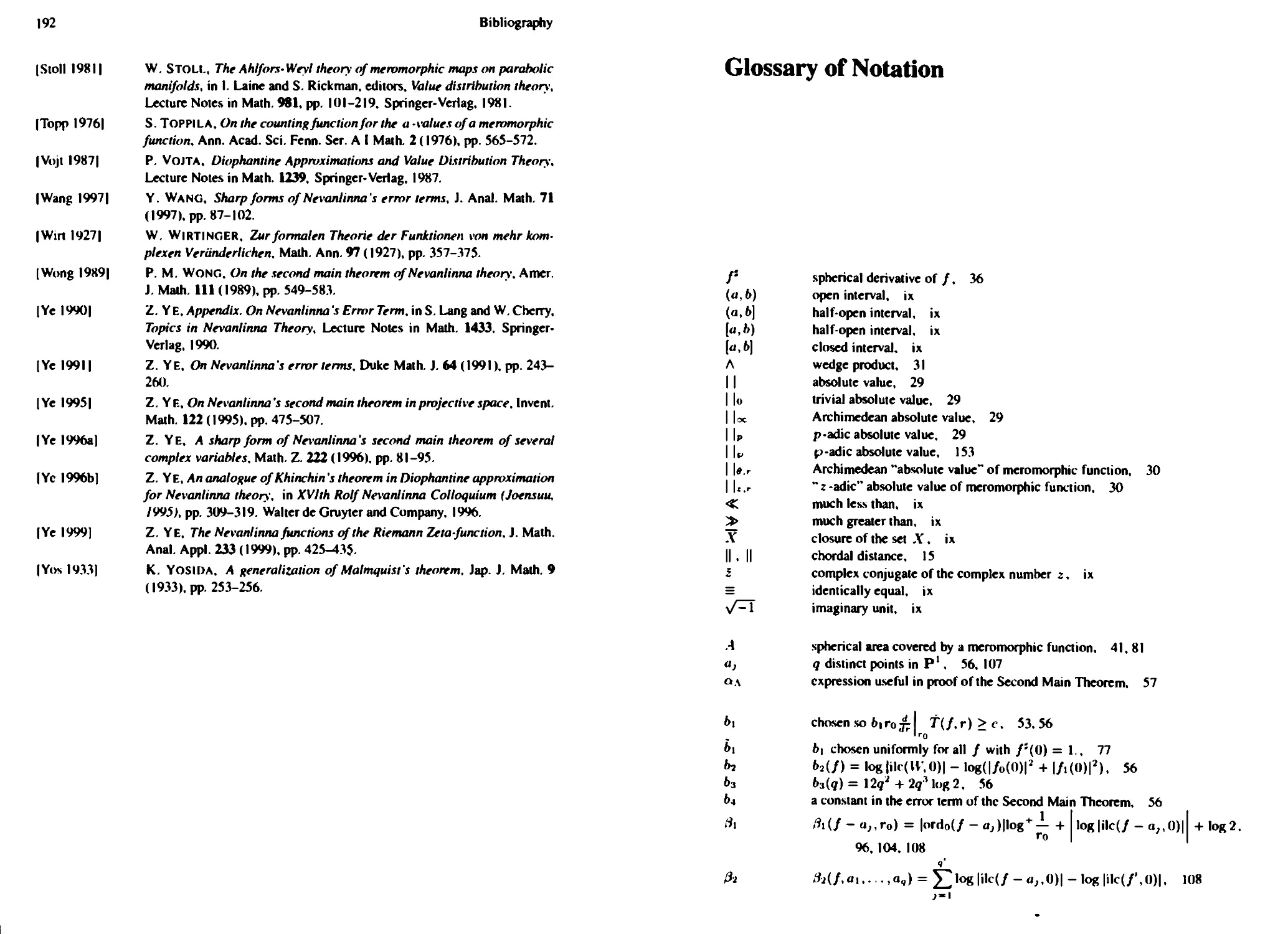
subscripts, such as c,m, or /?i. All such "long-term" constants appear in the Glossary
of Notation so that their definitions can be easily located.
Theorems, lemmas, propositions, and so forth are numbered by chapter and sec-
section. Thus. Theorem 2.3.1 would refer to the first theorem in the third section of
Chapter 2.
Especially important equations are also numbered by chapter and section. Equa-
Equations that we want to refer back to several times within the context of a single proof,
but never again later, are labeled by (*), (**), etc. Thus, there are many equation
(*) 's. and a reference to equation (*) always refers to the most recently occurring
equation (*).
Contents
Preface v
A Word on Notation ix
Introduction 1
1. The First Main Theorem 5
§1.1. The Poisson-Jensen Formula 5
§1.2. The Nevanlinna Functions 12
Counting Functions 12
Mean Proximity Functions 13
Height or Characteristic Functions 17
§1.3. The First Main Theorem 17
§ 1.4. Ramification and Wronskians 20
§ 1.3. Nevanlinna Functions for Sums and Products 23
§1.6. Nevanlinna Functions for Some Elementary Functions 24
§1.7. Growth Order and Maximum Modulus 27
§1.8. A Number Theoretic Digression: The Product Formula 28
§1.9. Some Differential Operators on the Plane 31
§1.10. Theorems of Stokes, Fubini, and Green-Jensen 33
§1.11. The Geometric Interpretation of the Ahlfors-Shimizu Characteristic . 33
§1.12. Why N and f are Used in Nevanlinna Theory Instead of n and A .41
§1.13. Relationships Among the Nevanlinna Functions on Average 43
§1.14. Jensen's Inequality 47
2. The Second Main Theorem via Negative Curvature 49
82.1. Khinchin Functions and Exceptional Sets 49
ij2.2. The Nevanlinna Growth Lemma and the Height Transform 51
§2.3. Definitions and Notation 56
§2.4. The Ramification Theorem 57
§2.5. The Second Main Theorem 60
§2.6. A Simpler Error Term 71
§2.7. The Unintegrated Second Main Theorem 73

XII
Contents
§2.8. A Uniform Second Main Theorem 74
§2.9. The Spherical Isoperimetric Inequality 78
3. Logarithmic Derivatives 89
§3.1. Inequalities of Smirnov and Kolokolnikov 89
§3.2. The Gordberg-Grinshtein Estimate 92
§3.3. The Borel-Nevanlinna Growth Lemma 98
§3.4. The Logarithmic Derivative Lemma 104
§3.5. Functions of Finite Order 106
4. The Second Main Theorem via Logarithmic Derivatives 107
§4.1. Definitions and Notation 107
§4.2. The Second Main Theorem 108
§4.3. Functions of Finite Order 117
5. Some Applications 119
§5.1. Infinite Products 120
§5.2. Defect Relations 123
§5.3. Picard's Theorem 128
§5.4. Totally Ramified Values 129
§5.5. Meromorphic Solutions to Differential Equations 129
§5.6. Functions Sharing Values 135
§5.7. Bounding Radii of Discs 136
§5.8. Theorems of Landau and Schottky Type 141
§5.9. Slowly Moving Targets 144
§5.10. Fixed Points and Iteration 146
6. A Further Digression into Number Theory: Theorems of Roth and
Khinchin 151
§6.1. Roth's Theorem and Vojta's Dictionary 151
§6.2. The Khinchin Convergence Condition 158
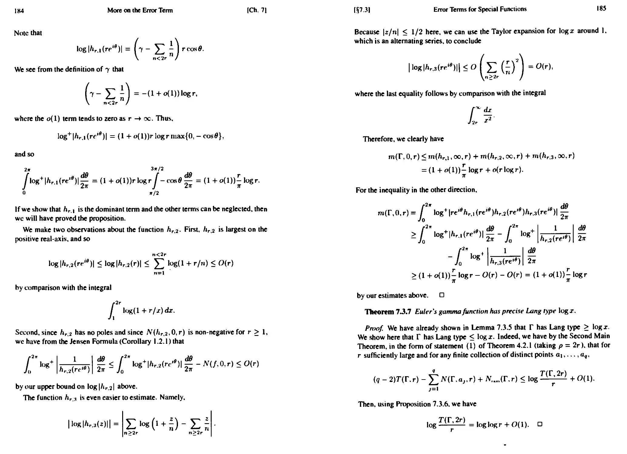
7. More on the Error Term 161
§7.1. Sharpness of the Second Main Theorem and the Logarithmic Deriva-
Derivative Lemma 161
§7.2. Better Error Terms for Functions with Controlled Growth 170
§7.3. Error Terms for Some Classical Special Functions 177
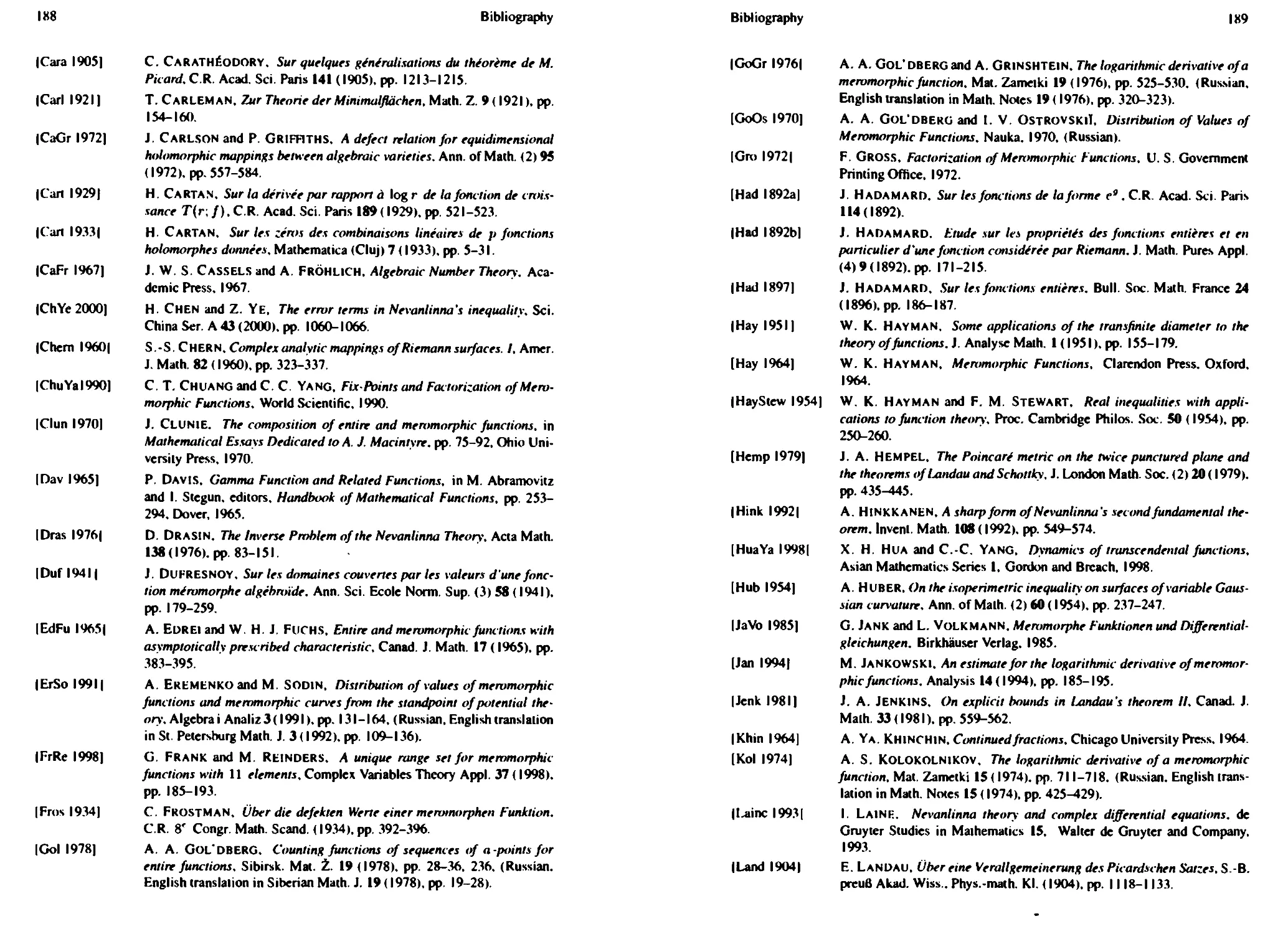
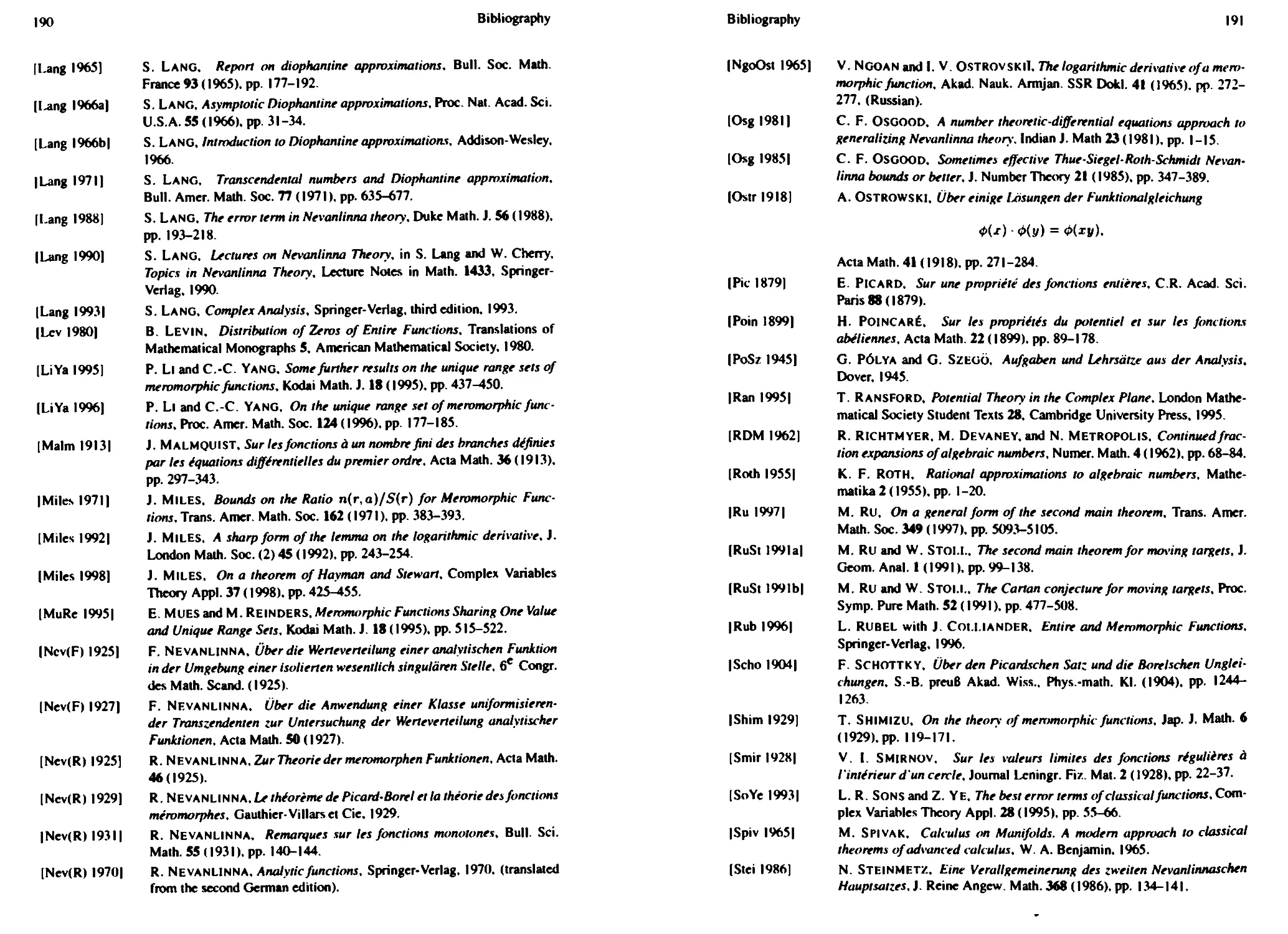
Bibliography 187
Glossary of Notation 193
Index 197
Introduction
One of the first theorems we learn as mathematics students is the the Fundamen-
Fundamental Theorem of Algebra, which says that a degree d polynomial of one complex
variable will have d complex zeros, provided that the zeros are counted with multi-
multiplicity. If P(z) is a degree d polynomial, then
max{\P(re")\ :0<9<2n}
grows essentially like rd as r -* oo. Therefore, we can rephrase the Fundamental
Theorem of Algebra as follows: a non-constant polynomial in one complex vari-
variable takes on every finite value an equal number of times counting multiplicity, and
that number is determined by the order of growth of the maximum modulus of the
polynomial on the circle of radius r centered at the origin as r -* oo. A good way
to sum up value distribution theory, otherwise known as Nevanlinna theory, is by
saying that the main theorems in value distribution theory are generalizations of the
Fundamental Theorem of Algebra to holomorphic and meromorphic functions. The
purpose of this book is to describe this theory for meromorphic functions on the
complex plane C, or more generally for functions meromorphic in a disc in C.
Before we begin to be precise about how the Fundamental Theorem of Alge-
Algebra can be extended to meromorphic functions, we make a few quick observations
about the differences between polynomials and transcendental functions. First, we
note that the entire function e: takes on many values infinitely often but never takes
on the value 0. Thus, the most naive generalization of the Fundamental Theorem
of Algebra that one might imagine is not true for entire functions. Second, tran-
transcendental functions take on values an infinite number of times, so we cannot really
speak of the total number of times that a function takes on a value. Since a function
meromorphic on the entire complex plane can have only finitely many zeros inside
any finite disc, what we can and will speak of instead is the rate at which the number
of zeros inside a disc of radius r grows as the radius tends to infinity.
Given a meromorphic function / and a value a € C U {oc}, Nevanlinna theory
studies the relationship between three associated functions: N(f, a, r), m(f, a, r),
and T(f,r). We will wait until §1.2 to give precise definitions of these functions
and content ourselves here with the following informal descriptions. The function
N(f, a, r) is called the "counting function" because it counts, as a logarithmic av-
average, the number of times / takes on the value a in the disc of radius r. The

2 Introduction
function m(f,a,r) is called the "mean-proximity function." and it measures the
percentage of the circle of radius r where the value of the function / is close to
the value a. The function T(f, r) is called the "characteristic" or "height" func-
function; it essentially measures the area on the Riemann sphere covered by the image
of the disc of radius r under the mapping / and does not depend on the value a. If
/ is an entire function, then the characteristic function measures the growth of the
maximum modulus of the function /. The characteristic function plays the same
role in Nevanlinna Theory that the degree of a polynomial plays in the Fundamental
Theorem of Algebra.
In Chapter 1 we define these "Nevanlinna functions" precisely, and we prove:
First Main Theorem // / is a non-constant mervmorphk function on C and a
is a point inCU{x},»Aen
T(f,r) - m(f,a,r) - N(f,a,r) =
as r
oo.
Since m(f,a,r) > 0 and T(f,r) does not depend on o, the First Main Theo-
Theorem says that the function / cannot take on the value a too often in the sense that
the frequency with which / takes on the value a cannot be so high that the func-
function N(f,a,r) grows faster than T(f,r). This is analogous to the statement that
a polynomial of degree d takes on every value a at most d times. Actually, the
First Main Theorem says even more in that it says the sum m(/,a,r) + N(f,a,r)
must be essentially independent of a. Thus, if / takes on the value a with a small
enough frequency that N(f,a,r) does not grow as fast as T(/,r), then the func-
function m(f.a,r) must compensate, meaning that the image of / stays near the value
a for sufficiently large arcs on large circles centered at the origin.
The subject of the later chapters is the deeper:
Second Main Theorem /// is a non-constant memmorphic function on C, and
ax a, are distinct points in C U {oc}, then
(q - 2)T(f,r) - ?N{f,aj,r) +
, r) < <4T{f,r))
for a sequence ofr-too.
In fact, we will prove stronger and more precise forms of this theorem. The term
A'..m(/> r) is positive (at least when r > 1) and measures how often the function /
is ramified. Thus, the Second Main Theorem provides a lower bound on the sum of
any finite collection of counting functions N(f,aj,r) for certain arbitrarily large
radii r. Thus, taken together with the First Main Theorem, which provides an upper
bound for the counting functions, we have our generalization of the Fundamental
Theorem of Algebra.
The key results presented in this book, namely the First and Second Main Theo-
Theorems, are essentially due to R. Nevanlinna INev(R) 1925] and F. Nevanlinna INev(F)
Introduction
1927]. The Nevanlinnas gave precise, though not "best possible," estimates for the
function implicit in the o(T(f, r)) on the right of the inequality in the Second Main
Theorem. This function is known as the "error term." The fine structure of the error
term was not considered especially interesting until relatively recently. In this book,
we pay careful attention to the error terms, and the error terms we give are better
than those obtained by the Nevanlinna brothers.
In many ways our presentation of this material resembles those of Nevanlinna
(Nev(R) 1970], Hayman (Hay 1964), and Lang ILang 1990]. Those familiar with
the Russian work by A. A. Gol'dberg and I. V. OstrovskiT [GoOs 1970] or the Ger-
German work by Jank and Volkmann [JaVo 1983] will also recognize their influence
on our presentation. The primary manner in which our presentation of the Second
Main Theorem differs from those of Nevanlinna and Hayman is that we are careful
in our treatment of the error terms, and of what is known as the "exceptional set."
There are several fundamentally different ways of proving the Second Main The-
Theorem. Each approach has its own advantages and disadvantages, and the Second
Main Theorems that result from each approach are not quite the same.
Chapter 2 contains the first of two fundamentally different proofs we will give for
the Second Main Theorem. This proof is based on "negative curvature," a technique
introduced by F. Nevanlinna into the theory almost from the very beginning INev(F)
1925], [Nev(F) 1927]. The error term estimate we give in Chapter 2 is essentially the
work of P.-M. Wong [Wong 1989], and our presentation is quite similar to Chapter I
of ILang 1990]. In §2.6 we incorporate the work of Z. Ye (Ye 1991] in order to
simplify the appearance of Wong's error term. Finally, in §2.8, we discuss how the
Second Main Theorem is uniform over families of functions, and we are not aware
of any other similar treatment.
In Chapter 3, we undertake a detailed study of Logarithmic derivatives. The main
result of that chapter is:
GoTdberg-Grinshtein Inequality // / is a memmorphic function on C. then
for any r and p with 1 < r < p < oc,
"*(/'//.
< max
JO,
log
r(p - r)
4
Here &\ and ru are constants that will be defined in Chapter 3.
In Chapter 4, using ideas from Ye's refinement of Cartan's approach to the Sec-
Second Main Theorem [Cart 1933], as in [Ye 1995], we use the precise estimate on
m(/7/tr*3°) provided by the Gol'dberg-Grinshtein estimates in Chapter 3 to
prove the Second Main Theorem and give a careful analysis of the error term and
exceptional set obtained by this method.
There is a third altogether different approach to proving the Second Main The-
Theorem, initiated by A. Eremenko and M. Sodin [ErSo 1991]. This relatively new
approach might be said to be a potential theoretic approach. Although this newer
approach to the subject is very interesting and important, we have chosen not to

4 Introduction
discuss this method in this volume because, as yet, no one has succeeded in proving
a version of the Second Main Theorem that includes the ramification term by this
potential theoretic approach, nor has a detailed analysis of the error term coming
from this approach been undertaken.
Although the applications of Nevanlinna's theory are not our focus, we feel that
some detailed discussion of applications is essential in order that those readers new
to the subject can gain an appropriate aesthetic and utilitarian appreciation for what
often appears to be a very technical and obscure subject. Therefore, we have in-
included a lengthy chapter. Chapter 5, on applications. We chose our applications
only to illustrate the utility of the theory, and thus we made no effort to choose the
most current or refined application of any given type. Our chosen applications are
for the most part as in [Hay 1964] and [Nev(R) 1970], and many of them are due
to R. Nevanlinna himself. In fact, those readers looking for more refined applica-
applications than those we give in Chapter 3 might well start by reading Nevanlinna's first
monograph [Nev(R) 1929]. Our applications chapter does differ somewhat though
from past treatments in that we have put some emphasis on what can be gained from
precise knowledge of the error terms, something ignored by most previous authors.
The material covered in Chapter 7, where we discuss the sharpness of the error
terms, the precise error terms of some classical special functions, and improvements
to the error term for functions with restricted growth, has, up till now, only been
available in the research literature.
The connection between Nevanlinna theory and Diophantine approximation the-
theory has inspired a lot of recent work in both fields, and we have therefore including
several sections, referred to as "number theoretic digressions," explaining and moti-
motivating in some detail this connection. We assume no background in number theory
in these sections and hope that these sections will encourage even the most pure
analysts to further explore this fascinating connection.
Given our emphasis on the Second Main Theorem and its error terms, we have
not discussed anywhere in this volume the various other techniques for studying
the distribution of values of meromorphic and entire functions. We instead refer
the reader to the recent book [Rub 1996] for an introduction to some of these other
techniques.
1 The First Main Theorem
As we mentioned in the introduction, the basis for Nevanlinna's theory are his two
"main" theorems. This chapter discusses the first and easier of the two.
To understand where we are headed, looking at the concrete example of the tran-
transcendental entire function ez is again helpful. We pointed out that r- takes on all
values other than zero infinitely often. Notice also that by periodicity each of these
non-zero values is also taken on with the same asymptotic frequency. Of course
e- never attains the value 0; nor does it attain the value oo. On the other hand,
on every large circle centered at the origin, the function e* spends most of its time
close to one of these two omitted values. That is. fixing a small e, the percentage of
the circle of radius r where <r is either smaller than ¦ or larger than l/e tends to
100% as the radius of the circle tends to infinity.
Nevanlinna's First Main Theorem will tell us that this behavior is typical. That
is, if a meromorphic function takes on a particular value less often than "expected,"
then it must compensate for this by spending a lot of time "near" that value. As
a consequence, Nevanlinna's First Main Theorem gives an upper bound (in terms
of the growth of the function) on how often a meromorphic function can attain
any value. This is analogous to the statement that a polynomial of degree d can
take on any value at most d times. Note this last statement about polynomials is
much easier to prove than the full Fundamental Theorem of Algebra. It is thus no
surprise that Nevanlinna's First Main Theorem is much easier than his Second Main
Theorem, which says that most values are taken on by a meromorphic function with
the maximum asymptotic frequency allowed by the First Main Theorem.
1.1 The Poisson-Jensen Formula
We begin this chapter with this brief section which recalls the Poisson Formula for
harmonic functions and applies this to the logarithm of the modulus of an analytic
function to derive what is known as the "Poisson-Jensen Formula." The material
in this first section is usually covered in a first course in complex analysis, and we
could have chosen to regard the material in this section as a prerequisite. On the
other hand, the Poisson Formula is at the very heart of Nevanlinna's theory of value
distribution, and the First Main Theorem of Nevanlinna theory is really nothing

The First Main Theorem
ICh. 1]
other than the Poisson-Jensen formula dressed up in new notation. Thus, we felt a
detailed treatment of this material here would be of value to the reader.
We begin with some general notation. We will use C to denote the complex
plane. We will use r and R to denote positive real numbers, which will usually
be radii of discs, we will always have r < R, and we will also allow R = oo,
whenever this makes sense. We will use D(r) and D(R) to denote open discs of
radius r and R, respectively, each centered at the origin. When R is allowed to
be infinite, D(R) will refer to the entire complex plane C. We will consider the
value distribution of meromorphic functions on D(/?), and it will be convenient to
consider a meromorphic function as a holomorphic map to what is known as the
Ricmann sphere or the projective line C = Cu{oo} = P'.Tobe more consistent
with the higher dimensional theory, we prefer to refer to the Riemann sphere as the
projective line P1.
If R < oo, we will use D(R) to denote the closure of the disc D(R) in the com-
complex plane. If we say a function is harmonic, respectively holomorphic, or respec-
respectively meromorphic on the closed disc D(R), then we mean that function should
be harmonic, respectively holomorphic, or respectively meromorphic on some open
neighborhood of D(R),
We will now recall the Poisson and Poisson-Jensen Formulas. Let
= KJlHi = Re/i±il.
The function P(z, Q is called the Poisson kernel. Note that for fixed C and for
|*|<IC|.
ill
is holomorphic, and hence P(z, Q being the real part of a holomorphic function is
harmonic in z.
We being by showing how the Poisson kernel transforms under a Mobius auto-
automorphism of a disc.
Proposition 1.1.1 Let
T(w) =
R2(z - w)
R? - zw
Then, T(w) is an automorphism of D(R) thai interchanges 0 and z. Moreover,
when \T(w)\ = R, then
when P(z, Q is the Poisson kernel and C = T(w).
(§111
Poisson-Jensen Formula
Proof. One easily verifies that T(w) is holomorphic on D(fl), and that when
\w\ = R, then \T(w)\ = R. Hence, T is an automorphism of D(R) that inter-
interchanges 0 and z.
Noting that T is its own inverse in the group of linear fractional transformations,
we have that
We then compute
2mw 2m\z-t R2-z() \z - C
Note that when |C|2 = R2,
- K)
\c-z\2
Our first theorem, called the Poisson Formula, allows us to express a harmonic
function in a disc as an integral around the boundary circle.
Theorem 1.1.2 (Poisson Formula) Let u be harmonic in the open disc D(/?),
R < oo and continuous on the closed disc D(R). Let z be a point inside the
disc. Then
u(z) =
where P(z, Q denotes the Poisson kernel.
Proof. First we will prove the theorem in the case that u is harmonic on the closed
disc D(R). Let C = T(w) as in Proposition 1.1.1. Because T is holomorphic on
D(R), we know u(T(w)) is harmonic on D(R). By the mean value property of
harmonic functions.
= u(T@)) =
dw
2niw
Letting C = Re'9, using Proposition 1.1.1, and recalling that -^ = d9,
.
In the case that u is not harmonic in a neighborhood of D(/?), all we need do is
note that for p < 1, u(pw) is harmonic on D(R), and we can use what we have
already proven to conclude that
The result follows by noting that u(pw)
D
u(w) uniformly on |u;| = R as p -> 1.

The First Main Theorem
ICh. 1]
Corollary 1.1 J Let P(z,Q denote the Poisson kernel and let R > 0. Then
/;
Proof Apply Theorem 1.1.2 to the constant function u(z) = 1. ?
We can also use the Poisson kernel to create harmonic functions in a disc if we are
just given a continuous function on the boundary circle. This is known as "solving
the Dirichlet Problem for the disc." To prove this, we need the following estimate.
Proposition 1.1.4 Let P(z,Q denote the Poisson kernel. Given Co such that
| Co | > 0, given e > 0, and given S > 0, there exists a 6' such that for all
C with |C - Co| > S and |fl = |Co|, and all z with 0 < \z - Col < <*'• we have
\P(z.O\<e.
Proof. We have for z near Co and |C - Col > 6 that
.v = ICI2 - \z? = ICol2 - H2 ICol2 - \z\2
J IC-*I2 l(C-Co)-(*-Co)|2- («*-|*-ColJ'
The term on the right clearly tends to zero as z -> Co- D
Theorem \.\JS (Solution to the Dirichlet Problem) Let <p(Rew) be a continu-
continuous function of 9 for a fixed R < oo. Then.
def f
Jo
~2' 4>(Reie)P(z,Reie)^-
o *n
is a harmonic function of z in D(#). and for each $o
lim u(z) = <t>(Re>8°).
Proof To check that u is harmonic, we differentiate under the integral sign with
respect to z, which we can do because <j> is continuous in 6 and so are P and its
z-derivatives since \z\ < R Because P is harmonic in z. so is u.
It remains to check that
lim u(z) e
We have by Corollary 1.1.3
\u(z) - <t>(Reie)\ =
dB
10) - <HRc'a<>)) P(z,Rc">) —
JO
\4>(Re">) - <t>(Reteo)\ P(z,Re">) g,
i§i-n
Poisson-Jensen Formula
since P(z, C) is always positive. Let e > 0. By the continuity of </>, there exists a
6 > 0 such that \4>(Reia) - <t>{Reia«)\ < e for those 9 with \Re'a° - Re'a\ < 6.
Hence
/
\<t>(Rtte) -
(z.R<'ie)^ < J eP(z
= e.
On the other hand, from Proposition 1.1.4, there exists a 6' such that if
0 < \z - Reia°\ < 6' and \Re'°° - Reia\ > 6,
then \P{z, Reie)\ < e. Thus, for these z.
J \<t>(Reia) - <t>(Re">°)\P(z, ReiB) ^
e"-Re"o\>{)
The proof is completed by noting that
Jo
27T
is bounded by the continuity of <j>. ?
If / is analytic and free from zeros, then log |/| is harmonic, and we can there-
therefore apply the Poisson Formula to it. However, since we are interested in the distri-
distribution of the zeros of /, we will want to see what happens in the case that / has
zeros. This is what is called the "Poisson-Jensen" Formula.
Before giving the precise statement of the Poisson-Jensen Formula, we introduce
some additional notation. Given a non-constant meromorphic function / and a
point a in the complex plane, we can always write f(z) — (z - a)mg(z), where
tn is an integer, and g is analytic and non-vanishing in a neighborhood of a. The
integer m is called the order of / at the point a and is denoted orda/. Note
that orda/ > 0 if and only if / has a zero at a, and orda/ < 0 if and only
if / has a pole at a. We will refer to the non-zero complex number g(a) as the
initial Laurent coefficient of / at a, denoted ilc(/,a), because it is the first non-
vanishing coefficient of the Laurent expansion of / expanded about a.
Theorem 1.1.6 (Poisson-Jensen Formula) Let f ? 0,oo be meromorphic on
T)(R). Let a\,...,ap denote the zeros of f in the open disc D(R), each zero
repeated according to its multiplicity, and let 6(,... ,6, denote the poles of f in

10
The First Main Theorem
ICh. II
D{R). also repeated according to multiplicity. For any z in D(R) which is not
a zero or pole of /, we have
2n
AQ
R2 - atz
R(z-ai)
1=1
R2-
R(z-
b,z
-b.)
(°rd</)lo8
R3 -
R(z-0
If z = 0, this simplifies to
= T \og\f(Re«)\? - ? (
R
Q
1=1
ord</)log
?
Corollary 1.1.7 Let fl, /, <M ap, am/ 6j,..., 6, 6e as in Theorem 1.1.6.
Then, for any z which is not a zero or pole of f,
z-a,
Proof of Corollary 1.1.7. Note that
where the last equality follows from the Cauchy-Riemann equations since
The corollary then follows by differentiating the equation in the theorem and moving
the derivative inside the integral. ?
l§ I 11
Poivson-Jcnsen Formula
II
Corollary l.U Let f ? 0, oo be meromorphic on D{R). Let at,... ,ap de-
denote the non-zero zeros of f in D(fl), repeated according to multiplicity, and
let 6|,..., 6, denote the non-zero poles of f in D(R), repeated according to
multiplicity. Then,
-r
- (ordo/)logfl
(ord</)log
-(ordo/)logfl.
A.1.9)
Remark. Equation A.1.9) in Corollary 1.1.8 as well as the second equation in
Theorem 1.1.6 are referred to simply as the Jensen Formula.
Proof of Corollary 1.1.8. Simply apply Theorem 1.1.6 (the Poisson-Jensen For-
Formula) to the function f(w)w~ordof. D
Proof of Theorem 1.1.6. First of all. note that it suffices to prove the theorem
when / has no zeros or poles on the circle of radius R. Indeed, because zeros and
poles on the circle of radius R do not cause the integrals on the right hand sides
of the formulas to diverge, we can consider the function f(pw), which will not
have any zeros on the circle of radius R for all p sufficiently close to, but less than
1. The theorem follows from this case by letting p -» 1 and Lebesgue dominated
convergence.
Now we assume / has no zeros or poles on the circle of radius R. Consider the
function
" 'Rz-aiw
-eg))
l\\R{w-b,)J
fJi\R(w
We have chosen F so that it has no zeros or poles in the closure of D(R) and so that
\F(w)\ = \f(w)\ when \w\ = R. The function log|F(u;)| is therefore harmonic in
an open neighborhood of D(R). The proof of the theorem is completed by applying
the Poisson Formula to log \F\. O
If we look closely at equation A.1.9). we can start to see our generalization of
the Fundamental Theorem of Algebra. The left-hand side of equation A.1.9) is just
a constant. The right-hand side of the equation has two different types of terms.
The first term on the right is an integral over the circle of radius R involving the
absolute value of /. The other term is a sum over the zeros and poles of /. If / is

12
The First Main Theorem
[Ch. IJ
holomorphic or meromorphic on the whole plane C, then as R -» oo, the left-hand
side of this equation does not change, so that means although all the terms on the
right-hand side might tend to infinity, if they do, then they always essentially cancel
each other out.
1.2 The Nevanlinna Functions
At the end of the last section, we noted that equation A.1.9) can be viewed as the
first step toward generalizing the Fundamental Theorem of Algebra to meromorphic
functions. In this section, we explore this in more detail. We begin by defining the
Nevanlinna functions and then state the first fundamental relationship between them,
known as the "First Main Theorem" of Nevanlinna theory. Although the First Main
Theorem is really just a restatement of the Jensen Formula (Corollary 1.1.8), it is
this formulation which makes clear that Jensen's Formula is a weak generalization
of the Fundamental Theorem of Algebra.
As we proceed to define the Nevanlinna functions. / will always be a meromor-
meromorphic function on D(/l), where R might be oo, and r < R. Note that most of our
definitions will not make any sense for certain constant functions /, and thus we
exclude any such constant functions fmm consideration.
Counting Functions
First, we define the counting functions. The unintegrated counting function
n(/. oc,r) simply counts the number of poles the function / has on the closed
disc D(r), each pole counted according to its multiplicity. Note that because / is
meromorphic on some larger disc, this number is always finite. If a is a complex
number, we define n(/,a,r) to be
which is simply the number of times / takes on the value a on D(r). We choose
to count the a-points of / in the closed disc D(r) instead of in the open disc D(r)
because we can then use n(f, 0, r) to denote the multiplicity with which / takes on
the value a at z = 0.
We then define the integrated counting function Ar(/. a, r) by
= n(/,a,0)Iogr+ / \n(f,a,t) -
J
So, in particular.
= (ord?/)logr
(§121
The Nevanlinna Functions
13
where ordtf = max{0,ordj/} is just the multiplicity of the zero. Note that the
points z on the circle \z\ — r where f(z) = 0 do not contribute to N(f,0,r) since
in that case log \r/z\ = 0. Thus we see that the integrated counting function is very
similar to the terms in the right hand side of equation A.1.9). In fact, with this new
notation, we can rewrite Corollary 1.1.8 as
Corollary 1.2.1 Let f ? 0,oo be meromorphic on D(r). Then,
Jo
|^ + A'(/,oo,r) - N(f,0,r).
The unintegrated counting function n(f,a,r) of course appears to be the more
"natural" of the two counting functions to consider, and those new to the field often
wonder why N(f, a, r) is used so often instead of n(/, a, r). One reason is that it
is N and not n that naturally appears in Corollary 1.2.1. Another advantage of N
over n is that it is a continuous function of r. We will say a bit more on this in
§111.
We will also have occasion to discuss truncated counting functions. We let
n(t)(/, oo, r) denote the number of poles / has in the closed disc of radius r,
but this time we only count each pole with a maximum multiplicity of k. In other
words, if z0 is a pole of / in the disc with multiplicity < it, then it is counted ac-
according to its multiplicity. If, however, zo is a pole of / in the disc with multiplicity
greater than k, then we count z0 as if it only had multiplicity k. We similarly de-
define n{k)(f,a,r). Note in particular that nil)(f,a,r) counts the number of times
/ takes on a without counting multiplicity at all. As the reader might now expect,
the integrated truncated counting function Nik)(f, a, r) is then defined by
N<k)(f,a,r) = n^(f,a,
Mean Proximity Functions
We will now explain the significance of the integral term in Corollary 1.2.1. To
begin with, it is useful to introduce the notion of a Weil function. Given a point a
in P1, a Weil function with singularity at a is a continuous map
Aa:P'\{a}->R
which has the property that in some open neighborhood U of a in P1, there is a
continuous function a on U such that
Aa(z) = -log\z~a\ + a(z),
where z is a holomorphic local coordinate on U. Thus, Weil functions are almost
continuous functions, except that they have a certain specified logarithmic singular-
singularity at the point a. Notice that the difference between any two Weil functions with

14
The Firsi Main Theorem
ICh. I]
the same singular point will be a continuous function on P1 and will therefore be
bounded since P1 is compact. Also notice that for a meromorphic function f(z)
on D(R), the composition of / with a Weil function Ao(/(z)) is large precisely
when f(z) is close to a. Given a Weil function Aa, one defines a mean proximity
function
m(/,A.,r)= I *
Jo
The mean proximity function measures how close / is, on average, to a on the
circle of radius r. Note that if we take two different Weil functions with the same
singularity a, then the mean proximity functions we get from each Weil function
will differ by a bounded amount as r -* R.
One has many choices for Weil functions, but many things do not depend on the
specific choice of Weil function. Two specific types of Weil functions come up often
in Nevanlinna theory, each type having its own advantages. R. Nevanlinna used the
following Weil functions in his first proof of the his main theorems.
Aa(oc) = 0
Aa(z) = log+ \z\
where for a positive real number x, log+i = max{0, logi}. Hence, we define
,2ir
m(/,o,r)=/ log+
Jo
1
f(reie)-a
aa . .
— a ^ oo and
When looking at things from an "analytic" viewpoint, we will find it convenient
to use Nevanlinna's choice of Weil function as above, but when we wish to look at
things "geometrically," we will prefer a different choice of Weil function, which we
now describe.
Let z\ = nei9x and z2 = r2e'*2 be two points in C. If we use stenographic
projection to identify the complex plane with the sphere of radius 1/2 centered at
the origin in R3, minus the north pole, and if {pj,0},(}), j = 1,2 are the cylin-
cylindrical coordinate representations of the images of z}> then we have the following
relations:
¦ - '> , - r?-1
P>-\+r) ^~4(l+rJ)'
Now, the square of the standard Euclidean distance in R3 between the two points
(Pj'Oj'Cj) is given by
p'i+pl- 2p,p2co8@, - 0,) + C? + C| - 2C1C2-
151-21
The Nevanlinna Functions
15
Writing p} and C> in terms of r} and simplifying, one sees that the square of the
distance between the images of z\ and z2 in R3 is given by
r? + r\ - 2r,r2cos(fl, - 02) _ \zx - z2|2
We therefore define the (square of the) chordal distance between two points in the
complex plane to be
The term "chordal distance" comes from the fact that we derived this formula by
measuring the length of the chord of the sphere connecting z\ and z7 when thought
of as points on the sphere. We note that it is not obvious by just looking at the
formula for ||zi, Z2II that this distance satisfies the triangle inequality. However,
since the chordal distance comes directly from the Euclidean distance in R3, it
clearly must satisfy the triangle inequality. We can continuously extend our notion
of chordal distance to P1 by saying that
We now define another Weil function associated to a by
and this is the other Weil function we will choose to work with.
Note that unlike the Weil function used by Nevanlinna, this more "geometric"
Weil function Aa is smooth, and even real analytic, away from the point a. In
Ahlfors's collected works [Ahlf 1982, pp. 56], Ahlfors says "rightly or wrongly"
he was initially "somewhat disturbed" by the non-smoothness of the Weil function
A-c used by Nevanlinna. He explains that his experimentation with A,*, as an al-
alternative was what led him [Ahlf 1929] to discover the geometric interpreUtion of
Nevanlinna's characteristic function (to be defined below). This interpretation had
previously been discovered by T. Shimizu [Shim 1929] and will be explained in
detail in §1.11.
Since we have identified the Riemann sphere with the sphere of radius 1/2 in
R:', we always have \a(z) > 0 since ||2,a|| < 1. We will take
m(f,a,r)= f" - log||/(re*),a|| f-
Jo *w
to be our definition of the "geometric" mean proximity function to a of /, which
we distinguish from our previous definition by writing a small circle above the m.
Since working with explicit constants is one of our goals in this book, we record
here the explicit constant relating Nevanlinna's definition of mean proximity to this
other mean proximity function.

16
The First Main Theorem
ICh. I]
Proposition 1.2.2 For all x > 0,
log+* < \ log(l + x1) < log+x ^
i4/io. #/v«t a 6 P1 and a meromorphic function f ? a onD(R), we have for
all r < ft.
m(/,o,r) < m(/,a,r) < m(/,a,r) + ^.
Proof. The inequalities
log+x < i log(l + x2) < log+x + !5|*.
are elementary, and the other inequality follows from this and the definitions. O
We also record here the following useful observation, which we will use to relate
the various proximity functions. For those already familiar with Nevanlinna theory,
this observation is what is used in what is often known as the "product into sum"
estimate. We will say more about this when we discuss the Second Main Theorem.
Proposition 1.23 Let a(,..., a, be q distinct points in P1. Then, for all w in
P1,
JJ llw.a^H > (-) [mjnni|a,,a>||]min||ti>,a,||.
Moreover, if AOj are Weil functions with singularities at the points aj such that
there exist non-negative constants C\ and Ci so that for all w ^ Qj in P1,
-C, < -log||a>fti;|| - K
then for all w ^ a, in P1, we have
Proof. The point is that w cannot be close to all the points at the same time. More
precisely, since ||z, w|l is a metric on P1, the triangle inequality implies that there
is at most one index j such that
IKll < Hll
For all other indices t, again by the triangle inequality.
Thus, the first statement. The second follows easily from the first. ?
Because Proposition 1.2.3 will be used on several occasions, it is convenient to
introduce some notation. Given distinct points a\,..., a,, we define
V(a a,) = logmax
1
+ (g-l)log2.
IS1-31
The First Main Theorem
17
Height or Characteristic Functions
Finally, we define the last of our Nevanlinna functions. The Nevanlinna height or
Nevanlinna characteristic function with respect to a is defined by
T(f,a,r) = m(f,a,r) + N(f,a,r),
and the "geometric" height or characteristic function with respect to a is defined
by
T(f,a,r) = m(/,a,r) + AT(/,a,r)+ <•«„,(/, o),
where c,mt(f, a) is a constant that does not depend on r and is defined by
c,m,(/,a) = nOg|ilc(/-a,0)| + 21og||a,oc|| if /@) = a,a # oo A.2.4)
= a = oc.
The geometric characteristic function is often called the Ahlfors-Shimizu charac-
characteristic function for reasons that we will explain in §1.11. The constant r,m, is
known as the First Main Theorem constant, for reasons which will become appar-
apparent below.
The height or characteristic function T (or T), the mean proximity function m
(or m), and the counting function TV are the three main Nevanlinna functions.
Nevanlinna theory can be described as the study of how the growth of these three
functions is interrelated. We would like to point out that there is not universal agree-
agreement on what the order of the three arguments to each of these functions should be,
and many authors use a subscript for one or more of the arguments. We have decided
we would like to avoid subscripts for typographical reasons, and we have ordered
the arguments the way we have because one often thinks of having one function /
at a time, a finite number of values a, and an infinite set of radii r. Our arguments
thus appear in order of increasing cardinality.
1.3 The First Main Theorem
This brings us to the main result of this section. Nevanlinna's First Main Theorem
says that the height function T does not really depend on a. More precisely.
Theorem 13.1 (First Main Theorem) Let a 6 C, and let f ? a, oo be a
meromorphic function in D(Ii), R < oo. Then.
T(f. a, r) - T(f, oc, r) + log |ilc(/ - a, 0)| | < log+ \a\ + log 2,
and f(f, a, r) = T(f, oo, r).

18
The First Main Theorem
ICh. I]
Remarks. The equality between the f explains the the definition of c,ml. This
equality is one of the advantages of the Weil function A coming from the chordal
metric. For the Nevanlinna characteristic T the best one can say is the difference
is bounded, as in the statement of the theorem, not that the difference is actually
constant.
Proof. We first prove the equality between the f. Directly from the definition of
the chordal distance.
/,«, r)-m(/,oo,r)
- logl/(re") - a\ g
i log(l + |al2) - I
e")-o|^ - log|la,ool|.
Corollary 1.2.1 applied to / - a gives us that
"-lQ6l/(re**)-a|~ =
Clearly N(f - a,0,r) = N(f,a,r), and since / and / - a have the same poles,
A'(/ - a, oo, r) = N{f, oo, r). Therefore, if /(O) # a, oo, then by the definition
of T and cfml,
T{f,a,r)-f{f,oo,r)
= m(/, a, r) - m(/, oo, r) + N(f, a, r) - N{f, oo, r)
+ log||/@),a||- log||/@),oo|l
= - log Ha, oo|| -log |/@) -a| + log ||/@), a|| -log |l/@), oo|l
= 0.
If /@) = a or oc, then the definition of c,m, was chosen so that we would get a
similar cancellation. This we leave as an exercise to the reader.
Using Corollary 1.2.1 with the m functions as we did with the rit functions, we
get
m(/,a,r)-m(/,oo,r)
[§131
The First Main Theorem
19
= 7V(/,oo,r) - N(/,a,r)-log|ilc(/-a,0)|
[log+|/(re")-o|-log+|/(rew)|] g.
For the inequality involving the T functions, note that if x and y are positive real
numbers, then
log+(x + y) <log+Bmax{x,y})< log+x + log+y + log2.
Thus, if w is any complex number,
|log+|u; - a\ - log+(u;|| < log+|a| + log2.
This then gives us
- r(/,oc,r)
^ < log+|a| + Iog2. D
Note that the First Main Theorem is really just Jensen's Formula written with
different notation, and is thus not particularly deep. Given the First Main Theorem,
one often writes just T(f, r) instead of T(f, a, r) since any two of these differ by
a term bounded independent of r. To be definite, we will take
T(f,r) = T(f,oo,r),\ and similarly \f(f,r) = f(f,oo,r).
We began this chapter by promising that it would contain a generalization of the
Fundamental Theorem of Algebra. Let's see where we are in that regard. If it were
true that N(f, a, r) were essentially independent of a, then we would indeed have
a generalization of the Fundamental Theorem of Algebra, because this would say
that the rate of growth of the set of points where / is equal to a is independent of a,
or loosely speaking / takes on all values equally often. We have already mentioned
that this cannot be true because, for example, e~ is never 0. In fact, if one allows
a = oo, this is not even true for polynomials, since polynomials have no poles.
What the First Main Theorem tells us though is that
m(f,a,r)+N(f,a,r)
does not depend on a, except for a bounded term independent of r. Thus, if we
measure the growth of not only the set of points where / is equal to a, but also

20
The Firsi Main Theorem
[Ch. I]
where / is "close to" a, then this combination grows in such a way that it is es-
essentially independent of a, and this is our first generalization of the Fundamental
Theorem of Algebra. Of course, this is not a strict generalization in the sense that
it in no way implies the Fundamental Theorem of Algebra. This also explains why
the function m(f, a, r) is sometimes called the compensation function because it
"compensates" for the fact that the most naive generalization of the Fundamental
Theorem of Algebra is not true for meromorphic functions. We point out that since
ni(/, a, r) is always positive, the First Main Theorem gives us an upper bound on
the number of times / takes on the value a. Thus, it can be regarded as an analog
of the statement that a polynomial of degree d has at most d zeros.
Looking back at our example of <\ we notice that although ez is never 0, it is
close to zero (meaning that it is less than e in absolute value, e a positive number
much less than one) on nearly half of each large circle centered at the origin. On
the other hand, if a is a non-zero finite value, then ez hits a regularly, tz being a
periodic function, but e! is close to a, meaning that e.: - a is less than e in abso-
absolute value, only on a very tiny arc of each large circle centered at the origin. Notice
that for v~-, the counting function N dominates the sum m(f,a,r) + N(f,a,r) for
most values of a, and only for the special values of 0 and oo is the mean proxim-
proximity function m significant. Those readers already familiar with Picard's Theorem,
which states that a non-constant meromorphic function on the complex plane can
omit at most two values in P1, might already suspect that for most a, the counting
function is the dominant term. This is indeed the case, and later when we discuss the
Second Main Theorem, we will turn toward proving deeper results in that direction.
In summary, the First Main Theorem gives us an upper bound on N(f, a, r) and
hence on the number of times / takes on the value a, whereas the more elusive
lower bounds on N(f, a, r) will have to wait until Chapter 2 and Chapter 4 where
we prove the Second Main Theorem.
1.4 Ramification and Wronskians
We now discuss "ramification" and introduce one last piece of notation. Although
we will not prove anything about ramification until Chapters 2 and 4, we would like
to introduce the concept and the notation here.
A point z0 in D(fl) is called a ramification point for a non-constant meromor-
meromorphic function /: D(fl) -> P1 if / is not locally a topological covering map at the
point zo. If }{zq) ^ oo, then / has a series expansion at zq of the form
f(z) = A + D(z - zo)> + (z- «o)p+lff(*).
where B ^ 0 and g(z) is analytic in a neighborhood of zo- One easily sees that /
is locally a topological covering map at zq precisely when p = 1, in which case /
is locally a one sheeted covering by the inverse function theorem. If p > 1, then
locally in a neighborhood of zq, the map / is a p to 1 cover, except at z0- If p > 1,
Ramification and Wronskians
21
then the integer (p - 1) is called the ramification index of / at zq. Note that if /
is analytic, then / ramifies precisely at the zeros of /', and if z0 is a ramification
point then its ramification index is given by ordj0/'. if /(*o) = oo, then one must
look at the series expansion of 1// at zo, and in that case, the ramification index
of / at zo is given by ord.0(l//)'. We emphasize that the ramification index is
always non-negative, even at a pole of /.
Let / be a meromorphic function and write / = /i //o. where /o and f\ are
holomorphic without common factors. We regard the fact that any meromorphic
function on D(fl), R < x can be written as the quotient of two holomorphic func-
functions without common zeros to be a fundamental fact from complex variables, and
we will make use of this fact throughout without further comment. Those unfamiliar
with this result should see, for example. Chapter XIII of [Lang 1993]. Then, away
from the poles of / (i.e. the zeros of /o), we have that
ft _ fof'l ~ /p/l
J (/oJ '
and this is zero precisely when /o/{ - }'of\ = 0. At the poles of /, which are not
zeros of /i since we have assumed /o and f\ to be without common factors.
(/iJ
and again the zeros of A//)' are given precisely by
Wronskian
- fof{ = 0. Thus, the
/o/i
/o/i'
= Ml - /o/i
of /o and }\ is a useful function since its zeros are precisely the ramification points
of /, and ord-0 W is exactly the ramification index of / at zq. The zeros of W
together with their multiplicities are referred to as the ramification divisor of /.
Note that W has no poles.
If P is a polynomial, then the ramification divisor for P is given by the zeros of
P', counted with multiplicity, and so the degree (= the number of points counted
with multiplicity) of the ramification divisor of P is one less than the degree of
P itself. In some sense, one of the consequences of the Second Main Theorem in
Nevanlinna theory will be a generalization of this observation to entire functions.
For meromorphic functions, looking only at polynomials is actually misleading.
Instead, we should look at rational functions. Let R = P/Q be a non-constant
rational function, where P and Q are polynomials without common factors. Let p
be the degree of P and let q be the degree of Q. The ramification divisor of R is
determined by the zeros of the Wronskian of P and Q, which is a polynomial of
degree at most {p+q) - 1. Thus, the number of points, counted with multiplicity, in
the ramification divisor cannot be more than a little less than the sum of the number
of zeros and poles of R, again counted with multiplicity. It is a generalization of this

22
The First Main Theorem
ICh. I]
statement to meromorphic functions that will be part of the content of the Second
Main Theorem.
Of course the ramification divisor of a holomorphic or meromorphic function can
have infinitely many points, and so we do not measure its size by counting the total
number of points, but rather its growth, just as we did with the zeros and a-points
(a in P1) of the function itself. We thus introduce the unintegrated and integrated
counting functions associated to the ramification divisor. Let / be a meromorphic
function on D(fl), and let W be the associated Wronskian. Then for r < R,
define
nrmm(f,r) = n(W,0,r) and #,.„(/, r) = N(W,0,r).
The following alternative to Wronskians for computing the ramification term will
also be useful.
Proposition 1.4.1 Let f be meromorphic on D(fi). Then, for r < R,
n,.m(/,r) = n(/',0,r)+2n(/,oo,r)-n(/',oo,r),
and
,r) = W,0,r) + 2N(f,oo,r) - N(f',oc,r).
Proof. If z0 is a ramification point of /, and if / is analytic at zo, then zo is a
zero of /', and moreover the ramification index of / at zq is the order of vanishing
of /' at zo- Clearly, such zo are not poles of / nor /'. On the other hand, if z0 is
both a pole of / and a ramification point with ramification index p- 1, then locally
at zo, / looks like
where g is analytic in a neighborhood of zq, and A is a non-zero constant. Thus,
h(z),
where h is analytic in a neighborhood of zo- Therefore / has a pole of order p at
zo and /' has a pole of order p + 1 at z0. Hence,
2ord,J - ordso/' = 2p - (p + 1) = p - 1,
and this is the ramification index at zo- D
Remark. We conclude this section by pointing out that R. Nevanlinna used the
notation Nx for ramification, and that Nevanlinna's notation is more widely used
than the notation A\.m that we use here. We prefer the N,mm notation because we
feel it is more descriptive notation, and therefore easier to remember what it stands
for. Moreover, we feel that the use of the Nt notation makes it harder for the reader
to distinguish when one means the ramification counting function from when one
means the counting function truncated to order 1.
(§15]
Sums and Products
23
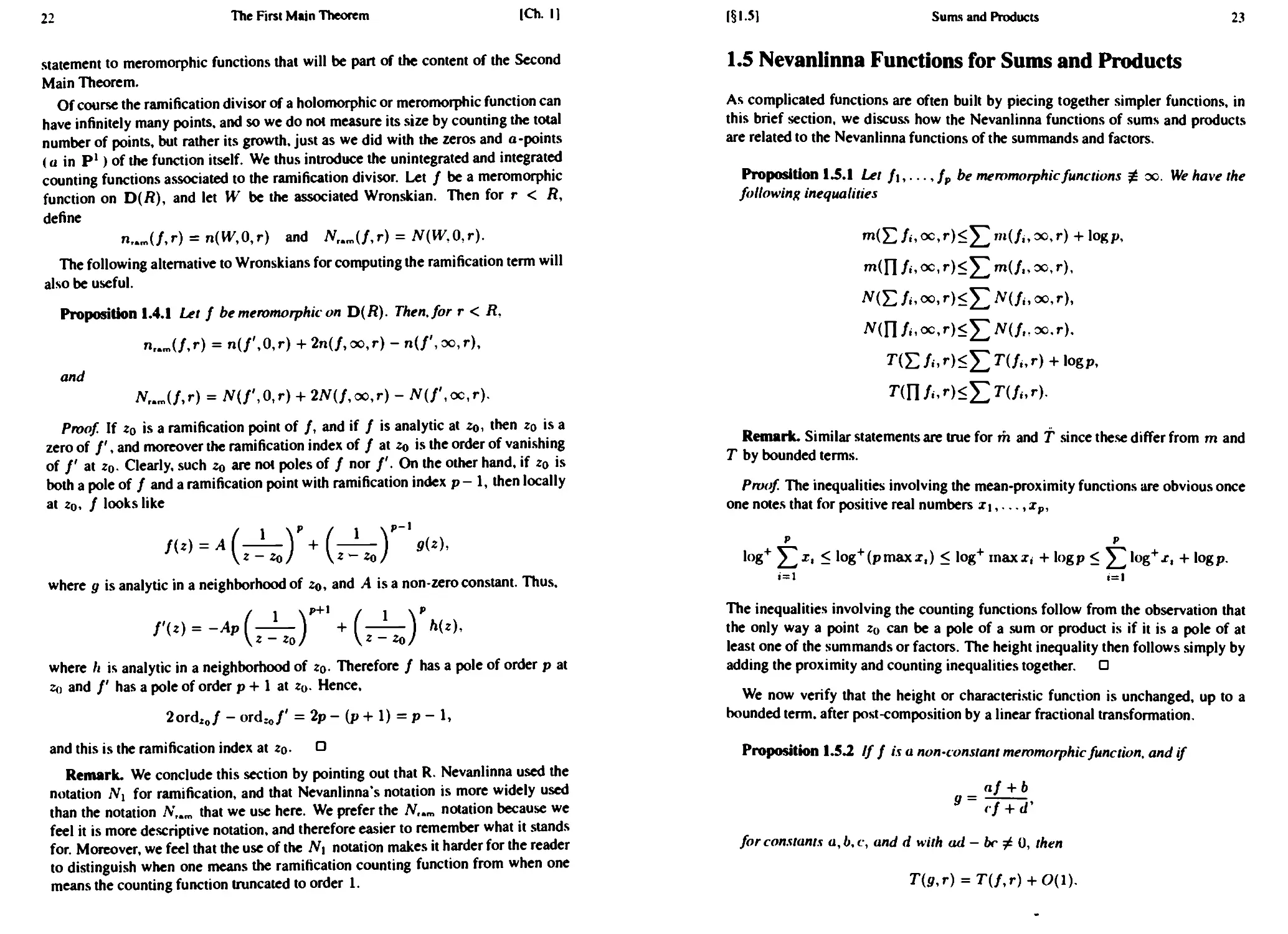
1.5 Nevanlinna Functions for Sums and Products
As complicated functions are often built by piecing together simpler functions, in
this brief section, we discuss how the Nevanlinna functions of sums and products
are related to the Nevanlinna functions of the summands and factors.
Proposition ISA Let f\,..., fp be meromorphic functions ? oo. We have the
following inequalities
Remark. Similar statements are true for m and t since these differ from m and
T by bounded terms.
Proof The inequalities involving the mean-proximity functions are obvious once
one notes that for positive real numbers x\,..., xp,
•°g+ 2.,x> - log+(pmaxi,) < log+ maxij + logp < ^ log+j, + log p.
The inequalities involving the counting functions follow from the observation that
the only way a point z0 can be a pole of a sum or product is if it is a pole of at
least one of the summands or factors. The height inequality then follows simply by
adding the proximity and counting inequalities together. O
We now verify that the height or characteristic function is unchanged, up to a
bounded term, after post-composition by a linear fractional transformation.
Proposition 1.5.2 // / is a non-constant meromorphic function, and if
9 =
af + b
v} + d'
for constants a,b.c, and d with ad - be ^ 0, then
T(9,r) = T(f,r) + 0A).

24
The First Main Theorem
[Ch. IJ
Proof. If c = 0, then this is trivial by Proposition 1.5.1. If c / 0, note that if we
set
then g = j\ + a/c, and so by repeated use of Proposition 1.5.1. and the First Main
Theorem (Theorem 1.3.1), we see that
T(g,r) =
= T(f,r)
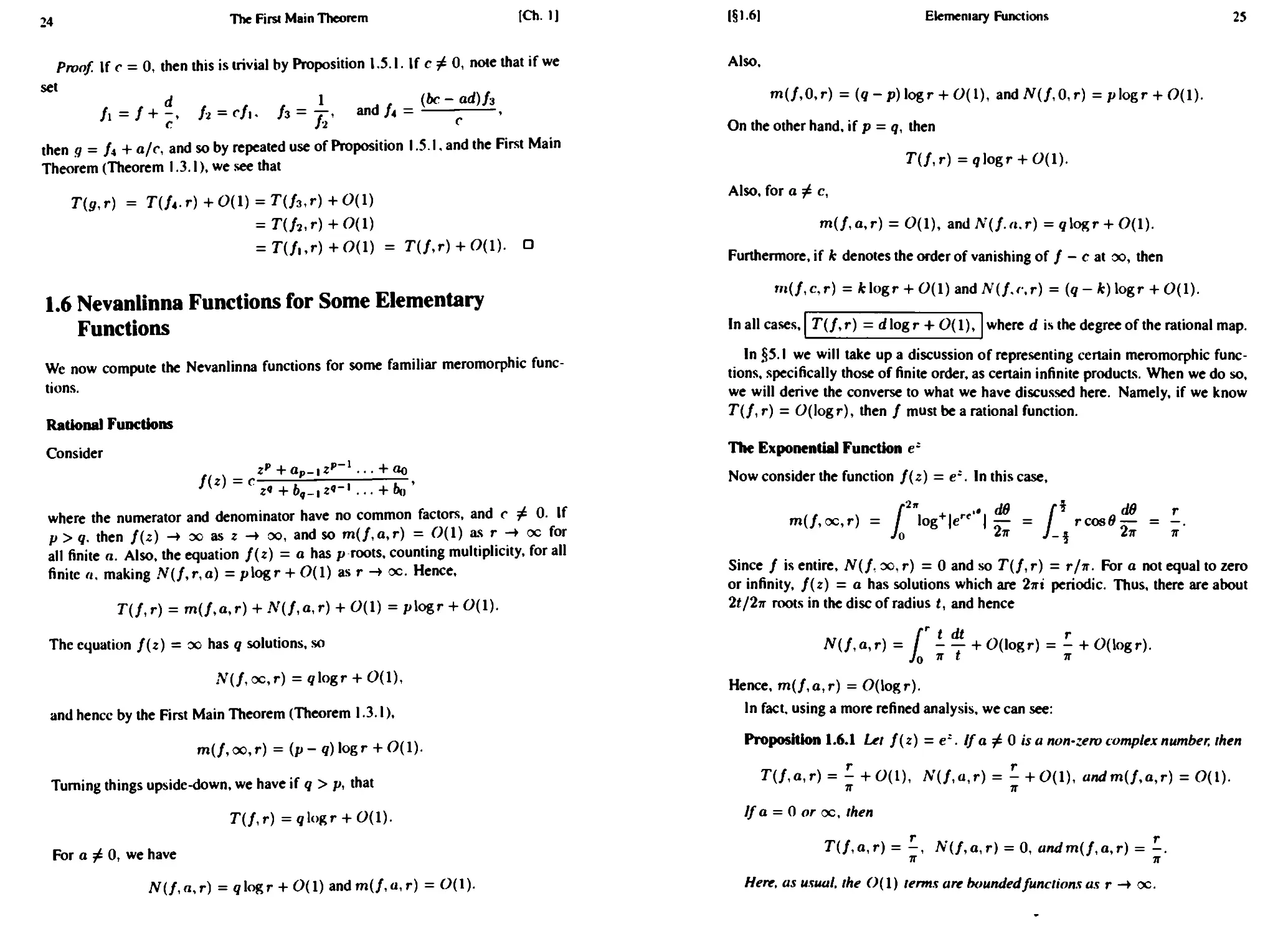
1.6 Nevanlinna Functions for Some Elementary
Functions
We now compute the Nevanlinna functions for some familiar meromorphic func-
functions.
Rational Functions
Consider
z«
where the numerator and denominator have no common factors, and c ^ 0. If
p > q. then f(z) -* oo as z -* oo, and so m(f,a,r) = 0A) as r-toe for
all finite a. Also, the equation }{z) = a has p roots, counting multiplicity, for all
finite «. making N(f,r,a) = plogr + 0A) as r -+ oc. Hence,
The equation f(z) = oo has q solutions, so
JV(/,oc,r) = glogr
and hence by the First Main Theorem (Theorem 1.3.1),
m(/,oo,r) = (p-</)logr
Turning things upside-down, we have if q > p, that
T(f,r)=q\ogr
For a ^ 0, we have
N(f,a,r) =glogr + 0(l)andm(/,a,r) =
l§N]
Elementary Functions
25
Also,
m(/,0,r) = (g-
On the other hand, if p = q, then
, and7V(/,0,r) = plogr + 0A).
Also, for a^ c,
m{f,a,r) = 0A), andA'(/.«.r) =
Furthermore, if k denotes the order of vanishing of / - c at oo, then
m(f,c,r) = fclogr + O(l) and N(f.r.r) = {q- k) logr + 0A).
In all cases.
T(f, r) = d log r + O( 1), where d is the degree of the rational map.
In §5.1 we will take up a discussion of representing certain meromorphic func-
functions, specifically those of finite order, as certain infinite products. When we do so,
we will derive the converse to what we have discussed here. Namely, if we know
T(f, r) = O(logr), then / must be a rational function.
The Exponential Function e-
Now consider the function f(z) = ez. In this case.
m(/,oc,r) =
Since / is entire, N{f, oo, r) =0 and so T(f, r) = r/n. For a not equal to zero
or infinity, f(z) = a has solutions which are 2ni periodic. Thus, there are about
2t/2ir roots in the disc of radius t, and hence
N(f,a,r) = / - - + O(logr) = - + O(logr).
Jo * l n
Hence, m(f,a,r) = O(logr).
In fact, using a more refined analysis, we can see:
Proposition 1.6.1 Let f(z) = ez. If a ^ 0 is a non-zero complex number, then
T(f,a,r) = -+O(l), N(f,a,r) = - + 0A), andm(f,a,r) = 0A).
if it
If a = 0 or oc, then
T(f,a,r) = -, N(f,a,r) = 0, andm(f,a,r) = -.
If IT
Here, as usual, the ()A) terms are bounded functions as r -* oc.

26
The First Main Theorem
iCh. I]
Proof. We have already proven this in the case a = 0, oo. and simply restated it
here for the convenience of the reader. That
-
It
for all other a then follows immediately from the First Main Theorem (Theo-
(Theorem 1.3.1). Also, that m(f,n,r) = O(l) for a ^ 0, ex will follow from the
First Main Theorem and the statement, N(f,a,r) = 2r/2ir + 0A).
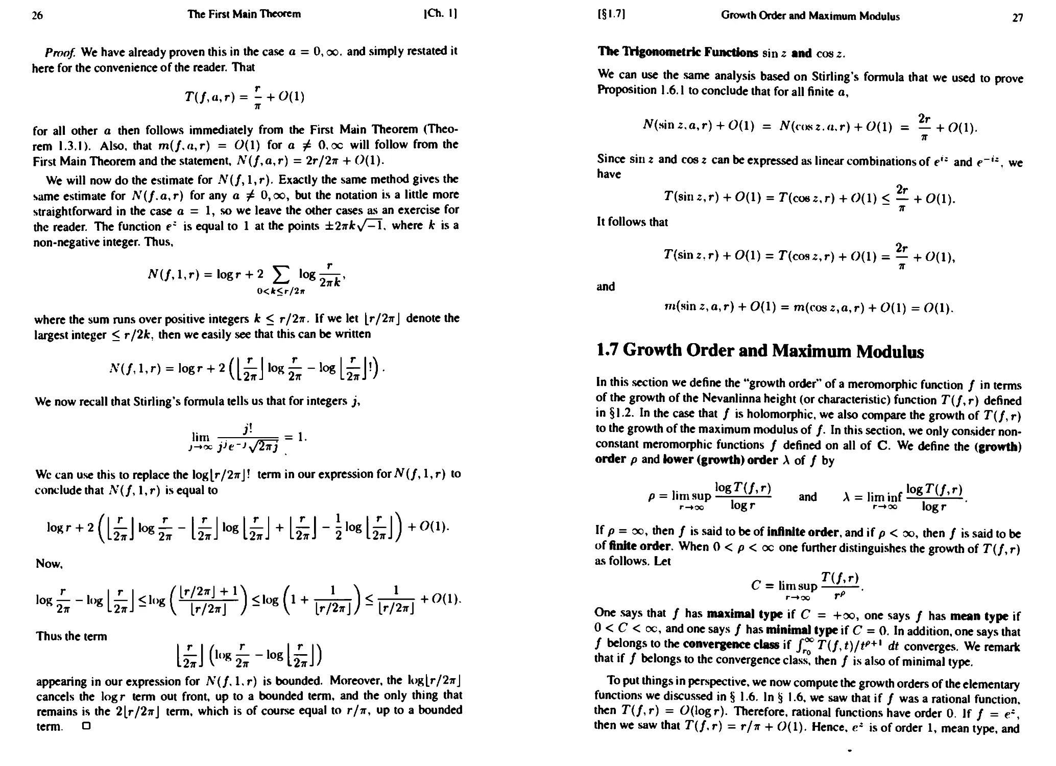
We will now do the estimate for A'(/, 1, r). Exactly the same method gives the
same estimate for Ar(/.a,r) for any a # 0,oo, but the notation is a little more
straightforward in the case a = 1, so we leave the other cases as an exercise for
the reader. The function e; is equal to 1 at the points ±2itk\/^l, where A: is a
non-negative integer. Thus,
2itk'
0<k<r/2n
where the sum runs over positive integers it < r/2it. If we let \r/2it\ denote the
largest integer < r/2k. then we easily see that this can be written
We now recall that Stirling's formula tells us that for integers j,
lim
j-»oc
= 1.
We can use this to replace the log[r/27rj! term in our expression forN{f, 1, r) to
conclude that Ar(/, 1, r) is equal to
Now,
s - "* Is! *-. (^) <-<*
Thus the term
appearing in our expression for N(f, l.r) is bounded. Moreover, the log|.r/2;rj
cancels the logr term out front, up to a bounded term, and the only thing that
remains is the 2[r/2ir\ term, which is of course equal to r/it, up to a bounded
term, o
Growth Order and Maximum Modulus
27
cos z.
The Trigonometric Functions sin z and
We can use the same analysis based on Stirling's formula that we used to prove
Proposition 1.6.1 to conclude that for all finite a,
N(s\nz.a,r)
—
it
Since sin z and cos z can be expressed as linear combinations of e': and e~'z, we
have
T(sinz,r) + 0A) = r(cos2,r) + 0A) < — + 0A).
it
It follows that
2r
T(smz,r) + 0A) = T(cosz,r) + 0A) = — + O(l),
it
and
m(siii2,a,r)
= m(cosz,a,r) + 0A) =0A).
1.7 Growth Order and Maximum Modulus
In this section we define the "growth order" of a meromorphic function / in terms
of the growth of the Nevanlinna height (or characteristic) function T(f, r) defined
in § 1.2. In the case that / is holomorphic, we also compare the growth of T(f, r)
to the growth of the maximum modulus of /. In this section, we only consider non-
constant meromorphic functions / defined on all of C. We define the (growth)
order p and lower (growth) order A of / by
and
p = limsup
r-»oo logr
If p = oo, then / is said to be of infinite order, and if p < oo, then / is said to be
of finite order. When 0 < p < oc one further distinguishes the growth of T(f, r)
as follows. Let
One says that / has maximal type if C = +oo, one says / has mean type if
0 < C < oc, and one says / has minimal type if C = 0. In addition, one says that
/ belongs to the convergence class if f™ T(f, r)/r')+l dt converges. We remark
that if / belongs to the convergence class, then / is also of minimal type.
To put things in perspective, we now compute the growth orders of the elementary
functions we discussed in § 1.6. In § 1.6, we saw that if / was a rational function,
then T(f,r) = O(logr). Therefore, rational functions have order 0. If / = <r,
then we saw that T(f, r) = r/it + 0A). Hence, e; is of order 1, mean type, and

28
The First Main Theorem
iCh. II
the same is true for sin z and cos z. The function e'' is an example of a function
with infinite order.
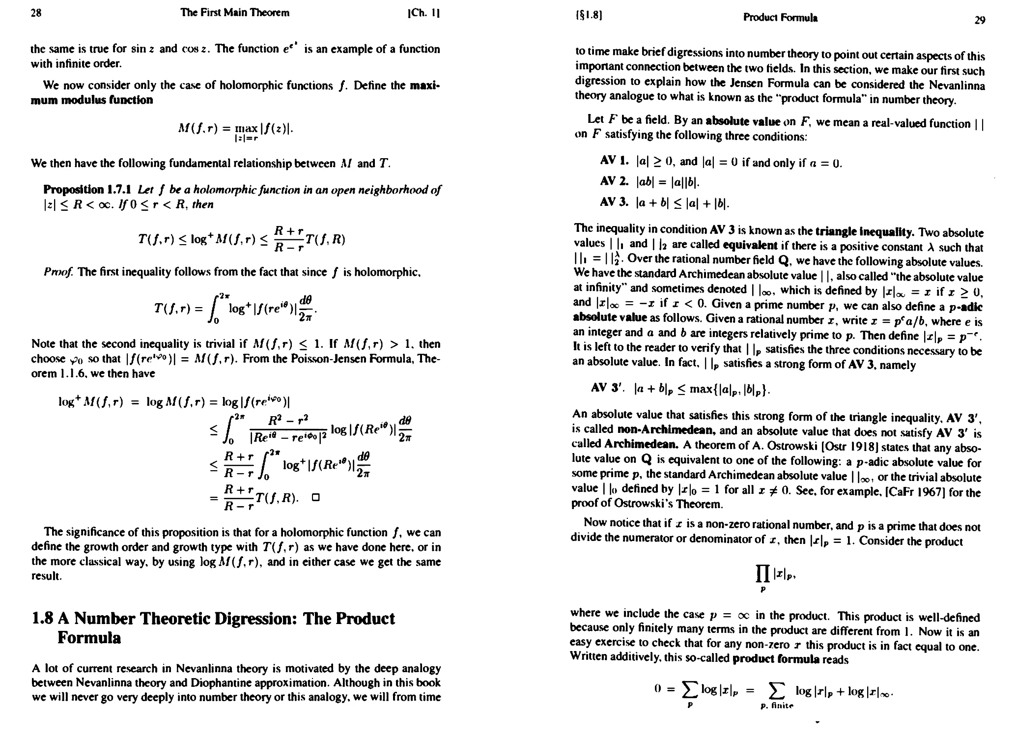
We now consider only the case of holomorphic functions /. Define the maxi-
maximum modulus function
We then have the following fundamental relationship between M and T.
Proposition 1.7.1 Let f be a holomorphic function in an open neighborhood of
\z\ < R < oc. //0 < r < R, then
T(f,r) < log+M(f,r) <
— r
Proof. The first inequality follows from the fact that since / is holomorphic.
T(f,r)= /"log+l/Cre*)!*
Jo *¦*
Note that the second inequality is trivial if A/(/,r) < 1. If A/(/, r) > 1. then
choose y>0 so that \f(re'*°)\ = A/(/, r). From the Poisson-Jensen Formula, The-
Theorem 1.1.6. we then have
R + r
R-r
T(f,R).
The significance of this proposition is that for a holomorphic function /, we can
define the growth order and growth type with T(f, r) as we have done here, or in
the more classical way, by using logil/(/, r), and in either case we get the same
result.
1.8 A Number Theoretic Digression: The Product
Formula
A lot of current research in Nevanlinna theory is motivated by the deep analogy
between Nevanlinna theory and Diophantine approximation. Although in this book
we will never go very deeply into number theory or this analogy, we will from time
E1.81
Product Formula
29
to time make brief digressions into number theory to point out certain aspects of this
important connection between the two fields. In this section, we make our first such
digression to explain how the Jensen Formula can be considered the Nevanlinna
theory analogue to what is known as the "product formula" in number theory.
Let F be a field. By an absolute value on F, we mean a real-valued function | |
on F satisfying the following three conditions:
AV 1. \a\ > <), and \a\ = 0 if and only if a = 0.
AV2. \ab\ = \a\\b\.
AV3. |a + 6| <|o| + |6|.
The inequality in condition AV 3 is known as the triangle inequality. Two absolute
values | 11 and | |3 are called equivalent if there is a positive constant A such that
||i = | |j. Over the rational number field Q, we have the following absolute values.
We have the standard Archimedean absolute value 11, also called "the absolute value
at infinity" and sometimes denoted | |oo. which is defined by Ix^ = x if x > 0,
and |i|oc = -x if x < 0. Given a prime number p, we can also define a p-adk
absolute value as follows. Given a rational number x, write x = pea/b, where e is
an integer and a and 6 are integers relatively prime to p. Then define \x\p = p~r.
It is left to the reader to verify that | |p satisfies the three conditions necessary to be
an absolute value. In fact, | |p satisfies a strong form of AV 3. namely
AV3'. |« + 6|p<max{|a|p,|6|p}.
An absolute value that satisfies this strong form of the triangle inequality, AV 3',
is called non-Archimedean, and an absolute value that does not satisfy AV 3' is
called Archimedean. A theorem of A. Ostrowski [Ostr 1918] states that any abso-
absolute value on Q is equivalent to one of the following: a p-adic absolute value for
some prime p, the standard Archimedean absolute value | |oo< or the trivial absolute
value I |(> defined by |x|0 = 1 for all x ? 0. See. for example, [CaFr 1967] for the
proof of Ostrowski's Theorem.
Now notice that if x is a non-zero rational number, and p is a prime that does not
divide the numerator or denominator of x, then |x|p = 1. Consider the product
m
where we include the case p — oc in the product. This product is well-defined
because only finitely many terms in the product are different from 1. Now it is an
easy exercise to check that for any non-zero x this product is in fact equal to one.
Written additively, this so-called product formula reads
0 =
p. finkr

30
The First Main Theorem
ICh. I]
Although the product formula is trivial to verify on Q, the Artin-Whaples Product
Formula says that over any number field F (a number field is just a finite extension
of Q). we can choose absolute values | |t, in the various equivalence classes t' of
absolute values on F so that
o =
iog|x|t, +
|(*i:ri- (L8I)
v non- Archimedean
Archimedean
We remark that for the non-Archimedean t\ we can choose exactly one absolute
value per equivalence class, and each equivalence class is counted precisely once.
However, for the Archimedean equivalence classes, we count each equivalence class
with multiplicity either one or two. This is a technical detail which can be ignored
for now; we will return to it in §6.1.
C. F. Osgood [Osg 1981] [Osg 1985] noticed similarities between the structure
of some proofs in Nevanlinna theory and the proofs of some Diophantine approxi-
approximation results from number theory. Later, but independently from Osgood. P. Vo-
jta [Vojt 1987] explored the connections between Nevanlinna theory and number
theory in much greater depth, creating a complete dictionary translating between
Nevanlinna theory and Diophantine approximation theory. We will discuss Vojta's
dictionary in greater detail in Chapter 6.
One of Vojta's observations was that the Artin-Whaples Product Formula, equa-
equation A.8.1), is the analogue of the Jensen Formula, equation A.1.9). To better
appreciate this, we can define the following absolute values on the field of mero-
morphic functions defined on D(r). Let / be a function meromorphic on D(r). If
z is a non-zero point in the interior of D(r), we can define
\r |-»rd,/
Notice that these absolute values are completely analogous to the p-adic absolute
values on Q. If z = 0, then we define
|/|0.r = r-ord«'.
The analogues to the Archimedean absolute values are given by the "absolute val-
values"
as 9 varies between 0 and 2tt. Note that technically these are not really absolute
values because they do not satisfy condition AV 1 and because they can be infinite
at poles of /. However, if / ^ 0,oo, then the zeros and poles of / are discrete,
so the \f\e.r are well-defined and non-zero for all but finitely many 0. We can then
re-write equation A.1.9) as
log|ilc(/,0)|=
Some Differential Operators on ihe Plane
31
This looks exactly like the Artin-Whaples Product Formula, except that on the left-
hand side we have a constant instead of zero, and on the right-hand side we have
an infinite number of Archimedean absolute values, so we have to integrate them
instead of adding them up.
1.9 Some Differential Operators on the Plane
As usual, let z = x + y\f^\. be the complex variable on the plane, where x and
y are the standard Cartesian coordinates on the plane. Let 0/dx and d/dy be the
usual partial differential operators on the plane. The following differential operators
will be useful:
0
1 = l f iL _ /ZT-il
dz 2 [Ox V 0y\
The operator d/dz goes back at least to H. Poincare" [Poin 1899] but was perhaps
first used systematically as we shall here by W Wirtinger [Win 1927]. We will
therefore refer to these operators as Wirtinger derivatives. Note that in terms of the
Wirtinger derivatives, the Cauchy-Riemann equations can be written df/dz = 0.
Associated to the Wirtinger derivatives, we have the differential operators d and 0.
If / is a Cl function, then df and df are the I-forms:
Of = ^dz and df = ^dz,
and the operators 0 and 8 are extended to forms of all degrees in the natural way.
Most often we will prefer to work with the operators:
and
A
4n
Note that d is just the standard exterior derivative, and that both operators are real
in the sense that if r; is a real-valued form, then so are drj and <fr/. The operator
<f was first introduced by J. Carlson and P. Griffiths in (CaGr 1972], and the con-
constant out front was chosen to help minimize the number of constants appearing in
important formulas. We also note at this point that if / is a C2 function, then
2tt dzoz
and so / is harmonic if and only if dcT f — 0. Here we have used the standard
notation A for the wedge product. We also remark that in polar coordinates (r.0),
the operator <F has the form:
2\dr2n 09 2nr J
A9.1)

32
The First Main Theorem
[Ch. I]
In terms of the holomorphic coordinate z, any 1 -form tj can be written as
r; = g(z, z)dz + h(z, z)dz,
where g and h are functions on the plane. The pull back of a 1 -form r; by a
differentiate function /, denoted f'rj, is then given by
Similarly, any 2-form Q can be written
ft = g(z, z)dzAdz,
and pull back by a function / takes the form
where J(f) denotes the determinant of the Jacobian matrix of /. Note in particular
that if r/ = g(z)dz is a holomorphic 1 -form and / is a holomorphic function, then
f'rj = (g o f)f'dz, and that if 17 = h(z, z)dz A dz is a 2-form and / is again
holomorphic, then
f'Q = (hof)\f'\'2dzAdz.
Combining the operator dd with the logarithm function will be important in var-
various contexts, so we state here a proposition containing some useful formulas. Note
that the operator dde log is an important operator, called the first Chern operator,
because it is related to the first Chern class associated to a line bundle. However,
we prefer not to discuss this relationship in the one variable setting so as to keep the
one variable discussion as simple as possible.
Proposition 1.9.2 Let u be a C'2 function. Then
ddcl
ddc2
ddc3
ddc4
u^dif log u = tuftfu — du A dcu,
ddru du,
du
1+u A+uJ'
t^dd^ log u
A + uJ '
udd* log u
uJ
u(l+uJ 1 + u
Proof. Equations ddcl and ddc2 follow by direct computation using the fact
that d and d are derivations, and hence they satisfy the Leibniz Rule. Equation
ddc3 follows by combining ddcl and ddc2, and ddc4 follows by again using
ddcl. D
Theorems of Stokes. Fubini. and Green-Jensen
33
1.10 Theorems of Stokes, Fubini, and Green-Jensen
We began this chapter with the Poisson and Poisson-Jensen formulas. We will look
at these again, but this time in the context of Stokes's Theorem (or Green's Theo-
Theorem). We first recall Stokes's Theorem in the form we will need.
Theorem 1.10.1 (Stokes's Theorem) Let r} be a 1 -form which is Cl in a neigh-
neighborhood of the disc of radius t, D(<). except possibly at a discrete set of points
Z. Assume that dr) is absolutely integrable on D(t), and that if is absolutely in-
tegrableon 0D(t). Denote by S(Z,e) the formal sum of small circles of radius
e around the points in Z. Then
Jdr,=
S(Z.e)
Remark. The formula in Stokes's Theorem consists of three different integral
terms, each of which we will give a name according to the following table:
interior term
D(/)
boundary term
/'
»D«)
singular term
lim / n
f-»0 J '
S(Z.t)
We also recall here Fubini's Theorem in a global form.
Theorem 1.10.2 (Fubini) Let n: X -* Y be a fibering of real manifolds, mean-
meaning a C00 map of manifolds which is locally isomorphic to a product. Let
q = dim >' and dim A" = p + q, so p is the dimension of a fiber. Let t) be
a p-form on X and let ? be a q-form on Y. Assume that n*? A t) is absolutely
integrable on X. Then,
/*•
<*
Proof By using a partition of unity, the proof reduces to a local statement which
is nothing more than the more familiar Fubini Theorem over a product space. O
Before stating the next theorem, we recall that dd can be considered as a 1 -form
on C\{0}. Namely.

The First Main Theorem
ICh. II
Theorem 1.10J (Green- Jensen Formula) Let u be a function that is C7 in a
neighborhood of D(r) except at a discrete set of singularities Z, and assume
that u is continuous at 0. Assume further that u satisfies the following three
conditions:
GJ 1. u is absolutely integrable on dD(r).
d$
GJ 2. duA — is absolutely integrable on D(r).
2tt
/(iff
u —- = 0.
2tt
|j-a|=f
GJ 4. ddeu is absolutely integrable on D(r).
Then
I'M
DID
«(re'")g - 2«@)-
where S(Z,e,t) is the portion of S(Z,e) inside D(t).
Proof We will evaluate the integral
f . d6
duA—-
J 2tt
D(r)
two different ways: by using Stokes's Theorem and by using Fubini's Theorem. We
remark that the integral is convergent by condition GJ 4.
If 0 is in Z, let Z' = Z \ {0}, and otherwise let Z' = Z. To apply Stokes's
Theorem, note that
/ <M «;r" ) = lim / d u— ) ,
()
D(r)
where D(Z',e) denotes the formal sum of open discs of radius e centered around
the points of Z'. Because d(d$) = 0,
, M .( dd\
duA—=d[ u — )
2n \ 2nJ
and applying Stokes's Theorem (Theorem 1. 10.1), we get
dd
D(r)
k»D(f)
(§1.111 The Geometric Interpretation of the Ahlfors-Shimizu Characierisiic
35
Now,
/dd
u — = u@)
2tt v
since u is assumed to be continuous at 0. The term
am / u —-
f-«o y 2tt
vanishes by assumption GJ 3.
Before applying Fubini, note that for any two C2 functions a and /?, we have,
for degree reasons,
da A dTff =d$Adca.
So in particular, away from singularities,
duA— =duAdc\og \z\2 = dlog \z\'2 A dcu.
2tt
The disc D(r) is fibered over the interval @, r) by the map z ¦-> |z|, and the
form (flog |z|2 is the pull back of the form 2dt/t on the interval @, r) under this
mapping. Therefore, when we apply Fubini (Theorem 1.10.2), we get
f _, dB n fT dt f _
duA — = 2 / — / d'u.
J 2k Jo t J
D(r) »D«)
Thus,
«D(r)
Since for almost all t, the set of singularities Z does not intersect the boundary of
D(t), we can therefore again apply Stokes's Theorem (Theorem 1.10.1) to the left
hand side of the above equality to complete the proof. O
1.11 The Geometric Interpretation of the
Ahlfors-Shimizu Characteristic
With these preliminaries out of the way. we begin to explore the geometric signifi-
significance of the Ahlfors-Shimizu characteristic function f(f, r). The Fubini-Study or
spherical area form w on P1 is defined in terms of a local coordinate z by
^l dzAdz

The First Main Theorem
|Ch. I]
Note that this form is well-defined on all of P1 because it remains invariant if we
replace z by \/w. The form u; is called the spherical area form because if D is a
subset of P' and if we think of P1 as a sphere in R3, then
is proportional to the area of D thought of as a subset of the sphere in R3. When
we discussed the chordal distance in §1.2, we identified P1 with the sphere in R'
of radius 1/2, which has total area n. Here, the form ui is normalized so that
so this is not entirely consistent with what we did in §1.2. Nonetheless, this dis-
discrepancy by a factor of n in our normalization of the area form turns out to be
convenient in that introducing the factor of n here once and for all keeps various
factors of n from entering into important formulas.
The Euclidean form * on the complex plane C is defined by
——dz hdz = -dx A dy = 2r dr A —,
tit n 2tt
where (x.y) and (r.8) are the standard Cartesian and polar coordinates on the
plane. If D is a subset of the complex plane, then
is. again up to a factor of 1/tt. the area of D considered as a subset of the plane.
If / = /, //0 is a meromorphic function with /o, /i holomorphic without com-
common zeros, then let
(/) - A
l/'l2
+ I/I2
J
11
" (l/ol2-
H/i
I2J'
where \\ = fof[ - /o/i is the Wronskian of /0 and fu which is holomorphic.
Note that |/0|2 + |/i |2 is a positive real analytic function, and hence (f1J is also
real analytic. Furthermore, we have
Since (/3J measures the ratio of the forms fui and *, we see that (p)'2 measures
how much / locally distorts area as it maps from the Euclidean plane to P1, where
[§ 1. 111 The Geometric Interpretation of the Ahlfors-Shimizu Characteristic
37
area on P1 is spherical area. For this reason, the quantity /' is called the spherical
derivative of the mapping /.
The form /*w is what is known as a "pseudo area form" Away from the zeros
of p. f'u> is an actual area form, but because f'w: is zero when p is zero, it is
not a true area form, and hence the term "pseudo."
The following proposition is an example of what is known as a "curvature com-
computation."
Proposition 1.11.1 We have
(«) /'w = (/')*¦ = *T loRd/ol3 + I/. I2)-
Away fmm the poles of /,
(u) rftr iog(i +1/|2) = dfiogd/oi2 +1/, |2).
Away from points z where P(z) = 0, which are precisely the ramification points
off.
(Hi) -de
Remark. The equation f'ui = -<W log /' is a manifestation of the fact that P1
with the Fubini-Study metric has constant curvature +1. Notice that with positive
curvature, one gets a negative sign in equations involving dtf log. Conversely, with
negative curvature, one does not get a minus sign in dtf log equations. Thus, in
many ways, it would have been more convenient had the notions of positive and
negative curvature been reversed.
Pmof Because
and because (Uf\og\f0\ = 0. we get (it). Since (pJ = |H'|2/(|/0|2 + I/'I2J'
and dtf log |U'| = 0, (Hi) follows similarly. To get (i). we apply equation ddc3
of Proposition 1.9.2 with u = |/|2. Away from the poles of /,
= |/'|2* and dtMog|/|a = 0.
Combining this with dtf log |/0| = 0 and (it) gives us (i). D
Proposition 1.1U Let g he holomorphic on an open neighborhood of the closed
disc of radius r, and assume #@) / 0. Let Z denote the zeros of g inside
D(r), and let S(Z.e) denote the formal sum of small dales of radius e cen-
centered at each of the points in Z. Then, log \y\2 satisfies the GJ conditions of
Theorem 1.10.3, and moreover
S(Z.i)

The First Main Theorem
(Ch. I)
Proof. If g has no zeros on the circle of radius r, then condition GJ 1 is clearly
satisfied. Since g has at most finitely many zeros on the circle of radius r, the
question of integrability is local. We leave it as an exercise to the reader to verify
that for a / 0, the function log|z — a\ is integrable on the circle of radius \a\.
From this, GJ 1 easily follows.
Because dde log \g\2 = 0 away from singularities, condition GJ 4 is trivially
satisfied.
Let w be a local coordinate around a zero of g, so that w = 0 corresponds to the
zero. Then, we can write
g(w) = wmh(w),
where ft is a holomorphic function with /i@) ^ 0.
For GJ 2. note that in terms of z,
g(z) z
Thus.
g\\z\>
Near 2 = 0, \g'/g\ is bounded since we assume that g@) ^ 0. Converting to polar
coordinates,
pj = ~ and \dz A dz\ = 2rdnW,
and so dlog \g\2 A dd is absolutely integrable in a neighborhood of 0. The other
possible problems could be the zeros of g. In terms of the local coordinate u\
g'(w) = m | h»
ff(u>) U) /«(U))
Because /i@) / 0, the term |/»'//>| is bounded in a neighborhood of w = 0. The
term l/\z\ is bounded in a neighborhood of w = 0, and so converting to polar
coordinates w = pe'v around w = 0, we again see dlog|ff|2 A d& is absolutely
integrable.
For condition GJ 3,
(§1.111 The Geomeiric Inierpretaiion of ihe Ahlfors-Shimizu Characierisiic
39
Since w = 0 is not at z = 0, by Stokes's Theorem.
d(dd)
2tt
= 0.
|u|<f
Also, since log \h\l is C00 near w = 0,
Jim /log 1/^=0.
Thus, log I.9I2 satisfies GJ 3.
We now compute
Jim
To finish the proof of the proposition, it suffices to show
lim / dc log \g\'* = ordu,=0 g.
Because
|u»|=«r
and because log |/i|2 is C°° at w = 0,
lim / <f log Id2 = lim / <nog|u)|2m.
r-»0 y f-»0 J
\w\=e |u-|=f
Using the polar coordinate formula for <f, equation A.9.1), we get
<riog|ufm = / m%? = m.
Jo 2tt
Combining Proposition I.I I.I and Proposition I.I 1.2 gives us a geometric in-
interpretation of the height or characteristic function, which was first discovered by
Ahlfors [Ahlf 19291 and Shimizu [Shim 19291. and this is why we have attached
their names to f.
Theorem 1.113 (Ahlfors-Shimizu) Let f be a non-constant function, mem-
morphic in an open neighborhood of D(r), and let u; be the Fubini-Study form
on P1. Then,
a,r)=T(/,oo,r) = jTr^ f f'» = ? J

We point out here that the geometric significance of this theorem is that the
Ahlfors-Shimizu height function measures, as a logarithmic average, the growth
of the spherical area on P1 covered by the map /. Hence the First Main Theorem
says that up to the constant rfm,(/, a), the sum m(/, a, r) + N(f, a, r) is equal to
the natural geometric quantity
I'M'--
D(M
Pnwf of Theorem I.I 1.3. By Proposition I.I I.I.
I'M>- I'M>>•- I'M'—<i+'"!>-
D@
Write / = /i //o, where f\ and /2 are holomorphic without common zeros. For
now. assume that /@) / oo. Recall that
l«>g(l + |/|2) = log(|/o|2 + |/, |2) - log|/o|2.
The function log(|/0|2 + |/i |2) is C00, and since /0@) / 0, the function log |/0|2,
and hence the function log(l + |/|2), satisfies the conditions of Theorem 1.10.3 by
Proposition 1.11.2. Applying Theorem 1.10.3, we get
^ / <feriog(l
fr dt
-I — lim
Jo t f-o
Directly from the definitions
\ I *
^ Jo
and
SiZ.c.t)
^)|2)^=m(/,oo,r),
, oo||.
Because logd/of2 + |/i|2) is C00, it does not contribute to the limit as e -> 0. and
so the final term becomes
IS' .1
Why N and 71
41
by Proposition 1.11.2. Putting these together gives us the theorem when 0 is not a
pole of /. In the case that 0 is a pole, then let g = l/f. Noting that ui is invariant
under zh l/z, and applying Theorem 1.3.1, we get
,r) = T(.<7,oc,r)
Since
D(O
/ /'w
is a nondecreasing, nonnegative function of (, an easy consequence of the Ahlfors-
Shimizu interpretation of the height is that T(f, r) is a convex, strictly increasing
function of log r. Recall that a real valued function \(t) of a real variable t is called
convex (sometimes called "concave up") if for every pair of real numbers x and y
and every t in the interval [0,1], one has
X(tx + A - t)y) < t\(x) + (I - t)X(y),
or in other words that every secant line for the graph of cp lies above the graph itself.
That #(/. a, r) is a nondecreasing convex function of log r is immediate from its
definition (since »(/, a, t) is a nonnegative nondecreasing function of t.) However,
the proximity function m(/, a, r) need not be nondecreasing nor a convex function
of log r. Thus, that f is a convex nondecreasing function of log r is not immediate
from the definition
T (/, o, r) = m(/, o, r) + N(f, a, r) + O( 1).
We will see in §1.13 that the Nevanlinna characteristic T(f,r) is also a convex
function of log r.
1.12 Why A' and f are Used in Nevanlinna Theory
Instead of n and A
We saw in §1.11 that
People first learning Nevanlinna theory often wonder about the logarithmic integra-
integration with respect to dt/t. If one lets
A(f
»= / /v
D(r)

42
The First Main Theorem
(Ch. II
then A(fy r) measures the amount of spherical area covered by the image of D(r)
under /. This seems like it might be a more natural quantity than t(f,r), and
similarly the unintegrated counting function n(/, a, r) seems more natural than the
integrated form A'(/, a, r). After all. if / is a degree d polynomial, then the Fun-
Fundamental Theorem of Algebra says
rf= lini n(/,a,r) = lim A(f,r)
r -fx. r-»oc
for all a in C. Thus, one might think that comparing u(f, a, r) to .4(/. r) for an
arbitrary meromorphic function is a more natural generalization of the Fundamental
Theorem of Algebra than the comparison between N(f, a, r) and T(f, a. r) given
by the First Main Theorem. However, the natural occurrence of Ar(/, a, r) in the
Jensen Formula (Corollary 1.2.1) indicates that working with N(f,a,r) may in
fact be more natural than working with n(f, a, r). Once one accepts that integrating
u(f. a, t) against dt/t is a natural thing to do. doing the same with A(f, r) to get
T(f, r) is clearly the natural quantity with which to compare N(f, a, r).
As it turns out. comparing n(f,a,r) and A(f,r) is a far more subtle busi-
business than comparing N(f,a,r) and T(f,r). Because ih(f,a,r) is positive. The-
Theorem 1.3.1 implies that Ntf,a,r) < f(f,r) - c,m,(f,a), and we interpreted this
informally as saying that t provides an upper bound on how often / can attain the
value a. An analog of the First Main Theorem would be an inequality of the form
n(f,a,r) < -4(/,r) + 0A). However, J. Miles (Miles 1971] gave an example of a
meromorphic function such that
hmsup
A(f,r)
=oo.
In fact, in IGol 1978], Goldberg constructed an entire function / such that for every
a in C.
n(/,a,r)
lim sup =oo.
r-.dC A(f,r)
Thus, unlike with N and T, one cannot bound n in terms of .4 for all sufficiently
large r.
There are weaker statements that one can prove. For example, if we replace
lim sup by lini iuf, then the First Main Theorem implies that if / is a meromorphic
function on C, then
«(/, a, r) < A(f, r) + o(l) for a sequence of r -* oc.
A.12.1)
Indeed, if inequality A.12.1) were false, then n(f,a,r) would be greater than
A(f.a,r) for all r sufficiently large. Integrating this inequality against dt/t would
then contradict the First Main Theorem. Inequality A.12.1) could be called the
"unintegrated First Main Theorem." One disadvantage of inequality A.12.1) is that
the sequence of r -* oc for which the inequality holds may depend on the point
a. This problem is addressed by a theorem of W. Hayman and F. Stewart (HayStew
1954] (see also [Hay 1964)).
(§1-131
Nevanlinna Functions on Average
43
Theorem 1.113 (Hayman-Stewart) Let} be a non-constant meromorphic func-
function on C and set
»(/»r) = sup n(f,a,r).
o€P'
Then.
A(f.r)
Hayman and Stewart asked whether the constant e in Theorem 1.12.2 could be
reduced to 1, and then this would have been an analog of the First Main Theorem
for u and A, However, S. Toppila [Topp 1976] constructed a meromorphic function
/ such that for all r sufficiently large.
The constant e in Theorem 1.12.2 is not best possible and has recently been im-
improved by J. Miles [Miles 1998].
1.13 Relationships Among the Nevanlinna Functions on
Average
Recall that the First Main Theorem (Theorem 1.3.1), said that for a function /
meromorphic on C,
is essentially independent of the value a, in that for fixed /, and r -> oc. changing
a changes T by a bounded term. We also promised we would see later that for
"most" values of a, N is the dominant term in the sum, and this was indeed the
case in the specific examples we considered in § 1.6. In the next chapter, we will
begin in earnest our journey toward Nevanlinna's Second Main Theorem, which
makes this statement precise in a very strong way. In the present section we content
ourselves with a weaker statement, first proved by H. Cartan [Cart 1929]. Cartan's
theorem allows us to conclude that N is the dominant term for "most" a, and it
follows almost immediately from the Jensen formula.
Theorem 1.13.1 (Cartan) Let f(z) be a meromorphic function in D(R), and
letO<r<R. Then.
T(f,r) =
where C = log+|/@)| if /(O) ^ oc, and C = log|ilc(/,0)| if /@) = oo.
Furthermore.

44
The Firsi Main Theorem
(Ch. 1]
Since the First Main Theorem tells us that N{f,a,r) < T{f,r) +OA), one
should think of Theorem 1.13.1 as saying that the proximity function m(f,a,r) is
insignificant for most values a on the unit circle, and that T(f. r) essentially equals
.V(/, a. r) for most values a on the circle. Note that there is nothing particularly
special about the unit circle. Indeed, since T remains invariant up to a bounded term
if / is replaced by to/, where L is a Mobius transformation (Proposition 1.5.2),
a similar inequality is true if the unit circle is replaced by any circle or line in the
plane. In fact, Frostman [Fros 1934] has shown that a similar result holds if the
circle is replaced by any set of positive capacity.
Since T differs from T by a bounded amount, we get similar results for T and
in, up to bounded terms.
Because N is convex function of log r, and we have expressed T as an integral
of .V. we immediately get the following corollary.
Corollary 1.13.2 The function T(f,r) is a convex function of logr.
We begin the proof of Theorem 1.13.1 with a Proposition.
Proposition 1.133 For any a 6 C,
/ log I
Jo
rel*\— = max{log|a|,logr}
Proof The case a = 0 is obvious, so we assume o / 0. We apply the Jensen
Formula (Corollary 1.2.1), to the function a- z when \z\ = r. If \a\ > r, we get
log \a\ = / log |a - re'*\ —,
and if 0 < \a\ < r, we get
log M = I* log\a - re*] ^ + log ^. O
Pnwf of Theorem 1.1.II. If /@) ? oc. then for all $ for which /@) ? ew,
Corollary 1.2.1 applied to f(z) - <¦'* gives us
log |/@) - c'*\ = J \o%\f(re'°) - e">\ - + N(f,oc,r) - JV(/,e"\r).
If /@) = oo. then we get instead
r'ix JO
r'ix JO
,U)| = / log|/(re'#) - r'»| — + ;V(/,oo,r) - AT(/,^,
Jo 2tt
[§1.13]
Nevanlinna Functions on Average
45
for all v?. In either case, we integrate with respect to y?. When /@) / oo, we get
Interchanging the order of integration in the double integral, and making use of
Proposition 1.13.3, we get
elfl)|^ + JV(/.oc.r) -
In case that /@) = c», we get log |ilc(/, 0)| on the left hand side instead, and we
have proved the first equality.
For the second inequality, by the First Main Theorem, Theorem 1.3.1, for each
ip, we have
m(/,elV\r)
,e^,r) - T{f,oo,r)
< Iog2.
We now integrate with respect to <p. From the first equality in the statement of the
theorem, we have that
T(/,oo,r)-y A'(/y*,r)g = C.
If /@) = oo, then ilc(/ - e'*,0) = ilc(/,0) for all yj, and so
|2*log|ilc(/-e'»,0)|^ = log|ilc(/,0)| = C.
If, on the other hand, /@) ^ oo, then for all y? such that /@) / e'*, we have
ilc(/ - e'*\0) = /@) - r1", and so
*
e'V|^ = C,
where the second inequality follows from Proposition 1.13.3. This cancellation
leaves us with the desired inequality. O
We now give another variation on this theme.
Theorem 1.13.4 // f(z) ismervmorphic in T>(R) and 0 < r < ft, then
t(f,r) = jN(f,a,r)u, and j m(/,a,r)u; = i,
o€P' o€P'
where w is the spherical area form defined in section §/.//.

46
The Firsi Main Theorem
ICh. II
Before proceeding to the proof, we state a couple of Propositions.
Proposition 1.13.5 For any z € C,
a€P'
Pnxtf From the definition of w and from Proposition 1. 13.3, we have
o€P'
2rdr
r°° 2rd
= / max{log|z|,logr}-
Jo A + r
Proposition 1.13.6
/ c,m,(/,a)a; =--.
06P1
Pnwf. For almost all a in P1,
rtm,(/,a) = log |/@) -o|-i log(l + |/@)|2) - 1 log(l
Integrating over a in P1 and applying Proposition 1.13.5, we find
f c,m,(/,a) = -i
o€P'
The integral on the right is a straightforward computation:
— = --. a
»€>'
Pnwf of Theorem 1.13.4. By replacing / by 1// if necessary, we may assume
without loss of generality that /@) / so. For all a ^ /@), we have again by
Corollary 1.2.1 that
log|/(reifl) - a| ^ + N(f,oo,r) - N(f,a,r).
Jensen's Inequality
47
Integrating over a e P1 and making use of Proposition 1. 13.5. we get
2 d&
|/(re'fl)|2)- + AT(/,oo,r)
o€P'
The term on the left is nothing other than -(•„,„(/• °c) and the first integral on the
right is the definition of m(/, 00, r). Hence
J N(f,a,r)uj = m(/,oo,r) + N(/,oc,r)+cfm,(/,oo) =T(/,r).
o€Pl
This together with the First Main Theorem (Theorem 1.3.1), and Proposition 1. 13.6
implies that
J m(f,a,r)uj = - j c,m,(fy
o€P'
a)u; = -. O
o€P'
In [Ahlf 1935a], Ahlfors extended the averaging technique presented in this sec-
section. Rather than integrating against just the spherical area form, Ahlfors considered
integrals of the form
I N(f,a,r)p(a)^
o€Pl
where p is an almost everywhere continuous and positive probability distribution
on P1, meaning in particular that
/ p(a)u = 1.
o€P'
Choosing p judiciously and using some of the techniques we will explain in Chap-
Chapter 2, Ahlfors gave a particularly clear and easy proof of Nevanlinna's Second Main
Theorem that illuminates the underlying geometry behind the Second Main Theo-
Theorem.
1.14 Jensen's Inequality
We conclude this chapter with an important lemma of a different character. Recall
that a real-valued function \ on the interval (a, 6) (where we allow a = -00 and
6 = +00) is called concave (or "concave down") if for every x and y in the interval
(a, 6), and for every t in the interval [0,1], we have
X(tx + A - t)y) > tX(x) + A - t)x(v)-
Note that this is just the familiar fact from calculus that a function is concave down
if and only if all the secant lines lie below the graph of the function.

48
The First Main Theorem
[Ch. 1)
Theorem 1.14.1 (Jensen's inequality) Let (A', /*) be a measure space such that
t*(X) = 1. Let \ be a concave function on the interval (a, 6) (where we allow
a = — oo and b = +oc). Then, for any integrable real valued function f with
a < f(x) < b for almost all x in A", we have
f
X(f(*))dfi(x) <
f(x)dti(x)
Remark. The concavity of \ implies that \ is continuous, and hence measur-
measurable, so the integral on the left makes sense. As we will only apply Theorem 1.14.1
to specific functions like log and log+ which are obviously continuous, we leave
this fact as an exercise. We will typically apply Theorem 1.14.1 in the following
context:
Proof of Theorem 1.14.1. Let
By the concavity of \, for any s and t such that a<s<c<t<b, we have
Hence, if we
then for a <
let
s <
c< t
c —
m =
<b,
X(c) - X1
C — 8
8
sup
c<«<fc
(s)
s —
x@
t
t»l ">
7#i ^
t -c
-X(c)
— r
X@ - X(r)
t-c
This implies that
x(/(*)) " X(r) < m(f(x) - c)
for almost all x because a < f(x) < b. Integrating this last inequality and making
use of the fact that p(X) = 1, we see that
f(x)d»(x)-c .
But.
X
as desired.
= / f(x) d,t(x)
and so
2 The Second Main Theorem via Negative
Curvature
Shortly after R. Nevanlinna's first proof of the Second Main Theorem, Nevanlinna's
brother, F. Nevanlinna, gave a "geometric" proof of the Second Main Theorem. In
this chapter, we give a geometric proof of the Second Main Theorem based on "neg-
"negative curvature," which broadly speaking, has the same overall structure as F. Nevan-
Nevanlinna's proof, although in terms of details, the proof we present here bears much
greater resemblance to the work of Ahlfors [Ahlf 1941 ]. In Chapter 4, we will give
another proof of the Second Main Theorem that is closer to R. Nevanlinna's original
proof. Of course, neither the Nevanlinna brothers nor Ahlfors were interested in the
exact structure of the error term. The error term we will present here is essentially
due to P.-M. Wong [Wong 1989].
We have decided to begin with a negative curvature proof because obtaining a
good error term using the geometric method requires less preparation than does the
logarithmic derivative approach used in R. Nevanlinna's original proof. The ge-
geometric proof also has the virtue that the explicit constants occurring in the error
terms have natural geometric interpretations. Another advantage of the geometric
method is that one can use it to obtain the best possible error term for what's known
as the "Ramification theorem," something which has yet to be accomplished using
logarithmic derivatives. Moreover, in higher dimensions, the geometric approach
has been successfully applied to a greater variety of situations than has the loga-
logarithmic derivative approach. On the downside, the structure of the error term here
initially appears to be somewhat more complicated than the error term we will ob-
obtain in Chapter 4.
2.1 Khinchin Functions and Exceptional Sets
Before proceeding directly to the Second Main Theorem, we introduce some nota-
notation and terminology that will help us in our discussion of "error terms."
We begin with a definition. A function ip will be called a Khinchin function if ip
is a real-valued, continuous, nondecreasing, and > 1 on the interval [e, oc), and %i>
satisfies the following convergence condition (known as the Khinchin convergence
condition):
1 .
,. . dx < oo.
xil'(x)
i:

50
Second Main Theorem via Negative Curvature
|Ch. 21
In fact, since we will be interested in the value of the above integral, we will give it
a name. Given a Khinchin function i/>, define
-i:
¦dx < oc.
We will explain in §6.2 why we have chosen the names "Khinchin function" and
"Khinchin convergence condition." We note that in the original work of Nevan-
Nevanlinna, V'(-t) was taken to be (logx)l+f for positive e. One might find it helpful to
keep this example in mind. Note that our choice of c. as the start of the interval of
definition of tl> could be replaced with an arbitrary positive number, but because we
have the prototypical example of V'(-r) — (logx)I+f in mind, and because we want
V(r) > 1, the number e is a convenient choice.
One technical element that exists in all proofs of Nevanlinna's Second Main The-
Theorem is the use of what is known as a "growth lemma." Historically, the growth
lemmas were stated and proved for arbitrary functions ip satisfying the Khinchin
convergence condition, but then before using the growth lemmas to prove theo-
theorems in value distribution theory, the function ip was immediately specialized to be
(log x)'+e. S. Lang suggested keeping V arbitrary throughout. We will also explain
the number theoretic motivation for keeping V arbitrary in §6.2.
Nevanlinna's Second Main Theorem will assert that a certain inequality holds for
all radii r outside of a certain set E known as the exceptional set (of radii). The
Second Main Theorem will have non-trivial content because the "size." in a sense
we will make more precise in the next paragraph, of the exceptional set will be
bounded in terms of our choice of Khinchin function i/>, or more precisely in terms
of ko(tl>). Thus, the larger our function 0, the smaller Jfco(t/-) will be, and therefore
the smaller our exceptional set. However, there, will also be a tradeoff, in that the
Khinchin function </> will also appear in the various inequalities themselves in such
a way that the larger the function v, the weaker the inequalities will be.
Included in the statements the Second Main Theorem, the Khinchin function tp
will always have a companion function which we will always denote by 4>- As we
mentioned above, the Second Main Theorem will tell us that a certain inequality
is true for all radii outside an exceptional set whose "size" is bounded in terms of
Mv')- The function <p is what specifies what we mean by "size." More precisely,
our exceptional sets E will be such that the integral
dr
can be bounded in terms of Jfco(V')- For example, if we take 4>(r) = 1, then our
exceptional sets will have finite Lebesgue measure, and in fact. Lebesgue measure
bounded in terms of Jfco(i.') If we take <p(r) = r, then our exceptional sets will have
finite "logarithmic measure." meaning that if E is such an exceptional set. then
dr
— < oo.
[§2.2]
The Nevanlinna Growth Lemma and the Height Transform
51
In applications of the Second Main Theorem, as in Chapter 5, the idea is to choose
ti> and <)> so that the exceptional set will be "small" and yet V will not be too "large."
When one studies meromorphic functions defined (except for poles) on the whole
plane, one often wants to choose 4> so that for every r\,
f
dr
W)
= DC.
Then, since inequalities coming from the growth lemmas will hold true for all r
outside a set ? with
f <*r
Je 4>{r)
we conclude that the exceptional set E cannot contain any intervals of the form
(ri, oo), and so there must be a sequence of r outside E which tends toward infin-
infinity. In other words, whatever inequality is of interest to us will hold for a sequence
of r tending toward infinity. For example, one often chooses <f>(r) = 1 or <j>(r) = r.
Similarly, when one studies functions meromorphic in a disc of radius R < oo, then
one often chooses, for example. <f>(r) = R - r so that for every rx < R,
dr
= 00,
and again we can find a sequence of r tending to R outside any exceptional set E
whose measure with respect to 4> is bounded.
If one chooses a larger function 4>, then the exceptional set E can grow larger.
However, it is also often true that the larger the function <j>, the better the inequality
that will hold. Thus, the advantage of keeping <j> arbitrary is that one can trade a
larger exceptional set for an improvement in an inequality. This trade-off was recog-
recognized by the Nevanlinnas almost from the beginning. So. although the appearance
of arbitrary Khinchin functions t/> in the statement of key theorems in value distribu-
distribution appears only recently, the presence of arbitrary functions <t> in these statements
goes back almost to the beginning.
Finally, we would like to point out that although continuity is part of our definition
of Khinchin function, it is not really necessary to require the continuity of ii>. With a
little effort, one easily sees that the same qualitative results can be obtained without
assuming the continuity of tp.
2.2 The Nevanlinna Growth Lemma and the Height
Transform
The main result of this section is a technical result, known as a "growth lemma."
When one is interested in good explicit error terms, as we shall be. one must care-
carefully formulate one's growth lemma because it affects the quality and structure both

52
Second Main Theorem via Negative Curvature
[Ch. 2]
of the error terms and of the exceptional set. Although the statement and proofs of
the results in this section can get a little "technical," the ideas involved are never
deeper than those of freshman calculus, and therefore growth lemmas are often re-
referred to as "calculus lemmas." A reader who is new to the subject of Nevanlinna
theory might want to skip this section on a first reading, referring back to it as the
various lemmas are used later on.
We now present the Nevanlinna growth lemma, an "elementary" growth lemma,
which we will use in an iterated fashion (Lemma 2.2.3 below) in what we term the
"curvature" approach to the proof of the Second Main Theorem. Because we iterate
the growth lemma in this way. the structure of the error terms we will obtain via the
curvature approach will be somewhat complicated.
Lemma 2.2.1 Let F(r) be a positive nondecreasing function defined and > e
for r0 < r < R < oo. Assume further that F has piecewise continuous
derivative. Let ?(x) be a positive, nondecreasing, continuous function defined
for e < x < oo, and let <j>(r) be any positive measurable function defined for
r0 < r < R. Let C be a positive constant and let E be the closed subset of
[r0. R) defined by
E = jr 6 [r0, R): F'(r) >
Then, for all p with r0 < p < R,
f dr \_ fFifi) dx
J W) ~ Cjr xtix)'
En[ro.)»|
Proof From the definition of E and change of variables.
J 0(r) " C Jro
En|ro.«|
F'(r)dr
F(r)UF(r))
c
dx
The lemma follows since F(r0) >e. ?
Lemma 2.2.2 (Nevanlinna) Let R, F(r), and <p be as in Lemma 2.2.1. and let
t!' be a Khinchin function. Then, there exists a measurable set of radii E with
dx
xip(x)'
such that for all r() < r < R and not in E, the inequality
F'(r) < F(r)
/5 valid.
[§2.2]
The Nevanlinna Growth Lemma and the Height Transform
53
Remark. Intuitively. Lemma 2.2.2 simply says that the derivative F' of a non-
decreasing function F cannot be big unless F itself is big most of the time.
Proof Let C = 1, let ?(z) = <f>(x), and choose E as in Lemma 2.2.1. Because
V> satisfies the Khinchin convergence condition, for all p < R, we have
dx
The proof is completed by letting p -t R. ?
In the Second Main Theorem we will want to bound a second derivative of the
characteristic function t in terms of t itself. Hence, we iterate Lemma 2.2.2 to get
the following complicated looking lemma which simply says the second derivative
of a nondecreasing function F can be bounded in terms of F outside an "excep-
"exceptional set."
Lemma 2.2J Let F(r) beaC2 function defined for r0 < r < R < oc. Assume
further that both F(r) andrF'(r) are positive nondecreasing functions of r, and
that F(r0) > e. Let bt be any number such that 6i rF'(r) > e for all r > r0.
(Such a number trivially exists since we have assumed rF'(r) is positive and
nondecreasing.) Let ip be a Khinchin function and let ij> be a positive measurable
function defined for r0 < r < R < oo. Then, there exists a measurable set of
radii E (called the "exceptionalset") such that
J.
dr
such that for all r0 < r < R and not in E, we have
and such that for all r0 < r < R and not in E, the inequality
-? \r—\ < Fir) ^ ^ ^ ^ '
is valid.
Proof Apply Lemma 2.2.2 twice, first to F{r), and then to 6i rF'(r). D
Remark. Lemma 2.2.3 was stated and proved in this generality by R. Nevanlinna.
However, Ncvanlinna and those who followed immediately specialized the function
\l> to tp(x) = (logx)I+e. S. Lang [Lang 1990] suggested keeping the function V
arbitrary to better see its connection to Diophantine approximation.
We now describe the main context in which the functions to which we will apply
Lemma 2.2.3 arise. Let u be a function defined on D(fl), R < oc satisfying the
following three hypotheses:

54
. Second Main Theorem via Negative Curvature
HT 1. u is continuous and > 0 except at a discrete set of points
HT 2. For all 0 < r < R, the integral
[Ch. 2]
is absolutely convergent and the function
is continuous.
HT 3. There exists r0 such that
D@
D@
Here * is the Euclidean area form on C, defined in §1.11. Given a function u
satisfying HT 1-3, define the height transform, which we will denote by ik(u, r),
by
D@
Lemma 2.2.4 // u satisfies HT 1-3, 7i(u, r) « a C2 function of r and
r. Recalling that in polar coordinates * = 2rdrd6/2n, we see that
Differentiating once more and dividing by r gives us the formula. ?
Combining Lemma 2.2.3 and Lemma 2.2.4, we immediately get the following
fundamental estimate for the height transform.
Lemma 2.2.5 Let u be a function on DG?), R < oo satisfying HT 1-3, let r0
be such that ?i(u, ro) > e, and let 6i be any number such that
6, ( u*>e.
D(r0)
1§2.21
The Nevanlinna Growth Lemma and the Height Transform
55
Let tp bea Khinchin function, and let 4> bea positive measurable function defined
for r0 < r < R. Then, there exists a set E of radii with
and such that for all r > r0 and not in E. the inequality
log
log?{(u,r)
log
/5 valid.
Remark. We could have subtracted log 2 from the right hand side, but we've
chosen to throw this out.
The right hand side of Lemma 2.2.S is a little messy, and we will use the following
lemma to simplify some results after applying Lemma 2.2.5.
Lemma 2.2.6 Let V(r) be a Khinchin function. Let p > 1 bea real number. Set
Then ip.(r) is also a Khinchin function with
ko(tl).)<2p-l+pko(ti>).
Moreover
0.(r) < r1/p, ip.(rp) < rp(r), and tf.(r) < tl>(max{e,r1/p}),
for all r > e.
Proof. Clearly rp. is continuous, nondecreasing, and greater than 1. Moreover,
dr
Clearly.
r dr = f dr
J t * *-
np.(r
Setting s = r1/p, we get

56 Second Main Theorem via Negative Curvature
2.3 Definitions and Notation
ICh. 2]
Throughout the remainder of this chapter, we maintain the following notational con-
conventions:
R will be a positive real number or oc.
D(R) will be the disc of radius R (or C when R = oc).
/ = /, //0 will be a meromorphic function on D(/?). and /0 and /i will be
holomorphic without common zeros.
»' = fofi - /1/0 will be the Wronskian of /.
S,m{f,r) = N{W,0,r).
q will be an integer > 0.
at a, will be distinct points in P1.
I>(ai,...,a,) = — log min TT ||ai, a, || 4- (q - I)log2.
j
r0 will be a positive real number so that t(f, r0) > e.
t> will be a Khinchin function.
4>(r) will be a positive measurable function on [r0, R).
fOC dx
-[
xv(x)
l>i will be any positive number such that
b\ r,, —
ar
T{f,r)>e.
= log|ilc(H\0)| - log(|/o@)|2
= 1292+2q3log2.
aj,0)| if for some j,
+ (ordo(/ - a,))log+(l/ro) /@) = a, ? oc
"(l/|ilc(/,0)|) if for some j,
+(ordo(l//))log+(l/r0) /@) = a} = oo.
dz A df will be the Euclidean form on C.
^ will be the Fubini-Study form on P1
2J
I§24]
The Ramification Theorem
57
A will be a positive constant between 0 and 1.
A(r) will be a nonincreasing function of r with values between 0 and 1.
Remarks. When /J@) t 0, then M/) = log/'@). We will see later that if
/6@) ^ 0, then we can estimate r0 and bx only in terms of /*(()).
2.4 The Ramification Theorem
One of the consequences of Nevanlinna's Second Main Theorem is a bound on how
"ramified" a meromorphic function can be, in terms of its growth. This bound is
known as the "Ramification Theorem," and obtaining the Ramification Theorem
by using negative curvature is somewhat easier than obtaining the general Second
Main Theorem. Hence, we will begin our discussion of the Second Main Theorem
with the Ramification Theorem. Before stating the Ramification Theorem, we state
a proposition expressing the Ahlfors-Shimizu height or characteristic function as a
height transform, as in §2.2.
Proposition 2.4.1 Let f be a meromorphic function on D(fi). Then for all
0<r<R, we have t(f,r) = n((f*)'2,r).
Proof This follows directly from Theorem 1.11.3 and the definitions. D
Proposition 2.4.2 Let f be a meromorphic function on D(R), and let b?(f) be
defined as in §2.i. Then, for all r < R, we have
1 /lr
A'r.m(/, r) - 2f (/, r) = ^ /
lfP(O) ? 0, then h(f) = 1or/c@), and this simplifies to

58
Second Main Theorem via Negative Curvature
[Ch. 2]
Proof. Let s = nt.m(/,0) and let
u = log(/'J-«log|*|2.
Note that because we have corrected for the ramification of / at 0, the function u
is C* at 0. and satisfies the conditions of Theorem 1.10.3 by Proposition 1.11.2.
The formula stated in the proposition is a consequence of the Green-Jensen formula
as follows.
To compute the interior term in Stokes's Theorem, note that away from singular-
singularities. dd° log \z\2 = 0, and so by Proposition 1.11.1 and Theorem 1.11.3. we have
D(/)
For the singular term, note that
tT dt ,. f „ fr dt f
I — Um I <f u = / — Inn / <r log
W
z'
S(Z.t.t)
S(Z.f.l)
Keeping in mind that we are canceling out the ramification at zero, we now have
from Proposition 1.11.2. and the fact that the zeros of W count the ramification,
that the singular term is
N,.m(/,r)-alogr.
Putting the singular and interior terms together and applying Green-Jensen (Theo-
(Theorem 1.10.3) we get that
*,.„(/, r)-slogr-2T(/,r)
Jo t <. oo J Jo t
S(Z,e.l)
D@
2 Jo 2tt 2
Now.
Canceling the alogr terms on both sides and computing u@) gives us what we
want. ?
Theorem 2.43 (Ramification Theorem) Let f be a non-constant meromorphic
function on D(/?). Let ip, <j>, r0, fo, *i, and 62 be defined as in §2.3. Then,
there exists a measurable set E of radii, called "the exceptional set." with
[§2.4)
The Ramification Theorem
59
such that for all r > r<j and outside E, the following inequality holds:
#„-.(/, r)-2f(/,r)
logT(/,r)
Ujt(f,r))\
\ 4(r) J
log
Proof From Proposition 2.4.2, we have that
N.m{f,r) - 2f(/,r) = \f log(/'J ^ - f>2(f).
We use the concavity of the logarithm. Theorem 1.14.1, to pull the logarithm out of
the integral
Noting that t(f,r) = W((/'J,r) by Proposition 2.4.1, and applying the growth
lemma, namely Lemma 2.2.5, we get a set ? as in the statement of the theorem
such that for r not in E,
log
<Hr)
and hence the theorem follows. D
The Ramification Theorem gives an upper bound on the growth of the ramifica-
ramification divisor of a meromorphic function /. Namely, it says that except for a small
error term, the ramification divisor can grow at most twice as fast as T(f, r). Com-
Compare this to the fact that the ramification divisor of a rational function has degree at
most twice that of the function itself.
Notice that / ramifies precisely when /' = 0. Recall also that the pseudo area
form f*u is "pseudo" precisely when /» = 0. In some sense, the ramification

60
Second Main Theorem via Negative Curvaiiture
[Ch.2]
of / is adding negative curvature to the pscudo area forrm /*u>, and thus what
is happening in this "curvature" proof of Theorem 2.4.3 ins that we are bounding
the growth of the ramification divisor of / by bounding t the amount of negative
curvature a pseudo area form on D( R) can have.
The right hand side of the inequality in Theorem 2.4.3 is* called the "error term."
It is called an error term because in many applications it is iimsignificant compared to
the terms on the left, and thus the error term can often be moore or less ignored. This
is one of the reasons that historically people were not very i interested in the precise
structure of the error term. We emphasize though that the sUtructure of the error term
is important for some applications, and we have chosen sonme of our applications in
Chapter S to illustrate this.
The Ramification Theorem, with this error term, is due tto Lang [Lang 1988]. It
is interesting that we can get the 1/2 out front here. That thhe coefficient 1/2 is best
possible was shown by Z. Ye I Ye 1991].
Notice also that although the exceptional set E in the Raamification Theorem can
and does depend on the particular function /. the size of E' is bounded independent
of /. Of course, the inequality only holds for r > ro(/)), and so there is some
dependence on /. However, this is a very explicit dependeence. and in applications
to certain families of functions, one can often easily estimable r0 uniformly over the
family. See Corollary 2.8.2 where such a uniform bound is > established.
2.5 The Second Main Theorem
We now state the Second Main Theorem that can be obtainned by the method of this
chapter.
Theorem 2.5.1 (Second Main Theorem) Let ax,..., aaq be a finite set of dis-
distinct points in P1, and let f be a non-constant memmorrphic function on T>(R).
Let t/>, <t>, P(«i aq), r0, ko, bu b-2. 63- and 64 be:definedas in §2.3. Then,
there exists a measurable set E of radii with
L
dr
f.
such that for all r > r0 and outside E, the following intequality holds:
1
(q-2)f(f,r) -
Iog{6:,(9)r2(/.r)}+log|
11,2.51
The Second Main Theorem
61
log
Remark. Recall that 64 = 0 if /@)
=(()) ? 0.
i. •-,<>,) + M/,a,,...,a,) + 1.
? a, for all j, and h(f) = log/'(()) if
When q > 2, Theorem 2.5.1 complements the upper bound on the counting
functions provided by the First Main Theorem by saying that the sum of q counting
functions is bounded below by (q - 2) times the characteristic function, again up
to the error term. Thus, for most values a, the characteristic function gives both an
upper and lower bound on the number of times the function / takes on the value a,
and the Second Main Theorem gives a precise limit on how much the lower bound
can fail for all a "s taken together.
Before proceeding toward the proof, we make some remarks about the error term.
First, notice that in Theorem 2.5.1. we have !*(/, r) on the right hand side, whereas
in Theorem 2.4.3. we onty had T(/, r). After combining logT2(/, r) with the
I /2 out front, we get log T(/, r) as the dominant term in the error term in Theo-
Theorem 2.5.1. Theorem 2.5.1 was proved by R. Nevanlinna with O(\ogrf(f, r)) for
an error term. Theorem 2.5.1 with the error term given is due to P.-M. Wong [Wong
1989]. S.-S. Chern. in [Chern I960], obtained an error term with dominant term
(I /2 + e) log f(f. r), but Chern "s paper contains an error that went unnoticed until
S. Lang |Lang 1988] found it. We will give examples of functions, due to Z. Ye
[ Ye 1990] (also [Ye 1991 ]) in §7.1 that show one cannot obtain an error term for the
Second Main Theorem with A /2 + e) log f(f, r) as the dominant term.
The overall structure of the proof of Theorem 2.5.1 using curvature is similar to
the proof of Theorem 2.4.3. Of course, the added complication here is the fact that
we now also have to deal with the points a\,..., a, via what is called a "curvature
computation." The use of curvature in value distribution theory was initiated by
V. Nevanlinna (cf. INev(R) 1970]). although the way curvature appears in this chap-
chapter is closer to Ahlfors [Ahlf 1941 ]. and was often used by Stoll (cf. [Stoll 1981]).
The result we present here in its precise form is due to P.-M. Wong |Wong 1989],
although a weaker version of it appears in Stoll [Stoll 1981. Theorem 10.3] as an
"Ahlfors estimate."
To describe what we mean by a "curvature computation." we begin by introducing
some notation. We let A(r) denote a (for now arbitrary) nonincreasing function of
r. and we recall the following functions and forms on D(/?), which we defined

62
Second Main Theorem via Negative Curvature
[Ch.21
in §2.3:
These functions and forms appear in the various works of Ahlfors, Stoll, and Wong.
The form ft(/, {a\,..., a,}, A) is known as a "singular area form." and note that
this is not quite an area form because it can be zero at those points z where f*(z)
vanishes. Moreover, il(f,{ai,...,aq},\) is not C°° at those points z where
f(z) = dj, and this is the reason that it is called a "singular" area form. The
"curvature" we will compute is the curvature of the singular metric coming from
the singular area form il(f, {oi,..., a,}, A).
In some sense, we would really like to consider A = 0, but in that case our
curvature estimates "blow up." The way to get around this is to choose A allowing
A -> 0 as r -» fi. The error in Chern's work [Chern I960] that was mentioned
above was caused by Chern's attempt to simplify Ahlfors's work by considering
only constant A, rather than functions A(r) of the radius r. In the end, Chern needs
to take a limit as A tends to zero (actually A -* 1 in Chern's notation), but as
this happens, the size of Chern's exceptional set might a priori grow and become
unbounded.
We present Wong's curvature computation in a sequence of lemmas. We be-
begin with a lemma collecting useful derivative formulas involving the expression
HA "I!"-
Lemma 1S2 Let f be a memmorphic function, let a be a point in P1, let A be
a real number > 0, and let u = ||/, a\\2. Then.
(i) dcflogu* = -A(/JJ*,
(ii) du A <f u = u(l - u)(/'J*,
(iii)ddcux = {Aau-(I-*> - A(A + l)uA}(
(iv) dtT log(l +ux) =
Proof. We recall that
A+u*J
all2 = (/—>(/-«>
111 A+//)(!+aa)-
IS2.51
The Second Main Theorem
63
For equation (i), note that taking log converts the product into a sum. and the only
term that contributes to ddc is therefore the A + //) term in the denominator.
For equation (ii), note that for any C2 function ?, d? A </""? differs from d(. A Of.
by a factor of \Z-T/2jr. By direct computation, we see that
Since ||/, a||2 is real valued, we get the 8 derivative just by conjugating the above.
Wedging them together gives us
, a||2 A 5||/, a||2 =
Of.
The definition of ||/, a||, switching back to d and dc, and noting that
completes the proof of (ii).
For the proof of (iii), first note that
= A(A - l)ux-'2du
Au^'dcfu.
We can use equation (ii) to express duAdcu in terms of (/'J$, and formula ddcl
from Proposition 1.9.2 gives us that
dcTu = tida* log u +
du A dcu
Using (i) for the <W" logu term and (ii) for the du A cfu term gives us another
expression in (/sJ$. Combining all the (/JJ$ factors results in the expression
on the right hand side of (iii).
For (iv), we can use ddc3 from Proposition 1.9.2 to express dcf" log(l + ux) in
terms of dd"ux and ddc log u\ We then use equations (iii) and (i) to convert dtfti*
and ddr log ux into expressions involving (/'J$. So doing, gives us (iv). D
Next we give the curvature estimate for constant A.
Lemma 2.5.3 Let f be a memmorphic function, let a be a point in P1, and let
A be « real number between 0 and 1. Then
< 4aVf log(l
12A(/JJ*.

64
Second Main Theorem via Negative Curvature
ICh. 2)
Pnwf. We start with equation (iv) of Lemma 2.5.2. and then note that since
< ||/,a||a*< 1, we get
1«KA + ILMI") > |^A2||/,a
- A(A+ 1) -
Now. A + 1 < 2, and so
<4f log(l + \\f,a\\2X) > {^||/,a||-^'-A> -
which, after rewriting, is what was to be shown. D
Now we check that we can apply the Green-Jensen formula.
Lemma ISA Let f be a meromorphic function on D(fi), let a be a point in
P1. let A be a real number > 0, and let u = ||/,a||2. Then, for all r < R,
f% f
D(t)
log(l
)AJ^~2l0gA + u(°)A)-
Proof. In what follows, one needs to make obvious adjustments for the case
a = oo. We leave these adjustments as an exercise for the reader.
Note that v = log(l + uA) is continuous, and so in particular it is continuous at
0. integrable on <9D(r), and satisfies condition GJ 3.
The singularities of v occur at points zq where /(zo) = a Let w be a local
coordinate around such a point zo such that w = 0 corresponds to zo Then,
\f(w) - a\2 = \w\2m0(w),
where m is a positive integer, and (i(w) is non-zero and C*- in a neighborhood of
w = 0. Let w = pettfi be polar coordinates in a neighborhood of z$.
To see that v satisfies GJ 4, note that by equation (iv) of Lemma 2.5.2, the dis-
discontinuity of dtfv comes from the term
To check that this is integrable reduces to checking that
\f(w) -a|2<'-;
l§2.51
The Second Main Theorem
65
is integrable in a neighborhood of w = 0. Up to invertible factors, \f'(w)\2 looks
like Iwl2'-1* and \f(w)-a\* looks like |u;|im. Thus, the question of integrability
boils down to whether
\w\2(m-l)
is integrable. Switching to polar coordinates, this is the same as
Since m\ > 0, this is indeed integrable.
To check GJ 2. note that
\ux~ldu
dv =
In a neighborhood of u< = 0,
for some constant A/. By direct computation,
du = m\w\2{m-lH(w){wdw + wdw) + \w\2md/i(w)y
where ji is a C°° function. Thus, in a neighborhood of w = 0,
for some constant A/'. If z0 / 0, then d9/2n is smooth in a neighborhood of
w = 0, and so
'A --
2tt
< Jl/"|u>|2mA-l|rf«f Adwl = M"p2mX-1 pdpcLp,
for a constant A/". Thus.
dv A —
2tt
is integrable (and even continuous) at z0. If ;0 = 0, then
d8
1
and so we only lose one power of p in the above estimate for
, d8
dv A —,
2tt
which is therefore still integrable.

66
Second Main Theorem via Negative Curvature
lCh.2]
It remains to check that the singular term in Stokes's Theorem makes no contribu-
contribution. Using the polar coordinate expression for dc, equation A.9.1), this amounts
to verifying that
inn JP§-p log (l + p^A(pr"))?=0.
where Hx is C°° and non-zero in a neighborhood of w = 0. But, by direct compu-
computation.
pj^ log (l + p2mA/?. (**•*))
and this clearly tends to 0 as p -* 0. ?
We now state the key estimate.
Lemma 2.5S Let A(r) be a nonincreasing function of r with 0 < A < 1. Let
f be a non-constant meromorphic function. Given q distinct points a\,... ,aq
in P1, we have for all r < R,
Pmof Because qa, and hence also H(aA,r), are additive in the a}, it suffices
to verify the inequality when q=\. Thus, we may assume
for some point a in P1. Let A = A(r), and let
Since A is nonincreasing and between 0 and 1,
Hence.
\z\ < r.
Then, from Lemma 2.S.3, we get
D(«)
[§2.5]
The Second Main Theorem
67
Now, applying the Green-Jensen formula in the form of Lemma 2.5.4, we get
Since ||/(i),a|| < 1, we get
In the above curvature estimate we used the additivity of as in the a,. However,
it is 7,\ that we will need in ourproof of the Second Main Theorem. Thus, we need
a way to go from 7a to a\. We do this by what is known as a "product into sum"
estimate, which we now state.
Proposition 2.5.6 (Product into Sum) Let ai, ..., aq be q distinct points in
P1. Then, for all w ^ a, in P1, and for all A with 0 < A < 1, we have
¦»='
where
T>(ai,...,aq) = -logmin JjHa^ajll + (q - I)log2,
just as in Proposition 1.2.3.
Proof. Let
/1\'~'
* = f 2 ) m)inIl|la"a>ll'
and note that by the triangle inequality, i.e. Proposition 1.2.3,
i=\
>=•
Since s, A < 1, we have s-W-» < s-2, and the proposition follows from the
definition of P(ai,..., a,). D
We have as an immediate corollary:

68
Second Main Theorem via Negative Curvature
ICh.2]
Corollary 2^.7 log->a < qa + 2P(<n,..., a,).
We now have all the tools we need to give the negative curvature proof of the
Second Main Theorem.
ProofofTheorem 2.5.1. Directly from the definition,
m(f,a},r) = i
Thus, for any constant A,
2*
(l-A)m(/,a;,r) = 5 .
* •'o
Combining this with the Proposition 2.4.2. we get that
- A)rh(/,a,,r)-2t(/,r) + N,m(f,r)
So. if we let
we have that
a«) =
1-2A -A)
Note that r remains constant in the integral on the right, so if we let
1
Mr) =
and let A = A(r), we get
- A(r))m(/.aJ.r)-2T(/,r) + A' (f,r)
[§25]
The Second Main Theorem
69
By concavity of the logarithm. Theorem 1.14.1.
/2
Note that by the definition of r0, A(r) < 1 for all r > r0. Therefore, by the
product into sum estimate. Lemma 2.5.7.
log/'
JO
for all r > r0.
Because o \ > (/cJ, we have
W(qa.t) > 1 forr > r0 and 6, A nA* > 1.
D(r0)
Therefore we can apply the growth lemma. Lemma 2.2.5. to get the existence of a
measurable set of radii E such that
dr
/
E
and such that for all r >r0,
< log F(r) +log
log
where F(r) = ?i(a\,r). From the curvature computation. Lemma 2.5.5, we get
that
Substituting l/qf{f,r) for A, we get
At this point, we have
92)r2(/,r) =b3{q)t2(f,r).
,Mj.r) -2T(/,r) + Ntmm.{f,r)

70
Second Main Theorem via Negative Curvature
[Ch.21
l§2.6]
A Simpler Error Term
71
log63T2(/,r)+log
Uib3t'(f,r))\
log
-M/) + P(ai a,)-
By the definition of f(f, r), we have that if /@) ^ a,, then
t(f,r) - N(f,aj,r) = m(/,aj,r) + \og\\f@),aj\\ < m
If /@) = a^ for some j, then for that particular j,
n/,r) - N(f,aj,r) < m(f,a},r)+C,
where
„_ Jmax{0,log|ilc(/-aj,0)|} if a} ^ oo
\max{0,-log|ilc(/,0)|} if Oj, = oo.
Hence, keeping in mind that 0 < A(r) < 1,
(l-A(r))
Thus,
\qtif,r)-'EiNif,ai,r)) <A-A(r)M2
< A - A(r))
,«*>.r)
< A-A(r))
f,a},r) + bA,
by our choice of constant bA. Recalling that
A(r) = -,
1
leaves us with
qT(f.r)
N(f,aj,r) < A - A(r)) J2m(/,aJtr) + 64
and completes the proof of the theorem. ?
2.6 A Simpler Error Term
As was done by Z. Ye [Ye 1991 J. we now use a calculus lemma (Lemma 2.2.6) to
show that the error terms in the theorems in this chapter can be simplified at the cost
of enlarging the exceptional set by a little bit.
Theorem 2.6.1 (Ramification Theorem) Let f be a non-constant memmorphic
function on D(R). Let rp, <f>, **,, 6,, and bj be defined as in §2.i. Then, there
exists a measurable set E of radii with
L
dr
IE <t>(r)
such that for all r outside E and so large that
f(/,r)>max{e,M/)},
the following inequality holds:
*,.„(/, r)-2f(/,r)
Proof Define V. as in Lemma 2.2.6 with p = 4. Apply Theoremi 2.4.3 with rp.
which provides an exceptional set such that
dr
We now examine the terms on the right-hand side of the inequality of Theorem 2.4.3
one by one. We leave the term A/2) logf (/, r) alone. For the next term, we have
fort>l

72
Second Main Theorem via Negative Curvature
[Ch. 21
by construction, and so
t.(t(f.r)) 1
We now come to the term involving
t".
By construction.
Moreover, we assume that T(f, r) > &i. Thus,
If T(/.r) > r/<(>(r), then the above expression is < T4(/,r). If. on the other
hand, T(f,r) < r/tf>(r), then the above expression is < (max{e,r/<j>(r)})A. By
construction, we have that v.(t4) < il>(t), and so we have
logf.
%(^(/'r)) ) <
The proof is completed by combining these estimates. ?
As was mentioned earlier, we know from the work of Z. Ye [Ye 1991] that the
coefficient 1/2 in front of the term logT(/, r), the dominant term in the error term,
is best possible, and the term log ii'(T(f, r))/<f>(r) is also necessary. It is not known
if the term
-logv>(max{e,r/0(r)})
is extraneous, and it remains an open question whether one can prove
N_(/.r)-2f(/.r) < 1
r) + log
for all r sufficiently large and outside a set whose measure with respect to <j> de-
depends only on V.
We can use the same trick to simplify the error term for the Second Main Theo-
Theorem. This time Lemma 2.2.6 is applied with p = 5, and we leave the details as an
exercise for the reader.
[§2.7|
Unintegrated Second Main Theorem
73
Theorem 2.62 (Second Main Theorem) Let a(..... a, be a finite set of dis-
distinct points in Pl, and let f be a non-constant memmorphk function on D(R).
Let ij>, <t>, V{at a,), fco, 6,, 6j, 63. and bA be defined as in §2.3. Then.
there exists a measurable set E of radii with
L
Ib 0(r)
auc/i that for all r and outside E and so large that
f(/,r)>max{e,6l(/N3(g)},
the following inequality holds:
(q-2)f(f,r)-
i=\
+ 2-|o«M<?)-M/) + P(ai «,)
In particular, if <j>{r) > r, then for all r as above,
(q- 2)f (/,r)-J2N(f,aj,r)+NtM{f,r)
2.7 The Unintegrated Second Main Theorem
In § 1. 12, we briefly discussed the unintegrated First Main Theorem, which said that
if / is a non-constant meromorphic function on C, then for all a, there exists a
sequence of r -t oc such that
n(f,a,r) < A(f,r)+o(l), where A(f,r) = / /*«.
D(r)
By "differentiating" the Second Main Theorem, we get what is known as the "unin-
"unintegrated Second Main Theorem."
Theorem 2.7.1 (Unintegrated Second Main Theorem) // / is a memmorphk
function on C and at, «, are q distinct points in Pl, then
n..n.(/,r) < o(A{f,r))
(q -
for a sequence of r -* oo.

74
Second Main Theorem via Negative Curvature
[Ch.2]
In (Ahlf I935bl. in work that won Ahlfors one of the first Fields medals. Ahlfors
developed a theory of "covering surfaces" to interpret Nevanlinna's theorems as ge-
geometric properties of the covering surface determined by the meromorphic function
/. In particular. Ahlfors proved the following.
Theorem 2.7.2 Let f he a non-constant meromorphic function on C and let
«j. ..., aq he a finite set of distinct points inP1, Then,
where k is a positive constant, L(f,r) is the length of the boundary of the cov-
covering surface determined hy f restricted to D(r), and moreover.
A(f,r)
Ignoring the geometric interpretation of L(f. r), the statement of Theorem 2.7.2
is weaker than Theorem 2.7.1, which was a trivial consequence of the Second Main
Theorem, but the significance of Theorem 2.7.2 is its geometric character and proof.
Ahlfors's method allowed him to generalize his theory to both quasiconformal map-
mappings and to replace the "points" a} by simply connected domains D}. We will
not attempt to give a detailed account of Ahlfors's theory here. We simply remark
that Theorem 2.7.2 can be viewed as the natural generalization of the Riemann-
Hurwitz Theorem to meromorphic functions. The geometric basis for Value Distri-
Distribution theory developed by Ahlfors in [Ahlf 1935b] and the explicit connection he
made between the Second Main Theorem and the "Gauss-Bonnet Formula" in [Ahlf
1937] were profoundly important in extending Nevanlinna's theory to quasiconfor-
quasiconformal mappings and to higher dimensional holomorphic mappings. For a detailed
discussion of Ahlfors's theory, we refer the reader to (Ahlf 1935b], [Nev(R) 1970],
or [Hay 1964],
In the case of entire functions, some may consider it more natural to compare
the counting functions n(f,aj,r) to logA/(/,r). In [Berg 1997], W. Bergweiler
gives a lower bound on the unintegrated counting functions associated to an entire
function in terms of logA/(/, r) that is analogous to the Second Main Theorem.
This is more subtle than Theorem 2.7.1 because one must be able to compare the
counting functions to -4(/,r) and A(f, r) to log M (/,r) using the same sequence
of r -> oo.
2.8 A Uniform Second Main Theorem
In Theorem 2.5.1, the constants ro, 61,62, and 64 depend on the function /• For
some of our applications, we wish to bound these constants uniformly in /. Recall
[§2.81
Uniform Second Main Theorem
75
that if /@) ^ ai,... ,aq, then the constant 64 is zero, so for convenience we
now assume that /@) / a, for all j. We wish to bound the remaining constants
uniformly in /. In particular, if we normalize our function so that /'@) = 1, then
we would like to find explicit bounds for these constants, independent of / given
this normalization. Of course, once we normalize /'@) to be 1, then 62 = 0
directly from the definition. Thus, we are faced with bounding r0 and 61.
We begin with an estimate for r0, which follows easily from the First Main The-
Theorem. The inequality in Theorem 2.5.1 is valid for all r (outside an exceptional
set) greater than r0, where r0 is such that f(f,r0) > e. We are thus looking for
a universal constant r0 such that if /'@) = I, then f(f,r0) > e for all such /.
In fact, we can take r0 to be the number e% which is an easy consequence of the
following proposition.
Proposition 2.8.1 Let f be a meromorphic function on D(R) with /'@)
Then far all r < R, we have
0.
Proof. Because replacing / by 1// affects neither /"@) nor f(f,r), by The-
Theorem I.I 1.3, we assume that /@) / oc. In that case, the First Main Theorem and
equation A.2.4), which defines f, give us
)| + 2log||/@),oo||.
Now, m iis always positive, and directly from the definition, since / is assumed
unramified at 0,
Since /' @) ^ 0, the other two terms combine together to give log /' @). ?
Corollary 2.8.2 ///"@) = 1, then f(f,r) > e for all r > e', or in other
words, iro(/) < ee.
Remark. The function f(z) = z shows that the constant ee cannot be improved.
The estiimate for 6] is more involved than the very elementary estimate we just
gave for ra>. Recall that 61 is a constant such that
61 r0 —
dr
t(f,r)>e.
or what is ithe same thing.
f (Z1J* > f •
J 61
D(r0)

76
Second Main Theorem via Negative Curvature
|Ch. 2)
In the case we are interested in we will take r0 = c', so the estimate for 61 amounts
to finding a lower bound for
-4(/,rr)= f (Z1J*-
D(r')
Geometrically this integral measures how much area on the Riemann sphere is cov-
covered by the function /. Thus giving an upper bound on 61 amounts to giving a
lower bound on the spherical area covered by /. The constant 61 is then also a
natural geometric constant.
We base our bound on 61 on the following theorem of Dufresnoy [Duf 1941J.
Theorem 2.8.3 (Dufresnoy) Suppose f is mervmorphic on D(R) and suppose
A(f. R) < 1. Then, for all 0 < r < R, we have
1 A(f,r) 1 A{f,R)
rM-.4(/,r) ~ ft2l-.4(/,ft)
Moreover,
~ R*l-A(f,R)'
Pmof. To prove the theorem we need a spherical isoperimetric inequality, which
we will prove in §2.9. Theorem 2.9.3 will tell us that because A{f,R) < 1, we
have
for all r < R. where
7*
dB
-.
We apply the Cauchy-Schwarz Inequality to the L2 term.
We recognize the right hand side as
2r dr
and hence we have
[§2.8]
Uniform Second Main Theorem
77
Thus,
and we get
I ^ -Jr -4(/.r)[l-.4(/,r)]'
Exponentiating results in
A(f,r)
J A{r,R)
rM-i4(/,r) " R'l
Now, for r near 0, we see from the definition of A(f, r) that A{f,r) is like
[/t@)]2r2. Thus, taking the limit as r -* 0 in the above inequality results in
R?l-A(f,R)
Corollary 2^.4 Set
6, =
Iff is a mervmorphic function with /'@) = 1, then
bx ro-
roar
t{f,r)>e,
for all r0 > e*.
Remark. Again the function f(z) = z shows the constant b\ cannot be im-
improved
Proof. It suffices to assume .4(/,e') < 1, in which case we can apply Theo-
Theorem 2.8.3 to conclude that
_ f/i(o)l2
<*<\-A(f,e<)
Isolating A{f,er) gives us that
,ce) >
Taking the reciprocal and multiplying by e gives us our bound. ?

78
Second Main Theorem via Negative Curvature
[Ch. 2]
Theorem 2.8.5 (Uniform Second Main Theorem) Let a,, ..., aq be a finite
set of distinct points inV1, and let f be a non-constant meromorphic function on
D(/l). Assume further that /@) ^ a, for all j and that /'@) = 1. Let ip, <t>,
Jfco, 63, and V(a\,... ,aq) be defined as in §2.3 (and note that none of the con-
constants depends on f). Let 61 < 2.74 be the constant defined in Corollary 2.8.4.
Then, there exists a measurable set E of radii with
f dr
I —rr < 2fco(^)
Je <f>(r)
such that for all r > vr and outside E, the following inequality holds:
log
(¦
* 61r63T'2(/,r)
Proof. Given Corollary 2.8.2 and Corollary 2.8.4, this "theorem" is an immediate
corollary of Theorem 2.5.1. ?
2.9 The Spherical Isoperimetric Inequality
In this section we introduce the spherical isoperimetric inequality which we needed
to prove Theorem 2.8.3, which we used in §2.8 to give the best possible estimate on
61. Our presentation here is potential theoretic and based on a paper of A. Huber
[Hub I9S4], with some ideas from [Ran 1995]. As such, this section is of a rather
different character from the rest of the book. We work toward our goal of our spe-
specific case of the isoperimetric inequality as quickly as possible and do not attempt
to give a detailed introduction to potential theory or isoperimetric inequalities in
general. To try to keep things as simple as possible for those reader unfamiliar with
potential theory and subharmonic functions, we work only with the specific subhar-
monic functions we have already met in this chapter. Those already familiar with the
theory will recognize the general principles behind what we do here. Those readers
l§29]
Spherical Isoperimetric Inequality
79
interested only in Nevanlinna's theory may skip this section without impairing their
understanding of the rest of the book.
We begin with the Ahlfors-Beurling Inequality [AhlBeu 1950].
Theorem 2.9.1 (Ahlfors-Beurling Inequality) Let K be a compact subset of C
and let A = fK *, where * is the Euclidean form defined in §7.9. Then, for any
z in C,
I A- Vf-z
Proof The inequality is clear if A = 0, so we may assume A positive. By
translating and rotating K, we may assume that 2 = 0 and that JK u;~'$(w) is
positive. Let
which is a disc of radius \/~A. Then, since fK w~l$(w) is real,
/ -*(u>) = / Re f-
By the definition of A, and since
Ja Jk
we have
fK Re (i
Thus,
/ -*{w) < f Re (-}*(«¦)
Jk ™ Ja \W
-s\L
r it
= \Z~A~. D
This leads immediately to the following version of the planar isoperimetric in-
inequality.

80 Second Main Theorem via Negative Curvature |Ch. 2]
Theorem 2.9.2 (Isoperimetric Inequality) Let F be analytic on D(r). Then.
/if»s[jf|iW)?]'.
D(r)
Remark. This form of the isoperimetric inequality is due to Carleman [Carl
19211.
Proof. Let G be analytic on D(r) such that G' = F Define
.4d=f j |F|2*= j G'*,
D(r)
D(r)
-
Then, by a change of variables formula that counts multiplicity.
.4=
D(r)
[Fubini
= r / —-
Jo J G(z) -
w
C;(D(r))
G'(D(r»
C?(D(r))
[Ahlfors-Bcurlingl <
(Change of Variables] <
L
O(D(r))
/" G'
D(r)
L = Lv/I. ?
Remark. One sees the geometric content of the theorem most clearly when one
thinks of F = G' with G a conformal homeomorphism of D(R). Then. Theo-
Theorem 2.9.2 says that of all curves of a fixed length, none encloses more area than a
[§2.9]
Spherical Isoperimetric Inequality
81
circle. In fact, one can also show that if equality holds, then the boundary curve
must be a circle.
Now we will work towards a spherical isoperimetric inequality. For the remainder
of this section we will let / be a meromorphic function on D(R), and will will have
0 < r < R. We also define
Theorem 2.9J (Spherical Isoperimetric Inequality) With notation as above.
A(f,r)[l-A(f,r)}<[L(f,r)\2.
Remark. Note that the spherical isoperimetric inequality only has non-trivial
content when A(f, r) < 1. This should not be a surprise because if A(f, r) is more
than one, then / can map D(r) onto the whole sphere.
Before proceeding to prove Theorem 2.9.3. we need to recall the notion of "sub-
harmonic function." A function 4> is said to be subharmonic if for every point zo
and for every p such that the disc \z - zo\ < p is in the domain of <f>, we have
,2*
< / <t>(zo
Jo
This inequality is known as the sub mean value property. Compare this with the
mean value property of harmonic functions, where equality holds. Also note that
if a harmonic function is added to or subtracted from a subharmonic function, the
result is still subharmonic.
As in the previous sections we choose holomorphic functions f0 and j\ without
common zeros so that / = /i //o, and we let W be the Wronskian of f0 and f\.
Proposition 2.9.4 The functions
*->log|H'(z)| and z * log(|/0B)|2 + |/,(z)|2)
are subharmonic on DG?).
Proof. Fix Jo in D(fl) and let p < R - |*o|- We need to show
log |M-(«o)|< / log|lVB0 + pt'ie)\ ^ and
log(|/oBo)|2
log(|/o(*o

82
Second Main Theorem via Negative Curvature
(Ch.2)
If Co is a zero of W, then the inequality is clear, so we may assume log|VV'| is
continuous at zq. Thus, we have by continuity in both cases, that
log|H'(*o)| =
^ and
= lini /
In both cases, we use Stokes's Theorem (Theorem 1.10.1) to compare the inte-
integral along \z^ - z\ = p and |«o — z\ = e. Noting that away from singularities
(Ur log|H'| =0, we have
/2n
in
peie)\ ~^>
in
ee'6)\ g
AQ
by Proposition 1. 11.2. On the other hand,
/2tt jo
¦og(|/o(*o + eew)|2+|/,(z0 + ee«)\3) ^
> /"log(|/0Bo + ^l<')|2-(-|/,Bo + ^"
Jo
by Proposition I.I I.I. ?
We now use Theorem 1. 1.5 to create harmonic functions associated with the two
subharmonic functions in Proposition 2.9.4. Henceforth we fix r so that the Wron-
skian U' has no zeros on the circle \z\ = r, and let P(z, 0 be the Poisson kernel.
Define
Then, by the definition of P and Theorem 1. 1.5, u\ and ua are harmonic functions
that agree with log|W| and log(|/0|2 + |/i|2) respectively on the boundary circle
\z\ = r. Let
and
Then, because -*i and — *2 are subharmonic functions that are identically zero
on the boundary circle |z| = r, we see from the sub mean value property for sub-
harmonic functions that *i and *2 are non-negative functions. We also define
| u = ui - u2. |
l§2.91
Spherical Isopcrimetric Inequality
83
It turns out it will be useful to have an integral representation for *2, so we briefly
introduce here the concept of a "Green's function," which has a close relationship
with the Poisson kernel. We define the Green's function g(z, 0 for D(r) by
r(z-0
Notice g is harmonic in both variables except for the singularity at z = ?• Notice
also that g is defined in terms of a Mobius automorphism of D(r). Those readers
familiar with distribution theory will recognize this as a distribution that inverts the
Laplacian. We make a connection here to the Poisson kernel.
Proposition 2.9.5 Let g(z,Q be the Green's function for D(r) and let P(z,Q
be the Poisson kernel. Then for \Q\ = r and all z € D(r), we have
, 0 = ^B,0^ log ICI
Remark. The C in the subscript of d° is to remind us that we are differentiating
with respect to C and keeping z fixed.
Proof Let
r2 - zw
as in Proposition I.I.I. Then, Proposition I.I.I tells us that for |w| = r,
But,
log|u/|=log
=log
This allows us to find our integral representation for
Proposition 2.9.6 With the notation above.
<eD(r)

84
Second Main Theorem via Negative Curvature
[Ch. 2)
Proof. By Proposition 1. 11.1. we have
C6D(r) <6D(r)
Let o and $ be C2 functions. Then.
diatfii - pd^a) = da A <f $ + addcii - d$ A (fa - liddca.
Since do A de3 = d# A <Fo, we find from Stokes's Theorem that,
f add0^- f ,Wo = f ad - f #fo.
D(r) D(r) \;\=r \z\ = r
We will apply this with
a@ = 9(z,C) and 3@ = log(|/0(O|a + l/i(O|2),
although we have to remember that a is singular at z. In fact, except for this singu-
singularity, o is harmonic, and hence we can use Proposition 1.11.2 to calculate that the
singular term in Stokes's Theorem will be precisely
Because g(z, 0 = 0 for |C| = r, we only have to compute the boundary term
"r
e'')|a + \fi(re'°)?)dcg(z,re'°)
1 /"**
= J / log(|/o(re'')|a
2 Jo
from Proposition 2.9.5 and the definition of u2. Putting this together we find
2 J9iz,0f'u>iC) = «a(*) - log(|/o(*)l* + \fi(z)f) = ¦*(«). ?
C6D(r)
We now begin putting together the proof of Theorem 2.9.3. We being by applying
the planar isoperimetric inequality as follows.
Lemma 2.9.7 // n is the harmonic function defined earlier in this section, then
D(r)
152.91
Spherical Isoperimetric Inequality
85
Proof. Let u* be a conjugate hannonic function for u on D(r). Then
u+lu*
F = e
is holomorphic on D(r) with \F\ = eu. Thus, the planar isoperimetric inequality
(Theorem 2.9.2) tells us
D(r)
Because *i and *2 vanish on \z\ = r, the integral on the right is just
f
Beginning of the proofofTheorem 2.9.3. Let -4(/,r), ?i, *i, and *2 be defined
as earlier in the section. Then,
A{f,r)= J fu
D(r)
= / (Z8J*
D(r)
= J expB[log|M-|-log(|/0|2 + |/,|2
D(r)
_ f
D(r)
< f
D(r)
since *i is non-negative.
Let
Tj(z) = / cxp(u-t-ni'),
Jo
where again u* is a conjugate hannonic function for u on D(r). Clearly r/ always
has non-zero derivative. Therefore, we can find a simply connected Riemann surface

86
Second Main Theorem via Negative Curvature
[Ch.2]
A' spread over a planer domain D so that A' is conformally homeomorphic to
D(r). Then, let T be the isometric mapping from X down onto D. By the change
of variables formula.
D(r)
¦/
D(r)
We now take a break from the proof of Theorem 2.9.3 in order to make some
estimates on the surface A'. Our first lemma comes from [PoSz 1945, IV.89J.
Lemma 2.9.8 Let D be a planar domain and let T': X -* D be an analytic
map with non-vanishing derivative from a simply connected Riemann surface X.
Assume
J.X
.P* < 00.
Let G ¦ X -* D(p) be a conformal homeomorphism of X onto a disc, and
choose p so that
= f
Jx
Then for all p' < p,
Proof. Write
Then,
J
n=0
a^ / r* = r f " y y nmCncnir+-v(f-m)* — 2tdt.
Jx Jo Jo t^xt^x 2ir
By periodicity, the 8 integrals remove all terms from the sum where m ^ n, and
we are left with
x
Similarly,
«=' / ^¦=?n|cn|V)
C-'(D(p-)) "='
(§2.9)
Spherical Isoperimetric Inequality
87
Thus.
n=2
n=l
The lemma follows from the assumption that A = p2. ?
Corollary 2.9.9 Let X be the Riemann surface for the proofof Theorem 2.9.3.
Choose p .to that
p>= I r*.
Jx
Let x0 in X and let Q be a conformal homeomorphism from X onto D(p) such
that G(xo) = 0. Note that such a Q exists by the Riemann mapping theorem.
Assume A{f,r) < 1. Let g(z,O) = log/?- log|z| be the Green's function on
D(p). Then.
f
Jx
,r)
Proof. Because the level lines of the function g(z, 0) are concentric circles cen-
centered at the origin in D(p), we conclude from Lemma 2.9.8 that
I exp[2A(f,r)g(G(z),0)\F* < f ™P[2A(f,r)g(z,Q)]*
•* X J
D(p)
= exp[2A(f,r)(\oKP-\ogtJtdt —
Jo Jo *"¦
The corollary then follows from
* = ID(r)<>* -
with the last inequality being Lemma 2.9.7. ?
Lemma 2.9.10 Let X, Q, ?, and u be as above. Assume that A(f,r) < 1.
Then

Second Main Theorem via Negative Curvature
[Ch. 2]
Proof. By Lemma 2.9.6, we can compute *2 as an integral representation in-
involving the Green's functions. Pulling this up to A', that means
f
= f cxp[4 I
:6.Y ue-Y
where dp is the Borel measure on A equal to (/ o tj~' o T)'u}. For AT a positive
constant, let
gs(z,w) = ium{N.y(g(z),g(w))}
and let
JN
= J exp[2
u-e.v
The point is that by cutting off the Green's function, the integral in the exponent
is well behaved and we can now approximate the Borel measure /i by a discrete
collection of point masses. Indeed, suppose that the points u>i, ..., wm with
weights q\, ..., qm approximate dft, which of course implies that
For convenience, set p} = qj/A(f,r). Then,
JN = J
m
= I Y[
.-e.v J=1
Now we apply the Holder inequality to get that the integral on the right is bounded
by
n
f
Now that the second integration is gone, we are in the situation of Corollary 2.9.9.
The proof is completed by taking a limit as N -t oo. ?
Completion of the proof of Theorem 2.9.3. Lemma 2.9.10 essentially completes
the proof of Theorem 2.9.3. except for the technical detail that we often assumed that
the Wronskian W did not have any zeros on |z| = r. This is not a serious problem
since these r values are discrete and the integrals in the statement of the theorem
are well-behaved for all values of r. Thus, we can conclude that the theorem holds
for all values of r by. for example. Lebesgue dominated convergence, n
3 Logarithmic Derivatives
For obvious reasons, a meromorphic function g is said to be a logarithmic deriva-
derivative if
for some meromorphic function /. Not any meromorphic function can be expressed
as a logarithmic derivative, and thus one might ask what special properties functions
which are logarithmic derivatives posses. For example, if g = f'/f is a logarithmic
derivative, then all the poles of a must be simple poles. In terms of what to expect
from a value distribution point of view, we again look at polynomials for a clue. If
P is a polynomial, then P' has degree smaller than P, and so P'/P stays small as
z goes to infinity. Of course, one cannot expect exactly this behavior in general. For
example, if / = e* , then /'// = 2z, and so \f'/f\ -* oc as |z| -> oo. However,
we see here that the rate at which log \f'/f\ approaches infinity is very slow by
comparison to T(f,r). The main result of this chapter is what is known as the
Lemma on the Logarithhmic Derivative (Theorem 3.4.1), which essentially says that
if / is a meromorphic function, then the integral means of log+ \f'/f\ over large
circles cannot approach infinity quickly compared with the rate at which T(f, r)
tends to infinity.
The Lemma on the Logarithmic Derivative was first proved by R. Nevanlinna and
was the basis for his first proof of the Second Main Theorem. The presentation we
give in this chapter is closer to that given in (GoOs 1970]. However, we incorporate
various refinements from the work of A. Gol'dberg and A. Grinshtein (GoGr 1976].
as in the work of J. Miles [Miles 1992]. In fact, it is often the Gol'dberg-Grinshtein
result, either in the form of Lemma 3.2.1 or in the form of Theorem 3.2.2. that is
most convenient to apply in applications, particularly if one is after the best error
terms.
3.1 Inequalities of Smirnov and Kolokolnikov
Before stating any results about logarithmic derivatives, we derive some preliminary
estimates. Our first lemma is due to V. Smirnov [Smir 1928).

Logarithmic Derivatives
[Ch. 3]
Lemma 3.1.1 (Smirnov's inequality) Let R < oo, and let F(z) be analytic in
the disc D(R). ForO<9< 2n, define u@) by
u@)= liminf \F(z)\.
If either of the functions ReF(z) or Im F(z) has constant sign, then for any a
with 0 < a < 1, we have
/ u°@)— <sec(jra/2)|F@)|'\
Proof Assume, without loss of generality, that ReF(z) > 0 for \z\ < R. The
function F is non-zero in D(/?), and we can fix a choice of arg F(z) so that
|argF(z)| < jt/2 for \z\ < R. Thus the function
Fa(z) = \F(z)\ae'a"*F(:)
is analytic in T>(R), and it follows that Ro {F°(z)} is harmonic. Since
= |F(z)|°cos(aargF(z)) > \F(z)\a vos(nn/2).
)^- = sec(an/2) ReF°@),
2n
, forany r < R.
we have
\F(rei0)\a^- < soc(«jr/2) /
o 2jt Jo
and so
/'i*
-?- <
2n
Finally, we conclude the proof of the lemma by passing to the limit as r -» R and
making use of Fatou's Lemma. O
We will apply Smirnov's inequality in the form of the following inequality due to
A. Kolokolnikov, who also studied logarithmic derivatives [Kol 1974].
Lemma 3.1.2 (Kolokolnikov's inequality) Let R < oo, and let {a} be a finite
sequence of complex numbers in D(/?). For <5* = ±1, define
Then, forany a with 0 < a < 1. and for 0 < r < R.
W')!^ < B + 2»-).ec(OT/2)
[§3.11
Inequalities of Smimov and Kolokolnikov
91
Proof Let <pk = arg c*, pk = 6k cos ^*, and q* = Sk sin v»*. We can then write
the function H(z) in the form
H(z)=
>0
*-* 7 — f,
i<0
- + V-l
>0
Since for |r*| > r and |;| < r, we have that Re{e""-/(z - ck)} < 0. we know
the functions Fi,..., F4 satisfy the assumptions of Lemma 3.1.1. Therefore, for
i = i 4,
When |z| = r, we have
\o\<r
z-ck
T r
*7L r2 - ckz
Therefore, if we define
k*l<r'
then because when |r* | < r and |;| < r we have Re (r2 - ckz) > 0, we can apply
Lemma 3.1.1 to
ft(re")| = \Fr>(rvi0)\ =
r2 — fire'*

92
Logarithmic Derivatives
|Ch. 3J
and we get
/2) |F5@)|° < «ec(air/2)
Similarly, we obtain
We remark that if dj are non-negative real numbers and 0 < « < 1, then
a
(?*) "V-
and we use this remark to conclude that
< 2sH:(ojr/2)
The proof is completed by noting that if 0 < d < 1, then
(l-d)a+d° <21"°. D
,oc,r)\a]
3.2 The Gol'dberg-Grinshtein Estimate
The fundamental estimate of A. Gol'dberg and A. Grinshtein [GoGr 1976] is essen-
essentially the following lemma bounding the integral of \f'/f\a over the circle of radius
r. The bound is in terms of m(f, [0] -I- [oo], a), and n(/, [0] + [oo],»), where s is
any number > r, and by definition
m(/,[0] + [oo],s)=m(/,0,s) + m(f,oc,s),
and n(/,[0] + [oo],s)=n(/,0,») + n(/,oc,«).
We similarly define N(f, [0] + [oo], s).
Lemma 3J.I (GoPdberg*Grinshtein) Let / be a memmorphic function on
D(R) @ < R < oo), and let 0 < « < 1. Then, for r < n< R, we have
l§3.2]
The Gol'dberg-Grinshtein Estimate
93
Proof. Let ot,..., ap (resp. 6t,... 6,) denote the zeros (resp. poles) of / in
D(»), repeated according to multiplicity. From the Poisson-Jensen fonnula (Corol-
(Corollary 1.1.7), we have that for any z in D(s) which is not a zero or pole of /.
\z>
2*
Co
nseque
ntly.
n
+
T 1 T 1
^t*-«> Uz~bj
For 0 < a < 1 and for positive real numbers d}, we know that C^dj)" <^ctj.
Applying this to the above inequality, we get
f(z)
Ea> v" bJ
J=l J J=l J
,
J-l
Now, set z = re'9 and integrate with respect to 9 to get
r
2,
I
I
P
82-a.re'e
2n
j=t
s* - a,re
- b}re'e
rc» - aj
2n
= A + h + h-
By applying the Holder inequality and interchanging the order of integration, we
see that
2ir

94
Logarithmic Derivatives
ICh. 31
By the Poisson Formula (Theorem 1.1.2). taking u = 1. we see that the inner
integral above is equal to
1
Moreover.
1
/(«<"¦")
2*
Thus.
where the last equality follows directly from s + r > 2r.
Now we estimate 72. For each zero a, (resp. each pole bj), let
(resp. Tfij = Rebj). and let &j = Ima> (resp. tfrj = ^6^). Write
= Re a,
E-r^-
- 6,2
/2-fi;*
, >o
+ v-
Note that we have Sj and 6, in the numerator, which accounts for the minus signs
in the imaginary parts. So.
Because Ro(«2 - 3/
Lemma 3.1.1 to get
s«H-(ajr/2) 2 ~
and Re(s2 - bjre'e) are positive, we can now apply
»s[(
+ (E \z*j\+
l§3.2]
The Gol'dberg-Grinshiein Esiimaie
95
Note that \?kj \ and \r)kj | are < s, so the last sum is
2
Let
So. in other words.
2
k=\
, >0 t)t, <0
7* =
k> <0 F»kj >0
< 1.
m.,<o
k-l
and hence
We will now estimate the second factor on the right in the last inequality. Note
that for any 7 between 0 and I. and for any a between 0 and 1,
2
7o + (l-7)°<21-° and so ?[7? + A - 7*)°] < 22~a.
Thus.
< sw(oir/2)«
-a'i
where the last inequality is simply s > r.
Finally, we estimate 73 by applying Lemma 3.1.2 on D(s), whereby
73 <

96
Logarithmic Derivatives
1O..3J
The lemma follows by combining the estimates for I\, 72 and 73 O
An important feature of Lemma 3.2.1 is that the constants involved are indepen-
independent of the function /. One often wants to bound the integral on the left in the
Lemma in terms of the characteristic function T. Such a bound is an easy conse-
consequence of the lemma and the First Main Theorem, as in the following theorem, but
because of the use of the First Main Theorem, one must either formulate the bound
under the normalizing assumptions /@) = 1, or one must allow the constant on the
right hand side to depend on /. Our precise formulation of Theorem 3.2.2 differs
a little bit from what is in [GoGr 1976] because Gol'dberg and Grinshtein chose to
normalize / so that /@) = 1, whereas we prefer to treat the general case.
Theorem 3.2.2 (Gol'dberg-Grinshtein) Let } be a memmorphic function in
T>(R) @ < R<oo), andletO<a<\, then, for ro<r<p<R, we have
Jo
where
and
ft = ft(/.r0) = |ordo/|log+- + I log|ilc(/,0)|| + Iog2
r0 I I
CM(a) = 2"+ (8+ 2-2")sec —.
Remark. It turns out that we will want to apply Theorem 3.2.2 with an a such
that
d#f
is small. Thus, we let
By doing some numerical calculation, we see that
<-„ < rM@.7866) < 4.5743.
Proof Let s = (r + p)/2. Then. Lemma 3.2.1 tells us
[oo],»)\a
[$3.2]
The Gol'dberg-Grinshtein Estimate
97
Note that s-r = p-s = (p- r)/2, and so
2p
r(» - r) r{p - r) r(p - r)
Now, using the definitions of the Nevanlinna functions together with the First Main
Theorem (Theorem 1.3.1), we see that
m(f,0,») = T(f,0,8) - N(f,0,s)
< T(f,0,s) + max{0,ordo/}log+ —
max{0,ord«/}log+-+
r
+log2.
Similarly, m(/,oo,s) < T(f,oo,s) + max{0,-onlo/}log+(l/ro), and so we
have
m(/,[0] + (oo],«) = m(f,0,8) + m(/,oo,«)
Moreover, because p > s, we know that T(f, s) < T(f,p). Thus, the first term on
the right in (*) is less than or equal to
2°
\r(p-r))
Now we estimate the second term on the right in (*) in terms of T(f,p). We
have
-*- (W [0] + [oo], p) + lordo/l log+ -)
p- s \ r0/
> -^ I n(/, [0] + [oo], t) j
>-e- r«(/,[o]+M,s)^
p ~ s Jt p
Hence.
p-8
2p
p-r
r0
BT(/,p)
where the last inequality follows from the First Main Theorem. Thus, the second
term on the right in (*) is
<(8 + 2-2")sec(a7r/2)f P \
\r(p-r)J
Choosing an <* lets us bound m(f'/f, oo. r).

98
Logarithmic Derivatives
ICh. 3]
Corollary 3.2J (GoTdberg-Grinshtein) Let f be a memmorphic function on
D(R) @ < R < oo). Then, for any r and p with r0 < r < p < R.
< log+r(/,p) + log+ P + log*/?, + cu + 2log2,
r(p - r)
1
where, as in the theorem.
Hi = /M/.ro) = |ordo/|log+^ + |log|ilc(/,0)|| + log 2.
and cu is the constant defined in the remark following the theorem.
Remark. In [GoGr 1976], Gol'dberg and Grinshtein consider only the case when
/@) = 1, but in that case they obtain
m(f'/f, r) < log+r(/,p) + log+
5.8501,
r(p - r)
where the 5.8501 is a somewhat better constant than what we obtain if we specialize
the inequality in Corollary 3.2.3 to the case /@) = 1.
Proof Using the concavity of log+ (Theorem 1.14.1) to pull the log+ outside
the integral, and then using Theorem 3.2.2, we get
d0
f(re»)
Q
Using the identity
we get.
log+(x + y) < log+x + log+y + log 2,
l) * ^TV'ri + lo«+
2b«2
The proof is completed by replacing ?log+ CM(a) with <•„. ?
33 The Borel-Nevanlinna Growth Lemma
In this section we will prove another "growth" or "calculus" lemma which will be
used in contexts similar to that of Lemma 2.2.3. If the reader has skipped Chapter 2,
he or she may now want to go back and read Section 2.1 before proceeding with the
rest uf this chapter. The growth lemma we state and prove here stems from E. Borel
[Bor 1897]. The idea was then further developed by R. Nevanlinna INev(R) 1931].
The form we present here is similar to the formulations in: [Hay 1964], [Hink 1992],
and IWang 1997].
l§3.3]
The Borel-Nevanlinna Growth Lemma
99
Lemma 3 J.I Let F(r) and <j>(r) be positive, nondecreasing, continuous func-
functions defined for r0 < r < oo, and assume that F(r) > t for r > r0. Let ?(z)
be a positive, nondecreasing, continuous function defined for e < x < oc. Let
C > 1 be a constant, and let E be the dosed subset of [r0, oo) defined by
Then, for all R < oc,
~ Z(e) + logC./,
dx
fn(ro.fi|
Proof. To ease notation, set h(r) = <j>(r)/?(F(r)).
We may assume the set ? is non-empty, otherwise the lemma is trivial. Since E
is not empty, let n be the smallest r e E with r >r0.
Now assume we have found numbers ri,... ,rn,«i,... ,«„-!• We describe here
how to inductively extend this set, and we continue this process as long as possible.
If there is no number s with F(s) > CF(rn), then stop here. Otherwise, by the
continuity of F, there exists an s with F(s) = CF(rn). Let sn be the smallest
such s. Then, if there is an r e E with r > sn, let rn+i be the smallest such r.
Otherwise, stop here.
For each pair rj,Sj, clearly sj > r}, and since r, e E,
Since F is nondecreasing, this implies r, + h(rj) > sj, and so«;- r, < h(rj).
Moreover, F(r,+ i) > F(Sj) = CF(tj) since rJ+] > Sj. Hence.
F(rn+l) > CF(rn) >
^) > > CnF(ri).
It follows that either we could only find finitely many rn or else the sequence rn
goes to oc as n goes to oo.
Let Ar < oc denote the largest n such that rn < R. If sn > R or could not be
found, then replace sn by R. The set E D [r0, R) is clearly contained in the union
of intervals
N
n=l
and so
f;n[ro.«)

100
Logarithmic Derivatives
|Ch.3]
Because <f> is nondecreasing, and since sn - rn < h(rn),
['" — < *" ~ r" < 1
Jrn <t>(r) ~ <t>{rn) ~ ?(F(rn))'
Since ? and F are nondecreasing,
, n n
J <t>(r) ~ 2-< ^(F(r,,)) ~ 4^ (,{Cn~l
f;n[ro.H|
The lemma follows since F(ri) > e and ?(z) > ?(e). D
We will apply Lemma 3.3.1 in the following two contexts, depending on whether
we are working with functions defined on the whole plane or only in a disc of finite
radius.
Lemma 33.2 (Plane Growth Lemma) Let F(r) be a positive, nondecreasing,
continuous function defined and > e for e < ro < r < oo. Let ip be a Khinchin
function, and let <j>(r) be a positive, nondecreasing, continuous function defined
for r0 < r < ex. Set p = r + <Mr)/V(F(r)). // <t>(r) < r for all r > r0, then
there exists a closed set EC [r0, oc) (called the "exceptional set") such that
I TT-T < l + MVO < OO,
Jf. <P\r>
and such that for all r > r0 and not in E, we have
log F(p)< log F(r)
and
// on the other hand, <t>(r) ? r, then there exists a closed set EC (fo,oc) (called
the "exceptional set") such that
f — <1
it: 0(r) "
and such that for all r > r0 and not in E, we have
log F(p) < log F(r) +
and
<oc,
(§3.31
The Borel-Nevanlinna Growth Lemma
101
Proof Apply Lemma 3.3.1 with
exists a set Et such that
= ti\ C = e, and R -» oo to conclude there
f ' '
and such that
for all r >r0 and not in E,. Thus, for r not in E\
logF(p) <logF(r) +
If 0(r) < r- then note that
r
and so the lemma follows with E = E\.
If ^(r) ? r, then let
= {r > r0 :
and observe that
We now work with the term
log
r(p - r)
and consider various cases. For those r not in .
have
p =J_A + pjj:) =
r(p-r) p-r\ r )
such that F(r) > r > r0, we
rp(F(r))
If, on the other hand. F{r) < r, and in addition p < 2r, then
< = 2
r(p - r) - p - r 0(r)

102
Logarithmic Derivatives
(Ch. 3]
Therefore, in either of these two cases.
log+
r(p - r) ~ °
The last case to consider is the case that F(r) < r, and p > 2r. Note that
±\-e.
-r"
and so
dp[r(p-r)\ r'(p-r)'
P
r(p - r)
is decreasing in p. Since 2r > p by assumption, if we replace p by 2r, we get
< =<2.
r(p - r) ~ rBr - r) r
where the last inequality follows since r > F(r) >e>l. Hence in this case.
log+
<log2.
r(p - r)
The proof of the lemma is completed by taking the E to be Ey U E?. D
Lemma 3JJ (Disc Growth Lemma) Let F(r) be a positive, nondecreasing,
continuous function defined and > e for 0 < r0 < r < R < oo. LeY ^ fte o
Khinchin function, and let 0(r) te a positive continuous function defined for
r0 <r < R, and such that the function r >-* (R - r)~'2<?(r) is nondecreasing.
Then, there exists a closed set E Q [r0, R) (called the "exceptional set") such
that
f dr
/ -rr < 1 + *o@) < oo,
and such that if we set
i -i
rr+ v,(F(r))
then for all r > r0 and not in E, we have
logF(p) <logF(r) + l,
and
Moreover, if <P(r) < R-r, then
(§3.31
The Borel-Nevanlinna Growth Lemma
103
Proof Consider the function
s = .s(r) =
R-r
whose inverse is given by
= r(a) = R--.
Clearly the functions s and r are increasing, and the function s is a bijection from
the interval [r0, R) to the interval [l/(R - r,,), x). Let
1
•«o = s(r0) =
R-r0'
Set F(s) = F(r(s)), and observe that F(s) is a continuous, positive, nondecreas-
nondecreasing function > e on the interval [so. oo). Set
which by assumption is positive, continuous, and nondecreasing on [a0, oo). Thus
we may apply Lemma 3.3.1 (with ? = xl>, C = e, and R -» oc) to get a closed set
E in [s0, oo) such that
da
Je <j>(a)
and such that for all ft > s0 and not in E, we have
<eF(a).
This can be rewritten as
F [R-
< eF(.s) = eF(r),
and the inequality holds provided r is not in the set E d= r(E). Let p be as in the
statement of the lemma, and note that since

104
Logarithmic Derivatives
ICh. 31
we have r < p < R. After some manipulation, one finds that
1 _ 1>(F(r)) , 1
p-r 0(r) R-r
If 0(r) <R-r, then
p-r
In general.
The proof of the theorem is completed by noting that for r outside E,
logF(p)<logF(r) + l,
and that by the change of variables formula,
f — - f ** - [ J*L
3.4 The Logarithmic Derivative Lemma
Theorem 3.4.1 (Lemma on the Logarithmic Derivative) Let cu be the con-
constant from Corollary 3.2.3, and let f be a non-constant memmorphic function
on D(R),R < oo. Assume that T(/, r0) > k for some r0, and that in the case
R = oc that r0 > e. Let
Hi = fix(/, n>) = |ord0/| K»g+ - + I log|ilc(/,0)|| + log2.
and let V' be a Khinchin function.
(I) In the case that R = oo. let 4>(r) be a positive, nondecreasing. continuous
function defined for r<> < r < oo. Then, there exists a closed set E of radii
such that
and such that for all r > ro outside of E, we have
m(/7/, oc.r) <lo|
+cM + log"/*, + 3 log 2 + 1.
l§341
The Logarithmic Derivative Lemma
105
Moreover, if<j>{r) < r, then
f dr
1 W)~
and for all r > r0 outside of E, we have
Mf'/f, oo,r) < logT(f,r) + log d^jr))
+cM + log+^i +3 log 2+ 1.
B) In the case that R < oo, let <f>(r) be a positive continuous function defined
for ro < r < R, such that r >-* (R— r)~2<f>(r) is a nondecreasing function.
Then, there exists a closed set E of radii such that
f dr
J <Hr) ~
cu + 31og2
and such that for all r0 < r < R and outside of E, we have
m(/7/,oc,r) < logT(/,r) + log+
+ log - + log+
Moreover, if<j>(r) < R - r, then
mU'/f, oo, r) < log T(f, r) + log
+ log - + log
cu + 31og2
Remarks. Theorem 3.4.1 is known as the "Lemma on the Logarithmic Deriva-
Derivative." but it is a significant result and of independent interest, so we have decided to
call it a "theorem."
So that the reader can appreciate the form in which we have stated the Lemma
on the Logarithmic Derivative, we briefly recall our discussion of exceptional sets
at the beginning of Chapter 2. Namely, the idea is to take rl>(x) small subject to the
Khinchin convergence condition, for example \i>(x) = (logxI+f. Similarly, one
often wants to choose <t> so that for every rt,

106
Logarithmic Derivatives
lCh.3]
and thus the exceptional set E cannot contain any intervals of the form (rx, R), and
so there must be a sequence of r tending toward R for which the key inequality
holds. Thus, the Lemma on the Logarithmic Derivative says that a logarithmic
derivative poorly approximates infinity when \z\ is large and outside of a small
exceptional set.
Proof. The theorem follows immediately from Corollary 3.2.3 and the Borel-
Ncvanlinna growth lemma in the form of Lemma 3.3.2 or Lemma 3.3.3 as appro-
appropriate. ?
3.5 Functions of Finite Order
In the case of meromorphic functions of finite order, the error term in the Lemma
on the Logarithmic Derivative can be further simplified.
Theorem 3.5.1 (Ngoan-Oslrovskff) // / is a non-constant meromorphic func-
function on C of finite order p, then for all e > 0, and for all r sufficiently large
(depending on e).
m(f'/f,r) <
Remark. Note how the order of the function appears as a coefficient in the error
term in a natural way. Theorem 3.5.1 says that the mean-proximity function of the
logarithmic derivative of a meromorphic function of order p grows essentially at
most like the characteristic function of a polynomial of degree p - 1. We emphasize
that the inequality in Theorem 3.5.1 is true for all sufficiently large r, and that
there is no need for an exceptional set of radii. Theorem 3.5.1 was first proved by
V. Ngoan and I. V. Ostrovskil in (NgoOst 1965].
Proof. From Corollary 3.2.3, we have for p> r,
Taking p = 2r, the right hand side simplifies to
For r sufficiently large, 4T(f,2r) + 0A) < oT(f,2r). Thus, for r sufficiently
large.
m(f'/f,r) < max{0,log5 + logr(/,2r) - logr}
Since / has order p, we have logT(/, 2r) < (p + e) logr for r sufficiently large,
and hence the theorem follows. ?
4 The Second Main Theorem via Logarithmic
Derivatives
In this chapter we give a logarithmic derivative based proof of the Second Main
Theorem. R. Nevanlinna's original proof of this theorem was along these lines, and
the proof we give here is generally speaking similar to the proof given in Hayman's
book IHay 1964]. Neither Nevanlinna nor Hayman were interested in the precise
structure of the error term, and they did not use the refined logarithmic derivative
estimates of Gol'dberg and Grinshtein, as we shall here. A sharp error term in the
Second Main Theorem using this type of method was first obtained by Hinkkanen
[Hink 1992]. The exact method of proof given here makes use of ideas from Yes
refinement of Cartan's method (Cart 1933]. as in [Ye 1995].
4.1 Definitions and Notation
Throughout this chapter, unless explicitly stated otherwise, we maintain the follow-
following notational conventions:
R will be a positive real number or oo.
D(fl) will be the disc of radius R (or C if R = oo).
/ will be a meromorphic function on D(fl).
N,..n(/,r) = N(/',0,r) + 2N(/,oo,r) - N(/',oc,r) (see Proposition 1.4.1).
q will be an integer > 2.
ai, . , a, will be distinct points in P1, at least two of which are finite. Without
loss of generality, we will assume that if one of the points a, is infinity, then it is
a, = oc.
q' > 2 will equal the number of finite aj.
P(a,,...,a,) = (</-1) log* max
a, + log+ f \ | .
•" * \ min a, -a. I
r0 will be a positive real number so that T(f,r0) > e. Moreover, if R = oo,
then we assume r0 > e.
v will be a Khinchin function.

108
= f
Second Main Theorem via Logarithmic Derivatives
00 dx
ICh. 4]
\ xtp(x)
< ex.
= |ordo(/ - u,
+-
Iog2.
><*i a,,r0)=log+ max {21og+|a>|
\<j<q'
- Oj.ro)}.
Remark. The constant V(a\,...,«,) is a geometric constant that more or less
measures how close the a} are to one another on the Riemann sphere. By this we
mean that P(oi,..., a,) gets big in one of two ways. Either one of the points gets
close to 00, or two of the finite points get close to one another. Compare this with
the term T>(a\,..., a,) defined in § 1.2 in connection with Proposition 1.2.3.
4.2 The Second Main Theorem
Theorem 4.2.1 (Second Main Theorem) Let a\,..., a, be a finite set of dis-
distinct points in P1 such that at least two of them art finite. Let f be a non-
constant mervmorphic function on D( R), and let ro, #2» $:\ * ond X>(a 1,..., a,)
be defined as at the beginning of the section. Then,
(I) We have for all r0 < r < p < R,
(q - 2)T(fyr) - ^ N(f,aj,r)+ JV..m(/, r)
+fh(f,ai o,
4
+ -
- r)
+ 0A).
B) If R ¦= oc. and 4>(r) is a positive, nondecreasing, continuous function on
[r0,00), then there exists a closed set of radii E such that
and such that for all r > r0 and outside of E,
oc,
(q - 2)T(f,r) -
N.m{f,r)
[§4.21
The Second Main Theorem
109
// in addition, 4>(r) < r, then
L
dr
1
and for all r > r0 and outside of E,
(q-2)T(f,r)-
00,
a,)
aq,r0)
C) If R < oo, and 4>{r) is a positive continuous function defined on [ro,R)
such that r >-? (R - r)~24>(r) is nondecreasing, then there exists a closed
set of radii E such that
and such that for all r0 < r < R and outside E,
1 R
+-5 + log-
n — r r
/i ai,...,a,) + /J3(/, ai,..
a,)
.,a,, r0)

no
Second Main Theorem via Logarithmic Derivatives
[Ch. 41
// in addition. <f>(r) < R - r, then for all ro < r < R and outside E,
{q-2)T{f,r)-YfN{f,ai,r)+N.mm{f,r)
log T(/,r)
. R
aq,r0)
6 + (q + 2)log2
Before we actually give a proof of the Second Main Theorem, we make a few
comments and state some corollaries.
If one chooses 4> and t/> appropriately, one sees that the error term in inequality
B) in the theorem is of order O(log7'(/,r)), and the error term in inequality C)
is of order
With an error term of order O(log rT(f, r)) in the R = oo case, and of order
in the case of finite R, the Second Main Theorem is due to R. Nevanlinna. An error
term of the form
"'"""'""+0A)
4>{r)
in the case R = oc, or of the form
0A)
in the case of finite R was first obtained by A. Hinkkanen [Hink 1992]. We will
see in §7.1 that the coefficient 1 in front of the log T(/,r) term in the error term
is best possible. Hinkkanen also gives explicit O(l) constants. Since the details of
our proof differ from Hinkkanen's proof, the explicit O( 1) constants we get are dif-
different from those that Hinkkanen gets, though not in any important way. However,
notice that in inequality A) in Theorem 4.2.1. we have
[§4-21
The Second Main Theorem
III
on the right-hand side, whereas Hinkkanen has log* in his corresponding term. We
will take advantage of this seemingly small improvement when we discuss func-
functions of finite order. Moreover, as we will show in Theorem 4.2.4, by combining
Theorem 4.2.1 with Theorem 2.6.2, one can avoid the use of log+ entirely in the
R = oo case.
We would also like to point out that by the First Main Theorem,
- 2T(/,r)+0A),
and thus the left-hand side of the inequalities in Theorem 4.2.1 (which is always the
same) can be replaced with
aj,r) - 2T{f,r)
>=¦
provided that the O( 1) term on the right is modified according to the constant terms
that appear in the First Main Theorem. Moreover, since the mean-proximity func-
functions are all positive, for any q\ < q, we have
NtM(f,r) <
Thus, we can immediately conclude the following corollaries.
Corollary 4.2.2 (Ramification Theorem) Let f he a non-constant meromor-
phic function on D(/?), and let ro, tfr and <f> be as in the theorem. Then
(I) If R = oo, then for r > ro, outside an exceptional set as in the theorem.
-2T{/,r)
,r) < bgT(/,r)
B) If R < oc, then for r > r«, outside an exceptional set as in the theorem.
< logT(/, r) + log*
log*
Corollary 4.2.3 Let ai..... a, be arbitrary distinct points in P1, without any
restriction on the number. Let f be a non-constant meromorphic function on
D(/?), and let ro, il> and 4> be as in the theorem. Then

112
Second Main Theorem via Logarithmic Derivatives
(Ch.4]
(I) If R = oc, then for r > ro, outside an exceptional set as in the theorem.
{q-2)T{f,r)-'J2N{f,ai,r)+N.m{f,r)
B) If R < oo, then for r > ro, outside an exceptional set as in the theorem.
(q - 2)T{f,r)- ? N(f,aJ}r) + tf,.J/,
- r
Remark. If one further restricts <f>, as in Theorem 4.2.1, then one can change
logV(r(/,r))/<i>(r) to log^(r(/,r))/^(r), as in Theorem 4.2.1.
Note that the difference between Corollary 4.2.3 and the theorem itself is that in
the corollary we allow q < 2 and we do not require that two of the a} be finite.
One could of course work out the precise constants 0A) in these corollaries, as
we did in the theorem itself. Indeed, one simply needs to add points aj until the
hypotheses of Theorem 4.2.1 are satisfied, apply the First Main Theorem to convert
to mean-proximity functions, and then adjust the explicit constants given in the
theorem accordingly. However, this is quite tedious, and so we have decided to omit
this computation. Recall that we gave explicit O(l) constants for the Second Main
Theorem, without any conditions on the number of points aj, in Chapter 2.
We remark that here in Corollary 4.2.2 the coefficient in front of the log T{f, r)
term in the error term is 1, whereas it was 1/2 in Theorem 2.6.1 (the Ramification
Theorem proven by way of negative curvature). On the other hand, the error term in
Theorem 2.6.1 had a term of the form logt/>(rnax{e,#(r)/r}), and no such term is
present here. To either prove or find a counterexample to the Ramification Theorem
with error term of the form
is still an open problem.
Proof of Theorem 4.2.1. Just as in the Lemma on the Logarithmic Derivative
(Theorem 3.4.1), inequalities B) and C) follow from inequality A) and the Borel-
Nevanlinna Growth Lemma in the form of Lemma 3.3.2 or Lemma 3.3.3 as appro-
appropriate. Thus we prove A).
Recall that we assume that if one of the a; "s is infinite, then it is aq = oc. Recall
also that q1 = q - 1 in that case, and otherwise q' = q.
(§4.21
The Second Main Theorem
113
s = min la, — aA.
Let
As in Proposition 1.2.3, for each z, f(z) can be close to at most one point a}. More
precisely, by the triangle inequality, for each z which is not a pole of /, there is at
most one index j0 < q' such that |/(z) - ujo\ < s/2. For now we will regard z as
a fixed point such that: (i) z is not a pole of /; (ii) f(z) # a, for any j; and (iii)
f'(z) ^ 0. We let j0 be an index such that
l/(«) " "J < 1/B) -aj | for all j < q',
and so in particular, by what was just said,
~a,\>\ for all j < q' and
j0.
Thus, for all j < q' and not equal to j0,
log+|/(*)| < log+|/U) -aj\ + U>g+\a}\ + Iog2
Therefore,
< log|/B) -aj\ + log+- + log+|a>|
s
log|/B) - aj\
log2.
+- + Iog2)
s
+ 2
1
Now,

114
Second Main Theorem via Logarithmic Derivatives
ICh. 41
This last expression does not involve j0, and therefore we no longer need to regard
; as fixed. Note that /' is the derivative of f - aJt and so the last term on the
right above involves logarithmic derivatives. We have thus established a bound for
(q' - l)log+|/(z)| that involves logarithmic derivatives.
The strategy for the rest of the proof will be to use the techniques of the previous
section to bound this logarithmic derivative term, and to use Jensen's Formula to
identify the other terms with terms in the statement of the theorem.
By integrating log+|/(z)| around the circle and making use of the bound we
established above, we find
r2
= /
—
J=
f(re«)
f(re>°)-aj\ 2n
-1) log 2.
From Jensen's Formula (Corollary 1.2.1), we have
s:
,aj,r) - N(f,oc,r)
and
Thus.
e'*)|^ = JV(/',0,r) - N{f',oo,r)
fin I 9
< f ioK E
Jo \j=l
. a>.r) +q'N(f,oc,r) + N{f,0,r) - A'(/\oc,r)
fire") \\ d8
f{rei6)-aj
, a,) + (q-l)log2
(§4.21
The Second Main Theorem
IIS
f{re»)
\f{re")-aj\) 2ir
+fri(f,at a,) + P(a, a,) + (q - 1) log2.
The left-hand side of this last inequality is nothing other than
(q' -
N(f,aj,r) - N(f. oo.r)
If aq = oo, then note that this is exactly
(q - 2)T{f,r) -
N.m[f,r),
which is what appears on the left-hand side of the inequality in the statement of
the theorem. If o, / oc, then since -T(f,r) < -N{f,oo,r), we still have the
expression on the left in the theorem bounded by
+ (q-l)log2.
To complete the proof of the theorem, we still need to bound the integral term
involving logarithmic derivatives. Let a be a real number between 0 and 1, so
f'(reiS)
d9
\f(re«)-aj
Since a < 1, we can bring the a inside the sum to get the above
2*
fire-)
Next, apply concavity of the logarithm in the form of Jensen's Inequality (Theo-
(Theorem 1.14.1) and interchange the integral with the sum to get this
<i
\fire»)-aj

116
Second Main Theorem via Logarithmic (Derivatives
ICh. 41
Now we apply the Goldberg-Grinshtein estimate (Theorem 3.2.2) to get that the
above expression is
< ,-„(«) + log
- <ij, p) + ih (f - a}, ro))°
where cM(a) is as in Theorem 3.2.2. We will eventually take a = 3/4, and then
one can check numerically that rKC/4) < 5. We thus concern ourselves with the
term involving the T{f - a},p). Now
±1<
° 7 = .
< -log(/'max{BT(/-a,,p)
ft 7<«'
= - logq' + log inax{2T(/ - a,, p) + fl| (/ -
Using Proposition 1.5.1. we see
logmax{2T(/-a,,/>) + 0\(f -aj,r0)}
< log max {2T{f, p) + 21og+ \aj\ + fl, (/ -
Finally, using log+(x + y) < log+ar + log+y + log 2, we get
log max{2r(/, p) + 21og+ \<ij \ + fl, (/ - aj, r0))
Combining these various estimates completes the proof of the theorem. ?
If we combine the Second Main Theorem in this Chapter with the Second Main
Theorem in Chapter 2, then we obtain the following Second Main Theorem with the
simplest error term possible:
Theorem 4.2.4 Let a\ a, be a finite set of distinct points in P1, let f be a
non-constant memmorphic function on C, let v be a Khinchin function, and let
4> be a positive, non-decreasing, continuous function on [r0,oc). Then for all r
sufficiently large and outside an exceptional set E of radii with
dr
I.
4>(r)
< oo,
we have
, r)
< log T(/,r)
(§4.31
Functions of Finite Order
117
Proof Combine Theorems 4.2.1 and Theorem 2.6.2. Use the inequality in The-
Theorem 4.2.1 for those r where <t>(r) < r, and use the inequality in Theorem 2.6.2
when 4>(r) > r. ?
That one could combine Theorems 4.2.1 and Theorem 2.6.2 to obtain an inequal-
inequality without any log+ 's in the error term, as in Theorem 4.2.4 was first observed by
H. Chen and Z. Ye [ChYe 2000],
4.3 Functions of Finite Order
We will now see how the error term in the Second Main Theorem can be simplified
in the event that the meromorphic function / has finite order.
Theorem 4.3.1 Let f be a non-constant memmorphic function on C of finite
order p, let a\,..., a, be q > 0 distinct points in P1, and let e > 0. Then, for
all r sufficiently large.
< (p-1+f)logr+ 0A).
>=¦
Remark. Note how the order of the function appears as a coefficient in the error
term in a natural way. and note that we again get (p - 1 + e) as in Theorem 3.5.1.
However, unlike in Theorem 3.5.1. the error term in Theorem 4.3.1 actually tends to
-oc in the case that / has order smaller than 1, and in particular if / is rational.
We emphasize, as we did in the logarithmic derivative case, that the inequality in
Theorem 4.3.1 is true for all sufficiently large r, and that there is no need for an
exceptional set. The error term of the precise form (p - 1 + e) logr + 0A) for
the Second Main Theorem is due to Z. Ye [Ye 1996a].
Proof. As in the discussion preceding Corollary 4.2.2, since we make no state-
statement about the value of the implicit constant in the O( 1) notation, we may. without
loss of generality, assume q > 3. If we then take p = 2r in statement A) of
Theorem 4.2.1. we get
< logT(/,2r)-logr+ 0A).
Note that to get the - logr term, it is important that we have written statement A)
of Theorem 4.2.1 with log on the right hand side and not with log+. Now, since /
has order p, and since e is regarded as fixed, we then have that for all r sufficiently
large (depending on e and /), that logT(/,2r) < (p + e) logr, and hence the
theorem is proved. ?

5 Some Applications
The emphasis of this book is Nevanlinna's Second Main Theorem, and the precise
structure of its error term; applications of the Second Main Theorem, or of Nevan-
Nevanlinna theory more generally, are not our focus. However, for the student just learning
Nevanlinna theory, we feel we must provide some sort of survey of what Nevanlinna
theory is "good for" so to speak, and this is what we aim to do in the present chapter.
Our goal here is to describe a variety of applications in as little space as possible, not
to present the most current or refined application of any given type. Indeed, many
of the applications we give here are due to R. Nevanlinna himself, and Nevanlinna's
own 1929 monograph (Nev(R) 1929] is one place the reader can find more refined
versions and more detailed exploration of some of the applications we present here.
We have, however, also made some limited effort to direct the interested reader to
some of the current literature related to the applications discussed here.
We have chosen the topics in this chapter according to whether we feel they meet
one of two criteria: (I) the problem to which the Second Main Theorem is applied
can be easily described to someone who is not familiar with Nevanlinna theory, or
B) the application requires knowledge about the structure of the error term in the
Second Main Theorem. Examples of applications meeting the first criterion are
our sharing values and iteration applications. Examples such as these were chosen
because we feel they have the greatest impact in convincing someone new to Nevan-
Nevanlinna theory of its utility. Examples, like our radius bound application, that fit the
second criterion were chosen because they illustrate the value of studying the error
terms, which is what distinguishes our book from most others on the subject. In
fact, a few of the applications we discuss do not really fit either of these criterion,
but have been included because they will help us discuss another application which
does. We do not mention a number of celebrated applications of the Second Main
Theorem, either because the result does not fit either of our criteria or because we
could not treat the application in what we felt to be a reasonable amount of space,
given the emphasis of our book. We therefore apologize to the expert in Nevanlinna
theory who docs not find his or her favorite type of application of the Second Main
Theorem in this chapter.
We remark that many of the applications that we chose because they fit our first
criterion are applications of the Second Main Theorem that do not require any
knowledge about the error term except that it is of order o(T(f,r)), and this is

120
Applications
ICh. 51
one of the reasons error terms were ignored for so long. We should also point out
that many of the results in this chapter can be proved without making use of the Sec-
Second Main Theorem at all, and that we occasionally give a brief indication of these
alternate approaches.
5.1 Infinite Products
We begin by discussing an application that does not even require the Second Main
Theorem, but which further emphasizes the connection Nevanlinna theory makes
between entire (meromorphic) functions and polynomials (rational functions). A
consequence of the Fundamental Theorem of Algebra is that any polynomial P(z)
can be written
P(z) = czp
n K •
where the z} are the non-zero zeros of P, repeated with multiplicity. Of course,
given any finite set of zeros, we can also use such a product to make a polynomial
with precisely those zeros.
We will now see how this can be generalized so that meromorphic functions of
finite order can be written as infinite products of functions specifying the zeros and
poles. We define, for any non-negative integer q, the Weierslrass primary factor
where for q = 0 we take E0(z) = 1 - z.
Theorem 5.1.1 Let f he a me mmorphie function on C with zeros a} and poles
bj repeated according to multiplicity: Suppose there exists an integer q such that
either
(a) liminf
Then, there exists an integer p and a polynomial of degree at most q such that
n
f(z) =
<» lim
converges uniformly on compact subsets of the plane, where in case (a) the limit
takes place over some sequence of r —> oc, whereas in case (b), the limit takes
place over all r -> oo.
[§5.11
Infinite Products
121
Remark. Theorem 5.1.1 does not assert that the products in the numerator and
denominator converge separately. Note also that if / is a meromorphic function of
finite order (respectively finite lower order), then / automatically satisfies hypoth-
hypothesis F) (respectively hypthesis (a)) of the theorem for sufficently large q.
Corollary 5.1.2 /// is a me mmorphie function on C then f is a rational func-
function ifandonlyifT(f,r) = O(logr) asr -> oc. Moreover, if f is not rational,
then
.in, BLU = +oo.
r-»oo logr
Proof of Corollary 5.1.2. We already saw in tjl.6 that rational functions satisfy
T(f, r) = O(logr). For the converse, note that if
= C < oc.
then because, for any r,
p-*<x
< lim inf
p—»oc
log/)- logr
T(f,p)+O{l)-N{f,a,r)
log/)-logr
= C < oo.
/ can only take on each value a at most C times. In particular, / has at most a
finite number of zeros and poles. The corollary follows by noting that we may take
q = 0 in the theorem, and hence the theorem tells us that / is the quotient of two
polynomials. D
Proof of Theorem 5.1.1. Because of the factor zp out front, we can always divide
out by zp and assume /@) ^ 0, oc. We wish to compute
log/U).
From the Poisson-Jensen Formula (Theorem 1.1.6). as long as z is not a zero or
pole of /, we can write
log |/U
= /'"
Jo
log|(/(reie)|Ro
rrie + z d9
re'e - z2n
r* - a,z
r(z-aj)
r2 -
r{z - b})
As in Corollary 1.1.7. from Cauchy-Riemann. multiplying by 2. and moving the
derivatives inside the integral, we get
\«,\<r
Sr[z)

122
Applications
[Ch. 51
where
.W
and
2re'
(Iff
The idea is to show that 5r and Ir tend to zero uniformly on compact subsets as
r-> x, possibly through a particular sequence in case (a). Once we know that,
we can write
dz*
Since the sums converge uniformly on compact subsets, we can integrate term by
term q + 1 times and exponentiate to get the statement of the theorem. Note that
Pq(z) is the polynomial of degree (at most) q such that
_
dzk
z=0
5?
log/B), k = 0 q.
z=0
Thus, we just need to show that Sr and Ir vanish uniformly on compact sets.
For Sr. note that for |*| < f < r, we have
Therefore.
r2 - hjZ
9+1
\"j\
1
r-t
Note that
f'r dt
H(/.0,r)=n(/.0,r)y y
<N{f,er,0) <
Therefore, since
or
[§5.2]
Defect Relations
123
the same is true for n(f, 0, r)/rq+l, and hence the sum converges uniformly for
I-z) < t. A similar estimates shows the convergence for the sum involving the poles
b}, and hence Sr tends to zero uniformly on compact sets asr-> oc, through an
appropirate sequence in case (a).
We now estimate /r. Again, let |*| < t. Then.
2to+l)![m(/,0,r)+m(/.oc,r)
(l/)+2+l
and hence Ir also tends to zero uniformly on compact subsets. D
5.2 Defect Relations
Given a meromorphic function /, and a,,..., a, distinct points in P1. denote by
S(/,{aj}J=,,r) = (,-2)r(/,r)-
= (q-2)t(f,r)-
The following weak formulation of the Second Main Theorem is all that is needed
for many of the applications discussed in this chapter.
Theorem5.2.1 (Weak Second Main Theorem) Let ai, ..., aq be distinct
points in P1. /// is a non-constant memmorphic function defined on C, then
<0
T(f,r) ~
If f is a meromorphic function defined on D(R),R < oo, such that
\og{l/{R-r))
0,
then
limint
^ l
< —.

124
Applications
[Ch. 51
Proof. If / is defined on all of C, then by taking <p(r) = 1 and by taking
V(i) = (logx)J in the Second Main Theorem, in the form of either Corollary 4.2.3
or Theorem 2.5.1, we have that
for r sufficiently large and outside of a set of finite Lebesguc measure.
If / is defined on D(R), R < oo, then instead choose o{r) = R -r and apply
the Second Main Theorem in the form of Theorem 2.S. I to conclude that
for all r sufficiently close to R and outside an exceptional set that cannot contain
any intervals of the form (R - e, R) for e > 0. Thus,
lim inf
T(f,r)
< hm sup
T(f,r)
by the definition of ft. Note that the lim sup is required on the right because we do
not know where the exceptional set lies. ?
We pause to remark that in the disc case R < oo, the precise bound of l//j
cannot be obtained by Theorem 4.2.1 or its corollaries; we must use the negative
curvature version of the theorem, as we have done in the proof. This is because the
error term in Theorem 4.2.1 has an extra term of the form log l/(R - r) which,
when combined with the log I/<p{r) term, makes the bound of 1//j unobtainable
by this method.
Our first application of the Second Main Theorem will be an application to the
study of what are known as "defects." In all honesty, this application is more of a
weaker re-formulation of the Second Main Theorem than a true application of it.
We introduce this topic first because we derive some of our other applications as a
consequence of the so-called "defect relation" rather than of the full Second Main
Theorem.
We begin by defining defects and introducing notation for them. Although defects
are most often discussed in the context of meromorphic functions defined on all of
C. we will also define them for merormorphic functions on a disc, D(/?), so let
/ be a meromorphic function on D(R),R < oo. We will only be able to make
meaningful statements about defects in the event that
lim T(/,r) = oo.
r—f/?
so we henceforth assume this, and we remark that if R = oo, then this assumption
is nothing more than assuming / to be non-constant. Given a point a in P1, the
Nevanlinna defect <$(/. a) is defined by
(§5.21
Defect Relations
125
We remark that by the First Main Theorem,
ilt , ,. . , m(f.a,r)
<5(/, a) = lim inf ' .
r->« T(f.r)
We also point out that one gets the same thing if one uses f(f. r) in place of T{f. r)
(or m(/, a, r) in place of m(f,a, r)).
Recall that we defined the truncated counting function .VA) in §1.2. and that
this function counts how often a meromorphic function takes on a particular value
without regard for multiplicity. We warn the reader not to confuse what we have
denoted by N{i) with what R. Nevanlinna and subsequent authors have denoted by
A'i , which they use to denote the counting function associated to the ramification
divisor. One of the reasons we have broken with tradition and use Ar,.m to denote
the ramification counting function is so that it will not be confused with the counting
function truncated to order 1.
We define the ramification defect
, a) = lim inf
r-*R
-A'<"(/,a,r)
T(f,r)
The quantity
, a) = 6{f, a) + 9(f. a) = lim inf j 1 -
is known as the truncated defect (to order 1) since the truncated counting function
is used in its definition. Calling the defect "truncated" is a bit of a misnomer though
in the sense that <5('' > <5. We also point out that what we have denoted by <5('' is
often denoted by 6. We prefer the <5('' notation because in higher dimensions one
wants to discuss defects truncated to order j, which is convenient to denote by Sij).
As a direct consequence of the First Main Theorem, we have
Proposition 5.2.2 For every a in P1,
). O<0(/,a), and
,a) = 6{f,a) + 9(f,a) <
A value a is called deficient for / if <5(/,a) > 0. The value a is said to be
maximally deficient if S(f,n) = 1. Note that any omitted value is maximally
deficient.
Theorem 5.2 3 Lei j be a non-constant meromorphic function on C. Then, the
set of values a such that S(f. a) > 0 or 0(/, a) > 0 is countable, and moreover.
n€P'

126
Applications
|Ch. 51
Pnwf, Let O|,..., a, be a finite number of distinct points in P1. Then,
7=1
= lini inf
r-»oc
9
7=1
'(/.a>,r)-5^
7 = 1
T(f,r)
Observe that
NU,a,r)-N<l>{f,a,r)
counts the number of times / = a with multiplicity greater than 1, and so
« « 1
22N(f,a},r) -22N{1)(f,aj,r)< ATt.m(/,r) + r»,.m(/,0)log+-.
7=1 7=1 r
Note that the log+ A /r) term is zero for r > 1, and in any case bounded as r -> oc.
Thus,
4
E(<5(/,a,)+0(/,a,)) < liminf
r-»3C
= 2+ liminf
r—»oo
r-,00
< 2.
the last inequality being Theorem 5.2.1.
Thus, for any finite collection of distinct points, the sum of the defects is at most
two. In particular, for every positive integer k, there are at most finitely many values
a with<S(l>(/,a) > 1/Jfc. Since
{« : <iA)(/,a) > 0} = (J {a : <JA)(/,a) > 1/*},
* = 1
there are at most countably many a such that <fA)(/,a) > 0. If there are only
finitely many such a. we are done. If there are countably many such a. then enu-
enumerate them by a, and note that
v
\j)= lim ?<S(l>(/,«,) <2,
7 = 1 "^^ j=\
since each finite sum is < 2 by what was shown above. ?
[§5.21
Defect Relations
127
Corollary 5.2.4 /// is an entire function, then
n€C
n€C
Pnwf. If/ is entire, then (J<'>(/,oc) = E(/.tc) = 1. ?
These so-called defect relations are our long sought after generalizations to the
Fundamental Theorem of Algebra. The defects measure how far the Fundamental
Theorem of Algebra is from holding for / at the value a (i.e. S(f, a) measures to
what extent / does not take on the value a with the expected frequency), and the
defect relation says in some sense that the analogue of the Fundamental Theorem of
Algebra fails by a finite amount, and provides a quantitative bound for that failure.
The following question was posed by Nevanlinna and is known as the Nevanlinna
Inverse Problem.
Question 5.2.5 (Nevanlinna Inverse Problem) For 1 < i < A' < oc, let {<$,}
and {9,} be sequences of non-negative real numbers such that
and
5i + 9,) < 2.
Let aj, 1 < i < N be distinct points in P1. Does there exist a meromorphic
function f on C such that
S(f,a,) = 6,
and so that 6(f,a) = 9(f,a) = 0 for all a # {a,}?
Nevanlinna solved this "inverse problem" in some special cases, and the problem
was completely solved by D. Drasin in [Dras 1976].
We conclude this topic by stating a disc version of the defect relation.
Theorem 5.2.6 Let f be a mervmorphic function on U(R),R < oo. If
= liminf , Tj/lr) » > 0,
« l(l/(K))
then the set of values a in P1 such that 6(f, a) > 0 or 0(/, a) > 0 is countable,
and moreover.
F(f,a)+$(f,a)) < 2 + -.
o6P'

128
Applications
[Ch. 51
Proof The proof is exactly the same as the proof of Theorem 5.2.3.
We mention without proof that if
f:T>{R)-*Pl\{ai aq)
is a universal covering map with q > 3, then
T(f,r) 1
=
?
10,A/A1-r))=^2
and / clearly has q maximally deficient values. Thus, the bound in Theorem 5.2.6
is sharp. We refer the reader to [Nev(R) 1929] for a further discussion.
For a more thorough treatment of defects as well as the discussion of some illu-
illuminating examples we refer the reader to Chapter X of [Nev(R) 1970]. Chapter 4
of [Hay 1964] consists of a much broader study of defects than we have presented
here, and includes, among other things, a partial solution to the Nevanlinna Inverse
Problem as well as some additional conditions that defects of functions of finite
order must satisfy.
5.3 Picard's Theorem
The defect relation we just derived has as immediate consequence:
Theorem 5J.I (Picard's Theorem) Let f be a memmorphic function on C. If
f omits three distinct values in P1, then f must be constant.
Proof. If / omits three distinct values, then there are three distinct points a with
<$(/. a) = 1. This clearly contradicts Theorem 5.2.3. ?
We take a moment to remind the reader of Picard's original proof f Pic 1879]. If /
omits three values, then by post-composition with a fractional linear transformation,
one may assume the values are 0, 1, and oo. Then, in present day language, the
Picard modular function gives a universal covering map from the unit disc to P1 \
{(). 1. oo}. Thus any meromorphic function on C that omits 0. 1, and oc can be
lifted to the universal cover, namely the disc. This lifted map is bounded (since it
maps into the disc) and therefore must be constant by Liouville's Theorem.
In some sense Picard's proof is simpler than the proof we present based on the
Second Main Theorem. On the other hand. Picard's proof relies on knowing that
the thrice punctured sphere is uniformized by the disc, and this is in some sense
"deeper" (though certainly not more complicated) than the proof of the Second Main
Theorem, which is really only Stokes's Theorem and a lot of calculus. Therefore,
some people regard the Second Main Theorem proof of Picard's Theorem as a more
"elementary." if more complicated, proof of Picard's Theorem. An advantage of the
proof being "elementary" is that this proof generalizes to prove higher dimensional
analogs of Picard's Theorem in cases that Picard's "uniformization" proof does not.
[55.41
Totally Ramified Values
129
5.4 Totally Ramified Values
We call a point a in P1 a totally ramified value for a meromorphic function /
if for every z such that f(z) = a, we have ord-(/ - a) > 1 if a is finite, or
ord./ < -1 if a = oc. Note that an omitted value trivially satisfies this definition,
but that it will be useful to distinguish between omitted values and non-omitted
totally ramified values.
Theorem 5.4.1 (R. Nevanlinna) // / is a non-constant meromorphic function
defined on all of C. then twice the number erf'omitted values plus the number of
non-omitted totally ramified values cannot exceed 4. In particular, a meromor-
meromorphic function f has at most four totally ramified values, a holomorphic function
has at most two finite totally ramified values, and a unit (i.e. a holomorphic func-
function that is never zero) can have no totally ramified values (other than 0 and oo
which are omitted).
Pmof. If a is an omitted value, then a is totally ramified and
6l"if.a)=6{f,a) = \.
If a is totally ramified, but not omitted, then since every value is taken with at least
multiplicity 2, we have by the First Main Theorem that
2
Thus, the defect relation. Theorem 5.2.3, implies that the number of omitted values,
plus half the number of totally ramified but not omitted values, can be no more than
two. ?
We remark that cos z is an entire function with 1 and -1 as totally ramified
values, and thus an entire function can have two totally ramified values. We leave it
as an exercise for the interested reader to check that the Weierstrass p function has
four totally ramified (and not omitted) values, and thus Theorem 5.4.1 is sharp.
5.5 Meromorphic Solutions to Differential Equations
Value distribution theory has proved to be an indispensable tool in the study of entire
or meromorphic solutions to differential equations. Here we give only one modest
example of a theorem which can be proven using Nevanlinna theory.
Theorem 5.5.1 (Malmquist's Theorem) Denote by C(z) the field of rational
functions in the variable z with complex coefficients. Denote by C(z)[X] the
one variable polynomial ring with coefficients in C(z). Let P(X) and Q{X) be
relatively prime elements of C{z)[X]. If the differential equation
/' =
P(f)
Q(f)

130
Applications
ICh. 51
has a transcendental memmorphic solution f, then Q has degree zero in X and
P has degree at most 2 in X.
Remarks. A differential equation of the form
is called a Riccati equation. Thus, Malmquist's Theorem says that the only differen-
differential equations of the form /' = P(f)IQU) that admit transcendental meromorphic
solutions are the Riccati equations.
Malmquist's proof [Malm 1913] of Theorem 5.5.1 was published in 1913, well
before Nevanlinna invented his theory. K. Yosida gave the first Nevanlinna the-
theory based proof when he generalized Malmquist's Theorem in [Yos 1933]. Since
that time, a whole range of theorems in differential equations can be classified as
"Malmquist- Yosida" theorems.
We break the proof of Malmquist's Theorem up into pieces. First we prove a
proposition relating the characteristic function of P(f)/Q(f) to the characteristic
function of /.
Proposition 5.5.2 Let P and Q be as in Theorem 5.5.1. and let f be a tran-
transcendental memmorphic function. Set g = P(f)/Q(f). Then
T(g, r) = max{deg P, dogQ}T(/, r) + o(T(f, r)).
Proof. Write
and Q(X) =
>=o
j=o
where n}(z) and b}(z) are rational functions of z. Note that by Corollary 5.1.2,
T((ij, r) = O(]ogr) = o(T(f, r)), and similarly for the bj.
We first treat the polynomial case, that is the case when </ = deg Q = 0, in which
case we may assume Q = 1.
We show T(g,r) = T(P(f),r) < pT(f.r) + o{T{f,r)) by induction on p.
When p = 0 this inequality is trivial. In general, note that
P(f)
Thus, by Proposition 1.5.1, we have
T(P(f),r)<T(f,r)
l§5.5]
Meromorphic Solutions to Differential Equations
131
and hence the induction step.
To show T(P(f),r) > pT(f,r) + «(T(/,r)), we consider the counting and
mean-proximity functions separately.
The counting function is the easier of the two. There are only finitely many points
where one of the rational functions a} can have zeros or poles. If z0 is not one of
these finitely many points and if / has a pole of order k at z0, then f has a pole of
order pk at z0, and hence so does P(/). Thus, if it weren't for the zeros and poles
of the coefficient functions aj, we would have N(P(f),oc,r) =pN(f,oo,r).
Taking the finitely many zeros and poles of the coefficients into account gives us
N(P(f),oc,r) >PN(f,oc,r) -O(logr).
Because the coefficient functions a} are rational functions, there exists an integer
d such that for r » 0 and for j = 0,... ,p - 1,
Define
\a,(re»)\ ~
[0,2*]:
and denote by S? the complement of Sr in the interval [0,2^]. Then, for z = re'
with 0 6 Sr and r » 0, we see
\P(f(z))\ =
1 +
> oK(*)ii/(*)r
and thus for these z and r » 0,
On the other hand, for z = reie with 0 # Sr, we have \f(z)\ <rd+l. Thus, for all
sufficiently large r,
,r) = Js log+|/(re")|*^ + JJog+|/(ir'')|' g
/2» in
\o&+\PU(re">))\ g + O(logr),

132
Applications
ICh. 51
and hence rn(P(/),oc,r) > pin(f,oc,r) - O(logr). Combining this with our
earlier estimate for the counting functions, we have
T(P(f),r)>pT(f,r)+o(T(f,r)).
We now show
T(g,r) <
in the general case g = P(f)/Q(f) when drgQ > 1. By the First Main Theorem
(Theorem 1.3.1), T(g,r) = T(l/g,r) + 0A), and so without loss of generality we
may assume p> q, and we proceed by induction on q. By the division algorithm,
we can write P/Q = A + B/Q, were .4, B € C(z)[A'], with the degree of A (in
.V) equal to p - q, and the degree of B strictly less than the degree of Q. Thus,
from Proposition 1.5.1,
T(9,r)<T(A(f),r) + T(B(f)/Q(f),r)+O(l).
We have already proven the inequality for polynomials, so
T(A(f),r) < (p- q)T(f,r) + o(T(f,r)).
Using the First Main Theorem (Theorem 1.3.1) and the induction hypothesis, we
have
T(B(f)/Q(f).r)=T(Q(f)/B(f),r) + O(l)<qT(f.r)+o(T(f,r)).
and hence T(g, r) < pT(f, r) + o(T{f, r)) as was to be shown.
It remains to show T(g,r) > max{p,q}T(f,r) + O(l), and here we need to use
the assumption that P and Q are relatively prime. Since P and Q are relatively
prime, we have by the Chinese Remainder Theorem. 1 = CP + DQ, for some
C, D € C(;)[A']. Dividing through by CQ, we have
IP D
Again by the First Main Theorem, we may assume q > p, in which case
Because CQ is a polynomial (in A'). and we have already proved the proposition
for polynomials.
T(C(f)Q(f), r) = (c + q)T(f, r) + o(T(f, r)).
IS5.51
Meromorphic Solutions to Differential Equations
133
On the other hand, by Proposition 1.5.1 and the inequality in the other direction
Making use of the First Main Theorem one last time.
¦') +o{T{/.r)).
< T
and hence the proposition. D
We now state a weaker version of Malmquist's Theorem as a lemma.
Lemma 5.5J Let P(A') and Q(x) be relatively prime polynomials in C(z)[X]
and let f he a transcendental meromorphic solution to
P(f)
Then, dog P < 2 and degQ < 2.
Proof. Let d = max{degP,degQ}. Since /' = P(f)/Q(f). by Proposi-
Proposition 5.5.2 we have
dT(f,r) = T(P(f)/Q(f),r)+o(T(f,r))
= T(f',r)+o(T(f.r)) = m(/',oc,r) + N(f, x,r) + o(T(f.r)).
Now. A'(/',oc.r) < 2Ar(/,oc,r) for r > 1. and by Proposition 1.5.1.
m(f, oc,r)<m(J-, oo. rJ + m(/. oc.r).
Clearly. m(f. x. r) + 2N(f, oc.r) < 2T(f, r), and so we conclude from the Log-
Logarithmic Derivative Lemma (Theorem 3.4.1) that
dT(f-r)<2T(f.r)+o{T(f.r)).
for a sequence of r -> oc. or in other words that d < 2. D
Lemma 5.5.3 reduces the proof of Theorem 5.5.1 to the case when P and Q
are quadratic. The proof is essentially completed by a the following elementary
proposition about quadratic polynomials.

134
Applications
ICh. 5]
Proposition 5.5.4 Let
P{X) = aiXi + a,A' + oo and Q(X) = b-2X'2 + btX + bo,
where rio, a\, a2, 6o, b\. and 6-2 are in C(z). Let
P(X) = cjo-V2 + a. A' + aj, and Q(A') = 6oA'2 + 6, A' + fc2.
Then, P and Q are relatively prime in CB)[A'] if and only if P and Q are
relatively prime in C (z) [X ].
Pmof Let Co and cx be elements of C(z). Then. (clA' + co) is a common factor
of P and Q if and only if (co A' + c.\) is a common factor of P and Q. O
Proof of Theorem 5.5.1. Let / be a transcendental meromorphic solution to the
differential equation
,, = P(f)
1 Q(fY
By Lemma 5.5.3,
P(X) = a2 A'2 + «, A' + a« and Q(X) = 6-2 A2 + 6, X + bo,
where a(>, a\, a?, 6o, 6i, and 62 are in C(z). We need to show that
bl(z)=f>2(z) = 0.
Let g = \/f Then.
, _
g'2[<k>g'2 + nig +
bog2 +610 + 6
Thus, g is a transcendental meromorphic solution to
where P(X) and Q(X) are defined as in Proposition 5.5.4. Since X2P(X) has
degree 4 > 2, Lemma 5.5.3 implies that A'2P(A) and Q(X) have a quadratic
factor in common. On the other hand. P and Q are relatively prime by Proposi-
Proposition 5.5.4. Thus. A2 divides g(A'). D
For a comprehensive introduction to the role of Nevanlinna theory in the study of
meromorphic solutions to differential equations, see [Laine 1993).
|§5.6| Functions Sharing Values 13S
5.6 Functions Sharing Values
Perhaps some of the most striking applications of'Nevanlinna theory are results
that state if two functions share values then they mbst be identical (or differ by a
constant, or differ by a fractional linear transformation, etc.). We content ourself
here with giving just one such example due to Nevanlinna himself.
Theorem 5.6.1 (Nevanlinna Five Values Theorem) Let fy and /2 he mero-
meromorphic functions on C. For a point a in Pl, and for t = 1,2, denote by
If G\ (<ij) = Gi{tij) for five distinct values a\,. ., 05. then either fy = fa or
f\ and J2 are both constant.
Remark. When G\(a) = Gi(a), the function* f\ and fi are said to share
the value a (ignoring multiplicity). Note that e* and c~: share the four values
0, 1, -1, and 00, so the 5 in the statement of tbe theorem cannot be replaced
by 4. We emphasize that the sets Gt do not account for multiplicity. If one takes
the multiplicities into account, meaning that f\ =' a and ft = a occur at the
same points and with the same multiplicities, then Mevanlinna [Nev(R) 1929] also
showed that apart from certain explicit exceptions (like the example of c: and e~z
mentioned above), three or four shared values are sufficient to determine /.
Proof. Suppose that f\ and fi are neither both constant, nor identical. If either
/1 or fx is constant, then our assumption implies the other omits at least four values,
and so is constant also by Picard's Theorem. Thus, we may assume neither fr is
constant. 1
Let g(z) = (f\(z)- fi(z))~x, and note that g is riot identically 00 since/1 and
fi are assumed not to be identical. From the First Main Theorem (Theorem 1.3.1)
and Proposition 1.5.1, we know that
T{g,r) =
- ft,r)
,r) + T(f7,r)
Letai,...,a* be five values such that Gi(a7) = G-2(aj) for each j = 1,...,5.
Without loss of generality, we may assume none of the n} are infinite. Define
JV«'»(r) =
By construction, for r > 1,
j=\
,oo,r) < N(g,oc,r) < T(g,r).
On the other hand, for t = 1,2, and r > 1. we have
5 J
>,,«;,r) - JV..m(/,r) = 3T{ft,r) -

136
Therefore,
Applications
[Ch. 5|
i=\
As the ft arc non-constant by assumption, this contradicts the weak Second Main
Theorem (Theorem 5.2.1). ?
We now describe a variation of this idea. Given a subset 5 of P' and a mero-
morphic function / on C, define
Gim(/,5) = {z eC: f(z) = a for some a 6 S)
andGtM(/,S) =
{(z, m) 6 C x Z>0 : f(z) = a with multiplicity m for some a 6 S}.
Here "IM" and "CM" stand for ignoring and counting multiplicity. If a subset S of
P1 is such that whenever Gim(/i,S) = G\\i(f-2.S) for two non-constant mero-
morphic functions ft and /a, then f\ must be identically equal to f2, then S is
called a unique range set ignoring multiplicity. We similarly define the notion of a
unique range set counting multiplicity. A very interesting and active topic of current
research in Nevanlinna theory is to provide necessary and sufficient conditions for
a subset of P1 to be a unique range set, and another problem is to find the minimal
cardinality of a unique range set (counting or ignoring multiplicity). As things are
not settled yet, and there is rapid progress in this area, we prefer not to state any
results, but simply reference the recent work of E. Mues and M. Reinders [MuRe
1995). the work of G. Frank and M. Reinders (FrRe 1998). and the work of P. Li
and C.C. Yang: [LiYa 19%) and (LiYa 1995].
5.7 Bounding Radii of Discs
We saw above in the discussion of Picard's Theorem that a meromorphic function
omitting three values in the Riemann sphere must be constant. We now turn to a
finite version of this question. That is to say suppose that a function meromorphic
in a disc omits at least three values, then is there a bound on how big the radius of
that disc can be? Of course for this question to make sense, one must normalize the
derivative of the meromorphic function at the origin. Thus, we will now examine
the following question:
[§5.7]
Bounding Radii of Discs
137
Question 5.7.1 Let q > 3, and let ai ,aq be q distinct points in P1. Let
f be a function meromorphic on D(/?). omitting the values a i,...,«,, and
normalized so that /'(O) = 1. Can we find an explicit upper bound on R (inde-
(independent of f)?
We remark that any such bound must certainly depend on the omitted values a}
because as the omitted values cluster together (i.e. as the distance between the a}
decreases) one can obviously map larger and larger discs into the sphere omitting
the a;.
It turns out that finding an explicit bound on R in Question 5.7.1 is a direct con-
consequence on our uniform Second Main Theorem (Theorem 2.8.5). although because
of the generality with which we have stated the fundamental inequality in Theo-
Theorem 2.8.5, we need to do some routine manipulations to get such a bound out of the
inequality. We also need to make several arbitrary choices as we proceed. We have
tried to make these choices in a relatively straightforward, yet efficient, manner; one
can make different such choices to get better bounds.
We begin with a proposition that chooses specific functions for the functions V
and 0 in Theorem 2.8.5 and then separates terms containing the characteristic func-
function T from the other terms.
Proposition 5.7.2 Let a,,..., a, be q > 3 distinct points in P1. Let 63(g), 6|.
and f>(a\,..., av) he as in Theorem 2.8.5. Let f he a meromorphic function
on D(R) which omits the a,. Assume that f is normalized so that /B@) = 1.
Then, for all r such that (logrJ > er and outside a set of Lebesgue measure at
moxt 2,
(q - 2)T(f, r)- log 7(/, r) - 2 log log t(f.r) - log log log T2(f, r)
< loglogr + P(«i a,) + -
+ log log log Mv) +
+ 4 log 2 + 1.
Remark. The right hand side of the above inequality is independent of /, and
(he only term on the right that depends on r is the log log r term.
Proof Start with the inequality in Theorem 2.8.5. and note that the A'(/,«>,r)
terms arc all zero since the nj are all omitted values. The function / is unramified
at the origin, and in any case r > 1. so the Ar,.n,(/. r) term is positive and can be
ignored. Choose
*(r) = 1 and v(x) = (logx)'2.
By freshman calculus, *o(v) = 1. and so the Lebesgue measure (since <p = 1) of
the exceptional set is bounded by 2. By the First Main Theorem, or more precisely
by Proposition 2.8.1. since we have assumed (logrJ > ec, we know that
2 log log T2(f,r) > 21oglog((logrJ) > 2.

138
Applications
fCh.5]
Similarly, log T(/,r), log 63, 2 log log b* and log 6163 are all > 2, and so we can
repeatedly use the inequality
log(x + y) < logx + logy x,y>2
to simplify the inequality in Theorem 2.8.5. Collecting all the terms involving
T(/, r) on the left then gives the desired inequality. D
To simplify our estimate, we now make the left had side of the inequality in the
previous proposition linear in T.
Proposition 5.7 3 The left hand.tide of the inequality in Proposition 5.7.2 can be
replaced by (q - 5/2)f(/, r).
Proof. We assume f'2(f,r) > e* > 9, and by elementary calculus one easily
sees that for all x > 9,
-x < x - logx - 21oglogx - logloglogx2. D
Next we again use that f(f,r) > logr to eliminate the f(f,r) terms, and we
will be left with a bound on r Namely,
Theorem 5.7.4 Let <n,... ,aq be q > 3 distinct points in Pl. Let b\, b3(q) and
V(a\ a,) be defined as in Theorem 2.8.5. Let f be a meromorphic function
in D(R) omitting the values a, and normalized so that /'@) = 1. Then, we
have that
log/? < (q- 13/5)-' I>(a,,...,a,) + - log 6., + log log 63
+ log log log 63 + log log 6163 + 41og2 + 1 + Iog2.
Proof. Since f(f,r) > logr by Proposition 2.8.1, we can replace the term
(q - o/2)t{f, r) with (q - 3/2) logr. Then we gather the terms depending on r
and use the fact that
2 1
- log r < - log r - log log r. (log rJ > er,
o Z
which can be verified by elementary calculus, to conclude that
(q - 13/5) logr < V(ax a,) + - log63 + log log 63 + log log log 63
+ log log 6163+ 4 log 2 + 1.
I §5.71
Bounding Radii of Discs
139
Solving for log r and adding log 2 to account for the possibility that the exceptional
set could be the interval [R - 2, R) gives us the upper bound for R. D
We would like to point out that one can prove a theorem like Theorem 5.7.4 with-
without actually using the Second Main Theorem. One can construct a negatively curved
singular area form (in a similar manner as in the curvature proof of the Second Main
Theorem) and then apply an Ahlfors-Schwarz type lemma. We also point out that
one cannot prove a theorem like Theorem 5.7.4 by using the Second Main Theorem
as we have if one only knows that the error term in the Second Main Theorem is of
order 0(log T(f, r)), because the error term (and the size of the exceptional set for
that matter) could a priori depend on the function / in some complicated way. To
get any kind of radius bound, one must have some son of uniform estimate on the
error term as we provided in Theorem 2.8.5, and if one wants an explicit bound as
we have given here, then the constants in the error term must be estimated explicitly
as well.
We conclude this topic with a discussion of the sharpness (or lack thereof) of
the bound in Theorem 5.7.4. For special cases. Theorem 5.7.4 is very far from
sharp. We leave it as an exercise to the reader to check that if q = 3 and if
{ai,a2,a3} = {0, l,oc}, then the bound given to us by Theorem 5.7.4 is on the
order of R < e30, which, although explicit, is much much larger than the sharp
bound. M. Bonk and W. Cherry [BoCh 19%] showed that the sharp bound in this
case is
On the other hand, thinking of q as fixed, the only pan of the bound in Theo-
Theorem 5.7.4 that depends on the points ct\,..., a, is P(ai, .,«,). If we set
then we easily see that as s -> 0,
--(en-
Thus the bound in Theorem 5.7.4 is of the type
as a -> 0, where the constants implicit in the O notation depend on q. Actually,
one easily sees that the same techniques we used to derive Theorem 5.7.4 from
Theorem 5.7.2. can be used to show that given any e > 0,
9-1
•
q-2-e

140
Applications
|Ch. 5]
where the implicit constants now depend on both q and e. In any case, the point we
wish to make here is that in either case, the exponent of 1/s tends to 1 as q -> oc.
To see the significance of this, specialize to the case that
j = l q.
and M large. Using stereographic projection to compute the minimal chorda! dis-
distance between the points a,, one easily sees that
- = O(M)
as M -> oo, where again the implicit constants depend on q. Thus, when the a}
are chosen in this manner,
q-l
R<0 A/93/5 .
On the other hand, the map f(z) = z satisfies /*(()) = 1 and maps the disc
of radius A/ into C \ {ai,... ,a,}, and so we see that Theorem 5.7.4 is in some
sense sharp as both s -> 0 and q -> oc at the same time. This leaves us with the
following question:
Question 5.7.5 Given a fixed q > 3, what is the smallest possible exponent
/>(</) such that if (i\, ..., aq are distinct points with \\a,,aj\\ > s for all
i ^ j. and if f is a memmorphic function on D(R) omitting the values a} and
normalized so that /c@) = 1, then
where the constants implicit in the big O notation may depend on q, but not on
f or the n}.
Remark. The discussion above shows that
for any positive e. Note that this does not imply p(q) < (q - l)/(q - 2), since the
constants implicit in the big O notation could a priori blow up as e -> 0.
1§5.8] Theorems of Landau and Schottky Type |4|
5.8 Theorems of Landau and Schottky Type
Theorem 5.7.4 gives us a bound on the radius of a map given a normalization of
its derivative at the origin. Obviously, one can turn this around and normalize the
radius, and then get a bound on the derivative at the origin. When such a theorem
is stated this way. it is known as a theorem of Landau type after E. Landau's
Theorem [Land 1904]. Composing with a disc automorphism allows one to bound
the derivative at any point, and it is this result we now state as a corollary of Theo-
Theorem 5.7.4.
Corollary 5.8.1 (Landau's Theorem) Let <n,..., a, be q > 3 distinct values
in Pl. Let 6,, 63(9) and V(ax,..., a,) be as in Theorem 2.8.5. Let
C = oxp < (q — 13/5) 2}(ai,...,««) + - log 63 + log log 63
I L 2
+ log log log 63 + log log 6163 +41or2+ 1 +log2l.
Let f be a meromorphic function on D(R),R < 00 omitting the a}. Then, for
all z in D(R).
-HiO"
Proof Assume the conclusion of the theorem is false for some z0 in D(R). Since
we may replace /by 1// and the aj by I/a, without changing the statement of
the corollary, we may assume without loss of generality that zq is not a pole of /.
Let
A/= «/«<*) (l-Hf)>C.
Let h be the automorphism of D(/?) given by
h(z) =
R2 -
and let
which is holomorphic in the disc of radius A/. We see that g@) = f(zii) and that
wm = a7 0 " l!

142
Applications
ICh. 5|
by construction. Hence. jj'(O) = 1. Theorem 5.7.4 then tells us that
logA/<logC. D
We remark that this theorem gives an effective upper bound on |/'@)| in terms
of |/@)| and the minimal distance between the a,. We point out that the version of
Landau's Theorem in [Land 1904] follows easily from the Schwarz Lemma and the
fact that P' minus the omitted points is covered by the unit disc. This observation,
first made by Caratheodory [Cara 1905], bounds |/'@)| in terms of |/@)| and the
universal covering map, which of course is not the same form of the theorem we
have given here. The bound we have given here is of the form
|/'@)| < Const. x(l + |/@)|2).
On the other hand, if the omitted values are 0,1 and oc, one knows (see Hempel
[Hemp 1979] and Jenkins [Jenk 1981]) that
and this is clearly a better bound, and in fact best possible, as |/@) | goes to zero or
infinity. Although, see [BoCh 1996] for a further discussion of the quadratic bound,
including the computation of the best possible constant.
Integrating Corollary 5.8.1 results in an effective version of Schottky's Theorem
[Scho 1904].
Corollary 5.8 J. Let at, ..., a, be q > 3 distinct values inP1, and let Cbe as
in Corollary 5.8.1. Let f be a mervmorphic function on D(R),R < oc omitting
the (ij. Then, for all r < R,
C2
R2
Pmof Using Theorem 1.11.3 expressing f as an integral of (/'J and the bound
on /: given in Corollary 5.8.1. we get
D(t)
r dt f2' f c1 o ,de
-JoTjo L Rm-s2IR>J2sdSTn
o [(I-t
IS5.81
Theorems of Landau and Schouky Type
143
If the function / is holomorphic. rather than meromorphic, we can use Propo-
Proposition 1.7.1 to restate this last corollary in terms of the maximum modulus of the
function, or in other words give an upper bound on \f{z)\ in terms of \z\. Such a
theorem is called a theorem of SchoUky type.
Corollary 5.8.3 (Schottky's Theorem) Let ay, ...,aqbeq>3 distinct values
in P1, and let C be as in Corollary 5.8.1. Let f be a holomorphic function on
D(/?),/?< esc omitting the aj. Then, for all r < R.
log l/B
47?
t l06
' "
Proof Let z be in D(/?) and let r = \z\. From Proposition 1.7.1 we have for
any p between r and R,
By taking p = (R + r)/2, we get
4/?
Using equation A.2.4) and Proposition 1.2.2 to relate T and f, we have
log\f{z)\ < -^ [f(/,(/? + r)/2) -log||/@),oc||] .
Finally, we use the estimate in Corollary 5.8.2 and the fact that
1 4
R2-r2
to conclude
^ log
-log 11/@), oo||j • D
We again point out that the version of Schottky's Theorem we have given here
is effective, but we again stress that for typical cases, such as the complement of
0,1, oo, the constant we give is very far from best possible.

144
Applications
ICh. 51
5.9 Slowly Moving Targets
Borrowing the language of number theory (see Chapter 6). the Second Main Theo-
Theorem gives us information about how well a meromorphic function / approximates a
finite number of points on the Riemann sphere. (If the function has large deficiency
for the value a, then it stays close to the value a often and so "well-approximates"
the value a. The Second Main Theorem says that a non-constant function cannot
well-approximate too many values.) One could also ask, "how well does / approx-
approximate other functions?" To be more precise, we say that a meromorphic function
u(;) on D(/Z) is slowly moving with respect to a meromorphic function / (also
delinedonD(fl))if
.. T{a,r)
One also calls a slowly moving function a small function. One can then define the
various Nevanlinna functions in this context of moving targets; for example.
and
-a,0.r).
Nevanlinna showed that the Second Main Theorem for fixed targets implies the
following partial second main theorem for moving targets.
Theorem5.9.1 Let f,a\,a-i and a$ he mervmorphic functions on C. Assume
that the a, are slowly moving with respect to f, and that no two of the dj are
identically equal. Then, for all r sufficiently large and outside of a set of finite
Lebesgue measure.
T[f,r)-
,aj,r)<o{Tif,r)).
Actually. Nevanlinna had an extra O(log r) term on the right because he had this
term in his error term for the Second Main Theorem. Since we do not have this term
in our error terms, we do not get it here either.
Because the main emphasis of this book is the precise structure of the error term
in Nevanlinna theory, and because the fine structure of the error term in the case
of moving targets has yet to be seriously studied, we have decided not to include
any discussion of the modern treatment of the Second Main Theorem with moving
targets. We content ourselves here with giving a proof for the theorem of Nevanlinna
stated above, which we will need for our discussion of iteration later in this section,
and we simply direct the readers attention to the work of Osgood. Steinmctz. Ru. and
Stoll: [Osg 1985], [Stei 1986]. [RuSt 1991a] [RuSt 1991b], and (Ru 19971 for more
detailed treatments of moving targets. However, we remark that the three moving
target theorem of Nevanlinna that we shall prove presently includes a "ramification
term" in that we have stated the theorem using the truncated counting functions.
This son of ramification term seems elusive in the more general slowly moving
155.91
Slowly Moving Targets
145
target theorems cited above, and finding a proof for a moving target second main
theorem that works with truncated counting functions is an important open problem.
Proof of Theorem 5.9.1. Let
_ (/-«i)(«-.» -as)
If we let
S(r) = T(g,r) - A'(I>(</,oc,r) - Nl"{g,O,r) - *<»(<,, l,r),
then we know from the Second Main Theorem for fixed targets that
S(r)<O(logT(g.r))
for all large r outside a set of finite Lebesgue measure. Using Proposition 1.5.1. the
First Main Theorem (Theorem 1.3.1), and the fact that the a, are slowly moving
with respect to /, we see
T(f,r) = r(/,oc,r):
<T(f-a3,0,r)
<T{{a3-ai)/{f-a3).oc,r)+o{T{f,r))
= T((f-al)/(f-a3U)+o(T(f,r)).
Similarly.
r((oa -a,)/(a2 -o3),r) =
and so T(/,r) < T(g,r) + o(T(f.r)). Therefore.
T{f,r) -?*(I)(/,a,,r) < S(r) + o(T(f,r)) < O{h
o(T(f,r))
for all r sufficiently large and outside a set of finite measure. But. again by Propo-
Proposition 1.5.1.
T{g.r)<T{f.r)+o(T{f,r)),
and so the theorem is proven. ?

146 Applications [Ch. S]
5.10 Fixed Points and Iteration
The study of the dynamics of rational functions is a rich and diverse branch of math-
mathematics. One can also study the dynamics of transcendental holomorphic functions;
namely if / is holomorphic. then consider
/"(«) =/o...o/(«),
where / is composed with itself n times. What happens as n becomes large? How
is the behavior of /" related to properties of /? These are some of the sorts of
questions one studies in complex dynamics. We will not discuss dynamics in any
detail, but we simply state that one theme that occurs frequently in dynamics is the
study of fixed points. A point zQ is called a fixed point for a holomorphic map /
if f(z0) = z0. Generalizing this idea, we call a point z0 a fixed point of order
n. if f"(z{)) = z<y. If zq is a fixed point of order n and not a fixed point of any
lower order, then z0 is called a fixed point of exact order n. We remark, that if
f"(zo) = zq, then z0 is a zero of the function f"(z) - z, and thus that Nevanlinna
theory should be a useful tool in the study of fixed points, or complex dynamics
more generally, really comes as no surprise.
We give here just one example of how Nevanlinna theory can be used in the study
of dynamics of transcendental holomorphic functions. Our discussion here is taken
essentially from Hayman [Hay 1964]. The result we discuss here depends on a
Schottky type theorem, and the only real difference between our treatment and that
of Hayman. is that we use Corollary 5.8.3. which was a direct consequence of the
Second Main Theorem, whereas Hayman uses a Schottky type theorem derived by
other means.
The example we have decided to give in this section is the following theorem of
Baker (Bakr I960].
Theorem 5.10.1 (Baker) // / is a transcendental (i.e. non-polynomial) entire
function, then except for at most one positive integer n. the function f possesses
infinitely many fixed points of exact order n.
We postpone the proof of Theorem 5.10.1 for now so that we may state and prove
some results we shall need for the proof of Theorem 5.101; these results are also of
idependcnt interest.
First we give a theorem of Bohr [Bohr 1923],
Theorem 5.10.2 Let f be a holomorphic function in the unit disc such that
/@) = 0 and such that A/(/, 1/2) > 1. Let
T\ =
p
where C is as in Corollary 5.8.1. Then, there exists some r > ro such that f
takes on every value w on the circle \w\ = r at least once inside the unit disc
1*1 < I-
I§5.IO)
Fixed Points and Iteration
147
Remark. Hayman [Hay 1951] has shown, by different methods, that Theo-
Theorem 5.10.2 remains true with rx = 1/8, which is much better than what we have
done here.
Proof. Let r2 > 0 be such that for every r > r2, there exists a point uv with
|uv| = r, and such that uv is omitted by /. We need to show that r2 > rx. For
j = 1,2, choose points w} so that |u>;| = jr2 and such that f(z) / Wj for all
\z\ < 1. Then, let
U'2 — U>1
and note that g is analytic on the unit disc and omits the values 0 and 1. Note also
that
-u?.
< 1.
Then, Schottky s Theorem (Corollary 5.8.3) tells us that
Thus.
\og\g(z)\ < C = 4 [c2 log j + log2^ for \z\ < l-.
\f(z)\ <\wi\ + \w2 - wi\\g(z)\ < ra(l
On the other hand, we've assumed the maximum modulus on \z\ = 1/2 to be at
least one. and thus
r2 > =• = rt. D
1 + 3e^
Next we will state and prove a lemma which tells us that the characteristic func-
function of the composite of two entire transcendental functions grows faster than the
characteristic function of the outside function.
Lemma 5.10.3 Let g and h be transcendental (i.e. non-polynomial) entire func-
functions, and let f(z) = go h(z). Then,
Proof. Let r be a positive number and let
- ,_x_ h(rz/2) - h@)
tlr(Z)- M(h-h(Q),r/4Y
Note that hr@) = 0 and A/(Ar, 1/2) = 1. Let n be as in Theorem 5.10.2 and
apply Theorem 5.10.2 to hr to conclude that there exists some f > rt such that hr

148
Applications
|Ch. 5|
assumes all values |w| = f at least once in the unit disc. In other words, h assumes
in \z\ < r/2, all values on some circle
with
Choose 0o so that
{w:\w-h@)\ = Ri),
-/i@),r/4) >ry(M(h,r/4)-
\w
\g(w)\,
and choose z0 so that \zo\ < r/2, and f(zo) = /i@) + Rieie°. Then, by the
maximum modulus principle.
\f(zo)\ = \g{h{zo))\ = \g(h(O) + Riei0o)\
= max \g{tv)\
|tt-A@|| = K,
> max \g(w)\ =
~ H=R,-|M0)|'
- \h{0)\).
In other words, A/(/,r/2) > A/(<?,/?*), where R2 = Ri - |A@)|. Thus, by using
Proposition 1.7.1 to relate the Nevanlinna characteristic function to the maximum
modulus, we obtain
T{f,r) > ^
> ? log Af(g,R2) > ^
Note that R-2 > nA/(A,r/4) - (rx + 1)|A(O)|. Because h is transcendental, for
any fixed positive integer k and for all r sufficiently large, we have
r,M(/,r/4)>r*+I+(r,
and so
By Corollary 1.13.2. T(g, r) is a convex function of log r and thus
T{g,r)-T{g,r-i)
logr-logn
is non-decreasing as r -> oo and rj remains fixed. Thus,
T(g,rkn)>(k+l)T(g,r)+O(l)
for r sufficiently large, where the O( 1) term does not depend on r or k. Thus, for
r sufficiently large (depending on k).
I§5.IO|
Fixed Poims and deration
149
and hence the theorem is proved, a
Proof of Theorem 5.10.1. Suppose that / has only a finite number of fixed points
of exact order n, and call them Ci, • • •, C« It suffices to prove that / has infinitely
many fixed points of exact order k for all k > n. So, let k > n, and let zq be a
solution to the equation fk(z) = fk~n(z). Then
;> or
and so C = fk~n(zo) is a fixed point of order n. Thus, either C is one of the
else C is a fixed point of exact order strictly less than n.
If C >s not among the Q, then note that
where m < n - 1 is the exact order of the fixed point ?• Thus, any solution to
fk(z) = /*"nB) is either a solution to fk~n{z) = Cj for some j, or a solution to
fk-n+m(z) = fk-n(z) for some 1 < m < n - 1. Thus.
n — I
m=l
where the last inequality follows from the First Main Theorem. Clearly.
/* = /'o/*-', 1<*<*-1,
and /' and /*"' are transcendental. Hence we know that T(fl,r) = o(T(fk,r))
by Lemma S. 10.3. Thus the functions
ax(z) = z, a2{z) = fk~"(z), and aj{z) = oc
are all slowly moving with respect to /*, and therefore by Theorem 5.9.1, we have
a sequence of radii r, -> oo such that
T(fk,r,)<
*,aJ,ri)+o(T(fk,ri)).
However. /* has no poles since it is entire, and we just saw that
N"Hfk,f"-",r)=o(T(fk,r)).

150
Applications
[Ch. 5|
Thus, T(fk,ri) < Nil)(f,ai,ri) + o(T(fk,ri)). Now. again by the First Main
Theorem and Lemma 5.10.3, the number of fixed points of order strictly less than
k is o(T(fk, r)), and so / has infinitely many fixed points of exact order k for all
k> n. O
Remark. In the proof, we used Lemma 5.10.3 simply to compare T(fk, r) with
T(f'.r). We chose to include Lemma 5.10.3 even though its proof, making use
of Theorem 5.10.2. is somewhat complicated because it is a nice application of
Schottky's Theorem (Corollary 5.8.3). However, if Theorem 5.10.1 were our only
goal, it would have sufficed to use the following lemma, which, given the Second
Main Theorem, is much easier to prove.
Lemma 5.10.4 Let g and h be transcendental (i.e. non-polynomial) entire func-
functions, and let f(z) = goh(z). Then, there exists an exceptional set E with finite
Lebesgue measure such that
.. T{h,r)
T(f,r)
= 0.
Proof. Because g is transcendental, there exists a point b € C such that g(z) = b
has infinitely many solutions, ax, a2, To see this, suppose no such b existed.
Then, we conclude from Theorem 5.1.2 that every value b is deficient for g. This
contradicts Theorem 5.2.3. Then, from the First Main Theorem, for each q,
9
.7=1
For each q we can use the Second Main Theorem to find an exceptional set Eq with
Lebesgue measure < 2~* such that
,a,,r) > (q-2)T(h,r)-o(T(h,r))
for all r>r0 outside Eq. Thus,
.. T(h,r)
lim
The proof is completed by taking E to the union of all the E,. ?
One can remove the exceptional set from Lemma 5.10.4. See, for instance. [Clun
1970].
We conclude by remarking without proof that W. Bergweiler [Berg 19911 has
improved Baker's Theorem.
Theorem 5.10.5 (Bergweiler) // / is a transcendental entire function and n is
an integer > 2, then f has infinitely many fixed points of exact order n.
For a general introduction to they dynamics of entire and meromorphic functions,
see [Berg 1993], [ChuYal990|, [Gro 1972),or [HuaYa 1998].
6 A Further Digression into Number Theory:
Theorems of Roth and Khinchin
This chapter is our second digression into number theory. We saw in §1.8 that
Jensen's Formula (or the First Main Theorem) can be viewed as an analogue of
the Artin-Whaples product formula in number theory. In the present chapter, we
discuss a celebrated number theory theorem known as Roth's Theorem, and we ex-
explain how this is analogous to a weak form of the Second Main Theorem. In fact, it
was the formal similarity between Nevanlinna's Second Main Theorem and Roth's
Theorem that led C. F. Osgood (see [Osg 1981 ] and [Osg 1985]) to the discovery
of an analogy between Nevanlinna theory and Diophantine approximations. As we
said previously, such an analogy was later, but independently, explored in greater
depth by P. Vojta. In this chapter we will discuss, without proof, some of the key
points in Vojta's monograph [Vojt 1987], and we include Vojta's so called "dictio-
"dictionary" relating Nevanlinna theory and number theory. This section is intended for
the analytically inclined and is only intended to provide the most basic insight into
the beautiful analogy between Nevanlinna theory and Diophantine approximation
theory. By omitting proofs, we have tried to make this section less demanding on
the reader than [Vojt 1987]. However, a true appreciation for Vojta's analogy cannot
be obtained without also studying the proofs of the number theoretic analogues in
their full generality. Any reader that is seriously interested in the connection be-
between Nevanlinna theory and Diophantine approximation is highly encouraged to
carefully read Vojta's monograph [Vojt 1987).
We will also discuss in this section some of the ways that the analogy we explore
here has affected the study of Nevanlinna theory, and in particular, we will discuss
how it led Lang [Lang 1988], and then others, to the more detailed study of the error
term in Nevanlinna's Second Main Theorem, which is the main emphasis of this
book.
6.1 Roth's Theorem and Vojta's Dictionary
We begin by stating Roth's theorem over the rational numbers, as in Roth's original
paper [Roth 1955]. We recall that a real or complex number is called an algebraic
number if it is the zero of a polynomial with rational coefficients.

152
Theorems of Roth and Khinchin
[Ch.6]
Theorem 6.1.1 (Roth's Theorem) Let a be an algebraic number and let e be a
real number > 0. Then, for all but finitely many pairs of relatively prime integers
m and n (n>0), the following inequality holds:
Roth's theorem is a quantitative statement, but qualitatively what it is saying is
that an algebraic number cannot be too closely approximated by infinitely many
rational numbers. The appearance of the 2 in the exponent in the inequality in
Roth's theorem, and the appearance of the 2 in the Second Main Theorem (as in
(q - 2)T(f, r), or as in the sum of the defects is less than 2) is what, in part, led
Osgood to find an analogy between Nevanlinna theory and number theory. We point
out here that the Euler characteristic of the Riemann sphere is also 2, and as one
sees if one studies higher dimensional Nevanlinna theory and higher dimensional
versions of Roth's Theorem, this is no coincidence.
Before explaining in more detail how Roth's Theorem connects to Nevanlinna
theory, we first introduce some notation and state a more general version of Roth's
theorem. This more general version of Roth's theorem demands some patience from
the reader unfamiliar with number theory and its notation, but we feel this general
version of Roth's theorem is essential to understanding the analogy. We will state the
general Roth theorem over an arbitrary number field, but we encourage the reader
who has never seen these ideas before to continually think of what happens in the
concrete case of the rational number field Q.
We will let F denote a number field, recalling that a number field is a finite
extension of the rationals Q. We let [F: Q] denote the degree of F over Q, or
in other words the dimension of F as a Q-vector space. Now, recall that in §1.8,
we discussed the Artin-Whaples product formula (equation A.8.1)). which says,
when written multiplicatively, that we can choose absolute values \\v in the various
equivalence classes v of absolute values on F such that for every x in F\{0}, we
have |i|,, # 1 for at most finitely many v, and moreover
We will now describe the absolute values | |,. in more detail, recalling that these
absolute values can be divided into Archimedean and non-Archimedean absolute
values.
The Archimedean absolute values arise in the following way. We note that any
number field has only a finite number of embeddings a: F -*• C. For each such
embedding a, and for x in F, we define the absolute value
where the absolute value on the right is the standard absolute value on C. We re-
remark that if a(F) is not contained in the real numbers R, then a has a conjugate
Roth's Theorem and Vojta's Dictionary
153
embedding a coming from complex conjugation, and that in this case \x\a = \x\9
for all i. In such cases, we consider both | \a and | |», even though they are really
the same. Alternatively, one can consider conjugate pairs of embeddings to be one
embedding, but counted with multiplicity two.
The non-Archimedean absolute values on F arise in much the same way as they
do on Q, although to get the product formula to work out. they have to be nor-
normalized appropriately. More precisely, recall that an algebraic number x is called
an algebraic integer if x is a root of a monk polynomial with coefficients in Z.
Recall that a polynomial with integer coefficients is said to be monk if the leading
coefficient is one. The elements of F which are also algebraic integers form a ring
R, called the ring of integers in F. Many of the nice properties we take for granted
about the ring Z need not apply to R. In particular, one may not be able to uniquely
factor elements of R into primes, nor need R be a principal ideal domain. A key
advance in number theory came about when one realized that rather than look at
the factorization of elements of R, one should look at the factorization of ideals in
A. Let x be an element of R, and let p be a prime ideal in R. Although we may
not be able to uniquely factor the element x into a product of prime or irreducible
elements, the principal ideal in R generated by x does factor uniquely into a prod-
product of prime ideals. We denote by ordpx the number of times the prime ideal p
appears in this ideal factorization. Every prime ideal p lies above some everyday
prime p in Q, namely the characteristic of the finite field R/p. Let Qp be the
completion of Q with respect to the p-adic absolute value | |p on Q. Note that
this completion is formed in the standard way by looking at equivalence classes of
Cauchy sequences, two Cauchy sequences being equivalent if their difference is a
sequence converging to 0. Write F = Q(xi,... ,x,) so that the xj generate F.
Then, let Fp = Qp(xi,... ,x,). Note that F '-> Fp, although this embedding is
not unique. We remark that some elements of F which are not in Q might already
be in Qp, and so [Fp: Qp] might be strictly less than [F: Q]. For elements x in R,
we now define
Note here the similarity with the absolute value | |p on Q. The factors [Fp: Qp]
are necessary for the product formula to work out. The absolute value | \p and the
order function ordp extend to F in the natural way by writing any x in F as the
quotient of two elements in R.
We remark that the factors [Fp: Qp] used in the normalization of | \p can be
thought of as the "multiplicities" with which we count an absolute value in that
equivalence class. In this way. these factors correspond to the "multiplicities"
[R: R] = 1 and [C: R] = 2 that arise in the Archimedean case depending on
whether for a complex embedding a, we have a(F) contained in R or not. If we
insist on sticking with absolute values, we cannot include the Archimedean multi-
multiplicities in the normalization, as we have in the non-Archimedean case, because | |\
does not satisfy the triangle inequality if | \o is an Archimedean absolute value.

154
Theorems of Roth and Khinchin
[Ch.6]
The product formula (equation A.8.1)) can then be written as
where if i # 0, then for all but finitely many prime ideals p, |i|p = 1.
Let x be an element of F, and define the relative height H(F, x), by
H(F,x) = I Y[mz*{\,\xU} j • (f[ max{l,|zU 1 .
\<7:F<-»C / V P /
The height H(F,x) measures the "size" or "complexity" of a number. To get an
intuitive feel for the height, the reader should right now verify that if F is the
rational number field Q, then
//(Q,i) = max{|m|,|n|},
where x - m/n, and m and n are relatively prime integers. Thus, the height of a
number is large if either the numerator or the denominator is large. For the reader
unfamiliar with number theory, it is useful to keep this special case in mind.
The height H(F,x) is called "relative" because it is relative to the number field
F. Note however that if ? is a finite extension of F and if x is in F, then
H(E,x) =
F.1.2)
Also note that:
Given a positive number M, only a finite number of elements x in F have
) < M.
Given a in P1, let Aa be any Weil function. For definiteness. one can take
30, z # a, ex
We are now ready to state the more general version of Roth's theorem.
Theorem 6.1.3 (General Roth Theorem) Let a, a, be (not necessarily
distinct) elements of F U {oc}, where F is a number field. Then, given e > 0,
there are only finitely many x in F that do not satisfy the inequality
a>)(o(jr)) < B+e)\ogH(F,x),
where the sum is taken overall embeddings a: F <-> C, and where by convention
we let ff(oo) = 30.
116.11
Roth's Theorem and Vojta's Dictionary
155
Remarks. The inequality does not make sense for x = a,, and so the a, are
among the finitely many exceptions.
We leave it as an exercise for the reader to prove that Theorem 6.1.3 actually
implies Theorem 6.1.1. Note that in Theorem 6.1.1 we do not require a to be
rational, but in Theorem 6.1.3 we require the a} to be in F. By way of a hint,
we remark that the one should consider for F the splitting field for the irreducible
polynomial of which a is a root, and then take a'1 (a) for the a, as a runs through
the embeddings a: F <-> C {i.e. the other roots of the irreducible polynomial). We
also point out that since to prove Theorem 6.1.1. one only needs to consider rational
numbers close to a, and so one need only consider rational numbers x = ±m/n
where m and n are relatively prime positive integers, and //(Q,x) < Cn for some
constant C.
If we introduce more notation, we will see how this is the analogue of Nevan-
Nevanlinna's Second Main Theorem. First, we modify our notion of height a little. Given
a non-zero algebraic number x contained in a number field F, we define the abso-
absolute logarithmic height by
We note that by equation F.1.2) this height does not depend on the number field
F, and hence the term absolute; we also thus omit F from the notation. This
height h(x) will be the Diophantine analogue to Nevanlinna's characteristic func-
function T(f,r).
Now, let's see what the analogues to the other Nevanlinna functions should be.
To do this, let's think back to our discussion of the product formula in § 1.8. In the
notation of § 1.8, for a in C,
m(f,a,r) = f log+ —l—— —.
JO \f ~ a\».r 27T
Now, recall that we thought of the "absolute values" |/|s>r for $ between 0 and
2tt as the analogues of the Archimedean absolute values on a number field, i.e. the
absolute values | \a coming from embeddings a of F into C. By this analogy then,
given a number field F, and two distinct points a and x in F, define
4- 1 1
and similarly.
where we have used A to denote the Weil function formed with log+. Of course,
one can define such "mean proximity" functions using any Weil function.
Now that we have all this additional notation, we can see the resemblance to the
Second Main Theorem by stating Roth's Theorem as follows.

156
Theorems of Roth and Khinchin
[Ch.6]
Theorem 6.1.4 Let F be a number field, and let a\,. ..,aq be q distinct ele-
elements of F U {ex}. Then, given s > 0, there are only finitely many x in F that
do not satisfy the inequality
Note to see that Theorem 6.1.4 is equivalent to Theorem 6.1.3 one must use the
fact that only finitely many elements of F have bounded height, and also Proposi-
Proposition 1.2.3 to go between the sum over j in Theorem 6.1.4 and the maximum over j
in Theorem 6.1.3.
To further explore the analogy, we introduce even more notation. Recall that in
Nevanlinna theory, we saw that when /@) / a,
N(f,a,r)= Y, (ord+(/-a))logpj.
Now. let p be a prime in F, and let Fp be as above. As usual, we define
ord*x = max{0,ordpx}.
We will replace the log(r/|z|) in the definition of N(f, a, r) with [Fp: Qp] logp to
define the number theoretic analogue of the counting function. Namely, given two
distinct elements x and a in a number field F, we define
N(F,a,x) = j^Qi ^(ord+(x-a))[Fp:Qp]logp,
and similarly we define
AT(F,cx,x)= ttt
taking N(F,oo,0) =0.
Let's now come back to the Artin-Whaples Product Formula. When put into the
present notation, this says that for non-zero x,
m(F,0,z) + A'(F,0,x) = /i(i) = m(/,oo,x) + N{f,oc,x).
The reader should right now verify this assertion in the case that F is Q. Moreover,
one easily sees that
h(x-a)=h(x)+O(l),
thinking of x as variable and a as fixed. Thus,
h(x) = m(F,a,x) + N{F,a,x)
where the (9A) term depends on a, and x is considered the variable. In other
words, we have the analogue of Nevanlinna's First Main Theorem, and so we can
again restate Roth's Theorem as
I§6I]
Roth's Theorem and Vojta's Dictionary
157
Table 6.1: Vojta's Dictionary
Value Distribution
non-constant /: C -> P1
A radius r
A finite measure set ? of radii
An angle 6
\f(rcig)\
Characteristic function:
+N(/,oo,r)
Mean-proximity function:
m(f,a,r) =
fin
fin
I log+
Jo
f(re'*)-a
2n
Counting function:
Nif,a,r)m
First Main Theorem:
,r) + m(/,a,r)
Second Main Theorem:
Weaker Second Main Theorem:
Jensen's Formula:
r
**
= N(f,0,r)-NV,oc,r)
Diophantine Approximation
infinite {x} in a number field F
An element x of F
A finite subset of {x)
An embedding u:F->C.
Logarithmic height:
h(x) = 5^ log+
+AT(F,oc,r)
Mean-proximity function:
m(F,a,x) =
1
x — a
Counting function:
N(F,a,x) =
1
Height property
,z) + m{F,a,x)
Roth type conjecture:
Roth's Theorem:
< eh(x)
Artin-Whaples Product Formula:
Y. '°R 1*1- =
= N(FA),x)-N(F,oo,x)

158
Theorems of Roth and Khinchin
[Ch.6]
Theorem 6.1.5 Let F be a number field. Let a\,... ,aq be q distinct elements
in FU {oo}. Then, given e > 0, there are only finitely many x in F that do not
satisfy the inequality
(q -
< eh(x).
In Vojta's dictionary, a non-constant meromorphic function in Nevanlinna theory
is the analogue of an infinite set of numbers {x} in a number field F. We empha-
emphasize that the meromorphic function in Nevanlinna theory does not correspond to an
individual number. Rather, a theorem in Diophantine approximation which holds
for all but finitely many numbers x corresponds to a theorem in Nevanlinna theory
that holds for all radii r outside a set of finite measure. Thus, in some sense, the
individual numbers x correspond to radii r.
As an illustration of how Roth's Theorem can be applied in ways similar to the
Second Main Theorem, we look at the following analogue of Picard's Theorem, the
proof of which we leave as an exercise to the reader.
Theorem 6.1.6 Let F be a number field, let a\, 02, and 03 be three distinct
elements in F U {00}. Then, there are only finitely many elements x in F such
that l/(x-a}) (or x itself if aj = 00) is an algebraic integerfor all j = 1,2,3.
Now that we have introduced this analogy and pointed out some similarities be-
between the Second Main Theorem and Roth's Theorem, let's make some observations
about the differences.
The most significant difference between Roth's Theorem and the Second Main
Theorem is that none of the versions of Roth's Theorem we have stated here contains
a term analogous to the ramification term N,.m(f, r) in Nevanlinna's Second Main
Theorem. Proving a version of Roth's Theorem with some sort of ramification term,
for example truncated counting functions, would have dramatic consequences in
number theory. In fact, one could convincingly argue that finding a proof for a Roth
type theorem that includes a ramification term is the most important open problem
in Diophantine approximation theory. For a more detailed discussion of conjectural
number theory analogs to the ramification term and their importance, see Chapter 5
of Vojta's monograph [Vojt 1987].
6.2 The Khinchin Convergence Condition
Another difference between the versions of Roth's Theorem stated here and the
Second Main Theorem is that the error term in the above Roth theorems is eh(x).
This is not as strong as the error term we have given for the Nevanlinna Second Main
Theorems. Given the error terms that have been obtained in Nevanlinna theory, one
could ask whether the following stronger refinement of Roth's Theorem is true.
(§6.2]
The Khinchin Convergence Condition
159
Conjecture 6.2.1 Let F be a number field and let a\,...,aq be distinct ele-
mentsof FU {00}. Let V» be a Khinchin function. Then, for all but finitely many
x in F,
In fact, that Roth's Theorem could be improved along the lines of Conjecture 6.2.1
is a conjecture of Lang dating back to the sixties, sec (Lang 1965] and (Lang 1971 ].
Similar conjectures were also made by Bryuno (Bry I964|. and by Richtmyer. De-
vaney. and Metropolis (RDM 1962]. Langs motivation for Conjecture 6.2.1 was
the following theorem of Khinchin (see (Khin 1964]).
Theorem 6.2.2 (Khinchin's Theorem) Let tj> be a positive increasing function
such that
Then, all real numbers a outside a set of measure 0 (depending only on xp)
are such that for all but finitely many pairs (m,n) of relatively prime integers,
n > 0, the inequality
- log a 2logn < logvHn)
I n I
is valid, the finitely many exceptional pairs depending on V" and a.
Note the similarity with Roth's Theorem. To compare Theorem 6.2.2 with Con-
Conjecture 6.2.1, set
t}>(n) = (logn)t/>(logn),
and note that because V is a Khinchin function, i/-' satisfies the conditions of Theo-
Theorem 6.2.2. In fact, this is why we call our functions v "Khinchin functions." Thus,
Conjecture 6.2.1 says that algebraic numbers behave like almost all numbers. After
Lang became aware of the analogy between the Second Main Theorem and Roth's
Theorem, he conjectured that the best possible error term for the Second Main Theo-
Theorem would have the same structure as his conjectured refinement of Roth's Theorem.
This is what led people to compute the exact form of the error term, as in this book,
and why Lang introduced the arbitrary Khinchin functions ip into the theory.
Lang (see |Lang 1966a] and (Lang 1966b]) defined a real number a to be of
type ^ if all but finitely many pairs of relatively prime integers (m, n) with n > 0
satisfy the following inequality:
- log a - — - 2 log n < log tj>(n).
I n I
Lang then posed the problem of computing the types of algebraic numbers, as well
as "classical" numbers like e, n and so forth. Lang also transposed this problem to

160
Theorems of Roth and Khinchin
[Ch. 6]
Nevanlinna theory, namely to compute the precise form of the error term in the Sec-
Second Main Theorem for the classical special functions. We will take up a discussion
of this in §7.3.
Z. Ye [Ye 1996b] addressed the question of finding a Nevanlinna theory analog
of Theorem 6.2.2.
7 More on the Error Term
In this final chapter, we further explore the error term in the Second Main Theorem
and the Logarithmic Derivative Lemma. In §7.1. we construct examples showing
that in the general case, the error terms we have given in the previous chapters
are essentially the best possible. In §7.2. we explain how by putting rather modest
growth restrictions on the functions under consideration and by enlarging the excep-
exceptional set. the lower order terms in the error term can be further improved. Finally,
in §7.3. we compute the precise form of the error term for some of the more familiar
special functions.
7.1 Sharpness of the Second Main Theorem and the
Logarithmic Derivative Lemma
In this section we will discuss the sharpness of the error terms in the Second Main
Theorem and in the Lemma on the Logarithmic Derivative. We do this by construct-
constructing specific holomorphic and meromorphic functions for which we can explicitly
estimate the growth of these error terms. We show that the coefficient 1 in front of
the log T(f, r) term in the error terms in the Second Main Theorem and Lemma on
the Logarithmic Derivative cannot be reduced, and we show that some sort of term
involving a Khinchin function t/> is necessary. More precisely.
Theorem 7.1.1 (Sharpness of SMT and LDL) Let r0 < R < oo, and let
h(r) be a positive continuous function on [ro,R). Let ?(z) be any positive non-
decreasing function defined on (e, oo) such that
dx
= oo.
G.1.2)
Then, there exists a closed set E in [r0, R) such that in the case that R = oo,
/.
dr < oo,
and in the case that R < oo,
dr

162
More on the Error Term
[Ch. 7]
and such that moreover,
(I) There exists a holomorphic function f on DG?) such that for all r > r0
and outside E,
and
{2) Given a\,... ,aq (q >1) distinct points in P1, there exists a meromorphic
function f such that for all r > r0 and outside E,
(q - 2)T(f,r)-Y,N(f,a},r) + Ntmm{f,r)
> \ogT(f,r)
h(r).
Before proving the theorem, we make various remarks.
Because ((z) = 1 satisfies equation 7.1.2, we see that for any function h{r), we
can find a meromorphic function whose error term in the Logarithmic Derivative
Lemma or Second Main Theorem is > logT(/, r) + h(r). Thus, the coefficient 1
in front of the logT(/, r) in the error terms for the Second Main Theorem and
Logarithmic Derivative Lemma cannot be reduced.
Compare the role of the function ( in Theorem 7.1.1 with the role of Khinchin
functions V in the Lemma on the Logarithmic Derivative and the Second Main
Theorem. Equation 7.1.2 says precisely that the functions ( in Theorem 7.1.1 do
not satisfy the Khinchin convergence condition. Thus, Theorem 7.1.1 shows that
some sort of term involving Khinchin functions is necessary in the error terms of
the Second Main Theorem and Logarithmic Derivative Lemma.
Notice that the role of the exceptional set E here in Theorem 7.1.1 is sort of
dual to the role of the exceptional set in the Second Main Theorem and Logarithmic
Derivative Lemmas.
The results in this section that we use to prove Theorem 7.1.1 are taken from the
work of J. Miles [Miles 1992], Z. Ye [Ye 1991), and A. Hinkkanen [Hink 1992).
The type of construction use here has been used in various contexts in value distri-
distribution theory before, see for example [EdFu 1965]. Miles [Miles 1992] was the first
to use this construction to demonstrate that the error term in the Lemma on the Log-
Logarithmic Derivative is sharp. For the case R = oc, Miles obtained statement I in
Theorem 7.1.1 in the special case that h(r) - - log r, except that he only showed
the inequality for a set of r outside a set E such that
dr
— < oo.
r
His treatment of the case R < oo was for the case h(r) = - \og(R - r), and
outside a set ? such that
dr
Sharpness
163
At around the same time. Ye [Ye 1991] improved Miles's result in the case
R = oo to the form presented here, and he observed that this same construction also
shows the sharpness of the error term in the Second Main Theorem. A. Hinkkanen
[Hink 1992] also constructed, in the same manner as we do here, examples show-
showing sharpness of the Logarithmic Derivative Lemma and the Second Main Theorem,
and Hinkkanen improved on Miles's treatment of the disc case (i.e. R< oo), which
was not addressed in [Ye 1991 ].
In [Ye 1991 ], Ye also showed that the coefficient 1/2 in front of the logT(/, r)
term in the error term in the Ramification Theorem (i.e. Theorem 2.4.3) is best pos-
possible. We have decided not to include the details of that computation here becuase
it is more involved than the other examples.
We further postpone the proof of Theorem 7.1.1 until after we prove some prelim-
preliminary results. We will use the given data, namely the functions ? and h, to construct
a holomorphic function g on D(R) and the exceptional set E. We will then prove
various properties about this function g, and we will finally see that elementary
modifications of the function g will give us the functions / needed in the theorem.
Given a sequence rj,j > j0, we will consider functions defined by infinite prod-
products of the following form:
G.1.3)
Notice that the multiplicity of the zeros of g grow exponentially with j, and that
therefore the function g has rather large growth.
Proposition 7.1.4 Let rj for j > jo be a nondecreasing sequence of real num-
numbers in [r0, R) such that rj -* R as j -> oo. Then the function g defined by
equation G.1.3) is holomorphic on DGi).
Proof. Let \z\ < t < R. Then, because r} -* R, we have for all j sufficently
large that
L2'
n
We thus have that for all j sufficiently large.
<2
and thus for \z\ < t < R, the sum
log

164
More on the Error Term
ICh. 7]
converges uniformly. ?
We now turn to the question of how to choose the r,. We begin by remarking
that we can make the following simplifying assumptions. First, without loss of
generality, we may assume that h is increasing and that h(r) -* oo as r -> R.
This is because replacing h by a bigger function only makes the statement of the
theorem stronger. Second, we can assume without loss of generality that ? and h
are both C°°. Indeed, it is easy to see that one can smooth h in such a way that
h only gets larger. It is only slightly harder to see that ? can be smoothed in such
a way that ( only increases, but not so much that the divergence of the integral in
equation G.1.2) is affected.
Proposition 7.1.5 Let ?(x) be as in the statement of Theorem 7.1.1, and assume
the i is C00. Let s0 > 0, let H(s) be a positive C°° function on [«o,oo) such
that //(«) is strictly increasing, and assume that H(s) -* oo as « -* oc. Then,
the function
-i:
is a C°° strictly increasing function taking [e, oc) onto [0, oo). Moreover, if we
then define
then V is a strictly increasing C°° function on [ao,oc), and
V'(s) = H(s)V(sK(V(s)).
Proof Freshman calculus. ?
Proposition 7.1.6 Let r0, R, (, and h beasin the statement of Theorem 7.1.1.
Assume ? and h are C°°, that h(r) is strictly increasing, and that h(r) -* oo
as r -? R. Let
s(r)
and let
{r ifR=oc
{s ifR = cc
R-- ifR<oc
8
be the inverse function of s(r). Let «0 = s(r0), and define //(«) on [.*<), oo) by
Let \'{s) be defined as in Proposition 7.1.5. Finally, define v(r) by
v(r) = rH(s(r))V(s(r))Z(V(s(r)))s'(r).
Sharpness
165
Then, there exists j0 such that for each integer j > j0, the equation
2J+l=v(rj) G.1.7)
has a unique solution rj in [r<j, R), and moreover the rj are strictly increasing
with rj-*Rasj-* oo.
Proof. The function H(s) is increasing by assumption, the function «(r) is in-
increasing by definition, the function ( is increasing by assumption, and the function
V'(s) is increasing by Proposition 7.1.5. Clearly s'(r) is nondecreasing, and so v
is therefore strictly increasing. Since we have assumed //(«) -t oo as » -> oc, we
clearly have v(r) -> oo as r -> R. The rest easily follows. ?
We now state the key lemma.
Lemma 7.1.8 Let r0, R, ?, and hbeas in the statement of Theorem 7.1.1, with
? and h also assumed C°°, h increasing, and h(r) -* oc as r -* R. Let
V(s) be as in Proposition 7.1.5, and let s(r), r(s), H(r), and v(r) be as in
Proposition 7.1.6. Let rj,j > j0 be defined as in equation G.1.7), and let g(z)
be defined by equation G.1.3) using these rj. Then, g is a holomorphic function
onD(R) such that
N(g,0,r)<V(s(r)) + O(\).
Moreover, there exists a closed set E in [r<j, R) such that
/ dr < oo if R =00 or I — -r < 00 if R < 00,
Jb JFAK-rr
such that for all r > r0 and not in E, we have
A) T(g,r) = N(g,0,r)+ 0A),
and such that for all z with \z\ — r, and r > r<j and not in E, we have
B) log
9(z)
> logT(.9,
h(r) + s(r) - 0A).
Proof. In as much as possible we try to uniformly treat the cases R < oc and
R = oo. Whenever we say, "for r sufficiently large," this will be mean for r
sufficiently close to R in the case that R < oo. We also point out we can add
any interval of the form [r0J] for any t < R to the set E without destroying the
finite measure condition required by the theorem. Thus, whenever we say for r
sufficiently large, we add such an interval to E, and provided we only do this a
finite number of times, we will be OK.
Now then, we already know that g is holomorphic on D(R) by Proposition 7.1.4,
so the first thing we need to show is:

166
More on the Error Term
ICh.7]
Given r sufficiently large,choose j such that r,~\ <r<r}. Then,
j
n(g,0,r) = ? 2* = 2' - 2JO < v(r) - 2jo.
*=J0
By the definition of t' and Proposition 7.1.5,
v(r)
= H(s(r))V(s(r))UV(s(r)))s'(r) = V'(s(
Thus
ro l
f^-dt - 2->°logr
ro *
ir)
fir)
< / V'(s)ds + 0A) < V(s(r))+O(l),
'•(ro)
as was to be shown.
We now describe the set E. For each j > j0, let
r'j = r(s(rj) -r2), r'; = r(s(rj) + j), and Ej = [r'j.r?].
In addition to any small r that we want to exclude as per our comment in the first
paragraph of this proof, we will take
ED \jEj.
If R = do, then clearly
dr<O(\)
If. on the other hand, R < oo, then
rz < 00.
Note that although the E, need not be disjoint, E has the property that for any r
not in E, there exists a unique integer k such that
r > r" for j = jo,...,k and r < r'j for j = k + 1, —
[§7.11
Sharpness
167
Note that if \z\ = r, and r is not in E, then if we choose k as above, we have
^v +i
We will now show that |Ei| and |E2| are 0A) asr->fl, from which A) in
the statement of the lemma follows. In order to do these estimates, we remark that
if R = oo, then for large r,
v(r) > eh(r)+r > er
and so r} < j + 1 for large j. On the other hand, if R < oo, then for large j,
Therefore, if r > r", and j is sufficiently large, then
Thus, for those r, we have
Similarly, if r < r'} and j is sufficiently large, then
So we have for these r,
Now. from (*¦), there exists I such that if j > t, and r > rj and not in E, we
have
I r I ~ 2

168
More on the Error Term
lCh.7]
Thus, for r sufficiently large, again using (¦¦),
k
/-i
-) +1
iog|(^y+i
Similarly, using (¦¦*), for r sufficiently large, we have
Hence, we have proven A).
We now proceed to prove B) in the statment of the lemma. Differentiating (¦)
and multiplying by z we get
-2'
(z/rj)
From (¦*) and (*¦*), we find
and
Thus, when |z| = r and r is not in E, we have
/'(*)
n(g,0,r)
0A).
Choose j so that r;_i < r < Tj, and so then.
nfo.O.r) = V - V = ^v(r}) - V° > |»(r) - O(l).
f§7.l]
Sharpness
169
Thus, using the definition of v and H,
f'(re»)
log
>log
>log-
-0A)
«(r)))) + log«'(r) - 0A)
> ft(r) + «(r) + log V(«(r)) + log^(l'(«(r))) - O(l).
Now, we have already shown that for r not in ?,
T(»,O,r) < N(9,0,r) + 0A) < V(«(r)) + 0A),
and hence we have shown B). D
Now that we have Lemma 7.1.8, it is very easy to complete the proof of Theo-
rem 7.1.1.
Proof of Theorem 7.1.1. Let g and E be as in Lemma 7.1.8. Let s(r) be as in
Proposition 7.1.6. Note that from B) in Lemma 7.1.8, we immediatly have for all
r >r0 and not in E, that
'/9,oc,r)> I
JE
log
f'(re'e)
/(re*»)
2tt
+
+ s(r) - 0A).
Now note that »(r) -* x> as r -> H, so by enlarging E if necessary we can
assume the «(r) term cancels the -0A) term and we have proven sutement A)
in Theorem 7.1.1 by taking / = g.
For sutement B) in the theorem, recall that we have assumed q > 1. In the case
that at = oc, then again take f = g. Otherwise, take
In either case, note that
Also note that
m(/,ai,r) = m(g,oc,r),
and of course T(/, r) = T(g, r) + 0A). Because g is holomorphic, we also have
m{g, oo, r) = T{g, r). and so we have
> m(/,fl|,r) + Arr.m(/,r)-2T(/,r)-0(l)
= N(g\0,r)-T(g.r)-O(l).

170
More on the Error Term
[Ch.7]
An easy computation reveals (again using that g is holomorphic),
N(g',0,r) = N(g,0,r) - N(g'/g,oo,r) + N(g'/g,0,r).
Now, the First Main Theorem (Theorem 1.3.1) tells us
N{g'/g,0,r) - N(g'/g,oo,r) = m(g'/g,oo,r) - m(g'/g,0,r) + 0A).
Thus,
N(g',Q,r) -T(g,r) = N{g,0,r) + m(g'/g,cc,r) - m(g'/g,O,r) - T(g,r).
Using A) in Lemma 7.1.8, we have
N{g,0,r)-T(g,r) =
for r outside E. Thus, for r outside E,
i
> N(g',0,r)-T(g,r)-O(l)
> m{g'/g,oo,r)-m(g'/g,0,r)-O(l)
9'(reie)
r2
= /
Jo
log
I - «»•
The proof is completed by applying B) of Lemma 7.1.8 and enlarging E as neces-
necessary so that s(r) absorbs any -0A) term. O
7.2 Better Error Terms for Functions with Controlled
Growth
The error terms in the versions of the Logarithmic Derivative Lemma and Second
Main Theorem presented in this book have always had terms of the form
log
where %i> satisfies the Khinchin convergence condition. Such inequalities are valid
for radii outside a set E of finite measure. The measure of the set E is bounded
by the integral in the Khinchin convergence condition, and the type of measure
(Lebesgue, logarithmic, etc.) is specified by the function <t>. As we have em-
emphasized before, taking smaller functions %l> and larger functions <j> improves the
[§7.21
Functions with Controlled Growth
171
log ip(T(f, r))l<t>(r) term in the error terms at the cost of enlarging the exceptional
set. It is then a natural question whether this kind of trade off can be further ex-
exploited. That is, can we get even further improvements in the error term by enlarging
the exceptional set even further?
We recall here the notion of the (upper) density of a set. Let 0 be a positive
function on (r0, R), and let E be a measureable subset of (r0, R). Then, we define
the upper density of the set E with respect to the function 0 to be
dt
En(ro,r)
lim sup
Thus, the upper density ofasetisarealnumberbetween 0 and 1 and measures what
percentage of the interval (r0, R) the set E fills up, where percentage is measured
with respect to <j>. If <j> is chosen so that
/
dt
= 00,
then any set E with finite measure with respect to <j>, i.e. such that
I —
< oo,
will clearly have upper density 0.
A natural question is "can the error term in the Second Main Theorem or the
Logarithmic Derivative Lemma be improved if we ask only that the inequality hold
outside a set of density zero or outside a set of density less than 1?" Recall that
for many applications, all that is needed to apply the Second Main Theorem is the
existence of a sequence of r -> fi such that the inequality holds. If the Second
Main Theorem holds outside an exceptional set with upper density less than one,
then the existence of such r would of course follow.
The examples constructed in the last section show that, in general, no such im-
improvement is possible. That is. Theorem 7.1.1 says that for ? not satisfying the
Khinchin convergence condition, there exist meromorphic functions / with error
terms greater than
for all r outside a set E of finite measure (at least for certain 0), and so in particular
the error terms are large outside a set of density zero.
On the other hand, we also remarked that the functions constructed in the pre-
previous section grow very rapidly. M. Jankowski [Jan 1994] recognized that by

172
More on the Error Term
ICh. 7]
restricting the growth of the functions under consideration and applying Borel-
Nevanlinna growth Lemma (Lemma 3.3.1) to functions that do not necessarily sat-
satisfy the Khinchin convergence condition, the error term in the Lemma on the Log-
Logarithmic Derivative could be improved outside an exceptional set of upper density
less than one. This idea was carried out in complete generality based on the Borel-
Nevanlinna growth lemma (Lemma 3.3.1) by Y. Wang [Wang 1997] and based on
the Nevanlinna growth lemma (Lemma 2.2.1 )by H. Chen and Z. Ye [ChYe 2000]. In
this section, we briefly describe this work for functions meromorphic on the whole
plane. Analogous results are true for functions meromorphic in a disc, but we leave
the precise formulations in the disc case to the reader.
Wang's key observation was that the Borel-Nevanlinna growth lemma in the form
of Lemma 3.3.1 immediately implies the following:
Lemma 7 J.I Let F and 4> be a positive, non-decreasing, continuous functions
on (r0,oo), and let ? be a positive, non-decreasing, continuous function defined
on (e,oo). Suppose further that
dx
msup .r ,
r-»oc I d*
Jr m
< t<oc,
and that
f
Jrn
dr
= 00.
Then, the upper density (with respect to <j>) of the set
is < r(logC), where C is a positive constant.
Note of course that Lemma 7.2.1 has non-trivial content only when log C > r.
Theorem 7.2.2 (Wang) Let & be a positive, nondecreasing, continuous function
defined for 0 < r» < r < oo such that
r
Jr0
dr
= oo.
Let ? be a positive, nondecreasing, continuous function defined on (e, oo). Let f
be a meromorphic function on C such that
I
T(f.r)
a = limsup fr ,—
Ji <t>(x)
< 00.
l§7.2]
Functions wiih Controlled Growth
173
If a > 0, let 0 < 0 < 1. If a = 0, then let 13 = 0. Then
A)
'//,r) < logT(/,r)
outside an exceptional set of radii of upper density (with respect to d>) < 11.
Moreover, for any finite set of distinct points ai,..., n, in P1,
;=I N(f,aj.r)
(q -
outside an exceptional set of radii of upper density (with respect to <*>) < ft.
Remark. Theorem 7.2.2 is only an improvement over the theorems in previous
chapters in the event that
dx
s;
= oo.
Proof. The theorem follows immediately from Corollary 3.2.3, statement A) of
Theorem 4.2.1, and Lemma 7.2.1 in a manner that the reader should by now find
routine. ?
Chen and Ye recognized that an argument similar to Wang's, but applied to
Lemma 2.2.1 instead of Lemma 3.3.1, would result in the following.
Lemma 7.2.3 Let F(r) he a C2 function defined for r0 < r < oo. Assume fur-
further that both F(r) and rF'(r) are positive nondecreasing functions of r and
that F(ro) > <\ Let b\ be any number such that 6|rF'(r) > e for all r > r0.
Let if> be a positive measureable function defined for r0 < r < oo. Let ? be a
positive nondecreasing continuous function defined on (p,oo.) Suppose further
that
limsup
Jr
dx
and that
fr dx
f
Jrn
< too
dr
= 00.
Let C he a positive constant. Then, there exists a set E of upper density (with
respect to 4>) < 2r/C such that for all r > ru and outside E.
ld_ [ d?
r dr I dr

174
More on the Error Term
fCh.7]
Proof. Let
Then, applying Lemma 2.2.1 to the function 6jrF'(r) and using
rf(r) dx
lini sup
t
r-»oc I
Je
we bound the upper density of Ei by r/C Outside E\,
Now, set
and apply Lemma 2.2.1 to F(r). Then, E? has upper density < t/C. Because ?
is nondecreasing. we have the desired inequality for all r outside Ei U Ei, which
has density < 2t/C. D
Theorem 7.2.4 (Chen-Ye) Let <\> be a positive, nondecreasing. continuous func-
function on 0 < r0 < r < oc such that
fx dr
Let ? be a positive, nondecreasing, continuous function defined on (e,oc). Let f
be a meromorphic function on C such that
'r) dx
a = lim sup —-—jf—-t-5-
r-»oo I <iX
Je <t>(x)
00.
// a > 0, let 0 < li < 1. // a = 0, then let 0 = 0. Then, for any finite set of
distinct points a\, ..., a, in P1,
(q - 2)T(f,r)+YiN(f,a},r) + ^^(/.r)
< Iog7-(/,r) + log
outside an exceptional set of radii of upper density (with respect to <j>) < /?.
f§7.21
Functions with Controlled Growth
175
Proof. We break the proof into two cases. If <j>(r) < r, then choose C large
in Lemma 7.2.1 and use statement A) of Theorem 4.2.1 and an argument as in
Lemma 3.3.2 to get the desired in equality.
If, on the other hand, <j>(r) > r, then we proceed as follows. As in Lemma 2.2.6,
we let
Notice that, using the same computation as in the proof of Lemma 2.2.6, we see
Moreover,
< limsup
r-»oo
and
Jt
oq < oc.
\,\X) S X {*)
Then, we replace the use of Lemma 2.2.3 in the proof of Theorem 2.5.1 with
Lemma 7.2.3 using (. in place of ( and choosing a large constant C. This gives
us a set ? of upper density < 10a/C such that for all r > r0 and outside E, we
have
(q-2)f(f,r) -
+ log
¦0A).
Here h and 63 are as in §2.3. We fix C so large that lOa/C < 0. Then, the first
term on the right in the above inequality becomes
Because we can add any finite interval to E without changing its upper density, we
may assume
f(f,r) >

176
Hence
More on the Error Term
[Ch. 7]
.Z(T(f,r))
by (*). For the last term,
Uhf2) < [b3f2]1'* < f
by the construction of ?. and since T(f,r) > 63. Moreover,
For each fixed r, either f(f,r) > r/<t>{r) or f(f,r) < r/<f>(r), and hence
< log
logtfmax{e,r/*(r)}),
again by (*). We are then done because we have assumed <j>(r) > r, so the second
term on the right is bounded. ?
Remark. Note that the proof of Theorem 7.2.4 shows that the theorem remains
true if <j> is assumed only to be positive and measureable, provided one adds the
term
-
to the error term in the inequality.
Corollary 7.2.5 Let f be meromorphk on C such that logT(/,r) = O(r),
and let a\,... ,aq be distinct points in P1. Then, outside an exceptional set of
Lebesgue upper density < 1,
m(/'//,r)< log T(f,r) + 0A)
and
(q - 2)T(f,r) - ? N(f,aj,r) + Nt.M,r) < logJ(/,r) + 0A).
[§7.3]
Error Terms for Special Functions
177
Proof. Apply Theorem 7.2.4 with ? = 1 and 0=1. ?
We leave it as an exercise for the reader to check that the inequality in Theo-
Theorem 4.3.1 is recovered by applying Theorem 7.2.2 or Theorem 7.2.4 with ? = 1 and
0(r) = r, but only outside an exceptional set of logarithmic density < 1.
Given natural growth restrictions on / it is usually easy to see that there exist
functions ? satisfying the hypotheses of either Theorem 7.2.2 or Theorem 7.2.4 for
/ such that
dx
= 00.
In fact in [Wang 1997], Wang shows that for any meromorphic function /, there
exists some function ( satisfying the hypotheses of Theorem 7.2.2 and such that
dx
xj(x)
= oc.
Moreover, one may always find such divergent ( so that the a in the theorems is 0.
73 Error Terms for Some Classical Special Functions
Recall that in §6.2 we discussed Khinchin's Theorem (Theorem 6.2.2), which said
that almost all real numbers a have the property that for all but finitely many rela-
relatively prime pairs of integers (m, n),
-logic*- —I -21ogn< log0(n),
I n I
where t/> is analogous to a Khinchin function. Recall that we also mentioned that
S. Lang defined the type of a number a to be the best (or smallest) function tj> that
could be taken so that the above inequality is satisfied for the specific number a.
Lang then posed the problem of finding the "types" of the well-known numbers like
e, 7T, 7, and so forth. After the analogy between Nevanlinna theory and Diophantine
approximation was established, Lang [Lang 1990] transposed this problem of find-
finding the type of well-known numbers to finding the type of well-known functions.
Lang's problem of determining the type of certain well-known functions was taken
up by L. Sons and Z. Ye in [SoYe 1993], where they compute the type of Euler's
gamma function and the various Weierstrass functions from the theory of elliptic
functions. In this chapter we will compute the types of rational functions, the expo-
exponential function, some trigonometric functions, and Euler's gamma function, which
is the easiest of the functions treated by Sons and Ye.
We now make a precise definition of what we mean by the "type" of a function,
which following Sons and Ye [So Ye 1993), we will call the "Lang type" Let ? be a
positive real-valued function on the interval (e,oo). A function / meromorphic on
C is said to be of Lang type less than or equal to ( if

178
More on the Error Term
[Ch. 7]
LT <. Given any finite set of distinct complex numbers a\, 02, •••, a,,
(q - 2)f(f,r) - ? W(/,a,,r) + N,m(f,r) < logtff (/,r)) + 0A),
for all r outside a set of finite Lebesgue measure.
In the other direction, a function / meromorphic on C is said to be of Lang type
greater than or equal to ? if
LT >. There exists some (possibly empty) set of distinct complex numbers a\,
02, • ••, aq such that
(q-2)f(f,r) -
, r)) + 0A),
for all r outside a set of finite Lebesgue measure.
If conditions LT < and LT > are satisfied at the same time for the same function ?
then we say that the meromorphic function / has precise Lang type ?. This agrees
with what Sons and Ye termed simply "Lang type."
If ? can be taken to be a constant function in LT < or LT >, then we say / has
Lang type less than or equal to 1, Lang type greater than or equal to 1, or precise
Lang type 1, accordingly.
If ?(z) = x/4>{x) for any Khinchin function ip, then the Second Main Theorem
exactly tells us that any non-constant meromorphic function has Lang type < ?. On
the other hand, if we take q — 0 in condition LT >, we see that for all r > 1,
-2T(/,r)
,r) > -2T(/,r) =
and so all non-constant meromorphic functions have Lang type > e~2x.
What interests us here is the determination of the precise Lang type for various
special functions. We begin with rational functions.
Rational Functions
Proposition 7.3.1 If f is a rational function of degree d > 0, then f has precise
Lang type e~xld.
Proof. Note that we determined in § 1.6 that
f(f, r) = T(f, r) + 0A) = d log r + 0A).
Thus,
[§7.3]
Error Terms for Special Functions
179
and so to prove the proposition, we must show on the one hand that for every finite
set of distinct points a\, ..., a,, we have
while on the other hand for some choice of a\, ..., aq,
{q-2)T{f,r)-Y,N(f,ai,r)+Nwm{f,r)>-\osr
Because / is rational, it extends to a function on all of P1. Let c = /(oo), and let
m be the multiplicity with which / takes on the value c at 00. Then, for a ^ c and
for all large r,
N(f,a,r) = dlogr + 0A) = f(f,r) + 0A).
On the other hand, for the value c,
for all large r. For all large r, we also have
Nnm(f,r) = 2(d - 1) logr - (m - 1) logr.
Let a\ — c and let 02 be any other point in P1 (so q = 2). Then,
(q-2)f(f,r) -
Nimm{f,r)
= 0 - [(d - m) logr + dlogr] + [2(d - 1) logr - (m - l)logr] + 0A)
- -logr+ 0A),
establishing that / has Lang type > e~xld. On the other hand, adding more points
a, does not change the left hand side, except by a bounded term, since the N and
f terms cancel. Taking away the points a\ or 02 makes the left hand side smaller.
Thus / also has Lang type < e~x/d. ?
Remark. Since rational functions have order 0, Theorem 4.3.1 implies the
weaker statement that rational functions of degree d > 0 have Lang type less than
or equal to e(s~1>x/d for all positive e.

180
More on the Error Term
ICh. 7]
Exponential and Trigonometric Functions
Now we turn our attention to a transcendental function, namely e*.
Proposition 7.3.2 The exponential function ez has precise Lang type 1.
Proof. Letting a\ = 0 and a2 = oo, the left hand side of the key inequality in
the Second Main Theorem is equal to 0, so e* is clearly of Lang type > 1. The
reverse inequality is a consequence of Proposition 1.6.1. ?
We leave it as an exercise for the reader to show that sin z and cos z also have
precise Lang type 1. The reader will need to show that for these functions
See the discussion of sin z and cos z in § 1.6 following Proposition 1.6.1.
Euler's Gamma Function
Recall that Euler's gamma Function T(z) is a meromorphic function with the fol-
following properties:
• F has simple poles at the non-positive integers: 0, —1, -2, ..., and these
are its only poles.
• T(z + 1) = zT(z) for all z which are not poles.
From this it follows that for all strictly positive integers n, T(n) = (n — 1)!, and
so F is a meromorphic function extending the factorial function on the positive
integers. We will take for our definition of F the following product development:
oo " 1
n( 1 + — ) e~ » , where 7 = lim ( — log n + V"* - ).
V n) n->oo \ ^—' 7/
l
The constant 7 is is called Euler's constant. For those unfamiliar with the proper-
properties of the gamma function, see Section 2.4 of Chapter S of [ Ahlf 1966].
As was said before, T has simple poles at the non-positive integers, and it is clear
from the product development of 1/T given above that it has no zeros.
We will now discuss some of the well-known properties of P, the derivative of
the gamma function.
Proposition 733 The derivative of the gamma function F' has at least one zero
on the positive real-axis, and for each integer k > 1, there exists a negative real
number Xk with -k < Xk < —k + 1 such that T'(ik) = 0.
l§7.3]
Error Terms for Special Functions
181
Remark. In fact, all the zeros of F' are real, there is precisely one zero between
every two non-positive integers, and there is exactly one positive real zero. This will
follow from what we will do a bit later in this chapter. See Corollary 7.3.8.
Proof. We consider F(i) as a function of a real-variable x. Then F is real-valued
and smooth away from the non-positive integers. Since F interpolates the factorial
function, we know T(l) = 0! = 1 = 1! = TB), and so by calculus, P has a zero
between 1 and 2. Similarly, F has poles at the non-positive integers, it is never zero,
and therefore must have local extrema between every non-positive integer. D
We now prove a well-known (see for example formula 6.3.20 of [Dav 1965])
estimate giving more precise information on the location of the negative real zeros
of P.
Proposition 73.4 Let Xk with —k<ik<-k+lbea negative real zero of
P. Then,
- ± O ( ., * ] .
g* \(\ogkJJ
log*
Proof We find the zeros of P by finding the zeros of
where this formula comes from logarithmically differentiating the product expan-
expansion for 1/r. We assume xk is a zero between -k and -k + 1 and plug in to
get
ll
Now we separate the sum
— \
j
The first sum on the right telescopes to
i=\

182
More on the Error Term
lCh.7]
and this differs from log A: by a bounded amount. The second sum is easily seen to
be bounded. Finally, since z* and k are bounded away from zero, 1/z* and 1/fc
are bounded. Thus,
-log* :
Tk+k
Prom this the proposition follows. ?
At this point, we know everything about the zeros and poles of F, and we know
quite a bit about the real zeros of its derivative. This is enough to give a lower bound
on the Lang type of F.
Lemma 7 3S Euler's gamma function has Lang type > logi.
Proof. Because N(V, 0, r) = 0 for all r, to prove the lemma, it suffices to show
Wr.,n(F,r) - AT(F,oc,r) > log log r -
for all sufficiently large r. We know all the poles of F. Thus, if A' is the largest
integer < r,
K
N{r,oo,r) =
All the poles of F are simple poles, so none of the poles are ramification points
for F. Thus Nt.m(F,r) = Ar(F',0,r). By Proposition 7.3.3, we know that for every
pole of F, there is a zero of F' to the right of the pole on the real-axis. Thus, for
r > 2, F' has at least as many zeros in D(r) as F has poles. Let x0 denote the
zero of F' on the positive real-axis, and let **, k > 1 denote the negative zeros of
F' as in Proposition 7.3.4. Then, if r > 2 and K is as before,
K
k=\
and so
iV,..n(F,r) - N(I\oc,r) >
x*
Note that logfc/(-z*) > 0 since k - 1 < -j-* < k. From Proposition 7.3.4,
k , k
*>0
-** ?-n*-l/(log*)±
log
A -I- -rr^—r ± O ( . ., *
IS7.3]
Error Terms for Special Functions
183
We now use the Taylor expansion for log in a neighborhood of 1 to conclude
From this the lemma follows. ?
Remark. From the fact that F is zero-free. Proposition 2.4.2, the First Main
Theorem, and the definition of the proximity functions m(F, 0, r) and m(F, oc, r),
we have
,2*
,oo,r)= /
Jo
log
In [SoYe 1993). Sons and Ye use a Stirling's formula type estimate for this integral
to prove Lemma 7.3.5 for all r outside a set of finite Lebesgue measure. M. Bonk
suggested the method of proof used here based on the precise locations of the zeros
ofF'.
We now directly estimate an upper bound for the Lang type of F. Our approach
here is the same as in [SoYe 1993].
Proposition7.3.6 T(F, r) = A + o(l))^ logr.
Proof. By the First Main Theorem. Theorem 1.3.1,
J(F, r) = m(F, 0, r) + A'(F, 0, r) + O( 1),
and since F is zero-free, we need only estimate
,2k
m(F,0,r)= / log+
Jo
1
We do this using the product development for 1/F. Write log 11/F| as
1
log
= log \Z\ + log \hrA(z)\ + log \hr.2(z)\ + log |/»r.3
where for fixed r > 1. the hr.i are the holomorphic functions defined by
n<2r
f
»,,.(*)= if
u>ir

1X4
More on (he Error Term
[Ch. 71
Note that
r.i(w*)| = G- Yi ~
\ n<2r n
We see from the definition of 7 that
-I =-(l + o(l))logr,
where the o( 1) term tends to zero as r -> oc. Thus.
log+|/»r-|(rf'*)| = A + o(l))r logrniax{0, — cos0},
and so
•iff 3ff/2
^ logr.
ff/2
If we show that /ir 1 is the dominant term and the other terms can be neglected, then
we will have proved the proposition.
We make two observations about the function /ir,2- First, /»r,2 is largest on the
positive real-axis, and so
n<2r
< log|/»r.2(r)| < Y, lo&A + r/") < °(r)
by comparison with the integral
r
Second, since hr:i has no poles and since N{hr2,0, r) is non-negative for r > 1,
we have from the Jensen Formula (Corollary 1.2.1) that
riog+1*^1 s * r ^i*-^)" 27 - w<™ *
by our upper bound on log |/ir.-j| above.
The function hr:, is even easier to estimate. Namely.
n>2r
n>2r
[§7.3]
Error Terms for Special Functions
185
Because \z/n\ < 1/2 here, we can use the Taylor expansion for logi around 1.
which is an alternating series, to conclude
n>2r
where the last equality follows by comparison with the integral
L *2
Therefore, we clearly have
, 0, r) < rn(/»r,i, 00, r) + m(/»r,2, oc, r) + m(/»r.3,00, r)
= A + o(l))- logr + o(rlogr).
For the inequality in the other direction.
jo
—
/ d0 f
log+|/»r i(re'*)| / log+
2?r y0
log+
2tt
d$
2tt
> A + o{l))^ logr - O(r) - 0{r) = A + o(l))^ logr
by our estimates above. D
Theorem 7.3.7 Euler's gamma function has precise Lang type logx.
Proof. We have already shown in Lemma 7.3.S that F has Lang type > logx.
We show here that F has Lang type < log x. Indeed, we have by the Second Main
Theorem, in the form of statement A) of Theorem 4.2.1 (taking p = 2r). that for
r sufficiently large and for any finite collection of distinct points ai..... a,,
(q - 2O(F.r) - T N(F.a,,r) + A',..n(F.r) < logl^^
Then, using Proposition 7.3.6. we have
log r(F'2r) = loglogr + O(l). D

186
More on the Error Term
[Ch. 7|
Corollary 7.3.8 The zeros of P are all real, each occurring with multiplicity
one. There is exactly one positive real zero, and for each integer k > 1, there is
exactly one zero x* with -k < x* < -k + 1.
Proof. We have already seen that the zeros specified in the corollary exist. Were
there any other zeros, we would have a term in /V,,,,,,(r, r) that would not be can-
canceled by a term in N(T, oc, r), and thus we would have
Ar..m(I\r) - N{r,oc,r) > logr ±o(logr).
This contradicts the theorem. O
Remark. Corollary 7.3.8 follows from "Laguerre's Theorem on Separation of
Zeros." This is because 1/F is contained in what is known as the "Polya-Laguerre
class," which consists of entire functions that are real on the real axis, have only
real zeros, and have "genus" 0 or 1. See (Rub 19%, Chapter 15] and [Lev 1980,
Chapter VIII1.
Sons and Ye did not compute the Lang type of the Riemann zeta function in their
paper [SoYe 1993]. Ye has since made some computations of the Nevanlinna func-
functions for the zeta function [Ye 1999]. Nevertheless, determining the Lang type for
the Riemann zeta function remains an open problem. In Corollary 7.3.8 we used
our precise determination of the error term for T to conclude that T' has no zeros,
other than the ones we know must exist for obvious reasons. Thus, Corollary 7.3.8
is an example of how the precise error term for a special function can be used to
deduce a strong statement about the value distribution of that function (or a closely
related function). Because precise error terms can sometimes be used to make such
conclusions, it would be very interesting to compute the Lang type of the Riemann
zeta function. Because determining the zero distribution of the Riemann zeta func-
function is known to be a hard problem, it is perhaps no surprise that the Lang type has
also yet to be determined.
Bibliography
[Ahlf I929| L. V. AHLFORS. Beitrage zur Theorie der mentmorphen Funklionen.
C.R. T Congr. Math. Scand. A929). pp. 84-88.
[Ahlf 1935a] L. V. AHLFORS, Ober eine Methode in der Theorie der meromorphen
Funklionen. Soc. Sci. Fenn. Comment. Phys.-Math. A935). pp. 1-14.
[Ahlf I935b| L. V. AHLFORS, Zur Theorie der Oberlagerungsfldchen. Acta Math. 65
A935). pp. 157-194.
[Ahlf 1937] L. V. AHLFORS, Ober die Anwendung differentialgeometrischer Meth-
oden zur Untersuchung von Oberiagerunsfldchen, Acta Soc. Sci. Fenn.
N.S. A, Tom II F) A937), pp. 1-17.
[Ahlf 1941) L. V. AHLFORS, The theory of meromorphic cun-es. Acta. Soc. Sci.
Fenn. Nova Ser. A 3 A941), pp. 1-31.
[Ahlf 1966) L. V. AHLFORS. Complex Analysis, McGraw-Hill, Inc., second edition.
1966.
[Ahlf I982| L. V. AHLFORS, Collected Papers. Birkhauser. 1982.
[AhlBeu I95O| L. V. AHLFORS and A. Beurling. Conformed invariants and function-
theoretic null-sets. Acta Math. 83 A950). pp. 101-129.
[Bakr 1960) I. N. Baker, The existence offixpoints of entire functions. Math. Z. 73
A960), pp. 280-284.
[Berg 19911 W. BerGWRii.F.R. Periodic points of entire functions: proof of a conjec-
conjecture of Baker, Complex Variables Theory Appl. 17 A991), pp. 57-72.
[Berg 1993] W. BerGWeILRR, Iteration of meromorphic functions. Bull. Amer.
Math. Soc. (N.S.) 29 A993), pp. 151-188.
[Berg 1997) W. Bergweiler. Some remarks on Picard's theorem and Nevanlinna
theory. Bull. Hong Kong Math. Soc. 1 A997), pp. 219-224.
[Bohr 1923) H. BOHR, Ober einen Satz von Edmund Landau. Scripta Univ. Hi-
erosolymitanarum 1 A923).
[BoCh 1996] M. BONK and W. CHERRY. Bounds on spherical derivatives for maps
into regions with symmetries. J. Anal. Math. 69 A996), pp. 249-274.
[Bor 1897) E. BoREL. Sur les ziros des fonctions entieres, Acta Math. 20 A897),
pp. 357-3%.
[Bry 1964) A. D. BRYUNO. The expansion of algebraic numbers into continued
fractions, 1. Vycisl. Mat. i Mat. Fiz. 4 A964), pp. 211-221, (Russian.
English translation in U.S.S.R. Comput. Math, and Math. Phys. 4 A964),
pp. 1-15).

188
Bibliography
ICara 1905] C. Carath^ODORY. Sur qurlqurs generalisations du thiorime de M.
Picard, C.R. Acad. Sci. Paris 141 A905), pp. 1213—1215.
|Carl 1921] T. CaRLEMAN, Zur Theorie der Minimalfldchen. Math. Z. 9A921). pp.
154-160.
|CaGr 1972] J. CARLSON and P. GRIFFITHS. A defect relation for equidimensional
holomorphic mappings between algebraic varieties. Ann. of Math. B) 95
A972). pp. 557-584.
|CaH I929| H. CaRTAN. Sur la derive'e par rapport a logr de la fonction de cnris-
nance T(r;/). C.R. Acad. Sci. Paris 189A929). pp. 521-523.
|Cari I933| H. CaRTAN. Sur lex zeros dex combinaisons lineaires de p fonctions
holomorphes donnees, Mathematica (Cluj) 7 A933). pp. 5-31.
|CaFr 1967] J. W. S. CASSELS and A. FROHLICH. Algebraic Number Theory. Aca-
Academic Press. 1967.
|ChYe 2000] H. CHEN and Z. Ye. The error terms in Nevanlinna's inequality. Sci.
China Ser. A 43 B000). pp. 1060-1066.
|Chem 19601 S.-S. CHERN, Complex analytic mappings of Riemann surfaces. /. Amer.
J. Math. 82 (I960), pp. 323-337.
|ChuYal990] C. T. Chuang and C. C. Yang. Fix-Points and Factorization ofMero-
morphic Functions, World Scientific. 1990.
ICIun 1970] J. CLUNIE. The composition of entire and menmorphic functions, in
Mathematical Essays Dedicated to A. J. Macintyre. pp. 75-92. Ohio Uni-
University Press. 1970.
|Dav 19651 P Davis. Gamma Function and Related Functions, in M. Abramovitz
and I. Stegun. editors. Handbook of Mathematical Functions, pp. 253—
294. Dover, 1965.
IDras I976| D. DRASIN. The Inverse Problem of the Nevanlinna Theory, Acta Math.
138A976). pp. 83-151.
|Duf 19411 J. DUFRESNOY. Sur les domaines couvenes par les valeurs d'une fonc-
fonction miromorphe algebnnde. Ann. Sci. Ecole Norm. Sup. C) 58 A941).
pp. 179-259.
|EdFu I965| A. EDREI and W. H. J. FUCHS. Entire and meromorphu: functions with
asymptotically prescribed characteristic, Canad. J. Math. 17 A965). pp.
383-395.
|ErSo 19911 A. ERbMbNKO and M. SODIN. Distribution of values of meromorphic
functions and meromorphic curves from the standpoint of potential the-
theory. Algebra i Analiz3( 1991). pp. 131-164. (Russian. English translation
in St. Petersburg Math. J. 3A992). pp. 109-136).
IFrRe 1998] G. FRANK and M. REINDERS. A unique range set for meromorphic
functions with 11 elements. Complex Variables Theory Appl. 37 A998).
pp. 185-193.
|Fros 1934] C. FrostMAN. Uber die defekten Werte einer meromorphen Funktion.
C.R. 8' Congr. Math. Scand. A934). pp. 392-3%.
|Gol 1978] A. A. GOL'DBERG. Counting functions of sequences of a-points for
entire functions, Sibirsk. Mat. Z. 19 A978). pp. 28-36. 236. (Russian.
English translation in Siberian Math. J. 19 A978). pp. 19-28).
Bibliography
189
IGoGr 19761 A. A. Gol' DBERG and A. GRINSHTEIN. The logarithmic derivative of a
meromorphic function. Mat. Zameiki 19 A976), pp. 525-530. (Russian,
English translation in Math. Notes 19 A976), pp. 320-323).
[GoOs 1970] A. A. Goldberg and I. V. OstrovskiI, Distribution of Values of
Meromorphic Functions. Nauka. 1970, (Russian).
|Gro I972| F. Gross. Factorization of Meromorphic Functions. U. S. Government
Printing Office. 1972.
[Had 1892a] J. HaDAMARD. Sur les fonctions de la forme e9 . C.R. Acad. Sci. Paris
114A892).
|Had 1892b] J. HADAMARD. Etude sur les proprielis des functions entieres el en
paniculier d'une fonction considiree par Riemann. J. Math. Pures Appl.
D) 9 A892). pp. 171-215.
|Had 1897] J. HADAMARD. Sur les fonitions entieres. Bull. Soc. Math. France 24
A8%). pp. 186-187.
| Hay 1951] W. K. HAYMAN. Some applications of the irons finite diameter to the
theory of functions. J. Analyse Math. 1 A951). pp. 155-179.
[Hay 1964] W. K. Hayman. Meromorphic Functions, Clarendon Press. Oxford.
1964.
IHayStew 1954] W. K Hayman and F. M. Stewart. Real inequalities with appli-
applications to function theory, Proc. Cambridge Philos. Soc. 50 A954). pp.
250-260.
[Hemp 1979] J. A. HEMPEL. The Poincari metric on the twice punctured plane and
the theorems of Landau andSchottky. J. London Math. Soc. B) 20 A979).
pp. 435^*45.
|Hink I992| A. HlNKKANEN. A sharp form of Nevanlinna's second fundamental the-
theorem. Invent. Math. 108 A992). pp. 549-574.
[HuaYa 19981 X. H. HtM and C.-C. YANG. Dynamics of transcendental functions.
Asian Mathematics Series 1. Gordon and Breach. 1998.
[Hub 1954] A. HUBER, On the isoperimetric inequality on surfaces of variable Gaus-
Gaussian curvature. Ann. of Math. B) 60 A954). pp. 237-247.
IJaVo 1985] G. JANK and L. VoLKMANN. Menmorphe Funktionen und Differential-
gleichungen. Birkhau&er Verlag. 1985.
[Jan I994| M. JANKOWSKl. An estimate for the logarithmic derivative of meromor-
meromorphic functions. Analysis 14A994). pp. 185-195.
|Jenk 1981] J. A. JENKINS. On explicit bounds in Landau's theorem II. Canad. J.
Math. 33 A981). pp. 559-562.
IKhin 1964) A. Ya. Khinchin. Continued fractions. Chicago University Press. l%4.
[Kol 1974] A. S. KOLOKOLNIKOV. The logarithmic derivative of a meromorphic
function. Mat. Zametki 15 A974). pp. 711-718. (Russian. English trans-
translation in Math. Notes 15 A974). pp. 425-429).
|Inline I993| I. Lainh. Nevanlinna theory and complex differential equations, de
Gruyter Studies in Mathematics 15. Walter de Gruyter and Company.
1993.
|Land 19041 E. Landau. Uber eine Verallgemeinerung des Puardschen Satzes, S.-B.
preuB Akad. Wiss.. Phys.-math. Kl. A904). pp. 1118-1133.

190
Bibliography
[Lang I96S] S. Lang. Report on diophantine approximations. Bull. Soc. Math.
France 93 A965). pp. 177-192.
(l.ang 1966a] S. Lang. Asymptotic Diophantine approximations, Proc. Nat. Acad. Sci.
U.S.A. 55 A966). pp. 31-34.
[Lang I966b| S. Lang. Introduction to Diophantine approximations, Addison-Wesley.
1966.
|Lang 1971) S. LANG. Transcendental numbers and Diophantine approximation.
Bull. Amer. Math. Soc. 77 A971). pp. 635-677.
[Lang 1988) S. LANG. The error term in Nevanlinna theory, Duke Math. J. 56 A988).
pp. 193-218.
|Lang 1990) S. Lang. Lectures on Nevanlinna Theory, in S. Lang and W. Cherry.
Topics in Nevanlinna Theory, Lecture Notes in Math. 1433. Springer-
Verlag. 1990.
[Lang 19931 S. Lang. Complex Analysis, Springer-Verlag. third edition. 1993.
|Lcv 1980) B. Levin, Distribution of Zeros of Entire Functions, Translations of
Mathematical Monographs 5. American Mathematical Society. 1980.
[LiYa 1995) P. Ll and C.-C. YANG. Some further results on the unique range sets of
meromorphic functions, Kodai Math. J. 18 A995). pp. 437-450.
ILiYa 19%) P. Ll and C.-C. YANG. On the unique range set of meromorphic func-
functions, Proc. Amcr. Math. Soc. 124 A9%). pp. 177-185.
[Malm 1913| J. MALMQUIST, Sur les fonctions a un nombrefini des branches difinies
par les Equations diffirentielles du premier ordre, Acta Math. 36 A913).
pp. 297-343.
IMiies 1971] J. MILES. Bounds on the Ratio n(r,a)/S(r) for Meromorphic Func-
tions. Trans. Amcr. Math. Soc. 162 A971). pp. 383-393.
[Miles I992| J. MILES. A sharp form of the lemma on the logarithmic derivative, J.
London Math. Soc. B) 45 A992). pp. 243-254.
(Miles 1998) J. MILES. On a theorem of Hayman and Stewart, Complex Variables
Theory Appl. 37 A998). pp. 425-^455.
[MuRe I995| E. MVESandM.RElNDERS, Meromorphic Functions Sharing One Value
and Unique Range Sets, Kodai Math. J. 18 A995). pp. 515-522.
|Ncv(F) 1925) F. Nevanlinna, Oberdie Werteverteilung einer analytischen Funktion
in der Umgebung einer isolierten wesentlich singularen Stelle, 6e Congr.
des Math. Scand. A925).
[Nev(F) 1927) F. Nevanlinna. Uber die Anwendung einer Klasse uniformisieren-
der Transzendenten zur Untersuchung der Werteverteilung analytischer
Funktionen. Acta Math. 50 A927).
[Nev(R) 1925] R. NtVANUNNA.ZurTheorieder meromorphen Funktionen, Acta Math.
46A925).
[Ncv(R) 1929) R. Nevanlinna. Le thior'eme de Picard-Borel et la theorie des fonctions
meromorphes, Gauthier-Villarset Cie, 1929.
|Nev(R) I93I| R. Nevanlinna. Remarques sur les fonctions monotones. Bull. Sci.
Math. 55 A931). pp. 140-144.
[Nev(R) I97O| R. Nevanlinna. Analytic functions, Springer-Verlag. 1970. (translated
from the second German edition).
Bibliography |9|
INgoOst l%5) V. NGOAN and I. V. O-STROVSKlI. The logarithmic derivative of a mem-
morphic function, Akad. Nauk. Armjan. SSR Dokl. 41 A%5). pp. 272-
277. (Russian).
[Osg 1981) C. F. OSGOOD. A number theoretic-differential equations approach to
generalizing Nevanlinna theory. Indian J. Math 23A981). pp. 1-15.
[Osg 19851 C. F. OSGOOD. Sometimes effective Thue-Siegel-Roth-Schmidt Nevan-
Nevanlinna bounds or better, J. Number Theory 2I A985). pp. 347-389.
|Ostr 1918) A. OSTROWSKI. Uber einige Lbsungen der Funktumalgleichung
4>(x) <sKy) = <j>(xy).
Acta Math. 41 A918). pp. 271-284.
|Pic 1879) E. PlCARD. Sur une propriete des fonctions entieres, C.R. Acad. Sci.
Paris 88 A879).
IPoin 1899) H. POINCARE. Sur les propriitts du potentiel et sur les fonctions
abiliennes, Acta Math. 22 A899). pp. 89-178.
IPoSz 1945) G. P6lya and G. Szego. Aufgaben und Lehrsatze aus der Analysis,
Dover. 1945.
|Ran I995| T. Ransford. Potential Theory in the Complex Plane. London Mathe-
Mathematical Society Student Texts 28. Cambridge University Press. 1995.
[RDM l%2) R. RICHTMYER. M. DEVANEY. and N. METROPOLIS. Continued frac-
fraction expansions of algebraic numbers, Numer. Math. 4 (l%2). pp. 68-84.
[Roth 19551 K. F. ROTH, Rational approximations to algebraic numbers, Mathe-
matika 2 A955). pp. 1-20.
|Ru I997| M. RU. On a general form of the second main theorem, Trans. Amer.
Math. Soc. 349 A997). pp. 5093-5105.
|RuSt 199la| M. RU and W. STOI.I.. The second main theorem for mo\<ing targets, J.
Geom. Anal. 1 A991). pp. 99-138.
|RuSt 1991b| M. RU and W. STOI.I.. The Carton conjecture for moving targets, Proc.
Symp. Pure Math. 52 A991). pp. 477-508.
|Rub I9%| L. RUBEL with J. Cot.UANDER. Entire and Meromorphic Functions,
Springer-Verlag. 19%.
|Scho I9O4| F. SCHOTTK Y. Uber den Picardschen Satz und die Borehchen Unglei-
chungen, S.-B. preuB Akad. Wiss.. Phys.-math. Kl. A904). pp. 1244-
1263.
IShim 1929) T. SHIMIZU. On the theory of meromorphic functions. Jap. J. Math. 6
A929). pp. 119-171.
[Smir I928| V. I. SMIRNOV. Sur les valeurs limites des fonctions riguliires a
I'intirieur d'uncercle. Journal Lcningr. Fiz. Mat. 2 A928). pp. 22-37.
[So Ye I993| L. R. SONS and Z. YE. The best error terms of classical functions. Com-
Complex Variables Theory Appl. 28 A995). pp. 55-66.
|Spiv l%5| M. Spivak. Calculus on Manifolds. A modem approach to classical
theorems of advanced calculus, W. A. Benjamin. 1965.
|Stei 1986) N. STEINMETZ. Eine Verallgemeinerung des zweiten Nevanlinnaschen
Hauptsatzes, J. Reine Angew. Math. 368 A986). pp. 134-141.

192 Bibliography
[Stoll 19811 W. STOLI., The Ahlfors-Weyl theory of meromorphic maps on parabolic
manifolds, in I. Laine and S. Rickman, editors. Value distribution theory.
Lecture Notes in Math. 981. pp. 101-219. Springer-Veriag. 1981.
|Topp I976| S. TOPPILA, On the counting function for the a-values of a meromorphic
function. Ann. Acad. Sci. Fenn. Ser. A I Math. 2 A976). pp. 565-572.
|Vojt I987| P. VOJTA. Diophantine Approximations and Value Distribution Theory.
Lecture Notes in Math. 1239. Springer-Veriag. 1987.
|Wang I997| Y. Wang. Sharp forms ofNevanlinnas error terms, J. Anal. Math. 71
A997). pp. 87-102.
|Wirl I927| W. WiRTlNGER. Zurformalen Theorie der Funktionen von mehr kom-
plexen Veriinderlichen. Math. Ann. 97 A927). pp. 357-375.
I Wong I989| P. M. WONG. On the second main theorem of Nevanlinna theory. Amcr.
J. Math. HI A989). pp. 549-583.
(Ye I99O| Z. \E.Appendix. On Nevanlinna's Error Term, in S.Lang and W. Cherry.
Topics in Nevanlinna Theory, Lecture Notes in Math. 1433. Springer-
Veriag. 1990.
[Ye 19911 Z YE. On Nevanlinna's error terms. Duke Math. J. 64 A991). pp. 243-
260.
1 Ye 19951 Z. Y E, On Nevanlinna's second main theorem in projective space. Invent.
Math. 122 A995). pp. 475-507.
|Ye 1996a) Z. YE, A sharp form of Nevanlinna's second main theorem of several
complex variables. Math. Z. 222 A9%). pp. 81-95.
|Ye 1996b] Z. Ye, An analogue of Khinchin's theorem in Diophantine approximation
for Nevanlinna theory, in XVIth Rolf Nevanlinna Colloquium (Joensuu,
IW5>, pp. 309-319. Walter deGruyter and Company. 1996.
|Ye 1999) Z. YE. The Nevanlinna functions of the Riemann Zeta-function. J. Math.
Anal. Appl. 233 A999). pp. 425-435.
|Yds 1933) K. YOSIDA. A generalization of Malmquist's theorem. Jap. J. Math. 9
A933). pp. 253-256.
Glossary of Notation
(a, 6]
\a,b)
id, 6]
l«
k
Ip
I,
X
II.
z
spherical derivative of /. 36
open interval, ix
half-open interval, ix
half-open interval, ix
closed interval, ix
wedge product. 31
absolute value, 29
trivial absolute value, 29
Archimedean absolute value, 29
p-adic absolute value, 29
p-adic absolute value, 153
Archimedean "absolute value" of meromorphic function,
" z -adic" absolute value of meromorphic function, 30
much less than, ix
much greater than, ix
closure of the set .V, ix
chordal distance, 15
complex conjugate of the complex number z. ix
identically equal, ix
imaginary unit, ix
30
A
spherical area covered by a meromorphic function, 41.81
q distinct points in P1, 56, 107
expression useful in proof of the Second Main Theorem, 57
6.
64
Hi
chosen so 61 r04: t(f.r)>c. 53.56
fci chosen uniformly for all / with /!@) = 1., 77
M/) = log|ilr(lV.0)| - log(|/«@)|2 + |/,@)|J). 56
b3(q) = l^ + V log 2. 56
a constant in the error term of the Second Main Theorem, 56
ft (/ " a,, r0) = |ordo(/ - a, )|log+ y +
96. 104. 108
log 2.
....., a,) =
-«,, 0)|- log |.lc(/\ 0)|. 108

194
Glossary of Notation
A A(/,ai,...,a<,,ro) = log+max {2log+K| + /?i(/-a,,r0)}. 108
C an unspecified constant, x
C complex numbers or plane, ix. 6
C Riemann sphere (or protective line), 6
C(z) field of rational functions in z with complex coefficients. 129
C(;)[.Y] one variable polynomial ring with coefficients in C(z). 129
r(n), First Main Theorem constant. 17
CM Gol'dberg-Grinshtein constant. 96
i „ Gol'dberg-Grinshtein constant, 96
Cx infinitely differentiate, ix
Ck ik-differentiable. ix
Cn complex n-space, ix
d exterior derivative = 8 + b. 31
T> constant depending on the distances between the points a,. 107. 108
T> constant from Proposition 1.2.3. 16.56
D(oo) a disc of infinite radius, or in other words the complex plane. 6
D(r) open disc of radius r in C centered at 0. 6, 56. 107
,F =^r(d-d). 31
(F polar coordinate form of dc. 31
diF complex Laplacian. 31
ddc log first Chem operator. 32
8 8 -operator, 31
8 b -operator, 31
d/dz Wirtinger derivative with respect to z. 31
8/dz Wirtinger derivative with respect to z, 31
& Nevanlinna defect. 124
de 1-form d6, 33
K
/
/o
/i
F,,
g
H
h
ilr(/, a)
exceptional set. 50
exponential function. 5
a meromorphic function on D(fl)., 12. 56. 107
analytic "denominator" of /, i.e. f = /i //o. 21. 56
analytic "numerator" of /, i.e. f = fi/fo. 21. 56
field extension of Qp. 153
Green's function. 83
gamma function. 180
Euler's constant. 180
relative height of an element of a field F, 154
absolute logarithmic height of an algebraic number,
height transform. 54
155
^T. "X
initial Laurent coefficient of the meromorphic function / at the point a. 9
Im
J
imaginary
Jacobian.
part.
32
Glossary of Notation
ix
195
L
A(r)
A
A
1og+
M
in
m
m
N
N
n
«-)
n,«n.
ko(tl>)
-i:
l/(xtl>(x))dr. 50.56.107
tenth. 81
nonincreasing function with values between 0 and 1. 57,61
lower (growth) order. 27
positive real number between 0 and 1. 56
Weil function with singularity at a, 13
Weil function with singularity at a (Nevanlinna's). 14
Weil function with singularity at a (geometric). 15
log+x = max{0. log x). 14
maximum modulus function. 28
mean proximity function (Nevanlinna's). 2. 14
number theoretic analog of mean proximity, 155
mean proximity function (geometric). 15
counting function (integrated). 1.12
number theoretic analog of counting function. 156
counting function (unintegrated). 12
Nevanlinna's original notation for .VrAn>. 22. 125
truncated counting function. 13
truncated counting function (unintegrated). 13
counting function associated to ramification divisor. 2. 22.56, 107
counting function (unintegrated) associated to ramification divisor, 22
o
o
ot
u;
ordn/
orda+/
P
P1
*
*
Q
i
big "oh", ix
little "oh", ix
big "oh" with implicit constant depending on e.
singular area form. 57
Fubini-Study form. 35. 56
order of the function / at the point a, 9
= max{0,ord,,/}. 13
Poisson kernel. 6
Weierstrass p -function. 129
prime ideal. 153
projectivc line (or Riemann sphere). 6
Euclidean form. 36. 56
companion to Khinchin function. 50. 56
Khinchin function. 49. 56. 107
rational numbers, 29
An integer - the number of points a,, 56, 107
An integer - the number of finite points a}. 107

196
Glossary of Notation
H
Ft
r
R
ro
R(>
p
R"
5
S(Z,e)
T
T
0
$
U'
Z
Z>o
field of p-adic numbers. I S3
an upper bound on the lengths of all radii under consideration. 6, 56, 107
ring of integers, I S3
the length of a radius, usually </?, 6
real numbers, ix
positive real number such that T(/, r0) > e or T(f, to) > c. 56,75, 107
real part, ix
(growth) order, 27
real n-space, ix
S(f,{ai a,},r) = G-
123
formal sum of small circles around Z, 33
embedding of a field in C, 152
characteristic (or height) function (Nevanlinna's), 2,17, 19
characteristic (or height) function (geometric), 17, 19, 39
traditional notation for the truncated defect S(>), 125
ramification defect. 125
Wronskian. 21.56
integers, ix
integers > 0, ix
Index
absolute value, 29
p-adic. 153
Archimedean. 29
on a number field, 152
at infinity, 29
equivalence between, 29
for meromorphic functions, 30
non-Archimedean, 29
on a number field, I S3
p-adic, 29
trivial, 29
Ahlfors's theory of covering surfaces, 74
Ahlfors. L. vi. 15. 39.47.49. 61. 62. 74.
79
Ahlfors-Beurling Inequality, 79
Ahlfors-Shimizu characteristic (or
height), see characteristic function
algebraic integer. I S3
algebraic number. 151
Archimedean absolute value, see absolute
value, Archimedean
Artin-Whaples Product Formula. 30. 152.
154,156
AV 1-3. 29
AV 3'. 29
Baker. I. N.. 146
B«rgweiler. W..74.150
Beurling, A.. 79
Bohr. H. 146
Bonk. M.. 139. 183
Borel. E.. v, 98
Borel-Nevanlinna growth lemma. 98
boundary term (in Stokes's Theorem), 33
Bryuno, A., 159
calculus lemma. 52. S3
Caratheodory, C. 142
Carleman. T, 80
Carlson. J. 31
Cartan's Theorem equating height or
characteristic with the average of
the counting function. 43
Cartan. H. 3.43. 107
Cauchy-Riemann equations, 31
characteristic function, 2
expressed as average of counting
function. 43,45
expressed as height transform, 57
geometric (Ahlfors-Shimizu), 17. 39
invariance under linear fractional
transformation, 23
Nevanlinna, 17
Chen. H., 117. 172. 173
Chem class. 32
Chem operator, see first Chem operator
Chem.S.-S.. vi.61.62
Cherry. W., 139
chordal distance. 15
compensation function, see mean prox-
proximity function
complex conjugate, ix
concave. 47
concavity of the logarithm. 48
conjugate, complex, see complex conju-
conjugate
constants, x
convergence class. 27
convex, 41
convexity of f(f, r) (in log r). 41
convexity of T(f, r) (in log r), 44

198
Index
cosine
Nevanlinna functions for. 27
order of. 28
counting function. I, 12
associated to ramification divisor, 22.
125
number theoretic analogue of. 156
truncated. 13.125
unintegrated. 12
compared to A, 42
upper bound on. 20
curvature. 37.60
curvature computation. 37. 61
ddel-4.32
defect. 124
ramification. 125
truncated, 125
deficient. 125
density
upper. 171
Dcvaney, M.. 159
differential equations. 129
Dufresnoy. J., 76
Eremenko. A., 3
error term. vi. 3, 60
Euclidean form, 36
Euler's constant, 180
Ruler's gamma function, see gamma
function
exceptional set. 3. 50
exponential function, 5, 20
Lang type of. 180
Nevanlinna functions for. 25
order of. 27
exterior derivative, 31
finite order, see order, finite
Second Main Theorem for functions
of. 117
first Chem operator. 32
First Main Theorem. 2.5. 17
equivalent to Jensen's Formula. 19
unintegrated. 42
First Main Theorem constant. 17
fixed point. 146
of order n. 146
Frank. G. 136
Fubini's Theorem. 33
Fubini-Study form. 35
Fundamental Theorem of Algebra, v. I.
11.19.42. 120
gamma function, 180
derivative of. 180
Lang type of, 185
Gauss-Bonnet Formula. 74
GJ 1-4. 34
Goldberg. A. A., v. 3.42. 89. 92. 96.98.
107
Goldberg Grinshtein inequality. 3. 92.
96.98
Green's function. 83
Green-Jensen Formula. 33
Greens function
relation to Poisson kernel. 83
Griffiths. P.. 31
Grinshtein. A.. 3. 89.92.96.98. 107
growth lemma. 52.53
growth order, see order, growth
growth type, see type, growth
Hadamard. J.. v
harmonic, 31
on closed disc, 6
Hayman. W.. v. 3.42. 107. 146. 147
Hayman-Stewart Theorem. 43
height
absolute logarithmic. 155
number theoretic, 154, 155
height function. 2
expressed as average of counting
function. 43.45
geometric (Ahlfors-Shimi/u). 17. 39
invariance under linear fractional
transformation. 23
Nevanlinna. 17
height transform. 54
Ahlfors-Shimizu characteristic ex-
expressed as, 57
fundamental estimate for, 54
second derivative expressed as inte-
integral on circle. 54
Hempel. J. 142
Hinkkanen. A.. 107. 110. 162. 163
holomorphic
on closed disc. 6
Index
199
HT 1-3.53
Huber. A.. 78
imaginary part, ix
infinite order, see order, infinite
example. 28
initial Laurent coefficient. 9
integers, in a number field. 153
interior term (in Stokes's Theorem), 33
isoperimetric inequality
planar. 79
spherical. 81
Jank.G..vi,3
Jankowski, M, 171
Jenkins. J.. 142
Jensen Formula. 11
Jensen's inequality, 48
Jensen. J.. 9
Khinchin convergence condition, 49, 159
Khinchin function. 49, 159
Khinchin's Theorem. 159. 177
Khinchin. A. 159
Kolokolnikov's inequality, 90
Kolokolnikov. A.. 90
Laguerre's Theorem. 186
Laine. I., vi
Landau type theorem, see theorem of
Landau type
Landau,E, 141
Lang type. 177
greater than or equal. 178
Lang type 1. 178
less than or equal. 177
of exponential function, 180
of gamma function. 185
of rational function. 178
of trigonometric functions. 180
precise, 178
Lang. S., vi, 3. 50. 53. 60. 61. 151. 159.
177
Lemma on the Logarithmic Derivative,
89. 104
sharpness of. 161
Li. P.. 136
logarithmic derivative. 89
logarithmic measure. 50
lower order, see order, growth, lower
LT <.177
LT>.I78
Malmquist's Theorem. 129
Malmquist. J.. 130
maximal type. 27
maximum modulus function. 28
mean proximity function
difference between Nevanlinna and
geometric. 15
geometric. 15
Nevanlinna. 14
number theoretic analog of. 155
sometimes called "compensation"
function. 20
mean type. 27
mean-proximity function. 2
meromorphic
on closed disc. 6
Metropolis, N., 159
Miles. J.. 42,43, 89. 162
minimal type. 27
monic polynomial. 153
moving targets. 144
Mues. E.. 136
Nevanlinna characteristic function, see
characteristic function
Nevanlinna defect, see defect
Nevanlinna functions. 17
for exponential function. 25
for rational functions. 24. 121
for sine and cosine. 27
for sums and products. 23
how they are related on average. 43
Nevanlinna growth lemma. 52, 53
Nevanlinna Inverse Problem. 127
Nevanlinna theory. 1.17
Nevanlinna. F. vi. 2. 3.49.61
Nevanlinna. R.. v, vi. 2-4. 14.49. 53.61.
89.98. 107. 127. 129.135. 144
Ngoan. V. 106
non-Archimedean, see absolute value,
non-Archimedean
number field. 30
number theoretic digression. 4. 29
numbering conventions, x

200
Index
"oh" notation, ix
order
finite. 27
growth, 27
lower, 27
infinite. 27
of a zero or pole. 9
Osgood. C. F. vi. 30. 144. 151
Ostrovskil. I. V. v. 3. 106
Ostrowski. A.. 29
p-adic absolute value, see absolute value,
p-adic
Picard's Theorem. 20. 128
number theory analogue of. 158
Picard. E. v. 128
Poincare. H.. 31
Poisson Formula, 7
Poisson kernel. 6
harmonic. 6
relation to Green's function. 83
transofmation under Mobius automor-
automorphism. 6
Poisson. S.. 7
Poisson-Jensen Formula. 9
polar coordinate form of <F, 31
Polya-Laguerre class, 186
product formula. 29
product into sum, 16, 67
protective line. 6
proximity function, see mean proximity
function
pseudo area form, 37
pseudo volume (area) form. 59
pull back. 32
radius bound. 138
ramification, 20
alternative to Wronskian, 22
counting function, see counting func-
function associated to ramification di-
divisor
defect. 125
divisor. 21
for polynomials and rational func-
functions. 21
index. 21
point. 20
term, see counting function asssoci-
ated to ramification divisor
Ramification Theorem. 58. 71. 111
coefficient 1/2 best possible. 60
open question about improving error
term. 72. 112
rational function
Lang type of. 178
rational functions
Nevanlinna functions for. 24, 121
real part, ix
Renders, M, 136
Riccati equation. 130
Richtmyer, R. 159
Riemann sphere. 6
Riemann zeta function. 186
Riemann-Hurwitz Theorem. 74
ring of integers, 153
Roths Theorem, 151. 154. 156. 158
conjectural improvement of. 159
Roth. K, 151
Ru. M.. 144
Schottky type theorem, see theorem of
Schottky type
Schottky. F. 142. 143
Second Main Theorem, vi, 2. 60. 72. 77.
108
for moving targets, 144
for functions of finite order, 117
sharpness of. 161
uniform. 77
via curvature. 60, 72
via logarithmic derivatives, 108
sharpness
of the Lemma on the Logarithmic
Derivative, 161
of the Second Main Theorem, 161
Shimizu. T.. vi. 15,39
sine
Nevanlinna functions for, 27
order of. 28
singular term (in Stokes's Theorem). 33
contribution from log \g\J. 37
singular volume (area) form. 62
slowly moving. 144
small function. 144
Smirnov's inequality. 90
Smirnov. V.. 89. 90
Index
201
Sodin. M, 3
Solution to the Dirichlet Problem. 8
Sons.L. 177. 183. 186
spherical area form. 35
spherical derivative. 37
Steinmetz. N., 144
stereographic projection. 14
Stewart. F. 42
Stirling's formula, 26
Stokes's Theorem, 33
Stoll.W.,61.62. 144
sub mean value property. 81
subharmonic. 81
theorem of Landau type. 141
theorem of Schottky type. 143
Toppila. S..43
totally ramified value. 129
triangle inequality, 29
for chordal distance. 15
trigonometric functions
Lang type of. 180
truncated counting function, see counting
function, truncated
truncated defect, see defect, truncated
type
of a function, see Lang type
of a number. 159. 177
growth, 27
uniform estimate for 6i. 77
uniform estimate for »o. 75
uniform Second Main Theorem, see Sec-
Second Main Theorem, uniform
unintegrated First Main Theorem. 42
unique range set. 136
upper density. 171
value distribution theory. I
Vojta's dictionary. 157. 158
Vojta. P.. vi. vii. 30. 151. 157. 158
Volkmann. L., vi. 3
Wang. Y. 172. 173. 177
wedge product, 31
Weierstrass p-function. 129
Weierstrass primary factor. 120
Weil function. 13. 155
for geometric proximity. 15
for Nevanlinna proximity. 14
Wirtinger derivatives, 31
Wirtinger, W, 31
Wong, P.M., 3.49. 61. 62
curvature computation of. 62
Wronskian. 21
Yang. C.C.. 136
Ye. Z.. 3. 60. 61. 71. 72. 107. 117. 162.
163. 172. 173.177. 183. 186
Yosida. K. 130

Springer Monographs in Mathematics
This series publishes advanced monographs giving well-written presentations of the "state-of-the-art"
in fields of mathematical research that have acquired the maturity needed for such a treatment. They are
sufficiently self-contained to be accessible to more than just the intimate specialists of the subject, and
sufficiently comprehensive to remain valuable references for many years. Besides the current state of
knowledge in its field, an SMM volume should also describe its relevance to and interaction with
neighbouring fields of mathematics, and give pointers to future directions of research.
Abhyankar, S.S. Resolution of Singularities of Embedded Algebraic Surfaces 2nd enlarged ed 1998
Armiugc, D.H., Gardiner, S.J. Classical Potential Theory 2001
Arnold, L Random Dynamical Systems 1998
Aubin, T. Some Nonlinear Problems in Riemannian Geometry 1998
Bang-lensen, I.; Gutin, G. Digraph* 2001
Baues, H.-|. Combinatorial Foundation of Homology and Homotopy 1999
Brown, K.S. Building* 1st ed.1998.3rd printing 2000
Cherry, W.; Ye, Z. Nevanlinna's Theory of Value Distribution 2001
Ching, W.K. Iterative Method* for Queuing and Manufacturing System* 2001
Crabb, M.C, lames. I.M. FlbrewUe Homotopy Theory 1998
Dineen, S. Complex Analysis on Infinite Dimensional Space* 1999
Elstrodt, |.; Grunewald, R; Mennicke, |. Group* Acting on Hyperbolic Space 1998
Faddl, E.R.; Husseini, S.Y. Geometry and Topology of Configuration Space* 2001
Fedorov, Y.N.; Kozlov, V.V. A Memoir on IntegraUe Systems 2001
Flenner, H . O'Carroll, L; Vogel, W. loins and Intersection* 1999
Griess, R.LJr. Twelve Sporadic Groups 1998
Ivrii, V. Microlocal Analysis and Precise Spectral Asymptotic* 1998
lorgenson, |.; Lang, S. Spherical Inversion on SLri(R) 2001
Kozlov, V; Maz'ya, V Differential Equations with Operator Coefficients 1999
Landsman, N.P. Mathematical Topic* between Classical ft Quantum Mechanics 1998
Lemmermeyer, F. Reciprocity Laws: From Euler to Eiaenttdn 2000
Malle.G.; Matzat, B.H. Inverse Galois Theory 1999
Mardesic, S. Strong Shape and Homology 2000
Narkiewicz, W. The Development of Prime Number Theory 2000
Prestel, A.; DdzeU, C.N. Positive Polynomials 2001
Ranicki, A. High-dimensional Knot Theory 1998
Ribenboim, P. The Theory of Classical Valuation* 1999
Rowe, E.G.P. Geometrical Physic* in Minkowski Spacctime 2001
Rudyak, Y.B. On Thorn Spectra, Orientability and Cobordism 1998
Serre,|-P. Complex Semisimple lie Algebras 2001 (reprint of first ed 1987)
Serre, |-P. Local Algebra 2000
Springer, T.A.; Veldkamp, F.D. Octonions, Ionian Algebras, and Exceptional Groups 2000
Sznitman, A.-S. Brownian Motion, Obstacle* and Random Media 1998
OstOnel, A.-S.; Zakai, M. Transformation of Measure on Wiener Space 2000