Algebraic Number Theory
and Fermat's Last Theorem
Third Edition

Algebraic Number Theory
and Fermat's Last Theorem
Third Edition
Ian Stewart
Mathematics Institute
University of WatWick
David Tall
Mathematics Education Research Centre
Institute of Education
University of Watwick
;
A K Peters
Natick, Massachusetts

Editorial, Sales, and Customer Service Office
A K Peters, Ltd.
63 South Avenue
Natick, MA 01760
www.akpeters.com
Cop)Tight C> 2002 by A K Peters, Ltd.
All rights reserved. No part of the material protected by this copyright notice may be
reproduced or utilized in any form, electronic or mechanical. including photocopying.
recording. or b)' any information storage and retrieval system, without written permission
from the copyright owner.
UbraryofCoDgress CatalogiDg-in-Publication Data
Stewart, lan, 1945-
Algebraic number theory and fermat's lasl theorem I Ian Stewart, David Tall.- 3rd ed.
p.cm.
Rev. ed. of: Algebraic number theory. 2nd. 1987.
Includes bibliographieal references and index.
ISBN 1-56881-119-5
I. Algebraic number theory. 2. Fermat's last theorem. I. Tall, David Orme. II. Stewart,
Ian, 1945- Algebraic number theory. III. Title.
QA247 .S76 2001
512'.74-dc21
2001036049
Printed in Canada
06 05 04 03 02
1098765 43 2 I

To Ronnie Brown whose brainchild it was

Preface
Index of Notation
'I1te Origins of Algebraic Number 'I1teory
I Algebraic Methods
1 Alpbraic 8Ic1rpJund
1.1 Rings and Fields . . . . . . . .
1.2 Factorization of Polynomials. .
1.3 Field Extensions ....
1.4 Symmetric Polynomials
1.5 Modules.......
1.6 &ee Abelian Groups
1. 7 Exercises ..
2 Algebraic Numbers
2.1 Algebraic Numbers . . . . . . .
2.2 Conjugates and Discriminants .
2.3 Algebraic Integers
2.4 Integral Bases . . .
2.5 Norms and Traces
2.6 Rings of Integers
2.7 Exercises .....
Contents
xi
xvii
1
7
9
10
13
20
22
25
26
32
85
36
38
42
45
49
51
57
vii

viii Coolents
3 Quadratic and Cyclotomic Fields 61
3.1 Quadratic Fields . 61
3.2 Cyclotomic Fields. 64
3.3 Exercises ..... 69
4 Factorization into Irreducibles 73
4.1 Historical BackgroWld . 75
4.2 Trivial Factorizations. . 76
4.3 Factorization into Irreducibles . 79
4.4 Examples of Non-Unique Factorization into Irreducibles 82
4.5 Prime Factorization .... 86
4.6 Euclidean Domains . . . . . . . . . . . 90
4.7 Euclidean Quadratic Fields . . . . . . 91
4.8 Consequences of Unique Factorization 94
4.9 The Ramanujan-Nagell Theorem 96
4.10 Exercises ................ 99
5 Ideals 101
5.1 Historical BackgroWld 102
5.2 Prime Factorization of Ideals 105
5.3 The Norm of an Ideal .... 114
5.4 Nonunique Factorization in Cyclotomic Fields . 122
5.5 Exercises ..................... 124
II Geometric Methods 127
6 Lattices 129
6.1 Lattices . . . . . . . 129
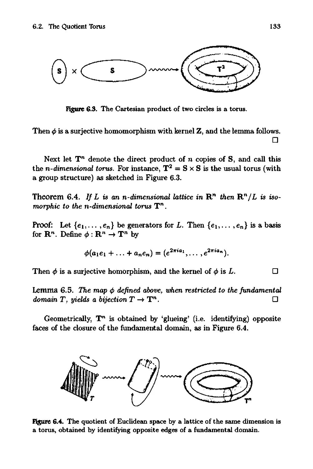
6.2 The Quotient Torus 132
6.3 Exercises .... 136
7 Minkowski's Theorem 139
7.1 Minkowski's Theorem 139
7.2 The Two-Squares Theorem 142
7.3 The Four-Squares Theorem 143
7.4 Exercises .......... 144
8 Geometric Representation of Algebraic Numbers 145
8.1 The Space Lst . 145
8.2 Exercises .................. 149

Contenls ix
9 CIass-Group and CIass*Numbe:r 151
9.1 The Class-Group . . . . . 152
9.2 An Existence Theorem. . 153
9.3 Finiteness of the Class-Group 157
9.4 How to Make an Ideal Principal. . 158
9.5 Unique Factorization of Elements in an Extension Ring 162
9.6 Exercises .......................... 164
III Number-Theoretic Applications 167
10 Computational Methods 169
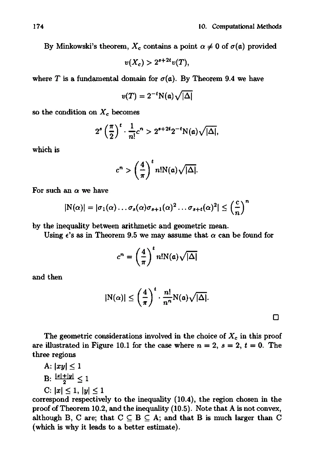
10.1 Factorization of a Rational Prime. 169
10.2 Minkowski's Constants. . . . . . 172
10.3 Some CINumber Calculations 176
10.4 Tables . . 179
10.5 Exercises ............. 180
11 ICu.mmer's Special Case of Fennat's Last Thecrem 188
11.1 Some History . . . . . . . . 183
11.2 Elementary Considerations 186
11.3 Kummer's Lemma . 189
11.4 Kummer's Theorem 193
11.5 Regular Primes . . . 196
11.6 Exercises ...... 198
12 The Path to the Final Breakthrou$h 201
12.1 The Wolfskehl Prize .. . . . . . . . . . 201
12.2 Other Directions . . . . . . . . . . . . . 203
12.3 Modular Functions and Elliptic Curves. 205
12.4 The Taniyama-Shimura-Weil Conjecture 206
12.5 Frey's Elliptic Equation . . . . . . . . . . 207
12.6 The Amateur who Became a Model Professional 207
12.7 Technical Hitch . . . 210
12.8 Flash of Inspiration. 211
12.9 Exercises ...... 212
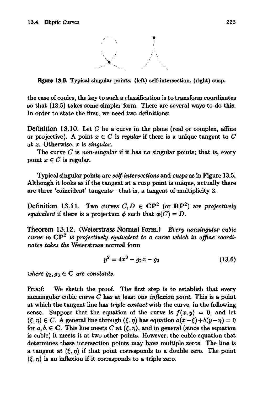
1 S miptic: Curves 21 S
13.1 Review of Conics . . . . . . . . . . . . . . . . . . 214
13.2 Projective Space .. . . . . . . . . . . . . . . . . 215
13.3 Rational Conics and the Pythagorean Equation . 220
13.4 Elliptic Curves . . . . . . . . . 222
13.5 The Tangent/Secant Process ........... 225

x
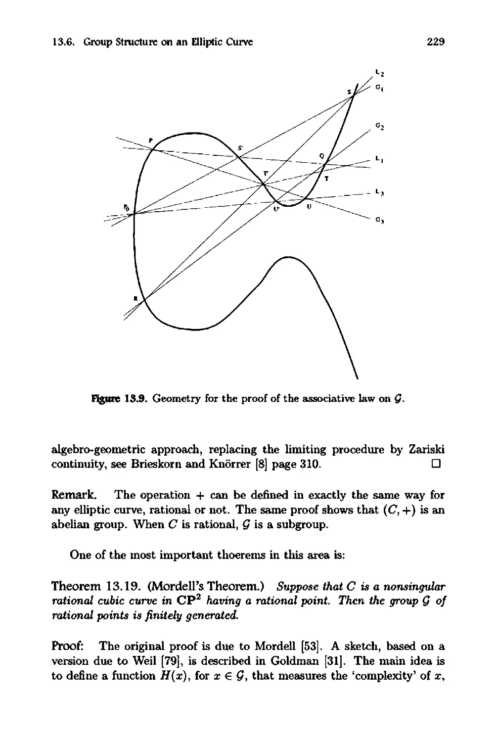
13.6 Group Structure on an Elliptic Curve .
13.7 Applications to Diophantine Equations .
13.8 Exercises .................
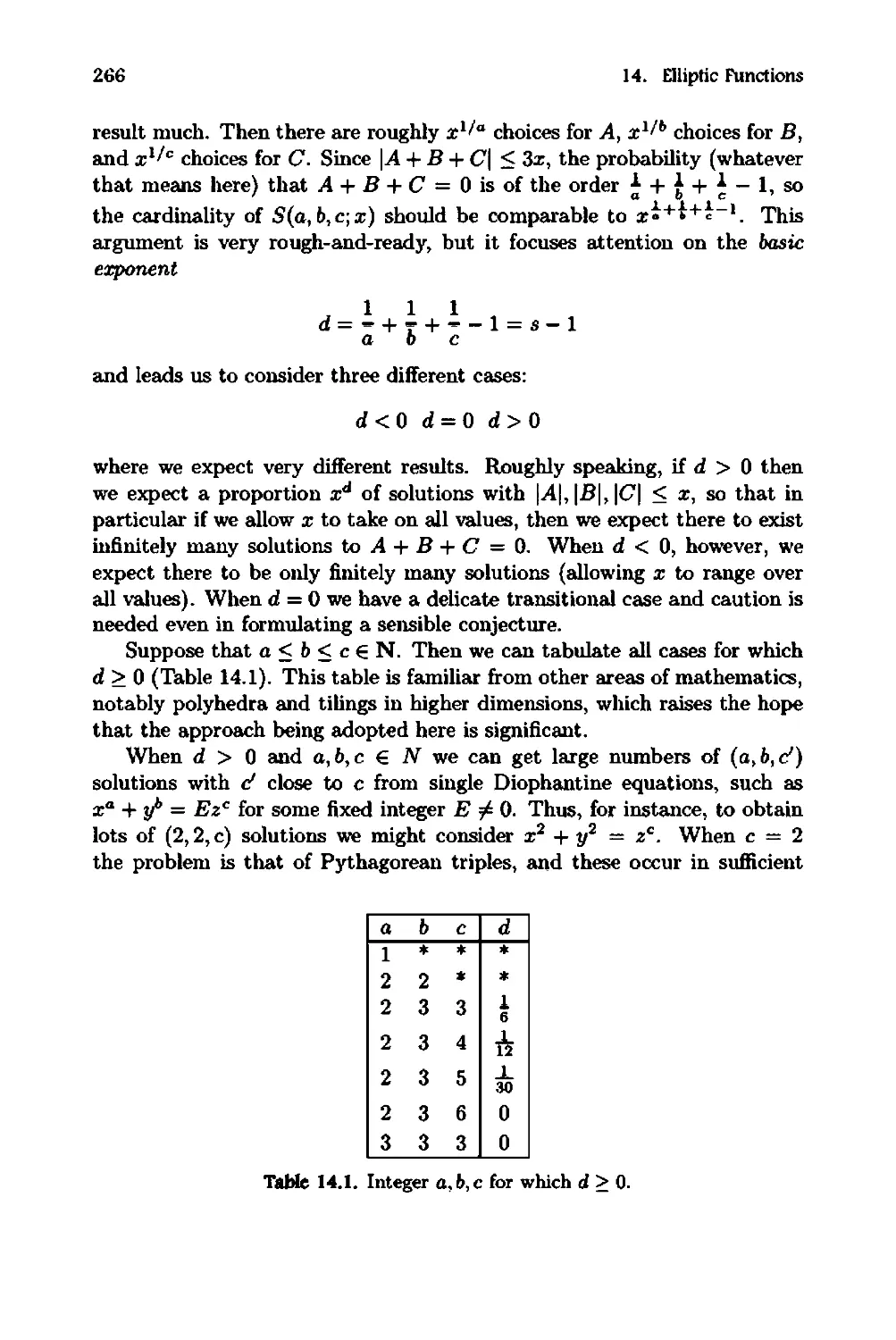
14 Elliptic Functions
14.1 Trigonometry Meets Diophantus
14.2 Elliptic Functions. . . . .
14.3 Legendre and Weierstrass
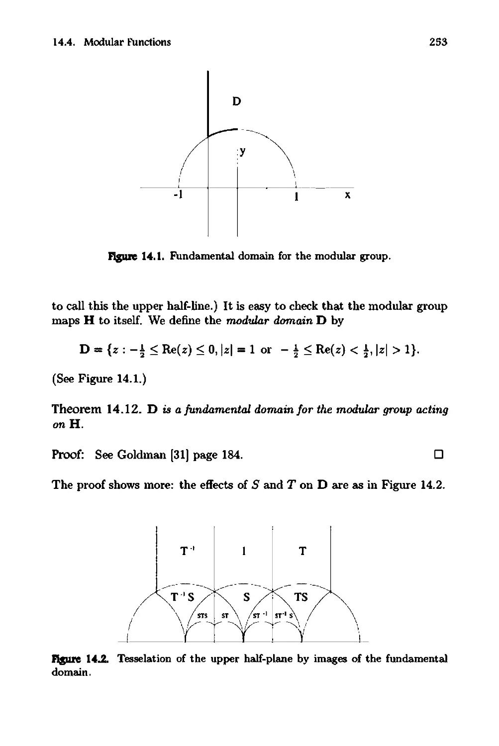
14.4 Modular FUnctions . . . .
14.5 The Frey Elliptic Curve .
14.6 The Taniyama-Shimura-Weil Conjecture
14.7 Sketch Proof of Fermat's Last Theorem
14.8 Recent Developments.
14.9 Exercises .................
IV Appendices
A Quadratic Residues
A.1 Quadratic Equations in Zm
A.2 The Units of Zm . . .
A.3 Quadratic Residues . . . .
A.4 Exercises .........
B Dirichlet's Units Theorem
B.1 Introduction. . . . . . . . . . . . . . . . . . . . . .
B.2 Logarithmic Space . . . . . . . . . . . . . . . . . .
B.3 Embedding the Unit Group in Logarithmic Space .
B.4 Dirichlet's Theorem
B.5 Exercises .......................
BibJiosraphy
Index
Conlents
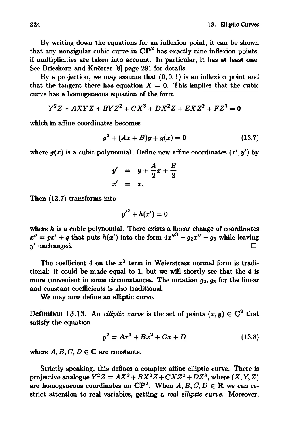
226
230
233
285
235
243
249
250
256
257
261
263
268
271
27S
274
276
281
290
298
293
294
295
296
301
80S
S09

Preface
The title of this book indicates a dual purpose. Our first aim is to introduce
fundamental ideas of algebraic numbers. The second is to tell one of the
most intriguing stories in the history of mathematics-the quest for a proof
of Fermat's Last Theorem. We use this celebrated theorem to motivate
a general study of the theory of algebraic numbers, from a reasonably
concrete point of view. The range of topics that we cover is selected to allow
students to make early progress in understanding the necessary concepts.
'Algebraic Number Theory' can be read in two distinct ways. One
is the theory of numbers viewed algebraically, the other is the study of
algebraic numbers. Both apply here. We illustrate how basic notions from
the theory of algebraic numbers may be used to solve problems in number
theory. However, our main focus is to extend properties of the natural
numbers to more general number structures: algebraic number fields, and
their rings of algebraic integers. These structures have most of the standard
properties that we associate with ordinary whole numbers, but some subtle
properties concerning primes and factorization sometimes fail to generalize.
A Diophantine equation (named after Diophantus of Alexandria, who-
it is thought-lived around 250 and whose book Arithmetica systematized
such concepts) is a polynomial equation, or a system of polynomial equa-
tions, that is to be solved in integers or rational numbers. The central
problem of this book concerns solutions of a very special Diophantine
equation:
x R + yR = zn
where the exponent n is a positive integer. For n = 2 there are many integer
solutions-in fact, infinitely many-which neatly relate to the theorem of
Pythagoras. For n  3, however, there appear to be no integer solutions.
xi

xii
Preface
It is this assertion that became known as Fermat's Last Theorem. (It is
equivalent to there being no rational solutions-try to work out why.)
One method of attack might be to imagine the equation x n + yn = zn
as being situated in the complex numbers, and to use the complex nth root
of unity ( = e 2ffi / n to obtain the factorization (valid for odd n)
x n + yn = (x + y)(x + (y) . .. (x + (n-ly).
This approach entails introducing algebraic ideas, including the notion of
factorization in the ring Z[() of polynomials in (. This promising line of
attack was pursued for a time in the 19th century, until it was discovered
that this particular ring of algebraic numbers does not possess all of the
properties that it 'ought to'. In particular, factorization into 'primes' is
not unique in this ring. (It fails, for instance, when n = 23, although this
is not entirely obvious.) It took a while for this idea to be fully Wlderstood
and for its consequences to sink in, but as it did so, the theory of algebraic
numbers was developed and refined, leading to substantial improvements
in our knowledge of Diophantine equations. In particular, it becanle pos-
sible to prove Fermat's Last Theorem in a whole range of special cases.
Subsequently, geometric methods and other approaches were introduced to
make further gains, Wltil, at the end of the 20th century, Andrew Wiles
finally set the last links in place to establish the proof after a three hundred
year search.
To gain insight into this extended story we must assume a certain
level of algebraic background. Our choice is to start with fundamental
ideas that are usually introduced into algebra courses, such as conunuta-
tive rings, groups and modules. These concepts smooth the way for the
modern reader, but they were not explicitly available to the pioneers of
the theory. The leading mathematicians in the 19th and early 20th cen-
turies developed and used most of the basic results and techniques of linear
algebra-for perhaps a hWldred years-without ever defining an abstract
vector space. There is no evidence that they suffered as a consequence of
this lack of an explicit theory. This historical fact indicates that abstraction
can be built only on an already existing body of specific concepts and rela-
tionships. This indicates that students will profit from direct contact with
the manipulation of examples of number-theoretic concepts, so the text is
interspersed with such examples. The algebra that we introduce-which
is what we consider necessary for grasping the essentials of the struggle to
prove Fermat's Last Theorem-is therefore not as 'abstract' as it might be.
We believe that in mathematics it is important to 'get your hands dirty'.
This requires struggling with calculations in specific contexts, where the
elegance of polished theory may disguise the essential nature of the math-
ematics. For instance, factorization into primes in specific number fields

Preface
xiii
displays the tendency of mathematical objects to take on a life of their own.
In some situations something works, in others it does not, and the reasons
why are often far from obvious. Withollt experiencing the struggle in per-
son, it is quite impossible to understand why the pioneers in algebraic
number theory had such difficulties. Of such frustrating yet stimulating
stuff is the mathematical fabric woven.
We therefore do not begin with later theories that have proved to be
of value in a wider range of problems, such as Galois theory, valuation rings,
Dedekind domains, and the like. Our purpose is to get students involved
in performing calculations that will enable them to build a platfonn for
understanding the theory. However, some algebraic background is neces-
sary. We assume a working knowledge of a variety of topics from algebra,
reviewed in detail in Chapter 1. These include commutative rings and
fields, ideals and quotient rings, factorization of polynomials with real coef-
ficients, field extensions, symmetric polynomials, modules, and free abelian
groups. Apart from these concepts we assume only some elementary results
from the theory of numbers and a superficial comprehension of multiple
integrals.
For organizational reasons rather than mathematical necessity, the book
is divided into four parts. Part I develops the basic theory from an algebraic
standpoint, introducing the ring of integers of a number field and exploring
factorization within it. Quadratic and cyclotomic fields are investigated
in more detail, and the Euclidean imaginary fields are classified. We then
consider the notion of factorization and see how the notion of a 'prime'
p can be pulled apart into two distinct ideas. The first is the concept
of being 'irreducible' in the sense that p has no factors other than 1 and
p. The second is what we now call 'prime': that if p is a factor of the
product ab (possibly multiplied by units-invertible elements) then it must
be a factor of either a or b. In tllis sense, a prime must be irreducible,
but an irreducible need not be prime. It turns out that factorization into
irreducibles is not always unique in a number field, but useful sufficient
conditions for uniqueness may be fOWld. The factorization theory of ideals
in a ring of algebraic integers is more satisfactory, in that every ideal is a
unique product of prime ideals. The extent to which factorization is not
unique can be 'measured' by the group of ideal classes (fractional ideals
modulo principal ones).
Part II emphasizes the power of geometric methods arising from Min-
kowski's theorem on convex sets relative to a lattice. We prove this key
result geometrically by looking at the torus that appears as a quotient of
Euclidean space by the lattice concerned. As illustrations of these ideas
we prove the two- and four-squares theorems of classical number theory; as
the main application we prove the finiteness of the class group.

xiv
Preface
Part III concentrates on applications of the theory thus far developed,
beginning with some slightly ad hoc computational techniques for class
numbers, and leading up to a special case of Fermat's Last Theorem that
exemplifies the development of the theory by Kummer, prior to the final
push by Wiles.
Part IV describes the final breakthrough, when-after a long period
of solitary thinking-Wiles finally put together his proof of Fermat's Last
Theorem. Even this tate is not without incident. His first announcement
in a lecture series in Cambridge turned out to contain a subtle unproved
assumption, and it took another year to rectify the error. However, the
proof is finally in a form that has been widety accepted by the mathematical
community. In this text we cannot give the full proof in all its glory.
Instead we discuss the new ingredients that make the proof possible: the
ideas of elliptic curves and elliptic integrals, and the link that shows that
the existence of a counterexample to Fermat's Last Theorem would lead
to a mathematical construction involving elliptic integrals. The proof of
the theorem rests upon showing that sllch a construction cannot exist. We
end with a brief survey of later developments, new conjectures, and open
problems.
There foUow two appendices which are of importance in algebraic num-
ber theory, but do not contribllte directly to the proof of Fennat's Last The-
orem. The first deals with quadratic residues and the quadratic reciprocity
theorem of Gauss. It uses straightforward computational techniques (de-
ceptively so: the ideas are very clever). It may be read at an early stage-
for example, right at the beginning, or alongside Chapter 3 which is rather
short: the two together would provide a block of work comparable to the
remaining chapters in the first part of the book. The second appendix
proves the Dirichtet Units Theorem, again a beacon in the development of
algebraic number theory, but not directly required in the proof of Fermat's
Last Theorem.
A preliminary version of Parts I-III of the book was written in 1974
by Ian Stewart at the University of Ti.ibingen, under the auspices of the
Alexander von Humbolt Foundation. This version was used as the basis of
a course for students in Warwick in 1975; it was then revised in the tight
of that experience, and was pllblished by Chapman and Hall. That edition
also benefited from the subtle comments of a perceptive but anonymous
referee; from the admirable persistence of students attending the course;
and from discussions with colleagues. The book has been used by successive
generations of students, and a second edition in 1986 brought the story up
to date-at that time-and corrected typographical and computational
errors.

Preface
xv
In the 19808 a proof of Fermat's Last Theorem had not been found.
In fact, graffiti on the wall of the Warwick Mathematics Institute declared
'I have a proof that Fermat's Last Theorem is equivalent to The Four
Colour Theorem, but this wall is too small for me to write it.' Since that
time, both Fermat's Last Theorem and the Four Colour Theorem have
fallen, after centuries of effort by the mathematical community. The final
conquest of Fermat's Last Theorem required a new version that would
give a reasonable idea of the story behind the complete saga. This new
version, brought out with a new publisher, is the result of further work
to bring the book up to date for the 21st century. It involved sllbstantial
rewriting of much of the material, and two new chapters on elliptic curves
and elliptic functions. These topics, not touched upon in previous editions,
were required to complete the final solution of the most elusive conundrum
in pure mathematics of the last three hundred years.
Coventry, February 2001.
Ian Stewart
David Tall

(q/p)
Z
Q
R
C
N
Zn
R/I
ker f
imf
(X)
(Xl>'" ,X n )
R[t]
iJp
bla
Df
L:K
[L:K]
K(all . . . , ern}
R(al,'" ,an)
Sr(tl,'" , t n }
NIM
(X)R
det (A)
(aij)
zn
A
Index of Notation
Legendre symbol
Integers
Rationals
Reals
Complex numbers
Natural numbers
Integers modulo n
Quotient ring
Kernel of f
Image of f
Ideal generated by X
Ideal generated by Xl' . .. ,X n
Ring of polynomials over R in t
Degree of polynomial p
b divides a
Fonnal derivative of f
Field extension
Degree of field extension
Field obtained by adjoining al, . .. , an to K
Ring generated by R and at. . . . , an
rth elementary symmetric polynomial in tl, . .. ,t n
Quotient module
R-submodule generated by X
Determinant of A
Matrix
Set of n-tuples with integer entries
Adjoint of matrix A
xvii

xviii
IXI
A
!a(t)
Pa(t)
W
[ob'.' ,an]
B
o
OK
NK(o)
TK(o)
N(o)
T(o)
t1.G
G)
U(R)
a, b, c, p, etc.
a-I
alb
N(a)
Br[x]
IIx-yll
S
Tn
v(X)
V
Ld
S
t
(1
:F
P
1-1.
h(O)
h
a"'b
[a]
t1.
Mst
)
Index 0( Notation
Cardinality of set x
Algebraic numbers
Field polynomial of a
Minimum polynomial of a
!( -1 + iY'3)
Discriminant of a basis
Algebraic integers
Ring of integers of number field
Ring of integers of number field K
Norm of a
Trace of a
Nonn of a
Trace of a
Discriminant of 01, . . . , an when this generates G
Binomial coefficient
Groups of units of R
Ideals
Inverse of a fractional ideal
a divides b: equivalently, a ;2 b
Nonn of a
Closed ball centre x, radius r
Distance from x to y in R n
Circle group
Nn jZn, the n-dimensional torus
Volume of X
Natllral homomorphism R N -+ Tn
RS X C t
Number or real monomorphisms K -+ C
Half number of complex monomorphisms K -+ C
Map K -+ Ls t
Group of fractional ideals
Group of principal ideals
Class-group :F I P
Class-number
Class-number
Equivalence of fractional ideals modulo principal ideals
Equivalence class of a
Discriminant of K
Minkowski constant ()t(s + 2t)-s-2t(s + 2t)!
Ideal of Z() generated by 1 - ( where ( = e 2 1<i/p

[ndex of Notation
A
Z
Bk
I
U
4>(x)
RP 2
P
Q
Cp 2
'"
92,93
o
g
P*Q
P+Q
F(k, v)
snu
cnu
dnu
Wl,W2
£Wt, W 2
P
P$Q
CU{oo}
SL z (Z)
PSL 2 (Z)
H
D
Xo(N)
:F
peN)
peA, B, C)
xix
1-(
Complex conjugate of z
kth BernouiUi number
Map Lst  Rs+t
Group of units of D
Euler function
Real projective plane
The plane {(x,y,z): z = I}
The plane {(x, y, z) : z = O}
Complex projective plane
Equivalence relation for homogeneous coordinates
Coefficients in Weierstrass normal form of a cubic
Specific rational point on an elliptic curve
Set of rational points on an elliptic curve
Geometric construction on elliptic curve
Group operation on elliptic curve
Elliptic integral of the first kind
Elliptic function
Elliptic function
Elliptic function
Periods of an elliptic function
Lattice generated by Wl, W2
Weierstrass p-function
Renaming of P + Q for clarity
Riemann sphere
Special linear group
Projective special linear group
Upper half-plane in C
Modular domain
Modular curve of level N
Frey elliptic curve
Power function of N
Power of (A,B,C)

The Origins of
Algebraic Number Theory
Numbers have fascinated civilized man for millennia. The Pythagoreans
studied many properties of the natural numbers 1,2, 3, . . . , and the famous
theorem of Pythagoras, though geometrical, has a pronounced number-
theoretic content. Earlier Babylonian civilizations had noted empirically
many so-called Pythagorean triads, such as 3, 4, 5 and 5, 12, 13. These are
natural numbers a, b, c such that
a 2 + b 2 = c 2 .
(1)
A clay tablet from about 1500 B.C. includes the triple 4961, 6480, 8161,
demonstrating the sophisticated techniques of the Babylonians.
The Ancient Greeks, though concentrating on geometry, continued to
take an interest in numbers. In c. 250 A.D. Diophantus of Alexandria wrote
a significant treatise on polynomial equations which studied solutions in
fractions. Particular cases of these equations with natural number solutions
have been called Diophantine equations to this day.
The study of algebra developed over the centuries, too. The Hindu
mathematicians dealt with increasing confidence with negative numbers
and zero. Meanwhile the Moslems conquered Alexandria in the 7th century,
sweeping across north Africa and Spain. The ensuing civilization brought
an enrichment of mathematics with Moslem ingenuity grafted onto Greek
and Hindu influence. The word 'algebra' itself derives from the arabic title
'al jabr w'al muqabalah' (literally 'restoration and equivalence') of a book
written by Al-Khowarizmi in c. 825. Peaceful coexistence of Moslem and
Christian led to the availability of most Greek and Arabic classics in Latin
translations by the 13th century.

2
The Origins of Algebraic Number Theory
In the 16th century, Cardano used negative and imaginary solutions in
his famous book Ars Magna, and in succeeding centuries complex numbers
were used with greater understanding and flexibility.
Meanwhile the theory of natural numbers was not neglected. One of the
greatest number theorists of the 17th century was Pierre de Fennat (1601-
1665). His fame rests on his correspondence with other mathematicians, for
he published very little. He would set challenges in number theory based
on his own calculations; and at his death he left a number of theorems
whose proofs were known, if at all, only to himself. The most notorious of
these was a marginal note in his own personal copy of Diophantus, written
in Latin, which translates:
To resolve a cube into [the sum of] two cubes, a fourth power into
fourth powers, or in general any power higher than the second into
two of the same kind, is impossible; of which fact I have found a
remarkable proof. The margin is too small to contain it ...
More precisely, Fermat asserted, in contrast to the case of Pythagorean
triads, that the equation
x n + yn = zn
(2)
has no integer solutions x, y, z (other than the trivial ones with one or more
of x,y,z equal to zero).
In the years following Fermat's death, almost all of his stated results
were furnished with a proof. An exception was his claim that Fn = 2 2n + 1
is prime for all positive integers n. It was subsequently shown that he was
wrong: for instance, Fs is divisible by 641. In a letter to Pierre de Carcavi in
1659 he claimed a proof of this conjecture. Even the great Fermat could be
wrong. But one by one his other assertions were furnished with proofs until,
by the mid-19th century, only one elusive jewel remained. His statement
about the non-existence of solutions of (2) for n  3 exceeded the powers of
all 19th century mathematicians. This beguiling and infuriating assertion,
so simple to state, yet so subtle in its labyrinthine complexity, became
known as 'Fermat's Last Theorem'. This romantic epithet is in fact doubly
inappropriate for, without a proof, it was not a 'theorem', neither was it
the last result that Fermat studied-only the last to remain Wlproved by
other mathematicians.
Given that a proof is so elusive, is it really credible that Fermat could
have possessed a genuine proof-a clever way of looking at the problem
which eluded later generations? Or had he made a subtle error, which
passed unnoticed, so that his 'theorem' had no proof at all? No one knows
for sure, but there is a strong consensus that if he did have what he thought

The Origins of Number Theory
3
was a proof, it would not survive modern scrutiny. Consensus and certainty
are not the same thing, however.
Be that as it may, during the late 19th and early 20th centuries the
name stuck, with its glow of romanticism-somehow lacking in the more
appropriate title 'the Fermat Conjecture'. It had the two classic ingredients
of a problem that can capture the imagination of a wider public-a simple
statement that can be widely Wlderstood, but a proof that defeats the
greatest intellects.
Another classic problem of this type-'the impossibility of trisecting
an angle using ruler and compasses alone'-took two thousand years to
be solved. This was posed by the Greeks in studying geometry and was
solved in the early 19th century using algebraic techniques. In the same
way the advancement in the solution of Fermat's Last Theorem has moved
out of the original domain, the theory of natural numbers, to a different
area of mathematical study, algebraic numbers. In the 19th century the
developing theory of algebra had matured to a state where it could usefully
be applied in number theory.
As it happened, Fermat's Last Theorem was not the major problem
being attacked by number theorists at the time; for example, when Kummer
made the all-important breakthrough that we are to describe in this text,
he was working on a different problem, a topic called the 'higher reciprocity
laws'. At this stage it is worth making a minor diversion to look at this
subject, for it was here that algebraic numbers entered number theory in
the work of Gauss. As an eighteen-year-old, in 1796 Gauss had given the
first proof of a remarkable fact observed empirically by Euler in 1783. Euler
had addressed himself to the problem of when an integer q was congruent
to a perfect square modulo a prime p,
xZ == q(mod p).
In such a case, q is said to be a quadratic residue of p. Euler concentrated
on the case when p, q were distinct odd primes and noted: if at least one
of the odd primes p, q is of the form 4r + 1, then q is a quadratic residue
of p if and only if p is a quadratic residue of q; on the other hand, if both
p, q are of the form 4r + 3, then precisely one is a quadratic residue of the
other.
Because of the reciprocal nature of the relationship between p and q,
this result Was known as the quadratic reciprocity law. Legendre attempted
a proof in 1785 but assumed that certain aritlunetic progressions contained
infinitely many primes-a theorem whose proof turned out to be far deeper
than the quadratic reciprocity law itself. Legendre introduced the symbol
( / ) _ { I if q is a quadratic residue of p
q P - -1 if not
,

4
The Origins of Algebraic Number Theory
in terms of which the law becomes
(q/p)(p/q) = (_1)(P-l)(Q-l)/4.
When Gauss gave the first proof in 1796 he was dissatisfied because
his method did not seem a natural way to attack so seemingly simple a
theorem. He went on to give several more proofs, two of which appeared
in his book Disquisitiones Arithmeticae (1801), a definitive text on number
theory which still remains in print, Gauss [29]. His second proof depends
on a numerical criterion that he discovered, and we give a computational
proof depending on this criterion in Appendix A.
Between 1808 and 1832 Gauss continued to look for similar laws for
powers higher than squares. This entailed looking for relationships between
p and q so that q was a cubic residue of p (x 3 == q(mod p» or a biquadratic
residue (x 4 == q(mod p», and so on. He found certain higher reciprocity
laws, but in doing so he discovered that his calculations were made easier
by working over the Gaussian integers a + In (a, b E Z, i = J=I), rather
than the integers alone. He developed a theory of prime factorization for
these, proved that decomposition into primes was unique, and developed
a law of biquadratic reciprocity. In the same way he considered cubic
reciprocity by using numbers of the form a + bw where w = e(2tci)/3. These
higher reciprocity laws do not have the same striking simplicity as quadratic
reciprocity and we shall not study them in this text. But Gauss' use of
these new types of number is of fundamental importance in Fermat's Last
Theorem, and the study of their factorization properties is a deep and
fruitful source of methods and problems.
The numbers concerned are all examples of a particular type of complex
number; namely, one which is a solution of a polynomial equation
anx n + . . . + alX + ao = 0
where all the coefficients are integers. Such a complex number is said to
be algebraic, and if an = 1, it is called an algebraic integer. Examples of
algebraic integers include i (which satisfies X2 + 1 = 0), v'2 (x2 - 2 = 0)
and more complicated examples, such as the roots of x 7 - 265x 3 + 7x 2 -
2x + 329 = O. The number i (satisfying 4x 2 + 1 = 0) is algebraic but not
an integer. On the other hand, there are complex numbers which are not
algebraic, such as e or 11'.
In the wider setting of algebraic integers we can factorize a solution of
Fennat's equation x n + yn = zn (if one exists) by introducing a complex
nth root of unity, ( = e2ffiln, and writing (2) as
(x + y)(x + (y)... (x + (n-ly) = zn.
(3)

The Origins of Number Theory
5
If Z[(J denotes the set of algebraic integers of the form (to + al ( + . . . + arC
where each aT is an ordinary integer, then this factorization takes place in
the ring Z[(].
In 1847 the French mathematician Lame announced a 'proof' of Fer-
mat's Last Theorem. In olltline his proposal was to show that only the case
where x, y have no common factors need be considered; and then deduce
that in this case x + y, x + (y,... , x + (n-ly have no common factors, that
is, they are relatively prime. He then argued that a product of relatively
prime numbers in (3) can be equal to an nth power only if each of the
factors is an nth power. So
x + y = ul'
x+(y = u;
x +(n-l = u: (4)
On this basis Lame derived a contradiction.
It was immediately pointed out to him by Liouville that the deduction
of (4) from (3) assumed uniqueness of factorization in a very subtle way.
Liouville's fears were confirmed when he later received a letter from Kum-
mer who had shown that uniqueness of factorization fails in some cases,
the first being n = 23. Over the summer of 1847 Kummer went on to
devise his own proof of Fermat's Last Theorem for certain exponents n,
surmounting the difficulties of non-uniqueness of factorization by introduc-
ing the theory of 'ideal' complex numbers. In retrospect this theory can
be viewed as introducing numbers from outside Z[(J to use as factors when
factorizing elements within Z[(]. These 'ideal factors' restore a version of
unique factorization.
Subsequently the theory began to take on a different form from that
in which Kummer left it, but the key concept of an 'ideal' (a reformula-
tion by Dedekind of Kummer's 'ideal number') gave the theory a major
boost. By using his theory of ideal numbers, Kummer proved Fermat's
Last Theorem for a wide range of prime powers-the so-called 'regular'
primes. He also evolved a powerful machine with applications to many
other problems in mathematics. In fact a large part of classical num-
ber theory can be expressed in the framework of algebraic numbers. This
point of view was urged most strongly by Hilbert in his Zahlbericht of 1897,
which had an enormous influence on the development of number theory,
see Reid [57J. As a result, algebraic number theory is today a flourishing
and important branch of mathematics, with deep methods and insights;
and-most significantly-applications not only to number theory, but also
to group theory, algebraic geometry, topology, and analysis. It was these

6
The Origins of Algebraic Number Theory
wider links that eventually led to the final proof of Fermat's Last Theo-
rem-establishing it once and for all as a theorem, not a conjecture. The
eventual proof was made possible by various significant inroads, which were
made using techniques from elliptic functions, modular forms, and Galois
representations.
The breakthrough, as indicated above, was made by Andrew Wiles.
As a teenager, fascinated by the simplicity of the statement of the theo-
rem, Wiles had begun a long and mostly solitary journey in search of the
proof. The event that triggered his final push was a conjecture put forward
by two Japanese mathematicians, Yutaka Taniyama and Goro Shimura,
who hypothesized a link between elliptic curves and modular forms. Their
ideas were later refined by Andre Weil. This proposal became known as
the Taniyanla-Shimura-Weil Conjecture, and it was discovered that if this
conjecture could be proved, then Fermat's Last Theorem could be deduced
from it. At this point, Wiles leaped into action. He worked in solitude for
seven years before he convinced himself that he had proved a special case of
the Taniyama-Shimura-Weil Conjecture that was strong enough to imply
Fermat's Last Theorem. He announced his result in a lecture in Cambridge
on 23 June 1993.
When his proof was being checked, a query from a colleague revealed a
gap, and Wiles accepted that there were still details to be attended to. It
took him so long to do this that others questioned whether he had ever been
close to the proof at all. However, in the autumn of 1994, working with his
former student Richard Taylor, he finally realised that he could complete
the proof satisfactorily. He released the proof for scrutiny in October 1994
and it was published in May 1995.
Fermat's Last Theorem has the distinction of being the theorem with
the greatest nwnber of false 'proofs', so the proof was scrutinized very
carefully. However, this time the ideas fit together so tightly that experts
in the mathematical community agreed that all was well. In the ensuing
period nothing has happened to change this opinion: Fermat's Last The-
orem has at last been declared true. However, the proof uses techniques
that lie far beyond what would have been available to Fermat. So when he
stated that he had found a proof that could not be fitted into the margin of
his book, had he truly found a perceptive insight that has been missed by
mathematicians for over 350 years? Or was it, as observed by the historian
Struik (741, that 'even the great Fermat slept sometimes'?

I
Algebraic Methods

1
Algebraic Background
Fermat's Last Theorem is a special case of the theory of Diophantine equa-
tions-integer solutions of polynomial equations. To place the problem in
context, we move to the wider realm of algebraic numbers, which arise as
the real or complex solutions of polynomials with integer coefficients; we
focus parlicularly on algebraic integers, which are solutions of polynomials
with integer coefficients where the leading coefficient is 1. For example, the
equation x 2 - 2 = 0 has no integer solutions, but it has two real solutions,
x = :f:V2. The leading coefficient of the polynomial x 2 - 2 is 1, so :f:V2
are algebraic integers.
To operate with such numbers, it is useful to work in subsystems of the
complex numbers that are closed under the usual operations of arithmetic.
Such subsystems include subrings (which are closed under addition, sub-
traction and multiplication) and subfields (closed under all four arithmetic
operations including division). Thus along with :f:V2 we consider the rin!
of all numbers a + bV2 for a, b E Z, a.nd the field of all numbers p + q../2
for p,q E Q.
In this chapter we lay the foundations for algebraic number theory by
considering some fundamental facts about rings, fields, and other algebraic
structures, including abelian groups and modules, which are relevant to
our theoretical development. We expect the reader to be acquainted with
elementary properties of groups, rings and fields, and to have an elementary
knowledge of linear algebra over an arbitrary field (up to simple properties
of determinants). Familiar results at this level will be stated without proof;
results which we consider less familiar to some readers may be proved in
full or in outline as we consider appropriate. Results not proved in full are
given appropriate references, in case the reader wishes to pursue them in
9

10
1. Algebraic Background
greater depth. Useful general references on abstract algebra, with emphasis
on rings and fields, are Fenrick [24], Fraleigh [25), Jacobson [40), Lang [43],
Sharpe [67], and Stewart and Tall [72]. For group theory, see Burn [11],
Humphreys [38], Macdonald [45], Neumann et al. [55], and Rotman [63].
First we set up the ring-theoretic language (and in particular the notion
of an ideal, which proves to be so important). Then we consider factoriza-
tion of polynomials over a ring (which in this book will often be a subfield
of the complex numbers). Topics of central importance at this stage are
the factorization of a polynomial over an extension field and the theory of
elementary symmetric polynomials. Module-theoretic language will help us
clarify certain points later; and results concerning finitely generated abelian
groups are proved because they are vital in describing the properties of the
additive group structure of the subrings of the complex numbers which
occur. With the prologue of the first chapter behind us we shall then be
ready to begin the main action.
1.1 Rings and Fields
Unless explicitly stated to the contrary, the term ring in this book will
always mean a conunutative ring R with identity element 1 (or 1R). If
such a ring has no zero-divisors (so that in R, a :/: 0, b:/: 0 implies ab :/: 0),
and if I:/: 0 in it, then it will be called a domain (or integral domain). An
element a in a ring R is called a unit if there exists b E R such that ab = 1.
Suppose ab = ac = 1. Then c = Ie = abc = acb = 1b = b. The unique b
such that ab = 1 will be denoted by a-I, and 00- 1 will also be denoted by
cfa. If 1 :/: 0 in R and every non-zero element in R is a unit, then R will
be called a field.
We shall use the standard notation N for the set of natural numbers
0, I, 2,. .., Z for the integers, Q for the rationals, R for the reals and C
for the complex numbers. Under the usual operations Q, R, C are fields,
Z is a domain and N is not even a ring. For n E N, n > 0, we denote
the ring of integers modulo n by Zn' If n is composite, then Zn has zero
divisors, but for n prime, then Zn, is a field (Fraleigh [25] p. 217; Stewart
[71] Theorem 1.1, p. 3).
A subring 5 of a ring R will be required to contain 1R. We can check
that 5 is a subring by demonstrating that 1R E 5, and if s, t E 5 then
s + t, - s, st E 5. It then forms a ring in its own right under the operations
restricted from R. In the same way, if K is a field, then a subfield F of K
is a field under the operations restricted from K. We can check that F is
a subfield of K by demonstrating 1k E F, and if s, t E F (s:/: 0), then
s + t, -s, st, S-1 E F.

1.1. Rings and Fields
11
The concept of an ideal will be of central importance in this text. Recall
that an ideal is a non-empty subset I of a ring R such that if r, s E I, then
r - s E I; and if r E R, s E I then rs E I. We shall also require the
concept of the qllotient ring R/ I of R by an ideal I. The elements of
R/ I are cosets I + r of the additive group of I in R, with addition and
mllltiplication defined by
(I + r) + (I + s) = 1+ (r + s)
(I + r)(I + s) = 1+ rs
for all r, s E R. For example, if nZ is the set of integer multiples of nEZ,
then Z/nZ is isomorphic to Zn'
A homomorphism f from a ring RI to a ring R 2 is a function f : RI -+
R2 sllch that
f(IRJ = 1R2
f(r + s) = f(r) + f(s)
f(rs) = f(r)f(s)
for all r,s E RI. A monomorphism is an injective (1-1) homomorphism
and an isomorphism is a bijective (1-1 and onto) homomorphism.
The kernel and image of a homomorphism f are defined in the usllal
way:
ker f = {r E RI I f(r) = O}
im f = {J(r) E  IrE Rd.
The kernel is an ideal of R 1 ; the image is a. subring of R2; and the iso-
morphism theorem states that there is an isomorphism from Rdkerf to
imf. (Stlldents requiring explanations of the relevant theory may consult
Fraleigh [25], Jacobson [40], or Sharpe [671.)
If X and Y are sllbsets of a ring R we write X + Y for the set of
all elements x + Y (x E X, Y E Y); and XY for the set of all finite sums
EXiYi (Xi E X, Yi E Y). When X and Y are both ideals, so are X + Y and
XY.
The sum X + Y of two sets can be generalized to an arbitrary collection
{XihEI by defining EiEIX i to be the set of all finite Sllms Xii + .. . + Xi"
of elements Xij E X ij .
We shall make the customary compression of notation with regard to
{x} and x, writing for example xY for {x}Y, X + Y for {x} + Y, and 0
for {O}.
The ideal generated by a subset X of R is the smallest ideal of R con-
taining X; we shall denote this by (X). If X = {x},... ,x n }, then we shall

12
1. Algebraic Background
write (X) as (Xi>'" ,x n ). (Some writers use (X) where we have written
(X), but then the last-mentioned simplification of notation would reduce
to the notation for an n-tuple (Xl,.' . ,X n ), so (X) is to be preferred.)
A simple calculation shows that
(X) = X R = L xR.
;r;EX
The identity element lR is crucial in this equation. In a commutative
ring without identity we would also have to add on the additive group
generated by X to X R and to I:;r;€X xR.
If there exists a finite subset X = {Xl,". ,xn} of R such that I = (X),
then we say that I is finitely generated as an ideal of R. If I = (x) for an
element X E R we say that I is the principal ideal generated by x.
Example 1.1. Let R = Z, X = {4,6}, then (4,6) is finitely generated. In
fact (4,6) contains 2.4 - 6 = 2 and it easily follows that (4,6) = (2}, so
that further this ideal is principal. More generally, every ideal of Z is of
the form (n) for some n EN, hence principal.
Example 1.2. Let R be the set Q under the usual operation of addition,
but define a non-standard multiplication on R by setting xy = 0 for all
x, y E R. The ideal (X) for a subset X  R is then equal to the abelian
group generated by X under addition. Now R is an ideal of R, bl1t is not
finitely generated. To see this, suppose that R is generated as an abelian
group by elements pdqi>'" ,Pnlqn. Then the only primes dividing the
denominators of elements of R will be those dividing ql, . . . , qn, which is a
contradiction.
If K is a field and R is a sl1bring of K then R is a domain. Conversely,
every domain D can be embedded in a field Lj and there exists such an
L consisting only of elements die where d, e E D and e ::f. O. Sl1ch an L,
which is l1nique up to isomorphism, is called the ji£1d of fractions or ji£ld
of qIWtients of D. (See Fraleigh [25] Theorem 26.1 p. 239.)
Theorem 1.3. Every finite integral domain is a field.
Proof: Let D be a finite integral domain. Since 1 ::f. 0, then D has at
least 2 elements. For 0 ::f. xED the elements xy, as y runs through D,
are distinctj for if xy = xz then x(y - z) = 0 and so y = z since D has
no zero-divisors. Hence, by counting, the set of all elements xy is D. Thus
1 = xy for some y ED, and therefore D is a field. 0

1.2. Factorization of Polynomials
13
Every field has a uniql1e minimal subfield, the prime suhfield, and this
is isomorphic either to Q or to Zp where p is a prime number. (See Fraleigh
[25] Theorem 29.7 p. 260; Stewart [71] Theorem 1.2, p. 4.) Correspond-
ingly, we say that the characteristic of the field is 0 or p. In a field of
characteristic p we have px = 0 for every element x, where as usual we
write
px = (1 + 1 +... + l)x
where there are p summands 1; and p is the smallest positive integer with
this property. In a field of characteristic zero, if nx = 0 for some non-
zero element x and integer n, then n = O. Our major concern in the
sequel will be subfields of C (the complex numbers), which of course have
characteristic zero, bl1t fields of prime characteristic will arise naturally
from time to time.
We shall use without further comment the fact that C is algebraically
closed: given any polynomial p over C there exists x E C Sl1ch that
p(x) = O. For a proof of tlus see Stewart [71] pp. 193 ff.; different proofs
using analysis or topological considerations are in Hardy [34] p. 492 and
Titcbmarsh [77] p.1l8.
1.2 Factorization of Polynomials
Later in the book we shall consider factorization in a more general con-
text. Here we concentrate on factorizing polynomials. First a few general
remarks.
In a ring 5, if we can write a = bc for a, b, c E 5, then we say that b, c
are factors of a. We also say 'b divides a' and write
b I a.
For any unit e E 5 we can always write
a = e(e-1a),
so, trivially, a unit is a factor of all elements in 5. If a = be where neither
b nor c is a l1nit, then b and c are called propC1' factors and a is said to be
reducible. In particular 0 = 0 . 0 is reducible.
Note that if a is itself a mut a.nd a = be, we have
1 = aa- 1 = bca- 1 ,

14
1. Algebraic Background
so b and c are both units. A unit cannot have a proper factorization. We
therefore concentrate on factorization of non-units. A non-unit a E S is
said to be irrcdwle if it has no proper factors.
Now we turn our attention to the case S = R[t], the ring of polynomials
in an indeterminate t with coefficients in a ring R. The elements of R[t]
are expressions
Tntn + Tn_lt n - l + ... + Tlt + TO
where TO, Tl,. .. ,Tn E R and addition and multiplication are defined in the
obvious way. (For a formal treatment of polynomials, and why not to use
it, see Fraleigh [25] pp. 263-265.)
Given a nOD-zero polynomial
p = Tntn + . . . + TO,
we define the degree of p to be the largest vall1e of n for which Tn -:f 0, and
write it &p. Polynomials of degree 0, 1,2,3,4,5, . . ., will often be referred
to as constant, linear, quadmtic, cubic, quartic, quintic, ... , polynomi-
als respectively. In particular a constant polynomial is just a (non-zero)
element of R.
If R is an integral domain, then
8pq = fJp + fJq
for non-zero p, q so R[t] is also an integral domain. If p = aq in R[t], then
{)p = oa + fJq implies that
oq $ &p.
When R is not a field, then it is perfectly possible to have a non-trivial
factorization in which ()p = oq. For example
3t 2 + 6 = 3(t 2 + 2)
in Z[t], where neither 3 nor t 2 + 2 is a unit. This is because of the existence
of non-units in R. However, if R is a field, then all (non-zero) constants
in R[t] are units and so if q is a proper factor of p for polynomials over a
field, then fJq < op.
Let us concentrate for a time on polynomials over a field K. Here we
have the division algorithm which states that if p, q -:f 0 then
p = qs + T
where either T = 0 or Or < fJq. The proof is by indl1ction on fJp and in
practice is no more than long division of p by q leaving remainder T, which
is either zero (in which case q I p) or of degree lower than q.

1.2. Factorization of Polynomials
15
The division algorithm is used repeatedly in the Euclidean algorithm,
which is a particularly efficient method for finding the highest common
factoT d of non-zero polynomials p, q.
This is defined by the properties:
(a) dip, d I q,
(b) If tf I p and d l I q then d! I d.
These define d uniquely up to non-zero constant multiples. To calculate
d we first suppose that p, q are named so that {}p  {}qi then divide q into
p to get
p = qSl + Tl
Or l < {}q :5 {}p,
a.nd continue in the following way:
q = TlS2 + T2
Tl = T2S3 + T3
Or2 < OTl
Or 3 < fJr2
T n -2 = Tn-lS n + Tn Or n < OTn-l
until we arrive at a zero remainder:
Tn-l = TnSn+l.
The last non-zero remainder Tn is the highest common factor. (From the
last equation Tn I Tn-h and working back successively, Tn is a factor of
Tn-2,' .. ,Tl,P, q, verifying (a). If f/ Ip, d' I q, then f.'om the first equation,
d' is a factor of Tl = P - qSl, and successively working down the eql1ations,
d' is a factor of T2,T3,... ,Tn, SO f/IT n , verifying (b).) Beginning with
the first equation, and substituting in those which follow, we find that
Ti = aiP + biq for suitable ai,b i E KIt], and in particular the highest
common factor d = Tn is of the form
d = ap + bq for suitable a, b E K[tJ.
(1.1)
A useful special case is when d = 1, when p, q are called coprime and (1.1)
gives
ap + bq = 1 for suitable a, bE K[t].
This technique for calcula.ting the highest common factor can also be used
to find the polynomials a, b.
Example 1.4. p = t 3 + l,q = t 2 + 1 E Q[t].

16
1. Algebraic Background
Then
t 3 + 1 = t(t 2 + 1) + (-t + 1),
t 2 +1 = (-t-1)(-t+l)+2,
-t + 1 = ( - tt + t)2.
The highest common factor is 2, or l1p to a constant factor, 1, so p and q
are coprime, a.nd substituting back from the second equation,
1 = t(t 2 + 1) + t(t + 1)( -t + 1).
Then substituting for -t + 1 using the first equation:
1 = !(t 2 + 1) + Ht + 1)«(t 3 + 1) - t(t 2 + 1»
= (_!t 2 - !t + !)(t 2 + 1) + (!t + t)(t 3 + 1).
Factorizing a single polynomial p is by no means as straightforward as
finding the highest common factor of two. It is known that every non-zero
polynomial over a field K is a product of finitely many irreducible factors,
and these are uniql1e up to the order in which they are multiplied and up
to constant factors. (See Fraleigh [25] Theorem 31.8 p.284; Stewart [71]
pp. 19-21.) Finding these factors is very ml1ch an ad hoc matter. Linear
factors are easiest, since (x - a) I p if and only if pea) = o.
IT pea) = 0, then a is called a zero of p. If (t - a)m I p where m  2,
then a is a repeated zero and the largest sl1ch m is the multiplicity of a.
To detect repeated zeroes, we use a method which (like much in this
chapter) was far more familiar at the turn of the century than it is now.
Given a polynomial
n
f = LTi ti
i=O
over a ring R we define
n
D f . t i - 1
=  tTi ,
i=O
called for obvious reasons the formal derivative of f. It is not hard to check
directly that
D(f + g) = Df + Dg
D(fg) = (Df)g + f(Dg).

1.2. Factorization of Polynomials
17
This enables us to check for repeated factors. A factor q of a polynomial p
is repeated if qT I p for some r 2: 2. In particular q is repeated if its square
divides p.
Theorem 1.5. Let K be a field 01 characteristic zero. A non-zero polyno-
mial lover K is divisihle by the square 01 a polynomial 01 degree > 0 il
and only il 1 and D f have a common factor of degree > O.
Proof: First suppose f = g2 h. Then
Df = lDh + 2g(Dg)h
and so 1 and D f have 9 as a common factor.
Now suppose that f has no squared irreducible factor. Then for any
irredl1cible factor 9 of f we find
1 =gh
where 9 and h are coprime (otherwise 9 would be a factor of h and would
occur as a squared factor in gh). Were f and Df to have a common factor g,
which we take to be irreducible, then on differentiating formally we would
obtain
DI = (Dg)h + g(Dh)
So 9 is a factor of (Dg)h, hence of Dg because 9 and h are coprime. Bl1t
Dg is of lower degree than g, hence it can only have 9 as a factor if Dg = O.
Since K has characteristic zero, by direct computation, this implies 9 is
constant, so f and 9 can have no non-trivial common factor. 0
Remark. If the field has characteristic p > 0, then the first part of
Theorem 1.5, that 1 having a squared factor implies f and D f have a
common factor, is stiU true, and the proof is the same as above.
A result which we shall need later is:
Corollary 1.6. An irreducible polynomial over a stdJfidd K 01 C has no
repeated zeros in C.
Proof: Suppose f is irreducible over K. Then f and D f must be coprime
(for a conunon factor would be a squared factor of f by (1.5), and 1 is
irreducible). Thus there exist polynomials a, b over K such that af +
bDf = 1, and the same equation interpreted over C shows f and Df to be
coprime over C. By Theorem 1.5 again, f cannot have repeated zeros. 0

18
1. Algebraic Background
We shall often consider factorization of polynomials over Q. When such
a polynomial has integer coefficients we shall find that we need consider only
factors which themselves have integer coefficients. This fact is enshrined in
a result due to Gauss:
Lemma 1. 7. Let P E Z[ t], and suppose that p = gh where g, h E Q[t]. Then
there exists >. E Q,>. =f:. 0, such that >.g,>.-1h E ZIt].
Proof: Ml1ltiplying by the prool1ct of the denominators of the coefficients
of g, h we can rewrite p = gh as
np = g'h'
where g', h' are rational multiples of g, h respectively, n E Z a.nd 9', h' E
Z[t]. This means that n divides the coefficients of the product g'h'. We
now divide the equation successively by the prime factors of n. We shall
establish that if k is a prime factor of n, then k divides all the coefficients
of g' or all those of h'. Whichever it is, we can divide that particular
polynomial by k to give another polynomial with integer coefficients. After
dividing in this way by all the prime factors of n, we are left with
p=gh
where g, h E ZIt] are rational ml1ltiples of g, h respectively. Pl1tting g = >.g
for >. E Q, we obtain h = >. -1 h and the result will follow.
It remains to prove that if
g' = 90 + g1 + ... + gr tr
h' = ho + h 1 + . . . + hst S
and a prime k divides all the coefficients of g' h', then k must divide all the
9i or all the h j . But if a prime k does not divide all the 9i and all the h j ,
we can choose the first of each set of coefficients, say gm, hq which are not
divisible by k. Then the coefficient of t m + q in the product g'h' is
90 h m+q + 91 h m+q-1 + . . . + 9m h g + . . .9m+q h O
and since every term in this expression is divisible by k except hq[}m, this
wOl1ld mean that the whole coefficient would not be divisible by k, a con-
tradiction. 0
We shall need methods for proving irreducibility of various specific poly-
nomials over Z. The first of these is known as Eisenstein's critcricm:

1.2. Factorization of Polynomials
19
Theorem 1,8. Let
f = ao + alt +... + ant n
be a polynomial over Z. Suppose there is a prime q such that
(a) q fan,
(b) q I ai,
(c) q2 t ao.
(i=O,l,... ,n-l),
Then, apart from constant factors, f is irreducible over Z, and hence i7TC-
ducible over Q.
Proof: By Lenuna 1.7 it is enough to show that f can have only constant
factors over Z.
If not, then f = 9h where
9 = 90 + 91 t + . . . + 9r tT
h = ho + hIt + ... + hst S
with all 9i,h j E Z and r,s > 1,r + s = n.
Now 90ho = Qo, so (b) implies q divides one of 90, ho whilst (c) implies
it cannot divide both. Without loss in generality, suppose q divides 90 but
not ho. Not all 9i are divisible by q because this would imply that q divides
an, contrary to (a). Let 9m be the first coefficient of 9 not divisible by q.
Then
am = 90k.". + . . . + 9mha
where m ::; r < n. All the sl1mmands 011 the right are divisible by q except
the last, which means that am is not divisible by q, contradicting (b). 0
A second useful method is reduction modulo n, as follows. Suppose
o =f:. p E ZIt], with P reducible: say p = qr. The natural homomorphism
Z -+ Zn gives rise to a homomorphism ZIt] -+ Zn[t]. Using bars to denote
images l1nder this map, we have p = qr . If fJP = {)p, then clearly 8q = Oq,
Of = Or, and p is also reducible. This proves:
Theorem 1.9. lfp E ZItI and its image 15 E Zn(t] is irreducible, with fJP =
op, then p is irreducible as an clement of Z[t). 0
In practice we take n to be prime, though this is not essential. The
point of reducing modulo n is that Zn being finite, there are only a finite
number of possible factors of p to be considered.

20
1. Algebraic Background
Examples.
1.1 The polynomial t 2 - 2 satisfies Eisenstein's criterion with q = 2.
1.2 The polynomial t ll -7t 6 +2lt 5 +49t-56 satisfies Eisenstein's criterion
with q = 7.
1.3 The polynomial t 5 - t + 1 does not satisfy Eisenstein's criterion for
any q. Instead we try reduction modulo 5. There is no linear factor
since none of 0, 1, 2, 3, 4 yield 0 when substituted for t, so the only
possible way to factorize is
t 5 - t + 1 = (t 2 + at + ,8)(t 3 + ')'t 2 + 6t + E)
where a,,8,')',6,E take values 0, 1,2,3 or 4 (mod 5). This gives a
system of equations on comparing coefficients: there are only a finite
nl1mber of possibilities all of which are easily eliminated. Hence the
polynomial is irreducible mod 5, so irreducible over Z.
1.3 Field Extensions
In finding the zeros of a polynomial p over a field K it is often necessary to
pass to a larger field L containing K. In these circumstances, L is called
a field extension of K. For example, p(t) = t 2 + 1 has no zeros in R, bl1t
considering p as a polynomial over C, it has zeros ::i:i and a factorization
p(t) = (t + i)(t - i).
Field extensions often arise in a slightly more general context as a
monomorphism j : K  L where K and L are fields. We shall see such
instances shortly. It is customary in these cases to identify K with its im-
age j(K), which is a sl1bfield of L; then a field extension is a pair of fields
(K, L) where K is a subfield of L. We talk of the extension
L:K
of K. Most field extensions with which we shall deal will involve two
subfields of C.
If L : K is a field extension, then L has a natural structure as a vector
space over K (where vector addition is addition in L and scalar multipli-
cation of >. E K on vEL is just AV E L). The dimension of this vector
space is called the degree of the extension, or the dc!J1U of Lover K, and
written
[L:K]
The degree has an important multiplicative property:

1.3. Field Extensions
21
Theorem 1,10. If H  K  L are fields, then
[L : H] = [L : K][K : H].
Proof: We sketch this. Details are in Stewart [71], Theorem 4.2 p. 50. Let
{ai}iel be a basis for Lover K, and {bj}jeJ a basis for Kover H. Then
{bj}(i,j)elxJ is a basis for L, over H. 0
If [L : K] is finite we say that L is a finite extension of K.
Given a field extension L:K and an element a E L, there mayor may
not exist a polynomial p E K[t] such that p(a) = 0, p :/: o. If not, we
say that a is tmnscen<kntal over K. If such a p exists, we say that a is
algebraic over K. If a is algebraic over K, then there exists a unique monic
polynomial q of minimal degree subject to q(a) = 0, and q is called the
minimum polynomial of a over K. (A monic polynomial is one with highest
coefficient 1.) The minimum polynomial of a is irredl1cible over K. (These
facts are to be found in Stewart [71] pp. 38,39.)
If al,'" an E L, we write
K(al,oo, ,an)
for the smallest subfield of L containing K and the elements al,... ,an'
In an analogous way, if S is a subring of a ring R and al,... ,an E R,
we write
S[al,' . . ,an]
for the smallest subring of R containing S and the elements a1>'" ,an'
Clearly S[al, . .. , an] consists of all polynomials in a},. .. , an with coeffi.
cients in S. For instance S[a] consists of polynomials
So + Sla +... + Smam
(Si E S).
The case of K(a) is more interesting. If a is transcendental over K, then
for k.n :/: 0 we have
1.0 + k l a + . . . + k m am :/: 0
( E K).
In this case K(a) must include all rational expressions
So + Sla + . . . + snan
ko + k 1 a + . . . + kma m
(Sj,k i E K,k m :/: 0)
and dearly consists precisely of these elements.

22
1. Algebraic Background
However, for a algebraic, we have:
Theorem 1.11, If L : K is a field extension and a E L, then a is al-
gebraic over K if and only if K (a) is a finite extension of K. In this
case, [K(a):K] = 8p 'Where p is the minimum polynomial of a over K, and
K(a) = K{a].
Proof: Once more we sketch the proof, given in full in Stewart [71] Propo-
sition 4.3, p. 52. If [K(a) : K] = n < 00 then the powers, 1, a, a 2 ,... , an
are linearly dependent over K, whence a is algebraic. Conversely, suppose
a algebraic with minimum polynomial p of degree m. We claim that K(a)
is the vector space over K spanned by l,a,... ,a m - 1 . This (call it V) is
certainly closed under addition, subtraction, and multipJication by a; for
the last statement note that am = -p(a) + am = q(a) where 8q < m.
Hence V is closed l1nder multiplication, and so forms a ring. All we need
prove now is that if 0 -:/: v E V then Ijv E V. Now v = h(a) where h E K[t]
and 8h < m. Since p is irredl1cible, p and h are coprime, so there exist
f,g E K[t] sl1ch that
f(t)p(t) + g(t)h(t) = 1.
Then
1 = f(a)p(a) + g(a)h(a) = g(a)h(a)
so that l/v = g(a) E Vas required. But it follows at once that [K(a): K] =
dimKV = m. 0
If we specify in advance K and an irreducible monic polynomial p(t) E
KIt] then there exists l1p to isomorphism a unique extension field L sl1ch
that L contains an element a with minim 11m polynomial p, and L = K(a).
This can be constructed as K[tJl(P}. It is customary to express this con-
struction by the phrase 'adjoin to K an element a with pea) = 0' and
to write K(a) for the resulting field. This, and ml1ch else, is discussed in
Stewart [71] Chapter 3, pp. 33-45.
1.4 Symmetric Polynomials
Let R[t}, t2, . . . , t n ] denote the ring of polynomials in indeterminates
tl, t2, . . . , t n with coefficients in a ring R. Let Sn denote the symmet-
ric group of permutations on {I, 2, . .. , n}. For any permutation 1TE Sn and

1.4. Symmelric Polynomials
23
any polynomial f E R[tl, . . . , tn] we define the polynomial r by
r(tl,'" ,t n ) = f(t"(l) , ... , t.,(n)'
For example if f = tl + t2t3 and 11' is the cycle (123) then r = t2 + t3tl'
The polynomial f is symmetric if f'l( = f for all 11' E S,.. For example
t 1 +. . . + t n is symmetric. More generally we have the elementary symmetric
polynomials
Sr(tl,'" , tn)
(l:5r:5 n)
defined to be the sum of all possible distinct products of r distinct ti'S.
Thus
Sl(tb...,t n ) = t1+ t 2+...+ t n,
S2(t1,... ,tn) = t1t2 + t1t3 +... + t2t3 +... + tn-It n ,
Sn(tb'" ,t n ) = t1 t 2... t n'
These arise in the following circumstances: consider a polynomial of degree
n over a subfield K of C,
f = a,.t" + . . . + ao,
and resolve it into linear factors over C:
f = an(t - ad ... (t - an)'
Then, expanding the product, we find
f = an(t n - S1 t ,.-1 +... + (-l)"sn),
where Si denotes si(al,... ,an)'
A polynomial in S1,", I s,. can clearly be rewritten as a symmetric
polynomial in tt.... ,t,.. The converse is also true, a fact first proved by
Newton:
Theorem 1.12. Let R be a ring. Then every symmetric p<Jlynomial in
R[ t 1, . .. ,tnl is expressible as a polynomial with coefficients in R in the
elementary symmetric polynomials S 1, . . . ,Sn'
Proof: We shall demonstrate a specific technique for reducing a symmetric
polynomial into elementary ones. First we order the monomials tr 1 ... tn

24
1. Algebraic Background
by a 'lexicographic' order in which tf' .. . n precedes tf! . . . tn if the first
nonzero ai - {3i is positive. Then given a polynomial p E R[t!,. .. , tn], we
order its tenns lexicographically. If p is symmetric, then for every mono-
mial atf! ... tn occurring in p, there occurs a similar monomial with the
exponents permuted. Let al be the highest exponent occurring in mono-
mials of p: then there is a tenn containing tr'. The leading term of p
in lexicographic ordering contains tr', and among all such monomials we
select the one with the highest occurring power of t2 and so on. In partic-
ular, the leading term of a symmetric polynomial is of the form at' .. . tn
where 0'1  ...  an. For example, the leading term of
8' .. . 8n = (tl + . . . + t n }"! . . . (tl .. . tn}"n
is
t "I+...+kn t k+...+"n t kn
1 2 '''n'
By choosing k 1 = al - a2, . .. , k n - l = a n -l - an, k n = an (which is
possible because al  . ..  an), we can make this the same as the leading
term of p. Then
p-asr!-02 ...s::l,-ansn
has a lexicographic leading term
bt fh t P "
1 ... n
({31  ...  {3n)
which comes after atr l . . . tn in the ordering. But only a finite number of
monomials tI' . . . tn satisfying ")'1  . . .  'Yn follow tf' . . . tn lexicograph-
ically, and so a finite number of repetitions of the given process reduce p
to a polynomial in 81,... ,8n. 0
Example 1.13. The symmetric polynomial
p = tt2 + tt3 + tlt + tlt + tt3 + t2t
is written lexicographically. Here n = 3, al = 2, a2 = 1, a3 = 0 and the
method tells us to consider
p - 81 8 2.
This simplifies to give
p- 81 8 2 = 3 t l t 2 t 3'

1.5. Modules
25
The polynomial 3tlt2t3 is visibly 3S3, but the method, using al = a2 =
a3 = 1, also leads us to this conclusion.
This result about symmetric functions proves to be extremely useful in
the following instance:
Corollary 1.14. SuptX>se that L is an extension of the field K, p E
K[t], 8p = n and the zeros of p are (h,... ,On E L. If h(Ll,... ,t n ) E
K[tI,... ,t n ] is symmetric, then h(OI,... ,On) E K.
1.5 Modules
Let R be a ring. By an R-module we mean an abelian group M (written
additively), together with a function a: R x M -+ M, for which we write
a(r, m) = rm (r E R, m EM), satisfying
(a) (r + s)m = rm + sm,
(b) r(m+n) = rm+rn,
(c) r(sm) = (rs)m,
(d) 1m = m
for all r,s E R, m,n E M.
(Although (d) is always obligatory in this text, be warned that in other
parts of mathematics it may not be required to be so.) The fl1nction a is
called an R-action on M.
If R is a field K, then an R- module is the same thing as a vector space
over K. In this sense one may think of an R-module as a generalization of
a vector space; but because of the lack of division in R, many of the tech-
niques in vector space theory do not carry over as they stand to R-modules.
The basic theory of modules may be found in Fraleigh [25] section 37.2,
p. 338. In particular we define an R-submoduk of M to be a sl1bgrol1p N of
M (l1nder addition) such that ifn E N, r E R, then rn E N. We may then
define the quotient module M/N to be the corresponding quotient group,
with R-action
r( N + m) = N + rm
(rER,mEM).
If X  M, Y  R,we define Y X to be the set of all finite sums i YiXi
where Yi E Y,Xi E X.
The submodllie of M genemtcd by X, which we write
(X)R,
is the smallest submodule containing X. This is equal to RX. If N =
{Xl, . ., , xn} R then we say that N is a. finitely generated R-module.

26
1. Algebraic Background
A Z-module is nothing more than an abelian group M (written addi-
tively), and conversely, given an additive abelian group M we can make it
into a Z-module by defining
Om = 0, 1m = m (m E M)
then indl1ctively
(n+l)m=nm+m (nEZ,n>O)
and
(-n)m = -nm (n E Z,n > 0).
We shall discuss this case further in the next section.
More generally there are several natl1ral ways in which R-modules can
arise, of which we distinguish three:
1. Suppose R is a. subring of a ring S. Then S is an R-module with
action
a(r,s) = rs (r E R,s E S)
where the product is just that of elements in S.
2. Suppose I is an ideal of the ring R. Then I is an R-module under
a(r, i) = ri (r E R, i E I)
where the product is that in R.
3. Suppose J S;;; I is another ideal: then J is also an R-module. The
ql10tient module 1/ J has the action
r(J + i) = J + ri (r E R, i E I).
1.6 Free Abelian Groups
The study of algebraic numbers in this text will be carried 011t not only in
subfields of C, but also will require properties of subrings of C. A typical
instance might be the subring
Z[i] = {a + hi Eel a,b E Z}.
Considering the additive group of Z[i], we find that it is isomorphic to
Z x Z. More generally the additive group of those sub rings of C that

1.6. Free Abelian Groups
27
we shall study will usually be isomorphic to the direct product of a finite
nwnber of copies of Z. In this section we study the properties of such
abelian groups which will prove of use later in this text.
Let G be an abelian group. In this section we shall use additive notation
for G, so the group operation will be denoted by , + ' the identity by 0,
the inverse of 9 by -9 and powers of 9 by 2g, 39,. . . . In later chapters
we shall encounter cases where multiplicative nota.tion is more appropriate
and expect the reader to make the transition without undue fuss.
If G is finitely generated as a Z-module, so that there exist 91, . . . , 9n E
G such that every 9 EGis a sum
9 = m191 + . . . + mng n
(mi E Z)
then G is called a finitely generated abelian group.
Generalizing the notion of linear independence in a vector space, we say
that elements 91,. .. ,9n in an abelian group G are linearly independent
(over Z) if any equation
m191 + . . . + Tnn9n = 0
with m1,." , m n E Z implies m1 = ... = m n = O. A linearly independent
set which generates G is called a basis (or a Z-basis for emphasis). If
{91' . . . ,9n} is a basis, then every 9 E G has a unique representation:
9 = m191 + . . . + tn,.9n
(mi E Z)
because an alternative expression
9 = k 1 91 + . . . + k n 9n
(k i E Z)
implies
(m1 - kd91 + . .. + (m n - k n )9n = 0
and linear independence implies m; = k i , (1  i  n).
If zn denotes the direct prodl1ct of n copies of the additive group of
integers, it follows that a group with a. basis of n elements is isomorphic to
zn.
To show that two different bases of G have the same nwnber of elements,
let 2G be the subgroup of G consisting of all elements of the form 9 + 9
(g E G). If G has a basis of n elements, then GJ2G is a group of order 2 n .
Since the definition of 2G does not depend on any particular basis, every
basis must have the same number of elements.

28
1. Algebraic Background
An abelian grol1p with a basis of n elements is called a free abelian group
of rank n. If G is free abelian ofrank n and {X b... ,Xn}, {Yl,... ,Yn} are
both bases, then there exist integers aij, b ij such that
Yi = L: aijXj,
j
Xi = L: bijYj.
j
If we consider the matrices
A = (aij),
B = (h ij )
it follows that AB = In' the identity matrix. Hence
det(A)det(B) = 1
and since det(A) and det(B) are integers, we must have
det(A) = det(B) = :1:1.
A square matrix over Z with determinant ::1:1 is said to be unimodular. We
have:
Lemma 1.15. Let G be a free abelian group of rank n with ba.sis {Xl, . .. ,x n }.
Suppose (aij) is an n x n matrix with integer entries. Then the elements
Yi = L: aojXj
j
form a basis of G if and only if (aij) is unimodular.
Proof: The 'only if' part has already been dealt with. Now suppose
A = (aij) is unimodular. Since det(A) :/: 0 it follows that the Yj are
linearly independent. We have
A-I = (det(A»-I A
where A is the adjoint matrix and has integer entries. Hence A-I = ::1:..1.
has integer entries. Putting B = A-I = (b ij ) we obtain Xi = j bijYj,
demonstrating that the Yj generate G. Thus they form a basis. 0
The central result in the theory of finitely generated free abelian groups
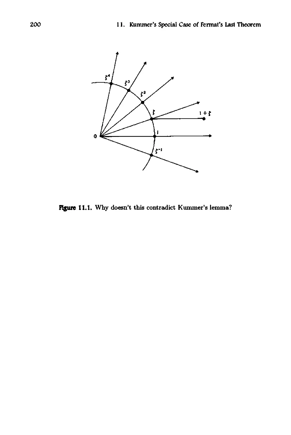
concerns the structure of subgroups:
Theorem 1.16. Every subgroup H of a free abelian group G of rank n is
free of rank s  n. Moreover there exists a basis Ul,. .. ,Un for G and
positive integers al, . . . , as such that al Ul,. . . , asu s is a basis for H.

1.6. Free Abelian Groups
29
Proof: We use induction on the rank n of G. For n = 1, G is infinite
cyclic and the result is a consequence of the subgroup structure of the
cyclic group. If G is rank n, pick any basis WI, . .. ,W n of G. Every h E H
is of the form
h = hlWl +... + hnw n .
Either H = to}, in which case the theorem is trivial, or there exist non-zero
coefficients  for some h E H. From all such coefficients, let ..\( WI. . .. ,w n )
be the least positive integer occurring. Now choose the basis WI> . . . , W n ,
to make ..\(WI,'" , w n ) minimal. Let al be this minimal value, and number
the Wi in such a way that
VI = alwl + P2 W 2 + ... + I3n w n
is an element of H in which al occurs as a coefficient. Let
Pi = alqi + Ti
(2 $ i $ n)
where 0 $ Ti < aI, so that ri is the remainder on dividing Pi byal. Define
UI = WI + (/'lW2 + . . . + qnwn'
Then it is easy to verify that Ul, W2, . ., ,W n is another basis for G. (The
appropriate matrix is clearly unimodular.) With respect to the new basis,
VI = alul + r2W2 + .. . + rnw n .
By the minimality of al = ..\(wI.'" ,w n ) for all bases we have
T2 = . . . = Tn = O.
Hence
VI = alUl.
With respect to the new basis, let
H' = {mlul + m2W2 +... + mnW n I ml = O}.
Clearly H'nV 1 = {O}, where VI is the subgroup generated by VI. We claim
tha.t H = H' + VI' For if h E H then
h = 'YIUl + 'Y2 W 2 + ... + 'YnWn
and putting
')'1 = alq + Tl
(0 $ Tl < al)

30
1. Algebraic Background
it follows that H contains
h - qVI = rlUI + 'Y2W2 + '" + 'YnWn
and the minimaJity of al once more implies that rl = O. Hence h-qvl E H'.
lt follows that H is isomorphic to H' x VI and H' is a subgroup of the
group G ' which is free abelian of rank n - 1 with generators W2,... ,W n .
By induction, H' is free of rank:::; n - 1, and there exist bases U2, .. . ,Un
of G' and V2,... 'V 6 of H' such that Vi = aiUi for positive integers ai. The
result follows. 0
From the above two results we can deduce a useful theorem about orders
of quotient groups. In its statement we use IXI to denote the cardinality
of the set X, and Ixi to denote the absolute vall1e of the real number x. No
confusion need arise.
Theorem 1.17. Let G be a free abelian group of rank r, and H a subgroup
of G. Then G / H is finite if and only if the ranks of G and H are equal.
If this is the case, and if G and H have Z-bases X.. ... , X r and YI,... ,Yr
with Yi = E j aijXj, tMn
IG/HI = Idet(aij)l.
Proof: Let H have rank s, and use Theorem 1.16 to choose Z-bases
U..... ,Ur of G and V..... ,V.. of H with Vi = aiUi for 1 :::; i :::; 8. Clearly
G / H is the direct product of finite cyclic groups of orders a., . . . , a.. and
r - 8 infinite cyclic groups. Hence IG / HI is finite if and only if r = s, and
in that case
IG/HI = al... a r .
Now we have
Ut = L bijxj
j
Vi = L: jUj
j
Yi = L£4jVj
j
where the matrices (b ij ) = B and (<4j) = D are unimodular by Lemma
1.15, and

1.6. Free Abelian Groups
31
01
o
02
C = (Cij) =
o
Or
Clearly if A = (aij) we have A = BCD, and hence
det(A) = det(B)det(C)det(D).
So
Idet(A)1 = I:I: 1 II det(C) II :I: 11 = 101...orl = IGIHI
as claimed.
o
For example, if G has rank 3 and Z-basis x, y, z; and if H has Z-basis
3x + y - 2z,
4x - 5y + z,
x +7z,
then IG I HI is the absolute value of
3 1-2
4 -5 1
1 0 7
namely 142.
Suppose now that G is a finitely generated group, and let its generators
be WI,'.' , W n where the latter need not be independent. Then we can
define a map f : zn -+ G by:
f(ml"" ,m n ) = m1 W I +... +mnw n .
This is surjective, so G is isomorphic to zn I H where H is the kernel of f.
We can use Theorem 1.16 to choose a new basis UI,' .. , Un of zn in such
a way that 0IUl,... ,a"u" is a basis for H. Let A be the subgroup of Zn
generated by Ul, . . . , u" and B be the subgroup generated by u"+1' . .. ,Un,
then clearly G is isomorphic to (AIH) x B, and so is the direct product of
a finite abelian group AI H and a free group B on n - s generators. Putting
n - 8 = k, we have:

32
1. Algebraic Background
Proposition 1.18. Every finitely generated abellan group with n generators
is the direct product of a finite abelian group and a free group on k gener-
ators where k  n. 0
If K is any subgroup of a finitely generated abelian group G, then
writing G = F x B where F is finite and B is finitely generated and free,
we find K  (F n K) x H where H  B. Then F n K is finite and (by
Theorem 1.16) H is finitely generated and free, so we find K is finitely
generated. Hence we have:
Proposition 1,19, A subgroup of a finitely generated abellan group is finitely
generat«l. 0
Of course the results in this section are not the best possible that can
be proved in finitely generated abeUan group theory. Refinements may
be found in Fraleigh {35] chapter 9 pp. 86-93. The results that we have
established are ample for our needs in this text, and we will delay no longer
in making a start on the substance of algebraic number theory.
1.7 Exercises
1. Show that Theorem 1.3 becomes false if the word 'finite' is omitted
from the hypotheses.
2. Which of the following polynomials over Z are irreducible?
(a) x 2 + 3
(b) x 2 - 169
(c) x 3 + x 2 + x + 1
(d) x 3 + 2x 2 + 3x + 4.
3. Write down some polynomials over Z and factorize them into irre-
ducibles.
4. Does Theorem 1.5 remain true over a field of characteristic p > O?
5. Find the minimunl polynomial over Q of
(i) (1 + i)/12
(ii) i + J2
(Hi) e 21fi / 3 + 2.

1.7. Exercises
33
6. Find the degrees of the following field extensions:
(a) Q(v7) : Q
(b) C( v7) : C
(c) Q(V5, v7,v'35): Q
(d) R(O) : R where (p - 70 + 6 = 0 and 0 f. R.
(e) Q(1I') : Q.
7. Let K be the field generated by the elements e 2fri / n (n = 1,2,...).
Show that K is an algebraic extension of Q, but that [K : Q] is not
finite. (It may help to show that the minimum polynomial of e 27ri / p
for p prime is t P - 1 + t P - 2 + .. . + 1.)
8. Express the following polynomials in terms of elemtary symmetric
polynomials, where this is possible.
(a) t 2 + t + t (n = 3)
(b)tf+t (n=2)
(c) tlt + t2t + t3t (n = 3)
(d) tl + t + t (n = 3).
9. A polynomial belonging to Z[tJ,. . . ,tn] is said to be antisymmetric if
it is invariant under even permutations of the variables, but changes
sign under odd permutations. Let
 = II (ti - tj)'
i<j
Show that  is antisymmetric. If f is any antisymmetric polyno-
mial, prove that f is expressible as a polynomial in the elementary
symmetric polynomials, together with. (Hint: consider f /.)
10. Find the orders of the groups G / H where G is free abelian with
Z-basis x, y, z and H is generated by:
(a) 2x, 3y, 7z
(b) x + 3y - 5z, 2x - 4y, 7x + 2y - 9z
(c) x
(d) 41x + 32y - 999z, 16y + 3z, 2y + 111z
(e) 41x + 32y - 999z.
11. Let K be a field. Show that M is a K-module if and only if it is a
vector space over K. Show that the submodules of M are precisely
the vector subspaces. Do these statements remain true if we do not
use convention (d) (page 25) for modules?

34
1. Algebraic Background
12. Let Z be a Z-module with the obvious action. Find all the submod-
ules.
13. Let R be a ring, and let M be a finitely generated R-module. Is it true
that M necessarily has only finitely many distinct R-submodules? If
not, is there an extra condition on R which will lead to this conclu-
sion?
14. An abelian group G is said to be torsion-free if 9 E G, g¥:O and
kg = 0 for k E Z implies k = O. Prove that a finitely generated
torsion-free abelian group is a finitely generated free group.
15. By examining the proof of Theorem 1.16 carefully, or by other means,
prove that if H is a subgroup of a free group G of rank n then there
exists a basis Ul,... , Un for G and a basis Vb" . ,V" for H where
8  n and Vi = a,u, (1  i  s) where the a, are positive integers
and ai divides ai+l (1 ::; i ::; 8 - 1).

2
Algebraic Numbers
In this chapter We introduce the algebraic numbers as solutions of polyno-
mial equations with integer coefficients. Among these numbers, the major
players are the solutions of equations with integer coefficients whose lead-
ing coefficient is 1. These are the algebraic integers. We shall develop a
theory of factorization of algebraic integers, analogous to factorization of
whole numbers. In many ways the theories are alike, but in at least one es-
sential way-uniqueness of factorization-there are important differences.
Factorization into irreducible elements depends on the ring in which the
factorization is performed. In Z the number 5 is irreducible. The only
ways to write it as a product are trivial: multiply :f:5 and :f:1. However, in
Z[J'S] it can be written as the non-trivial prodl1ct 5 = J'S. J'S; moreover,
it turns out that J5 cannot be further factorized in this ring. Thus 5 is
irreducible in Z, yet reducible in Z[ yS].
To clarify these issues it is therefore essential to specify in which ring
the factorization is to be carried out. The natural context is a ring of
algebraic integers, contained in its associated algebraic nwnber field. We
begin with algebraic number fields that obey a finiteness condition: they
are finite-dimensional as vector spaces over the rationals. It will foUow that
such a field is of the form Q[O] for a single algebraic number O.
We introduce the conjugates of an algebraic number and the discrim-
inant of a basis for Q[O] over Q, using the conjugates of 0 to show that
the discriminant is always a non-zero rational number. Algebraic integers
are defined and shown to form a ring. The ring of algebraic integers in a
nwnber field is shown to have an integral basis whose discriminant is an
integer. This integer is independent of the choice of integral basis and is
caUed the discriminant of the nwnber field.
35

36
2. Algebraic Numbers
Finally, we introduce the norm and trace of an algebraic number, which
prove to be ordinary integers when the algebraic number is an algebraic
integer. Using the norm and trace in later chapters we shall be able to
translate statements about algebraic integers into statements about ordi-
nary integers which are easier to handle.
2.1 Algebraic Numbers
A complex number a will be called algebraic if it is algebraic over Q,
that is, it satisfies a non-zero polynomial equation with coefficients in Q.
Equivalently (clearing out denominators) we may assume the coefficients
to be in Z. We let A denote the set of algebraic numbers. In fact A is a
field, by virtue of:
Theorem 2.1. The set A of algebraic numbers is a sub field of the complex
field C.
Proof: We use Theorem 1.11, which in this case says that a is algebraic
if and only if [Q(a) : Q] is finite. Suppose that a, {3 are algebraic. Then
[Q (a, (3) : Q] = [Q (a, (3) : Q (a)] IQ (a) : Q]
Now since {3 is algebraic over Q it is certainly algebraic over Q(a), so the
first factor on the right is finite; and the second factor is also finite. Hence
IQ(a,{3) : Q] is finite. But each of a + {3, a - {3, a{J, and (for (3:f. 0) al{3
belongs to Q(a, {3). So all of these are in A, and the theorem is proved. 0
The whole field A is not as interesting, for us, as certain of its subfields.
We define a number field to be a subfield K of C such that [K : Q] is finite.
This implies that every element of K is algebraic, and hence K  A.
The trouble with A is that [A : Q] is not finite (see Chapter 1, Exercise
7, or Stewart [71], Exercise 4.8, p. 55). If K is a nwnber field then K =
Q(ai'" . , an) for finitely many algebraic numbers aJ,.. . , an (for instance,
a basis for K as vector space over Q). We can strengthen this observation
considerably:
Theorem 2.2. If K is a number field then K = Q(9) for some algebmic
number 9.
Proof: Arguing by induction, it is sufficient to prove that if K = K 1 (a, (3)
then K = K 1 (9) for some 9, (where Kl is a sub-field of K). Let p and

2.1. Algebraic Numbers
37
q respectively be the minimum polynomials of Ol,{J over Kl, and suppose
that over C these factorize as
P (t) = (t - Old... (t - Ol n ),
q(t) = (t - {JI).. . (t - {Jm),
where we choose the numbering so that Oll = Ol, /31 = {J. By Corollary 1.6
the Oli are distinct, as are the {Jj. Hence for each i and each k :f. 1 there is
at most one element x E K 1 such that
ai + x/3k = al + X/3I'
Since there are only finitely many such equations, we may choose c :f. 0 in
K 1 , not equal to any of these x's, and then
ai + cf3k :f. al + c/31
for 1 $ i $ n, 2 $ k $ m. Define
8 = a + c/3.
We shall prove that K 1 (9) = KI (a,/3). Obviously K 1 (8)  K1(Ol,{J), and
it suffices to prove that /3 E K 1 (9) since Ol = 8 - c{J.
Now
p(fJ - c(3) = p(Ol) = o.
We define the polynomial
r(t) = p(9 - ct) E KI(9)[tJ
and then {J is a zero of both q(t) and r(t) as polynomials over K 1 (8). Now
these polynomials have only one conunon zero, for if q() = r() = 0 then
 is one of /31,... , {3m and also 8 -  is one of al,'.' , an. Our choice of c
forces  = (3. Let h(t) be the minimum polynomial of (3 over K 1 (9). Then
h(t) I q(t) and h(t) I r(t). Since q and r have just one common zero in C
we must have 8h = 1, so that
h(t) = t + /L
for /L E K 1 (9). Now 0 = h(/3) = {J+/L so that /3 = -/L E K 1 (9) as reql1ired.
o

38
2. Algebraic Numbers
Example 2.3. Q(.;2, ¥5).
We have
0'1 = h'0'2 = -h,
/31 = ,.B2 = w,.B3 = w2
where
w = H -1 + N)
is a complex cube root of 1. The number c = 1 satisfies
O'i + c/3k :/: 0' + c/3
for i = 1,2, k = 2,3; since the number on the left is not real in any of the
four cases, whereas that on the right is. Hence Q(.;2, {IS) = Q(.;2 + {IS).
The expression of K as Q(9) is, of course, not unique; for Q(9) =
Q( -9) = Q(9 + 1) = ... etc.
2.2 Conjugates and Discriminants
If K = Q(9) is a number field there will, in general, be several distinct
monomorphisms (1 : K -+ C. For instance, if K = Q(i) where i = A
then we have the possibilities
(11(x+iy) = x+iy,
(12(X + iy) = x - iy,
for x, y E Q. The full set of such monomorphislns will play a fundamental
part in the theory, so we begin with a description.
Theorem 2.4. Let K = Q(9) be a number field of degree n over Q. Then
there are exactly n distinct monomorphisms (1i : K -+ C (i = 1,... , n).
T elements (1i(9) = 9 i are the distinct zeros in C of the minimum poly-
nomial of9 over Q.
Proof: Let 9 1 , . . . , (In be the (by Corollary 1.3 distinct) zeros of the mini-
mum polynomial p of 9. Then each 9 i also has minimum polynomial p (it

2.2. Conjugates and Discriminants
39
must divide p, and p is irreducible) and so there is a unique field isomor-
phism Ui : Q(9)  Q(9 i ) such that ui(9) = fJ i . In fact, if a E Q(9) then
a = r(9) for a unique r E Q[t] with 8r < n; and we must have
Ui(a) = r(9 i ).
(See Garling [28] Corollary 2 to Theorem 7.4, p. 66; Stewart [71], Theorem
3.8, p. 43.) Conversely if U : K  C is a monomorphism then U is the
identity on Q. Then we have
0= u(P(9» = p(u(9»
so that u(9) is one of the ();, hence U is one of the U;.
o
Keep this notation, and for each a E K = Q( fJ) define the field polyno-
mial of a over K to be
n
fa(t) = II(t - ui(a».
i=1
As it stands, this is in K[t]. In fact more is true:
Theorem 2. 5. T roejJidents of t field polynomial are mtional numbers,
so that fa(t) E Q[t].
Proof: We have a = r(9) for r E Q[t], 8r < n. Now tbe field polynomial
takes the form
fo:(t) = II(t - r(9 i »
i
where the 9 i run through all zeros of the minimum polynomial p of (), whose
coefficients are in Q. It is easy to see that the coefficients of fo:(t) are of
the form
h«()I, . .. , ()n)
where h(tb.. . , t n ) is a symmetric polynomial in Q[t b ... ,t n ]. By Corol-
lary 1.14 the result follows. 0
The elements O'i(a), for i = 1,.. . , n, are called the K-conjugates of a.
Although the (); are distinct (and are the K -conjugates of 9) it is not always
the case that the K-conjugates of a are distinct: for instance ui(l) = 1 for
all i. The precise situation is given by:

40
2. Algebraic Numbers
Theorem 2.6. With the above notation,
(a) The field polynomial fo: is a power of the minimum polynomial Po:,
(b) The K-C()njugates of a are the zeros of Po: in C, each repeated n/m
times where m = Opo: is a divisor of n,
(c) The element a E Q if and only if all of its K -conjugates are equal,
(d) Q(a) = Q(9) if and only if all K -conjugates of a are distinct.
Proof: The main point is (a). Now q = po: is irreducible, and a is a
zero of f = f 0:, so that f = q" h where q and h are coprime and both are
monic. (This follows from factorizing f into irreducibles.) We claim that h
is constant. If not, some ai = O'i(a) = r(9 i ) is a zero of h, where a = r(9).
Hence if get) = h(r(t)) then g(9 i ) = O. Let P be the minimum polynomial
of 9 over Q, and hence also of each 9 j . Then pig, so that g(9j) = 0 for all
j, and in particular g(9) = O. Therefore, h(a) = h(r(O)) = g(9) = 0 and so
q divides h, a contradiction. Hence h is constant and monic, so h = 1 and
f=q".
(b) is an immediate consequence of (a) on referring to the definition of
the field polynomial.
To prove (c), it is clear that a E Q implies O'i(a) E Q. Conversely if all
0' i (a) are equal then, since the zeros of q = Po: are distinct and f 0: = q",
then 8q = 1 and so a E Q.
Finally for (d): if all O'i(a) are distinct then OpO'. = n, and hence
[Q(a): QI = n = [Q(O) : QI. This implies that Q(a) = Q(9). Conversely if
Q(a) = Q(9) then Opo; = n and so the O'i(a) are distinct. 0
WarniJtg. Note that the K-conjugates of a need not be elements of K.
Even the 9 i need not be elements of K. For example, let 9 be the real cube
root of 2. Then Q(9) is a subfield of R. The K-conjugates of 9, however,
are fJ, w9, w 2 9, where w = (-1 + .t=3). The last two of these are nonreal,
hence do not lie in Q( 9).
Still with K = Q(9) of degree n, let {ai"" , an} be a basis of K (as
vector space over Q). We define the discriminant of this basis to be
 [aI, ... ,an] = {det[O'i(aj)]}2.
If we pick another basis {.6I," . ,.6n} then
(2.1)
n
.6k = L Ci.l:ai
i=1
(Cik E Q)
for k = 1, . . . ,n, and
det(cik) ¥: O.

2.2. Conjugates and Discriminants
4(
The product formula for determinants, and the fact that the (T i are monomor-
phisms (and hence the identity on Q) shows that
.6.[/h, ... , 'on] = [det(cikW.6.[a., .. . , an]'
Theorem 2.7. The discriminant of any basis for K = Q(O) is rational and
non-zero. If all K -conjugates of 0 are real then the discriminant of any
basis is positive.
Proof: First we pick a basis with which we can compute: the obvious one
is {1,0, ... ,on-I}. If the conjugates of ° are 01,. .. , On then
.6.[1,0,... ,on-I] = (detef)2.
A detenmnant of the form D = det(t!) is called a Vandermonde determi-
nant, and has value
D = II (ti - tj).
li<jn
(2.2)
To see this, think of everything as lying inside Q(tl,'" ,t n ]. Then for
ti = tj the determinant has two equal rows, so vanishes. Hence D is
divisible by each (t i - tj)' To avoid repeating such a factor twice we take
i < j. Then comparison of degrees easily shows that D has no other non-
constant factors; comparing coefficients of tlt. .. t: gives 2.2.
Hence
.6. = .6.[1,0,... ,On-I] = (I1(Oi - OjW,
Now D is antisymmetric in the ti, so that D2 is symmetric. Hence by the
usual argument on symmetric polynomials (Corollary 1.14), .6. is rational.
Since the Oi are distinct, .6. '=I o.
Now let {BI"" ,.8n} be any basis. Then
.6.[.8.,.. . ,Pn] = (det Cik)2.6.
for certain rational numbers Cik. and det(cik) '=I 0 so that
.6.[/h, . . . .8n] '=I 0,
and is rational. Clearly if all fJ i are real then .6. is a positive real number,
hence so is .6.(.81.... ,'on]' 0
With the above notation, .6. vanishes if and only if some fJ i is equal to
another OJ. Hence the non-vanishing of .6. allows us to 'discriminate' the
Oi, which motivates calling  the discriminant.

42 2. Algebraic Numbers
2.3 Algebraic Integers
A complex number 0 is an algebraic integer if there is a monic polynomial
p(t) with integer coefficients such that p(O) = O. In other words,
on + a,,_10n-l + . . . + ao = 0
where ai E Z for all i.
For example, 0 = H is an algebraic integer, since 0 2 + 2 = 0; 7" =
!(1 + V5) is an algebraic integer, since 7"2 - 7" - 1 = O. But q, = 22/7
is not. It satisfies equations like 7q, - 22 = 0, but this is not monic; or
like q, - 22/7 = 0, whose coefficients are not integers; but it can be shown
without difficulty that q, does not satisfy any monic polynomial equation
with integer coefficients.
We write B for the set of algebraic integers. One of our aims is to prove
that B is a subring of A. We prepare for this by proving:
Lemma 2.8. A complex number 0 is an algebraic integer if and only if the
additive group generated by all powers 1,0,0 2 ,. .. is finitely generated.
Proof: If 0 is an algebraic integer, then for some n we have
on + an_l0n-1 +... + ao = 0
(2.3)
where the ai E Z. We claim that every power of 0 lies in the additive
group generated by 1,0,... ,0"-1. Call this group r. Then (2.3) shows
that on E r. Inductively, if m  nand 8"' E r then
om+l = Om+1- n (Jn = om+1-n( -a n _l 0n - 1 - '" - ao) E r.
This proves that every power of (J lies in r, which gives one implication.
For the converse, suppose that every power of 0 lies in a finitely gen-
erated additive group G. The subgroup r of G generated by the powers
1, (J, 0 2 ,. .. ,(In must also be finitely generated (Proposition 1.19), so we
will suppose that r has generators Vi, . .. , v n . Each Vi is a polynomial in
o with integer coefficients, so OVi is also such a polynomial. Hence there
exist integers b ij such that
n
OVi = LbijVj.
;=1

2.3. Algebraic Integers
43
This leads to a system of homogeneous equations for the Vi of the form
(b u - 8)Vl + b l2 V2 + . . . + blnv n
b:2IVl + (b 22 - 8)V2 +... + b:2nvn
=
o
o
=
b nl Vl + bn2V2 + . . . + (b nn - 8)v n
=
o.
Since there exists a solution VI, . .. ,V n E C, not all zero, it follows that the
determinant
b u - 8 b lZ bln
l b:22 - () b:2n
b nl
b n2
b nn - 8
is zero. Expanding this, we see that 8 satisfies a monic polynomial equation
with integer coefficients. 0
Theorem 2.9. The algebraic integers form a suhring of the field of algebraic
numbers.
Proof: Let 8,4> E B. We have to show that 4> + 8 and 84> E B. By Lemma
2.8 all powers of () lie in a finitely generated additive subgroup re of C, and
all powers of 4> lie in a finitely generated additive subgroup r 4>' But now
all powers of 8 + 4> and of 8<1> are integer linear combinations of elements
fJiq,; which lie in r er 4>  C. But if r e has generators Vl,. .. ,V n and r 4>
has generators Wi,... , W m , then rer 4> is the additive group generated by
all ViWj for 1  i  n, 1  j  m. Hence all powers of 8 + 4> and of 8<1> lie
in a finitely generated additive subgroup of C, so by Lemma 2.8 (J + 4> and
8<1> are algebraic integers. Hence B is a subring of A. 0
A simple extension of this technique allows us to prove the following
useful theorem.
Theorem 2.10. Let (J be a complex number satisfying a monic polynomial
equation whose coefficients are algebraic integers. Then 8 is an algebraic
integer.
Proof: Suppose that
en + tPn_l8n-l + .. . + tPo = 0
where '!/Jo,... , tPn-l E B. Then these generate a liubring 'II' of B. The
argument of Lenuna 2.8 shows that all powers of 8 lie inside a finitely

44
2. Algebraic Numbers
generated 'I1-submodule M of C, spanned by 1,8,. .. , on-I. By Theorem
2.9, each Wi and all its powers lie inside a finitely generated additive group
r i with generators '"Yij (1  j  ni)' It follows that M lies inside the
additive group generated by all elements
')'ljp')'2j2,... ,')'n_l,i,,_1 0k
(1  ji  ni, 0  i  n - 1, 0  k  n - 1), which is a finite set. So M is
finitely generated as an additive group, and the theorem follows. 0
Theorems 2.9 and 2.10 allow us to construct many new algebraic inte-
gers out of known ones. For instance, .J2 and J3 are clearly algebraic inte-
gers. Then Theorem 2.9 says that numbers such as .J2 + J3, 7.J2 - 41 J3,
(.J2)5(1 + J3)2 are also algebraic integers. And Theorem 2.10 says that
zeros of polynomials such as
t 23 _ (14 + )t9 + ()t5 - 19V3
are algebraic integers. It would not be easy, particularly in the last instance,
to compute explicit polynomials over Z of which these algebraic integers are
zeros; although it can in principle be done by using symmetric polynomials.
In fact Theorems 2.9 and 2.10 can be proved this way.
For any number field K we write
o = K n B,
and call 0 the ring of integers of K. The symbol '0' is a Gothic capital
o (for 'order', the old terminology). In cases where it is not immediately
clear which number field is involved, we write more explicitly 0 K. Since
K and B are subrings of C it follows that 0 is a subring of K. Further
Z  Q  K and Z  B so Z  O.
The following lenuna is easy to prove:
Lemma 2.11. If a E K then for some non-zero c E Z we have ca ED.
Corollary 2.12. If K is a number field tMn K = Q( 8) for an algebraic
integer 8.
Proof: We have K = Q(</» for an algebraic number </> by Theorem 2.2.
By Lemma 2.11, 0 = cfj> is an algebraic integer for some 0 =F c E Z. Clearly
Q(<p) = Q(O). 0
WarniJtg. For 8 E C let us write Z[O] for the set of elements p(8), for
polynomials p E ZIt]. If K = Q(O) where 8 is an algebraic integer then

2.4. Integral Bases
45
certainly.o contains Z[O] since.o is a ring containing O. However, .0 need
not equal Z[9]. For example, Q( v's) is a number field and v's an algebraic
integer. But
l+VS
2
is a zero of t 2 - t - 1, hence an algebraic integer; and it lies in Q( VS) so
belongs to.o. It does not belong to Z[v's].
There is a useful criterion, in terms of the minimum polynomial, for a
number to be an algebraic integer:
Lemma 2.13. An algebraic number a is an algebraic integer if and only if
its minimum polynomial over Q has coefficients in Z.
Proof: Let p be the minimum polynomial of a over Q, and recall that this
is monic and irreducible in Q[tj. If p E Z[t] then a is an algebraic integer.
Conversely, if a is an algebraic integer then q(a) = 0 for some monic
q E Z[t], and plq. By Gauss's Lemma 1.7 it follows that p E Z[t], because
some rational multiple )..p lies in Z[t] and divides q, and the monicity of q
and p implies ).. = 1. 0
To avoid confusion as to the usage of the word 'integer' we adopt the
following convention: a rational integer is an element of Z, and a plain
integer is an algebraic integer. (The aim is to reserve the shorter term
for the concept most often encowltered.) Any remaining possibility of
confusion is eliminated by:
Lemma 2.14. An algebraic integer is a rational number if and only if it is
a rational integer. Equivalently, B n Q = Z.
Proof: Clearly Z  B n Q. Let a E B n Q; since a E Q its minimum
polynomial over Q is t - a. By Lemma 2.13 the coefficients of this are in
Z, hence -a E Z, hence a E Z. 0
2.4 Integral Bases
Let K be a number field of degree n (over Q). A basis (or Q-basis for
emphasis) of K is a basis for K as a vector space over Q. By Corollary
2.11 we have K = Q(O) where 0 is an algebraic integer, and it follows that

46
2. Algebraic Numbers
the minimum polynomial p of 8 has degree n and that {l,O,... , en- 1 } is
a basis for K.
The ring .0 of integers of K is an abelian group under addition. A
Z-basis for (.0, + ) is caned an integral basis for K (or for .0). Thus
{al, . .. , a 8 , } is an integral basis if and only if all ai E .0 and every element
of.o is uniquely expressible in the form
alai + . . . + a"a 8
for rational integers 0.1>." , a". It is obvious from Lemma 2.11 that any
integral basis for K is a Q-basis. Hence in particular s = n. But we have
to verify that integral bases exist. In fact they do, but they are not always
what naively we might expect them to be.
For instance we can assert that K = Q[O] (= Q(8») for an algebraic
integer 8 (Coronary 2.12), so that {I, 0,... ,on-I} is a Q-basis for K which
consists of integers, but it does not fonow that {I, 8,... ,en-I} is an integral
basis. Some of the elements in Q[O] with rational coefficients may also be
integers. As an example, consider K = Q( v's). We have seen that the
element  + hIS satisfies the equation
t2-t+1=0
and so is an integer in Q(v5), but it is not an element of Z[v5].
Our first problem, therefore, is to show that integral bases exist. That
they do is equivalent to the statement that (.0, + ) is a free abelian group
of rank n. To prove this we first establish:
Lemma 2.15. If {ai, . . . , an} is a basis of K consisting of integers, then
the discriminant .6.[a1, . . . , an] is a rational integer, not equal to zero.
Proof: We know that .6. = .6. [a I> . . . , an] is rational by Theorem 2.7, and
it is an integer since the ai are. Hence by Lemma 2.14 it is a rational
integer. By Theorem 2.7, .6. =1= o. 0
Theorem 2.16. Every number field K possesses an integral basis, and the
additive group of.o is free abclian of rank n equal to the degree of K.
Proof: We have K = Q(B) for B an integer. Hence there exist bases for K
consisting of integers: for example {l,B,... , 8 n - 1 }. We have already seen
that such Q-bases need not be integral bases. However, the discriminant of
a Q-basis consisting of integers is always a rational integer (Lemma 2.15),
so what we do is to select a basis {Wl, . .. , w n } of integers for which
1.6.[wl, '" , wnJi

2.4. Integral Bases
47
is least. We claim that this is in fact an integral basis. If not, there is an
integer W of K such that
W = alwl + . . . + anW n
for ai E Q, not all in Z. Choose the numbering so that al  Z. Then
al = a + r where a E Z and 0 < r < 1. Define
'l/Jl = W - awl,
Wi = Wi
(i = 2,.. . ,n).
Then {'l/Jl, . . . ,1/In} is a basis consisting of integers. The determinant rele-
vant to the change of basis from the w's to the 1/J's is
al - a a2 a3 an
0 1 0 0
0 0 1 0 =r,
0 0 0 1
and so
.6.[Wl, . .. ,Wn] = r2.6.[wl, ." , w n ].
Since 0 < r < 1 this contradicts the choice of {w},... ,w n } making
1.6.[w},.. . ,wnll minimal.
It follows that {Wl,... ,w n } is an integral basis, and so (.0, + ) is free
abelian of rank n. 0
This raises the question of finding integral bases in cases such as Q( v5)
where the Q-basis {I, v5} is not an integral basis. We shall consider a more
general case in the next chapter, but this particular example is worth a brief
discussion here.
An element of Q( v's) is of the form p + qv's for p, q E Q, and has
minimum polynomial
(t - P - qV5)(t - p + qV5) = t 2 _ 2pt + (p2 _ 5q2).
Then p + qv5 is an integer if and only if the coefficients 2p, p2 - 5q2 are
rational integers. Thus p = tp where P is a rational integer. For P even,
we have p2 a rational integer, so 5q2 is a rational integer also, implying q
is a rational integer. For P odd, a straightforward calculation (performed
in the next chapter in greater generality) shows q = !Q where Q is also an
odd rational integer.
From this it follows that .0 = z[! + !J5) and an integral basis is
{I,  + tv's}.

48
2. Algebraic Numbers
We can prove this by another route using the discriminant. The two
monomorphisms Q( v5)  C are given by
o.(p + qv5) = p + q/5,
02(P + qv5) = p - qJ5.'
Hence the discriminant .6.[1,! + J51 is given by
I 
1 1  1 2
¥ + i V 5 = 5.
--- "5
2 2 V "
We define a rational integer to be squarefrec if it is not divisible by the
square of a prime. For example, 5 is squarefree, as are 6, 7, but not 8 or 9.
Given a Q-basis of K consisting of integers, we compute the discriminant
and then we have:
Theorem 2. 17. Suppose aI, ... , an E D form a Q-basis for K. If
.6.[al' . ., , an] is squarefree then {a),. . . , an} is an integral basis.
Proof: Let {/31"" ,/3n} be an integral basis. Then there exist rational
integers Cij such that ai = Et;j/3j, and
.6. [a}, ... , an] = (det Cij )2 .6.[.8l. .. . ,/3nl.
Since the left-hand side is squarefree, we must have detcij = :i:1, so that
(Cij) is unimodular. Hence by Lemma 1.15 {al,'" ,an} is a Z-basis for
.0, that is, an integral basis for K. 0
For example, the Q-basis {I,! + !v5} for Q( v5) consists of integers
and has discriminant 5 (calculated above). Since 5 is squarefree, this is an
integral basis. The reader should note that there exist integral bases whose
discriminants are not squarefree (as we shall see later on), so the converse
of Theorem 2.17 is false.
For two integral bases {a 1, . . . ,an}, {.81,. .. ,/3n} of an algebraic num-
ber field K, we have
.6.[a},... ,an] = (:i:1)2.6.[.8I,... ,.8n] = .6.[.8l.'" ,/3n],
because the matrix corresponding to the change of basis is unimodular.
Hence the discriminant of an integral basis is independent of which integral
basis we choose. This common value is called the discriminant of K (or
of D). It is always a non-zero rational integer. Obviously, isomorphic
number fields have the same discriminant. The important role played by
the discriminant will become apparent as the drama unfolds.

2.5. Nomas and Traces
49
2.5 Norms and Traces
These important concepts often allow us to transfoml a problem about
algebraic integers into one about rational integers. As usual, let K = Q(8)
be a number field of degree n and let UI,. . . , Un be the monomorphisms
K -+ C. Now the field polynomial is a power of the minimum polynomial
by Theorem 2.6(a), so by Lemma 2.13 and Gauss's Lemma 1.7 it follows
that a E K is an integer if and only if the field polynomial has rational
integer coefficients. For any a E K we define the norm
n
NK(a:) = II ui(a)
i=1
and trace
n
TK(a) = LUi(a:).
i=1
Where the field K is clear from the context, we will abbreviate the norm
and trace of a to N(a) and T(a) respectively.
Since the field polynomial is
n
fo.(t) = Il(t - ui(a»
i=1
it follows from the remark above that if a is an integer then the norm and
trace of a: are rational integers. Since the Ui are monomorphisms it is clear
that
N(a,B) = N(a)N(,B)
(2.4)
and if a: =1= 0 then N (a) =1= o. If P, q are rational numbers then
T(po + q,B) = pT(a) + qT(,B).
(2.5)
For instance, if K = Q(.,ff) then the integers of K are given by .0 =
Z[.,ff] (as we shall see in Theorem 3.2). The maps Ui are given by
Ul (p + q..;7) = p + q..;7,
U2(P + q..;7) = p - q..;9.
Hence
N(p + q..;9) = p2 - 7q2,
T(p + q..;7) = 2p.

50
2. Algebraic Numbers
Since norms are not too hard to compute (they can always be found
from syuunetric polynomial considerations, often with short-cuts) whereas
discriminants involve complicated work with determinants, the following
result is sometimes useful:
Proposition 2.18. Let K = Q(O) be a number field where 0 has minimum
polynomial p of degree n. The Q-basis {I, 0, ... , on-1} has discriminant
 [1,... ,on-1] = (_1)n(n-1)/2N(Dp(0»
where Dp is the formal derivative of p.
Proof: From the proof of Theorem 2.7 we obtain
 = [l,O,... ,On-1] = II «(h - OJ)2
1i<jn
where 0 1 , . .. , On are the conjugates of O. Now
n
p(t) = II (t - Oi)
;=1
so that
n n
Dp(t) = L II(t - 0;)
j=1 ;=1
;"tj
and therefore
n
Dp(Oj) = II (OJ - 0;).
i=1
;"tj
Multiplying all these equations for j = 1,... , n we obtain
n n
II Dp(Oj) = II (OJ - 6;).
j=1 ;,j=1
;"tj
The left-hand side is N(Dp(6». On the right, each factor (0; - OJ) for i < j
appears twice, once as (6; - 6j) and once as (6j - 6 i ). The product of these
two factors is -(0; _OJ)2. On multiplying up, we get  multiplied by (_1)3
where s is the number of pairs (i,j) with 1 ::; i < j ::; n, which is given by
s = n(n - 1).
The result follows.
o

2.6. Rings of Integers
51
We close this chapter by noting the following simple identity linking the
discriminant and trace:
Proposition 2.19. If {a1,... ,an} is any Q-basis of K, then
[a1'''' ,an] = det(T(aiaj».
Proof: T(aiaj) = E;=l O'r(aiaj) = E;=l O',.(a;)O',.(aj). Hence
[al,...,an] = (det(O'i(aj»))2
= (det(O'j(a;»))(det(O';(aj)))
n
= det(EO'r(a;)O'r(aj))
r=l
= det(T(a;aj))'
o
2.6 Rings of Integers
We now discuss how to find the ring of integers of a given number field.
With the methods available to us, this involves moderately heavy calcu-
lation; but by taking advantage of short cuts the technique can be made
reasonably efficient. In particular we show in Example 2.3 below that not
every nwnber field has an integral basis of the form {I, (},.. . ,()n-1}.
The method is based on the following result:
Theorem 2.20. Let G be an additive subgroup ofD of rank equal to the de-
gree of K, with Z.basis {a},... , an}' Then IDIGI2 divides [a1,'" ,an]'
Proof: By Theorem 1.16 there exists a Z- basis for D of the form {fJl, . . . ,!3n}
such that G has a Z-basis {J.&1.B..... , ltn..6n} for suitable J.&; E Z. Now
[al' . . . , an] = [Pl..61, . . . ,J.&n..6n]
since by Lemma 1.15 a basis-change has a Wlimodular matrix; and the
right-hand side is equal to
(J.&1 ... J.&n)2 [,lh,. .. , .Bn] = (J.&1 . . . J.&n)2 
where  is the discriminant of K and so lies in Z. But
1/11" ./1nl = IDIGI.

52
2. Algebraic Numbers
Therefore
1.0 IGI2 divides  [01'''' , anI.
o
In the above situation we use the notation
G = [a1,'" ,anI.
We then have a generalization of Theorem 2.17:
Proposition 2.21. Suppose that G '" .0. Then there exists an algebmic
integer of the form
1
-(A1al + . . . + AnOn)
p
(2.6)
where 0  Ai  P - 1, Ai E Z, and p is a prime such that p2 divitks G.
Proof: If G '" .0 then IDIGI > 1. Therefore (by the structure theory for
finite abelian groups) there exists a prime p dividing IDIGI and an element
u E DIG such that 9 = pu E G. By Theorem 2.20, r divides G' FUrther,
1 1
u = -g = -(Alai + . . . + AnOn)
p p
since {ai} fonns a Z-basis for G.
o
Note that this really is a generalization of Theorem 2.17: if G is
squarefree then no such p exists, so that G = .0.
We may use Proposition 2.21 as the basis of a trial-and-error search for
algebraic integers in .0 but not in G, because there are only finitely many
possibilities (6). The idea is:
(a) Start with an initial guess G for .0.
(b) Compute G'
(c) For each prime p whose square divides G, test all nwnbers of the
form (2.6) to see which are algebraic integers.
(d) If any new integers arise, enlarge G to a new G' by adding in the
new number (and divide G by p2 to get G')'
(e) Repeat until no new algebraic integers are fOWld.

2.6. Rings of Integers
53
Example 2.22. Find the ring of integers of Q( {IS).
Let 0 E R, 0 3 = 5. The natural first guess is that .0 has Z-basis
{1,0,02}. Let G be the abelian group generated by this set. Let w = e 21ri / 3
be a cube root of unity. We compute
1 0 02 2
G = 1 wi) W 2 (J2
1 w 2 0 w0 2
1 1 1 2
= oG 1 W w 2
1 w 2 W
= 52 . (w 2 + w 2 + w 2 - W - W _ w)2
= 5 2 .3 2 . (w 2 _W)2
= 3 2 .5 2 . (-3)
= _3 3 '5 2 .
By Proposition 2.21 we must consider two possibilities.
(a) Can (X = !P'1 +..\20+..\3(2) be an algebraic integer, for 0    2?
(b) Can (X = t(..\1 +..\20+..\3(2) be an algebraic integer, for 0 ..\i  4?
Consider case (b), which is harder. First use the trace: we have
T«(X) = 3..\1/5 E Z
so that ..\1 E 5Z. Then
(X' = !(..\20 + ..\3(2)
5
is also an algebraic integer.
Now compute the norm of (X'. (It is easier to do this for (x' than for (X
because there are fewer terms, which is why we use the trace first.) We
have
N(aO + blf) = (aD + blP)(awO + bw 2 ( 2 )(aw 2 (J + bw( 2 )
w . w 2 (aO + b(J2)(aO + wb(}2)(aO + w 2 b(}2)
= (aO)3 + (b(}2)3
= 5a 3 + 25b 3 .

54
2. Algebraic Numbers
It follows that for (X to be an algebraic integer, we must have N(a') E Z.
But N((XI) = (5A + 25A)/125 = (A + 5A)/25. One way to finish the
calculation is just to try all cases:
A2 A3 A + 5A Divisible by 25?
0 1 5 No
0 2 40 No
0 3 135 No
0 4 320 No
1 0 1 No
1 1 6 No
1 2 41 No
1 3 136 No
1 4 321 No
2 0 8 No
2 1 13 No
2 2 48 No
2 3 143 No
2 4 328 No
3 0 27 No
3 1 32 No
3 2 67 No
3 3 162 No
3 4 347 No
4 0 64 No
4 1 69 No
4 2 104 No
4 3 199 No
4 4 384 No
Whichever argwnent we use, we have shown that if there are no better
ideas, brute force can suffice. But here it is not hard to find a better idea.
Suppose A + 5A == 0 (mod 25). If A3 == 0 (mod 5), then we must also
have A2 == 0 (mod 5). If not, we have 5 == (-A2/ A3)3 (mod 25). Therefore
5 is a cubic residue (mod 25), that is, is congruent to a cube. The factor
5 shows that we must have 5 == (5k)3 (mod 25), but then 5 == 0 (mod 25),
an impossibility.
Whichever argwnent we use, we have shown that no new (x' occurs in
case (b). The analysis in case (a) is similar, and left as Exercise 6 in this
chapter.

2.6. Rings of Integers
55
Note that it is neassary for N(o-) and T(o-) to be rational integers, in
order for 0- to be an algebraic integer; but it may not be sufficient. If the
use of norms and traces produces a candidate for a new algebraic integer,
we still have to check that it is one-for example, by finding its minimum
polynomial. However, our main use of N(o-) and T(o-) is to rule out possible
candidates, so this step is not always needed.
Example 2.23.
(a) Find the ring of integers of Q( 175) .
(b) Show that it has no Z-basis of the form {I, 0, (J2}.
Solution:
(a) Let t = ?"175 = V(5 2 . 7) . Consider also u = ?'5. 7 2 = ?"245 . We
have
ut = 35
u 2 = 7t
t 2 = 5u.
Let.o be the ring of integers of K = Q( 175 ).
We have u = 35ft E K. But u 3 - 245 = 0 so u E B. Therefore
u E B n K = .0.
A good initial guess is that .0 = G, where G is the abelian group
generated by {I, t, u}.
To see if this is correct, we compute G' The monomorphisms K -+ C
are 0'., 0'2, 0'3 where O'l(t) = t, 0'2(t) = wt, 0'3(t) = w 3 t. Since tu = 35 which
must be fixed by each O'i, we have O'l(U) = U, 0'2(U) = w 2 u, 0'3(U) = WU.
Therefore
G=
1 t
1 wt
1 w 2 t
2
U
w 2 u
wu
which works out as -3 3 . 52 . 7 2 .
There are now three primes to try: p = 3,5, or 7.
If p = 5 or 7 then, as in Example 2.22, use of the trace lets us assume
that our putative integer is l(at + bu) for a, b, E Z. Now
p
N(at + bu.) = 175a 3 + 245b 3
and we must see whether this can be congruent to 0 (mod 53 or 73) for a,
b not congruent to zero.

56
2. Algebraic Numbers
Suppose 175a 3 + 245b 3 = 0 (mod 125), that is, 35a 3 + 49b 3 = 0 (mod
25). Write this as lOa 3 - b 3 = 0 (mod 25). IT a = 0 (mod 5) then also
b = 0 (mod 5). If not, 10 = (bfa)3 (mod 25) is a cubic residue; but then
10 = (5k)3 (mod 25), hence 10 = 0 (mod 25) which is absurd. The case
p = 7 is dealt with in the same way.
When p = 3 the trace is no help, and we must compute the norm of
1
3'(a+bt+cu)
for a , b, c E Z. The calculation is more complicated, but not too bad since
we only have to consider a, b, c = 0, 1,2. No new integers occur.
Therefore D = G as we hoped.
(b) Now we have to show that there is no Z-basis of the form {I, 0,8 2 },
where 8 = a + bt + cu. Note that {I, 0, t}2} is a Z-basis if and only if
{I, 0+ 1, (8+ 1)2} is a Z-basis; so we may without loss of generality asswne
that a = O. Now
(bt + cu)2 = b 2 t 2 + 2bctu + c 2 u 2
= 5b 2 u + 70bc + 7c'2t.
Therefore {l,bt + cu, (bt + cu)2} is a Z-basis if and only if the matrix
1 0 0
o b c
70bc 7 c'2 !)b2
is unimodular; that is,
5b 3 - 7c 3 = :!: 1.
Consider this modulo 7. Cubes are congruent to 0 , 1, or -1 (mod 7), so
we have 5(-1, 0, or 1) =:!: 1 (mod 7), a contradiction.
Hence no such Z-basis exists.
Example 2.24. Find the ring of integers of Q(V2,i).
(Here, our initial guess turns out not to be good enough, so this ex-
ample illustrates how to continue the analysis when this unfortunate event
occurs.)
The obvious guess is {I, /2, i, i/2}. Let G be the group these generate.
We have G = -64, so D may contain elements of the form g (and then
possibly ig or g) for 9 E G. The norm is
N(a + bV2 + ci + diV2) = (a 2 - CJ - 2b 2 + 2<P)2 + 4(oc - 2bd)2.

2.7. Exercises
57
We must find whether this is divisible by 16 for a, b, c, d = 0 or 1, and not
all zero. By trial and error the only case where this occurs is b = d = 1,
a = c = O. So
a=!(8+0i)
may be an integer (where 0 = Vi). In fact
a 2 = i
so that
a 4 + 1 = 0
and a is an integer.
We therefore revise our initial guess to
G' = {I, 0, i, Oi, to(1 + i)}.
Since 2 . !O(l + i) = (J + Oi this has a Z-basis
{I, 0, i, to(l + in.
Now
/j.G' = -64/22 = -16.
A recalculation of the usual kind shows that nothing of the form tg (where
we may now assume that the term in O( 1 + i) occurs with nonzero coeffi-
cient) has integer nonn. So no new integers arise and .0 = G'.
2.7 Exercises
1. Which of the following complex numbers are algebraic? Which are
algebraic integers?
(a) 355/113
(b) e 21ri /23
(c) e i /23
(d) .Jfi + v'i9
(e) (1 + v'i7)/ (2 v'-19 )
(f) V (1 + J2) + V (1 - J2).

58
2. Algebraic Numbers
2. Express Q(J3,) in the form Q(O).
3. Find all monomorphisms Q(.v7) -+ C.
4. Find the discriminant of Q( J3, vis).
5. Let K = Q( {12). Find aU monomorphisms q : K -+ C and the
minimum polynomials (over Q) and field polynomials (over K) of
(i) {12 (ii) J2 (Hi) 2 (iv) /2 + 1. Compare with Theorem 2.6.
6. Complete Example 2.22 above by discussing the case p = 3.
7. Complete Example 2.23 above by discussing the case p = 3.
8. Compute integral bases and discriminants of
(a) Q( /2, v3)
(b) Q( v2, i)
(c) Q()
(d) Q( {12).
9. Let K = Q(8) where 0 E DK. Among the elements
1 .
d(a o + ... + aiO')
(0 1: ai; ao, . .. ,ai E Z), where d is the discriminant, pick one with
minimal value of Ia.d and call it Xi- Do this for i = 1, . .. ,n = [K : Q]
show that {x b . . . , x..} is an integral basis.
10. If 0'1>' .. ,O'n are Q-linearly independent algebraic integers in Q(O),
and if
[0'1> . . . ,O'n) = d
where d is the discriminant of Q( 0), show that {ai,... ,O'n} is an
integral basis for Q(O).
11. If [K : Q) = n, a E Q, show
NK(a) =
TK(O') =
an
,
nO'.
12. Give examples to show that for fixed 0', NK(a) and TK(O') depend
on K. (This is to emphasize that the norm and trace must always be
defined in the context of a specific field K; there is no such thing as
the norm or trace of 0' without a specified field.)

2.7. Exercises
59
13. The norm and trace may be generalized by considering number fields
K 2 L. Suppose K = L(9) and [K : L] = n. Consider monomor-
phisms <7 : K -+ C such. that <7(x) = x for all x E L. Show that there
are precisely n such. monomorphisms <71, . . . ,(Tn and describe them.
For 0 E K, define
n
NK/d o ) = II <7i(O),
i=l
n
TK/d o ) = L(Ti(O).
i=l
(Compared with our earlier notation, we have NK = N K / Q , TK =
T K /Q') Prove that
NK/L( 0 102) = NK/L( o d N K/d 0 2),
TK/L(Ol + (2) = TK/L(ol) + TK/L(02).
Let K = Q( ), L = Q(v3). Calculate NK/L( Ja), TK/L(O) for
o =  and 0 =  + v3.
14. For K = Q(), L = Q(v3), calculate N K /dv3) and NK/Q(v3).
Deduce that NK/da) depends on K and L (provided that 0 E K).
Do the same for T K / L .

3
Quadratic and
Cyclotomic Fields
In this chapter we investigate two special cases of number fields in the
light of our previous work. The quadratic fields are those of degree 2, and
are especially important in the study of quadratic forms. The cyclotomic
fields are generated by pth roots of muty, and we consider only the case
p prime; it is these which are central to Kummer's approach to Fermat's
Last Theorem and playa substantial role in all subsequent work, including
Wiles's proof. We shall return to both types of field at later stages. For
the moment we content ourselves with finding the rings of integers, integral
bases, and discriminants.
3.1 Quadratic Fields
A quadratic field is a number field K of degree 2 over Q. Then K = Q(O)
where 0 is an algebraic integer, and e is a zero of
t 2 + at + b
(a, bE Z).
Thus
-a::!: ..j (a 2 - 4b)
(J= .
2
61

62
3. Quadratic and Cyclotomic i-'ields
Let a 2 - 4b = r 2 d where r, d E Z and d is squarefree. (That this is always
possible follows from prime factorization in Z.) Then
9 = -(1::1:: rv'd
2
and so Q(9) = Q(Vd). Hence we have proved:
Proposition 3.1. The quadratic fields are precisely those of the form Q( Vd)
for d a square free rational integer. 0
Next we determine the ring of integers of Q( Vd), for squarefree d. The
answer, it turns out, depends on the arithmetic properties of d.
Theorem 3.2. Let d be a square free rational integer. Then the integers of
Q(Vd) are:
(a) Z[v'dJ if d 1 (mod 4),
(b) ZH + v'd] if d == 1 (mod 4).
Proof: Every element a e Q( Vd) is of the form a = r + sVd for T, s e Q.
Hence we may write
a + bVd
a=
c
where a, b, c E Z, c > 0, and no prime divides all of a, b, c. Now a is an
integer if and only if the coefficients of the minimum polynomial
(t _ ( a + :Vd ) ) (t _ ( a - :Vd ) )
are integers. Thus
a 2 - b'2d
c 2 E Z,
(3.1)
2a Z
-E .
c
(3.2)
If c and a have a common prime factor p then (3.1) implies that p divides
b (since d is squarefree) which contradicts our previous assumption. Hence
from (3.2) we have c = 1 or 2. If c = 1 then a is an integer of K in any

3.1. Quadratic i-"ields
63
case, so we may concentrate on the case c = 2. Now a and b must both be
odd, and (a 2 - b'2d)/4 E Z. Hence
a 2 - b 2 d == 0 (mod 4).
Now an odd number 2k + 1 has square 4k 2 + 4k + 1 == 1 (mod 4), hence
a 2 == 1 == b'2 (mod 4), and this implies d == 1 (mod 4). Conversely, if d == 1
(mod 4) then for odd a, b we have a an integer because (3.1) and (3.2)
hold.
To sum up: if d == 1 (mod 4) then c = 1 and so (a) holds; whereas if
d == 1 (mod 4) we can also have c = 2 and a, b odd, whence easily (b)
holds. 0
The monomorphisms K  C are given by
0'1 (r + sVd) = r + sv'd,
0'2(r + sVd) = r - sJd.
Hence we can compute discriminants:
Theorem 3.3. (a) If d t 1 (mod 4) then Q(Vd) has an integral bam of
the form {I, Vd} and discriminant 4d. (b)!J d == 1 (mod 4) then Q(Vd)
has an integral basis of the form {I, t + tJd} and discriminant d.
Proof: The assertions regarding bases are clear from Theorem 3.2. Com-
puting discriminants we work out:
1 1 ../d 1 2 =
1 -Vd
1 1 1 + tJd 1 2 =
1 I - IJd
2 2
(-2Jd)2 = 4d,
(-v'd)2 = d.
o
Since the discriminants of isomoThic fields are equal, it follows that for
distinct squarefree d the fields Q("; d) are not isomorphic. This completes
the classification of quadratic fields.
A special case, of historical interest as the first number field to be
studied as such, is the Gaussian field Q(N). Since -1 t 1 (mod 4) the
ring of integers is Z[R] (known as the ring of Gaussian integers) and the
discriminant is -4.
Incidentally, these results show that Theorem 2.17 is not always ap-
plicable: an integral basis can have a discriminant which is not squarefree.
For instance, the Gaussian integers themselves.

64
3. Quadratic and Cyclotomic i-'ields
For future reference we note the norms and traces:
N(r + s.;d) = r 2 - ds 2 ,
T(r + s.;d) = 2r.
We also note some useful terminology. A quadratic field Q(.;d) is said to
be real if d is positive, imaginary if d is negative. (A real quadratic field
contains only real numbers, an imaginary quadratic field contains proper
complex numbers as well.)
3.2 Cyclotomic Fields
A cyclotomic field is one of the form Q«) where ( = e 21ri / m is a primitive
complex mth root of unity. (The nanle means 'circle-cutting' and refers
to the equal spacing of powers of ( around the unit circle in the complex
plane.) We shall consider only the case m = p, a prime number. FUrther,
if p = 2 then ( = -1 so that Q«) = Q, hence we ignore this case and
assume p odd.
Lemma 3.4. The minimum polynomial of ( = e 21ri / p , p an odd prime, over
Q is
f(t) = t p - 1 + t p - 2 + .. . + t + 1.
The degree of Q«) is p - 1.
Proof: We have
t P - 1
f(t) = -.
t-l
Since ( - 1 '" 0 and (P = 1 it follows that f«) = 0, so all we need prove is
that f is ilTeducible. This we do by a standard piece of trickery. We have
f(t + 1) = (t + It - 1 =  (  ) t r - 1 .
Now the binomial coefficient () is divisible by p if 1 S; r S; p - 1, and
m = p is not divisible by p2.
Hence by Eisenstein's criterion (Theorem 1.8) f(t + 1) is irreducible.
Therefore f(t) is irreducible, and is the minimum polynomial of (. Since
of = p - 1 we have IQ«) : Q] = p - 1 by Theorem 1.11. 0

3.2. Cyclotomic Fields
65
The powers (, (2, . .. , (1'-1 are also pth roots of unity, not equal to 1,
and so by the same argument have J(t) as minimum polynomial. Clearly
f(t) = (t - ()(t - (2)... (t _ (1'-1)
(3.3)
and thus the conjugates of ( are (, (2, . . . , (1'-1. This means that the
monomorphisms from Q«() to C are given by
O'i( () = (i
(1 ::; i ::; p - 1).
Because the minimum polynomial J(t) has degree p - 1, a basis for Q«)
over Q is 1, (, . .. , (1'-2, so for a general element
0' = ao + aI( + ... + a p _2(p-2
(ai E Q)
we have
( + ( + ( 1'-2 ) + ( i + ( i(p-2)
O'i ao + .. . IIp-2 = ao . . . + a p -2 .
&om this formula the norm and trace may be calculated using the basic
definitions
1'-1
N(a) = II O'i(a),
i=I
1'-1
T(a) = L O'i(a).
i=I
In particular
N«) = (. (2. ..(1'-1.
Now ( and (i(l ::; i ::; p - 1) are conjugates, so have the same norm, which
can be calculated by putting t = 0 in (3.3) to give
N«) = N«i) = (_1)1'-1
and since p is odd,
N«(i) = 1 (1::; i ::; P - 1).
(3.4)
The trace of (i can be found by a similar argument. We have
T«(i) = T«) = ( + (2 + . . . + (1'-1,

66
3. Quadratic and Cyclotomic i-'ields
and using the fact that
I«) = 1 + ( + . . . + (P-l = 0
we find
T«i) = -1 (1:5 i:5 p-1).
(3.5)
For a E Q we trivially have
N(a) = a P - 1
T(a) = (p - l)a.
Since (P = 1, we can use these formulas to extend (3.4) and (3.5) to
N(C) = 1
for all S E Z
(3.6)
and
T«6) = { -1 if s  0 (mod p)
p - 1 if s == 0 (mod p).
For a general element of Q«), the trace is easily calculated:
(3.7)
T (ai(i) =  T(ai(i)
p-2
= T(ao) + L T(ai(i)
i=l
p-2
= (p - l)ao - L ai
i=O
and so
T (a;c) =1"0 - 
The norm is more complicated in general, but a useful special case is
(3.8)
p-l
N(l - () = IT (1 - (i)
i=l
which can be calculated by putting t = 1 in (3.3) to obtain
p-l
IT (1 - (i) = p,
i=l
(3.9)

3.2. Cyclotomic Fields
67
so
N(l- () = p.
(3.10)
We can put these computations to good use, first by showing that the
integers of Q( () are what one naively might expect:
Theorem 3.5. The ring D of integers of Q( () is Z[(].
Proof: Suppose 0 = ao + aI( + ... + a p _2(p-2 is an integer in Q().
We must demonstrate that the rational numbers ai are actually rational
integers.
For 0  k  p - 2 the element
oC k - o(
is an integer, so its trace is a rational integer. But
T( oC k - a(}
= T(aoC k +... + ak +... + a p _2(p-k-2 - ao( - ... - a p _2(p-l)
= pak - (ao +... + a p -2) - (-ao - ... - a p -2)
= pak.
Hence b", = pa'" is a rational integer.
Put A = 1 - (. Then
[XX = b o + b I ( + ... + b p _ 2 (P-2
= Co + CIA + ... + Cp_2AP-2
(3.11)
where (substituting ( = 1 - A and expanding)
p-2 ( . )
t; = (_l)i  b j E Z.
J=I
Since A = 1 - ( we also have, symmetrically,
p-2 .
b i = (_l)i (  ) Cj.
J='
(3.12)
We claim that all t;, are divisible by p. Proceeding by induction, we may
assume this for all Ci with i :::; k - 1, where 0 :::; k  p - 2. Since Co =

68
3. Quadratic and Cyclotomic i-'ields
b o + . . . + b p - 2 = p( - T(a) + b o ), we have pleo, so it is true for k = O. Now
by (3.9)
p-l
P = IT (1 - (i)
i=l
p-l
= (l-()p-IIl(l+(+...+(i-l)
i=l
= >..p-lK,
(3.13)
where K, E Z[(J .o. Consider (3.11) as a congruence modulo the ideal
(>..k+l) of .0. By (3.13) we have
p == 0 (mod (>..k+l».
and so the left-hand side of (3.11), and the terms up to Ck_l>..k-l, vanish;
further the terms from Ck+1>..k+1 onwards are multiples of >..k+l and also
vanish. There remains:
Ck>..k == 0
(mod (>..k+1».
This is equivalent to
Ck>..k = JI>..k+1
for some JI E .0, from which we obtain
Ck = JI>...
Taking norms we get
-l = N(ck) = N(JI)N(>") = pN(JI),
since N(>") = p by (3.10). Hence pl-l, so pick' Hence by induction pick
for all k, and then (3.12) shows that plbk for all k. Therefore ak E Z for
all k and the theorem is proved. 0
Now we can compute the discriminant.
Theorem 3.6. The discriminant ofQ«), where (= e 2tri / p andp is an odd
prime, is
(_1)(p-l)/2 . pf'-2.

3.3. Exercises
69
Proof: By Theorem 3.5 an integral basis is {I, (,... ,(p-2}. Hence by
Proposition 2.18 the discriminant is equal to
(_1)(p-l)(p-2)/2 . N(D f«»
with f(t) as above. Since p is odd the first factor reduces to (_1)(p-l)/2.
To evaluate the second, we have
t P - 1
f(t) = t=!,
so that
(t - l)ptp-l - (t F - 1)
Df(t) = (t _ 1)2
whence
Df«) = _p(;-1
where ..\ = 1 - ( as before. Hence
o
The case p = 3 deserves special mention, for Q«) has degree p -1 = 2,
so it is a quadratic field. Since
2"i / 3 -1 + A
e =
2
it is equal to Q( A). As a check on our discriminant calculations:
Theorem 3.3 gives -3 (since -3 E 1 (mod 4», and Theorem 3.6 gives
(_1)2/23 1 = -3 as well.
N(Df«» = N(P)N«)P-l
N(..\)
= ( _p)P- 1 1 P - 1
P
= pp-2.
3.3 Exercises
1. Find integral bases and discriminants for:
(a) Q( V'3)
(b) Q(H)

70
3. Quadratic and Cyclotomic i-'ields
(c) Q( v'IT)
(d) Q( y'-ll)
(e) Q( v'6)
(f) Q(H)
2. Let K = Q«) where ( = e21riJ5. Calculate NK(a) and TK(a) for the
following values of a:
(i) (2 (ii) (+ (2 (ill) 1 + (+ (2 + (3 + (4.
3. Let K = Q«) where ( = e21riJp for a rational prime p. In the ring of
integers Z[(], show that a E Z[(I is a unit if and only ifNK(a) =::!: 1.
4. If ( = e 21ri / 3 , K = Q«), prove that the norm of a E Z[(J is of the
form i (a 2 + 3b 2 ) where a, b are rational integers which are either both
even or both odd. Using the result of Exercise 3, deduce that there
are precisely six units in Z[(] and find them all.
5. If ( = e 2 'J(i/5, K = Q«), prove that the norm of a E Z[(] is of the
form! (a 2 - 5b 2 ) where a, b are rational integers. (Hint: in calculating
N(a), first calculate 0'1(a)0'4(a) where O'i«) = (i. Show that this is
of the fonn q + r9 + 84> where q, r, s are rational integers, 9 = ( + (4,
4> = (2 + (3. In the same way, establish 112(a)0'3(a) = q + s9 + r4>.)
Using Exercise 3, prove that Z[(] has an infinite number of units.
6. Let ( = e 21ri / 5 . For K = Q«), use the formula NK(a + b() = (a 5 +
b 5 )f(a + b) to calculate the following norms:
(i) NK« + 2) (ii) NK« - 2) (ill) NK« + 3).
Using the fact that if a/3 = " then NK(a)NK(/3) = NK(-y), deduce
that ( + 2, ( - 2, ( + 3 have no proper factors (i.e. factors which are
not units) in Z[(].
Factorize 11, 31, 61 in Z[(J.
7. If ( = e 2tri / 5 , as in Exercise 6, calculate
(i) NK« + 4) (ii) NK« - 3).
Deduce that any proper factors of ( + 4 in Z[(] have norm 5 or 41.
Given ( - 1 is a factor of ( + 4, find another factor. Verify ( - 3 is a
unit times «2 + 2)2 in Z[(].
8. Show that the multiplicative group of non-zero elements of Z7 is
cyclic with generator the residue class of 3. If ( = e 21li / 7 , define the
monomorphism 0' : Q«)  C by 11«) = (3. Show that all other
monomorphisms from Q«) to C are of the form O'i(l  i  6) where

3.3. Exercises
7(
0'6 = 1. For any a E Q«), define c(a) = a0'2(a)0'4(a), and show
N(a) = c(a) . O'c(a). Demonstrate that c(a) = 0'2c(a) = 0'4c(a).
Using the relation 1 + ( + ... + (6 = 0, show that every element
a E Q«) can be written uniquely as E=I ai(i(ai E Q). Deduce
that c(a) = a l 8 1 + a3 8 2 where 8 1 = (+ (2 + (4,8 2 = (3 + (5 + (6.
Show 8 1 +8 2 = -1 and calculate 8 1 8 2 , Verify that c( a) may be written
in the form be + bl81 where be, bl E Q, and show O'c(a) = be + b182.
Deduce
N(a) = b - bob l + 2b.
Now calculate N« + 5(6).
9. Suppose p is a rational prime and ( = e 2wi / p . Given that the group
of non-zero elements of Zp is cyclic (see Appendix 1, Proposition 6
for a proof) show that there exists a monomorphism 0' : Q«) -+ C
such that O'p-I is the identity and all monomorphisms from Q«)
to C are of the form O'i(1 ::; i ::; p - 1). If p - 1 = kr, define
ck(a) = aO'r(a)0'2r(a). . .O'(k-I)r(a). Show
N(a) = ck(a) . O'ck(a). . .O'T-1ck(a).
Prove every element of Q«) is uniquely of the form Ef::: ai(i, and
by demonstrating that O'T(ck(a» = ck(a), deduce that ck(a) = b 1 111 +
. . . + b", 111" where
111 = (+ O'T«) + 0'2T«) +... + O'(k-l)T«)
and 11i+1 = O'i(l1d.
Interpret these resl1lts in the case p = 5, k = r = 2, by showing
that the residue class of 2 is a generator of the multiplicative group
of non-zero elements of Zs. Demonstrate that c2(a) is of the form
b l 111 + b 2 1J2 where 111 = ( + (4, 1J2 = (2 + (3.
Calculate the nonns of the following elements in Q«):
(i) (+ 2(2 (ii) (+ (4 (iii) 15( + 15(4 (iv) (+ (2 + (3 + (4,
10. In Z[v'=5], prove 6 factorizes in two ways as
6 = 2.3 = (1 + H)(1 - H)
Verify that 2,3, 1 + 1=5,1- 1=5 have no proper factors in Z[AJ.
(Hint: Take norms and note that if I factorizes as I = a{3, then
N(t) = N(a)N({3) is a factorization of rational integers.) Deduce
that it is possible in Z[J=5] for 2 to have no proper factors, yet 2
divides a product a!3 without dividing either a or {3.

4
Factorization into Irreducibles
Now we turn to the vexed question of uniql1eness of factorization in the
ring of integers of an algebraic number field. Historically, experience with
unique factorization of integers and polynomials over a field led to a general
intuition that factorization of algebraic integers should also be unique. In
the early days of algebraic number theory many experts, including Euler,
simply assumed uniqueness withol1t perceiving any need for a proof, and
used it implicitly to 'prove' results that were later found to be based on
a false assumption. The reason for this misconception is subtle, and has
its origins in the definition of a prime number. There are two distinct
properties that can be used to serve as a definition. The most familiar
of these is that a prime number cannot be factorized into the prodl1ct of
two integers other than itself and 1. For a prime p, tlus property may be
written more generally as: (a) If p = ab then one of a or b must be a unit.
In Z the only units are :H, so this reduces to the usual definition. How-
ever, there is a second property of prime numbers that is also of interest,
namely that if a prime number p divides a prodl1ct of two numbers then it
must divide one or the other: (b) If plab then pia or plb.
What fooled our predecessors was that although these properties are
equivalent in the ring of integers-and even in some algebraic number
rings-they are not equivalent in all cases. Of deeper psychological sig-
nificance is that the more familiar property (a) proves to be less powerful
than property (b). Property (b) can be shown in general to imply (a);
moreover, it is property (b) that guarantees uniqueness of factorization,
not the more comfortable property (a). In contrast, property (a) does
not imply (b), and (a) turns out to be inadequate to give uniqueness of
factorization.
73

74
4. Factorization into Irreducibles
The way out of this dilemma is to use the less familiar (b) for the
definition of a prime. An element p satisfying the weaker assumption (a)
is no longer called a prime: it is said to be irredl1cible. (We have used that
word in the same sense earlier in this text.) It can then be proved that if
factorization into primes (defined in the new sense) is pos;;ible, then it is
unique. In contrast, factorization into irreducibles may not be uniql1e even
when it is possible. For instance, if we work in Z[HL then there are two
factorizations 6 = 2.3 and 6 = R. R. Here the elements 2,3, Rare
all irreducible (because they cannot be written as a product of nontrivial
factors in Z[RJ); however, they are not prime. For instance, H is a
factor of 6 = 2 . 3, bl1t it is not a factor of either 2 or 3 in the ring Z[ RJ.
We must therefore proceed with care, and an awareness of precisely
what we are doing. For instance, if we attempt to factorize an element x
in a domain D, it is natural to seek proper factors x = ab (meaning that
neither a nor b is a unit). If either of these factors is further reducible, we
factorize it, and so on, seeking a factorization
x = al a2 . . . an
into factors that cannot be redl1ced any further. Reflecting on what we
are doing, we see that if this search for a factorization terminates, then
it naturally leads to elements which are irreducible (definition (a)) rather
than what we now call primes (definition (b)). So to begin with, we concern
ourselves with factorization into irreducibles.
In general a factorization into irreducibles may not be possible, because
the procedure may continue indefinitely, but it is in a ring D of integers in
a.ny nwnber field. (To prove this we introdl1ce the notion of a noetherian
ring, and show that factorization is always possible if the domain D is
noetherian; we then demonstrate that .0 is noetherian.)
Even thol1gh factorization into irreducibles is always possible in .0, we
give an extensive list of examples where such a factorization is not unique.
In other cases, however, the existence of a generalized version ofthe division
algorithm (which we term a 'El1clidean function') implies that every irre-
ducible is prime. We see that factorization into primes is unique, so some
rings .0 possess unique factorization. In particular we characterize such .0
for the fields Q( v'd) with d a negative rational integer: there are exactly
five of them, corresponding to d = -1, -2, -3, -7, -11. We also prove the
existence of a Euclidean function for some fields Q( v'd) with d positive. In
later chapters we shall see that D may have unique factorization without
possessing a Euclidean function.
To begin the chapter we consider a little history, and look at an example
of the intuitive use of unique factorization, to motivate the ideas.

4.1. Historical Background
75
4.1 Historical Background
In the 18th century and the first part of the 19th there were varying stan-
dards of rigour in nWllber theory. For example Euler, the most prolific
mathematician of the 18th century, was concerned with obtaining results
and would, on occasion, use intuitive methods of proof which the hindsight
of history has shown to be incorrect. For instance, in his famous textbook
011 algebra, he made several elegant applications of Wliql1e factorization to
'prove' number theoretic results in cases where Wliql1e factorization was
false. Gauss, on the other hand, found it necessary to demonstrate rig-
orol1sly that the so-called 'Gaussian integers' Z[i] did factorize l1niql1ely.
In 1847, Lame announced to a meeting of the Paris Academy that he
had proved Fermat's Last Theorem, but his proof was seen to depend on
uniqueness of factorization and was shown to be inadeql1ate. Kummer had,
in fact, published a paper three years earlier that demonstrated the fail-
ure of Wliql1e factorization for cyclotomic integers, thus destroying Lame's
proof. This resl1lt, which formed pal't of his habilitation thesis and was
pl1blished as a pamphlet, went unnoticed at the time.
Eisenstein put his finger on the property that characterizes unique fac-
torization in a letter of 1844 which translates
If one had the theorem which states that the product of two complex
numbers can be divisible by a prime number only when one of the
factors is-which seems completely obvious-then one would have
the whole theory at a single blow; but this theorem is totally false.
By 'the whole theory' he was referring to consequences of unique fac-
torization (in particular Fermat's Last Theorem).
In Eisenstein's letter, 'prime' meant definition (a) of this chapter, and
his comment translated into the terminology of this book is 'if every irre-
ducible is prime, then uniql1e factorization holds'. It is also clear from his
comment that he knew of instances of irreducibles which were not prime,
which gave rise to non-wliql1eness of factorization. AU this must have
seemed very confusing to average 19th century mathematicians who were
used to using intuitive ideas about factorization to demonstrate results. To
give the reader an idea of what it was like, before we explain the theory of
unique factorization, we give a concocted proof of a statement of Fermat
which uses this intuitive language. Fermat's proof has not survived, and
we are not suggesting that it resembled our faulty bl1t instructive attempt
below. Indeed it is not hard to reconstruct a rigorous proof using ideas
that were known to Femlat: See Weil [80].

76
4. Factorization into Irreducibles
A statement of Fermat. The equation y2 + 2 = x 3 has only the integer
solutions y = ::I: 5, x = 3.
Intuitive 'proof'. Clearly y cannot be even, for then the right-hand side
would be divisible by 8, bl1t the left-hand side only by 2. We now factorize
in the ring Z[A], consisting of all a + bH for a,b E Z, to give
(y + H)(y - H) = x 3 .
A common factor c + dA of y + R and y - A would also divide
their sum 2y and their difference 2yC2. Taking norms,
c 2 + 2d 2 14y2 ,
c 2 + 2d 2 18,
hence c 2 + 2<P14. The only solutions of this relation are c = :iI, d = 0,
or c = 0, d = ::1:1, or c = ::1:2, d = O. None of these give proper factors of
y + H, so y + H and y - H are coprime. Now the product of two
coprime numbers is a cube only when each is a cube, so
Y+H= (a+bH)3,
and comparing coefficients of A,
1 = b(3a 2 - 2b 2 )
for which the only solutions are b = 1, a = ::I: 1. Then x = 3, Y = ::1:5. 0
The flaw in this intuitive 'proof', as it stands, is that we are carrying
over the language of factorization of integers to factorization in Z[J=2]
withol1t checking that the l1sl1al properties actl1ally hold in Z[H]. In
this chapter we develop the appropriate theory and investigate when it
generalizes to a ring of integers in a number field.
4.2 Trivial Factorizations
If u is a unit in a ring R, then any element x E R can be trivially factorized
as
x=uy
where y = u-1x. An element y is called an associate of x if x = uy for a
unit u. Recall that a factorization of x E R, x = yz is said to be proper if
neither of y or z are units. If a factorization is not proper (in which case
we shall call it trivial) then it is clear that one of the factors is a wlit and

4.2. Trivial Factorizations
77
the other is an associate of x. Before going on to proper factorizations we
therefore look at elementary properties of units and associates. We denote
the set of units in a ring R by U(R).
Proposition 4.1. The units U(R) of a ring R form a group under multipli-
cation. 0
Examples.
4.1 R = Q. The units are U(Q) = Q\{O}, which is an infinite grol1p.
4.2 R = Z. The units are :i: 1, so U(Z) is cyclic of order 2.
4.3 R = Z[i], the Gaussian integers, a+ ib (a,b E Z). The element a+ ib
is a unit if and only if there exists c + id (c, d E Z) such that
(a + ib)(c + id) = 1.
This implies ac - bd = 1, ad + be = 0, whence c = a/(a 2 + b 2 ),
d = -bJ(a 2 +b 2 ). These have integer solutions only when a 2 + = 1,
so a = :i: 1, b = 0, or a = 0, b = :i: 1. Hence the units are {I, -1, i, -i}
and U(R) is cyclic of order 4.
By using norms, we can extend the results of Example 4.3 to the more
general case of the units in the ring of integers of Q( Vd) for d negative and
squarefree:
Proposition 4.2. The group of units U of the integers in Q( Vd) wM1'e d
is negative and squarefree is as follows:
(a) For d= -1, U = {:i:1,:i:i}.
(b) For d = -3, U = {:i: 1,:i: w,:i: w 2 } where w = e 2ffi / 3 .
(c) For all other d < 0, U = {:i: I}.
Proof: Suppose 0: is a unit in the ring of integers of Q( v'd) with inverse
/3; then 0:/1 = 1, 80 taking norms
N(o:)N(/3) = 1.
But N(o:), N(/3) are rational integers, so N(o:) = :i: 1. Writing 0: = a + bVd
(a, bE Q), then we see that N(o:) = a 2 - dJ>2 is positive (for negative d), so
N (0:) = + 1. Hence we are redl1ced to solving the equation
a 2 - dJ>2 = 1.

78
4. Factorization into Irreducibles
If a, b E Z, then for d = -1 this redl1ces to
a 2 + b 2 = 1
which has the solutions a = :i:1, b = 0, or a = 0, b = :i: 1, already found
in Example 4.3. This gives (a). For d < -3 we immediately conclude that
b = 0 (otherwise a 2 - dJ)2 would exceed 1), so the only rational integer
solutions are a = :i: 1, b = O. If d t 1 (mod 4), then a, bE Z, so the only
solutions are those discovered. For d == 1 (mod 4), however, we must also
consider the additional possibility a = A/2, b = B/2 where both A and B
are odd rational integers. In this case
A 2 - dB 2 = 4.
For d < -3, we deduce B = 0 and there are no additional solutions. This
completes (c). For d = -3, we find additional solutions A = :i: 1, B = :i: 1.
The case A = 1, B = 1 gives
Q = H -1 + H) = e 21ti / 3
which we have denoted by w. The other three cases give -w,w 2 , -w 2 .
These allied with the solutions already found give (b). 0
The general case of units in a ring of integers in a number field will be
postponed until Appendix B. We now return to simple properties of units
and associates.
It follows from Proposition 4.1 that 'being associates' is an eql1ivalence
relation on R. The only associate of 0 is 0 itself. Recall that a non-unit
x E R is called an irredl1cible if it has no proper factors. The zero element 0
= 0.0 has factors, neither of which is a unit, so in particular an irredl1cible
is non-zero. We now list a few elementary properties of units, associates
and irreducibles. To prove some of these we shall require the cancellation
law, so we must take the ring to be an integral domain.
Proposition 4,3. For a domain D,
(a) x is a unit if and only if xiI,
(b) Any two units arc associates and any associate of a unit is a unit,
(c) x, y are associates if and only if xly and ylx,
(d) x is irreducible if and only if every divisor of x is an associate of x
or a unit,
( e) an associate 0/ an irreducible is irreducible.
Proof: Most of these follow straight from the definitions. We prove (c)
which requires the cancellation law. Suppose xly and ylx; then there exist

4.3. Factorization into lrTeducibles
79
a, bED such that y = ax, x = . Sl1bstituting, we find
x = bax.
Now either x = 0, in which case y = 0 also and they are associates, or
x I- 0 and we cancel x to find
1 = ba,
so a and b are units. Hence x, yare associates. The converse is trivial. 0
Some of these ideas may be usefully expressed in terms of ideals:
Proposition 4.4. If D is a domain and x, y are non-zero elements of D
then
(a) xly if and only if (x) 2 (y),
(b) x and y are associates if and only if (x) = (y),
(c) x is a unit if and only if (x) = D,
(d) x is irreducible if and only if (x) is maximal among the proper
principal ideals of D.
Proof: (a) If xly then y = zx E (x) for some zED, hence (y)  (x).
Conversely, if (y)  (x) then y E (x), so Y = zx for some zED.
(b) is immediate from (a).
(c) If x is a unit then xv = 1 for some v E D, hence for any y E D we
have y = xvy E (x) and D = (x). If D = (x) then since 1 E D, 1 = zx for
some zED and x is a unit.
(d) Suppose x is irreducible, with (x)  (y)  D. Then ylx but is
neither a unit, nor an associate of x, contradicting 4.3 (d). Conversely, if
no such y exists, then every divisor of x is either a unit or an associate, so
x is irredl1cible. 0
4.3 Factorization into Irreducibles
In a domain D, if a non-unit is reducible, we can write it as
x = ab.
If either of a or b is reducible, we can express it as a product of proper
factors; then carryon the process, seeking to write
x = PIP2 . . . Pm

80
4. Factorization into Irreducibles
where each Pi is irreducible. We say that facwrization into irreducibles is
possible in D if every xED, not a unit nor zero, is a prodl1ct of a finite
number of irreducibles. In general sl1ch a factorization may not be possible;
and an example is ready to hand, namely the ring B of all algebraic integers.
For if a is not zero or a unit, neither is va. Since a = va. va and va is
a.n integer, it follows that a is not irreducible. Thus B has no irreducibles
at all, but it does have non-zero non-units, so factorization into irredl1cibles
is not possible.
This trouble does not arise in the ring .0 of integers of a number field
(which is another reason why we concentrate on such rings instead of the
whole of B). We will prove the possibility of factorization in D by intro-
ducing a more general notion which makes the arguments involved more
transparent. We define a domain D to be noetherian if every ideal in D
is finitely generated. The adjective commemorates Emmy Noether (1882-
1935) who introduced the concept. Having demonstrated the possibility of
factorization in any noetherian ring, we will show that D is noetherian, so
factorization is possible here also.
Two useful properties, which we shall see are each equivalent to the
noetherian condition are:
The ascending chain condition. Given an ascending chain of ideals:
10 <;, It <;, ... <;, In <;, ...
(4.1)
then there exists some N for which In = IN for all n  N. That is, every
ascending chain stops.
The maximal condition. Every non-empty set of ideals has a maximal
element, that is an element which is not properly contained in every other
element.
We remark that this maximal element need not contain all the other
ideals in the given set: we require only that there is no other element in
the set that contains it.
Proposition 4,5. The following conditions are equivalent for an integral
domain D:
(a) D is noetherian,
(b) D satisfies the ascending chain condition,
(c) D satisMs the maximal condition.
Proof: Assume (a). Consider an ascending chain as in (4.1). Let I =
U:=lIn. Then I is an ideal, so finitely generated: say I = (Xl"" ,x rn ).
Each Xi belongs to some In(i}' If we let N = maxi n(i), then we have
I = IN and it follows that In = IN for all n  N, proving (b).

4.3. Factorization into lrTeducibles
81
Now suppose (b) and consider a non-empty set 5 of ideals. Suppose
for a contradiction that 5 does not have a maximal element. Pick 10 E 5.
Since 10 is not maximal we can pick h E 5 with 10  h. Inductively,
having found In> since this is not maximal, we can pick In+! E 5 with
In  In+!' But now we have an ascending chain which does not stop,
which is a contradiction. So (b) implies (c). (The reader who wishes to
may ponder the use of the axiom of choice in this proof.)
Finally, suppose (c). Let I be any ideal, and let 5 be the set of all
finitely generated ideals contained in I. Then {O} E 5, so 5 is non-empty
and thus has a maximal element J. If J =/: I, pick x E I \ J. Then (J, x) is
finitely generated and strictly larger than J, a contradiction. Hence J = I
and I is finitely generated. 0
Theorem 4,6. If a domain D is noetherian, then factorization into irre-
ducibles is possible in D.
Proof: Suppose that D is noetherian, but there exists a non-unit x=/:O in
D which cannot be expressed as a product of a finite number of irreducibles.
Choose x so that (x) is maximal subject to these conditions on x, which
is possible by the maximal condition. By its definition, this x cannot be
irreducible, SO x = yz where y and z are not units. Then (y) 2 (x) by
4.4(a). If (y) = (x) then x and y are associates by 4.4(b) and this is not
the case because it implies that z is a unit. So (y)  (x), and similarly
(z)  (x). By maximality of (x), we must have
y = Pi... P..,
z = qi... q..,
where each Pi and qj is irreducible. Multiplying these together expresses
x as a product of irreducibles, a contradiction. Hence the assumption that
there existed a non-unit =/: 0 which is not a finite product of irreducibles is
false, and factorization into irreducibles is always possible. 0
We are now in business because:
Theorem 4.7. The ring of integers .0 in a number field K is noetherian.
Proof: We prove that every ideal I of.o is finitely generated. Now (.0, +)
is free abelian of rank n equal to the degree of K by Theorem 2.16. Hence
(1, +) is free abelian of rank s  n by Theorem 1.16. If {Xl,'" , x..} is a
Z-basis for (I, +), then clearly (Xb... ,x..) = I, so I is finitely generated
and .0 is noetherian. 0

82
4. Factorization into Irreducibles
Corollary 4,8. Factorization into irreducibles is possible in .0. 0
To get very far in the theory, we need some easy ways of detecting units
a.nd irreducibles in .0. The norm proves to be a convenient tool:
Proposition 4.9. Let.o be the ring of integers in a number field K, and let
x,y E D. Then
(a) x is a unit if and only ifN(x) =  1,
(b) If x and y are associates, then N(x) =  N(y),
(c) IfN(x) is a rational prime, then x is irreducible in D.
Proof: (a) If xu = 1, then N(x)N(u) = 1. Since N(x), N(u) E Z, we have
N(x) =  1. Conversely, if N(x) =  1, then
0'1 (X)0'2(X) .. .O'n(x) =  1
where the O'i are the monomorphisms K -+ C. One factor, without loss in
generality O'I(X), is equal to x; all the other O'i(X) are integers. Put
u = 0'2(X). . .00n(X).
Then xu = 1, so u = X-I E K. Hence u E KnB = D, and x is a unit.
(b) If x, yare associates, then x = uy for a unit u, SO N(x) = N(uy) =
N(u)N(y) =  N(y) by (a).
(c) Let x = yz. Then N(y)N(z) = N(yz) = N(x) = p, a rational prime;
so one of N(y) a.nd N(z) is p and the other is  1. By (a), one of y and
z is a unit, so x is irreducible. 0
We have not asserted converses to parts (b) and (c) because these are
generally false, as examples in the next section readily reveal.
4.4 Examples of Non-Unique Factorization
into Irreducibles
We say that factorization in a domain D is unique if, whenever
PI . . . Pr = q1 . . . q&
where every Pi and q; is irreducible in D, it follows that
(a) r = s,
(b) There is a pennutation 11' of {I,.. . , r} such that Pi and q...(i) are
associates for all i = 1,. . . , r.

4.4. Examples of Non-Unique Factorization into Irreducibles
83
In view of our earlier remarks about trivial factorizations, this is the best
we can hope for. It says that a factorization into irreducibles (if it exists)
is unique except for the order of the factors and tbe possible presence of
units. Variation to this extent is necessary, since even in Z we have, for
instance,
3 . 5 = 5. 3 = (-3)(-5) = (-5)( -3).
Unfortunately, factorization into irreducibles need not be unique in a ring
of integers of an algebraic number field. Examples are quite easy to come
by if one looks in the right places, and to drive the point home we shall give
quite a lot of them. They will be drawn from quadratic fields, and we state
them  positive theorems. The eiest come from imaginary quadratic
fields:
Theorem 4.10. Factorization into irreducibles is not unique in the ring of
integers of Q(vd) for (at least) the following values of d: -5, -6, -10,
-13, -14, -15, -17, -21, -22, -23, -26, -29, -30.
Proof: In Q( H) we have the factOlizations
6 = 2 . 3 = (1 + /=5)(1 - /=5).
We claim that 2,3,1 + /=5 and 1 - /=5 are ilTeducible in the ring D of
integers of Q( A). Since the norm is given by
N(a + b/=5) = a 2 + 5b 2
their norms are 4, 9, 6, 6, respectively. If 2 = xy where x, y E Dare non-
units, then 4 = N(2) = N(x)N(y) so that N(x) = :1:2, N(y) = :1:2. Similarly
non-trivial divisors of 3 must, if they exist, have norm :1:3, whilst non-trivial
divisors of 1:1: A must have norm :1:2 or :1:3. Since -5  1 (mod 4), the
integers in V are of the form a + bA for a, b E Z (Theorem 3.2) so we
are led to the equations
a 2 + 5b 2 = :1:2 or :I: 3
(a,b E Z).
Now Ibl  1 implies la 2 + 5b 2 1  5, so the only possibility is Ibl = 0; but
then we have a 2 = :1:2 or :1:3, which is impossible in integers. Thus the
putative divisors do not exist, and the four factors are aU irreducible. Since
N(2) = 4, N(1 :I: H) = 6, by Proposition 4.9(b), 2 is not an associate of
1 + J=5 or 1 - A, so factorization is not unique.
The other stated values of d are dealt with in exactly the same way
(with a few slight subtleties noted at the end of the proof) starting from
the following factorizations:

84 4. Factorization into Irreducibles
Q(.;=6): 6 = 2.3 = (.;=6)(-.;=6)
Q( y'-10 ) : 14 = 2.7 = (2 + y'-10 )(2 - y'-10)
Q( y'-13) : 14 =2.7 = (1 + y'-13)( 1- y'-13)
Q(J=I4) : 15 =3.5 = (1 + y'-14)( 1- y'-14)
Q( y'-15) : 4 = 2.2 - c + e- 
- 2 2
Q( y'-17) : 18 = 2.3.3 = (1 + -17)(1 - -17)
Q( J=2I) : 22 = 2.11 = (1 + y'-21)( 1- J=2I)
Q( y'-22) : 26 = 2.13 = (2 + y'-22 )(2 - y'-22)
Q( y'-23) : 6 =2.3 - c + e- A
- 2 2
Q( y'-26 ) : 27 =3.3.3 = (1 + -26)(1 - -26)
Q( y'-29) : 30 = 2.3. 5 = (1 + y'-29)( 1- y'-29)
Q( y'-30) : 34 = 2.17 = (2 + y'-30 )(2 - y'-30) .
Points to note are the following: In cases -15 and -23, note that
d = 1 (mod 4) and be careful. For -26 it is easy to prove 3 irreducible. For
1- y'-26 we are led to the equation N(x)N(y) = 27, so N(x) = :i:9, N(y) =
:i: 3, or the other way rOWld. This leads to the equations a 2 + 26b 2 = :i: 9
or :i: 3. There is a solution for  9, but not for  3, and the latter is
sufficient to show 1+ y'-26 is irreducible. 0
Examining this list, we see that in the ring of integers of Q( J=I7) there
is an example to show that even the number of irreducible factors may differ;
the case Q( y' -26) shows that the number of distinct factors may differ and
that even a (rational) prime power may factorize non-uniquely.
For real quadratic fields there are similar results, but these are harder
to find. Also, since the norm is a 2 - db 2 , it is harder to prove given numbers
irreducible. With the same range of values as in Theorem 4.10 we find:
Theorem 4.11. Factorization into irrcducibks is not unique in the ring of
integers of Q( Jd) for (at least) the following valUe$ of d:
10,15,26,30.
Proof: In the integers of Q( VW) we have factorizations:
6 = 2.3 = (4 + vW)(4 - vW).
We prove 2,3, 4  v'iO irreducible. Looking at norms this amounts to
proving that the equations
a 2 - 10b 2 = :i:2 or :i: 3

4.4. Examples of Non-Unique Factorization into Irreducibles
85
have no solutions in integers a, b. It is no longer helpful to look at the size
of Ibl, because of the minus sign. However, the equation implies
a 2 = :f:2 or :f: 3
(mod 10)
or equivalently
a 2 = 2,3,7 or 8
(mod 10).
The squares (mod 10) are, in order, 0, 1, 4, 9, 6, 5, 6, 9, 4, 1; by a seem-
ingly remarkable coincidence, the numbers we are looking for are precisely
those that do not occur. Hence no solutions exist and the four factors are
irreducible. Now 2 and 4 :f: JW are not associates, since their norms are
4, 6 respectively.
Simila.!!Y we have:
Q(vI5): 10 = 2.5 = (5 + JI5)(5 - JI5)
Q( \1'26) : 10 = 2.5 = (6 + \1'26)(6 - \1'26)
Q(V30): 6 = 2.3 = (6 + V30)(6 - V30).
The reader will find it instructive to do his (or her) own calculations.
o
The values of d considered in Theorelns 4.10 and 4.11 have not, despite
appearances, been chosen at random. If one attempts similar tricks with
other d in the range -30 to 30, nothing seems to work. Thus in Q( v-19)
we get
( 1 + fI9 ) ( 1-fI9 ) =5
but all this shows is that 5 is reducible.
Trying another obvious product in the integers of Q( v-19 ), we find
(2 + v-19 )(2 - v-19) = 23
which just tells us that 23 is also reducible. The case
( 3 + fI9 ) ( 3 - fI9 ) = 7
shows 7 is reducible. After more of these calculations we may alight 011
35 = 5.7 = (4 + v-19 )(4 - v-19 ).
Will this prove non-uniqueness? No, because neither 5 nor 7 is irreducible,
as we have seen; and neither is 4 :f: V -19 .

86
4. Factorization into Irreducibles
The complete factorization of 35 is
C + fI9 ) ( 3 + fI9 ) C - fI9 ) ( 3 - fI9 )
and the two apparently distinct factorizations come from different group-
ings of these in pairs. Eventually one is led to conjecture that the integers
of Q( v' -19 ) have unique factorization. This is indeed true, but we shall
not be in any position to prove it until Chapter 10. In fact the ring of
integers of Q( v'd) for negative squarefree d has unique factorization into
irreducibles if and only if d takes one of the values:
-1, -2, -3, -7, -11, -19, -43, -67, -163.
Numerical evidence available in the time of Gauss pointed to this result.
In 1934 Heilbronn and Linfoot [36) showed that at most one further value
of d could occur, and that Idl had to be very large. In 1952 Heegner [35]
offered a proof but it was thought to contain a gap. In 1967 Stark (69)
found a proof, as did Baker [3] soon after. Finally Birch [5], Deuring [20)
and Siegel [68] filled in the gap in Heegner's proof. The methods of this
book are not appropriate to give any of these proofs, but we will prove in
Chapter 10 that for these nine values factorization is unique.
The situation for positive d is not at all well understood. Factorization
is unique in many more cases, for instance 2, 3, 5, 6, 7, 11, 13, 14, 17, 19,
21, 22, 23, 29, 31, 33,37, 38,41, 43, 46, 47, 53, 57,59, 61,62,67, 69, 71,
73, 77, 83, 86, 89, 93, 94, 97, ... (these being all for d less than 100). It
is not even known whether unique factorization occurs for infinitely many
d> O.
So far we have not proved uniqueness of factorization for the ring of
integers in any number fields (apart from Z). In the next section we intro-
duce a criterion which tells us when factorization is unique in terms of a
special property of the irreducibles.
4.5 Prime Factorization
We have already noted that an irreducible p in Z satisfies the additional
property
plmn implies plm or pin.
In tbis section we shall show tbat it is this property which characterizes
uniqueness of factorization.

4.5. Prime Factorization
87
In a domain D an element x is said to be prime if it is not zero or a
unit and
xlab implies xla or xlb.
Note that the zero element satisfies the given property in a domain, but we
exclude it to correspond with the definition of prime in Z, where 0 is not
usually considered a prime. This convention allows us to state:
Proposition 4.12. A prime in a lkmain D is always irreducible.
Proof: Suppose that D is a domain, xED is prime, and x = ab. Then
xlab, so xla or xlb.
If xla, then a = xc (c E D), so
x = xcb
and cancelling x (which is non-zero), we see that
1 = cb
and b is a unit. In the same way, xlb implies a is a unit.
o
The converse of this result is not true, as Eisenstein lamented in 1844;
in many domains there exist irreducibles that are not primes. For example
in Z[RJ we have
6 = 2.3 = (1 + H)(1 - H),
but 2 does not divide either of 1 + R or 1 - R (as we saw in the
proof of Theorem 4.10). So 2 is an irreducible in Z[A], but not prime.
The factorizations in the proofs of Theorems 4.10 and 4.11 readily yield
other examples. The next theorem tells us that such examples are entirely
typical---every domain with non-unique factorization contains irreducibles
that are not prime:
Theorem 4.13. In a domain in which factorization into irrcducibles is
possible, fadorizatwn is unique if and only if every irreducible is prime.
Proof: Let D be the domain. It is convenient to rephrase the possibility
of factorization for all non-zero xED as
x = UPl . . . Pr

88
4. Factorization into Irreducibles
where U is a unit and Pi,'" ,Pr are irreducibles. When r = 0 this can
then be interpreted as x = u is a unit and when r ;::: 1, then UPl is an
irreducible, so x is a product of the irreducibles UP1,P2,... ,Pro
Now for the proof. Suppose first that factorization is unique and P is
an irreducible. We must show P is prime.
If plab, then pc = ab (c ED).
We need consider only the non-trivial case a  0, b  0 which implies c  0
also.
Factorize, a, b, c into irredudbles:
a = U1Pl" .Pn
b = u2ql . . . qm
C = U3rl . . . r"
where each Ui is a unit and Pi, qi and ri are irreducible. Then
P(U3 r l'" r,,) = (UIPl .. .Pn)(U2ql.', Qm),
and unique factorization implies P is an associate (hence divides) one of the
Pi or qj, so divides a or b. Hence P is prime.
Conversely, suppose that every irreducible is prime. We will demon-
strate that if
U1Pl" .Pm = u2ql" .q..
(4.2)
where Ul, U2 are units and the Pi> qj> are irreducibles, then m = n and
there is a pennutation 11' of {I, . .. , m} such that Pi and Q(i) are associates
(1  i  m).
This is trivially true for m = O.
For m ;::: 1, if (4.2) holds, then Pm IU2ql ... q... But Pm is prime, so (by
induction on n), PmlU2 or Pmlqj for some j. The first of these possibilities
would imply Pm is a unit (by Proposition 4.3(a», so we must conclude that
Pmlqj. We renumber so that j = n, then Pmlqn and qn = PmU where U is a
unit. So
UIPI.. .Pm = U2QI." qn-1UPm
and cancelling Pm,
U1Pl.. .Pm-l = (U2 U )ql ... qn-l'
By induction we may suppose m - 1 = n - 1 and there is a permutation of
1,... ,m-l such that Pi,q(i) are associates (1  i  m-1). We can then
extend 11' to {I,... , m} by defining l!'(m) = m to give the required result.
o

4.5. Prime Factorization
89
A domain D is called a unique factorization domain if factorization into
irreducibles is possible and unique. In a unique factorization domain all
irreducibles are primes, so we may speak of a factorization into irreducibles
as a 'prime factorization'. Theorem 4.13 tells us that a prime factorization
is unique in the usual sense.
We can immediately generalize many ideas on factorization to a unique
factorization domain. For instance, if a, bED, then the highest common
factor h of a, b is defined to be an element that satisfies
(i) hla, hlb,
(ii) If h'la, h'lb, then h'lh.
If a is zero, the highest common factor of a, b is b. For a, b  0, in a
unique factorization domain we can write
a = UlP'.. .p"
b = U2P{'.. . P!."
where Ul,U2 are units and the Pi are distinct (Le. non-associate) primes
with non-negative integer exponents ei, Ii. Then it is ey to show that
h = up;'" . . . P;:'''
where u is any unit and mi, is the smaller of ei, Ii (1  i  n). The highest
common factor is unique up to multiplication by a unit. We can say that
a, bare coprimc if their highest common factor is 1 (or any other unit).
In the same way we can define the wwest common multiple 1 of a, b to
satisfy
(Hi) all, bll,
(iv) If all', bll', then lil'.
For non-zero a, b this is
l - kl k..
- uPl ... Pn
where k i is the larger of Ci, /; ill the factorizations noted above.
Without uniqueness of factorization we can no longer guarantee the
existence of highest common factors and lowest common multiples. (See
Exercise 9 in this chapter.) The language of factorization of integers can
only be carried over sensibly to a unique factorization domain.
In the next section we shall see that if a domain has a property analogous
to the division algorithm, then we can show that every irreducible is prime,
so factorization is unique. In later chapters we shall develop more advanced
techniques which will show unique factorization in a wider class of domains
which do not have this property.

90 4. Factorization into Irreducibles
4.6 Euclidean Domains
The crucial property in the usual proofs of unique factorization in Z or
K{t] for a field K is the existence of a division algorithm. A reasonable
generalization of this is the following:
Let D be a domain. A Euclidean function for D is a function tP
D \ {O} -+ N such that
(i) If a,b E D\{O} and alb then (a)  tP(b),
(ii) If a,b E D\{O} then there exist q,r E D such that a = bq+r where
either r = 0 or f/>(r) < (b).
Thus for Z the function tP(n) = Inl and for KIt], (P) = 8p (the degree
of the polynomial p) are Euclidean functions.
If a domain has a Euclidean function we call it a Euclidean domain. We
shall prove that a Euclidean domain has unique factorization by showing
that every irreducible is prime. The route is this: first we show that in
a Euclidean domain every ideal is principal (a domain with this property
is called a principal ideal domain), then we show that the latter property
implies all irreducibles are primes.
Theorem 4.14. Every Euclidean domain is a principal ideal domain.
Proof: Let D be Euclidean, I an ideal of D. If I = 0 it is principal, so
we may assume there exists a non-zero element x of I. Further choose x
to make (x) as small as possible. If y E I then by (ii) we have y = qx + r
where either r = 0 or q)(r) < q)(x). Now rEI so we cannot have (r) <
(x) because tP(x) is minimal. This means that r = 0, so Y is a multiple of
x. Therefore I = (x) is principal. 0
Theorem 4.15. Every principal ideal domain is a unique factorization
domain.
Proof: Let D be a principal ideal domain. Since this implies D is
noetherian, factorization into irreducibles is possible by Theorem 4.6. To
prove uniqueness we show that every irreducible is prime.
Suppose p is irreducible, then (P) is maximal amongst the principal
ideals of D by Theorem 4.4(d), but since every ideal is principal, this
means that (P) is maximal anlongst all ideals.
Suppose plab but p f a. The fact that p f a implies (p, a)  {p}, so by
maximality, (p, a) = D.
Then 1 E (p,a), so
l=cp+da (C,dED).

4.7. Euclidean Quadratic Fields
91
Multiplying by b yields
b=cpb+dab
and since plab, we find pl(cpb + dab), so plb. This shows p to be prime and
completes the proof. 0
Theorem 4. I 6. A Euclidean domain is a unique facwrization domain.
D
4.7 Euclidean Quadratic Fields
(This subsection may be omitted if desired.)
In order to apply Theorem 4.16 it is necessary to exhibit some number
fields for which the ring of integers is Euclidean. We restrict ourselves to
the simplest case of quadratic fields Q( Jd) for squarefree d, beginning with
the easier situation when d is negative.
Theorem 4.17. The ring of integers .0 of Q( v'd) is EuclUkan for d =
-1, -2, -3, -7, -11, with Euclidean function
4>(a) = IN(a)l.
Proof: To begin with we consider the suitability of the function 4> defined
in the theorem. For this to be a Euclidean function, the following two
conditions must be satisfied for all a,/3 E .0 \ 0:
(a) If al/3 then IN(a)1 ::; IN(/3)I.
(b) There exist j,J E .0 such that a = /3'Y + J where either J = 0 or
IN(J)I < IN(/3)I.
It is clear that (a) holds, for if al/3 then /3 = Aa for A E .0 and then
IN(8) I = IN(aA)1 = IN(a)N(A)1 = IN(a)IIN(A)1
with rational integer values for the various norms.
To prove (b), we consider the alternative statement:
(c) For any E E Q( Jd) there exists K. E .0 such that
IN(E - K.)I < 1.
We shall prove (c) is equivalent to (b). First suppose (b) holds. We know
(Lemma 2.11) that CE E .0 for some C E Z. Applying (b) with a = CE,
/3 = c we get two possibilities:

92
4. Factorization into Irreducibles
(i) J = 0 and c£ = C"( for i E.o. Then f = i E .0 and we may take
K = f.
(ii) Cf = C"y + 6 where IN(J)I < IN(c)l. Now c ¥ 0, so this implies
IN(J/c)1 < 1
which is the same as
IN(f -1)1 < 1
so we may take K = 1. Hence (b) implies (c). To prove that (c) implies (b)
we put f = a/ /3 and argue similarly.
This allows us to concentrate on condition (c»).: which is relatively easy
to handle: in spirit it says that everything in Q(vd) is 'near to' an integer.
Suppose f = r + sVd (r,s E Q). If d :;. 1 (mod 4) we have to find
K = X + yVd (x, y E Z) with
I(r - x)2 - d(s - y)2J < 1.
For d = -1, - 2 we may do this by taking x and y to be the rational integers
nearest to rand s respectively, for then
I(r - X)2 - d(s - y)21 $1 (!)2 + 2 (!)21 = ! < 1.
The remaining three values of d to be considered have dEl (mod 4). In
this case we must find
( 1 + v'd )
K=X+Y 2
(x,y E Z)
such that
I(r - x - ty)2 - d(s - y)21 < 1.
Certainly we can take y to be the rational integer nearest to 2s, so that
12s - yl :5 ; and then we may find x E Z so that Ir - x - !YI $ k. For
d = -3, -7, or -11 this means that
I(r - x - y)2 - d(.s - y)21 :5 It + ttl = H < 1.
The theorem is proved.
o
To complete the picture for negative d we have:
Theorem 4.18. For squarefree d < -11 the ring of integers of Q(Vd) is
not Euclidean.

4.7. Euclidean Quadratic Fields
93
Proof: Let .0 be the ring of integers of Q( Vd) and suppose for a con-
tradiction that there exists a Euclidean function q,. (We do not assume
q, = INI.) Choose a E .0 such that a i- 0, a is not a unit, and q,<a) is
minimal subject to this. Let (3 be any element of .0. Now there exist j, {,
such that (3 = Qj + {, with (, = 0 or q,( (,) < q,( a). By choice of a the latter
condition implies that either {, = 0 or (, is a unit.
For d < -11 it is easy to see that the only units of Q(Jd) are 1
(Proposition 4.2). Hence for every (3 E .0 we have {3 == -1,0, or 1 (mod
(a)) and so 1.0/ (a) I :5 3.
Now we compute 1.0/ {a} I using Theorem 1.17. By Theorem 2.16 (.0, +)
is free abelian of rank 2. If d:/11 (mod 4) a Z-basis for (a) is {a, aVd}
since a Z-basis forD is {I, Vd}. If a = a + bVd (a, bE Z) the Z-basis for
(a) is
{a + bVd, db + aVd}.
Hence by Theorem 1.17 we have
1.0/ (a)1 = II:b : II = la 2 - db 2 1 = IN (a)l.
Similar calculations apply for d == 1 (mod 4) with the same end result
(These calculations are a special case of Corollary 5.10). It follows that
IN(a)1 :5 3. Thus if d:/11 (mod 4) we have la 2 - dltIl :5 3 with a,b E Z. If
d == 1 (mod 4) then a = A/2, b = B/2, for A,B E Z; and then IA2-dB21:5
12. Since d < -11 the only solutions are a =  1, b = 0; so IN(a)1 = 1 and
hence a is a unit. This contradicts the choice of a. 0
These two theorems together show that for negative d the ring of inte-
gers of Q( vd) is Euclidean if and only if d = -1, -2, -3, -7, -11. FUrther,
when it is Euclidean it has as Euclidean function the absolute value of the
norm. For brevity call such fields norm-Euclidean.
The determination of the norm-Euclidean quadratic fields with d p0s-
itive has been a long process involving many mathematicians. Dickson
proved Q (Jd) Euclidean for d = 2,3, 5, 13 (mistakenly asserting there were
no others); Perron added 6, 7, 11, 17,21,29 to the list; Oppenheimer, Re-
mal<:, and Redei added 19, 33, 37, 41, 55, 73. Redei claimed 97 as well
but this was disproved by Barnes and Swinnerton-Dyer. HeilbrOlill proved
the list finite in 1934, and the problem was finished off by Chatland and
Davenport [14} in 1950 (and Inkeri [39] in 1949, independently) who proved:
Theorem 4.19. The ring of integers of Q( Vd), for positive d, is norm-
Euclidean if and only if d = 2,3,5,6, 7, 11, 13, 17, 19,21,29,33,37,
41, 55, 73.

94
4. Factorization into Irreducibles
We cannot prove this theorem here. A good survey of the problem and
related questions, with references, is given by Narkiewicz [54].
Unlike the case d < 0, a real quadratic field Q(d) can be Euclidean but
not norm-Euclidean. This is the case when d = 69. 1 Samuel [65] suggests
that d = 14 might yield another example.
4.8 Consequences of Unique Factorization
When the integers in a number field have unique factorization, we can
carryover many arguments of the type used in the factorization of integers
(taking a little care at first). For example, if the reader refers back to the
proof of the statement of Fermat in Section 4.1 it will become clear that,
since Z[H] (the ring of integers in Q( H)) has unique factorization,
then the intuitive 'proof' given there is, in fact, valid. Let us consider
another example of the same sort of thing, again a statement of Fermat,
which we prove:
Theorem 4.20. The equation
y2 + 4 = z3
(4.3)
has only the inkger solutions y = :1:11, z = 5, or y = ::1:2, Z = 2.
Proof: First suppose y odd, and work in the ring Z[i], which is a unique
factorization domain (Theorem 4.17). Then Equation (4.3) factorizes as
(2 + iy)(2 - iy) = Z3.
A common factor a + ib of 2 + iy, 2 - iy is also a factor of their sum, 4,
and difference, 2y, so taking norms
a 2 + b 2 116,
a 2 + b 2 14y2,
implying
a 2 + b 2 14.
The only solutions of this relation are a = ::I: 1, b = 0, or a = 0, b = ::1:1,
or a = ::I: 1, b = ::I: 1, none of which turn out to give a proper factor a + ib
of 2 + iy. Hence 2 + iy, 2 - iy are coprime. By unique factorization in
Z[i] it follows that if their product is a cube then one is m 3 and the other
1 D.A. CllU"k, Manul/cnpta Mathematica 83 (1994) 327-330.

4.8. Consequences of Unique Factorization
95
c 1 {33 where f is a unit, and a,{3 E Z[i]. But the wilts in Z[i] are  i,  1
(Proposition 4.2), which are all cubes, so
2+iy=(a+ib)3
for some a, b E Z. Taking complex conjugates, we find that
2 - iy = (a - ib)3.
Adding the two equations,
4 = 2a(a 2 - 3b 2 )
so that
a(a 2 - 3b 2 ) = 2.
Now a divides 2, so a =  1 or  2; and the choice of a determines b. It is
easy to see that the only solutions are a = -1, b =  1, or a = 2, b =  1.
Then
Z3 = «a + ib)(a - ib))3 = (a 2 + b 2 )3,
so Z = a 2 + b 2 = 2, 5 respectively. Then y2 + 4 = 8, 125, so y = 2, 1l.
This gives the solutions with y =  11 as the only ones for y odd.
Now suppose y even, so that y = 2Y. Then z is even as well, say
z = 2Z, and
y 2 + 1 = 2Z 3 .
Then Y must be odd, say Y = 2k + 1. The highest common factor of Y + i
and Y - i divides the difference 2i = (1 + i)2. Now 1 + i divides Y + i and
Y - i but (1 + i)2 does not, so the highest common factor of Y + i and
Y - i is 1 + i. Now
(1 + iY)(1 - iY) = 2Z 3
and the common factor 1 + i OCCl1rs twice on the left (bearing in mind that
1 +iY = iCY - i), 1- iY = -iCY +i)). Hence there must be a factorization
1 + iY = (1 + i)(a + ib)3
whence as before
1 = (a + b)(a 2 - 4ab + b 2 )
so a = :i:: 1, b = 0, or a = 0, b = ::I:: 1. These imply y = ::i: 2, which
correspond to the other two solutions stated. 0

96 4. Factorization into Irreducibles
4.9 The Ramanujan-Nagell Theorem
We now give a more intricate and impressive example of how unique factor-
ization properties of algebraic number fields are used to prove theorems on
Diophantine equations. Using the uniqueness of factorization in Q(.,J7;)
NageU verified a conjecture of Ramanujan:
Theorem 4.21, The Qnly SQlutions Qf the equatiQn
x 2 + 7 = 2 n
in integers x, n are:
:I: x = 1 3 5 11 181
n = 3 4 5 7 15.
Proof: We work in Q( .,J7;), whose ring of integers has unique factoriza-
tion by Theorem 4.17. Clearly a solution for x is odd and we will suppose
x is positive.
Assume first that n is even: then we have a factorization of integers:
(2 n / 2 + x)(2 n / 2 - x) = 7
so that
2 n / 2 + x = 7, 2 n / 2 - x = 1,
so
21+n/2 = 8
and n = 4, x = 3.
Now let n be odd, and assume n > 3. We have the factorization into
primes:
2 = ( 1 + f7 ) ( 1- f7 ).
Now x is odd, x = 2k + 1, so x 2 + 7 = 4k 2 + 4k + 8 is divisible by 4. Putting
m = n - 2, we can rewrite the equation to be solved as
x 2 +7
_=2 m
4

4.9. The Ramanujan-Nagell Theorem
97
so that
( X + f1 ) ( X - f1 ) = C + f1 ) m C - f1 ) m
where the right-hand side is a prime factorization. Neither (1 + R)/2
nor (1- R)/2 is a common factor of the terms on the left because such
a factor would divide their difference, R, which is seen to be impossible
by taking norms. Comparing the two factorizations, since the only units
in the integers of Q( R) are :i: 1, (Proposition 4.2), we must have
x :i: f1 =:i: C :i: f1 ) m
from which we derive
r-;; ( 1 + R ) m ( 1- R ) m
:i:v -7 = -
2 2
We claim that the positive sign cannot occur. For, putting () =
a, e-F ) = b, we have
am - b m = a-b.
Then
a 2 E (1 - b)2 E 1
(mod b 2 )
since ab = 2, and so
am E a(a 2 )<m-l}/2 E a
(mod b 2 )
whence
aEa-b
(mod b 2 ),
a contradiction.
Hence the sign must be negative, and expanding by the binomial theo-
rem we have
_2 m - 1 = (7) - ()7 + (;) 7 2 ...:i: (:)7<m-l)/2
so that
_2 m - 1 E m
(mod 7).
(4.4)

98
4. Factorization into Irreducibles
Now 2 6 = 1 (mod 7) and it follows easily that the only solutions of Equation
(4.4) are
m = 3,5, or 13
(mod 42).
We prove that only m = 3,5,13 can occur. It suffices to show that we can-
not have two solutions of the original equation that are congruent modulo
42. So let m, ml be two such solutions, and let 7' be the largest power of
7 dividing m - mI. Then
an'U = ama ml - m = am (t)m 1 -m (1 + H)nu-m. (4.5)
Now
(t)m 1 -m = [(!)6fm l -m)/6 = 1
(mod i+1),
and
( _ c;nml-m r-;;
1+v-7, =1+(ml- m )v-7
(mod 7'+1)
(first raise to powers 7, 'fl,... ,7', then (m - ml)/7'). Since
m l+mN
a = 2 m
(mod 7)
substituting in (4.5) gives
ml - m r-;;
am, =a m + v-7
2 m
(mod 7'+1)
and
bml = bm _ ml - m R
2 m
(mod 7'+1).
But
am _ b m = ami _ b m1
so
(m-ml)H =0
(mod 7'+1).
Since m and ml are rational integers,
m = ml (mod 7'+1)
which contradicts the definition of I. 0

4.10. Exercises
99
4.10 Exercises
1. Which of the following elements of Z[i] are irreducible (i = H):
1 + i, 3 -7i, 5,7, 12i, -4+ 5i?
2. Write down the group of units of the ring of integers of: Q( yCI),
Q(yC2), Q(N), Q(yCS), Q(A).
3. Is the group of units of the integers in Q( v3) finite?
4. Show that a homomorphic image of a noetherian ring is noetherian.
5. Find aU ideals of Z which contain (120).
Show that every ascending chain of ideals of Z starting with (120)
stops, by direct exanlination of the possibilities.
6. Find a ring that is not noetherian.
7. Check the calculations required to complete Theorems 4.10,4.11.
8. Is 10 = (3 + i)(3 - i) = 2.5 an example of non-unique factorization
in Z(i]? Give reasons for your answer.
9. Show that 6 and 2(1 + J=S) both have 2 and 1 + J=5 as factors,
but do not have a highest common factor in Z[ R]. Do they have
a least common multiple? (Consider norms.)
10. Let D be any integral domain. Suppose an element xED has a
factorization
x = UPI . . . Pn
where U is a unit and PI,. .. , Pn are primes. Show that given any
factorization
x = l1ql . . . qm
where 11 is a unit and ql,... ,qm are irreducibles, then m = n and
there exists a permutation 7T of {I,... ,n} such that Pi, q"(i) are
associates (1 :5 i :5 n).
11. Show in Z(J=5) that RI(a + bA) if and only if 51a. Deduce
that yCS is prime in Z[ J=5). Hence conclude that the element 5
factorizes uniquely into irreducibles in Z(J=5) although Z[J=5) does
not have unique factorization.

100
4. Factorization into Irreducibles
12. Suppose D is a unique factorization domain, and a, b are coprime
non-units. Deduce that if
ab=c n
for c E D, then there exists a unit e E D such that ea and e-Ib are
nth powers in D.
13. Let P be an odd rational prime and ( = e 2 "1Ci/p. If a is a prime element
in Z(], prove that the rational integers which are divisible by a are
precisely the rational integer multiples of some prime rational integer
q. (Hint: aIN(a), so a divides some rational prime factor q of N(a).
Now show a is not a factor of any m E Z prime to q.)
14. Prove that the ring of integers of Q(e 21ri / 5 ) is Euclidean.
15. Prove that tbe ring of integers of Q( V2, i) is Euclidean.
16. Let Qz be the set of all rational numbers a/b, where a, b E Z and b
is odd. Prove that Q2 is a domain, and that the only irreducibles in
Q2 are 2 and its associates.
17. Generalize Exercise 16 to the ring Q,.., where 1[' is a finite set of
ordinary primes, this being defined as the set of all rationals a/b with
b prime to the elements of 1['.
18. The following purports to be a proof that in any number field K the
ring of integers contains infinitely many irreducibles. Find the error.
'Assume.o has only finitely many irreducibles PI,... ,Pn. The num-
ber 1 + PI . . . pn must be divisible by some irreducible q, and this
cannot be any of Pi, . . . , Pn. This is a contradiction. Of course the
argument breaks down unless we can find at least one irreducible in
.0; but since not every element of .0 is a unit this is easy: let x be
any non-unit and let P be some irreducible factor of x.'
Hint: The 'proof' does not use any properties of .0 beyond tbe exis-
tence of irreducible factorization and the fact that not every element
is a unit. Now Q2 has these properties. . .
19. Give a correct proof of the statement in Exercise 18.

5
Ideals
After the somewhat traumatic realization that uniqueness of factorization
into irreducibles holds in some rings of integers but not in others, we seek
some way to minimize the damage. Kummer, and then Dedekind, took
steps to develop more insightful theories. Kummer had the bright idea
that if he could not factorize a number uniquely in a given ring of integers,
then perhaps he could extend the ring to a bigger one in which further
factorization might be not only possible, but unique. For example, we
pointed out in chapter 4 that there are two factorizations 6 = 2. 3 =
A . A in j A1 , but A does not divide 2 or 3 in this ring. In
fact, 2/ A = -2/3, and 3/ A = vi -3/2 , neither of which belongs to
Z[Aj. Kummer's idea: throw them into the pot to create a larger ring.
He called the new elements introduced in this way 'ideal numbers'.
Dedekind looked at the same ideas from a different direction, introduc-
ing the notion of an 'ideal' in ring theory, a term arising from the corre-
spondence with Kummer's ideal numbers. In simple ring-theoretic terms,
Dedekind showed that although unique factorization may fail for numbers,
an elegant theory of unique factorization can be developed for ideals. In this
theory, the essential building blocks are 'prime ideals', which are defined
by adapting the definition of a prime element from the previous chapter.
Just as it is often easier to work with both a ring of integers and its corre-
sponding field of quotients, we generalize the concept of ideal to 'fractional
ideal'; this generalization has the advantage that the non-zero fractional
ideals fonn a group under multiplication. From this the uniqueness of fac-
torization into prime ideals follows easily. Several standard consequences
of unique factorization are easily deduced. We define the norm of an ideal
as a generalization of the norm of an element and prove that the new norm
101

102
5. Ideals
has the corresponding multiplicative property. We use this to show that
every ideal can be generated by at most two elements. This tightens the
noose around the neck of non-uniqueness of factorization. In the previous
chapter we saw that factorization of elements is unique in a principal ideal
domain (where every ideal is generated by a single element). We can now
refine this result to show that factorization of elements into irreducibles is
unique in a ring of integers if and only if every ideal is principal.
5.1 Historical Background
To motivate Kummer's introduction of 'ideal numbers' and Dedekind's re-
formulation of this concept in terms of 'ideals', we shall look more closely
at some examples of the failure of unique factorization, in the hope that
some pattern may emerge.
Many of our previous examples exhibit no obvious pattern, but others
do seem to have significant features. For instance, consider:
Q (v'I5) :
Q (v'3O) :
Q (J=IO) :
2.5 = (5 + Yl5)(5 - Yl5)
2.3 = (6 + V30)(6 - V30)
2.7= (2 + \1'-10 )(2 - \1'-10) .
In these we see a curious phenomenon: there is a prime p occurring on the
left, and on the right a factor a + bJd where a and d are multiples of p. One
feels somehow that .jP is a common factor of both sides, but .jP does not
lie in the given number field. As a specific case, consider the first example
where v'5looks a likely candidate for a common factor, but v'5 is not an
element of Q( Ji5). Leaving aside the niceties at the moment, introduce
v'5 into the factorization to get
5 + v'i5 = vS(vS +./3)
5 - Ji5 = V5(V5 - ./3).
Multiplying up and cancelling the 5, we get
2 = (V5 + V3)(V5 - V3).
We can now see that the two given factorizations of 10 are obtained by
grouping the factors in
(J5){ v'5)( J5 + J3)( v'5 - J3)
in two different ways.

5.1. Historical Background
103
Perhaps by introducing new numbers, such as v'5, we can restore unique
factorization. Can our problem be that we are not factorizing in the right
context? In other words, if factorization of some element in the ring of
integers of the given number field K is not lUlique, can we extend K to a
field L where it is? In our example to factorize the element 10 we extended
Q(  to Q( v3, V5). What about the others? The factorizations of 14
in Q( -10) can be fOWld by extending to Q(v'2, H) to get two possible
groupings of the factors in
14 = (v'2)(v'2)(v'2 + H)(v'2 - H).
The case of 6 in Q( V30) is even more interesting: we have
6 = (v'2)( v'2)( v3)()( J6 + V5)( J6 - v'5),
and the last two factors are units.
This is one way of viewing Kummer's theory. One starts with a number
field K and extends to a field L. Then DK  DL. Neither of these rings
of integers need have unique factorization, but an element in D K may
factorize uniquely into elements in DL.
At tbe outset Kummer did not describe tbe theory in this way. His
method involved detailed computations, which are described in Edwards
[21, 22]. This involved him introducing the notion of 'ideal' prime factors
for elements which may have no actual prime factors in D K at all. These
additional 'ideal' numbers may be interpreted as the elements introduced
from D L for factorization purposes.
A more appropriate formulation of the theory by Dedekind in terms
of ideals (in the modern sense, though the origin of the name goes back
to Kummer's theory) has clarified matters. To motivate this approach,
consider a factorization of an element
x= ab
in a ring R. Recalling from Chapter 1 that the product of ideals I J is
just the set of finite sums L XiYi (Xi E I, Yi E J), we see that the ideal
generated by X is the product of the ideals generated by a and by b:
(x) = (a) (b) .
More generally a product
x = PI . . . Pn
of elements in R corresponds to a product of principal ideals
(x) = (Pi) .. . (Pn) .

104
5. Ideals
In considering uniqueness of factorization, the formulation in terms of ideals
is marginally better, for if we replace Pl by UPl where u is a writ, we find
that the ideals (Pl) and (UP1) are the same (Proposition 4.4(b}). Thus if
the factors are unique up to multiplication by units and order, the ideals
{PI} ,. . . ,(Pn) are wrique up to order. By passing to ideals we eliminate
the problems introduced by units.
How does this tie in with the earlier discussion? First consider the
example
10 = (v'5)( v'5)( J5 + J3)( J5 - ./3)
in the integers of Q( J3, J5). Let K = Q( JiS), L = Q( J3, J5); then this
factorization holds in the ring of integers .0 L. In this ring we also have the
corresponding factorization of principal ideals:
(1O) = (J5)(J5)(J5 + J3}(J5 - J3).
We may intersect the ideals in this factorization with .oK, and once more
we get ideals in .0 K, but now these ideals may not be principal. For
instance, let I = (J5 + J3) n .0 K. Then J3( J5 + J3) = JiS + 3 E I,
a.nd v'5( v'5 + J3) = 5 + JiS E I, so their difference
(5 + JiS) - (3 + JiS) = 2 E I.
If I were principal, say I = (a + bJI5), then 2 would be a multiple of
a + bJiS, and taking norms,
a 2 - 15b 2 14.
Suppose that I is principal, say I = (k). Now N(5 + JiS) = 10 and
N(3 + J15) = -6, so N(k)12. We know that N(k) =f:. :l:: 1 since I is proper.
If N(k) = :l:: 2 then there exist a,b E Z with a 2 - 1511 = :l:: 2. But, taken
modulo 5, this leads to a contradiction. So I is not principal.
The moral is now clear. IT we wish to factorize the principal ideal (x)
in a ring of integers .oK, then we may get a unique factorization of ideals,
(x) = II . . . In'
but the ideals h,... ,In may not be principal.
Factorization into ideals proves to be most useful, however; for the ideals
in .0 K are not far off being principal, having (as we shall see) at most two
generators.

5.2. Prime Factorization of Ideals
105
5.2 Prime Factorization of Ideals
Throughout this chapter .0 is the ring of integers of a number field K of
degree n. We use small Gothic letters to denote ideals (and later 'fractional
ideals') of .0. We are interested in two special types of ideal, which we define
in a general situation as follows. Let R be a ring. Then an ideal a of R
is maximal if a is a proper ideal of R and there are no ideals of R strictly
between a and R. The ideal a =f:. R of R is prime if, whenever band care
ideals of R with be  a, then either b  a or e  a.
We can see where the latter definition comes from by considering the
special case where all three ideals concemed are principal, say a = (a),
b = (b), c = (c). Since xly is equivalent to (y)  (x) (Proposition 4.4(a»,
then the statement
be  a implies either b  a or (a
translates into
albc implies either alb or ajc.
If R is an integral domain, then the zero ideal is prime, and here we find
(P) is prime if and only if p is a prime or zero. (See Exercise 5 in this
chapter.) The fact that we exclude 0 from the list of prime elements but
include (0) as a prime ideal is a quirk of the historical development of the
subject. Elements came first and 0 was excluded from the list of primes of
Z. On the other hand, the definition we have given for a prime ideal allows
us to make the following simple characterizations:
Lemma 5.1. Let R be a ring and a an ideal of R. Then
(a) a is maximal if and only if RIa is a fieldi
(b) a is prime if and only if Ria is a domain.
Proof: The ideals of Ria are in bijective correspondence with the ideals
of R lying between a and R. Hence a is maximal if and only if Ria has no
non-zero proper ideals. Now it is easy to show that a ring S has no non-zero
proper ideals if and only if S is a field. Taking S = RIa proves (a).
To prove (b), first suppose a is prime. If x, y E R are such that in Ria
we have
(a+x)(a+y) =0
and then xy E a, so (x) (y)  a. Hence either (x)  a or (y)  a, so either
x E a or yEa. Hence one of (a +x) or (a+ y) is zero in Ria, and therefore
RI a has no zero-divisors so it is a domain. Conversely suppose RIa is a
domain. Then IRlal =f:. 1 so a =f:. R. Suppose if possible that be  a but

106
5. Ideals
b cJ, a, c <t. a. Then we can find elements b E b, e E c, with b, e t. a but
be E a. This means that (a + b) and (a + e) are zero-divisors in Ria, which
is a contradiction. 0
Corollary 5.2. Every maximal ideal is prime.
o
Next we list some important properties of the ring of integers of a
number field:
Theorem 5.3. The ring of integers D of a number field K has the following
properties:
(a) It is a domain, with field 01 fractions K,
(b) It is noetherian,
(c) If a E K satisfies a monic polynomial equation with coefficients in
D then a ED,
(d) Every non-zero prime ideal of D is maximal.
Proof: Part (a) is obvious. For part (b) note that by Theorem 2.16 the
group (D, +) is free abelian of rank n. It follows by Theorem 1.16 that if
a is an ideal of 0 then (a, +) is free abelian of rank  n. Now any Z-basis
for (a, +) generates a as an ideal, so every ideal of D is finitely generated
a.nd D is noetherian. Part (c) is immediate from Theorem 2.10. To prove
part (d) let p be a prime ideal of D. Let 0 =f:. a E p. Then
N = N(a) = al,.. .a n E p
(the ai being the conjugates of a) since al = a. Therefore (N)  p, and
hence D fp is a quotient ring of 01 ND whicb, being a finitely generated
abelian group with every element of finite order, is finite. Since DIp is a
domain by Lemma 5.1(b) and is finite, it is a field by Theorem 1.5. Hence
p is a maximal ideal by Lemma 5.1 (a). 0
The reader should note that part (d) of Theorem 5.3 is by no means
typical of general rings. For example if we take R = R[x, yJ, the ring
of polynomials in indeterminates x, y with real coefficients, then the ideal
(x) is prime but not maximal because RI(x)  R[yJ is a domain which
is not a field. A ring which satisfies the conditions 5.3(a)-(d) is called a
Dedekind ring after the mathematician who made ring-theoretic advances
in this area. The proof of unique factorization of ideals which we shall give
shortly will hold good in all Dedekind rings, although in applications we
shall only require the special case when the ring is a ring D of integers in
a number field.

5.2. Prime Factorization of Ideals
107
To prove uniqueness we need to study the 'arithmetic' of non-zero ideals
of 0, especially their behaviour under multiplication. Clearly this multipli-
cation is commutative and associative with 0 itself as an identity. However,
inverses need not exist, so we do not have a group structure. It turns out
that we can capture a group if we spread our net wider. Note that an ideal
may be described as an O-submodule of 0, so we look at O-submodules of
the field K. The particular subtnodules of interest to give the group struc-
ture we desire will turn out to be characterized by the following property:
an O-submodule Cl of K is called a fmctional ideal of 0 if there exists some
non-zero cEO such that CC1  O. In other words, the set b = CC1 is an ideal
of 0, and Cl = c-Ib; thus the fractional ideals of 0 are subsets of K of the
form c-Ib where b is an ideal of 0 and c is a non-zero element of O. (This
explains the name.)
Example 5.4. The fractional ideals of Z are of the form rZ where r E Q.
Of course if every ideal of 0 is principal, then the fractional ideals are
of the form c- l (d) = c-ldO where d is a generator. By Theorem 5.3(a)
this means the fractional ideals in a principal ideal domain 0 are just aO
where a E K. The interest in fractional ideals is greater because 0 need
not be a principal ideal domain.
In general, an ideal is clearly a fractional ideal and, conversely, a frac-
tional ideal Cl is an ideal if and only if Cl  O. The product of fractional
ideals is once more a fractional ideal. In fact, if ClI = c1lbl, Cl2 = c21b2
where b}, b 2 , are ideals and c}, C2 are non-zero elements of D, then
ClICl2 = (CIC2)-lblb2. The multiplication of fractional ideals is commu-
tative and associative with 0 acting as an identity.
Theorem 5.5. The non-zero fractional ideoo of 0 form an abelian group
under multiplication.
It is convenient to prove this result along with the main theorem of the
chapter:
Theorem 5.6. Every non-zero ideal of  ean be written as a product of
prime ideals, uniquely up to tM order of the factors.
Proof: We shall prove Theorems 5.5 and 5.6 together in a series of steps.
(i) Let Cl  0 be an ideal of O. TMn there exist prime ideals Pl,... ,p,.
such that Pl . . . p,.  Cl.
For a contradiction suppose not. Then since 0 is noetherian (Theorem
5.3 (b» we may choose a maximal, subject to the non-existence of such

108
5. Ideals
p's. Then a is not prime (since we could then take PI = a), so there exist
ideals b, e of 0 with be  a, b i a, cia. Let
al = a + b,
a2 = a + c.
Then ala2  a, al  a, a2  a. By maximality of a there exist prime ideals
Pit... ,P.., P"+l,'" ,Pr such that
PI ... P..  ai,
P..+1 . . . P,.  a2'
Hence
PI .. . Pr  ala2  a
contrary to the choice of a.
(ii) Definition of what will turn out to be the inverse of an ideal:
For each ideal a of 0, define
a-I = {x E Klxa  D}.
It is clear that a-I is an D-submodule. If a i' 0 then for any c E a,
e i' 0, we have ea- I <;: 0, so a-I is a fractional ideal. Clearly 0  a-I, so
a = aD  aa-I. From the definition we have
00- 1 = a-I a  D.
This means that the fractional ideal a«-I is actually an ideal. (Our aim
will be to prove aa- I = D.) A further useful fact for ideals p, a is that
a  P implies 0  p- I  a-I.
(iii) If a is a proper ideal, then a-I  O.
Since a  P for some maximal ideal P, whence p- I  a-I, it is sufficient
to prove p-I i' :!> for P maximal. We must therefore find a non-integer in
p- I . We start with any a E p, a i' O. Using (i) we choose the smallest r
such that
PI.. .p,.  (a)
for PI,... ,Pr prime. Since (a)  P and P is prime (remember maximal
implies prime), some Pi  p. Without loss of generality PI  p. Hence
PI = P since prime ideals in 0 are maximal (Theorem 5.3 (d» and further
P2 .. . p,.$?: (a)
by minimality of r. Hence we can find b E P2... P,. \ (a). But bp  (a)
so OO-Ip  0 and 00- 1 E p- I . But b f. aD and so 00- 1 f. 0, whence
p- 1 i' O.

5.2. Prime Factorization of Ideals
109
(iv) If a is a non-zero ideal and as  a for any subset S  K, then
S .o.
We must show that if a()  a for 8 E S, then 8 ED. Because.o is
noetherian, a = (al,'" ,a,..}, where not all the ai are zero. Then aD  a
implies
al(} = bllal +... + b 1m a m
(b ij E 'D)
4m(} = bmla l + ... + bmma m .
As in Lemma 2.8 we deduce that because the equations
(bll - 8) Xl + . . . + blmX m = 0
b ml Xl + . . . + (b mm - 8) X m = 0
have a non-zero solution Xl = a},... ,X m = am, then the determinant of
the array of coefficients is zero. This gives a monic polynomial equation in
8 with coefficients in .0, hence 8 E .0 by Theorem 5.3(c). (We remark that
we could short-cut part of this proof by noting, as in the proof of Lemma
2.8, that the b ij may be taken to be rational integers which gives (J E .0
directly. )
We are now in a position to take an important step in the proof of
Theorem 5.5:
( v) If P is 4 maximal ideal, then pp -1 = .0.
From (ii), pp-l is an ideal where p  pp-l  .0. Since p is maximal,
pp-l is equal to p or.o. But if pp-l = .0, then (iv) would imply p-l  .0,
contradicting (m). So pp-l = D.
We can now extend (v) to any ideal a:
(vi) For every ideal a =F O. aa- 1 = D.
If not, choose a maximal subject to aa- 1 =F D. Then a  p where p is
maximal. From (ii), .0  p-l  a-I, so
a  ap-l  oa- l  D.
In particular, ap-l  .0 implies ap-l is an ideal. Now we cannot have
a = ap-l, for that would imply p-l  D by (iv), contradicting (iii) once
more. So a  ap-l and the maximality condition on a implies the ideal
ap-l satisfies ap-l (01'-1) -1 = .0.
By the definition of a-I this means
p-l (ap-l) -1  a-I.

110
5. Ideals
Thus
.0 = ap-l (ap-l)-l S; aa- l S;.o
from which the result follows.
(vii) Every fractional ideal a has an inverse a-I such that aa- l = .0.
The set  of fractional ideals is already known to be a commutative
semigroup, so given a fractional ideal €I, we only need to find another frac-
tional ideal a' such that 00/ = .0, then a' will be the required inverse. But
there exists an ideal (oJ and a non-zero element c E .0 such that 0.= c-Ib.
Let a' = cb- 1 , then oa' =  as required.
This, of course, proves Theorem 5.5.
(viii) Every non-zero ideal Q is a product of prime ideals.
IT not, let Q be maximal subject to the condition of not being a product
of prime ideals. Then a is not prime, but we will have a S; P for some
maximal (hence prime) ideal, and as in (vi),
a  ap-l S; .0.
By the maximality condition on a,
ap-l = P2 .. . Pr
for prime ideals P2, . . . ,Pr, whence
Q = PP2 . . . p,..
(ix) Prime factorizatwn is unique.
By analogy with factorization of elements, for ideals a, (oJ we shall say
that Q divides b (written alb) if there is an ideal c such that b = 0.(. This
condition is equivalent to a :2 b since we may then take ( = a-lb. The
definition of prime ideal P shows that if plab then either pia or plb. IT we
now have prime ideals PI,'" ,p,., ql,... , qs with
PI" . Pr = ql ... qs,
then PI divides some qi, so by maximality PI = qi. Multiplying by Pll
and using induction we obtain uniqueness of prime factorization up to the
order of the factors.
This proves Theorem 5.6. 0
In fact, the fractional ideals also factorize uniquely if we allow negative
powers of prime ideals. Namely, if a is a fractional ideal with 0 =f:. c E .0
such that co. is an ideal, we have
(c) = PI . . . P,.,
co. = ql .. . qs,

5.2. Prime Factorization of Ideals
111
and hence
-1 -1
a = PI ... Pr ql... q..
One result in the proofs of Theorems 5.5 and 5.6 which is worth isolating
occurs in step (ix):
Proposition 5.7. For ideals a, b ofD,
alb if and only if a;2 b.
o
This tells us that in D the factors of an ideal b are precisely the ideals
containing b. The definition of a prime ideal P also translates into a notation
directly analogous to that of a prime element:
plab implies pia or plb.
An extended worked example. The factorization of the ideal (18) in
Z( V-17] .
From Theorem 4.10 we have the factorization of elements:
18 = 2.3.3 = (1 + v'-17)( 1 - v'-17 ).
Consider the ideal PI = (2,1 + J=I7) whose generators are both factors
of 18. Clearly 18 E PI. so (18)  p., which means that PI is a factor of
(18). In fact we also have
1 - v' -17 = 2 - (1 + V -17 ) E PI
so
18 = (1 + V-17)( 1 - V-17) E pi
which means that (18)  pi and PI is a factor of (18). Now the elements
of PI are of the form
2(a + b V-17 ) + (1 + V-l7) (c+ d V-17 )
= (2a+c-17d)+ (2b+c+d) v'-17
=r+s V-17
where
r - s = 2a - 2b - 18d,

112
5. Ideals
which is always even. Clearly r may be taken to be any integer and then
s may be any integer of the same parity (odd or even). This implies 1'1
is not the whole ring Z[ y-17J . On the other hand, PI is maximal, for if
m + n y -17 is any element not in PI then one of m, n is even and the other
odd, so
(pi>m + n y-17 ) = Z [J=17].
Similarly, considering
1'2 = (3,1 + J=I7) ,
we find that an element of P2 is of the form
r + s y' -17 = (3a + c - 17d) + (3b + c + d) y' -17
where r - s = 3(a + b - 6<1). Thus r, s can be any integers subject to the
constraint
r = s (mod 3).
Once more we find P2 maximal and 18 = 2 . 3 . 3 E P, so P is a factor
of (18).
Finally, considering
1'3 = (3,1- vC17),
we get another prime ideal such that p is a factor of {18}, and a calculation
similar to the previous ones shows that r + s y -17 E 1'3 if and only if
r+s=O
(mod 3).
Using the factorization theory of Theorem 5.6, we find that
PIPP 2 (18) .
The final step, to show that {18} = PIpP, is best performed using a
counting argwnent. Since every element in Z[.;=I7J is either in PI or of
the form 1 + x for x E Pi> the number of elements in the quotient ring
Z[-17J/Pl is
IZ[ y-17J! Pll = 2.
Similarly
IZ[ y'-17] /Prl = 3 (r = 2,3).

5.2. Prime Factorization of Ideals
113
In the next section we shall call
ID/p\
the norm of the ideal P and write it as N(p). The crucial property of this
new type of norm is that it is multiplicative,
N(ab) = N(a)N(b).
Granted this fact, we can deduce
N(ppp) = 2 2 .3 2 .3 2 = 18 2 .
Now the norm of the ideal (18) is
N «18») = IZ[ y'-17]/ (18) I
and since every element of Z[ y' -171 is uniquely of the form
a + b y' -17 + x
where a, b are integers in the range 0 to 17 and x E (18), we find 18 choices
each for a, b so
N «18») = 18 2 .
Suppose (18) factorizes as
(18) = pppa
for some ideal a. Then taking norms and using the multiplicative property,
we find N(a) = 1, whence a is the whole ring and
(18) = ppp.
(5.1)
If we consider the factorization of elements 18 = 2 . 3 . 3, we obtain
(2) (3)2 = ppp.
(5.2)
By the uniqueness of factorization of ideals, both (2), (3) are products of
prime ideals from the set {PhP2,P3}' Now 2 E Pl but 2  P2, 2 f/. P3. so
Pli (2), P2 f (2), P3 f (2), thus
(2) = pt.
Similarly 3 f/. Pi, 3 E P2, 3 E P3 implies
(3) = P2Pj.

114
5. Ideals
Substituting in Equation (5.2) gives
P q p Zr p ZB _ p Z p Z p Z
1 2 3 - 1 Z 3'
and uniqueness of factorization of ideals implies
q = 2, r = s = 1,
(2) = p, (3) = PZP3'
(5.3)
(The reader may find it instructive to check these by direct calculation.)
A similar argwnent using
(18} = (1 + V -17) (1 - V -17) = PPP (5.4)
where 1+ v-17 E Pl,PZ; 1+ v-17  P3; 1- v-17 E PbP3; 1- v-17  pz
gives
(1 + v-17 ) = PP2' (1- V-17 ) = pp.
Substituting in Equation (5.4) implies m = r = 1, n = s = 2, so
(1 + v-17 ) = PIP, (1- J=I7) = PIP,
(5.5)
From Equations (5.3) and (5.5) we see that the two alternative factor-
izations of the element 18 come from alternative groupings of the ideals:
(18) = (pD (PZP3)Z = (2) (3)z
= (PIP) (PIPn = (1 + F17) (1 - F17) .
We shall consider the norm of an ideal and its multiplicative property
in the next section, once we have dealt with some simple consequences of
unique factorization. Later on we shall develop certain other properties of
the norm which will help streamline the calculations in the above example.
5.3 The Norm of an Ideal
Once unique factorization is proved, several useful consequences follow in
the usual way. III particular, any two non-zero ideals a and b have a
greatest common divisor 9 and a least common multiple ( with the following
properties:
gla, glb;
al(, bl(j
and if
and if
g' has the same properties g'lg;
(' has the same properties (I ('.

5.3. The Norm 0( an Ideal
115
In fact, suppose we factorize a and b into primes as:
IT e.
a = Pi',
b = ITp{i
with distinct prime ideals Pi. Then we clearly have
IT min(e;,/;)
9 = Pi
(= IT p:"ax(ei,f;).
We have useful alternative expressions:
Lemma 5.8. If a and b are ideals of.o, and 9, ( are the greatest common
divisor and least common multiple, respectively, of a and b, then
9 = a + b, ( = an b.
Proof: We know that 11a if and only if 1 :2 a (Proposition 5.7). Hence
9 must be the smallest ideal containing a and b, and c the largest ideal
contained in a and b. The rest is obvious. 0
The proof of Theorem 5.3 shows that if a is a non-zero ideal of .0 then
the quotient ring .0/ a is finite. We define the norm of a to be
N(a) = ID/al.
Then N(o) is a positive integer. There is no reason to confuse this norm
with the old norm of an element N(a) since it applies only to ideals. In fact
there is a connection between the two norms, as we shall see in a moment.
Theorem 5.9.
(a) Every ideal a of .0 with 0 ::/: 0 has a Z-basis {Oh'" ,on} where n
is the degree of K;
(b) We have
[ ] 1/2
N(a) = I  Oh' ,On I
where  is the discriminant of K.
Proof: We know from Theorem 2.16 that (.0, +) is free abeUan of rank
n. Since .0/ a is finite it follows from Theorem 1.17 that (0, +) is free
abelian of rank n, hence has a Z-basis of the form {Ol,'" ,On}. This

116
5. Ideals
proves (a). For part (b) let {Wb'" ,W n } be a Z-basis for .0, and suppose
that ai = ECijWj. Then by Theorem 1.17,
N(a) = ID/al = Idett;jl.
But by the formula before Theorem 2.7 we have
 [a.,..., an] = (detC;j)2  [WI,... ,w n ]
= (N(a»2.
Taking square roots and remembering that N(a) is positive we obtain the
desired result. 0
Corollary 5.10. If a = (a) is a principal ideal then N(a) = IN(a)l.
Proof: A Z-basis for a is given by {awb'" ,awn}' The result follows from
the definition of [ab . . . , an] and Theorem 5.9.
This corollary helps us to make a straightforward calculation of the
norm of a principal ideal.
Example 5.11. If .0 is the ring of integers of Q( Vd) for a square-free
rational integer d, then
N«(a + b.fd) = la 2 - b<fl,
in particular, in .0 = Z [ ..; -17] , then
N ( (18)) = 18 2 .
The new norm, like the old, is multiplicative:
Theorem 5.12. If a and b are non-zero ideals of .0, then
N(ab) = N(a)N(b).
Proof: By lI1liqueness of factorization and induction on the number of
factors, it is sufficient to prove
N(ap) = N(a)N(p)
(5.6)
where p is prime.

5.3. The Norm 0( an Ideal
117
We establish
IDlapl = IDlalla/apl
(5.7)
and
lalapl = ID/pl.
(5.8)
Then Equation (5.6) follows immediately from Equation (5.7), Equation
(5.8), and the definition of the norm.
Equation (5.7) is a consequence of the isomorphism theorem for rings:
Define 4>: D/crp -t Dla by
4>( ap + x) = a + x
then <p is a surjective ring homomorphism with kernel a/ap; Lagrange's
theorem (applied to the additive groups) gives Equation (5.7).
To establish Equation (5.8L first note that Wlique factorization implies
a ::/: ap, so a  ap. Now we show that there is no ideal b strictly between a
and ap, for if
a ;2 b ;2 ap,
then, as fractional ideals,
a-Ia ;2 a- I b ;2 a-lap,
so
D 2a- I ft ;2 p.
Since a-Ib  D, we see that it is actually an ideal, and since p is maximal
(by Theorem 5.3 (d», we have
a- 1 ft = D or a- I b = p
so
b = a or b = ap.
This means that for any element a E a\GP, we have
crp + (a) = a.
(5.9)
Fix such an a and define (J: D -t a/ap by
8(x) = ap + ax,
then 0 is an D-module homomorphism, surjective by Equation (5.9), whose
kernel is an ideal satisfying
p  ker (J.

118
5. Ideals
Now ker 0 ::/:.0 (for that would mean alap  'D/ker8 = 0, which would
contradict a ::/: ap), and P is maximal, so
kerO = p.
Hence DIp  a/ap (as .o-modules), which gives Equation (5.8) and com-
pletes the proof. 0
Example 5.13. Ifj) = Z[ v'-17] , Pi = (2,1 + J=I7), P2 = (3,1 + J=I7),
P3 = (3,1 - yC17), then
N(ppp) = 2 2 . 3 2 . 3 2 = 18 2 .
This particular calculation completes the details of the extended example
in the previous section.
It is convenient to introduce yet another usage for the word 'divides'.
If a is an ideal of.o and b an element of.o such that al (b), then we also
write alb and say that a divides b. It is clear that alb if and only if b E a;
however, the new notation has certain distinct advantages. For example,
if p is a prime ideal and pi (a) (b), then we must have pI (a) or pi (b). Thus
for p prime,
plab implies pia or plb.
This new notation allows us to emphasize the correspondence between fac-
torization of elements and principal ideals which would otherwise be less
evident.
Theorem 5.14. Let a be an ideal oj .0, a::/: O.
(a) IJ N(a) is prime, then so is a.
(b) N(a) is an element of a, or equivalently aIN(a).
(c) If a is prime it divides exactly one rational prime p, and then
N(a) = pm
where m  n, the degree of K.
Proof: For part (a) write a as a product of prime ideals and equate norms.
For part (b) note that since N(a) = IDlal it follows that for any xED we
have N(a)x Ea. Now put x = 1. For part (c) we note that by part (b)
alN( a) = p';k . . . p":'r

5.3. The Norm 0( an Ideal
119
so (considering principal ideals in place of the Pi) we have alpi for some
rational prime Pi. If P and q were distinct rational primes, both divisible
by a, we could find integers u, v such that up + vq = 1, and then deduce
that all, which implies a =.0, a contradiction. Then
N(o)IN«(P» = pn
so that N(a) = pm for some m  n.
o
Example 5.15. If.o = Z[ y'-17] , Pl = (2,1+ J=I7), then because
N(Pl) = 2 we can immediately deduce that Pl is prime. Note that N(pI) =
2 E Pl, as asserted by Theorem 5.14 (b).
Example 5.16. A prime ideal 0 can satisfy
N(o) = pm
where m > 1, which means that a prime ideal does not necessarily have a
norm which is prime; for instance .0 = Z[i], 0 = (3). Here 3 is irreducible
in Z[i], hence prime because Z(i] has unique factorization. It is an easy
deduction (Exercise 1 at the end pf this chapter) that if an element is
prime, so is the ideal it generates. Hence (3) is prime in Z[i], but
N «(3») = 3 2 .
The next theorem collects together several useful finiteness assertions:
Theorem 5.17. (a) Every non-zero ideal of.o has a finite number of
divisors,
(b) A non-zero rational integer belongs to only a finite number of ideals
of.o,
(c) Only finitely many ideals of.o have given norm.
Proof: (a) is an immediate consequence of prime factorization, (b) is a
special case of (a), and (c) follows from (b) using Theorem 5.14 (b). 0
Example 5.18. Consider our earlier calculation
(18) = pipp
in Z[ y'-17] where Pl = (2,1+J=I7), P2 = (3,1+ v'-17 >, and
Pa = (3,1 - J=I7). We find the only prime divisors of (18) are Pi> P2, Pa.
If 18 belongs to some ideal 0, then (18)  0, whence al (18), so alpipp
and a = PYP2Pj where q, r, s are 0, lor 2. Thus 18 belongs only to a finite
nwnber of ideals.

120
5. Ideals
How many ideals a have norm 18? This can only happen when al18 by
Theorem 5.14 (b), so
a = pip2P
which implies
N ( a) = 2 9 . 3 r . 3 8 .
This norm is 18 only when q = 1 and r + s = 2, which means that a is
P1P, P1P2Pa or P1P,
We know that every ideal of.o is finitely generated. In fact, we shall
prove that two generators suffice.
Lemma 5.19. If a, b are non-zero ideals of.o then there exists a E a such
that
oa- 1 + b = .0.
Proof: First note that if 0 E a we have alo so that oa- 1 is an ideal and
not just a fractional ideal. Now oa- 1 + b is the greatest common divisor
of oa- 1 and b, so it is sufficient to choose 0 E a so that
oa- 1 + Pi =.0 (i = 1,... , r)
where p.,. .. ,Pr are the distinct prime ideals dividing b. This will follow
if
pd oa- 1
since Pi is a maximal ideal. So it is sufficient to choose 0 E a \ ClPi for all
i = 1,... ,T.
If r = 1 this is easy, for unique factorization of ideals implies a :1= api'
For r > 1 let
ai = aPI . .. Pi-IPiH . . . Pro
By the case r = 1 we can choose
Oi E aj \ 0iPi.
Define
o = 0'1 + . . . + Or.
Then each aj E OJ  (1, so 0 E a. Suppose if possible that 0 E apj. If j :1= i
then OJ E aj  apj' so it follows that
OJ = 0 - 01 - .. . - Oi-l - 0i+l - . . . - Or E aPi'
Hence apil (Oi}' On the other hand Oil (Oi}' We have CliPil (OJ). This
contradicts the choice of Oi.

5.3. The Norm 0( an Ideal
12(
Theorem 5,20. Let (1 =/: 0 be an ideal of.o, and 0 =/: {3 E (1. Then there
exists 0 E a such that a = (0,{3).
Proof: Let b = /3(1-1. By Lemma 5.19 there exists 0 E (1 such that
0'(1-1 + b = 0(1-1 + {3a- 1 = .0,
hence
«(0) + ({3»)(1-1 =.0,
so that
a = (0) + ({3) = (0,{3).
o
This theorem demonstrates that the experience of the earlier extended
example, where each ideal considered had at most two generators, is entirely
typical of ideals in a ring of integers of a number field.
We are now in a position to characterize those.o for which factorization
of elements into irreducibles is unique:
Theorem 5,21. Factorization of elements of.o into irreducibles is unique
if and only if every ideoI of.o is principal.
Proof: If every ideal is principal, then unique factorization of elements
follows by Theorem 4.15. To prove the converse, if factorization of elements
is unique, it will be sufficient to prove that every prime ideal is principal,
since every other ideal, being a product of prime ideals, would then be
principal. Let p=/:O be a prime ideal of .0. By Theorem 5.14 (b) there
exists a rational integer N = N(p) such that piN. We can factorize N as a
product of irreducible elements in .0, say
N=1I'1"'1I's.
Since pIN and p is a prime ideal, it follows that pI1l'" or equivalently, pI (11',).
But factorization being unique in .0, the irreducible 11', is actually prime
by Theorem 4.13, and then the principal ideal (1I'i) is prime (Exercise 1 at
the end of the chapter). Thus pI (1I'i), where both p, (1I'i) are prime, and by
uniqueness of factorization,
p = (11',) ,
so P is principal.
o
Using this theorem we can nicely round off the relationship between
factorization of elements and ideals. To do this, consider an element 11'

122
5. Ideals
which is irreducible but not prime. Then the ideal (11') is not prime, so has
a proper factorization into prime ideals:
(11') = PI. .. pro
Now none of these Pi can be principal, for if Pi = (a), then (a) I (11'), implying
a11l'. Since 11' is irreducible, a would either be a unit (contradicting (a)
prime), or an associate of 11', whence (11') = Pi, contradicting the fact that
(11') has a proper factorization.
Tying up the loose ends, we see that if.o has unique factorization of ele-
ments into irreducibles, then these irreducibles are all primes; and factoriza-
tion of elements corresponds precisely to factorization of the corresponding
principal ideals. On the other hand, if .0 does not have unique factoriza-
tion of elements, then not all irreducibles are prime, and any non-prime
irreducible generates a principal ideal which has a proper factorization into
non-principal ideals. We may add in the latter case that such non-principal
ideals have precisely two generators.
Example 5.22. In Z[ '1/ -17J , the elements 2, 3 are irreducible (proved by
considering norms) and not prime, with
(2) = (2,1+ '1/-17 )2
(3) = (3,1 + '1/-17 ) (3, 1 - '1/-17 ).
5.4 Nonunique Factorization in Cyclotomic Fields
We mentioned in the introductory section that unique prime factorization
fails in the cyclotomic field of 23rd roots of unity. (The failure, rather
than the precise value n = 23, is the crucial point!) In this (optional)
section we use the tools developed in this chapter to demonstrate this
result. The calculations are somewhat tedious and have been abbreviated
where feasible: the energetic reader may care to check the details. A few
tricks, inspired by the structure of the group of units of the ring Z23, are
used; but we lack the space to motivate them. For further details see the
admirable book by Edwards [22J.
Let ( = e2fri/23, and let K = Q( (). By Theorem 3.5 we know that the
ring of integers.oK is Z[(]. The group of units of Z23 is generated by -2,
whose powers in order are
1,-2,4,-8,-7,14,-5,... .
(5.10)

5.4. Nonunique Factorization in Cyclolomic Fields
123
For reasons that will emerge later we introduce two elements
80 = (+ (4 + ,-7 + ,-5 +... ,
8 1 = C 2 + CS + (14 + . . . .
The powers that occur are alternate elements in the sequence (5.10). We
have
8 0 + 8 1 = (+ (2 + ... + (22 = -1,
9 0 8 1 = 6.
The norm of a general element f«), with f a polynomial over Z of degree
:5 22, can be broken up as
22
N(J«» = II Nf«j)
j=1
= II Nf«j). II Nf«1)
j even j odd
= G«2)G(C 2 )
(5.11)
where
G«) = f( ()f( (4)f(C 7 )f(C':i)f«3)f(C ll )f«2)f«8)f( (9)f(C 10 )f«6).
By definition, G«) is invariant under the linear mapping 0' sending (i
to (41. But it is easy to check that an element fixed by a must be of the
form a + bOo for a, bE Z. (Either use Galois theory, or a direct argument
based on the linear independence over Q of {I, (,... ,(22}.)
We pull out of a hat the element
 = 1 - (+ e 1 = 1- (+ C 2 ,
which Kummer found by a great deal of (fairly systematic) experimenta-
tion. Using (5.10) above and a lot of paper and ink we eventually find
that
N() = (-31 + 28( 0 )(-31 + 28( 1 ) = 6533 = 47.139.
By Theorem 5.14 the principal ideal m = () cannot be prime, hence it
must be nontrivial product of prime ideals, say
m=pq.
Taking norms we must (without loss of generality) have N(p) = 47, N(q) =
139. If K has wuque factorization then every ideal, in particular p, is

124
5. Ideals
principal by Theorem 5.21. Hence p = (v) for some v E Z[(]. Clearly
N(v) =  47 by Corollary 5.10.
We claim this is impossible. We have already observed that G( () can
always be expressed in the form a + bOo (a,b E Z); and then G«-2) must
be equal to a + bOl. Hence, setting fee) = v, we get
:1:47 = (a + bOo)(a + bOd = a 2 - ab + 6b 2 .
Multiplying by 4 and regrouping, we find that
(2a - b)2 + 23rr =  188.
The sign must be positive. A simple trial-and-error analysis (involving
only two cases) shows that 188 cannot be written in the form p2 + 23Q2.
This contradiction establishes that prime factorization of elements cannot
be unique in .oK.
5.5 Exercises
1. In an integral domain D, show that a principal ideal (P) is prime if
and only if p is a prime or zero.
2. In Z[yCS], define the ideals
p = (2,1 + R) ,
q = (3,1 + v=s) ,
t = (3,1 - v=s) .
Prove that these are maximal ideals, hence prime. Show that
p2 = (2) , qt = (3) ,
pq = (1 + R), pt = (1 - J=5) .
Show that the factorizations of 6 given in the proof of Theorem 4.10
come from two different groupings of the factorization into prime
ideals (6) = p2qt.
3. Calculate the nomlS of the ideals mentioned in Exercise 2 and check
multiplicativity.
4. Prove that the ideals p, q, t of Exercise 2 cannot be principal.
5. Show the principal ideals (2), (3) in Exercise 2 are generated by
irreducible elements but the ideals are not prime.

5.5. Exercises
125
6. In Z[ R] we have
6 = 2.3 = (HH -H).
Factorize these elements further in the extension ring Z[V2, -.1=3] as
6 = (-l)yI2y12yC3yC3.
Show that ifJ'l is the principal ideal in Z[V2, A] generated by V2,
then
P1 =hnz[R] = (2,R).
Demonstrate that PI is maximal in Z[J=6), hence prime; and find
another prime ideal P2 in Z[J=6J such that
(6) = pp.
7. Factorize 14 = 2.7 = (2 + \1'-10) (2 - \1'-10) further in Z[H. V2J
and by intersecting appropriate ideals wit h Z[v' -10] , factorize the
ideal (14) into prime (maximal) ideals ill Z[J=IOJ.
8. Suppose p, q are distinct prime ideals in .0. Show p + q = .0 and
p n q = pq.
9. If D is a principal ideal domain, prove that every fractional ideal is
of the form {a4>la E D} for some q'> E K. Does the converse hold?
10. Find aU fractional ideals of Z and of Z[A].
11. In Z[J=5], find a Z-basis {al,a2} for the ideal (2,1 + H). Check
the formula
N (2,1 + H») = I [a, a2] 1 1 / 2
of Theorem 5.9.
12. Find all the ideals in Z[H] which contain the element 6.
13. Find all the ideals in Z(v2] with norm 18.
14. If K is a nwnber field of degree n with integers .0, show that if m E Z
and (m) is the ideal in.o generated by m, then
N«m)) = Iml n .

126
5. Ideals
15. In Z[ y'-29] we have
30 = 2. 3 . 5 = (1 + y' -29 )(1 - y' -29 )
Show
(30) !; (2, 1 + y'-29)
a.nd verify PI = (2,1 + y' -29) has norm 2 and is thus prime. Check
that 1 - y' -29 E PI a.nd deduce (30) !; p. Find prime ideals
P2,P2,P3,P3 with norms 3 or 5 such that
(30) !; PiP (i = 2,3).
Deduce that PP2P2P3P31 (30) and by calculating norms, or otherwise,
show that
(30) = PP2PP3P,
Comment on how this relates to the two factorizations:
(30) = (2) (3) (5),
(30) = (I + y'-29) (I - y'-29) .
16. Find all ideals in Z[ y'-29] containing the element 30.

II
Geometric Methods

6
Lattices
At this stage we take a radical new view of the theory, turning from purely
algebraic methods to techniques inspired by geometry. This approach re-
quires a different attitude of mind from the reader, in which formal ideas
are built on a visual foundation. We begin with basic properties of lattices:
subsets of R" which in some sense generalize the way Z is embedded in R.
We characterize lattices topologically as the discrete subgroups of R". We
introduce the fundamental domain and quotient torus corresponding to a
lattice and relate the two concepts. Finally we define a concept of volume
for subsets of the quotient torus.
6.1 Lattices
Let e},... ,em be a linearly independent set of vectors in R" (so that
m  n). The additive subgroup of (R", +) generated by t},.. . , em is
called a lattice of dimension m, generated by e 1, . . . , em. Figure 6.1 shows
a lattice of dimension 2 in R2, generated by (1,2) and (2, -1). (Do not
confuse this with any other uses of the word 'lattice' in algebra.) Obviously,
as regards the group-theoretic structure, a lattice of dimension m is a free
abelian group of rank m, so we can apply the terminology and theory of
free abelian groups to lattices.
We shall give a topological characterization of lattices. Let Rn be
equipped with the usual metric (a la Pythagoras), where IIx - yll denotes
the distance between x and y, and denote the (closed) ball centre x radius
r by Br[x]. Recall that a subset X  Rn is bounded if X  Br[O] for some
129

130 6. Lattices
0 0
0 0 0
0
0 0
0 0 0
el
. 0
0 0 0
0
. 0
0 0 0
Figure 6.1. The lattice in R 2 generated by el = (1,2) and e2 = (2, -1).
r. We say that a subset of R n is discrete if and only if it intersects every
Br[O] in a finite set.
Theorem 6.1. An additive subgroup of Rn is a lattice if and only if it is
discrete.
Proof: Suppose L is a lattice. By passing to the subspace spanned by L
we may assume L has dimension n. Let L be generated by el,. . . , en; then
these vectors form a basis for the space R n. Every v ERn has a unique
representation
v = AIel +... + Anen (Ai E R).
Define f : Rn  Rn by
f(Alel + .. . + Anen} = (AI.. .. , An).
Then f(Br[O]) is bounded, say
Ilf(v)1I  k for v E Br[O].

6.1. Lattices
131
Ifaiei EBr[OJ (ai EZ),thencertainly lI(al,'" ,a n )1I '5:k. This implies
lail '5: II(al,... ,an)ll '5: k.
(6.1)
The number of integer solutions of (6.1) is finite and so Ln Br[OJ, being a
subset of the solutions of (6.1), is also finite, and L is discrete.
Conversely, let G be a discrete subgroup of R". We prove by induction
on n that G is a lattice. Let {gl,... , gm} be a maximal linearly indepen-
dent subset of G, let V be the subspace spanned by {gI,... ,gm-l}, and
let Go = G n V. Then Go is discrete so, by induction, is a lattice. Hence
there exist linearly independent elements hI, . .. , hm' generating Go. Since
the elements gl,... ,gm-l E Go we have m ' = m - 1, and we can replace
{gl,'" ,gm-l} by {hI,... ,hm-d, or equivalently assume that every ele-
ment of Go is a Z-linear combination of gl, . . . , gm-l. Let T be the subset
of all x E G of the form
x = algI + . . . + amg m
with ai E R, such that
0'5: ai < 1 (i = 1,. . . , m - 1)
o '5: am '5: 1.
Then T is bounded, hence finite since G is discrete, and we may therefore
choose x' E T with smallest non-zero coefficient am, say
x' = bigi +... + bmgm.
Certainly {glo'" ,gm-loX'} is linearly independent. Now starting with
any vector 9 E G we can select integer coefficients Ci so that
g' = 9 - cmx' - Cigi - . .. - -lgm-l
lies in T, and the coefficient of gm in g' is less than b m , but non-negative.
By choice of x' this coefficient must be zero, so g' E Go. Hence
{X',gl,'" ,gm-d generates G, and G is a lattice. 0
If L is a lattice generated by {el,... , en} we define the fundamental
(/()main T to consist of all elements  aiei (ai E R) for which
o '5: ai < 1.
Note that this depends on the choice of generators.
Lemma 6.2. Each element of R n lies in exactly one of the sets T + I for
IE L.

132
6. Lattices
o
o
o
0
0 0 0
0
0 0
0
0
0 0 0
Figure 6.2. A fundamental domain T for the lattice of Figure 1, and a translate
T + t. Dotted lines indicate omission of boundaries.
Proof: Chop off the integer parts of the coefficients.
o
Figure 6.2 illustrates the concept of a fundamental domain, and the
result of Lemma 6.2, for the lattice of Figure 6.1.
6.2 The Quotient Torus
Let L be a lattice in R n, and assume to start that L has dimension n. We
shall study the quotient group Rn / L.
Let S denote the set of all complex numbers of modulus 1. Under
multiplication S is a group, called for obvious reasons the circle group.
Lemma 6.3. The quotient group R/Z is isomorphic to the circle group S.
Proof: Define a map </J : R -+ S by
</J(x) = e 27riz .

6.2. The Quotient Toms
133
Figure 6.S. The Cartesian product of two circles is a torus.
Then <p is a surjective homomorphism with kernel Z, and the lemma follows.
o
Next let Tn denote the direct product of n copies of S, and call this
the n-dimensional torus. For instance, T2 = S X S is the usual torus (with
a group structure) as sketched in Figure 6.3.
Theorem 6.4. If L is an n-dimensional lattice in R n then R n / L is iso-
morphic to the n-dimensional torus Tn.
Proof: Let {el,... ,en} be generators for L. Then {el,'" ,en} is a basis
for Rn. Define <p: Rn -+ Tn by
A. ( + + ) _ ( 2""01 211'iO,, )
'I' aiel... an en - e ,...,e .
Then <p is a surjective homorphism, and the kernel of <p is L.
o
Lemma 6.5. The map <p defined above, when restricted to the fundamental
domain T, yields a bijection T -+ Tn. 0
Geometrically, T" is obtained by 'glueing' (i.e. identifying) opposite
faces of the closure of the fundamental domain, as in Figure 6.4.
4  1,1:)
l,i:.,r-0;
.r
fI3ure 6.". The quotient of Euclidean space by a lattice of the same dimension is
a torus, obtained by identifying opposite edges of a fundamental domain.

134
6. Lattices
..... C"'")q.,...
. . . a .  . z
.
. ..
;.
'.
R 2
T 1 xR
Figure 6.5. The quotient of Euclidean space by a lattice of smaller dimension is
a cylinder.
If the dimension of L is less than n, we have a similar result:
Theorem 6.6. Let L be an m-dimensionallattice in R n . '.f'hen Rn / L is
isomorphic to Tm x R n-m .
Proof: Let V be the subspace spanned by L, and choose a complement
W so that Rn = V E9 W. Then L  V, VjL e! Tm by Theorem 6.4,
We! Rn-m, and the result follows. 0
For example, R2 jZ e! Tl X R, which geometrically is a cylinder as in
Figure 6.5.
The volume v(X) of a subset X  Rn is defined in the usual way: for
precision we take it to be the value of the multiple integral
Ix dXl.. .dx n
where (Xl"" ,X n ) are coordinates. Of course the volume exists only when
the integral does.
Let L  R n be a lattice of dimension n, so that Rn j L  Tn. Let T be
a fundamental domain of L. We have noted the existence of a bijection
<I> : T --+ Tn.
For any subset X of Tn we define the volume v(X) by
v(X) = v(<I>-l(X»
which exists if and only if <I>-l(X) has a volume in Rn.

6.2. The Quotient Toms
135
Let v : R n --+ Tn be the natural homomorphism with kernel L. It
is intuitively clear that v is 'locally volume-preserving', that is, for each
x E Rn there exists a ball B£[x] such that for all subsets X  B£[x] for
which v(X) exists we have
v(X) = v(v(X))
It is also intuitively clear that if an injective map is locally volume-preserving
then it is volume-preserving. We prove a result which combines these two
intuitive ideas:
Theorem 6.7. If X is a bounded subset of Rn and v(X) exists, and if
v(v(X» i: v(X), then vlx is not injective.
Proof: Assume vi x is injective. Now X, being bounded, intersects only
a finite number of the sets T + l, for T a fundamental domain and 1 E L.
Put
X, = X n (T + l).
Then we have
X = X't U . . . U X'n'
For each li define
Yi; = Xli - li,
so that Yi;  T. We claim that the 1'1; are disjoint. Since v(x -li) = v(x)
for all x E R n this follows from the assumed injectivity of v. Now
v(Xd = v(YiJ
for all i. Also
V(X,;) = q)(YiJ
where <p is the bijection T --+ Tn. Now we compute:
v(v(X» = v(v(UX,J)
= v(UYi,)
= L v(YiJ by disjointness
= LV(XI;)
= v(X),
which is a contradiction.
o
The idea of the proof can be swmned up pictorially by Figure 6.6.

136
6. Lattices
Xla XI, r
I
I
. I I
I I !
.--.. -- XI, i XI .!.H
Yi. y,l..._' --1
i f " i. -lJR"
VVVVVVVV'- ..-+
II
Figure 6.6. Proof of Theorem 6.7: if a locaJly volume-preserving map does not
preserve volume globally, then it cannot be injective.
6.3 Exercises
1. Let L be a lattice ill R 2 with L  Z2. Prove that the volume of a
fundamental domain T is equal to the number of points of Z2 lying
in T.
2. Generalize the previous exercise to R n and link this to Lemma 9.3
by using Theorem 1.17.
3. Sketch the lattices in R2 generated by:
(a) (0,1) and (1,0).
(b) (-1,2) and (2,2).
(c) (1,1) and (2,3).
(d) (-2, -7) and (4, -3).
(e) (1,20) and (1, -20).
(f) (1,11') and (11',1).
4. Sketch fundamental domains for these lattices.
5. Hence show that the fundamental domain of a lattice is not uniquely
detennined until we specify a set of generators.
6. Verify that nonetheless the volume of a fundamental domain of a
given lattice is independent of the set of generators chosen.

6.3. Exercises
137
7. Find two different fundamental domains for the lattice in R3 gener-
ated by (0,0,1), (0,2,0), (1,1,1). Show by direct calculation that
they have the same volume. Can you prove this geometrically by
dissecting the fundamental domains into mutually congruent pieces?

7
Minkowski's Theorem
The aim of this chapter is to prove a marvellous theorem, due to Minkowski
in 1896. This asserts the existence within a suitable set X of a non-zero
point of a lattice L, provided the volume of X is sufficiently large relative to
that of a fundamental domain of L. The idea behind the proof is deceptive
in its simplicity: it is that X cannot be squashed into a space whose volume
is less than that of X, unless X is allowed to overlap itself. Minkowski
discovered that this essentially trivial observation has many non-trivial
and important consequences, and used it as a foundation for an extensive
theory of the 'geometry of numbers'. As immediate and accessible instances
of its application we prove the two- and four-squares theorems of classical
number theory.
7.1 Minkowski's Theorem
A subset X  Rn is convex if whenever x, y E X then all points on the
straight line segment joining x to y also lie in X. In algebraic terms, X is
convex if, whenever x, y E X, the point
Ax + (1 - A)y
belongs to X for all real A, 0  A  1.
For example a circle, a square, an ellipse, or a triangle is convex in
R2, but an annulus or crescent is not (Figure 7.1). A subset X  Rn is
(centrally) symmetric if x E X implies -x E X. Geometrically this means
that X is invariant under reftection in the origin. Of the sets in Figure 7.1,
139

140
0Q
gj@
7. Minkowski's Theorem
Figure 7.1, Convex and non-convex sets. The circular disc, square, ellipse, and
triangle are convex; the annulus and crescent are not. The circle, square, ellipse,
and annulus are centrally symmetric about *j the triangle and crescent are not.
asswning the origin to be at the positions marked with an asterisk, the
circle, square, ellipse, and annulus are synunetric, but the triangle and
crescent are not.
We may now state Minkowski's theorem.
Theorem 7.1. (Minkowski's Theorem.) Let L be an n-dimensional lattice
in R n with fundamental domain T, and let X be a bounded symmetric
convex subset of an. If
v(X) > 2 n v(T)
then X contains a non-zero point of L.
Proof: Double the size of L to obtain a lattice 2L with fundamental
domain 2T of volume 2 n v(T). Consider the torus
Tn = Rn/2L.
By definition,
v(T n ) = v(2T) = 2 n v(T).
Now the natural map v: R n -+ Tn cannot preserve the volwne of X, since
this is strictly larger than v(Tn): since v(X)  Tn we have
v(v(X))  v(Tn) = 2"v(T) < v(X).

7.1. Minkowski's Theorem
141
It follows by Theorem 6.7 that vi X is not injective. Hence there exist
Xl :/; X2, XI,X2 E X, such that
V(XI) = V(X2),
or equivalently
Xl - X2 E 2L.
(7.1)
But X2 E X, so -X2 E X by symmetry; and now by convexity
!(XI) + !(-X2) EX,
that is,
!(XI - X2) E X.
But by Equation (7.1),
HXI - X2) E L.
.
T
0
. "VVVVV'-+
0
. 0 . 0 .
RIO L 2L
0 0 0 0 0
0 0
0 0 4WVVVVV'
0 0
0 0 0 0 0
Figure 7.2. Proof of Minkowsld's theorem. Expand the original lattice (0) to
double the size (e) and form the quotient torus. By computing volumes, the
natural quotient map is not injective when restricted to the given convex set.
From point Xl and X2 with the same image we may construct a non-zero lattice
point !(Xl - X2).

142
7. Minkowsld's Theorem
Hence
o # !(Xl - X2) E X () L,
as required.
o
The geometrical reasoning is illustrated in Figure 7.2. The decisive step
in the proof is that since Tn has smaller volume than X it is impossible to
squash X into Tn without overlap: the ancient platitude of quarts and pint
pots. That such olde-worlde wisdom becomes, in the hands of Minkowski, a
weapon of devastating power, was the wonder of the 19th century and a les-
son for the 20th. We will unleash this power at several crucial stages in the
forthcoming battle. (Note that our original Thespian metaphor has been
abandoned in favour of a military one, reinforcing the change of viewpoint
from that of the algebraic voyeu.r to that of the geometric participant.) As
a more immediate affirmation, we now give two traditional applications to
number theory: the 'two-squares' and 'four-squares' theorems.
7.2 The Two-Squares Theorem
We start by proving:
Theorem 7.2. If p is prime of the form 4k + 1 then p is a sum of two
integer squares.
Proof: The multiplicative group G of the field Zp is cyclic (Garling [28]
Corollary 1 to Theorem 12.3, p. 105; Stewart [71], p. 171) and has order
p - 1 = 4k. It therefore contains an element u of order 4. Then u 2 = -1
(mod p) since -1 is the only element of order 2 in G.
Let L  Z2 be the lattice in R2 consisting of all pairs (a, b) (a, bE Z)
such that
b = ua (mod p).
This is a subgroup of Z2 of index p (an easy verification left to the
reader) so the volume of a fundamental domain for Lisp. By Minkowski's
theorem any circle, centre the origin, of radius r, which has area
1I"r 2 > 4p
contains a non-zero point of L. This is the case for r 2 = 3p/2. So there
exists a point (a, b) E L, not the origin, for which
o # a 2 + b 2  r 2 = 3p/2 < 2p.

7.3. The Four-Squares Theorem
143
But modulo p we have
a 2 + b 2 :: a 2 + u?a 2 :: o.
Hence a 2 +#)2, being a multiple of p strictly between 0 and 2p, must equal p.
o
The reader should draw the lattice L a.nd the relevant circle in a few
cases (p = 5, 13, 17) and check that the relevant lattice point exists and
provides suitable a, b.
Theorem 7.2 goes back to Fermat, who stated it in a letter to Mersenne
in 1640. He sent a sketch proof to Pierre de Carcavi in 1659. Euler gave a
complete proof in 1754.
7.3 The Four-Squares Theorem
Refining this argument leads to another famous theorem:
Theorem 7.3. Every positive integer is a sum of four integcr squares.
Proof: We prove the theorem for primes p, and then extend the result to
all integers. Now
2 = 1 2 + 1 2 + 0 2 + 0 2
so we may suppose p is odd. We claim that the congruence
'11 2 + v 2 + 1 :: 0 (mod p)
has a solution u, v E Z. This is because u 2 takes exactly (p + 1) /2 distinct
values as u runs through 0,... ,p - 1; and -1 - v 2 also takes on (p + 1)/2
values: for the congruence to have no solution all these values, p + 1 in
total, will be distinct: then we have p + 1 :::; p which is absurd.
For such a choice of u, 11 consider the lattice L  Z4 consisting of
(a, b, c, d) such that
c::ua+vb, d::ub-va (modp).
Then L has index p2 in Z4 (another easy computation) so the volume of a
fundamental domain is r? Now a 4-dimensional sphere, centre the origin,
radius r, has volume
1I" 2 r 4 /2
and we choose r to make this greater than 16p2; say r 2 = 1.9p.

144
7. Minkowsld's Theorem
Then there exists a lattice point 0 </; (a, b, c, d) in this 4-sphere, and so
o </; a 2 + b 2 + c 2 + d 2  r 2 = 1.9p < 2p.
Modulo p, it is easy to verify that a 2 + b 2 + c'l + d 2 == 0, hence as before
must equal p.
To deal with an arbitrary integer n, it suffices to factorize n into primes
and then use the identity
(a 2 + b 2 + c?- + £l2)(A 2 + B 2 + C 2 + D2)
= (aA - bB - cC - dD)2 + (aB + bA + cD - dC)2
+(aC - bD + cA + dB)2 + (aD + bC - cB + dA)2.
o
Theorem 7.3 also goes back to Fermat. Euler spent 40 years trying to
prove it, and Lagrange succeeded in 1770.
7.4 Exercises
1. Which of the following solids are convex? Sphere, pyramid, icosahe-
dron, cube, torus, ellipsoid, parallelepiped.
2. How many different convex solids can be made by joining n unit cubes
face to face, so that their vertices coincide, for n = 1,2,3,4,5,6;
counting two solids as different if and only if they cannot be mapped
to each other by rigid motions? What is the result for general n?
3. Verify the two-squares theorem on all primes less than 200.
4. Verify the four-squares theorem on all integers less than 100.
5. Prove that not every integer is a sum of three squares.
6. Prove that tbe number Il(n) of pairs of integers (x, y) with x 2 +y2 < n
satisfies J.I.(n)fn -+ 11' as n -+ 00.

8
Geometric Representation of
Algebraic Numbers
The purpose of this chapter is to develop a method of embedding a nwnber
field K in a real vector space of dimension equal to the degree of K, in such
a way that ideals in K map to lattices in this vector space. This opens the
way to applications of Minkowski's theorem. The embedding is defined in
terms of the monomorphisms K -+> C, and we have to distinguish between
those which map K into R and those which do not.
8.1 The Space Lst
Let K = Q(O} be a number field of degree n, where () is an algebraic integer.
Let O'},... ,O'n be the set of all monomorphisms K -+> C (see Theorem 2.4).
If O'i(K}  R, which happens if and only if O"i(8} E R, we say that O"i, is
real; otherwise O"i is complex. As usual denote complex conjugation by bars
and define
C1i(a} = O"i(a} .
Since complex conjugation is an automorphism of C it follows that C1i is a
monomorphism K -+> C, so equals O"j for some j. Now O"i = C1i if and only if
O'i is real, and i = O"i, so the complex monomorphisms come in conjugate
pairs. Hence
n=s+2t
145

146
8. Geometric Representation of Algebraic Numbers
where s is the number of real monomorphisms and 2t the number of com-
plex. We standardize the numeration in such a way that the system of all
monomorphisms K -+ C is
0-1,. . . ,0-..;0-..+1, U..+b'" ,O'''+b U ..+t,
where 0-1, . .. , 0-.. are real and the rest complex.
Further define
v,t = R" X C t ,
the set of all (s + t)-tuples
X= (Xb'" ,x,,;x"+b'" ,x..+d
where Xl, . . . , X.. E Rand X..+1,. .. , X..+t E C. Then L.. t is a vector space
over R, and a ring (with coordinatewise operations): in fact it is an R-
algebra. As vector space over R it has dimension s + 2t = n.
For X E L..t we define the norm
N(x) = Xl" .X..IXH112.. .lx..+t1 2 .
(8.1)
(There is no confusion with other uses of the word 'norm" and we shall see
why it is desirable to use this apparently overworked word in a moment.)
The norm has two obvious properties:
(a) N(x) is real for all x,
(b) N(xy) = N(x)N(y).
We define a map
0- : K -+ L.. t
by
<1(0') = (0'1(0'),... ,0-..(0');0-,,+1(0'),... ,o-..+t(a))
for a E K. Clearly
0-(0'+13) = 0-(0') +o-(,B)
o-(a.B) =0-(0')0-(13)
(8.2)
for all 0',13 E K; so 0- is a ring homomorphism. H r is a rational number
then
O'(ra) = ro-(a)
so 0- is a Q-algebra homomorphism. Furthermore, we have
N(o-(a)) = N(a)
(8.3)

8.1. The Space Lst
147
since the latter is defined to be
O'l(a).. .O's(a)O's+1(a)i1 s +1(a).. .00s+t(O')i1 s +t(a)
which equals the former.
For example, let K = Q(O) where f) E R satisfies
0 3 - 2 = O.
Then the conjugates of () are (), w(}, w 2 (} where w is a complex cube root of
unity. The monomorphisnlS K -+ C are given by
0'1(0) = (), 0'2(f) = wO, i12(0) = w 2 0.
Hence 8 = t = 1.
An element of K, say
x = q + rO + sf)2
where q, r, s E Q, maps into L 1 ,1 according to
O'(x) = (q + rO + 80 2 , q + rwO + 8w 2 (P).
The kernel of 0' is an ideal of K since 0' is a ring homomorphism. Since
K is a field this means that either 0' is identically zero or 0' is injective.
But
0'(1) = (1,1,... ,1) ¥ 0
so 0' must be injective. Much stronger is the following result:
Theorem 8,1. If 0'1>". ,an is a basis for Kover Q then O'(al)"" ,O'(o' n )
are linearly independent over R.
Proof: Linear independence over Q is immediate since 0' is injective, but
we need more than this. Let
( (I)
O'k a/) = x k
( (I). (I)
0',,+; at) = Yj + %Zj
where x(/) V el) z(/) are real T h en
k , k , k .
( (I) (I) (I) . (I) (I). (I)
0' a/) = (xl ,... ,X" ; Yl +tZ l ,... ,Yt +%Zt ),
(k = 1,... ,8)
(j = 1,... ,t)
and it is sufficient to prove that the determinant
(1) (1) yl) (1) yP) (1)
Xl X" Zl Zt
D=
x(n) (n) (n) zen) (n) zen)
1 Xs Yl 1 Yt t

148
8. Geometric Representation of Algebraic Numbers
is non-zero. Put
(1) (1)
Xl ... X"
yI) + iZI)
(1) . (1)
Y1 - tZ I
E =
xi n ) . . . xi n ) yn) + izn) yn) _ izi n )
O'l(aI).. .00,,(aI) O'''+l(aI)i1''+l(aI)
=
O'I(a n ).. .O',,(a n ) O'''+l(a n )i1,,+I(a n )
Then
E 2 = A[al' . .. ,an]
by definition of the discriminant; and by Theorem 2.7, E2 1= o. Now
elementary properties of determinants (colWWl operations) yield
E = (-2i)tD
so that D 1= 0 as required. 0
Corollary 8.2. Q-linearly independent elements of K map under 0' to R-
linearly independent elements of Lst . 0
Corollary 8.3, If G is a finitely generated subgroup of (K, +) with z-
basis {aI,' .. ,am} then the image of G in Lst is a lattice with generators
O'(a}),...,O'(a m ). 0
The 'geometric representation' of K in L st defined by 0', in combina-
tion with Minkowski's theorem, will provide the key to several of the deeper
parts of our theory, in Chapters 9, 10, and Appendix B. For these appli-
cations we shall need a notion of 'distance' on Lst. Since Lst, as a real
vector space, is isomorphic to R,,+2t the natural thing is to transfer the
usual Euclidean metric from R,,+2f to Lsf. This amounts to choosing a
basis in L"t and defining an inner product with respect to which this basis
is orthonormal. The natural basis to pick is
(1,0,... ,0;0,... ,0)
(0,1,... ,0; 0,... ,0)
(0,0,... ,1;0,... ,0)
(0,0,... ,0;1,0,... ,0)
(0,0, ... ,0; i, 0, ... ,0)
(8.4)
(0,0,... ,0; 0, 0,... ,1)
(0,0,... ,0; 0, 0, ... ,i).

8.2. Exercises
149
With respect to this basis the element
(x},... ,x a ; Yl + iZl,... , Yt + iZt)
of L&t has coordinates
(Xl"" ,Xa,Yl,Z}"" ,YtoZt).
Changing notation slightly, i( we take
X = (x}, .. . , X s +2t)
x' = (x,... ,x+2t)
with respect to the new coordinates (4), then the inner product is defined
by
( , ) I I
X, X = Xl Xl + . . . + Xs+2tXa+2t.
The length of a vector X is then
IIxll = y(X,X)
and the distance between x and x' is IIx - x'II.
Referred to our original mixture of real and complex coordinates we
have, for
x = (X l,,,,,XsiYl+iz},...,Yt+iZt),
IIxll = .J (X + ... + X + Y + z + .., + y + Z;).
8.2 Exercises
1. Find the monomorphisms (Ti : K -t C for the following fields and
determine the number s of the (Ti satisfying (Ti(K) .;; R, and the
number t of distinct conj ugate pairs (T i, (T j such that i1 i = (T j :
(i) Q( VS)
(ii) Q( Fs)
(Hi) Q( VIS)
(iv) Q«() where ( = e 21ri / 1
(v) Q«() where ( = e 21ri / p for a rational prime p.

150
8. Geometric Representation of Algebraic Numbers
2. For K = Q( Jd) where d is a squarefree integer, calculate (J' : K -+
Lst, distinguishing the cases d < 0, d > O. Compute N(x) for x E Lst
a.nd by direct calculation verify
N(o) = N(O'(o)) (0 E K).
3. Let K = Q(8) where the algebraic integer () has minimum polynomial
f. If f factorizes over R into irreducibles as
J(t) = 91 (t) . . . 9q(t)h 1 (t) ., . hr(t)
where g; is linear and h j quadratic, prove that q = s and r = t in the
notation of the chapter for 8, t.
4. Let K = Q(8) where (J E R and (J3 = 3. What is the map (J' in this
case? Pick a basis for K and verify Theorem 8.1 for it.
5. Find a. map from R 2 to itself Wlder which Q-linearly independent sets
map to Q-linearly independent sets, but some R-linearly independent
set does not map to an R-linearly independent set.
6. If K = Q(6) where 6 E Rand (J3 = 3, verify Corollary 8.3 for the
additive subgroup of K generated by 1 + (J and (J2 - 2.

9
Class-Group and Class-Number
We now use the geometric ideas that we have developed to build further
insight into the property of uniql1e factorization. We already know that
the factorization of elements into primes is unique if and only if every ideal
in the ring of integers is principal. The plan now is to refine this statement
to give a quantitative measure of how non-unique factorization can be.
We do this by using the fractional ideals introdl1ced in Chapter 5. The
class-group of a number field is defined to be the quotient of the group of
fractional ideals by the (normal) subgroup of principal fractional ideals; the
class-number is the order of this group. This gives the required measure:
factorization in a ring of integers is unique if and only if the corresponding
class-number is 1. If the class-number is greater than 1, factorization is
non-unique. Intuitively, the larger the class-number, the more complicated
the possibilities for non-uniqueness become.
It turns out that the class-number is always finite, an important fact
which we prove using Minkowski's theorem. Simple group-theoretic con-
siderations then yield useful conditions for an ideal to be principal. These
conditions lead to a proof that every ideal becomes principal in a sl1itable
extension field, which is one fonnulation of the basic idea of Kummer's
'ideal numbers' within the ideal-theoretic framework.
The importance of the class-number can only be hinted at here. It is
crucial in the proof of Kwnmer's special case of Fermat's Last Theorem
in Chapter 11. Many deep and delicate results in the theory of numbers
are related to arithmetic properties of the class-number, or to algebraic
properties of the class-grol1p.
151

152 9. Class-Group and Class-Number
9.1 The Class-Group
As usual let D be the ring of integers of a number field K of degree n.
Theorem 5.21 tells us that prime factorization in D is uniql1e if and only if
every ideal of D is principal. Our aim here is to find a way of measuring
how far prime factorization fails to be unique in the case where D contains
non-principal ideals, or equivalently how far away the ideals of D are from
being principal.
To this end we use the group of fractional ideals defined in Chapter 5.
Say that a fractional ideal of D is principal if it is of the form c-1a where
a is a principal ideal of D. Let F be the group of fractional ideals under
multiplication. It is easy to check that the set P of principal fractional
ideals is a subgroup of F. We define the class-group of D to be the quotient
group
11. = FjP
The class-number h = h(D) is defined to be the order of 11..
Since each of F, P is an infinite group we have no immediate way of
deciding whether or not h is finite. In fact it is; and our subsequent ef-
forts will be devoted to a proof of tills deep and important fact. First,
however, we shall reformulate the definition of the class-group in a mallner
independent of fractional ideals.
Let us say that two fractional ideals are equivalent if they belong to the
same coset of P in F, or in other words if they map to the same element
of F jP. H a and b are fractional ideals we write
a-b
if a and b are equivalent, and use
[al
to denote the equivalence class of a.
The class-group 11. is the set of these equivalence classes.
H a is a fractional ideal then a = c-1b where c E D and b is an ideal.
Hence
b = CQ = (c) a
and since {c} E P this means that a ..... b. In other words, every equivalence
class contains an ideal.
Now let  and!) be equivalent ideals. Then  = '" where c is a principal
fractional ideal, say c = d-1e for d E D, e a principal ideal. Therefore
1= (d) = !)e.
Conversely if 1=b = !)e for b, e principal ideals, then 1= - I).

9.2. An Existence Theorem
153
This allows us to describe 1l as follows: take the set :F of all ideals,
and define upon it a relation..... by 1 "" I) if and only if there exist principal
ideals b, e with 1b = I)e. Then 1l is the set of equivalence classes [1], with
group operation defined by
[1][1)] = (11)].
It is for this reason that 1l is called the class-group.
The significance of the class-group is that it captures the extent to which
factorization is not unique. In particular we have
Theorem 9.1. Factorization in D is unique if and only if the class-group
1l has order 1, or equivalently the class-number h = 1.
Proof: Factorization is unique if and only if every ideal of D is principal
(Theorem 5.21), which in turn is true if and only if every fractional ideal is
principal, which is equivalent to:F = P, which is equivalent to 1111 = h = 1.
o
The rest of this chapter proves that h is finite, and deduces a few useful
consequences. In the next chapter we develop some methods whereby h,
and the structure of 1l. may be compl1ted: such methods are an obvious
necessity for applications of the class-group in particular cases.
9.2 An Existence Theorem
The finiteness of h rests on an application of Minkowski's theorem to the
space L-st. It is, in fact, possible to give a more elementary proof that h is
finite, see Lang [43], for example, but Minkowski's theorem gives a better
bound, and is in any case needed elsewhere. In this section we state and
prove the relevant result, leaving the finiteness theorem to the next section.
Lemma 9.2. If M is a lattice in L'st of dimension s+2t having fundamental
domain of volume V, and if Cl, . . . , C..+t are positive real numbers whose
product
Cl . .. C..+t > (;. r V
then there exists in M a non-zero element
x = (Xl>'" ,x..+t)

154
9. Class-Group and Class-Number
such that
IXll < Cl,... , Ix.. I < C..j
IX"+11 2 < C..+1,'" , IX..+t1 2 < c..+t.
Proof: Let X be the set of all points x E Ld for which the conclusion
holds. We compute
v(X) = t l dx l ... t. dx.. x { { 2 2 dyldz 1 ...
J -Cl J -c. J J !II +%1 <C.+I
X j r { dytdZt
J Y+Z1<C'H
= 2Cl. 2C2 . . . 2c& . 1fC s +l . . .1rC&+t
= 2"1I't Cl .. . c..+t.
Now X is a cartesian product of line segments and circular discs, so X is
bOWlded, synunetric, and convex. Minkowski's theorem yields the required
result provided
2"1I't C1 ", Cs +t > 2..+2t,
that is
Cl .. . c..+t > (;: r .
o
Let K be a number field of degree n = s + 2t as usual, with ring of
integers D; and let (I be an ideal of D. Then (a, +) is a fl-ee abelian group
of rank n (Theorem 2.16) so by Corollary 8.3 its image O'(a) in L'st is a
lattice of dimension n. To use the above lemma in this situation we must
know the volume of a fundamental domain for O'(a). First we note:
Lemma 9.3. Let L be an n-dimensionallaUice in Rn with basis {el,' . . ,en}.
Suppose
ei = (ali'" . , ani)'
Then the volume of the fundamental domain T of L defined by this basis is
veT) = I det a.jl.

9.2. An Existence Theorem
155
Proof: We have
v(T) = l dx I .. . dx n .
Define new variables by
Xi = LaijYj.
j
The Jacobian of this transformation is equal to det aij, and T is the set of
points E l1;jYi with 0  Yi < 1. By the transformation formula for multiple
integrals (Apostol [2] p. 271) we have
v(T) = lldetl1;jldYI...dYn
= Idet aijll1 dYl .. .1 1 dYn
= Idet aij I . 0
Given a lattice L there exist many different Z-bases for L, and hence
many distinct fundamental domains. However, since distinct Z-bases are
related by a unimodular matrix, it follows from Lemma 9.3 that the volumes
of these distinct fundamental domains are all equal.
Theorem 9.4. Let K be a number field of degree n = s + 2t as usual, with
ring of integers D, and let 0 :j: a be an ideal of D. Then the volume of a
fundamental domain for O'(a) in L"t is equal to
2-tN(a)
where A is the discrimiMnt of K.
Proof: Let {al,... ,an} be a Z-basis for «. Then, in the notation of
Theorem 8.1, a Z-basis for 0'(<<) in L'ot is
( I) (l) (I) (1) (1) (I} )
Xl' . . . ,X" , Yl , ZI ,..., Yt , Zt ,
( (n) (n) (n) (n) (n) (n» )
Xl ,... ,X" 'YI 'Zl ,... ,Yt ,Zt .
Hence by Lemma 9.3, if T is a fundamental domain for 0'(<<), we have
v(T) = IDI,

156
9. Class-Group and "lass-Number
where D is as in Theorem 8.1. Using the notation of that theorem we have
D = (-2i)-tE
so that
IDI = 2- t lEI.
Now E 2 = .6.[a1,. . . , an] and
N(a) = 1 .6.[a1,.,anl I1/2
by Theorem 5.9, whence the result.
o
We may now apply Theorem 9.4 and Lemma 9.2 to yield the important:
Theorem 9.5. If a f 0 is an ideal of D then a contains an integer a with
IN(a)1 $ (;)! N(a)M
where .6. is the discriminant of K.
Proof: For a fixed but arbitrary E > 0 choose positive real numbers
Cl, . . . ,C..+t with ( 2 ) /i'A'i
C1 . .. c..+! = ;: t N(a)y 1.6.1 + E.
By Lemma 9.2 and Theorem 9.4 it follows that there exists 0 f a E a such
that 10'1 (a)1 < Cl,..., 100..(a) I < c..,
10'..+da)12 < C..+1,.", 1 0'.. +! (a) 1 2 < c..+!.
Multiplying all these inequalities together we obtain
IN(a)1 < C1 .., C..C..+1'" c..+! = (;.) t N (a) JiAi + E.
Since a lattice is discrete, it follows that the set A( of such a is finite. Also
A( f 0, so that A = n(A( f 0. It we pick a E A then
IN(a)l $ (;) t N(a)JiAi.
o

9.3. Finiteness of the Class-Group
157
Corollary 9.6, EIJ non-zero ideal a of D equivalent to an ideal whose
norm is 5 (2/'IIYvl.6.l.
Proof: The class of fractional ideals equivalent to a-I contains an ideal c,
so ac'" D. We can use Theorem 9.5 to find an integer "y E c such that
IN{"'() I 5 () t N(c).
Since cl"'f we have
("'() = cb
for some ideal b. Since N(b)N(c) = N(bc) = N«("'f» = IN ("'f) I we have
N(b) 5 (;Y .
We claim that b '" a. This is clear since c'" a-I and b '" c- I . 0
An explicit computation. If K = Q(N), then D = Z[N] does
not have unique factorization, so h > 1. Because the monomorphisms
O'i : K  C are 0'., 0'2 where 0'1 :/: 0'2 and (11 = 0'2, we have t = 1. The
discriminant .6. of K is .6. = - 20. Hence
(;) \!!Xi = 2 < 2.85.
Every ideal of D is then equivalent to an ideal of norm less than 2.85, which
means a norm of 1 or 2. An ideal of norm 1 is the whole ring D, hence
principal. An ideal a of norm 2 satisfies al2 by Theorem 5.14 (b), so a is a
factor of (2). But
(2) = (2, 1 + H) 2
where (2,1 + J=5) is prime and has norm 2. So (2,1 + J=5) is the only
ideal of norm 2. Hence every ideal of D is equivalent to D or (2, 1 + A)
which are themselves inequivalent (since (2,1 +.J=5) is not principal),
proving h = 2.
9.3 Finiteness of the Class-Group
Theorem 9.7. The classwgroup of a number field is a finite abclian group.
The class-number h is finite.

158
9. Class-Group and Class-Number
Proof: Let K be a number field, of discriminant .6., and degree n = s+2t as
usual. We know that the class-group 'H = :F jP is abelian, so it remains to
prove 1i finite: this is true if and only if the number of distinct equivalence
classes of fractional ideals is finite. Let Ie] be such an equivalence class.
Then Ie] contains an ideal a, and by Corollary 9.6, a is equivalent to an
ideal b with N(b)  (2/11YM. Since only finitely many ideals have a
given norm (Theorem 5.17 (c» there are only finitely many choices for b.
Since [e] = [a] = [b) (because e ,... a ,... b) it follows that there are only
finitely many equivalence classes [e), whence 'H is a finite group and h = I'HI
is finite. 0
From simple group-theoretic facts we obtain the useful:
Proposition 9.8, Let K be a number field of class-number hi and a an ideal
of the ring of integers .0. Then
(a) a h is principal,
(b) If q is prime to hand a'l is principal, then a is principal.
Proof: Since h = I'HI we have [a)h = [D) for all [a) E 1£, because [D)
is the identity element of 'H. Hence [a h ) = [a)h = [.0], so a h ,... .0, so
a h is principal. This proves (a). For (b) choose u and v E Z such that
uh + vq = 1. Then [a]q = [..0], so we have
[a] = [at h + vq
= ([a]h) U ([a]q)V
= [.o]U[.o]V
= [.0]
hence again a is principal.
o
9.4 How to Make an Ideal Principal
This section and the next are not required elsewhere in the book and may
be omitted if so desired.
Given an ideal a in the ring .0 of integers of a number field K, we
already know that a has at most two generators
a = (Ot,{3) (Ot,{3 ED).
What we demonstrate in this section is that we can find an extension
number field E 2 K with integers 'D' such that the extended ideal .0' a in

9.4. How to Make an Ideal Principal
159
D' is principal. As a standard piece of notation we shall retain the symbols
(a), (a,/3) to denote the ideals in D generated by a and by a,/3 ED, whilst
writing the ideal in D' generated by 8  D' as D' 8. For example D' K will
denote the principal ideal in D' generated by KED'.
Lemma 9.9. If 8 1 ,82 are subsets of D', then
D'(8 1 82) = (D'8d(D'8 2 ).
Proof: Trivial (remembering 1 ED').
o
The central result is then:
Theorem 9.10. Let K be a number field, a an ideal in the ring of integers
D of K. Then there exists an algebraic integer K such that if D' is the ring
of integers of K(K), then
(i) D'K = D'a
(ii) (D'K) nD = Q
(iii) IfB is the ring of all algebraic integers, then (BK) n K = a.
(iv) If 1)"7 = D"a for any 7 E B, and any ring {J" of integers, then
7 = UK. where u is a unit of B.
Proof: By Proposition 9.8, a h is principal, say a h = (w). Let K = w 1 / h E
B, and consider E = K(,..). Let D' = B n E be the ring of integers in E,
then clearly,.. ED'. Since a h = (w), it follows, using Lemma 9.9, that
(D'a)h = D'(a h ) = D'w = D',..h = (D'K)h.
Uniqueness of factorization of ideals in D' easily yields
D'a = {J'K,
proving (i)
Since (Hi) implies (ii), we now consider (m). The inclusion a  BKnK
is straightforward. Conversely, suppose 7  BK n K, then
7 = At> (,\ E B)
and we are required to show 7 E a. First note that, since 7 E K, ,.. E E,
we have'\ = 7K- 1 E E, so A E EnB = D'.
This gives
7 h = ,\hK. h = ,\hw hE K,A E D',w ED)

160
9. Class-Group and Class-Number
so -yh E B, and by Theorem 2.10, -y E B. Thus -y E BnK = D. Considering
the equation -yh = >."w again, we find
>.h = -yhW- 1 E K
so >." E K n B = .0. Thus we finish up with
-yh = >.hw h, >.h,w ED).
Taking ideals in D we get
{-y)h = (>.") (w) = (>.h) a".
Unique factorization in .0 implies (>.") = b h for some ideal b, SO
h}h = bha h
and unique factorization once more implies
(-y) = ba,
whence -y E «, as required.
The proof of (iv) is found by noting that by Theorem 5.20, Q = (a, (3)
for a,{3 ED; and substituting in (iv) gives
D""'( = .0" (a,{3) .
Thus
-y = >.a + p{3
where >.,p ED", so certainly A,p E B. From (i), a,{3 ED'"" so
a=1J"', {3=('" (1J,(ED'B).
Hence -y = >''l'" + p('" and "'!'Y in B. Interchanging the roles of -y, ", proves
. 0
Theorem 9.10 can be improved, for as it stands the extension ring .0' in
which D'a is principal depends on a. We can actually find a single extension
ring in which the extension of every ideal is principal. This depends on the
following lemma and the finiteness of the class-number:
Lemma 9.11. If «, b are equivalent ideals in the ring D of integers of a
number field and .0'« is principal, then so is .o'b.

9.4. How to Make an Ideal Principal
161
Proof: By the definition of equivalence, there exist principal ideals ,e of
D such that a = be. Hence
(D'a)(D'lI) = (D'b)('D'e)
where now D'a, D', D'e are all principal. Since the set P of principal
fractional ideals of D' is a group, D/b is a principal fractional ideal which
is also an ideal, so D'b is a principal ideal. 0
Theorem 9.12. Let K be a number field with integers D K, then there exists
a number field L 2 K with ring D L of integers such that for every ideal a
in DK we have
(i) D La is a principal ideal,
(ii) (DLa) n DK = a.
Proof: Since h is finite, sele(:t a representative set of ideals aI, . . . , ah, one
from each class and choose algebraic integers K1>' . . ,Kh such that Diai is
principal where D i is the ring of integers of K(Ki)' Let L = K(K1,"', Kh),
then its ring D L of integers contains all the D i . Hence each ideal D Lai is
principal in DL. Since every ideal a in D is equivalent to some ai, then
DLa is principal by Lenuna 9.11, say
DLa = DLa (a E B).
This proves (i)
Clearly a  (DLa) nDK. For the converse inclusion, Theorem 9.10 (iv)
implies a = UK where u is a unit in B. Hence
(DLa)nDK = (DLa)nDK
 (Ba) n K
= (BK)nK
= a
by Theorem 9.10 (iii).
o
For many years it was an open question, going back to
Hilbert, whether every number field can be embedded in one with
unique factorization. However, in 1964 Golod and Safarevic [32) showed
that this is not always poss ible, citing the explicit example of
Q( ..j ( -3.5.7. 11 . 13.17.19». The proof is ingenious rather than hard,
but it uses ideas we have not developed.

162 9. Class-Group and Class-Number
9.5 Unique Factorization of Elements
in an Extension Ring
The results of tbe last section can be translated from principal ideals back
to elements to give the version of Kummer's theory alluded to in the in-
troduction to Chapter 5. There we considered examples of non-unique
factorization such as
10 = 2. 5 = (5 + v'i5)(5 - v'i5)
in the ring of integers of Q( v'i5). Viewing tbis as an equation in Q( J3, V5),
we saw that the factors could be further reduced as
2 =
5 =
5+v15 =
5-v15 =
(v'5 + J3)(v'5 - J3)
v'5v'5
v'5( v'5 + J3)
V5(v'5 - J3)
and the two factorizations of 10 found above were just regroupings of the
factors
10 = V5V5(V5 + V3)(V5 - J3).
We can now show that such a phenomenon occurs in all cases in rings of
integers.
Theorem 9.13. Suppose K is a number field with integers DK. Then there
exists an extension field L ;2 K with integers D L such that eveT'1J non-zero,
non-unit a E D K has a factorization
a = PI.. .pr (Pi E DL)
where the Pi are non-units in DL, and the following property is satisfied:
Given any factorization in D K :
a = al . .. a..
where the ai arc non-units in D K, there exist integers
1  nl < . . . < n.. = r
and a permutation '" of {I, . . . , r} su£h that the following elements arc
associates in D L:
abP"'{I)" .P,..(n!)
a",p1r(n'_I+I)" .P,..(n.)'

9.5. Unique Factorization of Elements in an Extension Ring
163
Remark. What this theorem says in plain language is that the factor-
izations of elements into irreducibles in OK may not be unique, but all
factorizations of an element in OK come from different groupings of asso-
ciates of a single factorization in D L. In this sense elements in 0 K have
unique factorization into elements in 0 L.
Proof: There is a unique factorization of (a) into prime ideals in OK, say
(a) = PI . . . Pro
Since a is a non-unit, we have r  1. Let 0 L be a ring of integers as in
Theorem 9.12 where every ideal of OK extends to a principal ideal, and
suppose
OLPi = OLPi (Pi E OL)'
Then a = UPI"'p.. where U is a unit in OL, and since r  1, we may
replace PI by UPI E 0 LPl to get a factorization ofthe form
a = PI . . . pro
Given any factorization of elements
a = al . . . a,
where the ai are non-units in OK, then
(a) = (al) . . . (as) ,
where all the (a..;) are proper ideals. Unique factorizatioll in 0 K gives us
the integers ni and the permutation 1T such that
(al) = P...(I) . . . P...(nd
(as) = P...(n'-I+1) ... P...(n.)'
Now take ideals in 0 L generated by these ideals and the result follows. 0
Example 9.14. From the explicit computation of Section 2, if
K = Q( H), then h = 2 and a representative set of ideals is 0, and
(2,1 + A) where (2,1 + yC5)2 = {2}. Hence we may take L = K(J2) =
Q( yC5, J2). Theorem 9.13 tells us that every element of Z[J=5J factor-
izes uniquely in the integers of Q( yC5, J2). The case of the factorization

164
9. Class-Group and Class-Number
of the element 6 will be dealt with in Exercise 7 at the end of this chapter
where we shall find
6 = V2V2(!V2 + t V-lO )(tV2 - ! V-lO ).
The fact that ! v'2  ! V -10 really are integers may be dealt with by
computing the explicit minimum polynomials of these elements over Q.
Granted this, it is an easy matter to check that the two alternative factor-
izations in Z(v'=5]:
6 = 2. 3 = (1 + H)(l - H)
are just different groupings of the factors in the integers of Q( A, V2).
(Do it!) The above example shows up a basic problem in factorizing ele-
ments in an extension ring. We have not given a general method of com-
puting the integers in a nwnber field. To date we have only explicitly calcu-
lated the integers in quadratic and cyclotomic fields and those calculations
were not trivial. There is also another weakness of factorizing elements in
an extension ring. The elements Pi occurring in the factorization of a in
Theorem 9.13 need not be irreducible. (For insta.nce we might work in a
slightly larger ring Ou containing y'pi'; the method of adjoining K. = w 1 / h
may very well add such roots.) However, the proof of Theorem 9.13 tells
us that the factorization of the element a in 0 L which gives the unique
factorization properties is given by the factorization of the ideal (a) in the
ring OK. For this reason we may just as well stick to ideals in the original
ring rather than embellish the situation by factorizing elements outside.
Our computatiol18 in future will be concerned mainly with ideals-unique
factorization of ideals proves so much easier to handle!
9.6 Exercises
1. Let K = Q( A), and let p, q, t be the ideals defined in Exercise 2
of Chapter 5 (page 124). Let 11. be the class group. Show that in 11.
we have
[p]2 = [0],
(p][q] = [0],
[p][t] = (OJ,
and hence show that p, q, t are equivalent.
2. Verify by explicit computation that p, q, t are equivalent.
3. Using Corollary 9.6, show that for K = Q( H) every ideal is equiv-
alent to one of norm at most 3. Verify
(2) = (2, vC6)2,
(3) = (3,H)2,

9.6. Exercises
165
and conclude that the only ideals of norm 2,3 are (2, A), (3, A).
Deduce h ::; 3 and using (2,.;=6)2 = (2), or otherwise, show h = 2.
4. Find principal ideAls (I, bin Z[J=6] such that
(I(2,H) = b(3,H).
5. Find all squarefree integers d in -10 < d < 10 such that the class-
number of Q( Vd) is 1. (Hint: look up a few theorems!)
6. Using methods simHar to Exercise 3, calculate the class-number of
Q(Vd) for d squarefree and -10::; d::; 10.
7. Suppose K = Q(v Cs ), p = (2,1 + J=5). Let 0' be the ring of
integers of Q( J=5, V'2). Show O'p = 0' V2. Find explicit integers
a, b E 0' such that
2 = V2a, 1 + J=5 = V2b,
and verify that a, b are integers by computing the monic polynomials
which they satisfy over Q. Using the notation of Exercise 1, find
"1, "2 E 0' such that
0'''1 = O'q, 0'''2 = O't
and use the factorization (6) = p2qt to factorize the element 6 in 0'.
Explain how this factorization relates to
6= 2.3 = (1 +H)(l+ H)
in Z[A].
8. In Z[ v-lO] we have the factorizations into irreducibles
14 = 2.7 = (2 + v-10 )(2 - v-10 ).
Find an extension ring OL ofZ[ v-10] and a factorization of 14 in OL
such that the given factorizations are fOWld by different groupings of
the factors.
9. Factorize 6 = 2.3 = (4 + Jiij) (4 - Jiij) E Z [Jiij] in an extension ring
to exhibit the given factors as different groupings of the new ones.
10. Relate the factorization
10 = V5V5( V5 + V3)( V5 - V3)

166
9. Class-Group and Class-Number
in the integers of Q( J3, v's) to the factorization of (10) into prime
ideals in the integers of Q( Vl5). Explain how this gives rise to the
different factorizations
10 = 2.5 = (5 + v15)(5 - v15)
into irreducibles ill the illtegers of Q(M).

III
Number- Theoretic
Applications

10
Computational Methods
The results of this chapter, although apparently diverse, all have a strong
bearing on the question of practical computation of the class-number,
within the limits of the techniques now at our command. In the first sec-
tion we study a special case of how a rational prime breaks up into prime
ideals in a number field. The second section supplements this by showing
that the distinct classes of fractional ideals may be found from the prime
ideals dividing a finite set of rational primes, this set being in some sense
'small' provided the degree of K and its discriminant are not too large'.
Several specific cases are studied, especially quadratic fields: in particular
we complete the list of fields Q( Jd} with negative d and with class-number
1 (although we do not prove our list complete).
10.1 Factorization of a Rational Prime
If p is a prime number in Z, it is not generally true that (P) is a prime ideal
in the ring of integers D of a number field K. For instance, in Q( V'=i) we
have the factorization
{2} = (1 + V'=i/ .
It is obviously useful to be able to compute the prime factors of (p). In the
case where the ring of integers is generated by a single element (which in-
cludes quadratic and cyclotomic fields), the following theorem of Dedekind
is decisive.
169

170
10. Computalional Methods
Theorem 10.1. Let K be a number field of degree n with ring of integers
D = Z[8] generated by 9 E D. Given a rational prime p, suppose the
minimum polynomial f of 0 over Q gives rise to the factorization into
irreducibles over Zp:
f - f -"I f -"r
= 1 ... r
where the bar denotes the natural map Z[tl -+ Zp[tl. Then if fi E Z[tl is
any polynomial mapping onto Ii, the ideal
Pi = w> + (fi(9)}
is prime and the prime factorization of (p) in D is
I > _ P "I "r
\l' - 1 '" Pr .
Proof: Let 8 i be a root of /; in Zp[9 i ]  Zp[t]j (Ii). There is a natural
map Vi: Z[81 -+ Zp[8i] given by
lIi(P(8)) = p(8 i ).
The image of Vi is Zp[8 i ], which is a field, so ker Vi is a prime ideal of
Z[O] = D. Clearly
w} + (/.(8)  kervi.
But if g(9) E kervi, then 9(0;) = 0, so 9 = kit for some Ii E Zp[t]; this
means tbat 9 - fih E ZIt] has coefficients divisible by p. Thus
g(8) = (g(O) - fi(8)h(8)) + /.(9)h(9) E (P) + (fi(O)} ,
showing
ker Vi = (P) + (fi(9)} .
Let
Pi = (P) + (fi(O)} ,
then for each Ii the ideal Pi is prime and satisfies (P)  Pi i.e. pil W).
For any ideals a, bl, b2 we have
(a + b1)(a + b2)  a + blb2,

10.1. Factorization of a Rational Prime
171
so by induction
pl ... pr S; {P} + (f1(8)e 1 ... fr(8)e r )
 {P} + (f(O)}
= {P}.
Thus (P) Ip1 . . . pr, and the only prime factors of (p) are PI, . .. , Pr, show-
ing
(P) = pl.. .p: r
(10.1)
where
o < k. :::; ei (1:::; i :::; r).
(10.2)
The norm of Pi is, by definition, l.ojpil, and by using the isomorphisms
.0 jP. = Z[O)jpi  Zp[Od
we find
N(pi) = IZ p [9 i Jl = pd;
where do = 01., or equivalently, d i = ok Also
N «(P}) = IZ[O]j (P»I = pn,
so, taking norIDS in Equation (10.1), we find
pn = N((P» = N(pd k1 .. .N(Pr)k r = pd1k1+".+drk r ,
which implies
d1k l +... + drk r = n = d1el + ... + dre r . (10.3)
From Equation (10.2) we deduce k i = ei (1 :::; i :::; r) and this completes
the proof. 0
This result is not always applicable, since .0 need not be of the form Z[9]
in general. See Section 2.6, Example 2.23. But for quadratic or cyclotomic
fields we have already shown that'D = Z[O], so the theorem applies in these
cases-and in many others. It also has the advantage of computability.
Since there is only a finite nwnber of polynomials over Zp of given degree,
the factorization of ! can be performed in a finite nwnber of steps. A little
native wit helps, but, ifthe worst comes to the worst, there are only a finite
number of polynomials of lower degree than ! to try as factors.

172
10. Computalional Methods
For example, in Q( A) we have .0 = Z[O] where () has minimum
polynomial t2 + 1.
To find the factorization of (2) we look at this polynomial (mod 2), where
we have
t 2 + 1 = (t + 1)2.
Hence (2) = p2 where
P = (2) + (R + 1)
= (1+vCI)
(because 2 = (1 + A)(1 - A), and we recover the exanlple noted at
the beginning of this section.
More generally, consider the factorization in Z[A of a prime p E Z.
There are three cases to consider:
(i) t 2 + 1 irreducible (mod p),
(ii) t 2 +1 == (t-'x)(t+'\)(modp), (where,\2 == -1 (modp» a.nd'\ -,\
(Le. p 1= 2),
(m) t 2 + 1 == (t + 1)2 (mod 2) when p = 2.
In case (i) (P) is prime; in case (ii) (p) = PI P2 for distinct prime ideals
PI, P2; in case (Hi) (P) = P for a prime ideal Pl'
The distinction between cases (i) and (ii) is whether or not -1 is con-
gruent to a square (mod p). In the appendix on quadratic residues it may
be seen that case (i) applies if p is of the form 4k - 1 (k E Z), case (ii) if P
is of the form 4k + 1 (k E Z).
The results in this section are, in fact, the tip of the iceberg of a large
and significant portion of algebraic number theory. Given a prime ideal
P in the ring .0 K of integers in a number field K, we may consider the
extension ideal .0 LP in the ring of integers .0 L of an extension algebraic
number field. We find
.oLP = ql . .. qr
where qb... ,qr are distinct prime ideals in .0 L.
10.2 Minkowski's Constants
The proof of Theorem 9.5 leaves room for improvement, in that it is based
on Lennna 9.2, which is far stronger than we really need. What we want
is a point Ct such that
1001(Ct)I.. . 100..(Ct) I 10'..+1 (Ct)1 2 .. .10'..+t(Ct)1 2 < CI'" c..+t; (10.4)

10.2. Minkowski's Constants
173
but what we actually find is a point a satisfying the considerably greater
restriction
100}(a)l < c},... ,10',,(0')1 < c",
10'''+1(0')1 2 < C,,+},. . . ,10' "H(a)1 2 < C"H'
(10.5)
Certainly Equation (10.5) implies Equation (10.4), but not the reverse.
Our reason for using Equation (10.5) is that we wish to employ Min-
kowski's theorem. For Equation (10.5) the relevant set of points in L st is
convex and symmetric, so the theorem applies; but for Equation (10.4) the
relevant set, although symmetric, is not convex. This means we cannot use
Equation (10.5) directly. The gap between Equation (10.4) and (10.5) is
so great, however, that one might hope to find another set of inequalities,
corresponding to a convex subset of L"t, and implying Equation(10.4): this
would lead to improved estimates in Theorem 9.5 (and Corollary 9.6).
This can be done if we use the well-known inequality between the arith-
metic and geometric means
}/ra 1
(a}.. . an) ::; - (a} + ... + an).
n
(10.6)
The result we obtain is:
Theorem 10.2. If a =f:. 0 is an ideal of.o then a contains an element a
with
( 4 ) t I
IN(a)l::; - . MN(a),
1T nn
where n is the dC!}Tee of K and.6. is the discriminant.
Proof: Let Xc be the set of all x E L"t such that
Ix}1 + . .. + Ix,,1 + 2 V (Y + zn + . . . + 2 V (Y'f + z'f) < c,
where C is a positive real nwnber. Then Xc is convex and centrally sym-
metric, and it is a routine though non-trivial exercise to compute
v(Xc) = 2" () t . ! cn
(using induction and a change to polar coordinates). For details of this
computation see Lang [43] p. 116.

174
10. Computalional Methods
By Minkowski's theorem, Xc contains a point 0: 1= 0 of O'(a) provided
v(Xc) > 2..+ 2t v(T),
where T is a fundamental domain for O'(a). By Theorem 9.4 we have
v(T) = 2- t N(a)M
so the condition on Xc becomes
2" () t . ! en > 2H2t2-fN(a)M,
which is
c n > (;) t n!N(a)M.
For such an a we have
IN(o:)1 = 10'1(0:)...0'..(0:)0'''+1(0:)2... 0'..+t(0:)21 :5 (r
by the inequality between arithmetic and geometric mean.
Using E'S as in Theorem 9.5 we may assume that 0: can be found for
en = (;Y n!N(a)M
and then
( 4 ) t I
IN(a)l:5 - . N(a)M.
1T nn
o
The geometric considerations involved in the choice of Xc in this proof
are illustrated in Figure 10.1 for the case where n = 2, s = 2, t = O. The
three regions
A: Ixyl  1
B: Izl;'yl :5 1
c: Ixl  1, Iyl :5 1
correspond respectively to the inequality (10.4), the region chosen in the
proof of Theorem 10.2, and the inequality (10.5). Note that A is not convex,
although B, C are; that C  B  A; and that B is much larger than C
(which is why it leads to a better estimate).

10.2. Minkowski's Constants
175
j' :,
, .
:. }.
",.
. <
a::,
::-;:0
". ........ ....:.'o_..
:;g .) . ::.,':" ,. ': ....
'::;;. ">:% .  . _ .  . w:a' . . ,:' .....
..:., :.... 
". PJ ' . ". .
. p:jI
. ?: y. .'
. 1',
'. .
., ..
1,'
.,  ,
 to.1. Geometry suggests the choice of Xc in the proof of Theorem 10.2,
here illustrated. for n = 8 = 2, t = O. Region B is convex, lies within region A,
and is larger than the more obvious region C: in consequence the use of B, in
conjunction with Minkowski's theorem, yields a better bound.
Corollary 10.3. Every elMs of fractional ideals contains an ideal a with
( 4 ) t I
N(a)  - . M.
7T nn
Proof: As for Corollary 9.6.
o
This result suggests the introduction of Minkows1."i constants
M _ (  ) t (s + 2t)!
at - 7T (s + 2t)a+2t'
For future use, we give a short table of their values, taken from Lang [43].
(The numbers in the last column have all been rounded upwards in the
third decimal place, to avoid under-estimates.)

176 10. Computalional Methods
n s t Mst
2 0 1 0.637
2 2 0 0.500
3 1 1 0.283
3 3 0 0.223
4 0 2 0.152
4 2 1 0.120
4 4 0 0.094
5 1 2 0.063
5 3 1 0.049
5 5 0 0.039
Table 10.1. Table of Minkowski constants.
We ca.n now give a criterion for a number field to have class-number 1,
for which the calculations required are often practicable.
Theorem lOA. Let.o be tM ring of integers of a number field K of degru
n = s + 2t. Suppose that for every prime p E Z with
p$MstM
(f1 being the discriminant of K), every prime ideal dividing fJJ) is principal.
Then.o has class-number h = 1.
Proof: Every class of fractional ideals contains an ideal a with N ( a) :5
MstM. Now
N(a) = Pi... Pk
where P..... ,Pk E Z and Pi :5 Mst/iXi; and aIN(a), so a is a product
of prime ideals, each dividing some Pi' By hypothesis these prime ideals
are principal, so a is principal. Therefore every class of fractional ideals is
equal to 1.0], and h = 1. 0
Specific numerical applications of this theorem, and related methods,
follow in the next section.
10.3 Some ClassNumber Calculations
Theorem 10.4 combines with Theorem 10.1 to provide a useful computa-
tional technique for fields of small degree and with small discriminant. The
following examples show what is meant by 'small' in these circumstances.

10.3. Some Class-Number Calculations
177
1. Q( V -19 ): The ring of integers is Z[8] where 8 is a zero of
f(t) = e - t + 5,
and the discriminant is -19. Then MstJiXi  0.637Ji9 so The-
orem 10.4 applies if we know the factors of primes  2. Now we
use Theorem 10.1: modulo 2, f(t) is irreducible, so (2) is prime in D
(and hence every prime ideal dividing (2) is equal to (2) so is princi-
pal); modulo 3, f(t) is also irreducible, so (3) is prime and the same
argument applies.
2. Q( V -43) : This is similar, but now
f(t) = t 2 - t + 11
and MstM  0.637Y'43 which involves looking at primes  4. But
j(t) is irreducible modulo 2 or 3.
3. Q( V -67 ): For this,
f(t) = t 2 - t + 17
and Mst  0.637J67 which involves looking at primes  5. But
f(t) is irreducible modulo 2, 3 or 5.
4. Q( V-163 ): Now
f(t) = t 2 - t + 41
and MstM  0.637 ./163 which involves looking at primes  8.
But f(t) is irreducible modulo 2, 3, 5, or 7.
Combining these results with Theorem 4.17 (or using the above methods
for the other values of ) we have:
Theorem 10.5. The class-number of Q( Vd) is equal to 1 for d = -1, -2,
-3, -7, -11, -19, -43, -67, -163. 0
As we have remarked in Section 4.3, these are in fact the only values
of d < 0 for which Q( vd) has unique factorization, or equivalently class-
number 1.
Comparing with Theorem 4.18 we obtain the interesting:

178
10. Computalional Methods
Corollary 10.6. There exist rings which have unique factorization but
are not Euclidean; for example the rings of integers of Q( Vd) for d =
-19, -43, -67, -163. 0
We can also deal with a few cyclotomic fields by the same method. H
K = Q«) where (P = 1, P prime, then the degree of K is P - 1, and the
ring of integers is Z[(]. For p = 3, K = Q(H) and we already know
h = 1 for this.
5. Q«) where (j = I: Here n = 4, s = 0, t = 2; and .6. = 125
by Theorem 3.6. Hence M..tM  0.152 y'125 so we must look at
primes  1. Since there are no such primes, Theorem 10.4 applies at
once to give h = 1.
6. Q«) where C = 1: Here n = 6, s = 0, t = 3, and .6. = _7 5 . We
have to look at primes  3. The ring of integers is Z[(] where ( is a
zero of
f(t) = t 6 + t 5 + t 4 + t 3 + t 2 + t + 1.
Modulo 2, this factorizes as
(t 3 + t 2 + 1)(t 3 + t + 1)
so (2) = PIP2 where PI, P2 are distinct prime ideals, by Theorem 10.1.
In fact
«3 + (2 + 1)(3 + ( + 1 )(4 = 2,
so we have
(2) = «3 + (2 + 1) «3 + ( + 1)
and PI, P2 are principal.
Modulo 3, f(t) is irreducible (by trying all possible divisors, or more
enlightened methods), so (3) is prime.
Hence by Corollary 10.4, h = 1.
Similar methods often allow us to compute h, even when it is not 1.
7. Q( y'W): The discriminant d = 40, n = 2, s = 2, t = O. Every class
of ideals contains one with nonn
 M 2 . o M  0.5J4Q

10.4. Tables
179
so we must factorize the primes  3. Now .0 = Z[8] where 8 is a zero
of
J(t) = t 2 - 10.
J(t) E (t + l)(t - 1) (mod 3), so (3) = 9192 where 91 = (3,1+ JIO),
92 = (3,1 - JiO). Modulo 2 we have J(t) = t . t so that (2) = p2
for a prime ideal p. If P is principal, say p = (a + bJiO), then the
equation
N (p)2 = N ( (2» = 4
implies that N (p) = 2. Hence
a 2 - 10b 2 = ::I: 2.
The latter, considered modulo 10, is impossible; hence p is not prin-
cipal.
We have P9l = (-2 + JIO) and [91] = [p]-l.
This means that every class of fractional ideals either contains a prin-
cipal ideal or P, hence equals [.0] or [pl. Since p is not principal, these
two classes are distinct, so h = 2. The class-group is cyclic of order
2, and as verification we have
[p]2 = [p2] = [(2)] = [.0].
As we said in Section 4.4, all the imaginary quadratic fields Q( Vd) with
unique factorization are now known, verifying a conjecture of Gauss. But
Gauss also stated a more general conjecture, the Class Number Problem
This states that for any given class number h, the set of d < 0 for which
Q( vd) = h is finite. It was proved in 1934 by Hans Heilbronn. A stronger
result was proved in 1983 by Goldfeld, Gross, and Zagier, and is described
in a masterly survey by Goldfeld [30).
lOA Tables
To give an idea of how irregularly the class-number of Q( Vd) depends
upon d, we give a short table (Table 10.21 showing, for square-free d with
o < d < 100, the class-numbers h of Q(..;ii) and h' of Q( H).
Methods more suited to such computations than ours above exist, es-
pecially analytic methods which are beyond our present scope. See Borevic
and Safarevic [7] p. 342 ff.

180 10. Computalional Methods
d h h' d h h' d h h'
1 1 34 2 4 69 1 8
2 1 1 35 2 2 70 2 4
3 1 1 37 1 2 71 1 7
5 1 2 38 1 6 73 1 4
6 1 2 39 2 4 74 2 10
7 1 1 41 1 8 77 1 8
10 2 2 42 2 4 78 2 4
11 1 1 43 1 1 79 3 5
13 1 2 46 1 4 82 4 4
14 1 4 47 1 5 83 1 3
15 2 2 51 2 2 85 2 4
17 1 4 53 1 6 86 1 10
19 1 1 55 2 4 87 2 6
21 1 4 57 1 4 89 1 12
22 1 2 58 2 2 91 2 2
23 1 3 59 1 3 93 1 4
26 2 6 61 1 6 94 1 8
29 1 6 62 1 8 95 2 8
30 2 4 65 2 8 97 1 4
31 1 3 66 2 8
33 1 4 67 1 1
Table 10.2.
10.5 Exercises
1. Let K = Q( '1'3). Use Theorem 10.1 to factorize the following princi-
pal ideals in the ring .0 of integers of K:
(2) , (3) , (5) , (1O) , (30) .
2. Factorize the following principal ideals in the ring of integers of Q( J5):
(2},(3},(5),(12},(25).
3. Factorize the following ideals in Z[<] where < = e 21ri / 5 :
(2},(5),(20},(50).
4. Compute the volume integral quoted in the proof of Theorem 10.2.

10.5. Exercises
181
5. If K is a number field of degree n, prove that
n ( n ) Z
II  () :! '
where  is the discriminant.
6. Prove that there can exist only finitely many number fields with any
given discriminant.
7. Using the methods of this chapter, compute the class-numbers of
fields Q( v'd) for - 20 S d S 20.

11
Kummer's Special Case of
Fermat's Last Theorem
We now have sufficient machinery at our disposal to tackle Fermat's Last
Theorem in a special case, namely when the exponent n in the equation
x R + yn = ZR is a so-called 'regular prime', and when n does not divide
any of x, y, or z. We begin with a short historical survey to set this version
of the problem in perspective. Following this we show how elementary
methods dispose of the case n = 4, and reduce the problem to odd prime
values of n. In this chapter we will not deal with the case where one of
x, y, or z is divisible by n, neither will we deal with the case of irregular
primes, since these cases will all be included in the full version of Fermat's
Last Theorem given in chapter 14. In a final discursive section we discuss
the regularity property and some related matters.
11.1 Some History
The origins of Fermat's Last Theorem have been explained in the introduc-
tion to this book. Useful references for background reading are Stewart [70J
and Ribenboim [58J. Fermat himself is considered to have disposed of the
cases n = 3, 4, because he issued these specific cases as mathematical chal-
lenges to others. In fact he produced only one written proof in the whole
of his mathematical career. This states that the area of a right-angled
triangle with rational sides cannot be a perfect square. Algebraically, this
statement translates to the assertion that there are no (non-zero) integer
183

184
11. Kummer's Special Case of Fennat's Last Theorem
solutions x, y, z of the equation x 2 + y2 = z2 where xy/2 is a square. From
this it is easy to deduce Fermat's Last Theorem for n = 4.
Euler (1706-1783) produced his own proof for the case n = 3 in his
Algebra of 1770. However, his proof contained a subtle error. He needed
to find cubes of the form p2 + 3q2, and ingeniously showed that, for any
integers a and b, if we define
p = a 3 - 9ab 2
q = 3(a 2 b - b 3 )
then
p2 + 3q2 = (a 2 + 3b 2 )3.
However, he then tried to show the reverse process also works, namely,
if p2 + 3q2 is a perfect cube, then there exist integers a, b satisfying the
above relationships. Here he worked with algebraic numbers of the form
x + yH, with x, y integers, believing that these numbers possessed the
same properties as ordinary integers-including uniqueness of factorization.
(As it happens, factorization is unique in this case, but Euler did not
realise that this needed proving.) This omission went unnoticed at the
time. However, other results that Euler published gave an alternative proof
for n = 3, without logical gaps, thus justifying giving him full credit for
this case.
Sophie Germain (1776-1831) was one of the very few women doing re-
search in mathematics at this time. As a woman, she was unable to attend
the Ecole Poly technique when it opened in Paris in 1794. Instead she as-
sumed the identity of a student, 'Monsieur Antoine-Auguste Le Blanc', who
had left the course without giving formal notice. So elegant and insightful
were her written solutions of weekly problems that her ability was noted
by Lagrange. He insisted on a meeting, which revealed her subterfuge.
He gave her positive encouragement, and she developed a serious interest
in Fermat's Last Theorem. Early in her work, she found it convenient to
divide the problem into two cases:
1. None of x, y, z is divisible by n
2. Only one of x, y, z is divisible by n
(If two of x, y, z are divisible by n then all three are, and if all three are,
then the common factor n R can be divided out, so only these cases are
needed for a proof.) Legendre credits her with a proof of the "first case"
if there exists an auxiliary prime satisfying two technical conditions, and
states that she verified these conditions for all n :::; 97. Thus she proved
the first case of Fermat's Last Theorem for all n in that range.
Attention then turned to case (2). A partial proof of this case for n = 5
was presented to the Paris Academy by Dirichlet in July 1825. Legendre

11.1. Some History
185
filled in the other details in September 1825, hence completing the full
proof for n = 5. Dirichlet continued to work on the case n = 7, only
to realise that the closely related case n = 14 was more amenable to his
methods. He published the proof for n = 14 in 1832. The case n = 7 was
finally proved in 1839 by Gabriel Lame (1796-1870). It required far more
subtle computations than those of earlier cases and gave the impression that
further progress was unlikely unless a completely different line of attack was
found. The next major step forward was followed by an immediate retreat.
On 1 March 1847, Lame addressed the Paris Academy and announced
a complete proof of Fennat's Last Theorem. He outlined a proof which
introduced the complex nth roots of unity and factorized the equation
x n + yn = zn into linear terms
x n + yn = (x + y)(x + (y) . . . (x + (n-ly)
where ( = e 21ri / n and n is odd. To prove this, consider x n - yn as a
polynomial in X with coefficients in Cry]. It is zero when x n = yn, that
is, x = (ky for 0 :5 k :5 n - 1. Therefore, by the Remainder Theorem,
x n - yn is divisible by x - (ky for 0 :5 k :5 n -1. It is therefore divisible by
(x-y)(x-(y). .. (x_(n-ly), but this has degree n and leading coefficient 1,
just like x n - yn , so the two are equal. Now replace y by -y and remember
that n is odd.
Lame acknowledged that he was indebted to Liouville for this idea.
Then Liouville took the stage and acknowledged his contribution, but
pointed out that the argument used depended on uniqueness of factor-
ization. He went on to explain that he suspected that this property might
fail. Immediately the focus was turned on uniqueness of factorization. A
fortnight later Wanzel, a member of the Academy, had his short time of
fame. On 15 March he announced a proof of uniqueness of factorization for
some cases, by providing arguments for n = 2,3,4. He also stated that his
method of proof failed for n = 23 (see Cauchy [12] p.308). On 24 May Li-
ouville informed the Academy that Kummer had already shown the failure
of unique factorization three years before, but had developed a teclmical
alternative that worked by introducing what he called 'ideal nwnbers'. In
1850 Kummer produced his sensational proof of Fermat's Last Theorem
for what he termed 'regular' primes, including all primes less than 100 ex-
cept for 37, 59, 67. Kummer asserted that there is an infinite nwnber of
regular primes, but this has never been proved (although Jensen proved
that there is an infinite number of irregular primes in 1915). The same
year, Kummer attended to the three cases 37, 59, 67, but made errors that
went WUloticed until Vandiver found them in 1920. A proof for n = 37
was given by Mirimanoff in 1893, and he extended this as far as n :5 257 in
1905. Vandiver laid down methods that made a computational approach

186
11. Kummer's Special Case of Fennat's Last Theorem
possible, which led to proofs for n :5 25,000 by Selfridge and Pollock [66],
then n :5 125,000 by Wagstaff [78]. By 1993 the record was n :5 4,000,000,
see Buhler et aI. [10].
The proof by Kummer therefore occupies a pivotal position in the devel-
opment of Fermat's Last Theorem. It changed the focus from increasingly
complicated ways of dealing with small values of n, using a variety of meth-
ods, before 1850, towards a more general proof for a wide variety of values
of n in the late 19th and 20th centuries. Before moving on to entirely new
techniques, it is therefore worth taking a detailed look at Kummer's proof
and the methods behind it.
11.2 Elementary Considerations
We consider what can be said about the Fermat equation
x n + yR = zn
(11.1 )
from an elementary point of view. If a solution to Equation (11.1) exists
then there must exist one solution in which x, y, z are coprime in pairs.
For if a prime q divides x and y, then x = qx', y = qy',
qn(x'n + y'R) = zn
so that q also divides z, say z = qz', and then x'n + y'n = z'n. Similarly
if q divides x and z, or y and z. In this way we can remove all common
factors from x, y, z.
N ext note that if Equation (11.1) is impossible for an exponent n then
it is impossible for all multiples of n. For if x mn + ymR = zmn then
(xm)n + (ym)n = (zm)n. Now any integer  3 is divisible either by 4 or by
an odd prime. Hence to prove (or disprove) the conjecture it is sufficient
to consider the cases n = 4 and n an odd prime.
We start with Fermat's proof for n = 4. It is based on the (well known)
general solution of the Pythagorean equation x2 + y2 = z2, given by:
Lemma 11.1. The solutions of x 2 + y2 = z2 with pairwise coprime integers
x, y, z arc given parametrically by
:I: x = 2r8
:l:y = r 2 _ 8 2
:l:z = r 2 + 8 2
(or with x, y interchanged) where r, 8 are coprime and exactly one is odd.

11.2. Elementary Considerations
187
Proof: We shall give the classical proof. It is sufficient to consider x, y,
z to be positive. They cannot all be odd, for this gives the contradiction
'odd + odd = odd'. Since they are pairwise coprime, this means precisely
one is even. It cannot be z, for then z = 2k, x = 2a + 1, y = 2b + 1 where
k, a, b are rational integers, and
(2a + 1)2 + (2b + 1)2 = 4k 2 .
This cannot occur since the left-hand side is clearly not divisible by 4 whilst
the right-hand side is. So one of x, y is even. We can suppose that this is
x. Then x 2 = z2 _ y2 = (z + y)(z _ y).
Because x, z + y, z - y are all even and positive, we can write x = 2u,
z + y = 2v, z - y = 2w, whence
(2U)2 = 2v .2w,
or
u 2 = vw.
(11.2)
Now v, w are coprime, for a common factor of v, w would divide their sum
v + w = z and their difference v - w = y, which have no proper common
factors. Factorizing u, v, w into prime factors, we see that (11.2) implies v,
w are both squares, say v = r 2 , w = s2. Moreover r, s are coprime because
v, ware.
Thus
z = v + w = r 2 + s2,
Y = v - w = r 2 - s2.
Because y, z are both odd, precisely one of r, s is odd. Finally
x 2 = z2 _ y2 = (r 2 + S2)2 _ (r 2 _ S2)2 = 4r 2 s 2 ,
so
x = 2rs.
o
Now we can prove a theorem even stronger than the impossibility of
Equation (11.1) for n = 4, namely:
Theorem 11.2. The equation x 4 + y4 = z2 has no integer solutions with
x,y,zi:O.
Proof: First note that this is stronger, since if x 4 + y4 = z4 then x, y, z2
satisfy the above equation.

188
11. Kummer's Special Case of Fennat's Last Theorem
Suppose a solution of
x 4 + y4 = Z2
(11.3)
exists. We may assume x, y, z are positive. Among such solutions there
exists one for which z is smallest: assume we have this one in (11.3). Then
x, y, z are coprime (or we can cancel a common factor and make z smaller)
and so by Lemma 11.1 we have
x 2 = r 2 - s2, 11 = 2rs, z = r Z + s2,
where x, z are odd and y is even. The first of these implies
x 2 + s2 = r 2
with x,s coprime. Hence by Equation (11.1) again, since x is odd
x = a 2 - 6 2 , S = 2a6, r = a 2 + b 2 .
But now we substitute back to get
y2 = 2rs = 2. 2ab(a 2 + 6 2 )
so y is even, say y = 2k, and
k 2 = ab(a 2 + b 2 ).
Since a, b and a 2 + b 2 are pail'wise coprime we have
a = c 2 , b = J2, a 2 + 6 2 = e 2 ,
so that
c 4 + ,r = e 2 .
This is an equation of type (11.3), but e :5 a 2 + b 2 = r < z, so we have
contradicted the minimality of z. 0
11.3 Kummer's Lemma
This section begins our build-up to the solution of a special case of Fermat's
Last Theorem, with a detailed study of the field K = Q«) where ( = e 21ri / p
for an odd prime p. As in Chapter 3 we write
A = 1 - (.

11.3. Kummer's Lemma
189
Further we define
{ = (A) ,
the ideal generated by A in the ring of integers Z[(] of K. We start with
some properties of L
Lemma 11.3. (a) (p-l = {P}, (b) N(I) = p.
Proof: First note that for j = 1,...,p - 1 the numbers 1 - ( and 1 - (j
are associates in Z[(]. Clearly 1 - (11 - (j. But if we choose t such that
jt == 1 (mod p) then 1 - ( = 1 - (jt so that 1 - (jll - (. Hence they are
associates.
Now Equation (3.9) of Chapter 3 leads to
p-l
(P} = II {I - (j)
j=l
but the above remarks show that {I - (j) = (1 - (} = {, so that
{P} = {P-l
and (a) is proved. Part (b) is immediate on taking norms.
o
A useful consequence of (b) should be noted. It implies that IZ[(J/II = p,
from which it follows (on looking at the natural homomorphism
Z[(] -jo Z[()fl) that every element of Z[(] is congruent modulo { to one
of 0, 1, 2, . . . ,p - 1.
The main aim of the rest of this section is to give a useful, though
incomplete, description of the units of Z[(]. We start by finding which
roots of unity occur, showing that there are no 'accidental' occurrences:
Lemma 11.4. The only roots of unity in K are :1;:(" for integers s.
Proof: First we show i fj. K. HiE K then since 2 = i(l - i)2 we have
{2} = {I - i}z .
Hence when (2) is resolved into prime factors in Z[(] it has repeated factors.

190
11. Kummer's Special Case of Fennat's Last Theorem
By Theorem 10.1 this implies that the polynomial
f(t) t;  11
has a repeated irreducible factor modulo 2, hence that t 1' - 1 has a repeated
irreducible factor modulo 2. Then the remark following Theorem 1.5 tells
us that t 1' -1 and D(t 1' -1) = pt 1' - 1 are not coprime. However, p is odd, so
these polynomials modulo 2 take the form t P + 1, t 1' - 1 which are obviously
coprime. This is a contradiction.
In exactly the same way we can show that for an odd prime q =F p,
e 21ri / q fj. K.
We just use
( ) 9-1
(q) = 1 _ e 21ri / 9 .
N ext we remark that
e21ri/p fj. K
For e21fi/1'2 satisfies t p2 - 1 = 0, but not t 1' - 1 = 0 and so is a root of
1'-1
  r
f(t) = (t 1' -l)f(t P -1) = t P = O.
r=O
By applying Eisenstein's criterion to f(t + 1), a little arithmetic shows
f(t + 1), and hence f(t), is irreducible. Thus f is the minimum polynomial
of e21ri/p2. Since [K : Q] = p - 1 it follows from Theorems 1.10 and 1.11
that e21ri/1'2 fj. K.
Suppose now that e 2ffi / m E K for an integer m. Then the above results
show that
4 t m, q t m, p2 t m.
Hence ml2p which leads at once to the desired result.
o
Lemma 11.5. For each a E Z[(] there exists a E Z such that a 1' ==
a(mod (1').
Proof: We have already remarked on the existence of b E Z such that
a == b (mod (). Now
1'-1
a P -II' = II (a - (jb)
j=O

11.3. Kummer's Lemma
191
and since ( == 1 (mod £) each factor on the right is congruent to a - b == 0
(mod I). Multiplying up, a P - b1' == 0 (mod IP). 0
Next comes a curious result about polynomials and roots of unity:
Lemma 11.6. If p(t) E Z[t] is a monic polynomrol, all of whose zeros in
C have absolute value 1, then every zero is a root of unity.
Proof: Let al,... ,ak be the zeros of p( t). For each integer 1 > 0 the
polynomial
Pl(t) = (t - oD ... (t - aU
lies in Z[t] by the usual argument on symmetric polynomials. Now if
Pt(t) = t k + ak_l tk - 1 + . . . + ao
then
lajl  ( ) (j =0,... ,k-l)
by estimating the size of elementary symmetric polynomials in the a j and
using 10j I = 1. But only finitely many distinct polynomials over Z can
satisfy this system of inequalities, so for some m =F 1 we must have
pt(t) = Pm(t).
Hence there exists a permutation 1T of {I,. .. , k} such that
Ol - am
j - ..(j)
for j = 1, ... , k. Inductively we find that
,r mT
OJ = a".r(j)
d . k l ( . ) . h i"! m'" d h
an so, SInce 1T ') =), we aye OJ = aj an ence
(l"'-m"!)
a. = 1.
)
Since lk! =F m k ! it follows that OJ is a root of unity.
o
Now we may prove the main result of this section, known as Kummer's
lemma:
Lemma 11.7. Every unit of Z[(] is of the form r(9 where r is real and 9
is an integcr.

192
11. Kummer's Special Case of Fennat's Last Theorem
Proof: Let f be a unit in Z[(]. There exists a polynomial e(t) E Z[t] such
that f = e((). For s = 1,... ,p - 1 we have
fa = e(a)
conjugate to f. Now 1 = :f: N(f) = :f: fl .. . fp-b so each fa is also a unit.
Further, if bars denote complex conjugation, we have
fp-a = e(p-a) = e(C a ) = e( a) = e(a) = Ea .
Therefore
fafp-a = If a l 2 > O.
Then
:f:1 = N(f) = (flfp-d(f2fp-2)'" > 0
so that N(f) = 1.
Now each fa/fp-a is a unit, of absolute value 1, and by a synunetric
polynomial argument p-l
II (t - fa/fp-a)
a=1
has coefficients in Z. By Lemma 11.6 its zeros are roots of unity. An appeal
to Lemma 11.4 yields the equation
f./fp-l = :f:(U
for integer u. Since p is odd either u or u + p is even, so we have
f/ fp-l = :f:(2 g
(11.4)
for 0 < 9 E Z.
The crucial step now is to find out whether the sign in (11.4) is positive
or negative. To do this we work out the left-hand side modulo I, as follows:
we know that for some v E Z
C 9 f == v (mod I)
whence by taking complex conjugates
(9 fp _ 1 == v (mod (X».
But X = 1 - (p-l is an associate of A, so in fact (X) = I. Eliminating v
leads to
f/fp-l == (29 (mod I).

11.4. Kummer's Theorem
193
With a negative sign in Equation (11.4) we are led to
112(29
and hence, taking norms,
N(OI2 P - 1
which contradicts Lemma 11.3(b). So the sign in (11.4) is positive. Hence
(-gf = (9 fp _ l .
The two sides of this equation are complex conjugates, so are in fact real;
hence (-9f = r E R which proves the lemma. 0
11.4 Kummer's Theorem
In order to state Kummer's special case of Fermat's Last Theorem, we need
a technical definition. A prime p is said to be regular if it does not divide
the class-number of Q((), where ( = e2wijp. By Section 10.3, p = 3,5,7 are
regular. Further discussion of the regularity property is postponed until
Section 11.5, for we are now in a position to state and prove:
Theorem 11.8. If p is an odd regular prime then the equation
x P + yP = zP
has no solutions in integers x, y, z satisfying
p t x, p ty, p f z.
Proof: We consider instead the equation
x P + if + zP = 0
(11.5)
which exhibits greater symmetry. Since we can pass from this to the Fermat
equation by changing z to -z, it suffices to work on Equation (11.5). We
assume, for a contradiction, that there exists a solution (x,y,z) of (11.5)
in integers prime to p. We may as usual assume further that x,y, z are
pairwise coprime. We may factorize (11.5) in Q() to obtain
p-I
II (x + (jy) = -zP
j=O

194
11. Kummer's Special Case of Fennat's Last Theorem
and pass to ideals:
p-l
II (x + (iy) = {z)P.
j=o
(11.6)
First we establish that all factors on the left of this equation are pairwise
coprime. For suppose p is a prime ideal dividing (x + (ky) and (x + (Iy)
with 0 S k < I S p - 1. Theil p contains
(x + (ky) _ (x + (Iy) = y(k(l_ (I-k).
Now 1 - (I-k is an associate of 1 - ( = A, and (k is a unit, so p contains
YA. Since p is prime either ply or piA. In the first case p also divides z from
Equation (11.6). Now y and z are coprime integers, so there exist a,b E Z
such that az + by = 1. But y, z E P so 1 E p, a contradiction. On the other
hand, since N(I) = p it follows from Theorem 5.14 (a) that I is prime; so if
pIA then p = L Then Ilz so
p = N(I)IN(z) = Zp-l
and plz contrary to hypothesis.
Uniqueness of prime factorization of ideals now implies that each factor
on the left of Equation (11.6) is a pth power of an ideal, since the right-
hand side is a pth power and the factors are pairwise coprime. In particular
there is an ideal a such that
(x + (y) = a P .
Thus a P is principal. Regularity of p means that p t h, the class-number of
Q«), and then Proposition 9.8(b) tells us that a is principal, say Q = (6).
It follows that
x + (y = f6 P
where f is a unit.
Now we use Lemma 11.7 to conclude that
x + (y = r(96 P
where r is real. By Lemma 11.5 there exists a E Z such that
6P == a (mod IP).
Hence
x + (y == ra(9 (mod IP).

11.4. Kummer's Theorem
195
Lemma 11.3 (a) shows that (P} liP, so
x + (y == ra(9 (mod (P».
Now (-9 is a unit, so
C9(X + (y) == ra (mod (p)).
Taking complex conjugates leads to
(9 (x + C1y) == ra (mod (P»
and so, eliminating ra, we obtain the important congruence
XC9 + y(1-9 - X(9 - y(9- 1 == 0 (mod (p)). (11.7)
Observe that 1 + ( is a unit (put t = -1 in Equation (3.3»). We
investigate possible values for 9 in Equation (11.7).
Suppose 9 == 0 (mod p). Then (9 = 1, the terms with x cancel, and
(11.7) becomes
y« - C 1 ) == 0 (mod (P})
and so
y(l + ()(1 - () == 0 (mod (P}).
Since 1 + ( is a unit,
y>.. == 0 (mod (P)).
Now (P} = {>..)p-l and p - 1  2, so we have >"Iy. Taking norms, ply,
contrary to hypothesis. Hence 9 t= 0 (mod p). A similar argument shows
that 9 t= 1 (mod p).
We rewrite (11.7) in the form
ap = xC9 + y(1-9 _ X(9 _ y(9- 1
for some a E Z!(]. Note that by the previous paragraph no exponent
-g,l - g,g,g - 1 is divisible by p. We have
a = :'C9 + (1-9 _ :'(P _ (9-1.
P P P P
Now a E Z!(] and {I, (,. .. , (p-2} is a Z-basis. Hence if all four exponents
are incongruent modulo p we have x/p E Z, contrary to hypothesis. So
(11.8)

196
11. Kummer's Special Case of Fennat's Last Theorem
some pair of exponents must be congruent modulo p. Since 9  0,1 (mod
p) the only possibility left is that 2g == 1 (mod p).
But now (11.8) can be rewritten as
ap(g = x + y( - x(2 g _ y(2 g -1
= (x - Y)A.
Taking norms we get pl(x - y), so
x == Y (mod p).
By the symmetry of (11.5) we also have
Y == z (mod p)
and hence
o == x P + yP + zP == 3x P (mod p).
Since p t x we must have p = 3.
It remains to deal with the possibility p = 3. Note that modulo 9, cubes
of numbers prime to p (namely 1, 2, 4, 5, 7, 8) are congl"1lent either to 1
or to -1. Hence modulo 9 a solution of (11.5) in integers prime to 3 takes
the fonn
::1:1 ::I: 1 ::I: 1 == 0 (mod 9)
which is impossible. Hence finally p =F 3 and we have a contradiction. 0
A complete solution of Fermat's Last Theorem (for regular primes!) is
thus reduced to the case where one of x, y, or z is a multiple of p. Kmnmer's
proof of this case also depends heavily on ideal theory and, although long,
would be accessible to us at this stage, except for one fact. We need to
know that (still for p regular) if a unit in Q«() is congruent modulo p to a
rational integer, then it is a pth power of another unit in Q( (). The proof
of this requires new methods. It seems best to refer the reader to Borevic
and Safarevic [71 pp. 378-81 for the missing details.
11.5 Regular Primes
Theorem 11.8 is, of course, useless without a test for regularity. There is,
in fact, quite a simple test, but once more the proofs are far beyond our

11.5. Regular Primes
197
present methods. We shall nonetheless sketch what is involved, and again
refer the reader to Borevic and Safarevic [71 for the details.
Everything rests on a remarkable gadget known as the analytic class-
number formula.. Let K be a number field, and define the Dedekind zeta-
fundion
(K(X) = 2: N(a)-Z
where a runs through all ideals of the ring of integers .0 of K, a.nd for the
moment 1 < x < 00. One then proves the formula.
2 3 +t 1T t R
lim(x - l)(K(X) = /i'Ai h
z-H mv II
in which s and t are the number of real, or complex conjugate pairs of,
monomorphisms K -+ C; m is the number of roots of unity in K;  is the
discriminant of K; R is a new constant called the regulator of K; and h is
the class-number.
The point is that nearly everything on the right, except h, is quite easy
to compute (R is not: it is much harder than the rest): if we couid evaluate
the limit on the left we could then work out h. To evaluate this limit we first
extend the definition of (K(X) to allow complex values of x, and then use
powerful techniques from complex function theory. These involve another
gadget known as a Dirichlet L-series.
In the case K = Q«) for ( = e21rilp, p prime, the analysis leads to an
expression for h in the form of a product
h = h I h 2 .
In this, h 2 is the class-number of the related number field Q« + (-1), and
hI is a computable integer. This would not be very heipful, except that it
can be proved that if hI is prime to p, then so is. (Therefore h is prime
to P, or equivalently p is regular, if and only if hI is prime to p.)
Analysis of hI leads to a criterion: hI is divisible by p if and only if one
of the numbers
p-I
Sk = L n k (k = 2,4, . . . , p - 3)
n=l
is divisible by p2.
The numbers Sk have long been associated with the Berrwulli numbers
Bk defined by the series expansion
t 00 B
- = 1 + '"" .2!.t m .
e t - 1 L..J m!
m=I

198
11. Kummer's Special Case of Fennat's Last Theorem
Their values behave very irregularly: for m odd '" 1 they are zero, for
m = 1 we have Bl = - , and for even m the first few are:
1 1 1
B2 = 6' B4 = - 30 ' B6 = 42 '
Bs 1 5 691
= 30' BIO - - B 12 = - 2730 '
- 66'
B l4 7 3617
= 6' B l6 = - 510 ,....
The cOIUlection between the Sk and the Bk may be shown to give:
Criterion 11.9. A prime p is regular if and only if it does not divide the
numerators of the Bernoulli numbers B2, B4,... ,Bp-3. 0
The first 10 irregular primes, found from this criterion, are 37, 59, 67,
101, 103, 131, 149, 157, 233, 257. As a check, it is possible to compute the
number hI, with the following results:
P hI P hI
3 1 43 211
5 1 47 5.139
7 1 53 4889
11 1 59 3 . 59 . 233
13 1 61 41 . 1861
17 1 67 67 . 12739
19 1 71 7 2 .79241
23 3 73 89 . 134353
29 2 3 79 5 . 53 . 377911
31 3 2 83 3 . 279405653
37 37 89 113 . 118401449
41 11 2 97 577.3457. 206209
Observe that hI is divisible by p exactly in the cases p = 37,59,67 (marked
in bold type) as expected.
11. 6 Exercises
1. H x, y, z are integers such that x 2 + y2 = Z2, prove that at least one
of x, y, z is a multiple of 3, at least one is a multiple of 4, and at
least one is a multiple of 5.

11.6. Exercises
199
2. Show that the smallest value of z for which there exist four distinct
solutions to x 2 + y2 = z2 with X, y, z pairwise coprime (not counting
sign changes or interchanges of x, yas distinct) is 1105, and find the
four solutions.
3. Show that there exist no solutions in non-zero integers to the equation
x 3 + y3 = 3z3.
4. Show that the general solution in rational numbers of the equation
x 3 + y3 = u 3 + v3
is
x = k(l - (a - 3b)(a 2 + 3b 2 )),
y = k«a + 3b)(a 2 + 3b 2 ) - 1),
u = k«a + 3b) - (a 2 + 3b 2 )2),
v = k«a 2 + 3b 2 )2 - (a - 3b)),
where a, b, k are rational and k ::f 0; or x = y = 0, U = -Vj or
x = u, y = v, or x = v, y = u. (Hint: write x = X - Y, y = X + Y,
U = U - V, v = U + V, and factorize the resulting equation in
Q( A).)
5. For p an odd prime, show that if ( = e 21fi / p , then
( 1 - ( . 1 - <- )
1 - ( 1 - (-1
is a real unit in Q«) for s = 1,2,... ,p - 1.
6. Let p be an odd prime, ( = e 21fi / p . Kummer's lemma says that
the units of Z[(], thought of in the complex plane C, lie on equally
spaced radial lines through the origin, passing through the vertices
of a regular p-gon (namely the powers C). Now 1 + ( is a unit, so
why does Figure 11.1 (page 2(0) not contradict Kummer's lemma?

200
11. Kummer's Special Case of Fennat's Last Theorem
o
 11.1. Why doesn't this contradict Kummer's lemma?

12
The Path to the
Final Breakthrough
In the late 19th and early 20th centuries, the study of Fermat's Last Theo-
rem built mainly on Kummer's methods, with the notion of 'ideal numbers'
being supplanted by Dedekind's theory of 'ideals' in a commutative ring.
The techniques required a high degree of mathematical and computational
facility, and were applied to more and more special cases. For instance, in
1905 Mirimanoff extended Kummer's results as far as n ::; 257. In 1908
Dickson generalized the theories of Germain and Legendre by investigating
x n + y" = z" in the case where (n is prime and) none of x, y, z is divisible
by n. Fermat's Last Theorem was proving to have a nasty sting in its
tail. Despite the appaxently simple statement of the problem, the proofs
of special cases were becoming ever more complex, requiring the highly
specialized activity of mathematical experts.
12.1 The Wolfskehl Prize
In 1908 the situation changed dramatically, and the problem was opened
up to other mathematicians and to a wider world of amateurs. The agent
of change was Paul Friedrich Wolfskehl, the son of a wealthy Jewish banker;
he was born in Daxmstadt in 1856. He first studied medicine, obtaining
his doctorate in 1880. However, debilitating multiple sclerosis made it
impossible for him to practice surgery, and in 1880 he turned instead to
201

202
12. The Path to the Final Breakthrough
mathematics. He began this activity in Bonn, but moved to Berlin the fol-
lowing year, where he attended the lectures ofthe 72-year old Kummer. So
fascinated did Wolfskehl become with the still unproved Last Theorem of
Fermat that he left 100,000 maxks in his will, to be awarded to the first per-
son either to prove the theorem or to give a counterexample, see Barner [41.
In today's currency, this would be worth around 1.7 million dollars. The
prize was announced by the Royal Society of Science in Gottingen, on 13
September 1908, exactly two years after Wolfskehl's death: it was to be
claimed on or before 13 September 2007. Although hyperinflation in Ger-
many in the 19208 greatly diminished the value of the bequest, it was still
valued at 75,000 ma.rks in modern currency at the start of the 21st century,
thanks to judicious investment.
Wolfskehl's act of altruism proved a mixed blessing to the mathemati-
cal community. In the first year alone, 621 solutions were submitted, and
although the frequency slowly decreased, attempted solutions continued to
flow in for the next ninety years. The total nwnber sent to the Gottingen
Academy has been estimated at over 5,000, and each attempt had to be
read and considered by one of the judges. The endless succession of 'proofs'
of Fermat's Last Theorem kept the staff and assistants involved continually
busy. Not only did they have to deal with problems regularly: they could
also become involved in protracted correspondence in addition to the initial
reply. One correspondence on record extended to over sixty communica-
tions.
Other universities did not escape the burden. At the Royal Society
of Science in Berlin the numerous attempted proofs were dealt with by a
single individual, Albert Fleck, who courteously replied to each aspirant,
highlighting the error in the manuscript and succinctly explaining the mis-
take.
Sometimes the solutions were put forward by eminent mathematicians.
Ferdinand Lindemann (1852-1939), who is famous for his proof of the tr&l-
scendence of 1T, published a fallacious proof of Fermat's Last Theorem in
1901. He soon withdrew it, but he continued his efforts with a 64-page
paper in 1908. Fleck showed him his error on pages 23 and 24, render-
ing the remainder of the enterprise worthless. Fleck was a true 'amateur'
who loved his work: his 'Fermat Clinic' at the Berlin Academy consisted
solely of himself, at his desk in his room in the Mathematics Department.
For these efforts, Fleck was awarded the Leibniz silver medal of the Berlin
Mathematical Society in 1915, and he continued in this task until his death
in 1943. As a Jew in Nazi Germany, his final years were blighted by per-
secution and hwniliation. As the 20th century continued, the volume of
solutions diminished, but they continued to arrive at intervals from all
corners of the world. When the Berlin wall was removed, the number of

12.2. Other Directions
203
solutions from Eastern Europe suddenly increased, because academics from
the former Soviet Union were once more able to communicate freely with
the West.
Despite the large number of attempted proofs, the actual advances in
the early 20th century were prosaic and highly technical. In 1909, Wieferich
focused on the case where p has no factors in common with x, y, z, and
proved that if there is a solution then the condition
2 P - 1 == l(mod p2)
must be satisfied. Relationships like this became much more useful with
the arrival of computers in the middle of the 20th century, because it was
then practical to check them for large p. The American mathematician
Harry Schultz Vandiver (1882-1973) introduced methods that made a com-
putational approach to the full theorem possible for any specific p (not too
large). He had little formal education, and left school early to work in his
father's firm. In 1904 he collaborated with the 2Q-year old George Birkhoff
in a paper on the factorization of integers of the form an - b n , becoming
yet another in the long line of amateurs who were fascinated with number
theory. He took a university appointment in 1919, and worked extensively
on Fermat's Last Theorem: he was awarded the Cole Prize of the American
Mathematical Society in 1931 for this work. His findings built on the work
of Kummer, and were particularly amenable to computation. In 1952, at
the age of seventy, he used a computer to prove Fermat's Last Theorem
for n  2,000. The value of n continued to be raised at intervals over the
years. In 1976, Wagstaff proved the theorem for n  125,000, and by 1993
subsequent computations by others had raised this to n  4,000,000, see
Buhler et at. [10].
The methods continued to involve heavy calculations, making painful
step-by-step progress without any simple fundamental insight that ad-
dressed the whole problem in a truly conceptual way. The proof was re-
markably elusive. It seemed that the Wolfskehl Prize would be unclaimed
in the few years left before time ran out in 2007.
12.2 Other Directions
Meanwhile, mathematics was continung to grow in other directions, which
seemed at the time to have nothing whatsoever to do with Fermat's Last
Theorem. However, history is littered with cases where mathematicians at-
tempting to solve one problem ended up by formulating and proving some-
thing quite different. Indeed, Kummer's original breakthrough in his proof

204
12. The Path to the Final Breakthrough
of many cases of Fermat's Last Theorem occurred when he was working
on a totally different problem in the generalized theory of quadratic reci-
procity. In the same manner, the ingredients that were to lead Wiles to the
final proof of Fermat's Last Theorem arose in areas which, at first, seemed
to have no possible link with it.
In the last decade of the 19th century, Henri Poincare developed the new
theory of algebraic topology in his book Analysis Situs (1895). He invented
ways to translate topological problems into algebraic form. He classified
surfaces in terms of their 'fundamental group' which, among other things,
gives information about the number of 'holes' in the surface and relates
this number to an integer called the 'genus'. A sphere with no holes has
genus 0, a torus has genus 1, and other surfaces with 'more holes' have
genus 9  2.
Initially, this idea seemed to have no relationship with Fermat's Last
Theorem. However, there is a connection. An integer solution of Fermat's
equation, say an+b n = en, corresponds to the rational solution x = a/e, y =
b/e of the polynomial equation
x n + yn _ 1 = O.
(12.1)
Therefore Fermat's Last Theorem is equivalent to showing that this poly-
nomial equation has no rational solutions. The Cambridge mathematician
Louis Mordell had the bright idea of looking not only at the rational solu-
tions of a polynomial equation Q(x, y) = 0 with rational coefficients, but
also at its complex solutions. Topologically, the complex solutions of (12.1)
are related to a surface whose genus happens to be (n - l)(n - 2)/2. For
n  4, the genus is therefore 2 or more. In 1922 Mordell formulated what
is now called the Mordell Conjecture: a polynomial equation Q(x,y) = 0
with rational coefficents and genus 9  2 has only finitely many rational
solutions. If this could be proved, then it would iuunediately follow that
the Fermat equation an + b n = c n (n  4) has at most a finite nl1mber of
solutions.
At first this seems not to carry the Fermat quest very far forward. To
start with, it is an unproved conjecture. Even if it were proved, it would
only show that the equation has a finite number of solutions, when what
we actually wish to show is that there are none. Nevertheless, the Mordell
Conjecture turned out to be an important step towards the final proof of
Fermat's Last Theorem. Early work of Weil [79] led to significant progress
in special cases, and the full Mordell Conjecture was finally proved by
Gerd Faltings in 1983, see Bloch [6]. The proof was immediately followed
by new results. In 1985, two different papel1i were published to confirm
that Fermat's Last Theorem is true for 'almost all' n. Both Granville and

12.3. Modular "unclions and Elliptic Curves
205
Heath-Brown showed that the proportion of those n for which Fermat's
Last Theorem is true tends to 1 as n becomes large. It is a remarkable
result, bl1t still not the full proof that was so eagerly being sought.
12.3 Modular Functions and Elliptic Curves
Other ideas of Poincare also proved to be seminal in the proof of Fermat's
Last Theorem, although again the link was not obvious when they were first
introduced. As a visual thinker, Poincare loved to study systems that have
symmetry. An area of particular interest was that of symmetries in complex
function theory. He studied complex functions fez) that remain invariant
when their domains are operated on by a complex transformation z .-+ (az+
b)/(cz+d) for integers a, b, c, d such that ad-be = 1. These transformations
are called Mobius transformations under composition. Note that when
z = -dIe, the image under the transformation is infinite, so that to obtain
a more satisfactory theory, it is best to adjoin the point at infinity to the
complex plane to give a surface that is topologically like the surface of a
sphere. Functions that are invariant under all Mobius transformations are
called automorphic.
Poincare went further, and considered those functions transforming the
upper half plane (z = x + iy where y > 0) that remain invariant under the
same kind of transformations. Adding one or two technical conditions, he
developed a theory of modular functions. These will be studied in Chap-
ter 13. For the moment, it is sufficient to know that modular functions
have certain properties that eventually made them a pivotal idea in the
proof of Fermat's Last Theorem.
The introduction of complex nl1mbers into the study of Fermat's Last
Theorem-particularly the study of polynomial equations with rational co-
efficients, as in the Mordell Conjecture-proved to play another important
role. This focuses on elliptic curvcs--curves defined by the formula
y2 = Ax 3 + Bx2 + Cx + D
where A, B, C, D are all rational. The trick that opens up a route to a
proof of Fermat's Last Theorem can be formulated as follows: imagine
this equation for complex x and y, and to attempt to parametrize it with
functions x = fez), y = g(z) satisfying the equation
g(z)2 = Af(z)3 + Bf(z)2 + Cf(z) + D.
However, this point of view on the ideas involved is a fairly recent one:
the early formulations were stated in more technical ways. See Rubin and
Silverberg [64].

206 12. The Path to the Final Breakthrough
12.4 The Taniyama-Shimura- Weil Conjecture
In 1955, a highly significant step was taken by two Japanese mathemati-
cians, who were planning a conference in Tokyo on algebraic number the-
ory. Yutaka Taniyama was interested in elliptic curves. He had a powerful
intuitive grasp of mathematics but was prone to making errors. Bl1t his
friend Goro Shimura, who was a much more formal mathematician, re-
alised that Taniyama had an instinctive ability to imagine new relationships
that were not available to more careful thinkers. At their conference they
presented a number of problems for consideration by the participants. Four
of these proposed by Taniyama dealt with possible relationships
between elliptic curves and modular functions. From these developed
what became known as the Taniyama-Shimura-Weil Conjecture. This
conjecture hypothesized that every elliptic curve can be parametrized by
modular functions. (Its technical statement was different, and only much
later was it reinterpreted in this way as a result of other discoveries in the
area. )
At the time this was a surprising idea to most workers in the field, who
saw elliptic curves and modular functions as inhabiting quite different parts
of mathematics, so at first the conjecture was not taken seriously. Shimura
left Tokyo for Princeton in 1957, resolving to return in two years to continue
work with his colleague. His plans were not realized: in November 1958
Taniyama committed suicide. A letter left beside his body explained that
he did not really know why he had decided on this action: simply that he
was in a frame of mind where he had lost confidence in his future. He was
due to be married within a month. A few weeks later his fiancee also took
her own life. They had promised each other they would never be parted
and she chose to follow him in death.
Shimura reacted to this double tragedy by devoting his energies to
understanding the relationship between elliptic curves and modular func-
tions. Over the years he gathered so much supporting evidence that the
Taniyama-Shimura-Weil Conjectl1re became more widely appreciated. It
occupies a pivotal position between two different areas of mathematics.
Both of these areas had been studied intensely, but had remained separate.
If the conjecture were true, then unsolved problems in one area could be
translated into the language and concepts of the other, and perhaps solved
by the novel methods available there.
In the 19608 and 1970s, hundreds of mathematical papers appeared
which showed that if the Taniyama-Shimura- Weil Conjecture were true,
then other-very important-results would follow. A whole mathematical
industry was being built on a principle that still eluded proof.

12.5. Frey's Elliptic Equation
207
12.5 Frey's Elliptic Equation
In the depths of the Black Forest in Germany, near the town of Ober-
wolCach, is a retreat for mathematical researchers, where they can gather
in a relaxed environment to share their ideas. In the summer of 1984 a
group of number theorists assembled to discuss their latest ideas on elliptic
equations. In a lecture at the meeting Gerhard Frey, from Saarbrucken,
formulated. an idea that forever changed the landscape in the search for a
proof of Fermat's Last Theorem.
In common with almost all of the great breakthroughs in number the-
ory, Frey's idea depended. on an ingenious calculation. Frey made the
assumption that a genuine solution to Fermat's equation did exist, in the
form an + b n = en, where a, b, e are integers and n > 2. The existence
of such a solution would, of course, show that Fermat's Last Theorem has
a counterexample. He then wrote the following elliptic equation on the
board:
y2 = x(x + an)(x _ b n )
= X3 + (an _ b n )x 2 _ anbnx
which later became known as the Frey curve. He explained. that he was
interested in this equation because it has very special properties. For in-
stance, the 'discriminant' of such an equation is defined to be
(Xl - X2)2(X2 - X3)2(X3 - xI)2
where Xl> X2, Xa are the roots of the right hand side. In this case Xl =
0,X2 = -a n ,x3 = b n , so the discriminant is
(_an _ b n )2(b n _ 0)2(0 _ (_a)n)2 = c2nb2na2n
(using an + b n = en). Frey remarked that it is highly unusual for a dis-
criminant to be a perfect power in this way, and went on to Sl1ggest that
the equation has other equally strange properties which mean that it con-
tradicts the Taniyama-Shimura-Weil Conjecture. He was unable to prove
this in full, but he offered convincing evidence for such a connection. So,
if the Taniyama-Shimura-Weil Conjecture is true, then there cannot be
any solution of the Fermat equation ... so Fermat's Last Theorem mllst
be true.
12.6 The Amateur who Became a Model Professional
Andrew Wiles now enters the story. His love of mathematics dated from his
childhood in Cambridge. As he recalled in the BBC Television Programme
Horizon on 27 September 1997:

208
12. The Path to the Final Breakthrough
I was a lO-year old, and one day I happened to be looking in my local
public library and 1 found a book on math and it told a bit about
the history of this problem-that someone had resolved this problem
300 years ago, but no one had ever seen the proof, no one knew if
there was a proof, and people ever since have looked for the proof.
And here "''8S a problem that I, a lO-year-old, could understand,
but none of the great mathematicians in the past had been able to
resolve. And from that moment of course I just tried to solve it
myself. It was such a challenge, such a beautiful problem.
This problem was Fermat's Last Theorem. It became an obsession. As
a teenager, Wiles reasoned that Fennat would have had only limited re-
sources, which did not incll1de the more sl1btle theories that Cattle after
him. Wiles therefore felt that it was worthwhile to attack Fennat's Last
Theorem using only the knowledge that he already had from school. As his
interest developed, though, he began to read the literature on the subject,
and to delve more and more deeply into it.
In 1971, he went to Merton College, Oxford, to study mathematics.
After graduating in 1974 he moved to Clare College, Cambridge, to study
for a doctorate. At the time he watlted to pursue his quest for a proof
of Fennat's Last Theorem, but his PhD supervisor John Coates advised
him against this, because it was possible to spend many years working on
the problem but getting nowhere. Instead, Wiles worked in his supervi-
sor's area of expertise which happened to be the Iwasawa theory of elliptic
curves-a fortuitous choice, given how the story would later turn out.
Wiles was a Junior Research Fellow at Clare College from 1977 to 1980,
spending a period during this time at Harvard. In 1980 he was awarded his
doctorate, and then he spent a time at Bonn before taking a post at the
Princeton Institute for Advanced Study in 1981. He became a professor at
Princeton University in 1982. He was awarded a Guggenheim Fellowship
to visit the hlStitut des Hautes Etl1des Scientifiques and the Ecole Normale
Superieure in Paris during 1985-86, and it was here that events occurred
which were to chatlge his life.
In 1986, Ken Ribet completed a chain of arguments that began with the
Frey curve and used ideas of Jean-Pierre Serre on modular Galois groups,
to prove Frey's contention that the Taniyama-Shimura-Weil Conjecture
implies Fermat's Last Theorem. Andrew Wiles took this as an opportl1nity
to begin work in earnest. If he could prove the Taniyama-Shimura-Weil
Conjecture, then he would finally crack the problem that had defeated the
entire mathematical community for nearly three hundred and fifty years.
He soon learned that so many people continued to have an interest in
Fermat's Last Theorem that talking about it would lead to wide-ranging
discussions that would use up valuable time. So for the next seven years

12.6. The Amateur who Became a Model Professional
209
he worked on the problem in secret. As he worked, only his wife, and later
his young children and his Head of Department, were aware of what he was
doing. He spent his life on his mathematics and with his family. When he
got stuck in his thinking, he took a walk down the road to the lake near
the Princeton Institute. Sometimes the combination of relaxation and deep
incubation of ideas wOl1ld suddenly come together in a new revelation. He
found it necessary always to have a pencil and paper with him, to write
down anything that occurred before it slipped his mind.
In 1988 he was stUIUled to see an annOWlcement in the Washington Post
and the New York Times that Fennat's Last Theorem had been proved by
Yoichi Miyaoka of Tokyo University. Miyaoka had used a technique parallel
to that of Wiles, by translating the number-theoretic problem into a dif-
ferent mathematical theory-in this case, differential geometry. Miyaoka's
first outline of the proof was presented at a seminar in Bonn. Two weeks
later he released a five-page algebraic proof, and close scrutiny by other
mathematicians began. Soon his 'theorem' was seen to contradict a re-
sult that had been proved conclusively several years before in geometry. A
fortnight later, Gerd Faltings pinpointed the fatal weakness in Miyaoka's
proof. Within two months the consensus was that Miyaoka had failed:
Wiles could breathe again and continue his work.
In the next three years he lllade considerable progress with various parts
of the proof. As he explained later,
Perhaps I can best describe my experience of doing mathematics in
terms of a journey through a dark unexplored mansion. You enter
the first room of the mansion, and it's completely dark. You stumble
around bumping into the furniture, but gradually you learn where
each piece of furniture is. Finally, after six months or so, you find
the light switch, you turn it on, and suddenly it's all illuminated.
You can see exactly where you were. Then you move into the next
room and spend another six months in the dark. So each of these
breakthroughs, while sometimes they're momentary, sometimes over
a period of a day or so, they are the cuJmination of-and couldn't
exist without-the many months of stwnbling around in the dark
that preceded them.
He tried to use the Iwasawa theory that he had studied for his Ph.D.
He knew that the theory as it stood would be of little help, so he tried to
generalize it and fix it up to attack his difficulties. It didn't work. After
a period of getting nowhere, in 1991 he met his supervisor John Coates at
a conference, and Coates told him of something that appeared to bridge
the gap. A brilliant young student, Mattheus Flach, had just written a
beautiful paper analysing elliptic equations. Wiles took a look at the work
and concluded that it was exactly what he needed. Progress thereafter was
more rapid.

210
12. The Path to the Final Breakthrough
In 1993 Wiles gave a series of three lectures at the Isaac Newton Insti-
tute in Cambridge, England, on Monday, Tuesday, and Wednesday 21-23
JWle. The title of the series was 'Modular forms, elliptic curves and Galois
representations'. With typical modesty, he made no advance announce-
ments of his recent activity. Even so, many of the giants of number theory
realised that something special was abol1t to happen, and they attended
the lectures-some with cameras ready to record the event for posterity. In
the course of his lectures, Wiles proved a partial version of the Thniyama-
Shimura-Weil Conjecture. It was sufficiently powerful to have a very spe-
cial corollary. At 10:30 am, at the end of his third lecture, he wrote this
corollary on the blackboard. It was the statement of Fermat's Last Theo-
rem. At this point he turned to the audience, and as he sat down he said
'I will stop here.'
12.7 Technical Hitch
Wiles was not allowed to stop there. His proof now had to be subject to
the usual reviewing process, and soon doubts began to arise. In response
to a query from a colleague, Nick Katz, he realised that there was a hole in
his use of the Flach technique that he had employed in the final stages of
his proof. On 4 December 1993 he made a statement that in the reviewing
process a number of issues had arisen, most of which had been resolved.
However, in view of the speculation buzzing around at the time, he acknowl-
edged that a certain problem had occurred, and he wished to withdraw his
claim that he had a proof. Despite this, he said that he remained confident
that he could repair the difficulty using the methods he had announced in
his Cambridge lectures. His life was suddenly in turmoil. Instead of being
able to work in secret, his difficulties were now public knowledge.
In view of the many false proofs of Fermat's Last Theorem that had
preceded Wiles's announcement, his mathematical colleagues now began to
voice doubts about the validity of his proof. In March 1994 Faltings wrote
in Scientific American, saying:
If it were easy, he would have solved it by now. Strictly speaking, it
was not a proof when it was announced.
In the same magazine, Andre Weil was even more damning:
I believe he has had some good ideas in trying to construct the
proof, but the proof is not there. To some extent, proving Fermat's
Theorem is like climbing Everest. If a man wants to climb Everest
and falls short of it by 100 yards, he has not climbed Everest.

12.8. Flash of Inspiration
211
From the beginning of 1994, Wiles began to collaborate with his former
student Richard Taylor in an attempt to fill the gaps in the proof. They
concentrated on the step based on the method of Flach, which was now seen
to be inadequate, but they were unable to find an alternative argument.
In August, Wiles addressed the International Congress of Mathematicians
and had to announce that he was no nearer to a solution. Taylor suggested
that they revisit Flach's method to see if another approach were possible,
but Wiles was sure it would never work. Nevertheless, he agreed to give it
another try to convince Taylor that it was hopeless.
12.8 Flash of Inspiration
They worked on alternative approaches for a couple of weeks, with no
result. Then Wiles suddenly had a blinding inspiration as to why the
Flach technique failed:
In a flash I saw that the thing that stopped it working was something
that would make another method I had tried previously work.
His inspiration cut through the final difficulties. On 6 October he sent
the new proof to three mathematicians primed for the job, and all three
reviewers found the new ideas satisfactory. The new method was even
simpler than his earlier failed attempt, and one of the three, Faltings, even
suggested a further simplification of part of the argwnent. By the following
year there was general agreement that the proof was acceptable. When
Taylor lectured at the British Mathematical CoUoquium in Edinburgh in
April 1995, there were no longer any real doubts about the proof's validity.
The proof was finally published in May 1995 in two papers in A nnaLt
of Mathematics. The first, from page 443 to 551, was Wiles's paper on
'Modular elliptic curves and Fermat's Last Theorem', the second, from page
553 to 572, was the final step by Taylor and Wiles, entitled 'Ring theoretic
properties of Hecke algebras'. See Wiles [82J, Taylor and Wiles [75J, and
the survey by Darmon et aI. [18J.
In the years that followed, Wiles was reted around the world. In 1995
he received the Schock Prize in Mathematics from the Royal Swedish Acad-
emy of Sciences and the Prix Fermat from the Universite Paul Sabatier.
The American Mathematical Society awarded him the Cole Prize in Num-
ber Theory, worth $4,000. He was presented with a $50,000 share in the
1995/6 Wolf Prize by the Israeli President Ezer Weizman for his'spectac-
ular contributions to number theory and related fields, major advances on
fundamental conjectures, and for settling Fermat's Last Theorem'. (The
other recipient, Robert Langlands, was honored for his own work in num-
ber theory, automorphic forms, and group representations.) In 1996 Wiles

212
12. The Path to the Final Breakthrough
received the National Academy of Sciences A ward ($5,000) followed in 1997
by a five year MacArthur Fellowship ($275,000). On 27 June 1997, (after
his proof had been published for the statutory two years laid down in the
rules) he received the 75,000 marks awarded for the Wolfskehl Prize. He
had solved the problem with more than a decade to go before the hundred-
year period laid down in the original bequest had been exhausted.
There is no Nobel Prize in mathematics: the equivalent honour is the
Fields Medal, awarded to up to four mathematicians every four years at the
International Congress of Mathematicians. But by tradition the medal is
limited to individuals under the age of forty, and Wiles was just over this age
when he proved Fermat's Last Theorem. So in August 1998 the Congress
celebrated this event at the Fields Medal Ceremony by awarding Wiles a
special Silver Plaque-a unique honour in the history of the organization.
In 1999 he won the King Faisal International Prize for Science ($200,OOO),
being nominated for this honour by the London Mathematical Society.
In addition he has been awarded honorary degrees at many universities
around the world and, in the New Years Honours List in 2000, he became
Sir Andrew Wiles, Knight Commander of the British Empire. The ten-
year-old boy had grown to achieve his lifetime ambition, and had been
lionized around the world for his success. He had conquered a problem
that had foiled the world of mathematicians for 358 years.
12.9 Exercises
These exercises really are intended to be taken seriously. Don't just be
amused (or not, according to taste): do them.
1. Think about how creative mathematics needs hard work (first) and
relaxation. Note how the great insights mentioned in this chapter
occurred. Does this suggest any way to help yourself understand
difficult mathematics?
2. Find a lake or other idyllic setting; relax and think great thoughts.
3. Prepare yourself for the rigours to come. Subtler details will be out-
lined in the next two chapters.

13
Elliptic Curves
In this chapter we introduce the important notion of an 'elliptic curve'.
Elliptic curves are a natural class of plane curves that generalise the straight
lines and conic sections studied in nearly all university mathematics courses
(and many high school courses). However, the study of elliptic curves
involves two new ingredients. First, it is useful to consider complex curves,
not just real ones. Second, for some purposes it is more satisfactory to work
in complex projective space rather than the complex 'plane' 0 2 . (Algebraic
geometers call 0 the complex line because it is I-dimensional over 0.) We
shall introduce these refinements in simple stages.
The main topics dicussed in this chapter are:
. Lines and conic sections in the plane.
. The 'secant process' on a conic section and its relation to Diophantine
equations.
. The definition and elementary properties of elliptic curves.
. The 'tangent/secant' process on an elliptic curve and the associated
group structure.
Our point of view will be to emphasise analogies between conic sections,
where the key ideas take on an especially familiar form, and elliptic curves.
This should help to explain the origin of the ideas involved in the theory
of elliptic curves, and make them appear more natural.
213

214 13. Elliptic Curves
13.1 Review of Conics
The simplest real plane curves are straight lines, which can be defined as
the set of solutions (x,y) E R 2 to a linear (or degree 1) polynomial equation
Ax + By + C = 0
(13.1)
where A, B, C E R are constants and (A, B) ¥: O.
Next in order of complexity come the conic sections or conics, defined
by a general quadratic (or degree 2) polynomial equation
Ax2 + Bxy + Cy2 + Dx + Ey + F = 0
(13.2)
where A, B, C, D, E, FER are consta.nts and A, B, C ¥: O.
It is well known (and can be found in most elementary texts on 
ordinate geometry or linear algebra) that conic sections can be classified
into seven different types: ellipse, hyperbola, parabola, two distinct lines,
one 'double' line, a point, or empty. A good way to see this is to trans-
form Equation (13.2) into a simpler form, usually known as a normal form,
by a change of coordinates. In fact, a general invertible linear change of
coordinates
x = ax+by
y = ex + dy
(with ad - be ¥: 0 for invertibility) transforms (13.2) into one or other of
the forms
l1X2 + l2 y2 + P = 0
X 2 + Y + Q = 0
where P,Q E Rand lJ,l2 = 0, 1, or-1.
The usual proof of this (see for example Loney [44] page 323, Anton [lJ
page 359, or Roe [62J page 251) begins by rotating coordinates orthogonally
to diagonalise the quadratic form Ax2 + Bxy + Cy2, which changes (13.2)
to the slightly simpler form
).lX,2 + ).2l + ax' + /3y' + 'Y = O.
If ).1 ¥: 0 then the term ax' can be eliminated by 'completing the square',
and similarly' if ).2 ¥: 0 then the term /3,y can be eliminated. The coefficients
of x,2 and y,2 can be scaled to 0, 1, or -1 by multiplying them by a nonzero
constant; furthermore, x' and y' can be interchanged if necessary. Finally,

13.2. Projective Space
215
the entire equation can be multiplied throughout by -1. The result is the
following catalogue of normal forms:
Theorem 13.1. By an invertible linear coordinate change, every conic can
be put in one of the following normal fr:nms:
1. X 2 + y 2 + p = 0
2. X 2 - y2 + p = 0
3. X2 + y + Q = 0
4. X2 + Q = 0
o
In case (1) we get an ellipse (indeed a circle) if P < 0, a. point if P = 0,
and the empty set if P > O. In case (2) we get a (rectangular) hyperbola if
P :f. 0 and two distinct intersecting lines if P = O. Case (3) is a parabola.
Case (4) is a pair of parallelUne5 if Q < 0, a 'double' line if Q = 0, and
empty if Q > O.
Transforming back into the original (x, y) coordinates, circles trans-
form into ellipses, rectangular hyperbolas transform into general hyper-
bolas, parabolas transform into parabolas, lines transform into lines, and
points transform into points.
Even the conics, then, exhibit a rich set of possibilities when viewed
as curves in the real plane R 2 . The situation simplifies somewhat if we
consider the same equations, but in complex variables; it simplifies even
more if we work in projective space. In complex coordinates, the map
Y H iY sends y2 to - y2, a scaling that cannot be performed over the
reals. This coordinate transformation sends normal fonn (1) to normal
form (2) and thereby abolishes the distinction between hyperbolas and
ellipses.
13.2 Projective Space
We now show that in projective space, all the different types of conic section
other than the double line and the point can be transformed into each
other. (This is the case even in real projective space.) First, we recall the
basic notions of projective geometry. For further details, see Coxeter [16],
Loney [44L or Roe [62].
Definition 13.2. The real projective plane Rp2 is the set oflines L through
the origin in R 3 . Each such line is referred to as a projective point. Each
plane through the origin in R 3 is called a projective line. A projective point

216
13. Elliptic Curves
is contained in a projective line if and only if the corresponding line through
the origin is contained in the corresponding plane through the origin.
A projedive transformation or projection is a map from Rp2 to itself of
the form L H 4>( L), where 4> is an invertible linear transformation of R 3 .
Two configurations of projective lines and projective points are projec-
tively equivalent if one can be mapped to the other by a projection.
This definition may seem strange when first enCowltered, but it repre-
sents the distillation of a considerable effort on the part of geometers to
'complete' the ordinary (or affine) plane R 2 by adding 'points at infinity'
at which parallel lines can be deemed to meet. We explain tllis idea in a
moment, but first We record:
Proposition 13.3. In the projective plane, any two projective lines meet in
a unique projedive point, and any two projective points can be joined by a
unique projective line.
Proof: These properties follow from the analogous properties of lines and
planes through the origin in R 3 . 0
Now we describe the interpretation of the projective plane in terms of
points at infinity. One way to see how this comes about is to consider
the plane 1> = {(x,y,z) : z = I}  R 3 . Each point (x,y, 1) E 'P can be
identified with a point (x,y) in the affine plane R 2 . We write (x,y) ==
(x, y, 1). Alternatively, the point (x, y, 1) ca.n be identified with the line
through the origin in R 3 that passes through it. Nearly every line through
the origin in R 3 is of this form: the exceptions are precisely the lines that
lie in the plane Q = {(x,y, z) : z = O}, that is, the lines parallel to P.
In the same way, any straight line M in P can be identified with either
a straight line in R 2 , or with a plane through the origin in R 3 - namely,
the unique plane that contains both the origin of R 3 and M. Precisely one
plane through the origin of R 3 is not of this form, namely, the plane Q
that is parallel to 'P. (See Figure 13.1.)
These identifications therefore embed the 'affine' plane R 2 in the pro-
jective plane RP2, in such a way that points embed as projective points
and lines embed as projective lines. However, RP 2 contains exactly one
extra projective line, called the line at infinity, namely the projective line
that corresponds to the plane Q through the origin of R 3 . Moreover, RP 2
contains extra projective points that do not correspond to points in R2;
indeed, these are precisely the projective points that lie on the line at in-
finity, since they correspond to lines through the origin in R 3 that lie in
the plane Q. These are called 'points at infinity'.

13.2. Projective Space
217
/
\
,
y
Figure IS. 1. Construction of the projective plane.
Each point at infinity corresponds to a unique 'direction' in the plane
R 2 , that is, a set of parallel lines. This follows since any such set is parallel
to precisely one line in the plane Q. Note that in these terms a 'direction'
and its exact opposite, a 180 0 rotation, are deemed to be identical. (See
Figure 13.2.)
The key feature of this set-up is:
Lemma 13.4. Any two parallel lines in R 2 meet in RP 2 at exactly one
point at infinity.
I ,;.
.' .'.C"
: fO'
point at
infinity
/-
-r- -
FIaure IS.2. Points at infinity correspond to directions in the affine plane.

218
13. Elliptic Curves
Proof: Suppose J, K are paraUellines in R 2 . They correspond to projec-
tive lines, namely, the planes J', K' through the origin that contain J, K
respectively. But these meet in a unique projective point, namely the line
in Q that is parallel to J and K. And this is a point at infinity in RP 2 .
o
There is also a complex analogue:
Definition 13.5. The complex projedive plane CP2 is the set of lines (that
is, I-dimensional vector subspaces over 0) through the origin in 0 3 .
Each such line is referred to as a C()mplex projective point.
Each plane through the origin in R 3 is called a C()mplex projedive line.
For notational convenience and simplicity we will break with tradition
and use x, y to denote complex variables, when convenient. The convention
that z = x + iy will be abandoned in this chapter and the next.
In complex projective space it is also the case that any two projective
lines meet in a unique projective point, and any two projective points can
be joined by a unique projective line.
The geometry of projective space, real or complex, is richer than mere
lines. Any curve in R 2 or 0 2 can be embedded in the corresponding RP 2
or OP2. If the equation of the curve is polynomial, then this can be done
in a systematic manner, so that 'points at infinity' on the curve can also
be defined. The easiest way to achieve this is to introduce 'homogeneous
coordinates'. Again, the idea is straightforward. A point in RP 2 is a line
through the origin in R 3 . Any nonzero point (X, Y, Z) on that line defines
the line uniquely. So we can use (X, Y, Z) as a system of coordinates.
However, this system has two features that distinguish it from Cartesian
coordinates. The first is that all values of X, Y, Z are permitted except
(X, Y,Z) = (0,0,0). The reason is that there is no unique line joining
(0,0,0) to the origin in R 3 . The second is that (aX,aY;aZ) represents
that same projective point as (X, Y, Z) for any nonzero constant a, since
clearly both points define the same line throl1gh the origin of R 3 . We
therefore define an equivalence l'elation '" by (X, Y, Z) '" (aX, aY, aZ) for
any nonzero constant a. In other words, it is not the values of (X, Y, Z)
that determine the corresponding projective point, but their ratios.
The embedding of R 2 into RP 2 defined above, which identifies (x, y) E
R 2 with (x,y,l) E P  R 3 , also identifies the usual coordinates (x,y) on
R 2 with the corresponding coordinates (x,y, 1) on RP 2 . This represents
the same projective point as (ax, ay, a) for any a :f. O. In other words, when
Z :f. 0 the projective point (X, Y, Z) is the same as (XjZ, YjZ, 1) E P. On
the other hand, when Z = 0 the projective point (X, Y, Z) lies in the plane
Q and hence represents a point at infinity.

13.2. Projective Space
219
This system of coordinates (X, Y, Z) on RP 2 is known as homogeneous
coordinates. Homogeneous coordinates are really ......-equivalence classes of
triples (X, Y, Z), but it is more convenient to work with representatives and
remember to take the equivalence relation...... into account. The choice of the
line at infinity is conventional: in principle any line in RP 2 can be deemed
to be the line at infinity, and there is then a corresponding embedding of
R 2 in RP 2 . Indeed, any projective line in RP 2 can be mapped to any
other projective line by a projection, since any plane through the origin in
R 3 can be transformed into any other plane by an invertible linear map.
For the purposes of this book, however, we enlploy the convention that
Z = 0 defines the line at infinity.
The way to transform a polynomial equation in affine coordinates (x, y)
into homogeneous coordinates is to replace x by X j Z and y by Y j Z, and
then to multiply through by the smallest power of Z that makes the result
a polynomial. For example the Cartesian equation y - x 2 = 0 becomes:
(YjZ) - (XjZ)2
YZ-l _ X2Z-2
Y Z - X 2
= 0,
= 0,
= O.
Notice that as well as the usual points (x, x 2 ) == (x, x 2 , 1), this projective
curve also contains the point at infinity given by Z = 0, which forces X = 0
but any nonzero Y. Since (0, Y,O) ...... (0,1,0) the parabola contains exactly
one new point at infinity, in addition to the usual points in R 2 . It is easy
to check that this point lies in the direction towards which the arms of the
affine parabola 'diverge', namely the y-axis. (See Figure 13.3.)
Moreover, adding this point at infinity to the parabola causes it to close
up (since the point at infinity lies on both arms). It is now plausible that the
point at
infinity
.
Figure IS.8. Adding a point at infinity to a parabola.

220
13. Elliptic Curves
parabola is just an ellipse in disguise-that is, that they are projectively
equivalent. We can verify this by means of the projection 4>(X, Y, Z) =
(X, Y + Z, Y - Z), which transforms Y Z - X2 = 0 into y2 - Z2 - X2 = 0
or X2 + Z2 = y2. Compose with 1/J(X, y, Z) = (X, Z, Y) to turn this
into X2 + y2 = Z2. Finally restrict back to the plane R 2 by setting
(X, Y, Z) = (x, y, 1) and we get x 2 + y2 = 1, a circle. Which, of course, is
just a special type of ellipse.
Note that if we had not interchanged Yand Z, the result would have
been x 2 - y2 = 1, a hyperbola. So in fact the ellipse, hyperbola, and
parabola are all projectively eql1ivalent over R.
In real projective space, then, the list of conics collapses to a smaller
one. Namely: ellipse (= parabola = hyperbola), intersecting lines (= pair
of parallel lines), double-line, point.
What about complex projective space? Think about it. Hint: the real
surprise is 'point'.
13.3 Rational Conics and the Pythagorean Equation
There is an interesting link between the geometry of conics and solutions
of quadratic Diophantine eql1ations.
Definition 13.6. A rational line in R 2 or C 2 is a line
ax+by+c=O
(13.3)
whose coefficients a, b, c are rational numbers.
A rational come in R 2 or C 2 is a conic
I(x, y) = ax 2 + bxy + cy2 + dx + ey + I = 0
(13.4)
whose coefficients a, b, c, d, e, I are rational numbers.
A rational point in R 2 or C 2 is a point whose coordinates are rational
numbers.
There are similar definitions for real and complex projective planes.
An intersection point of two rational lines is obviously a rational point.
However, an intersection point of a rational line and a rational conic need
not be rational-for example, consider the intersection of x - y = 0 with
x 2 + y2 - 2 = 0, which consists of the two points (::i:J2, ::i:J2).
Not all rational conics possess rational points. For an example see
Exercise 1 at the end of this chapter. A necessary and sufficient condition
for a rational conic to possess at least one rational point was proved by

13.3. Rational Conics and the Pythagorean Equation
221
Legendre, and can be found in Goldman [31] page 318. However, many
rational conics do possess rational points, and from now on we work with
such a conic.
Proposition 13.7. Let p be a ratioool point on a rational conic C. Then
any rational line through p intersects C in mtioool points.
Proof: We discuss real conics: the complex case is similar. Let I(x, y) be
a rational conic as in (13.4) and let Ax + By + C = 0 be a rational line.
Suppose that B ::j:. OJ if not, then A ::j:. 0 and a similar argument applies.
Their intersection is the set of all (x, y) for which y = (Ax - C) / B and
x satisfies the quadratic equation I(x, (Ax - C)/ B) = O. Suppose that
I(x, (Ax - C)j B) = Kx 2 + Lx + M: then K, L, M are rational. This
equation has at least one real root, given by p, so it has two real roots
(which are identical if and only if the line is tangent to the conic at p).
The sum of those roots is -L/K E Q, and the root given by p is rational;
therefore the second root is also rational. 0
This result immediately leads to a method for parametrizing all rational
points on a rational conic (provided it possesses at least one rational point).
Let C be a rational conic with a rational point p and let L be any rational
line. For any point q E L the line joining q to p meets C at p, and at some
other point (which is distinct from p unless the line concerned is tangent
to C). Define a map 7r : L  C by letting n(q) be this second point of
intersection of the line joining q to p. (See Figure 13.4.)
/
l
,
,
p.-- - - - - -__ C
.' \ ""'-..
\ '.,\.
\
'-,
\ / /
\1t(q) ///
- --- --- ,-- - //
\ //
.//
//- q
L/
/,./'"
 IS.4. Parametrization of the rational points of a rational conic in terms of
the rational points on a rational line.

222
13. Elliptic Curves
Theorem 13.8. With the above notation, 11'(q) is rational if and only if q
is rational.
Proof: Clearly 1I'(q) is rational if and only if the line joining p to q is
rational. But this is the case if and only if q is a rational point. 0
Example 13.9. Suppose that C is the wlit circle x 2 + y2 - 1 = 0, which is
a rational conic. It contains the rational point p = (-1,0). Let L be the
rational line x = O. The rational points on L are the points (0, t) where
t E Q.
The line joining p to (0, t) has equation
y = t(x + 1)
and this meets the circle at
1 - t 2 2t
(x, y) = ( 1 + t 2 ' 1 + t 2 )'
Thus we have the identity
1 - t 2 2 2t 2
( 1 + t 2 ) + ( 1 + t2 ) = 1
or equivalently
(1 - t)2 + (2t)2 = (1 + t)2
providing solutions of the Diophantine equation x 2 + y2 = Z2 ill rational
numbers. Indeed by Theorem 13.8 every rational solution is of this form.
This is very close to the parametrization of Pythagorean triples obtained
in Lemma 11.1. Indeed, if we set t = r / s we can easily obtain the result of
that lemma.
13.4 Elliptic Curves
Elliptic curves arise from the study of plane cubic curves
L: AijXiyi = 0
i+j:9
(13.5)
where the A ij are constants and AaoA21A12Aoa -:f:. O.
Over the reals, such curves were classified by Newton in (probably)
1668: he distinguished 58 different kinds. See Westfall [81] page 200. As in

13.4. EJliptic Curves
223
T
I
.:
Figure l:U. Typical singular points: (left) self-intersection, (right) cusp.
the case of conics, the key to such a classification is to transform coordinates
so that (13.5) takes some simpler foml. There are several ways to do this.
In order to state the first, we need two definitions:
Definition 13,10. Let C be a curve in the plane (real or complex, affine
or projective). A point x E C is regular if there is a unique tangent to C
at x. Otherwise, x is sing?Llar.
The curve C is non-singular if it has no singular points; that is, every
point x E C is regular.
Typical singular points are self-intersections and cusps as in Figure 13.5.
Although it looks as if the tangent at a cusp point is unique, actually there
are three 'coincident' tangents-that is, a tangent of multiplicity 3.
Definition 13.11. Two curves C, D E Cp2 (or RP2) are projectively
equivalent if there is a projection </> such that </>(C) = D.
Theorem 13.12. (Weierstrass Nonnal Form.) Every nonsingular cubic
curve in Cp2 is projectively equivalent to a curve which in affine coordi-
nates takes the Weierstrass normal form
y2 = 4x 3 - !/2X - 93
(13.6)
where {/2,93 E C are constants.
Proof: We sketch the proof. The first step is to establish that every
nonsingular cubic curve C has at least one inflexion point. This is a point
at which the tangent line has triple contact with the curve, in the following
sense. Suppose that the equation of the curve is I(x, y) = 0, and let
(, 11) E C. A general line through (, 11) has equation a(x-) +b(Y-11) = 0
for a, b, E C. This line meets C at (, 11), and in general (since the equation
is cubic) it meets it at two other points. However, the cubic equation that
determines these intersection points may have multiple zeros. The line is
a tangent at (, 11) if that point corresponds to a double zero. The point
({,11) is an inflexion if it corresponds to a triple zero.

224
13. Elliptic Curves
By writing down the equations for an inflexion point, it can be shown
that any nonsigular cubic curve in Cp2 has exactly nine inflexion points,
if multiplicities are taken into account. In particular, it has at least one.
See Brieskorn and Knorrer [8] page 291 for details.
By a projection, we may assume that (0,0, 1) is an inflexion point and
that the tangent there has equation X = O. This implies that the cubic
curve has a homogeneous equation of the form
y2Z + AXYZ + BYZ2 + ex 3 + DX 2 Z + EXZ 2 + FZ 3 = 0
which in affine coordinates becomes
y2 + (Ax + B)y+ g(x) = 0
(13.7)
where g(x) is a cubic polynomial. Define new affine coordinates (x', y') by
A B
'if = y + -x + -
2 2
x' = x.
Then (13.7) transforms into
y,2 + hex') = 0
where h is a cubic polynomial. There exists a linear change of coordinates
x" = px' + q that puts hex') into the form 4X,,3 - g2X" - g3 while leaving
11 unchanged. 0
The coefficient 4 on the x 3 term in Weierstrass normal form is tradi-
tional: it could be made equal to 1, but we will shortly see that the 4 is
more convenient in some circumstances. The notation g2, g3 for the linear
and constant coefficients is also traditional.
We may now define an elliptic curve.
Definition 13,13. An elliptic curve is the set of points (x, y) E C 2 that
satisfy the equation
y2 = Ax 3 + Bx2 + ex + D
(13.8)
where A, B, e, D E C are constants.
Strictly speaking, this defines a complex affine elliptic curve. There is
projective analogue y2 Z = AX3 + BX2 Z + ex Z2 + DZ3, where (X, Y, Z)
are homogeneous coordinates on CP2. When A, B, e, D E R we can re-
strict attention to real variables, getting a real elliptic curve. Moreover,

13.5. The Tangent/Secant Process
225
x
figure 13.6. The real elliptic curve y2 = 4x 3 - 3x + 2.
in the real case we can draw the graph of (13.8) in the plane to illustrate
certain features of the geometry: we do this frequently below. Figure 13.6
shows the real elliptic curve y2 = 4x 3 - 3x + 2 for which!l2 = 3,93 = -2.
The most important elliptic curves are those for which A, B, C, Dare
rational. We shall call these rational elliptic curves, and omit 'rational'
whenever the context pennits.
13.5 The Tangent/Secant Process
In Section 13.1 we showed that the rational points on a rational conic can
be parametrized by the rational points on a rational line, once we know
one rational point on the conic. A similar approach to rational points on a
rational elliptic curve does not lead to such a definitive result, but in some
respects the partial result that is thereby obtained is more interesting.
Proposition 13.14. Over Cp2 a rational line cuts a rational elliptic curve
in three points (counting multiplicities). If two of these points are rational,
then so is the third.
Proof: Suppose that the affine equation of the elliptic curve is f(x, y) = 0
and let the line have affine equation ax + by + c = O. Without loss of
generality assume that b ::j:. 0, and solve for y, to get y = -(ax + c)jb.
Substitute in f to get f(x, -(ax + c)jb) = O. Tllis is a cubic polynomial
px 3 + qx 2 + rx + s with rational coefficients, and its roots determine the
x-coordinates of the intersections points. The corresponding y-coordinates

226
13. Elliptic Curves
.-",,-.'
FIgure 15.7. Constructing new ra.tional points on an elliptic curve.
are equal to -(ax + c)jb, hence are rational if and only if x is rational.
Since the sum of the roots of the cubic is equal to the rational number
-p/q, if two roots are rational then SO is the third. 0
Incidentally, we stated Proposition 13.14 in projective form because in
the affine case there are occasions when the third root of the cubic is at
infinity. That is, the cubic actually reduces to a quadratic. We slid over
this point in the proof. The proposition implies that once we have found
two rational points on a rational elliptic curve, we can find another by
drawing the line through those points and seeing where else it cuts the
curve, as in Figure 13.7 (left). In fact, we can do slightly better: find one
rational point and see where else the tangent at that point cuts the curve,
Figure 13.7 (right).
13.6 Group Structure on an Elliptic Curve
We now show that the rational points on a rational elliptic curve foml an
abelian group, under an operation of 'addition' closely related to Proposi-
tion 13.14. This remarkable fact forms the basis of the arithmetical theory
of elliptic curves.
Assume that an elliptic curve C in CP2 contains at least one rational
point, which we denote by 0 for reasons soon to become apparent.
Definition 13.15. Let P and Q be rational points on C. Define P * Q to
be the third point in which the line through P and Q meets C.
Let 9 be the set of all rational points in C. For some fixed but arbitrary
choice 0 of a rational point on C, define the operation + on 9 by
P + Q = (P * Q) * 0
(13.9)

13.6. Group Stmcture on an Elliptic Curve
227
Figure 15.& The group operation on the rational points of an elliptic curve.
(See Figure 13.8.) We now prove that the operation + gives 9 the
structure of an abelian group.
In order to achieve this, we require the following fundamental theorem
in algebraic geometry.
Theorem 13.16. (Bezout's Theorem.) Let P(X, Y,Z) be a homogeneous
polynomial of degree p over C, let Q(X, Y, Z) be a homogeneous polynomial
of degree q over C, and suppose that P, Q Move no common facU>r of degree
> 1. Then the number of intersection points of the curves in CP2 defined
by P = 0, Q = 0 is precisely pq (provided multiplirities are taken into
account).
Proof: A detailed proof, along with a careful discussion of how to count
multiplicities, can be found in Brieskorn and Knorrer [8) page 227. 0
Next we state without proof a lemma from algebraic geometry:
Lemma 13,17. Let two curves of degree n meet in exactly n 2 distinct
points, and let 0  m  n. If exactly mn of these points lie on an irreducible
curve of degree mn, then the remaining n(n - m) lie on a curve of degree
n-m.
Proof: See Brieskorn and Knorrer [8) page 245.
o
We may now prove:
Theorem 13.18. The set 9 of rational points on a rational elliptic curve
forms an ahelian group under the operation +. The identity element is O.
Proof: First, observe that P*Q = Q*P, since the process of constructing
the third point on the line through P and Q does not depend on the order

228
13. Elliptic Curves
in which we consider P and Q. So
P + Q = (P * Q) * 0 = (Q * P) * 0 = Q + P
and the operation + is commutative.
We claim that P + 0 = P, so 0 is the identity element. This follows
since
P + 0 = (P * 0) * O.
If Q = P * 0, then P, 0, Q are collinear. Assume for a moment that these
are distinct. Then (P * 0) * 0 = Q * 0, and this must be P. If they are
not distinct, then either P = 0 or P = Q, and in either case it is easy to
complete the calculation.
The inverse of P is easily seen to be P * (0 * 0).
The most complicated part of the proof is the associative law
(P + Q) + R = P + (Q + R).
Figure 13.9 indicates the associated geometry.
First, we define
S = P + Q,
T = S+R,
U = Q+R.
We have to prove that P + U = T. Denote the auxiliary points used to
construct R, S, T by R', S', T', as in the figure. It suffices to show that
P, U, T' are collinear. To do so, let Ll be the line through P, Q, S', let L 2
be the line through S,R,T', let La be the line through O,U',U, let G 1 be
the line through 0, S', S, and let G2 be the line through Q, R, U'.
Recall from Lemma 13.17 that if two curves C, D of order n meet in
exactly n 2 points, nm of which lie on an irreducible curve E of order m,
then the remainder lie on a curve F of order n - m.
Apply this to the cubic curves C, D, where D = Ll U L 2 U L 3 , and take
E = G 1 . First, suppose enD contains exactly 9 distinct points. Then it
follows that Q, R, U', P, T', U lie on a conic. But Q, R, U' lie on the line
G 2 , so G 2 is a component of this conic. Let the other component, also a
line, be Ga. Then if P,T',U do not lie on G 2 , they must lie on G a , and
the proof is complete.
If C II D contains less than 9 distinct points, then some intersection
points are multiple. A suitable small perturbation of the curve C splits
these apart, and a limiting argument completes the proof. For a more

13.6. Group Stmcture on an Elliptic Curve
229
t2
G.
 18.9. Geometry for the proof of the associative law on g.
algebro-geometric approach, replacing the limiting procedure by Zariski
continuity, see Brieskorn and Knorrer [8] page 310. 0
Remark. The operation + can be defined in exactly the same way for
any elliptic curve, rational or not. The same proof shows that (C, +) is an
abelian group. When C is rational, g is a subgroup.
One of the most important thoerems in this area is:
Theorem 13.19. (Mordell's Theorem.) Suppose that C is a nonsingular
rational cubic curve in Cp2 having a rational point. Then the group g of
rational points is finitely generated.
Proof: The original proof is due to Mordell [53]. A sketch, based on a
version due to Weil (79], is described in Goldman [31]. The main idea is
to define a function H(x), for x E g, that measures the 'complexity' of x,

230
13. Elliptic Curves
and use H as the basis of an inductive argument. This function has the
following properties:
. For any K > 0 the set {P E 9 : H(P) < K} is finite.
. For each Q E 9 there exists a constant c depending only on Q such
that H(P + Q)  c(H(P)?
. There exists a constant d such that H(P)  d(H(2P»1/4.
. The quotient group 9/29 is finite.
In fact, if P = (x, y) and x = m/n in lowest terms, we take H(P) =
max(lml, InD. 0
Recall from Proposition 1.18 that a finitely generated abelian group is
of the form
F$Zk
where F is a finite abelian group, hence a direct sum of finite cyclic groups.
The group F, which is unique, consists of the elements of finite order, and
is called the torsion subgroup. The groups 9 determined by elliptic curves
are very special, as is shown by the following theorem of Mazur:
Theorem 13.20. Let 9 be the group of rational points on an elliptic cunle.
Then the torsion soogroup of 9 is isomorphic either to Z, where 1 ::; l ::; 10,
or Z2 $ Z21 where 1 :5 l :5 4.
Proof: The proof is very technical: see Mazur 148,49].
o
13.7 Applications to Diophantine Equations
We now describe an application of the above ideas to an equation very
similar to Fermat's. This application is due to Elkies 123].
We know that it is impossible for two cubes to sum to a cube, but might
it be possible for three cubes to sum to a cube? It is; in fact 33+43+53 = 6 3 .
Euler conjectured that in general n nth powers can sum to an nth power,
but not n - 1. It has been proved that Euler's conjecture is false. In 1966
L. J. Lander and T. R. Parkin 142] found the first counterexample to Euler's
conjecture: four fifth powers whose sum is a fifth power. In fact
27 5 + 84 5 + 110 5 + 133 5 = 144 5 .

13.7. Applications to Diophantine Equations
231
As a check:
27 5 = 14348907
84 5 = 4182119424
110 5 = 16105100000
133 5 = 41615795893
144 5 = 61917364224.
(13.10)
Tbey fOWld this example by exhaustive computer search.
In 1988 Noam Elkies found another cOWlterexample by applying the
theory of elliptic curves: three fourth powers whose sum is a fourth power.
26824404 = 51774995082902409832960000
15365639 4 = 55744561387133523724209779041
187967604 = 124833740909952854954805760000
20615673 4 = 180630077292169281088848499041
(13.11)
Instead of looking for integer solutions to the equation x 4 + y4 + Z4 = w 4 ,
Elkies divided out by w 4 and looked at the surface r 4 + S4 + t 4 = 1 in
coordinates (r,s,t). An integer solution to x 4 + y4 + Z4 = w 4 leads to a
rational solution r = x/w, s = y/w, z = t/w of r 4 +S4 +t 4 = 1. Conversely,
given a rational solution of r 4 +s 4 +t 4 = 1, we can assume that r, s, t all have
the same denominator w by putting them over a common denominator, and
that leads directly to a solution to x 4 + y4 + Z4 = w 4 . Demjanenko [19] had
found a rather complicated condition for a rational point (r, s, t) to lie on
the closely related surface r 4 + S4 + t 2 = 1. Namely, such a rational point
exists if and only if there exist x, y, u such that
r = x+y
s = x-y
(u 2 + 2)y2 = -(3u 2 - 8u + 6)x 2 - 2(u 2 - 2)x - 2u
(u 2 +2)t = 4(u 2 - 2)x 2 + 8ux + (2 - u 2 )
To solve Elkies's problem it is enough to show that t can be made a square.
A series of simplifications shows that this can be done provided the equation
y2 = -31790X 4 + 36941X 3 - 56158X 2 + 28849X + 22030
has a rational solution. This equation defines an elliptic curve. (Despite
the presence of a fourth power on the right hand side, it can be transformed
into a cubic. A similar transformation can be found in Section 14.2. See
also McKean and Moll [52] page 254.) Conditions are known under which
no solution can exist, but these conditions did not hold in this case, which

232
13. Elliptic Curves
showed that such a solution might possibly exist. At this stage ElIdes tried
a computer search, and fOWld the solution
x =
31
467
30731278
4672
y =
From this he deduced tbe rational solution
18796760
r = 20615673'
2682440
8 = 20615673'
2682440
t =
20615673
This led directly to the counterexample to Euler's conjecture for fourth
powers, namely
2682440 4 + 15365639 4 + 187960 4 = 20615673 4 .
In fact, there are infinitely many solutions. The theory of elliptic curves
provides a general procedure for constructing new rational points from
old ones-the tangent/secant construction. Using a version of this, Elldes
proved that infinitely many rational solutions exist. In fact he proved that
rational points are dense on the surface r 4 + 8 4 + t 4 = 1, that is, any patch
of the surface, however small, must contain a rational point. The second
solution generated by the tangent/secant construction is
x = 1439965710648954492268506771833175267850201426615300442218292336336633,
Y = 4417264698994538496943597489754952845854672497179047898864124209346920,
z = 9033964577482532388059482429398457291004947925005743028147465732645880,
w = 9161781830035436847832452398267266038227002962257243662070370888722169.
After Elkies had discovered there was a solution, Roger Frye of the Thinking
Machines Corporation did an exhaustive computer search. He fOWld a
smaller solution, indeed the smallest possible solution:
958 = 84229075969600000000
217519 4 = 2238663363846304960321
4145 = 29535857400192040960000
422481 4 = 31858749840007945920321.
(13.12)

13.8. Exercises
233
13.8 Exercises
1. Prove that the rational conic x 2 + y2 - 3 = 0 contains no rational
points.
[Hint: Rational solutions correspond to integer solutions of the equa-
tion X2 + y2 = 3Z 2 . Without loss of generality X, Y and Z have no
common factor> 1. Now consider the equation mod 3.]
2. Consider a cubic curve C in CP2 whose equation is
X 3 + y 3 + Z3 - AXY Z = 0
(13.13)
where A3 = 21. Show that C is singular.
[Hint: When A = 3 there is a factorization X 3 + y 3 + Z3 - 3XY Z =
(X + Y + Z)(X2 + y2 + Z2 - Xy - Y Z - ZX). Draw the real affine
versions of the two curves X + y + Z = 0 and X 2 + y2 + Z2 - Xy -
YZ - ZX = 0.]

14
EIIi ptic Functions
So far our discussion has been algebraic. We now introduce methods from
complex analysis, which lead up to the Taniyama-Shimura-Weil Conjec-
ture which forms the centrepiece of Wiles's approach to-and proof of-
Fermat's Last Theorem.
The main topics dicussed in this chapter are:
. Trigonometric functions as a link between conic sections, Diophantine
equations, and complex analysis.
. Weierstrassian elliptic fl1nctions and their connection with elliptic
curves.
. Elliptic modular functions and their connection with elliptic curves.
. The Frey elliptic curve, which links Fermat's Last Theorem to elliptic
curves.
. The Taniyama-Shimura-Weil Conjecture.
An excellent reference for the material covered in this chapter, and many
related topics, is McKean and Moll [52]. See also King [41] for the basic
material, plus some fascinating connections with the solution of polynomial
equations.
14.1 Trigonometry Meets Diophantus
In this section we explore a rich area of interconnections between trigono-
metric functions, complex analysis, aigebraic geometry, and the Pythagorean
235

236
14. £Jliptic Functions
equation
X 2 + y2 = Z2.
(14.1 )
We take the point of view that we do not yet have the machinery of trigono-
metric functions available, and show how to derive these functions from the
aforementioned interconnections. This is a useful 'dry run' for subsequent
generalisations to elliptic functions. Of course it helps to bear the standard
trigonometric functions in mind throughout, since then the manipulations
we perform make more sense.
14.1.1 An Approach to Trigonometric Functions
We can consider (14.1) as the projective form of the affine equation
x 2 + y2 = 1 (14.2)
by setting X = XI Z, y = Y I Z. Clearly integer or rational solutions of
(14.1) cor pond to rational solutions of (14.2). Solving (14.2) for y we
get y =::1: 1 - x 2 , which suggests looking at the integral
S(x) = f  = f dx .
y v I - x 2
(14.3)
In order to evaluate this integral we assume that there exists a function
8(U), with derivative c(u) = ds/du, such that
t?(u) + 8 2 (U) = 1.
(14.4)
To define these functions uniquely we impose 'initial conditions' 8(0) =
0, c(O) = 1.
Given such a function, we can evaluate (14.3) by substituting x = 8(U).
Then dx = c(u)du, so
f dx = f c(u) = f dU = u
vi - x 2 V I - 8 2 (U) .
Therefore
f h = 8- 1 (X).
1- x 2
Turning all this round, we can use (14.5) as the definition of the function
8, by means of the equation
(14.5)
1 .(U) dx
-u
o vI - x 2 -
(14.6)

14.1. Trigonometry Meets Diophantus
237
and we deduce that s and its derivative c satisfy (14.4), together with the
initial conditions. Similar arguments (Exercise 1 at the end of this chapter)
show that s( -u) = -s(u), c( -u) = c(u)
for all u for which s(u),c(u) are defined.
The abstract theory of the Riemann integral guarantees that s(u) is
defined for u in some neighbourhood of O. We can extend the definitions
of s, c to the whole of R by making use of some of their special properties.
So we now deduce the standard properties of trigonometric fWlctions from
our definition. Differentiate (14.4) to get
2c(u)c'(u) + 2s(u)c(u) = 0
proving that
d
du c(u) = -s(u)
(14.7)
We are now in a position to derive the standard power series for sine and
cosine by invoking Taylor's Theorem. By induction, successive derivatives
of s, c at the origin are given by
and
8(8)(0) = { 0 if n == 0 (mod 4)
1 if n == 1 (mod 4)
0 if n == 2 (mod 4)
-1 if n == 3 (mod 4)
C(8)(0) = { 1 if n == 0 (mod 4)
0 if n == 1 (mod 4)
-1 if n == 2 (mod 4)
0 if n == 3 (mod 4)
00 x2n+l
sex) = (_l)n (2n+ I)!'
00 2n (14.8)
C(x) = f;(-l)n (n)! '
so that
These series are absolutely convergent for all x E R and therefore define
s, c on the whole of R. Indeed, we can replace x E R by z E C and extend
the definitions to the complex plane: now s, c are complex analytic. The

238
14. Elliptic Functions
identity (14.4) now holds when x is replaced by any complex z, because
two power series that are equal on an open set of real values x are equal
throughout C. At this stage we are entitled to replace 8 by sin and c by
cos, but to emphasise the logical line of development we continue to use
the notation s, c.
14.1.2 Addition Fonnulas and Parametrization of the Circle
We next seek formulas for 8(U + v) and c(u + v). Working backwards
from (14.7) we see that Equation (14.4) is equivalent to X(U) = 8(U)
and X(u) = c(u) being independent solutions of the second order linear
differential equation
d!lx
du 2 + X = O.
The general solution of (14.9), with arbitrary initial conditions, is
(14.9)
X(u) = As(u) + Bc(u)
for constants A,B. Let v be any constant. Clearly X(u) = s(u + v) is a
solution of (14.9), so
s(u + v) = As(u) + Bc(u)
(14.10)
and by differentiation with respect to u we also have
c(u + v) = Ac(u) - Bs(u)
(14.11)
where the constants A, B may depend on v. Letting u = 0 we see that
A = -c(v), B = s(v). Thus we have the addition formulas
s(u + v) = s(u)c(v) + c(u)s(v),
c(u + v) = c(u)c(v) - s(u)s(v).
We are now ready to return to the Pythagorean equation (14.2), which
defines a curve in R 2 , the unit circle SI. By Equation (14.4) the point
( c( u), 8( u» lies in S 1 for any u E R. That is, there is a map
n : R  SI
U t-+ (c(u),s(u».
This map is continuous, indeed infinitely differentiable.

14.1. Trigonometry Meets Diophantus
239
The real line R has a natural abelian group operation +, and we can
use the map n to transport this to 8 1 if we define $ as follows:
(Xl>Yl) $ (X2' Y2) = (XIX2 - YIY2, XIY2 + YIX2).
Under this operation 8 1 is an abelian group with identity element (1,0).
The inverse of (C,8) is (c, -8). The addition formulas for 8, c now say that
n is a group homomorphism, that is,
n(u + v) = n(u) $ n(v).
(14.12)
The map n cannot be a group isomorphism since 8 1 is compact but R
is not. Therefore n has a non-trivial kernelIC. We claim that there is a
unique real number tv > 0 such that
IC = mZ
To see this observe that the derivative of n is nonsingular near u = 0, so
there exists €- > 0 such that n(u) ¥ (1,0) whenever 0 of: u and lul < €-. It
follows that there exists a smallest real number m > 0 for which n( m) =
(1,0). Then n(ntv) = (1,0) for all n E Z since 1C is a subgroup. We claim
that IC = tvZ. If not, there exists k E IC such that
nm < k < (n + l)tv
for some n E Z. But then k-ntv E 1C and 0 < k-nm < tv, a contradiction.
Numerical computations show that tv "" 6.28, and of course tv = 27T.
Since n is a homomorphism and tv E 1C, we deduce that n(u + m) =
n(u) for all u E R (hence also for all u E C). That is, both 8 and c are
m-periodic.
All of the usual properties of the trigonometric functions now follow
by standard methods. In particular we can show (Exercise 2) that n is
onto. Geometrically, n wraps R round 8 1 infinitely many times, in such a
manner that the usual distance in R becomes 1/27T times arc-length in 8 1 .
14.1.3 The Pythagorean Equation
The group structure on 8 1 defined by $ has an interesting implication for
the Pythagorean Equation. Namely, given two solutions
X2 + y2 = 1,
u 2 + v 2 = 1

240
14. £Jliptic Functions
it implies that there exists a further solution
(xu - yv)2 + (xv + yu)2 = 1.
(14.13)
For example, from the standard (3,4,5) right triangle we know that
x = 3/5, y = 4/5 is a solution, and so is u = 3/5, v = 4/5. By (14.13)
we compute a new solution (7/25,24/25), so that 7 2 + 24 2 = 25 2 . In this
manner we can obtain an infinite number of rational solutions of (14.2),
hence of integer solutions of (14.1).
We now seek to chara.cterise those u E R for which n(u) E Q2, that is,
both s(u) and c(u) are rational. To this end we introduce
u
t = t(u) = tan 2'
From the identities
2 U . 2 U
cosu = cos - -sm -
2 2
1 = cos 2  + sin 2 
2 2
we find that
1- t 2
cosu = 1 +t2
. 2t
SIn u = 1 + t 2 .
Proposition 14,1. n(u) E Q2 if and only ilt E Q.
Proof: Clearly t E Q implies n( u) E Q2.
IT n(u) E Q2 then
1 + t 2
2i=pEQ,
1 - t 2
-=qEQ
2t
so that
1 +t 2 = 2pt,
1 - t 2 = 2qt.
Adding,
2 = 2(p + q)t
so that p + q #: 0 and t = -L + E Q.
p q
o

14.1. Trigonometry Meets Diophantus
241
In other words, n( u) E Q2 if and only if u E 2 arctan Q.
The identity (14.4) is now equivalent to the rational identity
( 1 _ t 2 ) 2 ( 2t ) 2
1 + t 2 + 1 + t 2 = 1
which we have already encountered in Example 13.9. Putting t = u/v
where u, v E Z this yields
(u 2 _ v 2 )2 + (2uv)2 = (u 2 + v 2 )2.
In Lemma 11.1 we showed that all primitive integer solutions of the
Pythagorean equation (that is, solutions without common factors) are of
this form. Thus we have found a link between the trigonometric functions
(especially t(u», the Pythagorean equation, and the unit circle in the plane.
14.1.4 A Curious Series
Later in this chapter we will develop a profound generalisation of the above
to elliptic curves. We could continue to explore the circle and its links for
some time, but we content ourselves with one curious formula that makes
the 21T-periodicity of the trigonometric functions 'obvious'. Its analogue for
doubly periodic complex functions forms the basis of Weierstrass's approach
to elliptic functions. The relevant identity is
cscz = !. + 2: (_l)n (  + ..!.. ) .
z Z z - n1T n7l"
nE \{O}
(14.14)
This series is absolutely convergent and so may be differentiated tenn by
term, yielding the simpler identity
( _l)n
csczcotz =  ( )2 '
 Z -mr
nEZ
(14.15)
The series in (14.14) would itself be simpler if we could use
(_l)n
 (z - n7l")
nEZ
but unfortunately this series fails to converge, which is why the more com-
plicated (14.14) replaces it.
If we replace z in (14.15) by z + 271" then the entire series shifts one place
along, term by term. This makes it obvious that the function csc z cot z
(14.16)

242
14. Elliptic Functions
is 2'11"-periodic in z. It is straightforward to parlay this result into 2'11"-
periodicity of sin z and cos z. So it is possible to define the trigonometric
functions in terms of a series whose 21T-periodicity is immediately apparent
from its fonn.
We outline the derivation of (14.14). We rely on standard ideas from
complex analysis about residues. Suppose j(z) is a complex analytic func-
tion whose only singularities in C are poles z = aj,j = 1,2,3,... with
residues bj, where 0 < lall  lazl  laal  .... Suppose that there ex-
ists a sequence of circles G j , with centre the origin and of radius Rj which
tends to infinity with j, not passing through any poles, with j(z) uniformly
bounded on the circles G j ; that is, Ij(z)1 < M for all z E UjG j .
An example is j(z) = cscz, with Rj = (j + )'II", to which we return
shortly.
By the residue theorem (Stewart and Tall [73] Chapter 12) if x is not a
pole of j then
 f j(z) dz = f(x) + 2: 
2'11"t ie, z - x r a,. - X
where the sum is over all poles interior to G j . Now
 f j(z) dz =  f j(z) dz+  f f(z) dz
21Ti ie z - x 2'11"i le z 21Ti ie. Z ( z - X )
J J J
'" b r x 1 f(z)
= 1(0) + L... - +  ( ) dz.
r a r 'll"t Cj z Z - x
Let j -+ 00. Then the integral
f j(z) d
le j z(z - x) z
tends to zero, and we get
00 ( 1 1 )
j(x) = 1(0) + '" b n - + - .
L... x - an an
n=l
(14.17)
To prove (14.14) we now set j(z) = csc -. The singularities are at
z = aj = j'll", j ! 0, with residues b j = (-1)J. The conditions ofthe above
calculation are easily checked, so (14.14) follows.
Weierstrass uses a very similar series to define a class of doubly periodic
functions (and has a similar problem with convergence of the simplest form
of the series, which he solves in the same manner). We now begin the
development of Weierstrass's theory.

14.2. Elliptic Functions
243
14.2 Elliptic Functions
We have seen that the trigonometric fWlctions have a number of striking
properties, including:
. Periodicity: sinCe + 21T) = sin(e), cos(e + 211') = cos(e)
. Algebraic differential equation: u'(e)2 = l-u(e)2 where u(e) = sinCe)
or 008 ( e)
. Parametrization of circle: (cos(e),sin(e) lies on the unit circle x 2 +
y2 = 1 and every point on the circle is of this form
. Addition theorems: cos(e + 4» = OO8(e) cos(4)) - sinCe) sin(tj», sinCe +
4» = sin(e)cos(4» + cos(e) sin (4))
. Integration of algebraic functions: for example,
! dx = sin-lex).
Jf=X2
These properties are all interconnected; moreover, they illuminate the
theory of quadratic Diophantine equations, and in particular the Pythagorean
Equation X 2 + y2 - Z2 = 0, which in affine form is x 2 + y2 - 1 = O.
In 1811 Legendre published the first of a series of three volumes initi-
ating a profound generalization of trigonometric functions, known-for the
rather peripheral reason that they lead to a formula for the arc length of an
ellipse-as 'elliptic functions'. In fact Legendre worked only with 'elliptic
integrals', of which the most important is
1  dz
F(k, v) =
o vf (l - z2)(1 - k 2 z 2 )
(14.18)
for a complex variable z and a complex constant k. This particular integral
is the elliptic integral of the first kind: in Legendre's theory there are also
elliptic integrals of the second and third kind. A detailed treatment can be
found in Hancock [33] page 187.
Gauss, Abel, and Jacobi all noticed something that had eluded Legen-
dre. (The history is complicated. Gauss never published the idea; Jacobi
made it the basis of his monumental and influential work published in 1829;
and a manuscript by Abel was submitted to the French Academy of Sci-
ences in 1826, mislaid by Cauchy, and not published until 1841, by which
time Abel was long dead. Abel also published work on elliptic functions
in 1827, however.) Their common idea was to consider the integral (14.18)

244
14. Elliptic Functions
not as defining a function, but as defining its inverse function. Denote this
inverse function by sn u: it satifies the equation
F(k,sn u) = u.
Strictly speaking, sn is a family of functions parametrized by k. Associated
with it are two other functions
cn u = VI - sn 2 u,
dn u = V I - k 2 sn 2 u.
These functions have remarkable properties reminiscent of the trigonomet-
ric functions: a sample is
( ) snxcnydny+snycnxdnx
snx+y= 22 '
1- k 2 sn xsn y
A vast range of similar identities can be found in Cayley [13J and Han-
cock [33J. The most remarkable property of all, though, is that the func-
tions sn, cn, dn are all doubly periodic. That is, there exist two complex
constants W}'W2 (depending on k) that are linearly independent over R,
such that
sn(z + wd = sn(z + W2) = sn z,
cn(z + WI) = cn(z + W2) = cn z,
dn(z + wd = dn(z + W2) = dn z.
Legendre had recognised the equivalent property of his elliptic integrals,
but its expression is far more cumbersome. Moreover, sn, cn, dn are all
meromorphic functions of a complex variable, meaning that they are ana-
lytic except for isolated singularities, which are all poles. (See Stewart and
Tall [73J or any other text on complex analysis for terminology.)
In 1882 Weierstrass developed a somewhat different approach to the
whole topic of doubly periodic functions, based on a function denoted pz.
(The symbol p is pronounced 'pay' and is a stylized old German 'p'.) The
Weierstrass p-function is closely connected with elliptic curves, and the
remainder of this section is devoted to this connection.
The starting-point is to consider an arbitrary doubly periodic meromor-
phic function j(z), where z E C. Then there are two complex constants
WI, W2 that are linearly independent over R, such that
f(z + WI) = f(z + W2) = f(z).
(14.19)

14.2. Elliptic Functions
245
This implies that for all (m, n) E Z2
I(z + 7nW1 + nw2) = I(z)
(14.20)
and opens up some interesting geometry of C.
Definition 14.2. Let Wl,W2 E C be linearly independent over R. Then
the set
l = lWl.<-J2 = {z E C: z = 7nW1 + nw2 where m, n E Z2}
is the lattice generated by WI,W2.
We studied lattices in R n in Chapter 6. The above definition is a special
case, and arises when we identify C with R 2 . When (14.20) holds, we say
that I is l-periodic.
Suppose that T is the fundamental domain of l, see Chapter 6 just
before Lemma 6.2. Then by Lemma 6.2, every z E C lies in exactly one
of the sets T + 1 for 1 E l. Therefore I(z) is wliquely determined once
we know I(t) for all t E T. Classically, the topological closure T of T is
called the period parallelogram. We can consider I to be a function on the
quotient torus T 2 = Cj l.
The main problem is to define 'interesting' doubly periodic functions
for a given lattice l. Weierstrass's idea is a generalisation of (14.14,14.15),
namely that these can be obtained by summing over translates by the lat-
tice. That is, take some (initially arbitrary) function g(z) and consider
g(z) = I>(z - 1).
lei;
Then !J is obviously doubly periodic, because for any l' E l
g(z + 1') = Lg(z -1 + 1') = L g(z + I") = g(z)
le.c I" e.c
where I" = l' - 1.
This is all very well, but it is necessary to choose g(z) with care. Three
things can go wrong:
. The series defining 9 fails to converge.
. The series converges but !J is not meromorphic.
. The series converges but 9 turns out to be constant.

246
14. Elliptic Functions
Avoiding these pitfalls requires a certain amount of foresight. It led Weier-
strass to the choice g(z) = , for which g(z) = -p'(z), and from this to
a suitable choice of (some constant ml1ltiple of) the integral of this partic-
ular g. It turns out that taking g(z) =  is not a good idea: the series
for 9 fails to converge. However, by adding a suitable 'arbitrary constant'
(which, taken on its own, also fails to converge, but in the 'opposite' way)
he could obtain a meromorphic function. His final choice was:
Definition 14.3. Let £, s:;; C be a lattice. Then the associated Weierstrass
p-function is
1 ( 1 1 )
p(z) = Z2 + L (z _ 1)2 - 1 2 .
leC\o
(14.21)
This series is absolutely convergent provided z f/. £, (Exercise 3). Ev-
idently fp is an even function, that is, p( - z) = p( z). We may therefore
differentiate term by term to get
p'(z) = -2 L (z  1)3 '
lec
This series is also absolutely convergent provided z f/. £, (Exercise 3).
Lemma 14.4. The function p is meromorphic, and doubly periodic on the
lattice £'.
Proof: By the above discussion, p' is meromorphic, and doubly periodic
on the lattice £'. Therefore
p'(z + Wj) = P'(z).
Integrate, and remember to include an arbitrary constant:
p(z + Wj) = p(z) + Cj (j = 1,2)
(14.22)
for constants Cj E C. Since p is an even function, its derivative is odd, so
p'(-z) = -p(z). Setting u = -WI in (14.22) we have
p(wI) = p( -wd + CI = p(wd + Cl
so Cl = O. Similarly C2 = 0, so P is £,-periodic.
By absolute convergence, p(z) is analytic for all z f/. £'. When z E £, we
may without loss of generality take z = O. Then (14.21) shows that p(z)

14.2. Elliptic Functions
247
has a simple pole at 0, of order 2. Therefore all singularities are poles, and
p is meromorphic. 0
We now prove a useful lemma:
Lemma 14.5. Suppose th4t f is a d<>ubly perWdic junction tlutt is analytic
throughout C (that is, no poles or other singularities). Then f is constant.
Proof: Let T be the closure of the fundamental domain of C (the period
parallelogram). Since T is compact and f is analytic on T, there exists a
real constant M such that Ih(z)1 < M for all z E T. By double periodicity,
Ih(z)1 < M for all z E C. By Liouville's Theorem (Stewart and Tall [73J
page 184) h(z) is constant. 0
Define
92 = 60 EIEC\O fr
93 = 140 EIEC\O -k.
(14.23)
(These and similar expressions are called Eisenstein series.) Then it may
be shown (Hancock [33] page 324) that the Laurent series (Stewart and
Tall [731 page 195) of p, p' take the following form:
() 19229 3 4
P Z = z2 + 20 z + 140 z +...
' ( ) -2 !J2 93 3
P z = z3 + lO z+"7 z +....
(14.24)
(14.25)
Theorem 14.6. The Weierstrass p-function satisfies the differential equa-
tion
p'(Z)2 = 4p(z)3 - 92P(Z) - 93
(14.26)
Proof: By direct computation,
p'(Z)2 = .i.. _ 292 + 493 + O(z2) (14.27)
Z6 5Z2 7
p(z)3 =  + 392 + 393 z3 + O(z2) (14.28)
z6 20z 2 28
where O(z2) denotes a function whose Laurent series begins with terms in
Z2 or higher-which, in particular, is an analytic function for all z E C.
Therefore
p'(Z)2 - [4p{Z)3 - 92P(Z) - 93J = O(z2).

248
14. Elliptic Functions
The left-hand side, which we denote by h(z), is doubly periodic; the right-
hand side is analytic throughout C. Lemma 14.5 implies that h(z) is con-
stant. Since h(z) = O(z2), it follows that h(z) = O. 0
Corollary 14.7. Let C be an elliptic curve in Weierstrass normal form
v 2 = 4x 3 - 92X - 93 and let V be the (;()N'espondin9 Weierstrass V-function.
Then (x, V) = (v'(z), V(z)) lies on C for all z E C.
In fact, every point on C is of the above form, so the function V para-
metrizes C. There is a close analogy with the parametrization of a circle
by (cos(9), sin(9», especially since sin'(9) = cos(9). Moreover, the para-
metrization of C behaves naturally with respect to the group operation
(13.9) on C, which for clarity we now rename $ instead of +. (This
is not the same $ that arose earlier in this chapter in connection with
trigonometric functions.) More precisely, let C be an elliptic curve with
equation y" = 4x 3 - 92X - 93. Then C is nonsingular if and only if the
cubic 4x3 - 92x - 93 has distinct zeros, which happens if and only if the
discriminant
99 + 329 i: 0
There is one point at infinity on C, namely (0, 1, 0), and we choose this as
the identity 0 of the group g. Straightforward calculations in coordinate
geonletry then show that if
(X3, V3) = (Xl> Yd $ (X2, Y2)
then
1 YI - Y2 2
X3 = -( ) - (Xl + X2)
4 Xl - X2
YI - Y2 XIY2 - X2YI
Y3 = x3 + .
Xl - X2 Xl - X2
(14.29)
(14.30)
We now compare this with the addition theorem for the functions V, p':
Theorem 14.8. If u i: v E C then
V(u + v) =  ( : = v/ ) 2 _ (V(u) + V(v» (14.31)
V'(u + v) = : = ) V(u + v) + v(u): = ::pl(U) .
(14.32)

14.3. Legendre and Weierstrass
249
Proof: We sketch a proof: see Hancock [33] page 351 for details. Consider
the function
h(u) = p(u + v) _ ! ( p/(U) - p /(V» ) 2
4 p(u) - p(v)
This is doubly periodic and meromorphic: its only poles are at points
where u + v E £. However, by construction it is finite at u = -v, hence
at u = -v + l for alII E £. At u = 0 the function h(u) goes to infinity
like - . It follows that h( u) + p( u) is doubly periodic and analytic for all
u E C. Lemma 14.5 implies that h(u) + p(u) is constant. Setting u = 0 it
follows that the constant is -p(v).
The addition formula for p' can be obtained by differentiation and fur-
ther manipulations. 0
These formulas may appear complicated, but they lead immediately to
a very elegant theorem:
Theorem 14.9. The group structure on C h(JJ) the property
(p(u), p'(u» (!1 (p(v), p'(v» = (p(u + v), p'(u + v».
(14.33)
Proof: Compare formulas (14.29) and (14.31), and (14.30) and (14.32).
o
Another way to say this is that the map u >-+ (p(u), p/(U» is a homo-
morphism between (C,+) and (C,$).
14.3 Legendre and Weierstrass
Legendre's theory of elliptic integrals concerns the square root of a quartic
polynomial (1 - z2)(1 - k 2 z 2 ). Weierstrass's theory revolves around the
square root of a cubic polynomial 4z 3 - 92Z - 93. We briefly describe the
connection between the two approaches, which is essentially that suitable
birational maps transform the Legendre normal form into the Weierstrass
normal form, and conversely. The discussion is summarized from Han-
cock [33] page 190.
Consider the integral
! dz
v' 4z3 - 92Z - g3'
(14.34)

250
14. Elliptic Functions
By Theorem 14.26 the substitution z = p(t) transforms this into
f dt = t
so that (14.34) is equal to p-l(Z). The similarity with (14.18) is striking.
In fact, elementary computations show that if we make the substitution
(14.35)
a3 + a2 a3 - a2 z - k
w= + -
2 2 1 - kz
in (14.18), where
( : )2 =
al - az
al - a3
then (14.18) becomes
1 J a2 - a3 f dw
2 k / (w - ad(w - a2)(w - a3)'
Moreover, we can change variables from w to u = w + C, for a suitable
constant C, an eliminate the quadratic term in (w - al)(w - az)(w - a3),
reducing the cubic to Weierstrass normal form:
f dw f du
/(w - al)(w - a2)(w - a3) = 2 /4u 3 - 92U - 93
where
92 = -4(ala2 + a2 a 3 + a3 a l)
93 = 4ala2a3'
The transformation is invertible, so we can also change an elliptic integral
in Weierstrass normal form to one in Legendre normal form. In short, the
two theories are equivalent.
This brief description conceals some beautiful mathematics that ex-
plains the relation between quartics and cubics that is exploited in the
above transformation. This involves the invariants of cubic and quartic
curves, the 'resolvent cubic' of a quartic equation, and the cross-ratio in-
variant from projective geometry. See Hancock [33] Chapter VIII.
14.4 Modular Functions
The link between elliptic curves and Fermat's Last Theorem stems from
a profound generalisation of doubly periodic complex functions. Liouville

14.4. Modular i-unctions
251
proved that every single-valued doubly periodic meromorphic function on
a given lattice can be expressed as a rational function of Weierstrass's p-
function and its derivative (Hancock [33] page 437). This theorem classifies
all such dOl1bly periodic functions, and at first sight leaves little room for
generalisations. However, translations are not the only interesting trans-
formations of the complex plane.
Suppose that r is some grOl1p of invertible maps C -+ C. Then we can
seek complex functions f that are invariant under r, meaning that
fb(z)) = f(z)
for all z E C, 'Y E r. Doubly periodic functions arise in this way if we take
r to be the group of all translations
Z H Z + fflWl + nw2
by elements fflWl + nw2 of the lattice £.
The question is: what groups r lead to interesting results? Translations
are a special case of an important class of transformations of C:
Definition 14.10. Let a, b, c, d E C with ad - bc 0/= O. Then the function
az +b
g(z) = cz + d
is called a Mobius map or bilinear map.
There is a technical problem with such functions: they take the value
00 when z = -die. The usual way to get round this is to extend C to the
Riemann sphere C U {oo}, see Stewart and Tall [73] page 207. H this is
done, the set of Mobius maps forms a group under composition (Exercise
4).
Straight lines and circles in C correspond to circles on C U { 00 }. More-
over, every Mobius map sends circles on C U { oo} to circles. Being complex-
analytic, every MObius map is conformal: it preserves the angles at which
curves meet. So Mobius maps have several remarkable properties. Trans-
lations are Mobius maps: take a = 1, c = 1, d = 0 to get z H z + b. So we
may hope to find generalisations of doubly periodic functions among the
MObil1s maps.
The trick now is to choose fruitful subgroups of the group of Mobius
maps. Taking the whole group leads to nothing of interest, because it is
easy to see that a function that is invariant under all translations z t-+ z + b
must be constant. As a clue, the translations by a lattice are defined in

252
14. Elliptic Functions
terms of a pair of integers (m, n). This leads to the following choice of
group:
Definition 14.11. The modular group is the group of all Mobius maps
g(z) = az + b
cz +d
where a, b, C, d E Z and ad - be = 1.
It is easily seen to be a group (Exercise 5). Abstractly, it can be de-
scribed in terms of the grOl1p SL 2 (Z) of all matrices
[: :]
with a, b, c, d E Z and ad - be = 1. In fact, if Z is the subgroup comprising
:1:;1 where 1 is the identity matrix, the modular group is isomorphic to
PSL 2 (Z) = SL 2 (Z)/Z
which is known as the projedivc spcciallincar group. See Exercise 6.
For any lattice £, the group of lattice-translations has a fundamental
domain, as describe earlier. The defining property of a fundamental do-
main is that every point of C lies in exactly one of its translates by the
lattice. The modular group also has a fundamental domain, but this has
more sl1btle geometry than a parallelogram. Its construction is assisted by
defining two particular elements of the modular group, namely
S = [ 1 ]
T=[].
(14.36)
These correspond to the functions
1
S(z) = --
z
T=z+1.
It is easy to see that S2 = -1 which in PSL 2 (Z) represents the same
element as 1, that T has order 00, and (ST)3 = 1. See Exercise 7.
Let H = {z : Im(z) > o} be the upper halfplane in C. (Despite our
choice of terminology earlier, the pictures we shall draw make it difficult

14.4. Modular i-unctions
253
D
y-\
I----'
I
/
I
_L
-I
 14.1. Fundamental domain for the modular group.
to call this the upper half-line.) It is easy to check that the modular group
maps H to itself. We define the modular domain D by
D = {z : -t  Re(z)  0, Izi = 1 or - t  Re(z) < t, Izi > I}.
(See Figure 14.1.)
Theorem 14.12. D is a fundamental domain for the modular group acting
onH.
Proof: See Goldma.n [31) pa.ge 184.
o
The proof shows more: the effects of S and T on D are as in Figure 14.2.
T"
T
/
I
I
I
--1
/ -' b -- I -/----
\ STS I ST\ /ST -I ST-' s
\C-TY- _ -V
I,
L
fI3ure 14.2. Tesselation of the upper half-plane by images of the fundamental
domain.

254
14. Elliptic Functions
One final ingredient is needed before we can define an elliptic modular
function, namely: the concept of a Riemann surface. This concept was
introdl1ced in Riemann's Inal1gl1ral Dissertation [611 of 1851, as a general
method for making sense of 'multi-valued' complex functions. We explain
the idea briefly for the function j(z) = .;z, and then describe an abstract
generalization in which the surface is not associated with a previously de-
fined function.
Every non-zero complex number, like every non-zero positive real num-
ber, has two distinct square roots. Indeed if z = re i9 , then .,;z = +,Jre i9 / 2
or _.jrei9/2. When z is real and positive, the two choices can be distin-
guished by their sign, and it is reasonable to consider the positive square
root as the 'natural' choice and the negative one as a secondary alternative.
In the complex case, no straightforward distinction of this kind is possible,
for the following reason. The complex setting reveals exactly why there
are two choices of sign: the key point is that _vr ei9 / 2 = +vrei9/2+7r =
+vrei(9+27r)/2. That is, there are two alternatives not because the modu-
lus r has two real square roots, but because the argument 8 is defined only
modulo 211', and different choices of argument lead to two different values
for the square root. The role of the argument is clearer if we consider the
cube root , which takes any of three values:
?freill/3 ?fTei9/3+27r /3 ?freill/3+4"'/3
because the choices of argument 8,8+ 211',8 + 411' lead to different results.
(However, e + 611' leads to the same cube root as 8.)
The impossibility of defining one choice to be the 'natural' square or
cube root becomes obvious if we consider what happens as z moves along
a continuous path in C. For example, suppose that z = e it and t runs
from 0 to 211'. When t = 0 the two square roots are +1, -1. The same is
true when t = 211". However, if we require .,;z to vary continuously with
z, then 1 lies on the path of square roots given by ,;;;; = e it/2 , and -1
lies on the path of square roots given by ,;;;; = _e it/2 . As t inCl'eases
from 0 to 211", the choice 1 changes continuously into -1, while the choice
-1 changes continuously into 1. That is, the choices 1, -1 swap places.
Therefore neither can be considered more natural than the other.
Prior to Riemann, such phenomena were handled by declaring the func-
tion to be 'multi-valued', and prescribing rules for how choices of values
should be made. Riemann's idea for coping with such behaviour is radically
different: define the fWlction to be single-valued (as is now conventional
whenever the word 'function' is used), but specify a domain that is dif-
ferent from the usual complex plane C. For the function .,;z Riemann's
construction can be described in ternu; of two superposed copies C 1 and
C 2 of C \ {O}, slit from 0 to -00 along the real axis. The top left-hand

14.4. Modular i-unctions
255
quadrant of C 1 is glued to the bottom left-hand quadrant of C2, and the
top left-hand quadrant of C 2 is glued to the bottom left-hand quadrant
of C 1 . If we try to draw the resulting surface S in R 3 then it is forced
to intersect itself, but abstractly no such self-intersection is implied by the
gluing recipe.
There is a canonical projection p : S -+ C \ to} which identifies each
copy C j of C\ {O} with C\{O}. Any continuous path ')'(t) in C\ {O} lifts to a
continuous path .y(t) in S, by which we mean that p(.y(t)) = ')'(t). Suppose,
for example, that ')'(t) describes the unit circle in C \ {O}, anticlockwise, so
that ')'(t) = e if for 0  t  21r. As t increases from 0 to 1r, this curve lifts
to
.y(t) = e it E Cl'
However, because the two sheets CI, C 2 are cross-connected along their
negative real axes, the curve lifts to
i(t) = e it E C2
as t increases from 1r to 21r. So the lifted path, unlike the original, is not a
closed loop: instead, it returns to a different sheet, C2 rather than Cl.
If the argument of z describes the path ')'(t) in C \ {O}, and we choose
a continuously varying argument for .jZ, then the choices :I:.jZ change in
the same manner as the sheets of the surface S. That is, we can define a
single-valued square root on S. Tllis is Riemann's idea. The surface S is
one of the simplest examples of a Riemanll surface in the classical sense: for
further examples and proofs see Stewart and Tall [73] page 268 onwards.
The modern treatment of a Riemann surface is based on the geometry
of the surface and the 'complex structure' given by its relation to C:
Definition 14.13. A surface S is a topological space, covered by a count-
able collection of open subsets U called patches. Each patch U is equipped
with a local coordiMte map au : U -+ 'D where 'D  R 2 is the open unit
disc. Finally, if xES lies in the overlap U n V of two patches, then the
overlap map ai:;1au must be continuous where it is defined.
A Riemann surface is defined in the same way, but now we consider 'D
to be the open l1nit disc in C, and the overlap maps are required to be
conformal, that is, to preserve the angles at which curves cross.
For further details see McKean and Moll [52] pages 3-5.
We can now define an elliptic modular function:
Definition 14.14. Let N > 0 be an integer, and define a subgroup
ro(N)  SL 2 (Z)

256
14. Elliptic Functions
by
ro(N) = {[: :] ,a,b,c,d E Z,ad - be = 1,Nlc}.
This group acts on H and there is a compact Riemann surface Xo(N) such
that
H/ro(N) = Xo(N) \ J(.
where J(. is some finite set of points. The points in J(. are the cusps of the
modular curve Xo(N) of level N.
Definition 14.15. An (elliptic) modular jundion of level N on H is a
function fez) that is invariant under ro(N) and descends to a function
that is meromorphic on Xo(N), even at the cusps.
(Here 'descends' just means that f has the same wille on each orbit of
ro(N) on H, and hence defines a function on the quotient space H/ro(N).)
14.5 The Frey Elliptic Curve
A major reason why problems like Fermat's Last Theorem remain unsolved
for centuries is that it is difficult to find a reasonable line of attack-a place
to start from. As we have seen, the 'big idea' of the 18408 and 1850s was
to reformulate the problem in a cyclotomic number field. This idea led to
significant progress, and although in the end it failed to prove Fennat's Last
Theorem, it left a legacy that was far more important than the theorem
itself: the whole machinery of ideals in algebraic nl1mber theory. This
kind of development is quite common in mathematics: the significance
of a notorious unsolved problem often lies not in its answer (nothing of
great importance wOl1ld follow easily or directly from knowing whether
Fermat's Last Theorem is true or false) but in the methods that the search
for an answer can open up. Such problems serve as glorious reminders
of areas of massive ignorance, and quell any belief that mathematics is
'pretty much worked out'. As it turned out, Fermat's Last Theorem has
stimulated the creation of several major mathematical theories, whose far-
reaching consequences are still being discovered. Wiles's ideas, leading
to a complete proof of the Taniyama-Shimura-Weil Conjecture--which is
important in its own right because it opens up new lines of attack on all
kinds of questions-is the latest addition to the list.
When the approach to Fermat's Last Theorem by way of cyclotomic
number fields ground to a halt in the 19808, no plausible line of attack

14.6. The Taniyama-Shimura-Weil Conjecture
257
seemed to be visible. That situation changed dramatically with the work
of Hellegouarch [37] and Frey [26, 27], who indulged in some major lateral
thinking that revealed a startling link between Fennat's Last Theorem and
the theory of elliptic curves. Bearing in mind that elliptic curves form one
of the deepest areas of number theory, one equipped with a vast array of
powerful machinery, the significance of this breakthrough was immediately
evident to number-theorists.
It was Frey, above all, who made this link solid and complete. His
idea is to try to prove Fermat's Last Theorem by contradiction (of itself an
obvious way to proceed and nothing new) by assuming that there exist three
pairwise coprime non-zero integers a, b, c that satisfy the Fermat Equation
a P + If = <!'
for an odd prime p. On this as8l1mption, define the Prey elliptic curoe :F
by
y'l = x(x - aP)(x + if).
Since the above solution gives rise to two further solutions bP + a,'P = c'P
and a P + (-c)P = (-b)P we can arrange for b to be even and a == -1
mod 4. These conditions are needed to make :F 'semistable', a notion that
we discuss below. For technical reasons, it is also useful to assl1me p > 3,
which involves no loss of generality since both Fermat and El1ler proved
Fermat's Last Theorem for p = 3.
Frey's chief contribution was to recognise that the curve :F has such
strange properties that it cannot possibly exist. If this cOl1ld be proved,
then by contradiction there could be no soll1tions to the Fermat equation,
and Fermat's Last Theorem would be proved. Moreover, Frey [27] provided
strong but incomplete evidence why F cannot exist. Namely, if it does, then
it contradicts the Taniyama-Shimura-Weil Conjecture. The main gap in
his argument was filled in by Serre, but only by invoking a conjecture of his
own, the Special Level Reduction Conjecture. In 1986 Ribet [59] proved
Serre's Special Level Redl1ction Conjectl1re (the proof was not published
until 1990), at which stage the hoped-for proof of Fermat's Last Theorem
rested only on the Taniyama-Shimura-Weil Conjecture. It was a suffi-
ciently powerful special case of this conjecture that Wiles attacked, over a
period of seven years, and (not withol1t hiccups) demolished.
14.6 The Taniyama-Shimura-Weil Conjecture
The Taniyama-Shimura-Weil Conjecture (often also attributed to some
subset of those three mathematicians) can be stated in numerous forms,

258
14. Elliptic Functions
which look very different but are equivalent given the state of knowledge
in the field in the 19808. In essence, it is this:
Conjecture 14.16. (Taniyama-Shimura-Weil.)
over Q is modular.
Every elliptic curve
However, in order for this to make sense we have to explain what it
means for an elliptic curve to be modular, and this is where the different
alternatives arise.
The best known approach involves 'reduction modulo p', where p E Z is
a prime. Suppose that E is an elliptic curve over Q, and let F p be the field
with p elements. We can write E in projective form as a homogeneous cubic
with integer coefficients, and we can then reinterpret those coefficients as
integers modulo p. We then get a cubic equation over F p, also in projective
form; and we define b p to be the number of distinct solutions over F p,
including any that lie at infinity. For instance, sl1ppose that E has affine
equation
y2 = x 3 + 22
so that in projective form it becomes
y2z = x 3 + 22z 3
and let p = 5. In Fs we have 22 == 2, so we are trying to count the
projectively distinct solutions of
y2z = x 3 +2z3
with x, y, z E Fs. By trial and error we find that there are exactly 6 of
them, namely
(x,y,z) = (0,1,0),
(1,0,3),
(1,1,2),
(1,1,4),
(1,4,2),
(1,4,4).
The first two involve 0 so are at infinity. For example, when (x, y, z) =
(1,4,4) then y2z - (x 3 + 2z3) = -65, which is congruent to 0 modulo 5.
(Remember that if any solution is multiplied throughout by a non-zero

The Taniyama-Shimura-Weil Conjecture
259
constant, then projectively this is the same soll1tion-so that, for instance,
(1,1,2) is the same as (3,3,1).) We conclude that for this E,
bs = 6.
The nwnbers b p , for various p, encode useful information about E.
Wheu E is modl1lar, there is a forml1la relating all the mmlbers bpI for all
primes p, to a single function. This function is called an eigenjorm. It can
be written
OQ
j(z) = L a n e 2 ,dnz
n=l
(14.37)
and has some very specific properties (technically, it is a normalized cusp
form of weight 2 for the r o(N) of Definition 14.15, and it is an eigenfunction
for all Hecke operators). We then have:
Definition 14.17. An elliptic curve E over Q is modular if there exists an
eigenlorm (14.37) such that for all but finitely many primes p,
b p = p + 1 - a p .
It is now known that this definition leads to an alternative, equivalent
formulation of the Taniyama-Shimura-Weil Conjecture, which states that
E can be parametrized by modular functions of a certain kind-much as
the circle can be parametrized by trigonometric functions and every elliptic
curve can be parametrized by the Weierstrass p-function and its derivative:
Conjecture 14.18. (Taniyama-Shimura- Weil, alternative formulation.)
Let y2 = Ax3 + Bx2 + Cx + D be an elliptic cunle, where A, B, C, D E Q.
Then there exist modular functions j(z),g(z), both oj the same level N,
such that
g(Z)2 = Aj(Z)3 + Bj(z)2 + Cj(z) + D
See Cox [15] and Mazur [50] for fl1rther information on this alternative
forml1lation.
Wiles did not prove the full Taniyama-Shimura-Weil Conjecture, al-
though this has now been done as a consequence of Wiles's ideas. He
realised that a more accessible special case would be sufficient: this is
known as the Semistable Taniyama-Shimura-Weil Conjecture. In order to
explain what 'semistable' means, we must discuss some numerical invari-
ants of elliptic curves. Suppose, then, that we have a rational elliptic curve
y2 = Ax 3 + BX2 + Cx + D. Over the complex numbers, the cubic equation

260
14. Elliptic Functions
p( x) = Ax3 + Bx2 + Cx + D = 0 has three roots x I, X2, X3' Classically, the
discriminant of p(x) is defined to be (Xl - X2)2(XI - X3)2(X2 - X3)2. It is
so named because it vanishes if and only if p(x) has a multiple root, so it
'discriminates' between the roots. It is the forenmner of the discriminant
of an algebraic number field, defined in Chapter 2 Section 2. We may now
define four invariants of the Frey curve.
. The discriminant, which eql1als a 2p b 2p c2p. Already we see that the
Frey curve is special, since this is a perfect 2pth power, a highly
unusual circumstance.
. The minimal discriminant, equal to 2- 8 a2pb 2P c2 p . Since b is even and
p  5, this is an integer.
. The conducwr, which is the product of all primes that divide a, b,
or c. If an elliptic curve is modular, then it can be parametrised by
modular functions whose level is equal to the conductor of the curve.
... . 2$ { aP+b"+a"b" } 3.
. The J -mvanant, WhIch equals a,.b2,.c" and IS a complete
invariant in the sense that any two elliptic curves with the same j-
invariant are isomorphic over C.
Now we can define semistability.
Definition 14.19. An elliptic curve is semistable if whenever a prime I> 3
divides the discriminant, only two of the three roots of p(x) are congruent
modulo I; and similar bl1t more technical conditions on the primes 2 and 3
hold.
Lemma 14.20. The Frey curve:F is semistabre.
Proof: The discriminant is a 2p b 2p c2p and the roots are 0, a P , -bP where
aP,l;' are coprime. Whenl = 2,3 the conditions b even, a = -1 (mod 4)
are also required in the proof. 0
Wiles's main resl1lt is:
Theorem 14.21. (Semistable Taniyama-Shimura-Weil Conjecture.)
Every semistabre elliptic curve over Q is modular. 0

14.7. Sketch Proof of Fennat's Last Theorem
261
Thus every semistable elliptic curve over Q can be parametrised by
modular functions of some level N (equal to the conductor). This leads to:
lemma 14.22. If 1 is an odd prime dividing N, then the j-invariant of F
can be written in the form r-mpq where m > 0 and r is a ratioruU number
wMse numerator and denominator in lowest terms are not divisible by 1.
Proof: The j-invariant of F is
28(a 2p +P +aPbP)3
=
a 2p l)21'c2p
28(c2 p - bPc P )3
(abc)2 1'
The power of 1 dividing the denominator is a multiple of p. Since a, b, care
pairwise coprime, the above fraction is in lowest terms. The result follows
since N is the product of the primes dividing abc. 0
This lemma fails for 1 = 2 because of the factor 2 8 .
14.7 Sketch Proof of Fermat's Last Theorem
We cau now sketch Wiles's proof of Fermat's Last Theorem. We need
one further ingredient from complex analysis: that of a modular form of
weight 2. We begin with an elliptic integral of the first kind
f "';AX3+B+CX+D '
Setting y2 = Ax 3 + BX2 + Cx + D, defining an elliptic curve, this becomes
f  . H the elliptic curve is modular then there exist modular functions
f(z),g(z) such that x = f(z),y = g(z) parametrises the curve. In this case
dx = df = f'(z)dz = F(z)dz
y 9 g(z)
where
F(z) = j'(z) .
g(z)
It is not hard to see that although F is 110t a modular function, it comes
close:
az + b 2
F( _ d ) = (cz + d) F(z).
cz +

262
14. £Jliptic Functions
In this case we say that F is a modular form of weight 2 and level N.
Modular forms of this type have some distinctive features: in particular, if
the choice of parametrisation (f (z), g( z» is chosen carefully, the function
F(z) is analytic and vanishes at the cusps. Moreover, it is possible to work
out F(z) from arithmetic information about the elliptic curve, namely, the
number of solutions to the congruences y2 = Ax 3 + Bx 2 + Cx + D (mod p)
for all primes p. It is this connection, rather than anything to do with Fer-
mat's Last Theorem, that makes the Taniyama-Shimura-Weil Conjecture
so important.
And now for the climax of this book:
Theorem 14.23. (Fermat's Last Theorem.) lfp is an odd prime then the
Fermat equation
x P + 11' = zP
has no solutions in nonzero integers x, y, z.
Proof: The full proof can be found in Wiles [82] and Wiles and Taylor [75]
and is several hundred pages long. We can, however, sketch how the proof
follows from the concepts introduced above. For a longer, more technical
sketch, see Ribet [60].
We aim for a proof by contradiction, and suppose that there exists a
solution a P + lI' = d' for nonzero integers a, b, c. Let F be the corresponding
Frey elliptic curve. By Theorem 14.21 the curve F is modular, hence has
a cusp form F of weight 2 and level N, where N is the conductor of F.
Lemma 14.22 now allows us to invoke Serre's Level Reduction Conjec-
ture, proved by Ribet, and this implies that for any odd prime l dividing
N there exists a cusp form F' of weight 2 and level Nil, which inherits
various useful properties of F. (It would be too technical to say which).
Inductively, we can consider an odd prime I' dividing Nil and repeat the
argument to get a cusp form of level N Ill', and so on. The conductor is
divisible by 2 since b is even, and by definition the conductor is a product
of distinct primes. We may therefore remove all odd prime factors of N
and deduce that there exists a cusp form of level 2.
The dimension of the space of such cusp forms is equal to the genus of
the compact Riemann surface Xo(N). But by direct calculation, the genus
of X o (2) can be shown to equal O. (Indeed, the genus of Xo(N) is zero for
N  10.) That is, there are no cusp fOrI11s of weight 2 and level 2. This is
a contradiction, and Fermat's Last Theorem is therefore true. 0

14.8. Recent Developments
263
14.8 Recent Developments
Wiles's proof of Fermat's Last Theorem is not important because it solved
that problem and thereby closed down that line of research. On the con-
trary, it is important because it opened up many new areas for future
work. In this section we indicate some of these developments, including
appropriate backgroWld material.
Perhaps the ID05t significant development of all occurred six years af-
ter Wiles's breakthrough, when Christophe Breuil, Brian Conrad, Fred
Diamond, and Richard Taylor announced a proof of the full Taniyama-
Shimura- Weil Conjecture (Darmon [17]). Recall that Wiles required (and
proved) only the semistable case of this conjecture. Their methods are
firmly in the spirit of Wiles's pioneering work, and we content ourselves
with two observations. The first is that they prove a more general theorem
than the Taniyama-Shimura-Weil Conjecture by rephrasing it in algebraic
form. This more general conjecture has technical advantages, which make
the proof possible. The second is that their methods make heavy use of Ga-
lois Theory (Stewart [71]), which was introduced by Evariste Galois aroWld
1830 as a way to decide whether a polynomial equation can be solved in
terms of radicals-expressions involving nth roots of algebraic formulas.
One consequence of Galois's work is a simple and conceptual proof that
the quintic equation (the general polynomial equation of the fifth degree)
cannot be solved by radicals-a theorem proved slightly earlier by Abel,
using different methods.
Fermat's Last Theorem is just one of many questions in number theory
about integer powers. The Catalan Problem of 1844 asks whether 8 and 9
are the only consecutive perfect powers, that is, the only nontrivial solutions
of the equation
x m _ yn = 1.
(14.38)
In 1976 Tijdeman [76] proved that there exist only finitely many consecutive
perfect powers, and later work showed that the largest solution to (14.38)
satisfies
Ixl':::; expexpexpexp730.
More generally, we can consider the Diophantine equation
x a + yb = zC.
(14.39)
The 'surprising' solutions occur when a, b, c are 'large' in some sense. For
the Pythagorean equation (a = b = c = 2), with its infinite family of

264
14. £Jliptic Functions
solutions, the exponents a, b, c should clearly be considered small. We ex-
plain below why a sensible interpretation of the 'size' of a solution, in this
context, is the number
1 1 1
s = - + - + -.
a b c
The smaller s is, the larger a, b, c must be. The crucial distinction is that
'large' solutions have s < 1 but 'small' ones have 8 > 1. The only known
integer solutions of (14.39) for large a, b, c (see Mazur [51]) are:
1 + 2 3 = 3 2 ,
2 5 + 7 2 = 34,
7 3 + 13 2 = 2 9 ,
2 7 + 17 3 = 71 2 ,
3 5 + 11 4 = 122 2 ,
17 7 + 76271 3 = 21063928 2 ,
1414 3 + 2213459 2 = 65 7 ,
9262 3 + 15312283 2 = 113 7 ,
43 8 + 96222 3 = 30042907 2 ,
33 8 + 159034 2 = 15613 3 .
By convention 1 is treated as 1 00 and ;!; = O. So s = : for the first
solution above.
The first five of these solutions have been known for centuries; the last
five are due to Beukers and Zagier. The main conjecture here is:
Conjecture 14.24. (Fermat-catalan Conjecture.) In total, for all large
(a,b,c) (that is, s> 1) there exists only a finite number of coprime integer
solutions of Equation (14.39).
The name of the conjecture is modem, due to Darmon and Granville:
it reflects the fact that a positive solution would imply both the Catalan
Conjecture and Fermat's Last Theorem.
The main positive result is a recent theorem of Darmon and Merel, who
prove that there are no solutions with (a, b, c) = (g, g, 3) for g > 3. Darmon
and Granville have proved that for each individual triple (a, b, c) with s < 1
there exist only finitely many coprime integer solutions x, y, z of (14.39).
The Fermat-Catalan Conjecture says more than this: the number of triples
(a, b, c) with s < 1 for which coprime integer solutions exist is also finite.
In order to fonnulate conjectures and theorems in this area with greater
precision, we require the following simple concepts:

14.8. Recent Developments
265
Definition 14.25. Let N be an integer. Then the radical rad N is the
product of all distinct prime factors of N.
If N 1:- 0,:1::1 then the power function of N is
P(N) = log INI .
log rad N
By convention,
P(:l::1) = 00.
Obviously P(N) = 1 if and only if N is squarefree. H N is a perfect
kth power, then P(N)  k. We also define an a-powered number to be a
nwuber N for which P(N)  a. Roughly speaking, the larger a becomes,
the rarer a-powered numbers are. For example:
Proposition 14.26. As x --T 00 the number of square free integers between
o and x is of the form
6
2"x + O( yX).
1T
Proof: See Exercise 8.
o
Informally, this proposition tells us that roughly 60% of integers (up to
a given size) are squarefree.
Fermat's Last Theorem asserts that a particular 'linear relation' be-
tween perfect nth powers is rare (indeed, so rare that it never happens).
That is, the sum of two nth powers is never an nth power. More generally,
we can look at linear relations between three a-powered numbers and ask
how rare those are. To be precise, choose three real numbers a, b, C  1
and a real nwuber x. Let S(a,b,cjx) be the set of all triples (A,B,C) of
integers (assumed relatively prime and nonzero) such that
IAI  x IBI  x ICI  x,
A + B + C = 0,
P(A)  a P(B)  b P(c)  c.
Given a, b, c, how rapidly do we expect the cardinality of S(a, b, c; x) to
grow as x --T oo? That is, how rare (or how common) are solutions to
A + B + C = 0 in a, b, c-powered nwubers A, B, C?
A heuristic argument leads to a striking guess. Ignore the condition
that A, B, C be relatively prime, because this does not change the likely

266
14. £Jliptic Functions
result much. Then there are roughly x l/a choices for A, xl/l1 choices for B,
and x ljc choices for C. Since IA + B + CI 5 3x, the probability (whatever
that means here) that A + B + C = 0 is of the order  + t +  - 1, so
the cardinality of S(a,b,c;x) should be comparable to x:+t+-I. This
argument is very rough-and-ready, but it focuses attention on the basic
expoMnt
111
d=-+-+--l=s-l
a b c
and leads us to consider three different cases:
d<O d=O d>O
where we expect very different results. Roughly speaking, if d > 0 then
we expect a proportion x d of solutions with IAI, IBI, ICI  x, so that in
particular if we allow x to take on all values, then we expect there to exist
iufinitely many solutions to A + B + C = O. When d < 0, however, we
expect there to be only finitely many solutions (allowing x to range over
aU values). When d = 0 we have a delicate transitional case and caution is
needed even in formulating a sensible conjecture.
Suppose that a $ b $ c EN. Then we can tabulate all cases for which
d  0 (Table 14.1). This table is familiar from other areas of mathematics,
notably polyhedra and tilings in higher dimensions, which raises the hope
that the approach being adopted here is significant.
When d > 0 and a,b,c E N we can get large numbers of (a,b,c')
solutions with d close to c from single Diophantine equations, such as
x a + if = Ezc for some fixed integer E =f:. O. Thus, for instance, to obtain
lots of (2, 2, c) solutions we might consider x 2 + y2 = zC. When c = 2
the problem is that of Pythagorean triples, and these occur in sufficient
a b c d
1 * * *
2 2 :$ *
2 3 3 1
6
2 3 4 n
2 3 5 ..l..
30
2 3 6 0
3 3 3 0
Table 14.1. Integer a,b,c for which d  O.

14.8. Recent Developments
267
profusion to establish the conjectured asymptotics, in the sense that the
nwuber of solutions with IALIBI, ICI < x is at least xd-. for any £ > 0,
however small.
When d < 0 the problem becomes, if anything, more interesting. We
may state the following:
Conjecture 14.27. «ap,c) Conjecture.) If: + t +  < 1 then the number
of solutions A, B, C of the equation A + B + C = 0 with P(A)  a, P(B) 
b, P( C)  c is finite.
Indeed, there is a stronger conjecture:
Conjecture 14.28. (Unifonn (a,b,c) Conjecture.) Let do < 0 be real.
If : + t +  < 1 then the number of solutions A, B, C of the equation
A +B +C = 0 with P(A)  a,P(B)  b,P(C)  c and: + t +  -1::; do
is finite.
The Uniform (a,b,c) Conjecture implies the (a,b,c) Conjecture. At the
time of writing, neither conjecture has been proved in any case whatsoever!
However, both would be consequences of the so-called ABC-Conjecture of
Masser and Oesterle [46, 56], one of the biggest open questions in current
nwuber theory. We state this conjecture after setting up one necessary
concept.
Define an ABC solution to be a triple (A,B,C) of nonzero coprime
integers such that A + B + C = O. Define the power of (A, B, C) to be
P ( A B C ) = 10gmax(iAI,IBI, ICI)
, , log rad (ABC) .
Then the conjecture is:
Conjecture 14.29. (Masser and Oesterle ABC-Conjecture.) Far any real
p> 1 there exist only finitely many ABC solutions with P(A, B, C)  p.
Finally, we introduce tbe Beal Conjecture: see also Mauldin [47]. An-
drew Beal is a number theory enthusiast living in Dallas, Texas. When
Fermat's Last Theorem was proved, he decided to follow the example of
Paul Wolfskehl. He offered a prize of $5,000 (increasing annually by $5,000
up to a total of $50,000) for a proof of:
Conjecture 14.30. (Beat Conjecture.) Let x, y, z, a, b, c be positive inte.
gers with a, b, c > 2. If XO +Y' = zC, then x, y, z have a common factar > 1.

268
14. £Jliptic Functions
This conjecture is currently open. All ten 'large' solutions of xa+y" = ZC
have one exponent equal to 2, so the Beal Conjecture is consistent with the
known data related to the Femlat-Catalan Conjecture. It is clear that
plenty of unsolved questions about sums of powers remain to keep the next
generation of number theorists busy.
14.9 Exercises
1. Prove that
s(-u) = -s(u), c(-u) = c(u)
for all u for which s(u), c(u) are defined.
[Hint: s( -u) and c( -u) satisfy the differential Equation (14.9), hence
are of the form As(u) + Bc(u) for constants A, B. Which?j
2. Prove that the map 0 : R  gl defined by O(u) = (c(u), s(u» is
onto.
[Hint: show that the image of c is the interval [-1,1) and that both
signs for J 1 - c2( u) can be realised by s( u), s( -u).j
3. Prove that the series
I  1
P (z) = -2  (z _ 1)3
Ie£.
and
111
p( z) = z2 + L [ ( z _ 1)2 - [2 )
le£.\O
are absolutely convergent provided z fJ. £.
[Hint: Break the sum up in terms of lattice points that lie on the
parailelogranlS Pj with vertices :l:2jWl :I: 2jW2' Estimate the sums
over the points in these parallelograms.j See Ha.ncock [33} page 311.
4. Let
fez) = az + b
cz+d
( ) _ Az + B
9 z - Cz + D

14.9. Exercises
269
be Mobius maps, so that ad - be =f:. 0, AD - BC =f:. O. Show that
( f(z» = (Aa + Bc)z + (Ab + Bd) .
9 (Ca + Dc)z + (Cb + Dd)
Deduce that the set ofMCibius maps forms a group under composition.
5. Continuing Exercise 3, if ad - be = 1 and AD - BC =1, prove that
(Aa + Bc}(Cb + Dd) - (Ab + Bd)(Ca + Dc) = 1. Deduce that the
modular group really is a group.
6. Prove that the modular group is isomorphic to
PS(Z) = SL 2 (Z)/Z.
7. Let S, T be as defined ill (14.36). Prove that S2 = -1, T has order
00, and ST has order 3.
8. Give a heuristic argument to show that the number of squarefree
integers less than x is equal to -!-rx + O( VX'J for x  00.
[Hint: Let Pj be the primes in increasing order and consider the
sequence of integers 1,2,3, ...,X. Remove from this sequence all nllll-
tipl of P¥, leaving approximately (1 - :k)x integers. From these,
PI
remove all mutipl of 11, thenp, and soon. Continue untilpj '" ..jX,
so that the number of integers left (which are the squarefree ones) is
approximately
1
x II (1 - 2)'
p.
P,,ji 1
Now use Euler's result that
2 00 1 1
 = "" - = II (l--)
6  n 2 P 
n=l Pi 1
aud estimate errors.]

IV
Appendices

A
Quadratic Residues
The theory of quadratic residues is one of the great triumphs of the classical
period of nwnber theory. An integer k which is prime to a positive integer
m is said to be a quadratic residue modulo m if there exists Z E Z such that
Z2 == k (mod m).
Denoting the residue class of k modulo m by k, this can be rephrased as:
k is both a unit and a square in Zm'
We shall investigate the question of quadratic residues by determining
the structure of the units in z.... We shall also show how knowledge of
quadratic residues solves the more general question of finding solutions of
the quadratic equation
in Zm'
The most remarkable theorem abOl1t quadratic residues is known as the
quadratic reciprocity law which states:
If p, q are distinct odd primes, at least one of which is congruent to 1
modulo 4, then p is a quadratic residue of q if and only if q is a quadratic
residue of Pi otherwise precisely one of p, q is a quadratic residl1e of the
other.
The reciprocal nature of the relationship between p and q in the first
case gives rise to the name of the law. Gauss first proved it in 1796 when he
was but eighteen years old. The res111t had been conjectured earlier by Euler
and Legendre, though Gauss said that he did not know this at the time.
He thought so highly of it that he called it 'the gem of higher arithmetic'
and developed six different proofs. In the 19th century it continl1ed to
ax 2 + bx + c = 0
273

274
A. Quadratic Residues
arouse interest, with more than fifty different methods of proof from sl1ch
as Cal1chy, Eisenstein, Jacobi, Kronecker, Kummer, Liouville and Zeller. In
fact it was when Kummer was studying this and certain higher reciprocity
laws that he came upon his partial proof of Fermat's Last Theorem. In
1850 Kununer referred to the higher reciprocity laws as the 'the pinnacle
of contemporary number theory', regarding Fermat's Last Theorem as a
'curiosity' (see Edwards [21]). It is only right and proper, therefore, that
any text on Fermat's Last Theorem should include a description of the
result that so fascinated nwnber theorists and whose study led to Kummer's
proof of a special case of Fermat's Theorem as a by-prodl1ct.
A.I Quadratic Equations in Zm
An obvious topic of nwnber-theoretic study is the solution of polynomial
equations modulo a positive integer m.
A linear equation
ax + b == 0 (modm)
(A. 1)
can clearly be solved when a is prime to m, because there exist integers
c, d such that
ac + dm = 1.
Whence multiplying (A.I) by c and simplifying gives
x == -be (modm).
If, on the other hand, a, m have a highest common factor h, then (A.1) can
only have a solution if h divides b, in which case, writing a = aoh, b = boh,
m = moh, we can reduce (A.1) to
aox + bo == 0 (modmo)
where once more ao, mo are coprime. Thus the solution of linear equations
modulo m is straightforward.
Quadratic equations are more interesting. The equation
ax 2 + bx + c == 0 (modm)
(A.2)
where m does not divide a may be simplified by multiplying throughout
(including the modulus) by 4a and completing the square to get the equiv-
alent equation
4a 2 x 2 + 4abx + 4ac == 0 (mod4am)

A.I. Quadratic Equations in Z",
275
or
(2ax + b)2 E b 2 - 4ac (mod4am).
Now substituting 4am = ffl(), 2ax + b E Z mod mo and b 2 - 4ac E k mod
mo , we replace (A.2) by the two eql1ations:
Z2 E k (mod mo)
2ax+b E z (modmo)
(A.3)
(A.4)
If we find z from (A.3) we can then attack (AA) by the given method for
linear congruences, so the solution of the general ql1adratic (A.2) reduces
to solving (A.3). We can further reduce this if k, mo are not coprime by
supposing they have highest common factor h where k = koh and mo =
m1h, and then factorizing has
h = e 2 r
where e 2 is the largest square factor of h. Then for (A.3) to have a solution
for z we must have er as a factor of z. Let z = erw; then
e 2 r 2 w 2 E koe 2 r (mod ml e 2 r)
so
rw 2 E ko (modml)'
(A.5)
Now suppose that the highest common factor of r, ml is s. For (A.5) to
have a solution we must have s as a factor of ko. But ko, ml are coprime,
so s = 1 and r, ml are also coprime. Thus there exists an integer d prime
to ml such that
dr E 1 (modmd,
so multiplying (A.5) by d and simplifying gives
w 2 E clko (modml).
(A.6)
But d and ko are both prime to m}, so putting dko = k}, the solution of
the general quadratic equation (A.2) reduces to lineaI' congruences and
w 2 E k 1 (modml)
where kt, ml are coprime.
If m > 1 and k are integers, recall that k is a quadratic residue modulo
m if
(i) k, m are coprime
(ii) There exists w E Z such that
w 2 E k (modm).

276
A. Quadratic Residues
If k is the residue class of kin Zm, then these conditions are equivalent to
(i)' k is a unit in Zm,
(ii)' w 2 = k in Zm,
so that k is both a unit and a squa.re in Zm. We shall attack the problem
of finding quadratic residues by first computing the strl1cture of the units
in Zm.
A.2 The Units of Zm
An element k E Zm is a unit if and only if k, m are coprime, so the units
UCZm) of Zm are given by
U(Zm) = {k E Zml1  k < m; k, m coprime}.
The number of elements in U(Zm) is called the Euler function <p(m) and
is equal to the number of positive integers k less than m and prime to it.
For example <p(10) = 4 since 1, 3, 7, 9 are the integers between 1 and 10
and prime to 10, and there are four of them. For later reference we record:
Lemma A.I. If p is prime, then <PCP") = p"-l(p - 1), and in particular
<p(p) = p - 1.
Proof: There are p" - 1 elements satisfying 1  k < pe, and of these, if
k = rp, then
1  rp < pe
implies
1  r < p"-l,
so there are p,,-I - 1 elements not prime to p, giving
<pCpe) = (pe _ 1) _ (pe-I - 1).
o
The units U(Zm) form a group under multiplication whose structure we
shall compute. First we factorize m = p1 . . . pr where PI, . .. , Pr are dis-
tinct primes and reduce the problem to considering each prime separately.
For typographical reasons we write p' = ]'i.
Lemma A2. If m = Pll . . . pr where PI, . .. ,Pr are distinct primes, then,
writing P:' = Pi, there is a ring isomorphism
Zm  ZPI X .., x ZP...

A2. The Units of Zm
277
Proof: Define 11' : Z --+ ZP 1 x . .. X ZP r by 1I'(k) = (kb'" ,k r ) where k i is
the residue class of k modulo Pi = pi. Clearly 11' is a ring homomorphism
and k E leer 11' if and only if Pi divides k for every i, which implies ker 11' =
(m) (the ideal generated hy m). Thus 11' induces a monomorphism
11' : Zm --+ ZP 1 x ... X ZP r .
But ZPl x . .. X ZP r has PI x ... X Pr = m elements, so 11' is in fact an
isomorphism. []
Lemma A3. With the above notation,
U(Zm)  U(Zp 1 ) x ... x U(Zp,.).
Proof: Under the ring isomorphism 11', an element k E Zm is a unit if and
only if 1I'(k) is a unit, which holds if and only if each of its components is
a it. []
Lemma A.3 reduces the study of units in Zm to the case of Zp' where
p is prime. To tackle this case we begin with e = 1. Here we shall see that
U(Zp) is a cyclic group of order p-1. It might seem that the easiest way to
show this would be to fiud a generator, but to give an explicit construction
for one proves to be moderately intricate. So we attack the problem indi-
rectly by introducing an auxiliary notion which will prove usefl1i in several
ways:
The exponent h of a finite group a is defined to be the smallest positive
integer such that (in multiplicative notation) xh = 1 for all x E a. By
Lagrange's Theorem, x R = 1 where n is the order of a, so clearly h  n.
Also, for any x E a, if x has order k, then k divides h. An alternative
definition of tbe exponent is, therefore, the least common multiple of all
the orders of the elements in a.
We intend to establish that in an abelian group (such as U(Zp» there
actually exists an element Xo of order h. This will then establish two facts;
first that (by Lagrange's Theorem) the exponent h divides the order of a;
and second, if we can demonstrate that the exponent equals the order, then
a is cyclic with generator Xo.
To demonstrate the existence of such an Xo, we begin with:
Lemma A.4. In an abelian group a, if a, b have finite orders q, r which
arc coprime, then ab has ortl£r qr.
Proof: (ab)qr = aqrb qr = 1. Now suppose (ab)S = 1, then
as = b- s

278
A. Quadratic Residues
so the elements a 8 and b- 8 must have the same order kj however the order
of a 8 divides the order of a, so k divides q, similarly k divides r. Since q, r
are coprime, k = 1, which implies
a 8 = b- 8 = 1,
whence q divides s, r divides s, and since q, r are coprime, qr divides s,
completing the proof. 0
Lemma A.5. If the finite abelian group G has exponent h, then tMre exists
Xo E G such that the order of Xo is h.
Proof: Let pk be the highest power of a prime p dividing h. It is easy
to see that G must have an element x of order pkr where r is prime to p
(for if not, the highest power of p dividing the order of every element is
pk-l or less, contrary to the definition of h). The element y = x r is then
of order pk. Find elements y for all distinct primes p dividing h and then
use Lemma A.4. 0
Proposition A,G. U(Zp) is a cyclic group of order p - 1.
Proof: The order of U(Zp) is </J(p) = p-l by Lemma A.I. To show U(Zp)
is cyclic by Lemma A.5, we need only verify that the exponent h of U(Zp)
is p - 1. Certainly h ::; p - 1. Conversely, every element of U(Zp) satisfies
xh = 1 by definition, and interpreting xl' - 1 = 0 as a polynomial equation
over Zp, this has, at most, h roots, hence p - 1 ::; h. 0
Examples.
U(Z2) = {I}, generator I,
U(Za) = {I, 2}, generator 2,
U(Zs) = {I,2,3,4}, generators 2,3,
U(Z7) = {I,,3,4,5,6}, generators 3,5.
If s is a generator of U(Zp), then s E Z is called a primitive root modulo
p. Such primitive roots will playa central part in our computations, since
every element of U(Zp) is of the form sr where s is a primitive root modulo
p. If we can find a primitive root, then because the order of U(Zp) is even,
the even powers s2r are clearly ql1adratic residues and the odd powers s2or+l
are not. In general we shall not attack the problem this way (because we
do not know the value of s), but it illustrates the theoretical importance of
primitive roots. We isolate two properties which will prove essential later:

A.2. The Units of Zm
279
Lemma A7.
(i) If s is a primitive root modulo p, then so is ST if and only if r, p - 1
are coprime.
(ii) If s is a primitive root modulo p and k is a positive integer, then there
is another primitive root .x modulo p such that 8 = XP"
Proof: (i) If r, p - 1 are coprime, then there exist integers a, b sl1ch that
ar + b(p -1) = 1, so
s = ;saT+b{p-l) = (ST)",
and sr generates U(Zp).
Conversely, if r, p - 1 were to have common factor d > 1, where p - 1 =
dq, r = dc, then
(ST)q = -glcq = s(p-l)c = 1,
so sr cannot generate U(Zp).
(ii) Since pk, p -1 are coprime, there exist integers a, b where a is prime
to p - 1 such that
apk + b(p - 1) = 1.
Hence .x = sa is a primitive root mod1110 p by part (i) and
XP" = S"P" = S"p"+b(p-l) = s.
o
We are now in a position to describe the structl1re of U(Zpe) for prime
p, which we shall do by explicit compl1tation, first for an odd prime.
Proposition A.8. If p is a prime, p =F 2, e  2, then U(Zpe) is a cyclic
group of order p"-l(p - 1) with generator 8( 1 + p) , where 8 is a primitive
root modulo p.
Proof: Since the order of U(Zp.) is p"-l(p -1) by Lemma A.1, and p -1,
p,,-l are coprime, then using Lemma A.4 it is sufficient to show s has order
p - 1 and 1 + P has order p,,-l in U(Zp')' In the case of s we have
,sp-l = Xp'-l(p-l) using Lemma A.7 (ii)
= l(modp") by Lagrange's theorem.
On the other hand
ST =: 1 (modp")
implies
ST =: 1 (modp)

280
A. Quadratic Residues
and since s is a primitive root modulo p we have
sr  1 (modp") for 1 < r < p - 1,
demonstrating that s is of order p - 1 in U(Z,..). To prove that 1 + P is of
order p"-l, we establish by induction on e  2 that
(1 + p)p'- == 1 + kp.,-l (modp")
(A.7)
where k depends on e, bl1t k  0 (mod p). For e = 2 this is true with
k = 1. Assume it true for some e  2. Then
(1 + p)p'- = 1 + kp"-l + rp"
= 1 + sp,,-l
where s = k + rp  0 (mod p).
Hence
(1 + p)p'-l = (1 + sp..-l)p
= 1 + pspe-l + () s2 p 2(e-l) +... + sppP<e-l).
For e  2 and prime p :F 2 this is of the form
1 + spe + bpe+ 1 .
(For p = 2 this only breaks down when e = 2.) Hence
(1 + p)p'-l == 1 + spe (modpe+1)
(A.8)
where s  0 (mod p), completing the induction proof of (A.7).
Then (A.7) implies
- e-2 -
(1 + p)P :F 1 in Zp'
and (A.8) implies
_ .e:-1 _
(1 + p)P = 1 in Z,..,
which together show 1 + P is of order pe-l in U(Zp')'
o
Since the proof in Proposition A.8 breaks down for p = 2, we must treat
this case separately. We find:

A.3. Quadratic Residues
281
Proposition A9. U(Z4) = {I, -I} is cyclic with generator -1. For e ;::: 3,
U(Z2) is not cydic, but -I is of order 2, 5 is of order 2 e - 2 and U(Z2)
is the direct product of the cyclic groups generated fly -I, 5.
Proof: The assertion concerning U(Z4) is trivial. For e ;::: 3, by Lemma
A.l, the order of U(Z2) is 2 e - 1 . Clearly the order of -1 in U(Z2) is 2.
For the element 5 we note that by induction on e ;::: 3 we may establish
5 2 '-3 = (1 + 22)2-3 == 1 + 2 e - 1 (mod 2 e ).
Hence 52-3 =f I in Z2, but
52-2 == (1 + 2e-l)2 == 1 (mod 2 e )
which demonstrates that 5 is of order 2 e - 2 in U(Z2")'
Now -I is not a power of 5 in U(Z2) since
-115 r (mod 4),
so certainly
-115 r (mod2 e ).
Hence if e is the cyclic subgroup generated by 5, the cosets e, -Ie are
disjoint. But the index of e in U(Z2') is 2 e - 1 /2 e - 2 = 2, so these two
cosets exhaust U(Z2). Thus every element of U(Z2) is uniquely of the
form (-1)"Sb where a = 0 or 1 and 0 S b < Ze-2. Since multiplication
is conunutative, U(Z2') is the direct product of the cyclic subgroups gen-
erated by -I, 5. The exponent of U() is 2"-2 which is less than the
order, so U(Z2) cannot be cyclic. 0
Having described the structure of U(Zp), we are now in a position to
investigate quadratic residues.
A.3 Quadratic Residues
As in the last section we can speedily reduce the problem of finding residues
modulo m to the case of prime powers:
Proposition A 10. If m = p1 .. . pr where Pb ... , p,. are distinct primes
and k is relatively prime to m, then k is a quadratic residue modulo m if
and only if it is a quadratic residue of P:' for 1 S i Sr.

282
A. Quadratic Residues
Proof: Using the isomorphism 1r : U(Zm) -+ U(Zp 1 ) x ... X U(ZP r ) of
Lemma A.3, k is a square if and only if each component of 1i'(k) is a square,
a.nd the ith component is the residue class of k modulo P:' . 0
This reduces tbe general problem of finding quadratic residues to the
simpler problem of finding quadratic residues modulo a prime power. Fol-
lowing the last section we distinguish between the case of an odd prime
and p = 2 first, because this can be given an immediate answer:
Proposition A.II. The odd integer k is a quadratic residue modulo 4 if and
only if k == l(mod4), and is a quadratic residue modulo 2" for e  3 if and
only if k == 1 (mod 8).
Proof: Since U(Z4) = {I, 3} the only square in U(Z4) is L For e  3, if
£2 = k in U(Z2")' we use Proposition A.9 to write
z = (-1)"5", k = (_I)CSd,
then
(_1)2"S2& = (_I)CSd,
whence c is even and 2b == d (mod 2"-2). Given d, the congruence can be
solved for b if and only if d is even. Thus k is a quadratic residue modulo
2" if and only if
k = Sd
in Z2' where d is even. Putting d = 2r this implies
k == 5 2r (mod 2")
for e  3, hence
k == 25 r (mod 8)
== 1 (mod 8).
Conversely if k == 1 (mod 8) and k == (_I)C5 d (mod 2"), then
(-I)C5 d ==1 (mod 8).
This can only happen when c, d are even and then (-I)CSd is a square in
U(Z2')' 0
In the case p odd we first characterize the quadratic residues modulo p
by using a primitive root modulo p:

A3. Quadratic Residues
283
Lemma A.12. If s is a primitive root modulo p, then k = s" is a quadratic
residue if and only if a is even.
Proof: If a = 2b, then k = (sb)2. Now s has even order p - 1, it cannot
be a square, nor can sa for a odd. 0
This characterization of quadratic residues modulo p immediately gives
us:
Proposition A.13. If P is an odd prime, then k is a quadratic residue
modulo r for e  2 if and only if k is a quadratic residue modulo p.
Proof: If z2 == k (mod pe), then clearly z2 == k (mod p), so a quadratic
residue modulo pe also serves modulo p. Conversely, suppose k is a quadratic
residue modulo p. By Proposition A.8 we can write k == s"(l + p)" (mod
pe), and reducing this modulo p gives k == s" (mod p), so Lemma A.12 tells
us a = 2b for an integer b, whence k == [sb(l + p)b]2 (mod pe) and k is a
quadratic residue modulo pe. 0
This leaves us with the central core of the problem: determining quad-
ratic residues modulo an odd prime p. Legendre, who published two vol-
umes on number theory in 1830, introduced a deceptively simple notation
which is ideally suited to the task. He defined the symbol (kip) for an odd
prime p a.nd an integer k not divisible by p as
(kj ) = { + 1 if k is uadratic residue modulo p
p -1 otherwISe.
The value of this notation can be seen by writing k = s" where s is a
primitive root modulo p. By Lemma A. 12, k is a quadratic residue modulo
p if and only if a is even, hence
(kip) = (-1)".
From this it is easy to deduce the following useful properties:
Proposition A.14.
(i) k == r (mod p) implies (kip) = (rip),
(ii) (krlp) = (klp)(rlp).
Proof: (i) is immediate, and (ii) follows by writing k = sa, if = s", whence
kr = sa+b and
(krlp) = (_I)"+b = (_I)<J(_I)b = (kip) (rip).
o

284
A. Quadratic Residues
It is now possible to give a computational test for quadratic residues:
Proposition A.15. (Euler's Criterion.) For an odd prime p and an integer
k not divisible by p,
(kip) == k(1'-l)/2 (modp).
Proof: For a primitive root s modulo p we have sp-l == 1 (mod p), and
since p - 1 is even,
(8(P-l)/2 _ l)(s(p-l)/2 + 1) = (81'-1 - 1) == 0 (modp).
Because 8(1'-1)/2 :1= 1 mod p, we deduce
S(1'-l)/2 == -1 (modp).
Hence, writing k = S" as before, we have
(kip) = (-1)"
_ (S(1'-l)/2)" (modp)
= (s,,)(p-l)/2
_ k(p-l)/2 (modp).
o
Example A.16. k is a quadratic residue mod 5 if k 2 == 1 (mod 5), giving
k = 1,4.
We soon see the weakness in this criterion if we attempt to find the
quadratic residues modulo a larger prime, for example p = 19. In this case
k is a quadratic residue if and only if k 9 == 1 (mod 19), and the calculations
concerned involve more work than just calculating all the squares of ele-
ments in U(ZI9) and solving the problem by inspection. However, Euler's
criterion can be used to deduce a much more useful test, due to Gauss.
What Gauss did was to partition the units modulo p by writing them
in the form
U(Zp) = {-(p - 1)/2,... , -2, - I, 1,2,. .., (p - 1)/2}
= NuP
where N = {-(p - 1)/2 ,..., -2, -I}
and P = {I, 2,.. . , (p - 1)/2}.

A.3. Quadratic Residues
285
For instance, if p = 7, then
N = {-3, -2, -I}, P = {I,2,3}.
Using the usual multiplicative notation as = {asls E S}, we can write
N = (-I)P. To find out if k is a quadratic residue, Gauss computed the
set kP and proved:
Proposition A.I7. (Gauss's Criterion.) With the above notation, if kPnN
has II elements, then (k/p) = (-1)".
Proof: Since k is a unit, the elements of kP are distinct and so IkPI = IFI.
Furthermore if a, b are distinct elements of P, then we may take 0 < a <
b ::; (p - 1)/2. We ca.nnot have ka = r a.nd 1.1> = -1', for that implies
k(a + b) is divisible by p, hence a + b is divisible !>Y...E., cont radicting t he
inequalities satisfied by a, b. Thus the elements k, k2, . .. , k(p - 1) /2 of
kP consist precisely of the elements ::f;l, ::l:2,. " , ::l:(p - 1)/2, possibly in a
different order, where the number of minus signs is the number of elements
of kP in N. Hence
k. k2.. . k(P - 1)/2 = (::l:1)(::l:2) . .. (::l:(p - 1)/2)
so
f.:(,,-1)/2 = (_l)V
where II is the number of elements in kP n N.
Thus
k(p-l)/2 == (-1)" (mod p)
and Euler's criterion gives
(k/p) = (-1)".
o
Example A.I8. Is 3 a quadratic residue modulo 19? To answer this we
calculate 3P = {3, 6, 9, 12,15,18,2,5, 8}
= {3, 6,9, 2,5,8} U {-7, -4, -I},
so II = 3 and Gauss' criterion tells us that 3 is not a quadratic residue
modulo 19.
These two criteria take us further in the search for quadratic residues
k modulo an odd prime p, for by factorizing
k = (_1)a2bp' .. .pr

286
A. Quadratic Residues
then k is certainly a square if a, b, e1, . . . ,e r are even and will be a quadratic
residue if the factors with odd exponent are quadratic residues. Thus the
question of quadratic residues is finally reduced to the question of deter-
mining whether -1, 2 or an odd prime q (distinct from p) are quadratic
residues modulo an odd prime p. The given criteria solve the question for
-1,2:
Proposition A.19.
(i) (-I/p) = (_1)(,'-1)/ 2 , so -1 is a quadratic residue modulo p if and only
ifp = 1 (mod 4).
(ii) (2/p) = (_1)(1'2- 1 )/ 8 , so 2 is a quadratic residue modulo p if and only
ifp =::l: 1 (mod 8).
Proof: (i) is a trivial conseql1ence of Euler's criterion.
(ii) 2P = 2,4,... , p -1 , so 12pn NI is /I = (p -1)/2 - r where r is the
largest integer such that 2r  (p - 1)/2.
Case 1. (p - 1)/2 is even and 2r = (p - 1)/2, whence /I = (p - 1)/2 -
(P-1)/4 = (P-1)/4. Thus (2/p) = (-1)(1'-1)/ 4 .
Case 2. (p - 1)/2 is odd and 2r = (p -1)/2 -1, so that /I = (p -1)/2-
(p - 1)/4 +  = (p + 1)/4. Thus (2/p) = (_1)(p+1)/4. We can put these
two cases together by noting that in the first case (p - 1)/2 is even if and
only if (p + 1)/2 is odd. Raising (_1)n to an odd power does not change
it, so in case 1
(2/p) = [(_1){1'-l)/4](P+!)/2 = (_1)(1'2- 1 )/ 8 .
Case 2 gives the same result by raising to the odd power (p - 1)/2. 0
We can see by the work required in case (ii) of this proposition that the
Gauss criterion is still not subtle enough to decide easily whether an odd
prime q is a quadratic residue modulo p. To approach this final problem in
quadratic residues the criterion is further refined to give Gauss's 'gem of
higher arithmetic':
Theorem A.20. (Gauss's Quadratic Reciprocity Law.) lfp, q are distinct
odd primes, then
(P/q)(q/p) = (_I)(1'-1)(Q-1)/4.
Proof: (tough but worth it.) By the Gauss criterion,
(q/p) = (-It

A.3. Quadratic Residues
287
where II is the number of integers a in 1  a  (p - 1 )/2 such that there
exists an integer b satisfying
aq = bp+r, -p/2 < r < O.
There can be at most one such integer b for each a, so we can rephrase
the requirement: II is the number of ordered pairs (a, b) of integers
satisfying
1  a  (p - 1)/2,
-p/2 < aq - bp < O.
Now from (A.9) and (A.10) we can deduce
(A.9)
(A.1O)
bp < aq + p/2  (p - 1)q/2 + p/2 < pq/2 + p/2 = p(q + 1)/2.
Hence b < (q + 1)/2, and (A.lO) implies b  1, so we have
1  b  (q - 1)/2.
(A.ll)
Since (A.9) and (A.10) imply (A.ll), it does no hann to add (A.ll) to the
list of requirements to be satisfied by the ordered pair (a, b), so that II is the
number of pairs (a, b) of integers satisfying (A.9)-(A.ll). It actually does
a lot of good because of the symmetry of (A.9) and (A.ll). Interchanging
p, q, and a, b, we also have
(p/q) = (-1)1'
where J1. is the number of ordered pairs of integers (a, b) satisfying (A.ll),
(A.9) and
-q/2 < bp - aq < 0
(A.10)'
which can be written
o < aq - bp < q/2.
(A.12)
Since p, q are distinct primes, (A.9) and (A.ll) imply aq - bp '" 0, so II + J1.
is the number of ordered pairs of integers (a, b) satisfying (A.9), (A.ll)
and
-p/2 < aq - bp < q/2.
(A.13)
Now
(P/q)(q/p) = (-It+l',
(A.14)
so we only really require to know II + J1. mod 2.

288
A. Quadratic Residues
Let
R = {(a, b) E Z211 :5 a :5 (p - 1)/2, 1 :5 b:5 (q - 1)/2}.
Then R has (p - l)(q - 1)/4 elements. Now partition R as follows:
Rl = {(a, b) E Rlaq - bp :5 -p/2}
R 2 = {(a, b) E RI- p/2 < aq - bp < q/2}
R3 = {(a, b) E Rlq/2 :5 aq - bp}.
Then R 2 is the set of solutions of (9), (11), (13) as required. The map
f : Z2 -+ Z2 given by f(a, b) = «P + 1)/2 - a, (q + 1)/2 - b) is easily seen
to restrict to a bijection from Rl to R3 (check it!), hence IRll = IR 3 1. This
implies
so
IRI = IRll + IR21 + IR 3 1
_ IR21 (mod 2)
(P-1)(q-1)/4=v+p (mod 2).
From (A.14) we see
(P/q)(q/p) = (_I)(p-l)('l-1)/4.
o
AI> an immediate deduction we have the reciprocity law in the form
given by Gauss:
Theorem A,21. If p and q are distinct odd primes, at least one of which is
congruent to 1 modulo 4, then p is a quadratic residue of p if and only if q
is a quadratic residue of p; otherwise if neither is congruent to 1 modulo 4
then precisely one is a quadratic residue of the other.
Proof: Ifat least one ofp, q is congruent to 1 modulo 4, then (p-1)(q-1)/4
is even, so
(p/q)(q/p) = 1,
whence (P/q) = +1 if and only if (q/p) = +1. If neither is congruent to 1
modulo 4, then (p - l)(q - 1)/4 is odd,
(P/q)(q/p) = -1,
so precisely one of (P/q), (q/p) is +1 and the other is -1.
o

A.3. Quadratic Residues
289
We can imagine Gauss's intense pleasure at discovering this remarkable
result. To see its power, we only have to compare the easy way this resolves
problems involving quadratic residues compared with the two criteria given
earlier or with ad hoc methods. Its use is even more clear when allied with
Legendre's clever symbol.
Example A.22. Is 1984 a quadratic residue modulo 97?
(1984/91) = (44/97) = (2/97?(1l/97) = (:!:1)2(11/91)
= (11/97) = (97/11) = (9/11) = (3/11)2 = 1
(because 97 == 1 mod 4). Hence 1984 is a quadratic residue modulo 97.
By putting together the appropriate results of this chapter the question
of whether a specific number k is a quadratic residue modulo m may be
completely solved by a succession of reductions of the problem:
(i) By factorizing m and using Proposition A.10 which says k is a
quadratic residue modulo m if and only if it is a quadratic residue modulo
each prime factor of m.
(ii) If 2 is a prime factor, that part of the problem may be solved by
Proposition A.ll: if 2 e is the largest power of 2 dividing m, for e = 1, any
odd k is a quadratic residue, for e = 2 we must check that k == 1 (mod 4)
and for e  3 we must check that k == 1 (mod 8).
(iii) For an odd prime factor p of m, we calculate (k/p). First we can
reduce k modulo p so that we may assume 1 5. k < p. Then we factorize
k = q{l . . . q'!' where the qi are primes and write
(k/p) = (ql/p)/1 .. . (q,,/p)f..
We only need consider (qdp) for Ii odd and since qi < p, we can use Gauss
reciprocity to obtain
(qdp) = (P/qi)2(qdp) = (P/qi)(_I)(P-l)(Qi- 1 )/4
This reduces the problem to calculating (P/qi) where p > qi, and reducing p
modulo qi, we then have to calculate Legendre symbols for smaller primes.
Successive reductions of this nature lead to a complete solution.
Example A.23. Is 65 a quadratic residue modulo 124?
Since 124 = 2 2 X 31, we must check if 65 is a quadratic residue modulo
2 2 a.nd 31. Modulo 2 2 we have 65 == 1 (mod 4), so the answer is yes, by
Proposition A.11 (i). Modulo 31 we have
(65/31) = (3/31) = (31/3)( _1)30x2/4 = -(31/3) = -(1/3),

290
A. Quadratic Residues
and 1 is a quadratic residue modulo 3, so (65/31) = -1. Thus 65 is not a
quadratic residue modulo 124.
It is the reduction of the seemingly complicated problem of quadratic
residues to simple arithmetic sllch as this which highlights the brilliance of
the jewel in Gauss's number-theoretic crown.
AA Exercises
1. Solve the following congruences (where possible)
(i) 3x == 14 (mod 17),
(ii) 6x == 3 (mod 35),
(hi) 3x == 13 (mod 18),
(iv) 20x == 60 (mod 80).
2. Solve the quadratic congruences (where possible):
(i) 3x 2 + 6x + 5 == 0 (mod 7),
(ii) x 2 + 5x + 3 == 0 (mod 4),
(Hi) x 2 == 1 (mod 12),
(iv) x 2 == 0 (mod 12),
(v) x 2 == 2 (mod 12).
3. Let all a2, . .. ,an be the complete set of residues modulo n (not in
any specific order), and let b be an integer relatively prime to n and
c any integer. Show that
a1b + c, a2b + c, ... ,anb + c
is also a complete set of residues.
4. Calculate the Euler function 4>(n) = IU(Zn)1 for n = 4,6,12,18.
5. Determine all the generators of U(Z7), U(Zu), U(Z17)'
6. Show that there exist primitive roots s modulo p such that
Sp-l :1= 1 (modp2).
7. Calculate the exponents of the following groups: U(Z4), U(Z6), U(Zs),
U(ZlO)' Which of these groups are cyclic?

A.4. Exercises
29(
8. Show that for an odd prime p there are as many square residue classes
as non-squares in U(Zp') for e  1.
9. Show that in U(Z2') there are exactly 2 e - 3 squares and 3. 2 e - 3 n011-
squares for e  3.
10. Determine the squares in the following groups: U(Z7)' U(Z12)' U(Z49)'
11. Use Euler's criterion to check whether 7 is a quadratic residue modulo
23. Answer the same question using Gauss's criterion. Now calculate
(7/23) using Gauss reciprocity.
12. Compute the following Legendre symbols: (-1/179), (6/11), (2/97).
13. Compute (97/1117), (2437/811), (23/97).
14. Is 1984 a quadratic residue modulo 365?
15. Is 2001 a quadratic residue modulo 182O?
16. Find the primes for which 11 is a quadratic residue.
17. Define the Jacobi symbol (k/m) for relatively prime integers k, m
(m > 0) by factorizing m = pl .. .p;" and writing
(k/m) = (k/pI)e 1 ... (k/Pr)e r .
If k, r are prime to m and k == r (mod m), show
(k/m) = (r/m).
18. If (k/m) is the Jacobi symbol of Exercise 17, for m positive and odd,
prove
(i) (-I/m) = (_1)(m-l)/2,
(ii) (2/m) = (_1)(m 2 -1)/8.
For k, m positive and relatively prime, prove
(k/m)(m/k) = (_1)(k-l)(m-l)/4.

B
Dirichlet's Units Theorem
In this appendix we look a little more deeply at properties of the units in the
integers of a number field. These properties are significant for the general
theory, but are not essential to our development of Fenllat's Last Theorem.
Units are important because, while ideals are best suited to technicalities,
there may come a point at which it is necessary to return to elements.
But the generator of a principal ideal is ambiguous up to multiples by a
unit. To translate results about ideals to their corresponding generators,
we therefore need to know about the units in the ring of integers. The most
fundamental and far-reaching theorem on units is that of Dirichlet, which
gives an almost complete description, in abstract terms, of the group of
units in the integers of any number field. In particular it implies that this
group is finitely generated. We shall prove Dirichlet's theorem in this ap-
pendix. The methods are 'geometric' in that we use Minkowski's theorem,
together with a 'logarithmic' variant of the space L st .
B.l Introduction
We have already described the units in the integers of Q( v'd) for negative
squarefree d in Proposition 4.2. For d = -1 the units are {:H, :!:i}, for
d = -3 they are {:H I :i:w, :i:w 2 } where w = e21rif3, and for all other d < 0,
the units are just {:i:1}.
We see that in all cases U is a finite cyclic group of even order (2, 4, or
6) whose elements are roots of unity. (It is in any case obvious that every
unit of finite order is a root of unity in any number field.)
293

294
B. Dirichlet's Units Theorem
For other number fields the structure of U is more complicated. For
example in Q(J2) we have
(1 + '.12)(-1 + '.12) = 1
so £ = 1 + .;2 is a unit. Now £ is not a root of unity since 1£1 = 1 + .;2 '" 1.
It follows that all the elements :f: En (n E Z) are distinct units, so U is an
infinite group. In fact, though we shall not prove it here, the :t:E n are all
the units of Q( .;2); hence U is isomorphic to Z2 x Z.
After we have proved Dirichlet's theorem it will emerge that this more
complicated structure of U is in some sense typical.
B.2 Logarithmic Space
Let K be a number field of degree n = s + 2t, as in Chapter 8, and let L$t
be as there described. We use the notation of Chapter 8 in what follows.
Define a map
1 : L$t -+ R$+t
as follows. For x = (Xl, . .. , X$; X$+b .. . , x$+t) E Ld put
l ( ) { log IXkl for k = 1, . . . , S
k X = 2
log IXkl for k = s + 1,. .. s + t.
Then set
I(x) = (I)(x),... ,I$+t(x)).
The additive property of the logarithm leads at once to the property
I(xy) = l(x) + l(y)
(B.1)
for x, y E Ld. The set of elements of Ld with all co-ordinates non-zero
forms a group under multiplication, and 1 defines a homomorphism of this
group into RB+t. From Formula (8.1) of Chapter 8 it follows that
B+t
L lk(x) = log IN(x)l.
h=l
(B.2)
For a E K we define
l(a) = I(o-(a))
where 0- : K -+ L st is the standard map. This ambiguity in the use of l
causes no confusion, and is tantamount to an identification of a with 0-(0').
Explicitly we find that
1(0') = (loglo-l(a)I,... ,10glo-s(a)l,
log 10-$+1(0')1 2 ,... ,log lo-Ht(O')1 2 ).

B.3. Embedding Ihe Unit Group in Logarithmic Space
295
The map I : K -+ R"+t is the logarithmic representation of K, and R,,+t
the logarithmic space.
From Formula (8.2) of Chapter 8 and (B. 1) above, it follows that
l(afJ) = l(a) + 1({3) (a,{3 E K)
so that l is a homomorphism from the multiplicative group K. = K\ {o} of
K to the additive group of Rs+t. Further we have, setting lk(a) = Ik(O'(a)),
s+t
L lk(a) = log IN(a)1 ,
k=1
using (8.3) of Chapter 8 and (B.2) above.
8.3 Embedding the Unit Group in Logarithmic Space
Why all these logarithms? Because the group of units is multiplicative,
whereas Minkowski's theorem applies to lattices which are additive. We
must pass from one milieu to the other, and it is just for this purpose that
logarithms were created.
Let U be the group of units of D, the ring of integers of K. By restriction
we obtain a homomorphism
I : U -+ R"+t.
It is not injective, but the kernel is easily described:
Lemma B.1. The kernel W oj l : U -+ Rs+t is the set oj all roots oj unity
belonging to U. This is a finite cyclic group oj even order.
Proof: We have l(a) = 0 if and only if jO'i(a)1 = 1 for all i. The field
polynomial
II (t - O'i(a))
i
lies in Z[t] by Theorem 2.6 (a) combined with Lemma 2.13. We can there-
fore appeal to Lemma 11.6 to conclude that all the O'i(a) are roots of unity,
in particular a itself.
The image O'(D) in L"t is a lattice by Corollary 8.3, so it is discrete by
Theorem 6.1. Since the unit circle in C maps to a bounded subset in L"t
it follows that D contains only finitely many roots of unity, so W is finite.
But any finite subgroup of K. is cyclic (see Stewart [71], Theorem 16.7, p.
171). Finally, W contains -1 which has order 2, so W has even order. 0

296
B. Dirichlet's Units Theorem
Obviously the next thing to find out is the image of U in R..+t. Let us
call it E. We have:
Lemma B.2. The image E oj U in R ..+t is a laUice oj dimension  s + t -1.
Proof: The norm of every unit is ::i:1, so for a unit t we have
..+t
L 'k(t) = log IN(t)1 = log 1 = O.
k=l
Hence aU points of E lie in the subspace V ofR..+t whose elements (XI,... ,x..+t)
satisfy
Xl + . . . + X..+t = O.
This has dimension s + t - 1.
To prove E is a lattice it is sufficient to prove it discrete by Theorem
6.1. Let II II be the usual length function on R..+t. Suppose 0 < r E R,
and
1I'(t)1I < r.
Now l'k(t)1 :5 IIl(t)1I < r, from which we get
100k(t)1 < e r (k = 1,... ,s)
10'..+j(t)12 < e T (j = 1,.. . , t).
Hence the set of points 0'(£) in L.. t corresponding to units with 11'(t)11 < r
is bounded, so finite by Corollary 8.3. Hence E intersects each closed ball
in R..+ t in a finite set, so is discrete.
Therefore E is a lattice. Since E  V it has dimension ::; s + t - 1. 0
Already we know quite a lot about U. In particular, U is finitely gen-
erated; for W is finite and U /W 9!! E is a lattice, so free abelian, with rank
:5 s + t - 1. All that remains is to find the exact dimension of the lattice
E. In fact it is s + t - 1, as we prove in the next section.
B.4 Dirichlet's Theorem
The main thing we lack is a topological criterion for deciding whether a
lattice L in a vector space V has the same dimension as V. We remedy
this lack with:

8.4. Dirichlet's Theorem
297
Lemma B.3. Let L be a laUice in Rm. Then L has dimension m if and
only if there exists a bounded subset B of R m such that
Rm = UzELX + B.
Proof: If L has dimension m then we may take for B a fundamental
domain of L, and appeal to Lemma 6.2.
Suppose conversely that B exists but, for a contradiction, L has dimen-
sion d < m. An intuitive argument goes thus: the quotient Rm / L is, by
Theorem 6.6, the direct product of a torus and Rm-d. The condition on
B says that the image of B under the natural map v: Rm -+ Rm / L is the
whole of R m / L. But because B is bounded this contradicts the presence
of a direct factor R m - d which is unbounded. By taking more account of
the topology than we have done hitherto, this argument can easily be made
rigorous. Alternatively, we operate in R m instead of R m / L as follows.
Let V be the subspace of R m spanned by L. If L has dimension less than
m, then dim V < dim R m. Hence we can find an orthogonal complement
V'to V in Rm. The condition on B implies that Rm = UvEv v + B, which
means that V' is the image of B under the projection 11' : Rm -+ V'. But
11' is distance-preserving, so Viis bounded, an obvious contradiction. 0
In fact, what we are saying topologically is that L has dimension m if
and only if the quotient topological group R m / L is compact. (This can
profitably be compared with Theorem 1.17. In fact there is some kind
of analogy between free abelian groups and sublattices of vector spaces; as
witness to which the reader should compare Lemma 9.3 and Theorem 1.17.)
Before proving that E has dimension s + t - 1 it is convenient to extract
one computation from the proof:
Lemma B.4, Let Y E L d and let),y : Lat -+ Lat be defined by ),y(x) = yx.
Then),y is a linear map and
det),y = N(y).
Proof: It is obvious that ),31 is linear. To compute det ),31 we use the basis
(8.4) of Chapter 8. If
y= (Xl,... ,Xa;YI +iZI,... ,Yt +iZt)
then we obtain for det ),31 the expression

298
B. Dirichlet's Units Theorem
Xl
Xs
o
Yl -Zl
Zl Yl
o
Yt - Zt
Zt Yt
which is
Xl" 'Xs(Y + zn... (y: + z:) = N(y).
o
The way is now clear for the proof of:
Theorem B.5. The image E ofU in Rs+t is a lattU:e ofdimensions+t-l.
Proof: As before let V be the subspace of R Ht whose elements satisfy
Xl + . . . + X.+t = O.
Then E S;; V, and dim V = s + t - 1. To prove the theorem we appeal to
Lemma B.3: it is sufficient to find in V some bounded subset B such that
V = U..eE e + B.
This 'additive' property translates into a 'multiplicative' property in L&t.
Every point in R.+t is the image under I of some point in Lst, so every
point in V is the image of some point in Lot. In fact, for X E Ls t , we have
l(x) E V if and only if IN(x)1 = 1. So if we let
8 = {x E L st : IN(x)1 = I}
then 1(8) = V. If Xo S;; S is bounded, then so is l(X o ), as may be verified
easily. If xES then the multiplicativity of the norm implies that xXo  S
if Xo  8. In particular if l is a unit then O'(l)X O  8. So if we can find a
bounded subset Xo of S such that
S = U.eu O'(l)XO
then B = I(X o ) will do what is required in V.
(B.3)

8.4. Dirichlet's Theorem
299
Now we find a suitable Xo. Let M be the lattice in Ld corresponding
to D under a. Consider the linear transformation Ay : L..t -+ L..t(y E L..t)
of Lemma B.4. If yES then the determinant of Ay is N(y) which is ::!: 1.
Therefore Ay is unimodular. This, by the remark after Lemma 9.3, implies
that any fundamental domain for the lattice yM(= Ay(M» has the same
volume as a fl1ndamental domain for M. Call this volume v.
Choose real numbers Ci > 0 with
Q = Cl . . . C..+t > (;.) t v.
Let X be the set of x E L.. t for which
IXkl < Ck (k = 1, ... ,s)
Ix..+jI2 < c..+j (j = 1,... , t).
Then by Lemma 9.2 there exists in yM a non-zero point x E X. We have
x = ya(a) (0 ¥' a ED).
Since
N(x) = N(y)N(a) = ::!:N(a)
it follows that
IN(a)1 < Q.
By Theorem 5.17 (c) only finitely many ideals of D have norm < Q. Con-
sidering principal ideals, and recalling that the generators of these are am-
biguous up to unit multiples, it follows that there exist in D only finitely
many pairwise non-associated numbers
0'1,... ,aN
whose norms are < Q in absolute value. Thus for some i = 1,... , N we
have at = ai, with t a unit. It follows that
y = xa(a;l)a(f).
(B.4)
Now define
Xo = S n (Uf..l a(a;1 )X) .
(B.5)
Since X is bounded so are the sets a(a;I)X, and since N is finite Xo is
bounded. Obviously Xo does not depend on the choice of YES.

300
B. Dirichlet's Units Theorem
But now, since y and 0'(£) E S, we have xO'(a;l) E S, hence xO'(a;l) E
Xo. Then (B.4) shows that
y E O'(£)X o .
Hence (B.3) holds, y being an arbitrary element of S, and the theorem is
. 0
We can easily put this result into a more explicit fonn, obtaining the
Dirichlet Units Theorem:
Theorem B.6. The group oj units oj D is isomorphic to
WxZx...xZ
where W is as described in Lemma E.1 and there are s + t - 1 direct
Jactors Z.
Proof: By Theorem B.5, U jW  Z x ... x Z = Z..+t-l. Since W is
finite it follows that U is a finitely generated abelian group, hence a direct
product of cyclic groups (see Fraleigh [25], Theorem 9.3, p. 90). Since W
is finite and U jW torsion-free, it follows that W is the set of elements of
U of finite order, which is the product of all the finite cyclic factors in the
direct decomposition. The other factors are all infinite cyclic; looking at
U jW tells us there are exactly s + t - 1 of them. 0
In more classical tenns, Dirichlet's theorem asserts the existence of a
system of s + t - 1 fundamental units
'11> .. . ,'1..+t-l
such that every unit of D is representable uniquely in the fonn
r rJ r..+t-l
.. . '11 ... '1..+t-l
for a root of unity ( and rational integers Ti.
Let us return briefly to Q(V2), which we looked at in Section 1 of this
chapter. For this field, s = 2, t = 0, so s + t - 1 = 1. Hence U is of the
form W x Z where W consists of the roots of unity in Q( V2). These are
just  1, so we get U :;;: Z2 X Z as asserted in Section 1. Note, however,
that we have still not proved that 1 + V2 is a fundamental unit. In fact,
this is true in general of Dirichlet's theorem: it does not allow us to find
any specific system of fundamental units. Other methods can be developed
to solve this problem, and the Dirichlet theorem is still needed to tell us
when we have found sufficiently many units.

B.5. Exercises
30(
B.5 Exercises
1. Find units, not equal to 1, in the rings of integers of the fields Q( v'd)
for d = 2,3,5,6,7,10.
2. Use Dirichlet's theorem to prove that for any square-free positive
integer d there exist infinitely many integer solutions x, y to the Pell
equation
x 2 - dy2 = 1.
(Really this should not be called the Pelt equation, since Pell did not
solve it. It was mistakenly attributed to him by Euler, and the name
stuck.)
3. Prove that 1 + J2 is a fundamental unit for Q( J2).
4. Let '171,... , f]s+t-l be a system of fundamental units for a number
field K. Show that the regulator
R = Idet (log 100i(17j)l)!
is independent of the choice of'17..... ,'1s+t-l'
5. Show that the group of units of a number field K is finite if and only
if K = Q, or K is an imaginary quadratic field.
6. Show that a number field of odd degree contains only two roots of
unity.

Bibliography
[11 H. Anton. Ekm.entary Linear Algebro (5th 00.), Wiley, New York 1987.
[21 T.M. Apostol. Mathematical Analysis, Addison-Wesley, Reading MA 1957.
[31 A. Baker. Linear fonns ill the logarithms of algebraic numbers, Mathe-
matika 13 (1966) 204-216.
[41 K. Barner. Paul Wolfslcehl and the Wolfskehl Prize, Notices Amer. Math.
Soc. 44 (1997) 1294-1303.
[51 B.J. Birch. Diophantine analysis and modular functions, Proc. Conf. Ai-
gebroic Geometry, Tata Institute, Bombay 1968, 35-42.
[61 S. Bloch. The proof of the MordeU Conjecture, Math. Intelligencer 6 No.2
(1984) 41-47.
[7] Z.I. Borevic and I.R Safarevic. Number Theory, Academic Press, New York
1966.
[81 E. Brieskorn and H. Knoner. Plane Algebraic Curoes, Birkhiiuser, Basel
1986.
[91 J. Brillhart, J. Tonascia, and P. Weinherger. On the Fermat quotient, in
Computers in Number 'I'hrory, Academic Press, New York 1971, 213-222.
[101 J. Buhler, R. Crandall, R. ErnvaU, and T. Metsankyla. Irregular primes
and cyclotomic invariants to four million, Math. Compo 60 (1993) 161-153.
[111 R.P. Burn. Groups: a Path to Geometry, Cambridge University Press,
Cambridge 1985.
[121 A. Cauchy. Oeuvres l(X), Gauthier-Villars, Paris 1897, 276-285 and 296-
308.
303

304
Bibliography
[13] A. Cayley. An Elementary 7\-eatise on Elliptic Functiom, Dover, New York
1961.
[14] H. Chatland and H. Davenport. Euclid's algorithm in real quadratic fields,
Canad. J. Math. 2 (1950) 289-296.
[15] David A. Cox. Introduction to Fermat's Last Theorem, Amer. Math.
Monthly 101 (1994) 3-14.
[16] H.S.M. Coxeter. Introduction to Geometry (2nd 00.), Wiley, New York
1969.
[17] H. Darmon. A proof of the full Taniyama-Shimura Conjecture is an-
nounced, Notices Amer. Math. Soc. 46 (1999) 1397-1401.
[18] H. Darmon, F. Diamond, and R. Taylor. Fermat's Last Theorem, in Our-
rent Development.! in Mathematics 1995, International Press, Cambridge
MA 1994, 1-154.
[19] V.A. Demjanenko. L. Euler's Conjecture, Acta Arithmetica 25 (1973/4)
127-135.
[20] M. Deuring. Imaginare quadratischen Zahlkorper mit der Klassenzahl Eins,
Invent. Math. 5 (1968) 169-179.
[21] H.M. Edwards. The background of Kummer's proof of Fennat's Last The-
orem for regular primes, Arch. Hist. Exact Sci. 14 (1975) 219-236.
[22] H.M. Edwards. Fermat's Last Theorem, Springer-Verlag, New York 1977.
[23] N. ElIdes, On A 4 + B 4 + C 4 = D 4 , Math. Compo 51 (1988) 8835.
[24] M.H. Fenrick. Introduction to the Galois Correspondence, Birkhauser,
Boston 1992.
[25] J .B. Ftaleigh. A First CO'Urse in Abstract Algebra, Addison-Wesley, Read-
ing MA 1989.
[26] G. Frey. Rationale Punkte auf Fermatkurven und gewisteten Modularkur-
ven, J. &ine Angew. Math. 331 (1982) 185-191.
[27] G. Frey. Links between stable elliptic curves and certain diophantine equa-
tions, Ann. Univ. Sarav. 1 (1986) 1-40.
[28] D.J.H. Garling. A Course in Galois Theory, Cambridge University Press,
Cambridge 1986.
[29] C.F. Gauss. Disquisitiones Arithmeticae (translated by A.A. Clarke), Yale
University Press, New Haven CT 1966.

Biblicwaphy
305
[301 D.M. Goldfeld. Gauss's class number problem for imaginary quadratic
fields, Bull. A mer. Math. Soc 13 (1985) 23-37.
[311 J.R. Goldman. The Queen of Mathematics, A.K. Peters, Wellesley MA
1998.
[321 E.S. Golod and I.R. Safarevit. On class field towers, l:w. Akad. Nauk SSSR
ser. Mat. 28 (1964) 261-272; Amer. Math. Soc. 1Tans., 2nd ser. 48 (1965)
91-102.
[331 H. Hancock. Throry of Elliptic FUnctions, Dover, New York 1958.
[341 G.H. Hardy. A Course of Pure Mathematics, Cambridge University Press,
Cambridge 1960.
[351 K. Heegner. Diophantische Analysis und Modulfunktionen, Math. Zeit. 56
(1952) 227-253.
[36J H. Heilbronn and E.H. Linfoot. On the imagina.ry quadratic corpora of
class-number one, Quart. J. Math. (Oxford) :) (1934) 293-301.
[37J Y. Hellegouarch. Points d'ordre 2p" sur les courbes elliptiques, Acta Arith.
26 (1975) 253-263.
[381 J.F. Humphreys. A Course in Group Theory, Oxford University Press,
Oxford 1996.
[391 K. Inkeri. Uber den Euklidischen Algorithmus in quadratischen
Zahlk8rpern, Ann. Acad. Scient. Fennl'cae 41 (1947) pp.35.
[401 N. Jacobson. Basic Algebra vol. 1, Freeman, San Francisco 1980.
[41J R.B. King. Beyond the Quartic Equation, Birkhiiuser, Boston 1996.
[42J L.J. Lander and T.R. Parkin. Counterexamples to Euler's Conjecture on
sums of like powers, Bull. Amer. Math. Soc. 72 (1966) 1079.
[43J S. Lang. Algebraic Number Theory, Addison-Wesley, Reading MA 1970.
[441 S.L. Loney. The Element& of Coordinate Grometry, Macmillan, London
1960.
[45J J.D. Macdonald. The Theory of Groups, Oxford University Press, Oxford
1968.
[461 D. Masser. Open problems, Proc. Symp. Analytic Number Thy. (ed.
W.W.L. Chen), Imperial College, London 1985.
[47J R.D. Mauldin. A generaJization of Fermat's Last Theorem: the Beal Con-
jecture and prize problem, Notic£s Amer. Math. Soc. 44 (1997) 1436-1437.

306
Bibliography
[48] B. Mazur. Modular curves and the Eisenstein ideal, POOl. Math. IHES 47
(1977) 33-186.
[49] B. Mazur. Rational isogenie8 of prime degree, Invent. Math. 44 (1978)
129-162.
[50] B. Mazur. Number theory as gadfly, A mer. Math. Monthly 98 (1991) 593-
610.
[51] B. Mazur. Questions about powers of numbers, Notices Amer. Math. Soc.
47 (2000) 195-202.
[52] H. McKean and V. Moll. Elliptic Curves. Cambridge University Press,
Cambridge 1999.
[53] L.J. Mordell. Diophantine Eq'I.W.tiuns, Academic Press, New York 1969.
[54] W. Narkiewicz. Class number and factorization in quadratic number fields,
Colloq. Math. 17 (1967) 167-190.
[55] P.M. Neumann, G.A. Stay, and E.C. Thompson. Groups and Grometry,
Oxford University Press, Oxford 1994.
[56] J. Oesterle. Nouvelles approcbes du 'theort!lne' de Fermat, Asrerisque
161/162 (1988) 165-186.
[57] C. Reid. Hilbert, Springer-Verlag, Berlin 1970.
[58] P. Ribenboim. 13 Lectures un Fermat's Last Theorem, Springer-Verlag,
New York 1979.
[59] K. Ribet. On modular representations of Gal( Q/ Q) arising from modular
fonus, Invent. Math. 100 (1990) 431-476.
[60] K. Ribet. GaJois representations and modular forms, Bull. Amer. Math.
Soc. 32 (1995) 375-402.
[61] B. Riemann. Grundlagen fUr eine allgemeine Theorie der F\mktionen einer
yeranderlicben complexen Grosse, Werke (2nd ed.) 3-48.
[62] J. Roe. Elementary Geometry, Oxford University Press, Oxford 1993.
[63] J.J. Rotman. An Introduction to the Theory of Groups, Allyn & Bacon,
Boston 1984.
[64] K. Rubin and A. Silverberg. A report on Wiles' Cambridge lectures, Bull.
Amer. Math. Soc. 31 (1994) 15-38.
[65] P. Samuel. About Euclidean rings, J. Algebra 19 (1971) 282-301.

Biblicwaphy
307
[661 J.L. Selfridge and B.W. Pollock. Fermat's Last Theorem is true for any
exponent up to 25,000, Notices Amer. Math. Soc. 11 (1967) 97, abstract
no. 608-138.
[671 D. Sharpe. Rings and Factorization, Cambridge University Press, Cam-
bridge 1987.
[681 C.L. Siegel. Zum Beweise des Starkschen Satzes, Invent. Math. 5 (1968)
169-179.
[691 H.M. Stark. A complete determination of the complex quadratic fields of
class-number one, Michigan Math. J. 14 (1967) 1-27.
[701 I. Stewart. The Problems of Mathematics, Oxford University Press, Oxford
1987.
[711 I. Stewart. Galois Theory (2nd ed.), Chapman and Hall, London 1989.
[721 I. Stewart and D.O. Tall. The Foundations of Mathematics, Oxford Uni-
versity Press, Oxford 1977.
[731 I. Stewart and D.O. Tall. Complex Analysis, Cambridge University Press,
Cambridge 1983.
[741 D.J. Struik. A Concise History of Mathematics, Bell, London 1962.
[751 R.L. Taylor and A. Wiles. Ring theoretic properties of certain Heeke alge-
bras, Ann. of Math. 141 (1995) 553-572.
[761 R. Tijdeman. On the equation of Catalan, Acta Arith. 29 (1976) 197-209.
[771 E.C. Titchmarsh. The Theory of FUnctions, Oxford University Press, Ox-
ford 1960.
[781 S. Wagstaff. The irregular primes to 125000, Math. Compo 32 (1978) 583-
591.
[791 A. Weil. Sur un theoreme de Mordell, Bull. Sci. Math. 54 (1930) 182-191.
[SOl A. Weil. Number 1'heory: an Approach Through History from Hammurapi
to Legendre, Birkhauser, Boston 1984.
[811 R.S. Westfall. Never at Rest, Cambridge University Press, Cambridge 1980.
[821 A. Wiles. Modular elliptic curves and Fermat's Last Theorem, Ann. of
Math. 141 (1995) 443-551.

308
Bibliography
Further Reading on Algebraic Number Theory
1. J.W.S. Cassels and A. FrOhlich. Algebraic Number Theory, Academic
Press, New York 1967.
2. Ph. Cassou-Nogues and M.J. Taylor. Elliptic Functions and Rings
of Integers, Birkhauser, Basel 1987.
3. H. Cohn. A Classical Invitation to Algebraic Numbers and Class
Fields, Springer-Verlag, New York 1978.
4. P.M. Cohn. Algebraic Numbers and Algebraic Functions, Chapman
& Hall, London 1991.
5. G.H. Hardy and E.M. Wright. An Introduction to the Theory of
Numbers, Oxford University Press, Oxford 1954.
6. O.T. O'Meara. Introduction to Quadratic Porms, Springer-Verlag,
New York 1973.
7. H. Niederreiter and C. Xing. Rational Points on Curves over Finite
Fields, Cambridge University Press, Cambridge 2001.
8. H. Pollard. The Theory of Algebraic Numbers, Math. Assoc. Amer-
ica, Buffalo NY 1950.
9. P. Ribenboim. Algebraic Numbers, Wiley-Interscience, New York
1972.
10. P. Samuel. Theone Algebrique des Nombres, Hermann, Paris 1967;
English transl. Houghton Mifflin, New York 1975.
11. H. P. F. Swinnerton-Dyer. A Brief Guide to Algebraic Number The-
ory, Cambridge University Press, Cambridge, 2001.
12. A.D. Thomas. Zeta-functions: an introduction to algebraic geometry,
Res. Notes in Math. 12, Pitman, London 1977.
13. A. Weil. Basic Number The.ory, Springer-Verlag, New York 1967.
14. H. Weyl. Algebraic Theory of Numbers, Princeton University Press,
Princeton NJ 1940.

(a.,b,c) Conjecture, 267
ABC-Conjecture, 267
Abel, Niels Henrik, 243, 263
addition theorem, 243
affine plane, 216
AI-Khowarizmi, Mohammed, 1
algebra, 1
algebraic, 4, 21, 36
algebraic integer, 4, 9, 35, 42, 43, 73
algebraic number, 35, 43
algebraic number field, 35
algebraica.lJy closed, 13
algorithm
division, 14
Euclidean, 15
analytic class-number formula, 197
a-powered number, 265
ascending chain condition, 80
associate, 76
automorphic function, 205
Bezout's theorem, 227
Babylonian, 1
basic exponent, 266
basis, 27, 45
Beal, Andrew, 267
Beal Conjecture, 267
BernoulJinumber, 197, 198
Beukers, Frits, 264
bilinear map, 251
Birkhoff, George, 203
Index
bounded, 129
Breuil, Christophe, 263
Carcavi, Pierre de, 143
Cardano, Girolamo, 2
Catalan Conjecture, 264
Catalan Problem, 263
Cauchy, Augustin-Louis, 243,274
centrally symmetric, 139
characteristic, 13
CIMS Number Problem, 179
cgroup, 151, 152, 157
cnumber, 151, 152,157, 176, 177,
197
Coates, John, 208, 209
complex line, 213
complex projective line, 218
complex projective plane, 218
complex projective point, 218
conductor, 260
conformal, 251, 255
conic, 214, 215
conic section, 214
conjugate, 38
Conrad, Brian, 263
constant, 14
convex, 139
coprime, 15, 89
cubic, 14
cusp, 223, 256
cusp form, 259, 262
309

310
cyclotomic field, 122
cyclotomic number field, 256
Darmon, Henri, 264
Dedekind ring, 106
Dedekind zeta-function, 197
Dedekind, Richard, 5, 101, 102, 105,
201
degree, 14, 20
Diamond, Frederick, 263
Dickson, Leonard Eugene, 93, 201
dimension, 129
Diophantine equation, xi, 1,96,222,
230, 243, 263, 266
Diophantus, 2, 235
Diophantus of Alexandria, xi, 1
Dirichlet L-series, 197
Dirichlet's units theorem, 293, 296,
300
Dirichlet, Peter Lejeune, 185, 293
discrete, 130
discriminant, 38, 40, 46, 48, 63, 68,
115,155,207,248,260
distance, 149
divide, 13
domain, 10, 12, 79
Euclidean, 90, 91
noetherian, 80
principal ideal, 90
unique factorization, 89-91
doubly periodic, 244, 246, 247
eigenform, 259
Eisenstein series, 247
Eisenstein's criterion, 18, 64
Eisenstein, F. G., 75, 87, 274
Elkies, Noam, 231
elliptic curve, 205,213,222, 224, 248,
250, 258, 259
group structure on an, 226
elliptic function, 235, 243
elliptic integral, 243, 244
elliptic modular fW1Ction, 235, 254,
256
Index
equivalent, 152
Euclidean function, 90, 91
Euler function, 276
Euler's conjecture, 230
Euler's criterion, 284
Euler, Leonhard, 3, 73, 75,143,144,
184,257,273,276
exponent, 277
extension
finite, 21
factor, 13
proper, 13
factorization, 10, 13, 18, 35, 73, 80-
82, 121, 169
Faltings, Gerd, 209-211
Fermat equation, 186, 193, 262
Fermat's Last Theorem, xii, 2, 3, 5,
6,9,75,151,183,196,201,205,
208, 250, 256, 257, 262, 263,
267, 274
n=4, 186
sketch proof of, 261
Fermat, Pierre de, 2, 6, 75, 94, 143,
144, 183, 186, 257
Fermat-Catalan Conjecture, 264, 268
field, 10, 12
cyclotomic, 64
Gaussian, 63
quadratic, 61, 91, 169
field extension, 20
field of fractions, 12
field polynomial, 39, 40
finitely generated, 12
finitely generated R-module, 25
Flach, Mattheus, 209, 211
Fleck, Albert, 202
formal derivative, 16
four-squares theorem, 143
fractional ideal, 101
Frey curve, 207, 208, 260
Frey eHiptic curve, 235, 256, 257,
262
Frey, Gerhard, 207, 257
Frye, Roger, 232

Index
function
doubly periodic, 242
meromorphic, 244
fundamental domain, 131, 132, 154,
253
Galois, Evariste, 263
Gauss's criterion, 285
Gauss, Carl Friedrich, 3, 4, 75, 86,
179,243,273,284,286,288
Gaussian integer, 4, 63, 75
generate, 11,25, 129
genus, 204, 262
geometric representation, 148
Germain, Sophie, 184, 201
God6eld, Dorian, 179
Granville, Andrew, 264
greatest common divisor, 114
Gross, Benedict, 179
group
abelian, 275
additive, 26
circle, 132
finitely generated abelian, 27, 32
free abelian, 26,28, 129
of units, 77, 295, 300
symmetric, 22
Heeke operators, 259
Hellegouarch, Yves, 257
highest common factor, 15
Hilbert, David, 5, 161
homogeneous coordinates, 218, 219
homomorphism, 11
ideal, 11, 102, 103, 201
fractional, 107, 110, 151
maximal, 105
prime, 105, 107, 110
principal, 158
ideal number, 5, 101, 102, 151, 201
image, 11
integer, 45, 62
integral basis, 46, 63
integral domain, 10
invariant, 251
311
irreducible, 14, 17, 74,80,82, 87
isomorphism, 11
Jacobi, Carl Gustav Jacob, 243,274
Jensen, Johann Ludwig Wilhelm Walde-
mar, 185
j-invariant, 260,261
Katz, Nick, 210
kernel, 11
Kronecker, Leopold, 274
Kummer's lemma, 189, 191
Kummer's theorem, 193
Kummer, Ernst, 3, 5, 75, 101-103,
123, 151, 162, 183, 185, 196,
201, 203, 274
Lagrange, Joseph-Louis, 144, 184
La.me, Gabriel, 5, 75, 185
Langlands, Robert, 211
lattice, 129, 130, 140, 153, 245, 246,
251, 252, 296, 298
least common multiple, 114
Legendre normal form, 249
Legendre symbol, 281, 289
Legendre, Adrien-Marie, 3, 185, 201,
243, 244, 249, 273, 283
length, 149
level, 256, 262
Level Reduction Conjecture, 262
lexicographic order, 24
Lindemann, Ferdinand, 202
line at infinity, 216
linear, 14
linearly independent, 27
Liouville, Joseph, 5, 185, 250, 274
local coordinate map, 255
logarithmic representation, 295
logarithmic space, 294, 295
lowest common multiple, 89
C-periodic, 245
Mobius map, 251
Mobius transformation, 205
maximal condition, 80
Mazur, Barry, 230

312
meromorphic, 246
Mersenne, Marin, 143
minimal discriminant, 260
minimum polynomial, 21, 40, 64
Minkowski's constants, 172, 175
Minkowski's theorem, 140, 142, 145,
151, 153, 154, 173, 175, 293,
295
Minkowski, Hermann, 139, 142
Mirimanoff, Dimitri, 186, 201
Miyaoka, Yoichi, 209
modular, 258, 259, 262
modular curve, 256
modular domain, 253
modular form, 262
modular function, 205, 250, 261
modular group, 252
monic, 21
monomorphism, 11, 38
Mordell Conjecture, 204, 205
Mordell's theorem, 229
Mordell, Louis, 204
multi-valued, 254
multiplicity, 16
NageU, Trygve, 96
Newton, Isaac, 222
Noether, Emmy, 80
non-singular, 223
norm, 49, 82, 115, 146
norm-Euclidean, 93
normal form, 214, 215
number field, 36
overlap map, 255
parallel line, 217
parametrization, 238, 243, 248
parametrize, 259
patch, 255
period parallelogram, 245
Poincare, Henri, 204, 205
point at infinity, 216
pole, 242
Index
polynomial, 14
elementary symmetric, 23
symmetric, 22
prime, 3, 74,75, 87, 142, 169
regular, 193
prime factorization, 110
prime number, 73
prime subfreld, 13
primitive root, 276
principal fractional ideal, 152
principal ideal, 12, 103, 116
projection, 216
projective line, 215
projective point, 215
projective special linear group, 252
projective transformation, 216
projectively equivalent, 216
Pythagoras, xi, 1, 129
Pythagorean, 1
Pythagorean equation, 236, 238, 239,
241, 243
Pythagorean triad, 1,2
Pythagorean triple, 222, 266
quadratic, 14
quadratic reciprocity, 204
quadratic reciprocity law, 273, 286
quadratic residues, 273, 283
quartic, 14
quintic, 14
quotient module, 25
quotient ring, 11
R-action, 25
R-module,25
R-submodule, 25
radical,265
Ramanujan, Srinivasa, 96
Ramanujan-Nagell Theorem, 96
rank, 28
rational conic, 220
rational elliptic curve, 225
rational integer, 45
rational line, 220
rational point, 220
real elliptic curve, 225

[ndex
real projective plane, 215
reciprocity, 3
reducible, 13
reduction, 19, 258
regu, 193,198,223
regu prime, 5, 185
regulator, 197
residue, 242
biquadratic, 4
cubic, 54
quadratic, 3
Ribet, Kenneth, 257, 262
Riemann sphere, 251
Riemann surface, 254-256, 262
Riemann, Georg Bernhard, 254, 255
ring, 10
ring of integers, 44, 51, 67, 91
roots of unity, 189
self-intersection, 223
semistable, 259
Semistable Taniyama-8himura-Weil
Conjecture, 259, 260
Serre, Jean-Pierre, 208, 257, 262
Sbimura, Goro, 6, 206
singular, 223
Special Level Reduction Conjecture,
257
subring, 10
surface, 255
tangent/secant process, 225
Taniyama, Yutaka, 6, 206
Taniyama-Shimura- Weil Conjecture,
6, 206, 208, 210, 235, 256-259,
262, 263
Taylor, Richard, 6, 211, 263
topology
algebraic, 204
torsion subgroup, 230
313
torus, 133
trace, 49
transcendence
of'll',202
transcendental, 21
trigonometric function, 235, 236
trigonometry, 235
trivial, 76
two-squares theorem, 142
Uniform (a,b,c) Conjecture, 267
unimodulal', 28
unique factorization, 5, 74, 87, 94,
101, 151, 153
uniqueness of factorization, 35, 73,
185
unit, 10, 77, 276
upper half-plane, 252
Vandermonde determinant, 41
Vandiver, Harry Schultz, 186, 203
volume, 134, 154
Wanzel, Pierre, 185
Weierstrass p-function, 246-248
Weierstrass nonnal fonn, 223, 248,
249
Weierstrass, Karl, 246, 249
weight, 262
Weil, Andre, 6, 210
Wieferich, Arthur, 203
Wiles, Andrew, xii, 6,201,208,211,
257, 259, 263
Wolfskehl, Paul Friedrich, 201, 202,
267
Zagier, Don, 179,264
Zeller, Karl, 274
zero, 16
repeated, 16