Mathematical Modeling and Supercomputer Technologies. 22nd International Conference, MMST 2022 Nizhny Novgorod, Russia, November 14–17, 2022 Revised Selected Papers

Computational Methods for Mathematical Models Analysis
Diffusion in the Phase Space of the Autooscillatory System, Demonstrating the Stochastic Web in the Conservative Limit
1 Introduction
3 Dependence of Average Ensemble Energy on Time
Aberrator Shape Identification from 3D Ultrasound Data Using Convolutional Neural Networks and Direct Numerical Modeling
1 Introduction
2 Direct Problem
2.1 Problem Statement
2.2 Mathematical Model and Numerical Method
2.3 Numerical Results for the Direct Problem
3 Inverse Problem
3.1 Problem Statement
3.2 Neural Network Architecture
5 Conclusions and Future Work
References
Complex Dynamics of the Implicit Maps Derived from Iteration of Newton and Euler Methods
1 Introduction
Recognition of Vertical Migrations for Two Age Groups of Zooplankton
1 Introduction
3.2 Neural Network
3.3 Construction of the Training Sample
Nonintegrability of the Problem of Motion of an Ellipsoidal Body with a Fixed Point in a Flow of Particles
1 Introduction. V.V. Kozlov's Theorem on the Nonexistence of Analytic First Integral Near the Equilibrium Position of Hamiltonian System
2 Formulation of the Problem. Hamilton Function of the Problem
3 Application of V.V. Kozlov's Theorem 1
Numerical and Analytical Investigation of the Dynamics of a Body Under the Action of a Periodic Piecewise Constant External Force
1 Introduction
4 Numerical Study of the Dynamics of a Body
Motif of Two Coupled Phase Equations with Inhibitory Couplings as a Simple Model of the Half-Center Oscillator
1 Introduction
3 The Results
3.1 Maps of Temporal Patterns
3.2 Analytical Study of Bifurcation Transitions
Solutions of Multidimensional Hydrodynamic Evolution Equations Using the Fast Legendre Transformation
1 Introduction
2 Evolution Equations of Multidimensional Flows and Growth of Surfaces
3 Results of Numerical Simulation of Surface Growth and Multidimensional Velocity Field Using the Two-Dimensional Fast Legendre Transform Algorithm
3.1 Using the Fast Legendre Transform for the Numerical Calculation of Evolutionary Nonlinear Equations
An Iterative Method for Solving a Nonlinear System of the Theory of Radiation Transfer and Statistical Equilibrium in a Plane-Parallel Layer
1 Introduction
3 Proofs of Theorems
3.1 Preliminary Statements
4 Numerical Solution of the Transfer Equation
4.1 Difference Approximation of the Kinetic Equation
Role of Abnormal Calcium Signaling and Liver Tissue Structure in Glucose and Lipid Metabolism
1 Introduction
1.1 Main Processes
On the Period Length Modulo p of the Numerators of Convergents for the Square Root of a Prime Number p
1 Introduction
2 Preliminaries
Investigation of a Queueing System with Two Classes of Jobs, Bernoulli Feedback, and a Threshold Switching Algorithm
1 Introduction
3 Essays on Solving the Stationary Equations
3.3 Some Observations Concerning the Case L=2
Coexistence of Dissipative and Conservative Regimes in Unidirectionally Coupled Maps
1 Introduction
Regulation of Neural Network Activity by Extracellular Matrix Molecules
1 Introduction
2 Materials
2.1 Mathematical Model of Single Neuron
3 Results
3.1 Neural Network
3.2 Quasi-synchronous Neural Network Activity
Investigation of Ice Rheology Based on Computer Simulation of Low-Speed Impact
1 Introduction
Computation in Optimization and Optimal Control
Global Optimization Method Based on the Survival of the Fittest Algorithm
1 Introduction
2 Materials and Methods
2.1 Differential Evolution
3 Results
3.1 Convergence Proof for SoFDE
3.2 Comparison of Evolutionary Algorithms
Solving of the Static Output Feedback Synthesis Problem in a Class of Block-Homogeneous Matrices of Input and Output
1 Introduction
3 Synthesis of Controllers in a Class of Block-Homogeneous Input and Output Matrices
4 Synthesis of Controllers with Arbitrary Input and Output Matrices
Weak Penalty Decomposition Algorithm for Sparse Optimization in High Dimensional Space
1 Introduction
2 Weak Penalty Decomposition Method in Hilbert Spaces
2.1 The Cardinality Constrained Optimization Problem
2.2 The Weak Penalty Decomposition Algorithm
Mathematical Modelling and Optimization of Scheduling for Processing Beet in Sugar Production
1 Introduction
2 Mathematical Model and Statement of the Problem
3 Optimal Scheduling
3.1 Does Mixing Beet Varieties Lead to Maximizing the Objective Function?
3.2 ``Hungarian Algorithm'' for Solving the Optimization Problem
Integration of Information Systems Data to Improve the Petroleum Product Blends Quality
1 Introduction
High-Performance Graph Coloring on Intel CPUs and GPUs Using SYCL and KOKKOS
1 Introduction
3 Implementation of Coloring Algorithms on OpenMP, SYCL and KOKKOS
3.1 Overview
3.2 Implementation on C++
3.3 Implementation on SYCL
3.4 Implementation on KOKKOS
3.5 Optimizations
4 Numerical Results
4.1 Preliminaries
4.2 Experiments on CPU
Automated Debugging of Fragmented Programs in LuNA System
1 Fragmented Programs and the LuNA System
3 Methods and Tools of Automated Debugging. The Analysis of Applicability to the LuNA
4 The Tool for Analysis Hangups of the LuNA-Programs
Multi-GPU GEMM Algorithm Performance Analysis for Nvidia and AMD GPUs Connected by NVLink and PCIe
1 Introduction
2 Related Work
3 Performance Model Overview
Numerical Simulation of Quantum Dissipative Dynamics of a Superconducting Neuron
1 Introduction
3 Numerical Implementation and Acceleration
Using Coarray Fortran for Design of Hydrodynamics Code on Nested Grids
1 Introduction
Author: Balandin D. Barkalov K. Meyerov I
Tags: computer science mathematical modeling supercomputer technologies international conference
ISBN: 1865-0929
Year: 2022
Similar
Languages, compilers, and run-time systems for scalable computers 4th international workshop, LCR '98, Pittsburgh, PA, USA, May 28-30, 1998 selected papers
Mathematics of Program Construction 14th International Conference, MPC 2022, Tbilisi, Georgia, September 26–28, 2022, Proceedings
Advances on Intelligent Informatics and Computing
Advances in Memristors, Memristive Devices and Systems. Volume 701
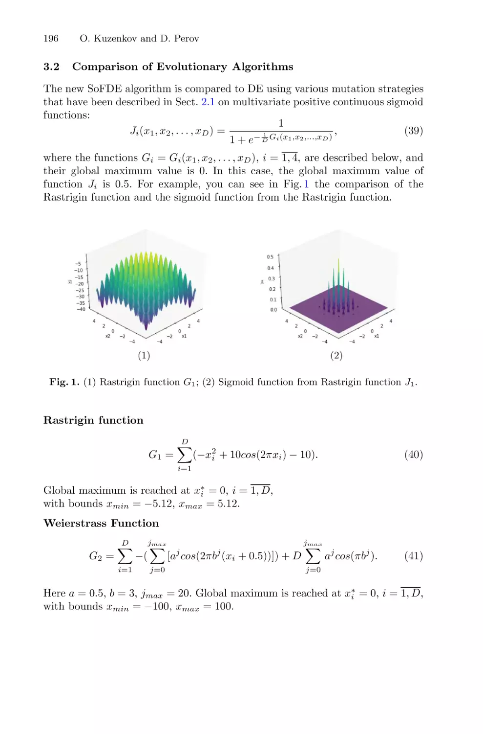
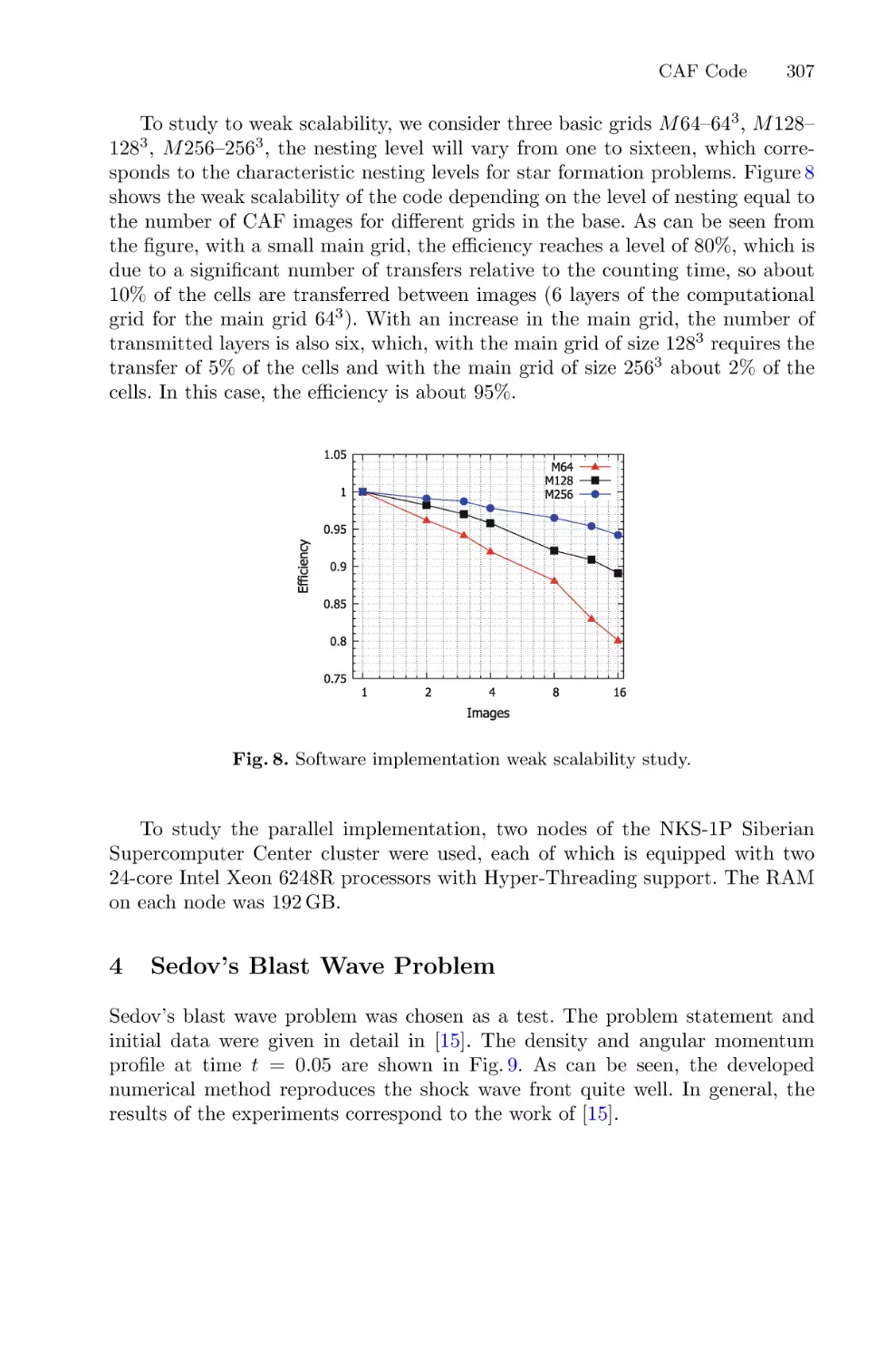
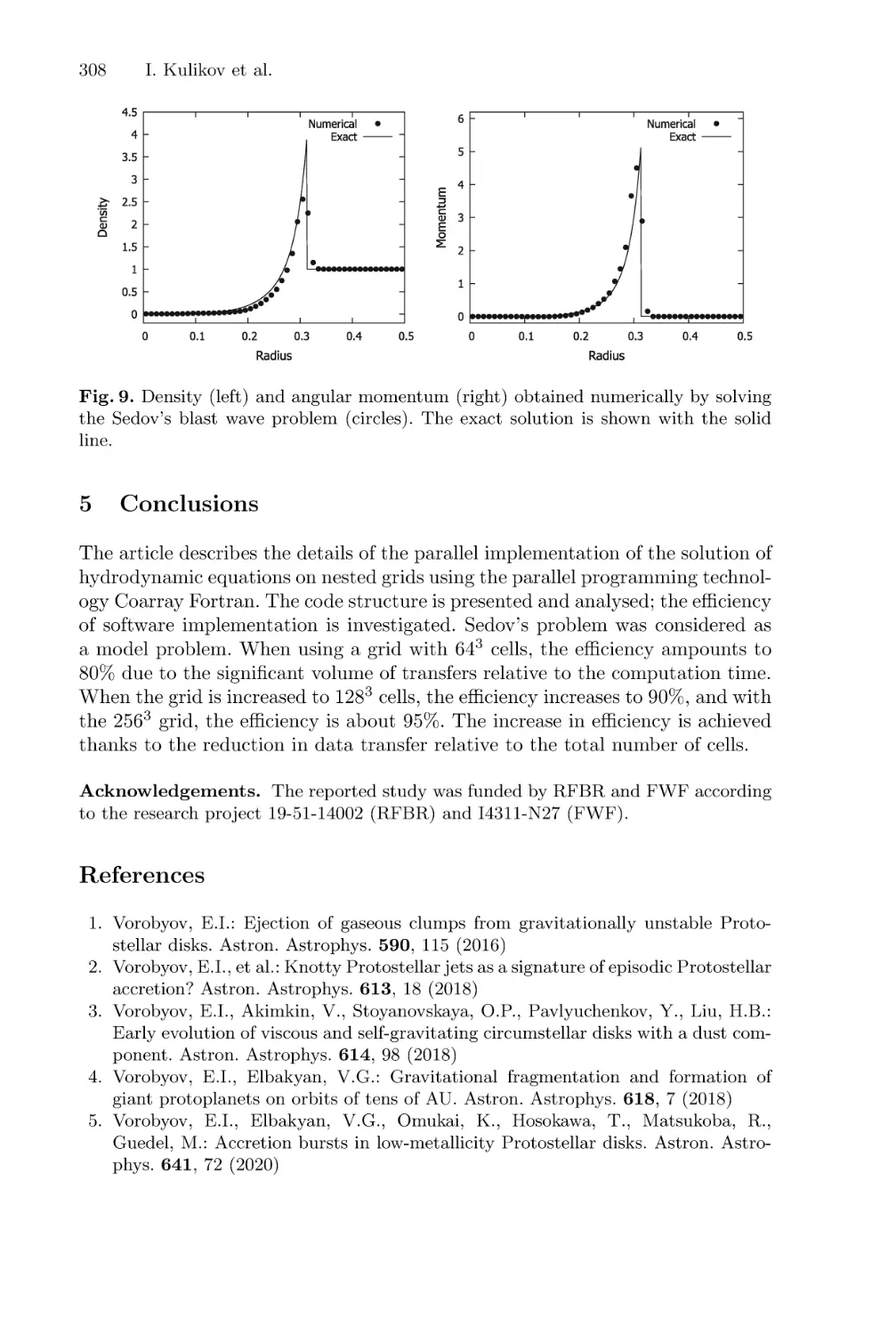
Text
                    Dmitry Balandin
Konstantin Barkalov
Iosif Meyerov (Eds.)

Communications in Computer and Information Science

Mathematical Modeling
and Supercomputer
Technologies
22nd International Conference, MMST 2022
Nizhny Novgorod, Russia, November 14–17, 2022
Revised Selected Papers

1750

Communications
in Computer and Information Science
Editorial Board Members
Joaquim Filipe
Polytechnic Institute of Setúbal, Setúbal, Portugal
Ashish Ghosh
Indian Statistical Institute, Kolkata, India
Raquel Oliveira Prates
Federal University of Minas Gerais (UFMG), Belo Horizonte, Brazil
Lizhu Zhou
Tsinghua University, Beijing, China

1750

More information about this series at https://link.springer.com/bookseries/7899

Dmitry Balandin · Konstantin Barkalov ·
Iosif Meyerov (Eds.)

Mathematical Modeling
and Supercomputer
Technologies
22nd International Conference, MMST 2022
Nizhny Novgorod, Russia, November 14–17, 2022
Revised Selected Papers

Editors
Dmitry Balandin
Lobachevsky State University of Nizhny
Novgorod
Nizhny Novgorod, Russia

Konstantin Barkalov
Lobachevsky State University of Nizhny
Novgorod
Nizhny Novgorod, Russia

Iosif Meyerov
Lobachevsky State University of Nizhny
Novgorod
Nizhny Novgorod, Russia

ISSN 1865-0929
ISSN 1865-0937 (electronic)
Communications in Computer and Information Science
ISBN 978-3-031-24144-4
ISBN 978-3-031-24145-1 (eBook)
https://doi.org/10.1007/978-3-031-24145-1
© The Editor(s) (if applicable) and The Author(s), under exclusive license
to Springer Nature Switzerland AG 2022
This work is subject to copyright. All rights are reserved by the Publisher, whether the whole or part of the
material is concerned, specifically the rights of translation, reprinting, reuse of illustrations, recitation,
broadcasting, reproduction on microfilms or in any other physical way, and transmission or information
storage and retrieval, electronic adaptation, computer software, or by similar or dissimilar methodology now
known or hereafter developed.
The use of general descriptive names, registered names, trademarks, service marks, etc. in this publication
does not imply, even in the absence of a specific statement, that such names are exempt from the relevant
protective laws and regulations and therefore free for general use.
The publisher, the authors, and the editors are safe to assume that the advice and information in this book are
believed to be true and accurate at the date of publication. Neither the publisher nor the authors or the editors
give a warranty, expressed or implied, with respect to the material contained herein or for any errors or
omissions that may have been made. The publisher remains neutral with regard to jurisdictional claims in
published maps and institutional affiliations.
This Springer imprint is published by the registered company Springer Nature Switzerland AG
The registered company address is: Gewerbestrasse 11, 6330 Cham, Switzerland

Preface

The 22nd International Conference and School for Young Scientists “Mathematical Modeling and Supercomputer Technologies” (MMST 2022) was held during November 14–
17, 2022, in Nizhni Novgorod, Russia. The conference and school were organized by the
Mathematical Center “Mathematics of Future Technologies” and the Research and Educational Center for Supercomputer Technologies of the Lobachevsky State University
of Nizhni Novgorod. MMST 2022 was organized in partnership with the International
Congress “Russian Supercomputing Days”.
The topics of the conference and school cover a wide range of problems of mathematical modeling of complex processes and numerical methods of research, as well
as new methods of supercomputing aimed to solve state-of-the-art problems in various
fields of science, industry, business, and education.
This edition of the MMST conference was dedicated to Professor Victor Gergel,
who passed away in 2021. Victor Gergel chaired the Program Committee of the conference from 2001 to 2020 and was a brilliant scholar and innovator. Since his student
years he had developed mathematical models, methods, and software systems to solve
global and multi-criteria optimization, pattern recognition, and classification problems.
Starting from the early 2000s, Professor Gergel became involved in the world’s rapidly
developing area of parallel computing, where he achieved a great deal of success and
international recognition. He led one of Russia’s first research and education centers for
supercomputing technologies at the Lobachevsky State University of Nizhni Novgorod,
which became part of the national supercomputing research and training system. Professor Gergel was a member of Program Committees, gave plenary speeches at major
conferences on supercomputing in Russia and worldwide, and contributed to many expert
groups on the subject. His pioneering ideas in the field of programming education have
played a significant role in the training of software professionals at the Lobachevsky
State University of Nizhni Novgorod. The educational packages and textbooks on parallel programming developed by Professor Gergel and his co-authors are used throughout
Russia.
The scientific program of the conference featured the following plenary lectures
given by outstanding researchers and practitioners:
• Yuri Boldyrev (Peter the Great St. Petersburg Polytechnic University)—On the
fundamentals of the digital economy (a case study of material production).
• Alexander Leytman (TIAA) and Mikhail Soloveitchik (Independent Analyst)—Mathematical modeling of organizations’ risks in the global financial industry using
supercomputer technologies.
• Alexander Naumov (Huawei Technologies Co.), The use of neural networks for
solving first-order partial differential equations.
• Mikhail Yakobovskiy (Keldysh Institute of Applied Mathematics of the Russian
Academy of Sciences)—Supercomputer Simulation—Processor Load Balancing

vi

Preface

• Sergey Yakushkin (Syntacore Company)—Open and free RISC-V processor architecture—from microcontrollers to supercomputers
These proceedings contain 20 full papers and five short papers carefully selected to
be included in this volume from the main track and special sessions of MMST 2022.
The papers accepted for publication were reviewed by three referees from the members
of the MMST 2022 Program Committee and independent reviewers in a single blind
process.
The proceedings editors would like to thank all members of the conference committees, especially the Organizing and Program Committee members as well as external
reviewers for their contributions. We also thank Springer for producing these high-quality
proceedings of MMST 2022.
November 2022

Dmitry Balandin
Konstantin Barkalov
Iosif Meyerov
Publication Chairs

Organization

Program Committee Chair
Balandin, D. V.

Lobachevsky State University of Nizhni
Novgorod, Russia

Program Committee
Barkalov, K. A.
Belykh, I. V.
Boccaletti, S.
Dana, S. K.
Denisov, S. V.
Feygin, A. M.
Ghosh, D.
Gonchenko, S. V.
Hramov, A. E.
Ivanchenko, M. V.
Kazantsev, V. B.
Koronovskii, A. A.
Kurths, J.
Malyshkin V. E.
Mareev, E. A.
Moshkov, M. Y.
Meyerov, I. B.
Nekorkin, V. I.
Osipov, G. V.
Pikovsky, A. S.
Sergeyev, Ya. D.

Lobachevsky State University of Nizhni
Novgorod, Russia
Georgia State University, USA
Institute of Complex Systems, Italy
Indian Institute of Chemical Biology, India
Oslo Metropolitan University, Norway
Institute of Applied Physics, RAS, Russia
Indian Statistical Institute, India
Lobachevsky State University of Nizhni
Novgorod, Russia
Innopolis University, Russia
Lobachevsky State University of Nizhni
Novgorod, Russia
Lobachevsky State University of Nizhni
Novgorod, Russia
Saratov State University, Russia
Potsdam Institute for Climate Impact Research,
Germany
Institute of Computational Mathematics and
Mathematical Geophysics, SB RAS, Russia
Institute of Applied Physics, RAS, Russia
King Abdullah University of Science and
Technology, Saudi Arabia
Lobachevsky State University of Nizhni
Novgorod, Russia
Institute of Applied Physics, RAS, Russia
Lobachevsky State University of Nizhni
Novgorod, Russia
University of Potsdam, Germany
University of Calabria, Italy; Lobachevsky State
University of Nizhni Novgorod, Russia

viii

Organization

Turaev, D. V.
Wyrzykowski, R.
Yakobovskiy, M. V.
Zaikin, A. A.

Imperial College London, UK
Czestochowa University of Technology, Poland
Institute of Applied Mathematics, RAS, Russia
University College London, UK

Organizing Committee
Zolotykh, N. Yu. (Chair)
Balandin, D. V.
Barkalov, K. A.
Kozinov, E. A.
Lebedev, I. G.
Meyerov, I. B.
Oleneva, I. V.
Sysoyev, A. V.

Lobachevsky State University of Nizhni
Novgorod, Russia
Lobachevsky State University of Nizhni
Novgorod, Russia
Lobachevsky State University of Nizhni
Novgorod, Russia
Lobachevsky State University of Nizhni
Novgorod, Russia
Lobachevsky State University of Nizhni
Novgorod, Russia
Lobachevsky State University of Nizhni
Novgorod, Russia
Lobachevsky State University of Nizhni
Novgorod, Russia
Lobachevsky State University of Nizhni
Novgorod, Russia

Contents

Computational Methods for Mathematical Models Analysis
Diffusion in the Phase Space of the Autooscillatory System, Demonstrating
the Stochastic Web in the Conservative Limit: Numerical Investigation . . . . . . . .
Alexander V. Golokolenov and Dmitry V. Savin
Aberrator Shape Identification from 3D Ultrasound Data Using
Convolutional Neural Networks and Direct Numerical Modeling . . . . . . . . . . . . .
Alexey Vasyukov, Andrey Stankevich, Katerina Beklemysheva,
and Igor Petrov
Complex Dynamics of the Implicit Maps Derived from Iteration of Newton
and Euler Methods . . . . . . . . . . . . . . . . . . . . . . . . . . . . . . . . . . . . . . . . . . . . . . . . . . . .
Andrei A. Elistratov, Dmitry V. Savin, and Olga B. Isaeva
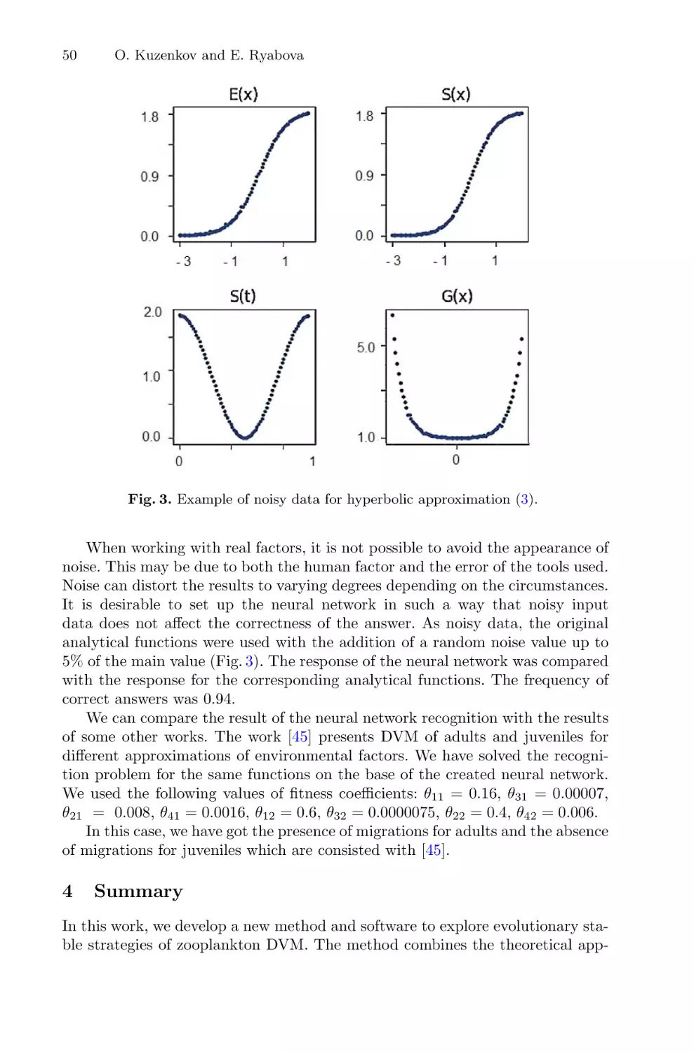
Recognition of Vertical Migrations for Two Age Groups of Zooplankton . . . . . .
O. Kuzenkov and E. Ryabova

3

15

29

41

Nonintegrability of the Problem of Motion of an Ellipsoidal Body
with a Fixed Point in a Flow of Particles . . . . . . . . . . . . . . . . . . . . . . . . . . . . . . . . . .
Alexander S. Kuleshov and Maxim M. Gadzhiev

55

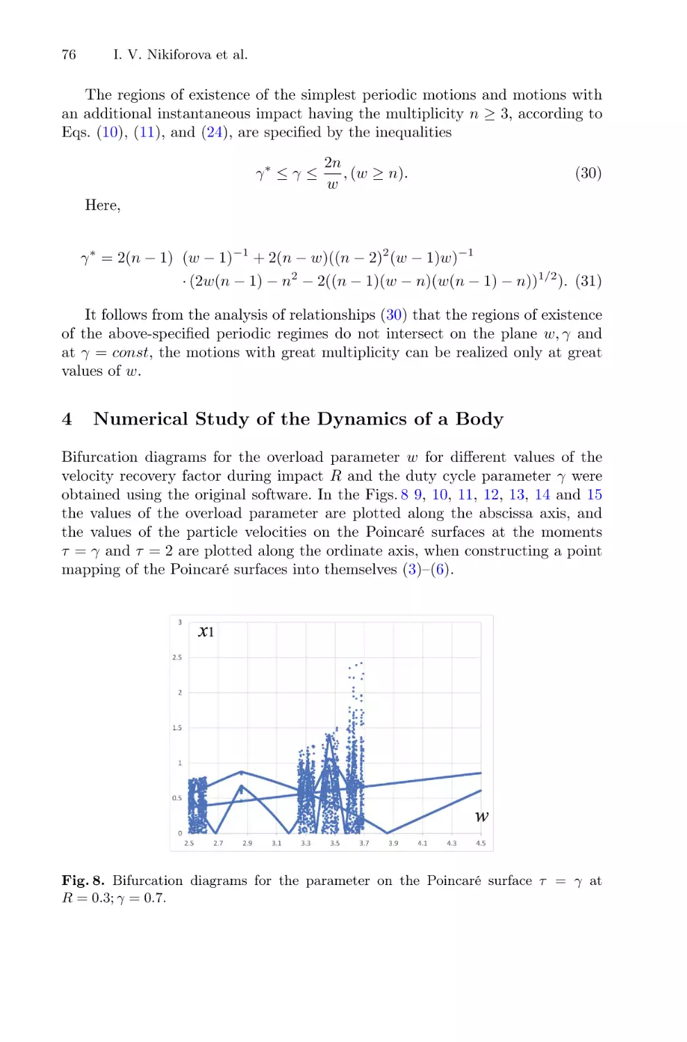
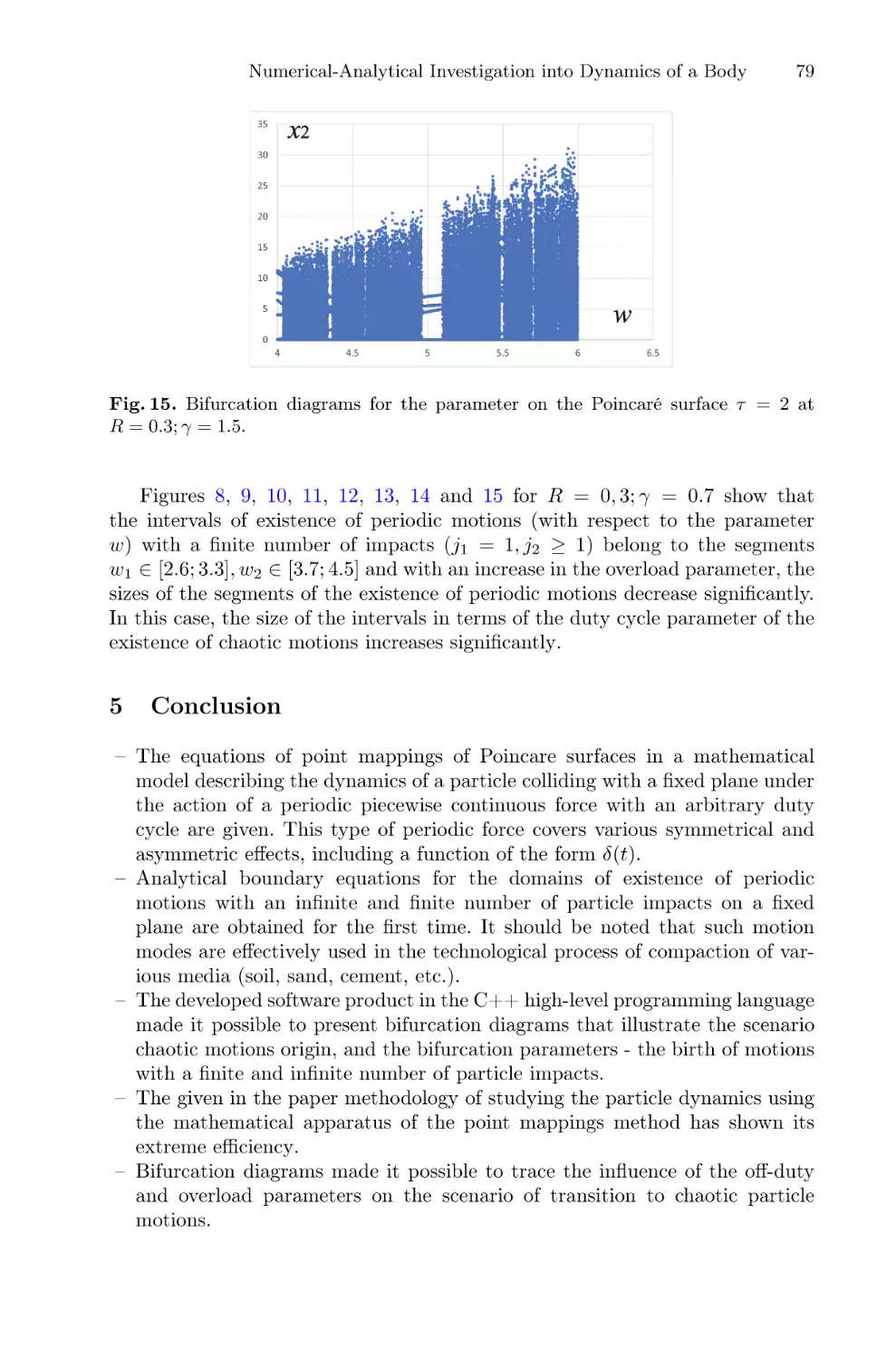
Numerical and Analytical Investigation of the Dynamics of a Body Under
the Action of a Periodic Piecewise Constant External Force . . . . . . . . . . . . . . . . . .
Irina V. Nikiforova, Vladimir S. Metrikin, and Leonid A. Igumnov

67

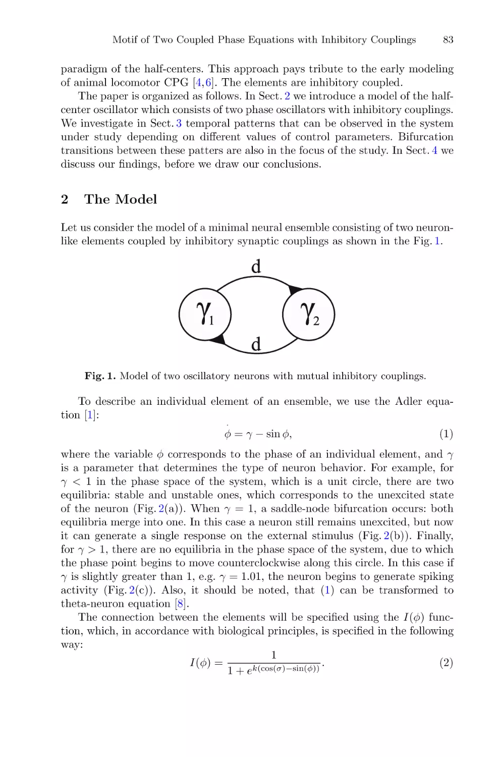
Motif of Two Coupled Phase Equations with Inhibitory Couplings
as a Simple Model of the Half-Center Oscillator . . . . . . . . . . . . . . . . . . . . . . . . . . .
Artyom Emelin, Alexander Korotkov, Tatiana Levanova,
and Grigory Osipov
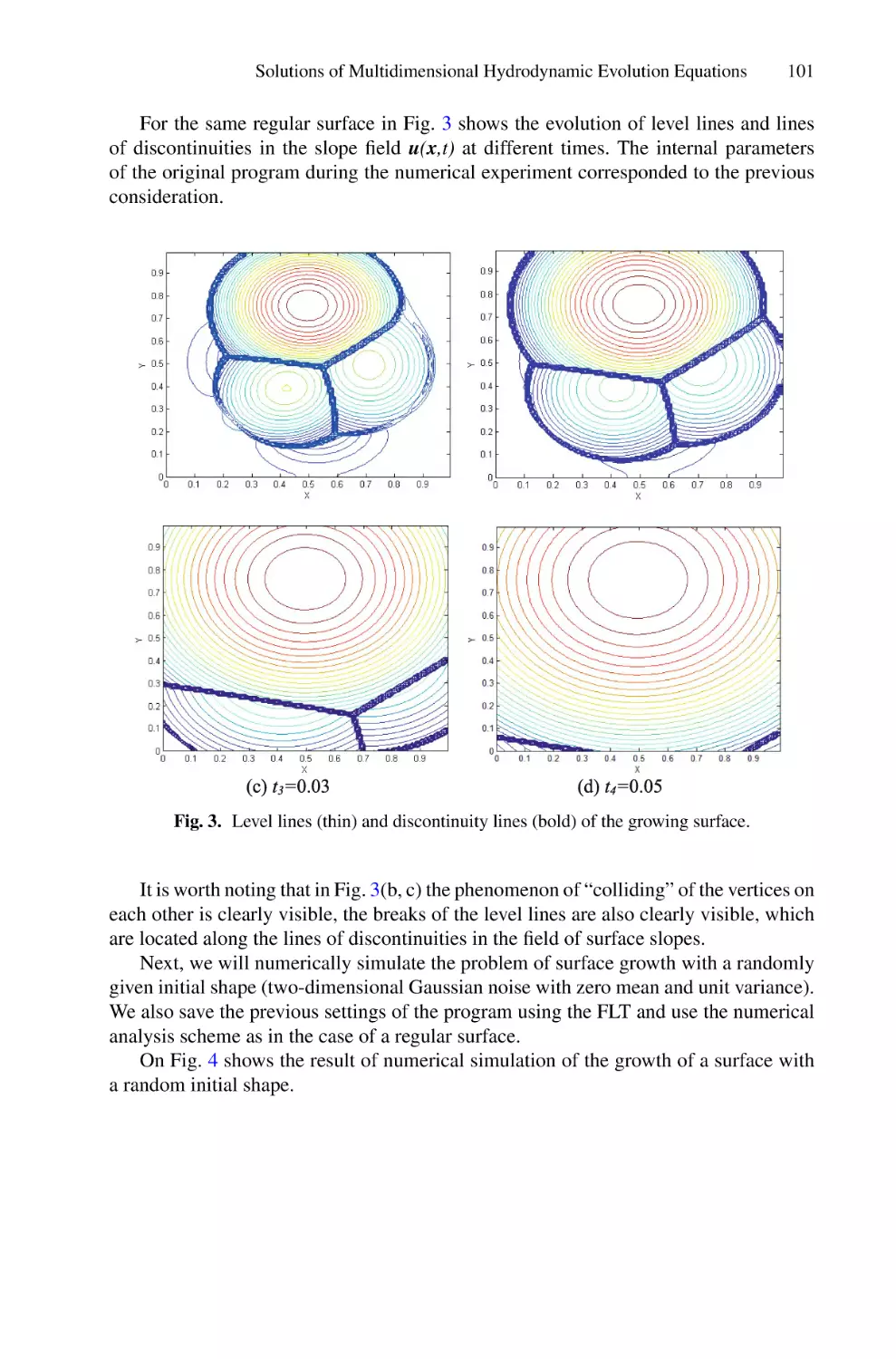
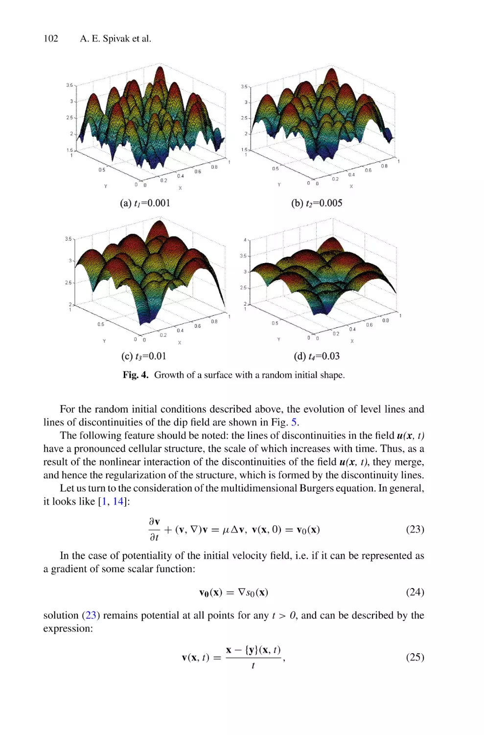
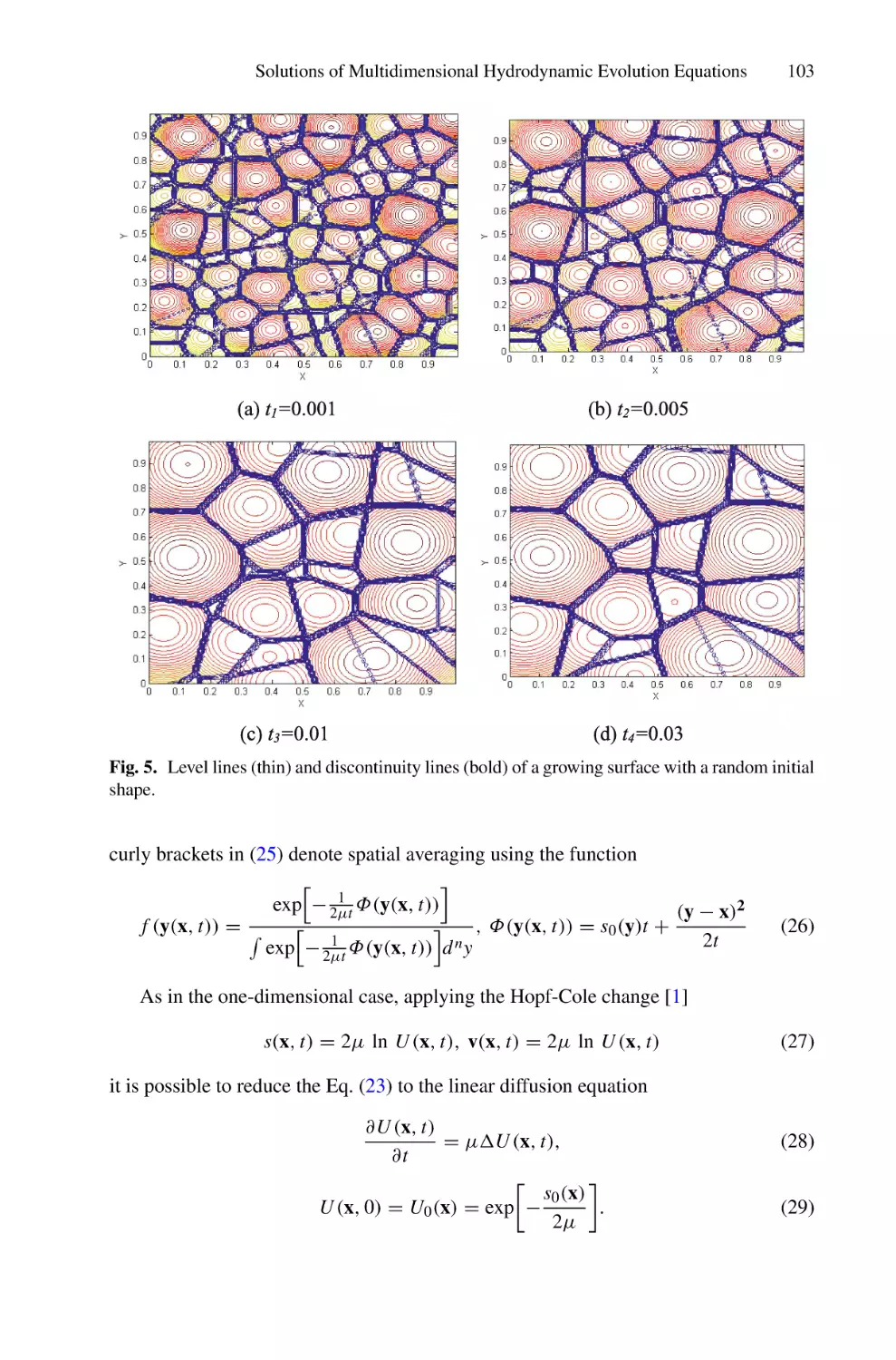
Solutions of Multidimensional Hydrodynamic Evolution Equations Using
the Fast Legendre Transformation . . . . . . . . . . . . . . . . . . . . . . . . . . . . . . . . . . . . . . . .
A. E. Spivak, S. N. Gurbatov, and I. Yu. Demin

82

95

An Iterative Method for Solving a Nonlinear System of the Theory
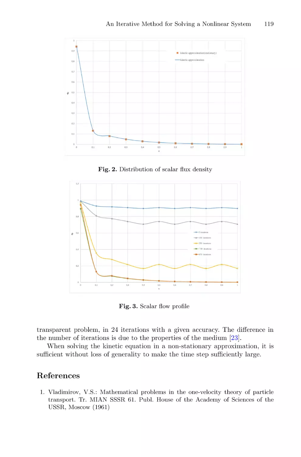
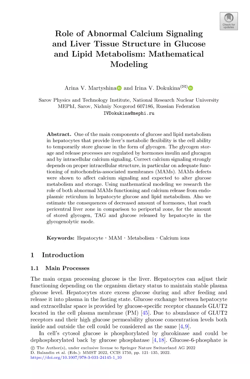
of Radiation Transfer and Statistical Equilibrium in a Plane-Parallel Layer . . . . . 106
Aleksey Kalinin, Alla Tyukhtina, and Aleksey Busalov

x

Contents

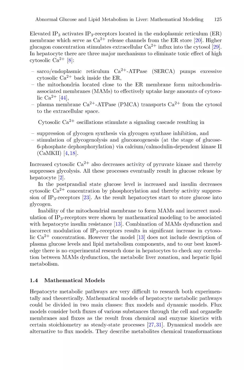
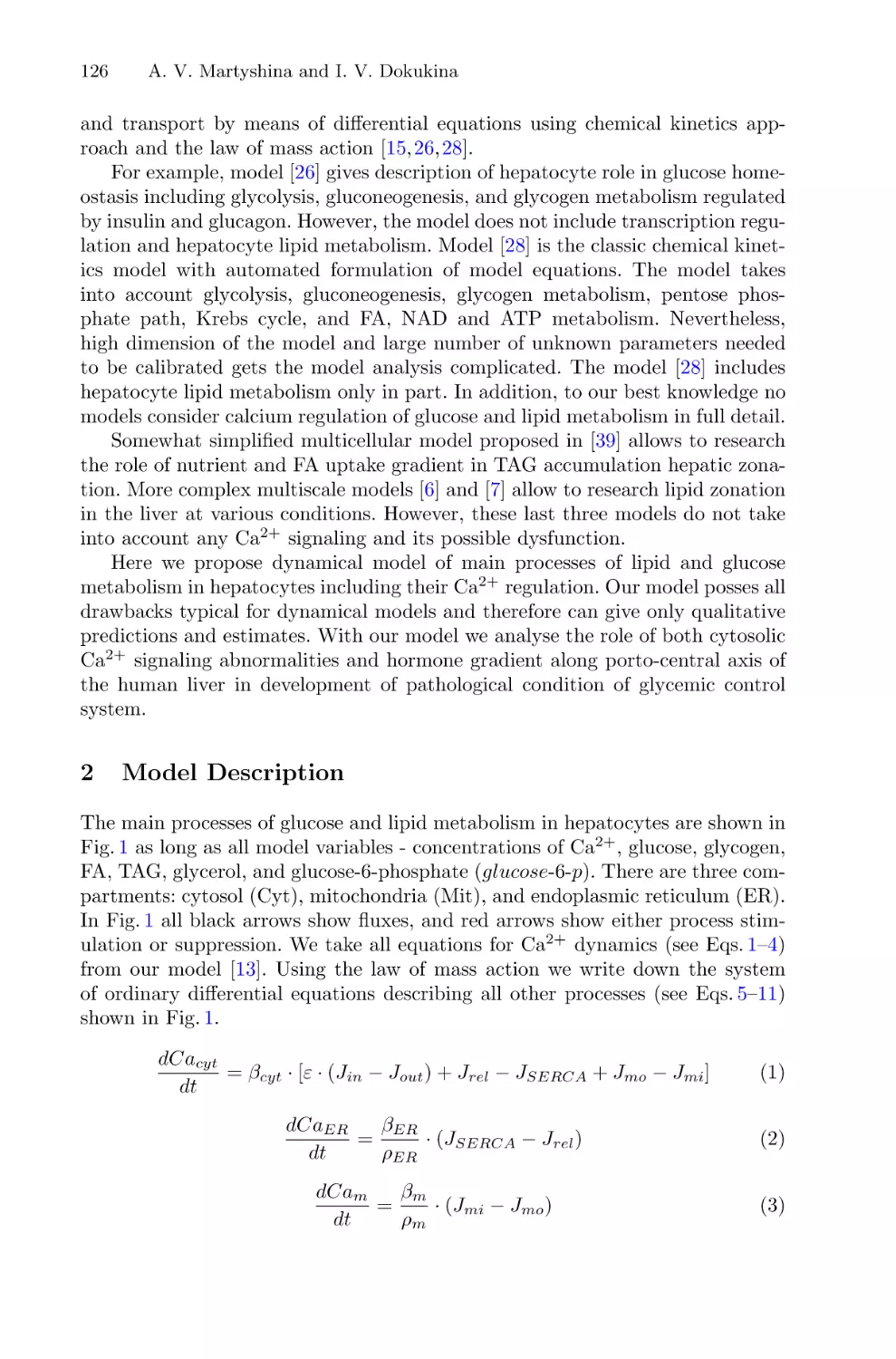
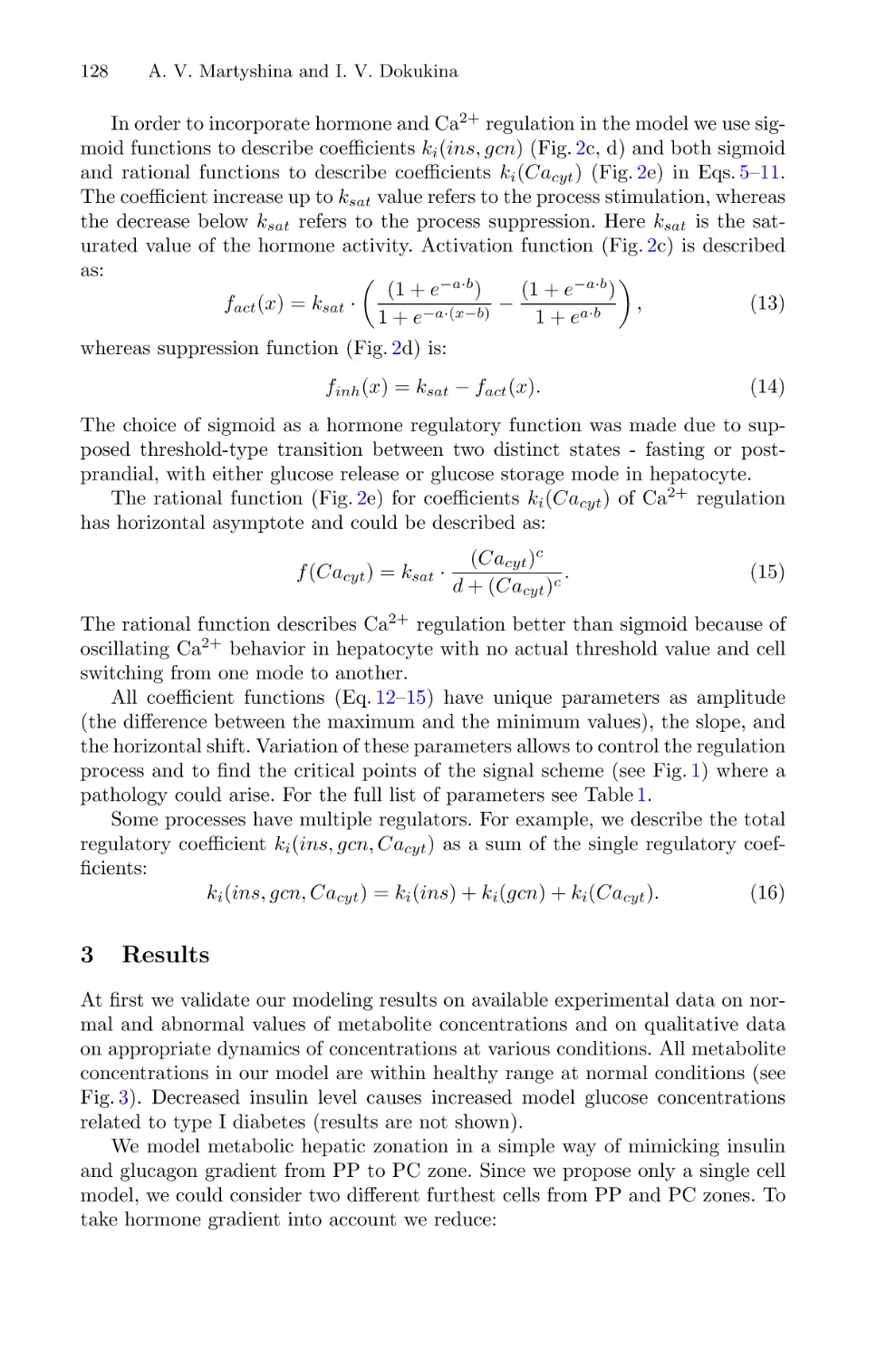
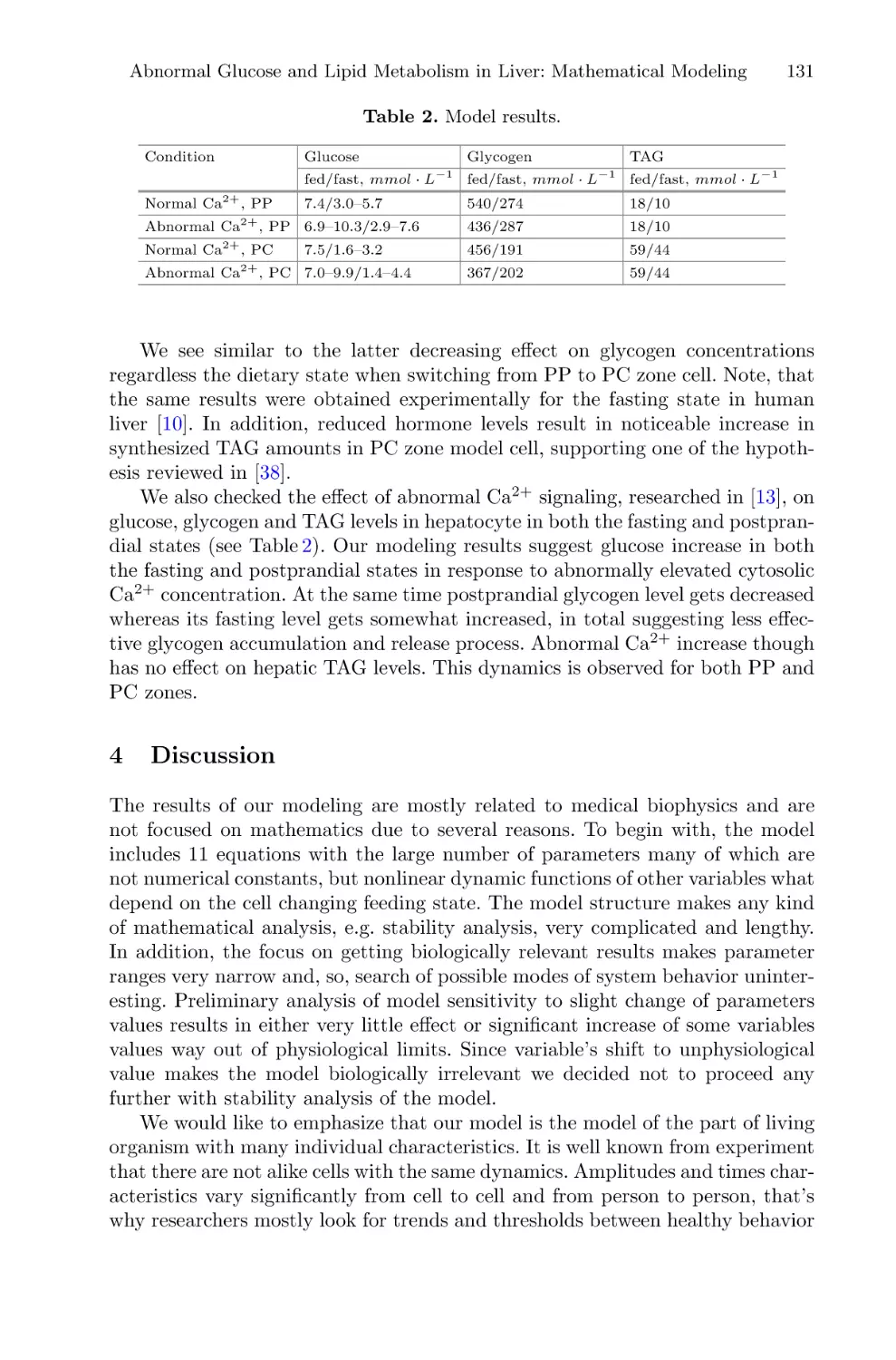
Role of Abnormal Calcium Signaling and Liver Tissue Structure
in Glucose and Lipid Metabolism: Mathematical Modeling . . . . . . . . . . . . . . . . . . 121
Arina V. Martyshina and Irina V. Dokukina
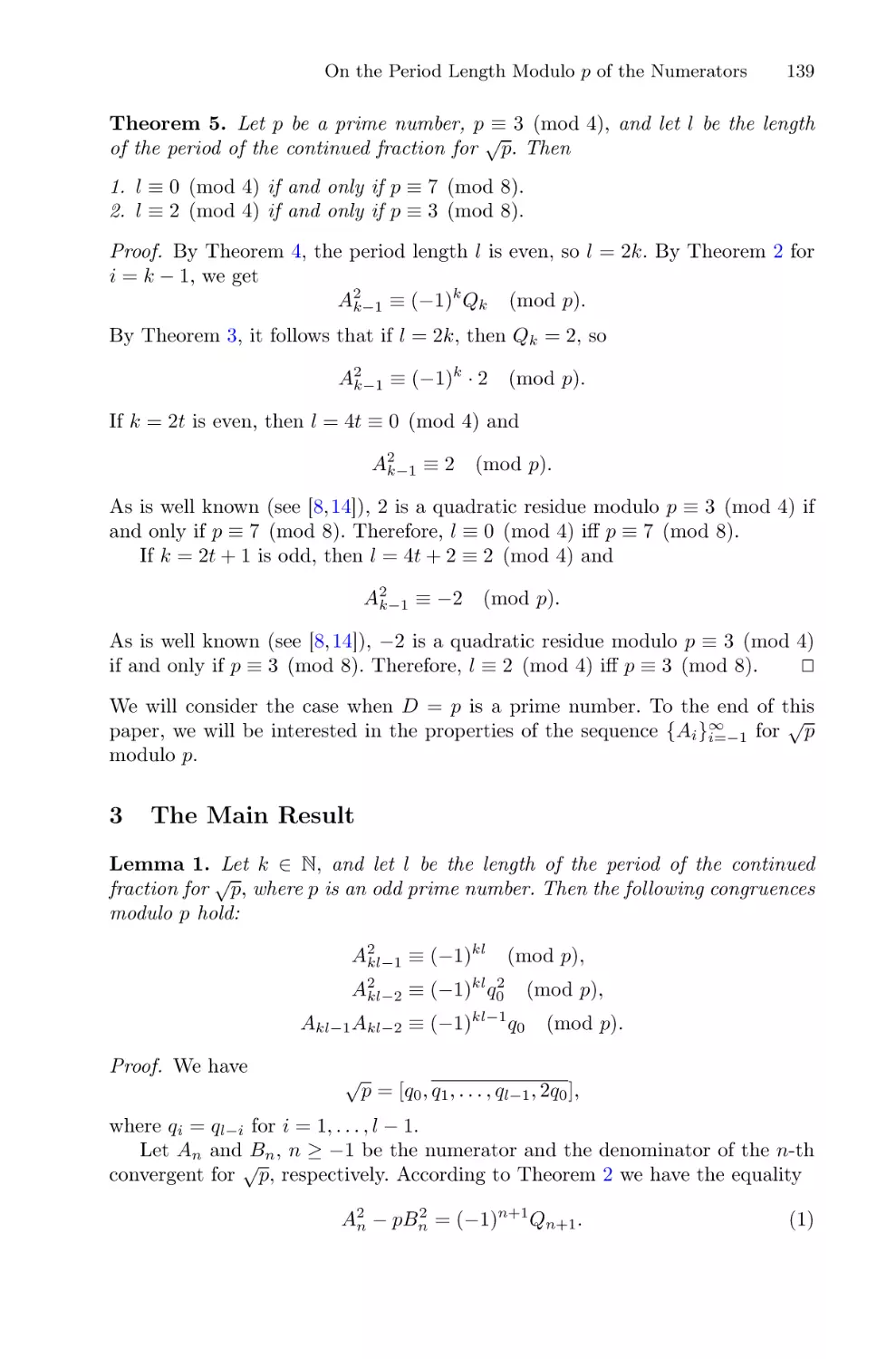
On the Period Length Modulo p of the Numerators of Convergents
for the Square Root of a Prime Number p . . . . . . . . . . . . . . . . . . . . . . . . . . . . . . . . . 136
S. V. Sidorov and P. A. Shcherbakov
Investigation of a Queueing System with Two Classes of Jobs, Bernoulli
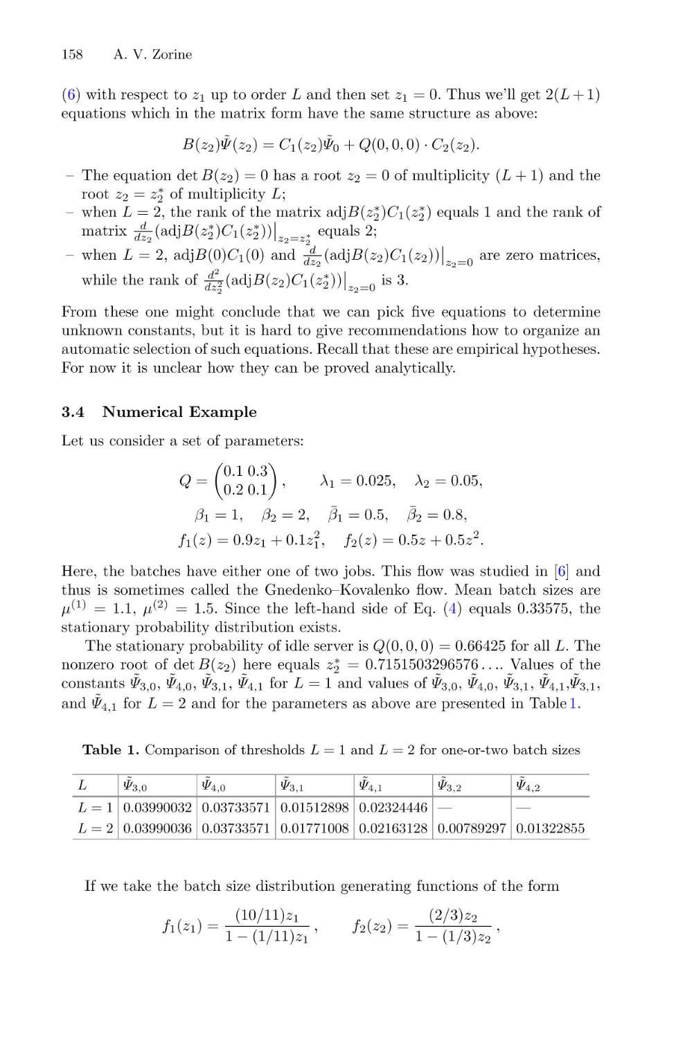
Feedback, and a Threshold Switching Algorithm . . . . . . . . . . . . . . . . . . . . . . . . . . . 148
Andrei V. Zorine
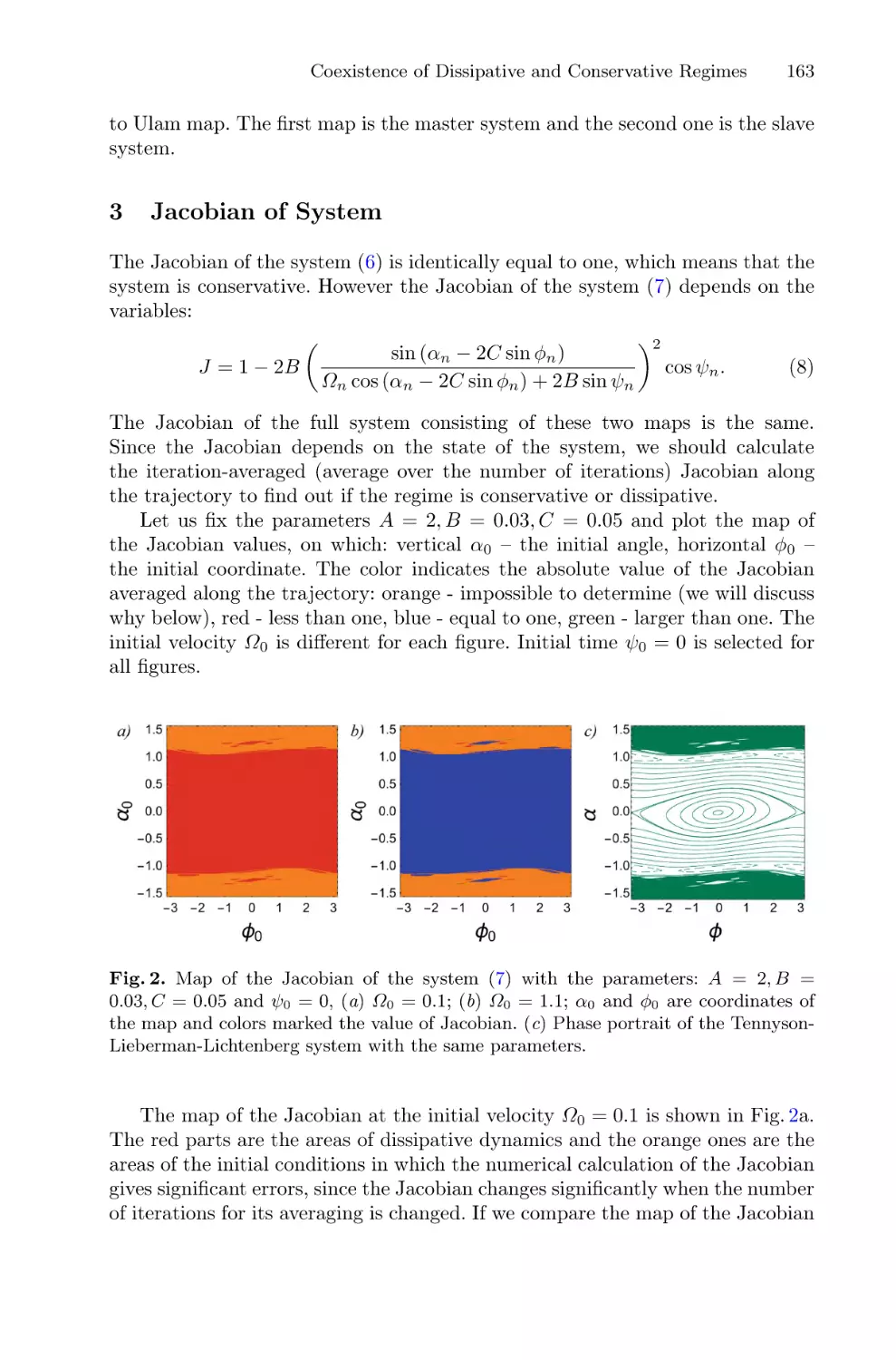
Coexistence of Dissipative and Conservative Regimes in Unidirectionally
Coupled Maps . . . . . . . . . . . . . . . . . . . . . . . . . . . . . . . . . . . . . . . . . . . . . . . . . . . . . . . . 160
Dmitry Lubchenko and Alexey Savin
Regulation of Neural Network Activity by Extracellular Matrix Molecules . . . . . 167
Sergey Stasenko and Victor Kazantsev
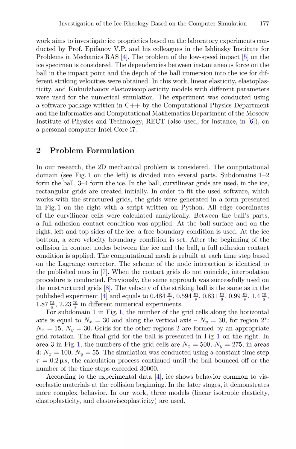
Investigation of Ice Rheology Based on Computer Simulation
of Low-Speed Impact . . . . . . . . . . . . . . . . . . . . . . . . . . . . . . . . . . . . . . . . . . . . . . . . . . 176
Evgeniya K. Guseva, Katerina A. Beklemysheva, Vasily I. Golubev,
Viktor P. Epifanov, and Igor B. Petrov
Computation in Optimization and Optimal Control
Global Optimization Method Based on the Survival of the Fittest Algorithm . . . 187
Oleg Kuzenkov and Dmitriy Perov
Solving of the Static Output Feedback Synthesis Problem in a Class
of Block-Homogeneous Matrices of Input and Output . . . . . . . . . . . . . . . . . . . . . . 202
A. V. Mukhin
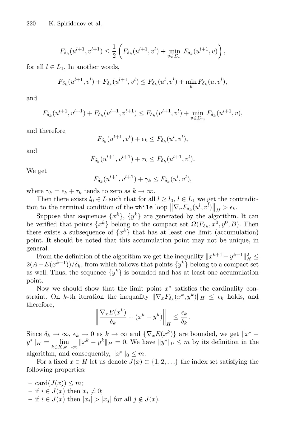
Weak Penalty Decomposition Algorithm for Sparse Optimization in High
Dimensional Space . . . . . . . . . . . . . . . . . . . . . . . . . . . . . . . . . . . . . . . . . . . . . . . . . . . . 215
Kirill Spiridonov, Sergei Sidorov, and Michael Pleshakov
Mathematical Modelling and Optimization of Scheduling for Processing
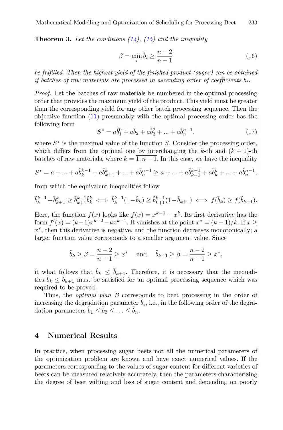
Beet in Sugar Production . . . . . . . . . . . . . . . . . . . . . . . . . . . . . . . . . . . . . . . . . . . . . . . 227
Dmitry Balandin, Albert Egamov, Oleg Kuzenkov,
Oksana Pristavchenko, and Vadim Vildanov
Integration of Information Systems Data to Improve the Petroleum
Product Blends Quality . . . . . . . . . . . . . . . . . . . . . . . . . . . . . . . . . . . . . . . . . . . . . . . . . 239
Viacheslav Kuvykin, Artem Kolpakov, and Mikhail Meleshkevich

Contents

xi

Supercomputer Simulation
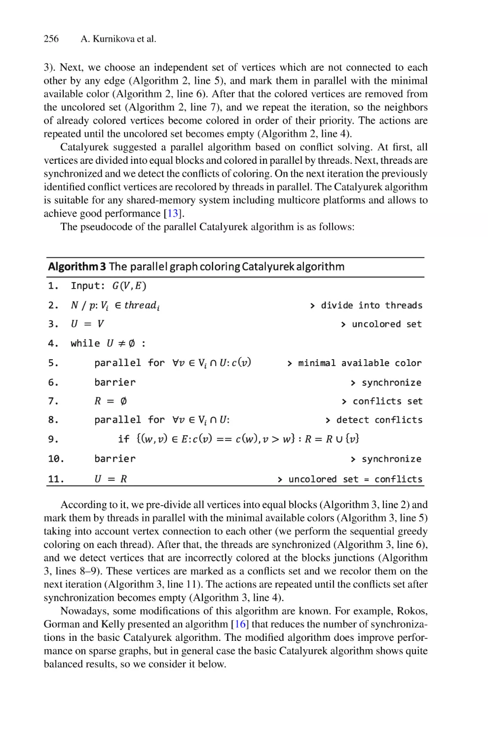
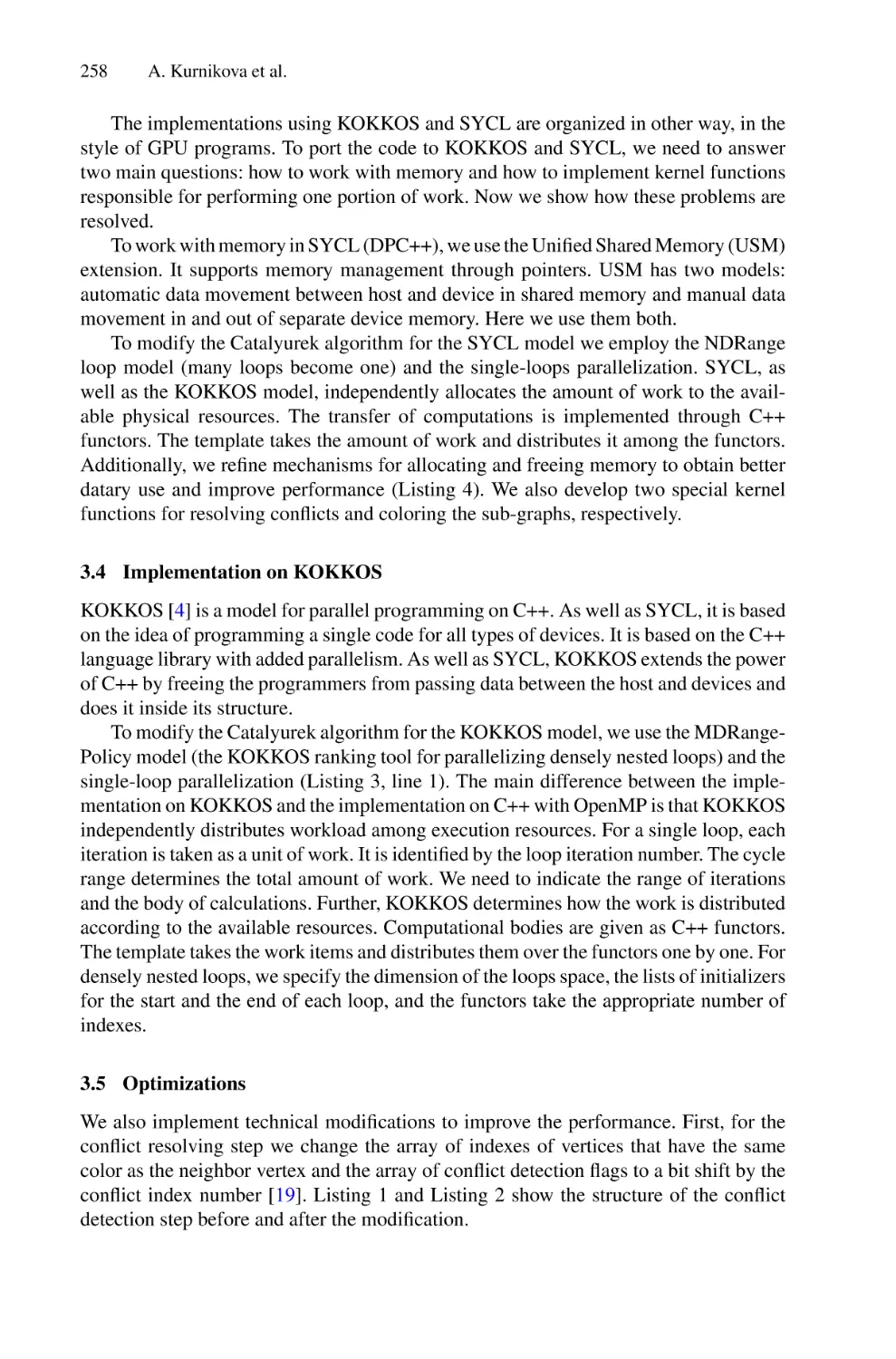
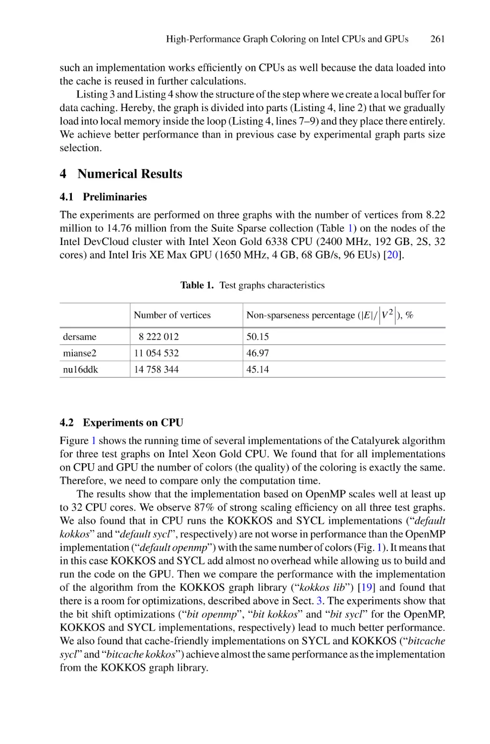
High-Performance Graph Coloring on Intel CPUs and GPUs Using SYCL
and KOKKOS . . . . . . . . . . . . . . . . . . . . . . . . . . . . . . . . . . . . . . . . . . . . . . . . . . . . . . . . 253
Anastasia Kurnikova, Anna Pirova, Valentin Volokitin, and Iosif Meyerov
Automated Debugging of Fragmented Programs in LuNA System . . . . . . . . . . . . 266
Victor Malyshkin, Andrey Vlasenko, and Mihail Michurov
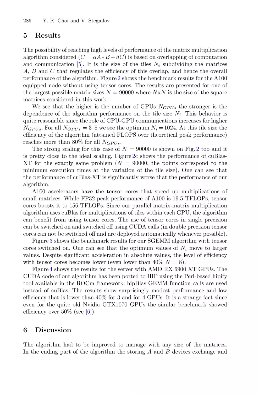
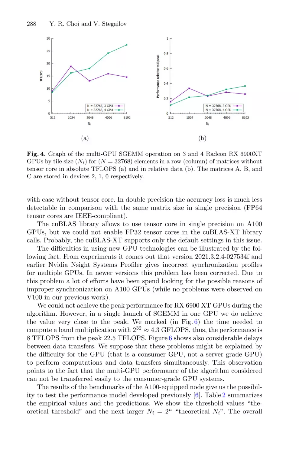
Multi-GPU GEMM Algorithm Performance Analysis for Nvidia and AMD
GPUs Connected by NVLink and PCIe . . . . . . . . . . . . . . . . . . . . . . . . . . . . . . . . . . . 281
Yea Rem Choi and Vladimir Stegailov
Numerical Simulation of Quantum Dissipative Dynamics
of a Superconducting Neuron . . . . . . . . . . . . . . . . . . . . . . . . . . . . . . . . . . . . . . . . . . . 293
P. V. Pikunov, D. S. Pashin, and M. V. Bastrakova
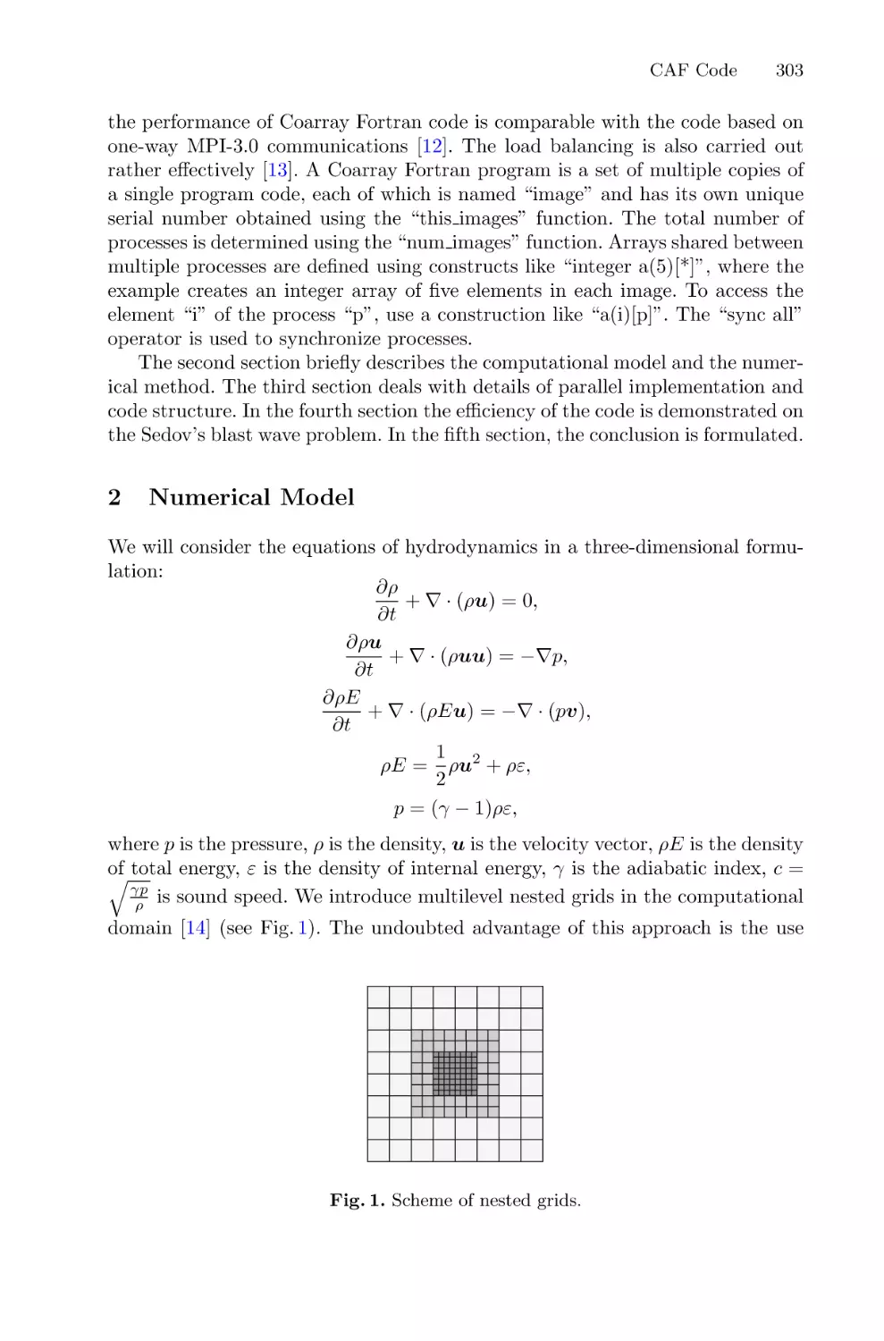
Using Coarray Fortran for Design of Hydrodynamics Code on Nested Grids . . . 302
Igor Kulikov, Igor Chernykh, Eduard Vorobyov, and Vardan Elbakyan
Author Index . . . . . . . . . . . . . . . . . . . . . . . . . . . . . . . . . . . . . . . . . . . . . . . . . . . . . . . . . 311

Computational Methods
for Mathematical Models Analysis

Diﬀusion in the Phase Space
of the Autooscillatory System,
Demonstrating the Stochastic Web
in the Conservative Limit: Numerical
Investigation
Alexander V. Golokolenov(B)

and Dmitry V. Savin(B)

Saratov State University, Astrakhanskaya 83, 410012 Saratov, Russia
golokolenovav@gmail.com, savin.dmitry.v@gmail.com
Abstract. The paper investigates diﬀusion in the phase space of the
weakly dissipative version of the pulse-driven Van der Pol system. Amplitude of external pulses depends on the dynamical variable in the same
way as in the Zaslavsky generator of the stochastic web, and the system under investigation transforms into the stochastic web generator
in the conservative limit. Whilst the conservative system demonstrates
the unbounded diﬀusion in the phase space through the stochastic layer,
trajectories of the autooscillatory system converge to several attractors,
and diﬀusion can be obtained only in some limited time interval. The
trajectories demonstrating diﬀusion properties were detected using the
ﬁnite-time Lyapunov exponents, and for an ensemble of such trajectories dependence of average energy on time was analyzed. Whilst in the
conservative system average energy grows linearly versus time, in the
autooscillatory system this dependence appears to be rather complex. In
the time interval associated with existence of diﬀusion it can be, however,
approximated with the power law. The dependence of it’s exponent on
the dissipation parameter value and on the initial energy of the ensemble
was investigated. The exponent increases with the decrease of dissipation
and decreases up to 0 with the increase of the initial ensemble energy.
Dependence on the initial energy have the same shape in wide interval
of dissipation parameter values.
Keywords: Stochastic web
Autooscillations

1

· Weak dissipation · Diﬀusion ·

Introduction

The stochastic web is a special type of organization of phase space of conservative systems, which are degenerate in sense of the KAM theorem [9]. Originally
found by Zaslavsky in a model, derived from a plasma physics problem [12],
it was widely studied from both theoretical and applied points of view (see,
e.g., [11,13]). The main feature of systems, demonstrating existence of a stochastic web in phase space, is a possibility of an unbounded diﬀusion through the
c The Author(s), under exclusive license to Springer Nature Switzerland AG 2022

D. Balandin et al. (Eds.): MMST 2022, CCIS 1750, pp. 3–14, 2022.
https://doi.org/10.1007/978-3-031-24145-1_1

4

A. V. Golokolenov and D. V. Savin

stochastic layer. Parameters and features of this diﬀusion process were also thoroughly studied by diﬀerent authors (see, e.g., [1,8]). The simplest model, demonstrating the uniform stochastic web, is the pulse-driven linear oscillator with
amplitude of pulses depending on the dynamical variable [13]. Such oscillatorbased models are widely used in theoretical nonlinear dynamics and can demonstrate various dynamical phenomena. Particularly, addition into such systems
small dissipative terms, which can be done very naturally, allows to use them
as rather convenient model for analyzing the weakly dissipative, or almost conservative dynamics, which is characterized by extreme multistability [4,5] and
extremely long transients [7]. Usually dynamics of such systems is studied for
models which are nondegenerate in the sense of the KAM theorem [9]. In recent
years several works appeared where the dynamics of weakly dissipative systems
demonstrating the stochastic web in the conservative limit was analyzed, but the
main focus was held on the long-time behavior and structure of their coexisting
attractors [2,3,10]. On the other hand, since one of the main features of stochastic web is a diﬀusion through the phase space, analysis of transient processes in
dissipative versions of such systems and their connection with the properties of
conservative trajectories seems to be an interesting task. In the present paper we
analyze diﬀusion properties of trajectories of the system, generating the uniform
stochastic web in the conservative case, with an addition of small dissipation of
autooscillating type.

2

Methods of the Investigation

We consider the pulse-driven Van der Pol oscillator
ẍ − (γ − μx2 )ẋ + x =

∞


F (x)δ(t − nT ).

(1)

n=−∞

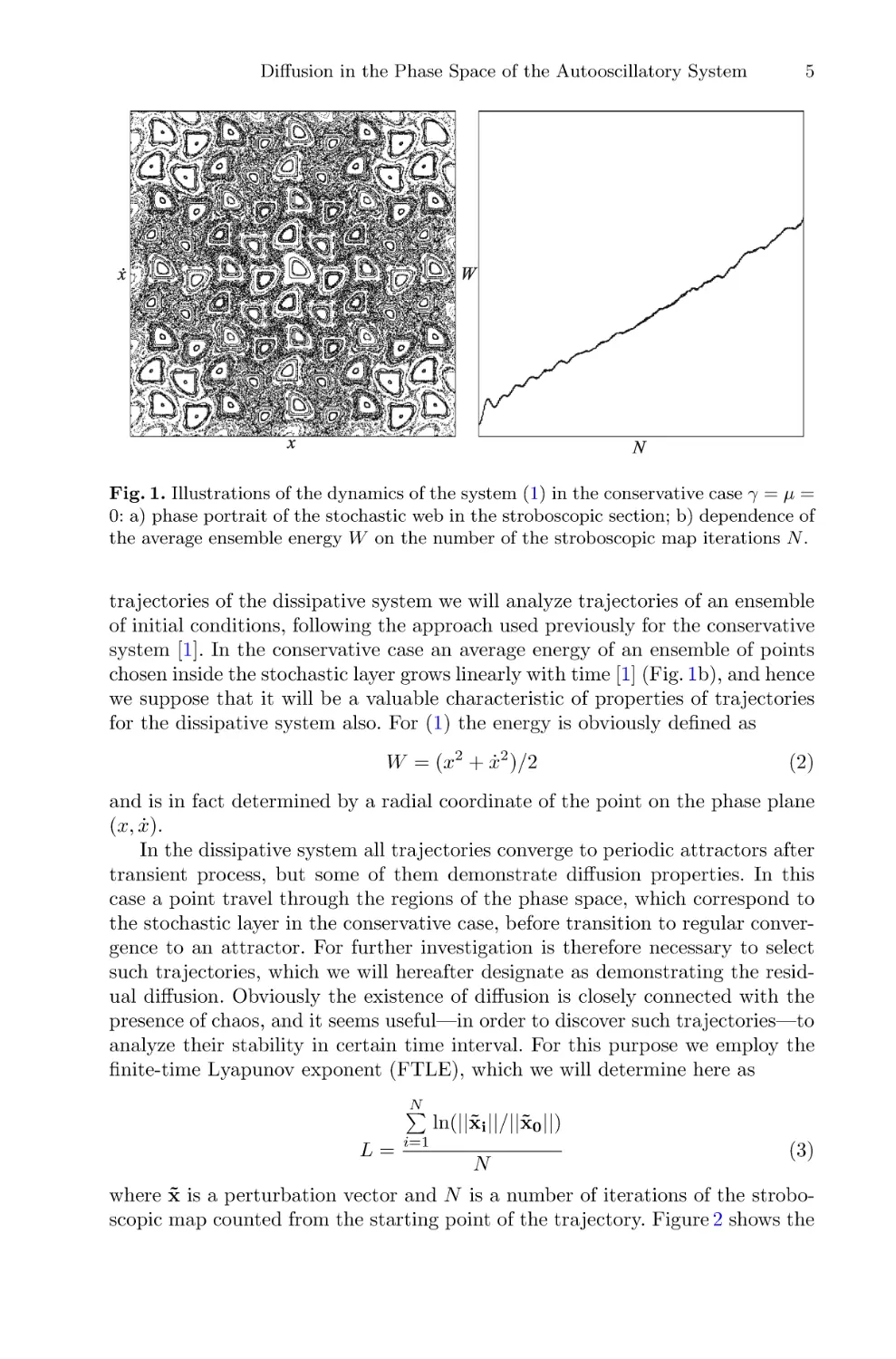
where F (x) is following Zaslavsky [13] chosen to be λ cos x, and hence in the
conservative case (γ = μ = 0) system (1) demonstrates the uniform stochastic web in the phase space (Fig. 1a). We will further consider the frequency of
an external pulses 2π/T four times greater than the natural frequency of the
autonomous system, in this case the phase space of the conservative system
has a crystal-type symmetry with the rotation angle π/2 [13]. For the purpose of
numerical investigation we will use the stroboscopic section map, integrating the
Eq. (1) between the external pulses with the Runge-Kutta method of 4th order
with integration step 0.01T —one iteration of such a map corresponds to one
period of the external force.1 In order to investigate diﬀusion properties of the
1

We also have tested the symplectic Forest-Stremer-Verlet (FSV) method [6] for integration of (1) in the conservative case and in the case of small dissipation—in the
latter case the fourth-order FSV method was modiﬁed for systems with small nonHamiltonian perturbation, and values of the dissipation parameters were typical
for further investigation—but did not found any diﬀerences visually comparing the
structure of the phase portraits and attractors obtained via both methods.

Diﬀusion in the Phase Space of the Autooscillatory System

5

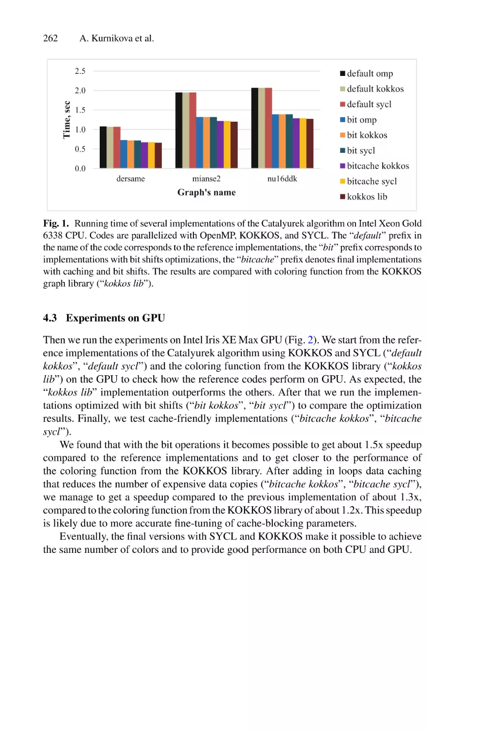
Fig. 1. Illustrations of the dynamics of the system (1) in the conservative case γ = μ =
0: a) phase portrait of the stochastic web in the stroboscopic section; b) dependence of
the average ensemble energy W on the number of the stroboscopic map iterations N .

trajectories of the dissipative system we will analyze trajectories of an ensemble
of initial conditions, following the approach used previously for the conservative
system [1]. In the conservative case an average energy of an ensemble of points
chosen inside the stochastic layer grows linearly with time [1] (Fig. 1b), and hence
we suppose that it will be a valuable characteristic of properties of trajectories
for the dissipative system also. For (1) the energy is obviously deﬁned as
W = (x2 + ẋ2 )/2

(2)

and is in fact determined by a radial coordinate of the point on the phase plane
(x, ẋ).
In the dissipative system all trajectories converge to periodic attractors after
transient process, but some of them demonstrate diﬀusion properties. In this
case a point travel through the regions of the phase space, which correspond to
the stochastic layer in the conservative case, before transition to regular convergence to an attractor. For further investigation is therefore necessary to select
such trajectories, which we will hereafter designate as demonstrating the residual diﬀusion. Obviously the existence of diﬀusion is closely connected with the
presence of chaos, and it seems useful—in order to discover such trajectories—to
analyze their stability in certain time interval. For this purpose we employ the
ﬁnite-time Lyapunov exponent (FTLE), which we will determine here as
N


L=

i=1

ln(||x̃i ||/||x̃0 ||)
N

(3)

where x̃ is a perturbation vector and N is a number of iterations of the stroboscopic map counted from the starting point of the trajectory. Figure 2 shows the

6

A. V. Golokolenov and D. V. Savin

Fig. 2. Three trajectories of the system (1) demonstrating residual diﬀusion: the phase
portraits in the stroboscopic section (left column, a, c, e), the color intensity is proportional to the number of the stroboscopic map iterations N , the red dots correspond
to the attractors; the dependences of the FTLE values on time L(N ) for corresponding trajectories (right column, b, d, f). Values of parameters: λ = 1.2, γ = 0.00001,
μ = 0.00001, the length of the trajectories Nmax = 4000. (Color ﬁgure online)

Diﬀusion in the Phase Space of the Autooscillatory System

7

phase portraits and the time dependences of the FTLE value (3) for the typical
trajectories demonstrating residual diﬀusion. The phase portraits demonstrate
that the complex behavior of the trajectory after some transient switches to
regular convergence, and the positive value of the FTLE begins to decrease.
Time dependences of FTLE similar to shown in right column in the Fig. 2
were obtained for a variety of other trajectories demonstrating the residual diffusion: after short initial part with very complex behavior of L a plateau exist
at certain positive level until regular convergence starts. The length and level
of this plateau can be used to determine a criterion of presence of the residual diﬀusion. Based on obtained data, we found that at the 500th iteration the
transition to regular convergence has not yet occurred for the majority of trajectories, and hence it is possible to use the FTLE value (3) at this point as such
a criterion. In order to determine the boundary value we use distribution of L
for an ensemble of systems. Since dissipation level in the autooscillating system
as well as diﬀusion properties of the trajectories in the conservative case both
depend on the energy of the system, one can expect that properties of trajectories and dependence of average ensemble energy on time can also depend on the
interval, where the initial energy—or, because of (2), the radial coordinate on
the phase plane—of the ensemble elements is distributed. Several ensembles of
systems were created by choosing initial conditions with the radial coordinates
inside certain intervals, diﬀerent for each ensemble. Examples of such ensembles with diﬀerent initial values of the radial coordinate are shown in the Fig. 3,
and distributions of the FTLE values (3) for three of such ensembles are shown
in the Fig. 4. Distribution in all cases looks like a narrow “bell” located inside
the interval (−0.01; 0.02), with the maximum of distribution around 0.01, and

Fig. 3. Distribution of initial conditions on the phase plane (red dots) and corresponding phase portraits (black dots) for diﬀerent ensembles. Initial values of the radial
coordinate are distributed inside the interval (1–4) (a); (4–7) (b). (Color ﬁgure online)

8

A. V. Golokolenov and D. V. Savin

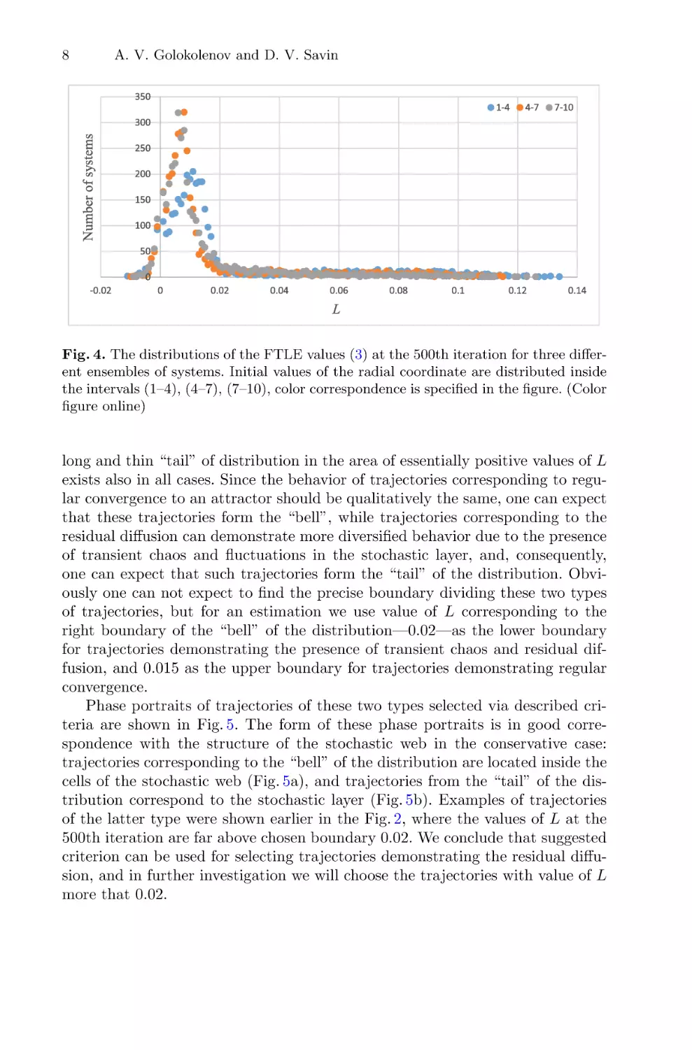
Fig. 4. The distributions of the FTLE values (3) at the 500th iteration for three diﬀerent ensembles of systems. Initial values of the radial coordinate are distributed inside
the intervals (1–4), (4–7), (7–10), color correspondence is speciﬁed in the ﬁgure. (Color
ﬁgure online)

long and thin “tail” of distribution in the area of essentially positive values of L
exists also in all cases. Since the behavior of trajectories corresponding to regular convergence to an attractor should be qualitatively the same, one can expect
that these trajectories form the “bell”, while trajectories corresponding to the
residual diﬀusion can demonstrate more diversiﬁed behavior due to the presence
of transient chaos and ﬂuctuations in the stochastic layer, and, consequently,
one can expect that such trajectories form the “tail” of the distribution. Obviously one can not expect to ﬁnd the precise boundary dividing these two types
of trajectories, but for an estimation we use value of L corresponding to the
right boundary of the “bell” of the distribution—0.02—as the lower boundary
for trajectories demonstrating the presence of transient chaos and residual diffusion, and 0.015 as the upper boundary for trajectories demonstrating regular
convergence.
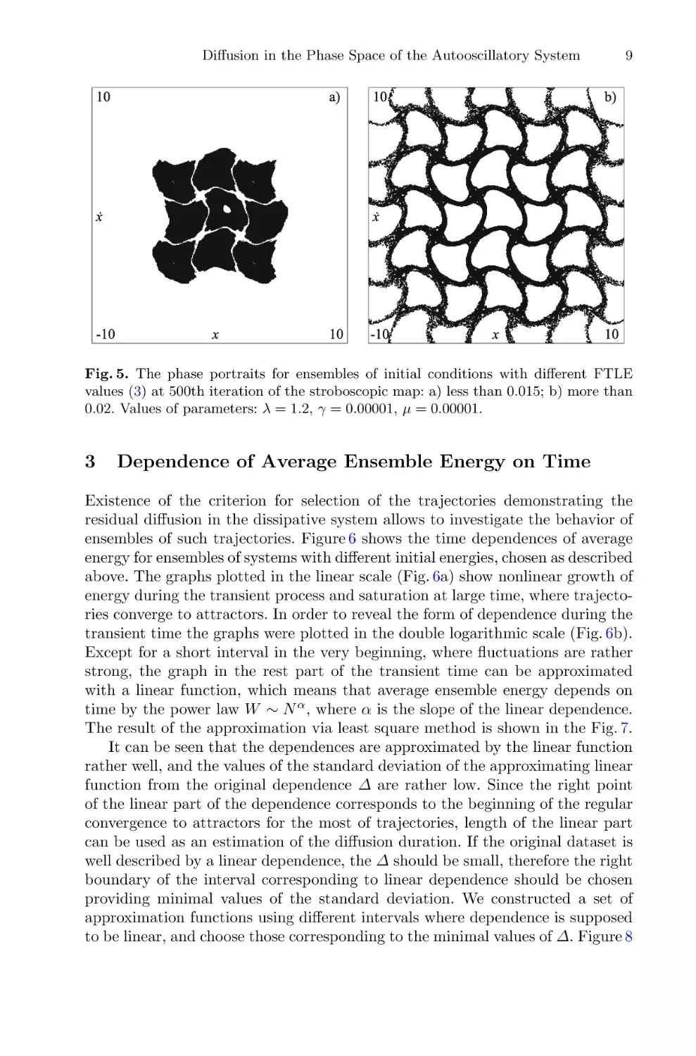
Phase portraits of trajectories of these two types selected via described criteria are shown in Fig. 5. The form of these phase portraits is in good correspondence with the structure of the stochastic web in the conservative case:
trajectories corresponding to the “bell” of the distribution are located inside the
cells of the stochastic web (Fig. 5a), and trajectories from the “tail” of the distribution correspond to the stochastic layer (Fig. 5b). Examples of trajectories
of the latter type were shown earlier in the Fig. 2, where the values of L at the
500th iteration are far above chosen boundary 0.02. We conclude that suggested
criterion can be used for selecting trajectories demonstrating the residual diﬀusion, and in further investigation we will choose the trajectories with value of L
more that 0.02.

Diﬀusion in the Phase Space of the Autooscillatory System

9

Fig. 5. The phase portraits for ensembles of initial conditions with diﬀerent FTLE
values (3) at 500th iteration of the stroboscopic map: a) less than 0.015; b) more than
0.02. Values of parameters: λ = 1.2, γ = 0.00001, μ = 0.00001.

3

Dependence of Average Ensemble Energy on Time

Existence of the criterion for selection of the trajectories demonstrating the
residual diﬀusion in the dissipative system allows to investigate the behavior of
ensembles of such trajectories. Figure 6 shows the time dependences of average
energy for ensembles of systems with diﬀerent initial energies, chosen as described
above. The graphs plotted in the linear scale (Fig. 6a) show nonlinear growth of
energy during the transient process and saturation at large time, where trajectories converge to attractors. In order to reveal the form of dependence during the
transient time the graphs were plotted in the double logarithmic scale (Fig. 6b).
Except for a short interval in the very beginning, where ﬂuctuations are rather
strong, the graph in the rest part of the transient time can be approximated
with a linear function, which means that average ensemble energy depends on
time by the power law W ∼ N α , where α is the slope of the linear dependence.
The result of the approximation via least square method is shown in the Fig. 7.
It can be seen that the dependences are approximated by the linear function
rather well, and the values of the standard deviation of the approximating linear
function from the original dependence Δ are rather low. Since the right point
of the linear part of the dependence corresponds to the beginning of the regular
convergence to attractors for the most of trajectories, length of the linear part
can be used as an estimation of the diﬀusion duration. If the original dataset is
well described by a linear dependence, the Δ should be small, therefore the right
boundary of the interval corresponding to linear dependence should be chosen
providing minimal values of the standard deviation. We constructed a set of
approximation functions using diﬀerent intervals where dependence is supposed
to be linear, and choose those corresponding to the minimal values of Δ. Figure 8

10

A. V. Golokolenov and D. V. Savin

Fig. 6. Energy growth vs. number of iterations of the stroboscopic map in linear (a) and
double logarithmic (b) scales for diﬀerent ensembles with radial coordinates of initial
conditions distributed inside the intervals (1–4) (1), (4–7) (2), (7–10) (3). Values of
parameters: λ = 1.2, γ = 0.00001, μ = 0.00001.

Fig. 7. Energy growth vs. number of iterations of the stroboscopic map in double
logarithmic scale for diﬀerent ensembles with radial coordinates of initial conditions
distributed inside the intervals (1–4) (1), (4–7) (2), (7–10) (3): the linear approximations. Values of slope α and standard deviation Δ: 1) α = 0.3921; Δ = 9.4541 · 10−5 , 2)
α = 0.1589; Δ = 2.1173 · 10−5 , 3) α = 0.0112; Δ = 1.3295 · 10−5 . Values of parameters:
λ = 1.2, γ = 0.00001, μ = 0.00001.

Diﬀusion in the Phase Space of the Autooscillatory System

11

shows the dependence of the standard deviation Δ on time with the minimum
points marked. We found that as the initial energy of the ensemble increases,
the diﬀusion duration also increases, and the absolute values of Δ decreases.

Fig. 8. The dependence of the standard deviation of linear dependence Δ on time
for ensembles of systems with initial values of the radial coordinate distributed inside
the intervals (1–4), (4–7), (7–10). Color correspondence is speciﬁed in the ﬁgure, the
minimum points are marked with black dots. (Color ﬁgure online)

Distributions of energy for ensembles under consideration are shown in the
Fig. 9. While the average ensemble energy demonstrates growth with the increase
of time, peaks of energy distributions inside each ensemble become wider and
lower because of diﬀusion. It is also worth mentioning here that even after rather
long transients energy distributions remain suﬃciently diﬀerent for diﬀerent
ensembles (Fig. 9b).
As we mentioned earlier, the behavior of the system depends on the interval Δr, where initial values of the radial coordinate of the ensemble elements
are distributed. In order to investigate this dependence in more detail it seems
productive to use greater number of intervals, making the intervals themselves
smaller. When approaching the conservative case, the maximal value of the power
exponent α increases. At the same time an increase of the initial energy causes
the decrease of α, which approaches 0 at certain values of initial energy, as shown
in the Table 1. Let us designate an average radial coordinate of initial points in
such an ensemble as the saturation radius rsat . The saturation radius deﬁned this
way also increases as the dissipation decreases. For the convenience of analyzing
data for diﬀerent values of μ we normalize radial coordinates to rsat , which is
diﬀerent for diﬀerent values of μ. Figure 10 shows the dependences of the power
exponent α on the normalized radial coordinate ρ = r/rsat for diﬀerent values
of the nonlinear dissipation parameter μ. Note that they have the same form in
wide range of μ values.

12

A. V. Golokolenov and D. V. Savin

Fig. 9. Distributions of the energy of systems at starting point (a) and at 1000th iteration of the stroboscopic map (b) for several ensembles with initial values of the radial
coordinate distributed inside the intervals (1–4), (4–7), (7–10). Color correspondence
is speciﬁed in the ﬁgure. (Color ﬁgure online)

Diﬀusion in the Phase Space of the Autooscillatory System

13

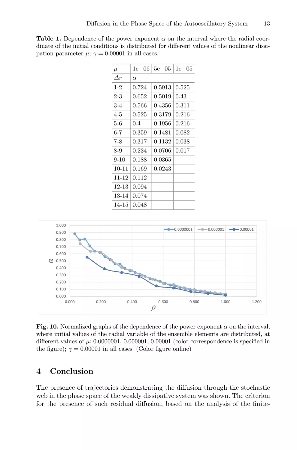
Table 1. Dependence of the power exponent α on the interval where the radial coordinate of the initial conditions is distributed for diﬀerent values of the nonlinear dissipation parameter μ; γ = 0.00001 in all cases.
μ
Δr

1e−06 5e−05 1e−05
α

1-2
2-3
3-4
4-5
5-6
6-7
7-8
8-9
9-10
10-11
11-12
12-13
13-14
14-15

0.724
0.652
0.566
0.525
0.4
0.359
0.317
0.234
0.188
0.169
0.112
0.094
0.074
0.048

0.5913
0.5019
0.4356
0.3179
0.1956
0.1481
0.1132
0.0706
0.0365
0.0243

0.525
0.43
0.311
0.216
0.216
0.082
0.038
0.017

Fig. 10. Normalized graphs of the dependence of the power exponent α on the interval,
where initial values of the radial variable of the ensemble elements are distributed, at
diﬀerent values of μ: 0.0000001, 0.000001, 0.00001 (color correspondence is speciﬁed in
the ﬁgure); γ = 0.00001 in all cases. (Color ﬁgure online)

4

Conclusion

The presence of trajectories demonstrating the diﬀusion through the stochastic
web in the phase space of the weakly dissipative system was shown. The criterion
for the presence of such residual diﬀusion, based on the analysis of the ﬁnite-

14

A. V. Golokolenov and D. V. Savin

time Lyapunov exponent values, was introduced, and properties of dependence
of the average ensemble energy on time were analyzed for ensembles of such
trajectories. This energy depends on time by the power law. A power exponent
decreases down to 0 with the increase of the initial ensemble energy, and it’s
dependence on the initial ensemble energy has the similar shape in wide interval
of the parameter of nonlinear dissipation.

References
1. Daly, M.V., Heﬀernan, D.M.: Chaos in a resonantly kicked oscillator. J. Phys. A:
Math. Gen. 28(9), 2515–2528 (1995)
2. Felk, E.V.: The eﬀect of weak nonlinear dissipation on structures of the stochastic
web type. Izvestiya VUZ. Appl. Nonlinear Dyn. 21(3), 72–79 (2013). (in Russian)
3. Felk, E.V., Kuznetsov, A.P., Savin, A.V.: Multistability and transition to chaos in
the degenerate Hamiltonian system with weak nonlinear dissipative perturbation.
Physica A 410, 561–572 (2014)
4. Feudel, U.: Complex dynamics in multistable systems. Int. J. Bifurcation Chaos
18(06), 1607–1626 (2008)
5. Feudel, U., Grebogi, C., Hunt, B.R., Yorke, J.A.: Map with more than 100 coexisting low-period periodic attractors. Phys. Rev. E 54(1), 71–81 (1996)
6. Forest, E., Ruth, R.D.: Fourth-order symplectic integration. Physica D 43(1), 105–
117 (1990)
7. Kuznetsov, A.P., Savin, A.V., Savin, D.V.: On some properties of nearly conservative dynamics of Ikeda map and its relation with the conservative case. Physica
A 387(7), 1464–1474 (2008)
8. Lichtenberg, A.J., Wood, B.P.: Diﬀusion through a stochastic web. Phys. Rev. A
39(4), 2153–2159 (1989)
9. Reichl, L.: The Transition to Chaos: Conservative Classical and Quantum Systems,
vol. 200. Springer, Heidelberg (2021)
10. Savin, A.V., Savin, D.V.: The basins of attractors in the web map with weak
dissipation. Nonlinear World 8(2), 70–71 (2010). (in Russian)
11. Soskin, S.M., McClintock, P.V.E., Fromhold, T.M., Khovanov, I.A., Mannella, R.:
Stochastic webs and quantum transport in superlattices: an introductory review.
Contemp. Phys. 51(3), 233–248 (2010)
12. Zaslavskii, G.M., Zakharov, M.I., Sagdeev, R.Z., Usikov, D.A., Chernikov, A.A.:
Stochastic web and particle diﬀusion in a magnetic ﬁeld. Zhurnal Eksperimentalnoi
i Teoreticheskoi Fiziki 91, 500–516 (1986)
13. Zaslavsky, G.M.: The Physics of Chaos in Hamiltonian Systems. World Scientiﬁc
(2007)

Aberrator Shape Identification from 3D
Ultrasound Data Using Convolutional
Neural Networks and Direct Numerical
Modeling
Alexey Vasyukov(B) , Andrey Stankevich , Katerina Beklemysheva ,
and Igor Petrov
Moscow Institute of Physics and Technology, Dolgoprudny, Russia
a.vasyukov@phystech.edu
Abstract. The paper considers the problem of silicon aberrator shape
identiﬁcation from 3D medical ultrasound data using convolutional neural networks.
This work demonstrates that it is possible to obtain high quality
numerical 3D ultrasound images using direct numerical modeling methods. Current study models reﬂections from long smooth boundaries and
individual large reﬂectors, as well as background noise from point reﬂectors. The synthetic computational data obtained in this way can be used
to develop convolutional neural networks for 3D ultrasound data.
This work shows that 3D convolutional neural network can identify
position and shape of the silicone aberrator boundary from an ultrasound data. The papers covers the cases of strong noise and signiﬁcant
signal distortions. It is demonstrated that 3D network can handle the
distortions and correctly distinguish the boundary of materials from the
responses of individual large reﬂectors. This possibility of the network is
due to its three-dimensional architecture, which uses all spatial information from all directions.
Keywords: Ultrasound · Matrix probe · Numerical modeling
problem · Convolutional neural networks

1

· Inverse

Introduction

Ultrasound is one of the widely used methods of medical studies. Recent advances
of ultrasound equipment signiﬁcantly enhanced both resolution and contrast of
traditional ultrasonic images. Another important area of research is a development of matrix probes that allow to obtain 3D volumetric ultrasonic scans
that provide signiﬁcant new capabilities compares with classical 2D ultrasound
images obtained with linear probes.
Traditional 2D ultrasound images are widespread. The methods for automated analysis of these images are well developed, including the techniques based
Supported by RSF project 22-11-00142.
c The Author(s), under exclusive license to Springer Nature Switzerland AG 2022

D. Balandin et al. (Eds.): MMST 2022, CCIS 1750, pp. 15–28, 2022.
https://doi.org/10.1007/978-3-031-24145-1_2

16

A. Vasyukov et al.

on machine learning methods and convolutional neural networks. This area of
research is covered in modern scientiﬁc literature very well. Several papers to
mention demonstrate the convolutional network’s feasibility for diﬀerent biomedical imaging problems. The paper [1] studied an application of deep learning to
artifacts correction on single-shot ultrasound images obtained with sparse linear
arrays. The initial results demonstrated an image quality comparable or better
to that obtained from conventional beamforming. The work [2] used neural networks to identify the shape of the aberration prism that distorts the ultrasonic
signal. The work [3] applied convolutional networks to elasticity imaging to distinguish benign tumors from their malignant counterparts based on measured
displacement ﬁelds on the boundary of the domain.
It should be noted that the vast majority of modern works use 2D problem
statements and 2D ultrasound images. This fact naturally raises the question
of generalizing similar machine learning approaches to a fully three-dimensional
case. This should allow to fully unlock the potential of modern ultrasound equipment. The papers devoted to this area show that this approach is really promising. The work [4] covered 3-class classiﬁcation problem for 3D images of human
thyroid. The paper [5] used 3D neural networks for ovary and follicle detection
from ultrasound volumes. The authors of [6] studied the application of 3D convolutional neural networks for super-resolution of microvascularity visualization.
The study [7] compared directly the results of 2D and tracked 3D ultrasound
with an automatic segmentation based on a deep neural network regarding interand intraobserver variability, time, and accuracy.
Processing of ultrasound images with convolutional neural networks is typically based on U-Net architecture [8] for 2D cases. 3D cases mostly use the same
approach implemented in 3D [9]. Diﬀerent modiﬁcations of these approaches
exist. For example, the work [10] used three U-Nets that segmented the 3D
ultrasound images in the axial, lateral and frontal orientations, and these three
segmentation maps were consolidated by a separate segmentation average network.
However, full 3D neural networks for medical ultrasound are still not well
covered. One of the reasons limiting the research in this area of research is a limited amount of open 3D ultrasound data available for development and testing of
machine learning algorithms. The limited amount of data is especially important
because it can lead to overﬁtting of the network to the data from the existing
samples [11]. The current paper demonstrates an approach for the development
of convolutional neural networks for 3D ultrasound image processing using direct
numerical modeling methods.
This paper is organized as follows. Section 2 is devoted to the direct problem
of 3D ultrasound images modeling - problem statement, mathematical model
and numerical method are described. This works covers for the direct problem
the following artifacts: the reﬂection from the boundary between acoustically
contrasting layers, the noise caused by small bright reﬂectors in the media, the
distortions caused by large reﬂectors. Section 3 presents the approach for the
inverse problem of determining the position of the boundary between layers

Aberrator Shape Identiﬁcation from 3D Ultrasound Data Using CNN

17

using convolutional neural networks. The architecture of the network, the dataset
creation procedures, the training of the network are covered. The results of
numerical experiments and their discussion are given in Sect. 4. The concluding
remarks are given in Sect. 5.

2
2.1

Direct Problem
Problem Statement

This paper considers the problem of forming a 3D ultrasound image in the area
containing the boundary between acoustically contrasting layers. The computational domain is a parallelepiped. The upper face of the parallelepiped corresponds to the outer border of the body, on which the 3D matrix ultrasound
probe is located. This face is considered to be a free surface outside the area
of the contact with the sensor. The external pressure condition is set under the
sensor.
The boundary between two layers is smooth, the shape of the boundary is
taken arbitrary, the boundary is at an arbitrary depth ranging from 10% to 90%
of the total depth of the computational domain. The upper layer contains many
reﬂective objects that distort the ﬁnal ultrasound image. Small point reﬂectors
and large pores are considered. Small reﬂectors are used to simulate imperfections in the top layer material. Each individual small reﬂector generates a weak
echo response. However, a large number of such reﬂectors (from hundreds to tens
of thousands in diﬀerent calculations) leads to a signiﬁcant noise in the ultrasound image. Large pores describe macroscopic inclusions. Echo responses from
these inclusions can be comparable to the reﬂection from the boundary between
the layers.
2.2

Mathematical Model and Numerical Method

This paper uses an acoustics model to describe the medium. According to the
acoustic model [12], the ultrasound signal propagation is described by the following equations:
ρ(x)

∂v(x, t)
+ ∇p(x, t) = 0
∂t

in Ω,

(1)

∂p(x, t)
+ ρ(x)c2 (x)∇ · v(x, t) = −α(x)c(x)p(x, t) in Ω,
(2)
∂t
where Ω is the computational domain, ρ(x) is the material density, v(x, t) is the
velocity vector, p(x, t) is the acoustic pressure, c(x) is the speed of sound, α(x)
is the Maxwell’s attenuation coeﬃcient [13].
The acoustic model takes into account longitudinal (pressure) waves in soft
tissues and does not account transverse (shear) waves. This model is conventional
in diagnostic ultrasound simulations since the attenuation coeﬃcient for shear

18

A. Vasyukov et al.

waves in soft tissues is four orders of magnitude greater than that for pressure
waves at MHz frequencies [14].
The wavefront construction method is used for the numerical solution. The
implementation uses the modiﬁcations described in [15]. This numerical method
is focused exclusively on acoustic equations, which is an acceptable limitation
for the present work. The paper [15] demonstrated that calculations using this
method allow to obtain numerical ultrasound images that match the experimental data qualitatively and quantitatively. The method allows one to describe the
reﬂection from long boundaries and from point reﬂectors. The boundary between
the layers and the boundaries of large pores are described using long boundaries
approach. The small reﬂectors are considered as point ones. Signal processing
and B-scan image generation follow the algorithms described in [16].
2.3

Numerical Results for the Direct Problem

The statement of the direct problem extends the results presented in [15]. The
previous work studied the scan of the medical phantom through the silicone aberrator prism. That study was performed for the 2D setup with the linear probe and
showed the applicability of the wavefront construction method acoustic model
to this problem. Current research considers a similar problem statement in full
3D using a matrix probe.
The matrix sensor considered in this work is square and consists of an arraty
of 24 × 24 elements. The transmitted signal has the frequency ω = 3 MHz. The
signal is digitized using 45 MHz frequency. The size of the obtained volumetric
3D image is 24 × 24 × 1024.
The speed of sound in both layers is ﬁxed. The outer layer is more rigid,
the speed of sound is 3.0 km/s. The second layer is softer, the speed of sound is
1.5 km/s, this value is typical for the soft tissues of the human body. The number
of small reﬂectors in the volume of the outer layer under the probe varied from
100 to 2500. The number of large pores ranged from 5 to 50.
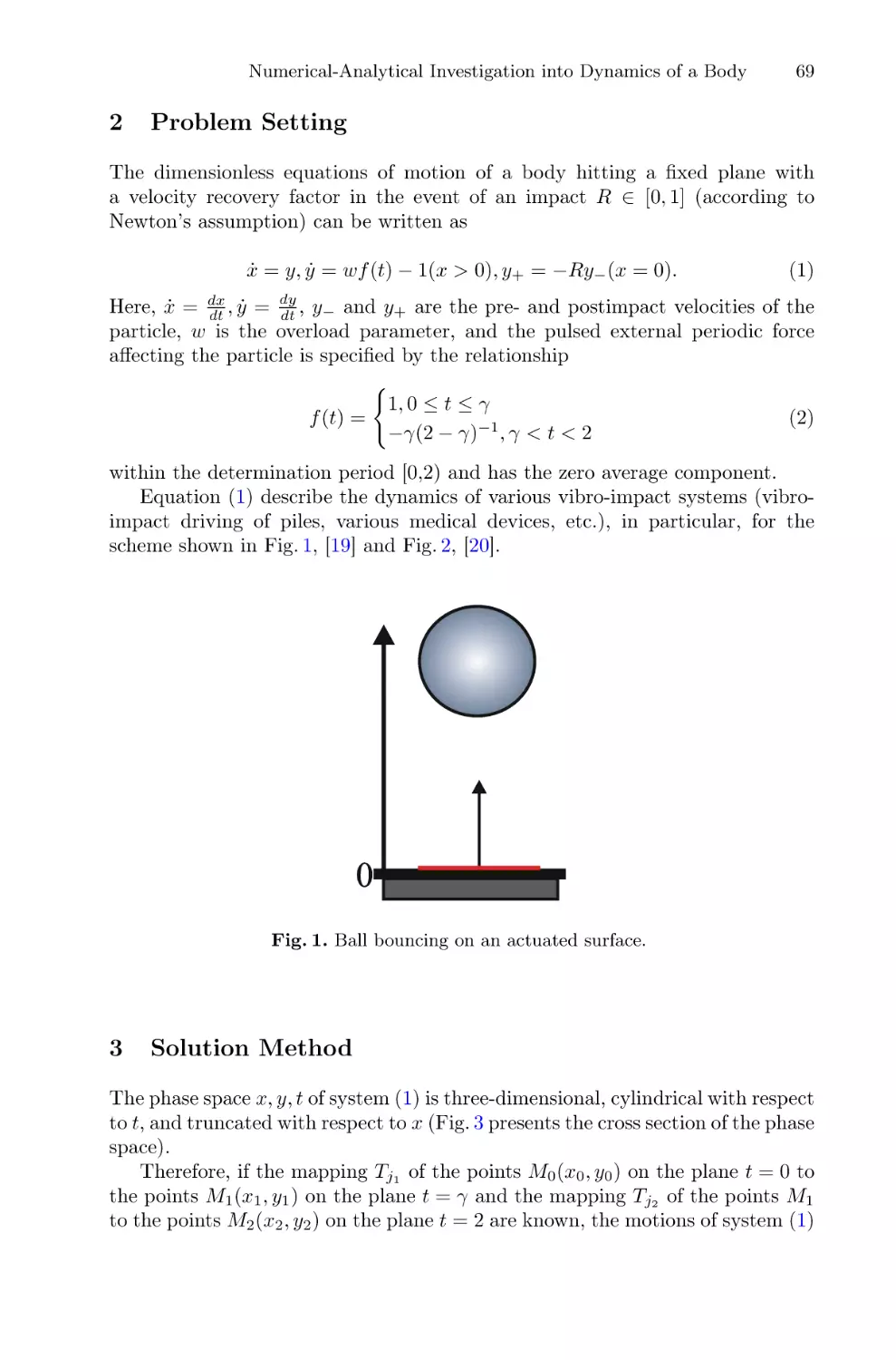
Figure 1 shows an example image for the problem statement without reﬂectors that distort the signal. Reﬂection from the boundary between two layers
is clearly visible for all slices, the location of the boundary is obvious. Figure 2
demonstrates an example of an image with a large number of pores and small
reﬂectors in the upper layer. In this particular image, the boundary between
the layers is easily distinguishable, but this is due solely to the fact that all the
reﬂectors were artiﬁcially localized near the surface, and the signal from them
was weakly superimposed on the signal from the boundary. The general view of
this image allows to estimate the level of noise and distortion compared with
the echo from the boundary. When noise and reﬂection from pores are superimposed on the echo signal from the boundary, the interpretation of the response
will become extremely diﬃcult.

Aberrator Shape Identiﬁcation from 3D Ultrasound Data Using CNN

19

Fig. 1. A sample of 3D scan without distortions. The ﬁrst eight slices are presented.
The image is zoomed to the area around the border for better visibility.

20

A. Vasyukov et al.

Fig. 2. A sample of 3D scan with distortions. The ﬁrst eight slices are presented. The
image is zoomed to the area around the border for better visibility.

Aberrator Shape Identiﬁcation from 3D Ultrasound Data Using CNN

3
3.1

21

Inverse Problem
Problem Statement

The inverse problem in this work is to determine the position of the boundary
between two layers based on 3D ultrasound data. The input data of the inverse
problem is a three-dimensional array of dimensions 24 × 24 × 1024. The ﬁrst two
dimensions correspond to the numbers of elements in the matrix probe along
two axes, and the third dimension corresponds to the depth in time domain.
The output of the inverse problem is the position of the interface between two
media in the volume presented as the input.
As shown above, the quality of the input images can vary a lot. In the absence
of signal distortions, the inverse problem becomes trivial, the position of the
boundary is easily determined both visually and by the simple signal processing
algorithms. The samples with strong distortions can be extremely diﬃcult to
interpret both visually and automatically. This work uses convolutional neural
networks to solve the inverse problem.
3.2

Neural Network Architecture

There are three possible approaches to building a convolutional neural network
for volumetric 3D ultrasound data.
1. A 3D image can be represented as a set of 2D slices. This allow to use a
traditional 2D convolutional network for each of the slices. The network has
one input channel that takes a slice data as a grayscale image. This approach
is easy to implement, but it has obvious drawbacks. When working with a 2D
slice, the network fundamentally cannot use the full spatial information that
was originally contained in the full 3D image.
2. A 2D network with multiple input channels can be used to overcome the obvious disadvantage of the previous option. The implementation of this approach
can be based on a large number of ready to use technical solutions, since
multichannel 2D convolutional neural networks are routinely used for color
image processing. Classical pipeline uses several channels to input separate
RGB color components of the image. However, there is an experience showing
that similar approach is applicable to a signiﬁcantly diﬀerent nature of data
in diﬀerent channels. For example, the work [17] considered seismic inversion and used multichannel 2D network to encode the data acquired for the
same object using diﬀerent positions of the source of the signal. In the case
of 3D ultrasound, separate input channels can be used to represent adjacent
2D slices of the full 3D image. This will allow the network to use inter-slice
information to some extent. For example, the work [18] used this approach
to classify 3D ultrasound data.
3. It is possible to implement a fully 3D convolutional network using 3D convolution kernels. This approach is much more diﬃcult to implement technically,
since there are very few ready to use technical components for such networks.

22

A. Vasyukov et al.

However, there are no fundamental obstacles to the implementation of such
a network. In this case, the input data of the network is a 3D volume representing the original data as a 3D grayscale image. The use of 3D convolution
seems to be the most promising option. This approach does not require an
artiﬁcial separation of spatial variables and makes it possible to fully reﬂect
the physical nature of the problem being considered.
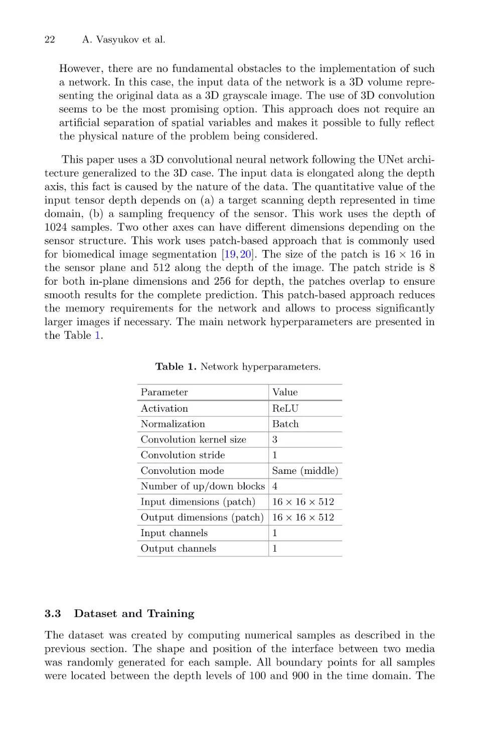
This paper uses a 3D convolutional neural network following the UNet architecture generalized to the 3D case. The input data is elongated along the depth
axis, this fact is caused by the nature of the data. The quantitative value of the
input tensor depth depends on (a) a target scanning depth represented in time
domain, (b) a sampling frequency of the sensor. This work uses the depth of
1024 samples. Two other axes can have diﬀerent dimensions depending on the
sensor structure. This work uses patch-based approach that is commonly used
for biomedical image segmentation [19,20]. The size of the patch is 16 × 16 in
the sensor plane and 512 along the depth of the image. The patch stride is 8
for both in-plane dimensions and 256 for depth, the patches overlap to ensure
smooth results for the complete prediction. This patch-based approach reduces
the memory requirements for the network and allows to process signiﬁcantly
larger images if necessary. The main network hyperparameters are presented in
the Table 1.
Table 1. Network hyperparameters.
Parameter

Value

Activation

ReLU

Normalization

Batch

Convolution kernel size

3

Convolution stride

1

Convolution mode

Same (middle)

Number of up/down blocks 4
Input dimensions (patch)

16 × 16 × 512

Output dimensions (patch) 16 × 16 × 512

3.3

Input channels

1

Output channels

1

Dataset and Training

The dataset was created by computing numerical samples as described in the
previous section. The shape and position of the interface between two media
was randomly generated for each sample. All boundary points for all samples
were located between the depth levels of 100 and 900 in the time domain. The

Aberrator Shape Identiﬁcation from 3D Ultrasound Data Using CNN

23

number of small reﬂectors varied from 100 to 2500, the number of large pores
varied from 5 to 50.
The input data contained noisy and distorted synthetic ultrasound images.
Ground truth images contained true position of the border between two layers. A
separate ground truth data manual preparation was not required since an exact
border position is knows for synthetic data.
A total of 10 000 numerical samples were prepared. They were divided into
training and validation datasets using the ratio of 75:25. Separate samples were
used for ﬁnal testing, they were generated additionally and not used in any way
during network training.
The Adam optimization algorithm was used for training with a constant
learning rate of 1e−4 and the BCEWithLogits loss function. The training was
performed from scratch, pretrained networks were not used. Training was performed for 100 epochs with the batch size of 12 samples. The loss function was
observed to become stable around the 30th–40th epoch, the value of the loss only
slightly oscillated for the next epochs around the achieved values. We used the
weights from the epoch at which the best value of the loss function was achieved
on the validation set. Typical training time was about 12 h.

4

Numerical Experiments and Discussion

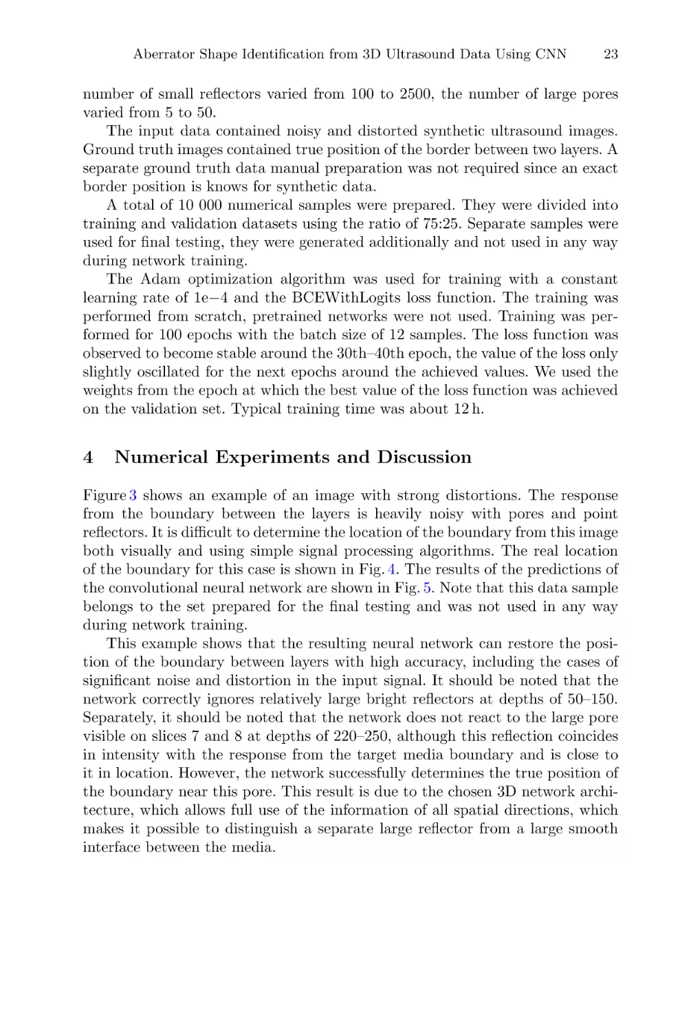
Figure 3 shows an example of an image with strong distortions. The response
from the boundary between the layers is heavily noisy with pores and point
reﬂectors. It is diﬃcult to determine the location of the boundary from this image
both visually and using simple signal processing algorithms. The real location
of the boundary for this case is shown in Fig. 4. The results of the predictions of
the convolutional neural network are shown in Fig. 5. Note that this data sample
belongs to the set prepared for the ﬁnal testing and was not used in any way
during network training.
This example shows that the resulting neural network can restore the position of the boundary between layers with high accuracy, including the cases of
signiﬁcant noise and distortion in the input signal. It should be noted that the
network correctly ignores relatively large bright reﬂectors at depths of 50–150.
Separately, it should be noted that the network does not react to the large pore
visible on slices 7 and 8 at depths of 220–250, although this reﬂection coincides
in intensity with the response from the target media boundary and is close to
it in location. However, the network successfully determines the true position of
the boundary near this pore. This result is due to the chosen 3D network architecture, which allows full use of the information of all spatial directions, which
makes it possible to distinguish a separate large reﬂector from a large smooth
interface between the media.

24

A. Vasyukov et al.

Fig. 3. A sample of 3D scan with high level of distortions. The image is zoomed to the
area around the border for better visibility.

Aberrator Shape Identiﬁcation from 3D Ultrasound Data Using CNN

25

Fig. 4. Ground truth position of the border between two layers for the sample with
high level of distortions. The image is zoomed to the area around the border for better
visibility.

26

A. Vasyukov et al.

Fig. 5. Prediction of the border between two layers for the sample with high level of
distortions. The image is zoomed to the area around the border for better visibility.

Aberrator Shape Identiﬁcation from 3D Ultrasound Data Using CNN

5

27

Conclusions and Future Work

This work shows that it is possible to obtain numerical 3D ultrasound images
of suﬃciently high quality using direct numerical modeling methods. This work
considers reﬂections from smooth boundaries and individual large reﬂectors, as
well as background noise from point reﬂectors. The synthetic computational data
obtained in this way can be used to explore the possibilities of 3D ultrasound,
as well as to develop convolutional neural networks for 3D ultrasound for the
cases that lack real experimental data available.
This work shows that 3D convolutional neural network can identify position and shape of the silicone aberrator boundary based on the ultrasound data,
including the cases of strong noise and signiﬁcant distortions. It is shown that the
network can correctly distinguish the boundary of materials from the responses
of individual large reﬂectors comparable in brightness. This possibility of the
network is due to its three-dimensional architecture, which uses all spatial information from all directions.
Further steps should include an implementation of an elastic material model
and a contact between elastic (bone) and acoustic (soft tissues) media. This
should allow to simulate the statements that cannot be described in terms of a
purely acoustic approximation. It is possible that after the transition to the full
elasticity model, it will be necessary to revise the parameters of the convolutional
network, since a signiﬁcant complication of the wave pattern should be expected.

References
1. Dimitris, P., Manuel, V., Florian, M., Marcel, A, Jean-Philippe, T.: Single-shot
CNN-based ultrasound imaging with sparse linear arrays. In: 2020 IEEE International Ultrasonics Symposium (IUS), pp. 1–4 (2020)
2. Stankevich, A.S., Petrov, I.B., Vasyukov, A.V.: Numerical solution of inverse problems of wave dynamics in heterogeneous media with convolutional neural networks.
In: Favorskaya, M.N., Favorskaya, A.V., Petrov, I.B., Jain, L.C. (eds.) Smart Modelling for Engineering Systems. SIST, vol. 215, pp. 235–246. Springer, Singapore
(2021). https://doi.org/10.1007/978-981-33-4619-2 18
3. Patel, D., Tibrewala, R., Vega, A., Dong, L., Hugenberg, N., Oberai, A.: Circumventing the solution of inverse problems in mechanics through deep learning:
application to elasticity imaging. Comput. Methods Appl. Mech. Eng. 353, 448–
466 (2019)
4. Lu, H., Wang, H., Zhang, Q., Yoon, S., Won, D.: A 3D convolutional neural network
for volumetric image semantic segmentation. Procedia Manuf. 39, 422–428 (2019)
5. Potočnik, B., Šavc, M.: Deeply-supervised 3D convolutional neural networks
for automated ovary and follicle detection from ultrasound volumes. Appl. Sci.
12(1246) (2022)
6. Brown, K., Dormer, J., Fei, B., Hoy, K.: Deep 3D convolutional neural networks
for fast super-resolution ultrasound imaging. In: Proceedings of the SPIE 10955,
Medical Imaging 2019: Ultrasonic Imaging and Tomography, p. 1095502 (2019)
7. Krönke, M., et al.: Tracked 3D ultrasound and deep neural network-based thyroid
segmentation reduce interobserver variability in thyroid volumetry. PLoS ONE
17(7), Article e0268550 (2022)

28

A. Vasyukov et al.

8. Ronneberger, O., Fischer, P., Brox, T.: U-Net: convolutional networks for biomedical image segmentation. arXiv:1505.04597 (2015)
9. Çiçek, Ö., Abdulkadir, A., Lienkamp, S.S., Brox, T., Ronneberger, O.: 3D U-Net:
learning dense volumetric segmentation from sparse annotation. arXiv:1606.06650
(2016)
10. Jiang, M., Spence, J.D., Chiu, B.: Segmentation of 3D ultrasound carotid vessel
wall using U-Net and segmentation average network. In: 42nd Annual International
Conference of the IEEE Engineering in Medicine and Biology Society (EMBC), pp.
2043–2046. IEEE (2020)
11. Zheng, Y., Liu, D., Georgescu, B., Nguyen, H., Comaniciu, D.: 3D deep learning
for eﬃcient and robust landmark detection in volumetric data. In: Proceedings of
2015 IEEE Medical Image Computing and Computer-Assisted Intervention, pp.
565–572. IEEE (2015)
12. Mast, T.D., Hinkelman, L.M., Metlay, L.A., Orr, M.J., Waag, R.C.: Simulation of
ultrasonic pulse propagation, distortion, and attenuation in the human chest wall.
J. Acoust. Soc. Am. 6, 3665–3677 (1999)
13. Beklemysheva, K., et al.: Transcranial ultrasound of cerebral vessels in silico: proof
of concept. Russ. J. Numer. Anal. Math. Model. 31(5), 317–328 (2016)
14. Madsen, E.L., Sathoﬀ, H.J., Zagzebski, J.A.: Ultrasonic shear wave properties of
soft tissues and tissuelike materials. J. Acoust. Soc. Am. 74(5), 1346–1355 (1983)
15. Beklemysheva, K., Grigoriev, G., Kulberg, N., Petrov, I., Vasyukov, A., Vassilevski,
Y.: Numerical simulation of aberrated medical ultrasound signals. Russ. J. Numer.
Anal. Math. Model. 33, 277–288 (2018)
16. Vassilevski, Y., Beklemysheva, K., Grigoriev, G., Kulberg, N., Petrov, I., Vasyukov,
A.: Numerical modelling of medical ultrasound: phantom-based veriﬁcation. Russ.
J. Numer. Anal. Math. Model. 32(5), 339–346 (2017)
17. Stankevich, A., Nechepurenko, I., Shevchenko, A., Gremyachikh, L., Ustyuzhanin,
A., Vasyukov, A.: Learning velocity model for complex media with deep convolutional neural networks. arXiv:2110.08626 (2021)
18. Paserin, O., Mulpuri, K., Cooper, A., Abugharbieh, R., Hodgson, A.: Improving
3D ultrasound scan adequacy classiﬁcation using a three-slice convolutional neural
network architecture. In: Zhan, W., Baena, F. (eds.) CAOS 2018 (EPiC Series in
Health Sciences), vol. 2, pp. 152–156 (2018)
19. Coupeau, P., Fasquel, J.-B., Mazerand, E., Menei, P., Montero-Menei, C.N., Dinomais, M.: Patch-based 3D U-Net and transfer learning for longitudinal piglet brain
segmentation on MRI. Comput. Methods Programs Biomed. 214, 106563 (2022)
20. Ghimire, K., Chen, Q., Feng, X.: Patch-based 3D UNet for head and neck tumor
segmentation with an ensemble of conventional and dilated convolutions. In:
Andrearczyk, V., Oreiller, V., Depeursinge, A. (eds.) HECKTOR 2020. LNCS,
vol. 12603, pp. 78–84. Springer, Cham (2021). https://doi.org/10.1007/978-3-03067194-5 9

Complex Dynamics of the Implicit Maps
Derived from Iteration of Newton
and Euler Methods
Andrei A. Elistratov1,2(B) , Dmitry V. Savin2(B) ,
and Olga B. Isaeva1,2(B)
1

2

Kotel’nikov Institute of Radio-Engineering and Electronics of RAS,
Saratov Branch, Zelenaya 38, Saratov 410019, Russia
zhykreg@gmail.com, isaevao@rambler.ru
Saratov State University, Astrakhanskaya 83, Saratov 410012, Russia
savin.dmitry.v@gmail.com

Abstract. Special exotic class of dynamical systems—the implicit
maps—is considered. Such maps, particularly, can appear as a result
of using of implicit and semi-implicit iterative numerical methods. In the
present work we propose the generalization of the well-known NewtonCayley problem. Newtonian Julia set is a fractal boundary on the complex plane, which divides areas of convergence to diﬀerent roots of
cubic nonlinear complex equation when it is solved with explicit Newton
method. We consider similar problem for the relaxed, or damped, Newton method, and obtain the implicit map, which is non-invertible both
time-forward and time-backward. It is also possible to obtain the same
map in the process of solving of certain nonlinear diﬀerential equation
via semi-implicit Euler method. The nontrivial phenomena, appearing in
such implicit maps, can be considered, however, not only as numerical
artifacts, but also independently. From the point of view of theoretical
nonlinear dynamics they seem to be very interesting object for investigation. Earlier it was shown that implicit maps can combine properties of
dissipative non-invertible and Hamiltonian systems. In the present paper
strange invariant sets and mixed dynamics of the obtained implicit map
are analyzed.
Keywords: Julia set

1

· Hamiltonian system · Implicit map

Introduction

One of the wide-known examples of fractal sets—Newtonian Julia set (Fig. 1)—
arises as a boundary of areas of convergence to diﬀerent roots of the cubic polynomial equation on the complex plane
φ(z) = z 3 + c = 0,
Supported by Russian Science Foundation, Grant No. 21-12-00121.
c The Author(s), under exclusive license to Springer Nature Switzerland AG 2022

D. Balandin et al. (Eds.): MMST 2022, CCIS 1750, pp. 29–40, 2022.
https://doi.org/10.1007/978-3-031-24145-1_3

(1)

30

A. A. Elistratov et al.

when it is solved with the Newton method [18]. This problem, ﬁrst suggested by
Cayley [5], allows generalization, if relaxed, or damped Newton method
φ(zn )
z3 + c
= zn − h n 2

φ (zn )
2zn

zn+1 = zn − h

(2)

is used [13,14]. At the same time the iteration process (2) can be considered as
a trivial discretization of the ordinary diﬀerential equation
ż = f (z)

(3)

zn+1 = zn + hf (zn ),

(4)

with the Euler method
where
f (z) = −

φ(z)
z3 + c
=
−
.
φ (z)
3z 2

(5)

Roots of the polynomial Eq. (1) are the stable nodes of the ODE (3). At the
same time these roots are the attractors of the Newton and Euler iteration process (2), at least, when the discretization step h is small enough. The boundary
between basins of attraction of the iteration process (2)—the fractal Newtonian
Julia set—corresponds to a separatrix of (3), which should be smooth when f (z)
is deﬁned by (5) (see Fig. 1). Fractalization of the separatrix occures due to the
Euler discretization. This is a numerical artifact, which can be considered as
neglectable for practical applications at h → 0.

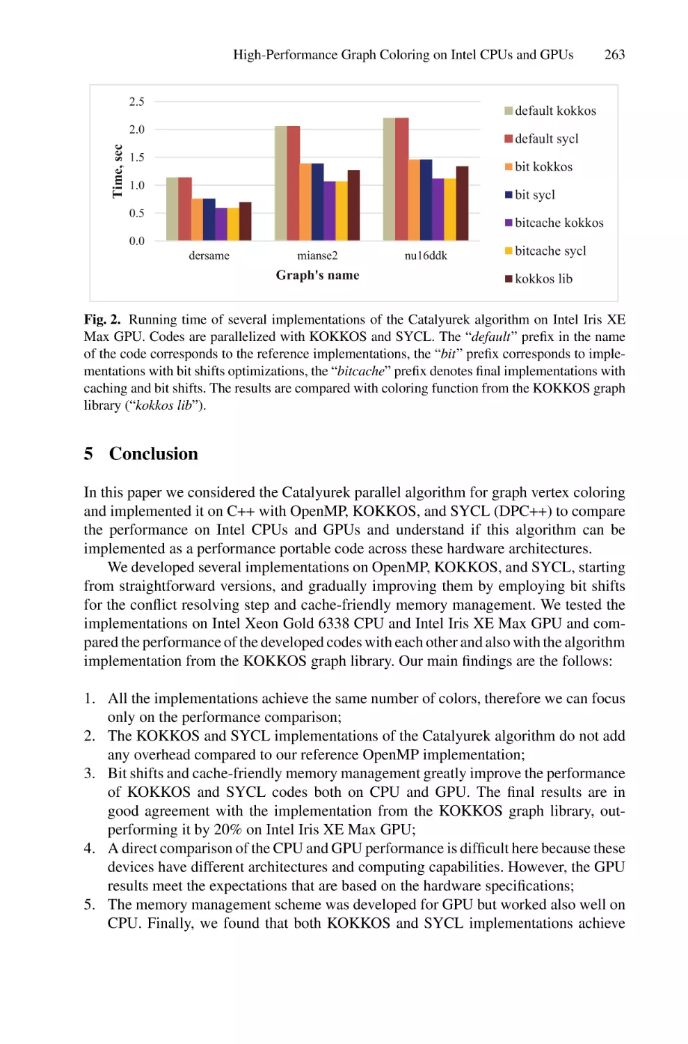
Fig. 1. Newtonian Julia set—fractal boundary between white, black and gray regions,
which are the basins of attraction of three roots of the Eq. (1) with c = −1 (left panel)
and Newtonian pie—phase plane of the ﬂow dynamical system (3) (right panel): three
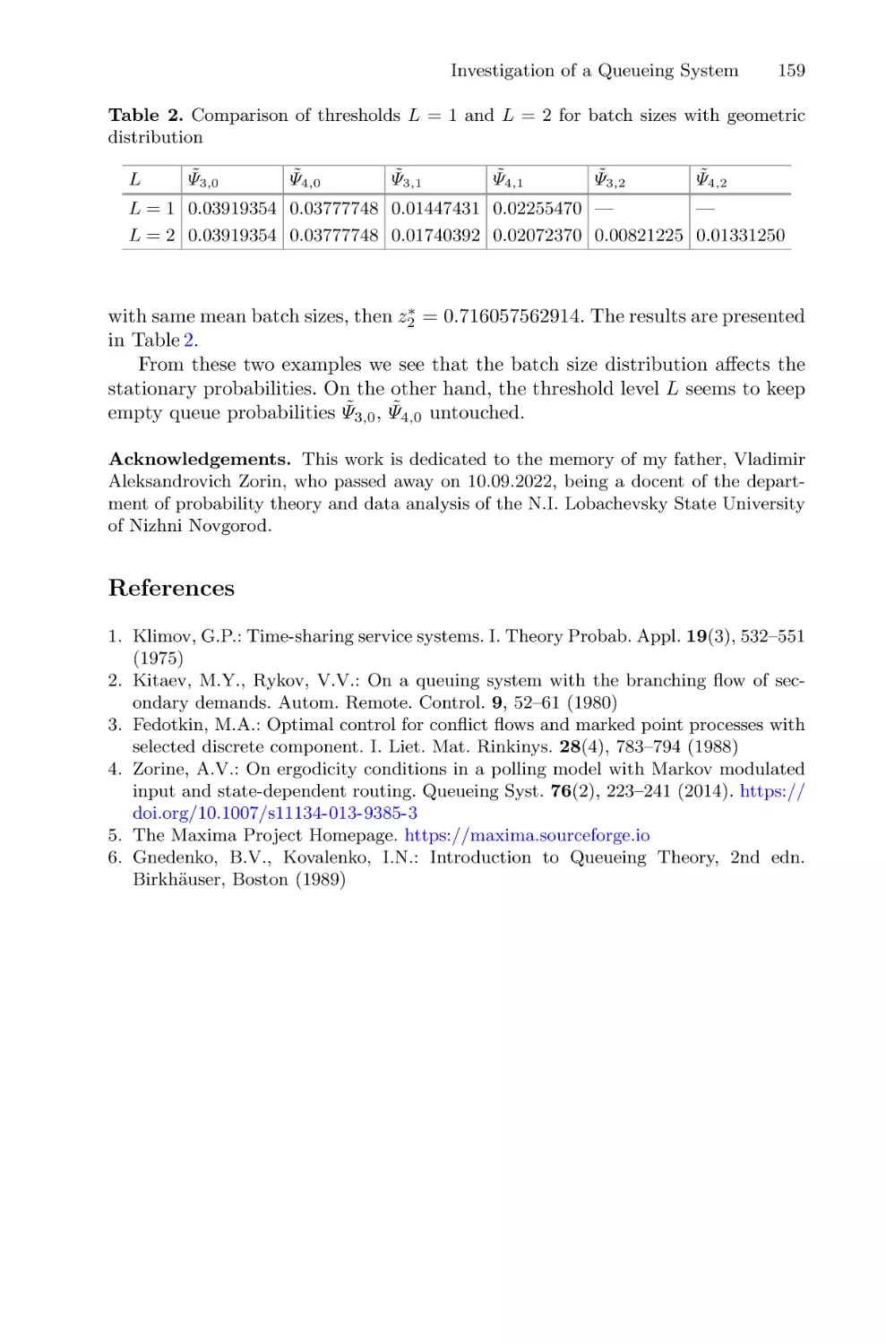
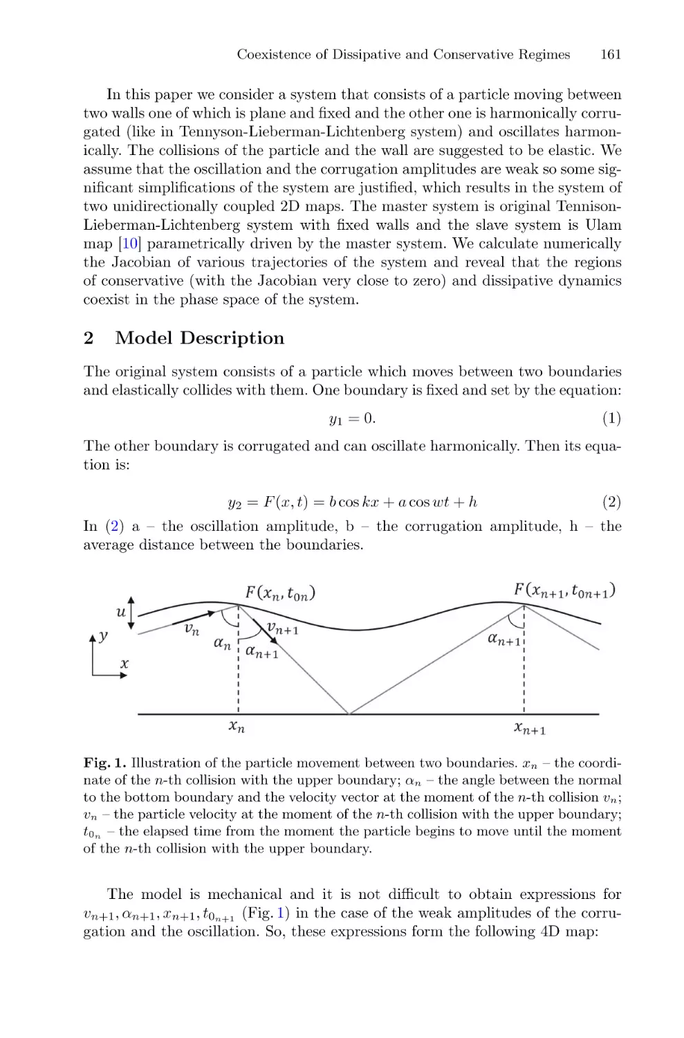
roots of (1) are the stable nodes of the ODE (3), its basins of attraction are divided
by the smooth separatrix. Euler discretization (4) of (3) results in emergence of fractal
basin boundary, like one on the left panel, which degenerates to the true smooth linear
separatrix at h → 0.

Complex Dynamics of the Implicit Maps

31

While in general discretization of ﬂow dynamical systems caused by numerical time-integration can lead to emergence of solutions which do not represent
the dynamics of the original system and manifest themselves in changes of the
phase space structure, as in example discussed above, or changes in bifurcation
diagrams etc. (see, e.g., [12,16,17] and references there), this problem can be
considered from another angle: such discretization of well-known ﬂow systems
can be regarded as a fruitful approach, which is widely used in modern nonlinear
theory and allows to generate new model maps (see, e.g., [1,2,11,22] and references there). Due to emergence of numerical artifacts mentioned above dynamical systems generated this way can demonstrate various nontrivial phenomena.
The discretization step h is usually deﬁned in such models in a wide range—
moreover, it can be complex [18]. This approach can also establish a background
for introducing and considering of a new class of systems, one example from
which is proposed in present work.
Simple construction (2), being considered as an abstract dynamical system,
allows a wide spectrum of generalizations and parametrizations. Types of dynamical behavior and obtained phenomena can also be rather diverse. Particularly,
the implicit dynamics, when every point in the phase space of the system has
both several images and several preimages [3,4,15], is also possible. Such implicit
correspondences have wide spectrum of applications besides implicit numerical
schemes of equations solving. Implicit functions can occur in problems of reconstruction of a multidimensional object (or system) from its projection [6], in
the theory of generalized synchronization [19], in economics [7,10], computer
graphics [20], chaos control techniques [8], topology [21].
In the present paper we try to give an example of generalization of the iteration process (2) and to investigate obtained system from the point of view of
theoretical nonlinear dynamics. In the Sect. 2 we present the procedure of deriving an implicit map using the modiﬁed Euler method. In the Sect. 3 we analyze
the fractalization of both unstable and stable invariant sets of such exotic system.

2

Basic Model

Among the numerical recipes of the ODE integration the semi-implicit Euler
method is listed:
(6)
zn+1 = zn + h(f (zn ) + f (zn+1 ))/2.
Let us generalize this scheme by parameterization:
zn+1 = zn + h((1 − α)f (zn ) + αf (zn+1 ).

(7)

In case when f (z) chosen in form (5) this equation can be rewrited as following:
3
2
2
(αh + 3)zn+1
zn2 + ((1 − α)h − 3)zn+1
zn3 + (1 − α)hczn+1
+ αhczn2 = 0.

(8)

This is also some iteration process, but, in contrast to (4), not traditional for the
nonlinear dynamical system theory. This is an implicit map with the evolution
operator looking like
(9)
Ψ (zn+1 , zn ) = 0.

32

A. A. Elistratov et al.

Both forward and backward iterations of this map are deﬁned by multi-valued
functions,
(10)
zn+1 = Ψ+ (zn )
and
zn = Ψ− (zn+1 )

(11)

respectively.
Two examples of implicit maps are described in [4,9]. Below we are trying to
study the implicit dynamics on the new example of such map (8).

3
3.1

Numerical Simulation
Repellers

We will start investigation from studying backward dynamics of the map (8)
at α = 0. In this case the map is single-valued time-forward and multi-valued
time-backward. We will study structure of its repellers, which form boundaries of
basins of attraction. It is worth mentioning here that since the map (8) is deﬁned
by the cubic polynomial, solutions of the Eq. (11) can be found analytically. The
repellers of the map (8) at diﬀerent values of |h| ≤ 1 are shown in the Fig. 2.
At h = 1 we obtain the classical Newtonian Julia set, other positive values of
h correspond to transformations of this fractal (see Fig. 2a, b). Repellers in this
case still deﬁne boundaries of areas of convergence of the Newton method (2) to
diﬀerent roots of (1)—or of the Euler method to diﬀerent nodes of the ODE (3).
At negative values of h the process of search of repellers of the map (8) corresponds to solving the ODE (3) with the time reversed with the Euler method.
The result of this process is a fractal set similar to the Sierpińsky gasket (see
Fig. 2d, e). h = 0 is a degenerate case corresponding transition between these
two situations (see Fig. 2c, f).
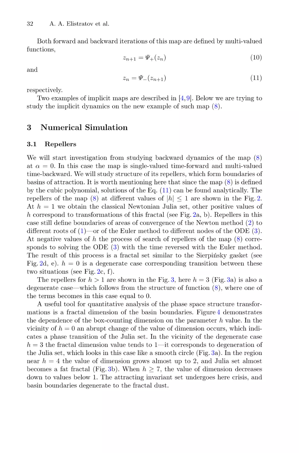
The repellers for h > 1 are shown in the Fig. 3, here h = 3 (Fig. 3a) is also a
degenerate case—which follows from the structure of function (8), where one of
the terms becomes in this case equal to 0.
A useful tool for quantitative analysis of the phase space structure transformations is a fractal dimension of the basin boundaries. Figure 4 demonstrates
the dependence of the box-counting dimension on the parameter h value. In the
vicinity of h = 0 an abrupt change of the value of dimension occurs, which indicates a phase transition of the Julia set. In the vicinity of the degenerate case
h = 3 the fractal dimension value tends to 1—it corresponds to degeneration of
the Julia set, which looks in this case like a smooth circle (Fig. 3a). In the region
near h = 4 the value of dimension grows almost up to 2, and Julia set almost
becomes a fat fractal (Fig. 3b). When h ≥ 7, the value of dimension decreases
down to values below 1. The attracting invariant set undergoes here crisis, and
basin boundaries degenerate to the fractal dust.

Complex Dynamics of the Implicit Maps

33

Fig. 2. The repellers in the phase space of the map (8) with h = 1.0 (a), h = 0.5 (b),
h → +0 (c) and h = −1.0 (d), h = −0.5 (e), h → −0 (f). Parameter α is equal to zero.
Parameter c is not essential, here and further it is ﬁxed being equal to (1 − i)/2.

34

A. A. Elistratov et al.

Fig. 3. The repellers in the phase space of the map (8) with α = 0 and diﬀerent values
of h: 3 (a), 5 (b), 7 (c).

3.2

Attractors

In general case every point in the phase space of the implicit map (8) has three
images—roots of qubic polynomial equation. Time-forward dynamics of such
map is, as backward dynamics also, not single-valued. To study time-forward
dynamics it seems productive to apply methods which are usually employed for
an analysis of repellers. Particularly, we apply the “chaos game” algorithm [18]
in order to ﬁnd attracting chaotic trajectories. To ﬁnd periodic trajectories we
choose the roots of (8) at each iteration according to a periodic sequence. We
construct symbolic codes, consisting of characters «1», «2» and «3»—which
correspond to the choice of the ﬁrst, the second or the third root respectively.
The period of dynamical orbit should be in this case equal or larger than a
minimal period of such a sequence.

Complex Dynamics of the Implicit Maps

35

Fig. 4. Box-counting dimension of the repellers of the implicit map (8) with α = 0.0
for |h| ≤ 1 (upper panel) and 1 ≤ h ≤ 10 (bottom panel).

Let us start from the illustration of the evolution of attractors in special case
α = 0, which is shown in the Fig. 5. This situation corresponds to the use of
the explicit Euler method, and the forward-time dynamics is in this case singlevalued. Figure 5a represents three attracting nodes at h → 0, while an increase
of parameter h causes several period doubling bifurcations (Fig. 5c–e), and the
transition to chaos occurs (Fig. 5f).
The bifurcation diagram shown in the Fig. 6 gives more complete picture of
the forward-time behavior of the system (8). Here the real part of the complex
variable z on the attracting invariant set is plotted versus parameter h. At this
picture the evolution of one of three attracting ﬁxed points is demonstrated. It
undergoes several period-doubling bifurcations, transition to chaos and back to
the periodic regime, and ﬁnally is destroyed via crisis. In the vicinity of the point

36

A. A. Elistratov et al.

Fig. 5. Transformation of the attracting invariant sets of the implicit map (8) with α =
0.0 and with h → 0 (a), h = 0.5 (b), 1.0 (c), 2.15 (d), 2.75 (e), 2.792 (f).

Complex Dynamics of the Implicit Maps

37

Fig. 6. The bifurcation diagram for one of attracting invariant sets of the implicit
map (8) with α = 0.0 (a) and its enlarged fragment (b).

h = 4, where, as we mentioned above, Julia set almost becomes a fat fractal,
time-forward dynamics is chaotic.
Next Fig. 7 demonstrates the picture of dynamical regimes on the parameter
plane (h, α). When α = 0, the map (8) becomes an implicit one, which means
that its dynamics is now muti-valued both time-forward and time-backward.
Except the simplest case, when the symbolic sequence has period 1 (Fig. 7a),
charts for diﬀerent periodic sequences demonstrate similar features. Areas of
periodic dynamics in the quadrant (h > 0, α < 0.5) have typical “tongue” shape

38

A. A. Elistratov et al.

Fig. 7. The charts of dynamical regimes of the implicit map (8) for the following periodic sequences of time-forward roots choice: 1 (a), 12 (b), 112 (c), 1112 (d), 11112 (e),
1(×8)2 (f).

Complex Dynamics of the Implicit Maps

39

with spikes in the point α = 0, h = 3, where the map (8) is degenerate. Another
typical feature is partial symmetry of the parameter plane: borders of areas of
aperiodic dynamics are in many cases symmetrical with respect to the point (h =
0, α = 0.5) in quadrants (h > 0, α < 0.5) and (h < 0, α > 0.5), and points with
periodic dynamics are symmetrical to points with aperiodic dynamic, especially
for |h| ≤ 3. It is a consequence of speciﬁc symmetry of the map (8), which is
invariant with respect to the transformation h → −h, α → 1 − α, zn ↔ zn+1 .

4

Conclusion

In this paper we present a short preliminary view on the dynamics of one example of implicit systems, namely, the map (8). We demonstrate some approaches
for studying of such systems. Advanced investigation of this implicit map should
clarify the structure of its invariant sets. It seems a promising and very interesting direction of research, since in implicit systems, in contrast to traditionally
studied explicit ones, an inﬁnite number of trajectories can coexist in forward
time, which makes their attracting invariant sets very complicated. Moreover,
complexiﬁcation of the parameter h in the map (8) leads to the possibility of a
situation, when Ψ (zn+1 , zn ) = −Ψ ∗ (zn , zn+1 ).1 For the map (8) this happens at
h = ±i, α = 1/2. This situation, deﬁned in [4,9] as generalized unitarity, manifests the emergence of phenomena typical for Hamiltonian and almost Hamiltonian systems. In this context the implicit maps, being an artiﬁcial construct,
can help to describe strong multistability, mixed dynamics and other complex
phenomena of nonlinear dynamics.

References
1. Adilova, A.B., Kuznetsov, A.P., Savin, A.V.: Complex dynamics in the system
of two coupled discrete Rossler oscillators. Izvestiya VUZ. Appl. Nonlinear Dyn.
21(5), 108–119 (2013). (in Russian)
2. Arrowsmith, D.K., Cartwright, J.H., Lansbury, A.N., Place, C.M.: The Bogdanov
map: bifurcations, mode locking, and chaos in a dissipative system. Int. J. Bifurcation Chaos 3(04), 803–842 (1993)
3. Bullett, S.R.: Dynamics of quadratic correspondences. Nonlinearity 1(1), 27–50
(1988)
4. Bullett, S.R., Osbaldestin, A.H., Percival, I.C.: An iterated implicit complex map.
Physica D 19(2), 290–300 (1986)
5. Cayley, A.: Desiderata and suggestions: no. 3. The Newton-Fourier imaginary problem. Am. J. Math. 2(1), 97 (1879)
6. DiFranco, D.E., Cham, T.J., Rehg, J.M.: Reconstruction of 3D ﬁgure motion from
2D correspondences. In: Proceedings of the 2001 IEEE Computer Society Conference on Computer Vision and Pattern Recognition, CVPR 2001, vol. 1, pp.
307–314. IEEE (2001)

1

∗
Here Ψ ∗ (zn+1 , zn ) = (Ψ (zn+1
, zn∗ ))∗ .

40

A. A. Elistratov et al.

7. Gardini, L., Hommes, C., Tramontana, F., De Vilder, R.: Forward and backward
dynamics in implicitly deﬁned overlapping generations models. J. Econ. Behav.
Organ. 71(2), 110–129 (2009)
8. Hill, D.: Control of implicit chaotic maps using nonlinear approximations. Chaos:
Interdisc. J. Nonlinear Sci. 10(3), 676–681 (2000)
9. Isaeva, O.B., Obychev, M.A., Savin, D.V.: Dynamics of a discrete system with the
operator of evolution given by an implicit function: from the Mandelbrot map to
a unitary map. Russ. J. Nonlinear Dyn. 13(3), 331–348 (2017). (in Russian)
10. Kennedy, J.A., Stockman, D.R.: Chaotic equilibria in models with backward
dynamics. J. Econ. Dyn. Control 32(3), 939–955 (2008)
11. Kuznetsov, A.P., Savin, A.V., Sedova, Y.V.: Bogdanov-Takens bifurcation: from
ﬂows to discrete systems. Izvestiya VUZ. Appl. Nonlinear Dyn. 17(6), 139–158
(2009). (in Russian)
12. Lóczi, L., Páez Chávez, J.: Preservation of bifurcations under Runge-Kutta methods. Int. J. Qual. Theory Diﬀer. Equ. Appl. 3, 81–98 (2008)
13. Magreñán, Á.A., Gutiérrez, J.M.: Real dynamics for damped Newton’s method
applied to cubic polynomials. J. Comput. Appl. Math. 275, 527–538 (2015)
14. McLaughlin, J.: Convergence of a relaxed Newton’s method for cubic equations.
Comput. Chem. Eng. 17(10), 971–983 (1993)
15. Mestel, B.D., Osbaldestin, A.H.: Renormalisation in implicit complex maps. Physica D 39(2–3), 149–162 (1989)
16. Páez Chávez, J.: Discretizing bifurcation diagrams near codimension two singularities. Int. J. Bifurcation Chaos 20(5), 1391–1403 (2010)
17. Páez Chávez, J.: Discretizing dynamical systems with generalized Hopf bifurcations. Numer. Math. 118(2), 229–246 (2011)
18. Peitgen, H.O., Richter, P.H.: The Beauty of Fractals: Images of Complex Dynamical Systems. Springer, Heidelberg (1986)
19. Pikovsky, A., Rosenblum, M., Kurths, J.: Synchronization: A Universal Concept
in Nonlinear Sciences. Cambridge Nonlinear Science Series. Cambridge University
Press (2001)
20. Sclaroﬀ, S., Pentland, A.: Generalized implicit functions for computer graphics.
ACM SIGGRAPH Comput. Graph. 25(4), 247–250 (1991)
21. Vlasenko, I.Y.: Internal maps: topological invariants and their applications. In: Proceedings of Institute of Mathematics of Ukrainian NAS, Institute of Mathematics
of Ukrainian NAS (2014). (in Russian)
22. Zaslavsky, G.M.: The Physics of Chaos in Hamiltonian Systems. World Scientiﬁc
(2007)

Recognition of Vertical Migrations
for Two Age Groups of Zooplankton
O. Kuzenkov

and E. Ryabova(B)

Lobachevsky State University, Gagarin Avenue 23, 603950 Nizhny Novgorod, Russia
{oleg.kuzenkov,elena.ryabova}@itmm.unn.ru

Abstract. The purpose of the work is to predict the appearance of signiﬁcant vertical movements of two age zooplankton groups as a result of
adaptation to habitat conditions. The methodological basis for solving
the problem is the maximization of the ﬁtness function. Vertical migrations are considered as a strategy that ensures the achievement of the
greatest value of this function for given environmental conditions. The
environmental factors inﬂuencing the appearance of vertical migrations
are the availability of food and predator activity, water temperature and
hydrogen sulﬁde concentration. Experimentally recorded data on these
factors have always some noise and are of a discrete selective nature. In
this regard, machine learning tools are used to solve the problem. The
most important stage of the work is the construction of the training sample. For this purpose, the results of an analytical and numerical search
for the optimal behavior are used with linear-quadratic and hyperbolic
approximations of external factors.
As a result of the study, a neural network was built that solves the
problem of classifying input data sets into four classes corresponding
to the presence or absence of signiﬁcant vertical movements in young
and adult individuals under these conditions. This makes it possible to
fairly accurately recognize the presence or absence of signiﬁcant vertical migrations for young and adult zooplankton individuals according to
approximately speciﬁed environmental factors.
Keywords: Fitness function · Neural networks
Zooplankton diel vertical migration

1

· Pattern recognition ·

Introduction

Currently, the importance of mathematical modeling is increasing in the studying
the behavior of living systems [1–4]. In particular, modeling of zooplankton diel
vertical migration (DVM) is of great interest [5]. This phenomenon was discover
more than two hundred years ago [6]. It was established that zooplankton daily
rises at night to the near-surface layers of water and descends into the depths
during the day [7]. It is known that the daily migrations of zooplankton represent
one of the most signiﬁcant synchronous movements of biomass on earth and,
as a result, aﬀect the carbon exchange and climate of the planet [8–13]. The
c The Author(s), under exclusive license to Springer Nature Switzerland AG 2022

D. Balandin et al. (Eds.): MMST 2022, CCIS 1750, pp. 41–54, 2022.
https://doi.org/10.1007/978-3-031-24145-1_4

42

O. Kuzenkov and E. Ryabova

presence of vertical migrations was tried to be explained by the inﬂuence of a
predator, solar radiation, etc. [7]. However, attempts to explain this phenomenon
on the basis of traditional approaches of biology have encountered signiﬁcant
diﬃculties [7]. This is due to the wide variety of zooplankton hereditary behavior
modes. In particular, it is known that some species can carry out signiﬁcant
vertical migrations, while others cannot [7]. Moreover, diﬀerent age groups of
the same species may have diﬀerent behaviors [14–16]. Then, it is necessary
to use the methods of mathematical modeling [8,10,11,17–20]. Mathematical
modeling allows us to explain the quantitative characteristics of this behavior
and the dependence of the implemented migration strategy on the age of the
organism [21–23].
Now, the Darwinian idea of the survival of the ﬁttest spicies is eﬀectively used
for modeling biological processes [24–26]. DVM of zooplankton are considered as
an evolutionarily stable behavior, that is, the behavior that is preserved in the
population as the result of the struggle for existence [27]. Evolutionarily stable
behavior ensures maximum adaptability to the conditions of existence. In the
mathematical modeling of such behavior, the main diﬃculty is to identify the
ﬁtness function, which numerically characterizes the competitive advantages of
diﬀerent strategies.
The problem of deriving evolutionary ﬁtness is still far from a ﬁnal solution.
Diﬀerent authors oﬀer diﬀerent deﬁnitions of ﬁtness, for example, the expected
individual reproductive value [7,21], generalized entropy [28], etc. Diﬀerent deﬁnitions of the ﬁtness function sometimes lead to conﬂicting predictions of evolutionary results [21,29]. One of the most general approaches to the formalization
of the ﬁtness function was proposed by A. Gorban [30–32], who deﬁned ﬁtness
in the equations of the dynamics of measures with inheritance as the average
time value of the speciﬁc reproduction rate. This approach was later developed
in [33–35], where a technique for constructing a ﬁtness function for wide classes
of models was proposed [36].
Maximization of the ﬁtness function by classical methods of calculus of variations makes it possible to construct an evolutionarily stable strategy for zooplankton migrations depending on environmental conditions [22,29].
However, the experimentally recorded data of the external environment are
always inaccurate and have a discrete selective character; only their estimates
are available in a certain range. At the same time, the synchronous movement
of a population always admits only a statistical description; inevitably there is
a random variation in the behavior of individuals. From this point of view, it is
of interest not to build an optimal movement strategy, but only to predict its
main qualitative characteristics, such as the presence or absence of signiﬁcant
vertical movements. Classical methods for solving optimization problems are not
suitable here. The problem is solved by using the technology of learning neural
networks [37–39].
The purpose of this work is to predict the presence or absence of signiﬁcant
vertical migrations of zooplankton according to approximately given environmental factors, taking into account the age of the individual. In this work, the

Recognition of Vertical Migrations for Two Age Groups of Zooplankton

43

presence of signiﬁcant migrations is predicted separately in young and adult
individuals using a neural network.

2

Materials and Methods

We consider a community consisting of m diﬀerent species of zooplankton
{v1 , . . . , vm }.
Each species of zooplankton has two age groups - juveniles and adult mature
individuals, diﬀering in the hereditary migration regime, which is a continuous
periodic (with a period of one day) function of the vertical position x depending
on the time of day τ . Here τ = 0 corresponds to the noonday, τ = 0.5 corresponds
to the midnight, and τ = 1 corresponds to the noon of the next day; x - depth
of migration, measured in meters, level x = 0 corresponds to the water surface.
The function x1i (τ ) corresponds to the mode of movement of young individuals,
the function x2i (τ ) corresponds to the mode of movement of adults of the i-th
zooplankton species. It is assumed that these functions are continuously diﬀerentiable on the interval [0, 1] and satisfy the conditions xji (0) = xji (1), i = 1, m,
j = 1, 2.
Let z1i (t) be the number of young individuals of the i-th zooplankton species,
z2i (t) - the number of adults of the i-th zooplankton species. The following
population model is used, which describes the interaction between young and
adult individuals, taking into account their competition

= −pi z1i − qi z1i + ri z2i − z1i
z1i

z2i
= pi z1i − si z2i − z2i

m

j=1

m


(z1j + z2j ),

j=1

(1)

(z1j + z2j ), i = 1, m.

Here ri is the breeding rate, qi is the juvenile mortality rate, si is the adult
mortality rate due to predation; pi is the proportion of young individuals that
have passed into a mature state (coeﬃcient of maturation); it is assumed that
these coeﬃcients do not depend on time. The last term reﬂects the intraspeciﬁc
competition. This model is consistent with the general approach to modeling
population dynamics [40].
To construct the ﬁtness function, the technique proposed in [36] are used. Its
essence is as follows. Let
zi = z1i + z2i
be the number of individuals of all ages of species i. It is known that zi = 0 if
zi (0) = 0 [40,41]. Species i will be better (or ﬁtter) than species j if the ratio of
the number of j-th species to the number of i-th species tends to zero over time:
lim zj /zi = 0.

t→∞

In this case, species i will displace species j from the community. Thus,
an order relation (ranging) is introduced on the set of species. A numerical

44

O. Kuzenkov and E. Ryabova

function J(vi ) deﬁned on this set that preserves the introduced relation (that is,
J(vi ) > J(vj ) when vi is better than vj ) is called a ﬁtness function.
As it was shown in [36], the ﬁtness function has the form of the time-averaged
speciﬁc growth rate for zi (t):
<zi (t)/zi >

1
= lim
T →∞ T

T

zi (t)/zi dt

t0

or any other equivalent function.
Empirical evidence suggests that the diel vertical migrations of zooplankton
are mainly determined by the following environmental factors: the distribution
of food (phytoplankton) E(x) by depth x, the distribution density of predators Sx (x), the distribution of unfavorable habitat factors (temperature and
hydrogen sulﬁde) G(x), as well as daily predator activity Sτ (τ ) [7,15,21,36]. All
these factors can be considered as continuous functions of the vertical coordinate x or the time of day τ .
To study vertical migrations, we used empirical data collected in the northeastern part of the Black Sea in summer of 2011 [15]. The data from [7,15,21,36]
were used to describe environmental factors such as the depth distribution of
predators and their activity during the day. The simplest linear and quadratic
approximations of the functions of external factors E, Sx and G were used:
E = σ1 (x + D), Sx = σ2 (x + D), −D < x < 0; G = (x + D0 )2 ,

(2)

as well as the approximation of the function Sτ in the form of a sinusoidal
dependence:
Sτ = cos(2πτ ) + 1, 0 < τ < 1.
Here D is the depth of the hydrogen sulﬁde layer, the lower limit of zooplankton
habitation, D0 is the optimal depth of zooplankton habitation in terms of temperature, σ1 and σ2 are constant coeﬃcients of decrease in the amount of food
and predator with increasing depth.
We also used hyperbolic approximations of environmental factors:
E(x) = σ1 (tanh(ξ1 (x + D)) + 1),
Sx (x) = σ2 (tanh(ξ2 (x + D)) + 1),
G(x) = cosh(ξ3 (x + D0 )),

(3)

that are more precise. Here ξi is the growth rate of the function, the steepness
of its slope at zero.
The primary analysis of the data made it possible to identify eight key
macroparameters that have the greatest impact on the population growth of
young (j = 1) and adult (j = 2) individuals: daily average energy gains as
a result of food intake M1j , energy costs for vertical movements M3j (kinetic
energy proportional to the square of the speed of movement), losses due to predation M2j , losses due to unfavorable external conditions M4j .

Recognition of Vertical Migrations for Two Age Groups of Zooplankton

M1j (vi ) =

1

45

E(xji (τ )) dτ,

0

1
M2j (vi ) = − Sτ (τ )Sx (xji (τ )) dτ,
0

1

M3j (vi ) = − (xji (τ ))2 dτ,
0

1

M4j (vi ) = − G(xji (τ )) dτ.
0

Accordingly, the ﬁtness function must be a function of eight key parameters
M = (M11 , . . . , M41 , M12 , . . . , M42 ): J = J(M (vi )).
In model (1), the coeﬃcients ri , qi , si , pi are determined by these parameters.
We will use the simplest linear approximations of the coeﬃcients
ri
si
pi
qi

= θ12 M12 + θ32 M32 + θ42 M42 ,
= θ22 M22 ,
= θ11 M11 + θ31 M31 + θ41 M41 ,
= −θ22 M22 .

Here, the weight coeﬃcients θkj reﬂect the inﬂuence of each key factor and do
not depend on the implemented strategies.
The hereditary behavioral strategies of young and adult individuals are
approximated by harmonic oscillations xj = Aj + Bj cos(2πτ ), where Aj is the
average depth of immersion, Bj is the oscillation amplitude during the day, τ is
the time of day, varying from 0 to 1, j = 1 corresponds to the strategy of young
individuals, j = 2 corresponds to the strategy of adults. Notice, that
−D < Aj + Bj cos(2πτ ) < 0, −

D
D
< Aj < 0, 0 < Bj < .
2
2

For given simplest linear and quadratic approximations of the behavior strategy and environmental factors, formulas for key parameters can be derived
M1j
M2j
M3j
M4j

3
3.1

= σ1 (Aj + D),
B
= −σ2 (Aj + D + 2j ),
2 2
= −π Bj ,
B
= −((Aj + D0 )2 + 2j ).

Results
Fitness Identification

First of all, we obtain an explicit expression for the ﬁtness function in the considered model (1) in terms of its coeﬃcients. Let’s make a change of variables in

46

O. Kuzenkov and E. Ryabova

system (1): ξi = z1i /zi , ηi = z2i /zi . Obviously, ηi = 1 − ξi . Then system (1) is
transformed to the form
ξi = (ri + qi − si )ξi2 − (pi + qi − si + 2ri )ξi + ri ,
m

zj ), i = 1, m.
zi = zi (−(ri + qi − si )ξi + ri − si −
j=1

It is clear that each of the ﬁrst m equations of this system does not depend
on the others and can be considered independently. Let ri + qi − si = 0, then
the values ξi tend to

pi + qi − si + 2ri − (pi + qi − si )2 + 4pi ri
∗
ξi =
.
2(ri + qi − si )
Last m equations describe the dynamics of the total population of the species i,
the reproductive factor for zi is
zi (t)/zi = −(ri + qi − si )ξi + ri − si −

m


zj .

j=1

Since the summand

m

j=1

zj does not depend on the index i and the mean time

of ξi coincides with its limit ξi∗ , then the best strategy i corresponds to the
maximum of the following function

−pi − qi − si + (pi + qi − si )2 + 4pi ri
∗
.
J = −(ri + qi − si )ξi + ri − si =
2
This function is the ﬁtness function in this model.
Knowing the ﬁtness function, environmental functions, and coeﬃcients of
inﬂuence of environmental factors on model parameters, one can easily obtain
optimal, i.e., evolutionarily stable behavioral strategies for young and adult individuals. To do this, we need to solve the problem of the calculus of variations,
taking the ﬁtness function as the objective functional. Then, by analyzing the
obtained strategies, one can ﬁnd the amplitudes of vertical displacements.
It can be seen that for diﬀerent functions of external factors and for diﬀerent weight coeﬃcients, the oscillation amplitude will be diﬀerent. In some cases,
there will be noticeable vertical movements of young or adult zooplankton during the day, in other cases they will be practically indistinguishable against the
background of constant random ﬂuctuations. For the researcher, the most important thing is to answer the question not so much about the exact proﬁle of the
resulting movements, but about the presence or absence of signiﬁcant vertical
migrations of juveniles or adults.
To answer this question, we need to set the threshold value of the vertical
movement, starting from which the movement is considered noticeable. Then
separately compare the amplitudes of the obtained movements of individuals
of diﬀerent ages with a threshold value. If the amplitude exceeds the threshold

Recognition of Vertical Migrations for Two Age Groups of Zooplankton

47

value, then the movements will be signiﬁcant. Then the sets of external factors
can be divided into four classes, each of which corresponds to one possible case:
the absence of signiﬁcant movements of zooplankton, the presence of signiﬁcant
movements only in young individuals, the presence of signiﬁcant movements only
in adults, the presence of signiﬁcant movements in zooplankton of any age.
Practically, it is very important to recognize the presence or absence of such
movements by known external factors, even without an accurate determination
of the optimal trajectory of movement. The signiﬁcance of this problem is aggravated by the fact that our knowledge of external factors is always incomplete
and approximate, and because of this, it is usually impossible to construct an
exact solution.
3.2

Neural Network

The second part of the work consisted of the creation of a software package
that makes it possible to recognize the presence or absence of signiﬁcant migrations of zooplankton, using only approximate characteristics of the environment.
This problem was solved using artiﬁcial neural networks and machine learning
methods [42,43].
A neural network was built using libraries Keras3 and Tensorﬂow2 based on
Python. The input data is a discrete set of values of four external functions of
the state of the environment, eight weight coeﬃcients, as well as a threshold
value of vertical displacements. The output information is a response regarding
the presence/absence of pronounced vertical movements separately in juveniles
and adults in given environmental conditions relative to a given threshold value.
The architecture of the artiﬁcial neural network is shown in Fig. 1.
Each environmental function as a set of 104 values alternately passes through
two pairs of convolution (conv) and pooling (maxpool) layers. This highlights
information about the behavior of each of the functions in separate parts of
the scope. Further, the received information passes through 5 fully connected
layers of the neural network (dense). In parallel, a vector of weight coeﬃcients
of 8 values is introduced (4 for each age group). Each group of weight coeﬃcients is supplemented with previous information obtained from the analysis of
environmental functions, and independent processing of each group of data is
carried out through two fully connected layers. Further, to study the possible
mutual inﬂuence of one age group on another, all information is passed through
another 3 fully connected layers. The result is 2 numbers that determine the
presence/absence of vertical movements for each of the 2 age groups of zooplankton. The constructed classiﬁer based on the neural network assigns each
new set of environmental functions to one of four classes.
3.3

Construction of the Training Sample

An important point in the work is the construction of a training sample. For
this, the analytical and numerical results of the approximation of environmental
conditions with the help of linear-quadratic and hyperbolic functions were used.

48

O. Kuzenkov and E. Ryabova

Fig. 1. Neural network architecture.

At the same time, the analytical functions were converted into tabular ones
according to the discrete nature of the recorded environmental conditions.
The training sample is built as follows: a series of quadruples of initial functions are set in turn, and the oscillation amplitudes of young and adult individuals are found using optimization procedures [44]. The found values are compared
with the threshold. If the amplitude value is higher than the threshold, then this
precedent is considered as a case of the presence of a signiﬁcant oscillation. If not,
then the movement is considered not to be expressed against the background of
the inevitable random ﬂuctuations of zooplankton. Each four external factors is
assigned a two-dimensional vector, each coordinate of which is a logical value
“yes/no” - the presence/absence of signiﬁcant migrations for the corresponding
age group. Accordingly, the quadruples of external factors are divided into four
non-overlapping classes. Fragments of the training sample are given in Tables 1, 2
for a threshold value of 10.
Table 1. Fragment of the training sample for linear and quadratic approximations (2).
D

D0

σ1

σ2

θ11

θ12

θ31

140 44.3 8.61 7.53 16.8 23.7 0.16
140 37.8 1.54 8.99 59

θ32

θ21

θ22

0.04 4.94 1

θ41

θ42

DVM
Juv Ad

0.67 0.81 Yes Yes

29.8 0.027 0.02 3.38 0.84 0.61 0.67 Yes No

140 29.3 1.21 5.49 31.8 72.7 0.034 0.03 2.74 0.09 0.26 0.68 No

Yes

140 37.8 78.2 1.95 3

No

24.5 32.8

0.04 0.03 2.95 0.26 0.38 No

Recognition of Vertical Migrations for Two Age Groups of Zooplankton

49

Table 2. Fragment of the training sample for hyperbolic approximations (3).
D

D0

σ1

σ2

θ11

θ12

θ31

θ32

θ21

θ22

θ41

θ42

ξ1

ξ2

ξ3

DVM
Juv

Ad

140

66.5

2.68

4.06

100.7

61.2

0.05

0.07

4.81

4.83

0.27

0.23

1.6

1.6

1.2

Yes

Yes

140

64.7

1.62

6.24

84.2

39

0.02

0.009

4.67

3.82

0.64

0.49

1.04

8.52

4.67

Yes

No

140

44.2

2.34

6.92

8.5

27.2

0.009

0.045

0.148

0.89

0.32

0.23

1.12

7.76

6.86

No

Yes

140

114.7

1.56

5.81

63.5

93.7

0.04

0.03

1.51

1.82

0.37

0.65

1.39

9.18

6.72

No

No

We should note that hyperbolic functions approximate the real environment
much more accurately then linear-quadratic functions. Then the training set
should contain mainly hyperbolic approximations to train the neural network for
the work with real data. Linear-quadratic approximations are used only as rare
auxiliary cases. The power of the training sample for functions given by linearquadratic approximations was 1200 generated pairs of elements; for functions
deﬁned by hyperbolic approximation – 40 000 generated pairs of elements. 70%
of the received records were used to train the neural network, the remaining 30%
were used to test its work. At the same time, the frequency of correct answers
on the original functions (Fig. 2) was approximately 0.97.

Fig. 2. Example of input data for hyperbolic approximation (3) with σ1 = σ2 = 1,
ξ1 = ξ2 = ξ3 = 1, D = D0 = 0.

50

O. Kuzenkov and E. Ryabova

Fig. 3. Example of noisy data for hyperbolic approximation (3).

When working with real factors, it is not possible to avoid the appearance of
noise. This may be due to both the human factor and the error of the tools used.
Noise can distort the results to varying degrees depending on the circumstances.
It is desirable to set up the neural network in such a way that noisy input
data does not aﬀect the correctness of the answer. As noisy data, the original
analytical functions were used with the addition of a random noise value up to
5% of the main value (Fig. 3). The response of the neural network was compared
with the response for the corresponding analytical functions. The frequency of
correct answers was 0.94.
We can compare the result of the neural network recognition with the results
of some other works. The work [45] presents DVM of adults and juveniles for
diﬀerent approximations of environmental factors. We have solved the recognition problem for the same functions on the base of the created neural network.
We used the following values of ﬁtness coeﬃcients: θ11 = 0.16, θ31 = 0.00007,
θ21 = 0.008, θ41 = 0.0016, θ12 = 0.6, θ32 = 0.0000075, θ22 = 0.4, θ42 = 0.006.
In this case, we have got the presence of migrations for adults and the absence
of migrations for juveniles which are consisted with [45].

4

Summary

In this work, we develop a new method and software to explore evolutionary stable strategies of zooplankton DVM. The method combines the theoretical app-

Recognition of Vertical Migrations for Two Age Groups of Zooplankton

51

roach to reveal evolutionary ﬁtness in the model and the computational tools. As
a result of the study, the neural network was built. It solves the problem of classifying input data sets into four classes corresponding to the presence or absence
of signiﬁcant vertical movements in young and adult individuals. The important
stage of the work is the construction of the training sample. For this purpose,
the results of an analytical and numerical search for the optimal behavior are
used with linear-quadratic and hyperbolic approximations of external factors.
The trained neural network fairly accurately recognizes the presence or
absence of detectable vertical migrations of two age groups of zooplankton
according to approximately speciﬁed observable information about environmental factors (distribution of food and predators in water layers, predator behavioral responses, temperature distribution of water). As future extensions, we are
planning to analyse a large number of empirical cases of DVM and include more
complicated theoretical models of zooplankton population growth to better train
neural networks.
The results of the research were implemented into the educational process
within the framework of the academic discipline “Mathematical modeling of
selection processes” for 3rd year students of the studying area “Fundamental
Informatics and Information Technology” [46,47].
The materials of the work formed the basis of the educational and research
project of UNN students. Some results of the project are used in this work.
We thank UNN students (Kolesnikov I. V., Ivina A. S., Feoktistov A. A.,
Yarov M. A.) for technical help of the work.

References
1. Stucchi, L., et al.: A general model of population dynamics accounting for multiple
kinds of interaction. Complexity 2020, 7961327 (2020). https://doi.org/10.1155/
2020/7961327
2. Frisman, E.Y., Zhdanova, O.L., Kulakov, M.P., Neverova, G.P., Revutskaya, O.L.:
Mathematical modeling of population dynamics based on recurrent equations:
results and prospects. Part I. Biol. Bull. 48(1), 1–15 (2021). https://doi.org/10.
1134/S1062359021010064
3. McBride, J.M., Nimphius, S.: Biological system energy algorithm reﬂected in subsystem joint work distribution movement strategies: inﬂuence of strength and
eccentric loading. Sci. Rep. 10, 12052 (2020). https://doi.org/10.1038/s41598-02068714-8
4. Demidova, A., Druzhinina, O., Jaćimović, M., Masina, O., Mijajlovic, N.: Problems of synthesis, analysis and optimization of parameters for multidimensional
mathematical models of interconnected populations dynamics. In: Jaćimović, M.,
Khachay, M., Malkova, V., Posypkin, M. (eds.) OPTIMA 2019. CCIS, vol. 1145,
pp. 56–71. Springer, Cham (2020). https://doi.org/10.1007/978-3-030-38603-0 5
5. Ringelberg, J.: Diel Vertical Migration of Zooplankton in Lakes and Oceans.
Springer, Dordrecht (2010)
6. Bandara, K., et al.: Two hundred years of zooplankton vertical migration research.
Biol. Rev. 96(4), 1547–1589 (2021). https://doi.org/10.1111/brv.12715

52

O. Kuzenkov and E. Ryabova

7. Clark, C., Mangel, M.: Dynamic State Variable Models in Ecology: Methods and
Applications. Oxford University Press, Oxford (2000)
8. Ducklow, H., Steinberg, D., Buesseler, K.: Upper ocean carbon export and the
biological pump. Oceanography 14(4), 50–58 (2001). https://doi.org/10.5670/
oceanog.2001.06
9. Hays, G.: A review of the adaptive signiﬁcance and ecosystem consequences of
zooplankton diel vertical migrations. Hydrobiologia 503(1–3), 163–170 (2003).
https://doi.org/10.1023/B:HYDR.0000008476.23617.b0
10. Kaiser, M., et al.: Marine Ecology: Processes, Systems and Impacts. Oxford University Press, Oxford (2005)
11. Buesseler, K., et al.: Revisiting carbon ﬂux through the ocean’s twilight zone.
Science 316(5824), 567–570 (2007). https://doi.org/10.1126/science.1137959
12. Isla, A., Scharek, R., Latasa, M.: Zooplankton diel vertical migration and contribution to deep active carbon ﬂux in the NW Mediterranean. J. Mar. Syst. 143,
86–97 (2015). https://doi.org/10.1016/j.jmarsys.2014.10.017
13. Archibald, K.M., Siegel, D.A., Doney, S.C.: Modeling the impact of zooplankton
diel vertical migration on the carbon export ﬂux of the biological pump. Glob.
Biogeochem. Cycles 33, 181–199 (2019). https://doi.org/10.1029/2018GB005983
14. Ohman, M.D.: The demographic beneﬁts of diel vertical migration by zooplankton.
Ecol. Monogr. 60(3), 257–281 (1990). https://doi.org/10.2307/1943058
15. Morozov, A., Kuzenkov, O., Arashkevich, E.: Modelling optimal behavioral strategies in structured populations using a novel theoretical framework. Sci. Rep. 9,
15020 (2019). https://doi.org/10.1038/s41598-019-51310-w
16. Baumgartner, M.F., Tarrant, A.M.: The physiology and ecology of diapause in
marine copepods. Annu. Rev. Mar. Sci. 9, 387–411 (2017). https://doi.org/10.
1146/annurev-marine-010816-060505
17. Hansen, A.N., Visser, A.W.: Carbon export by vertically migrating zooplankton:
an optimal behavior model. Limnol. Oceanogr. 61(2), 701–710 (2016). https://doi.
org/10.1002/lno.10249
18. Arcifa, M.S., et al.: Microcrustaceans and predators: diel migration in a tropical
lake and comparison with shallow warm lakes. Limnetica 35(2), 281–296 (2016).
https://doi.org/10.23818/limn.35.23
19. Hafker, N.S., Meyer, B., Last, K.S., Pond, D.W., Huppe, L., Teschke, M.: Circadian clock involvement in zooplankton diel vertical migration. Curr. Biol. 27(14),
2194.e3–2201.e3 (2017). https://doi.org/10.1016/j.cub.2017.06.025
20. Guerra, D., Schroeder, K., Borghini, M., et al.: Zooplankton diel vertical migration
in the Corsica channel (North-western Mediterranean sea) detected by a moored
acoustic doppler current proﬁler. Ocean Sci. 15(3), 631–649 (2019). https://doi.
org/10.5194/os-15-631-2019
21. Fiksen, O., Giske, J.: Vertical distribution and population dynamics of copepods
by dynamic optimization. ICESJ Mar. Sci. 52, 483–503 (1995). https://doi.org/
10.1016/1054-3139(95)80062-X
22. Morozov, A., Kuzenkov, O.: Towards developing a general framework for modelling
vertical migration in zooplankton. J. Theor. Biol. 405, 17–28 (2016)
23. Sandhu, S.K., Morozov, A., Kuzenkov, O.: Revealing evolutionarily optimal strategies in self-reproducing systems via a new computational approach. Bull. Math.
Biol. 81(11), 4701–4725 (2019). https://doi.org/10.1007/s11538-019-00663-4
24. Gyllenberg, M., Metz, J., Service, R.: When do optimisation arguments make evolutionary sense? In: Chalub, F., Rodrigues, J. (eds.) The Mathematics of Darwin’s
Legacy. MBI, pp. 233–268. Springer, Basel (2011). https://doi.org/10.1007/978-30348-0122-5 12

Recognition of Vertical Migrations for Two Age Groups of Zooplankton

53

25. Birch, J.: Natural selection and the maximization of ﬁtness. Biol. Rev. 91(3), 712–
727 (2016). https://doi.org/10.1111/brv.12190
26. Gavrilets, S.: Fitness Landscapes and the Origin of Species (MPB-41). Princeton
University Press, Princeton (2004)
27. Wilfried, G., Bernhard, T.: Vertical migration of zooplankton as an evolutionarily
stable strategy. Am. Nat. 132(2), 199–216 (1988). https://doi.org/10.1086/284845
28. Klimenko, A.Y.: Entropy and equilibria in competitive systems. Entropy 16(1),
1–22 (2014). https://doi.org/10.3390/e16010001
29. Parvinen, K., Dieckmann, U., Heino, M.: Function-valued adaptive dynamics and
the calculus of variations. J. Math. Biol. 52, 1–26 (2006). https://doi.org/10.1007/
s00285-005-0329-3
30. Gorban, A.: Equilibrium Encircling. Equations of Chemical Kinetics and Their
Thermodynamic Analysis. Nauka, Novosibirsk (1984). (in Russian)
31. Gorban, A.: Selection theorem for systems with inheritance. Math. Model. Nat.
Phenom. 2(4), 1–45 (2007). https://doi.org/10.1051/mmnp:2008024
32. Gorban, A.N.: Self-simpliﬁcation in Darwin’s systems. In: Gorban, A., Roose, D.
(eds.) Coping with Complexity: Model Reduction and Data Analysis. LNCSE, vol.
75, pp. 311–344. Springer, Berlin, Heidelberg (2011). https://doi.org/10.1007/9783-642-14941-2 17
33. Kuzenkov, O.: Investigation of a dynamical system of Radon probability measures.
Diﬀer. Equ. 31(4), 549–554 (1995)
34. Kuzenkov, O., Ryabova, E.: Variational principle for self-replicating systems. Math.
Model. Nat. Phenom. 10(2), 115–129 (2015). https://doi.org/10.1051/mmnp/
201510208
35. Kuzenkov, O., Novozhenin, A.: Optimal control of measure dynamics. Commun.
Nonlinear Sci. Numer. Simul. 21(1–3), 159–171 (2015). https://doi.org/10.1016/j.
cnsns.2014.08.024
36. Kuzenkov, O., Morozov, A.: Towards the construction of a mathematically rigorous
framework for the modelling of evolutionary ﬁtness. Bull. Math. Biol. 81(11), 4675–
4700 (2019). https://doi.org/10.1007/s11538-019-00602-3
37. Abiodun, O.I., et al.: State-of-the-art in artiﬁcial neural network applications:
a survey. Heliyon 4(11), e00938 (2018). https://doi.org/10.1016/j.heliyon.2018.
e00938
38. Kuzenkov, O., Morozov, A., Kuzenkova, G.: Recognition of patterns of optimal diel
vertical migration of zooplankton using neural networks. In: International Joint
Conference on Neural Networks, Budapest Hungary, IJCNN 2019 (2019). https://
doi.org/10.1109/IJCNN.2019.8852060
39. Kuzenkov, O.: Information technologies of evolutionarily stable behavior recognition. Mod. Inf. Technol. IT Educ. 1201, 250–257 (2020). https://doi.org/10.1007/
978-3-030-46895-8-20
40. Kuzenkov, O., Ryabova, E.: Mathematical modeling of selection processes.
Lobachevsky State University, Nizhnii Novgorod (2007). (in Russian)
41. Kuzenkov, O.A., Kuzenkova, G.V.: Optimal control of self-reproduction systems. J. Comput. Syst. Sci. Int. 51(4), 500–511 (2012). https://doi.org/10.1134/
S1064230712020074
42. Mohri, M., Rostamizadeh, A., Talwalkar, A.: Foundations of Machine Learning.
The MIT Press, Cambridge (2012)
43. Bishop, Ch.M.: Pattern Recognition and Machine Learning. Springer, Heidelberg
(2006)

54

O. Kuzenkov and E. Ryabova

44. Morozov, A.Y., Kuzenkov, O.A., Sandhu, S.K.: Global optimization in Hilbert
spaces using the survival of the ﬁttest algorithm. Commun. Nonlinear Sci. Numer.
Simul. 103, 106007 (2021). https://doi.org/10.1016/j.cnsns.2021.106007
45. Kuzenkov, O., Morozov, A., Kuzenkova, G.: Exploring evolutionary ﬁtness in biological systems using machine learning methods. Entropy 23(1), 35 (2021). https://
doi.org/10.3390/e23010035
46. Kuzenkov, O., Kuzenkova, G., Kiseleva, T.: The use of electronic teaching tools
in the modernization of the course “mathematical modeling of selection processes”. Educ. Tech. Soc. 21(1), 435–448 (2018). https://www.elibrary.ru/item.
asp?id=32253185. (in Russian)
47. Kuzenkov, O., Kuzenkova, G., Kiseleva, T.: Computer support of training and
research projects in the ﬁeld of mathematical modeling of selection processes.
Educ. Technol. Soc. 22(1), 152–163 (2019). https://www.elibrary.ru/item.asp?
id=37037790. (in Russian)

Nonintegrability of the Problem
of Motion of an Ellipsoidal Body
with a Fixed Point in a Flow of Particles
Alexander S. Kuleshov(B)

and Maxim M. Gadzhiev

Department of Mechanics and Mathematics, Lomonosov Moscow State University,
Moscow, Russia
kuleshov@mech.math.msu.su

Abstract. The problem of motion in the free molecular ﬂow of particles
of a rigid body with a ﬁxed point, bounded by the surface of an ellipsoid
of revolution is considered. This problem is similar in many aspects to
the classical problem of motion of a heavy rigid body about a ﬁxed point.
In particular, this problem possesses the integrable cases, correspond to
the classical Euler – Poinsot, Lagrange and Hess cases of integrability of
equations of motion of a heavy rigid body with a ﬁxed point. Equations
of motion of the body in the ﬂow of particles are presented in hamiltonian form. Using the theorem on the Liouville – type nonintegrability
of Hamiltonian systems near elliptic equilibrium positions we present
the necessary conditions for the existence in the considered problem of
an additional analytic ﬁrst integral independent of the energy integral.
We proved that the obtained necessary conditions are not fulﬁlled for
the rigid body with a mass distribution corresponding to the classical
Kovalevskaya integrable case in the problem of motion of a heavy rigid
body with a ﬁxed point.
Keywords: Rigid body with a ﬁxed point · Free molecular ﬂow of
particles · Hamiltonian system · Nonintegrability

1

Introduction. V. V. Kozlov’s Theorem
on the Nonexistence of Analytic First Integral Near
the Equilibrium Position of Hamiltonian System

In 1976 V.V. Kozlov in his paper [1] (see also [2,3]), proved the theorem, which
gives the suﬃcient conditions of the nonexistence for the Hamiltonian system
the analytic with respect to canonical variables ﬁrst integral, independent with
Hamilton function H. Below we give the statement of the problem using the
notations from [1] and the formulation of the corresponding theorem.
Let us consider the system of canonical equations
∂H
dxi
=
,
dt
∂yi

∂H
dyi
=−
,
dt
∂xi

i = 1, . . . n,

n≥2

This research was supported ﬁnancially by the RFBR (grant no. 20-01-00637).
c The Author(s), under exclusive license to Springer Nature Switzerland AG 2022

D. Balandin et al. (Eds.): MMST 2022, CCIS 1750, pp. 55–66, 2022.
https://doi.org/10.1007/978-3-031-24145-1_5

(1)

56

A. S. Kuleshov and M. M. Gadzhiev

with the Hamilton function H (y1 , . . . , yn , x1 , . . . , xn , ε), depending analytically
on the variables y = (y1 , . . . , yn ), x = (x1 , . . . , xn ) and on the parameter ε,
which takes values in some connected domain D ∈ Rr . Suppose that for all ε the
point yi = 0, xi = 0, (i = 1, . . . , n) be an equilibrium position of the system (1).
In the vicinity of an equilibrium position yi = 0, xi = 0, (i = 1, . . . , n) the
Hamilton function H can be represented as follows:
H = H (2) + H (3) + · · · ,
where H (s) is a homogeneous form of degree s with respect to y = (y1 , . . . , yn )
and x = (x1 , . . . , xn ). The coeﬃcients of this expansion are analytic functions
of the parameter ε. Let us assume that for all ε ∈ D the frequencies of linear
oscillations ω (ε) = (ω1 (ε) , . . . , ωn (ε)) do not satisfy any resonant relation
(m · ω) = m1 ω1 + · · · + mn ωn = 0
of order |m1 | + · · · + |mn | ≤ m − 1. Using Birkhoﬀ’s normalization method (see,
for example [4,5]), we can ﬁnd a canonical transformation (y, x) → (p, q), such
that in the new variables
n

H (2) =

1
ωi ρi ,
2 i=1

H (k) = H (k) (ρ1 , . . . , ρn , ε) ,

k ≤ m − 1,

where ρi = p2i + qi2 . The corresponding transformation is analytic in ε. Now we
introduce the canonical action – angle variables (I, ϕ) by the formulas:
Ii =

ρi
,
2

ϕi = arctan

pi
,
qi

(1 ≤ i ≤ n) .

In the canonical variables (I, ϕ) we have
H = H (2) (I, ε) + · · · + H (m−1) (I, ε) + H (m) (I, ϕ, ε) + · · ·
We represent the trigonometric polynomial H (m) as a ﬁnite Fourier series
 (m)
hk (I, ε) exp (i (k · ϕ)) .
H (m) =

Theorem 1 (V. V. Kozlov [1–3]). Let (k · ω (ε)) ≡ 0 for all k ∈ Zn \0. Suppose that for some ε0 ∈ D the resonant relation (k0 · ω (ε0 )) = 0, |k0 | = m
(m)
is satisfied and hk 0 ≡ 0. Then the canonical Eqs. (1) with Hamilton function
 (s)
 (s)
do not have a complete set of (formal) integrals Fj =
Fj ,
H =
H
(2)

whose quadratic terms Fj

(y, x, ε) are independent for all ε ∈ D. 

Remark 1. Note that under the assumptions of the V. V. Kozlov’s Theorem 1
there may exist independent integrals with dependent (for certain values of ε)

Nonintegrability of the Problem of Motion of an Ellipsoidal Body

57

quadratic parts of their Maclaurin expansions. Here is a simple example: the
canonical equations with Hamilton function
H=

 α 2

1 2
x1 + y12 +
x2 + y22 + 2x1 y1 y2 − x2 y12 + x21 x2
2
2

have a ﬁrst integral



F = x21 + y12 + 2 x22 + y22 .

For α = 2, it is dependent on the quadratic form H (2) . However, all conditions
of the Theorem 1 are satisﬁed.

The advantage of the V. V. Kozlov’s Theorem 1 consists in the absence of
preliminary restrictive assumptions regarding the parameters of the system. This
advantage substantially compensates for the fact that the additional integral
must belong to the class of analytic functions, the quadratic part of which are
functionally independent with the quadratic part of the Hamilton function.
V. V. Kozlov’s Theorem 1 was successfully applied for proving the nonexistence of an additional ﬁrst integral in the plane circular restricted three body
problem [1–3]; for studying the integrability of the problem of motion about a
ﬁxed point of a dynamically symmetric rigid body with the center of mass lies
in the equatorial plane of the ellipsoid of inertia [1,3,6]; for proving the nonexistence of an additional integral in the problem of motion of a plane heavy double
pendulum [6–8]; for obtaining the necessary conditions for the existence of an
additional ﬁrst integral in the problem of motion of a dynamically symmetric
ellipsoid on a smooth horizontal plane [9]; for the study of nonintegrability of
the Kirchhoﬀ equations of motion of a rigid body in a ﬂuid [10,11].
In this paper V. V. Kozlov’s Theorem 1 is used to derive necessary conditions
for the existence of an additional analytic integral in the problem of motion in
the ﬂow of particles of a rigid body with a ﬁxed point bounded by the surface
of an ellipsoid of revolution.

2

Formulation of the Problem. Hamilton Function
of the Problem

Equations of motion of a rigid body with a ﬁxed point, bounded by the surface
of an ellipsoid and exposed by the ﬂow of particles, have the form [12,13]:

γ12
γ2
γ2
2
+ 22 + 32 (h2 γ3 − h3 γ2 ) ,
A1 ω̇1 + (A3 − A2 ) ω2 ω3 = ρv0 πa1 a2 a3
2
a
a2
a3
 1
2
2
γ1
γ2
γ32
+
+
(h3 γ1 − h1 γ3 ) ,
A2 ω̇2 + (A1 − A3 ) ω1 ω3 = ρv02 πa1 a2 a3
(2)
a2
a22
a23
 1
γ12
γ2
γ2
+ 22 + 32 (h1 γ2 − h2 γ1 ) ;
A3 ω̇3 + (A2 − A1 ) ω1 ω2 = ρv02 πa1 a2 a3
2
a1
a2
a3
γ̇1 = ω3 γ2 − ω2 γ3 , γ̇2 = ω1 γ3 − ω3 γ1 , γ̇3 = ω2 γ1 − ω1 γ2 .

58

A. S. Kuleshov and M. M. Gadzhiev

Here A1 , A2 , A3 are the moments of inertia of the body about the principal
axes of inertia Ox1 x2 x3 with the origin at the ﬁxed point O; ω = (ω1 , ω2 , ω3 )
is the angular velocity vector of the body; γ = (γ1 , γ2 , γ3 ) is the unit vector
directed along the ﬂow of particles; ρ is the constant density of the ﬂow of
particles; v0 is the constant velocity of particles in the ﬂow, a1 , a2 , a3 are the
lengths of the semiaxes of the ellipsoid, bounding a rigid body; h = (h1 , h2 , h3 )
is the vector directed from a ﬁxed point to the center of the ellipsoid bounding
the rigid body.
For any values of parameters Eqs. (2) possess the ﬁrst integrals:
J1 = A1 ω1 γ1 + A2 ω2 γ2 + A3 ω3 γ3 = c1 = const,

J2 = γ12 + γ22 + γ32 = 1. (3)

Let us assume that the center of the ellipsoid lies on the ﬁrst principal axis
of inertia Ox1 with the origin at the ﬁxed point O, at a distance l from the ﬁxed
point. In other words, in the Eqs. (2) we put
h1 = l,

h2 = 0,

h3 = 0.

We also assume that the ellipsoid bounding the rigid body is an ellipsoid
of revolution with the axis of symmetry passing through the ﬁxed point O.
Therefore in the Eq. (2) we put
a1 = b,

a2 = a3 = a.

In addition we assume, that the body is dynamically symmetric, and the axis
of dynamical symmetry of the body does not coincide with the axis of symmetry
of the ellipsoid, that bounds the body. In other words we assume, that
A1 = A2 = A,

A3 = C.

Then the equations of motion in the ﬂow of particles of a rigid body with a
ﬁxed point bounded by the surface of an ellipsoid of revolution will be rewritten
as follows:
Aω̇1 + (C − A) ω2 ω3 = 0,



1 − γ12
γ12
Aω̇2 + (A − C) ω1 ω3 =
+
γ3 ,
a2
b2

2
2
1 − γ1
γ
C ω̇3 = ρv02 πa2 bl
+ 21 γ2 ;
a2
b
γ̇1 = ω3 γ2 − ω2 γ3 , γ̇2 = ω1 γ3 − ω3 γ1 , γ̇3 = ω2 γ1 − ω1 γ2 .
−ρv02 πa2 bl

(4)

We multiply the ﬁrst equation of system (4) by ω1 , the second—by ω2 , the
third—by ω3 and add them. As a result we get the following equation:

A (ω1 ω̇1 + ω2 ω̇2 ) + Cω3 ω̇3 =

2
2
ρv0 πa bl

1 − γ12
γ2
2
2
+ 21 (ω3 γ2 − ω2 γ3 ) = ρv0 πa blγ̇1
a2
b



1 − γ12
γ2
+ 21 .
a2
b

Thus we can conclude that Eqs. (4) admit in addition to ﬁrst integrals (3)
the energy type ﬁrst integral
H=

 C
A 2
ω1 + ω22 + ω32 − G (γ1 ) = h = const.
2
2

Nonintegrability of the Problem of Motion of an Ellipsoidal Body

59

The function G (γ1 ) is written diﬀerently depending on whether the ellipsoid, bounding the rigid body is prolate (b > a) or oblate (a > b). For a prolate
ellipsoid of revolution (b > a), the function G (γ1 ) has the form:
⎛ 
⎞
1
1

−
γ
1 ⎟
⎜
1 − γ12
ρv 2 πa2 bl
γ2
ρv 2 πbl
a2
b2
⎟.

G (γ1 ) = 0
γ1
+ 21 +  0
arctan ⎜
⎝
⎠
2
2
a
b
1
1
1 − γ12
γ12
2
−
+
a2
b2
a2
b2
For an oblate ellipsoid of revolution (a > b), the function G (γ1 ) has the form:
ρv02 πa2 bl
γ1
G (γ1 ) =
2



1 − γ12
γ2
+ 21 +
a2
b

⎞
⎛ 

1
1 − γ12
ρv02 πbl
1
γ12
⎝
ln a
− 2 γ1 + a
+ 2 ⎠.

b2
a
a2
b
1
1
2
−
b2
a2

Further we will consider the case of a prolate ellipsoid of revolution (the
case of an oblate ellipsoid of revolution is considered in a similar way and gives
the same result). As generalized coordinates in this problem we introduce the
standard Euler angles θ, ψ and ϕ. Then we have
γ1 = sin θ sin ϕ,

γ2 = sin θ cos ϕ,

γ3 = cos θ

and the Hamilton function of the problem in standard notations has the form:




p2ϕ
p2θ
(pψ − pϕ cos θ)2
ρv02 πa2 bl
+
+
−
sin θ sin ϕ
A
C
A sin2 θ
2
⎞
⎛

1
1
⎟
⎜
− 2 sin θ sin ϕ
⎟
⎜
ρv 2 πbl
a2
b
⎟.
−  0
arctan ⎜

⎟
⎜
2
2
2
2
1
1
⎝ 1 − sin θ sin ϕ
sin θ sin ϕ ⎠
2
−
+
2
2
a
b
a2
b2

1
H =
2

1 − sin2 θ sin2 ϕ
sin2 θ sin2 ϕ
+
−
a2
b2

(5)
Obviously, the Hamilton function H does not depend on the generalized
coordinate ψ, that is the generalized momentum pψ is a constant. The generalized
momentum pψ is the area integral J1 (see (3)). The equations of motion of the
body have a hamiltonian form with the Hamilton function (5), in which pψ is
a parameter. We will assume that the parameter pψ is the parameter that was
mentioned in the statement of the V. V. Kozlov’s Theorem 1. Let us obtain the
necessary conditions for the existence of an additional ﬁrst integral, analytic in
pψ and independent of the Hamilton function H.

3

Application of V. V. Kozlov’s Theorem 1

For any value of pψ the point


π π
−
(pθ , pϕ , θ, ϕ) = 0, 0, ,
2 2

is the equilibrium of the considered Hamiltonian system. We denote
π
π
pθ = y1 , pϕ = y2 , θ = + x1 , ϕ = + x2 .
2
2

60

A. S. Kuleshov and M. M. Gadzhiev

The units of measurement can always be chosen so, that
πρv02 la2 = 1,

A = 1.

We introduce also the following parameters:
pψ =

√
x,

1
= y,
C

b2
= z.
a2

Then (x, y, z) are change in the domain R3+ = {x, y, z : x > 0, y > 0, z > 0}.
In a neighborhood of the equilibrium point y1 = 0, y2 = 0, x1 = 0, x2 = 0 the
expansion of the Hamilton function (5) has the form:
H = H (2) + H (3) + H (4) + · · · ,
H (2) (y1 , y2 , x1 , x2 ) =

1 2 y 2 √
(1 + x) 2 1 2
y1 + y2 + xx1 y2 +
x1 + x2 ,
2
2
2
2

H (3) (y1 , y2 , x1 , x2 ) = 0,
H

(4)

(y1 , y2 , x1 , x2 ) =

1 2 2
5√ 3
x y +
xx1 y2 +
2 1 2
6

z
1
−
4
2

2

2

x1 x2 +

x
z
1
+ −
3
8
6

4

x1 +

z
1
−
8
6

4

x2 .

Note that in the case of z = 1, i.e. when the rigid body is bounded by
the sphere, the expressions H (2) (y1 , y2 , x1 , x2 ) and H (4) (y1 , y2 , x1 , x2 ) exactly
coincide with the corresponding expressions obtained by V. V. Kozlov [1–3] when
studying the problem of motion of a heavy dynamically symmetric rigid body
with a ﬁxed point, with the center of mass situated in the equatorial plane of
the ellipsoid of inertia.
Equations of motion of the system with the Hamilton function H (2) has the
form of the linearized equations of the system, namely
⎞⎛ ⎞
⎛ ⎞ ⎛
√
0 − x − (x + 1) 0
p1
ṗ1
⎟⎜ ⎟
⎜ ⎟ ⎜
⎟⎜ ⎟
⎜ ⎟ ⎜
⎜ ⎟
⎜ ṗ2 ⎟ ⎜ 0
0
0
−1 ⎟
⎟ ⎜ p2 ⎟
⎜ ⎟ ⎜
⎟⎜ ⎟.
⎜ ⎟=⎜
(6)
⎟⎜ ⎟
⎜ ⎟ ⎜
⎟ ⎜ q1 ⎟
⎜ q̇1 ⎟ ⎜ 1
0
0
0
⎟⎜ ⎟
⎜ ⎟ ⎜
⎠⎝ ⎠
⎝ ⎠ ⎝
√
q̇2
x
0
q2
0
y
The characteristic equation for determining the natural frequencies of the
linear system (6) with the Hamilton function H = H (2) is written as follows:
λ4 + (1 + x + y) λ2 + y (1 + x) − x = 0.

(7)

Obviously, the roots of the characteristic equation are purely imaginary if
y>

x
.
1+x

Nonintegrability of the Problem of Motion of an Ellipsoidal Body

61

Let us denote by E the subset of R2+ , where this inequality is satisﬁed. The
characteristic Eq. (7) is biquadratic, therefore, if the frequency ratio is three,
then the ratio of the squares of the frequencies should be nine. Calculating
the squares of the frequencies and equating their ratio to nine, we obtain the
following condition for the parameters x and y:

(8)
4 (1 + x + y) = 5 1 + 6x − 2y + x2 − 2xy + y 2 .
Therefore, squaring both sides of this equation and subtracting the left side
from the right side, we ﬁnd that the ratio of the frequencies λ1 /λ2 = 3 if the
parameters x and y are connected by the following equation
9x2 − 82xy + 9y 2 + 118x − 82y + 9 = 0.

(9)

This is the equation of a hyperbola; for x > 0 and y > 0 its branches are
entirely in E.
From the triangle inequality for the moments of inertia (A1 + A2 ≥ A3 ) it
follows, that y ≥ 1/2. For any ﬁxed y0 ≥ 1/2, there exists x0 > 0, such that the
point (x0 , y0 ) satisﬁes Eq. (9). Consider a small interval (a, b) of variation of
the parameter x, including the point x0 . For x ∈ (a, b), y = y0 the roots of the
characteristic equation are purely imaginary and distinct. When x = x0 , then
the frequencies λ1 and λ2 are connected by the equation λ1 −3λ2 = 0. It remains
(4)
to ﬁnd out, when the secular coeﬃcient h1,−3 is zero.
(4)

To calculate the coeﬃcient h1,−3 let us make the canonical change of variables
(y1 , y2 , x1 , x2 ) → (p1 , p2 , q1 , q2 ) such, that in the new variables the quadratic
part H (2) of the Hamilton function H is represented in the form:
H (2) =

B1 2 K1 2 B2 2 K2 2
p +
q +
p +
q ,
2 1
2 1
2 2
2 2

where Bi and Ki , (i = 1, 2) are coeﬃcients to be determined.
The required change of variables in linear with respect to the variables p1 ,
p2 , q1 , q2 . Let us represent it in the most general form, namely:
y1 = α1 p1 + β1 p2 + ξ1 q1 + η1 q2 ,

y2 = α2 p1 + β2 p2 + ξ2 q1 + η2 q2 ,

x1 = α3 p1 + β3 p2 + ξ3 q1 + η3 q2 ,

x2 = α4 p1 + β4 p2 + ξ4 q1 + η4 q2 .

(10)
This change of variables must satisfy two properties:
1. it should be a canonical transformation;
2. in the new variables the expression H (2) do not contain the mixed products
p1 p 2 , p 1 q 1 , p 1 q 2 , p 2 q 1 , p 2 q 2 , q 1 q 2 .
Using the standard condition of the canonicity of the change of variables in
the Hamiltonian system (see, for example, [14,15])
p1 dq1 + p2 dq2 − y1 dx1 − y2 dx2 = −dF

62

A. S. Kuleshov and M. M. Gadzhiev

it can be shown that a linear change of variables (10) will be canonical transformation if the following conditions are satisﬁed:
β1 α3 + β2 α4 − β3 α1 − β4 α2 = 0,

ξ1 α3 + ξ2 α4 − ξ3 α1 − ξ4 α2 + 1 = 0,

η1 α3 + η2 α4 − η3 α1 − η4 α2 = 0,

ξ1 β3 + ξ2 β4 − ξ3 β1 − ξ4 β2 = 0,

η1 β3 + η2 β4 − η3 β1 − η4 β2 + 1 = 0,

(11)

η1 ξ3 + η2 ξ4 − η3 ξ1 − η4 ξ2 = 0.

In addition to these six equations, we should write down the condition for the
vanishing of the coeﬃcients of the mixed terms in the Hamilton function H (2) ,
written in the variables p1 , p2 , q1 , q2 (there also be six such mixed members:
p1 p2 , p1 q1 , p1 q2 , p2 q1 , p2 q2 , q1 q2 ). These conditions are as follows:
√
ξ1 η1 + ξ3 η3 + ξ4 η4 + x (ξ2 η3 + ξ3 η2 ) + xξ3 η3 + yξ2 η2 = 0,
√

α1 ξ1 + α3 ξ3 + α4 ξ4 +
β1 ξ1 + β3 ξ3 + β4 ξ4 +

√

α1 η1 + α3 η3 + α4 η4 +

x (β2 ξ3 + β3 ξ2 ) + xβ3 ξ3 + yβ2 ξ2 = 0,

√

α1 β1 + α3 β3 + α4 β4 +
β1 η1 + β3 η3 + β4 η4 +

x (α2 ξ3 + α3 ξ2 ) + xα3 ξ3 + yα2 ξ2 = 0,

(12)
x (α2 η3 + α3 η2 ) + xα3 η3 + yα2 η2 = 0,

√
x (α2 β3 + α3 β2 ) + xα3 β3 + yα2 β2 = 0,

√

x (β2 η3 + β3 η2 ) + xβ3 η3 + yβ2 η2 = 0.

Thus we have 12 Eqs. (11)–(12) on the 16 unknown coeﬃcients αi , βi , ξi and
ηi , i = 1, . . . , 4. In order for the number of equations to be equal to the number
of unknown coeﬃcients, we assume from the very beginning that
β1 = 0,

α2 = 0,

η3 = 0,

ξ4 = 0.

The solution of the obtained system of 12 Eqs. (11)–(12) with respect to 12
unknown coeﬃcients α1 , α3 , α4 , β2 , β3 , β4 , ξ1 , ξ2 , ξ3 and η1 , η2 , η4 was found
using the software for symbolic computations MAPLE 7. It turned out, that the
solution has the form:
ξ1 = 0,

η2 = 0, α3 = 0, β4 = 0, ξ2 = Δξ3 ,
√
√
x
Δ x
√
√
, η1 =
,
α1 =
ξ3 (2 x + (y − 1 − x) Δ)
β2 (2 x + (y − 1 − x) Δ)
√
√
x + (y − 1 − x) Δ
β2 ( x + (y − 1 − x) Δ)
√
√
β3 = −
, α4 = −
,
Δ x
ξ3 Δ (2 x + (y − 1 − x) Δ)
√
x
√
η4 =
,
β2 (2 x + (y − 1 − x) Δ)

Nonintegrability of the Problem of Motion of an Ellipsoidal Body

63

where β2 and ξ3 are free parameters, and Δ is the positive root of the quadratic
equation:
√
√ 2
xΔ + (x + 1 − y) Δ − x = 0
We will assume that the free parameters take the following values:
√
Δ x
, ξ3 = 1.
β2 = √
( x + (y − 1 − x) Δ)
For these values of the free parameters, the linear canonical transformation
(y1 , y2 , x1 , x2 ) → (p1 , p2 , q1 , q2 ) takes the most simple form
y1 =

1
Δ2
p
+
q2 ,
1
1 + Δ2
1 + Δ2

y2 =

1
p2 +Δq1 ,
Δ

x1 = q1 −p2 ,

x2 =

Δ
(q2 − p1 )
1 + Δ2

The quadratic part H (2) of the Hamilton function H is represented as follows:
B1 2 K1 2 B2 2 K2 2
p +
q +
p +
q ,
2 1
2 1
2 2
2 2


√
√
1 + Δ2 (y − xΔ)
1
y − 2Δ x + (1 + x) Δ2
B1 =
, B2 =
=
,
1 + Δ2
Δ2
Δ2

√ 


√
x
Δ2
.
K1 = Δ2 y + 2Δ x + 1 + x = 1 + Δ2 y +
, K2 =
Δ
1 + Δ2
H (2) =

Now we introduce action – angle variables (I, ϕ) by the formulas:
 

I
B1
1
q1 = i
(exp (−iϕ1 ) − exp (iϕ1 )) ,
2
K1

 

I
K1
1
p1 = 
(exp (iϕ1 ) + exp (−iϕ1 )) ,
2
B1

 

I
B2
2
(exp (−iϕ2 ) − exp (iϕ2 )) ,
q2 = i
2
K2

 

I
K2
2
p2 = 
(exp (iϕ2 ) + exp (−iϕ2 )) .
2
B2

Here i is the unit imaginary number. In the new variables the form H (4) will
be written as follows:

H (4) =
h(4)
m1 ,m2 exp (i(m1 ϕ1 + m2 ϕ2 )) .
0≤|m1 |+|m2 |≤4
(4)

Let us calculate now the coeﬃcient h1,−3 explicitly. Note, that the exponent
exp (i (ϕ1 − 3ϕ2 )) can only appear in the following expressions: p1 p32 , p1 p22 q2 ,
p1 p2 q22 , p1 q23 , q1 p32 , q1 p22 q2 , q1 p2 q22 , q1 q23 .
(4)
This remark greatly simpliﬁes the process of calculating the coeﬃcient h1,−3 .
The condition for this coeﬃcient to be zero can be written as follows:
√
√
5 xΔ3 + (3z + 8x − 10) Δ2 + 3 (z − 7) xΔ + 6y − 3zy + 6 =
(13)
√

√
= (4 − 3z) (y − Δ x) + 3 (z − 2) Δ2
xy + y − x.

64

A. S. Kuleshov and M. M. Gadzhiev

Further simpliﬁcations of the Eq. (13) are based on the Eqs. (8)–(9) and also
on the equations
√
3
(1 + x + y) ,
xy + y − x =
10

Δ=

9y − x − 1
√
,
10 x

which can be derived by direct calculations from Eqs. (8)–(9) and from the
deﬁnition of the parameter Δ.
(4)
Finally, the condition for vanishing of the coeﬃcient h1,−3 in the expansion
of the function H (4) can be reduced to the following form:
27x3 z + 111x2 yz − 159xy 2 z − 243y 3 z − 9x3 − 617x2 y − 39x2 z + 2093xy 2 − 118xyz + 1701y 3 +
+621y 2 z + 653x2 − 4374xy − 59xz − 2727y 2 − 129yz + 2633x + 543y + 7z − 29 = 0.

(14)
Thus, the following theorem is valid.
Theorem 2. Necessary conditions for the existence of an additional integral,
analytic in canonical variables and the parameter x and independent with the
Hamilton function H, in the problem of motion in the flow of particles of a
dynamically symmetric rigid body with a fixed point, bounded by the surface of
an ellipsoid of revolution, whose center lies in the equatorial plane of the ellipsoid
of inertia, have the form of Eqs. (9), (14).
Remark 2. For z = 1 i.e. in the case when the rigid body is bounded by a sphere,
the conditions (9), (14) take the form
9x2 − 82xy + 9y 2 + 118x − 82y + 9 = 0,
3

2

2

3

2

(15)

2

18x − 506x y + 1934xy + 1458y + 614x − 4492xy − 2106y + 2574x + 414y − 22 = 0,

(16)
and coincide with the necessary conditions for the existence of an additional
integral in the problem of motion of a heavy dynamically symmetric rigid body
with a ﬁxed point and with the center of mass situated in the equatorial plane of
the ellipsoid of inertia, obtained by V. V. Kozlov [1–3,6]. Algebraic curves (15)
and (16) intersect at two points (x, y):


4
,1
and (7, 2) ,
3
which correspond to the Lagrange integrable case (A = C) and Kovalevskaya
integrable case (A = 2C).

Let us put in the conditions (9), (14) y = 2, i.e. consider a rigid body with the
mass distribution corresponding to the Kovalevskaya integrable case in the problem of motion of a heavy rigid body with a ﬁxed point. Then the condition (9)
takes the form:
(9x + 17) (x − 7) = 0,

Nonintegrability of the Problem of Motion of an Ellipsoidal Body

65

and can only be valid if x = 7. Substituting the values x = 7 and y = 2 into the
condition (14) gives
12000 (z − 1) = 0.
Thus, for a rigid body with a mass distribution corresponding to the
Kovalevskaya case, an additional ﬁrst integral, independent of the energy integral, can exist only when the rigid body is bounded by a sphere. In the case,
when a rigid body, exposed by the ﬂow of particles, is bounded by the ellipsoid,
there is no additional ﬁrst integral.
Analysis of Eqs. (9), (14), performed using MAPLE 7 symbolic computations
software, shows that this system has solutions
x = 0, y =

1
;
9

x=−

16
, y = 1;
3

x=

4
, y = 1.
3

(17)

existing for any value of the parameter z. The ﬁrst two of the solutions (17) do
not satisfy the conditions
1
x > 0, y ≥
2
and therefore they have no physical meaning. As for the third solution, it corresponds to the Lagrange integrable case (A = C). Thus, in this problem, for any
shape of the ellipsoid (both when it is prolate and when it is oblate), there is an
integrable case, corresponding to the Lagrange case.
In addition to the three solutions (17), Eqs. (9), (14) admit a z – dependent solution, in which y is a root of the quadratic equation with coeﬃcients,
depending on z, and x is expressed in terms of y and z:


(3z − 4) (7z − 52) y 2 − 76z 2 − 632z + 736 y + 20z 2 − 432z + 592 = 0,



4048z 2 − 471z 3 − 3200 − 2672z y + 3252z 2 − 54z 3 − 17424z + 18816
.
x=
2 (3z − 4) (7z − 52) ((23z − 32) y − 38z + 56)
Among the parameters (x, y, z) that belong to this solution, one can ﬁnd
such parameters, that have a physical meaning. These are, for example, the
parameters
57
30
1
x=
, y=
, z= .
23
23
5
Thus for some values of parameters, the necessary conditions for the existence
of an additional ﬁrst integral in the problem of motion of a rigid body with a
ﬁxed point in the ﬂow of particles are satisﬁed. The study of existence of an
additional ﬁrst integral for such values of parameters is a problem, which we will
try to investigate in the future.

4

Conclusions

In this paper we presented necessary conditions for the existence of an additional
analytic ﬁrst integral independent of the energy integral in the problem of motion

66

A. S. Kuleshov and M. M. Gadzhiev

of a rigid body with a ﬁxed point in the ﬂow of particles. The obtained necessary
conditions is always fulﬁlled in the case of motion of a dynamically symmetric
rigid body with the center of mass situated on the axis of dynamical symmetry
of the body (the case similar to the Lagrange integrable case of the classical
problem of motion of a heavy rigid body with a ﬁxed point) and these conditions
is not fulﬁlled for the dynamically symmetric rigid body with the center of mass
situated in the equatorial plane of the ellipsoid of inertia (the mass distribution
similar to the Kovalevskaya integrable case in the classical problem of motion of
a heavy rigid body with a ﬁxed point). Thereby we proved the nonexistence of
the integrable case similar to the Kovalevskaya integrable case in the problem
of motion in the ﬂow of particles of a rigid body with a ﬁxed point.

References
1. Kozlov, V.V.: The nonexistence of analytic integrals near equilibrium positions of
Hamiltonian systems. Vestnik Moskov. Univ. Ser. 1. Maths. Mechs. (1), 110–115
(1976). (in Russian)
2. Kozlov, V.V.: Integrability and non-integrability in Hamiltonian mechanics. Russ.
Math. Surv. 38(1), 1–76 (1983)
3. Kozlov, V.V.: Symmetries, Topology and Resonances in Hamiltonian Mechanics.
Springer, Heidelberg (1996)
4. Birkhoﬀ, G.: Dynamical Systems, vol. IX. American Mathematical Society Colloquium Publications, Providence (1927)
5. Deprit, A., Henrard, J., Price, J.F., Rom, A.: Birkhoﬀ’s normalization. Celest.
Mech. 1(2), 222–251 (1969)
6. Guseva, N.A., Kuleshov, A.S.: On the application of V.V. Kozlov’s theorem to
prove the nonexistence of analytic integrals for some problems in mechanics. In:
Problems in the Investigation of the Stability and Stabilization of Motion, pp. 84–
109. Ross. Akad. Nauk, Vychisl. Tsentr im A. A. Dorodnitsyna, Moscow (2009).
(in Russian)
7. Burov, A.A.: On the non - existence of a supplementary integral in the problem of
a heavy two - link plane pendulum. J. Appl. Math. Mech. 50(1), 123–125 (1986)
8. Burov, A.A., Nechaev, A.N.: On nonintegrability in the problem of the motion of
a heavy double pendulum. In: Problems in the Investigation of the Stability and
Stabilization of Motion, pp. 128–135. Ross. Akad. Nauk, Vychisl. Tsentr im A. A.
Dorodnitsyna, Moscow (2002). (in Russian)
9. Ivochkin, M.Y.: The necessary conditions of the existence of an additional integral
in the problem of the motion of a heavy ellipsoid on a smooth horizontal plane. J.
Appl. Math. Mech. 73(5), 616–620 (2009)
10. Kozlov, V.V., Onishchenko, D.A.: Nonintegrability of Kirchhoﬀ’s equations. Soviet
Math. Dokl. 26(2), 495–498 (1983)
11. Onishchenko, D.A.: Normalization of canonical systems depending on a parameter.
Vestnik Moskov. Univ. Ser. 1. Math. Mech. (3), 78–81 (1982). (in Russian)
12. Gadzhiev, M.M., Kuleshov, A.S.: On the motion of a rigid body with a ﬁxed point
in a ﬂow of particles. Moscow Univ. Mechs. Bull. 77(3), 75–86 (2022)
13. Kuleshov, A.S., Gadzhiev, M.M.: Problem of motion of a rigid body with a ﬁxed
point in a particle ﬂow. Vest. St. Petersburg Univ. Math. 55(3), 353–360 (2022)
14. Vilasi, G.: Hamiltonian Dynamics. World Scientiﬁc, Singapore (2001)
15. Dittrich, W., Reuter, M.: Classical and Quantum Dynamics. Springer, Heidelberg
(2017)

Numerical and Analytical Investigation
of the Dynamics of a Body Under
the Action of a Periodic Piecewise
Constant External Force
Irina V. Nikiforova(B) , Vladimir S. Metrikin , and Leonid A. Igumnov
Lobachevsky University, Gagarin Avenue, 23 bld,
603022 Nizhny Novgorod, Russia
tsii@list.ru
Abstract. The paper investigates the dynamics of a body under the
action of a piecewise constant periodic force with an arbitrary duty cycle
and an oscillation limiter. Analytical relations for point mappings are
presented for the ﬁrst time using the Poincaré point mapping method.
These relations allow one to study arbitrarily complex periodic motions
both with a ﬁnite and inﬁnite number of ﬁxed points on the Poincaré surfaces. As a result, exact equations are presented in an analytical form that
determine in the parameter space the existence and stability domains of
periodic motions with an inﬁnite number of ﬁxed points on the Poincaré
surfaces. The constructed with the help of a software product developed in the C++ language, bifurcation diagrams demonstrate, for some
parameter values, the existence of chaotic regimes of body motion. Thus,
the scenario for chaos origin is given. The comparison of numerical and
analytical calculations is presented for diﬀerent sets of parameters of the
dynamical system.

Keywords: Non-linear dynamics
regimes

1

· Point mapping method · Chaotic

Introduction

Mechanisms whose motion is accompanied by impact interaction of the mechanisms components are widely used in practice. It turned out that the eﬃciency
of many technological processes associated with the use of vibrational actions
can be increased signiﬁcantly by including collisions in the operating regime
(vibroplatforms for consolidation of concrete mixtures, vibrating tools, vibrotransporting devices, etc.). There is another important reason for the keen interest in studying vibroimpact systems. The matter is that the enhanced speciﬁc
speed of various machines and their sophisticated structure leads inevitably to
Supported by organization National Research Lobachevsky State University of Nizhny
Novgorod.
c The Author(s), under exclusive license to Springer Nature Switzerland AG 2022

D. Balandin et al. (Eds.): MMST 2022, CCIS 1750, pp. 67–81, 2022.
https://doi.org/10.1007/978-3-031-24145-1_6

68

I. V. Nikiforova et al.

an increase in dynamic stresses at the junctions of their units. This makes it necessary to allow for unwanted side eﬀects caused by arising collisions. The overwhelming majority of the problems describing the impact interaction directly
includes Newton’s concept of the proportional dependence between relative preand post-impact velocities of translational bodies. It is assume that the proportionality factor depends on the property of the impactors and is independent of
the impact velocity. The most interesting dynamic feature of vibroimpact systems, which can be detected using Newton’s impact model, is the existence of
an inﬁnite impact process in a ﬁnite time interval. It is known that in collisional
systems, motions with any ﬁnite number of impacts per period are possible theoretically. Therefore, studies of ﬁnite-impact and inﬁnite-impact periodic motion
regimes [1–4], as well as the conditions of creation of chaotic motions [5] are of
great interest in the vibration engineering problems and the theory of vibroimpact systems. The conditions for existence of the above-speciﬁed motions are
studied, as a rule, within an assumption of the harmonic character of the external force [5–8] using approximate consideration. In this case, the equations for
the boundaries of existence of inﬁnite-impact periodic motions with diﬀerent
multiplicity in the parameter space are presented mainly as approximate relationships [4,5]. For example, the authors of [9–15] consider a non-autonomous
system of bouncing balls, which consists of a mass point in a constant gravity
ﬁeld, which bounces inelastically on a ﬂat vibration bed. It is proved that there
exists a ﬁnite time, within which the solution converges exactly on the equilibrium state. The top boundary of the gravitation time is presented. In this
work, we study the body dynamics aﬀected by a piecewise constant periodic
force with a random duty factor and an oscillation limiter. Similar real technological processes, such as vibrotamping, pile driving, soil compaction in cramped
production conditions, are widely used in many ﬁelds of science and technology
[16–18]. The mathematical model is a strongly nonlinear dynamic system with a
phase space truncated with respect to the phase coordinate. The mathematical
apparatus of the method of point mapping of Poincare surfaces is used for the
ﬁrst time to present analytical relationships for point maps, which allow one to
study arbitrary complex motions, both periodical, with a ﬁnite number of stationary points on Poincare surfaces, and with an inﬁnite number of stationary
points. As a result, exact equations, which determine the regions of existence
and stability of periodic motions with an inﬁnite number of stationary points
on Poincare surfaces, are presented analytically. The specially developed C++
language code is used to construct bifurcation diagrams that demonstrate the
existence of chaotic body motion regimes at certain values of the parameters.
The scenario of chaos origination is described. The results of comparing the
numerical calculations with analytical data for diﬀerent sets of the parameters
of the dynamic system are presented.

Numerical-Analytical Investigation into Dynamics of a Body

2

69

Problem Setting

The dimensionless equations of motion of a body hitting a ﬁxed plane with
a velocity recovery factor in the event of an impact R ∈ [0, 1] (according to
Newton’s assumption) can be written as
ẋ = y, ẏ = wf (t) − 1(x > 0), y+ = −Ry− (x = 0).

(1)

dy
Here, ẋ = dx
dt , ẏ = dt , y− and y+ are the pre- and postimpact velocities of the
particle, w is the overload parameter, and the pulsed external periodic force
aﬀecting the particle is speciﬁed by the relationship

1, 0 ≤ t ≤ γ
f (t) =
(2)
−γ(2 − γ)−1 , γ < t < 2

within the determination period [0,2) and has the zero average component.
Equation (1) describe the dynamics of various vibro-impact systems (vibroimpact driving of piles, various medical devices, etc.), in particular, for the
scheme shown in Fig. 1, [19] and Fig. 2, [20].

Fig. 1. Ball bouncing on an actuated surface.

3

Solution Method

The phase space x, y, t of system (1) is three-dimensional, cylindrical with respect
to t, and truncated with respect to x (Fig. 3 presents the cross section of the phase
space).
Therefore, if the mapping Tj1 of the points M0 (x0 , y0 ) on the plane t = 0 to
the points M1 (x1 , y1 ) on the plane t = γ and the mapping Tj2 of the points M1
to the points M2 (x2 , y2 ) on the plane t = 2 are known, the motions of system (1)

70

I. V. Nikiforova et al.

Fig. 2. Scheme of a single-piston vibro-impact mechanism.

Fig. 3. Cross section of the phase space.

can be studied by considering the stationary points of the mapping T = Tj1 Tj2 ,
where j1 and j2 are the numbers of the particle’s impact on the plane in the
intervals 0 ≤ t < γ and γ < t < 2.
Using the invariability of the right-hand parts of system (1) in each of the
above-speciﬁed intervals, one can easily obtain the point mapping in the following
form:
Tj1 at j1 = 0
y1 = y0 + (w − 1)γ; x1 = x0 + γy0 + (w − 1)

γ2
; (x1 ≥ 0);
2

(3)

Tj1 at j1 = 1
y1 = Rη0 + (w − 1)(γ − τ ); η0 = (y 2 − 2(w − 1)x0 )1/2 ,
x1 = (Rη0 + 0, 5(w − 1)(γ − τ ))(γ − τ ), (x1 ≥ 0),
y0 + η0
τ=
, (0 ≤ τ ≤ γ).
1−w

(4)

Numerical-Analytical Investigation into Dynamics of a Body

71

Tj2 at j2 = 0
x2 = x1 + (2 − γ)y1 − 0, 5(γ(w − 1) + 2)(2 − γ);
y2 = y1 − (w − 1)γ − 2, (x2 ≥ 0).

(5)

Tj2 at j2 = m ≥ 1
y2 = Rm η1 − (2 − γ − τm )(γw(2 − γ)−1 + 1);
x2 = (Rm η1 − 0, 5(2 − γ − τm ))(γw(2 − γ)−1 + 1)(2 − γ − τm );
τm = (2 − γ)(γ(w − 1) + 2)−1 (y1 + (1 − R)−1 η1 (1 + R − 2Rm ));

(6)

η1 = (y12 + 2(γw(2 − γ)−1 + 1)x1 )1/2 ; (0 ≤ τm ≤ 2 − γ, x2 ≥ 0).
The typical feature of the simplest ﬁnite-impact and inﬁnite-impact particle
motions with the period being an n-multiple (n = 1, 2, ...) of the period of the
external force is a nonimpact pass during the (n − 1)th period and an impact
process of the interaction with the plane for the nth period of the external force.
Using relationships (3) and (5), one can easily see that the coordinates
x2,n−1 , y2,n−1 of the point M2,n−1 = T n−1 M0 are determined by the formulas
y2,n−1 = y0 − 2(n − 1);
x2,n−1 = x0 + 2(n − 1)y0 + (n − 1)(γw − 2(n − 1)).

(7)

The qualitative form of the regions of existence and stability of the periodic
motions for n = 1, 2, 3 on the plane w, R at various values of the duty factor γ
is shown in Fig. 4 and Fig. 5.
The simplest inﬁnite-impact n-fold periodic motion regime is characterized
by a non-impact passage of the particle over the plane in the time interval (2(n−
1) + γ) and an inﬁnite-impact exhaustive process during the second half-interval
of the nth period of the external force. In this case, either the development of
the process (τm=∞ ≥ 0), or its disappearance (τm=∞ ≤ 2 − γ) correspond to the
boundaries of the region of regime existence. Assuming that x0 = y0 = 0 in (7),
we get the values x2,n−1 = y2,n−1 , which we substitute into (3) as x0 , y0 and
ﬁnd the values of x1 , y1 . Then, substituting into (6) the found values x1 , y1 and
m = ∞, we ﬁnd that for the indicated boundary processes

Fig. 4. Regions of existence and stability of the periodic motions for γ > 1.

72

I. V. Nikiforova et al.

Fig. 5. Regions of existence and stability of the periodic motions for γ < 1.

τ∞ =

2−γ
1+R 2
γw
(y1 +
(y1 + 2(
+ 1)x1 )1/2 ).
γ(w − 1) + 2
1−R
2−γ

(8)

Here,
y1 = (w − 1)γ − 2(n − 1);
x1 = 0, 5y1 (γ + 2(n − 1)).

(9)

Allowing for (8) and (9), the condition τ∞ ≥ 0 takes on the form
w ≥ w1 = 1 + 2(n − 1)γ −1 , (y1 ≥ 0);

(10)

and the condition τ∞ ≤ 2 − γ will look as



2 1/2 
1−R
2
(2γ)−1 ; (11)
w ≤ w2 = 2n−2+γ + (2n−2+γ) +8n(2−γ)
1+R
Inequalities (10) and (11) allow one to estimate the inﬂuence of the parameter
γ on the size and shape of the regime existence region with suﬃcient ease.
One can easily check that at any admissible values of γ the value Δ(R, γ) =
w2 − w1 ≥ 0, and Δ(R = 1, γ) = Δ(R, γ = 2) = 0, while at n → ∞
Δ → Δ∞ = (2 − γ)(1 − R)2 (1 + R)−2 γ −1 .

(12)

Since ∂w1 /∂γ < 0 at n ≥ 2 and ∂w2 /∂γ < 0 at n = 1, 2, ..., then, as γ
increases, the regions of existence of the n-fold inﬁnite-impact periodic regime
on the plane w, R shift towards smaller values of w, excluding the stationary
boundary w = 1, and decrease in size. At γ → 0, only the one-fold regime exists
of the considered inﬁnite-impact periodic regimes for any values of R and ﬁnite
w ≥ 1.
At γ → 2 (as opposed to the one-fold n-fold periodic motions) the regions
of existence of the inﬁnite-impact regime disappear due to the merging of the
boundaries w2 , w1 with the corresponding intervals w = n, 0 ≤ R ≤ 1(n =
1, 2, ...).

Numerical-Analytical Investigation into Dynamics of a Body

73

From (10) and (11), at γ → 0, w → ∞ and wγ = C = const we obtain the
asymptotic representation of the boundaries w2 , w1 in the form
C1 = 2(n − 1);

(13)

C2 = (n − 1) + ((n − 1)2 + 4n(1 − R)2 (1 + R)−2 )1/2 ).

In this case, on the plane C, R we have a denumerable number of successive
regions of existence of the inﬁnite-impact periodic regime, which correspond to
diﬀerent multiplicity of the motion.
The points C = n, R = 0 are common for the neighboring regions (Fig. 6).

Fig. 6. Regions of existence of the inﬁnite-impact periodic regime.

The inﬁnite-impact n-fold periodic motion of a particle with a non-impact
passage during the (n − 1) period of the external force, one impact in the interval
2(n − 1) ≤ t ≤ 2(n − 1) + γ, and an inﬁnite-impact exhaustive process in the
time interval 2(n − 1) + γ ≤ t ≤ 2(n − 1) according to (4), (6), and (7) exists, if
the inequalities




0 ≤ τ ≤ γ; 0 ≤ τ∞ ≤ 2 − γ.

(14)

are fulﬁlled, as well as the conditions x0 = y0 = 0, x2 = y2 = 0 of the motion
periodicity. In (14),




τ∞

2
− 2(w − 1)x2,n−1 )1/2 );
τ = (1 − w)−1 (y2,n−1 + (y2,n−1

 1/2 


γw
2−γ
1+R 2
y1 +
+ 1 x1
.
=
y +2
γ(w − 1) + 2
1−R 1
2−γ

(15)
(16)

In this case, the coordinates x2,n−1 , y2,n−1 and x1 , y1 satisfy the system
y2,n−1 = −2(n − 1); x2,n−1 = (γw − 2(n − 1))(n − 1);

(17)



2
− 2(w − 1)x2,n−1 )1/2 + (w − 1)(γ − τ );
y1 = R(y2,n−1




2
x1 = (R(y2,n−1
− 2(w − 1)x2,n−1 )1/2 ) + 0, 5(w − 1)(γ − τ ))(γ − τ ).

(18)

74

I. V. Nikiforova et al.

From (15) and (16), one can easily make sure that inequalities (14) take one,
respectively, the form
2(n − 1)γ −1 ≤ w ≤ w1 ,

(19)

w3 ≤ w ≤ w1 ,

(20)

where w1 is determined by relationship (10), and w3 at γ, R = const is the
maximum, and smaller than w1 , root of the equation
H1 (w) = H2 (w),

(21)

in which

2
1−R
H1 (w) = (2 − γ) (w − 1)
1+R

· (2n − (1 + R) 2w(n − 1)(2(n − 1) − γ(w − 1)))2 ; (22)

H2 (w) = 2w(2(n − 1) − γ(w − 1))(((1 + R)


· 2(n − 1)w − 2(n − 1) − γ(w − 1))2 − R2 (n − 1)(2 + γ(w − 1))). (23)
It should be noted that H2 (w = w1 ) < H1 (w = w1 ), and at w = 2(n − 1)γ −1
H2 > H1 . Therefore, the value of w3 > 2(n − 1)γ −1 and the region of existence
of the considered inﬁnite-impact periodic motion is determined by the inequality
w3 ≤ w ≤ w1 .

(24)

The properties of the boundary w = w1 have been considered above. Let us
study the properties of the boundary w = w3 .
It follows from (21) that at R = 1, w3 = w1 and ∂w3 /∂R = 0, i.e., the
boundary w = w3 on the plane w, R passes through the point (w1 , 1) having the
vertical tangent.
In the speciﬁc case at γ → 0, w → ∞ and γw = C = const w3 → w1
according to Eqs. (20)–(23). Therefore, the region of existence of the considered
inﬁnite-impact regime collapses to zero.
At R = 0, the partitioning of the parameter plane w, γ into the regions of
existence of single-impact periodic regimes, both with instantaneous, and longterm stops [9] can be performed using the previously found relationships and
the method of constructing the formulas for point mapping T in a period of the
external force. For example, the regions of existence of the single-impact periodic
motion with instantaneous stops are determined by the inequality
2
≤ w ≤ 2, (1 ≤ γ ≤ 2),
γ

(25)

and the regions of existence of single-impact periodic motions with higher multiplicity do not exist.

Numerical-Analytical Investigation into Dynamics of a Body

75

According to (10) and (11), the region of existence of a single-fold periodic
motion with a long-term stop is determined by the inequality
1≤w≤

2
(0 < γ ≤ 1).
γ

(26)

It follows directly from conditions (25) and (26) that the left-hand boundary
of the region of existence of the single-impact motion on the plane w, γ is a part
of the right-hand boundary of the region of existence of the single-fold periodic
motion (Fig. 7).
The equations of the boundaries, at which the single-fold regime with an
instantaneous stop and the single-fold regime with a long-term stop are transformed, as they cross this boundary, into the regime with a long-term stop and
an additional instantaneous impact are determined, respectively, by the relationships
w = 2; 1 ≤ γ ≤ 2;

(27)

w = 2/γ; 0 < γ ≤ 1.

(28)

As the parameter w increases, the above-stated two-fold periodic regime is
transformed continuously into the simplest two-fold regime. The boundary of
disappearance of the latter, according to (11), is determined as follows:
w=

4
.
γ

(29)

Fig. 7. Regions of existence of the single-impact motion with instantaneous stops and
the periodic motion with long-term stops for various n.

76

I. V. Nikiforova et al.

The regions of existence of the simplest periodic motions and motions with
an additional instantaneous impact having the multiplicity n ≥ 3, according to
Eqs. (10), (11), and (24), are speciﬁed by the inequalities
γ∗ ≤ γ ≤

2n
, (w ≥ n).
w

(30)

Here,
γ ∗ = 2(n − 1) (w − 1)−1 + 2(n − w)((n − 2)2 (w − 1)w)−1
· (2w(n − 1) − n2 − 2((n − 1)(w − n)(w(n − 1) − n))1/2 ). (31)
It follows from the analysis of relationships (30) that the regions of existence
of the above-speciﬁed periodic regimes do not intersect on the plane w, γ and
at γ = const, the motions with great multiplicity can be realized only at great
values of w.

4

Numerical Study of the Dynamics of a Body

Bifurcation diagrams for the overload parameter w for diﬀerent values of the
velocity recovery factor during impact R and the duty cycle parameter γ were
obtained using the original software. In the Figs. 8 9, 10, 11, 12, 13, 14 and 15
the values of the overload parameter are plotted along the abscissa axis, and
the values of the particle velocities on the Poincaré surfaces at the moments
τ = γ and τ = 2 are plotted along the ordinate axis, when constructing a point
mapping of the Poincaré surfaces into themselves (3)–(6).

Fig. 8. Bifurcation diagrams for the parameter on the Poincaré surface τ = γ at
R = 0.3; γ = 0.7.

Numerical-Analytical Investigation into Dynamics of a Body

77

Fig. 9. Bifurcation diagrams for the parameter on the Poincaré surface τ = 2 at R =
0.3; γ = 0.7.

Fig. 10. Bifurcation diagrams for the parameter on the Poincaré surface τ = γ at
R = 0.3; γ = 0.7.

Fig. 11. Bifurcation diagrams for the parameter on the Poincaré surface τ = 2 at
R = 0.3; γ = 0.7.

78

I. V. Nikiforova et al.

Fig. 12. Bifurcation diagrams for the parameter on the Poincaré surface τ = γ at
R = 0.3; γ = 1.5.

Fig. 13. Bifurcation diagrams for the parameter on the Poincaré surface τ = 2 at
R = 0.3; γ = 1.5.

Fig. 14. Bifurcation diagrams for the parameter on the Poincaré surface τ = γ at
R = 0.3; γ = 1.5.

Numerical-Analytical Investigation into Dynamics of a Body

79

Fig. 15. Bifurcation diagrams for the parameter on the Poincaré surface τ = 2 at
R = 0.3; γ = 1.5.

Figures 8, 9, 10, 11, 12, 13, 14 and 15 for R = 0, 3; γ = 0.7 show that
the intervals of existence of periodic motions (with respect to the parameter
w) with a ﬁnite number of impacts (j1 = 1, j2 ≥ 1) belong to the segments
w1 ∈ [2.6; 3.3], w2 ∈ [3.7; 4.5] and with an increase in the overload parameter, the
sizes of the segments of the existence of periodic motions decrease signiﬁcantly.
In this case, the size of the intervals in terms of the duty cycle parameter of the
existence of chaotic motions increases signiﬁcantly.

5

Conclusion

– The equations of point mappings of Poincare surfaces in a mathematical
model describing the dynamics of a particle colliding with a ﬁxed plane under
the action of a periodic piecewise continuous force with an arbitrary duty
cycle are given. This type of periodic force covers various symmetrical and
asymmetric eﬀects, including a function of the form δ(t).
– Analytical boundary equations for the domains of existence of periodic
motions with an inﬁnite and ﬁnite number of particle impacts on a ﬁxed
plane are obtained for the ﬁrst time. It should be noted that such motion
modes are eﬀectively used in the technological process of compaction of various media (soil, sand, cement, etc.).
– The developed software product in the C++ high-level programming language
made it possible to present bifurcation diagrams that illustrate the scenario
chaotic motions origin, and the bifurcation parameters - the birth of motions
with a ﬁnite and inﬁnite number of particle impacts.
– The given in the paper methodology of studying the particle dynamics using
the mathematical apparatus of the point mappings method has shown its
extreme eﬃciency.
– Bifurcation diagrams made it possible to trace the inﬂuence of the oﬀ-duty
and overload parameters on the scenario of transition to chaotic particle
motions.

80

I. V. Nikiforova et al.

Acknowledgements. The work was carried out with the ﬁnancial support of the
Ministry of Science and Higher Education of the Russian Federation (task 0729-20200054).

References
1. Blekhman, I.I.: Synchronization of dynamic systems. Fizmatgiz, Moscow (1971).
(in Russian)
2. Blekhman, I.I., Dzhanelidze, Yu.G.: Vibratory movement. Nauka, Moscow (1964).
(in Russian)
3. Kobrinsky, A.E.: Mechanisms with elastic links. Nauka, Moscow (1964). (in Russian)
4. Kobrinsky, A.E., Kobrinsky, A.A.: Vibroimpact systems (dynamics and stability).
Nauka, Moscow (1973). (in Russian)
5. Ksendzov, A.A., Nagaev, R.F.: Inﬁnite-impact periodic modes in the problem of
vibrotransport with tossing. Izv.AN SSSR, MTT, no. 5, pp. 29–35 (1971)
6. Nagaev, R.F.: General problem of quasi-plastic impact. Izv. USSR Academy of
Sciences, MTT, no. 3. pp. 94–103 (1971)
7. Feigin, M.I.: Forced oscillations of systems with discontinuous nonlinearities.
Nauka, Moscow (1994). (in Russian)
8. Zheleztsov, N.A.: The method of point transformations and the problem of forced
oscillations of an oscillator with combined friction. Prikl. Mat. I Mekh. 13(1), 30–40
(1949)
9. Leine, R.I., Heimsch, T.F.: Global uniform symptotic attractive stability of the
non-autonomous bouncing ball system. Phys. D 241, 2029–2041 (2012)
10. Luck, J.M., Mehta, A.: Bouncing ball with a ﬁnite restitution: chattering, locking,
and chaos. Phys. Rev. E 48(5), 3988–3997 (1993)
11. Everson, R.M.: Chaotic dynamics of a bouncing ball. Phys. D 19(3), 355–383
(1986)
12. Giusepponi, S., Marchesoni, F.: The chattering dynamics of an ideal bouncing ball.
Europhys. Lett. 64, 36–42 (2003)
13. Klages, R., Barna, I.F., Matyas, L.: Spiral modes in the diﬀusion of a granular
particle on a vibrating surface. Phys. Lett. A 333, 79–84 (2002)
14. Or, Y., Teel, A.R.: Zeno stability of the set-valued bouncing ball. IEEE Trans.
Autom. Control 56(2), 447–452 (2011)
15. Biemond, J.B., van de Wouw, N., Heemels, W.P.M.H., Sanfelice, R.G., Nijmeijer,
H.: Tracking control of mechanical systems with a unilateral position constraint
inducing dissipative impacts. In: 51st IEEE Conference on Decision and Control,
10–13 December 2012, Maui, Hawaii, USA, pp. 4223–4228 (2012)
16. Nikiforova, I.V., Metrikin, V.S., Igumnov, L.A.: Mathematical modeling of multidimensional strongly nonlinear dynamic systems. In: Balandin, D., Barkalov, K.,
Gergel, V., Meyerov, I. (eds.) MMST 2020. CCIS, vol. 1413, pp. 63–76. Springer,
Cham (2021). https://doi.org/10.1007/978-3-030-78759-2_5
17. Pavlovskaia, E., Hendry, D.C., Wiercigroch, M.: Modelling of high frequency vibroimpact drilling. Int. J. Mech. Sci. 91, 110–119 (2015)
18. Woo, K.-C., Rodger, A.A., Neilson, R.D., Wiercigroch, M.: Application of the harmonic balance method to ground moling machines operating in periodic regimes.
Chaos Solitons Fract. 11(15), 2515 (2000)

Numerical-Analytical Investigation into Dynamics of a Body

81

19. Naldi, R., Sanfelice, R.G.: Passivity-based control for hybrid systems with applications to mechanical systems exhibiting impacts. Automatica 49, 1104–1116 (2013).
https://doi.org/10.1016/j.automatica.2013.01.018
20. Igumnov L.A., Metrikin, V.S., Nikiforova, I.V.: The dynamics of eccentric vibration
mechanism (part 1). J. Vibroeng. 19(7) (2017). ISSN 1392-8716

Motif of Two Coupled Phase Equations
with Inhibitory Couplings as a Simple
Model of the Half-Center Oscillator
Artyom Emelin , Alexander Korotkov , Tatiana Levanova(B) ,
and Grigory Osipov
Lobachevsky University, Nizhny Novgorod 603950, Russia
tatiana.levanova@itmm.unn.ru
Abstract. We propose a new simple model of the half-center oscillator
(HCO) consists of two oscillatory neurons interacting via the inhibitory
coupling. We found the regions of dynamics, typical for central pattern
generators, in the parameter space of the model. Various bifurcation
transitions between all these states are in the focus of the proposed study.
Keywords: Adler equation · Chemical synaptic coupling · Half-center
oscillator · In-phase and anti-phase synchronization · Bifurcations

1

Introduction

Locomotor dynamics of animals is based on the rhythmic limb movements. It
is well known that the basic rhythmic pattern of ﬂexion-extension alternation
can be generated in absence of any inputs by neural circuits known as central
pattern generators (CPGs) [3,9,10]. It is widely accepted that such rhythmic
activity involves reciprocal inhibitory couplings between neuronal ensembles.
Nevertheless, the precise topology of the CPG circuits in many animals and in
humans, as well as the mechanisms of rhythmogenesis and control of locomotor
pattern, are not fully understood [2]. A large amount of experimental studies
devoted to the organization of CPGs in experimental models allowed to formulate
several general concepts of rhythm generation.
The most widely used hypothesis on the organization of locomotor CPG is
based on the classical half-center model that was proposed by Brown [3] and further elaborated by others [11,16]. This concept suggests a quasi-symmetric organization of two half-center oscillators. Also, mutual inhibition for ﬂexor-extensor
alternation is critical for rhythmogenesis. A great amount of data collected from
experimental studies also support the half-center hypothesis [5–18].
In this study we propose a new simple model of the half-center oscillator,
which consists of two identical neurons coupled by chemical inhibitory synapses.
The proposed mathematical model is described by two phase oscillators, each
of them, without coupling, demonstrates regular oscillatory dynamics (spiking).
We use the phase oscillator as a single unit because reproduction of temporal
patterns, not the dynamics of an individual neuron, plays a crucial role [17] in the
c The Author(s), under exclusive license to Springer Nature Switzerland AG 2022

D. Balandin et al. (Eds.): MMST 2022, CCIS 1750, pp. 82–94, 2022.
https://doi.org/10.1007/978-3-031-24145-1_7

Motif of Two Coupled Phase Equations with Inhibitory Couplings

83

paradigm of the half-centers. This approach pays tribute to the early modeling
of animal locomotor CPG [4,6]. The elements are inhibitory coupled.
The paper is organized as follows. In Sect. 2 we introduce a model of the halfcenter oscillator which consists of two phase oscillators with inhibitory couplings.
We investigate in Sect. 3 temporal patterns that can be observed in the system
under study depending on diﬀerent values of control parameters. Bifurcation
transitions between these patters are also in the focus of the study. In Sect. 4 we
discuss our ﬁndings, before we draw our conclusions.

2

The Model

Let us consider the model of a minimal neural ensemble consisting of two neuronlike elements coupled by inhibitory synaptic couplings as shown in the Fig. 1.

Fig. 1. Model of two oscillatory neurons with mutual inhibitory couplings.

To describe an individual element of an ensemble, we use the Adler equation [1]:
·

φ = γ − sin φ,

(1)

where the variable φ corresponds to the phase of an individual element, and γ
is a parameter that determines the type of neuron behavior. For example, for
γ < 1 in the phase space of the system, which is a unit circle, there are two
equilibria: stable and unstable ones, which corresponds to the unexcited state
of the neuron (Fig. 2(a)). When γ = 1, a saddle-node bifurcation occurs: both
equilibria merge into one. In this case a neuron still remains unexcited, but now
it can generate a single response on the external stimulus (Fig. 2(b)). Finally,
for γ > 1, there are no equilibria in the phase space of the system, due to which
the phase point begins to move counterclockwise along this circle. In this case if
γ is slightly greater than 1, e.g. γ = 1.01, the neuron begins to generate spiking
activity (Fig. 2(c)). Also, it should be noted, that (1) can be transformed to
theta-neuron equation [8].
The connection between the elements will be speciﬁed using the I(φ) function, which, in accordance with biological principles, is speciﬁed in the following
way:
1
.
(2)
I(φ) =
k(cos(σ)−sin(φ))
1+e

84

A. Emelin et al.

Fig. 2. Phase space and corresponding time series showing the saddle-node bifurcation
in the Eq. (1). (a) For γ < 1, the system has stable and unstable equilibria, which
corresponds to the absence of oscillations (unexcited state of the neuron) with the
ability to generate activity with a small external stimulus. (b) If the value of the
parameter γ > 1, there are no equilibria left in the system and the neuron generates
spiking activity.

A coupling function of this kind was ﬁrst introduced in [13] and then tested in
[12,14,15]. Here we use its inhibitory analogue. This function simulates signal
transmission from the presynaptic element to the postsynaptic element as follows. When the phase φ of the active presynaptic element reaches the value π2 −σ,
this element stops inhibitory eﬀect on the postsynaptic element. The duration
of the cessation of the inhibitory eﬀect is determined by the σ parameter and is
2σ. The dependence of the link function I(φ) on the phase of the presynaptic
element φ is shown in the Fig. 3(a). It is important to note that this connection function takes into account the basic principles of the chemical interaction
of neurons: (i) the presence or absence of activity of the postsynaptic element
depends on the level of activity of the presynaptic element; (ii) all interactions
between neuron cells are inertial due to the fact that signal transmission is not
instantaneous. Using the σ parameter, which is responsible for the duration of
the eﬀect, we can simulate diﬀerent types of couplings.
Thus, the system of two neuron-like phase elements with mutual synaptic
inhibitory couplings is described by the following system of ordinary diﬀerential
equations:
⎧
⎨ ·
φ1 = γ1 − sin φ1 − d · I(φ2 )
(3)
⎩ φ· = γ − sin φ − d · I(φ )
2

2

2

1

where parameter d corresponds to the strength of inhibitory coupling I(φ). The
phase space of (3) is torus (φ1 , φ2 ). In this case, the regions where the inhibitory
eﬀect of the corresponding neurons stops are marked with blue and green areas
in the Fig. 3(b).

Motif of Two Coupled Phase Equations with Inhibitory Couplings

85

Fig. 3. (a) Type of inhibitory coupling function. (b) Regions on the phase torus in
which the inhibitory eﬀect of one element on another stops. In the green area, the ﬁrst
element ceases inhibit the second one. Similarly, in the blue area, the second element
stops inhibitory eﬀect on the ﬁrst one. In the blue-green area, the mutual inﬂuence of
elements on each other completely stops. (Color ﬁgure online)

3

The Results

In this section we study the case of identical elements. Each element is initially
in a oscillatory activity, so we choose the values of natural frequencies slightly
greater than one. To do this, we ﬁx the parameters γ1 = γ2 = 1.01. We also
ﬁx the parameter k = −500, which is responsible for the switching speed in the
coupling function (2). We will study the dynamics of the half-center oscillator by
changing the parameter σ, which is responsible for the duration of the inhibitory
eﬀect, as well as the parameter d, which is responsible for the strength of the
inﬂuence of elements on each other. It follows from the method of choosing the
coupling function (2) that the parameter σ can take values from 0 to π2 . The
values of the parameter of coupling strength d for biological reasons should not
be chosen too large, since in this case the simulation will not be biologically
relevant. Also, the parameter d obviously cannot take negative values. For the
convenience of modeling, we assume that d can vary in the range from 0 to 1.5.
3.1

Maps of Temporal Patterns

To study and classify the dynamics in the system under consideration on the
parameter plane P = (σ; d), where σ ∈ [0; π2 ], d ∈ [0; 1.5], two-parameter maps
of neuron-like activity were obtained.
Let us note that initially, without couplings, both neuron-like elements
demonstrated spiking activity. This situation corresponds to the parameter
d = 0. Next, we consider how the dynamics of the system changes for diﬀerent values of couplings parameters. To do this, we will study and describe each
of the areas of neuron-like activity in the Fig. 4.

86

A. Emelin et al.

Fig. 4. Map of neuron-like temporal patterns in the system (3). Curves of diﬀerent
colors mark diﬀerent bifurcation transitions. Curves l1 , l3 correspond to a saddle-node
bifurcation, and l2 to a heteroclinic one. Regions A and B doesn’t show any spiking
activity and demonstrate only silence temporal pattern, sub-threshold oscillations or
both. The next region C is characterized by the fact that the regime of anti-phase
oscillations is added to the previously observed temporal patterns. In the case of D,
only two temporal patterns remain in phase space: anti-phase spiking pattern and
in-phase spiking pattern.

Next, some implementations of phase portraits and their corresponding time
series will be demonstrated. Let us deﬁne some notation. Thus, on the phase
portraits, dots of diﬀerent colors mark the states of equilibria, namely:
–
–
–
–
–

The red dot with a red outline is the saddle state of equilibrium.
A pink dot with a purple outline is a state of equilibrium of the center type.
The blue dot with a dark blue outline is a stable node.
The blue dot with a red outline is an unstable node.
A gray dot with a black outline is a complex equilibrium state.

Further, the pale red curves represent the vector ﬁeld. In the phase portrait,
the solid or dashed blue trajectories marks the trajectory calculated according
to some initial conditions and correspond to blue (phase φ1 ) and red (phase φ2 )
solid or blue and red dashed ones on the time series respectively. The beginning
of such a trajectory is marked with a dark blue dot. The time series of the
corresponding trajectory is also shown to the right of the phase portrait. Finally,
the areas where the inhibitory eﬀect on the corresponding elements ceases are
marked in green.

Motif of Two Coupled Phase Equations with Inhibitory Couplings

87

Let us list the types of neuron-like activity that can be observed in diﬀerent
regions from Fig. 4. The dynamics in region A is rather simple and corresponds
to silence regime (absence of spikes). All other regions in the map Fig. 4 are
regions of multistability, i.e. in this case several attractors coexist in the phase
space of the system (3). In region B in addition to silence regime one can observe
sub-threshold oscillations. Region C is characterized by three types of neuronlike temporal patterns: absence of oscillations, sub-threshold oscillations and
anti-phase spiking. The region D features both anti-phase and in-phase spiking
regimes.
Let us have a closer look at each of described regions in Fig. 4 and transitions
between observed types of temporal activity patterns.
In the region A, the system (3) is characterized by the smallest area of interaction between elements in the ensemble. In this case, the system is able to
demonstrate only the absence of activity (silence temporal pattern, see Fig. 5 (a,
b)), since there are only four equilibria in its phase space, namely: a stable and
unstable nodes, as well as two saddles.

Fig. 5. (a) Phase portrait for the region A, demonstrating the silence temporal pattern.
Here σ = 0.08, d = 0.5.(b) Time series for the ﬁrst trajectory (blue and red solid lines
represent phases φ1 and φ2 respectively) starting from φ01 = 2, φ02 = 2.5 and for the
second trajectory (blue and red dashed lines represent phases φ1 and φ2 respectively)
starting from φ01 = 3.2, φ02 = 2.7. (Color ﬁgure online)

The transition from region A to the region B occurs when crossing the curve
l1 . When the parameter σ reaches the bifurcation value, a complex equilibrium
state is formed with zero eigenvalues at the point with coordinates (φ1 , φ2 ) =
( π2 ; π2 ). Which the value of σ increases further, complex one splits into two
equilibria of the type center and two saddle ones (Fig. 6).
As a result, in addition to the silence regime (Fig. 7(a, b)), a sub-threshold
oscillations also appear (Fig. 7(c, d)). Note, however, that the amplitude of these

88

A. Emelin et al.

Fig. 6. Phase portraits showing the transition through the l1 curve corresponding to
the saddle-node bifurcation. The phase portraits are plotted for a ﬁxed parameter
d = 0.6896 and diﬀerent values of the parameter σ: (a) σ = 0.05, (b) σ = 0.13, (c)
σ = 0.5. (Color ﬁgure online)

sub-threshold oscillations is signiﬁcantly less than the spike amplitude, i.e., it
does not exceed the value of 2π. Thus, there is no spiking activity in the region
B. From the point of view of constructing a dynamical model of HCO, the region
B does not diﬀer signiﬁcantly from the previously considered region A.
Moving towards a further increase in the value of the σ, we cross the l2 heteroclinic bifurcation curve and get into the C region. In this case, the separatrices
of the saddles merge, forming two heteroclinic trajectories, which subsequently
form a channel, leading to the occurrence of periodic trajectories inside it that
correspond to anti-phase oscillations (Fig. 8). Such oscillations are called spikes
and correspond to the rotator temporal pattern. The width of the resulting
channel is determined by the value of the parameter σ.
Let us note that in the region C the multistability takes place: diﬀerent temporal patterns coexist, including silence regime (Fig. 9(a, b)), anti-phase spiking
(Fig. 9(c, d)) and sub-threshold oscillations (Fig. 9(e, f)).
Finally, by suﬃciently increasing the parameter σ, we intersect the curve of
the saddle-node bifurcation l3 and get into the region D. During the bifurcation
at the l3 boundary, two centers, a stable and an unstable node with saddles,
merge pairwise, resulting in the formation of four complex equilibrium states,
which subsequently disappear (Fig. 10).
The region D is also a region of multisatbility, and the system strongly
depending on the initial conditions. In that case only two temporal patterns
remain in phase space: anti-phase spiking pattern (Fig. 11(a, b)) and in-phase
spiking pattern (Fig. 11(c, d)).
3.2

Analytical Study of Bifurcation Transitions

Let us describe the bifurcation scenarios for the appearance and disappearance
of various temporal patterns of neuron-like activity that are observed at the
boundaries between regions in Fig. 4.

Motif of Two Coupled Phase Equations with Inhibitory Couplings

89

Fig. 7. Phase portraits and time series for the region B, demonstrating the silence
regime (absence of oscillations) (a), (b) and sub-threshold oscillations (c), (d). Here
σ = 0.6171, d = 1.5. In the phase portrait, the solid or dashed blue trajectories
correspond to blue (phase φ1 ) and red (phase φ2 ) solid or blue and red dashed ones on
the time series respectively. (Color ﬁgure online)

The equilibrium states of the system can be found from the following system
of equations:

γ1 − sin φ1 − d · I(φ2 ) = 0
(4)
γ2 − sin φ2 − d · I(φ1 ) = 0
Eigenvalues of equilibrium states can be found from the equation:

−(cos φ1 + cos φ2 ) ± (cos φ1 − cos φ2 ) + 4d2 I  (φ1 )I  (φ2 )
λ1,2 =
2

(5)

Equilibrium states of the ﬁrst type φ1 = φ2 = φ. Let us write down the conditions
under which a saddle-node bifurcation occurs for such equilibrium states:

γ − sin(φ) − I(φ) = 0
(6)
− cos(φ) ± dI  (φ) = 0

90

A. Emelin et al.

Fig. 8. Scenario of birth of the anti-phase limit cycle via the heteroclinic bifurcation.
The separatrices of one saddle are marked with red color, and the separatrices of the
other are marked with blue color. Heteroclinic trajectories are marked with red-blue
marker. The phase portraits are plotted for a ﬁxed parameter d = 0.8 and various
parameters σ: (a) σ = 0.9177, (b) σ = 1.025, (c) σ = 1.1507. (Color ﬁgure online)

We transform the second equation and get
cos(φ)(−1 ± dk

ek(cos(σ)−sin(φ))
)=0
1 + ek(cos(σ)−sin(φ))

(7)

This relation shows that the equilibrium state φ = π2 + πk, k ∈ Z is complex
and has both zero eigenvalues. Substituting this value φ into the ﬁrst equation
of the system (6), we obtain an equation of bifurcation curve on the parameter
plane (σ, d), which correspond to the curve l1 in the Fig. 4. Thus, the equations
will have the following form
d = (γ ± 1)(1 + ek(cos σ±1) )

(8)

Now consider the expression in the parentheses. For the values of the parameters d ≥ 0 and k << 0, it is satisﬁed only for the case
− 1 − dk

ek(cos(σ)−sin(φ))
=0
(1 + ek(cos(σ)−sin(φ)) )2

(9)

Using the replacement A = ek(cos(σ)−sin(φ)) , provided ek(cos(σ)+1) ≤ A ≤
, we get

−(2 + dk) ± (2 + dk)2 − 4
k(cos(σ)−sin(φ))
e
(10)
=
2

k(cos(σ)−1)

e

Expressing sin φ from this equation and substituting it into the ﬁrst equation of
the system (6), we get
√
⎧
⎨ γ − cos σ + 1 ln −(2+dk)± (2+dk)2 −4 −
√ 2d
=0
k
2
−dk± (2+dk)2 −4
(11)
√
2
⎩ k(cos(σ)+1)
−(2+dk)± (2+dk) −4
k(cos(σ)−1)
e
≤
≤
e
2

Motif of Two Coupled Phase Equations with Inhibitory Couplings

91

Fig. 9. Phase portraits and time series for the region C, demonstrating the silence
regime (a), (b), anti-phase spiking (c), (d) and sub-threshold oscillations (e), (f). Here
σ = 1.0306, d = 0.7738. In the phase portrait, the solid or dashed blue trajectories
correspond to blue (phase φ1 ) and red (phase φ2 ) solid or blue and red dashed ones on
the time series respectively. (Color ﬁgure online)

92

A. Emelin et al.

Fig. 10. Phase portraits showing the transition through the l3 curve corresponding
to the saddle-node bifurcation. The phase portraits were built for a ﬁxed parameter
d = 0.8322 and various parameters σ: (a) σ = 1.1, (b) σ = 1.3777, (c) σ = 1.5.

Fig. 11. Phase portraits and time series for region D, demonstrating anti-phase spiking
(a), (b) and in-phase spiking (c), (d). Here σ = 1.1175, d = 0.369. In the phase portrait,
the solid blue trajectory correspond to blue (phase φ1 ) and red (phase φ2 ) solid one
on the time series. (Color ﬁgure online)

Motif of Two Coupled Phase Equations with Inhibitory Couplings

93

It can be veriﬁed numerically that the described system with given parameters is valid only for the case
√
⎧
⎨ γ − cos σ + 1 ln −(2+dk)− (2+dk)2 −4 −
√ 2d
=0
k
2
−dk− (2+dk)2 −4
(12)
√
2
⎩ k(cos(σ)+1)
−(2+dk)− (2+dk) −4
k(cos(σ)−1)
e
≤
≤
e
2
The resulting system of equations describes the curve l3 in Fig. 4.
The l2 curve was constructed numerically using the MatCont [7] mathematical package and corresponds to a heteroclinic bifurcation (Fig. 8).
In this case, before the bifurcation, stable separatrices come to the saddle
from an unstable node, and unstable separatrices leaving the saddle tend to a
stable node (Fig. 8(a)). As the parameter σ increases until it meets the curve l2 ,
a heteroclinic bifurcation occurs, during which unstable separatrices of one of
the saddles become stable separatrices of the other saddle (Fig. 8(b)). Finally,
after the σ parameter passes the l2 curve and further increases, the heteroclinic
trajectories between the saddles are preserved forming a channel (Fig. 8(c)).

4

Conclusion

In this study we have proposed a new phenomenological model of the HCO,
consists of two oscillatory neurons coupled by chemical inhibitory synapses. On
the one hand, it is simple and thus allows one to conduct analytical studies;
on the other hand, despite its simplicity, it reﬂects the main properties of the
biological HCO and reproduces all typical temporal patterns, including silent
state, in-phase and anti-phase spiking. We have identiﬁed regions in the control
parameters space that correspond to multistability, which support the hypothesis
that the same pattern generator circuit can generate several types of neuron-like
activity. We also have analyzed bifurcation transitions that lead to the occurrence
of the speciﬁed temporal patterns.
This study may help one to gain new insights into the nature of the locomotor
CPG and its functioning under diﬀerent conditions. Namely, suggested model
can be used as a building block of speciﬁc complex CPGs in studies of animal
and robot locomotion.
Acknowledgements. This work was supported by the Ministry of Science and Education of Russian Federation (Project No. 0729-2020-0036).

References
1. Adler, R.: A study of locking phenomena in oscillators. Proc. IEEE 61(10), 1380–
1385 (1973)
2. Ausborn, J., Snyder, A.C., Shevtsova, N.A., Rybak, I.A., Rubin, J.E.: Statedependent rhythmogenesis and frequency control in a half-center locomotor CPG.
J. Neurophysiol. 119(1), 96–117 (2018)

94

A. Emelin et al.

3. Brown, T.G.: The intrinsic factors in the act of progression in the mammal. Proc.
Roy. Soc. London Ser. B Containing Pap. Biol. Character 84(572), 308–319 (1911)
4. Buono, P.L., Golubitsky, M.: Models of central pattern generators for quadruped
locomotion I. Primary gaits. J. Math. Biol. 42(4), 291–326 (2001)
5. Burke, R., Degtyarenko, A., Simon, E.: Patterns of locomotor drive to motoneurons
and last-order interneurons: clues to the structure of the CPG. J. Neurophysiol.
86(1), 447–462 (2001)
6. Cohen, A.H., Holmes, P.J., Rand, R.H.: The nature of the coupling between segmental oscillators of the lamprey spinal generator for locomotion: a mathematical
model. J. Math. Biol. 13(3), 345–369 (1982)
7. Dhooge, A., Govaerts, W., Kuznetsov, Y.A.: MATCONT: a MATLAB package for
numerical bifurcation analysis of ODEs. ACM Trans. Math. Softw. (TOMS) 29(2),
141–164 (2003)
8. Ermentrout, G.B., Kopell, N.: Parabolic bursting in an excitable system coupled
with a slow oscillation. SIAM J. Appl. Math. 46(2), 233–253 (1986)
9. Grillner, S.: Neurobiological bases of rhythmic motor acts in vertebrates. Science
228(4696), 143–149 (1985)
10. Grillner, S.: Biological pattern generation: the cellular and computational logic of
networks in motion. Neuron 52(5), 751–766 (2006)
11. Jankowska, E., Jukes, M., Lund, S., Lundberg, A.: The eﬀect of DOPA on the
Spinal Cord 5. Reciprocal organization of pathways transmitting excitatory action
to alpha motoneurones of ﬂexors and extensors. Acta Physiol. Scand. 70(3–4),
369–388 (1967)
12. Korotkov, A.G., Kazakov, A.O., Levanova, T.A.: Eﬀects of memristor-based coupling in the ensemble of FitzHugh-Nagumo elements. Eur. Phys. J. Spec. Top.
228(10), 2325–2337 (2019)
13. Korotkov, A.G., Kazakov, A.O., Levanova, T.A., Osipov, G.V.: Chaotic regimes
in the ensemble of FitzhHugh-Nagumo elements with weak couplings. IFACPapersOnLine 51(33), 241–245 (2018)
14. Korotkov, A.G., Kazakov, A.O., Levanova, T.A., Osipov, G.V.: The dynamics of
ensemble of neuron-like elements with excitatory couplings. Commun. Nonlinear
Sci. Numer. Simul. 71, 38–49 (2019)
15. Korotkov, A.G., Levanova, T.A., Zaks, M.A., Maksimov, A.G., Osipov, G.V.:
Dynamics in a phase model of half-center oscillator: two neurons with excitatory
coupling. Commun. Nonlinear Sci. Numer. Simul. 104, 106045 (2022)
16. Lundberg, A.: Half-centres revisited. In: Regulatory Functions of the CNS Principles of Motion and Organization, pp. 155–167. Elsevier (1981)
17. Sakurai, A., Newcomb, J.M., Lillvis, J.L., Katz, P.S.: Diﬀerent roles for homologous
interneurons in species exhibiting similar rhythmic behaviors. Curr. Biol. 21(12),
1036–1043 (2011)
18. Yakovenko, S., McCrea, D., Stecina, K., Prochazka, A.: Control of locomotor cycle
durations. J. Neurophysiol. 94(2), 1057–1065 (2005)

Solutions of Multidimensional Hydrodynamic
Evolution Equations Using the Fast Legendre
Transformation
A. E. Spivak(B)

, S. N. Gurbatov , and I. Yu. Demin

Lobachevsky State University of Nizhny Novgorod, 23 Gagarin Avenue, Nizhny
Novgorod 603950, Russia
spivak@rf.unn.ru

Abstract. The numerical solution of multidimensional nonlinear evolution equations, in which the field depends on several spatial coordinates, is considered.
The work was based on the Fast Legendre Transform algorithm. A model for the
numerical calculation of the processes of surface growth and the evolution of a
two-dimensional velocity field, implemented in the MATLAB software environment, is presented. With the help of this model, the growth of regular surfaces
and surfaces with a random initial shape (two-dimensional Gaussian noise with
zero mean and unit variance) was considered, and the level lines and lines of
discontinuities of the growing surfaces were also shown. The result of numerical
simulation of a localized random velocity field with an initial field in the form of
two-dimensional Gaussian noise with zero mean and unit variance is presented.
Keywords: Nonlinear acoustics · Fast Legendre Transform · Burgers equation ·
MATLAB

1 Introduction
The equation of nonlinear diffusion, presented by J. Burgers in 1939 [1], is a model
of hydrodynamic turbulence and describes two main effects: nonlinear redistribution of
energy over the spectrum and dissipation in the region of small scales. This equation has
much in common with the Navier-Stokes equation: the type of nonlinearity, invariance
groups, the energy-dissipation relation [2, 3].
In the absence of external forces, the Burgers equation describes the degeneration
of turbulence, i.e. nonlinear Transformation of a random initial perturbation. However,
despite the fact that this equation has an exact solution - the Hopf-Cole solution, the
study of the statistical properties of this equation is a complex mathematical problem.
In this case, the initial conditions significantly affect the turbulence degeneracy regime.
In nonlinear acoustics, the BE is derived from a system of hydrodynamic equations taking into account the viscosity and thermal conductivity of the medium [2–5].
In particular, under random initial conditions, this equation describes the evolution of
intense acoustic noise (such solutions are called one-dimensional acoustic turbulence).
© The Author(s), under exclusive license to Springer Nature Switzerland AG 2022
D. Balandin et al. (Eds.): MMST 2022, CCIS 1750, pp. 95–105, 2022.
https://doi.org/10.1007/978-3-031-24145-1_8

96

A. E. Spivak et al.

The variation of this equation in the multidimensional case with external random forces
is widely used as a pressureless Navier-Stokes hydrodynamic turbulence model.
In 1986 M. Kardar, G. Parisi and Yu.K. Zhang was the first to propose a non-linear
equation with a random source describing the non-equilibrium evolution of a surface (the
Kardara-Parisi-Zhang equation or KPZ equation) [5, 6]. This equation coincides with
the nonlinear equation for the potential of the velocity field and describes the growth
of the surface, the deposition of impurities, and the propagation of the flame front. In
these cases, the velocity potential corresponds to the surface profile, and the equation
describing its evolution is equivalent to the KPZ equation.
The Burgers vector equation, which is a natural generalization of the one-dimensional
equation, is used to model the evolution of the large-scale structure (LSS) of the Universe
[7–9]. Elements of this structure are objects with a higher concentration of galaxies—
galaxy groups and clusters, filaments (fiber-like groups of galaxies connecting galaxy
clusters) and “walls”. It is believed that the large-scale formations existing today were
formed from small initial density perturbations due to gravitational instability.
In astrophysics, the solution of this equation in the case of vanishingly small viscosity
is commonly known as the adhesion model. In this case, the Burgers equation describes
a “skeleton” of the large-scale matter distribution. As it follows from the properties of
the three-dimensional Burgers equation, at long times, there appears a cellular structure
of matter: regions with a density much smaller than the mean density, surfaces with an
elevated concentration of matter separating these dark regions, surface intersections—
lines and, finally, line intersections—clusters.
From the point of view of numerical simulation, the Burgers equation is of great
interest, because it is possible to construct sufficiently simple and fast algorithms for the
numerical solution of this equation [2].
The purpose of this work is to consider the problem of changing the shape of the
surface, which is of the statistical nature of the equations described above using the Fast
Legendre Transform method.

2 Evolution Equations of Multidimensional Flows and Growth
of Surfaces
The equation for the velocity field of a multidimensional flow of uniformly moving
particles is written as follows [2, 3]:
∂v
+ (v,∇)v = 0, v(x,0) = v0 (x).
∂t

(1)

In this case, the velocity field potential s(x,t) satisfies the following equation:
1
∂s
= (∇s(x, t))2 , s(x, 0) = s0 (x).
∂t
2

(2)

In the Lagrangian description, the above nonlinear partial differential equations are
reduced to ordinary differential equations.

Solutions of Multidimensional Hydrodynamic Evolution Equations

97

For the Euler coordinates, the Lagrangian velocity field and its potential, the
equations are as follows:
dX
= V, X(y, 0) = y,
dt

(3)

dV
= 0, V(y, 0) = v0 (y),
dt

(4)

dS
1
= V2 , S(y, 0) = s0 (y).
dt
2

(5)

Solving Eqs. (3) and (4) together, we obtain a mapping of Lagrangian coordinates
into Euler coordinates:
x = X(y,t) = y + v0 (y)t.

(6)

The solution of Eqs. (4) and (5) gives the Lagrangian velocity fields and its potential:
1
V(y, t) = v0 (y), S(y, t) = s0 (y) + v20 (y)t
2

(7)

Now, to define the Euler fields, we need to find the inverse mapping (6)
y = y(x, t)

(8)

If mapping (8) is known, then the velocity and potential fields are determined by the
equalities:
1
v(x, t) = v0 (y(x, t)), s(x, t) = s0 (y(x, t)) + v20 (y(x, t))t
2

(9)

or in explicit notation through the map of Lagrangian coordinates to Euler coordinates
(8):
v(x, t) =

x − y(x, t)
,
t

s(x, t) = s0 (y) +

(y − x)2
.
2t

(10)
(11)

We will analyze the growth of the surface using the example of the propagation of
a volumetric fire. Let us consider the leading edge of a bulk flame propagating at unit
speed in a direction perpendicular to the front, while the front surface z = h(x, t) satisfies
the following [2–5]:

∂h
= 1 + (∇h)2
(12)
∂t
If the front propagates predominantly along the z axis, then the inequality ∇h  1.

98

A. E. Spivak et al.

The right side of Eq. (12) can be expanded in a Taylor series, restricting ourselves
to only the first two terms of the expansion, and we get the following equation for h:
1
∂h
= (∇h(x, t))2 , h(x, 0) = h0 (x).
∂t
2

(13)

Let us introduce a field u(x, t), whose modulus characterizes the tangent of the slope
angle between the front normal and the z axis, and obeys the equation
∂u
+ (u, ∇)u = 0, u(x, t) = −∇h(x, t)
∂t

(14)

To solve Eqs. (13) and (14), we pass to the system of characteristic equations:
dX
dU
dH
1
= U,
= 0,
+ U2 = 0,
dt
dt
dt
2

(15)

whose solutions look like:
X(y,t) = y − ∇h0 (y)t, U(y, t) = −∇h0 (y),

(16)

1
H (y, t) = h0 (y) − (∇h0 (y))2 t
2

(17)

Moreover, if the mapping y(x, t) is single-valued, then the expressions for the desired
fields h(x, t) and u(x, t) are written as (9) and (10).
In the case when the mapping becomes multi-valued, the real appearance of the
surface will be determined by the absolute maximum principle, i.e. from all branches of
the multivalued function h(x, t), one should choose the branch that has the largest value
at a given point x. Thus, the solution of the surface growth equation can be represented
as:


(y(x, t) − x)2
h(x, t) = max h0 (y(x, t)) −
(18)
y
2t

3 Results of Numerical Simulation of Surface Growth
and Multidimensional Velocity Field Using the Two-Dimensional
Fast Legendre Transform Algorithm
3.1 Using the Fast Legendre Transform for the Numerical Calculation
of Evolutionary Nonlinear Equations
In this paper, for numerical experiments, we used the Fast Legendre Transform algorithm,
which allows us to significantly reduce the number of required operations compared to
standard methods [10]. The Legendre Transform of a scalar function (a) is
φ(x) = min[(a) + x · a]
a

(19)

Solutions of Multidimensional Hydrodynamic Evolution Equations

99

provided that the second derivative of (a) with respect to a exists.
An increase in the speed of the algorithm is possible due to the fact that y(x) is a
non-decreasing function of the argument x at constant time. Mathematically, this will be
written as follows:
[y(x) = y(x )](x − x ) ≥ 0

(20)

Below is a graphical interpretation of the described algorithm for sixteen points
(Fig. 1).

Fig. 1. Graphical interpretation of the Fast Legendre Transform.

As applied to the Burgers equation in the case of vanishingly low viscosity
∂v
∂v
+v
=0
∂t
∂x

(21)



(x − y)2
min Φ(y(x, t), x, t) = min s0 (y) +
y
y
2t

(22)

we get the expression:

which is essentially also the Legendre Transform. This is what underlies the algorithm
for solving the problem [11].
Using (22) we find y(x) corresponding to the minimum of the function S(y(x, t), x, t)
at a given time t and coordinate x, we determine velocity field (10).

100

A. E. Spivak et al.

3.2 Results of Numerical Simulation
For numerical calculation, the MATLAB software environment was used [12, 13]. For
the 2D Fast Legendre Transform, a grid of 129 × 129 pixels was defined. As you can see,
as a result of nonlinear interaction, its surface shape changes. In particular, in Fig. 2(b)
one can see that the troughs are sharpened and the vertices are smoothed. Further on
Fig. 2(c) one can see a clear “collision” of the vertices with each other, and it is also
clearly seen that at the junctions the field u(x,t) is broken, while small vertices are
“absorbed” by large ones. In the end (Fig. 2(d)) there will be only one peak, which at
the initial moment of time was the highest. Further, it can be observed that the peak
becomes more and more flat with increasing time.

Fig. 2. The growth of a regular surface.

Solutions of Multidimensional Hydrodynamic Evolution Equations

101

For the same regular surface in Fig. 3 shows the evolution of level lines and lines
of discontinuities in the slope field u(x,t) at different times. The internal parameters
of the original program during the numerical experiment corresponded to the previous
consideration.

Fig. 3. Level lines (thin) and discontinuity lines (bold) of the growing surface.

It is worth noting that in Fig. 3(b, c) the phenomenon of “colliding” of the vertices on
each other is clearly visible, the breaks of the level lines are also clearly visible, which
are located along the lines of discontinuities in the field of surface slopes.
Next, we will numerically simulate the problem of surface growth with a randomly
given initial shape (two-dimensional Gaussian noise with zero mean and unit variance).
We also save the previous settings of the program using the FLT and use the numerical
analysis scheme as in the case of a regular surface.
On Fig. 4 shows the result of numerical simulation of the growth of a surface with
a random initial shape.

102

A. E. Spivak et al.

Fig. 4. Growth of a surface with a random initial shape.

For the random initial conditions described above, the evolution of level lines and
lines of discontinuities of the dip field are shown in Fig. 5.
The following feature should be noted: the lines of discontinuities in the field u(x, t)
have a pronounced cellular structure, the scale of which increases with time. Thus, as a
result of the nonlinear interaction of the discontinuities of the field u(x, t), they merge,
and hence the regularization of the structure, which is formed by the discontinuity lines.
Let us turn to the consideration of the multidimensional Burgers equation. In general,
it looks like [1, 14]:
∂v
+ (v, ∇)v = μv, v(x, 0) = v0 (x)
∂t

(23)

In the case of potentiality of the initial velocity field, i.e. if it can be represented as
a gradient of some scalar function:
v0 (x) = ∇s0 (x)

(24)

solution (23) remains potential at all points for any t > 0, and can be described by the
expression:
v(x, t) =

x − {y}(x, t)
,
t

(25)

Solutions of Multidimensional Hydrodynamic Evolution Equations

103

Fig. 5. Level lines (thin) and discontinuity lines (bold) of a growing surface with a random initial
shape.

curly brackets in (25) denote spatial averaging using the function


1
exp − 2μt
Φ(y(x, t))
(y − x)2


, Φ(y(x, t)) = s0 (y)t +
f (y(x, t)) =
1
2t
exp − 2μt
Φ(y(x, t)) d n y

(26)

As in the one-dimensional case, applying the Hopf-Cole change [1]
s(x, t) = 2μ ln U (x, t), v(x, t) = 2μ ln U (x, t)

(27)

it is possible to reduce the Eq. (23) to the linear diffusion equation
∂U (x, t)
= μU (x, t),
∂t


s0 (x)
U (x, 0) = U0 (x) = exp −
.
2μ

(28)
(29)

104

A. E. Spivak et al.

Considering the solution of the problem in the limit of infinitely small viscosity μ
→ 0, we obtain the following expressions for the potential of the velocity field (9–11).
Let us present the results of numerical simulation of the evolution of the velocity field.
For a random velocity field, the qualitative form of evolution for lines of discontinuities
and lines of the potential level does not qualitatively differ from the results given for the
growth of a random surface; therefore, we will give an example of the evolution of a
localized initial perturbation.
In Fig. 6. a picture of the evolution of a localized random velocity field is presented
for the following parameters: the size of the FLT grid is 257 × 257; initial field - twodimensional Gaussian noise with zero mean and unit variance; the field is localized in
the region 0.375 < x < 0.625; 0.375 < y < 0.625.
Due to the fact that the potential of the velocity field in a medium without dispersion
in the case of a vanishingly low viscosity obeys an equation similar to (13), its evolution
is similar to a change in the growing surface.

Fig. 6. Potential level lines of a localized random velocity field.

An important feature of the evolution of a localized field is the fact that its delocalization occurs, that is, an increase in the region of localization of the velocity
field.

Solutions of Multidimensional Hydrodynamic Evolution Equations

105

Acknowledgement. This work has been supported by the grants the Russian Science Foundation,
RSF 19-12-00256.

References
1. Burgers, J.M.: Mathematical examples illustrating relations occurring in the theory of turbulent fluid motion. In: Nieuwstadt, F.T.M., Steketee, J.A. (eds.). Selected Papers of J.M.
Burgers, pp. 281–334. Springer, Dordrecht (1995). https://doi.org/10.1007/978-94-011-01950_10
2. Gurbatov, S.N., Rudenko, O.V., Saichev, A.I.: Waves and Structures in Nonlinear Nondispersive Media. 1st edn. Springer, Heidelberg (2011). https://doi.org/10.1007/978-3-642-236
17-4
3. Saichev, A.I., Woyczyński, W.A.: Distributions in the Physical and Engineering Sciences,
vol. 2, 1st edn. Birkhäuser, New York (2013). https://doi.org/10.1007/978-0-8176-4652-3
4. Rudenko, O.V., Soluyan, S.I.: Theoretical Foundations of Nonlinear Acoustics. Consultants
Bureau, New York (1977)
5. Saichev, A.I., Woyczyński, W.A.: Distributions in the Physical and Engineering Sciences,
vol. 3, 1st edn. Birkhäuser, Cham (2008). https://doi.org/10.1007/978-3-319-97958-8
6. Mehran, K.M., Giorgio, P.G., Zhang, Y.-C.: Dynamic scaling of growing interfaces. Phys.
Rev. Lett. 56(9), 889 (1986). https://doi.org/10.1103/PhysRevLett.56.889
7. Gurbatov, S.N., Saichev, A.I., Shandarin, S.F.: The large-scale structure of the Universe in
the frame of the model equation of non-linear diffusion. Mon. Not. R. Astron. Soc. 236(2),
385–402 (1989)
8. Vergassola, M., Dubrulle, B., Frisch, U., Noullez, A.: Burgers’ equation, Devil’s staircases
and the mass distribution for large-scale structures. Astron. Astrophys. 289, 325–356 (1994)
9. Gurbatov, S.N., Saichev, A.I., Shandarin, S.F.: Large-scale structure of the Universe. The
Zeldovich approximation and the adhesion model. Phys. Usp. 55(3), 223–249 (2012). https://
doi.org/10.3367/UFNe.0182.201203a.0233
10. Noullez, A., Vergassola, M.: A fast Legendre transform algorithm and applications to the
adhesion model. J. Sci. Comput. 9, 259–281 (1994). https://doi.org/10.1007/BF01575032
11. Spivak, A.E., Gurbatov, S.N., Demin, I.Yu.: Numerical solution of the Burgers equation in
the case of vanishingly small viscosity using the fast Legendre transformation. Memoirs of
the Faculty of Physics (2022). (in press)
12. Murugan, S.D., Frisch, U., Nazarenko, S., Besse, N., Ray, S.S.: Suppressing thermalization
and constructing weak solutions in truncated inviscid equations of hydrodynamics: lessons
from the Burgers equation. Phys. Rev. Res. 2(3), 033202 (2020). https://doi.org/10.1103/Phy
sRevResearch.2.033202
13. Bequin, P.: Burgers equation and convexification method: propagation of wave packets and
narrowband noise. J. Acoust. Soc. Am. 151(2), 1223 (2022). https://doi.org/10.1121/10.000
9578
14. Gurbatov, S.N., Moshkov, A., Noullez, A.: The evolution of anisotropic structures and turbulence in the multi-dimensional Burgers equation. Phys. Rev. E 81(4), 046312 (2010). https://
doi.org/10.1103/PhysRevE.81.046312

An Iterative Method for Solving
a Nonlinear System of the Theory
of Radiation Transfer and Statistical
Equilibrium in a Plane-Parallel Layer
Aleksey Kalinin1,2 , Alla Tyukhtina1(B) , and Aleksey Busalov1
1

N.I. Lobachevsky State University, 23 Gagarin Av., 603022 Nizny Novgorod, Russia
tyukhtina@iee.unn.ru
2
Institute of Applied Physics, Russian Academy of Sciences,
46 Ulyanova St., 603950 Nizhny Novgorod, Russia
Abstract. A nonlinear system of integro-diﬀerential equations of radiation transfer and statistical equilibrium in a plane-parallel layer is studied
within the framework of a two-level atom model under the assumption
of a complete redistribution of radiation in frequency. A boundary value
problem for the kinetic transport equation with a condition corresponding to the absence of an external particle ﬂux incident on the boundary of
the region is considered. The results on the existence and uniqueness of
the solution of the problem are presented. To ﬁnd this solution, an iterative linearizing algorithm is proposed and justiﬁed. A ﬁnite-diﬀerence
scheme of the integro-interpolation method is used for the numerical
solution of the problem. Its main properties - the stability condition, the
approximation order, the conservativeness condition of the scheme - are
investigated. The eﬃciency of the algorithm is numerically illustrated on
model problems for speciﬁc media under various assumptions about the
optical density of the matter.
Keywords: System of radiation transfer equations · Nonlinear
integro-diﬀerential equations · Iterative method · Finite-diﬀerence
scheme · DSn method

1

Introduction

The mathematical foundations and issues of numerical solution of linear problems of the theory of radiation transfer are discussed in [1–7]. Taking into account
the interaction of radiation with the medium in the absence of local thermodynamic equilibrium leads to rather complex nonlinear systems of integrodiﬀerential equations [7–11]. The principal aspects of these nonlinear problems
can be described by a system of integro-diﬀerential equations of radiation transfer and statistical equilibrium [9,10].
Supported by the Scientiﬁc and Education Mathematical Center “Mathematics for
Future Technologies” (Project No. 075-02-2022-883).
c The Author(s), under exclusive license to Springer Nature Switzerland AG 2022

D. Balandin et al. (Eds.): MMST 2022, CCIS 1750, pp. 106–120, 2022.
https://doi.org/10.1007/978-3-031-24145-1_9

An Iterative Method for Solving a Nonlinear System

107

The issues of mathematical correctness and properties of solutions of the
system of radiation transfer equations and statistical equilibrium in bounded
domains were studied in [12–15]. In the present work, we study a nonlinear
system of integro-diﬀerential equations of radiative transfer and statistical equilibrium for the model of a two-level atom in a plane-parallel layer in the spatially one-dimensional case. The problem under consideration has speciﬁc features associated with the unboundedness of the domain and requires independent
research [2].
The paper proves the theorem on the existence and uniqueness of the solution
of the boundary value problem for the system under consideration, a linearizing
iterative algorithm for its search is proposed and justiﬁed. The proposed iterative algorithm is numerically implemented. The issues of stability and approximation of the ﬁnite-diﬀerence scheme of the integro-interpolation method [7] are
investigated. The eﬃciency of the algorithm is numerically illustrated on model
problems for speciﬁc media under various assumptions about the optical density
of matter.

2

Problem Statement and Main Results

We consider a stationary nonlinear system of integro-diﬀerential equations of
radiation transfer and statistical equilibrium corresponding to the model of a
two-level atom under the assumption of a complete redistribution of radiation
in frequency [9,10] in a plane-parallel layer:
μ

κ(ν)
∂
ϕ(x, ν, μ) + hν12
[B12 C1 (x) − B21 C2 (x)]ϕ(x, ν, μ)
∂x
2
= hν12

κ(ν)
A21 C2 (x),
2


κ(ν)
ϕ(x, ν, μ)dμdν C1 (x)
I −1 2


  1
κ(ν)
ϕ(x, ν, μ)dμdν C2 (x),
= A21 + C21 ne (x) +
I −1 2


 

(1)

1

C12 ne (x) + B12

(2)

C1 (x) + C2 (x) = f (x),

(3)

ϕ(x1 , ν, μ) = 0, μ > 0, ϕ(x2 , ν, μ) = 0, μ < 0.

(4)

Here x ∈ [x1 , x2 ], x2 − x1 = d > 0, μ ∈ [−1, 1], ν ∈ I = [0, ν0 ]. The function ϕ is
the speciﬁc radiation intensity, C1 and C2 are the spatial densities of the atoms
of the medium in the ground and excited states respectively. The boundary
conditions (4) mean the absence of an external particle ﬂux incident on the
boundary of the region.
It is assumed that h, ν12 , ν0 , A21 , B12 , B21 , C12 , C21 are given positive
numbers satisfying the condition B12 C21 − B21 C12 > 0. Functions ne (x), f (x),

108

A. Kalinin et al.

x ∈ (x1 , x2 ), κ(ν), ν ∈ I are given, measurable and non-negative almost everywhere in their domains,
esssupx∈(x1 ,x2 ) ne (x) = n∗e < ∞, esssupx∈(x1 ,x2 ) f (x) = f ∗ < ∞,
esssupν∈I κ(ν) = κ∗ < ∞,

(5)


I

κ(ν)dν = 1.

(6)

Detailed information about the physical meaning of these functions and coeﬃcients is given in [9,10].
For an arbitrary subset Π of Euclidean space we denote by K∞ (Π) the cone
of non-negative functions in L∞ (Π). Let D = [x1 , x2 ] × I × [−1, 1], D∞ (D) is
the class of functions ϕ ∈ L∞ (D) that absolutely continuous on [x1 , x2 ] with
almost all ﬁxed ν ∈ I, μ ∈ [−1, 1], satisfy the boundary conditions (4) and such
+
(D) = D∞ (D) ∩ K∞ (D). Similar functional spaces
that μ∂ϕ/∂x ∈ L∞ (D); D∞
were generally considered in [1].
A solution of problem (1)–(4) is a function
+
Φ(x, ν, μ) = {ϕ(x, ν, μ), C1 (x), C2 (x)} ∈ D∞
(D) × K∞ (x1 , x2 ) × K∞ (x1 , x2 ),

that satisﬁes (1)–(3) almost everywhere.
From (2), (3) the equalities
C1 (x) =

A21 + C21 ne (x) + B21 J(ϕ)(x)
f (x),
A21 + (C12 + C21 )ne (x) + (B12 + B21 )J(ϕ)(x)

(7)

C2 (x) =

C12 ne (x) + B12 J(ϕ)(x)
f (x)
A21 + (C12 + C21 )ne (x) + (B12 + B21 )J(ϕ)(x)

(8)

follow, where

 
J(ϕ)(x) =

I

1

−1

κ(ν)
ϕ(x, ν, μ)dμdν.
2

Equation (1) takes the form
μ

∂
κ(ν) (A21 B12 + (B12 C21 − B21 C12 )ne (x)) f (x)
ϕ(x, ν, μ) + hν12
∂x
2 A21 + (C12 + C21 )ne (x) + (B12 + B21 )J(ϕ)(x)
= hν12

κ(ν)
C12 ne (x) + B12 J(ϕ)(x)
A21
f (x).
2
A21 + (C12 + C21 )ne (x) + (B12 + B21 )J(ϕ)(x)

(9)

Thus Φ(x, ν, μ) = {ϕ(x, ν, μ), C1 (x), C2 (x)} if and only if is a solution of
system (1)–(3) when it satisﬁes almost everywhere (7)–(9). Therefore, to study
the solvability of problem (1)–(4), it is enough to study the solvability of a
+
(D). After that, using (7), (8),
nonlinear integro-diﬀerential equation (9) in D∞
functions C1 , C2 ∈ K∞ (x1 , x2 ) can be found.
Theorem 1. Let formulated conditions on the coeﬃcients of the system (1)–(3)
are satisﬁed. Then there exists a unique solution of problem (7)–(9).

An Iterative Method for Solving a Nonlinear System

109

We consider the following iterative linearizing algorithm for solving problem
(1)–(4). Let ϕ0 ∈ K∞ (D). For k = 0, 1, ... deﬁne the functions C1k , C2k by the
right hands of (7), (8) respectively, where ϕk is substituted instead ϕ, and let
+
(D) is a solution of the linear diﬀerential equation
ϕk+1 ∈ D∞
μ

κ(ν)
κ(ν)
∂ k+1
ϕ
[B12 C1k − B21 C2k ]ϕk+1 = hν12
A21 C2k .
+ hν12
∂x
2
2

(10)

Theorem 2. There exists N > 0, that for any ϕ0 ∈ K∞ (D), ϕ0 L∞ (D) ≤ N ,
there is a limit
ϕ = lim ϕk
k→∞

of the iterative process (10) by the norm of Lp (D), 1 ≤ p < ∞. Moreover
+
+
(D) and {ϕ, C1 , C2 } ∈ D∞
(D) × K∞ (x1 , x2 ) × K∞ (x1 , x2 ), where C1 ,
ϕ ∈ D∞
C2 determined by the relations (7) and (8), is a solution of problem (1)–(4).
Let ψ ∈ K∞ (D). We denote
F (ψ)(x) = hν12 f (x)

A21 B12 + (B12 C21 − B21 C12 )ne (x)
;
A21 + (C12 + C21 )ne (x) + (B12 + B21 )J(ψ)(x)

P (ψ)(x) = hν12 f (x)A21

(11)

C12 ne (x) + B12 J(ψ)(x)
. (12)
A21 + (C12 + C21 )ne (z) + (B12 + B21 )J(ψ)(x)

Equation (9) take the form
μ

∂
κ(ν)
κ(ν)
ϕ(x, ν, μ) +
F (ϕ)(x)ϕ(x, ν, μ) =
P (ϕ)(x).
∂x
2
2

(13)

The Theorems 1, 2 are a consequence of a more general result. Let “” is the
order relation generated by the cone K∞ (D) in L∞ (D). Consider diﬀerentialoperator equation (13), where F , P : K∞ (D) → K∞ (x1 , x2 ) are operators satisfying the following conditions for all ψ, ψ1 , ψ2 ∈ K∞ (D), ψ1  ψ2 , and almost
all x ∈ (x1 , x2 ).
1) P (ψ)(x) ≤ M , F (ψ)(x) ≤ M for some M ≥ 0.
2) P (ψ)/F (ψ) ∈ K∞ (x1 , x2 ) and there is N ≥ 0 that if ψL∞ (D) ≤ N then
P (ψ)(x)
≤ N.
F (ψ)(x)
3) P (ψ1 )(x) − P (ψ2 )(x) ≥ 0, F (ψ1 )(x) − F (ψ2 )(x) ≤ 0.
4) F (ψ1 )(x) − F (ψ2 )(x) = 0 if P (ψ1 )(x) − P (ψ2 )(x) = 0.
5)
F (ψ1 )(x)J(ψ1 )(x) − F (ψ2 )(x)J(ψ2 )(x) ≥ P (ψ1 )(x) − P (ψ2 )(x).

110

A. Kalinin et al.

6)


F (ψ2 ) − F (ψ1
Lp (x1 ,x2 ) ≤ Cψ1 − ψ2 Lp (D) ,
F (ψ1 )



P (ψ1 ) − P (ψ2 )
Lp (x1 ,x2 ) ≤ Cψ1 − ψ2 Lp (D)
F (ψ1 )

for some C > 0.
+
Theorem 3. If conditions 1)–3) are satisﬁed, there exist a solution ϕ ∈ D∞
(D)
of equation (13); if conditions 1)–5) are satisﬁed, the solution of (13) is unique.
Under conditions 1)–6), the solution of Eq. (13) can be obtained as the limit

ϕ = lim ϕk
k→∞

+
by the norm of space Lp (D) (1 ≤ p < ∞), where the functions ϕk ∈ D∞
(D) (k =
1, 2, . . .) are deﬁned recursively as a result of solving the sequence of problems

μ

κ(ν)
∂ k+1 κ(ν)
ϕ
F (ϕk )ϕk+1 =
P (ϕk ),
+
∂x
2
2

(14)

ϕ0 ∈ K∞ (D) an arbitrary element such that ϕ0 L∞ (D) ≤ N .

3
3.1

Proofs of Theorems
Preliminary Statements

To prove Theorem 3, preliminary statements formulated in the following lemmas
will be required.
Lemma 1. Let a, b ∈ K∞ (D), b/a ∈ K∞ (D). There is a unique solution
ϕ ∈ D∞ (D) of the equation
μ

∂
ϕ(x, ν, μ) + a(x, ν, μ)ϕ(x, ν, μ) = b(x, ν, μ).
∂x

(15)

+
Moreover ϕ ∈ D∞
(D) and

ϕL∞ (D) ≤ b/aL∞ (D) .

(16)

For any 1 ≤ s < p < ∞ there is a constant C(s, p) > 0 that
1/p

ϕLs (D) ≤ C(s, p)aL∞ (D) b/aLp (D) .
Proof. The solution of (15), (4) has the form

ϕ− (x, ν, μ), μ < 0,
ϕ(x, ν, μ) =
ϕ+ (x, ν, μ), μ > 0,

(17)

An Iterative Method for Solving a Nonlinear System

where
1
ϕ− (x, ν, μ) =
μ
ϕ+ (x, ν, μ) =

1
μ




x

x2

1
b(ξ, ν, μ) exp{
μ

x

x1

b(ξ, ν, μ) exp{

1
μ




ξ

x
ξ

x

111

a(ξ  , ν, μ)dξ  }dξ,
a(ξ  , ν, μ)dξ  }dξ.

+
(D). We have for all x ∈ [x1 , x2 ] and almost all ν ∈ I, μ > 0
Obviously, ϕ ∈ D∞



1 x
a(ξ, ν, μ)dξ} ≤ b/aL∞ (D) .
ϕ+ (x, ν, μ) ≤ b/aL∞ (D) 1 − exp{−
μ x1

Let 1 ≤ s < p < ∞, q = p/(p − 1). Then

ϕ+ (x, ν, μ) =

x

x1

1
− q1 − p

μ

b(ξ, ν, μ) q1 + p1
1
a
(ξ, ν, μ) exp{
a(ξ, ν, μ)
μ



ξ

x

a(ξ  , ν, μ)dξ  }dξ

≤ μ−1/p aL∞ (D) b/aLp (D) q −1/q ,
1/p



1

ϕs+ (x, ν, μ)dμ ≤ q −s/q

0

p
b
s/p
aL∞ (D)  sLp (D) .
p−s
a

Similar estimates are fulﬁlled for ϕ− (x, ν, μ). Thus, inequalities (16) and (17)
are valid, C(s, p) = (2dν0 )1/s (p − 1)1−1/p (p − s)−1/s p1/p+1/s−1 .
Lemma 2. Let a, b ∈ K∞ (x1 , x2 ), a(x) > 0, x ∈ [x1 , x2 ], κ ∈ K∞ (I) and
+
(D) satisﬁes the inequality
conditions (6) are met, a function ϕ ∈ D∞
μ

κ(ν)
κ(ν)
∂
ϕ(x, ν, μ) +
a(x)ϕ(x, ν, μ) ≥
b(x).
∂x
2
2

Then for some α > 0
 x2  
x1

I

1

∂
μ ϕ(x, ν, μ)dμdνdx ≥ α
∂x
−1



x2

x1

b(x)dx.

Lemma 3. Let an , bn ∈ K∞ (x1 , x2 ), n = 1, 2, a1 (x) ≤ a2 (x), b1 (x) ≥ b2 (x)
almost everywhere; ϕn ∈ D(D), n = 1, 2, are solutions of corresponding equations
κ(ν)
κ(ν)
∂
an (x)ϕn (x, ν, μ) =
bn (x).
(18)
μ ϕn (x, ν, μ) +
∂x
2
2
Then ϕ1  ϕ2 .
Lemmas 2, 3 are proved in [16].

112

A. Kalinin et al.

3.2

Proof of Theorem 3

+
(D), which assigns each function
We deﬁne the operator A : K∞ (D) → D∞
+
(D) of
ψ ∈ K∞ (D) the function ϕ = A(ψ), deﬁned as a solution from D∞
equation

μ

κ(ν)
κ(ν)
∂
ϕ(x, ν, μ) +
F (ψ)(x)ϕ(x, ν, μ) =
P (ψ)(x).
∂x
2
2

(19)

+
It follows from Lemma 1 that a solution ϕ ∈ D∞
(D) exists, is unique and,
according to condition 2), ϕL∞ (D) ≤ N if ψL∞ (D) ≤ N . Therefore the
operator A leaves the cone segment 0, U = {ψ ∈ K∞ (D) : ψ ≺ U } invariant,
where U (x, ν, μ) = N almost everywhere. The cone segment 0, U is a complete
+
(D).
sublattice [17] of a conditionally complete lattice D∞
+
(D) reduces to the
Thus, the problem of solvability of Eq. (13) in the class D∞

problem of determining ﬁxed points of the operator A , which is the restriction
of A to the complete sublattice 0, U .
Let ψ1 , ψ2 ∈< 0, U >, ψ1  ψ2 . Then, by condition 3), P (ψ1 )(x) ≥ P (ψ2 )(x),
F (ψ1 )(x) ≤ F (ψ2 )(x). Applying Lemma 3, we conclude that A : 0, U → 0, U
is an isotone operator. According to Tarski’s theorem [17] and from results of
[12], the set of its ﬁxed points is not empty and contains its inﬁmum ψ∗ and
supremum ψ ∗ .
Assuming now that conditions 4), 5) are satisﬁed, we show that the operator
+
(D) satisfy
A has at most one ﬁxed point. Suppose that functions ψ∗ , ψ ∗ ∈ D∞
∗
the Eq. (13). Then we get that ϕ = ψ − ψ∗ satisﬁes the equation

μ

∂
κ(ν)
κ(ν)
ϕ+
[F (ψ ∗ )ψ ∗ − F (ψ∗ )ψ∗ ] =
[P (ψ ∗ ) − P (ψ∗ )].
∂x
2
2

It follows that
 x2  
x1

I



1

∂ϕ
μ (x, ν, μ)dμdνdx −
−1 ∂x
x2

+
x1



x2

x1

(20)

[P (ψ ∗ )(x) − P (ψ∗ )(x)]dx

[F (ψ ∗ )(x)J(ψ ∗ )(x) − F (ψ∗ )(x)J(ψ∗ )(x)] dx = 0.

Using condition 5), we get
 x2 
x1

1

−1



ν0

μ
0

∂ϕ
(x, ν, μ)dνdμdx ≤ 0.
∂x

(21)

On the other hand, from condition 3) we conclude that the inequality
μ

∂
κ(ν)
κ(ν)
ϕ(x, ν, μ) +
F (ψ ∗ )(x)ϕ(x, ν, μ) ≥
[P (ψ ∗ )(x) − P (ψ∗ )(x)]
∂x
2
2

is true. Applying Lemma 2, we have
 x2
 x2  1 
∂
μ ϕ(x, ν, μ)dνdμdx ≥ α
[P (ψ ∗ )(x) − P (ψ∗ )(x)]dx,
∂x
−1 I
x1
x1

(22)

An Iterative Method for Solving a Nonlinear System

113

1
where α = 0 exp[−κ∗ M d/(2μ)]dμ > 0. Comparing (21) and (22) and taking
into account condition 3) we obtain that P (ψ ∗ )(x) = P (ψ∗ )(x) almost everywhere. Therefore, by condition 4) F (ψ ∗ ) = F (ψ∗ ). Thus, ψ ∗ , ψ∗ satisfy the same
equation
μ

κ(ν)
κ(ν)
∂
ψ(x, ν, μ) +
F (ψ∗ )(x)ψ(x, ν, μ) =
P (ψ∗ )(x).
∂x
2
2

Since by Lemma 1 the solution of this equation is unique, so ψ ∗ = ψ∗ . Thus, the
+
(D) is established.
uniqueness of the solution of Eq. (13) in the class D∞
The convergence of the iterative method formulated in Theorem 3, by virtue
of the deﬁnition of the operator A, is obviously equivalent to the convergence
for any ϕ0 ∈ 0, U ⊂ K∞ (D) of successive approximations
ϕk+1 = Aϕk .

(23)

∞
We deﬁne the sequences {ξn }∞
n=0 , {ηn }n=0 of elements of the complete lattice
0, U , taking ξ0 = 0, ξn+1 = Aξn , η0 = U , ηn+1 = Aηn , n = 0, 1, . . .. Obviously,

ξ0 ≺ ξ1 ≺ . . . , η0  η1  . . . .
Denote ξ = sup{ξn }, η = inf{ηn }. Since the order convergence in Lp (D) implies
convergence according to the norm [18], ξ − ξn Lp (D) → 0, η − ηn Lp (D) → 0.
Let 1 ≤ s < p < ∞. Applying Lemma 1 and condition 6), we obtain for any
ψ1 , ψ2 ∈ 0, U , ψ1  ψ1
Aψ1 − Aψ2 Ls (D) ≤ C(s, p)(M κ∗ /2)1/p C(1 + N )ψ1 − ψ2 Lp (D) .
Thus, Aξ − Aξn Ls (D) → 0, Aη − Aηn Ls (D) → 0.
As the norm  · Ls (D) is monotone, we conclude that
Aξ − ξLs (D) ≤ Aξ − Aξn Ls (D) → 0, Aη − ηLs (D) ≤ Aη − Aηn Ls (D) → 0,
so ξ, η are ﬁxed points of the operator A , and ξ = η due to the uniqueness of
the ﬁxed point of A . Therefore, limn→∞ ξn − ηn Lp (D) = 0.
0
Let us now take the sequence {ϕk }∞
k=0 deﬁned by (23) for ϕ ∈ 0, U . How
(n+1) 0
ϕ ≺ ηn , from which it follows that
easy to see, ξn ≺ A
A(n+1) ϕ0 − ξLp (D) ≤ A(n+1) ϕ0 − ξn Lp (D) + ξ − ξn Lp (D) ≤ 2ξn − ηn Lp (D) .
Theorem 3 is proved.
3.3

Proof of Theorems 1, 2

To prove Theorems 1, 2, it is enough to show that the operators F , P taken in
a concrete form (11), (12) satisfy conditions 1)–6).
The positivity of the operators follows from the conditions on the coeﬃcients
of the problem, condition 1) is fulﬁlled for M = ν12 hf ∗ max{A21 , B12 }.

114

A. Kalinin et al.

Further, for all ψ ∈ K∞ (D) and for almost all x ∈ (x1 , x2 )
A21 [C12 ne (x) + B21 ψL∞ (D) ]
P (ψ)(x)
≤
.
F (ψ)(x)
A21 B12 + (B12 C21 − B21 C12 )ne (x)
Condition 2) is met, therefore, for N ≥ A21 C12 /(B12 C21 − B21 C12 ).
Let ψ1 , ψ2 ∈ K∞ (D), ψ1  ψ2 .
F (ψ2 ) − F (ψ1 ) = hν12 f (B12 + B21 )
P (ψ1 ) − P (ψ2 ) = hν12 f A21

A21 B12 + (B12 C21 − B21 C12 )ne
J(ψ1 − ψ2 ),
R(ψ1 )R(ψ2 )

A21 B12 + (B12 C21 − B21 C12 )ne
J(ψ1 − ψ2 ),
R(ψ1 )R(ψ2 )

where
R(ψi ) = A21 + (C12 + C21 )ne + (B12 + B21 )J(ψi ), i = 1, 2.
Thus, contitions 3) is true.
P (ψ1 )(x) − P (ψ2 )(x) = 0 if and only if f (x)J(ψ1 − ψ2 )(x) = 0, hence the
condition 4) is fulﬁlled.
F (ψ1 )(x)J(ψ1 ) − F (ψ2 )(x)J(ψ2 ) − [P (ψ1 )(x) − P (ψ2 )(x)]
= hν12 f (x)(C12 + C21 )ne (x)

A21 B12 + (B12 C21 − B21 C12 )ne (x)
J(ψ1 − ψ2 )(x),
R(ψ1 )(x)R(ψ2 )(x)

that is, inequality 5) is true.
Since
F (ψ2 ) − F (ψ1 )
B12 + B21
A21
P (ψ1 ) − P (ψ2 )
=
J(ψ1 − ψ2 ),
=
J(ψ1 − ψ2 ),
F (ψ1 )
R(ψ2 )
F (ψ1 )
R(ψ2 )
condition 6) is satisﬁed, where C = κ∗ 2−1/p ν0
max{1, (B12 + B21 )/A21 }.
The validity of the assertions of Theorems 1, 2 follows from Theorem 3.
1−1/p

4
4.1

Numerical Solution of the Transfer Equation
Diﬀerence Approximation of the Kinetic Equation

We apply the considered iterative algorithm to solve the nonstationary transport
equation
∂
κ(ν)
κ(ν)
1 ∂ϕ(x, ν, μ, t)
+ μ ϕ(x, ν, μ, t) +
F (ϕ)(x, t)ϕ(x, ν, μ, t) =
P (ϕ)(x, t).
c
∂t
∂x
2
2
(24)
Let ϕ0 ∈ 0, U ⊂ K∞ (D). For k = 0, 1, ...
C1k (x, t) =

A21 + C21 ne (x) + B21 J(ϕk )(x, t)
f (x),
A21 + (C12 + C21 )ne (x) + (B12 + B21 )J(ϕk )(x, t)

(25)

An Iterative Method for Solving a Nonlinear System

C2k (x, t) =

C12 ne (x) + B12 J(ϕk )(x, t)
f (x),
A21 + (C12 + C21 )ne (x) + (B12 + B21 )J(ϕk )(x, t)

115

(26)

κ(ν)
κ(ν)
F (ϕk )(x, t) = hν12
[B12 C1k (x, t) − B21 C2k (x, t)],
2
2
κ(ν)
κ(ν)
P (ϕk )(x, t) = hν12
A21 C2k (x, t).
bk (x, ν, t) =
2
2

ak (x, ν, t) =

The function ϕk+1 is a solution of the equation
1 ∂ϕk+1
∂
+ μ ϕk+1 + ak ϕk+1 = bk .
c ∂t
∂x

(27)

We introduce a diﬀerence grid for the variables t (index n), x (index i) and μ
(indexj), and approximate Eq. (27) at step k + 1 using the integro-interpolation
method:
n+1
n+1
n
ϕn+1
1 ϕi+1/2,j+1/2 − ϕi+1/2,j+1/2
i+1,j+1/2 − ϕi,j+1/2
+ μj+1/2
c
Δtt
Δx
n+1
n+1
+ an+1
i+1/2 ϕi+1/2,j+1/2 = bi+1/2 ,

(28)

where Δt = tn+1 − tn , Δx = xi+1 − xi .
To close the system of grid equations (28) with respect to the spatial variable
x, we use an additional approximation relation of the WDD scheme [7]
n+1
n+1
ϕn+1
i+1,j+1/2 = (δ + 1)ϕi+1/2,j+1/2 − δϕi,j+1/2 , μj+1/2 > 0,
n+1
n+1
ϕn+1
i,j+1/2 = (δ + 1)ϕi+1/2,j+1/2 − δϕi+1,j+1/2 , μj+1/2 < 0,

where weight δ ∈ [0, 1] determines the order of approximation in space: for δ = 1
we get a DD-scheme of the second order of approximation, for δ = 0 we get a STscheme of the ﬁrst order. In general, for δ < 1, the WDD scheme is non-positive
and non-monotonic.
The function of radiation intensity, due to “physicality” cannot take negative
values. Correction algorithms are used to improve the properties of the diﬀerence scheme. They allow, at the cost of some deterioration in the accuracy of
calculating integral expressions that depend on the solution, to improve its local
characteristics. In this work, two correction algorithms were used – the zero ﬁx
up method and step-by-step correction (St-method) [7].
The essence of the zero ﬁx up method is that if during the calculation according to the DD-scheme on the interval [xi , xi+1 ] negative solutions are obtained,
then this solution is forced to zero.
The correction according to the St-scheme consists in that when negative
solutions are obtained during the solution according to the DD-scheme on the
interval [xi , xi+1 ], the parameter δ on this segment is chosen equal to zero, which
implies that the DD-scheme goes into St, which is positive. After recalculation
of the solution at this interval, further calculations continue according to the
DD-scheme.

116

A. Kalinin et al.

The resulting system of grid equations is solved by a simple iteration method
in accordance with the linearizing algorithm:
n+1,k+1
n,k+1
n+1,k+1
n+1,k+1
ϕi+1,j+1/2
− ϕi,j+1/2
1 ϕi+1/2,j+1/2 − ϕi+1/2,j+1/2
+ μj+1/2
c
Δtt
Δx
n+1,k n+1,k+1
n+1,k
ϕi+1/2,j+1/2 = bi+1/2
,
+ ai+1/2

(29)

where k is the iteration number.
4.2

Properties of the Diﬀerence Dcheme

The Order of Approximation
Consider an operator equation Au = F and its diﬀerence analog Ah uh = fh .
The expression fh − Ah u, where u is an exact solution of the operator equation,
is called the discrepancy of diﬀerence scheme [19].
Find the discrepancy for scheme (29). To do this, we decompose the solution
into a Taylor series at the node (xi+1/2 , tn ).
n
ϕn+1
i+1/2 = ϕi+1/2 + Δt
n
ϕn+1
i+1 = ϕi+1/2 +

∂ϕ
Δt2 ∂ 2 ϕ
|i+1/2,n +
|i+1/2,n + O(Δt3 ),
∂t
2 ∂t2

Δx ∂ϕ
Δx2 ∂ 2 ϕ
Δx3 ∂ 3 ϕ
|i+1/2,n +
|
+
|i+1/2,n + O(Δx4 ),
i+1/2,n
2 ∂t
8 ∂x2
48 ∂x3

Δx ∂ϕ
Δx2 ∂ 2 ϕ
Δx3 ∂ 3 ϕ
|i+1/2,n +
|i+1/2,n −
|i+1/2,n + O(Δx4 ).
2
2 ∂t
8 ∂x
48 ∂x3
Taking into account that

ϕn+1
= ϕni+1/2 −
i

∂ϕ
1 ∂ϕ
|i+1/2,n + μj+1/2
|i+1/2,n + ani+1/2 ϕ|i+1/2,n = bni+1/2 ,
c ∂t
∂x
we get that the discrepancy is equal to
ψ=

1 Δt ∂ 2 ϕ
Δx2 ∂ 3 ϕ
2
|
+O(Δt
)+
|i+1/2,n +O(Δx4 ) = O(Δt)+O(Δx2 ).
i+1/2,n
c 2 ∂t2
24 ∂x3

Therefore, we obtain the ﬁrst order of approximation in the time variable
and the second in the spatial variable.
Stability of the Diﬀerence Scheme
Write the diﬀerence scheme (29) as
B

ϕk+1 − ϕk
+ Aϕk = F.
Δt

With a ﬁxed right-hand side, the solution error satisﬁes the homogeneous equation
BΔϕk+1 = (B − ΔtA)Δϕk .

An Iterative Method for Solving a Nonlinear System

117

We represent the solution of this equation in the form of separable variables:
Δϕ(xi , tn ) = λnq eiqxi , q = 0, ±1, ±2, ...
Then Δϕn+1 = λq Δϕn , so λq is a the growth multiplier of the q-th harmonic.
According to the stability attribute [19], for all q the inequality |λq | ≤ 1 + CΔτ
must be satisﬁed. Applying this method to the diﬀerence scheme (29) we obtain:
λq − 1
μ
+
λq eiqΔx/2 − e−iqΔx/2 + aλq = 0,
Δt
Δx

|λq | =

1 + aΔt +

2
2Δtμ
Δx
sin(q
)
Δx
2

−1/2

< 1.

Therefore, the diﬀerence scheme under consideration is stable.
Conservativeness of the Diﬀerence Scheme
When the conservation law regarding particle transfer is fulﬁlled, the number of
particles entering the cell is equal to the number of particles that ﬂew out of
neighboring cells in the direction of the speciﬁed cell.
Write the scheme (29) for two adjacent cells [xi , xi+1 ], [xi+1 , xi+2 ].
n+1,k+1
n,k+1
n+1,k+1
n+1,k+1
ϕi+1,j+1/2
− ϕi,j+1/2
1 ϕi+1/2,j+1/2 − ϕi+1/2,j+1/2
+ μj+1/2
c
Δt
Δx
n+1,k n+1,k+1
n+1,k
+ ai+1/2
ϕi+1/2,j+1/2 = bi+1/2
;
n+1,k+1
n,k+1
n+1,k+1
n+1,k+1
ϕi+2,j+1/2
− ϕi+1,j+1/2
1 ϕi+3/2,j+1/2 − ϕi+3/2,j+1/2
+ μj+1/2
c
Δt
Δx
n+1,k n+1,k+1
n+1,k
+ ai+3/2
ϕi+3/2,j+1/2 = bi+3/2
.

The direction of particle transfer is determined by the μj+1/2 sign: for positive
values, this is movement in the positive direction of the x axis; when negative,
vice versa. The number of particles passing through x = xi+1 in both cases is
n+1,k+1
/Δx.
equal to μj+1/2 ϕi+1,j+1/2
Thus, the diﬀerence scheme (29) preserves the balance of movement across
cell boundaries, which determines the conservativeness property of this scheme
with respect to transfer.

5

Computational Results

Numerical studies of the performance of the proposed iterative algorithm for the
selected diﬀerence scheme (WDD scheme) were carried out on two test problems
with diﬀerent optical properties (optically dense and transparent). The values
of the Einstein coeﬃcients of spontaneous and forced radiation and absorption
A21 , B12 , B21 , C12 , C21 were taken from [20–22].

118

A. Kalinin et al.

The transfer equation is solved in Π = {0 ≤ x ≤ 1}. The initial value of the
total number of particles in the system is ϕ0 = 1, the input ﬂow ϕ = 1 is set
on the left boundary of the region. A series of calculations were carried out in
both stationary and non-stationary modes. The space step was taken uniform
Δx = 0, 1, the time step was taken Δt = 0, 0001.

Fig. 1. Distribution of scalar ﬂux density

The calculation in the non-stationary mode was carried out before the solu1
tion entered the stationary mode. The scalar ﬂow of particles ϕ̃ = −1 ϕdμ is
considered as a result.
The iterative process is repeated until the condition of achieving the speciﬁed
accuracy according to the criterion
|ϕ̃k+1 − ϕ̃k | ≤ ε0 ϕ̃k+1 + ε1 ,

(30)

ε0 , ε1 are given constants, we take ε0 = 10−4 , ε1 = 10−16 .
For the angular variable μ the 32 directions were selected.
Figure 1 shows a comparison of the scalar ﬂux density (stationary and nonstationary).
In the second example the region is optically dense and ﬁlled with rubidium
vapors. The 12 directions were selected for the angular variable μ.
Figure 2 shows a comparison of the scalar ﬂux density (stationary and nonstationary). Figure 3 shows the scalar ﬂow proﬁles for the 5th, 100, 350, 750 and
the last 870 iterations, respectively.
Based on the results of numerical studies, the following conclusions can be
made.
The proposed numerical iterative algorithm is convergent. In the optically
dense problem the iterative process converged in 870 iterations, in the optically

An Iterative Method for Solving a Nonlinear System

119

Fig. 2. Distribution of scalar ﬂux density

Fig. 3. Scalar ﬂow proﬁle

transparent problem, in 24 iterations with a given accuracy. The diﬀerence in
the number of iterations is due to the properties of the medium [23].
When solving the kinetic equation in a non-stationary approximation, it is
suﬃcient without loss of generality to make the time step suﬃciently large.

References
1. Vladimirov, V.S.: Mathematical problems in the one-velocity theory of particle
transport. Tr. MIAN SSSR 61. Publ. House of the Academy of Sciences of the
USSR, Moscow (1961)

120

A. Kalinin et al.

2. Germogenova, T.A.: Local Properties of the Transport Equation Solutions. Nauka,
Moscow (1986). (in Russian)
3. Marchuk, G.I., Lebedev, V.I.: Numerical Methods in the Theory of Neutron Transport. Harwood Academic Pub (1986)
4. Prokhorov, I.V., Sushchenko, A.A.: The Cauchy problem for the radiative transfer
equation in an unbounded medium (in Russian). Dal’nevost. Mat. Zh. 18(1), 101–
111 (2018). https://doi.org/10.1134/S0001433821030105
5. Amosov, A.A.: Initial-boundary value problem for the nonstationary radiative
transfer equation with diﬀuse reﬂection and refraction conditions. J. Math. Sci.
235(2), 117–137 (2018). https://doi.org/10.1007/s10958-018-4063-y
6. Sushkevich, T.A., Falaleeva, V.A.: Hyperspectral model of solar radiation transfer
in an atmosphere with cirrus clouds Izv. Atmos. Ocean. Phys. 57(3), 277–285
(2021)
7. Bass, L.P., Voloshchenko, A.M., Germogenova, T.A.: Methods of discrete ordinates
in problems of radiation transfer. IPM im. Keldysha AN SSSR, Moscow (1986).
(in Russian)
8. Gol’din, V.Ya.: A quasi-diﬀusion method of solving the kinetic equation.
Comp. Math. Math. Phys. 4(6), 136–149 (1964). https://doi.org/10.1016/00415553(64)90085-0
9. Ivanov, V.V.: Transfer Theory and the Spectra of Calestial Objects. Nauka,
Moscow (1969). (in Russian)
10. Mihalas, D.: Stellar Atmospheres. Freeman, San Francisco (1978)
11. Chetverushkin, B.N., Mingalev, I.V., Chechetkin, V.M., Orlov, K.G., Fedotova,
E.A., Mingalev, V.S.: Block of calculation of the solar radiation ﬁeld in the general
circulation model of the Earth’s lower and middle atmosphere (in Russian). Matem.
Mod. 34(3), 43–70 (2022). https://doi.org/10.20948/mm-2022-03-03
12. Kalinin, A.V., Morozov, S.F.: A non-linear boundary-value problem in the theory
of radiation transfer. Comput. Math. Math. Phys. 30(4), 76–83 (1990). https://
doi.org/10.1016/0041-5553(90)90046-U
13. Kalinin, A.V., Morozov, S.F.: Solvability “in the large” of a nonlinear problem of
radiative transfer. Diﬀer. Uravn. 21(3), 484–494 (1985)
14. Kalinin, A.V., Morozov, S.F.: A mixed problem for a nonstationary system of nonlinear integro-diﬀerential equations. Sib. Math. J. 40(5), 887–900 (1999). https://
doi.org/10.1007/BF02674718
15. Kalinin, A.V., Tyukhtina, A.A.: On a nonlinear problem for a system of integrodiﬀerential equations of radiative transfer theory. Comput. Math. Math. Phys.
62(6), 933–944 (2022). https://doi.org/10.1134/S0965542522060094
16. Kalinin, A.V., Kozlov, A.Y.: On anonlinear problem of radiative transfer in a
plane-parallel layer (in Russian). Vest. NNGU 4(1), 140–145 (2011)
17. Birkhoﬀ, G.: Lattice Theory. American Mathematical Society (1961)
18. Kantorovich, L.V., Akilov, G.P.: Functional Analysis. Pergamon Press (1982)
19. Kalitkin, N.N.: Numerical Methods. Nauka, Moscow (1978). (in Russian)
20. Frisch, S.E.: Optical Spectra of Atoms. Fizmatlit, Moscow (1963). (in Russian)
21. Elyashevich, M.A.: Atomic and Molecular Spectroscopy. Fizmatlit, Moscow (1962).
(in Russian)
22. Allen, C.W.: Astrophysical Quantities. The Athlone Press, London (1973)
23. Zel’dovich, Ya.B., Raizer, Y.P.: Physics of Shock Waves and High-Temperature
Hydrodynamic Phenomena. Academic Press, Cambridge (1967)

Role of Abnormal Calcium Signaling
and Liver Tissue Structure in Glucose
and Lipid Metabolism: Mathematical
Modeling
Arina V. Martyshina

and Irina V. Dokukina(B)

Sarov Physics and Technology Institute, National Research Nuclear University
MEPhI, Sarov, Nizhniy Novgorod 607186, Russian Federation
IVDokukina@mephi.ru

Abstract. One of the main components of glucose and lipid metabolism
in hepatocytes that provide liver’s metabolic ﬂexibility is the cell ability
to temporarily store glucose in the form of glycogen. The glycogen storage and release processes are regulated by hormones insulin and glucagon
and by intracellular calcium signaling. Correct calcium signaling strongly
depends on proper intracellular structure, in particular on adequate functioning of mitochondria-associated membranes (MAMs). MAMs defects
were shown to aﬀect calcium signaling and expected to alter glucose
metabolism and storage. Using mathematical modeling we research the
role of both abnormal MAMs functioning and calcium release from endoplasmic reticulum in hepatocyte glucose and lipid metabolism. Also we
estimate the consequences of decreased amount of hormones, that reach
pericentral liver zone in comparison to periportal zone, for the amount
of stored glycogen, TAG and glucose released by hepatocyte in the
glycogenolytic mode.
Keywords: Hepatocyte

1
1.1

· MAM · Metabolism · Calcium ions

Introduction
Main Processes

The main organ processing glucose is the liver. Hepatocytes can adjust their
functioning depending on the organism dietary status to maintain stable plasma
glucose level. Hepatocytes store excess glucose during and after feeding and
release it into plasma in the fasting state. Glucose exchange between hepatocyte
and extracellular space is provided by glucose-speciﬁc receptor channels GLUT2
located in the cell plasma membrane (PM) [45]. Due to abundance of GLUT2
receptors and their high glucose permeability glucose concentration levels both
inside and outside the cell could be considered as the same [4,9].
In cell’s cytosol glucose is phosphorylated by glucokinase and could be
dephosphorylated back by glucose phosphatase [4,18]. Glucose-6-phosphate is
c The Author(s), under exclusive license to Springer Nature Switzerland AG 2022

D. Balandin et al. (Eds.): MMST 2022, CCIS 1750, pp. 121–135, 2022.
https://doi.org/10.1007/978-3-031-24145-1_10

122

A. V. Martyshina and I. V. Dokukina

the basic compound of early stages of glucose metabolism. It is utilized in several ways: in glycogen storage, energy production, and lipid synthesis. Glycogen
storage process - glycogenesis - is multistage enzymatic process regulated by
glycogen synthase [1]. The opposite process glycogenolysis is a two-step process
regulated by glycogen phosphorylase [4,18].
Conversion of glucose into energy starts with glucose breakdown by glycolysis. This is a complex multistage process, regulated among others by phosphofructokinase and pyruvate kinase, with pyruvate as the end product [30]. In the
mitochondria pyruvate transforms into acetyl-CoA with the help of pyruvate
dehydrogenase. After that acetyl-CoA molecules enter Krebs cycle to produce
energy [4] and get transported to cytosol where they are used as the substrate
for de novo lipogenesis with the fatty acids (FA) as the end product and as the
substrate for further triglyceride (TAG) synthesis [19]. In addition to FA, TAG
synthesis requires glycerol-3-phosphate produced during glycolysis. Glycerol is
obtained from glycerol-3-phosphate. Both glycerol and FA could also come from
the bloos plasma as a part of chylomicron and as a result of adipocyte lipolysis.
Glycerol entering the cell gets phosphorylated by glycerol kinase. Hepatocyte
glycerol and FA uptake from chylomicrons takes place with delay due to the
food absorbtion by intestine and further delivery to the liver via blood ﬂow. FA
could be transformed into energy molecules via β-oxidation [37].
Opposite to glycolysis is the process of gluconeogenesis by which hepatocytes
can produce glucose from glycerol, amino acids, lactate and other substrates
[35]. In particular, glycerol-3-phosphate with the help of glycerol-3-phosphate
dehydrogenase and fructose-1,6-bisphosphatase turns into glucose-6-phosphate
[4].
TAG molecules form very low density lipoproteins (VLDL) that are released
into the blood plasma to be delivered to muscles to fulﬁll their energy needs and
adipose tissue for later storage [12].
Normal values of main metabolites in mmol · L−1 are:
–
–
–
–
–
–

glucose 3.39–5.5 in fasting and less than 7.72 postprandial [16],
glycogen 200–300 in fasting and about 500 postprandial [43],
FA 0.4–0.7 [34],
TAG about 10–30 [17,32],
plasma glycerol 0.1–0.2 [32],
glucose-6-phosphate 0.2–0.3 [43].

1.2

Hormonal Regulation

Key regulators of glucose and lipid metabolism are hormones insulin and
glucagon produced by pancreas. They provide metabolic ﬂexibility of the liver.
Hormonal regulation can stimulate some processes and suppress another [4]. In
particular,
– when plasma glucose level is elevated insulin induces gene transcription of
glucokinase, phosphofructokinase, pyruvate kinase, and glycogen synthase. At

Abnormal Glucose and Lipid Metabolism in Liver: Mathematical Modeling

–

–

–

–

–

–

123

the same time insulin suppresses fructose-1,6-bisphosphatase, glucose phosphatase and glycogen phosphorylase. Glucagon acts opposite to insulin: it suppresses glucokinase, phosphofructokinase, pyruvate kinase, induces transcription of glucose phosphatase, increases activity of fructose-1,6-bisphosphatase
and glycogen phosphorylase, and deactivates glycogen synthase;
hormone-sensitive lipase regulating adipocyte lipolysis is activated by phosphorylation by protein kinase A in response to elevated plasma glucagon.
Gluconeogenesis as well as lipolysis are inhibited by insulin;
gluconeogenesis from glycerol ir regulated by insulin and glucagon via
fructose-1,6-bisphosphatase. Both glycerol kinase and glycerol-3-phosphate
dehydrogenase are not regulated by either insulin or glucagon;
glycerol-3-phosphate production from glucose-6-phosphate is regulated by
both insulin and glucagon in the same way as glycolysis, via phosphofructokinase, since early stages of both processes overlap;
despite enzymatic suppression of gluconeogenesis by insulin experimental
research conﬁrms its low eﬃciency [37], so we do not include the regulation
in our model;
glucagon induces transcription of carnitine palmitoyltransferase I (CPT-1),
which provides catabolism of long-chain FA transforming them into acylcarnitines for further transportation into the mitochondria and β-oxidation
[25,41];
insulin suppresses apolipoprotein B synthesis needed for VLDL assembly.
Insulin also activates phosphatidylinositol-3-kinase needed for phosphatidylinositol-3,4,5-trisphosphate (PIP3), which prevents merging nascent VLDL
with TAG droplets [33,40]. In other words, insulin suppresses VLDL formation.

Metabolic zonation is an important structure property of the liver.
Researchers single out three main zones inside each liver lobule: pericentral
(PC), periportal (PP) and intermediate zone. For rodents changes in mitochondria size and morphology, graded depositions of glycogen, and gradients
in certain important substrates, hormones and enzymes responsible for glycolysis, gluconeogenesis, FA oxidation, and others across the porto-central axis of
the liver lobule are very well characterized [5,24]. Human hepatocyte heterogeneity is much less researched due to limited availability of healthy human
liver lobule samples at physiological conditions [5,11]. Despite some diﬀerences
between rodent and human liver zonation characteristics [11], many similarities
are still present. For example, hormones glucagon and insulin decrease during
blood passage through the liver from PP to PC zone by 50% in the fasting,
whereas glucagon decreases by the same 50% and insulin decreases only by 15%
in the postprandial state [22]. Note, that GLUT2 glucose transporters appear
to be evenly distributed throughout the normal liver tissue [22]. It was shown
that glucose release by hepatocytes in the fasting state is signiﬁcantly reduced
if stimulated by glucagon concentrations half below saturated [42]. Shortage in
hormones in PC zone could be somewhat compensated through Ca2+ signaling
with Ca2+ , inositol-1,4,5-triphosphate (IP3 ) and glucose molecules being able

124

A. V. Martyshina and I. V. Dokukina

to pass through gap junctions connecting adjacent hepatocytes [46]. It was also
shown in human liver that accumulated glycogen amounts in the fasting state
were higher in PP than in PC zone [10].
There are still very little and controversial data regarding lipid zonation in
hepatocytes (for review see [38]). Several research works results suggest higher
TAG synthesis and VLDL secretion in PC zone in both normal and pathological organ (non-alcoholic fatty liver disease), whereas others report the opposite
results with prevalence of PP zone.

Fig. 1. The scheme of processes and their regulations included in the model. See text
for details.

1.3

Calcium Regulation

Both glucagon and insulin regulate glucose and lipid metabolism in hepatocytes partially via Ca2+ signaling pathway [3,36]. In the fasting state even small
amount of glucagon stimulate production of IP3 in the hepatocyte cytosol [8].

Abnormal Glucose and Lipid Metabolism in Liver: Mathematical Modeling

125

Elevated IP3 activates IP3 -receptors located in the endoplasmic reticulum (ER)
membrane which serve as Ca2+ release channels from the ER store [20]. Higher
glucagon concentration stimulates extracellular Ca2+ inﬂux into the cytosol [29].
In hepatocyte there are three major mechanisms to eliminate toxic eﬀect of high
cytosolic Ca2+ [8]:
– sarco/endoplasmic reticulum Ca2+ -ATPase (SERCA) pumps excessive
cytosolic Ca2+ back inside the ER,
– the mitochondria located close to the ER membrane form mitochondriaassociated membranes (MAMs) to eﬀectively uptake large amounts of cytosolic Ca2+ [44],
– plasma membrane Ca2+ -ATPase (PMCA) transports Ca2+ from the cytosol
to the extracellular space.
Cytosolic Ca2+ oscillations stimulate a signaling cascade resulting in
– suppression of glycogen synthesis via glycogen synthase inhibition, and
– stimulation of glycogenolysis and gluconeogenesis (at the stage of glucose6-phosphate dephosphorylation) via calcium/calmodulin-dependent kinase II
(CaMKII) [4,18].
Increased cytosolic Ca2+ also decreases activity of pyruvate kinase and thereby
suppresses glycolysis. All these processes eventually result in glucose release by
hepatocyte [2].
In the postprandial state glucose level is increased and insulin decreases
cytosolic Ca2+ concentration by phosphorylation and thereby activity suppression of IP3 -receptors [23]. As the result hepatocytes start to store glucose into
glycogen.
Inability of the mitochondrial membrane to form MAMs and incorrect modulation of IP3 -receptors were shown by mathematical modeling to be associated
with hepatocyte insulin resistance [13]. Combination of MAMs dysfunction and
incorrect modulation of IP3 -receptors results in signiﬁcant increase in cytosolic Ca2+ concentration. However the model [13] does not include description of
plasma glucose levels and lipid metabolism components, and to our best knowledge there is no experimental research done in hepatocytes to check any correlation between MAMs dysfunction, the metabolic liver zonation, and hepatic lipid
metabolism.
1.4

Mathematical Models

Hepatocyte metabolic pathways are very diﬃcult to research both experimentally and theoretically. Mathematical models of hepatocyte metabolic pathways
could be divided in two main classes: ﬂux models and dynamic models. Flux
models consider both ﬂuxes of various substances through the cell and organelle
membranes and ﬂuxes as the result from chemical and enzyme kinetics with
certain stoichiometry as steady-state processes [27,31]. Dynamical models are
alternative to ﬂux models. They describe metabolites chemical transformations

126

A. V. Martyshina and I. V. Dokukina

and transport by means of diﬀerential equations using chemical kinetics approach and the law of mass action [15,26,28].
For example, model [26] gives description of hepatocyte role in glucose homeostasis including glycolysis, gluconeogenesis, and glycogen metabolism regulated
by insulin and glucagon. However, the model does not include transcription regulation and hepatocyte lipid metabolism. Model [28] is the classic chemical kinetics model with automated formulation of model equations. The model takes
into account glycolysis, gluconeogenesis, glycogen metabolism, pentose phosphate path, Krebs cycle, and FA, NAD and ATP metabolism. Nevertheless,
high dimension of the model and large number of unknown parameters needed
to be calibrated gets the model analysis complicated. The model [28] includes
hepatocyte lipid metabolism only in part. In addition, to our best knowledge no
models consider calcium regulation of glucose and lipid metabolism in full detail.
Somewhat simpliﬁed multicellular model proposed in [39] allows to research
the role of nutrient and FA uptake gradient in TAG accumulation hepatic zonation. More complex multiscale models [6] and [7] allow to research lipid zonation
in the liver at various conditions. However, these last three models do not take
into account any Ca2+ signaling and its possible dysfunction.
Here we propose dynamical model of main processes of lipid and glucose
metabolism in hepatocytes including their Ca2+ regulation. Our model posses all
drawbacks typical for dynamical models and therefore can give only qualitative
predictions and estimates. With our model we analyse the role of both cytosolic
Ca2+ signaling abnormalities and hormone gradient along porto-central axis of
the human liver in development of pathological condition of glycemic control
system.

2

Model Description

The main processes of glucose and lipid metabolism in hepatocytes are shown in
Fig. 1 as long as all model variables - concentrations of Ca2+ , glucose, glycogen,
FA, TAG, glycerol, and glucose-6-phosphate (glucose-6-p). There are three compartments: cytosol (Cyt), mitochondria (Mit), and endoplasmic reticulum (ER).
In Fig. 1 all black arrows show ﬂuxes, and red arrows show either process stimulation or suppression. We take all equations for Ca2+ dynamics (see Eqs. 1–4)
from our model [13]. Using the law of mass action we write down the system
of ordinary diﬀerential equations describing all other processes (see Eqs. 5–11)
shown in Fig. 1.
dCacyt
= βcyt · [ε · (Jin − Jout ) + Jrel − JSERCA + Jmo − Jmi ]
dt

(1)

dCaER
βER
=
· (JSERCA − Jrel )
dt
ρER

(2)

βm
dCam
=
· (Jmi − Jmo )
dt
ρm

(3)

Abnormal Glucose and Lipid Metabolism in Liver: Mathematical Modeling

127

dh
dinh
= a · (Cacyt + dinh ) · [
− h]
dt
Cacyt + dinh

(4)

d[glucose]
= k1 − (k2 + k3 (ins, gcn)) · [glucose]
dt
+ k4 (ins, gcn, Cacyt ) · [glucose-6-p]

(5)

d[glycogen0 ]
= k5 (ins, gcn, Cacyt ) · [glucose-6-p]
dt
− k6 (ins, gcn, Cacyt ) · [glycogen0 ]

(6)

d[glycogen]
[glycogen0 ] − [glycogen]
=
dt
τ

(7)

d[F A]
= k13 (ins, gcn) + k9 (ins, gcn, Cacyt ) · [glucose-6-p]
dt
− (k12 (gcn) + k10 · [glycerol]) · [F A]

(8)

d[T AG]
= k10 · [F A] · [glycerol] − k14 (ins) · [T AG]
dt

(9)

d[glycerol]
= k11 (ins, gcn) + k7 (ins, gcn) · [glucose-6-p]−
dt
− (k8 (gcn) + k10 · [F A]) · [glycerol]

(10)

d[glucose-6-p]
= k3 (ins, gcn) · [glucose] + k8 (gcn) · [glycerol]
dt
(11)
+ k6 (ins, gcn, Cacyt ) · [glycogen] − (k4 (ins, gcn, Cacyt )
+ k5 (ins, gcn, Cacyt ) + k9 (ins, gcn, Cacyt ) + k7 (ins, gcn)) · [glucose-6-p]
Note, that we introduce in the model a time delay (τ = 200 s) in glycogenolysis via additional Eq. 7 as in [21].
To qualitatively describe insulin and glucagon dynamics during transitions
between the fasting and postprandial states we use smoothed time-dependent
step functions (Fig. 2a, b). Low insulin and high glucagon values are related to
the fasting state, and high insulin and low glucagon values are related to the
postprandial (fed) state. The dependence could be described as:
f (t) = (A − B) ·

(t − p)ord
+ B,
(t − p)ord + lord

(12)

where A and B are high and low extreme values of hormone concentrations. For
insulin we use: A = 10 μIU · mL−1 , B = 50 μIU · mL−1 , ord = 6, p = 7200 s,
l = 3000 s, for glucagon: A = 50 pg · mL−1 , B = 10 pg · mL−1 , ord = 6,
p = 7200 s, l = 3000 s. We describe the fasting/postprandial state-dependent
dynamics of coeﬃcients k11 and k13 for dietary fat uptake and k1 for dietary
glucose uptake with the same function type as in Eq. 12.

128

A. V. Martyshina and I. V. Dokukina

In order to incorporate hormone and Ca2+ regulation in the model we use sigmoid functions to describe coeﬃcients ki (ins, gcn) (Fig. 2c, d) and both sigmoid
and rational functions to describe coeﬃcients ki (Cacyt ) (Fig. 2e) in Eqs. 5–11.
The coeﬃcient increase up to ksat value refers to the process stimulation, whereas
the decrease below ksat refers to the process suppression. Here ksat is the saturated value of the hormone activity. Activation function (Fig. 2c) is described
as:


(1 + e−a·b )
(1 + e−a·b )
−
,
(13)
fact (x) = ksat ·
1 + ea·b
1 + e−a·(x−b)
whereas suppression function (Fig. 2d) is:
finh (x) = ksat − fact (x).

(14)

The choice of sigmoid as a hormone regulatory function was made due to supposed threshold-type transition between two distinct states - fasting or postprandial, with either glucose release or glucose storage mode in hepatocyte.
The rational function (Fig. 2e) for coeﬃcients ki (Cacyt ) of Ca2+ regulation
has horizontal asymptote and could be described as:
f (Cacyt ) = ksat ·

(Cacyt )c
.
d + (Cacyt )c

(15)

The rational function describes Ca2+ regulation better than sigmoid because of
oscillating Ca2+ behavior in hepatocyte with no actual threshold value and cell
switching from one mode to another.
All coeﬃcient functions (Eq. 12–15) have unique parameters as amplitude
(the diﬀerence between the maximum and the minimum values), the slope, and
the horizontal shift. Variation of these parameters allows to control the regulation
process and to ﬁnd the critical points of the signal scheme (see Fig. 1) where a
pathology could arise. For the full list of parameters see Table 1.
Some processes have multiple regulators. For example, we describe the total
regulatory coeﬃcient ki (ins, gcn, Cacyt ) as a sum of the single regulatory coefﬁcients:
(16)
ki (ins, gcn, Cacyt ) = ki (ins) + ki (gcn) + ki (Cacyt ).

3

Results

At ﬁrst we validate our modeling results on available experimental data on normal and abnormal values of metabolite concentrations and on qualitative data
on appropriate dynamics of concentrations at various conditions. All metabolite
concentrations in our model are within healthy range at normal conditions (see
Fig. 3). Decreased insulin level causes increased model glucose concentrations
related to type I diabetes (results are not shown).
We model metabolic hepatic zonation in a simple way of mimicking insulin
and glucagon gradient from PP to PC zone. Since we propose only a single cell
model, we could consider two diﬀerent furthest cells from PP and PC zones. To
take hormone gradient into account we reduce:

Abnormal Glucose and Lipid Metabolism in Liver: Mathematical Modeling

129

Fig. 2. Model description of dietary state-dependent concentrations of insulin (a) and
glucagon (b). Sigmoid functions of hormone activation (c) and suppression (d) in the
model. Rational function of Ca2+ regulation (e) in the model. See text for detailed
description.

Fig. 3. Modeling results for normal cell metabolites in fasting and postprandial (from
1 h 10 min to 2 h 50 min) states.

130

A. V. Martyshina and I. V. Dokukina
Table 1. Model parameters.
Coeﬃcient

Parameters
−1

k1 (t), mmol · s

·L

−1

k2 , s−1

A = 0, B = 155, ord = 6, p = 7200, l = 3000
20

−1

k3 (ins), s
k3 (gcn), s−1

ksat = 7.5, a = 0.05, b = 30
ksat = 0.5, a = 0.05, b = 30

k4 (ins), s−1
k4 (gcn), s−1
k4 (Cacyt ), s−1

ksat = 220, a = 0.05, b = 30
ksat = 220, a = 0.05, b = 30
ksat = 220, c = 0.9, d = 0.2

k5 (ins), s−1
k5 (gcn), s−1
k5 (Cacyt ), s−1

ksat = 50, a = 0.1, b = 30
ksat = 10, a = 0.1, b = 30
ksat = 200, a = 0.1, b = 0.13

k6 (ins), s−1
k6 (gcn), s−1
k6 (Cacyt ), s−1

ksat = 0.2, a = 1, b = 30
ksat = 0.16, a = 0.5, b = 30
ksat = 2, c = 0.9, d = 0.2

k7 (ins), s−1
k7 (gcn), s−1

ksat = 0.03, a = 0.1, b = 30
ksat = 0.01, a = 0.1, b = 30

k8 (gcn), s−1

ksat = 100, a = 0.2, b = 30

k9 (ins), s−1
k9 (gcn), s−1
k9 (Cacyt ), s−1

ksat = 0.001, a = 0.1, b = 30
ksat = 0.001, a = 0.1, b = 30
ksat = 0.0003, a = 0.1, b = 0.13

k10 , L · s−1 · mmol−1
−1

0.12
−1

k11 (t), mmol · s · L
A = 0, B = 0.1, ord = 4, p = 10800, l = 3000
k11 (ins), mmol · s−1 · L−1 ksat = 39.6, a = 0.5, b = 30
k11 (gcn), mmol · s−1 · L−1 ksat = 39.6, a = 0.5, b = 30
k12 (gcn), s−1

ksat = 1.35, a = 0.4, b = 30

k13 (t), mmol · s−1 · L−1
A = 0, B = 0.002, ord = 4, p = 10800, l = 3000
k13 (ins), mmol · s−1 · L−1 ksat = 0.75, a = 0.5, b = 30
k13 (gcn), mmol · s−1 · L−1 ksat = 0.75, a = 0.5, b = 30
k14 (ins), s−1

ksat = 0.01, a = 0.4, b = 30

– glucagon level for the PC cell by 50% both in the fasting and postprandial
state, and
– insulin level by 50% in the fasting and by 15% postprandial (as was shown in
[22]).
Reduced hormone levels have almost no eﬀect on the postprandial glucose levels,
but result in hypoglycemia in the fasting state (see Table 2), consistent with
available experimental data [42].

Abnormal Glucose and Lipid Metabolism in Liver: Mathematical Modeling

131

Table 2. Model results.
Condition

Glucose

Glycogen

TAG

fed/fast, mmol · L−1 fed/fast, mmol · L−1 fed/fast, mmol · L−1
Normal Ca2+ , PP

7.4/3.0–5.7

540/274

18/10

Abnormal Ca2+ , PP 6.9–10.3/2.9–7.6

436/287

18/10

Normal Ca2+ , PC

456/191

59/44

367/202

59/44

7.5/1.6–3.2

Abnormal Ca2+ , PC 7.0–9.9/1.4–4.4

We see similar to the latter decreasing eﬀect on glycogen concentrations
regardless the dietary state when switching from PP to PC zone cell. Note, that
the same results were obtained experimentally for the fasting state in human
liver [10]. In addition, reduced hormone levels result in noticeable increase in
synthesized TAG amounts in PC zone model cell, supporting one of the hypothesis reviewed in [38].
We also checked the eﬀect of abnormal Ca2+ signaling, researched in [13], on
glucose, glycogen and TAG levels in hepatocyte in both the fasting and postprandial states (see Table 2). Our modeling results suggest glucose increase in both
the fasting and postprandial states in response to abnormally elevated cytosolic
Ca2+ concentration. At the same time postprandial glycogen level gets decreased
whereas its fasting level gets somewhat increased, in total suggesting less eﬀective glycogen accumulation and release process. Abnormal Ca2+ increase though
has no eﬀect on hepatic TAG levels. This dynamics is observed for both PP and
PC zones.

4

Discussion

The results of our modeling are mostly related to medical biophysics and are
not focused on mathematics due to several reasons. To begin with, the model
includes 11 equations with the large number of parameters many of which are
not numerical constants, but nonlinear dynamic functions of other variables what
depend on the cell changing feeding state. The model structure makes any kind
of mathematical analysis, e.g. stability analysis, very complicated and lengthy.
In addition, the focus on getting biologically relevant results makes parameter
ranges very narrow and, so, search of possible modes of system behavior uninteresting. Preliminary analysis of model sensitivity to slight change of parameters
values results in either very little eﬀect or signiﬁcant increase of some variables
values way out of physiological limits. Since variable’s shift to unphysiological
value makes the model biologically irrelevant we decided not to proceed any
further with stability analysis of the model.
We would like to emphasize that our model is the model of the part of living
organism with many individual characteristics. It is well known from experiment
that there are not alike cells with the same dynamics. Amplitudes and times characteristics vary signiﬁcantly from cell to cell and from person to person, that’s
why researchers mostly look for trends and thresholds between healthy behavior

132

A. V. Martyshina and I. V. Dokukina

and pathology. We do the same in our model. We are unable to compare our
results with any experimental dependency since there is no such a dependency
available for the system we model. We have to rely on normal ranges of metabolites concentrations and vague textual descriptions of corresponding trends from
experimental research papers to validate our model. Thus our model should be
considered qualitative rather than quantitative since it only could and it does
provide some new insights in possible reasons in pathology development and
some estimates of its severity.
In particular, we consider two feeding states (fast and fed) in norm and
pathology. Here we check only one possible reason of pathology development,
namely abnormal calcium signaling for diﬀerent zones of liver lobule. To the
best of our knowledge there are no models incorporating calcium regulation of
hepatocyte lipid metabolism. Also there is no such experimental research done
to this day. That’s why we believe that our results could be considered new
and original and could improve understanding of hepatocyte lipid metabolism
pathology development.
Thus we propose the valid model of glucose and lipid metabolism process in
hepatocytes which correctly takes into account hormone gradient between PP
and PC zone and its eﬀect on hepatic glucose, glycogen and TAG concentration.
The model also allows to check the impact of abnormal MAMs and IP3 -receptor
dysfunction on the process. Further model parameters variation will allow to get
insight into other aspects of the process. Though our single cell model is not
able to take into account the eﬀect of cell connectivity via gap junctions [14] we
consider this as an important next step in our modeling research on the problem
of metabolic hepatic zonation.

References
1. Agius, L.: Glucokinase and molecular aspects of liver glycogen metabolism.
Biochem. J. 414, 1–18 (2008). https://doi.org/10.1042/BJ20080595
2. Amaya, M.J., Nathanson, M.H.: Calcium signaling in the liver. Compr. Physiol. 3,
515 (2013). https://doi.org/10.1002/cphy.c120013
3. Arruda, A.P., Hotamisligil, G.S.: Calcium homeostasis and organelle function in the
pathogenesis of obesity and diabetes. Cell Metabol. 22, 381–397 (2015). https://
doi.org/10.1016/j.cmet.2015.06.010
4. Bayens, J.W., Dominiczak, M.: Medical Biochemistry, 5th edn. Elsevier, Amsterdam (2018)
5. Ben-Moshe, S., Itzkovitz, S.: Spatial heterogeneity in the mammalian liver. Nat.
Rev. Gastroenterol. Hepatol. 16(7), 395–410 (2019). https://doi.org/10.1038/
s41575-019-0134-x
6. Berndt, N., Horger, M.S., Bulik, S., Holzhütter, H.G.: A multiscale modelling approach to assess the impact of metabolic zonation and microperfusion on the hepatic
carbohydrate metabolism. PLoS Comput. Biol. 14(2), e1006005 (2018). https://
doi.org/10.1371/journal.pcbi.1006005
7. Berndt, N., et al.: Functional consequences of metabolic zonation in murine livers:
insights for an old story. Hepatology 73(2), 795–810 (2021). https://doi.org/10.
1002/hep.31274

Abnormal Glucose and Lipid Metabolism in Liver: Mathematical Modeling

133

8. Berridge, M.J., Bootman, M.D., Roderick, H.L.: Calcium signalling: dynamics,
homeostasis and remodelling. Nat. Rev. Mol. Cell Biol. 4, 517–529 (2003). https://
doi.org/10.1038/nrm1155
9. Bhagavan, N.: Medical Biochemistry, 4th edn. Elsevier, Amsterdam (2021).
https://doi.org/10.1016/B978-012095440-7/50017-2
10. Chamlian, A., Benkoel, L., Minko, D., Njee, T., Gulian, J.M.: Ultrastructural heterogeneity of glycogen in human liver. Liver 9(6), 346–350 (1989). https://doi.org/
10.1111/j.1600-0676.1989.tb00422.x
11. Cunningham, R.P., Porat-Shliom, N.: Liver zonation - revisiting old questions with
new technologies. Front. Physiol. 12, 1433 (2021). https://doi.org/10.3389/fphys.
2021.732929
12. Day, C.P., James, O.F.: Steatohepatitis: a tale of two ‘hits’ ? Gastroenterology 114,
842–845 (1998). https://doi.org/10.1016/S0016-5085(98)70599-2
13. Dokukina, I.V., Yamashev, M.V., Samarina, E.A., Tilinova, O.M., Grachev, E.A.:
Calcium-dependent insulin resistance in hepatocytes: mathematical model. J.
Theor. Biol. 522, 110684 (2021). https://doi.org/10.1016/j.jtbi.2021.110684
14. Dokukina, I., Tsukanov, A., Gracheva, M., Grachev, E.: Eﬀect of the tissue architecture on cell-to-cell calcium signaling. Bioﬁzika 53(2), 305–314 (2008)
15. Foguet, C., et al.: HepatoDyn: a dynamic model of hepatocyte metabolism that
integrates 13C isotopomer data. PLoS Computat. Biol. 12, e1004899 (2016).
https://doi.org/10.1371/journal.pcbi.1004899
16. Freckmann, G., et al.: Continuous glucose proﬁles in healthy subjects under everyday life conditions and after diﬀerent meals. J. Diab. Sci. Technol. 1(5), 695–703
(2007). https://doi.org/10.1177/193229680700100513
17. Grzegorczyk, E., et al.: Eﬀect of sleeve gastrectomy on proprotein convertase subtilisin/kexin type 9 (Pcsk9) content and lipid metabolism in the blood plasma and
liver of obese wistar rats. Nutrients 11(9), 2174 (2019). https://doi.org/10.3390/
nu11092174
18. Hall, J.E., Hall, M.: Guyton and Hall Textbook of Medical Physiology, 14th edn.
Elsevier, Amsterdam (2021)
19. Heacock, A.M., Agranoﬀ, B.W.: CDP-diacylglycerol synthase from mammalian tissues. Biochim. Biophys. Acta - Lipids Lipid Metab. 1348, 166–172 (1997). https://
doi.org/10.1016/S0005-2760(97)00096-9
20. Hirata, K., et al.: Regulation of CA2+ signaling in rat bile duct epithelia by inositol
1,4,5-trisphosphate receptor isoforms. Hepatology 36, 284–296 (2002). https://doi.
org/10.1053/jhep.2002.34432
21. Jelic, K., Hallgreen, C.E., Colding-Jørgensen, M.: A model of NEFA dynamics
with focus on the postprandial state. Ann. Biomed. Eng. 37(9), 1897–1909 (2009).
https://doi.org/10.1007/s10439-009-9738-6
22. Jungermann, K., Kietzmann, T.: Zonation of parenchymal and nonparenchymal
metabolism in liver. Ann. Rev. Nutr. 16, 179–203 (1996). https://doi.org/10.1146/
annurev.nu.16.070196.001143
23. Khan, M.T., Wagner, L., Yule, D.I., Bhanumathy, C., Joseph, S.K.: AKT kinase
phosphorylation of inositol 1, 4, 5-trisphosphate receptors. J. Biol. Chem. 281,
3731–3737 (2006). https://doi.org/10.1074/jbc.M509262200
24. Kietzmann, T.: Metabolic zonation of the liver: the oxygen gradient revisited.
Redox Biol. 11, 622–630 (2017). https://doi.org/10.1016/j.redox.2017.01.012
25. Kim, J.Y., Hickner, R.C., Cortright, R.L., Dohm, G.L., Houmard, J.A.: Lipid oxidation is reduced in obese human skeletal muscle. Am. J. Physiol. Endocrinol.
Metab. 279, E1039–E1044 (2000). https://doi.org/10.1152/ajpendo.2000.279.5.
e1039

134

A. V. Martyshina and I. V. Dokukina

26. König, M., Bulik, S., Holzhütter, H.G.: Quantifying the contribution of the liver to
glucose homeostasis: a detailed kinetic model of human hepatic glucose metabolism.
PLoS Computat. Biol. 8, e1002577 (2012). https://doi.org/10.1371/journal.pcbi.
1002577
27. Lee, K., Berthiaume, F., Stephanopoulos, G.N., Yarmush, M.L.: Proﬁling of
dynamic changes in hypermetabolic livers. Biotechnol. Bioeng. 83, 400–415 (2003).
https://doi.org/10.1002/bit.10682
28. de Mas, I.M., et al.: Compartmentation of glycogen metabolism revealed from 13C
isotopologue distributions. BMC Syst. Biol. 5, 1–14 (2011). https://doi.org/10.
1186/1752-0509-5-175
29. Mine, T., Kojima, I., Ogata, E.: Role of calcium ﬂuxes in the action of glucagon
on glucose metabolism in rat hepatocytes. Am. J. Physiol. - Gastrointest. Liver
Physiol. 265, G35–G42 (1993). https://doi.org/10.1152/ajpgi.1993.265.1.g35
30. Okar, D.A., Lange, A.J., Manzano, À., Navarro-Sabatè, A., Riera, L., Bartrons,
R.: PFK-2/FBPase-2: maker and breaker of the essential biofactor fructose-2,6bisphosphate. Trends Biochem. Sci. 26, 30–35 (2001). https://doi.org/10.1016/
S0968-0004(00)01699-6
31. Orman, M.A., Arai, K., Yarmush, M.L., Androulakis, I.P., Berthiaume, F., Ierapetritou, M.G.: Metabolic ﬂux determination in perfused livers by mass balance
analysis: eﬀect of fasting. Biotechno. Bioeng. 107, 825–835 (2010). https://doi.
org/10.1002/bit.22878
32. Perry, R.J., et al.: Leptin mediates a glucose-fatty acid cycle to maintain glucose
homeostasis in starvation. Cell 172(1–2), 234–248 (2018). https://doi.org/10.1016/
j.cell.2017.12.001
33. Phung, T.L., Roncone, A., Jensen, K.L.D.M., Sparks, C.E., Sparks, J.D.: Phosphoinositide 3-kinase activity is necessary for insulin-dependent inhibition of
apolipoprotein b secretion by rat hepatocytes and localizes to the endoplasmic
reticulum. J. Biol. Chem. 272, 30693–30702 (1997). https://doi.org/10.1074/jbc.
272.49.30693
34. Pratt, A.C., Wattis, J.A., Salter, A.M.: Mathematical modelling of hepatic lipid
metabolism. Math. Biosci. 262, 167–181 (2015). https://doi.org/10.1016/j.mbs.
2014.12.012
35. Previs, S.F., Cline, G.W., Shulman, G.I.: A critical evaluation of mass isotopomer
distribution analysis of gluconeogenesis in vivo. Am. J. Physiol. - Endocrinol.
Metab. 277, E154–E160 (1999). https://doi.org/10.1152/ajpendo.1999.277.1.e154
36. Roach, P.: Glycogen and its metabolism. Curr. Mol. Med. 2, 101–120 (2005).
https://doi.org/10.2174/1566524024605761
37. Samuel, V.T., Shulman, G.I.: The pathogenesis of insulin resistance: integrating
signaling pathways and substrate ﬂux. J. Clin. Invest. 126, 12–22 (2016). https://
doi.org/10.1172/JCI77812
38. Schleicher, J., et al.: Zonation of hepatic fatty acid metabolism - the diversity of
its regulation and the beneﬁt of modeling. Biochim. Biophys. Acta Mol. Cell Biol.
Lipids 1851(5), 641–656 (2015). https://doi.org/10.1016/j.bbalip.2015.02.004
39. Schleicher, J., Dahmen, U., Guthke, R., Schuster, S.: Zonation of hepatic fat accumulation: insights from mathematical modelling of nutrient gradients and fatty
acid uptake. J. Roy. Soc. Interface 14(133), 20170443 (2017). https://doi.org/10.
1098/rsif.2017.0443
40. Sparks, J.D., Sparks, C.E., Adeli, K.: Selective hepatic insulin resistance, VLDL
overproduction, and hypertriglyceridemia. Arterioscler. Thromb. Vasc. Biol. 32,
2104–2112 (2012). https://doi.org/10.1161/ATVBAHA.111.241463

Abnormal Glucose and Lipid Metabolism in Liver: Mathematical Modeling

135

41. Stephens, F.B., Constantin-teodosiu, D., Greenhaﬀ, P.L.: New insights concerning
the role of carnitine in the regulation of fuel metabolism in skeletal muscle. J.
Physiol. 581, 431–444 (2007). https://doi.org/10.1113/jphysiol.2006.125799
42. Stümpel, F., Ott, T., Willecke, K., Jungermann, K.: Connexin 32 gap junctions
enhance stimulation of glucose output by glucagon and noradrenaline in mouse
liver. Hepatology 28(6), 1616–1620 (1998). https://doi.org/10.1002/hep.510280622
43. Sydne J. Carlson-Newberry, R.B.C.: Emerging Technologies for Nutrition
Research: Potential for Assessing Military Performance Capability. National
Academies Press (1997). https://doi.org/10.17226/5827
44. Theurey, P., et al.: Mitochondria-associated endoplasmic reticulum membranes
allow adaptation of mitochondrial metabolism to glucose availability in the liver.
J. Mol. Cell Biol. 8, 129–143 (2016). https://doi.org/10.1093/jmcb/mjw004
45. Thorens, B.: GLUT2, glucose sensing and glucose homeostasis. Diabetologia 58(2),
221–232 (2014). https://doi.org/10.1007/s00125-014-3451-1
46. Willebrords, J., et al.: Structure, regulation and function of gap junctions in liver.
Cell Commun. Adhesion 22(2–6), 29–37 (2015). https://doi.org/10.3109/15419061.
2016.1151875

On the Period Length Modulo p
of the Numerators of Convergents
for the Square Root of a Prime Number p
S. V. Sidorov(B)

and P. A. Shcherbakov

Lobachevsky State University of Nizhni Novgorod, Nizhni Novgorod, Russia
sergey.sidorov@itmm.unn.ru, woolfer707@gmail.com

Abstract. In this paper, we investigate the properties of the sequence
of numerators of convergents for the square root of a prime number. It
is proved that the period length L of this sequence modulo p is equal to
l, 2l or 4l, where l is the period length of the continued fraction for the
square root of the prime p. Namely, if the remainder of dividing p by 8
is equal to 7, then L = l; if the remainder of dividing p by 8 is equal to
3, then L = 2l; if the remainder of dividing p by 4 is equal to 1, then
L = 4l.
Keywords: Continued fraction
Numerator · Square root

1

· Convergent · Prime number ·

Introduction

A continued fraction is a classical concept of number theory, which is the subject
of extensive literature (see [3,8–10,16,17,19]). Continued fractions have been
used since ancient times to approximate real numbers with rational numbers
(Diophantine approximation, see [12]). In particular, the continued fractions can
be used in calendars to create intercalation cycles. In addition, continued fractions can be used to solve Pell’s equation x2 − Dy 2 = 1 (also called the PellFermat equation) and generalized Pell’s equation x2 − Dy 2 = N, where D > 1
and is not a perfect square, N ∈ Z (see [13]). One application of Pell’s equation
is creating a public key cryptosystem based on it (see [21]).

2

Preliminaries

It is known that any real number x can be represented as a continued fraction
x = [q0 , q1 , q2 , . . . , qn , . . .] = q0 +

1
q1 +

1
q2 + ...

,

where q0 ∈ Z, and qi ∈ N for i = 1, 2, . . . . A continued fraction is ﬁnite if
and only if x ∈ Q. The integers q0 , q1 , q2 , . . . are called the coeﬃcients, the
c The Author(s), under exclusive license to Springer Nature Switzerland AG 2022

D. Balandin et al. (Eds.): MMST 2022, CCIS 1750, pp. 136–147, 2022.
https://doi.org/10.1007/978-3-031-24145-1_11

On the Period Length Modulo p of the Numerators

137

terms or partial quotients of the continued fraction. The continued fraction αi =
[qi , qi+1 , qi+2 , . . .] is the i-th complete quotient of x; and the continued fraction
[q0 , q1 , . . . , qi ] is the i-th convergent to x. A convergent, being deﬁned as a ﬁnite
Ai
continued fraction, is always a rational number, so [q0 , q1 , . . . , qi ] =
, where
Bi
Ai , Bi are positive integers (except possibly A0 = q0 , that can be negative). A
continued fraction is called a periodic continued fraction if its terms eventually
repeat from some point onwards. The minimal number of repeating terms is
called the period length of the continued fraction. In general, a periodic continued
fraction has the form [q0 , q1 , . . . , qm , qm+1 , . . . , qm+l ], where the bar indicates
the periodic part, which is repeated indeﬁnitely, l is the period length. Lagrange
proved in 1770 that a continued fraction is periodic if and only if x is a quadratic
irrationality, that is, x arises as the solution of quadratic equation with integral
coeﬃcients.
There are the following recursive formulas for the numerator and the denomAi
:
inator of the ith convergent
Bi
⎧
⎧
⎪
⎪
⎨B−1 = 0,
⎨A−1 = 1,
A0 = q0 ,
B0 = 1,
⎪
⎪
⎩
⎩
Ai+1 = qi+1 Ai + Ai−1 , i ≥ 0,
Bi+1 = qi+1 Bi + Bi−1 , i ≥ 0.
The algorithm for calculating the terms qi of a continued fraction for an
irrational number x is as follows. Initial settings: α0 = x, q0 = α0 . Recursive
formulas are
1
, qi+1 = αi+1 , i ≥ 0.
αi+1 =
αi − qi
If
√ D > 0 is an integer which is not a perfect square, the continued fraction
for D is not only periodic, but also has remarkable properties. Namely (see
[3,17]),
√
D = [q0 , q1 , q2 , . . . , ql−2 , ql−1 , ql ],
where l is the period length, ql = 2q0 and qi = ql−i for i = 1, . . . , l − 1, i.e. the
sequence q1 , q2 , . . . , ql−2 , ql−1 is a palindrome.
Note that the classical method of extracting the integer part and «reversing»
the √
remainder is not suitable for calculating the period of the continued fraction
for D using a computer. At some point, we will not have enough accuracy. But
there is an algorithm
that allows you to calculate the terms qi of the continued
√
fraction for D without losing accuracy. This algorithm is given below and it is
sometimes called P Q-algorithm (see [15,17,20]).
Initial settings:

√
√ 
P0 + D √
P0 + D
.
= D, q0 =
P0 = 0, Q0 = 1, α0 =
Q0
Q0

138

S. V. Sidorov and P. A. Shcherbakov

For i ≥ 0 set
Pi+1 = qi Qi − Pi ,
αi+1 =

√
Pi+1 + D
,
Qi+1

D−P 2

Qi+1 = Qii+1 ,

√
+ D
.
qi+1 = Pi+1
Qi+1

It is easy
√ to verify that this algorithm reproduces the continued fraction expansion of D.
√
To ﬁnd of the period length of the continued fraction for D, it need to
ﬁnish the calculation when the condition qi = 2q0 is hold. Under this condition,
we get the period length l = i.
∞
∞
∞
The following properties of sequences {Ai }∞
i=−1 , {Bi }i=−1 , {Pi }i=1 , {Qi }i=0
are well known.
√
Theorem 1 ([17]). If l is the period length of the continued fraction for D,
∞
where D is not a perfect square, then sequences {Pi }∞
i=1 , {Qi }i=0 are purely
periodic with the period length l, that is
Pl+i+1 = Pi+1 ,

Ql+i = Qi

i ≥ 0,

for all

and
Pi+1 = Pl−i ,
Qi = Ql−i ,
In addition,

0 ≤ i ≤ l − 1,
0 ≤ i ≤ l.

√
1 ≤ Qi ≤ 2q0 = 2 D

for all

i ≥ 0,

and
Qi = 1

if and only if

l | i.

Theorem 2 ([17], p. 92). If D is not a perfect square, then for all i ≥ −1 the
following equality holds
A2i − DBi2 = (−1)i+1 Qi+1 .
Theorem 3 ([17], pp. 84–85). If l is the period length of√the continued fraction
√
Pi + D
for D, where D is not a perfect square, and αi =
, i = 1, 2, . . . , l − 1
Qi
√
are the complete quotients of D, then Qi ≥ 3, i = 1, 2, . . . , l − 1 except for even
l = 2k, while Qk = 2.
Theorem 4 ([3], p. 108). Let l be the length of the period of the continued
√
fraction for p, where p is an odd prime number. Then
1. l is odd if and only if p ≡ 1 (mod 4).
2. l is even if and only if p ≡ 3 (mod 4).
The following theorem is proved in [7], but we give a new proof using some
results from [17].

On the Period Length Modulo p of the Numerators

139

Theorem 5. Let p be a prime number, p ≡ 3 (mod 4), and let l be the length
√
of the period of the continued fraction for p. Then
1. l ≡ 0 (mod 4) if and only if p ≡ 7 (mod 8).
2. l ≡ 2 (mod 4) if and only if p ≡ 3 (mod 8).
Proof. By Theorem 4, the period length l is even, so l = 2k. By Theorem 2 for
i = k − 1, we get
A2k−1 ≡ (−1)k Qk (mod p).
By Theorem 3, it follows that if l = 2k, then Qk = 2, so
A2k−1 ≡ (−1)k · 2 (mod p).
If k = 2t is even, then l = 4t ≡ 0 (mod 4) and
A2k−1 ≡ 2 (mod p).
As is well known (see [8,14]), 2 is a quadratic residue modulo p ≡ 3 (mod 4) if
and only if p ≡ 7 (mod 8). Therefore, l ≡ 0 (mod 4) iﬀ p ≡ 7 (mod 8).
If k = 2t + 1 is odd, then l = 4t + 2 ≡ 2 (mod 4) and
A2k−1 ≡ −2 (mod p).
As is well known (see [8,14]), −2 is a quadratic residue modulo p ≡ 3 (mod 4)
if and only if p ≡ 3 (mod 8). Therefore, l ≡ 2 (mod 4) iﬀ p ≡ 3 (mod 8).
We will consider the case when D = p is a prime number. To the end of this
√
p
paper, we will be interested in the properties of the sequence {Ai }∞
i=−1 for
modulo p.

3

The Main Result

Lemma 1. Let k ∈ N, and let l be the length of the period of the continued
√
fraction for p, where p is an odd prime number. Then the following congruences
modulo p hold:
A2kl−1 ≡ (−1)kl
A2kl−2

≡

(−1)kl q02
kl−1

Akl−1 Akl−2 ≡ (−1)
Proof. We have

√

(mod p),
(mod p),
q0

(mod p).

p = [q0 , q1 , . . . , ql−1 , 2q0 ],

where qi = ql−i for i = 1, . . . , l − 1.
Let An and Bn , n ≥ −1 be the numerator and the denominator of the n-th
√
convergent for p, respectively. According to Theorem 2 we have the equality
A2n − pBn2 = (−1)n+1 Qn+1 .

(1)

140

S. V. Sidorov and P. A. Shcherbakov

Therefore, reducing the equality (1) modulo p, we obtain
A2n ≡ (−1)n+1 Qn+1

(mod p)

(2)

for n ≥ −1. Theorem 1 and the P Q-algorithm imply P1 = q0 Q0 − P0 = q0 ,
p − P12
= p − q02 for all k ∈ N. Substituting
Qkl = 1, Qkl−1 = Qkl+1 = Q1 =
Q0
n = kl − 1 into (2), we get
A2kl−1 ≡ (−1)kl

(mod p).

Substituting n = kl − 2 into (2), we get
A2kl−2 ≡ (−1)kl−1 Qkl−1 ≡ (−1)kl−1 (p − q02 ) ≡ (−1)kl q02

(mod p).

Hence, we have
A2kl−2 ≡ (−1)kl q02

(mod p).

It remains to prove only the congruence Akl−1 Akl−2 ≡ (−1)kl−1 q0 (mod p). To
do this, squaring the equality
An = qn An−1 + An−2 ,
we get

A2n = qn2 A2n−1 + 2qn An−1 An−2 + A2n−2 ,

so

2qn An−1 An−2 = A2n − qn2 A2n−1 − A2n−2 .

(3)

Considering the equality (3) modulo p and substituting the congruences (2)
into its right side, we get
2qn An−1 An−2 ≡ (−1)n+1 Qn+1 − qn2 (−1)n Qn − (−1)n−1 Qn−1 ≡
≡ (−1)n−1 Qn+1 + qn2 (−1)n−1 Qn − (−1)n−1 Qn−1 ≡
≡ (−1)n−1 (Qn+1 + qn2 Qn − Qn−1 ) (mod p),
so for all n ≥ 1
2qn An−1 An−2 ≡ (−1)n−1 (Qn+1 + qn2 Qn − Qn−1 )

(mod p).

(4)

Since Theorem 1 implies that Qkl = 1, Qkl+1 = Qkl−1 for all k ∈ N, then from
(4) for n = kl we obtain
2
(mod p).
2qkl Akl−1 Akl−2 ≡ (−1)kl−1 qkl
√
Since qkl = 2q0 = 2 p < p for all odd primes p, then qkl is not divisible by p,
so, reducing by 2qkl , we get

Akl−1 Akl−2 ≡ (−1)kl−1 q0

(mod p).

On the Period Length Modulo p of the Numerators

Lemma 2. Let l be the length of the period of the continued fraction for
where p is a prime number. Then
Al−k ≡ (−1)k−1 Al−1 Ak−2

141

√

p,

(mod p)

for all k = 1, . . . , l + 1.
Proof. By Lemma 1 for k = 1 we have:
Al−1 Al−2 ≡ (−1)l−1 q0
A2l−1 ≡ (−1)l

(mod p),

(5)

(mod p).

(6)

It follows from (6) that Al−1 ≡ 0 (mod p), so dividing (5) by (6), we get
Al−2 A−1
l−1 ≡ −q0 (mod p). Hence Al−2 ≡ −Al−1 q0 (mod p).
Let’s prove by induction on k that Al−k ≡ (−1)k−1 Al−1 Ak−2 (mod p), k =
1, . . . , l + 1. For k = 1, it’s obvious. For k = 2, it’s true, as we have just proved
Al−2 ≡ −Al−1 q0 ≡ −Al−1 A0 (mod p). By the induction hypothesis, Al−(k−1) ≡
(−1)k−2 Al−1 Ak−3 (mod p) and Al−(k−2) ≡ (−1)k−3 Al−1 Ak−4 (mod p). Hence
Al−k = Al−k+2 − ql−k+2 Al−k+1 ≡ (−1)k−3 Al−1 Ak−4 − qk−2 (−1)k−2 Al−1 Ak−3
= (−1)k−3 Al−1 (qk−2 Ak−3 + Ak−4 ) = (−1)k−1 Al−1 Ak−2

(mod p).

Corollary 1. Let l be the length of the period of the continued fraction for
where p is an odd prime number.

√

p,

1. If p ≡ 7 (mod 8), then l ≡ 0 (mod 4), Al−1 ≡ 1 (mod p), and
Al−k ≡ (−1)k−1 Ak−2

(mod p), k = 1, . . . , l + 1.

2. If p ≡ 3 (mod 8), then l ≡ 2 (mod 4), Al−1 ≡ −1 (mod p), and
Al−k ≡ (−1)k Ak−2

(mod p), k = 1, . . . , l + 1.

3. If p ≡ 1 (mod 4), then l is odd, A2l−1 ≡ −1 (mod p), and
Al−k ≡ (−1)k−1 Al−1 Ak−2

(mod p), k = 1, . . . , l + 1.

Proof. 1, 2. If l is even, then, by Theorem 4, p ≡ 3 (mod 4), and, by Lemma 1,
for k = 1 we have:
Al−1 Al−2 ≡ −q0

(mod p),

A2l−1 ≡ 1 (mod p),

A2l−2 ≡ q02

(mod p).

Therefore, there are 2 cases.
Case 1: Al−1 ≡ 1 (mod p), Al−2 ≡ −q0 (mod p).
Case 2: Al−1 ≡ −1 (mod p), Al−2 ≡ q0 (mod p).
In the ﬁrst case, by Corollary 1, we have Al−k ≡ (−1)k−1 Ak−2 (mod p), k =
1, . . . , l + 1.

142

S. V. Sidorov and P. A. Shcherbakov

In the second case, by Corollary 1, we have Al−k ≡ (−1)k Ak−2 (mod p), k =
1, . . . , l + 1.
Note that p  Ai for all i ≥ 0. Indeed, by Theorem 2, we have A2i ≡
(−1)i+1 Qi+1 (mod p), so p | Ai if and only if p | Qi+1 . Since, by Theorem
√
1, we have 1 ≤ Qi+1 ≤ 2 p < p for all i ≥ 0, so 1 ≤ Qi+1 < p. Thus, p  Qi+1 ,
so p  Ai .
If Al−1 ≡ 1 (mod p), then for k = 2l + 1, M = l − k = k − 2 we have
l
AM ≡ (−1) 2 AM (mod p). Hence l ≡ 0 (mod 4) (since otherwise l ≡ 2 (mod 4)
we get a contradiction 2AM ≡ 0 (mod p)). Thus, by Theorem 5, a prime p has
the form p ≡ 7 (mod 8).
If Al−1 ≡ −1 (mod p), then for k = 2l + 1, M = l − k = k − 2 we have AM ≡
l
(−1) 2 +1 AM (mod p). Hence l ≡ 2 (mod 4) (since otherwise l ≡ 0 (mod 4) we
get a contradiction 2AM ≡ 0 (mod p)). Thus, by Theorem 5, a prime p has the
form p ≡ 3 (mod 8).
3. If l is odd, then, by Theorem 4, p ≡ 1 (mod 4), and, by Corollary 1, we
have Al−k ≡ (−1)k−1 Al−1 Ak−2 (mod p), k = 1, . . . , l + 1. Moreover, it follows
from (6) that A2l−1 ≡ −1 (mod p).
The proof of Corollary 1 does not answer the question which of two solutions
of the congruence x2 ≡ −1 (mod p) congruent to Al−1 modulo p, where p ≡ 1
(mod 4). Now denote by r exactly the one of two solutions that satisﬁes the
condition 1 ≤ r ≤ p−1
2 . Then we can’t know in advance whether the congruences
Al−1 ≡ r (mod p) or Al−1 ≡ −r (mod p) holds. The results of calculations for
primes p ≡ 1 (mod 4), p ≤ 181 are summarized below.
p
5 13 17 29 37 41 53 61 73 89 97 101 109 113 137 149 157 173 181
p mod 8 5 5 1 5 5 1 5 5 1 1 1 5 5 1 1 5 5 5 5
Al−1 mod p 2 5 4 12 6 32 23 11 46 55 75 10 33 98 100 44 129 80 162
r
2 5 4 12 6 9 23 11 27 34 22 10 33 15 37 44 28 80 19
l
1 5 1 5 1 3 5 11 7 5 11 1 15 9 9 9 17 5 21
We propose the following conjecture.
Conjecture 1. Denote by P4,1 = {p1 , p2 , . . . , pN , . . .} the set of all primes p ≡ 1
(mod 4). Let XN be the number of primes in the set {p1 , p2 , . . . , pN } such that
Al−1 ≡ r (mod p). Let YN be the number of primes in the set {p1 , p2 , . . . , pN }
such that Al−1 ≡ −r (mod p). It’s obvious that XN + YN = N for all N ≥ 1.
Then
1. XN > YN for all N ≥ 1.
XN
2. lim
= 1.
N →∞ YN
The experimental results give support for this conjecture (see Fig. 1).

On the Period Length Modulo p of the Numerators

143

Fig. 1. The graph of the ratio of the number of primes p ≡ 1 (mod 4) with Al−1 ≡ r
(mod p) to the number of primes p ≡ 1 (mod 4) with Al−1 ≡ −r (mod p), N < 107 .

The following theorem is the main result of this paper.
Theorem 6. Suppose p is a prime number, l is the length of the period of the
√
continued fraction for p, and L is the length of the period of the numerators
modulo p of the corresponding convergents.
1. If p = 2, then L = l = 1.
2. If p ≡ 7 (mod 8), then L = l, l = 4t for some t ∈ N, and the periodic part is
1, A0 , A1 , . . . , A2t−3 , A2t−2 , A2t−1 , −A2t−2 , A2t−3 , . . . , A1 , −A0 .
l

3. If p ≡ 3 (mod 8), then L = 2l, l = 4t + 2 for some t ∈ N ∪ {0}, and the
periodic part is
1, A0 , A1 , . . . , A2t−1 , A2t , −A2t−1 , . . . , −A1 , A0 ,
−1, −A0 , −A1 , . . . , −A2t−1 , −A2t , A2t−1 , . . . , A1 , −A0 .
4. If p ≡ 1 (mod 4), then L = 4l, l = 2t + 1 for some t ∈ N ∪ {0}, and the
periodic part is
1, A0 , A1 , . . . , At−2 , At−1 , (−1)t rAt−1 , (−1)t−1 rAt−2 , . . . , rA1 , −rA0 ,
r, rA0 , rA1 , . . . , At−2 , rAt−1 , (−1)t−1 At−1 , (−1)t−2 At−2 . . . , −A1 , A0 ,
−1, −A0 , −A1 , . . . , −At−2 , −At−1 , (−1)t−1 rAt−1 , (−1)t−2 rAt−2 , . . . , −rA1 , rA0 ,
−r, −rA0 , −rA1 , . . . , −rAt−2 , rAt−1 , (−1)t At−1 , (−1)t−1 At−2 , . . . , A1 , −A0 ,

where r satisfies the congruence r2 ≡ −1 (mod p).
Proof. Let’s prove that the sequence {An mod p}∞
n=−1 is periodic, starting from
A−1 = 1.

144

S. V. Sidorov and P. A. Shcherbakov

√
For p = 2 the theorem is obvious. Indeed, 2 = [1, 2], so A−1 ≡ 1
(mod 2), A0 ≡ 1 (mod 2), A1 = 2 · 1 + 1 ≡ 1 (mod 2) and so on. In general,
Ak = 2Ak−1 + Ak−2 ≡ Ak−2 (mod 2), so we get Ak ≡ 1 (mod 2) for k ≥ −1 by
induction. Thus, we have L = l = 1 for p = 2.
If p ≡ 7 (mod 8), then, by Corollary 1, we have l = 4t for some t ∈ N,
Al−k ≡ (−1)k−1 Ak−2 (mod p) for k = 1, . . . , l + 1. Hence
A4t−k ≡ (−1)k−1 Ak−2

(mod p),

that is
A2t ≡ −A2t−2

(mod p), A2t+1 ≡ A2t−3

(mod p), . . . , A4t−2 ≡ −A0

(mod p).

Let’s prove by induction on j that Al+j ≡ Aj for j ≥ −1. For j = −1, j = 0
it’s true, since
Al−1 ≡ 1 (mod p),
Al = ql Al−1 + Al−2 ≡ 2q0 · 1 − q0 = q0 ≡ A0

(mod p).

By the induction hypothesis, Al+j−1 ≡ Aj−1 (mod p) and Al+j−2 ≡ Aj−2
(mod p). Therefore,
Al+j = ql+j Al+j−1 + Al+j−2 ≡ qj Aj−1 + Aj−2 ≡ Aj

(mod p).

Thus, L = l.
If p ≡ 3 (mod 8), then, by Corollary 1, we have l = 4t + 2 for some t ≥ 0,
Al−k ≡ (−1)k Ak−2 (mod p) for k = 1, . . . , l + 1. Hence
A4t+2−k ≡ (−1)k Ak−2

(mod p),

that is
A2t+1 ≡ −A2t−1

(mod p), A2t+2 ≡ A2t−2

(mod p), . . . , A4t ≡ A0

(mod p).

Let’s prove by induction on j that Al+j ≡ −Aj (mod p) for j ≥ −1. For
j = −1, j = 0 it’s true, since
Al−1 ≡ −1

(mod p),

Al = ql Al−1 + Al−2 ≡ 2q0 · (−1) + A0 = −2q0 + q0 = −q0 = −A0

(mod p).

By the induction hypothesis, Al+j−1 ≡ −Aj−1 (mod p) and Al+j−2 ≡ −Aj−2
(mod p). Therefore,
Al+j = ql+j Al+j−1 + Al+j−2 ≡ qj (−Aj−1 ) − Aj−2 = −Aj

(mod p).

It remains to prove that for p ≡ 3 (mod 8) the period of the sequence {Ai
(mod p)}∞
i=−1 is equal to 2l, that is A2l+j ≡ Aj for j ≥ −1. In fact,
A2l+j ≡ −Al+j ≡ −(−Aj ) = Aj

(mod p).

On the Period Length Modulo p of the Numerators

145

Hence L = 2l.
If p ≡ 1 (mod 4), then, by Corollary 1, we have
Al−k ≡ (−1)k−1 rAk−2

(mod p), k = 1, . . . , l + 1,

where Al−1 ≡ r (mod p), r2 ≡ −1 (mod p). Let’s prove by induction on j that
Al+j ≡ rAj (mod p) for j ≥ −1. For j = −1, j = 0 it’s true, since
Al−1 ≡ rA−1 = r

(mod p),

Al = ql Al−1 + Al−2 ≡ 2q0 rA−1 − rA0 ≡ 2q0 r − rq0 = rq0 = rA0

(mod p).

By the induction hypothesis, Al+j−1 ≡ rAj−1 (mod p) and Al+j−2 ≡ rAj−2
(mod p). Therefore,
Al+j = ql+j Al+j−1 + Al+j−2 ≡ qj rAj−1 + rAj−2 = r(qj Aj−1 + Aj−2 ) = rAj

Hence

A2l+j ≡ rAl+j ≡ r2 Aj ≡ −Aj
A3l+j ≡ rA2l+j ≡ −rAj
2

(mod p).

(mod p),

(mod p),

A4l+j ≡ rA3l+j ≡ −r Aj ≡ Aj

(mod p).

Thus, L = 4l.
We attach some examples of the periodic parts. The periods are marked in
bold in the tables.
√
1. 31 = [5, 1, 1, 3, 5, 3, 1, 1, 10]. Here L = l = 8.
n
−1 0 1 2 3 4 5 6 7 8 9 10
qn
5 1 1 3 5 3 1 1 10 1 1
An mod 31 1 5 6 11 8 20 6 26 1 5 6 11
2.

√
19 = [4, 2, 1, 3, 1, 2, 8]. Here L = 2l = 12.
n
−1 0 1 2 3 4 5 6 7 8 9 10 11 12
qn
42 1 3 1 2 8 2 13 1 2 8
An mod 19 1 4 9 13 10 4 18 15 10 6 9 15 1 4

3.

√
13 = [3, 1, 1, 1, 1, 6]. Here L = 4l = 20.
n
−1 0 1 2 3 4 5 6 7 8 9 10 11 12 13 14 15 16 17 18 19 20
qn
311 1 16111 1 6 1 1 1 1 6 1 1 1 1 6
An mod 13 1 3 4 7 11 5 2 7 9 3 12 10 9 6 2 8 11 6 4 10 1 3

146

4

S. V. Sidorov and P. A. Shcherbakov

Related Works

The sequences of numerators and denominators of convergents of the continued
√
fraction for p satisfy a second order linear recurrence relation with non-constant
coeﬃcients qi (which are periodic). There are many works that are devoted to
the study of periods of sequences, that satisfy linear recurrences with constant
coeﬃcients (see [1,2,4–6,18,22,23]). But we do not know the existence of works
in which the periods of linear recurrent sequences with non-constant coeﬃcients
(for example, with periodic coeﬃcients) were studied. Most of them consider
perhaps the most famous recurrent sequence, namely, the Fibonacci sequence
{Fi }∞
i=0 , i.e. F0 = 0, F1 = 1, Fn = Fn−1 + Fn−2 for n ≥ 2. It was known to
Lagrange [11] that the sequence of Fibonacci numbers is periodic modulo m for
any integer m > 1. The period of this sequence modulo m is called the Pisano
period. Let’s call the rank of Fi modulo m the minimal integer r > 0 such
that p | Fr . Let’s denote the rank and the Pisano period by α(p) and π(p),
π(p)
. Then β(p) takes only three
respectively. The order Fi modulo m is β(p) = α(p)
values: 1, 2 and 4 (see [18], p. 37, Corollary 2.39). We would like to note that
these are the same coeﬃcients that appear in Theorem 6 (L = 1 · l, L = 2 · l and
L = 4 · l depending on a prime p).

5

Conclusion

The next natural problem we would like to consider is the study of the sequence
√
of denominators of convergents modulo p for p and its relation to the sequence
of numerators. It would be interesting to investigate how the period of the
sequence of denominators depends
on p. In addition, we would like to gener√
alize the obtained results for D, where D is not a prime number.
We put forward the following conjectures. Let’s denote the length of the
period
√ numerators√and the denominators of convergents
√ of the sequences of the
for D modulo D by LA ( D) and LB ( D), respectively (D is not a perfect
square).
Conjecture 2. For any prime p, the following equality holds
√
√
LB ( p) = p · LA ( p).
√
Conjecture 3. Let D be a positive
square-free integer. Let x + y D be the fun√
damental unit of the ﬁeld Q( D). If y is divisible by D then
√
√
LB ( D) = LA ( D).
Acknowledgements. The authors are grateful to anonymous reviewers for valuable
comments.

On the Period Length Modulo p of the Numerators

147

References
1. Bloom, D.M.: Periodicity in generalized Fibonacci sequences. Amer. Math.
Monthly 72(8), 856–861 (1965)
2. Brent, R.P.: On the periods of generalized Fibonacci sequences. Math. Comput.
63(207), 389–401 (1994)
3. Davenport, H.: The Higher Arithmetic: An Introduction to the Theory of Numbers.
Cambridge University Press, Cambridge (1999)
4. Engstrom, H.T.: On sequences defined by linear recurrence relations. Trans. Am.
Math. Soc. 33(1), 210–218 (1931)
5. Falcon, S., Plaza, A.: k-Fibonacci sequence modulo m. Chaos, Solitons Fractals 41
(1), 497–504 (2009)
6. Fulton, J.D., Morris, W.L.: On arithmetical functions related to the Fibonacci
numbers. Acta Arith 16, 105–110 (1969)
7. Golubeva, E.P.: Quadratic irrationalities with a fixed length of the expansion
period into a continued fraction. Zap. Nauch. Sem. LOMI 196, 5–30 (1991). [in
Russian]
8. Hardy, G.H., Wright, E.M.: An Introduction to the Theory of Numbers. Oxford
University Press, Oxford (1962)
9. Khinchin, A.Y.: Continued fractions (1978). In Russian
10. Khovansky, A.N.: Application of continued fractions and their generalizations to
questions of approximate analysis, 206 (1956). In Russian
11. Lagrange, J.L.: Oeuvres de Lagrange. Gauthier Villars, Paris (1877)
12. Lang, S.: Introduction to Diophantine Approximations. Addison-Wesley, Boston
(1966)
13. Matthews K.R.: The Diophantine equation x2 − Dy 2 = N, D > 0. Expositiones
Math. 18, 323–331 (2000)
14. Nagell, T.: Introduction to Number Theory. Wiley, New York (1981)
15. Niven, I., Zuckerman, H.S., Montgomery, H.L.: An Introduction to the Theory of
Numbers, 5th edn. Wiley, New York (1991)
16. Olds, C.D.: Continued Fractions. Random House, New York (1963)
17. Perron, O.: Die Lehre von den Kettenbrüchen. - Stuttgart: Teubner. Bd. l. Elementare Kettenbrüche. - Reprograph. Nachdr. d. 3, verb. u. erw. Aufi. Stuttgart,
p. 202 (1977)
18. Renault, M.: The Fibonacci Sequence Under Various Moduli. Master’s Thesis.
Wake Forest University, p. 82 (1996)
19. Rockett, A.M., Szüsz, P.: Continued Fractions. World Scientific, New York (1992)
20. Rosen, K.H.: Elementary Number Theory And Its Applications. Addison-Wesley,
Boston (1984)
21. Sarma K.V.S.S.R.S.S., Avadhani P.S.: Public Key Cryptosystem based on Pell’s
Equation Using The Gnu Mp Library. Int. J. Comput. Sci. Eng. 4, 739–743 (2012)
22. Wall, D.D.: Fibonacci series modulo m. Amer. Math. Monthly 67(6), 525–532
(1960)
23. Ward, M.: The characteristic number of a sequence of integers satisfying a linear
recursion relation. Trans. Am. Math. Soc. 33(1), 153–165 (1931)

Investigation of a Queueing System
with Two Classes of Jobs, Bernoulli
Feedback, and a Threshold Switching
Algorithm
Andrei V. Zorine(B)
Lobachevsky State University of Nizhni Novgorod,
Nuzhni Novgorod 603022, Russian Federation
andrei.zorine@itmm.unn.ru
Abstract. A server with jobs of two classes, Bernoulli feedback, and
setup times is considered. Jobs arrive in batches according to a Poisson process. Diﬀerent job classes have diﬀerent arrival intensities and
diﬀerent batch size distributions. Service times and setup times are random with exponential probability distributions. A control algorithm is
parametrized by a threshold L: ﬁrst-class jobs are taken for service only if
the number of the second-class jobs in the system doesn’t exceed L. This
kind of queueing models is often used to model computer systems and
other information-processing systems. On the other hand, threshold-type
controls for multiclass jobs have not been widely studied yet. A timehomogeneous Markov process describing the server state and numbers
in the queues is introduced, its inﬁnitesimal intensities are identiﬁed,
a necessary and suﬃcient condition for the existence of the stationary
probability distribution is found. Steady-state probabilities for the server
states are found explicitly, and independence of the threshold parameter L is established. An algorithm for the numerical solution of a system
of functional equations for the steady-state probability generating functions, the main objective of the talk, is presented for several particular
values of the threshold L. This algorithm is a result of the problem
investigation by means of computer algebra software since the size of
intermediate formulas exceeds human capabilities to manage them by
hand.
Keywords: Multiclass jobs · Queueing system with dynamic
priorities · Threshold control algorithm · Steady-state probabilities
Solution in terms of probability generating functions

1

·

Introduction

Multi-class job queueing systems with dynamic priorities (e.g. priority indices for
queues, dependent on numbers in the queues at decision epochs) and feedback
were studied in papers [1–3]. Such systems are adequate models for information
processing processes in computer systems. The main practical result of these
c The Author(s), under exclusive license to Springer Nature Switzerland AG 2022

D. Balandin et al. (Eds.): MMST 2022, CCIS 1750, pp. 148–159, 2022.
https://doi.org/10.1007/978-3-031-24145-1_12

Investigation of a Queueing System

149

papers was as follows: it was shown that an algorithm for optimal priority indices
assignment such that the mathematical expectation of sojourn cost of all jobs
in the system per unit of time or per a working tact is the least is a classic rule
with time-independent priority indices. Such indices can be pre-computed based
on data about expected service durations and sojourn costs per time unit for
each job class.
At the same time, another optimization problems are also of certain interest.
In paper [4], a minimization problem for the expected time of the ﬁrst hit of a
given subset of states in presence of a subset of taboo states by a Markov random
process was studied. It turned out that under a particular choice of the subsets of
permitted states, target states, and taboo states, better results (in comparison
with a classic priority algorithm and serve-the-longest-queue algorithm) were
observed from a threshold-type algorithm. Now it is natural to conduct a deeper
study of threshold control in a multi-class jobs queueing system with feedback. In
the present paper we focus on building a numerical algorithm to obtain a stationary probability distribution for the queueng system state in terms of probability
generating functions. In the future it will enable obtaining theoretical mean and
variance and other numerical characteristics for the numbers in the queues and
stationary probabilities for the server states by mean of the theory of a complex
variable.

2

The Problem Statement

Two Poisson batch ﬂows of jobs Π1 , Π2 enter the queueing system, one ﬂow per
job class. Arrival intensity of batches from the ﬂow Πj , j = 1, 2, is a constant
λj > 0, and a batch size equals n with a known probability f (b, j)  0, b = 1,
∞

2, . . . ;
f (b, j) = 1. Jobs from the ﬂow Πj join a dedicated buﬀer Oj with
b=1

unlimited capacity. Service time for a job from the buﬀer Oj has the exponential
probability distribution with parameter βj > 0. A served job from the queue Oj
either becomes class r job with probability pj,r and joins Or for another service
quantum, or leaves the queueing system with probability pj,0 = 1−pj,1 −pj,2  0
and joins an output ﬂow. After every service operation for a job from Oj , the
server needs a setup time which is also random with an exponential probability
distribution with parameter β̄j . After a setup period, if the number in the queues
are described by a non-zero vector (x1 , x2 ), the next service begins for a job from
a queue s = h(x1 , x2 ) where h(·, ·) estis a given mapping of a non-negative
integer lattice X = {0, 1, . . .} × {0, 1, . . .} onto {0, 1, 2}. This mapping should
obey the following: s = h(x1 , x2 ) implies xs > 0 and the only point which
is mapped to 0 is the zero vector 0̄ = (0, 0) in X. If, upon a setup period
termination, the queues are empty then the server goes into an idle state and
waits for the ﬁrst batch of jobs to arrive from any of the two ﬂows. When a new
batch of jobs arrives into an empty queueing system, a service begins for one job
from the batch and the rest join its dedicated queue.
Let κj (t) be the number in the queue Oj at the time instant t  0, κ(t) =
(κ1 (t), κ2 (t)). Let Γ = {Γ (0) , Γ (1) , . . . , Γ (4) } be the set of the server states; here

150

A. V. Zorine

Γ (0) means the idle state when waiting for new jobs, Γ (j) for j = 1, 2 means
processing a job in the queue Oj , while for j = 3, 4 it means a setup period after
processing a job in the queue Oj−2 . Let the random element Γ (t) ∈ Γ denote
the server state at the time instant t  0.
The random process {(Γ (t), κ(t)); t  0} is a time-homogeneous continuoustime Markov process. Its state space can be taken as
{(Γ (0) , 0, 0)} ∪ {Γ (1) , Γ (2) , Γ (3) , Γ (4) } × X.
Set
Q(r, x1 , x2 ; t) = P({Γ (t) = Γ (r) , κ(t) = (x1 , x2 )});
∞

fj (z) =
z b f (b, j),
|z|  1;
b=1

 κ (t) κ (t)

Ψ (z1 , z2 , r; t) = E z1 1 z2 2 I(Γ (t) = Γ (r) )
∞
∞ 

=
z1x1 z2x2 Q(r, x1 , x2 ; t), |z1 | < 1.|z2 | < 1.
x1 =0 x2 =0

Theorem 1. For r = 1, 2 the following diﬀerential equations hold:
∂
Ψ (z1 , z2 , r; t) = Ψ (z1 , z2 , r; t)(λ1 (f1 (z1 ) − 1) + λ2 (f2 (z2 ) − 1) − βr )
∂t
2

 κ (t) κ (t)

+
β̄j E z1 1 z2 2 I({Γ (t) = Γ (2+j) , h(κ1 (t), κ2 (t)) = r})
j=1

+λr fr (zr )Q(0, 0, 0; t),
∂
Ψ (z1 , z2 , 2 + r; t) = Ψ (z1 , z2 , 2 + r; t)(λ1 (f1 (z1 ) − 1) + λ2 (f2 (z2 ) − 1) − β̄r )
∂t
+βr zr−1 (1 + pr,1 (z1 − 1) + pr,2 (z2 − 1))Ψ (z1 , z2 , r; t),
d
Q(0, 0, 0, t) = −(λ1 + λ2 )Q(0, 0, 0; t) + β̄1 Q(3, 0, 0, t) + β̄2 Q(4, 0, 0, t).
dt

3

Essays on Solving the Stationary Equations

In the rest of the paper assume that the Markov process {(Γ (t), κ(t)); t  0} is
stationary and will focus on its stationary probabilities. If we set the initial probability distribution we guarantee the existence of limits equal to the stationary
probability distribution
Q(r, x1 , x2 ) = lim Q(r, x1 , x2 ; t),
t→∞

Ψ (z1 , z2 , r) = lim Ψ (z1 , z2 , r; t),
t→∞

Investigation of a Queueing System

151

and the diﬀerential equations of Theorem 1 turn info functional algebraic equations
Ψ (z1 , z2 , r)(λ1 (1 − f1 (z1 )) + λ2 (1 − f2 (z2 )) + βr )
=

2


 κ (t) κ (t)

β̄j E z1 1 z2 2 I({Γ (t) = Γ (2+j) , κ(t) ∈ Xr })

j=1

+λr fr (zr )Q(0, 0, 0),

r = 1, 2;

(1)

Ψ (z1 , z2 , 2 + r)(λ1 (1 − f1 (z1 )) + λ2 (1 − f2 (z2 )) + β̄r )
r = 1, 2
= βr zr−1 (1 + pr,1 (z1 − 1) + pr,2 (z2 − 1))Ψ (z1 , z2 , r),
(λ1 + λ2 )Q(0, 0, 0) = β̄1 Q(3, 0, 0) + β̄2 Q(4, 0, 0).

(2)
(3)

Let us denote by μj = fj (1) the mean batch size for the ﬂow Πj . Let us
introduce vectors and a matrix




 
λ1 μ1
p1,1 p1,2
10
β = (β1−1 , β2−1 ), β̄ = (β̄1−1 , β̄2−1 ), λ̄ =
, Q=
, I=
.
λ2 μ2
p2,1 p2,2
01
We assume that the matrix (I − Q) is invertible. From the deﬁnition of the
generating functions it follows that Ψ (1, 1, r) is the stationary probability of the
server state Γ (r) no matter what the queues are, r = 1, 2, 3, 4.
Theorem 2. Some of the stationary probabilities are
Q(0, 0, 0) = 1 − (β + β̄)(I − QT )−1 λ̄,
β2 β(I − QT )−1 λ̄ − (1, 1)(I − QT )−1 λ̄
,
β2 − β1
(1, 1)(I − QT )−1 λ̄ − β1 β(I − QT )−1 λ̄
,
Ψ (1, 1, 2) =
β2 − β1
β̄2 β̄(I − QT )−1 λ̄ − (1, 1)(I − QT )−1 λ̄
,
Ψ (1, 1, 3) =
β̄2 − β̄1
(1, 1)(I − QT )−1 λ̄ − β̄1 β̄(I − QT )−1 λ̄
.
Ψ (1, 1, 4) =
β̄2 − β̄1

Ψ (1, 1, 1) =

These formulas do not depend on the switching function h(·).
Proof. Set zj = 1 − θj u in a neighborhood of the zero, the quantities θ1 > 0 and
θ2 > 0 to be deﬁned later. Set θ = (θ1 , θ2 ). Then expansions take place:
λr fr (zr ) = λr + λr μr u + o(u),
(λ1 (1 − f1 (z1 )) + λ2 (1 − f2 (z2 )) + βr ) = βr − (λ1 μ1 θ1 + λ2 μ2 θ2 )u + o(u),
(λ1 (1 − f1 (z1 )) + λ2 (1 − f2 (z2 )) + β̄r ) = β̄r − (λ1 μ1 θ1 + λ2 μ2 θ2 )u + o(u),
βr zr−1 (1 + pr,1 (z1 − 1) + pr,2 (z2 − 1)) = βr (1 + (pr,1 θ1 + pr,2 θ2 − θr )u + o(u))

152

A. V. Zorine

Summing up Eqs. (1) and (2) for r = 1, 2 we get:
2




Ψ (z1 , z2 , r)(βr − θλ̄u + o(u)) + Ψ (z1 , z2 , 2 + r)(β̄r − θλ̄u + o(u))

r=1

=

2


β̄r (Ψ (z1 , z2 , 2 + j) − Ψ (0, 0, 2 + j)) + Q(0, 0, 0)(λ1 + λ2 + θλ̄u + o(u))

j=1

+

2


Ψ (z1 , z2 , r)(βr + βr (pr,1 θ1 + pr,2 θ2 − θr )u + o(u)).

r=1

After collecting terms, divide by u and send u → 0, so that z1 → 1, z2 → 1. In
result, we obtain:
− θλ̄(Ψ (1, 1, 1) + Ψ (1, 1, 2) + Ψ (1, 1, 3) + Ψ (1, 1, 4))
= θλ̄Q(0, 0, 0) +

2


Ψ (1, 1, r)(pr,1 θ1 + pr,2 θ2 − θr ).

r=1

The normalization condition here is
Ψ (1, 1, 1) + Ψ (1, 1, 2) + Ψ (1, 1, 3) + Ψ (1, 1, 4) + Q(0, 0, 0) = 1.
So, we necessarily get:
θλ̄ +

2


Ψ (1, 1, r)βr (pr,1 θ1 + pr,2 θ2 − θr ) = 0.

r=1

If we let θ1 and θ2 to be the solution of a system of equations
θr = pr,1 θ1 + pr,2 θ2 + βr−1 ,

r = 1, 2,

i.e. θ = β(I − QT )−1 , then
β(I − QT )−1 λ̄ − Ψ (1, 1, 1) − Ψ (1, 1, 2) = 0.
Next, substituting z1 = z2 = 1 into Eq. (2) we get:
Ψ (1, 1, 2 + r)β̄r = βr Ψ (1, 1, r).
Now consider a system of equations
θr = pr,1 θ1 + pr,2 θ2 + β̄r−1 ,

r = 1, 2,

i.e. let θ = β(I − QT )−1 . Then
Ψ (1, 1, 3) + Ψ (1, 1, 4) =

β1
β2
Ψ (1, 1, 1) + Ψ (1, 1, 2) = β̄(I − QT )−1 λ̄.
β̄1
β̄2

Investigation of a Queueing System

153

By virtue of the normalization condition we get
Q(0, 0, 0) = 1 − (β + β̄)(I − QT )−1 λ̄.
Now, let us consider a system of equations
θr = pr,1 θ1 + pr,2 θ2 + 1,
then we get

r = 1, 2,

β1 Ψ (1, 1, 1) + β2 Ψ (1, 1, 2) = (1, 1)(I − QT )−1 λ̄.

So,
β2 β(I − QT )−1 λ̄ − (1, 1)(I − QT )−1 λ̄
,
β2 − β1
(1, 1)(I − QT )−1 λ̄ − β1 β(I − QT )−1 λ̄
.
Ψ (1, 1, 2) =
β2 − β1

Ψ (1, 1, 1) =

then,
Ψ (1, 1, 3) + Ψ (1, 1, 4) = 1 − Q(0, 0, 0) − (Ψ (1, 1, 1) + Ψ (1, 1, 2))
= β̄(I − QT )−1 λ̄,
β̄1 Ψ (1, 1, 3) + β̄2 Ψ (1, 1, 4) = β1 Ψ (1, 1, 1) + β2 Ψ (1, 1, 2)
= (1, 1)(I − QT )−1 λ̄.
Solving a system of equations
β̄2 β̄(I − QT )−1 λ̄ − (1, 1)(I − QT )−1 λ̄
,
β̄2 − β̄1
(1, 1)(I − QT )−1 λ̄ − β̄1 β̄(I − QT )−1 λ̄
Ψ (1, 1, 4) =
.
β̄2 − β̄1

Ψ (1, 1, 3) =

we prove the claim.
Moreover, using methods from paper [4], we can prove that the inequality
(β + β̄)(I − QT )−1 λ̄ < 1

(4)

is a necessary and suﬃcient for the the existence of the stationary probability
distribution.
A switching function for a threshold control algorithm with a threshold
parameter L  0 (an integer) has the form
⎧
⎪
⎨1, if either x1 > L or x2 = 0, x1 > 0;
h(x1 , x2 ) = 2, if x1  L, x2 > 0;
⎪
⎩
0, if x1 = x2 = 0.

154

A. V. Zorine

In this particular class of controls we have also
 κ (t) κ (t)

E z1 1 z2 2 I({Γ (t) = Γ (2+j) , h(κ1 (t), κ2 (t)) = 1}) = Ψ (z1 , z2 , 2 + j)
L

z1k ∂ k
(Ψ (z1 , z2 , 2 + j) − Ψ (z1 , 0, 2 + j))
,
k! ∂z1k
z1 =0
k=1

 κ (t) κ (t)
E z1 1 z2 2 I({Γ (t) = Γ (2+j) , κ(t) ∈ X2 }) = Ψ (0, z2 , 2 + j) − Ψ (0, 0, 2 + j)

−Ψ (0, z2 , 2 + j) −

+

L

z1k ∂ k
(Ψ (z1 , z2 , 2 + j) − Ψ (z1 , 0, 2 + j))
k! ∂z1k
k=1

z1 =0

,

Ψ (0, 0, 2 + j) = Q(2 + j, 0, 0).
We will need the following new notations
q1 (z1 .z2 ) = z1

(λ1 (1 − f1 (z1 )) + λ2 (1 − f2 (z2 )) + β̄1 )
β1 (1 + p1,1 (z1 − 1) + p1,2 (z2 − 1))

×(λ1 (1 − f1 (z1 )) + λ2 (1 − f2 (z2 )) + β1 ) − β̄1 ,
q2 (z1 , z2 ) =

(λ1 (1 − f1 (z1 )) + λ2 (1 − f2 (z2 )) + β̄2 )
β2 (1 + p2,1 (z1 − 1) + p2,2 (z2 − 1))

×(λ1 (1 − f1 (z1 )) + λ2 (1 − f2 (z2 )) + β2 ),
Ψ̃r (z2 , k) = z2−1

∂ k (Ψ (z1 , z2 , r) − Ψ (z1 , 0, r))
∂z1k

Ψ̃r,k =

∂ k Ψ (z1 , 0, r))
∂z1k

z1 =0

,

k = 0, 1, . . . , L; r = 3, 4;

(at that, Ψ̃r,0 = Ψ (0, 0, r)).

z1 =0

Then the stationary equations for the unknown probability degeneration functions can be reduced to the following ones:
q1 (z1 , z2 )Ψ (z1 , z2 , 3) − β̄2 Ψ (z1 , z2 , 4) = −β̄1 z2

L

zk
1

k=0

− β̄2 z2

L

zk
1

k=0

q2 (z1 , z2 )Ψ (z1 , z2 , 4) = β̄1
+

L

zk
1

k!

k!

k!

Ψ̃3 (z2 , k)

Ψ̃4 (z2 , k) + λ1 f1 (z1 )Q(0, 0, 0),

Ψ̃3 (z2 , k) + β̄2

L

zk

k=0
k=0
λ2 z2−1 f2 (z2 )Q(0, 0, 0).

1

k!

(5)

Ψ̃4 (z2 , k)
(6)

At the ﬁrst step of the solution, one can eliminate Ψ (z1 , z2 , 3) and Ψ (z1 , z2 , 4).
For this purpose we will need the following lemma.
Lemma 1. Let β be a positive constants, then the quantity β + λ1 (1 − w1 ) +
λ(1 − w2 ) is nonzero everywhere in the polydisk |w1 |  1, |w2 |  1.

Investigation of a Queueing System

155

Proof. From a geometric viewpoint, the real parts (1 − w1 )  0, (1 − w2 )  0,
because the complex numbers (1 − w1 ) and (1 − w2 ) lie in a unit disk centered
at 1. So,
(λ1 (1 − w1 ) + λ2 (1 − w2 ))  0.
Moreover,
(λ1 (1 − w1 ) + λ2 (1 − w2 ) + β) > 0,
hence the claim follows.
As a corollary of the Lemma, the equation q2 (z1 , z2 ) = 0 has no solutions in
the polydisk |z1 |  1, |z2 |  1. Finding out the number of solutions z1 = z1 (z2 )
q1 (z1 , z2 ) = 0 such that |z1 | < 1 for |z2 | < 1 can be done using the well-known
formula from complex analysis
∂
∂z1 q1 (z1 , z2 )

1
√

2π −1

|z1 |=1.01

q1 (z1 , z2 )

dz1

and using numerical quadratures. Let z1 = z1 (w) be the (unique) solution of the
equation q1 (z1 , w) = 0 such that it takes on value |z1 |  1 when |w|  1. Let us
substitute z1 = z1∗ into Eq. (5) and use (6). After rearranging the terms we get:
β̄1 (β̄2 − z2 q2 (z1∗ , z2 ))

L

(z ∗ )k
1

k=0

×

L

(z ∗ )k
1

k=0

k!

k!

Ψ̃3 (z2 , k) + β̄2 (β̄2 − z2 q2 (z1∗ , z2 ))


Ψ̃4 (z2 , k) = Q(0, 0, 0) q2 (z1∗ , z2 )(λ1 (1 − f1 (z1∗ )) + λ2 )

− β̄2 λ2 z2−1 f2 (z2 ) . (7)

Substituting z1 = 0 into (6) we get:
Ψ̃4 (z2 , 0)(z2 q2 (0, z2 ) − β̄2 ) = β̄1 Ψ̃3 (z2 , 0) − q2 (0, z2 )Ψ (0, 0, 4)
+ λ2 z2−1 f2 (z2 )Q(0, 0, 0).
3.1

(8)

Priority Algorithm (Case L = 0)

For L = 0 we have the classic priority control algorithm. In this case equations
(7) and (8) take the form
β̄1 (z2 q2 (z1∗ , z2 ) − β̄2 )Ψ̃3 (z2 , 0) + β̄2 (z2 q2 (z1∗ , z2 ) − β̄2 )Ψ̃4 (z2 , 0)


= β̄2 λ2 z2−1 f2 (z2 ) + q2 (z1∗ , z2 )(λ1 (f1 (z1∗ ) − 1) − λ2 ) Q(0, 0, 0),

(9)

− β̄1 Ψ̃3 (z2 , 0) + (z2 q2 (0, z2 ) − β̄2 )Ψ̃4 (z2 , 0)
= λ2 z2−1 f2 (z2 )Q(0, 0, 0) − Ψ (0, 0, 4)q2 (0, z2 ).

(10)

156

A. V. Zorine

When z2 = 0 the determinant of the system of Eqs. (9), (10) with respect to
unknowns Ψ̃3 (z2 ), Ψ̃4 (z2 ) is
−β̄1 β̄2 −(β̄2 )2
−β̄1 −β̄2
= β̄2 ·
= 0.
−β̄1 −β̄2
−β̄1 −β̄2
So, we can multiply the system of Eqs. (9), (10) by an adjoint matrix and set
z2 = 0 in order to get linear equations for unknown constant Ψ (0, 0, 3) and
Ψ (0, 0, 4). By combining it with Eq. (6) we ﬁnally obtain a system of linear
equations for Ψ (0, 0, 3) and Ψ (0, 0, 4). Now that we have these constants, we can
ﬁnd both Ψ̃3 (z2 ), Ψ̃4 (z2 ), and Ψ (z1 , z2 , 3), Ψ (z1 , z2 , 4), by backtracking.
3.2

Case L = 1

Let us take the derivative of Eqs. (5), (6) with respect to z1 and then set z1 = 0.
Altogether with Eqs. (7) and (8) we get the following system of equations
β̄1 (β̄2 − z2 q2 (z1∗ , z2 ))(Ψ̃3 (z2 , 0) + z1∗ Ψ̃3 (z2 , 1)) + β̄2 (β̄2 − z2 q2 (z1∗ , z2 ))
×(Ψ̃4 (z2 , 0) + z1∗ Ψ̃4 (z2 , 1)) = Q(0, 0, 0)
×(q2 (z1∗ , z2 )(λ1 (1 − f1 (z1∗ )) + λ2 ) − β̄2 λ2 z2−1 f2 (z2 )),
−β̄1 Ψ̃3 (z2 , 0) + (z2 q2 (0, z2 ) − β̄2 )Ψ̃4 (z2 , 0)
= −q2 (0, z2 )Ψ̃4,0 + λ2 z2−1 f2 (z2 )Q(0, 0, 0),
∂q2
(0, z2 )z2 Ψ̃4 (z2 , 0) + (β̄2 − z2 q2 (0, z2 ))Ψ̃4 (z2 , 1)
β̄1 Ψ̃3 (z2 , 1) −
∂z1
∂q2
=
(0, z2 )Ψ̃4,0 + q2 (0, z2 )Ψ̃4,1 ,
∂z1
∂q1
∂q1
(0, z2 )z2 Ψ̃3 (z1 , 0) = −
(0, z2 )Ψ̃3,0 + β̄1 Ψ̃3,1 + β̄2 Ψ̃4,1 + λ1 p(1, 1)Q(0, 0, 0).
∂z1
∂z1
Consider it as a system of equations for unknowns Ψ̃3 (z2 , 0), Ψ̃3 (z2 , 1), Ψ̃4 (z2 , 0),
Ψ̃4 (z2 , 1). The system’s main matrix B(z2 ) is (two ﬁrst columns ﬁrst, then the
last two columns in the next line)
⎛
⎜
⎜
⎜
⎜
⎝

β̄1 (β̄2 − z2 q2 (z1∗ , z2 ))
−β̄1
0
∂q1
z2
(0, z2 )
∂z1

z1∗ β̄1 (β̄2 − z2 q2 (z1∗ , z2 ))
0
β̄1
0
β̄2 (β̄2 − z2 q2 (z1∗ , z2 ))
(z2 q2 (0, z2 ) − β̄2 )
∂q2
(0, z2 )z2
−
∂z1
0

z1∗ β̄2 (β̄2 − z2 q2 (z1∗ , z2 ))
0
(β̄2 − z2 q2 (0, z2 ))
0

⎞
⎟
⎟
⎟
⎟
⎠

Investigation of a Queueing System

157

In the matrix form, with notations easy to guess, the system of equations
looks like
B(z2 )Ψ̃ (z2 ) = C1 (z2 )Ψ̃0 + Q(0, 0, 0) · C2 (z2 ).
Multiplying it by the adjoint matrix we get


(adjB(z2 ))B(z2 )Ψ̃ (z2 ) = adjB(z2 )C1 (z2 ) Ψ̃0 +Q(0, 0, 0)adjB(z2 )·C2 (z2 ). (11)
To proceed, we need to answer to the questions: how many values z2 exist,
with |z2 | < 1, such that det B(z2 ) = 0? And what are they exactly? Computing
this determinant manually is a tedious task, with little hope to answer to the two
questions above in general, for arbitrary parameters satisfying the stationarity
condition. Instead, we can numerically test for the number of zeros of the determinant at any particular values of the parameters, and then ﬁnd approximate
values for the zeros. Here we need symbolic computations software to generate
code for an integration routine (we used MAXIMA in this research [5]), taking
into account that z1∗ is an implicitly deﬁned function.
In out experiments we saw that the zeros of the equation det B(z2 ) = 0 are
z2 = 0 with multiplicity 2 and another simple zero z2∗ = 0. Furthermore, the
rank of the matrix B(z2 ) at z2 = 0 equals 2 and not 3 so that the adjoint matrix
adjB(0) is degenerate. The rank of B(z2 ) at z2 = z2∗ equals 3, so the rank of
adjB(z2∗ ) turns out to be 1 and we can pick any nonzero element of the matrix
identity (11).
The product matrix (adjB(z2 ))B(z2 ) is diagonal with det B(z2 ) on the main
diagonal.
Since the rank of the product of tw matrices is no greater that the ranks of
the factors, setting z2 = 0 into (11) gives a zero vector on the left, but the rank
of the matrix adjB(0)C1 (0) is also zero, i.e. the coeﬃcients in front of Ψ̃3,0 , Ψ̃3,1 ,
Ψ̃4,0 , Ψ̃4,1 , vanish too.
Taking the derivative of (11) with respect to z2 and then set z2 = 0, we get
an identity
0=


d 
(adjB(z2 ))C1 (z2 )
dz2

z2 =0

· Ψ̃0

+ Q(0, 0, 0)


d 
(adjB(z2 ))C2 (z2 )
dz2

z2 =0

. (12)

Taking (12) together with (λ1 + λ2 )Q(0, 0, 0) = β̄1 Ψ̃3,0 + β̄2 Ψ̃4,0 we get a system
of linear equations for the four unkowns Ψ̃3,0 , Ψ̃4,0 , Ψ̃4,0 , and Ψ̃4,1 which can be
solved numerically.
3.3

Some Observations Concerning the Case L= 2

Our experiments using the developed program in the MAXIMA programming
language allow to make a few observations. Let us take the derivatives of Eqs. (5),

158

A. V. Zorine

(6) with respect to z1 up to order L and then set z1 = 0. Thus we’ll get 2(L + 1)
equations which in the matrix form have the same structure as above:
B(z2 )Ψ̃ (z2 ) = C1 (z2 )Ψ̃0 + Q(0, 0, 0) · C2 (z2 ).
– The equation det B(z2 ) = 0 has a root z2 = 0 of multiplicity (L + 1) and the
root z2 = z2∗ of multiplicity L;
– when L = 2, the rank of the matrix adjB(z2∗ )C1 (z2∗ ) equals 1 and the rank of
matrix dzd2 (adjB(z2∗ )C1 (z2∗ )) z =z∗ equals 2;
2

2

d
dz2 (adjB(z2 )C1 (z2 )) z2 =0
2
d
(adjB(z2 )C1 (z2∗ )) z =0 is 3.
dz22
2

– when L = 2, adjB(0)C1 (0) and
while the rank of

are zero matrices,

From these one might conclude that we can pick ﬁve equations to determine
unknown constants, but it is hard to give recommendations how to organize an
automatic selection of such equations. Recall that these are empirical hypotheses.
For now it is unclear how they can be proved analytically.
3.4

Numerical Example

Let us consider a set of parameters:


0.1 0.3
Q=
,
λ1 = 0.025,
0.2 0.1
β1 = 1,

β2 = 2,

f1 (z) = 0.9z1 +

0.1z12 ,

β̄1 = 0.5,

λ2 = 0.05,
β̄2 = 0.8,

f2 (z) = 0.5z + 0.5z 2 .

Here, the batches have either one of two jobs. This ﬂow was studied in [6] and
thus is sometimes called the Gnedenko–Kovalenko ﬂow. Mean batch sizes are
μ(1) = 1.1, μ(2) = 1.5. Since the left-hand side of Eq. (4) equals 0.33575, the
stationary probability distribution exists.
The stationary probability of idle server is Q(0, 0, 0) = 0.66425 for all L. The
nonzero root of det B(z2 ) here equals z2∗ = 0.7151503296576 . . .. Values of the
constants Ψ̃3,0 , Ψ̃4,0 , Ψ̃3,1 , Ψ̃4,1 for L = 1 and values of Ψ̃3,0 , Ψ̃4,0 , Ψ̃3,1 , Ψ̃4,1 ,Ψ̃3,1 ,
and Ψ̃4,1 for L = 2 and for the parameters as above are presented in Table 1.
Table 1. Comparison of thresholds L = 1 and L = 2 for one-or-two batch sizes
L

Ψ̃3,0

Ψ̃4,0

Ψ̃3,1

Ψ̃4,1

Ψ̃3,2

Ψ̃4,2

L = 1 0.03990032 0.03733571 0.01512898 0.02324446 —
—
L = 2 0.03990036 0.03733571 0.01771008 0.02163128 0.00789297 0.01322855

If we take the batch size distribution generating functions of the form
f1 (z1 ) =

(10/11)z1
,
1 − (1/11)z1

f2 (z2 ) =

(2/3)z2
,
1 − (1/3)z2

Investigation of a Queueing System

159

Table 2. Comparison of thresholds L = 1 and L = 2 for batch sizes with geometric
distribution
L

Ψ̃3,0

Ψ̃4,0

Ψ̃3,1

Ψ̃4,1

Ψ̃3,2

Ψ̃4,2

L = 1 0.03919354 0.03777748 0.01447431 0.02255470 —
—
L = 2 0.03919354 0.03777748 0.01740392 0.02072370 0.00821225 0.01331250

with same mean batch sizes, then z2∗ = 0.716057562914. The results are presented
in Table 2.
From these two examples we see that the batch size distribution aﬀects the
stationary probabilities. On the other hand, the threshold level L seems to keep
empty queue probabilities Ψ̃3,0 , Ψ̃4,0 untouched.
Acknowledgements. This work is dedicated to the memory of my father, Vladimir
Aleksandrovich Zorin, who passed away on 10.09.2022, being a docent of the department of probability theory and data analysis of the N.I. Lobachevsky State University
of Nizhni Novgorod.

References
1. Klimov, G.P.: Time-sharing service systems. I. Theory Probab. Appl. 19(3), 532–551
(1975)
2. Kitaev, M.Y., Rykov, V.V.: On a queuing system with the branching ﬂow of secondary demands. Autom. Remote. Control. 9, 52–61 (1980)
3. Fedotkin, M.A.: Optimal control for conﬂict ﬂows and marked point processes with
selected discrete component. I. Liet. Mat. Rinkinys. 28(4), 783–794 (1988)
4. Zorine, A.V.: On ergodicity conditions in a polling model with Markov modulated
input and state-dependent routing. Queueing Syst. 76(2), 223–241 (2014). https://
doi.org/10.1007/s11134-013-9385-3
5. The Maxima Project Homepage. https://maxima.sourceforge.io
6. Gnedenko, B.V., Kovalenko, I.N.: Introduction to Queueing Theory, 2nd edn.
Birkhäuser, Boston (1989)

Coexistence of Dissipative
and Conservative Regimes
in Unidirectionally Coupled Maps
Dmitry Lubchenko(B)

and Alexey Savin

Institute of Physics, Saratov State University, 83 Astrakhanskaya str.,
410012 Saratov, Russia
dima4398lub@mail.ru

Abstract. We consider the billiard system consisting of a particle moving between two walls one of which is plane and ﬁxed and the other one
is harmonically corrugated (like in Tennyson-Lieberman-Lichtenberg system) and oscillates harmonically. The collisions of the particle and the
wall are suggested to be elastic. We assume that the oscillation and
the corrugation amplitudes are weak so some signiﬁcant simpliﬁcations
of the system are justiﬁed which results in the system of two unidirectionally coupled 2D maps. The master system is the original TennisonLieberman-Lichtenberg system with ﬁxed walls and the slave system is
Ulam map parametrically driven by the master system. The variables of
the slave system are the velocity of a particle before the collision and
the time between the collisions. We calculate numerically the Jacobian
of various trajectories of the system and reveal that the regions of conservative (with the Jacobian very close to zero) and dissipative dynamics
coexist in the phase space of the system.

Keywords: Time-dependent billiards
dynamics

1

· Numerical research · Mixed

Introduction

Billiard-like dynamical systems are of great interest, both from applied and fundamental points, since a wide variety of nonlinear phenomena is observed in
them and they are easy to research [1–4]. Usually billiards are assumed to be
conservative (i.e. without loss of energy) but also they can be dissipative [5]
(e.g. with energy loss by friction or inelastic collisions). Dissipative dynamics is
characterized by the existence of attracting invariant sets [6]. The conservative
behavior of billiards is well described by Hamiltonian systems [7]. For example,
the phase space of Tennyson-Lieberman-Lichtenberg system [8] is typical for
non-integrable two-dimensional Hamiltonian systems. It has regular trajectories
that are quasi-periodic (KAM) tori and chaotic ones that are destructed tori as
a result of the perturbations of an integrable Hamiltonian system [9].
c The Author(s), under exclusive license to Springer Nature Switzerland AG 2022

D. Balandin et al. (Eds.): MMST 2022, CCIS 1750, pp. 160–166, 2022.
https://doi.org/10.1007/978-3-031-24145-1_13

Coexistence of Dissipative and Conservative Regimes

161

In this paper we consider a system that consists of a particle moving between
two walls one of which is plane and ﬁxed and the other one is harmonically corrugated (like in Tennyson-Lieberman-Lichtenberg system) and oscillates harmonically. The collisions of the particle and the wall are suggested to be elastic. We
assume that the oscillation and the corrugation amplitudes are weak so some signiﬁcant simpliﬁcations of the system are justiﬁed, which results in the system of
two unidirectionally coupled 2D maps. The master system is original TennisonLieberman-Lichtenberg system with ﬁxed walls and the slave system is Ulam
map [10] parametrically driven by the master system. We calculate numerically
the Jacobian of various trajectories of the system and reveal that the regions
of conservative (with the Jacobian very close to zero) and dissipative dynamics
coexist in the phase space of the system.

2

Model Description

The original system consists of a particle which moves between two boundaries
and elastically collides with them. One boundary is ﬁxed and set by the equation:
y1 = 0.

(1)

The other boundary is corrugated and can oscillate harmonically. Then its equation is:
y2 = F (x, t) = b cos kx + a cos wt + h

(2)

In (2) a – the oscillation amplitude, b – the corrugation amplitude, h – the
average distance between the boundaries.

Fig. 1. Illustration of the particle movement between two boundaries. xn – the coordinate of the n-th collision with the upper boundary; αn – the angle between the normal
to the bottom boundary and the velocity vector at the moment of the n-th collision vn ;
vn – the particle velocity at the moment of the n-th collision with the upper boundary;
t0n – the elapsed time from the moment the particle begins to move until the moment
of the n-th collision with the upper boundary.

The model is mechanical and it is not diﬃcult to obtain expressions for
vn+1 , αn+1 , xn+1 , t0n+1 (Fig. 1) in the case of the weak amplitudes of the corrugation and the oscillation. So, these expressions form the following 4D map:

162

D. Lubchenko and A. Savin


⎧
2
2
⎪
vn+1 = vn+1
+ vn+1
;
⎪
x
y
⎪
⎪
⎪
v
⎨αn+1 = arctan n+1x ;
vn+1y
vn+1x
⎪
=
x
+
2h
x
⎪
n+1
n
vn+1y ;
⎪
⎪
⎪
2h
⎩t
0n+1 = t0n + vn+1 .

(3)

y

In (3): vn+1x = vn sin (αn + 2γ) − 2γu, vn+1y = vn cos (αn + 2γ) − 2u, u =
−aw sin wt0n , γ = −kb sin kxn . The number of the parameters can be reduced
via the following replacement:
⎧
⎪
⎪φn = kxn ;
⎪
⎪
⎪
ψ = wt0n ;
⎪
⎪
⎪
⎨Ω = vnx ,y ;
2hw
(4)
⎪
A
=
2hk;
⎪
⎪
⎪
⎪
⎪
B = ha ;
⎪
⎪
⎩
C = bk.
It results in the 4D map with four parameters:

⎧
2
2
⎪
Ω
=
Ωn+1
+ Ωn+1
;
n+1
⎪
x
⎪
 y

⎪
⎪
Ω
⎨α
= arctan n+1x ;
n+1

Ωn+1y

Ω
x
⎪
φn+1 = φn + A Ωn+1
;
⎪
⎪
n+1y
⎪
⎪
⎩ψ
1
n+1 = ψn + Ωn+1 .

(5)

y

In (5): Ωn+1x = Ωn sin (αn + 2γ) − 2γu, Ωn+1y = Ωn cos (αn + 2γ) − 2u,
γ = −C sin φn , u = −B sin ψn , Ωn – the dimensionless velocity, φn – the dimensionless coordinate, ψn – the dimensionless time, A – the dimensionless average
distance between the boundaries, B – the dimensionless oscillation amplitude,
C – the dimensionless corrugation amplitude.
The system (5) is of interest because the critical velocity appears in the
system with weak corrugation and oscillation of the boundary [12] and if the
initial velocity is lower than the critical velocity, then the particle has slow Fermi
acceleration, otherwise the particle has fast or classical Fermi acceleration [11].
If the particle is moving with slow Fermi acceleration, then u << Ωn and (5)
can be simpliﬁed as follows:
αn+1 = αn − 2C sin φn
φn+1 = φn + A tan αn+1

(6)

Ωn+1 = Ωn + 2B sin ψn cos αn+1
ψn+1 = ψn + Ωn +2B1 sin ψn

(7)

The four-dimensional map is split into two-dimensional ones, where (6) is the
Tennison-Lieberman-Lichtenberg map that aﬀects the system (7) which is similar

Coexistence of Dissipative and Conservative Regimes

163

to Ulam map. The ﬁrst map is the master system and the second one is the slave
system.

3

Jacobian of System

The Jacobian of the system (6) is identically equal to one, which means that the
system is conservative. However the Jacobian of the system (7) depends on the
variables:
J = 1 − 2B

sin (αn − 2C sin φn )
Ωn cos (αn − 2C sin φn ) + 2B sin ψn

2

cos ψn .

(8)

The Jacobian of the full system consisting of these two maps is the same.
Since the Jacobian depends on the state of the system, we should calculate
the iteration-averaged (average over the number of iterations) Jacobian along
the trajectory to ﬁnd out if the regime is conservative or dissipative.
Let us ﬁx the parameters A = 2, B = 0.03, C = 0.05 and plot the map of
the Jacobian values, on which: vertical α0 – the initial angle, horizontal φ0 –
the initial coordinate. The color indicates the absolute value of the Jacobian
averaged along the trajectory: orange - impossible to determine (we will discuss
why below), red - less than one, blue - equal to one, green - larger than one. The
initial velocity Ω0 is diﬀerent for each ﬁgure. Initial time ψ0 = 0 is selected for
all ﬁgures.

Fig. 2. Map of the Jacobian of the system (7) with the parameters: A = 2, B =
0.03, C = 0.05 and ψ0 = 0, (a) Ω0 = 0.1; (b) Ω0 = 1.1; α0 and φ0 are coordinates of
the map and colors marked the value of Jacobian. (c) Phase portrait of the TennysonLieberman-Lichtenberg system with the same parameters.

The map of the Jacobian at the initial velocity Ω0 = 0.1 is shown in Fig. 2a.
The red parts are the areas of dissipative dynamics and the orange ones are the
areas of the initial conditions in which the numerical calculation of the Jacobian
gives signiﬁcant errors, since the Jacobian changes signiﬁcantly when the number
of iterations for its averaging is changed. If we compare the map of the Jacobian

164

D. Lubchenko and A. Savin

with the phase portrait of the system (6) we can see that the orange regions
are situated in the chaotic layer of the phase space. The chaotic trajectories are
located close to the angle π2 . It means that the collisions of a particle with the
wall occur almost tangentially to it. Due to this reason the time between hits
becomes extremely large. This situation seems to be similar to Levy’s ﬂight [13]
i.e. the extremely long ﬂight without collisions. It causes that the values of the
time derivatives become large and they signiﬁcantly aﬀect the value of the local
Jacobian, thereby leading to a signiﬁcant change in averaged Jacobian.
If we increase the initial velocity to Ω0 = 1.1 then most of the dissipative
regions become the conservative ones, the numerical value of the Jacobian is
equal to one with adequate accuracy (Fig. 2b). We assumed that the region is
conservative when |J| < 1 − ||. If  is gradually reduced, then at one moment
all values of the average Jacobians that fell into this region stop doing this.
Also, this region is resistant to weak variation of the parameters or the initial
conditions. We calculated the largest Lyapunov exponent, which is zero with
adequate accuracy for this region, to validate that these areas are not the regions
of unstable initial conditions. All this makes it possible to conﬁrm that the blue
parts are the areas of conservative dynamics. Note that there are small green
areas where attractors exist, but their Jacobian is also calculated incorrectly due
to Levy ﬂights.

Fig. 3. Some trajectories of the system (7) with the parameters: A = 2, B = 0.03, C =
0.05 and ψ0 = 0; (a, b, c) Ω0 = 0.1; (d, e, f) Ω0 = 1.1; (a, d) α0 = 0.41π, φ0 = −0.57π;
(b, e) α0 = 0.382π, φ0 = −0.19π; (c, f) α0 = 0.05π, φ0 = 0.

Coexistence of Dissipative and Conservative Regimes

165

It should be noted that we also calculated values of the largest Lyapunov
exponent for such initial conditions and we found that it is positive in the orange
areas and is equal to zero with adequate accuracy in the other areas. Examples
of numerical values of the largest Lyapunov exponent are provided below.
Let us consider some of the phase trajectories of the system (7). For all
trajectories in Fig. 3 the initial time ψ0 = 0, in Fig. 3a, b, c Ω0 = 0.1, and in
Fig. 3d, e, f Ω0 = 1.1. The trajectory in Fig. 3a with φ0 = −0.57π and α0 = 0.41π
(chaotic region) has the largest Lyapunov exponent Λ = 1.49 (the Jacobian
is incorrect). This is a chaotic trajectory and it has not undergone signiﬁcant
changes while the initial velocity increases. (Fig. 3e). The trajectory in Fig. 3b
with φ0 = −0.19π and α0 = 0.382π (the stability island) has the dissipative
Jacobian J = −0.61 and the largest Lyapunov exponent Λ = 6.76 × 10−6 which
can be assumed equal to zero. Since there are only two Lyapunov exponents of the
system (7), the second one has to be negative because for dissipative Jacobians
the sum of the Lyapunov exponents has to be negative. In 2D maps one zero and
one negative Lyapunov exponents indicate that there is a two-frequency torus in
the phase space. The attractor changes with the increase of the initial velocity
(Fig. 3e) and this trajectory has J = 0.95 and Λ = 6.85 × 10−6 , which indicates
the existence of the multistability in the system. The trajectory in Fig. 3c with
φ0 = 0 and α0 = 0.05π (close to the elliptic point) has the J = 0.97 and
Λ = 5.29 × 10−6 , which indicates the existence of the attractor. The attractor
disappears as the initial velocity increases (Fig. 3f), J = 1 − 0.2 × 10−6 and
Λ = 1.10 × 10−6 . We believe that the Jacobian is equal to one with adequate
accuracy, which indicates either conservative dynamics or instability. Since the
largest Lyapunov exponent is equal to zero with adequate accuracy, it means
that blue parts are regions of the conservative dynamics. Note that a part of the
trajectory is shown in Fig. 3f. In fact, it continues to move upwards in the same
way and its velocity increases without limit.

4

Conclusion

The research shows numerically that in the Ulam-like map parametrically driven
by Tennison-Lieberman-Lichtenberg map the dissipative and the conservative
regimes coexist in the phase space. For both maps the Jacobian was found. The
Tennison-Lieberman-Lichtenberg map is conservative while the other one has
the Jacobian which depends on the system’s state and has to be either larger
than one or less than one. When we calculated the Jacobian averaged along the
trajectory for diﬀerent initial conditions, it turned out that if the initial velocity
is small then the average Jacobian is less than one and if the initial velocity is
large enough then the system has to behave conservatively. This consideration
is true for trajectories that are not located in the area of chaos of the TennisonLieberman-Lichtenberg system. Another problem is that for chaotic trajectories
it is impossible to calculate the Jacobian numerically.
The similar phenomenon of conservative regimes and attractors coexisting in
the phase space was studied in [14] and was called mixed dynamics there. It was

166

D. Lubchenko and A. Savin

shown that such dynamics occur if the system is time-reversible with involution.
That means that some homeomorphism in the phase space exists when there
is some transformation of the orbits into themself with the reversion of time.
However there is no such homeomorphism (at least, the evident one) in our
system, so we think that the phenomenon in our system is not exactly the same.

References
1. Bunimovich, L.A.: Mushrooms and other billiards with divided phase space. Chaos
11, 802 (2001)
2. Chernov, N., Markarian, R.: Chaotic Billiards. Mathematical Surveys and Monographs, USA (2006)
3. Loskutov, A.: Dynamical chaos: systems of classical mechanics. Phys. Usp. 50,
939–964 (2007)
4. Sinai, Y.G.: Dynamical systems with elastic reﬂections. Russ. Math. Surv. 25, 137
(1970)
5. Oliveira, D.F.M., Leonel, E.D.: Evolution to the equilibrium in a dissipative and
time dependent billiard. Phys. A 465, 043122 (2011)
6. Kuznetsov, Y.A.: Elements of Applied Bifurcation Theory, 2nd edn. Applied Mathematical Sciences, New York (1998). https://doi.org/10.1007/978-1-4757-3978-7
7. Zaslasvsky, G.M.: Hamiltonian Chaos and Fractional Dynamics. Oxford University
Press, Oxford (2005)
8. Tennyson, J.L., Lieberman, M.A., Lichtenberg, A.J.: Diﬀusion in near-integrable
Hamiltonian systems with three degrees of freedom. AIP Conf. Proc. 57, 272 (1980)
9. Lichtenberg, A.J., Lieberman, M.A.: Regular and Chaotic Dynamics, 1st edn.
Applied Mathematical Sciences, New York (1983)
10. Ulam, S.M.: On Some Statistical Properties of Dynamical Systems. Berkeley Sympos. Math. Stat. Prob. 4(3), 315–320 (1961)
11. Fermi, E.: On the origin of the cosmic radiation. Phys. Rev. 75, 1169 (1949)
12. Lubchenko, D.O., Savin, A.V.: Critical velocity for the onset of fast fermi acceleration. IJBC 32(12), 2250177 (2022)
13. Lévy, P.: Téorie de l’addition des variables aléatoires. Gauthier-Villars, Paris (1937)
14. Gonchenko, S.V., Turaev, D.V.: On three types of dynamics and the notion of
attractor. Trudy Mat. Inst. Steklova 297, 133–157 (2017)

Regulation of Neural Network Activity
by Extracellular Matrix Molecules
Sergey Stasenko1,2(B)

and Victor Kazantsev1,3

1

Lobachevsky University, Nizhny Novgorod 603950, Russia
stasenko@neuro.nnov.ru
2
Institute of Applied Physics RAS, Nizhny Novgorod 603022, Russia
3
Immanuel Kant Baltic Federal University, Kaliningrad 236016, Russia

Abstract. The study of the mechanisms of synchronization of neural
ensembles is an important task of modern neurodynamics. The synchronous dynamics of neuron activity underlies many cognitive functions, and its violation leads to socially signiﬁcant diseases of the brain.
In this paper, the mechanism of regulation of the neural activity of the
spike neural network by the extracellular matrix of the brain is considered. It is assumed that such regulation can lead to the emergence of
quasi-synchronous activity.
Keywords: Spiking neural network
matrix molecules

1

· Synchronization · Extracellular

Introduction

Understanding the mechanisms and principles of transmission, storage and processing of information in the brain is an important problem in modern neurodynamics and requires the construction of biologically relevant models of these
processes. Traditionally, it was believed that only neurons, which form the concept of a two-partite synapse, are predominantly involved in the transmission of
information in the brain. With the development of experimental techniques, new
data were obtained indicating the participation in the process of transmission
and processing of information between neurons of structural formations.
Burst activity is a dynamic state in which sets of spikes are repeatedly formed
on a neuron, alternating with a state of rest. The neurons that form burst dynamics are important for generating and synchronizing motor patterns. They can be
found in many areas of the brain, such as: the neocortex (intrinsically ruptured
neurons [1], vibrating neurons [2]), the hippocampus [3], the thalamus and cerebellum [4]. Burst activity is widely represented in the brain and is often associated with the ensemble dynamics of neurons in the brain. It should be noted
that burst activity is usually associated with various brain states, both representing normal and pathological states of the brain (for example, in epilepsy).
Burst activity has been shown in a series of experiments to be involved in various cognitive functions of the brain, in particular with the development of the
c The Author(s), under exclusive license to Springer Nature Switzerland AG 2022

D. Balandin et al. (Eds.): MMST 2022, CCIS 1750, pp. 167–175, 2022.
https://doi.org/10.1007/978-3-031-24145-1_14

168

S. Stasenko and V. Kazantsev

visual system [5], sensory processing [6], neural transmission [7], learning and
memory [8]. Burst activity was studied on cultures of neurons placed and developed on multielectrode arrays (MEA) [9]. At the same time, most often in such
experiments, he observes changes in the structural or functional connections of
neurons [10–15]. The dynamic properties of burst activity, such as self-adjusting
complexity [16] or dynamic attractors [17], have also been studied in detail.In the
work of Ben-Jacob, the role of burst activity in information encoding [18] and
memory size [16] was studied. Understanding the principles and mechanisms of
burst activity can lead to the creation of a living neural chip [19] with predeﬁned
functions.
The structure of the brain that aﬀects synaptic transmission is the extracellular matrix of the brain (ECM) [20]. It has been shown that brain structure
(ECM) has a signiﬁcant role in the homeostatic regulation of neuronal activity
at times of the order of hours, days and months [20,21]. At a functional level,
ECM-maintained homeostatic plasticity can regulate neuronal hypo- and hyperexcitation, leading to a pathological brain condition that can lead to neuronal
death. For example, the synaptic scaling mechanism can keep neurons active for
various sensory inputs [22,23]. Changes in expression of ECM receptors (integrins) on the postsynaptic side cause changes in AMPA receptor expression, thus
modulating the eﬀective synaptic weight [20]. Another ECM-mediated pathway
of synaptic modulation in through the action of hyaluronic acid and heparan
sulfate proteoglycans on voltage-dependent L-type calcium channels (L-VDCC)
[24]. ECM concentration is determined by the activity of various proteases (such
as tissue plasminogen activator, plasmin, matrix metalloproteinases 2 and 9,
agrecanases 1 and 2, neuropsin and neurotrypsin), which are released pre- and
postsynaptically and cleave ECM molecules. Thereby ECM can act as excitator/inhibitor of neural activity.
In this paper, we consider the eﬀect of such feedback on synaptic transmission
and the formation of quasi-synchronous dynamics. Based on a mean-ﬁeld approach we propose a multiscale mathematical model accounting neuronal activity
modulation by the extracellular matrix molecular. The model predicts several
dynamic eﬀects of homeostatic neural activity at the time scale of seconds up
to days, including coordination between excitation and inhibition and very slow
“homeostatic” oscillations of neuronal activity, which are spontaneously generated due to coherent activation of the extracellular matrix of the brain.

2
2.1

Materials
Mathematical Model of Single Neuron

To describe the dynamics of a single neuron, the Hodgkin-Huxley model [26,27]
was used, which is determined by the dynamics of sodium, IN a , potassium, IK ,
and leakage current, IL , with the corresponding gate variables (n, m, h) (Eq. (1)):

Regulation of Neural Network Activity by Extracellular Matrix Molecules

C

dV
= Iinj −
dt



gi pi (V − Vi )

169

(1)

i=K,N a,L

dp
= αp (V )(1 − p) − βp (V )p,
dt

(2)

where:
Iinj = Ith + Inoise + Isyn
p∞ (V )
αp (V ) =
τp
1 − p∞ (V )
,
βp (V ) =
τp

(3)
(4)
(5)

for p = (n, m, h).
The shifted Nernst equilibrium potentials for IN a , IK and IL are VN a =
50 mV, VK = −77 mV and VL = −54.4 mV, respectively. Typical values of maximal conductances for IN a , IK and IL are ḡN a = 36 mS/cm2 , ḡK = 120 mS/cm2
and ḡL = 0.3 mS/cm2 , respectively. Equations from 4 to 5 describe the transition rates between the open and closed states of the respective channels. C =
1µF/cm2 is the membrane capacitance and Iinj (Eq.(3)) is the applied current
which consists from two parts: Ith , Inoise and Isyn . Ith describes the activation threshold of a neuron, which is regulated by the ECM. The thalamic input
(Inoise ) in our model is represented by a noise signal coming in addition to the
synaptic input to the neuron. The noisy thalamic input is set in a random way
for all neurons in the range from 0 to Anoise . The synaptic current, Isyn , was
described by the following equations:
Isyn = ge (Ee − V ) + gi (Ei − V )
1
g˙e = −ge
τe
1
g˙i = −gi ,
τi

(6)
(7)
(8)

where ge , gi - the excitatory (inhibitory) conductance in the postsynaptic neuron,
respectively.
2.2

Mathematical Model of ECM

To describe the dynamics of the extracellular matrix of the brain, a mean-ﬁeld
approach was used, presented by the authors in the works [21,25]. The ECM
dynamics equations can be written as follows
Ż = −(αZ + γP P )Z + βZ HZ (E)
Ṗ = −αP P + βP HP (E),

(9)
(10)

170

S. Stasenko and V. Kazantsev

Z and P are concentration of extracellular matrix molecular and proteasis,
respectively. In equations from 9 to 10, all activation functions HZ,P have a
sigmoid form that is canonical for biological processes [21,25].

3

Results

To demonstrate the eﬀect of the formation of ECM burst dynamics, a spike
neural septum was constructed. described in the next Subsect. 3.1.
3.1

Neural Network

The neural network consists of 100 neurons. In accordance with the experimental
data of the mammalian cortex, the ratio of excitatory and inhibitory neurons
was chosen as 4 to 1. The probability of connection of excitatory neurons is 1%,
the probability of connection of inhibitory neurons is 20%.
3.2

Quasi-synchronous Neural Network Activity

Consider the regulation of neuronal activity by the extracellular matrix of the
brain. In the absence of inﬂuence on the excitability threshold of a neuron,
spontaneous activity is observed in the network (Fig. 1).
The following ﬁgure (Fig. 2) shows the neural network activity in the case of
regulation of the neuron excitability threshold by the extracellular matrix of the
brain. As you can see, a quasi-synchronous dynamics is formed in the network
with a period of repetition of the activity of the extracellular matrix of the brain.
It can also be seen that in this mode, the ECM goes into the oscillatory mode,
which modulates the formation of the quasi-synchronous activity of the neural
network on the order of the ECM time.

Regulation of Neural Network Activity by Extracellular Matrix Molecules

171

Fig. 1. The absence of regulation of neuronal activity by the extracellular matrix of
the brain: rastr neural activity (top panel), local ﬁeld potential and time series for
concentration of extracellular matrix molecular (Z), proteases (P ), average activity
of neuron (Q), membrane potential of neuron (V ) and applied currents (Ith , Inoise ),
respectively.

172

S. Stasenko and V. Kazantsev

Fig. 2. The presence of regulation of neuron activity by the extracellular matrix of
the brain: rastr neural activity (top panel), local ﬁeld potential and time series for
concentration of exctracellular matrix molecular (Z), proteases (P ), average activity
of neuron (Q), membrane potential of neuron (V ) and applied currents (Ith , Inoise ),
respectively.

Regulation of Neural Network Activity by Extracellular Matrix Molecules

4

173

Conclusion

Compared to Hebbian synaptic plasticity, which may be initiated relatively fast
in response to aﬀerent stimulation, homeostatic plasticity associated with ECM
molecules are implemented relatively slowly. Homeostatic processes help to regulate neuronal hypo- and hyperexcitation, leading to a pathological brain condition that can lead to neuronal death.
In this study, based on the simpliﬁed phenomenological description of the
available experimental data, we proposed a mathematical model of the spiking
neural network that considers - for the ﬁrst time - interactions between neurons
and ECM.
Acknowledgements. The work in terms of developing a mathematical model was
supported by RSCF grant # 19-72-10128, in term of data analysis within the framework
of the Development Program of the Regional Scientiﬁc and Educational Mathematical
Center “Mathematics of Future Technologies”, project No. 075-02-2020-1483/1 and in
terms of numerical calculations was supported by the grant of the President of the
Russian Federation NSh-2256.2022.1.2.

References
1. Connors, B., Gutnick, M.: Intrinsic ﬁring patterns of diverse neocortical neurons.
Trends Neurosci. 13(3), 99–104 (1990). https://www.sciencedirect.com/science/
article/abs/pii/016622369090185D
2. Gray, C., McCormick, D.: Chattering cells: superﬁcial pyramidal neurons contributing to the generation of synchronous oscillations in the visual cortex. Science. 274,
109–113 (1996). https://www.science.org/doi/10.1126/science.274.5284.109
3. Su, H., Alroy, G., Kirson, E. Yaari, Y.: Extracellular calcium modulates persistent sodium current-dependent burst-ﬁring in hippocampal pyramidal neurons. J.
Neurosci. 21, 4173–4182 (2001). https://www.jneurosci.org/lookup/doi/10.1523/
JNEUROSCI.21-12-04173.2001
4. Womack, M., Khodakhah, K.: Active contribution of dendrites to the tonic
and trimodal patterns of activity in cerebellar purkinje neurons. J. Neurosci. 22, 10603–10612 (2002). https://www.jneurosci.org/lookup/doi/10.1523/
JNEUROSCI.22-24-10603.2002
5. Meister, M., Wong, R., Baylor, D., Shatz, C.: Synchronous bursts of action potentials in ganglion cells of the developing mammalian retina. Science. 252, 939–943
(1991,5), https://www.science.org/doi/10.1126/science.2035024
6. Krahe, R., Gabbiani, F.: Burst ﬁring in sensory systems. Nat. Rev. Neurosci. 5(1),
13–23 (2004)
7. Salinas, E., Sejnowski, T.: Correlated neuronal activity and the ﬂow of neural information. Nat. Rev. Neurosci. 2, 539–550 (2001). http://www.nature.com/articles/
35086012
8. Axmacher, N., Mormann, F., Fernández, G., Elger, C., Fell, J.: Memory formation by neuronal synchronization. Brain Res. Rev. 52, 170–182 (2006). https://
linkinghub.elsevier.com/retrieve/pii/S0165017306000099
9. Wagenaar, D., Pine, J., Potter, S.: An extremely rich repertoire of bursting patterns
during the development of cortical cultures. BMC Neurosci. 7, 11 (2006). https://
bmcneurosci.biomedcentral.com/articles/10.1186/1471-2202-7-11

174

S. Stasenko and V. Kazantsev

10. Ito, D., Tamate, H., Nagayama, M., Uchida, T., Kudoh, S., Gohara, K.: Minimum
neuron density for synchronized bursts in a rat cortical culture on multi-electrode
arrays. Neuroscience. 171, 50–61 (2010). https://linkinghub.elsevier.com/retrieve/
pii/S0306452210011668
11. Ivenshitz, M., Segal, M.: Neuronal density determines network connectivity and
spontaneous activity in cultured hippocampus. J. Neurophysiol, 104, 1052–1060
(2010). https://www.physiology.org/doi/10.1152/jn.00914.2009
12. Wilson, N., Ty, M., Ingber, D., Sur, M., Liu, G.: Synaptic Reorganization in Scaled
Networks of Controlled Size. J. Neurosci. 27, 13581–13589 (2007). https://www.
jneurosci.org/lookup/doi/10.1523/JNEUROSCI.3863-07.2007
13. Biﬃ, E., Regalia, G., Menegon, A., Ferrigno, G., Pedrocchi, A.: The inﬂuence
of neuronal density and maturation on network activity of hippocampal cell cultures: a methodological study. PLoS ONE. 8, e83899 (2013). https://dx.plos.org/
10.1371/journal.pone.0083899
14. VanPelt, J., Wolters, P., Corner, M., Rutten, W., Ramakers, G.: Long-term characterization of ﬁring dynamics of spontaneous bursts in cultured neural networks. IEEE Trans. Biomed. Eng. 51, 2051–2062 (2004). http://ieeexplore.ieee.
org/document/1344208/
15. Penn, Y., Segal, M., Moses, E.: Network synchronization in hippocampal neurons.
Proc. Natl Acad. Sci. 113, 3341–3346 (2016). https://pnas.org/doi/full/10.1073/
pnas.1515105113
16. Hulata, E., Baruchi, I., Segev, R., Shapira, Y., Ben-Jacob, E.: Self-regulated complexity in cultured neuronal networks. Phys. Rev. Lett. 92, 198105 (2004). http://
www.ncbi.nlm.nih.gov/pubmed/15169451
17. Wagenaar, D., Nadasdy, Z., Potter, S.: Persistent dynamic attractors in activity
patterns of cultured neuronal networks. Physical Review E - Statistical, Nonlinear,
And Soft Matter Physics (2006)
18. Segev, R., Baruchi, I., Hulata, E., Ben-Jacob, E.: Hidden neuronal correlations in
cultured networks. Phys. Rev. Lett. 92, 118102 (2004). https://link.aps.org/doi/
10.1103/PhysRevLett.92.118102
19. Baruchi, I., Ben-Jacob, E.: Towards neuro-memory-chip: Imprinting multiple memories in cultured neural networks. Phys. Rev E. 75, 050901 (2007). https://link.
aps.org/doi/10.1103/PhysRevE.75.050901
20. Dityatev, A., Rusakov, D.: Molecular signals of plasticity at the tetrapartite
synapse. Current Opin. Neurobiol. 21, 353–359 (2011). https://linkinghub.elsevier.
com/retrieve/pii/S0959438810002084
21. Kazantsev, V., Gordleeva, S., Stasenko, S., Dityatev, A.: A Homeostatic Model
of Neuronal Firing Governed by Feedback Signals from the Extracellular Matrix.
Public Library of Science San Francisco, USA (2012)
22. Turrigiano, G.: Homeostatic signaling: the positive side of negative feedback. Curr.
Opin. Neurobiol. 17, 318–324 (2007)
23. Rich, M., Wenner, P.: Sensing and expressing homeostatic synaptic plasticity.
Trends Neurosci. 30, 119–125 (2007)
24. Kochlamazashvili, G., et al.: The extracellular matrix molecule hyaluronic acid regulates hippocampal synaptic plasticity by modulating postsynaptic L-type Ca2+
channels. Neuron. 67, 116–128 (2010)
25. Lazarevich, I., Stasenko, S., Rozhnova, M., Pankratova, E., Dityatev, A., Kazantsev, V.: Activity-dependent switches between dynamic regimes of extracellular
matrix expression. PLoS ONE 15, e0227917 (2020)

Regulation of Neural Network Activity by Extracellular Matrix Molecules

175

26. Izhikevich, E.: Dynamical systems in neuroscience: the geometry of excitability and
bursting. Dynamical Syst. First, 441 (2007). http://www.amazon.com/DynamicalSystems-Neuroscience-Excitability-Computational/dp/0262090430
27. Hodgkin, A., Huxley, A.: A quantitative description of membrane current and its
application to conduction and excitation in nerve. J. Physiol. 117, 500–544 (1952)

Investigation of Ice Rheology Based
on Computer Simulation of Low-Speed
Impact
Evgeniya K. Guseva1(B) , Katerina A. Beklemysheva1 ,
Vasily I. Golubev1(B) , Viktor P. Epifanov2 , and Igor B. Petrov1(B)
1

2

Moscow Institute of Physics and Technology (National Research University),
Dolgoprudny, Russia
guseva.ek@phystech.edu, {golubev.vi,petrov}@mipt.ru
Ishlinsky Institute for Problems in Mechanics of the Russian Academy of Sciences,
Moscow, Russia

Abstract. Ice is a complex heterogeneous medium that can be described
using diﬀerent mathematical models, for instance, elasticity, viscosity,
plasticity, and viscoplasticity models. This work is aimed at the ice
properties investigation based on the data of laboratory experiments.
The dependencies between instantaneous force on the ball in the impact
point and the depth of ball immersion into ice for diﬀerent striking velocities were obtained experimentally by other scientists. In this work, linear
elasticity, elastoplasticity, and Kukudzhanov elastoviscoplasticity models
with diﬀerent parameters were applied to the collision process simulation.
The governing system of equations was solved using grid-characteristic
method on structured moving meshes. The results of numerical experiments were compared with the dependencies from the laboratory experiments. Qualitative evaluation of the relation between the chosen model
parameters and the calculated dependencies was performed.
Keywords: Numerical simulation · Ice rheology · Plasticity model
Viscoplasticity model · Grid-characteristic method

1

·

Introduction

As more oil deposits are found in the Arctic region, it is becoming more popular for investigation [1]. The numerical simulation is a prominent technology
for planning eﬀectively seismic surveys. It should be noticed that the considered
geological models contain ice cover area. Ice is a complex heterogeneous medium
that can be described using diﬀerent mechanical models. Furthermore, full-scale
experiments show signiﬁcant diﬀerences in ice behavior and a broad range of elastic parameters depending on ice type, its temperature, salinity, etc. [2,3]. This
The reported study was funded by the Russian Foundation for Basic Research, project
no. 20-01-00649.
c The Author(s), under exclusive license to Springer Nature Switzerland AG 2022

D. Balandin et al. (Eds.): MMST 2022, CCIS 1750, pp. 176–184, 2022.
https://doi.org/10.1007/978-3-031-24145-1_15

Investigation of the Ice Rheology Based on the Computer Simulation

177

work aims to investigate ice proprieties based on the laboratory experiments conducted by Prof. Epifanov V.P. and his colleagues in the Ishlinsky Institute for
Problems in Mechanics RAS [4]. The problem of the low-speed impact [5] on the
ice specimen is considered. The dependencies between instantaneous force on the
ball in the impact point and the depth of the ball immersion into the ice for different striking velocities were obtained. In this work, linear elasticity, elastoplasticity, and Kukudzhanov elastoviscoplasticity models with diﬀerent parameters
were used for the numerical simulation. The experiment was conducted using
a software package written in C++ by the Computational Physics Department
and the Informatics and Computational Mathematics Department of the Moscow
Institute of Physics and Technology, RECT (also used, for instance, in [6]), on
a personal computer Intel Core i7.

2

Problem Formulation

In our research, the 2D mechanical problem is considered. The computational
domain (see Fig. 1 on the left) is divided into several parts. Subdomains 1–2
form the ball, 3–4 form the ice. In the ball, curvilinear grids are used, in the ice,
rectangular grids are created initially. In order to ﬁt the used software, which
works with the structured grids, the grids were generated in a form presented
in Fig. 1 on the right with a script written on Python. All edge coordinates
of the curvilinear cells were calculated analytically. Between the ball’s parts,
a full adhesion contact condition was applied. At the ball surface and on the
right, left and top sides of the ice, a free boundary condition is used. At the ice
bottom, a zero velocity boundary condition is set. After the beginning of the
collision in contact nodes between the ice and the ball, a full adhesion contact
condition is applied. The computational mesh is rebuilt at each time step based
on the Lagrange corrector. The scheme of the node interaction is identical to
the published ones in [7]. When the contact grids do not coincide, interpolation
procedure is conducted. Previously, the same approach was successfully used on
the unstructured grids [8]. The velocity of the striking ball is the same as in the
published experiment [4] and equals to 0.484 ms , 0.594 ms , 0.831 ms , 0.99 ms , 1.4 ms ,
1.87 ms , 2.23 ms in diﬀerent numerical experiments.
For subdomain 1 in Fig. 1, the number of the grid cells along the horizontal
axis is equal to Nx = 30 and along the vertical axis – Ny = 30, for region 2∗ :
Nx = 15, Ny = 30. Grids for the other regions 2 are formed by an appropriate
grid rotation. The ﬁnal grid for the ball is presented in Fig. 1 on the right. In
area 3 in Fig. 1, the numbers of the grid cells are Nx = 500, Ny = 275, in areas
4: Nx = 100, Ny = 55. The simulation was conducted using a constant time step
τ = 0.2 µs, the calculation process continued until the ball bounced oﬀ or the
number of the time steps exceeded 30000.
According to the experimental data [4], ice shows behavior common to viscoelastic materials at the collision beginning. In the later stages, it demonstrates
more complex behavior. In our work, three models (linear isotropic elasticity,
elastoplasticity, and elastoviscoplasticity) are used.

178

E. K. Guseva et al.

Fig. 1. Computational domain - on the left, the ball’s grid - on the right.

Let’s ﬁrst consider at the isotropic linear elasticity model. It can be formulated in terms of the velocity v and the stress tensor σ using the following
hyperbolic system of equations [9]:
ρv̇ = ∇·σ + f ,

(1)

σ̇ = λ(∇·v)I + μ(∇⊗v + (∇⊗v)T ) + F.

(2)

Here, λ and μ are the Lame parameters, which relate to the Young’s modulus
Eν
E
E and the Poisson coeﬃcient ν with formulas: λ = (1+ν)(1−2ν)
, μ = 2(1+ν)
. Here,
ρ is the medium density, f is the external force, and the additional term F is equal
to zero. This system of
equations produces two types of waves. The
 velocity of
the pressure wave cp =

λ+2μ
ρ ,

the velocity of the shear wave cs =

μ
ρ.

For this

cs =
model, several wave velocities are considered. The velocities cp = 3940
2493 ms are chosen as an upper boundary, which is common to fresh ice. Another
velocities cp = 3600 ms , cs = 1942 ms are calculated using the Berdennicov’s
formula (E = (87, 6 − 0, 21T − 0, 0017T 2 )·108 P a, [10]) for ice with a temperature
of −10 ◦ C, which is the same as in the laboratory experiment and the constant
Poisson coeﬃcient ν = 0.295. Finally, the velocities cp = 2450 ms , cs = 1450 ms
are taken as a lower boundary, which is typical of pack-ice. The density of the
kg
ice is set to ρ = 917 m
3 for each experiment. For the ball, the wave velocities are
kg
m
equal to cp = 5700 s , cs = 3100 ms and the density is ρ = 7800 m
3.
Next, let’s discuss the elastoplasticity model. In this work, a simpliﬁed version
of the Prandtl-Reuss ﬂow rule [11] based on the von Mises yield criterion is
applied. If 12 sij sij − k 2 < 0, where sij = σij − σ3ll δij is the stress deviator and k
is the maximum sheer stress, then the elasticity model is used. If the von √
Mises
0 √ 2k
criterion is not satisﬁed, then the stress deviator is normalized sij = sij sel sel .
In this work, the maximum sheer stress equals to 10, 103 , 105 , 2.5 · 105 , 3 · 105 ,
5 · 105 , 106 , 2.2 · 106 , 109 in diﬀerent tests.
Now let’s proceed to the Kukudzhanov elastoviscoplasticity model [12]. Its
equations are similar to the elastic model, but the additional term F is non zero
m
s ,

Investigation of the Ice Rheology Based on the Computer Simulation
√

−sij 2μ
τ0

sel sel

179

√
− 2

√k
and Fij =
, where τ0 is the relaxation time. In this work, it
sel sel
is set to 0.5 s, 1 s and 2 s in diﬀerent experiments. For the Kukudzhanov model,
the splitting along the physical processes is used. So, aftereach elastic step, the

diﬀerential equation is integrated as: sij = s0ij exp(−2μ ττ0
is the time step.

√
sel sel
k

√

√
− 2

sel sel

), where τ

Fig. 2. Dependencies P (x) from the laboratory experiment [4] for diﬀerent striking
velocities, 1 state for the minimum velocity, 7 state for the maximum velocity in the
experiment.

3

Simulation Results

The presented above hyperbolic system of equations is solved using the gridcharacteristic method [13–15]. Each of 1D transport equations are solved using
the third approximation order Rusanov scheme [16] modiﬁed by the gridcharacteristic monotonicity criterion [17]. In this work the simulation results are
evaluated qualitatively. The dependence of projection σyy which is orthogonal
to the ice surface on depth x is checked to resemble the real experiments’ graph
at Fig. 2. In Fig. 2 the dependencies from the laboratory experiment between
instantaneous force P on the ball in the impact point and the depth of ball
immersion into the ice x for diﬀerent striking velocities which are presented.
Let’s ﬁrst take a look at the simulation results with the linear isotropic elasticity model used for the ice (see Fig. 3). They show that the elasticity model
with physically correct wave velocities cp , cs produce less depths of the ball
immersion x and not similar later stages of the collision in regards to the fullscale experiment in Fig. 2. According to the obtained dependence, the following
trends can be seen: less wave velocities and less striking velocities v result in less
amplitude of σyy . Nevertheless, less wave velocities lead to greater depths of the

180

E. K. Guseva et al.

Fig. 3. Dependency of σyy (x) for the linear isotropic elasticity ice model.

ball immersion, which is opposite to the cases of less striking velocities that also
move the point when the ice with the immersed ball start to have stress along
the vertical axes to the earlier stages of the collision.
Next, let’s proceed to the case of elastoplasticity used for the ice rheology
simulation. According to Fig. 4, lessening of the maximum sheer stress k leads
to lessening of the amplitude of σyy , while the ball goes into the ice deeper. The
point when the ice with the immersed ball starts to have stress along the vertical
axes moves to the later stages of the collision. The situation changes when the
shear stress is around k = 103 P a, and the behavior is similar to k = 10P a, where
the ball continues to go into the ice until the end of the simulation. The case with
k = 109 P a is not included into the ﬁgures because the calculated dependence
is fully consistent with the results of the linear isotropic elasticity model. The
reason for it is the fact that the von Mises criterion is not fulﬁlled during the
simulation.
Lessening of the wave velocities cp , cs does not any produce explicit eﬀect:
the amplitude of σyy is similar, the maximum depth of the ball immersion and
the point when the ice with the immersed ball starts to have stress along the
vertical axes change. Overall, the behavior of the σyy (x) in the late collision stage
is similar to the experimental data in Fig. 2. Among the used sheer stresses,
the value k = 3·105 P a produced the maximum depth close to the laboratory
experimental maximum depth. Thus, this value was chosen for further numerical
tests with diﬀerent striking velocities (see Fig. 5). According to Fig. 5, lessening
of the striking velocities results in less maximum depth of the ball’s immersion
in the ice, which is compatible with the full-scale experiment.

Investigation of the Ice Rheology Based on the Computer Simulation

181

Fig. 4. Dependency of σyy (x) for the elastoplasticity ice model with diﬀerent maximum
shear stresses k and diﬀerent wave velocities cp , cs .

The results of the simulations using the elastoviscoplasticity with diﬀerent
parameters are presented in Fig. 6. The overall proﬁle of the dependence looks
like two hills that merge to one a in diﬀerent test, which does not correspond
the dependence from the real experiment. Changing of the parameters τ and
k does not have any explicit eﬀect on the amplitude of σyy , nonetheless, their
decrease leads to greater maximum depths of the ball immersion into the ice.
The lessening of the striking velocities lessens the amplitude of σyy and the
immersion depth. Notwithstanding, the decrease of the wave velocities cp , cs
results in an increase of the σyy amplitude and deeper ball immersion.
Finally, let’s compare all considered models in case of similar parameters.
Figure 7 shows that the elasticity model produces the highest amplitude of σyy
but the smallest maximum depth of ball immersion. The usage of the elastoviscoplasticity model results in less amplitude of σyy , the division of the dependence
into two hills and the deeper ball immersion. Finally, the elastoplasticity model
keeps the lowest amplitude of σyy and the greatest depth of the ball immersion,
which is close to the value obtained in the laboratory experiment.

182

E. K. Guseva et al.

Fig. 5. Dependency of σyy (x) for the elastoplasticity ice model with diﬀerent striking
velocities v.

Fig. 6. Dependency of σyy (x) for the elastoviscoplasticity ice model with diﬀerent
parameters.

Investigation of the Ice Rheology Based on the Computer Simulation

183

Fig. 7. Comparison of dependencies σyy (x) for all models used for the ice description
with similar parameters.

4

Conclusion

In this work, the linear isotropic elasticity, elastoplasticity, and elastoviscoplasticity models with diﬀerent parameters were used for ice simulation. The results
showed that the elastoplasticity model produces results compatible with the laboratory experiments. The parameters that produce depths of the ball’s immersion in the ice close to the laboratory ones were selected. Further research should
be directed to a three-dimensional case simulation and consideration of more
complicated non-linear mechanical models [18]. It should be also noted that the
Berdennicov’s formula was used to take into account the elastic modulus dependency on the ice temperature. However, during the collision simulation process,
these modules were treated as a constant. At this stage, we neglected the thermal eﬀect. During the laboratory experiment, the temperature variation was
not measured either. This improvement should be a perspective direction of the
further investigation too.
Acknowledgements. We thank Dr. E. Bazanova for critical reading of the paper and
helpful recommendations. The reported study was funded by the Russian Foundation
for Basic Research, project no. 20-01-00649.

184

E. K. Guseva et al.

References
1. Petrov, I.B.: Problems of simulation of natural and anthropogenous processes in
the arctic zone of the Russian federation. Matem. Mod. 30(7), 103–136 (2018)
2. Neumeier, J.J.: Elastic constants, bulk modulus, and compressibility of H2O ice
Ih for the temperature range 50 K–273 K. J. Phys. Chem. Ref. Data 47, 033101
(2018)
3. Schwarz, J., Weeks, W.: Engineering properties of sea ice. J. Glaciol. 19(81), 499–
531 (1977)
4. Epifanov, V.P.: Contact fracture behavior of ice. Ice Snow 60(2), 274–284 (2020).
[in Russian]
5. Beklemysheva, K.A., Golubev, V.I., Petrov, I.B., Vasyukov, A.V.: Determing
eﬀects of impact loading on residual strength of ﬁber-metal laminates with the
grid-characteristic numerical method. Chin. J. Aeronaut. 34(7), 1–12 (2021)
6. Petrov, I.B., Khokhlov, N.I.: Modeling 3D seismic problems using highperformance computing systems. Math. Models Comput. Simul. 6(4), 342–350
(2014). https://doi.org/10.1134/S2070048214040061
7. Golubev, V.I., Khokhlov, N.I., Grigorievyh, D.P., Favorskaya, A.V.: Numerical
simulation of destruction processes by the grid-characteristic method. Procedia
Comput. Sci. 126, 1281–1288 (2018)
8. Beklemysheva, K.A., Petrov, I.B., Favorskaya, A.V.: Numerical simulation of processes in solid deformable media in the presence of dynamic contacts using the
grid-characteristic method. Math. Models Comput. Simul. 6(3), 294–304 (2014).
https://doi.org/10.1134/S207004821403003X
9. Novatskii, V.: Theory of Elasticity. Mir, Moscow (1975). [in Russian]
10. Berdennikov, V.P.: Izuchenie modulya uprugosti lda. Trudi GGI 7(61), 13–23
(1948). [in Russian]
11. Lee, Yung-Li, Barkey, M.E.: Chapter 7 - Fundamentals of Cyclic Plasticity Theories. Metal Fatigue Analysis Handbook, pp. 253–297 (2012)
12. Kukudzhanov, V.N.: Numerical Solution of Stress Non-One-Dimensional Wave
Propagation Problems in Solids. Vychisl. Tsentr Akad, Nauk SSSR, Moscow
(1976). [in Russian]
13. Golubev, V.I., Guseva, E.K., Petrov, I.B.: Application of quasi-monotonic schemes
in seismic arctic problems. Smart Innovations, Syst. Technol. 274, 289–307 (2022)
14. Golubev, V.I., Shevchenko, A.V., Khokhlov, N.I., Petrov, I.B., Malovichko, M.S.:
Compact grid-characteristic scheme for the acoustic system with the piece-wise
constant coeﬃcients. Int. J. Appl. Mech. 14(2), 2250002 (2022)
15. Golubev, V.I., Shevchenko, A.V., Petrov, I.B.: Simulation of seismic wave propagation in a multicomponent oil deposit mode. Int. J. Appl. Mech. 12(8), 2050084
(2020)
16. Rusanov, V.: The calculation of the interaction of non-stationary shock waves with
barriers. J. Comput. Math. Phys. USSR. 1, 267–279 (1961)
17. Kholodov, A.S., Kholodov, Y.A.: Monotonicity criteria for diﬀerence schemes
designed for hyperbolic equations. Comput. Math. Math. Phys. 46(9), 1560–1588
(2006)
18. Nikitin, I.S., Golubev, V.I.: Higher order schemes for problems of dynamics of
layered media with nonlinear contact conditions. Smart Innovations, Syst. Technol.
274, 273–287 (2022)

Computation in Optimization
and Optimal Control

Global Optimization Method Based
on the Survival of the Fittest Algorithm
Oleg Kuzenkov

and Dmitriy Perov(B)

Lobachevsky State University, Gagarin Av. 23, Nizhny Novgorod 603950, Russia
unn@unn.ru, diper1998@yandex.ru
http://www.unn.ru

Abstract. One of the most important theoretical questions for evolutionary methods of global optimization is their convergence. The majority of evolutionary methods do not guarantee that the generated sequence
of test points converges to a global extremum in any sense. The purpose
of this paper is to construct and prove convergence of a new evolutionary
global optimization algorithm. This algorithm is created on the base of
the Survival of the Fittest algorithm using ideas of Diﬀerential Evolution.
It is proved that the sequence of test points of this algorithm converges
to the solution with probability one. The new method is compared with
other evolutionary algorithms. It is shown that the method has higher
eﬃciency for some classes of relevant multidimensional functions.
Keywords: Global optimization · Convergence proof
evolution · Survival of the ﬁttest algorithm

1

· Diﬀerential

Introduction

Global optimization problems appear in many areas of theoretical and practical
research, and there are many eﬃcient algorithms for solving them [1–4]. Evolutionary algorithms occupy an important place among the algorithms of global
optimization. They are based on modeling various aspects of biological evolution, such as mutations and selection [5]. Currently, evolutionary computations
are widely used for global optimization in various application areas including
neural networks, machine learning and artiﬁcial intelligence [6–9]. New modiﬁcations of evolutionary algorithms are permanently created to increase eﬃciency
of the optimization and take into account speciﬁcs of diﬀerent classes of problems
[10–16]. Of all evolutionary algorithms, we can single out Diﬀerential Evolution
(DE) [8], which is eﬃcient in solving global optimization problems. There are a
huge number of modiﬁcations that improve this algorithm [17–19]. Despite the
existence of diﬀerent evolutionary optimization methods, there are still crucial
theoretical problem of their usage [20]. One of the most important questions for
evolutionary methods of global optimization is their convergence. When we use
some method, we need to be sure that the generated sequence of test points
c The Author(s), under exclusive license to Springer Nature Switzerland AG 2022

D. Balandin et al. (Eds.): MMST 2022, CCIS 1750, pp. 187–201, 2022.
https://doi.org/10.1007/978-3-031-24145-1_16

188

O. Kuzenkov and D. Perov

converges to the global extremum in some sense. In the work [21], the new
stochastic global optimization algorithm was proposed, called the Survival of
the Fittest Algorithm (SoFA). It is based on fundamental principle of biological
evolution - the survival of the ﬁttest. Numerically, the algorithm uses the probability measure concentration in a vicinity of the global maximum [22–25]. It has
been rigorously proven that the sequence of points of this algorithm converges
to the solution with probability one. It was shown that SoFA eﬃciently works in
multidimensional spaces and inﬁnite-dimensional Hilbert spaces. This algorithm
shows a higher convergence rate than several other evolutionary methods (Evolutionary Strategy with Cauchy distribution [26,27], Controlled Random Search
with local mutation [28–30], and Multi Level Single-Linkage [31,32]) for some
important classes of optimization problems in the spaces of a high dimension. It
was tested in a class of relevant objective functions and was successfully applied
for investigations of physical and biological models [33,34].
The purpose of this paper is to construct a new, more eﬃcient convergent
global optimization algorithm based on Diﬀerential Evolution and the Survival
of the Fittest algorithm for high-dimensional spaces. We have proved that the
sequence of test points generated by this algorithm converges in probability to
the global maximum. We compared this method with other evolutionary algorithms. It is shown that the method has higher eﬃciency for some classes of
relevant multidimensional functions.

2

Materials and Methods

Suppose that the continuous positive function J(x1 , x2 , . . . , xD ) (the objective
function or ﬁtness) is deﬁned in a D-dimensional parallelepiped:
Π = {X = {x1 , . . . , xD } : xmin ≤ xi ≤ xmax , i = 1, D}.
∗

(1)

{x∗1 , x∗2 , . . . , x∗D }

Here xmin and xmax are some constants. Let X =
be a
unique point of global maximum for J(x1 , x2 , . . . , xD ) in Π, then the goal of
optimization is to ﬁnd the point X ∗ .
2.1

Diﬀerential Evolution

First of all, let us remind the main ideas of Diﬀerential Evolution (DE). At each
stage, the DE method works with the ﬁnite set of points from Π, this set is called
the population, its elements are called agents, the stage is called the generation.
A population Pg contains N P agents: Pg = (X1,g , . . . , XN P,g ). Here g is the
generation index, g = 1, Gmax . Agent Xi,g is called the parent for agent Xi,g+1 .
Each agent is the vector of D components Xi,g = {xi,1,g , xi,2,g , . . . , xi,D,g }.
DE sequentially selects new test points with next steps:
1) Initialization. At the beginning, the initial population is randomly created.
Each component of each vector receives a random value uniformly distributed
between the lower and upper bounds: xi,j,0 = rand(xmin , xmax ).

Global Optimization Method SoFDE

189

Further, the method consists of the sequence of steps (generations), the new
current population is created at each step using three operations Mutation,
Crossover and Selection.
i,g+1 , i = 1, N P , are generated by
2) Mutation. The new (mutant) vectors X
a mutation operator [17]. Some of the most popular operators are described
below.
DE rand 1:
Three vectors are randomly selected from the current population; the diﬀerence between two ﬁrst vectors is multiplied by the scaling factor Fi,g , and the
result is added to the third vector:
i,g+1 = Xr ,g + Fi,g (Xr ,g − Xr ,g ),
X
1
2
3

(2)

where r1 , r2 , r3 are indexes from the set {1, . . . , N P } and r1 = r2 = r3 = i.
DE best 1:
Two vectors are randomly selected from the current population; the diﬀerence
between them is multiplied by the scaling factor Fi,g , and the result is added
to the vector Xbest,g , which corresponds to the maximum value of the ﬁtness
function of the current generation:
i,g+1 = Xbest,g + Fi,g (Xr ,g − Xr ,g ).
X
1
2

(3)

DE current to best 1:
Two vectors are randomly selected from the current population; the diﬀerence
between them is multiplied by the scaling factor (1 − Fi,g ), and the result is
added to the diﬀerence between the vector Xbest,g and the parent vector from
population Xi,g . This diﬀerence is multiplied by the scaling factor Fi,g and
the result is added to the parent vector Xi,g :
i,g+1 = Xi,g + Fi,g (Xbest,g − Xi,g ) + (1 − Fi,g )(Xr ,g − Xr ,g ).
X
1
2

(4)

DE current to pBest 1:
Two vectors are randomly selected from the current population; the diﬀerence
between two vectors is multiplied by the scaling factor (1 − Fi,g ), the result
is added to the diﬀerence between the vector XpBest,g , which is uniformly
selected from p vectors with the maximum value of the ﬁtness function for
the current generation, and the parent vector from population Xi,g . This
diﬀerence is multiplied by the scaling factor Fi,g and the result is added to
the parent vector Xi,g :
i,g+1 = Xi,g + Fi,g (XpBest,g − Xi,g ) + (1 − Fi,g )(Xr ,g − Xr ,g ).
X
1
2

(5)

i,g+1 participates in the formation of
3) Crossover. The created mutant vector X
the test vector X̄i,g+1 as follows:
x̄i,j,g+1 = x
i,j,g+1 , if rand(0, 1) ≤ CRi,g or j = jr , else xi,j,g ,

(6)

where i = 1, N P and j = 1, D. Here CRi,g ∈ [0, 1] is the crossover parameter,
which represents the probability of selecting components for the test vector

190

O. Kuzenkov and D. Perov

from the mutant vector. The randomly selected index jr ∈ {1, 2, . . . , D} is
responsible for ensuring that the test vector contains at least one component
from the mutant vector. If the component was not selected from the mutant
vector, then it is taken from the parent vector Xi,g .
4) Selection. After the crossover operation, the test vector is evaluated – the
ﬁtness function J(X̄i,g+1 ) is calculated, then its value is compared with the
corresponding value from the population J(Xi,g ). The best vector will remain
in the next generation:
Xi,g+1 = X̄i,g+1 , if J(Xi,g ) ≤ J(X̄i,g+1 ), else Xi,g .

(7)

5) The stopping criteria. It can be expressed by the maximum number of ﬁtness
function calculations, a time limit, or reaching the required accuracy. For
example, let’s introduce the maximum number of iterations – calculations of
the ﬁtness function Kmax and a variable that tracks the current number of
calculations of the ﬁtness function k = (g −1)N P +i, g = 1, Gmax , i = 1, N P .
The algorithm ﬁnishes its work if k > Kmax .
Classical diﬀerential evolution has several conﬁgurable hyperparameters:
N P , CRi,g , Fi,g , which can signiﬁcantly aﬀect the optimization process. There
are a large number of ways to set parameters and corresponding modiﬁcations of
Diﬀerential Evolution [17–19]. This paper considers a simple approach to choosing parameters CRi,g , Fi,g , called jDE [17]:
1) Initialization of parameters CRi,0 = CRi = 0.9, Fi,0 = Fi = 0.5.
2) Updating parameters:
Fi,g = rand(0.1, 1), if rand(0, 1) ≤ 0.1, else Fi .

CRi,g = rand(0, 1), if rand(0, 1) ≤ 0.1, else CRi .

(8)
(9)

3) Saving parameters when successfully replacing the parent vector with the test
vector:
(10)
CRi = CRi,g , if J(Xi,g ) ≤ J(X̄i,g+1 ),
Fi = Fi,g , if J(Xi,g ) ≤ J(X̄i,g+1 ),

(11)

where i = 1, N P and g = 1, Gmax .
The population size is often taken proportional to the dimension of the problem N P = 10D [17].
2.2

The New Algorithm SoFDE

We introduce the new algorithm called SoFDE based on DE with a new mutation
operator inspired by the SoFA and a modiﬁed crossover:

Global Optimization Method SoFDE

191

1) Mutation. Each vector in the population is assigned once per generation for
N P iterations the probability of participation for further mutation as a reference vector:
J ψg (Xi,g )
.
(12)
ψ
J g (X1,g ) + . . . + J ψg (XN P,g )
Here ψg is a parameter of the method, an inﬁnitely increasing sequence,
depending on the generation, regulating the rate of convergence. Given the
probabilities found, the reference vector Xr,g , r ∈ {1, . . . N P } and its corresponding coordinates xr,j,g are randomly selected from the population. The
mutant vector Xi,g+1 is created randomly, the components of which xi,j,g+1
take values at the segment [xmin , xmax ] with probability density:
Ai,r,j,g εi,g
.
ε2i,g + (
xi,j,g+1 − xr,j,g )2

(13)

Here εi,g is a sequence decreasing to zero and Ai,r,j,g is the normalizing probability density constant for the segment [xmin , xmax ]:
Ai,r,j,g = (arctan(

xmax − xr,j,g
xmin − xr,j,g −1
) − arctan(
)) .
εi,g
εi,g

(14)

In other words, a mutant vector is obtained with the following mutation of
its components:
1
).
x
i,j,g+1 = xr,j,g + εi,g tan((rand(0, 1) − )A−1
2 i,r,j,g

(15)

2) Crossover. The population Pg is divided into two parts; the crossover operator
is not applied for the ﬁrst part X̄q,g+1 , q = 1, Qmax . This means that the test
vectors of the ﬁrst part will receive a mutation for all their components:
q,j,g+1 , j = 1, D, where and g = 1, Gmax . For the second part the
x̄q,j,g+1 = x
l,g+1 participates in the formation of the test vector
created mutant vector X
X̄l,g+1 as follows:
l,j,g+1 , if rand(0, 1) ≤ CRl,g or j = jr , else xl,j,g .
x̄l,j,g+1 = x

(16)

Here l = Qmax + 1, N P , j = 1, D. Crossover parameter CRl,g ∈ [0, 1] represents the probability of selecting components for the test vector from the
mutant vector. The randomly selected index jr ∈ {1, 2, . . . , D} is responsible
for ensuring that the test vector contains at least one component from the
mutant vector. If the component was not selected from the mutant vector,
then it is taken from the parent vector Xl,g .
Thus, the new SoFDE algorithm was introduced, which follows the steps
from DE with the new mutation operator and the crossover constraint. The ﬁrst
part of the population converges to the global maximum under the condition:
εq,g =

1
1

((g − 1)N P + q) 2D

,

(17)

192

O. Kuzenkov and D. Perov

the proof of this is described below. The second part of the population may
reﬁne the solution due to the faster tendency of εl,g to zero.
Due to the fact that the new algorithm based on DE with the new mutation
operator and the modiﬁed crossover, it is assumed that it is possible to use the
modiﬁcations of DE presented in [17–19] without much diﬃculty. Therefore, the
same approach as for DE is used to choosing the hyperparameter εi,g and CRi,g ,
called jDE [17], but with some changes:
1) Initialization of parameters CRl,0 = CRl = 0.9, εq,0 = εl,0 = εl = 1.
2) Updating parameters:
εq,g =

1
1

((g − 1)N P + q) 2D

.

CRl,g = rand(0, 1), if rand(0, 1) ≤ 0.1, else CRl .
εl,g =

1
1

((g − 1)N P + l) 2

, if rand(0, 1) ≤ 0.1, else εl .

(18)
(19)
(20)

3) Saving parameters when successfully replacing the parent vector with the test
vector:
(21)
CRl = CRl,g , if J(Xl,g ) ≤ J(X̄l,g+1 ),
εl = εl,g , if J(Xl,g ) ≤ J(X̄l,g+1 ),

(22)

where q = 1, Qmax , l = Qmax + 1, N P and g = 1, Gmax .
The parameter ψg , which regulates the convergence rate, takes the following
value:
1
(23)
ψg = ((g − 1)N P + 1) λ ,
where λ is some positive constant.

3
3.1

Results
Convergence Proof for SoFDE

This section demonstrates the proof of convergence of the proposed SoFDE algorithm in the D-dimensional parallelepiped Π for the continuous positive function
J. The proof consists of the following three theorems:
Theorem 1. Let εq,g =

1

1

((g−1)N P +q) 2D

, then the subset of test vectors X̄q,g ,

q = 1, Qmax , forms an everywhere dense subsequence in Π with probability of
one at g → ∞, i.e., for any vector X ∈ Π and for any positive number σ the
probability of having a vector X̄q,g in the neighborhood Oσ (X) tends to unity at
g → ∞.

Global Optimization Method SoFDE

193

Proof. We introduce a cubic sigma neighborhood Oσ (X) for X = {x1 , . . . , xD }
with σ < 12 . If |x̄j − xj | ≤ σ, j = 1, D, then the vector X̄ = {x̄1 , . . . , x̄D } belongs
to Oσ (X).
The test vector X̄q,g is constructed on the basis the randomly selected reference vector Xr,g = {xr,1,g , . . . , xr,D,g } from the population Pg . The coordinates
of the test vector X̄q,g have the following probability density:
ε2q,g

Aq,r,j,g εq,g
,
+ (x̄q,j,g − xr,j,g )2

(24)

where Aq,r,j,g is the normalizing constant for the segment [xmin , xmax ]:
Aq,r,j,g = (arctan(

xmax − xr,j,g
xmin − xr,j,g −1
) − arctan(
)) .
εq,g
εq,g

(25)

Obviously, the following inequality holds:
Aq,r,j,g ≥

1
.
π

(26)

Probability Pq,g (∀j ∈ {1, 2 . . . , D}, |x̄q,j,g − xj | ≤ σ) that the test vector X̄q,g
will be included in Oσ (X) at the generation g is deﬁned as follows:
Pq,g (∀j ∈ {1, 2 . . . , D}, |x̄q,j,g − xj | ≤ σ)
 xj +σ
Aq,r,j,g εq,g
(
)dx̄q,j,g
D
xj −σ ε2 + (x̄
2

q,j,g − xr,j,g )
q,g
.
=
 xmax
Aq,r,j,g εq,g
j=1
(
)dx̄
q,j,g
xmin ε2 + (x̄
2
q,j,g − xr,j,g )
q,g
Assume εq,g =

1

1

((g−1)N P +q) 2D

D

j=1

=

 xj +σ

D 


D

j=1

xj +σ

(

(

Aq,r,j,g εq,g
)dx̄q,j,g
ε2q,g + (x̄q,j,g − xr,j,g )2

Aq,r,j,g εq,g
ε2q,g + (xmax − xmin )2
=

=

(

xj −σ

j=1

≥

. In this case, we can estimate the probability:

Aq,r,j,g εq,g
)dx̄q,j,g
ε2q,g + (x̄q,j,g − xr,j,g )2
 xmax
Aq,r,j,g εq,g
(
)dx̄q,j,g
xmin ε2 + (x̄
2
q,j,g − xr,j,g )
q,g
xj −σ

(27)

D


ε2
j=1 q,g



xj +σ

xj −σ

dx̄q,j,g )

2Aq,r,j,g εq,g σ
+ (xmax − xmin )2

D


2Aq,r,j,g ((g − 1)N P + q) 2D σ

j=1

1 + ((g − 1)N P + q) D (xmax − xmin )2

1

1

194

O. Kuzenkov and D. Perov

≥

≥

D


2Aq,r,j,g ((g − 1)N P + q) 2D σ

j=1

((g − 1)N P + q) D (1 + (xmax − xmin )2 )

1

1

D


2σ
1

π((g − 1)N P + q) 2D (1 + (xmax − xmin )2 )
j=1
1

= c((g − 1)N P + q)− 2 ,
where the constant c =

D

j=1

(28)

2σ
does not depend on the
π(1 + (xmax − xmin )2 )

number of generations.
The probability of not getting into the neighborhood Oσ (X) is estimated as:
1

Pq,g (∃j ∈ {1, 2, . . . , D} : |x̄q,j,g − xj | > σ) ≤ 1 − c((g − 1)N P + q)− 2 ,
then

1

lim (1 − c((g − 1)N P + q)− 2 )g = 0.

g→∞

(29)
(30)

In other words, the probability that the vector X̄q,g will not be selected from
Oσ (X) for g generations tends to zero at g → ∞. Consequently, the subsequence
of the generated test vectors X̄q,g is everywhere dense in Π with probability one.
Theorem 2. Let J(X) be a continuous positive function defined in Π, X ∗ =
(x∗1 , . . . , x∗D ) is a single point of its global maximum, then for any positive number σ, the probability of choosing a reference vector Xr,g , r ∈ 1, N P , from the
neighborhood Oσ (X ∗ ) tends to unity at g → ∞.
Proof. We introduce the following deﬁnitions: J0 = supX∈Π\Oσ (X ∗ ) J(X); Ig is
the set of indices of vectors Xi,g , i = 1, N P , belonging to Oσ (X ∗ ); I g is the set
of indices of vectors Xi,g , i = 1, N P , that do not belong to Oσ (X ∗ ).
By the Theorem 1 X̄q,g is everywhere a dense sequence (with probability
one) in Π. Since J is a continuous function, there will always be a vector
Xp,n ∈ Oσ (X ∗ ) such that J(Xp,n ) > J0 . Then we can estimate the probability of choosing the vector Xr,g as a reference vector with index r from the set
I g for g > n:


ψg
(Xr,g )
i∈I g J
N P ψ
g (X
i,g )
i=1 J



ψ

i∈I g

≤ N P

i=1

J0 g J −ψg (Xp,n )

J ψg (Xi,g )J −ψg (Xp,n )

(31)

J0
g→∞
)ψg N P −−−→ 0.
< (
J(Xp,n )
It can be seen that this probability tends to zero as g tends to inﬁnity, therefore
the probability of choosing the vector Xr,g as a reference vector with the index
r from the set Ig tends to unity.

Global Optimization Method SoFDE
1

Theorem 3. Let εq,g =

195

and the continuous positive function

1

((g−1)N P +q) 2D

J(X) defined in Π has a unique global maximum, which is reached at X ∗ =
(x∗1 , . . . , x∗D ), then for any positive number σ, the probability of selecting new
test vectors X̄q,g , q = 1, Qmax , from the neighborhood Oσ (X ∗ ) tends to unity at
g → ∞. In other words, a subset of the test vectors X̄q,g , q = 1, Qmax , forms a
probability-convergent subsequence to the global maximum vector:
∀σ > 0, lim P (||X̄q,g − X ∗ || > σ) = 0.

(32)

g→∞

Proof. Assuming that Oσ (X ∗ ) = {X = (x1 , . . . , xm ) : |xi − x∗i | ≤ σ, i = 1; D},
we estimate the probability of choosing test vectors X̄q,g from the neighborhood
Oσ (X ∗ ) provided that Xr,g with the index r from the set Ig is taken as the
reference vector, i.e., Xr,g ∈ Oσ (X ∗ ):

Pq,g (∀j, |x̄q,j,g − x∗j | ≤ σ) =

D

j=1

≥

D


 x∗j +σ

Aq,r,j,g εq,g
)dx̄q,j,g
+ (x̄q,j,g − xr,j,g )2
 xmax
Aq,r,j,g εq,g
(
)dx̄q,j,g
xmin ε2 + (x̄
2
q,j,g − xr,j,g )
q,g
x∗
j −σ

(

F (x∗j + σ − xr,j,g ) −

j=1

F (x) =
1

D


F (x∗j − σ − xr,j,g ),

(33)

(34)

j=1

where

Since εq,g =

ε2q,g

1

((g−1)N P +q) 2D

x
1
1
arctan(
)+ .
π
εq,g
2

(35)

and x∗j + σ − xr,j,g > 0 we have:
1

g→∞

arctan(x((g − 1)N P + q) 2D ) −−−→
g→∞

π
,
2

(36)

F (x∗j + σ − xr,j,g ) −−−→ 1.
Since x∗j − σ − xr,j,g < 0 we have:
1
π
g→∞
arctan(x((g − 1)N P + q) 2D ) −−−→ − ,
2
g→∞
∗
F (xj − σ − xr,j,g ) −−−→ 0.

(37)

Therefore:
Pq,g (∀j, |x̄q,j,g − x∗j | ≤ σ)
≥

D

j=1

F (x∗j + σ − xr,j,g ) −

D


g→∞

F (x∗j − σ − xr,j,g ) −−−→ 1.

j=1

This fact completes the proof of convergence for the new algorithm.

(38)

196

3.2

O. Kuzenkov and D. Perov

Comparison of Evolutionary Algorithms

The new SoFDE algorithm is compared to DE using various mutation strategies
that have been described in Sect. 2.1 on multivariate positive continuous sigmoid
functions:
1
,
(39)
Ji (x1 , x2 , . . . , xD ) =
1
−
G
i
1 + e D (x1 ,x2 ,...,xD )
where the functions Gi = Gi (x1 , x2 , . . . , xD ), i = 1, 4, are described below, and
their global maximum value is 0. In this case, the global maximum value of
function Ji is 0.5. For example, you can see in Fig. 1 the comparison of the
Rastrigin function and the sigmoid function from the Rastrigin function.

Fig. 1. (1) Rastrigin function G1 ; (2) Sigmoid function from Rastrigin function J1 .

Rastrigin function
D

(−x2i + 10cos(2πxi ) − 10).

G1 =

(40)

i=1

Global maximum is reached at x∗i = 0, i = 1, D,
with bounds xmin = −5.12, xmax = 5.12.
Weierstrass Function
D

jmax

i=1

jmax

[aj cos(2πbj (xi + 0.5))]) + D

−(

G2 =

j=0

aj cos(πbj ).

(41)

j=0

Here a = 0.5, b = 3, jmax = 20. Global maximum is reached at x∗i = 0, i = 1, D,
with bounds xmin = −100, xmax = 100.

Global Optimization Method SoFDE

197

Schwefel Function
D

G3 = −418.9829D +

xi sin(

|xi |).

(42)

i=1

Global maximum is reached at x∗i = 420.9687, i = 1, D,
with bounds xmin = −500, xmax = 500.
Griewank Function
D

G4 = −
i=1

D

x2i
xi
+ 10
cos( √ ) − 10.
4000
i
i=1

(43)

Global maximum is reached at x∗i = 0, i = 1, D,
with bounds xmin = −100, xmax = 100.
The global maximum is found for functions Ji , i = 1, 4, by setting hyperparameters from Sect. 2.2, with parameters D = 10, N P = 100, Qmax = 10,
λ = 100, p = 10, kmax = 2 · 104 .

Fig. 2. Comparison of the average convergence rate on the modiﬁed (1) Rastrigin
function; (2) Weierstrass function; (3) Schwefel function; (4) Griewank function.

198

O. Kuzenkov and D. Perov

The comparison of the convergence rate for the methods is shown in Fig. 2.
The average dependence of the found best value of the ﬁtness function on the
number of iterations at 100 runs is presented. It can be seen that SoFDE provides
a higher convergence rate for the modiﬁed Weierstrass and Schwefel functions,
shows greater accuracy in ﬁnding the maximum for the modiﬁed Weierstrass
function, competes in the convergence rate and accuracy of DE with the mutation current to pBest for the modiﬁed Rastrigin function, shows not the worst
convergence and great accuracy for the modiﬁed Griewank function. The new
method is eﬃcient for functions with a large number of local maxima, due to
the fact that the ﬁrst part of the set is a convergent subsequence to the global
maximum, and the second part clariﬁes the results of the ﬁrst part.
100 Cosine Functions with Regularization Rule
G5,j

1
=
2

D

i
2i2 xi
1
2ixi
) + cos(
)) −
(cos(
100
D
100
4
i=1

D
i=1

1
|xi |
− (3D + 1).
(i + j) 4

(44)

Here j = 1, 100. Global minimum is reached at x∗i = 0, i = 1, D,
with bounds xmin = −100, xmax = 100.
We compare the methods on the family of cosine functions with regularization
rule G5,j , j = 1, 100 and on the corresponding sigmoid functions J5,j . We use
the approach that was presented in the work [35]. The problem of ﬁnding the
maximum of function J5,j is solved if the following inequality holds:
|J5,j (x1 , x2 , . . . , xD ) − 0.5| ≤ 0.1 − (j − 1)10−3 .

(45)

The main feature of functions G5,j , j = 1, 100 is that the larger j, the more
diﬃcult to distinguish the value of the local maximum from the global maximum,
and we need to solve the optimization problem with greater accuracy. We use
the same hyperparameter settings as in the previous comparisons. The average
dependence of the number of solved tasks on the number of iterations at 10 runs is
shown in Fig. 3. It can be seen that the new method copes perfectly with solving
optimization problems with a given accuracy, relative to other algorithms. In
addition, the method maintains the good convergence scalability when increasing
the dimension of the problem from D = 10 to D = 20.
Also, experiments were performed on 100 randomly generated ten dimensional functions with a hundred randomly chosen attraction regions at the segment [−1, 1]10 . These functions are similar to the hump functions from the paper
[36] and paraboloid functions from [37,38]. The example of randomly generated
two–dimensional function can be seen in Fig. 4 (1). We use the same hyperparameter settings as in the previous comparisons except kmax = 5 · 103 . The
averaged convergence rate for all randomly generated ten–dimensional functions
on 3 runs is shown in Fig. 4 (2). On these functions the new method shows
greater eﬃciency, relative to other algorithms, and competes with the method
DE with the mutation current to pBest.

Global Optimization Method SoFDE

199

Fig. 3. Comparison of the average number of solved problems on 100 Cosine functions
with the regularization rule for (1) D = 10; (2) D = 20.

Fig. 4. (1) Example of the randomly generated function; (2) Comparison of the average
convergence rate for all 100 randomly generated functions.

4

Summary

In this paper we present the new SoFDE algorithm, which is the modiﬁcation for
Diﬀerential Evolution (DE) with the crossover constraint and the new mutation
operator that is based on the Survival of the Fittest algorithm (SoFA). We have
proved the convergence of SoFDE algorithm to the global maximum with the
probability of unite. Then we compared the convergence rate of the new method
to the Diﬀerential Evolution with various mutation operators and to the original
SoFA. We use a well-known multidimensional test functions and demonstrate
good performance of the new method.

References
1. Strongin, R., Barkalov, K., Bevzuk, S.: Global optimization method with dual Lipschitz constant estimates for problems with non-convex constraints. Soft. Comput.
24(16), 11853–11865 (2020)

200

O. Kuzenkov and D. Perov

2. Zhigljavsky, A., Žilinskas, A.: Stochastic Global Optimization. Springer, Boston
(2008). https://doi.org/10.1007/978-0-387-74740-8
3. Zhigljavsky, A., Sergeyev, Y.D., Strongin, R.G., Lera, D.: Introduction to global
optimization exploiting space-lling curves. J. Glob. Optim. 60(3), 595–596 (2014)
4. Gergel, V., Grishagin, V., Israﬁlov, R.: Local tuning in nested scheme of global
optimization. Proc. Comput. Sci. 51, 865–874 (2015)
5. Deb, K.: Multiobjective Optimization Using Evolutionary Algorithms. Wiley, New
York (2001)
6. Rai, D., Tyagi, K.: Bio-inspired optimization techniques: a critical comparative
study. SIGSOFT Softw. Eng. Notes 38(4), 1–7 (2013)
7. Galletly, J.: Evolutionary algorithms in theory and practice: evolution strategies,
evolutionary programming, genetic algorithms. Kybernetes 27(8), 979–980 (1998)
8. Storn, R., Price, K.: Diﬀerential evolution - a simple and eﬃcient heuristic for
global optimization over continuous spaces. J. Glob. Optim. 11(4), 341–359 (1997)
9. Patti, F.D., Fanelli, D., Piazza, F.: Optimal search strategies on complex multilinked networks. Sci. Rep. 5(1), 1–6 (2015)
10. Lynn, N., Ali, M.Z., Suganthan, P.N.: Population topologies for particle swarm
optimization and diﬀerential evolution. Swarm Evol. Comput. 39, 24–35 (2018)
11. Hui, S., Suganthan, P.N.: Ensemble and arithmetic recombination-based speciation
diﬀerential evolution for multimodal optimization. IEEE Trans. Cybern. 46(1), 64–
74 (2016)
12. Brest, J., Greiner, S., Boskovic, B., Mernik, M., Zumer, V.: Self-adapting control
parameters in diﬀerential evolution: a comparative study on numerical benchmark
problems. IEEE Trans. Evol. Comput. 10(6), 646–657 (2006)
13. Qin, A.K., Huang, V.L., Suganthan, P.N.: Diﬀerential evolution algorithm with
strategy adaptation for global numerical optimization. IEEE Trans. Evol. Comput.
13(2), 398–417 (2009)
14. Zhang, J., Sanderson, A.C.: JADE: adaptive diﬀerential evolution with optional
external archive. IEEE Trans. Evol. Comput. 13(5), 945–958 (2009)
15. Guo, S.-M., Tsai, J.S.-H., Yang, C.-C., Hsu, P.-H.: A self-optimization approach
for l-shade incorporated with eigenvector-based crossover and successful-parent
selecting framework on CEC 2015 benchmark set. In: 2015 IEEE Congress on
Evolutionary Computation (CEC), pp. 1003–1010 (2015)
16. Das, S., Mullick, S.S., Suganthan, P.N.: Recent advances in diﬀerential evolution an updated survey. Swarm Evol. Comput. 27, 1–30 (2016)
17. Brest, J., Maučec, M.S., Bošković, B.: The 100-digit challenge: algorithm JDE100.
In: 2019 IEEE Congress on Evolutionary Computation (CEC), pp. 19–26 (2019)
18. Viktorin, A., Senkerik, R., Pluhacek, M., Kadavy, T., Zamuda, A.: Dish algorithm
solving the CEC 2019 100-digit challenge. In: 2019 IEEE Congress on Evolutionary
Computation (CEC), pp. 1–6 (2019)
19. Kumar, A., Misra, R.K., Singh, D., Das, S.: Testing a multi-operator based diﬀerential evolution algorithm on the 100-digit challenge for single objective numerical
optimization. In: 2019 IEEE Congress on Evolutionary Computation (CEC), pp.
34–40 (2019)
20. Mavrovouniotis, M., Li, C., Yang, S.: A survey of swarm intelligence for dynamic
optimization: Algorithms and applications. Swarm Evol. Comput. 33, 1–17 (2017)
21. Morozov, A.Y., Kuzenkov, O.A., Sandhu, S.K.: Global optimisation in hilbert
spaces using the survival of the ttest algorithm. Commun. Nonlinear Sci. Numer.
Simul. 103, 106007 (2021)
22. Gorban, A.N.: Selection theorem for systems with inheritance. Math. Model. Nat.
Phenom. 2(4), 1–45 (2007)

Global Optimization Method SoFDE

201

23. Kuzenkov, O.A., Ryabova, E.A.: Limit possibilities of solution of a hereditary control system. Diﬀer. Eqn. 51(4), 523–532 (2015). https://doi.org/10.1134/
S0012266115040096
24. Kuzenkov, O.A., Novozhenin, A.V.: Optimal control of measure dynamics. Commun. Nonlinear Sci. Numer. Simul. 21(1), 159–171 (2015)
25. Kuzenkov, O., Morozov, A.: Towards the construction of a mathematically rigorous
framework for the modelling of evolutionary ﬁtness. Bull. Math. Biol. 81(11), 4675–
4700 (2019). https://doi.org/10.1007/s11538-019-00602-3
26. Da Silva Santos, C.H., Gonçalves, M.S., Hernández-Figueroa, H.E.: Designing novel
photonic devices by bio-inspired computing. IEEE Photonics Technol. Lett. 22(15),
1177–1179 (2010)
27. Da Silva Santos, C.H.: Parallel and bio-inspired computing applied to analyze
microwave and photonic metamaterial strucutures (2010)
28. Kaelo, P., Ali, M.M.: Some variants of the controlled random search algorithm for
global optimization. J. Optim. Theory Appl. 130(2), 253–264 (2006)
29. Price, W.L.: Global optimization by controlled random search. J. Optim. Theory
Appl. 40(3), 333–348 (1983)
30. Price, W.L.: A controlled random search procedure for global optimisation. Comput. J. 20(4), 367–370 (1977)
31. Rinnooy Kan, A.H.G., Timmer, G.T.: Stochastic global optimization methods part
1: clustering methods. Math. Programm. 39(1), 27–56 (1987)
32. Rinnooy Kan, A.H.G., Timmer, G.T.: Stochastic global optimization methods part
2: multi level methods. Math. Program. 39(1), 57–78 (1987)
33. Kuzenkov, O.A., Grishagin, V.A.: Global optimization in hilbert space. AIP Conf.
Proc. 1738(1), 400007 (2016)
34. Irkhina, A.L., Kuzenkov, O.: Identiﬁcation of the distribution of deformations in
a rod as a problem of optimal control. J. Comput. Syst. Sci. Int. 44(5), 689–94
(2005)
35. Sergeyev, Y.D., Kvasov, D.E., Mukhametzhanov, M.S.: On the eﬃciency of
natureinspired metaheuristics in expensive global optimization with limited budget. Sci. Rep. 8(1), 453 (2018)
36. Rönkkönen, J., Li, X., Kyrki, V., Lampinen, J.: A framework for generating tunable
test functions for multimodal optimization. Soft Computing 15, 1689–1706 (2011)
37. Gaviano, M., Kvasov, D.E., Lera, D., Sergeyev, Y.D.: Software for generation of
classes of test functions with known local and global minima for global optimization
(2011)
38. Sergeyev, Y.D., Kvasov, D.E., Mukhametzhanov, M.S.: A generator of multiextremal test classes with known solutions for black-box constrained global optimization. IEEE Trans. Evol. Comput. (2021)

Solving of the Static Output Feedback Synthesis
Problem in a Class of Block-Homogeneous
Matrices of Input and Output
A. V. Mukhin(B)
Lobachevsky State University, Nizhny Novgorod, Russia
myhin-aleksey@yandex.ru

Abstract. The paper studies the static output feedback synthesis problem solving
for unstable linear continuous stationary systems. The problem solution in a special
class of input and output matrices is proposed. It is assumed that input and output
matrices can be represented as block matrices, one of the block of which is a square
matrix of full rank, and the second block is a zero matrix. The necessary condition
for stabilization using static output feedback is the existence of a stable diagonal
block of arbitrary dimension in the matrix of the system. There are determined
some special cases when the problem is solvable. The possible solutions of the
synthesis problem with the given input matrix and the given output dimension are
considered. It is shown that the problem of static output feedback synthesis can be
reduced to solving an auxiliary problem of convex optimization with constraints
given in the form of linear matrix inequality.
Keywords: Hurwitz matrix · Static output feedback · Lyapunov theorem ·
Linear matrix inequality

1 Introduction
The stabilization problem of unstable linear systems with the static output feedback is the
one of the central ones in control theory. A large number of works have been proposed
for solving the problem. Several of them are mentioned in works [1–6]. Nevertheless the
fundamental question of the existence of the stabilizing static output feedback in general
case is still open. In the general formulation the problem is NP-hard and is classified as
a nonconvex optimization problem [7].
The paper shows that if there is one stable diagonal block of arbitrary dimension in
the system matrix, then by means of the special class of input and output matrices the
synthesis of the static output controller ensuring the closed loop system matrix stability
can be reduced to the linear matrix inequality solving. It is determined all possible cases
when the synthesis problem is guarantee solvable. In particular, it is shown that if we
organize control and measurement in such a way that the controller matrix allows us
to change the unstable diagonal block of the system matrix, then this problem can be
reduces to the linear matrix inequality solving. Also the some approaches to the synthesis
problem solving with the arbitrary matrices are considered.
© The Author(s), under exclusive license to Springer Nature Switzerland AG 2022
D. Balandin et al. (Eds.): MMST 2022, CCIS 1750, pp. 202–214, 2022.
https://doi.org/10.1007/978-3-031-24145-1_17

Solving of the Static Output Feedback Synthesis Problem

203

The remainder of the paper is organized as follows. The second section presents the
formulation of the problem in terms of the linear matrix inequalities. The third section
presents the problem solution in the special class of input and output matrices. The
Sect. 4 contains the possible synthesis problem solutions for the given input matrix and
the given number of outputs. The last one contains the main concluding remarks.

2 Formulation of the Problem
Let us consider a linear unstable continuous stationary control system describes by the
equation
ẋ = Ax + Bu, x(0) = x0 ,

(1)

where x ∈
is the state of the system, A ∈
is the nonsingular matrix of the
system, B ∈ Rn×m is the input matrix, u ∈ Rm is the input.
To stabilize the system (1) we apply a static output feedback, which is describes by
the equation
Rn

Rn×n

u = KCx,

(2)

where K ∈
is the controller matrix, C ∈
is the output matrix.
As a result, the closed loop system takes the next form:
Rm×p

Rp×n

ẋ = (A + BKC)x = Ac x.

(3)

The problem is to calculate the controller matrix K, which ensures the asymptotic
stability of the closed loop system (3). The most universal and convenient approach
to solving this problem is based on the methods developed by A.M. Lyapunov [8]. In
accordance with this approach, to solve the static output feedback synthesis problem it
is necessary to solve bilinear matrix inequality [9, 10], which is defined as:
AY + YAT + BKCY + YC T K T BT < 0,

(4)

where Y = Y T > 0.
Solvability (4) means the existence of matrices Y and K, which is equivalent to
stability of the closed loop system (3). It is known [11] that inequality (4) is solvable with
respect to the matrix K if and only if the matrix Y satisfying the following inequalities:


T
NCT Y −1 A + A Y −1 NC < 0,
(5)


NBTT AY + YAT NBT < 0,
where NC and NBT are the kernels of the matrices C and BT , respectively.
Thus, to solve the static output feedback synthesis problem, it is necessary to solve
either inequality (4) with respect to two matrix variables, or system (5) with respect to
matrix Y and its inverse matrix. In the both cases, the constraint sets are nonconvex,
which does not allow the use of convex optimization methods. To solve (4) and (5),
various algorithms have been developed, such as linearization algorithms, or an algorithm
for finding reciprocal matrices, and others [11–16]. There are special bilinear matrix
inequality solvers such as the commercial software package PENBMI [13].

204

A. V. Mukhin

3 Synthesis of Controllers in a Class of Block-Homogeneous Input
and Output Matrices
Let us introduce block-homogeneous input and output matrices, which we define as
follows [6]:


Bm
B=
,
(6)
0(n−m)×m


0(n−m)×m
,
(7)
B=
Bm


C = Cp 0p×(n−p) ,
(8)


C = 0p×(n−p) Cp .

(9)

where Bm and Cp are nonsingular matrices.
If we set the input matrix in the form (6) and the output matrix in the form (8), then
the matrix product BKC can be represented as a block matrix


0m×(n−p)
K m×p
,
(10)
BKC =
0(n−m)×p 0(n−m)×(n−p)




where K m×p = Bm KCp .
Since Bm and Cp are nonsingular matrices, the equation K m×p = Bm KCp is always
solvable with respect to K. So let us assume that K = K . Note that if the conditions (6)
and (8) are satisfied, then by means of a linear transformation of the system matrix and
renaming of the state variables, the conditions (7) and (9) can be also satisfied.
Let us consider the solving of the static output feedback synthesis problem in such
class of input and output matrices. Let us assume that in an arbitrary unstable matrix of
the system there is at least one stable subspace in the form of a diagonal block of any
nonzero dimension. In accordance with the dimension of the latter, let’s divide it into
blocks as follows


A11 A12
.
(11)
A=
A21 A22




Let, for definiteness, A11 ∈ Rk×k is an unstable matrix, and A22 ∈ R(n−k)×(n−k) is
Hurwitz matrix, i.e. the spectral abscissa of this matrix is negative quantity. Firstly we
consider the stabilization of the matrix using (10). Let us write the closed loop system
matrix:
 


0m×(n−p)
Km×p
A11 A12
+
.
(12)
Ac =
A21 A22
0(n−m)×p 0(n−m)×(n−p)
We should match the dimensions of the matrix blocks. To do this we size the following
condition on the output dimension
p = k.

(13)

Solving of the Static Output Feedback Synthesis Problem

Then the matrix (12) takes the form


A11 + B11 K A12
,
Ac =
A21
A22

where B11 =

205

(14)



Im

∈ Rk×m .
0(k−m)×m
If p = m then B11 = I . However, this condition is a redundant. Instead we impose
the rank condition on the input dimension and the corresponding matrix [9]:


k−m
rank B11 A11 B11 . . . A11
(15)
B11 = k.
Since A11 is an arbitrary unstable matrix, then (13) and (15) are necessary and sufficient conditions for its stabilization. If at least one of these conditions is not fulfilled,
then the matrix A11 cannot be stabilized. Moreover the matrix A11 defines an unstable
subspace of Ac , since the stabilization of the latter in this case is also impossible. Therefore, if there is not a single stable diagonal block in the original matrix, then stabilization
of such a matrix in the class of block-homogeneous input and output matrices by static
output feedback is not possible.
Let us show that the static output feedback synthesis problem under conditions (13)
and (15) is solvable, and it reduces to solving a linear matrix inequality. Prove the
following theorem:
Theorem 1. For the existence of a static output feedback ensuring the stability of the
matrix (14), it is necessary and sufficient that there exists the matrix Y = Y T > 0,
satisfying the linear matrix inequality


(16)
NBTT AY + YAT NBT < 0.
Proof. Need. Rewrite the Lyapunov inequality (4) as the symmetric matrix


H11 H12
T
< 0,
Ac Y + YAc =
T H
H12
22

where Y =

Y11 Y12
T Y
Y12
22

(17)


> 0.

Blocks Hij are defined as follows:
T
T
H11 = A11 Y11 + Y11 AT11 + A12 Y12
+ Y12 AT12 + B11 KY11 + Y11 K T B11
,

(18)

H12 = A11 Y12 + A12 Y22 + Y 11 AT21 + Y12 AT22 + B11 KY12,

(19)

T T
H22 = A21 Y12 + Y12
A21 + A22 Y22 + Y22 AT22 .

(20)

206

A. V. Mukhin


Consider solution (17) in the class of block-diagonal matrices Y =


Y11 0
.
0 Y22

Then inequality (17) takes the form
(A11 + B11 K)Y11 + Y11 (A11 + B11 K)T A12 Y22 + Y 11 AT21

T
A12 Y22 + Y 11 AT21
A22 Y22 + Y22 AT22

< 0,

(21)

where Yii > 0.
By applying Schur lemma [8] to (21) we can conclude that the solvability of this
inequality for some matrices Y11 > 0 and Y22 > 0 can be ensured by the controller
matrix. This means that solution (17) in the class of block-diagonal matrices Y is justified
and conditions (13) and (15) allow us to solve the problem. Let us prove that the synthesis
problem is convex and reduces to solving (16). As is shown in the first section, a static
output
feedback
exists if and only if system (5) is solvable. Let us denote Y −1 = X =


X11 0
, Xii = Yii−1 , and rewrite the first inequality of (5) as
0 X22

NCT


X11 A11 + AT11 X11 X11 A12 + AT21 X22
NC < 0.
X22 A22 + AT22 X22
(∗)T



Since C = Cp 0 , then we can take NC =

(22)

 
0
. As a result, the system (5) takes
I

the form:
X22 A22 + AT22 X22 < 0,

(23)



NBT T AY + YAT NBT < 0.
−1
Let us multiply the first inequality (23) right and left by X22
= Y22 and write the
result

A22 Y22 + Y22 AT22 < 0,

(24)



NBTT AY + YAT NBT < 0.
The matrix BT kernel can be divided into blocks as follows:


N1 0
NBT =
,
0 I

(25)

 
0
.
I
After substituting (25) into the second inequality (24), we obtain

where N1 =

A22 Y22 + Y22 AT22 < 0,

(26)

Solving of the Static Output Feedback Synthesis Problem



207





N1T A11 Y11 + Y11 AT11 N1 N1T A12 Y22 + Y 11 AT21
< 0.
A22 Y22 + Y22 AT22
(∗)T

Due to these computations, instead of the original nonlinear system (5), we obtain
one linear matrix inequality, which is equivalent to (16). Therefore, if this inequality is
unsolvable, then the problem is unsolvable and the static output controller does not exist.
Sufficiency. The solvability of (16) is equivalent to the existence of the static output
feedback. The controller matrix K can be found from inequality (17) which for the given
matrix Y = Y T > 0 is linear matrix inequality. The theorem is proved.
The considered case allows us to transform the static output feedback synthesis problem to the problem of convex optimization. To do this, it is necessary to organize control
and measurement and set the corresponding matrices in such a way that the controller
matrix allows us to change the unstable diagonal block of the system matrix. If the input
and output matrices are not block-homogeneous, but the controlled and measured variables partially or completely coincide, then using a linear transformation it is possible
to choose a basis in which the input and output matrices are block-homogeneous. The
matrix of the system in the new basis is similar to the matrix of the same name in the
original basis [6].
Consider now the case when the input and output matrices are block-homogeneous,
but the above conditions are not satisfied. Suppose that the input matrix has the form (6),
and the output matrix has the form (9). We define the dimensions m and p as follows:
m = k,

(27)

p = n − k.

(28)

The corresponding matrix of the closed loop system takes the form


A11 A12 + K
.
Ac =
A21 A22

(29)

Consider the next auxiliary linear matrix inequality:
AY + YAT + BKC + C T K T BT < 0,

(30)

where Y = Y T > 0.
Prove the theorem:
Theorem 2. The problem of the matrix (29) stabilization is solvable in the terms of
linear matrix inequalities.
Proof. The inequality (30) is solvable if and only if the system


NCT AY + YAT NC < 0,


NBTT AY + YAT NBT < 0
is solvable.

(31)

208

A. V. Mukhin

Show that (31) is solvable. The kernels of BT and C0 can be the following matrices:
 
0
NBT =
,
(32)
I
 
I
NC =
.
(33)
0
In accordance with dimensions of blocks of (29) divide the matrix Y = Y T > 0 into
the blocks of appropriate dimensions. Then, on the strength of (32) and (33) the system
(31) takes the form


D11 0
< 0,
(34)
0 D22
where
T
D11 = A11 Y11 + Y11 AT11 + A12 Y12
+ Y12 AT12 ,
T T
D22 = A21 Y12 + Y12
A21 + A22 Y22 + Y22 AT22 .

We can see that under the conditions (27) and (28) the matrix space D is decomposed
into two non-intersecting subspaces. Let us show that inequality (34) is solvable. Assume
that A22 is Hurwits matrix. For A12 = 0 the inequality D11 < 0 can be solved by the
matrices Y11 > 0 and Y12 . Then the second inequality D22 < 0 with respect to unknown
T Y −1 Y and a scalar parameter γ 2  = 0 can be written as
matrix Y22 > Y12
11 12
γ 2 L(Y22 ) < M,

(35)

where L(Y22 ) = A22 Y22 + Y22 AT22 .
The matrix L(Y22 ) is a variable negative definite matrix, and M is a given symmetric
matrix without sign definition. The parameter γ 2 allows increase the left-hand side of
(35) and hence we can achieve the negative definiteness of (34). In order to find the
controller matrix it is necessary to solve inequality (30). Find it from the next system
AY + YAT + BK1 C + C T K1T BT < 0,

(36)

−1 T
−1 T
D11 + K1 Y22
Y12 + Y12 Y22
K1 < 0.

The system (36) is the linear matrix inequalities system with respect to K1 . Let us
prove that the system is solvable. Assume that K1 = AY12 , where
  A is the some
 square
−1 T
−1 T
matrix, defined from the solvable inequality A Y12 Y22 Y12 + Y12 Y22 Y12 AT < 0.
Then the system (36) can be rewrite as follows


D12 + AY12
D11
< 0,
(37)
T + Y T AT
D12
D22
12

Solving of the Static Output Feedback Synthesis Problem

209

where D12 = A11 Y12 + A12 Y22 + Y 11 AT21 + Y12 AT22 .
The solvability of this inequality for some matrix Y > 0 can be ensured by the
matrix A. Since (37) is solvable, then the system (36) is also solvable. As result we get
the negative defined matrix (37). Similar, the main inequality (4) with the same matrix
Y = Y T > 0 and an unknown matrix K2 takes the form


T + Y KT D + K Y
D11 + K2 Y12
12 2
12
2 22
< 0.
(38)
T + Y KT
D12
D22
22 2
−1
If K2 = K1 Y22
, then (38) is also the negative defined matrix. The theorem is proved.
It is necessary to note that the Theorem 2 is also valid for the case when the input
matrix has the form (7), the output matrix has the form (8) and the corresponding
dimensions equal

m = n − k,
p = k.
The closed loop system matrix in such case takes the form


A11 A12
Ac =
.
A21 + K A22
The all results are guarantee valid if the matrices B and C are block-homogeneous.
The some possible solutions of the synthesis problem when B and C are an arbitrary
matrices are discussed in the next section.

4 Synthesis of Controllers with Arbitrary Input and Output
Matrices
Let B and C are an arbitrary matrices. In is known [17] that the general formulation
of the static output feedback synthesis problem is as follows: for given matrices A, B
and C find a matrix K that ensures the stability of (3). In scope of this section consider
two other problems. Let us at first consider the solution of the static output feedback
synthesis problem supposing that the matrix C elements can be changed. We assume
that the couple (A, B) is controllable. Without loss of generality, we will consider that
the condition rank(C) = p is satisfied. If not, then it can be corrected by a linear
transformation. As before, we assume that one diagonal block of the system matrix is
Hurwitz. For solving such problem let us prove the next lemma:
Lemma 1. For the existence of a static output feedback ensuring the closed loop system
matrix (3) stability, it is sufficient that linear matrix inequality (30) be solvable.
Proof. Assume that the auxiliary inequality (30) is solvable. Denote X = Y −1 and
rewrite (30) in the form
AY + YAT + BKCX Y + YCXT K T BT < 0,
where CX = CX .

(39)

210

A. V. Mukhin

The solvability of (39) implies that the closed loop system matrix
Ac = A + BKCX
is stable. Consider the main inequality (4). Comparing it and (39), we come to the
conclusion that if we substitute in the first one C = CX , then it is equivalent to the
second one. The lemma is proven.
Lemma 1 is only sufficient condition, i.e. if inequality (30) is unsolvable, then the
question of the existence of a static output feedback is open. Next consider a somewhat
different problem. If in the main inequality (4) to set of matrix K, then we obtain a
inequality with respect to Y and C. Because the dimension of the C more than the
dimension of the K, the problem of C calculating is simpler then the problem of K
calculating. The mathematical formulation of the such problem is as follows: for given
matrices A, B and dimension m ≤ p < n find a matrix C of minimal dimension that
ensures the solvability of (4). It can be show that the problem is convex. In order to solve
it to prove the theorem:
Theorem 3. For the existence of a minimal dimension matrix ensuring the closed loop
system matrix (3) stability, it is necessary and sufficient the controllability of the C(A, B).
Proof. Need. Rewrite (4) as the linear matrix inequality:
AY + YAT + BZ + Z T BT < 0,

(40)

where Y = Y T > 0.
If the controllability of the (A, B) is not fulfilled, then (40) as well as (4) are
unsolvable.
Sufficiency. Let the controllability of the (A, B) is fulfilled. Then (40) is solvable.
Consider the next equation
KCY = Z.

(41)

KC = ZY −1 .

(42)

Rewrite it in the form

Dimensions of right side of (41) and (42) equal (m × n). If p ≥ m this equation is
solvable with respect to the unknown matrix C. Let p = m. We obtain the square matrix
K of the minimal dimension. Then the unknown matrix C of the minimal dimension can
be found as follows:
C = K −1 ZY −1 .

(43)

So if we get the output matrix in according with (43), then the inequality (4) is
solvable. Note that the Eq. (42) is also solvable with respect to C for any another p > m.
The theorem is proved.

Solving of the Static Output Feedback Synthesis Problem

211

Let’s illustrate the Theorem 3 application. Consider the stabilization of a rigid rotor,
rotating in electromagnets bearings [18, 19]. Electromagnetic bearings are electromechanical systems that use magnetic forces to levitate a rotor without physical contact.
Magnetic forces are created by four pairs of electromagnets. The systems are of great
interest for a number of industrial applications [20, 21]. One of the main advantages
of such systems is frictionless operation. As a result, it allows significantly increase
the service life and efficiency compared to the traditional mechanical counterparts. The
most actual problem in electromagnetic bearings is the rotor control. The system matrix
equals [18].
⎞
⎛
0
0 00 1 0 0 0 0
0
0 0
⎜ 0
0 00 0 1 0 0 0
0
0 0 ⎟
⎟
⎜
⎟
⎜
0 00 0 0 1 0 0
0
0 0 ⎟
⎜ 0
⎟
⎜
⎜ 0
0 00 0 0 0 1 0
0
0 0 ⎟
⎟
⎜
⎜ 10.2 0 0 0 0 −2 0 0 −5.1 −5.1 0 0 ⎟
⎟
⎜
⎜ 0 10.2 0 0 2 0 0 0 0
0 −5.1 5.1 ⎟
⎟.
⎜
A=⎜
0 20 0 0 0 0 0
0 −1 −1 ⎟
⎟
⎜ 0
⎜ 0
0 0 2 0 0 0 0 −1 −1 0 0 ⎟
⎟
⎜
⎟
⎜
0 0 0 −1 0 0 −1 −1 0
0 0 ⎟
⎜ 0
⎟
⎜
⎜ 0
0 0 0 −1 0 0 −1 0 −1 0 0 ⎟
⎟
⎜
⎝ 0
0 00 0 1 1 0 0
0 −1 0 ⎠
0
0 0 0 0 1 −1 0 0
0
0 −1
The corresponding state space dimension equals n = 12. It is necessary to determine
a matrix C of minimal possible dimension ensuring the solvability of (4). Let’s the matrix
B satisfy to the next view


I1
.
B=
011×1
The matrix form means that the first state variable is measured, i.e. the angle of
rotation of the rotor relative to the axis of the rotor mass center. It is easy to verify that
the rank condition for the controllability of the (A, B) is satisfied. If p = m, then it follows
from Theorem 1 that the synthesis problem of the static output feedback of minimum
output dimension is solvable. Note that in this case we obtain a scalar controller, which,
in general, is no obviously. Let’s K = 1. Next, we solve (40) and then calculate the

212

A. V. Mukhin

matrix according with (43). As a result we obtain the next matrix
⎞
⎛
−0.0219
⎜ −7.8549 ⎟
⎟
⎜
⎟
⎜
⎜ −9.6834 ⎟
⎟
⎜
⎜ 3.4886 ⎟
⎟
⎜
⎜ −0.0621 ⎟
⎟
⎜
⎜ −1.2457 ⎟
⎟
C T = 103 × ⎜
⎜ −5.2934 ⎟.
⎟
⎜
⎜ 2.4632 ⎟
⎟
⎜
⎟
⎜
⎜ −1.0339 ⎟
⎟
⎜
⎜ −1.0119 ⎟
⎟
⎜
⎝ 4.8731 ⎠
0.2526
The spectral abscissa of the closed loop matrix equals is negative quantity:
max {Reλi (A + BC)} = −0.4907.

1≤i≤12

So, the closed loop matrix is stable. Consider another approach to control. Let’s the
matrix B satisfies to the next form:


011×1
.
B=
I1
In this case the current in the electromagnet circuit is the controllable variable. The
system is also controllable. If K = 1, then we obtain the next matrix
⎞
⎛
−2.3091
⎜ −1.2361 ⎟
⎟
⎜
⎟
⎜
⎜ −1.2341 ⎟
⎟
⎜
⎜ 4.7760 ⎟
⎟
⎜
⎜ −0.1912 ⎟
⎟
⎜
⎜ −0.1351 ⎟
T
4
⎟.
⎜
C = 10 × ⎜
⎟
⎜ −0.6167 ⎟
⎜ 2.8764 ⎟
⎟
⎜
⎟
⎜
⎜ −1.8851 ⎟
⎟
⎜
⎜ −0.7126 ⎟
⎟
⎜
⎝ 0.6211 ⎠
−0.0038
The spectral abscissa of the closed loop matrix is also negative quantity:
max {Reλi (A + BC)} = −0.4774.

1≤i≤12

Thus we can make the conclusion that it is reasonably to set C as result of solving
(40). Due to this the synthesis problem is solvable by the static output feedback of the

Solving of the Static Output Feedback Synthesis Problem

213

minimal dimension. If C is some arbitrary matrix of full rank, then the synthesis problem
will most probably be unsolvable, because, as rule, the dimension of the K less than the
dimension of the C.

5 Conclusion
Based on the obtained results it can be concluded that the introduction of blockhomogeneous input and output matrices simplifies the synthesis problem. In order
to stabilize unstable matrices using the static output feedback in the class of blockhomogeneous matrices, the dimensions of the input and output should be matched with
the dimensions of the stable and unstable blocks in the system matrix. In all such cases
it can be guaranteed that the static output feedback synthesis problem will be solvable
and the sum of m and p will be no more than n. Also it is showed that the problem of
C calculating is significantly simpler then the problem of K calculating and it can be
reduces to solving a linear matrix inequality.

References
1. Syrmos, V.L., Abdallah, C.T., Dorato, P., Grigoriadis, K.: Static output feedback. a survey.
Automatica 33(2), 125–137 (1997)
2. Astolfi, A., Colaneri, P.: Static output feedback stabilization of linear and nonlinear systems.
In: Proceeding 39th Conference on Decision and Control, Sydney, Australia, pp. 2920–2925
(2000)
3. Astolfi, A., Colaneri, P.: An algebraic characterization for the static output feedback stabilization problem. In: Proceedings American Control Conference, Arlington, VA, pp. 1408–1413
(2001)
4. Kimura, H.: Pole assignment by gain output feedback. IEEE Trans. Autom. Control 20,
509–516 (1975)
5. Röbenack, K., Voswinkel, R., Franke, M., Franke, M.: Stabilization by static output feedback:
a quantifier elimination approach. In: International Conference on System Theory, Control,
Computing (ICSTCC), Sinaia, Romania (2018)
6. Mukhin, A.V.: About static output controller existing. Large-Scale Syst. Control 96, 16–30
(2022)
7. Nemirovskii, A.A.: Several NP-hard problems arising in robust stability analysis. Math.
Control Signals Syst. 6, 99–105 (1994)
8. Malkin, I.G.: Theory of stability of motion. Moscow-Leningrad (1952)
9. Balandin, D.V., Kogan, M.M.: Sintez zakonov upravleniya na osnove lineinykh matrichnykh
neravenstv (Design of Control Laws on the Basis of Matrix Inequalities). Fizmatlit, Moscow
(2007)
10. Polyak, B.T., Khlebnikov, M.V., Rapoport, L.B.: Matematicheskaya teoriya avtomaticheskogo upravleniya (Mathematical Theory of Automatic Control). LENAND, Moscow
(2019)
11. Balandin, D.V., Kogan, M.M.: Synthesis of controllers on the basis of a solution of linear
matrix inequalities and a search algorithm for reciprocal matrices. Autom. Remote. Control.
66, 74–91 (2005)
12. Hassibi, A., How, J., Boyd, S.: A path following method for solving BMI problems in control.
In: Proceedings of American Control Conference, pp. 1385–1389 (199)

214

A. V. Mukhin

13. Henrion, D., Loefberg, J., Kocvara, M., Stingl, M.: Solving polynomial static output feedback
problems with PENBMI. In: Proceedings IEEE Conference on Decision Control and European
Control Conference, Sevilla, Spain (2005)
14. Cao, Y.-Y., Lam, J., Sun, Y.-X.: Static output feedback stabilization: an ILMI approach.
Automatica 34, 1641–1645 (1998)
15. El Ghaoui, L., Oustry, F., Aitrami, M.: A cone complementarity linearization algorithm for
static output-feedback and related problems. IEEE Trans. Autom. Control 42, 1171–1176
(1997)
16. Sadabadi, M.S., Peaucelle, D.: From static output feedback to structured robust static output
feedback: a survey. Annu. Rev. Control 42, 11–26 (2016)
17. Polyak, B.T., Scherbakov, P.S.: Hard problems in linear control theory: possible approach to
solution. Autom. Remote Control 66(5), 681–718 (2005)
18. Balandin, D.V., Kogan, M.M.: Motion control for a vertical rigid rotor rotating in electromagnetic bearings. J. Comput. Syst. Sci. Int. 50, 683–697 (2011)
19. Mukhin, A.V.: Mathematical modeling of a rigid rotor stabilization process, rotating in
electromagnetic bearings. Trans. NNSTU n.a. R.E. Alekseev 2, 36–48 (2021)
20. Zhuravlev, Yu.N.: Active magnetic bearings. Theory, calculation, application. Politechnica,
St. Petersburg (2003)
21. Schweitzer, G., Maslen, E.: Magnetic Bearings. Theory, Design, and Application to Rotating
Machinery. Springer, Berlin (2009). https://doi.org/10.1007/978-3-642-00497-1

Weak Penalty Decomposition Algorithm
for Sparse Optimization in High
Dimensional Space
Kirill Spiridonov, Sergei Sidorov(B) , and Michael Pleshakov
Saratov State University, Saratov, Russian Federation
sidorovsp@sgu.ru
http://www.sgu.ru

Abstract. Many machine learning problems may be reduced to ﬁnding
a sparse approximation to a loss function minimum, i.e. to ﬁnding the
inﬁmum of a given convex function among all elements of the search
space that satisfy a cardinality constraint. One of the well-known iterative methods for solving such problems is the penalty decomposition
algorithm (PDA), which uses two auxiliary optimization problems at
each iteration. However, when applying PDA in practice, there is a diﬃculty associated with the computational complexity of the sub-problems
being solved. To reduce it, we propose to add some weakening conditions
to the algorithm. We study the properties of the proposed algorithm,
which we called the Weak Penalty Decomposition Algorithm (WPDA),
and we show that the sequence of points of the search space generated
by WPDA converges to a stationary point that satisﬁes the ﬁrst-order
necessary optimality conditions. In real applications, the dimension of
the search space can be extremely large, therefore, to study the independence of the properties of the applied algorithms from dimension, in this
paper we assume that the search space is inﬁnite-dimensional.
Keywords: Machine learning · Convex optimization · Penalty
decomposition algorithm · Cardinality constraint · Sparse solution

1

Introduction

Finding sparse solutions to optimization problems is of interest in many applied
areas. A sparse solution is a point in the search space that can be represented
as a linear combination of a small number of basis vectors (or elements of some
dictionary deﬁned in the search space). For example, machine learning methods
are often reduced to ﬁnding the minimum of a parametric loss function on a
set of training examples, or to maximizing the expectation for the maximum
This work was supported by the Ministry of science and education of the Russian
Federation in the framework of the basic part of the scientiﬁc research state task,
project FSRR-2020-0006.
c The Author(s), under exclusive license to Springer Nature Switzerland AG 2022

D. Balandin et al. (Eds.): MMST 2022, CCIS 1750, pp. 215–226, 2022.
https://doi.org/10.1007/978-3-031-24145-1_18

216

K. Spiridonov et al.

likelihood function [3,22,31]. At the same time, deep learning problems have a
huge number of parameters, and for stable operation of deep neural networks
on out-of-sample data, one should look for sparse solutions during the learning
process. Sparse solutions are especially important in feature selection problems,
and is also often used in the ﬁght against overﬁtting.
Further, to select features in classiﬁcation problems, a logistic regression
model is used, the parameters of which are found as a sparse solution of the
problem of minimizing the mathematical expectation of losses [14,17]. Similar
problems are arisen in sparse inverse covariance selection [2,5,27,32] and in
multivariate linear regression with a small number of training points. Another
applications arise in portfolio investment, where it is necessary to ﬁnd portfolio
weights (shares of investments in assets), for which some risk evaluation function
takes the smallest values, under certain restrictions on the return and on the
number of assets included in the portfolio [12,26,28].
The most obvious way to obtain a sparse solution to an optimization problem
is to use an additional constraint on its cardinality (which is the constraint on the
number of basis vectors used in linear combinations representing approximate
solutions to the problem).
At the same time, optimization problems with the cardinality constraint
have non-polynomial complexity in many cases. In this regard, in real applications, data analysts prefer to use alternative methods. Perhaps one of the most
common approaches to solving sparse optimization problems is l1 -regularization
[8,13,20], i.e. the addition of the l1 -norm constraint on solutions. It turned out
that l1 -norm relaxation methods can eﬀectively ﬁnd sparse solutions under certain assumptions for a fairly wide class of problems, including the compressed
sensing. Recently, a diﬀerent approach has been attracted interest, in which a
constraint on the lp -norm for some p ∈ (0, 1) is added. However, it seems that it
is too early to judge its eﬀectiveness. Another favorite of practitioners for ﬁnding approximate sparse solutions to convex conditional optimization problems
in Euclidean spaces are greedy algorithms, one of which is the conditional gradient method. For convex optimization problems in Banach spaces, its analogue,
for example, is the class of weak biorthogonal greedy algorithms. Convergence
results for this class of algorithms were obtained in [7,15]. By design, greedy
algorithms are capable of producing sparse solutions because exactly one basis
vector (or dictionary element) is added at each iteration to the linear combination representing the solution.
In this paper, we will use the ideas of the paper [21], which proposed another
approach for solving the problem with the cardinality constraint that uses the
penalty decomposition. This technique of ﬁnding sparse solutions to optimization problems has been turned out to be very eﬀective, which has been conﬁrmed
by the ever-growing interest in these methods in recent years [9,11,23,29,33],
[16,20,24,25], [9,18,19,30]. The penalty decomposition algorithm (PDA) solves
two auxiliary optimization problems at each of sub-iterations. However, when
applying PDA in practice, there is a diﬃculty associated with the computational complexity of the sub-problems being solved. To reduce it, we propose to

Weak Penalty Decomposition Algorithm

217

add some weakening conditions to the algorithm. We study the properties of the
proposed method, which we called the Weak Penalty Decomposition Algorithm
(WPDA), and we show that the sequence of points of the search space generated by the WPDA converges to a stationary point that satisﬁes the ﬁrst-order
necessary optimality conditions.

2
2.1

Weak Penalty Decomposition Method in Hilbert
Spaces
The Cardinality Constrained Optimization Problem

In real applications, the dimension of the search space can be extremely large,
therefore, to study the independence of the properties of the applied algorithms
from dimension, in this paper we assume that the search space is an inﬁnitedimensional (Hilbert) space H endowed with norm ·H . Denote B = {e1 , e2 , . . .}
the orthonormal basis in H.
Let us consider a convex diﬀerentiable function E deﬁned on H. We are
interested in solving the following problem:
E(x) → inf ,
x∈Σm

where Σm is the set of all m-term polynomials with respect to B:



Σm = Σm (B) = x ∈ H : x =
xi ei , card(I) = m ,

(1)

(2)

i∈I

where the index set I = I(x) is such that xi = 0 for all i ∈ I and xi = 0 if i ∈
/ I.
The quantity x0 := card(I) represents the number of non-zero coeﬃcients
in the expansion of x with respect to the basis B (note that l0 -norm x0 does
not satisfy norm properties). Thus, an equivalent for problem (1)–(2) can be
presented as E(x) → inf x0 ≤m .
Necessary optimality conditions for cardinality constrained problems in
Euclidean spaces have been proposed in paper [21]. The same conditions may
be applied to analyze
the convergence of the PD method in Hilbert spaces.
An element x∗ = i∈I ∗ x∗i ei of H is said to satisfy the ﬁrst order optimality
conditions of Lu–Zhang type [21] for problem (1)–(2) if x∗ 0 = m, and ∇E(x∗ )
is orthogonal to the linear subspace span{ei : i ∈ I ∗ }.
It can be shown in paper [25] that if an element x∗ of H is the solution to the
problem (1)–(2), then x∗ satisﬁes ﬁrst order optimality conditions of Lu–Zhang
type.
2.2

The Weak Penalty Decomposition Algorithm

Let us deﬁne the auxiliary function Fδ as follows
δ
Fδ (x, y) = E(x) + x − y2H ,
2

(3)

218

K. Spiridonov et al.

where the parameter δ > 0 calibrates the importance of two penalty components.
An PD algorithm for solving problem (1)–(2) was considered in [25]. This
algorithm is based on the method proposed in paper [21], but is designed to
solve the problem in Hilbert space. At each main iteration k of the algorithm,
a while–loop is started (which is executed until the gradient of the auxiliary
function is less than k ), within which two auxiliary optimization problems are
solved. The ﬁrst of them ﬁnds the unconditional minimum of the function Fδ with
respect to the ﬁrst variable (while the second one is ﬁxed). Then the minimum of
the function Fδ is found with respect to the second variable (with the ﬁxed ﬁrst
variable) over all elements that satisfy the cardinality constraint. Despite the fact
that the ﬁrst sub problem is a convex unconstrained optimization problem, for
which there are a wide variety of suﬃciently eﬃcient methods, its exact solution
in high-dimensional spaces is cost ineﬀective. For the second problem, there is
a closed-form solution in Euclidean space, but in high-dimensional spaces, its
exact ﬁnding can be diﬃcult.
In this paper, we propose a development of this algorithm (Algorithm 1) that
allows ﬁnding approximate solutions to these sub problems at each iteration. We
use two weakening sequences {ξl } and {τl } that describe the allowable error in
solving these sub-problems at each iteration. The algorithm is called the weak
penalty decomposition algorithm (WPDA), since the weakened conditions are
used.
Algorithm 1: WPDA in Hilbert space
begin
· Input x0 = y 0 ∈ Ω(F ), s.t. x0 0 ≤ m, {δk } s.t. δk → ∞ and δk > 0,
k → 0 and k > 0, {ξl } s.t. ξl → 0, {τl } s.t. τl → 0,
{k } s.t.

0
0
ξ
+
l l
l τl < B, A ≥ max{E(x ), inf x Fδ0 (x, y )} + B;
for each k ≥ 0 do
· l = 0;
· u0 = xk ;
· if inf x Fδk (x, y k ) ≤ A then
v0 = yk
0
v = y k−1
· while ∇u Fδk (ul , v l )H > k do
· Find ul+1 s.t. Fδk (ul+1 , v l ) ≤ minu Fδk (u, v l ) + ξl ;
· Find v l+1 ∈ Σm s.t. Fδk (ul+1 , v l+1 ) ≤ min Fδk (ul+1 , v) + τl ;
· l := l + 1;

v∈Σm

· xk+1 = ul , y k+1 = v l ;
· Output {xk }, {y k };
end
The sequence {xk } is generated as the output of the WPDA in the following
way. The algorithm starts with any feasible element x0 of H, i.e. such that
x0 0 ≤ m. At each subsequent iteration (k = 1, 2, . . .), the algorithm ﬁnds xk
based on xk−1 by using the while loop of the block coordinate descent until the

Weak Penalty Decomposition Algorithm

219

norm of the gradient for Fδk−1 at a current element would not be bounded by
k−1 . The while loop consists of two main steps, the ﬁrst of which minimizes
(with an error depending on ξl ) the auxiliary penalty function Fδk−1 (ul , v l ) over
ul without any restriction on cardinality. The second ﬁnds a point ul as the
“nearest” element to v l (with an error depending on τl ) satisfying the cardinality
constraint v l 0 ≤ m.
The notation ∇u F (u, v) denotes the gradient of F over u with ﬁxed v.
As the number of iteration increases, the penalty parameter δk tends to
inﬁnity to ensure that the generated elements {xk } are getting closer to a point
satisfying the cardinality constraint. The sequence {k } decreases to zero to
obtain the acceptable level of the approximation to the minimum of the auxiliary
function Fδk−1 .
Before the k-th iteration starts, we verify that the elements xk−1 and y k−1
generated on the previous iteration belong to a compact set. If it is true, the
k-th iteration starts with xk−1 and y k−1 ; otherwise, the iteration should use the
pair xk−1 and y k−2 as its starting points.
2.3

Convergence Analysis

Theorem 1. Let the function Fδ (x, y) be deﬁned in (3) and suppose that E is
diﬀerentiable and convex, and for any x ∈ H, x = 0, we have E(αx) → ∞ if
{ξl }l≥1 
and {τl }l≥1 be two
α → ∞. Let k → 0 and δk → ∞ as k → ∞. Let 
positive and decreasing to zero sequences such that l ξl + l τl < B for some
positive B.
Suppose that x∗ is the limit points of sequence {xk }k≥0 generated by Algorithm 1, i.e. there is K ⊂ {1, 2, . . .}, such that xk →K x∗ .
Then
1. x∗ is a feasible point for problem (1)–(2) .
2. x∗ satisﬁes the ﬁrst order optimality conditions of Lu–Zhang type for problem
(1)–(2).
Proof. First we will show that Ω(Fδ , x0 , y 0 , B) := {x, y ∈ H : Fδ (x, y) ≤
Fδ (x0 , y 0 ) + B} is a compact set in H for any δ, x0 , y 0 , B > 0. It follows from
the deﬁnition of Fδ (x, y) that Fδ is diﬀerentiable and convex on H × H, and for
any x ∈ H, x = 0, we have both Fδ (αx, y) → ∞ and Fδ (x, αy) → ∞ as α → ∞.
It follows from the coercivity and convexity of Fδ (x, y) on H × H that the set
Ω(Fδ , x0 , y 0 , B) is compact.
Next we will show that the while loop of the algorithm can be terminated in
a ﬁnite number of iterations for any k. Let us suppose the opposite, i.e. for some
k, the k-th iteration generates an inﬁnite sequence {ul , v l }. Then Fδk (ul , v l ) ≤
Fδk (u0 , v 0 )+B, and therefore all {ul , v l } belong to the compact Ω(Fδk , u0 , v 0 , B).
Then there exists L ⊂ {0, 1, . . .} such that ul →L u∗ , v l →L v ∗ . The while loop
of the algorithm and the convergence of ξl and τl to zero implies that there is a
subsequence L1 ⊂ L such that

1
Fδk (ul+1 , v l ) ≤
Fδk (ul , v l ) + min Fδk (u, v l ) ,
u
2

220

K. Spiridonov et al.

Fδk (ul+1 , v l+1 ) ≤

1
2



Fδk (ul+1 , v l ) + min Fδk (ul+1 , v) ,
v∈Σm

for all l ∈ L1 . In another words,
Fδk (ul+1 , v l ) + Fδk (ul+1 , v l ) ≤ Fδk (ul , v l ) + min Fδk (u, v l ),
u

and
Fδk (ul+1 , v l+1 ) + Fδk (ul+1 , v l+1 ) ≤ Fδk (ul+1 , v l ) + min Fδk (ul+1 , v),
v∈Σm

and therefore
and

Fδk (ul+1 , v l ) + k ≤ Fδk (ul , v l ),
Fδk (ul+1 , v l+1 ) + τk ≤ Fδk (ul+1 , v l ).

We get

Fδk (ul+1 , v l+1 ) + γk ≤ Fδk (ul , v l ),

where γk = k + τk tends to zero as k → ∞.
Then there exists l0 ∈ L such that for all l ≥ l0 , l ∈ L1 we get the contradiction to the terminal condition of the while loop ∇u Fδk (ul , v l ) H > k .
Suppose that sequences {xk }, {y k } are generated by the algorithm. It can
be veriﬁed that points {xk } belong to the compact set Ω(Fδk , x0 , y 0 , B). Then
there exists a subsequence of {xk } that has at least one limit (accumulation)
point. It should be noted that this accumulation point may not be unique, in
general.
From the deﬁnition of the algorithm we get the inequality xk+1 − y k+1 2H ≤
2(A − E(xk+1 ))/δk , from which follows that points {y k } belong to a compact set
as well. Thus, the sequence {y k } is bounded and has at least one accumulation
point.
Now we should show that the limit point x∗ satisﬁes the cardinality constraint. On k-th iteration the inequality ∇x Fδk (xk , y k )H ≤ k holds, and
therefore,
∇x E(xk )
k
+ (xk − y k )
≤ .
δk
δk
H
Since δk → ∞, k → 0 as k → ∞ and {∇x E(xk )} are bounded, we get x∗ −
lim xk − y k H = 0. We have y ∗ 0 ≤ m by its deﬁnition in the
y ∗ H =
k∈K,k→∞

algorithm, and consequently, x∗ 0 ≤ m.
For a ﬁxed x ∈ H let us denote J(x) ⊂ {1, 2, . . .} the index set satisfying the
following properties:
– card(J(x)) ≤ m;
– if i ∈ J(x) then xi = 0;
– if i ∈ J(x) then |xi | > |xj | for all j ∈
/ J(x).

Weak Penalty Decomposition Algorithm

221

Let K1 be any inﬁnite subset of K such that J(xk ) = J(x∗ ) for all k ∈ K1 .
It follows from ∇x Fδk (xk , y k )H ≤ k that for any i ∈ J(x∗ )
∂E(xk )
(k)
(k)
+ δk−1 (xi − yi ) →K1 0.
∂xi
k

)
→K1 0, for all i ∈ J ∗ , i.e.
Since xi = yi for every i ∈ J(x∗ ), we get ∂E(x
∂xi
the ﬁrst order optimality condition of Lu–Zhang type holds.
(k)

(k)

Let X be a closed convex subset of Hilbert space H. Let us consider the
constrained optimization problem
E(x) → min,
under constraints
x ∈ X, g(x) ≤ 0, h(x) = 0, x0 ≤ r,
for some ﬁxed integer r ≥ 0.
Starting from this problem, let us denote
Gδ (x, y) = E(x) +

δ
|g(x)|+ 2H + h(x)2H + x − y2H
2

(4)

where δ > 0 is a penalty parameter. Then the next proposition is an analogue
of Theorem 1.
Theorem 2. Let the function Gδ (x, y) be deﬁned in (4) and suppose that E is
diﬀerentiable and convex, and for any x ∈ H, x = 0, we have E(αx) → ∞ if
{ξl }l≥1 
and {τl }l≥1 be two
α → ∞. Let k → 0 and δk → ∞ as k → ∞. Let 
positive and decreasing to zero sequences such that l ξl + l τl < B for some
positive B.
Suppose that x∗ is the limit points of sequence {xk }k≥0 generated by Algorithm 1 with respect to the penalty function Gδ (x, y), i.e. there is K ⊂ {1, 2, . . .},
such that xk →K x∗ .
Then
1. x∗ is a feasible point for problem (1)–(2).
2. x∗ satisﬁes the ﬁrst order optimality conditions of Lu–Zhang type for problem
(1)–(2).
2.4

Empirical Results

2.4.1 The Compressed Sensing Problem To evaluate applicability of the
WPDA in practice, in this section we compare its performance with the basic
PD algorithm [21] on the compressed sensing problem. A sparse signal of a large
dimension is decoded by a signal of much smaller one, and in order to recover
it, one should ﬁnd a sparse solution to the system of linear equalities [4,6,10].

222

K. Spiridonov et al.

Let A be a p×n matrix with p < n, ξ ∈ Rn be such that ξ0 ≤ m, b := Aξ ∈
Rp . We obtain elements of matrix A using the Gaussian random generator. We
recover ξ from b by solving the optimization problem E(x) := Ax − b22 → min
with the cardinality constraint x0 ≤ m.
All experiments were performed on a personal computer with an Apple M1
CPU (3.2 GHz) and 8 GB memory, using a Python package.
We compare the WPD algorithm with the original PD algorithm for diﬀerent
p. The dimension n = 5000 was ﬁxed and the cardinality of signals was ﬁxed
at level m = 100. We let k = k1 , δk = log k, τl = ξl = l12 . For each p =
500, . . . , 1000, the algorithms generated 100 solutions, and then they values were
averaged. The averaged performance for the two algorithms are shown in Fig. 1.
The results show that the WDP algorithm has a signiﬁcant increase in solution
generation speed, while the accuracy of solutions in terms of M SE = n1 x∗ −xH
remains at about the same level as for the original PD method.

Fig. 1. Results of performance for the WPDA and the PDA for the compressed sensing
problem with diﬀerent p averaged over 100 independent experiments. (a) MSE over p;
(b) CPU time over p.

2.4.2 The Index Tracking Problem Let n be the number of assets and let
R = (rti ) be the matrix of asset returns, where rti is the i-th asset return at
time t, where 1 ≤ i ≤ n and 1 ≤ t ≤ m. A portfolio is a vector composed of
asset weights, i.e. x = (x1 , . . . , xn )T ∈ Rn . Denote It the index return at time
t, 1 ≤ t ≤ m, I = (I1 , . . . , It )T ∈ Rm . We consider the simple version of index
tracking problem in which the portfolio does not change over time. Moreover,
we will assume that transaction costs are equal to 0, all weights xi can be as
positive and negative, and the constraint xT 1n = 1 holds, where 1n denotes the
vector from Rn with all its component equal to 1.
We will compare two algorithms for solving the index tracking problem with
the cardinality constraint:
x∗ = arg min

1
I − Rx2 s.t. xT 1n = 1, x0 ≤ K,
m

(5)

Weak Penalty Decomposition Algorithm

223

where K is the maximum number of assets in the portfolio with non-zero weights.
We use a personal computer with an Apple M1 CPU (3.2 GHz) and 8 GB
memory, using a Python package. In our empirical analysis we use publicly available data taken from the OR-Library [1]. In our experiments we use S&P 100
dataset (USA, n = 98), for which the number of time periods each is m = 290
(weekly data). We transformed the original data in form of absolute asset price
into asset return matrix.
The comparison of the WPD algorithm with the original PD algorithm for
diﬀerent p is shown in Fig. 2. The dimension of 290 was ﬁxed and the cardinality
took its level from 6 ≤ K ≤ 25. Again, we take k = k1 , δk = log k, τl =
ξl = l12 . For each K = 6, . . . , 25, the algorithms generated 20 solutions, and
1
I − Rx2 as well as their run times were
then they values of error E(x) = m
averaged. The averaged performance for the two algorithms are visualized in
Fig. 1. Figure 2 shows that the WDP algorithm has an increase in solution rate,
while the accuracy of solutions in terms of M SE = n1 x∗ − xH remains at
about the same level as for the original PD method.

Fig. 2. Results of performance for the WPDA and the PDA for the index tracking
problem with diﬀerent p averaged over 100 independent experiments. (a) MSE over p;
(b) CPU time over p.

3

Conclusion

This paper proposed a new penalty decomposition algorithm with relaxation
constraints. These weakening conditions allow one to solve two sub-problems
on while-loop inexactly. Despite this relaxation, Theorem 1 shows that the
sequences generated by the WPDA converge to a stationary point satisfying the
Lu–Zhang type necessary optimality conditions (that is, this important property, which is valid for the original algorithm, holds as well). Empirical results
show that the WPD algorithm has a faster execution speed without losing the
accuracy of the solutions obtained compared to the original PD algorithm.

224

K. Spiridonov et al.

References
1. Beasley, J.E., Meade, N., Chang, T.J.: An evolutionary heuristic for the index
tracking problem. Eur. J. Oper. Res. 148(3), 621–643 (2003). https://doi.org/10.
1016/s0377-2217(02)00425-3, https://www.sciencedirect.com/science/article/pii/
S0377221702004253
2. Bollhofer, M., Eftekhari, A., Scheidegger, S., Schenk, O.: Large-scale sparse inverse
covariance matrix estimation. SIAM J. Sci. Comput. 41(1), A380–A401 (2019).
https://doi.org/10.1137/17M1147615
3. Bubeck, S.: Convex optimization: algorithms and complexity. Found. Trends Mach.
Learn. 8(3–4), 231–358 (2015). https://doi.org/10.1561/9781601988614
4. Chen, Z., Huang, C., Lin, S.: A new sparse representation framework for compressed sensing MRI. Knowl.-Based Syst. 188, 104969 (2020). https://doi.org/
10.1016/j.knosys.2019.104969, http://www.sciencedirect.com/science/article/pii/
S0950705119303983
5. Dempster, A.P.: Covariance selection. Biometrics 28(1), 157–175 (1972). https://
doi.org/10.2307/2528966
6. Deng, Q., et al.: Compressed sensing for image reconstruction via back-oﬀ and rectiﬁcation of greedy algorithm. Signal Process. 157, 280–287 (2019). https://doi.
org/10.1016/j.sigpro.2018.12.007, http://www.sciencedirect.com/science/article/
pii/S0165168418303980
7. Dereventsov, A., Temlyakov, V.: Biorthogonal greedy algorithms in convex optimization (2020). https://doi.org/10.48550/ARXIV.2001.05530, https://arxiv.org/
abs/2001.05530
8. Dereventsov, A., Temlyakov, V.N.: Biorthogonal greedy algorithms in convex optimization. CoRR abs/2001.05530 (2020). https://arxiv.org/abs/2001.05530
9. Dong, Z., Zhu, W.: An improvement of the penalty decomposition method
for sparse approximation. Signal Process. 113, 52–60 (2015). https://doi.
org/10.1016/j.sigpro.2015.01.012, http://www.sciencedirect.com/science/article/
pii/S0165168415000353
10. Donoho, D.L.: Compressed sensing. IEEE Trans. Inf. Theor. 52(4), 1289–1306
(2006). https://doi.org/10.1109/TIT.2006.871582
11. Dou, H.X., Huang, T.Z., Deng, L.J., Zhao, X.L., Huang, J.: Directional l0 sparse
modeling for image stripe noise removal. Remote Sens. 10(3) (2018). https://doi.
org/10.3390/rs10030361, https://www.mdpi.com/2072-4292/10/3/361
12. Fan, J., Lv, J., Qi, L.: Sparse high-dimensional models in economics. Ann. Rev.
Econ. 3(1), 291–317 (2011). https://doi.org/10.1146/annurev-economics-061109080451
13. Figueiredo, M.A.T., Nowak, R.D., Wright, S.J.: Gradient projection for sparse
reconstruction: application to compressed sensing and other inverse problems.
IEEE J. Sel. Top. Signal Process. 1(4), 586–597 (2007). https://doi.org/10.1109/
JSTSP.2007.910281
14. Gajare, S., Sonawani, S.: Improved logistic regression approach in feature selection
for EHR. In: Abraham, A., Cherukuri, A.K., Melin, P., Gandhi, N. (eds.) ISDA
2018 2018. AISC, vol. 940, pp. 325–334. Springer, Cham (2020). https://doi.org/
10.1007/978-3-030-16657-1 30
15. Jiang, B., Ye, P., Zhang, W.: Uniﬁed error estimate for weak biorthogonal greedy
algorithms. Int. J. Wavelets Multiresolution Inf. Process. 2250010 (2022). https://
doi.org/10.1142/S0219691322500102

Weak Penalty Decomposition Algorithm

225

16. Jin, Z.F., Wan, Z., Zhao, X., Xiao, Y.: A penalty decomposition method for rank
minimization problem with aﬃne constraints. Appl. Math. Model. 39(16), 4859–
4870 (2015). https://doi.org/10.1016/j.apm.2015.03.054
17. Kampa, K., Mehta, S., Chou, C.A., Chaovalitwongse, W.A., Grabowski, T.J.:
Sparse optimization in feature selection: application in neuroimaging. J. Glob.
Optim. 59, 439–457 (2014). https://doi.org/10.1007/s10898-013-0134-2
18. Lapucci, M., Levato, T., Sciandrone, M.: Convergent inexact penalty decomposition methods for cardinality-constrained problems. J. Optim. Theory Appl. 188,
473–496 (2020). https://doi.org/10.1007/s10957-020-01793-9
19. Leung, H.M.F., Dong, Z., Lin, G., Chen, N.: An inexact penalty decomposition
method for sparse optimization. Comput. Intell. Neurosci. 2021(9943519), 1–8
(2021). https://doi.org/10.1155/2021/9943519
20. Lu, Z., Li, X.: Sparse recovery via partial regularization: Models, theory, and algorithms. Math. Oper. Res. 43(4), 1290–1316 (2018). https://doi.org/10.1287/moor.
2017.0905
21. Lu, Z., Zhang, Y.: Sparse approximation via penalty decomposition methods. SIAM
J. Optim. 23(4), 2448–2478 (2013). https://doi.org/10.1137/100808071
22. Luo, X., Chang, X., Ban, X.: Regression and classiﬁcation using extreme learning machine based on L1-norm and L2-norm. Neurocomputing 174, 179–186
(2016). https://doi.org/10.1016/j.neucom.2015.03.112, http://www.sciencedirect.
com/science/article/pii/S092523121501139X
23. Pan, L.L., Xiu, N.H., Fan, J.: Optimality conditions for sparse nonlinear programming. Sci. China Math. 60(5), 759–776 (2017). https://doi.org/10.1007/s11425016-9010-x
24. Patrascu, A., Necoara, I.: Penalty decomposition method for solving ? 0 regularized
problems: application to trend ﬁltering. In: 2014 18th International Conference on
System Theory, Control and Computing (ICSTCC), pp. 737–742 (2014). https://
doi.org/10.1109/ICSTCC.2014.6982506
25. Pleshakov, M., Sidorov, S., Spiridonov, K.: Convergence analysis of penalty decomposition algorithm for cardinality constrained convex optimization in hilbert
spaces. In: Kononov, A., Khachay, M., Kalyagin, V.A., Pardalos, P. (eds.) MOTOR
2020. LNCS, vol. 12095, pp. 141–153. Springer, Cham (2020). https://doi.org/10.
1007/978-3-030-49988-4 10
26. Pun, C.S., Wong, H.Y.: A linear programming model for selection of sparse
high-dimensional multiperiod portfolios. Eur. J. Oper. Res. 273(2), 754–
771 (2019). https://doi.org/10.1016/j.ejor.2018.08.025, http://www.sciencedirect.
com/science/article/pii/S0377221718307203
27. Scheinberg, K., Ma, S., Goldfarb, D.: Sparse inverse covariance selection via alternating linearization methods. In: Laﬀerty, J.D., Williams, C.K.I., Shawe-Taylor,
J., Zemel, R.S., Culotta, A. (eds.) Advances in Neural Information Processing Systems, vol. 23, pp. 2101–2109. Curran Associates, Inc. (2010). https://ui.adsabs.
harvard.edu/abs/2010arXiv1011.0097S
28. Sidorov, S.P., Faizliev, A.R., Khomchenko, A.A.: Algorithms for L1-norm minimisation of index tracking error and their performance. Int. J. Math. Oper. Res.
11(4), 497–519 (2017). https://doi.org/10.1504/ijmor.2017.087743, https://ideas.
repec.org/a/ids/ijmore/v11y2017i4p497-519.html
29. Teng, Y., Yang, L., Yu, B., Song, X.: A penalty palm method for sparse portfolio
selection problems. Optim. Methods Softw. 32(1), 126–147 (2017). https://doi.
org/10.1080/10556788.2016.1204299

226

K. Spiridonov et al.

30. Wang, D., Jin, Z.F., Shang, Y.: A penalty decomposition method for nuclear norm
minimization with L1-norm ﬁdelity term. Evol. Eqn. Control Theory 8(4), 695–708
(2019). https://doi.org/10.3934/eect.2019034
31. Wipf, D.P., Rao, B.D.: Sparse Bayesian learning for basis selection. IEEE
Trans. Signal Process. 52(8), 2153–2164 (2004). https://doi.org/10.1109/TSP.
2004.831016
32. Xu, F., Deng, R.: Fast algorithms for sparse inverse covariance estimation. Int. J.
Comput. Math. 96(8), 1668–1686 (2019). https://doi.org/10.1080/00207160.2018.
1506108
33. Zhu, W., Dong, Z., Yu, Y., Chen, J.: Lagrange dual method for sparsity constrained optimization. IEEE Access 6, 28404–28416 (2018). https://doi.org/10.
1109/ACCESS.2018.2836925

Mathematical Modelling
and Optimization of Scheduling
for Processing Beet in Sugar Production
Dmitry Balandin , Albert Egamov(B) , Oleg Kuzenkov ,
Oksana Pristavchenko , and Vadim Vildanov
Lobachevsky University of Nizhny Novgorod, Gagarin Avenue,
23, Nizhny Novgorod 603950, Russia
dmitriy.balandin@itmm.unn.ru, albert810@yandex.ru, pristavchenko@unn.ru

Abstract. The article is devoted to the problems of mathematical modeling and optimization of the sugar beet processing schedule, taking into
account the level of its sugar content which varies over time. The problem of finding the optimal processing schedule that ensures the maximum
yield of the final product (sugar) is set. It is shown that the optimization problem reduces to a well-known assignment problem. Algorithms
for solving the problem are discussed. Some special cases allowing to
obtain the solution of the optimization problem in an analytical form
are considered. Numerical experiments for the real parameters of sugar
beet are carried out. Recommendations on the practical implementation
of the obtained optimal solutions are proposed. These results are useful
in the practical activities of sugar production enterprises. In addition,
the results obtained can be used as a basis for the development of more
general mathematical models describing the process of sugar beet processing, taking into account a number of other factors.
Keywords: Mathematical modelling · Sugar beet processing
Optimal schedule · Assignment problem

1

·

Introduction

The food supply of the population is among the most important factors determining the sovereignty of the country. The problem of the availability, suﬃciency and
accessibility of food for the population is an integral part of ensuring national
The article was carried out under the contract No SSZ-1771 dated 22.04.2021 on the
implementation of R&D on the topic: “Creation of high-tech sugar production on the
basis of JSC “Sergach Sugar Plant”, within the framework of the Agreement on the provision of subsidies from the federal budget for the development of cooperation between
the Russian educational organization of higher education and the organization of the
real sector of the economy in order to implement a comprehensive project to create hightech production No. 075-11-2021-038 of 24.06.2021 (IGC 000000S407521QLA0002).
c The Author(s), under exclusive license to Springer Nature Switzerland AG 2022

D. Balandin et al. (Eds.): MMST 2022, CCIS 1750, pp. 227–238, 2022.
https://doi.org/10.1007/978-3-031-24145-1_19

228

D. Balandin et al.

security. Sustainable provision of the country’s population with economically
and physically accessible high-quality food products in volumes corresponding
to scientiﬁcally based consumption standards is the most important task of the
agricultural and industrial complex. An essential factor inherent in the production of agricultural products is the seasonality of this production, that is, the
unevenness of production during the year associated with the season (time of
year). This feature ﬁnds its expression in the rise, reduction or even complete
cessation of production in certain periods of the year. As is well known, the
seasonality of production is characteristic of many sectors of the economy, but
the most distinct properties of the seasonality of production are manifested in
agriculture. An important aspect of agricultural production, along with the problem of preservation in proper condition, is the eﬃcient processing of agricultural
products [1,2].
Sugar production is an important industry in many countries of the world
[3,4], because sugar is of great importance not only as one of the most important
food products, but also as a raw material for other industries. Sugar production
is one of the most complex and energy-consuming, and therefore, at present, its
indicators such as quality, energy consumption, and cost are coming to the fore.
It is believed that one of the main ways to reduce the cost of production is to
increase the duration of processing plants due to proper storage of agricultural
products, more rational use and processing. Currently, the processing period
of sugar beet is about 100 days after the start of harvesting. The introduction
of modern resource-saving technologies for storage and processing allows both
to increase the duration of the processing season and to improve its quality,
preventing excessive loss of sucrose in root crops [5,6]. Storage of root crops is
often accompanied by excessive losses of beet pulp and sucrose. The reason for
such losses is both the wrong choice of the storage mode of raw materials and an
irrational schedule for processing raw materials. Usually, the greatest attention
during processing is paid to ensuring that beet processing is completed as soon as
possible immediately after harvesting. In principle, this is correct, since reducing
the time of “laying” beets in the beet pile ﬁelds reduces the loss of sucrose during
its storage. In addition, part of the beet remaining in the ﬁelds has not yet been
harvested, manages to “grow up” somewhat and increase the sucrose content.
However, an important role can also be played by the order of processing of
certain batches of beets coming for processing from various beet producers.
This article describes a mathematical model of optimal processing of sugar
beet, which takes into account the minimum number of factors aﬀecting the
result of processing [7]. This “minimality” of the model allows us to obtain, using
mathematical methods, very important conclusions in practical terms about the
nature and features of the optimal schedule for processing raw materials. The
problem of optimal schedule for processing beet in sugar production was considered in papers [8–12]. It turns out that the stated problem is a special case of
the classical linear programming problem, which can be solved by using the simplex algorithm. Moreover, this problem is one of the variants of the well-known
assignment problem [13,14].

Mathematical Modelling and Optimization of Scheduling for Processing Beet

229

The rest of this paper is organized as follows. In Sect. 2 the mathematical
model of sugar beet processing is described and optimization problem is stated.
In Sect. 3 the rigorous mathematical results concerning optimal scheduling for
sugar beet processing age given. Section 4 is devoted to numerical experiments
by using real data. The last Sect. 5 summarizes the contribution and results
obtained.

2

Mathematical Model and Statement of the Problem

Let sugar beet of n varieties be harvested for further processing. The quantity
(mass) M of beets of each variety is the same and is processed during one production cycle during a ﬁxed period of time (one day). Accordingly, n processing
periods are necessary to process the entire beet, individual batches of raw materials must be stored for a certain number of periods before being processed. We
introduce the following notation: ai is the sugar content (percentage of sugar
content) of the i-th beet variety, i = 1, n, bij is the reduction coeﬃcient of sugar
content of the i-th beet variety as a result of storage for the j-th period of time,
0 < bij < 1. The sugar content of the i-th beet variety changes as follows: ai bi1
is after the ﬁrst period, ai bi1 bi2 ...bik−1 is by the beginning of the k-th processing
period (unless, of course, it is processed before this moment). Denote pij as sugar
content of the i-th beet variety by the beginning of the j-th processing period,
then pi1 = ai , pi2 = ai bi1 , ..., pin = ai bi1 bi2 ...bin−1 , i = 1, n. From the elements
pij we will form a square matrix P so that
(P )ij = pij .

(1)

In this n × n-matrix, the column number determines the number of the processing stage, and the row number corresponds to the batch number of beets. The
output of the ﬁnished product (sugar) at each processing period, other things
being equal, is the greater, the greater the sugar content of the substance processed at this stage. Let a batch of raw materials for the j-th processing period
be prepared as follows: all beet varieties are mixed in unequal proportions so
that the total mass is M , the proportion of ﬁrst grade beets is x1j , the share of
second grade beets is x2j , share of i-th grade is xij , share of the n-th grade is
xnj . Obviously, these shares must satisfy the following conditions
n


xij = 1 for i = 1, n,

j=1

n


xij = 1 for j = 1, n.

(2)

i=1

The product yield for the entire processing time is proportional to
S=

n 
n


pij xij .

(3)

i=1 j=1

The optimization problem consists in choosing xij ≥ 0, satisfying the conditions
(2), under which the objective function (3) takes the maximum value S.

230

3
3.1

D. Balandin et al.

Optimal Scheduling
Does Mixing Beet Varieties Lead to Maximizing the Objective
Function?

The answer to the question put in the heading of this subsection is given in the
following theorem.
Theorem 1. The largest value of the objective function (3) can always be achieved with arguments xij , taking the values 0 or 1 only.
Proof. From the equalities (2) we can express

xin = 1 −

n−1


xij , i = 1, n − 1;

xnj = 1 −

j=1

xnn = 1 −

n−1


xij , j = 1, n − 1;

(4)

i=1

n−1


xin = 1 −

i=1

n−1


⎛

n−1


⎝1 −

i=1

⎞
xij ⎠ = 2 − n +

j=1

n−1
 n−1


xij .

(5)

i=1 j=1

Therefore, it is possible to evaluate the presented expressions as follows
0 ≤ xij ≤ 1,

n−1


xij ≤ 1, i = 1, n − 1;

j=1

n−1


xij ≤ 1, j = 1, n − 1;

(6)

i=1

n−2≤

n−1
 n−1


xij ≤ n − 1.

(7)

i=1 j=1

Substituting expressions (4) and (5) into the objective function (3), we arrive
at the linear programming problem of maximizing a linear function on the set of
independent variables xij , i = 1, n − 1, j = 1, n − 1, in the (n − 1)2 -dimensional
domain given by inequalities (6) and (7). This domain is a polyhedron in (n−1)2 dimensional space. Its faces satisfy one of the following equations:
xij = 0,
n−1


i = 1, n − 1,

xij = 1, i = 1, n − 1;

j=1

n−1


j = 1, n − 1;
xij = 1, j = 1, n − 1;

(8)
(9)

i=1
n−1
 n−1


xij = n − 2.

(10)

i=1 j=1

Equations (9) correspond to cases where one of the variables xin or xnj , i =
1, n − 1, j = 1, n − 1, goes to zero, the Eq. (10) refers to the case when xnn = 0.
Thus, any face of this polygon corresponds to the set of variables xij , i = 1, n, j =

Mathematical Modelling and Optimization of Scheduling for Processing Beet

231

1, n, that satisfy conditions (2), in which one variable vanishes. It is known that
a linear function does not occur (because of the rare trivial case of degeneration
into a constant) of the largest value at points inside the domain. This follows from
the fact that the partial derivatives of a nontrivial linear function are constants
not equal to zero together. Thus, the largest value of the objective function
must be sought on one of the boundaries of the domain, which corresponds to
zero at least one of the arguments. Then the original problem is reduced to
the problem of maximizing the same linear function in a bounded set of lower
dimension. For the reduced problem, all the properties of the original problem
noted above are valid. Consequently, there are two possibilities – the objective
function degenerates into a constant on this set (face), or its maximum is reached
on one of the boundaries of this set. In the ﬁrst case, any point of the set is
optimal, while there is always a point whose components are equal only to zeros
and units. The second case again corresponds to zero or unit of new arguments.
Repeating these arguments a ﬁnite number of times, we come to narrowing
the possible location domain of the objective function largest value to sets of
arguments that are only zero (or unit). This completes the proof.
Thus, mixing beet varieties never leads to an increase in yield, the highest
possible yield can always be achieved without mixing varieties in the process of
sequential processing of each variety in one production period.
3.2

“Hungarian Algorithm” for Solving the Optimization Problem

Now, to solve the optimization problem, it is necessary to ﬁnd the optimal
sequence for processing diﬀerent batches of beets without mixing them. We number the batches of raw materials in the order of their processing. Then the sugar
yield after completion of all stages will be proportional to the value of the objective function
S ∗ = a1 + a2 b21 + a3 b31 b32 + ... + an bn1 bn2 bnn−1

(11)

The problem of searching for an optimal processing schedule is reduced to ﬁnding such a sequence of processing of raw materials for which the value of S will
be maximal. Taking into account the matrix P that is deﬁned in (1), the problem of choosing the optimal processing schedule can be reformulated as follows:
from each row of the matrix P , select exactly one element so that each column
contains only one of the selected elements, and the sum of the selected elements
is maximum. This task can be considered as a special case of the well-known
assignment problem [13–16]. The assignment problem is a fundamental problem
of combinatorial optimization. To solve it, in 1955, Harold Kuhn developed an
algorithm called the “Hungarian algorithm” [17], later it was proved that it has
polynomial complexity O(n4 ). Sometime later, the Hungarian algorithm was
modiﬁed to polynomial complexity O(n3 ). The Hungarian algorithm can ﬁnd
both the maximum and minimum value of the objective function, as well as the
corresponding choice of matrix rows, that is, the extreme processing schedule.

232

3.3

D. Balandin et al.

Analytical Solutions

Under some assumptions regarding the parameters ai and bij , it is possible to
obtain accurate analytical solutions for optimal raw material processing schedules.
Optimal Plan A. Let the degradation coeﬃcient not depend on the batch of
raw materials, but depend only on the processing period, that is
bij = b̄j ,

i = 1, n,

j = 1, n.

(12)

In this case, the following theorem takes place.
Theorem 2. Let the conditions (12) be fulﬁlled, then the highest yield of the
ﬁnished product (sugar) can be obtained if batches of raw materials are processed
in descending order of the coeﬃcients ai , i = 1, n.
Proof. Let the batches of raw materials be numbered in the optimal processing
order that provides the maximum yield of the product. This yield must be greater
than the corresponding yield for any other batch processing sequence. Then the
objective function (11) with the optimal processing order has the following form
S ∗ = a1 + a2 b̄1 + a3 b̄1 b̄2 + ... + an b̄1 b̄2 ...b̄n−1 ,

(13)

where S ∗ is the maximal value of the function S. Consider the processing order,
which diﬀers from the optimal one by interchanging the k-th and k+1-th batches
of raw materials, where k = 1, n − 1. In this case, we have the inequality
S ∗ = a1 + a2 b̄1 + ... + ak b̄1 b̄2 ...b̄k−1 + ak+1 b̄1 b̄2 ...b̄k + ... + an b̄1 b̄2 ...b̄n−1
≥ a1 + a2 b1 + ... + ak+1 b̄1 b̄2 ...b̄k−1 + ak b̄1 b̄2 ...b̄k + ... + an b̄1 b̄2 ...b̄n−1 ,
from which the equivalent inequalities follow
ak b̄1 b̄2 ...b̄k−1 + ak+1 b̄1 b̄2 ...b̄k ≥ ak+1 b̄1 b̄2 ...b̄k−1 + ak b̄1 b̄2 ...b̄k
⇐⇒ ak b̄1 b̄2 ...b̄k−1 (1 − b̄k ) ≥ ak+1 b̄1 b̄2 ...b̄k−1 (1 − b̄k ) ⇐⇒ ak ≥ ak+1 .
The proof is completed.
Thus, the optimal plan A corresponds to beet processing in the order of
descending the parameter ai characterizing the content of sucrose in the various
batches of raw material, i.e. a1 ≥ a2 ≥ . . . ≥ an .
Optimal Plan B. Let us consider another particular case. It is assumed that
bij = b̃i ,

i = 1, n,

j = 1, n − 1.

(14)

In other words, the parameters bi depend only on the batch number of the raw
material and do not depend on the stage of processing. In addition, it is assumed
that all varieties of beets have the same initial sugar content, that is
ai = a,

i = 1, n.

(15)

Mathematical Modelling and Optimization of Scheduling for Processing Beet

233

Theorem 3. Let the conditions (14), (15) and the inequality
β = min b̃i ≥
i

n−2
n−1

(16)

be fulﬁlled. Then the highest yield of the ﬁnished product (sugar) can be obtained
if batches of raw materials are processed in ascending order of coeﬃcients bi .
Proof. Let the batches of raw materials be numbered in the optimal processing
order that provides the maximum yield of the product. This yield must be greater
than the corresponding yield for any other batch processing sequence. Then the
objective function (11) presumably with the optimal processing order has the
following form
,
(17)
S ∗ = ab̃01 + ab̃2 + ab̃23 + ... + ab̃n−1
n
where S ∗ is the maximal value of the function S. Consider the processing order,
which diﬀers from the optimal one by interchanging the k-th and (k + 1)-th
batches of raw materials, where k = 1, n − 1. In this case, we have the inequality
k
n−1
S ∗ = a + ... + ab̃k−1
+ ab̃kk+1 + ... + ab̃n−1
≥ a + ... + ab̃k−1
,
n
k
k+1 + ab̃k + ... + ab̃n

from which the equivalent inequalities follow
k−1
k
b̃k−1
+ b̃kk+1 ≥ b̃k−1
(1− b̃k ) ≥ b̃k−1
k
k+1 b̃k ⇐⇒ b̃k
k+1 (1− b̃k+1 ) ⇐⇒ f (b̃k ) ≥ f (b̃k+1 ).

Here, the function f (x) looks like f (x) = xk−1 − xk . Its ﬁrst derivative has the
form f  (x) = (k −1)xk−2 −kxk−1 . It vanishes at the point x∗ = (k − 1)/k. If x ≥
x∗ , then this derivative is negative, and the function decreases monotonically; a
larger function value corresponds to a smaller argument value. Since
b̃k ≥ β =

n−2
≥ x∗
n−1

and

b̃k+1 ≥ β =

n−2
≥ x∗ ,
n−1

it what follows that b̃k ≤ b̃k+1 . Therefore, it is necessary that the inequalities b̃k ≤ b̃k+1 must be satisﬁed for an optimal processing sequence which was
required to be proved.
Thus, the optimal plan B corresponds to beet processing in the order of
increasing the degradation parameter b̃i , i.e., in the following order of the degradation parameters b̃1 ≤ b̃2 ≤ . . . ≤ b̃n .

4

Numerical Results

In practice, when processing sugar beets not all the numerical parameters of
the optimization problem are known and have exact numerical values. If the
parameters corresponding to the values of sugar content for diﬀerent varieties of
beets can be measured relatively accurately, then the parameters characterizing
the degree of beet wilting and loss of sugar content and depending on poorly

234

D. Balandin et al.

predicted weather conditions cannot be speciﬁed in advance before processing
the entire harvested beet crop. In addition, in order to apply the Hungarian
algorithm, it is necessary to know what the degradation factors of the batches
would be before they have been processed. This can only be predicted by some
empirical means, therefore, the optimal plan, in practice, generally speaking, is
not achievable. The question arises, how, in this case, to correctly organize the
process of beet processing. Further, it is proposed to discuss and evaluate some
processing strategies.
Despite the simplicity of the above optimal plans A and B, their exact implementation in practice is rather problematic, due to the lack of reliable information on the degradation parameters bij at the beginning of the raw material
processing season. In this regard, approximate solutions can be proposed, which
will take into account the current information on the residual sugar content of
beet varieties that have not yet been processed to this stage. Based on the optimal plan A the following processing strategy can be proposed: at the next stage,
raw materials with the highest residual sugar content are supplied for processing.
This strategy will be called the greedy algorithm [18,19], meaning that the best
of the remaining varieties of raw materials is sent to the next stage of processing. Another processing strategy can be associated with the optimal plan B: at
the next stage, raw materials with the lowest residual sugar content enter the
processing. Such a strategy can be called a thrifty algorithm, emphasizing by
this name that the processing of the best varieties should be carried out to the
last stages, and the processing of less valuable beet varieties (before they have
completely lost their production value) should be carried out at the beginning
of the season.
The initial data of sugar content and the rate of its loss by diﬀerent batches
of beets were recorded during many years of measurements carried out at the
Sergachsky sugar plant. In the computational experiments below, it is assumed
that there are a total of 100 batches and sugar beet processing takes place at
a hundred stages (n = 100). The sugar content parameters are set randomly
on some interval (empirical observations). The coeﬃcients bij are set as random
variables, from interval (β, 1), in other words, the distribution of parameters ai
and bij are obtained in accordance with the law on the uniform distribution of
a random variable on the corresponding segments.
Figures 1 and 2 show the resulting graphs of the dependence of the objective
function S on the number of processed batches when implementing the optimal,
greedy and thrifty algorithms for diﬀerent input data. The graphs in Fig. 1 correspond to the situation when the coeﬃcients bij are uniformly distributed in
the interval (0.97, 1), the coeﬃcients ai are uniformly distributed in the interval
(0.16, 0.20). The graphs in Fig. 2 correspond to the situation when the coeﬃcients ai are uniformly distributed in the interval (0.16, 0.2), the coeﬃcients bij
are chosen from the interval (0.95, 1), with restriction |bij − bik | ≤ 0.01 and the
distribution for each ﬁxed i is uniform.
The blue line marks the change in the objective function when implementing the optimal processing algorithm, the green line shows the change in the

Mathematical Modelling and Optimization of Scheduling for Processing Beet

235

Fig. 1. Product dynamics versus the number of stages for three algorithms in the case
when greedy algorithm is better than thrifty one (Color figure online)

Fig. 2. Product dynamics versus the number of stages for three algorithms in the case
when thrifty algorithm is better than greedy one (Color figure online)

236

D. Balandin et al.

objective function when implementing the thrifty algorithm, and the orange dotted line shows the change in the objective function when implementing the greedy
algorithm.
The results of the calculations shown in Fig. 1 allow us to conclude that in
the considered situation, when the parameters are uniformly distributed over
the given sections, when implementing the greedy algorithm, the losses will be
insigniﬁcant in relation to the implementation of the optimal algorithm. In this
case, the greedy algorithm can be considered as a simple, convenient and eﬃcient
approximation of the optimal algorithm. The calculation results shown in Fig. 2
allow us to conclude that in the case when there is a small scatter in the values
of the degradation coeﬃcients in each batch relative to the periods of processing
and the scatter of the initial sugar content is also small, then the thrifty algorithm
gives a better result than the it greedy one. In this case, it is better to use the
thrifty algorithm as an approximation of the optimal algorithm.

Fig. 3. Comparison of optimal, arbitrary and minimal plans

Figure 3 shows curves at n = 100 for three scheduling of processing beet,
namely: an optimal plan, an arbitrary processing plan and a plan corresponding
to the worst processing case (minimal plan). Any arbitrary schedule of beet processing gives the value of the ﬁnal product, not less than the value corresponding
to the minimal plan and not exceeding the value corresponding to the optimal
plan. It is worth noting that the minimal plan gives the value of the ﬁnal product
(sugar) at the end of the processing season by 20% less than the optimal plan
allows.

Mathematical Modelling and Optimization of Scheduling for Processing Beet

5

237

Conclusion

This article deals with the problem of the optimal processing schedule for sugar
beet. An upper bound for the objective function is given. In the case when all
the coeﬃcients of the stage-by-stage degradation of beets are known, the task is
reduced to the known assignment problem, therefore, the exact solution of the
problem posed can theoretically be obtained by using the Hungarian algorithm
or its varieties, but is practically not feasible in real life. In practice, all the exact
coeﬃcients of the stage-by-stage degradation of beets during the season are not
known in advance. Therefore, it is more justiﬁed to use simpler solutions that
are quasi-optimal and based on some estimates of the degradation rates of raw
materials.
Two strategies for beet processing under uncertainty are proposed. The ﬁrst
strategy based on the use of a greedy algorithm, relies on measurements of the
sugar content of each variety at the beginning of each stage. According to this
strategy at the next stage one must choose raw materials with the highest residual sugar content. The second strategy is so called thrifty algorithm. According
to this strategy at the next stage one must choose raw materials with the lowest
residual sugar content. The numerical results obtained show that by the end of
the sugar beet processing season, the relative losses of the ﬁnal product for these
two quasi-optimal strategies in comparison with the optimal plan do not exceed
8.5%.
The conducted studies allow us to make the following recommendations to
sugar producers. If diﬀerent beet varieties that diﬀer signiﬁcantly in sugar content are stored under approximately the same conditions, i.e. the degradation
parameter depends mainly on the processing stage and weakly depends on the
beet variety, then a processing strategy similar greedy algorithm may be recommended. On the contrary, if diﬀerent beet varieties slightly diﬀering in sugar
content are stored in signiﬁcantly diﬀerent conditions, then a processing strategy
similar thrifty algorithm may be recommended.

References
1. Sapronov, A.R.: Technology of sugar production. Kolos, Moscow (1999). [in Russian]
2. Anichin, V.L.: Theory and practice of production resources management in the beet
sugar subcomplex of the agro-industrial complex. Publ. House of the BelGSHA,
Belgorod (2005). [in Russian]
3. Jiao, Z., Higgins, A.J., Prestwidge, D.B.: An integrated statistical and optimisation
approach to increasing sugar production within a mill region. Comput. Electron.
Agric. 48, 170–181 (2005)
4. Junqueira, R., Morabito, R.: Modeling and solving a sugarcane harvest front
scheduling problem. Int. J. Prod. Econ. 231(1), 150–160 (2019)
5. Shirokov, E.P.: Technology of storage and processing of fruits and vegetables with
the basics of standardization. Agropromizdat, Moscow (1988). [in Russian]
6. Manzhesov, V.I.: Technology of storage, processing and standardization of crop
production. Troitsky Bridge, St. Petersburg (2010). [in Russian]

238

D. Balandin et al.

7. Kukhar, V.N., Chernyavsky, A.P., Chernyavskaya, L.I., Mokanyuk, Y.A.: Methods
for assessing the technological properties of sugar beet using indicators of the
content of potassium, sodium and α-amine nitrogen determined in beetroot and
its processing products. Sugar 1, 18–36 (2019). [in Russian]
8. Balandin, D.V., Vildanov, V.K., Kuzenkov, O.A., Egamov, A.I.: Optimal schedule of sugar beet processing in conditions of uncertainty. In: Actual Problems of
Applied Mathematics, Computer Science and Mechanics: Proceedings of the International Scientific Conference, pp. 328–334. Voronezh (2022). [in Russian]
9. Balandin, D.V., Vildanov, V.K., Kuzenkov, O.A., Zakharova, I.V., Egamov, A.I.:
Strategy of processing sugar beet batches with close parameters of its withering. In: Proceedings of the Second All-Russian scientific and Practical Seminar
“Mathematical and Computer Modeling and Business Analysis in the Conditions
of Digitalization of the Economy”. Lobachevsky University of Nizhny Novgorod,
pp. 10–18. N.Novgorod (2022). [in Russian]
10. Balandin, D.V., Kuzenkov, O.A., Vildanov, V.K.: A software module for constructing an optimal schedule for processing raw materials. Mod. Inf. Technol. IT Educ.
17(2), 442–452 (2021). [in Russian]
11. Balandin, D.V., Kuzenkov, O.A.: Optimization of the schedule of processing of raw
materials in the food industry. Mod. Eng. Innov. Technol. 17(1), 59–66 (2021). [in
Russian]
12. Balandin, D.V., Kuznetsov, Y.A.: The problem of optimizing the schedule of processing perishable agricultural products. Econ. Anal. Theory Pract. 20(11), 2134–
2150 (2021). [in Russian]
13. Bunday, B.: Basic linear programming. London (1984)
14. Sigal, I.H., Ivanova, A.P.: Introduction to Applied Discrete Programming: Models
and Computational Algorithms. Textbook, Moscow (2002). [in Russian]
15. Lelyakova, L.V., Kharitonova, A.G., Chernyshova, G.D.: Applied assignment problems (models, solution algorithms). Bull. Voronezh State Univ. 2, 22–27 (2017).
[In Russian]
16. Rainer, B., Mauro, D., Silvano, M.: Assignment problems. Society for Industrial
and Applied Mathematics, Philadelphia, USA (2009)
17. Kuhn, H.: The Hungarian Method for the assignment problem. Naval Res. Logist.
Q. 2, 83–97 (1955)
18. Asanov, M.O., Baransky, V.A., Racin, V.V.: Discrete Mathematics: Graphs,
Matroids, Algorithms, 2nd edn. Textbook. St. Petersburg (2010). [in Russian]
19. Roughgarden, T., Algorithms Illuminated. Part 3: Greedy Algorithms and
Dynamic. Soundlikeyourself Publishing, LLC, New York (2019)

Integration of Information Systems Data
to Improve the Petroleum Product
Blends Quality
Viacheslav Kuvykin1 , Artem Kolpakov2 , and Mikhail Meleshkevich3(B)
1

National Research Lobachevsky State University of Nizhny Novgorod,
Nizhny Novgorod, Russia
vkuvykin@yandex.ru
2
PJSC LUKOIL, Moscow, Russia
kolpakovav@list.ru
3
LLC LUKOIL-Nizhegorodnefteorgsintez, Kstovo, Russia
meleshkevichma@mail.ru

Abstract. The article deals with innovative solutions to improve the
preparation of mixtures with the data integration of advanced planning,
material balance and laboratory information management systems. The
problem of developing models for calculating the kinematic viscosity of
blending petroleum products was considered. To assess the discrepancy
between the optimal planned recipes and real recipes when blending oil
products, the cosine similarity was used. If the discrepancy was large, the
optimal planning model should be updated. To calculate the viscosity of
blends, a number of formulas was considered that are most widely used in
modern NLP-models. The results were compared with the experimental
data. To optimize blending, it was necessary to adjust the parameters of
the calculation formulas depending on the current state of production.
The parametric analysis of the NLP-model of a real reﬁnery was carried
out based on numerical calculations of the optimal plan. It is shown
that the change in the parameter signiﬁcantly inﬂuences the optimal
utilization of process units and the magnitude of marginal proﬁt. The
economic evaluation of the proposed solutions during the operation of
the reﬁnery was performed.
Keywords: Cyber-physical systems · Mathematical modeling ·
Optimization · Viscosity · Blending · Nonlinear programming ·
Automation in industry · Systems integration · Data reconciliation
Material balance · Reﬁnery

1

·

Introduction

The relationship between reﬁnery optimal production planning and the cyberphysical production environment is a new question posed in the study of process
systems engineering [1]. To solve the optimization problems of reﬁneries have
been successfully used methods of mathematical programming with the application of advanced planning system (APS), such as RPMS (Honeywell) [2], PIMS
c The Author(s), under exclusive license to Springer Nature Switzerland AG 2022

D. Balandin et al. (Eds.): MMST 2022, CCIS 1750, pp. 239–250, 2022.
https://doi.org/10.1007/978-3-031-24145-1_20

240

V. Kuvykin et al.

(Aspen Technology) [3], GRTMPS (Haverly Systems) [4], Plan and Schedule
(Aveva) [5] and others. One of the features of modern NLP-models of reﬁneries
is their high dimensionality. At the same time, the mathematical model of an
enterprise should be as simple as possible, not clogged with a mass of secondary
details, since their consideration complicates the economic analysis and further
increases the dimensionality. Although modern planning systems allow modeling
non-linear dependencies, in practical applications for reﬁneries are widely used
various indices that allow to linearize the problem. However, the use of blending
indices with some pre-set coeﬃcients often leads to unacceptable errors [6–8].
The parameters of the model calculation formulas should not be taken as the
prescriptive ones, but should be adjusted in accordance with the existing state
of production [9–11].
According to dynamical systems theory, for practical applications it is important that the mathematical model is structurally stable, namely the conclusions
do not vary signiﬁcantly with a small change in the parameters and functions
describing the model. Such systems are called crude [12]. It is known that optimization of plan parameters can result in incorrect solutions because of the
instability arising due to optimization [13]. The concept of crude models can
be extended to the problems of mathematical programming. Although in NLPmodels the solutions vary step-wise, but there are parameter values at which
the variations in solutions is so great that it is physically unrealizable and the
model at these points does not reﬂect actual production and requires detailed
study and adjustment [14].
Production planning process is included in a system with supply chain planning, inventory management, scheduling, compounding and dynamic process
control systems [15–17]. Improper modeling can lead to incorrect management
decisions while developing production and product shipment schedules, setting
up management systems. For example, one of the main technical and economic
indicators is the volume of hydrocarbon feed conversion, which determines the
plan for the feed supply, volume of the shipped products, utilization of process
units, consumption of energy resources, and auxiliary materials, etc. At the same
time, the practice shows that the calculating methods of a blend viscosity have
a signiﬁcant impact on the economic results of the reﬁnery [6].
Data reconciliation is widely used in the petrochemical industry as a method
of error reduction measuring side with instrument redundancy [18,19]. Large
dimension of modern production models production inevitably requires appropriate information systems. Enterprise digitalization contributed to the active use
Manufacturing execution systems (MES) such as Production Balance (Honeywell) [20], ROMeo Material Balance (AVEVA) [21], I-DRMS (IndaSoft) [22], Sigmaﬁne (Pimsoft) [23], Aspen Operations Reconciliation and Accounting (AspenTech) [24], etc.
The paper [25] considers the ways to improve the quality of oil reﬁnery process
models in information systems at various management levels. The integration of
such systems today is an important problem [26,27].The authors demonstrate
the necessity to introduce a universal (basic) model for all management systems

Integration of Information Systems Data

241

in order to ensure their eﬀective interaction and integration [25]. The methodology for the automated reﬁnery material balance reconciliation, based on the
technology of reverse balancing and integration of data reconciliation and optimal planning systems has been developed [28].
In order to set up planning models correctly, it is important to use reliable
data that can be obtained by balancing the material balance of an enterprise.
Due to the constant increase in the complexity of modern technological processes,
production chains are changing and becoming more complex, which ultimately
leads to the need to use special information systems to correctly solve the problem of data reconciliation. Planning models and material balance models should
be integrated into a single information space for comparative analysis of recipes,
“plan-fact” analysis of deviations and statistical analysis [28]. At the same time,
the integration of planning systems and material balance systems brings production automation to a qualitatively new level: instead of using a set of separate
unrelated systems, a new cyber-physical system appears with constant feedback
between all subsystems [1]. This approach makes it possible to use intelligent
planning, namely, the timely updating of constraint sets for the NLP model, the
operational adjustment of “on-line” mixture control systems, as well as a reliable
forecast for making eﬀective management decisions.
Viscosity is one of the most important physical and chemical indicators of oil
and petroleum products. Rheological properties play an important role in pumping through pipelines, drain-ﬁll operations and fuel system operations. When
blending hydrocarbons, the actual task is to predict the viscosity of the blend,
which is a non-linear function of the components. The analysis of various formulas for calculating the viscosity of binary blends was carried out in a review
papers [29,30], and it was noted that there are no universal calculation rules
suitable for all types of oil and petroleum products. Formulas with blending
indices are widely used, they are additive in terms of the volume or weight basis
at a constant temperature [31,32].
The study primarily focuses on the data integration of production planning
and material balance reconciliation systems to improve the petroleum product
blends quality.

2

Experiment

The rheological characteristics of an oil products blend were studied with different percentages of the components in the laboratory information management system (LIMS) of LLC LUKOIL-Nizhegorodnefteorgsintez. LUKOIL has
been operating in Nizhny Novgorod Region since 2002. Today the Nizhny Novgorod region is one of the key areas for the Company. The region is home to
LLC LUKOIL-Nizhegorodnefteorgsintez, one of the largest petroleum reﬁneries
in Russia [33].
The kinematic viscosity of liquid petroleum products was measured in accordance with GOST 33-2000 [34]. The density of liquid petroleum products was
measured in accordance with ASTM D 4052 [35].

242

V. Kuvykin et al.

The blend compositions, which where the most similar to the actual blending
of heating oil, the content of the components varied. In addition to the viscosity,
we consider the density of the blend, since it is often necessary to meet the
requirements for the density of fuel oil, for example, according to the standard
ISO 8217 [36].
The viscosity was measured at the temperature of 100◦ C, the density was
adjusted to values at 15◦ C in accordance with standards for the production of
heating oil GOST 10585-2013 [37]. Seven blends of six components (B1, B2, B3,
B4, B5, B6) were used.
The following notations have been introduced: component B1 is combined
product of vacuum residue visbreaking unit, B2 is vacuum residue of crude
distillation unit, B3 is light gasoil of FCC unit, B4 is vacuum fraction of crude
distillation unit, B5 is heavy residue of FCC unit, B6 is asphalt of vacuum
residue deasphalting unit. The main part of the blend (from 50% to 75%) is the
combined product of the tar visbreaking unit.
The kinematic viscosity measurement results v e of the blend at 100◦ C are
shown in Table 1.
Table 1. Results of kinematic viscosity measurement v e at 100◦ C.
Blend No B1,% B2,% B3,% B4,% B5,% B6,% v e , cSt
B1

100

B2

118.4
100

B3

909.1
100

B4

1.0
100

B5

3.7
100

B6

10.4
100

3379.0

1

55

25

20

0

0

0

35.0

2

65

15

10

10

0

0

37.9

3

60

20

15

0

2

3

46.8

4

50

25

10

10

2

3

46.4

5

65

20

10

5

0

0

51.7

6

55

22

7

10

3

3

55.0

7

75

15

10

0

0

0

63.1

The composition of the blends was varied in such a way that the viscosity of
the blended product was around 50 cSt at 100◦ C. The kinematic viscosity of the
blend varied from 34 cSt to 63 cSt with the median of 47 cSt and the boundaries
of the ﬁrst quartile of 38 cSt and the third of 55 cSt, the density was in the range
from 998 kg/m3 to 1011 kg/m3 , median was of 1003 kg/m3 , the ﬁrst and third
quartiles were 1001 kg/m3 and 1008 kg/m3 .

Integration of Information Systems Data

3

243

Results and Discussions

Now we will turn to the analysis of optimal planning issues related to the constraints in the model and nonlinear dependencies. We will consider the mathematical programming problem for variables x1 , x2 , . . . , xn , that would ensure
the maximum of the objective function
L(x1 , x2 , . . . , xn )
and satisfy the set of constraints
⎧
⎪
⎨gi (x1 , x2 , . . . , xn , Cl ) = bi ,
gj (x1 , x2 , . . . , xn , Cl ) ≥ bj ,
⎪
⎩
gk (x1 , x2 , . . . , xn , Cl ) ≤ bk ,

i = 1, 2, . . . , m1
j = m1 + 1, m1 + 2, . . . , m2 ,
k = m2 + 1, m2 + 2, . . . , m

(1)

(2)

where x1 , x2 , . . . , xn ≥ 0, bi , bj , bk are constants (describe the limitations
of plant utilization, the quality of blends, ﬂows, marketable products, etc.),
g(x1 , x2 , . . . , xn , Cl ) are linear and nonlinear functions containing l parameters
Cl [6,25].
With respect to an industrial enterprise, the L(x1 , x2 , . . . , xn ) is to be maximized up to Lmax . The reﬁnery model is described by a system of Eqs. (1) and
constraints (2), which number m is several thousand. It should be noted that the
dependence of the marginal proﬁt Lmax on the amount of feed processing in the
general case is a non-monotonic function, and can have several local maxima.
At the same time, the parameters of the problem, including the parameters of
the model for calculating the rheological characteristics, signiﬁcantly inﬂuence
the magnitude of the marginal proﬁt and the position of the extremum.
In problems of mathematical programming, when calculating the viscosity of
a blend, blending indices of the following type are usually used
Ii = log log(vi + C),

wi Ii l,
Ib =

(3)
(4)

i

where vi is the measured kinematic viscosity of i-component, wi is the volume
(or weight) fraction of i-component in the blend, C is the parameter of the
calculation formula.
The inverse transformation allows calculating the viscosity of the blend viblend
v blend = 1010

Ib

− C.

Let us consider some formulas that are widely used in practical calculations.
Walther equation [38] for calculating the viscosity of the blend v blend based
on the known values of the kinematic viscosity of i-component can be written
as follows

Vi log log(vi + C),
(5)
log log(v blend + C) =
i

where C is empirical coeﬃcient, Vi is volume fraction of i-componentin the blend.

244

V. Kuvykin et al.

The Eq. (5) can be easily represented in the form of (3)–(4).
In Refutas equation the blending indices
Ii = 23.097 + 33.469 log log(vi + 0.8),

(6)

are calculated for the weight fractions of the blend wi , C = 0.8 [32].
The RPMS software calculates the kinematic viscosity (which is recommended at 50◦ C) as per the formula [31]:
Ii = 41.10743 − 49.08258 log log(vi + 0.8),

(7)

for volume fractions of the blend. Other formulas are also available in RPMS in
particular such as (3–4).
In should be noted that formulas (3) with parameter C = 0.7 are used for
the viscosity calculation in accordance with ASTM D7152 [39]

Vi log log(vi + 0.7),
(8)
log log(v blend + 0.7) =
i

both for the weight and volumetric methods. The summands and multipliers in
formulas (6–7), as it is shown in the work [6], do not inﬂuence the solution of
the problem and serve for the convenience of numerical calculations.
Let us compare the calculating results for the blend viscosity vjblend according
to various formulas (5)–(8) with experimental viscosity vje (j is the experiment
number) and choose the optimal parameter C for calculating the viscosity of
blends considered in the article. For this purpose, we estimate the absolute relative error REj expressed as percentage

 e
 vj − vjblend 
 × 100.

(9)
REj = 

vje
The Mean absolute percentage error (M AP E) for N blends is used as a
criterion, when comparing diﬀerent algorithms for calculating the viscosity with
experimental data
N
1
M AP E =
REj .
(10)
N j=1
The optimal parameter C in Walther equation, which ensures the minimum
M AP E (9), (10) for blends, corresponds to the value C = 1.06.
The results of calculations using Eqs. (9) and (10) are given in Table 2. As
it follows from Table 2, the best convergence of the calculated and experimental
data is achieved using Walther equation with bulk blending. Standard methods
with parameters of 0.7 and 0.8 show the worst results.
Formulas (3) and (4) with diﬀerent parameter values in mathematical programming problems lead to a solution with diﬀerent optimal blending formulas.
If you use incorrect formulas in the planning of blending, then as a result of
compounding, either substandard products are obtained, or there is a quality
giveaway, which leads to the lost proﬁts.

Integration of Information Systems Data

245

Table 2. Comparison of M AP E (Mean absolute percentage error) calculating results
with the use of various methods for a blend of petroleum products.
Parameter M AP E Max REi
0.70

12.9

17.9

0.80

8.9

12.5

0.97

3.2

6.6

1.06

1.8

4.6

We estimate the eﬀect of the parameter C of the calculation formula (4)
on the enterprise’s economy. For clarity, we consider the model of a reﬁnery,
where the functional dependence on the plant utilization has one extremum. We
introduce a dimensionless function, where L∗ = L/L0 , where L0 is characteristic
value of the marginal proﬁt, rated value of the feed M∗ = M/M0 , M0 is the
characteristic value of the throughput. The results of the calculation using RPMS
system are shown in Fig. 1. The mathematical programming problem (1), (2) was
solved in the optimal planning system RPMS (Honeywell) using the XPRESS
software package. In the XPRESS, the high-dimensional problem is solved by
the Primal-Dual Barrier method. If this method fails to obtain a solution with
the required accuracy, then the found solution can be considered as a starting
point for solving by the simplex method [40].
Variation of the parameter values C leads to a change in the marginal proﬁt
L and the optimal reﬁnery utilization.
The model for viscosity calculating has an eﬀect on the optimal feed utilization of the reﬁnery. As the parameter value increases, the maximum marginal
proﬁt L∗max = Lmax /L∗ decreases (Fig. 2), upon that the optimal utilization
of the reﬁnery increases. The function M (C), describing the dependence of the
optimal throughput volume on the parameter C near C = 1.3, has discontinuity
(in the dimensional variables of the annual plan the discontinuity value is around
100 tons). When using such parameter values, the model ceases to describe the
behavior of the real production and requires a detailed analysis of the scenario
conditions and constraints in the model (2).
To assess the discrepancy between the optimal planned recipes and real
recipes when blending oil products, the angular distance was used. The component composition of the blending recipe from optimal APS can be represented
as a vector Bpl , and the real recipe from Process Data Reconciliation (PDR)
[19] system by the vector Bf . One of the methods for estimating the deviation
of the planned recipe from the reconciliation recipe is to compare the angle α
between the vectors Bpl and Bf .
The Angular distance α is determined from the ratio
cos α =

(Bpl , Bf )
.
|Bpl ||Bf |

246

V. Kuvykin et al.

Fig. 1. Dependence of the objective function L∗ on the reﬁnery utilization M∗ .

Fig. 2. Dependence of the maximum margin proﬁt L∗max on parameter C in the formula for viscosity calculating.

When the value of the angle α = 0◦ , the recipes completely coincide, an
increase in the angle α corresponds to an increase in the deviation of the recipes.
If α > α∗ , where α∗ is the critical value, then the deviation from the planned
vipl and actual values vif of the kinematic viscosity was compared (Fig. 3).
If the deviations are insigniﬁcant βi ≤ β∗ , where

 pl
 v − vf 
βi =  i pl i  × 100,
vi

Integration of Information Systems Data

247

Fig. 3. Blending model improvement algorithm.

then the empirical coeﬃcient C in formula (5) was changed (Fig. 3) in accordance with the above algorithm. To improve the model, it is necessary to use
laboratory information management system data or special experimental data.
It was necessary to adjust the parameters of the calculation formulas depending on the current state of production. It was found that in a certain variation
range of the viscosity index, the value of the reﬁnery optimal utilization varies
step-wise, the model was structurally unstable.
The application of the methodology described in the article made it possible
to reduce the angular distance when mixing fuel oil by more than two times.
The selection of the relevant parameters improved the accuracy of the production and economic planning of the reﬁnery, made it possible to optimize the
costs while compounding petroleum products. For a reﬁnery with the throughput of 16 million tons of hydrocarbon feed per year, the change in the coeﬃcient
from 0.8 to 1.1 will result in the increase of the optimal utilization by 100 tons
per year. At the same time, the economic results will diﬀer by 1$ per ton of
petroleum fuel.

248

4

V. Kuvykin et al.

Conclusion

It is proposed to monitor the deviation of data integrated into a single information system of the system of optimal planning and material balance. To assess the
discrepancy between the optimal planned recipes and real recipes when blending oil products, the angular distance was used. If the discrepancy is large, the
optimal planning model should be updated. To improve the model, it is necessary to use as a laboratory information management system (LIMS) and special
experimental studies.
The adequacy of the mathematical models of a reﬁnery with various formulas for calculating the blend viscosity on the basis of the full-scale experiment
was veriﬁed. The calculation of the marginal proﬁt and utilization of reﬁnery
process units showed its high sensitivity to the change in the parameters in the
formulas for predicting the blend viscosity. The selection of appropriate formulas and parameters makes it possible to increase the accuracy of production and
economic planning of reﬁneries, make calculations for capacity management and
optimize costs for compounding petroleum products.

References
1. Joly, M., Odloak, D., Miyake, M.Y., et al.: Reﬁnery production scheduling toward
Industry 4.0. Front. Eng. 5(2), 202–213 (2018)
2. Honeywell Reﬁnery and Petrochemical Modeling System (RPMS). www.
processonline.com.au/content/software-it/product/honeywell-reﬁnery-andpetrochemical-modeling-system-rpms-1335653382. Accessed 11 Oct 2021
3. Aspen PIMS. www.aspentech.com/en/products/pages/aspen-pims. Accessed 11
Oct 2021
4. Haverly GRTMPS. www.haverly.com/planning. Accessed 11 Oct 2021
5. Aveva. Plan and Schedule. www.aveva.com/en/ solutions/operations/reﬁneryplanning-scheduling. Accessed 11 Oct 2021
6. Kuvykin, V.I., Bryukhanov, M.V., Kuvykina, E.V., Piskunov, I.V., Sychev, A.G.:
Updating the viscosity calculations for blends of heavy petroleum products in the
production planning system of the reﬁnery. World Pet. Prod. Bull. Oil Co. 9, 25–31
(2017)
7. Kuzora, I.E., Dubrovskiy, D.A., Semenov, I.A., et al.: Reduction of the quality
giveaway of petroleum fuels based on the results of the precise assessment of viscosity parameters of heavy components. World Pet. Prod. Bull. Oil Co. 9, 25–31
(2017)
8. Centeno, G., Sánchez-Reyna, G., Ancheyta, J., et al.: Testing various mixing rules
for calculation of viscosity of petroleum blends. Fuel 90, 3561–3570 (2011)
9. Essien, G., Kuye, A.: Development and validation of linear programming models
for gasoline and fuel oil blending. Int. J. Sci. Eng. Res. 7(7), 1204–1209 (2016)
10. Stratiev, D., et al.: Dependence of visbroken residue viscosity and vacuum residue
conversion in a commercial visbreaker unit on feedstock quality. Fuel Proces. Technol. 138, 595–604 (2015)
11. Piskunov, I.V., Bashkirceva, N.Y., Emelyanycheva, E.A.: The mathematical modeling of bitumen properties interrelations (Review). J. Chem. Technol. Metall. 57(3),
464–479 (2022)

Integration of Information Systems Data

249

12. Andronov, A.A., Pontryagin, L.S.: Crude systems. Rep. Sci. Acad. USSR 14(5),
247–250 (1937)
13. Arnold, V.I.: Hard and Soft Mathematical Models. Moscow Center for Continuous
Mathematical Education, Moscow (2004)
14. Kuvykin, V.I., Kuvykina, E.V., Petukhov, M.Y.: Analysis of optimal solutions in
problems of nonlinear programming. Bull. Lobachevsky State Res. Univ. Nizhny
Novgorod 4–5, 2285–2286 (2011)
15. Joly, M.: Reﬁnery production planning and scheduling: the reﬁning core business.
Braz. J. Chem. Eng. 29(02), 371–384 (2012)
16. Kuvykin, V.I.: Optimal planning and analysis of continuous production models. Autom. Remote. Control. 79(2), 384–390 (2018). https://doi.org/10.1134/
S0005117918020170
17. Piskunov, I.V., Shamanin, M., Bashkirtseva, N.Y.: Development of It-systems for
planning and control of technological processes in oil reﬁning. Bull. Technol. Univ.
24(10), 62–71 (2021)
18. Câmara, M.M., et al.: Numerical aspects of data reconciliation in industrial applications. Processes 5(4), 56 (2017)
19. Narasimhan, S., Jordache, C.: Data Reconciliation and Gross Error Detection: An
Intelligent Use of Process Data. Golf Publishing Company, Houston (2000)
20. Production Balance PIN - Honeywell Process Solutions. http://paperzz.com/doc/
6820600/production-balance-pin-honeywell-process-solutions. Accessed 11 Oct
2021
21. ROMeo Material Balance. www.utitech.com.tw/download/DataSheet/AVEVA/
O&O/AVEVA%20Proces%20Optimization/%E7%89%A9%E6%96%99%E5%B9
%B3%E8%A1%A1.pdf. Accessed 11 Oct 2021
22. Data Reconciliation Management System - I-DRMS. http://indusoft.ru/en/
products/indusoft/ Accessed 11 Oct 2021
23. Sigmaﬁne. https://sigmaﬁne.pimsoftinc.com/ Accessed 11 Oct 2021
24. Aspen Operations Reconciliation and Accounting, www.aspentech.com/en/
products/msc/aspen-operations-reconciliation-and-accounting Accessed 11 Oct
2021
25. Kuvykin, V.I., Petukhov, M.Y.: Improving the quality of process models in oil
reﬁnery information systems. Int. J. Qual. Res. 13(3), 539–552 (2019)
26. Chu, H., You, F.: Model-based integration of control and operations: overview,
challenges, advances, and opportunities. Comput. Chem. Eng. 83(1), 2–20 (2015).
https://doi.org/10.1016/j.compchemeng.2015.04.011
27. Martinez, M.E.C., Aranda, D.A., Gutierrez, L.G.: IT integration, operations ﬂexibility and performance: an empirical study. J. Ind. Eng. Manage. 9(3), 684–707
(2016). https://doi.org/10.3926/jiem.1869
28. Kuvykin, V.I., Logunov, P.L.: Data reconciliation for reﬁnery material balance.
Autom. Inf. Fuel Energy Complex 2(583), 41–48 (2022)
29. Centeno, G.: Testing various mixing rules for calculation of viscosity of petroleum
blends. Fuel 90(12), 3561–3570 (2011)
30. Piskunov, I.V., Kuvykin, V.I., Tankov, D.Y., Tychkin, A.A., et al.: Methods for
calculation of the viscosity of oil and residualpetroleum products. Oil Reﬁning
Petrochemistry 1, 25–38 (2022)
31. Antonchenkov, V.P.: Calculation of fuel viscosity in the linear programming model.
Chem. Technol. Fuels Oils 41(4), 323–324 (2005)
32. Maples, R.E.: Petroleum reﬁnery process economics. PennWell Corp (2000)
33. LLC LUKOIL-Nizhegorodnefteorgsintez. https://nnos.lukoil.ru Accessed 11 Oct
2021

250

V. Kuvykin et al.

34. GOST 33–2000 (ISO 3104–94): Petroleum products. Transparent and opaque liquids. Determination of the kinematic viscosity and calculation of dynamic viscosity
35. ASTM D4052: standard test method for density and relative density of liquids by
digital density meter
36. ISO 8217:2010: petroleum products – Fuels (class F) – Speciﬁcations of marine
fuels (MOD)
37. GOST 10585–2013: petroleum fuel. Mazut
38. Walther, C.: The evaluation of viscosity data. Erdol und Teer 7, 382–384 (1931)
39. ASTM D7152: standard practice for calculating viscosity of a blend of petroleum
products
40. Tsodikov, Y.M.: Successive linear programming method eﬃciency in solving the
problems of production planning at oil reﬁnery. Control Sci. 6, 55–61 (2018)

Supercomputer Simulation

High-Performance Graph Coloring on Intel
CPUs and GPUs Using SYCL and KOKKOS
Anastasia Kurnikova(B) , Anna Pirova, Valentin Volokitin, and Iosif Meyerov
OneAPI Center of Excellence, Lobachevsky State University of Nizhny Novgorod, Nizhny
Novgorod, Russia
alxndrvna@icloud.com

Abstract. A variety of high-performance computing devices opens up many
opportunities for numerical simulation in science and industry. Therefore, there
is a growing need to investigate approaches for heterogeneous programming that
allow developing and using a single code for different devices, sometimes with
minor modifications to improve performance. In this paper, we explore the efficiency of using SYCL (Data Parallel C++) and KOKKOS to develop portable codes
solving the graph coloring problem. We employ the commonly used Catalyurek
algorithm, implement it on C++/OpenMP, SYCL (DPC++) and KOKKOS, and
evaluate performance on Intel CPUs and GPUs. The paper discusses approaches
of optimization performance that allow getting portable codes that run efficiently
on both CPUs and GPUs. It is shown that performance portability takes place
for this algorithm. We hope that our results can be used by researchers who
implement graph algorithms for high-performance computing devices of various
architectures.
Keywords: Graph coloring · SYCL · KOKKOS · OpenMP · CPU · GPU ·
Performance analysis and optimization

1 Introduction
Great progress has been made in the area of heterogeneous computing in the last decade.
So, nowadays various languages, libraries and frameworks for heterogeneous programming are developed and actively used. They make it possible to use processors and
co-processors of various architectures for computations. At the same time, the problem
of code portability between different hardware platforms is still not totally resolved. On
the one hand, we have powerful frameworks and toolkits (OpenCL [1], OpenACC [2],
OneAPI [3], KOKKOS [4], Alpaka [5], HIP [6], HPX [7] and others) that allow us to
write a single code for different devices. On the other hand, performance portability is
an open question. So, we cannot be sure that code originally optimized for x86 CPUs
run with at least acceptable performance on GPUs without several rounds of fine-tuning.
It is also interesting how difficult are the improvements that we need to make for each
specific device.
In this paper we discuss these questions for one of the key graph theory problems.
The area of graph theory applications is rapidly expanding, the number of problems
© The Author(s), under exclusive license to Springer Nature Switzerland AG 2022
D. Balandin et al. (Eds.): MMST 2022, CCIS 1750, pp. 253–265, 2022.
https://doi.org/10.1007/978-3-031-24145-1_21

254

A. Kurnikova et al.

that can be solved by means of graph theory methods is increasing. At the same time,
many algorithms in this area are very difficult to optimize for modern high-performance
systems. So, graph algorithms are characterized by low arithmetic intensity, irregular
memory access, imbalance of the computational load in decomposing into subtasks and
distributing them among threads. These and other problems lead to insufficient use of
the modern HPC systems potential [8]. This paper considers the problem of finding the
chromatic number of a graph that is the minimal number of colors needed to mark all
the vertices.
The graph coloring problem is NP-hard [9], and in practice greedy algorithms [10],
contraction algorithms [11], polynomial algorithms [12] and others are used to solve
it. High-performance applications use parallel graph coloring algorithms for computing
systems with shared and distributed memory. In this paper we consider the Catalyurek
algorithm that is one of the best algorithms for systems with shared memory [13]. At
first, we implement this algorithm using C++ with OpenMP considering this implementation as the baseline. Next, we develop portable codes using the KOKKOS library
and the SYCL language, compare their performance on Intel CPUs with the baseline
implementation and move on to experiments on Intel GPUs. We pose the following key
questions:
1. Is there any overhead when switching to KOKKOS and SYCL?
2. What code optimization techniques on KOKKOS and SYCL can speed up calculations on Intel CPUs?
3. What performance can be achieved when switching to Intel GPUs? Is fine-tuning
required?
4. Do we end up with an implementation that works well on both CPUs and GPUs?
The paper is organized as follows. In Sect. 2 we review related work and developments in the area of solving the graph vertex coloring problem. In Sect. 3 we present
implementations of the Catalyurek parallel graph coloring algorithm using OpenMP,
SYCL and KOKKOS, and discuss performance optimization techniques. Section 4
presents the numerical results. Section 5 concludes the paper.

2 Background and Related Work
At first, we consider the graph vertex coloring problem. Assume that a graph G = (V , E)
is given with a set of vertices V and a set of edges E. It is required to find such partition
of the vertex set V into L non-intersecting subsets when each subset does not contain
adjacent vertices. If now each of these subsets is marked with a certain color (an integer
number), then all vertices inside one subset can be marked with only this color. Now
we get the Distance − 1 vertex coloring of the graph (the type of the vertex coloring
when the correctness of the resulting coloring is checked by colors of vertices that are
adjacent through one edge to this vertex) [14]. The minimal possible number of colors
L is called the chromatic number of the graph. Finding a correct optimal coloring is an
NP-hard problem, so in practice heuristic algorithms are applied for large graphs.
The most preferable sequential graph coloring algorithm is the greedy algorithm.
It makes locally optimal decisions at each step assuming that the final solution is also

High-Performance Graph Coloring on Intel CPUs and GPUs

255

optimal. Parallelization of this algorithm raises lots of problems. For example, the simplest version of the parallel greedy algorithm requires O(n) synchronization iterations
in the worst case [10].
The pseudocode of the sequential greedy algorithm is as follows:

At first, all vertices are marked as uncolored (Algorithm 1, line 2). Next, they are
reordered according to the priority function (Algorithm 1, line 4), and each vertex in
order of its priority gets a minimal available color (Algorithm 1, lines 5–6). After that,
the colored vertex is removed from the uncolored set (Algorithm 1, line 7).
Jones and Plassmann suggested a parallel vertex coloring algorithm based on the
choice of independent sets [15]. The vertices in each set are colored together. The JonesPlassmann algorithm requires a large number of synchronization iterations, but allows
the use of priority functions to improve the quality of the coloring (to reduce the number
of colors).
The pseudocode of the parallel Jones-Plassmann algorithm is as follows:

Here, in the first step we assign to each vertex a priority according to the priority
function (Algorithm 2, line 2) and mark all vertices as uncolored (Algorithm 2, line

256

A. Kurnikova et al.

3). Next, we choose an independent set of vertices which are not connected to each
other by any edge (Algorithm 2, line 5), and mark them in parallel with the minimal
available color (Algorithm 2, line 6). After that the colored vertices are removed from
the uncolored set (Algorithm 2, line 7), and we repeat the iteration, so the neighbors
of already colored vertices become colored in order of their priority. The actions are
repeated until the uncolored set becomes empty (Algorithm 2, line 4).
Catalyurek suggested a parallel algorithm based on conflict solving. At first, all
vertices are divided into equal blocks and colored in parallel by threads. Next, threads are
synchronized and we detect the conflicts of coloring. On the next iteration the previously
identified conflict vertices are recolored by threads in parallel. The Catalyurek algorithm
is suitable for any shared-memory system including multicore platforms and allows to
achieve good performance [13].
The pseudocode of the parallel Catalyurek algorithm is as follows:

According to it, we pre-divide all vertices into equal blocks (Algorithm 3, line 2) and
mark them by threads in parallel with the minimal available colors (Algorithm 3, line 5)
taking into account vertex connection to each other (we perform the sequential greedy
coloring on each thread). After that, the threads are synchronized (Algorithm 3, line 6),
and we detect vertices that are incorrectly colored at the blocks junctions (Algorithm
3, lines 8–9). These vertices are marked as a conflicts set and we recolor them on the
next iteration (Algorithm 3, line 11). The actions are repeated until the conflicts set after
synchronization becomes empty (Algorithm 3, line 4).
Nowadays, some modifications of this algorithm are known. For example, Rokos,
Gorman and Kelly presented an algorithm [16] that reduces the number of synchronizations in the basic Catalyurek algorithm. The modified algorithm does improve performance on sparse graphs, but in general case the basic Catalyurek algorithm shows quite
balanced results, so we consider it below.

High-Performance Graph Coloring on Intel CPUs and GPUs

257

3 Implementation of Coloring Algorithms on OpenMP, SYCL
and KOKKOS
3.1 Overview
Parallel algorithms can have two strategies of coloring vertices depending on the requirements for the resulting coloring. If it is required to mark the graph with the minimal
possible number of colors, then the algorithm is usually based on a choice of the minimal color that is not yet used in coloring neighbor vertices. If the goal of the coloring
is a balanced vertex coloring, then the algorithm chooses the minimally used available
color to balance a number of each color vertices. We consider the Catalyurek algorithm
focused on the first strategy.
The Catalyurek algorithm is already parallel and can be easily implemented for systems with shared memory. However, we still should care about how to implement the
code in the most effective way and think out what tools and frameworks we need to
provide performance and portability between different hardware architectures. Nowadays, there are several languages and open-source software libraries for parallel programming, whose developers claim the possibility of writing a single code for various
computing devices including CPUs and GPUs. That is an indisputable advantage of such
parallelization tools.
This paper explores the developing a portable code that runs with good performance
on Intel CPUs and GPUs. To do this, we use the SYCL programming language [17]
(we consider the Intel OneAPI implementation which is Data Parallel C++, hereinafter
referred as DPC++) and the KOKKOS library [18]. The main interest is whether the code
that is originally optimized for CPUs runs efficiently on GPUs, and whether it requires
any GPU-specific optimizations.
3.2 Implementation on C++
At first, we implement the basic Catalyurek algorithm (Algorithm 3) using C++ and
OpenMP. For storing graphs, we use an adjacency list structure. Note that we implement
the code using KOKKOS and SYCL with the same data structure. The parallel algorithm
for multicore CPUs is based on OpenMP. We implement it using the “parallel for”
construct (Algorithm 3, lines 5–6, 8–10). Such mean of parallelization is straightforward,
but, as it is shown below, quite effective.
3.3 Implementation on SYCL
SYCL [3] is a high-level programming model for improving performance on different
devices. It is based on the idea of programming a single code for all types of devices.
Data Parallel C++ is the oneAPI Implementation of SYCL. SYCL borrowed the concepts of portability and efficiency from OpenCL [1]. It allows the CPU to rely on the
runtime without any specific compiler. SYCL extends the power of C++ by freeing the
programmer from explicitly passing data between the host and devices. SYCL provides
single-source programming where C++ template functions can contain both host and
device code, and allows them to be reused in source code for different data types.

258

A. Kurnikova et al.

The implementations using KOKKOS and SYCL are organized in other way, in the
style of GPU programs. To port the code to KOKKOS and SYCL, we need to answer
two main questions: how to work with memory and how to implement kernel functions
responsible for performing one portion of work. Now we show how these problems are
resolved.
To work with memory in SYCL (DPC++), we use the Unified Shared Memory (USM)
extension. It supports memory management through pointers. USM has two models:
automatic data movement between host and device in shared memory and manual data
movement in and out of separate device memory. Here we use them both.
To modify the Catalyurek algorithm for the SYCL model we employ the NDRange
loop model (many loops become one) and the single-loops parallelization. SYCL, as
well as the KOKKOS model, independently allocates the amount of work to the available physical resources. The transfer of computations is implemented through C++
functors. The template takes the amount of work and distributes it among the functors.
Additionally, we refine mechanisms for allocating and freeing memory to obtain better
datary use and improve performance (Listing 4). We also develop two special kernel
functions for resolving conflicts and coloring the sub-graphs, respectively.
3.4 Implementation on KOKKOS
KOKKOS [4] is a model for parallel programming on C++. As well as SYCL, it is based
on the idea of programming a single code for all types of devices. It is based on the C++
language library with added parallelism. As well as SYCL, KOKKOS extends the power
of C++ by freeing the programmers from passing data between the host and devices and
does it inside its structure.
To modify the Catalyurek algorithm for the KOKKOS model, we use the MDRangePolicy model (the KOKKOS ranking tool for parallelizing densely nested loops) and the
single-loop parallelization (Listing 3, line 1). The main difference between the implementation on KOKKOS and the implementation on C++ with OpenMP is that KOKKOS
independently distributes workload among execution resources. For a single loop, each
iteration is taken as a unit of work. It is identified by the loop iteration number. The cycle
range determines the total amount of work. We need to indicate the range of iterations
and the body of calculations. Further, KOKKOS determines how the work is distributed
according to the available resources. Computational bodies are given as C++ functors.
The template takes the work items and distributes them over the functors one by one. For
densely nested loops, we specify the dimension of the loops space, the lists of initializers
for the start and the end of each loop, and the functors take the appropriate number of
indexes.
3.5 Optimizations
We also implement technical modifications to improve the performance. First, for the
conflict resolving step we change the array of indexes of vertices that have the same
color as the neighbor vertex and the array of conflict detection flags to a bit shift by the
conflict index number [19]. Listing 1 and Listing 2 show the structure of the conflict
detection step before and after the modification.

High-Performance Graph Coloring on Intel CPUs and GPUs

259

Hereby, we manage to get by with one auxiliary element (Listing 2, line 8) instead
of two as it was before (Listing 1, lines 8–9), and also change the bool array (Listing 1,
line 8) to the bit shift (Listing 2, line 8).

260

A. Kurnikova et al.

Secondly, we should think about smart memory management and implement caching
for the primary coloring and recoloring steps to improve efficiency of working with
memory. In this case, it is necessary to take into account the difference in memory
architecture in CPUs and GPUs. On CPUs, we must ensure that the data loaded into
the cache is reused as much as possible. On GPUs, the local memory needs to be used
efficiently. At first glance, it may seem that these differences require the development
and subsequent support of two implementations. However, it turns out that this can be
avoided. To do this on KOKKOS and SYCL in this particular case, we can focus on the
architecture of GPUs. For this we need to make an auxiliary local block, due to that the
data is prepared for loading into local memory of GPU in advance. As it is shown below,

High-Performance Graph Coloring on Intel CPUs and GPUs

261

such an implementation works efficiently on CPUs as well because the data loaded into
the cache is reused in further calculations.
Listing 3 and Listing 4 show the structure of the step where we create a local buffer for
data caching. Hereby, the graph is divided into parts (Listing 4, line 2) that we gradually
load into local memory inside the loop (Listing 4, lines 7–9) and they place there entirely.
We achieve better performance than in previous case by experimental graph parts size
selection.

4 Numerical Results
4.1 Preliminaries
The experiments are performed on three graphs with the number of vertices from 8.22
million to 14.76 million from the Suite Sparse collection (Table 1) on the nodes of the
Intel DevCloud cluster with Intel Xeon Gold 6338 CPU (2400 MHz, 192 GB, 2S, 32
cores) and Intel Iris XE Max GPU (1650 MHz, 4 GB, 68 GB/s, 96 EUs) [20].
Table 1. Test graphs characteristics
Number of vertices

 
 
Non-sparseness percentage (|E|/V 2 ), %

dersame

8 222 012

50.15

mianse2

11 054 532

46.97

nu16ddk

14 758 344

45.14

4.2 Experiments on CPU
Figure 1 shows the running time of several implementations of the Catalyurek algorithm
for three test graphs on Intel Xeon Gold CPU. We found that for all implementations
on CPU and GPU the number of colors (the quality) of the coloring is exactly the same.
Therefore, we need to compare only the computation time.
The results show that the implementation based on OpenMP scales well at least up
to 32 CPU cores. We observe 87% of strong scaling efficiency on all three test graphs.
We also found that in CPU runs the KOKKOS and SYCL implementations (“default
kokkos” and “default sycl”, respectively) are not worse in performance than the OpenMP
implementation (“default openmp”) with the same number of colors (Fig. 1). It means that
in this case KOKKOS and SYCL add almost no overhead while allowing us to build and
run the code on the GPU. Then we compare the performance with the implementation
of the algorithm from the KOKKOS graph library (“kokkos lib”) [19] and found that
there is a room for optimizations, described above in Sect. 3. The experiments show that
the bit shift optimizations (“bit openmp”, “bit kokkos” and “bit sycl” for the OpenMP,
KOKKOS and SYCL implementations, respectively) lead to much better performance.
We also found that cache-friendly implementations on SYCL and KOKKOS (“bitcache
sycl” and “bitcache kokkos”) achieve almost the same performance as the implementation
from the KOKKOS graph library.

A. Kurnikova et al.

Time, sec

262

2.5

default omp

2.0

default kokkos
default sycl

1.5

bit omp
1.0

bit kokkos

0.5

bit sycl
bitcache kokkos

0.0
dersame

mianse2

Graph's name

nu16ddk

bitcache sycl
kokkos lib

Fig. 1. Running time of several implementations of the Catalyurek algorithm on Intel Xeon Gold
6338 CPU. Codes are parallelized with OpenMP, KOKKOS, and SYCL. The “default” prefix in
the name of the code corresponds to the reference implementations, the “bit” prefix corresponds to
implementations with bit shifts optimizations, the “bitcache” prefix denotes final implementations
with caching and bit shifts. The results are compared with coloring function from the KOKKOS
graph library (“kokkos lib”).

4.3 Experiments on GPU
Then we run the experiments on Intel Iris XE Max GPU (Fig. 2). We start from the reference implementations of the Catalyurek algorithm using KOKKOS and SYCL (“default
kokkos”, “default sycl”) and the coloring function from the KOKKOS library (“kokkos
lib”) on the GPU to check how the reference codes perform on GPU. As expected, the
“kokkos lib” implementation outperforms the others. After that we run the implementations optimized with bit shifts (“bit kokkos”, “bit sycl”) to compare the optimization
results. Finally, we test cache-friendly implementations (“bitcache kokkos”, “bitcache
sycl”).
We found that with the bit operations it becomes possible to get about 1.5x speedup
compared to the reference implementations and to get closer to the performance of
the coloring function from the KOKKOS library. After adding in loops data caching
that reduces the number of expensive data copies (“bitcache kokkos”, “bitcache sycl”),
we manage to get a speedup compared to the previous implementation of about 1.3x,
compared to the coloring function from the KOKKOS library of about 1.2x. This speedup
is likely due to more accurate fine-tuning of cache-blocking parameters.
Eventually, the final versions with SYCL and KOKKOS make it possible to achieve
the same number of colors and to provide good performance on both CPU and GPU.

High-Performance Graph Coloring on Intel CPUs and GPUs
2.5

default kokkos

2.0

Time, sec

263

default sycl

1.5

bit kokkos

1.0

bit sycl

0.5

bitcache kokkos

0.0
dersame

mianse2

Graph's name

nu16ddk

bitcache sycl
kokkos lib

Fig. 2. Running time of several implementations of the Catalyurek algorithm on Intel Iris XE
Max GPU. Codes are parallelized with KOKKOS and SYCL. The “default” prefix in the name
of the code corresponds to the reference implementations, the “bit” prefix corresponds to implementations with bit shifts optimizations, the “bitcache” prefix denotes final implementations with
caching and bit shifts. The results are compared with coloring function from the KOKKOS graph
library (“kokkos lib”).

5 Conclusion
In this paper we considered the Catalyurek parallel algorithm for graph vertex coloring
and implemented it on C++ with OpenMP, KOKKOS, and SYCL (DPC++) to compare
the performance on Intel CPUs and GPUs and understand if this algorithm can be
implemented as a performance portable code across these hardware architectures.
We developed several implementations on OpenMP, KOKKOS, and SYCL, starting
from straightforward versions, and gradually improving them by employing bit shifts
for the conflict resolving step and cache-friendly memory management. We tested the
implementations on Intel Xeon Gold 6338 CPU and Intel Iris XE Max GPU and compared the performance of the developed codes with each other and also with the algorithm
implementation from the KOKKOS graph library. Our main findings are the follows:
1. All the implementations achieve the same number of colors, therefore we can focus
only on the performance comparison;
2. The KOKKOS and SYCL implementations of the Catalyurek algorithm do not add
any overhead compared to our reference OpenMP implementation;
3. Bit shifts and cache-friendly memory management greatly improve the performance
of KOKKOS and SYCL codes both on CPU and GPU. The final results are in
good agreement with the implementation from the KOKKOS graph library, outperforming it by 20% on Intel Iris XE Max GPU;
4. A direct comparison of the CPU and GPU performance is difficult here because these
devices have different architectures and computing capabilities. However, the GPU
results meet the expectations that are based on the hardware specifications;
5. The memory management scheme was developed for GPU but worked also well on
CPU. Finally, we found that both KOKKOS and SYCL implementations achieve

264

A. Kurnikova et al.

good performance on CPU and GPU. Both implementations are performance
portable.
Next, we are planning to check how extent our conclusions about performance
portability for the Catalyurek parallel graph coloring algorithm are valid if we move
to NVIDIA GPUs, and also to consider modifications of this algorithm for working with
sparse graphs.
Acknowledgements. The authors gratefully acknowledge funding from Ministry of Science and
Higher Education of the Russian Federation project № 0729-2020-0055 supporting this work.

References
1. Stone, J.E., Gohara, D., Shi, G.: OpenCL: a parallel programming standard for heterogeneous
computing systems. Comput. Sci. Eng. 12(3), 66 (2010)
2. Farber, R.: Parallel programming with OpenACC. Newnes (2016)
3. Nozal, R., Bosque, J.L.: Exploiting co-execution with OneAPI: heterogeneity from a modern
perspective. In: Sousa, L., Roma, N., Tomás, P. (eds.) Euro-Par 2021. LNCS, vol. 12820,
pp. 501–516. Springer, Cham (2021). https://doi.org/10.1007/978-3-030-85665-6_31
4. Edwards, H.C., Trott, C.R.: Kokkos: enabling performance portability across manycore
architectures. In: Extreme Scaling Workshop, pp. 18–24. IEEE (2013)
5. Zenker, E., et al.: Alpaka--an abstraction library for parallel kernel acceleration. In: IEEE
International Parallel and Distributed Processing Symposium Workshops, pp. 631–640 (2016)
6. HIP C++ Runtime API and Kernel Language. https://github.com/ROCm-Developer-Too
ls/HIP. Accessed 18 Sep 2022
7. HPX C++ Standard Library for Concurrency and Parallelism. https://github.com/STEllARGROUP/hpx. Accessed 18 Sep 2022
8. TOP500 Modern HPC systems. https://www.top500.org/lists/top500/2022/06/. Accessed 15
July 2022
9. Dandashi, A., Al-Mouhamed, M.: Graph coloring for class scheduling. In: ACS/IEEE
International Conference on Computer Systems and Applications, pp. 1–4 (2010)
10. Culberson, J.: Iterated greedy graph coloring and the difficulty landscape (1992)
11. Gabow, H.N., Galil, Z., Spencer, T.H.: Efficient implementation of graph algorithms using
contraction. J. ACM 36(3), 540 (1989)
12. Gutjahr, W., Welzl, E., Woeginger, G.: Polynomial graph-colorings. Discret. Appl. Math.
35(1), 29 (1992)
13. Çatalyürek, Ü.V., et al.: Graph coloring algorithms for multi-core and massively multithreaded
architectures. Parallel Comput. 38(10–11), 576 (2012)
14. Gebremedhin, A.H., et al.: Colpack: software for graph coloring and related problems in
scientific computing. ACM Trans. Math. Softw. 40(1), 1 (2013)
15. Jones, M.T., Plassmann, P.E.: A parallel graph coloring heuristic. SIAM J. Sci. Comput. 14(3),
654 (1993)
16. Rokos, G., Gorman, G., Kelly, P.H.J.: A fast and scalable graph coloring algorithm for multicore and many-core architectures. In: Träff, J.L., Hunold, S., Versaci, F. (eds.) Euro-Par 2015.
LNCS, vol. 9233, pp. 414–425. Springer, Heidelberg (2015). https://doi.org/10.1007/978-3662-48096-0_32
17. SYCL Overview - The Khronos Group Inc. https://www.khronos.org/sycl/. Accessed 16 July
2022

High-Performance Graph Coloring on Intel CPUs and GPUs

265

18. Kokkos C++ Performance Portability Programming EcoSystem. https://github.com/kokkos.
Accessed 16 July 2022
19. Kokkos Graph Library Coloring Function. https://github.com/kokkos/kokkos-kernels/blob/
master/src/graph/KokkosGraph_Distance1Color.hpp. Accessed 30 July 2022
20. Specifications of Intel DevCloud. https://software.intel.com/content/www/us/en/develop/
tools/devcloud.html. Accessed 17 Mar 2022

Automated Debugging of Fragmented
Programs in LuNA System
Victor Malyshkin1,2,3 , Andrey Vlasenko1,2(B) , and Mihail Michurov2
1

Institute of Computational Mathematics and Mathematical Geophysics SB RAS,
Novosibirsk, Russian Federation
2
Novosibirsk State University, Novosibirsk, Russian Federation
a.vlasenko@g.nsu.ru
3
Novosibirsk State Technical University, Novosibirsk, Russian Federation
https://www.nsu.ru/n/information-technologies-department/

Abstract. The LuNA system, which was created in ICMMG SB RAS,
follows the approach of fragmented programming. The LuNA-program
runs in parallel, but the programmer does not specify the behaviour
of individual processes or threads when creating it. Instead, the user
deﬁnes the content of computational fragments that may have dependencies on each other. Then, during the execution of the LuNA-program, the
runtime system allocates independent computational fragments and distributes them to computing nodes and cores of the multicomputer.Some
properties of the system play signiﬁcant role, e.g. LuNA is the single
assignment language and the execution order of operators in the subprogram body is undeﬁned in general case. That is why LuNA-programs are
characterized by speciﬁc errors. They are not peculiar neither to sequential programs, nor to parallel in classical technologies (MPI, OpenMP
etc.) The paper contains classiﬁcation of semantic errors that are speciﬁc for fragmented programs. The analysis of the various approaches
applicability to automated debugging in the LuNA system is given. The
paper also describes the operation principle of the tool created by the
authors for detecting some popular fragmented program errors. The work
of the tool is shown on the example of a test programs with diﬀerent
errors. Since the debugging tool is based on a “post-mortem” analysis, it
is important to evaluate overhead. The evaluation results are also given
in the paper. The directions of further work are described.
Keywords: Automated debugging · Post-mortem analysis
Fragmented programs · LuNA system

1

·

Fragmented Programs and the LuNA System

The problem considered in the article is the detection of semantic errors in
fragmented programs on the example of the LuNA (Language for Numerical
Algorithms) parallel programming system.
This work was carried out under state contract with ICMMG SB RAS 0251-2021-0005.
c The Author(s), under exclusive license to Springer Nature Switzerland AG 2022

D. Balandin et al. (Eds.): MMST 2022, CCIS 1750, pp. 266–280, 2022.
https://doi.org/10.1007/978-3-031-24145-1_22

Automated Debugging of Fragmented Programs in LuNA System

267

The system of fragmented programming LuNA [1,2] was created in the Institute of Computational Mathematics and Mathematical Geophysics (Siberian
Branch of the Russian Academy of Sciences). “System of fragmented programming” means that a program for the system is represented in the form of a fragmented algorithm, which consists of data fragments (DFs) and computational
fragments (CFs). One can draw some analogy with conventional programming
languages (C/C++, Fortran, etc.) by mapping DFs to variables, and CFs to calls
of procedures. CFs accept as inputs some data fragments and produce others
(called output DFs). In other words, a fragmented algorithm may be described
by the Fig. 1.

Fig. 1. Diagram of a fragmented algorithm.

The elements «DF xy»on the diagram are data fragments. Thus, the ovals
on the left and on the right encircle the sets of input and output DFs for the
program. Elements «CF xy»are computational fragments. The number of DFs
that are input to each CF, as well as the number of output DFs, does not have
a strict limit and depends on the program speciﬁcity.
CFs may be either subprograms written in the LuNA or sequential program
modules, such as a C/C++-functions. In the ﬁrst case CFs are called “structured
computational fragments” because the LuNA system can distinguish individual
structures of these fragments. In the second case CFs are “imported atomic computational fragments”. The LuNA takes entire function “as is” and doesn’t know
anything about the content. DFs are variables of integer (int), ﬂoating (real), or
string (string) type. DF may also be of “custom value” type.

268

V. Malyshkin et al.

DFs also may be indexed (e.g. M[3], M[i] ). These are something like arrays.
But in conventional programming languages an array has a ﬁxed length, which is
deﬁned statically or dynamically. The memory is allocated for an entire array. In
the LuNA there is no explicit operation of memory allocation and the access to
two indexed data fragments x[2] and x[5] is equal to the access to two diﬀerently
named data fragments (e.g. a and b). Also there is no explicit boundary for
indexed data fragments. It is not described anywhere and nothing stops the user
from accessing data fragment with any integer index.
When the LuNA-program is compiled, it passes the number of intermediate phases and at ﬁnish results in a dynamic library, containing binary code of
fragments. After that, the runtime system of the LuNA is started, it takes this
library (.so-ﬁle) as an argument and executes CFs. During operation, the runtime system allocates independent and “ready-to-execute” CFs, running them
on diﬀerent computing nodes of the multi-computer or on diﬀerent cores of the
multi-processor. “Ready-to-execute” CFs are those for which all the input DFs
have received their values. So the LuNA is suited for both computing systems
with shared and distributed memory.
The user may also specify some directives in a program code to optimize
implementation of the fragmented algorithm by reusing memory, mapping fragments to computational nodes, deleting no longer needed DFs etc. As already
mentioned, the execution order of operators in the LuNA-program is undeﬁned
in general case. The only thing that limits this order is the data dependencies
between the CFs. This is one of the reasons why there are many ways to execute
a fragmented program. Directives reduce this set.
As for other programming technologies, for the LuNA-programs there are
some speciﬁc semantic errors. Existing debugging tools cannot discover them.
That’s why the task of classifying such errors was set, analyzing the applicability
of various approaches for debugging the LuNA-programs, and creating a tool that
can help the user to detect the most common errors.

2

Errors in the LuNA-Programs

Syntactical errors discovered by the LuNA or C++-compilers are not considered
in this paper as they are relatively easy for automated detecting and the user
correction. The following categories of semantic errors may be distinguished (the
meaning of these errors is given below):
1. Erroneous directives [3]:
(a) One directive puts a DF on computational node №1 while later another
directive requests it from node №2.
(b) Incorrectly speciﬁed number of DF uses after which this fragment is
deleted.
(c) The DF is used after the directive that deletes it.
(d) Too many deletions of DFs.
(e) Some others.

Automated Debugging of Fragmented Programs in LuNA System

269

2. Errors in the imported C/C++-code fragments
3. Errors in the fragmented algorithm:
(a) DF is produced by several non-mutually exclusive CFs.
(b) CF requires a DF that is not produced by any other CF.
(c) DF is initialized with a value of one type, but after that is used as another
type.
(d) A cycle in the graph representing a fragmented algorithm (deadlock).
Such a graph without cycles is shown on Fig. 1.
This classiﬁcation may be not absolutely complete, but it contains most types
of errors that LuNA users encountered during the testing and the operation of
this system.
Directives are not obligatory elements of the LuNA-program. Correct directives do not aﬀect the correctness of the program results. The purpose of using
directives is to help a runtime system in optimizing the program execution. But
an invalid directive may lead to a program malfunction.
However, one of the main directions of the LuNA system development is
the reduction of the number of directives. The work that is currently performed
by the user with the help of directives should be performed automatically by
the system in the future. From version to version, the directives are modiﬁed
and their level is raised. That’s why semantic errors associated with incorrect
directives are not discussed in detail in the paper.
Another type of errors comes from imported code fragments in C/C++. The
compiler of the LuNA-programs does not analyze those functions and puts them
in the ﬁnal C++-ﬁle “as is”. To analyze errors in the C/C++-code there are
many high-quality, eﬃcient, and widely-used tools that include static analyzers
and dialog debuggers (Microsoft Visual Studio Debugger, gdb). For this reason,
our paper will not consider such errors.
The last category of errors – “errors in the fragmented algorithm” – requires
a detailed analysis and development of tools for their detection. There may be
numerous situations in which the user may commit such an error.
The LuNA is a language of a single assignment. Every DF may have only
one value throughout the entire program. This relates to the type of error 3a in
the classiﬁcation above. The LuNA-program in Listing 1 should initialize even
elements of indexed DF x with zeros and odd elements – with ones. However,
the user has made an error and written the subprogram init_2 with (ind - 1)
instead of ind.
Listing 1. Two CFs initialize one and the same DF
import c_init( name, int) as init; //code fragments init and
//print are imported
import c_print( value) as print;
// C/C++-functions
sub init_1( name arr, int ind) { //LuNA-subprogram init_1 with
init(arr[ind], 0);
//2 arguments imported code

270

V. Malyshkin et al.

//fragment that performs
//initialization
//of first argument by second
}
sub init_2(name arr, int ind) {
init(arr[ind-1], 1);
//an error was made here
}
sub main() {
df x;
for i = 0..10 {
init_1(x, 2*i);
print(x[2*i])@{
delete x[2*i];
};

//LuNA-program starts here
//definition of Data Fragment
//the cycle from 0 to 10
//call of subprogram init_1
//call of imported code fragment

init_2(x, 2*i+1);
print(x[2*i+1])@{
delete x[2*i+1];
};
}
}
The essence of the error is that a DF x[2*i] is computed twice for each i.
The result of executing such a program is undeﬁned. The reason is that the
order of execution of the LuNA-program operators is generally undeﬁned. After
initializing some DF x[2*i], it can be displayed with the CF print, and then
deleted due to the delete directive. In this case, the init_2 procedure will create
a new DF with the same name and index. The program will work successfully
and no conﬂicts will occur. But on the other hand, init_2 can be run after the
CF init_1 immediately. Then the runtime system LuNA will detect an attempt
to reinitialize DF and crashes all processes with an error.
The second reason for non-deterministic behavior of the program in Listing
1 is the distribution of CFs across the nodes of multicomputer. If CFs init_1
and init_2 are executed on diﬀerent nodes, then there will be no such report in
any case.
A serious problem for the user may come from errors of the type 3b “A CF
requires some DF, which is not produced by any other CF”. Such errors cause
the program hang. In the example below (Listing 2 ) an error is evident - when
the indexed DF y is initialized the second loop boundary is set as ‘size-1 ’ while
a screen output with the print CF requires every element up to and including
size. Being unable to get the value y[10] CF print hangs up.

Automated Debugging of Fragmented Programs in LuNA System

271

Listing 2. The lack of a required DF
import c_init( name, int) as init;
import c_print( value) as print;
#define SIZE 10
//’’define’’ like in C/C++
sub main() {
df x, y, product;
//definition of 3 data fragments
let size = \$SIZE { //operator of assigning a value to variable
for i = 1..size
init( x[i], i);
for i = 1..size-1
init( y[i], i);
for i = 1..size
print( x[i] + y[i]);
}
}
Errors of the following type (3c) are relatively easy to detect, and the LuNA
runtime system throws an exception in case of an attempt to transmit an instrument of another type than what it should be.
The last type of errors that will be considered here is the occurrence of
dependency cycle in algorithm graph (3d ). This error also causes the program
hang. The reason here is not that a required DF is not produced by any CF in
its code but that CFs of the cycle cannot run in order to produce their DFs. An
elementary example of program with a dependency cycle is given in Listing 3.
Listing 3. Fragment of the program with a dependency loop of CFs
sub main() {
df x, y;
init(x, y);
init(y, x);
print(x);
print(y);
}

// x := y
// y := x

The two CFs init must initialize the DFs x and y respectively with a value
of each other but, obviously, fail to do so.

3

Methods and Tools of Automated Debugging.
The Analysis of Applicability to the LuNA

The LuNA is a system that ‘accompanies’ the user’s program from the original code to the ﬁnal result. After the user gives a command “luna myprog.fa”
(myprog.fa - source code ﬁle in the LuNA programming language) his program

272

V. Malyshkin et al.

runs through several stages of processing and a C++-code is produced. This code
goes to a dynamic library that connects to the runtime system LuNA and works
under its command. Thus, during development of the LuNA system we have
various methods for automated debugging. It should be mentioned that the typical errors vary depending on the chosen programming technology, such as MPI,
OpenMP etc. But there are not so many methods of automated debugging. And
often for ﬁnding errors in programs of diﬀerent languages and of diﬀerent technologies the same methods are suitable. For example, [4] provides an overview of
the applicability of the following approaches to the analysis of MPI-programs.
During the compilation of the LuNA program the static analysis is applied
for relatively simple errors, which are not hard to ﬁnd in the source code. Examples may be the following: invoking a subprogram with several arguments that do
not correspond to the speciﬁcation; invoking a subprogram that is not deﬁned
in the code; attempting to use an undeﬁned DF; etc. For C/C++-programs
there several debugging tools exist that use the method of the static analysis.
The very ﬁrst tool of this group was analyzer Lint [5]. At this moment there
static analyzers PC-lint, Splint [6], PVS-Studio [7], Clang Static Analyzer [8]
exist and are being developed. A signiﬁcant problem for this category of tools
is “false positives”. This approach can be at least partially applied to analyze
the LuNA programs (modules or generated C++ code). Many static analysis
features are already included in C++ compiler, which is employed in the LuNA
as a compilation step. Some static analysis is performed by the LuNA compiler.
Further on, during the program runs, the runtime system may analyze the
program online (runtime analysis). The system processes the events of the
creation and the completion of each CF with actual parameters as well as the
creation and the deletion of each DF. A separate thread (or several threads)
may gather this information in service structures and analyze it for the semantic
errors from classiﬁcation above. The problem of this approach in general case
is high overheads. At each computation node, the runtime system of the LuNA
tries employing all processor cores for the parallel execution of computational
fragments. In the case of runtime-analysis, at least one core will be busy with
these service operations. There may be a situation when a big program will
be quickly generating and deleting many objects (CFs and DFs). In this case
the service thread may become a performance bottleneck and fail to run all
the assigned checks as soon as needed. The work on a program analysis may
be parallelized but then the service function will involve several processor cores
instead of one. Of course, the analysis work can be performed not in the service
threads, but in the main threads that are busy by computations. In this case after
each analyzed event the thread should stop and do analysis, but this will cause
even greater overhead. The method of analysis for the occurrence of semantic
errors during execution is used, in particular, in MUST [9–11], built on the
basis of the experience in creating Marmot [12] and Umpire [13] to discover
errors speciﬁc to MPI programs. Since an MPI program can run on diﬀerent
nodes of a computing system with distributed memory, the architecture of these
systems has a separate service process or service thread within one of the worker

Automated Debugging of Fragmented Programs in LuNA System

273

processes, to which the processes transmit information about the MPI-calls, and
it analyzes for errors from a certain list.
Another approach would be «post-mortem analysis» - looking for semantic errors over a collected trace. For this method, overheads are considerably
lower than for the runtime-analysis. Roughly speaking, the information about
events, which in the case of runtime-analysis goes to the service thread, here simply puts into a ﬁle. Of course frequently recording to the hard drive is a negative
factor for performance. However, the situation is smoothed out, ﬁrstly, by the
spooling mechanism of the operating system. And, secondly, by an opportunity
to set up an intermediate buﬀer in the tracing tool. Event data can be dumped
to the trace ﬁle from this intermediate buﬀer when a certain number of these
events is reached, by buﬀer saturation, or by a timer. This approach is also used
in some software tools for automated debugging of MPI programs, including, for
example, Intel Trace Analyzer and Collector (ITAC). The error detection tool
for the LuNA programs described below also uses this method.
Another approach for automated error detection in the LuNA-programs is
comparative debugging. The main essence of the method is running two
versions of the same program or to have the same program run under diﬀerent
conditions. One version of the program (one run) is called “original”, another is
“development”. The original version, for example, may be running the program at
one node (without MPI). A development version may be running several copies
of the runtime system LuNA on diﬀerent nodes communicating with each other.
At certain “control points” of the program, data about the values of variables and
other objects is collected during these two runs and compared with each other.
A great diﬀerence is considered the error and the user gets informed about it.
Comparative debugging has been implemented in systems such as the Guard [14]
debugger and the DVM system [15].
One more method of automated debugging is model checking. The basic
principle of the operation of systems using this method is as follows. The user
speciﬁes the properties that the program should satisfy using the formulas of
temporal logic. An abstract formal model is formed in some pseudo-language,
containing only those elements of the analysed program that are signiﬁcant for
checking the speciﬁed properties. During veriﬁcation, a search is conducted along
diﬀerent traces for those states in the graph in which the speciﬁed properties are
not fulﬁlled. This graph is built implicitly according to the model. If the test
results are negative, then the user is provided with a trace containing an error
(the so-called “counterexample”).

4

The Tool for Analysis Hangups of the LuNA-Programs

The authors of the article have developed a module for backtracing the LuNAprograms (trace-module) as well as the luna_trace utility for analysis of collected
trace ﬁles. This tool provides the user with information that helps to detect the
causes of semantic errors in the LuNA-programs.

274

V. Malyshkin et al.

First of all the luna_trace was developed for dealing with situations, when
the LuNA-programs hang. Hangups may be caused by errors in a fragmented
algorithm related to the categories 2) and 3) of the classiﬁcation above. If one is
to draw an analogy with programs in standard imperative languages (C, Fortran,
Pascal, . . .), the hangup eﬀect may involve the following errors:
–
–
–
–

Deadlock between threads executing diﬀerent procedures.
Violation of the array boundary.
Trying to use noninitialized values.
Some others.

With standard languages some of these errors are discovered by a compiler,
some lead to a program crash during operation, and some to other consequences.
Thus, the hangup-problem is very relevant for the LuNA-programs and the user
needs the information, which can help him to explain the cause of the hangup.
Since the luna_trace uses the method of the post-mortem analysis, during
the operation of the user program, a special module (trace-module) of the LuNA
system only collects the trace from each process. If the program hangs, it must
be completed in some way so that the luna_trace starts an analysis to identify
semantic errors. The completion of a hung LuNA-program can be performed by
two methods: automatically and by a SIGINT signal.
The automatic hang detection has a lot in common with solving the problem
of stopping a distributed computing system. In the LuNA system, there is a
module responsible for stopping the runtime system after performing all the
CFs. It is based on the Dijkstra—Scholten algorithm [16].
The algorithm implies that each process can be in one of two states — “there
is some work” and “there is no work”. In short, the algorithm is as follows. The
whole set of processes organized in a ring bypasses the integer counter. Initially,
it is located in some process where there is work. When the work on the process
ends, the counter is incremented and passed to the next process along the ring.
If there is some work on this process, where the counter is transferred, then it
is reset to 0. If there is no work, then it is incremented and transmitted further.
When the value of the counter is equal to twice the number of processes (the
counter made 2 rounds without ﬁnding work anywhere), then the module stops
the LuNA-program.
To stop the hung program, the module was modiﬁed as follows. A process is
considered to be in the “no work” state not only if all its CFs are completed, but
also when the existing CFs have sent requests for the delivery of input DFs and
cannot be executed until these DFs are delivered. And the state “there is work”
means that at least one CF has received the necessary DFs or when it is already
being executed.
If all the CFs in the system are waiting for input DFs, then the LuNAprogram is hanging. In this case, according to the algorithm, the system will be
stopped. After stopping, it is possible to determine whether the LuNA-program
has hung up, or ﬁnished normally by the presence of unﬁnished CFs on the entire
set of processes.

Automated Debugging of Fragmented Programs in LuNA System

275

The feature of automatic hang detection can be disabled. The user may wish
to disable this feature, because the Dijkstra-Scholten algorithm is not universal
- it can give “false-positive” and the program will be terminated, despite the fact
that the CFs could continue to be executed.
Thus, the decision to automatically force termination by the LuNA runtime
system is better suited for the case when the user has no opportunities to interact
with his program (e.g. during work on a supercomputer with the batch system).
In this regard, the second method of terminating a hung program is by a
SIGINT signal. This signal is sent to the application by pressing the key combonation “Ctrl+C”. If the user can interact with the program during an execution,
then forcibly interrupt of the program is best left to him.
When the LuNA-program stops by module of the automatic termination
or intercepts SIGINT-signal, trace-module for each MPI-process ﬁnals writing
2 ﬁles. The ﬁrst one - a json-ﬁle with information on uncompleted CFs with
identiﬁers of needed DFs for them and a call stack. Another one is a ﬁle with
matching identiﬁers of DFs, their names and relevant CF numbers.
It is worth noting that the trace-module writes information to these ﬁles
throughout the entire operation of the program. As MPI-processes generate and
perform CFs, the information about this gets into the intermediate buﬀer in
memory. When the buﬀer size exceeds the value set by a certain parameter, its
contents are written to a ﬁle and the buﬀer is cleared. Thus, by varying the
buﬀer size using the parameter, the user has the opportunity to inﬂuence the
performance of the program as a whole.
After stopping the LuNA-program the user starts up the analysis of the
luna_trace utility. It parses these 2 ﬁles and for every hanging CF determines
the element of call history that corresponds to the earliest subprogram, where
the base name for an absent DF was declared. The luna_trace prints out the
call history starting with this element and for every absent DF, it gives the local
name and the expression corresponding to the local name in the code as well as
the name of the subprogram where this DF was declared. The printout of the
call history contains the lines of the original code that correspond to calls of
subprograms, cycle notiﬁcations, etc. This is done with the help of service ﬁles
generated by the compiler.
Let’s analyze the output of the luna_trace on the example of the program
from Listing 2. After starting, the program outputs the sums «x[i] + y[i]» for
all i from 0 to 9. Without having a data fragment y[10], the program hangs
on the call «print(x[10] + y[10])». After interrupting the program using the
combination “Ctrl+C” and running the luna_trace utility, the user will see the
following output (Fig. 2).
The utility outputs a line of code of the hung CF, as well as the entire
stack of procedure calls preceding the hung fragment (in this program, the hang
occurred in the main procedure, which is called ﬁrst, so the stack consists of only
one element). As you can see, the utility shows a certain value of index for the
missing piece of data. In addition, the luna_trace makes an assumption about
which part of the code should initialize the missing indexed DF.

276

V. Malyshkin et al.

Fig. 2. Output of the luna_trace utility on the program with lack of required DF.

The developed tool is able to detect cyclic dependencies between hung up
CFs (the category 3c from the classiﬁcation above), giving a message about all
fragments involved in the cycle.
Among all the hung CFs, there are often dependencies of one on the other.
For example, it could be that fragments CF2, CF3, and CF4 hang and can not
be executed because of hanging. Displaying all the hung CFs will make it more
diﬃcult for the user to ﬁnd and analyze the cause of the error. That’s why the
created tool outputs only the “root cause” hung fragment of calculations (in the
considered case - CF1) and the total number of hung fragments.
In addition, the luna_trace is able to detect errors of multiple initialization
of DF (category of errors 3a). In the trace ﬁles for the CFs created during the
operation of the program, there is in-formation about the identiﬁers of the input
and output DFs. The luna_trace iterates through pairs of CFs that have at least
one output DF, and determines whether there are those among them where both
elements of the pair initialize the same DF.
So, for the program from Listing 1, the output of the utility will be as follows
(Fig. 3):
The user is provided with information about the DF initialized several times,
as well as about the expressions performing initialization, with reference to the
LuNA-program code.

5

Overhead Evaluation

An important characteristic of any automated debugging system is the overhead
when running user programs under the control of the system. The most interesting is the evaluation of the overhead costs in the program’s running time and
the memory usage. For the tools of “post-mortem analysis”, the working time of
the trace analyzer is also important.
To evaluate overheads, a program in the LuNA language was used, implementing an algorithm for block multiplication of square matrices. Further, the
size of the matrix and the number of blocks will be understood as these values
along one of the axes.

Automated Debugging of Fragmented Programs in LuNA System

277

Fig. 3. Part of output of the luna_trace utility on the program with multiple initialization of DF.

The tests were conducted on a computer with an Intel Core i7-3537U@
2.00 GHz processor, 12 Gb DDR3, 2 MPI-processes, 4 threads per process, OS
Ubuntu 20.04 LTS. Since an important parameter of the trace-module in the
LuNA system which can aﬀect overhead costs is the buﬀer size (“–log-buﬀersize” key), a series of measurements was carried out depending on the value of
this parameter. Table 1 shows the results for block size 50 and number of blocks
40.
Table 1. The operating time and the memory usage depending on the log-buﬀer-size
value
The size of the trace
ﬁle buﬀer, KB

The program operating
time, sec.

The memory usage,
MB

1

91, 48

2 679, 6

10

49, 54

2 678, 1

100

46, 23

2 680, 5

1000

35, 8

2 683, 1

10000

30, 01

2 688, 4

According to Table 1, it can be concluded that the choice of the buﬀer size
can have a very signiﬁcant eﬀect on the total operating time while collecting
the trace of a “suﬃciently large program”. However, the memory consumption
increases slightly at the same time.
As for the operating time of the luna_trace utility itself, a signiﬁcant part
of it takes the search for re-initialization of the DFs. The luna_trace operating
time for the same task of the block matrix multiplication of 2000 by 2000 with a
variable block size (2004 by 2004 for block size 167) was estimated in the presence
and absence of the “–no-double-init” key for a diﬀerent number of CFs generated

278

V. Malyshkin et al.

during LuNA-program run. Depending on this key, the data reinitialization check
is performed or disabled.
The same computer was used for the tests. The buﬀer size was set to 1 MB.
Table 2. The luna_trace operating time for diﬀerent number of CFs
The
block
size

The number The number The program The operating
of blocks
of CFs
operating
time of luna_trace
time, sec
without the key
“–no-double-init”,
sec

500
250
167
125
100

4
8
12
16
20

247
1483
4479
10003
18823

47,
17,
15,
14,
12,

25
93
67
05
38

0, 49
0, 68
3, 4
12, 24
45, 7

The operating
time of
luna_trace
with the key “–
no-double-init”,
sec
0, 37
0, 37
0, 44
0, 63
0, 64

Thus, with a large number of CFs, the time to search for cases of repeated
initialization, and, as a result, the running time of the luna_trace can be quite
long, and even exceed the running time of the program itself. In this regard, the
use of the “–no-double-init” key may be justiﬁed (Table 2).

6

Conclusion and Future Work

Fragmented programming technology is characterized by its own errors that do
not have a one-to-one mapping to errors in imperative languages, as well as in
parallel programs that use MPI, OpenMP, and other technologies. That’s why
speciﬁc to fragmented programs debugging tools are needed. In addition, searching for errors in the C++-code that is generated from the source program by
the LuNA-compiler does not make much sense. The reason is that the resulting
C++-program is diﬃcult for the user to match with the original LuNA-program.
In this regard, the well-known dialog debugging tools (gdb, TotalView [17], Arm
DDT [18]) are not suitable for the task of debugging fragmented programs. In
addition, in the case of large computing programs, an automated tool is most
convenient for the user, providing him with a list of errors found without his
participation at all or with minimal participation.
At the moment, an automated debugging tool based on the “post-mortem”
analysis approach has been developed. It is able to give the user information
about those “primary” CF that caused hanging of all the rest. For these CFs, the
names of the missing DFs are output according to the original LuNA-program.
The tool is also able to detect dependency cycles between CFs. In addition, a
module for automatic completion of the hung LuNA-program was added to the
runtime system.

Automated Debugging of Fragmented Programs in LuNA System

279

Work on the detection of semantic errors in LuNA-programs will be continued. In our plans, there are improving static analysis algorithms in order to
detect errors that are speciﬁc to fragmented programs.
All errors listed in the classiﬁcation above can also be found using the model
checking method. As it known, the feature of this method is the ability to detect
errors caused by the non-determinism of the behavior of a parallel program. In
this regard, another area of our work is the development of an automatic model
construction and a veriﬁer that can detect errors by the model.

References
1. Malyshkin, V.: Technology of fragmented programming. Bulletin of YuUrGU,
Series “computational Mathematics and Informatics”, vol. 46(305), pp. 45–55 (2012)
2. Akhmed-Zaki, D., Lebedev, D., Malyshkin, V., Perepelkin, V.: Automated
construction of high performance distributed programs in LuNA system. In:
Malyshkin, V. (ed.) PaCT 2019. LNCS, vol. 11657, pp. 3–9. Springer, Cham (2019).
https://doi.org/10.1007/978-3-030-25636-4_1
3. Malyshkin, V., Perepelkin, V.: Optimization methods of parallel execution of
numerical pro-grams in the LuNA fragmented programming system. J. Supercomput. 61(1), 235–248 (2012). https://doi.org/10.1007/s11227-011-0649-6. Special
issue on Enabling Technologies for Programming Extreme Scale Systems
4. Vlasenko, A.Y., Gudov, A.M.: The use of erratic behavior templates in debugging
parallel programs by the automated validity veriﬁcation method. J. Comput. Syst.
Sci. Int. 56(4), 708–720 (2017). https://doi.org/10.1134/S1064230717040153
5. Kunst, F.: Lint, a C Program Checker. Vrije Universiteit, Amsterdam (1988)
6. Evans, D., Larochelle, D.: Improving security using extensible lightweight static
analysis. IEEE Softw. 19(1), 42–51. IEEE Computer Society Press, Washington
(2002). https://doi.org/10.1109/52.976940
7. Introduction to the PVS-Studio Static Code Analyzer on Windows (2020). https://
pvs-studio.com/ru/m/0007/. Accessed 25 June 2022
8. Clang Static Analyzer. https://clang-analyzer.llvm.org/. Accessed 21 June 2022
9. Hilbrich, T., Schulz, M., de Supinski, B.R., Muller, M.S.: MUST: a scalable approach to runtime error detection in MPI programs. In: Müller, M., Resch, M.,
Schulz, A., Nagel, W. (eds.) Proceedings of the 3rd International Workshop on Parallel Tools for High Performance Computing, pp. 53–66. Springer, Berlin (2009).
https://doi.org/10.1007/978-3-642-11261-4_5
10. Cramer, T., Münchhalfen, F., Terboven, C., Hilbrich, T., Müller, M.S.: Extending MUST to check hybrid-parallel programs for correctness using the OpenMP
tools interface. In: Knüpfer, A., Hilbrich, T., Niethammer, C., Gracia, J., Nagel,
W.E., Resch, M.M. (eds.) Tools for High Performance Computing 2015, pp. 85–101.
Springer, Cham (2016). https://doi.org/10.1007/978-3-319-39589-0_7
11. Protze, J., Hilbrich, T., Schulz, M., de Supinski, B.R.: MPI runtime error detection
with MUST: a scalable and crash-safe approach. In: 43rd International Conference
on Parallel Processing Workshops, pp. 206–215. Minneapolis, MN, USA (2014)
12. Krammer, B., Müller, M.S., Resch, M.M.: MPI application development using the
analysis tool MARMOT. In: Bubak, M., van Albada, G.D., Sloot, P.M.A., Dongarra, J. (eds.) ICCS 2004. LNCS, vol. 3038, pp. 464–471. Springer, Heidelberg
(2004). https://doi.org/10.1007/978-3-540-24688-6_61

280

V. Malyshkin et al.

13. Vetter, J., de Supinski, B. R.: Dynamic software testing of MPI applications with
umpire. In: Proceedings of the ACM/IEEE Conference on Supercomputing (SC
2000), pp. 70–79. Article No 51. Dallas, USA (2000)
14. Abramson, D., Watson, G., Dung, L.P.: Guard: a tool for migrating scientiﬁc applications to the .NET framework. In: Sloot, P.M.A., Hoekstra, A.G., Tan, C.J.K.,
Dongarra, J.J. (eds.) ICCS 2002. LNCS, vol. 2330, pp. 834–843. Springer, Heidelberg (2002). https://doi.org/10.1007/3-540-46080-2_88
15. Bakhtin, V., Zakharov, D., Ermichev, A., Krukov, V.: Comparative debugging of
parallel DVMH programs. In: Scientiﬁc Service on the Internet: Proceedings of the
XXI All-Russian Scientiﬁc Conference, 23–28 Sep 2019, Novorossiysk, pp. 91–104
(2019). https://doi.org/10.20948/abrau-2019-37
16. Fokkink, W.: Distributed Algorithms: An Intuitive Approach. MIT Press, Cambridge (2013)
17. TotalView Tutorial. https://hpc.llnl.gov/training/tutorials/totalview-tutorial.
Accessed 29 May 2022
18. Get started with DDT. https://developer.arm.com/documentation/101136/2101/
DDT/Get-started-with-DDT. Accessed 29 May 2022

Multi-GPU GEMM Algorithm
Performance Analysis for Nvidia
and AMD GPUs Connected by NVLink
and PCIe
Yea Rem Choi1(B)

and Vladimir Stegailov1,2,3

1

HSE University, Moscow, Russia
echoj@hse.ru
2
Joint Institute for High Temperatures of RAS, Moscow, Russia
3
Moscow Institute of Physics and Technology, Dolgoprudny, Russia
Abstract. Modern types of multi-GPU servers combine up to 8 A100
GPUs connected by NVLink 3.0 links through NVSwitch. This connectivity provides unprecedented capabilities for multi-GPU algorithms. In
this work, we analyze the performance of matrix-matrix multiplication
algorithm developed by us previously. Tuning principles and limits for
maximum performance are discussed. Algorithm performance for much
more aﬀordable 4 AMD Radeon RX 6900 XT based server with PCI 4.0
working under ROCm HIP is described for comparison.
Keywords: Parallel computing · CUDA · HIP
GPU interconnect · Multi-GPU programming

1

· GEMM · High-speed

Introduction

Modern high performance computing shows an evident trend of the growing use
of specialized computational elements. Among the top 10 systems in the current
Top500 list (June 2022) there is only one CPU-only supercomputer Fugaku with
the number 2. The number 6 is the Sunway TaihuLight supercomputer based on
the special Sunway SW26010 processors (each with 260 computing cores) requiring special programming techniques. The number 9 is the Tianhe-2A supercomputer combining Intel Xeon CPUs with the Matrix-2000 accelerators. All other
systems (the numbers 1, 3–5, 7, 8 and 10) provide the major share of computing
power via GPU accelerators: the numbers 1 (Frontier), 3 (Lumi), 4 (Summit), 5
(Sierra), 7 (Perlmutter), 8 (Selene) and 10 (Adastra).
After the long period of Nvidia dominance in GPU computing technologies,
now the real competition of vendors is developing. New GPUs made by AMD
can be found in several largest supercomputers of the current top 10 systems
(Frontier, Lumi and Adastra). The Aurora supercomputer that is to be commissioned soon in Argonne National Laboratory will be based on the new GPUs
made by Intel. Each of these major GPU vendors proposes its own programming framework. In 2007 Nvidia pioneered the CUDA technology. In 2015 AMD
c The Author(s), under exclusive license to Springer Nature Switzerland AG 2022

D. Balandin et al. (Eds.): MMST 2022, CCIS 1750, pp. 281–292, 2022.
https://doi.org/10.1007/978-3-031-24145-1_23

282

Y. R. Choi and V. Stegailov

proposed the ROCm infrastructure and HIP for its GPUs as a nearly complete
substitute for CUDA. In 2019 Intel announced the oneAPI infrastructure that
uses the DPC++ cross-architecture language based on the SYCL standard for
GPU programming. Interoperability of CUDA and the new technologies of AMD
and Intel is crucial developing portable HPC software [1–3]. Many speciﬁc middle layers focused on performance portability are under active development (e.g.
OpenMP, OpenACC, KOKKOS, Alpaka). Porting of linear algebra libraries is
among the ﬁrst priorities for the proper introduction of new technology. For
example, the ROCm framework provides the hipBlas library that is a very close
analogue of cuBlas and has similarly high eﬃciency [4].
Computing nodes of GPU-based supercomputers have multiple GPUs per
node. The systems with AMD GPUs Frontier, Lumi and Adastra have very
similar design with 4 GPUs/node. The systems with Nvidia GPUs diﬀer: Summit has 6 GPU/node, Sierra and Perlmutter have 4 GPU/node and Selene
has 8 GPU/node. In all these systems GPUs are interconnected by ultrafast
communication links (Nvidia NVLink or AMD Inﬁnity Fabric). For example,
one A100 accelerator has 12 NVLink 3.0 links with 50 GB/s peak bandwidth
each. One MI250X accelerator has 8 Inﬁnity Fabric links with 100 GB/s peak
bandwidth each. Such connectivity between GPUs within a supercomputer node
opens unprecedented opportunities for parallel computations.
In this paper, we analyse the performance of the multi-GPU matrix-matrix
multiplication algorithm developed and implemented by us previously [5] for
two systems: a node with 8 A100 GPUs connected by NVLink 3.0 links through
NVSwitch and a node with much more aﬀordable AMD Radeon RX 6900 XT
GPUs connected by PCIe 4.0. The SGEMM variant of the algorithm is considered. The accuracy of the previously proposed theoretical model [6] for performance tuning is validated. The performance inﬂuence of the tensor cores available in A100 [7,8] is described. The peculiarities of porting the algorithm from
CUDA to HIP and running it on the AMD GPUs are described.

Fig. 1. The topology of the A100-equipped node of the cHARISMa supercomputer
with two CPUs and eight Nvidia A100 GPUs by NVLink 3.0 (a) and the server with
one CPU and four AMD RTX 6900 XT connected by PCIe 4.0 (b).

Multi-GPU GEMM Algorithm Performance Analysis

2

283

Related Work

Parallel algorithms for matrix multiplication evolve together with the development of the parallel computing technologies. The MPI algorithm for parallel
matrix multiplication has been published soon after the MPI standard was introduced [9]. A runtime system called SuperMatrix that parallelize matrix operations for SMP and/or multi-core architectures was described in [10]. SuperMatrix introduced the concept of a set of tiles for work distribution among multiple threads. The PaRSEC framework [11] introduced the direct acyclic graph
scheduling for dense algebraic operations. The subsequent PaRSEC implementation of the GEMM algorithm showed very high eﬃciency [12]. The near optimal
parallel matrix-matrix multiplication algorithm COSMA was introduced based
on the red-blue pebble game ideas [13]. Matrix multiplication is a generic test
case for evaluation new programming models in HPC, e.g. the use for the Rust
programming language [14].
Along with the academic projects SuperMatrix, PaRSEC and COSMA, there
is a commercial multi-GPU Level-3 BLAS library cuBlas-XT developed by
Nvidia. It was shown, however, that cuBlas-XT provides sub-optimal performance [15]. The multi-GPU level-3 BLAS library BLASX with improved scheduling was developed by Wang et al. [15]. The problem of communication optimal
partitioning of a square computation domain over three heterogeneous processors
has been considered recently [16].
PaRSEC, BLASX and COSMA are complex and multipurpose software
projects. These projects (as well as cuBlas-XT) allow making calculations for
matrices that are stored in the CPU memory (via special scheduling of CPUGPU data transfers). The aim of this work is to analyze a much simpler matrixmatrix multiplication algorithm for matrices stored in GPU memory only [5,6].
Such an algorithm suits better for the purpose of benchmarking diﬀerent types
of GPUs and GPU-GPU interconnects.

3

Performance Model Overview

Here, we give a brief overview of the performance model developed in our previous work [5,6].
The GEMM algorithm is solving the equation
C = αA ∗ B + βC.
The uniqueness of the developed algorithm is that it uses only the resources of
GPUs for its work, avoiding the necessity to wait for the data from the host CPU
during the algorithm execution. This makes it possible to deploy such high bandwidth links as Nvlink between GPUs available in GPU servers nowadays (e.g.,
in DGX-like systems). Also, the asynchronous data transfers and computation
overlap have been organized in the algorithm, providing the high performance
rate.

284

Y. R. Choi and V. Stegailov

For the case when we work with big matrix sizes the algorithm performance
is limited by the computational abilities of GPUs. In the observed experiments
the sizes of the tiles could be expected to be optimal for algorithm performance
if they match the following conditions [6]
⎧
N > 2kBW
⎨ Ni > 4kBW N/(N − 2kBW ),
Ni > 2(N umGP U s − 1)BWmath /BWtransf er ,
⎩
Ni > 2(N umGP U s − 1)BWmath /BWtransf er ,
where N and Ni are the sizes of original matrices and tile matrices, kBW =
BWmath /BWmem is the bandwidth coeﬃcient, BWmath and BWmem are the
mathematical and memory bandwidths of a GPU device, and N umGP U s is the
number of implemented in computation GPUs.

4

Testing Platforms

The results reported in this study are obtained on the nodes of the cHARISMa
supercomputer at HSE University [17,18]. The nodes are based on the 8x Nvidia
A100 GPU “Delta” platform with NVSwitch (Fig. 1a). Each GPU has 80 Gb of
HBM2 memory, and eight GPUs are connected by NVLINK 3.0 via NVSwitch.
The benchmarking studies on the A100 equipped node are carried out using
the standard HPC software stack based on CentOS Linux release 7.9.2009, GNU
compilers 8.3.0, and CUDA Version 11.7.64 with the driver ver. 515.43.04.
The second platform is the server with 4 AMD RX 6900 XT GPUs connected
by PCIe 4.0 (Fig. 1b). Each GPU has 16 Gb of GDDR6 memory. The server is
based on the ASRock ROMED8-2T single socket motherboard with one AMD
EPYC 7742 CPU. The benchmarking studies on this server are carried out using
Ubuntu 20.04 Linux with AMD ROCm 5.2.1. RX 6900 XT GPUs have RDNA2
architecture that is a close relative of CDNA2 architecture of MI250X GPUs
used in Frontier, Lumi and Adastra supercomputers.
Table 1 summarizes the key features of two type of GPUs considered in terms
of the parameters used in the performance model proposed in [6].
Table 1. Test platforms parameters
Hardware parameters

Nvidia A100 AMD RX 6900 XT

Peak FP32 performance (TFLOPS)

19.5

22.5

Real FP32 performance (TFLOPS)

18.4

21.4

Peak FP32 tensor core performance (TFLOPS) 156

–

Real FP32 tensor core performance (TFLOPS) 124

–

Peak GPU memory bandwidth (GB/s)

2039

512

Peak GPU-GPU bandwidth (GB/s)

300

32

Real GPU-GPU bandwidth (GB/s)

281

25.5

Multi-GPU GEMM Algorithm Performance Analysis

285

Fig. 2. Graph of the multi-GPU SGEMM operation on 3, 4, 5, 6, 7, and 8 A100 GPUs
by tile size (Ni ) for (N = 90000) elements in a row (column) of matrices without
tensor core in absolute TFLOPS (a) and in relative data (b). The graph (c) is the time
dependency by number of GPUs for tile size (Ni = 1024). The matrices A, B, and C
are stored in devices 2, 1, 0 respectively.

286

5

Y. R. Choi and V. Stegailov

Results

The possibility of reaching high levels of performance of the matrix multiplication
algorithm considered (C = αA ∗ B + βC) is based on overlapping of computation
and communication [5]. It is the size of the tiles Ni subdividing the matrices
A, B and C that regulates the eﬃciency of this overlap, and hence the overall
performance of the algorithm. Figure 2 shows the benchmark results for the A100
equipped node without using tensor cores. The results are presented for one of
the largest possible matrix sizes N = 90000 where N xN is the size of the square
matrices considered in this work.
We see that the higher is the number of GPUs NGP U s the stronger is the
dependence of the algorithm performance on the tile size Ni . This behavior is
quite reasonable since the role of GPU-GPU communications increases for higher
NGP U s . For all NGP U s = 3–8 we see the optimum Ni = 1024. At this tile size the
eﬃciency of the algorithm (attained FLOPS over theoretical peak performance)
reaches more than 80% for all NGP U s .
The strong scaling for this case of N = 90000 is shown on Fig. 2 too and it
is pretty close to the ideal scaling. Figure 2c shows the performance of cuBlasXT for the exactly same problem (N = 90000, the points correspond to the
minimum execution times at the variation of the tile size). One can see that
the performance of cuBlas-XT is signiﬁcantly worse that the performance of our
algorithm.
A100 accelerators have the tensor cores that speed up multiplications of
small matrices. While FP32 peak performance of A100 is 19.5 TFLOPs, tensor
cores boosts it to 156 TFLOPs. Since our parallel matrix-matrix multiplication
algorithm uses cuBlas for multiplications of tiles within each GPU, the algorithm
can beneﬁt from using tensor cores. The use of tensor cores in single precision
can be switched on and switched oﬀ using CUDA calls (in double precision tensor
cores can not be switched oﬀ and are deployed automatically whenever possible).
Figure 3 shows the benchmark results for our SGEMM algorithm with tensor
cores switched on. One can see that the optimum values of Ni move to larger
values. Despite signiﬁcant acceleration in absolute values, the level of eﬃciency
with tensor cores becomes lower (even lower than 40% N = 8).
Figure 4 shows the results for the server with AMD RX 6900 XT GPUs. The
CUDA code of our algorithm has been ported to HIP using the Perl-based hipify
tool available in the ROCm framework. hipBlas GEMM function calls are used
instead of cuBlas. The results show surprisingly modest performance and low
eﬃciency that is lower than 40% for 3 and for 4 GPUs. It is a strange fact since
even for the quite old Nvidia GTX1070 GPUs the similar benchmark showed
eﬃciency over 50% (see [6]).

6

Discussion

The algorithm had to be improved to manage with any size of the matrices.
In the ending part of the algorithm the storing A and B devices exchange and

Multi-GPU GEMM Algorithm Performance Analysis

287

Fig. 3. Graph of the multi-GPU SGEMM operation on 3, 4, 5, 6, 7, and 8 A100 GPUs
by tile size (Ni ) for (N = 90000) elements in a row (column) of matrices with tensor
core in absolute TFLOPS (a) and in relative data (b). The matrices A, B, and C are
stored in devices 2, 1, 0 respectively.

compute the left matrices part after division them into bands. This way has been
chosen ﬁrstly because we had an idea to improve the algorithm which requires
it. Secondly, it is the one of less computationally expensive solution to manage
with left parts at the same time. However, in some cases the eﬀect of this step
is too strong to be able to move the performance maxima. Moreover, for small
block sizes the GPUs have to multiply tall-and-skinny matrices. Improvement of
this issue has not been implemented in the algorithm yet.
Figure 5 shows the proﬁles of the algorithm execution with and without tensor
cores. While we use tensor core, we achieve reasonably fast computational speed,
but also we moderately, but sensibly lose the accuracy. The observed performance
on each computation kernels are unduly low from peak for example in comparison

288

Y. R. Choi and V. Stegailov

Fig. 4. Graph of the multi-GPU SGEMM operation on 3 and 4 Radeon RX 6900XT
GPUs by tile size (Ni ) for (N = 32768) elements in a row (column) of matrices without
tensor core in absolute TFLOPS (a) and in relative data (b). The matrices A, B, and
C are stored in devices 2, 1, 0 respectively.

with case without tensor core. In double precision the accuracy loss is much less
detectable in comparison with the same matrix size in single precision (FP64
tensor cores are IEEE-compliant).
The cuBLAS library allows to use tensor core in single precision on A100
GPUs, but we could not enable FP32 tensor cores in the cuBLAS-XT library
calls. Probably, the cuBLAS-XT supports only the default settings in this issue.
The diﬃculties in using new GPU technologies can be illustrated by the following fact. From experiments it comes out that version 2021.3.2.4-027534f and
earlier Nvidia Nsight Systems Proﬁler gives incorrect synchronization proﬁles
for multiple GPUs. In newer versions this problem has been corrected. Due to
this problem a lot of eﬀorts have been spend looking for the possible reasons of
improper synchronization on A100 GPUs (while no problems were observed on
V100 in our previous work).
We could not achieve the peak performance for RX 6900 XT GPUs during the
algorithm. However, in a single launch of SGEMM in one GPU we do achieve
the value very close to the peak. We marked (in Fig. 6) the time needed to
compute a band multiplication with 232 ≈ 4.3 GFLOPS, thus, the performance is
8 TFLOPS from the peak 22.5 TFLOPS. Figure 6 shows also considerable delays
between data transfers. We suppose that these problems might be explained by
the diﬃculty for the GPU (that is a consumer GPU, not a server grade GPU)
to perform computations and data transfers simultaneously. This observation
points to the fact that the multi-GPU performance of the algorithm considered
can not be transferred easily to the consumer-grade GPU systems.
The results of the benchmarks of the A100-equipped node give us the possibility to test the performance model developed previously [6]. Table 2 summarizes
the empirical values and the predictions. We show the threshold values “theoretical threshold” and the next larger Ni = 2n “theoretical Ni ”. The overall

Fig. 5. The proﬁles of the multi-GPU SGEMM operation on 8 A100 GPUs without tensor core (upper) and with tensor core (lower)
usage. Number of elements (N = 90000) in a row (column) of matrices and tile size (Ni = 1024) in case without tensor core and
(Ni = 4096) in case with tensor core. The matrices A, B, and C are stored in devices 2, 1, 0 respectively. The green bars are the data
supply from the host to devices for execution, the red bars are the resulting data supply to the host, the blue bars are the computations
in GPUs, and the brown bars are the peer-to-peer data transfer operations between devices. (Color ﬁgure online)

Multi-GPU GEMM Algorithm Performance Analysis
289

Fig. 6. The proﬁles of the multi-GPU SGEMM operation on 4 A100 GPUs without tensor core (upper) and 4 RX 6900 XT GPUs (lower).
Number of elements (N = 32768) in a row (column) of matrices and tile size (Ni = 1024) in case on A100 GPUs and (Ni = 8192) in case
on RX 6900 XT GPUs. The matrices A, B, and C are stored in devices 2, 1, 0 respectively. The green bars (upper, in lower omitted) are
data supply from the host to devices for execution, the red bars (upper, in lower omitted) are result data supply to the host, the blue
bars (upper) and purple bars (lower) are computations in GPUs, and the brown bars (upper) and pink bars (lower) are peer-to-peer data
transfer operations between devices. (Color ﬁgure online)

290
Y. R. Choi and V. Stegailov

Multi-GPU GEMM Algorithm Performance Analysis

291

accuracy of the predictions is higher than 50%. There are two factors that limit
this accuracy: 1) the model does not take into account the possible last stage
of the algorithm with poor load balancing, 2) the GPU performance for smaller
tile sizes can be much lower than the maximum performance for larger tiles.
Table 2. The optimal tile sizes (Ni ): the empirical values from the benchmarks of
A100 system (see Fig. 2 and Fig. 3) and the predictions of the model [6].
A100 with NVLink

NGP U s
3
4

5

6

7

8

Without tensor cores Empirical
1024 1024 1024 1024 1024 1024
Theoretical threshold 262 393 524 655 786 917
Theoretical Ni
512 512 1024 1024 1024 1024
With tensor cores

Empirical
2048 4096 4096 4096 4096 4096
Theoretical threshold 1766 2648 3531 4413 5296 6178
Theoretical Ni
2048 4096 4096 8192 8192 8192

In the future, it would be interesting to see how the performance of the
our algorithm compares with the performance of the SuperMatrix, ParSEC and
COSMA implementations. Deployment of our algorithm in such a standard test
as, for example, High Performance Linpack (HPL) would be another interesting
problem for further study.

7

Conclusions

The empirical optimum parameters for our multi-GPU SGEMM algorithm
obtained for 8 A100 based server with NVLink are compared with the theoretical model predictions. It is shown how using tensor cores changes the balance between communication and computation. The benchmark results obtained
using the server with 4 AMD RDNA2-type GPUs connected by PCI 4.0 reveals
certain peculiarities of porting our multi-GPU SGEMM algorithm from CUDA
to HIP.
Acknowledgment. The article was prepared within the framework of the HSE University Basic Research Program. This research was supported in part through resources
of supercomputer facilities provided by HSE University. This research was supported
in part through computational resources of HPC facilities at HSE University [18].

References
1. Kondratyuk, N., Nikolskiy, V., Pavlov, D., Stegailov, V.: GPU-accelerated molecular dynamics: state-of-art software performance and porting from Nvidia CUDA
to AMD HIP. Int. J. High Perform. Comput. Appl., p. 10943420211008288 (2021)
2. Williams-Young, D.B., et al.: Achieving performance portability in gaussian basis
set density functional theory on accelerator based architectures in NWChemEx.
Parallel Comput. 108, 102829 (2021)

292

Y. R. Choi and V. Stegailov

3. Cojean, T., Tsai, Y.H.M., Anzt, H.: Ginkgo-A math library designed for platform
portability. Parallel Comput. 111, 102902 (2022)
4. Brown, C., Abdelfattah, A., Tomov, S., Dongarra, J.: Design, optimization, and
benchmarking of dense linear algebra algorithms on AMD GPUs. In: 2020 IEEE
High Performance Extreme Computing Conference (HPEC), pp. 1–7. IEEE (2020)
5. Choi, Y.R., Nikolskiy, V., Stegailov, V.: Matrix-Matrix Multiplication using multiple GPUs connected by NVLink. In: 2020 Global Smart Industry Conference
(GloSIC), pp. 354–361. IEEE (2020)
6. Choi, Y.R., Nikolskiy, V., Stegailov, V.: Tuning of a matrix-matrix multiplication
algorithm for several GPUs connected by fast communication links. In: Sokolinsky,
L., Zymbler, M. (eds.) PCT 2022. CCIS, vol. 1618, pp. 158–171. Springer, Cham
(2022). https://doi.org/10.1007/978-3-031-11623-0 12
7. Markidis, S., Der Chien, S.W., Laure, E., Peng, I.B., Vetter, J.S.: Nvidia tensor core
programmability, performance and precision. In: 2018 IEEE International Parallel
and Distributed Processing Symposium Workshops (IPDPSW), pp. 522–531. IEEE
(2018)
8. Dakkak, A., Li, C., Xiong, J., Gelado, I., Hwu, W.m.: Accelerating reduction and
scan using tensor core units. In: Proceedings of the ACM International Conference
on Supercomputing, pp. 46–57 (2019)
9. Van De Geijn, R.A., Watts, J.: SUMMA: scalable universal matrix multiplication
algorithm. Concurrency Pract. Experience 9(4), 255–274 (1997)
10. Chan, E., et al.: SuperMatrix: a multithreaded runtime scheduling system for
algorithms-by-blocks. In: Proceedings of the 13th ACM SIGPLAN Symposium
on Principles and Practice of Parallel Programming, pp. 123–132 (2008)
11. Wu, W., Bouteiller, A., Bosilca, G., Faverge, M., Dongarra, J.: Hierarchical DAG
scheduling for hybrid distributed systems. In: 2015 IEEE International Parallel
and Distributed Processing Symposium, pp. 156–165. IEEE (2015)
12. Herault, T., Robert, Y., Bosilca, G., Dongarra, J.: Generic matrix multiplication
for multi-GPU accelerated distributed-memory platforms over PaRSEC. In: 2019
IEEE/ACM 10th Workshop on Latest Advances in Scalable Algorithms for LargeScale Systems (ScalA), pp. 33–41. IEEE (2019)
13. Kwasniewski, G., Kabić, M., Besta, M., VandeVondele, J., Solcà, R., Hoeﬂer, T.:
Red-blue pebbling revisited: near optimal parallel matrix-matrix multiplication.
In: Proceedings of the International Conference for High Performance Computing,
Networking, Storage and Analysis, SC 2019, pp. 1–22. Association for Computing
Machinery, New York, NY, USA (2019)
14. Bychkov, A., Nikolskiy, V.: Rust language for supercomputing applications. In:
Voevodin, V., Sobolev, S. (eds.) RuSCDays 2021. CCIS, vol. 1510, pp. 391–403.
Springer, Cham (2021). https://doi.org/10.1007/978-3-030-92864-3 30
15. Wang, L., Wu, W., Xu, Z., Xiao, J., Yang, Y.: BLASX: a high performance level3 BLAS library for heterogeneous multi-GPU computing. In: Proceedings of the
2016 International Conference on Supercomputing, pp. 1–11 (2016)
16. Malik, T., Lastovetsky, A.: Towards optimal matrix partitioning for data parallel
computing on a hybrid heterogeneous server. IEEE Access 9, 17229–17244 (2021)
17. Kondratyuk, N., et al.: Performance and scalability of materials science and
machine learning codes on the state-of-art hybrid supercomputer architecture. In:
Voevodin, V., Sobolev, S. (eds.) RuSCDays 2019. CCIS, vol. 1129, pp. 597–609.
Springer, Cham (2019). https://doi.org/10.1007/978-3-030-36592-9 49
18. Kostenetskiy, P.S., Chulkevich, R.A., Kozyrev, V.I.: HPC resources of the higher
school of economics. J. Phys. Conf. Ser. 1740, 012050 (2021). https://doi.org/10.
1088/1742-6596/1740/1/012050

Numerical Simulation of Quantum
Dissipative Dynamics
of a Superconducting Neuron
P. V. Pikunov(B) , D. S. Pashin, and M. V. Bastrakova
Lobachevsky State University of Nizhni Novgorod, Nizhny Novgorod, Russia
pavel.pikunov@internet.ru, bastrakova@phys.unn.ru
Abstract. The process of dynamic state switching in a modiﬁed scheme
of a superconducting quantum parametron in a heat reservoir is studied
numerically. In the Born-Markov approximation, the system evolution
is reduced to an adiabatic generalized master equation for the density
matrix in the instantaneous basis. The numerical solution of the Redﬁeld
equation and the possibility of using secular approximation and random
phase approximation (Pauli equation) is discussed. We provide a comparison of the eﬃciency of two numerical simulations based on the OpenMP
technology in diﬀerent representations of the system Hamiltonian: coordinate and occupation number.
Keywords: Superconducting quantum neuron · Quantum
dissipation · Born-Markov approximation · Generalized master
equation · Redﬁeld equation · OpenMP

1

Introduction

One of promising applications of superconducting circuits in electronics and computing is the creation of elements of artiﬁcial quantum neural networks (QNN).
These systems combine the ideas of quantum and neural network computing by
using the possibilities of macroscopic quantum eﬀects in superconductors [1–3].
In the future, a new hardware implementation of the QNN with fast calculation
of activation functions, suitable for working with quantum information, can radically improve eﬃciency of intelligent data processing systems. Such QNN can
be adapted for deep machine learning algorithms [4,5], which is one of promising
applications of modern quantum processors [6,7]. One way to create a quick and
reliable implementation of the considered quantum-classical system is to use a
well-developed technology suitable for superconducting qubits. In this case, it is
necessary to take into account the inﬂuence of quantum eﬀects on the operation
of neuromorphic elements.
In this paper, we consider a physical model of a superconducting neural cell
that can function in both classical [8,9] and quantum [10] modes. Note that
this scheme is similar to the ﬂux qubit used by D-Wave systems in quantum
annealers [11]. In our recent paper [10], we found conditions that provide the
c The Author(s), under exclusive license to Springer Nature Switzerland AG 2022

D. Balandin et al. (Eds.): MMST 2022, CCIS 1750, pp. 293–301, 2022.
https://doi.org/10.1007/978-3-031-24145-1_24

294

P. V. Pikunov et al.

required sigmoidal activation function (conversion of the input magnetic ﬂux
into the average output current) for the operation of this cell in QNN as a
perceptron [12]. However, an important unexplained issue in [10] remains the
inﬂuence of dissipation on the dynamics of a neural cell. In the Born-Markov
approximation, after averaging over the states of the environment, the system
evolution is reduced to an adiabatic generalized master equation for the density matrix in the instantaneous basis. The eigenfunctions and energies for the
instantaneous Hamiltonian are found numerically at each moment of time and
the corresponding transition rates are calculated. The numerical algorithm is
compared for diﬀerent representations of instantaneous bases: coordinate and
occupation number (the Fock basis). It is found out that the eﬃciency (program
execution speed at a given accuracy) for calculating dissipative dynamics in the
occupation number representation bigger than similar calculations in the coordinate representation. At the same time, OpenMP parallelization technology in
C++ and intel MKL libraries were used.

2

Phisical Model

The basic element of a neural network, functioning in classical [9] and quantum [10] modes of operation, can be implemented on the basis of superconducting elements in the scheme of a parametric quantron with a SQUID instead of
a Josephson junction (perceptron [8]).
The Hamiltonian of the quantum neural cell was derived in [10], and has the
form


2
(bϕin (t) − aϕ)
p2
+ EJ
+ (1 − cos ϕ) .
(1)
H(t) =
2M
2a
The system under consideration is similar to a moving particle with mass
2
∂
M = 2E
and momentum p = −i ∂ϕ
(where EC charge and EJ Josephson
c
energies) and the phase, ϕ, of the Josephson junction is the eﬀective coordinate
of the particle. The coeﬃcients a, b are parameters determined experimentally.
Dynamic control of the system states is carried out by a changing external magnetic ﬂux:

−1 
−1 
+ 1 + e2D(t−τ2 )
ϕin (t) = A 1 + e−2D(t−τ1 )
− A.
(2)
The external ﬂux is characterized by amplitude A, rise and fall times τ1 and
τ2 = 3τ1 , steepness parameter D.
Within the framework of the adiabatic approach, the time-independent
Schrodinger equation can be solved numerically for each moment of time to ﬁnd
“instantaneous energy levels” En (t) and “instantaneous eigenfunctions” |Ψn (t)
of the system:
(3)
H(t)|Ψn (t) = En (t)|Ψn (t).
To calculate the activation function of the neuron (the dependence of output
current iout on the input ﬂux ϕin (t)), it is necessary to calculate the evolution of

Numerical Simulation of Quantum Dissipative Dynamics

295

the average phase of the quantum state ϕ(t) = Ψ (t)|ϕ|Ψ (t) and the average
current i(t) = bϕin (t) − aϕ(t) when the input ﬂux changes. The activation
function of the neuron is determined as

2b (a − b)
1+a
i(t)
.
(4)
iout = ϕin (t) −
b
a (1 + a)
For a correct description of the system evolution, it is necessary to take into
account dissipative processes that can lead to the destruction of coherence in the
system and aﬀect the functioning of the circuit in experiments. As the simplest
dissipation model, we consider the superconducting neuron to be coupled to a
thermal reservoir, which is modeled as a collection of harmonic oscillators. The
linear interaction between the quantum system and the reservoir can be written
as


b†i + bi ,
(5)
Hint = kϕ
i

b†i

where
and bi are creation and annihilation operators of the reservoir harmonic oscillators, and k is the coupling constant. Within the framework of an
adiabatic change of the external ﬂux, we can write the system density matrix in
the instantaneous basis |Ψn (t) as
ρmn (t) |Ψm (t)  Ψn (t)| .

ρ(t) =

(6)

m,n

Under the Born-Markov approximation, dissipative dynamics is described by
the adiabatic generalized master equation [13]. The density matrix in terms of
the instantaneous basis in the Schrodinger picture obeys the Redﬁeld equation:
ρ̇mn = i

En (t) − Em (t)
ρmn −

ρmd Wdccn (t) +

−
c,d

ρbn Wbama (t)
a,b

(ρef Wemf n (t) + ρf e Wenmf (t)) ,

(7)

e,f

where we neglect the Lamb shift and the transition rates Wabcd (t) are deﬁned
by
λ
Ψa |ϕ| Ψb  Ψc |ϕ| Ψd  {θ(ωab ) [n̄((ωab ) + 1] + θ(ωba )n̄((ωba )} ,
2
(8)
2
where λ = 2πgk
is
the
renormalized
coupling
constant,
θ
is
the
Heaviside
step
2
1
is the Planck’s distribution and g is the density of
function, n̄(ω) = eω/kT
−1
bosonic modes, which is constant in our model. Note that Eq. (7) requires the
system levels are not nearly degenerate during the considered time evolution.
Note that if the energy relaxation rate of the system is much less than the
frequency of transitions between levels, we can calculate the evolution within the
framework of the secular approximation [14]. The generalized master equation
with the secular approximation can be easily obtained from Eq. (7) by multiplying the fourth term with the Kronecker delta symbol δmn and by imposing
Wabcd (t) =

296

P. V. Pikunov et al.

additional conditions on the indices of summations, that is, b = m, d = n and
e = f . Moreover, if the system satisﬁes the additional condition that the phase
relaxation rate is much bigger than the energy relaxation rate, then we can
average over the phases (random phase approximation). In this case, keeping
only the diagonal terms of the density matrix, the Pauli master equation can be
obtained.

3

Numerical Implementation and Acceleration

The numerical solution of the Redﬁeld equation for the system density matrix
with the time-dependent Hamiltonian involves many challenges. Firstly, it is necessary to solve the problem on eigenvalues and eigenvectors to ﬁnd transition
rates. That problem is needed to be solved at each moment of time to calculate in
framework of the system instantaneous basis. The correct calculation of the activation function requires taking into account a large number of the system levels
dim[ρ] = N , hence the dimension of the system of diﬀerential equations reaches
N 2 . Secondly, additional computational diﬃculties arise due to the speciﬁcs of
the coordinate representation. According to the node theorem, the wave function
of the n-th excited state has n zeros, i.e. the function oscillates rapidly. Additionally, the behavior of the wave functions imposes an additional requirement
for a small coordinate step Δϕ << L/N , where L is the phase range of interest.
Thus, at each moment of time it is required to ﬁnd eigenvalues and eigenvectors
of the matrix which dimension equals dim[H] = L/Δϕ × L/Δϕ. All of the above
shows that the problem is very demanding on computational performance.
There are several approaches to solve this problem. The ﬁrst is a modiﬁcation
of the numerical algorithm.
A signiﬁcant acceleration in the numerical calculation can be obtained by
changing the representation of the Hamiltonian. Introducing the creation, â,
and annihilation operators, â† , in Eq. (1) as
ϕ=

4

2
(â† + â),
4aEJ M

(9)

2 aEJ M †
(â − â),
(10)
4
we can get the Hamiltonian in the Fock basis. Note that in terms of the physical
model and simulation results, coordinate and occupation number representations
are equivalent, and only the mathematical notation changes. The advantages of
the Fock basis are less the Hamiltonian dimension and high accuracy. The disadvantages include the fact that the matrix becomes hermitian instead of symmetric as in the case of the coordinate representation, which entails operations with
complex numbers that cause an additional burden on a computational system.
Figure 1 shows the dependence of the program execution time, t1 , on the
dimension of the density matrix dim[ρ] in two diﬀerent representations of the
Hamiltonian. Calculations are carried out on the basis of single-threaded mode.
The Hamiltonian dimension was chosen in such a way that the correct activation
p=i

4

Numerical Simulation of Quantum Dissipative Dynamics

297

Fig. 1. Dependence of the program execution time on the dimension of the density
matrix. The black line corresponds to the Redﬁeld equation, the blue dashed line corresponds to the Redﬁeld equation with secular approximation, the red dotted line corresponds to the Pauli equation. (a) The coordinate representation. (b) The occupation
number representation. (Color ﬁgure online)

function was obtained as a result [10]. As discussed above, for the coordinate
representation the required dimension of the Hamiltonian is bigger than for the
occupation number representation. In this regard, the main diﬃculty in the coordinate representation is to ﬁnd eigenvalues and eigenvectors of the Hamiltonian
at each moment of time. Since this is necessary for all approaches, they diﬀer
slightly in Fig. 1a. The reverse situation occurs in the occupation number representation (Fig. 1b), where when solving the Redﬁeld equation, the main time
is spent calculating the transition rates Eq. (8). As we can see, the Fock basis

Fig. 2. The activation function was calculated in three diﬀerent ways, the black-red
corresponds the Pauli master equation, the solid orange-blue corresponds to the Redﬁeld equation, dashed orange-blue corresponds to the Redﬁeld equation with secular
approximation. Numerical calculations are made for A = 2π, τ1 = 500, D = 0.008,
a = 0.385, b = 0.198, EJ /EC = 1. (Color ﬁgure online)

298

P. V. Pikunov et al.

becomes more reasonable with increasing the dimension of the density matrix.
This is a consequence of the fact that the complexity of calculating the eigenvectors of a matrix depends more on the dimension of the matrix than on the
fact that it is hermitian or symmetric. The typical dependence iout (ϕin ) are
shown in Fig. 2 for various approximations. Note that the activation function is
marked with diﬀerent colors in the rise time (ϕin = 0 → A) and the fall time
(ϕin = A → 0).
The second approach to solve the problem of computational diﬃculty is the
eﬃcient using of computing resources. In this research we used the parallelization method with the OpenMP and MKL libraries for the C++ programming
language. The OpenMP library is used to parallelize on the stages of calculating
matrix elements, which can be calculated independently of each other at each
moment of time. The MKL library is used to solve problems on eigenvalues and
eigenvectors, based on the optimal choice according to the type of matrix (symmetric, three-diagonal, hermitian, etc.). All calculations in MKL can be done on
one core or several cores on one processor. By using these libraries, it is possible
to signiﬁcantly optimize memory handling processes for operations with large
data sets.

// N is a dimension of the density matrix that stores in full or
band storage
// M is a dimension of the density matrix in full storage
// L is a number of time intervals
complex DensityM atrix[N ] ;
complex k1 [M ], k2 [M ], k3 [M ], k4 [M ] = 0;
real ActivationF unction[L];
for T imeInterval = 0 to EndT ime/dt do
T ime = T imeInterval ∗ dt ;
#pragma omp parallel
Setting hamiltonian matrix at T ime ;
Finding eigen values/vectors of hamiltonian ;
Finding k-matrices for Runge-Kutta ;
Finding DensityMatrix at T ime + dt ;
Changing to another instantaneous basis;
Finding activation function at T ime + dt ;
end

Algorithm 1: Example of the algorithm for solving the diﬀerential equation
for the density matrix by the Runge-Kutta 4th order. method

Our pseudo-code is presented in Algorithm 1 and includes the following steps.
1. Find eigenvalues/eigenvectors of hamiltonian.
To ﬁnd the eigenvalues and eigenvectors of the Hamiltonian matrix, different MKL functions are used for each of the representations. Thus, the
LAPACKE-ssbevd function was used for the coordinate representation. It

Numerical Simulation of Quantum Dissipative Dynamics

299

takes a band matrix of ﬂoating-point real numbers of single precision. For
the Fock representation, the function LAPACKE-cheevd was used, which
takes a matrix of complex numbers with single-precision ﬂoating point. Both
of these functions use a parallel divide and conquer algorithm.
2. Finding k-matrices for Runge-Kutta and density matrix at T ime + dt.
To ﬁnd k matrices and density matrix at next step, we use the standard
Runge-Kutta method of fourth order.
3. Changing to another instantaneous basis
At each time step we change one instantaneous basis to another, which is
given by the following expression:
∗
∗
ρkl Ckn Clm
Cin Cmj
,

ρij =
n,m k,l



|Ψn , |Ψm
 is the instantaneous basis in the current time
where Cmn = Ψm
step, |Ψn  is the instantaneous basis in the next time step.

It is general for ﬁnding the activation functions for the three equations. There
are diﬀerences between them only in ﬁnding the k-matrices and eigenvalues/eigenvectors of the hamiltonian.
OpenMP with #pragma omp parallel and #pragma omp for directives
was used to ﬁll matrices, change instantaneous basis, ﬁnd k-matrices for RungeKutta method, ﬁnd activation function, and other operations that use matrices.

Fig. 3. Dependence of acceleration t/t1 on the number of threads Nthreads in the system
with dimension of the density matrix dim[ρ] = 100. Here the black line corresponds to
the Redﬁeld equation, the blue dashed line corresponds to the Redﬁeld equation with
secular approximation, the red dotted line corresponds to the Pauli equation. (Color
ﬁgure online)

Figure 3 shows the dependence of acceleration, t/t1 , on the number of threads,
NT hreads involved, calculated in the occupation number representation. It can be

300

P. V. Pikunov et al.

seen that the Redﬁeld equation has an almost linear dependence of acceleration
on the number of threads due to the fact that the most complex calculation
of the transition rates Eq. (8) can be performed independently by each thread.
The Pauli and the Redﬁeld equation with secular approximation have the same
acceleration tendency, because these approaches require much fewer transition
probabilities to be calculated, and the part related to the solution of a system of
diﬀerential equations is poorly amenable to parallelization. We assume that the
deviation from the linear behavior as the number of threads increases is due to
the need to store eigenvectors for each thread in memory.
Numerical experiments were performed on computer with the following conﬁguration: Intel i9-7960X (16 cores, 2.80 GHz), 32 GB RAM, OS Windows 10.
We use Intel C/C++ Compiler Intel OneAPI HPC Toolkit [15].

4

Conclusion

The dissipative dynamics under adiabatic switching of a quantum neural cell
is studied in this work. The numerical analysis is based on the solution of the
Redﬁeld equation and the possibility of using the secular approximation and
the random phase approximation (the Pauli equation) is studied. To optimize
the ﬁnding of transition rates in this system, two approaches were considered:
coordinate and occupation numbers. Based on the analysis of the parallelization
of the program using OpenMP technology and the MKL library, it is shown that
with the same accuracy, the calculation of quantum dynamics in the Fock basis
is several times superior to similar calculations in the coordinate representation.
Thus it was shown that to solve complex diﬀerential equations it is possible
to use MKL and OpenMP. However, The Pauli and the Redﬁeld equation with
secular approximation cannot be well parallelized, unlike the Redﬁeld equation.
Moreover, the Pauli equation has a similar computational complexity as the
Redﬁeld with secular approximation equation for our problem. This feature is
associated with the explicit dependence of the Hamiltonian on time and necessity
ﬁnding eigenvalues and eigenvectors of the Hamiltonian at each moment of time.
Note that the considered approaches to accounting for dissipative processes
are quite general. These methods can be easily generalized to the case of other
multilevel quantum systems in a bosonic thermostat (coupled qubits, resonators,
quantum dots, etc.)
Acknowledgement. The development of the main idea of superconducting neuron
and the analysis of dynamics was carried out with the support of the Russian Science
Foundation No. 22-72-10075. The development of the optimization algorithm is performed under support of the President of the Russian Federation No.MK-2740.2021.1.2.
The M.B. acknowledges the Basis Foundation scholarship.

Numerical Simulation of Quantum Dissipative Dynamics

301

References
1. Schneider, M.L., et al.: Ultralow power artiﬁcial synapses using nanotextured magnetic Josephson junctions. Sci. Adv. 4(1), e1701329 (2018)
2. Cheng, R., Goteti, U.S., Hamilton, M.C.: Superconducting neuromorphic computing using quantum phase-slip junctions. IEEE Trans. Appl. Supercond. 29(5), 1–5
(2019)
3. Schneider, M.L., et al.: Synaptic weighting in single ﬂux quantum neuromorphic
computing. Sci. Rep. 10(1), 1–7 (2020)
4. Müller, O., Rotter, S.: Neurotechnology: current developments and ethical issues.
Front. Syst. Neurosci. 11, 93 (2017)
5. Beer, K., et al.: Training deep quantum neural networks. Nat. Commun. 11, 808
(2020)
6. Krantz, P., Kjaergaard, M., Yan, F., Orlando, T.P., Gustavsson, S., Oliver, W.D.:
A quantum engineer’s guide to superconducting qubits. Appl. Phys. Rev. 6, 2
(2019)
7. Vozhakov, V.A., et al.: State control in superconducting quantum processors. Phys.
Usp. 65, 421–439 (2022)
8. Schegolev, A.E., Klenov, N.V., Soloviev, I.I., Tereshonok, M.V.: Adiabatic superconducting cells for ultra-low-power artiﬁcial neural networks. Beilstein J. Nanotechnol. 7, 1397–1403 (2016)
9. Bastrakova, M., et al.: Dynamic processes in a superconducting adiabatic neuron
with non-shunted Josephson contacts. Symmetry 13(9), 1735 (2021)
10. Bastrakova, M., et al.: A superconducting adiabatic neuron in a quantum regime.
Beilstein J. Nanotechnol. 13, 653–665 (2022)
11. Boothby, K., King, A. D., Raymond, J.: Zephyr topology of D-Wave quantum
processors. D-Wave Tech. Rep. Ser., 1–18 (2021)
12. da Silva, A.J., Ludermir, T.B., de Oliveira, W.R.: Quantum perceptron over a ﬁeld
and neural network architecture selection in a quantum computer. Neural Netw.
76, 55–64 (2016)
13. Albash, T., Boixo, S., Lidar, D.A., Zanardi, P.: Quantum adiabatic Markovian
master equations. New J. Phys. 14(12), 123016 (2012)
14. Blum, K.: Density Matrix Theory and Applications. Plenum, New York (1981)
15. Intel oneAPI Toolkits. https://www.intel.com/content/www/us/en/developer/
tools/oneapi/toolkits.html. Accessed 2022

Using Coarray Fortran for Design
of Hydrodynamics Code on Nested Grids
Igor Kulikov1(B) , Igor Chernykh1 , Eduard Vorobyov2 ,
and Vardan Elbakyan3
1

3

Institute of Computational Mathematics and Mathematical Geophysics SB RAS,
Novosibirsk, Russia
kulikov@ssd.sscc.ru, chernykh@parbz.sscc.ru
2
Department of Astrophysics, University of Vienna, Vienna, Austria
eduard.vorobiev@univie.ac.at
Research Institute of Physics, Southern Federal Univeristy, Rostov-on-Don, Russia
vgelbakyan@sfedu.ru

Abstract. The paper contains details of Coarray Fortran (CAF) usage
for parallel development of the hydrodynamic code on nested grids. The
code structure is described in details. For each procedure the CAF patterns was described. Code performance analysis was carried out. The
Sedov blast wave test was used as a model problem. When using a base
mesh of 2563 , the eﬃciency amounts to 95%.

Keywords: HPC

1

· Computational astrophysics · Coarray Fortran

Introduction

Sun, like other low-mass stars, is formed during the gravitational collapse of
dense clouds of gas and dust. During the collapse, part of the cloud material
is accreted onto the circumstellar disk and then onto the nascent protostar. It
is from this disk that planetary systems are formed. The study of circumstellar
disks is the main key to understanding the accumulation of stellar mass, the formation of planets, and the origin of life [1–5]. A key feature of collapse problems
is a strong scatter in spatial scales and density [6], which places demands on the
computational model.
In this paper, we use the nested grid approach to solve hydrodynamic equations. The main purpose of the article is a detailed description of the parallel
implementation of the nested grid approach using Coarray Fortran technology.
Although the Coarray Fortran technology appeared more than twenty years
ago, it has been included in the Fortran language standard since 2008, and in
the modern version with the use of reducing operations since 2018. Nevertheless,
the technology is actively used to solve the problems of designing materials [7],
geophysics [8], modelling by cellular automata [9], magnetic [10] and relativistic
hydrodynamics [11]. It was shown that on the problems of continuum mechanics
c The Author(s), under exclusive license to Springer Nature Switzerland AG 2022

D. Balandin et al. (Eds.): MMST 2022, CCIS 1750, pp. 302–309, 2022.
https://doi.org/10.1007/978-3-031-24145-1_25

CAF Code

303

the performance of Coarray Fortran code is comparable with the code based on
one-way MPI-3.0 communications [12]. The load balancing is also carried out
rather eﬀectively [13]. A Coarray Fortran program is a set of multiple copies of
a single program code, each of which is named “image” and has its own unique
serial number obtained using the “this images” function. The total number of
processes is determined using the “num images” function. Arrays shared between
multiple processes are deﬁned using constructs like “integer a(5)[*]”, where the
example creates an integer array of ﬁve elements in each image. To access the
element “i” of the process “p”, use a construction like “a(i)[p]”. The “sync all”
operator is used to synchronize processes.
The second section brieﬂy describes the computational model and the numerical method. The third section deals with details of parallel implementation and
code structure. In the fourth section the eﬃciency of the code is demonstrated on
the Sedov’s blast wave problem. In the ﬁfth section, the conclusion is formulated.

2

Numerical Model

We will consider the equations of hydrodynamics in a three-dimensional formulation:
∂ρ
+ ∇ · (ρu) = 0,
∂t
∂ρu
+ ∇ · (ρuu) = −∇p,
∂t
∂ρE
+ ∇ · (ρEu) = −∇ · (pv),
∂t
1
ρE = ρu2 + ρε,
2
p = (γ − 1)ρε,
where p is the pressure, ρ is the density, u is the velocity vector, ρE is the density
of total energy, ε is the density of internal energy, γ is the adiabatic index, c =

γp
ρ is sound speed. We introduce multilevel nested grids in the computational
domain [14] (see Fig. 1). The undoubted advantage of this approach is the use

Fig. 1. Scheme of nested grids.

304

I. Kulikov et al.

of well-developed numerical methods for solving hydrodynamic equations for
regular grids [15,16] and the possibility of extension to more complex models
[17].

3

Parallel Implementation

For the parallel implementation, we will use the geometric decomposition of the
computational domain by placing each level of the nested grid on a separate
Coarray Fortran image of the program (see Fig. 2). Such decomposition allows
to evenly distribute the main calculations over the images of the CAF code.
Here is the listing of the main computational cycle (see Fig. 3). Figure 4 shows
the percentage of time spent on each procedure. As can be seen from the ﬁgure,
most of the time is spent on the procedures of piecewise parabolic reconstruction
of primitive variables and the solution of the Riemann problem. Next, we describe
each procedure in more detail.
1. The Projection procedure implements the recalculation of the conservation
laws from each nested grid to a grid of a higher level. The recalculation
scheme is illustrated in Fig. 5. In the ﬁrst part of the procedure, conservative
values are averaged from four (or eight in the three-dimensional case) cells
using conservation laws. In the right part of the ﬁgure, CAF code of onesided communications is written, which transfers a part of the array to the

Fig. 2. Decomposition of calculations.

Fig. 3. The main code of the program in Fortran language.

CAF Code

305

Fig. 4. Distribution of time for the main procedures.

Fig. 5. Scheme for recalculating the conservation laws.

previous (by number) image. Note that the recalculation of the conservation
laws is carried out in sequence according to the images of the CAF program.
However, taking into account the small time-fraction of the procedure, such
an organization of calculations does not cause a signiﬁcant increase in the
total calculation time.
2. In the Boundary procedure, the setting of boundary conditions is implemented. For that purpose, one outer layer of cells is added at each level of the
nested grid (see Fig. 6) Phantom boundary cells are shown with dark grey.
The boundary conditions for the outer mesh are determined from the problem statement. The corresponding values on all nested grids are read from the
grid cells from the previous CAF image. Note that the setting of boundary
conditions is implemented in parallel.
3. The Primitive procedure implements the recalculation of physical variables
from conservative variables in each computational cell. Such a procedure
is implemented in parallel for each level of the nested grid without data
exchanges between grids.
4. In the CFL procedure, the time step is calculated, which is the same for all
levels of nested grids. Since each grid level is located in its own CAF image,
after ﬁnding the maximum wave velocity v = |u| ± c for each level of the
grid, it is necessary to determine the maximum velocity in the entire grid.
To do this, the CAF reduction procedure call co max(v), is used, which

306

I. Kulikov et al.

Fig. 6. Statement of boundary conditions.

determines the maximum number of arguments passed in each image, and
writes the maximum value in the argument.
5. The Reconstruction procedure independently implements the piecewiseparabolic reconstruction of physical variables in all cells in all directions at
each level of the grid. An important feature of this procedure is the setting of
boundary conditions similar to the Boundary, procedure, only for parabolas.
6. The Riemann problem is solved independently for each level of the grid in
the Godunov procedure. Let us consider the level of the computational grid,
which is diﬀerent from the outer grid, and is also not the last nested level
(see Fig. 7).

Fig. 7. Cells of diﬀerent levels of nesting in the implementation of the Godunov method.

The calculation of conservation laws according to the Godunov scheme is carried
out in grey cells. The solution of the Riemann problem on the boundary between
two grey cells is trivial from the point of view of the calculation organization. At
the boundary with a ﬁner grid, the ﬂuxes of conservative values are calculated
on each face of the grey cells and then averaged over the boundary. At the outer
boundary, two (four in the three-dimensional case) grey cells participate in the
solution of the Riemann problem with the same neighbouring cell. The problem
of setting external boundary conditions is removed for the external grid; the
problem of setting internal boundary conditions is removed for the last nested
grid.

CAF Code

307

To study to weak scalability, we consider three basic grids M 64–643 , M 128–
1283 , M 256–2563 , the nesting level will vary from one to sixteen, which corresponds to the characteristic nesting levels for star formation problems. Figure 8
shows the weak scalability of the code depending on the level of nesting equal to
the number of CAF images for diﬀerent grids in the base. As can be seen from
the ﬁgure, with a small main grid, the eﬃciency reaches a level of 80%, which is
due to a signiﬁcant number of transfers relative to the counting time, so about
10% of the cells are transferred between images (6 layers of the computational
grid for the main grid 643 ). With an increase in the main grid, the number of
transmitted layers is also six, which, with the main grid of size 1283 requires the
transfer of 5% of the cells and with the main grid of size 2563 about 2% of the
cells. In this case, the eﬃciency is about 95%.

Fig. 8. Software implementation weak scalability study.

To study the parallel implementation, two nodes of the NKS-1P Siberian
Supercomputer Center cluster were used, each of which is equipped with two
24-core Intel Xeon 6248R processors with Hyper-Threading support. The RAM
on each node was 192 GB.

4

Sedov’s Blast Wave Problem

Sedov’s blast wave problem was chosen as a test. The problem statement and
initial data were given in detail in [15]. The density and angular momentum
proﬁle at time t = 0.05 are shown in Fig. 9. As can be seen, the developed
numerical method reproduces the shock wave front quite well. In general, the
results of the experiments correspond to the work of [15].

308

I. Kulikov et al.

Fig. 9. Density (left) and angular momentum (right) obtained numerically by solving
the Sedov’s blast wave problem (circles). The exact solution is shown with the solid
line.

5

Conclusions

The article describes the details of the parallel implementation of the solution of
hydrodynamic equations on nested grids using the parallel programming technology Coarray Fortran. The code structure is presented and analysed; the eﬃciency
of software implementation is investigated. Sedov’s problem was considered as
a model problem. When using a grid with 643 cells, the eﬃciency ampounts to
80% due to the signiﬁcant volume of transfers relative to the computation time.
When the grid is increased to 1283 cells, the eﬃciency increases to 90%, and with
the 2563 grid, the eﬃciency is about 95%. The increase in eﬃciency is achieved
thanks to the reduction in data transfer relative to the total number of cells.
Acknowledgements. The reported study was funded by RFBR and FWF according
to the research project 19-51-14002 (RFBR) and I4311-N27 (FWF).

References
1. Vorobyov, E.I.: Ejection of gaseous clumps from gravitationally unstable Protostellar disks. Astron. Astrophys. 590, 115 (2016)
2. Vorobyov, E.I., et al.: Knotty Protostellar jets as a signature of episodic Protostellar
accretion? Astron. Astrophys. 613, 18 (2018)
3. Vorobyov, E.I., Akimkin, V., Stoyanovskaya, O.P., Pavlyuchenkov, Y., Liu, H.B.:
Early evolution of viscous and self-gravitating circumstellar disks with a dust component. Astron. Astrophys. 614, 98 (2018)
4. Vorobyov, E.I., Elbakyan, V.G.: Gravitational fragmentation and formation of
giant protoplanets on orbits of tens of AU. Astron. Astrophys. 618, 7 (2018)
5. Vorobyov, E.I., Elbakyan, V.G., Omukai, K., Hosokawa, T., Matsukoba, R.,
Guedel, M.: Accretion bursts in low-metallicity Protostellar disks. Astron. Astrophys. 641, 72 (2020)

CAF Code

309

6. Bate, M.R.: Collapse of a molecular cloud core to stellar densities: the formation
and evolution of pre-stellar discs. Mon. Notices Royal Astron. Soc. 417, 2036–2056
(2011)
7. Shterenlikht, A., Margetts, L., Cebamanos, L.: Modelling fracture in heterogeneous
materials on HPC systems using a hybrid MPI/Fortran Coarray multi-scale CAFE
framework. Adv. Eng. Softw. 125, 155–166 (2018)
8. Reshetova, G., Cheverda, V., Khachkova, T.: Numerical experiments with digital
twins of core samples for estimating eﬀective elastic parameters. In: Voevodin, V.,
Sobolev, S. (eds.) RuSCDays 2019. CCIS, vol. 1129, pp. 290–301. Springer, Cham
(2019). https://doi.org/10.1007/978-3-030-36592-9 24
9. Shterenlikht, A., Cebamanos, L.: MPI vs Fortran Coarrays beyond 100k cores: 3D
cellular automata. Parallel Comput. 84, 37–49 (2019)
10. Garain, S., Balsara, D., Reid, J.: Comparing Coarray Fortran (CAF) with MPI for
several structured mesh PDE applications. J. Comput. Phys. 297, 237–253 (2015)
11. Kulikov, I., et al.: A new parallel code based on a simple piecewise parabolic
method for numerical modeling of colliding ﬂows in relativistic hydrodynamics.
Mathematics. 10(11), 1865 (2022)
12. Reshetova, G., Cheverda, V., Koinov, V.: Comparative eﬃciency analysis of MPI
blocking and non-blocking communications with Coarray Fortran. In: Voevodin,
V., Sobolev, S. (eds.) RuSCDays 2021. CCIS, vol. 1510, pp. 322–336. Springer,
Cham (2021). https://doi.org/10.1007/978-3-030-92864-3 25
13. Cardellini, V., Fanfarillo, A., Filippone, S.: Coarray-based load balancing on heterogeneous and many-core architectures. Parallel Comput. 68, 45–58 (2017)
14. Matsumoto, T., Hanawa, T.: A fast algorithm for solving the Poisson equation on
a nested grid. Astrophys. J. 583, 296–307 (2003)
15. Kulikov, I., Vorobyov, E.: Using the PPML approach for constructing a lowdissipation, operator-splitting scheme for numerical simulations of hydrodynamic
ﬂows. J. Comput. Phys. 317, 318–346 (2016)
16. Kulikov, I., Chernykh, I., Tutukov, A.: A new hydrodynamic code with explicit
vectorization instructions optimizations, dedicated to the numerical simulation of
astrophysical gas ﬂow. I. Numerical method, tests and model problems. Astrophys.
J. Suppl. Ser. 243, 4 (2019)
17. Kulikov, I.: A new code for the numerical simulation of relativistic ﬂows on supercomputers by means of a low-dissipation scheme. Comput. Phys. Commun. 257,
107532 (2020)

Author Index

Balandin, Dmitry 227
Bastrakova, M. V. 293
Beklemysheva, Katerina 15
Beklemysheva, Katerina A. 176
Busalov, Aleksey 106
Chernykh, Igor 302
Choi, Yea Rem 281
Demin, I. Yu. 95
Dokukina, Irina V.

Malyshkin, Victor 266
Martyshina, Arina V. 121
Meleshkevich, Mikhail 239
Metrikin, Vladimir S. 67
Meyerov, Iosif 253
Michurov, Mihail 266
Mukhin, A. V. 202
Nikiforova, Irina V.
Osipov, Grigory

67

82

121

Egamov, Albert 227
Elbakyan, Vardan 302
Elistratov, Andrei A. 29
Emelin, Artyom 82
Epifanov, Viktor P. 176
Gadzhiev, Maxim M. 55
Golokolenov, Alexander V. 3
Golubev, Vasily I. 176
Gurbatov, S. N. 95
Guseva, Evgeniya K. 176
Igumnov, Leonid A. 67
Isaeva, Olga B. 29
Kalinin, Aleksey 106
Kazantsev, Victor 167
Kolpakov, Artem 239
Korotkov, Alexander 82
Kuleshov, Alexander S. 55
Kulikov, Igor 302
Kurnikova, Anastasia 253
Kuvykin, Viacheslav 239
Kuzenkov, O. 41
Kuzenkov, Oleg 187, 227
Levanova, Tatiana 82
Lubchenko, Dmitry 160

Pashin, D. S. 293
Perov, Dmitriy 187
Petrov, Igor 15
Petrov, Igor B. 176
Pikunov, P. V. 293
Pirova, Anna 253
Pleshakov, Michael 215
Pristavchenko, Oksana 227
Ryabova, E. 41
Savin, Alexey 160
Savin, Dmitry V. 3, 29
Shcherbakov, P. A. 136
Sidorov, S. V. 136
Sidorov, Sergei 215
Spiridonov, Kirill 215
Spivak, A. E. 95
Stankevich, Andrey 15
Stasenko, Sergey 167
Stegailov, Vladimir 281
Tyukhtina, Alla

106

Vasyukov, Alexey 15
Vildanov, Vadim 227
Vlasenko, Andrey 266
Volokitin, Valentin 253
Vorobyov, Eduard 302
Zorine, Andrei V.

148