Languages, compilers, and run-time systems for scalable computers 4th international workshop, LCR '98, Pittsburgh, PA, USA, May 28-30, 1998 selected papers

Languages, Compilers, and Run-Time Systems for Scalable Computers

Expressing Irregular Computations in Modern Fortran Dialects
Introduction

Expressing Irregular Computations Using Nested Data Parallelism

Implementation Issues
Implementation Strategies

Nested Parallelism Using Current Fortran Compilers

Memory System Support for Irregular Applications
Introduction

Related Works
Menhir's Target System Description (PD1OT1cmrcmrmmnnnscMTSD)

Overview of Menhir's Compilation Process

On the Automatic Parallelization of Sparse and Irregular Fortran Programs
Introduction

Loop Patterns for Indirectly Accessed Arrays

New Transformation Techniques
Parallelizing Loops Containing Consecutively Written Arrays

Loop-pattern-aware run-time dependence test

Loop Transformations for Hierarchical Parallelism and Locality
Introduction

Algorithm for Selection of Hierarchical Parallelism and Locality

Performing Loop Transformations after Tiling

Performing Transformations on Parallel Loops

Data Flow Analysis Driven Dynamic Data Partitioning
Introduction

Program Representation and Communication Costs

A Case for Combining Compile-Time and Run-Time Parallelization
Introduction

Predicated Array Data-Flow Analysis
Extending Traditional Data-Flow Analysis

Deriving Low-Cost Run-Time Parallelization Tests

Compiler and Run-Time Support for Adaptive Load Balancing in Software Distributed Shared Memory Systems
Introduction

Design and Implementation
The Base Software DSM Library

Example
Experimental Evaluation
Environment
Load Balancing Results

Locality-Conscious Load Balancing Results

Efficient Interprocedural Data Placement Optimisation in a Parallel Library
Introduction

Optimisation
Calculating Required Redistributions
A Cost Model for Redistributions
The Algorithm

Related Work
Re-Using Execution Plans
Run-Time Optimisation Strategies

Comparison with Sequential, Compiled Model
Parallel Performance

Conclusions
Run-Time vs. Compile-Time Optimisation

A Framework for Specializing Threads in Concurrent Run-Time Systems
Introduction

Experience with Threads in the SR Run-Time System

Implementation Issues for Threads and Run-Time Systems
Thread Control Blocks

The Mezcla Thread Framework
Thread Control Blocks

Load Balancing with Migrant Lightweight Threads
Introduction

Load Balancing Commands
The Load Balancing Function

Performance
Thread Migration Performance

Integrated Task and Data Parallel Support for Dynamic Applications
Introduction

Integration of Task and Data Parallelism

Supporting Self-Adaptivity for SPMD Message-Passing Applications
Introduction

Evaluating the Effectiveness of a Parallelizing Compiler
Introduction

Parallel Programming Environment
Overflow

Experimental Study
Execution Times of the Parallel Versions

Additional Experimental Data and Analysis

Comparing Reference Counting and Global Mark-and-Sweep on Parallel Computers
Introduction

Collection Algorithms and Implementations
Local Collector and Entry Table
Reference Counting

Performance Analysis on a Simple Model
Cost of Garbage Collection

Design of the GODIVA Performance Measurement System
Introduction

Comparison with Other Systems
Conclusions

Instrumentation Database for Performance Analysis of Parallel Scientific Applications
Introduction

A Performance Prediction Framework for Data Intensive Applications on Large Scale Parallel Machines
Introduction

Data Intensive Applications Suite
Remote Sensing - Titan and Pathfinder

Virtual Microscope
Application Emulators

Tightly-Coupled Simulation
Loosely-Coupled Simulation

Experimental Evaluation of Simulation Models

Data Transformations on Linearised Arrays

Reducing Access Overhead for Linearised Arrays
Experiments

More on Scheduling Block-Cyclic Array Redistribution
Introduction

The Overlapped Redistribution Problem
Communication Model

Graph-Theoretic Algorithms
Complexity
A Counter-Example

Flexible and Optimized IDL Compilation for Distributed Applications
Introduction

IDL Compilation for a Global Memory Service
Khazana

Decomposed Stubs for Distributed Applications
Related Work

QoS Aspect Languages and Their Runtime Integration
Introduction

Overview of QuO
Execution Model of a QuO Application

The QuO Toolkit for Building QuO Applications

The QuO Aspect Languages and Code Generators

The Structure Description Language (SDL)

The Statistical Properties of Host Load
Introduction

Measurement Methodology
Statistical Analysis

Locality Enhancement for Large-Scale Shared-Memory Multiprocessors
Introduction

Inter-Loop-Nest Locality Enhancement
Intra-Loop-Nest Locality Enhancement

Language and Compiler Support for Out-of-Core Irregular Applications on Distributed-Memory Multiprocessors
Introduction

Compilation Strategies
Basic Parallelization Strategy

Detection of Races and Control-Flow Nondeterminism
Introduction

Improving Locality in Out-of-Core Computations Using Data Layout Transformations
Introduction

Preliminaries
Hyperplanes and File Layouts
Determining Optimal File Layouts

Optimizing Computational and Spatial Overheads in Complex Transformed Loops
Introduction

Reducing the Overhead of Guard Computations

Optimization of Spatial Overhead for Temporaries

Building a Conservative Parallel Simulation with Existing Component Libraries
1. Introduction

2.1 Manufacturing Simulation Benchmark
3. Preliminary Implementation

A Coordination Layer for Exploiting Task Parallelism with HPF
Introduction

Task-Parallel Structures to Coordinate HPF Tasks

Implementation Issues
Address Translation

Object Modification Detection
Consistency Maintenance

Standard Templates Adaptive Parallel Library (STAPL)
Motivation

P_Forall Function Template
Generic P_algorithms

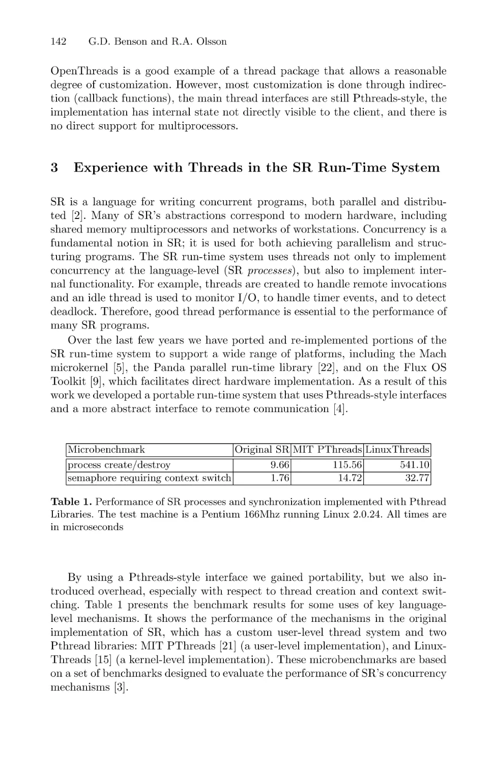
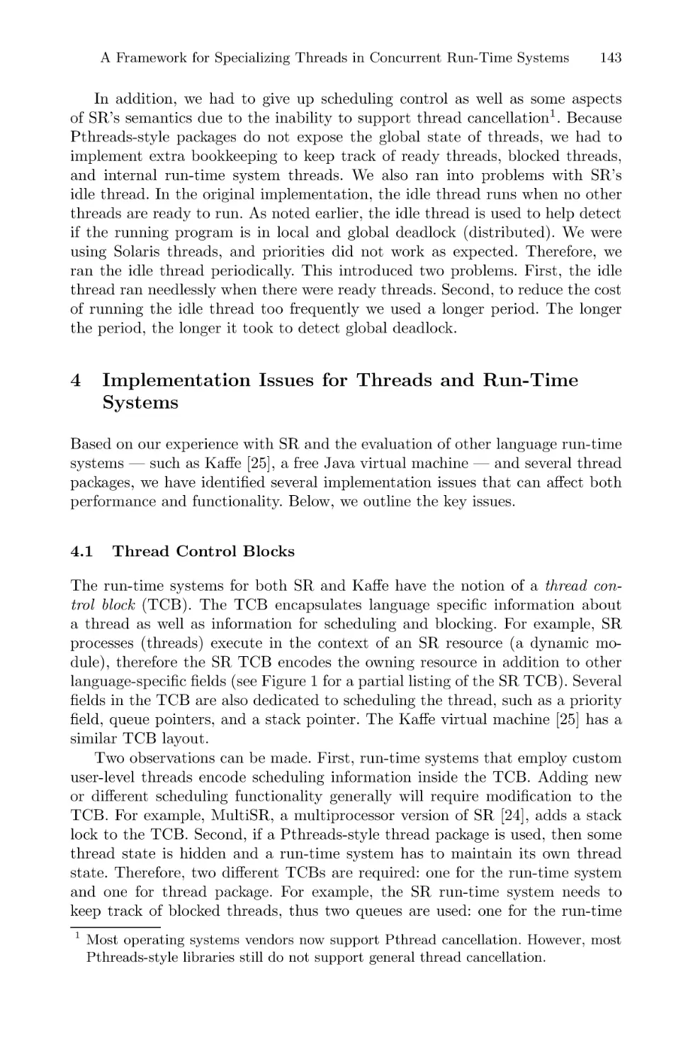
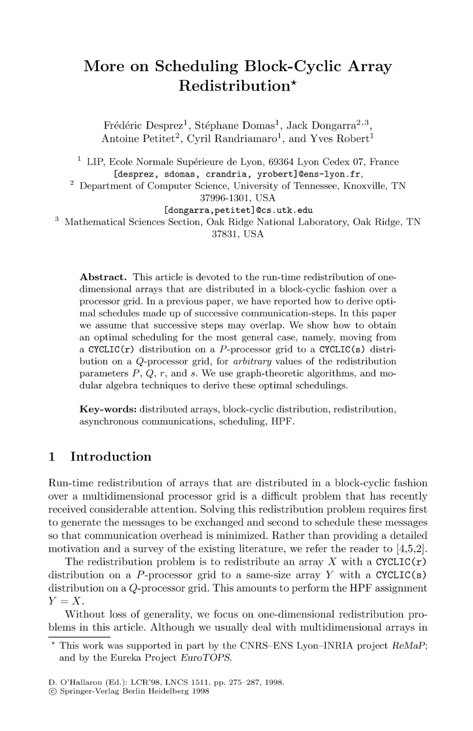
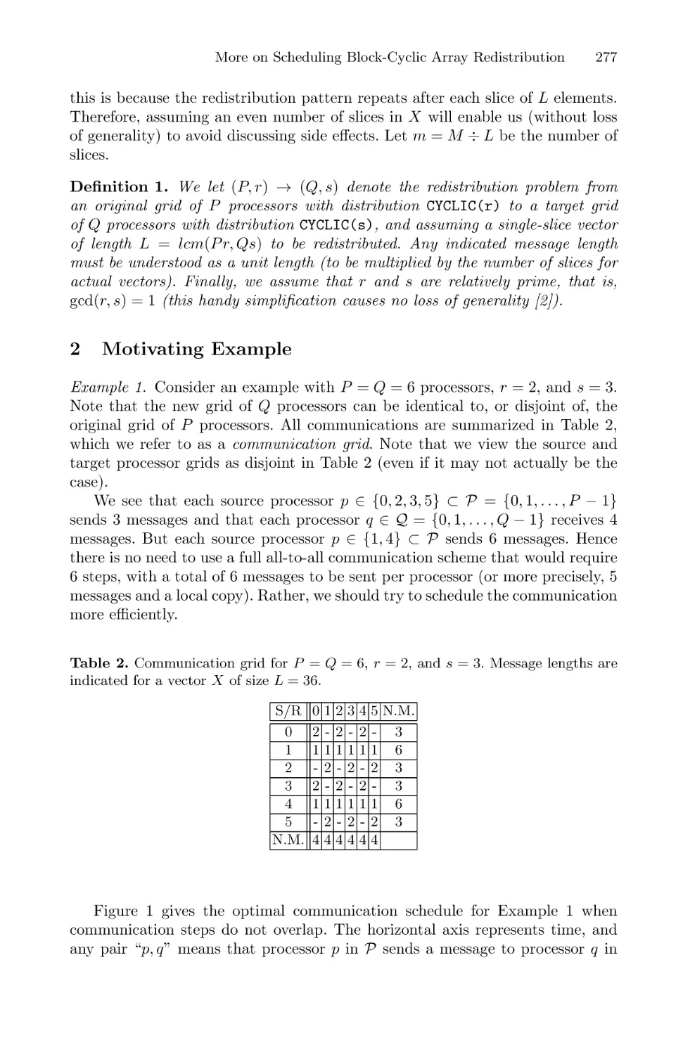
Author: O’Hallaron R.D.

Tags: programming languages programming higher mathematics computer science springer publisher lecture notes

ISBN: 3-540-65172-1

Year: 1998

Similar

Mathematical Modeling and Supercomputer Technologies. 22nd International Conference, MMST 2022 Nizhny Novgorod, Russia, November 14–17, 2022 Revised Selected Papers

Mathematics of Program Construction 14th International Conference, MPC 2022, Tbilisi, Georgia, September 26–28, 2022, Proceedings

Data Science at the Command Line. Obtain, Scrub, Explore, and Model Data with Unix Power Tools

Introduction to Development Engineering - A Framework with Applications from the Field

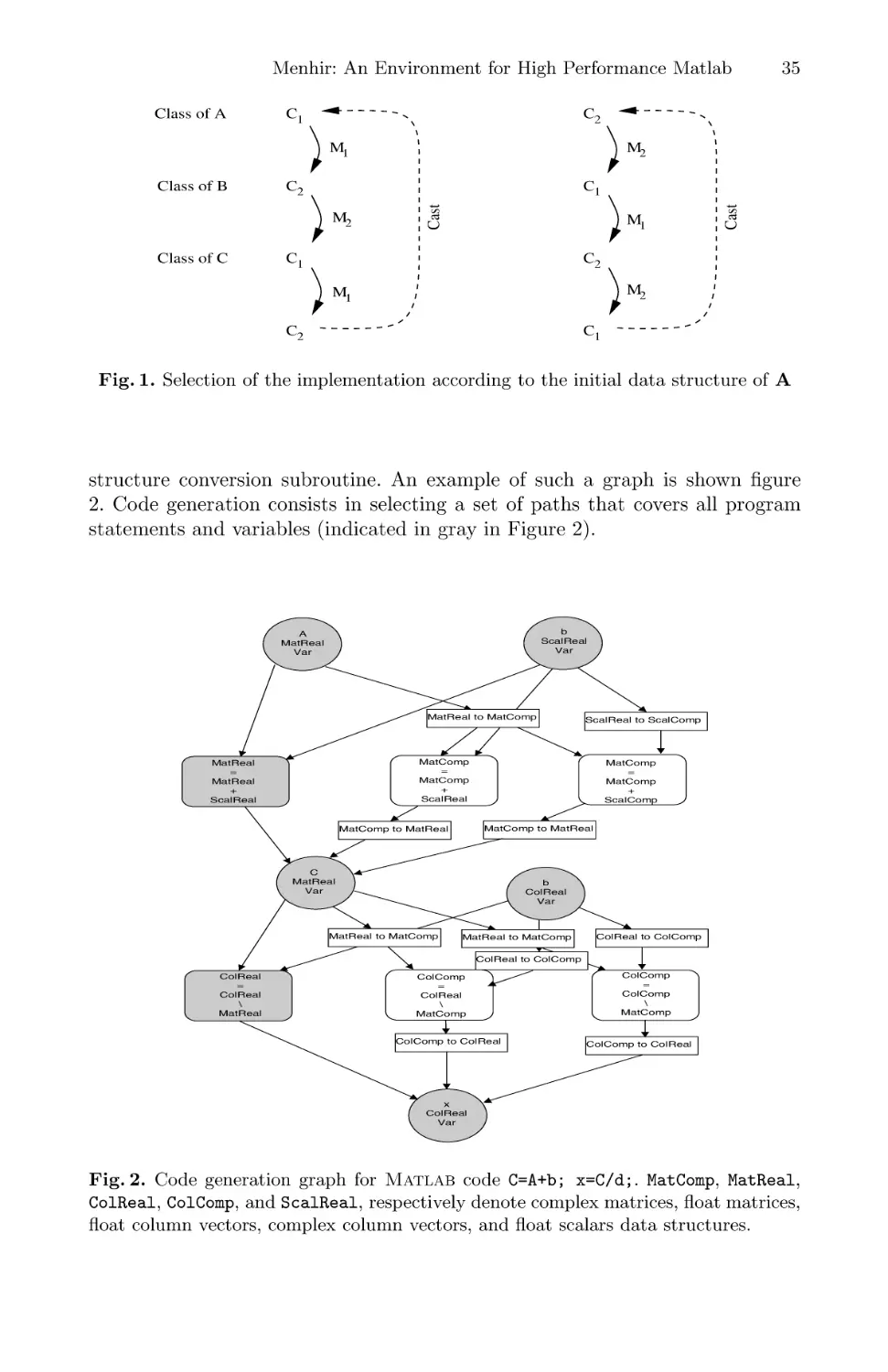
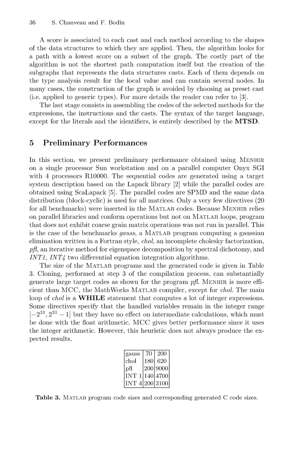
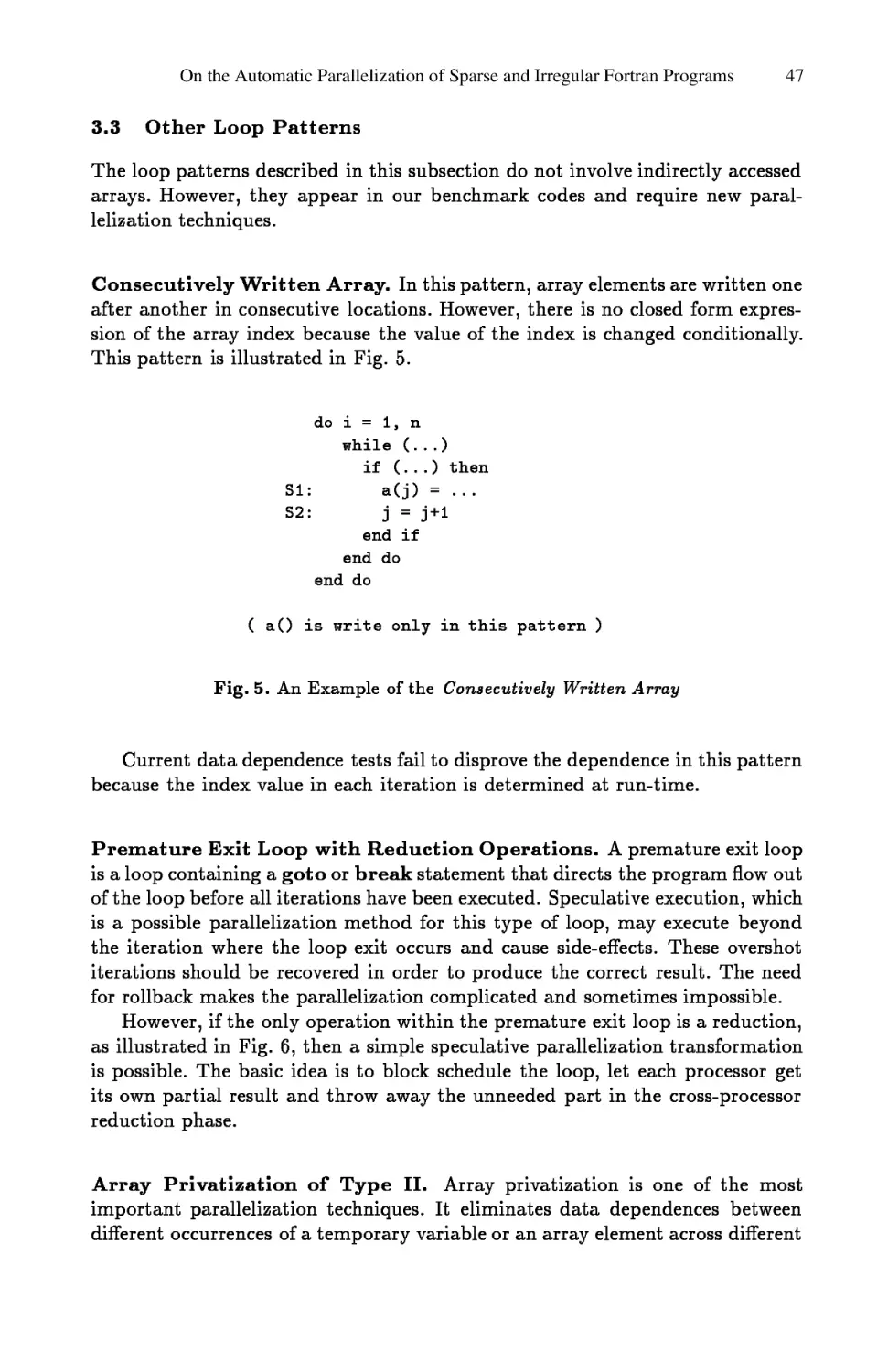
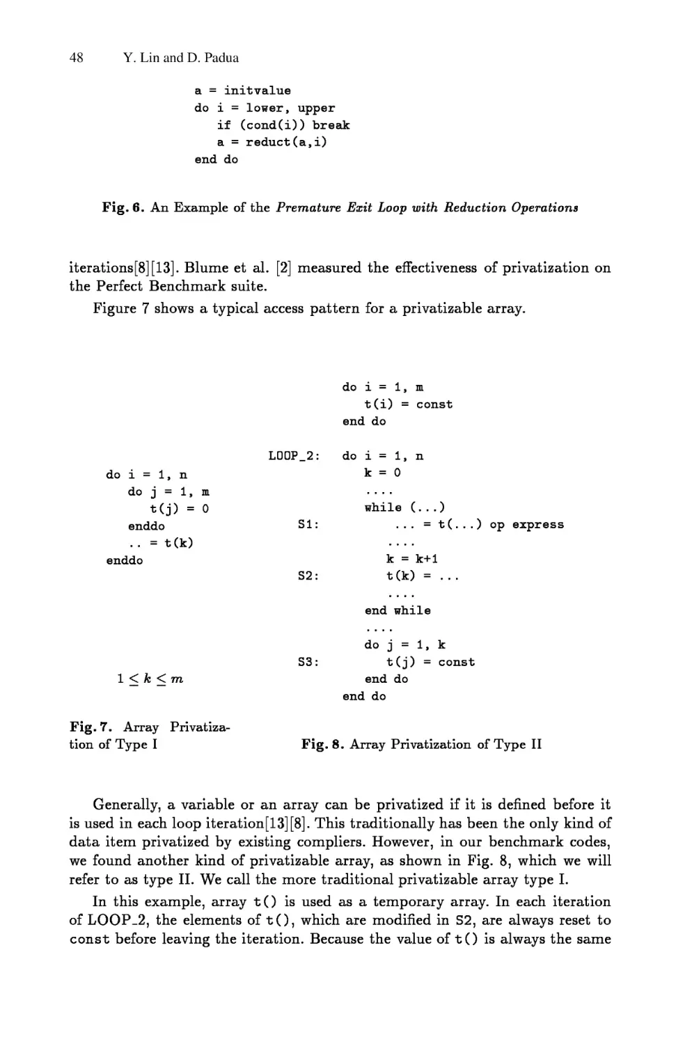
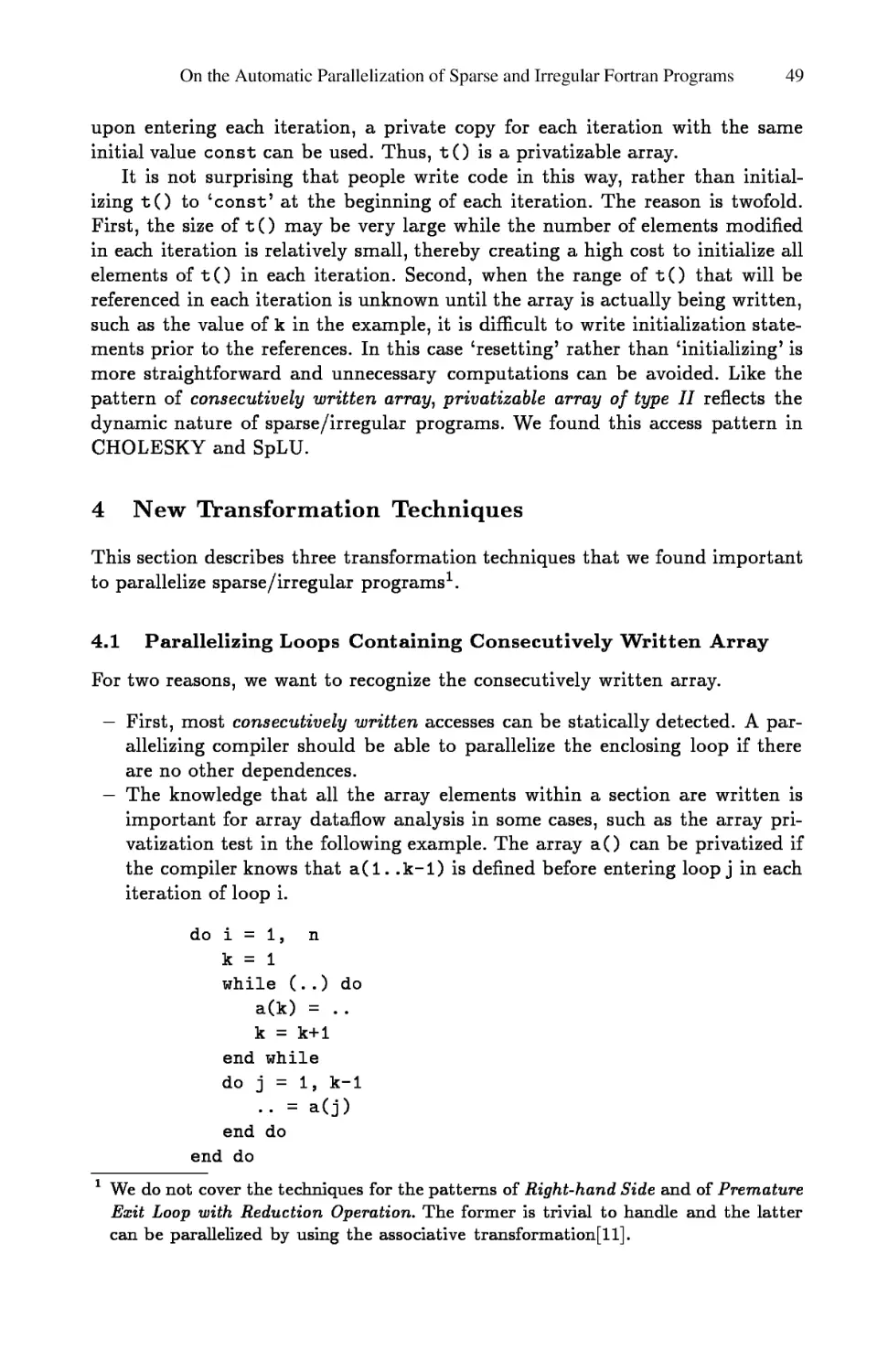
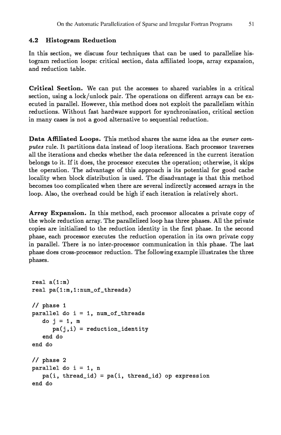
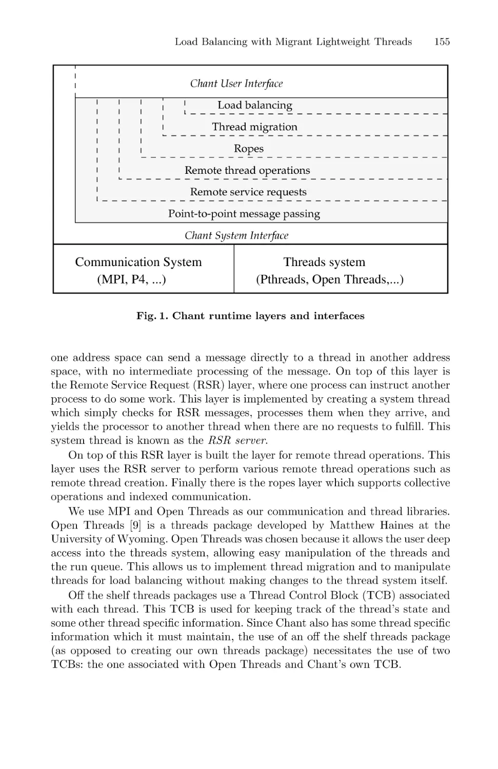
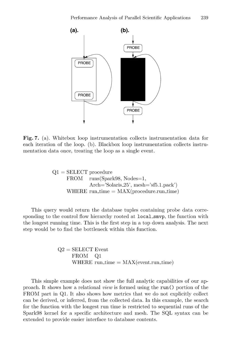
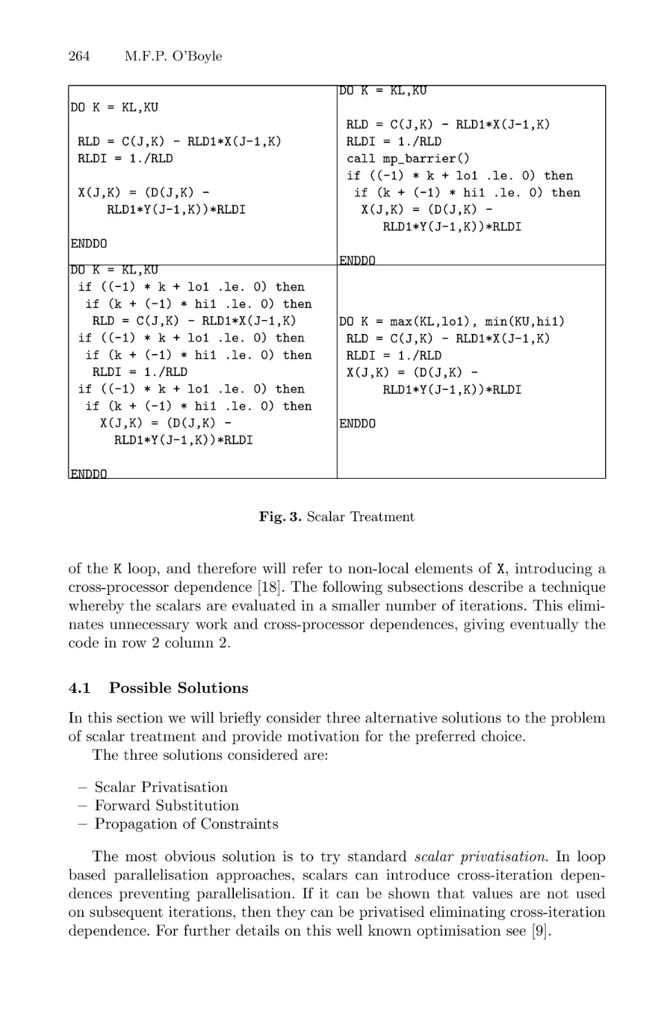
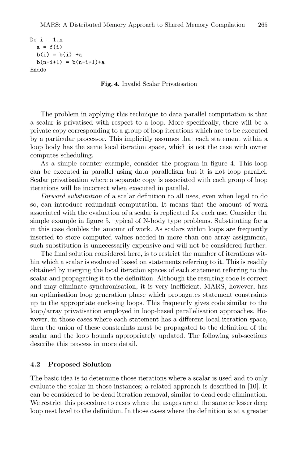
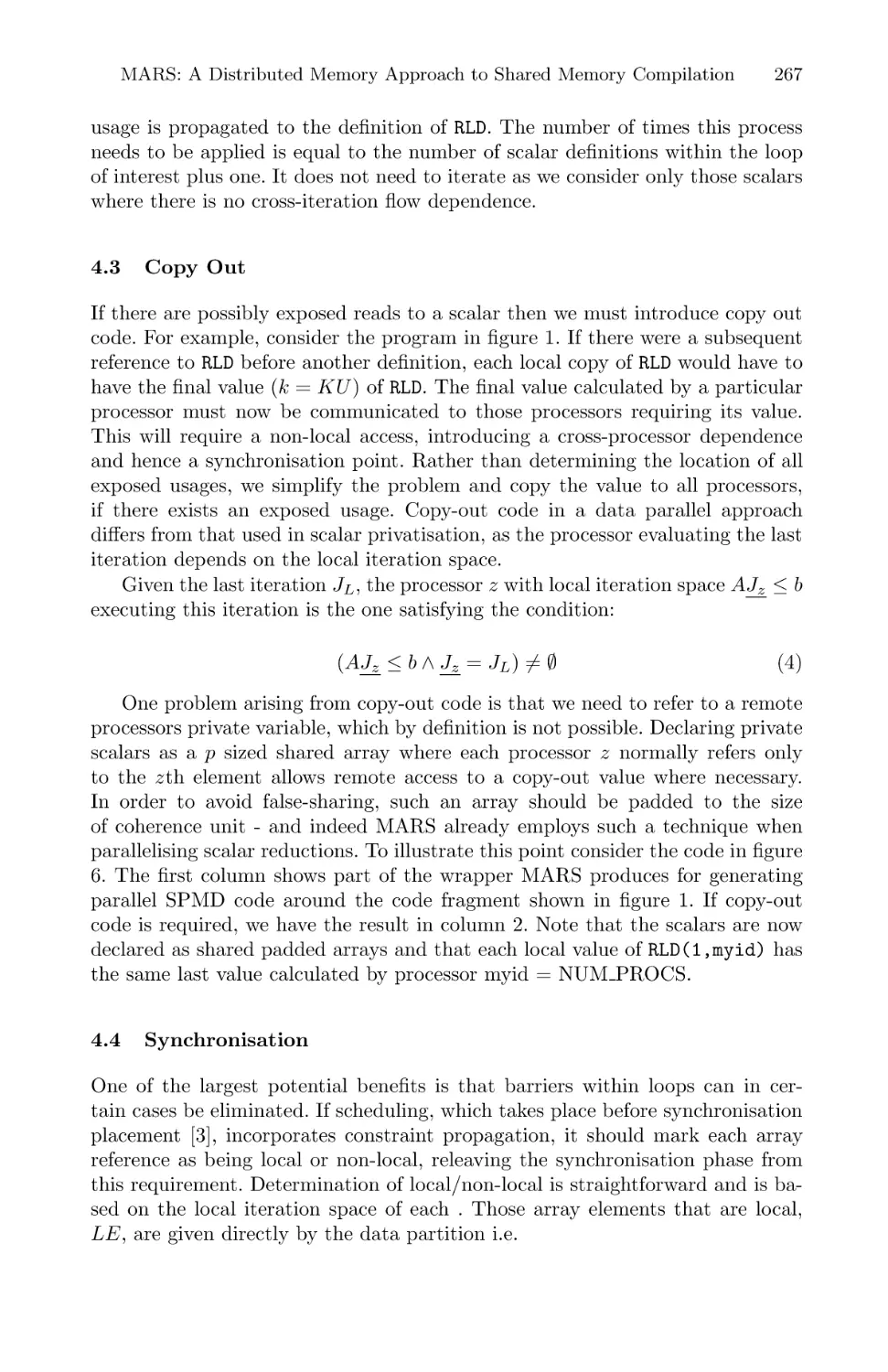
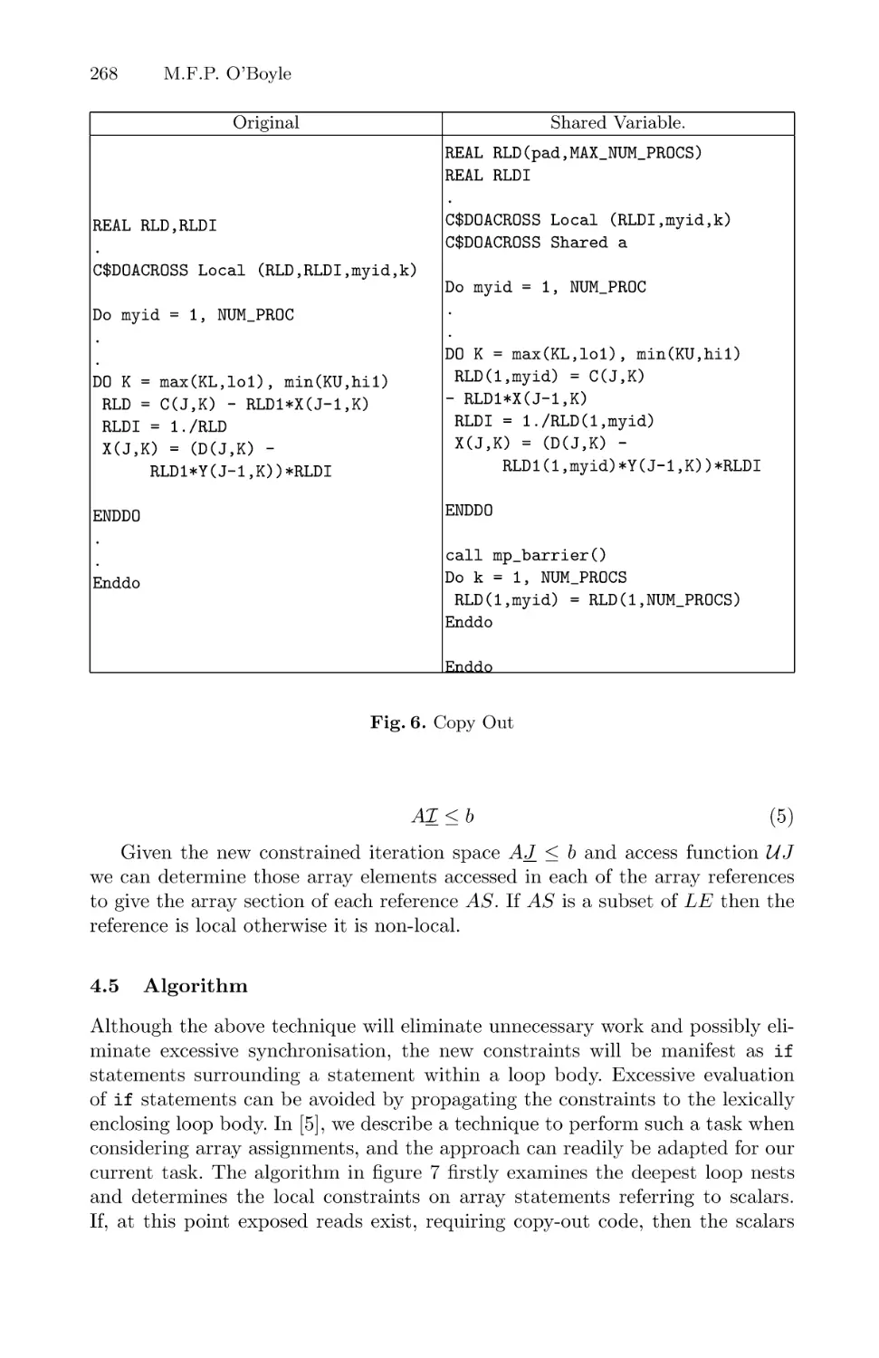
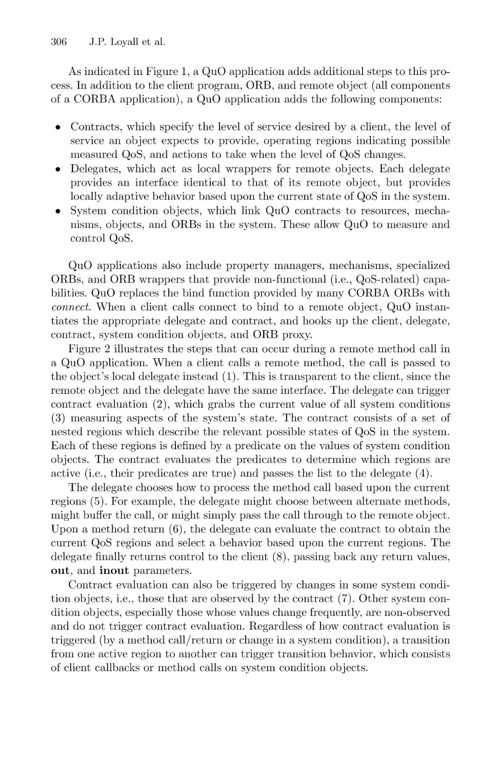
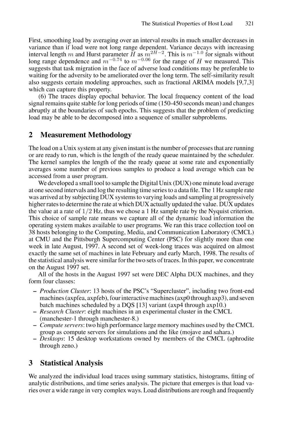
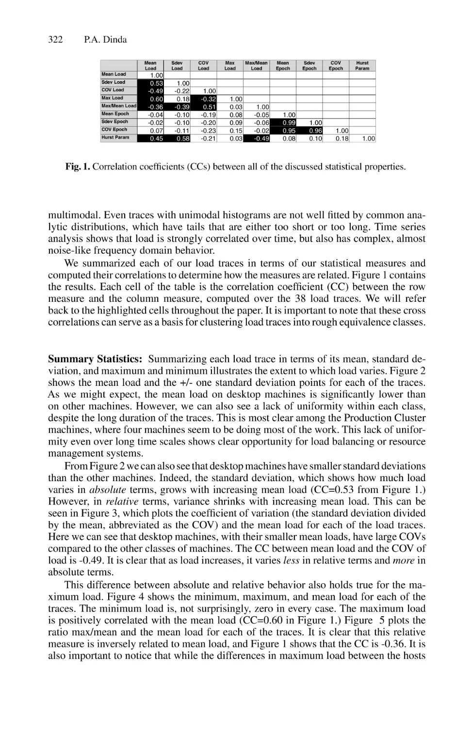
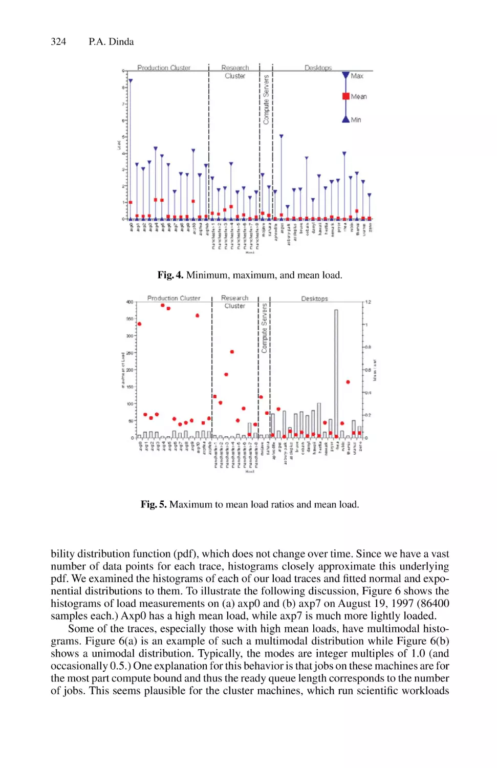
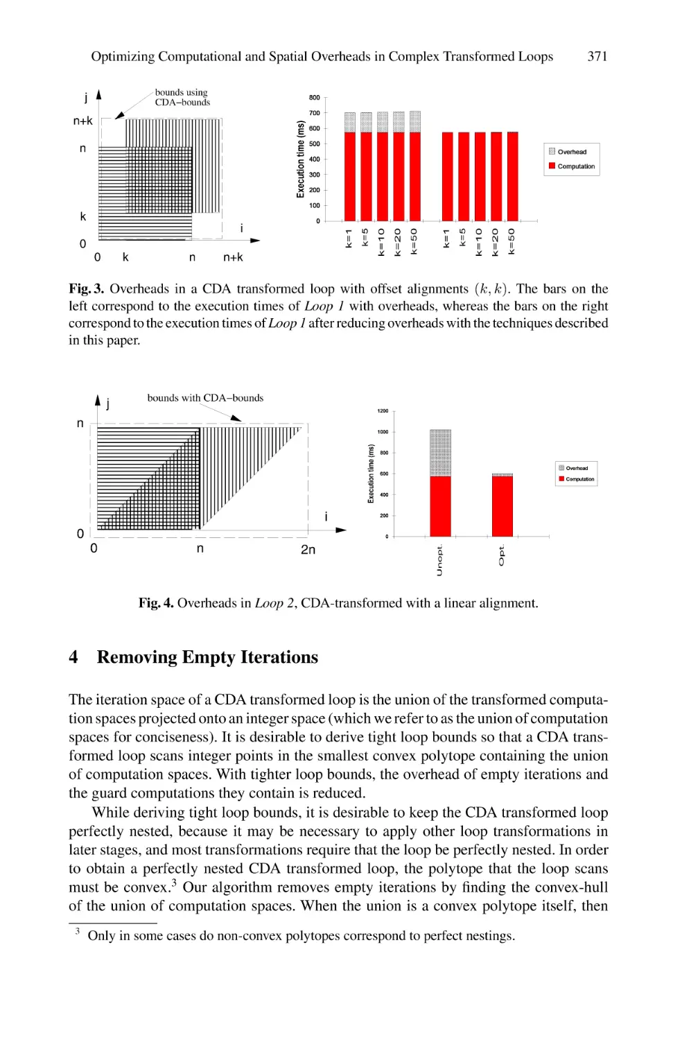
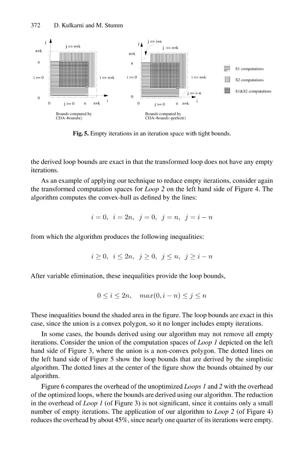
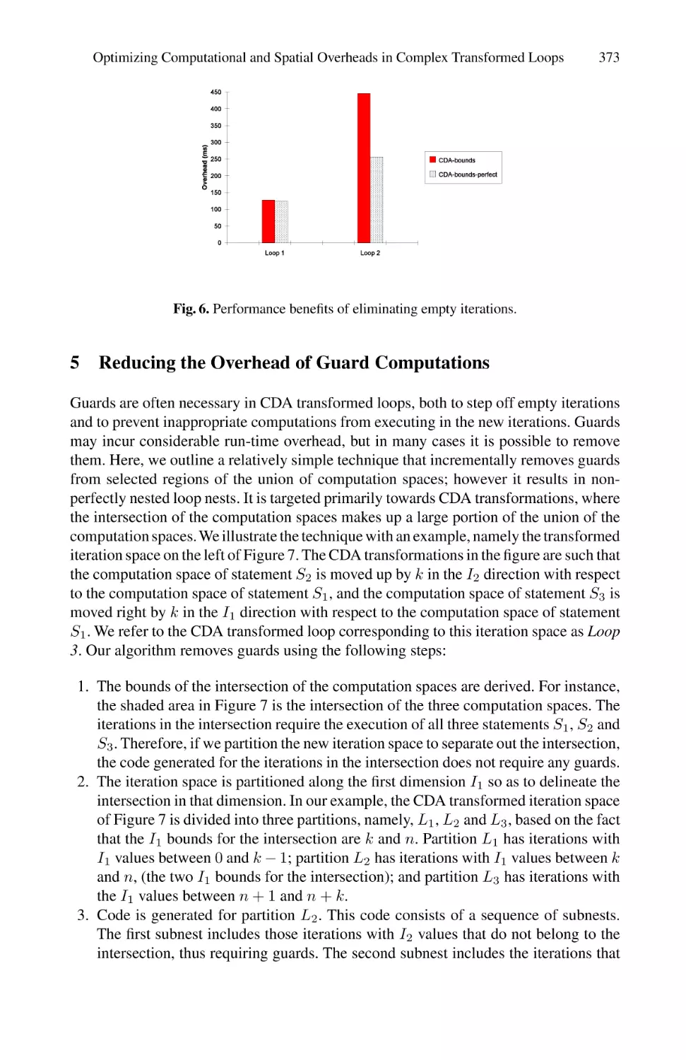
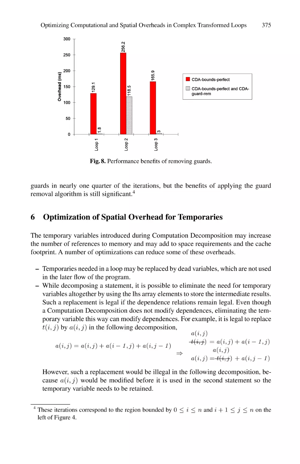
Text

Lecture Notes in Computer Science
Edited by G. Goos, J. Hartmanis and J. van Leeuwen

1511

3
Berlin
Heidelberg
New York
Barcelona
Budapest
Hong Kong
London
Milan
Paris
Singapore
Tokyo

David R. O’Hallaron (Ed.)

Languages, Compilers,
and Run-Time Systems
for Scalable Computers
4th International Workshop, LCR ’98
Pittsburgh, PA, USA, May 28-30, 1998
Selected Papers

Series Editors
Gerhard Goos, Karlsruhe University, Germany
Juris Hartmanis, Cornell University, NY, USA
Jan van Leeuwen, Utrecht University, The Netherlands

Volume Editor
David R. O’Hallaron
Computer Science and Electrical and Computer Engineering
School of Computer Science, Carnegie Mellon University
5000 Forbes Avenue, Pittsburgh, PA 15213-3891, USA
E-mail: droh@cs.cmu.edu

Cataloging-in-Publication data applied for
Die Deutsche Bibliothek - CIP-Einheitsaufnahme
Languages, compilers, and run-time systems for scalable
computers : 4th international workshop ; selected papers / LCR ’98,
Pittsburgh, PA, USA, May 28-30, 1998. David R. O’Hallaron (ed.). Berlin ; Heidelberg ; New York ; Barcelona ; Budapest ; Hong Kong
; London ; Milan ; Paris ; Singapore ; Tokyo : Springer, 1998
(Lecture notes in computer science ; Vol. 1511)
ISBN 3-540-65172-1

CR Subject Classification (1991): F.2.2, D.1.3, D.4.4-5, C.2.2, D.3, F.1, C.2.4,
C.3
ISSN 0302-9743
ISBN 3-540-65172-1 Springer-Verlag Berlin Heidelberg New York
This work is subject to copyright. All rights are reserved, whether the whole or part of the material is
concerned, specifically the rights of translation, reprinting, re-use of illustrations, recitation, broadcasting,
reproduction on microfilms or in any other way, and storage in data banks. Duplication of this publication
or parts thereof is permitted only under the provisions of the German Copyright Law of September 9, 1965,
in its current version, and permission for use must always be obtained from Springer-Verlag. Violations are
liable for prosecution under the German Copyright Law.
c Springer-Verlag Berlin Heidelberg 1998

Printed in Germany
Typesetting: Camera-ready by author
SPIN 10692671
06/3142 – 5 4 3 2 1 0

Printed on acid-free paper

Preface

It is a great pleasure to present this collection of papers from LCR ’98, the
Fourth Workshop on Languages, Compilers, and Run-time Systems for Scalable
Computers. The LCR workshop is a bi-annual gathering of computer scientists
who develop software systems for parallel and distributed computers. LCR is
held in alternating years with the ACM Symposium on Principles and Practice
of Parallel Programming (PPoPP) and draws from the same community.
This fourth meeting was held in cooperation with ACM SIGPLAN on the campus of Carnegie Mellon University, May 28–30, 1998. There were 60 registered
attendees from 9 nations. A total of 47 6-page extended abstracts were submitted. There were a total of 134 reviews for an average of 2.85 reviews per
submission. Submissions were rank ordered by average review score. The top 23
submissions were selected as full papers and the next 9 as short papers.
The program committee consisted of David Bakken (BBN), Ian Foster (Argonne), Thomas Gross (CMU and ETH Zurich), Charles Koelbel (Rice), Piyush
Mehrotra (ICASE), David O’Hallaron, Chair (CMU), Joel Saltz (Maryland), Jaspal Subhlok (CMU), Boleslaw Szymanski (RPI), Katherine Yelick (Berkeley),
and Hans Zima (Vienna).
In addition to the members of the committee, the following people chaired sessions: Lawrence Rauchwerger, Peter Brezany, Terry Pratt, Alan Sussman, Sandhya Dwarkadis and Rajiv Gupta. Also, the following people generously provided
additional reviews: Sigfried Benkner, Chen Ding, Guoha Jin, Erwin Laure, Pantona Mario, Eduard Mehofer, and Bernd Wender. We very much appreciate the
efforts of these dedicated volunteers.
Barbara Grandillo did a wonderful job of chairing the organizing committee and
handling the local arrangements. Thomas Gross and Jaspal Subhlok made numerous suggestions. Peter Dinda, Peter Lieu, Nancy Miller, and Bwolen Yang
also helped out during the workshop itself. We are very grateful for their help.
Finally I would like to thank Mary Lou Soffa at the Univ. of Pittsburgh, for her
help in getting SIGPLAN support, Bolek Szymanski at RPI, who chaired the
previous meeting and was always helpful and encouraging, and Alfred Hofmann
at Springer, whose advice and encouragement enabled us to produce this volume.
Carnegie Mellon University
August, 1998

David O’Hallaron
LCR ’98 General/Program Chair

Table of Contents

Expressing Irregular Computations in Modern Fortran Dialects . . . . . . . . . . . . . 1
Jan F. Prins, Siddhartha Chatterjee, and Martin Simons
Memory System Support for Irregular Applications . . . . . . . . . . . . . . . . . . . . . . . . 17
John Carter, Wilson Hsieh, Mark Swanson, Lixin Zhang, Erik Brunvand,
Al Davis, Chen-Chi Kuo, Ravindra Kuramkote, Michael Parker,
Lambert Schaelicke, Leigh Stoller, and Terry Tateyama
MENHIR: An Environment for High Performance Matlab . . . . . . . . . . . . . . . . . . 27
Stéphane Chauveau and Francois Bodin
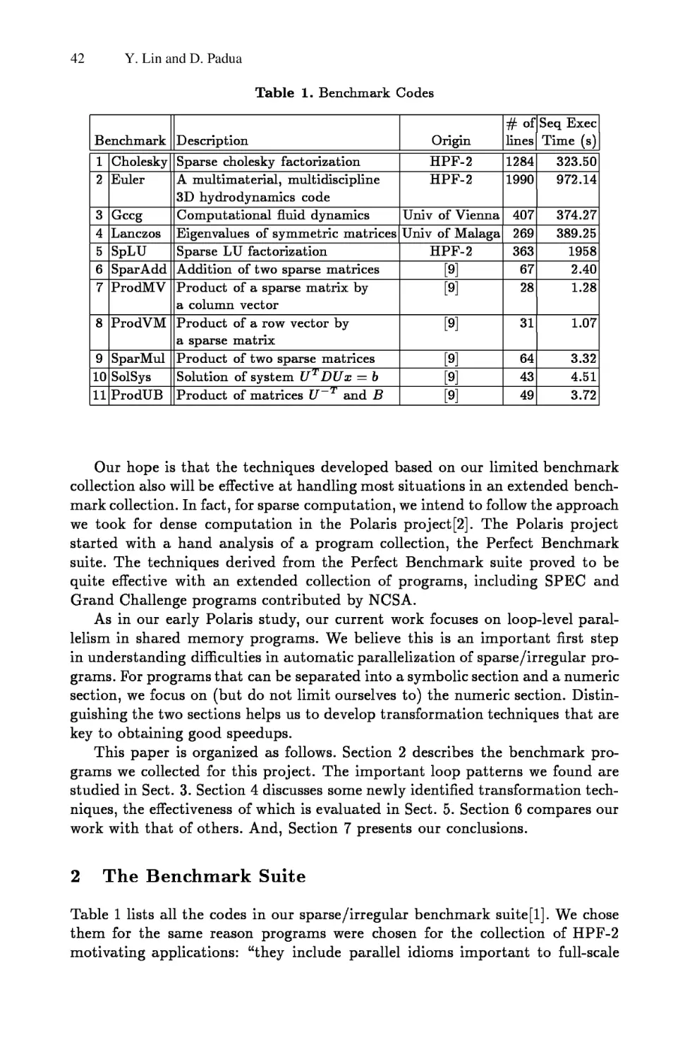
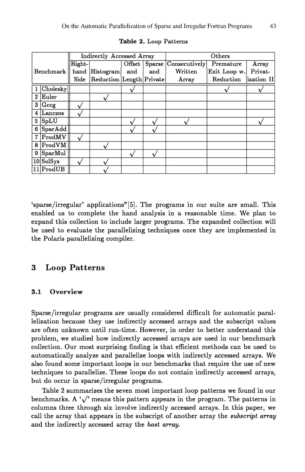
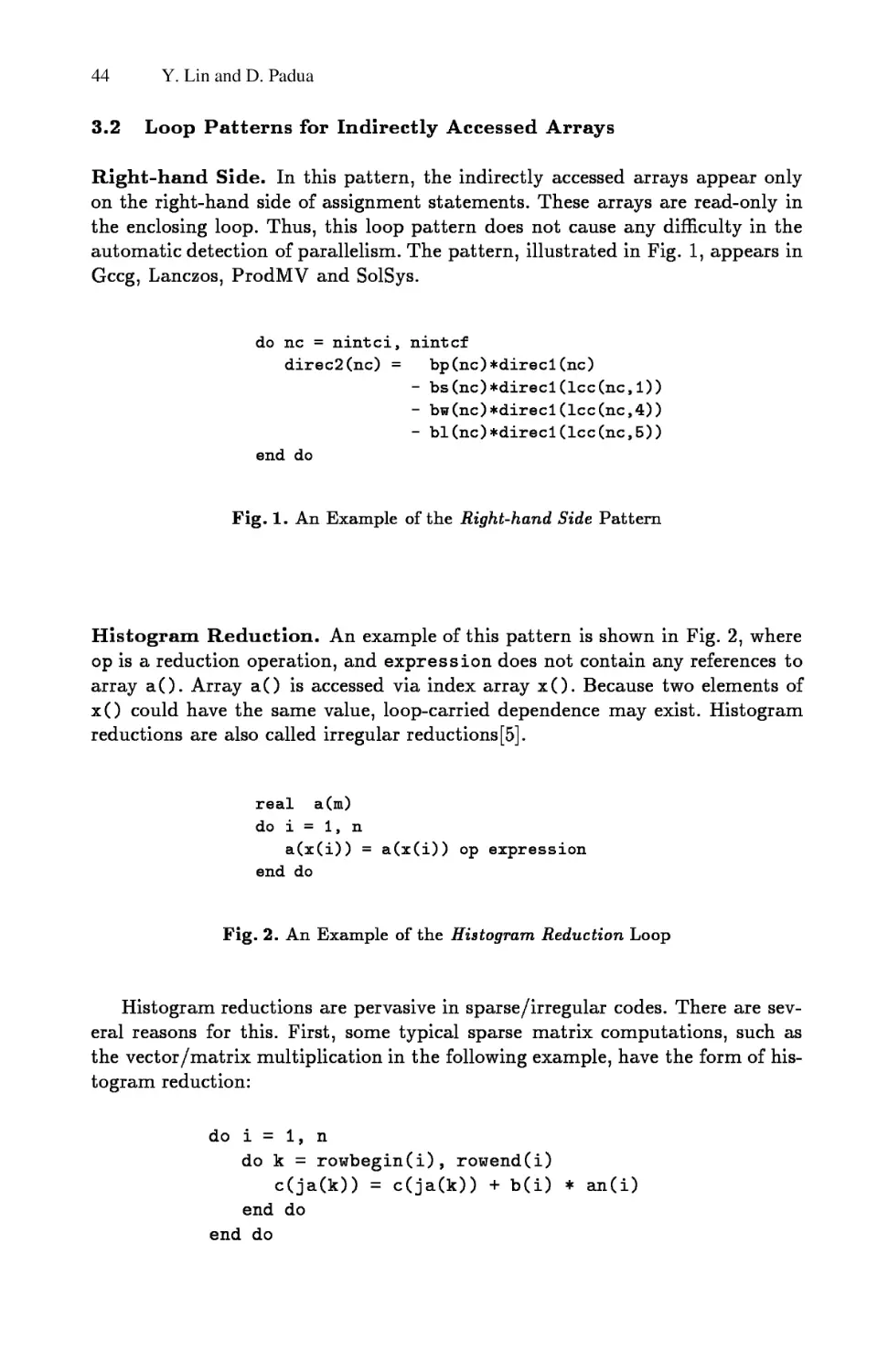
On the Automatic Parallelization of Sparse and Irregular
Fortran Programs . . . . . . . . . . . . . . . . . . . . . . . . . . . . . . . . . . . . . . . . . . . . . . . . . . . . . . . . . .41
Yuan Lin and David Padua
Loop Transformations for Hierarchical Parallelism and Locality . . . . . . . . . . . . 57
Vivek Sarkar
Dataflow Analysis Driven Dynamic Data Partitioning . . . . . . . . . . . . . . . . . . . . . . 75
Jodi Tims, Rajiv Gupta, and Mary Lou Soffa
A Case for Combining Compile-Time and Run-Time Parallelization . . . . . . . . 91
Sungdo Moon, Byoungro So, Mary W. Hall, and Brian Murphy
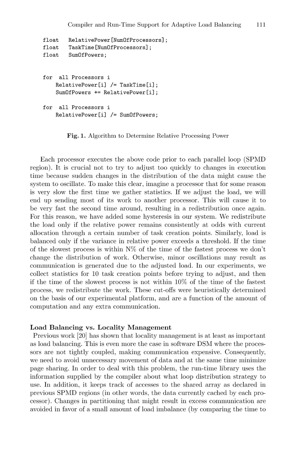
Compiler and Run-Time Support for Adaptive Load Balancing in
Software Distributed Shared Memory Systems . . . . . . . . . . . . . . . . . . . . . . . . . . . . 107
Sotiris Ioannidis and Sandhya Dwarkadas
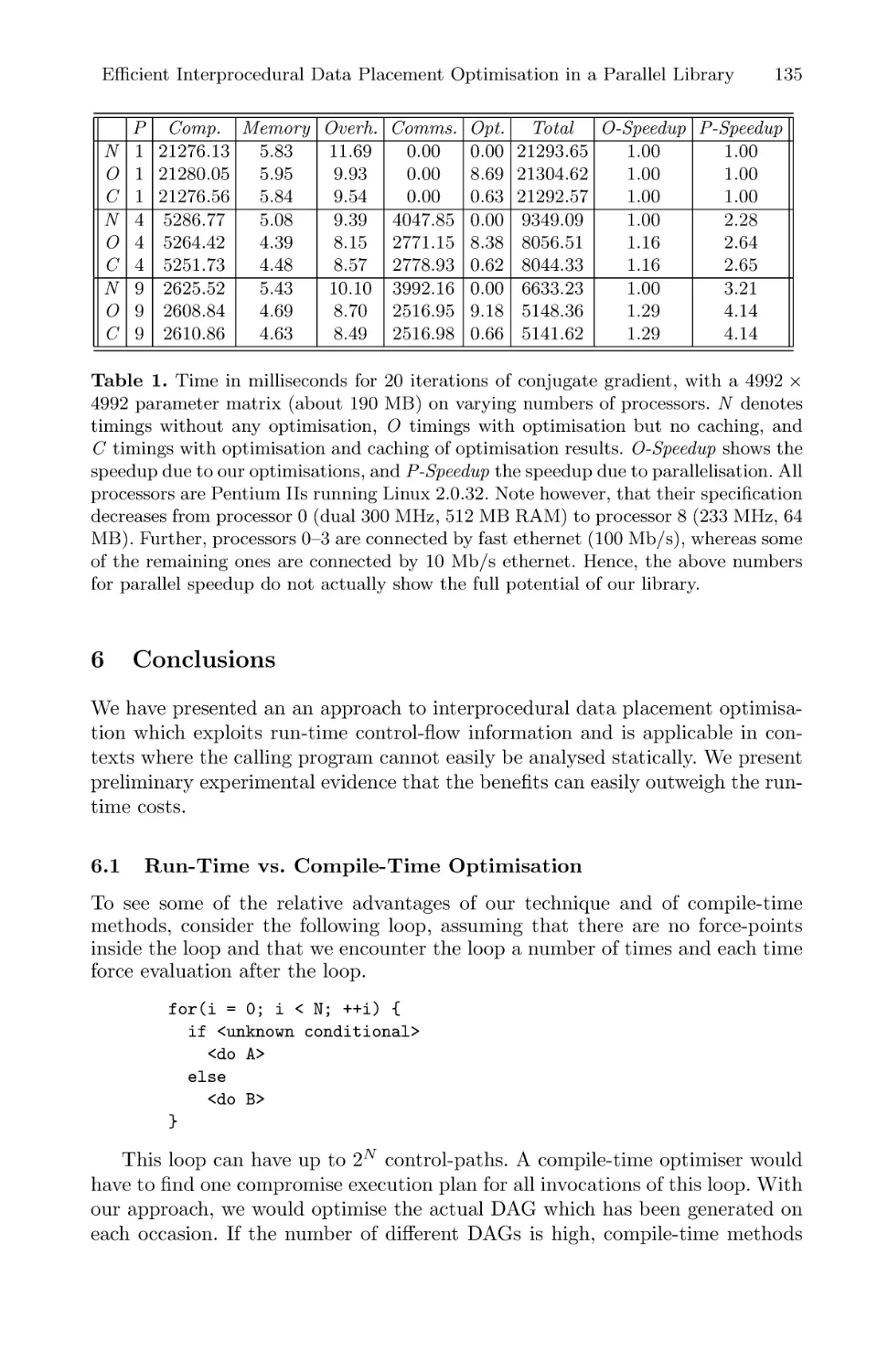
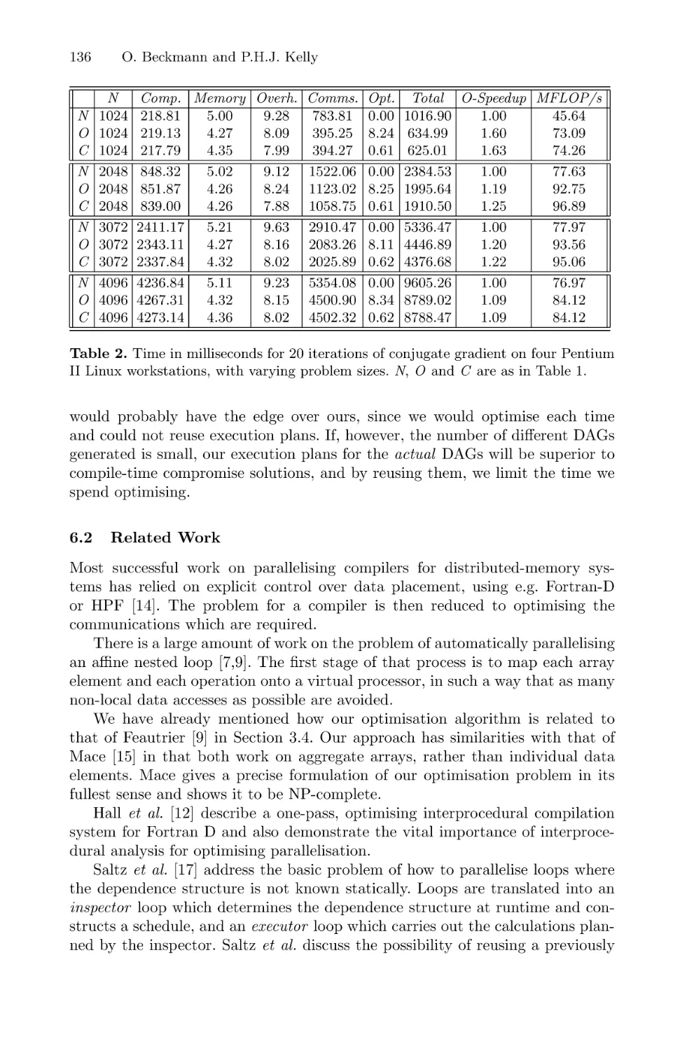
Efficient Interprocedural Data Placement Optimisation in a
Parallel Library . . . . . . . . . . . . . . . . . . . . . . . . . . . . . . . . . . . . . . . . . . . . . . . . . . . . . . . . . . 123
Olav Beckmann and Paul H. J. Kelly
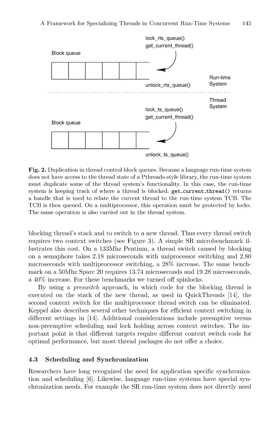
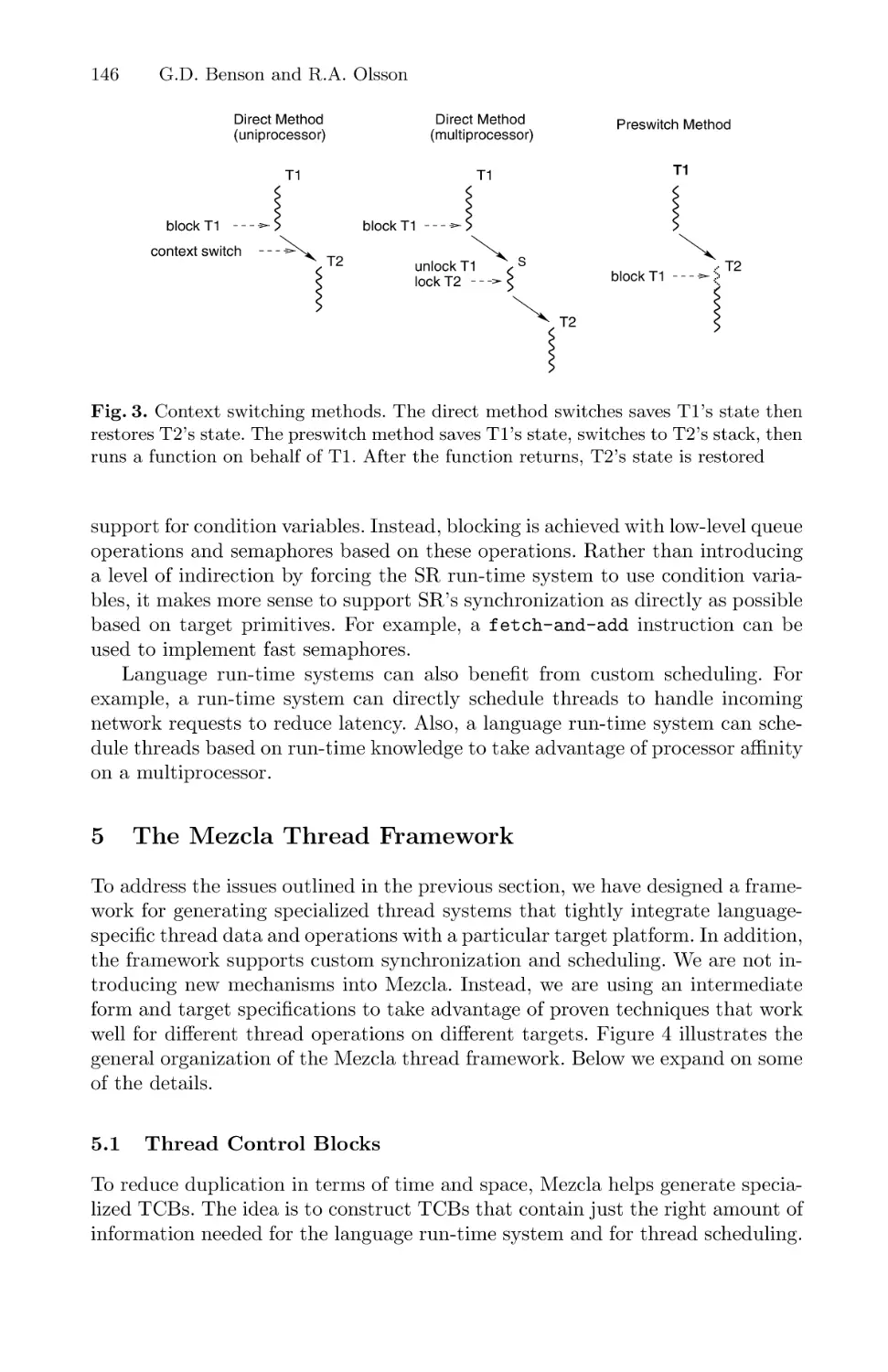
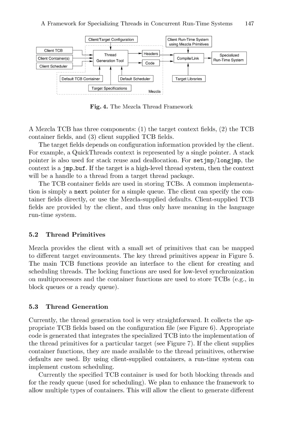
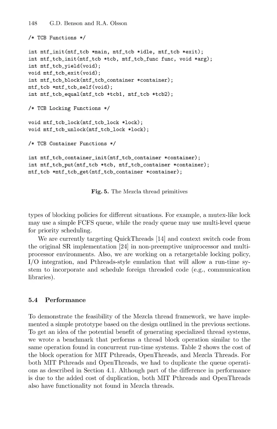
A Framework for Specializing Threads in Concurrent Run-Time Systems . . 139
Gregory D. Benson and Ronald A. Olsson
Load Balancing with Migrant Lightweight Threads . . . . . . . . . . . . . . . . . . . . . . . .153
David Cronk and Piyush Mehrotra
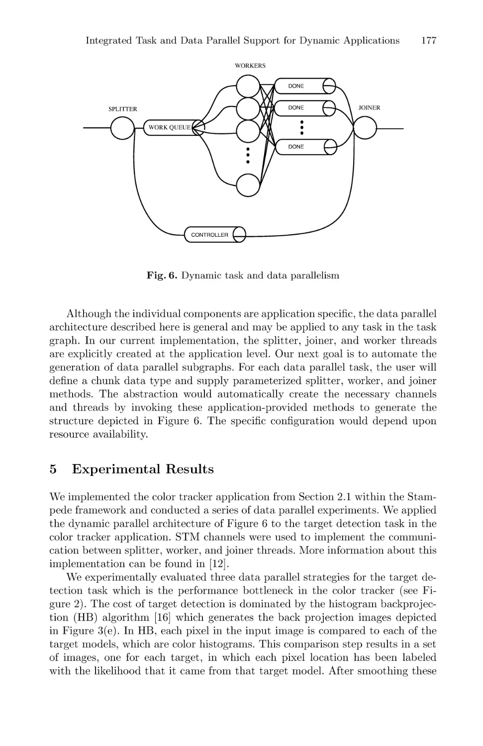
Integrated Task and Data Parallel Support for Dynamic Applications . . . . . 167
James M. Rehg, Kathleen Knobe, Umakishore Ramachandran,
Rishiyur S. Nikhil, and Arun Chauhan
Supporting Self-Adaptivity for SPMD Message-Passing Applications . . . . . . 181
M. Cermele, M. Colajanni, and S. Tucci
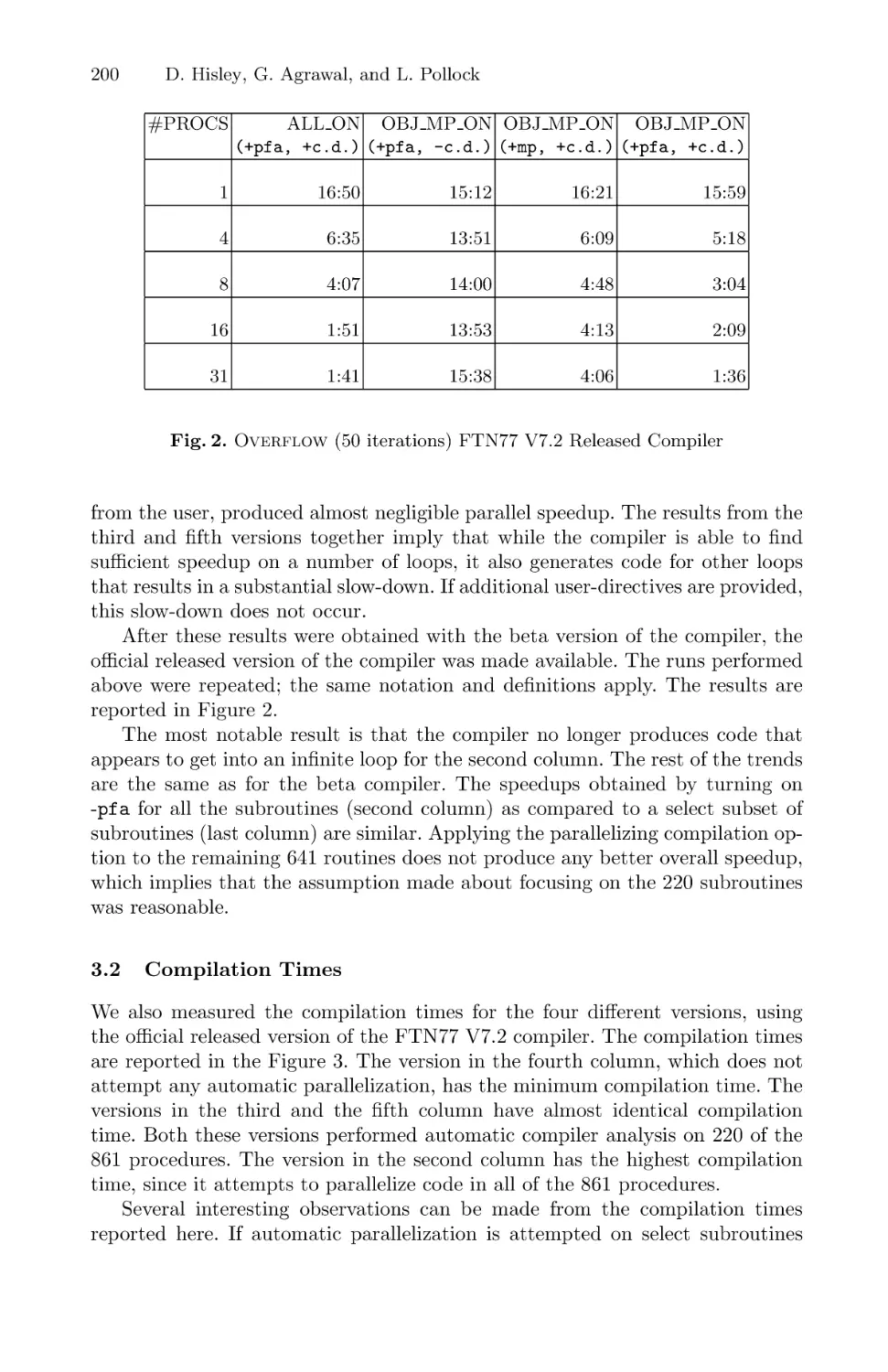
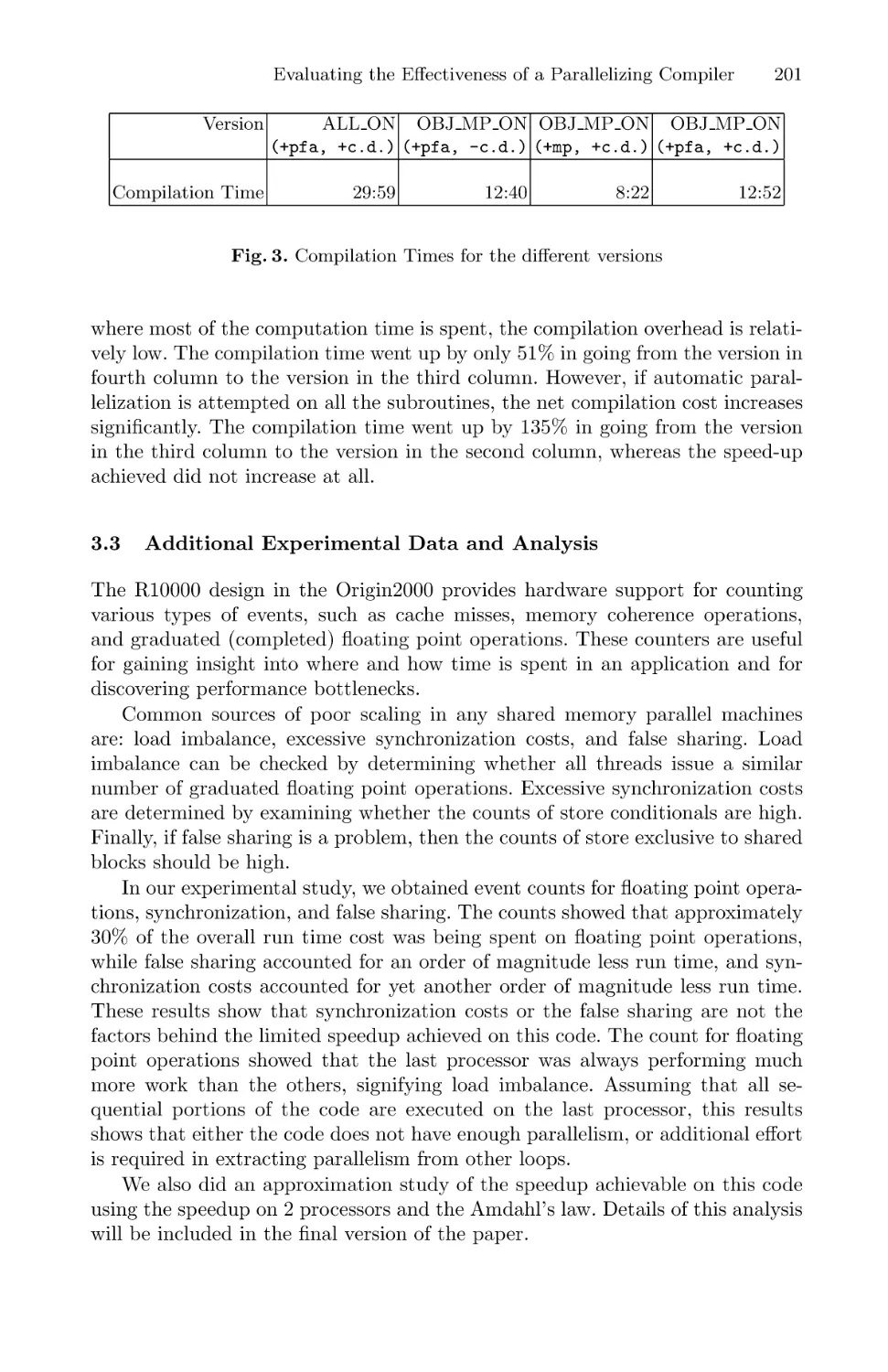
Evaluating the Effectiveness of a Parallelizing Compiler . . . . . . . . . . . . . . . . . . . 195
Dixie Hisley, Gagan Agrawal and Lori Pollock

VIII

Table of Contents

Comparing Reference Counting and Global Mark-and-Sweep
on Parallel Computers . . . . . . . . . . . . . . . . . . . . . . . . . . . . . . . . . . . . . . . . . . . . . . . . . . . . 205
Hirotaka Yamamoto, Kenjiro Taura, and Akinori Yonezawa
Design of the GODIVA Performance Measurement System . . . . . . . . . . . . . . . . 219
Terrence W. Pratt
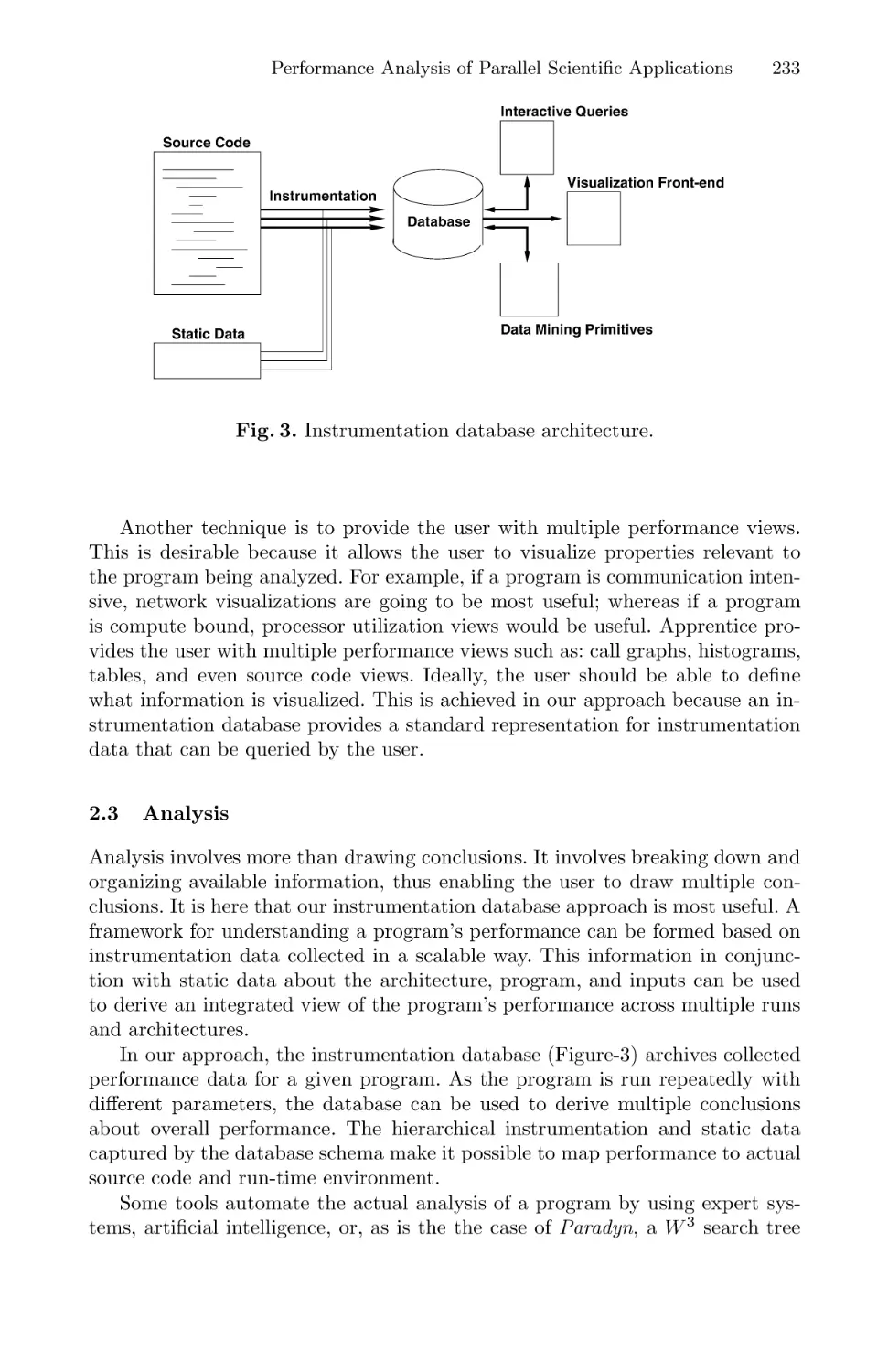
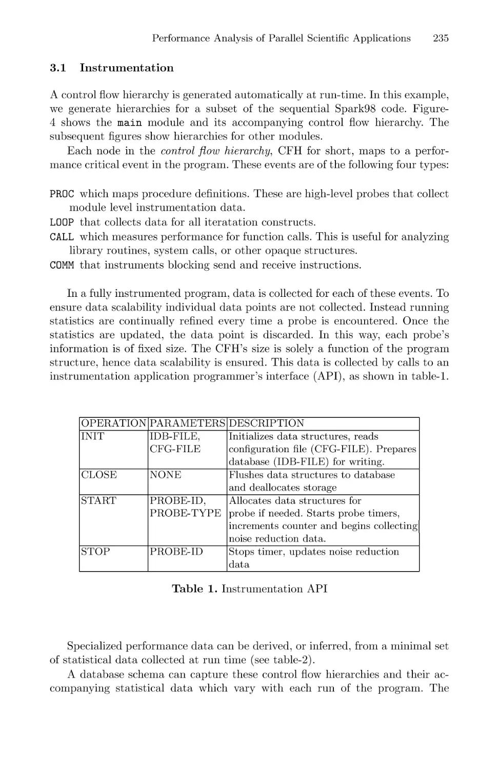
Instrumentation Database for Performance Analysis of Parallel
Scientific Applications . . . . . . . . . . . . . . . . . . . . . . . . . . . . . . . . . . . . . . . . . . . . . . . . . . . . 229
Jeffrey Nesheiwat and Boleslaw K. Szymanski
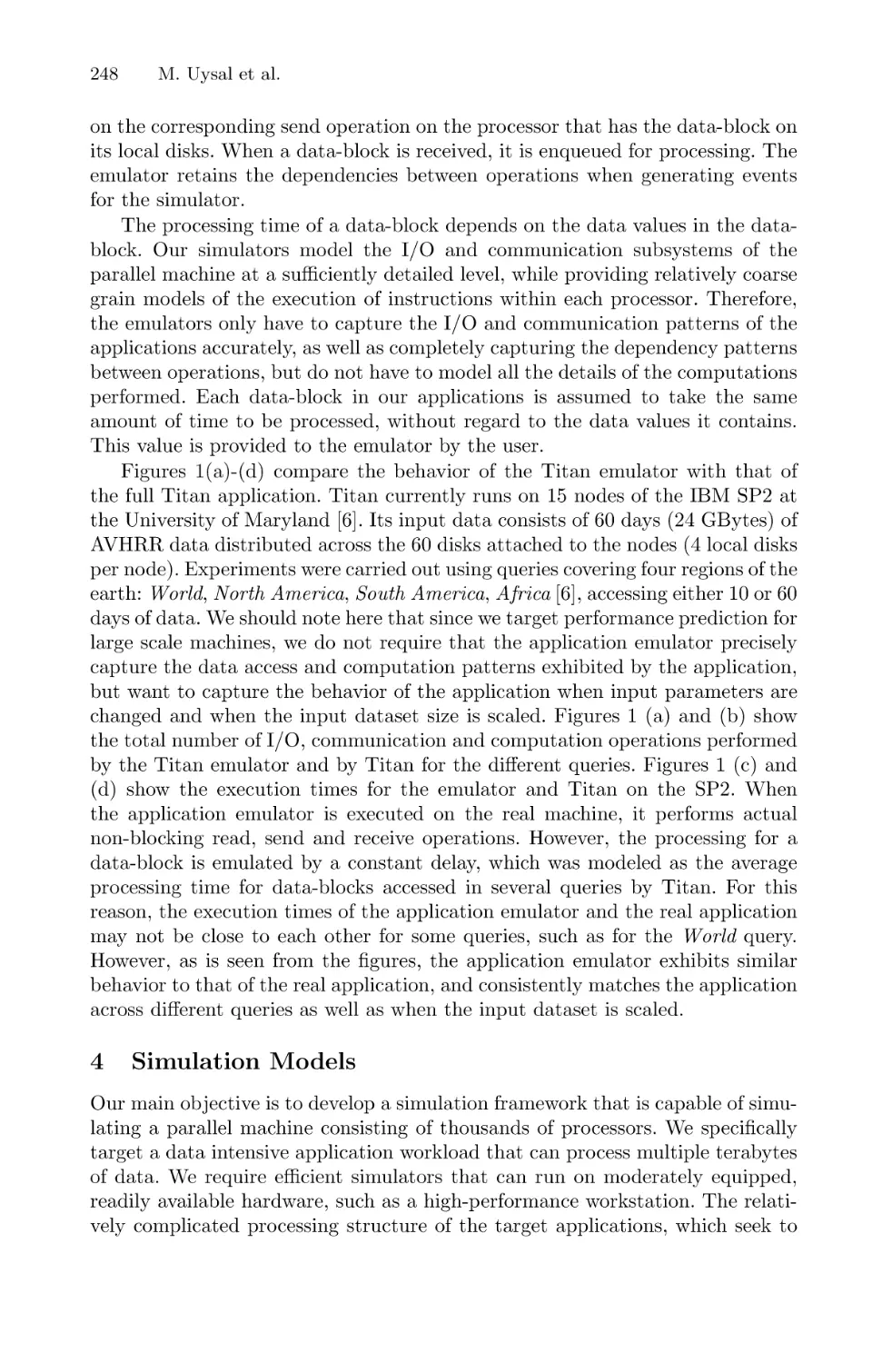
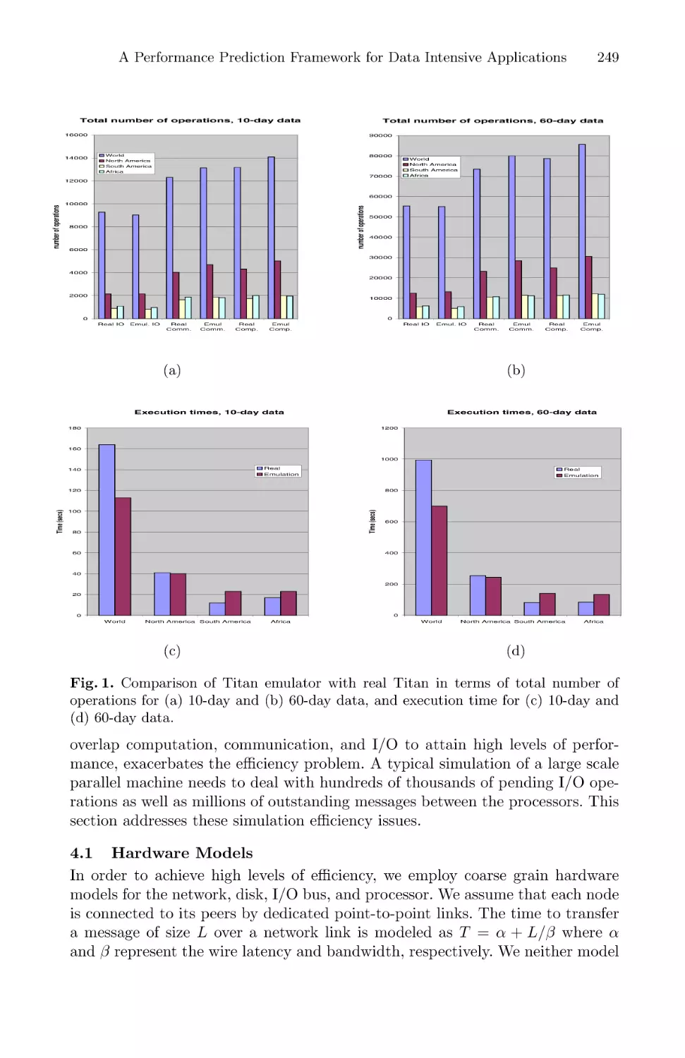
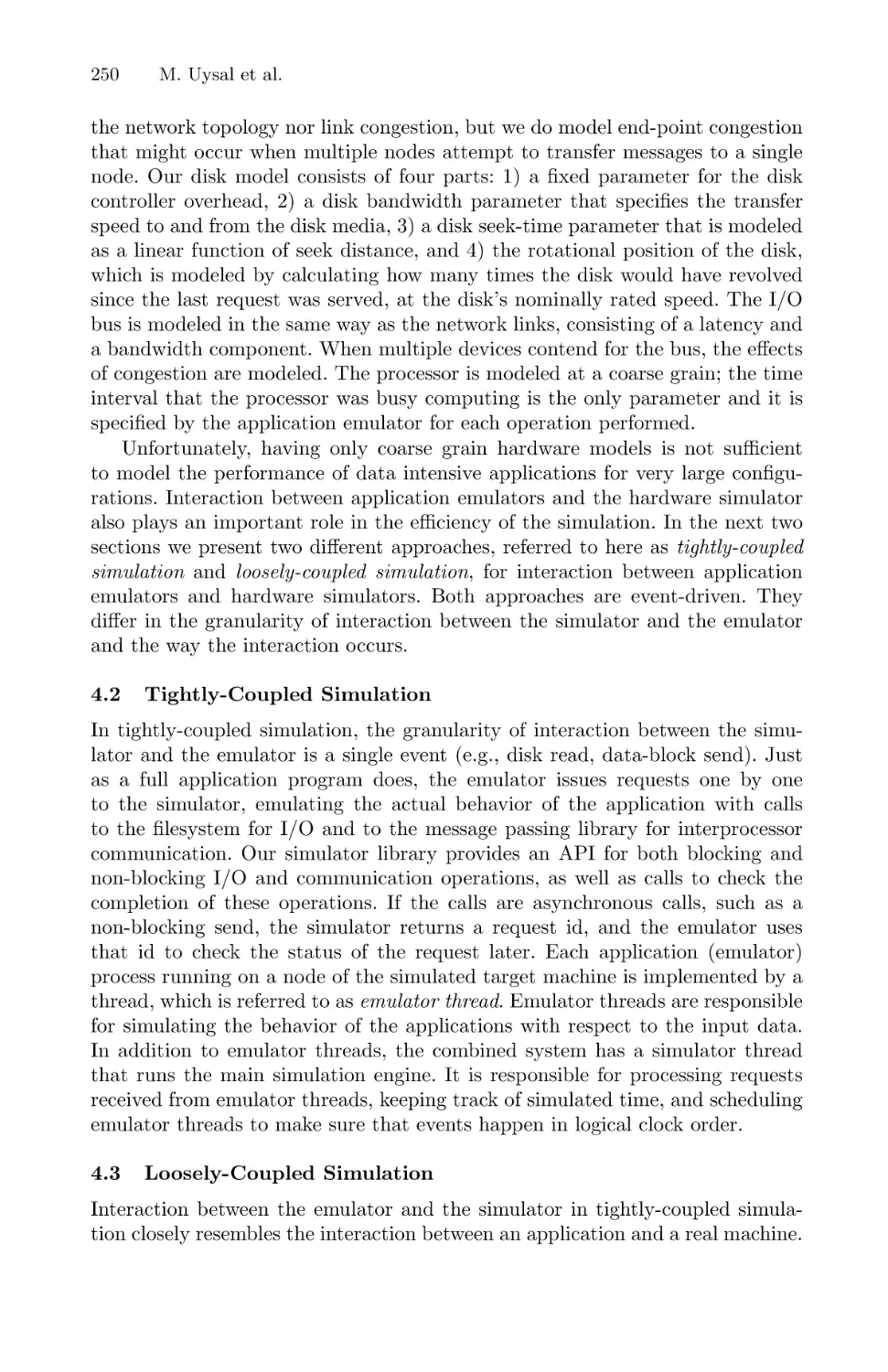
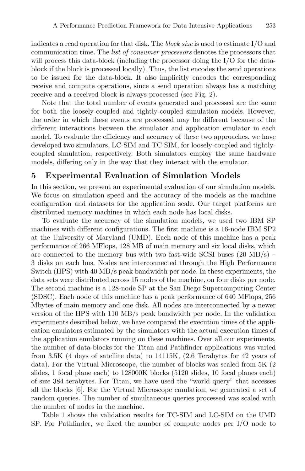
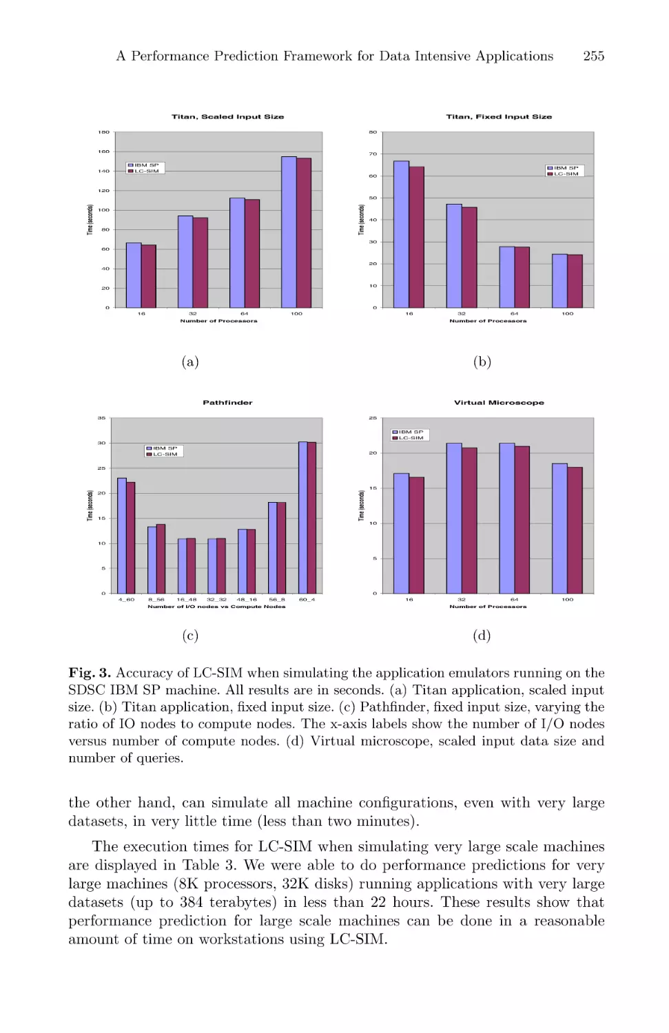
A Performance Prediction Framework for Data Intensive Applications
on Large Scale Parallel Machines . . . . . . . . . . . . . . . . . . . . . . . . . . . . . . . . . . . . . . . . . 243
Mustafa Uysal, Tahsin M. Kurc, Alan Sussman, and Joel Saltz
MARS: A Distributed Memory Approach to Shared Memory Compilatio . . 259
M.F.P. O’Boyle
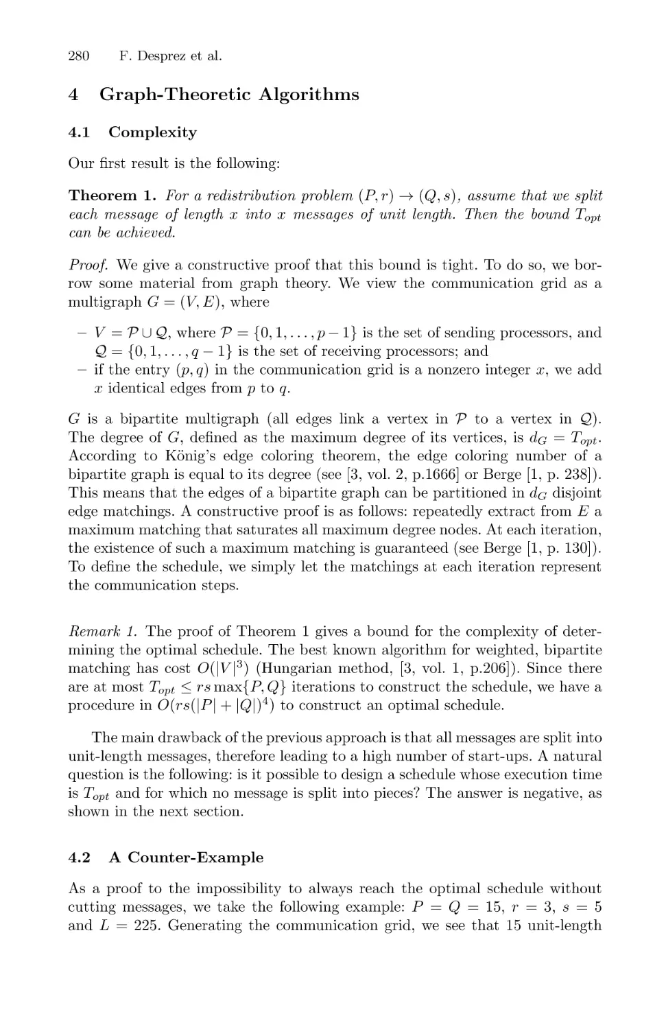
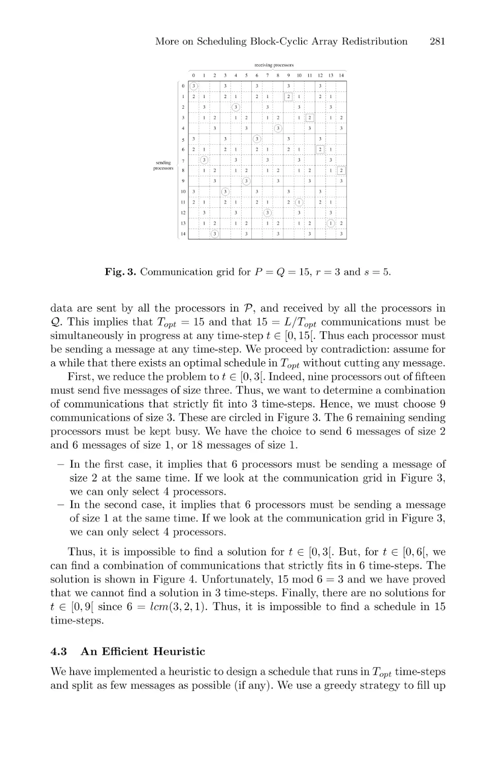
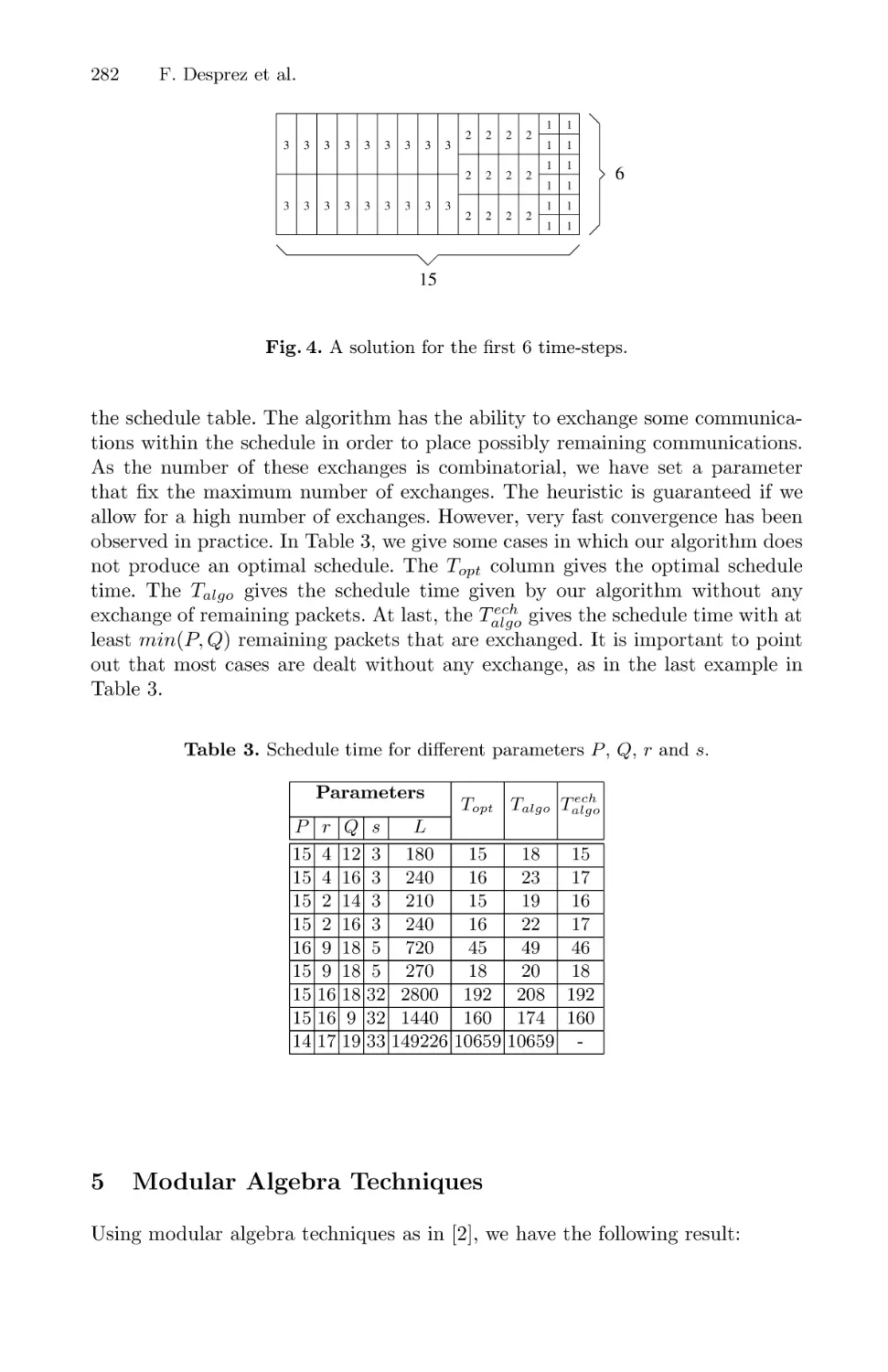
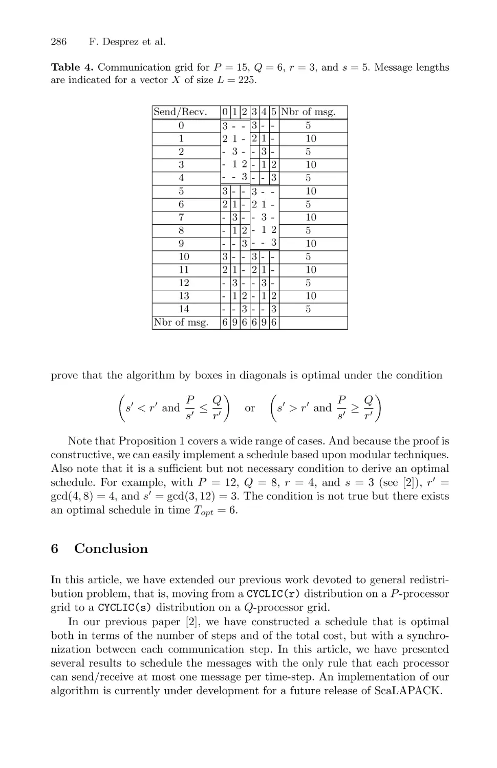
More on Scheduling Block-Cyclic Array Redistribution . . . . . . . . . . . . . . . . . . . . 275
Frédéric Desprez, Stéphane Domas, Jack Dongarra, Antoine Petitet,
Cyril Randriamaro, and Yves Robert
Flexible and Optimized IDL Compilation for Distributed Applications . . . . 288
Eric Eide, Jay Lepreau, and James L. Simister
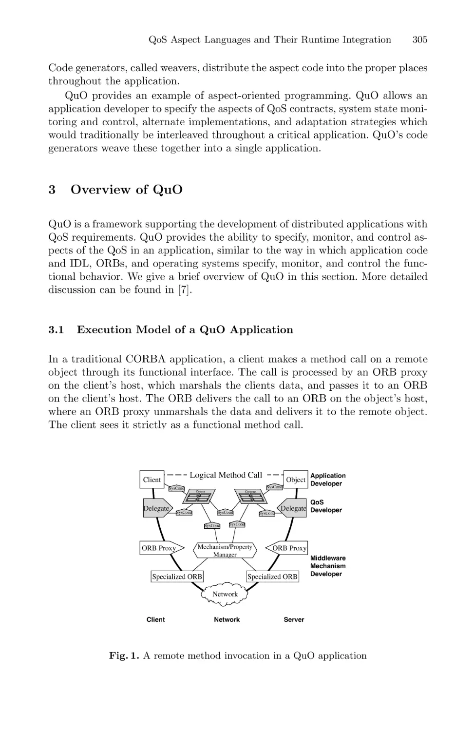
QoS Aspect Languages and Their Runtime Integration . . . . . . . . . . . . . . . . . . . . 303
Joseph P. Loyall, David E. Bakken, Richard E. Schantz, John A. Zinky,
David A. Karr, Rodrigo Vanegas, and Kenneth R. Anderson
Statistical Properties of Host Load . . . . . . . . . . . . . . . . . . . . . . . . . . . . . . . . . . . . . . . .319
Peter A. Dinda
Locality Enhancement for Large-Scale Shared-Memory Multiprocessors . . . 335
Tarik Abdelrahman, Naraig Manjikian, Gary Liu, and S. Tandri
Language and Compiler Support for Out-of-Core Irregular Applications
on Distributed-Memory Multiprocessors . . . . . . . . . . . . . . . . . . . . . . . . . . . . . . . . . . 343
Peter Brezany, Alok Choudhary, and Minh Dang
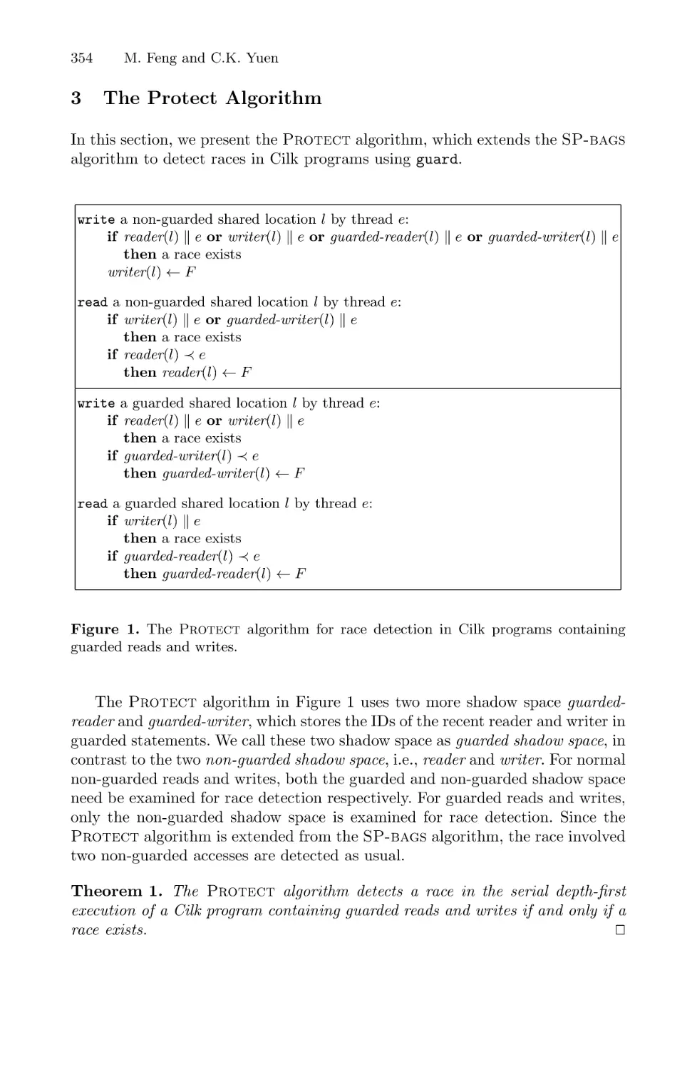
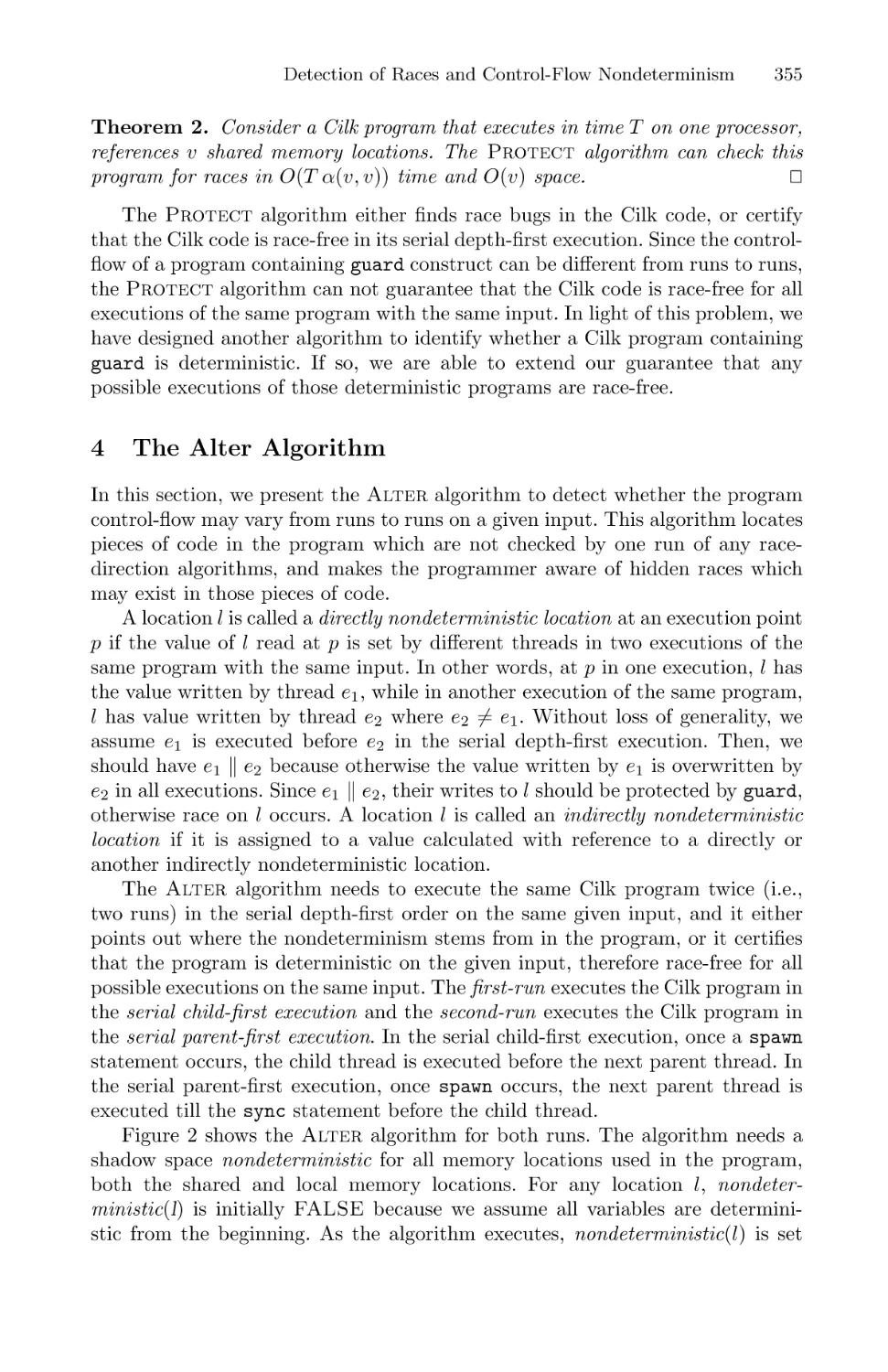
Detection of Races and Control-Flow Nondeterminism . . . . . . . . . . . . . . . . . . . . 351
Mindong Feng and Chung Kwong Yuen
Improving Locality in Out-of-Core Computations Using Data
Layout Transformations . . . . . . . . . . . . . . . . . . . . . . . . . . . . . . . . . . . . . . . . . . . . . . . . . . 359
M. Kandemir, A. Choudhary, and J. Ramanujam
Optimizing Computational and Spatial Overheads in Complex
Transformed Loops . . . . . . . . . . . . . . . . . . . . . . . . . . . . . . . . . . . . . . . . . . . . . . . . . . . . . . . 367
Dattatraya Kulkarni and Michael Stumm

Table of Contents

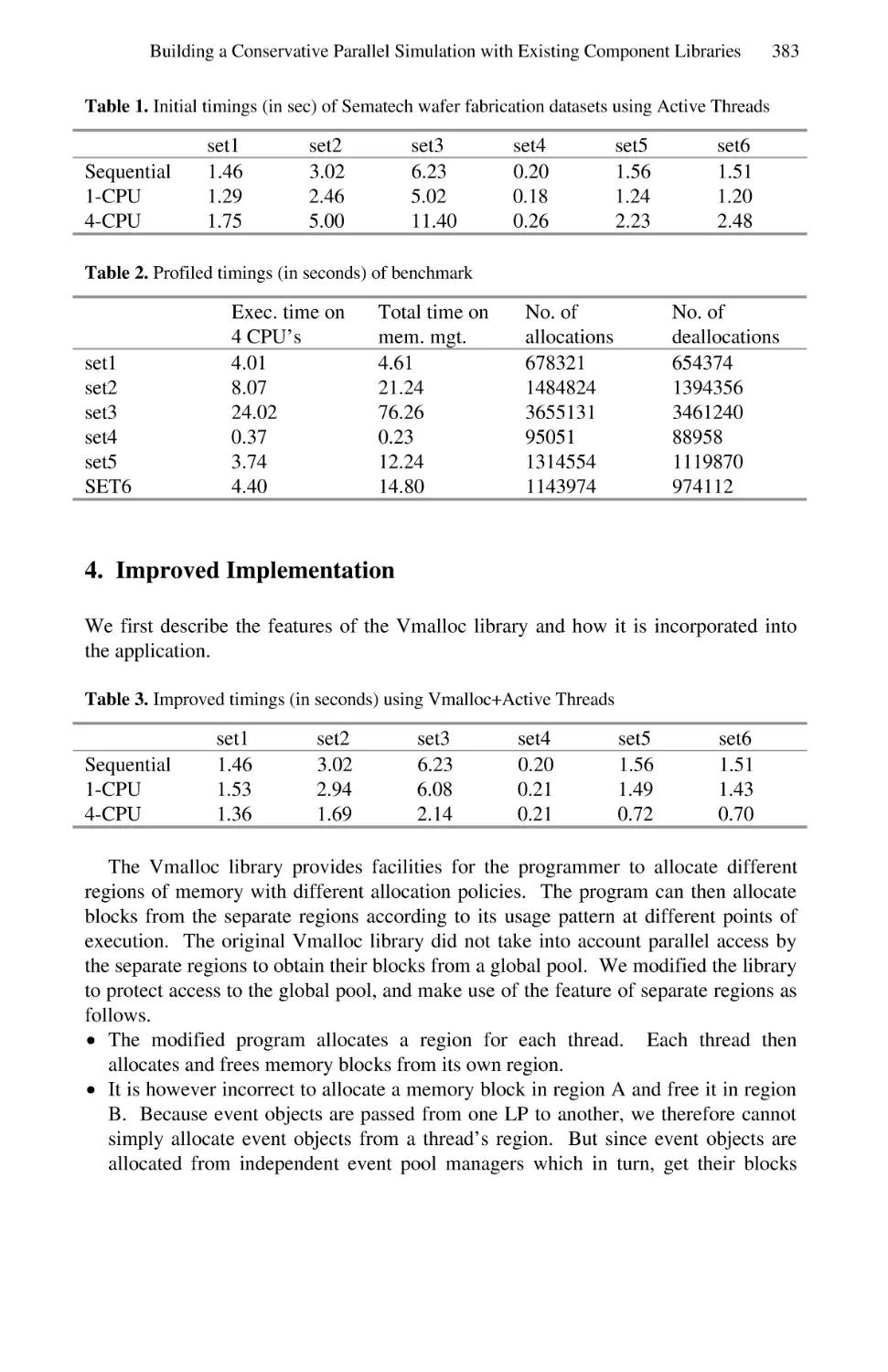
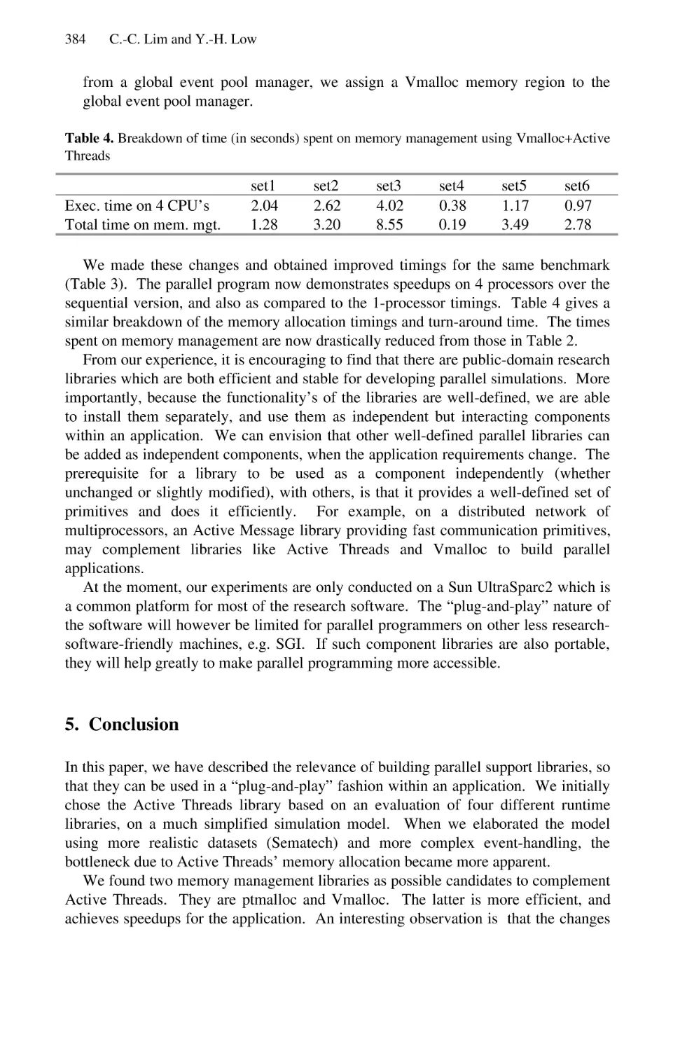
Building a Conservative Parallel Simulation with Existing
Component Libraries . . . . . . . . . . . . . . . . . . . . . . . . . . . . . . . . . . . . . . . . . . . . . . . . . . . . . 378
Chu-Cheow Lim and Yoke-Hean Low
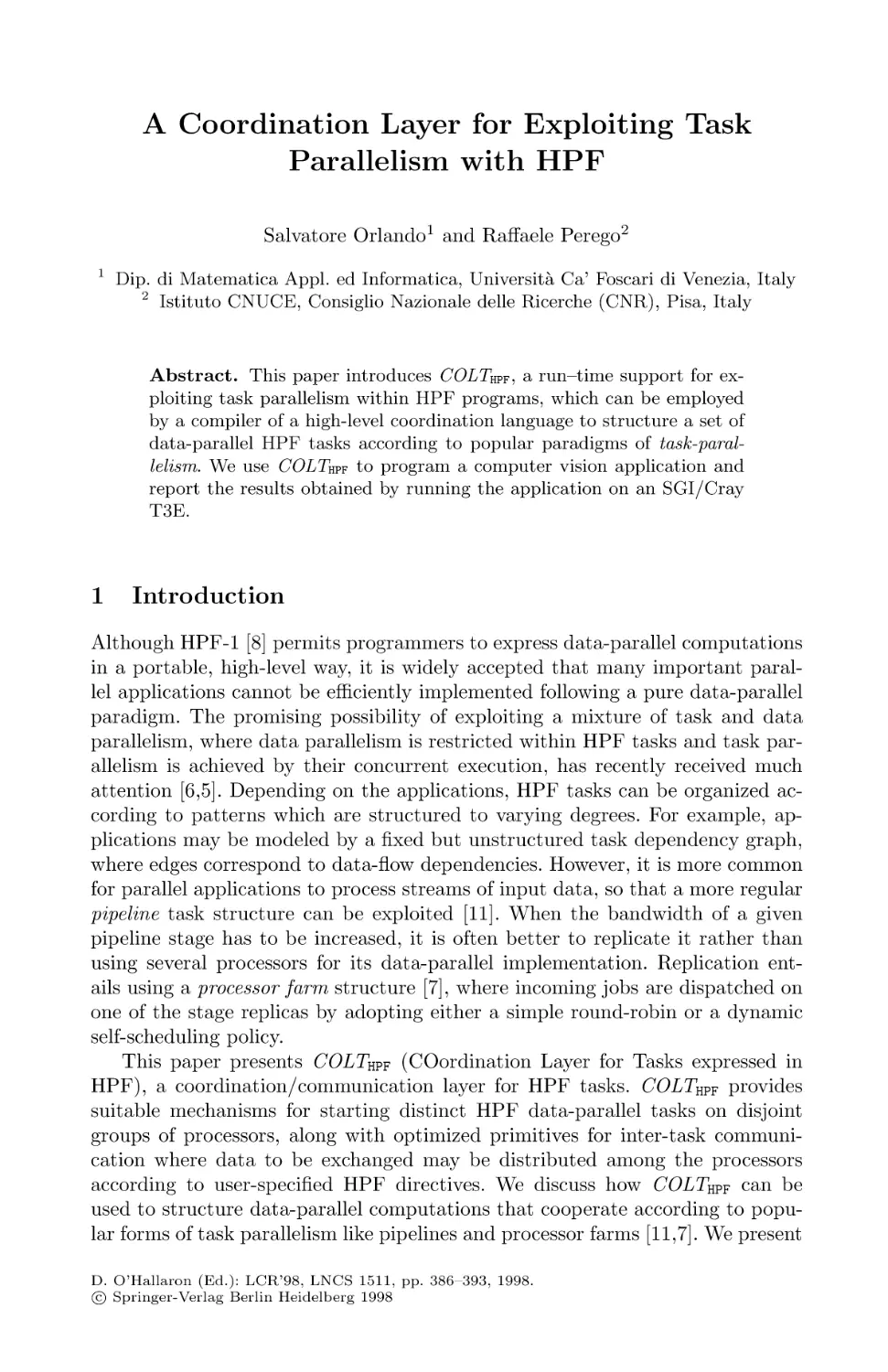
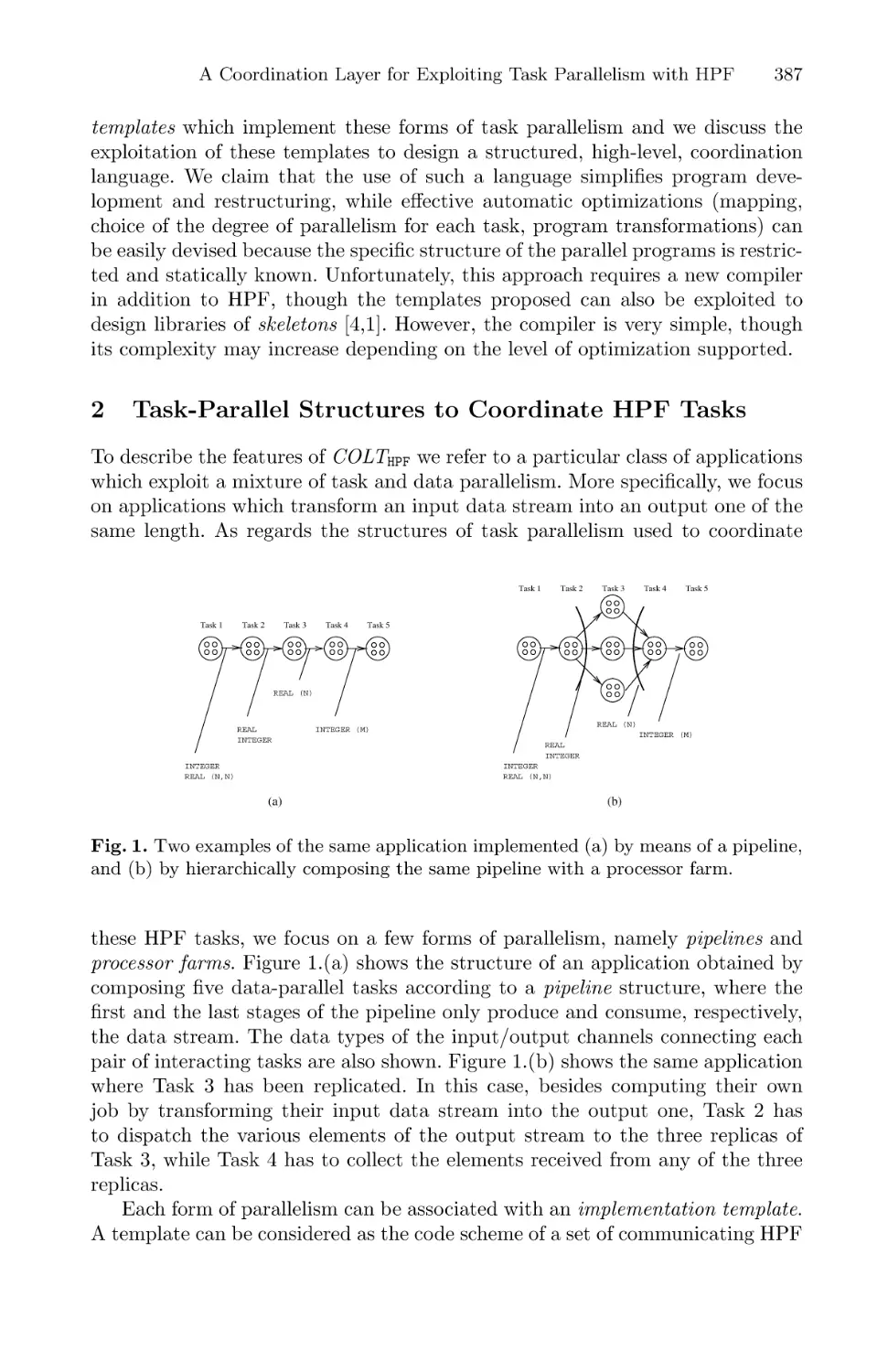
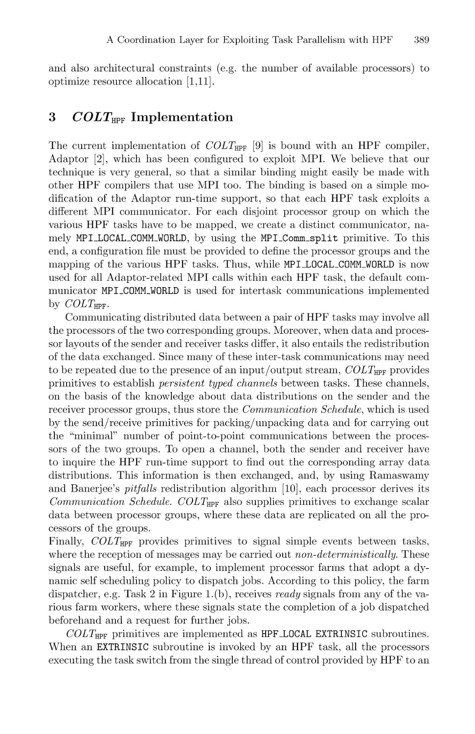
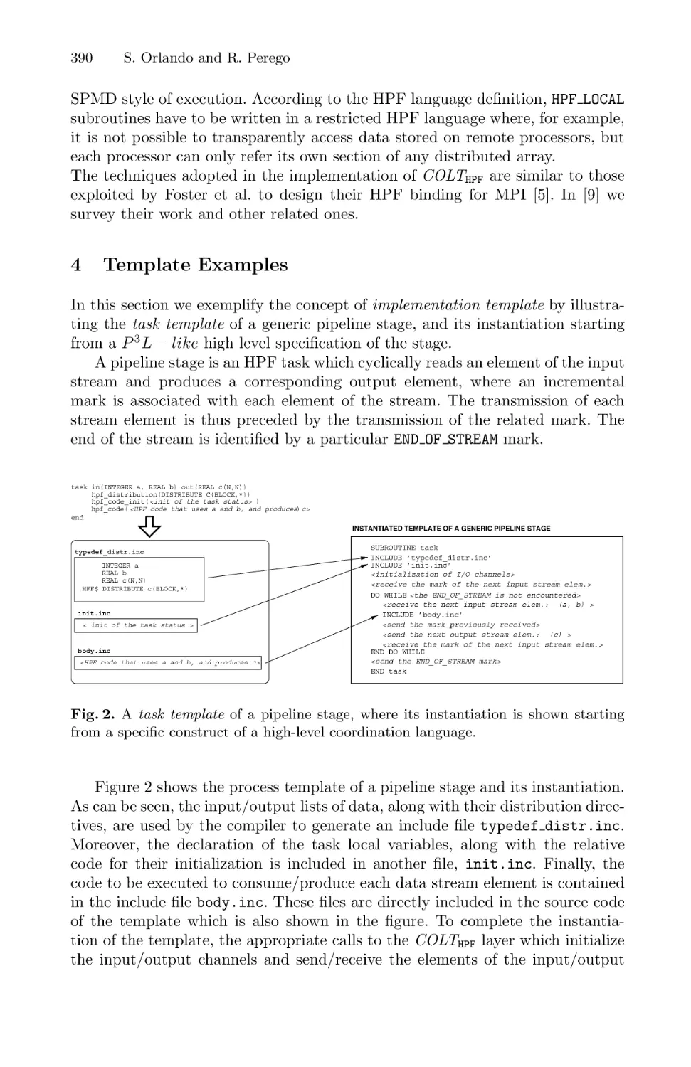
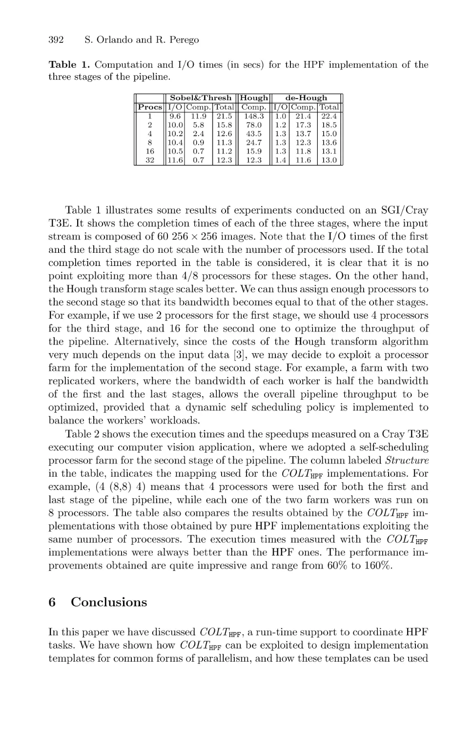
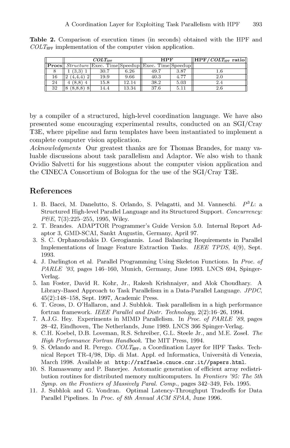
A Coordination Layer for Exploiting Task Parallelism with HPF . . . . . . . . . . 386
Salvatore Orlando and Raffaele Perego
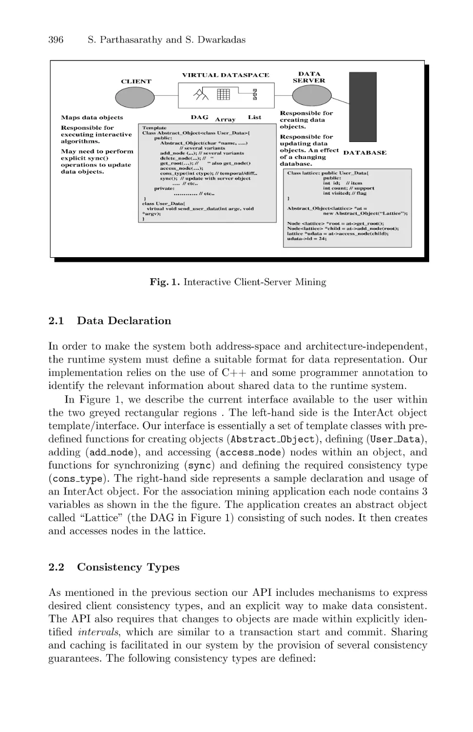
InterAct: Virtual Sharing for Interactive Client-Server Applications . . . . . . . 394
Srinivasan Parthasarathy and Sandhya Dwarkadas
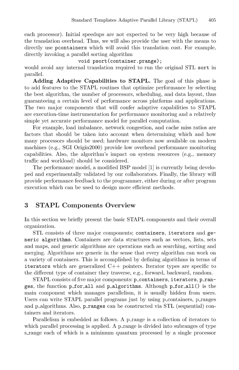
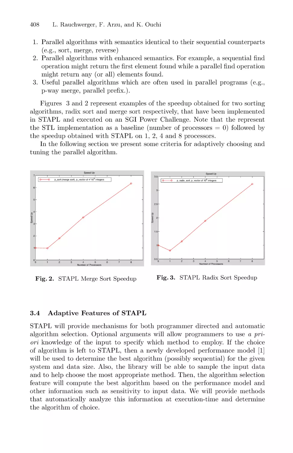
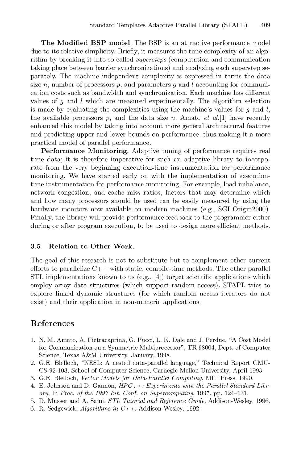
Standard Templates Adaptive Parallel Library (STAPL) . . . . . . . . . . . . . . . . . . 402
Lawrence Rauchwerger, Francisco Arzu, and Koji Ouchi
Author Index . . . . . . . . . . . . . . . . . . . . . . . . . . . . . . . . . . . . . . . . . . . . . . . . . . . . . . . . . . . . . 411

Expressing Irregular Computations
in Modern Fortran Dialects?
Jan F. Prins, Siddhartha Chatterjee, and Martin Simons
Department of Computer Science
The University of North Carolina
Chapel Hill, NC 27599-3175
{prins,sc,simons}@cs.unc.edu

Abstract. Modern dialects of Fortran enjoy wide use and good support on highperformance computers as performance-oriented programming languages. By providing the ability to express nested data parallelism in Fortran, we enable irregular
computations to be incorporated into existing applications with minimal rewriting
and without sacrificing performance within the regular portions of the application. Since performance of nested data-parallel computation is unpredictable and
often poor using current compilers, we investigate source-to-source transformation techniques that yield Fortran 90 programs with improved performance and
performance stability.

Introduction

Modern science and engineering disciplines make extensive use of computer simulations. As these simulations increase in size and detail, the computational costs of naive
algorithms can overwhelm even the largest parallel computers available today. Fortunately, computational costs can be reduced using sophisticated modeling methods that
vary model resolution as needed, coupled with sparse and adaptive solution techniques
that vary computational effort in time and space as needed. Such techniques have been
developed and are routinely employed in sequential computation, for example, in cosmological simulations (using adaptive n-body methods) and computational fluid dynamics
(using adaptive meshing and sparse linear system solvers).
However, these so-called irregular or unstructured computations are problematic
for parallel computation, where high performance requires equal distribution of work
over processors and locality of reference within each processor. For many irregular
computations, the distribution of work and data cannot be characterized a priori, as
these quantities are input-dependent and/or evolve with the computation itself. Further,
irregular computations are difficult to express using performance-oriented languages
such as Fortran, because there is an apparent mismatch between data types such as
trees, graphs, and nested sequences characteristic of irregular computations and the
statically analyzable rectangular multi-dimensional arrays that are the core data types in
?

This research was supported in part by NSF Grants #CCR-9711438 and #INT-9726317. Chatterjee is supported in part by NSF CAREER Award #CCR-9501979. Simons is supported by a
research scholarship from the German Research Foundation (DFG).

D. O’Hallaron (Ed.): LCR’98, LNCS 1511, pp. 1–16, 1998.
c Springer-Verlag Berlin Heidelberg 1998

J.F. Prins, S. Chatterjee, and M. Simons

modern Fortran dialects such as Fortran 90/95 [19], and High Performance Fortran (HPF)
[16]. Irregular data types can be introduced using the data abstraction facilities, with a
representation exploiting pointers. Optimization of operations on such an abstract data
type is currently beyond compile-time analysis, and compilers have difficulty generating
high-performance parallel code for such programs. This paper primarily addresses the
expression of irregular computations in Fortran 95, but does so with a particular view
of the compilation and high performance execution of such computations on parallel
processors.
The modern Fortran dialects enjoy increasing use and good support as mainstream
performance-oriented programming languages. By providing the ability to express irregular computations as Fortran modules, and by preprocessing these modules into a form
that current Fortran compilers can successfully optimize, we enable irregular computations to be incorporated into existing applications with minimal rewriting and without
sacrificing performance within the regular portions of the application.
For example, consider the NAS CG (Conjugate Gradient) benchmark, which solves
an unstructured sparse linear system using the method of conjugate gradients [2]. Within
the distributed sample sequential Fortran solution, 79% of the lines of code are standard
Fortran 77 concerned with problem construction and performance reporting. The next
16% consist of scalar and regular vector computations of the BLAS 2 variety [17], while
the final 5% of the code is the irregular computation of the sparse matrix-vector product.
Clearly we want to rewrite only this 5% of the code (which performs 97% of the work
in the class B computation), while the remainder should be left intact for the Fortran
compiler. This is not just for convenience. It is also critical for performance reasons;
following Amdahl’s Law, as the performance of the irregular computation improves, the
performance of the regular component becomes increasingly critical for sustained high
performance overall. Fortran compilers provide good compiler/annotation techniques
to achieve high performance for the regular computations in the problem, and can thus
provide an efficient and seamless interface between the regular and irregular portions of
the computation.
We manually applied the implementation techniques described in Sect. 4 to the
irregular computation in the NAS CG problem. The resultant Fortran program achieved
a performance on the class B NAS CG 1.0 benchmark of 13.5 GFLOPS using a 32
processor NEC SX-4 [25]. We believe this to be the highest performance achieved for
this benchmark to date. It exceeds, by a factor of 2.6, the highest performance reported in
the last NPB 1.0 report [27], and is slightly faster than the 12.9 GFLOPS recently achieved
using a 1024 processor Cray T3E-900 [18]. These encouraging initial results support the
thesis that high-level expression and high-performance for irregular computations can
be supported simultaneously in a production Fortran programming environment.

Expressing Irregular Computations Using Nested Data
Parallelism

We adopt the data-parallel programming model of Fortran as our starting point. The dataparallel programming model has proven to be popular because of its power and simplicity.
Data-parallel languages are founded on the concept of collections (such as arrays) and

Expressing Irregular Computations in Modern Fortran Dialects

a means to allow programmers to express parallelism through the application of an
operation independently to all elements of a collection (e.g., the elementwise addition
of two arrays). Most of the common data-parallel languages, such as the array-based
parallelism of Fortran 90, offer restricted data-parallel capabilities: they limit collections
to multidimensional rectangular arrays, limit the type of the elements of a collection
to scalar and record types, and limit the operations that can be applied in parallel to
the elements of a collection to certain predefined operations rather than arbitrary userdefined functions. These limitations are aimed at enabling compile-time analysis and
optimization of the work and communication for parallel execution, but make it difficult
to express irregular computations in this model.
If the elements of a collection are themselves permitted to have arbitrary type, then
arbitrary functions can be applied in parallel over collections. In particular, by operating on a collection of collections, it is possible to specify a parallel computation, each
simultaneous operation of which in turn involves (a potentially different-sized) parallel
subcomputation. This programming model, called nested data parallelism, combines aspects of both data parallelism and control parallelism. It retains the simple programming
model and portability of the data-parallel model while being better suited for describing
algorithms on irregular data structures. The utility of nested data parallelism as an expressive mechanism has been understood for a long time in the LISP, SETL [29], and
APL communities, although always with a sequential execution semantics and implementation.
Nested data parallelism occurs naturally in the succinct expression of many irregular
scientific problems. Consider the sparse matrix-vector product at the heart of the NAS
CG benchmark. In the popular compressed sparse row (CSR) format of representing
sparse matrices, the nonzero elements of an m × n sparse matrix A are represented as
a sequence of m rows [R1 , . . . , Rm ], where the ith row is, in turn, represented by a
(possibly empty) sequence of (v, c) pairs where v is the nonzero value and 1 ≤ c ≤ n is
the column in which it occurs: Ri = [(v1i , ci1 ), . . . , (vki i , ciki )]. With a dense n-vector x
represented as a simple sequence of n values, the sparse matrix-vector product y = Ax
may now be written as shown using the Nesl notation [4]:
y = {sparse dot product(R,x) : R in A}.
This expression specifies the application of sparse_dot_product, in parallel, to each
row of A to yield the m element result sequence y. The sequence constructor { . . . }
serves a dual role: it specifies parallelism (for each R in A), and it establishes the
order in which the result elements are assembled into the result sequence, i.e., yi =
sparse dot product(Ri , x). We obtain nested data parallelism if the body expression
sparse dot product(R, x) itself specifies the parallel computation of the dot product
of row R with x as the sum-reduction of a sequence of nonzero products:
function sparse dot product(R,x) = sum({v*x[c]: (v,c) in R})
More concisely, the complete expression could also written as follows:
y = {sum({v*x[c]: (v,c) in R}): R in A}
where the nested parallelism is visible as nested sequence constructors in the source text.

J.F. Prins, S. Chatterjee, and M. Simons

MODULE Sparse_matrices
IMPLICIT none
TYPE Sparse_element
REAL
INTEGER
END TYPE Sparse_element

:: val
:: col

TYPE Sparse_row_p
TYPE (Sparse_element), DIMENSION (:), POINTER :: elts
END TYPE Sparse_row_p
TYPE Sparse_matrix
INTEGER
TYPE (Sparse_row_p), DIMENSION (:), POINTER
END TYPE Sparse_matrix

:: nrow, ncol
:: rows

END MODULE Sparse_matrices
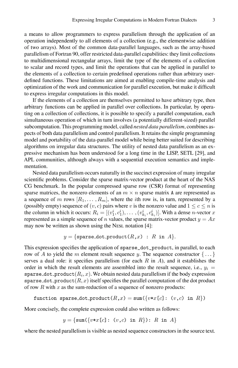
Fig. 1. Fortran 90 definition of a nested sequence type for sparse matrices

Nested data parallelism provides a succinct and powerful notation for specifying parallel
computation, including irregular parallel computations. Many more examples of efficient
parallel algorithms expressed using nested data parallelism have been described in [4].

Nested Data Parallelism in Fortran

If we consider expressing nested data parallelism in standard imperative programming
languages, we find that they either lack a data-parallel control construct (C, C++) or else
lack a nested collection data type (Fortran).A data-parallel control construct can be added
to C [11] or C++ [30], but the pervasive pointer semantics of these languages complicate
its meaning. There is also incomplete agreement about the form of parallelism should
take in these languages.
The FORALL construct, originated in HPF [16] and later added into Fortran 95, specifies data-parallel evaluation of expressions and array assignments. To ensure that there are
no side effects between these parallel evaluations, functions that occur in the expressions
must have the PURE attribute. Fortran 90 lacks a construct that specifies parallel evaluations. However, many compilers infer such an evaluation if specified using a conventional
DO loop, possibly with an attached directive asserting the independence of iterations.
FORALL constructs (or Fortran 90 loops) may be nested. To specify nested data-parallel
computations with these constructs, it suffices to introduce nested aggregates, which we
can do via the data abstraction mechanism of Fortran 90.
As a consequence of these language features, it is entirely possible to express nested
data-parallel computations in modern Fortran dialects. For example, we might introduce
the types shown in Fig. 1 to represent a sparse matrix. Sparse_element is the type of

Expressing Irregular Computations in Modern Fortran Dialects

SUBROUTINE smvp(a, x, y)
USE Sparse_matrices, ONLY : Sparse_matrix
IMPLICIT none
TYPE (Sparse_matrix), INTENT(IN) :: a
REAL, DIMENSION(:), INTENT(IN)
:: x
REAL, DIMENSION(:), INTENT(OUT) :: y
FORALL (i = 1:a%nrow)
y(i) = SUM(a%rows(i)%elts%val * x(a%rows(i)%elts%col))
END FORALL
END SUBROUTINE smvp
Fig. 2. Use of the derived type Sparse matrix in sparse matrix-vector product.

a sparse matrix element, i.e., the (v, c) pair of the Nesl example. Sparse_row_p is the
type of vectors (1-D arrays) of sparse matrix elements, i.e., a row of the matrix. A sparse
matrix is characterized by the number of rows and columns, and by the nested sequence
of sparse matrix elements.
Using these definitions, the sparse matrix-vector product can be succinctly written
as shown in Fig. 2. The DO loop specifies parallel evaluation of the inner products for all
rows. Nested parallelism is a consequence of the use of parallel operations such as sum
and elementwise multiplication, projection, and indexing.
Discussion
Earlier experiments with nested data parallelism in imperative languages include V [11],
Amelia [30], and F90V [1]. For the first two of these languages the issues of sideeffects in the underlying notation (C++ and C, respectively) were problematic in the
potential introduction of interference between parallel iterations, and the efforts were
abandoned. Fortran finesses this problem by requiring procedures used within a FORALL
construct to be PURE, an attribute that can be verified statically. This renders invalid those
constructions in which side effects (other than the nondeterministic orders of stores) can
be observed, although such a syntactic constraint is not enforced in Fortran 90.
The specification of nested data parallelism in Fortran and Nesl differ in important ways, many of them reflecting differences between the imperative and functional
programming paradigms.
First, a sequence is formally a function from an index set to a value set. The Nesl
sequence constructor specifies parallelism over the value set of a sequence while the
Fortran FORALL statement specifies parallelism over the index set of a sequence. This

J.F. Prins, S. Chatterjee, and M. Simons

allows a more concise syntax and also makes explicit the shape of the common index
domain shared by several collections participating in a FORALL construct.
Second, the Nesl sequence constructor implicitly specifies the ordering of result
elements, while this ordering is explicit in the FORALL statement. One consequence is
that the restriction clause has different semantics. For instance, the Nesl expression
v = {i: i in [1:n] | oddp(i) }
yields a result sequence v of length bn/2c of odd values while the Fortran statement
FORALL (i = 1:n, odd(i)) v(i) = i
replaces the elements in the odd-numbered positions of v.
Third, the Fortran FORALL construct provides explicit control over memory. Explicit
control over memory can be quite important for performance. For example, if we were
to repeatedly multiply the same sparse matrix repeatedly by different right hand sides
(which is in fact exactly what happens in the CG benchmark), we could reuse a single
temporary instead of freeing and allocating each time. Explicit control over memory
also gives us a better interface to the regular portions of the computation.
Finally, the base types of a nested aggregate in Fortran are drawn from the Fortran
data types and include multidimensional arrays and pointers. In Nesl, we are restricted to
simple scalar values and record types. Thus, expressing a sparse matrix as a collection of
supernodes would be cumbersome in Nesl. Another important difference is that we may
construct nested aggregates of heterogeneous depth with Fortran, which is important,
for example, in the representation of adaptive oct-tree spatial decompositions.

Implementation Issues

Expression of nested data-parallelism in Fortran is of limited interest and of no utility if
such computations can not achieve high performance. Parallel execution and tuning for
the memory hierarchy are the two basic requirements for high performance. Since the
locus of activity and amount of work in a nested data-parallel computation can not be
statically predicted, run-time techniques are generally required.
4.1

Implementation Strategies

There are two general strategies for the parallel execution of nested data parallelism,
both consisting of a compile-time and a run-time component.
The thread-based approach. This technique conceptually spawns a different thread of
computation for every parallel evaluation within a FORALL construct. The compile-time
component constructs the threads from the nested loops. A run-time component dynamically schedules these threads across processors. Recent work has resulted in run-time
scheduling techniques that minimize completion time and memory use of the generated
threads [9, 6, 20]. Scheduling very fine-grained threads (e.g., a single multiplication in
the sparse matrix-vector product example) is impractical, hence compile-time techniques
are required to increase thread granularity, although this may result in lost parallelism
and increased load imbalance.

Expressing Irregular Computations in Modern Fortran Dialects

FORALL (i = 1:4)
WHERE C(i) DO
FORALL (j = 1:i) DO
G(i,j)
END FORALL
ELSEWHERE
H(i)
END WHERE
END FORALL
(a)
T1

C
G

(c)

(b)

C
G

(d)

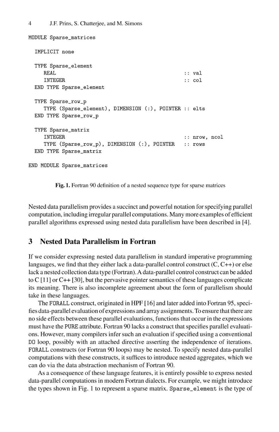
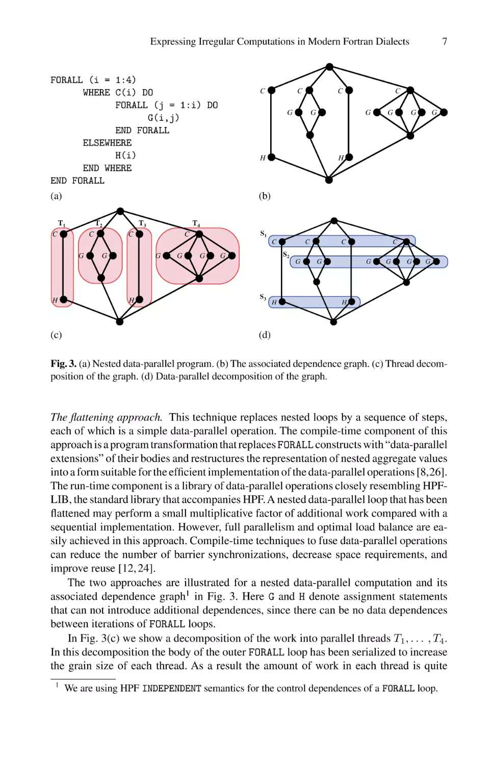
Fig. 3. (a) Nested data-parallel program. (b) The associated dependence graph. (c) Thread decomposition of the graph. (d) Data-parallel decomposition of the graph.

The flattening approach. This technique replaces nested loops by a sequence of steps,
each of which is a simple data-parallel operation. The compile-time component of this
approach is a program transformation that replaces FORALL constructs with “data-parallel
extensions” of their bodies and restructures the representation of nested aggregate values
into a form suitable for the efficient implementation of the data-parallel operations [8,26].
The run-time component is a library of data-parallel operations closely resembling HPFLIB, the standard library that accompanies HPF. A nested data-parallel loop that has been
flattened may perform a small multiplicative factor of additional work compared with a
sequential implementation. However, full parallelism and optimal load balance are easily achieved in this approach. Compile-time techniques to fuse data-parallel operations
can reduce the number of barrier synchronizations, decrease space requirements, and
improve reuse [12, 24].
The two approaches are illustrated for a nested data-parallel computation and its
associated dependence graph1 in Fig. 3. Here G and H denote assignment statements
that can not introduce additional dependences, since there can be no data dependences
between iterations of FORALL loops.
In Fig. 3(c) we show a decomposition of the work into parallel threads T1 , . . . , T4 .
In this decomposition the body of the outer FORALL loop has been serialized to increase
the grain size of each thread. As a result the amount of work in each thread is quite
1

We are using HPF INDEPENDENT semantics for the control dependences of a FORALL loop.

J.F. Prins, S. Chatterjee, and M. Simons

different. On the other hand, since each thread executes a larger portion of the sequential
implementation, it can exhibit good locality of reference.
In Fig. 3(d) we show a decomposition of the work into sequential steps S1 , . . . , S3 ,
each of which is a simple data-parallel operation. The advantage of this approach is that
we may partition the parallelism in each operation to suit the resources. For example,
we can create parallel slack at each processor to hide network or memory latencies. In
this example, the dependence structure permits the parallel execution of steps S1 and
S2 , although this increases the complexity of the run time scheduler.
4.2

Nested Parallelism Using Current Fortran Compilers

What happens when we compile the Fortran 90 sparse matrix-vector product smvp shown
in Fig. 2 for parallel execution using current Fortran compilers?
For shared-memory multiprocessors we examined two auto-parallelizing Fortran 90
compilers: the SGI F90 V7.2.1 compiler (beta release, March 1998) for SGI Origin
class machines and the NEC FORTRAN90/SX R7.2 compiler (release 140, February
1998) for the NEC SX-4. We replaced FORALL construct in Fig. 2 with an equivalent
DO loop to obtain a Fortran 90 program. Since the nested parallel loops in smvp do not
define a polyhedral iteration space, many classical techniques for parallelization do not
apply. However, both compilers recognize that iterations of the outer loop (over rows)
are independent and, in both cases, these iterations are distributed over processors. The
dot-product inner loop is compiled for serial execution or vectorized. This strategy is not
always optimal, since the distribution of work over outermost iterations may be uneven
or there may be insufficient parallelism in the outer iterations.
For distributed memory multiprocessors we examined one HPF compiler. This compiler failed to compile smvp because it had no support for pointers in Fortran 90 derived
types. Our impression is that this situation is representative of HPF compilers in general,
since the focus has been on the parallel execution of programs operating on rectangular
arrays. The data distribution issues for the more complex derived types with pointers are
unclear. Instead, HPF 2.0 supports the non-uniform distribution of arrays over processors. This requires the programmer to embed irregular data structures in an array and
determine the appropriate mapping for the distribution.
We conclude that current Fortran compilers do not sufficiently address the problems of irregular nested data parallelism. The challenge for irregular computations is to
achieve uniformly high and predictable performance in the face of dynamically varying
distribution of work. We are investigating the combined use of threading and flattening
techniques for this problem.
Our approach is to transform nested data parallel constructs into simple Fortran 90,
providing simple integration with regular computations, and leveraging the capabilities
of current Fortran compilers. This source-to-source translation restricts our options somewhat for the thread scheduling strategy. Since threads are not part of Fortran 90, the
only mechanism for their (implicit) creation are loops, and the scheduling strategies
we can choose from are limited by those offered by the compiler/run-time system. In
this regard, standardized loop scheduling directives like the OpenMP directives [23] can
improve portability.

Expressing Irregular Computations in Modern Fortran Dialects

A nested data parallel computation should be transformed into a (possibly nested) iteration space that is partitioned over threads. Dynamic scheduling can be used to tolerate
variations in progress among threads. Flattening of the loop body can be used to ensure
that the amount of work per thread is relatively uniform.
4.3

Example

Consider a sparse m × n matrix A with a total of r nonzeros. Implementation of the
simple nested data parallelism in the procedure smvp of Fig. 2 must address many of the
problems that may arise in irregular computations:
– Uneven units of work: A may contain both dense and sparse rows.
– Small units of work: A may contain rows with very few nonzeros.
– Insufficient units of work: if n is less than the number of processors and r is sufficiently large, then parallelism should be exploited within the dot products rather
than between the dot products.
We constructed two implementations of smvp. The pointer-based implementation
is obtained by direct compilation of the program in Fig. 2 using auto-parallelization.
As mentioned, this results in a parallelized outer loop, in which the dot products for
different rows are statically or dynamically scheduled across processors.
The flat implementation is obtained by flattening smvp. To flatten smvp we replace
the nested sequence representation of A with a linearized representation (A0 , s). Here
A0 is an array of r pairs, indexed by val and col, partitioned into rows of A by s.
Application of the flattening tranformations to the loop in Fig. 2 yields
y = segmented sum(A0 %val * x(A0 %col),s),
where segmented_sum is a data-parallel operation with efficient parallel implementations [3]. By substituting A0 %val * x(A0 %col) for the first argument in the body of
segmented_sum, the sum and product may be fused into a segmented dot-product. The
resulting algorithm was implemented in Fortran 90 for our two target architectures.
For the SGI Origin 200, A0 is divided into pσ sections of length r/(pσ) where
p is the number of processors and σ ≥ 1 is a factor to improve the load balance in
the presence of multiprogramming and operating system overhead on the processors.
Sections are processed independently and dot products are computed sequentially within
each section. Sums for segments spanning sections are adjusted after all sections are
summed.
For the NEC SX-4, A0 is divided into pq sections where q is the vector length required
by the vector units [5]. Section i, 0 ≤ i < pq, occupies element i mod q in a length q
vector of thread bi/pc. Prefix dot-products are computed independently for all sections
using a sequence of r/(pq) vector additions on each processor. Segment dot-products
are computed from the prefix dot-products and sums for segments spanning sections are
adjusted after all sections are summed [25]. On the SX-4, σ is typically not needed since
the operating system performs gang-scheduling and the threads experience very similar
progress rates.

J.F. Prins, S. Chatterjee, and M. Simons
Constant number of non-zeros [20] / varying matrix size (SGI Origin 200)
flat
pointer

performance in MFLOPS

20
4 proc
2 proc

1 proc

20000

40000

60000

80000
100000
120000
number of rows/columns

140000

160000

180000

Varying number of non-zeros / constant matrix size [20000] (SGI Origin 200)
flat
pointer

4 proc

performance in MFLOPS

30
2 proc
20

1 proc
10

80
100
120
number of non-zeros per row

140

160

180

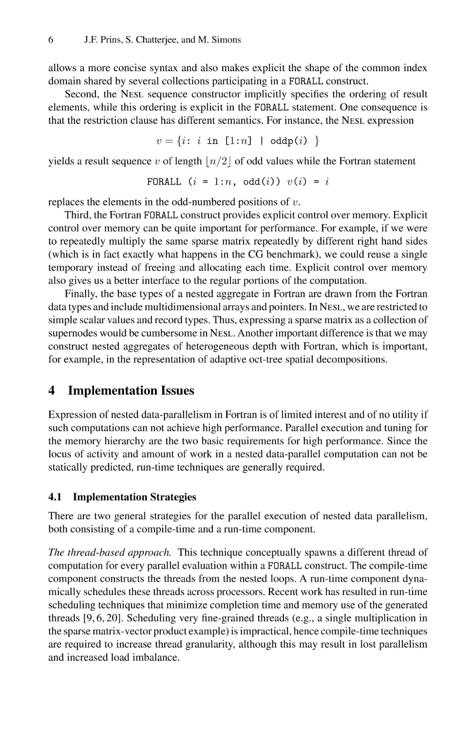
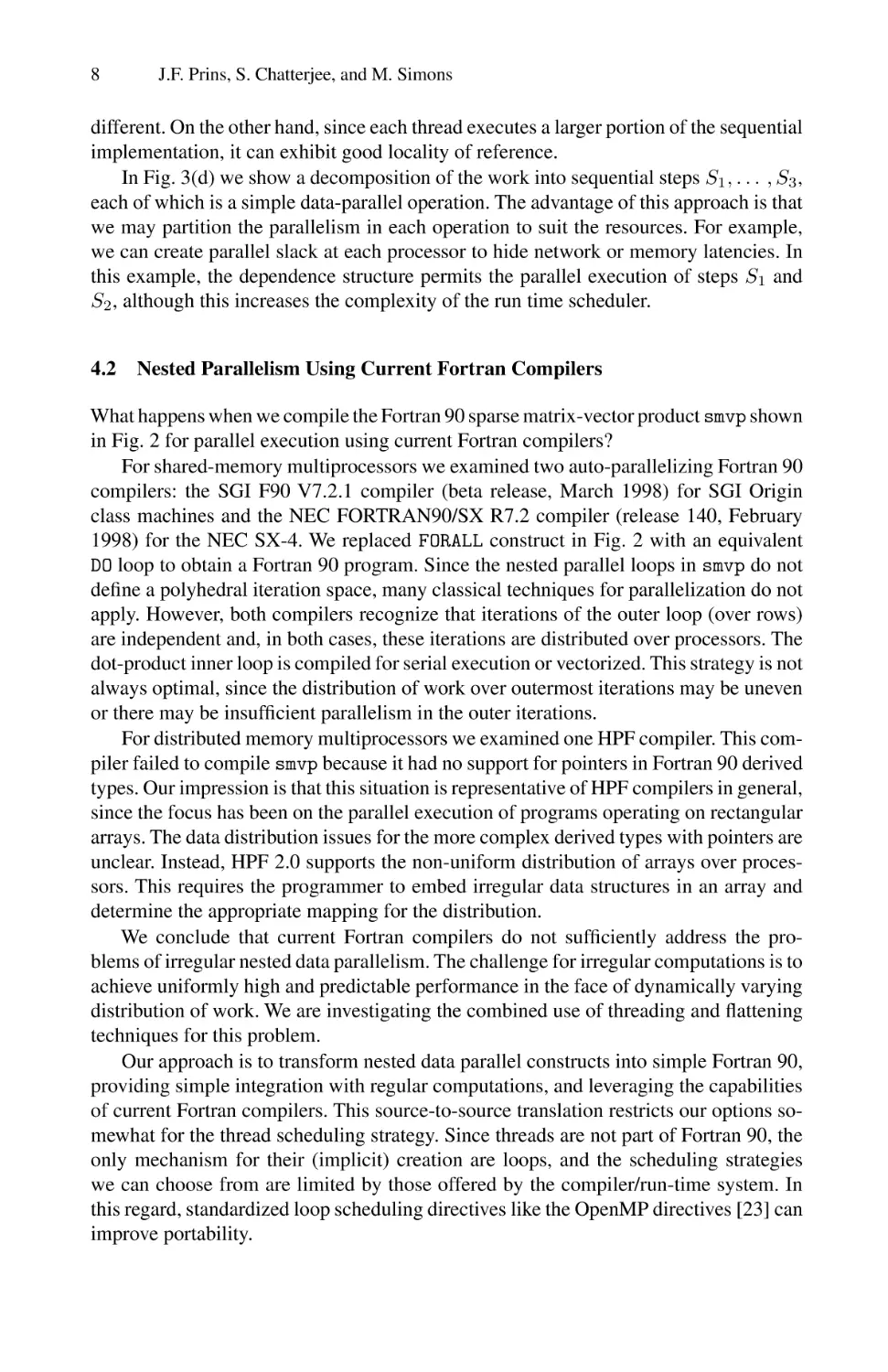
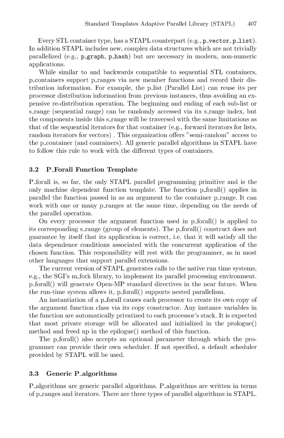
Fig. 4. Performance measurements for the pointer-based and the flattened implementations of
smvp on the SGI Origin 200.

4.4

Results

The SGI Origin 200 used is a 4 processor cache-based shared memory multiprocessor.
The processors are 180MHz R10000 with 1MB L2 cache per processor. The NEC SX-4
used is a 16 processor shared-memory parallel vector processor with vector length 256.
Each processor has a vector unit that can perform 8 or 16 memory reads or writes per
cycle. The clock rate is 125 MHz. The memory subsystem provides sufficient sustained
bandwidth to simultaneously service independent references from all vector units at the
maximum rate.
The performance on square sparse matrices of both implementations is shown for
1, 2, and 4 processors for the Origin 200 in Fig. 4 and for the SX-4 in Fig. 5. The top
graph of each figure shows the performance as a function of problem size in megaflops

Expressing Irregular Computations in Modern Fortran Dialects

Constant number of non-zeros [20] / varying matrix size (NEC SX-4)
flat
pointer

4 proc
1000
performance in MFLOPS

2 proc
1 proc

100
4 proc
2 proc
1 proc

1
0

20000

40000

60000

80000
100000
120000
number of rows/columns

140000

160000

180000

Varying number of non-zeros / constant matrix size [20000] (NEC SX-4)
flat
pointer
4 proc

performance in MFLOPS

1000

2 proc
1 proc
4 proc
2 proc

100
1 proc

1
0

80
100
120
number of non-zeros per row

140

160

180

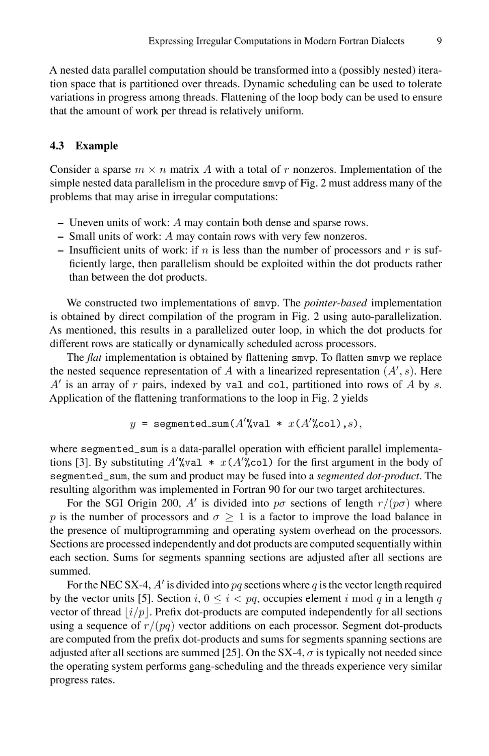
Fig. 5. Performance measurements for the pointer-based and the flattened implementations of
smvp on the NEC SX-4. (Note the logarithmic scale of the y-axis.)

per second, where the number of floating point operations for the problem is 2r. Each
row contains an average of 20 nonzeros and the number of rows is varied between 1000
and 175000. The bottom graph shows the influence of the average number of nonzeros
per row (r/n) on the performance of the code. To measure this, we chose a fixed matrix
size (n = 20000) and varied the average number of nonzeros on each row between 5
and 175. In each case, the performance reported is averaged over 50 different matrices.
On the Origin 200 the flattened implementation performed at least as well as the
pointer-based version over most inputs. The absolute performance of neither implementation is particularly impressive. The sparse matrix-vector problem is particularly tough
for processors with limited memory bandwidth since there is no temporal locality in
the use of A (within a single matrix-vector product), and the locality in reference to
x diminishes with increasing n. While reordering may mitigate these effects in some

J.F. Prins, S. Chatterjee, and M. Simons

(a)

regular (a)
irregular (b)

SGI Origin 200
flat
pointer
41
42
40
26

(b)
flat
1870
1278

NEC SX-4
pointer
80
76

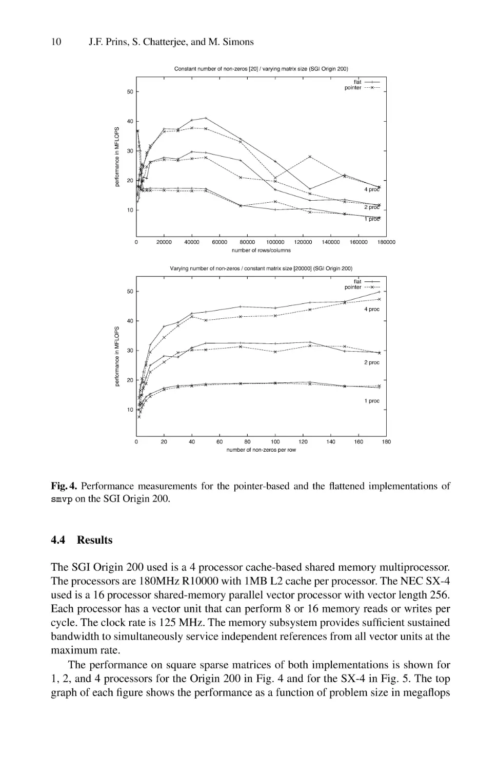
Fig. 6. Performance in Mflops/s using four processors on two different problems.

applications, it has little effect for the random matrices used here. The Origin 200 implementations also do not exhibit good parallel scaling. This is likely a function of limited
memory bandwidth that must be shared among the processors. Higher performance can
be obtained with further tuning. For example, the current compiler does not perform
optimizations to map the val and col components of A into separate arrays. When
applied manually, this optimization increases performance by 25% or more.
On the SX-4 the flattened implementation performs significantly better than the
pointer implementation over all inputs. This is because the flattened implementation
always operates on full-sized vectors (provided r ≥ pq), while the pointer-based implementation performs vector operations whose length is determined by the number of
nonzeros in a row. Hence the pointer-based implementation is insensitive to problem
size but improves with average row length. For the flattened implemementation, absolute performance and parallel scaling are good primarily because the memory system
has sufficient bandwidth and the full-sized vector operations fully amortize the memory
access latencies.
Next, we examined the performance on two different inputs. The regular input is a
square sparse matrix with n = 25000 rows. Each row has an average of 36 randomly
placed nonzeros for a total of r = 900000 nonzeros. The irregular input is a square
sparse matrix with n = 25000 rows. Each row has 20 randomly placed nonzeros, but
now 20 consecutive rows near the top of A contain 20000 nonzeros each. Thus the total
number of nonzeros is again 900000, but in this case nearly half of the work lies in less
than 0.1% of the dot products.
The performance of the two implementations is shown in Fig. 6. The pointer-based
implementation for the Origin 200 is significantly slower for the irregular problem,
regardless of the thread scheduling technique used (dynamic or static). The problem is
that a small “bite” of the iteration space may contain a large amount of work, leading to
a load imbalance that may not be correctable using a dynamic scheduling technique. In
the case of the SX-4 pointer-based implementation this effect is not as noticeable, since
the dot product of a dense row operates nearly two orders of magnitude faster than the
dot product of a row with few nonzeros.
The flattened implementation delivers essentially the same performance for both
problems on the Origin 200. The SX-4 performance in the irregular case is reduced

Expressing Irregular Computations in Modern Fortran Dialects

because dense rows span many successive sections, and incur an O(pq) cost in the final
sum adjustment phase that is not present for shorter rows. However, this cost is unrelated
to problem size, so the disparity between the performance in the two problems vanishes
with increasing problem size.
4.5

Discussion

This example provides some evidence that the flattening technique can be used in an implementation to improve the performance stability over irregular problems while maintaining or improving on the performance of the simple thread-based implementation.
The flattening techniques may be particularly helpful in supporting the instruction-level
and memory-level parallelism required for high performance in modern processors. The
example also illustrates that dynamic thread scheduling techniques, in the simple form
generated by Fortran compilers, may not be sufficient to solve load imbalance problems
that may arise in irregular nested data-parallel computations.
While these irregular matrices may not be representative of typical problems, the
basic characteristic of large amounts of work in small portions of the iteration space is
not unusual. For example, it can arise with data structures for the adaptive spatial decomposition of a highly clustered n-body problem, or with divide-and-conquer algorithms
like quicksort or quickhull [4].

Related Work

The facilities for data abstraction and dynamic aggregates are new in Fortran 90. Previously, Norton et al. [21], Deczyk et al. [14], and Nyland et al. [22] have experimented
with these advanced features of Fortran 90 to analyze their impact on performance.
HPF 2.0 provides a MAPPED irregular distribution to support irregular computations.
This is a mechanism, and makes the user responsible for developing a coherent policy
for its use. Further, the ramifications of this distribution on compilation are not yet
fully resolved. Our approach is fundamentally different in attempting to support well a
smaller class of computations with an identifiable policy (nested data parallelism) and
by preprocessing the irregular computation to avoid reliance on untested strategies in the
HPF compiler. While HPF focuses on the irregular distribution of regular data structures,
our approach is based on the (regular) distribution of irregular data structures.
Split-C [13] also provides a number of low-level mechanisms for expressing irregular
computations. We are attempting to provide a higher level of abstraction while providing
the same level of execution efficiency of low-level models.
The Chaos library [28] is a runtime library based on the inspector/executor model of
executing parallel loops involving irregular array references. It is a suitable back end for
the features supporting irregular parallelism in HPF 2.0. The library does not provide
obvious load balancing policies, particularly for irregularly nested parallel loops. Recent
work on Chaos is looking at compilation aspects of irregular parallelism.
Flattening transformations have been implemented for the languages Nesl [7], Proteus [26], Amelia [30], and V [11], differing considerably in their completeness and
in the associated constant factors. There has been little work on the transformation of

J.F. Prins, S. Chatterjee, and M. Simons

imperative constructs such as sequential loops within a FORALL, although there do not
appear to be any immediate problems. The flattening techniques are responsible for
several hidden successes. Various high performance implementations are really handflattened nested data-parallel programs: FMA [15], radix sort [32], as well as the NAS
CG implementation described in the introduction. Furthermore, the set of primitives in
HPFLIB itself reflects a growing awareness and acceptance of the utility of the flattening
techniques.
The mainstream performance programming languages Fortran and SISAL [10, 31]
can express nested data parallelism, but currently do not address its efficient execution
in a systematic way. Languages that do address this implementation currently have
various disadvantages: they are not mainstream languages (Nesl, Proteus); they subset
or extend existing languages (Amelia, V, F90V); they do not interface well with regular
computations (Nesl, Proteus); they are not imperative, hence provide no control over
memory (Nesl, Proteus); and they are not tuned for performance at the level of Fortran
(all).

Conclusions

Nested data parallelism in Fortran is attractive because Fortran is an established and
important language for high-performance parallel scientific computation and has an
active community of users. Many of these users, who are now facing the problem of
implementing irregular computations on parallel computers, find that threading and
flattening techniques may be quite effective and are tediously performing them manually
in their codes [22,15].At the same time, they have substantial investments in existing code
and depend on Fortran or HPF to achieve high performance on the regular portions of
their computations. For them it is highly desirable to stay within the Fortran framework.
The advanced features of modern Fortran dialects, such as derived data types, modules, pointers, and the FORALL construct, together constitute a sufficient mechanism to
express complex irregular computations. This makes it possible to express both irregular
and regular computations within a common framework and in a familiar programming
style.
How to achieve high performance from such high-level specifications is a more
difficult question. The flattening technique can be effective for machines with very
high and uniform shared-memory bandwidth, as that found in current parallel vector
processors from NEC and SGI/Cray or the parallel multithreaded Tera machine. For
cache-based shared-memory processors, the improved locality of the threading approach
is a better match. The flattening techniques may help to extract threads from a nested
parallel computation that, on the one hand, are sufficiently coarse grain to obtain good
locality of reference and amortize scheduling overhead, and, on the other hand, are
sufficiently numerous and regular in size to admit good load balance with run-time
scheduling.
Thus we believe that irregular computations can be expressed in modern Fortran
dialects and efficiently executed through a combination of source-to-source preprocessing, leveraging of the Fortran compilers, and runtime support. Looking ahead, we are

Expressing Irregular Computations in Modern Fortran Dialects

planning to examine more complex irregular algorithms such as supernodal Cholesky
factorization, and an adaptive fast n-body methods.

References
1. P. Au, M. Chakravarty, J. Darlington, Y. Guo, S. Jähnichen, G. Keller, M. Köhler, M. Simons,
and W. Pfannenstiel. Enlarging the scope of vector-based computations: Extending Fortran
90 with nested data parallelism. In W. Giloi, editor, International Conference on Advances
in Parallel and Distributed Computing, pages 66–73. IEEE, 1997.
2. D. H. Bailey, E. Barszcz, J. T. Barton, D. S. Browning, R. L. Carter, L. Dagum, R. A. Fatoohi,
P. O. Frederickson, T. A. Lasinski, R. S. Schreiber, H. D. Simon, V. Venkatakrishnan, and S. K.
Weeratunga. The NAS parallel benchmarks. The International Journal of Supercomputer
Applications, 5(3):63–73, Fall 1991.
3. G. E. Blelloch. Vector Models for Data-Parallel Computing. The MIT Press, Cambridge,
MA, 1990.
4. G. E. Blelloch. Programming parallel algorithms. Commun. ACM, 39(3):85–97, Mar. 1996.
5. G. E. Blelloch, S. Chatterjee, and M. Zagha. Solving linear recurrences with loop raking.
Journal of Parallel and Distributed Computing, 25(1):91–97, Feb. 1995.
6. G. E. Blelloch, P. B. Gibbons, and Y. Matias. Provably efficient scheduling for languages
with fine-grained parallelism. In Proceedings of the 7th Annual ACM Symposium on Parallel
Algorithms and Architectures, pages 1–12, Santa Barbara, CA, June 1995.
7. G. E. Blelloch, J. C. Hardwick, J. Sipelstein, M. Zagha, and S. Chatterjee. Implementation
of a portable nested data-parallel language. Journal of Parallel and Distributed Computing,
21(1):4–14, Apr. 1994.
8. G. E. Blelloch and G. W. Sabot. Compiling collection-oriented languages onto massively
parallel computers. Journal of Parallel and Distributed Computing, 8(2):119–134, Feb. 1990.
9. R. D. Blumofe, C. F. Joerg, B. C. Kuszmaul, C. E. Leiserson, K. H. Randall, andY. Zhou. Cilk:
An efficient multithreaded runtime system. In Proceedings of the Fifth ACM SIGPLAN Symposium on Principles and Practice of Parallel Programming, pages 207–216, Santa Barbara,
CA, July 1995. ACM.
10. D. Cann and J. Feo. SISAL versus FORTRAN: A comparison using the Livermore loops. In
Proceedings of Supercomputing’90, pages 626–636, New York, NY, Nov. 1990.
11. M. M. T. Chakravarty, F.-W. Schröer, and M. Simons. V—Nested parallelism in C. In W. K.
Giloi, S. Jähnichen, and B. D. Shriver, editors, Programming Models for Massively Parallel
Computers, pages 167–174. IEEE Computer Society, 1995.
12. S. Chatterjee. Compiling nested data-parallel programs for shared-memory multiprocessors.
ACM Trans. Prog. Lang. Syst., 15(3):400–462, July 1993.
13. D. E. Culler, A. Dusseau, S. C. Goldstein, A. Krishnamurthy, S. Lumetta, T. von Eicken, and
K. Yelick. Parallel programming in Split-C. In Proceedings of Supercomputing ’93, pages
262–273, Nov. 1993.
14. V. K. Decyk, C. D. Norton, and B. K. Szymanski. High performance object-oriented programming in Fortran 90. ACM Fortran Forum, 16(1), Apr. 1997.
15. Y. C. Hu, S. L. Johnsson, and S.-H. Teng. High Performance Fortran for highly irregular
problems. In Proceedings of the Sixth ACM SIGPLAN Symposium on Principles and Practice
of Parallel Programming, pages 13–24, Las Vegas, NV, June 1997. ACM.
16. C. H. Koelbel, D. B. Loveman, R. S. Schreiber, G. L. Steele Jr., and M. E. Zosel. The High
Performance Fortran Handbook. Scientific and Engineering Computation. The MIT Press,
Cambridge, MA, 1994.

J.F. Prins, S. Chatterjee, and M. Simons

17. C. L. Lawson, R. J. Hanson, D. R. Kincaid, and F. T. Krogh. Basic linear algebra subprograms
for Fortran usage. ACM Trans. Math. Softw., 5(3):308–323, Sept. 1979.
18. J. McCalpin. Personal communication, Apr. 1998.
19. M. Metcalf and J. Reid. Fortran 90/95 Explained. Oxford University Press, 1996.
20. G. J. Narlikar and G. E. Blelloch. Space-efficient implementation of nested parallelism. In
Proceedings of the Sixth ACM SIGPLAN Symposium on Principles and Practice of Parallel
Programming, pages 25–36, Las Vegas, NV, June 1997. ACM.
21. C. D. Norton, B. K. Szymanski, and V. K. Decyk. Object-oriented parallel computation for
plasma simulation. Commun. ACM, 38(10):88–100, Oct. 1995.
22. L. S. Nyland, S. Chatterjee, and J. F. Prins. Parallel solutions to irregular problems using
HPF. First HPF UG meeting, Santa Fe, NM, Feb. 1997.
23. OpenMP Group. OpenMP: A proposed standard API for shared memory programming. White
paper, OpenMP Architecture Review Board, Oct. 1997.
24. D. W. Palmer, J. F. Prins, S. Chatterjee, and R. E. Faith. Piecewise execution of nested dataparallel programs. In C.-H. Huang, P. Sadayappan, U. Banerjee, D. Gelernter, A. Nicolau,
and D. Padua, editors, Languages and Compilers for Parallel Computing, volume 1033 of
Lecture Notes in Computer Science, pages 346–361. Springer-Verlag, 1996.
25. J. Prins, M. Ballabio, M. Boverat, M. Hodous, and D. Maric. Fast primitives for irregular
computations on the NEC SX-4. Crosscuts, 6(4):6–10, 1997. CSCS.
26. J. F. Prins and D. W. Palmer. Transforming high-level data-parallel programs into vector
operations. In Proceedings of the Fourth ACM SIGPLAN Symposium on Principles and
Practice of Parallel Programming, pages 119–128, San Diego, CA, May 1993.
27. S. Saini and D. Bailey. NAS Parallel Benchmark (1.0) results 1-96. Technical Report NAS96-018, NASA Ames Research Center, Moffett Field, CA, Nov. 1996.
28. J. Saltz, R. Ponnusammy, S. Sharma, B. Moon, Y.-S. Hwang, M. Uysal, and R. Das. A manual
for the CHAOS runtime library. Technical Report CS-TR-3437, Department of Computer
Science, University of Maryland, College Park, MD, Mar. 1995.
29. J. T. Schwartz, R. B. K. Dewar, E. Dubinsky, and E. Schonberg. Programming with Sets: An
Introduction to SETL. Springer-Verlag, New York, NY, 1986.
30. T. J. Sheffler and S. Chatterjee. An object-oriented approach to nested data parallelism. In
Proceedings of the Fifth Symposium on the Frontiers of Massively Parallel Computation,
pages 203–210, McLean, VA, Feb. 1995.
31. S. K. Skedzelewski. Sisal. In B. K. Szymanski, editor, Parallel Functional Languages and
Compilers, pages 105–157. ACM Press, New York, NY, 1991.
32. M. Zagha and G. E. Blelloch. Radix sort for vector multiprocessors. In Proceedings of
Supercomputing’91, pages 712–721, Albuquerque, NM, Nov. 1991.

Memory System Support for
Irregular Applications
John Carter, Wilson Hsieh, Mark Swanson, Lixin Zhang,
Erik Brunvand, Al Davis, Chen-Chi Kuo,
Ravindra Kuramkote, Michael Parker, Lambert Schaelicke,
Leigh Stoller, and Terry Tateyama
Department of Computer Science, University of Utah
Abstract. Because irregular applications have unpredictable memory
access patterns, their performance is dominated by memory behavior.
The Impulse configurable memory controller will enable significant performance improvements for irregular applications, because it can be configured to optimize memory accesses on an application-by-application
basis. In this paper we describe the optimizations that the Impulse controller supports for sparse matrix-vector product, an important computational kernel, and outline the transformations that the compiler and
runtime system must perform to exploit these optimizations.

Introduction

Since 1985, microprocessor performance has improved at a rate of 60% per year;
in contrast, DRAM latencies have improved by only 7% per year, and DRAM
bandwidths by only 15-20% per year. One result of these trends is that it is
becoming increasingly hard to make effective use of the tremendous processing
power of modern microprocessors because of the difficulty of providing data in
a timely fashion. For example, in a recent study of the cache behavior of the
SQLserver database running on an Alphastation 8400, the system achieved only
12% of its peak memory bandwidth [11]; the resulting CPI was 2 (compared
to a minimum CPI of 1/4). This factor of eight difference in performance is a
compelling indication that caches are beginning to fail in their role of hiding the
latency of main memory from processors. Other studies present similar results
for other applications [4, 5].
Fundamentally, modern caches and memory systems are optimized for applications that sequentially access dense regions of memory. Programs with high
degrees of spatial and temporal locality achieve near 100% cache hit rates, and
will not be affected significantly as the latency of main memory increases. However, many important applications do not exhibit sufficient locality to achieve
such high cache hit rates, such as sparse matrix, database, signal processing,
multimedia, and CAD applications. Such programs consume huge amounts of
memory bandwidth and cache capacity for little improvement in performance.
Even applications with good spatial locality often suffer from poor cache hit
rates, because of conflict misses caused by the limited size of processor caches
and large working sets.
D. O’Hallaron (Ed.): LCR’98, LNCS 1511, pp. 17−26, 1998.
 Springer−Verlag Berlin Heidelberg 1998

J. Carter et al.
Virtual
Addresses

Physical
Addresses

Shadow
Addresses

Virtual
Addresses

diagonal[sz]

A[sz][sz]

Impulse code:
remap(diagonal, stride, size, ...);
for (i=0; i<sz; i++)
x += diagonal[i];

Original code:
for (i=0; i<sz; i++)
x += A[i][i];

Conventional CPU, DRAMs,
and memory controller

Conventional CPU and DRAMs,
plus Impulse memory controller

Fig. 1. Remapping shadow addresses using the Impulse memory controller. For clarity
of exposition, we leave out how the Impulse controller supports non-contiguous physical
pages for A.

A number of ongoing projects have proposed significant modifications to conventional CPU or DRAM designs to attack this memory problem: supporting
massive multithreading [1], moving processing power on to the DRAM chips [6],
or building completely programmable architectures [14]. While these projects
show promise, unconventional CPU or DRAM designs will likely be slower than
conventional designs, due to slow industry acceptance and the fact that processors built on current DRAM processes are 50% slower than conventional processors. In the Impulse project, we address the memory problem without modifying
conventional CPUs, caches, memory busses, or DRAMs. Instead, we are building
an adaptable memory controller that will enable programs to control how data
is moved between cache and main memory at a fine grain, which will result in
significantly improved memory performance for irregular applications. The Impulse memory controller implements this functionality by supporting an extra
level of address translation in the memory controller.
The Impulse controller allows applications to make use of unused physical
addresses, which it then translates into real physical addresses. Suppose a processor exports 32 address lines across the memory bus, but has only 1GB of
memory installed. The remaining 3GB of physical address normally would be
considered invalid. The Impulse controller makes use of these otherwise unused
physical addresses by letting software specify mapping functions between these
so-called shadow addresses and physical addresses directly backed by DRAM.
Consider a simple function that calculates the sum of the diagonal of a dense
matrix, as illustrated in Figure 1. The left-hand side of the figure represents how
the data would be accessed on a conventional system, where the desired diagonal elements are spread across physical memory. Each diagonal element is on a
different cache line, and each such cache line contains only one useful element.

Memory System Support for Irregular Applications

The right-hand side of the figure shows how data is accessed on an Impulse system. The application would specify that the contents of the diagonal vector are
gathered using a simple strided function, using the remap operation. Once the
remap operation has been performed, the memory controller knows to respond
to requests for data in this shadow region by performing a gather-read operation from the physical memory storing A. The code then accesses the synthetic
data structure, diagonal, which is mapped to a region of shadow memory. By
accessing a dense structure, the application will see fewer cache misses, suffer
less cache pollution, and more effectively utilize scarce bus bandwidth and cache
capacity.
In Section 2, we use the sparse matrix-vector product algorithm from conjugate gradient to illustrate in detail two Impulse optimizations: (i) efficient
scatter-gather access of sparse data structures and (ii) no-copy page recoloring
to eliminate conflict misses between data with good locality and data with poor
locality. In Section 3, we briefly discuss several other optimizations that are enabled by an Impulse memory system, describe related projects, and summarize
our conclusions.

Sparse Matrix-Vector Multiplication

Sparse matrix-vector product is an irregular computational kernel critical to
many large scientific algorithms. For example, most of the time spent performing
a conjugate gradient computation [2] is spent in a sparse matrix-vector product.
Similarly, the Spark98 [9] kernels are all sparse matrix-vector product codes. In
this section, we describe several optimizations that Impulse enables to improve
the performance of sparse matrix-vector muliplication, and sketch the transformations that the compiler and runtime system must perform to exploit these
optimizations.
To avoid wasting memory, sparse matrices are generally encoded so that
only non-zero elements and corresponding index arrays need to be stored. For
example, the Class B input for the NAS Conjugate Gradient kernel involves a
75,000 by 75,000 sparse matrix with only 13,000,000 non-zeroes - far less than 1%
of the entries. Although these encodings save tremendous amounts of memory,
sparse matrix codes tend to suffer from poor memory performance because of the
use of indirection vectors and the need to access sparse elements of the dense
vector. In particular, when we profiled the NAS Class B conjugate gradient
benchmark on a Silicon Graphics Origin 2000, we found that its L1 cache hit
rate was only 58.5% and its L2 cache hit rate was only 92.7%.
Figure 2 illustrates the key inner loop and matrix encodings for conjugate
gradient. Each iteration multiplies a row of the sparse matrix A with the dense
vector x. On average, less than 1% of the elements of each row are non-zeroes,
and these non-zeroes are “randomly” distributed. While matrix-vector product
is trivially parallelizable or vectorizable, this code performs quite poorly on conventional memory systems because the accesses to x are both indirect (via the
COLUMN[] index vector) and sparse. When x[] is accessed, a conventional memory

J. Carter et al.
A

ROWS

1
2
5

3
6

=
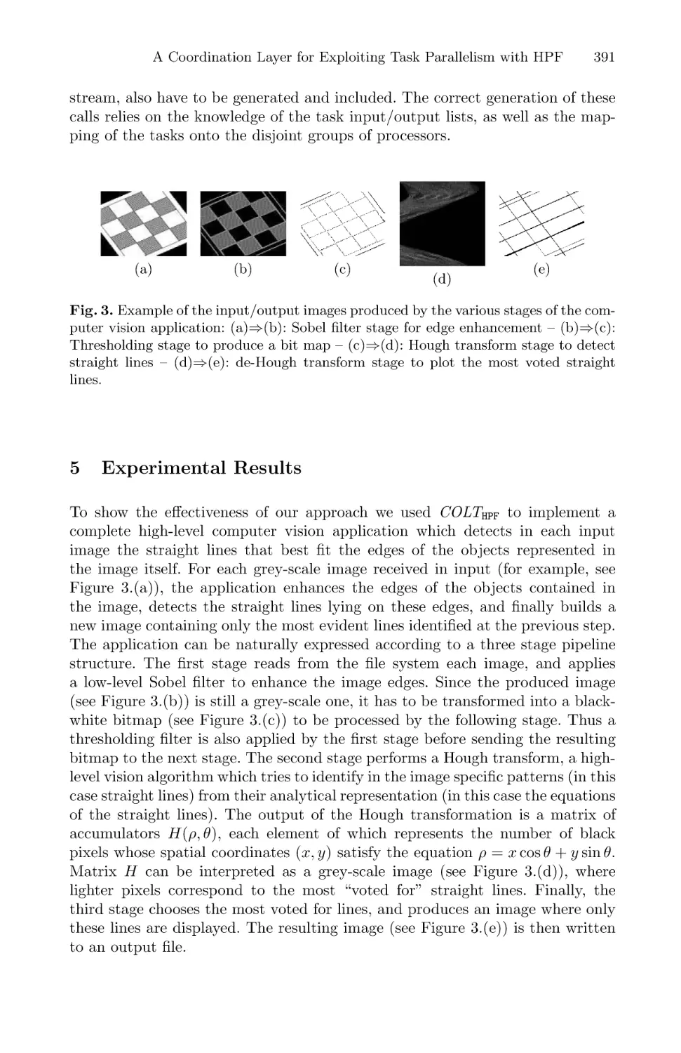
for i := 0 to n-1 do
sum := 0
for j := ROWS[i] to ROWS[i+1]-1 do
sum += DATA[j]*x[COLUMN[j]]
b[i] := sum

COLUMN
1 2 3 4 5 6

DATA

Fig. 2. Conjugate gradient’s sparse matrix-vector product. The sparse matrix A is
encoded using three arrays: DATA, ROWS, and COLUMN. A is encoded densely in DATA.
ROWS[i] indicates where the ith row begins in DATA. COLUMN[i] indicates which column
of A the element stored in DATA[i] is in, and thus which value of x must be fetched
when performing the inner product.

system will fetch a cache line of data, of which only one element is used. Because
of the large size of x and A and the sparse nature of accesses to x during each
iteration of the loop, there will be very little reuse in the L1 cache — almost every access to x results in an L1 cache miss. If data layouts are carefully managed
to avoid L2 cache conflicts between A and x, a large L2 cache can provide some
reuse of x, but conventional memory systems do not provide simple mechanisms
for avoiding such cache conflicts.
Because the performance of conjugate gradient is dominated by memory
performance, it performs poorly on conventional architectures. Two previously
studied solutions to this problem are to build main memory exclusively from fast
SRAM or support massive multithreading. The Cray T916, whose main memory
consists solely of fast (and expensive) SRAM, achieved 759.9 Mflops/second on
the NAS CG benchmark in July 1995 [12]. The Tera MTA prototype achieves
good single-node performance on the NAS conjugate gradient benchmark because its support for large numbers of cheap threads allows it to tolerate almost
arbitrary memory latencies [3]. However, both of these solutions are very expensive compared to conventional hardware.
In Impulse, we take a different position — we employ off-the-shelf CPUs and
memories, but build an adaptable memory controller. Our memory controller
supports two major optimizations for improving the memory behavior of sparse
matrix-vector product. First, it can perform scatter/gather operations, which
trades temporal locality in the second-level cache for spatial locality in the firstlevel cache. Second, it can be used to color pages so as to better utilize physically
indexed, second-level caches. We discuss these optimizations in the following two
subsections.

Memory System Support for Irregular Applications

setup x’[k] = x[COLUMN[k]]
for i := 0 to n-1
sum := 0
for j := ROWS[i] to ROWS[i+1]-1
sum += DATA[k] * x’[j]
b[i] := sum
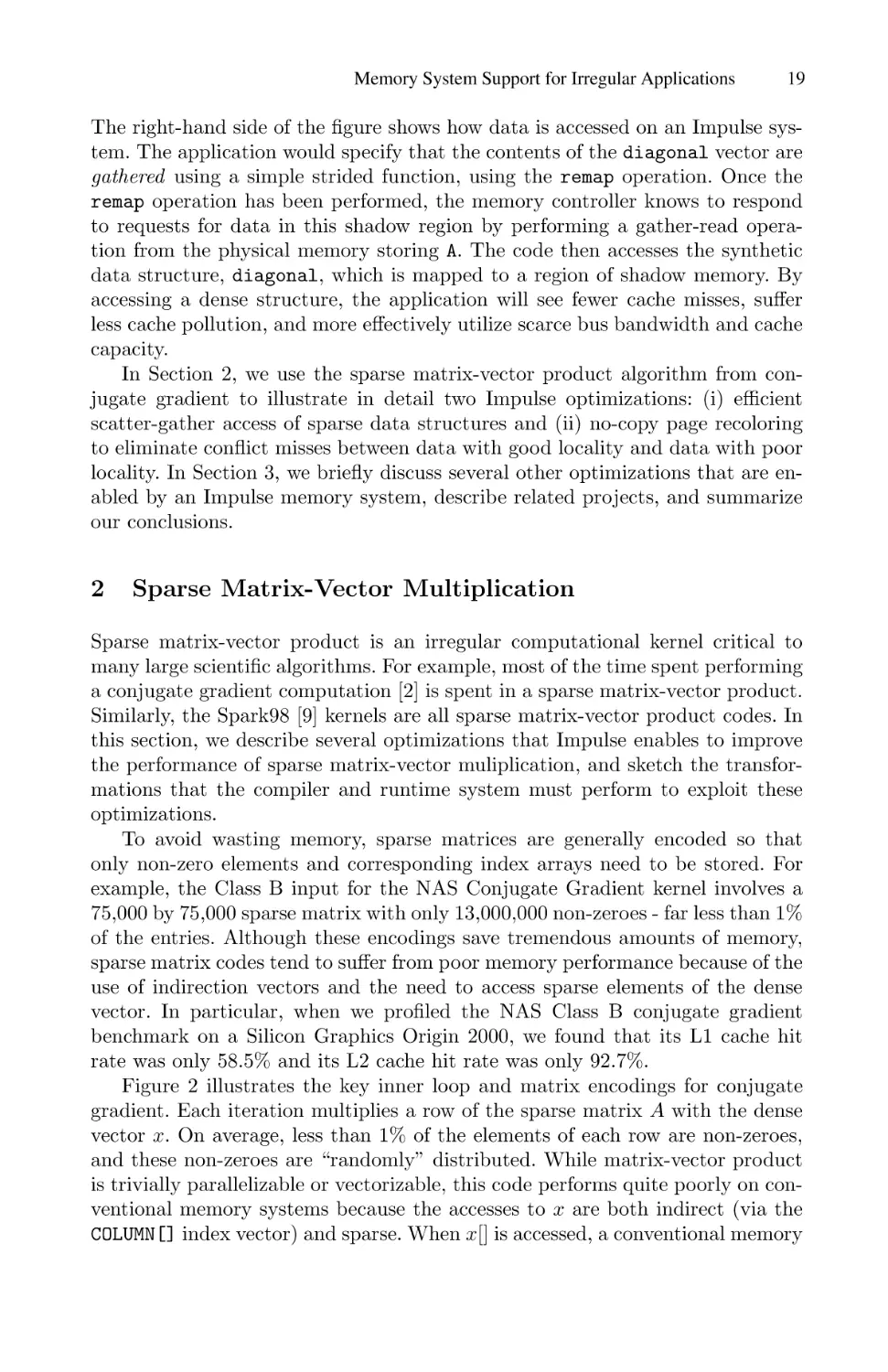
Fig. 3. Code for sparse matrix-vector product on Impulse

2.1

Scatter/Gather

As described in Section 1, the Impulse memory controller will support scatter/gather reads and writes. We currently envision at least three forms of scatter/gather functions: (i) simple strides (ala the diagonal example), (ii) indirection vectors, and (iii) pointer chasing. The type of scatter/gather function that
is relevant to conjugate gradient is the second, the use of indirection vectors.
The compiler technology necessary to exploit Impulse’s support for scatter/gather is similar to that used in vectorizing compilers. Figures 3 and 4illustrate
the code generated for the inner loop of conjugate gradient by a compiler designed to exploit the Impulse memory controller. The compiler must be able
to recognize the use of indirection vectors, and download to the memory controller a description of the data structure being accessed (x) and the indirection
vector used to specify which elements of this structure to gather (COLUMN[]).
This code can be safely hoisted outside of the inner loops, as shown in Figure 3.
After performing this setup operation, the compiler will then emit accesses to
the remapped version of the gathered structure (x0 ) rather than accesses to the
original structure (x).
Scatter/gather memory operations take longer than accessing a contiguous
cache line, since the memory controller needs to perform multiple actual DRAM
accesses to fill the x0 structure. The low-level design details of the Impulse DRAM
scheduler are beyond the scope of this paper – suffice it to say that it is possible to pipeline and parallelize many of the DRAM accesses required to read and
write the sparse data through careful design of the controller. For optimal performance, the compiler should tell the memory controller to sequentially prefetch
the elements of x’ (i.e., pre-gather the next line of x’), since it can tell that
x’ is accessed sequentially. When all of these issues are considered, the compiler
should unroll the inner loop according to the cache line size and software pipeline
accesses to the multiplicand vector, as shown in Figure 4. In this example, we
assume a cache line contains four doubles; for clarity we assume that each row
contains a multiple of eight doubles.
These optimizations improve performance in two ways. First, fewer memory
instructions need to be issued. Since the read of the indirection vector (COLUMN[])
occurs at the memory, the processor does not need to issue the read. Second,
spatial locality is improved in the L1 cache. Since the memory controller packs

J. Carter et al.
setup x’[k] = x[COLUMN[k]]
for i := 0 to n-1
lo := ROWS[i]
hi := ROWS[i+1]-1
sum := DATA[lo]*x’[lo]
for j := lo to hi step 8 do
sum += DATA[j+4]*x’[j+4]
sum += DATA[j+1]*x’[j+1]
sum += DATA[j+2]*x’[j+2]
sum += DATA[j+3]*x’[j+3]
sum += DATA[j+8]*x’[j+8]
sum += DATA[j+5]*x’[j+5]
sum += DATA[j+6]*x’[j+6]
sum += DATA[j+7]*x’[j+7]
sum -= DATA[hi+1]*x’[hi+1]
b[i] := sum

Fig. 4. Code for sparse matrix-vector product on Impulse with strip mining and software pipelining

the gathered elements into cache lines, the cache lines contain 100% useful data,
rather than only one useful element each.
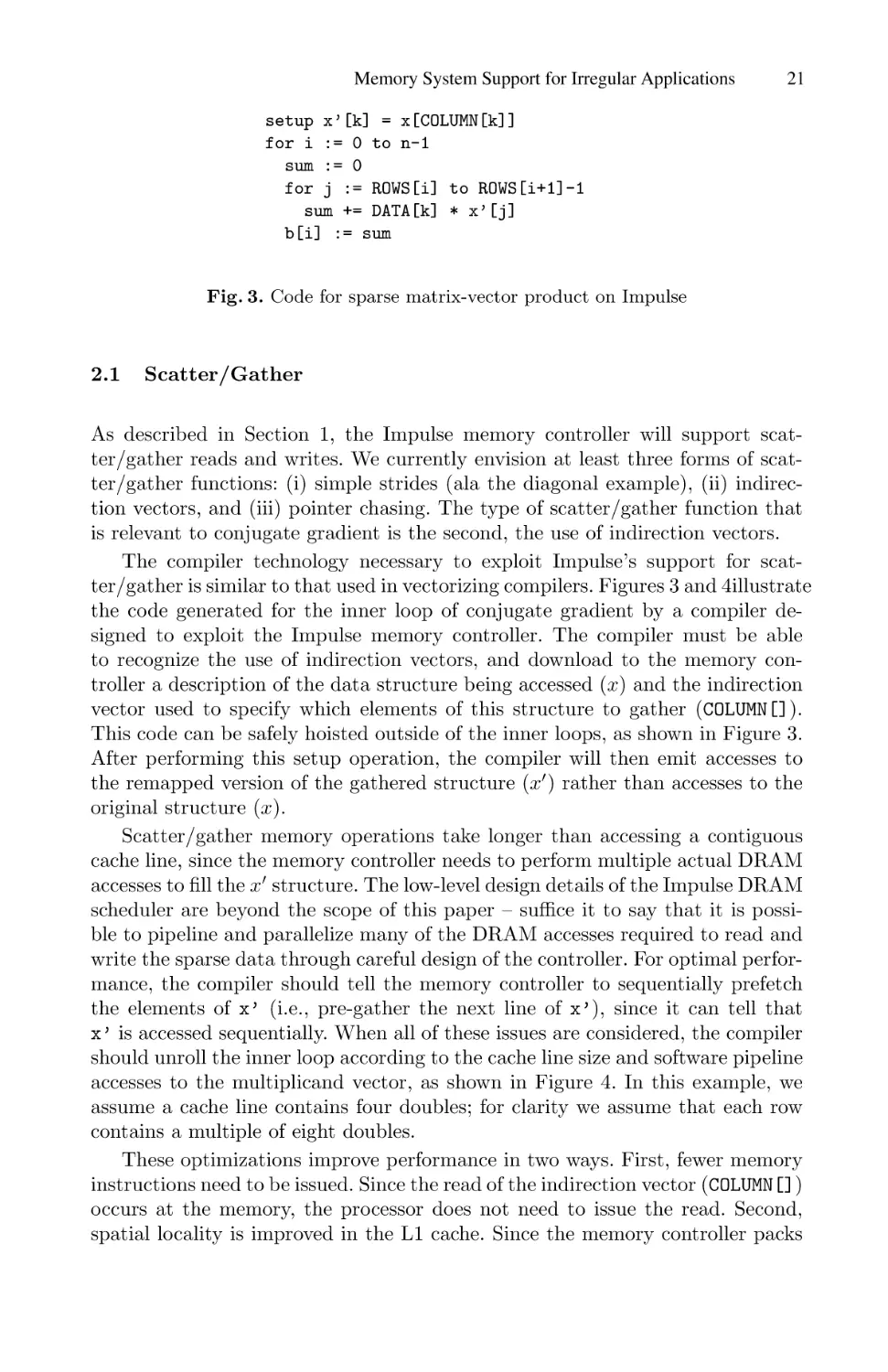
Since a detailed simulation of the scatter/gather capability is not yet available, we performed a simple analysis of its impact. If we examine just the inner
loop of the original algorithm, it is dominated by the cost for performing three
loads (to DATA[i], COLUMN[i], and x[COLUMN[i]]). If we assume a 32-byte cache
line that can hold four doubles, we can see where Impulse wins in Table 1. Conv.
(Best) represents the best case performance of a conventional memory system.
In this case, the L2 cache is large enough to hold x and there are no L2 cache
conflicts between x and any other data. Conv. (Worst) represents the worst case
performance of a conventional memory system. In this case, either the L2 cache
is too small to hold a significant fraction of x or frequent conflicts between x
and other structures cause the useful elements of x to be conflicted out of the
L2 cache before they can be reused in a subsequent iteration. Because x is not
accessed directly in Impulse, its best and worst case are identical.
As we see in Table 1, Impulse eliminates four memory accesses, each of which
are hits in the L2 cache, from the best case for a conventional system. In place
of these four accesses, Impulse incurs the miss marked in the table with an
asterisk, which is the gathered access to x0 . Compared to the worst case for a
conventional system, Impulse eliminates both the four L2 hits and four misses
to main memory. Note that except on machines with large L2 caches and very
careful data layout, the worst case is also the expected case because of the
large size of x and its poor locality. If we assume that software pipelining and
prefetching will hide cold misses to linearly accessed data, the misses to DATA[i],
COLUMN[i], and x’[i] can be hidden. In this case, using Impulse will allow the
processor to perform floating point operations as fast as the memory system can

Memory System Support for Irregular Applications

Load

Conv. Conv. Impulse
(Best) (Worst)
DATA[i]
miss
miss
miss
COLUMN[i]
.5 miss .5 miss
x[COLUMN[i]] L2 hit miss
x’[i]
miss*
DATA[i+1]
L1 hit L1 hit L1 hit
COLUMN[i+1] L1 hit L1 hit
x[COLUMN[i+1]] L2 hit miss
x’[i+1]
L1 hit
Load
Conv. Conv. Impulse
(Best) (Worst)
DATA[i+2]
L1 hit L1 hit L1 hit
COLUMN[i+2] L1 hit L1 hit
x[COLUMN[i+2]] L2 hit miss
x’[i+2]
L1 hit
DATA[i+3]
L1 hit L1 hit L1 hit
COLUMN[i+3] L1 hit L1 hit
x[COLUMN[i+3]] L2 hit miss
x’[i+3]
L1 hit
Table 1. Simple performance comparison of conventional memory systems (best and
worst cases) and Impulse. The starred miss requires a gather at the memory controller.

supply two streams of dense data (x0 and DATA). However, since the non-linear
acccess to x[COLUMN[i]] cannot be hidden, a conventional machine will suffer
frequent high latency read misses, thereby dramatically reducing performance.
It is important to note that the use of scatter/gather at the memory controller
reduces temporal locality in the second-level cache. The remapped elements of
x0 are themselves never reused, whereas a carefully tuned implementation of CG
would be able to reuse many elements of x cached in a large L2 cache. Such
a situation would approach the best case column of Figure 1, modulo conflict
effects in the L2 cache. In the next section, we propose a way to achieve the best
case using Impulse.
2.2

Page Coloring

As an alternative to gathering elements of x, which achieves the performance
indicated under the Impulse column of Table 1, Impulse allows applications to
manage the layout of data in the L2 cache. In particular, on an Impulse machine,
we can achieve the best-case memory performance for a conventional machine
on conjugate gradient by performing page coloring.
Page coloring optimizes the physical memory layout of data structures so
that data with good temporal locality (e.g., x) is mapped to a different part of a
physically-indexed cache than data with poor temporal locality (e.g., DATA, ROW,

J. Carter et al.

and COLUMN). In a physically-indexed second level cache, physical pages from
different data structures can wind up being mapped to the same location. As a
result, data in these pages will tend to conflict with one another. For conjugate
gradient, the x vector is reused within an iteration, while elements of the DATA,
ROW, and COLUMN vectors are used only once each in each iteration. Thus, we
would like to ensure that x does not conflict in the L2 cache with the other
data structures. In the NAS CG benchmarks, x ranges from 600 kilobytes to 1.2
megabytes, and the other structures range from 100-300 megabytes. Thus, x will
not fit in most processor’s L1 caches, but can fit in many L2 caches.
On a conventional machine, page coloring is hard to exploit. Coloring requires
that the system not map data to physical pages that have the same “color” (i.e.,
map to the same portion of the cache) as data with good locality. If you wish to
devote a large percentage of your cache to data with good temporal locality, this
effectively means that you cannot use large portions of your physical memory,
which is impractical for problems with large data sets. In addition, coloring often
requires data to be copied between physical pages to eliminate conflicts, which
is expensive.
Impulse eliminates both of these problems, which makes page coloring simple and efficient. Since Impulse can map data structures to shadow physical
addresses, rather than real physical addresses, and because wasting shadow address space does not waste physical memory, data with good locality can be
mapped to pages that do not conflict with other data. And, because of the extra
level of translation, this recoloring can be done without copying. In the case of
conjugate gradient, Impulse can be used to remap x to pages that map to most
of the physically-indexed L2 cache, and can remap DATA, ROWS, and COLUMNS to a
small number of pages that do not conflict with either x or each other. In effect,
we can use a small part of the second-level cache, e.g., two pages each for DATA,
ROWS, and COLUMNS, as a stream buffer [8].

Conclusions

We have described two optimizations that the Impulse controller supports for
irregular applications. An Impulse system can also improve the performance of
dense matrix kernels. Dense matrices are tiled to improve cache behavior, but the
effectiveness of tiling is limited by the fact that tiles do not necessarily occupy
contiguous blocks in caches. Tile copying [7] can improve the performance of
tiled algorithms by reducing cache conflicts, but the cost of copying is fairly
high. The Impulse controller allows tiles to be copied virtually. The cost that
virtual copying incurs is that read-write sharing between virtual copies requires
cache flushing to maintain coherence.
An Impulse memory controller can be used to dynamically build superpages,
so as to save processor TLB entries [13]. This optimization can dramatically
improve the performance of applications with large working sets. Unfortunately,
because the physical memory associated with a superpage must be contiguous
and aligned, superpages cannot easily be used to map user data on conven-

Memory System Support for Irregular Applications

tional memory systems. However, by using shadow memory to map superpages,
and then remapping the shadow addresses back to the non-contiguous physical addresses corresponding to the user data, Impulse can create superpages for
arbitrarily shuffled user data.
An Impulse memory system also helps support efficient message passing.
First, its support for scatter/gather means that the memory controller, rather
than software, can handle the chore of gathering data into messages. As a result,
the Impulse controller can reduce the overhead of sending a message. Second, its
support for building superpages means that network interfaces need not perform
complex and expensive address translation. Instead, an Impulse controller could
handle the translations necessary for messages that span multiple pages.
Other research projects are looking at similar issues in designing memory
systems; we briefly describe a few of them. The Morph architecture [14] is almost entirely configurable: programmable logic is embedded in virtually every
datapath in the system. As a result, optimizations similar to those that we have
described are possible using Morph. The Impulse project is designing hardware
that will be built in an academic environment, which requires that we attack
hardware outside of the processor. The RADram project at UC Davis is building a memory system that lets the memory perform computation [10]. RADram
is a PIM (“processor-in-memory”) project similar to IRAM [6], where the goal
is to put processors close to memory. In contrast, Impulse does not seek to put
a processor in memory; instead, its memory controller is programmable.
In summary, the Impulse project is developing a memory system that will
help to improve the memory performance of irregular applications. We have
used sparse matrix-vector product as our motivating example, but we expect
that the ability to configure an Impulse memory system to various memory
access patterns will be useful for a wide range of irregular problems. We are
investigating both manual and automatic mechanisms for taking advantage of
the flexibility that Impulse provides.

References
1. R. Alverson, D. Callahan, D. Cummings, B. Koblenz, A. Porterfield, and B. Smith.
The Tera computer system. In Proceedings of the International Conference on
Supercomputing, pages 272–277, Amsterdam, The Netherlands, June 1990.
2. D. Bailey et al. The NAS parallel benchmarks. Technical Report RNR-94-007,
NASA Ames Research Center, Mar. 1994.
3. J. Boisseau, L. Carter, K. S. Gatlin, A. Majumdar, and A. Snavely. NAS benchmarks on the Tera MTA. In Proceedings of the Multithreaded Execution Architecture and Compilation, Las Vegas, NV, Jan. 31–Feb. 1, 1998.
4. D. Burger, J. Goodman, and A. Kagi. Memory bandwidth limitations of future
microprocessors. In Proceedings of the 23rd Annual International Symposium on
Computer Architecture, pages 78–89, May 1996.
5. A. Huang and J. Shen. The intrinsic bandwidth requirements of ordinary programs.
In Proceedings of the 7th Symposium on Architectural Support for Programming
Languages and Operating Systems, pages 105–114, Oct. 1996.

J. Carter et al.

6. C. E. Kozyrakis et al. Scalable processors in the billion-transistor era: IRAM.
IEEE Computer, pages 75–78, Sept. 1997.
7. M. S. Lam, E. E. Rothberg, and M. E. Wolf. The cache performance and optimizations of blocked algorithms. In Proceedings of the 4th ASPLOS, pages 63–74,
Santa Clara, CA, Apr. 1991.
8. S. McKee and W. A. Wulf. Access ordering and memory-conscious cache utilization. In Proceedings of the First IEEE Symposium on High Performance Computer
Architecture, pages 253–262, Raleigh, NC, Jan. 1995.
9. D. R. O’Hallaron. Spark98: Sparse matrix kernels for shared memory and message
passing systems. Technical Report CMu-CS-97-178, Carnegie Mellon University
School of Computer Science, Oct. 1997.
10. M. Oskin, F. T. Chong, and T. Sherwood. Active pages: A model of computation
for intelligent memory. In Proceedings of the 25th International Symposium on
Computer Architecture, June 1998. To appear.
11. S. E. Perl and R. Sites. Studies of Windows NT performance using dynamic
execution traces. In Proceedings of the Second Symposium on Operating System
Design and Implementation, pages 169–184, October 1996.
12. S. Saini and D. H. Bailey. NAS parallel benchmark (version 1.0) results. Technical
Report NAS-96-18, NASA Ames Research Center, Moffett Field, CA, Nov. 1996.
13. M. Swanson, L. Stoller, and J. Carter. Increasing TLB reach using superpages
backed by shadow memory. In Proceedings of the 25th Annual International Symposium on Computer Architecture, June 1998.
14. X. Zhang, A. Dasdan, M. Schulz, R. K. Gupta, and A. A. Chien. Architectural
adaptation for application-specific locality optimizations. In Proceedings of the
1997 IEEE International Conference on Computer Design, 1997.

Menhir: An Environment for High Performance
Matlab
Stéphane Chauveau, François Bodin
schauvea@irisa.fr, bodin@irisa.fr
IRISA-INRIA
Campus de Beaulieu, 35042 Rennes, FRANCE

Abstract. In this paper we present Menhir a compiler for generating
sequential or parallel code from the Matlab language. The compiler
has been designed in the context of using Matlab as a speciﬁcation
language. One of the major features of Menhir is its retargetability
that allows generating parallel and sequential C or Fortran code. We
present the compilation process and the target system description for
Menhir. Preliminary performances are given and compared with MCC,
the MathWorks Matlab compiler.

Introduction

Current approaches for the development of numerical applications are frequently
decomposed in two phases. First a prototype or speciﬁcation is written using a
popular high level tool such as Matlab [10,11]. Then, the application is rewritten in Fortran or C so eﬃciency can be achieved. When high performance is
needed, the application is also parallelized. This manual process is error prone
and very time consuming which makes Matlab compilers very attractive, especially when the target is a parallel computer.
Automatically generating an eﬃcient implementation from a Matlab code
encompasses two main aspects. First, the generated code must be eﬃcient and
able to exploit a wide range of architectures from sequential computers to parallel
ones. Secondly the user must be able to change the generated code so it can be
automatically inserted or exploited in an existing development environment. For
instance, when the user has special data structures for implementing its matrices
and the corresponding speciﬁc highly optimized libraries the compiler should be
able to exploit them.
In this paper we present Menhir (Matlab ENvironment for HIgh peRformance), a multi-target compiler for Matlab 4.21 . The main feature of Menhir
is its target description system that allows addressing sequential and parallel
systems. The user may add its own data structures and functions to this description, thus enabling better code generation. To exploit parallelism Menhir
relies on libraries such as ScaLapack [5].
1

With a few restriction such as the operators eval, feval that take Matlab statements
as input are not supported.

D. O’Hallaron (Ed.): LCR’98, LNCS 1511, pp. 27–40, 1998.
c Springer-Verlag Berlin Heidelberg 1998

S. Chauveau and F. Bodin

In Section 2, we present a short summary of related tools. In Section 3, we
overview the Menhir’s target system description (MTSD). In Section 4, we
describe the type analysis and the code generation method used in Menhir.
Finally in Section 5, we present preliminary performance results on a set of
Matlab programs running on sequential and parallel architectures.

Related Works

Number of studies hava already been based on the Matlab language. The ﬁrst
set of tools are interpreted Matlab clones such as Scilab and Octave. Another
class of tools proposes parallel extensions to Matlab such as message passing
in MultiMatlab [12] or a client-server mechanism in MathServer [8] or IPSCMATLAB [4]. The main diﬀerence between those tools and Matlab compilers
is the lack of static type analysis.
Three existing compilers MCC, distributed by The MathWorks Inc,
MATCOM [13], distributed by MathTools, and Falcon are available to generate eﬃcient codes. The Falcon [9,7] system encompasses a compiler and an
interactive environment for transforming and optimizing Matlab programs. The
Falcon project was focused on the type analysis, one of the keypoint in compiling Matlab. Menhir diﬀers from these two systems by two aspects. Firstly
Menhir relies on a retargetable code generator which Falcon, MATCOM and
MCC do not. Secondly, Menhir is able to exploit parallel numerical libraries.

Menhir’s Target System Description (MTSD)

The MTSD is a major component of Menhir. Its goal is to describe the property
and implementation details of target system. The target system, in our case, is a
programming language such as Fortran, C or other and a linear algebra library.
The MTSD indicates to Menhir how to implement the matrix data structures
as well as all the Matlab operators and functions. Menhir code generation
algorithm is independent from the target system. In Table 1, we present the
main constructs of the MTSD. These constructs indicate to Menhir how to
allocate and access matrices and declare the library functions which implements
Matlab operators and functions.
As shown in Table 1.b, the data structures are described in an object oriented
manner. Each data structure is described in a class construct which members
specify its properties. The ﬁelds elem, shape, minreal, maxreal, minimag and
maximag respectively indicate the basic type of the elements of the data structure,
the rank of the structure and a complex value interval. The prop ﬁeld is used
to declare properties about the content of the objects. These properties are
declared as shown in Table 1.a. They are associated to classes, variables and
expression results and propagated by the type analysis presented in Section
4.1. The identiﬁer bname indicates that the data structure is inherited from class
bname. This mechanism allows to deﬁne new classes with diﬀerent properties but
which share the same implementation. In example Table 1.b, the class UTMatReal

Menhir: An Environment for High Performance Matlab

is declared to the compiler to be an upper triangular matrix with element values
in 0 to 216 which is implemented with the same data structure as the real matrix
(i.e. MatReal). The default data structures to be used by the code generator are
declared as shown Table 1.c.
The declaration of the accesses to data structure elements is shown Table
2.g while code generation for memory allocation is illustrated in Table 1.j. The
assign and cast constructs are provided to allow the compiler to copy and
convert data structures from one type to another. Cast operations are necessary
to ensure that the result of operators/functions can be converted in a format
suitable to the routines exploiting the results. They are shown Table 1.f.
Matlab operators and functions are declared as shown in Table 1.d and
1.e. The code to generate is an expression or a sequence of statements. For each
parameter in the list, an attribute (att) and a class name (cname) are given.
The attribute indicates how the parameter is used in the target code ; out for
a result, const for a constant variable, expr for an expression (i.e. without
an address) etc. The type indicates the data structure class name. Contrary
to operators, Matlab functions are declared in two parts (Table 1.e). First
some target subroutines are declared. Then, they are gathered in the function
construct. Matlab control statements are deﬁned similarly as shown in Table
2.h.
The conform statement iterators given in Table 2.i are used by the compiler to
implement conform statement, such as the point-wise addition of two matrices,
in an eﬃcient manner that minimizes the number of temporary variables. For
instance, if we consider the Matlab expression R = B−A∗x, an implementation
based on library function calls would imply to generate the code in two parts,
ﬁrst T = A ∗ x and then R = B − T resulting in poor performance. Instead
Menhir generates the following C code using the loop construct:
...
for (tmp136 = 1; tmp136 <= tmp128; tmp136++) {
for (tmp135 = 1; tmp135 <= tmp127; tmp135++) {
(*tmp133++) = ((*tmp129++)((*tmp131++)*tmp94));
}
tmp129 = &tmp129[tmp130];
tmp131 = &tmp131[tmp132];
tmp133 = &tmp133[tmp134];
}
...

As shown by this example, the generated code can be close to what “hand
programming” would produce. In the case of parallel code generation, a similar
principle, shown in Table 2.k, is used to describe the scanning of a distributed
matrix local elements.

S. Chauveau and F. Bodin

Syntax
a) Properties

Example

property name ;
b) Data Structure
class name : bname
elem = id
shape = scal,row,col,matrix
minreal = constant ;
maxreal = constant ;
minimag = constant ;
maximag = constant ;
prop = list of properties;
end
c) Default Data Structure
default shape, elemtype
[,prop] = cname

property DIAG ;
property UPPERTRI ;

class UTMatReal: MatReal
elem = Real ;
shape = matrix;
minreal = 0 ;
maxreal = 216 ;
prop = UPPERTRI;
end

default matrix,complex = MatComplex ;
default matrix,real,DIAG = DiagMatReal ;

d) Matlab Operators
inline name (att cname var1,...)
=> statement 1
=> ...
inline real @op add(real A,int B)
"(A+((double)B))" ;
;
inline res name (att cname var1,...)
"expression" ;
e) Matlab Functions
inline func1(parameters)
=> code ;
;
function res = name(parameter)
add f unc1;
add f unc2;
end function

inline C lup real(out MatReal MATL,
out MatReal MATU, ...,MatReal MATA)
=> lup RRI R(&MATL,&MATU,
&MATP,MATA) ;
;
function [L,U,P] = lu(A)
add C lup real(L,U,P,A) ;
end function

f ) Assign and Cast Operators
inline @assign(out cname r,
inline @assign(out MatReal DEST,
const cname i)
const TranspMatReal SRC)
=> statement 1 ;
=> transpose R R(&DEST,&SRC) ;
=> ...;
;
;
inline int @cast(RowInt VAR)
inline cname @cast(att cname var)
"VAR.get(1)"
”expression”
;
;

Table 1. Target System Description Content.

Menhir: An Environment for High Performance Matlab
Syntax
g) Index Accesses

Example

inline @get|put|...()
=> statement 1 ;
=> ...;
;

inline real @get(MatReal MAT)
"get Rii(&MAT,I1,I2)" ;
inline @put(MatReal MAT,real VAL)
=> set Riir(&MAT,I1,I2,VAL) ;
;

h) Matlab Control Statement
inline @do(real CP T ,real ST ART ,
const real ST EP ,real EN D)
=> loop code(BODY);
;

inline @do(real CPT,real START,
const real STEP,real END)
=> for(CPT=START;CPT<=END;CPT+ =STEP){
=>
BODY
=> }
;

i) Conform Statement Iterators
inline @loop(local variablelist)
=> statement 1(BODY) ;
=> ...;
;

inline @loop(local int I1,int I2)
=> for (I1=1;I1<=DIM1;I1++)
=>
for (I2=1;I2<=DIM2;I2++)
=>
{
=>
BODY
=>
}
;

j) Memory Management, Declaration, Target Language Statements
inline @declar(cname var)
=> statement 1 ;
inline @declar(MatReal MAT)
=> MatReal *MAT ;
=> ...;
;
;
inline @alloc(cname var,
inline @alloc(MatReal VAR,
int DIM 1,int DIM 2)
int DIM1,int DIM2)
=> statement 1 ;
=> alloc R(&VAR,DIM1,DIM2) ;
;
=> ...;
;
k) Local scan of distributed matrix
defaccess matrix paralocal ;
inline @loopinit:paralocal(PMatReal MAT)
=> LOCD1 = MAT.local.dim1;
defaccess matrix name ;
=> LOCD2 = MAT.local.dim2;
inline @loopinit:name(cname var)
;
=> statement 1 ;
inline @loop:paralocal(..., int LOCD1,
;
int LOCD2)
inline @loop:name(parameter list)
=> STAT1
=> statement 1 ;
=> for (I2=1;I2<=LOCD2;I2++){
;
=>
for (I1=1;I1<=LOCD1;I1++) {
inline real @get:name(cname var)
=>
BODY }
"(expression)" ;
=>
STAT2 }
;
inline real @get:paralocal(PMatReal MAT)
"(*PTR++)" ;

Table 2. Target System Description Content.

S. Chauveau and F. Bodin

Overview of Menhir’s Compilation Process

Menhir’s compilation process is divided in the following steps:
1. lexical and syntactic analysis: this step performs the lexical and syntactic
analysis of the Matlab M-Files.
2. identifiers analysis: this preliminary step of the type analysis determines
the nature of the identiﬁer. The nature of an identiﬁer can be a script ﬁle
(M-ﬁle), a function or a variable. The ambiguities are resolved statically and
the compiler assumes that the nature of an identiﬁer is constant in a program
unit (Matlab allows a identiﬁer to reference a variable and a function or a
script in the same program unit).
3. function cloning and restructuring in canonical form: At this step, all
functions are cloned and most of the special cases of Matlab are removed
by expanding them in a canonical form. Temporary variables are added to
limit code expansion for large expressions. All runtime choices are expanded
at that step. For instance, the statement A=B+C is expanded in:
if (dim1(B)==1 & dim2(B)==1) then
if (dim1(C)==1 & dim2(C)==1) then
A = B+C % scalar+scalar
else
A = B+C % scalar+matrice
...

a simple local type analysis is applied locally to each expression to avoid
useless cases. Later, after the type analysis has been performed, dead code
elimination is applied.
type analysis and dead code elimination: this type analysis determines
the properties of each expression and variable according to the semantic of
Matlab and the target system description. If an operator or a function returns an object with special properties, they are propagated. The type analysis is completed by removing all dead codes (i.e. runtime operator/function
selection that have been solved statically). The remaining conditionals added
at step 3 are left as run-time checking.
data structure selection: This step selects an implementation for each
variable according to the type computed in previous step and the defaults
given in the MTSD (Table 1.c).
operators and functions implementation selection: At this step operator and function implementations are selected. Data structure casts are
inserted to ensure that returned results can be used as input parameters of
the subsequent function calls.
code issue: This step gathers the selected implementations to issue the ﬁnal
code.

In the following, we present in more details steps 4 and 6.

Menhir: An Environment for High Performance Matlab

4.1

Type Analysis

The type analysis is a major component in Menhir as its result has a great
impact on the quality of the generated code. In Matlab, all operators and
functions are polymorph and the default is to implement all objects as complex
matrices. Furthermore, variable types can change during the program execution
and matrices can be resized by any assignment. An accurate analysis limits
runtime type checking overheads and allows selecting the appropriate library
methods (for instance, operators on ﬂoats instead of complex variables).
A type in Menhir is deﬁned as a set of possible shapes (scalar, row vector,
column vector and matrix), an interval of complex value, a string, an integer
status and a set of numerical properties. A class from the MTSD deﬁnes such a
type. The properties are used to select optimized implementations. To illustrate
this feature consider the following Matlab statement sequence:
A = triu(...);
...
v=b/A;

Matlab function triu returns a matrix that is upper triangular. To execute
eﬃciently specialized solver (this solver does not check at runtime if matrix
A is upper triangular). This is achieved in Menhir by having the following
declaration in the MTSD that use the UPPERTRI property that is propagated
by the type analysis:
property UPPERTRI ;
class UTMatReal : MatReal
prop = UPPERTRI;
end ;
inline triu Real(out UTMatReal A, MatReal B)
=> ... ;
;
function [A] = triu(B)
add triu Real;
...
end function
inline @op matdiv(MatReal RES,
MatReal PARAM1,
UTMatReal PARAM2)
=> ...;
;

This powerful feature is not restricted to Matlab functions and operators.
User’s libraries can be exploited in a similar fashion and new properties can be
created at any time.
The type propagation algorithm is interprocedural and based on an iterative
data ﬂow solver [1,6] that is closed to the one proposed by DeRose [9]. The analysis computes a superset of the possible values for each variable and expression

S. Chauveau and F. Bodin

at each point of the program. However, in many cases, there is not enough information to propagate in a Matlab program to compute accurately the types
describing these supersets. Via directives, Menhir allows specifying information
on objects that are used by the type analysis. The most frequent directives give
information about the contents (i.e. the shape, the properties or the element
types) of some variables at a given point of the program. These directives cannot be regarded as global type declarations since their scope is limited and they
do not specify the implementation of the objects. A variable declared as a scalar
in a point of program can become a matrix or a vector in another point.
The second kind of directives is used to simplify the semantic of the Matlab
language. For instance the directive
%$VAR var [,var] : [no] RESIZE/MASK
allows to declare if a variable is subject to resizing or to be acceded using a mask
index2 .
4.2

Code Generation

The code generation must solve three problems:
1. selecting the data structure for each variable and expression according to
the type analysis
2. selecting the implementations (the methods) for Matlab operators and
functions
3. inserting data structure cast operations
These choices are interdependent. The methods whose operand data structures match more the current parameters data structures are most suitable.
Conversely, it seems interesting to adapt the data structures to the methods
using them. To illustrate this problem, consider the class C1 and C2 and the implementations of F, M1 : C1 → C2 and M2 : C2 → C1 , in the following Matlab
code:
for i=1:n
B=F(A) ; C=F(B) ; A=F(C) ;
end

The ﬁgure 1 shows how the initial choice for the data structure of A can
inﬂuence the remaining of the analysis.
In Menhir, the choice of variable data structures is made ﬁrst according to
the result of the type analysis and to the defaults given in the MTSD. Although
imperfect, this strategy is acceptable since only a few types are provided into
the MTSD.
Then, the selection for operators/functions and the insertion of cast operations is made. This is performed by building on the flight a directed acyclic
graph. Vertices correspond to variables, Matlab operators/functions and data
2

A mask variable in Matlab is a matrix containing only 0 or 1 element values used
as booleans.

Menhir: An Environment for High Performance Matlab
C1

C2
M1

C1
M2

Class of C

Cast

Class of B

Cast

Class of A

C2
M2

M1
C2

Fig. 1. Selection of the implementation according to the initial data structure of A

structure conversion subroutine. An example of such a graph is shown ﬁgure
2. Code generation consists in selecting a set of paths that covers all program
statements and variables (indicated in gray in Figure 2).

b
ScalReal
Var

A
MatReal
Var

MatReal to MatComp

ScalReal to ScalComp

MatComp
=
MatComp
+
ScalReal

MatReal
=
MatReal
+
ScalReal

MatComp
=
MatComp
+
ScalComp

MatComp to MatReal

C
MatReal
Var

b
ColReal
Var

MatReal to MatComp

ColReal to ColComp

ColReal
=
ColReal
\
MatReal

ColComp
=
ColReal
\
MatComp
ColComp to ColReal

ColComp
=
ColComp
\
MatComp

ColComp to ColReal

x
ColReal
Var

Fig. 2. Code generation graph for Matlab code C=A+b; x=C/d;. MatComp, MatReal,
ColReal, ColComp, and ScalReal, respectively denote complex matrices, ﬂoat matrices,
ﬂoat column vectors, complex column vectors, and ﬂoat scalars data structures.

S. Chauveau and F. Bodin

A score is associated to each cast and each method according to the shapes
of the data structures to which they are applied. Then, the algorithm looks for
a path with a lowest score on a subset of the graph. The costly part of the
algorithm is not the shortest path computation itself but the creation of the
subgraphs that represents the data structures casts. Each of them depends on
the type analysis result for the local value and can contain several nodes. In
many cases, the construction of the graph is avoided by choosing as preset cast
(i.e. applied to generic types). For more details the reader can refer to [3].
The last stage consists in assembling the codes of the selected methods for the
expressions, the instructions and the casts. The syntax of the target language,
except for the literals and the identiﬁers, is entirely described by the MTSD.

Preliminary Performances

In this section, we present preliminary performance obtained using Menhir
on a single processor Sun workstation and on a parallel computer Onyx SGI
with 4 processors R10000. The sequential codes are generated using a target
system description based on the Lapack library [2] while the parallel codes are
obtained using ScaLapack [5]. The parallel codes are SPMD and the same data
distribution (block-cyclic) is used for all matrices. Only a very few directives (20
for all benchmarks) were inserted in the Matlab codes. Because Menhir relies
on parallel libraries and conform operations but not on Matlab loops, program
that does not exhibit coarse grain matrix operations was not run in parallel. This
is the case of the benchmarks gauss, a Matlab program computing a gaussian
elimination written in a Fortran style, chol, an incomplete cholesky factorization,
pfl, an iterative method for eigenspace decomposition by spectral dichotomy, and
INT1, INT4 two diﬀerential equation integration algorithms.
The size of the Matlab programs and the generated code is given in Table
3. Cloning, performed at step 3 of the compilation process, can substantially
generate large target codes as shown for the program pfl. Menhir is more eﬃcient than MCC, the MathWorks Matlab compiler, except for chol. The main
loop of chol is a WHILE statement that computes a lot of integer expressions.
Some directives specify that the handled variables remain in the integer range
[−231 , 231 − 1] but they have no eﬀect on intermediate calculations, which must
be done with the ﬂoat arithmetic. MCC gives better performance since it uses
the integer arithmetic. However, this heuristic does not always produce the expected results.
gauss
chol
pﬂ
INT 1
INT 4

70
180
200
140
200

200
620
9000
4700
3100

Table 3. Matlab program code sizes and corresponding generated C code sizes.

Menhir: An Environment for High Performance Matlab

Two programs illustrate the parallel code generation: a conjugate gradient
algorithm with preconditioning and a Jacobi computation.
Figure 4 gives the execution times for the conjugate gradient. On the x axis,
Matlab 4.2 and 5 correspond to the Matlab interpreters execution time, MCC
is the execution time of the code produced by the MathWorks compiler, Menhir
is the time for the sequential code generated by our compiler and ONYXn × m
and PARAGONn×m are the execution times on the Onyx and the Paragon parallel computers. As it can be seen, Menhir performs better that the interpreter
and MCC except in one case, chol. In this case Menhir’s code contains ﬂoat to
integer conversions that slow down the algorithm. In general, the code produced
by Menhir is closed, for most of the benchmarks of the “hand-coded” versions
of the algorithms. However, these “hand coded” versions were not aggressively
optimized.
Parallel codes reach good speedups thanks to the ScaLapack library but also
to the type analysis3 . Figure 5 gives the execution times for two versions of the
same version of Jacobi compiled with diﬀerent MTSD. In the second version,
good performance is obtained when the MTSD propagates the information that
the preconditioning matrix M, shown Figures 3, is diagonal. Then, the run-time
checking of this property disappears and a large amount of memory space and
communication is saved.

...
m=size(A,1) ;
n=size(A,2) ;
[ M, N ] = split( A , b, 1.0, 1 ) ;
for iter = 1:max it,
x 1 = x;
y = N*x + b ;
x = M /y ;
error = norm(x-x 1 )/norm( x );
if ( error <= tol ), break, end
end
...

Fig. 3. Main loop of the Jacobi benchmark.

We don’t have MCC or Matlab on the Onyx computer, so the performance numbers
in sequential are not given for this architecture.

S. Chauveau and F. Bodin

Conclusion

250

In this paper we brieﬂy present Menhir, a retargetable compiler for Matlab. The strength of Menhir is its original target system description that allows
generating code that exploits optimized sequential and parallel libraries. Performance shows that the generated code is in most of the cases more eﬃcient than
the one obtained by the Mathworks compiler MCC on sequential workstation.
Future work will focus on exploiting more aggressively parallelism by also considering Matlab loops.

234
225

200

175

150

C Code
Matlab 4.2
Matlab 5
MCC
Menhir

F
H
V
125
H
P
L
W

104

100
100

28
25

20
17
6 5

pfl

ol
ch

s
us
ga

1
INT

4
INT

#ONJUGATE 'RADIENT
250

208
198

200

150

140

139

100

50
27

27
15
9

M
C
C

M
en
hi
r
O
N
Y
X
1x
1
O
N
Y
X
1x
2
O
N
Y
X
P
A
2.
R
2
A
G
O
N
P
1
A
x1
R
A
G
O
N
P
2x
A
R
2
A
G
O
N
5x
5

C
C
od
e
M
at
la
b
4.
2
M
at
la
b
5

Fig. 4. Execution time in seconds of the sequential and parallel generated C codes.

Menhir: An Environment for High Performance Matlab

500

443

450

400

395
376

350

300

dynamic evaluation
static propagation

250

200

150
116
100
61
43

49
39
9
4

0
Matlab
4.2

Matlab
5

MCC

Menhir

ONYX
1x1

ONYX
1x2

ONYX
2x2

Fig. 5. Execution time in seconds for the jacobi code with and without the static
propagation of the preconditioning matrix diagonal nature.

References
1. A. Aho, R. Sethi, and J. Ullman. Compilers: Principles, Techniques and Tools.
Addisson-Wesley Publishing Compagny, 1985. 33
2. E. Anderson, Z. Bai, C. Bischof, J. Demmel, J. Dongarra, J. Du Croz, A. Greenbaum, S. Hammarling, A. McKenney, S. Ostrouchov, and D. Sorensen. LAPACK
Users’ Guide. SIAM, Philadelphia, second edition, 1995. 36
3. Stphane Chauveau. MENHIR. un environnement pour l’excution eﬃcace des codes
Matlab (in French). PhD thesis, Universit de Rennes 1, February 1998. 36
4. Shirish Chinchalkar. IPSC-MATLAB reference manual. Technical Report 92-106,
Cornell Theory Center, September 1992. 28
5. J. Choi, J. DEmmel, I. Dhillon, J. Dongarra, S. Ostrouchov, A. Petitet, K. Stanley,
D. Walker, and R.C. Whaley. ScaLAPACK: A portable linear algebra library
for distributed memory computers - design issues and performance. Technical
Report CS-95-283, Computer Science Dept., University of Tennesse, Knoxville,
1995. (LAPACK Working Note 95). 27, 36
6. John B. Kam and Jeﬀrey D. Ullman. Global data ﬂow analysis and iterative
algorithms. Journal of the ACM, 31(1):158–171, January 1976. 33
7. Bret Andrew Marsolf. Techniches for the interactive development of numerical
linear algebra libraries for scientiﬁc computation. Master’s thesis, University of
Illinois at Urbana-Champaign, 1997. 28
8. M. Rezny. MATHSERVER: A client-server approach to scientiﬁc computation.
Department of Mathematics, The University of Queensland, Australia. 28
9. Luis De Rose. compiler techniques for MATLAB programs. Master’s thesis, University of Illinois at Urbana-Champain, 1996. 28, 33
10. INC THE MATHWORKS. MATLAB, High-Performance Numeric Computation
and Visualization Software. Reference Guide, August 1992. 27

S. Chauveau and F. Bodin

11. INC THE MATHWORKS. MATLAB, High-Performance Numeric Computation
and Visualization Software. User’s Guide, August 1992. 27
12. Anne E. Trefethen, Vijay S. Menon, Chi-Chao Chang, Grzegorz J. Czajkowski,
Chirs Myers, and Lloyd N. Trefethen. MultiMATLAB: MATLAB on multiple
processors. Technical Report 239, Cornel Theory Center, 1996. 28
13. Keren Yaron. MATCOM, a Matlab to C++ Translator, March 1996. 28

[

]

[

]

[

Ä
¿

¼
¿

]

[

]

[

]

[

]

[

]

[

Ä
Á

[

]

¼
F

Ä
F

[

]

;

[

]

[

Ä
F

Ä
¿

Ä
Ø

]

¼
Ã

)

(

]

¼
@

]

¼
À

[

¼
@

]

}

[

]

}

[

]

¼
@

]

}

[

]

[

]

[

]

{

Æ
½

¼
Þ

¼
½

Ä
>

Æ
@

¼
Ë

¼
Á

Æ
Ë

Ä
F

Ä
¿

Æ
¿

¼
¾

Æ
Í

Ä
¿

]

[

]

[

]

D. O’Hallaron (Ed.): LCR’98, LNCS 1511, pp. 41−56, 1998.
 Springer−Verlag Berlin Heidelberg 1998

]

[

]

[

Y. Lin and D. Padua
ú

]

[

]

[

]

Ä
½

[

]

[

]

(

Æ
½

Ä
>

Ä
Ã

¼
Ù

¼
¿

[

Ä
Ç

]

[

]

[

]

[

]

[

]

Ä
¿

]

¼
>

Ä
À

[

]

[

]

[

]

(

¼
F

Ä
Ü

Ä
½

¼
Í

Ä
Í

¼
@

Æ
J

¼
F

;

Ä
½

Ä
À

»
Á

Ä
F

¼
Á

¼
Ã

Ä
¿

(

¼
Ã

Ä
@

Ä
>

»
Ù

»
¿

¼
F

¼
¿

Ä
B

¼
Á

»
¾

Ä
@

Æ
½

Æ
Ú

Æ
>

Ä
¾

¼
¿

¼
½

Æ
B

¼
F

Ä
¿

Ä
Ð

Ä
¿

¼
F

Ä
Á

Ä
à

On the Automatic Parallelization of Sparse and Irregular Fortran Programs
ú

]

[

]

[

]

[

]

Y
Z

y
Z

]

®
Z

¬
Z

[

¼
¿

Ä
¿

Ä
Ã

]

¼
¿

¼
@

Ä
¿

Ä
F

Ä
¿

Æ
F

Ä
¿

Æ
F

Æ
@

Ä
¿

Ä
Ç

Ä
@

Ä
Á

¼
Ë

¼
¿

Ä
@

Ä
¾

¼
È

¼
\

Ä
Ã

Ä
À

[
¿

Ä
Í

Æ
½

Ä
@

¼
>

¼
¿

¼
¾

Ä
@

Ä
>

Ä
À

Ä
½

}

{

}

44
e

Y. Lin and D. Padua

Þ
q

Ä
@

¼
F

Ä
¿

Æ
À

¼
>

Ä
Ã

Æ
Á

]

[

¼
Í

]

¼
F

Ä
@

Ä
Ô

Ä
½

}

¼
Ã

}

[

Ä
F

Æ
Ã

]

Ä
Ã

Ä
¿

Ä
>

}

Æ
F

Æ
¿

}

On the Automatic Parallelization of Sparse and Irregular Fortran Programs
»

Ä
¿

;

Ä
B

Ä
F

Ä
¿

Æ
Ó

Æ
¾

Æ
@

¼
Á

Ä
J

Þ
j

»
Þ

Ä
>

Æ
È

Ä
@

Ä
F

¼
¾

Æ
½

;

Æ
¿

offset(1)

offset(2)

offset(3)

offset(4)

offset(n)

offset(n+1)

Host Array
length(1)

length(2)

length(3)

length(4)

length(n)

}

¼
Ð

[

¼
¿

Æ
à

Ä
Í

¼
Á

;

¼
¿

Æ
@

Ä
¿

¼
Ù

»
½

Ä
½

¼
¿

;

»
@

¼
@

Æ
Â

¼
Á

Y. Lin and D. Padua
Æ

Ä
Ã

}

{

Æ
Ù

Ä
Ô

Æ
¾

Ä
@

¼
@

¼
}

Ä
Á

}

[

Ä
Å

(

]

;

]

{

}

Ä
@

}

{

}

{

}

Æ
@

¼
J

{

Ä
Ë

]

Æ
Ã

Ä
¿

Æ
F

}

Ä
F

Ä
Í

Æ
~

Ä
@

Æ
@

(

¼
Á

On the Automatic Parallelization of Sparse and Irregular Fortran Programs
e

Ä
Í

¼
@

Ä
¿

¼
T

¼
Í

Ä
¾

Ä
@

}

]

[

{

¼
1

}

;

[

]

Ä
Ç

Ä
F

Ä
Å

¼
F

Ä
Å

Ä
@

¼
F

Ä
Á

¼
¿

¼
¾

Ä
Á

Æ
>

¼
F

Ä
Á

¼
Ç

Ä
F

¾
n

»
F

Ä
Ã

¼
½

¼
Ð

¼
F

Ä
F

Ä
Á

¼
J

Ä
¿

Y. Lin and D. Padua
}

]

}

{

V
¦

}

Æ
á

Ä
F

}

[

}

]

2
B

'
Å

]

Ä
Ã

Ä
Ë

Æ
¿

¼
¿

Ä
R

¼
Þ

¼
½

¼
Ù

¼
J

Ä
Ë

Ä
¾

Ä
¿

Ä
>

On the Automatic Parallelization of Sparse and Irregular Fortran Programs
¼

Ä
F

Æ
Ï

Ä
¿

Ä
¾

Ä
½

»
¿

Ä
¿

Ä
F

Ä
¿

[

¼
Ã

Æ
F

¼
Â

[

Æ
Â

[

¼
@

}

{

}

¼
J

'
1

»
=

{

}

{

}

¼
Í

¼
Ã

}

{

Ä
á

Æ
á

}

¼
@

Ä
Í

¼
F

Ä
O

¼
Ã

¼
¿

Ä
F

(

]

[

]

[

]

Y. Lin and D. Padua
Æ
Í

Ä
N

Ä
+

Ä
@

Ä
=

Ä
Í

Ä
À

»
F

{

}

;

Æ
@

;

Ä
¾

Ä
¿

Ä
Â

Ä
¾

Ä
B

Ä
Ù

Ä
>

Ä
Ë

Æ
¿

¼
Ã

¼
.
h

Ä
Ã

{

}

{

;

Ä
Ë

.. 12 43 54 44 23 ..

]

54 44 23 ..

[

89 23 18
Y

]

Æ
@

31 45 62 78 ..

Original Array A()

.. 12 43

31 45 62 78 ..

Private Copy for Processor 2 - PA2()

Private Copy for Processor 1 - PA1()

¼
>

¼
@

¼
Ã

¼
À

¼
@

¼
Ë

Æ
Á

Ä
á

Æ
¾

¼
@

¼
Ù

¼
¿

Ä
Á

¼
Ð

Ä
¿

¼
Á

89 23 18

On the Automatic Parallelization of Sparse and Irregular Fortran Programs
Í

¼
Þ

Æ
Ã

Ä
@

¼
T

ä
n

Æ
¾

¼
¿

Æ
F

Ä
}

Ä
Á

¼
Á

Ä
¿

«
ü

¼
È

¼
½

Ä
@

¼
F

¼
Á

¼
È

¼
Ì

Ä
¿

¼
È

Ä
Ù

Ä
F

Þ
n

¼
À

Ä
Ã

¼
È

Ä
Á

¼
½

Y. Lin and D. Padua

«
ü

Ä
Í

¼
¿

¼
Ã

Ä
@

Ä
Ê

Ä
Ì

Ä
¿

}

{

}

index

b(4)

b(1)+b(3)

b(2)

]

[

]

b(7)
0

Reduction Table
of Processor 2

]

Ä
¿

b(5)+b(6)
+b(8)

value

0
8

Reduction Table
of Processor 1

¼
½

Ä
¿

value

Ä
½

Æ
J

Ä
Ã

Ä
Ê

hash(x)

Æ
È

Ä
>

k(i)

do i=1, n
a(k(i)) = a(k(i)) + b(i)
end do

Æ
Ã

Æ
á

¼
¿

Ä
Á

Æ
@

¼
½

Æ
½

Ä
/

c
l

Æ
Á

¼
¾

¼
È

Ä
½

Æ
¿

¼
À

Ä
¿

¼
¿

Ä
J

Ä
>

¼
Ï

Ä
¿

Ä
Ë

On the Automatic Parallelization of Sparse and Irregular Fortran Programs
¼
¾

Æ
F

Æ
Á

¼
À

Ä
Â

¼
Â

¼
>

Ä
È

¼
¿

¼
B

¼
@

Ä
¿

¼
Ã

¼
½

Ä
F

Ä
Í

¼
Ã

Ä
>

Ä
Â

¼
Á

{

}

{

Ä
Á

Æ
Ã

{

}

¼
@

Ä
{

Ä
>

Æ
Â

Ä
@

¼
Þ

}

Æ
À

¼
À

¼
¾

{

Ä
Å

Æ
F

}

Ä
Ã

Ä
¿

Æ
Ã

Ä
¿

¼
Á

¼
F

¼
¾

Ä
È

Ä
¿

¼
½

Ä
Á

¼
{

}

Æ
B

¼
Ë

Ä
@

Ä
¿

Ä
F

¼
;

¼
Á

Ä
¿

¼
Á

Ä
Ë

Y. Lin and D. Padua

Manual

Polaris without H-R

speedup

Polairs with H-R

6
5
4

Polaris with H-R

Polaris without H-R

0
Cholesky

Euler

SpLU

GCCG

SparAdd ProdMV ProdVM SparMul SolSys

LANCZOS

]

[

Ä
F

Ä
R

¼
Ë

Ä
Ù

Ä
À

ProdUB

Ä
Þ

Æ
á

Ä
½

;

»
¿

¼
D

Ä
Á

¼
D

Ä
½

¼
½

¼
Ã

Æ
@

;

Ä
¿

¼
@

¼
½

Ä
Á

Ä
¿

Ä
J

Æ
½

¼
¿

]

[

]

[

]

[

]

[

]

On the Automatic Parallelization of Sparse and Irregular Fortran Programs
ú

¼
È

[

]

[

]

[

]

¼
Ë

Ä
¾

]

[

]

Ä
@

(

Ä
È

¼
F

Æ
Á

Ä
½

Ä
À

Ä
F

¼
Á

¼
¾

Ä
Á

Ä
¿

¼
Á

¼
@

Æ
½

¼
¾

Ä
¿

Æ
Ã

[

¼
@

]

¼
J

]

[

Æ
Ë

[

Ä
Á

¼
½

'
¿

[

Ä
Â

Æ
J

Ä
Ã

[
Á

¼
¿

]

¼
¿

¼
@

¼
¾

]

Æ
F

]

[

Æ
½

]

Ä
Í

]

¼
Á

]

Ä
Í

[

Ä
¿

»
@

]

Ä
>

¼
Þ

¼
J

Ä
@

Ä
¿

¼
F

¼
Á

Ä
¿

Ä
Ç

¼
@

Y. Lin and D. Padua

Æ
Å

¼
Ã

}

{

}

Ä
¿

¼
J

[

]

}

]

[

]

[

]

[

]

[

]

[

]

[

]

[

]

}

]

[

]

}

]

[

]

[

]

[

]

[

]

[

]

[

]

[

]

[

]

[

]

[

]

[

]

[

]

[

]

[

]

[

]

[

]

[

]

[

]

[

]

[

]

[

]

[

]

[

]

[

Ä
@

¼
Ã

¼
D

Loop Transformations for
Hierarchical Parallelism and Locality
Vivek Sarkar
IBM Research
Thomas J. Watson Research Center
P. O. Box 704, Yorktown Heights, NY 10598, USA
vivek@watson.ibm.com

Abstract. The increasing depth of memory and parallelism hierarchies
in future scalable computer systems poses many challenges to parallelizing compilers. In this paper, we address the problem of selecting and
implementing iteration-reordering loop transformations for hierarchical
parallelism and locality. We present a two-pass algorithm for selecting
sequences of Block, Unimodular, Parallel, and Coalesce transformations
for optimizing locality and parallelism for a specified parallelism hierarchy model. These general transformation sequences are implemented
using a framework for iteration-reordering loop transformations that we
developed in past work [15].

Introduction

The widening gap between processor speeds and memory speeds is leading to
deeper memory hierarchies in current and future high-performance computer
systems than ever seen before. Two levels of cache are now commonplace in
many processors. The local memory serves as a third-level cache in today’s
parallel systems that are now being built as clusters of workstations. If we also
take into account registers, TLB, and main memory, we already have computer
systems today with more than five levels of memory hierarchy. With the wellestablished trend towards deeper memory hierarchies in the future, it should
not be surprising to see computer systems with memory hierarchies that are ten
levels deep within a decade from now.
In conjunction with hierarchical memories, there is a growing trend towards
hierarchical parallelism. Many large-scale parallel machines are built as clusters
of symmetric shared-memory multiprocessors (SMP’s) as shown in figure 1, and
thus have two levels of parallelism. A third level of parallelism is also exploited
within each processor via instruction-level parallelism or multithreading. It is
natural to expect the parallelism hierarchy to grow deeper as interconnects
with smaller latencies and smaller bandwidth are used at the lower levels of
the hierarchy and interconnects with larger latencies and larger bandwidth are
used at the upper levels.
The increasing depths of memory and parallelism hierarchies will pose many
challenges to parallelizing compilers for future scalable computer systems. In
D. O’Hallaron (Ed.): LCR’98, LNCS 1511, pp. 57−74, 1998.
 Springer−Verlag Berlin Heidelberg 1998

V. Sarkar
Interconnect

Memory

L3 cache

L2 cache

L1 cache

CPU

Processor

SMP

Memory

L3 cache

Processor

SMP
Cluster of SMPs

Fig. 1. A cluster of SMP’s

this paper, we address the problem of selecting and implementing loop transformations for hierarchical parallelism and locality. In this paper, we restrict our
attention to iteration-reordering loop transformations [18, 15], a special class of
loop transformations that only change the execution order of loop iterations in
a perfect loop nest without changing the contents of the loop body e.g., unimodular loop transformations [2, 17], loop tiling/blocking [16], loop parallelization [18], loop coalescing [11], and loop interleaving [15]. Iteration-reordering loop
transformations are used extensively by restructuring compilers for optimizing
parallelism and data locality [16, 17, 9, 3, 13].
The past experience with iteration-reordering transformations for optimizing
parallelism and locality has primarily been targeted to a single level of cache.
Loop transformations for hierarchical parallelism and locality require support
for transformation sequences that have not been addressed in past work, such
as performing multiple levels of blocking interspersed with unimodular transformations and parallelization. In this paper, we outline a general approach
for selecting transformation sequences for multiple levels of parallelism and
memory hierarchy. Our approach uses the framework for iteration-reordering
loop transformations reported in our past work [15]. We know of no other
framework that can support these general transformation sequences that are
necessary for optimizing hierarchical locality and parallelism.
We are in the process of implementing the algorithm and framework described
in this paper as a prototype extension of the “high order transformer” [13, 3]
component of the IBM XL Fortran product compilers for RS/6000 uniprocessors
and multiprocessors. To the best of our knowledge, this is the first compiler that
can support loop transformations for unbounded levels of hierarchical parallelism
and locality. We believe that this capability will be essential for parallelizing
compilers for future scalable computer systems.

Loop Transformations for Hierarchical Parallelism and Locality

The rest of the paper is organized as follows. Section 2 contains a brief summary of the framework for iteration-reordering loop transformations reported in
our past work [15]. Section 3 outlines our algorithm for automatically selecting a
loop transformation sequence for hierarchical parallelism and locality. Section 4
illustrates how our algorithm performs unimodular and parallelization transformations after blocking. Section 5 shows how our algorithm performs unimodular
and coalescing transformations after parallelization. Section 6 discusses related
work, and section 7 contains our conclusions.

Transformation Framework

This section briefly describes a general framework that can support the various
loop transformation sequences discussed later in this paper. This framework
builds on our past work reported in [15], and has now been completely implemented in the IBM XL Fortran product compilers [13].
We define an iteration-reordering transformation to be a sequence of template
instantiations from a small but extensible kernel set of transformation templates.
A transformation template has parameters, and providing specific values for these
parameters creates a particular instantiation of this transformation template.
The optimizer selects templates from this kernel set and instantiates them with
specific values so as to build a desired iteration-reordering transformation as a
sequence of template instantiations. The kernel set of transformation templates
assumed in this paper is shown in Table 1 along with a description of their
parameters.
The transformation template specifies rules for mapping dependence vectors,
mapping loop bound expressions, and creating initialization statements for a
transformed loop nest. The dependence vectors of a loop nest are used to test
the legality of applying a transformation, with respect to the data dependence
constraints of the original loop nest. When the loop nest is transformed, its dependence vectors will also change, as specified by the dependence vector mapping
rules. This avoids recomputing the dependence vectors for the transformed loop
nest, which is in general an expensive operation and is also intractable when the
transformed loop becomes too complicated to be analyzed by a compiler (e.g.,
after blocking and/or coalescing). The mapping rules for dependence vectors are
described in [15]. Transformation of loop bounds and creation of initialization
statements are actions required to generate code for the transformed loop nest.
The preconditions in the loop bounds mapping rules are used to test the legality
of applying a transformation, with respect to the loop bounds constraints. The
mapping rules for loop bounds are also discussed in [15].
In summary, our framework treats a transformation sequence as an entity
that is distinct from the loop nests on which it may be applied. Thus, transformations may be created, instantiated, composed, and destroyed, without being
tied to a particular loop nest. An advantage of this framework is that it makes
it easy to consider several alternative transformation sequences for a loop nest,

V. Sarkar

if we choose to consider alternative algorithms in the future for selecting loop
transformations for optimizing locality and parallelism.

Kernel Set of Templates Description
Unimodular(n, M )

n is the input loop nest size (in all templates). M is
the n×n unimodular transformation matrix specifying
the desired transformation [1].

Parallelize(n, parf lag) parf lag[i] = true means that loop i is to be parallelized.

Block(n, i, j, bsize)

The range i . . . j specifies a set of contiguous loops
to be blocked (tiled), and bsize is a vector such that
bsize[k] contains an expression for the block size of
loop k. Blocking can be viewed as a combination of
strip mining and interchanging [18].

Coalesce(n, i, j)

The range i . . . j specifies a set of contiguous loops to
be coalesced (or collapsed) into a single loop [12].

Table 1. Kernel Set of Transformation Templates

Algorithm for Selection of Hierarchical Parallelism and
Locality

In this section, we outline our algorithm for automatically selecting a loop
transformation sequence for hierarchical parallelism and locality. This algorithm
is an outcome of our experience with selecting loop transformations for a single
level of locality and parallelism [13, 3].
We assume that the target architecture is specified by a parallelism hierarchy
model for q ≥ 1 levels of parallelism, P = (P1 , . . . Pq ), numbered from outer
to inner. Each Pi in turn contains a memory hierarchy model for ri ≥ 1 levels
of memory hierarchy at the ith level of parallelism, Mi = (M1i , . . . Mrii ), also
numbered from outer to inner. Thus, we assume that each level of parallelism
can contain multiple levels of memory hierarchy, and that each memory hierarchy
level is completely contained within a single level of parallelism.
As an example, consider a parallel machine built as a cluster of SMP’s, in
which each SMP processor has an L1-cache and an L2-cache, and each cluster
has an L3-cache. The parallelism hierarchy model for this case will then look
like P = (P1 , P2 ), with M1 = (M11 ) representing the cluster-level L3-cache, and
M2 = (M12 , M12 ) representing the processor-level L2-cache and L1-cache. (Recall
that the numbering of levels is outside-in for our parallelism
hierarchy model.)
P
The total number of memory hierarchy levels is R = i ri . When each level

Loop Transformations for Hierarchical Parallelism and Locality

of parallelism has the same number of memory hierarchy levels, ri = r, then
R = q × r.
A high-level view of our algorithm for optimizing hierarchical locality and
parallelism is as follows. First, we perform an inside-out locality optimization
pass that cascades at most R pairs of Unimodular and Block transformations to
obtain a sequence of ≤ 2R transformations of the form,
σ 0 = Unimodular–Block– . . . –Unimodular–Block.
This transformation sequence captures the hierarchical blocking required for all
R levels of memory hierarchy. Then, we perform an outside-in parallelization
pass that appends at most q triples of Unimodular, Parallel, and Coalesce
transformations i.e., appends a sequence of ≤ 3q transformations of the form,
σ 00 = –Unimodular–Parallelize–Coalesce– . . . –Unimodular–Parallelize–Coalesce.
The combined sequence of transformations selected for both passes is σ = σ 0 –σ 00
i.e., σ 0 followed by σ 00 .
Our justification for performing the locality optimization pass prior to the
parallelization pass is that effective cache utilization is a prerequisite for effective
parallelization on parallel machines with one or more levels of cache. In general,
loops that carry more locality are good candidates for serial execution (so as to
exploit cache reuse), and loops that carry less locality are good candidates for
parallel execution. Had we performed the parallelization pass before the locality
optimization pass, we would not have locality information to distinguish among
multiple candidate loops for parallelization.
However, it is possible for there to be a conflict between locality optimization
and parallelization e.g., there may be a single loop in the loop nest that both
carries locality and is parallelizable. This conflict is addressed by using the
blocking transformation, after which the inner blocked loop is executed serially
to exploit cache reuse and the outer blocked loop is executed concurrently to
exploit multiprocessor parallelism. The block size parameter is then selected
at run-time to fine-tune the balance between locality and parallelism based on
hardware parameters that might only be known at run-time such as the number
of processors, cache size, etc.
Figure 2 outlines the algorithm for the first pass, inside-out locality optimization. As mentioned earlier, the transformation sequence built by this algorithm
is a cascade of Unimodular–Block transformations, which has the net effect of
hierarchical blocking (also referred to as hierarchical tiling in [10]). The algorithm
works inside-out, by starting at the memory hierarchy model at the innermost
level, Mrqi , and working outwards. Each Block transformation adds g loops to the
loop nest, where g is the size of the “locality group” at that memory hierarchy
level; Unimodular transformations do not change the number of loops in the
nest. An important invariant for this pass is that it is always the outermost n
loops that are eligible for locality transformations performed at each memory
hierarchy level, where n is the number of loops in the original loop nest. In this
way, the outer controlling loops of a Block transformation become eligible for

V. Sarkar

Inputs: A set of n perfectly nested loops, L = (L1 , . . . , Ln ), and a parallelism
hierarchy model for q levels of parallelism P = (P1 , . . . Pq ). Each Pi contains a memory
hierarchy model for ri levels of memory hierarchy at the ith level of parallelism,
Mi = (M1i , . . . Mrii ).
Output: A sequence of loop transformations, σ 0 , for loop nest L that performs
hierarchical blocking for the memory hierarchy models in P. L0 = σ 0 (L) denotes the
transformed loop nest obtained by applying σ 0 on L.
Method:
Initialize L0 := L (with n0 = n), and σ 0 to the empty sequence.
for i := q downto 1 do
for j := ri downto 1 do
1. Let the current loop nest be L0 = (L01 , . . . , L0n0 ), where n0 ≥ n. Compute
F (b1 , . . . , bn ), the estimated memory cost per iteration for memory hierarchy
model Mji , assuming symbolic block sizes b1 , . . . , bn for the n outermost loops
in loop nest L0 .
2. Identify the locality group G consisting of loops L0k (1 ≤ k ≤ n) that carry
locality (i.e., that have δF/δbk < 0) and that can be interchanged with L0n .
3. Compute estimated block sizes b1 , . . . , bn at compile-time as follows. If loop
k has an estimated block size of bk = 1, it will be removed from the locality
group. Actual block sizes are computed later at run-time. The estimated block
sizes b1 , . . . , bn are computed so as to minimize F (b1 , . . . , bn ), while obeying
the following constraints:
• 1 ≤ bk ≤ Nk0 , if loop L0k is in the locality group, G. (Nk0 is the number of
iterations in loop L0k .)
• bk = 1, if loop L0k is not in the locality group, G.
• DL(b1 , . . . , bn ) ≤ EFFECTIVE-SIZE(Mji ). The number of distinct
“lines” accessed by a single block/tile of b1 × . . . × bn iterations of the
n outer loops in L0 must not exceed the effective size of the memory
hierarchical model Mji .
4. Update the locality goup G by removing any loops assigned bk = 1 in step 3.
5. if |G| > 0 then /* Let g = |G| be the size of the locality group */
(a) Append to σ 0 a single n0 × n0 Unimodular transformation containing
the combination of interchange and reversal transformations required to
bring the g loops in the locality group to positions n − g + 1, . . . , n. Let
L0U represent the transformed loop nest after applying this unimodular
transformation to loop nest L0 .
(b) Append to σ 0 a single n0 7→ (n0 + g) Block transformation for blocking
loops n − g + 1, . . . , n in L0U . Let L0B represent the transformed loop nest
after applying this blocking transformation to loop nest L0U .
(c) Set L0 := L0B to represent the transformed loop nest to be used as input
when optimizing locality at the next outer memory hierarchy level.
end if
end for
end for
Fig. 2. Inside-out algorithm for selecting a loop transformation sequence for hierarchical blocking

Loop Transformations for Hierarchical Parallelism and Locality

transformation when optimizing locality in outer levels of the memory hierarchy;
the inner blocked loops in a Block transformation will not be eligible for further
transformation till the parallelization pass.
Step 1 in figure 2 builds a symbolic cost function for the estimated memory cost per iteration using the approach from [4, 13]. (b1 , . . . , bn are symbolic
variables used in the cost function.) Step 2 identifies the locality group G for
the current memory hierarchy level by extending the definition from [14, 13] so
that it can apply to any memory hierarchy level. Step 3 estimates block sizes
at compile-time for loops in the locality group by using the approach from [4,
13]. The “effective-size” constraint ensures that the execution of a single block
of iterations will not incur any capacity or conflict misses at the current memory
hierarchy level, Mji (assuming that the block of iterations starts with a clean
cache at that level). Step 4 updates the locality group G by removing any loops
that were given an estimated block size of 1. Step 5 checks if the locality group
is non-empty (no transformations are created if the locality group is empty). If
so, step 5.a appends a Unimodular transformation to bring the g loops in the
locality group to positions n − g + 1, . . . , n, the innermost positions among the
outermost n loops. Step 5.b then appends a Block transformation to block the
g loops in the locality group. Step 5.c updates the loop nest which now has g
additional loops; the n outermost loops are thus still eligible for transformation
when optimizing outer memory hierarchy levels.
Figure 3 outlines the algorithm for the second pass, outside-in parallelization.
While algorithms for finding nested parallel loops have appeared earlier in the
literature (e.g., [18, 17]), the main challenge here is to perform the hierarchical
parallelization in conjunction with locality transformations so as to match the
structure of the given parallelism hierarchy model. In fact, when possible, our
algorithm will coalesce adjacent nested parallel loops that are found at the same
level of the parallelism hierarchy. Thus, the maximum nesting of parallelism
generated by our algorithm will not exceed the nesting of parallelism in the
machine model i.e., the nesting will be at most q deep.
As mentioned earlier, the transformation sequence built by this algorithm is
(in general) a cascade of Unimodular–Parallel–Coalesce transformations, which
has the net effect of hierarchical nested parallelization. The Coalesce step is omitted when not required. Unimodular and Parallel transformation do not change
the number of loops in the nest, but the Coalesce transformation decreases the
number of loops.
The algorithm in figure 3 works outside-in by stepping through the q levels
of parallelism hierarchy. Step 1 identifies the eligible loops for memory hierarchy
level Mi1 i.e., the outermost memory hierarchy level in parallelism level i. These
are the loops that appear outside of the locality groups for memory hierarchy
level Mi1 (or any of its inner memory hierarchy levels), but (if i > 1) appear
(or any of its
inside of the locality groups for memory hierarchy level Mri−1
i−1
outer memory hierarchy levels). By only considering these loops as eligible for
parallelization at level i, we ensure that we do not violate the hierarchical blocking transformations selected in the previous pass. Step 2 uses the parallelization

V. Sarkar

Inputs: A hierarchical blocking transformation σ 0 , and the set of n0 perfectly nested
loops, L0 = (L01 , . . . , L0n0 ) obtained after hierarchical blocking i.e., L0 = σ 0 (L). As
before, the parallelism hierarchy model for q levels of parallelism is specified by P =
(P1 , . . . Pq ), where each Pi contains a memory hierarchy model for ri levels of memory
hierarchy at the ith level of parallelism, Mi = (M1i , . . . Mrii ).
Output: An sequence of loop transformations, σ 00 , for loop nest L0 that performs
hierarchical parallelization for the parallelism hierarchy model P. L00 = σ 00 (L0 ) denotes
the transformed loop nest obtained by applying σ 00 on L0 .
Method:
Initialize L00 := L0 (with n00 = n0 ), and σ 00 to the empty sequence.
for i := 1 to q do
1. Let loops L00v , . . . , L00w be the eligible loops for memory hierarchy level Mi1 .
2. Use the algorithm from [17] to:
(a) First find the (unique) largest fully permutable outermost loop nest in loops
L00v , . . . , L00w .
(b) Then find the largest set of coalescable outermost parallel loops that can be
obtained in the fully permutable outermost loop nest identified in step 2.a.
3. Append to σ 00 the (single) n00 ×n00 Unimodular transformation from step 2 required
to obtain the largest fully permutable outermost loop nest and to reveal the largest
set of coalescable outermost parallel loops.
4. Set L00 := σ 00 (L0 ) to represent the updated loop nest.
5. Let L00x , . . . , L00y be the set of coalescable outermost parallel loops in loop nest L00
revealed by the unimodular transformation in step 2. Append to σ 00 the single
n00 7→ n00 Parallel transformation that parallelizes loops L00x , . . . , L00y .
6. if x < y then
Append to σ 00 the single n00 7→ (n00 − (y − x)) Coalesce transformation that
coalesces the (y − x + 1) parallel loops L00x , . . . , L00y into a single parallel loop.
end if
7. Set L00 := σ 00 (L0 ) to represent the transformed loop nest after the Parallel and
Coalesce transformations for use in the next iteration of the i loop.
end for
Fig. 3. Outside-in algorithm for selecting a loop transformation sequence for hierarchical parallelization

algorithm from [17] to find the (unique) largest fully permutable outermost loop
nest among the eligible loops, and then to find the largest set of coalescable
outermost parallel loops that can be obtained in this fully permutable outermost
loop nest. A set of adjacent parallel loops L00x , . . . , L00y is said to be coalescable
if it satisfies the loop bounds constraints [15] for the Coalesce transformation
i.e., no loop bound expression for L00k (x ≤ k ≤ y) must use the index variable
of any loop in the range L00x , . . . , L00k−1 . Step 3 appends to σ 00 the unimodular
transformation selected in step 2, and step 4 updates L00 to reflect the output
loop nest after step 2. Step 5 appends the Parallel transformation to σ 00 for

Loop Transformations for Hierarchical Parallelism and Locality

parallelizing loops L00x , . . . , L00y . Step 6 appends a Coalesce transformation when
multiple loops were selected in the set of coalescable outermost parallel loops
identified in step 2 (i.e., when x < y). Finally, step 7 updates L00 to represent
the output loop nest obtained after parallelization at level i.
Now that we have presented the algorithms for the inside-out locality optimization pass and the outside-in parallelization pass, the following sections use
simple examples to illustrate how our framework enables implementation of the
transformation sequences selected by these algorithms. Section 4 illustrates how
our algorithm performs unimodular and parallelization transformations after
blocking. Section 5 shows how our algorithm performs unimodular and coalescing
transformations after parallelization.

Performing Loop Transformations after Tiling

In this section, we use a simple example program to illustrate how our compiler
implements a Block–Unimodular–Parallelize transformation sequence in which
unimodular and parallelization transformations are performed after blocking.
This basic Block–Unimodular–Parallelize transformation sequence is necessary
for targeting a machine with just a single level of parallelism and a single level
of cache. As discussed in section 3, longer transformation sequences of this
form become necessary when targeting deeper levels of memory and parallelism
hierarchies.
However, even this basic Block–Unimodular–Parallelize transformation sequence cannot be supported by past work on loop transformations. A fundamental problem is that Block is not a unimodular transformation and hence the
Block–Unimodular combination cannot be handled by unimodular transformation frameworks such as those described in [2, 16]. And if the Block transformation is attempted as a prepass (by rewriting the loop nest), today’s compilers
are unable to perform a unimodular transformation on the output loop nest
generated by blocking due to its complex loop bound expressions and the fact
that the block sizes may be unknown at compile-time.
The example program is a four point stencil operation shown in Figure 4(a).
There are two loops in this loop nest, with index variables j and i. The set of
loop-carried data dependence vectors for the original loop nest is {(0, 1), (1, 0)}.
Since both loops carry data locality, the locality optimization pass described in
section 3 will decide to block both loops. After applying the blocking transformation, we obtain the loop nest of size four shown in Figure 4(b), with loops
jj and ii serving as the outer controlling loops. Variables bj and bi contain the
block sizes for loops j and i, which are computed (in general) at run-time as a
function of the loop iteration lengths, number of available processors, and the
target processor’s cache geometry.
Now consider the parallelization pass described in section 3. Since none of
the outer jj or ii loops can be parallelized at this stage, a Normalize–Skew–
Interchange–Parallel transformation sequence is selected after blocking to enable
loop parallelization. This sequence has the effect of performing a wavefront

V. Sarkar

(a) INPUT LOOP NEST:
-------------------do j = 2, n-1
do i = 2, n-1
A(i,j) = 0.25 * ( A(i-1,j) + A(i+1,j) + A(i,j-1) + A(i,j+1) )
end do
end do
INPUT DEPENDENCE VECTORS = { (0,1), (1,0) }
(b) AFTER BLOCKING LOOPS j AND i WITH BLOCK SIZES bj AND bi:
-----------------------------------------------------------do jj = 2, n-1, bj
do ii = 2, n-1, bi
do j = jj, min(jj+bj-1,n-1)
do i = ii, min(ii+bi-1,n-1)
A(i,j) = 0.25 * ( A(i-1,j) + A(i+1,j) + A(i,j-1) + A(i,j+1) )
end do
end do
end do
end do
DEPENDENCE VECTORS AFTER BLOCKING =
{ (0,0,0,1), (0,0,1,0), (0,1,0,*), (1,0,*,0) }
(c) AFTER NORMALIZATION AND SKEWING LOOP iii W.R.T. LOOP jjj:
------------------------------------------------------------do jjj = 0, (n-3)/bj
do temp = jjj, jjj + (n-3)/bi
iii = temp - jjj
jj = 2 + jjj*bj
ii = 2 + iii*bi
do j = jj, min(jj+bj-1,n-1)
do i = ii, min(ii+bi-1,n-1)
A(i,j) = 0.25*(A(i-1,j)+A(i+1,j)+A(i,j-1)+A(i,j+1))
end do
end do
end do
end do
DEPENDENCE VECTORS AFTER SKEWING =
{ (0,0,0,1), (0,0,1,0), (0,1,0,*), (1,1,*,0) }
Fig. 4. A Block-Skew Transformation Sequence

Loop Transformations for Hierarchical Parallelism and Locality

AFTER INTERCHANGING LOOPS jjj AND temp, AND PARALLELIZING LOOP jjj:
------------------------------------------------------------------do temp = 0, (n-3)/bj + (n-3)/bi
pardo jjj = max(temp-(n-3)/bi,0), min(temp,(n-3)/bj)
iii = temp - jjj
jj = 2 + jjj*bj
ii = 2 + iii*bi
do j = jj, min(jj+bj-1,n-1)
do i = ii, min(ii+bi-1,n-1)
A(i,j) = 0.25 * ( A(i-1,j) + A(i+1,j) + A(i,j-1) + A(i,j+1) )
end do
end do
end do
end do
DEPENDENCE VECTORS AFTER INTERCHANGE =
{ (0,0,0,1), (0,0,1,0), (1,0,0,*), (1,1,*,0) }
DEPENDENCE VECTORS AFTER PARALLELIZATION =
{ (0,0,0,1), (0,0,1,0), (1,0,0,*), (1,*,*,0) }
Fig. 5. Result of a Block-Skew-Interchange-Parallelize Transformation Sequence
do temp2 = 0, (n-3)/bj2 + (n-3)/bi2
pardo jjj2 = max(temp2-(n-3)/bi2,0), min(temp2,(n-3)/bj2)
iii2 = temp2 - jjj2
jj2 = 2 + jjj2*bj2
ii2 = 2 + iii2*bi2
do temp = 0, min(bj2-1,n-1-jj2)/bj2 + min(bi2-1,n-1-ii2)/bi2
pardo jjj = max(temp-min(bi2-1,n-1-ii2)/bi2,0),
min(temp,min(bj2-1,n-1-jj2)/bj2)
iii = temp - jjj
jj = jj2 + jjj*bj
ii = ii2 + iii*bi
do j = jj, min(jj+bj-1, min(jj2+bj2-1,n-1))
do i = ii, min(ii+bi-1, min(ii2+bi2-1,n-1))
A(i,j) = 0.25*(A(i-1,j)+A(i+1,j)+A(i,j-1)+A(i,j+1))
end do
end do
end do
end do
end do
end do
Fig. 6. Result of a Block–Block–Unimodular–Parallelize–Unimodular–Parallelize
Transformation Sequence for Hierarchical Blocking and Parallelization

V. Sarkar

transformation [8] on the outer blocked loops. The result of the Normalize
and Skew transformations is shown in figure 4(c), and the final result after the
Interchange and Parallelize steps is shown in figure 5. Therefore, the complete
sequence of transformations performed for this example is Block–Normalize–
Skew–Interchange–Parallelize, which can be viewed more generally as the Block–
Unimodular–Parallelize sequence discussed at the start of this section.
One concern with the transformed code in figure 5 might be that the additional assignment statements for mapping index variables could be a source
of extra overhead. However, these statements have little impact on the overall
execution time because they do not appear in the innermost loop. Also, their
overhead is further reduced when the transformed code is compiled by an optimizing back-end because the index mapping statements are usually translated
into simple register-register operations after strength reduction and register
allocation.
As mentioned earlier, longer transformation sequences may be necessary for
multiple levels of parallel and memory hierarchies. As an example, figure 6
shows the output nest of six loops obtained when applying the Block–Block–
Unimodular–Parallelize–Unimodular–Parallelize transformation sequence to the
two-dimensional loop nest in figure 4(a). This code is too complicated for a
programmer to write by hand; however, it is easy to generate this kind of code
mechanically for unbounded levels of hierarchy by using our algorithm.

Performing Transformations on Parallel Loops

In this section, we discuss the importance of transforming parallel loops i.e.,
transforming loop nests after some loops have been parallelized. The two-pass
algorithm outlined in section 3 assumes the ability to perform unimodular transformations as well as loop coalescing [11] after parallelization. The framework
described in section 2 allows these loop transformations to follow parallelization
as needed.
The question of how to model transformation of parallelized loops has been
largely ignored in past work because most parallelizing compilers view parallelization as the last step in a transformation sequence. The answer is not trivial.
For example, note that interchanging loops temp and jjj is legal for the loop
nest in figure 4(c), when both temp and jjj are sequential loops. However,
interchanging loops temp and jjj becomes illegal after loop jjj is parallelized
as in figure 5. Our framework addresses this problem by treating Parallelize
like another iteration-reordering loop transformation, and by using a special
dependence vector mapping rule for the Parallelize transformation [15]. The
transformed dependence vectors after parallelization are shown at the bottom of
Figure 5. Based on these transformed vectors, we can use the standard legality
test for loop interchange to recognize that interchanging loops jjj and temp is
illegal after loop jjj is parallelized. As we will see in the next example, there
are also cases in which interchange is legal after parallelization.

Loop Transformations for Hierarchical Parallelism and Locality

(a) Input loop nest:
-------------------do j = 1, n
do k = 1, n
do i = 1, n
A(i,j) = A(i,j) + B(i,k) * C(k,j)
end do
end do
end do
INPUT DEPENDENCE VECTORS = { (0,1,0) }
(b) After blocking loops j, k, i with block sizes bj, bk, bi:
------------------------------------------------------------do jj = 1, n, bj
do kk = 1, n, bk
do ii = 1, n, bi
do j = jj, min(jj+bj-1,n)
do k = kk, min(kk+bk-1,n)
do i = ii, min(ii+bi-1,n)
A(i,j) = A(i,j) + B(i,k) * C(k,j)
end do
end do
end do
end do
end do
end do
DEPENDENCE VECTORS AFTER BLOCKING = { (0,0,0,0,1,0), (0,1,0,0,*,0) }
Fig. 7. A Blocking Transformation

V. Sarkar

(a) After parallelizing loops jj and ii, and interchanging loops kk and ii:
--------------------------------------------------------------------------pardo jj = 1, n, bj
pardo ii = 1, n, bi
do kk = 1, n, bk
do j = jj, min(jj+bj-1,n)
do k = kk, min(kk+bk-1,n)
do i = ii, min(ii+bi-1,n)
A(i,j) = A(i,j) + B(i,k) * C(k,j)
end do
end do
end do
end do
end do
end do
DEPENDENCE VECTORS AFTER PARALLELIZATION = {(0,0,0,0,1,0), (0,1,0,0,*,0)}
DEPENDENCE VECTORS AFTER INTERCHANGE

= {(0,0,0,0,1,0), (0,0,1,0,*,0)}

(b) After coalescing parallel loops jj and ii:
---------------------------------------------pardo temp = 1, (n-1+bj)/bj * (n-1+bi)/bi
lo_j = 1 + (temp - 1) / ( (n - 1 + bi) / bi ) * bj
hi_j = 1 + min(lo_j + bj - 1, n)
lo_i = 1 + ((temp-((n-1+bi)/bi)*((temp-1)/((n-1+bi)/bi)))-1)*bi
hi_i = 1 + min(hi_i + bi -1, n)
do kk = 1, n, bk
do j = lo_j, hi_j
do k = kk, min(kk+bk-1,n)
do i = lo_i, hi_i
A(i,j) = A(i,j) + B(i,k) * C(k,j)
end do
end do
end do
end do
end do
DEPENDENCE VECTORS AFTER COALESCING

= {(0,0,0,1,0), (0,1,0,*,0)}

Fig. 8. Result of a Block-Parallelize-Permute-Coalesce Transformation Sequence

Loop Transformations for Hierarchical Parallelism and Locality

The example program discussed in this section is the matrix multiply loop
nest shown in Figure 7(a). The ordering of loops from outer to inner in the input
loop nest is j, k, i. After applying the blocking transformation selected by the
locality optimization pass described in section 3, we obtain the loop nest of size
six shown in Figure 7(b), with loops jj, kk, ii serving as the outer controlling
loops. Variables bj, bk, and bi contain the block sizes which may be initialized
at run-time, as in the previous example.
Performing the parallelization pass described in section 3 results in parallelizing loops jj and ii as shown in Figure 8(a). (For simplicity, the algorithm
did not consider the possibility of parallelizing loop kk, even though its loopcarried dependence is only a sum reduction). The dependence vectors after
parallelization are shown in Figure 8(a) as well. The algorithm also interchanges
loops ii and kk so as to move parallel loop ii outwards as shown in Figure 8(a).
Unlike the previous example in figure 5(c), this interchange of a parallel loop
is legal — the legality condition can be verified by examining the dependence
vectors after parallelization in Figure 8(a).
The final transformation selected for this example by the parallelization pass
in section 3 is loop coalescing. The rules for transforming data dependence
vectors and for generating new loop bounds and initialization statements for
loop coalescing were described in [15]. The code generated by our algorithm for
the transformed loop nest after the entire Block-Parallelize-Permute-Coalesce
transformation sequence is shown in Figure 8(b). As before, this code is too
complicated for a programmer to write by hand, but it is easy to generate
mechanically by using our algorithm. Also, despite their complexity, the index
mappings created for coalescing are invariant in all but the outermost loop and
hence their run-time overhead is negligible.

Related Work

There are several papers related to loop transformations for parallelism and
locality that have been published in the literature. Space limitations prevent us
from discussing all these references; instead, we outline a representative subset
that, to the best of our knowledge, covers the prior work related to our paper.
Lamport [8] introduced the hyperplane method and the coordinate method for
loop parallelization. The framework used in [8] included dependence vectors that
contain distance or direction values, and iteration-reordering transformations
that can be represented by Z n 7→ Z n linear mappings. Further, the legality test
for a linear mapping was based on the existence of a lexicographically negative
tuple in the set of transformed dependence vectors. Therefore, the framework
from [8] can be used to implement a two-step Unimod–Par transformation sequence.
Irigoin and Triolet [6] describe a framework for iteration-reordering transformations based on supernode partitioning, an aggregation technique achieved
by hyperplane partitioning, followed by iteration space tiling across hyperplane
boundaries. In this framework, data dependences are represented by dependence

V. Sarkar

cones rather than dependence vectors. They also provide a general code generation algorithm for any linear transformation that corresponds to a unimodular
change of basis [5]. Their framework incorporates loop interchange, hyperplane
partitioning, and loop tiling (blocking) in a unified way, for loop nests with linear
bounds expressions. Our framework takes its inspiration from this kind of unified
approach to loop transformations. Their framework is more general than ours
in its ability to support non-rectangular tiling through hyperplane partitioning.
Our framework is more general than theirs in its ability to support non-linear
transformations like loop parallelization and loop coalescing. Our framework
is also more practical because it is based on dependence vectors rather than
dependence cones.
Recently, unimodular transformations have gained popularity as a practical framework for iteration-reordering transformations. Banerjee [2] shows how
transformations like loop interchange, loop reversal, and loop skewing, can be
represented by a unimodular transformation matrix; however, the results in
the paper are proved only for loop nests of size = 2, and containing constant
loop bounds. Wolf and Lam [17] also show how unimodular transformations
can be used to unify loop interchange, loop reversal, and loop skewing; the
results in their paper are applicable to loop nests of arbitrary size and with
linear bounds constraints. Therefore, the framework from [17] can be used to
implement a two-step Unimod–Par transformation sequence. In other work [16],
Wolf and Lam incorporate the tiling (blocking) transformation into their framework by proposing a two-step approach, where a unimodular transformation
is followed by a tiling transformation. Thus, the framework from [16] can be
used to implement a two-step Unimod–Block transformation sequence. More
recently, McKinley, Carr, and Tseng [9] studied improvements in data locality by
using the loop permutation, fusion, distribution, and reversal transformations.
Their experimental results show wide applicability of these locality-improving
transformations for existing Fortran 77 and Fortran 90 programs.
The key advantage of the approach reported in this paper over past work
is that it allows arbitrary hierarchical composition of a large class of iterationreordering transformations (Unimodular, Block, Parallel, Coalesce) while maintaining a uniform legality test and code generation scheme. In addition, we
present an algorithm for selecting hierarchical combinations of these transformations for optimizing locality and parallelism for a specified parallelism hierarchy
model.

Conclusions and Future Work

In this paper, we addressed the problem of selecting iteration-reordering loop
transformations for hierarchical parallelism and locality. We outlined a general algorithm that can be used for selecting these transformations for a given
parallelism hierarchy model. We then showed how our compiler framework can
support the combinations of Block, Unimodular, Parallel, and Coalesce transformations that are required when optimizing for hierarchical parallelism and

Loop Transformations for Hierarchical Parallelism and Locality

locality, and that cannot be supported by past loop transformation frameworks
reported in the literature.
One of the main directions for future work is to experimentally evaluate the
performance of the algorithm presented in this paper for selecting a sequence of
loop transformations for a specified parallelism hierarchy model. Our prototype
compiler implementation can be used to generate code for such an evaluation.
However, we are still considering different possibilities for the target architecture
(including simulators vs. real machines) for carrying out such a study. Other
directions for future work include extending the set of transformations to include
loop distribution and fusion as considered in [9, 13] and data-centric blocking
transformations as considered in [7].

Acknowledgments
The author would like to thank Radhika Thekkath for her contribution to the
underlying loop transformation framework [15] used in this paper, and to its
initial implementation in the ASTI transformer [13] in 1992 at the IBM Santa
Teresa Laboratory. The author would also like to thank Alan Adamson and other
members of the Parallel Development group in the IBM Toronto Laboratory for
their ongoing work on extending the ASTI optimizer component and delivering
it as part of the IBM xl fortran compiler products for RS/6000 uniprocessors
and multiprocessors.

References
1. Utpal Banerjee. Dependence Analysis for Supercomputing. Kluwer Academic
Publishers, Norwell, Massachusetts, 1988.
2. Utpal Banerjee. Unimodular Transformations of Double Loops. Proceedings of
the Third Workshop on Languages and Compilers for Parallel Computing, August
1990.
3. Jyh-Herng Chow, Leonard E. Lyon, and Vivek Sarkar. Automatic Parallelization
for Symmetric Shared-Memory Multiprocessors. CASCON ’96 conference, November 1996.
4. Jeanne Ferrante, Vivek Sarkar, and Wendy Thrash. On Estimating and Enhancing
Cache Effectiveness. Lecture Notes in Computer Science, (589):328–343, 1991.
Proceedings of the Fourth International Workshop on Languages and Compilers
for Parallel Computing, Santa Clara, California, USA, August 1991. Edited by U.
Banerjee, D. Gelernter, A. Nicolau, D. Padua.
5. Francois Irigoin. Code generation for the hyperplane method and for loop
interchange. Technical report, Ecole Nationale Superieure des Mines de Paris,
October 1988. Report ENSMP-CAI-88-E102/CAI/I.
6. Francois Irigoin and Remi Triolet. Supernode Partitioning. Conference Record of
Fifteenth ACM Symposium on Principles of Programming Languages, 1988.
7. Induprakas Kodukula, Nawaaz Ahmed, and Keshav Pingali. Data-centric Multilevel Blocking. Proceedings of the ACM SIGPLAN ’97 Conference on Programming
Language Design and Implementation, Las Vegas, Nevada, pages 346–357, June
1997.

V. Sarkar

8. L. Lamport. The Parallel Execution of DO Loops. Communications of the ACM,
17(2):83–93, February 1974.
9. Kathryn S. McKinley, Steve Carr, and Chau-Wen Tseng. Improving Data Locality
with Loop Transformations. ACM Transactions on Programming Languages and
Systems, 18:423–453, July 1996.
10. Nicholas Mitchell, Larry Carter, Jeanne Ferrante, and Karin Hogstedt. Quantifying
the Multi-Level Nature of Tiling Interactions. In Languages and compilers for
parallel computing. Proceedings of the 10th international workshop. Held Aug., 1997
in Minneapolis, MN., Lecture Notes in Computer Science. Springer-Verlag, New
York, 1998. (to appear).
11. Constantine Polychronopoulos. Loop Coalescing: A Compiler Transformation
for Parallel Machines. Technical report, U. of Ill., January 1987. Submitted
for publication to the 1987 International Conference on Parallel Processing, St.
Charles, Ill.
12. Constantine D. Polychronopoulos and David J. Kuck. Guided Self-Scheduling: A
Practical Scheduling Scheme for Parallel Supercomputers. IEEE Transactions on
Computers, C-36(12), December 1987.
13. Vivek Sarkar. Automatic Selection of High Order Transformations in the IBM XL
Fortran Compilers. IBM Journal of Research and Development, 41(3), May 1997.
14. Vivek Sarkar, Guang R. Gao, and Shaohua Han. Locality Analysis for Distributed
Shared-Memory Multiprocessors. In Languages and compilers for parallel computing. Proceedings of the 9th international workshop. Held Aug., 1996 in Santa Clara,
CA., Lecture Notes in Computer Science. Springer-Verlag, New York, 1997.
15. Vivek Sarkar and Radhika Thekkath. A General Framework for IterationReordering Loop Transformations. Proceedings of the ACM SIGPLAN ’92
Conference on Programming Language Design and Implementation, pages 175–187,
June 1992.
16. Michael E. Wolf and Monica S. Lam. A Data Locality Optimization Algorithm.
Proceedings of the ACM SIGPLAN Symposium on Programming Language Design
and Implementation, pages 30–44, June 1991.
17. Michael E. Wolf and Monica S. Lam. A Loop Transformation Theory and an
Algorithm to Maximize Parallelism. IEEE Transactions on Parallel and Distributed
Systems, 2(4):452–471, October 1991.
18. Michael J. Wolfe. Optimizing Supercompilers for Supercomputers. Pitman, London
and The MIT Press, Cambridge, Massachusetts, 1989. In the series, Research
Monographs in Parallel and Distributed Computing.

Data Flow Analysis Driven Dynamic Data
Partitioning
Jodi Tims

Rajiv Gupta
Mary Lou Soffa
Department of Computer Science

University of Pittsburgh Pittsburgh, PA 15260
{jlt, gupta, soffa@cs.pitt.edu}
Abstract. The use of distributed memory architectures as an effective
approach to parallel computing brings with it a more complex program
development process. Finding a partitioning of program code and data
that supports sufficient parallelism without incurring prohibitive communication costs is a challenging and critical step in the development
of programs for distributed memory systems. Automatic data distribution techniques have the goal of placing the responsibility of determining a suitable data partitioning into the domain of the compiler. Static
program analysis techniques that expose data interrelationships and derive performance estimates are central to the development of automatic
data distribution heuristics. In this paper we present a data partitioning
heuristic that makes use of array data flow analysis information in the
modeling of data interrelationships and the estimation of costs associated
with resolving interrelationships via communication. The global view
provided by data flow analysis permits consideration of potential communication optimizations before data partitioning decisions are made.
Our heuristic uses tiling techniques to determine data partitionings. The
resulting data distributions, while still regular, are not limited to the
standard BLOCK, CYCLIC and BLOCK-CYCLIC varieties. Preliminary results indicate an overall reduction in communication cost with
our technique.

Introduction

The distributed memory approach to parallel computing offers benefits of scalability and cost effectiveness. As in shared memory systems, program development
for distributed memory architectures requires the parallelization of program code
in order to exploit the power of multiple processors. Distributed memory systems
encounter additional complexity, however, in the need to partition data among
the independent memory units of each processor. If data is distributed to the
local memories in a haphazard fashion, any gains due to parallel execution of
the code may well be equaled or exceeded by communication costs.
The problems of process decomposition and data distribution share a high
degree of coupling. The Single-Program—Multiple-Datastream (SPMD) model
of execution [5] assumed in this work, addresses this interaction by requiring
that computations occur on the processor where the result operand has been
D. O’Hallaron (Ed.): LCR’98, LNCS 1511, pp. 75−90, 1998.
 Springer−Verlag Berlin Heidelberg 1998

J. Tims, R. Gupta, and M.L. Soffa

mapped. This “owner-computes” rule simplifies program development for distributed memory architectures somewhat, in that process decomposition is implicit in the determination of a data decomposition. Even assuming the SPMD
execution model, however, data distribution is a complex task. Automatic data
distribution algorithms place the burden of determining a data partitioning into
the domain of the compiler. This approach not only simplifies program development for distributed memory systems, but also encourages the use of nonstandard distribution patterns.
Automatic data distribution techniques fall into two primary categories.
Static data distribution techniques [10, 12] determine a single distribution for
each array variable for the duration of the program’s execution. The limitation
of this approach is that if data interrelationship patterns vary significantly during
the course of a program, some phases of the execution will incur significant communication costs. Dynamic data distribution techniques [2, 3, 4, 6, 7, 13, 15, 17]
address this limitation by allowing arrays to be realigned and redistributed during execution so that more of the program’s interrelationships may be resolved
by the data distribution. Care must be taken, however, that the communication
saved by changing the data distribution is not offset or exceeded by the inherent
cost of relocating data values during realignment and redistribution operations.
Finding the optimal dynamic data distribution for a given program has been
determined to be an NP-complete problem [14].
Existing dynamic distribution techniques share a common view that a single distribution encompasses the partitioning of multiple array variables that
are used within a particular code segment, most commonly a loop nest. Using
an estimate of communication cost as a basis, all interrelationships within the
code segment are analyzed to determine the “best” distribution for the segment.
Distribution conflicts between adjacent code segments are resolved either by sacrificing parallelism, merging distributions and inserting communication into one
of the nests, or redistributing all arrays involved in both segments. After determining the data distribution, a communication optimization phase tries to reduce
communication costs using techniques such as message aggregation, overlapping
communication and computation, and elimination of redundant messages.
In this paper we present an automatic data partitioning heuristic that makes
significant use of array data flow analysis information in the modeling of data
interrelationships and the estimation of costs associated with resolving interrelationships via communication. To support the analysis required by the distribution heuristic, we develop the Distribution Interrelationship Flowgraph (DIF)
representation of a program. The DIF supports data flow analysis and makes explicit those interrelationships that impact data distribution decisions. The global
view of data interrelationships provided by data flow analysis permits consideration of potential communication optimizations before data partitioning decisions
are made. This allows the partitioning heuristic to choose a data distribution that
resolves data interrelationships whose communication costs would be highest if
communication were required. Our heuristic uses tiling techniques [16] to determine data partitionings. The resulting data distributions, while still regular, are

Data Flow Analysis Driven Dynamic Data Partitioning

not limited to the standard BLOCK, CYCLIC and BLOCK CYCLIC varieties.
Experimental results indicate an overall reduction in communication cost with
our technique.
The technique presented in this paper differs from existing dynamic distribution techniques in two significant ways. First, the interrelationships that
affect the partitioning of an array at a program point are extracted from global
data flow analysis information. Thus the interrelationships discovered are valuecentric rather than location-centric and span the lifetime of the values rather
than their use in a localized code segment. The precision of array analysis information realizable using interval data flow analysis techniques [9] in comparison
to other methods of dependence detection (e.g., dependence vectors) enables
some false interrelationships to be excluded from consideration in partitioning
decisions. The nature of the interrelationship information impacts the philosophy underlying our heuristic. A data distribution refers to the partitioning of
a group of values generated at a single program point and exists until those
values are no longer live. This group of values may span an entire array or some
regular section of the array. Distribution of array locations is an implicit side
effect of the computation of new values into the locations. The computation of
the new values is carried out on their owner processor(s) rather than on the
owner(s) of previous values. This approach avoids the need to communicate the
newly generated values if there is a change in ownership. Our technique assigns
a distribution to each section of array values generated during the program’s
execution. Disjoint sections of the same array may have different distributions
at the same program point. Decisions to redistribute array locations are implicit
in assigning distributions to the sections.
The second difference in our technique concerns the integration of communication optimization information into the communication cost estimates that
drive data partitioning decisions. The applicability of many communication optimizations is determined from reaching definitions data flow analysis information.
This is the same data flow information used to determine data interrelationships.
Thus, it is known before partitioning decisions are made whether or not certain
communication optimizations can be exploited if communication of values is necessary. The savings realizable by those optimizations are incorporated into the
communication cost estimates. Consequently, our technique aligns and orients
the programs arrays so that those data interrelationships that will incur the
highest communication costs are satisfied by the data distribution.
The remainder of this paper is organized as follows. Section 2 discusses the
intermediate representation and communication cost estimates used by the partitioning heuristic. Section 3 presents our data partitioning heuristic. Section 4
summarizes experimental results. Conclusions are presented in Section 5.

Program Representation and Communication Costs

A program representation that supports automatic data distribution driven by
array data flow analysis information must have two primary characteristics.

J. Tims, R. Gupta, and M.L. Soffa

First, the representation must include control flow information to support the
performance of data flow analysis. Secondly, the representation must make explicit those interrelationships that affect data partitioning decisions. Such interrelationships result both from the use of multiple variables within a single
expression and from multiple uses of the same variable in different expressions.
We have developed the Distribution Interrelationship Flow Graph (DIF) to meet
both of these requirements.
The DIF is based upon the Control Flow Graph (CFG) representation of a
program. This CFG basis enables data flow analysis to be performed and also
allows the DIF to be used for phases of compilation subsequent to automatic
data distribution (e.g., code generation). The CFG constructed by our heuristic is an extension of the traditional CFG in that merge nodes are inserted at
the join points of alternate control paths. While these merge nodes in no way
affect the semantics represented, they allow for the establishment of a single
last distribution point for each array value in much the same manner as the
phi nodes of Static Single Assignment form [8] provide for single last definition
points. This approach serves to constrain set sizes during data flow analysis and
to simplify automatic generation of communication statments at the expense of
some realignment/redistribution communication at the merge nodes associated
with conditional constructs. The CFG with merge nodes is referred to as the
Extended Control Flow Graph (ECFG) representation to distinguish it from the
traditional CFG representation.
Efficient generation of data flow analysis information is supported in the
DIF by the addition of a set of distribution flow edges associated with each of
a program’s array variables. Distribution flow edges bypass single-entry-singleexit regions of the ECFG where an array variable is not accessed. Placement of
distribution flow edges is similar to the placement of dependence flow edges in the
Dependence Flow Graph (DFG) [11]. The subgraph induced by the distribution
flow edges for an array variable A is termed the Distribution Control Flow Graph
of A (DCF GA ).
Explicit representation of data interrelationships in the DIF comes through
the extension of the ECFG with a set of relationship edges. These undirected
edges connect nodes in the ECFG which represent distribution points of array
sections. An edge between node n and node m indicates that the distribution
of the array section that originates at node n interacts with the distribution of
the array section that originates at node m at some program point. Since each
array definition point in the program is considered to be a distribution point,
reaching definitions data flow information is used to determine the placement of
relationship edges. The undirected subgraph induced by the set of relationship
edges is termed the Interrelationship Graph (IG) of the program.
Relationship edges are labeled with ordered pairs consisting of nodes and
costs. In each ordered pair, the first element is the ECFG node number at which
an interrelationship represented by the edge occurs. This information is needed
so that the partitioning heuristic can retrieve information about the specific
reference functions involved in the interrelationship. The second element of each

Data Flow Analysis Driven Dynamic Data Partitioning

ordered pair is an estimate of the cost incurred if the interrelationship needs to
be resolved via communication. It is assumed that the send statement of the
communication is moved as far away from the actual access as possible. If the
communication can be initiated outside any loops in which the access is nested,
its cost is adjusted to reflect a savings realizable through message aggregation.
The cost also incorporates an estimated savings attributable to the overlap of
communication with computation between the send and receive statements.
Figure 1b shows the ECFG for the program example in Fig. 1a. Nodes of the
ECFG have been labeled for ease of reference. The boldfaced, undirected edges
are the relationship edges of the DIF and are discussed below. Figure 1c shows
the subgraph induced by the distribution flow edges for array variable C. Since
the middle loop nest of the program does not reference array C, DCF GC does
not include any of the ECFG associated with that loop.
The relationship edges in Fig. 1b are labeled only with the ECFG node names
where the relationships originate. Communication costs are discussed below.
Since arrays C and D are not assigned values before they are used, it is assumed
that their distributions occur at the start node prior to the first loop. The use
of elements of array C to compute elements of array A at node d results in the
generation of a relationship edge (a, d) labeled d. In an analogous manner, edges
(d, i) and (a, j) with labels i and j are inserted. The final interrelationship in
the example results from the use of elements from arrays A and C at node o.
Since relationship edges are placed between the distribution points of the arrays
involved in an interrelationship, the appropriate edge in this instance is (a, j).
Since edge (a, j) already exists, it is given a second label, o, to indicate another
interrelationship involving the same distribution points. When the IG is further
processed by the partitioning heuristic, the single physical node, a, is treated
as two nodes, aC and aD , and the single physical edge, (a, j), is treated as two
logical edges, (aC , j) and (aD , j), since two different sets of variables are involved
in the interrelationships labeling the edge.
Relationship edges are labeled with symbolic communication cost estimates
derived for each relationship. As an example of these costs, consider relationship
edge (d, i) labeled i. This interrelationship arises from the use of a[i][j] to define b[i][j] at node i. Since process decomposition is accomplished via the owner
computes rule [5], the values of a[i][j] will be communicated if the distribution
does not resolve this interrelationship. Given that the values of a[i][j] are defined
prior to the loop nest in which node i occurs, the values involved in this communication can be aggregated and sent prior to the start of the loop nest. If there
10000
.
are p processors available, this results in p(p−1) messages, each of length p(p−1)
10000
The expression T ransf er( p(p−1) ) represents the time required for one of these
messages. The send statement of the communication is scheduled immediately
after the loop in which the values of a[i][j] are computed. Thus, the communication cost is adjusted to reflect the savings due to overlapping the communication
with the computation that occurs between the send statement and node i. This
savings is represented as the expression time(f, i). Thus, the symbolic commu10000
) − time(d, i).
nication cost derived for edge (d, i) is p(p − 1) ∗ T ransf er( p(p−1)

J. Tims, R. Gupta, and M.L. Soffa
for (i=1; i<101l u++)
for (j=1; j<101; j++)
a[i][j] = c[i][j] + 1;
for (i=1; i<101; i++)
for (j=1; j<101; j++)
{
b[i][j] = a[i][j] - 2;
a[i][j] = d[i] * 2;
}
for (i=1; i<101; i++)
for (j=1; j<101; j++)
x = a[i][j] + c[j][i]

start

a
LoopHead
for (i=1; i<101; i++)

d
LoopHead
for (j=1; j<101; j++)

c
a[i][j] = c[i][j] + 1

j, o
LoopBranch

e
LoopBranch

(a)

LoopHead
for (i=1; i<101; i++)

g
LoopHead
for (j=1; j<101; j++)

start

h
LoopHead
for (i=1; i<101; i++)

b[i][j] = a[i][j] - 2

b
LoopHead
for (j=1; j<101; j++)

a[i][j] = d[i] * 2

a[i][j] = c[i][j] + 1

LoopBranch

k
LoopBranch

LoopBranch

LoopHead
for (i=1; i<101; i++)

LoopHead
for (j=1; j<101; j++)

n
x = a[i][j] + c[j][i]

x = a[i][j] + c[j][i]

LoopBranch

p
LoopBranch

LoopBranch

q
exit

exit

(c)

(b)
Figure 1.

The Distribution Interrelationship Flowgraph

The Partitioning Heuristic

Determining relationship clusters. The data distribution heuristic begins
by partitioning the IG into groups of related nodes termed relationship clusters.
Each cluster is built by starting with the ECFG node closest to the ECFG
end node that is not already in a cluster. An adjacent node, d, is added to the

Data Flow Analysis Driven Dynamic Data Partitioning

cluster if two conditions are met. First, d must not belong to another cluster.
This condition ensures that each value is owned by a single processor at each
program point. Secondly, if there is another node, e, already in the cluster that
represents values also represented by d, then d will only replace e in the cluster
if the highest cost interrelationship involving node d is greater than the highest
cost interrelationship involving node e. This condition enables each definition
point of a value to be considered as a potential redistribution point for the array
locations defined there. This second condition also establishes that lower cost
interrelationship edges will fall between clusters while higher cost edges will fall
within clusters. Those edges between relationship clusters are not considered
as data distributions are derived. Therefore it is likely that those relationships
between clusters will have to be resolved via communication and thus should
carry as small a cost as possible. If node d is added to the cluster, nodes adjacent
to d in the IG are also considered for inclusion. The cluster is complete when
there are no more nodes that satisfy the conditions.
All nodes in a cluster are mapped to a single virtual data space. Selecting
a distribution for the virtual data space implicitly selects a distribution for all
array sections mapped to it. Specification of a section’s orientation is represented
by a function π such that dimension i of the section is mapped to dimension π(i)
of the virtual data space. The alignment within a dimension is specified by a
linear function, f (x) = ax + b, where a specifies the stride within the virtual
data space between adjacent points of the section and b represents the offset of
each point of the section.
Determining alignment and orientation. If the alignment and orientation of an array section represented by a node in a relationship cluster are
known, the interrelationship labeling an edge to an adjacent node in the cluster
can be used to determine a communication-free alignment and orientation of the
array section of the adjacent node. Assume section s1 represented by node n1 has
permutation function π1 and alignment f1,i in dimension i. Let s2 be the section
represented by adjacent node n2 in the relationship cluster. Assume that in the
relationship labeling edge (n1 , n2 ) that s1 is accessed by the function R1 in dimension i and that R1 references index variable I. If s2 is accessed in dimension
j by function R2 involving the same index variable I, then to avoid communication the orientation function π2 of s2 should specify that π2 (j) = π1 (i). With
respect to alignment, each coordinate in dimension i of s1 can be mapped to a
corresponding point in dimension j of s2 via the function composition R2 R1−1 . In
order to avoid communication, these corresponding points of s1 and s2 must also
coincide in the virtual data space. Thus, the alignment function f2,j is defined
by the composite function R2 R1−1 f1,i .
If a relationship cluster is acyclic, the highest cost interrelationship on each
edge can be satisfied through proper alignment and orientation of the array sections in the cluster to the virtual data space. If a relationship cluster contains
a cycle, then it is possible that two conflicting alignments and orientations are
required for a single array section in order to avoid communication. Such conflicts are detected by traversing the biconnected components of each relationship

J. Tims, R. Gupta, and M.L. Soffa

cluster. The starting node of each traversal is arbitrarily aligned and oriented
in direct relationship to its virtual data space. As each new node is encountered
during the traversal, its alignment and orientation are computed. When a cycle
is detected the two partitionings computed for the node are compared. If there is
a conflict, the edge in the cycle with the minimum communication cost estimate
is removed from the cluster. It is assumed this relationship will be resolved via
communication and it is not further considered during the partitioning process.
Figure 2 presents an example of determining alignment and orientation. The
partitioned IG for the program segment of Fig. 2a is shown in Fig. 2b. The nodes
of the IG are labeled to correspond to the programs statements that define each
array section. Only the highest cost interrelationship that affects partitioning
decisions is indicated on each edge of the IG. The cluster containing nodes 2, 5
and 10 contains no cycles and therefore no conflicts. Assume that the section at
node 10 is arbitrarily given orientation π10 = (1, 2) and alignment f10,1 (x) = x
and f10,2 (x) = x. Given the interrelationship C(I, J) ⇐⇒ A(100 − J, I) on edge
(10,5), the orientation of the section at node 5 is determined to be π5 = (2, 1). In
−1
=
computing the alignment of dimension two of A with dimension 1 of C, R10,1
−1
I, R5,2 = I and f10,1 (x) = x. Therefore, f5,2 (x) = x. Similarly, R10,2 = J,
R5,1 = 100 − J and f10,2 (x) = x yielding f5,1 (x) = 100 − x. The alignment and
orientation of the section represented by node 2 are computed from the section
at node 5. The section represented by node 1 is arbitrarily given an alignment
and orientation that maps each point directly to the virtual data space.
Selecting tile shape and size. Once the sections of a relationship cluster
have been aligned and oriented to the virtual data space, those interrelationships that have not been satisfied by the alignments and orientations chosen are
examined to determine what constraints they place on the distribution of the
virtual data space. Whenever two values from an array section (e.g., B[I, J] and
(1)
(2)
(3)
(4)
(5)
(6)
(7)
(8)
(9)
(10)
(11)
(12)

read A
read B
for I=2,100
for J = 2,100
A(I,J) = A(I,J) + B(I-1, J-2) + B(I,J)
end for
end for
for I=2,100
for J = 2,99
C(I,J) = C(I-1,J) + A(100-J, I)
end for
end for

'$
&% '$
&%
'$
&% '$
&%
A(1 : 100;
1 : 100)

1 = (1; 2)
f1 1 (x) = x
f1 2 (x) = x
;

;

B (1 : 100; f 2 =(x(2) =; 1)99 , x
21
1 : 100)
f2 2 (x) = x , 2
2

; A I; J () B I ,
HHH
HH
HHH
HC ;
() A , J; I

5 = (2; 1)
: 100
f5 1 (x) = 100 , x A(2
2 : 100)
f5 2 (x) = x
;
;

C (I; J )

(

(100

)

(

(2 : 100

)

1 : 99)

(a) Example program

Figure 2.

;

; J , 2)
10 = (1; 2)
f10 1 (x) = x
f10 2 (x) = x
;
;

(b) Partitioned IG with Alignment/Orientation

Example of Determining Alignment and Orientation

Data Flow Analysis Driven Dynamic Data Partitioning

B[I − 1, J − 1]) are accessed in the same statement or with a single value from
another array section (e.g., A[I, J]), then there is a preference for the two values
(i.e., B[I, J] and B[I − 1, J − 1]) to reside in the same processor memory. When
possible, this preference is represented in the form of a distance vector (e.g., (1,1))
and is termed a communication dependence. Since constraints on the distribution
must be relative to the virtual data space, communication dependences derived
from the reference functions of an interrelationship are transformed based upon
the alignments and orientations of the array sections to that space.
Consider the relationship cluster containing nodes 2, 5 and 10 from the example in figure 2. Figure 3 shows this cluster labeled with all interrelationships.
The self loop on node 10 results in the creation of a communication dependence,
(1,0), specifying that C(I, J) should reside with C(I − 1, J). Since array C is
directly aligned to the virtual data space, no transformation of this dependence
is required. There are 9801 non-invariant data values associated with this dependence. The interrelationships labeling edge (10,5) indicate a preference for the
points defined by A(100 − J, I) to reside in the same partition as those defined
by A(100 − J, I + 1). This gives rise to the dependence (0, -1). The orientation
and alignment functions of array A indicate a transposition of dimensions and
inversion in dimension 1. Thus, the transformed communication dependence is
the vector (1,0). There are 10000 loop-invariant data values associated with this
dependence. The two interrelationships on the edge (5,2) give rise to the dependence (1,2), indicating a preference for the points B(I − 1, J − 2) and B(I, J) to
reside in the same processor memory. The reorientation indicated by π2 and the
inversion indicated by f2,1 transform this communication dependence from (1,2)
to (-2,1). There are 10000 loop-invariant values associated with this dependence.
The self loop on node 2 gives rise to the communication dependence (1,2). Again,
the orientation/alignment of array B results in a transformation of this vector
to (-2, 1). There are 9801 loop-invariant values associated with this dependence.

generates (1; 2)
'$ maps
to (,2;1)
B (1 : 100; B (I; J ) () B (I , 1; J , 2)

1 : 100)
2
&%

'$
generates (1; 2)
A(2 : 100; A(I; J ) () B (I , 1; J , 2)

H
maps to (,2; 1)
2 : 100)
HHH A(I; J ) () B(I; J )
&%
5
HH '$
HH
C (I; J ) () A(100 , J; I ) H C (2 : 100;
C (I; J ) () C (I , 1; J )
C (I , 1; J ) () A(100 , J; I ) 1 : 99)

&% generates
(1;0)
10

maps to (1; 0)
generates (0; ,1)
maps to (1; 0)
Figure 3. Example of Generating Communication Dependences

J. Tims, R. Gupta, and M.L. Soffa

In order to minimize communication costs, tile boundaries are aligned with
communication dependences. The extreme vectors [16] in the set of all dependences for a cluster are used for this purpose so that the tiles formed will encapsulate the most communication. Each tile is constrained to have length equal to
some constant multiple of the length of its associated dependence vector. Determination of those constants is based upon estimates of the communication
cost and parallelism derived as functions of the unknown constant multipliers.
This approach enables the tradeoff between parallelism and communication inherent in some programs to be considered while determining the tile size. The
communication cost function is also adjusted to reflect savings due to message
aggregation when applicable.
Consider the representative tile shown in Fig. 4. The tile boundaries are
formed by two dependences, a = (a1 , a2 ) and b = (b1 , b2 ), and have angles of
−1
−1
inclination denoted by θa =
p tan (a2 /a1 ) and
p θb = tan (b2 /b1 ). The lengths
2
2
2
2
of the sides are given as c1 a1 + a2 and c2 b1 + b2 .
The distance vector, d, represents a communication dependence in the virtual data space. Each point in the tile is the source of an equivalent dependence.
Those points that lie within the inner parallelogram will not incur any communication costs since their respective vectors lie completely within the tile. Those
dependences whose source is in the boundary area between the inner and outer
parallelograms will require communication to be satisfied.
The total number of communications generated within the tile is equal to the
area of the boundary between the parallelograms. This boundary area is divided
into three sections such that all of the communication within an area has a
common destination. The areas of these sections, A1 , A2 and A3 , are expressed
as functions of the constants c1 and c2 .
If the values being communicated for a given instance i of dependence vector
d are loop invariant then those values can be aggregated into three messages of

c1pa21 + a22

,
A1
,,Ad2,,,,,,
,,
,

, ,, ,,
,,
,
,
,,
,, ,, ,,
,
,
,c2pb21 +,b22
,
,
A
3
,
,,
,, ,, ,
,
,
, ,, ,,,
,,
,
,
,,
,, ,, ,,
,
,
, ,,
, b-a
,
,@b ,
,@
,
a
@
@
@
@

Figure 4.

Representative Tile for Communication Analysis

Data Flow Analysis Driven Dynamic Data Partitioning

sizes A1 , A2 and A3 . If the values are not loop invariant then A1 + A2 + A3
messages of size one data value (m words) are needed. The communication for
instance i in a single tile follows.
P3
T ransf er(Ai ∗ m) if invariant
i
Ct = Pi=1
3
i=1 Ai ∗ T ransf er(m) otherwise
Assume the size of the data space associated with instance i is Si . Then the
number of tiles, ti , that will be in that space is given by
ti =

c1 c2

a21

a22

Si
b21 + b22 sin(θb − θa )

If D is the set of all communication dependences in the cluster, then the total
communication cost over all dependences is
X X
Cti ∗ ti .
C=
all dD all i

The parallelism estimate used is an approximation based upon the size of a
tile relative to the size of the virtual data space. Tile boundaries are oriented
with the extreme vectors, a = (a1 , a2 ) and b = (b1 , b2 ), such that they form
angles of θa = arctan( aa21 ) and θb = arctan( bb21 ) with the horizontal boundary of
the virtual data space. A diagonal line segment drawn through the virtual data
space and coinciding with the diagonal of the tile forms the angle θd with the
horizontal boundary of the virtual data space such that
!
a1 + b1
θd = arccos p
(a1 + b1 )2 + (a2 + b2 )2
The length of the line segment, Ld , passing through the virtual data space at
angle θd is given by
(
Nh
Nv
if | θd |≤ arctan( N
)
d)
h
Ld = cos(θ
Nv
sin(θd ) otherwise
where Nh and Nv are the horizontal and vertical lengths of the virtual data
space respectively.
The length of the tile diagonal, ld , is given by the equation
q
ld = (c1 ā cos(θa ) + c2 b̄ cos(θb ))2 + (c1 ā sin(θa ) + c2 b̄ sin(θb ))2
where ā and b̄ are the lengths of vectors a and b. The parallelism estimate used
is the quotient P = Lldd .
Values for the constants c1 and c2 are determined using the method of LaGrange multipliers. Parallelism is constrained so that P is the number of available processors. The communication cost function is viewed as an objective function in multiple variables to be minimized subject to the parallelism constraint.

J. Tims, R. Gupta, and M.L. Soffa

Representing the data distribution. The partitioning of the virtual data
space is expressed as families of parallel lines that form the tiles with the chosen
orientation and size. Assume that the bottom left corner of the virtual data
space is the point (is , js ). The two families of lines that are defined as functions
of the constants k1 , k2 Z follow.
1. lines with slope b2 /b1 will pass through points

q
q
is + k1 cos(θa )c1 a21 + a22 , js + k1 sin(θa )c1 a21 + a22
2. lines with slope a2 /a1 will pass through points

q
q
is + k2 cos(θb )c2 b21 + b22 , js + k2 sin(θb )c2 b21 + b22
Transformation of these families of lines into a partitioning of a related array
section requires two steps. The orientation functions for the array sections must
be examined to determine the relative roles of the variables i and j in the two
sections. If the sections are transposed with respect to one another in the virtual
data space, the roles of i and j must interchange. Secondly, any inversion (i.e.,
negation of i or j) or shifting for alignment purposes requires translation of the
lines. This information is available as the inverse of the alignment function that
mapped each array section to the virtual data space.

Experimental Results

To assess the effectiveness of our heuristic, we have performed an experimental
evaluation using a communication emulation system [18] that gathers statistics
about the actual communication resulting from a series of send statements issued
by a program. The emulator is implemented as a C library routine that simulates
communication in a set of physical processors. A client program of the emulator
invokes the library’s primary function at the point of each send statement, passing parameters of the communication in the form of a Section Communication
Descriptor (SCD) [18]. The SCD includes the name of the array, a bounded regular section descriptor defining which elements are to be communicated and a
description of the mappings of the elements to both the source and destination
processors of the communication. A description of the virtual-to-real processor
mapping is provided. The emulator enumerates each point that is to be communicated and determines if the source and destination processors for the point
differ. The total number of points that actually result in communication and the
number of messages required to send those points after aggregation opportunities are exploited is recorded. The quotient of the number of data points divided
by the number of messages is also reported as a measure of the average message
length.
Five test programs were chosen for evaluation of the partitioning heuristic.
The program kernel ARTDIF is taken from the Hydro2D program of the SPEC95

Data Flow Analysis Driven Dynamic Data Partitioning

benchmark suite. It is an astrophysical program for the computation of galactical
jets using hydrodynamical Navier Stokes equations. The tomcatv grid generation
program was also taken from the SPEC95 benchmark suite. The third program
contains a Conjugate Gradient solver. The alternating-direction implicit (adi)
program solves a tridiagonal system using cyclic reduction. Swim is a weather
prediction program from the SPEC95 benchmark suite. Its procedures have been
inlined to produce a single procedure for this experimentation.
The experimental evaluation compares the results of the communication emulator for each of the five test programs when compiled with the dynamic distribution technique and with a static distribution technique followed by a communication optimization phase. The compiler used to generate and optimize
communications given a static data distribution is an extension to the Stanford
SUIF compiler [1]. A data flow analysis based communication optimizer then
performs message aggregation, redundant communication emulation and global
message scheduling. For each of the five test programs, multiple static distributions were tested. The chosen distribution for each program was one that had
the lowest communication cost while enabling an acceptable level of parallelism.
Figure 5 summarizes the output of the communication emulator. The results
indicate a reduction in the number of messages generated and the total number
of data points communicated for three of the five test programs. In the program
ARTDIF, the distributions chosen by the dynamic technique are virtually identical to those chosen for the static distribution. Consequently, communication
savings in this program cannot be contributed to choosing better distributions.
Instead, the savings can be traced to more effective redundant communication
elimination in the dynamic technique. As the dynamic heuristic creates a list of
potential communications, each new entry is compared to the other entries in
the list. If two different sections of the same array are both defined and used
at the same program point, a union operation is performed and the intersection
of the sections appears only once in the list. The data flow based communication optimizer did not uncover such redundant communications. As can be seen
from the results of ARTDIF, such redundancy may not significantly impact the
total number of messages required but dramatically increases the total number
of data points communicated. Thus the average message length of the dynamic
technique is much smaller, indicating a savings in communication cost.
The program tomcatv has two significant sources of communication savings
in the dynamic distribution approach. First, some parallelism is sacrificed by
the heuristic when loop-invariant communications arise in order to reduce communication costs. Secondly, the largest cluster of definition points created by
the heuristic exhibits several non-vertical, non-horizontal communication dependences. The generalized tiling approach allows the set of extreme vectors to
better encompass those dependences than a standard BLOCK tiling would.
The conjugate gradient program alternately accesses several one-dimensional
arrays with each other and with a single two-dimensional array. When the program’s one-dimensional arrays are distributed for access with the two-dimensional
array, the block sizes of the one-dimensional arrays are chosen to match that of

J. Tims, R. Gupta, and M.L. Soffa

Results of the communication emulator for programs compiled
using static and dynamic data distribution techniques

Table 1.

Program

total messages

total values communicated

average message size

ARTDIF (static)
ARTDIF (dynamic)
tomcatv (static)
tomcatv (dynamic)

18
16
10804
3896

1470576
1124
13095388
9666462

81698.664
70.25
1212.087
2480.611

adi (static)
adi (dynamic)
conjugate gradient (static)
conjugate gradient (dynamic)

23544
27700
669
243

124692
1667354
330735
3384

5.296
60.123
495.372
13.296

2469
4379

3994204
20072364

1617.742
4583.778

swim (static)
swim (dynamic)

the two-dimensional array. Whenever the one-dimensional arrays are reinitialized
for use with each other exclusively, the block sizes are reduced so that more
parallelism can be exploited. In the static case, matching one-dimensional block
sizes to those of the two dimensional arrays restricts available parallelism at
program points where the two-dimensional array is not accessed. Consequently, a
static distribution must incur higher communication costs on the elements of the
one-dimensional arrays when accessed in conjunction with the two-dimensional
array.
The final two test programs in the suite performed more poorly when compiled using the dynamic distribution technique than when a static distribution
was used. In the case of adi, this degradation can be traced to a common type
of access pattern for array sections involving two adjacent loop nests. The first
loop nest initializes an array section and the second loop nest reuses those initial
values to redefine the same array elements. The use of the elements in the second
loop is the only occurrence of a use for the values of the section in the first loop.
However, since the heuristic demands that two definition points for the same
array elements cannot be in the same partitioning cluster, the possibility exists
that the two references to x[i][j] in the second loop refer to values on different
processors. This happened several times in this program. While any inter-cluster
relationship edge has a high probability of requiring communication to resolve
the interrelationship it represents, a case like the above is unnecessarily detrimental to the performance of the program.
In the case of the swim program, there are two reasons the dynamic heuristic
performed poorly. First, swim has a significant number of program statements
not contained in loops that assign to single array elements. The present implementation is ineffective at aligning and orienting clusters containing significant
numbers of array sections with constant reference functions. A more significant
source of increased communication in swim comes from a high number of messages that are generated at the merge point of a conditional control construct.
If the last distribution point of an array along a control path of a conditional is
given a partitioning different than the one assigned to the section at the merge

Data Flow Analysis Driven Dynamic Data Partitioning

node, the values must be redistributed at the merge node. Unlike redistributions upon assignment, explicit communication must be inserted to move those
values. Furthermore, any values distributed by the merge node may require separate communication to resolve other interrelationships. The end result is that
many points may be redistributed, only to be immediately communicated to yet
another processor. Clearly this is inefficient. Extensions to the heuristic must
consider the possibility of developing communication optimizations aimed at
reducing communication costs at the merge points of alternate control paths.

Conclusion and Future Work

This paper details the development of an automatic data distribution heuristic for distributed memory parallel architectures. Through the use of global
data flow analysis information and a program representation that makes explicit
those data interrelationships that impact the level of communication required
by a program, the heuristic selects data distributions and performs communication optimizations. Experimental results indicate a reduction in communication
requirements for programs compiled using our heuristic when compared with
programs compiled using a static distribution technique followed a data flow
analysis based communication optimization phase.
Comparison of the effectiveness of our approach relative to other dynamic
data distribution heuristics is a topic of future work. A code generator must be
developed to allow execution statistics to be generated to support this work.
Additional future work will center on the development of communication optimizations techniques applicable at the merge points of conditional constructs.

References
1. S.P. Amarashinge, J.M. Anderson, M.S. Lam, and C.W. Tseng. “The SUIF Compiler for Scalable Parallel Machines”. In Proceedings of the Seventh SIAM Conference on Parallel Processing for Scientific Computing, Feb. 1995.
2. Jennifer M. Anderson and Monica S. Lam. “Global Optimizations for Parallelism
and Locality on Scalable Parallel Machines”. In ACM SIGPLAN ’93 Conference on
Programming Language Design and Implementation, pages 112–125, Albuquerque,
NM, Jun. 1993.
3. Eduard Ayguade, Jordi Garcia, Merce Girones, M. Luz Grande, and Jesus Labarta.
“Data Redistribution in an Automatic Data Distribution Tool. In Proceedings of
the 8th Workshop on Languages and Compilers for Parallel Computing, pages 407–
421, Columbus, Ohio, Aug. 1995.
4. R. Bixby, K. Kennedy, and U. Kremer. “Automatic Data Layout Using 0-1 Integer Programming”. In Proceedings of the International Conference on Parallel
Architectures and Compilation Techniques (PACT94), pages 111–122, Montreal,
Canada, Aug. 1994.
5. D. Callahan and K. Kennedy. “Compiling Programs for Distributed-Memory Multiprocessors”. The Journal of SuperComputing, 2, 1988.

J. Tims, R. Gupta, and M.L. Soffa
6. Barbara M. Chapman, Thomas Fahringer, and Hans P. Zima. “Automatic Support for Data Distribution on Distributed Memory Multiprocessor Systems”. In
Proceedings of the 6th Workshop on Languages and Compilers for Parallel Computing, pages 184–199, Portland, Oregon, Aug. 1993.
7. S. Chatterjee, J. R. Gilbert, R. Schreiber, and T.J. Sheffler. “Array Distribution
in Data-Parallel Programs”. In Proceedings of the 7th Workshop on Languages and
Compilers for Parallel Computing, pages 76–91, 1994.
8. Ron Cytron, Jeanne Ferrante, Barry Rosen, Mark N. Wegman, and F. Kenneth
Zadeck. “Efficiently Computing Static Single Assignment Form and the Control
Dependence Graph”. In ACM Transactions on Programming Languages and Systems, volume 13, pages 451–490, Oct. 1991.
9. Thomas Gross and Peter Steenkiste. “Structured Dataflow Analysis for Arrays and
its Use in an Optimizing Compilers”. Software Practice and Experience, 20(2):133–
155, Feb. 1990.

10. Manish Gupta and Prithviraj Banerjee. “Demonstration of Automatic Data Partitioning Techniques for Parallelizing Compilers on Multicomputers”. IEEE Transactions on Parallel and Distributed Systems, 3(2):179–193, Mar. 1992.
11. Richard Johnson and Keshav Pingali. “Dependence-Based Program Analysis”. In
ACM SIGPLAN ’93 Conference on Programming Language Design and Implementation, pages 78–89, Jun. 1993.
12. M. Kandemir, J. Ramanujam, and A. Choudhary. “Compiler Algorithms for Optimizing Locality and Parallelism on Shared and Distributed Memory Machines”.
In Proceedings of the International Conference on Parallel Architectures and Compilation Techniques (PACT97), San Francisco, CA, Nov. 1997.
13. Kathleen Knobe, Joan D. Lukas, and Guy L. Steele Jr. “Data Optimization: Allocation of Arrays to Reduce Communication on SIMD Machines”. Journal of
Parallel and Distributed Computing, 8:102–118, 1990.
14. Uli Kremer. “NP-completeness of Dynamic Remapping”. In Proceedings of the
Fourth Workshop on Compilers for Parallel Computers, The Netherlands, Dec.
1993.
15. Daniel J. Palermo and Prithviraj Banerjee. “Automatic Selection of Dynamic Data
Partitioning Schemes for Distributed-Memory Multipcomputers”. In Proceedings
of the 8th Workshop on Languages and Compilers for Parallel Computing, pages
392–406, Columbus, OH, Aug. 1996.
16. J. Ramanujam and P. Sadayappan. “Nested Loop Tiling for Distributed Memory
Machines”. In 5th Distributed Memory Computing Conference, pages 1088–1096,
Charleston, SC, Apr. 1990.
17. Thomas J. Sheffler, Robert Schreiber, William Pugh, John R. Gilbert, and Siddhartha Chatterjee. “Efficient Distribution Analysis via Graph Contraction”. In
Frontiers ’95: The 5th Symposium on the Frontiers of Massively Parallel Computation, pages 377–391, McLean, VA, Feb. 1995.
18. X. Yuan, R. Gupta, and R. Melhem. “An Array Data Flow Analysis based Communication Optimizer”. In Proceedings of the 10th Workshop on Languages and
Compilers for Parallel Computing, Minneapolis, MN, Aug. 1997.

A Case for Combining Compile-Time
and Run-Time Parallelization?
Sungdo Moon1 , Byoungro So1 , Mary W. Hall1 , and Brian Murphy2
1

USC Information Sciences Institute
Marina del Rey, CA 90292, {sungdomo,bso,mhall}@isi.edu
2
Dept. of Computer Science, Stanford University
Stanford, CA 94305, brm@cs.stanford.edu

Abstract. This paper demonstrates that significant improvements to
automatic parallelization technology require that existing systems be
extended in two ways: (1) they must combine high-quality compile-time
analysis with low-cost run-time testing; and, (2) they must take control
flow into account during analysis. We support this claim with the results
of an experiment that measures the safety of parallelization at run time
for loops left unparallelized by the Stanford SUIF compiler’s automatic
parallelization system. We present results of measurements on programs
from two benchmark suites – Specfp95 and Nas sample benchmarks
– which identify inherently parallel loops in these programs that are
missed by the compiler. We characterize remaining parallelization opportunities, and find that most of the loops require run-time testing,
analysis of control flow, or some combination of the two. We present a
new compile-time analysis technique that can be used to parallelize most
of these remaining parallel loops. This technique is designed to not only
improve the results of compile-time parallelization, but also to produce
low-cost, directed run-time tests that allow the system to defer binding
of parallelization until run-time when safety cannot be proven statically.
We call this approach predicated array data-flow analysis. We augment
array data-flow analysis, which the compiler uses to identify independent
and privatizable arrays, by associating with each array data-flow value
a predicate. Predicated array data-flow analysis allows the compiler to
derive “optimistic” data-flow values guarded by predicates; these predicates can be used to derive a run-time test guaranteeing the safety of
parallelization.

Introduction

Parallelizing compilers are becoming increasingly successful at exploiting coarsegrain parallelism in scientific computations, as evidenced by recent experimental
results from both the Polaris system at University of Illinois and from the Stanford SUIF compiler [2, 11]. While these results are impressive overall, some of
?

This work has been supported by DARPA Contract DABT63-95-C-0118, a fellowship from AT&T Bell Laboratories, the Air Force Materiel Command and DARPA
contract F30602-95-C-0098.

D. O’Hallaron (Ed.): LCR’98, LNCS 1511, pp. 91–106, 1998.
c Springer-Verlag Berlin Heidelberg 1998

S. Moon et al.

the programs presented achieve little or no speedup when executed in parallel.
This observation raises again questions that have been previously addressed by
experiments in the early 90s [3, 21]: is the compiler exploiting all of the inherent parallelism in a set of programs, and if not, can we identify the techniques
needed to exploit remaining parallelism opportunities?
These earlier experiments motivated researchers and developers of parallelizing compilers to begin incorporating techniques for locating coarse-grain parallelism, such as array privatization and interprocedural analysis, that have significantly enhanced the effectiveness of automatic parallelization. Now that the
identified techniques are performed automatically by some compilers, it is an
appropriate time to revisit these questions to determine whether further improvements are possible. This paper empirically evaluates the remaining parallelism
opportunities using an automatic run-time parallelization testing system. We
augment the Lazy Privatizing Doall (LPD) test to instrument and test whether
any of the candidate unparallelized loops in the program can be safely parallelized at run time [18]. The LPD test determines whether remaining loops contain
data dependences (different iterations access the same memory location, where
at least one of the accesses is a write), and further, whether such dependences can be safely eliminated with privatization (whereby each processor accesses
a private copy of the data). The implementation is based on the automatic
parallelization system that is part of the Stanford SUIF compiler. We present
measurements on programs from the Specfp95 and Nas sample benchmarks.
The results of this experiment indicate that a new analysis technique, predicated array data-flow analysis, can be used to parallelize most of the remaining
loops missed by the compile-time analysis in the SUIF compiler. This technique
extends an existing implementation of array data-flow analysis by associating
with each data-flow value a predicate; analysis interprets these predicate-value
pairs as describing a relationship on the data-flow value when the predicate evaluates to true. A few existing techniques incorporate predicates, most notably
guarded array data-flow analysis by Gu, Li, and Lee [8]. Our approach goes
beyond previous work in several ways, but the most fundamental difference is
the application of these predicates to derive run-time tests used to guard safe
execution of parallelized versions of loops that the compiler cannot parallelize
with static analysis alone. Run-time parallelization techniques that use an inspector/executor model to test all access expressions and decide if parallelization
is safe can be applied to these same loops, but such techniques can potentially
introduce too much space and time overhead to make them profitable [18, 19].
The run-time tests introduced by predicated analysis are, by comparison, much
simpler.
Predicated data-flow analysis unifies in a single analysis technique several
different approaches that combine predicates with array data-flow values. By folding predicates into data-flow values, which we call predicate embedding, we can
produce more precise data-flow values such as is achieved in the PIPS system by
incorporating constraints derived from control-flow tests [14]. By deriving predicates from operations on the data-flow values, which we call predicate extraction,

A Case for Combining Compile-Time and Run-Time Parallelization

we can obtain breaking conditions on dependences and for privatization, such
that if the conditions hold, the loop can be parallelized. The notion of breaking
conditions has been suggested by Goff and by Pugh and Wonnacott [7, 17]. We
discuss how such conditions can be derived in much broader ways, and present
how to use these conditions both to improve compile-time analysis or as the
basis for run-time tests.
The remainder of the paper is organized into three sections, related work
and a conclusion. The next section presents the results of the instrumentation
experiment. The subsequent section describes predicated array data-flow analysis. Section 4 presents speedup measurements from applying predicated array
data-flow analysis.

Instrumentation

To determine remaining parallelization opportunities automatically, our system
extends the LPD test to instrument multiple loops in a nest, and perform instrumentation across procedure boundaries. We are thus able to locate all the
loops in the program whose iterations can be safely executed in parallel for a
particular program input, possibly requiring array privatization to create private
copies of an array for each processor. The run-time parallelization system [22]
augments the existing automatic parallelization system that is part of the Stanford SUIF compiler. We have evaluated the system on the Specfp95 and
Nas sample benchmark suites. We used reference inputs for Specfp95 and the
small inputs for Nas. One program was omitted from our results, fpppp, due to
non-standard Fortran that our compiler does not accept.
Our experiments consider two benchmark suites for which the SUIF compiler was already mostly successful at achieving good speedups. In a previous
publication, SUIF achieved a speedup on seven of the Specfp95 programs; of
these seven, su2cor achieved a speedup of only 4 on 8 processors of a Digital
Alphaserver 8400 [11]. The remaining six obtained a speedup of more than 6.
The programs apsi, wave5 and fpppp were the only three not to obtain a speedup.
In the Nas benchmark suite, only buk and fftpde failed to achieve a speedup.
To obtain the results presented below, we executed the instrumented program
to locate the LPD-proven parallel loops.
From the results, we see that overall the compiler was already doing a good
job of parallelizing these applications. Only eight of the seventeen programs
(where mgrid and applu are counted twice) contain LPD-proven parallelizable
loops that the compiler missed. Once we identified the programs with remaining
parallelism opportunities, we examined the LPD-proven parallelizable loops in
these programs to evaluate how a parallelizing compiler might exploit this additional parallelism automatically. We characterized the requirements of these
additional loops as presented in Table 11 .
1

The difference in these results as compared to a previously published version is
mostly due to eliminating from the count those loops that only execute a single

S. Moon et al.
Table 1. Requirements of remaining parallel loops.
Program Total NL CF BC C+B CI IE DD
apsi
19 1 12 0
6 0 0
0
mgrid
1 0 0 0
0 0 1
0
su2cor
17 0 8 5
0 4 0
0
wave5
11 0 0 7
2 0 0
2
buk
1 0 0 0
0 0 1
0
cgm
2 0 0 0
0 0 0
2
fftpde
3 0 3 0
0 0 0
0
mgrid
1 0 0 0
0 0 1
0
Total
55 1 23 12
8 4 3
4

In the table, the programs are listed in the first column, with counts appearing in the second column. The remaining seven columns provide a count of how
many of the loops could potentially be parallelized with a particular technique.
These techniques and requirements are defined as follows:
– NL: Identifies loops with nonlinear array subscript expressions, in an array reshape across procedure boundaries. These loops could be parallelized
statically with some extensions to the compiler’s symbolic analysis.
– CF: Identifies loops for which parallelization analysis fails because of control
flow within the loop. The control flow paths that would result in a dependence can potentially be ruled out at compile time by associating predicates
with array data-flow values during analysis and comparing predicates on
reads and writes to rule out impossible control flow paths. While not in
common practice, a few techniques refine their array data-flow analysis results in this way [8, 25].
– BC: Identifies certain loops whose safe parallelization depends on values of
variables not known at compile time. For the loops in this category, it is
straightforward to derive breaking conditions by extracting constraints on
dependences directly from the dependence and privatization tests [7, 17].
– C+B: Identifies loops that require both of the previously described techniques. In some cases, derivation of breaking conditions is not as simple as
extracting them directly from the dependence test.
– CI: Identifies loops that carry dependences only along certain control paths,
but where the control flow test is based on array values. Such dependences
can be parallelized with a simple inspector/executor that only determines
control flow paths taken through the loop (a control inspector).
– IE: Identifies loops that can probably only be parallelized with an inspector/executor model [18]. These loops contain potential dependences on arrays
with subscript expressions that include other arrays (i.e., index arrays)
Parallelizing such loops is obviously not going to improve performance, and counting
them skews the results.

A Case for Combining Compile-Time and Run-Time Parallelization

– DD: Identifies loops where an inspector/executor model is probably not even
suitable, because they contain dependences that occur only under certain
control flow paths through the loop, and the control flow tests are based
on loop-varying variables within the loop. The only approach we know that
could parallelize such loops is a speculative inspector/executor model, where
the loop is parallelized speculatively, and the inspector is run concurrently
with executing the loop [18].
The eight programs contain a total of 55 additional parallelizable loops found
by the LPD test. (Note that this number contains only loops that were executed
at run time.) The two programs apsi and su2cor have the most loops, nineteen.
The keys to parallelizing apsi are to take control flow tests into account during
analysis and derive simple run-time tests. Several of the loops in the CF column
have compiler-assumed dependences on scalar variables only. The bulk of the
large loops in su2cor can be parallelized by taking control flow into account,
with four loops in a nest requiring a control inspector. Wave5 has two large
loops that require analysis that incorporates control-flow tests and introduces
some run-time testing. The Nas program fftpde has large loops that can be
parallelized by taking control flow into account.
Overall, we see that most of the loops require some sort of run-time testing
to verify the safety of parallelization, at least 31 of the 55 loops. But rather
than always reverting to a potentially expensive inspector/executor model, we
see that in 24 of the 31 loops requiring run-time testing, a less expensive and
more directed run-time test can potentially be derived with other techniques.
We also observe from the table that taking control flow tests into account in
analysis is very important, required for 31 of the 55 loops. These results indicate
that there is still some room for improvement in automatic parallelization in
two areas: incorporating control flow tests into analysis and extracting low-cost
run-time tests wherever applicable instead of using an inspector/executor.

Predicated Array Data-Flow Analysis

In this section, we present an overview of predicated array data-flow analysis. A
more complete treatment is found elsewhere [15]. This technique can be used to
parallelize the 43 loops that fall into the CF, BC and CF+BC categories from the
experiment in the previous section.
3.1

Extending Traditional Data-Flow Analysis

Traditional data-flow analysis computes what is called the meet-over-all-paths
(MOP) solution, which produces data-flow values based on the conservative assumption that all control-flow paths through a program may be taken. Traditional analyses are also formulated on a meet-semilattice, where two data-flow
values at a merge point are combined to a single data-flow value that conservatively approximates the two values. These two ways in which traditional analysis

S. Moon et al.

conservatively approximates the true data flow in the program may significantly
limit the precision of program analysis. Predicated data-flow analysis integrates
an existing data-flow analysis with an analysis on a predicate lattice to eliminate the need for many of these approximations. At the same time, analysis
maintains optimistic data-flow values guarded by predicates that can be used to
derive run-time tests that guarantee the safety of parallelization for loops that
cannot be safely parallelized at compile time.
To make these points more concrete, we consider one straightforward way
to derive useful predicates holding at a statement s (but only one of the ways
considered in this paper). We can form the conjunction of control-flow tests along
all paths reaching s from the beginning of the program (or from program end, if
solving a problem that analyzes backward data flow). Predicates incorporating
control-flow tests allow the compiler to improve data-flow information by ruling
out certain control flow as impossible.
This point is illustrated by the example in Figure 1(a). The two control flow
tests are identical, so any path through the loop body that includes execution
of the statement help[j] = . . . must also execute the statement . . . = help[j].
Incorporating the control-flow tests into the data-flow analysis, the compiler can
prove at compile time that data-flow values corresponding to executing one but
not the other statement within an iteration of the loop are infeasible. Considering
only feasible data-flow values, our analysis can produce results of two kinds:
– A meet-over-feasible-predicates solution (MOFP) eliminates data-flow values
from the traditional meet-over-all-paths solution (MOP) that the compiler
can prove are infeasible. Through the MOFP solution, the compiler can
improve the precision of static, compile-time analysis.
– A value-to-predicate solution (VPS) of a given analysis, when given a particular (optimistic) desirable data-flow value for the original problem, produces
a predicate that, when true at run time, guarantees the value holds at run
time. The VPS solution is derived from the MOFP solution, and can be applied by the compiler to derive run-time tests guarding safety of executing
a particular optimized body of code.
Related to these solutions are operators that use values from the predicate
domain to enhance the data-flow values in the original problem domain, and vice
versa.
– Predicate embedding applies a predicate to the data-flow value it guards to
produce a refined data-flow value.
– Predicate extraction derives a predicate from a data-flow value to produce a
refined data-flow value guarded by the extracted predicate.
We illustrate how predicated array data-flow analysis uses the MOFP and
VPS solutions and predicated embedding and extraction with the examples in
Figures 1, and 2, loosely based on examples from our experiment. In each example, the goal is to determine whether the loop contains any array data dependences, or if so, if they can be eliminated safely with array privatization. As

A Case for Combining Compile-Time and Run-Time Parallelization
for i = 1 to c
for j = 1 to d
if (x > 5) then
help[j] = . . .
endfor
for j = 1 to d
if (x > 5) then
. . . = help[j]
endfor
endfor
(a) benefits from
MOFP solution

for i = 1 to c
for j = 1 to d
help[j] = . . .
endfor
for j = 1 to d
if (j = 1) then
. . . = help[j]
else
. . . = help[j-1]
endfor
endfor
(b) MOFP solution benefits
from predicate embedding

Fig. 1. Predicated analysis improves compile-time analysis.

part of array privatization analysis, the compiler must determine whether any
read accesses are upwards exposed to the beginning of the iteration. If there are
no upwards exposed read regions, privatization is safe. Otherwise, privatization
is only possible if these upwards exposed read regions are not written by any
other iteration. Predicated array data-flow analysis extends SUIF’s existing array data-flow analysis implementation [12]. This analysis computes a four-tuple
at each program region, h Read, Exposed, Write, MustWrite i, which are the set
of array sections that may be read, may be upwards exposed, may be written and
are always written, respectively. Dependence and privatization testing performs
comparisons on these sets of array sections.
The notion of predicated data-flow analysis described above is not restricted
to parallelization analysis. Nevertheless, our approach is particularly appropriate
for array data-flow analysis for parallelization because parallelization is a highpayoff optimization (so that low-cost run-time tests are worth the run-time cost)
and because predicates can introduce additional constraints into the solution of
systems of linear inequalities (yielding a benefit beyond simply a more precise
understanding of control flow). While most parallelizing compilers do not make
explicit use of predicates in producing their optimizations, there are a few related
techniques that we will describe here. The power of the predicated analysis
paradigm, when applied to parallelization analysis, is that it unifies these existing
techniques in a single framework, and at the same time, introduces an important
new capability – deriving low-cost run-time parallelization tests to significantly
increase the parallelism exposed by the compiler.
3.2

Improving Compile-Time Analysis

MOFP solution. For Figure 1(a), traditional data-flow analysis determines
that there may be an upwards-exposed use of array help because there is a
possible control flow path through the loop that references help without defining

S. Moon et al.

for i = 1 to c
help[i] = help[i+m]
endfor

for i = 1 to c
for j = 1 to d
if (x > 5) then
help[j] = . . .
endfor
for j = 1 to d
if (x > 2) then
. . . = help[j]
endfor
endfor

(a) VPS solution benefits
from predicate extraction

(b) Benefits from
VPS solution

for i = 1 to c
for j = 1 to d-1 step 2
help[j] = . . .
help[j+1] = . . .
endfor
for j = 1 to d
. . . = help[j]
endfor
endfor
(c) Benefits from extracting
“optimistic” predicate

Fig. 2. Using predicated analysis in run-time parallelization.

it. That is, there is a possible path within the loop that bypasses the definition
of help but not the references to it. An MOFP solution could discover that the
predicates for the definition and reference of help are equivalent; thus, none of
array help is upwards exposed. Previous work by Gu, Li and Lee, and by Tu and
Padua, produce a similar such solution [8, 25].
Predicate Embedding. In examples such as in Figure 1(b), most compilers
would assume that the element help[0] is upwards exposed because the loop assigns to only help[1 : d] but it possibly references help[j − 1] and j ranges from
1 to d. But observe that the data dependence and array data-flow analyses, particularly if based on integer linear programming techniques, make use of integer
constraints on scalar variables used in array accesses to determine whether two
accesses in different iterations can refer to the same memory location. The compiler can utilize the constraint j > 1 inside the else branch of the second j loop
to prove that help[0] is not accessed by the loop, and, as a result, help can be
safely privatized and the loop parallelized. The PIPS system includes such linear
constraints in its data dependence and array data-flow analysis [14]. Predicated
data-flow analysis that incorporates a predicate embedding operator can also
derive this result and parallelize the loop at compile time.
3.3

Deriving Low-Cost Run-Time Parallelization Tests

Breaking Conditions on Data Dependences. In some cases, it is safe to
parallelize a loop only for certain input data. A few researchers have considered
how to derive breaking conditions on data dependences, conditions that would
guarantee a data dependence does not hold at run time [7, 17]. In the example
in Figure 2(a), the loop is parallelizable under the run-time condition (m ≥ c or
m = 0). Pugh and Wonnacott present an integer programming solution to derive
such linear constraints on the scalar variables used in array accesses directly from

A Case for Combining Compile-Time and Run-Time Parallelization

the constraints on the data dependence problem [17]. Predicated analysis that
incorporates a predicate extraction operator can also derive this predicate and
use it to guard execution of a conditionally parallelized loop at run time. Further,
breaking conditions derived from predicate extraction can be propagated during
analysis and used in conjunction with computing the MOFP solution described
above to refine the precision of compile-time analysis.
VPS Solution. The VPS solution can go beyond previous work and be used
in a more aggressive way, to enable optimizations that may only be performed
conditionally. The VPS solution can provide run-time evaluable tests to guard
execution of conditionally transformed code as would be useful in Figure 2(b).
Here, help is upwards exposed for certain values of x. The VPS solution for two
problems assists our analysis in parallelizing this loop. First, we consider whether
a dependence exists on help, which occurs if there is an intersection of read
and write regions and their predicates both hold. Thus, there is a dependence
only if both x > 2 and x > 5 hold, which is equivalent to x > 5. Thus, if
N OT (x > 5), the loop can be parallelized as written. Second, we compare the
upwards exposed read regions and the write regions to determine if privatization
is safe and discover that array help is privatizable if x > 5, the only condition
where an upwards exposed read intersects with a write. These two cases enable
the compiler to parallelize all possible executions of the loop.
Predicate Extraction for Optimistic Assumptions. A distinguishing feature of our approach is the use of predicate extraction to introduce reasonable
assumptions by the compiler to guard much more precise (i.e., optimistic) dataflow values. An example illustrating this point is the code excerpt in Figure 2(c).
The first j loop accesses either help[1 : d] or help[1 : d−1], depending on whether
d is even or odd, respectively. Thus, help may have an upwards exposed read
of the last element if d is not even, and then this potentially upwards exposed
read intersects with the subsequent write of the entire help array. It is only safe
to privatize help and parallelize the loop if d is even. If the compiler separates
the written region from the first loop to include two predicate-value pairs, one
with predicate true containing help[1 : d − 1] and one with (d mod 2 = 0) containing help[d], then it can determine at the read access that the only exposed
read region is help[d] with predicate N OT (d mod 2 = 0). From this, the compiler can conditionally parallelize the loop by simply introducing the predicate
(d mod 2 = 0) to guard the parallel version. We are not aware of any other
analysis-based technique that is capable of parallelizing this loop.
3.4

Description of Technique

The above presentation describes features of a prototype implementation of predicated array data-flow analysis that is part of the Stanford SUIF compiler.
While space considerations preclude a formal description of predicated array
data-flow analysis, we touch on what modifications to an existing array data-

100

S. Moon et al.

flow analysis are required to realize this solution. The technique is described in
more detail elsewhere [15].
1. Analysis augments array data-flow values with predicates. Array data-flow
analysis in the SUIF compiler already maintains, for a particular array, a
set of regions of the array (instead of a single region that conservatively
approximates all of the accesses within a loop). The SUIF compiler maintains a set of regions to avoid loss of precision when multiple very different
accesses to an array occur within a loop. Our experience has shown that
keeping more than one region per array, when necessary to avoid loss of
precision, significantly improves precision of analysis while not introducing
prohibitive cost. Since SUIF is already maintaining multiple regions per array, it is straightforward to extend each array region to have an associated
predicate. Depending on the data-flow problem being solved, this predicate
is interpreted as being conservative towards true (for union problems such
as Read, Write and Exposed ) or conservative towards false (for intersection
problems such as MustWrite). That is, for union problems, analysis errs towards assuming a value holds, while for intersection problems, analysis errs
towards assuming a value cannot hold.
2. Analysis redefines key operators to correctly support predicated array dataflow values. At a given program point, calculating upwards exposed read
regions involves a subtraction of the Exposed regions of a body of code (such
as a basic block) with the MustWrite regions of the preceeding body of code.
The subtraction operator, as well as intersection and union operators (the
meet functions for MustWrite, and the other data-flow problems, respectively) have been redefined for predicated array data-flow analysis. All other
operators remain unchanged.
3. The system modifies dependence and privatization tests. These tests must
derive as solutions, instead of true or false, run-time parallelization tests
that can be used to guard execution of a parallelized version of the loop.

Experimental Results

To measure the impact of predicated array data-flow analysis at finding additional parallelism, we applied our prototype implementation to programs in the
Specfp95 benchmark suite. We have identified loops in three of the four programs for which speedup was previously limited (see discussion in 2, apsi, su2cor,
and wave5, that would benefit from predicated array data-flow analysis.
We present a set of results for the three programs in Table 2 and Figure 3.
The table shows a list of the major loops in these programs that were previously
left sequential by the SUIF compiler but are now automatically parallelized using
predicated array data-flow analysis. Figure 3 shows the speedup resulting from
parallelizing these additional loops as compared to results using the base SUIF
system. In performing these experiments, we encountered some limitations in
the base SUIF system that interfered with our analysis, most notably the interface between the symbolic analysis and the array data-flow analysis. To focus on

A Case for Combining Compile-Time and Run-Time Parallelization

101

Table 2. Additional loops parallelized by predicated analysis.
Loop
run-909
run-953
run-1015
run-1044
run-1083
run-1155
dcdtz-1331
dtdtz-1448
dudtz-1642
dvdtz-1784
dkzmh-6265
sweep-420
loops-1557
loops-1613
loops-1659
fftf-5064
fftb-5082

LOC Coverage Granularity Speedup Req.
apsi
1281
8.40
0.037
3.56 ⇐,R
1281
8.38
0.037
3.60 ⇐,R
1281
8.39
0.037
3.61 ⇐,R
1216
5.89
0.026
3.48 ⇐,R
1281
8.36
0.037
3.61 ⇐,R
1266
6.05
0.027
3.60 ⇐,R
235
4.94
0.022
3.00
⇒
260
7.08
0.031
3.28
⇒
237
10.77
0.047
3.09
⇒
240
7.16
0.032
3.22
⇒
164
4.75
0.021
3.43 ⇐,R
su2cor
237
32.73
0.032
2.12
⇐
185
0.95
0.133
2.84
⇐
243
2.64
0.372
2.94
⇐
573
21.34
3.000
3.26
⇐
wave5
1154
3.84
0.053
3.46 ⇐,R
1147
4.05
0.055
3.21 ⇐,R

issues specific to predicated data-flow analysis, we performed a few transformations by hand to parallelize some of the loops. The second group of five loops in
apsi were parallelized completely automatically with no transformations to the
code. The first six loops in apsi and the loops in wave5 required transformations
to the original source before performing our analysis: forward substitution and
cloning and loop peeling to enable forward substitution. The loops in su2cor were
parallelized completely automatically.
In Table 2, the first column gives the subroutine and line number for the loop.
The second column provides the number of lines of code in the loop body. All
of these loops span multiple procedure boundaries, so this line count is the sum
of the number of lines of code in each procedure body invoked inside the loop.
Even if a procedure is invoked more than once in the loop, it is counted only
once. The column labeled Coverage is a measure of the percentage of sequential
execution time of the program spent in this loop body. The column labeled Granularity provides a per-invocation measure of the loop in seconds, indicating the
granularity of the parallelism. (In our experience, granularities on the order of a
millisecond are high enough to yield speedup.) The fifth column gives 4-processor
speedups for just the loop, measured on an SGI Origin 2000 multiprocessor with
195MHz R10000 processors. The final column describes what components of the
analysis are needed to parallelize each loop. The symbols ⇒ and ⇐ refer to
whether predicate embedding or extraction are required, and R refers to loops
that are only parallelizable under certain run-time values and require a run-time

102

S. Moon et al.
4

orig
pred
pred*

Speedup

3
2
1

apsi

su2cor

wave5

Fig. 3. Speedups due to predicated array data-flow analysis.

test. For those requiring a run-time test, we produced the parallel version using
a user tool and modifications to the final output of the SUIF compiler; that is,
the analysis is automated but the generation of conditionally parallel code is
not.
Certainly, the most dramatic results are from apsi, which contains eleven
loops benefitting from predicated array data-flow analysis, comprising 80% of
the program’s execution time. All of the loops cross multiple procedure boundaries, and the first six are the largest loops ever parallelized by the SUIF compiler.
All of the loops obtain speedup of 3 or better on 4 processors (we believe the
speedups are less than 4 because of locality issues, which we have not addressed
in our experiments). We observe that every loop requires either predicate extraction or embedding, and seven of the loops require some run-time testing, either
for safe parallelization, or in the case of dkzmh-6265, to eliminate the initialization region on a private array. Parallelizing these additional loops translates to
substantial improvement in speedup for the program, 2.3 on 4 processors. Without parallelizing these loops, the 4-processor parallel program does not speed up
at all.
The compiler finds four additional loops to parallelize in su2cor, comprising
58% of the program’s execution time. These loops also require predicate extraction, but they can be parallelized statically. If all four loops are parallelized, such
as with the second bar in Figure 3, the program speeds up only a tiny amount
from the base speedup of 2 on 4 processors. However, if we sequentialize the first
loop, sweep-420, we observe the result in the third bar labelled pred*, a speedup
of 2.4 on 4 processors. While the sweep-420 loop is reasonably coarse-grained
and makes up over 32% of the program’s execution time, it executes only a
few iterations and has a load imbalance problem that limits the individual loop
speedup to 2.1. These problems could be mitigated if the SUIF run-time system
exploited multiple levels of parallelism in a nest, but in the current system, it is
more cost-effective to execute the inner loops nested inside of this one in parallel.
Note that the real benefit of predicated analysis for su2cor is in parallelizing the
fourth loop, which has a stunning granularity of 3 seconds per invocation.
There are also two loops in wave5, comprising roughly 8% of the program’s
execution time. Both require extracting a run-time test to guarantee safe paral-

A Case for Combining Compile-Time and Run-Time Parallelization

103

lelization. Parallelizing these loops improves the speedup from no speedup with
the base compiler to a speedup of 1.2 with predicated array data-flow analysis.

Related Work

A number of experiments in the early 90s performed hand parallelization of
benchmark programs to identify opportunities to improve the effectiveness of
parallelizing compilers [3, 21]. These experiments compared hand-parallelized
programs to compiler-parallelized versions, pointing to the large gap between
inherent parallelism in the programs and what commercial compilers of the time
were able to exploit. Blume and Eigenmann performed such a comparison for 13
programs from the Perfect benchmark suite [3]. They cited the need for compilers
to incorporate array privatization and interprocedural analysis, among other
things, to exploit a coarser granularity of parallelism. These early studies focused
developers of commercial and research compilers to investigate incorporating
these techniques, and now they are beginning to make their way into practice.
As stated earlier, our experiment goes beyond these previous studies because it
measures parallelism potential empirically using run-time testing. Further, now
that these previously missing techniques are now performed automatically by
the compiler, a new experiment can identify the next set of missing analysis
techniques.
Analysis techniques exploiting predicates have been developed for specific
data-flow problems including constant propagation [26], type analysis [23], symbolic analysis for parallelization [10, 4], and the array data-flow analysis described above [9, 24]. Tu and Padua present a limited sparse approach on a gated
SSA graph that is demand based, only examining predicates if they might assist
in loop bounds or subscript values for parallelization, a technique that appears
to be no more powerful than that of Gu, Li and Lee [24]. Related to these array
analysis techniques are approaches to enhance scalar symbolic analysis for parallelization. Haghighat describes an algebra on control flow predicates [10] while
Blume presents a method for combining control flow predicates with ranges of
scalar variables [4]. As compared to this previous work, our approach is distinguished in several ways: (1) it is capable of deriving low-cost run-time tests,
consisting of arbitrary program expressions, to guard conditionally optimized
code; (2) it incorporates predicates other than just control flow tests, particularly those derived from the data-flow values using predicate extraction; and,
(3) it unifies a number of previous approaches in array data-flow analysis, as
previously discussed.
Some previous work in run-time parallelization uses specialized techniques
not based on data-flow analysis. An inspector/executor technique inspects array
accesses at run time immediately prior to execution of the loop [18, 19]. The
inspector decides whether to execute a parallel or sequential version of the loop.
Predicated data-flow analysis instead derives run-time tests based on values of
scalar variables that can be tested prior to loop execution. Thus, our approach,

104

S. Moon et al.

when applicable, leads to much more efficient tests than inspecting all of the
array accesses within the loop body.
There are some similarities between our approach and much earlier work
on data-flow analysis frameworks. Holley and Rosen describe a construction of
qualified data-flow problems, akin to the MOFP solution, but with only a fixed,
finite, disjoint set of predicates [13]. Cousot and Cousot describe a theoretical
construction of a reduced cardinal power of two data-flow frameworks, in which
a data-flow analysis is performed on the lattice of functions between the two
original data-flow lattices, and this technique has been refined by Nielson [6, 16].
Neither of the latter two prior works were designed with predicates as one of the
data-flow analysis frameworks, and none of the three techniques derives run-time
tests.
Recently, additional approaches that, in some way, exploit control-flow information in data-flow analysis have been proposed [1, 5, 20]. Ammons and Larus’s
approach improves the precision of data-flow analysis along frequently taken
control flow paths, called hot paths, by using profile information. Bodı́k et al.
describe a demand-driven interprocedural correlation analysis that eliminates
some branches by path specialization. Both approaches utilize code duplication
to sharpen data-flow values but are only applicable if the information is available at compile time. Deferred data-flow analysis proposed by Sharma et al.
attempts to partially perform data-flow analysis at run time, using control-flow
information derived during execution.

Conclusion and Future Work

This paper has presented the results of an important experiment to determine
whether there are remaining opportunities for improving automatic parallelization systems for a set of 16 programs from two benchmark suites. With a model
where a loop’s iterations can only execute in parallel if it accesses independent
memory locations, possibly after privatization of array data structures, we have
identified all the remaining loops not parallelized by the SUIF compiler for which
parallelization is safe. Our results indicate that there is still some room for improvement in automatic parallelization in two areas: incorporating control flow
tests into analysis and extracting low-cost run-time tests wherever applicable
instead of using an inspector/executor. These two requirements can be met with
a single new analysis technique, predicated array data-flow analysis, whereby
predicates are associated with data-flow values. We have shown preliminary results that predicated array data-flow analysis can improve the speedup of three
of the four programs in the Specfp95 benchmark suite that previously did not
speed up well.
In future work, we envision extending predicated data-flow analysis to derive more aggressive run-time tests to enable parallelization of additional loops.
Of particular interest is parallelizing loops with run-time tests involving certain
classes of loop-varying variables. Such a run-time test would execute a small
portion of the loop body prior to the loop’s execution. For example, this would

A Case for Combining Compile-Time and Run-Time Parallelization

105

allow the compiler to verify that a nonlinear subscript expression was monotonically increasing, even if this could not be proven at compile time. Loops
requiring a control inspector could also be parallelized in this way. Neither of
these techniques requires the use of shadow arrays, so this type of inspector
can be significantly more efficient than the more general inspectors used by the
LRPD test. Another interesting issue is how to integrate the run-time tests from
predicated data-flow analysis with inspector/executor techniques. With all of
thethese extensions to the predicated array data-flow analysis, the overhead of
the run-time tests, because they involve executing a loop body, can become higher. For this reason, further work in this area would benefit from optimizations
to hoist these inspectors out of loops and across procedure boundaries to less
frequently executed portions of the code.

References
[1] Ammons, G., and Larus, J. R. Improving data-flow analysis with path profiles.
In Proceedings of the ACM SIGPLAN ’98 Conference on Programming Language
Design and Implementation (Montreal, Canada, June 1998), pp. 72–84.
[2] Blume, W., Doallo, R., Eigenmann, R., Grout, J., Hoeflinger, J., Lawrence, T., Lee, J., Padua, D., Paek, Y., Pottenger, B., Rauchwerger,
L., and Tu, P. Parallel programming with Polaris. IEEE Computer 29, 12
(December 1996), 78–82.
[3] Blume, W., and Eigenmann, R. Performance analysis of parallelizing compilers on the Perfect Benchmark programs. IEEE Transaction on Parallel and
Distributed Systems 3, 6 (November 1992), 643–656.
[4] Blume, W. J. Symbolic Analysis Techniques for Effective Automatic Parallelization. PhD thesis, Dept. of Computer Science, University of Illinois at UrbanaChampaign, June 1995.
[5] Bodı́k, R., Gupta, R., and Soffa, M. L. Interprocedural conditional branch elimination. In Proceedings of the ACM SIGPLAN ’97 Conference on Programming
Language Design and Implementation (Las Vegas, Nevada, June 1997), pp. 146–
158.
[6] Cousot, P., and Cousot, R. Systematic design of program anaysis frameworks. In Conference Record of the Sixth Annual ACM Symposium on Principles
of Programming Languages (San Antonio, Texas, January 1979), pp. 269–282.
[7] Goff, G. Practical techniques to augment dependence analysis in the presence
of symbolic terms. Tech. Rep. TR92–194, Dept. of Computer Science, Rice University, October 1992.
[8] Gu, J., Li, Z., and Lee, G. Symbolic array dataflow analysis for array privatization and program parallelization. In Proceedings of Supercomputing ’95 (San
Diego, California, December 1995).
[9] Gu, J., Li, Z., and Lee, G. Experience with efficient array data-flow analysis for
array privatization. In Proceedings of the Sixth ACM SIGPLAN Symposium on
Principles & Practice of Parallel Programming (Las Vegas, Nevada, June 1997),
pp. 157–167.
[10] Haghighat, M. R. Symbolic Analysis for Parallelizing Compilers. PhD thesis,
Dept. of Computer Science, University of Illinois at Urbana-Champaign, August
1994.

106

S. Moon et al.

[11] Hall, M. W., Anderson, J. M., Amarasinghe, S. P., Murphy, B. R., Liao,
S.-W., Bugnion, E., and Lam, M. S. Maximizing multiprocessor performance
with the SUIF compiler. IEEE Computer 29, 12 (December 1996), 84–89.
[12] Hall, M. W., Murphy, B. R., Amarasinghe, S. P., Liao, S.-W., and Lam,
M. S. Interprocedural analysis for parallelization. In Proceedings of the 8th International Workshop on Languages and Compilers for Parallel Computing (Columbus, Ohio, August 1995), pp. 61–80.
[13] Holley, L. H., and Rosen, B. K. Qualified data flow problems. In Conference
Record of the Seventh Annual ACM Symposium on Principles of Programming
Languages (Las Vegas, Nevada, January 1980), pp. 68–82.
[14] Irigoin, F. Interprocedural analyses for programming environments. In Proceedings of the NSF-CNRS Workshop on Environment and Tools for Parallel Scientific Programming (September 1992).
[15] Moon, S., Hall, M. W., and Murphy, B. R. Predicated array data-flow analysis for run-time parallelization. In Proceedings of the 1998 ACM International
Conference on Supercomputing (Melbourne, Australia, July 1998).
[16] Nielson, F. Expected forms of data flow analysis. In Programs as Data Objects,
H. Ganzinger and N. D. Jones, Eds., vol. 217 of Lecture Notes on Computer
Science. Springer-Verlag, October 1986, pp. 172–191.
[17] Pugh, W., and Wonnacott, D. Eliminating false data dependences using
the Omega test. In Proceedings of the ACM SIGPLAN ’92 Conference on Programming Language Design and Implementation (San Francisco, California, June
1992), pp. 140–151.
[18] Rauchwerger, L., and Padua, D. The LRPD test: Speculative run-time parallelization of loops with privatization and reduction parallelization. In Proceedings
of the ACM SIGPLAN ’95 Conference on Programming Language Design and
Implementation (La Jolla, California, June 1995), pp. 218–232.
[19] Saltz, J. H., Mirchandaney, R., and Crowley, K. Run-time parallelization
and scheduling of loops. IEEE Transaction on Computers 40, 5 (May 1991),
603–612.
[20] Sharma, S. D., Acharya, A., and Saltz, J. Defeered data-flow analysis: Algorithms, proofs and applications. Tech. Rep. UMD–CS–TR–3845, Dept. of Computer Science, University of Maryland, November 1997.
[21] Singh, J. P., and Hennessy, J. L. An empirical investigation of the effectiveness
and limitations of automatic parallelization. In Proceedings of the International
Symposium on Shared Memory Multiprocessing (April 1991).
[22] So, B., Moon, S., and Hall, M. W. Measuring the effectiveness of automatic
parallelization in SUIF. In Proceedings of the 1998 ACM International Conference
on Supercomputing (Melbourne, Australia, July 1998).
[23] Strom, R. E., and Yellin, D. M. Extending typestate checking using conditional liveness analysis. IEEE Transaction on Software Engineering 19, 5 (May
1993), 478–485.
[24] Tu, P. Automatic Array Privatization and Demand-driven Symbolic Analysis. PhD thesis, Dept. of Computer Science, University of Illinois at UrbanaChampaign, May 1995.
[25] Tu, P., and Padua, D. Automatic array privatization. In Proceedings of the
6th International Workshop on Languages and Compilers for Parallel Computing
(Portland, Oregon, August 1993), pp. 500–521.
[26] Wegman, M. N., and Zadeck, F. K. Constant propagation with conditional
branches. ACM Transaction on Programming Languages and Systems 13, 2 (April
1991), 180–210.

Compiler and Run-Time Support for Adaptive
Load Balancing in Software Distributed Shared
Memory Systems ?
Sotiris Ioannidis and Sandhya Dwarkadas
Department of Computer Science
University of Rochester
Rochester, NY 14627–0226
{si,sandhya}@cs.rochester.edu

Abstract. Networks of workstations offer inexpensive and highly available high performance computing environments. A critical issue for achieving good performance in any parallel system is load balancing, even
more so in workstation environments where the machines might be shared among many users. In this paper, we present and evaluate a system
that combines compiler and run-time support to achieve load balancing
dynamically on software distributed shared memory programs. We use
information provided by the compiler to help the run-time system distribute the work of the parallel loops, not only according to the relative
power of the processors, but also in such a way as to minimize communication and page sharing.

Introduction

Clusters of workstations, whether uniprocessors or symmetric multiprocessors
(SMPs), offer cost-effective and highly available parallel computing environments. Software distributed shared memory (SDSM) provides a shared memory
abstraction on such distributed memory machines, with the advantage of easeof-use. Previous work [5] has shown that an SDSM run-time can prove to be an
effective target for a parallelizing compiler. The advantages of using an SDSM
system include reduced complexity at compile-time, and the ability to combine
compile-time and run-time information to achieve better performance ([6,18]).
One issue in achieving good performance in any parallel system is load balancing. This issue is even more critical in a workstation environment where
the machines might be shared among many users. In order to maximize performance based on available resources, the parallel system must not only optimally
distribute the work according to the inherent computation and communication
demands of the application, but also according to available computation and
communication resources.
?

This work was supported in part by NSF grants CDA–9401142, CCR–9702466, and
CCR–9705594; and an external research grant from Digital Equipment Corporation.

D. O’Hallaron (Ed.): LCR’98, LNCS 1511, pp. 107–122, 1998.
c Springer-Verlag Berlin Heidelberg 1998

108

S. Ioannidis and S. Dwarkadas

In this paper, we present and evaluate a system that combines compiler and
run-time support to achieve load balancing dynamically on SDSM programs. The
compiler provides access pattern information to the run-time at the points in the
code that will be executed in parallel. The run-time uses these points to gather
statistics on available computational and communication resources. Based on the
access patterns across phases, as well as on available computing power, the runtime can then make intelligent decisions not only to distribute the computational
load evenly, but also to maximize locality (based on current processor caching)
and minimize communication overhead in the future. The result is a system
that uniquely combines compile-time and run-time information to adapt both
to changes in access patterns as well as to changes in computational power in
order to reduce execution time.
Our target run-time system is TreadMarks [2], along with the extensions
for prefetching and consistency/communication avoidance described in [6]. We
implemented the necessary compiler extensions in the SUIF [1] compiler framework. Our experimental environment consists of eight DEC AlphaServer 2100
4/233 computers, each with four 21064A processors operating at 233 MHz. Preliminary results show that our system is able to adapt to changes in load, with
performance within 20% of ideal.
The rest of this paper is organized as follows. Section 2 describes the runtime system, the necessary compiler support, and the algorithm used to make
dynamic load balancing decisions. Section 3 presents some preliminary results.
Section 4 describes related work. Finally, we present our conclusions and discuss
on-going work in Section 5.

Design and Implementation

We first provide some background on TreadMarks [2], the run-time system we
used in our implementation. We then describe the compiler support followed by
the run-time support necessary for load balancing.
2.1

The Base Software DSM Library

TreadMarks [2] is an SDSM system built at Rice University. It is an efficient
user-level SDSM system that runs on commonly available Unix platforms. TreadMarks provides parallel programming primitives similar to those used in hardware shared memory machines, namely, process creation, shared memory allocation, and lock and barrier synchronization. The system supports a release
consistent (RC) memory model [10]. The programmer is required to use explicit synchronization to ensure that changes to shared data become visible.
TreadMarks uses a lazy invalidate [14] version of RC and a multiple-writer protocol [3] to reduce the overhead involved in implementing the shared memory
abstraction.
The underlying virtual memory hardware is used to detect accesses to shared memory. Consequently, the consistency unit is a virtual memory page. The

Compiler and Run-Time Support for Adaptive Load Balancing

109

multiple-writer protocol reduces the effects of false sharing with such a large
consistency unit. With this protocol, two or more processors can simultaneously
modify their own copy of a shared page. Their modifications are merged at the
next synchronization operation in accordance with the definition of RC, thereby
reducing the effects of false sharing. The merge is accomplished through the use
of diffs. A diff is a run-length encoding of the modifications made to a page, generated by comparing the page to a copy saved prior to the modifications (called
a twin).
With the lazy invalidate protocol, a process invalidates, at the time of an
acquire synchronization operation [10], those pages for which it has received
notice of modifications by other processors. On a subsequent page fault, the
process fetches the diffs necessary to update its copy.
2.2

Compile-Time Support for Load Balancing

For the source-to-source translation from a sequential program to a parallel
program using TreadMarks, we use the Stanford University Intermediate Format
(SUIF) [11] compiler. The SUIF system is organized as a set of compiler passes
built on top of a kernel that defines the intermediate format. The passes are
implemented as separate programs that typically perform a single analysis or
transformation and then write the results out to a file. The files always use the
same format.
The input to the compiler is a sequential version of the code. The output that
we start with is a version of the code parallelized for shared address space machines. The compiler generates a single-program, multiple-data (SPMD) program
that we modified to make calls to the TreadMarks run-time library. Alternatively, the user can provide the SPMD program (instead of having the SUIF
compiler generate it) by identifying the parallel loops in the program that are
executed by all processors.
Our SUIF pass extracts the shared data access patterns in each of the SPMD
regions, and feeds this information to the run-time system. The pass is also
responsible for adding hooks in the parallelized code to allow the run-time library
to change the load distribution in the parallel loops if necessary.
Access Pattern Extraction
In order to generate access pattern summaries, our SUIF pass walks through
the program looking for accesses to shared memory (identified using the sh prefix). A regular section [12] is then created for each such shared access. Regular
section descriptors (RSDs) concisely represent the array accesses in a loop nest.
The RSDs represent the accessed data as linear expressions of the upper and
lower loop bounds along each dimension, and include stride information. This
information is combined with the corresponding loop boundaries of that index,
and the size of each dimension of the array, to determine the access pattern.
Depending on the kind of data sharing among parallel tasks, we follow different strategies of load redistribution in case of imbalance. We will discuss these
strategies further in Section 2.3.

110

S. Ioannidis and S. Dwarkadas

Prefetching
The access pattern information can also be used to prefetch data [6]. The TreadMarks library offers prefetching calls. These calls, given a range of addresses,
prefetch the data contained in the pages in that range, and provide appropriate
(read/write) permissions on the page. This prefetching prevents faulting and
consistency actions on uncached data that is guaranteed to be accessed in the
future, as well as allows communication optimization by taking advantage of
bulk transfer.
Load Balancing Interface and Strategy
The run-time system needs a way of changing the amount of work assigned to
each parallel task. This essentially means changing the number of loop iterations
performed by each task. To accomplish this, we augment the code with calls to
the run-time library before the parallel loops. This call is responsible for changing
the loop bounds and consequently the amount of work done by each task.
The compiler can direct the run-time to choose between two partitioning
strategies for redistributing the parallel loops. The goal is to minimize execution
time by considering both the communication and the computation components.
1. Shifting of loop boundaries: This approach changes the upper and lower bounds of each parallel task, so that tasks on lightly loaded processors will
end up with more work than tasks on heavily loaded processors. With this
scheme, we avoid the creation of new boundaries, and therefore possible sharing, on the data accessed by our tasks. Applications with nearest neighbor
sharing will benefit from this scheme. This policy, however, has the drawback of causing more communication at the time of load redistribution, since
data has to be moved among all neighboring tasks rather than only from the
slow processor.
2. Multiple loop bounds: This scheme is aimed at minimizing unnecessary data
movement. When using this policy, each process can execute non-continuous
loop indices by using multiple loop bounds. This policy possibly fragments
the shared data among the processors, but reduces communication at load
redistribution time. Hence, care must be taken to ensure that this fragmentation does not result in either false sharing or excess true sharing due to
load redistribution.
2.3

Run-Time Load Balancing Support

The run-time library is responsible for keeping track of the progress of each
process. It collects statistics about the execution time of each parallel task and
adjusts the load accordingly. The execution time for each parallel task is maintained on a per-processor basis (TaskTime). The relative processing power of
the processor (RelativePower) is calculated on the basis of current load distribution (RelativePower) as well as the per-processor TaskTime as described in
Figure 1.

Compiler and Run-Time Support for Adaptive Load Balancing
float
float
float

111

RelativePower[NumOfProcessors];
TaskTime[NumOfProcessors];
SumOfPowers;

for

all Processors i
RelativePower[i] /= TaskTime[i];
SumOfPowers += RelativePower[i];

for

all Processors i
RelativePower[i] /= SumOfPowers;
Fig. 1. Algorithm to Determine Relative Processing Power

Each processor executes the above code prior to each parallel loop (SPMD
region). It is crucial not to try to adjust too quickly to changes in execution
time because sudden changes in the distribution of the data might cause the
system to oscillate. To make this clear, imagine a processor that for some reason
is very slow the first time we gather statistics. If we adjust the load, we will
end up sending most of its work to another processor. This will cause it to
be very fast the second time around, resulting in a redistribution once again.
For this reason, we have added some hysteresis in our system. We redistribute
the load only if the relative power remains consistently at odds with current
allocation through a certain number of task creation points. Similarly, load is
balanced only if the variance in relative power exceeds a threshold. If the time
of the slowest process is within N% of the time of the fastest process we don’t
change the distribution of work. Otherwise, minor oscillations may result as
communication is generated due to the adjusted load. In our experiments, we
collect statistics for 10 task creation points before trying to adjust, and then
if the time of the slowest process is not within 10% of the time of the fastest
process, we redistribute the work. These cut-offs were heuristically determined
on the basis of our experimental platform, and are a function of the amount of
computation and any extra communication.
Load Balancing vs. Locality Management
Previous work [20] has shown that locality management is at least as important
as load balancing. This is even more the case in software DSM where the processors are not tightly coupled, making communication expensive. Consequently,
we need to avoid unnecessary movement of data and at the same time minimize
page sharing. In order to deal with this problem, the run-time library uses the
information supplied by the compiler about what loop distribution strategy to
use. In addition, it keeps track of accesses to the shared array as declared in
previous SPMD regions (in other words, the data currently cached by each processor). Changes in partitioning that might result in excess communication are
avoided in favor of a small amount of load imbalance (by comparing the time to

112

S. Ioannidis and S. Dwarkadas

process the data locally against the time to communicate the data in order to
effect a balanced computational load). We call this method Locality-Conscious
Load Balancing.
2.4

Example

Consider the parallel loop in Figure 2. Our compiler pass transforms this loop
into that in Figure 3. The new code makes a redistribute call to the run-time
library, providing it with all the necessary information to compute the access
patterns (the arrays, the types of accesses, the upper and lower bounds of the
loops, as well as their stride, and the format of the expressions for the indices).
The redistribute computes the relative powers of the processors (using the
algorithm shown in Figure 1), and then uses the access pattern information to
decide how to distribute the workload.
int

sh_dat1[N], sh_dat2[N];

for (i = lowerbound; i < upperbound; i += stride)
sh_dat1[a*i + b] += sh_dat2[c*i + d];
Fig. 2. Initial parallel loop.

3
3.1

Experimental Evaluation
Environment

Our experimental environment consists of eight DEC AlphaServer 2100 4/233
computers. Each AlphaServer is equipped with four 21064A processors operating
at 233 MHz and with 256 MB of shared memory, as well as a Memory Channel
network interface. Each AlphaServer runs Digital UNIX 4.0D with TruCLuster
v. 1.5 extensions. The programs, the run-time library, and TreadMarks were
compiled with gcc version 2.7.2.1 using the -O2 optimization flag.
3.2

Load Balancing Results

We evaluate our system on two applications: a Matrix Multiply of three 256x256
shared matrices of longs (which is repeated 100 times), and Jacobi, with a matrix
size of 2050x2050 floats. Jacobi is an iterative method for solving partial differential equations, with nearest-neighbor averaging as the main computation.
Our current implementation only uses the first loop redistribution policy,
shifting of loop boundaries, and does not use prefetching. To test the performance
of our load balancing library, we introduced an artificial load on one of the

Compiler and Run-Time Support for Adaptive Load Balancing
int

113

sh_dat1[N], sh_dat2[N];

redistribute(
list of shared arrays, /* sh_dat1, sh_dat2
list of types of accesses,
/* read/write
list of lower bounds,
/* lower_bound
list of upper bounds,
/* upper_bound
list of strides,
/* strides
list of coefficients and
constants for indices
/* a, c, b, d
);

*/
*/
*/
*/
*/
*/

while (There are still ranges) {
lowerbound = new lower bound for that range;
upperbound = new upper bound for that range;
range = range->next;

}

for (i = lowerbound; i < upperbound; i += stride)
sh_dat1[a*i + b] += sn_dat2[c*i + d];

Fig. 3. Parallel loop with added code that serves as an interface with the run-time
library. The run-time system can then change the amount of work assigned to each
parallel task.

processors of each SMP. This consists of a tight loop that writes on an array of
10240 longs. This load takes up 50% of the CPU time.
Our preliminary results appear in Figures 4 and 5. We present execution
times on 1, 2, 4, 8, and 16 processors, using up to four SMPs. We added one
artificial load for every four processors except in the case of two processors where
we only added one load. The load balancing scheme we use is the shifting of loop
boundaries (we do not use multiple loop bounds). The first column shows the
execution times for the cases where there was no load in the system. The second
column shows the execution times with the artificial load, and finally the last
column is the case where the system is loaded but we are using our load balancing
library.
The introduction of load slows down both Matrix Multiply and Jacobi by as
much as 100% in the case of two processors (with the overhead at 4, 8, and 16
not being far off).
Our load balancing strategy provides a significant improvement in performance compared to the execution time with load. In order to determine how
good the results of our load balancing algorithm are, we compare the execution
times obtained using 8 processors with load and our load balance scheme, with
that using 7 processors without any load. This 7-processor run serves as a bound
on how well we can perform with load balancing, since that is the best we can
hope to achieve (two of our eight processors are loaded, and operate at only 50%

114

S. Ioannidis and S. Dwarkadas

Matrix Multiplication
600

No load
Times in seconds

500

With load

With load balance

400

300

200

100

0
1p

16p

Number of processors
Fig. 4. Execution Times for Matrix Multiply

of their power, giving us the equivalent of seven processors). The results are
presented in Figure 6. For Matrix Multiply, our load balancing algorithm is only
9% slower than the seven processor load-free case. Jacobi is 20% slower, partly
due to the fact that while computation can be redistributed, communication per
processor remains the same.
In Figure 7, we present a breakdown of the normalized execution time relative
to that on 8 processors with no load, indicating the relative time spent in user
code, in the protocol, and in communication and wait time (at synchronization
points). When we use our load balancing algorithm, we reduce the time spent
waiting at synchronization points relative to the execution time with load and no
load balance because we have better distribution of work, and therefore improve
overall performance.
Finally, we conducted experiments to determine the overhead imposed by
our run-time system. We ran Matrix Multiply and Jacobi in a load-free environment with and without use of our run-time library. The results are presented in
Figure 8. In the worst case, we impose less than 6% overhead.

Compiler and Run-Time Support for Adaptive Load Balancing

115

Jacobi
300

No load
Times in seconds

250

With load

With load balance

200

150

100

0
1p

16p

Number of processors
Fig. 5. Execution Times for Jacobi

3.3

Locality-Conscious Load Balancing Results

For the evaluation of our locality-conscious load balancing policy, we used Shallow, with an input size resulting in matrices of 514x514 doubles. Shallow is the
shallow water benchmark from the National Center for Atmospheric Research.
The code is used in weather prediction and solves difference equations on a twodimensional grid. Shallow operates on the interior elements of the arrays and then
updates the boundaries. Compiler parallelized code or a naive implementation
would have each process update a part of the boundaries along each dimension
in parallel. This can result in multiple processes writing the same pages, or false
sharing. A smarter approach is to have the processes that normally access the
boundary pages do the updates, thus eliminating false sharing. Our integrated
compiler/run-time system is able to make the decision at run-time, using the
access pattern information provided by the compiler. It identifies which process
caches the data and can repartition the work so that it maximizes locality.
We present our results in Figure 9. In these experiments, we don’t introduce
any load imbalance into our system, since we want to evaluate our localityconscious load balancing policy. We have optimized the manual parallelization to
eliminate false sharing, as suggested earlier. A naive compiler parallelization that

116

S. Ioannidis and S. Dwarkadas

Matrix Multiplication - Jacobi
80
7p no load

8p with load balance

Times in seconds

60
50
40
30
20
10
0
Matrix Multiplication

Jacobi

Fig. 6. Comparison of the running times of the applications using our load balancing algorithm on 8 loaded processors, compared to their performance on 7 load-free
processors.

does not take data locality into account performs very poorly as the number of
processors increases because of multiple writers on the boundary pages. However,
when we combine the complier parallelization with our locality-conscious load
balancing run-time system, the performance is equivalent to the hand-optimized
code.

Related Work

There have been several approaches to the problems of locality management and
load balancing, especially in the context of loop scheduling. Perhaps the most
common approach is the Task Queue Model. In this scheme, there is a central
queue of loop iterations. Once a processor has finished its assigned portion, more
work is obtained from this queue. There are several variations, including selfscheduling [23], fixed-size chunking [15], guided self-scheduling [22], and adaptive
guided self-scheduling [7].
Markatos and Le Blanc in [20], argue that locality management is more important than load balancing in thread assignment. They introduce a policy they
call Memory-Conscious Scheduling that assigns threads to processors whose local memory holds most of the data the thread will access. Their results show

Compiler and Run-Time Support for Adaptive Load Balancing

117

Normalized Execution Time

Normalized Times for MM - Jacobi
200

Protocol
Communication & wait
User

180
160
140
120
100
80
60
40
20

Jacobi 8p with lb

Jacobi 7p no load

Jacobi 8p with load

Jacobi 8p no load

MM 8p with lb

MM 7p no load

MM 8p no load

MM 8p with load

Fig. 7. Break-up of normalized time for Matrix Multiply and Jacobi into time spent
in user code, communication and wait at synchronization points, and protocol time.

that the looser the interconnection network, the more important the locality
management.
Based on the observation that the locality of the data that a loop accesses
is very important, affinity scheduling was introduced in [19]. The loop iterations
are divided over all the processors equally in local queues. When a processor is
idle, it removes 1/k of the iterations in its local work queue and executes them.
k is a parameter of their algorithm, which they define as P in most of their
experiments, where P is the number of processors. If a processor’s work queue
is empty, it finds the most loaded processor and removes 1/P of the iterations
in that processor’s work queue and executes them.
Building on [19], Yan et al. in [24] suggest adaptive affinity scheduling. Their
algorithm is similar to affinity scheduling but their run-time system can modify k
during the execution of the program. When a processor is loaded, k is increased so
that other processors with a lighter load can get loop iterations from the loaded
processor’s local work queue. They present four possible policies for changing k:
an exponential adaptive mechanism, a linear adaptive mechanism, a conservative
adaptive mechanism, and a greedy adaptive mechanism.

118

S. Ioannidis and S. Dwarkadas

Times for MM - Jacobi without load
70

Execution Time

60
50
40
30
20
10

Jacobi 8p with lb

Jacobi 8p no lb

MM 8p with lb

MM 8p no lb

Fig. 8. Running times for Matrix Multiply and Jacobi in a load-free environment, with
and without use of our run-time library.

In [4], Cierniak et al. study loop scheduling in heterogeneous environments
with respect to programs, processors, and the interconnection networks. Their
results indicate that taking into account the relative computation power as well
as any heterogeneity in the loop format while doing the loop distribution improves the overall performance of the application. Similarly, Moon and Saltz [21]
also looked at applications with irregular access patterns. To compensate for load
imbalance, they examine periodic re-mapping, or re-mapping at predetermined
points of the execution, and dynamic re-mapping, in which they determine if
repartitioning is required at every time step.
In the context of dynamically changing environments, Edjlali et al. in [8] and
Kaddoura in [13] present a run-time approach for handling such environments.
Before each parallel section of the program they check if there is a need to remap the loop. This is similar to our approach. However, their approach deals
with message passing programs.
A discussion on global vs. local and distributed vs. centralized strategies for
load balancing is presented in [25]. The strategies are labeled local or global
based on the information they use to make load balancing decisions. Distributed
and centralized refers to whether the load balancer is one master processor, or
distributed among the processors. The authors argue that depending on the
application and system parameters, different schemes can be the most suitable
for best performance.

Compiler and Run-Time Support for Adaptive Load Balancing

119

Shallow
180

Manual Parallelization

Times in seconds

160
140

Compiler Parallelization

120

Adaptive Parallelization

100
80
60
40
20
0
1p

16p

Number of processors
Fig. 9. Running times of the three different implementations of Shallow in seconds.
The manual parallelization takes data location into account in order to avoid page
sharing. The compiler parallelization does not consider data location. The adaptive
parallelization uses the compiler parallelization with our run-time library, which adjusts
the workload by dynamically taking the data location into account.

The system that seems most related to ours is Adapt, presented in [17]. Adapt
is implemented in concert with the Distributed Filaments software kernel [9], a
DSM system. It monitors communication and page faults, and dynamically modifies loop boundaries so that the processes access data that are local if possible.
Adapt is able to extract access patterns by inspecting page faults. It can recognize two patterns: nearest-neighbor and broadcast. In our system, we use the
compiler to extract the access patterns and provide them to the run-time system,
making our approach capable of handling dynamic phase changes.
Finally, systems like Condor [16] support transparent migration of processes
from one workstation to another. However, such systems don’t support parallel
programs efficiently.
Our system deals with software distributed shared memory programs, in contrast to closely coupled shared memory or message passing. Our load balancing
method targets both irregularities of the loops as well as possible heterogeneous
processors and load caused by competing programs. Furthermore, our system

120

S. Ioannidis and S. Dwarkadas

addresses locality management by trying to minimize communication and page
sharing.

Conclusions

In this paper, we address the problem of load balancing in SDSM systems by
coupling compile-time and run-time information. SDSM has unique characteristics that are attractive: it offers the ease of programming of a shared memory
model in a widely available workstation-based message passing environment.
However, multiple users and loosely connected processors challenge the performance of SDSM programs on such systems due to load imbalances and high
communication latencies.
Our integrated system uses access information available at compile-time,
along with run-time information, to dynamically adjust load at run-time based on the available relative processing power and communication speeds. The
same access pattern information is also used to prefetch data. Preliminary results are encouraging. Performance tests on two applications and a fixed load
indicate that the performance with load balance is within 9 and 20% of the
ideal performance. Additionally, our system is able to partition the work so that
processes attempt to limit their accesses to local data, thereby minimizing false
sharing. Our system identifies regions where false sharing exists and changes the
loop boundaries to avoid it. The performance on our third application, when
the number of processors was high, was equivalent to the best possible workload
partitioning.
Further work to collect results on a larger number of applications is necessary.
In addition, for a more thorough evaluation, we need to determine the sensitivity
of our strategy to dynamic changes in load, as well as to changes in the hysteresis
factor used when determining when to redistribute work. The tradeoff between
locality management and load must also be further investigated.

References
1. S. P. Amarasinghe, J. M. Anderson, M. S. Lam, and C. W. Tseng. The SUIF
compiler for scalable parallel machines. In Proceedings of the 7th SIAM Conference
on Parallel Processing for Scientific Computing, February 1995.
2. C. Amza, A.L. Cox, S. Dwarkadas, P. Keleher, H. Lu, R. Rajamony, and W. Zwaenepoel. TreadMarks: Shared memory computing on networks of workstations.
IEEE Computer, 29(2):18–28, February 1996.
3. J.B. Carter, J.K. Bennett, and W. Zwaenepoel.
Techniques for reducing
consistency-related information in distributed shared memory systems. ACM Transactions on Computer Systems, 13(3):205–243, August 1995.
4. M. Cierniak, W. Li, and M. J. Zaki. Loop scheduling for heterogeneity. In Fourth
International Symposium on High Performance Distributed Computing, August
1995.

Compiler and Run-Time Support for Adaptive Load Balancing

121

5. A.L. Cox, S. Dwarkadas, H. Lu, and W. Zwaenepoel. Evaluating the performance
of software distributed shared memory as a target for parallelizing compilers. In
Proceedings of the 11th International Parallel Processing Symposium, pages 474–
482, April 1997.
6. S. Dwarkadas, A.L. Cox, and W. Zwaenepoel. An integrated compile-time/runtime software distributed shared memory system. In Proceedings of the 7th Symposium on Architectural Support for Programming Languages and Operating Systems,
October 1996.
7. D. L. Eage and J. Zahorjan. Adaptive guided self-scheduling. Technical Report
92-01-01, Department of Computer Science, University of Washington, January
1992.
8. G. Edjlali, G. Agrawal, A. Sussman, and J. Saltz. Data parallel programming in an
adaptive environment. In Internation Parallel Processing Symposium, April 1995.
9. V. W. Freeh, D. K. Lowenthal, and G. R. Andrews. Distributed filaments: Efficient
fine-grain parallelism on a cluster of workstations. In Proceedings of the First
USENIX Symposium on Operating System Design and Implementation, pages 201–
213, November 1994.
10. K. Gharachorloo, D. Lenoski, J. Laudon, P. Gibbons, A. Gupta, and J. Hennessy.
Memory consistency and event ordering in scalable shared-memory multiprocessors. In Proceedings of the 17th Annual International Symposium on Computer
Architecture, pages 15–26, May 1990.
11. The SUIF Group. An overview of the suif compiler system.
12. P. Havlak and K. Kennedy. An implementation of interprocedural bounded regular
section analysis. IEEE Transactions on Parallel and Distributed Systems, 2(3):350–
360, July 1991.
13. M. Kaddoura. Load balancing for regular data-parallel applications on workstation
network. In Communication and Architecture Support for Network-Based Parallel
Computing, pages 173–183, February 1997.
14. P. Keleher, A. L. Cox, and W. Zwaenepoel. Lazy release consistency for software distributed shared memory. In Proceedings of the 19th Annual International
Symposium on Computer Architecture, pages 13–21, May 1992.
15. C. Kruskal and A. Weiss. Allocating independent subtasks on parallel processors.
In Transactions on Computer Systems, October 1985.
16. M. Litzkow and M. Solomon. Supporting checkpointing and process migration
outside the unix kernel. In Usenix Winter Conference, 1992.
17. D. K. Lowenthal and G. R. Andrews. An adaptive approach to data placement.
In 10th International Parallel Processing Symposium, April 1996.
18. H. Lu, A.L. Cox, S. Dwarkadas, R. Rajamony, and W. Zwaenepoel. Software
distributed shared memory support for irregular applications. In Proceedings of
the 6th Symposium on the Principles and Practice of Parallel Programming, pages
48–56, June 1996.
19. E. P. Markatos and T. J. LeBlanc. Using processor affinity in loop scheduling on
shared-memory multiprocessors. IEEETPDS, 5(4):379–400, April 1994.
20. E. P. Markatos and T. J. LeBlanc. Load balancing versus locality management
in shared-memory mult iprocessors. PROC of the 1992 ICPP, pages I:258–267,
August 1992.
21. B. Moon and J. Saltz. Adaptive runtime support for direct simulation monte
carlo methods on distributed memory architectures. In Salable High Performance
Computing Comference, May 1994.

122

S. Ioannidis and S. Dwarkadas

22. C. D. Polychronopoulos and D. J. Kuck. Guided self-scheduling: a practical scheduling scheme for parallel supercomputers. In Transactions on Computers, September
1992.
23. P. Tang and P. C. Yew. Processor self-scheduling: A practical scheduling scheme for
parallel computers. In International Conference On Parallel Processing, Augoust
1986.
24. Y. Yan, C. Jin, and X. Zhang. Adaptively scheduling parallel loops in distributed shared-memory systems. In Transactions on parallel and sitributed systems,
volume 8, January 1997.
25. M. J. Zaki, W. Li, and S. Parthasarathy. Customized dynamic load balancing for a
network of workstations. Technical Report 602, Department of Computer Science,
University of Rochester, December 1995.

Efficient Interprocedural Data Placement
Optimisation in a Parallel Library
Olav Beckmann and Paul H.J. Kelly
Department of Computing, Imperial College
180 Queen’s Gate, London SW7 2BZ, U.K.
{ob3,phjk}@doc.ic.ac.uk

Abstract. This paper describes a combination of methods which make
interprocedural data placement optimisation available to parallel libraries. We propose a delayed-evaluation, self-optimising (DESO) numerical
library for a distributed-memory multicomputer. Delayed evaluation allows us to capture the control-flow of a user program from within the
library at runtime, and to construct an optimised execution plan by
propagating data placement constraints backwards through the DAG
representing the computation to be performed.
Our strategy for optimising data placements at runtime consists of an
efficient representation for data distributions, a greedy optimisation algorithm, which because of delayed evaluation can take account of the
full context of operations, and of re-using the results of previous runtime optimisations on contexts we have encountered before. We show
performance figures for our library on a cluster of Pentium II Linux
workstations, which demonstrate that the overhead of our delayed evaluation method is very small, and which show both the parallel speedup
we obtain and the benefit of the optimisations we describe.

Introduction

Parallelising applications by using parallel libraries is an attractive proposition
because it allows users to use any top-level calling language convenient to them,
such as Fortran, C, C++ or spreadsheets. Further, it has been argued [10,11]
that, at least for the time being, library-oriented parallelism, i.e. the use of
carefully tuned routines for core operations, is often the only way to achieve
satisfactory performance. A disadvantage of accessing parallelism through libraries, however, is that we seem set to miss opportunities for optimisation across
library calls.
We propose a delayed evaluation, self-optimising (DESO) parallel linear algebra library as a way of avoiding this drawback: the actual execution of function
calls is delayed for as long as possible. This provides the opportunity to capture the control flow of a user program at runtime. We refer to those points
in a program where execution cannot be delayed anymore as force points. The
most common reasons for this are output or conditional tests which depend on
the result of a sequence of delayed operations. On encountering a force-point,
D. O’Hallaron (Ed.): LCR’98, LNCS 1511, pp. 123–138, 1998.
c Springer-Verlag Berlin Heidelberg 1998

124

O. Beckmann and P.H.J. Kelly

we can construct an optimised execution plan for the DAG representing the
computation to be performed.
r

fr (~{ ) = ( 01 10 )~{ + ( 00 )

HHH
HHH
HHH
j

p = Copy r

llR

q = Ap

fq (~{ ) = ( 01 10 )~{ + ( 00 )

bbj q:p
f ~{ ~{

= =
f (~{ ) = ( 10 01 )~{ + ( 00 )

fp (~{ ) = ( 10 01 )~{ + ( 00 )

fA (~{ ) = ( 10 01 )~{ + ( 00 )

= r:r
f (~{ ) = ( 10 01 )~{ + ( 00 )

=
1
0
( ) = (0
1 0) + (0)

fx (~{ ) = ( 10 01 )~{ + ( 00 )

aaa
,
aaa
,,
aaa
,
aas =,,

x= p+x

fx (~{ ) = ( 10 01 )~{ + ( 00 )

Fig. 1. DAG for the first iteration of the conjugate gradient algorithm. The “open
ends” are: A, the parameter matrix, x the initial guess for a solution vector and r, the
initial remainder-vector, r = b − Ax. The DAG has been annotated with the affine
placement functions for the results of all operations. We refer to these in Section 2.1.

Example. Consider the DAG shown in Figure 1. The highlighted dot-product,
α = q.p, gives rise to a data placement conflict: If p is blocked over the rows
of a mesh of processors, then the natural parallel implementation of the vectormatrix product q = Ap means that q is blocked down the columns. Therefore, we
need to redistribute either p or q in order to calculate the dot-product α = q.p.
If we perform the computation immediately, we have no information available
about the future use of p and q to guide our choice. Delayed evaluation allows us
to make a better decision by taking account of the use of p in the vector update
x = αp + x.
Key issues. The main challenge in optimising at run-time is that optimisation
itself has to be very efficient. We achieve this with a combination of the following
techniques:
– Working from aggregate loop nests, which have been optimised in isolation
and which are not re-optimised at run-time.

Efficient Interprocedural Data Placement Optimisation in a Parallel Library

125

– Using a purely mathematical formulation for data distributions, which allows
us to calculate, rather than search for optimal distributions.
– Re-using optimised execution plans for previously encountered DAGs. A
value-numbering scheme is used to recognise cases where this may be possible. The value numbers are used to index a cache of optimisation results, and
we use a technique adapted from hardware dynamic branch prediction for
deciding whether to further optimise DAGs we have previously encountered.
Delayed evaluation introduces runtime anti-dependence hazards which we overcome using a mechanism analogous to register renaming [18].
Related Work, Contribution of this Paper. This paper builds on related work
in the field of automatic data placement [9,15], runtime parallelisation [6,17],
automatic, compile-time parallelisation [3,7], interprocedural optimisation [12]
and conventional compiler and architecture technology [1,8]. In our earlier paper [5] we described our method for re-using runtime-optimised execution plans
in more fundamental terms. In this current paper, we add to this by describing
our actual optimisation algorithm and by illustrating the benefits of our re-use
strategy when combined with this particular algorithm.
Structure of this paper. We begin in Section 2 by outlining the fundamentals of
our approach towards fast, runtime optimisation. Section 3 describes the optimisation algorithm we use and Section 4 presents our techniques for avoiding
re-optimisation where appropriate. Finally, Section 5 shows performance results
for our library. This is followed by a concluding discussion in Section 6, which
includes a review of related and future work.

2
2.1

Basic Approach
Data Distributions

Our representation for data distributions is based on a combination of affine
transformation functions (“alignment” in HPF [14]) and non-affine folding functions (“distribution” in HPF), together with a copying function which represents
data replication.
– We augment the dimensionality of all arrays in an optimisation problem to
the highest number of dimensions occurring in that problem: for the example
shown in Figure 1, the matrix A is the array with the highest number of
dimensions. We therefore augment scalars and vectors to two dimensions,
treating them as 1 × 1 and 1 × N matrices respectively. Thus we refer to the
i th element of a vector as element ( 0i ).
– Affine transformation functions act on array index vectors i and map them
onto virtual processor indices. They take the form
f (i ) = Ai + t

(1)

126

O. Beckmann and P.H.J. Kelly

Example. The affine transformation function for mapping an N -element
vector down column 0 of a virtual processor mesh is f (i ) = ( 01 10 ) i + ( 00 ),
that is, vector element ( 0i ) is mapped to virtual processor ( 0i ).
– The replication of scalars and vectors, such as whether or not a vector which
is mapped down the first column of a virtual processor mesh is replicated on
all columns, is represented by a special copying function which we will not
describe further here.
– Between any two affine placement functions f and g, we can calculate a
redistribution function r such that g = r ◦f , which is itself an affine function.
We optimise with respect to affine placement functions, aiming to minimise the
cost of affine redistributions.
2.2

Library Operator Placement Constraints

Each of our library operators has one or more parallel implementations. For each
implementation, we formulate placement constraints as follows.
– Operators are implemented for one arbitrarily but reasonably chosen set of
placements for the result and the operands. Naturally, when these placements
are obeyed, the loop nest will execute correctly. As an example, for vectormatrix products, such as q = A.p in Figure 1, the chosen placements are
fA (i ) = fp (i ) = ( 10 01 ) i + ( 00 ) and
fq (i ) = ( 01 10 ) i + ( 00 ) .
We also use the notation Aq = ( 01 10 ) and tq = ( 00 ).
– From that, we can calculate constraint equations which characterise each
operator implementation by describing the relationship between the placements of the result and of the operands. In our example, we have
AA = ( 01 10 ) Aq
t A = tq

Ap = ( 01 10 ) Aq
t p = tq .

(2)

– For “open ends” in a DAG, i.e. for nodes representing either arrays which
have already been evaluated or the result of a force, the placement is fixed
and we obtain constraint equations such as (for Figure 1)
Ar = ( 10 01 )

tr = ( 00 )

(3)

– Our optimiser is permitted to change the placement of the result or of one
of the operands of a node in the DAG at optimisation time in order to
avoid data redistributions. If that happens, we re-calculate the placements
for the other arrays involved in the computation at that node by means of
the constraint equations described above. Further, we dynamically transform
the operator’s loop nest, loop bounds and communication pattern. See [3]
for a basic introduction to the techniques required.
When a value is forced, the optimisation problem we need to solve consists of
the union of of the equations as shown in (2) and (3) for all nodes in a DAG.

Efficient Interprocedural Data Placement Optimisation in a Parallel Library

3
3.1

127

Optimisation
Calculating Required Redistributions

Once we have a DAG available for optimisation, our algorithm begins by calculating the affine redistribution functions (see Section 2.1) between the placements
of arrays at the source and sink of all edges in the DAG. Let nodes in a DAG
be denoted by the values they calculate. For an edge a → b, we denote the placement of a at the source by fa and the placement at the sink by fab . We then
define the redistribution function for this edge to be the affine function ra→b
such that
fa = ra→b ◦ fab

(4)

For our example in Figure 1, p is generated with distribution fp = ( 10 01 ) i + ( 00 )
and used in the dot-product α = q.p with distribution fpα = ( 01 10 ) i + ( 00 ),
i.e. aligned with q. The redistribution function for the edge p → α therefore is
rp→α (i ) = ( 01 10 ) i + ( 00 ) .
3.2

A Cost Model for Redistributions

We define the size vector Na of an array a to be the vector consisting of the
n
),
array’s data size in all dimensions, so for an n × m matrix M, we have NM = ( m
1
and for an n-element vector v, Nv = ( n ). Next, we define r̄ to be the function
obtained from a redistribution function r by substituting all diagonal elements
in the matrix A with 0. For identity functions, we obtain a matrix A = ( 00 00 )
and for the transpose in our example, r̄p→α = rp→α . Then, we define the weight
Wa→b of an edge a → b as
Wa→b = kr̄a→b (Na )k2

(5)

In our example, assuming that p is an n-element vector, Wp→α ≈ n. This model
captures the amount of data movement involved in a redistribution and we have
so far found it to give a sufficiently accurate reflection of which redistributions
in a DAG are the most costly and should therefore be eliminated first.
3.3

The Algorithm

1. We select the edge with the highest weight. Suppose this is an edge a → b.
2. We change the distribution at the sink of the edge such that the redistribution ra→b is avoided, i.e., we substitute fab ← fa . We then use the constraint
equations at node b for calculating the resulting placement of b and any
other operands and forward-propagate this change through the DAG.
3. We check the weight of the DAG following the change. If the weight has gone
up, we abandon the change and proceed to step 4. If the weight has gone
down, we jump to step 6.

128

O. Beckmann and P.H.J. Kelly

4. We change the distribution at the source of the edge by substituting fb ← fab .
We update the placements of the operands at node a and backwards-propagate the change through the DAG.
5. We check the weight of the DAG. If it has gone up, we abandon the change
and mark the edge a → b as “attempted”. Otherwise, we accept the change.
6. If the weight of the DAG has become zero, or, if the remaining weight is
entirely due to edges which have already been attempted, we stop optimising.
Otherwise, we have the option of optimising further. We describe in Section 4
how we decide whether or not to do this.
3.4

Related Work

Our optimisation algorithm resembles that of Feautrier [9] in that we optimise
with respect to affine placement functions disregarding the non-affine mapping
of virtual processors onto physical ones, and use a greedy algorithm, attempting
to resolve edges with the highest weight first. However, our approach differs in
that we work from aggregate data structures and use a different cost model for
communication. The fact that we work at runtime and capture the control flow
of a program by delayed evaluation means that we do not have to impose any
restrictions on the user’s source code, as is the case in [9], where programs are
required to be of “static control”.

Re-Using Execution Plans

The previous section has described our algorithm for finding an optimal execution plan for any one DAG. In real programs, essentially identical DAGs often
recur. In such situations, our runtime approach is set to suffer a significant performance disadvantage over compile-time techniques unless we can reuse the
results of previous optimisations we have performed. This section shows how we
can ensure that our optimiser does not have to carry out any more work than
an optimising compiler would have to do, unless there is the prospect of a performance benefit by doing more optimisation than would be possible with static
information.
4.1

Run-Time Optimisation Strategies

We begin by discussing and comparing two different basic strategies for performing run-time optimisation. We will refer to them as “Forward Propagation
Only” and “Forward And Backward Propagation”. We use the following terminology: n is the number of operator calls in a sequence, a the maximum arity of
operators, m is the maximum number of different methods per operator. If we
work with a fixed set of data placements, s is the number of different placements,
and in DAGs, d refers to the degree of the shared node (see [15]) with maximum
degree.

Efficient Interprocedural Data Placement Optimisation in a Parallel Library

129

m Methods

Fig. 2. Left. Optimisation of a linear stream of operators under Forward Propagation
Only. Complexity is Θ(mn). Right.The only type of DAG we can recognise as such
under Forward Propagation Only.

Forward Propagation Only. This is the only strategy open to us if we perform
run-time optimisation of a sequence of library operators under strict evaluation:
We optimise the placements for each new operator based purely on information
about its ancestors.
– In Figure 2, we illustrate that the total optimisation time for a linear sequence of n operators with m different available methods per operator under
this strategy has complexity Θ(mn).
– For our library (where, as stated in Section 2.2, each method captures a
number of possible placements for operands), we would be able to optimise
the placement of any a-ary operator in O(a) time, i.e., the time for optimising
any call graph would be O(an).
– Linear complexity in the number of operators is probably all we can afford
in a runtime system.
– However, as we already illustrated in Figure 1, the price we pay for using
such an algorithm is that it may give a significantly suboptimal answer. This
problem is present even for trees, but it is much worse for DAGs: Figure 2
shows the only type of DAG we can recognise as a DAG under Forward
Propagation Only. All other DAGs can not be handled in an optimal way.
Note 1. If we choose to use Forward Propagation Only, there is no benefit in delaying optimisation decisions, since we already have all optimisation information
available at the time when operators are called.
Forward And Backward Propagation. Delayed evaluation gives us the opportunity to propagate placement constraint information backwards through a
DAG since we accumulate a full DAG before we begin to optimise.
– We illustrate in Figure 3 that this type of optimisation is much more complex
than Forward Propagation Only.
– Mace [15] has shown it to be NP-complete for general DAGs, but presents
algorithms with complexity O((m + s2 )n) for trees and with complexity
O(sd+1 n) for a restricted class of DAG.

130

O. Beckmann and P.H.J. Kelly
s Shapes
m Methods
s Shapes
m Methods
s Shapes
m Methods

Fig. 3. Optimisation of a linear stream of operators under Forward And Backward
Propagation. The additional complexity derives from the fact that it may be necessary
to choose sub-optimal placements for one step in the calculation in order to gain optimal
performance overall: we need to calculate the cost of generating each result in every
possible shape, not just the cheapest for that step.

– Our own greedy optimisation algorithm does not enumerate different possible placements, but captures all distributions with one representation (see
Section 2.2). This means that the complexity of our optimisation algorithm
is independent of the number of possible placements we allow. Its complexity
is similar to that of Gaussian elimination, i.e. O((kn)2 ) for some constant
k. Note that this is an upper bound, the algorithm will often run in linear
time.
– The point to note here is that Forward and Backward Propagation does give
us the opportunity to find the optimal solution to a problem, provided we
are prepared to spend the time required.
What we would like to do therefore is to use the full context information to
derive correct, optimal placements, but to then re-use the results of such a full
optimisation whenever the same optimisation problem occurs.
4.2

Recognising Opportunities for Reuse

We now deal with the problem of how to recognise a DAG, i.e. optimisation problem, which we have encountered before. The full optimisation problem, characterised by the full DAG or the resulting system of equations, is a large structure.
To avoid having to traverse it to check for cache hits, we derive a hashed “value
number” [1,8] for each node and use that value number to determine whether
we have encountered a DAG before.
– Our value numbers have to encode data placements and placement constraints, not actual data values. For nodes which are already evaluated, we
simply apply a hash function to the placement descriptor of that node. For
nodes which are not yet evaluated, we have to apply a hash function to the
placement constraints on that node.

Efficient Interprocedural Data Placement Optimisation in a Parallel Library

131

– The key observation is that by seeking to encode all placement constraints
on a node in our value numbers, we are in danger of deriving an algorithm
for calculating value numbers which has the same O-complexity as Forward
and Backward Propagation optimisation algorithms: each node in a DAG
can potentially exert a placement constraint over every other node.
– Our algorithm for calculating value numbers is therefore based on Forward
Propagation Only: we calculate value numbers for unevaluated nodes by
applying a hash function to those placement constraints deriving from their
immediate ancestor nodes only.
– According to Note 1, there is therefore no point in delaying the calculation of
value numbers; they are generated on-the-fly, as library operators are called.
– The only way to detect hash conflicts would be to traverse the full DAGs
which the value numbers represent. Apart from the fact that such a validation
would have O(n) complexity, it would also mean having to store full DAGs
which we have previously encountered and optimised. We return to this point
shortly.
4.3

When to Re-Use and When to Optimise

We now discuss when we re-use the results of previous optimisations and when
we re-optimise a problem. Because our value numbers are calculated on Forward
Propagation Only information, we have to address the problem of how to handle
those cases where nodes which have identical value numbers are used in a different context later on; in other words, how to to avoid the drawbacks of Forward
Propagation Only optimisation. This is a branch-prediction problem, and we use
a technique adapted from hardware dynamic branch prediction (see [13]) for
predicting heuristically whether identical value numbers will result in identical
future use of the corresponding node and hence identical optimisation problems.
We store a bit, OPTIMISE, to implement a strategy of re-optimising in the
following three situations:
1. A DAG has not been encountered before.
2. We have encountered a DAG before and successfully performed some optimisation when we last saw it. We “predict” that more optimisation might
lead to further improvements.
3. We re-used a previously stored execution plan when we last encountered a
DAG, but found this execution plan to give sub-optimal performance.
– In all other cases, we have seen the encountered DAG before, and we re-use
a cached execution plan (see below).
– Point 3 deals with the problem of false cache hits, which we cannot detect
directly. The run-time system automatically introduces any necessary redistributions, so the effect of using a wrong cached plan is that the number of
redistributions may be larger than expected.
– The metrics which are required for deciding whether or not to invoke the optimiser therefore are (a) the success or otherwise of the optimiser in reducing

132

O. Beckmann and P.H.J. Kelly

the “weight” of a DAG when we last encountered it, (b) the communicationcost of evaluating the DAG when we last encountered it, and (c) the communication cost of the ‘optimal’ execution plan for a DAG. We have instrumented our system such that these metrics are available.
Caching Execution Plans. Value numbers and ‘dynamic branch prediction’
together provide us with a fairly reliable mechanism for recognising the fact that
we have encountered a node in the same context before. Assuming that we optimised the placement of that node when we first encountered it, our task is then
simply to re-use the placement which the optimiser derived. We do this by using
a “cache” of optimised placements, which is indexed by value numbers. Each
cache entry has a valid-tag which is set by our branch prediction mechanism.
Competitive Optimisation. As we showed in Section 4.1, full optimisation
based on Forward And Backward Propagation can be very expensive. Each time
we invoke the optimiser on a DAG, we therefore only spend a limited time
optimising that DAG. For a DAG which we encounter only once, this means
that we only spend very little time trying to eliminate the worst redistributions.
For DAGs which recur, our strategy is to gradually improve the execution plan
used until our optimisation algorithm can find no further improvements.
Finally, it should be pointed out that although our value numbers are calculated on-the-fly, under Forward Propagation Only, we still delay the execution
of DAGs we have encountered before. This is to allow new, yet unseen contexts
to trigger a re-optimisation of DAGs which we have already optimised for other
contexts.
Summary. We use the full optimisation information, i.e. Forward and Backward Propagation, to optimise. We obtain access to this information by delayed
evaluation. We use a scheme based on Forward Propagation Only, with linear
complexity in program length, to ensure that we re-use the results of previous
optimisations.

Implementation and Performance

The implementation of our library is based on MPI. This offers portability and,
MPI allows parallel libraries to be designed in such a way that they can safely be
used together with other communication libraries and in user programs which
themselves carry out communication [11]. In this Section, we show performance
figures for our library on a cluster of desktop Pentium II Linux workstations
here at Imperial College. As a benchmark we used the non-preconditioned conjugate gradient iterative algorithm. The pseudo-code for the algorithm (adapted
from [4]) and the source code when implemented using our library are shown in
Figure 4.

Efficient Interprocedural Data Placement Optimisation in a Parallel Library

r(0) = b − Ax(0)
for i = 1, . . . , imax
T
ρi−1 = r(i−1) r(i−1)
if
i=1
p(1) = r(0)
else βi−1 = ρi−1 /ρi−2
p(i) = r(i−1) + β(i−1) p(i−1)
endif
q (i) = Ap(i)
T
αi = ρi−1 /p(i) q (i)
(i)
(i−1)
x =x
+ αi p(i)
(i)
(i−1)
r =r
− αi q (i)
check convergence
end

133

for(i = 1; i <= max iter; i++) {
if (i != 1)
L Dcopy(rho, &rho o);
L Ddot(r, r, &rho);
if (i == 1)
L Dcopy(r, &p);
else {
L Ddiv(rho o, rho, &beta);
L Daxpy(beta, p, r, &p);
};
L Dgemv(one, A, p, zero, q, &q);
L Ddot(q, p, &alpha);
L Ddiv(alpha, rho, &alpha);
L Daxpy(alpha, p, x, &x);
L Dscal(alpha, minusone, &alpha);
L Daxpy(alpha, q, r, &r);
/* Check convergence. */
};

Fig. 4. Pseudo-code for the conjugate gradient algorithm (left) and source code
(slightly cut down) when implemented using our library.

5.1

Comparison with Sequential, Compiled Model

Figure 5 compares the performance of the single processor version of our parallel
code with two different purely sequential implementations of the same algorithm.
One of these uses the same BLAS kernels which our parallel code calls; these are
routines which we have manually optimised for the Pentium II processor. The
other version links with the Intel / ASCI Red [2] BLAS kernels.
There is virtually no distinction between the performance of our parallel code
running on 1 processor and the “best effort” purely sequential version which
calls our own optimised BLAS implementation. For the smallest data size in our
experiment (512 × 512 parameter matrix), the code using our parallel library
has about 10% less performance in terms of MFLOP/s, but this becomes almost
indistinguishable for larger data sizes. Both the codes using our BLAS kernels
do, however consistently perform somewhat better than the purely sequential
code which links with the Intel / ASCI Red BLAS kernels. This demonstrates
that the overhead of our delayed evaluation scheme is very small and that the
baseline sequential performance of our code is very respectable.
5.2

Parallel Performance

Table 1 shows the parallel speedup we obtain with our library on a cluster
of Pentium II Linux workstations. As noted in the caption of the table, these
figures underestimate the actual parallel speedup we obtain. Nevertheless, a
parallel speedup of 2.65 for 4 processors is encouraging, given the nature of the
platform. On our current configuration, and with the problem size we used (this

134

O. Beckmann and P.H.J. Kelly
Timings for Conjugate Gradient Method on 1 Processor (PII 233)

Performance of Conjugate Gradient Method on 1 Processor (PII 233)
60

14000

12000

CG using our library on 1 processor
Sequential CG, using our BLAS kernels
Sequential CG, using ASCI Red BLAS kernels

Performance in MFLOPs

Time in Milliseconds

10000

8000

6000

CG using our library on 1 processor
Sequential CG, using our BLAS kernels
Sequential CG, using ASCI Red BLAS kernels

4000
35

2000

30
500

1000

1500
2000
2500
Problemsize (N for N*N Matrix)

3000

3500

500

1000

1500
2000
2500
Problemsize (N for N*N Matrix)

3000

3500

Fig. 5. Performance comparison of the single processor version of our parallel code with
two different purely sequential implementations of the same algorithm on a Pentium II
233 with 128MB RAM running Linux 2.0.30. Both purely sequential codes are a direct
transcription of the conjugate gradient template which is distributed with [4]; the only
difference is in the underlying BLAS implementation they call.

is limited by the machine with least free RAM), our benchmark does not scale
well to 9 processors.
5.3

Performance of Our Optimisations

Tables 1 and 2 show detailed measurements which break up the overall time
spent by our benchmark into different categories. Note that the CG algorithm
has O(N 2 ) computation complexity, but only O(N ) communication complexity.
This can be seen in Table 2.
– Our optimiser avoids two out of three vector transposes. This was determined
by analysis and by tracing communication.
– Optimisation achieves a reduction in communication time of between 30%
and 40%. We do not achieve more because a significant proportion of the
communication in this algorithm is due to reduce-operations.
– Runtime overhead and optimisation time are virtually independent of the
number of processors and of the problem size. We suspect that the slight
differences are due to cache effects.
– With caching of optimisation results, the overall time spent by our optimiser
is very small. On platforms with less powerful nodes than PII 300–233s, this
aspect or our optimisation strategy is crucial. On such platforms, optimisation without re-use can easily result in overall slowdown.
– The optimisations we have described in this paper achieve speedups over the
non-optimised code using our library of between 9% and 29% for reasonably
large problem sizes. The overall benefit of our optimisations decreases with
increasing problem size on the same number of processors. This is due to the
CG algorithm’s O(N 2 ) computation complexity with only only O(N ) communication complexity. However, the benefit of our optimisations increases
with the amount of parallelism we use to solve a problem.

Efficient Interprocedural Data Placement Optimisation in a Parallel Library

N
O
C
N
O
C
N
O
C

P
1
1
1
4
4
4
9
9
9

135

Comp. Memory Overh. Comms. Opt. Total O-Speedup P-Speedup
21276.13
5.83
11.69
0.00
0.00 21293.65
1.00
1.00
21280.05
5.95
9.93
0.00
8.69 21304.62
1.00
1.00
21276.56
5.84
9.54
0.00
0.63 21292.57
1.00
1.00
5286.77
5.08
9.39 4047.85 0.00 9349.09
1.00
2.28
5264.42
4.39
8.15 2771.15 8.38 8056.51
1.16
2.64
5251.73
4.48
8.57 2778.93 0.62 8044.33
1.16
2.65
2625.52
5.43
10.10 3992.16 0.00 6633.23
1.00
3.21
2608.84
4.69
8.70 2516.95 9.18 5148.36
1.29
4.14
2610.86
4.63
8.49 2516.98 0.66 5141.62
1.29
4.14

Table 1. Time in milliseconds for 20 iterations of conjugate gradient, with a 4992 ×
4992 parameter matrix (about 190 MB) on varying numbers of processors. N denotes
timings without any optimisation, O timings with optimisation but no caching, and
C timings with optimisation and caching of optimisation results. O-Speedup shows the
speedup due to our optimisations, and P-Speedup the speedup due to parallelisation. All
processors are Pentium IIs running Linux 2.0.32. Note however, that their specification
decreases from processor 0 (dual 300 MHz, 512 MB RAM) to processor 8 (233 MHz, 64
MB). Further, processors 0–3 are connected by fast ethernet (100 Mb/s), whereas some
of the remaining ones are connected by 10 Mb/s ethernet. Hence, the above numbers
for parallel speedup do not actually show the full potential of our library.

Conclusions

We have presented an an approach to interprocedural data placement optimisation which exploits run-time control-flow information and is applicable in contexts where the calling program cannot easily be analysed statically. We present
preliminary experimental evidence that the benefits can easily outweigh the runtime costs.
6.1

Run-Time vs. Compile-Time Optimisation

To see some of the relative advantages of our technique and of compile-time
methods, consider the following loop, assuming that there are no force-points
inside the loop and that we encounter the loop a number of times and each time
force evaluation after the loop.
for(i = 0; i < N; ++i) {
if <unknown conditional>
<do A>
else
<do B>
}

This loop can have up to 2N control-paths. A compile-time optimiser would
have to find one compromise execution plan for all invocations of this loop. With
our approach, we would optimise the actual DAG which has been generated on
each occasion. If the number of different DAGs is high, compile-time methods

136

N
O
C
N
O
C
N
O
C
N
O
C

O. Beckmann and P.H.J. Kelly
N
1024
1024
1024
2048
2048
2048
3072
3072
3072
4096
4096
4096

Comp. Memory Overh. Comms. Opt. Total O-Speedup MFLOP/s
218.81
5.00
9.28
783.81 0.00 1016.90
1.00
45.64
219.13
4.27
8.09
395.25 8.24 634.99
1.60
73.09
217.79
4.35
7.99
394.27 0.61 625.01
1.63
74.26
848.32
5.02
9.12 1522.06 0.00 2384.53
1.00
77.63
851.87
4.26
8.24 1123.02 8.25 1995.64
1.19
92.75
839.00
4.26
7.88 1058.75 0.61 1910.50
1.25
96.89
2411.17
5.21
9.63 2910.47 0.00 5336.47
1.00
77.97
2343.11
4.27
8.16 2083.26 8.11 4446.89
1.20
93.56
2337.84
4.32
8.02 2025.89 0.62 4376.68
1.22
95.06
4236.84
5.11
9.23 5354.08 0.00 9605.26
1.00
76.97
4267.31
4.32
8.15 4500.90 8.34 8789.02
1.09
84.12
4273.14
4.36
8.02 4502.32 0.62 8788.47
1.09
84.12

Table 2. Time in milliseconds for 20 iterations of conjugate gradient on four Pentium
II Linux workstations, with varying problem sizes. N, O and C are as in Table 1.

would probably have the edge over ours, since we would optimise each time
and could not reuse execution plans. If, however, the number of different DAGs
generated is small, our execution plans for the actual DAGs will be superior to
compile-time compromise solutions, and by reusing them, we limit the time we
spend optimising.
6.2

Related Work

Most successful work on parallelising compilers for distributed-memory systems has relied on explicit control over data placement, using e.g. Fortran-D
or HPF [14]. The problem for a compiler is then reduced to optimising the
communications which are required.
There is a large amount of work on the problem of automatically parallelising
an affine nested loop [7,9]. The first stage of that process is to map each array
element and each operation onto a virtual processor, in such a way that as many
non-local data accesses as possible are avoided.
We have already mentioned how our optimisation algorithm is related to
that of Feautrier [9] in Section 3.4. Our approach has similarities with that of
Mace [15] in that both work on aggregate arrays, rather than individual data
elements. Mace gives a precise formulation of our optimisation problem in its
fullest sense and shows it to be NP-complete.
Hall et al. [12] describe a one-pass, optimising interprocedural compilation
system for Fortran D and also demonstrate the vital importance of interprocedural analysis for optimising parallelisation.
Saltz et al. [17] address the basic problem of how to parallelise loops where
the dependence structure is not known statically. Loops are translated into an
inspector loop which determines the dependence structure at runtime and constructs a schedule, and an executor loop which carries out the calculations planned by the inspector. Saltz et al. discuss the possibility of reusing a previously

Efficient Interprocedural Data Placement Optimisation in a Parallel Library

137

constructed schedule, but rely on user annotations for doing so. Ponnusamy et
al. [16] propose a simple conservative model which avoids the user having to
indicate to the compiler when a schedule may be reused.
Benkner et al. [6] describe the reuse of parallel schedules via explicit directives in HPF+: REUSE directives for indicating that the schedule computed for
a certain loop can be reused and SCHEDULE variables which allow a schedule to
be saved and reused in other code sections.
Value numbering schemes were pioneered by Ershov [8], who proposed the
use of “convention numbers” for denoting the results of computations and avoid
having to recompute them. More recent work on this subject is described by
Aho et al. [1].
6.3

Future Work

– The most direct next step is to store cached execution plans persistently, so
that they can be reused subsequently for this or similar applications.
– Although we can derive some benefit from exploiting run-time control-flow
information, we also have the opportunity to make run-time optimisation
decisions based on run-time properties of data; we plan to extend this work
to address sparse matrices shortly.
– The run-time system has to make on-the-fly data placement decisions. An
intriguing question raised by this work is to compare this with an optimal
off-line schedule.
Acknowledgments. This work was partially supported by the EPSRC, under the
Futurespace and CRAMP projects (references GR/J 87015 and GR/J 99117).
We extend special thanks to Fujitsu and the Imperial College / Fujitsu Parallel
Computing Research Centre for providing access to their AP1000 multicomputer, and to the Imperial College Parallel Computing Centre for the use of their
AP3000 machine.

References
1. Alfred V. Aho, Ravi Sethi, and Jeffrey D. Ullman. Compilers. Addison-Wesley,
Reading, Massachusetts, 1986.
2. ASCI Red Pentium Pro BLAS 1.1e. See
http://www.cs.utk.edu/˜ghenry/distrib/ and
http://developer.intel.com/design/perftool/perflibst/.
3. Uptal Banerjee. Unimodular transformations of double loops. Technical Report
TR–1036, Center for Supercomputing Research and Development (CSRD), University of Illinois at Urbana-Champaign, 1990.
4. Richard Barrett, Mike Berry, Tony Chan, Jim Demmel, June Donato, Jack Dongarra, Victor Eijkhout, Roldan Pozo, Chuck Romine, and Henk van der Vorst.
Templates for the Solution of Linear Systems: Building Blocks for Iterative Methods. Society for Industrial and Applied Mathematics (SIAM), Philadelphia, PA,
USA, 1994.

138

O. Beckmann and P.H.J. Kelly

5. Olav Beckmann and Paul H J Kelly. Data distribution at run-time; re-using execution plans. To appear in Euro-Par ’98, Southampton, U.K., September 1st - 4th,
1998. Proceedings will be published by Springer Verlag in the LNCS Series.
6. Siegfried Benkner, Piyush Mehrotra, John Van Rosendale, and Hans Zima. Highlevel management of communication schedules in HPF-like languages. Technical
Report TR-97-46, Institute for Computer Applications in Science and Engineering,
NASA Langley Research Center, Hampton, VA 23681, USA, September 1997.
7. Michele Dion, Cyril Randriamaro, and Yves Robert. Compiling affine nested loops:
How to optimize the residual communications after the alignment phase. Journal
of Parallel and Distributed Computing, 38(2):176–187, November 1996.
8. Andrei P. Ershov. On programming of arithmetic operations. Communications of
the ACM, 1(8):3–6, 1958. Three figures from this article are in CACM 1(9):16.
9. Paul Feautrier. Toward automatic distribution. Parallel Processing Letters,
4(3):233–244, 1994.
10. William D. Gropp. Performance driven programming models. In MPPM’97, Proceedings of the 3rd International Working Conference on Massively Parallel Programming Models, London, U.K., November 1997. To appear.
11. William D Gropp, Ewing Lusk, and Anthony Skjellum. Using MPI: Portable Parallel Programming with the Message-Passing Interface. MIT Press, Cambridge,
MA, USA, 1994.
12. Mary W. Hall, Seema Hiranandani, Ken Kennedy, and Chau-Wen Tseng. Interprocedural compilation of Fortran D. Journal of Parallel and Distributed Computing,
38:114–129, 1996.
13. John L. Hennessy and David A. Patterson. Computer Architecture A Quantative
Approach. Morgan Kaufman, San Mateo, California, 1st edition, 1990.
14. High Performance Fortran Forum. High Performance Fortran language specification, version 1.1. TR CRPC-TR92225, Center for Research on Parallel Computation, Rice University, Houston, TX, November 1994.
15. Mary E. Mace. Storage Patterns in Parallel Processing. Kluwer Academic Press,
1987.
16. Ravi Ponnusamy, Joel Saltz, and Alok Choudhary. Runtime compilation techniques for data partitioning and communication schedule reuse. In Proceedings
of Supercomputing ’93: Portland, Oregon, November 15–19, 1993, pages 361–370,
New York, NY 10036, USA, November 1993. ACM Press.
17. Joel H. Saltz, Ravi Mirchandaney, and Kay Crowley. Run-time parallelization and
scheduling of loops. IEEE Transactions on Computers, 40(5):603–612, May 1991.
18. R. M. Tomasulo. An efficient algorithm for exploiting multiple arithmetic units.
IBM Journal of Research and Development, 11(1):25–33, January 1967.

A Framework for Specializing Threads in
Concurrent Run-Time Systems
Gregory D. Benson and Ronald A. Olsson
Department of Computer Science
University of California, Davis
Davis, CA 95616, USA
{benson,olsson}@cs.ucdavis.edu

Abstract. Many thread packages support only a limited number target configurations and are generally inflexible with respect to scheduling. Even configurable thread packages distance core thread operations
and thread state from client code. In addition, most thread implementations duplicate some of the functionality found in concurrent language run-time systems. To address these limitations, we have developed
the Mezcla thread framework. Unlike conventional thread packages, Mezcla enables a language implementor to generate specialized, light-weight
thread systems based on the requirements of the run-time system and
the functionality of the target platform. This paper presents several current techniques for implementing threads in concurrent run-time systems
and evaluates their effectiveness. We then describe our experience with
threads in the SR concurrent programming language. Finally, we present the design and implementation of the Mezcla thread framework
with some preliminary performance results.

Introduction

The implementation of a programming language with concurrency semantics,
such as SR [2], Java [11], and Modula-3 [19], requires an underlying thread
system, that is, a set of mechanisms to create and synchronize independent
execution streams. Threads are usually implemented within a language’s runtime system. To date, a language implementor has had essentially two broad
options for incorporating threads into a run-time system: construct a custom
thread package based on low-level context switching code or use a high-level
thread package. The problem is that both of these options have limitations and
there is no middle ground between them.
Many thread packages support only a limited number target configurations
and are generally inflexible with respect to scheduling. Even configurable thread
packages distance core thread operations and thread state from client code. In
addition, most thread implementations duplicate some of the functionality found
in concurrent language run-time systems. In contrast, a custom thread implementation allows a run-time system to have low-level control over thread scheduling
and thread state, but lacks the portability found in high-level libraries.
D. O’Hallaron (Ed.): LCR’98, LNCS 1511, pp. 139–152, 1998.
c Springer-Verlag Berlin Heidelberg 1998

140

G.D. Benson and R.A. Olsson

To address these limitations, we have developed the Mezcla thread framework.
Unlike conventional thread packages, Mezcla enables a language implementor to
generate specialized, light-weight thread systems based on the requirements of
the run-time system and the functionality of the target platform. Our work is
based on the following principles:
1. Eliminate redundancies found in run-time systems and thread packages.
2. Facilitate the best match between language mechanisms and the underlying
platform (architecture and operating system).
3. Allow run-time systems to be retargeted to different platforms and configurations from a single thread specification.
Mezcla allows the language implementor to choose among a variety of configuration options such as uniprocessors versus shared memory multiprocessors, or
preemptive scheduling versus non-preemptive scheduling. To this end, we are developing intermediate primitives, target specifications, and a thread generation
tool. The tool generates specialized code that depends on the client (run-time
system) and the desired target. By generating specialized thread code, we can
minimize the amount of work done on the critical path of all thread operations
and expose the thread state to a run-time system. The Mezcla primitives allow the creation of custom schedulers and synchronization mechanisms that are
independent of the target platform. This approach raises the status of thread
implementation to that of a compiler tool rather than a library. Although our
work focuses on languages used for systems applications, our techniques should
work for other run-time systems that use stack-based threads.
The rest of this paper is organized as follows. Section 2 describes current
alternatives for thread implementation. Section 3 discusses our experience with
threads in the context of the SR run-time system. Section 4 details some fundamental problems with current thread implementation techniques. Section 5
presents the Mezcla thread framework and some results with an initial prototype. Finally, Section 6 makes some concluding remarks.

Thread Implementation Alternatives

As mentioned previously, many imperative languages, such as SR, Java, and
Modula-3, provide constructs for concurrency. Implementations of these languages use various techniques for mapping concurrency to threads. Two common
techniques are: custom threads and Pthreads-style threads.
The custom threads approach usually produces the most efficient implementations because user-level threads almost always outperform kernel-level threads
and custom threads are tuned for a particular run-time system. Both SR and
Java have implementations that use custom threads.
Packages exist to help construct custom threads systems [14,18] and a fairly
portable technique for implementing user-level threads is to use the C Library

A Framework for Specializing Threads in Concurrent Run-Time Systems

141

routines setjmp() and longjmp(). The run-time systems based on these lowlevel thread building blocks generally perform well, but support only a few target
configurations.
Two notable problems with user-level threads are the lack of blocking I/O
support and the mismatch between the kernel scheduler and the user-level scheduler. The former problem requires sophisticated support to allow user-level
threads to block on I/O operations. The latter problem can lead to poor performance on shared-memory multiprocessors if the kernel preempts a user-level
thread that is holding a lock needed by other threads. Techniques such as Scheduler Activations [1], First Class User-Level Threads [16], and, more recently,
Strands [23] have been used to enable better coordination between user-level
scheduling and kernel scheduling. Unfortunately, all these techniques require
kernel support and are currently restricted to research systems or private kernel
interfaces.
The Pthreads-style approach is attractive from a portability standpoint. Most
operating system vendors supply a Pthreads library, and usually these libraries support kernel-level threads or multiplex user-level threads onto kernel-level
threads [20]. Also, many other thread systems and parallel run-time systems
provide a Pthreads-style interface, such as Mach Cthreads [8], Georgia Tech
Cthreads [17], Nexus [10], and Panda [7]. However, our experience has shown that
Pthreads libraries generally perform much worse than custom thread implementations for basic thread operations such as thread creation, context switching,
and blocking. Even Pthreads-style libraries implemented entirely in user-space
tend to perform much worse than custom user-level threads [4]. Poor performance in Pthreads-style libraries is partly attributed to the generality in the
Pthreads-style interface. In addition, using a Pthreads-style interface usually
means giving up scheduling control. Such control may not be necessary for applications that use Pthreads directly, but a language’s run-time system can often
make better scheduling decisions.
Parallel run-time libraries usually provide some type of thread interface. Nexus [10] and Panda [7] have Pthreads-style interfaces; Converse [13] has a slightly
lower-level interface built on top of QuickThreads [14]. Using a parallel run-time
library is generally useful if one wants to take advantage of a particular communication interface. However, this approach can lead to implementations that are
tightly coupled to a particular parallel run-time system. In addition, many languages do not require all the functionality found in such run-time systems. Parallel
run-time systems can also introduce overhead in the core thread operations due
to added functionality and indirection through procedure calls.
The approaches above have many variants. In particular, several thread packages support varying degrees of customization [6,13,12]. OpenThreads [12] is a
user-level thread package that provides Pthreads-style interfaces and a metainterface that can be used to modify the behavior of the basic thread abstractions. Among other things, the meta-interface allows a client to modify the stack
allocation function, to customize the queueing mechanism for thread scheduling,
and to add callback functions to various thread events for tracing and debugging.

142

G.D. Benson and R.A. Olsson

OpenThreads is a good example of a thread package that allows a reasonable
degree of customization. However, most customization is done through indirection (callback functions), the main thread interfaces are still Pthreads-style, the
implementation has internal state not directly visible to the client, and there is
no direct support for multiprocessors.

Experience with Threads in the SR Run-Time System

SR is a language for writing concurrent programs, both parallel and distributed [2]. Many of SR’s abstractions correspond to modern hardware, including
shared memory multiprocessors and networks of workstations. Concurrency is a
fundamental notion in SR; it is used for both achieving parallelism and structuring programs. The SR run-time system uses threads not only to implement
concurrency at the language-level (SR processes), but also to implement internal functionality. For example, threads are created to handle remote invocations
and an idle thread is used to monitor I/O, to handle timer events, and to detect
deadlock. Therefore, good thread performance is essential to the performance of
many SR programs.
Over the last few years we have ported and re-implemented portions of the
SR run-time system to support a wide range of platforms, including the Mach
microkernel [5], the Panda parallel run-time library [22], and on the Flux OS
Toolkit [9], which facilitates direct hardware implementation. As a result of this
work we developed a portable run-time system that uses Pthreads-style interfaces
and a more abstract interface to remote communication [4].
Microbenchmark
Original SR MIT PThreads LinuxThreads
process create/destroy
9.66
115.56
541.10
semaphore requiring context switch
1.76
14.72
32.77
Table 1. Performance of SR processes and synchronization implemented with Pthread
Libraries. The test machine is a Pentium 166Mhz running Linux 2.0.24. All times are
in microseconds

By using a Pthreads-style interface we gained portability, but we also introduced overhead, especially with respect to thread creation and context switching. Table 1 presents the benchmark results for some uses of key languagelevel mechanisms. It shows the performance of the mechanisms in the original
implementation of SR, which has a custom user-level thread system and two
Pthread libraries: MIT PThreads [21] (a user-level implementation), and LinuxThreads [15] (a kernel-level implementation). These microbenchmarks are based
on a set of benchmarks designed to evaluate the performance of SR’s concurrency
mechanisms [3].

A Framework for Specializing Threads in Concurrent Run-Time Systems

143

In addition, we had to give up scheduling control as well as some aspects
of SR’s semantics due to the inability to support thread cancellation1 . Because
Pthreads-style packages do not expose the global state of threads, we had to
implement extra bookkeeping to keep track of ready threads, blocked threads,
and internal run-time system threads. We also ran into problems with SR’s
idle thread. In the original implementation, the idle thread runs when no other
threads are ready to run. As noted earlier, the idle thread is used to help detect
if the running program is in local and global deadlock (distributed). We were
using Solaris threads, and priorities did not work as expected. Therefore, we
ran the idle thread periodically. This introduced two problems. First, the idle
thread ran needlessly when there were ready threads. Second, to reduce the cost
of running the idle thread too frequently we used a longer period. The longer
the period, the longer it took to detect global deadlock.

Implementation Issues for Threads and Run-Time
Systems

Based on our experience with SR and the evaluation of other language run-time
systems — such as Kaffe [25], a free Java virtual machine — and several thread
packages, we have identified several implementation issues that can affect both
performance and functionality. Below, we outline the key issues.
4.1

Thread Control Blocks

The run-time systems for both SR and Kaffe have the notion of a thread control block (TCB). The TCB encapsulates language specific information about
a thread as well as information for scheduling and blocking. For example, SR
processes (threads) execute in the context of an SR resource (a dynamic module), therefore the SR TCB encodes the owning resource in addition to other
language-specific fields (see Figure 1 for a partial listing of the SR TCB). Several
fields in the TCB are also dedicated to scheduling the thread, such as a priority
field, queue pointers, and a stack pointer. The Kaffe virtual machine [25] has a
similar TCB layout.
Two observations can be made. First, run-time systems that employ custom
user-level threads encode scheduling information inside the TCB. Adding new
or different scheduling functionality generally will require modification to the
TCB. For example, MultiSR, a multiprocessor version of SR [24], adds a stack
lock to the TCB. Second, if a Pthreads-style thread package is used, then some
thread state is hidden and a run-time system has to maintain its own thread
state. Therefore, two different TCBs are required: one for the run-time system
and one for thread package. For example, the SR run-time system needs to
keep track of blocked threads, thus two queues are used: one for the run-time
1

Most operating systems vendors now support Pthread cancellation. However, most
Pthreads-style libraries still do not support general thread cancellation.

144

G.D. Benson and R.A. Olsson

struct tcb_st {

}

/* process control block */

enum pr_type ptype;
enum in_type itype;
char *pname;
char *locn;
int priority;
Sem wait;

/*
/*
/*
/*
/*
/*

type of process */
type of invocation if a PROC */
proc name, or "body" or "final" */
current source location */
process priority */
sem for initial completion */

Ptr
stack;
Mutex stack_mutex;

/* process context and stack */
/* is the stack free yet? */

int status;
Procq *blocked_on;
Bool should_die;
Sem waiting_killer;

/*
/*
/*
/*

Rinst res;
...

/* resource process belongs to */

process status */
list process is blocked on */
is someone trying to kill this? */
if so, is blocked on this */

Fig. 1. Partial thread control block for SR

system and one for the thread package. Not only are queues duplicated, but
both queues will require separate locks when running on a multiprocessor (see
Figure 2). Similarly, in Kaffe, thread groups are used to keep track of collections
of threads for combined operations. The two TCBs will also have to be related, so
some form of thread-specific data is required to associate the run-time system’s
TCB with its corresponding thread in the thread package. This creates a level
of indirection to the language-specific TCB information.
4.2

Context Switching

As described in Section 3, basic thread performance can have significant impact
on the performance of programs written in concurrent languages. Many thread
packages and run-time systems use the same context switch code for different
types of targets (e.g., uniprocessors and multiprocessors). While this may lead to
better portability, the resulting run-time systems for certain targets will exhibit
less than optimal performance.
The original SR implementation uses direct context switch to pass control
from one thread to another. The direct switch simply saves the register state
and stack pointer of the current thread and then restores the register state and
stack pointer of the new thread. However, in MultiSR, when a thread blocks, two
context switches are required to prevent a race condition involving the blocking
thread’s stack. An intermediate thread with its own stack is used to unlock the

A Framework for Specializing Threads in Concurrent Run-Time Systems

145

lock_rts_queue()
get_current_thread()
Block queue

unlock_rts_queue()

lock_ts_queue()
get_current_thread()

Run-time
System
Thread
System

Block queue

unlock_ts_queue()

Fig. 2. Duplication in thread control block queues. Because a language run-time system
does not have access to the thread state of a Pthreads-style library, the run-time system
must duplicate some of the thread system’s functionality. In this case, the run-time
system is keeping track of where a thread is blocked. get current thread() returns
a handle that is used to relate the current thread to the run-time system TCB. The
TCB is then queued. On a multiprocessor, this operation must be protected by locks.
The same operation is also carried out in the thread system.

blocking thread’s stack and to switch to a new thread. Thus every thread switch
requires two context switches (see Figure 3). A simple SR microbenchmark illustrates this cost. On a 133Mhz Pentium, a thread switch caused by blocking
on a semaphore takes 2.18 microseconds with uniprocessor switching and 2.80
microseconds with multiprocessor switching, a 28% increase. The same benchmark on a 50Mhz Sparc 20 requires 13.74 microseconds and 19.28 microseconds,
a 40% increase. For these benchmarks we turned off spinlocks.
By using a preswitch approach, in which code for the blocking thread is
executed on the stack of the new thread, as used in QuickThreads [14], the
second context switch for the multiprocessor thread switch can be eliminated.
Keppel also describes several other techniques for efficient context switching in
different settings in [14]. Additional considerations include preemptive versus
non-preemptive scheduling and lock holding across context switches. The important point is that different targets require different context switch code for
optimal performance, but most thread packages do not offer a choice.
4.3

Scheduling and Synchronization

Researchers have long recognized the need for application specific synchronization and scheduling [6]. Likewise, language run-time systems have special synchronization needs. For example the SR run-time system does not directly need

146

G.D. Benson and R.A. Olsson
Direct Method
(multiprocessor)

Direct Method
(uniprocessor)

block T1

block T1
context switch

Preswitch Method

unlock T1
lock T2

block T1

Fig. 3. Context switching methods. The direct method switches saves T1’s state then
restores T2’s state. The preswitch method saves T1’s state, switches to T2’s stack, then
runs a function on behalf of T1. After the function returns, T2’s state is restored

support for condition variables. Instead, blocking is achieved with low-level queue
operations and semaphores based on these operations. Rather than introducing
a level of indirection by forcing the SR run-time system to use condition variables, it makes more sense to support SR’s synchronization as directly as possible
based on target primitives. For example, a fetch-and-add instruction can be
used to implement fast semaphores.
Language run-time systems can also benefit from custom scheduling. For
example, a run-time system can directly schedule threads to handle incoming
network requests to reduce latency. Also, a language run-time system can schedule threads based on run-time knowledge to take advantage of processor affinity
on a multiprocessor.

The Mezcla Thread Framework

To address the issues outlined in the previous section, we have designed a framework for generating specialized thread systems that tightly integrate languagespecific thread data and operations with a particular target platform. In addition,
the framework supports custom synchronization and scheduling. We are not introducing new mechanisms into Mezcla. Instead, we are using an intermediate
form and target specifications to take advantage of proven techniques that work
well for different thread operations on different targets. Figure 4 illustrates the
general organization of the Mezcla thread framework. Below we expand on some
of the details.
5.1

Thread Control Blocks

To reduce duplication in terms of time and space, Mezcla helps generate specialized TCBs. The idea is to construct TCBs that contain just the right amount of
information needed for the language run-time system and for thread scheduling.

A Framework for Specializing Threads in Concurrent Run-Time Systems
Client/Target Configuration
Client TCB
Generation Tool

Client Scheduler
Default TCB Container

Client Run-Time System
using Mezcla Primitives
Headers

Thread
Client Container(s)

Compile/Link
Code

Default Scheduler

Target Specifications

147

Specialized
Run-Time System

Target Libraries

Mezcla

Fig. 4. The Mezcla Thread Framework

A Mezcla TCB has three components: (1) the target context fields, (2) the TCB
container fields, and (3) client supplied TCB fields.
The target fields depends on configuration information provided by the client.
For example, a QuickThreads context is represented by a single pointer. A stack
pointer is also used for stack reuse and deallocation. For setjmp/longjmp, the
context is a jmp buf. If the target is a high-level thread system, then the context
will be a handle to a thread from a target thread package.
The TCB container fields are used in storing TCBs. A common implementation is simply a next pointer for a simple queue. The client can specify the container fields directly, or use the Mezcla-supplied defaults. Client-supplied TCB
fields are provided by the client, and thus only have meaning in the language
run-time system.
5.2

Thread Primitives

Mezcla provides the client with a small set of primitives that can be mapped
to different target environments. The key thread primitives appear in Figure 5.
The main TCB functions provide an interface to the client for creating and
scheduling threads. The locking functions are used for low-level synchronization
on multiprocessors and the container functions are used to store TCBs (e.g., in
block queues or a ready queue).
5.3

Thread Generation

Currently, the thread generation tool is very straightforward. It collects the appropriate TCB fields based on the configuration file (see Figure 6). Appropriate
code is generated that integrates the specialized TCB into the implementation of
the thread primitives for a particular target (see Figure 7). If the client supplies
container functions, they are made available to the thread primitives, otherwise
defaults are used. By using client-supplied containers, a run-time system can
implement custom scheduling.
Currently the specified TCB container is used for both blocking threads and
for the ready queue (used for scheduling). We plan to enhance the framework to
allow multiple types of containers. This will allow the client to generate different

148

G.D. Benson and R.A. Olsson

/* TCB Functions */
int mtf_init(mtf_tcb *main, mtf_tcb *idle, mtf_tcb *exit);
int mtf_tcb_init(mtf_tcb *tcb, mtf_tcb_func func, void *arg);
int mtf_tcb_yield(void);
void mtf_tcb_exit(void);
int mtf_tcb_block(mtf_tcb_container *container);
mtf_tcb *mtf_tcb_self(void);
int mtf_tcb_equal(mtf_tcb *tcb1, mtf_tcb *tcb2);
/* TCB Locking Functions */
void mtf_tcb_lock(mtf_tcb_lock *lock);
void mtf_tcb_unlock(mtf_tcb_lock *lock);
/* TCB Container Functions */
int mtf_tcb_container_init(mtf_tcb_container *container);
int mtf_tcb_put(mtf_tcb *tcb, mtf_tcb_container *container);
mtf_tcb *mtf_tcb_get(mtf_tcb_container *container);
Fig. 5. The Mezcla thread primitives

types of blocking policies for different situations. For example, a mutex-like lock
may use a simple FCFS queue, while the ready queue may use multi-level queue
for priority scheduling.
We are currently targeting QuickThreads [14] and context switch code from
the original SR implementation [24] in non-preemptive uniprocessor and multiprocessor environments. Also, we are working on a retargetable locking policy,
I/O integration, and Pthreads-style emulation that will allow a run-time system to incorporate and schedule foreign threaded code (e.g., communication
libraries).
5.4

Performance

To demonstrate the feasibility of the Mezcla thread framework, we have implemented a simple prototype based on the design outlined in the previous sections.
To get an idea of the potential benefit of generating specialized thread systems,
we wrote a benchmark that performs a thread block operation similar to the
same operation found in concurrent run-time systems. Table 2 shows the cost of
the block operation for MIT Pthreads, OpenThreads, and Mezcla Threads. For
both MIT Pthreads and OpenThreads, we had to duplicate the queue operations as described in Section 4.1. Although part of the difference in performance
is due to the added cost of duplication, both MIT Pthreads and OpenThreads
also have functionality not found in Mezcla threads.

A Framework for Specializing Threads in Concurrent Run-Time Systems

149

# TCB (thread control block) fields
tcb {
int id;
char name[256];
}
# TCB container fields
tcb_container {
struct tcb *next;
}
# TCB blocking
tcb_block {
mtf_tcb_container_put(mtf_tcb_self(), container)
}
Fig. 6. Client thread specification

Microbenchmark MIT PThreads OpenThreads Mezcla
thread blocking
46
10.7
2.5
Table 2. Performance of thread blocking using different thread systems. Both MIT
Pthreads and OpenThreads require TCB and TCB queue duplication. The test machine
is a Pentium 133Mhz running Linux 2.0.24. All times are in microseconds

We incorporated Mezcla threads into the SR run-time system to demonstrate
the benefits of supporting multiple types of context switching methods. Figure 8
shows the performance of two common thread operations in SR: process creation
and process blocking on a semaphore. In both benchmarks, Mezcla threads use
preswitch context switching method instead of the direct method to achieve
better performance.
Figure 9 compares the performance of the traveling salesman problem running on the original SR implementation and on an implementation using Mezcla.
We achieved about a 12% improvement in performance.

Conclusions

In this paper, we have evaluated several current techniques for implementing
threads in concurrent run-time systems. We also described our experiences with
threads in the SR concurrent programming language. Based on this work, we
designed the Mezcla thread framework, which allows a language implementor to
create specialized user-level thread systems. Our early performance results are

150

G.D. Benson and R.A. Olsson
Direct Method
T1
Mezcla Primitive:
mtf_tcb_block(C)
T2

Client Block:
mtf_tcb_lock(C)
mtf_container_put(tcb, C)
mtf_tcb_unlock(C)

Preswitch Method
T1

Fig. 7. Specialization using code templates

promising. We are concurrently refining the framework and integrating it into
Kaffe [25], a free Java virtual machine.

References
1. T. E. Anderson, B. N. Bershad, E. D. Lazowska, and H. M. Levy. Scheduler
activations: Effective kernel support for the user-level management of parallelism.
ACM Transactions on Computer Systems, 10(1):53–70, February 1992.
2. G. R. Andrews and R. A. Olsson. The SR Programming Language: Concurrency
in Practice. The Benjamin/Cummings Publishing Co., Redwood City, California,
1993.
3. M. S. Atkins and R. A. Olsson. Performance of multi-tasking and synchronization
mechanisms in the programming language SR. Software – Practice and Experience,
18(9):879–895, September 1988.
4. G. D. Benson and R. A. Olsson. A portable run-time system for the SR concurrent
programming language. In Proceedings of the Workshop on Runtime Systems for
Parallel Programming, pages 21–30, Geneva, Switzerland, April 1997. Held in
conjunction with the 11th International Parallel Processing Symposium (IPPS’97).
5. G.D. Benson and R.A. Olsson. The Design of Microkernel Support for the SR Concurrent Programming Language, chapter 17, pages 227–240. Languages, Compilers,
and Run-Time Systems for Scalable Computers. Kluwer Academic Publishing, Boston, MA, 1996. B. K. Szymanski and B. Sinharoy (editors).
6. B. Bershad, E. Lazowska, and H. Levy. Presto: A system for object oriented parallel
programming. Software: Practice and Experience, 18(8), August 1988.

A Framework for Specializing Threads in Concurrent Run-Time Systems

151

117.94
120

100

80.3

42.98
31.38

UnixSR (Solaris)
Mezcla SR (Solaris)

0
Process
Semaphore
Create/Destroy
Context Switch
50 Mhz SPARC 10 -- 4 Processors
(time in microseconds)

Fig. 8. The performance of Mezcla Threads on a multiprocessor
7. R. Bhoedjang, T. Rühl, R. Hofman, K. Langendoen, H. Bal, and F. Kaashoek.
Panda: A portable platform to support parallel programming languages. In Symposium on Experience with Distributed and Multiprocessor Systems IV, pages 213–
226, San Diego, California, September 1993. USENIX.
8. E. Cooper and R. Draves. C threads. Technical Report CMU-CS-88-154, Carnegie
Mellon University, Department of Computer Science, 1988.
9. B. Ford, G. Back, G. Benson, J. Lepreau, O. Shivers, and A. Lin. The Flux OS
Toolkit: A substrate for kernel and language research. In Proceedings of the Sixteenth Symposium on Operating Systems Principles, pages 38–52, St. Malo, France,
October 1997.
10. I. Foster, C. Kesselman, and S. Tuecke. The Nexus approach to integrating multithreading and communication. Journal of Parallel and Distributed Computing,
37(1):70–82, August 1996.
11. J. Gosling, B. Joy, and G. Steele. The Java Language Specification. AddisonWesley, 1996.
12. M. Haines. On designing lightweight threads for substrate software. In The Proceeding of the Annual Technical Conference on UNIX and Advanced Computing
Systems, Anaheim, California, January 1997. USENIX.
13. L. V. Kale, Milind Bhandarkar, Narain Jagathesan, Sanjeev Krishnan, and Joshua
Yelon. Converse: An interoperable framework for parallel programming. In Proceedings of the 10th International Parallel Processing Symposium, pages 212–217,
April 1996.
14. D. Keppel. Tools and techniques for building fast portable threads package. Technical Report UW-CSE-93-05-06, University of Washington, Department of Computer
Science and Engineering, May 1993.
15. X. Leroy. LinuxThreads, 1996. http://sunsite.unc.edu/pub/Linux/docs/faqs/
Threads-FAQ/html/.

152

G.D. Benson and R.A. Olsson

41.36
36.38
45
40
35
30
25
Seconds
20
15
10
5
0
UnixSR
(Solaris)

Mezcla SR
(Solaris)
TSP in SR -- 9 Cities
(50 Mhz SPARC 10 -- 4 Processors)

Fig. 9. The performance of the traveling salesman problem on a multiprocessor
16. B. D. Marsh, M. L. Scott, T. J. LeBlanc, and E. P. Markatos. First-class userlevel threads. In Proceedings of the Thirteenth Symposium on Operating Systems
Principles, pages 110–121, Pacific Grove, CA, October 1991.
17. B. Mukherjee. A portable and configurable threads package. Technical Report
GIT-ICS-91/02, College of Computing, Georgia Institute of Technology, Atlanta,
Georgia, 1991. Also appears in Proceedings of Sun User’s Group Technical Conference, pages 101–112.
18. B. Mukherjee, G. Eisenhauer, and K. Ghosh. A machine independent interface
for lightweight threads. Technical Report GIT-CC-93/53, College of Computing,
Georgia Institute of Technology, Atlanta, Georgia, 1991.
19. G. Nelson, editor. Systems Programming with Modula-3. Prentice Hall, Englewood
Cliffs, New Jersey, 1991.
20. M. L. Powell, S. R. Kleiman, S. Barton, D. Shah, D. Stein, and M. Weeks. SunOS multi-thread architecture. In Proceedings of the Winter USENIX Conference,
Dallas, TX, 1991.
21. C. Provenzano. MIT PThreads, 1996. http://www.mit.edu:8001/people/proven/
pthreads.html.
22. T. Rühl, H. Bal, G. D. Benson, R. Bhoedjang, and K. G. Langendoen. Experience with a portability layer for implementing parallel programming systems. In
Proceedings of the International Conference on Parallel and Distributed Processing
Techniques and Applications, pages 1477–1488, Sunnyvale, CA, August 1996.
23. E. G. Sirer, P. Pardyak, and B. N. Bershad. Strands: An efficient and extensible
thread management architecture. Technical Report UW-CSE-97-09-01, University
of Washington, Department of Computer Science and Engineering, 1997.
24. Gregg Townsend and Dave Bakken. Porting the SR Programming Language. Department of Computer Science, University of Arizona, 1994. From the SR distribution: http://www.cs.arizona.edu/sr/.
25. Tim Wilkinson.
Kaffe - a free virtual machine to run java code.
http://www.kaffe.org/.

Load Balancing with
Migrant Lightweight Threads?
David Cronk1 and Piyush Mehrotra2
1
2

Computer Science Department, Williamsburg, VA 23187 cronk@cs.wm.edu
ICASE, NASA Langley Research Center, Hampton, VA 23681 pm@icase.edu

Abstract. The use of lightweight threads in a distributed memory environment is becoming common. As distributed lightweight threads have
become popular, there has been increased interest in migrating threads
across process boundaries. One possible use of thread migration is to
perform dynamic load balancing. This paper introduces our implementation of a dynamic load balancing mechanism using thread migration
as the means for load redistribution. We provide a brief description of
the thread migration mechanism and a detailed description of the load
balancing layer. We also present the performance of this load balancing
mechanism on a variety of parallel applications.

Introduction

As distributed lightweight threads become more popular [1,8,10], the idea of
mobile lightweight threads gains momentum [2,3,4,5,6,12,13]. If a multi-threaded
application exhibits load imbalance, thread migration is a natural mechanism for
balancing the load. When designing and implementing a load balancing mechanism based on thread migration there are several factors which must be considered.
In many distributed applications it is difficult to determine where the majority of work must be performed. This can lead to some of the processors finishing
their work quickly and becoming idle, while other processors continue to have
a significant amount of work to perform. This situation is known as load imbalance, and can diminish performance since idle processors are not contributing
to the computation. When a load imbalance is encountered, it is often advantageous to move work from the overloaded processors to the idle processors. This
moving of work is known as load balancing. Load balancing can improve overall
execution time by allowing processors that would otherwise be idle to contribute
to the computation. Different applications require different load balancing schemes. While some applications perform optimally when the load is distributed
nearly evenly across all processors, others simply require that no processor be
idle while others have sufficient work to perform.
?

This work supported in part by the National Aeronautics and Space Administration
under NASA Contract No. NAS1-97046, while the authors were in residence at
ICASE, NASA Langley Research Center, Hampton VA, 23681.

D. O’Hallaron (Ed.): LCR’98, LNCS 1511, pp. 153–166, 1998.
c Springer-Verlag Berlin Heidelberg 1998

154

D. Cronk and P. Mehrotra

An important component of any load balancing scheme is the decision making phase. This includes the decisions of: when is a load redistribution necessary, what processors gain and lose work, and which load units are redistributed. These decisions are application dependent. That is, decision making criteria
which perform well for one application may perform poorly for other applications. Therefore, any load balancing package which is to be used with a variety of
applications must allow customization of the decision making phase.
In a multi-threaded application, a natural choice for units of work is the
thread. This translates to thread migration being a natural choice as a means
of load redistribution. That is, when a load redistribution is necessary, threads
can be migrated between processors.
Thread migration allows a thread residing in one process to move to another
process, possibly on a different processor. While there are different models of
thread migration, our implementation allows threads to migrate at arbitrary
suspension points during execution. When a thread migrates from one processor
to another, its state and all associated data is moved to the destination processor.
Additionally, our system supports thread migration in the presence of user-level
pointers. When the migrant thread resumes on the remote processor, it continues
execution as if nothing has changed, providing seamless execution as viewed by
the user.
This paper discusses an implementation of dynamic load balancing using
thread migration in a distributed memory environment. The system we describe
here is built on top of Chant [10,11], which is a distributed lightweight threads
package we have developed for supporting point-to-point communication between threads.
The remainder of this paper is organized as follows: Section 2 briefly describes the design of Chant while Section 3 briefly discusses our thread migration
implementation. Section 4 discusses our load balancing layer including our user
interface and customized load balancing. Section 5 provides performance results
based on a variety of applications and in Section 6 we present some brief conclusions and future directions.

Chant.

Chant [10,11] is a distributed lightweight threads package we have developed
for supporting point-to-point communication between threads. It was designed
and implemented as a runtime system with a user interface using MPI like and
Pthreads like calls.
Chant is designed as a layered system (as shown in Figure 1) where the Chant
System interface makes standard communication and thread package calls for
efficient communication and thread manipulation. On top of this communication
and threads system interface is a layer supporting point-to-point communication.
In standard communication packages such as MPI, there is no concept of any
entities besides processes. This means messages can be sent only to processes,
not directly to entities such as threads. Chant is designed such that a thread in

Load Balancing with Migrant Lightweight Threads

155

Chant User Interface
Load balancing
Thread migration
Ropes
Remote thread operations
Remote service requests
Point-to-point message passing
Chant System Interface

Communication System
(MPI, P4, ...)

Threads system
(Pthreads, Open Threads,...)

Fig. 1. Chant runtime layers and interfaces

one address space can send a message directly to a thread in another address
space, with no intermediate processing of the message. On top of this layer is
the Remote Service Request (RSR) layer, where one process can instruct another
process to do some work. This layer is implemented by creating a system thread
which simply checks for RSR messages, processes them when they arrive, and
yields the processor to another thread when there are no requests to fulfill. This
system thread is known as the RSR server.
On top of this RSR layer is built the layer for remote thread operations. This
layer uses the RSR server to perform various remote thread operations such as
remote thread creation. Finally there is the ropes layer which supports collective
operations and indexed communication.
We use MPI and Open Threads as our communication and thread libraries.
Open Threads [9] is a threads package developed by Matthew Haines at the
University of Wyoming. Open Threads was chosen because it allows the user deep
access into the threads system, allowing easy manipulation of the threads and
the run queue. This allows us to implement thread migration and to manipulate
threads for load balancing without making changes to the thread system itself.
Off the shelf threads packages use a Thread Control Block (TCB) associated
with each thread. This TCB is used for keeping track of the thread’s state and
some other thread specific information. Since Chant also has some thread specific
information which it must maintain, the use of an off the shelf threads package
(as opposed to creating our own threads package) necessitates the use of two
TCBs: the one associated with Open Threads and Chant’s own TCB.

156

D. Cronk and P. Mehrotra

Thread Migration

In this section we discuss the implementation of the thread migration mechanism.
This includes the packing, shipping, and unpacking of the thread’s state, which
consists of its private stack and thread control blocks. Additionally, both user
level pointers and system pointers are maintained. Migrating a thread’s state
takes place from two perspectives, sending data and receiving data. The source
processor sends data to the destination processor, which processes this data.
Figure 2 gives an outline of the steps taken by each.

Source Process
Send size of thread’s stack
Send Open Threads TCB
Send Chant TCB
Send Thread’s stack
Receive thread’s new local thread id
Inform other processors of new location of thread
Forward messages intended for thread

Destination Process
Receive size of thread’s stack
Receive Open Threads TCB
Receive Chant TCB
Receive thread’s stack
Send new local thread id to source
Update pointers
Repost outstanding receives

Fig. 2. Steps taken to migrate a thread

The source processor first sends a message informing the destination processor that a migrant thread is about to arrive. This message contains the size of
the migrant thread’s stack. The source processor then sends the Open Threads
TCB followed by the Chant TCB. To complete the actual migration, the source
processor sends the migrant thread’s stack to the destination processor. Thus,
the source processor sends four messages to the destination processor to migrate
a thread. After the thread has been migrated, the source processor receives, from
the destination processor, the new local thread id of the migrant thread. This
new thread id is sent to all the processors allowing each processor to update the
thread’s location for future communication. Finally, the source processor leaves
a stub of the migrant thread for the purpose of forwarding messages.
The destination processor receives a message letting it know a thread is about
to arrive, including the size of said thread’s stack. The destination processor then
allocates memory for the arriving thread’s stack, its underlying thread package’s
TCB, and its Chant TCB. Next the two TCBs are received and the fields updated
as needed (some fields have processor specific data which must be updated to
reflect the new processor on which the thread resides). Next the thread’s stack
is received from the source processor and stored in the newly allocated memory.
Some bookkeeping is required to handle pointers and communication. Finally,
the thread is added to the run queue of the destination processor. When it
gets control of the processor, the thread will resume by executing the same

Load Balancing with Migrant Lightweight Threads

157

instruction it would have executed had there been no migration, making the
migration seamless.
A more detailed description of the implementation can be found in [6,7].

Load Balancing

In Chant, the RSR layer is implemented by creating a system thread, on each
processor, which simply checks for RSR messages, processes them when they
arrive, and yields the processor to another thread when there are no requests to
fulfill. This system thread is known as the RSR server.
Our load balancing mechanism uses this RSR server to carry out load balancing operations. When users turn load balancing on, they specify how often
the RSR server should attempt to perform load balancing. Since the situation
where load balancing is not necessary often indicates a fairly stable system, this
frequency may vary. The user can specify that the RSR server never attempts
load balancing (on a processor by processor basis), or attempts load balancing
every time it gains control of the processor. Alternatively, this frequency can
vary linearly or exponentially. A linear variation means that load balancing is
attempted every nth time the RSR server gets on the processor, where n starts
at 1 and increases by one each time a load redistribution is not necessary. The
parameter n is reset to 1 following an actual load redistribution. An exponential variation means that load balancing is attempted every nth time the RSR
server gets on the processor, where n starts at 1 and doubles each time a load
redistribution is not necessary. The parameter n is reset to 1 following an actual
load redistribution.
When the RSR server gets control of the processor, it checks to see when load
balancing was last performed. If it has been long enough (using the frequency
discussed above) the RSR server makes a call to the load balancing function.
If load balancing is actually performed it resets the frequency counter. If no
load balancing is performed, the RSR server uses the user defined frequency to
indicate when load balancing should be attempted again.
Different applications perform better under different load balancing schemes.
That is, a load balancing scheme that performs well for one application, may
perform poorly for another application. For this reason, our primary goal while
designing the load balancing layer was to provide support for building customized load balancing systems tailored to specific applications. This has been
accomplished by providing a default load balancing implementation which can
be re-written by the user. The level of customization is left to the user, from
nearly no user support, to a near 100% user implementation.
The load balancing layer is itself built with a layered approach, consisting
of three sub-layers. The bottom sub-layer consists of lower level load balancing
routines. These routines range from gathering state information to manipulating
the run queue. The middle layer consists of load balancing commands. These
commands either determine which threads to move where, or instruct the system
to move specific threads to specific processors. The commands which are used

158

D. Cronk and P. Mehrotra

for decision making can be customized by the user, while the commands which
instruct the system to move threads are, by their nature, statically implemented.
These commands make use of the lower level routines to make decisions and to
move threads. The top-most sub-layer is the actual load balancing function.
This is the function which is called by the system whenever it is to attempt load
balancing. We provide a default load balancing function, but allow the user to
register a customized load balancing function which may make use of the two
lower layers. These layers are described in greater detail below.
4.1

Lower Level Load Balancing Routines

The lower level load balancing routines are used to set system parameters, manipulate the system, obtain and manipulate thread characteristics, obtain global
state information, and manipulate the run queue.
Set System Parameters One of the most important of these routines is the
one that allows load balancing to be switched on and offdynamically. This may be
important for a computation which goes through phases, some of which require
load balancing and some of which do not. One example would be a rendering
algorithm that renders multiple images. In many such applications, the rendering
stage is the only one which requires load balancing. In such a situation the user
may turn load balancing on prior to rendering an image, turn it off once the
image has been rendered, and turn load balancing back on when the next image
is ready to be rendered.
When load balancing is turned on the user must supply three parameters.
These are upper and lower thresholds and a frequency for attempting load balancing. The upper and lower thresholds are used by the default load balancing
function to determine if a load redistribution is needed, but they are also available to any user supplied implementations. The frequency, as described above,
is used by the system to determine when load balancing should be attempted.
Another routine which sets system parameters defines the load balancing
domain, i.e., the set of processors to be involved in load balancing operations.
This domain can include all the processors within the computation, or any subset of processors. This routine is called on each processor in the computation and
different processors may have different load balancing domains. This domain is
used for any subsequent global operations.
Manipulating the System There are two routines provided for manipulating
the system. The first allows synchronization of all processors within the calling
processor’s load balancing domain. This routine informs all the processors within
the domain to stop computation and participate in a load balancing phase. This
may be useful when the load balancing domain is small and it is beneficial to
have quick responses to remote queries. It may also be necessary if the load
balancing scheme depends on the state of the system (within the domain) not
changing during a load balancing phase.

Load Balancing with Migrant Lightweight Threads

159

The other routine which fits this category is the one that actually migrates
threads from one processor to another. This routine takes a thread which is not
on the run queue, and migrates the entire thread state to the specified processor.
Upon return the thread has been added to the run queue of the destination
processor. The caller must also, however, return the thread to the run queue on
the source processor, so the underlying thread system can do some cleaning up
following the migration.
Thread Characteristics One important characteristic of a thread is its migratability. The user may create certain special threads which should remain
on the the same processor throughout its lifetime. Chant provides for this by
allowing the user to specify, at thread creation time, if a thread is migratable or
non-migratable. A non-migratable thread will never migrate to another processor. However, there may also be a situation where a thread should be allowed
to migrate at certain times and not be allowed to migrate at other times. Thus,
we provide routines for checking the migratability of thread (so one never attempts to migrate a non-migratable thread), along with routines for temporarily
marking a thread as non-migratable and returning it to a migratable state.
Another important characteristic is how much a thread contributes to the
overall load of of its processor. Some threads are known to have more work to
perform than others. Thus, Chant provides for a thread’s load to be specified
at the time of its creation. Additionally, a thread may have a specified amount
of work to do, such as a certain number of iterations. As the thread performs
work it is known how much work it has left to do. For these reasons we provide
routines for checking the amount of load threads contribute at any given time
as well as a routine for altering the amount of load a thread is contributing.
Finally, communication patterns may affect the decision of which threads to
migrate where. A load balancing system may wish to minimize communication
overhead at the same time as it attempts to balance the load. That is, if thread
A is doing a lot of communication with threads residing on the same processor
as it resides, it is a poor choice for migration. If, however, thread A is doing a lot
of communication with processor X, it may be a good candidate for migration
to X. Therefore, we provide routines for returning the communication history of
threads i.e., the number of messages which have been sent to each processor in
the computation.
Global State Information There are also low level routines for returning global state information. This includes the local loads of each processor in either the
domain or the entire computation. It also includes returning the communication
histories of these processors.
Manipulating the Run Queue The final type of low level routines are those
that manipulate the run queue. We provide routines for getting a thread from
the run queue. This includes getting the thread from the front of the run queue

160

D. Cronk and P. Mehrotra

as well as getting a specific thread from the run queue. Threads can be specified
either as an offset from the front of the run queue or with a pointer to the Chant
TCB. Additionally, threads can be put back on the run queue. However, threads
can only be added to the end of the queue.
4.2

Load Balancing Commands

There are two types of load balancing commands: those that can be customized
by the user and those which are statically implemented. Among these statically
implemented commands are commands for moving threads to different processors. For these commands, threads are specified along with the processors to
which these threads should be migrated.
Others of these types of commands instruct a processors to send specific
amounts of work to specific processors. This can either be such that the processor
is instructed to send different amounts of work to different processors, or it can be
a processor requesting a certain amount of work from another processor. While
these commands themselves cannot be customized by the user, their effects can.
The commands simply inform a processor how to redistribute its load, but it
is up to the specified processor to decide how this load redistribution should
be carried out. These decisions are made by calling some other load balancing
commands, which can be customized by the user.
One of these customizable commands determines which threads to migrate
to a specific processor, based on a specified amount of work to be moved This
command would be called by a processor that has had a certain amount of work
requested by another processor, as mentioned above. The default implementation simply traverses the run queue, choosing all migratable threads until the
requested load has been reached. However, a user may wish to use a more sophisticated approach. For this reason, the user may register a customized routine,
which would be called in place of the default impementation.
Another, related, customizable command, decides which threads to migrate
to various other processors, based on different amounts of work needing to be sent
to different processors. This would be called by the processor when a specific load
redistribution is requested. The default implementation simply traverses the run
queue, choosing all the migratable threads until enough work has been selected
to satisfy the request. Again, a more sophisticated approach may be desired, and
the user can register a customized routine.
A final customizable command is called by an underloaded processor. This
command decides from which processors, how much work should be requested.
The default implementation simply polls all the processors in its domain, for their
current load. It then chooses the most heavily loaded processor and requests work
from it. The amount of work requested is the sum of all the loads divided by the
total number of processors. Again, this command can be replaced by the user.

Load Balancing with Migrant Lightweight Threads

4.3

161

The Load Balancing Function

As mentioned above, the load balancing function is called by the system anytime
it attempts to balance the system load. We provide a very simple default implementation for this function. If the local load (that is, the load of the processor
calling the load balancing function) is below a user defined lower threshold, the
customizable command described above is called to decide from which processors how much work is requested. If the user has not registered a customized
command, this will be carried out as described above. If, however, the user has
customized this command, the default load balancing function will call the user
supplied command and be returned a list of processors and an amount of work
to be requested from each. These results will be passed to a non-customizable
command which will make the actual requests.
Thus, it is possible for the user to use the default load balancing function
while customizing the load balancing commands. It is also possible for the user
to customize the load balancing function while using the default load balancing
commands. Finally, it is possible for the user to replace the default load balancing function and any or all of the customizable load balancing commands. The
customized commands can make use the lower level load balancing routines and
the other load balancing commands. By allowing such customization we hope to
enable users to tailor the load balancing layer to specific applications to a degree
of their choosing, from almost no customization to complete customization.

Performance

This section presents the performance of our system both in terms of overhead
and in terms of overall execution times for a small test suite. We present the time
it takes to migrate threads with varying sized stacks as well as the time it takes
to forward messages following a migration. Finally, we tested our default load
balancing mechanism on three applications: An artificially unbalanced traveling
salesman problem, an adaptive quadrature problem using Simpson’s algorithm,
and a parallel volume renderer.
We ran our tests on a dedicated network of four Sun SPARCstation 20 workstations, model 612 (dual 60 MHz SuperSPARC processors). Each machine was
running Solaris 2.6 with full patches. Machine P0 was the OS server for the rest
of the machines, all of which were auto clients. The experiment was set up with
only a single user process running on each processor, so that the tests would not
be affected by any other processes except normal system services. The machines
were interconnected via a private FDDI Network and thus there was no external
network traffic. We used the MPICH version 1.0.13 implementation of MPI with
debug flags turned off during compilation.
5.1

Thread Migration Performance

Two sets of tests were conducted for the purpose of comparison. The first set of
tests used MPI primitives with no multi-threading. In this set of tests we varied

162

D. Cronk and P. Mehrotra

the size of a message being exchanged and measured the average message passing
times. The second set of tests used threads with stack sizes corresponding to the
sizes of the messages used in the first set of tests. This set of tests measured the
average amount of time it took to take the thread off the run queue, migrate it
to another processor, and put it back on the run queue.
Table 1 shows the results of these tests where Size is the size of both the
message and the thread’s stack. Communication is the average time to send a
message of size m using MPI primitives (first set of tests) while Migration is the
average time it takes to migrate a thread with a stack of size m (second set of
tests). Overhead is simply the difference between Communication and Migration.
The times are all in milliseconds.
Size (m) Communication Migration Overhead
16K
4.1
7.6
3.5
32K
8.2
12.2
4.0
64K
14.3
18.4
4.1
128K
25.7
30.5
4.8
256K
49.8
54.1
4.3
Table 1. Thread migration time (in ms) with varying sized stacks

The differences in overhead for the various sizes can be attributed to experimental fluctuation. Since the migration takes place in several steps, we tried to
account for this overhead. Migration is accomplished with four messages being
sent to the destination processor. These messages are: an integer indicating the
size of the thread’s stack, the underlying thread package’s thread control block
(TCB), Chant’s TCB, and the thread’s stack. The underlying TCB has a size of
72 bytes while Chant’s TCB has a size of 4400 bytes. The size of the Chant TCB
is dependent upon the maximum number of processors used in the application
and the maximum number of message tags that can be used for message passing.
For these experiments the values were 8 and 100 respectively. These first three
messages together take approximately 3.0 ms to send.
These numbers show that other than message transfer overhead, which cannot be avoided, there is very little overhead associated with the thread migration.
If we could send the two TCBs as a single message we could reduce this overhead
somewhat. The small additional overhead (ranging from 0.5 ms to 1.8 ms) can
be attributed to table traversal for updating pointers and a list traversal for
reposting pending receive operations. This overhead is only on the destination
processor.
5.2

Message Forwarding Performance

The previous section only studies thread transmission overhead and overhead
paid by the destination processor. This section presents the overhead associated

Load Balancing with Migrant Lightweight Threads

163

with forwarding messages, i.e., the time it takes the source processor to forward
messages to the migrant thread. These tests were run on 2, 4, and 8 processors
with a varying number of messages needing to be forwarded.

No messages
1 message per proc
2 message per proc
3 message per proc
per message

2 processors 4 processors 8 processors
5.5
8.1
13.7
6.6
10.9
21.5
7.8
13.6
28.6
9.6
18.4
41.8
+0.51
+0.64
+0.88

Table 2. Forwarding overhead and per message time (in ms.)

Table 2 shows the results of these tests where the first row is the amount
of time spent when there are no messages which need to be forwarded. This is
overhead associated with the forwarding algorithm itself. These numbers increase
with the number of processors since each processor must be handled separately.
The next three rows show the total time needed to forward all messages with
1, 2, and 3 messages per processor, respectively. The total number of messages
forwarded is equal to the number of messages per processor times the number of
processors. The final row indicates the average time per message for forwarding.
The average amount of time it takes to forward a message increases with the
number of processors. This is due to the fact that the MPI implementation we
used takes longer to retrieve messages from the system buffer when there are
more processors.
These times only reflect the extra time spent by the source processors. They
do not take into account any effects of increased network contention or increased
work on other processors. Still, these numbers show acceptable overhead associated with the forwarding algorithm and low overhead associated with the actual
forwarding of the messages.
5.3

Test Applications

This section presents the overall execution times for our set of test applications.
Each application has four versions:
–
–
–
–

A
A
A
A

sequential, non-threaded version
parallel non-threaded version
parallel multi-threaded version with no load balancing
parallel multi-threaded version with load balancing

TSP The first test application is an artificially unbalanced traveling salesman
problem. Since we are only interested in how well our load balancing layer performs, we used a very naive algorithm, unconcerned with the relative performance of the algorithm. Because we are concerned with the performance of the

164

D. Cronk and P. Mehrotra

load balancing layer, we wanted an instance that would be significantly unbalanced. For this reason, we created a graph which forces almost all the work to a
single branch of the search tree. This causes almost all the work to be performed
by a single processor in the parallel version.
Table 3 shows the results for a 13 city traveling salesman problem (TSP).
The first column shows the application. The second and third columns show the
time in seconds for a single processor and four processors respectively.
Implementation
1 Processor 4 Processors
Non-threaded
107.7
114.3
Multi-threaded with no load balancing
119.5
117.5
Multi-threaded with load balancing
122.4
36.9
Table 3. Execution time (in sec) for 13 city TSP

The non-threaded version runs slower on four processors due to the fact that
it periodically checks to see if a message has arrived informing it of a new best
solution on another processor. It does this every 10000 iterations and the comparisons alone, to see if it should check for a message, account for approximately
8.0 seconds. Timings are more consistent in the multi-threaded version because it
performs a context switch every 1000 iterations, thus the single processor version
incurs the comparison cost also. This table clearly shows low overhead associated
with multi-threading and significant speedup achieved from load balancing.
Adaptive Quadrature The next test application is an adaptive quadrature
problem using Simpson’s algorithm. Again, since we are concerned with the
performance of our load balancing layer, we chose a function which forces the
large majority of work to be performed in the last 8th of the domain.
Implementation
Non-threaded
Multi-threaded with no load balancing
Multi-threaded with load balancing

1 Proc 2 Procs 4 Procs 8 Procs
147.1 145.8 145.2 144.9
151.2 150.4 149.7 149.5
151.9 77.0
41.1
25.0

Table 4. Execution time (in seconds) for adaptive quadrature

Table 4 shows the results for 1, 2, 4, and 8 processors. These numbers show
negligible speedup for the non-threaded case with low overhead associated with
the multi-threading. Once again, we see significant speedup achieved from load
balancing the multi-threaded code.

Load Balancing with Migrant Lightweight Threads

165

Volume Rendering The final application is a volume renderer using a real
life set of volume data. Though we are interested in the performance of the
load balancing layer, we also want to show that the overhead does not cause
performance degradation of an application which is not severely unbalanced.
Implementation
Non-threaded
Multi-threaded with no load balancing
Multi-threaded with load balancing

1 Proc
364.3
402.2
402.8

2 Procs
185.0
221.8
216.1

4 Procs 8 Procs
115.9
62.3
117.5
69.0
109.5
58.0

Table 5. Execution time (in seconds) for volume rendering

Table 5 shows the results for the volume rendering on 1, 2, 4, and 8 processors. We are still not sure why we get such poor performance for the multithreaded implementation running on two processors. However, for four and eight
processors we once again show little overhead associated with multi-threading.
However, when we use load balancing, we actually show a small performance
improvement for both four and eight processors. While we are pleased by this,
the main result is that we did not have performance degradation associated with
the load balancing layer, i.e., even for a test which is only slightly unbalanced,
offering little room for improvement, the overhead associated with the load balancing layer does not exceed the benifit gained from load redistribution.

Conclusions and Future Work

Distributed lightweight threads have become a popular parallel programming
environment. As threads have gained in popularity there has been an increased
interest in mobile threads. A natural extension is using thread migration as a
mechanism for dynamic load balancing.
We have implemented a simple dynamic load balancing scheme using thread
migration as a means for load redistribution. We have shown that this can be
done such that significant speedup can be achieved for severely unbalanced cases.
Additionally, we have shown that the load balancing layer does not degrade
performance for cases which are only slightly unbalanced.
In the near future we would like to run some tests with applications which are
perfectly balanced, in order to further evaluate potential performance degradation associated with the load balancing. Additionally, we would like to compare
the thread migration approach to some traditional load balancing methods.

166

D. Cronk and P. Mehrotra

References
1. Raoul Bhoedjang, Tim Rühl, Rutger Hofman, Koen Langendoen, Henri Bal, and
Frans Kaashoek. Panda: A portable platform to support parallel programming languages. In Symposium on Experiences with Distributed and Multiprocessor Systems
IV, pages 213–226, San Diego, CA, September 1993.
2. A. Black, N. Hutchinson, E. Jul, and H. Levy. Object structure in the Emerald
system. In Proceedings of the ACM Conference on Object-Oriented Programming
Systems, Languages and Applications, pages 78–86, Portland, OR, October 1986.
3. Jeremy Casas, Ravi Konuru, Steve W. Otto, Robert Prouty, and Jonathan Walpole.
Adaptive load migration systems for PVM. In Proceedings of Supercomputing,
pages 390–399, Washington D.C., November 1994. ACM/IEEE.
4. J.S. Chase, F.G. Amador, E.D. Lazowska, H.M. Levy, and R.J. Littlefield. The
Amber system: Parallel programming on a network of multipocessors. In ACM
Symposium on Operating System Principles, December 1989.
5. Nikos P. Chrisochoides. Multithreaded model for dynamic load balancing parallel
adaptive PDE computations. Technical Report CTC95TR221, Cornell University,
October 1995.
6. David Cronk, Matthew Haines, and Piyush Mehrotra. Thread migration in the
presence of pointers. In Proceedings of the 30th Annual Hawaii International Conference on System Sciences, vol I, pages 292–298, Maui, HI, January 1997.
7. David Cronk and Piyush Mehrotra. Migrating communicating threads. Submitted
to 1998 International Conference on Supercomputing. July 1998.
8. Ian Foster, Carl Kesselman, Robert Olson, and Steven Tuecke. Nexus: An interoperability layer for parallel and distributed computer systems. Technical Report
Version 1.3, Argonne National Labs, December 1993.
9. Matthew Haines. On designing lightweight threads for substrate software. Technical Report TR-97-4, Institute for Computer Applications in Science and Engineering, January 1997.
10. Matthew Haines, David Cronk, and Piyush Mehrotra. On the design of Chant: A
talking threads package. In Proceedings of Supercomputing, pages 350–359, Washington D.C., November 1994. ACM/IEEE.
11. Matthew Haines, Piyush Mehrotra, and David Cronk. Ropes: Support for collective operations among distributed threads. Technical Report 95-36, Institute for
Computer Applications in Science and Engineering, November 1994.
12. Edward Mascarenhas and Vernon Rego. Ariadne: Architecture of a portable thread
system supporting mobile processes. Technical Report CSD-TR-95-017, Purdue
University, March 1995.
13. R. Namyst and J. F. Mehaut. PM2 : Parallel Multithreaded Machine. In Proceedings
of Parco ’95, Gent, Belgium, September 1995.

Integrated Task and Data Parallel Support
for Dynamic Applications
James M. Rehg1 , Kathleen Knobe1 , Umakishore Ramachandran2 , Rishiyur S.
Nikhil1 , and Arun Chauhan3
1

Cambridge Research Laboratory† , Compaq Computer Corporation,
Cambridge, MA 02139 {rehg|knobe|nikhil}@crl.dec.com
College of Computing, Georgia Institute of Technology, Atlanta GA 30332
rama@cc.gatech.edu
3
Computer Science Department, Rice University, Houston, TX 77005
achauhan@cs.rice.edu

Abstract. There is an emerging class of real-time interactive applications that require the dynamic integration of task and data parallelism. An
example is the Smart Kiosk, a free-standing computer device that provides information and entertainment to people in public spaces. The kiosk
interface employs vision and speech sensing and uses an animated graphical talking face for output. Due to the interactive nature of the kiosk,
the structure of its tasks and the available computational resources can
vary with the number of customers and the state of the interaction. In
particular, using experimental results from a color-based people tracking
module, we demonstrate the existence of distinct operating regimes in
the kiosk application. These regimes require dynamic trade-offs in data
parallel strategy. We present a framework for the dynamic integration
of task and data parallelism. Our solution has been implemented in the
context of Stampede, a cluster programming system under development
at the Cambridge Research Laboratory.

Introduction

There is an emerging class of real-time interactive applications that require dynamic integration of task and data parallelism for effective computation. The
Smart Kiosk system [18,5] under development at the Cambridge Research Laboratory (CRL) is an example which motivates this work. Kiosks provide public
access to information and entertainment. The CRL Smart Kiosk supports natural, human-centered interaction. It uses camera and microphone inputs to drive
the behavior of a graphical talking face which speaks to its customers. It has
features that we believe are typical of future scalable applications. It is both
reactive and interactive, since it must respond to changes in its environment as
new customers arrive and it must interact with multiple people. It is computationally demanding due to the need for real-time vision, speech, and graphics
†

This work was performed at the Cambridge Research Laboratory.

D. O’Hallaron (Ed.): LCR’98, LNCS 1511, pp. 167–180, 1998.
c Springer-Verlag Berlin Heidelberg 1998

168

J.M. Rehg et al.

processing. It is also highly scalable, both at the task level in supporting a variable number of users and functions, and at the data level in processing multiple
video and audio streams.
Although the Smart Kiosk depends critically on integrated task and data
parallel computing [1,4,9,15,3] for sufficient computational resources, existing
techniques are not well-suited to this type of application. The current state-ofthe-art in task and data parallelism integration [15] employs extensive off-line
analysis of the memory requirements, communication patterns and scalability
aspects of the tasks. This information is then used to make a static determination
of the ideal distribution of work among processors.
In contrast, the computational requirements of even simple vision algorithms
for the kiosk are proportional to the number of customers, which cannot be predicted in advance. This variability has a direct influence on the optimal resource
assignment, as we will demonstrate. Furthermore, computational requirements
that are unrelated to sensing tasks (such as database access, remote content
retrieval, and conversation with the customer) will also vary as customers use
the kiosk, impacting the resources available for sensing. Some previous work has
been done on dynamic integration of task and data parallelism for scientific applications [3]. However, that work is focused on parallel numerical algorithms
such as can be found in ScaLAPACK.
In this paper, we describe the dynamic integration of task and data parallelism for interactive real-time applications like the Smart Kiosk. This work takes
place within the context of Stampede, a cluster programming system under development at CRL. Stampede is aimed at making it easy to program this emerging
class of applications on clusters of SMPs, the most economically attractive scalable platforms. Stampede provides a task-parallel substrate: dynamic cluster-wide
threads, together with Space-Time Memory channels, a high-level, flexible mechanism for threads to communicate time-sequenced data (such as video frames).
Our integration of task and data parallelism is a way to dynamically organize
threads and channels into task and data parallel structures based on instantaneous computational requirements and resource constraints.
We present experimental results from a color-based people tracking algorithm
that demonstrate the existence of distinct operating regimes requiring dynamic
trade-offs in data parallel strategy. Strictly static strategy may not be optimal
since transitions among these regimes only become apparent during execution.
We describe an approach to this problem using a combination of on-line adaptation and off-line analysis. The best strategy for each regime is determined
off-line. Changes in state that indicate a transition between regimes trigger a
change to the new regime-specific optimal strategy.

The Smart Kiosk: A Dynamic Vision Application

This work is motivated by the computational requirements of a class of dynamic, interactive computer vision applications. We introduce this class through
a specific example: a vision-based user-interface for a Smart Kiosk [18,13]. A

Integrated Task and Data Parallel Support for Dynamic Applications

169

Smart Kiosk is a free-standing computerized device that is capable of interacting with multiple people in a public environment, providing information and
entertainment.
We are exploring a social interface paradigm
for kiosks. In this paradigm, vision and speech
sensing provide user input while a graphical speaking agent provides the kiosk’s output. A description of the project, including results from a
recent public installation, can be found in [5]. A
related kiosk application is described in [7].
Figure 1 shows a picture of our most recent
Smart Kiosk prototype. The camera at the top
of the device acquires images of people standing
in front of the kiosk display. The kiosk employs
vision techniques to track and identify people based on their motion and clothing color [13]. The
estimated position of multiple users drives the
behavior of an animated graphical face, called
DECface [17], which occupies the upper left corner of the display.
Vision techniques support two kiosk behaviors which are characteristic of public interactions
between humans. First, the kiosk greets people
as they approach the display. Second, during an
interaction with multiple users DECface exhibits
Fig. 1. The Smart Kiosk
natural gaze behavior, glancing in each person’s
direction on a regular basis. Future versions of
the kiosk will include speech processing and face detection and recognition.
There is currently a great deal of interest in vision- and speech-based userinterfaces (see the recent collections [6,8]). We believe the Smart Kiosk to be
representative of a broad class of emerging applications in surveillance, autonomous agents, and intelligent vehicles and rooms.
A key attribute of the Smart Kiosk application is the real-time processing
and generation of multimedia data. Video and speech processing combined with
computer graphics rendering and speech synthesis are critical components of a
human-centered style of interaction. The number and bandwidth of these data
streams results in dramatic computational requirements for the kiosk application. However, there is significant task-level parallelism as a result of the loose
coupling between data streams. This can be exploited to improve performance.
Unfortunately the complex data sharing patterns between tasks in the application make the development of a parallel implementation challenging.
One source of complexity arises when tasks share streams of input data which
they sample at different rates. For example, a figure tracking task may need to
sample every frame in an image sequence in order to accurately estimate the
motion of a particular user. A face recognition task, in contrast, could be run

170

J.M. Rehg et al.

much less frequently. Differences in these sampling rates complicate the recycling
and management of the frame buffers that hold the video input data.
The dynamics of the set of tasks that make up the kiosk application is a
second source of complexity. These dynamics are a direct result of the interactive
nature of the application. A task such as face recognition, for example, is only
performed if a user has been detected in the scene. Thus, whether a task in the
application is active or not can depend upon the state of the external world and
the inputs the system has received. This variability also complicates frame buffer
management. In particular, it raises the question of which image frames in an
input video sequence a newly-activated task should be allowed to see.
2.1

Color-Based Tracking Example

The Smart Kiosk application can be viewed as a dynamic collection of tasks
that process streams of input data at different sampling rates. To explore this
point further, we focus on a subpart of the Smart Kiosk application that tracks
multiple people in an image sequence based on the color of their shirts.
Figure 2 shows the task graph for a color-based person tracking algorithm
taken from [13]. It was used in our first Smart Kiosk prototype, which is described
in [18]. It tracks multiple people in the vicinity of the kiosk by comparing each
video frame against a set of previously defined histogram models of shirt colors.
There are four distinct tasks: digitizer, change detection, histogram, and target
detection, which are shown as elliptical nodes in the diagram. The inputs and
outputs for these tasks are shown as rectangles. For example, the histogram task
reads video frames and writes color histograms. The target detection task is
based on a modified version of the standard histogram intersection algorithm
described in [16].
Change
Detection
Digitizer

Motion
Mask

Target
Detection

Model 1
Location

Model 1

Video
Frame
Histogram

Histogram
Model

Target
Detection

Model 2
Location

Model 2

Fig. 2. Task graph for the color-based tracker. Ellipses denote tasks, implemented as
threads. Rectangles denote channels which hold streams of data flowing between tasks.

Figure 3 illustrates the flow of data in the color tracker by following a single
image through the task graph. Processing begins at the digitizer task, which
generates the video frame shown in Figure 3(a). The change detection task subtracts a previously acquired background image from this frame to produce a
motion mask (b) showing the foreground objects and their shadows. Similarly,

Integrated Task and Data Parallel Support for Dynamic Applications

171

the histogram task produces a histogram model (c) of the video frame (a). Figure
(c) shows an 8 by 8 bin histogram of the normalized red and green pixel values
from the input frame, rendered as an intensity image. The brightness of each
square bin reflects the number of pixels it contains.
Each instantiation of the target detection task compares the image histogram
in Figure 3(c) to a previously defined model histogram, resulting in a backprojection image. There is a separate backprojection image for each model. Figure (d)
shows the sum of the two backprojection images for the two targets. Each pixel
in a backprojection image encodes the likelihood that its corresponding image
pixel belongs to a particular color model. Connected component analysis and
peak detection on the smoothed backprojection images results in the detected
positions of the two models, shown with crosses in (e).
Parallelism at both the task and the data level are visible in the diagram of
Figure 2. Task parallelism arises when distinct tasks can be executed simultaneously. It is most obvious in the change detection and histogram tasks, which
have no data dependencies and can therefore be performed in parallel. It is also
present in the form of pipelining, where for example the histogram and target
detection tasks can be performed simultaneously on different frames of an image
sequence.
Data parallelism occurs when a single task can be replicated over distributed data. The target detection task is data parallel, since it performs the same
operation for each color model in the application. The search for a set of models
can be performed in parallel by multiple instances of the target detection task.
For example, Figure 2 illustrates a parallel search for two models. Similarly, data
parallelism at the pixel level can be exploited in many image processing tasks,
such as change detection or histogram, by subdividing a single frame into regions
and processing them in parallel.
In designing a parallel implementation of the color tracker we could focus
on task parallelism, data parallelism, or some combination of the two. Our experimental results in Section 5 confirm our hypothesis that in this application’s
dynamic environment, we need to combine task and data parallelism and, moreover, that the combined structure must vary dynamically.

Stampede

In this section we briefly describe Stampede, the programming system within
which we explore integrated task and data parallelism (a more detailed description may be found in [11]). Stampede is currently based entirely on C library
calls, i.e., it is implemented as a run-time system, with calls from standard C.
Stampede extends the well-known POSIX dynamic threads model [10] from
SMPs to clusters of SMPs, which constitute the most economically attractive
scalable platforms today. It provides various “shared-memory” facilities for
threads to share data uniformly and consistently across clusters.
More pertinent to the current discussion, Stampede provides a high-level,
concurrent, distributed data structure called Space-Time Memory (STM), which

172

J.M. Rehg et al.

(a) Video Frame

(b) Motion Mask

(d) Backprojection Image

(e) Model Locations

Fig. 3. Data flow in the color tracker of Figure 2 during a search for two models,
corresponding to the two figures in the input frame (a). The final output is the positions
of the detected targets in (e). Intermediate results are shown in (b)–(d).

Integrated Task and Data Parallel Support for Dynamic Applications

173

allows threads to produce and consume time-sequenced data in flexible ways,
addressing the complex “buffer management” problem that arises in managing
temporally indexed data streams as in the Smart Kiosk application. There are
four sources of this complexity:
– streams become temporally sparser as we move up the analysis hierarchy,
from low-level vision processing tasks to high-level recognition tasks;
– threads may not access items in strict stream order;
– threads may combine streams using temporal correlation (e.g., stereo vision,
or combining vision and sound), and
– the hierarchy itself is dynamic, involving newly created threads that may
re-examine earlier data.
Traditional data structures such as streams, queues and lists are not sufficiently
expressive to handle these features.
Stampede’s Space-Time Memory (STM) is our solution to this problem. The
key construct in STM is the channel, which is a location-transparent collection of
objects indexed by time. The API has operations to create a channel dynamically,
and for a thread to attach and detach a channel. Each attachment is known as
a connection, and a thread may have multiple connections to the same channel.
Figure 4 shows an overview of how channels are used. A thread can put a data
thread

thread

STM
channel
item, size := get (conn, ts)

put (conn, ts, item, size)

thread

consume (conn, ts)

conn = "connection" (API: attach/ detach/ ...)
ts = "timestamp" (specific, wildcard, ...)

Fig. 4. Overview of Stampede channels.

item into a channel via a given output connection using the call:

spd_channel_put_item (o_connection, timestamp, buf_p, buf_size, ...)

The item is described by the pointer buf p and its buf size in bytes. A channel
cannot have more than one item with the same timestamp, but there is no constraint that items be put into the channel in increasing or contiguous timestamp
order. Indeed, to increase throughput, a module may contain replicated threads
that pull items from a common input channel, process them, and put items into
a common output channel. Depending on the relative speed of the threads and

174

J.M. Rehg et al.

the particular events they recognize, it may happen that items are placed into
the output channel “out of order”. Channels can be created to hold a bounded
or unbounded number of items. The put call takes an additional flag that allows
it to block or to return immediately with an error code, if a bounded output
channel is full.
A thread can get an item from a channel via a given connection using the
call:
spd_channel_get_item (i_connection, timestamp,
& buf_p, & buf_size,
& timestamp_range, ...);
The timestamp can specify a particular value, or it can be a wildcard re-

questing the newest/oldest value currently in the channel, or the newest value
not previously gotten over any connection, etc. As in the put call, a flag parameter specifies whether to block if a suitable item is currently unavailable, or to
return immediately with an error code. The parameters buf p and buf size can
be used to pass in a buffer to receive the item or, by passing NULL in buf p,
the application can ask Stampede to allocate a buffer. The timestamp range parameter returns the timestamp of the item returned, if available; if unavailable,
it returns the timestamps of the “neighboring” available items, if any.
The put and get operations are atomic. Even though a channel is a distributed
data structure and multiple threads across the cluster may simultaneously be
performing operations on the channel, these operations appear to all threads as
if they occur in a particular serial order.
The semantics of put and get are copy-in and copy-out, respectively. Thus,
after a put, a thread may immediately safely re-use its buffer. Similarly, after a
successful get, a client can safely modify the copy of the object that it received
without interfering with the channel or with other threads. Of course, an application can still pass a datum by reference– it merely passes a reference to the
object through STM, instead of the datum itself. The notion of a “reference” can
be based on any of the “shared-memory” mechanisms supported by Stampede,
described in more detail in [11].
Puts and gets, with copying semantics, are of course reminiscent of messagepassing. However, unlike message-passing, these are location-independent operations on a distributed data structure. These operations are one-sided: there is
no “destination” thread/ process in a put, nor any “source” thread/ process in a
get. The abstraction is one of concurrently putting items into and getting items
from a temporally ordered collection, not of communicating between processes.
Additional information about STM can be found in [14].

Integration of Task and Data Parallelism

In this section, we examine the integration of task and data parallelism in the
context of the color tracker application from Figure 2. We will discuss both static
and dynamic integration strategies within the Stampede framework.
For tasks like the color tracker there is a basic performance tradeoff between
latency and throughput. Since the digitizer can generate images significantly

Integrated Task and Data Parallel Support for Dynamic Applications

175

faster than the downstream tasks can process them, pipeline parallelism can be
used to increase throughput. Alternatively, a data parallel implementation of the
target detection task can be used to remove the bottleneck and reduce latency.
An earlier set of experiments described in [14] addressed throughput issues for
the color tracker. The integration of task and data parallelism makes it possible
to address latency and throughput in a single framework.
We introduce a framework for performing tasks with collections of data parallel threads. The key idea is that any node in the task graph can be replaced
with a subgraph consisting of multiple worker threads that exactly duplicates
the task’s behavior on its input and output channels.
We will describe the general form of the data parallel subgraph which may be
applied to any node in the task graph. The details of its operation will depend
upon the application. For example, the color tracker operates on two data types,
image frames and target color models, and three distinct approaches to data parallelism are possible as a result. The tracker data space can be characterized as
the cross product of frames, pixels in each frame, and models. Correspondingly,
there are three possible strategies for exploiting data parallelism: distribute distinct whole frames, distribute parts of the same frame, and distribute models.
Distributing distinct frames is equivalent to pipelining and would increase
throughput. Since the focus of this work is on latency we address the other two
strategies. In distributing parts of the same frame each data parallel thread searches in distinct image regions for all of the models. Alternatively, in distributing
models, each thread searches the entire frame for a distinct subset of target
models. Combinations of these two approaches are also possible.
4.1

Static Data Parallel Strategy

We begin by describing a static data parallel strategy to introduce three basic
components: splitter, worker, and joiner threads. The structure is illustrated in
Figure 5. For some task T we execute N instances of the task concurrently, each
on approximately one N th of the data. A data parallel worker thread performs
each instance. The splitter thread reads from the input channels for task T and
converts a single chunk of work into N data parallel chunks, one for each of the
workers. The joiner combines the N partial results from the workers into a single
result, which it places on T ’s output channels.
The splitter and joiner threads provide the interface between the worker
threads and the rest of the task graph. They ensure that the data parallelism
within T is not visible to the rest of the application.
The extent of the data parallelism employed is determined by the number
of workers. Each worker implements a parameterized version of the original application code, designed to work on arbitrary chunks. Distribution across pixels
and models can be accomplished by passing image regions or subsets of models
to the workers, respectively. Note that distribution across whole frames can also
be handled easily: the splitter reads multiple frames and passes them to the
workers, and the joiner places the processed frames on its output channel.

176

J.M. Rehg et al.
WORKERS

JOINER

SPLITTER

Fig. 5. Static task and data parallelism

The data parallel approach of Figure 5 is static in that there is a fixed
assignment of chunks to workers and a fixed number of worker threads. Note
however that the splitter does not have to wait until one set of chunks has been
completed before sending the next set of chunks to the workers.
4.2

Dynamic Data Parallel Strategy

The static assignment of chunks to workers is unnecessarily restrictive. It limits
the flexibility of the splitter to respond to changes in the task and makes it
difficult to vary the number of workers. In the color tracking application, for
example, the splitter’s strategy should vary with the number of targets, as we
demonstrate experimentally in Section 5.
Figure 6 illustrates a dynamic data parallel architecture that avoids the limitations of the static approach. Here a single work queue acts as the source
of chunks for all of the worker threads, supporting the dynamic assignment of
chunks based on worker availability. This strategy minimizes latency and makes
it easier to vary the number of worker threads, N , during execution.
The splitter divides an item of work into M chunks, where we no longer
require M = N and, in fact, M may vary with each item provided that M ≤
Mmax . In the static scenario the joiner knew the number of chunks for each
item and where to find them. Here, the splitter communicates its data parallel
strategy for each item, including the number of chunks, to the joiner through the
controller queue. The workers communicate with the joiner through Mmax done
channels. The splitter tags each chunk with its target done channel. (Chunk
i goes to done channel i). This mechanism allows any worker to process any
chunk since the done channels act as a sorting network for the results. The
joiner reads the partial results from the appropriate done channels, combines
them, and outputs the complete result.

Integrated Task and Data Parallel Support for Dynamic Applications

177

WORKERS
DONE

DONE

SPLITTER

JOINER

WORK QUEUE
DONE

CONTROLLER

Fig. 6. Dynamic task and data parallelism

Although the individual components are application specific, the data parallel
architecture described here is general and may be applied to any task in the task
graph. In our current implementation, the splitter, joiner, and worker threads
are explicitly created at the application level. Our next goal is to automate the
generation of data parallel subgraphs. For each data parallel task, the user will
define a chunk data type and supply parameterized splitter, worker, and joiner
methods. The abstraction would automatically create the necessary channels
and threads by invoking these application-provided methods to generate the
structure depicted in Figure 6. The specific configuration would depend upon
resource availability.

Experimental Results

We implemented the color tracker application from Section 2.1 within the Stampede framework and conducted a series of data parallel experiments. We applied
the dynamic parallel architecture of Figure 6 to the target detection task in the
color tracker application. STM channels were used to implement the communication between splitter, worker, and joiner threads. More information about this
implementation can be found in [12].
We experimentally evaluated three data parallel strategies for the target detection task which is the performance bottleneck in the color tracker (see Figure 2). The cost of target detection is dominated by the histogram backprojection (HB) algorithm [16] which generates the back projection images depicted
in Figure 3(e). In HB, each pixel in the input image is compared to each of the
target models, which are color histograms. This comparison step results in a set
of images, one for each target, in which each pixel location has been labeled
with the likelihood that it came from that target model. After smoothing these

178

J.M. Rehg et al.
Total Models
1
8
Partitions MP = 1 MP = 8 MP = 1
FP = 1 0.876 (1) 1.857 (8) 6.850 (1)
FP = 4 0.275 (4) 2.155 (32) 2.033 (4)

Table 1. Timing results in seconds/frame for the backprojection task with one and
eight target models.

images to reduce the effects of image noise, connected components analysis is
used to identify blobs corresponding to the location of each target in the image.
In parallelizing the HB algorithm for a single frame we can divide the data
by target models and by image regions. For a small number of target models,
distribution over regions is the only option, but as the number of models increases
there is a choice. We would expect distributing over regions to result in increased
overhead over processing whole frames. For example, there are certain set-up
costs involved in processing a region of pixels regardless of its size. In addition,
there are book-keeping costs involved in partitioning a frame of pixel data into
regions for processing. This expectation is borne out by the experimental timing
results given in Table 1. These results demonstrate the superiority of distributing
over models in the eight target case.
Table 1 shows the total time to detect all targets in a single frame. In this
experiment there were two regimes, in which the total number of models was
one and eight. The model and frame data are both partitioned. MP gives the
number of partitions of the models and FP the number of partitions of the
frames. The total number of chunks in each experiment (shown in parentheses)
is the product of MP and FP. For example, in the case MP = 8 and FP = 1
each of eight chunks searched for a single model across the entire frame. The
experiments were performed using four worker threads on a four processor SMP,
the DIGITAL AlphaServer 4100.
In the case where total models is one (first column), we tested the sequential
approach of searching the entire frame in one chunk (FP = 1) against the data
parallel strategy of dividing the frame across four chunks (FP = 4). The parallel
approach was faster, as expected, by more than a factor of three.
In the case of eight total models (second column) we tested four combinations
of two strategies, corresponding to partitioning the data across models (MP = 8)
and across frames (FP = 4). The three parallel approaches corresponding to 8,
32, and 4 chunks were all more than three times faster than the sequential
approach in the upper right of the table, which corresponds to a single chunk.
As expected, the division across models was 17 percent faster than the division
across pixels due to the increased overhead in the region case.
These results demonstrate that dynamic data parallel strategies are required
even for a relatively simple vision algorithm. In this example the optimal strategy

Integrated Task and Data Parallel Support for Dynamic Applications

179

depends upon the number of targets. Below some threshold we should divide over
regions, above it we should divide over models.
The color tracker itself makes up only a small part of the complete kiosk
application. As additional vision, speech, and graphics functionalities are implemented, an even more complex set of dynamic choices will have to be made.

Conclusions and Future Work

There is a class of emerging applications that requires the integration of task
and data parallelism. However, these applications are not well suited to static
techniques because they exhibit wide variability over time. In some cases this
variability is over a small number of distinct regimes each of which is amenable
to static techniques. For example, in the case of the color tracker, each regime
corresponds to a specific number of people in front of the kiosk.
We have experimentally demonstrated the need for a dynamic approach in
even fairly simple algorithms such as the vision-based color tracker. We have described and implemented a mechanism for integrating task and data parallelism
which supports dynamic changes in strategy.
The next step is to provide a higher level of support for generating these
data parallel structures. This involves the addition of data parallel data types
and methods to our API, through which the application can specify a variety
of data parallel strategies. We plan to allow the application to provide a table
which identifies the correct strategy for each of its operating regimes. The runtime system can then switch strategies by querying the table as the application
progresses. A key issue is to identify the types of state variables that may be
useful in indexing the different operating regimes.
We are interested in exploring the use of machine learning techniques to
identify optimal strategies and operating regimes (see [2] for an application of
learning techniques to dynamic packet routing.) A key issue is the identification
of metrics for measuring the quality of competing data parallel solutions. One
possibility is to look at flow control issues such as a build-up of unread items on
channels suggesting a bottleneck.

Acknowledgments
We would like to thank the members of the Scalable Group at CRL, especially
Robert H. Halstead, Jr., Leonidas Kontothanassis, Christopher Joerg, and James
Hicks for their comments and support.

References
1. R. Bagrodia, M. Chandy, and M. Dhagat. UC: A set-based language for data
parallel programs. J. of Parallel and Distributed Computing, Aug. 1995.

180

J.M. Rehg et al.

2. J. A. Boyan and M. L. Littman. Packet routing in dynamically changing networks:
A reinforcement learning approach. In Advances in Neural Information Processing
Systems 6, 1994.
3. S. Chakrabarti, J. Demmel, and K. Yelick. Models and scheduling algorithms for
mixed data and task parallel programs. J. of Parallel and Distributed Computing,
47:168–184, 1997.
4. K. M. Chandy, I. Foster, K. Kennedy, C. Koelbel, and C.-W. Tseng. Integrated
support for task and data parallelism. Intl. J. of Supercomputer Applications, 1994.
5. A. D. Christian and B. L. Avery. Digital smart kiosk project. In ACM SIGCHI
’98, pages 155–162, Los Angeles, CA, April 18–23 1998.
6. R. Cipolla and A. Pentland, editors. Computer Vision for Human-Machine Interaction. Cambridge University Press, 1998. In press.
7. T. Darrell, G. Gordon, J. Woodfill, and M. Harville. A virtual mirror interface
using real-time robust face tracking. In Proc of 3rd Intl. Conf. on Automatic Face
and Gesture Recognition, pages 616–621, Nara, Japan, April 1998.
8. Proc. of Third Intl. Conf. on Automatic Face and Gesture Recognition, Nara, Japan, April 14–16 1998. IEEE Computer Society.
9. I. Foster, D. Kohr, R. Krishnaiyer, and A. Choudhary. A library-based approach
to task parallelism in a data-parallel language. J. of Parallel and Distributed
Computing, 1996.
10. IEEE. Threads standard POSIX 1003.1c-1995 (also ISO/IEC 9945-1:1996), 1996.
11. R. S. Nikhil, U. Ramachandran, J. M. Rehg, R. H. Halstead, Jr., C. F. Joerg,
and L. Kontothanassis. Stampede: A Programming System for Emerging Scalable
Interactive Multimedia Applications. In Proc. Eleventh Intl. Wkshp. on Languages
and Compilers for Parallel Computing, Chapel Hill NC, Aug. 7-9 1998. See also
Technical Report 98/1, Cambridge Research Lab., Compaq Computer Corp.
12. J. M. Rehg, K. Knobe, U. Ramachandran, R. S. Nikhil, and A. Chauhan. Integrated
task and data parallel support for dynamic applications. Technical Report CRL
98/3, Compaq Computer Corporation Cambridge Research Lab, Cambridge MA,
May 1998.
13. J. M. Rehg, M. Loughlin, and K. Waters. Vision for a smart kiosk. In Computer
Vision and Pattern Recognition, pages 690–696, San Juan, Puerto Rico, 1997.
14. J. M. Rehg, U. Ramachandran, R. H. Halstead, Jr., C. Joerg, L. Kontothanassis,
and R. S. Nikhil. Space-time memory: A parallel programming abstraction for
dynamic vision applications. Technical Report CRL 97/2, Digital Equipment Corp.
Cambridge Research Lab, April 1997.
15. J. Subhlok and G. Vondran. Optimal latency - throughput tradeoffs for data
parallel pipelines. Proc. 8th Symposium on Parallel Algorithms and Architecture
(SPAA), June 1996.
16. M. Swain and D. Ballard. Color indexing. Intl J. of Computer Vision, 7(1):11–32,
1991.
17. K. Waters and T. Levergood. An automatic lip-synchronization algorithm for
synthetic faces. Multimedia Tools and Applications, 1(4):349–366, Nov 1995.
18. K. Waters, J. M. Rehg, M. Loughlin, S. B. Kang, and D. Terzopoulos. Visual
sensing of humans for active public interfaces. Technical Report CRL 96/5, Digital
Equipment Corp. Cambridge Research Lab, 1996. To appear in Computer Vision
for Human-Machine Interaction, Cambridge University Press. In press.

Supporting Self-Adaptivity for
SPMD Message-Passing Applications
M. Cermele, M. Colajanni, and S. Tucci
Dipartimento di Informatica, Sistemi e Produzione
Università di Roma “Tor Vergata”, Italy 00133
{cermele, colajanni, tucci}@uniroma2.it
Abstract. Real parallel applications find little benefits from code portability that does not guarantee acceptable efficiency. In this paper, we
describe the new features of a framework that allows the development
of Single Program Multiple Data (SPMD) applications adaptable to different distributed-memory machines, varying from traditional parallel
computers to networks of workstations. Special programming primitives
providing indirect accesses to the platform and data domain guarantee
code portability and open the way to runtime optimizations carried out
by a scheduler and a runtime support.

Introduction

The SPMD paradigm is the most widely adopted model for a large class of
problems. However, this programming paradigm does not facilitate portability
because it requires the choice of a specific domain decomposition, and the insertion of communications and parallel primitives in a decomposition dependent
way. If we want a parallel application to be portable with efficiency (performance portability), the best domain decomposition and communication pattern
cannot be chosen during implementation. Although standard message-passing
libraries, such as PVM and MPI, guarantee code portability, performance portability requires more sophisticated frameworks. They have to provide an abstract
machine for the parallel implementation and a runtime environment for adapting the application to the status of the actual platform. The solution can be at
different levels of abstraction going from explicit tools to transparent supports.
The former approach leads to parallel programs that we call reconfigurable because the adaptivity is achieved at the price of some programming overhead.
The latter solution makes a program self-adaptable to various platforms without
any programming effort greater than the parallelization itself.
This paper proposes a method to add self-adaptivity to SPMD messagepassing applications running on multicomputers, clusters or distributed systems,
where each (possibly, heterogeneous and nondedicated) node has its own local
memory. The focus is on the new features of the Dame framework that was initially proposed for cluster computing to dynamically switch from one type of
data-distribution to another type [9]. With respect to that version, now Dame
includes a new abstract machine interface and a new scheduler that improve
D. O’Hallaron (Ed.): LCR’98, LNCS 1511, pp. 181–194, 1998.
c Springer-Verlag Berlin Heidelberg 1998

182

M. Cermele, M. Colajanni, and S. Tucci

transparency and enlarge the class of applications and target machines. This
paper describes the role of those components in achieving self-adaptivity, while
does not present other features under implementation, such as the capability of
dynamically changing the number of processes that actually carry out computation, the new algorithms for mapping the application’s communication pattern
onto the active nodes, the automatic method to choose the frequency of activation of the reconfiguration support.
Section 2 describes the basic approach, the programming paradigm and the
abstract machine interface. Section 3 outlines how the scheduler adapts the application to the platform status at startup. Section 4 details the operations of the
runtime scheduling. Section 5 discusses related works. The paper is concluded
by some final remarks.

Abstract Machine Interface

The simplicity of the SPMD model is preserved if the programmer can assume
a regular and homogeneous environment. The question whether a support can
provide easy-to-use parallelism, facilitate the portability and not sacrifice performance requires a decision about the most appropriate level of abstraction. The
proposed levels go from an abstract machine that hides only system and network
heterogeneity such as in PVM and MPI, to an explicit use of facilities for load
balancing such as in ADM [4] and DRMS [17], until the more abstract Linda
machine that hides distributed memory [3]. The solution suggested in this paper
is an intermediate degree of abstraction that guarantees code portability without sacrificing performance portability. The Dame abstract machine emulates the
main features of a distributed memory parallel computer. It hides system heterogeneity, node nonuniformity, actual (typically, irregular) domain decomposition
and the underlying architecture, however it still requires the explicit insertion of
communication primitives. The programmer or the supercompiler can refer to a
virtual platform and a virtual data-distribution. The virtual platform consists of
homogeneous nodes with the same static computational power. Each node executes one SPMD thread that has its own address space. The need for any data
placed in the memory of other nodes requires explicit message-passing. The virtual data-distribution is regular because each node is supposed to have the same
amount of data items. The programmer can choose the virtual data-distribution
which is most appropriate to the application without caring of the platform.
Presently, Dame manages one- and two-dimensional decompositions with block,
cyclic, or intermediate decomposition formats [5].
The complexity of portable parallel computing is effectively hidden in the
Dame Library (DML). The DML primitives are simpler than standard messagepassing constructs because they refer to the virtual platform and virtual datadistribution. These primitives, providing indirect accesses to the platform and
data domain, replace any SPMD operation (e.g., system inquiry, domain inquiry, communication) that typically depends on the platform and/or datadistribution. This choice guarantees code portability and allows the dynamic

Supporting Self-Adaptivity for SPMD Message-Passing Applications

183

reconfigurations that are at the basis of performance portability. Indirect accesses to data items were previously proposed in CHAOS [19] and Multiblock
Parti libraries [1] to manage irregular parallel applications. Here we outline the
primitives that are relevant to dealing with data parallelism without taking care
of the distributed platform and related issues.
System inquiries. System inquiries give information about the number of
nodes involved in computation. Moreover, these primitives are crucial for
establishing the role of each node when it executes an SPMD program. The library provides the programmer with primitives for node identification which
are based on the subset of data domain they own. A process is not referred
in the code through explicit Cartesian coordinates or static identifier such as
pid, but always through a formula like ‘node(s) holding certain data items’,
where this information is given by the data inquiry primitives.
Data inquiries. These are the key primitives that support the decomposition
independence of Dame applications since the programmer is never required
to specify exactly data locations and bounds of local domain. The data inquiry primitives have typically three arguments: <domain>, <row index>,
<column index>, where the indexes can refer to the local or global domain
or can be the wildcard -1. For example, dml f(A,i,j) applies the primitive
f to the local or global entry (i, j) of the matrix A, while dml f(A,k,-1)
refers to all the row k. Let us distinguish the data inquiry primitives into
five classes.
– Owner identifiers return the node or set of nodes that hold a specified
data set. The former primitive dml which node(A,i,j) returns the node
identifier to which the global entry (i, j) is assigned. The wildcard parameter is not allowed for this function.
The latter primitive dml which set(A,i1,i2,j1,j2) returns the set of
node identifiers that contain the subdomain delimited by the rows i1−i2
and by the columns j1 − j2. The wildcard parameter -1 can be used
in any of the last four input positions. Depending on the position, the
meaning is either from the beginning or until the end. For example,
dml which set(A,i1,-1,j1,-1) denotes all nodes containing the submatrix starting from row i1 and column j1. Moreover,
dml which set(A,i,i,-1,-1) denotes all nodes containing row i.
– Local data extractors get from the global data domain the part contained
in the address space of the calling node or set of nodes.
– Index conversion functions consist of three primitives: local-to-global,
global-to-local, local loop ranges.
Local-to-global primitives take as input a local row (column) index and
return the equivalent global row (column) index.
Dual results are given by the global-to-local conversion functions. For
example, dml gtol(A,i,-1) translates the global row index i into the
equivalent global row index within the address space of the calling node.
Local-to-global and global-to-local primitives return a negative value
(that is, error) if the input index is out of the local domain range.

184

M. Cermele, M. Colajanni, and S. Tucci

The index conversion class contains also proximity primitives that are
mainly used to iterate over the local data domain. They compute lower and upper bounds of index loops by taking as input an array and
a row (column) global index and returning the closest local index. For
example, dml close(A,i,-1) translates the global row index i into the
local row index h which is closest to i. Let us consider that the global
identifiers of the first and last rows held by the calling node are i1 and
i2, respectively. Three cases are in order. If i < i1, the primitive returns
h = 0; if i > i2, it returns the local index of the last row located in the
calling node; otherwise, it behaves analogously to dml gtol(A,i,-1).
– Owned domain bounds take the global domain name as input parameter and return the local or global index of the first and last row (column) of the subdomain contained in the address space of the calling
node. The primitives returning the global indexes are dml gminX(A),
dml gmaxX(A), dml gminY(A), dml gmaxY(A), while the local indexes are
obtained by analogous primitives such as dml lminX(A).
– Locality predicates take as input a global index and execute locality tests.
For example, dml in mynode(A,i,-1) returns true if a part of row i is
located in the address space of the calling node.
Communications. Dame communications conform to the PVM/MPI standard
by supporting three classes of communications: point-to-point, multicast, gather. All these primitives are based on the send-receive mechanism provided
by PVM or MPI.
The use is slightly different and in some sense simplified. Evaluation of the
destination nodes and message transmission has to be seen as an atomic action in the sense that no reconfiguration primitive can occur between these
two operations. The destination nodes must be always evaluated before the
communication through the owner identifier primitives.
A point-to-point communication of a data d to the node owning the (i, j)
entry is done through the couple dest=dml which node(A,i,j) and
dml send(tag,d,dest). A multicast to the nodes having a portion of column
and
h
is
done
through
mdest=dml which set(A,-1,-1,h,h)
dml mcast(tag,d,mdest), where mdest is an integer array containing the
process identifiers to be sent to (the number of these processes are specified
in the first position of the array). Keeping message transmission and destination evaluation as an atomic action allows to compute at runtime the actual
scope of each communication.
Interface primitives. They represent the only non-transparent interface between the abstract machine and the support that guarantees adaptivity. The
dml init and dml end primitives initialize and close the Dame environment,
while dml check load activates the runtime scheduler. This last function will
be discussed in Section 4.
There is no complexity of converting legacy MPI/PVM applications to the
Dame library because self-adaptivity simplifies SPMD programming. Let us consider the example in Figure 1. It contains a naive SPMD code where the nodes

Supporting Self-Adaptivity for SPMD Message-Passing Applications

185

% if row k is in my_node, sum the local entries %
if ((k/dimblock)==(mynode/p1))
{for(j=0; j<dimblock; j++)
sum = sum + Loc_A[k%dimblock][j] };
......
% if A[k][h] is in my_node, send it to the nodes %
% owning column h %
if (h/dimblock)==(mynode%p1)
{if (k/dimblock)==(mynode/p1)
{for(i=0;i<(p1-1);i++)

0
k

11
00
00
11
6

mdest[i]=(mynode+(i+1)*p2)%numnodes;
x=Loc_A[k%dimblock][h/dimblock];
mcast(tag,x,mdest) };

Decomposition1

else receive(tag,x) };

SPMD program

Fig. 1. An example of SPMD program.

owning a portion of row k evaluate the sum of their local entries, and the node
having the A(k, h) entry sends it to each node containing elements of column
h. Note that tedious and error-prone operations, such as the evaluation of the
iterative loop bounds, conditional checks and communications, are replaced by
simple calls to DML primitives. Moreover, if we want to execute the program
of Figure 1 on an irregular platform where the nodes have different speeds, the
SPMD program does not work well because it strictly refers to a block decomposed matrix which is uniformly mapped onto a p1 × p2 mesh.
On the other hand, the Dame version of the same algorithm (Figure 2) is independent of the actual platform and data-distribution. The same program can be
executed without requiring changes and recompilations. If necessary, Dame scheduler achieves the nonuniform data-distribution shown in Decomposition2, and
the same Dame code is able to self-adapt to this balanced decomposition. Node
behavior is different depending on data-distributions. As example, for Decomposition1 the A(k, h) entry is sent by node 6 to nodes 2 and 10, for Decomposition2,
the same entry is sent by node 4 to nodes 1 and 11.
Dame achieves self-adaptivity by intervening in all phases of program’s life.
We have already seen the peculiarities of the Dame implementation style. The
compilation does not alter the program’s independence, because it generates a
code that leaves unset all indirect accesses to the platform and data domain.
The runtime support translates the Dame primitives referring to the abstract
parallel machine into explicit accesses to actual data locations and active nodes.
Modifications of the active platform and data-distribution do not require any
adjustment of the high level code because the semantic flexibility of the indirect

186

M. Cermele, M. Colajanni, and S. Tucci

1
0

% if row k is in my_node, sum the local entries %
if (in_mynode(A,k,-1))
{for(j=dml_lminY(A); j<=dml_lmaxY(A); j++)
sum = sum + Loc_A[dml_gtol(A,k,-1)][j] };
.....

11
h

Decomposition1

% if A[k][h] is in my_node, send it to the nodes %
% owning column h %
if (in_mynode(A,-1,h))
{if (in_mynode(A,k,h))
{mdest=dml_which_set(A,-1,-1,h,h);
x=Loc_A[gtol(A,k,-1),gtol(A,-1,h)];
dml_mcast(tag,x,mdest) };

11
00
00
11

k
3

else dml_receive(tag,x) };

DAME program

Decomposition2

11
h

Fig. 2. The same program of Figure 1 written in Dame.

accesses allows the library runtime support to take different actions at different
time for the same primitive call. When the scheduler modifies the actual platform and/or data-distribution, the application is indirectly informed through the
updated results of the Dame primitives.
An interesting property is that the semantic flexibility does not introduce big
overhead to the underlying layers. Table 1 shows that the cost of the
decomposition-independent Dame primitives is equivalent to the cost of analogous constructs that are explicitly implemented in PVM and MPI on the basis
of a single data-distribution.
The slightly higher time of some Dame primitives is entirely rewarded by
the simplicity of implementation and self-adaptivity of the code. Moreover, that
overhead becomes quite negligible when the primitives are used in a real contest.
To this purpose, we compare the execution time of a template implementing a
portion of the LU factorization algorithm (identification of the nodes owning
the pivot column and evaluation of the multipliers). The transmission times are
quite comparable because the Dame communications are based on PVM or MPI
layers. The cost due to the dynamic evaluation of the destinations is much lower
than any message transmission and does not affect the overall performance.

Supporting Self-Adaptivity for SPMD Message-Passing Applications

187

Table 1. Execution time (µsec., as average of 100 runs) of some programming primitives.
Class
Primitive
System inquiry dml my node
dml which set(A,k,-1)
Data inquiry
dml lmaxX(A)/dml gmaxY(A)
dml gtol(A,-1,k)
if(dml in mynode(A,k,-1))
template
Communication dml send (single data)

PVM

Dame-PVM MPI

Dame-MPI

< 0.001
0.23
0.01
0.18
0.8
33
1.3E + 3

< 0.001
0.48
0.01
0.23
0.9
34
1.3E + 3

< 0.001
0.59
0.01
0.28
0.9
34
1.1E + 3

< 0.001
0.37
0.01
0.22
0.8
33
1.1E + 3

Initial Adaptivity

The initial adaptivity is guaranteed at startup time by the scheduler through
three main activities:
– choice of the active platform that is, the set of nodes that actually carry out
computation at a certain time;
– mapping of the communication pattern of the application onto the topology
of the active platform;
– mapping of the virtual data-distribution onto the nodes of the active platform.
3.1

Active Platform

The user chooses the maximum set of machines that participate in computation
at startup time. This set, called maximum platform, may differ from the active
platform. For example, a node of the platform could be excluded because it does
not provide adequate efficiency or because an external application with higher
priority requires exclusive use of this node. If the platform is static that is, we
are guaranteed that all the initial nodes provide the same computational power,
the active platform does not change at runtime. Otherwise, if the real platform
is dynamic, we could have various active platforms during computation.
The algorithm that chooses the initial active platform works on the basis of
three kinds of startup information. Some of them are provided by the user at
startup (U), others are typically set once and for all (O), others are automatically
get by the scheduler (A).
Maximum platform (U).
This is the maximum set of machines that can participate in the computation. Typically, there is a list of default machines from which the user can

188

M. Cermele, M. Colajanni, and S. Tucci

select the maximum set for that computation. The set chosen at startup
does not vary at runtime. The Dame scheduler, differently from the Piranha
scheduler [3], does not try to dynamically acquire machines external to the
maximum set. Hence, the active platform is always a subset of the maximum
platform.
Startup platform conditions (A).
The scheduler evaluates the status of each node of the maximum platform
such as availability, computational power and, if the nodes belong to a platform distributed among multiple subnetworks, mean inter-communication
times.
Exclusion thresholds (O).
There are three set of thresholds that are useful when the actual platform is
not a traditional parallel machine: power threshold Π, latency threshold Λ,
N
sharing thresholds ϑD
i and ϑi .
In a heterogeneous platform, the nodes may have different computational
powers. The scheduler excludes from the initial active platform the nodes
that offer a relative power so small that the ratio between that value and
the average platform speed is below Π.
In a platform where the nodes have different inter-communication times, the
threshold Λ is used to exclude from the initial active platform the nodes that
are connected so slowly to cause a bottleneck for the application.
When the platform is used as a parallel compute server and by individual
users, the scheduler requires for each node i a couple of sharing threshold
N
ϑD
i and ϑi that is, the maximum percentage of power that the parallel application is allowed to employ on node i during day-time and night-time,
respectively. When an external application requires more power than that
specified by the sharing threshold value, the scheduler withdrawals the parallel application from that node. Typically, each node has its default ϑD
i
and ϑN
i values that can be changed only upon explicit request at startup.
These values are negotiated when the parallel user asks for accounts on nonproperty machines. The use of shared thresholds provides a twofold contribution. They reduce suspicious look at a shared use of resources, and allow
a flexible degree of obtrusiveness of the Dame applications. For example, if
the shared threshold for each node is close to zero, Dame behaves similarly
to frameworks such as Condor [16] and Piranha [3] that leave a node as soon
as an interactive user logs in.
3.2

Mapping Algorithms

Once defined the active platform, central to the scheduler role are the notions of
embedding and data mapping. The scheduler binds the application’s communication pattern to the active platform topology, and the virtual data-distribution
to the data-distribution that best adapt itself to the status of each node.
The problem of embedding the communication pattern onto the active platform is highly simplified thanks to the assumption that the number of nodes
of the active platform coincides with the number of active application threads.

Supporting Self-Adaptivity for SPMD Message-Passing Applications

189

Analogously, the data mapping is simplified because the computational domain
has a fine granularity. Hence, data entries can be almost optimally assigned with
no computational effort. Embedding and data mapping require the following
user’s information.
1. Virtual data-distribution.
The programmer has implemented the SPMD application on the basis of
this distribution. Two parameters characterize the division that has to be
made on the computational domain: the decomposition dimension and the
decomposition format. Presently, Dame manages one-dimensional (by row or
column) and two-dimensional decompositions, and pure block, cyclic, or intermediate combinations of decomposition formats. Other frameworks that
provide nonuniform data-distributions for cluster-based computing consider
only static decompositions [8], block decompositions [12] or are not transparent to the user [4].
One-dimensional decompositions typically lead to applications with lower
number of communications. The advantage of two-dimensional decompositions is a smaller granularity of the items that can be reconfigured and, hence,
a potential better load balancing. This choice is especially recommended
for irregular applications. It should be noted that a parallel program implemented on the basis of a two-dimensional decomposition can run even for
one-dimensional decompositions, whereas the opposite does not hold.
2. Actual topology.
Various topologies are proposed in literature. However, the topologies of
existing platforms are rather restricted. Presently, the scheduler manages
most common topologies such as hypercube (e.g., Ncube2), two-dimensional
mesh (e.g., Paragon), single-line cluster (e.g., nodes in the same physical
network connected through one line such as Ethernet), multiple-lines cluster
(e.g., IBM SP-2, or a Myrinet cluster where multiple lines connect the nodes),
multi-cluster (e.g., a distributed system where the nodes belong to different
physical subnetworks).
3. Communication pattern.
Each SPMD message-passing application follows a prevalent pattern to exchange information among nodes. For the embedding task, the scheduler
takes into account common patterns: master/slave, near-neighbor, multicast,
irregular.

Dynamic Adaptivity

The dynamic adaptivity of the SPMD application is guaranteed by a runtime
environment that consists of a dynamic activation of the scheduler to manage
load and platform reconfigurations, and a runtime support that adapts the effects
of Dame primitives in a transparent way, thereby masking any modification to
the high-level code. The runtime scheduler aims to solve dynamic load imbalance
due to the platform and/or to the application.

190

M. Cermele, M. Colajanni, and S. Tucci

In particular, at runtime the scheduler copes with external factors such as
active set modifications and relative node power variations when the platform
is shared among multiple users. The internal factors are due to irregular applications. (As example, we have investigated the WaTor algorithm [5] and large
scale molecular dynamics.) The overall process of platform and workload reconfiguration is hidden to the programmer. Moreover, the new version of the
runtime scheduler uses a decision support system that automatically chooses
the frequency of activation on the basis of information monitored at runtime [6].
The runtime scheduler maintains the workload proportional to the computational power of each node through migrations of data items from overloaded to
underloaded nodes. Although the decision is centralized, a possible remapping
is not performed by the master node that only indicates to each process which
data are to be sent or received. The SPMD paradigm allows a very light-weight
reconfiguration: only the local data of a process need to be moved during the
migration phase. At the end of this phase, the data domain is partitioned in
proportion to the power of each node.
We designed the support in a modular way so that different load balancing
strategies can be easily plugged in. The dynamic load balancing model is similar
to that given in [21]. It consists of four phases that can be implemented in
different ways:
1. Activation mechanism.
Various protocols such as synchronous/asynchronous and implicit/explicit
have different degrees of interference between the support and internal processes. We propose a partial transparent framework that does not leave any
responsibility for data reconfiguration to the programmer, however it requires the programmer to specify the place of the application where the support
has to be activated through the dml check load() primitive. The activation
interval can be chosen by the programmer or automatically set by the support [6].
2. Load monitoring.
Once the support has been activated, each process evaluates the status of
the external workload on its node. This phase is usually executed in a distributed way. We use two active methods for load monitoring. The alternatives
regard the ways in which the load parameter can be evaluated. The first
method exploits Unix system information. One can obtain different kinds
of information about current computational power such as average number
of tasks in the run queue, one-minute load average, rate of CPU context
switches. Following Kunz’s results [15], we use the number of tasks in the
run queue as basis for measuring the external workload.
An available alternative estimates the current load through a synthetic microbenchmark that is, a purposely implemented function which gives an immediate estimate about the available capacity. The code of the micro-benchmark
is specifically designed for scientific-based programs. Other classes of parallel applications would require different micro-benchmarks. The Unix call is
faster in the evaluation of the load but requires some additional computati-

Supporting Self-Adaptivity for SPMD Message-Passing Applications

191

ons to evaluate the available capacity. Moreover, this estimate causes some
approximation in the load information.
3. Decision.
This phase takes two important decisions: whether to redistribute and how
to redistribute. We implemented policies which are based on a centralized
approach. The reconfiguration master is responsible for collecting the load
parameters, executing one decision policy, and broadcasting the results to
the internal processes. This message consists of three parts: operation (to
reconfigure or not), node information (map of sender and receiver nodes),
data information (map of data to transmit). Even if a centralized approach
tends to be more time consuming and less feasible than distributed strategies
as the number of processors in the system becomes large, we preferred a
central scheme such as in [18,2,20] because it guarantees the consistency of a
generic SPMD application, and allows the master to keep track of the global
load situation to evaluate the relative capacities. Various decision policies can
be used in Dame. They use different state information, such as instantaneous
workload variation, present and past load, maximum system imbalance.
4. Data reconfiguration.
When the runtime scheduler decides a data reconfiguration, each application process has to be blocked. Data migrations occur in a distributed way
among the nodes that own parts of neighbor data domain. In this way, the
scheduler ensures the locality of data-distribution after the reconfiguration.
The scheduler is in charge of the flow control of messages for data migrations. If a one-dimensional data distribution is used, each node communicates
with the two neighbor nodes. For two-dimensional data distributions, data
exchanges occur first horizontally and then, if necessary, vertically.

In our current implementation, the framework follows a master/slave policy.
It is activated explicitly by a call to the dml check load() function that we
provide together with the run-time support. When this function is activated,
each process independently evaluates the load status of its node, and transmits
the new parameters to the reconfiguration master process.
Although an explicit activation of the runtime scheduler partially violates
the transparency requirement that frameworks such as Dame should satisfy,
the programmer’s task is very limited. The check-load points are specified by
the programmer if the application is parallelized by hand, or may be automatically chosen by the compiler if the application is automatically parallelized
by frameworks such as HPF. However, even in this latter case, an explicit intervention of the user through some directive seems the most efficient choice
because the admissible check-load points risk to be too many and the insertion
of a dml check load call in each of them is impractical because of excessive
overhead. Additional considerations for the automatic insertion of check-load
points are discussed in [12].

192

M. Cermele, M. Colajanni, and S. Tucci

Related Work

Dame provides a new abstract machine interface consisting of a programming
model, a language to use it and a runtime support. From the portability point of
view, it is not important if the parallelization is done by hand or automatically
because the main goal is that the programmer or the supercompiler refers the
implementation to the abstract machine. The code is adapted to the real platform
by the scheduler that monitors the platform status and workload conditions.
As the runtime environment does not force any adjustment on the high level
code and does not require programmer’s intervention, the Dame program can be
considered self-adaptable. This property differentiates this version of Dame from
other projects oriented to SPMD message-passing applications [17,9,12].
The focus on the SPMD model is the main difference among Dame solutions and the approaches of other projects that aim at a self-adaptable parallel
code, but in the context of task migration [4,11] and thread migration [10] solutions, object-oriented parallelism [2,13], special languages such as Linda [3] and
Dataparallel C [18], or multidisciplinary applications [7].
The DRMS support [17] achieves reconfigurable SPMD codes but not a true
self-adaptivity because most responsibility for node and data repartitioning is
still left to the programmer. More related to Dame’s goals is the Adaptive Multiblock Parti (AMP) project [12]. An AMP programmer explicitly activates the
reconfiguration support through the remap function. Unlike the dml check load
primitive that specifies only the reconfiguration points and the domains to be
reconfigured, the remap function requires also an explicit update of all variables
and data structures that reconfiguration may affect. For this reason, a complete
self-adaptivity could be achieved by the ongoing project of integrating AMP
with a supercompiler, such as HPF [14], that can autonomously indicate the
variables in the remap function.
The integration of Dame with a supercompiler would mainly address programming issues than reconfiguration aspects. The main reason is that the
dml check load function is designed in such a way that it does not require
the explicit specification of the data structures subject to modifications. Indeed,
the semantic flexibility of Dame primitives already allows the code to self-adapt
to runtime variations thus masking them to the programmer and high-level program. Another important difference of Dame from related projects is the possibility of automatically choosing the load balancing interval. Such a solution is
useful to increase the degree of transparency and to optimize the performance
of the load balancing support.

Conclusions

The importance of frameworks that guarantee self-adaptivity of SPMD applications has a twofold motivation. This paradigm is the most widely adopted for
parallel programs (some estimations say about 80%) and represents the typical
output of supercompilers. Moreover, the typical platform on which executing a

Supporting Self-Adaptivity for SPMD Message-Passing Applications

193

parallel application is changing with respect to that of some years ago. Interconnected or shared platforms are becoming popular. Therefore, it is likely that
a modern programmer or a supercompiler does not (want to) know the exact
platform on which its application will run, but wants that code and performance
portability is guaranteed at least for some large class of platforms.
This paper presents the Dame solution that enriches SPMD message-passing
applications with self-adaptivity for the broad class of platforms consisting of
nodes with local memory. This attribute is achieved with no additional efforts
on the programmer. To preserve the simplicity of the SPMD model, we provide
the programmer with an abstract machine interface, a scheduler, and a runtime
environment. The abstract machine interface provides the programmer with a
regular platform and data decomposition model. The scheduler adapts the computation written for the abstract machine to the real platform. The runtime
environment performs platform reconfiguration and translates the primitives referring to the virtual platform and virtual decomposition into accesses to the
actual platform.
Dame simplifies SPMD programming and provides code portability without
sacrificing performance. The experimental results demonstrate that using the
Dame primitives does not add significant overheads to a PVM/MPI code that
is not even reconfigurable. Moreover, we verified that the benefits of Dame adaptivity are more appreciable when the platform is subject to intense power
variations.
We are examining how to enrich Dame with a dynamic fault recovery mechanism. Another interesting development is the integration of Dame adaptivity
mechanisms into a supercompiler such as HPF to generate portable SPMD code
that does not require explicitly message passing and local memory management.

Acknowledgements
This research is supported by the Italian Ministry of University and Scientific
Research in the framework of the project High Performance Systems for Distributed Applications.

References
1. G. Agrawal, A. Sussman, J. Saltz, “An integrated runtime and compile-time approach for parallelizing structured and block structured applications”, IEEE Trans.
on Parallel and Distributed Systems, v. 6, n. 7, pp. 747–754, July 1995.
2. J.N.C. Árabe, A. Beguelin, B. Lowekamp, E. Seligman, M. Starkey, P. Stephan,
“Dome: Parallel programming in a distributed computing environment”, Proc. 10th
Int. Parallel Processing Symposium (IPPS’96), Honolulu, April 1996.
3. N. Carriero, D. Kaminsky, “Adaptive parallelism and Piranha”, IEEE Computer,
v. 28, n. 1, Jan. 1995.
4. J. Casas, R. Konuru, S.W. Otto, R. Prouty, J. Walpole, “Adaptive load migration
systems for PVM”, Proceedings of Supercomputing ’94, Washington, DC, pp. 390–
399, Nov. 1994.

194

M. Cermele, M. Colajanni, and S. Tucci

5. M. Cermele, M. Colajanni, “Nonuniform and dynamic domain decomposition for
hypercomputing”, Parallel Computing, v. 23, n. 6, pp. 697–718, June 1997.
6. M. Cermele, M. Colajanni, and S. Tucci, “Check-load interval analysis for balancing
distributed SPMD applications”, Proc. of Int. Conf. on Parallel and Distributed
Techniques and Applications, Las Vegas, v. 1, pp 432–442, June 1997
7. B. Chapman, M. Haines, P. Mehrotra, H. Zima, J. Van Rosendale, “Opus: A coordination language for multidisciplinary applications”, Tech. Rep. TR-97-30, ICASE,
June 1997.
8. A.L. Cheung, A.P. Reeves, “High performance computing on a cluster of workstations”, Proc. 1st Int. Symp. on High-Performance Distributed Computing, Syracuse,
NY, pp. 152–160, Sept. 1992.
9. M. Colajanni, M. Cermele, “Dame: An environment for preserving efficiency of
data parallel computations on distributed systems”, IEEE Concurrency, v. 5, n. 1,
pp. 41–55, Jan.-Mar. 1997.
10. D. Cronk, M. Haines, P. Mehrotra, “Thread migration in the presence of pointers”,
Tech. Rep. TR-96-73, ICASE, Dec. 1996.
11. P. Dinda, D. O’Hallaron, J. Subhlok, J. Webb, B. Yang, “Language and run-time
support for network parallel computing”, Proc 8th Int. Work. on Languages and
Compilers for Parallel Computing (LCPC’95), Columbus, OH, Aug. 1995.
12. G. Edjlali, G. Agrawal, A. Sussman, J. Humphries, J. Saltz, “Runtime and compiler
support for programming in adaptive parallel environments”, Scientific Programming, v. 6, Jan. 1997.
13. A.S. Grimshaw, J.B. Weissman, W.T. Strayer, “Portable run-time support for
dynamic object-oriented parallel processing”, ACM Trans. on Comp. Systems, v.
14, n. 2, pp. 139–170, May 1996.
14. C. Koelbel, D. Loveman, R. Schreiber, G. Steele, M. Zosel, The High Performance
Fortran Handbook, MIT Press, Cambridge, MA, 1993.
15. T. Kunz, “The influence of different workload descriptions on a heuristic load
balancing scheme”, IEEE Trans. on Software Engineering, vol. 17, no. 7, pp. 725–
730, July 1991.
16. M. Litzkow, M. Livny , M.W. Mutka, “Condor - A Hunter of Idle Workstations”,
Proc. of the 8th International Conference of Distributed Computing Systems, pp.
104-111, June 1988.
17. J.E. Moreira, K. Eswar, R.B. Konuru, V.K. Naik, “Supporting dynamic data and
processor repartitioning for irregular applications”, Proc. IRREGULAR’96, Santa
Barbara, pp. 237–248, Aug. 1996.
18. N. Nedeljkovic, M.J. Quinn, “Data-parallel programming on a network of heterogeneous workstations”, Concurrency: Practice and Experience, v. 5, n. 4 , pp.
257–268, June 1993.
19. R. Ponnusamy, J. Saltz, A. Choudhary, Y.-S. Hwang, G. Fox, “Runtime support
and compilation methods for user-specified irregular data distributions”, IEEE
Trans. on Parallel and Distributed Systems, v. 6, n. 8, pp. 815–829, Aug. 1995.
20. B.S. Siegell, “Automatic generation of parallel programs with dynamic load balancing for a network of workstations”, Tech. Report CMU-CS-95-168, Carnegie
Mellon University, May 1995.
21. M.H. Willebeek-LeMair, and A.P. Reeves, “Strategies for dynamic load balancing
on highly parallel computers”, IEEE Trans. on Parallel and Distributed Systems,
vol. 4, no. 9, pp. 979–993, Sept. 1993.

Evaluating the Effectiveness of a Parallelizing
Compiler
Dixie Hisley1 , Gagan Agrawal2 , and Lori Pollock2
1

High Performance Computing Division
U.S. Army Research Laboratory
Aberdeen Proving Ground, MD 21005
2
Computer and Information Sciences
University of Delaware
Newark, DE 19716

Abstract. An important question of concern for both compiler writers
and computational scientists is: How does the existing compiler technology, when implemented in a production level tool, help in achieving
improved performance for real scientific and engineering applications on
state-of-the-art parallel systems? In this paper, we evaluate the effectiveness of the SGI compiler in parallelizing Overflow, a 40,000 line
production CFD code, on a 32 processor Origin 2000. Based upon our
experimental results and user experiences, we describe some desirable
properties of the compilation technology and software tools that would
be helpful to the applications community.

Introduction

Compiling for parallelism has been an important research area within computer science for the past twenty years. A large number of researchers has made
significant contributions to the development of fundamental dependence analyses [9] and compilation and code-improvement techniques for vector machines [1],
shared memory parallel machines [3], distributed memory message passing machines [11] and distributed shared memory machines [2]. An important, yet still
inadequately answered, question of concern to the compiler researchers as well
as the computational scientists is:
To what extent can this compiler technology, when implemented in a production-level compiler, help the applications programmers effectively exploit the stateof-the-art parallel systems?
Academic parallelizing compiler research initially focused on developing theoretical foundations [9], followed by development of prototypes which were tested
on small (typically single loop-nest) templates [11], and more recently, more integrated systems have been evaluated using some of the SPEC and SPLASH
benchmarks [6], typically the codes with a few thousand lines.
In this paper, we report on our experiences in parallelizing a computational
fluid dynamics (CFD) code called Overflow [5], running on the distributed
shared memory parallel machine, Origin 2000, using SGI’s compilation system.
D. O’Hallaron (Ed.): LCR’98, LNCS 1511, pp. 195–204, 1998.
c Springer-Verlag Berlin Heidelberg 1998

196

D. Hisley, G. Agrawal, and L. Pollock

Overflow is a production code consisting of 861 procedures in 45 subdirectories and a total of 40,000 lines of code. Thus, it represents an order of magnitude
higher level of complexity than most of the codes previously used for evaluating parallelizing compilers. Moreover, an important limitation of the evaluation
performed using the academic prototypes rather than production codes is that
compilers are not responsible for generating correct codes for any possible input,
and this can sometimes allow them to optimize some of the cases more aggressively.
Based upon our results and experience, we make recommendations along the
following lines: (1) What additional research or results from the compiler researchers could potentially help compiler vendors and the applications community?
(2) Besides compilers, what additional tools or environments would be useful to
the applications community involved in a parallelization effort of this kind? and
(3) How should the application scientists go about using compilers and tools to
achieve good performance with a reasonable effort?
The rest of this paper is organized as follows. Section 2 presents background
information on the Origin 2000 architecture and programming environment, the
Overflow code, and the CFD demonstration problem. Section 3 details the experimental study performed with the automatic parallelizing compiler and the
user-inserted compiler directives. Performance results are given for the beta and
released version of the F77 V7.2 compiler. Additional profiling data, such as
cache misses, false sharing counts and synchronization costs, using SGI’s hardware support for event counts are also presented. Section 4 discusses the results
and provides recommendations for compiler researchers, tool development, and
application scientists. Finally, conclusions are presented in Section 5.

Background

In this section, we give further details of the Origin 2000 system, the SGI parallelizing compiler used for our study and the Overflow code.
2.1

Origin 2000

The Origin 2000 is a distributed shared memory (DSM) architecture. The Origin
2000 utilized for this study is part of the Army Research Laboratory’s (ARL)
Major Shared Resource Center (MSRC) supercomputing assets. It is configured
with 16 nodes, each of which has 2 195 Mhz IP27 processors and 800 Mbytes
of main memory. The Origin nodes are connected together by a scalable fast
ethernet interconnection network. The memory associated with each node is
physically distinct, however, the directory-based cache coherence protocol is at
the heart of a layer of abstraction that allows the user to see the memory across
nodes as one logical memory space. The access time to all memory is not uniform,
but instead depends on the data distribution and the network topology.
We believe that a DSM system like the Origin 2000 is an important and
interesting architecture to target for our study on the effectiveness of parallelizing

Evaluating the Effectiveness of a Parallelizing Compiler

197

compilers. We expect that distributed shared memory machines will be machines
of choice for applications programmers who rely on parallelizing compilers and
need to use a large system. Unlike centralized shared memory machines, these
systems are scalable to large configurations. For example, the Origin 2000 is
expandable to 1024 processors (512 nodes) and 1 TB of main memory. Message
passing parallel machines are also scalable like the DSM systems, however, the
compilers for DSM systems have had considerable more success with a variety of
applications [4], as compared to the academic and production level compilers for
message passing systems [8,12,10]. Since such systems provide a shared address
space to the programmer, most of the techniques for compiling centralized shared
memory machines are applicable to these systems. Compiling for shared memory
machines is almost two decades old as a research topic, so we can expect sufficient
technology transfer to the compiler vendors.
2.2

Parallel Programming Environment

The Origin 2000 can be programmed as a distributed shared memory machine, by
parallelizing individual loops (which we will refer to as the loop-level parallelism),
or as a message passing machine by creating a SPMD version of the code. We are
interested in focusing on using the Origin 2000 as a distributed shared memory
machine, its main intended use.
Loop-level parallelism can be achieved by: 1) using hand-inserted data parallel compiler directives, 2) using hand-inserted task parallel compiler directives,
or 3) by using automatic compiler parallelization. These techniques may be used
singly or in combination with each other. One advantage of loop-level parallelization is that it can be done incrementally, while checking for correctness and
performance increases.
For our experimental study, we first used a beta version, and then the official
released version, of SGI’s FTN77 V7.2 compiler with the Power Fortran Analyzer
(-pfa). The SGI compiler allows the automatic parallelizing option (-pfa) to be
applied to selected subroutines. All Overflow program modules were compiled with the application binary interface (ABI) set to -64 and the instruction set
architecture set to MIPS IV (-mips4). Also, all modules were compiled with the
highest level of optimization (-O3), which invokes aggressive optimizations including software pipelining, intrafile inlining, interprocedural analysis (inlining,
common block array padding, constant propagation, dead function elimination,
alias analysis, etc.) and loop nest optimizations (for example, loop fission and
loop fusion). Overall, this parallelizing compiler incorporates a number of the
advanced optimization techniques developed within the past few years, and therefore, it serves as a good candidate for this experimental study.
2.3

Overflow

Overflow originated at the NASA Ames Research Center in the sequential
F3D/Chimera CFD code developed by Joseph Steger. Over the years, a number of people have made significant contributions that have taken the Chimera

198

D. Hisley, G. Agrawal, and L. Pollock

overlapped grid capability from a research vehicle to a production code status.
The Overflow documentation, written by Pieter Buning [5], identifies these
individuals and their contributions.
Overflow is a thin-layer Reynolds-averaged Navier Stokes solver that utilizes a finite volume, implicit, factored diagonal scheme. In this study, code options
were selected that produce second order spatial accuracy, first order temporal
accuracy, local time-stepping, central differencing in all directions, and BaldwinLomax turbulence modeling [3] plus Degani-Schiff cutoff criteria. Overflow
has been tuned for optimizing memory accesses on a single processor RISCbased system.
For computational testing purposes, we selected a demonstration geometry
that has been previously studied and is well-documented in terms of experimental
results. The geometry is an ogive-cylinder body configuration. The configuration
was tested at Mach = 1.2 and at an angle of attack of 14 degrees. For timing
comparison purposes, a 50-iteration sequential run was benchmarked at a wall
clock time of 15:07 minutes.
We believe that Overflow is an interesting code for the study of parallelizing compilers for at least two reasons. First, it is a regular code; optimizing
and parallelizing compiler technology is the most well developed and has seen
the most success in prototypes on regular codes. Secondly, the developers of
the code, Buning, et al., carefully hand-parallelized sections of this code, which
allows a comparison of the compiler-parallelized and hand-parallelized versions.

Experimental Study

In this section, we first report on the execution and compilation times obtained
using SGI’s FTN77 automatic parallelizing compiler. The results obtained from
the beta release of SGI’s FTN77 parallelizing We then report on various other
performance measures that the Origin 2000 enables through its profiling tools
perfex and speedshop.
3.1

Execution Times of the Parallel Versions

The results obtained from the beta release of SGI’s FTN77 parallelizing compiler
are summarized in Figure 1. All reported numbers are in minutes. #PROCS
refers to the number of processors used. Though we had a 32 processor machine,
we have reported results from a maximum of 31 processors. This is because the
version of operating system we used (Irix 6.4) employs one processor to run
all the system daemons. In ths figure shown, pfa refers to automatic compiler
parallelization and mp means that only the loops with user-inserted compiler
directives are parallelized, i.e., automatic parallelization is not performed. +c.d.
refers to the use of hand-inserted compiler directives and -c.d. implies that
compiler directives are commented out, i.e., they are not seen by the compiler.
ALL ON indicates that all 861 subroutines in Overflow were compiled with
the features given in parentheses. OBJ MP ON indicates that only 220 of the

Evaluating the Effectiveness of a Parallelizing Compiler
#PROCS

ALL ON OBJ MP ON OBJ MP ON OBJ MP ON
(+pfa, +c.d.) (+pfa, -c.d.) (+mp, +c.d.) (+pfa, +c.d.)

15:07

15:08

15:20

13:48

6:41

4:42

13:43

4:48

2:47

13:43

4:12

2:01

13:45

3:58

1:35

16
31

199

126:20+

Fig. 1. Overflow (50 iterations) FTN77 V7.2 Beta Compiler

original 861 subroutines were compiled with the features given in parentheses; the
other routines had no compiler directives and no effort was made to parallelize
them through the compiler. This subset of 220 subroutines was chosen with
two considerations. First, only a very small fraction of the overall time in the
sequential run was spent in the remaining subroutines, and second, the other
subroutines did not appear to have parallel loops.
The second column shows what happens when pfa is used on all of the subroutines in Overflow including those with hand-inserted compiler directives
(+c.d.). The generated executable appears to get into an infinite loop. This job
was repeated and left to run overnight and still did not complete after 24 hours.
The run had to be manually aborted.
The third column shows the timings generated when pfa is used on a carefully
selected subset of the subroutines (220 out of 861), but with the user-inserted
compiler directives commented out (-c.d.). Parallel speedup is practically nil
and there is no noticeable scalability. This can have one of two implications:
either the compiler is unable to find any parallelism by itself, or the parallelism
obtained on a certain set of loops is offset by the slow-down that the compiler
causes on other loops.
The fourth column uses an option to the Fortran compiler (-mp) that only
produces parallel code for the loops preceded by user-inserted compiler directives. No automatic parallelism is attempted by the compiler. The timings show
reasonable speedup.
The final column presents the timings that are obtained when the -pfa option
is used on the selected subset of subroutines and the user-inserted compiler
directives are also turned on. This column produces the best level of speedup
and scalability. Note that on 31 processors, the speedup with the combination
of user directives and compiler analysis is nearly 2.5 times better speedup than
what could be obtained from just the user directives.
These results are very interesting in view of the results in the third column.
In the third column, we had shown that the compiler, without any involvement

200

D. Hisley, G. Agrawal, and L. Pollock
#PROCS

ALL ON OBJ MP ON OBJ MP ON OBJ MP ON
(+pfa, +c.d.) (+pfa, -c.d.) (+mp, +c.d.) (+pfa, +c.d.)

16:50

15:12

16:21

15:59

6:35

13:51

6:09

5:18

4:07

14:00

4:48

3:04

1:51

13:53

4:13

2:09

1:41

15:38

4:06

1:36

Fig. 2. Overflow (50 iterations) FTN77 V7.2 Released Compiler

from the user, produced almost negligible parallel speedup. The results from the
third and fifth versions together imply that while the compiler is able to find
sufficient speedup on a number of loops, it also generates code for other loops
that results in a substantial slow-down. If additional user-directives are provided,
this slow-down does not occur.
After these results were obtained with the beta version of the compiler, the
official released version of the compiler was made available. The runs performed
above were repeated; the same notation and definitions apply. The results are
reported in Figure 2.
The most notable result is that the compiler no longer produces code that
appears to get into an infinite loop for the second column. The rest of the trends
are the same as for the beta compiler. The speedups obtained by turning on
-pfa for all the subroutines (second column) as compared to a select subset of
subroutines (last column) are similar. Applying the parallelizing compilation option to the remaining 641 routines does not produce any better overall speedup,
which implies that the assumption made about focusing on the 220 subroutines
was reasonable.
3.2

Compilation Times

We also measured the compilation times for the four different versions, using
the official released version of the FTN77 V7.2 compiler. The compilation times
are reported in the Figure 3. The version in the fourth column, which does not
attempt any automatic parallelization, has the minimum compilation time. The
versions in the third and the fifth column have almost identical compilation
time. Both these versions performed automatic compiler analysis on 220 of the
861 procedures. The version in the second column has the highest compilation
time, since it attempts to parallelize code in all of the 861 procedures.
Several interesting observations can be made from the compilation times
reported here. If automatic parallelization is attempted on select subroutines

Evaluating the Effectiveness of a Parallelizing Compiler
Version
Compilation Time

201

ALL ON OBJ MP ON OBJ MP ON OBJ MP ON
(+pfa, +c.d.) (+pfa, -c.d.) (+mp, +c.d.) (+pfa, +c.d.)
29:59

12:40

8:22

12:52

Fig. 3. Compilation Times for the different versions

where most of the computation time is spent, the compilation overhead is relatively low. The compilation time went up by only 51% in going from the version in
fourth column to the version in the third column. However, if automatic parallelization is attempted on all the subroutines, the net compilation cost increases
significantly. The compilation time went up by 135% in going from the version
in the third column to the version in the second column, whereas the speed-up
achieved did not increase at all.
3.3

Additional Experimental Data and Analysis

The R10000 design in the Origin2000 provides hardware support for counting
various types of events, such as cache misses, memory coherence operations,
and graduated (completed) floating point operations. These counters are useful
for gaining insight into where and how time is spent in an application and for
discovering performance bottlenecks.
Common sources of poor scaling in any shared memory parallel machines
are: load imbalance, excessive synchronization costs, and false sharing. Load
imbalance can be checked by determining whether all threads issue a similar
number of graduated floating point operations. Excessive synchronization costs
are determined by examining whether the counts of store conditionals are high.
Finally, if false sharing is a problem, then the counts of store exclusive to shared
blocks should be high.
In our experimental study, we obtained event counts for floating point operations, synchronization, and false sharing. The counts showed that approximately
30% of the overall run time cost was being spent on floating point operations,
while false sharing accounted for an order of magnitude less run time, and synchronization costs accounted for yet another order of magnitude less run time.
These results show that synchronization costs or the false sharing are not the
factors behind the limited speedup achieved on this code. The count for floating
point operations showed that the last processor was always performing much
more work than the others, signifying load imbalance. Assuming that all sequential portions of the code are executed on the last processor, this results
shows that either the code does not have enough parallelism, or additional effort
is required in extracting parallelism from other loops.
We also did an approximation study of the speedup achievable on this code
using the speedup on 2 processors and the Amdahl’s law. Details of this analysis
will be included in the final version of the paper.

202

D. Hisley, G. Agrawal, and L. Pollock

Discussion

Our experience with the parallelizing compiler in this study has been both positive and negative. Without any user-directives for parallelization, the compiler
failed to provide any speedup on 31 processors. However, combined with additional user-directives, the compiler parallelized code performed significantly
better than the code with only user-inserted parallelism. Based upon our results
and our experiences in producing and analyzing our results, we can make the
following recommendations.
Recommendations for Compiler Researchers: A user not sufficiently familiar
with parallel machines and/or the details of the sequential code, and not having
a version of the code with hand-inserted parallel directives, will only achieve the
performance shown in the third columns in Figures 1 and 2, and will therefore be extremely disappointed with the use of the parallelizing compiler. When
compiler tries to parallelize certain additional loops (which were parallelized by
user-directives in other runs), the performance degrades below the performance
when these loops were not parallelized. This implies that while attempting to
parallelize certain loops, the compiler generates code that performs much worse
than the sequential code, and results in substantial overall slow-down for the
entire code.
Our experiments suggest that an important aspect for a parallelizing compiler is to disallow parallelization of certain loops, which are difficult to analyze,
to avoid degrading the performance of the overall code. We are not aware of any
research publications that focus on this aspect of the compilers. The compiler
community has historically focused on developing new techniques for parallelizing loops, and has always presented positive results from certain set of loops or
codes. There is a lack of reports that explain negative results, i.e., the loops for
which the compiler generated worse than sequential code, and how such behavior
can be avoided.
Recommendations for Developing Additional Tools: We believe that our results
also strongly motivate the need for production-level tools of two types. The first
is the interactive parallelizing environments, such as the Parascope Editor [7],
which can allow the the compiler and the knowledgeable application programmers to work together on achieving the best possible parallelism. The ability to
see what sections of the code have already been parallelized by the compiler is
the key to the application programmer being able to effectively use his/her effort
in parallelizing the code. The second kind of tools are the tools for profiling the
execution of the code, which can allow the programmers to gather information
about where time is spent in the code. Such tools are available on SGI, however,
they can be improved in two directions: 1) Ability to better visualize the distribution of time graphically and 2) Integration with the compilers, especially
graphically presenting the comparison of the time spent on the various parts of
the code, in sequential and compiler parallelized versions.

Evaluating the Effectiveness of a Parallelizing Compiler

203

Recommendations for Application Scientists: Our study suggests that while the
application programmers cannot fully rely on the compilers to parallelize the
code, they can use the compiler’s abilities in conjunction with their own parallelization of the parts of the code, and other tools which may be available. More
over, if the compilation time is of concern, it is important to profile the code,
understand where most of the execution time is spent, and then attempt automatic parallelization on loop nests or subroutines where most of the execution
time is spent.

Conclusions

We believe that the usefulness of advanced compiler technology for the application programmers community needs to be evaluated through experiences with
large, production-level application codes. In this paper, we have presented one
such experiemental study, by parallelizing a production CFD code Overflow
on the SGI Origin 2000. Our results have been both positive and negative for parallelizing compilers. When the automatic parallelization capabilities of the compiler were combined with some additional user-inserted compiler directives, impressive speedups were obtained. However, without any additional user-inserted
directives, the compiler parallelized code resulted in only small speedups on
31 processors. Based upon our results, we have made recommendations for the
compiler researchers, tools developers and application programmers.
Acknowledgements:
Gagan Agrawal was supported in part by NSF CAREER award.

References
1. Randy Allen and Ken Kennedy. Automatic translation of Fortran programs to vector form. ACM Transactions on Programming Languages and Systems, 9(4):491–
542, October 1987.
2. J.M. Anderson, S.P. Amarasinghe, and M.S. Lam. Data and computation transformations for multiprocessors. In Proceedings of the Fifth ACM SIGPLAN Symposium on Principles & Practice of Parallel Programming (PPOPP), pages 166–178.
ACM Press, July 1995. ACM SIGPLAN Notices, Vol. 30, No. 8.
3. Utpal Banerjee, Rudolf Eigenmann, Alexandru Nicolau, and David A. Padua. Automatic program parallelization. Proceedings of the IEEE, 81(2):211–243, February
1993. In Special Section on Languages and Compilers for Parallel Machines.
4. S. Chandra and J. R. Larus. Optimizing Communication in HPF Programs for
Fine-Grain Distributed Shared Memory. In Proc. of the Sixth ACM SIGPLAN
Symp. on Principles and Practice of Parallel Programming (PPOPP’97), pages
100–111, June 1997.
5. P. Buning et al. Overflow user’s manual. Technical report, NASA-Ames Research
Center, 1995.

204

D. Hisley, G. Agrawal, and L. Pollock

6. M. W. Hall, S. Amarsinghe, B. R. Murphy, S. Liao, and Monica Lam. Detecting Course-Grain Parallelism using an Interprocedural Parallelizing Compiler. In
Proceedings Supercomputing ’95, December 1995.
7. Mary W. Hall, Timothy J. Harvey, Ken Kennedy, Nathaniel McIntosh, Kathryn S.
McKinley, Jeffrey D. Oldham, Michael H. Paleczny, and Gerald Roth. Experiences using the ParaScope editor: an interactive parallel programming tool. In
Proceedings of the Fourth ACM SIGPLAN Symposium on Principles & Practice of
Parallel Programming (PPOPP), pages 33–43, May 1993. ACM SIGPLAN Notices,
Vol. 28, No. 7.
8. Seema Hiranandani, Ken Kennedy, and Chau-Wen Tseng. Compiling Fortran D for
MIMD distributed-memory machines. Communications of the ACM, 35(8):66–80,
August 1992.
9. D.J. Kuck, R.H. Kuhn, D.A. Padua, B. Leasure, and M. Wolfe. Dependence graphs
and compiler optimizations. In Proceedings of the Eighth ACM Symposium on
Principles of Programming Languages, pages 207–218. ACM Press, 1981.
10. Larry Meadows and Douglas Miles. Migrating CM Fortran applications to HPF.
In Proceedings of the Fifth Symposium on Frontiers of Massively Parallel Computation, pages 37–40, February 1995.
11. C.-W. Tseng, S. Hiranandani, and K. Kennedy. Preliminary experiences with the
Fortran D compiler. In Proceedings Supercomputing ’93, pages 338–350. IEEE
Computer Society Press, November 1993.
12. Gene Wagenbreth. APR’s approach to high performance fortran for distributed
memory multiprocessor systems. In Proceedings of the Fifth Symposium on Frontiers of Massively Parallel Computation, pages 41–45, February 1995.

Comparing Reference Counting and Global
Mark-and-Sweep on Parallel Computers
Hirotaka Yamamoto, Kenjiro Taura, and Akinori Yonezawa
Department of Information Science, University of Tokyo,
Hongo 7-3-1, Bunkyo-ku, Tokyo, Japan
{ymmt,tau,yonezawa}@is.s.u-tokyo.ac.jp

Abstract. We compare two dynamic memory management schemes for
distributed-memory parallel computers, one based on reference counting
and the other based on global mark-and-sweep. We present a simple
model in which one can analyze performance of the two types of GC
schemes, and show experimental results. The two important observations
drawn from the analysis are: 1) the performance of reference counting
largely depends on shapes of data structures; specifically, it is bad when
applications use deeply nested data structures such as distributed trees.
2) the cost of reference counting has a portion that is independent of the
heap size while that of global mark-and-sweep does not. We confirmed
these observations through experiments using three parallel applications.

Introduction

Most of the proposed algorithms and implementations of garbage collection (GC)
on distributed-memory parallel computers can be classified into two groups: Reference Counting and Global Mark-and-Sweep[13]. Reference counting has often
been considered superior to global mark-and-sweep because it does not require
any synchronization, but previous arguments are often superficial, not confirmed
by experiments, and lack a macroscopic viewpoint on the overall efficiency of
these two collection schemes.
This paper reports a performance comparison of these two schemes, with
simple analyses on the overall efficiency of both reference counting and global
mark-and-sweep, and experimental results. Experiments have been done on a
parallel computer in which processes communicate solely via message passing,
using three parallel applications.
Observations drawn from the analyses and experimental results include:
– Performance of reference counting is sensitive to the “shape” of distributed
data structure to be collected. More specifically, it is bad when the application uses deeply nested distributed data structures, such as distributed
trees.
– For applications that do not heavily use such deeply nested structures, performance of a simple global mark-and-sweep and a reference counting are
comparable.
D. O’Hallaron (Ed.): LCR’98, LNCS 1511, pp. 205–218, 1998.
c Springer-Verlag Berlin Heidelberg 1998

206

H. Yamamoto, K. Taura, and A. Yonezawa

The rest of this paper is organized as follows. Section 2 specifies the algorithms and implementations we used, then Sect. 3 analyze the performance of
both reference counting and global mark-and-sweep on a simple model. Section 4
shows the results of the experiments we did to confirm our analyses. After briefly
discussing other performance studies of distributed garbage collections in Sect. 5,
we finally summarize our claim and state future work in Sect. 6.

2
2.1

Collection Algorithms and Implementations
Local Collector and Entry Table

Like other collectors, our reference counting and global mark-and-sweep consist
of two levels — local and global. Reference counting-based collectors are often
combined with a local tracing collector and keep track of reference counts only for
remote references , since managing reference counts on every pointer duplication
and deletion will incur very large overhead. Global mark-and-sweep also often
has a local collector besides the global collector to collect local garbage quickly.
To prevent local collections from reclaiming objects that may still be referenced by other processors, an entry table is used. An entry table keeps pointers of
an object until a global collector (either a reference counter or a global marker)
finds that the object is no longer remotely referenced. The local collector simply
considers the entry table as a root of a local collection.
Local collections in our collectors are co-scheduled, that is, when one processor performs a local collection, it requests all processors to perform a local
collection. This does not require any synchronization, but it merely try to do
local collections at the same time on all processors. This appears to entail excessive local collections at a glance and may be a waste of time; we confirmed,
however, that this does not degrade performance of the applications we tested,
and in fact often improves it, because scheduling local collections independently
disturbs the synchronization performed by the applications. Further accounts
on this issue whether local collections should be synchronized or not have been
published in separate papers[16,18].
Garbage collections generally equip a strategy that adjusts the heap size according to the amount of live data, and dynamically expands heap (i.e., request
memory from OS) when needed. When heap is exhausted, garbage collection is
triggered if the application has made enough allocations since the last collection. Otherwise, heap is expanded. In [16], we have presented an adaptation of
this strategy to distributed-memory parallel computers, but for the purpose of
experiments in this paper, we simply give a fixed heap size when the application
starts. As will be described in Sect. 4, we compare reference counting and global
mark-and-sweep giving the same amount of memory.
We implemented our collectors by extending Boehm’s conservative garbage
collection library[5,6], which runs mainly on uniprocessor systems.

Comparing Reference Counting and Global Mark-and-Sweep

2.2

207

Reference Counting

In reference counting collectors, each processor increments a reference count of an
object when it sends a reference to another processor and decrements a reference
count of an object when it no longer uses a remote reference to the object.
Objects whose reference count reached zero are unregistered from the entry
table and thus can be reclaimed by a local collector. Actual implementations
are more complicated to deal with communication delays and our algorithm is
a variant of Weighted Reference Counting[3,17], which do not send any message
when it duplicates a remote reference in contrast to naive reference countings.
Details are unimportant for the purpose of this paper, though.
The question is how does a processor detect remote references that it will no
longer use. Typical reference counting-based collectors on distributed environments, including ours, detect them by local collections; a local collection traverses
objects from its local root (including its entry table) and, as a by-product of this
traversal, finds remote references that are no longer reachable from its local root.
It then sends “delete messages” to the owner of such references. Upon reception
of a delete message, the receiver processor decrements the reference count of the
corresponding object. Reference counting scheme we focus in this paper should
thus be called a hybrid of a local tracing collector and a remote reference counting.
The overhead involved in the above hybrid scheme seems very small; it merely
adds a small amount of communication overhead to each local collection. At the
first glance, it seems as efficient as local mark-and-sweep on uniprocessors, and
therefore more involved schemes, such as global mark-and-sweep, are unnecessary
(or necessary only for collecting cycles). A careful analysis and experiments
reveal that this is not quite right, however.
Leaving detailed discussion to Sect. 3, here we just illustrate a situation in
which a reference counting can become very inefficient. Consider a distributed
binary tree, in which all references between a parent and a child are remote,
and the reference count of the root node has just become zero. The first local
collection after this point only reclaims its root node, because reference counts of
other nodes are still non-zero. This local collection not only retains these objects,
but also spends time to traverse these (garbage) objects. Thus, the efficiency of
this local collection – space reclaimed per work – can be as bad as reclaiming a
single node by traversing the rest of the entire tree. The second collection only
reclaims two nodes at the second level from the root, whose reference counts now
become zero, again spending time to traverse the rest of the tree, and the third
one reclaims four objects at the third level, and so forth. This is, of course, an
overly pessimistic scenario, but the point we would like to clarify is that hybrid
schemes of this form retain objects that could be reclaimed by one stroke of
global mark-and-sweep, spending a considerable amount of time to mark them
repeatedly.

208

2.3

H. Yamamoto, K. Taura, and A. Yonezawa

Global Mark-and-Sweep

Our global collector is a natural extension to a mark-and-sweep collector on
uniprocessors, which has been described in [16]. Upon a global collection, each
processor starts marking from its local root (excluding its entry table) and traces remote references by sending “mark messages” to traverse the entire object
graph. Objects that are not marked when marking finishes are reclaimed.
A global collector requires global coordination of all processors to detect the
termination of this global marking, which has been deprecated by many studies that naive global mark-and-sweep is worse and less scalable than reference
counting. We claim, however, that arguments like this lack a macroscopic viewpoint on the cost of garbage collection. A garbage collection scheme, or any
memory management scheme in general, is more efficient than another as long
as it reclaims a larger amount of memory with the same amount of work. In the
next section, we analyze how much work is required to collect the same amount
of garbage for both reference counting and global mark-and-sweep.
There remains a question as to which of local/global collections should be
performed when heap overflows. We adaptively choose one by comparing the
efficiency (space reclaimed per work) of the last local collection and the last
global collection. A global collection is also performed when otherwise heap
was expanded in the original algorithm, because we suppress heap expansion as
mentioned above.

3
3.1

Performance Analysis on a Simple Model
Cost of Garbage Collection

A major goal of garbage collection is to reclaim larger amount of memory with
less amount of work; in other words, to minimize the cost of garbage collection,
which is defined as:
Cost =

Time spent on GC
.
Amount of Allocated Memory

(1)

The amount of allocated memory becomes equal to the amount of reclaimed
memory if the application runs for sufficiently long term and reuses reclaimed
memory many times. Therefore the cost of garbage collection can also be expressed as:
Time spent on GC
.
(2)
Cost =
Amount of Reclaimed Memory
For example, the cost of a tracing collector on uniprocessor systems is:
Clocal =

αlocal L
H −L

(3)

Comparing Reference Counting and Global Mark-and-Sweep

209

where H is the heap size, L is the amount of live objects, and αlocal is a constant,
which represents a cost to traverse one word of memory.1 Obviously, given a
larger heap, the cost of GC on uniprocessors becomes smaller.
In the rest of this section, we extend this argument to the cost of reference
counting and global mark-and-sweep, assuming following simple behavior of applications.
– Applications repeat the same computation many (= n) times.
– Applications allocate A bytes of objects during one period of computation,
and then discards all of them when it reaches the end of the period.
3.2

Analysis of Reference Counting

Depth of Garbage. As mentioned in Sect. 2, the intuitive explanation of
the possible bad performance is that nodes near leaves of a distributed tree
are marked many times until their reference counts become zero. Below, we
formalize this intuition. First we define the depth of a garbage object as the
minimum number that satisfies the following constraints:
– If the reference count of a garbage object o is zero, the depth of o is zero.
– If a garbage object o is referenced by a local reference from an object of
depth d, the depth of o is at least d.
– If a garbage object o is referenced by a remote reference by an object of
depth d, the depth of o is at least d + 1.
The definition captures our intuition that objects that are put at the end of a
long chain of remote references are “deep”. Figure 1 shows a graph of garbage
objects and their depths. Under this definition, an object whose depth is d when
it becomes garbage survives d local collections after it becomes garbage, and is
collected by the (d + 1)th local collection.
Impact of Deep Garbage. Letting Gi be the total size of objects that are
allocated inPa period and whose depths are i when becoming garbage. Thus we
have A = i≥0 Gi . The application repeat the computation n times, thus the
total amount of allocated memory is:
X
Gi .
(4)
nA = n
i≥0

Since garbage at depth d is marked d times until reclaimed, the total work
required to reclaim all objects is:
X
iGi ,
(5)
Wrc = αlocal mL + αlocal n
i≥0
1

The cost for sweeping is ignored. In fact, it merely adds a small constant to (3) because the time spent on sweeping is proportional to the amount of allocated memory.

210

H. Yamamoto, K. Taura, and A. Yonezawa
PE0
0

PE1
0

0
0

PE2

1
1

Fig. 1. Depth of Garbage. Squares, circles, and arrows represent processors, objects,
and references (either remote or local) respectively. Numbers in circles are the depths
of objects.

where m is the number of GCs performed during n periods of computation, which
is determined by the heap size and live objects. The first term (αlocal mL)
P represents the amount of work for live objects, and the second term (αlocal n i≥0 iGi )
for garbage.2
The total number of GCs (m) is determined as follows. Since objects at depth
i when they become garbage will survive i local GCs, and the amount of such
n
Gi , the total amount of such
garbage allocated during two successive GCs is m
garbage (originally at depth i) just before a local GC (TGi ) is:
TGi = (i + 1)

n
Gi .
m

Therefore the total amount of garbage (TG ) just before a local GC is:
n X
(i + 1)Gi .
TG =
m

(6)

(7)

i≥0

From the fact that TG is equal to H − L,
P
P
( i≥0 iGi + i≥0 Gi )n
.
m=
H −L
Thus, the cost of reference counting is:
Wrc
= Clocal (d¯ + 1) + αlocal d¯
Crc =
nA

P
i≥0 iGi
¯
.
where d = P
i≥0 Gi

(8)

(9)

d¯ indicates the average depth of garbage. (d¯ + 1)Clocal is the cost to mark live
objects and αlocal d¯ is the cost to mark garbage.
2

For simplicity, we do not include the amount of work required to send/receive delete
messages. It would add a constant (depending on applications) to the cost of reference
counting (Crc ).

Comparing Reference Counting and Global Mark-and-Sweep

211

Again, the first term represents the cost for marking live objects and the
second term for dead objects. It is intuitive that the first term decreases as the
heap becomes large and that the second term is proportional to the average
¯ because an object at depth d will get marked d times after
depth of garbage (d),
¯ This is
it becomes garbage. Less intuitively, the first term also increases as d.
because deep garbage survives local GCs many times, hence occupies a part of
heap. Therefore, deep garbage shrinks effective heap size that are available for
allocation, making GCs more frequent.
Two important interpretations of this result are:
¯ is very close to zero, Crc ≈ Clocal ,
– When the average depth of garbage (d)
which means reference counting is as efficient as uniprocessor garbage collection. When d¯ is large, however, this no longer holds; Crc is much larger than
the cost of uniprocessor garbage collection (Clocal ), especially when d¯ is large
or the heap is large (hence Clocal is very small).
– The cost cannot be less than αlocal d¯ no mater how large is the heap, because
αlocal d¯ is independent of the heap size. More specifically, the cost approaches
¯ as the heap size (H) becomes sufficiently large.
a constant (αlocal d)
3.3

Analysis of Global Mark-and-Sweep

Cost of Global Collection. Global mark-and-sweep works only on live objects,
therefore we can express the cost of global mark-and-sweep as:
Cgms =

αgms
αgms L
=
Clocal ,
H −L
αlocal

(10)

where αgms is a constant, which represents an average cost to traverse a remote/local reference. Apparently, this does not capture dependencies on the
number of processors which affects the cost for synchronization, communication
latency of the network, the proportion of remote references to local references, or
load in-balancing among processors which results in increase of idle time during
GC. These are simply represented as an increase in αgms . αgms remains being a
constant and independent of the heap size, however, as long as we use the same
application and the same number of processors on the same machine to compare
global mark-and-sweep and reference counting. Experiments in the next section
are limited to meet these conditions.3
The cost of global mark-and-sweep thus may be several times as large as that
of a local collector, but it retains a preferable feature of local GC, namely, larger
heaps will reduce the cost of global mark-and-sweep.
Cost of Local Collections. As mentioned in Sect. 2, we use a local collector
together with a global collector expecting that the local collector is often more
efficient than the global collector.
3

We agree that some of these conditions are to be removed to get more detailed
characteristics of global mark-and-sweep. Our analysis is, however, still usable for
the purpose of comparing two GC schemes.

212

H. Yamamoto, K. Taura, and A. Yonezawa

A local collector used with a global collector can reclaim only garbage at
depth zero (G0 ). Assuming that a global collection is performed every m local
collections, we can calculate the total amount of work of m local collections at:
Wlgc = αlocal

m
X
X
m(m + 1) X
j
Gi = αlocal
Gi ,
2
j=1 i>1
i>1

(11)

P
since the amount of garbage to be marked by local collector increases by i>1 Gi
for every local collection. The average cost of m local collections is thus:
P
αlocal (m + 1) i>1 Gi
(12)
Clgc =
2G0
Equation (12) indicates that:
– The cost of local collection gets worse as m becomes large.
– The cost ofP
local collection depends on proportion of local garbage (G0 ) to
the other ( i>1 Gi ); specifically, it is often bad when applications heavily
use remote references.
In our implementation, however, one of local/global collection that seems to
be better than another will be selected and performed dynamically. Thus the
cost of local collection will never excess that of global collection. In addition,
since the cost of global collection becomes smaller as heap becomes larger, the
whole performance of global mark-and-sweep gets better with larger heaps.

Experiments

We performed experiments to compare the performance of the two distributed
garbage collectors and to confirm our analyses. We used three parallel applications (Bin-tree, Puzzle, and N-body) written in a concurrent object oriented
language ABCL/f in the experiments on Sun’s Ultra Enterprise 10000.
4.1

Environments

ABCL/f is a concurrent object-oriented language proposed by Taura et al.[15].
It supports concurrent objects and dynamic thread creation via future call of
procedures and methods. A concurrent object can be dynamically created on any
processor and shared among multiple processors via remote references. Besides
concurrent objects, a special object called communication channel is created by a
remote procedure/method call to communicate the result value of the invocation.
Objects that can be shared among processors thus consist of this concurrent
objects and communication channels.
Sun Ultra Enterprise 10000 consists of 64 Ultra SPARC I processors operating
at 250MHz, and 6 G-bytes shared-memory. We emulated distributed-memory
parallel computers by running ABCL/f on a communication layer using sharedmemory of a group of processes. The shared-memory has never been used except
for message-passing purposes. We used only 48 processors out of 64 in experiments not to be disturbed by other system processes.

Comparing Reference Counting and Global Mark-and-Sweep

4.2

213

Applications

Bin-tree makes a binary tree spanning all processors whose height is 13, and
traverses every node of the tree once. The construction and traverse of a tree is
executed successively 60 times. Upon creating a new tree, the old tree becomes
garbage. The majority of garbage therefore consists of the binary trees and
communication channels.
Puzzle solves an 8-puzzle (small version of 15-puzzle) whose shortest solution is
17 steps using distributed list successively 30 times. Communication in 8-puzzle
is very frequent so that it makes a number of garbage communication channels.
N-body solves N-body problem that contains 8000 objects using a hierarchical
oct-tree structure[2]. It successively simulates the problem for 60 steps and replaces the old tree with a new tree for each step. Similar to Bin-tree, N-body
generates distributed tree structures; it also generates, however, much more local
garbage than Bin-tree while computing.
4.3

Results

To confirm the observations drawn from our analyses, we measured for each
application 1) the distribution of garbage, and 2) time spent on GC for both
reference counting and global mark-and-sweep.
The distribution of garbage is measured by running each application for only
a single period of computation, and then repeatedly performing local collections
of reference counting, without making any allocation thereafter. The amount of
memory reclaimed by (i + 1)th local collection gives the amount of garbage at
depth i (Gi ). The result is shown in Fig. 2.
From Fig. 2(a), it is clear that Bin-tree generates a considerable amount of
deep garbage, which required many local collections to be collected. Figure 2(c),
on the other hand, indicates that most garbage generated by N-body is shallow
and thus can be efficiently reclaimed by the reference counting. Note that garbage
of depth 0 is special in that they can be collected without reference counting; a
simple local collection that is used in the global garbage collection suffices.
Figure 3 shows the time spent on GC in each application. GC time is totaled
over all (48) processors. LGC, RRC, and GGC are elapsed time in local collections,
sending and receiving delete messages, and global collections, respectively. The
x-axis represents the heap size of one processor, where L refers to the minimum
heap size required to run that application. L is measured by invoking global
mark-and-sweep very eagerly and frequently. Each application was then run
with various heap sizes ranging from 2L to 8L. L was 6M bytes for Bin-tree,
2.5M bytes for Puzzle, and 5.5M bytes for N-body.
Global mark-and-sweep was better in two applications, and most notably,
was significantly better in Bin-tree. In addition, when the heap size increases,
global mark-and-sweep consistently becomes better, whereas reference counting
does not.

214

H. Yamamoto, K. Taura, and A. Yonezawa

´
³

Èßöñâð

²
±
°
¯
®

´ µ ¶ ® ®® ®¯ ®° ®± ®² ®³ ®´ ®µ
ÁâíñåìãÌßçâàñð

(a) Bin-tree

®¯
®

Èßöñâð

µ
³
±
¯

¯
ÁâíñåìãÌßçâàñð

(b) Puzzle

¯
®µ
®³

Èßöñâð

®±
®¯
®
µ
³
±
¯

¯
ÁâíñåìãÌßçâàñð

(c) N-body
Fig. 2. Distribution of Garbage. The x-axis indicates the depth of garbage whose amount is shown by the y-axis.

Comparing Reference Counting and Global Mark-and-Sweep

215

±²
±
°²

Ðâàìëáð

°
ÉÄÀ
ÏÏÀ
ÄÄÀ

¯²
¯
®²
®
²

¯É

±É

³É

ÅâÞíÐæ÷â

µÉ

(a) Bin-tree

®
¶
µ

Ðâàìëáð

´
³

ÉÄÀ
ÏÏÀ
ÄÄÀ

²
±
°
¯
®

¯É

±É

ÅâÞíÐæ÷â

³É

µÉ

(b) Puzzle

®³
®±

Ðâàìëáð

®¯
®

ÉÄÀ
ÏÏÀ
ÄÄÀ

µ
³
±
¯

¯É

±É

³É

µÉ

ÅâÞíÐæ÷â

(c) N-body
Fig. 3. Elapsed Time in GC. Vertical bars represent the time spent on GC; left bars
represent the time of global mark-and-sweep, and right bars represent the time of
reference counting.

216

H. Yamamoto, K. Taura, and A. Yonezawa

These results match fairly well to our experimental results; as to Bin-tree and
Puzzle where the weighted average of depth of garbage are larger than that of
N-body, reference counting performed worse than global mark-and-sweep as our
analyses predicted. As to N-body, on the other hand, most garbage is shallow
and reference counting performed better.
Moreover, larger heaps did not improve the performance of reference counting
in Bin-tree and Puzzle, whereas they improved the performance of reference
counting in N-body. This also matches to our analysis of reference counting in
which we predicted the performance of reference counting becomes independent
of the heap size when d¯ and H are sufficiently large, like in Bin-tree and Puzzle.
The presented performance of global mark-and-sweep does not fit our prediction so much, in sense that doubling heap size did not half the total time spent
on global mark-and-sweep. We guess that there are some inherent overheads in
Boehm’s library when handling so large heaps, and this is probably also why the
performance of reference counting was gradually getting worse as heap became
larger in Bin-tree and Puzzle.

Related Work

A number of algorithms for reference counting and global mark-and-sweep have
been proposed in the literature[9,13]. Performance studies are rare, presumably because most of them are not implemented. Existing performance studies
[10,14,16,19] only show performance of either a global mark-and-sweep or a reference counting and do not compare them.
Most of previous works about distributed garbage collection schemes have
been saying that:
– Reference counting can do local collections independently and can incrementally reclaim global garbage without any difficulties, whereas global markand-sweep requires global coordination of all processors.
– Naive reference counting-based collectors cannot reclaim cyclic garbage while
mark-and-sweep based collectors can.
These statements are correct; however, they do not clearly explain the difference between performance of these two collection schemes, or explain it without
experiments or sufficiently convincing analysis.

Conclusion and Future Work

Analysis shown in Sect. 3 clarified that the efficiency of (hybrid) reference counting schemes can potentially be very bad. Experimental results in Sect. 4.3
confirmed that a reference counting could perform much worse than a (fairly
unsophisticated) global mark-and-sweep.
A better understanding on the benefit of reference counting is:

Comparing Reference Counting and Global Mark-and-Sweep

217

– It is as efficient as uniprocessor mark-and-sweep, as long as most distributed garbage is shallow, (i.e., not put at the end of a long chain of remote
references).
– Reference counting does not require any extra implementation effort to make
it latency-tolerant, because communication latency is naturally masked by
the application. Notice that while the global mark-and-sweep presented in
this paper may be sensitive to latency, it is certainly possible to make a
global mark-and-sweep latency-tolerant, in ways described in [7] or [10], for
example. Hence, the real benefit is that the latency tolerance comes free for
reference counting.
To summarize, it will be a choice in environments where communication latency is very long, or we know that most distributed garbage is shallow. They
will be the case, for example, in distributed server-client computing in which
most references direct from a client to the server, hence long chains of remote
references are rarely created. This was not the case, on the other hand, in parallel
applications in which deeply nested data structures are often created and the latency of communication is typically much smaller than that of LAN. Interestingly
enough, the situation may be changing in distributed computing environments
too, with the emerging low-latency interconnect technologies [4,8] and global
computing paradigms[1].
We are now planning to:
– adapt our analysis to other GC algorithms such as Hughes’ time-stamp based global collector[7], indirect reference counting[12], or generational local
collector[11],
– perform more experiments using realistic applications and true distributedmemory computers,
– and extend our analysis of global mark-and-sweep.

Acknowledgment
A discussion with Takashi Chikayama was a start to extend our previous incomplete work. Naoki Kobayashi gave us lots of invaluable comments on drafts of
this paper. We are also thankful to the anonymous referees for their insightful
comments. We extend our thanks to many people who read and commented on
earlier versions of this paper: Tomio Kamada, Toshio Endo, and Norifumi Gotoh.

References
1. A. D. Alexandrov, M. Ibel, K. E. Schauser, and C. J. Scheiman. SuperWeb: Research Issues in Java-Based Global Computing. Concurrency: Practice and Experience, June 1997.
2. Josh Barnes and Piet Hut. A hierarchical O(N log N ) force-calculation algorithm.
Nature, (324):446–449, 1986.

218

H. Yamamoto, K. Taura, and A. Yonezawa

3. David I. Bevan. Distributed garbage collection using reference counting. In Parallel
Architectures and Languages Europe, number 258 in Lecture Notes in Computer
Science, pages 176–187. Springer-Verlag, 1987.
4. Nanette J. Boden, Danny Cohen, Robert E. Felderman, Alan E. Kulawik, Charles L. Seitz, Jakov N. Seizovic, and Wen-King Su. Myrinet: A gigabit-per-second
local area network. IEEE Micro, 15(1):29–36, February 1995.
5. Hans-Juergen Boehm. Space efficient conservative garbage collection. In Conference on Programming Language Design and Implementation, SIGPLAN NOTICES, pages 197–206. ACM, June 1993.
6. Hans-Juergen Boehm and David Chase. A proposal for garbage-collector-safe c
compilation. The Journal of C Language Translation, 4(2):126–141, December
1992.
7. John Hughes. A distributed garbage collection algorithm. In Proceedings of Functional Programming Languages and Computer Architecture, number 201 in Lecture
Notes in Computer Science, pages 256–272. Springer-Verlag, 1985.
8. IEEE Computer Society, New York, USA. IEEE Standard for Scalable Coherent
Interface (SCI), August 1993.
9. Richard Jones and Rafael Lins. Garbage Collection, Algorithms for Automatic
Dynamic Memory Management. Joen Wiley & Sons, 1996.
10. Tomio Kamada, Satoshi Matsuoka, and Akinori Yonezawa. Efficient parallel global
garbage collection on massively parallel computers. In Proceedings of SuperComputing, pages 79–88, 1994.
11. Henry Lieberman and Carl Hewitt. A real-time garbage collector based on the
lifetimes of objects. Communications of the ACM, June 1983.
12. Jose M. Piquer. Indirect reference-counting, a distributed garbage collection algorithm. In Parallel Architectures and Languages Europe, Lecture Notes in Computer
Science, number 365,366, pages 150–165. Springer-Verlag, June 1991.
13. David Plainfossé and Marc Shapiro. A survey of distributed garbage collection
techniques. In Proceedings of International Workshop on Memory Management,
number 986 in Lecture Notes in Computer Science. Springer-Verlag, 1995.
14. Kazuaki Rokusawa and Nobuyuki Ichiyoshi. Evaluation of remote reference management in a distributed KL1 implementation. IPSJ SIG Notes 96-PRO-8
(SWoPP’96 PRO), 96:13–18, August 1996. (in Japanese).
15. Kenjiro Taura, Satoshi Matsuoka, and Akinori Yonezawa. ABCL/f :a future-based
polymorphic typed concurrent object-oriented language — its design and implementation. In Specification of Parallel Algorithms, DIMACS, pages 275–291, 1994.
16. Kenjiro Taura and Akinori Yonezawa. An effective garbage collection strategy for
parallel programming languages on large scale distributed-memory machines. In
Proceedings of Principles and Practice of Parallel Programming, SIGPLAN, pages
264–275. ACM, June 1997.
17. Paul Watson and Ian Watson. An efficient garbage collection scheme for parallel
computer architectures. In Parallel Architectures and Languages Europe, number
258 in Lecture Notes in Computer Science, pages 432–443. Springer-Verlag, 1987.
18. Hirotaka Yamamoto, Kenjiro Taura, and Akinori Yonezawa. A performance comparison between reference count and distributed marking for global garbage collection
scheme on distributed-memory machines. IPSJ SIG Notes 97-PRO-14 (SWoPP’97
PRO), 97(78):109–114, August 1997. (in Japanese).
19. Masahiro Yasugi. Evaluation of distributed concurrent garbage collection on a
data-driven parallel computer. In Proceedings of Joint Symposium on Parallel
Processing, volume 97, pages 345–352, May 1997.

Design of the GODIVA Performance
Measurement System ?
Terrence W. Pratt
CESDIS
NASA Goddard Space Flight Center
Greenbelt, Maryland
pratt@cesdis.gsfc.nasa.gov

Abstract. GODIVA (GODdard Instrumentation Visualizer and Analyzer) is a software system for instrumentation and performance analysis of
large Fortran and C science codes executing on scalable parallel systems,
including traditional MPPs and Beowulf-class clusters. The system consists of an annotation ”language” used to add annotations to Fortran or
C codes, a preprocessor for translating annotated codes into standard
Fortran or C with embedded calls to the Godiva run-time library, the
run-time library itself, and a set of postprocessors for generating analyses of instrumentation data collected during program execution. This
paper provides an overview of the system and discusses several of the
most important and unique design decisions that differentiate Godiva
from other performance measurement systems.

Introduction

Godiva is a new software system for performance measurement and analysis.
Work on Godiva began in 1995 and the first version became available in April
1996. Godiva Version 3.4 is currently in regular use by the author on the Goddard 1088- processor SGI/Cray T3E, two Beowulf-class machines at Goddard
(networked PC’s running parallel Linux), and uniprocessor Sun workstations.
This paper represents the first public presentation of the system. It provides a
brief overview of the system structure and then focuses on discussion of several
of the key design decisions that differentiate Godiva from other performance
measurement systems, such as Pablo, AIMS, Paradyn, and the SGI/Cray Apprentice and PAT tools. A companion paper[3] describes in greater detail the
novel aspects of Godiva that target the analysis of data and data flow. The
complete Godiva User’s Manual may be viewed on the Web[2].
The development of Godiva is part of a larger project within the NASA
HPCC Program in Earth and Space Science (HPCC/ESS). This program is
?

This work was supported by the NASA HPCC Project in Earth and Space Science,
through Task 31 at the Center of Excellence in Space Data and Information Sciences
(CESDIS) at the NASA Goddard Space Flight Center. CESDIS is operated by the
Universities Space Research Association (USRA), a university consortium, under
contract to NASA.

D. O’Hallaron (Ed.): LCR’98, LNCS 1511, pp. 219–228, 1998.
c Springer-Verlag Berlin Heidelberg 1998

220

T.W. Pratt

currently funding nine ”Grand Challenge” science teams at U.S. universities together with a cooperative agreement with SGI/Cray that has placed a T3E at
Goddard, primarily for use by the Grand Challenge teams to run large science
simulation programs in various areas of Earth and space science. Performance
milestones, stated in terms of 10, 50, and 100 Gflop/s sustained computation rates, are an important aspect of this program. As part of the HPCC/ESS program,
the author heads a small research activity to study new methods for understanding the performance of these large science simulation codes on scalable parallel
systems. The goal of this ”Performance Evaluation Project” is to understand
in depth how these ESS codes perform on the current scalable parallel systems,
such as the T3E, with an eye to later NASA procurements of large scalable systems to support ESS research activity. For more detail about this project see
sdcd.gsfc.nasa.gov/ESS.
Within this programmatic context, the Performance Evaluation Project is
attempting to do a comprehensive analysis of about a dozen large science codes, produced by the Grand Challenge teams and submitted to the NASA
HPCC/ESS project for distribution through the HPCC Software Exchange. The
Godiva software is being used to support this activity. Godiva is not yet available
for general distribution.
The requirement that Godiva be useful for the comprehensive analysis of
large production science codes, and that it be useful on a traditional MPP with
500+ processors, has played an important role in some of the design decisions
discussed below. Because the concept of a ”Beowulf” system (a networked cluster
of PC’s running parallel Linux) was invented by Thomas Sterling at CESDIS as
part of the NASA HPCC/ESS project and implemented in two major systems
currently at Goddard, there also has been continuing interest in using Godiva to
compare performance of traditional MPPs and Beowulf-class machines on ESS
codes. This requirement has also been important in the Godiva design.

Overview of Godiva Structure and Use

The Godiva software system has a structure typical of many performance measurement tools: preprocessor, run-time library, and postprocessor, but with several
unique elements. We begin with a brief overview of how Godiva is used.
The Godiva user begins with a source code in Fortran or C. Special Godiva
annotations are inserted into the source code by the user to identify elements
to be counted and timed in various ways. The number and complexity of these
annotations may range from a simple counting and timing of the executions of
one or more code segments to a complete data flow analysis of the entire code
executing in parallel on hundreds of processors.
The annotated source code is fed to the preprocessor, which reads the annotations and processes them. Some annotations are data descriptions, which
are tabled for later use. Most other annotations generate calls to routines in the
Godiva run-time library. The preprocessor produces as its output a Fortran or
C source program. A key design element is that the preprocessor does not pro-

Design of the GODIVA Performance Measurement System

221

cess any of the underlying program’s source code; the preprocessor only looks at
Godiva annotations and skips over the source code itself.
The source program produced by the preprocessor can be compiled by the
user with whatever optimization or other compilation options are desired. Because Godiva annotations only introduce subroutine/function calls and are usually placed outside of inner loops, most compiler optimizations of inner loops are
not affected by the instrumentation. Godiva annotations appear as comments to
the Fortran compiler (in C, they are simply removed by the Godiva preprocessor).
The compiled object code is next linked with the Godiva run-time library
(more accurately described as a run-time ”package” consisting of both data
structures and routines). The object code is then run and the Godiva library
routines generate the desired statistics and other measurements. To avoid the
need for frequent recompilation, various elements of Godiva tracing are controlled
by a run-time Godiva input file, which can be modified and the code rerun
without source code changes.
Execution of the program on a parallel system produces one trace output
file for each processor. The Godiva post-processors are used to produce various
tables and histograms from each trace file, again controlled by a list of user
choices. Graphical output is produced as data and command files for the widely
available gnuplot graphical plotting and display tool.
Annotating a Source Code
The Godiva preprocessor recognizes about thirty different types of annotations,
including the following:
1. Data declarations: annotations global/local/defblks/undef for defining
”interesting” global and local arrays.
2. Subprogram interfaces: annotations main/rstart/arg/formal-arg for defining main program and subprogram names and data passed in a subprogram
call.
3. Code segments: annotations kstart/kend delimiting ”interesting” code segments that should be timed and counted.
4. Activity within a code segment: annotations in/out/inout describing data
flow in and out of code segments, read/write/open/close/seek describing
input/output activity, send/recv/bcast/recvany describing parallel communication, flops for flop counts, and the like.
5. Cache alignments: annotations cache/endcache/in/out/inout allowing display of where array slices fall in cache.
6. Asynchronous counters and timers: annotations count/timeron/timeroff
for counters and timers that may be used anywhere.
7. Trace control: Annotations traceon/traceoff to toggle tracing on/off.
Example. Annotation of a Fortran 77 routine for matrix multiplication might
look like this. The user-provided Godiva annotations are comments that begin

222

T.W. Pratt

with the tag ”!...”. Explanatory comments follow ”–” and are not part of the
annotation.
!...rstart matmul
-- define a routine matmul
subroutine matmul (A,B,C,n)
!...formal-arg 1 = A,B,C
-- first arg of interest is #1
real A(n,n), B(n,n), C(n,n)
!...local [8](n,n) :: A,B,C
-- each array elem has 8 bytes
!...defblks
-- data def lib calls go here
c
!...kstart
-- begin interesting code seg
!...in (*,*) :: A,B
-- use the declared array dims
!...out (*,*) :: C
!...flops [n*n*n*2]
-- count 2 flops per loop iter
do i = 1,n
do j = 1,n
C(i,j) = 0.0
do k = 1,n
C(i,j) = C(i,j) + A(i,k) * B(k,j)
enddo
enddo
enddo
!...kend
-- end of timed segment
return
end
This annotated code would be combined with other annotated routines and the
main program (which must always be included) and run through the Godiva
preprocessor to produce the source code to be compiled. After compilation and
linking with the Godiva run-time library, the object file is ready for execution.
Executing the Annotated Code
A run-time options file is read by the Godiva library routines at the start of
execution. The options available in this file allow the program to be executed
in a variety of configurations without recompilation. Options include setting the
trace file name and path, setting points at which to toggle tracing on and off
during the run, getting a ”progress display” of the number of traced segments
executed, choosing a time step size for time-histograms (to control the level of
detail in histograms), and setting a point at which to end tracing completely,
possibly coupled with termination of the run. For live-dead data flow analysis, a
particularly costly tracing option, the option may be used or disabled. Most of
the basic trace data gathering is always done during execution; only live-dead
analysis may be disabled in the current version of Godiva.
For example, in the matmul code above, execution would cause the loop nest
to be timed on each execution and the number of executions counted. At each

Design of the GODIVA Performance Measurement System

223

execution, the ’flops’ expression would be evaluated and the value added to the
flops total for the segment. Also the formal argument arrays A, B, and C would
be associated with the actual argument arrays back in the calling program, and
the volume of in and out data for the code segment would be computed and
tallied, both for the segment and for the individual actual parameter arrays.
At the user’s option, the in-out data flow information could also be used in
tracking the live-dead data throughout execution in each of the actual arrays
corresponding to the formal arrays A, B, and C.
Generating Results from Trace Files
When execution is complete, each parallel process will have generated its own
trace file (named with the user chosen file name appended with a node number).
Trace file size is determined by the run-time trace options chosen and the execution path followed. The Godiva postprocessor reads a second options file created
by the user (which specifies the output tables and histograms the user wants
to see) and then applies these options in postprocessing a trace file to produce
usable results. The same options may be applied to all trace files, or separate
options may be chosen for different trace files. Options include the following
(chosen by including the tag word in the options file for the postprocessor):
ksegs: Summarize the timing and data flow activity for each annotated code
segment (kseg).
flops: Summarize the flop counts, timings, and flop/sec rates for each kseg.
blocks: Summarize data block activity – sizes of blocks and data flow volumes.
ios: Summarize input/output activity and send/receive activity.
mpi: Summarize parallel communication and synchronization activity.
histos: Generate a set of histograms (displayed using gnuplot) which show variations in kseg execution rates, flop rates, and communication volumes during
execution.
cache: Generate a set of snapshot plots showing layout in cache of data segments.
mem: Generate a set of histograms showing variations in live-dead-allocated
data volumes during execution for each data block.
Of course, each option only generates displays of data that the user gathered
through annotations. For example in the matmul code, the choice of the postprocessing options ksegs, flops, and blocks would cause tables to be produced
which summarized the total number of times the kseg in matmul was executed,
the total time taken, the average time/execution, the total and average volume of
in-out data for these executions, the total flops counted and the average flop/sec
rate for the loop nest. Choice of the histos option would generate histogram files
showing the pattern of execution of the kseg, the variations in flop rate over time,
and the variations in in-out data volume. If the live-dead data analysis option
were chosen during execution, so that live-dead data was actually collected, then
choice of the mem option would also allow a look at variations in the amount

224

T.W. Pratt

of live-dead data in each data block during execution, including the effect of the
references, during execution of matmul, to arrays A and B (keeping the values
alive) and the setting of new values in array C (making the old values dead and
creating new live values).

Design Choices: Pro’s and Con’s

Because of its total reliance on user provided annotations of applications codes,
the Godiva design represents one extreme in the design space of performance
measurement systems for scalable computers. The major contribution of this
paper lies in the identification of some of the key design choices in Godiva and
discussion of the advantages and disadvantages of these choices as they have
played out in practice over the past two years. We believe other designers might
benefit from our experience. In this section, we address some of these choices,
starting with the most obviously controversial.
Choice 1: Manual user annotation of source codes. The user is responsible
for identifying what to instrument and measure and for providing the details
of exactly how to count many elements such as flops and data volumes. The
alternative design would provide automatic measurement of these elements.
Advantages: Annotations have proven to be a remarkably flexible instrumentation technique. In our experience, each new large code has unique measurement
issues. Annotations have allowed many unforeseen measurement problems to be
successfully addressed. Annotations also allow careful user control of the tradeoff
between the cost of measurement and the detail of measurement: a fast run to
gather basic information about a code, or a slower run to gather more detail
about a particular part of a code.
In addition, note that Godiva is a rapidly evolving prototype. We want to
keep the software design simple so that its rapid evolution may continue as we
gain experience. As the design matures and stabilizes it will be relatively easy to
scan the source code and automatically generate many of the annotations now
generated manually.
Disadvantages: Manual annotation of some code elements such as flops counts
and the shape of in/out/inout data slices can be tedious, error-prone, and time
consuming.
Choice 2: All instrumentation is at the source code level. Godiva counts
and measures things that are visible in the source code, such as code segments
and user data objects. Flop counting is a good example. With the flops annotation, the user specifies the flop count to associate with a particular code
segment. No attempt to access hardware flop counters is made in the current
system (although later versions will provide this access as an option).
Advantages: All instrumentation results are immediately in terms of source
code constructs such as routines, arrays, code segments, I/O statements, MPI
calls, and the like.

Design of the GODIVA Performance Measurement System

225

Disadvantages: If a compiler radically reorganizes a code segment, the instrumentation could be wrong. If accurate hardware or OS measurements are
available they are ignored (with the exception of the use of OS timers).
Choice 3: Preprocessor scans only annotations, not source code.
Advantages: Annotations may be used to creatively ”lie” about the source
code, for example, in specifying counts and data volumes. This option can sometimes be useful to answer ”what if” questions about a code without actually
changing the code, or to ignore some pathological code component whose accurate measurement might skew the measurements desired.
Disadvantages: Annotations can inadvertently ”lie” about the source code,
through user error. No cross checking is provided.
Choice 4: Tracing results are aggregated on-the-fly during execution.
Originally we thought it would be best to generate time-stamped event traces
during execution, to be postprocessed later into aggregate statistics of various
kinds. Version 1 of Godiva did this; it was a mistake. The event trace files were
far too large to save for any length of time and they took a lot of time to generate.
Advantages: Because the trace data is aggregated during execution, trace
files are relatively small. On-the-fly trace data aggregation scales well to larger,
longer running codes.
Disadvantages: To see different aggregations of the data, the code may need
to be rerun.
Choice 5: Single node performance gets as much attention as parallel
activity. Annotations are provided in Godiva that allow detailed analysis of
loops, library function calls, cache layouts, and other on-node code activities
that often dominate performance issues in real codes.
Advantages: This has turned out to be a major strength of Godiva. In several
codes we have used Godiva to look deeply into performance issues of key loops.
It is possible to instrument relatively easily most on-node code segments and
count and time the key elements.
Disadvantages: Accurate timing of small, frequently executed segments can
introduce a prohibitive measurement cost and severe timing measurement errors.
Annotation of complex loops may be quite tedious.
Choice 6: Data and data flow get as much attention as computation
and control flow. Perhaps the most unique Godiva annotations are those that
allow a complete instrumentation of the data flow (of slices of major arrays)
in a code (see [3]). Annotations can be used to track the flow of data through
the major levels of the storage/ memory hierarchy (secondary storage to remote
memories to local memory and through the processor cache).
Advantages: In parallel machines, data flow is a major element in many performance issues. The ability to accurately describe and track this data flow can
provide deep insight into how a code behaves.
Disadvantages: Annotating data flow accurately is the most difficult and
tedious of the Godiva instrumentation options, and a full data flow analysis can
add significant overhead to a run.

226

T.W. Pratt

Choice 7: Measuring application code ”stress patterns” gets as much
attention as measuring system performance. Much of the Godiva design is
concerned with providing ways to understand and characterize how large science
application codes ”stress” scalable parallel machines. These stress patterns are
independent of the machine ”response” (in terms of good or bad performance).
By attempting to quantify these stress patterns we hope to gain a deeper understanding of how different applications codes differ in their stress patterns.
Advantages: The ability to easily ”quantify” performance related stress patterns in a code provides a deeper understanding of the code’s behavior, and
allows the ”response” of different machines to be understood in terms of these
patterns rather than simply in terms of overall timings. Issues of scaling and
load balance may also be understood more fully in terms of these patterns.
Disadvantages: Gathering a comprehensive and accurate picture of the stress
patterns produced by an applications code using only annotations can be tedious
and error prone.

Comparison with Other Systems

Browne, Dongarra, and London[1] have recently completed a useful comparison
of several major performance measurement systems for scalable parallel machines that have broadly similar goals to the Godiva effort. AIMS, Nupshot, Pablo,
Paradyn, VAMPIR, and VT (see the references in [1]) are the systems reviewed.
In addition we have used the SGI/Cray Apprentice and PAT tools for the T3E.
In general, these other systems provide much more sophisticated graphical user
interfaces, reflecting their maturity and the level of effort involved in their construction. For the most part, these systems allow the user to choose various types
of code constructs to be measured (MPI calls, loops, I/O) and then the system
automatically inserts the instrumentation required. For many types of analysis,
such as a detailed understanding of patterns of MPI parallel communication and
synchronization, one of these other tools will be superior to Godiva in both ease
of use and detail of analysis. In our work on the T3E, we often use both the
SGI/Cray tools and Godiva in studying a code’s performance.
Godiva differs from these tools primarily in its emphasis on user annotations
and in its features for analysis of data and data flow. For some types of analysis,
Godiva provides more flexibility and user control. However, Godiva clearly suffers
in the simplicity of its user interface and its lack of automatic instrumentation.

Conclusions

Full technical details of the Godiva design and use may be found in the Godiva
User’s Manual[2]. After two years of rapid evolution of the Godiva design based
on practical experience with earlier versions, our evaluation of the current design
is this, using the same evaluation framework used by Browne, Dongarra, and
London [1].

Design of the GODIVA Performance Measurement System

227

Portability: Godiva has a relatively simple interface to the operating system
and compilers. It is written entirely in standard C and uses only a few system
services (timers, processor numbers, I/O). The preprocessor does not scan source
code and generates only Fortran 77 or standard C subroutine/function calls as
output. This combination has allowed relatively easy porting to several machines
(in a few hours typically).
Versatility: The current annotation set in Godiva 3.4 provides a fairly comprehensive set of instrumentation capabilities to measure both on-node and off-node
performance, and to probe a code either broadly across all of its components or
deeply within a single component. The Godiva annotation scheme allows precise
user control over exactly what is instrumented and measured in a code. This provides excellent flexibility in adapting to unforeseen measurement requirements
and in balancing the cost of tracing against the detail desired. In addition (although this is not an option for the user but a benefit in a prototype) the relatively
simple Godiva software structure has allowed repeated extension to meet new
requirements through the addition of new annotation forms, new library control
options, and new postprocessing options.
Usability: The lack of a graphical user interface and of automatic insertion
of instrumentation is a detriment to usability. The straightforward annotation
syntax and the flexible set of run-time and postprocessing options, however, have
proven to make the system reasonably easy to use for most analyses of interest.
Speed in analysis is important to usability. The Godiva run-time library is
fast for most analyses, usually adding only a few percent to overall execution
time. At the opposite extreme, data flow analysis is the most time-consuming
form of analysis during execution (because of the need to track all elements of all
arrays being traced) and a full data flow analysis with live-dead data tracking
can more than double execution time. In most cases, the user can adjust the
amount of data-flow tracing to get an acceptable level of tracing overhead. The
Godiva preprocessor and postprocessors are extremely fast (although speed here
is usually not an issue).
Scalability: Godiva has been used on codes as large as 40K lines, involving
dozens of routines and hundreds of arrays and code segments, during runs that
take 15–30 minutes on machines of up to 512 processors. It has proven to be
easy to make simple analyses on larger codes. Comprehensive annotation of
larger codes has proven to be tedious and error-prone.
Robustness: Considerable attention is placed on robustness in the internal
software design, in that much checking is done for user and system errors that
might cause a software failure. However, because the prototype has been rapidly
evolving through use and is not intended for general distribution, systematic
testing has not been performed for all options.
The Godiva software has benefited from the chance to rapidly evolve the
design during use analyzing the actual target codes and machines of interest.
A number of features that appeared initially to be of value have been either
extensively modified or deleted based on experience, and new features have been

228

T.W. Pratt

added. We expect the system to continue to evolve, although somewhat more
slowly, in the future.

References
1. S. Browne, J. Dongarra, and K. London. Review of performance analysis tools for
mpi parallel programs. Technical Report CEWES MSRC/PET TR/98-02, CEWES
Major Shared Resource Center, Vicksburg, MS, January 1998.
2. T. Pratt. Godiva Users Manual, Version 3.4. CESDIS, 1997. see the System
Performance Evaluation icon at sdcd.gsfc.nasa.gov/ESS.
3. T. Pratt. Using godiva for data flow analysis. In 2nd SIGMETRICS Symposium on
Parallel and Distributed Tools, Welches, Oregon, August 1998. ACM.

Instrumentation Database for Performance
Analysis of Parallel Scientific Applications
Jeﬀrey Nesheiwat and Boleslaw K. Szymanski
E-mail: {neshj, szymansk}@cs.rpi.edu
Rensselaer Polytechnic Institute
Department of Computer Science
Troy, NY 12180-3590, USA

Abstract. Parallel codes, especially scientific applications, have increased
the need for performance analysis tools. In this paper we present an approach that addresses some of the diﬃculties inherent to the analysis of
parallel codes. To this end we examine the three components that comprise performance analysis: instrumentation, visualization, and analysis.
The essence of our approach is to use a database to capture instrumentation data. We discuss how this approach inﬂuences the design of performance analysis components. We further motivate our approach with
an example using a sparse matrix vector product code. We conclude by
discussing some of the key implementation issues and outlining future
plans.

Introduction

Performance analysis has become a vital part of the software development process, given the complex nature of scientiﬁc applications and the changing landscape of computer architectures. The diﬃculties inherent to analyzing the performance of sequential programs are exacerbated when we move to parallel codes
[2].
A problem inherent to most proﬁling systems is the probe eﬀect, [5] where
adding instrumentation alters the performance of the application. Not only are
the timings of events tainted, but control ﬂows governed by asynchronous events
are altered. Probing the state of the machine is not suﬃcient enough for localizing
bottlenecks with respect to the executing program. Moreover, parallel codes, like
sequential codes, behave diﬀerently depending on the inputs they act on. Input
vectors and machine state have a dramatic eﬀect on where bottlenecks are found.
Traditional performance tools simply probe the state of the machine and
provide little or no way to map instrumentation data to actual source code.
It is far more useful to map a potential bottleneck to a given loop, module,
or other program construct. Moreover, some algorithms lend themselves well
to speciﬁc architectures. There is a need for a standard instrumentation and

This work was partially supported by NSF Grant CCR-9527151. The content does
not necessarily reﬂect the position or policy of the U.S. Government.

D. O’Hallaron (Ed.): LCR’98, LNCS 1511, pp. 229–242, 1998.
c Springer-Verlag Berlin Heidelberg 1998

230

J. Nesheiwat and B.K. Szymanski

analysis tool that can collect generic data that supports comparative analysis.
Mapping performance data to source code and architecture helps ensure that a
given architecture is appropriate.
In this paper we outline an approach to performance analysis that addresses
these issues. This will be preceded by an overview of the central components of
performance analysis tools, namely: instrumentation, visualization, and analysis.
We also discuss some existing tools and their approach to these key areas.
The essence of our approach is to exploit database technology to collect and
organize instrumentation data. The collected data can be queried by the user
to derive meaningful performance information. At the same time, a database
interface shields the user from being overwhelmed by the sheer volume of the
collected data. Our approach is illustrated by instrumenting a portion of the
Spark98 [8] code. This is a sparse matrix vector product kernel that operates
on meshes, modeling ground movement in the San Fernando Valley during an
earthquake.

Tool Components

A performance tool must closely approximate the process of analyzing a program’s performance. This involves instrumenting the program, visualizing the
data, and lastly analyzing the data.
2.1

Instrumentation

Instrumentation can be deﬁned as the steps taken to gather performance data.
These can be counters showing how frequently a module is invoked, timers showing how much time was spent executing, or timers measuring communication
and synchronization delays. The granularity of these data range from individual program statements up to the state of the machine. Instrumentation can be
introduced at various levels:
Hardware: Hardware can be used to count the number of mathematical operations, monitor network utilization, time critical events, etc.
Kernel: Special facilities can be provided by the kernel and operating system
to monitor system call usage and probe the state of the machine using timed
interrupts.
Compiler: Instrumentation can be added to a program without modifying the
original program text by having the compiler collect information about the
program structure and linking in proﬁling libraries that extend the functionality of standard libraries.
Binary: Some tools, e.g., Paradyn [7], actually modify the binary image of an
executing program to collect timing and frequency information for critical
areas of the program. This technique involves overwriting a portion of the
binary with a jump to a module that will start/stop a timer or increment a
counter.

Performance Analysis of Parallel Scientiﬁc Applications

231

Source: When other means are not available or appropriate, adding code to
the program is the easiest way to collect performance data. This can be as
simple as adding timers and counters to measure speciﬁc regions of the code
where bottlenecks are likely to exist.
There are advantages and drawbacks to instrumenting at each of these levels.
Hardware provides the most accurate and ﬁne grain data, however it is costly to
implement, not portable, and cannot be easily modiﬁed. Many supercomputers
provide hardware instrumentation facilities. All of the other methods provide
varying degrees of granularity and invasiveness. In short, they all suﬀer from
the Probe Eﬀect to varying degrees. This goes beyond the issue of tainting timing data, it also alters the control ﬂow of the program. Asynchronous events
governed by the program’s execution are now governed by the program and its
accompanying instrumentation. Periodically probing the state of the machine
will generate a lot of data which are diﬃcult to reconcile with the source program. Most sampling facilities included as part of the operating system provide
no mapping to the executing program. Instrumenting at the binary level is dynamic, in that it can be added and removed during execution. This technique is
only applicable to long running programs. In recent years, the use of object oriented languages for parallel programming has increased, exacerbating the need
for new instrumentation techniques.
There is also an issue of data scalability. The amount of instrumentation
data collected is usually proportional to the execution time of the program and
to the number of processors used. In some cases, tools such as AIMS [5] collect and write instrumentation data to disk at a rate of megabytes per second.
Overwhelming system resources by such a ﬂood of data will invariably aﬀect
measured performance.
Performance analysis usually begins with running the program and determining if the performance is acceptable. If not, the modules of the program are
proﬁled to determine where the majority of time is being spent. Time critical
modules are further examined to ﬁnd which loops and communication events are
consuming the most time. To facilitate this top down approach we generate the
program’s control ﬂow hierarchy [6] at compile time (Figure-1).
A control ﬂow hierarchy is tightly coupled with the structure of the program
and it ensures data scalability since the structure of the program does not change
with the execution time or the size of input data. Moreover, instrumentation data
associated with this hierarchy maps to the source code nicely. This technique can
be extended to support object oriented programs. A control ﬂow hierarchy, once
captured by a database schema, allows queries to the instrumentation database
to be cast in terms of source code features. The mapping of control ﬂow hierarchy
onto a database schema is a fundamental feature of our approach.
2.2

Visualization

A great deal of eﬀort has gone into performance visualization. There are a large
number of tools on many platforms that provide visual displays of performance

232

J. Nesheiwat and B.K. Szymanski
main_program
CALL proc1

COMM recv

COMM send

proc1
CALL proc2

LOOP

proc2
LOOP

Fig. 1. Sample control ﬂow hierarchy generated at compile time.

Fig. 2. Upshot visualization of mesh partitioning algorithm using 8 processors.
High degrees of interprocessor communication render this an ineﬃctive way to
visualize performance.

data [3]. Similar to data scalability, there is the notion of visual scalability. Most
visualizations work well for programs that run for a short time on a small number
of processors. As these quantities increase, the visual display becomes less useful
and more overwhelming to the user. A good example of this eﬀect is Upshot [9],
the performance visualization tool that is distributed with the MPI library. It
uses Gantt charts to display the status for each processor. Such a display becomes overwhelming for programs with large running times, high interprocessor
communication, or that use many processors (Figure-2).
Apprentice [5], the performance tool that runs on Cray supercomputers, does
an excellent job at ensuring visual scalability. It shows module performance
relative to other modules. The values it displays are maintained as running
sums, thus ensuring scalable displays.

Performance Analysis of Parallel Scientiﬁc Applications

233

Interactive Queries
Source Code
Visualization Front-end
Instrumentation
Database

Static Data

Data Mining Primitives

Fig. 3. Instrumentation database architecture.

Another technique is to provide the user with multiple performance views.
This is desirable because it allows the user to visualize properties relevant to
the program being analyzed. For example, if a program is communication intensive, network visualizations are going to be most useful; whereas if a program
is compute bound, processor utilization views would be useful. Apprentice provides the user with multiple performance views such as: call graphs, histograms,
tables, and even source code views. Ideally, the user should be able to deﬁne
what information is visualized. This is achieved in our approach because an instrumentation database provides a standard representation for instrumentation
data that can be queried by the user.
2.3

Analysis

Analysis involves more than drawing conclusions. It involves breaking down and
organizing available information, thus enabling the user to draw multiple conclusions. It is here that our instrumentation database approach is most useful. A
framework for understanding a program’s performance can be formed based on
instrumentation data collected in a scalable way. This information in conjunction with static data about the architecture, program, and inputs can be used
to derive an integrated view of the program’s performance across multiple runs
and architectures.
In our approach, the instrumentation database (Figure-3) archives collected
performance data for a given program. As the program is run repeatedly with
diﬀerent parameters, the database can be used to derive multiple conclusions
about overall performance. The hierarchical instrumentation and static data
captured by the database schema make it possible to map performance to actual
source code and run-time environment.
Some tools automate the actual analysis of a program by using expert systems, artiﬁcial intelligence, or, as is the the case of Paradyn, a W 3 search tree

234

J. Nesheiwat and B.K. Szymanski

[4]. This is a tree of possible bottleneck causes and condition when they occur.
By traversing the tree from the root through nodes where conditions are satisﬁed, the system will converge on the bottleneck. The quality of the result is
dependant on how well the tree is deﬁned.
A W 3 search traverses a tree of possible bottleneck causes based on proving hypotheses as to what, where and when bottlenecks could occur. The tree
and answers are deﬁned by the programmer. In contrast, our instrumentation
database approach does not automate analysis. Instead, it ensures that the user
has access to information necessary to draw meaningful conclusions about a
program’s performance. To this end, there are three interfaces to the instrumentation database:
1. An interactive query language allows the user to retrieve speciﬁc information from the database. The information required to analyze a program is
embedded in the source code in a complex way. It is for this reason that
the user should have direct access to the database. Queries provide an expressive means through which the user can sift through large amounts of
information without being overwhelmed. It is up to the user to determine
what information is relevant.
2. Data mining primitives built on top of the interactive query language provide
a set of powerful queries that derive performance characteristics based on
trends in the raw instrumentation data. These primitives can be extended
to meet more specialized needs.
3. A front-end visualization tool to display general performance information
graphically. This can be useful for zooming into the instrumentation hierarchy to determine where the majority of execution time is spent within
the program. The limitation of this tool is that it can only visualize general information. Since the front-end visualizes query results, it can be easily
extended to provide specialized views.
These interfaces shield the user from the sheer volume of collected data while
providing the means for deriving meaningful performance information.

Sparse Matrix Vector Product Example

Spark98 is a set of kernels for Sparse Matrix Vector Product (SMVP) computations [8]. The kernels run a number of shared and distributed memory implementations of a SMVP problem. The matrices are derived from ﬁnite element
simulation of ground movement in the San Fernando Valley during an earthquake. The Spark98 kernels are well suited to illustrate the basics of the instrumentation database approach. The small size makes working with the codes
easy. Multiple parallel and sequential implementations are useful for comparative analysis. Lastly, the kernels are a realistic representation of a large class of
scientiﬁc applications. The example presented in this section is a subset of the
sequential implementation of the SMVP problem.

Performance Analysis of Parallel Scientiﬁc Applications

3.1

235

Instrumentation

A control ﬂow hierarchy is generated automatically at run-time. In this example,
we generate hierarchies for a subset of the sequential Spark98 code. Figure4 shows the main module and its accompanying control ﬂow hierarchy. The
subsequent ﬁgures show hierarchies for other modules.
Each node in the control ﬂow hierarchy, CFH for short, maps to a performance critical event in the program. These events are of the following four types:
PROC which maps procedure deﬁnitions. These are high-level probes that collect
module level instrumentation data.
LOOP that collects data for all iteratation constructs.
CALL which measures performance for function calls. This is useful for analyzing
library routines, system calls, or other opaque structures.
COMM that instruments blocking send and receive instructions.
In a fully instrumented program, data is collected for each of these events. To
ensure data scalability individual data points are not collected. Instead running
statistics are continually reﬁned every time a probe is encountered. Once the
statistics are updated, the data point is discarded. In this way, each probe’s
information is of ﬁxed size. The CFH’s size is solely a function of the program
structure, hence data scalability is ensured. This data is collected by calls to an
instrumentation application programmer’s interface (API), as shown in table-1.

OPERATION PARAMETERS DESCRIPTION
INIT
IDB-FILE,
Initializes data structures, reads
CFG-FILE
conﬁguration ﬁle (CFG-FILE). Prepares
database (IDB-FILE) for writing.
CLOSE
NONE
Flushes data structures to database
and deallocates storage
START
PROBE-ID,
Allocates data structures for
PROBE-TYPE probe if needed. Starts probe timers,
increments counter and begins collecting
noise reduction data.
STOP
PROBE-ID
Stops timer, updates noise reduction
data

Table 1. Instrumentation API

Specialized performance data can be derived, or inferred, from a minimal set
of statistical data collected at run time (see table-2).
A database schema can capture these control ﬂow hierarchies and their accompanying statistical data which vary with each run of the program. The

236

J. Nesheiwat and B.K. Szymanski
DATA
DESCRIPTION
AVG
Average time spent executing event
MIN
Shortest time spent executing event
MAX
Longest time spent executing event
TIME
Time spent on current execution of event
SDEV
Standard deviation of measured times
COUNT/ITER Number of times event was executed

Table 2. Statistics collected by each probe for a given PROC, CALL, LOOP,
or COMM event.

/* main program */
void main (int argc, char **argv) {
init(argc, argv, gip);
assemble_matrix(K1, gip);
assemble_matrix(K2, gip);
assemble_vector(v1, gip);
assemble_vector(v2, gip);

CALL main():133

smvpthreads(&cids[0];
}
CALL init():139

CALL smvpthreads():227

CALL assemble_matrix():177
CALL assemble_matrix():178

CALL assemble_vector():180
CALL assemble_vector():179

Fig. 4. A fragment of the Spark98 main program and its accompanying control
ﬂow hierarchy.

schema is also augmented with static information such as target architecture,
compile options, and inputs. In this case the input refers to the mesh read in
by the Spark98 kernel. The kernels are distributed with three diﬀerently sized
meshes that model ground movement at diﬀerent sampling rates.

3.2

Analysis

The database is populated when the program is run. To form a general view of
the program’s performance, we permute parameters, such as mesh that is used
or optimization levels. Once populated, queries can be issued to the database
to determine the performance characteristics of the program. Queries originate
from one of three sources. A front-end visualization tool can query the database
to generate its graphical views. A set of canned queries can be used to extract
information across multiple runs of the same program. This is particularly useful
in determining which inputs are particularly well suited to the program. Lastly,
the database can be queried directly using an interactive query language. Since

Performance Analysis of Parallel Scientiﬁc Applications

237

void *smvpthread(void *a)
{
for (i=0;i<gip->iters; i++) {
/* w1 = K1*v1 */
zero_vector(w1, 0, gip->nodes);
local_smvp(gip->nodes, K1, gip->matrixcol,
v1, w1, 0, gip->nodes, id, gip);
/* w2 = K1*v2 */
PROC smvpthread():310
zero_vector(v2, 0, gip->nodes);
local_smvp(gip->nodes, K2, gip->matrixcol,
v2, w2, 0, gip->nodes, id, gip);
}
LOOP for:319
return NULL;
}

CALL zero_vector():325
CALL local_smvp():326

CALL local_smvp():331
CALL zero_vector():330

Fig. 5. A fragment of the smvpthread module and its accompanying control ﬂow
hierarchy.

the program is instrumented evenly, all parts of the program incur similar delays
thus preserving the relative timings of events, even on diﬀerent architectures.

Noise Reduction Performance tools strive to collect accurate data with as
little intrusion to the executing program as possible. Various noise reduction
techniques are used to ensure that the collected data is accurate. Instrumented
programs suﬀer from a dialation eﬀect which causes the program to take longer
to execute because of the instrumentation overhead. Dialation and noise are
reduced by factoring out instrumentation costs, eﬃcient implementation, and
selective instrumentation of only portions of the program.
Each probe in the CFH has noise associated with it. This noise is a function of
two parameters; the nesting level of probes from the root node, and the number
of times that these probes are executed. Each time a probe is encountered, data is
collected and stored in the CFH, incurring an overhead on every PROC, CALL,
LOOP, and COMM event. We employ two techniques to minimize and factor
out this noise.
Each probe measures how long it takes to complete its own instrumentation
activities. This information is stored locally for each probe in the CFH as its
cumulative overhead contribution. The total noise of the program can be factored
out by summing these values for all nested probes. For example, to factor out the
total noise for the program, simply sum these values for every node in the CFH
and subtract the resulting value from the time stored at the root node. The best
way to eliminate instrumentation overhead is to avoid instrumenting at all. There
are many regions of a program that do not need to be instrumented because the
code is provably optimal or is simply not in the critical execution path and will
not impact performance signiﬁcantly. Instrumentation at the source code level
can be inserted selectively to probe only those areas of the program that are of

238

J. Nesheiwat and B.K. Szymanski

void assemble_matrix(double (*K)[DOF][DOF], struct gi *gip)
{
for (i=0;i<gip->matrixlen; i++) {
for (j=0;j<DOF;j++) {
for (k=0;k<DOF;k++) {
K[i][j][k] = 0.0;
}
}
}
for (elem = 0;elem<gip->elems;elem++) {
for (j=0;j<gip->corners;j++) {
for (k=0;i<gip->corners;k++) {
while (gip->matrixcol[temp1] != gip->vertex[elem][k]) {
}
for (l=0;l<3;l++) {
for (m=0;m<3;m++) {
K[temp1][l][m++];
}
}

PROC assemble_matrix():347

}
}

LOOP for:351

LOOP for:358

LOOP for:352

LOOP for:359

LOOP for:353

LOOP for:360

}
}

LOOP while:367

LOOP for:375

LOOP for:376

Fig. 6. A fragment of the assemble matrix module and its accompanying control ﬂow hierarchy.

interest. Figure-7 illustrates the notion of blackening out loops. Trivial loops are
the most common source of noise, by blackening them out, we avoid unnecessary
probing thus reducing noise and dialation.

Derived Attributes Given the information in table 3, simple queries can be issued to the instrumentation database to ascertain which function has the longest
running time.

Function
Running Time
local smvp()
50.37s
assemble matrix()
23.21s
zero vector()
00.69s

Table 3. Running times of selected Spark98 functions measured using gprof.

Performance Analysis of Parallel Scientiﬁc Applications

(a).

239

(b).
PROBE

PROBE

Fig. 7. (a). Whitebox loop instrumentation collects instrumentation data for
each iteration of the loop. (b). Blackbox loop instrumentation collects instrumentation data once, treating the loop as a single event.

Q1 = SELECT procedure
FROM runs(Spark98, Nodes=1,
Arch=’Solaris 25’, mesh=’sf5.1.pack’)
WHERE run time = MAX(procedure.run time)

This query would return the database tuples containing probe data corresponding to the control ﬂow hierarchy rooted at local smvp, the function with
the longest running time. This is the ﬁrst step in a top down analysis. The next
step would be to ﬁnd the bottleneck within this function.

Q2 = SELECT Event
FROM Q1
WHERE run time = MAX(event.run time)

This simple example does not show the full analytic capabilities of our approach. It shows how a relational view is formed using the run() portion of the
FROM part in Q1. It also shows how metrics that we do not explicitly collect
can be derived, or inferred, from the collected data. In this example, the search
for the function with the longest run time is restricted to sequential runs of the
Spark98 kernel for a speciﬁc architecture and mesh. The SQL syntax can be
extended to provide easier interface to database contents.

240

J. Nesheiwat and B.K. Szymanski

Conclusion

In this paper we lay out an approach for instrumenting and analyzing the performance of parallel programs in a data scalable way. Our initial work suggests
that this is a valid approach to performance analysis. The next step is to address
some fundamental design issues.
4.1

Design Issues

The instrumentation techniques outlined previously make it possible to collect a
small amount of information from which performance data can be derived. This
gives rise to two questions that must be answered: How do we represent this data
internally in a database? and How do we extend our instrumentation approach
to deal with distributed memory parallel programs?
Schema Design. The data to be stored in the instrumentation database falls
into one of three categories:
1. Static Data which associates program executions with static information
such as: architecture, input vector, compiler, etc.
2. Probe Data contains actual statistical information about each probe, namely
MIN, MAX, AVG, SDEV, TIME, COUNT, NOISE, etc.
3. CFH Data deﬁnes how all probes for a given run are related to each other.
This hierarchy resembles the control ﬂow graph of the program. It diﬀers in
that the only nodes represented correspond to CALL, PROC, LOOP, and
COMM events.
A relational database is ideal for storing tabular information[1] such as the
Static Data or the Probe Table as shown in ﬁgure-8. Relational databases are not
adequate for storing graph based information, such as the CFH, in such a way
that it can be eﬃciently queried. Object-oriented databases are particularly well
suited to storing and querying graph data. An object oriented database will be
used to capture the control ﬂow hierarchy and traditional relations will be used
to store statistical and static information. In this way, queries can be cast in
terms of how probes are interconnected across multiple control ﬂow hierarchies
representing diﬀerent runs.
Parallel Support. For parallel programs, collecting the instrumentation data
globally would necessitate syncronizing the data gathering and could lead to
resource contention. To avoid these diﬃculties, each processor in our approach
maintains its own CFH and probe data. After execution, the local data for each
processor are coalesced during the post-processing phase (see ﬁgure-9).
Two other possible approaches involve communicating all data to a singe node
for on-the-ﬂy processing or having each processor write output sequentially using
synchronization barriers [10]. The disadvantage to these methods is that network
load and processor synchronization is adversely aﬀected during run time.

Performance Analysis of Parallel Scientiﬁc Applications

241

Static Data
CFH

CFH_ID

RUN
ARCH
INPUT
COMPILER
ETC...

Probe_ID

TIME

PROBE TABLE
MIN
MAX AVG

SDEV

COUNT

NOISE

1111111111111111111111111111111111111111111
0000000000000000000000000000000000000000000
0000000000000000000000000000000000000000000
1111111111111111111111111111111111111111111
0000000000000000000000000000000000000000000
1111111111111111111111111111111111111111111
0000000000000000000000000000000000000000000
1111111111111111111111111111111111111111111
0000000000000000000000000000000000000000000
1111111111111111111111111111111111111111111
0000000000000000000000000000000000000000000
1111111111111111111111111111111111111111111
0000000000000000000000000000000000000000000
1111111111111111111111111111111111111111111
0000000000000000000000000000000000000000000
1111111111111111111111111111111111111111111
0000000000000000000000000000000000000000000
1111111111111111111111111111111111111111111
0000000000000000000000000000000000000000000
1111111111111111111111111111111111111111111

Fig. 8. Static Data is associated with numerous Control Flow Heirarchies, one
for each run of the program. A CFH is associated with the Probe Table. The
CFH provides parent and child pointer information for each probe. The dotted
box around the ﬁrst two entries in the Probe Table signiﬁes that the CFH ID
and the PROBE ID together act as the primary key for indexing probes. This
means that no two entries in the database will have the same values for these
two attributes.
PE1
Run
Time

PE2

PE3

PEn

Processing
Elements
Local Data

Post
Processing
Phase

Instrumentation
Database

Fig. 9. Each processing element collects instrumentation data locally at runtime. This data is merged into the instrumentation database after the program
has completed executing.

4.2

Future Work

The described approach is in its early stages of development and much of the
work remains to be done. Short term goals include automating the instrumentation process. This will allow larger codes to be analyzed. Schema design and
implementation must be completed to facilitate basic query development and
ultimately data mining primitives. Long term goals include building support
for object oriented parallel languages, extending SQL syntax to support basic
analysis semantics, and developing front-end visualization tools.

242

J. Nesheiwat and B.K. Szymanski

References
1. Elmasri and Navathe. Fundamentals of Database Systems Second Edition. The
Benjamin/Cummings Publishing Company, Inc., 1994. 240
2. Michael T. Heath. Visualization of Parallel and Distributed Systems, chapter 31.
McGraw-Hill, 1996. 229
3. Michael T. Heath and Jennifer A. Etheridge. Visualizing the performance of parallel programs. IEEE Software, pages 29–39, September 1991. 232
4. Jeﬀrey K. Hollingsworth, James E. Lumpp Jr., and Barton P. Miller. Techniques for
performance measurement of parallel programs. Computer Sciences Department,
University of Wisconin and Department of Electrical Engineering, University of
Kentucky. 234
5. Anna Hondroudakis. Performance analaysis tools for parallel programs. Technical
report, Edinburgh Parallel Computing Centre, The University of Edinburgh, July
1995. 229, 231, 232
6. Kei-Chun Li and Kang Zhang. Stamp: A stopwatch approach for monitoring performance of parallel programs. Department of Computing, Macquarie University,
1996. 231
7. Barton P. Miller, Mark D. Callaghan Jeﬀrey K. Hollingsworth, Jonathan M.
Cargille, R. Bruce Irvin, Karen L. Karavanik, Krishna Kunchithapadam, and Tia
Newhall. The paradyn parallel performance measurement tools. IEEE Computer,
28(11), November 1995. Special Issue on Performance Analysis Tools for Parallel
and Distributed Computer Systems. 230
8. David R. O’Hallaron. Spark98: Sparse matrix kernels for shared memory and
message passing systems. Technical Report CMU-CS-97-178, School of Computer
Sciences, Carnegie Mellon University, October 1997. 230, 234
9. Peter S. Pacheco. Parallel Programming with MPI. Morgan Kaufmann Publishers,
Inc., 1997. 232
10. Marc Snir, Steve W. Otto, Steven Huss-Lederman, David W. Walker, and Jack
Dongarra. MPI: The Complete Reference. The MIT Press, 1996. 240

A Performance Prediction Framework for Data
Intensive Applications on Large Scale Parallel
Machines?
Mustafa Uysal, Tahsin M. Kurc, Alan Sussman, and Joel Saltz
UMIACS and Department of Computer Science
University of Maryland
College Park, MD 20742
{uysal,kurc,als,saltz}@cs.umd.edu
Abstract. This paper presents a simulation-based performance prediction framework for large scale data-intensive applications on large scale
machines. Our framework consists of two components: application emulators and a suite of simulators. Application emulators provide a parameterized model of data access and computation patterns of the applications
and enable changing of critical application components (input data partitioning, data declustering, processing structure, etc.) easily and flexibly.
Our suite of simulators model the I/O and communication subsystems
with good accuracy and execute quickly on a high-performance workstation to allow performance prediction of large scale parallel machine
configurations. The key to efficient simulation of very large scale configurations is a technique called loosely-coupled simulation where the processing structure of the application is embedded in the simulator, while
preserving data dependencies and data distributions. We evaluate our
performance prediction tool using a set of three data-intensive applications.

Introduction

In recent years, data-intensive parallel applications [1,2,5,6,8] have emerged as
one of the leading consumers of cycles on parallel machines. The main distinction of these applications from more traditional compute-intensive applications
is that they access and perform operations on huge amounts of disk-resident
data. It is critical that future parallel machines be designed to accommodate the
characteristics of data-intensive applications. Conversely, application developers
need tools to predict the performance of their applications on existing and future
parallel machines.
In this paper we present a simulation-based framework for performance prediction of large scale data-intensive applications on large scale parallel machines.
?

This research was supported by the Department of Defense, Advanced Research Projects Agency and Office of Naval Research, under contract No. N66001-97-C-8534, by
NSF under contracts #BIR9318183, #ACI-9619020 (UC Subcontract #10152408)
and #CDA9401151, by ARPA under contract No. #DABT63-94-C-0049 (Caltech
subcontract #9503), and by grants from IBM and Digital Equipment Corporation.

D. O’Hallaron (Ed.): LCR’98, LNCS 1511, pp. 243–258, 1998.
c Springer-Verlag Berlin Heidelberg 1998

244

M. Uysal et al.

Our framework consists of two components: application emulators and a suite of
simulators. We have developed application emulators that accurately capture the
behavior of three data-intensive applications that represent three typical classes
of data-intensive applications, in a sufficient level of detail for performing performance prediction for large scale parallel machines. Emulators provide parameterized models of these applications, which make it possible to scale applications in
a controlled way. We have also developed a set of simulation models that are both
sufficiently accurate and execute quickly, so are capable of simulating parallel
machine configurations of up to thousands of processors on a high-performance
workstation. These simulators model the I/O and communication subsystems
of the parallel machine at a sufficiently detailed level for accuracy in predicting
application performance, while providing relatively coarse grain models of the
execution of instructions within each processor. We describe a new technique,
loosely coupled simulation, that embeds the processing structure of the application in the form of work flow graphs into the simulator while preserving the
application workload. This technique allows accurate, yet relatively inexpensive
performance prediction for very large scale parallel machines.
The rest of the paper is organized as follows. Section 2 presents the class
of applications for which we have developed application emulators. Section 3
describes in detail what an application emulator is, and presents an application
emulator for one of the applications as an example. In Section 4, we present the
suite of simulation models we have developed and discuss the various tradeoffs
that can be made between accuracy of prediction and speed of simulation. In
particular, we discuss the issues involved in coupling application emulators to
simulators, and describe loosely-coupled simulation as an efficient technique for
interaction between an application emulator and a simulator. Section 5 presents
an experimental evaluation of the simulation models. Related work is briefly
summarized in Section 6, and we conclude in Section 7.

Data Intensive Applications Suite

In this section we briefly describe the data intensive applications that have motivated this work.
2.1 Remote Sensing - Titan and Pathfinder
Titan [6] is a parallel shared-nothing database server designed to handle satellite
data. The input data for Titan are sensor readings from the entire surface of the
earth taken from the AVHRR sensor on the NOAA-7 series of satellites. The
satellite orbits the earth in a polar orbit, and the sensor sweeps the surface of
the earth gathering readings in different bands of the electro-magnetic spectrum.
Each sensor reading is associated with a position (longitude and latitude) and the
time the reading was recorded for indexing purposes. In a typical operation for
Titan, user issues a query to specify the data of interest in space and time. Data
intersecting the query are retrieved from disks and processed to generate the
output. The output is a two-dimensional multi-band image generated by various
types of aggregation operations on the sensor readings, with the resolution of its
pixels selected by the query.

A Performance Prediction Framework for Data Intensive Applications

245

Titan operates on data-blocks, which are formed by groups of spatially close
sensor readings. When a query is received, a list of data-block requests for each
processor is generated. Each list contains read requests for the data-blocks that
are stored on the local disks of the processor and that intersect the query window.
The operation of Titan on a parallel machine employs a peer-to-peer architecture.
Input data-blocks are distributed across the local disks of all processors and
each processor is involved in retrieval and processing of data-blocks. The 2D
output image is also partitioned among all processors, and each processor is
responsible for processing data-blocks that fall into its local subregion of the
image. Processors perform retrieval, processing and exchange of data-blocks in a
completely asynchronous manner [6]. In this processing loop, a processor issues
disk reads, sends and receives data-blocks to and from other processors, and
performs the computation required to process the retrieved data-blocks. Nonblocking I/O and communication operations are used to hide latency and overlap
these operations with computation. The data-blocks are the atomic units of I/O
and communication. That is, even if a data-block partially intersects with the
query window and/or the subregion of the output image assigned to a processor,
the entire data-block is retrieved from disk and is exchanged between processors.
Pathfinder [1] is very similar to Titan except that it always processes all the
input data that is available for a particular time period, over the entire surface of
the earth. In addition, the operation of Pathfinder on a parallel machine employs
a client/server architecture with separate I/O nodes and compute nodes.
2.2 Virtual Microscope
The Virtual Microscope [8] is designed to emulate the behavior of a high-power
light microscope. The input data for the Virtual Microscope are digitized images
of full microscope slides under high power. Each slide consists of several focal
planes. The output of a query into the Virtual Microscope is a multi-band 2D
image of a region of a slide in a particular focal plane at the desired magnification
level (less than or equal to the magnification of the input images). The server
part of the software running on the parallel machine employs a peer-to-peer
architecture. As in Titan and Pathfinder, input data is partitioned into datablocks and distributed across the disks on the parallel machine. In a typical
operation, multiple clients can simultaneously send queries to the server. When
a query is received, each processor in the server retrieves the blocks that intersect
with the query from its disks, processes these blocks, and sends them to the client.
There is no communication or coordination between server processors. Different
processors can even operate on different queries at the same time.

Application Emulators

An application emulator is a program that, when run, exhibits computational
and data access patterns that closely resemble the patterns observed when executing a particular class of applications. In practice, an emulator is a simplified
version of the real application, but contains all the necessary communication,
computation and I/O characteristics of the application required for the performance prediction study. Using an emulator results in less accurate performance

246

M. Uysal et al.

estimations than using full application, but it is more robust and enables fast
performance predictions for rapid prototyping of new machines. An application
emulator models the computation and data access patterns of the full application
in a parameterized way. Adjusting the values of the parameters makes it possible
to generate various application scenarios within a single class of applications.
In a simulation-based performance prediction framework, application emulator provides a specification of the behavior of the application to the simulator.
Using an application emulator has several advantages over using traces from
actual program runs or running the full application on the simulator. First, a
trace is static and represents the behavior of the application for a single run on a
particular configuration of the machine. Since an application emulator is a program that can be run on the simulator, it can model the dynamic nature of an
application and can be used for different machine configurations. Second, running a real application may complicate the task of the simulator unnecessarily.
By abstracting away parts of the application that are not critical to predicting
performance, an application emulator can allow an efficient simulation without getting bogged down in the unimportant details of the application. Third,
execution of a complete application requires the availability of real input data.
Since the application behavior is only emulated, an application emulator does
not necessarily require real input data, but can also emulate the characteristics
of the actual data. This can enable performance studies of applications on large
machine configurations with large datasets. Fourth, the level of abstraction in
the emulator can be controlled by the user. An application emulator without a
great amount of detail can be used for rapid prototyping of the performance of
the application on a new machine configuration; while a highly detailed emulator can be used, for instance, to study different parallelization strategies for the
application.
In this work we target a framework that enables the studying of large scale
applications and large scale machines (consisting of several thousands of processors). For this reason, application emulators developed in this work do not
provide very detailed models of applications in order to conduct performance
prediction studies in reasonable amount of time. However, they model the salient characteristics of each application class in a parameterized and flexible way,
thus making it possible to generate various application scenarios within the same
class of applications and to emulate the behavior of application with larger datasets for large scale machines. We now describe the emulator for Titan in more
detail.
3.1

Case Study: An Application Emulator for Titan

Titan has three major components that characterize the I/O, communication
and processing patterns in this class of applications: input data set(s), output
data set(s), and the processing loop.
Input data: As we discussed in Section 2.1, Titan operates on data-blocks.
Although each data-block contains the same number of input elements (sensor
readings), the spatial extent of each data-block varies. This is because of the

A Performance Prediction Framework for Data Intensive Applications

247

characteristics of the satellite orbit and the AVHRR sensor, which causes the
extent of data-blocks containing sensor readings near the earth’s poles to be
larger than that of data-blocks near the equator. In addition, there are more
spatially overlapping data-blocks near the poles than near equator. Thus, each
Titan data-block and the distribution of the data-blocks through the input attribute space are somewhat irregular. The irregular nature of the input data
also determines the irregular communication and computation patterns of Titan. In the emulator, a data-block is represented by four parameters. A bounding
rectangle represents the spatial extent of a data-block. The disk id, offset into
the disk, and block size are used to emulate I/O patterns. Synthetic data-blocks
are generated using simple parameterized functions. In this way, the number of
data-blocks can be scaled for large scale machines quickly, while preserving the
important characteristics of such satellite input data, as described above. Using
simple functions also allows us to change the input characteristics in a controlled
way. A user can control the partitioning of input data into blocks, the number of
data-blocks, and the distribution of the data-blocks through the input attribute
space to generate different application scenarios.
Titan uses Moon’s minimax algorithm [12] to distribute data-blocks across
the disks in the machine. This algorithm achieves good load balance in disk
accesses for a wide class of queries. However, it takes a long time to decluster even
a moderate number of blocks across a small number of disks [6]. In the emulator,
a simple round-robin assignment strategy has been employed to decluster the
blocks across the available disks quickly. We are therefore trading off accuracy in
modeling the application for efficiency in performing the emulation. Nevertheless,
not much accuracy is lost, since we have observed that a round-robin assignment
achieves good load balance (but not always as good as the minimax algorithm,
especially for queries with small spatial extent).
Output data: Titan implements a workload partitioning strategy. The output,
which is a 2D image bounded by the spatial extent of the query in longitude
and latitude, is partitioned among processors. Processors are (logically) organized into a 2D grid. This grid is superimposed on the output grid to create
rectangular subregions of the output with equal areas. In the emulator, the output is represented by a 2D rectangle bounded by the spatial extent of the input
query. The number of processors in each dimension of the 2D processor grid is
controlled by the user.
Processing loop: The most important characteristic of the processing loop of
Titan is that all disk reads, message sends and receives are non-blocking operations. Despite this seemingly very dynamic structure, there do exist dependencies
between operations. First, all message send operations on a data-block depend
on the completion of the disk read for that data-block. A completed disk read
operation can initiate message send operations to other nodes if the retrieved
data-block intersects with their output regions. Moreover, if a data-block intersects with the local output image, then it is enqueued for processing locally. Initiation of receive operations in a processor does not depend directly on the reads
or sends in that processor. However, completion of a receive operation depends

248

M. Uysal et al.

on the corresponding send operation on the processor that has the data-block on
its local disks. When a data-block is received, it is enqueued for processing. The
emulator retains the dependencies between operations when generating events
for the simulator.
The processing time of a data-block depends on the data values in the datablock. Our simulators model the I/O and communication subsystems of the
parallel machine at a sufficiently detailed level, while providing relatively coarse
grain models of the execution of instructions within each processor. Therefore,
the emulators only have to capture the I/O and communication patterns of the
applications accurately, as well as completely capturing the dependency patterns
between operations, but do not have to model all the details of the computations
performed. Each data-block in our applications is assumed to take the same
amount of time to be processed, without regard to the data values it contains.
This value is provided to the emulator by the user.
Figures 1(a)-(d) compare the behavior of the Titan emulator with that of
the full Titan application. Titan currently runs on 15 nodes of the IBM SP2 at
the University of Maryland [6]. Its input data consists of 60 days (24 GBytes) of
AVHRR data distributed across the 60 disks attached to the nodes (4 local disks
per node). Experiments were carried out using queries covering four regions of the
earth: World, North America, South America, Africa [6], accessing either 10 or 60
days of data. We should note here that since we target performance prediction for
large scale machines, we do not require that the application emulator precisely
capture the data access and computation patterns exhibited by the application,
but want to capture the behavior of the application when input parameters are
changed and when the input dataset size is scaled. Figures 1 (a) and (b) show
the total number of I/O, communication and computation operations performed
by the Titan emulator and by Titan for the different queries. Figures 1 (c) and
(d) show the execution times for the emulator and Titan on the SP2. When
the application emulator is executed on the real machine, it performs actual
non-blocking read, send and receive operations. However, the processing for a
data-block is emulated by a constant delay, which was modeled as the average
processing time for data-blocks accessed in several queries by Titan. For this
reason, the execution times of the application emulator and the real application
may not be close to each other for some queries, such as for the World query.
However, as is seen from the figures, the application emulator exhibits similar
behavior to that of the real application, and consistently matches the application
across different queries as well as when the input dataset is scaled.

Simulation Models

Our main objective is to develop a simulation framework that is capable of simulating a parallel machine consisting of thousands of processors. We specifically
target a data intensive application workload that can process multiple terabytes
of data. We require efficient simulators that can run on moderately equipped,
readily available hardware, such as a high-performance workstation. The relatively complicated processing structure of the target applications, which seek to

A Performance Prediction Framework for Data Intensive Applications

Total number of operations, 10-day data

Total number of operations, 60-day data

16000

14000

249

90000

World
North America
South America
Africa

80000

World
North America
South America
Africa

70000
12000

number of operations

60000
10000

8000

6000

50000

40000

30000

4000

20000

2000

10000

0
Real IO

Emul. IO

Real
Comm.

Emul
Comm.

Real
Comp.

Real IO

Emul
Comp.

Emul. IO

(a)

Real
Comm.

Emul
Comm.

Real
Comp.

Emul
Comp.

(b)
Execution times, 60-day data

Execution times, 10-day data
1200

180

160

1000
Real
Emulation

140

Real
Emulation

800

100

Time (secs)

120

600

400

200
20

0
World

North America

(c)

South America

Africa

World

North America South America

Africa

(d)

Fig. 1. Comparison of Titan emulator with real Titan in terms of total number of
operations for (a) 10-day and (b) 60-day data, and execution time for (c) 10-day and
(d) 60-day data.

overlap computation, communication, and I/O to attain high levels of performance, exacerbates the efficiency problem. A typical simulation of a large scale
parallel machine needs to deal with hundreds of thousands of pending I/O operations as well as millions of outstanding messages between the processors. This
section addresses these simulation efficiency issues.
4.1 Hardware Models
In order to achieve high levels of efficiency, we employ coarse grain hardware
models for the network, disk, I/O bus, and processor. We assume that each node
is connected to its peers by dedicated point-to-point links. The time to transfer
a message of size L over a network link is modeled as T = α + L/β where α
and β represent the wire latency and bandwidth, respectively. We neither model

250

M. Uysal et al.

the network topology nor link congestion, but we do model end-point congestion
that might occur when multiple nodes attempt to transfer messages to a single
node. Our disk model consists of four parts: 1) a fixed parameter for the disk
controller overhead, 2) a disk bandwidth parameter that specifies the transfer
speed to and from the disk media, 3) a disk seek-time parameter that is modeled
as a linear function of seek distance, and 4) the rotational position of the disk,
which is modeled by calculating how many times the disk would have revolved
since the last request was served, at the disk’s nominally rated speed. The I/O
bus is modeled in the same way as the network links, consisting of a latency and
a bandwidth component. When multiple devices contend for the bus, the effects
of congestion are modeled. The processor is modeled at a coarse grain; the time
interval that the processor was busy computing is the only parameter and it is
specified by the application emulator for each operation performed.
Unfortunately, having only coarse grain hardware models is not sufficient
to model the performance of data intensive applications for very large configurations. Interaction between application emulators and the hardware simulator
also plays an important role in the efficiency of the simulation. In the next two
sections we present two different approaches, referred to here as tightly-coupled
simulation and loosely-coupled simulation, for interaction between application
emulators and hardware simulators. Both approaches are event-driven. They
differ in the granularity of interaction between the simulator and the emulator
and the way the interaction occurs.
4.2

Tightly-Coupled Simulation

In tightly-coupled simulation, the granularity of interaction between the simulator and the emulator is a single event (e.g., disk read, data-block send). Just
as a full application program does, the emulator issues requests one by one
to the simulator, emulating the actual behavior of the application with calls
to the filesystem for I/O and to the message passing library for interprocessor
communication. Our simulator library provides an API for both blocking and
non-blocking I/O and communication operations, as well as calls to check the
completion of these operations. If the calls are asynchronous calls, such as a
non-blocking send, the simulator returns a request id, and the emulator uses
that id to check the status of the request later. Each application (emulator)
process running on a node of the simulated target machine is implemented by a
thread, which is referred to as emulator thread. Emulator threads are responsible
for simulating the behavior of the applications with respect to the input data.
In addition to emulator threads, the combined system has a simulator thread
that runs the main simulation engine. It is responsible for processing requests
received from emulator threads, keeping track of simulated time, and scheduling
emulator threads to make sure that events happen in logical clock order.
4.3

Loosely-Coupled Simulation

Interaction between the emulator and the simulator in tightly-coupled simulation closely resembles the interaction between an application and a real machine.

A Performance Prediction Framework for Data Intensive Applications

251

However, this approach has several drawbacks which make it unsuitable for simulation of large scale machines. First, the number of emulator threads increases
with the number of processors. Handling a large number of threads becomes very
costly for the simulator, as it has to schedule emulator threads to ensure correct
logical ordering of events. Second, as hardware configurations get larger, message
and I/O tables for outstanding non-blocking operations grow very large, becoming very costly to manage and slowing down the network model, which must
check for end-point congestion. Moreover, each emulator thread has to maintain local data structures to keep track of outstanding non-blocking operations,
replicating the simulator’s work and increasing memory requirements. As in a
real machine, the status of non-blocking operations is determined by explicitly
checking with the simulator; for multiple terabyte datasets, the overheads for
these checks become enormous and contribute both to processing time and to
the number of context switches between emulator and simulator threads.
To address these efficiency issues, we introduce a technique called looselycoupled simulation. Loosely coupled simulation is currently applicable to applications with a processing loop similar to the one described in Section 2.1, although we are working on applying it to other types of applications. The key idea
in loosely-coupled simulation is to embed the processing loop of the application
and its dependency structure, modeled by work flow graphs, into the simulator.
Therefore only two threads are required; a simulator thread and an emulator
thread. As in tightly-coupled simulation, the emulator thread is responsible for
generating events and the simulator thread is responsible for processing these
events. However, unlike tightly-coupled simulation, the emulator and the simulator interact in distinct phases, called epochs, rather than interacting at every
event.
Modeling the Application Processing Structure: Work Flow Graphs
A work flow graph describes the dependencies between operations performed on
a single data-block. A node in the graph represents an operation performed on
the data-block. In our current set of applications, there are four types of operations: read, send, receive, and compute. The directed graph edges represent
the dependencies between these operations. For example, an edge from a read
operation to a send operation indicates that a send operation on a data-block
should start after the read operation is completed. In the applications considered in this work, there are no dependencies between operations performed on
different data-blocks neither within the same processor nor across different processors. As a result, work flow graphs impose a partial order on events, and in a
sense describe the life cycle of a single data-block. Work flow graphs for Titan,
Pathfinder, and the Virtual Microscope are illustrated in Figure 2.
The basic skeleton of a work flow graph is independent of specific instances
of input data, output data and machine configuration. This skeleton depends on
the characteristics of the application. The skeleton is embedded in the simulator.
However, we need to parameterize work flow graphs to reflect the behavior of the
application for a specific instance of input data, output data and machine configuration. For example, the number of send operations performed on a data-block

252

M. Uysal et al.

(a)

(b)
SEND
SEND

READ
SEND

RECEIVE

COMPUTE

RECEIVE

COMPUTE

RECEIVE

COMPUTE

SEND
SEND

READ
SEND

I/O Nodes

COMPUTE

RECEIVE

COMPUTE

RECEIVE

COMPUTE

RECEIVE

COMPUTE

Compute Nodes

SEND

Fig. 2. Work flow graphs for (a) Titan, (b) Pathfinder, (c) Virtual Microscope. The
dashed circles for Pathfinder denote the operations performed on client and server
nodes. Solid arrows denote dependencies within a processor, while dashed arrows denote
inter-processor dependencies

in Titan depends on the spatial extent of the data-block and the partitioning of
the output data structure across the processors. Parameterization of work flow
graphs is done by the application emulators.
Epoch-Based Interaction between Emulator and Simulator
In epoch-based interaction, the emulator and the simulator interact in distinct
phases, called epochs, instead of interacting for each event. In an epoch, the
emulator passes the simulator a set of events for each simulated processor at
the same time, along with the dependency information shown in Figure 2. The
simulator then processes all the events, without invoking the emulator for each
event. The simulator is responsible for determining the order in which these
events are executed, while enforcing the dependencies. As a result, the emulator
does not need to keep track of completed and outstanding events. When the
simulator finishes processing all the events for a particular processor, it requests
another set of events for that processor from the emulator. There are two main
reasons for having the emulator pass the events in epochs rather than passing
all the events at once. The first reason is to decrease the memory requirements
of the simulator by limiting the number of events passed at the same time. The
second is to give some control also to the emulator over the order in which
events are executed. The operations represented by events in distinct epochs
cannot be executed concurrently. This gives the emulator the ability to impose
dependencies that cannot be represented as work flow graphs. For example, in the
Virtual Microscope, processing of separate queries is currently not overlapped.
The emulator generates events for these queries in distinct epochs, thus imposing
this dependency.
In an epoch, the emulator passes the simulator the events for a set of datablocks for each simulated processor. For the current suite of applications, the
emulator encodes the following information for each data-block: disk number,
block size, list of consumer processors, and data-block computation time. The
disk number denotes the local disk where the block is stored, and implicitly

A Performance Prediction Framework for Data Intensive Applications

253

indicates a read operation for that disk. The block size is used to estimate I/O and
communication time. The list of consumer processors denotes the processors that
will process this data-block (including the processor doing the I/O for the datablock if the block is processed locally). Thus, the list encodes the send operations
to be issued for the data-block. It also implicitly encodes the corresponding
receive and compute operations, since a send operation always has a matching
receive and a received block is always processed (see Fig. 2).
Note that the total number of events generated and processed are the same
for both the loosely-coupled and tightly-coupled simulation models. However,
the order in which these events are processed may be different because of the
different interactions between the simulator and application emulator in each
model. To evaluate the efficiency and accuracy of these two approaches, we have
developed two simulators, LC-SIM and TC-SIM, for loosely-coupled and tightlycoupled simulation, respectively. Both simulators employ the same hardware
models, differing only in the way that they interact with the emulator.

Experimental Evaluation of Simulation Models

In this section, we present an experimental evaluation of our simulation models.
We focus on simulation speed and the accuracy of the models as the machine
configuration and datasets for the application scale. Our target platforms are
distributed memory machines in which each node has local disks.
To evaluate the accuracy of the simulation models, we used two IBM SP
machines with different configurations. The first machine is a 16-node IBM SP2
at the University of Maryland (UMD). Each node of this machine has a peak
performance of 266 MFlops, 128 MB of main memory and six local disks, which
are connected to the memory bus with two fast-wide SCSI buses (20 MB/s) –
3 disks on each bus. Nodes are interconnected through the High Performance
Switch (HPS) with 40 MB/s peak bandwidth per node. In these experiments, the
data sets were distributed across 15 nodes of the machine, on four disks per node.
The second machine is a 128-node SP at the San Diego Supercomputing Center
(SDSC). Each node of this machine has a peak performance of 640 MFlops, 256
Mbytes of main memory and one disk. All nodes are interconnected by a newer
version of the HPS with 110 MB/s peak bandwidth per node. In the validation
experiments described below, we have compared the execution times of the application emulators estimated by the simulators with the actual execution times of
the application emulators running on these machines. Over all our experiments,
the number of data-blocks for the Titan and Pathfinder applications was varied
from 3.5K (4 days of satellite data) to 14115K, (2.6 Terabytes for 42 years of
data). For the Virtual Microscope, the number of blocks was scaled from 5K (2
slides, 1 focal plane each) to 128000K blocks (5120 slides, 10 focal planes each)
of size 384 terabytes. For Titan, we have used the “world query” that accesses
all the blocks [6]. For the Virtual Microscope emulation, we generated a set of
random queries. The number of simultaneous queries processed was scaled with
the number of nodes in the machine.
Table 1 shows the validation results for TC-SIM and LC-SIM on the UMD
SP. For Pathfinder, we fixed the number of compute nodes per I/O node to

254

M. Uysal et al.
Emulator
Titan

Data set
IBM SP2
9K blocks
113
27K blocks
347
Pathfinder
9K blocks
166
27K blocks
497
Virtual
5K blocks (200 queries)
127
Microscope 7.5K blocks (400 queries)
243

TC-SIM
105 (7%)
322 (7%)
153 (8%)
467 (6%)
122 (4%)
236 (3%)

LC-SIM
100 (12%)
306 (12%)
149 (10%)
452 (9%)
119 (6%)
234 (4%)

Table 1. Accuracy of the simulation models. All timings are in seconds. IBM SP2
figures represent the actual execution time of the emulators on 15 nodes of the UMD
SP. The numbers in parentheses denote the percent error in estimating the actual
runtime.

three in all measurements. The values in parentheses indicate the percent error
in estimated execution times and are calculated as ratio of the difference between real execution time and estimated execution time to real execution time.
As is seen from the table, the error of the predictions versus the actual execution times remains under 9% for TC-SIM and under 13% for LC-SIM for all
the applications. As expected TC-SIM is more accurate than LC-SIM, because
the interaction between the emulator and simulator more closely resembles the
interaction between emulator and the real machine.
Figures 3 (a)-(d) show the validation results for LC-SIM on the SDSC SP.
For the Titan application, we ran two different scenarios with the application
emulators. For the first scenario, the input data size is scaled with the machine
size (Fig. 3(a)). In this case, the input data size was varied from 14K datablocks (16 days of satellite data) to 91K data-blocks (100 days). For the second
scenario, the input data size is fixed at 14K data-blocks and the machine size
is scaled (Fig. 3(b)). For the Pathfinder application, we varied the ratio of I/O
nodes to compute nodes on 64 processors (Fig. 3(c)). The number of data-blocks
was fixed at 3.5K, which was the largest number of data blocks that could be
stored on the machine configuration with the smallest number of I/O nodes. For
the Virtual Microscope application, we scaled the number of data-blocks from
10K to 64K, and scaled the number of queries from 160 to 1000 along with the
machine size (Fig. 3(d)). As is seen from the figures, the estimated execution
times are very close to the actual execution times for all application scenarios
and for all machine sizes. The percent error remains below 4% for all cases. Our
validation results show that we do not lose much from accuracy from using the
loosely-coupled simulation model.
The execution times for the simulators for up to 128 processors are presented
in Table 2. We ran our simulations on Digital Alpha 2100 4/275 workstations
with 256 MB of memory. For LC-SIM, the application emulator was run on
one workstation, while the simulator was run on a different workstation. The
data exchange between the two programs was carried out using the Unix socket
interface. As is seen in the table, TC-SIM executes for almost one hour to simulate even the smallest machine configuration. It runs for more than 32 hours
for performance estimation of Titan on 128 processors. This shows that TC-SIM
is only feasible for simulating a fairly small numbers of processors. LC-SIM, on

A Performance Prediction Framework for Data Intensive Applications

Titan, Scaled Input Size

255

Titan, Fixed Input Size

180

160

70
IBM SP
LC-SIM

140

IBM SP
LC-SIM

120

Time (seconds)

50
100

30
60

20
40

0
16

100

Number of Processors

100

Number of Processors

(a)

(b)
Pathfinder

Virtual Microscope

IBM SP
LC-SIM

30
IBM SP
LC-SIM

Time (seconds)

4_60

8_56

16_48

32_32

48_16

56_8

Number of I/O nodes vs Compute Nodes

(c)

60_4

100

Number of Processors

(d)

Fig. 3. Accuracy of LC-SIM when simulating the application emulators running on the
SDSC IBM SP machine. All results are in seconds. (a) Titan application, scaled input
size. (b) Titan application, fixed input size. (c) Pathfinder, fixed input size, varying the
ratio of IO nodes to compute nodes. The x-axis labels show the number of I/O nodes
versus number of compute nodes. (d) Virtual microscope, scaled input data size and
number of queries.

the other hand, can simulate all machine configurations, even with very large
datasets, in very little time (less than two minutes).
The execution times for LC-SIM when simulating very large scale machines
are displayed in Table 3. We were able to do performance predictions for very
large machines (8K processors, 32K disks) running applications with very large
datasets (up to 384 terabytes) in less than 22 hours. These results show that
performance prediction for large scale machines can be done in a reasonable
amount of time on workstations using LC-SIM.

256

M. Uysal et al.

Emulator

Data set

27K blocks
55K blocks
110K blocks
55K blocks
Pathfinder 110K blocks
220K blocks
500K blocks
Virtual 1000K blocks
Microscope 2000K blocks
Titan

P
32
64
128
32
64
128
32
64
128

TC-SIM
LC-SIM
Estimated Execution Estimated Execution
Application Time of Application Time of
Time
Simulation
Time
Simulation
211
3426
182
6
285
13154
217
14
604
116224
420
28
551
11595
496
22
718
30446
579
57
1020
97992
881
126
135
7155
118
4
145
14097
126
8
158
37534
138
17

Table 2. Execution times of TC-SIM and LC-SIM. Estimated application times and
simulator execution times are in seconds.
P

256
512
1024
2048
4096
8192

Titan
Pathfinder
Virtual Microscope
Estimated Execution Estimated Execution Estimated Execution
Application Time of Application Time of Application Time of
Time
Simulation
Time
Simulation
Time
Simulation
1147
172
1579
270
136
36
2276
520
2342
685
137
78
4525
1454
4621
1762
144
189
9031
4897
9177
5032
136
498
18028
16388
18274
24562
142
1481
36035
77641
36437
65137
148
4873

Table 3. Execution times for loosely coupled simulation. Both estimated and execution
times are in seconds.

Related Work

Performance prediction of applications on parallel machines is a widely studied area. Previous work in this area mainly focused on performance prediction
of compute intensive scientific applications, but has taken several approaches.
In [4,7,15], applications are modeled by a set of equations as a function of size
of the input and number of processors. In [16,17], applications are modeled as
directed graphs (i.e. task graphs). The graph representation models the data
and control flow in the application. The performance estimation is done by traversing the graph. Although these approaches are fast, so are feasible for large
machine configurations and datasets, it is very difficult to model the dynamic
and data dependent nature of applications (such as the ones we want to model) by equations or graphs. In addition, the graph modeling the application
may grow very large for large scale machines. Traces obtained from application
runs are used in [9,11]. The main drawback of using traces is that a trace only
represents the behavior of the application on a particular configuration of the

A Performance Prediction Framework for Data Intensive Applications

257

machine, and cannot be used when the machine configuration is changed. An alternative approach to using traces or analytical models is to use simulators that
run application programs. A variety of such simulators are available [3,10,13,14].
In general, application source or binary codes must be augmented or the application is required to use the simulator API so that events can be passed to the
simulator so that simulated time can progress. In order to increase the efficiency
of simulation, most simulators use the direct-execution technique, in which the
application code is executed on the host machine on which the simulator runs,
and only the operations that cannot be run on the host machine, plus other
events of interest, are captured by the simulator and simulated. Moreover, the
simulators can employ less detailed architectural models for less accurate but
fast simulation, or use parallel machines to run the simulators [3,13].
Our work differs from previous work in several ways. In our work we specifically target large scale data-intensive applications on large scale machines.
The application emulators presented in this paper lie in between pure analytical
models and full applications. They provide a simpler, but parameterized, model
of the application by abstracting away the details not related to a performance
prediction study. Since an application emulator is a program, it preserves the
dynamic nature of the application, and can be simulated using any simulator
that can run the full application. The loosely-coupled simulation model reduces
the number of interactions between the simulator and the application emulator
by embedding the application processing structure into the simulator. As our
experimental results show, our optimizations enable simulation of large scale
machines on workstations.

Conclusions

In this paper, we have presented a performance prediction framework for dataintensive applications running on large scale machines. We have have implemented a performance prediction tool, which contains two components; application
emulators and architecture simulators. We have developed application emulators
that capture data access and computation patterns for three data-intensive applications. Emulators allow the critical components of applications to be changed
and scaled easily, enabling performance prediction studies for large scale configurations. We have developed simulation models that are both sufficiently accurate
and execute quickly. We presented a new technique, called loosely coupled simulation, that makes it possible to simulate large scale machines (up to several
thousands of processors) inexpensively and accurately. Our preliminary results
are very encouraging. We were able to model application datasets of up to 384
terabytes in size and run simulations that involve 8K processors on typical high
performance workstations.
Acknowledgements
We would like to thank Jeff Hollingsworth and Hyeonsang Eom for their invaluable discussions about performance prediction on large scale machines.

258

M. Uysal et al.

References
1. A. Acharya, M. Uysal, R. Bennett, A. Mendelson, M. Beynon, J. K. Hollingsworth, J. Saltz, and A. Sussman. Tuning the performance of I/O intensive parallel
applications. In Proc. of IOPADS’96. ACM Press, May 1996.
2. R. Agrawal and J. Shafer. Parallel mining of association rules. IEEE Transactions
on Knowledge and Data Engineering, 8(6):962–9, Dec. 1996.
3. R. Bagrodia, S. Docy, and A. Kahn. Parallel simulation of parallel file systems and
I/O programs. In Proceedings of the 1997 ACM/IEEE SC97 Conference. ACM
Press, Nov. 1997.
4. J. Brehm, M. Madhukar, E. Smirni, and L. Dowdy. PerPreT - a performance prediction tool for massively parallel systems. In Proceedings of the Joint Conference
on Performance Tools / MMB 1995, pages 284–298. Springer-Verlag, Sept. 1995.
5. C. F. Cerco and T. Cole. User’s guide to the CE-QUAL-ICM three-dimensional
eutrophication model, release version 1.0. Technical Report EL-95-15, US Army
Corps of Engineers Water Experiment Station, Vicksburg, MS, 1995.
6. C. Chang, B. Moon, A. Acharya, C. Shock, A. Sussman, and J. Saltz. Titan: a highperformance remote-sensing database. In Proceedings of the 13th International
Conference on Data Engineering, Apr. 1997.
7. M. J. Clement and M. J. Quinn. Using analytical performance prediction for architectural scaling. Technical Report TR BYU-NCL-95-102, Networked Computing
Lab, Brigham Young University, 1995.
8. R. Ferreira, B. Moon, J. Humphries, A. Sussman, J. Saltz, R. Miller, and A. Demarzo. The Virtual Microscope. In Proc. of the 1997 AMIA Annual Fall Symposium, pages 449–453. American Medical Informatics Association, Oct. 1997.
9. A. Gürsoy and L. V. Kalé. Simulating message-driven programs. In Proceedings
of Int. Conference on Parallel Processing, volume III, pages 223–230, Aug. 1996.
10. S. Herrod. Tango lite: A multiprocessor simulation environment. Technical report,
Computer Systems Laboratory, Stanford University, 1993.
11. C. L. Mendes. Performance prediction by trace transformation. In Fifth Brazilian
Symposium on Computer Architecture, Sept. 1993.
12. B. Moon and J. H. Saltz. Scalability analysis of declustering methods for multidimensional range queries. IEEE Transactions on Knowledge and Data Engineering,
10(2):310–327, March/April 1998.
13. S. Reinhardt, M. Hill, J. Larus, A. Lebeck, J. Lewis, and D. Wood. The Wisconsin
Wind Tunnel: Virtual prototyping of parallel computers. In Proc. of the 1993 ACM
SIGMETRICS Conf. on Measuring and Modeling of Computer Systems, 1993.
14. M. Rosenblum, S. Herrod, E. Witchel, and A. Gupta. Complete computer system simulation: The SimOS approach. IEEE Parallel and Distributed Technology,
3(4):34–43, Winter 1995.
15. J. M. Schopf. Structural prediction models for high-performance distributed applications. In Cluster Computing Conference, 1997.
16. J. Simon and J.-M. Wierum. Accurate performance prediction for massively parallel systems and its applications. In Proceedings of Euro-Par’96, volume 1124 of
LNCS, pages 675–688. Springer-Verlag, Aug. 1996.
17. Y. Yan, X. Zhang, and Y. Song. An effective and practical performance prediction
model for parallel computing on non-dedicated heterogeneous NOW. Journal of
Parallel and Distributed Computing, 38:63–80, Oct. 1996.

MARS: A Distributed Memory Approach to
Shared Memory Compilation
M.F.P. O’Boyle
Department of Computer Science
University of Edinburgh
King’s Buildings
Mayfield Rd.
Edinburgh EH9 3JZ UK
mob@dcs.ed.ac.uk
WWW home page: http://www.dcs.ed.ac.uk/home/mob

Abstract. This paper describes an automatic parallelising compiler,
MARS, targeted for shared memory machines. It uses a data partitioning
approach, traditionally used for distributed memory machines, in order
to globally reduce overheads such as communication and synchronisation.
Its high-level linear algebraic representation allows direct application of,
for instance, unimodular transformations and global application of data
transformation. Although a data based approach allows global analysis
and in many instances outperforms local, loop-orientated parallelisation
approaches, we have identified two particular problems when applying
data parallelism to sequential Fortran 77 as opposed to data parallel
dialects tailored to distributed memory targets. This paper describes two
techniques to overcome these problems and evaluates their applicability.
Preliminary results, on two SPECf92 benchmarks, show that with these
optimisations, MARS outperforms existing state-of-the art loop based
auto-parallelisation approaches.

Introduction

Traditionally, shared memory compilation and distributed memory compilation
have shared little commonality due to the differing underlying communication
models. Shared memory parallelisation focussed on discovering independent loop
iterations, while distributed memory compilation was primarily focussed at partitioning data so that appropriate message passing code could be inserted. With
the advent of distributed shared memory architectures such as the SGi Origin,
Convex Exemplar which have a single shared address space, but memory which
is physically distributed, there is merging of the these two approaches.
This paper describes an auto-parallelising compiler, MARS, which uses the
core idea of distributed memory autoparallelisation, i.e. data partition, as its
basis for parallelising code for shared address space machines. By explicitly considering the automatic partitioning of data, issues such as locality and synchronisation are naturally incorporated. This paper does not describe MARS’s
D. O’Hallaron (Ed.): LCR’98, LNCS 1511, pp. 259–274, 1998.
c Springer-Verlag Berlin Heidelberg 1998

260

M.F.P. O’Boyle

Loop Nest (1)
Do i = 1,n
Do j = 1,n
Do k = 1,i
a(i,j) = a(i,j) + b(i,k) *c(j,k)
Enddo
Enddo
Enddo
Access Matrix (3)



System of Inequalities (2)







−1 0 0
−1
 0 −1 0  " #  −1 

 i
 
 0 0 −1 
 −1 
 1 0 0 j ≤  n

 k
 
 0 1 0
 n
0
−1 0 1
Polyhedron (4)

100
010

"i#
a

j
k

k
Fig. 1. Linear Representation

automatic data partitioning algorithm [15] nor its strategy [3]; instead it describes the benefits and drawbacks to a data partitioning approach and develops
new optimisations to improve its performance. MARS is not alone in trying to
globally parallelise programs. The Jasmine compiler [1] uses an affinity graph to
determine how to parallelise loop nests. The SUIF compiler [11] also considers
data layout, but only after program parallelisation has taken place. Other compilers such as VFC [2] consider data layout explicitly, but are targeted towards
distributed memory systems and consider data parallel language input rather
than sequential FORTRAN.
MARS uses a linear algebraic representation as its core internal representation. Recent work in program transformation including [12,7], has focussed on
linear algebraic loop and data transformations and therefore such an internal
representation allows direct application of new techniques within MARS.
The following section describes the overall compiler infra-structure. This is
followed by a section describing the particular approach used by MARS in autoparallelisation. Sections 4 and 5 identify particular problems with this approach
and develop techniques to overcome this. Section 6 applies the newly developed
techniques to two example benchmarks and compares them with the existing
approach and a state of the art commercial auto-parallelising compiler. Section
7 provides some concluding remarks.

Compiler Infra-Structure

At the heart of the MARS compiler is an extended linear algebraic framework.
This is a high level abstraction of the key components of data parallelism, namely

MARS: A Distributed Memory Approach to Shared Memory Compilation

261

iteration spaces, arrays and access functions. Iteration spaces and the index
domain of the arrays are represented as integer lattice points within convex
polyhedra, stored as an ordered set of linear constraints. Access functions are
stored as linear transformations on the iteration vector.
In figure 1 the loop nest in box 1 can be considered graphically as shown in
box 4. The loop indices, or iterators, can be represented as an M × 1 column
vector J where M is the number of enclosing loops. The loop ranges, or affine
bounds of the iterators, can be described by a system of inequalities defining
the polyhedron AJ ≤ b, where A is a (` × M ) integer matrix and b an (` × 1)
vector. The integer values taken on by J define the iteration space of the loop.
For example, box 2 shows the internal representation of the loop nest iteration
space shown in box 1.
The range of array elements declared in a program can be similarly described.
The formal indices I describe the array index domain which can be represented
by a N × 1 column vector I, where N is the dimension of array A. The formal
indices have a certain range which describe the size of the array, or index space,
as follows: AI ≤ b where A is a (2N × N ) integer matrix and b an (2N × 1)
vector. The integer values taken on by I define the index space of the indices.
Finally, the third component, array access, can be straightforwardly described.
by UJ + u where U is a N × M matrix and u is a N × 1 vector. As an example,
box 3 shows the internal representation of the reference to array a.
This representation allows high-level rapid analysis of program structure and
the simple application of high level transformations. For instance, unimodular
and non-singular loop transformations are implemented as a simple matrix multiplication with the appropriate loop constraint matrix and enclosed access matrices. As MARS is a data based approach to parallelisation, data transformations
such as data partitioning, alignment, array padding etc. can also be similarly
achieved, this time by multiplication of the appropriate index domain and all
corresponding accesses.
The overall structure of the MARS compiler can be seen in figure 2. Fortran
is read in by the Sage++[4] front-end to produce a decorated abstract syntax
tree which is then translated in the augmented linear algebraic framework. This
framework allows non-affine objects to be represented but this is beyond the
scope of this paper. The parallelisation strategy is based on global data partitioning and is described in [3]. The current version of MARS uses separate
analysis and transformation engines to make the optimisation process more modular and orthogonal. Once the appropriate transformations have taken place,
the Sage++ parse tree is regenerated and unparsed to give a transformed parallel program. Different “parallel wrappers” are placed around the code depending
on the target. At present MARS targets shared memory machines including the
SGi family of parallel machines, KSR and the SVM software platforms KOAN
[13] and VOTE.
Due to its algebraic nature, existing packages such as the Omega Test (Omega
Calculator) and PIP can readily be used to perform high level analysis for array
section analysis and loop generation respectively. In order that MARS may also

262

M.F.P. O’Boyle

Transformation
ToolBox

Fortan
Source

Octave
Sage ++

Machine Specific
Parallel Fortran

PIP

Augmented Linear
Algebraic Framework

Parallelisation
Strategy

Polaris

Analysis

Omega Test

Fig. 2. MARS Structure

be used as a straightforward transformation engine, links to two further front
ends, Octave and Polaris, are currently under development.

Data Parallel Approach

MARS has a data rather than loop orientated parallelisation strategy. Once an
automatic global data partitioning decision has been made, the work is partitioned and scheduled to processors, such that each processor is responsible for
calculation of a sub-portion of each of the global arrays. The underlying model of
computation is SPMD, i.e. there is but one fork at the beginning of the program
and one join at the end. Thus, all loops are partitioned, whether they execute
in parallel or sequentially depends on whether there is any synchronisation within. Typically, it is not possible to actually allocate portions of an array to a
physical processor in distributed shared memory. However, if an array portion
is first written on one particular processor, this will become its home, assuming
an allocation on first write policy. The main benefits of this approach are briefly
summarised thus:
Communication and Synchronisation Communication and synchronisation are
due to the references or the source and a sink of a dependence being scheduled
to separate processors. MARS explicitly considers the layout of data and hence
the amount of communication and synchronisation when parallelising the application program. This helps reduce the amount of communication and allows the
insertion of the minimal number of synchronisation points [18].
Memory Coherence The owner-computes scheduling of data guarantees that
only one processor will write to a particular cache line or page. This prevents
invalidation traffic due to write misses on other processors. As the scheduling

MARS: A Distributed Memory Approach to Shared Memory Compilation

263

of data and work is compile-time known, it is possible for the insertion of local
invalidation calls if supported by the hardware. In [16], a technique developed
within MARS, can, in certain instances, completely eliminate invalidation based
coherence traffic.
Global Analysis Arrays frequently persist throughout large sections of a program
and their layout in memory will determine the costs described below. MARS applies a global data partitioning phase which trades off the differing data layout
requirements of the entire program. This is in stark contrast to loop based parallelisation, where each loop nest is treated in isolation. It has the overall effect
of providing affinity based parallelisation, where costs between loop nests are
explicitly considered.
Applying owner-computes scheduling to sequential F77, implies that each
statement has its own local iteration space, guaranteeing that the write access
is to local data. Difficulties arise when there is more than one statement in a
loop nest each having a different local iteration space. Such problems are not
encountered in data parallel languages such as HPF, HPF+ [2] or other dataparallel forms [6] as, implicitly, there is but one statement per loop in when using,
say, the FORALL loop. This is one of the draw-backs to a data-based approach
which can be overcome with loop generation techniques [5]. In the following
sections, we concentrate on two particular phenomena which, however, in our
experience cause difficulties in a number of codes.

Scalars

The naive treatment of scalars within multiple-statement loop nests can introduce unnecessary work and cross-processor dependences, completely destroying
available parallelism. Arrays are distributed across the processors but scalars are
frequently replicated, each processor having its own copy. This has the advantage that frequently read scalars are guaranteed to be local, eliminating crossprocessor dependences and hence reduces communication and synchronisation
overhead. However, when writing to a scalar within a simple loop, replication
means that all iterations of that loop must be executed by all processors. This
in itself is not a problem, as the alternative of just one processor executing the
loop and sending the results to others, can frequently be more expensive as
the other processors remain idle until the result is available incurring additional
synchronisation and communication.
The problem occurs in loops where there are potential parallel writes to an
array in one statement and a scalar assignment in other. If there is a data dependence between them, preventing loop distribution, then the decision to replicate
scalar variables introduces unnecessary cross-processor dependences. Consider
the code fragment from vpenta in figure 3 row 1 column 1. MARS decides to
partition the code on the second dimension generating the code in row 1 column
2. The assignment to X(J,K) refers to local data and thus cannot introduce a
cross-processor dependence. As RLD is replicated, it must perform all iterations

264

M.F.P. O’Boyle
DO K = KL,KU

DO K = KL,KU
RLD = C(J,K) - RLD1*X(J-1,K)
RLDI = 1./RLD
X(J,K) = (D(J,K) RLD1*Y(J-1,K))*RLDI
ENDDO
DO K = KL,KU
if ((-1) * k + lo1 .le. 0) then
if (k + (-1) * hi1 .le. 0) then
RLD = C(J,K) - RLD1*X(J-1,K)
if ((-1) * k + lo1 .le. 0) then
if (k + (-1) * hi1 .le. 0) then
RLDI = 1./RLD
if ((-1) * k + lo1 .le. 0) then
if (k + (-1) * hi1 .le. 0) then
X(J,K) = (D(J,K) RLD1*Y(J-1,K))*RLDI

RLD = C(J,K) - RLD1*X(J-1,K)
RLDI = 1./RLD
call mp_barrier()
if ((-1) * k + lo1 .le. 0) then
if (k + (-1) * hi1 .le. 0) then
X(J,K) = (D(J,K) RLD1*Y(J-1,K))*RLDI
ENDDO

DO K = max(KL,lo1), min(KU,hi1)
RLD = C(J,K) - RLD1*X(J-1,K)
RLDI = 1./RLD
X(J,K) = (D(J,K) RLD1*Y(J-1,K))*RLDI
ENDDO

ENDDO
Fig. 3. Scalar Treatment

of the K loop, and therefore will refer to non-local elements of X, introducing a
cross-processor dependence [18]. The following subsections describe a technique
whereby the scalars are evaluated in a smaller number of iterations. This eliminates unnecessary work and cross-processor dependences, giving eventually the
code in row 2 column 2.
4.1

Possible Solutions

In this section we will briefly consider three alternative solutions to the problem
of scalar treatment and provide motivation for the preferred choice.
The three solutions considered are:
– Scalar Privatisation
– Forward Substitution
– Propagation of Constraints
The most obvious solution is to try standard scalar privatisation. In loop
based parallelisation approaches, scalars can introduce cross-iteration dependences preventing parallelisation. If it can be shown that values are not used
on subsequent iterations, then they can be privatised eliminating cross-iteration
dependence. For further details on this well known optimisation see [9].

MARS: A Distributed Memory Approach to Shared Memory Compilation

265

Do i = 1,n
a = f(i)
b(i) = b(i) +a
b(n-i+1) = b(n-i+1)+a
Enddo
Fig. 4. Invalid Scalar Privatisation

The problem in applying this technique to data parallel computation is that
a scalar is privatised with respect to a loop. More specifically, there will be a
private copy corresponding to a group of loop iterations which are to be executed
by a particular processor. This implicitly assumes that each statement within a
loop body has the same local iteration space, which is not the case with owner
computes scheduling.
As a simple counter example, consider the program in figure 4. This loop
can be executed in parallel using data parallelism but it is not loop parallel.
Scalar privatisation where a separate copy is associated with each group of loop
iterations will be incorrect when executed in parallel.
Forward substitution of a scalar definition to all uses, even when legal to do
so, can introduce redundant computation. It means that the amount of work
associated with the evaluation of a scalar is replicated for each use. Consider the
simple example in figure 5, typical of N-body type problems. Substituting for a
in this case doubles the amount of work. As scalars within loops are frequently
inserted to store computed values needed in more than one array assignment,
such substitution is unnecessarily expensive and will not be considered further.
The final solution considered here, is to restrict the number of iterations within which a scalar is evaluated based on statements referring to it. This is readily
obtained by merging the local iteration spaces of each statement referring to the
scalar and propagating it to the definition. Although the resulting code is correct
and may eliminate synchronisation, it is very inefficient. MARS, however, has
an optimisation loop generation phase which propagates statement constraints
up to the appropriate enclosing loops. This frequently gives code similar to the
loop/array privatisation employed in loop-based parallelisation approaches. However, in those cases where each statement has a different local iteration space,
then the union of these constraints must be propagated to the definition of the
scalar and the loop bounds appropriately updated. The following sub-sections
describe this process in more detail.
4.2

Proposed Solution

The basic idea is to determine those iterations where a scalar is used and to only
evaluate the scalar in those instances; a related approach is described in [10]. It
can be considered to be dead iteration removal, similar to dead code elimination.
We restrict this procedure to cases where the usages are at the same or lesser deep
loop nest level to the definition. In those cases where the definition is at a greater

266

M.F.P. O’Boyle

Original
Forward Sub.
Do i = 1,n
Do i = 1,n
a = expensiveFunction(i)
x(y(i))= x(y(i)) + expensiveFunction(i)
x(y(i))= x(y(i)) + a
x(z(i))= x(z(i)) + expensiveFunction(i)
x(z(i))= x(z(i)) + a
Enddo
Enddo
Fig. 5. Scalar Forward Substitution

depth, then we implicitly require the last value which is considered in section
4.3. We further restrict attention to those cases where there is no cross-iteration
flow-dependence on the scalar value. This eliminates the possibility of upwardly
exposed reads to a scalar [14]. Multiple reaching definitions are, however, allowed
where they arise from separate branches within an if statement.
Once the global data partition has been determined, the local iteration spaces
for each statement can be derived. Thus, each statement S has an associated
local iteration space which will be denoted by AJ ≤ b or the constraint set CS .
We are interested in those statements consisting of array assignments referring
to one or more scalars. We shall denote these by S u and will be indexed by
k ∈ 1, . . . , n i.e. Sku is a particular statement with a usage or read reference to
a particular scalar. If we denote S d to be the statement defining such a scalar
then we determine the new local iteration space of the scalar definition to be
[
(1)
CS0 d = (CS d ∩ CSku )
k

As we restrict attention to same or higher loop nest depth we have the condition:
(2)
dim(J d ) ≤ dim(J u ), ∀u
and as we restrict attention to the case where there is no cross-iteration flow
dependence:
δf = 0

(3)

Once the new constraint set of the definition is calculated, frequently there
will be constraints on iterators not in scope at this level e.g. when the definition
is at a higher loop nest depth than the usage. Such iterators will be eliminated
by fourier-motzkin elimination and the remaining constraints form the new local
iteration space.
In the case of scalar definitions referring to other scalars, the propagation of
constraints will have to be repeated. If we just consider array definitions, they
will propagate constraints to the definitions of any scalar referred to, forming
the first modified iteration space of the relevant scalar assignment. If that scalar
definition refers to another scalar, then it too must propagate its newly modified
iteration space to the definition of the scalar it is referring to and so on. For
example, consider the program in figure 1. The constraint on RLDI from its

MARS: A Distributed Memory Approach to Shared Memory Compilation

267

usage is propagated to the definition of RLD. The number of times this process
needs to be applied is equal to the number of scalar definitions within the loop
of interest plus one. It does not need to iterate as we consider only those scalars
where there is no cross-iteration flow dependence.
4.3

Copy Out

If there are possibly exposed reads to a scalar then we must introduce copy out
code. For example, consider the program in figure 1. If there were a subsequent
reference to RLD before another definition, each local copy of RLD would have to
have the final value (k = KU ) of RLD. The final value calculated by a particular
processor must now be communicated to those processors requiring its value.
This will require a non-local access, introducing a cross-processor dependence
and hence a synchronisation point. Rather than determining the location of all
exposed usages, we simplify the problem and copy the value to all processors,
if there exists an exposed usage. Copy-out code in a data parallel approach
differs from that used in scalar privatisation, as the processor evaluating the last
iteration depends on the local iteration space.
Given the last iteration JL , the processor z with local iteration space AJz ≤ b
executing this iteration is the one satisfying the condition:
(AJz ≤ b ∧ Jz = JL ) 6= ∅

(4)

One problem arising from copy-out code is that we need to refer to a remote
processors private variable, which by definition is not possible. Declaring private
scalars as a p sized shared array where each processor z normally refers only
to the zth element allows remote access to a copy-out value where necessary.
In order to avoid false-sharing, such an array should be padded to the size
of coherence unit - and indeed MARS already employs such a technique when
parallelising scalar reductions. To illustrate this point consider the code in figure
6. The first column shows part of the wrapper MARS produces for generating
parallel SPMD code around the code fragment shown in figure 1. If copy-out
code is required, we have the result in column 2. Note that the scalars are now
declared as shared padded arrays and that each local value of RLD(1,myid) has
the same last value calculated by processor myid = NUM PROCS.
4.4

Synchronisation

One of the largest potential benefits is that barriers within loops can in certain cases be eliminated. If scheduling, which takes place before synchronisation
placement [3], incorporates constraint propagation, it should mark each array
reference as being local or non-local, releaving the synchronisation phase from
this requirement. Determination of local/non-local is straightforward and is based on the local iteration space of each . Those array elements that are local,
LE, are given directly by the data partition i.e.

268

M.F.P. O’Boyle
Original

Shared Variable.

REAL RLD,RLDI
.
C$DOACROSS Local (RLD,RLDI,myid,k)
Do myid = 1, NUM_PROC
.
.
DO K = max(KL,lo1), min(KU,hi1)
RLD = C(J,K) - RLD1*X(J-1,K)
RLDI = 1./RLD
X(J,K) = (D(J,K) RLD1*Y(J-1,K))*RLDI

REAL RLD(pad,MAX_NUM_PROCS)
REAL RLDI
.
C$DOACROSS Local (RLDI,myid,k)
C$DOACROSS Shared a
Do myid = 1, NUM_PROC
.
.
DO K = max(KL,lo1), min(KU,hi1)
RLD(1,myid) = C(J,K)
- RLD1*X(J-1,K)
RLDI = 1./RLD(1,myid)
X(J,K) = (D(J,K) RLD1(1,myid)*Y(J-1,K))*RLDI
ENDDO

ENDDO
.
.
Enddo

call mp_barrier()
Do k = 1, NUM_PROCS
RLD(1,myid) = RLD(1,NUM_PROCS)
Enddo
Enddo
Fig. 6. Copy Out

AI ≤ b

(5)

Given the new constrained iteration space AJ ≤ b and access function UJ
we can determine those array elements accessed in each of the array references
to give the array section of each reference AS. If AS is a subset of LE then the
reference is local otherwise it is non-local.
4.5

Algorithm

Although the above technique will eliminate unnecessary work and possibly eliminate excessive synchronisation, the new constraints will be manifest as if
statements surrounding a statement within a loop body. Excessive evaluation
of if statements can be avoided by propagating the constraints to the lexically
enclosing loop body. In [5], we describe a technique to perform such a task when
considering array assignments, and the approach can readily be adapted for our
current task. The algorithm in figure 7 firstly examines the deepest loop nests
and determines the local constraints on array statements referring to scalars.
If, at this point exposed reads exist, requiring copy-out code, then the scalars

MARS: A Distributed Memory Approach to Shared Memory Compilation

269

Forall Loops L, deepest loop first
1. Determine Schedule ∀ statements S, given data partition P , determine local
iteration space/constraint set CS = AJ ≤ b.
2. Check Exposed Reads If there exists exposed reads redeclare scalar as shared
padded array and update all scalar references.
3. Propagation phase: ∀ statements S with read references to scalar, propagate
CS to definition of scalar.
4. Determine Union of Constraints: Calculate new CS for definition of scalar. For
each array ref, determine if local.
5.Consider Scalar Definitions: Repeat stages 1 to 3 for each scalar assignment in
reverse order.
6. Annotation pass: ∀ statements S propagate CS and a pointer to S to the
outermost parent loop L in which CS remains invariant.
7. Loop generation: ∀ loop L, generate irredundant bounds for the affine part of
L. Reconstruct directly bounds corresponding to non-affine constraints.
8. Copy-Out If copy-out insert copy-out code at highest legal loop level
Fig. 7. Scalar Algorithm

involved must be redeclared as shared arrays. The constraints are propagated
and a new constraint set determined for the scalar assignments. This is repeated
for each scalar definition in the loop nest. Once this is complete, the next two
steps generate efficient loop bounds. Copy-out code is inserted where necessary.
Applying the algorithm to figure 1 after the propagation of constraints we
have the program in row 2 column 1. Applying the loop generation phase, which
propagates statement constraints up to the enclosing loops, we have the program
in row 2 column 2.

Data Reshaping

At the heart of a data parallel approach, is the need to consistently apply a data
layout to all affected portions of the code. However, difficulties arise when an
array is linearised or reshaped as it has not previously been generally possible
to statically determine the local programs. This frequently occurs across procedure boundaries [8]. At present, MARS has to calculate the new upper and
lower bounds of the local iteration space at the beginning of each subroutine if
there is a possibility of reshaped array access. Synchronisation points also need
to be inserted due to possible data redistribution and hence cross-processor dependences. Not only does reshaping incur communication and synchronisation,
but potentially write misses and invalidation traffic. In [17], an extension to the
MARS transformation toolbox is proposed, namely rank-modifying transformations. This allows the propagation of data transformations in the presence of
reshaped array access. If this is combined with loop restructuring, where the inverse data transformation is applied to the enclosing loop structure, then in the
particular case of the partitioning data transformation, it allows efficient code

270

M.F.P. O’Boyle
Original

Real A(0:1,0:3)
Real B(0:7)
Equivalence(A,B)
.
.
Do j = 0,3
Do i = 0,1
A(i,j ) = B(i +2*j)
+ C(i,j)
Enddo
Enddo
Do j = 0,7
B(j) = j*3
Enddo

Data Transformation

Loop Transformation
Real A(0:1,0:4)
Real A(0:1,0:4)
Real B(0:9)
Real B(0:9)
Equivalence(A,B)
Equivalence(A,B)
.
.
.
.
Do j = 0,3
Do j = 0,3
Do i = 0,1
Do i = 0,1
A(i,i+j)=B(3*i +2*j)
A(i,i+j) = B(3*i+2*j)
+ C(i,j)
+ C(i,j)
Enddo
Enddo
Enddo
Enddo
Do j = 0,3
Do j = 0,7
Do i = 0,1
B(3*mod(j,2)+2*(j/2))
B(3*i+2*j)=3*i+6*j
= j*3
Enddo
Enddo
Enddo

Fig. 8. Linearised Aliasing

to be produced. This eliminates the need for any data redistribution and consequent synchronisation, communication and invalidation overhead. The next
section briefly describes a technique to apply data layout transformations to
arrays and shows how loops may be restructured to improve performance.
5.1

Data Transformations on Linearised Arrays

Data transformations such as alignment and partitioning must be applied to
every reference to the particular array throughout the program. Difficulties occur
when linearised references exist. Let I1 be the index space of the array to be
transformed and I2 be the linearised space where:
I2 = LI1

(6)
1

and L is the linearising transformation. We therefore have :
I1 = L† I2

(7)

If we wish to apply a non-singular data transformation A globally, this gives
the new index domain I10

and from equation 6 we have
1

where †denotes pseudo-inverse

I10 = AI1

(8)

I20 = L0 I10

(9)

MARS: A Distributed Memory Approach to Shared Memory Compilation

and therefore

I20 = L0 I10 = L0 AI1 = L0 AL† I2

271

(10)
0

†

Thus, when applying A to the index domain I1 , we must apply L AL to the
linearised domain I2 . Now, given two references U1 and U2 , where U2 is a linearised reference, then on applying A we have as usual U10 = AU1 . However for the
linearised access we have:
U20 = L0 AL† U2

(11)

L and L and their inverses are readily derived from the array bounds before
and after applying A. E.g., for a two dimensional array we have

L = 1 n and L0 = 1 n0

(12)

To illustrate this, consider the example in figure 8 column 1. Let A have the
value:

10
A=
(13)
11
that is, a simple data skew which is applied to the array A. This is in fact a data
alignment transformation; the same applies to data partitioning. The access to
array A in the first loop is readily found:

10
10
j
10
j
×
=
(14)
11
01
i
11
i
i.e., A(i, i + j) which is shown in figure 8, column 2. To update the equivalenced access to array b, we need to determine L0 and L† .
Examining the original array bounds we have:

(15)
L = 1 2 and L† = (·)%2 (·)/2
Applying A gives the new array bounds A(0:1,0:4). Hence

L0 = 1 2
0

(16)

†

If we apply L AL to the linearised access to B in the first loop we get:

10
(·)%2
j
12 ×
×
× [2, 1]
11
(·)/2
i
= [2 ∗ j, 3 ∗ i]

(17)

i.e., A(3*i +2*j) which is shown in figure 8 column 2. Repeating the procedure
for the second loop we have:

10
(·)%2
12 ×
×
× [1][j]
11
(·)/2
= [3 ∗ (j%2) + 2 ∗ (j/2)]

(18)

i.e., A(3*mod(j,2) +2 *(j/2)). Thus, our formulation allows systematic application of data transformations such as data alignment even in the presence of
linearised array accesses.

272

5.2

M.F.P. O’Boyle

Reducing Access Overhead for Linearised Arrays

Although correct, the program in figure 4, column 2 is far from ideal due to the
% and / operators. We wish to remove these by introducing two new iterator
variables corresponding to j%2 and j/2. The % and / operators are introduced
by rank-increasing transformation such as S or, in this case, the L† matrix in
equation 10. If we can apply a transformation such that S or L† are eliminated,
then the corresponding j%2 and j/2 will be also be eliminated.
Let T be defined as follows:

and

T = U −1 L† U,

(19)

T −1 = U −1 LU

(20)

Applying this transformation to array accesses U20 (defined in equation 11)
gives the new access matrix:
U20 T −1 = L0 AL† UT −1 = L0 AL† UU −1 LU = L0 AU

(21)

which is free from any rank-increasing matrices. Applying such a transformation
to the second loop, gives the code in column 3 of figure 8. Thus, by combining
loop and data transformations within one framework, we can can readily restructure programs so as to partially undo the effect of previous transformations.

Experiments

VPENTA (n=128)

VPENTA (n=512)

2.0
Scalar/Data Prop.
Scalar
PFA
Original

1.8
1.6

Scalar/Data Prop.
Scalar
PFA
Original

0.100

0.080

1.4

1/t

1.2
1.0
0.8

0.060

0.040

0.6
0.4

0.020

0.2
0.0

0.000
1

4
Number of processors

Fig. 9. Vpenta

In order to demonstrate the usefulness of a data parallel approach MARS was
compared to the automatic paralleliser PFA which uses a traditional loop based
fork+join approach to parallelisation. Both compilers were applied to the Specf92
benchmark programs vpenta and btrix and executed on an SGI Origin 200 on

MARS: A Distributed Memory Approach to Shared Memory Compilation

273

BTRIX (n = 30)
0.120

Scalar/Data Prop.
PFA

0.100

1/t

0.080
0.060
0.040
0.020
0.000
1

4
Number of processors

Fig. 10. Btrix

varying processor sizes. Although the data sizes for vpenta is fixed at 128 in
the benchmark, a different data size was also considered to see how the two
approaches scaled with data size. Three versions of MARS were tested on the
vpenta benchmark: the basic version (Original), with restricted scalar evaluation
(Scalar) and with data transformation propagation (Scalar/Data Prop.) and the
results compared to PFA (PFA). Both PFA and the original basic version of
MARS have almost identically poor performance. The addition of restricted
scalar evaluation improved MARS’s performance by up to a factor of 10, while
the new version, with both restricted scalar evaluation and static propagation of
data partitioning across reshaped arrays, gave the best performance; over twenty
times as fast as PFA on eight processors. The graphs in figure 9 shows PFA versus
the three versions of MARS for two differing data sizes(n =128,512) and varying
processor size. The y-axis represents 1/time giving a measure of speedup. In the
case of btrix only the benchmark data size of (n = 30) was considered due to the
size of the arrays and just the modified version of MARS (Scalar/Data Prop.)
compared against PFA. Once again, MARS outperforms PFA, this time by up
to a factor of 3.

Conclusion

This paper has described certain aspects of MARS, a shared memory compiler
that uses data layout as a starting point for global parallelisation of applications.
It has a high-level linear algebraic representation which allows direct application
of non-singular loop and data transformations. It provides, automatically, affinity
style scheduling and enables aggressive synchronisation and locality optimisations to be applied. This paper described two frequently occurring problems with
such an approach, namely scheduling of scalars and data reshaping. It described
two techniques to overcome these problems and initial experimental results are
highly encouraging. Future work will consider whether the constraint propagation techniques employed can be extended to further eliminate synchronisation.

274

M.F.P. O’Boyle

References
1. Abdelrahman T., Manjikian N., Liu G. and Tandri S., Locality Enhancement
for Large-Scale Shared-Memory Multiprocessors, LCR 98,Fourth Workshop
on Languages, Compilers and Runtime Systems, Springer-Verlag, 1998.
2. Beckner S., Neuhold C., Egger M., Sajari K., Sipkova V. and Velkov B., VFC The
Vienna HPF+ Compiler Compilers for Parallel Computers Sweden, July 1998 .
3. Bodin F. and O’Boyle M.F.P., A Compiler Strategy for SVM Third Workshop
on Languages, Compilers and Runtime Systems, New York, Kluwer Press, May 1995.
4. Bodin F., Beckman P., Gannon D. and Srinivas J.G.S., Sage++: A Class Library
for Building Fortran and C++ Restructuring Tools, Second Object-Oriented
Numerics Conference, Oregon (USA), April 1994.
5. Chamski Z. and O’Boyle M.F.P., Practical Loop Generation HICSS-29, Hawaii
International Conference on System Sciences, IEEE Press, Hawaii, January 1996.
6. Choudhary A., Fox G., Hiranandani S., Kennedy K., Koelbel C., Ranka S. and
Tseng C.-W., Unified Compilation of Fortran 77D and 90D, ACM Letters on
Programming Languages and Systems Vol2 Nos 1-4, March - December 1993.
7. Cierniak M. and Li W., Unifying Data and Control Transformations for
Distributed Shared-Memory Machines, Programming Language Design and
Implementation, June 1995.
8. M. Cierniak and W. Li. Validity of Interprocedural Data Remapping, Technical Report 642, Department of Computer Science, University of Rochester, November
1996.
9. Cytron R. and Ferrante J., What’s in a name or the value of renaming for
parallelism detection and storage allocation, Proc ICPP, 1987.
10. Gupta M., On privatization for Data-Parallel Execution IPPS ’98, IEEE
Press, Geneva, April 1998
11. Hall M., Anderson J., Amarsinghe S., Murphy B., Liao S., Bugnion E. and Lam
M., Maximizing multiprocessor performance with the SUIF compiler, IEEE
Computer 29(12):84-89,1996.
12. Kandemir M., Ramanujam J. and Choudhary A., A Compiler Algorithm for
Optimizing Locality in Loop Nests, Proc. of International Conference on Supercomputing g, ACM Press, Vienna, July 1997
13. Lahjomri Z. and Priol T., Koan : A Shared Virtual Memory for the iPSC/2
Hypercube, Proceedings of CONPAR/VAPP92, Lyon, September 1992.
14. Li Z., Array Privatization for Parallel Execution of Loops, ICS, 6th ACM
International Conference on Supercomputing, ACM Press, Washington, July 1992.
15. O’Boyle M.F.P., A Data Partitioning Algorithm for Distributed Memory
Compilation, PARLE ’94: Parallel Architectures and Languages Europe, LNCS 817
Springer-Verlag, Athens July 1994.
16. O’Boyle M.F.P., Ford R.W and Nisbet A.P., A Compiler Algorithm to Reduce
Invalidation Latency in Virtual Shared Memory Systems, PACT ’96, Parallel
Architectures and Compiler Technology, IEEE Press, Boston, October 1996.
17. O’Boyle M.F.P. and P.M.W. Knijnenburg,Integrating Loop and Data Transformations for Global Optimisation , to appear PACT ’98, Parallel Architectures
and Compiler Technology, IEEE Press, Paris, October 1998.
18. O’Boyle M.F.P., Kervella L. and Bodin F., Synchronisation Minimisation in
a SPMD Execution Model, Journal of Parallel and Distributed Computing Vol
29. 196-210, Academic Press Inc., September 1995.

More on Scheduling Block-Cyclic Array
Redistribution?
Frédéric Desprez1 , Stéphane Domas1 , Jack Dongarra2,3 ,
Antoine Petitet2 , Cyril Randriamaro1 , and Yves Robert1
1

LIP, Ecole Normale Supérieure de Lyon, 69364 Lyon Cedex 07, France
[desprez, sdomas, crandria, yrobert]@ens-lyon.fr,
2
Department of Computer Science, University of Tennessee, Knoxville, TN
37996-1301, USA
[dongarra,petitet]@cs.utk.edu
Mathematical Sciences Section, Oak Ridge National Laboratory, Oak Ridge, TN
37831, USA

Abstract. This article is devoted to the run-time redistribution of onedimensional arrays that are distributed in a block-cyclic fashion over a
processor grid. In a previous paper, we have reported how to derive optimal schedules made up of successive communication-steps. In this paper
we assume that successive steps may overlap. We show how to obtain
an optimal scheduling for the most general case, namely, moving from
a CYCLIC(r) distribution on a P -processor grid to a CYCLIC(s) distribution on a Q-processor grid, for arbitrary values of the redistribution
parameters P , Q, r, and s. We use graph-theoretic algorithms, and modular algebra techniques to derive these optimal schedulings.
Key-words: distributed arrays, block-cyclic distribution, redistribution,
asynchronous communications, scheduling, HPF.

Introduction

Run-time redistribution of arrays that are distributed in a block-cyclic fashion
over a multidimensional processor grid is a difficult problem that has recently
received considerable attention. Solving this redistribution problem requires first
to generate the messages to be exchanged and second to schedule these messages
so that communication overhead is minimized. Rather than providing a detailed
motivation and a survey of the existing literature, we refer the reader to [4,5,2].
The redistribution problem is to redistribute an array X with a CYCLIC(r)
distribution on a P -processor grid to a same-size array Y with a CYCLIC(s)
distribution on a Q-processor grid. This amounts to perform the HPF assignment
Y = X.
Without loss of generality, we focus on one-dimensional redistribution problems in this article. Although we usually deal with multidimensional arrays in
?

This work was supported in part by the CNRS–ENS Lyon–INRIA project ReMaP;
and by the Eureka Project EuroTOPS.

D. O’Hallaron (Ed.): LCR’98, LNCS 1511, pp. 275–287, 1998.
c Springer-Verlag Berlin Heidelberg 1998

276

F. Desprez et al.

high-performance computing, the problem reduces to the “tensor product” of
the individual dimensions. This is because HPF does not allow more than one
loop variable in an ALIGN directive. Therefore, multidimensional assignments
and redistributions are treated as several independent one-dimensional problem
instances.
In a previous paper [2], we have reported how to derive optimal schedules
made up of successive communication-steps, assuming a synchronization at the
end of each step. The goal was to minimize either the number of steps, or the
total cost of the redistribution computed as follows: for each step, the cost is
(proportional to) the length of the longest message; the total cost is the sum of
the cost of all steps.
In this paper we assume that successive steps may overlap. We show how to
obtain an optimal scheduling using this new hypothesis that models more adequately state-of-the-art distributed-memory machines. Now the meaning of a
“communication step” is simply that at any time-step, each processor sends/receives at most one message, thereby optimizing the amount of buffering and
minimizing contention on communication ports. The construction of our optimal schedules relies on graph-theoretic algorithms, and on modular algebra
techniques.
Notations
The main variables used in the next sections are listed in Table 1. The abbreviations “N.M.” and “S/R” are used in a few communication tables. They
respectively mean “Number of Messages” and “Sender/Receiver”.
Table 1. Main notations in the paper.
variable
P
Q
r
s
X
M
L
m

definition
The number of processors in the source grid
The number of processors in the target grid
The block factor of the source distribution
The block factor of the target distribution
The array to be redistributed
The (global) size of X
The least common multiple of P r and Qs
The number of slices of L data elements in array X

Consider an array X[0...M − 1] of size M that is distributed according to the
block cyclic distribution CYCLIC(r) onto a linear grid of P processors (numbered
from p = 0 to p = P − 1). Our goal is to redistribute X into an array Y distributed according to the block-cyclic distribution CYCLIC(s) onto Q processors
(numbered from q = 0 to q = Q − 1). For simplicity, we assume that the size M
of X is a multiple of L = lcm(P r, Qs), the least common multiple of P r and Qs:

More on Scheduling Block-Cyclic Array Redistribution

277

this is because the redistribution pattern repeats after each slice of L elements.
Therefore, assuming an even number of slices in X will enable us (without loss
of generality) to avoid discussing side effects. Let m = M ÷ L be the number of
slices.
Definition 1. We let (P, r) → (Q, s) denote the redistribution problem from
an original grid of P processors with distribution CYCLIC(r) to a target grid
of Q processors with distribution CYCLIC(s), and assuming a single-slice vector
of length L = lcm(P r, Qs) to be redistributed. Any indicated message length
must be understood as a unit length (to be multiplied by the number of slices for
actual vectors). Finally, we assume that r and s are relatively prime, that is,
gcd(r, s) = 1 (this handy simplification causes no loss of generality [2]).

Motivating Example

Example 1. Consider an example with P = Q = 6 processors, r = 2, and s = 3.
Note that the new grid of Q processors can be identical to, or disjoint of, the
original grid of P processors. All communications are summarized in Table 2,
which we refer to as a communication grid. Note that we view the source and
target processor grids as disjoint in Table 2 (even if it may not actually be the
case).
We see that each source processor p ∈ {0, 2, 3, 5} ⊂ P = {0, 1, . . . , P − 1}
sends 3 messages and that each processor q ∈ Q = {0, 1, . . . , Q − 1} receives 4
messages. But each source processor p ∈ {1, 4} ⊂ P sends 6 messages. Hence
there is no need to use a full all-to-all communication scheme that would require
6 steps, with a total of 6 messages to be sent per processor (or more precisely, 5
messages and a local copy). Rather, we should try to schedule the communication
more efficiently.
Table 2. Communication grid for P = Q = 6, r = 2, and s = 3. Message lengths are
indicated for a vector X of size L = 36.
S/R
0
1
2
3
4
5
N.M.

0
2
1
2
1
4

1
1
2
1
2
4

2
2
1
2
1
4

3
1
2
1
2
4

4
2
1
2
1
4

5 N.M.
- 3
1 6
2 3
- 3
1 6
2 3
4

Figure 1 gives the optimal communication schedule for Example 1 when
communication steps do not overlap. The horizontal axis represents time, and
any pair “p, q” means that processor p in P sends a message to processor q in

278

F. Desprez et al.

Q. For example, during the third time-step, processor 1 in P sends a message to
processor 1 in Q and processor 4 in P sends a message to processor 2 in Q. We
obtain there a total of 9 time-steps, which is optimal with the non-overlapping
assumption, but which can be further reduced if we suppress this assumption.
Table 2 shows that each processor completes its own communications in 6 time
steps. If we allow the communication steps to overlap, we can pack the smaller
communications to fill the “holes” in the schedule. This is what we do in Figure 2:
we obtain an optimal schedule with 6 time steps. The communication links of
the processors are always used and we do not have to split any message. It can
be checked in Figure 2 that each processor sends/receives at most one message
at any time-step.

1,0

1,1

4,1

4,2

1,2

1,3

1,4

1,5

4,3

4,4

4,5

4,0

0,2

0,4

0,0

2,3

2,5

2,1

3,4

3,0

3,2

5,5

5,1

5,3

Fig. 1. Communication Scheduling for Example 1 (without overlap of time steps).

3
3.1

The Overlapped Redistribution Problem
Communication Model

According to the previous discussion, we concentrate on “overlapped schedules”.
The rules are the following:
– At any time-step, each sending processor is sending at most one message.
– At any time-step, each receiving processor is receiving at most one message.
This model is oriented to one-port communication machines, but is wellsuited to any architectural platform because it minimizes the amount of buffering
that has to be managed by the hardware or operating system.
To compute the cost of a redistribution, we simply take the delay between
the initiation of the first message and the termination of the last one. The cost

More on Scheduling Block-Cyclic Array Redistribution
1

1,0

1,1

1,2

1,3

1,4

1,5

4,1

4,0

4,3

4,2

4,5

4,4

0,2

0,4

0,0

2,3

2,5

2,1

3,4

3,0

3,2

5,5

5,1

5,3

279

Fig. 2. Communication Scheduling for Example 1 (with overlap of time steps).

of each message is simply modeled by its length. For Example 1, the total cost
is 6 as shown in Figure 2.
As for startups, we do not take them into account in the cost (because of
the asynchronism, there is no way of determining the cost of a schedule including start-ups). This is not a limitation for long messages or for new-generation
machines which exhibit a reduced communication start-up, but it may induce
a problem for redistributing short messages on machines with a high communication start-up. Hence, another objective in the redistribution problem is to
minimize the number of start-ups, which amounts to minimizing the number
of messages that are sent/received. Therefore, a secondary goal when designing
a good schedule is to “decompose” or “split” as few messages as possible. Of
course this is an algorithmic issue, not an implementation issue (the system may
well split all messages into packets).
The obvious bound is that we need as many time-steps as the sum of the
entries in any row or column of the communication grid. We state this formally
as follows:
Lemma 1. For a redistribution problem (P, r) → (Q, s), the length of any schedule is at least
Topt = max{

L L
, }.
P Q

Surprisingly, this bound cannot be met in all instances of the problem, unless we split some messages into smaller ones (note that the bound was met in
Example 1). We use two main approaches to solve the redistribution problem:
one uses graph-theoretic algorithms, and the other relies on modular algebra
techniques.

280

4
4.1

F. Desprez et al.

Graph-Theoretic Algorithms
Complexity

Our first result is the following:
Theorem 1. For a redistribution problem (P, r) → (Q, s), assume that we split
each message of length x into x messages of unit length. Then the bound Topt
can be achieved.
Proof. We give a constructive proof that this bound is tight. To do so, we borrow some material from graph theory. We view the communication grid as a
multigraph G = (V, E), where
– V = P ∪ Q, where P = {0, 1, . . . , p − 1} is the set of sending processors, and
Q = {0, 1, . . . , q − 1} is the set of receiving processors; and
– if the entry (p, q) in the communication grid is a nonzero integer x, we add
x identical edges from p to q.
G is a bipartite multigraph (all edges link a vertex in P to a vertex in Q).
The degree of G, defined as the maximum degree of its vertices, is dG = Topt .
According to König’s edge coloring theorem, the edge coloring number of a
bipartite graph is equal to its degree (see [3, vol. 2, p.1666] or Berge [1, p. 238]).
This means that the edges of a bipartite graph can be partitioned in dG disjoint
edge matchings. A constructive proof is as follows: repeatedly extract from E a
maximum matching that saturates all maximum degree nodes. At each iteration,
the existence of such a maximum matching is guaranteed (see Berge [1, p. 130]).
To define the schedule, we simply let the matchings at each iteration represent
the communication steps.
Remark 1. The proof of Theorem 1 gives a bound for the complexity of determining the optimal schedule. The best known algorithm for weighted, bipartite
matching has cost O(|V |3 ) (Hungarian method, [3, vol. 1, p.206]). Since there
are at most Topt ≤ rs max{P, Q} iterations to construct the schedule, we have a
procedure in O(rs(|P | + |Q|)4 ) to construct an optimal schedule.
The main drawback of the previous approach is that all messages are split into
unit-length messages, therefore leading to a high number of start-ups. A natural
question is the following: is it possible to design a schedule whose execution time
is Topt and for which no message is split into pieces? The answer is negative, as
shown in the next section.
4.2

A Counter-Example

As a proof to the impossibility to always reach the optimal schedule without
cutting messages, we take the following example: P = Q = 15, r = 3, s = 5
and L = 225. Generating the communication grid, we see that 15 unit-length

More on Scheduling Block-Cyclic Array Redistribution

281

receiving processors
0
0

1
3

9
3

1
3

2
3

3
1

3
2

2
3

3
2

12
3

9
3

3
2

6
3

sending
processors

1
3

2
3

Fig. 3. Communication grid for P = Q = 15, r = 3 and s = 5.

data are sent by all the processors in P, and received by all the processors in
Q. This implies that Topt = 15 and that 15 = L/Topt communications must be
simultaneously in progress at any time-step t ∈ [0, 15[. Thus each processor must
be sending a message at any time-step. We proceed by contradiction: assume for
a while that there exists an optimal schedule in Topt without cutting any message.
First, we reduce the problem to t ∈ [0, 3[. Indeed, nine processors out of fifteen
must send five messages of size three. Thus, we want to determine a combination
of communications that strictly fit into 3 time-steps. Hence, we must choose 9
communications of size 3. These are circled in Figure 3. The 6 remaining sending
processors must be kept busy. We have the choice to send 6 messages of size 2
and 6 messages of size 1, or 18 messages of size 1.
– In the first case, it implies that 6 processors must be sending a message of
size 2 at the same time. If we look at the communication grid in Figure 3,
we can only select 4 processors.
– In the second case, it implies that 6 processors must be sending a message
of size 1 at the same time. If we look at the communication grid in Figure 3,
we can only select 4 processors.
Thus, it is impossible to find a solution for t ∈ [0, 3[. But, for t ∈ [0, 6[, we
can find a combination of communications that strictly fits in 6 time-steps. The
solution is shown in Figure 4. Unfortunately, 15 mod 6 = 3 and we have proved
that we cannot find a solution in 3 time-steps. Finally, there are no solutions for
t ∈ [0, 9[ since 6 = lcm(3, 2, 1). Thus, it is impossible to find a schedule in 15
time-steps.
4.3

An Efficient Heuristic

We have implemented a heuristic to design a schedule that runs in Topt time-steps
and split as few messages as possible (if any). We use a greedy strategy to fill up

282

F. Desprez et al.

Fig. 4. A solution for the first 6 time-steps.

the schedule table. The algorithm has the ability to exchange some communications within the schedule in order to place possibly remaining communications.
As the number of these exchanges is combinatorial, we have set a parameter
that fix the maximum number of exchanges. The heuristic is guaranteed if we
allow for a high number of exchanges. However, very fast convergence has been
observed in practice. In Table 3, we give some cases in which our algorithm does
not produce an optimal schedule. The Topt column gives the optimal schedule
time. The Talgo gives the schedule time given by our algorithm without any
ech
gives the schedule time with at
exchange of remaining packets. At last, the Talgo
least min(P, Q) remaining packets that are exchanged. It is important to point
out that most cases are dealt without any exchange, as in the last example in
Table 3.
Table 3. Schedule time for different parameters P , Q, r and s.
Parameters
P
15
15
15
15
16
15
15
15
14

r
4
4
2
2
9
9
16
16
17

Q
12
16
14
16
18
18
18
9
19

ech
Topt Talgo Talgo

s
L
3 180
15
18
3 240
16
23
3 210
15
19
3 240
16
22
5 720
45
49
5 270
18
20
32 2800 192 208
32 1440 160 174
33 149226 10659 10659

15
17
16
17
46
18
192
160
-

Modular Algebra Techniques

Using modular algebra techniques as in [2], we have the following result:

More on Scheduling Block-Cyclic Array Redistribution

283

Proposition 1. We have the following case analysis:
– if gcd(r, Q) = gcd(s, P ) = 1, we are always able to derive a schedule whose
execution time is Topt and which splits no message at all
– otherwise, let gcd(s, P ) = s0 and gcd(r, Q) = r0 . We are able to derive a
schedule whose execution time is Topt and which splits no message at all
under the condition

P
Q
P
Q
or
s0 > r0 and 0 ≥ 0
s0 < r0 and 0 ≤ 0
s
r
s
r
Proof.

– Since gcd(r, s) = 1, we introduce integers u and v such that
ru − sv = 1.

In our previous paper [2], we defined classes by

PQ
p
s
u
P
},
class(k) = {
=λ
+k
mod
; 0≤λ<
q
r
v
Q
g
for 0 ≤ k < g.
In [2] we showed that a schedule based upon classes is optimal when
gcd(r, Q) = gcd(s, P ) = 1.
– Otherwise, assume that g > r + s − 1. Consider r < s, s0 = gcd(s, P ),
r0 = gcd(r, Q), P = s0 P 0 , Q = r0 Q0 , and g0 = gcd(P 0 , Q0 ). Then g =
gcd(P r, Qs) = r0 s0 g0 . The communication table is divided into subtables of
size s0 × r0 .
Now, we propose to find an optimal scheduling inside such subtables.
Lemma 2. We can assume that g0 = 1.
We define a new class by class(k) with the elements of a subtable:
class’(k) = {(p, q) ∈ class(k); 0 ≤ p < s0 ; 0 ≤ q < r0 }

Lemma 3. With such conditions, for 1 − r ≤ k < s − 1, each communication
class class’(k) contains one element only: class’(k) = (pk , qk ).
Proof. By definition, if (p, q) ∈ class’(k) then (p, q) ∈ class(k), so

PQ
p
s
u
P
;
=λ
+k
mod
; 0≤λ<
q
r
v
Q
g
While s0 = gcd(s, P ) and r0 = gcd(r, Q), then

p
s
u
P
=λ
+k
mod
;0 ≤ λ
r0
q
v
Q

284

F. Desprez et al.

As 0 ≤ p < s0 and 0 ≤ q < r0 , then λ = 0. In addition, by definition of s0 and r0 ,
gcd(s0 , P ) = s0 and gcd(r0 , Q) = r0 , hence

p
u mods0
=k
q
v modr0
Now consider (p0 , q 0 ) ∈ class’(k), so

0
u mods0
p
0
=
k
0
v modr0
q
it implies
(k − k 0 )u = αs0
s0 |(k − k 0 ) because gcd(s0 , u) = 1
ku = k 0 u mod s0
0
0 ⇒
0
0 ⇒ 0
kv = k v mod r
(k − k )v = βr
r |(k − k 0 ) because gcd(r0 , v) = 1
then r0 s0 |(k − k 0 ). 1 − r ≤ k, k 0 < s − 1, then 0 < |k − k 0 | < g. g = r0 s0 so k = k 0 .
Lemma 4. For any k ∈ [1 − r, s − 1], there is no contention (i.e. same sender
or same receiver) between class’(k) and class’(k + x), where x ∈ [1, r0 − 1]
Proof. Consider a contention between senders of class’(k) and class’(k +x), then,
if (p, q) = class’(k) then class’(k + x) = (p0 , q 0 ) = (p, q 0 ). Hence p = ku mod s0 =
(k +x)u mod s0 so xu mod s0 = 0. In the same way, there is a contention between
receivers of class’(k) and class’(k + x) iff xv mod r0 = 0. Assuming that r0 < s0 ,
if x > 0 a contention implies x ≥ r0 .
Lemma 5. Sending messages by classes from class’(1 − r) to class’(s − 1) generates no contention.

Fig. 5. The piecewise linear function vol.

More on Scheduling Block-Cyclic Array Redistribution

285

Proof. In paper [2], it is proved that function vol(k) given by Figure 5 for k ∈
[1 − r, s − 1] represents the size of each communication in class(k), for a vector
of length L = lcm(P r, Qs). While class’(k) ⊂ class(k) this result is still correct
for class’(k).
During the first step of that schedule, the r0 communications in class’(k) with
k ∈ [1 − r, −r + r0 ] can be performed in the same time (lemma 4) shows that
there is no contention).
vol(1 − r) = 1
vol(−r + 2) = 2
vol(−r + 3) = 3
..
.
vol(−r + r0 − 1) = r0 − 1
vol(−r + r0 ) = r0

The next step is composed by the next r0 communications in class’(k) (i.e.
k ∈ [1−r+r0 , −r+2r0 ]) during that step due to the same lemma, for any k ∈ [1−
r + r0 , −r + 2r0 ], class’(k) generates no contention with any class’(k 0 ) where k 0 ∈
[k+1, −r+2r0 ] or k 0 ∈ [k−r0 +1, k−1]. Because sizes are sorted, communications
in class’(k 0 ≤ k − r0 ) are already performed when the communication of class’(k)
begins. Hence, there is no contention at all during the execution of the first two
steps. In the same way, we can prove that there in no contention during the next
steps up to messages of size r, and then when the message size decreases:
0
vol(s − r0 ) = r0
vol(1 − r + r0 ) = r0 + 1 (r) vol(s − 2r ) = r
..
..
vol(s − r0 − 1) = r0 − 1
.
(r) .
.
..
vol(−1) = r − 1
(r) vol(r − s) = r
vol(0) = r
(r) vol(r − s + 1) = r − 1 vol(s − 3) = 3
..
.
(r) ...
vol(s − 2) = 2
0
(r) vol(s − r0 − 1) = r0 vol(s − 1) = 1
vol(−r + 2r ) = r
Lemma 6. If an optimal schedule is found in a s0 × r0 grid, an optimal schedule
can be found for the P × Q grid if s0 > r0 and sP0 ≥ rQ0 .
Proof. The idea is to perform schedule in boxes by diagonals.
Example 2. Consider the following example where P = 15, Q = 6, r = 3, and
s = 5, r0 = gcd(3, 6) = 3, and s0 = gcd(5, 15) = 5. As shown in Table 4, the
communication table is divided into boxes of size 5 × 3. In that example, the
communication in two diagonal boxes can be performed in the same time with
no contention: there is no intersection between the set of senders (or receivers)
of the boxes. While the number of sender is greater than the number of receiver,
it is the maximum number of boxes that can be taken: when communications
are performed in a box, all receivers are always receiving. Then, performing
communication by boxes in the same diagonal is optimal. Hence, it is easy to

286

F. Desprez et al.

Table 4. Communication grid for P = 15, Q = 6, r = 3, and s = 5. Message lengths
are indicated for a vector X of size L = 225.
Send/Recv.
0
1
2
3
4
5
6
7
8
9
10
11
12
13
14
Nbr of msg.

0
3
2
3
2
3
2
6

1
1
3
1
1
3
1
1
3
1
9

2
2
3
2
3
2
3
6

3
3
2
3
2
3
2
6

4
1
3
1
1
3
1
1
3
1
9

5 Nbr of msg.
5
10
5
2
10
3
5
10
5
10
2
5
3
10
5
10
5
2
10
3
5
6

prove that the algorithm by boxes in diagonals is optimal under the condition

P
Q
P
Q
0
0
0
0
or
s > r and 0 ≥ 0
s < r and 0 ≤ 0
s
r
s
r
Note that Proposition 1 covers a wide range of cases. And because the proof is
constructive, we can easily implement a schedule based upon modular techniques.
Also note that it is a sufficient but not necessary condition to derive an optimal
schedule. For example, with P = 12, Q = 8, r = 4, and s = 3 (see [2]), r0 =
gcd(4, 8) = 4, and s0 = gcd(3, 12) = 3. The condition is not true but there exists
an optimal schedule in time Topt = 6.

Conclusion

In this article, we have extended our previous work devoted to general redistribution problem, that is, moving from a CYCLIC(r) distribution on a P -processor
grid to a CYCLIC(s) distribution on a Q-processor grid.
In our previous paper [2], we have constructed a schedule that is optimal
both in terms of the number of steps and of the total cost, but with a synchronization between each communication step. In this article, we have presented
several results to schedule the messages with the only rule that each processor
can send/receive at most one message per time-step. An implementation of our
algorithm is currently under development for a future release of ScaLAPACK.

More on Scheduling Block-Cyclic Array Redistribution

287

References
1. Claude Berge. Graphes et hypergraphes. Dunod, 1970. English translation by
Elsevier, Amsterdam (1985).
2. Frédéric Desprez, Jack Dongarra, Antoine Petitet, Cyril Randriamaro, and Yves
Robert. Scheduling block-cyclic array redistribution. IEEE Trans. Parallel Distributed Systems, 9(2):192–205, 1998.
3. R.L. Graham, M. Grötschel, and L. Lovász. Handbook of combinatorics. Elsevier,
1995.
4. David W. Walker and Steve W. Otto. Redistribution of block-cyclic data distributions using MPI. Concurrency: Practice and Experience, 8(9):707–728, 1996.
5. Lei Wang, James M. Stichnoth, and Siddhartha Chatterjee. Runtime performance of
parallel array assignment: an empirical study. In 1996 ACM/IEEE Supercomputing
Conference. http://www.supercomp.org/sc96/proceedings, 1996.

Flexible and Optimized IDL Compilation for
Distributed Applications
Eric Eide, Jay Lepreau, and James L. Simister
University of Utah Department of Computer Science
3190 MEB, Salt Lake City, Utah 84112
flick@cs.utah.edu, http://www.cs.utah.edu/projects/flux/flick/

Abstract. The author of a distributed system is often faced with a dilemma when writing the system’s communication code. If the code is
written by hand (e.g., using Active Messages) or partly by hand (e.g.,
using mpi) then the speed of the application may be maximized, but the
human effort required to implement and maintain the system is greatly
increased. On the other hand, if the code is generated using a high-level
tool (e.g., a corba idl compiler) then programmer effort will be reduced, but the performance of the application may be intolerably poor.
The tradeoff between system performance and development effort arises
because existing communication middleware is inefficient, imposes excessive presentation layer overhead, and therefore fails to expose much of the
underlying network performance to application code. Moreover, there is
often a mismatch between the desired communication style of the application (e.g., asynchronous message passing) and the communication style
of the code produced by an idl compiler (synchronous remote procedure
call). We believe that this need not be the case, but that established
optimizing compiler technology can be applied and extended to attack
these domain-specific problems.
We have implemented Flick, a flexible and optimizing idl compiler, and
are using it to explore techniques for producing high-performance code
for distributed and parallel applications. Flick produces optimized code
for marshaling and unmarshaling data; experiments show that Flickgenerated stubs can marshal data between 2 and 17 times as fast as stubs
produced by other idl compilers. Further, because Flick is implemented
as a “kit” of components, it is possible to extend the compiler to produce
stylized code for many different application interfaces and underlying
transport layers. In this paper we outline a novel approach for producing
“decomposed” stubs for a distributed global memory service.

This research was supported in part by the Defense Advanced Research Projects Agency, monitored by the Department of the Army under contract number
DABT63–94–C–0058, and Air Force Research Laboratory, Rome Research Site,
USAF, under agreement number F30602–96–2–0269. The U.S. Government is authorized to reproduce and distribute reprints for Governmental purposes notwithstanding any copyright annotation hereon.
D. O’Hallaron (Ed.): LCR’98, LNCS 1511, pp. 288–302, 1998.
c Springer-Verlag Berlin Heidelberg 1998

Flexible and Optimized IDL Compilation for Distributed Applications

289

Introduction

Modern computer networks are becoming increasingly fast, and modern operating systems are now supporting efficient, lightweight communication mechanisms such as shared memory-based intra-node communication channels [1], highly optimized kernel ipc paths [22, 11], and new inter-node communication models such as active messages [31] and sender-based protocols [5, 30]. As Clark
and Tennenhouse predicted in 1990 [8], these improvements in low-level communication systems have moved the performance bottlenecks for distributed applications out of the network and operating system layers and into the applications
themselves [19, 20].
It is now possible to write high-performance, distributed applications that
efficiently utilize network bandwidth. However, in order to realize the benefits
of modern communication networks, the authors of parallel and distributed applications are generally forced to write their applications’ communication code
by hand. In order to squeeze the necessary performance out of the communication code, programmers must often write their own routines to marshal and
unmarshal data, to dispatch and receive messages, and to handle communication
failures. Writing this code requires a great amount of effort, is error-prone, and
places a significant maintenance burden on the application programmer. Unfortunately, all this effort is necessary because today’s high-level tools for producing
communication code are inadequate for the demands of high-performance distributed applications.
An interface definition language (idl) compiler is one tool for producing
communication code with minimal programmer effort. An idl compiler reads a
high-level specification of an interface to a software component, and from that
produces “stubs”: functions that encapsulate the communication between the
client that invokes an operation and the server that implements the operation.
The stubs output by the idl compiler hide the details of communication and allow the client and server to interact through a procedural interface. For example,
consider the following corba [24] idl specification of a simple file server:
interface FS {
typedef sequence<octet> content;

};

content read(in string filename);
void
write(in string filename, in content data);

Given this interface, a corba idl compiler for C will generate the following
stub prototypes for the read and write operations:1
1

For clarity, we have omitted the declaration of the FS object type and the declaration
of the FS content type.

290

E. Eide, J. Lepreau, and J.L. Simister

FS_content *FS_read(FS obj,
CORBA_char *filename,
CORBA_Environment *env);
void FS_write(FS obj,
CORBA_char *filename, FS_content *data,
CORBA_Environment *env);
The compiler will also output implementations of the FS read and FS write
stubs that implement remote procedure call (rpc) [4] or remote method invocation (rmi) semantics: the client that invokes FS read or FS write will block
until the server replies to the client’s request. From the client’s point of view,
the FS read and FS write functions behave like normal, local procedure calls.
idls and idl compilers can increase programmer productivity and eliminate
the errors that are common in hand-written communication code. Traditionally,
however, this benefit has come at a cost: poor optimization of the idl-derived
code. The code generated by existing idl compilers like rpcgen [29] contains
a great deal of overhead; Schmidt et al. [19] and others have quantified this
overhead for a number of existing corba implementations. This overhead is
often not a problem for applications that make infrequent rpc calls; similarly, it
is often not a problem if the underlying network layers are slow (thus causing the
network or operating system layers to be the performance bottleneck). However,
the inefficiency of idl-derived code can make it completely unsuitable for use
in an application that demands maximum rpc performance. For this reason,
the designers of highly distributed and parallel applications have been unable to
take advantage of tools that ease the creation of communication code.
Beyond the substantial concerns about performance, there is a further and
perhaps more significant barrier to the use of idl compilers for many distributed applications: namely, that traditional idl compilers can produce only rpc
or rmi stubs. Many distributed applications require greater control over their
communication; other applications simply have communication patterns that do
not easily mesh with traditional rpc semantics. In order to support these kinds
of applications, an idl compiler must be flexible: it must give the application
writer a great deal of control over the stubs that are generated by the idl compiler. This level of control is also required in order to provide a migration path
for existing applications already written to other communication models such as
mpi [23].
We believe that parallel and distributed applications would be improved if
they were designed to use either idls or other languages incorporating optimized
presentation layer code, and that the barriers described above can be eliminated
by bringing well-established compiler techniques to bear on the domain of idl
compilation. To explore these ideas we have implemented Flick [10], the Flexible
idl Compiler Kit. Flick is a “toolkit” of compiler components that may be specialized for particular idls, stub styles, and transport systems. Flick has three
separate front ends that parse interface specifications written in the corba [24],
onc rpc (a.k.a. Sun rpc) [28], and mig [26] idls. A specification in any of these

Flexible and Optimized IDL Compilation for Distributed Applications

291

languages is sent through a series of separate compiler passes to produce optimized corba-, rpcgen-, or mig-style C stubs communicating via tcp, Mach [1]
messages, Trapeze [2] messages, or Fluke [15] kernel ipc. Section 2 summarizes
the structure of Flick, and Sec. 3 describes how we are extending Flick to create
specialized, “decomposed” stubs for a class of distributed applications heretofore
unsupported by traditional idl compilers. Our new idl compilation techniques
provide fine-grained control over communication and will soon be applied to
generating stubs for Khazana [6], a distributed global memory service.

Flick

Figure 1 shows the design of the Flick idl compiler. Flick is organized like a
traditional language compiler with separate front ends, intermediate code generators, and back ends.
The first phase of the compiler is the front end, which reads an idl specification and produces an intermediate file called an Abstract Object Interface
(aoi). The second phase, the presentation generator, reads the aoi file produced
by the front end and outputs a file that describes the programmer’s interface to
the stubs that will be generated by the compiler. This is called the presentation
of the interface. A presentation is a “programmer’s contract” that describes everything an application programmer must know in order to use the functions and
data type declarations created by an idl compiler. This contract includes such
things as the names of the generated functions, the types of their arguments,
the memory allocation conventions, and so on.
Consider the stub prototypes shown previously for the read and write operations of our simple filesystem interface. Those prototypes conform to the corba
specification for mapping idl constructs onto the C programming language. However, that mapping is not the only possible mapping, nor it is necessarily the
most useful one. Previous experiments [13, 14] have shown that by modifying
the mapping from idl to stub, a programmer can adapt the stubs to better meet
the needs of a particular system. Section 3 will explore this idea further.
Flick provides support for different presentation styles through its multiple
presentation generators. Each presentation generator implements a specific presentation style for a particular programming language (e.g., the corba C language mapping). The output of the presentation generator is another intermediate
file, called a Presentation in C (pres c) file.
The third and final phase of the compiler, the back end, transforms the presentation description into the source code that will implement client/server communication. Each of Flick’s back ends is specialized for a particular communications
infrastructure (e.g., corba iiop or Mach typed messages). The back end decides the internals of the stubs — message format, message data encoding, and
underlying transport facility — and finally produces the optimized stub code.
Flick’s back ends apply numerous domain-specific optimizations to reduce
the overheads that typically hinder idl-based communication. For instance, Flick
analyzes the overall storage requirements of every message and for each produces

292

E. Eide, J. Lepreau, and J.L. Simister

ONC RPC IDL File

CORBA IDL File

MIG IDL File

Front End
CORBA
Front End

MIG
Front End

ONC RPC
Front End

AOI File

Presentation Generator
CORBA
Presentation

Fluke
Presentation

rpcgen
Presentation

MIG
Presentation

PRES_C File

Back End
CORBA IIOP
Back End

.c, .h Files

ONC RPC
Back End

.c, .h Files

Fluke
Back End

.c, .h Files

Mach 3
Back End

.c, .h Files

Trapeze
Back End

.c, .h Files

Fig. 1. The components of the Flick idl compiler. Flick is implemented as three separate compiler passes which communicate through intermediate files. Each pass is
primarily implemented by a large library of code which is specialized in order to create
particular compiler components.

Flexible and Optimized IDL Compilation for Distributed Applications

293

efficient memory allocation code. Flick also exploits opportunities to copy objects with efficient copy routines; for example, arrays of integers may be copied
with memcpy when Flick is able to determine that no byte-swapping or other
presentation layer conversion is required. Previous experiments with Flick [10]
show that Flick-generated stubs can marshal data between 2 and 17 times as
fast as stubs generated by other idl compilers. This reduction in presentation
layer overhead results in significant end-to-end throughput improvements for
applications running on stock operating systems, communicating over tcp.

IDL Compilation for a Global Memory Service

As described in Sec. 2, the presentation of an interface is a description of everything that client or server code must know in order to use the stubs and other
code output by an idl compiler. There may be many different presentations of a
single interface; that is, there are many different ways of translating an idl specification into bits of code to implement the interface. Traditional idl compilers
produce rpc stubs, but this is not the only possible way to implement an interface, and may in fact be a bad match with the needs of particular distributed or
parallel applications. This section presents one such application and describes a
novel presentation style for corba idl that we are implementing within Flick,
thus allowing Flick to accommodate the application in a way that traditional
idl compilers cannot.
3.1

Khazana

The application is Khazana [6], a “global memory service” being developed by
Carter et al. at the University of Utah. Khazana is a middleware layer for distributed applications that provides the abstraction of a distributed, persistent,
globally shared store in which applications may save state. Khazana is implemented as a collection of peer processes; there is no single “server” process.
Instead, all of the Khazana processes cooperate in order to provide the illusion
of a single shared resource.
Khazana processes communicate by exchanging asynchronous messages. Although there are conceptual requests and replies, Khazana nodes must be able to
process events after a request is sent but before the corresponding reply is received. When responding to a request, a Khazana node may discover that it needs
to forward the message to another node (e.g., the home node of some requested
Khazana memory page). A node may also discover that it can only service part
of a request, and that the request needs to be “pushed back” onto the queue of
incoming requests along with the partial results that have been so far computed.
The current implementation of Khazana uses hand-coded functions to handle
the exchange of messages between nodes, perform asynchronous sends and receives, and save partially handled requests. The Khazana implementors, however,
anticipate that as development continues, the number of message types will

294

E. Eide, J. Lepreau, and J.L. Simister

Client

Server

Pickling Stub

Request
Demux

Queue

Client Work
Function

Send Stub

Server
Work
Function
Send Stub

Reply
Demux

Queue

Other
Client

Pickling
Stub

Other
Server

Fig. 2. A new presentation style for corba interfaces. Unlike the standard presentation
of corba interfaces, this new presentation allows for asynchronous requests and replies,
efficient message forwarding, and saving intermediate results.

increase and that the burden of writing all the messaging code will be overwhelming. For this reason they are interested in using Flick to generate the Khazana
communication stubs — but the generated code must meet the requirements
outlined above. The design of Khazana is incompatible with the traditional presentation of idl interfaces as simple, synchronous rpc stubs.
3.2

Decomposed Stubs: A New Presentation Style for CORBA

We have therefore designed a new presentation style for corba idl specifications
that breaks apart traditional rpc stubs and better meets the needs of Khazana.
This new presentation style is illustrated in Fig. 2 and consists of:
–
–
–
–
–
–

pickling stubs, to marshal (encode) request and reply messages;
unpickling stubs, to unmarshal (decode) request and reply messages;
send stubs, to transmit pickled messages to other nodes;
server work functions, to handle received requests;
client work functions, to handle received replies; and
continuation stubs, to postpone the processing of messages.

The stub and function prototypes generated by Flick for this new “decomposed” presentation style are summarized in Table 1.

Flexible and Optimized IDL Compilation for Distributed Applications

295

Table 1. Summary of the stubs and functions that are part of Flick’s “decomposed”
corba presentation style. The italicized elements (e.g., Interface ) are replaced with
the appropriate names and elements from the input idl file.
Pickling
Stubs

Interface _Request Interface _operation _encode_request(
in and inout parameters ,
CORBA_Environment *env);
Interface _Reply Interface _operation _encode_reply(
return and inout and out parameters ,
CORBA_Environment *env);
Interface _Reply Interface _operation _encode_exception(
CORBA_Environment *reply_env,
CORBA_Environment *env);

Unpickling
Stubs

void Interface _operation _decode_request(
Interface _Request msg,
in and inout parameters ,
CORBA_Environment *env);
void Interface _operation _decode_reply(
Interface _Reply msg,
return and inout and out parameters ,
CORBA_Environment *env);

Send
Stubs

void Interface _send_request(
Interface target, Interface _Request msg,
Invocation_id inv_id, Client client,
CORBA_Environment *env);
void Interface _send_reply(
Client client, Interface _Reply msg,
Invocation_id inv_id, Interface target,
CORBA_Environment *env);

Work
Functions

void Interface _operation _do_request(
Interface target, Interface _Request msg,
Invocation_id inv_id, Client client);
void Interface _operation _do_reply(
Client client, Interface _Reply msg,
Invocation_id inv_id, Interface target);

Continuation
Stubs

typedef void Interface _Request_Continuer(...);
typedef void Interface _Reply_Continuer(...);
void Interface _operation _continue_request(
Interface target, Interface _Request msg,
Invocation_id inv_id, Client client,
Interface _Request_Continuer func, void *data);
void Interface _operation _continue_reply(
Client client, Interface _Reply msg,
Invocation_id inv_id, Interface target,
Interface _Reply_Continuer func, void *data);

296

E. Eide, J. Lepreau, and J.L. Simister

Pickling and Unpickling Stubs. Each operation in the idl specification
results in three “pickling” stubs: one to marshal operation requests, a second
to marshal ordinary operation replies, and a third to marshal exceptional (errorsignaling) replies. A pickling stub takes as parameters the data to be encoded,
followed by a standard corba environment parameter used to communicate
exceptions back to the caller (i.e., errors that occur as the message is being
encoded). The pickled message is returned by the stub so that the application
can send the message at a later time; that is, the encoding and transmission
events are decoupled. Note that the type of the pickled message is specific to a
single interface (object type); this helps prevent programming errors in which
a request or reply is sent to an object of an inappropriate type. Also note that
the returned message is opaque. This allows each of Flick’s back ends to choose
a message format, data encoding, and implementation that is best suited to the
application’s requirements and the underlying transport facility (e.g., corba
iiop messages, or some more specialized system).
Each operation also results in two “unpickling” stubs: one to unmarshal requests and one to unmarshal replies (ordinary or exceptional). An unpickling
stub takes a pickled message, parameters into which the message data will be
decoded (the corba inout, out, and return values), and a corba environment
parameter that allows the unpickling stub to report decoding errors to the application.
Pickling and unpickling stubs provide applications with greater control over
the handling of messages and enable certain application-specific optimizations
that are not possible within a traditional rpc model. For example, a message
can be pickled once and then sent to multiple targets; also, common replies can
be premarshaled and cached, thus reducing response times. An especially useful
optimization for Khazana is that a message can be redirected to another node
without the overhead of decoding and re-encoding the message (assuming that
the message data is not needed in order to make the forwarding decision).
Send Stubs. Once a request or reply message has been marshaled, an application transmits the message by invoking the appropriate send stub. Two send
stubs are defined for each corba interface (object type): one for requests and
another for replies. Unlike a traditional rpc stub, a send stub returns immediately after the message has been sent; it does not wait for a reply.
Also unlike a traditional rpc stub, the send stubs produced by Flick take
two special parameters as shown in Table 1: an invocation identifier and a client
reference. These parameters are unique to Flick’s “decomposed” stub presentation style and are not standard corba stub parameters. An invocation identifier
(Invocation id) corresponds to a single message transmission event and is used
to connect a reply with its associated request. The application is responsible for
providing invocation identifiers to the send stubs; this allows for applicationspecific optimizations in the generation and management of the identifiers. A
client reference (Client) is a corba pseudo-object [24], managed by the communications runtime layer, that provides additional contextual information for

Flexible and Optimized IDL Compilation for Distributed Applications

297

handling requests and replies. A client reference serves two primary functions.
First, it locates the entity that will receive the reply for a given request. Keeping
explicit client references makes it possible, for instance, for one node to forward
a request message to another node and direct the eventual reply back to the
original requester. Second, the client reference allows the application to save
state from the time a request is sent until the corresponding reply is received.
A process can allocate as many client references as it needs and associate them
with request transmission events as it sees fit. Then, whenever a reply message
is received, the runtime locates the client reference that was provided with the
original request, and gives that reference to the function that will process the
newly received reply.
Server and Client Work Functions. The server and client work functions
are the functions that ultimately receive and service request and reply messages,
respectively. Traditional rpc presentations contain server work functions only;
traditional clients process requests and replies synchronously. In contrast, Flick’s
decomposed stub presentation allows replies to be handled asynchronously, and
therefore, clients must contain explicit functions to receive and handle incoming
replies. A server work function receives the pickled representation of the request
that it is to service. This makes it straightforward and efficient for a Khazana
node to forward the request to another node, or to delay local processing. If
the request is to be handled immediately, the server work function will invoke
the unpickling stub to extract the request data. Similarly, a client work function
receives a pickled reply message so that it may choose to handle the reply immediately, forward the reply (to another client), or delay processing by invoking
a continuation stub.
Continuation Stubs. While handling a request or reply, a client or server work
function may need to postpone processing — for instance, a server handling a
request may find that it needs data from another server before it can continue.
To allow applications to handle these situations gracefully, Flick produces two
“continuation” stubs for each operation: one for the request and another for
the reply. These are essentially normal send stubs, except that they direct the
message back into the node’s own message queue. Each continuation stub accepts
a pickled message, a pointer to the function that will be invoked to service the
continued message (i.e., a special work function), and an opaque pointer that
allows the application to pass arbitrary state information along to the function
that will resume processing.2
Dispatch Functions. Given an interface specification, Flick also produces the
server dispatch function that is invoked to demultiplex incoming requests, and a
client dispatch function that is invoked to demultiplex incoming replies. These
2

We have not yet specified the interface that allows the application to tell the runtime
layer when the new work function should be invoked.

298

E. Eide, J. Lepreau, and J.L. Simister

functions, however, are not properly part of the presentation because they are
visible only to the runtime layers, not to application code.
3.3

Decomposed Stubs for Distributed Applications

We expect that this new presentation style for corba interfaces will be useful not
only to Khazana but also to other, similar parallel and distributed applications.
Since this new style is more like traditional message-passing, we believe that it
will be useful as a migration path for applications that wish to move away from
hand-written communication code and toward the use of higher-level tools. This
will reduce the application writers’ burden and eliminate what is currently an
error-prone process, without compromising application performance.

Related Work

Recent work by Schmidt et al. [19, 27] has quantified the impact of presentation
layer overhead for rpcgen and two commercial corba implementations. On
average, due to inefficiencies at the presentation and transport layers, compilergenerated stubs achieved only 16–80% of the throughput of hand-coded stubs.
To address these and similar performance issues, several attempts have been
made to improve the code generated by idl compilers. These are discussed in
our earlier paper on Flick [10]. In summary, these other idl compilers are either
not very flexible (e.g., Mach’s mig compiler [26]) or they generate very slow code
(e.g., ilu [21]).
Like Flick, the Concert/C distributed programming system [3] quite fully
develops the concept of flexible presentation. The primary purpose of flexible
presentation in Concert is to handle the vagaries of rpc mappings to different
target languages, striving for a “minimal contract” in order to achieve maximal
interoperability between target languages. However, this technique is not leveraged for optimizations. In earlier work [14, 13] we concentrated on leveraging
Flick’s explicit separation of presentation from interface in order to produce
application-specialized stubs. We showed that programmer-supplied interface annotations that coerce the “programmer’s contract” to applications’ needs could
provide up to an order of magnitude speedup in rpc performance.
The corba Event Service [25] is an Object Management Group standard
for decoupling requests and replies between corba objects. The specification
defines an event channel as an object that mediates communication between sets
of suppliers and consumers. Because an event channel is a heavyweight object,
it can provide many services — but these extra services may come at a price.
To make use of any channel services, including asynchronous messaging, clients
and servers must be specially written to communicate through event channels.
This is in contrast to Flick’s decomposed stubs which allow a client or server (or
both) to use asynchronous messaging without cooperation or knowledge from
the other side. Also, because event channels interpose on communication, they
may introduce overheads that are not present in Flick’s optimized stubs.

Flexible and Optimized IDL Compilation for Distributed Applications

299

Asynchronous communication and message forwarding are not new ideas.
Anderson et al. [2] describe these same mechanisms for a Global Memory Service [12] built on top of Trapeze. However, their work focuses on the transport
layer rather than the presentation and application layers. Further, they provide
no support for automatically generating stubs to exploit asynchronous communication and message forwarding. Our work focuses on presenting these mechanisms to the application and automatically generating the appropriate stubs.
We believe that our work is complementary to that of Anderson et al.; Flick
can leverage the benefits of an efficient transport system to produce optimized
communication stubs.
For parallel applications, there are a large number of specialized programming languages such as CC++ [7], Fortran M [16], and Split-C [9]. In most
of these cases the language handles marshaling and unmarshaling of parameters. However, it is our belief that the techniques used by Flick, and possibly
even its code, could be incorporated into the compilers for these languages to
substantially reduce presentation layer costs, e.g., by minimizing data copying.
There are also a large number of parallel runtime systems providing various levels of abstraction and functionality, such as mpi [23], pvm [18], and Nexus [17].
Typically, these systems require the programmer to write the marshaling code
by hand, although they do abstract away byte-swapping in order to accommodate heterogeneous machines. We believe these provide an attractive target for
optimizations provided by Flick.

Conclusion

High-level tools such as idl compilers can greatly reduce the effort and time required to implement distributed and parallel systems. Unfortunately, the limits
of traditional idl compilation often prevent the use of such tools in applications that require maximum performance. Traditional idl compilers may produce
stubs that have excessive presentation layer overheads; furthermore, traditional
rpc stubs are not a good match for the needs of many modern systems.
We have described Flick, a novel, modular, and flexible idl compiler that
generates optimized code for a variety of stub styles and transport mechanisms.
We have described how Flick is being adapted to meet the needs of a particular distributed application, Khazana, and provide a new style of corba-based
stubs that are appropriate for other similar systems. The work presented here is
currently in progress.

Availability
Complete Flick source code and documentation are available at http://www.
cs.utah.edu/projects/flux/flick/.

300

E. Eide, J. Lepreau, and J.L. Simister

References
[1] M. Accetta, R. Baron, W. Bolosky, D. Golub, R. Rashid, A. Tevanian, and M. Young. Mach: A new kernel foundation for UNIX development. In Proc. of the
Summer 1986 USENIX Conf., pages 93–112, June 1986.
[2] D. C. Anderson, J. S. Chase, S. Gadde, A. J. Gallatin, K. G. Yocum, and M. J.
Feeley. Cheating the I/O bottleneck: Network storage with Trapeze/Myrinet. In
Proc. of the USENIX 1998 Annual Technical Conf., pages 143–154, New Orleans,
LA, July 1998.
[3] J. S. Auerbach and J. R. Russell. The Concert signature representation: IDL
as an intermediate language. In Proc. of the Workshop on Interface Definition
Languages, pages 1–12, Jan. 1994.
[4] A. D. Birrell and B. J. Nelson. Implementing remote procedure calls. ACM
Transactions on Computer Systems, 2(1), Feb. 1984.
[5] G. Buzzard, D. Jacobson, M. Mackey, S. Marovich, and J. Wilkes. An implementation of the Hamlyn sender-managed interface architecture. In Proc. of the
Second Symp. on Operating Systems Design and Implementation, pages 245–259,
Seattle, WA, Oct. 1996. USENIX Assoc.
[6] J. Carter, A. Ranganathan, and S. Susarla. Khazana: An infrastructure for building distributed services. In Proc. of the Eighteenth International Conf. on Distributed Computing Systems, May 1998.
[7] K. M. Chandy and C. Kesselman. CC++: A declarative concurrent object oriented
programming notation. Technical Report CS-TR-92-01, California Institute of
Technology, Mar. 1993.
[8] D. D. Clark and D. L. Tennenhouse. Architectural considerations for a new
generation of protocols. In Proc. of the SIGCOMM ’90 Symp., pages 200–208,
1990.
[9] D. E. Culler, A. Dusseau, S. C. Goldstein, A. Krishnamurthy, S. Lumetta, T. von
Eicken, and K. Yelick. Parallel programming in Split-C. In Proceedings of Supercomputing ’93, pages 262–273, Portland, OR, Nov. 1993.
[10] E. Eide, K. Frei, B. Ford, J. Lepreau, and G. Lindstrom. Flick: A flexible, optimizing IDL compiler. In Proc. ACM SIGPLAN Conf. on Programming Language
Design and Implementation, pages 44–56, Las Vegas, NV, June 1997.
[11] D. R. Engler, M. F. Kaashoek, and J. O’Toole Jr. Exokernel: An operating system
architecture for application-level resource management. In Proc. of the 15th ACM
Symp. on Operating Systems Principles, pages 251–266, Copper Mountain, CO,
Dec. 1995.
[12] M. J. Feeley, W. E. Morgan, F. H. Pighin, A. R. Karlin, and H. M. Levy. Implementing global memory management in a workstation cluster. In Proc. of the 15th
ACM Symp. on Operating Systems Principles, pages 201–212, Copper Mountain,
CO, Dec. 1995.
[13] B. Ford, M. Hibler, and J. Lepreau. Using annotated interface definitions to
optimize RPC. Technical Report UUCS-95-014, University of Utah Department
of Computer Science, Mar. 1995.

Flexible and Optimized IDL Compilation for Distributed Applications

301

[14] B. Ford, M. Hibler, and J. Lepreau. Using annotated interface definitions to
optimize RPC. In Proc. of the 15th ACM Symp. on Operating Systems Principles,
page 232, 1995. Poster.
[15] B. Ford, M. Hibler, J. Lepreau, P. Tullmann, G. Back, and S. Clawson. Microkernels meet recursive virtual machines. In Proc. of the Second Symp. on Operating Systems Design and Implementation, pages 137–151, Seattle, WA, Oct. 1996.
USENIX Assoc.
[16] I. T. Foster and K. M. Chandy. Fortran M: A language for modular parallel
programming. Journal of Parallel and Distributed Computing, 25(1), Feb. 1995.
[17] I. T. Foster, C. Kesselman, and S. Tuecke. The Nexus task-parallel runtime
system. In Proceedings of First International Workshop on Parallel Processing,
pages 457–462, 1994.
[18] G. Geist and V. Sunderam. The PVM system: Supercomputer level concurrent computation on a heterogenous network of workstations. In Sixth Annual
Distributed-Memory Computer Conference, pages 258–261, 1991.
[19] A. Gokhale and D. C. Schmidt. Measuring the performance of communication
middleware on high-speed networks. Computer Communication Review, 26(4),
Oct. 1996.
[20] A. Gokhale and D. C. Schmidt. Optimizing the performance of the CORBA Internet Inter-ORB Protocol over ATM. Technical Report WUCS–97–09, Washington
University Department of Computer Science, St. Louis, MO, 1997.
[21] B. Janssen and M. Spreitzer. ILU 2.0alpha8 Reference Manual. Xerox Corporation, May 1996. ftp://ftp.parc.xerox.com/pub/ilu/ilu.html.
[22] J. Liedtke. Improving IPC by kernel design. In Proc. of the 14th ACM Symp. on
Operating Systems Principles, Asheville, NC, Dec. 1993.
[23] Message Passing Interface Forum. MPI-2: Extensions to the Message-Passing
Interface, July 1997. http://www.mpi-forum.org/.
[24] Object Management Group. The Common Object Request Broker: Architecture
and Specification, 2.0 edition, July 1995.
[25] Object Management Group. Event service specification. In CORBAservices Specification, chapter 4. Object Management Group, Dec. 1997.
[26] Open Software Foundation and Carnegie Mellon University, Cambridge, MA.
Mach 3 Server Writer’s Guide, Jan. 1992.
[27] D. C. Schmidt, T. Harrison, and E. Al-Shaer. Object-oriented components for
high-speed network programming. In Proceedings of the First Conference on
Object-Oriented Technologies and Systems, Monterey, CA, June 1995. USENIX
Assoc.
[28] R. Srinivasan. RPC: Remote procedure call protocol specification version 2. Technical Report RFC 1831, Sun Microsystems, Inc., Aug. 1995.
[29] Sun Microsystems, Inc. ONC+ Developer’s Guide, Nov. 1995.

302

E. Eide, J. Lepreau, and J.L. Simister

[30] M. R. Swanson and L. B. Stoller. Direct deposit: A basic user-level protocol for
carpet clusters. Technical Report UUCS-95-003, University of Utah Department
of Computer Science, Mar. 1995.
[31] T. von Eicken, D. E. Culler, S. C. Goldstein, and K. E. Schauser. Active messages:
A mechanism for integrated communication and computation. In Proc. of the 19th
International Symp. on Computer Architecture, pages 256–266, May 1992.

QoS Aspect Languages and Their Runtime
Integration
Joseph P. Loyall, David E. Bakken, Richard E. Schantz, John A. Zinky,
David A. Karr, Rodrigo Vanegas, and Kenneth R. Anderson
BBN Technologies/GTE Internetworking, Cambridge, MA 02138, USA
{jloyall, dbakken, schantz, jzinky, vanegas, dkarr, kanderson}@bbn.com
http://www.dist-systems/bbn/com

Abstract. Distributed object middleware, such as CORBA, hides system- and network-specific characteristics of objects behind functional
interface specifications. This simplifies development and maintenance of
distributed objects, contributing to their growing acceptance. Critical
applications have Quality of Service (QoS) requirements, however, such
as real-time performance, dependability, or security, that are hidden by
middleware. Because of this, application developers often bypass distributed object systems, thus gaining little or no advantage from the middleware. We have developed Quality Objects (QuO), a framework for developing distributed applications with QoS requirements. QuO provides a
set of aspect languages, called Quality Description Languages (QDL), for
specifying possible QoS states, the system resources and mechanisms for
measuring and controlling QoS, and behavior for adapting to changing
levels of available QoS at runtime. This paper describes QuO’s aspect
languages, their usage, and how they interact with the QuO runtime
system to form the QuO framework.

Introduction

Distributed object middleware, such as CORBA [5], hides system- and networkspecific characteristics of objects behind Interface Description Language (IDL)
specifications, which describe how clients and objects interact functionally, i.e.,
the methods that can be invoked on an object and the types of data that can be
exchanged. This simplifies development and maintenance by promoting abstract
design, code reuse, and interoperability, and has contributed to the growth and
acceptance of distributed object computing. However, many distributed applications have quality of service (QoS) requirements in addition to their functional
requirements. Applications such as multimedia, video-on-demand, national security, military, health care, medical, and financial systems often have critical
requirements such as real-time performance, synchronization of data, security,
and dependability. Current commercial distributed object middleware products
fall short of supporting QoS requirements because they hide the details necessary to specify, measure, and control QoS and to adapt to changing levels of
QoS. Because of this, developers of critical applications often find themselves
D. O’Hallaron (Ed.): LCR’98, LNCS 1511, pp. 303–318, 1998.
c Springer-Verlag Berlin Heidelberg 1998

304

J.P. Loyall et al.

programming around the distributed object abstraction and gaining little or no
advantage from middleware. The problem gets worse as the number and diversity of distributed applications increase and as applications are distributed over
wide-area networks (WANs), which are inherently more dynamic, unpredictable,
and unreliable than LANs.
We have developed Quality Objects (QuO) [7,4], a framework for developing
distributed applications with QoS requirements. QuO provides the ability to specify, monitor, and control aspects of the QoS in an application, and to adapt to
changing levels of QoS at runtime. A major component of the QuO framework
is a set of Quality Description Languages (QDL) for specifying possible QoS
states, the system resources and mechanisms for measuring and providing QoS,
and behavior for adapting to changes in QoS. This QoS specification, monitoring, and adaptation are aspects of the program that would normally have to be
distributed throughout the program, cross-cutting the components and objects
comprising the functional decomposition of the program. Because of this, the
QuO framework and QDL represent an instance of aspect-oriented programming
(AOP) [1]. AOP allows programmers to divide an application into both functional components and aspects, more global concerns that cross-cut the functional
decomposition. QDL consists of aspect languages for describing aspects of a program related to QoS: providing it, monitoring it, and adapting to changing levels
of it.
In this paper, we describe QuO’s aspect languages; how they are used to
specify, measure, control, and adapt to QoS; and how they interact with the
QuO runtime system to form the QuO framework.

Overview of Aspect-Oriented Programming

In Aspect-Oriented Programming (AOP) [1], a program is divided into aspects
of concern, each of which is programmed separately in a language suitable for
expressing the particular aspect. The application is constructed by weaving the
aspects together into a single, executable application using code generators. Aspectual decomposition is different from, but complementary to, functional decomposition. In functional decomposition, problems are divided into procedures,
objects, modules, etc., each of which is programmed to hide its implementation
and expose its functional interface. Each functional module is usually compiled
into a specific section of code in the application’s executable code.
In contrast, aspectual decomposition divides a problem into aspects, i.e.,
global concerns that cut across functional module boundaries, such as distribution, synchronization, or security. The executable code that deals with each
of these aspects does not exist in a specific section, but occurs throughout the
application’s executable code. Traditionally, programmers would pepper code
throughout each module to satisfy each aspect, until the modules become tangled with concerns. AOP avoids the “tangling of concerns” phenomenon [1] by
providing abstractions that correspond to the different aspects. AOP allows programmers to divide an application into both function components and aspects.

QoS Aspect Languages and Their Runtime Integration

305

Code generators, called weavers, distribute the aspect code into the proper places
throughout the application.
QuO provides an example of aspect-oriented programming. QuO allows an
application developer to specify the aspects of QoS contracts, system state monitoring and control, alternate implementations, and adaptation strategies which
would traditionally be interleaved throughout a critical application. QuO’s code
generators weave these together into a single application.

Overview of QuO

QuO is a framework supporting the development of distributed applications with
QoS requirements. QuO provides the ability to specify, monitor, and control aspects of the QoS in an application, similar to the way in which application code
and IDL, ORBs, and operating systems specify, monitor, and control the functional behavior. We give a brief overview of QuO in this section. More detailed
discussion can be found in [7].
3.1

Execution Model of a QuO Application

In a traditional CORBA application, a client makes a method call on a remote
object through its functional interface. The call is processed by an ORB proxy
on the client’s host, which marshals the clients data, and passes it to an ORB
on the client’s host. The ORB delivers the call to an ORB on the object’s host,
where an ORB proxy unmarshals the data and delivers it to the remote object.
The client sees it strictly as a functional method call.

Logical Method Call

Client
SysCond

Delegate

Contra
ct

Object Developer

Contract

QoS

SysCond

SysCond
SysCond

ORB Proxy

Application

SysCond

Delegate Developer

SysCond

Mechanism/Property
Manager

Specialized ORB

ORB Proxy

Specialized ORB

Middleware
Mechanism
Developer

Network

Client

Network

Server

Fig. 1. A remote method invocation in a QuO application

306

J.P. Loyall et al.

As indicated in Figure 1, a QuO application adds additional steps to this process. In addition to the client program, ORB, and remote object (all components
of a CORBA application), a QuO application adds the following components:
• Contracts, which specify the level of service desired by a client, the level of
service an object expects to provide, operating regions indicating possible
measured QoS, and actions to take when the level of QoS changes.
• Delegates, which act as local wrappers for remote objects. Each delegate
provides an interface identical to that of its remote object, but provides
locally adaptive behavior based upon the current state of QoS in the system.
• System condition objects, which link QuO contracts to resources, mechanisms, objects, and ORBs in the system. These allow QuO to measure and
control QoS.
QuO applications also include property managers, mechanisms, specialized
ORBs, and ORB wrappers that provide non-functional (i.e., QoS-related) capabilities. QuO replaces the bind function provided by many CORBA ORBs with
connect. When a client calls connect to bind to a remote object, QuO instantiates the appropriate delegate and contract, and hooks up the client, delegate,
contract, system condition objects, and ORB proxy.
Figure 2 illustrates the steps that can occur during a remote method call in
a QuO application. When a client calls a remote method, the call is passed to
the object’s local delegate instead (1). This is transparent to the client, since the
remote object and the delegate have the same interface. The delegate can trigger
contract evaluation (2), which grabs the current value of all system conditions
(3) measuring aspects of the system’s state. The contract consists of a set of
nested regions which describe the relevant possible states of QoS in the system.
Each of these regions is defined by a predicate on the values of system condition
objects. The contract evaluates the predicates to determine which regions are
active (i.e., their predicates are true) and passes the list to the delegate (4).
The delegate chooses how to process the method call based upon the current
regions (5). For example, the delegate might choose between alternate methods,
might buffer the call, or might simply pass the call through to the remote object.
Upon a method return (6), the delegate can evaluate the contract to obtain the
current QoS regions and select a behavior based upon the current regions. The
delegate finally returns control to the client (8), passing back any return values,
out, and inout parameters.
Contract evaluation can also be triggered by changes in some system condition objects, i.e., those that are observed by the contract (7). Other system condition objects, especially those whose values change frequently, are non-observed
and do not trigger contract evaluation. Regardless of how contract evaluation is
triggered (by a method call/return or change in a system condition), a transition
from one active region to another can trigger transition behavior, which consists
of client callbacks or method calls on system condition objects.

QoS Aspect Languages and Their Runtime Integration

307

Client
Functional Code
Method call
1

8
7

Contract

4 7

3
73
Syscond

Delegate

Callback

QuO Kernel
2

QoS requirement

Mechanism

Syscond
Manager

ORB
Network
ORB
Object

Fig. 2. Example remote method call in a QuO application

3.2

The QuO Toolkit for Building QuO Applications

As indicated in Figure 1, the development of QuO applications requires an additional role over those necessary to build a distributed application:
• Application developers who develop functional code for the clients and distributed objects;
• QoS developers who develop QuO contracts, system condition objects, callback mechanisms, and object delegate behavior; and
• Mechanism developers who develop system components, ORB wrappers, mechanisms, and libraries providing access to or control of system- or ORB-level
capabilities.
To support the added role of QoS developer, we are developing a QuO toolkit,
which consists of the following components:
• A suite of Quality Description Languages (QDL) for describing contracts,
system condition objects, and the adaptive behavior of objects and delegates
• The QuO kernel, which coordinates evaluation of contracts and monitoring
of system condition objects
• Code generators which weave together QDL descriptions, the QuO kernel
code, and client code to produce a single application program.
The QuO kernel and runtime system are described in detail in [15].

The QuO Aspect Languages and Code Generators

QuO currently provides two aspect languages, collectively called Quality Description Languages (QDL): a Contract Description Language (CDL) and a Structure

308

J.P. Loyall et al.

Description Language (SDL). CDL is used to describe the QoS contract between
a client and an object. This includes the QoS that the client desires from the
object; the QoS that the object expects to provide; regions of possible levels
of QoS; system conditions that need to be monitored; and behavior to invoke
when client desires, object expectations, or actual QoS conditions change. CDL
is described in detail in [4].
SDL describes the structural aspects of the QuO application. This includes
the implementation alternatives of remote object, including alternate implementations (i.e., object instances) of IDL interfaces and alternate methods on specific
objects, their tradeoffs, and characteristics. It also includes the local adaptive
behavior of object delegates and binding and connection strategies.
We are also currently designing a third aspect language, the Resource Description Language (RDL). RDL will describe available system resources and
their status.
Figure 3 illustrates the QDL aspect languages and how the QuO code generators weave them together to create QuO applications. We currently have parsers
and code generators for IDL, CDL, and SDL. The code generators generate Java
code for the following:
• contract classes
• connection code that creates or locates the appropriate contract instances,
delegates, and system condition objects, and hooks them up
• code that is woven into the QuO runtime code for triggering and performing
contract evaluation, grabbing the values of system condition objects, etc.
In addition, the code generators generate code for both client-side and serverside object delegate code. They generate delegates written in both Java and C++
code, to interface to client code written in either of these languages.
4.1

Contract Description Language (CDL)

CDL is a language for specifying a QoS contract between a client and object in
an application. The contract describes the QoS that the client desires and that
the object expects to provide in terms of a set of operating regions; behavior to
invoke to adapt to or notify of changes in QoS; and interfaces to elements of the
system that can be used to measure and control QoS. In this section we briefly
describe CDL, by example. A more complete discussion of CDL, including its
syntax and semantics, is provided in [4].
Elements of a CDL contract. A QuO contract consists of the following:
• a set of nested operating regions, each representing a possible state of QoS.
Each region has a predicate indicating whether it is active (the predicate is
true) or not (the predicate is false).
• transitions for each level of regions, specifying behavior to trigger when the
active region changes.

QoS Aspect Languages and Their Runtime Integration

309

• references to system condition objects for measuring and controlling QoS.
These are either passed in as parameters to the contract or declared local to
the contract. System condition objects are used in the predicates of regions
to get values of system resources, object or client state, etc. and used in
transitions to access QoS controls and mechanisms.
• callbacks for notifying the client or object. Callbacks are passed in as parameters to the contract and are used in transitions.

typedef sequence<long> LongSeq;
CORBA IDL
interface Targeting {
long calculate_distance_to_target(in long xcoord, in long ycoord);
long identify_target(in long xcoord, in long ycoord);
};

delegate behavior for Targeting and repl_contract is
obj
: bind Targeting with name SingleTargetingObject;
group : bind Targeting with characteristics
{ Replicated = True };
call calculate_distance_to_target :
region Available.Normal :
pass to group;
region Low_Cost.Normal :
pass to obj;
region Available.TooLow :
throw AvailabilityDegraded;
return calculate_distance_to_target :
pass_through;
default : pass_through
end delegate behavior;

Code
Code
Generators
Generators
SDL

contract Replication( object client, object server ) is ...
negotiated regions are
region Low_Cost :
...
region Available :
when client.expectations.requested > 1 =>
reality regions are
region Too_Low : when measured <= 1 =>
region Normal
: when measured > 1 =>
transitions are
transition any->Too_Low :
client.callbacks.availability_degraded();
transition any->Normal :
client.callbacks.availability_back_to_normal();
...
transitions are ...
end Replication;

Delegate

Contract

QuO
QuORuntime
Runtime

CDL

Fig. 3. The QuO code generators

The contract organizes the possible states of QoS, the information needed
to monitor and control it, the actions to take when QoS changes, and the times
at which information is available. The nesting of regions can be used to arrange
regions according to logical groupings of information or time. For example, the
contract in Figure 3 contains two sets of nested regions, an outer nesting called
negotiated regions and an inner nesting called reality regions. The negotiated
regions represent the QoS desired by the client and the QoS that the remote
object expects to provide and their predicates consist of system condition objects that interface to the client and object. The reality regions represent the
QoS measured in the system and have predicates consisting of system condition
objects that interface to system resources. This grouping distinguishes the QoS
associated with operating modes of the client and object, which will likely change
infrequently, from the measured QoS of the system, which will probably change
more frequently.

310

J.P. Loyall et al.

A programmer programs a contract class in CDL. At runtime, a connection
between a client and an object is established, creating an object delegate instance, and creating a contract instance and passing in pointers to the client’s
expectations, client’s callbacks, and any other necessary system condition objects or callbacks. Any system condition objects local to the contract instance
are created and connected to the contract instance.

contract Replication(
syscond ValueSC ValueSCImpl ClientExpectedReplicas,
callback AvailCB ClientCallback,
syscond ValueSC ValueSCImpl MeasuredNumberReplicas,
syscond ReplSC ReplSCImpl ReplMgr ) is
negotiated regions are
region Low Cost : when ClientExpectedReplicas == 1 =>
reality regions are
region Low : when MeasuredNumberReplicas < 1 =>
region Normal : when MeasuredNumberReplicas == 1 =>
region High : when MeasuredNumberReplicas > 1 =>
transitions are
transition any->Low : ClientCallback.availability degraded();
transition any->Normal : ClientCallback.availability back to normal();
transition any->High : ClientCallback.resources being wasted();
end transitions;
end reality regions;
region Available : when ClientExpectedReplicas >= 2 =>
reality regions are
region Low : when MeasuredNumberReplicas < ClientExpectedReplicas =>
region Normal : when MeasuredNumberReplicas >= ClientExpectedReplicas =>
transitions are
transition any->Low : ClientCallback.availability degraded();
transition any->Normal : ClientCallback.availability back to normal();
end transitions;
end reality regions;
transitions are
transition Low Cost->Available :
ReplMgr.adjust degree of replication(ClientExpectedReplicas);
transition Available->Low Cost :
ReplMgr.adjust degree of replication(ClientExpectedReplicas);
end transitions;
end negotiated regions;
end repl contract;
Fig. 4. A Sample CDL Contract - Replication

QoS Aspect Languages and Their Runtime Integration

311

A simple CDL example contract. Figure 4 illustrates a sample CDL contract
with CDL keywords in boldface. This contract specifies and controls replication
for a QuO application. The client has two operating modes, one in which it desires a high level of availability from the remote object and another in which it
does not require the high level of availability and desires to use fewer resources. This contract is simple, the client either requests one replica (encoded as
the Low Cost region) or more than one replica (encoded as the Available region). Each negotiated region has a set of reality regions, representing when the
measured replication is lower than, higher than, or exactly as desired.
The negotiated region predicates use the client’s expectation system condition object, ClientExpectedReplicas. It is passed as an argument to the contract
because it is probably shared by all the contracts in which the client is involved,
and therefore must be created outside the contract. The reality region predicates
use a system condition object called MeasuredNumberReplicas, which observes
the actual number of replicas.
The reality region transitions notify the client about changes in the number of replicas. The negotiated region transitions access mechanism routines
to control the level of replication. A transition to either of the Low regions
notifies the client via the callback method availability degraded. A transition to either of the Normal regions notifies the client via the callback method
availability back to normal. The keyword any is used to indicate that the
contract and client don’t care in which region the transition originated. Callback
behavior is specified in the callback code (probably in the client or a separate
object).
The negotiated region transitions use a replication policy manager system
condition object, ReplMgr, that is passed into the contract. When the client
changes its desired replication, causing a transition between negotiated regions,
the method adjust degree of replication is called to suggest a new level of
replication.
4.2

The Structure Description Language (SDL)

SDL allows a QuO programmer to specify adaptation alternatives and strategies
based upon the QoS measured in the system. Currently, SDL allows a program
to specify behaviors to invoke for method calls and/or returns based upon the
current regions of contracts when the calls or returns occur. Later versions of
SDL will also allow QuO programmers to specify QuO connections, i.e., the
contracts, delegates, system condition objects, remote objects, and clients that
need to be created or located and how they are hooked together to create a QuO
application.
Elements of an SDL description. An SDL description is essentially a large
table, in textual form, associating method calls or returns with contract regions,
and specifying behavior for each relevant association. It consists of the following:

312

J.P. Loyall et al.

• a list of interfaces and contracts for which the SDL description is specifying
adaptive behavior
• a list of method calls and/or returns, each of which must be a method on
one of the interfaces. These are the method calls and returns for which the
QuO programmer wants to specify adaptive behavior
• inside each method call and return, a list of contract regions, each of which
is a region on one of the contracts listed above. These represent the states
of QoS that can trigger the adaptive behavior for method calls and returns.
• inside each method and contract region association, a behavior specification.
The specified behavior can choose between alternate object bindings, choose
between alternate methods on an object, create new bindings, throw an
exception, or execute a section of code.
• default behavior specifications. These can be specified within a method call
or return specification, to be used for that method call or return and any
other contract regions not enumerated. A default behavior can also be specified to be used for any method calls that aren’t explicitly listed.
The code generator creates a delegate for each interface in the SDL description. Each delegate acts as a local wrapper around a remote object and presents
an interface to the client with the same methods and argument types as are
compiled from the remote object’s IDL interface. However, it also generates two
dispatch statements, i.e., switch statements in Java and C++, within each method, one for the call and one for the return. The dispatch statement checks the
current regions of the relevant contracts and dispatches the proper behavior. The
code inside each case of the dispatch statement is generated from the behavior
specifications in the SDL description.
interface Targeting {
long calculate distance to target(long x, long y);
};
Fig. 5. Simple IDL for a targeting interface

A simple SDL example. As an example, consider the SDL description in
Figure 6. This is a simple SDL description with only one interface, Targeting,
specified in Figure 5, and one contract, Replication, specified in Figure 4.
This SDL description creates two bindings for the delegate, one to a specific
object (known by a CORBA name server as SingleTargetObject) and a second
to a replicated object group, i.e., an object tagged with the characteristic that
it is replicated. Since these bindings are specified at the beginning of the SDL
description, i.e., before the behavior table, they are established upon delegate
creation. That is, the delegate code generated by the code generator will establish

QoS Aspect Languages and Their Runtime Integration

313

delegate behavior for Targeting and Replication is
obj : bind Targeting with name SingleTargetingObject;
group : bind Targeting with characteristics { Replicated = True };
call calculate distance to target :
region Available.Normal :
pass to group;
region Low Cost.Normal :
pass to obj;
region Available.Low :
throw AvailabilityDegraded;
default :
pass to obj;
return calculate distance to target :
pass through;
default :
pass to obj;
end delegate behavior;
Fig. 6. SDL that chooses between replicated and non-replicated server objects

these bindings upon creation and initialization of the delegate. As described
below, the SDL language also permits dynamic binding to objects.
Following the binding section is the behavior table, arranged as a list of
method calls and returns, with region names nested inside them, finally with
behavior descriptions nested inside them. The SDL description in Figure 6 essentially chooses between sending a remote method call to a single object or to
an object group based upon whether the client desires and is getting availability
through object replication.
When the calculate distance to target method is called, the delegate
checks the Replication contract and chooses one of the following behaviors:
• When the client desires availability and is receiving it, i.e., the contract is in
the Available negotiated region and the Normal reality region, the method
call is passed to the object group
• When the client does not desire availability and everything is okay, i.e., the
contract is in the Low Cost negotiated region and the Normal reality region,
the method call is passed to the object
• When the client desires higher availability than what is measured, i.e., the
contract is in the Available negotiated region and the Low reality region, the
delegate chooses to throw an exception. This can save the cost of a remote
method call when the measured QoS indicates the call is likely to fail or the
client needs to be notified immediately of an exception.
• When the method returns, any value returned is passed through to the client.
• For all other method calls, i.e., the default behavior, the delegate will pass
the method call through to the corresponding method on obj.

314

J.P. Loyall et al.

Overview of SDL features and semantics. Structure descriptions written
in SDL have the following form:
delegate behavior for interfaces interface list
and contracts contract list is
local variable declarations
adaptive behavior descriptions
default behavior description
end delegate behavior;
The header specifies the interfaces for which delegates need to be generated
and the contracts that determine their behaviors. The code generated from SDL
code builds a delegate object for each interface in interface list, containing a
dispatch statement for the regions in each contract in contract list.
The next section, i.e., local variable declarations, contains a list of statements
binding local variables to remote objects. The current version of SDL allows
a delegate to bind to remote objects by interface type, by name, or by QoS
characteristics. Bindings in the declaration section of an SDL description, as
illustrated in Figure 6, are established when a delegate is created and initialized.
In the behavior description parts of the SDL description, the variables can be
used to refer to the local objects. The variables can be rebound in the behavior
descriptions.
The adaptive behavior descriptions section describes the dispatch statements
for the generated delegates. It takes one of the following forms:
call method name : region behavior list default behavior
return method name : region behavior list default behavior
The first form specifies the behavior to perform when a client calls a remote
method. The second specifies the behavior to perform upon the return from
a remote method call. The method name can be simply the name of a unique
method in one of the interfaces or can be an interface name followed by a method
on that interface.
The region behavior list is a list of contract regions, inside of each is nested
a behavior specification. Each element of region behavior list is of the following
form:
region region name : behavior statement list
The region name is the name of a unique region in one of the contracts or
the name of a contract followed by the name of a region in that contract.
The default behavior statement above is simply the keyword default: followed by a behavior statement list.
A behavior statement list is a list of alternative behaviors. SDL currently
supports the following specifications of behavior in a behavior statement list:

QoS Aspect Languages and Their Runtime Integration

315

Choosing between methods and/or remote objects. The delegate uses SDL’s pass
primitive to pass the method call through to any method on any remote object
to which the delegate is bound. This statement is one of the following forms:
pass
pass
pass
pass

to var;
to var.method;
to method;
through;

If var is specified, the delegate passes the method call through to the remote
object to which var is bound (var must be bound in the declaration section).
If var.method is specified, the method call is still passed to the remote object
bound to var, but to the alternate method method, which must currently take
the same number and type of arguments as the original method.
The third and fourth forms of the pass statement are only meaningful if the
delegate has a binding to only one remote object. The pass through statement
passes the method call to the corresponding method on the remote object. The
pass to method passes the call to the alternate method on the remote object. If
the delegate has bindings to more than one remote object (i.e., either the delegate
header specifies more than one interface type or there are binding statements
in the local variable declarations section), the semantics of the third and fourth
forms are undefined.
Throwing an exception. A statement of the form
throw exception;
can be used to throw an exception without making a remote call.
Breaking and/or establishing a binding to a remote object. The delegate can
choose to rebind any of its bindings or establish a new binding in order to try
and improve QoS, access a service previously not available, etc. The following
statement specifies this:
rebind [var] [exclusive] [to iface] [with name name | with
characteristics ch list];
This rebind statement breaks and/or establishes bindings to objects at runtime by interface type, by name, or by QoS characteristics. Using this feature,
a remote connection that is not satisfying its expected QoS can be broken and
reestablished with different mechanisms, a different object, or a different implementation of an interface.
The optional keyword exclusive tells the QuO runtime to rebind to an
object different from the current binding. Without the exclusive keyword, the
QuO runtime is free to bind again to the same object, providing it has the
specified interface (iface), name (name), or characteristics (ch list).
The characteristics are currently specified by a list of keyword/value pairs,
as illustrated in Figure 6. The list can use any relative operator, e.g., < or <=,
to specify the values that the keyword can take.

316

J.P. Loyall et al.

Java or C++ functionality. The behavior description can specify Java and/or
C++ code that is placed verbatim into the proper delegate, i.e., the Java delegate or the C++ delegate. Using this, the delegate can perform arbitrary local
processing in place of, or in addition to, the remote call. This is specified by the
following statements:
Java code code
C++ code code
The programmer uses SDL to specify behavior for relevant method calls,
method returns, and QoS regions. In addition, the programmer can use SDL’s
default statement to specify behavior for all other QoS regions for a method, or
for all other methods. For example, the SDL code in Figure 3 specifies default
behavior (i.e., pass through) for all other methods in the Targeting interface
other than calculate distance to target.

Related Work

QuO contracts are an example of open implementation [2,3], which provides
programmers control over previously hidden or internal aspects of an application,
such as alternate implementations of an algorithm, insight or control over choice
of data structures, or control of scheduling. QuO contracts provide programmers
control of implementation details affecting QoS.
As discussed in Section 2, QuO also represents an example of Aspect-Oriented
Programming [1], in which a program is divided into aspects of concern, each of
which is programmed separately in a language suitable for expressing the particular aspect. The application is constructed by weaving (using code generators)
the aspects together into a single, executable application. QuO allows an application developer to separate the aspects of functional behavior, QoS contracts,
system state monitoring and control, and alternate implementation and adaptation which would traditionally be interleaved throughout a critical application.
QuO’s code generators weave these together into a single application.
There are several other groups that have developed or are developing languages for describing aspects of QoS. The QUASAR project is working on techniques
for specifying application-level QoS using the Z specification language and translating it into resource reservation requests [9]. Leue describes the use of other
formal specification languages, specifically Specification and Description Language (SDL), Message Sequence Charts (MSCs), and temporal logic, to specify
QoS[10].
Frølund and Koistinen describe a specification language, QoS Modeling Language (QML), for specifying QoS [11]. QML is an extension of the Unified Modeling Language (UML) [12]. QML includes concepts of QoS contract types and
contracts, similar to QuO’s QDL, although QML’s contract type and contract
concerns a particular dimension of QoS, such as performance or availability. In
contrast, a contract in QDL represents more of an application client’s view of
QoS, combining the QoS desires of the client, the service that an object expects

QoS Aspect Languages and Their Runtime Integration

317

to provide, the resources throughout the system that must be monitored and
controlled, and adaptations to adjust to changes in QoS. A contract in QDL
does not have to be limited to only one QoS dimension, e.g., a contract might
describe aspects of both availability and security, and it does not have to fully
describe a QoS dimension, e.g., performance might be captured fully in several
contracts describing managed communication, algorithm processing time, and
response time.
BeeHive provides a set of service-specific application programming interfaces
(APIs), through which objects can request QoS from an underlying resource
manager [13]. They are currently developing APIs for real-time, fault-tolerance,
and security requirements. Each API allows an object to request a requirement
in application terms, e.g., Mean Time to Failure for fault-tolerance. The resource
manager translates each request into low-level resource requests.
Monteiro et al. describe a technique for specifying QoS for congestion in
networks [14]. The technique involves selecting a set of quantifiable parameters
that comprise the QoS. Then the upper and lower bounds for a correct operating
interval are selected, followed by the upper and lower values of an interval in
which service is degraded, but the degradation is acceptable. These values are
combined into a matrix which defines the service contract between a client and
a service provider. The contracts they describe map naturally into CDL; we
simply use a programming language syntax in contrast to their matrix notation.
The concept of operating regions is implicit in their notion of intervals, but they
only support three intervals, normal operating range, degraded but acceptable,
and unacceptable (implicit), whereas QuO does not limit the number or types
of regions. In addition, there doesn’t seem to be any provision for adaptation to
changing levels of service.

Conclusions

Distributed object applications, especially those with critical requirements, need
to be able to specify and control the QoS provided them, monitor it, and adapt as
QoS changes. QuO provides a framework for describing, controlling, monitoring,
and adapting to changes in QoS. Central to the QuO framework is QDL, a
suite of aspect languages for describing aspects of QoS and adaptation. QDL
supports the specification of QoS contracts between clients and objects, adaptive
behavior on the client and object side, and the system resources that must be
observed to monitor QoS. In this paper, we described the QDL aspect languages,
concentrating on the Contract Description Language, CDL, and the Structure
Description Language, SDL. Each of these enables a QuO programmer to specify
aspects of a QuO application, i.e., QoS contracts in CDL and adaptive behavior
based upon states of Qos in SDL. A set of code generators generates Java and
C++ code from these description languages and weaves the generated code into
the QuO runtime and application code.

318

J.P. Loyall et al.

References
1. Gregor Kiczales, John Irwin, John Lamping, Jean-Marc Loingtier, Cristina Videria Lopes, Chris Maeda, Anurag Mendhekar: Aspect-Oriented Programming. ACM
Computing Surveys 28(4es) (1996)
2. Gregor Kiczales: Beyond the Black Box: Open Implementation. IEEE Software
(1996)
3. Chris Maeda, Arthur Lee, Gail Murphy, Gregor Kiczales: Open Implementation
Analysis and Design
4. Joseph P. Loyall, Richard E. Schantz, John A. Zinky, David E. Bakken: Specifying
and Measuring Quality of Service in Distributed Object Systems. Proceedings of the
First International Symposium on Object-oriented Real-time distributed Computing
(ISORC ’98) (1998) 43-52
5. Object Management Group: CORBA 2.0, July 96 revision, OMG Document 96-0804 (1996).
6. Lixia Zhang, Steve Deering, Deborah Estrin, Scott Shenker, Daniel Zappala: RSVP:
A New Resource ReSerVation Protocol. IEEE Network (1993)
7. John A. Zinky, David E. Bakken, Richard E. Schantz: Architectural Support for
Quality of Service for CORBA Objects. Theory and Practice of Object Systems,
3(1) (1997)
8. Sean Landis, Silvano Maffeis: Constructing Reliable Distributed Communications
Systems with CORBA. Theory and Practice of Object Systems, 3(1) (1997)
9. Richard Staelhli, Jonathan Walpole, David Maier: Quality of Service Specification
for Multimedia Presentations. Multimedia Systems, 3(5/6) (November, 1995)
10. Stefan Leue: QoS Specification based on SDL/MSC and Temporal Logic. G. v.
Bochmann, J. de Meer, and A. Vogel (eds.), Proceedings of the Montreal Workshop
on Multimedia Applications and Quality of Service Verification, Montreal, May 31
- June 2, 1994
11. Svend Frølund, Jari Koistinen: Quality of Service Specification in Distributed Object Systems Design. submitted to COOTS 98.
12. Grady Booch, Ivar Jacobson, Jim Rumbaugh: Unified Modeling Language, Rational Software Corporation, version 1.0, (1997)
13. John A. Stankovic, Sang H. Son, Joerg Lieberherr: BeeHive: Global Multimedia
Database Support for Dependable, Real-Time Applications. Computer Science Report No. CS-97-08, University of Virginia (April 21, 1997)
14. Edmundo Monteiro, Fernando Boavida, Gonzalo Quadros, Vasco Freitas: Specification, Quantification and Provision of Quality of Service and Congestion Control
for New Communication Services. Proceedings of the 16th AFCEA Europe Symposium, AFCEA(Association for Communications, Electronics, Intelligence & Information Systems Professionals)/IEEE COMSOC/IEE, Brussels, Belgium, (October
18-20, 1995) 58-68
15. Rodrigo Vanegas, John A. Zinky, Joseph P. Loyall, David Karr, Richard E. Schantz,
David E. Bakken: QuO’s Runtime Support for Quality of Service in Distributed Objects. Middleware’98: IFIP International Conference on Distributed Systems Platforms and Open Distributed Processing, The Lake District, England (September
15-18, 1998)

The Statistical Properties of Host Load
Peter A. Dinda
Carnegie Mellon University
5000 Forbes Avenue, Pittsburgh, PA 15213, USA
pdinda@cs.cmu.edu

Abstract. Understanding how host load changes over time is instrumental in
predicting the execution time of tasks or jobs, such as in dynamic load balancing
and distributed soft real-time systems. To improve this understanding, we collected
week-long, 1 Hz resolution Unix load average traces on 38 different machines
including production and research cluster machines, compute servers, and desktop
workstations Separate sets of traces were collected at two different times of the
year. The traces capture all of the dynamic load information available to user-level
programs on these machines. We present a detailed statistical analysis of these
traces here, including summary statistics, distributions, and time series analysis
results. Two significant new results are that load is self-similar and that it displays
epochal behavior. All of the traces exhibit a high degree of self similarity with
Hurst parameters ranging from .63 to .97, strongly biased toward the top of that
range. The traces also display epochal behavior in that the local frequency content
of the load signal remains quite stable for long periods of time (150-450 seconds
mean) and changes abruptly at epoch boundaries.

Introduction

The distributed computing environments to which most users have access consist of a
collection of loosely interconnected hosts running vendor operating systems. Tasks are
initiated independently by users and are scheduled locally by a vendor supplied operating
system; there is no global scheduler that controls access to the hosts. As users run their
jobs the computational load on the individual hosts changes over time.
Deciding how to map computations to hosts in systems with such dynamically changing loads (what we will call the mapping problem) is a basic problem that arises in a
number of important contexts, such as dynamically load-balancing the tasks in a parallel
program [20,1,22], and scheduling tasks to meet deadlines in a distributed soft real-time
system [12,18,19].
Host load has a significant effect on running time. Indeed, the running time of a
compute bound task is directly related to the average load it encounters during execution.
Determining a good mapping of a task requires a prediction, either implicit or explicit,
of the load on the prospective remote hosts to which the task could be mapped. Making
such predictions demands an understanding of the qualitative and quantitative properties
Effort sponsored in part by the Advanced Research Projects Agency and Rome Laboratory, Air
Force Materiel Command, USAF, under agreement number F30602-96-1-0287, in part by the
National Science Foundation under Grant CMS-9318163, and in part by a grant from the Intel
Corporation. The U.S. Government is authorized to reproduce and distribute reprints for Governmental purposes notwithstanding any copyright annotation thereon. The views and conclusions
contained herein are those of the authors and should not be interpreted as necessarily representing the official policies or endorsements, either expressed or implied, of the Advanced Research
Projects Agency, Rome Laboratory, or the U.S. Government.
D. O’Hallaron (Ed.): LCR’98, LNCS 1511, pp. 319–334, 1998.
c Springer-Verlag Berlin Heidelberg 1998

320

P.A. Dinda

of load on real systems. If the tasks to be mapped are short, this understanding of load
should extend to correspondingly fine resolutions. Unfortunately, to date there has been
little work on characterizing the properties of load at fine resolutions. The available
studies concentrate on understanding functions of load, such as availability [17] or job
durations [6,14,8]. Furthermore, they deal with the coarse grain behavior of load — how
it changes over minutes, hours and days.
This paper is a first step to a better understanding the properties of load on real
systems at fine resolutions. We collected week-long, 1 Hz resolution traces of the Unix
load average on 38 different machines that we classify as production and research cluster
machines, compute servers, or desktop workstations. We collected two sets of such
traces at different times of the year. The 1 Hz sample rate is sufficient to capture all of
the dynamic load information that is available to user-level programs running on these
machines. In this paper, we present a detailed statistical analysis of the first set of traces,
taken in August, 1997. The results are similar for the second set, so we have omitted
them to save space. We also contemplate the implications of those properties for the
mapping problem.
The basic question is whether load traces that might seem at first glance to be random
and unpredictable might have structure that could be exploited by a mapping algorithm.
Our results suggest that load traces do indeed have some structure in the form of clearly
identifiable properties. In essence, our results characterize how load varies, which should
be of interest not only to developers of mapping and prediction algorithms, but also to
those who need to generate realistic synthetic loads in simulators or to those doing
analytic work. Here is a summary of our results and their implications:
(1) The traces exhibit low means but very high standard deviations and maximums.
Only four traces had mean loads near 1.0. The standard deviation is typically at least
as large as the mean, while the maximums can be as much as two orders of magnitude
larger. The implication is that these machines have plenty of cycles to spare to execute
jobs, but the execution time of these jobs will vary drastically.
(2) Standard deviation and maximum, which are absolute measures of variation, are
positively correlated with the mean, so a machine with a high mean load will also tend to
have a large standard deviation and maximum. However, these measures do not grow as
quickly as the mean, so their corresponding relative measures actually shrink as the mean
increases. The implication is that if the mapping problem assumes a relative metric, it
may not be unreasonable to use the host with higher mean load.
(3) The traces have complex, rough, and often multimodal distributions that are not
well fitted by analytic distributions such as the normal or exponential distributions. Even
for the traces which exhibit unimodally distributed load, the normal distribution’s tail
is too short while the exponential distribution’s tail is too long. The implication is that
modeling and simulation that assumes convenient analytical load distributions may be
flawed.
(4) Time series analysis of the traces shows that load is strongly correlated over
time. The autocorrelation function typically decays very slowly while the periodogram
shows a broad, almost noise-like combination of all frequency components.An important
implication is that history-based load prediction schemes seem very feasible. However,
the complex frequency domain behavior suggests that linear modeling schemes may have
difficulty. From a modeling point of view, it is clearly important that these dependencies
between successive load measurements are captured.
(5) The traces are self-similar. Their Hurst parameters range from .63 to .97, with a
strong bias toward the top of that range. This tells us that load varies in complex ways
on all time scales and is long term dependent. This has several important implications.

The Statistical Properties of Host Load

321

First, smoothing load by averaging over an interval results in much smaller decreases in
variance than if load were not long range dependent. Variance decays with increasing
interval length m and Hurst parameter H as m2H−2 . This is m−1.0 for signals without
long range dependence and m−0.74 to m−0.06 for the range of H we measured. This
suggests that task migration in the face of adverse load conditions may be preferable to
waiting for the adversity to be ameliorated over the long term. The self-similarity result
also suggests certain modeling approaches, such as fractional ARIMA models [9,7,3]
which can capture this property.
(6) The traces display epochal behavior. The local frequency content of the load
signal remains quite stable for long periods of time (150-450 seconds mean) and changes
abruptly at the boundaries of such epochs. This suggests that the problem of predicting
load may be able to be decomposed into a sequence of smaller subproblems.

Measurement Methodology

The load on a Unix system at any given instant is the number of processes that are running
or are ready to run, which is the length of the ready queue maintained by the scheduler.
The kernel samples the length of the the ready queue at some rate and exponentially
averages some number of previous samples to produce a load average which can be
accessed from a user program.
We developed a small tool to sample the Digital Unix (DUX) one minute load average
at one second intervals and log the resulting time series to a data file. The 1 Hz sample rate
was arrived at by subjecting DUX systems to varying loads and sampling at progressively
higher rates to determine the rate at which DUX actually updated the value. DUX updates
the value at a rate of 1/2 Hz, thus we chose a 1 Hz sample rate by the Nyquist criterion.
This choice of sample rate means we capture all of the dynamic load information the
operating system makes available to user programs. We ran this trace collection tool on
38 hosts belonging to the Computing, Media, and Communication Laboratory (CMCL)
at CMU and the Pittsburgh Supercomputing Center (PSC) for slightly more than one
week in late August, 1997. A second set of week-long traces was acquired on almost
exactly the same set of machines in late February and early March, 1998. The results of
the statistical analysis were similar for the two sets of traces. In this paper, we concentrate
on the August 1997 set.
All of the hosts in the August 1997 set were DEC Alpha DUX machines, and they
form four classes:
– Production Cluster: 13 hosts of the PSC’s “Supercluster”, including two front-end
machines (axpfea, axpfeb), four interactive machines (axp0 through axp3), and seven
batch machines scheduled by a DQS [13] variant (axp4 through axp10.)
– Research Cluster: eight machines in an experimental cluster in the CMCL
(manchester-1 through manchester-8.)
– Compute servers: two high performance large memory machines used by the CMCL
group as compute servers for simulations and the like (mojave and sahara.)
– Desktops: 15 desktop workstations owned by members of the CMCL (aphrodite
through zeno.)

Statistical Analysis

We analyzed the individual load traces using summary statistics, histograms, fitting of
analytic distributions, and time series analysis. The picture that emerges is that load varies over a wide range in very complex ways. Load distributions are rough and frequently

322

P.A. Dinda
Mean
Load
Mean Load
Sdev Load
COV Load
Max Load
Max/Mean Load
Mean Epoch
Sdev Epoch
COV Epoch
Hurst Param

1.00
0.53
-0.49
0.60
-0.36
-0.04
-0.02
0.07
0.45

Sdev
Load

1.00
-0.22
0.18
-0.39
-0.10
-0.10
-0.11
0.58

COV
Load

1.00
-0.32
0.51
-0.19
-0.20
-0.23
-0.21

Max
Load

1.00
0.03
0.08
0.09
0.15
0.03

Max/Mean
Load

1.00
-0.05
-0.06
-0.02
-0.49

Mean
Epoch

1.00
0.99
0.95
0.08

Sdev
Epoch

1.00
0.96
0.10

COV
Epoch

1.00
0.18

Hurst
Param

1.00

Fig. 1. Correlation coefficients (CCs) between all of the discussed statistical properties.

multimodal. Even traces with unimodal histograms are not well fitted by common analytic distributions, which have tails that are either too short or too long. Time series
analysis shows that load is strongly correlated over time, but also has complex, almost
noise-like frequency domain behavior.
We summarized each of our load traces in terms of our statistical measures and
computed their correlations to determine how the measures are related. Figure 1 contains
the results. Each cell of the table is the correlation coefficient (CC) between the row
measure and the column measure, computed over the 38 load traces. We will refer
back to the highlighted cells throughout the paper. It is important to note that these cross
correlations can serve as a basis for clustering load traces into rough equivalence classes.
Summary Statistics: Summarizing each load trace in terms of its mean, standard deviation, and maximum and minimum illustrates the extent to which load varies. Figure 2
shows the mean load and the +/- one standard deviation points for each of the traces.
As we might expect, the mean load on desktop machines is significantly lower than
on other machines. However, we can also see a lack of uniformity within each class,
despite the long duration of the traces. This is most clear among the Production Cluster
machines, where four machines seem to be doing most of the work. This lack of uniformity even over long time scales shows clear opportunity for load balancing or resource
management systems.
From Figure 2 we can also see that desktop machines have smaller standard deviations
than the other machines. Indeed, the standard deviation, which shows how much load
varies in absolute terms, grows with increasing mean load (CC=0.53 from Figure 1.)
However, in relative terms, variance shrinks with increasing mean load. This can be
seen in Figure 3, which plots the coefficient of variation (the standard deviation divided
by the mean, abbreviated as the COV) and the mean load for each of the load traces.
Here we can see that desktop machines, with their smaller mean loads, have large COVs
compared to the other classes of machines. The CC between mean load and the COV of
load is -0.49. It is clear that as load increases, it varies less in relative terms and more in
absolute terms.
This difference between absolute and relative behavior also holds true for the maximum load. Figure 4 shows the minimum, maximum, and mean load for each of the
traces. The minimum load is, not surprisingly, zero in every case. The maximum load
is positively correlated with the mean load (CC=0.60 in Figure 1.) Figure 5 plots the
ratio max/mean and the mean load for each of the traces. It is clear that this relative
measure is inversely related to mean load, and Figure 1 shows that the CC is -0.36. It is
also important to notice that while the differences in maximum load between the hosts

Production Cluster

Research
Cluster

1.5

Load

Compute Servers

The Statistical Properties of Host Load

323

Desktops
+SDev
Mean

-SDev

0.5

-0.5

axp0
axp1
axp2
axp3
axp4
axp5
axp6
axp7
axp8
axp9
axp10
axpfea
axpfeb
manchester-1
manchester-2
manchester-3
manchester-4
manchester-5
manchester-6
manchester-7
manchester-8
mojave
sahara
aphrodite
argus
asbury-park
asclepius
bruce
cobain
darryl
hawaii
hestia
newark
pryor
rhea
rubix
themis
uranus
zeno

-1

Host

Fig. 2. Mean load +/- one standard deviation.

Research
Cluster

1.2

0.8

0.6

0.4

0.2

0
axp0
axp1
axp2
axp3
axp4
axp5
axp6
axp7
axp8
axp9
axp10
axpfea
axpfeb
manchester-1
manchester-2
manchester-3
manchester-4
manchester-5
manchester-6
manchester-7
manchester-8
mojave
sahara
aphrodite
argus
asbury-park
asclepius
bruce
cobain
darryl
hawaii
hestia
newark
pryor
rhea
rubix
themis
uranus
zeno

COV (sdev/mean) of Load

Desktops

Mean Load

Production Cluster

Compute Servers

Host

Fig. 3. COV of load and mean load.

are rather small (Figure 4), the differences in the max/mean ratio can be quite large
(Figure 5.) Desktops are clearly more surprising machines in relative terms.
With respect to the mapping problem, the implication of the differences between
relative and absolute measures of variability is that lightly loaded (low mean load) hosts
are not always preferable over heavily loaded hosts. For example, if the performance
metric is itself a relative one (that the execution time not vary much relative to the mean
execution time, say), then a more heavily loaded host may be preferable.

Distributions: We next treated each trace as a realization of an independent, identically
distributed (IID) stochastic process. Such a process is completely described by its proba-

324

P.A. Dinda

Fig. 4. Minimum, maximum, and mean load.

Fig. 5. Maximum to mean load ratios and mean load.

bility distribution function (pdf), which does not change over time. Since we have a vast
number of data points for each trace, histograms closely approximate this underlying
pdf. We examined the histograms of each of our load traces and fitted normal and exponential distributions to them. To illustrate the following discussion, Figure 6 shows the
histograms of load measurements on (a) axp0 and (b) axp7 on August 19, 1997 (86400
samples each.) Axp0 has a high mean load, while axp7 is much more lightly loaded.
Some of the traces, especially those with high mean loads, have multimodal histograms. Figure 6(a) is an example of such a multimodal distribution while Figure 6(b)
shows a unimodal distribution. Typically, the modes are integer multiples of 1.0 (and
occasionally 0.5.) One explanation for this behavior is that jobs on these machines are for
the most part compute bound and thus the ready queue length corresponds to the number
of jobs. This seems plausible for the cluster machines, which run scientific workloads

The Statistical Properties of Host Load
4

325

x 10

3.5

x 10

2.5

Number of observations

2.5

1.5

0.5

0
0

0.5

1.5

2
Load

2.5

3.5

0
0

0.5

1.5

Load

(a) axp0

(b) axp7

Fig. 6. Histograms for load on axp0 and axp7 on August 19, 1997.

1.5

2.5

2
1

Quantiles of axp7

1.5

0.5

0.5
0
0

−0.5
−0.4

−0.3

−0.2

−0.1

0
0.1
0.2
Quantiles of fitted Normal

0.3

0.4

(a) axp7 versus normal

0.5

0.6

−0.5
0

0.5
1
Quantiles of fitted Exponential

1.5

(b) axp7 versus exponential

Fig. 7. Quantile-quantile plots for axp7 trace of August 19, 1997.

for the most part. However, such multimodal distributions were also noticed on the some
of the other machines.
The rough appearance of the histograms (consider Figure 6(b)) is due to the fact that
the underlying quantity being measured (ready queue length) is discrete. Load typically
takes on 600-3000 unique values in these traces. Shannon’s entropy measure [21] indicates that the load traces can be encoded in 1.4 to 8.48 bits per value, depending on the
trace. These observations and the histograms suggest that load spends most of its time
in one of a small number of levels.
The histograms share very few common characteristics and did not conform well to
the analytic distributions we fit to them. Quantile-quantile plots are a powerful way to
assess how a distribution fits data (cf. [11], pp. 196–200.) The quantiles (the α quantile
of a pdf (or histogram) is the value x at which 100α % of the probability (or data) falls to
the left of x) of the data set are plotted against the quantiles of the hypothetical analytic
distribution. Regardless of the choice of parameters, the plot will be linear if the data
fits the distribution.
We fitted normal and exponential distributions to each of the load traces. The fits are
atrocious for the multimodal traces, and we do not discuss them here. For the unimodal
traces, the fits are slightly better. Figure 7 shows quantile-quantile plots for (a) normal and

326

P.A. Dinda

Fig. 8. Time series analysis of axp7 load trace collected on August 19, 1997.

(b) exponential distributions fitted to the unimodal axp7 load trace of Figure 6(b). Neither
the normal or exponential distribution correctly captures the tails of the load traces. This
can be seen in the figure. The quantiles of the data grow faster than those of the normal
distribution toward the right sides of Figures 7(a). This indicates that the data has a longer
or heavier tail than the normal distribution. Conversely, the quantiles of the data grow
more slowly than those of the exponential distribution, as can be seen in Figures 7(b).
This indicates that the data has a shorter tail than the exponential distribution. Notice
2
that the exponential distribution goes as e−x while the normal distribution goes as e−x .
There are two implications of these complex distributions. First, simulation studies
and analytic results predicated on simple, analytic distributions may produce erroneous
results. Clearly, trace-driven simulation studies are to be preferred. The second implication is that prediction algorithms should not only reduce the overall variance of the load
signal, but also produce errors that are better fit an analytic distribution. One reason for
this is to make confidence intervals easier to compute.
Time Series Analysis: We examined the autocorrelation function, partial autocorrelation function, and periodogram of each of the load traces. These time series analysis tools
show that past load values have a strong influence on future load values. For illustration,
Figure 8 shows (a) the axp7 load trace collected on August 19, 1997, (b) its autocorrelation function to a lag of 600, and (c) its periodogram. The autocorrelation function,
which ranges from -1 to 1, shows how well a load value at time t is linearly correlated
with its corresponding load value at time t + ∆ — in effect, how well the value at time
t predicts the value at time t + ∆. Autocorrelation is a function of ∆, and in the figure
we show the results for 0 ≤ ∆ ≤ 600. Notice that even at ∆ = 600 seconds, values are
still strongly correlated. This very strong, long range correlation is common to each of
the load traces. For space reasons, we do not discuss the partial autocorrelation results
here. However, it is important to note that the behavior of the autocorrelation and partial

The Statistical Properties of Host Load

327

autocorrelation functions is instrumental to the Box-Jenkins linear time series model
identification process [4].
The periodogram of a load trace is the magnitude of the Fourier transform of the load
data, which we plot on a log scale (Figure 8(c).) The periodogram shows the contribution
of different frequencies (horizontal axis) to the signal. What is clear in the figure, and is
true of all of the load traces, is that there are significant contributions from all frequencies
— the signal looks much like noise. We believe the two noticeable peaks to be artifacts
of the kernel sample rate — the kernel is not sampling the length of the ready queue
frequently enough to avoid aliasing. Only a few of the other traces exhibit the smaller
peaks, but they all share the broad noise-like appearance of this trace.
There are several implications of this time series analysis. First, the existence of such
strong autocorrelation implies that load prediction based on past load values is feasible.
It also suggests that simulation models and analytical work that eschews this very clear
dependence may be in error. Finally, the almost noise-like periodograms suggest that
quite complex, possibly nonlinear models will be necessary to produce or predict load.

Self-Similarity

The key observation of this section is that each of the load traces exhibits a high degree
of self-similarity. This is significant for two reasons. First, it means that load varies
significantly across all time-scales — it is not the case that increasing smoothing of the
load quickly tames its variance. A job will have a great deal of variance in its running time
regardless of how long it is. Second, it suggests that load is difficult to model and predict
well. In particular, self-similarity is indicative of long memory, possibly non-stationary
stochastic processes such as fractional ARIMA models [9,7,3], and fitting such models
to data and evaluating them can be quite expensive.
Figure 9 visually demonstrates the self similarity of the axp7 load trace. The top graph
in the figure plots the load on this machine versus time for 10 days. Each subsequent
graph “zooms in” on the highlighted central 25% of the previous graph, until we reach
the bottom graph, which shows the central 60 seconds of the trace. The plots are scaled
to make the behavior on each time scale obvious. In particular, over longer time scales,
wider scales are necessary. Intuitively, a self-similar signal is one that looks similar on
different time scales given this rescaling. Although the behavior on the different graphs
is not identical, we can clearly see that there is significant variation on all time scales.
An important point is that as we smooth the signal (as we do visually as we “zoom
out” toward the top of the page in Figure 9), the load signal strongly resists becoming
uniform. This suggests that low frequency components are significant in the overall
mix of the signal, or, equivalently, that there is significant long range dependence. It is
this property of self-similar signals that most strongly differentiates them and causes
significant modeling difficulty.
Self-similarity is more than intuition — it is a well defined mathematical statement
about the relationship of the autocorrelation functions of increasingly smoothed versions of certain kinds of long-memory stochastic processes. These stochastic processes
model the sort of the mechanisms that give rise to self-similar signals. We shall avoid
a mathematical treatment here, but interested readers may want to consult [15] or [16]
for a treatment in the context of networking or [2] for its connection to fractal geometry,
or [3] for a treatment from a linear time series point of view.

328

P.A. Dinda

Fig. 9. Visual representation of self-similarity. Each graph plots load versus time and “zooms in”
on the middle quarter

The Statistical Properties of Host Load

329

100000

Log(Abs(Load(Frequency)))

H=(1-slope)/2

H=0.375

10000

H=0.5

1000

H=0.625

H=0.875
100
10
1
0.1
0.01
0.0001

0.001

0.01
Log(Frequency)

0.1

Fig. 10. Meaning of the Hurst parameter in frequency domain.

Production Cluster

Research
Cluster

Desktops

0.8

0.6

+SDev

Compute Servers

Mean Estimated Hurst Parameter +/- one std dev

1.2

0.4

Mean
0.2

-SDev

axp0
axp1
axp2
axp3
axp4
axp5
axp6
axp7
axp8
axp9
axp10
axpfea
axpfeb
manchester-1
manchester-2
manchester-3
manchester-4
manchester-5
manchester-6
manchester-7
manchester-8
mojave
sahara
aphrodite
argus
asclepius
bruce
cobain
darryl
hawaii
hestia
newark
pryor
rhea
rubix
themis
uranus
zeno

Host

Fig. 11. Mean Hurst parameter estimates for traces +/- one standard deviation.

The degree and nature of the self-similarity of a sequence is summarized by the Hurst
parameter, H [10]. Intuitively, H describes the relative contribution of low and high
frequency components to the signal. Consider Figure 10, which plots the periodogram
(the magnitude of the Fourier transform) of the axp7 load trace of August 19, 1997 on
a log-log scale. In this transformed form, we can describe the trend with a line of slope
−β (meaning that the periodogram decays hyperbolically with frequency ω as ω −β .
The Hurst parameter H is then defined as H = (1 + β)/2. As we can see in Figure 10,
H = 0.5 corresponds to a line of zero slope. This is the uncorrelated noise case, where all
frequencies make a roughly equal contribution. As H increases beyond 0.5, we see that
low frequencies make more of a contribution. Similarly, as H decreases below 0.5, low
frequencies make less of a contribution. H > 0.5 indicates self-similarity with positive
near neighbor correlation, while H < 0.5 indicates self-similarity with negative near
neighbor correlation.
We examined each of the 38 load traces for self-similarity and estimated each one’s
Hurst parameter. There are many different estimators for the Hurst parameter [23], but
there is no consensus on how to best estimate the Hurst parameter of a measured series.
The most common technique is to use several Hurst parameter estimators and try to

330

P.A. Dinda

find agreement among them. The four Hurst parameter estimators we used were R/S
analysis, the variance-time method, dispersional analysis, and power spectral analysis.
A description of these estimators as well as several others may be found in [2]. The
advantage of these estimators is that they make no assumptions about the stochastic
process that generated the sequence. However, they also cannot provide confidence
intervals for their estimates. Estimators such as the Whittle estimator [3] can provide
confidence intervals, but a stochastic process model must be assumed over which an H
can be found that maximizes its likelihood.
We implemented R/S analysis and the variance-time method using Matlab and performed dispersional analysis and power spectral analysis by hand on graphs prepared
via Matlab. We validated each method by examining degenerate series with known H
and series with specific H generated using the random midpoint displacement method.
The dispersional analysis method was found to be rather weak for H values less than
about 0.8 and the power spectral analysis method gave the most consistent results.
Figure 11 presents our estimates of the Hurst parameters of each of the 38 load traces.
In the graph, each central point is the mean of the four estimates, while the outlying points
are at +/- one standard deviation. Notice that for small H values, the standard deviation
is high due to the inaccuracy of dispersional analysis. The important point is that the
mean Hurst estimates are all significantly above the H = 0.5 line and except for three
traces with low H values, their +/- one standard deviation points are also above the line.
The traces exhibit self-similarity with Hurst parameters ranging from 0.63 to 0.97,
with a strong bias toward the top of that range. On examination of the correlation coefficients (CCs) of Figure 1, we can see that the Hurst parameter has some correlation with
mean load (CC=0.45), standard deviation of load (CC=0.58), and is inversely correlated
with the max/mean load ratio (CC=-0.49). The latter seems somewhat surprising.
As we discussed above, self-similarity has implications for load modeling and for
load smoothing. The long memory stochastic process models that can capture selfsimilarity tend to be expensive to fit to data and evaluate. Smoothing the load (by mapping
large units of computations instead of small units, for example) may be misguided since
variance may not decline with increasing smoothing intervals as quickly as quickly as
expected. Consider smoothing load by averaging over an interval of length m. Without
long range dependence (H = 0.5), variance would decay with m as m−1.0 , while
with long range dependence, as m2H−2 or m−0.74 and m−0.06 for the range of Hurst
parameters we measured.

Epochal Behavior

The key observation in this section is that while load changes in complex ways, the
manner in which it changes remains relatively constant for relatively long periods of
time. We refer to a period of time in which this stability holds true as an epoch. For
example, the load signal could be a 0.25 Hz Sin wave for a minute and a 0.125 Hz
sawtooth wave the next minute — each minute is an epoch. That these epochs exist
and are long is significant because it suggests that modeling load can be simplified by
modeling epochs separately from modeling the behavior within an epoch. Similarly, it
suggests a two stage prediction process.
The spectrogram representation of a load trace immediately highlights the epochal
behavior we discuss in this section. A spectrogram combines the frequency domain
and time domain representations of a time series. It shows how the frequency domain
changes locally (for a small segment of the signal) over time. For our purposes, this local
frequency domain information is the “manner in which [the load] changes” to which we

The Statistical Properties of Host Load

331

1.5

Load

0.5

0
0

4
5
Time − seconds

9
4

x 10

0.5

0.45

0.4

Frequency − Hz

0.35

0.3

0.25

0.2

0.15
0.1

0.05

0
0

5
4
Time − seconds

8
4

x 10

Fig. 12. Time domain and spectrogram representations of load for host axp7 on August 19, 1997.

referred earlier. To form a spectrogram, we slide a window of length w over the series,
and at each offset k, we Fourier-transform the w elements in the window to give us
w complex Fourier coefficients. Since our load series is real-valued, only the first w/2
of these coefficients are needed. We form a plot where the x coordinate is the offset
k, the y coordinate is the coefficient number, 1, 2, . . . , w/2 and the z coordinate is the
magnitude of the coefficient. To simplify presentation, we collapse to two dimensions
by mapping the logarithm of the z coordinate (the magnitude of the coefficient) to color.
The spectrogram is basically a midpoint in the tradeoff between purely time-domain or
frequency-domain representations. Along the x axis we see the effects of time and along
the y axis we see the effects of frequency.
Figure 12 shows a representative case, a 24 hour trace from the PSC host axp7, taken
on August 19, 1997. The top graph shows the time domain representation, while the
bottom graph shows the corresponding spectrogram representation. What is important
to note (and which occurs in all the spectrograms of all the traces) are the relatively wide
vertical bands. These indicate that the frequency domain of the underlying signal stays
relatively stable for long periods of time. We refer to the width of a band as the duration
of that frequency epoch.
That these epochs exist can be explained by programs executing different phases,
programs being started and shut down, and the like. The frequency content within an
epoch contains energy at higher frequencies because of events that happen on smaller
time-frames, such as user input, device driver execution, and daemon execution.
We can algorithmically find the edges of these epochs by computing the difference
in adjacent spectra in the spectrogram and then looking for those offsets where the
differences exceed a threshold. Specifically, we compute the sum of mean squared errors
for each pair of adjacent spectra. The elements of this error vector are compared to an
epsilon (5% here) times the mean of the vector. Where this threshold is exceeded, a new
epoch is considered to begin. Having found the epochs, we can examine their statistics.
Figure 13 shows the mean epoch length and the +/- one standard deviation levels for each
of the load traces. The mean epoch length ranges from about 150 seconds to over 450
seconds, depending on which trace. The standard deviations are also relatively high (80
seconds to over 600 seconds.) It is the Production Cluster class which is clearly different
when it comes to epoch length. The machines in this class tend to have much higher

P.A. Dinda
Production Cluster

1200

Research
Cluster

1000

Epoch Length (seconds)

800

Desktops

Compute Servers

332

+SDev
Mean

-SDev
600

400

200

-200

Host

Fig. 13. Mean epoch length +/- one standard deviation.
Research
Cluster

COV (sdev/mean) of Epoch Length

1.2

Desktops

500
450
400
350
300

0.8

250
0.6

200

Mean Epoch Length

Production Cluster

Compute Servers

1.4

150

0.4

100
0.2
50
0
axp0
axp1
axp2
axp3
axp4
axp5
axp6
axp7
axp8
axp9
axp10
axpfea
axpfeb
manchester-1
manchester-2
manchester-3
manchester-4
manchester-5
manchester-6
manchester-7
manchester-8
mojave
sahara
aphrodite
argus
asbury-park
asclepius
bruce
cobain
darryl
hawaii
hestia
newark
pryor
rhea
rubix
themis
uranus
zeno

Host

Fig. 14. COV of epoch length and mean epoch length.

means and standard deviations than the other machines. One explanation might be that
most of the machines run batch-scheduled scientific jobs which may well have longer
computation phases and running times. However, two of the interactive machines also
exhibit high means and standard deviations. Interestingly, there is no correlation of the
mean epoch length and standard deviation to the mean load or to the Hurst parameter,
as can be seen in Figure 1.
The standard deviations of epoch length in Figure 13 give us an absolute measure of
the variance of epoch length. Figure 14 shows the coefficient of variance (COV) of epoch
length and mean epoch length for each trace. The COV is our relative measure of epoch
length variance. Unlike with load (Section 3), these absolute and relative measures

The Statistical Properties of Host Load

333

of epoch length variance are both positively correlated with the mean epoch length.
In addition, the correlation is especially strong (CC=0.99 for standard deviation and
CC=0.95 for COV). As epoch length increases, it varies more in both absolute and
relative terms. The statistical properties of epoch lengths are independent of the statistical
properties of load.
The implication of long epoch lengths is that the problem of predicting load may be
able to be decomposed into a segmentation problem (finding the epochs) and a sequence
of smaller prediction subproblems (predicting load within each epoch.)
Lack of seasonality: It is important to note that the epochal behavior of the load traces is
not the same thing as seasonality in the time series analysis sense [5,4]. Seasonality means
that there are dominant (or at least visible) underlying periodic signals on top of which
are layered other signals. It is not unreasonable to expect seasonality given that other
studies [17] have found that availability of compute resources to change regularly over
the hours of the working day and the days of the working week. However, examination of
the power spectrums and autocorrelations of the load traces suggests that load does not
exhibit seasonality. We feel this does not contradict the earlier results — the fluctuation
of resources simply is not sufficiently periodic to qualify as seasonality in the strict time
series sense.

Conclusions and Future Work

We collected long, fine grain load measurements on a wide variety of machines at two
different times of the year. The results of an extensive statistical analysis of these traces
and their implications are the following:
1. The traces exhibit low means but very high standard deviations and maximums. This
implies that these machines have plenty of cycles to spare to execute jobs, but the
execution time of these jobs will vary drastically.
2. Absolute measures of variation are positively correlated with the mean while relative
measures are negatively correlated. This suggests that it may not be unreasonable
to map tasks to heavily loaded machines under some performance metrics.
3. The traces have complex, rough, and often multimodal distributions that are not
well fitted by analytic distributions such as the normal or exponential distributions,
which are particularly inept at capturing the tail of the distribution. This implies that
modeling and simulation that assumes convenient analytical load distributions may
be flawed. Trace-driven simulation may be preferable.
4. Load is strongly correlated over time, but has a broad, almost noise-like frequency
spectrum. This implies that history-based load prediction schemes are feasible, but
that linear methods may have difficulty. Realistic load models should capture this
dependence, or trace-driven simulation should be used.
5. The traces are self-similar with relatively high Hurst parameters. This means that
load smoothing will decrease variance much more slowly than expected. It may be
preferable to migrate tasks in the face of adverse load conditions instead of waiting
for the adversity to be ameliorated over the long term. Self-similarity also suggests
certain modeling approaches such as fractional ARIMA models [9,7,3] and nonlinear models which can capture the self similarity property.
6. The traces display epochal behavior in that the local frequency content of the load
signal remains quite stable for long periods of time and changes abruptly at the
boundaries of such epochs. This suggests that the problem of predicting load may
be able to be decomposed into a sequence of smaller subproblems.

334

P.A. Dinda

We are currently exploring how well the hierarchy of linear time series models [4]
perform for short term prediction of load. Part of this work involves quantifying the
benefit of capturing the self-similarity of load using fractional ARIMA models [7,9,3].
Initial results show that fractional models provide as much as a 40% improvement in
prediction error and rarely perform worse than their non-fractional counterparts.

References
1. Arabe, J., Beguelin, A., Lowekamp, B., E. Seligman, M. S., and Stephan, P. Dome:
Parallel programming in a heterogeneous multi-user environment. Tech. Rep. CMU-CS-95137, Carnegie Mellon University, School of Computer Science, April 1995.
2. Bassingthwaighte, J. B., Beard, D. A., Percival, D. B., and Raymond, G. M. Fractal
structures and processes. In Chaos and the Changing Nature of Science and Medicine:
An Introduction (April 1995), D. E. Herbert, Ed., no. 376 in AIP Conference Proceedings,
American Institute of Physics, pp. 54–79.
3. Beran, J. Statistical methods for data with long-range dependence. Statistical Science 7, 4
(1992), 404–427.
4. Box, G. E. P., Jenkins, G. M., and Reinsel, G. Time Series Analysis: Forecasting and
Control, 3rd ed. Prentice Hall, 1994.
5. Brockwell, P. J., and Davis, R. A. Introduction to Time Series and Forecasting. SpringerVerlag, 1996.
6. Eager, D. L., Lazowska, E. D., and Zahorjan, J. The limited performance benefits of
migrating active processes for load sharing. In SIGMETRICS ’88 (May 1988), pp. 63–72.
7. Granger, C. W. J., and Joyeux, R. An introduction to long-memory time series models and
fractional differencing. Journal of Time Series Analysis 1, 1 (1980), 15–29.
8. Harchol-Balter, M., and Downey, A. B. Exploiting process lifetime distributions for
dynamic load balancing. In Proceedings of ACM SIGMETRICS ’96 (May 1996), pp. 13–24.
9. Hosking, J. R. M. Fractional differencing. Biometrika 68, 1 (1981), 165–76.
10. Hurst, H. E. Long-term storage capacity of reservoirs. Transactions of the American Society
of Civil Engineers 116 (1951), 770–808.
11. Jain, R. The Art of Computer Systems Performance Analysis. John Wiley and Sons, Inc.,
1991.
12. Jensen, E. D. A real-time manifesto. http://www.realtime-os.com, 1996.
13. Kaplan, J. A., and Nelson, M. L. A comparison of queueing, cluster, and distributed
computing systems. Tech. Rep. NASA TM 109025 (Revision 1), NASA Langley Research
Center, June 1994.
14. Leland, W. E., and Ott, T. J. Load-balancing heuristics and process behavior. In Proceedings of Performance and ACM SIGMETRICS (1986), vol. 14, pp. 54–69.
15. Leland, W. E., Taqqu, M. S., Willinger, W., and Wilson, D. V. On the self-similar nature
of ethernet traffic. In Proceedings of ACM SIGCOMM ’93 (September 1993).
16. Morin, P. R. The impact of self-similarity on network performance analysis. Tech. Rep.
Computer Science 95.495, Carleton University, December 1995.
17. Mutka, M. W., and Livny, M. The available capacity of a privately owned workstation
environment. Performance Evaluation 12, 4 (July 1991), 269–284.
18. Object Management Group. Realtime corba: A white paper. http://www.omg.org, December 1996. In Progess.
19. Polze, A., Fohler, G., and Werner, M. Predictable network computing. In Proceedings
of the 17th International Conference on Distributed Computing Systems (ICDCS ’97) (May
1997), pp. 423–431.
20. Rinard, M., Scales, D., and Lam, M. Jade: A high-level machine-independent language
for parallel programming. IEEE Computer 26, 6 (June 1993), 28–38.
21. Shannon, C. E. A mathematical theory of communication. Bell System Tech. J. 27 (1948),
379–423, 623–656.
22. Siegell, B., and Steenkiste, P. Automatic generation of parallel programs with dynamic
load balancing. In Proceedings of the Third International Symposium on High-Performance
Distributed Computing (August 1994).
23. Taqqu, M. S., Teverovsky, V., and Willinger, W. Estimators for long-range dependence:
An empirical study. Fractals 3, 4 (1995), 785–798.

Locality Enhancement for Large-Scale
Shared-Memory Multiprocessors
Tarek Abdelrahman1 , Naraig Manjikian2 , Gary Liu3 , and S. Tandri3
1

Department of Electrical and Computer Engineering
University of Toronto
Toronto, Ontario, Canada M5S 3G4
Department of Electrical and Computer Engineering
Queens University
Kingston, Ontario, Canada K7L 3N6
3
IBM Canada, Ltd
Toronto, Ontario, Canada M3C 1V7

Abstract. This paper gives an overview of locality enhancement techniques used by the Jasmine compiler, currently under development at
the University of Toronto. These techniques enhance memory locality,
cache locality across loop nests (inter-loop-nest cache locality) and cache locality within a loop nest (intra-loop-nest cache locality) in densematrix scientific applications. The compiler also exploits machine-specific
features to further enhance locality. Experimental evaluation of these
techniques on different multiprocessor platforms indicates that they are
effective in improving overall performance of benchmarks; some of the
techniques improve parallel execution time by up to 6 times.

Introduction

Large-scale Shared-memory Multiprocessors (LSMs) are being increasingly used
as platforms for high-performance scientific computing. A typical LSM consists of
processors, caches, physically-distributed memory and an interconnection network, as shown in Figure 1. The memory is physically distributed to achieve
scalability to reasonably large numbers of processors. Nonetheless, the hardware supports a shared address space that allows a processor to transparently
access memory through the network. Caches are used to mitigate the latency
of accessing both local and remote memory. The hardware also enforces cache
coherence. Examples of LSMs include the Stanford Flash [8], the University of
Toronto NUMAchine [17], the HP/Convex Exemplar [4], and the SGI Origin
2000 [6].
Today’s parallelizing compilers are capable of detecting loop-level parallelism
in scientific applications, but often favor greater parallelism over locality, resulting in parallel code with poor performance [3,5]. Hence, a key challenge facing
the parallelizing compilers research community today is how to restructure code
and data to effectively exploit locality of reference while maintaining parallelism.
This is particularly the case for LSMs, where the physically-distributed shared
memory and the use of high-speed caches dictate careful attention to memory
and cache locality, yet the large number of processors requires a high degree
of parallelism. To address this issue, we have investigated new code and data
D. O’Hallaron (Ed.): LCR’98, LNCS 1511, pp. 335–342, 1998.
c Springer-Verlag Berlin Heidelberg 1998

336

T. Abdelrahman et al.
Interconnection Network
Mem
Cache

Mem
Cache

Local
Remote
Procr memory Procr memory

Mem
Cache
Remote
Procr memory

Fig. 1. A large-scale shared-memory multiprocessor.

transformations that enhance cache and memory locality in scientific programs
while preserving compiler-detected parallelism. We have prototyped these transformations in the Jasmine compiler at the University of Toronto. The goal of this
paper is to give an overview of these transformations and to present recent experimental evaluation of their effectiveness in improving the parallel performance
of applications on state-of-the-art LSMs.
There are 4 types of locality enhancement techniques employed by Jasmine.
They are: memory locality enhancement (described in Section 2); inter-loopnest locality enhancement (Section 3); intra-loop-nest locality enhancement (Section 4); and machine-specific locality enhancement (Section 5).

Memory Locality Enhancement

The placement of data in the physically-distributed shared memory of a LSM
system has been traditionally delegated to the operating system. Page placement
policies, such as “first-hit” and “round-robin” place pages in memory as these
pages are initially accessed [9]. Unfortunately, operating system policies are oblivious to applications’ data access patterns and manage data at too coarse of a
granularity. It is too often the case that these policies fail to enhance memory
locality, cause contention and hot-spots, and lead to poor performance [1,9].
Data partitioning is an approach used by compilers for distributed memory
multiprocessors, such as High-Performance Fortran (HPF), to map array data
onto separate address spaces. Although such partitioning of an array is not
necessary on a LSM because of the presence of a single coherent address space,
data partitioning can be used to enhance memory locality—the compiler can
place an array partition in the physical memory of the processor that uses this
partition the most. Furthermore, data partitioning can eliminate false sharing,
reduce memory contention and enhance cache locality across loop nests [15].
However, the task of selecting good data partitions requires the programmer to
understand both the target machine architecture and data access patterns in the
program [7]. Consequently, porting programs to different machines and tuning
them for performance becomes a tedious and laborious process.
Hence, we designed and implemented an algorithm for automatically deriving computation and data partitions in dense-matrix scientific applications on
LSMs [16]. The algorithm derives partitions taking into account not only the
non-uniformity of memory accesses, but also shared memory effects, such as
synchronization, memory contention and false sharing. It is used by Jasmine to
place array data in the memory modules of a multiprocessor so as to enhance
memory locality, reduce false-sharing, avoid contention and minimize the cost of
synchronization. The algorithm consists of two main phases. In the first phase,

Locality Enhancement for Large-Scale Shared-Memory Multiprocessors

337

forward node

L1: for j = 1 to N−1
forall i = j to N−1
A(i,j) = (B(i)+B(i+1))*A(i,j+1)
end for
end for

reverse node

loop node

L2: forall j = 1 to N
for i = 2 to N
A(i,j) = A(i−1,j) −B(j)+C(N−j+1,i)
end for
end for
(a) Example code.

1
L2

i
A

array node

(b) Associated ALAG.

Fig. 2. An example code and its ALAG.

33.8

No Data Partitions - "RoundRobin" Page Placement

29.4

Derived Partitions

28.4

30.2

S
p
e
e
d
u
p

21.3
20

16.3 16.1
14.5

9.1

4.53

5
2.1

4.3

2.4
0.9

0
vpenta

mxm

tomcatv

adi

fft2d

svd

psinv

fft3d

Fig. 3. Performance of benchmarks with and without CDP.

affinity relationships are established between parallel loops and array data using
array references in the program. These relationships are captured by the ArrayLoop Affinity Graph, or the ALAG. Each node in this graph represents either
a parallel loop or an array dimension. Edges are introduced when the subscript
expression in an array dimension contains the iterator of a parallel loop. Figure 2 shows a short program segment and its associated ALAG. The nodes in
the ALAG are assigned initial distribution attributes and an iterative algorithm
is used to derive static partitions. These partitions may not be optimal for some
arrays that stand to be distributed differently in different loop nests. Hence,
in the second phase of the algorithm, the static partitions for such arrays are
re-evaluated to determine if dynamic partitions are more profitable. It is in this
phase the machine-specific parameters and shared-memory effects are taken into
account. The details of the algorithm are presented in [16].
The speedup (with respect to sequential execution) of 8 benchmarks applications on a 32-processor Convex SPP-1000 multiprocessor is shown in Figure 3.
The parallel speedup of the applications using our derived computation and data
partitions is superior to their speedup using operating system policies (about 2
times better on average for the applications). A more complete set of results
on overall performance, on the importance of taking shared memory effects into
account and on the computational efficiency of our approach is presented in [16].

338

T. Abdelrahman et al.

Inter-Loop-Nest Locality Enhancement

Programs often contain sequences of parallel loop nests which reuse a common
set of data. Hence, in addition to exploiting loop-level parallelism, a parallelizing
compiler must restructure loops to effectively translate this reuse into cache locality. Existing techniques employ loop transformations which exploit data reuse
within individual loop nests (e.g., tiling and loop permutations). Unfortunately,
the benefit of these transformations is limited because there is often little reuse
within a loop nest, or because today’s large caches are capable of capturing what
reuse exists [13]. In contrast, there exists considerable unexploited reuse between
loop nests; the volume of data accessed in one loop nest is normally larger than
the cache, causing data to be ejected from the cache before it can be reused in
a subsequent loop nest.
Loop fusion is used to combine a sequence of parallel loop nests into a single
loop nest and enhance inter-loop-nest locality. In addition, fusion increases the
granularity of parallelism when the resulting loop nest is parallel, and it also
eliminates barrier synchronization between the original loop nests. However,
data dependences between iterations from different loop nests may become loopcarried in the fused loop nest, and may make the resulting fusion illegal, or may
prevent parallelization of the fused loop.
We present a transformation called shift-and-peel that enables the compiler
to apply fusion and maintain parallelism despite the presence of dependences
that would otherwise render fusion illegal or prevent parallelization [12]. The
transformation consists of two operation, which respectively overcome fusionpreventing and serializing dependences. Figure 4 illustrates the application of
shifting and peeling to a pair of one-dimensional parallel loops. Backward dependences (upward arrows) that prevent fusion are eliminated by alignment of
iterations spaces. Cross-processor forward dependences (downward arrows) that
prevent parallelization are eliminated by peeling their sink statements, as shown
in the figure. Peeling enables the main blocks of fused iterations to be executed
in parallel. The individual peeled statements are collected into smaller independent blocks that are executed after all main blocks have been executed. The
details of the technique are in [12].
The speedup of 3 applications on the Convex SPP-1000 is shown in Figure 5
and it indicates that shift-and-peel improves parallel performance by 10%-30%.
In one application, spem, there are 11 loop nest sequences which require our shiftand-peel transformation to enable legal fusion and subsequent parallelization.
The longest sequence consisted of 10 loop nests, and most of the sequences
contain 4 or more loop nests. The total data size for the application is 70 MBytes,
which exceeds the total cache capacity of all processors and necessitates the use
of inter-loop-nest locality enhancement.

Intra-Loop-Nest Locality Enhancement

Complex loop nest structures often consist of an outermost loop surrounding an
inner sequence of loop nests. The shift-and-peel transformation enhances interloop-nest locality for the inner sequence of nest by fusing it into a single loop
nest. This allows the reuse that may be carried by the outermost loop to further
be exploited using tiling. Tiling re-orders and blocks iterations of the original
loop into units of tiles to reduce the number of inner-loop iterations between uses

Locality Enhancement for Large-Scale Shared-Memory Multiprocessors
L1

doall i = 2,n-1
L1
a(i) = ...
end do

L1 + L2

339

L1 + L2

doall i = 2,n-1
... = a(i-1) + a(i+1)
end do

(a) Example loops.

(b) Associated transformation.

Fig. 4. The shift-and-peel transformation.

11.2
9.9

10
S 8
p
e
e 6
d
u 4
p
2

9.7

8.3

Original
Enhanced

8.2

7.7

7.2
6.6

5.5
4.6

4.6

4.0

3.9

3.6

3.4

4.5
3.9

3.1

1.2

1.0 1.1

1.2

1.0

0
1

tomcatv

hydro2d
Applications

spem

Fig. 5. The performance of applications with and without shift-and-peel.

of the same data. However, data dependences in a loop nest are often such that
tiling violates the semantics of the original loop. It becomes necessary to use loop
skewing to enable tiling, which introduces dependences that limit parallelism to
wavefronts in the tiled iteration space. Skewing also modifies the data access
patterns such that there is data reuse between adjacent tiles, as well as the
data reuse that is captured within individual tiles, as shown in Figure 6 for the
well-known SOR kernel.
Traditionally, dynamic scheduling has been used to execute wavefront parallelism [18]. However, dynamic scheduling does not exploit the reuse between
adjacent tiles. We adapt block and cyclic static scheduling strategies in order to
exploit this reuse in tiled loop nests on LSMs [11]. Our strategies also enable the
use of small tiles to increase the degree of parallelism on each wavefront. The
strategies are described in [11].

340

T. Abdelrahman et al.
t

j
iteration space
array data space
(a) Iteration and data spaces for original SOR loop nest

skewed, tiled iteration space

array data space

(b)Skewed data access patterns within each tile

t
i
j
skewed, tiled iteration space

array data space

Fig. 6. Data access patterns that result after skewing and tiling of SOR.
40
Block, tile size = 8
Fused
Original
30
Dynamic, tile size = 32
25

Speedup

5
5

10
15
20
25
Number of processors

Fig. 7. The performance of 2048 × 2048 Jacobi with and without our wavefront scheduling.

The use of our block scheduling strategy for the Jacobi PDE solver kernel on
a 30-processor Convex SPP-1000 demonstrates its advantage over the dynamic
strategy. The kernel consists of two inner loop nests and an outer loop which
carries reuse. The shift-and-peel transformation is required in order to fuse the
two inner loop nests. Loop skewing is required prior to tiling, which gives rise
to wavefront parallelism. Figure 7 shows the speedup of the original Jacobi, the
speedup after fusion but without tiling, the speedup after tiling with dynamic
scheduling and the speedup after tiling with our adapted block scheduling. The
best performance for a large number of processors is obtained by fusing and by
using our adapted block scheduling strategy. Although not shown in the graph
(for the sake of readability), dynamic scheduling with a small tile size performs
far worse.

Machine-Specific Locality Enhancement

Several research and commercial LSMs incorporate architectural features that
offer additional opportunities for locality enhancement. For example, the NUMAchine multiprocessor [17] supports block transfers from memory to a third
level cache which operates at main memory speed, called the Network Cache

Locality Enhancement for Large-Scale Shared-Memory Multiprocessors

341

(NC). Similarly, the POW network-of-workstation multiprocessor [14] supports
coherent memory-to-memory prefetching in a single address space. The Jasmine
compiler exploits these features to reduce the latency of remote memory accesses
in parallel loops. This is done by transferring to the local memory of a processor
(i.e., the NC associated with a processor in NUMAchine, or the local workstation
memory in POW) the remote data which is accessed by iterations assigned to
the processor [10]. The data partitions automatically derived by our algorithm
(or otherwise specified by the programmer) are utilized to determine local and
remote data for each processor. In addition, computation partitions and array
references are used to determine iterations of a parallel loop that access only local data (referred to as local-computation) and iterations that also access remote
data. The iterations that access remote data are removed from the parallel loop
and are inserted after the local-computation. An asynchronous transfer of the
remote data is initiated before the local-computation to overlap remote access
latency with the local-computations and make remote data local.
The speedup of Jacobi on POW (8 RS6000 workstations connected by Fast
Ethernet and using the TreadMarks [2] software) is shown in Figure 8 with and
without computation-communication overlap. The performance of the first parallel loop in Jacobi is shown in Figure 8(a) and overall performance is shown in
Figure 8(b). The overlap transformation benefits both parallel loop performance
and overall performance by about 30%.

4.50

4.00

3.50

3.00

Speedup

3.50

Original
Overlap

4.00

Original
Overlap

2.50
2.00
1.50

3.00
2.50
2.00
1.50

1.00

0.50

0.00

0.00
1

Processors

(a) Parallel loop.
(b) Application.
Fig. 8. Speedup of 512 × 512 Jacobi with 640 iterations.

Concluding Remarks

Compiler techniques that enhance locality are critical for obtaining high performance levels on LSMs. This paper gave an overview of code and data transformations used by the Jasmine compiler to enhance memory and cache locality.
These techniques address not only the relevant architectural issues of LSMs
(physically-distributed memory, cache, contention, etc.) but also characteristics
of real applications (sequences of loop nest and complex dependences). Experimental evaluation of these transformations on state-of-the-art multiprocessors
demonstrates their effectiveness in improving overall performance of applications.

342

T. Abdelrahman et al.

References
1. T. Abdelrahman and T. Wong. Compiler support for array distribution on NUMA
shared memory multiprocessors. The Journal of Supercomputing, to appear, 1998.
2. C. Amza, A. Cox, et al. Treadmarks: shared memory computing on networks of
workstations. IEEE Computer, 29(12):78–82, 1996.
3. W. Blume, R. Doallo, R. Eigenmann, J. Grout, J. Hoeflinger, T. Lawrence, J. Lee,
D. Padua, Y. Paek, B. Pottenger, L. Rauchwerger, and P. Tu. Parallel programming
with Polaris. IEEE Computer, 29(12):78–82, 1996.
4. Convex Computer Corporation. Convex Exemplar System Overview. Richardson,
TX, USA, 1994.
5. M. Hall, J. Anderson, S. Amarasinghe, B. Murphy, S. Liao, E. Bugnion, and
M. Lam. Maximizing multiprocessor performance with the SUIF compiler. IEEE
Computer, 29(12):84–89, 1996.
6. Silicon Graphics Inc. The SGI Origin 20000. Mountain View, CA, 1996.
7. K. Kennedy and U. Kremer. Automatic data layout for High Performance Fortran.
In Proc. of Supercomputing, pages 2090–2114, 1995.
8. J. Kuskin, D. Ofelt, M. Heinrich, et al. The Stanford FLASH multiprocessor. In
Proc. of the 21st Annual Int’l Symposium on Computer Architecture, pages 302–
313, 1994.
9. R. LaRowe Jr., J. Wilkes, and C. Ellis. Exploiting operating system support for
dynamic page placement on a NUMA shared memory multiprocessor. In Proc.
of the 3rd ACM Symposium on Principles and Practice of Parallel Programming,
pages 122–132, 1991.
10. G. Liu and T. Abdelrahman. Computation-communication overlap on networkof-workstation multiprocessors. In Proc. of the Int’l Conference on Parallel and
Distributed Processing Techniques and Applications, to appear, 1998.
11. N. Manjikian and T. Abdelrahman. Scheduling of wavefront parallelism on scalable shared memory multiprocessors. In Proc. of the Int’l Conference on Parallel
Processing, pages III–122–III–131, 1996.
12. N. Manjikian and T. Abdelrahman. Fusion of loops for parallelism and locality.
IEEE Trans. on Parallel and Distributed Systems, 8(2):193–209, 1997.
13. K. McKinley and O. Temam. A quantitative analysis of loop nest locality. In Proc.
of the 7th Int’l Conference on Architectural Support for Programming Languages
and Operating Systems, pages 94–104, 1996.
14. The
POW
multiprocessor
project.
University
of
Toronto.
http://www.eecg.toronto.edu/parallel/sigpow, 1995.
15. S. Tandri and T. Abdelrahman. Computation and data partitioning on scalable
shared memory multiprocessors. In Proc. of the Int’l Conference on Parallel and
Distributed Processing Techniques and Applications, pages 41–50, 1995.
16. S. Tandri and T. Abdelrahman. Automatic partitioning of data and computation
on scalable shared memory multiprocessors. In Proc. of the Int’l Conference on
Parallel Processing, pages 64–73, 1997.
17. Z. Vranesic, S. Brown, et al. The NUMAchine multiprocessor. Technical Report
CSRI-324, Computer Systems Research Institute, University of Toronto, 1995.
18. M. Wolf. Improving locality and parallelism in nested loops. PhD thesis, Department of Computer Science, Stanford University, 1992.

Language and Compiler Support for Out-of-Core
Irregular Applications on Distributed-Memory
Multiprocessors?
Peter Brezany1 , Alok Choudhary2 , and Minh Dang1
1

Institute for Software Technology and Parallel Systems, University of Vienna
Liechtensteinstrasse 22, A-1090 Vienna, EM: {brezany,dang}@par.univie.ac.at
ECE Department, Northwestern University, Evanston, EM: choudhar@ece.nwu.edu
Abstract. Current virtual memory systems provided for scalable computer systems typically offer poor performance for scientific applications
when an application’s working data set does not fit in main memory.
As a result, programmers who wish to solve “out-of-core” problems efficiently typically write a separate version of the parallel program with
explicit I/O operations. This task is onerous and extremely difficult if
the application includes indirect data references. A promising approach
is to develop a language support and a compiler system on top of an
advanced runtime system which can automatically transform an appropriate in-core program to efficiently operate on out-of-core data. This
approach is presented in this paper. Our proposals are discussed in the
context of HPF and its compilation environment.

Introduction

A wide class of scientific and engineering applications, called irregular applications, greatly benefit from the advent of powerful parallel computers. However,
the efficient parallelization of irregular applications for distributed-memory multiprocessors (DMMPs) is still a challenging problem. In such applications, access
patterns to major data arrays are only known at runtime, which requires runtime
preprocessing and analysis in order to determine the data access patterns and
consequently, to find what data must be communicated and where it is located.
The standard strategy for processing parallel loops with irregular accesses,
developed by Saltz, Mehrotra, and Koelbel [9], generates three code phases,
called the work distributor, the inspector, and the executor. Optionally, a dynamic
partitioner can be applied to the loop [2,12].
?

The work described in this paper is being carried out as part of the research project
“Aurora” supported by the Austrian Research Foundation.

D. O’Hallaron (Ed.): LCR’98, LNCS 1511, pp. 343–350, 1998.
c Springer-Verlag Berlin Heidelberg 1998

344

P. Brezany, A. Choudhary, and M. Dang

Large scale irregular applications
involve
large data structures. Runtime
512.7 sec
preprocessing provided for these applications results in construction of ad160.1 sec
Virtual
memory
ditional large data structures which
Optimized
I/O
increase the memory usage of the
program substantially. Consequently,
a parallel program may quickly run
37.3 sec
out of memory. Therefore, some data
structures must be stored on disks
and fetched during the execution of
23.8 sec
the program. Such applications and
14.2 sec
8.4 sec
data structures are called out-of-core
(OOC) applications and OOC data
16 processors
32 processors
64 processors
structures, respectively. The performance of an OOC program strongly
Fig. 1. Optimized file I/O vs. VM
depends on how fast the processors,
the program runs on, can access data
from disks. Traditionally, in scientific computations, OOC problems are handled
in two different ways: (1) virtual memory (VM) which allows the in-core program version to be run on larger data sets, and (2) specific OOC techniques
which explicitly interface file I/O and focus on its optimization. Although VM
is an elegant solution (it provides the programming comfort and ensures the
program correctness), it has been observed that the performance of scientific applications that rely on virtual memory is generally poor due to frequent paging
in and out of data.
Number of Mesh Nodes: 360000
Number of Mesh Edges: 2516402

In our recent papers [3,4], we describe the runtime support CHAOS+ we have
developed for parallelization of irregular OOC applications on DMMPs. Fig. 1
shows the performance improvement obtained by the OOC version1 of the Euler
3-D solver which was built on top of CHAOS+ against VM on the Intel Paragon.
Although the interface to CHAOS+ is a level higher than the interface to a
parallel file system and the interface to a communication library, it is still difficult
for the application programmer to develop efficient OOC irregular programs. A
promising approach is to develop a language support and a compiler system
on top of an advanced runtime system which can automatically transform an
appropriate in-core program to efficiently operate on OOC data. This approach
is discussed in this paper.
1

Only indirection arrays were out-of-core in this program version.

Out-of-Core Irregular Applications on Distributed-Memory Multiprocessors

345

In Section 2, we describe the language directives available to the programmer
which provide useful information to the compiler. These directives are proposed
as a part of the language HPF+ [5]. Section 3 presents basic and advanced compiler methods to transform the OOC program and insert communication and
I/O. Experimental results are discussed in Section 4. We review related work
and conclude in Sections 5 and 6.

Language Support

The DISTRIBUTE directive in HPF partitions an array among processors by
specifying which elements of the array are mapped to each processor. This results
in each processor storing a local array which is called the distribution segment.
In order to allocate memory and handle accesses to OOC arrays, the HPF
compiler needs information about which arrays are out-of-core and also the maximum amount of in-core memory that is allowed to be allocated for each array.
The user may provide this information by a directive of the following form:
!HPF+$ [dist spec,] OUT OF CORE [, IN MEM (ic portion spec)] :: ar1 , .., ark
where ari specify array identifiers, and the optional part dist spec represents an
HPF distribution-specification annotation. The keyword OUT OF CORE indicates that all ari are out-of-core arrays.
In the second optional part, the keyword IN MEM indicates that only the
array portions of the global shape that corresponds to ic portion spec are allowed
to be kept in main memory. During computation, each processor brings a section
of ari into its memory part, called in-core local array (ICLA), and operates
on it and stores it back, if necessary. The shape of ICLA is computed from
ic portion spec.
If the data for an OOC array comes from an input file or is to be written
to an output file then the file name must be specified. For this the ASSOCIATE
directive ([7]) is used.
The OUT OF CORE directives can be introduced in the specification part of
the program unit or can immediately precede the parallel loop specification. For
example, in Fig. 2, arrays X, Y, EDGE1 and EDGE2 will be handled as OOC
arrays in the loop L which represents a sweep over the edges of an unstructured
mesh. The data for X comes from the file ’X file.dat’. ICLAs of shape (dK/M ]e)
are allocated for EDGE1 and EDGE2 on each processor. The shape of ICLAs
allocated for X and Y is determined by the programming environment.

346

P. Brezany, A. Choudhary, and M. Dang

!HPF$ PROCESSORS P(M)
REAL X(NNODE), Y(NNODE); INTEGER EDGE1(NEDGE), EDGE2(NEDGE)
!HPF$ DISTRIBUTE (BLOCK) ONTO P :: X, Y, EDGE1, EDGE2
...
... X and Y are data arrays, EDGE1 and EDGE2 are indirection arrays ...
!HPF+$ ASSOCIATE (’X file.dat’, X)
... ASSOCIATE directives for Y, EDGE1, and EDGE2 ...
!HPF+$ OUT OF CORE :: X, Y
!HPF+$ OUT OF CORE , IN MEM (K) :: EDGE1, EDGE2
!HPF+$ INDEPENDENT , REDUCTION (Y), USE (SPECTRAL PART(X,Y))
L: DO I = 1, NEDGE
...
Y(EDGE1(I)) = Y(EDGE1(I)) + F(X(EDGE1(I)),X(EDGE2(I)))
Y(EDGE2(I)) = Y(EDGE2(I)) – F(X(EDGE1(I)),X(EDGE2(I)))
END DO
Fig. 2. Code for Out-of-Core Unstructured Mesh in HPF Extension

HPF+ enables the user to specify a partitioning strategy either for all or
a selected set of arrays. We illustrate this approach by the example in Fig. 2.
The USE clause of the INDEPENDENT loop enables the programmer to select
a partitioner from those provided in the environment (in the example, this is
SPECTRAL PART) and the arrays (in the example, X and Y) to which it is
applied.

Compilation Strategies

The compilation process consists of four steps: (1) processing the input HPF+
program by the front end, program normalization, and initial program analysis,
(2) basic restructuring, (3) optimizations, and (4) target code generation. In the
first part of this section, we describe the basic restructuring strategy and then
discuss several optimizing techniques.
3.1

Basic Parallelization Strategy

The out-of-core parallelization strategy is a natural extension of the inspectorexecutor approach. The set of iterations assigned to each processor by the work
distributor is split into a number of iteration tiles. Sections of arrays referenced

Out-of-Core Irregular Applications on Distributed-Memory Multiprocessors

347

in each tile, called data tiles, are small enough to fit into local memory of that
processor. The inspector-executor strategy is then applied to each iteration tile.
Generally, the code generated for an OOC data-parallel loop consists of four
phases which are connected by control flow depicted in Fig. 3. In the following
we describe briefly each phase2 .

Work Distributor

Phase A

Compute Execution Set and Tiles

Phase B
Partitioner
Determine Distribution
for Data and Iterations

Redistribute Data and Iterations

Processing Tiles 1, ..., m

Inspector for Tile i

Phase C

Compute I/O Schedules (IOSs)
and Communication Schedules (CSs)

Executor for Tile i

Phase D

Read Data from Local Files (Using IOSs)
Gather Non-Local Data (Using CSs)
Execute Loop for Iterations in Tile i
Scatter Updates of Non_Local Elements
(Using CSs)
Write Back Updated Elements (Using IOSs)

Fig. 3. Computing Phases

A. Default initial data and work distribution Initially, the iterations and
data and indirection arrays are distributed among processors in block
fashion. The distribution segment of
each OOC array belonging to a processor is stored in a separate local file
of this processor3 . Next, an ICLA is
allocated for each OOC indirection array. Moreover, the iteration set assigned to a processor, called the execution set of this processor, is blockwise
split into a number of iteration tiles.
The result of this operation depends
on the shape of ICLAs allocated for
the indirection arrays.
B. OOC Partitioning
This optional phase involves the use of a diskoriented partitioner which uses OOC
data (for example, the node coordinates of the mesh) to determine a new
data and work distribution. The data
and indirection arrays are then redistributed. The redistribution results
into the modification of the local files
storing the corresponding distribution
segments.

C. OOC Inspector This preprocessing phase results in computation of I/O schedules which describe the required I/O operations and communication schedules
which describe the required communication. The inspector phase also computes
the shape of ICLAs for the data arrays.
2
3

This compilation strategy is based on the CHAOS+ runtime support.
We consider the Local Placement Execution Model [6].

348

P. Brezany, A. Choudhary, and M. Dang

D. OOC Executor Once preprocessing is completed, we are in a position to carry
out the necessary memory allocation, I/O, communication, and computation,
following the plan established by the inspector.
A simplified compilation scheme can be applied to the OOC applications in
which data arrays can fit in main memory, while indirection arrays are OOC.
3.2

Optimizations

We have proposed a set of optimizations which minimize the file access costs
and other runtime overheads. Some of them are discussed below.
Redundancy elimination. Execution of the loop iteration tiles performed in the
execution phase corresponds to the computation specified in the HPF program.
On the other hand, other phases introduce additional runtime and memory
overhead associated with the parallelization method. Reduction of this overhead
is a crucial issue in the compiler development. The optimization techniques we
apply to OOC problems are based upon a data flow framework called Partial
Redundancy Elimination.
Hiding I/O latency. To overlap time expensive I/O accesses, the compiler can
generate a code for two types of processes: application processes and I/O processes. The application processes implement the computation specified by the
original program. The I/O processes serve the data requests of the application
processes.
Eliminating extra file I/O by reordering computation. In order to minimize I/O
and communication, it is important to update the value of a mesh node (see Fig.
2) for the maximum number of times before it is written back to the file. To
achieve this goal the loop iterations and indirection arrays must be reorganized.
Our approach [4] is based on a loop transformation called the loop renumbering.

Performance Results

This section presents the performance of the unstructured mesh linear equation
solver GCCG which is a part of the program package FIRE [1]. The application
was hand-coded using the methods described in Section 3. All the experiments
were carried out on the Intel Paragon. To be able to compare the performance of
OOC program versions with the in-core versions using the Paragon’s virtual memory system, the programs operated on big unstructured meshes. So, the paging

Out-of-Core Irregular Applications on Distributed-Memory Multiprocessors

349

mechanism of Paragon was activated in some experiments. The performance of
this solver for different number of processors and tiles is given in Table 1. We
compare the performance of the implementation which includes overlapping I/O
with communication and computation with the solution in which the application
process is blocked while waiting on I/O. Each I/O process was running on the
same node as the corresponding application process. The experimental results
show a big performance improvement obtained by the OOC versions against virtual memory. The performance was significantly improved by overlapping I/O
with computation and communication.

Table 1. Performance of the OOC GCCG Solver (time in seconds).

Related Work

Compiling OOC data-parallel programs is a relatively new topic and there has
been little research in this area. Bordawekar, Choudhary, and Thakur [11] have
worked on compiler methods for out-of-core HPF regular programs. Cormen and
Colvin have worked on a compiler for out-of-core C*, called ViC* [8]. Paleczny,
Kennedy, and Koelbel [10] propose a compiler support and programmer I/O
directives which provide information to the compiler about data tiles for OOC
regular programs.

Conclusions

The difficulty of efficiently handling out-of-core irregular problems limits the performance of distributed-memory multiprocessors. Since coding out-of-core version of an irregular problem might be a very difficult task and virtual memory
does not perform well in irregular programs, there is a need for compiler-directed
explicit I/O approach.

350

P. Brezany, A. Choudhary, and M. Dang

In this paper, we have presented a preliminary design for addressing these
problems which is based on an HPF compilation system and the advanced runtime support CHAOS+. We have evaluated the effectiveness and feasibility of
this approach on an out-of-core irregular kernel and compared its performance
with the corresponding in-core versions supported by virtual memory. The results achieved are encouraging.

References
1. G. Bachler and R. Greimel. Parallel CFD in the Industrial Environment. UNICOM
Seminars, London, 1994.
2. P. Brezany and V. Sipkova. Coupling Parallel Data and Work Partitioners to the
Vienna Fortran Compilation System. In Proceedings of the Conference EUROSIM
– HPCN Challenges 1996. North Holland, Elsevier, June 1996.
3. P. Brezany, A. Choudhary, and M. Dang. Parallelization of Irregular Out-of-Core
Applications for Distributed-Memory Systems. Proc. of HCPN 97, Vienna, April
1997, Springer-Verlag, LNCS 1225.
4. P. Brezany, A. Choudhary, and M. Dang. Parallelization of Irregular Codes Including Out-of-Core Data and Index Arrays. In Proceedings of the conference “Parallel
Computing 1997 - PARCO’97”, North Holland, Elsevier, April 1998.
5. B. M. Chapman, P. Mehrotra, and H. P. Zima. Extending HPF for advanced data
parallel applications. TR 94-7, Univ. of Vienna, 1994.
6. A. Choudhary, et al. PASSION: Parallel and Scalable Software for Input-Output.
CRPC-TR94483, Rice University, Houston, 1994.
7. A. Choudhary, C. Koelbel, and K. Kennedy. Preliminary Proposal to Provide
Support for OOC Arrays in HPF. Document of the HPFF, Sep. 7, 1995.
8. T. H. Cormen and A. Colvin. ViC*: A Preprocessor for Virtual-Memory C*. TR:
PCS-TR94-243, Dept. of Computer Science, Dartmouth College, Nov. 1994.
9. C. Koelbel, P. Mehrotra, J. Saltz, and S. Berryman. Parallel Loops on Distributed
Machines. In Proceedings of the 5th Distributed Memory Computing Conference,
Charleston, pages 1097–1119, IEEE Comp. Soc. Press, April 1990.
10. M. Paleczny, K. Kennedy, and C. Koelbel. Compiler Support for Out-of-Core
Arrays on Parallel Machines. In Proceedings of the 7th Symposium on the Frontiers
of Massively Parallel Computation, McLean, VA, pages 110-118, February 1995.
11. R. Thakur, R. Bordawekar, and A. Choudhary. Compiler and Runtime Support
for Out-of-Core HPF Programs. In Proceedings of the 1994 ACM International
Conference on Supercomputing, pages 382–391, Manchester, July 1994.
12. R. Ponnusamy, et al. A Manual for the CHAOS Runtime Library. Technical Report,
University of Maryland, May 1994.

Detection of Races and Control-Flow
Nondeterminism
Mingdong Feng and Chung Kwong Yuen
School of Computing
National University of Singapore
Kent Ridge, Singapore 119260
{fengmd,yuenck}@iscs.nus.edu.sg

Abstract. When either of two concurrent accesses of the same data
is not in its critical section, a “race condition” occurs. Previous racedetection techniques are only applicable to parallel programs without
using critical sections, or to parallel programs with critical sections implemented by mutex locks. This paper presents a race-detection algorithm, called the Protect algorithm, for parallel programs where critical
sections are defined in a higher-level programming construct – “critical
region”. Both the time and space complexity of the Protect algorithm
is improved over ones of the previous race-detection algorithms. If the
control-flow of a parallel execution on a given input is deterministic,
then a single-run of any race-detection algorithm guarantees to find out
all races. In the presence of nondeterministic control-flow, a single-run of
any race-detection algorithm cannot find out all races. We present another algorithm, called the Alter algorithm, which either guarantees to
detect any nondeterministic control-flow in a program using critical regions, or certifies that the program is control-flow deterministic, thereafter
all races can be detected by the Protect algorithm.

Introduction

In multithreaded systems, several threads can access and manipulate the same
data concurrently. If the outcome of the execution depends on the particular
order in which access take place, a race condition occurs. Since different runs of
the same program may produce different results depending on the scheduling of
the threads, debugging is extremely difficult in the presence of races. Therefore
it is desirable to detect races automatically.
Race detection has been studied extensively in the past [11]. Techniques can
be classified into two categories: ones for a parallel program which doesn’t have
any critical sections; and ones for a parallel program with critical sections.
Examples of the race-detection algorithms in the first category are [12, 3,
15, 8, 5]. Running one of these algorithms once is able to detect all races in a
parallel program on a given input. We call this property as single-run property.
The single-run property is desirable because even if the thread scheduling varies
from runs to runs, the race detection is independent of the scheduling. Among
D. O’Hallaron (Ed.): LCR’98, LNCS 1511, pp. 351–358, 1998.
c Springer-Verlag Berlin Heidelberg 1998

352

M. Feng and C.K. Yuen

these algorithms, the SP-bags algorithm [5] is the best in terms of time and
space usage, taking almost linear time and space compared with the original
program’s serial execution without race detection.
Example of the race-detection algorithms in the second category are [4, 9, 13,
14, 1]. None of these algorithms holds the single-run property. This is because
critical sections allow a shared location to be updated in some nondeterministic
fashion depending on the scheduling. The order of two critical sections being
executed can be different in two executions of the same program on the same
given input. Therefore the value stored in the shared location may be nondeterministic. If the value is used in the boolean expression of a control statement, for
example, if, while or for statement, to determine which branch to be taken,
then control-flow of the program execution is produced nondeterministically. Different runs of the same program with the same input may execute different parts
of the program, thus the program execution also becomes nondeterministic. In
general, the problem of finding all races in a program using critical sections is
proved to be NP-hard [10], partly because enumerating all possible control-flows
of a parallel program cannot be achieved in polynomial time.
Moreover, the performance of all race-detection algorithms in the second
category is worse than the algorithms in the first category. These algorithms
assume a parallel program using mutex locks for critical sections, therefore, the
time and space complexity of these algorithms is related to the total number
of different lock acquisition patterns, which is non-linear compared with the
original program’s serial execution without race detection.
The contributions of this paper are two-fold. First, we show that if the critical
section is enforced by a high-level programming construct, critical region [7, 6],
rather than locks, then the time and space complexity of the corresponding racedetection algorithm, which we call the Protect algorithm, can be reduced to
almost linear complexity, same as the SP-bags algorithm in the first category.
For a program that runs in T time serially and uses v shared-memory locations,
the Protect algorithm runs in O(T α(v, v)) time where α is Tarjan’s functional
inverse of Ackermann’s function [16], a very slowly growing function which, for
all practical purposes, is bounded above by 4.
Second, we propose another algorithm, called the Alter algorithm, to detect
the control-flow nondeterminism in a parallel program. The control-flow nondeterminism is the main cause of the failure of the single-run property. The Alter
algorithm runs a parallel program with the same given input twice, and either
guarantees to detect any nondeterministic control-flow in the program, or certifies that the program is control-flow deterministic. If a program’s control-flow is
deterministic, then the single-run property holds. If the program doesn’t exhibit
any races when further checked by the Protect algorithm, then we can certify
that the program using the critical regions is race-free for any runs on the given input. If the Alter algorithm finds nondeterministic control-flow, then the
Protect algorithm can only check races in the particular run of the parallel
program. The Alter algorithm runs in O(T α(v, v)) time, almost linearly with
the original program’s serial execution.

Detection of Races and Control-Flow Nondeterminism

353

We have initial implementations of both Protect and Alter algorithms
for shared-memory programs written in Cilk multithreaded programming language [2]. In the following, Section 2 gives an overview of the SP-bags algorithm,
and introduces the programming construct guard for critical regions. Sections 3
and 4 present the the Protect and Alter algorithms respectively and state
their correctness. Section 5 concludes the paper.

Preliminaries

In this section we give an overview of the algorithm and data structures used
in the SP-bags algorithms. We then explain the guard construct used in our
discussion of race-detection algorithms.
The SP-bags algorithm works by executing a Cilk program on a given input
in serial, depth-first order. This execution order mirrors that of normal C programs: every subcomputation that is spawned executes completely before the
thread that spawned it continues. While executing the program, SP-bags maintains a disjoint-set data structure, which allows it to determine the series/parallel
relation between the currently executing thread and any previously executed
thread in O(α(v, v)) amortized time, where v is the number of shared-memory
locations. In addition, SP-bags maintains two shadow spaces of shared memory,
called reader and writer , in which the ID of the “most parallel” thread which
either read from or wrote to each memory location is kept. As the program executes, each access to location l is checked for a race against previous accesses
by using the data structure described above to determine the series/parallel relation of the current thread to reader [l] and writer [l]. For a Cilk program that
runs in T time serially and references v shared memory locations, the SP-bags
algorithm runs in O(T α(v, v)) time and O(v) space.
Protected memory operations are normally achieved by encapsulating them
into critical sections. Mutex locks are normally used to protect the execution of
critical sections mutually exclusive. However, the possibilities that a location is
protected by one or more locks, and that several locations are protected by a
same lock, make the race-detection algorithms complex both in time and space.
Here, we use the critical region concept [7, 6], and introduce a guard construct.
The guard construct takes a list of arguments as memory locations being protected, and a statement that is executed atomically on the guarded locations.
The guard allows atomic execution of any number of memory operations on any
number of memory locations. Accesses of shared variables not in the guarded
argument list are performed non-atomically in the statement. The runtime system guarantees that operations on a guarded memory location in a guarded
statement are performed atomically, therefore no race exists between concurrent
threads executing their guarded statements on the same memory location. On
the other hand, concurrent accesses to a guarded memory location without using
the guard construct constitute races. Races cause non-atomic execution of critical regions, and they are failures in programs that access and update shared
data in critical regions.

354

M. Feng and C.K. Yuen

The Protect Algorithm

In this section, we present the Protect algorithm, which extends the SP-bags
algorithm to detect races in Cilk programs using guard.

write a non-guarded shared location l by thread e:
if reader(l) k e or writer(l) k e or guarded-reader(l) k e or guarded-writer(l) k e
then a race exists
writer(l) ← F
read a non-guarded shared location l by thread e:
if writer(l) k e or guarded-writer(l) k e
then a race exists
if reader(l) ≺ e
then reader(l) ← F
write a guarded shared location l by thread e:
if reader(l) k e or writer(l) k e
then a race exists
if guarded-writer(l) ≺ e
then guarded-writer(l) ← F
read a guarded shared location l by thread e:
if writer(l) k e
then a race exists
if guarded-reader(l) ≺ e
then guarded-reader(l) ← F

Figure 1. The Protect algorithm for race detection in Cilk programs containing
guarded reads and writes.

The Protect algorithm in Figure 1 uses two more shadow space guardedreader and guarded-writer, which stores the IDs of the recent reader and writer in
guarded statements. We call these two shadow space as guarded shadow space, in
contrast to the two non-guarded shadow space, i.e., reader and writer. For normal
non-guarded reads and writes, both the guarded and non-guarded shadow space
need be examined for race detection respectively. For guarded reads and writes,
only the non-guarded shadow space is examined for race detection. Since the
Protect algorithm is extended from the SP-bags algorithm, the race involved
two non-guarded accesses are detected as usual.
Theorem 1. The Protect algorithm detects a race in the serial depth-first
execution of a Cilk program containing guarded reads and writes if and only if a
race exists.
t
u

Detection of Races and Control-Flow Nondeterminism

355

Theorem 2. Consider a Cilk program that executes in time T on one processor,
references v shared memory locations. The Protect algorithm can check this
program for races in O(T α(v, v)) time and O(v) space.
t
u
The Protect algorithm either finds race bugs in the Cilk code, or certify
that the Cilk code is race-free in its serial depth-first execution. Since the controlflow of a program containing guard construct can be different from runs to runs,
the Protect algorithm can not guarantee that the Cilk code is race-free for all
executions of the same program with the same input. In light of this problem, we
have designed another algorithm to identify whether a Cilk program containing
guard is deterministic. If so, we are able to extend our guarantee that any
possible executions of those deterministic programs are race-free.

The Alter Algorithm

In this section, we present the Alter algorithm to detect whether the program
control-flow may vary from runs to runs on a given input. This algorithm locates
pieces of code in the program which are not checked by one run of any racedirection algorithms, and makes the programmer aware of hidden races which
may exist in those pieces of code.
A location l is called a directly nondeterministic location at an execution point
p if the value of l read at p is set by different threads in two executions of the
same program with the same input. In other words, at p in one execution, l has
the value written by thread e1 , while in another execution of the same program,
l has value written by thread e2 where e2 6= e1 . Without loss of generality, we
assume e1 is executed before e2 in the serial depth-first execution. Then, we
should have e1 k e2 because otherwise the value written by e1 is overwritten by
e2 in all executions. Since e1 k e2 , their writes to l should be protected by guard,
otherwise race on l occurs. A location l is called an indirectly nondeterministic
location if it is assigned to a value calculated with reference to a directly or
another indirectly nondeterministic location.
The Alter algorithm needs to execute the same Cilk program twice (i.e.,
two runs) in the serial depth-first order on the same given input, and it either
points out where the nondeterminism stems from in the program, or it certifies
that the program is deterministic on the given input, therefore race-free for all
possible executions on the same input. The first-run executes the Cilk program in
the serial child-first execution and the second-run executes the Cilk program in
the serial parent-first execution. In the serial child-first execution, once a spawn
statement occurs, the child thread is executed before the next parent thread. In
the serial parent-first execution, once spawn occurs, the next parent thread is
executed till the sync statement before the child thread.
Figure 2 shows the Alter algorithm for both runs. The algorithm needs a
shadow space nondeterministic for all memory locations used in the program,
both the shared and local memory locations. For any location l, nondeterministic(l) is initially FALSE because we assume all variables are deterministic from the beginning. As the algorithm executes, nondeterministic(l) is set

356

M. Feng and C.K. Yuen
write u into a guarded shared location l by e:
if guarded-writer(l) ≺ e
then nondeterministic(l) ← FALSE
if u is evaluated with reference to any location l0
where nondeterministic(l0 ) = TRUE
then nondeterministic(l) ← TRUE
read a guarded shared location l by e:
if guarded-writer(l) k e
then nondeterministic(l) ← TRUE
write u into a non-guarded or non-shared location l:
if u is evaluated with reference to any location l0
where nondeterministic(l0 ) = TRUE
then nondeterministic(l) ← TRUE
branch on u:
if u is evaluated with reference to any location l
where nondeterministic(l) = TRUE
then nondeterministic control-flow exists

Figure 2. The Alter algorithm detects the deviation of the program control-flow.
In the first-run, a spawned child thread always executes before the next parent thread,
while in the second-run, the next parent thread always executes before the spawned
child thread till the sync statement. The nondeterministic shadow space is set when
the location becomes directly or indirectly deterministic.

to TRUE when l becomes a directly or indirectly nondeterministic location.
The situation when l becomes a directly nondeterministic location takes place
when the currently-executing guarded reader or a guarded writer of l finds
guarded-writer(l) is logically in parallel, which means there are concurrent writers, therefore the value of l becomes nondeterministic. If the current writer
finds guarded-writer(l) in series with the current thread, which means there is
no concurrent writer before the current writer in any surrounding sync block,
therefore nondeterministic(l) is set to FALSE because location l becomes deterministic. The situation when l becomes an indirectly nondeterministic location
takes place when an assignment of l assigns a value evaluated with reference to
other known directly or indirectly nondeterministic memory locations. During its
execution, the Alter algorithm also examines every branching instruction in the
parallel program to see whether the branching expression is evaluated with the
reference to any known nondeterministic memory locations. If so, a warning is
issued because this is the case where a nondeterministic control-flow may occur.
We can give an informal explanations why two runs are needed. The firstrun detects the occurrences of readers after any concurrent writer, while the
second-run detects the occurrences of readers before any concurrent writer. For
two threads e1 and e2 , suppose e1 k e2 , and e1 writes location l, and e2 reads l.

Detection of Races and Control-Flow Nondeterminism

357

Then, the value of l read by e2 is nondeterministic. If e1 executes before e2 in
a serial depth-first child-first execution order (i.e., the first-run), e2 can simply
check the nondeterminism of l by checking whether e1 is logically in series or
parallel. If e1 executes after e2 in order in a serial depth-first child-first execution,
then the first-run can not identify the value read by e2 being nondeterministic
because the write of e1 has not yet happened when e2 executes. But in a serial
depth-first parent-first execution order (i.e., the second-run), e2 executes after
e1 , therefore, the second-run can identify l being a directly nondeterministic
location.
Theorem 3. The Alter algorithm issues a nondeterminism warning if and
only if nondeterministic control-flow exists.
t
u
Theorem 4. Consider a Cilk program that executes in time T on one processor,
references v shared memory locations. The Alter algorithm can check this program for control-flow nondeterminism in O(T α(v, v)) time and O(v) space. u
t

Conclusion

We have presented two algorithms. The Protect algorithm detects races in
a program using critical regions in one execution order. The Alter algorithm
detects whether the control-flow of a program using critical regions is deterministic. If deterministic, the Protect algorithm guarantees that all races have been
detected. In our implementation of both algorithms, we combine the Protect
algorithm with the Alter program such that both control-flow determinism and
races are detected at the same time. We will present timing of our implementations in the full version of this paper.
Many extensions to this work are possible. If two branches of the branch
instruction write the same value to shared locations, then the nondeterministic
control-flow detected by the Alter algorithm however won’t affect the singlerun property. We are currently experimenting user annotations to assist the
Alter algorithm avoiding false alarms. It is conceivable to combine the Alter
algorithm with other race-detection algorithms. We are more interested in using
our techniques to detect race in real programs, for example, many server programs which are written in multithreaded fashion. We are also integrating our
implementations into a debugging tool for parallel programming.

Acknowledgments
Thanks are due to Charles Leiserson for introducing this topic and many help
discussions, when the first author was a postdoctoral fellow in MIT Laboratory
of Computer Science.

358

M. Feng and C.K. Yuen

References
1. Guang-Ien Cheng, Mingdong Feng, Charles E. Leiserson, Keith H. Randall, and
Andrew F. Stark. Detecting data races in Cilk programs that use locks. In Proceedings of the Tenth Annual ACM Symposium on Parallel Algorithms and Architectures (SPAA), June 1998.
2. Cilk-5.1 Reference Manual.
Available
on
the
Internet
from
“http://theory.lcs.mit.edu/˜cilk”.
3. Anne Dinning and Edith Schonberg. An empirical comparison of monitoring algorithms for access anomaly detection. In Proceedings of the Second ACM SIGPLAN
Symposium on Principles & Practice of Parallel Programming (PPoPP), pages 1–
10. ACM Press, 1990.
4. Anne Dinning and Edith Schonberg. Detecting access anomalies in programs with
critical sections. In Proceedings of the ACM/ONR Workshop on Parallel and Distributed Debugging, pages 85–96. ACM Press, May 1991.
5. Mingdong Feng and Charles E. Leiserson. Efficient detection of determinacy races
in Cilk programs. In Proceedings of the Ninth Annual ACM Symposium on Parallel
Algorithms and Architectures (SPAA), pages 1–11, Newport, Rhode Island, June
1997.
6. P. Brinch Hansen. Structured multiprogramming. Communication of the ACM,
15(7):574–578, July 1972.
7. C. A. R. Hoare. Towards a theory of parallel programming. In C. A. Hoare
and R. H. Perrott, editors, Operating Systems Techniques, pages 61–71. Academic
Press, London, 1972.
8. John Mellor-Crummey. On-the-fly detection of data races for programs with nested
fork-join parallelism. In Proceedings of Supercomputing’91, pages 24–33. IEEE
Computer Society Press, 1991.
9. Robert H. B. Netzer and Sanhoy Ghosh. Efficient race condition detection for
shared-memory programs with post/wait synchronization. In Proceedings of the
1992 International Conference on Parallel Processing, St. Charles, Illinois, August
1992.
10. Robert H. B. Netzer and Barton P. Miller. On the complexity of event ordering
for shared-memory parallel program executions. In Proceedings of the 1990 International Conference on Parallel Processing, pages II: 93–97, August 1990.
11. Robert H. B. Netzer and Barton P. Miller. What are race conditions? ACM Letters
on Programming Languages and Systems, 1(1):74–88, March 1992.
12. Itzhak Nudler and Larry Rudolph. Tools for the efficient development of efficient
parallel programs. In Proceedings of the First Israeli Conference on Computer
Systems Engineering, May 1986.
13. Dejan Perković and Peter Keleher. Online data-race detection via coherency guarantees. In Proceedings of the Second USENIX Symposium on Operating Systems
Design and Implementation (OSDI), Seattle, Washington, October 1996.
14. Stefan Savage, Michael Burrows, Greg Nelson, Patric Sobalvarro, and Thomas Anderson. Eraser: A dynamic race detector for multi-threaded programs. In Proceedings of the Sixteenth ACM Symposium on Operating Systems Principles (SOSP),
October 1997.
15. Guy L. Steele Jr. Making asynchronous parallelism safe for the world. In Proceedings of the Seventeenth Annual ACM Symposium on Principles of Programming
Languages (POPL), pages 218–231. ACM Press, 1990.
16. Robert Endre Tarjan. Applications of path compression on balanced trees. Journal
of the Association for Computing Machinery, 26(4):690–715, October 1979.

Improving Locality in Out-of-Core Computations Using
Data Layout Transformations
M. Kandemir1 , A. Choudhary2 , and J. Ramanujam3
1

2
3

EECS Dept., Syracuse University, Syracuse, NY 13244 (mtk@ece.nwu.edu)
ECE Dept., Northwestern University, Evanston, IL 60208 (choudhar@ece.nwu.edu)
ECE Dept., Louisiana State University, Baton Rouge, LA 70803 (jxr@ee.lsu.edu)

Abstract. Programs accessing disk-resident arrays, called out-of-core programs,
perform poorly in general due to an excessive number of I/O calls and insufficient
help from compilers. In order to alleviate this problem, we propose a data layout
optimization in this paper. Experimental results provide evidence that our method
is effective for out-of-core nests whose data sizes far exceed the size of memory.

Introduction

An important characteristic of out-of-core computations is that the large data structures they
access do not fit in main memory. Consequently, the data has to be stored on disk, and brought
into memory only when they are to be processed. The time spent on these disk accesses is the
primary determinant of the performance of out-of-core programs. Two main issues related with
these large data structures are (1) when and how to transfer them between different levels of
memory hierarchy, and (2) how to operate on them. It is certainly true that over the years, the I/O
subsystems of parallel machines have evolved from simple-minded architectures that reserve a
single processor for I/O to sophisticated systems where a number of I/O nodes can collectively
perform I/O on behalf of all compute nodes. However, in general, it has been difficult to exploit
these capabilities.
Several aspects of of the software support system for out-of-core computations have been
addressed so far. Most of the previous research has focused on operating systems, parallel file systems, run-time libraries and applications themselves. In particular, run-time libraries and parallel
file systems have received a lot of attention recently, resulting in a number of powerful and fast
run-time libraries as well as a few commercial parallel file systems. In spite of these advances,
it is very important for the user to exploit this capacity; inserting calls to library functions is
tedious, error-prone and results in programs whose performance varies widely from machine to
machine. Even in cases where a user is allowed to convey semantic information to the library, the
programmer faces the burden of ensuring that what is provided is indeed correct.
In this paper we offer a less widely studied alternative to deal with the I/O problem at the
software level. Instead of relying on programmer-supplied information to the run-time libraries
and parallel file systems, we use techniques based on compiler analysis to obtain high-level information about the data access behavior of the scientific codes. After the information is collected, the
compiler can plug it into a run-time system and/or parallel file system. Thus our approach is based
on the idea of dividing responsibility between compiler and run-time system. This, in principle,
should work as current optimizing compilers for shared and distributed memory machines are
successful in detecting the data access behavior of scientific programs. Using the relevant information, a compiler can restructure the code such that I/O will be less of a bottleneck. In low-level
terms, this restructuring of code should result in two improvements: first, the number of accesses to
D. O’Hallaron (Ed.): LCR’98, LNCS 1511, pp. 359–366, 1998.
c Springer-Verlag Berlin Heidelberg 1998

360

M. Kandemir, A. Choudhary, and J. Ramanujam

the disk subsystem should be reduced; secondly, the volume of data transferred between memory
and disk system should be reduced. Overall, these reductions will lead to reduced I/O overhead,
which in turn, hopefully, will reduce the execution time of the codes.
The rest of this paper is organized as follows. In Section 2, we elaborate on why cache memory
oriented techniques may not work well for I/O intensive applications, and motivate the need for
data-oriented techniques to improve the performance. In Section 3 we present an overview of
our data restructuring framework. In Section 4, we give preliminary experimental results on three
example kernels. In Section 5 we discuss related work and conclude the paper in Section 6.

Existing Techniques

Our main goal is to improve the file locality exhibited by out-of-core programs. Of course, a
simple way of looking at this problem is to think of the disk subsystem as yet another level in
the memory hierarchy, and apply the code restructuring techniques [7] available for optimizing
the performance of cache–main memory hierarchy. While in some cases this approach can work
reasonably well, the observation of the following fact is important: The techniques developed
for optimizing cache–main memory performance are access pattern oriented; that is the main
goal there is to change the access pattern of the program (specifically the order of the loops in
programs) to obtain an optimized program such that the majority of data accesses is satisfied from
cache instead of memory. Improving data locality indirectly by changing the access pattern is
problematic for main memory–disk hierarchy because of two points:
(1) The applications that use memory–disk hierarchy frequently are I/O intensive. They do
I/O either because the data that they handle are too big to fit in the memory as in out-of-core
computations or the data should be written into (read from) disk in regular intervals as in checkpointing, or visualization or a combination of both. The main issue here is the data itself; that is,
the restructuring techniques should focus more on the data (instead of the access pattern) and seek
ways to improve the transfer of data between disk and memory.
(2) Restructuring techniques for cache memories are in general limited by data dependences.
That is, data dependences may prevent some locality optimizations from taking place. In the case
of cache memories, this is fine for many programs. But for I/O intensive programs, traditional
loop restructuring techniques are not sufficient since the penalty for going to the disk instead of
memory can be very severe.
Thus, it is important for restructuring techniques for I/O intensive programs to be “dataoriented” rather than “control-oriented” (e.g., program dependences). With these issues in mind,
we offer a program restructuring technique based on data layout transformations for out-of-core
dense matrix computations. Specifically, our technique detects the optimal layouts in files and
memory for out-of-core arrays referenced in a program. The overall effect is a much better I/O
performance in terms of the number of I/O calls, the I/O volume and hence the execution time.
In order to explain the problem with loop transformation based techniques in detail, we
consider loop permutation [7], a well-known transformation to improve locality in loop nests.
Assuming column-major layouts, the locality of the code in Figure 1(a) will be poor, because
successive iterations of the innermost loop touch different columns of the array. Loop permutation
can improve the performance by interchanging the order of the loops; the resulting code shown in
Figure 1(b) has good locality. Unfortunately, loop interchange may not be possible in every case.
Consider the code in Figure 1(a) again, this time assuming that there is another right hand side
reference A(i-1,j+1). In this case, the data dependence [7] due to this and the left hand side
reference prevents loop interchange.
Our objective is to derive an optimized out-of-core version of a program from its in-core
version. Specifically, we would like to determine optimal file layouts for the arrays referenced in the

Improving Locality in Out-of-Core Computations Using Data Layout Transformations

361

program. The input to our framework is a program annotated (by user or compiler) using compiler
directives that indicate which arrays are out-of-core. The output is a layout–optimized program
which includes I/O calls to a run-time system as well as communication calls (for message-passing
machines).
Since the size of an out-of-core array is larger than the memory available, the array should
be divided into chunks such that each chunk can fit into memory. At a time, for a given array,
only a single data chunk can be brought from file into memory, can be operated on and (if it is
modified) stored back in file. In handling a data chunk, there are two main issues: (1) how to
read/write it from (into) file efficiently; and (2) how to process it efficiently. The first issue is very
important as file I/O is much more expensive as compared to memory or processor operations in
terms of latency. An efficient compilation framework should minimize the file access time. This
can be achieved by reducing the number of I/O calls as well as the volume of the transferred
data. Reducing the number of I/O calls is more important, because it is the dominant factor. The
second issue is related to the efficient use of memory which is a valuable resource in out-of-core
computations. In essence, the elements of a data chunk that are brought into memory should be
reused as much as possible before they are stored back on file. There is no point in bringing a data
chunk when the ongoing computation will use only a part of it.
To see how the compilation of out-of-core arrays is handled, we again consider the program
in Figure 1(a), assuming that the reference A(i-1,j+1) is also there. Suppose that A is an n × n
out-of-core array and resides in a file with a column-major layout and brought into memory in
chunks whose sizes and orientations are dictated by the innermost loop. Assuming that M is the size
of memory allocated for this array and at most n consecutive items can be read/written in a single
I/O call, to read a chunk of size (M/n)×n from file into memory (as shown in Figure 2(a)) will
entail n I/O calls, each of which is for a sub-column of data of size M/n. For the entire execution
of the code, n3 /M I/O calls should be issued. Of course, one might think of bringing a chunk
of size n×(M/n) (instead of size of (M/n)×n) by issuing only M/n I/O calls (instead of n) for it
(see Figure 2(b)). Unfortunately, this is not very useful, as due to the access pattern, most of the
data in this chunk will not be assigned new values as they are themselves dependent on the data
which will be residing in file. The source of the problem here is that the data should not be stored
as column-major in file. Rather, if it is stored as row-major as illustrated in Figure 2(c), then an
(M/n)× n size data chunk can be brought into memory and operated on by issuing only M/n I/O
calls. Therefore, it is possible to minimize the number of I/O calls by changing the file layout of
the data.
To see the difference in performance between column-major and row-major file layouts quantitatively, consider Figure 3. The figure on the left shows (on a log scale) the number of I/O calls
issued by the two versions (column-major and row-major file layouts) for different input sizes
(n) between 2K and 10K elements. The memory size (M) is fixed at 4M elements for illustrative
purposes. We note that when the input size is increased, the gap between the number of I/O calls
in the two versions widens. The figure on the right illustrates the number of I/O calls when the
memory size is varied and the input size is fixed at 4K elements. As one would expect, 16M
elements is the minimum memory size to accommodate all the data. These figures indicate that
with a careful choice of file layouts, huge savings can be obtained in the number of I/O calls issued
in an application.
More importantly, file layout transformations, in most cases, do not get affected by data
dependences; because they do not change the access order, they just rename the data points (array
elements). This gives the file layout transformations a capability to optimize some loop nests
where iteration space based optimization techniques fail due to existing data dependences.
We note that what we have done for this nest is tiling, a well-known transformation technique
[7]. However, instead of tiling the iteration space first and then focusing on the data requirements of
individual tiles, we first tile the data space and then execute all the iterations that assign new values

362

M. Kandemir, A. Choudhary, and J. Ramanujam
DO j = 2, n
DO i = 2, n
A(i,j) = A(i-1,j) + A(i,j-1)
END DO
END DO

DO i = 2, n
DO j = 2, n
A(i,j) = A(i-1,j) + A(i,j-1)
END DO
END DO

(b)

(a)

Fig. 1. (a) Original program. (b) Transformed program. [The transformed program exhibits good
spatial locality for column-major memory layout].

(a)

M/n

(b)

(c)

: a data element and dependences

Fig. 2. Different memory layouts of the array accessed in Figure 1. [The shaded block in each
figure denotes a data tile (chunk). The dashed arrows indicate the storage order of the array. Except
near the boundaries, each data element is dependent on three others. An example data element and
its dependences are also shown].

to the elements of the tile currently stored in memory. Our file layout transformation allows us to
read an (M/n)×n data tile by issuing just M/n I/O calls. In this example, a simple column-major to
row-major layout conversion (i.e., a dimension permutation) is sufficient to optimize the layout.
In general, a compiler may have to deal with more complex data layouts. In the next section, we
focus on detecting optimal file layouts automatically by using a simple linear algebra techniques
using hyperplanes.

Layout Restructuring Framework

In this section, we outline a method using which an optimizing compiler can restructure array
layouts. The method was originally developed for in-core computations to determine memory
layouts for optimal cache performance; but with appropriate modifications it can be adapted for
out-of-core programs. In the out-of-core computation domain, this approach reduces the number
of I/O calls as well as the volume of data transferred between disk and memory. The details of
the approach can be found in [4]. In order to keep the presentation simple, we focus only on twodimensional out-of-core arrays. However, our method works with arrays of any dimensionality.

Improving Locality in Out-of-Core Computations Using Data Layout Transformations

3.1

363

Preliminaries

We focus on programs where array subscript expressions and loop bounds are affine functions
of enclosing loop indices or constants. Under this assumption, each array reference to an mdimensional array that occurs in a k-deep loop nest can be represented by LI¯ + ō, where the
access (or reference) matrix L is of size m × k and the offset vector ō is of size m. For example,
the reference A(i-1,j) in Figure 1(a) can be represented by LI¯ + ō, where

10
01

, I¯ =

i
j

, ō =

−1
0

Notice that access pattern in the innermost loop is captured by the last column of L.

3.2

Hyperplanes and File Layouts

In an m-dimensional data space, a hyperplane can be defined as a set of tuples
{(a1 , a2 , ..., am ) | g1 a1 + g2 a2 + ... + gm am = c}
where g1 , g2 ,...,gm are rational numbers called hyperplane coefficients and c is a rational number
called hyperplane constant [6]. For convenience, we use a row vector g T = (g1 , g2 , ..., gn ) to
denote an hyperplane family (for different values of c) whereas ḡ corresponds to the column vector
representation of the same hyperplane family. At least one of the hyperplane coefficients should
be non-zero.
In a two-dimensional data space, the hyperplanes are defined by (g1 , g2 ). We can think of a
hyperplane family as parallel lines for a fixed coefficient set and different values of c. An important
property of the hyperplanes is that two data points (array elements) (a, b) and (c, d) belong to the
same hyperplane if

(g1 , g2 )

a
b

= (g1 , g2 )

c
d

(1)

For example, (g1 , g2 ) = (0, 1) indicates that two elements belong to the same hyperplane as long
as they have the same value for the column index (i.e., the second dimension); the value for the
row index does not matter.
It is important to note that a hyperplane family can be used to partially define the file layout
of an out-of-core array. In a two-dimensional case (0, 1) is sufficient to indicate that the elements
in a column of the array (i.e., the elements in a hyperplane with a specific c value) will be stored
consecutively in file and will have spatial locality. The relative order of these columns are not
important provided the array is large enough compared to the memory size which is the case
in out-of-core computations. Similarly, the hyperplane vectors (1, 0) and (1, −1) correspond to
row-major and diagonal file layouts, respectively.

3.3

Determining Optimal File Layouts

The following claim gives us a simple method to determine optimal file layout for a given reference
to have spatial locality in the innermost loop (see [4] for the proof).
Claim. Consider a reference LI¯ + ō to a two-dimensional array inside a loop nest of depth k
where

a11 a12 · · · a1k
L=
a21 a22 · · · a2k
In order to have spatial locality in the innermost loop, this array should have a layout represented
by a hyperplane (g1 , g2 ) such that (g1 , g2 ) ∈ Ker{(a1k , a2k )T }.

364

M. Kandemir, A. Choudhary, and J. Ramanujam

Returning to our example in Figure 1(a), using this result, we have (g1 , g2 ) ∈ Ker{(0, 1)T }
which means (g1 , g2 ) = (1, 0) is the spanning vector for that Ker set (null set). This vector
corresponds to the row-major layout; therefore, in order to have spatial locality in the innermost
loop, the array should have a row-major file layout

Preliminary Results

In this section, we present performance results for three example programs: an out-of-core matrix
transpose nest, an out-of-core matrix multiplication nest, and the Fast Fourier Transform (FFT).
For each case, we report the I/O times on an Intel Paragon message-passing machine. The machine
that we used had 56 compute nodes, 3 service nodes, and one HIPPI node. Each compute node is
an Intel i860 XP microprocessor with 32 MBytes of memory.

Matrix transpose: Figure 4(a) shows the I/O times for an out-of-core matrix transpose nest
which transposes an out-of-core array into another. Each array is of size 2048 × 2048 double
elements and only 256 KBytes of the memory of each compute node is used. Note that this small
amount of memory makes the problem out-of-core. We conducted experiments with 4, 8, and 16
processors. The results show that optimizing file layouts can lead to huge savings in I/O times.
The super-linear speedups in this case are due to memory effects.

Matrix multiplication: Figure 4(b) shows the I/O times for an out-of-core matrix multiplication
routine that computes C = A × B, where A, B, and C are 2048 × 2048 out-of-core matrices. The
results here are not as impressive as those of the matrix-transpose example. The reason is that due
to the access pattern of the loop nest, only two of the three arrays could be layout-optimized. The
improvements are between 6% and 26%.

FFT: The fast Fourier Transform (FFT) is widely used in several scientific and engineering
problems. The 2-D out-of-core FFT consists of three steps: (1) 1-D out-of-core FFT, (2) 2-D outof-core transpose, and (3) 1-D out-of-core FFT. The 1-D FFT steps consist of reading data from
a two-dimensional out-of-core array and applying 1-D FFT on each of the columns. Of course,
in order to perform 1-D out-of-core FFTs the data on disk should be strip-mined into processors
memory. After this, the processed columns are written to the file. In the transpose step, the outof-core array is staged into memory, transposed and written to file. The innermost loop of the
transpose routine uses two files that are accessed by all processors. In the original program, file
layout for these two arrays is column-major. The transpose is performed by reading a rectangular
data tile from one of the files, transposing it in the local memory, and writing it in the other file.
Since both the files are column-major, optimizing the block dimension for one array has a negative
impact on I/O performance of the other array, resulting in the poor I/O performance observed in
Figure 5(a) and the poor overall performance shown in Figure 5(b) (for 2048 × 2048 double
arrays). If we store one of the arrays in row-major order the I/O performance of both the arrays
improve. This is evident from Figures 5(a) and (b).

Related Work

Due to lack of space, we discuss related work on compilation of dense matrix codes which access
out-of-core arrays. Brezany et al. [1] perform I/O optimizations in out-of-core compilation in a
compilation framework with a runtime system called VIPIOS. The user provides hints for the I/O

Improving Locality in Out-of-Core Computations Using Data Layout Transformations

1,000,000

365

100,000

column-major

column-major
row-major

row-major

I/O calls

100,000
10,000

10,000

1,000
2,000 3,000 4,000 5,000 6,000 7,000 8,000 9,000 10,000
problem size (n)

1,000

4,000,000

8,000,000
12,000,000
memory size (M)

16,000,000

Fig. 3. The number of I/O calls in example shown in Figure 1 as a function of the input size (left)
and the memory size (right).

(a)

(b)

400
339.0

unoptimized
layout-optimized

3,000

200

I/O time (sec.)

3,413.2
3,212.1

3,500

300

173.1

2,500
2,039.4

2,000

1,628.9
1,500
1,000

100

10.0

10
4

500

24.4
5.6
8
processors

391.4

2.8
16

8
processors

290.1

Fig. 4. I/O times (in seconds) on Intel Paragon for (a) matrix transpose and (b) matrix multiplication.

(b)
10,000

8,000

6,000

total time

I/O time

(a)
10,000

4,000

2,000

original - 2 I/O nodes
original - 4 I/O nodes
optimized - 2 I/O nodes
2

8
processors

4,000

2,000

original - 2 I/O nodes
original - 4 I/O nodes
optimized - 2 I/O nodes
2

8
processors

Fig. 5. Performance of the FFT on Intel Paragon (all times are in seconds).

366

M. Kandemir, A. Choudhary, and J. Ramanujam

modes, I/O distribution etc., using the language constructs. Paleczny et al.[5] incorporate out-ofcore compilation techniques with Fortran D. The main philosophy behind their approach is to
choreograph I/O from disks along with the corresponding computation. Their idea, however, is
based on computation re-ordering, and therefore is different from ours. Cormen and Colvin [2]
introduce ViC* (Virtual C*), a preprocessor which transforms a C* program that uses out-of-core
data structures into a program with appropriate library calls from the ViC* library in order to
read/write data from/to disks. Finally, the previous work of the authors [3] considered unified loop
and file layout transformations. However, the search space for possible file layout transformations
was restricted to the dimension-wise transformations (e.g., from column-major to row-major). As
against to that work, the approach presented in this paper uses a more powerful technique based
on hyperplanes.

Summary and Ongoing Work

In this paper, we have presented an approach that can optimize file layouts of multi-dimensional
out-of-core arrays. The approach can work with a large set of layouts which can be expressed
using hyperplanes. In practice, the technique can optimize affine accesses to out-of-core arrays
in two different yet complementary ways: (1) by reducing the number of file accesses, and (2)
by reducing the data volume transferred between disk and main memory. The combined effect of
these is a reduction in I/O as well as the overall execution time. The main issue that we are dealing
with currently is to design a conflict resolution scheme that can decide near-optimal file layouts
in cases where an out-of-core array is accessed with conflicting access patterns. This will allow
us to apply our technique to longer programs. Another important issue is to combine computation
reordering transformations with the layout optimization technique offered in this paper.

Acknowledgments A. Choudhary and M. Kandemir are supported in part by NSF Young Investigator Award CCR-9357840 and NSF CCR-9509143. J. Ramanujam is supported in part by an
NSF Young Investigator Award CCR-9457768 and by an NSF grant CCR-9210422.

References
1. P. Brezany, T. Muck, and E. Schikuta. Language, compiler and parallel database support for
I/O intensive applications, In Proc. HPCN 95, May 1995.
2. T.H. Cormen, and A. Colvin. ViC*: A preprocessor for virtual memory C*. Dartmouth College
CS Tech. Rep. PCS-TR94-243, Nov. 1994.
3. M. Kandemir, A. Choudhary, J. Ramanujam, and R. Bordawekar. Compilation techniques for
out-of-core parallel computations. Parallel Computing, 24(3-4):597–628, June 1998.
4. M. Kandemir, A. Choudhary, N. Shenoy, P. Banerjee, and J. Ramanujam. A data layout optimization technique based on hyperplanes. Tech. Rep. CPDC-TR-97-04, Northwestern Univ.,
Dec. 1997. A short version appears in Proc. ACM International Conference on Supercomputing, Jul. 1998.
5. M. Paleczny, K. Kennedy, and C. Koelbel. Compiler support for out-of-core arrays on parallel
machines. CRPC TR 94509-S, Rice University, Dec. 1994.
6. J. Ramanujam, and P. Sadayappan. Compile-time techniques for data distribution in distributed memory machines. In IEEE Trans. Par. & Dist. Sys., 2(4):472–482, Oct. 1991.
7. M. Wolfe. High Performance Compilers for Parallel Computing, Addison-Wesley, 1996.

Optimizing Computational and Spatial Overheads in
Complex Transformed Loops
Dattatraya Kulkarni1 and Michael Stumm2
1

IBM Toronto Laboratory, Toronto, CANADA M3C 1V7
dkulki@vnet.ibm.com
Department of Electrical and Computer Engineering, University of Toronto, Toronto,
CANADA M5S 3G4
stumm@eecg.toronto.edu

Abstract. In this paper, we stress the need for aggressive loop transformation
techniques, such as CDA (Computation Decomposition and Alignment), that
have improved ability to optimize nested loops. Unfortunately, these types of
aggressive techniques may also generate complex nested loops with relatively
higher overheads. In this paper, we demonstrate that the computational and spatial overhead in complex transformed loops can be effectively reduced, often by
simple techniques.

Introduction

Techniques for linearly transforming nested loops have matured immensely during the
past several years [1,5,8,9,11] to the point where today’s production compilers can transform arbitrary perfect loop nests with affine references to arrays and pointer structures
that have a single level of indirection [4]. However, we believe that more aggressive
techniques are necessary in order to exploit the performance of uniprocessor and multiprocessor systems to the fullest degree possible. The need for more aggressive transformation techniques is even more critical when considering the forthcoming processors
with over 1GHz clock frequency. On these processors, the miss penalties for memory
references will be large enough to warrant program transformations that improve locality
of reference at the cost of a higher computational and spatial overhead in the transformed
code. In fact, these processors may well require a new family of optimizations, capable
of hiding the multiple cycle latency to access cache memory.
Several groups have been involved in research exploring extensions to the linear
loop transformation framework [2,3,6,10]. The extended frameworks are considerably
more aggressive and more powerful than the linear loop transformation framework,
because the transformations in the new frameworks can alter not only the execution
order of the iterations, but also the composition of the new iterations [7]. In particular,
they i) examine computation structures in loops at much finer granularity, ii) explore
transformation spaces left unexplored by linear loop transformations, and iii) consider
loops that are not perfectly nested.
One undesirable side effect of improved transformation capability is increased code
complexity of the transformed loops. The transformed loops may have complex loop
D. O’Hallaron (Ed.): LCR’98, LNCS 1511, pp. 367–377, 1998.
c Springer-Verlag Berlin Heidelberg 1998

368

D. Kulkarni and M. Stumm

control structures and higher computational and spatial overhead when compared to
linearly transformed loops. The overhead in linearly transformed loop nests tends to be
small relative to the execution time of the original loop. Therefore, it has sufficed for the
compilers to use only traditional optimization techniques to minimize the overhead of
linearly transformed loops. In the extended frameworks, however, the overhead created is
much more significant, requiring techniques to reduce the overhead as much as possible.
In this paper we demonstrate that simple techniques exist that can substantially reduce
the overhead in complex transformed loops.

CDA: A Representative Extended Transformation Framework

Computation Decomposition and Alignment (CDA) is a representative example of a
framework that extends the linear loop transformation framework [3,7]. We use it here
to illustrate our techniques and thus briefly describe it first in this section.
A CDA transformation consists of two stages. In the first stage, Computation Decomposition decomposes the loop body initially into its individual statements, and then
optionally the individual statements into statements of finer granularity. A statement is
decomposed by rewriting it as a sequence of smaller statements that produce the same
result as the original statement. In doing so, it is necessary to introduce temporary variables to pass intermediate results between the new statements. For example, the statement
a = b + c + d + e can be partitioned into t = d + e and a = b + c + t, where t is a
temporary variable used to pass the result of the first statement to the second. A statement
can be decomposed multiple times into possibly many statements. The choice of which
sub-expressions to elevate to the status of statements is a key decision in CDA optimization and is determined largely by the specific optimization objective being pursued.
A sequence of decompositions produces a new loop body that can have more statements than the original, but the loop references and loop bounds remain unchanged. For
each new statement S, there is a computation space, CS(S), which is an integer space
that represents all execution instances of statement S in the loop.
In the second stage of CDA, Computation Alignment applies a separate linear transformation to each of the computation spaces. The set of all transformed computation
spaces together defines the new iteration space. Unlike the original iteration space, the
new iteration space may be non-convex, so the corresponding new loop may have complex bounds.
Figure 1 illustrates the application of a simple CDA transformation. Computation
decomposition first splits the loop body into two statements S1 and S2 . Statement S1 is
further decomposed into two smaller statements S1.1 and S1.2 , using a temporary array
t to pass the result of S1.1 to S1.2 . The result is a loop with 3 statements in the body:
S1 .1 : t(i, j ) = A(i − 1 , j ) + A(i − 1 , j − 1 ) + B (i − 1 , j )
S1 .2 : A(i, j ) = t(i, j ) + B (i, j + 1 ) + A(i, j − 1 )
S2 : B (i, j − 1 ) = A(i, j − 1 ) + B (i, j )

This computation decomposition effectively partitions the iteration space into three computation spaces, namely CS(S1.1 ), CS(S1.2 ) and CS(S2 ). The particular decomposition
for S1 was chosen so that it separates all (i − 1, ∗) references into a new statement, S1.1 .

Optimizing Computational and Spatial Overheads in Complex Transformed Loops
Code

Iteration space

369

Computation spaces

Original Loop

j
CS(S1.2)

for i = 1, n
for j = 1, n
S1: A(i,j) = B(i,j+1)+A(i,j−1)+
A(i−1,j)+A(i−1,j−1)+B(i−1,j)
S2: B(i,j−1) = A(i,j−1)+B(i,j)
end for
end for

CS(S2)

Computation

Decomposition

CS(S1.1)

1
i

Computation

Alignment

Transformed Loop

j
n

CS(S1.2)

for i = 0, n
for j =0, n
S1.2: (i>0&j>0) A(i,j) = t(i,j)+B(i,j+1)+A(i,j−1)
S2 : (i>0&j<n) B(i,j) = A(i,j)+B(i,j+1)
S1.1: (i<n&j>0) t(i+1,j) = A(i,j)+A(i,j−1)+B(i,j)
end for
end for

CS(S1.1)

1
CS(S2)

0
0

Fig. 1. Application of a simple CDA transformation.

This will allow a subsequent transformation to modify the (i−1, ∗) references into (i, ∗)
references, without affecting the other references in S1 that are now in S1.2 .
The three computation spaces are computationally aligned by applying transformations
"
T1.1 =

1 0 −1
01 0
00 1

"
T1.2 =

100
010
001

"
and T2 =

10 0
0 1 −1
00 1

to CS(S1.1 ), CS(S1.2 ) and CS(S2 ), respectively. As a result, computation spaces
CS(S1.1 ) and CS(S2 ) move relative to CS(S1.2 ), since T1.2 is the identity matrix.
CS(S1.1 ) moves one stride in direction i so that the (i − 1, ∗) references in S1.1 change
to (i, ∗) references. CS(S2 ) moves one stride in direction j so that the B(i, j − 1)
reference changes to B(i, j). The transformations thus align the computation spaces so
that most references are aligned to A(i, j). Figure 1 shows the transformed computation
spaces and highlights three computations that are now executed in one iteration. The
new iteration space is defined by the projection of the transformed computation spaces
onto a plane. Iteration (i, j) in the new iteration space now has new, different instances
of S1.2 , S2 and S1.1 computations, namely those that were originally in iterations (i, j),
(i, j + 1) and (i + 1, j), respectively. The new iteration space is non-convex, and the
limits of the new, transformed loop correspond to the convex hull of this new iteration
space. An iteration now no longer necessarily entails the execution of all three statements.
The transformed loop thus requires guards that allow a statement to be executed only if
appropriate.

370

D. Kulkarni and M. Stumm
for i = 0 , n
for j = 0 , n
U (i, j ) = c(0 ) ∗ U (i, j )
R(i, j ) = c(0 ) ∗ R(i, j )
end for
end for
Fig. 2. The loop used to illustrate the effect of techniques to reduce overheads.

Computational and Spatial Overheads

The overheads in complex nested loops, such as those generated by applying CDA
transformations, are: i) computational overhead due to empty iterations and guard computations, and ii) spatial overhead for storing temporary variables. In this paper, we
briefly outline techniques to reduce both types of overheads. We illustrate the generated
overheads and the effectiveness of the techniques to reduce them on the nested loops
that result from applying two different CDA transformations on the loop of Figure 2.
The loop is deliberately chosen to be simple so that the transformed loops demonstrate
only the overheads and none of the benefits.
The transformed iteration space for the first transformation is shown on the left hand
side of Figure 3, where one of the computation spaces is applied an offset alignment of
(k, k), where k is a positive integer. The left hand side of Figure 4 shows the transformed
iteration space for the second transformation, where one of the computation spaces is
skewed with respect to the other. We will refer to the CDA transformed loops as Loop 1
and Loop 2, respectively.
The overhead for these two loops was measured on a Sun workstation with hyperSPARC CPU, and is shown in Figure 3. For the purpose of the experiments, the loop size
n was set to 1000 and k was set to 5, unless otherwise specified. The overhead of Loop 1
with the loop bounds generated by a simplistic algorithm that generates the subsumption
of the union of computation spaces is shown as the first five bars on the right hand side
of Figure 3. The overhead increases slightly with large k’s, due to increasing number of
empty iterations and guard computations. For k = 5, the overhead is about 22% of the
execution time of the original loop. The last five bars on the right hand side of Figure 3
correspond to Loop 1 optimized using the techniques outlined in the following sections;
the overhead is then less than 0.1% of the original loop.
The overheads can also be reduced significantly when the alignments are more general than offsets. The overhead of Loop 2 with the bounds generated by the simplistic
algorithm mentioned above is shown as the first bar on the right hand side of Figure 4.
The overhead can be much higher than when using offset alignments (nearly 78% of the
original loop in this case), since nearly one quarter of the iterations are empty. However,
the overhead is reduced to about 5% of the original loop when Loop 2 is optimized by
removing empty iterations and guards, using the techniques outlined next.

Optimizing Computational and Spatial Overheads in Complex Transformed Loops
bounds using
CDA−bounds

AAA
AAAAAA
AAA AAA
AAAAAA
AAA AAA
AAA
AAAAAA AAA
AAA
AAAAAA
AAAAAA AAA
AAA AAA
AAAAAA
AAA AAA

n+k

371

AAAAAA AAAAAA AAA
AA
AA

k
i
0
0

n+k

Fig. 3. Overheads in a CDA transformed loop with offset alignments (k, k). The bars on the
left correspond to the execution times of Loop 1 with overheads, whereas the bars on the right
correspond to the execution times of Loop 1 after reducing overheads with the techniques described
in this paper.

bounds with CDA−bounds

AAAAAA
AAAAAA
AAAAAA
AAAAAA
AAAA
AA
AAAA
AAAAAA
AA
AAAAAA
AAAA
AA
AAAA
AAAAAA
AA
AAAA
AAAAAA
AA

AAAAAA

AA
AA

i
0
0

Fig. 4. Overheads in Loop 2, CDA-transformed with a linear alignment.

Removing Empty Iterations

The iteration space of a CDA transformed loop is the union of the transformed computation spaces projected onto an integer space (which we refer to as the union of computation
spaces for conciseness). It is desirable to derive tight loop bounds so that a CDA transformed loop scans integer points in the smallest convex polytope containing the union
of computation spaces. With tighter loop bounds, the overhead of empty iterations and
the guard computations they contain is reduced.
While deriving tight loop bounds, it is desirable to keep the CDA transformed loop
perfectly nested, because it may be necessary to apply other loop transformations in
later stages, and most transformations require that the loop be perfectly nested. In order
to obtain a perfectly nested CDA transformed loop, the polytope that the loop scans
must be convex.3 Our algorithm removes empty iterations by finding the convex-hull
of the union of computation spaces. When the union is a convex polytope itself, then
3

Only in some cases do non-convex polytopes correspond to perfect nestings.

372

D. Kulkarni and M. Stumm
j

j <= i+n

j <= n+k

n+k

i >= 0

S1 computations
i <= n+k

i <= n+k

j >= i−n

0
0

j >= 0

n+k

Bounds computed by
CDA−bounds()

j >= 0

n n+k

S2 computations
S1&S2 computations

Bounds computed by
CDA−bounds−perfect()

Fig. 5. Empty iterations in an iteration space with tight bounds.

the derived loop bounds are exact in that the transformed loop does not have any empty
iterations.
As an example of applying our technique to reduce empty iterations, consider again
the transformed computation spaces for Loop 2 on the left hand side of Figure 4. The
algorithm computes the convex-hull as defined by the lines:
i = 0, i = 2n, j = 0, j = n, j = i − n
from which the algorithm produces the following inequalities:
i ≥ 0, i ≤ 2n, j ≥ 0, j ≤ n, j ≥ i − n
After variable elimination, these inequalities provide the loop bounds,
0 ≤ i ≤ 2n,

max(0, i − n) ≤ j ≤ n

These inequalities bound the shaded area in the figure. The loop bounds are exact in this
case, since the union is a convex polygon, so it no longer includes empty iterations.
In some cases, the bounds derived using our algorithm may not remove all empty
iterations. Consider the union of the computation spaces of Loop 1 depicted on the left
hand side of Figure 3, where the union is a non-convex polygon. The dotted lines on
the left hand side of Figure 5 show the loop bounds that are derived by the simplistic
algorithm. The dotted lines at the center of the figure show the bounds obtained by our
algorithm.
Figure 6 compares the overhead of the unoptimized Loops 1 and 2 with the overhead
of the optimized loops, where the bounds are derived using our algorithm. The reduction
in the overhead of Loop 1 (of Figure 3) is not significant, since it contains only a small
number of empty iterations. The application of our algorithm to Loop 2 (of Figure 4)
reduces the overhead by about 45%, since nearly one quarter of its iterations were empty.

Optimizing Computational and Spatial Overheads in Complex Transformed Loops

AAA
AAA
AAA
AAA
AAA
AAA
AAA
AAA
AAA

AAAA
AAAA
AAAA
AAAA
AAAA
AAAA
AAAA
AAAA
AAAA
AAAA
AAAA
AAAA
AAAA
AAAA
AAAA
AAAA
AAAA
AAAA

373

AA
AA

Fig. 6. Performance benefits of eliminating empty iterations.

Reducing the Overhead of Guard Computations

Guards are often necessary in CDA transformed loops, both to step off empty iterations
and to prevent inappropriate computations from executing in the new iterations. Guards
may incur considerable run-time overhead, but in many cases it is possible to remove
them. Here, we outline a relatively simple technique that incrementally removes guards
from selected regions of the union of computation spaces; however it results in nonperfectly nested loop nests. It is targeted primarily towards CDA transformations, where
the intersection of the computation spaces makes up a large portion of the union of the
computation spaces. We illustrate the technique with an example, namely the transformed
iteration space on the left of Figure 7. The CDA transformations in the figure are such that
the computation space of statement S2 is moved up by k in the I2 direction with respect
to the computation space of statement S1 , and the computation space of statement S3 is
moved right by k in the I1 direction with respect to the computation space of statement
S1 . We refer to the CDA transformed loop corresponding to this iteration space as Loop
3. Our algorithm removes guards using the following steps:
1. The bounds of the intersection of the computation spaces are derived. For instance,
the shaded area in Figure 7 is the intersection of the three computation spaces. The
iterations in the intersection require the execution of all three statements S1 , S2 and
S3 . Therefore, if we partition the new iteration space to separate out the intersection,
the code generated for the iterations in the intersection does not require any guards.
2. The iteration space is partitioned along the first dimension I1 so as to delineate the
intersection in that dimension. In our example, the CDA transformed iteration space
of Figure 7 is divided into three partitions, namely, L1 , L2 and L3 , based on the fact
that the I1 bounds for the intersection are k and n. Partition L1 has iterations with
I1 values between 0 and k − 1; partition L2 has iterations with I1 values between k
and n, (the two I1 bounds for the intersection); and partition L3 has iterations with
the I1 values between n + 1 and n + k.
3. Code is generated for partition L2 . This code consists of a sequence of subnests.
The first subnest includes those iterations with I2 values that do not belong to the
intersection, thus requiring guards. The second subnest includes the iterations that

374

D. Kulkarni and M. Stumm
// Code for L1
...

empty iterations

n+k
S2

S1,S2,S3

S2
k
S1
0
L1
0 k

S1,S3
L2

L3
n n+k

// code for L2
for I1 = k, n
for I2 = 0, k−1
g(S1) S1:
g(S2) S2:
g(S3) S3:
end for
for I2 = k, n
S1:
S2:
S3:
end for
for I2 = n+1, n+k
g(S1) S1:
g(S2) S2:
g(S3) S3:
end for
end for
// code for L3
...

Fig. 7. Transformed computations spaces to illustrate steps in algorithm to remove guards. The
transformed loop corresponding to the transformed computation spaces is called Loop 3.

belong to the intersection. This code constitutes most of the iterations of the loop
that need to be executed and require no guards. The final subnest includes those
iterations with I2 values higher than those of the intersection, thus requiring guards
again. The three subnests for our example are shown on the right hand side of
Figure 7. Note that the subnest corresponding to the intersection does not have any
guard computations.
4. The algorithm is applied recursively to remove guards from partitions L1 and L3 .
The iterations in these partitions contain only a subset of the statements of the
original loop body. Thus, only a subset of the computation spaces participate in the
intersections of these partitions. Recursive application of the algorithm to partition
L1 , does not partition it further along I1 , since the intersection of computation spaces
for S1 and S2 spans the entire I1 bounds of L1 . The intersection in L1 has I2 bounds
of k and n, and guards can be similarly removed from L1 .
The result of applying the guard removal algorithm is thus a sequence of loop nests,
which typically are imperfectly nested. The right hand side of Figure 7 shows a template
of the code generated for the transformed computation spaces on the left hand side.
Figure 8 shows the effectiveness of the guard removal algorithm. The dark bars
correspond to the overhead of CDA transformed code with guards, where the algorithm
to remove empty iterations was applied to remove as many empty iterations as possible.
The grey bars correspond to code for which the guard removal algorithm was applied.
The figure shows that additional removal of guards can reduce the overhead substantially,
when the loops are transformed by offset alignments. The reduction in overhead for Loop
2 was not as large as for Loops 1 and 3, since the code for Loop 2 continues to have

Optimizing Computational and Spatial Overheads in Complex Transformed Loops

AAA

AAA
AAA
AAA
AAA
AAA
AAA
AAA
AAA
AAA
AAA
AAA
AAA
AAA

375

AA
AA

Fig. 8. Performance benefits of removing guards.

guards in nearly one quarter of the iterations, but the benefits of applying the guard
removal algorithm is still significant.4

Optimization of Spatial Overhead for Temporaries

The temporary variables introduced during Computation Decomposition may increase
the number of references to memory and may add to space requirements and the cache
footprint. A number of optimizations can reduce some of these overheads.
– Temporaries needed in a loop may be replaced by dead variables, which are not used
in the later flow of the program.
– While decomposing a statement, it is possible to eliminate the need for temporary
variables altogether by using the lhs array elements to store the intermediate results.
Such a replacement is legal if the dependence relations remain legal. Even though
a Computation Decomposition does not modify dependences, eliminating the temporary variable this way can modify dependences. For example, it is legal to replace
t(i, j) by a(i, j) in the following decomposition,
a(i, j )
——–
t(i, j ) = a(i, j ) + a(i − 1 , j )
a(i, j ) = a(i, j ) + a(i − 1 , j ) + a(i, j − 1 )
a(i, j )
⇒
a(i, j ) =——–
t(i, j ) + a(i, j − 1 )

However, such a replacement would be illegal in the following decomposition, because a(i, j) would be modified before it is used in the second statement so the
temporary variable needs to be retained.
4

These iterations correspond to the region bounded by 0 ≤ i ≤ n and i + 1 ≤ j ≤ n on the
left of Figure 4.

376

D. Kulkarni and M. Stumm
a(i, j ) = a(i, j ) + a(i − 1 , j ) + a(i, j − 1 )

t(i, j ) = a(i − 1 , j ) + a(i, j − 1 )
⇒ a(i, j ) = t(i, j ) + a(i, j )

Hence, storage requirements can be reduced in this way for only some decompositions. Moreover, note that the dependences introduced by replacing the temporary
variable can constrain later opportunities for Computation Alignment. It is therefore
better to replace the references to the temporary by references to the lhs after the
CDA transformation.
– Temporary variables that were introduced in one loop can be reused in subsequent
loops. This is possible since the temporaries are intended to store only the results
inside a loop, and these results are not needed outside the loop.
– Temporary arrays are typically initially chosen to have the same dimension and
size as the iteration space, since the subexpressions that generate values for the
temporaries potentially have a new value in each iteration. The dimension and size
of the temporary arrays can be reduced following the CDA transformation. It is only
necessary to have as many storage locations as there are iterations between when
the temporary is defined and when it is used. For simple offset alignments, the size
of the temporary arrays can be just a fraction of the size of the iteration space. For
example, consider the decomposition of a statement S in a two dimensional loop
into statements S1 and S2 . The results of S1 are stored in a temporary array t. When
statement S1 is aligned to statement S2 along the outer loop level by an offset c,
then t need only be of size c × n, assuming n iterations in the inner loop.

Concluding Remarks

In this paper, we observed the need for aggressive transformation techniques that have
improved ability to optimize nested loops, but that may also generate complex nested
loops with attendant overhead. We demonstrated that the computational and spatial
overhead in these complex transformed loops can be effectively reduced, often by simple
techniques. We believe that with the reduction in overhead achieved using the techniques
we have described, complex loop transformations become suitable for integration into
production compilers.

References
1. Banerjee, U. (1990) Unimodular transformations of double loops. In Proceedings of Third
Workshop on Programming Languages and Compilers for Parallel Computing, Irvine, CA,
August 1990.
2. Kelly, W. and Pugh, W. (1992) A framework for unifying reordering transformations. Technical Report UMIACS-TR-92-126, University of Maryland, 1992.
3. Kulkarni, D. (1997) CDA: Computation Decomposition and Alignment. PhD thesis, Department of Computer Science, University of Toronto, 1997.
4. Kulkarni, D. et al. (1997) XL Fortran Compiler for IBM SMP Systems. AIXpert Magazine,
December 1997.
5. Kulkarni, D., Kumar, K.G., Basu, A., and Paulraj, A. (1991) Loop partitioning for distributed
memory multiprocessors as unimodular transformations. In Proceedings of the 1991 ACM
International Conference on Supercomputing, Cologne, Germany, June 1991.

Optimizing Computational and Spatial Overheads in Complex Transformed Loops

377

6. Kulkarni, D. and Stumm, M. (1995) CDA loop transformations. In Chapter 3, Languages,
compilers and run-time systems for scalable computers, B.K. Szymanski and B. Sinharoy
(eds), pages 29–42, Boston, May 1995. Kluwer Academic Publishers.
7. Kulkarni, D. and Stumm, M. (1997) Linear and Extended Linear Transformations for Shared
Memory Multiprocessors. The Computer Journal, 40(6), pp. 373-387, December 1997.
8. Kumar, K.G., Kulkarni, D., and Basu, A. (1992) Deriving good transformations for mapping
nested loops on hierarchical parallel machines in polynomial time. In Proceedings of the
1992 ACM International Conference on Supercomputing, Washington, July 1992.
9. Li, W. and Pingali, K. (1994) A singular loop transformation framework based on non-singular
matrice. International Journal of Parallel Programming, 22(2), 1994.
10. Torres, J. and Ayguade, E. (1993) Partitioning the statement per iteration space using nonsingular matrices. In Proceedings of 1993 International Conference on Supercomputing,
Tokyo, Japan, July 1993., 1993.
11. Wolf, M and Lam, M. (1991) A loop transformation theory and an algorithm to maximize
parallelism. IEEE Trans. Parallel Distributed Systems, 2(4):452–471, 1991.

Building a Conservative Parallel Simulation with
Existing Component Libraries
Chu-Cheow Lim and Yoke-Hean Low
Gintic Institute of Manufacturing Technology
71 Nanyang Drive, Singapore 638075, Singapore
Email: {cclim,yhlow}@gintic.gov.sg

Abstract. Our application is a parallel discrete event simulation of a wafer
fabrication plant. When implementing such an application using a conservative
protocol [2] on a shared-memory multiprocessor, an effective approach is for
the programmer to use a general parallel runtime library, and implement
optimizations specific to the simulation application. We initially evaluated four
runtime libraries [9] and found Active Threads [3] to be most suitable and
efficient for thread-creation and synchronization. But Active Threads’ memory
management does not scale well. We therefore added a different memory
management library called Vmalloc [7] to provide a more efficient way to
dynamically allocate and deallocate objects. For parallel application
development, it is good news that there are public-domain research libraries
which are both efficient and stable enough to build applications on sharedmemory multiprocessor. The ability to use independent component libraries
cannot be over-emphasized, and is very relevant to making parallel
programming easier and more accessible to application programmers.

1. Introduction
The background of this work is from an ongoing collaborative project* between the
Gintic Institute of Manufacturing Technology and the School of Applied Science in
Nanyang Technological University, Singapore. The objective of our project is to
study how parallel and distributed simulation techniques can be applied in a virtual
factory simulation [8]. The simulations will be plant-wide, and include the modeling
of manufacturing and business processes, and communications network. Such a
simulation environment will allow one to model and analyze the effects of different
system configurations and control policies on actual system performance. The initial
focus is the electronics industry, because it is a major contributor to the manufacturing
*

This research is supported by National Science and Technology Board, Singapore, under
project: Parallel And Distributed Simulation of Virtual Factory Implementation. The project is
currently located in the Centre for Advanced Information Systems, School of Applied Science,
Nanyang Technological University, Singapore.

Building a Conservative Parallel Simulation with Existing Component Libraries

379

sector in Singapore. We therefore begin our study with a parallel discrete event
simulation of a wafer fabrication plant (without considering the business process and
communications aspect). We chose Active Threads [3] as the parallel runtime library
from a comparison study of four runtime libraries [9] with a simplified model. We
then proceeded to elaborate the model based on the Sematech datasets [11]. Each
machine set in the model shares a common queue, and executes a realistic set of rules
to decide which wafer-lot should be scheduled next. The program then requires
efficient dynamic allocation and deallocation of objects. Because Active Threads’
memory library calls do not scale well, we use a different memory management
library called Vmalloc [7]. From the point of view of parallel application
development, it is encouraging that there are efficient research libraries which can be
used as independent and complementary components to build parallel applications on
shared-memory multiprocessor.
The rest of the paper is organized as follows. Section 2 covers our application in
more details, in particular the simulation protocol and simulation benchmark used.
Section 3 summarizes our evaluation of four parallel runtime packages, and the
selection of Active Threads. We also present the initial performance timings, and
examine the memory allocation overheads. In Section 4, we describe how the
Vmalloc library fits nicely as a component in our application and then new
performance results are presented. We conclude our study and outline the future
directions of our project in Section 5.

2. Parallel Discrete Event Simulation: Protocol and Model
In this paper, we adopted a parallel simulation protocol that executes in super-steps.
The algorithm was modified from the one first proposed in [2]. It is a conservative
algorithm because at each super-step, a logical process (LP) can only process the
events that are safe to be simulated. We selected this algorithm in our initial
experiments because it is simple to implement, compared to the optimistic protocols.
The algorithm is given in Figure 1. At each super-step, the events whose simulation
time is smaller than the SafeTime are processed. In the original algorithm, the
calculation of SafeTime, which is set to be the maximum of InClock and the global
simulation time (GST), uses both local and global information. In the modified
algorithm, if we let Ti be the minimum of the local time of those LP’s which has a link
to LPi, the calculation of SafeTime for LPi is set to be the maximum of GST and Ti.
This is calculated at the beginning of a super-step. The assumption is that all the
earlier messages already sent out by an LP is earlier or equal to its local time, and that
all future messages will be later or equal to its local time. We are therefore
guaranteed that in the current super-step, no further message earlier than SafeTime
will be sent to LPi.
In order to decide when to terminate the simulation, at each super-step’s barrier
synchronization, we calculate a GST value which is defined as the minimum of all
queued events’ time and the timestamp of all messages that have been sent but not yet
received. Therefore, it is the smallest timestamp of any event in the whole system and

380

C.-C. Lim and Y.-H. Low

so no event can be generated with a smaller timestamp than GST. The global
reduction operation to calculate GST is done at the super-step barrier.
Initialize the links between LP’s and each LP’s state.
for all InternalEvent ie caused by InitialState do
OrderInsert(ie@OccurrenceTime(ie), lp[i].event_q); endfor
for all ExternalEvent ee by InitialState do
OrderInsert(ee@lp[i].local_time, NewBuff[k,j])
where ee is for LP k and LP i connected to jth input link of LP k;
endfor
while (GST <= endtime) do
/* calculate SafeTime */
SafeTime = infinity
for each LP k, s.t. LP k has a directed link to LP i
SafeTime = min (SafeTime, LP k’s local time)
endfor
SafeTime = max(GST, SafeTime)
lp[i].out = infinity
/* To keep track of timestamp of generated events */
/* simulate all safe events */
while (FirstElementTime(lp[i].event_q) <= SafeTime) do
/* dequeue an event and process it */
e = RemoveFirstElem(lp[i].event_q);
Set LP i’s local time to TimeStamp(e);
lp[i].state = Simulate(e);
/* enqueue new internal events */
for all InternalEvent ie caused by Simulate(e) do
OrderInsert(ie@OccurenceTime(ie), lp[i].event_q); endfor
/* output external events */
for all ExternalEvent ee caused by Simulate(e) do
OrderInsert(ee@lp[i].local_time, NewBuff[k,j])
where ee is for LP k and LP i connected to jth input link of LP k;
lp[i].out = min(lp[i].out, TimeStamp(ee));
endfor
endwhile
/* calculate smallest timestamp of any event in this LP */
if (lp[i].event_q !=empty) then MinTime = FirstElementTime(lp[i].event_q);
else MinTime = infinity; endif
MinTime = min(lp[i].out, MinTime);
/* global reduction to calculate new GST, after all LP’s synchronize at a barrier */
GST = min_reduce(MinTime);
endwhile

Figure 1: Super-step parallel simulation algorithm
From the above discussion, it can be seen that our algorithm guarantees that there is
no violation of causality. The major difference between our algorithm and other superstep based parallel simulation algorithms (e.g. YAWNS [10]), is the calculation of the
SafeTime. In [10], only the global information (i.e., GST) is used to determine up to
what simulation time the current super-step can simulate.

Building a Conservative Parallel Simulation with Existing Component Libraries

381

To show that deadlock cannot occur, we note that for each LP, we have SafeTime
GST. Since GST is the smallest timestamp of any event in the whole system, at least
those events with a timestamp equal to GST will be executed in the current super-step.
In each super-step, there must be at least one event with a timestamp equal to GST, so
the simulation will progress and deadlock will not occur.

2.1 Manufacturing Simulation Benchmark
Our simulation model of a manufacturing plant is built from the Sematech datasets.
We have however made two major simplifications. The first is to remove the
bottlenecks due to choice of protocol and inherent parallelism in the model because
our main aim is to study the implementation overheads.
In the original dataset, each production route is specified by a sequence of
processing steps. Different steps may share a machine set. When each machine set is
treated as an LP, and consecutive steps from machine set k to machine set i
corresponds to a directed link from LP k to LP i, the resulting graph of LP’s has a
complex structure. We therefore assume that the processing steps do not share any
machine set, and each production route is now a simple pipeline.
The second simplification is that we only implement one type of machines – lotprocessing machines. In wafer fabrication, the wafers move from one machine to the
next in terms of lot’s. Sematech specifies that there are machines which (a) process
wafers within a lot individually, (b) process a wafer-lot as a whole, and (c) group
multiple lot’s into a batch for processing.
Even though we implement only lot-processing machines, we do incorporate the
rules which simulationists normally associate with each machine set. The rules
include: (a) a dispatching rule to decide how the waiting lot’s (in the common queue
for a machine set) are prioritized for scheduling, (b) a setup rule to decide if the setup
of an available machine (within a set) is suitable for a waiting lot, or if the setup is to
be changed, and (c) a time-out to prevent wafer-lot’s from waiting indefinitely.
The simulation model has a generator which releases lot’s into the production
routes, as specified by the dataset, and a collector to gather all the completed lot’s.
We have an LP each for the generator and collector. Each production route is treated
as a single LP. With such an arrangement, the original algorithm [2] would have
taken a significant number of super-steps, but the modified algorithm only consists of
three super-steps: generation of lots, independent processing for all production routes,
and gathering of lots at the collector. Because the execution is now embarrassingly
parallel, the program performance depends on the efficiency of the runtime systems.

3. Preliminary Implementation
We did a preliminary comparison of four runtime libraries [9]: POSIX threads [4],
Active threads [3], Cilk [1], and Oxford BSP [6] which is an implementation of Bulk
Synchronous Parallel (BSP) model. Our choices were determined mainly by our

382

C.-C. Lim and Y.-H. Low

target platforms which are machines that support shared-address spaces, whether it be
Non-Uniform Memory Access (NUMA) (e.g. SGI Origin 2000) or UMA (e.g. Sun
Ultra2 Enterprise 3000).
Because multithreading is a common programming model on such platforms, three
of our choices are thread-based libraries.
They however offer different
synchronization mechanisms and have different system performance. We included
POSIX in our comparison, because it is an industry standard. Active threads has a
similar interface to POSIX threads, and is especially targeted for fine-grain irregular
parallel computations. Cilk has an efficient thread implementation, and a provably
good scheduling and load balancing mechanism. While it is thread-based, its
synchronization mechanism is unlike that for POSIX and Active threads. A Cilk
parent thread only synchronizes with its children by waiting for their termination.
Last but not least, we included Oxford BSP in our study, because it has a synchronous
message-passing model, an alternative different from the other thread-based libraries.
We obtained our timings on a 4-CPU Ultra2 using models which were simpler than
the benchmark in this paper. In general, the POSIX threads’ overheads are still too
high for fine-grain computation. The other three research libraries all show speedups
on 4 processors, but to different extents. Cilk speedup curves improve with larger
thread granularity, while Active threads’ speedup is consistent across different thread
granularity’s. After considering the ease of programming and efficiency, we decided
to use Active Threads as the runtime library.
We ran our updated benchmark application (Section 2.1) on a 4-CPU Sun
Enterprise 3000 UltraSparc 2. A major difference between the original benchmark
used in [9] and the current benchmark is that the latter incorporates the additional rules
for each lot-processing machine, and there are now more intermediate calculations
which allocates and frees objects dynamically.
The timings are shown in Table 1. We found that the parallel version on 1-CPU
was actually faster than the sequential version, probably because the sequential
version utilizes a global event list, while the events are distributed into smaller lists at
different LP’s in the parallel version. The parallel version ran slower on 4 processors
than a single processor. We took a profile of the memory management calls in the
benchmark. The results are shown in Table 2, with the turn-around time, and the total
time spent on memory allocations (by all the threads). The turnaround time on 4
processors (in Table 2) is greater than the corresponding timings in Table 1, because
of the additional overheads in calling gethrtime() in the profiling. The efficiency of a
runtime’s memory management was not a prominent factor during our preliminary
study, because then the emphasis was on thread creation and synchronization
overheads, and our model then had simple event-handling computations.
From the profile, it was clear that we need to find a more efficient memory
management library, to replace that provided by Active Threads. We found two
packages that appear to be suitable: (a) ptmalloc library [5], and (b) Vmalloc library
[7]. A preliminary test showed that Vmalloc performs better than ptmalloc. We
therefore modified our program to use Vmalloc’s memory management calls, while
retaining Active Threads for its threads and synchronization facilities.

Building a Conservative Parallel Simulation with Existing Component Libraries

383

Table 1. Initial timings (in sec) of Sematech wafer fabrication datasets using Active Threads

Sequential
1-CPU
4-CPU

set1
1.46
1.29
1.75

set2
3.02
2.46
5.00

set3
6.23
5.02
11.40

set4
0.20
0.18
0.26

set5
1.56
1.24
2.23

set6
1.51
1.20
2.48

Table 2. Profiled timings (in seconds) of benchmark

set1
set2
set3
set4
set5
SET6

Exec. time on
4 CPU’s
4.01
8.07
24.02
0.37
3.74
4.40

Total time on
mem. mgt.
4.61
21.24
76.26
0.23
12.24
14.80

No. of
allocations
678321
1484824
3655131
95051
1314554
1143974

No. of
deallocations
654374
1394356
3461240
88958
1119870
974112

4. Improved Implementation
We first describe the features of the Vmalloc library and how it is incorporated into
the application.
Table 3. Improved timings (in seconds) using Vmalloc+Active Threads

Sequential
1-CPU
4-CPU

set1
1.46
1.53
1.36

set2
3.02
2.94
1.69

set3
6.23
6.08
2.14

set4
0.20
0.21
0.21

set5
1.56
1.49
0.72

set6
1.51
1.43
0.70

The Vmalloc library provides facilities for the programmer to allocate different
regions of memory with different allocation policies. The program can then allocate
blocks from the separate regions according to its usage pattern at different points of
execution. The original Vmalloc library did not take into account parallel access by
the separate regions to obtain their blocks from a global pool. We modified the library
to protect access to the global pool, and make use of the feature of separate regions as
follows.
The modified program allocates a region for each thread. Each thread then
allocates and frees memory blocks from its own region.
It is however incorrect to allocate a memory block in region A and free it in region
B. Because event objects are passed from one LP to another, we therefore cannot
simply allocate event objects from a thread’s region. But since event objects are
allocated from independent event pool managers which in turn, get their blocks

384

C.-C. Lim and Y.-H. Low

from a global event pool manager, we assign a Vmalloc memory region to the
global event pool manager.
Table 4. Breakdown of time (in seconds) spent on memory management using Vmalloc+Active
Threads

Exec. time on 4 CPU’s
Total time on mem. mgt.

set1
2.04
1.28

set2
2.62
3.20

set3
4.02
8.55

set4
0.38
0.19

set5
1.17
3.49

set6
0.97
2.78

We made these changes and obtained improved timings for the same benchmark
(Table 3). The parallel program now demonstrates speedups on 4 processors over the
sequential version, and also as compared to the 1-processor timings. Table 4 gives a
similar breakdown of the memory allocation timings and turn-around time. The times
spent on memory management are now drastically reduced from those in Table 2.
From our experience, it is encouraging to find that there are public-domain research
libraries which are both efficient and stable for developing parallel simulations. More
importantly, because the functionality’s of the libraries are well-defined, we are able
to install them separately, and use them as independent but interacting components
within an application. We can envision that other well-defined parallel libraries can
be added as independent components, when the application requirements change. The
prerequisite for a library to be used as a component independently (whether
unchanged or slightly modified), with others, is that it provides a well-defined set of
primitives and does it efficiently. For example, on a distributed network of
multiprocessors, an Active Message library providing fast communication primitives,
may complement libraries like Active Threads and Vmalloc to build parallel
applications.
At the moment, our experiments are only conducted on a Sun UltraSparc2 which is
a common platform for most of the research software. The “plug-and-play” nature of
the software will however be limited for parallel programmers on other less researchsoftware-friendly machines, e.g. SGI. If such component libraries are also portable,
they will help greatly to make parallel programming more accessible.

5. Conclusion
In this paper, we have described the relevance of building parallel support libraries, so
that they can be used in a “plug-and-play” fashion within an application. We initially
chose the Active Threads library based on an evaluation of four different runtime
libraries, on a much simplified simulation model. When we elaborated the model
using more realistic datasets (Sematech) and more complex event-handling, the
bottleneck due to Active Threads’ memory allocation became more apparent.
We found two memory management libraries as possible candidates to complement
Active Threads. They are ptmalloc and Vmalloc. The latter is more efficient, and
achieves speedups for the application. An interesting observation is that the changes

Building a Conservative Parallel Simulation with Existing Component Libraries

385

to the simulation code are minimal, and both Active Threads and Vmalloc are now
independent components for a larger program. Another example of a component
library that we might need in future is a parallel number generator.
Making such component libraries generally available and portable will allow
parallel programmers to implement more complex applications (e.g. simulations), and
make parallel programming more manageable. The important prerequisite is that a
library be well-encapsulated, with well-defined interface and functionality. For
example, Vmalloc library’s interface is strictly for memory allocation/deallocation.
Our simulation model is still relatively simple because it only looks at wafer
fabrication. We are currently integrating various aspects of a virtual factory model,
including business processes, manufacturing and communications network support,
and evaluating the different protocols to find out which will give better performance
for our application. We also foresee the need to study load balancing and scheduling
issues when the implementation work on the prototype gets further underway.

References
1. R. D. Blumofe, C. F. Joerg, B. C. Kuszmaul, C. E. Leiserson, K. H. Randall and Y. Zhou.
Cilk: An Efficient Multithreaded Runtime System. Journal of Parallel and Distributed
Computing, Vol.37, No.1, pp.55-69, 1996.
2. Wentong Cai, E. Letertre and S. J. Turner. Dag Consistent parallel Simulation: a Predictable
th
and Robust Conservative Algorithm. In Proceedings of 11 Workshop on Parallel and
Distributed Simulation (PADS’97), pp. 178-181, Lockenhaus Austria, June 1997.
3. Boris Weissman. Active threads manaul. International Computer Science Institute,
Berkeley, CA 94704. Technical Report TR-97-037. 1997.
4. The Institute of Electrical and Electronics Engineers. Portable Operating System Interface
(POSIX) -Part 1: Amendment 2: Threads Extensions [C Language]. POSIX P1003.4a/D7.
April 1993.
5. Wolfram Gloger. ptmalloc Library. ftp://ftp.dent.med.uni-muenchen.de/pub/wmglo /
ptmalloc.tar.gz
6. Jonathan M.D. Hill. Installation and User Guide for the Oxford BSP toolset (v1.1)
implementation of BSPlib. Oxford Parallel Computing Laboratory, Oxford University. June
1997.
7. Kiem-Phong Vo. Vmalloc: A General and Efficient Memory Allocator. Software – Practice
and Experience. Vol. 26 (3), pp. 357 – 374, March 1996.
8. Sanjay Jain. Virtual Factory Framework: A Key Enabler for Agile Manufacturing.
Proceedings of 1995 INRIA/ IEEE Symposium on Emerging Technologies and Factory
Automation, Paris, Oct. 1995, Vol. 1, pp. 247-258, IEEE Computer Society Press, Los
Alamitos, CA.
9. Chu-Cheow Lim, Yoke-Hean Low et al. An Empirical Comparison of Runtime Systems for
Conservative Parallel Simulation. 2nd Workshop on Runtime Systems for Parallel
Programming (RTSPP 98). Orlando, Florida - USA, March 30, 1998.
10. David M. Nicol, “The Cost of Conservative Synchronization in Parallel Discrete Event
Simulation”, Journal of the ACM, Vol.40, No.2, pp.304-333, April 1993.
11. Sematech. Modeling Data Standards, version 1.0. Technical report, Sematech, Inc., Austin,
TX78741, 1997.

A Coordination Layer for Exploiting Task
Parallelism with HPF
Salvatore Orlando1 and Raffaele Perego2
1

Dip. di Matematica Appl. ed Informatica, Università Ca’ Foscari di Venezia, Italy
2
Istituto CNUCE, Consiglio Nazionale delle Ricerche (CNR), Pisa, Italy

Abstract. This paper introduces COLTHPF , a run–time support for exploiting task parallelism within HPF programs, which can be employed
by a compiler of a high-level coordination language to structure a set of
data-parallel HPF tasks according to popular paradigms of task-parallelism. We use COLTHPF to program a computer vision application and
report the results obtained by running the application on an SGI/Cray
T3E.

Introduction

Although HPF-1 [8] permits programmers to express data-parallel computations
in a portable, high-level way, it is widely accepted that many important parallel applications cannot be efficiently implemented following a pure data-parallel
paradigm. The promising possibility of exploiting a mixture of task and data
parallelism, where data parallelism is restricted within HPF tasks and task parallelism is achieved by their concurrent execution, has recently received much
attention [6,5]. Depending on the applications, HPF tasks can be organized according to patterns which are structured to varying degrees. For example, applications may be modeled by a fixed but unstructured task dependency graph,
where edges correspond to data-flow dependencies. However, it is more common
for parallel applications to process streams of input data, so that a more regular
pipeline task structure can be exploited [11]. When the bandwidth of a given
pipeline stage has to be increased, it is often better to replicate it rather than
using several processors for its data-parallel implementation. Replication entails using a processor farm structure [7], where incoming jobs are dispatched on
one of the stage replicas by adopting either a simple round-robin or a dynamic
self-scheduling policy.
This paper presents COLTHPF (COordination Layer for Tasks expressed in
HPF), a coordination/communication layer for HPF tasks. COLTHPF provides
suitable mechanisms for starting distinct HPF data-parallel tasks on disjoint
groups of processors, along with optimized primitives for inter-task communication where data to be exchanged may be distributed among the processors
according to user-specified HPF directives. We discuss how COLTHPF can be
used to structure data-parallel computations that cooperate according to popular forms of task parallelism like pipelines and processor farms [11,7]. We present
D. O’Hallaron (Ed.): LCR’98, LNCS 1511, pp. 386–393, 1998.
c Springer-Verlag Berlin Heidelberg 1998

A Coordination Layer for Exploiting Task Parallelism with HPF

387

templates which implement these forms of task parallelism and we discuss the
exploitation of these templates to design a structured, high-level, coordination
language. We claim that the use of such a language simplifies program development and restructuring, while effective automatic optimizations (mapping,
choice of the degree of parallelism for each task, program transformations) can
be easily devised because the specific structure of the parallel programs is restricted and statically known. Unfortunately, this approach requires a new compiler
in addition to HPF, though the templates proposed can also be exploited to
design libraries of skeletons [4,1]. However, the compiler is very simple, though
its complexity may increase depending on the level of optimization supported.

Task-Parallel Structures to Coordinate HPF Tasks

To describe the features of COLTHPF we refer to a particular class of applications
which exploit a mixture of task and data parallelism. More specifically, we focus
on applications which transform an input data stream into an output one of the
same length. As regards the structures of task parallelism used to coordinate
Task 1

Task 1

Task 2

Task 3

Task 4

Task 2

Task 3

Task 4

Task 5

REAL (N)

REAL
INTEGER
INTEGER
REAL (N,N)

REAL (N)

INTEGER (M)

INTEGER (M)
REAL
INTEGER
INTEGER
REAL (N,N)

(a)

(b)

Fig. 1. Two examples of the same application implemented (a) by means of a pipeline,
and (b) by hierarchically composing the same pipeline with a processor farm.

these HPF tasks, we focus on a few forms of parallelism, namely pipelines and
processor farms. Figure 1.(a) shows the structure of an application obtained by
composing five data-parallel tasks according to a pipeline structure, where the
first and the last stages of the pipeline only produce and consume, respectively,
the data stream. The data types of the input/output channels connecting each
pair of interacting tasks are also shown. Figure 1.(b) shows the same application
where Task 3 has been replicated. In this case, besides computing their own
job by transforming their input data stream into the output one, Task 2 has
to dispatch the various elements of the output stream to the three replicas of
Task 3, while Task 4 has to collect the elements received from any of the three
replicas.
Each form of parallelism can be associated with an implementation template.
A template can be considered as the code scheme of a set of communicating HPF

388

S. Orlando and R. Perego

tasks which cooperate according to a fixed interaction pattern. In order to obtain
the actual implementation of a user application, the template corresponding to
the chosen parallel structure must be instantiated by inserting the user-provided
code, as well as the correct calls to the COLTHPF primitives to initialize channels
and to exchange data between tasks.
Since most of the code production needed to instantiate a template can be
automated, we believe that the best usage of COLTHPF is through a simple highlevel coordination language. Roughly speaking, the associated compiler should
in this case be responsible for instantiating templates for users. To use such
a coordination language a programmer should only be required to provide the
HPF code of each task, its parameter lists to specify the types of the elements
composing the input and the output streams, and finally the language constructs
to express how these tasks must be coordinated, e.g. according to a pipeline or
a processor farm form of parallelism. A simple coordination language to express
this kind of structured parallel programming strategy, P 3 L, has already been
proposed elsewhere [1], even if the host language adopted was sequential (C)
rather than parallel (HPF). For example, a P 3 L-like code to express the structure
represented in Figure 1.(b) would be:
task_3 in(INTEGER a, REAL b) out(REAL c(N,N))
pipe in() out()
hpf_distribution(DISTRIBUTE C(BLOCK, *))
task_1 in()
hpf_code_init(<initialiaze the task status>)
task_2 in(a,b)
hpf_code(<use a and b, compute, and produce c>) foo
in(c,d)
end
task_4 in(e)
task_5 in(f)
end pipe
farm foo in(INTEGER a, REAL b) out(REAL c(N,N))
task_3 in(a, b) out(c)
end farm

out(INTEGER a, REAL b(N,N))
out(INTEGER c, REAL d)
out(REAL e(N,N))
out(INTEGER f(M))
out()

Note the definition of Task 3, with the relative input and the output lists of parameters, the specification of the layout for distributed parameters, and the HPF
user code. Since Task 3 must be replicated, a farm named foo is thus defined,
whose identical workers are replicas of Task 3. Finally, the farm must be composed with the other tasks to obtain the final pipeline structure of Figure 1.(b)1 .
Note the hierarchical composition of the task-parallel constructs: there is a pipe,
which invokes a farm, which, in turn, invokes a simple HPF data-parallel task.
The specification of the structure of the application is concise, simple, and highlevel. Moreover, by only modifying this high-level description we can radically
change the parallel structure of the application to test alternative implementations.
The code shown does not specify the number of processors to be exploited by
each task, nor the number of workers of the farm (e.g. the number of replicas of
Task 3). Suitable directives could be provided, so that a programmer can tune
these parameters to optimize performance (performance debugging), although,
since we are concentrating on a set of restricted and structured forms of parallelism, the compiler could use suitable performance models, profiling information
1

For the sake of brevity, the definition of the other tasks of the pipe is not reported.

A Coordination Layer for Exploiting Task Parallelism with HPF

389

and also architectural constraints (e.g. the number of available processors) to
optimize resource allocation [1,11].

COLTHPF Implementation

The current implementation of COLTHPF [9] is bound with an HPF compiler,
Adaptor [2], which has been configured to exploit MPI. We believe that our
technique is very general, so that a similar binding might easily be made with
other HPF compilers that use MPI too. The binding is based on a simple modification of the Adaptor run-time support, so that each HPF task exploits a
different MPI communicator. For each disjoint processor group on which the
various HPF tasks have to be mapped, we create a distinct communicator, namely MPI LOCAL COMM WORLD, by using the MPI Comm split primitive. To this
end, a configuration file must be provided to define the processor groups and the
mapping of the various HPF tasks. Thus, while MPI LOCAL COMM WORLD is now
used for all Adaptor-related MPI calls within each HPF task, the default communicator MPI COMM WORLD is used for intertask communications implemented
by COLTHPF .
Communicating distributed data between a pair of HPF tasks may involve all
the processors of the two corresponding groups. Moreover, when data and processor layouts of the sender and receiver tasks differ, it also entails the redistribution
of the data exchanged. Since many of these inter-task communications may need
to be repeated due to the presence of an input/output stream, COLTHPF provides
primitives to establish persistent typed channels between tasks. These channels,
on the basis of the knowledge about data distributions on the sender and the
receiver processor groups, thus store the Communication Schedule, which is used
by the send/receive primitives for packing/unpacking data and for carrying out
the “minimal” number of point-to-point communications between the processors of the two groups. To open a channel, both the sender and receiver have
to inquire the HPF run-time support to find out the corresponding array data
distributions. This information is then exchanged, and, by using Ramaswamy
and Banerjee’s pitfalls redistribution algorithm [10], each processor derives its
Communication Schedule. COLTHPF also supplies primitives to exchange scalar
data between processor groups, where these data are replicated on all the processors of the groups.
Finally, COLTHPF provides primitives to signal simple events between tasks,
where the reception of messages may be carried out non-deterministically. These
signals are useful, for example, to implement processor farms that adopt a dynamic self scheduling policy to dispatch jobs. According to this policy, the farm
dispatcher, e.g. Task 2 in Figure 1.(b), receives ready signals from any of the various farm workers, where these signals state the completion of a job dispatched
beforehand and a request for further jobs.
COLTHPF primitives are implemented as HPF LOCAL EXTRINSIC subroutines.
When an EXTRINSIC subroutine is invoked by an HPF task, all the processors
executing the task switch from the single thread of control provided by HPF to an

390

S. Orlando and R. Perego

SPMD style of execution. According to the HPF language definition, HPF LOCAL
subroutines have to be written in a restricted HPF language where, for example,
it is not possible to transparently access data stored on remote processors, but
each processor can only refer its own section of any distributed array.
The techniques adopted in the implementation of COLTHPF are similar to those
exploited by Foster et al. to design their HPF binding for MPI [5]. In [9] we
survey their work and other related ones.

Template Examples

In this section we exemplify the concept of implementation template by illustrating the task template of a generic pipeline stage, and its instantiation starting
from a P 3 L − like high level specification of the stage.
A pipeline stage is an HPF task which cyclically reads an element of the input
stream and produces a corresponding output element, where an incremental
mark is associated with each element of the stream. The transmission of each
stream element is thus preceded by the transmission of the related mark. The
end of the stream is identified by a particular END OF STREAM mark.
task in(INTEGER a, REAL b) out(REAL c(N,N))
hpf_distribution(DISTRIBUTE C(BLOCK,*))
hpf_code_init( <init of the task status> )
hpf_code( <HPF code that uses a and b, and produces) c>
end
INSTANTIATED TEMPLATE OF A GENERIC PIPELINE STAGE

typedef_distr.inc
INTEGER a
REAL b
REAL c(N,N)
!HFF$ DISTRIBUTE c(BLOCK,*)

init.inc

< init of the task status >

body.inc

SUBROUTINE task
INCLUDE ’typedef_distr.inc’
INCLUDE ’init.inc’
<initialization of I/O channels>
<receive the mark of the next input stream elem.>
DO WHILE <the END_OF_STREAM is not encountered>
<receive the next input stream elem.: (a, b) >
INCLUDE ’body.inc’
<send the mark previously received>
<send the next output stream elem.: (c) >
<receive the mark of the next input stream elem.>
END DO WHILE
<send the END_OF_STREAM mark>
END task

Fig. 2. A task template of a pipeline stage, where its instantiation is shown starting
from a specific construct of a high-level coordination language.

Figure 2 shows the process template of a pipeline stage and its instantiation.
As can be seen, the input/output lists of data, along with their distribution directives, are used by the compiler to generate an include file typedef distr.inc.
Moreover, the declaration of the task local variables, along with the relative
code for their initialization is included in another file, init.inc. Finally, the
code to be executed to consume/produce each data stream element is contained
in the include file body.inc. These files are directly included in the source code
of the template which is also shown in the figure. To complete the instantiation of the template, the appropriate calls to the COLTHPF layer which initialize
the input/output channels and send/receive the elements of the input/output

A Coordination Layer for Exploiting Task Parallelism with HPF

391

stream, also have to be generated and included. The correct generation of these
calls relies on the knowledge of the task input/output lists, as well as the mapping of the tasks onto the disjoint groups of processors.

(a)

(b)

(c)

(d)

(e)

Fig. 3. Example of the input/output images produced by the various stages of the computer vision application: (a)⇒(b): Sobel filter stage for edge enhancement – (b)⇒(c):
Thresholding stage to produce a bit map – (c)⇒(d): Hough transform stage to detect
straight lines – (d)⇒(e): de-Hough transform stage to plot the most voted straight
lines.

Experimental Results

To show the effectiveness of our approach we used COLTHPF to implement a
complete high-level computer vision application which detects in each input
image the straight lines that best fit the edges of the objects represented in
the image itself. For each grey-scale image received in input (for example, see
Figure 3.(a)), the application enhances the edges of the objects contained in
the image, detects the straight lines lying on these edges, and finally builds a
new image containing only the most evident lines identified at the previous step.
The application can be naturally expressed according to a three stage pipeline
structure. The first stage reads from the file system each image, and applies
a low-level Sobel filter to enhance the image edges. Since the produced image
(see Figure 3.(b)) is still a grey-scale one, it has to be transformed into a blackwhite bitmap (see Figure 3.(c)) to be processed by the following stage. Thus a
thresholding filter is also applied by the first stage before sending the resulting
bitmap to the next stage. The second stage performs a Hough transform, a highlevel vision algorithm which tries to identify in the image specific patterns (in this
case straight lines) from their analytical representation (in this case the equations
of the straight lines). The output of the Hough transformation is a matrix of
accumulators H(ρ, θ), each element of which represents the number of black
pixels whose spatial coordinates (x, y) satisfy the equation ρ = x cos θ + y sin θ.
Matrix H can be interpreted as a grey-scale image (see Figure 3.(d)), where
lighter pixels correspond to the most “voted for” straight lines. Finally, the
third stage chooses the most voted for lines, and produces an image where only
these lines are displayed. The resulting image (see Figure 3.(e)) is then written
to an output file.

392

S. Orlando and R. Perego

Table 1. Computation and I/O times (in secs) for the HPF implementation of the
three stages of the pipeline.
Procs
1
2
4
8
16
32

Sobel&Thresh Hough
de-Hough
I/O Comp. Total Comp. I/O Comp. Total
9.6 11.9 21.5
148.3 1.0 21.4 22.4
10.0 5.8
15.8
78.0
1.2 17.3 18.5
10.2 2.4
12.6
43.5
1.3 13.7 15.0
10.4 0.9
11.3
24.7
1.3 12.3 13.6
10.5 0.7
11.2
15.9
1.3 11.8 13.1
11.6 0.7
12.3
12.3
1.4 11.6 13.0

Table 1 illustrates some results of experiments conducted on an SGI/Cray
T3E. It shows the completion times of each of the three stages, where the input
stream is composed of 60 256 × 256 images. Note that the I/O times of the first
and the third stage do not scale with the number of processors used. If the total
completion times reported in the table is considered, it is clear that it is no
point exploiting more than 4/8 processors for these stages. On the other hand,
the Hough transform stage scales better. We can thus assign enough processors to
the second stage so that its bandwidth becomes equal to that of the other stages.
For example, if we use 2 processors for the first stage, we should use 4 processors
for the third stage, and 16 for the second one to optimize the throughput of
the pipeline. Alternatively, since the costs of the Hough transform algorithm
very much depends on the input data [3], we may decide to exploit a processor
farm for the implementation of the second stage. For example, a farm with two
replicated workers, where the bandwidth of each worker is half the bandwidth
of the first and the last stages, allows the overall pipeline throughput to be
optimized, provided that a dynamic self scheduling policy is implemented to
balance the workers’ workloads.
Table 2 shows the execution times and the speedups measured on a Cray T3E
executing our computer vision application, where we adopted a self-scheduling
processor farm for the second stage of the pipeline. The column labeled Structure
in the table, indicates the mapping used for the COLTHPF implementations. For
example, (4 (8,8) 4) means that 4 processors were used for both the first and
last stage of the pipeline, while each one of the two farm workers was run on
8 processors. The table also compares the results obtained by the COLTHPF implementations with those obtained by pure HPF implementations exploiting the
same number of processors. The execution times measured with the COLTHPF
implementations were always better than the HPF ones. The performance improvements obtained are quite impressive and range from 60% to 160%.

Conclusions

In this paper we have discussed COLTHPF , a run-time support to coordinate HPF
tasks. We have shown how COLTHPF can be exploited to design implementation
templates for common forms of parallelism, and how these templates can be used

A Coordination Layer for Exploiting Task Parallelism with HPF

393

Table 2. Comparison of execution times (in seconds) obtained with the HPF and
COLTHPF implementation of the computer vision application.
COLTHPF
HPF
HPF/COLTHPF ratio
Procs Structure Exec. Time Speedup Exec. Time Speedup
8
1 (3,3) 1
30.7
6.26
49.7
3.87
1.6
16
2 (4,4,4) 2
19.9
9.66
40.3
4.77
2.0
24
4 (8,8) 4
15.8
12.14
38.2
5.03
2.4
32
8 (8,8,8) 8
14.4
13.34
37.6
5.11
2.6

by a compiler of a structured, high-level coordination language. We have also
presented some encouraging experimental results, conducted on an SGI/Cray
T3E, where pipeline and farm templates have been instantiated to implement a
complete computer vision application.
Acknowledgments Our greatest thanks are for Thomas Brandes, for many valuable discussions about task parallelism and Adaptor. We also wish to thank
Ovidio Salvetti for his suggestions about the computer vision application and
the CINECA Consortium of Bologna for the use of the SGI/Cray T3E.

References
1. B. Bacci, M. Danelutto, S. Orlando, S. Pelagatti, and M. Vanneschi. P 3 L: a
Structured High-level Parallel Language and its Structured Support. Concurrency:
P&E, 7(3):225–255, 1995, Wiley.
2. T. Brandes. ADAPTOR Programmer’s Guide Version 5.0. Internal Report Adaptor 3, GMD-SCAI, Sankt Augustin, Germany, April 97.
3. S. C. Orphanoudakis D. Gerogiannis. Load Balancing Requirements in Parallel
Implementations of Image Feature Extraction Tasks. IEEE TPDS, 4(9), Sept.
1993.
4. J. Darlington et al. Parallel Programming Using Skeleton Functions. In Proc. of
PARLE ’93, pages 146–160, Munich, Germany, June 1993. LNCS 694, SpingerVerlag.
5. Ian Foster, David R. Kohr, Jr., Rakesh Krishnaiyer, and Alok Choudhary. A
Library-Based Approach to Task Parallelism in a Data-Parallel Language. JPDC,
45(2):148–158, Sept. 1997, Academic Press.
6. T. Gross, D. O’Hallaron, and J. Subhlok. Task parallelism in a high performance
fortran framework. IEEE Parallel and Distr. Technology, 2(2):16–26, 1994.
7. A.J.G. Hey. Experiments in MIMD Parallelism. In Proc. of PARLE ’89, pages
28–42, Eindhoven, The Netherlands, June 1989. LNCS 366 Spinger-Verlag.
8. C.H. Koebel, D.B. Loveman, R.S. Schreiber, G.L. Steele Jr., and M.E. Zosel. The
High Performance Fortran Handbook. The MIT Press, 1994.
9. S. Orlando and R. Perego. COLTHPF , a Coordination Layer for HPF Tasks. Technical Report TR-4/98, Dip. di Mat. Appl. ed Informatica, Università di Venezia,
March 1998. Available at http://raffaele.cnuce.cnr.it//papers.html.
10. S. Ramaswamy and P. Banerjee. Automatic generation of efficient array redistribution routines for distributed memory multicomputers. In Frontiers ’95: The 5th
Symp. on the Frontiers of Massively Paral. Comp., pages 342–349, Feb. 1995.
11. J. Subhlok and G. Vondran. Optimal Latency-Throughput Tradeoffs for Data
Parallel Pipelines. In Proc. of 8th Annual ACM SPAA, June 1996.

InterAct: Virtual Sharing for Interactive
Client-Server Applications ?
Srinivasan Parthasarathy and Sandhya Dwarkadas
Department of Computer Science
University of Rochester
Rochester, NY 14627–0226
{srini,sandhya}@cs.rochester.edu

Abstract. We describe InterAct, a framework for interactive clientserver applications. InterAct provides an efficient mechanism to support
object sharing while facilitating client-controlled consistency. Advantages
are two-fold: the ability to cache relevant data on the client to help support interactivity, and the ability to extend the computation boundary to
the client in order to reduce server load. We examine its performance on
the interactive data-mining domain, and present some basic results that
indicate the flexibility and performance achievable.

Introduction

Many applications require interaction among disparate components, often running in different environments. Simulation of interactive virtual environments,
interactive speech recognition, interactive vision (object recognition systems),
and interactive data mining, are some examples. A large number of such applications are client-server in nature and involve processes that exchange data in
an irregular fashion.
In such application domains, both the data sharing mechanisms and the
consistency models are important. While the use of shared memory improves
ease-of-use, employing a spatial memory model such as release consistency [6] is
not always the most efficient alternative. Roughly speaking, release consistency
guarantees a coherent view of all shared data at synchronization points. This can
have an adverse effect on performance especially in high-latency message-based
environments.
Interactive client-server applications can often use consistency mechanisms
that are more flexible, with client-controlled consistency and object sharing. For
instance, some clients might require updates to shared objects at regular intervals instead of whenever the object is modified, while others might require
updates whenever the object is modified “by a certain amount”. In other words,
such applications may tolerate stale data based on a temporal or change-based
?

This work was supported in part by NSF grants CDA–9401142, CCR–9702466, and
CCR–9705594; and an external research grant from Digital Equipment Corporation.

D. O’Hallaron (Ed.): LCR’98, LNCS 1511, pp. 394–401, 1998.
c Springer-Verlag Berlin Heidelberg 1998

InterAct: Virtual Sharing for Interactive Client-Server Applications

395

criterion, thereby reducing communication overhead and improving efficiency.
Since traditional shared memory environments do not provide such alternatives, developers of interactive applications are forced to use cumbersome and
unsuitable programming interfaces in order to achieve efficiency.
InterAct is a runtime system that provides both efficiency and ease-of-use. It
presents the user with a transparent and efficient data sharing mechanism across
disparate processes. This feature enables clients to cache relevant shared data
locally, enabling faster response times to interactive queries. Further, InterAct
provides flexible client-controlled mechanisms to map and specify consistency
requirements for shared objects. The consistency specifications are exploited by
our system to enhance application performance. We evaluate our system on an
interactive data mining application. Our results show upto a 3-fold improvement
in client side response times to interactive queries.
The rest of this paper is organized as follows. Section 2 describes our overall
goals, and the design of the runtime interface. Section 3 describes the implementation details of maintaining address independence and enforcing consistency
requirements. Section 4 describes our experimental results. Section 5 describes
related work. Our conclusions and on-going work are outlined in Section 6.

The Runtime Interface

In order to accomplish its goal of transparently supporting interactive applications, Interact must provide an interface that:
– Defines a data (structure) format for shared objects that is address space
and architecture independent.
– Identifies, defines, and supports the types of consistency required.
We illustrate the design using the interactive data mining domain in particular an association mining system [12]. Data mining algorithms typically operate
on large data sets and are compute intensive. The process is also largely repetitive, with the user perturbing the input parameters to a given task in order
to arrive at the desired result. Due to the large datasets involved, some functions must be performed on the server since they would otherwise involve huge
amounts of communication with the client. However, the interactive querying
component is naturally performed on the client. This creates a natural split in
work allocation. An efficient split entails sharing data summaries between client and server. This sharing can improve interaction efficiency while potentially
reducing the server load.
In Figure 1, we describe a general-purpose interactive mining algorithm mapped onto InterAct. The client has mapped an array, a DAG, and a list onto the
virtual shared dataspace. An element in the list points to the DAG object, represented by the dotted connection. Once mapped, a client can synchronize the
local version of the data structure with the server at appropriate points. The
server is responsible for creating and updating the data structures in the virtual
dataspace. InterAct transparently handles all consistency and sharing-related
updates as well as client-server communication.

396

S. Parthasarathy and S. Dwarkadas

Fig. 1. Interactive Client-Server Mining

2.1

Data Declaration

In order to make the system both address-space and architecture-independent,
the runtime system must define a suitable format for data representation. Our
implementation relies on the use of C++ and some programmer annotation to
identify the relevant information about shared data to the runtime system.
In Figure 1, we describe the current interface available to the user within
the two greyed rectangular regions . The left-hand side is the InterAct object
template/interface. Our interface is essentially a set of template classes with predefined functions for creating objects (Abstract Object), defining (User Data),
adding (add node), and accessing (access node) nodes within an object, and
functions for synchronizing (sync) and defining the required consistency type
(cons type). The right-hand side represents a sample declaration and usage of
an InterAct object. For the association mining application each node contains 3
variables as shown in the the figure. The application creates an abstract object
called “Lattice” (the DAG in Figure 1) consisting of such nodes. It then creates
and accesses nodes in the lattice.
2.2

Consistency Types

As mentioned in the previous section our API includes mechanisms to express
desired client consistency types, and an explicit way to make data consistent.
The API also requires that changes to objects are made within explicitly identified intervals, which are similar to a transaction start and commit. Sharing
and caching is facilitated in our system by the provision of several consistency
guarantees. The following consistency types are defined:

InterAct: Virtual Sharing for Interactive Client-Server Applications

397

– One Time Updates specifies a one-time request for data by the client. No
history need be maintained. This is the default consistency type.
– Polled Updates specifies that the client will make requests for updates
when necessary.
– Immediate Updates specifies that the server should notify the client whenever there are any changes to the mapped data in any interval.
– Diff Content Updates specifies that the client must be updated if the
data changes by a specified amount.
– Temporal Updates specifies that the client must be updated every x units
of time. In other words, the data cannot be out of sync for > x time units.
The different consistency types can be exploited by our system to enhance
application performance. For instance, in some data mining applications, where
a visual map is evaluated over equispaced time points, changes to the visual
map need not be communicated immediately .Identifying this requirement using
Temporal Update allows the runtime to make this optimization. In the process
of discretization, it has been shown that small changes to the probability density
function estimate does not severely affect the result quality. Identifying this
property using Diff-Content Update, indicating that the application can live
with stale data, allows the runtime to reduce the frequency of updates. Similarly,
knowing that a client requires a Polled Update as opposed to a One Time
Update tells the runtime system that shipping object changes might be more
beneficial than resending the object on each poll.

Implementation Issues

The key to the efficient support of sharing is efficient address translation while
maintaining address independence, efficiently identifying modifications to an object, and minimizing when these changes are communicated. We address each of
these issues here.
3.1

Address Translation

InterAct objects request memory in page chunks using a segment-based memory
placement library [9]. The library, which uses the Unix malloc routines, provides
mechanisms to control memory placement policies for dynamic data structures.
Using the library functions, we can identify the pages that belong to a given
object. An object refers to a recursive data structure such as a tree or graph.
Each such object is composed of a set of nodes that may be interconnected.
Determining the address of a particular node within an object is similar to array
indexing, since the size of each node is fixed. Communication is also simplified,
since we communicate changes to the object at the granularity of a node.
Like any distributed object system, our interface identifies any pointers and
their associated types to the runtime system in order to provide address-independence. During object creation, the object’s internal representation is divided

398

S. Parthasarathy and S. Dwarkadas

into data and connection pages. Data pages contain all the data information for
an object. Similarly, connection pages store the actual connection information for
nodes within an object. Information in the connection pages identify the object
(in the case of inter-object pointers) and the node within the object in terms
of an index, making address independence feasible. Separating connection and
data information, co-locates all the pointers, enabling the runtime to perform
rapid address translation.
3.2

Object Modification Detection

The technique we use to detect modifications is similar to that used by multiplewriter page-based software distributed shared memory systems [4,2]. At the beginning of every interval, all relevant object pages are marked read-only using
the mprotect VM call. When a processor incurs a write fault, it creates a write
notice (WN) for the faulting page and appends the WN to a list of WNs associated with the current interval. It simultaneously saves a pristine copy of each page
called a twin and enables write permissions [4]. The twin serves two purposes.
First, if a client request comes in during an interval, data is delivered from the
twin, thereby ensuring atomicity. Second, at the end of an interval the twin is
used to identify the nodes modified within an interval.
When an interval completes, all objects that have been modified within the
transaction interval (identified through the WN list) increment their associated
object timestamp. Each object has an associated timestamp map. A timestamp
map contains an entry for each node indicating the last time at which it was
modified. The timestamp map for all the nodes contained in pages in the WN list
are updated. Work is thus limited only to those pages that are actually modified.
The update is done by comparing the page to its twin to determine the nodes
that have been modified.
When asked for changes by the client, the object compares its timestamp
map entries for each node against the last time the client has been appraised of
object updates. The result of the timestamp comparison is a run-length encoding
of the node data and node connections that have been modified, which constitute
the diff of the object. Header information also specifies the object identifier, and
number of node data and connection updates.
On the client side, we maintain information corresponding to the objects
that are mapped and where they are stored in local memory. On receiving a
diff message, we update the corresponding object by decoding the header to
determine the object identifier. This object identifier is then used to determine
the local location of the object. Data and connection information for nodes
within the object are similarly address independent.
3.3

Consistency Maintenance

The runtime system optimizes data communication by using the consistency types specified by the user to determine when communication is required. The goal

InterAct: Virtual Sharing for Interactive Client-Server Applications

399

is to reduce messaging overhead and allow the overlap of computation and communication. Implementation of the Immediate Update, Polled Update, and
One-Time Update consistency guarantees are fairly straightforward. OneTime Update does not require any meta-data maintenance. Immediate Update and Polled Update are implemented by having the client send the most
recent timestamp of the object it has seen. Only those nodes with timestamps
greater than this value are communicated. Temporal Updates are supported
by having the runtime system on the client’s side poll for updates at the intervals defined by the user. To keep track of Diff Content Updates, an additional
element in the client timestamp array maintains a cumulative count of nodes modified since the last client update. If this cumulative count exceeds a preset (by
the user) number, the client is sent an update. For this case the server has to
maintain the last timestamp seen by the respective clients.

Experimental Evaluation

We evaluate our framework on the interactive association mining algorithm,
used as a running example in this paper (Figure 1). In this application, the data
server is responsible for creating a shared data structure (itemset lattice [12])
based on the local database. This lattice is subsequently mapped by the client.
The client executes some non-trivial interactions on the lattice, as described in
previous work [1]. The server updates the mapped data structure corresponding
to changes in the database (which we simulate), and commits these changes.
Updates are transmitted to the client on a client poll.
In our experimental setup, the server was running on a 143 MHz Sun UltraSparc machine, with 128 MB of memory. We evaluated the framework on 3
separate client configurations. Client1 was a 50 MHz Sun SPARCstation-LX
with 24 MB of memory, Client2 was an 85 MHz Sun SPARCstation-4 with
32 MB of memory, and Client3 was a 143 MHz Sun UltraSparc with 64 MB of
memory. Our network was a 10 Mbps Ethernet.
Communication Performance: We evaluated the effectiveness of using
diffs (with Polled Updates) as opposed to resending the entire object (using
One Time Send). We found sending diffs could be 10-30 times faster than
resending the entire object for reasonable sized changes. The size of the diff message is much smaller, resulting in reduced communication overhead. The gains
due to reduction in communication cost also reflect the reduction in overhead
from client-server flow control due to finite buffer sizes.
Client Info Client Side
Client1
4.74
Client2
1.65
Client3
0.83

Exec-Server Speedup
6.0+0.54
1.4
3.8+0.54
2.6
1.7+0.54
2.7

Table 1. Interactive Performance (times in seconds, object sizes in bytes)

400

S. Parthasarathy and S. Dwarkadas

Interactive Performance: In order to estimate the benefits of permitting
interactivity (through client side caching), in Table 1, we compare executing a
mining query on the locally mapped data structure (Client-Side) as opposed
to executing it on the server side and shipping the results to the client (ExecServer[communication time + execution time]). For this particular query, the
response time is reduced by about a factor of two when executing on the clientside. The faster the client, the bigger the speedup, since the difference in raw
query execution times between client-side execution and server-side execution is
reduced, resulting in higher relative communication overhead.
Runtime Overhead: We evaluated the overhead imposed by our system on
the server side during normal execution without client connections. To evaluate
this overhead we compared the test application written using the InterAct interface against a program written using standard C++. We found the runtime
overhead imposed by adhering to our framework, for the above interactive experiments, to be less than 6%.

Related Work

Remote Procedure Call (RPC) mechanisms, and Remote Method Invocation
(RMI) mechanisms have been used for building client-server applications. Distributed object systems such as Emerald [8], Rover [7], and Globe [11], also
permit object sharing in the presence of replicated objects and object migration. Clearly, InterAct shares some features with such systems, such as support
for address-independent objects (serialization/marshalling), and a need to identify where the pointers are and what they point to. However, in these systems,
shared objects can be kept consistent only in one of two ways: modifications result in the entire data structure being communicated, or object logs keep track
of method invocations and these methods are re-executed on object replicas. The
former results in extra communication, while the latter may not be possible for
interactive applications if the methods require data available only on the server
side as in data mining applications. Our system provides a transparent mechanism to identify modifications made to these data structures, thereby reducing
data communication.
Computer Supported Collaborative Work (CSCW) [5] systems share some
of the features of our system (supporting interactive sessions across disparate
systems, update notification etc.). However, most such applications support only
a particular aspect of work, e.g., informal communication, distributed meetings,
document co-authoring etc. This leads to a proliferation of isolated tools with
little or no inter-operability.
Our work derives some of its characteristics from the distributed shared memory domain. In particular, the way we compute changes to our objects is a
hybrid combination of the approaches described in TreadMarks [2] and Midway [13]. Orca [3] is similar in some respects to our work, particularly in that
it provides an address independent object format similar to ours. Beehive [10]
is a distributed shared memory system that also supports a temporal notion
of consistency called delta consistency. This is similar to temporal updates in
InterAct.

InterAct: Virtual Sharing for Interactive Client-Server Applications

401

Our system differs from the above distributed shared memory approaches in
that it supports sharing across disparate processes. Further, InterAct differs from
these related approaches in its flexible supports for relaxed consistency types on
a per client basis rather than on a per application basis. For instance, in InterAct,
two clients can map the same data structure using a different consistency type.

Conclusions

We have described a general framework that supports efficient data structure
sharing with client-controlled consistency for interactive client-server applications. The interface enables clients to cache relevant shared data locally, enabling
faster response times to interactive queries. The interface eliminates the complexity of determining exactly what data to communicate among clients and
servers, as well as when that data must be communicated. We are in the process
of using the framework to develop applications in the interactive data-mining
domain.

References
1. C. Aggarwal and P. Yu. Online generation of association rules. In ICDE, Feb 1998.
2. C. Amza, A.L. Cox, S. Dwarkadas, P. Keleher, H. Lu, R. Rajamony, and W. Zwaenepoel. TreadMarks: Shared memory computing on networks of workstations.
IEEE Computer, 29(2):18–28, Feb 1996.
3. H.E. Bal, M.F. Kaashoek, and A.S. Tanenbaum. Orca: A language for parallel
programming of distributed systems. IEEE TSE, Jun 1992.
4. J.B. Carter, J.K. Bennett, and W. Zwaenepoel. Implementation and performance
of Munin. In Proceedings of the 13th ACM SOSP, Oct 1991.
5. Prasun Dewan. A Survey of Applications of CSCW Including Some in Educational
Settings. ED-MEDIA, pages 147–152, Jun 1993.
6. K. Gharachorloo, D. Lenoski, J. Laudon, P. Gibbons, A. Gupta, and J. Hennessy.
Memory consistency and event ordering in scalable shared-memory multiprocessors. In Proceedings of the 17th ISCA,May 1990.
7. A.D. Joseph, A.F. deLespinasse, J.A. Tauber, D.K. Gifford, and M.F. Kaashoek.
Rover: A toolkit for mobile information access. In 15th SOSP, Dec 1995.
8. E. Jul, H. Levy, N. Hutchinson, and A. Black. Fine-grained mobility in the Emerald
system. ACM TOCS, 6(1):109–133, Feb 1988.
9. S. Parthasarathy, M. J. Zaki, and W. Li. Memory placement for parallel data
mining on shared-memory systems. To appear in KDD, Aug 1998.
10. A. Singla, U. Ramachandran, and J. Hodgins. Temporal notions of synchronization
and consistency in beehive. In PROC of the 9TH SPAA, Jun 1997.
11. M. vanSteen, P. Homburg, and A.S. Tanenbaum. The architectural design of globe:
A wide-area distributed system. In Technical Report (Vrije University) IR-431,
Mar 1997.
12. M. J. Zaki, S. Parthasarathy, M. Ogihara, and W. Li. New parallel algorithms
for fast discovery of association rules. Data Mining and Knowledge Discovery: An
International Journal, Dec 1997.
13. M.J. Zekauskas, W.A. Sawdon, and B.N. Bershad. Software write detection for
distributed shared memory. In PROC of first OSDI, pages 87–100, Nov 1994.

Standard Templates Adaptive Parallel Library
(STAPL)
Lawrence Rauchwerger, Francisco Arzu, and Koji Ouchi
Dept. of Computer Science
Texas A&M University
College Station, TX 77843-3112
http://www.cs.tamu.edu/faculty/rwerger
{rwerger,farzu,kouchi}@cs.tamu.edu

Abstract. STAPL (Standard Adaptive Parallel Library) is a parallel
C++ library designed as a superset of the STL, sequentially consistent for functions with the same name, and executes on uni- or multiprocessors. STAPL is implemented using simple parallel extensions of
C++ which provide a SPMD model of parallelism supporting recursive
parallelism. The library is intended to be of generic use but emphasizes
irregular, non-numeric programs to allow the exploitation of parallelism
in areas such as geometric modeling or graph algorithms which use dynamic linked data structures. Each library routine has several different
algorithmic options, and the choice among them will be made adaptively based on a performance model, statistical feedback, and current
run-time conditions. Built–in performance monitors can measure actual
performance and, using an extension of the BSP model predict the relative performance of the algorithmic choices for each library routine.
STAPL is intended to possibly replace STL in a user transparent manner and run on small to medium scale shared memory multiprocessors
which support OpenMP.

Motivation

Although multi-processors have become commercially viable, exploiting their
potential to obtain scalable speedups has remained an elusive goal, and today
their use is still mostly confined to research environments. This lack of popularity among users is due to the difficulty of developing parallel applications that
can efficiently exploit the hardware. We believe that parallel processing can be
successful only when the effort to achieve scalable performance across a variety
of applications and architectures is comparable to that of developing sequential
codes.
In sequential computing, standardized libraries have proven to be valuable
tools for simplifying the program development process by providing routines
for common operations that allow programmers to concentrate on higher level
problems. Similarly, libraries of elementary, generic, parallel algorithms would
provide important building blocks for parallel applications or specialized libraries [2,3,6]. Due to the added complexity of programming parallel machines, we
D. O’Hallaron (Ed.): LCR’98, LNCS 1511, pp. 402–409, 1998.
c Springer-Verlag Berlin Heidelberg 1998

Standard Templates Adaptive Parallel Library (STAPL)

403

believe that the potential impact of libraries on the future of parallel computing
will be more profound than for sequential computing. Properly designed libraries
could insulate naive users from managing parallelism by providing routines that
are easily interchangeable with their sequential counterparts, while allowing more
sophisticated users to use their expertise to extract higher performance gains.
Unfortunately, however, designing parallel libraries that are both portable
and efficient is a challenge that has so far not been met. This is due mainly to
the difficulty of managing concurrency and the wide variety of parallel and distributed architectures. For example, due to the differing costs of an algorithm’s
communication patterns on different memory systems, the best algorithm on
one machine is not necessarily the best on another. On a given machine, the
algorithm of choice may vary depending upon the data and run-time conditions (e.g., network traffic and system load). We believe programmers should be
liberated from such concerns by parallel libraries that automatically determine
which algorithm to use and how to schedule it based on a performance model,
statistical feedback, and run-time conditions.
An important constraint on the development of any software is its interoperability with existing codes and standards. The dissemination and eventual
adoption by the public of any new library depends on how well programmers
can interface the old programs with the new software packages. At the same
time, extending or building on top of existing work can greatly reduce both the
developing efforts as well as the users’ learning experience. It is for this reason
that we have chosen to develop a parallel template library (STAPL) that offers
full compatibility with the recently ANSI adopted Standard Template Library
(STL) [5].
In a departure from previous approaches to libraries which have almost exclusively targeted scientific, numerical applications, STAPL will emphasize irregular, non-numeric programs. It will allow users to exploit parallelism when dynamic linked data structures replace vectors as the fundamental data structure
in application areas such as geometric modeling or when algorithms operate on
graphs. While we understand the difficulty of this task we believe that modern
applications in all fields are rapidly evolving in this direction.
For STAPL to gain widespread acceptance and use, it is essential that the
library routines achieve reasonable performance across a wide spectrum of applications and architectures and free its users from problems related to portability
and algorithm choice. In STAPL, each library routine will have several different
algorithmic options, and the choice among them will be made adaptively based
on a performance model, statistical feedback, and current run-time conditions.
Built–in performance monitors will measure actual performance and, using a an
extension of the BSP model [1] that incorporates system specific information,
STAPL will predict the relative performance of the algorithmic choices for each
library routine and thus become an adaptive library.

404

L. Rauchwerger, F. Arzu, and K. Ouchi

STAPL General Specifications

STAPL will be a parallel C++ library with functionality similar to STL. To ease
the transition to parallel programming and to insure portability and continuity
for the current use of STL, STAPL will be a superset of the STL, it will be
sequentially consistent for functions with the same name, and will execute on
uni- or multi-processors. These characteristics will have the added benefit of
introducing programmers to parallelism in a rather smooth and painless manner.
STAPL will be implemented using simple parallel extensions of C++ which
provide a SPMD model of parallelism and will support recursive (nested) parallelism (as in NESL [2]). Although nested parallelism is not widely supported
in the currently targeted commercial DSM machines we believe that it is an
important feature that needs to be provided from the very beginning for several
reasons: (i) large parallel processors have a hierarchical topology and will support
a hierarchical run-time system in the near future, (ii) current compilers do not
exploit well parallelism at the multi- and microprocessor level (at the same time)
– but we believe improvement will come soon, and (iii) library functions are used
as basic, elementary blocks which can be themselves nested or incorporated in
a larger parallel application, thus requiring appropriate support. We intend to
use the machine native run-time system and, as soon as it becomes available,
generate OpenMP directives, thus insuring portability across platforms.
We have defined and have initial implementations of the three key extensions:
(i) pforall, (ii) prange, and (iii) pcontainer. The pforall function applies a
function to every object in a container in parallel and its implementation is so
far the only architecture specific component of STAPL. The prange class is a
parallel equivalent of the iterator class in STL that allows random access to
all objects in a (certain range) in a container. The pcontainer is the parallel
equivalent of the STL container and offers (semi–) random access to its elements,
a pre-condition for parallel processing.
We will embrace the STL design philosophy of separating container from generic algorithm, which will be connected by pranges. There will be three types
of parallel algorithms in STAPL. First, parallel algorithms with semantics identical to their sequential counterparts (e.g., sort, merge, reverse). Second, parallel
algorithms with enhanced semantics. For example, a sequential find operation
might return the first element found while a parallel find operation might return
any (or all) elements found. Third, parallel algorithms with no sequential equivalent in STL, e.g., parallel prefix, a basic operation in many parallel algorithms.
These algorithms will be implemented in the extended C++ language mentioned
above and the containers will be manipulated through pranges. STAPL will use
its own specially designed pcontainers that will allow pseudo-random access to
its elements and thus be usable in parallel computation. For compatibility STL
containers and pcontainers can co-exist in the same program. Furthermore,
STAPL functions can use STL containers which, when necessary, can be translated internally into their parallel counterparts (pcontainers). For example, a
linked list which does not support random access will be translated internally
(without changing the interface) into a parallel linked list (e.g., one sublist for

Standard Templates Adaptive Parallel Library (STAPL)

405

each processor). Initial speedups are not expected to be very high because of
the translation overhead. Thus, we will also provide the user with the means to
directly use pcontainers which will avoid this translation cost. For example,
directly invoking a parallel sorting algorithm
void psort(container.prange);
would avoid any internal translation required to run the original STL sort in
parallel.
Adding Adaptive Capabilities to STAPL. The goal of this phase is
to add features to the STAPL routines that optimize performance by selecting
the best algorithm, the number of processors, scheduling, and data layout, thus
guaranteeing a certain level of performance across platforms and applications.
The two major components that will confer adaptive capabilities to STAPL
are execution-time instrumentation for performance monitoring and a relatively
simple yet accurate performance model for parallel computation.
For example, load imbalance, network congestion, and cache miss ratios are
factors that should be taken into account when determining which and how
many processors should be used; hardware monitors now available on modern
machines (e.g., SGI Origin2000) provide low overhead performance monitoring
capabilities. Also, the algorithm’s impact on system resources (e.g., memory
traffic and workload) should be considered.
The performance model, a modified BSP model [1] is currently being developed and experimentally validated by our collaborators. Finally, the library will
provide performance feedback to the programmer, either during or after program
execution which can be used to design more efficient methods.

STAPL Components Overview

In this section we briefly present the basic STAPL components and their overall
organization.
STL consists of three major components; containers, iterators and generic algorithms. Containers are data structures such as vectors, lists, sets
and maps, and generic algorithms are operations such as searching, sorting and
merging. Algorithms are generic in the sense that every algorithm can work on
a variety of containers. This is accomplished by defining algorithms in terms of
iterators which are generalized C++ pointers. Iterator types are specific to
the different type of container they traverse, e.g., forward, backward, random.
STAPL consists of five major components: p containers, iterators, p ranges, the function p for all and p algorithms. Although p for all() is the
main component which manages parallelism, it is usually hidden from users.
Users can write STAPL parallel programs just by using p containers, p ranges
and p algorithms. Also, p ranges can be constructed via STL (sequential) containers and iterators.
Parallelism is embedded as follows. A p range is a collection of iterators to
which parallel processing is applied. A p range is divided into subranges of type
s range each of which is a minimum quantum processed by a single processor

406

L. Rauchwerger, F. Arzu, and K. Ouchi
p_for_all
p_range
iterators
s_range
p_list

p_scheduler

processor

s_range

processor

s_range

processor

p_sort

Fig. 1. STAPL Components

at a time. The function p for all() has a subcomponent p scheduler which
gets another s range, associates it with a copy of p algorithm and executes the
algorithm over the s range on some processor. Note that we provide random
access to the set of s ranges. Figure 1 shows the overal organization of STAPL’s
major components.
3.1

P ranges and P containers

The p range class in STAPL is a generalization of the STL iterator. It allows,
in essence, semi-parallel access to all objects in a container or within a certain
range. The p range type provides the same begin() and end() functions that
the container provides, since a p range can be seen as a parallel adapter to the
container. p ranges allow the programmer to work with different containers in a
uniform manner.
To support nested parallelism the p range is partioned in a set of sub–
p ranges. At the lowest level of parallelism every p range will hold a group of
serial ranges, called s ranges, which are a range of contiguous elements in the
container. The s range is the minimum quantum that the scheduler can send
to a processor for parallel processing. The union of all s ranges constitutes the
p range of a container (or p container). At the limit this means that if we have a
list of N elements and every s range has only one element, we obtain full random
access to the list. The ratio between the number of s ranges of a container to
the number of processors (currently kept at 1:1) is a user modifiable parameter
and will be adaptively tunable. The scheduler maps each s range to a specific
processor at run time. The p range class provides methods for partitioning the
container or p container in an efficient way. Any modification of the STAPL
P container (e.g., dynamic insertion or deletion of elements) will be reflected in
the information kept by its associated p range and will be memorized for future
instantiations. On the other hand, a STL container is unable to inform its associated p range of any structural change and the responsibility of keeping its
associated p range up-to-date rests with the programmer.

Standard Templates Adaptive Parallel Library (STAPL)

407

Every STL container type, has a STAPL counterpart (e.g., p vector, p list).
In addition STAPL includes new, complex data structures which are not trivially
parallelized (e.g., p graph, p hash) but are necessary in modern, non-numeric
applications.
While similar to and backwards compatible to sequential STL containers,
p containers support p ranges via new member functions and record their distribution information. For example, the p list (Parallel List) can reuse its per
processor distribution information from previous instances, thus avoiding an expensive re-distribution operation. The beginning and ending of each sub-list or
s range (sequential range) can be randomly accessed via its s range index, but
the components inside this s range will be traversed with the same limitations as
that of the sequential iterators for that container (e.g., forward iterators for lists,
random iterators for vectors) . This organization offers ”semi-random” access to
the p container (and containers). All generic parallel algorithms in STAPL have
to follow this rule to work with the different types of containers.
3.2

P Forall Function Template

P forall is, so far, the only STAPL parallel programming primitive and is the
only machine dependent function template. The function p forall() applies in
parallel the function passed in as an argument to the container p range. It can
work with one or many p ranges at the same time, depending on the needs of
the parallel operation.
On every processor the argument function used in p forall() is applied to
its corresponding s range (group of elements). The p forall() construct does not
guarantee by itself that its application is correct, i.e. that it will satisfy all the
data dependence conditions associated with the concurrent application of the
chosen function. This responsibility will rest with the programmer, as in most
other languages that support parallel extensions.
The current version of STAPL generates calls to the native run time systems,
e.g., the SGI’s m fork library, to implement its parallel processing environment.
p forall() will generate Open-MP standard directives in the near future. When
the run-time system allows it, p forall() supports nested parallelism.
An instantiation of a p forall causes each processor to create its own copy of
the argument function class via its copy constructor. Any instance variables in
the function are automatically privatized to each processor’s stack. It is expected
that most private storage will be allocated and initialized in the prologue()
method and freed up in the epilogue() method of this function.
The p forall() also accepts an optional parameter through which the programmer can provide their own scheduler. If not specified, a default scheduler
provided by STAPL will be used.
3.3

Generic P algorithms

P algorithms are generic parallel algorithms. P algorithms are written in terms
of p ranges and iterators. There are three types of parallel algorithms in STAPL.

408

L. Rauchwerger, F. Arzu, and K. Ouchi

1. Parallel algorithms with semantics identical to their sequential counterparts
(e.g., sort, merge, reverse)
2. Parallel algorithms with enhanced semantics. For example, a sequential find
operation might return the first element found while a parallel find operation
might return any (or all) elements found.
3. Useful parallel algorithms which are often used in parallel programs (e.g.,
p-way merge, parallel prefix.).
Figures 3 and 2 represent examples of the speedup obtained for two sorting
algorithms, radix sort and merge sort respectively, that have been implemented
in STAPL and executed on an SGI Power Challenge. Note that the represent
the STL implementation as a baseline (number of processors = 0) followed by
the speedup obtained with STAPL on 1, 2, 4 and 8 processors.
In the following section we present some criteria for adaptively choosing and
tuning the parallel algorithm.
Speed Up

Speed Up

3.5

p_sort (merge sort), p_vector of 4*10 6 integers

p_radix_sort, p_vector of 106 integers

6
3

Speed Up

2.5

1.5

0.5

4
5
Number of Processors

Fig. 2. STAPL Merge Sort Speedup

3.4

4
5
Number of Processors

Fig. 3. STAPL Radix Sort Speedup

Adaptive Features of STAPL

STAPL will provide mechanisms for both programmer directed and automatic
algorithm selection. Optional arguments will allow programmers to use a priori knowledge of the input to specify which method to employ. If the choice
of algorithm is left to STAPL, then a newly developed performance model [1]
will be used to determine the best algorithm (possibly sequential) for the given
system and data size. Also, the library will be able to sample the input data
and to help choose the most appropriate method. Then, the algorithm selection
feature will compute the best algorithm based on the performance model and
other information such as sensitivity to input data. We will provide methods
that automatically analyze this information at execution-time and determine
the algorithm of choice.

Standard Templates Adaptive Parallel Library (STAPL)

409

The Modified BSP model. The BSP is an attractive performance model
due to its relative simplicity. Briefly, it measures the time complexity of an algorithm by breaking it into so called supersteps (computation and communication
taking place between barrier synchronizations) and analyzing each superstep separately. The machine independent complexity is expressed in terms the data
size n, number of processors p, and parameters g and l accounting for communication costs such as bandwidth and synchronization. Each machine has different
values of g and l which are measured experimentally. The algorithm selection
is made by evaluating the complexities using the machine’s values for g and l,
the available processors p, and the data size n. Amato et al.[1] have recently
enhanced this model by taking into account more general architectural features
and predicting upper and lower bounds on performance, thus making it a more
practical model of parallel performance.
Performance Monitoring. Adaptive tuning of performance requires real
time data; it is therefore imperative for such an adaptive library to incorporate from the very beginning execution-time instrumentation for performance
monitoring. We have started early on with the implementation of executiontime instrumentation for performance monitoring. For example, load imbalance,
network congestion, and cache miss ratios, factors that may determine which
and how many processors should be used can be easily measured by using the
hardware monitors now available on modern machines (e.g., SGI Origin2000).
Finally, the library will provide performance feedback to the programmer either
during or after program execution, to be used to design more efficient methods.
3.5

Relation to Other Work.

The goal of this research is not to substitute but to complement other current
efforts to parallelize C++ with static, compile-time methods. The other parallel
STL implementations known to us (e.g., [4]) target scientific applications which
employ array data structures (which support random access). STAPL tries to
explore linked dynamic structures (for which random access iterators do not
exist) and their application in non-numeric applications.

References
1. N. M. Amato, A. Pietracaprina, G. Pucci, L. K. Dale and J. Perdue, “A Cost Model
for Communication on a Symmetric Multiprocessor”, TR 98004, Dept. of Computer
Science, Texas A&M University, January, 1998.
2. G.E. Blelloch, “NESL: A nested data-parallel language,” Technical Report CMUCS-92-103, School of Computer Science, Carnegie Mellon University, April 1993.
3. G.E. Blelloch, Vector Models for Data-Parallel Computing, MIT Press, 1990.
4. E. Johnson and D. Gannon, HPC++: Experiments with the Parallel Standard Library, In Proc. of the 1997 Int. Conf. on Supercomputing, 1997, pp. 124–131.
5. D. Musser and A. Saini, STL Tutorial and Reference Guide, Addison-Wesley, 1996.
6. R. Sedgewick, Algorithms in C++, Addison-Wesley, 1992.

Author Index

Abdelrahman, T.
Agrawal, G.
Anderson, K. R.
Arzu, F.

335
195
303
402

Bakken, D. E.
Beckmann, O.
Benson, G. D.
Bodin, F.
Brezany, P.
Brunvand, E.

303
123
139
27
343
17

Carter, J.
Cermele, M.
Chatterjee, S.
Chauhan, A.
Chauveau, S.
Choudhary, A.
Colajanni, M.
Cronk, D.

17
181
1
167
27
343, 359
181
153

Dang, M.
Davis, A.
Desprez, F.
Dinda, P. A.
Domas, S.
Dongarra, J.
Dwarkadas, S.

343
17
275
319
275
275
107, 394

Eide, E.

288

Feng, M.

351

Gupta, R.

Hall, M. W.
Hisley, D.
Hsieh, W.

91
195
17

Ioannidis, S.

107

Kandemir, M.
Karr, D.
Kelly, P. H. J.
Knobe, K.
Kulkarni, D.
Kuo, C.
Kuramkote, R.
Kurc, T. M.

359
303
123
167
367
17
17
243

Lepreau, J.
Lim, C.
Lin, Y.
Liu, G.
Low, Y.-H.
Loyall, J. P.

288
378
41
335
378
303

Manjikian, N.
Mehrotra, P.
Moon, S.
Murphy, B.

335
153
91
91

Nesheiwat, J
Nikhil, R.

229
167

O’Boyle, M. F. P.
Olsson, R.
Orlando, S.
Ouchi, K.

259
139
386
402

412

Author Index

Padua, D.
Parker, M.
Parthasarathy, S.
Perego, R.
Petitet, A.
Pollock, L.
Pratt, T. W.
Prins, J. F.

41
17
394
386
275
195
219
1

Ramachandran, U.
Ramanujam, J.
Randriamaro, C.
Rauchwerger, L.
Rehg, J. M.
Robert, Y.

167
359
275
402
167
275

Saltz, J.
Sarkar, V.
Schaelicke, L.
Schantz, R. E.
Simister, J. L.
Simons, M.
So, B.
Soffa, M.
Stoller, L.
Stumm, M. L.
Sussman, A.
Swanson, M.
Szymanski, B. K.

243
57
17
303
288
1
91
75
17
367
243
17
229

Tandri, S.
Tateyama, T.
Taura, K.
Tims, J.
Tucci, S.

335
17
205
75
181

Uysal, M.

243

Vanegas, R.

303

Yamamoto, H.
Yonezawa, A.
Yuen, C.

205
205
351

Zhang, L.
Zinky, J. A.

17
303