/


Author: Phhetteplace G.
Tags: construction architecture district cooling guide cooling building building design streets planning climate control
ISBN: 978-1-936504-42-8


Text
district COOLING guide
Comprehensive Reference
Planning & System Selection • Central Plants • Distribution Systems
• Thermal Storage • System O&M • End User Interface
d
i
s
t
r
i
c
t
C
O
O
L
I
N
G
g
u
i
d
e
ASHRAE
1791 Tullie Circle
Atlanta, GA 30329-2305
404-636-8400 (worldwide)
www.ashrae.org
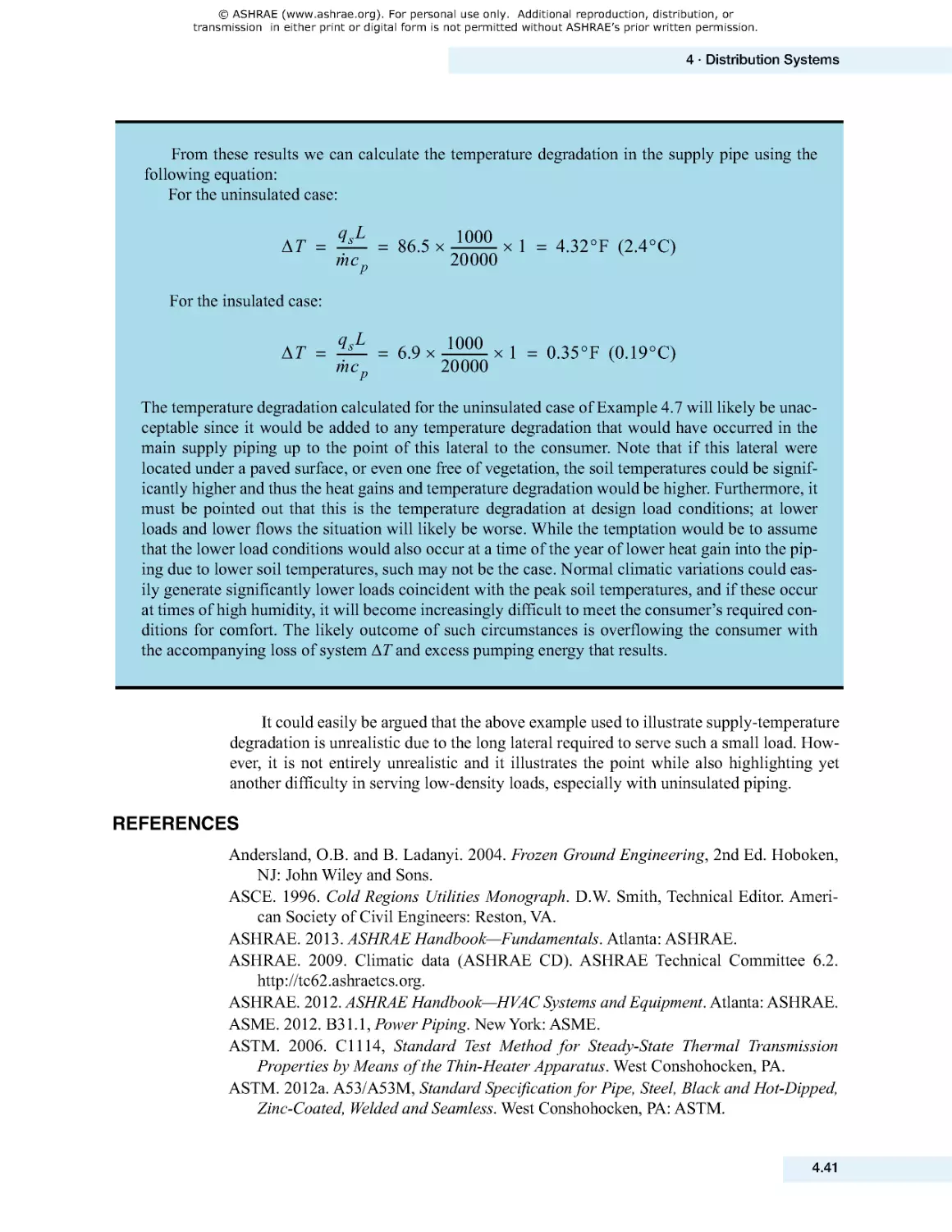
Complete Design Guide for District Cooling Systems
District Cooling Guide provides design guidance for all major aspects of district cooling
systems, including central chiller plants, chilled-water distribution systems, and consumer
interconnection. It draws on the expertise of an extremely diverse international team with
current involvement in the industry and hundreds of years of combined experience.
In addition to design guidance, this book also includes a chapter dedicated to planning, with
additional information on system enhancements and the integration of thermal storage into
a district cooling system. Guidance on operations and maintenance, including several case
studies, is provided to help operators ensure that systems function as intended. Finally, for
those interested in a more in-depth analysis, District Cooling Guide contains a wealth of
references to information sources and publications where additional details may be found.
This guide will be a useful resource for both the inexperienced designer as well as those
immersed in the industry, such as consulting engineers with campus specialization, utility
engineers, district cooling system operating engineers, central plant design engineers, and
chilled-water system designers.
9 781936 504428
ISBN 978-1-936504-42-8
Product code: 90560 8/13
ASHRAE_DC_Guide_On-Template.indd 1
7/30/2013 8:42:37 AM
This publication was developed as a result of ASHRAE Research Project RP-1267, under the auspices of
ASHRAE Technical Committee 6.2, District Energy, and Special Project 97.
CONTRIBUTORS
Gary Phetteplace, PhD, PE (Principal Investigator)
(Chapters 1,2, 3, 4, 5, 8, 9)
GWA Research LLC
Lyme, NH
Salah Abdullah
(Chapter 7)
Allied Consultants Ltd.
Laselky, Maadi, Cairo
John Andrepont
(Chapter 6)
The Cool Solutions Company
Lisle, IL
Donald Bahnfleth, PE
(Chapter 2)
Bahnfleth Group Advisors LLC
Cincinnati, OH
Ahmed A. Ghani
(Chapters 3, 7)
Allied Consultants Ltd.
Laselky, Maadi, Cairo
Vernon Meyer, PE
(Chapters 4)
Heat Distribution Solutions
Omaha, NE
Steve Tredinnick, PE, CEM
(Chapters 2, 3, 5)
(volunteer contributor)
Syska Hennessy Group, Inc.
Verona, WI
It is not a consensus document.
PROJECT MONITORING COMMITTEE
Steve Tredinnick, PE, CEM (Chair)
Syska Hennessy Group, Inc.
Verona, WI
Moustapha Assayed
EMPOWER Energy Solutions
Dubai, United Arab Emirates
Lucas Hyman, PE
Goss Engineering, Inc.
Corona, CA
Samer Khoudeir
EMPOWER Energy Solutions
Dubai, United Arab Emirates
Victor Penar, PE
Hanover Park, IL
David W. Wade, PE
RDA Engineering, Inc.
Marietta, GA
EX-OFFICIO REVIEWER
Kevin Rafferty, PE
Modoc Point Engineering
Klamath Falls, OR
SUPPLEMENTAL FUNDING
EMPOWER Energy Solutions
Dubai, United Arab Emirates
Updates/errata for this publication will be posted on the
ASHRAE Web site at www.ashrae.org/publicationupdates.
Front1.fm Page ii Monday, July 29, 2013 2:11 PM
© ASHRAE (www.ashrae.org). For personal use only. Additional reproduction, distribution, or
transmission in either print or digital form is not permitted without ASHRAE’s prior written permission.
District
Cooling
Guide
Front1.fm Page iii Monday, July 29, 2013 2:11 PM
© ASHRAE (www.ashrae.org). For personal use only. Additional reproduction, distribution, or
transmission in either print or digital form is not permitted without ASHRAE’s prior written permission.
ISBN 978-1 -936504-42 -8
© 2013 ASHRAE
1791 Tullie Circle, NE
Atlanta, GA 30329
www.ashrae.org
All rights reserved.
Cover design by Laura Haass.
ASHRAE is a registered trademark in the U.S . Patent and Trademark Office, owned by the
American Society of Heating, Refrigerating, and Air-Conditioning Engineers, Inc.
ASHRAE has compiled this publication with care, but ASHRAE has not investigated, and
ASHRAE expressly disclaims any duty to investigate, any product, service, process, proce-
dure, design, or the like that may be described herein. The appearance of any technical data or
editorial material in this publication does not constitute endorsement, warranty, or guaranty by
ASHRAE of any product, service, process, procedure, design, or the like. ASHRAE does not
warrant that the information in the publication is free of errors, and ASHRAE does not neces-
sarily agree with any statement or opinion in this publication. The entire risk of the use of any
information in this publication is assumed by the user.
No part of this publication may be reproduced without permission in writing from ASHRAE,
except by a reviewer who may quote brief passages or reproduce illustrations in a review with
appropriate credit, nor may any part of this publication be reproduced, stored in a retrieval sys-
tem, or transmitted in any way or by any means—electronic, photocopying, recording, or
other—without permission in writing from ASHRAE. Requests for permission should be sub-
mitted at www.ashrae.org/permissions.
Library of Congress Cataloging-in-Publication Data
District cooling guide.
pages cm
Includes bibliographical references.
Summary: "Provides guidance for the major aspects of district cooling system design for inexperienced designers and
offers a comprehensive reference for those immersed in the district cooling industry; also includes information on
operations and maintenance and comprehensive terminology for district cooling"-- Provided by publisher.
ISBN 978-1 -936504-42 -8 (softcover)
1. Air conditioning from central stations--Handbooks, manuals, etc. I. American Society of Heating, Refrigerating and
Air-Conditioning Engineers.
TH7687.75 .D47 2013
697.9'3--dc23
2013012051
ASHRAE Staff Special Publications Mark S. Owen, Editor/Group Manager of Handbook and Special Publications
Cindy Sheffield Michaels, Managing Editor
James Madison Walker, Associate Editor
Roberta Hirschbuehler, Assistant Editor
Sarah Boyle, Editorial Assistant
Michshell Phillips, Editorial Coordinator
Publishing Services David Soltis, Group Manager of Publishing Services and Electronic Communications
Jayne Jackson, Publication Traffic Administrator
Tracy Becker, Graphics Specialist
Publisher
W. Stephen Comstock
Front1.fm Page iv Monday, July 29, 2013 2:11 PM
© ASHRAE (www.ashrae.org). For personal use only. Additional reproduction, distribution, or
transmission in either print or digital form is not permitted without ASHRAE’s prior written permission.
Acknowledgments.................................................................................................................... xi
Acronyms ............................................................................................................................... xiii
Purpose and Scope ............................................................................................................... 1.1
District Cooling Background ................................................................................................. 1.1
Applicability .......................................................................................................................... 1.1
Components.......................................................................................................................... 1.2
Benefits................................................................................................................................. 1.3
Environmental Benefits ......................................................................................................................1 .3
Economic Benefits .............................................................................................................................1 .3
Typical Applications .............................................................................................................. 1.4
References............................................................................................................................ 1.4
Introduction .......................................................................................................................... 2.1
Establish and Clarify Owner’s Scope .................................................................................... 2.3
Development of the Database ............................................................................................... 2.4
Alternative Development ...................................................................................................... 2.5
Codes and Standards ........................................................................................................................2 .5
Local and Institutional Constraints ...................................................................................................2 .8
Integrated Processes .........................................................................................................................2 .8
Phased Development and Construction ........................................................................................... 2.8
Central Plant Siting ............................................................................................................................2 .8
Chiller Selection .................................................................................................................................2 .9
Chilled-Water Distribution Systems ................................................................................................ 2.10
Construction Considerations and Cost...........................................................................................2 .11
Consumer Interconnection .............................................................................................................. 2.12
Energy Cost ......................................................................................................................................2 .13
Operations and Maintenance Costs ............................................................................................... 2 .14
Economic Analysis and User Rates..................................................................................... 2.14
Conclusions ........................................................................................................................ 2.15
References.......................................................................................................................... 2.19
Chapter 1 · Introduction
Chapter 2 · System Planning
Contents
Front2_TOC.fm Page v Monday, July 29, 2013 2:15 PM
© ASHRAE (www.ashrae.org). For personal use only. Additional reproduction, distribution, or
transmission in either print or digital form is not permitted without ASHRAE’s prior written permission.
vi
District Cooling Guide
Plant Components and Alternative Arrangements ................................................................ 3 .1
Temperature Design Basis for the Central Plant .................................................................. 3 .2
Chiller Basics ........................................................................................................................ 3 .3
Chiller Types....................................................................................................................................... 3.3
Chiller Performance Limitations ........................................................................................................ 3.4
Electrical-Driven Water-Cooled Centrifugal Chillers ........................................................................ 3.8
Engine-Driven Chillers ....................................................................................................................... 3.8
Absorption Chillers ............................................................................................................................ 3.9
Chiller Configuration........................................................................................................... 3.13
Chiller Staging .................................................................................................................... 3.14
Chiller Arrangements and Pumping Configurations ........................................................... 3.15
Chiller Arrangements ....................................................................................................................... 3.15
Circulating Fundamentals................................................................................................................ 3.15
Pumping Schemes .............................................................................................................. 3.20
Plant Pumping .................................................................................................................................. 3.20
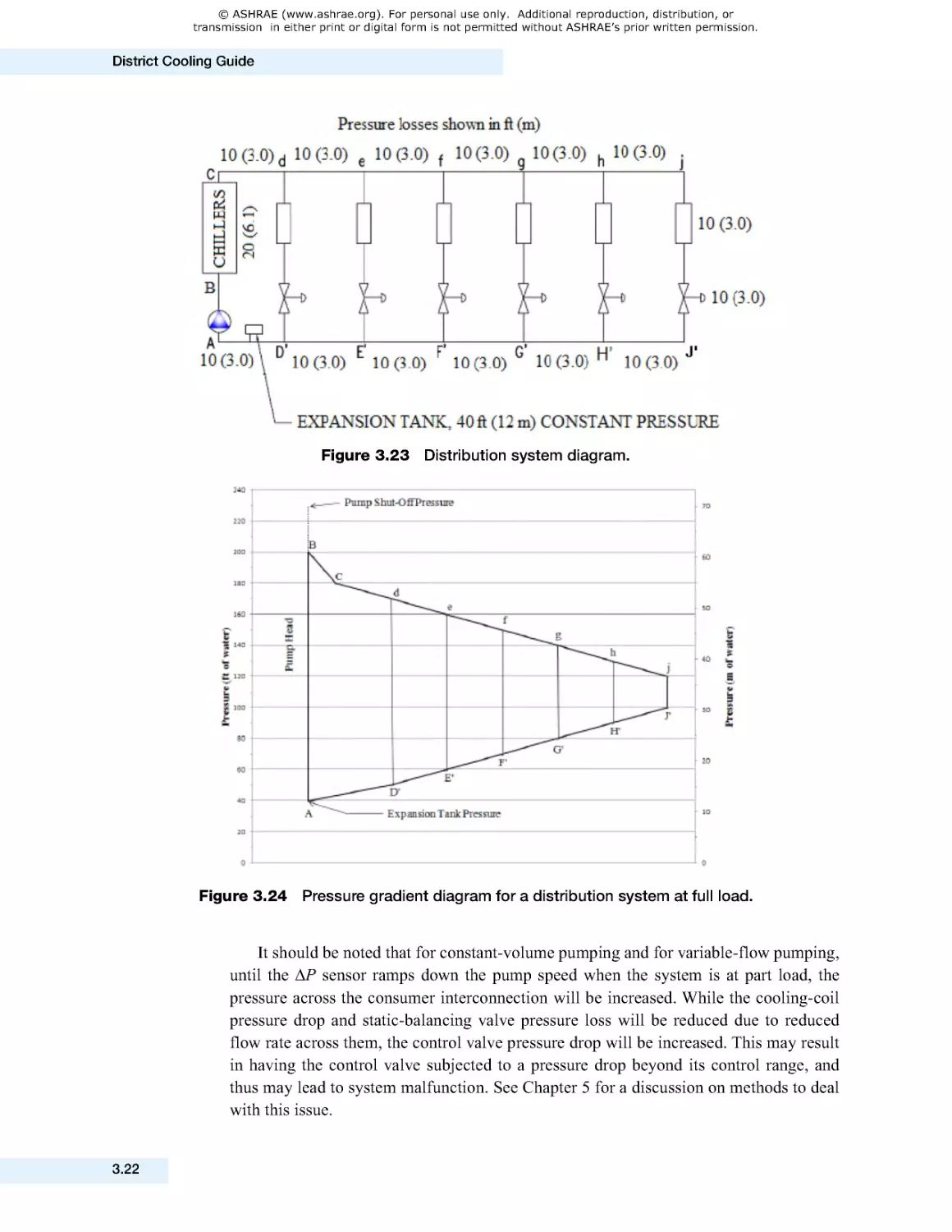
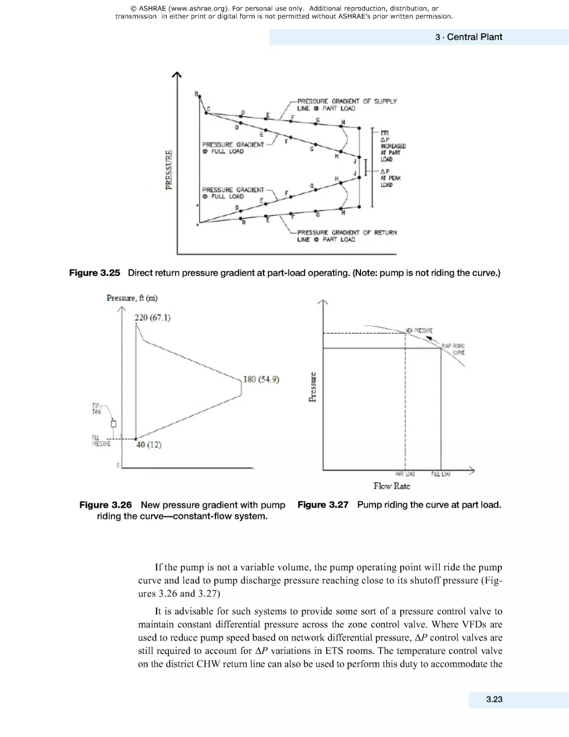
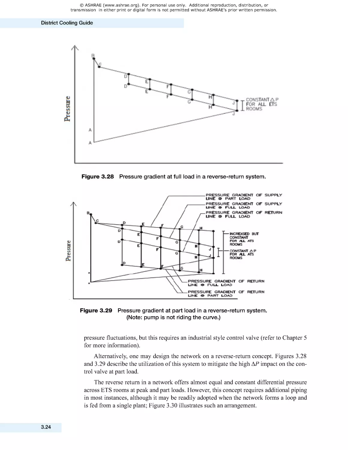
Pressure Gradient in CHW Distribution Systems ........................................................................... 3.21
Distribution Network Pumping System Configurations ................................................................. 3.25
CHW Primary Pumping Configuration ............................................................................................ 3.28
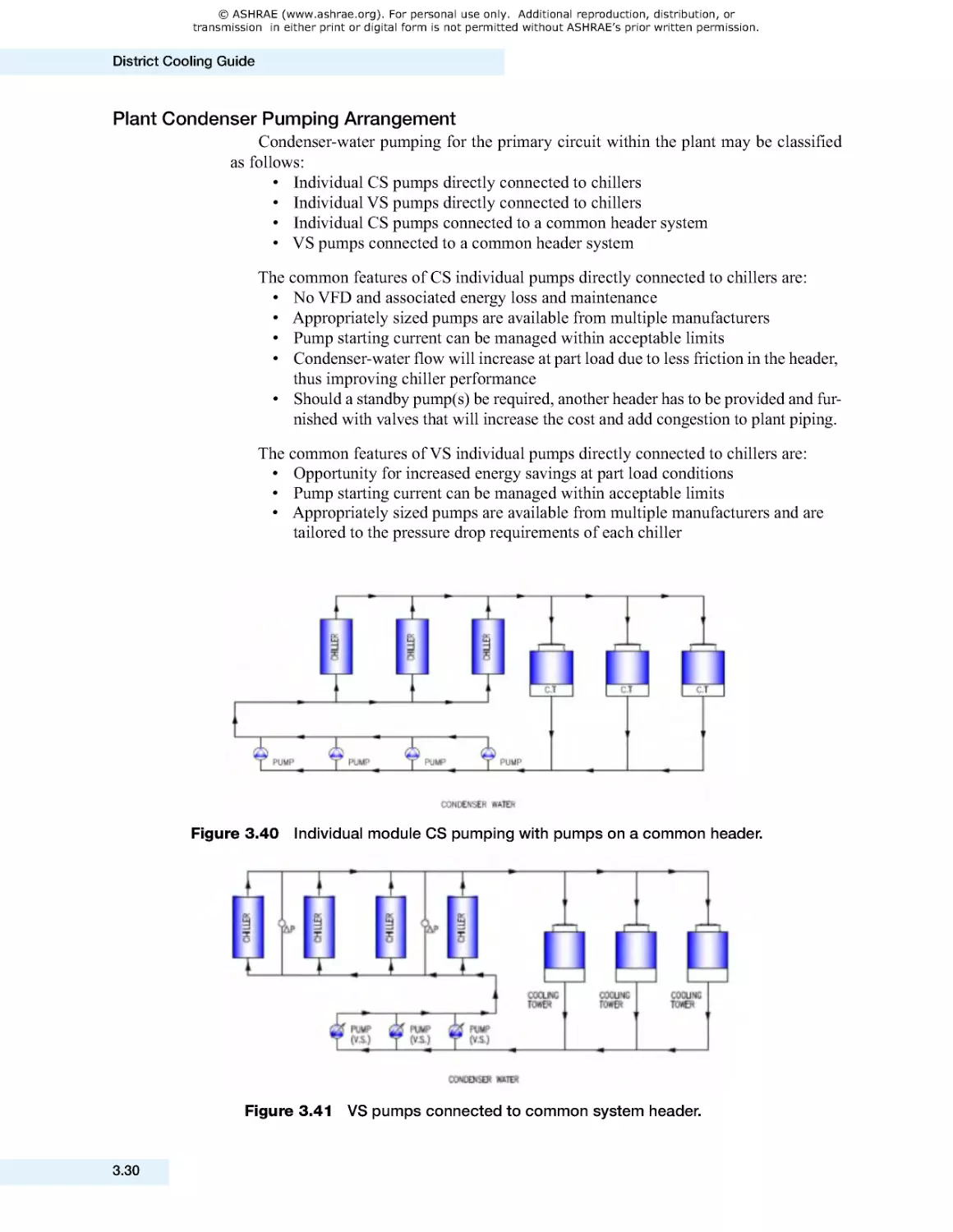
Plant Condenser Pumping Arrangement ........................................................................................ 3.30
Condenser-Water Piping and Pumping for
Unequal Numbers of Chillers and Cooling Towers ........................................................................ 3.31
Pumps .............................................................................................................................................. 3.31
Heat Rejection .................................................................................................................... 3.32
Heat Rejection Equipment ............................................................................................................... 3.33
Condenser Water ................................................................................................................ 3.33
Cooling Towers ................................................................................................................... 3.34
Tower Selection ............................................................................................................................... 3.35
Fan Speed Type ............................................................................................................................... 3.38
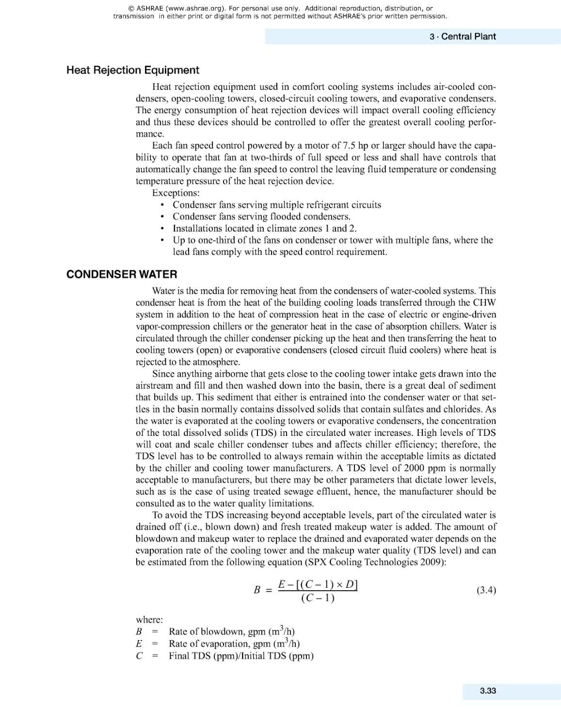
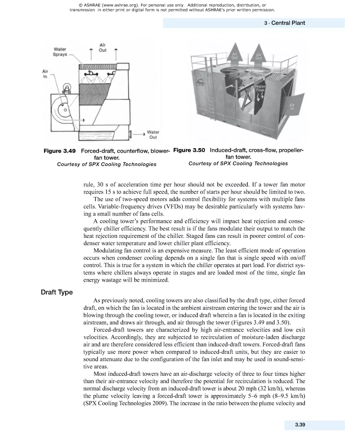
Draft Type ......................................................................................................................................... 3.39
Tower Basin ..................................................................................................................................... 3.40
Tower Fill Options ............................................................................................................................ 3.42
Materials of Construction ................................................................................................................ 3.43
Water Sources.................................................................................................................................. 3.43
Water Filtration Systems..................................................................................................... 3.46
Air Venting .......................................................................................................................... 3.48
Plant Piping and Insulation ................................................................................................. 3.51
Mechanical Room Design ................................................................................................... 3.52
Electrical Room Design....................................................................................................... 3.54
References.......................................................................................................................... 3.55
Bibliography ........................................................................................................................ 3.55
Introduction .......................................................................................................................... 4 .1
Distribution System Types .................................................................................................... 4 .2
Piping and Jacketing Materials............................................................................................. 4 .4
Steel ....................................................................................................................................................4.4
Copper ................................................................................................................................................ 4.6
Ductile Iron ......................................................................................................................................... 4.6
Cementitious Pipe.............................................................................................................................. 4.6
FRP .....................................................................................................................................................4.7
Chapter 3 · Central Plant
Chapter 4 · Distribution Systems
Front2_TOC.fm Page vi Monday, July 29, 2013 2:15 PM
© ASHRAE (www.ashrae.org). For personal use only. Additional reproduction, distribution, or
transmission in either print or digital form is not permitted without ASHRAE’s prior written permission.
Contents
vii
PVC .....................................................................................................................................................4.7
PE and HDPE .....................................................................................................................................4.7
Piping Systems Considerations ............................................................................................ 4.7
Leak Detection .................................................................................................................... 4.11
Cathodic Protection ............................................................................................................ 4.11
Geotechnical Considerations .............................................................................................. 4.13
Valve Vaults and Entry Pits ................................................................................................. 4.14
Valve Vault Issues ............................................................................................................................ 4 .15
Thermal Design Conditions................................................................................................. 4.18
Soil Thermal Properties ...................................................................................................... 4.19
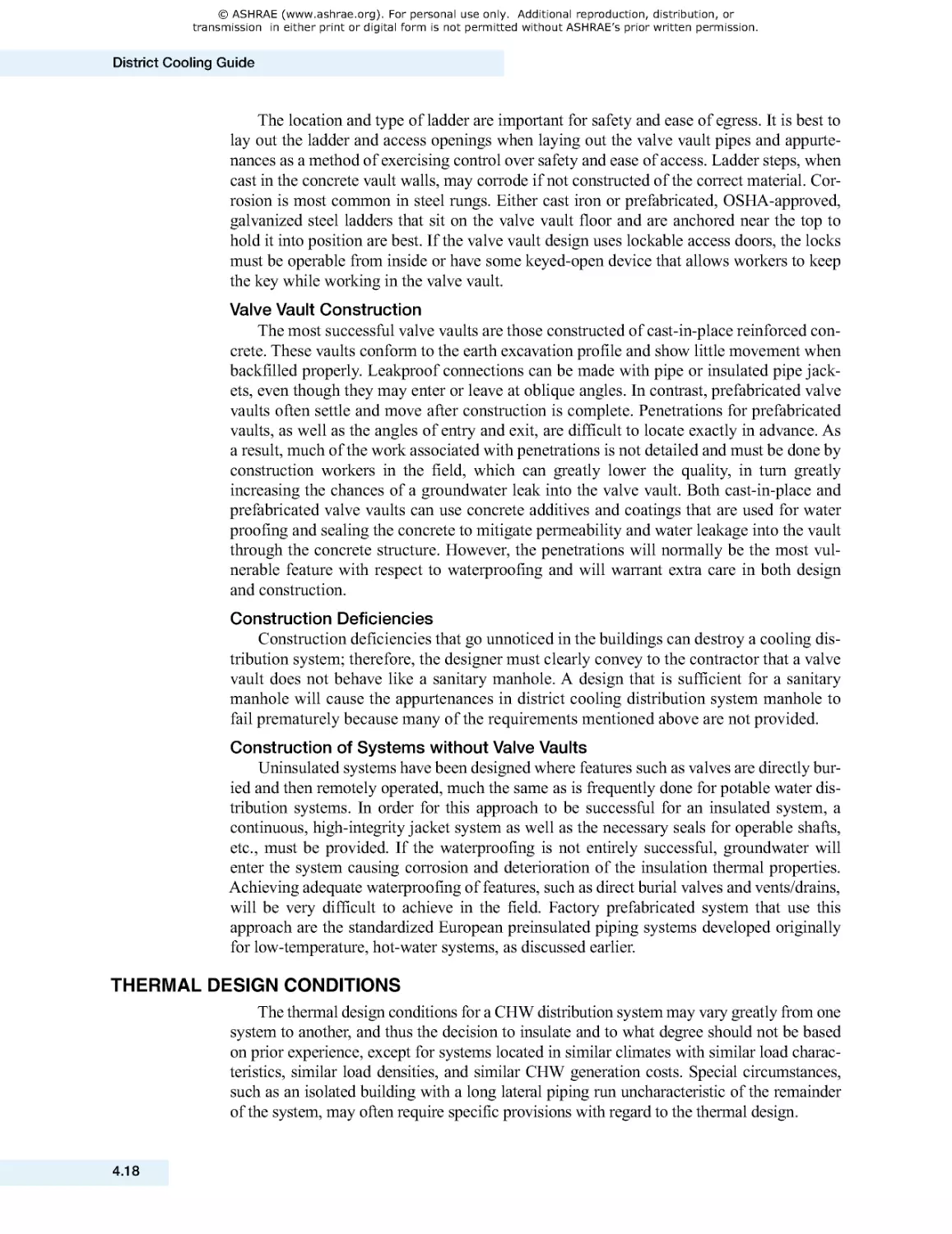
Soil Thermal Conductivity................................................................................................................4 .21
Temperature Effects on Soil Thermal Conductivity and Frost Depth............................................4 .20
Specific Heats of Soils ..................................................................................................................... 4 .21
Undisturbed Soil Temperatures .......................................................................................... 4.22
Heat Transfer at Ground Surface ....................................................................................................4 .24
Insulations and their Thermal Properties ........................................................................... 4.28
Steady-State Heat Gain Calculations for Systems .............................................................. 4.28
Single Un-Insulated Buried Pipe ..................................................................................................... 4 .29
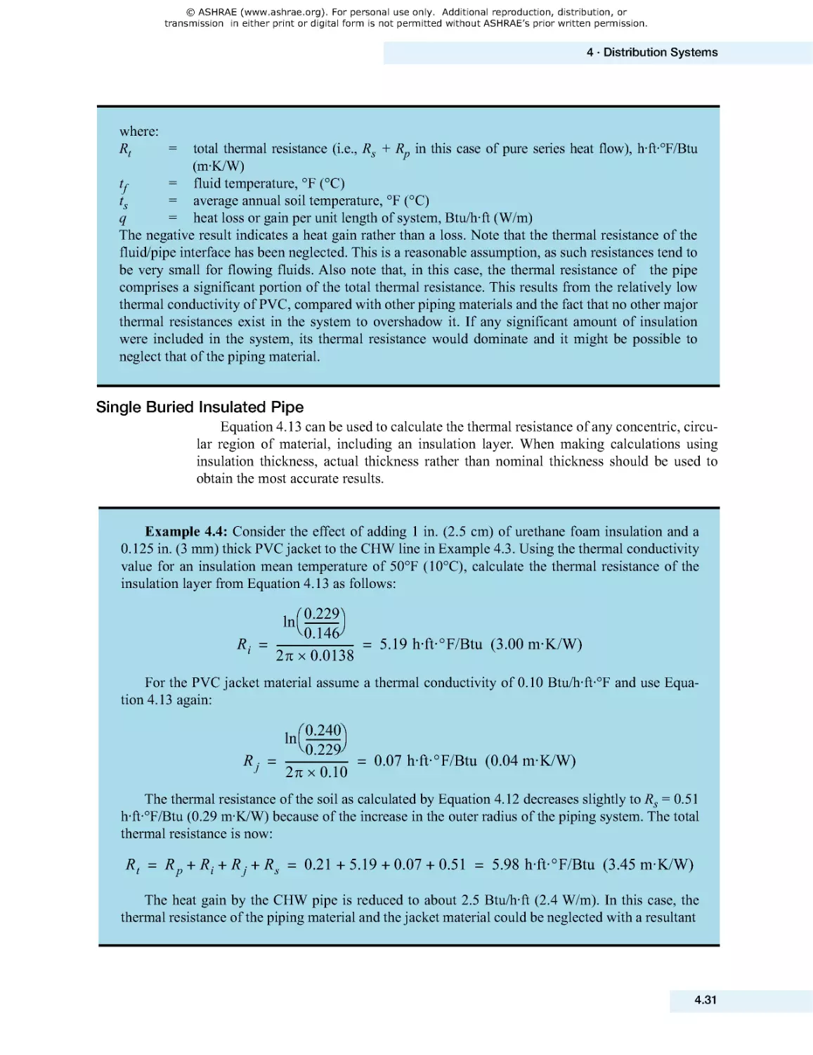
Single Buried Insulated Pipe ........................................................................................................... 4 .31
Two Buried Pipes or Conduits ........................................................................................................ 4 .32
When to Insulate District Cooling Piping ............................................................................ 4.35
Impact of Heat Gain ......................................................................................................................... 4 .35
Cost of Additional Chiller Plant Capacity........................................................................................4 .36
Impacts of Heat Gain on Delivered Supply Water Temperature....................................................4 .39
References.......................................................................................................................... 4.41
Temperature Differential Control.......................................................................................... 5.1
Connection Types ................................................................................................................. 5.2
Direct Connection ................................................................................................................. 5.3
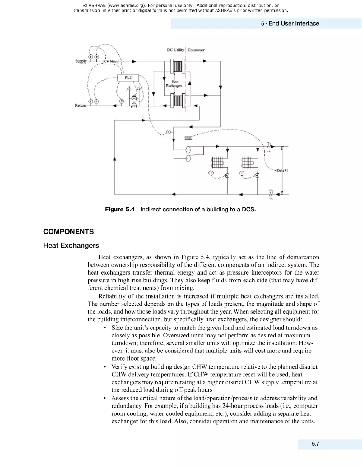
Indirect Connection ........................................................................................................................... 5.6
Components.......................................................................................................................... 5.7
Heat Exchangers ................................................................................................................................ 5.7
Flow Control Devices ....................................................................................................................... 5 .11
Instrumentation and Control............................................................................................................5 .12
Temperature Measurement .............................................................................................................5 .13
Pressure Measurement....................................................................................................................5 .13
Pressure Control Devices ................................................................................................................ 5 .14
Metering.............................................................................................................................. 5.14
References.......................................................................................................................... 5.16
Overview of TES Technology and Systems for District Cooling ............................................ 6.1
TES Technology Types .......................................................................................................... 6.4
Latent Heat TES .................................................................................................................................6.4
Sensible Heat TES .............................................................................................................................6.7
Comparing TES Technologies ......................................................................................................... 6 .10
Drivers for and Benefits of Employing TES in Distict Cooling Systems .............................. 6.10
Primary Benefits of Using TES in District Cooling Systems ..........................................................6 .10
Potential Secondary Benefits of Using TES in District Cooling Systems......................................6 .11
Chapter 5 · END USER INTERFACE
Chapter 6 · THERMAL ENERGY STORAGE
Front2_TOC.fm Page vii Monday, July 29, 2013 2:15 PM
© ASHRAE (www.ashrae.org). For personal use only. Additional reproduction, distribution, or
transmission in either print or digital form is not permitted without ASHRAE’s prior written permission.
viii
District Cooling Guide
System Integration.............................................................................................................. 6.12
Location of TES Equipment ............................................................................................................. 6.12
Hydraulic Integration of TES ........................................................................................................... 6.14
Sizing and Operation of TES ............................................................................................... 6.17
Full versus Partial-shift TES Systems ............................................................................................. 6.17
Daily versus Weekly Cycle TES Configurations ............................................................................. 6.19
TES Control ...................................................................................................................................... 6.19
Economics of TES in District Cooling ................................................................................. 6.20
Capital Costs .................................................................................................................................... 6.20
An Actual Case Study of TES for District Cooling,
with Economics (Andrepont and Kohlenberg 2005)...................................................................... 6.21
References.......................................................................................................................... 6.22
Bibliography ........................................................................................................................ 6.23
General ................................................................................................................................. 7 .1
BMS or SCADA? .................................................................................................................... 7 .1
Major Differences ............................................................................................................................... 7.1
Summary ............................................................................................................................................7.2
System Components ............................................................................................................. 7 .2
Management Layer ............................................................................................................................ 7.3
Communication Layer ........................................................................................................................ 7.3
Automation Layer ............................................................................................................................... 7.3
Field Instruments Layer ..................................................................................................................... 7.4
System Configuration ........................................................................................................... 7 .5
System Structure ............................................................................................................................... 7.5
Plant Control Room ........................................................................................................................... 7.6
System Features and Capabilities .................................................................................................... 7.7
Operation Philosophy............................................................................................................ 7 .8
The ICMS for Plant Management ......................................................................................................7.8
Control Philosophy Statement ..........................................................................................................7.8
ICMS Global Monitoring and Alarming Procedure ......................................................................... 7.12
Interface with BMS .......................................................................................................................... 7.13
Rotation Sequence .......................................................................................................................... 7.13
Energy and Operational Considerations ............................................................................. 7.14
Condenser-Water Return Temperature Setpoint Reset ................................................................. 7.14
CHWS Temperature Setpoint Reset ............................................................................................... 7.14
TES Tanks ........................................................................................................................................ 7.15
Introduction .......................................................................................................................... 8 .1
Workplace Safety .................................................................................................................. 8 .1
Security................................................................................................................................. 8 .2
Water Treatment ................................................................................................................... 8 .2
Corrosion ............................................................................................................................................ 8.2
Corrosion Protection and Preventive Measures .............................................................................. 8.3
White Rust on Galvanized Steel Cooling Towers ............................................................................. 8.4
Scale Control ........................................................................................................................ 8 .5
Nonchemical Methods ....................................................................................................................... 8.6
External Treatments........................................................................................................................... 8.6
Chapter 7 · INSTRUMENTATION AND CONTROLS
Chapter 8 · OPERATION AND MAINTENANCE
Front2_TOC.fm Page viii Monday, July 29, 2013 2:15 PM
© ASHRAE (www.ashrae.org). For personal use only. Additional reproduction, distribution, or
transmission in either print or digital form is not permitted without ASHRAE’s prior written permission.
Contents
ix
Biological Growth Control ..................................................................................................... 8.6
Control Measures............................................................................................................................... 8.7
Legionnaires’ Disease...................................................................................................................... 8 .10
Suspended Solids and Deposition Control .......................................................................... 8.10
Mechanical Filtration........................................................................................................................ 8 .11
Selection of Water Treatment ............................................................................................. 8.14
Once-Through Systems (Seawater or Surface Water Cooling) .....................................................8 .14
Open Recirculating Systems (Cooling Towers) ..............................................................................8 .14
Closed Recirculating Systems (Distribution System) .....................................................................8 .15
European Practice in Closed Distribution Systems .......................................................................8 .16
Water Treatment in Steam Systems ...............................................................................................8 .16
Maintenance ....................................................................................................................... 8.16
References.......................................................................................................................... 8.17
Integration with Heating and Power Generation ................................................................... 9.1
Unconventional Working Fluids ............................................................................................ 9.2
References............................................................................................................................ 9.3
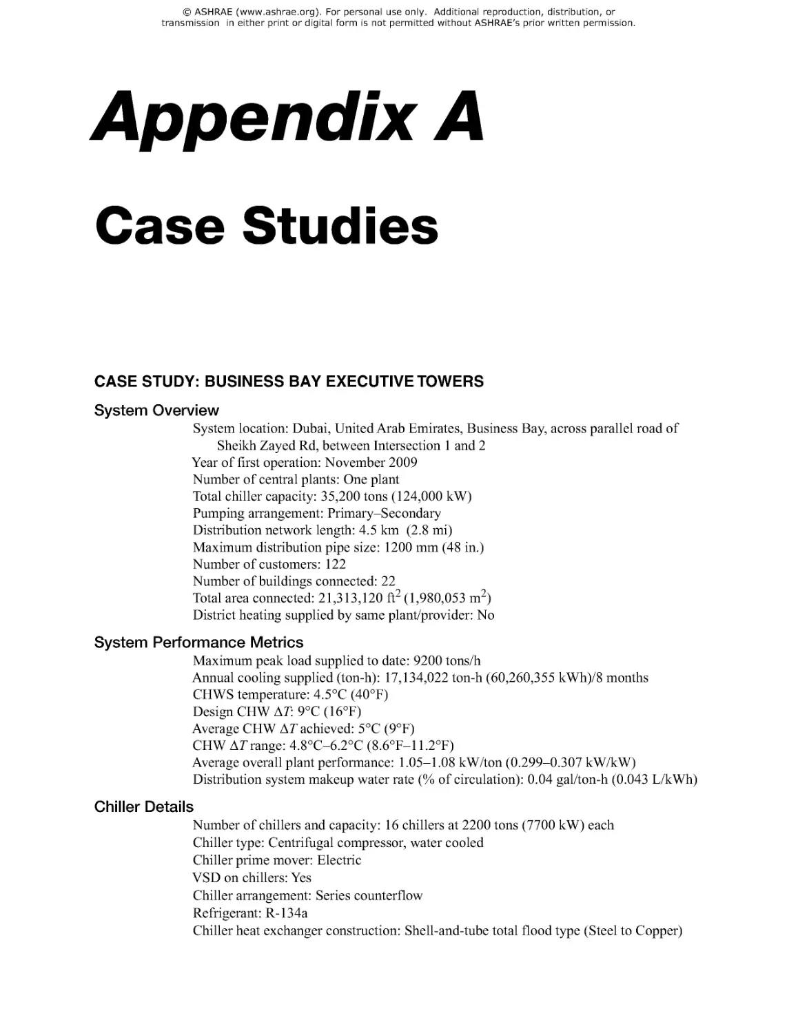
Case Study: Business Bay Executive Towers ....................................................................... A.1
System Overview .............................................................................................................................. A .1
System Performance Metrics ........................................................................................................... A .1
Chiller Details .................................................................................................................................... A .1
Pumping ........................................................................................................................................... A .2
Water Treatment ............................................................................................................................... A .2
Cooling Towers ................................................................................................................................. A .2
Distribution System........................................................................................................................... A .2
Consumer Interconnect .................................................................................................................... A .3
Special Features ............................................................................................................................... A .3
Contact for More Information ........................................................................................................... A .3
Case Study: Texas Medical Center ....................................................................................... A.4
System Overview .............................................................................................................................. A .4
System Performance Metrics ........................................................................................................... A .4
Chiller Details .................................................................................................................................... A .4
Pumping ............................................................................................................................................ A .4
Water Treatment ............................................................................................................................... A .4
Cooling Towers ................................................................................................................................. A .4
Thermal Storage................................................................................................................................ A .5
Distribution System........................................................................................................................... A .5
Consumer Interconnect .................................................................................................................... A .5
Special Features ............................................................................................................................... A .5
Contact for More Information ........................................................................................................... A .5
Case Study: District Cooling St. Paul .................................................................................... A.7
System Overview .............................................................................................................................. A .7
System Performance Metrics ........................................................................................................... A .7
Electric Details .................................................................................................................................. A .7
Chiller Details .................................................................................................................................... A .7
Water Treatment ............................................................................................................................... A .7
Cooling Towers ................................................................................................................................ A .7
Thermal Storage................................................................................................................................ A .7
Chapter 9 · SYSTEM ENHANCEMENTS
Appendix A · CASE STUDIES
Front2_TOC.fm Page ix Monday, July 29, 2013 2:15 PM
© ASHRAE (www.ashrae.org). For personal use only. Additional reproduction, distribution, or
transmission in either print or digital form is not permitted without ASHRAE’s prior written permission.
x
District Cooling Guide
Distribution System........................................................................................................................... A .8
Consumer Interconnect .................................................................................................................... A .8
Special Features ............................................................................................................................... A .8
Environmental and Economic Benefits ............................................................................................ A .8
Published Articles on the System or Websites with Details ........................................................... A .8
Contact for More Information ........................................................................................................... A .8
.... ...... ...... ...... ...... ...... ...... ...... ...... ...... ...... ...... ...... ...... ...... ...... ...... ...... ...... ...... ...... ....... ...... ..... B.1
Appendix B · TERMINOLOGY FOR DISTRICT COOLING
Front2_TOC.fm Page x Monday, July 29, 2013 2:15 PM
© ASHRAE (www.ashrae.org). For personal use only. Additional reproduction, distribution, or
transmission in either print or digital form is not permitted without ASHRAE’s prior written permission.
The principal investigator and authors would like to thank the members of the Project
Monitoring Subcommittee (PMS) for their patience through the long process of creating
this document. This includes many discussions of scope and content as well as the actual
review. This document has benefited tremendously from the careful review of the PMS
members and their many suggestions based on the vast and diverse knowledge of district
heating that their composite experience represents.
The chair of the PMS, Steve Tredinnick, deserves special recognition for the count-
less hours he has invested in this effort both in his role as the PMS chair and as a major
unpaid contributor and a sounding board for the principal investigator.
Gary Phetteplace
January 2013
Acknowledgments
Front3_Acknowledgments.fm Page xi Monday, July 29, 2013 2:25 PM
© ASHRAE (www.ashrae.org). For personal use only. Additional reproduction, distribution, or
transmission in either print or digital form is not permitted without ASHRAE’s prior written permission.
ABS
acrylonitrile butadiene styrene
AEE
Association of Energy Engineers
AFD
adjustable-frequency drive
AHRI
Air-Conditioning, Heating, and Refrigeration Institute
ASME
American Society of Mechanical Engineers
ASCE
American Society of Civil Engineers
BOD
biochemical oxygen demand
BMS
building management systems
CFU
colony-forming unit
CEC
California Energy Commission
CEN
European Committee for Standardization
CFD
computational fluid dynamics
CHP
combined heat & power
CHW
chilled water
CHWS
chilled-water supply
CHWR
chilled-water return
COD
chemical oxygen demand
COWS
central operator workstation
CPVC
chlorinated polyvinylchloride
CT
cooling tower
COP
coefficient of performance
CS
constant speed
CTI
Cooling Tower Institute
CUP
central utility plant
DC
district cooling
DCP
district cooling plant
DCS
district cooling systems
DPS
distribution piping system
DSM
demand-side management
EPRI
Electric Power Research Institute
EMS
energy monitoring/control system
ETS
energy transfer station
EOR
engineer of record
Acronyms
Acronyms.fm Page xiii Monday, July 29, 2013 2:26 PM
© ASHRAE (www.ashrae.org). For personal use only. Additional reproduction, distribution, or
transmission in either print or digital form is not permitted without ASHRAE’s prior written permission.
xiv
District Cooling Guide
FM
factory mutual
FRP
fiberglass-reinforced plastic
HDPE
high-density polyethylene
HMI
human-machine interface
IEA
International Energy Agency
IDEA
International District Energy Association
LTF
low temperature fluid
MEP
mechanical, electrical, and plumbing
MF
micron filter
DDC
direct digital control
NACE
National Association of Corrosion Engineers
NIST
National Institute of Standards and Technology
NDT
nondestructive testing
NOVEM
Netherlands Agency for Energy and Environment
NPS
nominal pipe size
NPSH
net-positive suction head
OSHA
Occupational Safety and Health Administration
O&M
operations and maintenance costs
OR̄
hypohalous ion form
PWT
physical water treatment
PVC
polyvinylchloride
PICV
pressure independent control valve
PSV
pressure sustaining valve
PVC
polyvinyl chloride
RTD
resistive temperature detector
RTP
real time pricing
RTU
remote terminal units
SBS
sodioum bisulfite
SCADA
supervisory control and data acquisition
SOX
sulfur oxide
SS
suspended solids
TDR
time domain reflectometry
TDS
total dissolved solids
TES
thermal energy storage
THPS
tetrakis(hydroxymethyl)phosphonium sulfate
TSE
treated sewage effluent
TIC
turbine inlet cooling
UF
ultra filter
UV
ultra violet
VFD
variable frequency drive
VS
variable speed
WEEC
World Energy Engineering Congress
WBDG
Whole Building Design Guide
Acronyms.fm Page xiv Monday, July 29, 2013 2:26 PM
© ASHRAE (www.ashrae.org). For personal use only. Additional reproduction, distribution, or
transmission in either print or digital form is not permitted without ASHRAE’s prior written permission.
PURPOSE AND SCOPE
The purpose of this design guide is to provide guidance for all major aspects of dis-
trict cooling system (DCS) design. The guidance is organized to be of use to both the
inexperienced designer of DCSs as well as to provide a comprehensive reference to those
immersed in the district cooling industry. In addition to design guidance, information on
operations and maintenance have also been included.
DISTRICT COOLING BACKGROUND
District cooling (DC) normally distributes thermal energy in the form of chilled water
from a central source to residential, commercial, institutional, and/or industrial consum-
ers for use in space cooling and dehumidification. Thus, cooling effect comes from a dis-
tribution medium rather than being generated on site at each facility.
Whether the system is a public utility or user owned, such as a multibuilding campus,
it has economic and environmental benefits depending largely on the particular applica-
tion. Political feasibility must be considered, particularly if a municipality or governmen-
tal body is considering a DC installation. Historically, successful DCSs have had the
political backing and support of the community.
Early attempts at district cooling date back to the 1880s (Pierce 1994). By the 1930s
commercial systems were being built (Pierce 1994). While development in district cool-
ing had been confined mostly to the United States in recent years, there has been
increased activity outside of the US, notably in the Middle East and in Europe. The Inter-
national District Energy Association that represent both heating and cooling utilities,
reports (IDEA 2008a) that approximately 86% of the conditioned building space added
by its members was added outside of the United States; all of that growth was district
cooling in the Middle East.
APPLICABILITY
DCSs are best used in markets where the thermal load density is high and the number
of equivalent full load hours of cooling (or operating hours) is high. A high load density is
needed to cover the capital investment for the transmission and distribution system, which
usually constitutes a significant portion of the capital cost for the overall system, often
amounting to 50% or more of the total cost. This makes DCSs most attractive in serving
densely populated urban areas and high-density building clusters with high thermal loads,
especially tall buildings. Urban settings where real estate is very valuable are good places
1
Introduction
Chapter 1.fm Page 1 Monday, July 29, 2013 2:27 PM
© ASHRAE (www.ashrae.org). For personal use only. Additional reproduction, distribution, or
transmission in either print or digital form is not permitted without ASHRAE’s prior written permission.
1.2
District Cooling Guide
for DCSs since they allow building owners to make maximum use of their footprint by
moving most of the cooling equipment off-site. Low-density residential areas have usually
not been attractive markets for district cooling. The equivalent full load hours of cooling are
important because the DCS is capital intensive and maximum use of the equipment is nec-
essary for cost recovery.
COMPONENTS
DCSs consist of three primary components: the central plant(s), the distribution net-
work, and the consumer systems or customer’s interconnection (i.e ., energy transfer sta-
tion or ETS); see
Figure 1.1 District cooling system.
Figure 1.1 . In the central plant (see Chapter 3) chilled water is produced
by one or more of the following methods:
•
Absorption refrigeration machines
•
Electric-driven compression equipment (reciprocating, rotary screw, or centrifu-
gal chillers)
•
Gas/steam turbine or engine-driven compression equipment
•
Combination of mechanically driven systems and thermal energy driven absorp-
tion systems
The second component is the distribution or piping network that conveys the chilled
water (see Chapter 4). The piping may be the most expensive portion of a DCS. Chilled-water
piping usually consists of uninsulated or preinsulated directly buried systems. These networks
require substantial permitting and coordinating with nonusers of the system for right-of-way
if the networks are not on the owner’s property. Because the initial cost is high, it is important
to maximize the use of the distribution piping network.
The third component is the consumer interconnection to the district cooling distribu-
tion system, which includes in-building equipment. Chilled water may be used directly by
the building systems or isolated indirectly by a heat exchanger (see Chapter 5).
Chapter 1.fm Page 2 Monday, July 29, 2013 2:27 PM
© ASHRAE (www.ashrae.org). For personal use only. Additional reproduction, distribution, or
transmission in either print or digital form is not permitted without ASHRAE’s prior written permission.
1·Introduction
1.3
BENEFITS
Environmental Benefits
Generating chilled water in a central plant is normally more efficient than using in-building
equipment (i.e., decentralized approach) and thus the environmental impacts are normally
reduced. The greater efficiencies arise due to the larger, more efficient equipment and the ability
to stage that equipment to closely match the load yet remain within the equipment’s range of
highest efficiency. DCSs may take advantage of diversity of demand across all users in the sys-
tem and may also implement technologies such as thermal storage more readily than individual
building cooling systems. For electric-driven district cooling plants, higher efficiency becomes
the central environmental benefit since in-building plants are normally electric driven as well.
There may be additional environmental benefits from cooling supplied from a large central
plant, such as the ability to use treated sewage effluent as cooling tower makeup water and the
ability to handle refrigerants in a safer and more controlled environment.
When fuels are burned to generate cooling via absorption or gas/steam turbine and/or
engine-driven chillers, emissions from central plants are easier to control than those from
individual plants, and on an aggregate generate less pollutants due to higher quality of
equipment, higher seasonal efficiencies, and higher level of maintenance. A central plant
that burns high-sulfur coal can economically remove noxious sulfur emissions, where
individual combustors could not. Similarly, the thermal energy from municipal wastes can
provide an environmentally sound system, an option not likely to be available on a build-
ing scale system.
Refrigerants and other chemicals can be monitored and controlled more readily in a
central plant. Where site conditions allow, remote location of the plant reduces many of
the concerns with the use of ammonia systems for cooling.
Economic Benefits
A DCS offers many economic benefits. Even though the basic costs are still borne by
the central plant owner/operator, because the central plant is large, the customer can real-
ize benefits of economies of scale.
Operating Personnel
One of the primary advantages for a building owner is that operating personnel for the
HVAC system can be reduced or eliminated. Most municipal codes require operating
engineers to be on site when high-pressure boilers, as would be used to drive absorption
chillers, are in operation. Some older systems require trained operating personnel to be in
the boiler/mechanical room at all times. When chilled water is brought into the building
as a utility, depending on the sophistication of the building HVAC controls, there will
likely be opportunity to reduce or eliminate operating personnel.
Insurance
Both property and liability insurance costs may be significantly reduced with the
elimination of boilers, chillers, pumps, and electrical switch gear from within the building
since risk of a fire or accident is reduced.
Usable Space
Usable space in the building increases when a boiler and/or chiller and related equip-
ment are no longer necessary. The noise associated with such in-building equipment is
also eliminated. In retrofit applications, this space cannot usually be converted into prime
office space, however it does provide the opportunity for increased storage or other use.
Chapter 1.fm Page 3 Monday, July 29, 2013 2:27 PM
© ASHRAE (www.ashrae.org). For personal use only. Additional reproduction, distribution, or
transmission in either print or digital form is not permitted without ASHRAE’s prior written permission.
1.4
District Cooling Guide
Equipment Maintenance
With less mechanical equipment, there is proportionately less equipment mainte-
nance, resulting in less expense and a reduced maintenance staff.
Higher Efficiency
A larger central plant can achieve higher thermal and emission efficiencies than can
several smaller units. When strict regulations must be met for emissions, water consump-
tion, etc., control equipment is also more economical for larger plants. Partial load perfor-
mance of central plants may be more efficient than that of many isolated small systems
because the larger plant can modulate output and operate one or more capacity modules
as the combined load requires. While a recent study (Thornton et al. 2008) found that
actual operating data on in-building cooling plants is scarce, the limited data the study
uncovered indicates that in-building systems were operating at an average efficiency of
1.2 kW/ton (2.9 COP). Another study (Erpelding 2007) found that central district cooling
plants can have efficiencies of 0.85 kW/ton (4.1 COP) under less than optimal design/
operation. Thus, the efficiency of chilled water generation in a central plant is approxi-
mately 40% greater than an in-building chiller plant. Others (IDEA 2008b) have sug-
gested much greater efficiency improvements relative to air-cooled in-building cooling
systems, i.e ., approximately 1.65 kW/ton (2.1 COP) for air-cooled in-building systems
versus approximately 0.70 kW/ton (5.0 COP) for electric-driven district cooling with
thermal storage, an increase in efficiency of nearly 140% for district cooling.
Similarly, typically industrial based controls systems are used that offer a higher level
of controls and monitoring of the overall system and efficiency as compared to commer-
cial decentralized cooling systems. Furthermore, with the higher level of monitoring
comes additional scrutiny in operations to optimize the system performance and effi-
ciency resulting in reduced operating costs.
Available Primary Energy
While on a building scale it may not be practical to generate chilled water via absorption
chillers, this is possible in larger central chiller plants and larger central absorption chiller
plants may even use fuels such as coal or refuse, or multiple fuels. The use of high-voltage
chillers may also be impractical from all but the largest in-building chiller plants.
TYPICAL APPLICATIONS
District cooling has seen a wide variety of applications, and the reader is referred to
IDEA (2008a) for examples. These applications span all major sectors of the building
market: residential, commercial, institutional, and industrial. For many of the applica-
tions, such as college campuses and military bases, the loads are captive. At the opposite
end of the spectrum are DCSs that operate as commercial enterprises in urban areas com-
peting with in-building equipment for cooling loads. Between these two extremes are
many other business models such as district cooling providers, who operate under con-
tract, or a plant owned by the developer of a real estate project. For information on busi-
ness models and business development for district cooling enterprises see IDEA (2008b).
REFERENCES
Erpelding, B. 2007. Real efficiencies of central plants. Heating/Piping/Air-Conditioning
Engineering: May 2007.
IDEA. 2008a. District Energy Space’08. Westborough, MA: International District Energy
Association (IDEA).
IDEA. 2008b. District Cooling Best Practices Guide. Westborough, MA: International
District Energy Association (IDEA).
Chapter 1.fm Page 4 Monday, July 29, 2013 2:27 PM
© ASHRAE (www.ashrae.org). For personal use only. Additional reproduction, distribution, or
transmission in either print or digital form is not permitted without ASHRAE’s prior written permission.
1·Introduction
1.5
Pierce, M. 1994. Competition and cooperation: The growth of district heating and cool-
ing, Proceeding of the International District Energy Association, Westborough, MA:
1182–1917.
Thornton, R., R. Miller, A. Robinson, and K. Gillespie. 2008. Assessing the actual energy
efficiency of building scale cooling systems. Report 8DHC-08 -04, Annex VIII, Inter-
national Energy Agency (IEA), IEA District Heating and Cooling Program. www.iea-
dhc.org.
Chapter 1.fm Page 5 Monday, July 29, 2013 2:27 PM
© ASHRAE (www.ashrae.org). For personal use only. Additional reproduction, distribution, or
transmission in either print or digital form is not permitted without ASHRAE’s prior written permission.
INTRODUCTION
For buildings, the cost of utility services and infrastructure needed to provide these
services is significant and may even exceed the cost of the buildings themselves over their
lifetimes. Planning has the potential to reduce both the initial and future costs. The objec-
tive of planning should be to guide decision making such that cost savings in providing
utilities over the life expectancy of the building(s)/campus/system are realized. Due to
their capital intensive nature, the need for planning is significant for DCSs, and the cur-
rent rate of growth of these systems has made system planning a topic of much current
interest.
The term master plan will be used here, but there are several levels of planning. A
master plan covers all levels of planning and is typically integrated with the planning of
the development of both new and existing sites. Throughout this section, the development
of utility master plans will typically be applicable to private, public, and utility owned
systems. Differences in planning for the different systems will be identified whenever
they are significant.
For totally new systems in a greenfield project, master planning is an essential first
step to assuring that the owner’s requirements are fulfilled in the delivered system.
Appropriate planning will have significant impacts, not just on the first cost of the project,
but also the future operations and maintenance (O&M) costs. The master plan will also
provide valuable information to those responsible for the O&M of the system, and it is
thus essential that the individuals who will be responsible for the O&M of the system be
involved in the planning process. For sites with existing systems/other utilities, involve-
ment of the system operators in the development of a master plan is essential; there is no
substitute for corporate knowledge when dealing with buried systems. A plan properly
prepared will also benefit the users served by the system, and it may be prudent to engage
these representatives in the planning process. Potential stakeholders in the development
of a master plan are:
•
Building/campus/site owner
•
Owner’s project engineer
•
Site master planners
•
Utility system operators
•
Operators/engineers of other utilities on site or within utility right-of-way
2
System Planning
Chapter 2.fm Page 1 Monday, July 29, 2013 2:45 PM
© ASHRAE (www.ashrae.org). For personal use only. Additional reproduction, distribution, or
transmission in either print or digital form is not permitted without ASHRAE’s prior written permission.
2.2
District Cooling Guide
•
Potential contractors
•
District cooling customer (the building’s users)
•
Adjacent residential neighborhood associations and business enterprises
This list is by no means exhaustive; special circumstances could result in many differ-
ent and varied stakeholders. The planning process should include everyone involved in
the design, construction, operation, and use of the facilities provided with district cooling.
Master utility plans for existing facilities also must consider correcting deficiencies
built into them initially or during periods of rapid expansion. Utility plans for existing
systems also must account for the aging of the existing infrastructure and must also con-
sider appropriate timing for replacement and upgrading efforts. Furthermore, building
functions can change over the life of the building, (i.e., college dorms converted to
offices, etc.) therefore the service lines to the building and distribution mains must be of
adequate size to accommodate future facility remodeling or expansion.
Planning is a difficult task that takes time and creative energy to explore the many
variables that must be considered to develop a system that will operate in accordance with
design intent and is: sustainable, reliable, energy efficient, environmentally friendly, sup-
ports expansion to serve new chilled-water (CHW) loads, and is easily operated and
maintained. One additional variable, that may be the most important of all considerations,
is the development of a concept-level budget estimate (opinion of probable cost). Due to
poor preliminary cost estimates, many systems have to be modified with lower quality
materials during the bidding process before construction begins. This ultimately is detri-
mental to the functionality, efficiency, and life expectancy of the system during its entire
operational lifetime. Early planning and concept designs of adequate detail used to
develop more accurate cost estimates can mitigate many of these issues. In this chapter,
guidance will be given for developing a system master plan that is sustainable, meets the
owner’s performance needs and desires, and can be constructed within the owner’s con-
straints for overall capital cost and cash flow.
What should a utility master plan provide an owner? At minimum, a utility master
plan should provide a prioritized program for long term guidance for building, expanding,
and upgrading the district systems, which are typically built incrementally. A good master
plan serves as a technically sound marketing tool for the owner's engineers to present
needs and solutions to management or to prospective customers. Unfortunately many
owners view utility master plans as an interesting technical exercise with a life of one or
two years. When this has been an owner’s experience, it usually results from one or more
of the following reasons:
•
Failure to involve the owner’s staff
•
Failure to provide intermediate owner reviews
•
Use of an unverified database
•
Lack of creativity in developing technically sound system alternatives for
screening and final selection by the owner
•
Inaccurate cost estimation, often related to overly optimistic estimation using
unit costs that do not include all elements of the systems
The process for developing a utility master plan may be likened to a pyramid (Figure
2.1) (Bahnfleth 2004). The success of the plan depends on the foundation, a strong data-
base that includes discovery and verification. The development of a strong and accurate
database is the foundation on which all other aspects of a master plan stand and get their
credibility. With the database in place, the identification of alternatives and the prelimi-
nary estimates of cost (screening grade) for each alternative are used to select (with the
Chapter 2.fm Page 2 Monday, July 29, 2013 2:45 PM
© ASHRAE (www.ashrae.org). For personal use only. Additional reproduction, distribution, or
transmission in either print or digital form is not permitted without ASHRAE’s prior written permission.
2·System Planning
2.3
owner) the most promising alternatives. These alternatives are then subjected to more
intense analysis before making the final decisions of how the new plant (or expansion of
an existing plant) will be developed as well as how plans for future projects will be laid
out. Thus, the pinnacle of the pyramid is a prioritized, priced list of projects needed to
both keep pace with the physical growth of a facility and to provide replacements and
upgrades to the existing system, if there is one.
ESTABLISH AND CLARIFY OWNER’S SCOPE
Before the planning process can begin in earnest, as with every project, the owner’s
scope and expectations for the project must be fully clarified. While a scope may have
been written in the preliminary stages of the owner’s development of the project, often
this scope will need clarification and refinement. Meeting with the owner, the staff who
will inhabit the facilities, those performing the O&M, and those responsible for budgeting
the project and its O&M costs will help clarify and refine the scope and ultimately can
eliminate many potential issues and challenges later. In fact, such open meetings can
bring new insights to the owner, sometimes resulting in a totally new scope being devel-
oped. During the initial scope review, other factors affecting the system planning can be
determined through proper interaction with those present. Among the things that should
be learned are the level of system quality expected, the budget and cash flow limitations,
and the anticipated potential long-term expansion of the system. With the present empha-
sis on sustainability, this is an appropriate time to discuss the owner’s interest and desires
with respect to this important aspect of system design and development.
Throughout the process of establishing and refining the scope, it is paramount that all
parties recognize that every system is subject to three basic constraints: budget (owner’s),
Figure 2.1 The master planning pyramid.
Chapter 2.fm Page 3 Monday, July 29, 2013 2:45 PM
© ASHRAE (www.ashrae.org). For personal use only. Additional reproduction, distribution, or
transmission in either print or digital form is not permitted without ASHRAE’s prior written permission.
2.4
District Cooling Guide
scope limitations (jointly developed by the engineer and the owner), and quality versus
cost (a champagne quality system cannot be built on a beer budget).
DEVELOPMENT OF THE DATABASE
Because gathering information for developing a suitable system-planning database
takes some time from the owner’s staff who already have their regular jobs to do, it is
helpful at the outset to provide a list of information and data that will be required to com-
plete a good system plan. The list includes whatever cooling-load data exists, either in the
form of estimated loads for new buildings to be served by the DCS or recorded-load data
in existing systems. When considering historic cooling-load data it is particularly impor-
tant to bear in mind the bias in recent years towards increased cooling requirements that
have resulted from the combined impacts of increased ventilation rates; increasing elec-
tronics use in offices, dorms, and other spaces; as well as tightening of building envelopes
by retrofit measures.
In existing systems, inventories of available equipment that will become a part of the
new or expanded system must be obtained from the owner’s records and/or by gathering
data from available shop drawings and equipment nameplates. Additionally, condition
assessments of equipment that may be reused in a new system should be conducted.
Equipment condition can be found in maintenance records; code inspections, where
required; and from operating personnel interviews. Site utility maps showing the loca-
tions of existing utilities are essential for planning distribution system routing to avoid
interferences and to minimize the expense of installing tunnels, shallow trenches, or
direct burial piping. The site electrical drawings will identify the location of existing elec-
trical system feeders and available substations. A single-line electrical drawing showing
system loads and feeder capacities among other things should be obtained when avail-
able. As the planning process proceeds, each of these databases will be expanded by the
planning team, but early identification of the need for them can assist in meeting time
deadlines established by the owner.
Estimating cooling loads to establish the CHW production capacity needed during the
life ascribed to the master plan is one task that too often is complicated by attempts to
develop computer-based load profiles for each and every building. But for large systems
serving tens and even hundreds of buildings, experience indicates that computer-based
load analyses of each building may not be necessary and can be very deceptive. It is an
example of precision exceeding the accuracy needed, especially when the future addition
of large numbers of minimally-defined buildings are to be added to the mix. Furthermore,
too much credence can be given to loads calculated by a computer program without ade-
quate scrutiny for reality. Good examples of such additions were new chemistry facilities
in the 1990s and the large number of biological research buildings under construction
today that have extremely high-load densities. The use of proper unit-load densities in
square feet per ton for example, often provides estimates of adequate accuracy when con-
sideration is given to the mix of buildings being served. Hyman (2010) provides a sum-
mary of the options for obtaining load data:
•
Energy metering data from an energy monitoring/control system (EMS)
•
Meter readings at the building or equipment level
•
Analysis of utility bills
•
Computer energy modeling; requires calibration for existing buildings
•
Installed equipment capacity
•
Load densities for capacity per unit area, i.e., unit area per ton
Chapter 2.fm Page 4 Monday, July 29, 2013 2:45 PM
© ASHRAE (www.ashrae.org). For personal use only. Additional reproduction, distribution, or
transmission in either print or digital form is not permitted without ASHRAE’s prior written permission.
2·System Planning
2.5
While all of these methods may be applicable to existing buildings, only computer
modeling and the use of norms per unit area may be readily applied to planned future
buildings. For preliminary planning, Table 2.1 provides unit area load data. Such data
must be used with extreme caution given the variability of loads across facility types, or
even within a given type of facility, due to factors such as occupancy, climate, building
construction, etc.
Regardless of the method(s) used to establish individual building loads, it must be
recognized that diversity, which is often a judgment call based upon experience, plays an
important part in the process as well. A district energy system’s diversity factor varies
from 0.5% to 0.95% of summing the individual building peak loads. The diversity factor
is directly dependent upon the number and character of the group of buildings being
served, recognizing that different building functions will not peak at the exact same time
of day. Establishing the correct diversity factor is more of an art than a science and its
development should involve the system owner and operators so they are aware of the
assumptions created. The diversity factor also does not have to be accurate to the third
decimal point because accuracy to the last ton is not useful in accommodating future
growth and is often misleading. If the district energy system already exists and each
building or customer has an energy meter, then the diversity for a specific year or years
can be calculated by determining the peak load day at the central plant and comparing it
to when each building actually peaked during the season.
Finally, when determining plant peak capacity it is also important to include the load
that is placed on the chiller plant by heat gains or losses to the distribution system. Chapter
4 covers the calculation of heat gains from both insulated and uninsulated CHW distribu-
tion piping.
ALTERNATIVE DEVELOPMENT
Codes and Standards
Once loads have been established, both existing and planned, and all data on existing
system(s), if any, and other utilities have been gathered, identification of alternatives can
begin. Identifying potential sites for new central plant(s) will be the first task. This task
should begin with a review of codes, standards, and regulations. Early review of voluntary
and mandatory codes, standards, and regulations is a necessary step in planning DCSs
that will preclude potential conflicts that could result in wasted effort and resources in
planning and design. Codes include local and state codes applicable to the following:
•
Construction of the central utility plant (CUP) or satellite plant
•
Construction of piping systems above and below ground
•
Introduction of loops in the distribution system to reduce system pressure drop
and increase redundancy
•
Determining limits of emissions
•
Preparation of construction and operating permits
•
Selection of equipment to meet limits on emissions, noise, wastewater quality, etc.
•
System performance with emphasis on safety and energy efficiency as it relates
to sustainability
Standards from organizations such as ASHRAE, the American Society of Mechanical
Engineers (ASME), NFPA, and the Air-Conditioning, Heating, and Refrigeration Insti-
tute (AHRI) should be consulted for the following purposes:
•
To ensure systems and equipment employed in the district cooling plant (DCP)
meet minimum construction and performance requirements specified in design
documents
Chapter 2.fm Page 5 Monday, July 29, 2013 2:45 PM
© ASHRAE (www.ashrae.org). For personal use only. Additional reproduction, distribution, or
transmission in either print or digital form is not permitted without ASHRAE’s prior written permission.
2.6
District Cooling Guide
Table 2.1 Approximate Unit-Area Cooling-Load Values
Application
Occupancy
Lighting
Refrigeration Load1
ft2/person
m2/person
W/ft2
W/m2
ft2/ton
m2/kW
Low Avg. High Low Avg. High Low Avg. High Low Avg. High Low Avg. High Low Avg. High
Apartment, High Rise 325 175 100 30.2 16.3 9.3 1 2
4 11 22 4345040035011.910.69.3
Auditoriums, Churches,
Theaters
151161.41.00.61231122324002509010.66.62.4
Educational Facilities
(Schools, Colleges,
Universities)
3025202.82.31.92462243652401851506.34.94.0
Factories:
Assembly Areas
5035254.63.32.3324.5262322482652240150906.34.02.4
Light
Manufacturing
200 150 100 18.6 13.9 9.3 92 102 122 972 1082 1292 200 150 100 5.3 4.0 2 .6
Heavy
Manufacturing3 300 250 200 27.9 23.2 18.6 152 452 602 1612 4842 6462 100 80 60 2.6 2 .1 1 .6
Hospitals:
Patient Rooms4
7550257.04.62.311.521116222752201657.35.84.4
Public Areas
10080509.37.44.611.521116221751401104.63.72.9
Hotels, Motels,
Dormitories
20015010018.613.99.3 1 2 3 11 22 323503002209.37.95.8
Libraries and Museums 80 60 40 7.4 5.6 3.7 1 1.5 3 11 16 32 340 280 200 9.0 7.4 5.3
Office Buildings4
1301108012.110.27.4 4 62 92 43 6529723602801909.57.45.0
Private Offices
15012510013.911.69.3 2 5.8 8 22 62 86
Stenographic
Department
100 85 70 9.3 7.9 6.5 52 7.52 102 542 812 1082
Residential:
Large
600 400 200 55.8 37.2 18.6 1 2
4 11 22 43 600 500 380 15.9 13.2 10.0
Medium
600 360 200 55.8 33.5 18.6 0.7 1.5 3 8 16 32 700 550 400 18.5 14.5 10.6
Restaurants:
Large
1715131.61.41.21.51.72161822135100803.62.62.1
Medium
150 120 100 4.0 3.2 2.6
Shopping Centers, Department Stores and Specialty Shops
Beauty and
Barber Shops
4540254.23.72.33252923225429722401601056.34.22.8
Department
stores:
Basement
3025202.82.31.923
42232433402852259.07.55.9
Department
stores:
Main Floors
4525164.22.31.53.56292386529723502451509.36.54.0
Department
stores:
Upper Floors
7555407.05.13.7 2 2.53.5222 2738240034028010.69.07.4
Dress Shops
5040304.63.72.812
41122433452801859.17.44.9
Drug Stores
3523173.32.11.61231122321801351104.83.62.9
5¢and10¢Stores 35 25 15 3.3 2.3 1.4 1.5 3
51632543452201209.15.83.2
Hat Shops
5043304.64.02.81231122323152701858.37.14.9
Shoe Stores
5030204.62.81.91231122323002201507.95.84.0
Malls
10075509.37.04.611.521116223652301609.66.14.2
Chapter 2.fm Page 6 Monday, July 29, 2013 2:45 PM
© ASHRAE (www.ashrae.org). For personal use only. Additional reproduction, distribution, or
transmission in either print or digital form is not permitted without ASHRAE’s prior written permission.
2·System Planning
2.7
•
To ensure that performance testing is carried out using accepted test procedures
and instrumentation
•
To ensure safety of refrigeration systems, including various water chillers and
refrigerant storage systems
•
To provide adequate ventilation of the building that houses the refrigerants in
order to protect operators from exposure to excessive amounts of the chemical
•
To select chillers, boilers, hot-water generators, and various pressure vessels that
meet safety requirements
Regulations that must be followed may be both local and national. Federal regula-
tions from the Department of Energy (DOE) and the Environmental Protection Agency
(EPA) may impact the following:
•
Emissions—especially applicable to system burning fuels where new sources of
emissions may require permitting
•
Fuel handling
•
Energy efficiency
•
Carbon footprint
State and local regulations that may impact the proposed project include the following:
•
Building codes and standards covering materials and safety requirements
•
Emission limits for heating plants
•
Construction and operating permits
•
Boiler and pressure piping codes
•
Right-of-way for installing piping and electrical systems, where required
The significance of reviewing and becoming very familiar with various codes, stan-
dards, and regulations should not be underestimated. Codes, standards, and regulations
impact the design and cost of DCSs. They are especially important when meeting special
building and operating requirements, such as restrictive emission limits and chemical
storage and handling. In addition, codes may significantly impact the aesthetic and
mechanical design of a utility plant and its distribution system.
Application
Occupancy
Lighting
Refrigeration Load1
ft2/person
m2/person
W/ft2
W/m2
ft2/ton
m2/kW
Low Avg. High Low Avg. High Low Avg. High Low Avg. High Low Avg. High Low Avg. High
Refrigeration for Central Heating and Cooling Plant
Urban Districts
475 380 285 12.6 10.0 7.5
College
Campuses
400 320 240 10.6 8.5 6.3
Commercial
Centers
330 265 200 8.7 7.0 5.3
Residential
Centers
625 500 375 16.5 13.2 9.9
Note: Refrigeration for applications listed in this table of estimated cooling loads are based on all-air system and normal outdoor air quantities
for ventilation, except as noted.
1 Refrigeration loads are for entire application.
2 Includes other loads expressed in W/unit floor area.
3 Air quantities for heavy manufacturing areas are based on supplementary means to remove excess heat.
4 Air quantities for hospital patient rooms and office buildings (except internal areas) are based on induction (air-water) system.
Table 2.1 Approximate Unit-Area Cooling-Load Values (continued)
Chapter 2.fm Page 7 Monday, July 29, 2013 2:45 PM
© ASHRAE (www.ashrae.org). For personal use only. Additional reproduction, distribution, or
transmission in either print or digital form is not permitted without ASHRAE’s prior written permission.
2.8
District Cooling Guide
Local and Institutional Constraints
Institutional/community practices and priorities may also be considered as an addi-
tional level of code that must be complied with. For example, local practices may require
the central plant be constructed with visual screening, so as to disguise cooling towers.
Another important institutional or local factor that must be considered is disruption from
the construction/expansion of a buried CHW distribution system. While routing of piping
across a common, park, or green might be the most expeditious route, doing so might be
unacceptable. Trees are usually sacred, and as well they should be when they are special
or rare species, not to mention their role as good oxygen producers. Good practice is to
search out the client’s forester or arborist, if there is one, before routing large under-
ground piping near trees. Trees and other campus-type monuments may sometimes have
greater impact upon pipe routing than congestion from existing active and abandoned
utilities. If a forester or arborist is not available, avoiding the tree’s drip line is good prac-
tice. A good composite utility map is the starting point for pipe routing, but ultimately a
three-dimensional representation of the underground utilities is key and it should include
a representation of surface factors such as buildings, trees, paved surfaces, etc.
Integrated Processes
Where heating requirements are also being met with a district system, it may be advan-
tageous to combine the processes and consider generation of electricity and cogeneration
of heat and power as covered by Chapter 7 of ASHRAE (2012). Absorption-based cooling
may be combined with vapor compression chillers to accomplish the CHW production. If
the generation of heat and electricity will be combined with the generation of chilled water,
the array of possibilities that must be considered is greatly expanded. In addition, the selec-
tion of fuels may be much broader, which will have impacts on plant siting as discussed
below. In the planning stage, consideration should be given to thermal storage as both a
means of reducing electric costs but also for the chiller capacity reduction possible and for
the backup capacity it provides; thermal storage is covered in Chapter 6.
Phased Development and Construction
In some instances, phased development will be the logical alternative for the con-
struction of a DCS. Such cases normally occur where the full load is projected over a
period of time, service provision is committed, and risk mitigation is crucial. Phased
development and construction can be managed by several options to suit the site condi-
tions:
•
Temporary plant(s) and a temporary/permanent distribution network to serve
firm cooling capacity requirements until reaching a feasible threshold for build-
ing the permanent arrangement
•
One permanent network with multiple permanent plants (if feasible), con-
structed in phases in accordance with load escalation
•
One network and one permanent plant properly designed and engineered for ini-
tial partial operating load planned to reach the ultimate capacity over a period of
time
Central Plant Siting
Because site constraints are so highly varied, it is difficult to provide general guid-
ance on plant siting. For larger systems, it may be prudent to consider multiple chiller
plants, which may include phased construction of the plants. In addition to the code and
standards constraints discussed above, the following factors should be considered in
choosing a plant site.
Chapter 2.fm Page 8 Monday, July 29, 2013 2:45 PM
© ASHRAE (www.ashrae.org). For personal use only. Additional reproduction, distribution, or
transmission in either print or digital form is not permitted without ASHRAE’s prior written permission.
2·System Planning
2.9
Aesthetics
While ideally the plant would be located at the centroid of the loads to be served, sit-
ing will be heavily influenced by the aesthetics and arrangement of the buildings. In eval-
uating alternative sites, it may be necessary to conduct preliminary hydraulic analysis
(discussed later) in order to evaluate the distribution system first-cost and operating-cost
impacts of competing plant locations.
Acoustics
The plant should be sited away from sound-sensitive adjacencies, such as residential
areas, music halls, libraries, etc., and all measures should be taken to keep all load equip-
ment noises from transmitting through the central plant building openings. Further scru-
tiny and calculations relating to acoustical and vibration abatement should be undertaken.
Topography
Topographical factors may play a large role in plant siting: a plant located at the low
point in the system will be subjected to system hydrostatic heads, which may be signifi-
cant where elevations differences are great. Where a thermal energy storage system is
used, it should be located at a higher elevation than the building equipment served,
regardless of if the in-building equipment consists of the heat exchangers of an indirectly
connected system or the coils of a directly connected system.
Fuel Availability, Storage, and Handling
For a chiller plant using electric driven vapor-compression chillers, adequate electric
infrastructure will be a major consideration in plant siting. For systems that use engine-driven
chillers as well as plants that cogenerate heat and/or electric power, the fuel used may have
significant impacts on site selection. Obviously, a natural gas fueled plant will require either
location near an adequate existing supply pipeline or construction of a supply pipeline from a
nearby main. For systems that use liquid and solid fuels, adequate space must be available on
site for fuel unloading and storage. Fuels such as biomass that have relatively low heat con-
tent per unit volume will require frequent deliveries or increased storage capacity on site.
Solid fuels such as biomass or coal may be delivered on trucks, or by rail where available,
and specialized facilities may be required at the plant site to unload the trucks or rail cars.
Cooling Tower Location
Site selection should consider the many benefits of locating the cooling towers on the
ground. The extra effort required and the additional land used on a life-cycle cost basis
are typically a good investment. The cost-benefit advantages are ease of tower mainte-
nance, elimination of roof repairs and the cost of roof leakage, ease of increasing capac-
ity, the aesthetic advantage that can be realized, and the control of tower noise.
Chiller Selection
Chiller selection must include consideration of a number of variables. Among them
are anticipated-peak diversified loads; winter-minimum loads, if any; expected-average
load or normal operating loads; range of capacity of available water chillers; reliability
issues as an increasing number of chillers are put in place; and of course, refrigerant pref-
erences and energy efficiency both at maximum capacity and at in the sweet spot in the
50% to 80% range of capacity. Selection of a modular capacity that meets the variables
listed and permits optimization of energy usage is preferred to simplify maintenance and
stocking of parts to ensure continuity of service to mission-critical users. A proper selec-
tion may permit the plant to provide the much sought after variable primary flow without
the complication or expense of special pump drives.
Chapter 2.fm Page 9 Monday, July 29, 2013 2:45 PM
© ASHRAE (www.ashrae.org). For personal use only. Additional reproduction, distribution, or
transmission in either print or digital form is not permitted without ASHRAE’s prior written permission.
2.10
District Cooling Guide
Due to their high installation costs, it is desirable to have chillers selected on a life-cycle
basis in lieu of the basis of lowest first cost or best efficiency. Only when the annual mainte-
nance costs, the cost of prime driver utilities, and the replacement and repair costs are
included over the life of the equipment along with the first cost, can the most optimum
selection be determined.
Chilled-Water Distribution Systems
Once the loads at the buildings have been established, the distribution system can be
laid out (i.e., a plan view developed). Normally the distribution system is modeled by a
simple hydraulic analysis using the flow rates required to satisfy the loads at the design
loads, given assumed supply and return CHW temperatures. Numerous commercially-
available computer-aided design programs are available for conducting hydraulic analy-
ses. CHW supply and return temperatures impact many aspects of the DCS design and
they are discussed throughout this design guide. In the planning phase for the calculation
of flows, the engineer may simply need to have an assumed value for the temperature dif-
ference between supply and return, often called the system T, or simply T. Chapter 5
discusses typical design T values and suggests that values in the range of 12°F to 16°F
(6.7°C to 8.9°C) at full load may be achieved. With designs that place well deserved
emphasis on achieving high T, values as high as 20°F (11°C) or more are possible. How-
ever, for systems that have many older buildings connected that cannot be properly retro-
fitted for connection to a DCS, lower T values should be assumed, or if experience is
available that T should be used as the basis. Values at the higher end of the T range will
be associated with systems that have mostly newer buildings designed for district cooling
and may also have ice-based thermal storage systems, which will often result in lower
CHW supply temperature and thus higher T. The importance of maximizing T cannot
be overemphasized; see Chapter 5 for further discussion.
With the assumed T and the loads, the design flows are calculated and the hydraulic
analysis of the distribution network may proceed. Pipe sizes must be chosen and that will
be the critical aspect of the planning process. Pipe sizing will have a profound effect on
both the operation of the system planned, but also on the ability to expand the system in
the future. The choice of pipe size is the classic optimization problem, as described in
Phetteplace (1994) for hot-water district heating systems, which are largely analogous to
DCSs in this aspect of their design. The basic trade-off is that increasing pipe size results
in lower pumping energy, but higher capital costs as well as higher costs associated with
heat gain in the case of CHW pipelines. A second order effect is that higher pumping
energy consumption results in additional heat load on the system that must be removed by
the chillers. For district heating hot-water distribution systems, guidelines for pressure
losses are given by ASHRAE (2012) as 0.44 psi per 100 ft of pipe (100 pa/m) based on
European experience (Bøhm 1988). Other studies have suggested that higher levels of
pressure loss may be acceptable (Stewart and Dona 1987) and warranted from an eco-
nomic standpoint (Bøhm 1986; Koskelainen 1980; Phetteplace 1989). However, where
there is high uncertainty in the planning process regarding future loads, over sizing of
pipes is generally preferable to the converse. The prospect of having to excavate and
replace an undersized segment of existing piping can be very costly after surfaces, vegeta-
tion, and buildings are established and occupied. This replacement is further complicated
by the fact that there are buildings connected that must have continuous service and can-
not be without cooling for an extended period of time. Very often the cost of increasing
pipe size in the first instance to provide low pumping heads (as low as 65 ft [20 m] total
dynamic head from the plant to the most remote user) is a good investment. Low primary-
system head eliminates many of the control valve problems that sometimes result from
Chapter 2.fm Page 10 Monday, July 29, 2013 2:45 PM
© ASHRAE (www.ashrae.org). For personal use only. Additional reproduction, distribution, or
transmission in either print or digital form is not permitted without ASHRAE’s prior written permission.
2·System Planning
2.11
overpressure during light load periods. If the system end users depend solely on the sec-
ondary pumps to provide the necessary head for required flow rates, reducing pressures
with a variable frequency drive (VFD) may create user dissatisfaction.
Hydraulic analyses should also look for the potential to establish loops within the sys-
tem. Loops within distribution systems are to be favored when the routes are available for
them as the loops provide alternate flow paths, which may be used during disruption to
flow via the primary path, and when the primary path is in use; secondary paths via loops
will reduce flow and thus pressure losses via the primary path. Hydraulic simulation of the
network is essential if loops are to be used and their functioning under various load condi-
tions understood. Hydraulic analyses are also useful tools for selecting control valves at
end users. In essence, valves that are capable of dissipating the excess available head must
be selected at the building interface with the distribution system; see Chapter 5.
In existing systems, the hydraulic analysis should look closely at bottlenecks within
the system. The critical flow paths must be identified by the analyses; otherwise efforts to
redimension the network for future requirements or to correct existing deficiencies will
fail. The addition of more loops will often be the solution to bottleneck problems and to
reducing overall system pressure drop.
One other note on underground CHW distribution piping is the benefit of insulating
the supply and return piping. The notion that soil/groundwater temperatures approximate
those of the chilled water should be cast aside. Soil temperatures are highly variable, as
discussed in Chapter 4, not just owing to climate differences, but also the type of surface
and burial depth. Despite the fact that insulated piping is significantly more expensive,
insulation will often pay for itself during its life cycle. Obviously, savings come from
lower heat gain to the piping from the ground, but more importantly there can be signifi-
cant impacts on system pumping costs as well. This may occur especially during light
loads when water in the piping of remote reaches of the system would otherwise be flow-
ing in at low velocities. Due to heat gain in the distribution piping, under these circum-
stances supply water temperatures may be increased to a level where consumer demands
for dehumidification cannot be met. Under those circumstances, it is often necessary to
pump much more water than is required bypassing a significant percentage just to achieve
adequate flow and supply temperature. This not only increases pumping but it erodes sys-
tem T (see Chapters 3 and 5 for a discussion of the impacts of system T). Chapter 4
contains an example calculation on the temperature impacts of CHW piping insulation.
Construction Considerations and Cost
A key element in the decision making process in any master planning effort is the cost
estimation of equipment, materials, and labor required to implement the proposed alterna-
tives. Thinking like a mechanical contractor during the cost-estimating process is essen-
tial if the results are to be appropriation grade estimates. The master plan or, its ultimate
implementation, will fail if proper attention is not given to the estimating process.
Although systems have not been designed in the master planning process, enough data is
generated to take estimates to a fair amount of detail. Experience indicates that estimates
made today can be used with cost-escalation data out as far as ten years or more, when
they are based on knowledge of the systems proposed and not some generalized unit cost
data that is readily available.
The construction costs of the central plant and distribution system depend on the
quality of the concept planning and design. Although the construction cost usually
accounts for most of the initial capital investment, neglect of future operational and/or
maintenance costs could mean the difference between economic success and failure.
Field changes usually increase the final cost and delay start-up. Even a small delay in
start-up can adversely affect both economics and consumer confidence. It is extremely
Chapter 2.fm Page 11 Monday, July 29, 2013 2:45 PM
© ASHRAE (www.ashrae.org). For personal use only. Additional reproduction, distribution, or
transmission in either print or digital form is not permitted without ASHRAE’s prior written permission.
2.12
District Cooling Guide
important that the successful contractors have experience commensurate with the project.
It is not unusual for the specifications to require a contractor to have a minimum of five
years of experience in similar type projects to ensure that costly novice mistakes are not
made. Capital costs of district cooling projects range greatly and are dependent upon local
construction environment and site conditions such as the following:
•
Labor rates
•
Construction environment (slow or busy period)
•
Distance for shipping of equipment
•
Permits and fees (franchise fees)
•
Local authorities (traffic control, times of construction in city streets)
•
Soil conditions (clay, bedrock)
•
Quality of equipment and controls (commercial or industrial)
•
Availability of materials
•
Size of piping in distribution system
•
Type of insulation or cathodic protection of piping system
•
Type of distribution-system installation (direct buried, tunnel, etc.)
•
Depth of bury and restoration of existing conditions (city streets, green areas)
•
Below-grade conflict resolutions
•
Economies of scale
Sample construction cost-unit pricing is summarized by ASHRAE (2012) and is pro-
vided in Table 2.2; however, the designer is cautioned that cost can vary widely based on
the conditions outlined above. For example, very large chiller plants that have been con-
structed in the Middle East can cost as little as $1250 per ton ($350/kW) while more typical
values for chiller plants are in the $2500 to $3000 range for plants of around 10,000 tons
(35 MW) capacity. In the case of distribution systems, large diameter piping can increase
costs significantly as can urban construction conditions.
Lead time needed to obtain equipment generally determines the time required to build
a DCS. In some cases, lead time on major components in the central plant can be over a
year. Installation time of the distribution system depends, in part, on the routing interfer-
ences with existing utilities. A distribution system in a new industrial park is simpler and
requires less time to install than a system being installed in an established business district.
Consumer Interconnection
The interconnection of the buildings with the distribution system will be a major cost
component of the system that must not be ignored in the planning phase. Consumer inter-
connection costs will vary widely dependant on the type of existing system in the existing
buildings (if any) and the type of building interconnection; direct or indirect. Table 5.1 pro-
vides a summary of the relative merits of direct versus indirection connections. Consumer
Table 2.2 Sample Cost Information (ASHRAE 2012)
Item
Cost Range per Unit1
Unit of Measure
Chiller plants (including building, chillers, cooling towers, pumps,
piping, and controls)
$1,800–$3,500
($500–$1000)
ton (kW) of capacity
Direct buried distribution piping (includes excavation, piping,
backfill, surface restoration)
$500–$1500
(S1500–$5000)
foot (m) of trench length
Distribution system, for buried inaccessible tunnels
$700–$1500
($2300–$5000)
foot (m) of trench length
Distribution system, buried walk through tunnels
$3,500–$15,000
($11,500–$50,000)
foot (m) of trench length
1 Costs include design fees, contingencies, and taxes.
Chapter 2.fm Page 12 Monday, July 29, 2013 2:41 PM
© ASHRAE (www.ashrae.org). For personal use only. Additional reproduction, distribution, or
transmission in either print or digital form is not permitted without ASHRAE’s prior written permission.
2·System Planning
2.13
interconnection costs are usually borne by the consumer for a system that is a commercial
venture. However the magnitude of interconnection costs must be considered in the eco-
nomic analysis discussed below. High interconnection costs may favor an in-building plant
for the customer instead of a DCS.
The consumer interconnection, the consumer’s in-building equipment, and their con-
trol will ultimately determine the T that the system will be able to achieve. Chapter 5 dis-
cusses the consumer interconnection and its impacts on the all important system T. This
fact cannot be highlighted enough as to its importance. In the planning phase, it is impor-
tant to recognize the importance that must be placed on proper consumer interconnection
and in-building systems, and thus be certain that adequate study of the existing building
systems has been conducted and that future buildings are being planned for connection to
a DCS. To achieve a high T, as well as to provide proper comfort and control within the
building, the building design should follow to the recommendations of Chapter 5. For ret-
rofit of existing buildings, Chapter 5 should also be consulted in the planning phase to be
certain that adequate resources are allocated to this portion of the system.
Retrofit costs for buildings will vary widely. Factors that will tend to increase cost are:
•
Tall buildings
•
The need to run piping to the roof to connect to header piping from prior chillers
•
Replacing 3-way valves with 2-way valves to improve T
•
Implementing variable flow pumping to improve T
•
Adding redundancy or oversizing equipment (pumps, heat exchangers, etc.)
Metering is a necessary component in most all consumer interconnections and appro-
priate allowance should be made for such costs in budget construction cost estimates.
While it is tempting to not include metering when there is a common owner for all build-
ings (i.e., a college, military, or institution campus), experience has shown that trouble-
shooting both network and building systems operations and any problems therein is
greatly enhanced by metering. Metering should include the ability to obtain flow and tem-
perature data as well as energy usage, and many systems will allow for remote monitoring
of this data at a central point such as the district cooling central plant. See Chapter 5 for a
detailed discussion on metering and remote systems monitoring.
Energy Cost
Energy will be the major operating cost of a DCS, and, thus, where multiple alterna-
tives are available, each should be carefully considered. For example, the higher capital
and maintenance cost of engine-driven chillers could possibly be more than offset by
lower energy costs for the engine fuel as opposed to electricity.
Since the prime driver of the chiller (electric motor, steam turbine, gas engine, etc.) is
usually the largest motor, it is typically the largest consumer of energy in the CHW sys-
tem. Pumps for the CHW distribution system water as well as condenser water pumps
will also require significant amounts of energy, as will the cooling towers fan motors.
Because distribution system pumping is normally accomplished at the chilled water plant,
it is conventional practice to quote overall chiller plant performance including all pump-
ing, chillers, and cooling towers in terms electric energy consumed at the plant per unit of
cooling produced, normally in kW/ton (kW/kW). The overall efficiency of the chiller
plant expressed in this manner will vary significantly depending on many factors, includ-
ing the climate, chillers, system T, load density of the users, etc. The expected range of
overall chiller plant performance at peak-load conditions will normally fall within the
range of 0.80 to 1.2 kW/ton (0.23 to 0.34 kW/kW).
Chapter 2.fm Page 13 Monday, July 29, 2013 2:41 PM
© ASHRAE (www.ashrae.org). For personal use only. Additional reproduction, distribution, or
transmission in either print or digital form is not permitted without ASHRAE’s prior written permission.
2.14
District Cooling Guide
As part of the central-chiller plant operating energy costs, it is important to also
include the heat gain within the CHW distribution system; calculating the heat gains and
their associated costs is covered in Chapter 4. While distribution system heat gains may
add as little as a few percent to load when the system is at capacity, the impact on annual
energy consumption will be greater as the heat gains will persist with little or no reduc-
tion at times when CHW demand by the consumers is significantly lower.
Operations and Maintenance Costs
Aside from the major cost of energy, there will be other significant O&M costs that
should be considered. At the planning stage, a detailed analysis of these costs is normally
not warranted. A method of making a first order accounting for these costs is to assume
they are a percentage of the capital cost of the system on an annual basis. For heat distribu-
tion systems Phetteplace (1994) has suggested 2% of the initial capital cost as the annual
costs, excluding the cost of heat loss and pumping energy. On a similar basis, O&M costs
for a chilled water distribution system are probably lower, perhaps 1% to 1 1/2% of initial
capital cost. For central plant O&M costs, a higher percentage of capital costs may be jus-
tified on an annual basis, perhaps 2% to 3% exclusive of energy costs; see Example 2.1
later in this chapter and refer to Chapter 3 for chiller maintenance costs.
Equipment lifetimes will be an important factor in an economic analysis. Chapter 37
of ASHRAE (2011) provides data on service life estimates for chillers, cooling towers,
pumps, and other major equipment as would be used in a district cooling central plant, as
well as the expected life of alternative systems to district cooling such as air-cooled chill-
ers or through the wall air-conditioners. As ASHRAE (2011) points out, much of this data
is quite old and recent efforts to update it have yet to provide a large enough database to
provide high confidence estimates for many types of equipment. Currently ASHRAE
maintains an online database where additional data can be added by users and the data-
base can be queried to find the most recent statistics; this database may be found at
www.ashrae.org/database (ASHRAE 2013). At the time that this guide was prepared,
there were significant amounts of data for chiller life, for example, and even a limited
sample of data on the lifetime of DCSs. In the case of the latter, it is assumed that this is
from a building owner’s perspective rather than a district cooling provider’s perspective,
which of course in the case of campus systems, for example, may be identical.
ECONOMIC ANALYSIS AND USER RATES
This section covers economic topics in more detail and assists consultants and build-
ing owners in comparing the costs of self-generated (in-building) central cooling plants to
that of a district cooling contract or offer since a proper analysis will include more inputs
than just energy and construction costs. The evaluation is extremely site specific, and
while not complex, it will have many input parameters, some that are economically quan-
tifiable and others that are qualitative and a monetary value cannot be assigned, yet those
parameters do add/subtract value.
For the parameters that are quantifiable, the most common method of evaluation is a
net-present value or life-cycle cost (LCC) analysis that encompasses all the major costs
and charges associated with each option and includes the time value of money over the
life of the project or life of the contract. The following discussion is intended to assist the
evaluator in understanding the big picture and identifying all the costs to prepare a fair
comparison. Typically a district cooling contract is for a minimum 20 year period and the
contract includes all conceivable charges including charges that the evaluator may not be
aware of. The duration of the contract enables the district cooling provider to recoup their
Chapter 2.fm Page 14 Monday, July 29, 2013 2:41 PM
© ASHRAE (www.ashrae.org). For personal use only. Additional reproduction, distribution, or
transmission in either print or digital form is not permitted without ASHRAE’s prior written permission.
2·System Planning
2.15
costs for the expenses incurred in connecting the building or reserving the capacity at the
district cooling plant for the building’s load.
Ideally a complete economic comparison between the in-building (self-generated) and
district cooling options would include 8760 h thermal energy load data from an existing
building or the results from a computer energy model looking at the annual energy usage.
An 8760 h analysis is desirous especially for cooling applications utilizing electrically
driven equipment, since many times, the reduction in electrical demand charges by con-
necting to district cooling will result in tremendous savings to the building owner. These
savings are best captured by utilizing the exact utility electric rate structure on an annual
basis and the information shared with all parties. This is especially true when the building
electric rate utilizes real time pricing (RTP). The information in Table 2.3 summarizes the
key parameters that are input into a detailed economic comparison calculation.
Table 2.3 Summary of Economic Analysis Factors
Capital Costs
Construction costs of the building plant vs. energy transfer
station equipment
Includes the materials and labor for chillers, boilers, piping, pumps, heat
exchangers, valving, instrumentation, controls, cost of electric service, cost
of additional structures due to equipment weight on roof of building, etc.
Value of increased mechanical and electrical space that would
house the plant equipment
Includes value of penthouse, basement, roof, and vertical chases for
flues, condenser-water piping, etc.
Value of any equipment screening
Many times municipalities require screening for any equipment mounted
on grade or on the roof
Cost of financing
Amount of project that is financed at the loan interest rate of the duration
of the loan
Construction permits and fees
Typically a percentage of construction
Life of major equipment overhauls and replacement costs
This could include the replacement or overhauls of chillers, cooling
towers, boilers, etc., over the life of the analysis/contract duration. If the
district-energy contract is for 20 years and a piece of equipment must be
replaced or overhauled (i.e., cooling tower replaced after 15 years or
chiller-condenser-water tube replacement) this cost must be accounted
for
Contract vs. installed capacity
The district-energy capacity will most likely be less than the planned in-
building installed capacity, as dictated by the consultant due to many
reasons, but mostly over sizing and diversity. Typically, the estimated
peak loads can be reduced to 70%
Cost of redundant equipment for emergency or standby
capacity
Similar to above, N+1 redundancy requirements would be accommodated
and added to the first cost
Energy and Utility Costs
Electric rate
From usage of each option from energy model or other estimate
Natural gas rate
From usage of each option from energy model or other estimate
Water and sewer charges for steam, chilled, and condenser-
water systems
From usage of each option from energy model or other estimate.Water is
increasingly becoming an important resource, hence makeup water and
equipment blowdown/sewer discharge amount are estimated. It is not
uncommon for this utility to have a different escalation rate
Operations and Maintenance Costs
Labor and benefits of operations staff assigned to central plant
activities
This would include any staff that is assigned to the duties of maintaining
and operating the central plant including supervisors and overtime due to
unplanned outages
Replacement or refilling of refrigerants
If refrigerant is scheduled for phasing out, chillers must be retrofitted to
accept new refrigerant plus any topping off of refrigerants (or
replacement)
Spare parts and supplies
Chiller and boiler and auxiliary equipment require replacement of parts for
normal maintenance procedures including gears, oil, tubes, etc.
Cost of chemical treatment for steam, chilled, condenser, and
hot-water systems
Includes scale and corrosion inhibitors, biocides, oxygen scavengers,
etc., and these costs could be considerable
Cost of contracted maintenance
Some owners outsource specific tasks to service companies such as
chiller or boiler maintenance and overhauls
Chapter 2.fm Page 15 Monday, July 29, 2013 2:41 PM
© ASHRAE (www.ashrae.org). For personal use only. Additional reproduction, distribution, or
transmission in either print or digital form is not permitted without ASHRAE’s prior written permission.
2.16
District Cooling Guide
Since there are benefits to the building owner that cannot be assigned a monetary
value, the comparison between the two alternatives should be a value-based decision. In
other words, the analysis should not only include the quantitative variables itemized
above, but also the qualitative variables and benefits that have intrinsic value for the prop-
osition. For example, some qualitative variables that add value to a building connecting to
a district cooling system would be:
•
Reuse of the space vacated by the cooling equipment since some of the mechan-
ical and electrical space can be rented out for uses other than storage. Uses such
as office space, or a clean roof area that could be used for more sustainable pur-
poses such as a roof garden, pool, etc.
•
No plumes from cooling towers or boiler stacks
•
Increased thermal cooling source reliability
•
More stability in energy costs
•
Other than a possible demand charge, a customer is only billed for the energy
used (metered)
•
Less green house gas emissions and a lower carbon footprint
•
Not having any equipment in hot standby that is idling and using energy
•
Freeing up maintenance staff to perform other duties other than central plant
operations
Of course, the building owner would have to determine from the above list if any or
all of the parameters would be pertinent or valuable to his building(s).
Refer to Chapter 37 of ASHRAE (2011) for a more detailed explanation of preparing
a life-cycle cost calculation.
Energy and Resource Usage
Peak heating and cooling thermal loads
Used to apply the energy demand rate and the sizing of the plant
equipment (chillers, boilers, pumps, electrical service, water service, etc.)
Annual heating and cooling usage
Used to apply the energy consumption rate of the utilities to the
equipment meeting the thermal loads
Annual water and sewer usage
Quantify makeup water usage and blowdown discharge pertinent to the
cooling towers and boilers
Other Costs
Architectural and engineering design services
Specifically for new or retrofit applications
Fees and licenses
Air and water permits, high-pressure steam operator licenses, city
franchise fees for running piping in street, etc.
Insurance of equipment
Typically a percentage of construction costs
Water and sewer charges for steam, chilled, and condenser-
water systems
From usage of each option from energy model or other estimate. Water is
increasingly becoming an important resource, hence makeup water and
equipment blowdown/sewer discharge amounts are estimated. It is not
uncommon for this utility to have a different escalation rate
Table 2.3 Summary of Economic Analysis Factors (continued)
Example 2.1: A building owner is evaluating two different methods of providing chilled water
for cooling an office building: purchasing chilled water from a local district cooling provider, or
installing a conventional chiller plant. The building load is estimated to be 2400 tons with an annual
cooling load of 6,264,000 ton-hours. The contract is for 25 years, the discount rate is 5.5% and all
costs except water/sewer will be escalated at 3.5% with water/sewer escalated at 10% per year
(based on historical data from municipality).
Chapter 2.fm Page 16 Monday, July 29, 2013 2:41 PM
© ASHRAE (www.ashrae.org). For personal use only. Additional reproduction, distribution, or
transmission in either print or digital form is not permitted without ASHRAE’s prior written permission.
2·System Planning
2.17
For Alternative 1, the district cooling provider charges are $285 capacity charge (dollars/ton
applied to annual peak load) and $0.13 consumption charge (dollars/ton-h) for a total annual energy
cost of $1,498,320. The interconnection charge (heat exchanger, piping, instrumentation, etc.) to the
district cooling entity is $289,500. The building owner has decided to pay for this cost by over the life
of the contract in lieu of a lump sum basis.
For Alternative 2, the on-site chilled water plant (chillers, pumps, piping and cooling tower,
etc.) is estimated to cost $8,981,000, with an expected life of 25 years and 90% of the cost will be
financed at 5.5% interest rate. The owner has instructed his engineer to increase the chiller sizes
(three at 900 tons) to accommodate for any future growth, add a little redundancy, and compensate
for the aging of equipment. The cost estimate reflects these instructions. An escrow account for
major chiller plant overhaul ($400/ton) was established and is expensed annually. Annual costs for
preventative maintenance ($6.00/ton for electrical chillers) were obtained from the local chiller
vendor; there is one operator assigned to the plant with an annual salary of $99,000 (includes bene-
fits burden of 40%), and water and sewer charges are at $4/1000 gallons for water and $4/1000 gal-
lons for blowdown to sewer and chemical treatment ($0.0025/ton-h). The cost of insurance per year
is based on 0.75% of the total construction costs.
The chiller plant (chillers, cooling towers, pumps, etc., but not including the distribution pumps)
uses 4,389,950 kWh annually at a blended electrical rate of $0.10/kWh. Through an energy analysis,
it has been determined that a district energy connection will reduce the electrical demand dramati-
cally with a new blended rate to $0.0875/kWh. If all costs are to be escalated to keep pace with infla-
tion, which option has the lowest life-cycle cost and the lowest net present value?
Solution. Table 2.4 provides the annual utility consumption for the two alternatives, while Table
2.5 contains the maintenance and utility-cost comparison for each alternative, and Table 2.6 provides
a comparison of the capital costs. The entire LCC analysis is summarized in Table 2.7 and Table 2.8.
For the values provided, Alternative 1 has a 25-year life cycle cost of $51,525,051 and Alterna-
tive 2 has a 25-year life cycle cost of $53,034,510. While these two values are very similar, if LCC
is the only basis for the decision, Alternative 1 is preferable because it has the lower life-cycle cost
of $1,509,460 and saves close to $900,000 in initial costs.
Figure 2.2 summarizes the major cost components for the on-site generation of chilled water
graphically. It is important to note how much the total costs are composed of water and sewer costs
and that the energy costs only make up one-third of the life-cycle costs.
Table 2.4 Annual Utility Consumption Summary for the Alternatives
Utility
Alternative 1
Alternative 2
Electrical (kWh)
0
4,389,947
Water (1000 gallons [3785 L])
0
16,181
Sewer (1000 gallons [3785 L])
0
3,773
Table 2.5 Estimates of Annual Maintenance and Utility Costs
Cost Category
Alternative 1
Alternative 2
Chiller O&M
$0
$32,460
Chiller Replacement Escrow
$0
$43,200
Operator Salaries
$0
$99,000
Estimated Water & Sewer
$0
$78,816
Estimated Chemicals
$0
$15,660
Insurance
$0
$67,358
Total O&M, Except Electricity
$0
$336,494
Electric Utility Cost
($182,316)
$438,995
Chapter 2.fm Page 17 Monday, July 29, 2013 2:41 PM
© ASHRAE (www.ashrae.org). For personal use only. Additional reproduction, distribution, or
transmission in either print or digital form is not permitted without ASHRAE’s prior written permission.
2.18
District Cooling Guide
Table 2.6 Capital Cost Estimate for the Two Alternatives
Description of Cost Category
Alternative 1 Alternative 2
Electrical Equipment
$18,000
$520,000
Chilled-Water Side Equipment and Piping
$140,000
$1,650,000
Condenser-Water Side Equipment and Piping
$0
$2,075,000
Plumbing (floor drains, makeup water piping, etc.)
$5,000
$131,000
Miscellaneous Mechanical (HVAC, lighting, for equipment rooms)
$5,000
$120,000
General Construction (walls, floors, equipment pads, cooling-tower
support, etc.)
$15,000
$1,146,000
Controls (BMS, instrumentation, startup, commissioning)
$8,000
$325,000
Total Construction Costs
$191,000
$5,967,000
Contractors Fee (7%)
$13,000
$420,000
Construction Contingency (10%)
$19,000
$595,000
Subtotal
$223,000
$6,965,000
Contractors General Conditions (10%)
$22,300
$696,500
Subtotal
$245,300
$7,662,000
Sales Tax (5.6%)
$14,000
$429,000
Subtotal
$259,300
$8,091,000
Consultant Design Fees (9.0%)
$25,000
$728,000
Permits and Fees (2%)
$5,000
$162,000
Total
$289,500
$8,981,000
Chapter 2.fm Page 18 Monday, July 29, 2013 2:41 PM
© ASHRAE (www.ashrae.org). For personal use only. Additional reproduction, distribution, or
transmission in either print or digital form is not permitted without ASHRAE’s prior written permission.
2·System Planning
2.19
T
a
b
l
e
2
.
7
L
C
C
f
o
r
t
h
e
P
u
r
c
h
a
s
e
d
C
h
i
l
l
e
d
-
W
a
t
e
r
A
l
t
e
r
n
a
t
i
v
e
A
l
t
e
r
n
a
t
i
v
e
1
:
P
u
r
c
h
a
s
e
C
h
i
l
l
e
d
W
a
t
e
r
f
r
o
m
D
i
s
t
r
i
c
t
C
o
o
l
i
n
g
P
r
o
v
i
d
e
r
Y
e
a
r
0
1
2
3
4
5
6
7
8
9
F
i
N
a
n
c
i
n
g
P
l
a
n
t
F
i
r
s
t
C
o
s
t
$
0
$
2
1
,
5
8
2
$
2
1
,
5
8
2
$
2
1
,
5
8
2
$
2
1
,
5
8
2
$
2
1
,
5
8
2
$
2
1
,
5
8
2
$
2
1
,
5
8
2
$
2
1
,
5
8
2
$
2
1
,
5
8
2
C
h
i
l
l
e
d
-
W
a
t
e
r
C
o
s
t
$
0
$
1
,
4
9
8
,
3
2
0
$
1
,
5
5
0
,
7
6
1
$
1
,
6
0
5
,
0
3
8
$
1
,
6
6
1
,
2
1
4
$
1
,
7
1
9
,
3
5
7
$
1
,
7
7
9
,
5
3
4
$
1
,
8
4
1
,
8
1
8
$
1
,
9
0
6
,
2
8
1
$
1
,
9
7
3
,
0
0
1
E
l
e
c
t
r
i
c
i
t
y
S
a
v
i
n
g
s
$
0
(
$
1
8
9
,
3
1
6
)
(
$
1
9
5
,
9
4
3
)
(
$
2
0
2
,
8
0
1
)
(
$
2
0
9
,
8
9
9
)
(
$
2
1
7
,
2
4
5
)
(
$
2
2
4
,
8
4
9
)
(
$
2
3
2
,
7
1
8
)
(
$
2
4
0
,
8
6
3
)
(
$
2
4
9
,
2
9
4
)
N
e
t
A
n
n
u
a
l
C
a
s
h
F
l
o
w
$
0
$
1
,
3
3
0
,
5
8
6
$
1
,
3
7
6
,
4
0
0
$
1
,
4
2
3
,
8
1
9
$
1
,
4
7
2
,
8
9
7
$
1
,
5
2
3
,
6
9
4
$
1
,
5
7
6
,
2
6
7
$
1
,
6
3
0
,
6
8
2
$
1
,
6
8
7
,
0
0
0
$
1
,
7
4
5
,
2
8
9
1
0
1
1
1
2
1
3
1
4
1
5
...
2
3
2
4
2
5
F
i
n
a
n
c
i
n
g
P
l
a
n
t
F
i
r
s
t
C
o
s
t
$
2
1
,
5
8
2
$
2
1
,
5
8
2
$
2
1
,
5
8
2
$
2
1
,
5
8
2
$
2
1
,
5
8
2
$
2
1
,
5
8
2
—
$
2
1
,
5
8
2
$
2
1
,
5
8
2
$
2
1
,
5
8
2
C
h
i
l
l
e
d
-
W
a
t
e
r
C
o
s
t
$
2
,
0
4
2
,
0
5
6
$
2
,
1
1
3
,
5
2
8
$
2
,
1
8
7
,
5
0
2
$
2
,
2
6
4
,
0
6
4
$
2
,
3
4
3
,
3
0
7
$
2
,
4
2
5
,
3
2
2
—
$
3
,
1
9
3
,
6
8
6
$
3
,
3
0
5
,
4
6
5
$
3
,
4
2
1
,
1
5
7
E
l
e
c
t
r
i
c
i
t
y
S
a
v
i
n
g
s
(
$
2
5
8
,
0
1
9
)
(
$
2
6
7
,
0
5
0
)
(
$
2
7
6
,
3
9
6
)
(
$
2
8
6
,
0
7
0
)
(
$
2
9
6
,
0
8
3
)
(
$
3
0
6
,
4
4
6
)
—
(
$
4
0
3
,
5
3
0
)
(
$
4
1
7
,
6
5
4
)
(
$
4
3
2
,
2
7
2
)
N
e
t
A
n
n
u
a
l
C
a
s
h
F
l
o
w
$
1
,
8
0
5
,
6
1
9
$
1
,
8
6
8
,
0
6
0
$
1
,
9
3
2
,
6
8
8
$
1
,
9
9
9
,
5
7
6
$
2
,
0
6
8
,
8
0
6
$
2
,
1
4
0
,
4
5
8
—
$
2
,
8
1
1
,
7
3
8
$
2
,
9
0
9
,
3
9
3
$
3
,
0
1
0
,
4
6
7
2
5
-
y
e
a
r
N
e
t
P
r
e
s
e
n
t
V
a
l
u
e
$
5
1
,
5
2
5
,
0
5
0
S
o
u
r
c
e
:
2
0
1
2
A
S
H
R
A
E
H
a
n
d
b
o
o
k
—
H
V
A
C
S
y
s
t
e
m
s
a
n
d
E
q
u
i
p
m
e
n
t
C
h
a
p
t
e
r
2
.
f
m
P
a
g
e
1
9
M
o
n
d
a
y
,
J
u
l
y
2
9
,
2
0
1
3
2
:
4
1
P
M
© ASHRAE (www.ashrae.org). For personal use only. Additional reproduction, distribution, or
transmission in either print or digital form is not permitted without ASHRAE’s prior written permission.
2.20
District Cooling Guide
T
a
b
l
e
2
.
8
L
C
C
f
o
r
t
h
e
O
n
-
S
i
t
e
G
e
n
e
r
a
t
e
d
C
h
i
l
l
e
d
-
W
a
t
e
r
A
l
t
e
r
n
a
t
i
v
e
A
l
t
e
r
n
a
t
i
v
e
2
:
D
e
s
i
g
n
a
n
d
I
n
s
t
a
l
l
O
n
-
S
i
t
e
2
7
0
0
t
o
n
(
8
4
4
0
k
W
)
C
h
i
l
l
e
d
-
W
a
t
e
r
S
y
s
t
e
m
Y
e
a
r
0
1
2
3
4
5
6
7
8
9
I
n
i
t
i
a
l
c
o
s
t
$
8
9
8
,
1
0
0
—
—
—
—
—
—
—
—
—
F
i
n
a
n
c
i
n
g
P
l
a
n
t
F
i
r
s
t
C
o
s
t
$
6
0
2
,
5
7
5
$
6
0
2
,
5
7
5
$
6
0
2
,
5
7
5
$
6
0
2
,
5
7
5
$
6
0
2
,
5
7
5
$
6
0
2
,
5
7
5
$
6
0
2
,
5
7
5
$
6
0
2
,
5
7
5
$
6
0
2
,
5
7
5
$
6
0
2
,
5
7
5
E
q
u
i
p
m
e
n
t
R
e
p
l
a
c
e
m
e
n
t
F
u
n
d
$
0
$
4
4
,
7
1
2
$
4
6
,
2
7
7
$
4
7
,
8
9
7
$
4
9
,
5
7
3
$
5
1
,
3
0
8
$
5
3
,
1
0
4
$
5
4
,
9
6
2
$
5
6
,
8
8
6
$
5
8
,
8
7
7
E
l
e
c
t
r
i
c
i
t
y
C
o
s
t
$
0
$
4
3
8
,
9
9
5
$
4
5
4
,
3
5
9
$
4
7
0
,
2
6
2
$
4
8
6
,
7
2
1
$
5
0
3
,
7
5
6
$
5
2
1
,
3
8
8
$
5
3
9
,
6
3
7
$
5
5
8
,
5
2
4
$
5
7
8
,
0
7
2
C
h
e
m
i
c
a
l
C
o
s
t
$
0
$
1
6
,
7
7
5
$
1
7
,
3
6
3
$
1
7
,
9
7
0
$
1
8
,
5
9
9
$
1
9
,
2
5
0
$
1
9
,
9
2
4
$
2
0
,
6
2
1
$
2
1
,
3
4
3
$
2
2
,
0
9
0
W
a
t
e
r
C
o
s
t
$
0
$
7
8
,
3
1
8
$
8
6
,
1
5
0
$
9
4
,
7
6
5
$
1
0
4
,
2
4
1
$
1
1
4
,
6
6
5
$
1
2
6
,
1
3
2
$
1
3
8
,
7
4
5
$
1
5
2
,
6
2
0
$
1
6
7
,
8
8
2
S
e
w
e
r
C
o
s
t
$
0
$
1
8
,
2
5
9
$
2
0
,
0
8
5
$
2
2
,
0
9
4
$
2
4
,
3
0
3
$
2
6
,
7
3
3
$
2
9
,
4
0
7
$
3
2
,
3
4
7
$
3
5
,
5
8
2
$
3
9
,
1
4
0
L
a
b
o
r
C
o
s
t
$
0
$
1
0
2
,
4
7
3
$
1
0
6
,
0
6
0
$
1
0
9
,
7
7
2
$
1
1
3
,
6
1
4
$
1
1
7
,
5
9
0
$
1
2
1
,
7
0
6
$
1
2
5
,
9
6
6
$
1
3
0
,
3
7
5
$
1
3
4
,
9
3
8
E
q
u
i
p
m
e
n
t
O
p
e
r
a
t
i
o
n
a
n
d
M
a
i
n
t
e
n
a
n
c
e
C
o
s
t
$
0
$
1
7
,
3
5
4
$
1
7
,
9
6
1
$
1
8
,
5
9
0
$
1
9
,
2
4
1
$
1
9
,
9
1
4
$
2
0
,
6
1
1
$
2
1
,
3
3
2
$
2
2
,
0
7
9
$
2
2
,
8
5
2
I
n
s
u
r
a
n
c
e
C
o
s
t
$
0
$
7
2
,
1
5
5
$
7
4
,
6
8
0
$
7
7
,
2
9
4
$
8
0
,
0
0
0
$
8
2
,
8
0
0
$
8
5
,
6
9
8
$
8
8
,
6
9
7
$
9
1
,
8
0
1
$
9
5
,
0
1
4
N
e
t
A
n
n
u
a
l
C
a
s
h
F
l
o
w
$
1
,
5
0
0
,
6
7
5
$
1
,
3
9
1
,
6
1
6
$
1
,
4
2
5
,
5
1
0
$
1
,
4
6
1
,
2
1
9
$
1
,
4
9
8
,
8
6
7
$
1
,
5
3
8
,
5
9
1
$
1
,
5
8
0
,
5
4
5
$
1
,
6
2
4
,
8
8
2
$
1
,
6
7
1
,
7
8
5
$
1
,
7
2
1
,
4
4
0
1
0
1
1
1
2
1
3
1
4
1
5
...
2
3
2
4
2
5
I
n
i
t
i
a
l
C
o
s
t
$
6
0
2
,
5
7
5
$
6
0
2
,
5
7
5
$
6
0
2
,
5
7
5
$
6
0
2
,
5
7
5
$
6
0
2
,
5
7
5
$
6
0
2
,
5
7
5
—
$
6
0
2
,
5
7
5
$
6
0
2
,
5
7
5
$
6
0
2
,
5
7
5
F
i
n
a
n
c
i
n
g
P
l
a
n
t
F
i
r
s
t
C
o
s
t
$
6
0
,
9
3
8
$
6
3
,
0
7
1
$
6
5
,
2
7
8
$
6
7
,
5
6
3
$
6
9
,
9
2
8
$
7
2
,
3
7
5
—
$
9
5
,
3
0
4
$
9
8
,
6
4
0
$
1
0
2
,
0
9
2
E
q
u
i
p
m
e
n
t
R
e
p
l
a
c
e
m
e
n
t
F
u
n
d
$
5
9
8
,
3
0
5
$
6
1
9
,
2
4
5
$
6
4
0
,
9
1
9
$
6
6
3
,
3
5
1
$
6
8
6
,
5
6
8
$
7
1
0
,
5
9
8
—
$
9
3
5
,
7
2
2
$
9
6
8
,
4
7
3
$
1
,
0
0
2
,
3
6
9
E
l
e
c
t
r
i
c
i
t
y
C
o
s
t
$
2
2
,
8
6
3
$
2
3
,
6
6
3
$
2
4
,
4
9
2
$
2
5
,
3
4
9
$
2
6
,
2
3
6
$
2
7
,
1
5
4
—
$
3
5
,
7
5
7
$
3
7
,
0
0
8
$
3
8
,
3
0
4
C
h
e
m
i
c
a
l
C
o
s
t
$
1
8
4
,
6
7
0
$
2
0
3
,
1
3
7
$
2
2
3
,
4
5
0
$
2
4
5
,
7
9
5
$
2
7
0
,
3
7
5
$
2
9
7
,
4
1
2
—
$
6
3
7
,
5
3
0
$
7
0
1
,
2
8
3
$
7
7
1
,
4
1
1
W
a
t
e
r
C
o
s
t
$
4
3
,
0
5
4
$
4
7
,
3
6
0
$
5
2
,
0
9
6
$
5
7
,
3
0
5
$
6
3
,
0
3
6
$
6
9
,
3
3
9
—
$
1
4
8
,
6
3
5
$
1
6
3
,
4
9
8
$
1
7
9
,
8
4
8
S
e
w
e
r
C
o
s
t
$
1
3
9
,
6
6
1
$
1
4
4
,
5
4
9
$
1
4
9
,
6
0
8
$
1
5
4
,
8
4
4
$
1
6
0
,
2
6
4
$
1
6
5
,
8
7
3
—
$
2
1
8
,
4
2
3
$
2
2
6
,
0
6
8
$
2
3
3
,
9
8
0
L
a
b
o
r
C
o
s
t
$
2
3
,
6
5
2
$
2
4
,
4
7
9
$
2
5
,
3
3
6
$
2
6
,
2
2
3
$
2
7
,
1
4
1
$
2
8
,
0
9
1
—
$
3
6
,
9
9
0
$
3
8
,
2
8
5
$
3
9
,
6
2
5
E
q
u
i
p
m
e
n
t
o
p
e
r
a
t
i
o
n
a
n
d
m
a
i
n
t
e
n
a
n
c
e
c
o
s
t
$
9
8
,
3
4
0
$
1
0
1
,
7
8
2
$
1
0
5
,
3
4
4
$
1
0
9
,
0
3
1
$
1
1
2
,
8
4
7
$
1
1
6
,
7
9
7
—
$
1
5
3
,
7
9
9
$
1
5
9
,
1
8
2
$
1
6
4
,
7
5
4
I
n
s
u
r
a
n
c
e
c
o
s
t
$
1
,
7
7
4
,
0
5
8
$
1
,
8
2
9
,
8
6
1
$
1
,
8
8
9
,
0
9
8
$
1
,
9
5
2
,
0
3
6
$
2
,
0
1
8
,
9
7
0
$
2
,
0
9
0
,
2
1
4
—
$
2
,
8
6
4
,
7
3
5
$
2
,
9
9
5
,
0
1
2
$
3
,
1
3
4
,
9
5
8
N
e
t
a
n
n
u
a
l
c
a
s
h
f
l
o
w
$
4
3
,
0
5
4
$
4
7
,
3
6
0
$
5
2
,
0
9
6
$
5
7
,
3
0
5
$
6
3
,
0
3
6
$
6
9
,
3
3
9
—
$
1
4
8
,
6
3
5
$
1
6
3
,
4
9
8
$
1
7
9
,
8
4
8
2
5
-
y
e
a
r
N
e
t
P
r
e
s
e
n
t
V
a
l
u
e
$
5
3
,
0
3
4
,
5
1
0
S
o
u
r
c
e
:
2
0
1
2
A
S
H
R
A
E
H
a
n
d
b
o
o
k
—
H
V
A
C
S
y
s
t
e
m
s
a
n
d
E
q
u
i
p
m
e
n
t
C
h
a
p
t
e
r
2
.
f
m
P
a
g
e
2
0
M
o
n
d
a
y
,
J
u
l
y
2
9
,
2
0
1
3
2
:
4
1
P
M
© ASHRAE (www.ashrae.org). For personal use only. Additional reproduction, distribution, or
transmission in either print or digital form is not permitted without ASHRAE’s prior written permission.
2·System Planning
2.21
CONCLUSIONS
Master planning is as much art as science. It is only as good as the knowledge, cre-
ativity, and interest of the individuals that completed the tasks outlined above and, how
capable they are of establishing strong client/engineer relationships that lead to honest
and open communication. The owner must be free to challenge the engineer, and concur-
rently the engineer must be straightforward in discussing sensitive issues that challenge
the owner. The most effective plans are built on communication, credibility, integrity, and
trust of the parties involved.
Forty years of CHW system master planning in systems ranging from 300 to 30,000
tons (1000 to 100,000 kW) supports the notion that master plans can have long lives and
serve clients well for years and even decades. To be sure of their success, master plans
need updating as the database is modified by the growth of the owner’s requirements and
facilities, new technology or system concepts should be developed, and there are delays in
implementing the prioritized plan. If there has been an understanding of engineering fun-
damentals well supported by the data, system flow and control diagrams developed, sys-
tem hydraulic models constructed in the plan, the master plan updates are straight forward
and relatively low in cost.
It is recommended at the early planning phase in a project, an experienced designer
be consulted if those undertaking the master plan and design do not have wide experience
with DCSs. Early in the design process, wide and varied experience will normally provide
large dividends.
Figure 2.2 Cost breakdown for on-site generation of chilled water.
Chapter 2.fm Page 21 Monday, July 29, 2013 2:41 PM
© ASHRAE (www.ashrae.org). For personal use only. Additional reproduction, distribution, or
transmission in either print or digital form is not permitted without ASHRAE’s prior written permission.
2.22
District Cooling Guide
REFERENCES
ASHRAE. 2009. Pocket Guide for Air-Conditioning, Heating, Ventilation and Refrigera-
tion, 7th Ed. Atlanta: ASHRAE.
ASHRAE. 2011. ASHRAE Handbook—HVAC Applications. Atlanta: ASHRAE.
ASHRAE. 2012. ASHRAE Handbook—HVAC Systems and Equipment. Atlanta: ASHRAE.
ASHRAE. 2013. ASHRAE owning and operating cost database. www.ashrae.org/database.
Bahnfleth, Donald R. 2004. A utility master planning pyramid for university, hospital, and
corporate campuses. HPAC Heating, Piping, AirConditioning Engineering 76(5):76–81.
Bøhm, B. 1986. On the optimal temperature level in new district heating networks. Fern-
wärme International 15(5):301–06 .
Bøhm, B. 1988. Energy-economy of Danish district heating systems: A technical and eco-
nomic analysis. Lyngby, Denmark: Laboratory of Heating and Air Conditioning,
Technical University of Denmark.
Hyman, L.B. 2010. What building owners & designers need to consider for utility master
planning for multiple building sites, Annual ASHRAE Meeting, June 23–27, Albu-
querque, NM.
Koskelainen, L. 1980. Optimal dimensioning of district heating networks. Fernwärme
International 9(4):84–90 .
Phetteplace, G. 1989. Simulation of district heating systems for piping design. Interna-
tional Symposium on District Heat Simulation, April 13–16. Reykjavik, Iceland.
Phetteplace, G. 1994. Optimal design of piping systems for district heating. Ph.D. Disser-
tation, Department of Mechanical Engineering, Stanford University.
Stewart, W.E. and C.L. Dona. 1987. Water flow rate limitations. ASHRAE Transactions
93(2):811–25.
Chapter 2.fm Page 22 Monday, July 29, 2013 2:41 PM
© ASHRAE (www.ashrae.org). For personal use only. Additional reproduction, distribution, or
transmission in either print or digital form is not permitted without ASHRAE’s prior written permission.
DCSs have been introduced in several regions of the world. Most notably, the United
States, the Middle East, and the Arabian Gulf Area are currently involved in large DCPs
to serve new development in a centralized approach rather than individual building solu-
tions. The centralized approach aims at optimizing energy, minimizing maintenance
costs, and reducing peak power demands, compared to a decentralized approach with
each building having its own cooling plant. Several approaches have been made by
designers to achieve the intended goals; the DCS design approaches will be affected by
several parameters, including temperature difference, land configurations, supply temper-
ature, energy availability and cost, water availability and cost, etc.
This chapter will discuss district plant components, chiller types, different refriger-
ants, pump types, chiller arrangements, pumping arrangements, plant-specific design
issues, and cooling tower water as adopted in district networks.
PLANT COMPONENTS AND ALTERNATIVE ARRANGEMENTS
A DCS consists of a CHW production plant, hereinafter defined as district cooling
plant (DCP), distribution piping system (DPS), and consumer interconnection often
called energy transfer stations (ETSs) if applicable.
The DCP(s) is the heart of the system and contains all major plant components with
the DPS being the main distribution arteries. The successful performance of DCSs
depends on how such components are selected and how they interact with one another.
Designers should have the proper background regarding plant components and their char-
acteristics, energy and water consumption, efficiencies, operation and maintenance
requirements, and life expectancy to achieve the most reliable and efficient design. More
importantly, however, each of the components is integrated into the DCS to achieve the
total system efficiency; for no matter how efficiently the plant is designed, it is only as
efficient as its weakest link will permit.
The DCP(s) major plant components are:
•
Chillers
•
Heat rejection component (cooling towers/radiators)
•
Pumps
•
Air separators and air elimination devices
•
Expansion tanks
•
Chilled/condenser-water filtration system
3
Central Plant
Chapter 3.fm Page 1 Monday, July 29, 2013 2:58 PM
© ASHRAE (www.ashrae.org). For personal use only. Additional reproduction, distribution, or
transmission in either print or digital form is not permitted without ASHRAE’s prior written permission.
3.2
District Cooling Guide
•
Chemical treatment
•
Controls (See Chapter 7)
Proper attention should be paid to the plant component’s environmental impact. Not
only must the plant’s impact on its surroundings be considered, but also the plant’s envi-
ronment must be safe and in an environmentally friendly condition for the operators and
the surrounding area.
TEMPERATURE DESIGN BASIS FOR THE CENTRAL PLANT
The temperature difference (T) between CHW supply and return plays an important
role in the plant’s as well as the pumping system’s design. The T, as this temperature dif-
ferential is often called, is largely determined by the consumer’s equipment, as is dis-
cussed in Chapter 5 on the end user interface or energy transfer station (ETS). While the
design of the consumer’s equipment is discussed in detail in Chapter 5, some key points
warrant repeating here due to their impact on efficient system design.
To minimize pumping power consumption, flow rate should be reduced to the mini-
mum possible. The flow-rate reduction is a function of the system temperature differences
and the load. The higher the system T, the lower the circulated flow rate for a given load.
To maximize T and thus plant efficiency, the return temperature should be as high as
possible and the supply temperature should be as low as possible.
On the other hand, increasing T too
Figure 3.1 Chilled-water coil capacity (Chapter 13, ASHRAE 2012).
much may impact end user cooling coil perfor-
mance and impact the coil’s ability to maintain humidification requirements due to less
flow than expected. Furthermore, lower flow rates correspond to deeper cooling coil rows,
and additional rows create more air pressure drop and are more difficult to clean. There-
fore, selecting coils that are a maximum of eight rows and preferably six rows deep will
help keep coil pressure drops in acceptable ranges and ensure they will still be cleanable.
Figure 3.1 shows the reduction in the ability to dehumidify if the flow is less than
40% of design. It is currently possible with several manufacturers to select chillers with a
Chapter 3.fm Page 2 Monday, July 29, 2013 2:58 PM
© ASHRAE (www.ashrae.org). For personal use only. Additional reproduction, distribution, or
transmission in either print or digital form is not permitted without ASHRAE’s prior written permission.
3·Central Plant
3.3
low supply temperature. However, it is recommended that supply temperature should not
go below 36°F–37°F (2.2°C–2 .8°C) to avoid freezing in the evaporator, especially in vari-
able flow systems. Lower supply temperature, if required, may be achieved via circula-
tion of a glycol solution, however this is normally cost prohibitive due to the initial and
operating costs of glycol solution.
When CHW storage is feasible, care should be taken to not reduce the chilled water
temperature below 39.2°F (4°C) to allow proper temperature stratification within the ther-
mal energy storage (TES) tank. A TES tank charging temperature lower than 39°F
(3.9°C) without low temperature additives will result in mixing within the tank, loss of
tank stratification, and may disturb the system supply temperature and the storage con-
cept. Refer to Chapter 6 for additional information on TES.
Due to the above considerations, it is normal to find that the majority of CHW DCPs
are designed for a 40°F (4.4°C) supply temperature and a 56°F (13.3°C) return tempera-
ture. Some plants may be designed for temperatures lower than 40°F by using multiple
cascaded heat exchangers in series, such as high-rise towers; however, it should be noted
that each 1°F (0.6°C) reduction in supply temperature will increase chiller-specific
energy consumption (i.e., kW/ton [kw/kw]) by approximately 2%. Some plants are
designed for a higher return temperature (up to 60°F [15.5°C] or higher) to increase the
T, but there must be a great deal of additional coordination with the design of the cus-
tomer’s building’s HVAC system to ensure the system operates per design intent.
CHILLER BASICS
Chiller Types
Chiller types utilized in DCSs vary from one location to another depending on differ-
ent parameters including water availability, power availability, maximum power demand
that can be offered by the utility, steam availability, gas availability, fuel oil availability,
distribution temperature required, plant location with respect to development, and applied
environment impact regulations including pollution and noise control, etc.
The chillers may be classified according to:
•
Heat rejection source
•
Driving energy source
•
Supply temperature required
•
Capacity
There are two methods of rejecting chiller-condenser heat, either air-cooled or water-
cooled. Air-cooled chillers are typically packaged type where the controls, compressors,
evaporator, and air-cooled condenser are all on the same skid. The capacity of such chill-
ers may go up as high as 450 tons (1600 kW), and they have been implemented in several
central plants by installing multiple units in chiller farms, either on-grade or on building
rooftops. The unit transfers absorbed building heat indirectly to the ambient. The life span
of such equipment if properly maintained is typically around 15 years depending on
ambient temperature and annual run time (e.g ., the hotter the climate, the more run time
hours at severe duty conditions and hence a shorter life). Care should be taken when
selecting an air-cooled chiller so as not to use just the design dry-bulb temperature as the
ambient temperature. Consideration should be given if the unit(s) are located on-grade or
on a rooftop and to how the characteristics of these areas add to the ambient temperature.
This is especially true in a chiller farm since the discharge of one chiller may affect the
inlet of another thus derating it. The manufacturer’s recommendations should be followed
in selecting chillers and in making sure there are adequate clearances between adjacent
chillers and structures.
Chapter 3.fm Page 3 Monday, July 29, 2013 2:58 PM
© ASHRAE (www.ashrae.org). For personal use only. Additional reproduction, distribution, or
transmission in either print or digital form is not permitted without ASHRAE’s prior written permission.
3.4
District Cooling Guide
Water-cooled chillers utilize water as the media to remove the heat from the chiller
condenser. The heat carried by the water circuit is either rejected through bodies of water
(rivers, lakes, and oceans), cooling towers (evaporative cooling), or radiators. The limiting
factor of the capacity of a cooling tower is the ambient wet-bulb temperature (WB). Since
the WB is lower than the coincident dry-bulb temperature (DB), using a cooling tower with
a water-cooled chiller is more efficient at removing chiller heat due to lower condensing
temperature, when compared to air-cooled ones. Thus water-cooled chillers using cooling
towers are more efficient than air-cooled chillers since more energy can be rejected by
evaporating one pound of water than in raising the temperature of an equivalent amount of
air. Therefore, water-cooled chiller plants are typically a great deal more efficient than
either air-cooled or water-cooled radiator plants and require less heat rejection area. The
water-cooled chillers in the Gulf consume 0.7 kW/ton (0.2 kw/kw) versus 1.7 kW/ton
(0.5 kW/kW) for the air cooled. The heat rejection area excluding surrounding free spaces
around an area 0.04 m2/ton versus 0.07 m2/ton for air cooled. Hence, water-cooled
plants are used in the majority of large DCPs.
Dependent upon the refrigerant selected, water-cooled chillers may be as large as
10,000 tons (35,170 kW) per unit with some manufacturers. However, the most cost-
effective size in the market tends to be around 2500 tons (8800 kW) as the larger sizes are
of the industrial type and are more expensive on a unit capacity basis. The expected life
span of such units is at least 25 years or greater.
Chiller Performance Limitations
The basic compression refrigeration cycle is shown in Figure 3.2 . The COP (coeffi-
cient of performance) is a useful tool to characterize the equipment’s performance and its
efficiency and is defined for a chiller as the heat in divided by the work in:
(3.1)
where:
COP
= the coefficient of performance for the refrigeration cycle, dimensionless.
Heatin
= heat input in the evaporator, i.e., the cooling load, Btu/h (W).
Workin
= work input to the refrigeration cycle, Btu/h (W).
COP
Heat in
Workin
-- --- --- --- --- ---
=
Figure 3.2 Refrigeration cycle.
Chapter 3.fm Page 4 Tuesday, July 30, 2013 8:11 AM
© ASHRAE (www.ashrae.org). For personal use only. Additional reproduction, distribution, or
transmission in either print or digital form is not permitted without ASHRAE’s prior written permission.
3·Central Plant
3.5
The Carnot COP is the maximum COP that may be achieved by an idealized refriger-
ation cycle operating between an isothermal heat load and an isothermal heat sink. This
limitation is imposed by the Second Law of Thermodynamics. The Carnot COP can be
expressed only in terms of the temperatures of the heat load (evaporator) and the heat sink
(condenser):
(3.2)
where:
COPCarnot = the Carnot COP, dimensionless
Tevap
= evaporator (i.e., heat source) temperature, °R (K).
Tcond
= condenser (i.e ., heat sink) temperature, °R (K).
Note that Equation 3.2 requires the use of absolute temperatures. Using Equation 3.2,
it is a simple exercise to plot the COPCarnot as a function of the condensing and evaporat-
ing temperatures (see Figure 3.3).
By examining Figure 3.3, it should come as no surprise that increases in condensing
temperature or reductions in evaporator temperature result in lower COPCarnot values; either
of these changes results in increase lift within the refrigeration cycle. Unfortunately for
space cooling, there is little flexibility in either the condensing or evaporator temperatures as
these are dictated by prevailing weather conditions and indoor comfort parameters.
Approach temperatures within the condenser and evaporator and other heat-transfer devices
within the system (e.g ., indoor cooling coils, cooling towers) will only increase the tempera-
ture difference or lift of the refrigeration cycle and thus reduce its COPCarnot. In addition, the
performance of a real refrigeration cycle is impacted by the refrigerant used and its relative
COPCarnot
T evap
T cond T evap
–
--- --- --- --- --- ---- --- --- --- ---
=
Figure 3.3 Carnot COP as a function of condensing and evaporator temperatures.
Chapter 3.fm Page 5 Tuesday, July 30, 2013 8:11 AM
© ASHRAE (www.ashrae.org). For personal use only. Additional reproduction, distribution, or
transmission in either print or digital form is not permitted without ASHRAE’s prior written permission.
3.6
District Cooling Guide
cycle efficiency versus ideal. Furthermore, the efficiency of the prime mover (e.g ., electric
motor, engine, turbine, etc.) must also be factored into determination of the effective COP.
When all of these impacts are taken into account, the COP of an electric chiller typically var-
ies from about 4.7–7 .0. The chiller has a corresponding kW/ton range of 0.75–0 .50 kW/ton
(0.21 –0.14 kW/kW) and depends on the system-entering condensing temperature and leav-
ing-evaporator temperature, which influences the compressor work or lift.
Table 3.1 shows the approximate range for COP of chillers types normally used in
DCSs.
The system COP may be improved if heat recovery equipment is used. Figure 3.4
illustrates a system with heat recovery. The system COP will be increased and the COP
equation will be as follows:
(3.3)
where:
COP
= the coefficient of performance for the refrigeration cycle, dimensionless.
Heatin
= heat input in the evaporator, i.e., the cooling load, Btu/h (W).
Heatout
= heat recovered (e.g., for hot-water heating), Btu/h (W).
Workin
= work input to the refrigeration cycle, Btu/h (W).
In DCSs, the chiller is not the only component that consumes energy, but the entire inte-
grated components of the plant including primary pumps, secondary pumps, condenser-
water pumps, cooling towers, etc. In the Middle East, clients are targeting plants with an
COP
Heatout Heat in
+
Workin
-- --- --- --- --- --- --- --- ---- --- --- --- --
=
Figure 3.4 Chiller with heat recovery.
Table 3.1 Chiller Technology
Compression Chillers
Absorption Chillers
Parameter
Reciprocating
Screw
Centrifugal
One-Stage
Two-Stage
Primary Energy Electric Motor
Electric Motor
Electric Motor
Hot water, 65°C
<temp, <80°C
Steam or fire,
temperature > 170°C
Fluids
R 134a, HCFC, NH3 R 134a, HCFC, NH3 R 134a, HCFC, NH3
H2O with LiBr,
NH3 with H2O
H2O with LiBr, NH3
with H2O
COP
4–6
4–6
>7.0
0.6 –0 .75
1.2
Chapter 3.fm Page 6 Tuesday, July 30, 2013 8:23 AM
© ASHRAE (www.ashrae.org). For personal use only. Additional reproduction, distribution, or
transmission in either print or digital form is not permitted without ASHRAE’s prior written permission.
3·Central Plant
3.7
overall plant efficiency rating of 0.95 kW/ton which includes the chillers, cooling towers
fans, and chilled water and condenser water pumps. However, in the United States where
conditions are not as extreme, modern DCS plants can typically achieve 0.8 kW/ton or less.
The differences can be explained by the higher distribution system pressure drops and there-
fore more pump energy due to the larger scale of the network to be pumped as well as the
higher ambient temperature impact on chiller and cooling tower efficiencies experienced in
the Middle East.
Chillers are available in low, medium, and high voltage. Not all manufacturers can pro-
vide high-voltage chillers. In the Middle East, low voltage at 400 V for large plants is pre-
ferred versus medium voltage (3.3 and 6.6 kV) or high voltage (11 & 13.8 kV) at 50 Hz. In
North America, low voltage is nominally 460 V, 5 kV (4.16 kV) for medium voltage and
15 kV (13.2 or 13.8 kV) for high-voltage chillers. While high-voltage motors will provide
some economy to the project (less transformation and smaller wire size), the designer
should be aware that high-voltage motors are special order motors and take a long time to
manufacture. This fact is critical to any reliability concerns if a motor should go down.
The COP of any vapor-compression or absorption machine and the distribution-pumping
energy, depends on the temperature difference on which the evaporator and condenser oper-
ates. Increasing the evaporator temperature and reducing the condenser temperature, will
improve the refrigeration machine COP.
Figure 3.5 Impact of chilled water temperature on COP.
The evaporator temperature depends on the load,
chiller design and network length, whereas the condensing temperature will depend on pre-
vailing weather, power and water cost, and any other available heat rejection sink parameters.
On the other hand, increasing the evaporator temperature will impact the temperature
difference between the CHW supply and return and consequently the flow rate and pump-
ing energy.
According to vapor-compression chiller manufacturers, each 1°F would save around
2% of chiller-input energy (1°C would save around 4%). Figure 3.5 indicates the impact
on COP of centrifugal chillers when entering-condenser temperature is 85°F (29.4°C).
Chapter 3.fm Page 7 Monday, July 29, 2013 2:58 PM
© ASHRAE (www.ashrae.org). For personal use only. Additional reproduction, distribution, or
transmission in either print or digital form is not permitted without ASHRAE’s prior written permission.
3.8
District Cooling Guide
Electrical-Driven Water-Cooled Centrifugal Chillers
Electrical-driven water-cooled centrifugal chillers utilize the principles of a vapor-
compression cycle. These chillers are able to produce CHW temperatures below 37°F
(2.8°C) and can tolerate entering condenser-water temperatures above 95°F (35°C). In
smaller size ranges, the equipment is packaged and in larger sizes (typically industrial
installations) the equipment is field erected on site due to shipping limitations.
The chillers common to DCS systems use either HCFCs (R-123) or HFCs (R-134a)
as the refrigerants of choice. These refrigerants have reduced effects on ozone depletion
compared to the previously used and banned CFCs. The summary in Table 3.2 identifies
and compares some of the fundamental properties of these two refrigerants.
Both of these refrigerants are acceptable by most governing bodies and are currently
being used around the world in many projects, however the production of chillers using
R-123 will be phased out in the year 2020 and several countries also have banned the use
of R-134a. Check local refrigerant suitability during the early design phase of the project.
Electrically-driven water-cooled centrifugal-type chillers (Figure 3.6) are quite common
in the industry and are becoming the chiller of choice for many owners and engineers due
to their high efficiencies and reliable operation.
Engine-Driven Chillers
Engine-driven chillers (Figure 3.7) utilize the same centrifugal chiller described
above with the difference being that instead of use an electric motor to drive the compres-
sor, an engine is used. There are two ways of using engines in chillers as prime drivers.
One method uses the engine as a generator of electricity (similar to emergency power
applications) that serves the compressor’s electric motor. This is typical for a chiller that
has a hermetic compressor that uses R-123. The other method has the engine directly cou-
pled to the compressor, and the compressor is open type and is piped to the evaporator
and condenser shells of the chiller. The engine can run on fuel oil or natural gas. System
designers must take into account noise and vibration as well as the combustion and venti-
lation air requirements due to the engine’s
Table 3.2 Chiller Refrigerant Comparison
Refrigerant Type
Refrigerant Property
R-123
R-134a
Classification
HCFC
HFC
Safety group (ASHRAE classification)1
B1
A1
Pressure classification
Low (5.6 in. Hg at 72°F)
High (74 psig at 72°F)
Ozone depleting potential
0.014
0
Global warming potential
90
1300
Atmospheric life (years)
1.4
14.6
Anesthetic effect2
40,000 ppm (10 min)
205,000 ppm (4 h)
LC50 (4 h)3
32,000 ppm
>500,000 ppm
Cardiac sensation4
20,000 ppm
75,000 ppm
Phase-out date
2040
n/a
Allowable exposure limit 5 (ppm)
50
1000
1. This is based on the ASHRAE safety classification.
2. The anesthetic effect is defined as the ability of the chemical to cause drowsiness in test animals.
3. LC50 stands for the lethal concentration at which 50% of test animals perish after a given period of time, which in this case is 4 h.
4. Cardiac sensitization is the chemical's ability to cause cardiac arrhythmia under stress.
5. Allowable exposure limit (AEL) is the allowable exposure limit-8 hours/day per week.
needs and heat loss to the machine room.
Chapter 3.fm Page 8 Monday, July 29, 2013 2:58 PM
© ASHRAE (www.ashrae.org). For personal use only. Additional reproduction, distribution, or
transmission in either print or digital form is not permitted without ASHRAE’s prior written permission.
3·Central Plant
3.9
Absorption Chillers
Absorption chillers are available in two types: lithium bromide-water (water as the
refrigerant and lithium bromide as the carrier) and water-ammonia (water as the carrier and
ammonia as refrigerant). Lithium bromide (LiBr) chillers use a nontoxic salt solution as
the absorbent and water as the
Figure 3.6 Electric centrifugal chiller.
Courtesy of Carrier Corporation
refrigerant. An LiBr/H2O
Figure 3.7 Engine-driven chiller.
Courtesy of York
absorption cycle is based on two
principles: first, LiBr solution, a salt, has a high affinity for water vapor; and second, water
boiling in a flash process cools itself at a relatively low temperature when subjected to low
absolute pressure (high vacuum), which is typically 0.25 in. Hg (6.4 mm Hg) absolute.
This low pressure is equivalent to the refrigerant (water) at a saturated temperature of
around 40°F (4.4°C) and allows CHW supply to be produced above 42°F (6°C). The
water-ammonia machine essentially has the same cycle as the LiBr-water chiller, with
additional equipment to deal with the ammonia. The ammonia machines are typically uti-
lized in industrial processes where lower-chilled water temperatures are required.
The absorption cycle is similar to the vapor-compression cycle, except that the com-
pressors are replaced by pumps. The vapor from the evaporator is converted into a solu-
tion using the absorber. The absorption cycle is shown in Figure 3.8 .
The chilled water is circulated in the tubes; heat is given up to the refrigerant in the
shell side as it is vaporized. The vaporized refrigerant is absorbed into the LiBr solution
in the absorber section of the chiller and is pumped from there to the generator section
Chapter 3.fm Page 9 Monday, July 29, 2013 2:58 PM
© ASHRAE (www.ashrae.org). For personal use only. Additional reproduction, distribution, or
transmission in either print or digital form is not permitted without ASHRAE’s prior written permission.
3.10
District Cooling Guide
where the diluted solution is heated to drive off the previously absorbed refrigerant. The
refrigerant (water) is then condensed and returned to the evaporator.
The heat that is generated in the absorber section, as a result of the heat of condensa-
tion and heat of dilution between the LiBr and the H2O, has to be removed to maintain the
proper solution temperature. This heat combined with the heat
Figure 3.8 Absorption cycle, single effect.
that is generated in the con-
denser is rejected to the atmosphere by means of cooling towers and the condenser-water
circuit flowing through the absorber and condenser.
For direct-fired absorption chillers, the source of heat in the generator section is typi-
cally fuel oil or natural gas.
The use of absorption chillers has certain limitation in terms of the chilled and
condenser-water temperatures:
•
The lowest CHW supply temperature for stable operation is approximately 42°F
(5.6°C). This is simply a function of the refrigerant and the machine's construction.
In fact, there are few manufacturers that will guarantee a leaving-water temperature
of 40°F (4.5°C) or lower, which may be required for district cooling application.
•
On the condenser side, absorption chillers are usually rated at nominal tonnage
for operation with an entering condenser-water temperature of 89.6°F (32°C).
The performance curves are derated up to 95°F (35°C) and the chiller is not
rated beyond this point. At 95°F (35°C) the chiller's performance is approxi-
mately 10% less for every 1.8°F (1°C) above 89.6°F (32°C). For the Gulf Coast
and similar regions, the design wet-bulb temperature is approximately 86°F
(30°C), which means that the cooling tower approach would have to be 3.6°F
(2°C) to achieve an 89.6°F condenser-water supply temperature. This is not only
impractical to achieve, but also extremely expensive.
Chapter 3.fm Page 10 Monday, July 29, 2013 2:58 PM
© ASHRAE (www.ashrae.org). For personal use only. Additional reproduction, distribution, or
transmission in either print or digital form is not permitted without ASHRAE’s prior written permission.
3·Central Plant
3.11
The absorption chiller’s rejected heat is higher than electrically operated chillers.
Therefore, gas-fired absorption chillers must have cooling
Figure 3.9 Typical direct-fired absorption chiller.
Courtesy of Kawasaki
Figure 3.10 Typical steam-fired absorption
chiller.
Courtesy of Kawasaki
towers sized for almost 40%
more capacity compared to electrically driven chillers.
The indirect-fired chiller functions much the same as the direct-fired chiller, however
it utilizes steam or hot water as its source of heat for the generation process.
Applications of absorption chillers must consider the following unique issues to
ensure long chiller life span and to maintain its performance:
•
Crystallization occurs when LiBr, as a function of temperature and concentra-
tion, begins to change from a liquid to a solid. When this happens, the piping
within the machine can become plugged. A build up of noncondensable gasses
can cause the LiBr concentration equilibrium to shift and hence cause crystalli-
zation. Crystallization is also caused when cooling tower water is supplied too
cold or the entering condenser-water temperature decreases rapidly. Absorption
chillers usually cannot tolerate entering condenser-water temperatures lower
than 75°F (24°C), which means that a bypass/blending line must be installed in
order to ensure that the condenser-water supply temperature does not fall below
this temperature.
•
Noncondensable gases must be continuously purged in order to allow the
machine to function as intended. A buildup of noncondensable gasses within the
chiller will result in a loss of vacuum, which will drastically affect the chiller's
performance.
•
The shell side of the chiller must remain airtight and under a continuous vac-
uum. This is required to first allow the refrigerant to vaporize, and secondly to
prevent and retard corrosion on the inside of the machine. LiBr is a salt, and it
has the characteristic of being extremely corrosive to steel, particularly in the
presence of oxygen.
•
Direct-fired absorption chillers may be considered as boilers and require trained
personnel to operate, dependant on the steam operating temperature.
•
Ammonia chillers for low-temperature applications utilize inhibitors to prevent
corrosion. These inhibitors require special handling.
Chapter 3.fm Page 11 Monday, July 29, 2013 2:58 PM
© ASHRAE (www.ashrae.org). For personal use only. Additional reproduction, distribution, or
transmission in either print or digital form is not permitted without ASHRAE’s prior written permission.
3.12
District Cooling Guide
•
Ammonia has a flammability range of 16%–25% by volume of air. It is also very
toxic and if released to the atmosphere in large quantities may affect the local
community.
Local chiller service organizations should be consulted to determine appropriate
maintenance costs. One significant consideration in the use of absorption chillers is the
higher heat rejection rates per unit of net cooling, which require significantly larger heat
rejection equipment capacity (e.g ., condenser-water piping and pumping, and cooling
tower), and thus increased costs in that regard should be accounted for.
One of the absorption chiller features is the linear reduction of energy consumption at
part-load operation, as shown
Figure 3.11 Absorption chiller part-load capacity chart, single-effect.
in Figure 3.11 .
As stated earlier, the refrigerant in LiBr CHW absorption chillers is water, and hence
does not pose any environmental problems. Since LiBr is essentially a nontoxic salt solu-
tion, its environment impact is negligible. Corrosion inhibitors are typically used in con-
junction with the LiBr to retard the natural corrosion between the LiBr and internal metal
surfaces. These inhibitors can be toxic and must therefore be handled carefully and dis-
posed of in accordance with environmental laws.
The demand for absorption chillers is increasing as these machines are used through-
out the world where waste steam heat is available from power generation or other pro-
cesses. Experience with these types of machines is that they require constant attendance
by technicians that are factory trained and qualified, or else they become prone to failure,
such as crystallization.
Absorption chillers have parasitic loads such as solution pumps, purge pumps, and
refrigerant pumps that must be taken into account if an energy analysis is being performed.
These parasitic loads are dependent on chiller size, but are typically 1% (0.28%) (in kW) of
chiller output in tons for chillers above 1000 tons; 1.5% between 500 and 900 tons and 2.5%
for chillers under 300 tons. For SI units this would be 0.28% (in kW) of chiller output (in
kW) for chillers above 3500 kW; 0.43% between 1750 and 3200 kW, and 0.71% for chillers
under 1050 kW. As an example, for a 300 ton chiller the ancillary electric load would be
approximately 300 × 2.5% = 7.5 kW, for a 1250 ton chiller the ancillary electric load would
be approximately 1250 × 1% = 12.5 kW). The designer should consult with the chiller man-
ufacturer for information pertaining to a specific chiller selection.
Chapter 3.fm Page 12 Monday, July 29, 2013 2:58 PM
© ASHRAE (www.ashrae.org). For personal use only. Additional reproduction, distribution, or
transmission in either print or digital form is not permitted without ASHRAE’s prior written permission.
3·Central Plant
3.13
CHILLER CONFIGURATION
The size and number of chillers in a plant are impacted by several parameters, includ-
ing but not limited to the type of chiller (screw, centrifugal, absorption, etc.), commercially
available chiller capacities, plant-maximum load, plant-minimum load, plant-construction
phasing, and minimum part load. Table 3.3 provides a summary of chiller characteristics
for consideration establishing plant chiller configuration.
It is typically recommended to have one additional unit of production of each chiller
type and size to act in a standby capacity in case one unit of production fails. Further-
more, the size of a chiller is dictated by the peak and part-load profile of the plant, so if
the selected unit’s size cannot turn down adequately to meet the part-load conditions,
either variable speed (VS) driven chillers or even smaller sized chillers are selected to
meet this operating condition.
Despite manufacturers’ claims that centrifugal chillers might operate at low part load
down to 10% of full load, centrifugal chillers are not recommended to work below 40% of
their design load unless provided with VS drives; otherwise, chillers will operate at very
low efficiency and will have higher specific energy consumption (i.e ., higher kW/t). Also
chillers operating at low part load and high condensing temperature are more prone to
surge. However, absorption chillers have a linear relationship with capacity and input
energy and may work down to 10%–15% part load.
When selecting multiple sizes of chillers in a plant, more care should be directed
towards a pumping scheme where pumps on the primary side will have different flows
and heads (due to different chiller characteristics) and consequently differences in pump
and system curves.
Sometimes there are no redundant or standby units of production in large district plants
since the system has a known, large
Table 3.3 Summary Table of Chiller Characteristics
Chiller Type
Typical Efficiency
Size Range
(ton)
Equipment Cost
($/ton)
Maintenance Cost*
(Estimated Annual
Maintenance Costs)
Electric Centrifugal
(Standard Single Compressor)
0.61–0 .7 kW/ton
(COP 4.7 to 5.4)
500 to +1500
200 to 275
$3,700
Electric Centrifugal
(Standard Dual Compressor)
0.61–0 .7 kW/ton
(COP 4.7 to 5.4)
1500 to +4,000
250 to 350
$4,400–$5,000
Electric Centrifugal
(Standard Dual Compressor)
0.61–0 .7 kW/ton
(COP 4.7 to 5.4)
1500 to +4,000
400 to 450
$3,700–$4,200
Electric Centrifugal
(Single Compressor Industrial
– F ield Erected)
0.61–0 .7 kW/ton
(COP 4.7 to 5.4)
2,500 to +5,500
650 to 800
$4,800–$5,500
Engine-Driven Centrifugal
(COP 1.5 –1.9)
100 to +3000
450 to 650
$4,400 + engine maintenance
Steam Driven Centrifugal
—
100 to +4000
—
$3,500+ depending on size
Direct Fired (Double Effect)
Absorption Chiller
(COP 0.85–1 .20)
<100 to >3250
400 to 2000
$4,800–$5,500
HW Absorption Chiller
(Single Effect)
(COP 0.55 –0 .70)
<60 to >3250
450 to 1000
$4,800–$5,500
Steam Absorption Chiller
(Single Effect)
(COP 0.60 –0.75)
<60 to >3250
450 to 800
$4,800–$5,500
*Maintenance costs courtesy of Johnson Controls, Inc./York International. Typical annual activities include changing oil filter, oil filter analysis and
motor checks. Costs do not include cleaning tubes, eddy current testing or complete oil or refrigerant replacement. For approximate pricing:
1. Cleaning evaporator or condenser tubes as required use $1,200.
2. Eddy current testing for under 500 ton chiller use $1,700 and $2,500 for larger chillers.
3. Complete oil replacement contact vendor’s service department.
For all absorbers a Bromide test is conducted twice per year. Costs do not include chemicals.
diversity factor between the sum of the customer’s
Chapter 3.fm Page 13 Monday, July 29, 2013 2:58 PM
© ASHRAE (www.ashrae.org). For personal use only. Additional reproduction, distribution, or
transmission in either print or digital form is not permitted without ASHRAE’s prior written permission.
3.14
District Cooling Guide
peak loads and the coincident peak load of the entire system. This is not typical since it is
not advisable to lose total plant capacity when a unit of production fails. Where plants are
operated by highly qualified, trained staff or by district-energy providers, implementing
proper preventive maintenance by planning ahead of peak time is recommended, thus miti-
gating the risk of lost capacity if the plant does not have planned redundancy.
Similarly, the oversizing of units of production, such as cooling tower cells, will
assist in overcoming any operation issue resulting from a tower failure or a tower under-
going maintenance. Under normal operating conditions, this oversizing improves chiller
efficiency by providing lower entering condenser-water temperature.
CHILLER STAGING
Staging constant-speed (CS) chillers (i.e ., no VFDs) in a chiller plant that utilizes
supply temperature reset, works best if the leaving-water temperature is reset as low as
possible to ensure chillers are fully loaded before starting the next chiller. This will
reduce operating chiller efficiency for that period of time, but the total plant energy
remains less than starting another chiller and its auxiliaries. Chillers must be staged off
conservatively to avoid staging back on too quickly, causing excessive wear and tear on
chillers and starters, so the manufacturer typically adds an antirecycle timer in the control
sequence to limit the number of starts and stops in a certain time frame
For plants with variable-speed (VS) chillers, the most efficient plant operation has to
be analyzed based on chiller make and model necessary to meet a certain load criteria
since it might be more energy efficient to operate three chillers at low load and low speed
(33%) than one chiller at full load (100%). This is true because most VS chillers operate
more efficiently at part loads above 30%, compared to a constant speed chiller at 100%
loading.
Proper sequencing chillers in a DCP plays a vital role in reducing energy costs and
improving plant COP. The most efficient chiller sequence takes advantage of the type of
chiller employed in a plant and the way chillers unload or modulate to meet the load. The
sequence of operating single-stage chillers varies from those with multistage or modulat-
ing type compressors. Sequencing will also vary when a hybrid plant uses both absorption
and centrifugal chillers.
Single-stage chillers are sequenced on and off depending on the cooling load, which
is usually in response to return-water temperature or flow in the secondary (distribution
loop) compared to the primary (chiller loop) side, depending on the pumping configura-
tion. Since the majority of DCPs have identically sized chillers, it does not matter which
one operates first or second, except for maintaining the same equivalent operating hours;
however, if a plant consists of different types or sizes, there are advantages to starting the
smaller and more efficient chillers first. Where multistage chillers are used, unloading
takes place by disabling a chiller stage.
In applications where chiller types are different, such as centrifugal and screw chill-
ers, the chillers should be switched off at the minimum-acceptable load condition that the
chiller manufacturer recommends. Where thermal storage is applied, it is recommended
to operate chillers at their best efficiency point and divert the excess load to storage to
optimize their operation and efficiency of the plant. This is more of a trickle charge than a
well-defined charge mode. When several centrifugal/screw chillers in a plant are oper-
ated, it is normally advisable to start with the smaller size chillers first. If the chillers are
the same size, always attempt to have all chillers share the load and operate with the same
loading percentage instead of different loadings. It is also a good idea to load each chiller
Chapter 3.fm Page 14 Monday, July 29, 2013 2:58 PM
© ASHRAE (www.ashrae.org). For personal use only. Additional reproduction, distribution, or
transmission in either print or digital form is not permitted without ASHRAE’s prior written permission.
3·Central Plant
3.15
as close as possible to the best efficiency point; hence the control system should use the
compressor map of each chiller to determine what that operating condition is.
Hybrid plants with both absorption and vapor-compression chillers should have the
absorption chiller(s) upstream of the vapor-compression chiller in order to optimize the
absorber’s efficiency and provide stable operating conditions. When sequencing chillers,
care should be taken to enable and operate the absorption chillers in advance of demand,
due to the lengthy delay before they reach capacity. For plants with CS chillers, only an
adequate amount of chillers to serve the load should be energized. Running more chillers
than is required to meet the load usually means the chillers are not operating at their best
efficiency point (70%–80% loaded) and are wasting energy since each chiller in operation
means energizing its auxiliary equipment—primary pumps, condenser pumps, cooling
tower fans, etc. This is a symptom of low T syndrome, which should be addressed at the
cooling load location (i.e ., cooling coil and control valve).
CHILLER ARRANGEMENTS AND PUMPING CONFIGURATIONS
A DCS consists of three main components: the production (plant), the transport (dis-
tribution), and the utilization (consumer interconnection or ETS). Each of these compo-
nents consumes energy and designers should design each at its point of maximum
efficiency and cost-effectiveness. However, it is not possible to optimize the design of one
component without consideration of the other two components and to achieve optimal
overall performance for the system. Depending on the selected configuration, when these
components are combined together the total energy consumed and cost-effectiveness of
the sum of all three components might not necessarily be the best possible. To achieve the
optimal result, the components must be arranged together properly and operated in a man-
ner that takes advantages of that arrangement. In some instances the cooling production is
selected at its best efficiency and the distribution pumping is selected at its best efficiency
point, but when combined the total system efficiency is less than optimal. This section
will highlight the different chiller arrangements and pumping schemes that impact the
overall plant and system efficiency.
Chiller Arrangements
With respect to the chilled water systems, chillers may be arranged either in parallel
or in-series as shown in Figures 3.12 to 3.20. The chillers can be either centrifugal,
absorption, or a combination of both.
Circulating Fundamentals
There are essential fundamentals for the circuiting of chillers that should be followed
in order to maintain the design intent and system-maximum efficiency. Some of these are:
•
Circuit piping so that energy consumption of chillers is not increased.
•
Arrange piping so that all chillers receive the same return water-temperature
•
Size piping so that part-load operation will not lead to flow increase beyond the
flow range acceptable to the chiller when some number of pumps in the system
have been deenergized and consequently the friction loss reduced through the
system.
•
Ensure that the minimum required flow through the evaporators is achieved.
When secondary pump flow is less than primary flow, chiller-entering temperature
will vary according to flow variation and will not be constant. As indicated in Figure 3.12,
colder primary supply water will blend with the warmer return on chiller number one to
create a lower mixed entering temperature that will result in a different entering condition
Chapter 3.fm Page 15 Monday, July 29, 2013 2:58 PM
© ASHRAE (www.ashrae.org). For personal use only. Additional reproduction, distribution, or
transmission in either print or digital form is not permitted without ASHRAE’s prior written permission.
Figure 3.12 Improper decoupler location that will impact chiller loading.
3.16
District Cooling Guide
than chiller number two, thereby unequally loading the two chillers even though the flow
volume will be the same since each chiller is individually pumped.
Parallel Chillers Arrangement
The parallel chiller
Figure 3.13 Hydraulic decoupler arrangement to avoid adverse impacts from loop flow momentum.
arrangement has all chillers arranged in-parallel and pumps may
be individual per chiller or use a headered or manifold arrangement.
The advantages of the parallel-chiller arrangement over the series-chiller arrangement are:
•
In dedicated pumping, failure of one pump has less impact on plant total capac-
ity compared to the in-series module arrangement.
•
Chiller piping and accessories are smaller and easier to handle during construction.
•
Where primary/secondary pumping is used, the circulated water through the
decoupler is smaller compared to the series arrangement case, thus better plant
efficiency may be achieved.
Chapter 3.fm Page 16 Monday, July 29, 2013 2:58 PM
© ASHRAE (www.ashrae.org). For personal use only. Additional reproduction, distribution, or
transmission in either print or digital form is not permitted without ASHRAE’s prior written permission.
Figure 3.14 Parallel chillers with individual pumping for each chiller.
Figure 3.15 Parallel chiller arrangement with headered constant-speed pumping.
3·Central Plant
3.17
Series Chillers Arrangement
To improve chiller performance, chillers may be arranged in-series such that two chillers
form a single module. The CHW return will enter the upsteam chiller in the module to be
cooled prior to entering the downstream chiller. The condenser water will start with the
downstream chiller then continue to the upstream chiller for series counterflow configuration
or alternatively each chiller will have its own condenser circuit, refer to Figures 3.17 to 3.18.
The advantage of the series arrangement over the parallel arrangement is the
increased overall chiller-module efficiency, especially where large CHW Ts are used.
However, other plant components such as primary pumps and condenser pumps might
have higher-power consumption since the combined chiller pressure requirements at the
combined series chillers flows must be considered. Thus, total plant energy consumption,
taking into consideration the chiller-loading percentages according to load profile and the
energy wastages due to pumping energy, has to be evaluated for any efficiency gains. Due
to higher pump head in series chiller arrangement, chillers should be a single pass type to
mitigate the higher pump head.
Chapter 3.fm Page 17 Monday, July 29, 2013 2:58 PM
© ASHRAE (www.ashrae.org). For personal use only. Additional reproduction, distribution, or
transmission in either print or digital form is not permitted without ASHRAE’s prior written permission.
Figure 3.16 Parallel chiller arrangement with headered variable-speed primary pumping.
Figure 3.17 Condenser-water flow for in-series chillers with individual pumping per module.
3.18
District Cooling Guide
Figures 3.20 and 3.21 show the difference in ideal chiller performance due to arrange-
ment, assuming a close approach between saturated refrigerant temperature in the evapo-
rator and condenser. In examining Figure 3.20 and 3.21, note the following:
•
For the parallel flow arrangement, refrigeration temperature lift is 95°F – 40°F =
55°F (35°C – 4.4°C = 30.6°C)
•
For the series-counterflow arrangement the lift
•
Upstream chiller: 95°F – 50°F = 45°F (35°C – 10°C = 25°C)
•
Downstream chiller: 90°F – 40°F = 50°F (32.2°C – 4 .4°C = 27.8°C)
Thus it can be seen that in the series-counterflow arrangement, the chillers will be sub-
jected to lower average lift and thus can achieve higher performance. Chiller manufacturers
normally will claim that series-counterflow arrangement will reduce chiller energy con-
sumption by approximately 5%.
Series chillers can handle large CHW Ts more efficiently than parallel chillers.
Series chillers are more suited to the variable primary pumping concept as no flow
through a decoupler will be experienced at all conditions, other than low flow and flow
through chillers, which will be reduced leading to lower pressure drops through the evap-
orator. It is recommended that in-series chillers be applied for plants with capacities
Chapter 3.fm Page 18 Monday, July 29, 2013 2:58 PM
© ASHRAE (www.ashrae.org). For personal use only. Additional reproduction, distribution, or
transmission in either print or digital form is not permitted without ASHRAE’s prior written permission.
Figure 3.18 Chilled-water flow with in-series chillers with individual pumping per chiller module.
Figure 3.19 Series chillers with headered variable-speed pumping.
3·Central Plant
3.19
exceeding 15,000 tons (52,750 kW) in order to reduce the impact of high-circulated water
flow through the decoupler when primary and secondary flows are mismatched and also
to reduce the impact of losing a dedicated pump on the plant total capacity.
Absorption Plus Centrifugal Chillers
Where absorption chillers are used with centrifugal chillers to form a series-chiller
arrangement, the absorption chillers should be on the upstream side while the centrifugal
chillers are installed on the downstream. This piggyback module arrangement offers the
following advantages:
•
The centrifugal chillers will be able to reduce CHW supply below 42°F (5.6°C),
which is typically about the lower limit for absorption chillers.
•
Absorption chillers operating at higher entering and leaving-water temperatures
increases the chiller COP.
Chapter 3.fm Page 19 Monday, July 29, 2013 2:58 PM
© ASHRAE (www.ashrae.org). For personal use only. Additional reproduction, distribution, or
transmission in either print or digital form is not permitted without ASHRAE’s prior written permission.
Figure 3.20 For parallel flow each chiller operates at
maximum system lift.
Figure 3.21 With series-counterflow
arrangement each chiller has lower lift than
when in a parallel arrangement.
3.20
District Cooling Guide
•
The absorption chiller will handle part-load return temperature with no energy
penalty as the chiller performance is linear with return temperature, unlike cen-
trifugal chillers that lose efficiency and exhibit higher specific energy consump-
tion with lower return temperature.
•
Absorption-chiller evaporator flow can typically be reduced by 10% of peak
flow.
•
When the centrifugal chillers flow is not matched with the absorption chiller
flow due to size restrictions or when a variable primary pumping concept is
used, the arrangement of the centrifugal-absorption chillers may be separated as
shown in Figure 3.22 .
PUMPING SCHEMES
Plant Pumping
Understanding different pumping schemes is vital in the design of DCPs. The pumps
and their installation and operation on district cooling CHW systems are of utmost impor-
tance in achieving efficiency and cost-effectiveness.
The designer must recognize that the pumping arrangement and the type of pumps used
will positively or negatively impact the chiller performance, and he/she should install
pumps in a way that will not adversely affect the chiller energy consumption and impair
efficiency. All else being equal, a reduction in water flow through the chiller evaporator will
lead to capacity loss and a flow increase will potentially lead to increased CHW supply tem-
perature.
Also, a reduction in water flow through the condenser will lead to chiller efficiency
reduction in addition to capacity reduction, while an increase of condenser-water flow
will reduce chiller-specific energy consumption up to the point of cooling tower capacity.
For series chillers, the pumping energy will be increased when flow is increased as pres-
sure loss through the chiller will be increased. The designer should evaluate the overall
Chapter 3.fm Page 20 Monday, July 29, 2013 2:58 PM
© ASHRAE (www.ashrae.org). For personal use only. Additional reproduction, distribution, or
transmission in either print or digital form is not permitted without ASHRAE’s prior written permission.
Table 3.4 Example Condenser Temperature Impact on
Chiller Performance and Pumping Energy for a Series Chiller Module
Condenser
Temperature
°F (°C)
Chiller Module
Capacity
(2 Series
Chillers)
Tons (kW)
Chillers
Power
Consumption
kW
Chiller
Pressure
Drop
ft (m)
Condenser
Flow GPM
(m3/h)
Condenser
Pump
Head
ft (m)
Condenser
Pumps
Power
kW
Total Power
Consumption
kW
Power
Savings
%
95–105
(35–40.5)
5,000
(17,580)
3,242
49.5
(15.1)
15,000
(3,406.9)
121.6 (37.1)
531
3,773
—
95–107
(35–41 .6)
5000
(17,580)
3,320
32.7
(10)
11,855
(2,692.6)
103.1 (31.4)
356
3,676
2.6
3·Central Plant
3.21
chiller plant performance and use the condenser-water temperature difference that would
result in the lowest total power consumption. Table 3.4 shows the impact of condenser
temperature on both chiller performance and
Figure 3.22 Arrangement of absorption and centrifugal chillers in series or piggyback configuration.
the condenser-pump power consumption.
Pressure Gradient in CHW Distribution Systems
Pressure gradient diagrams are an excellent tool for checking pump energy use in a
DCS. Figure 3.23 shows a simple flow diagram for a sample distribution system at full load.
The static pressure, or fill pressure, of the system is shown in Figure 3.24 as point A; in this
case it is 40 ft (12 m). The pump head in this figure is 160 ft (48.5 m) of H2O. The pressure
drop through the network is 120 ft (36.4 m) total, while the pressure drop across the critical
consumer’s cooling coil, control valve, and piping is 20 ft (6 m) in total. Note that typical
buildings at different locations in the network will have differing pressure drops as shown in
the pressure gradient diagrams of Figures 3.23 and 3.24.
Part-Load Condition
At part load, the friction loss in the distribution network is considerably reduced due to
less flow in the distribution system and consequently lower velocity and pressure losses.
Figure 3.25 illustrates what the pressure gradient diagram will look like at part load.
Chapter 3.fm Page 21 Monday, July 29, 2013 2:58 PM
© ASHRAE (www.ashrae.org). For personal use only. Additional reproduction, distribution, or
transmission in either print or digital form is not permitted without ASHRAE’s prior written permission.
Figure 3.23 Distribution system diagram.
Figure 3.24 Pressure gradient diagram for a distribution system at full load.
3.22
District Cooling Guide
It should be noted that for constant-volume pumping and for variable-flow pumping,
until the P sensor ramps down the pump speed when the system is at part load, the
pressure across the consumer interconnection will be increased. While the cooling-coil
pressure drop and static-balancing valve pressure loss will be reduced due to reduced
flow rate across them, the control valve pressure drop will be increased. This may result
in having the control valve subjected to a pressure drop beyond its control range, and
thus may lead to system malfunction. See Chapter 5 for a discussion on methods to deal
with this issue.
Chapter 3.fm Page 22 Monday, July 29, 2013 2:58 PM
© ASHRAE (www.ashrae.org). For personal use only. Additional reproduction, distribution, or
transmission in either print or digital form is not permitted without ASHRAE’s prior written permission.
Figure 3.25 Direct return pressure gradient at part-load operating. (Note: pump is not riding the curve.)
Figure 3.26 New pressure gradient with pump
riding the curve—constant-flow system.
Figure 3.27 Pump riding the curve at part load.
3·Central Plant
3.23
If the pump is not a variable volume, the pump operating point will ride the pump
curve and lead to pump discharge pressure reaching close to its shutoff pressure (Fig-
ures 3.26 and 3.27)
It is advisable for such systems to provide some sort of a pressure control valve to
maintain constant differential pressure across the zone control valve. Where VFDs are
used to reduce pump speed based on network differential pressure, P control valves are
still required to account for P variations in ETS rooms. The temperature control valve
on the district CHW return line can also be used to perform this duty to accommodate the
Chapter 3.fm Page 23 Monday, July 29, 2013 2:58 PM
© ASHRAE (www.ashrae.org). For personal use only. Additional reproduction, distribution, or
transmission in either print or digital form is not permitted without ASHRAE’s prior written permission.
3.24
District Cooling Guide
pressure fluctuations, but this requires an industrial style control valve (refer to Chapter 5
for more information).
Alternatively, one may design the network on a reverse-return concept. Figures 3.28
and 3.29
Figure 3.28 Pressure gradient at full load in a reverse-return system.
describe the utilization of this system
Figure 3.29 Pressure gradient at part load in a reverse-return system.
(Note: pump is not riding the curve.)
to mitigate the high P impact on the con-
trol valve at part load.
The reverse return in a network offers almost equal and constant differential pressure
across ETS rooms at peak and part loads. However, this concept requires additional piping
in most instances, although it may be readily adopted when the network forms a loop and
is fed from a single plant; Figure 3.30 illustrates such an arrangement.
Chapter 3.fm Page 24 Monday, July 29, 2013 2:58 PM
© ASHRAE (www.ashrae.org). For personal use only. Additional reproduction, distribution, or
transmission in either print or digital form is not permitted without ASHRAE’s prior written permission.
3·Central Plant
3.25
Distribution Network Pumping-System Configurations
The distribution system circulates chilled water from the plant to the end user’s heat
exchangers and then returns the water back to plant. To achieve the objectives of the CHW
distribution system, the following pumping schemes are used:
•
CS primary
•
VS primary
•
Primary-secondary
•
Primary-secondary-tertiary
•
Primary-distributed secondary
The pumping arrangement and pressure gradient diagram of each system are pre-
sented in Figures 3.31–3 .35.
The layout and pressure gradient figures at peak and part loads, illustrate (Figures
3.31–3 .35) the advantages and
Figure 3.30 Reverse return implemented in a loop-distribution system.
parameters that should be taken
Figure 3.31 Primary pumping system.
into consideration while
designing a network. The pressure gradient demonstrates that the primary-distributed sec-
ondary consumes less pumping energy than other pumping configurations. It also indicates
Chapter 3.fm Page 25 Monday, July 29, 2013 2:58 PM
© ASHRAE (www.ashrae.org). For personal use only. Additional reproduction, distribution, or
transmission in either print or digital form is not permitted without ASHRAE’s prior written permission.
3.26
District Cooling Guide
that the pressure within the plant is reduced, the secondary pump surge
Figure 3.32 Primary-secondary pumping system.
is avoided, and the
network pressure is reduced as ETS room pressure is dealt with by ETS pumps. However,
there is a cost in having the pumps in each ETS
Figure 3.33 Primary-secondary-tertiary pumping system.
room. In distributed secondary pumping,
the speed of the in-building secondary pumps will vary to maintain the required differential
pressure across the building heat exchange, thus maintaining the control valve authority at
its peak during partial load conditions. This system requires attention to the pressure loss in
the network at the peak condition and is suitable when the system peak loads are well
defined from the start of the project. The friction loss through the network, and accordingly
the CHW velocity, should be maintained at low values to avoid the need to pressurize the
expansion tank at high levels to maintain the required net-positive suction head (NPSH) for
the pumps, particularly those at the end of the network. One of the features of this system is
the high pressure of the network return line compared to the supply. Precautions should be
taken to avoid the situation where a user exceeds the return pressure at that location and
thus impacts other users. Typically, the distribution system pipe sizes in this system are
oversized compared to other systems to keep the distribution system’s pressure drops down.
The primary-distributed secondary is very attractive when the development loads are well
Chapter 3.fm Page 26 Monday, July 29, 2013 2:58 PM
© ASHRAE (www.ashrae.org). For personal use only. Additional reproduction, distribution, or
transmission in either print or digital form is not permitted without ASHRAE’s prior written permission.
Figure 3.34 Primary with distributed secondary pumping system.
3·Central Plant
3.27
known and when the network length is not so extensive. The disadvantage is, if a building is
located somewhere within the distribution system where it was not planned, its pumps will
impact all the other existing pumps in the system since their pressure drops now have
changed. To overcome this, distributed pumps might be oversized or operated at a higher
frequency.
The pressure gradient
Figure 3.35 Primary with distributed secondary pumping.
of the primary-secondary or the variable primary highlights the
need to have a differential pressure sensor at each building ETS (energy transfer station).
This is to mitigate the impact of the higher differential pressure on the ETS control valves
close to the plant at peak load and also those at the network end during part load conditions.
The primary-secondary system could be used where network length is long and there is a
possibility of pump cavitation in the case of primary distributed secondary approach. Also,
this system has a flexibility of changing building loads from planned ones without affecting
the systems in other buildings. Where supply pressure becomes high due to lengthy net-
work, it may be desirable to introduce a cascaded pumping concept in the network.
Chapter 3.fm Page 27 Monday, July 29, 2013 2:58 PM
© ASHRAE (www.ashrae.org). For personal use only. Additional reproduction, distribution, or
transmission in either print or digital form is not permitted without ASHRAE’s prior written permission.
3.28
District Cooling Guide
CHW Primary Pumping Configuration
CHW pumping for the primary circuit within plants may be classified as follows:
•
Individual CS pumps directly connected to the chillers
•
Individual CS pumps connected to a common system header
•
VS pumps connected to a common system header
•
VS pumps directly connected to the chillers
The following are common features of constant or VS individual pumps directly con-
nected to chillers:
•
A constant flow pump has no associated energy losses or increased maintenance
due to a VFD.
•
A variable-flow pump
Figure 3.36 Individual module with CS pumping directly connected to each chiller.
has the advantage
Figure 3.37 Individual module CS pumping and a common header.
of varying the flow at part load for
pump energy conservation.
•
Appropriately sized pumps are available from multiple manufacturers and are
tailored to the pressure drop requirements of each chiller.
•
Pump starting current can be managed within acceptable limits.
•
Condenser-water flow will increase at part load due to less friction in the header,
thus improving chiller-specific performance.
Chapter 3.fm Page 28 Monday, July 29, 2013 2:58 PM
© ASHRAE (www.ashrae.org). For personal use only. Additional reproduction, distribution, or
transmission in either print or digital form is not permitted without ASHRAE’s prior written permission.
3·Central Plant
3.29
The disadvantages of CS or VS primary pumps connected directly to chillers are:
•
Failure of a pump will affect a module unless a costly standby pump with a
bypass arrangement, including additional header and valving, are installed.
•
Pumps need to have a space close to chillers to avoid extensive runs of pipes
from pumps to chillers.
The advantages of CS individual pumps
Figure 3.38 VS pumps connected to common system header.
connected to chillers through a common
header are:
•
No VFD and
Figure 3.39 Individual module CS pumping, pump is directly connected to the chiller.
its associated energy loss and increased maintenance
•
Appropriately sized pumps are available from multiple manufacturers
•
Pump starting current can be managed within acceptable limits
•
Any pump may serve as a standby pump for the others
•
No need for extra header for standby pump(s)
The advantages of VS pumps connected to chillers via a common header are:
•
Constant flow through chillers regardless of varying load conditions, thus main-
taining constant supply temperature
•
Less number of pumps and associated accessories
Chapter 3.fm Page 29 Monday, July 29, 2013 2:58 PM
© ASHRAE (www.ashrae.org). For personal use only. Additional reproduction, distribution, or
transmission in either print or digital form is not permitted without ASHRAE’s prior written permission.
3.30
District Cooling Guide
Plant Condenser Pumping Arrangement
Condenser-water pumping for the primary circuit within the plant may be classified
as follows:
•
Individual CS pumps directly connected to chillers
•
Individual VS pumps directly connected to chillers
•
Individual CS pumps connected to a common header system
•
VS pumps connected to a common header system
The common features of CS individual pumps directly connected to chillers are:
•
No VFD and associated energy loss and maintenance
•
Appropriately sized pumps are available from multiple manufacturers
•
Pump starting current can be
Figure 3.40 Individual module CS pumping with pumps on a common header.
managed within acceptable limits
•
Condenser-water flow will increase at part load due to less friction in the header,
thus improving chiller performance
•
Should a standby pump(s) be required, another header has to be provided and fur-
nished with valves that will increase the cost and add congestion to plant piping.
The common features of VS individual
Figure 3.41 VS pumps connected to common system header.
pumps directly connected to chillers are:
•
Opportunity for increased energy savings at part load conditions
•
Pump starting current can be managed within acceptable limits
•
Appropriately sized pumps are available from multiple manufacturers and are
tailored to the pressure drop requirements of each chiller
Chapter 3.fm Page 30 Monday, July 29, 2013 2:58 PM
© ASHRAE (www.ashrae.org). For personal use only. Additional reproduction, distribution, or
transmission in either print or digital form is not permitted without ASHRAE’s prior written permission.
3·Central Plant
3.31
The common features of CS individual pumps connected to chillers via a common
header are:
•
Absence of VFD and associated energy loss and maintenance
•
Appropriately sized pumps are available from multiple manufacturers
•
Pump starting current can be managed within acceptable limits
•
Condenser-water flow will increase at part load due to less friction in header,
thus improving chiller performance
•
Standby pump(s) can be any of the pumps
•
No need for extra header for standby pump(s)
The features of VS individual pumps connected to chillers via a common header are:
•
Constant flow through chillers regardless of varying load conditions; this is rec-
ommended when absorption type chillers are in use
•
Lower number of pumps and relevant accessories
•
Possible increase of condenser flow by varying frequency to improve chiller per-
formance
Condenser-Water Piping and Pumping for
Unequal Numbers of Chillers and Cooling Towers
When the number of cooling tower modules are unequal to the number of chiller
modules, a special pumping arrangement may be needed. For such systems the goals are:
•
Maintain the design flow through the chiller condenser
•
Maintain the cooling tower desired flow rates
The flow to each chiller condenser can be controlled or trimmed via a monitoring sig-
nal from either a differential
Figure 3.42 P Sensor to adjust flow.
pressure sensor or through a flowmeter across the chiller
cooling water headers. A control valve or VFD on the pump can be modulated to vary the
flow based on input from the monitoring signal in order to equalize pressure drops or
flows. The P sensor (Figure 3.42) is normally used when the chillers are of the same
model, capacity, and the chillers are headered. The flowmeter with modulating valve
(Figure 3.43) can be used when pressure drop through chillers are different.
Pumps
District plants require large flow rates and therefore large pumps. The pump head var-
ies from low head for cooling systems (condensers) and primary CHW circuits to large
head pumps for distribution. With such large flow-rate pumps, centrifugal pumps are the
most suitable.
Chapter 3.fm Page 31 Monday, July 29, 2013 2:58 PM
© ASHRAE (www.ashrae.org). For personal use only. Additional reproduction, distribution, or
transmission in either print or digital form is not permitted without ASHRAE’s prior written permission.
Figure 3.43 Flowmeter and modulating valve to vary flow.
3.32
District Cooling Guide
Horizontal spilt case or vertical in-line pumps are commonly used in district plants,
and pump efficiency can be selected at efficiencies higher than 80%.
Base-mounted pumps are used for most applications. These large pumps are typically
double-suction design to minimize the end thrust due to water entering the impeller.
Designers should select the pump such that the pump curve intersects with the system
curve at all possible applicable design conditions.
HEAT REJECTION
CHW systems that absorb the heat from the end user must ultimately reject this heat
to a sink. The heat sink could be the ambient air, sea, river, lake, or the groundwater. It
should be noted that ground coupling (as is done with a ground-coupled or geothermal
heat pump system) using a central plant chiller does not produce the same building energy
performance as a unitary building system connected to a ground loop. The energy effi-
ciency of a ground-coupled or geothermal heat pump systems is as much a function of the
building-mechanical-system-type as it is to the use of the ground as a heat source/sink.
Ground-coupled systems also require a balance between heat rejection and heat extraction
to achieve their best performance and economics. While the undisturbed ground tempera-
ture might look very attractive as a heat sink, as heat is rejected to the ground its tempera-
ture will rise due to the limitations imposed by heat transfer to the surrounding earth.
Geothermal DCSs require careful design by those who fully understand and appreciate
the limitations of heat transfer with the ground.
Many times, the ambient air is used as the heat sink. Ambient air is used to cool the
compressed hot gas either through a direct connection between hot gas tubes and ambient
dry bulb and using an air-cooled condenser; or water-cooled using evaporative cooling
techniques that wet tubes or fill in evaporative condensers or cooling towers. Evaporative
cooling efficiency is linked to the ambient wet bulb where air-cooled equipment is associ-
ated with the ambient dry-bulb. Another use of water-cooled chillers is to circulate con-
denser water from the chiller condenser to an air-cooled radiator. While the chiller may be
more efficient by being water cooled, the radiator’s performance is related to ambient dry-
bulb temperature and not wet-bulb temperature and this process will not be as efficient, but
it is used where there is a lack of makeup water for an evaporative cooling process. Since
the ambient wet-bulb temperature is lower than the dry-bulb temperature, the latter will
lead to lower compressor lift and consequently less compression energy.
Chapter 3.fm Page 32 Monday, July 29, 2013 2:58 PM
© ASHRAE (www.ashrae.org). For personal use only. Additional reproduction, distribution, or
transmission in either print or digital form is not permitted without ASHRAE’s prior written permission.
3·Central Plant
3.33
Heat Rejection Equipment
Heat rejection equipment used in comfort cooling systems includes air-cooled con-
densers, open-cooling towers, closed-circuit cooling towers, and evaporative condensers.
The energy consumption of heat rejection devices will impact overall cooling efficiency
and thus these devices should be controlled to offer the greatest overall cooling perfor-
mance.
Each fan speed control powered by a motor of 7.5 hp or larger should have the capa-
bility to operate that fan at two-thirds of full speed or less and shall have controls that
automatically change the fan speed to control the leaving fluid temperature or condensing
temperature pressure of the heat rejection device.
Exceptions:
•
Condenser fans serving multiple refrigerant circuits
•
Condenser fans serving flooded condensers.
•
Installations located in climate zones 1 and 2.
•
Up to one-third of the fans on condenser or tower with multiple fans, where the
lead fans comply with the speed control requirement.
CONDENSER WATER
Water is the media for removing heat from the condensers of water-cooled systems. This
condenser heat is from the heat of the building cooling loads transferred through the CHW
system in addition to the heat of compression heat in the case of electric or engine-driven
vapor-compression chillers or the generator heat in the case of absorption chillers. Water is
circulated through the chiller condenser picking up the heat and then transferring the heat to
cooling towers (open) or evaporative condensers (closed circuit fluid coolers) where heat is
rejected to the atmosphere.
Since anything airborne that gets close to the cooling tower intake gets drawn into the
airstream and fill and then washed down into the basin, there is a great deal of sediment
that builds up. This sediment that either is entrained into the condenser water or that set-
tles in the basin normally contains dissolved solids that contain sulfates and chlorides. As
the water is evaporated at the cooling towers or evaporative condensers, the concentration
of the total dissolved solids (TDS) in the circulated water increases. High levels of TDS
will coat and scale chiller condenser tubes and affects chiller efficiency; therefore, the
TDS level has to be controlled to always remain within the acceptable limits as dictated
by the chiller and cooling tower manufacturers. A TDS level of 2000 ppm is normally
acceptable to manufacturers, but there may be other parameters that dictate lower levels,
such as is the case of using treated sewage effluent, hence, the manufacturer should be
consulted as to the water quality limitations.
To avoid the TDS increasing beyond acceptable levels, part of the circulated water is
drained off (i.e ., blown down) and fresh treated makeup water is added. The amount of
blowdown and makeup water to replace the drained and evaporated water depends on the
evaporation rate of the cooling tower and the makeup water quality (TDS level) and can
be estimated from the following equation (SPX Cooling Technologies 2009):
B EC1
–
D
–
C1
–
- --- --- --- --- --- --- --- --- --- --- --- ---- --- --
=
(3.4)
where:
B = Rate of blowdown, gpm (m3/h)
E = Rate of evaporation, gpm (m3/h)
C = Final TDS (ppm)/Initial TDS (ppm)
Chapter 3.fm Page 33 Monday, July 29, 2013 2:58 PM
© ASHRAE (www.ashrae.org). For personal use only. Additional reproduction, distribution, or
transmission in either print or digital form is not permitted without ASHRAE’s prior written permission.
3.34
District Cooling Guide
D = Rate of drift loss, gpm (m3/h)
If the rate of evaporation is not known, it can be estimated as (SPX Cooling Technol-
ogies 2009):
E(gpm) = 0.0008 × circulating flow rate (gpm) × tower temperature range (°F)
or for metric units:
E(m3/h) = 0.0014 × circulating flow rate (m3/h) × tower temperature range (°C)
If the drift loss rate is not known, it may be estimated from (SPX Cooling Technolo-
gies 2009):
D(gpm) = 0.0002 × circulating flow rate (gpm)
or for metric units:
D(m3/h) = 0.0002 × circulating flow rate (m3/h)
The total amount fresh makeup water is calculated from:
Total amount of fresh makeup water = E + D + B
COOLING TOWERS
Cooling towers are evaporative cooling devices that spray water across an airstream
and are characterized by several design features. Cooling towers can be classified by the
nature of the contact between the air and water—direct or indirect contact. Direct contact
refers to a typical open-cooling tower where the water to be cooled is in direct contact
with the ambient air. Indirect contact typically refers to closed-circuit fluid coolers that
have a heat exchanger between the air and water, similar to a radiator on a car.
Another classification basis is the flow path relationship between the air and water
within the tower. The two most commonly used cooling towers in DCPs are cross-flow
and counterflow. Cross-flow towers are configured to flow air horizontally across the
downward path of the water and counterflow towers move air upward through the fill
against the flow of water. A further method of characterizing cooling towers is the air is
circulated through the tower by either natural ventilation or mechanical draft using fans.
Mechanical draft units are further categorized as whether the airflow is forced draft at the
air inlet of the tower or induced draft at the outlet of the tower.
Cooling tower fans also differ and may impact tower electric power consumption.
Axial flow and centrifugal fans are commonly used in cooling towers; however, axial
flow fans integrated with cross-flow or counterflow consume less power and are more
commonly found in large DCSs.
Centrifugal fans are used where a large static pressure is required due to cooling
tower location, particularly when indoor towers are required or acoustic louvers or sound
attenuators are needed, which typically are forced draft applications. Figures 3.44 and
3.45 schematically show the difference between the counter and cross-flow towers.
As shown, the cross-flow type cooling tower relies on water that flows by gravity to
contact with air that flows crossing the water droplets. The fill is located around the tower
perimeter with small fill width. This configuration minimizes pumping pressure as the
water falls by gravity and also fan pressure as the fill is not deep. Accordingly, the fan and
condenser-water pumps consume less power.
Chapter 3.fm Page 34 Monday, July 29, 2013 2:58 PM
© ASHRAE (www.ashrae.org). For personal use only. Additional reproduction, distribution, or
transmission in either print or digital form is not permitted without ASHRAE’s prior written permission.
3·Central Plant
3.35
In the counterflow concept, the air moves vertically upward through the fill, counter
to the downward fall of water thus the driest air comes into contact with the coolest drop-
lets of the falling water that improves the tower performance. To distribute warm con-
denser water over the fill, high-pressure spray nozzles are used.
Because of the need for extended intake and discharge plenums, the use of high-pressure
spray systems; and the typically high air pressure losses, some of the smaller counterflow
towers are typically taller; require more pump head; and utilize more fan power than cross-
flow towers.
In addition, it may be concluded that counterflow towers have a smaller foot print as
compared to cross-flow towers and are well utilized where the plant foot print is of a limited
area. Pump head is higher in counterflow cooling towers due to spray nozzle pressure drop
and consequently condenser pumps head are higher compared to cross-flow cooling. As the
intake louvers in cross-flow cooling towers takes up the tower side majority, less resistance
to air flow is expected and
Figure 3.44 Induced-draft counterflow tower.
Courtesy of SPX Cooling Technologies
Figure 3.45 Induced-draft cross-flow tower.
Courtesy of SPX Cooling Technologies
consequently lower fan power.
Due to their higher thermal efficiency, counterflow towers are the best option in
plants where height does not pose a limitation. Cross-flow towers are sub-classified by
the number of intake sides that are served by each fan. Towers can have multiple air inlets
where a fan induces air through either one, two, three, or even all four sides. The pros and
cons of different types of cooling towers normally utilized in DCPs are summarized in
Table 3.5 .
Tower Selection
Tower selection is affected by the thermal load to be rejected, inlet hot-water temper-
ature, outlet cold-water temperature, and design wet-bulb temperature. Design wet-bulb
values are typically derived from the Evaporation WB 1% value from ASHRAE (2009).
Furthermore, this value is typically increased by 2°F (1.1°C) by designers as a safety fac-
tor to account for fouling of the fill and deleterious aging affects.
Figure 3.46 graphically shows the relationship of range and approach as the heat load
is applied to the tower. The approach temperature is defined as the difference between the
cooling tower leaving-water temperature and the ambient wet-bulb temperature and
relates to the size and efficiency of the cooling tower. Unreasonably low approach tem-
Chapter 3.fm Page 35 Monday, July 29, 2013 2:58 PM
© ASHRAE (www.ashrae.org). For personal use only. Additional reproduction, distribution, or
transmission in either print or digital form is not permitted without ASHRAE’s prior written permission.
Table 3.5 Comparison of Field-Erected Versus Packaged Cooling Towers
Field-Erected Counterflow Cooling Towers
Packaged Cross-flow Cooling Towers
Advantages
Advantages
Service life - Typically longer life since constructed of
fiberglass or concrete with concrete, stainless steel or
fiberglass basin.
Flexibility - More flexible due to multiple variety of wet deck
available to suit type of liquid being cooled. Each cooling
tower is specially designed and constructed for the site and
application. Available in both belt drive and gear drive. Can
effectively wet the fill at variable flow conditions down to 40%
of peak load.
Maintenance – Easier to maintain since cold-water basin is
open on all sides with no restrictions from wet deck.
Space usage - For many applications this style of cooling
tower has the smallest footprint of any cooling tower design.
Less space is needed because of this increased efficiency
and lack of plenum space required for cross-flow cooling
towers.
Flexibility - Available in both belt drive and gear drive.
Size - Usually shorter in height than counterflow towers.
Costs – Typically lower first cost than counterflow towers.
Construction - Water distribution system is constructed of
non-corrosive PVC piping and ABS nozzles.
Design - Most sizes are usually FM rated and do not require
fire sprinkling. Usually CTI certified for performance. Lower
draft losses.
Delivery - Shorter manufacturing and installation lead-times.
Arrives fully assembled (larger units come in 2 pieces)
Energy use - Induced-draft counterflow cooling tower design
offers lower fan power design compared to most other styles.
Construction - The wet deck (fill) is supported from structural
supports underneath. This prevents sagging and creates a
working platform on top of the fill for service. Upper casing is
under negative pressure reducing the risk of water leaks.
Water distribution system is constructed of noncorrosive PVC
piping and ABS nozzles.
Design - Entire working system is guarded from the sun's
rays and helps reduce algae growth. The wet deck (fill) is
encased on all four sides. The prevailing winds do not directly
affect the fill. Air inlet louvers serve as screens to prevent
debris from entering system.
Field-Erected Counterflow Cooling Towers
Disadvantages
Packaged Cross-flow Cooling Towers
Disadvantages
Costs - Typically higher initial cost vs. cross-flow.
Size - Typically taller than other styles and require handrails or
piping at top of tower if motor is mounted on top of tower.
Layout - Requires airflow on all four sides for maximum
performance.
Delivery - Longer to engineer and construct.
Construction - May have to be sprinkled depending on
materials of construction.
Service life – Usually shorter life due to limited material
selection.
Maintenance – Requires cleaning of hot water basin on top of
tower where applicable. Difficult to clean cold water basin
under wet deck (fill) because of limited access. May require
handrail, safety cage, & service platform to meet local code
requirements. Usually have shorter life than counterflow
towers. However, some manufacturers offer internal platforms
for servicing of motors, therefore, eliminating the need for
handrails and ladders on the exterior of the unit.
Flexibility - Shorter height means more prone to recirculation
effects and de-rating. Limited configurations available to fit
layout. Care must be taken not to lay out more than (2) towers
side by side or middle cells will be difficult to access, outer
cells may have to be shut down to service inner cells.
Construction - Wet deck (fill) is encased on two sides only.
The prevailing winds directly affect the fill. If rods support the
fill, wear may deteriorate the fill making it sag, which may affect
performance. Open gravity hot-water basins require balancing
valves to insure even flow and maximum performance. Most
working components exposed to sun’s rays.
Energy Use - Higher installed power and operating costs.
3.36
District Cooling Guide
Chapter 3.fm Page 36 Monday, July 29, 2013 2:58 PM
© ASHRAE (www.ashrae.org). For personal use only. Additional reproduction, distribution, or
transmission in either print or digital form is not permitted without ASHRAE’s prior written permission.
3·Central Plant
3.37
perature requirements will result in over sized cooling towers and have cost implications.
Furthermore, typically
Figure 3.46 Diagram showing definition of Cooling Range and Approach. Note: All temperatures
used are illustrative only and subject to wide variation.
Courtesy of SPX Cooling Technologies
cooling towers are not
Figure 3.47 Effect of chosen approach on tower size at fixed heat load, water flow rate and wet-
bulb temperature.
Courtesy of SPX Cooling Technologies
selected with an approach less than 5°F
(2.8°C) due to the fact the Cooling Technology Institute (CTI) will not certify a tower’s
performance below this approach temperature.
Figure 3.47 indicates the increase in tower cost as a result of reduced approach, and it
is recommended to select towers based on the ASHRAE maximum wet-bulb temperature
after adding the circulation impact on wet bulb with 7°F (3.9°C).
Figure 3.48 shows the effect of the chosen approach on tower size at a fixed heat load,
gpm, and wet-bulb temperature.
Chapter 3.fm Page 37 Monday, July 29, 2013 2:58 PM
© ASHRAE (www.ashrae.org). For personal use only. Additional reproduction, distribution, or
transmission in either print or digital form is not permitted without ASHRAE’s prior written permission.
3.38
District Cooling Guide
The recirculation impact and increase of wet-bulb temperature can be calculated most
accurately though computational fluid dynamics (CFD) modeling, typically carried out
by the cooling tower supplier, however it may be estimated from the following equations:
For dry coolers:
Percent recirculation
intake temperature ambient temperature
–
discharge temperature ambient temperature
–
-- --- --- --- --- --- --- --- --- --- ---- --- --- --- --- --- --- --- --- --- --- --- --- ---- --- --- --- --- --- --- --- --- --- --- --- --
100
=
(3.5)
where:
•
The temperatures can be expressed in any consistent set of units.
For wet coolers:
Percent recirculation
intake humidity ambient humidity
–
discharge humidity ambient humidity
–
- --- --- ---- --- --- --- --- --- --- --- --- --- --- --- --- ---- --- --- --- --- --- --- --- --- --- --- --- --- ---- ---
100
=
(3.6)
where:
•
Humidity is expressed in absolute units of moisture
Figure 3.48 Effect of varying range on tower size when heat load, wet-bulb temperature and cold-
water temperature are constant.
Courtesy of SPX Cooling Technologies
content, for example, grains
of moisture per pound of air (grams of moisture per kilogram of air).
Fan Speed Type
Cooling tower fans are constant speed, dual speed, or VS. The fans should be capable
of moving large amounts of air efficiently, yet with minimum vibration. A vibration switch
should be provided to switch the tower off when a potentially damaging vibration thresh-
old is exceeded. The fan blade materials and construction must be capable of withstanding
the corrosive effect of the environment. Due to large delivered volume of air at low static
pressure, cooling towers with propeller type axial fans are commonly employed in
DCPs. Fan noise in standard type fans is around 80 dBA, however fans with 72 dBA are
available in the market as special order. As a safety measure, a fan discharge hood
should be provided with a fan guard when the hood is less than 6 ft (1.8 m) high.
Due to high inrush current at motor startup and consequent heat buildup in the motor
windings, the number of start–stop or speed change cycles should be limited. As a general
Chapter 3.fm Page 38 Monday, July 29, 2013 2:58 PM
© ASHRAE (www.ashrae.org). For personal use only. Additional reproduction, distribution, or
transmission in either print or digital form is not permitted without ASHRAE’s prior written permission.
3·Central Plant
3.39
rule, 30 s of acceleration time per hour should not be exceeded. If a tower fan motor
requires 15 s to achieve full speed, the number of starts per hour should be limited to two.
The use of two-speed motors adds control flexibility for systems with multiple fans
cells. Variable-frequency drives (VFDs) may be desirable particularly with systems hav-
ing a small number of fans cells.
A cooling tower’s performance and efficiency will impact heat rejection and conse-
quently chiller efficiency. The best result is if the fans modulate their output to match the
heat rejection requirement of the chiller. Staged fans can result in poorer control of con-
denser water temperature and lower chiller plant efficiency.
Modulating fan control is an expensive measure. The least efficient mode of operation
occurs when condenser cooling depends on a single fan that is single speed with on/off
control. This is true for a system in which the chiller operates at part load. For district sys-
tems where chillers always operate in stages and are loaded most of the time, single fan
energy wastage will be minimized.
Draft Type
As previously noted, cooling towers are also classified by the draft type, either forced
draft,
Figure 3.49 Forced-draft, counterflow, blower-
fan tower.
Courtesy of SPX Cooling Technologies
Figure 3.50 Induced-draft, cross-flow, propeller-
fan tower.
Courtesy of SPX Cooling Technologies
on which the fan is located in the ambient airstream entering the tower and the air is
blowing through the cooling tower, or induced draft wherein a fan is located in the exiting
airstream, and draws air through, and air through the tower (Figures 3.49 and 3.50).
Forced-draft towers are characterized by high air-entrance velocities and low exit
velocities. Accordingly, they are subjected to recirculation of moisture-laden discharge
air and are therefore considered less efficient than induced-draft towers. Forced-draft fans
typically use more power when compared to induced-draft units, but they are easier to
sound attenuate due to the configuration of the fan inlet and may be used in sound-sensi-
tive areas.
Most induced-draft towers have an air-discharge velocity of three to four times higher
than their air-entrance velocity and therefore the potential for recirculation is reduced. The
normal discharge velocity from an induced-draft tower is about 20 mph (32 km/h), whereas
the plume velocity leaving a forced-draft tower is approximately 5–6 mph (8–9.5 km/h)
(SPX Cooling Technologies 2009). The increase in the ratio between the plume velocity and
Chapter 3.fm Page 39 Monday, July 29, 2013 2:58 PM
© ASHRAE (www.ashrae.org). For personal use only. Additional reproduction, distribution, or
transmission in either print or digital form is not permitted without ASHRAE’s prior written permission.
3.40
District Cooling Guide
wind velocity will affect the recirculation percentage. Figures 3.51 to 3.53 show how veloc-
ity and shape of plume will affect the recirculation percentage.
Due to the possibility of recirculation, it is advised that towers are properly oriented
such that plume will not be in the intake direction as presented in Figure 3.54 . Figures 3.55
and 3.56 are guides for proper distance and orientation of cooling towers in district plants.
Tower Basin
Large cooling towers located on-grade normally have concrete basins, whereas roof-
mounted units could be fabricated with concrete, or be stainless steel or fiberglass provided
by the cooling tower manufacturer or constructed on site. Concrete basins are constructed
by the structural contractor and must have close coordination with the cooling tower man-
ufacturer’s data. Fiberglass basins are
Figure 3.51 Effect of wind velocity and
discharge velocity on plume behavior. Note that
the higher the discharge velocity, the better the
plume velocity.
Courtesy of SPX Cooling Technologies
Figure 3.52 Recirculation potential in a forced-
draft cooling tower.
Courtesy of SPX Cooling Technologies
typically used with
Figure 3.53 Comparative recirculation potential of round and rectangular towers.
Courtesy of SPX Cooling Technologies
fiberglass towers.
Chapter 3.fm Page 40 Monday, July 29, 2013 2:58 PM
© ASHRAE (www.ashrae.org). For personal use only. Additional reproduction, distribution, or
transmission in either print or digital form is not permitted without ASHRAE’s prior written permission.
3·Central Plant
3.41
The pressurized supply and the
Figure 3.54 Recommended tower cells orientation.
return pipes are
Figure 3.55 Proper orientation of towers in a prevailing longitudinal wind. (Requires relatively
minimal tower size adjustment to compensate for recirculation and interference effects.)
Courtesy of SPX Cooling Technologies
headered in multiple CT (cooling
tower) installations with a valve on each cell to open or close when a cell is utilized or
isolated from the rest of the cells. With headered towers, the supply flow to each cooling-
tower cell must be balanced at the tower using balancing valves to ensure that each active
cell gets approximately the same flow since the total system flow is affected by how many
cells and condenser water pumps are in operation. If suction is not the same from the
cooling towers, an equalizing line sized for 20%–30% of the flow should be provided and
fitted with an isolating valve to close the cell during maintenance. The concrete basin of
multiple cells should be subdivided into sections to form one basin for each tower for eas-
ier isolation of the tower during maintenance.
Where the basin sump pits concept is used, the water-entering velocity to the sump
should not exceed 3 ft/s (0.9 m/s). Velocities lower than this are recommended. The sump
should be of sufficient depth to satisfy pump NPSH requirements.
The depth should also avoid water vortex creation that may lead to air intrusion into the
system. Vortex plates can be provided by manufacturers. The sump/basin should consider
Chapter 3.fm Page 41 Monday, July 29, 2013 2:58 PM
© ASHRAE (www.ashrae.org). For personal use only. Additional reproduction, distribution, or
transmission in either print or digital form is not permitted without ASHRAE’s prior written permission.
3.42
District Cooling Guide
that the water volume within the pipes that is located higher than the tower will flow back
into the sump when the tower is switched off (transient water in the system at shutdown).
The basin or sump depth is normally 24 in. (600 mm) in addition to the aforementioned
requirements. More depth may be added to act like a water reservoir, should make-up water
interruption take place or to stabilize water temperatures under highly variable loads or to
act as a reservoir to supply the plant fire protection system if authority accepts.
The basin could be concrete, glass fiber, treated galvanized steel, or stainless steel.
Concrete basins are most common in large DCPs.
Tower Fill
Figure 3.56 Proper orientation of towers in a prevailing broadside wind. Note this requires
significantly greater tower size adjustment to compensate for recirculation and interference effects.
Courtesy of SPX Cooling Technologies
Options
The tower fill acts as the heat exchanger between the ambient air and the condenser
water and the most important component of the cooling tower. There are two basic classi-
fications of fill, splash type and film type, and the applicability of their use is dependent
upon what style of tower is used. For example, packaged cooling towers, whether coun-
terflow or cross flow, all use polyvinyl chloride (PVC), polypropylene, or other polymer
fills that are a film-type classification. PVC is a light weight, relatively low cost product
that is thermoformed into corrugated sheets and then constructed into stackable blocks
that create a great deal of surface area for water and air contact and offer multiple air
paths and channels with a typical honeycomb shape. There are different thicknesses avail-
able for use. Thicker PVC with a larger honeycomb design is advisable if the water is not
clean and could foul a thinner and smaller opening. However, with thicker media also
comes an energy penalty since it is not as efficient as rejecting heat as thinner media.
Film-type fill can also be used in field-erected towers. Film thicknesses from 10–25 mils
(0.25–0 .63 mm) are available with 15 mil (0.38 mm) being a typical thickness. PVC is
limited to 125°F (51.7°C) condenser-water temperatures; other fill materials, such as
chlorinated polyvinyl chloride (CPVC), should be investigated if the temperature will be
higher.
Splash fill is almost entirely used in field-erected cooling towers and there are several
methods. Simplistically, the fill is layered within the tower and water is sprayed on it and
splashes. With each progression of splashing, the water droplets decrease in size and are
Chapter 3.fm Page 42 Monday, July 29, 2013 2:58 PM
© ASHRAE (www.ashrae.org). For personal use only. Additional reproduction, distribution, or
transmission in either print or digital form is not permitted without ASHRAE’s prior written permission.
3·Central Plant
3.43
able to exchange heat more effectively with the air. Splash fill can be treated wood, fiber-
glass, steel, plastic, and ceramic.
The tower manufacturer should be consulted on their recommendation on fill type
based on the material requirements to be resistive to fire and smoke spread, fireproof,
quality of water, etc.
Materials of Construction
While the internal components of cooling towers can be very similar from style to style,
the exterior materials of construction can be varied. Prior to the advent of plastics, wood
constructed cooling towers were extremely popular. While wood was readily available and
relatively inexpensive, it had the disadvantages of being extremely heavy, less durable with
decreased life due to rotting and decay, as well as being prone to algae formation. Galva-
nized steel is the most cost-effective material for the construction of packaged towers with
G-235 being the heaviest galvanizing thickness available, and it offers reliable corrosion
protection. Stainless steel, while being more expensive than galvanized steel, is extremely
durable and is used where longer tower life is desired or the location of the tower is in a cor-
rosive area such as coastal areas.
Fiber-reinforced plastic (FRP) has gained popularity because the material is light-
weight but strong, chemically resistant, and fire retardant. Hybrid towers with stainless
steel basins and fiberglass enclosures can also be fabricated by most packaged tower
manufacturers. Field-erected cooling towers constructed out of concrete are exceedingly
durable, having life expectancies similar to the building they serve and they can be
formed into many aesthetically pleasing shapes and finishes, but are extremely expensive
and typically cost prohibitive.
Water Sources
Water sources for the condenser water could be municipal domestic water, gray
water, treated sewage effluent (TSE), ground/lake water, or seawater.
Municipal Domestic
Municipal domestic or potable water is most favored by designers due to its availabil-
ity, high level of cleanliness, requirement of less space for the treatment-process equip-
ment, and lower TDS. However, in some regions due to scarcity of water, coupled in
some cases (i.e ., the Arabian Gulf region) with the expansion of water-cooled district sys-
tems to serve the rapid development of new construction, governments have issued regu-
lations to limit its use or they have increased the domestic water tariff rate. The TDS of
municipal water is normally in the range between 300–450 TDS.
Seawater
Where available, seawater is a potential heat rejection medium. For example, as Ara-
bian Gulf developers target locations for their properties, water fronts and islands are the
developer’s prime selection. Seawater at such locations is normally available for condenser
water use. The seawater might be used in a once-through manner or as a make up for evapo-
rative seawater cooling towers. Due to the impact of temperature change on marine life and
the small difference between suction and discharge temperature, the once-through system
installation will be a costly choice. Consequently, evaporative seawater cooling has become
the choice of several developers as well as district energy providers in regions close to sea-
water and where municipal domestic water is a precious resource and thus costly. The once-
through system might be the only seawater option if cooling towers cannot physically be
installed. The seawater temperature has to be determined if a once-through system is the
choice. For example, the seawater temperature in certain Arabian Gulf locations might
Chapter 3.fm Page 43 Monday, July 29, 2013 2:58 PM
© ASHRAE (www.ashrae.org). For personal use only. Additional reproduction, distribution, or
transmission in either print or digital form is not permitted without ASHRAE’s prior written permission.
3.44
District Cooling Guide
reach as high as 100°F (38°C), which will impact plant chiller energy use.
Evaporative seawater faces some design challenges, including the presence of concen-
trated salts in drift and blowdown and also on the size of towers. To avoid drift issues, the
cooling towers should be designed with a maximum drift rate of 0.0005%. The arrange-
ment and orientation of the cooling towers needs to be studied such that the plume direction
shall not discharge towards sensitive items like switchgears and other similar items. A CFD
model should be carried out to demonstrate that the plume will not impact surrounding
buildings and sensitive components based on the frequency of wind directions.
The blowdown water TDS concentration should not exceed 55,000 ppm, which is also
considered the maximum limit acceptable by chillers and cooling tower manufacturers.
The blowdown water may be diluted prior to discharge back into the intake source to make
sure concentration will not exceed the values recommended by the environmental authori-
ties.
Cooling tower thermal performance, and consequently its size, will also be impacted
by the seawater properties. The vapor pressure will be lowered, which reduces the rate of
evaporation. The water density will be increased, which increases the thermal perfor-
mance; however, the specific heat will be reduced resulting in thermal performance
reduction. The end result of the above water properties will lead to a cooling tower net
efficiency reduction of approximately 7.5%.
The designer should also consider the appropriate system materials to use for all
equipment that comes in contact with the seawater. For example, the chiller tubes must be
stainless steel or titanium, the cooling towers should be fiberglass with stainless steel
hardware, and the condenser pumps should be duplex stainless steel. The condenser and
makeup water pipes should be nonferrous and should be suitable for seawater. High-den-
sity polyethylene and glass reinforced plastic are suitable materials for condenser water
pipes in seawater applications.
Elaborate intake and discharge
Figure 3.57 TSE treatment for cooling tower.
chambers must be provided and evaluated using life-
cycle-cost analysis methodology to demonstrate the system feasibility as compared to
other traditional alternatives.
Treated Sewage Effluent
TSE is an alternative to municipal domestic water and may be used if available as
make up to the cooling towers. The TSE is characterized by its high TDS, suspended sol-
ids (SS), and might also contain bacteria. TSE will normally require polishing, disinfec-
tion, and filtration systems to enable its use, but it still will remain nonpotable.
Chapter 3.fm Page 44 Monday, July 29, 2013 2:58 PM
© ASHRAE (www.ashrae.org). For personal use only. Additional reproduction, distribution, or
transmission in either print or digital form is not permitted without ASHRAE’s prior written permission.
3·Central Plant
3.45
As a process to conserve domestic water use in water-cooled DCPs, TSE is used. It is
becoming a mandatory issue in several countries in the Gulf area, in addition to the saving
it makes for the energy provider.
The TSE water will require treatment prior its use. The treatment process will depend
on the TSE water quality. The TSE water adopted in the Gulf is distributed with the fol-
lowing quality:
Influent Water:
•
Total dissolved solids (TDS): 1250 ppm
•
Feed water temperature: 25°C–35°C
•
Total suspended solids: 1–20 ppm
•
Chemical oxygen demand (COD): 5–40 ppm
•
Biochemical oxygen demand (BOD): 0.5 –5 ppm
•
Total coliform: Maximum 2000 CFU/100 ml
•
Fecal coliform: Maximum 220 CFU/100 ml
•
E-coli: Maximum 200 CFU/100 ml
The water quality acceptable to the majority of manufacturers is as follows:
•
Total dissolved solids (TDS): <500 mg/l
•
pH: 6.5 –8 .0
•
Chlorides: <750 mg/l
•
Sulfates: <20.0 mg/l
•
Sodium bicarbonate: <200.0 mg/l
•
Suspended Solids: Negligible mg/l
The eject water parameters should be obtained from local authorities of each country.
To meet with the above requirement, a polishing RO plant would be required. The RO
plant will reduce TDS of TSE, thus allowing the tower operator to circulate water several
times prior to blowdown.
To prevent fast closing and damage of the RO membrane, a pretreatment and filtration
process should take place. The permeate (water from the RO) should be subjected to
chemical treatment to maintain the makeup water treatment.
The pretreatment normally consist of media filter (or two-stage filter) followed by
activated-carbon filter to remove organic matters that are harmful to the RO cells. Coagu-
lants, antiscalant, and chlorine are added. The media filter is to be back washed using fil-
tered water. Due to heavy cake that will be collected in the media filter, air blowers are
normally used in addition to the backwash pump to properly backwash the filters. Chemi-
cals shall be injected on the discharge from the media filter as follows:
•
Acid: to maintain acidic fluid to the membrane
•
SBS: to remove the chlorine residuals
•
Sodium: to protect the filter media of the ultra filter and the RO
The water from the media filter will pass through ultra filter (UF) or micron filter
(MF) then will pass through ultraviolet (UV) unit to kill the bacteria prior passing to the
RO. Water from the RO permeate is normally collected in a break tank then pumped to
the CT basin. The total hardness of this water shall not be <50 ppm to enable adding
cooling tower chemicals. The following chemicals are normally injected as tower
treatment:
•
Scale inhibitor
•
Corrosion inhibitor
•
Ph adjuster
•
Biocide
Chapter 3.fm Page 45 Monday, July 29, 2013 2:58 PM
© ASHRAE (www.ashrae.org). For personal use only. Additional reproduction, distribution, or
transmission in either print or digital form is not permitted without ASHRAE’s prior written permission.
3.46
District Cooling Guide
A bypass should be provided around RO to reduce RO cost when treatment is not
needed. The ejected water from the RO process should be blended with the media filter
backwash and cooling tower bleed to achieve the level acceptable to the regulatory
authority.
Groundwater
If available, this source will often require the approval of the governing or regulating
authority. The treatment of the system and storage requirement will be dictated by the
well water quality and its possible peak discharge rate. Filtration may be needed and pos-
sibly reverse osmosis could be necessary, dependent on the water quality. The use of
alternative materials for chiller tubes, towers, piping, etc., as discussed above for seawater
use, may be an alternative to treatment/purification under some circumstances.
WATER FILTRATION SYSTEMS
Filtration of chilled and condenser water
Figure 3.58 Groundwater treatment flow diagram.
systems in DCSs is important in order to
maintain clean chiller tubes and thus avoid degrading chiller performance.
A closed CHW system network must be properly flushed initially to remove all sus-
pended dirt, particles, and debris from welding and then subsequently filtered to continue
the removal of any contaminants from the system. Flushing is mainly required at the
startup of a DCS and might be also required if, due to development, building connections
are taking place progressively and cross contamination from the new connections cannot
be avoided.
The open type condenser-water system cooling in a DCS is subject to more dirt and
debris accumulation particularly when the plant is located in areas having other construc-
tion activities. Water in condenser-water systems is extremely turbid. The towers are open
to the atmosphere and act as air scrubbers collecting all kinds of dirt.
The conventional filtration systems used include sand filters, multimedia filters, and
multi-cartridge vessels. Depending on the technology used in sand and multimedia filters,
one can experience bed fouling, excessive backwash requirements, and high initial and
operating costs of duplex systems. Experience has shown that multicartridge vessels plug
rapidly and are labor intensive and costly to replace.
Chapter 3.fm Page 46 Monday, July 29, 2013 2:58 PM
© ASHRAE (www.ashrae.org). For personal use only. Additional reproduction, distribution, or
transmission in either print or digital form is not permitted without ASHRAE’s prior written permission.
3·Central Plant
3.47
Several approaches are utilized to filter the water of both CHW and condenser water sys-
tems. Either side-stream or full-stream approaches are used depending on the severity of the
filtration needs. The full-stream approach is to circulate all (100%) of the process water
through the filtration system and the side-stream approach only circulates a part of the pro-
cess water. Filter manufacturers should be consulted as to their recommended flow rate
respective of their product. The CHW network is normally filtered using side-stream filtra-
tion with 10%–20% capacity of circulated water. The filter could be either cyclone-type fil-
ters or bag-type filters (see Chapter 8). Some installations might use a condenser-water side-
stream filtration system to flush the CHW network at the start of the plant and subsequently
whenever the need arises. Bag-cartridge type filters are available from several manufacturers
in large sizes, yet the bags are disposable and they offer a fine particles removal down to 5 m
that cannot be achieved with the cyclone type filters.
An open type of condenser-water cooling
Figure 3.59 Typical cross-section of concrete sump pit.
Courtesy of SPX Cooling Technologies
system uses a side-stream filtration system
with 10%–20% capacity of circulated water or cooling tower sweeper system that consist
of filters, pumps, and basin nozzles properly spaced and leveled in the tower basin to
sweep out particles. When the environment contains a high level of particles, the sweeper
mechanism may be manually used to clean the tower basin if this is possible, given the
constraints of the tower supporting system. Screens are available that offer some filtration
measures on the intake openings of cooling towers, but will require maintenance to
remove any debris collected. While the screens are dirty, the condenser water is cleaner
and thus protecting the chiller and tower heat-transfer areas. Another very effective option
is to use a common tower basin and sump for all towers where dirt can be easily collected
and filtered from the system.
Figure 3.59 illustrates a typical condenser-water sump basin.
In plants using cooling towers and located where dirt is severe and cannot be avoided,
the chiller condensers will be susceptible to fouling impacting condenser tube-water heat
transfer, increasing condenser temperature and thus increasing chiller energy consumption.
In such severe cases, manual condenser-tube cleaning might be difficult and auto-
matic condenser-tube cleaning should be employed. The automatic tube-cleaning system
Chapter 3.fm Page 47 Monday, July 29, 2013 2:58 PM
© ASHRAE (www.ashrae.org). For personal use only. Additional reproduction, distribution, or
transmission in either print or digital form is not permitted without ASHRAE’s prior written permission.
3.48
District Cooling Guide
consists of plastic brushes that shuttle back and forth using a reversing valve in the con-
denser-water line. The brushes should be cycled several times per day using an automatic
controller. The automatic cleaning system will increase the condenser pump head by
approximately 2 ft (0.6 m) but will avoid chiller capacity reduction that might reach up to
10% of chiller performance.
AIR VENTING
Air in water systems can cause major issues for district systems since it acts as insula-
tor for heat transfer and increases the corrosion in system components including chillers,
pipes, and heat exchangers. Trapped air causes air pockets in the CHW system that can
accumulate at fittings and prohibit flow and the system is referred to as being air bound.
Figure 3.60 shows the impact of air in water on pump performance.
The air in a closed system is created through:
•
Normal amount of air dissolved in the makeup water
•
Air trapped in the system after the initial filling
•
Diffusion
•
Air ingress due to negative pressure
The air dissolved in the makeup water contains oxygen and nitrogen. The dissolved
oxygen is quickly reduced by the initial corrosion process and will be completely used up
within four to five hours of system fill. Air may be trapped in the system due to poor vent-
ing at the initial fill. The nitrogen content in cold water after several hours is three times
higher than the initial filling.
Air diffusion mainly takes place through pipe materials that are not airtight like plas-
tic and synthetic pipes and hoses, also through any expansion tank rubber bag/dia-
phragms. Piping installations constructed of traditional materials, such as steel and
copper, have proven to be most reliable in
Figure 3.60 Impact of gas pump curve and performance from HVAC Pump Handbook (Doolin 1963).
Reprinted by special permission from CHEMICAL ENGINEERING (January 7, 1963) ©1963,
by Access Intelligence, New York, NY 10005.
avoiding air diffusion.
The loss of oxygen and nitrogen through diffusion in the expansion tank will result in
loss of pressure in the expansion tank leading to a loss of pressure in the system. This loss
in system pressure may lead to:
•
A vacuum at the top of the system
•
Drawing in large amounts of air
•
Severe corrosion
Chapter 3.fm Page 48 Monday, July 29, 2013 2:58 PM
© ASHRAE (www.ashrae.org). For personal use only. Additional reproduction, distribution, or
transmission in either print or digital form is not permitted without ASHRAE’s prior written permission.
3·Central Plant
3.49
When the pressure of the air cushion is lower than the static pressure, system water
flows into the expansion tank. That water must come from somewhere like piping and
heat emitters above the expansion tank. The automatic air vents located at the highest
points in the system may open and become an automatic aerator allowing large quantities
of air into the system. To minimize the risk of diffusion, the designer should use expan-
sion vessels with a bag and not a membrane; see Figures 3.61 & 3.62.
The expansion tanks should be fully welded and not rolled joint seal with greatest
possible gas tightness. The rubber bag should be isobutene-isoprene rubber symmetri-
cally suspended with vulcanized o-ring sealing.
Several devices
Figure 3.62 Expansion tank with a membrane.
Courtesy of TA Hydronics
Figure 3.61 Expansion tank with a bag.
Courtesy of TA Hydronics
are employed to eliminate
Figure 3.63 Surface tension breaker.
Courtesy of TA Hydronics
Figure 3.64 Large bore vent to pass air bubble.
Courtesy of TA Hydronics
the presence of gas in CHW systems. Gas
exists within the system in three forms: stagnant bubbles, gas entrained within the flow,
and as dissolved gases. The large stagnant bubbles can be removed via manual or auto-
matic venting if enough pressure is available. If bubble size exceeds the air vent passage,
a capillary problem occurs and prevents the removal of the bubbles. In this case either a
surface tension breaker (Figure 3.63) or a large bore vent (0.5 in. [12 mm]) (Figure 3.64)
should be used.
Chapter 3.fm Page 49 Monday, July 29, 2013 2:58 PM
© ASHRAE (www.ashrae.org). For personal use only. Additional reproduction, distribution, or
transmission in either print or digital form is not permitted without ASHRAE’s prior written permission.
3.50
District Cooling Guide
The elimination of visible bubbles takes place most effectively when the water veloc-
ity is low (Figure 3.65 and 3.66).
Air vents will be effective for the elimination of stagnant bubbles that are separated
from the flow and not totally dissolved in it, if the air vent passage is big enough to avoid
a capillary problem. Also
Figure 3.65 Water speed versus removal time—ascending flow.
Courtesy of TA Hydronics
removal effectiveness
Figure 3.66 Water speed versus removal time—horizontal pipe.
Courtesy of TA Hydronics
will be improved in locations where
velocity is lowest, such as plant headers.
Large and microbubbles in district systems are separated in water by the use of baffle
separators, centrifugal separators, or wire mesh separators (Figures 3.67–3.69).
The separators are ideally suited for continuous gas venting in district plants. Figure 3.70
indicates the effectiveness of different approaches.
To enable proper separator function, the velocity through the separator should not
exceed 6 fpm (0.03 m/s) and should allow for water turbulence. Some separators contain
a zone to collect any dirt and blow it down.
The air vents and separators are not an effective tool for the separation and removal of
the microbubbles. Degassers could be employed to remove and separate such gas bubbles.
Chapter 3.fm Page 50 Monday, July 29, 2013 2:58 PM
© ASHRAE (www.ashrae.org). For personal use only. Additional reproduction, distribution, or
transmission in either print or digital form is not permitted without ASHRAE’s prior written permission.
3·Central Plant
3.51
Dissolved gas (invisible) is difficult to remove through separators or air vents, but can
be removed using a vacuum-pressure degasser. In this device, a fraction of the circulated
water is put into a vacuum allowing the separation and removal of dissolved gas.
The microbubbles dissolved in water can be removed if the water is heated or put
under negative pressure. Figures 3.71 –3 .73 show the nitrogen gas solubility at different
pressures and temperature. It illustrates that gas contents in water will be reduced at a
lower pressure. The degasser circulates part
Figure 3.67 Baffle separator.
Courtesy of TA Hydronics
Figure 3.69 Wire mesh
separator.
Courtesy of TA Hydronics
Figure 3.68 Centrifugal
separator.
Courtesy of TA Hydronics
of the water
Figure 3.70 Different trapped air venting tools.
Courtesy of TA Hydronics
and lowers its pressure, then sep-
arates the gas content, removes it, and returns back water to the system.
PLANT PIPING AND INSULATION
Piping within the plant is normally welded steel with the possibility for mechanical
coupling in equipment branches due to the number of accessories on such branches. Insu-
lation materials commonly used in DCPs are polyurethane foam, polyisocyanurate glass
fiber or cellular glass. Furthermore to extend the life of the piping and mitigate external
corrosion, it is recommended that all piping be epoxy painted prior to insulating. A suit-
able vapor barrier and protective jacket (aluminum, stainless steel, or PVC) should also be
used and the insulation, vapor retarder, and jacketing flame spread and smoke developed
Chapter 3.fm Page 51 Monday, July 29, 2013 2:58 PM
© ASHRAE (www.ashrae.org). For personal use only. Additional reproduction, distribution, or
transmission in either print or digital form is not permitted without ASHRAE’s prior written permission.
3.52
District Cooling Guide
indices, as measured using ASTM Test Method E84, must comply with the applicable
building codes or job specifications (ASTM 2012).
Refer to Chapter 4 for information on distribution piping systems.
MECHANICAL ROOM DESIGN
The architectural
Figure 3.71 Microbubble separation by heating.
Courtesy of TA Hydronics
Figure 3.72 Microbubble separation by
pressure reduction.
Courtesy of TA Hydronics
features of a central plant will be
Figure 3.73 Nitrogen reduction.
Courtesy of TA Hydronics
somewhat dictated by the cost of
land and its availability. District plants may be installed in a separate building or within a
building used for other functions.
The plant building may only have a ground floor with the cooling towers located
either adjacently on-grade or on the rooftop. Where leaving a foot print is an issue, plants
are designed with basement floors to house tanks, and water treatment pumps and ground
floor to contain chillers and cooling towers are on top of the building. CHW TES tanks
are commonly located on-grade adjacent to the plant to keep costs down, but also could
be located underground or anywhere along the distribution system. For ice-based TES,
the tanks may be installed within the plant or outside the plant building as space permits.
Chapter 3.fm Page 52 Monday, July 29, 2013 2:58 PM
© ASHRAE (www.ashrae.org). For personal use only. Additional reproduction, distribution, or
transmission in either print or digital form is not permitted without ASHRAE’s prior written permission.
3·Central Plant
3.53
When ice storage is located within the building, a proper means of getting the ice banks in
and out of the building must be implemented into the design.
In large district plants, pump room clear heights should not be less than 23 feet (7 m);
whereas, chiller hall height should not be less than 26–30 feet (8–9 m) clear to allow for
the installation of overhead cranes above chillers to remove the heaviest components,
which are typically the motors and compressors. Monorails are also recommended run-
ning parallel to equipment to facilitate the removal of pump casings, pump motors, and
chiller-marine boxes.
A compressed air system should be provided for the operators in order to use air-driven
equipment for maintenance and cleaning purposes. A high-pressure water washer should
also be made available for chiller-tube cleaning.
A chemical storage room with racks for chemical tank storage should be provided.
The walls and floors of such rooms should be suitable to withstand the stored material’s
aggressive behaviors. The room should have a lab-grade sink and cabinet for periodic
testing of the water quality. All water based coupon racks should also be located in this
room. A chemical treatment contractor should be consulted as to how much space is
required to house all the chemical tubs. Ideally, access to this room directly from the exte-
rior of the plant is preferred so chemical tubs can be filled and tests can be run without
interrupting plant operation staff. The chemical storage room should also house a wet-lab
type sink with cabinets in order to have space and storage for equipment to test and ana-
lyze the quality of the water systems in the plant.
The plant should have a plant management zone where offices, a manager room, stor-
age, a conference room, and control room should be located. The management zone floor
should be isolated from other plant zones that vibrate or are noisy. Vibration matt and
thick wall and floor construction should be used for this purpose. The control room
should be adjacent to the chiller room and have a large acoustic window for observing the
equipment.
Emergency eye and shower wash should be provided and located close to chemical
stores and chemical injection systems.
The plant should contain toilet rooms with lockers and showers for operations staff, a
workshop, and a spare parts storeroom. Where cooling towers are located on the building
roof, a way to remove and download major parts (motor/blades/gear box) should be
arranged. In some applications a larger service elevator might be used.
If the plant site is located adjacent to a development, care should be taken to abide by
local environmental regulations related to noise and discharge of chemicals from cooling
and CHW systems.
A chiller mechanical room contains extremely costly and hazardous plant compo-
nents. The plant design should take into consideration the heat radiated from motors,
starters, VS drives, transformers etc., and keep the indoor design conditions below 90°F
(32°C) to maintain a tenable environment for the operators.
The exhaust system should be designed such that refrigerant leakages will be moni-
tored, alarmed, diluted, and evacuated from within the plant machine room. According to
ASHRAE Standard 15, the exhaust rate of the mechanical room where vapor-compres-
sion chillers are installed should be based on the refrigerant contents and should be esti-
mated as follows:
Q100G
0.5
=
(3.7a)
where:
Q = airflow, cfm
G = mass of refrigerant in the largest chiller, lbm
Chapter 3.fm Page 53 Monday, July 29, 2013 2:58 PM
© ASHRAE (www.ashrae.org). For personal use only. Additional reproduction, distribution, or
transmission in either print or digital form is not permitted without ASHRAE’s prior written permission.
Table 3-6 Approximate Guide to Plant Floor Area Requirements
Zone
Area ft2/ton (m2/ton)
Chillers (electrical)
0.75 (0.07)
Pumps (primary only)
0.32 (0.03)
Cooling towers
0.43 (0.04)
Electrical
0.54 (0.05)
Q70G
0.5
=
3.54
District Cooling Guide
(3.7b)
where:
Q = airflow, L/s
G = mass of refrigerant in the largest chiller, kg
While the ventilation rates must be:
•
Operated, when occupied, to supply at least 0.5 cfm/ft2 (2.54 L/s·m
2)of
machine room area or 20 cfm (9.5 L/s) per person.
•
Operated, when occupied, at a flow rate sufficient to avoid a max temperature
rise of 18°F (10°C) above temperature of inlet air or temperature recommended
by installed equipment suppliers.
If direct-fired absorption chillers are used, the ventilation rate should be sufficient to
ventilate the space and maintain the required combustion air. Where direct-fired absorp-
tion chillers are used with vapor-compression chillers, the two different types of chillers
should be in separate rooms to avoid the exposure of refrigerant vapor to open flame
burners.
The plant space requirement should be adequate to allow for equipment access and
proper maintenance. Table 3.6 may be used as a preliminary guide to allocate zone area
when conceptually planning the plant.
ELECTRICAL ROOM DESIGN
Electrical rooms within DCPs need to be properly located to serve the purpose of pro-
viding low-cost installation, yet meeting codes and local regulations.
The majority of electrical equipment, including incoming metering room, transformer
room, switch gear, and generator rooms are normally located at ground floor for authority
access reasons and ventilation equipment. In specific applications, some of the rooms men-
tioned could be located in floors other than the lower levels. There may be other reasons
such as being flood prone or in areas susceptible to tidal surges to keep the electrical rooms
higher and other noncritical areas lower in the building. Care should be taken to avoid hav-
ing electrical rooms located directly above water tanks or below drain pipes serving floors
above. Chillers are normally selected to operate on medium voltage (3.3 kV or 6.6 kV or 11
kV or 13.8 kV). In some cases of moderate chiller loads, 400 V chiller motors are selected.
The 11 kV or the 13.8 kV chillers could operate on direct connection if authority permits
this. To match with regulations in the majority of countries, soft starters should be used for
all medium voltage motors. Solid state soft starters are common in DCP chiller application.
Motor control centers should be close to the corresponding cooling towers and pumps.
Chiller starters should be located in rooms such that the shortest routing to chillers is pro-
vided. Low-voltage starters are either solid-state soft starters or VS drives as applicable.
Chapter 3.fm Page 54 Monday, July 29, 2013 2:58 PM
© ASHRAE (www.ashrae.org). For personal use only. Additional reproduction, distribution, or
transmission in either print or digital form is not permitted without ASHRAE’s prior written permission.
3·Central Plant
3.55
REFERENCES
ASHRAE. 2009. ASHRAE Handbook—Fundamentals. Atlanta: ASHRAE.
ASHRAE. 2010. ANSI/ASHRAE Standard 15-2010, Safety Standard for Refrigeration
Systems. Atlanta: ASHRAE.
ASHRAE. 2012. ASHRAE Handbook—HVAC Systems and Equipment. Atlanta:
ASHRAE.
ASTM. 2012. ASTM E84-12c, Standard Test Method for Surface Burning Characteris-
tics of Building Materials. West Conshohocken, PA: ASTM.
Doolin, J. 1963. Centrifugal pumps and entrained-air problems. Chemical Engineering
January 7: 103.
Grunewald, M. with Johnson Controls Inc./York International. Email communication,
February 5, 2013.
SPX Cooling Technologies, Inc. 2009. Cooling Tower Fundamentals, Overland Park,
Kansas: SPX Cooling Technologies, Inc.
Spanswick, I. 2003. Advances in steam. ASHRAE Journal 45(9):20–24 .
BIBLIOGRAPHY
DOD. 2004. Unified facilities criteria: Central heating plants. UFC 3-430-08N, US
Department of Defense, Washington, D.C .
DOE. 2003. The energy smart guide to campus cost savings. Washington, D.C .: US
Department of Energy. www.nrel.gov/docs/fy03osti/34291.pdf.
DOE. 2004. How to buy an energy-efficient water-cooled electric chiller. Washington,
D.C . Department of Energy. http://infohouse.p2ric.org/ref/05/04186.pdf.
Energy Design Resources. 2009. Chilled water plant design guide. www.taylor-
engineering.com/downloads/cooltools/
EDR_DesignGuidelines_CoolToolsChilledWater.pdf.
IDEA. 2008. District Cooling Best Practices Guide. Westborough, MA: International
District Energy Association (IDEA).
Kirsner, W. 1996. The demise of the primary-secondary pumping paradigm for chilled
water plant design, HPAC Heating/Piping/AirConditioning.
Kirsner, W. 1998. Designing for 42°F chilled water supply temperature—does it save
energy? ASHRAE Journal 40(1):37–42 .
Lizardos, E.J . 1995. Engineering primary-secondary chilled water systems, Engineered
Systems 12(8):30–33 .
McQuay International. 2002. Application guide: Chiller plant design. AG 31-003 -1,
McQuay International, Staunton, VA.
Schwedler, M. 1998. Chiller/Tower interaction: take it to the limit ...or just halfway?
ASHRAE Journal 40(7):32–33 .
Schwedler, M., and A. Yates. 2001. Applications Engineering Manual: Multiple-Chiller-
System Design and Control. La Crosse, WI: The Trane Company.
Smith, B. 2002. Economic analysis of hybrid chiller plants. ASHRAE Journal 44(7):42–45 .
Taylor, S.T. 2002. Primary-only vs. primary-secondary variable flow systems. ASHRAE
Journal 44(2):25–29.
Taylor, S.T. 2002. Degrading chilled water plant delta-t: causes and mitigation. ASHRAE
Transactions 108(1):641–53.
Chapter 3.fm Page 55 Monday, July 29, 2013 2:58 PM
© ASHRAE (www.ashrae.org). For personal use only. Additional reproduction, distribution, or
transmission in either print or digital form is not permitted without ASHRAE’s prior written permission.
INTRODUCTION
While the moderate temperatures involved would suggest that a CHW distribution
system could be constructed using the materials and methods used for potable water dis-
tribution, often it is advisable not to follow that inclination. A CHW distribution system
should function as a closed loop where the water has been treated to minimize its impact
on the distribution system, the chiller plant, and the consumer interface or building equip-
ment. Potable water distribution systems routinely have significant rates of leakage, and
even when newly constructed, a certain degree of leakage is considered acceptable. With
age, potable water distribution systems tend to have increasing rates of leakage. Signifi-
cant rates of leakage are well documented in the literature (Ghezzi 2005) and the press
(Twedt 2002; Sicaras 2007; Long 2008). In potable water distribution, 10% water loss is
the industry norm and losses can reach 25% (Twedt 2002). Clearly for a DCS that has
water that is significantly more expensive to treat, as well as the investment in energy
used to chill the water, such rates of leakage are unacceptable. In areas where feedwater
for the DCS is a scarce resource, and thus a significant expense, it becomes even more
imperative that the distribution system be of high integrity and leak free. There may also
be environmental regulatory requirements that would prohibit significant losses of treated
DCS water into the surrounding soil.
Most district cooling distribution systems will be directly buried. The inability to eas-
ily inspect the vast majority of the system once it has been constructed is a major draw-
back to a buried distribution system. In addition, the nearly universal presence of water in
soil presents several challenges for a buried distribution system:
•
Maintaining a dry environment for the thermal insulation where used
•
Providing corrosion protection for all metallic portions of the buried system
•
Providing dry environments for appurtenances such as valves, drains, vents, etc.
The joints within the piping system are normally the weak points of the system and
this is especially true for insulated distribution systems. It is often difficult to execute a
proper field joint of a prefabricated system under normal construction tolerance, prac-
tices, and field conditions.
All these factors conspire to make it more difficult to design and construct a buried
CHW distribution system when compared to most other buried utilities; however, there
are direct-buried systems in existence that have been successfully serving customers for
over 40 years.
4
Distribution
Systems
Chapter 4.fm Page 1 Monday, July 29, 2013 3:23 PM
© ASHRAE (www.ashrae.org). For personal use only. Additional reproduction, distribution, or
transmission in either print or digital form is not permitted without ASHRAE’s prior written permission.
4.2
District Cooling Guide
DISTRIBUTION SYSTEM TYPES
The combination of aesthetics, first cost, safety, and life-cycle cost naturally divide
distribution systems into two distinct categories—aboveground and underground distribu-
tion systems. Fortunately, the temperature range in which DCSs operate enables a wide
variety of materials to be used including efficient insulation materials and inexpensive
pipe materials that resist corrosion.
The aboveground system typically has the lowest first cost and the lowest life-cycle
cost because it can be easily maintained and constructed with readily available materials.
Generally, aboveground systems are acceptable where they are hidden from view or can
be hidden by landscaping. Poor aesthetics, physical security, right-of-way issues, and the
risk of vehicle damage to the aboveground system removes them from contention for
many projects, and thus they have seldom been used on DCSs. For more information on
the construction of aboveground systems see Phetteplace et al. (2013).
Several types of systems that are completely field fabricated include the walk-through
tunnel, the concrete surface trench, and the deep-burial small tunnel and may be used for
insulated district cooling distribution piping; however, due to high cost, they are seldom
seen in practice. For more information on these systems and calculating heat gains for
them see Phetteplace et al. (2013).
The most common piping system for buried CHW distribution is preinsulated piping,
although uninsulated piping has also been widely used in cooler climates where soil tem-
peratures are low enough to prevent excessive heat gain; the impact of the heat gain on the
decision to insulate or not is discussed later in this chapter. Insulated piping is much more
costly than uninsulated piping due in part to the cost of its fabrication, but also it is much
more costly to install in many cases. The higher cost comes from the need to keep the
insulation dry in order to preserve its insulating properties, and thus, the need to preserve
the integrity of the jacketing material that protects the insulation at the fittings and the
field joints in the piping systems. Some approaches do not insulate the field joints or fit-
ting on an otherwise insulated system, but this obviously allows for elevated heat gain at
those locations, and where metallic piping is used, due to corrosion there will still be a
requirement to protect the piping itself from exposure to groundwater or soil moisture.
When this approach, end seals should be used on each section of preinsulated piping and
these end seals should have passed a pressure test commensurate with the burial condi-
tions for the site.
Underground district cooling distribution systems should be designed for little or no
leakage and must account for high pressure and transient shock waves, heat gain
impacts, the presence of groundwater, traffic axle loads and differential ground settle-
ment, and the potential for corrosion.
Regardless of the type of construction, it is usually cost effective to route distribution
piping through the basements of buildings, but only after liability and right-of-way issues
are addressed. As discussed in Chapter 2, in the planning phase, the use of hydraulic analy-
sis to optimize distribution system pipe sizing and to reduce the differential pressure
between supply and return will normally be very beneficial. In laying out the main supply
and return piping, redundancy of supply and return should be considered. If a looped system
is used to provide redundancy, flow rates under all possible failure modes must be addressed
when sizing and laying out the piping. Where system layout permits, a reverse return
arrangement as discussed in Chapter 3 should be considered.
For larger systems, and in some instances where the piping is insulated, connections
to the system are often made in manholes or valve vaults. For small and moderately sized
insulated-buried distribution systems, preinsulated fittings and valves suitable for direct
Chapter 4.fm Page 2 Monday, July 29, 2013 3:23 PM
© ASHRAE (www.ashrae.org). For personal use only. Additional reproduction, distribution, or
transmission in either print or digital form is not permitted without ASHRAE’s prior written permission.
4 · Distribution Systems
4.3
burial may be used. An example of a preinsulated valve suitable for direct burial would be
one meeting EN 488 (CEN 2011), as discussed later. Manholes are used to provide access
to the distribution system at critical points, such as where there are high or low points on
the system profile that vent the trapped air, or where the system can be drained; where
there are elevation changes in the distribution system that are needed to maintain the
required slope; and where there are major branches with isolation valves. Any appurte-
nances to a preinsulated system must assure the integrity of the waterproofing jacket. For
any buried piping system, preinsulated or otherwise, corrosion of the components
exposed to the soil must be considered and the metal piping must be protected, as dis-
cussed later in the section on Cathodic Protection. This complicates direct burial of fix-
tures such as vents and drains. A sump pump or some method of positive manhole
drainage is required for all manholes.
Where provided, manholes or other access points should be spaced no farther than
500 ft (150 m) apart. For CHW systems it is possible to exceed the 500 ft (150 m) criteria.
However, significantly longer distances are not recommended; the manholes provide the
only access to the buried system for testing such as leak location, isolation for emergency
repairs, etc. Special attention must be given to the safety of personnel who must enter
spaces occupied by underground systems. The regulatory authority’s definition of a con-
fined space and the possibility of exposure to high-pressure piping can have a significant
impact on the access design, which must be addressed by the EOR. Moreover, manholes
should have electric
Figure 4.1 Preinsulated piping system cross section.
sump pumps, adequate lighting, and convenience outlets to inspect
and maintain the system as needed. Electric sump pumps may not be required if the man-
holes can be drained by gravity to a sanitary system. French drains are usually not accept-
able because groundwater will backflow into the manhole when high groundwater levels
occur.
Preinsulated piping (Figure 4.1) encloses the insulation in an envelope that will not
allow water to contact the insulation. Some systems rely on a watertight field joint between
joining-casing sections to extend the envelope to a distant envelope termination point where
the casing is sealed to the carrier pipe. Other systems form the waterproof insulation envelope
in each individual preinsulated pipe section using the casing and the carrier pipe to form part
of the envelope and a waterproof bulkhead to seal the casing to the carrier pipe. The typical
insulation is polyurethane foam. It is important to note that the material properties for
Chapter 4.fm Page 3 Monday, July 29, 2013 3:23 PM
© ASHRAE (www.ashrae.org). For personal use only. Additional reproduction, distribution, or
transmission in either print or digital form is not permitted without ASHRAE’s prior written permission.
4.4
District Cooling Guide
polyurethane foam can vary widely depending on the formulation, blowing agent, blow-
ing process, and process quality control; not all polyurethane foams are equal nor can
that assumption be safely made. It is important that the insulation be fully bonded to the
jacket and the carrier pipe to prevent relative movement.
In Europe, a very successful preinsulated piping system used in low-temperature water
district heating systems has been developed and standardized. This system is also well suited
to insulated district cooling applications. These systems, which are available essentially
worldwide, meet EN 253 with regard to all major construction and design details (CEN
2009a). Standards also have been established for fittings (EN 448 [CEN 2009b]), preinsu-
lated valves (EN 488 [CEN 2011]), and the field joint assemblies (EN 489 [CEN 2009c]).
Another district cooling piping system alternative that was developed for low temper-
ature district heating applications is a flexible piping systems. These are presently only
available in smaller carrier pipe diameters, up to approximately 4 in. nominal diameter
(110 mm) and are used primarily for connections between the main distribution system
and the consumer. For these flexible systems, carrier pipe materials that have been used
include corrugated steel and stainless steel, thin-walled steel, copper, aluminum, and
cross-linked high-density polyethylene (sometimes referred to as PEX). The PEX pipes
must be equipped with a diffusion barrier to prevent the diffusion of oxygen into the water.
The flexible piping is normally delivered on rolls in lengths up to approximately 330 ft
(100 m). The advantage of these flexible piping systems is the ease of installation, result-
ing primarily from fewer field joints, and to a lesser degree the ability of the system to
conform to varying trench configurations. The disadvantages are the higher material cost,
and in the case of PEX, the pressure limitations of the material.
PIPING AND JACKETING MATERIALS
A wide variety of materials have been used for district cooling distribution piping
systems and jackets on insulated systems including:
•
Steel
•
Copper
•
Ductile iron
•
Cement-based products including reinforced concrete and polymer mortar
•
Fiberglass-reinforced plastic (FRP), used for jackets as well
•
Polyvinylchloride (PVC), used for jackets as well
•
Polyethylene (PE) or high-density polyethylene (HDPE), used for jackets as
well
Table 4.1 provides a summary of some of the important aspects of the various piping
materials, and an approximate relative cost of the most popular materials is shown in Fig-
ure 4.2. In addition, the following is a list of the major advantages and disadvantages of
each of these materials as well as applicable standards when used for the carrier pipe.
Steel
Advantages: High strength and good flexibility, can be joined by welding for a high-
integrity joint that can be inspected for quality control, widely available in all sizes, famil-
iar material to most workforces.
Disadvantages: Relatively high cost, highly susceptible to corrosion and will require
corrosion protection. Skilled labor force required for welding. Slower installation espe-
cially in larger diameters.
Standards: ASTM A53/A53M (2012a), ASTM A106A/106M (2011), C200 (2012).
Chapter 4.fm Page 4 Monday, July 29, 2013 3:23 PM
© ASHRAE (www.ashrae.org). For personal use only. Additional reproduction, distribution, or
transmission in either print or digital form is not permitted without ASHRAE’s prior written permission.
T
a
b
l
e
4
.
1
R
e
l
a
t
i
v
e
M
e
r
i
t
s
o
f
P
i
p
i
n
g
M
a
t
e
r
i
a
l
s
C
o
m
m
o
n
l
y
U
s
e
d
f
o
r
D
i
s
t
r
i
c
t
C
o
o
l
i
n
g
D
i
s
t
r
i
b
u
t
i
o
n
S
y
s
t
e
m
s
P
i
p
i
n
g
S
y
s
t
e
m
C
a
r
r
i
e
r
P
i
p
e
J
o
i
n
t
I
n
t
e
g
r
i
t
y
J
o
i
n
t
I
n
s
p
e
c
t
i
o
n
I
n
s
u
l
a
t
e
d
J
o
i
n
t
s
P
o
s
s
i
b
l
e
1
C
o
r
r
o
s
i
o
n
R
e
s
i
s
t
a
n
c
e
I
n
s
t
a
l
l
a
t
i
o
n
S
k
i
l
l
L
e
v
e
l
I
n
s
t
a
l
l
a
t
i
o
n
T
i
m
e
S
t
r
e
n
g
t
h
U
n
d
e
r
B
u
r
i
a
l
C
o
n
d
i
t
i
o
n
s
R
e
l
a
t
i
v
e
I
n
s
t
a
l
l
e
d
C
o
s
t
W
e
l
d
e
d
S
t
e
e
l
E
x
c
e
l
l
e
n
t
N
D
T
(
X
-
r
a
y
,
e
t
c
)
,
P
r
e
s
s
u
r
e
t
e
s
t
i
n
g
Y
e
s
L
o
w
,
r
e
q
u
i
r
e
s
p
r
o
t
e
c
t
i
o
n
H
i
g
h
H
i
g
h
E
x
c
e
l
l
e
n
t
H
i
g
h
S
o
l
d
e
r
e
d
C
o
p
p
e
r
M
e
d
i
u
m
P
r
e
s
s
u
r
e
t
e
s
t
i
n
g
Y
e
s
G
o
o
d
M
e
d
i
u
m
M
e
d
i
u
m
G
o
o
d
S
m
a
l
l
D
=
H
i
g
h
D
u
c
t
i
l
e
I
r
o
n
L
o
w
P
r
e
s
s
u
r
e
t
e
s
t
i
n
g
N
o
L
o
w
,
r
e
q
u
i
r
e
s
p
r
o
t
e
c
t
i
o
n
L
o
w
–
M
e
d
i
u
m
L
o
w
V
e
r
y
G
o
o
d
L
o
w
–
M
e
d
i
u
m
C
e
m
e
n
t
P
i
p
e
L
o
w
P
r
e
s
s
u
r
e
t
e
s
t
i
n
g
N
o
E
x
c
e
l
l
e
n
t
L
o
w
–
M
e
d
i
u
m
L
o
w
G
o
o
d
L
o
w
–
M
e
d
i
u
m
F
R
P
L
o
w
–
M
e
d
i
u
m
P
r
e
s
s
u
r
e
t
e
s
t
i
n
g
Y
e
s
E
x
c
e
l
l
e
n
t
M
e
d
i
u
m
L
o
w
–
M
e
d
i
u
m
L
o
w
L
o
w
–
M
e
d
i
u
m
P
V
C
L
o
w
P
r
e
s
s
u
r
e
t
e
s
t
i
n
g
N
o
E
x
c
e
l
l
e
n
t
L
o
w
–
M
e
d
i
u
m
L
o
w
L
o
w
L
o
w
H
D
P
E
H
i
g
h
P
r
e
s
s
u
r
e
t
e
s
t
i
n
g
Y
e
s
E
x
c
e
l
l
e
n
t
M
e
d
i
u
m
S
m
a
l
l
D
=
L
o
w
L
a
r
g
e
D
=
M
e
d
i
u
m
E
x
c
e
l
l
e
n
t
S
m
a
l
l
D
=
L
o
w
L
a
r
g
e
D
=
M
e
d
i
u
m
–
H
i
g
h
1
I
n
s
u
l
a
t
e
d
j
o
i
n
t
s
a
r
e
n
o
t
r
e
c
o
m
m
e
n
d
e
d
f
o
r
p
i
p
i
n
g
s
y
s
t
e
m
s
t
h
a
t
h
a
v
e
a
l
l
o
w
a
b
l
e
l
e
a
k
a
g
e
r
a
t
e
s
f
o
r
t
h
e
j
o
i
n
t
s
.
4 · Distribution Systems
4.5
C
h
a
p
t
e
r
4
.
f
m
P
a
g
e
5
M
o
n
d
a
y
,
J
u
l
y
2
9
,
2
0
1
3
3
:
2
3
P
M
© ASHRAE (www.ashrae.org). For personal use only. Additional reproduction, distribution, or
transmission in either print or digital form is not permitted without ASHRAE’s prior written permission.
4.6
District Cooling Guide
Copper
Advantages: Good flexibility, can be joined by soldering for a high-integrity joint,
corrosion resistant but may still require protection, familiar material to most workforces.
Disadvantages: Expensive, only available/practical in small diameters (approxi-
mately 6 in. [150 mm] and smaller).
Standards: ASTM B88 (2009a).
Ductile Iron
Advantages: Reasonable strength and flexibility, available in sizes from 4 in. (100 mm)
up to about 64 in. (1.6 m), familiar material to many workforces. Faster installation.
Disadvantages: Heavy, susceptible to corrosion and will require corrosion protection,
can only be joined by mechanical joints, some mechanical joint designs will require thrust
blocks at all changes in direction. Fittings are expensive. Allowable leakage per stan-
dards.
Standards: AWWA C151 (2009)
Figure 4.2 Relative costs for piping alone, uninsulated. Includes joining, but does not include design,
supervision and inspection, fittings, excavation, backfill, or surface restoration. Cost data are from
RSMeans-CostWorks® (www.rsmeansonline.com) for third quarter 2012 water utilities.
.
Cementitious Pipe
Advantages: Reasonable strength, available in all sizes, familiar material to many
workforces.
Disadvantages: Heavy, poor flexibility, can only be joined by mechanical joints,
thrust blocks will be required, difficult to add branch line piping to. Lower pressure and
velocity limits. Allowable leakage per standards.
Standards: AWWA C300 (2011a), AWWA C301 (2007a), AWWA C302 (2011b),
AWWA C303 (2008a).
Chapter 4.fm Page 6 Monday, July 29, 2013 3:23 PM
© ASHRAE (www.ashrae.org). For personal use only. Additional reproduction, distribution, or
transmission in either print or digital form is not permitted without ASHRAE’s prior written permission.
4 · Distribution Systems
4.7
FRP
Advantages: Light weight and high strength, available in all sizes.
Disadvantages: Poor flexibility, can only be joined by cement/field layup or mechan-
ical joints, difficult to add branch line piping to, cemented joints must be kept clean and
dry and may be slow to cure at low ambient temperatures, unfamiliar material to many
workforces. Point of leakage may not be obvious.
Standards: AWWA C950 (2013), ASTM D2996 (2007) e1.
PVC
Advantages: Light weight, low cost, available in sizes up to 48 in. (1.2 m).
Disadvantages: Low strength and poor flexibility, loses strength very quickly at ele-
vated temperatures and becomes brittle at low temperatures, can only be joined by cement
or mechanical joints, cemented joints must be kept clean and dry, difficult to add branch
line piping to. Water hammer will fracture piping. Requires thrust blocks and has lower
velocity limits.
Standards: AWWA C900 (2007b), AWWA C905 (2010), ASTM D1785 (2012c),
ASTM D2241 (2009b).
PE and HDPE
Advantages: Light weight, very flexible, can be fusion welded for high-integrity joints,
available in sizes up to 63 in. (1.6 m). Leak free and fully restrained (no anchor blocks).
Disadvantages: Low strength when compared to steel and FRP results in significant
wall thickness and thus cost in larger diameters. Additionally, increased wall thickness
reduces the inside diameter, which will result in higher pressure losses and may require
larger sizes for the same flow rates. Larger diameter fusion welding machines may be of
limited availability. Cost will fluctuate with petroleum pricing.
Standards: AWWA C901(2008b), AWWA C906 (2007c).
PIPING SYSTEM CONSIDERATIONS
Factors to Consider when Choosing Piping Material for a DCS
Pressure Testing and Acceptable Levels of Water Leakage
Pressure testing of the system will normally be conducted to verify that the system
meets industry accepted levels of leakage. The pressure testing procedure will vary with the
type of piping material used, for example, for steel-carrier piping the pressure testing proce-
dure is described in Section 137 of ASME B31.1 (2012). The method of joining the carrier
piping will largely determine the rates of leakage to be expected both initially as well as
over the life of the system. For example, a system with a steel-carrier pipe with inspected-
welded joints can be expected to be virtually leak free and remain that way over its useful
lifetime. The same can be said for systems using butt-welded PE or HDPE carrier pipes,
although the level of inspection methods for joints is not as highly developed as it is for
welded-steel piping. Systems with cemented joints, such as is possible with PVC or FRP,
can be expected to have higher rates of leakage than a welded system owing to factors like
varied environmental conditions as well as the dirt and moisture that are common on con-
struction sites. Finally, systems that use various types of mechanical methods of joining,
such as is common in potable water distribution systems, can be expected to have the high-
est rates of initial leakage and can experience increases in the leakage rate over their lifetime
as sealing materials degrade, sealing surfaces become fouled, and joints become further
misaligned due to differential settlement.
Chapter 4.fm Page 7 Monday, July 29, 2013 3:23 PM
© ASHRAE (www.ashrae.org). For personal use only. Additional reproduction, distribution, or
transmission in either print or digital form is not permitted without ASHRAE’s prior written permission.
4.8
District Cooling Guide
Insulated Systems
The addition of insulation to the system also requires that the insulation be protected
from water intrusion by a high-integrity jacket. If the system will be insulated, preinsu-
lated piping is recommended. Efforts at field insulating and providing a fully effective
waterproofing jacket for the insulation on a construction site have not proven effective.
The designer should always consider that the moisture in the soil will naturally migrate
towards a CHW pipe when its temperature is lower than the soil temperature, which is
normally the case. The choices of readily available preinsulated piping may be much
more limited than the range of materials detailed above. The most common and widely
available preinsulated piping systems use steel, PVC, HDPE carrier piping, and either
HDPE or FRP jackets. PVC is also used as both a carrier pipe and a jacket material for
preinsulated pipe. While it is possible for a fabrication shop to preinsulate any type of car-
rier pipe, unless the process is well established, the quality of the product could be infe-
rior, especially with respect to providing a high-integrity waterproof jacket for the entire
system.
Field Joints
The field joint between successive lengths of piping and fittings is the most critical
aspect of the system that must be executed on the construction site. It can be the Achilles
heel of an otherwise superior design and construction effort, and this cannot be overem-
phasized. As discussed above, the method of joining the carrier piping and the quality
control exercised in the process will largely determine the leakage that can be expected
from the system.
The type of method used for joining successive lengths of pipe and fittings will largely
be dependent on the type of carrier piping used. Where welding can be used, as is the case
for steel and HDPE carrier piping, it is recommended since it will produce the most secure
joint. Copper is normally silver soldered, which also provides for a high-integrity joint. For
PVC and FRP, cements or solvent cements are often used and are normally recommended
over mechanical-type joints that may be available. Cemented/glued joints may not achieve
the full tensile strength of the adjacent piping, and thus it may be advisable to use thrust
blocks at changes in direction. For ductile iron and cementitious pipes, mechanical joints
must be used. These joints are available in a number of designs as described in Nayyar
(2000). Some designs provide for mechanical restraint so that the joint cannot be pulled
apart by thrust forces, soil settlement/movement, water hammer, etc. Designs without this
feature will require thrust blocks at all changes of direction. Mechanical joints have the
advantage of rapid assembly and the ability to tolerate angular deflections normally in the
3.5 –7 .0° range (Nayyar 2000). However, despite the presence of sealing surfaces, mechan-
ical joints often will leak and their specification normally includes accepted rates of leak-
age. The potential for leakage precludes mechanical joints from being insulated in most
cases. Furthermore, leaks at mechanical joints provide an additional source of water that
may infiltrate the insulation of the adjacent piping sections if the end-seal or jacket fails to
perform its intended function. Slip-type mechanical joints, such as o-ring couplings on
steel or copper carrier pipes are not recommended due to the potential for fouling of the o-
ring/sealing surfaces by either soil from the exterior or debris/scale from the carrier fluid
side. Fouling of the o-ring/sealing surfaces is more likely where the coupling is allowed to
take up movement caused by piping expansion and contraction or surrounding soil move-
ment.
For insulated systems, the field joint in the piping and the integrity of the water proof-
ing jacket at those locations is very important and is a detail that must not be overlooked or
underappreciated. Some methods of insulating the field joint and providing a jacket for that
Chapter 4.fm Page 8 Monday, July 29, 2013 3:23 PM
© ASHRAE (www.ashrae.org). For personal use only. Additional reproduction, distribution, or
transmission in either print or digital form is not permitted without ASHRAE’s prior written permission.
4 · Distribution Systems
4.9
insulation allow the joint to be pressure tested to ensure that the method of extending the
waterproof jacket over the joint is leak tight. These types of field joints are essential where
installation will be below the water table and are generally preferable to designs that do not
allow the joint to be leak tested in any application. When selecting an insulated piping sys-
tem, pay particular attention to the details that are provided regarding the field joint. Nor-
mally, if requested in the procurement process, the preinsulated piping manufacturer will
provide a kit with the necessary materials including both the insulation and jacketing mate-
rials; although on larger projects, a special machine may be provided for mixing polyure-
thane insulation in the proper proportions for field joints. The manufacturer of the system
will normally also provide training to the construction crew. Aside from the joining of the
carrier piping itself, the seal to the casing of the adjacent piping system is the most critical
aspect of the field joint. Many methods are used, including heat shrink materials and fusion
of the jacket by electric heating or welding with filler material in the case of HDPE casing.
For FRP casing field layups of fiberglass are common; extra care must be exercised to
ensure that the casing of the adjacent sections of pipe are properly prepared, cleaned, and
dried to ensure the success of the joint. The cemented joints of FRP casing can be slow to
cure in cold ambient temperatures.
System Size
The ultimate size and expanse of the system will have an impact on the piping mate-
rial chosen. For the largest systems, where carrier pipe diameters can be 72 in. (1.8 m),
only a few of the materials will be available, (e.g ., steel and FRP). For larger diameters,
unreinforced plastic piping requires a very thick wall to withstand the hoop stress induced
by common pressures in DCSs. In addition, there can be issues with the carrier pipe
deforming even under its own weight in larger diameters.
Material and Labor Availability
Steel is probably the most universally available piping material in either preinsulated
or uninsulated pipe. It is also common to find qualified welders who can join steel pipe in
any location where a DCS would be under consideration. It will be more difficult, for
example, when butt-fusing HDPE piping to find equipment and labor that are trained in
its use. Many of the materials that are used primarily with mechanical joints, such as duc-
tile iron, lend themselves to installation with the minimum amount of specialized labor or
equipment. While materials that may use bonded or cemented joints, such as PVC or
FRP, do not require specialized equipment or significant workforce training, diligence in
cleaning and preparing the joint is required and additional care and skill may be required
under inclement weather conditions such as cold and rain/snow. Shipping costs may also
be an issue where heavy piping materials such as ductile iron and cement pipe need to be
shipped over long distances.
Environmental Factors
When selecting a material, the environment where the piping will be installed should
be considered. Corrosive soil conditions will be less favorable to metallic products due to
cathodic protection requirements, as discussed later in the chapter. Note however, cathodic
protection is only required at exposed metal/soil contact and thus fully insulated systems
(i.e., including insulated fitting and field joints) will not normally require cathodic protec-
tion. The joining of dissimilar metals must also be approached with caution and may
require isolating couplings (Sperko 2009). On sites where it will be difficult to prevent dif-
ferential settlement, piping systems with lower flexibility such as cement and FRP should
be avoided. Painting or coating of CHW piping prior to insulating is recommended for
aboveground installations in areas of high humidity and in all belowground installations.
Chapter 4.fm Page 9 Monday, July 29, 2013 3:23 PM
© ASHRAE (www.ashrae.org). For personal use only. Additional reproduction, distribution, or
transmission in either print or digital form is not permitted without ASHRAE’s prior written permission.
4.10
District Cooling Guide
The designer should always consider that moisture will naturally migrate towards a CHW
pipe when its temperature is lower than the surroundings, which is normally the case. Insu-
lations used today for CHW include polyurethane and polyisocyanurate cellular plastics,
phenolics, and fiberglass (aboveground only). With the exception of fiberglass, the rest can
form acidic solutions (pH 2–3) once they hydrolyze in the presence of water. The acids
emanate from the chlorides, sulfates, and halogens added in the manufacturing process to
increase fire retardancy or expand the foam. Phenolics can be more than six times more
corrosive than polyurethane due to the acids used in their manufacture and can develop
environments to pH 1.8 . The easiest way of mitigating corrosion is to coat the pipe exterior
with a strong rust-preventative coating (two-part epoxy) prior to insulating. This is good
engineering practice and most insulation manufacturers will suggest this, but it may not be
in their literature and is an additional requirement that must be specified in the procure-
ment process. For aboveground installations, a high-integrity vapor barrier is also para-
mount in order to minimize the amount of moisture migrating into the insulation and the
pipe surface. Belowground systems will also require a high-integrity vapor barrier formed
by a jacket that will also provide protection from the rigors of burial.
Service and Maintainability
Various materials have differing operations and maintenance requirements. Nonmetal-
lic piping is more difficult to locate than metallic piping and it is recommended for nonme-
tallic piping that a locating wire/tape be buried directly over the piping. Some pipe
materials may be more difficult to add branches to at later dates, or to make repairs to. In
general, nonmetallic piping will have lower limits on permitted flow velocity in order to
avoid erosion, although it may have lower relative roughness reducing pressure losses.
Expansion and Contraction Forces and System Transient Stresses
While expansion and contraction are much more limited in DCSs than they are in
heat distribution systems, pipe expansion and contraction still must be considered.
Anchors will normally be required at entrances to buildings and valve vaults for example.
Anchors may be located within a building or manhole. Nonmetallic piping systems will
typically have much higher rates of expansion/contraction than metals, although the
forces ultimately generated, if restrained, will be lower. For preinsulated systems, particu-
larly those with steel pipes where the expansion/contraction forces can be significant,
care must be exercised to assure that the forces generated are properly accounted for so
that damage to the insulation and jacket will not occur. As noted above, one option for
insulated district cooling applications is a preinsulated piping system developed and
standardized in Europe for use in low-temperature water district heating. With this sys-
tem, the carrier pipe, insulation, and the casing are bonded together to form a single unit;
special precautions are taken in the choice and preparation of the materials to ensure the
strength of the bonds. A significant portion of the forces caused by thermal expansion/
contraction are passed as shear forces to the mating components and ultimately to the soil.
Thus, the system is restrained to a degree by the surrounding soil and hence the amount of
expansion/contraction is significantly reduced and all the materials are selected such that
the system will not be damaged by these forces. For this type of system to be successful,
all the components as well as the processes used in its manufacture must be properly
engineered and performance must be verified by testing. If for example, the foam insula-
tion is not strong enough or if it is not adequately bonded to the piping or jacket, relative
movement may occur with expansion and contraction. Relative movement may abrade the
materials or crush them at changes in direction with ultimate failure of the jacket, and
water intrusion into the insulation being one possibility.
Chapter 4.fm Page 10 Monday, July 29, 2013 3:23 PM
© ASHRAE (www.ashrae.org). For personal use only. Additional reproduction, distribution, or
transmission in either print or digital form is not permitted without ASHRAE’s prior written permission.
4 · Distribution Systems
4.11
DCSs, like any hydraulic system, are subject to flow transients that may cause signif-
icant pressure surges, as discussed in the Chapter 2. These can come about due to pump
failures or rapid valve closure for example. For these reasons, it may be advisable to con-
duct transient hydraulic analyses on DCSs to assess the potential for system damage from
such events.
Cost
Ultimately cost will play a large role in the choice of piping material for DCSs. The
design should consider the entire life-cycle cost of the piping system and not just the first
costs. For example, systems that may offer reduced installation costs but higher rates of
leakage may not be the best choice, especially in areas where water is an expensive and
precious commodity. Leakage also may be a major concern where the treated DCS water
is considered environmentally hazardous or is otherwise regulated. Insulated piping will
be significantly more costly than uninsulated piping and its installation will also be
slower and more costly. However, the increased heat gains over the life of the system may
result in a lower life-cycle cost for the insulated systems; example calculations are pro-
vided later in this chapter.
LEAK DETECTION
The distribution system may require excavation to repair construction errors after
burial. Various techniques are available for detecting leaks in district cooling piping. They
range from performing periodic pressure tests on the piping system to installing a sensor
cable within the insulation along the entire length of the piping to continuously detect and
locate leaks. Pressure testing should be performed on all piping to verify integrity during
installation and during the life of the piping.
Where leaks cause damage such as sink holes, erosion, flooding of underground
structures, etc., it may be possible to use dyes or tracer chemicals within the DCS water if
there is a dispute over the source of the offending water. It may also be possible to effec-
tively use the chemicals of the district cooling utility as part of their water treatment pro-
gram as tracers.
Minor leaks can be very difficult to locate without the aid of a cable-type leak detector
as discussed below. Finding a leak typically involves excavating major sections between
valve vaults. Infrared detectors and acoustic detectors can help narrow down the location
of a leak, but they do not work equally well for all underground systems. Also, they are
not as accurate with underground systems as compared with an aboveground system.
For preinsulated piping with foam insulation, special wires or cables can be installed
during fabrication to aid in detecting and locating liquid leaks. The wires may be insulated
or uninsulated depending on the manufacturer. Some systems monitor the entire wire
length while others only monitor at the joints of the piping system. The detectors either
look for a short in the circuit using Ohm’s Law or monitor for impedance change using
time domain reflectometry (TDR). For this type of system to be effective, the system must
be dry when the field closures are made and the field closures must be leaktight. Because
CHW temperatures are normally lower than the adjacent soil temperature, moisture will be
drawn from the surrounding soil towards the CHW system and even in burial situations
where a heat distribution system might remain dry, water ingress into the CHW system
insulation may occur.
CATHODIC PROTECTION
If steel or ductile iron piping is directly buried, it must be coated or insulated to reduce
the potential for corrosion. For ductile iron piping, PE sleeves are available and provide
some degree of corrosion protection, although not to the same degree as a continuous-coated
Chapter 4.fm Page 11 Monday, July 29, 2013 3:23 PM
© ASHRAE (www.ashrae.org). For personal use only. Additional reproduction, distribution, or
transmission in either print or digital form is not permitted without ASHRAE’s prior written permission.
4.12
District Cooling Guide
welded-steel piping system. In addition to any coating or protective sleeve systems, it may
be necessary or advisable to provide a cathodic protection system for uninsulated steel or
ductile iron piping as well. Corrosion is an electrochemical process that occurs when a cor-
rosion cell is formed. A corrosion cell consists of an anode, a cathode, a connecting path
between them, and an electrolyte (soil or water). The structure of this cell is the same as a
dry-cell battery, and like a battery it produces a direct electrical current. The anode and cath-
ode in the cell may be dissimilar metals, and due to differences in their natural electrical
potentials, a current flows from anode to cathode. When the current leaves an anode, it
destroys the anode material at that point. The anode and cathode may also be the same mate-
rial. Differences in composition, environment, temperature, stress, or shape make one sec-
tion of the same material anodic and an adjacent section cathodic. With a connection path
and the presence of an electrolyte, this combination also generates a direct electrical current
and causes corrosion at the anodic area. The cathodic protection system generates a reverse
voltage strong enough to stop the corrosion cell.
Cathodic protection is a standard method used by the underground pipeline industry
to further protect coated steel against corrosion. Cathodic protection systems are routinely
designed for a minimum life of 20 years. Cathodic protection may be achieved by the sac-
rificial anode method or the impressed-current method.
Cathodic protection systems require maintenance. Although the maintenance manual
that delineates the required maintenance may be furnished to the owner by the construction
contractor, the EOR should be given responsibility for prescribing and reviewing its con-
tent. A National Association of Corrosion Engineers (NACE) registered engineer should
design the cathodic protection system.
Sacrificial anode systems are normally used with well-coated structures. A direct cur-
rent is induced to the outer surface of the steel structure with a potential driving force that
prevents the current from leaving the steel structure. This potential is created by connect-
ing the steel structure to another metal, such as magnesium, aluminum, or zinc, which
becomes the anode and forces the steel structure to be the cathode. The moist soil acts as
the electrolyte. These deliberately connected materials become the sacrificial anode and
corrode. If the sacrificial anodes generate sufficient current, they adequately protect the
coated structure, while their low current output is not apt to corrode other metallic struc-
tures in the vicinity.
Impressed-current systems use a rectifier to convert an alternating current power
source to usable direct current. The current is distributed to the metallic structure to be
protected through relatively inert anodes such as graphite or high-silicon cast iron. The
rectifier allows the current to be adjusted over the life of the system. Impressed-current
systems, also called rectified systems, are used on long pipelines in existing systems with
insufficient coatings, on marine facilities, and on any structure where current require-
ments are high. Impressed-current systems are installed selectively in congested pipe
areas to ensure that other buried metallic structures are not damaged.
The design of effective cathodic protection requires information on the diameter of
the carrier pipe, the length of run, the number of pipes in a common trench, and the num-
ber of system terminations in access areas, buildings, etc. Soil from the construction area
should be analyzed to determine the soil resistivity, or the ease at which current flows
through the soil. Areas of low soil resistivity require fewer anodes to generate the
required cathodic protection current, but the life of the system depends on the weight of
anode material used. The design life expectancy of the cathodic protection must also be
defined. All anode material is theoretically used up at the end of the cathodic protection
system life. At this point, the corrosion cell reverts to the unprotected system and corro-
sion occurs at points along the conduit system or buried metallic structure. Anodes may
Chapter 4.fm Page 12 Monday, July 29, 2013 3:23 PM
© ASHRAE (www.ashrae.org). For personal use only. Additional reproduction, distribution, or
transmission in either print or digital form is not permitted without ASHRAE’s prior written permission.
4 · Distribution Systems
4.13
be replaced or added periodically to continue the cathodic protection and increase the
conduit life.
A cathodically protected system must be electrically isolated at all points where the
pipe is connected to building or access (manhole) piping and where a new system is con-
nected to an existing system. Piping is generally tied to another building or access piping
with flanged connections. Flange isolation kits, including dielectric gaskets, washers, and
bolt sleeves, electrically isolate the cathodically protected structure. If an isolation flange
is not used, any connecting piping or metallic structure will be in the protection system,
but protection may not be adequate. Isolation flanges are extremely important when con-
necting to existing piping systems because new steel is slightly anodic when compared to
older piping because the old steel has lost some of its electrons already.
The effectiveness of cathodic protection can only be determined by an installation
survey after the system has been energized. Cathodically protected structures should be
tested at regular intervals to determine the continued effectiveness and life expectancy of
the system. Sacrificial anode cathodic protection is monitored by measuring the potential
(voltage) between the underground metallic structure and the soil versus a stable refer-
ence. This potential is measured with a high resistance voltmeter and a reference cell. The
most commonly used reference cell material is copper/copper sulfate. One criterion for
protection of buried steel structures is a negative voltage of at least 0.85 V as measured
between the structure surface and a saturated copper/copper sulfate reference electrode in
contact with the electrolyte (the soil). Impressed-current systems require more frequent
and detailed monitoring than sacrificial anode systems. The rectified current and potential
output and operation must be verified and recorded at monthly intervals. NACE SPO169
has further information on the control of external corrosion on buried, metallic structures
(NACE 2007).
GEOTECHNICAL CONSIDERATIONS
There are stringent burial requirements for underground district cooling distribution
systems, as compared to most other utilities associated with buildings. The elevation of
the trench bottom must not have slope reversals between valve vaults and building entry
locations. These piping systems normally have the coatings or jackets needed for corro-
sion protection or insulation protection that must not be damaged by rocks, debris, or con-
struction equipment. Thus, proper burial conditions must be established for the district
cooling distribution system to achieve its design life. Requirements vary and manufactur-
ers of the piping system should be able to provide guidance specific to their system. It is
the responsibility of the EOR to assure that these requirements are included in the con-
tract documents. It is recommended that the services of a licensed geotechnical engineer
familiar with the local conditions be engaged to conduct a site survey in advance of con-
struction, to recommend any soil testing required, and to develop the specifications for
excavation and backfill. The geotechnical and structural engineer should also be responsi-
ble for the design of any thrust blocks or anchors that are needed based on forces provided
to her/him by the EOR.
In general, trenches must be overexcavated by a minimum of 4 in. (100 mm) in depth to
remove any unyielding material; overexcavation may need to be greater at the locations of
the field joints depending on the type of system being installed and the method of construc-
tion. The overexcavation is generally filled with a select backfill material; normally this
would be a sandy, noncohesive material free of any stones greater than 0.75 in. (19 mm). If
unstable materials are encountered in the excavation, those materials should be removed and
properly backfilled and compacted. The select backfill in the trench bottom should be pre-
pared to achieve the minimum slope for the carrier pipe of 1 in. in 20 ft (0.2%) (1 cm in 2.4 m
Chapter 4.fm Page 13 Monday, July 29, 2013 3:23 PM
© ASHRAE (www.ashrae.org). For personal use only. Additional reproduction, distribution, or
transmission in either print or digital form is not permitted without ASHRAE’s prior written permission.
4.14
District Cooling Guide
[0.4%]) and compacted to 95% of laboratory maximum density per ASTM D 698 (2012b).
Some of the methods of carrier pipe joining, such as welding, will require a working area
around the entire circumference of the field joint. One method of achieving this is to overex-
cavate under the pipe, and potentially even at the sides of the trench at the locations of the
field joints. If this is done, care must be taken to fully compact the backfill material under the
field joint area. Another method used to provide working clearance for making the field joint
is to block the piping up off the bottom of the trench during that process. When this method
is used, care must be taken to block the pipe sufficiently to achieve proper alignment for join-
ing and to emulate the pipe, as it will ultimately lay on the sloped trench bottom. Once the
field joints have been completed, the blocking should be removed and the piping carefully
and uniformly placed in the trench bottom that has been prepared as described above. The
blocking should not be left in place as this creates point loading on the piping and may con-
tribute to differential settlement as well. In some situations when welded-steel piping is being
used, for example, it may be possible to join two sections of piping together adjacent to the
trench and then lift the assembly in as a unit and thus reduce the work required in the trench.
After the piping is placed in the trench and all field joints and pressure tests have been
completed, immediately preceding the backfilling, the elevation of the top invert of the
pipe/jacket should be taken at each pipe section midpoint and field joint. These elevations
should be recorded and subsequently transferred to the as-built drawings. Backfill of the
piping should then be accomplished in layers of no more than 6 in. (150 mm) with the
same select backfill material used for the pipe bedding. The select backfill should be
extended to approximately 12 in. (300 mm) above the top of the pipe or jacketing. Buried
utility warning tape should be buried in the trench at this depth. Compaction of this back-
fill material should also be to 95% of laboratory maximum density per ASTM D 698
(2012b). Care should be exercised to ensure that the backfill adequately fills the void cre-
ated under the pipe and between the supply and return pipes. Care should also be exer-
cised not to damage any pipe coating or insulation jacketing material and if any such
damage does occur, it should be repaired per the pipe system manufacturer’s field repair
instructions. Final backfill of the remainder of the trench should be accomplished using
the native soil, but removing any stones greater than 3 in. (75 mm), compacted in layers
of no more than 6 in. (150 mm). This final backfill should be compacted to 95% of labo-
ratory maximum density per ASTM D 698 for noncohesive soils, or 90% of laboratory
maximum density per ASTM D 698 for cohesive soils. Note that it is not advisable to
complete the final backfilling process with anything other than native soil as its permea-
bility may be much different than the native material. For example, using a permeable
backfill material in a native soil that is impermeable is essentially placing your DCS in a
drainage ditch for surface water.
It should also be noted that horizontal boring, jacking, and microtunneling have
become popular methods of installing buried pipelines where the normal cut and cover
methods described above may be difficult or impossible, or simply cost prohibitive for
one or more reasons. These alternate burial methods preclude the use of protective back-
filling approaches discussed above, but in many cases may also negate such requirements.
However, protection of the pipeline from corrosion will still be necessary for metallic
pipelines and methods appropriate for the installation method must be used.
VALVE VAULTS AND ENTRY PITS
Manholes or valve vaults may be required on underground distribution systems to
provide access to underground systems at critical points, such as where there are high or
low points on the system profile that vent trapped air or where the system can be drained;
where there are elevation changes in the distribution system that are needed to maintain
Chapter 4.fm Page 14 Monday, July 29, 2013 3:23 PM
© ASHRAE (www.ashrae.org). For personal use only. Additional reproduction, distribution, or
transmission in either print or digital form is not permitted without ASHRAE’s prior written permission.
4 · Distribution Systems
4.15
the required constant or nonreversing slope (a slope of 1:240 is a reasonable construction
value that can be achieved); and where there are major branches with isolation valves. To
facilitate leak location and repair, and to limit damage caused by leaks, access points gen-
erally should be spaced no farther than 500 ft (150 m) apart. Special attention must be
given to the safety of personnel who come in contact with distributions systems or who
must enter spaces occupied by underground systems. The regulatory authority’s definition
of a confined space and the possibility of exposure to high-pressure piping have a signifi-
cant impact on the access design, which must be addressed by the project designer or
EOR. Moreover, valve vaults should have electric sump pumps with lighting and conve-
nience outlets to inspect the system components located therein. Electric sump pumps
may not be required if the manholes can be drained to a sanitary system. French drains
are usually not acceptable because groundwater will backflow into the manhole when
high groundwater levels occur.
It should be noted that valve vaults are often classified as a confined space, and for
those entering may require training, obtaining entry permits, and following entry proce-
dures. For additional information on Occupational Safety and Health Administration
(OSHA) regulations and requirements, refer to Chapter 8.
Valve vaults allow a user to isolate one segment of a system rather than analyze the
entire system or a large section thereof. Isolation may be for both the purpose of routine
maintenance as well as operational problems or failures. The term vault is used to eliminate
confusion with sanitary manholes. Valve vaults are important when the underground distri-
bution system cannot be maintained without excavation, as is the case for all direct-buried
district cooling piping systems. Valve vaults allow for step elevation change in the distribu-
tion system piping, while maintaining an acceptable slope on the system; they also allow the
designer to better match the topography and avoid unreasonable and expensive burial
depths. For all their positive attributes, valve vaults also have a significant potential to gen-
erate maintenance requirements of their own as well as to provide the potential for prob-
lems, and if left uncorrected, allow the problems to cascade into the adjacent buried portions
of the distribution system.
Valve Vault Issues
Penetrations
One of the basic functions of a valve vault is to provide a dry, corrosion-free environ-
ment for the piping and appurtenances that are located in the valve vault. This means that
the vault walls must not let groundwater enter the vault. Typical types of penetrations of
the vault walls are the district cooling piping, electrical service conduits, sump pump dis-
charge pipes, and sanitary drains. All penetrations must have a method to provide a posi-
tive water seal between the vault wall and the pipe or electrical conduit. Often a leak plate
is welded to a steel sleeve that is cast into the concrete vault wall. Existing vault walls or
precast valve vaults that do not have the leak plate cast into the wall may still be sealed
acceptably, as long as the surface of the wall penetration is smooth and an adequate seal
can be achieved. The annular space between the outside of the piping/conduit and the
valve vault wall penetration is typically sealed with a link seal or other type of adjustable
compressed rubber seal. These rubber seals will work poorly where construction quality
control is poor as the holes in the vault wall are often the wrong diameter or are irregular.
Piping that penetrates the vault wall at an angle causes especially difficult sealing prob-
lems for precast construction when the hole in the vault wall is not perpendicular to the
conduit. In addition, in the case of some nonmetallic systems, the casing of the district
cooling pipe tends to deflect when the seal exerts the radial compressive load it needs to
Chapter 4.fm Page 15 Monday, July 29, 2013 3:23 PM
© ASHRAE (www.ashrae.org). For personal use only. Additional reproduction, distribution, or
transmission in either print or digital form is not permitted without ASHRAE’s prior written permission.
4.16
District Cooling Guide
achieve the water seal. When plastic piping or casings are used, a special design is needed
to prevent radial deflection, or some other type of sealing method is required.
Ponding Water
The most significant problem with valve vaults is that water ponds in them. Ponding
water may be from either carrier pipe leaks or the intrusion of surface or groundwater into
the valve vault. When the hot and CHW distribution systems share the same valve vault,
plastic CHW lines often fail because ponded water heats the plastic to failure. Historical
experience indicates that water gathers in the valve vaults irrespective of climate; there-
fore, a sound design strives to eliminate the water for the entire life of the underground
distribution system. Where possible, the most successful water removal systems are those
that drain to sanitary or storm drainage systems; this technique is successful because the
system is affected very little by corrosion and has no moving parts to fail. Backwater
valves are recommended in case the drainage system backs up.
Duplex sump pumps with lead-lag controllers and a failure annunciation system are
used when storm drains and sanitary drains are not accessible. Because pumps have a his-
tory of frequent failures, duplex pumps help eliminate short cycling and provide standby
pumping capacity. A labeled, lockable, dedicated electrical service should be used for
electric pumps. The circuit label should indicate what the circuit is used for; it should also
warn of the damage that will occur if the circuit is deenergized. Alarms that indicate fail-
ure of the sump pump or its circuitry are desirable. Where the application permits, these
can simply be warning lights aboveground at the manhole location. Alternately, a more
desirable solution is where the manholes can be connected to a SCADA (supervisory con-
trol and data acquisition) system (see Chapter 7). In this case, alarms can be displayed at
a central location, which is normally the central plant control room.
Electrical components have experienced accelerated corrosion in the high humidity of
closed, unventilated vaults. A pump that works well under normal conditions often per-
forms poorly or not at all when subjected to an environment of 100% relative humidity.
To resolve this problem, one approach specifies components that have demonstrated high
reliability at 100% relative humidity with a damp-proof electrical service. The pump
should have a corrosion-resistant shaft (when immersed in water), an impeller, and have
demonstrated 200,000 cycles of successful operation, including the electrical switching
components, at 100% relative humidity. The pump must also pass foreign matter; there-
fore, the requirement to pass a 0.375 in. (1 cm) ball should be specified. The sump pump
intake should be screened to prevent the entry of foreign matter that could prevent the
pump from working as intended.
Redundant methods may be necessary if maximum reliability is needed or future
maintenance is questionable. The pump can discharge to the sanitary or storm drain or to
a splash block near the valve vault; local codes should be checked before discharge to
storm drains or sewers is planned. Water pumped to a splash block has a tendency to enter
the vault, but this is not a significant problem if the vault construction joints have been
sealed properly. Extreme caution must be exercised if the bottom of the valve vault has
French drains. These drains work backward when the groundwater level is high and allow
groundwater to enter the vault and flood the insulation on the distribution system during a
high groundwater condition. Adequate ventilation of the valve vault is also important as it
will help reduce humidity.
Crowding of Components
The valve vault must be laid out in three dimensions, considering the space needed
for the standing room for the worker, wrench swings, the size of valve operators, variation
Chapter 4.fm Page 16 Monday, July 29, 2013 3:23 PM
© ASHRAE (www.ashrae.org). For personal use only. Additional reproduction, distribution, or
transmission in either print or digital form is not permitted without ASHRAE’s prior written permission.
4 · Distribution Systems
4.17
between manufacturers in the size of appurtenances, and all other variations that the spec-
ifications allow with respect to any item placed in the vault. To achieve desired results, the
vault layout must be shown to scale on the contract drawings.
High Humidity
High humidity develops in a valve vault when it has no positive ventilation. Open
structural grate tops are the most successful covers for ventilation purposes and safety.
Open grates allow debris and rain to enter the vault, however the techniques mentioned in
the section on ponding water are sufficient to handle the rainwater. Some vaults have a
closed top and use screened, elevated sides to allow free ventilation. In this design, the
solid vault sides extend slightly above grade, then a screened window is placed in the wall
on at least two sides. The overall above-grade height may be only 18 in. (45 cm). Open
grates or other designs with high ventilation rates should not be used in environments
where freezing is possible.
Deep Burial
When a valve vault is buried too deeply, the structure is exposed to potentially greater
groundwater pressures, entry and exit often become a safety problem, construction becomes
more difficult, and the cost of the vault is greatly increased. The most common way to limit
burial depth is to place the valve vaults closer together. Steps in the distribution system
slope are made in the valve vault (i.e ., the carrier pipes come into the valve vault at one ele-
vation and leave at a different elevation). If the slope of the distribution system is changed to
more closely match the earth’s topography, the valve vaults will be shallower; however, the
allowable range of slope of the carrier pipes restricts this method. In most systems, the slope
of the distribution system can be reversed in a valve vault, but not out in the system between
valve vaults. The minimum slope for the carrier pipes is 1 in. in 20 ft (1 cm in 2.4 m
[0.4%]). Lower slopes are outside the range of normal construction tolerance. If the entire
distribution system is buried too deeply, the designer must determine the maximum allow-
able burial depth of the system and survey the topography of the distribution system to
determine where the maximum and minimum depth of burial will occur. All elevations must
be adjusted to limit the minimum and maximum allowable burial depths.
Freezing Conditions
In cold climates, the failure of distribution systems due to water freezing in the com-
ponents is common. The designer must consider the coldest temperature that may occur at
a site and not the 99% or 99.6% condition used in building design (ASHRAE 2013). Insu-
lation should be on all items that can freeze and it must be kept in good condition. Electri-
cal heat tape and pipe-type heat tracing can be used under insulation. In extremely cold
climates during the winter, the water may have to be circulated (possibly with heat addi-
tion) or drained. Circulation may be provided by the use of shunts or bypasses around the
control valves at the location of the building interconnect.
Safety and Access
Owing to high pressure, in addition to the potential for drowning, the water used in
district cooling underground distribution systems can cause severe injury and/or death if
accidentally released in a confined space such as a valve vault. The shallow valve vault
with large openings is desirable because it allows personnel to escape quickly in an emer-
gency. The layout of the pipes and appurtenances must allow easy access for maintenance
without requiring maintenance personnel to crawl underneath or between other pipes. The
task of the designer is to keep clear work spaces for maintenance personnel so that they can
work efficiently and if necessary exit quickly. Engineering drawings must show pipe insu-
lation thickness to scale; otherwise they will give a false impression of the available space.
Chapter 4.fm Page 17 Monday, July 29, 2013 3:23 PM
© ASHRAE (www.ashrae.org). For personal use only. Additional reproduction, distribution, or
transmission in either print or digital form is not permitted without ASHRAE’s prior written permission.
4.18
District Cooling Guide
The location and type of ladder are important for safety and ease of egress. It is best to
lay out the ladder and access openings when laying out the valve vault pipes and appurte-
nances as a method of exercising control over safety and ease of access. Ladder steps, when
cast in the concrete vault walls, may corrode if not constructed of the correct material. Cor-
rosion is most common in steel rungs. Either cast iron or prefabricated, OSHA-approved,
galvanized steel ladders that sit on the valve vault floor and are anchored near the top to
hold it into position are best. If the valve vault design uses lockable access doors, the locks
must be operable from inside or have some keyed-open device that allows workers to keep
the key while working in the valve vault.
Valve Vault Construction
The most successful valve vaults are those constructed of cast-in-place reinforced con-
crete. These vaults conform to the earth excavation profile and show little movement when
backfilled properly. Leakproof connections can be made with pipe or insulated pipe jack-
ets, even though they may enter or leave at oblique angles. In contrast, prefabricated valve
vaults often settle and move after construction is complete. Penetrations for prefabricated
vaults, as well as the angles of entry and exit, are difficult to locate exactly in advance. As
a result, much of the work associated with penetrations is not detailed and must be done by
construction workers in the field, which can greatly lower the quality, in turn greatly
increasing the chances of a groundwater leak into the valve vault. Both cast-in-place and
prefabricated valve vaults can use concrete additives and coatings that are used for water
proofing and sealing the concrete to mitigate permeability and water leakage into the vault
through the concrete structure. However, the penetrations will normally be the most vul-
nerable feature with respect to waterproofing and will warrant extra care in both design
and construction.
Construction Deficiencies
Construction deficiencies that go unnoticed in the buildings can destroy a cooling dis-
tribution system; therefore, the designer must clearly convey to the contractor that a valve
vault does not behave like a sanitary manhole. A design that is sufficient for a sanitary
manhole will cause the appurtenances in district cooling distribution system manhole to
fail prematurely because many of the requirements mentioned above are not provided.
Construction of Systems without Valve Vaults
Uninsulated systems have been designed where features such as valves are directly bur-
ied and then remotely operated, much the same as is frequently done for potable water dis-
tribution systems. In order for this approach to be successful for an insulated system, a
continuous, high-integrity jacket system as well as the necessary seals for operable shafts,
etc., must be provided. If the waterproofing is not entirely successful, groundwater will
enter the system causing corrosion and deterioration of the insulation thermal properties.
Achieving adequate waterproofing of features, such as direct burial valves and vents/drains,
will be very difficult to achieve in the field. Factory prefabricated system that use this
approach are the standardized European preinsulated piping systems developed originally
for low-temperature, hot-water systems, as discussed earlier.
THERMAL DESIGN CONDITIONS
The thermal design conditions for a CHW distribution system may vary greatly from one
system to another, and thus the decision to insulate and to what degree should not be based
on prior experience, except for systems located in similar climates with similar load charac-
teristics, similar load densities, and similar CHW generation costs. Special circumstances,
such as an isolated building with a long lateral piping run uncharacteristic of the remainder
of the system, may often require specific provisions with regard to the thermal design.
Chapter 4.fm Page 18 Monday, July 29, 2013 3:23 PM
© ASHRAE (www.ashrae.org). For personal use only. Additional reproduction, distribution, or
transmission in either print or digital form is not permitted without ASHRAE’s prior written permission.
4 · Distribution Systems
4.19
Another special circumstance that must be considered in the design is the startup of a
large system where the initial loads may be small. Heat gains in this case may represent a
large portion of the load, and due to low demand, the consumers’ flow rates will be low
supply-temperature degradation may possibly be unacceptable.
For a CHW distribution system, two thermal design conditions must be considered to
ensure satisfactory system performance (example calculations are provided later):
1. The normal condition used for the life-cycle cost analysis determines appropri-
ate insulation thickness. Average values for the temperatures, burial depth, and
thermal properties of the materials are used for design. If the thermal properties
of the insulating material are expected to degrade over the useful life of the sys-
tem, appropriate allowances should be made in the cost analysis. Polyurethane
foam thermal conductivity will increase over time as the blowing agent diffuses
through the plastic jacket and is replaced by air. This aging can be reduced by
systems that utilize an aluminum diffusion barrier between the polyurethane
foam and jacket.
2. Because heat transfer in piping is not related to the instantaneous connected load,
it can be a large part of the total load at times of low load. The maximum heat
transfer rate determines the load on the central plant due to the distribution sys-
tem. It also determines the temperature increase in the CHW distribution system,
which determines the delivered temperature to the consumer. For this calculation,
the thermal conductivity of each component must be taken at its maximum value,
and the temperatures must be assumed to take on their extreme values, which
would result in the greatest temperature difference between the CHW and the soil
or air. The burial depth will normally be at its lowest value for this calculation.
Uncertainty in heat transfer calculations for CHW distribution systems results from
the uncertainty in the thermal properties of the materials involved as well as approxima-
tions that must be made in the calculation procedure. Generally, the designer must rely on
the manufacturers’ specifications and handbook data to obtain approximate values. The
data in this chapter should only be used as guidance in preliminary calculations until spe-
cific products have been identified; then specific data should be obtained from the manu-
facturer of the product in question. In the case of soils, as much information as is practical
should be gathered to determine the thermal properties. Uninsulated systems will be more
sensitive to soil properties in heat gain calculations than will systems with insulation.
SOIL THERMAL PROPERTIES
Heat transfer in buried systems is determined largely by the thermal conductivity of
the soil and by the depth of burial for uninsulated systems. For insulated systems, if the
thermal insulation of the system has low thermal resistance, the soil thermal conductivity
and burial depth will also have a significant impact on heat transfer. Soil thermal proper-
ties are principally a function of three factors:
1. The type of soil (grain size and composition),
2. The moisture content of the soil, and
3. The density (state of compaction) of the soil.
Soil Thermal Conductivity
In the absence of specific information on the soil type, moisture content, and density the
thermal conductivity factors in Table 4.2 may be used as an estimate. Because dry soil is rare
in most areas, low moisture content should be assumed only where it can be validated for
calculation of heat gains in the normal operational condition. Because moisture will migrate
Chapter 4.fm Page 19 Monday, July 29, 2013 3:23 PM
© ASHRAE (www.ashrae.org). For personal use only. Additional reproduction, distribution, or
transmission in either print or digital form is not permitted without ASHRAE’s prior written permission.
Table 4.2 Soil Thermal Conductivities
Soil Moisture Content (By Mass)
Thermal Conductivity, Btu/h·ft·°F (W/m·K)
Sand
Silt
Clay
Low, <4%
0.17 (0.29)
0.08 (0.14)
0.08 (0.14)
Medium, 4%–20%
1.08 (1.87)
0.75 (1.30)
0.58 (1.00)
High, >20%
1.25 (2.16)
1.25 (2.16)
1.25 (2.16)
4.20
District Cooling Guide
toward a chilled pipe, a thermal conductivity value of 1.25 Btu/h·ft·°F (2.16 W/m·K) is rec-
ommended for CHW systems in the absence of any site-specific soil data.
Ideally, when confronted with an engineering problem requiring soil thermal properties,
one would obtain samples from the site and have them tested. For most applications, this is
much too expensive, although in-situ thermal properties testing has become very popular for
the design of ground-source heat pump systems (see Kavanaugh 2000). If an analysis of the
soil is available or can be done, the thermal conductivity of the soil can be estimated from
published data for soils with similar composition and gradation (Kersten 1949; Farouki
1981; Lunardini 1981). For steady-state analyses, only the thermal conductivity of the soil
is required. If a transient analysis is required, the specific heat and density are also required.
If neither laboratory tests for thermal properties or soil composition and gradation are avail-
able, the approximate equations developed by Kersten (1949) may be used. Kersten (1949)
presents one set of equations for fine-grained soils (silts and clays) and another set for
coarse-grained soils (sands and gravels). These equations are presented below. These equa-
tions apply to moisture contents of 7% or more for silts and clays and 1% or more for sands
and gravels. Soils with more than 50% silt and clay would fall into the fine-grained group.
For sandy soil with relatively high silt and clay content (i.e ., 40%), Kersten (1949) suggests
that the average of the fine-grained and coarse-grained equations would provide a reason-
able prediction. If applied judiciously, Kersten (1949) suggests that the resulting thermal
conductivity predictions from Equations 4.1–4.4 should be within ±25%.
For I-P units:
ks 0.083 0.9 log w 0.2
–
10
0.01d
unfrozen silts-clay
=
k s 0.00083 10
0.022 d
0.0071
+
10
0.008 d
w
frozen silts-clay
=
ks 0.083 0.7 log w 0.4
+
10
0.01d
unfrozen sand-gravel
=
k s 0.0063 10
0.013 d
0.0027 10
0.0146 d
w
frozen sand-gravel
+
=
(4.1a)
(4.2a)
(4.3a)
(4.4a)
where
ks
=
thermal conductivity, Btu/h·ft·°F
d
=
dry density of soil, lbm/ft3
w
=
moisture content of soil, % (dry basis)
For SI units (Farouki 1981):
ks 0.1442 0.9 log w 0.2
–
10
0.6243 d
unfrozen silts-clay
=
(4.1b)
Chapter 4.fm Page 20 Monday, July 29, 2013 3:23 PM
© ASHRAE (www.ashrae.org). For personal use only. Additional reproduction, distribution, or
transmission in either print or digital form is not permitted without ASHRAE’s prior written permission.
k s 0.001442 10
1.373 d
0.01226 10
0.4994 d
w
frozen silts-clay
+
=
ks 0.1442 0.7 log w 0.4
+
10
0.6243 d
unfrozen sand-gravel
=
ks 0.01096 10
0.8116 d
0.00461 10
0.9115 d
w
frozen sand-gravel
+
=
4 · Distribution Systems
4.21
(4.2b)
(4.3b)
(4.4b)
where
ks
=
thermal conductivity, W/m·°C
d
=
dry density of soil, g/cm3
w
=
moisture content of soil, % (dry basis)
Note that in Equations 4.1a–4 .4a and Equations 4.1b–4 .4b the moisture content of the
soil is expressed as a percentage of the dry weight of the soil, which is the convention nor-
mally used.
Temperature Effects on Soil Thermal Conductivity and Frost Depth
It should also be noted that the thermal conductivity of soils, like most materials, is a
function of temperature. Kersten (1949) provides data for the soils he studied, however
normally for moderate temperature ranges near normal ambient temperature it is not nec-
essary to compensate for this effect. What must not be ignored is the dramatic increase in
thermal conductivity between unfrozen and frozen soils when there is significant mois-
ture present. Frozen soils may be encountered in the immediate vicinity of buried district
cooling pipelines in areas of seasonal frost and permafrost. In such climates, consider-
ation must be given to freeze protection for CHW piping that is not in operation during
the periods when frost penetration is expected to reach the burial depth of the pipelines.
The calculation of frost depth is beyond the scope here; the reader is referred to Lunardini
(1981), ASCE (1996), or Andersland and Ladanyi (2004). Furthermore, the reader is cau-
tioned against using overly generalized frost depth maps; in addition to the large microcli-
matic variations that such maps fail to capture, the surface type, soil type, and soil
moisture content can have substantial impacts on frost depth.
Specific Heat of Soils
The specific heat of soils with moisture within them is a function of the soil solids
and water content and the specific heat of those two components in the soil/water system.
The following equation is a commonly used, simple proration of these impacts:
cs
css c
w
w
100
--- --- --
-
+
=
(4.5)
where
cs
=
specific heat of soil, % (dry basis)
css
=
specific heat of dry-soil solids, Btu/lbm·°F (kJ/kg·K)
cw
=
specific heat of water, Btu/lbm·°F (kJ/kg·K)
w
=
moisture content of soil, % (dry basis)
Note that in Equation 4.5, the moisture content of the soil is expressed as a percentage
of the dry weight of the soil, which is the convention normally used. The specific heat of
liquid water, cw can be taken as 1 Btu/lbm·°F (4.18 kJ/kg·K) for our purposes here.
Because the specific heat of dry soil is nearly constant for all types of soil, css may be
taken as 0.175 Btu/lbm·°F (0.73 kJ/kg·K).
Chapter 4.fm Page 21 Monday, July 29, 2013 3:23 PM
© ASHRAE (www.ashrae.org). For personal use only. Additional reproduction, distribution, or
transmission in either print or digital form is not permitted without ASHRAE’s prior written permission.
Example 4.1: Soil Thermal Property Calculations
As an example of the use of the soil thermal conductivity equations, consider the case of an
unfrozen sandy soil with a moisture content of 10% at a dry density of 100 lbm/ft3 (1.60 g/cm
3).
Working the problem in I-P units using Equation 4.3a:
ks 0.083 0.7 log w 0.4
+
10
0.01 d
0.083 0.7 log 10
0.4
+
10
0.01 100
==
0.91 Btu/h·ft· F
=
Repeating this calculation using metric units with Equation 4.3b:
ks 0.1442 0.7 log w 0.4
+
10
0.6243 d
=
0.1442 0.7 log 10
0.4
+
10
0.6243 1.60
1.58 W/m·K
==
Calculating the specific heat for this same soil using Equation 4.5 yields:
cs
css c
w
w
100
--- --- --
-
+
0.175 1.0 10
100
--- --- --
-
+
0.275 Btu/lbm
·F
(I-P)
==
=
cs
css c
w
w
100
--- --- --
-
+
0.73 4.18 10
100
--- --- --
-
+
1.15 kJ/kg·K
(SI)
==
=
The calculation of the thermal diffusivity using the thermal conductivity, the specific heat, and
the density is illustrated in the next section.
4.22
District Cooling Guide
UNDISTURBED SOIL TEMPERATURES
Before any heat gain calculations may be conducted, the undisturbed soil temperature
at the site must be determined. The choice of soil temperature is guided primarily by the
type of calculation being conducted; see the section on thermal design considerations.
The appropriate choice of undisturbed soil temperature also depends on the location of
the site, time of year, depth of burial, and thermal properties of the soil. Some methods for
determining undisturbed soil temperatures are as follows:
1. The average annual air temperature may be used to approximate the average
annual soil temperature. The groundwater temperature is also a very good
approximation of the average annual soil temperature. However, groundwater
must not be confused with shallow perched water tables. Use of the average
annual soil temperature is appropriate when the objective of the calculation is to
yield the average heat gain over the yearly weather cycle. Average annual air
temperatures may be obtained from various sources of climatic data; ASHRAE
Handbook—Fundamentals contains a summary of climatic design information
for 6443 locations worldwide on a CD included with the publication (ASHRAE
2013).
2. Use the maximum/minimum air temperature as an estimate of the maximum/
minimum undisturbed soil temperature for pipes buried at a shallow depth. This
approximation is normally a conservative assumption. Maximum and minimum
expected air temperatures may be found in ASHRAE Handbook—Fundamentals
Chapter 4.fm Page 22 Monday, July 29, 2013 3:23 PM
© ASHRAE (www.ashrae.org). For personal use only. Additional reproduction, distribution, or
transmission in either print or digital form is not permitted without ASHRAE’s prior written permission.
4 · Distribution Systems
4.23
for 5564 locations worldwide on the CD included with the publication
(ASHRAE 2013).
3. For systems that are buried at other than shallow depths, maximum/minimum
undisturbed soil temperatures may be estimated as a function of depth, soil ther-
mal properties, and prevailing climate. The following equations may be used to
estimate the minimum and maximum expected undisturbed soil temperatures.
For maximum temperature:
Tsz
Tms A
s
e
z
---- --
–
+
=
(4.6)
For minimum temperature:
Tsz
Tms A
s
e
z
–
--- ---
–
=
(4.7)
where:
Ts,z
=
temperature, °F (°C)
z
=
depth, ft (m)
=
annual period length, 365 days
=
thermal diffusivity of the soil, ft2/day (m2/day)
Tms
=
mean annual surface temperature, °F (°C)
As
=
surface temperature amplitude, °F (°C)
Values for the climatic constants Tms and As for 5564 locations worldwide on the CD
included with ASHRAE Handbook—Fundamentals (ASHRAE 2013) may be found at
http://tc62.ashraetcs.org/pdf/ASHRAE_Climatic_Data.pdf (ASHRAE 2009). Alternately,
Phetteplace et al. (2013) provides a method to find the climatic constants given any set of
observed or derived climatic data.
Thermal diffusivity for soil may be calculated as follows:
24ks
sc
s
-- --- --- ---
(I-P)
=
86.4ks
sc
s
---------------
(SI)
=
(4.8a)
(4.8b)
where:
s
soil density, lbm/ft3 (kg/m3)
4. For instances where specific temperatures other than the maximum or minimum
are needed, the undisturbed soil temperatures may be estimated for any time of
the year as a function of depth, soil thermal properties, and prevailing climate.
This temperature, as well as those calculated with Equations 4.6 and 4.7, may be
used in lieu of the soil surface temperature normally called for by the steady-state
heat transfer equations when estimates of heat loss/gain as a function of the time
of year are desired. The substitution of the undisturbed soil temperatures at the
pipe depth allows the steady-state equations to be used as a first approximation to
the solution to the actual transient heat transfer problem with its annual tempera-
Chapter 4.fm Page 23 Monday, July 29, 2013 3:23 PM
© ASHRAE (www.ashrae.org). For personal use only. Additional reproduction, distribution, or
transmission in either print or digital form is not permitted without ASHRAE’s prior written permission.
4.24
District Cooling Guide
ture variations at the surface. The following equation may be used to estimate the
undisturbed soil temperature at any depth at any point during the yearly weather
cycle (ASCE 1996).
Tsz
Tms A
s
e
z
--- ---
–
sin
2 tt
lag
–
-- --- --- --- --- --- --- ---- ----
z
--- --- --
–
+
=
(4.9)
Note: argument for sin function is in radians.
where:
t
=
Julian date, (i.e ., numerical day of year, 1 to 365,0=1January), days
tlag
=
phase lag of soil surface temperature, days
Values for the climatic constants Tms, As, and tlag are available from http://
tc62.ashraetcs.org/pdf/ASHRAE_Climatic_Data.pdf (ASHRAE 2009) for 5564 locations
worldwide on the CD included with ASHRAE Handbook—Fundamentals (ASHRAE
2013). In additioin, Phetteplace et al. (2013) provides a method to find the climatic con-
stants given any set of observed or contrived climatic data. Equation 4.8 may be used to
calculate soil thermal diffusivity.
Equation 4.9 does not account for latent heat effects due to freezing, thawing, or
evaporation. For buried CHW systems, freezing may be a consideration, and thus systems
that are not used or drained during the winter months should be buried below the seasonal
frost depth. For systems that are in use but are buried above the frost depth, freezing may
still occur if flow is low or nonexistent in portions of the system and/or the burial depth is
shallow when compared to the frost depth.
In the calculation of the climatic constants available at http://tc62.ashraetcs.org/
meetings_files/Climatic%20data,%20from%20ASHRAE%20CD.pdf, the ground sur-
face temperature is assumed to equal the air temperature, which is an acceptable assump-
tion for most design calculations. If a more accurate calculation is desired, the methods
presented below may be used to compensate for the convective thermal resistance to heat
transfer at the ground surface and the impacts of the type of surface cover.
Heat Transfer at Ground Surface
Heat transfer between the ground surface and the ambient air occurs by convection.
In addition, heat transfer also takes place as a result of incident precipitation and radia-
tion. The heat balance at the ground surface is too complex to warrant detailed treatment
in the design of buried district heating and cooling systems, the interested reader is
referred to Lunardini (1981).
As a first approximation for the convective heat transfer, an effective thickness of a
fictitious soil layer may be added to the burial depth to account for the effect of the con-
vective heat transfer resistance at the ground surface. The effective thickness is calculated
as follows:
ks
h
-- --
=
(4.10)
where
δ
=
effective thickness of fictitious soil layer, ft (m)
h
=
convective heat transfer coefficient at ground surface, Btu/h·ft2·°F
(W/m2
·K)
Chapter 4.fm Page 24 Monday, July 29, 2013 3:23 PM
© ASHRAE (www.ashrae.org). For personal use only. Additional reproduction, distribution, or
transmission in either print or digital form is not permitted without ASHRAE’s prior written permission.
4 · Distribution Systems
4.25
The effective thickness calculated with Equation 4.10 is simply added to the actual
burial depth of the pipes in calculating the soil thermal resistance using Equations pre-
sented in the section Steady State Heat Gain Calculations for Systems.
The surface type (e.g ., asphalt, concrete, grass) can have a large impact on the heat
balance at the ground’s surface and the resulting soil temperatures below. The type of sur-
face impacts the heat transfer from radiation, convection, and precipitation. The impacts
are well known and McCabe et al. observed significant temperature variations due to the
type of surfaces and predicted significant impacts for DCSs (1995). While there has not
been any detailed study beyond the work of McCabe et al. (1995) on the impacts of sur-
face type on soil temperatures surrounding DCSs specifically, there has been significant
study of the impacts of surface type on soil freezing and thawing. For this application, a
method of adjusting the air temperature to find an effective surface temperature has been
developed. This method is referred to as the n-factor method, with n-factors having been
determined empirically by a number of investigators. Because the impacts of solar radia-
tion in particular are so important, n-factors have been developed for the summer (thaw-
ing) and winter (freezing) seasons and these factors vary appreciably with surface and
climate types. For more discussion of n-factors, the reader is referred to Lunardini (1978)
and Lunardini (1981) where the theory is explained as well as values tabulated. Freitag
and McFadden (1997) also contains tabulated values of n-factors.
The reader is cautioned when using n-factors because one must recognize that they
are not only specific to the surface, they are also site-specific, and thus one should only
extrapolate with caution and understanding. With that understanding as a first approxima-
tion, lacking other data, the n-factor method can be used to estimate soil temperatures
beneath various surfaces, an example of the impact will be provided in the example soil
temperature calculation.
Example 4.2: Soil Temperature Calculations
To illustrate the use of the equations presented in this section, consider the most general case of
determining soil temperatures both as a function of time and depth using Equation 4.9 . We will
assume a coastal Massachusetts climate, which yields the following values for the climatic con-
stants:
For soil, this example will use the same unfrozen, sandy soil with a moisture content of 10% at
a dry density of 100 lbm/ft3 (1,600 kg/m3) from the example in the previous section, which yielded
the following thermal properties:.
Tms 49.0F 9.5C
=
As 20.6 F 11.4 K
=
tlag
115.9 days
=
ks 0.91 Btu/h·ft·F 1.58 W/m·K
=
cs
0.275 Btu/lbm
· F 1.15 kJ/kg·K
=
Chapter 4.fm Page 25 Monday, July 29, 2013 3:23 PM
© ASHRAE (www.ashrae.org). For personal use only. Additional reproduction, distribution, or
transmission in either print or digital form is not permitted without ASHRAE’s prior written permission.
The thermal diffusivity is calculated with Equation 4.8a:
Substituting these thermal property and climatic constant values into Equation 4.9 we have:
This result is for I-P units, and for simplicity, the result for the SI version of Equation 4.9 is omit-
ted.1 With this result, we can now evaluate the soil temperature for any depth, z (ft) and time, t (Julian
day). A series of calculations have been made using this result and they are presented in Figure 4.3 .
These calculations are based on the assumption that the ground surface temperature is equal to the
air temperature; to adjust for a convective coefficient, the value calculated by Equation 4.10 would
simply be added to the burial depth of interest to calculate the appropriate depth value in Figure 4.3 .
24ks
sc
s
- --- ---- ---
24 0.91
100 0.275
--- --- --- --- --- --- --- --- ---
0.79ft
2
/day 0.074 m
2
/day
==
=
Tsz
49.0 20.6 e
0.79 365
---- ---- ---- ---- ---- ----
z
–
sin 2 t 115.9
–
365
--- --- --- --- --- --- --- --- --- --- ---
z
0.79 365
-- --- --- --- --- --- --- ----
–
+
=
49.0 20.6 e
0.10
–
z
sin 0.0172 t 115.9
–
0.10 z
–
+
=
Figure 4.3 Soil temperatures calculated with Equation 4.9 for a coastal Massachusetts
climate and the assumption that surface temperature is equal to air temperature.
4.26
District Cooling Guide
To illustrate the use of the n-factor concept, Figure 4.4 has been prepared in a manner
similar to Figure 4.3. The same climate and soil has been assumed for Figure 4.4 as for the
calculation of Figure 4.3 . A surface of concrete pavement has been assumed and the n-fac-
tors have been estimated, based on the data provided by Lunardini, as 0.66 during the freez-
ing season and 1.7 during the thawing season (1981). The calculation is somewhat complex
to detail here, but to summarize it proceeds by first calculating surface temperatures using
the air temperatures calculated by the Equation 4.9 at zero burial depth and the assumed n-
factors. Subsequently, a sinusoidal curve is fitted to these surface temperatures using the
method found in Phetteplace et al. (2013). The constants from that sinusoidal curve fit are
Chapter 4.fm Page 26 Monday, July 29, 2013 3:23 PM
© ASHRAE (www.ashrae.org). For personal use only. Additional reproduction, distribution, or
transmission in either print or digital form is not permitted without ASHRAE’s prior written permission.
4 · Distribution Systems
4.27
then used in Equation 4.9 as before, noting
Figure 4.4 Soil temperatures calculated with Equation 4.9 for a coastal Massachusetts climate and
the use of n-factors to adjust for a concrete pavement surface.
that no adjustment would be made to depths
for the convective coefficient at the surface as this impact has been included in the n-fac-
tor. The use of n-factors for this purpose is a significant extrapolation of the technique as
discussed above, and thus these results should be taken as very approximate. That being
said, by comparing Figures 4.3 and 4.4 one can see that at 3 ft (0.91 m) of depth, the high-
est temperature reached in the summer under the concrete pavement is predicted to be
about 23°F (13°C) greater than for our calculation that ignored any surface-type impacts
and assumed the air temperature and surface temperature were equal.
It is interesting to compare the results of this approximation method with the measure-
ments of McCabe et al. (1995) who found peak summer temperatures of 82°F (28°C) under
pavement approximately at a 3 ft (0.91 m) depth. Using the method described above with
climatic constants from http://tc62.ashraetcs.org/pdf/ASHRAE_Climatic_Data.pdf
(ASHRAE 2009) for the Ithaca, NY area, where the measurements of McCabe et al. (1995)
were made, the peak ground temperature under a concrete pavement at a depth of 3 ft (0.91
m) is predicted to be 85°F (29°C). This is considered a reasonable agreement given the
approximate nature of the method outlined here, as well as the difficulty in making measure-
ments of soil temperatures. Clearly, as McCabe et al. (1995) points out, consideration
should be given to surface impacts on subsurface soil temperatures when making calcula-
tions to determine appropriate insulation thickness. In addition, other impacts such as
those on the materials within CHW distribution systems should be considered.
Accurate undisturbed soil temperatures are a significant concern in DCS design as the
temperatures of the carrier fluid are quite close to undisturbed soil temperatures. Thus,
errors in undisturbed soil temperature estimation may result in significant errors in esti-
mated heat gain for a DCS. Consider, for example, the peak heat gains from a 40°F (4.4°C)
CHW supply pipe buried at 3 ft (0.91 m) in the coastal Massachusetts climate used in
Example 4.2. Peak temperature at that depth is estimated at 64°F (18°C) when the surface
heat transfer impacts are excluded and 87°F (31°C) when the estimated impacts of a con-
crete surface pavement are included. The heat gains for the 87°F (31°C) undisturbed soil
temperature would be 1.96 times greater [(87–40)/(64–40)] than those for the 64°F
Chapter 4.fm Page 27 Monday, July 29, 2013 3:23 PM
© ASHRAE (www.ashrae.org). For personal use only. Additional reproduction, distribution, or
transmission in either print or digital form is not permitted without ASHRAE’s prior written permission.
4.28
District Cooling Guide
(18°C) soil temperature. If, for example, the decision not to insulate the buried piping sys-
tem (discussed later) had been made with the assumption of the lower ground tempera-
ture, it is likely that the result would not be valid for the higher ground temperature. Also,
design heat gains for the system in the summer months would be significantly higher than
expected and delivered water temperature to the end consumer would be higher than
expected.
INSULATIONS AND THEIR THERMAL PROPERTIES
Insulation normally provides the primary thermal resistance against heat gain in insu-
lated district cooling distribution systems. The thermal properties and other characteristics
of insulations normally used in district cooling distribution systems are listed in Table 4.3.
The material properties provided in Table 4.3
Table 4.3 Insulations for Buried DCSs
Mean Temperature
Thermal Conductivity, Btu/h·ft·°F (W/m·K)
Urethane Foam
Cellular Glass ASTM C 552
0°F (–18°C)
0.0145 (0.0251)
0.0206 (0.0356)
50°F (10°C)
0.0138 (0.0238)
0.0231 (0.0399)
100°F (40°C)
0.0138 (0.0238)
0.0258 (0.0445)
150°F (66°C)
0.0150 (0.0260)
0.0285 (0.0493)
Density, lb/ft3 (kg/m3)
2.0 (32)
7.5 (120)
(Data from Nayyar 2000)
should only be used in the absence of data
specific to the actual insulation material to be used/in use. Material properties such as ther-
mal conductivity, density, compressive strength, moisture absorption, dimensional stability,
and combustibility are typically reported in the ASTM standard for the respective material.
Some properties have more than one associated standard. For example, thermal conductivity
for insulation material in block-form may be reported using ASTM C 177 (2010a), C518
(2010b), or C1114 (2006). Thermal conductivity for insulation material that is fabricated or
molded for use on piping is reported using ASTM C335 (2010c).
Table 4.3 contains the two most common insulations used in the construction of dis-
trict cooling piping systems. For other insulations, refer to the insulation manufacturer or
for preliminary calculations Phetteplace et al. (2013) or Nayyar (2000).
STEADY-STATE HEAT GAIN CALCULATIONS FOR SYSTEMS
This section presents the formulas necessary to calculate steady-state heat gains from
the most common district cooling piping system geometries, for other types of buried sys-
tems refer to Phetteplace et al. (2013). The most important factors affecting heat transfer
are the difference between earth and fluid temperatures and the thermal insulation. Other
factors that affect heat transfer are depth of burial, related to the earth temperature and
soil thermal resistance; soil thermal conductivity, related to soil moisture content and den-
sity; and distance between adjacent pipes.
For complex geometries and to compute transient heat gains, numerical methods that
approximate any physical problem, and include factors such as the effect of temperature on
thermal properties, provide the most accurate results. For most designs, numerical analyses
are probably not warranted, except where simpler steady-state analyses predict that the
potential exists to thermally damage the CHW distribution system due to an adjacent heat-
ing system or heated object. Albert and Phetteplace (1983); Minkowycz et al. (1988); and
Rao (1982) and have further information on numerical methods.
Chapter 4.fm Page 28 Monday, July 29, 2013 3:23 PM
© ASHRAE (www.ashrae.org). For personal use only. Additional reproduction, distribution, or
transmission in either print or digital form is not permitted without ASHRAE’s prior written permission.
Figure 4.5 Single uninsulated buried pipe.
4 · Distribution Systems
4.29
Steady-state calculations are appropriate for determining the annual heat gain from a
buried DCS if the average annual earth temperatures are used. Steady-state calculations
may also be appropriate to approximate the maximum heat gain during the peak summer
period to establish the design cooling load.
The following steady-state methods of analysis use resistance formulations developed
by Phetteplace and Meyer (1990) that simplify the calculations needed to determine tem-
peratures within the system. Each type of resistance is given a unique subscript and is
defined only when introduced. In each case, the resistances are on a unit-length basis so
that heat flows per unit length result directly when the temperature difference is divided
by the resistance.2
Single Uninsulated Buried Pipe
For this case (Figure 4.5), an approximation for the soil thermal resistance has been
used extensively. This approximation is sufficiently accurate (within 1%) for the ratios of
burial depth to pipe radius indicated next to Equations 4.11 and 4.12 . Both the actual
resistance and the approximate resistance are presented, along with the depth/radius crite-
ria for each.
Rs
lnd
ro
----
d
ro
----
2
1
–
1
2
--
-
+
2ks
--- --- --- --- --- --- --- ---- --- --- --- --- --- --- --- --- --- --- ---
-
for
d
ro
----
2
=
(4.11)
2. For consistency and simplicity, thermal conductivities in I-P units are given in Btu/h·ft·°F with all dimen-
sions in feet (not the more traditional Btu·in./h·ft2·°F). By doing so, conversion factors within the equa-
tions themselves are not needed and in most instances the equations apply for either I-P or SI units.
Chapter 4.fm Page 29 Monday, July 29, 2013 3:23 PM
© ASHRAE (www.ashrae.org). For personal use only. Additional reproduction, distribution, or
transmission in either print or digital form is not permitted without ASHRAE’s prior written permission.
Rs
ln 2d
ro
-- ----
2ks
- --- --- --- ---- ---
=
for
d
ro
- ---
4
4.30
District Cooling Guide
(4.12)
where
Rs
=
thermal resistance of soil, h·ft·°F/Btu (m·K/W)
ks
=
thermal conductivity of soil, Btu/h·ft·°F (W/m·K)
d
=
burial depth to centerline of pipe, ft (m)
ro
=
outer radius of pipe or conduit, ft (m)
Include the thermal resistance of the pipe if it is significant when compared to the soil
resistance. The thermal resistance of a pipe or any concentric circular region is given by
Rp
ln
ro
ri
- ---
2k p
--- --- --- --- ---
=
(4.13)
where
Rp
=
thermal resistance of pipe wall, h·ft·°F/Btu (m·K/W)
kp
=
thermal conductivity of pipe, Btu/h·ft·°F(W/m·K)
ri
=
inner radius of pipe, ft (m)
Example 4.3: Consider an uninsulated, 3 in. (75 mm) Schedule 40 PVC CHW supply line car-
rying 45°F (7°C) water. Assume the pipe is buried 3 ft (0.91 m) deep in soil with a thermal conduc-
tivity of 1 Btu/h·ft·°F (1.7 W/m·K), and no other pipes or thermal anomalies are within close
proximity. Assume the average annual soil temperature is 60°F (16°C).
ri
=
1.54 in. = 0.128 ft (0.0390 m)
ro
=
1.75 in. = 0.146 ft (0.0445 m)
d
=
3 ft (0.91 m)
ks
=
1 Btu/h·ft·°F (1.7 W/m·K)
kp
=
0.10 Btu/h·ft·°F (0.17 W/m·K)
Solution: Calculate thermal resistance of the pipe using Equation 4.13:
Calculate the thermal resistance of the soil using Equation 4.12 . (Note:
= 21 is greater than 4;
thus Equation 4.12 may be used in lieu of Equation 4.11 .)
Calculate the rate of heat transfer by dividing the overall temperature difference by the total
thermal resistance:
R p 0.21 h·ft·°F/Btu (0.12 m·K/W)
=
d
ro
----
Rs 0.59 h·ft· F/Btu (0.34 m· K/W)
=
q
tf ts
–
Rt
--- --- --- --- --
45 60
–
0.80 h·ft· F/Btu
--- --- --- ---- --- --- --- --- --- --- --- ----
–
1 9 Btu/h·ft (–18 W/m)
==
=
Chapter 4.fm Page 30 Monday, July 29, 2013 3:23 PM
© ASHRAE (www.ashrae.org). For personal use only. Additional reproduction, distribution, or
transmission in either print or digital form is not permitted without ASHRAE’s prior written permission.
where:
Rt
=
total thermal resistance (i.e ., Rs +Rp in this case of pure series heat flow), h·ft·°F/Btu
(m·K/W)
tf
=
fluid temperature, °F (°C)
ts
=
average annual soil temperature, °F (°C)
q
=
heat loss or gain per unit length of system, Btu/h·ft (W/m)
The negative result indicates a heat gain rather than a loss. Note that the thermal resistance of the
fluid/pipe interface has been neglected. This is a reasonable assumption, as such resistances tend to
be very small for flowing fluids. Also note that, in this case, the thermal resistance of the pipe
comprises a significant portion of the total thermal resistance. This results from the relatively low
thermal conductivity of PVC, compared with other piping materials and the fact that no other major
thermal resistances exist in the system to overshadow it. If any significant amount of insulation
were included in the system, its thermal resistance would dominate and it might be possible to
neglect that of the piping material.
4 · Distribution Systems
4.31
Single Buried Insulated Pipe
Equation 4.13 can be used to calculate the thermal resistance of any concentric, circu-
lar region of material, including an insulation layer. When making calculations using
insulation thickness, actual thickness rather than nominal thickness should be used to
obtain the most accurate results.
Example 4.4: Consider the effect of adding 1 in. (2.5 cm) of urethane foam insulation and a
0.125 in. (3 mm) thick PVC jacket to the CHW line in Example 4.3 . Using the thermal conductivity
value for an insulation mean temperature of 50°F (10°C), calculate the thermal resistance of the
insulation layer from Equation 4.13 as follows:
For the PVC jacket material assume a thermal conductivity of 0.10 Btu/h·ft·°F and use Equa-
tion 4.13 again:
The thermal resistance of the soil as calculated by Equation 4.12 decreases slightly to Rs = 0.51
h·ft·°F/Btu (0.29 m·K/W) because of the increase in the outer radius of the piping system. The total
thermal resistance is now:
The heat gain by the CHW pipe is reduced to about 2.5 Btu/h·ft (2.4 W/m). In this case, the
thermal resistance of the piping material and the jacket material could be neglected with a resultant
Ri
ln 0.229
0.146
--- --- --- ----
2 0.0138
- --- --- --- --- ---- --- --- --- ---
5.19 h·ft· F/Btu (3.00 m· K/W)
==
Rj
ln 0.240
0.229
- --- --- --- ---
2 0.10
--- --- --- --- --- --- --- ---
0.07 h·ft· F/Btu (0.04 m· K/W)
==
RtRpRiRjRs
++ + 0.21 5.19 0.07 0.51
+++ 5.98 h·ft· F/Btu (3.45 m· K/W)
==
=
Chapter 4.fm Page 31 Monday, July 29, 2013 3:23 PM
© ASHRAE (www.ashrae.org). For personal use only. Additional reproduction, distribution, or
transmission in either print or digital form is not permitted without ASHRAE’s prior written permission.
error of <5%. Considering that the uncertainties in the material properties are likely greater than
5%, it is usually appropriate to neglect minor resistances such as those of piping and jacket materi-
als when insulation is present.
Figure 4.6 Two buried pipes or conduits.
4.32
District Cooling Guide
Two Buried Pipes or Conduits
This case (Figure 4.6) may be formulated in terms of the thermal resistances used for
a single buried pipe or conduit and some geometric and temperature factors. The factors
needed are
1
tp2 ts
–
tp1 ts
–
---------------------
=
2
1
1
-- ---
tp1 ts
–
tp2 ts
–
--- --- --- --- --- --- ---
==
P1
1
2k s
----------- ln
d1 d2
+
2
a
2
+
d1 d2
–
2
a
2
+
---- --- --- --- --- --- --- --- --- --- --- --
-
0.5
=
P2
1
2k s
----------- ln
d2 d1
+
2
a
2
+
d2 d1
–
2
a
2
+
---- --- --- --- --- --- --- --- --- --- --- --
-
0.5
=
(4.14)
(4.15)
(4.16)
(4.17)
where
a = horizontal separation distance between centerline of two pipes, ft (m)
Chapter 4.fm Page 32 Monday, July 29, 2013 3:23 PM
© ASHRAE (www.ashrae.org). For personal use only. Additional reproduction, distribution, or
transmission in either print or digital form is not permitted without ASHRAE’s prior written permission.
4 · Distribution Systems
4.33
And the thermal resistance for each pipe or conduit is given by
Re1
Rt1
P1
2
Rt2
--- ----
–
1
P11
Rt2
--- --- --- ---
–
-- --- --- --- ---- --- --- --- ---
=
Re2
Rt2
P2
Rt1
--- ----
–
1
P22
Rt1
--- --- --- ---
–
-- --- --- --- ---- --- --- --- ---
=
(4.18)
(4.19)
where
= temperature factor, dimensionless
P = geometric/material factor, h·ft·°F/Btu (m·K/W)
Re = effective thermal resistance of one pipe/conduit in two-pipe system, h·ft·°F/Btu
(m·K/W)
Rt = total thermal resistance of one pipe/conduit if buried separately,
h·ft·°F/Btu (m·K/W)
Heat flow from each pipe is then calculated from
q1
tp1 ts
–
Re1
- ---- --- --- --- ---- ---
=
q2
tp2 ts
–
Re2
- ---- --- --- --- ---- ---
=
Example 4.5: Consider the buried supply and return lines for a DCS typical of a Middle Eastern
application. The carrier pipes are 42 in. (1050 mm) standard weight steel (42 in. outer diameter [1067
mm]) with 2 in. (50 mm) of urethane foam insulation. The insulation is protected by a 0.25 in. (6.4 mm)
thick HDPE jacket. The thermal conductivity of the insulation is per Table 4.3: 0.0138 Btu/h·ft·°F
(0.0238 W/m·K) mean annual temperature of 82°F (27.8°C). The horizontal distance between the
pipe centerlines is 7 ft (2.13 m). The supply water is 40°F (4.4 °C), and the return water is 55°F
(12.8°C).
Solution: Neglect the thermal resistances of the carrier pipes and the HDPE jacket. Because the
pipes are large but burial is not deep, we need to check to see if Equation 4.11 or 4.12 should be used.
First, we calculate the outer radius of the piping system:
ro
21 2 0.25
++
12
--- --- --- --- --- --- --- --- --- --- --- ----
1.94 ft (0.59 m)
==
(4.20)
(4.21)
Chapter 4.fm Page 33 Monday, July 29, 2013 3:23 PM
© ASHRAE (www.ashrae.org). For personal use only. Additional reproduction, distribution, or
transmission in either print or digital form is not permitted without ASHRAE’s prior written permission.
Now the ratio of the depth-to-pipe outer radius is calculated:
Since this result is less than 4, we must use the more complicated Equation 4.11 in lieu of
Equation 4.12 for calculating the soil thermal resistances. Using Equation 4.11 as if the pipes were
independent of each other:
The insulation resistances are calculated with Equation 4.13, again as if the pipes were inde-
pendent of each other:
Now the total resistance of the soil and insulation is calculated, once again as if the pipes were
independent:
From Equations 4.16 and 4.17, the geometric and temperature factors are:
Calculate the effective total thermal resistances from Equations 4.18 and 4.19 as:
d
ro
-- --
6
1.93
-- ---- ----
3.1
==
Rs1
Rs2
ln 3.1
3.1
2
1
–
1
2
--
-
+
2 1.25
---- --- --- --- --- --- --- --- --- --- --- --- --- ---- --- --- --- --
0.23 h·ft · F/Btu (0.13 m· K/W)
==
=
Ri1
Ri2
ln 1.92
1.75
-- --- --- --
2 0.0138
-- --- --- --- --- --- --- --- --- ---
1.07 h·ft· F/Btu (0.618 m· K/W)
==
=
Rt1
Rt2
0.23 1.07
+
1.30 h·ft· F/Btu (0.751 m· K /W)
==
=
P1 P2
1
2 1.25
--- --- ---- --- --- --- ---- ln 66
+
2
7
2
+
66
–
2
7
2
+
- --- --- --- --- --- --- --- --- ---- --
0.5
0.0873 h·ft· F/Btu (0.0504 m· K/W)
==
=
1
55 82
–
40 82
–
- --- --- --- --- --- --- ---
0.643
==
2
1
1
--- --
1.56
==
Re1
1.30 0.0873
2
1.30
------------------
–
1 0.0873 0.643
1.30
--- --- --- --- --- --- --- --- --- --- --- ---
–
-- --- --- --- --- --- --- --- --- --- ---- --- --- --- --- --- --
-
1.35 h·ft· F/Btu (0.782 m· K/W)
==
4.34
District Cooling Guide
Chapter 4.fm Page 34 Monday, July 29, 2013 3:23 PM
© ASHRAE (www.ashrae.org). For personal use only. Additional reproduction, distribution, or
transmission in either print or digital form is not permitted without ASHRAE’s prior written permission.
The heat flows are then given by Equations 4.20 and 4.21:
Note that when the resistances and geometry for the two pipes are identical, the total heat flow
into the two pipes is the same if the temperature corrections are used or if they are set to unity. The
individual heat gains will vary somewhat, however.
Re2
1.30 0.0873
2
1.30
--- --- --- --- --- ---
–
1 0.0873 1.56
1.30
--- --- --- --- --- --- --- --- ---- --- --
–
-- --- --- --- --- --- --- ---- --- --- --- --- --- --- --- --
-
1.45 h·ft F/Btu (0.836 m· K/W)
==
q1
40 82
–
1.35
-- --- --- --- --- --- --- --
31.1
–
Btu/h·ft (–29.9 W/m)
==
q2
55 82
–
1.45
- --- --- --- --- -----
18.6 Btu/h·ft (–17.9 W/m)
–
==
qt
31.1
–
18.6
–
+
49.7 Btu/h·ft (–47.8 W/m)
–
==
4 · Distribution Systems
4.35
WHEN TO INSULATE DISTRICT COOLING PIPING
The decision to insulate buried CHW piping is driven by three principal issues:
•
The energy use impact of heat gain into the system
•
The cost of the additional chiller plant capacity needed due to the system heat
gain
•
The impact that heat gains will have on the ability to deliver an adequate supply
temperature to the consumer and the subsequent impact on the consumer’s
equipment
Impact of Heat Gain
Calculating the heat gain into the distribution system is a straightforward exercise using
the methods outlined earlier in this chapter. Where the system is in operation for 12 months
per year, this calculation would be done using the average annual soil temperature, which
can be approximated by the average annual air temperature as discussed earlier. If the sys-
tem will only be in operation for a portion of the year, then the average annual temperature
should not be used, but rather the average soil temperature for the season of operation
should be used; otherwise, the heat gain will be underestimated as the cooling season will
be the warmest time of the year. When operation is seasonal, the soil temperatures at the
depth of burial should be used for the most accurate analysis. These would be computed
using Equation 4.9 and then averaged for the period of operation. Regardless of the period
of operation, if significant portions of the system will be located under paved areas the
adjustment described in the earlier section, Heat Transfer at Ground Surface, should be
considered.
Chapter 4.fm Page 35 Monday, July 29, 2013 3:23 PM
© ASHRAE (www.ashrae.org). For personal use only. Additional reproduction, distribution, or
transmission in either print or digital form is not permitted without ASHRAE’s prior written permission.
4.36
District Cooling Guide
As an example cost of the heat gain from insulated versus uninsulated piping, consider
the piping of Example 4.5. Buried under the same conditions but without insulation, the aver-
age annual heat gain from the piping system would be 153 Btu/h·ft (147 W/m) for the supply
pipe and 56 Btu/h·ft (54 W/m) for the return pipe, or a total of 209 Btu/h·ft (201 W/m). The
total heat gain is thus 159 Btu/h·ft (153 W/m) more for the uninsulated system. Assuming
year-round operation, average overall chiller plant performance of 1 kW/ton, and electricity
at $0.12/kWh, the additional heat gain would amount to $13.70 per year per foot of piping
($45 per year per meter). Over a 30-year system life, simple payback indicates this would
justify an additional expense for the insulated piping of about $400 per foot ($1312 per
meter). This is only the energy consumption and it does not account for additional costs at the
chiller plant of generating the CHW, for example condenser water and its treatment. These
costs should be considered when comparing the cost of both uninsulated and insulated sys-
tems fully installed. For example, uninsulated steel piping will require a coating be installed,
something that would be part of the insulated system. An uninsulated system might also
require cathodic protection. Another factor that should be considered is that the insulated sys-
tem will require more labor for installation due to the need to insulate and jacket the field
joints.
In theory, such a calculation could be carried out for each pipe size (and in instances
of seasonal operation, pipe size and burial depth combination) in the system; however, in
practicality, a decision will be reached based on insulated or uninsulated piping for essen-
tially the entire system. It is possible that in some circumstances insulation may not be
warranted due to the economic impact of the heat gain, but rather it may be required due
to unacceptable supply-temperature degradation, as discussed later. In those cases, it may
turn out that it will be necessary to insulate the smaller diameter piping where the heat
gain is much greater in proportion to the heat capacity of the water being transported
(transport capacity varies with the square of pipe diameter, while heat gain varies in a
nearly linear fashion).
Cost of Additional Chiller Plant Capacity
This calculation must proceed under the design conditions, i.e ., the worst condition
that will be encountered, thus the use of the average annual soil temperature is not appro-
priate. The following is an example using the system of Example 4.5 where the maximum
annual soil temperature at the depth of the pipes is calculated.
Example 4.6: Calculate the maximum rate of heat gain for the system of Example 4.5 for the
design condition in both the uninsulated and insulated condition.
Solution: The climatic constants Tms, As, and tlag are found at http://tc62.ashraetcs.org/pdf/
ASHRAE_Climatic_Data.pdf as:
Tms
=
81.8°F (27.7°C)
As
=
13.6°F (7.5°C)
tlag
=
114 days
Since the pipe is not buried at a shallow depth, the temperature at the depth of the pipe needs to
be calculated. Now that we have the climatic constants, the temperature at the depth of the pipe can
be calculated; Equation 4.6 is used to obtain the maximum temperature, or Equation 4.9 may be
used to obtain the temperature for any time of the year. Before doing so, a density and moisture
content for the soil will need to be assumed in order to compute the specific heat and then the ther-
mal diffusivity (the thermal conductivity is taken from Example 4.5). The density will be assumed
Chapter 4.fm Page 36 Monday, July 29, 2013 3:23 PM
© ASHRAE (www.ashrae.org). For personal use only. Additional reproduction, distribution, or
transmission in either print or digital form is not permitted without ASHRAE’s prior written permission.
to be 110 lbm/ft3 (1760 kg/m3) and the moisture content will be taken as 10%. With this, the spe-
cific heat can be calculated from Equation 4.5:
And now we may compute the thermal diffusivity using Equation 4.8:
Now we use Equation 4.6 to obtain the maximum soil temperature at our depth of 6 ft (1.83 m)
to the centerline:
Equation 4.9 has also been used to prepare the following graph showing the calculated soil tem-
peratures at various depths for the assumptions of this example.
3
Figure 4.7 Annual soil temperature variation with depth for Example 4.6.
cs
css c
w
w
100
-- --- ---
-
+
0.175 1.0 10
100
--- --- --
-
+
0.275 Btu/lbm
· °F 1.15kJ/kg·K
==
=
24ks
sc
s
- --- ---- ---
24 1.25
110 0.275
-- ---- --- --- --- --- --- --- ---
0.99 ft
2
/day
0.092 m
2
/day
==
=
Tsz
Tms A
s
e
z
–
-- ----
+
81.8 13.6 e
6–
0.99 365
- ---- ---- ---- ---- ---- ----
+
89.6 F (32.0 C)
==
=
4 · Distribution Systems
4.37
Chapter 4.fm Page 37 Monday, July 29, 2013 3:23 PM
© ASHRAE (www.ashrae.org). For personal use only. Additional reproduction, distribution, or
transmission in either print or digital form is not permitted without ASHRAE’s prior written permission.
Now recalculate the temperature factors from Example 4.5:
Next we calculate the effective total thermal resistances from Equations 4.18 and 4.19 as:
The heat flows are then given by Equations 4.20 and 4.21:
Thus this maximum total heat gain is approximately 22% higher than the average total heat
gain of 49.7 Btu/h·ft (47.8 W/m) calculated in Example 4.5 . Repeating the calculation for uninsu-
lated piping buried under the same conditions results in the maximum heat gain from the piping
system of 177 Btu/h·ft (170 W/m) for the supply pipe and 80.0 Btu/h·ft (76.9 W/m) for the return
pipe, or a total of 257 Btu/h·ft (247 W/m). This maximum heat gain represents an increase of
approximately 23% above the average total heat gain of 209 Btu/h·ft (201 W/m) calculated above
for the uninsulated system.
3. Note that it could be argued that since the maximum soil temperature at some significant burial depth will always
occur after the theoretical peak of the cooling season, the maximum load imposed by the distribution network
should not be added to the plant capacity required to meet the design cooling day. Rather, one might suggest that
the load from the network on the theoretical design cooling day should be used. For example, in this case the
theoretical peak of the cooling season would occur on approximately Julian day 205 (the lag time of 114.2 days
plus one-fourth the period of 365 days); yet, close examination of the data used to generate the figure of Exam-
ple 4.6 reveals that the peak temperature at the 6 foot (1.8 m) burial depth occurs at approximately Julian day
238, over a month later. Given normal climate variations it would not be difficult to imagine a design cooling
day occurring a month or more from the theoretical peak of the cooling season.
1
55 89.6
–
40 89.6
–
--- --- --- --- --- ---- --- --- --
0.698
==
2
1
1
--- --
1.43
==
Re1
1.30 0.0873
2
1.30
------------------
–
1 0.0873 0.698
1.30
--- --- --- --- --- --- --- --- --- --- --- ---
–
-- --- --- --- --- --- --- --- --- ---- --- --- --- --- --- --- --
-
1.36 h·ft·°F/Btu (0.786 m· K/W)
==
Re2
1.30 0.0873
2
1.30
--- --- --- --- --- ---
–
1 0.0873 1.53
1.30
--- --- --- --- --- --- --- --- --- --- ---
–
-- --- --- --- --- --- --- --- --- --- ---- --- --- --- --- --
-
1.44 h·ft · F/Btu (0.834 m· K/W)
==
q1
40 89.6
–
1.36
--- --- --- --- --- --- --- ---- --
36.5 Btu/h·ft (–35.0 W/m)
–
==
q2
55 89.6
–
1.44
--- --- --- --- --- --- --- ---- --
24.0 Btu/h·ft (–23.1 W/m)
–
==
q1
36.5
–
24.0
–
+
60.5
–
Btu/h·ft (–58.1 W/m)
==
4.38
District Cooling Guide
Chapter 4.fm Page 38 Monday, July 29, 2013 3:23 PM
© ASHRAE (www.ashrae.org). For personal use only. Additional reproduction, distribution, or
transmission in either print or digital form is not permitted without ASHRAE’s prior written permission.
4 · Distribution Systems
4.39
The maximum total heat gain calculated in Example 4.6 is thus 197 Btu/h·ft (189 W/m)
more for the uninsulated system. To calculate the impact of this higher heat gain rate of the
uninsulated system on the chiller plant, it would be necessary to make this calculation for
each pipe diameter in the distribution system and multiply these results by the lengths and
then sum them. In terms of the incremental cost of the cooling plant capacity that would be
needed per unit length of uninsulated versus insulated pipe, if we use the median cost for a
chiller plant of $2650/ton from ASHRAE Handbook—HVAC Systems and Equipment,we
find that an additional cost of approximately $44/ft ($144/m) of pipe will be incurred over
the effective life of the chiller plant ASHRAE (2012). This is somewhat overshadowed by
the energy cost impacts of the uninsulated system, which we estimated above to be approx-
imately $400/foot ($1312/meter); however, it is still significant. Note that under a different
set of assumptions, the relative results would likely change.
Impacts of Heat Gain on Delivered Supply Water Temperature
This calculation is predicated by yet another design condition, i.e., the worst condi-
tion that will be encountered not just over the annual cycle, but also in terms of the con-
nected loads. The most distant customer from a supply-temperature degradation
standpoint will establish the location in the distribution system where the design condi-
tion occurs, the maximum soil temperature at the depth of burial must be applied at that
location. In calculating temperature degradation in the distribution network, the impacts
will normally be greatest in the piping most distant from the plant and closest to the con-
sumer as this piping will be the smallest in diameter, and as noted earlier, transport capac-
ity varies with the square of pipe diameter while heat gain varies in a nearly linear
fashion. The impact
Example 4.7: Following the Middle Eastern district cooling application of Example 4.5 and
Example 4.6, now consider buried supply and return laterals from the main distribution system to a
small consumer with a 25 ton (88 kW) peak cooling load. The objective is to calculate the supply-
temperature degradation in the supply lateral which is 1000 ft (305 m) long under the design condi-
tion. Given our temperature difference between supply and return of 15°F (8.3°C), the 25 ton (88 kW)
peak heat load will require a flow rate of 40 gal/min (0.25 l/s). From ASHRAE Handbook—Funda-
mentals, we see that a steel 2 in. (50 mm) NPS (nominal pipe size) pipe is able to carry that flow at a
head loss of approximately 3.2 ft per 100 ft of pipe (313 Pa per meter of pipe), which is within the cri-
teria of ASHRAE (2013). Thus, carrier pipes of 2 in. (50 mm) standard weight steel (2.375 in. outer
diameter [60 mm]) will be used and both insulated and uninsulated cases will be examined. For the
insulated case, the pipes are insulated with 1 in. (25 mm) of urethane foam insulation. The insulation
is protected by a 0.25 in. (6.4 mm) thick HDPE jacket. The thermal conductivity of the insulation is
per Table 4.3: 0.0138 Btu/h·ft·°F (0.0238 W/m·K) and is assumed constant with respect to tempera-
ture. The pipes are buried 3 ft (0.91 m) deep into the centerline in soil with a thermal conductivity of
1.25 Btu/h·ft·°F (2.16 W/m·K). The soil temperature to be used is the maximum annual temperature
at the depth of the pipes as determined from the calculations performed for the figure of Example
4.6, which yields 92.1°F (33.4°C). The horizontal distance between the pipe centerlines is 2 ft
(0.61 m). As before, the supply water is at 40°F (4.4°C), and the return water is at 55°F (12.8°C),
i.e., temperature degradation up to this point in the system is being neglected for the purpose of this
calculation.
Solution: Neglect the thermal resistances of the carrier pipes and the HDPE jacket. Unlike
Example 4.5 and Example 4.6 where the pipes were large relative to the burial depth, here we have
of insulation on the service pipes will be illustrated in Example 4.7 .
Chapter 4.fm Page 39 Monday, July 29, 2013 3:23 PM
© ASHRAE (www.ashrae.org). For personal use only. Additional reproduction, distribution, or
transmission in either print or digital form is not permitted without ASHRAE’s prior written permission.
much smaller pipes so even at one half the burial depth, the criteria for the use of Equation 4.12
rather than Equation 4.11 is easily met. Otherwise, the calculations follow the procedure used in
Examples 4.5 and 4.6 . For the sake of brevity, the details of the calculations have been omitted
here. However, so that the reader may duplicate the calculations as an exercise, the following inter-
mediate results are provided:
For the uninsulated case:
For the insulated case:
The results of the calculations are summarized in the table:
Heat Gain, Btu/h·ft (W/m)
Supply
Return
Total
Uninsulated
– 86 .5 (83.1)
– 46.7 (–44 .9)
– 133 (128)
Insulated
– 6 .9 (–6.6)
–4 .8 (–4.6)
–1 1.7 (11.2)
Rt1
Rt2
Rs1
Rs2
0.523 h·ft· F/Btu (0.302 m· K/W)
====
P1 P2 0.147 h·ft· F/Btu (0.0850 m·K/W)
==
1 0.712
=
2 1.40
=
Re1
0.602 h·ft· F/Btu (0.348 m· K/W)
=
Re2
0.794 h·ft· F/Btu (0.459 m· K/W)
=
Rs1
Rs2
0.431 h·ft· F/Btu (0.249 m· K/W)
==
Ri1
Ri2
7.04 h·ft· F/Btu (4.07 m· K/W)
==
Rt1
Rt2
7.47 h·ft· F/Btu (4.32 m· K/W)
==
P1 P2 0.147 h·ft· F/Btu (0.0850 m·K/W)
==
1 0.712
=
2 1.40
=
Re1
7.57 h·ft· F/Btu (4.38 m· K/W)
=
Re2
7.68 h·ft· F/Btu (4.44 m· K/W)
=
4.40
District Cooling Guide
Chapter 4.fm Page 40 Monday, July 29, 2013 3:23 PM
© ASHRAE (www.ashrae.org). For personal use only. Additional reproduction, distribution, or
transmission in either print or digital form is not permitted without ASHRAE’s prior written permission.
From these results we can calculate the temperature degradation in the supply pipe using the
following equation:
For the uninsulated case:
For the insulated case:
The temperature degradation calculated for the uninsulated case of Example 4.7 will likely be unac-
ceptable since it would be added to any temperature degradation that would have occurred in the
main supply piping up to the point of this lateral to the consumer. Note that if this lateral were
located under a paved surface, or even one free of vegetation, the soil temperatures could be signif-
icantly higher and thus the heat gains and temperature degradation would be higher. Furthermore, it
must be pointed out that this is the temperature degradation at design load conditions; at lower
loads and lower flows the situation will likely be worse. While the temptation would be to assume
that the lower load conditions would also occur at a time of the year of lower heat gain into the pip-
ing due to lower soil temperatures, such may not be the case. Normal climatic variations could eas-
ily generate significantly lower loads coincident with the peak soil temperatures, and if these occur
at times of high humidity, it will become increasingly difficult to meet the consumer’s required con-
ditions for comfort. The likely outcome of such circumstances is overflowing the consumer with
the accompanying loss of system T and excess pumping energy that results.
T
qsL
m· cp
--- --- ----
86.5 1000
20000
--- --- --- --- ---1
4.32F (2.4 C)
==
=
T
qsL
m· cp
--- --- ----
6.9 1000
20000
--- --- --- --- ---1
0.35F (0.19C)
==
=
4 · Distribution Systems
4.41
It could easily be argued that the above example used to illustrate supply-temperature
degradation is unrealistic due to the long lateral required to serve such a small load. How-
ever, it is not entirely unrealistic and it illustrates the point while also highlighting yet
another difficulty in serving low-density loads, especially with uninsulated piping.
REFERENCES
Andersland, O.B . and B. Ladanyi. 2004. Frozen Ground Engineering, 2nd Ed. Hoboken,
NJ: John Wiley and Sons.
ASCE. 1996. Cold Regions Utilities Monograph. D.W. Smith, Technical Editor. Ameri-
can Society of Civil Engineers: Reston, VA.
ASHRAE. 2013. ASHRAE Handbook—Fundamentals. Atlanta: ASHRAE.
ASHRAE. 2009. Climatic data (ASHRAE CD). ASHRAE Technical Committee 6.2 .
http://tc62.ashraetcs.org.
ASHRAE. 2012. ASHRAE Handbook—HVAC Systems and Equipment. Atlanta: ASHRAE.
ASME. 2012. B31.1, Power Piping. New York: ASME.
ASTM. 2006. C1114, Standard Test Method for Steady-State Thermal Transmission
Properties by Means of the Thin-Heater Apparatus. West Conshohocken, PA.
ASTM. 2012a. A53/A53M, Standard Specification for Pipe, Steel, Black and Hot-Dipped,
Zinc-Coated, Welded and Seamless. West Conshohocken, PA: ASTM.
Chapter 4.fm Page 41 Monday, July 29, 2013 3:23 PM
© ASHRAE (www.ashrae.org). For personal use only. Additional reproduction, distribution, or
transmission in either print or digital form is not permitted without ASHRAE’s prior written permission.
4.42
District Cooling Guide
ASTM. 2011. A106/A106M, Standard Specification for Seamless Carbon Steel Pipe for
High-Temperature Service.West Conshohocken, PA: ASTM.
ASTM. 2009a. B88, Standard Specification for Seamless Copper Water Tube. West Con-
shohocken, PA: ASTM.
ASTM. 2010a. C177, Standard Test Method for Steady-State Heat Flux Measurements and
Thermal Transmission Properties by Means of the Guarded-Hot-Plate Apparatus.
West Conshohocken, PA: ASTM.
ASTM. 2010b. C518, Standard Test Method for Steady-State Thermal Transmission Prop-
erties by Means of the Heat Flow Meter Apparatus. West Conshohocken, PA: ASTM.
ASTM. 2010c. C335/C335M - 10e1, Standard Test Method for Steady-State Heat Trans-
fer Properties of Pipe Insulation. West Conshohocken, PA: ASTM.
ASTM. 2012b. D698, Standard Test Methods for Laboratory Compaction Characteristics
of Soil Using Standard Effort (12 400 ft-lbf/ft3 (600 kN-m/m3)). West Conshohocken,
PA: ASTM.
ASTM. 2007. ASTM D2996 - 01(2007)e1, Standard Specification for Filament-Wound
“Fiberglass” (Glass-Fiber-Reinforced Thermosetting-Resin) Pipe. West Con-
shohocken, PA: ASTM.
ASTM. 2012c. D1785, Standard Specification for Poly(Vinyl Chloride) (PVC) Plastic
Pipe, Schedules 40, 80, and 120, West Conshohocken, PA: ASTM.
ASTM. 2009b. D2241, Standard Specification for Poly(Vinyl Chloride) (PVC) Pressure-
Rated Pipe (SDR Series). West Conshohocken, PA: ASTM.
AWWA. 2009. C151, Ductile Iron Pipe, Centrifgually Cast, for Water. Denver, CO:
AWWA.
AWWA. 2012. C200, Steel Water Pipe 6 Inch (150 Mm) and Larger. Denver, CO: AWWA.
AWWA. 2011a. C300, Reinforced Concrete Pressure Pipe, Steel-Cylinder Type. Denver,
CO: AWWA
AWWA. 2007a. C301, Prestressed Concrete Pressure Pipe, Steel-Cylinder Type. Denver,
CO: AWWA.
AWWA. 2011b. C302, Reinforced Concrete Pressure Pipe, Noncylinder Type. Denver, CO:
AWWA.
AWWA. 2008a. C303, Concrete Pressure Pipe, Bar-Wrapped, Steel-Cylinder Type. Den-
ver, CO: AWWA.
AWWA. 2013. C950, Fiberglass Pressure Pipe. Denver, CO: AWWA.
AWWA. 2007b. C900, Polyvinyl Chloride (PVC) Pressure Pipe and Fabricated Fittings, 4
In. Through 12 In. (100 mm Through 300 mm), for Water Transmission and Distribu-
tion. Denver. CO: AWWA.
AWWA. 2010. C905, Polyvinyl Chloride (PVC) Pressure Pipe and Fabricated Fittings, 14
In. Through 48 In. (350 mm Through 1,200 mm) for Water Transmission and Distribu-
tion. Denver. CO: AWWA.
AWWA. 2008b. C901, Polyethylene (PE) Pressure Pipe and Tubing, 1⁄2 In. (13 mm) 3 In.
Through (76 mm) for Water Service.
AWWA. 2007c. C906, Polyethylene (PE) Pressure Pipe and Fittings 4 In. (100 mm)
Through 63 In. (1,600 mm) for Water Distribution and Transmission. Denver. CO:
AWWA.
Chyu, M.C ., X. Zeng, and L. Ye. 1997a. Performance of fibrous glass insulation subjected
to underground water attack. ASHRAE Transactions 103(1):303–308 .
Chyu, M.C ., X. Zeng, and L. Ye. 1997b. The effect of moisture content on the perfor-
mance of polyurethane insulation on a district heating and cooling pipe. ASHRAE
Transactions 103(1):309–17 .
Chapter 4.fm Page 42 Monday, July 29, 2013 3:23 PM
© ASHRAE (www.ashrae.org). For personal use only. Additional reproduction, distribution, or
transmission in either print or digital form is not permitted without ASHRAE’s prior written permission.
4 · Distribution Systems
4.43
Chyu, M.C., X. Zeng, and L. Ye. 1998a. Behavior of cellular glass insulation on a DHC
pipe subjected to underground water attack. ASHRAE Transactions 104(2):161–67.
Chyu, M.C ., X. Zeng, and L. Ye. 1998b. Effect of underground water attack on the perfor-
mance of mineral wool pipe insulation. ASHRAE Transactions 104(2):168–75 .
CEN. 2009a. EN 253, District heating pipes - Preinsulated Bonded Pipe Systems for
Directly Buried Hot Water Networks - Pipe Assembly of Steel Service Pipe, Polyure-
thane Thermal Insulation and Outer Casing of Polyethylene. Brussels, Belgium:
CEN.
CEN. 2009b. EN 448, District Heating Pipes - Preinsulated Bonded Pipe Systems for
Directly Buried Hot Water Networks - Fitting Assemblies of Steel Service Pipes, Poly-
urethane Thermal Insulation and Outer Casing of Polyethylene. Brussels, Belgium:
CEN.
CEN. 2011. EN 488, District Heating Pipes - Preinsulated Bonded Pipe Systems for
Directly Buried Hot Water Networks - Steel Valve Assembly for Steel Service Pipes,
Polyurethane Thermal Insulation and Outer Casing of Polyethylene. Brussels, Bel-
gium: CEN.
CEN. 2009. EN 489, District Heating Pipes - Preinsulated Bonded Pipe Systems for
Directly Buried Hot Water Networks - Joint Assembly for Steel Service Pipes, Poly-
urethane Thermal Insulation and Outer Casing of Polyethylene. Brussels, Belgium:
CEN.
Farouki, O.T. 1981. Thermal Properties of Soils, CRREL Monograph 81-1 . Hanover, NH:
U.S . Army Cold Regions Research and Engineering Laboratory.
Freitag, D.R . and T. McFadden. 1997. Introduction to Cold Regions Engineering.New
York: American Society of Civil Engineers Press.
Ghezzi, P. 2005. Draining resources, American City and County, January, Penton Media,
Inc.
Kavanaugh, S.P. 2000. Investigation of methods for determining soil and rock formation
thermal properties from short-term field tests. ASHRAE Research Project 1118 TRP
Final Report, ASHRAE, Atlanta.
Kersten, M.S . 1949. Laboratory research for the determination of the thermal properties
of soils, engineering experiment station. Contract Report for the US Army Corps of
Engineers, St. Paul District, University of Minnesota.
Long, C. 2008. US water pipelines are breaking, Associated Press, April 8.
Lunardini, V.J . 1978. Theory of n-factors and correlation of data. Proceeding of the Third
International Conference on Permafrost, Edmonton, Alberta. National Research
Council of Canada publication no. 16529.
Lunardini, V.J . 1981. Heat Transfer in Cold Climates. New York: Van Nostrand Reinhold.
McCabe R.E., J.J . Bender, and K.R . Potter. 1995. Subsurface ground temperature—
Implications for a district cooling system. ASHRAE Journal 37(12):40–45 .
NACE. 2007. SP0169, Control of External Corrosion on Underground or Submerged
Metallic Piping Systems. Houston: NACE.
Nayyar, M. 2000. Piping Handbook, 7th Ed. New York: McGraw-Hill Book Co.
Phetteplace, G., P. Mildenstein, J. Overgaard, K. Rafferty, D.W. Wade, I. Oliker, P.M .
Overbye, V. Meyer, S. Tredinnick. 2013. District Heating Guide. Atlanta: ASHRAE.
Sicaras, V. 2007. Every drops counts. Public Works, March 12.
Sperko, W. 2009. Dissimilar metals in heating and AC piping systems, ASHRAE Journal
51(4):28–32.
Twedt, S. 2002. A sea of drinking water lost between treatment, tap, Pittsburg Post-
Gazette, July 15.
Chapter 4.fm Page 43 Monday, July 29, 2013 3:23 PM
© ASHRAE (www.ashrae.org). For personal use only. Additional reproduction, distribution, or
transmission in either print or digital form is not permitted without ASHRAE’s prior written permission.
TEMPERATURE DIFFERENTIAL CONTROL
The CHW that is produced at the central plant is transported via the distribution net-
work and is finally transferred to the connected buildings or to consumers. The intercon-
nection to the building may be called an energy transfer station (ETS), the end user
interface, or a consumer interface; however, the purpose is the same. The consumer inter-
connection to the system is a critical aspect of district cooling that has impacts not only at
the consumer building but also far beyond. The success of a DCS is often measured in
terms of the temperature differential achieved between supply and return at the central
plant. Generally, maintaining a high temperature differential (T) between supply and
return lines is most cost-effective because it allows smaller pipes to be used in the distri-
bution system and may also reduce pumping energy consumed.
Largely, the consumer interconnection and the in-building equipment at the consumer’s
location determine the T between supply and return CHW at that connection. Low T is a
chronic problem in DCSs and has earned the distinction of the moniker “low T syn-
drome.” Low T may be the Achilles’ heel of a DCS that is otherwise well-designed and
operated. For this reason, the consumer’s building HVAC equipment and the interconnec-
tion with the DCSs should be afforded much more attention in design than might initially
be apparent. Successful operation of a DCS will normally require that the customer's T be
monitored, controlled, and optimized in most circumstances.
When DCSs are connected to existing buildings, the HVAC equipment within those
buildings will often place severe limitations on the ability of the DCSs to achieve ade-
quate T at that connection while maintaining acceptable comfort within the building.
Retrofit and potential optimization of building HVAC equipment to achieve acceptable
T may be expensive, but should be fully considered in the context of the impacts on T.
The savings possible from increased T must be weighed against any higher building
conversion costs that may result. For DCSs operating as commercial ventures, where con-
sumers are not able to achieve adequate T, tariff structures should be considered that
adequately compensate the district cooling utility for the impacts.
When new buildings that will be connected to a DCS are constructed, it is possible to
design the in-building HVAC equipment to achieve acceptable T’s by following the guid-
ance below. While the solution to achieving high T is similar to an existing building con-
nection, the additional costs for doing so in a new building will not be as onerous; however,
it may be difficult to convince the building owner and/or designer to make the necessary
modifications to the conventional design used with in-building CHW generation. The district
5
End User Interface
Chapter 5.fm Page 1 Monday, July 29, 2013 3:41 PM
© ASHRAE (www.ashrae.org). For personal use only. Additional reproduction, distribution, or
transmission in either print or digital form is not permitted without ASHRAE’s prior written permission.
5.2
District Cooling Guide
cooling utility/proponent must be prepared to make additional effort in order to convince
others of the necessity of designing the building for district cooling service.
To optimize the T and meet the customer's CHW demand, the flow from the central
plant should vary. Varying the flow also saves pump energy. CHW flow in the customer’s
side must be varied and will be discussed later. Terminal units in the building connected
to the CHW loop (i.e., air-handling units, fan-coils, etc.) may require modifications (e.g.,
changing three-way valves to two-way, etc.) to operate with variable water flow to ensure
a maximum return-water temperature.
For cooling coils, six-row 12–14 fins per inch (5–6 fins per centimeter) coils are the
minimum size coil applied to central station air-handling units to provide adequate perfor-
mance. With this type of coil, the T should range from 12°F–16°F (6.7°C–8 .9°C) at full
load. Coil performance at reduced loads should be considered as well and fluid velocity in
the tube should remain high to stay in the turbulent flow range. To maintain a reasonable
temperature differential at design conditions, fan-coil units should be sized for an entering-
water temperature several degrees above the main CHW plant supply temperature. Often,
the most cost-effective retrofit is to replace the CHW control valve with a pressure indepen-
dent control valve (PICV). PICVs are essentially two valves in one—combining a pressure
reducing device with a flow throttling valve.
A summary of additional suggestions that will aid in achieving high T is provided
below, some have been discussed above and others are discussed later in this chapter:
•
Use variable primary flow
•
Use variable secondary flow
•
Provide cooling coils with a minimum of 6 rows and 8–10 fins per inch
(3–4 fins per centimeter)
•
Size fan-coils for 2°F–3°F (1.1°C–1.7°C) above the main CHW supply temperature
•
Eliminate three-way valves from building terminal equipment to maximum
extent possible
•
Use direct connections at the building where possible
•
Size heat exchangers for low approach temperatures (2°F [1.1°C]) where a cus-
tomer requires low supply temperature
•
Use high quality (industrial) control valves capable of control and positive shut-
off under the highest expected pressure
CONNECTION TYPES
CHW may be used directly by the building HVAC system or process loads, or indi-
rectly via a heat exchanger that transfers energy from one media to another. When CHW
is used directly, it may be reduced in pressure commensurate with the buildings’ systems.
The design engineer must perform an analysis to determine which connection type is best.
Table 5.1 outlines the relative merits of direct versus indirect connections; additional
details are contained in the sections below devoted to each type of connection and an
overview of various types of connections and their control is provided by Richel (2007).
For commercially operated systems, a contract boundary or point of delivery divides
responsibilities between the energy provider and the customer. This point can be at a
piece of equipment, as in a heat exchanger with an indirect connection, or flanges as in a
direct connection. A chemical treatment analysis must be performed (regardless of the
type of connection) to determine the compatibility of each side of the system (district and
consumer) prior to energizing. Cathodic isolating flanges should also be provided; nor-
mally these flanges would be located at the point where the CHW distribution system first
enters the building. This is especially important where the CHW distribution systems has
a cathodic protection system. For more information on corrosion and cathodic protection
see Tredinnick (2008) and Sperko (2009).
Chapter 5.fm Page 2 Monday, July 29, 2013 3:41 PM
© ASHRAE (www.ashrae.org). For personal use only. Additional reproduction, distribution, or
transmission in either print or digital form is not permitted without ASHRAE’s prior written permission.
Table 5.1 Relative Merits of Direct and Indirect Consumer Interconnection
Issue
Direct Connection
Indirect Connection
Water Quality
DCS water is exposed to a building system which
may have lower levels of treatment and filtering.
Components within existing building systems may
have scale and corrosion.
Water quality of the DCS is isolated from
building system and can be controlled.
Water Consumption
Leakage and consumption of DCS water within the
building may be difficult to control and correct.
Water leakage is within the control of the
district heating utility.
Contractual
Demarcation of consumer’s building system may not
be clear.
Clear delineation between the consumer
and district cooling utility equipment.
Cost
Generally lower in overall cost due to the absence of
a heat exchanger and possible deletion of building
pumps and controls.
Higher cost due to a heat exchanger and
additional controls.
Reliability
Failures within the building may cause problems or
potentially even outages for the district system.
The DCS is largely isolated of any
problems in the building beyond the
interconnection.
Pressure Isolation
Building systems may need to be protected from
higher pressure in a DCS or for tall buildings, a DCS
may be subjected to higher pressures by the building
system.
The heat exchanger provides isolation
from building system pressure from the
DCS pressure and each may operate at
their preferred pressures without
influence from the other.
T
Potential for greater T due to absence of heat
exchanger.
Approach temperature in heat exchanger
is a detriment to T.
In-building Space
Requirements
Low space requirements.
Additional space required for heat
exchanger and controls
5·End User Interface
5.3
DIRECT CONNECTION
Because a direct connection offers no barrier between the district water and the build-
ing’s own system (e.g ., air-handling unit cooling coils, fan-coils, process loads), the water
circulated at the district plant has the same quality as the customer’s water. Direct connec-
tions, therefore, are at a greater risk of incurring damage or contamination based on the
poor water quality of either party. Typically, district systems have contracts with water
treatment vendors or trained in-house staff and monitor water quality continuously. This
may not be the case with all consumers. A direct connection is often more economical
than an indirect connection because it is not burdened by the installation of heat exchang-
ers, additional circulation pumps, or water treatment systems; therefore, investment costs
are reduced and return temperatures identical to design values are possible, i.e., there is
no loss of T in a heat exchanger. In general a direct connection should be considered
when a number of the following parameters are true: the building owner is the DCS owner
or they are related entities, first cost control is important; buildings are generally low rise
in nature; building systems are new or in good condition; in-building space for the inter-
connection is limited; and the building owner, if different than the district cooling utility,
respects the need for high T and will maintain the building systems accordingly and ret-
rofit the building equipment where necessary to achieve adequate T.
A form of a direct connect is shown in Figure 5.1. This traditional connection includes
secondary or tertiary pumping within the building with a variable-speed drive controlled by
a differential pressure sensor at a location that is representative of the most hydraulically
remote point; hence if the differential pressure sensor is satisfied, then all coils are satis-
fied. In this example, the consumer’s return temperature is being controlled. With this type
Chapter 5.fm Page 3 Monday, July 29, 2013 3:41 PM
© ASHRAE (www.ashrae.org). For personal use only. Additional reproduction, distribution, or
transmission in either print or digital form is not permitted without ASHRAE’s prior written permission.
5.4
District Cooling Guide
of control, it may also be necessary
Figure 5.1 Direct consumer interconnection with in-building pumping.
to provide an override control
Figure 5.2 Direct consumer interconnection without in-building pumping or T control.
on the consumer supply
temperature in order to maintain adequate humidity control in some circumstances. A ther-
mostatic control valve is used to control each individual in-building terminal unit.
It is possible to have an interconnection without secondary or tertiary pumping or an
ETS return temperature control valve such as shown in Figure 5.2. The ETS return temper-
ature control valve is not required if the return temperature from the building meets the sys-
tem design parameters. It is a more simple and holistic approach to ETS connections, and
relies on the individual thermostatic control valves at each individual in-building terminal
unit for ultimate control. This type of connection is the Holy Grail of ETS designs, because
if it works correctly, it is the most efficient and cost-effective design. However, it is only
successful if the building EOR has done a superb job of ensuring proper coil and control
valve selections at the terminal units. Hence, a connection of this type leaves the district
cooling utility entirely at the mercy of the consumer’s equipment with respect to T con-
trol. If the in-building heat exchangers are undersized or not of the proper configuration
Chapter 5.fm Page 4 Monday, July 29, 2013 3:41 PM
© ASHRAE (www.ashrae.org). For personal use only. Additional reproduction, distribution, or
transmission in either print or digital form is not permitted without ASHRAE’s prior written permission.
5·End User Interface
5.5
(i.e., not enough rows of coils), adequate T may not be achieved. If the cooling coil con-
trol valve is not properly sized or is a 3-way type, excess flow will be present, which will
cause degradation of CHW T. This can occur even in an otherwise well-designed and bal-
anced system when loads less than the design load are encountered, as discussed later.
There are many caveats for this type of connection with a big concern being that each ter-
minal unit control valve must be able to close-off tightly against the significant system
pressure that the DCP distribution pumps will create. This is not only specific to the valve
but also its actuator. Typical commercial-grade terminal unit control valves and actuators
may only close-off against 40–50 psid (2.8 –3 .4 bar); therefore, it is up to the building EOR
to design the system with this in mind.
As shown in Figures 5.1 and 5.2, most commercial systems have a flowmeter
installed as well as temperature sensors and transmitters to calculate the energy used;
metering is discussed later in this chapter. Temperature and pressure indicators should
always be installed at the location of the consumer interconnection. In addition, the dis-
trict cooling provider typically will have access to the ETS equipment and will monitor
the operation from the DCP; instrumentation and control at the consumer’s location are
discussed in more detail later in this chapter.
With a direct connection, particular attention must be paid to connecting high-rise
buildings because they induce a static head. Pressure control devices should be investi-
gated carefully. It is not unusual to have a DCS with a mixture of direct and indirect con-
nections in which heat exchangers isolate the systems hydraulically for the taller
buildings.
In a direct system, the pressure in the main distribution system must meet local build-
ing codes to protect the customer’s installation and the reliability of the district system. To
minimize noise, cavitation, and control problems, constant-pressure differential control
valves could be installed in the buildings. Since the pressure energy consumed by the con-
trol valves can be extreme, noise can become an issue, hence special attention should be
given to potential noise problems at the control valves. A proper valve selection will
reveal the calculated noise level of the valve. These valves must correspond to the design
pressure differential in a system that has constantly varying distribution pressures due to
load shifts. Similar to steam pressure-reducing stations, multiple valves may be required
in order to serve the load under all flow and pressure ranges. Industrial quality valves and
actuators should be used for this application due to the high pressure drops, turndown and
controllability requirements.
If the temperature in the main distribution system is lower than that required in the
consumer cooling systems, a larger temperature differential between supply and return
occurs, thus reducing the required pipe size. In the connection type shown in Figure 5.1,
the consumer’s desired supply temperature can be attained by mixing the return water
with the district cooling supply water. Depending on the size and design of the main sys-
tem, elevation differences, and types of customers and building systems, additional safety
equipment, such as automatic shutoff valves on both supply and return lines, may be
required.
When buildings have separate circulation pumps, primary/secondary piping, and
pumping-isolating techniques are used (cross-connection shunts between return and sup-
ply piping, decouplers, and bypass lines). This ensures that two-way control valves are
subjected only to the differential pressure established by the customer’s building (tertiary)
pump. Figure 5.3 shows a connection using an in-building pumping scheme with a T
control valve.
Chapter 5.fm Page 5 Monday, July 29, 2013 3:41 PM
© ASHRAE (www.ashrae.org). For personal use only. Additional reproduction, distribution, or
transmission in either print or digital form is not permitted without ASHRAE’s prior written permission.
5.6
District Cooling Guide
When tertiary (i.e., in-building) pumps are used, all series connections between the
district system pumps should be removed or closely scrutinized for proper pump controls.
Without proper pump control, a series connection may cause the district system return to
operate at a higher pressure than the distribution system supply and disrupt normal flow
patterns. Series operation usually occurs during improper use of three-way mixing valves
in the primary to secondary connection.
Indirect Connection
Many of the components are similar to those used in the direct connection applica-
tions with the exception that a heat exchanger performs one or more of the following
functions: heat transfer, pressure interception, and buffer between potentially different
qualities of water treatment. Figure 5.4 shows a form of an indirect connection.
Identical to the direct connection, the rate of energy extraction in the heat exchanger
is governed by a control valve that reacts to the building load demand. Once again, the
control valve usually modulates to maintain a temperature setpoint on either side of the
heat exchanger depending on the contractual agreement between the consumer and the
producer. In Figure 5.4, the return temperature of the district cooling network water is
being controlled primarily; however, an override is provided if the supply temperature of
the water on the consumer side becomes too high to provide adequate comfort or dehu-
midification.
The three major advantages of using heat exchangers are (1) the static head influ-
ences of a high-rise building are eliminated, (2) the two water streams are separated, and
(3) consumers must make up all of their own lost water and chemicals used in its treat-
ment. The primary disadvantages of using an indirect connection are (1) the additional
cost of the heat exchanger, (2) the increase in supply temperature to the consumer due to
the heat exchanger approach temperature limitation, (3) and the increased pumping pres-
sure due to the addition of another heat transfer surface.
Figure 5.3 Direct connection with in-building and primary-secondary pumping of district cooling CHW.
Chapter 5.fm Page 6 Monday, July 29, 2013 3:41 PM
© ASHRAE (www.ashrae.org). For personal use only. Additional reproduction, distribution, or
transmission in either print or digital form is not permitted without ASHRAE’s prior written permission.
5·End User Interface
5.7
COMPONENTS
Figure 5.4 Indirect connection of a building to a DCS.
Heat Exchangers
Heat exchangers, as shown in Figure 5.4, typically act as the line of demarcation
between ownership responsibility of the different components of an indirect system. The
heat exchangers transfer thermal energy and act as pressure interceptors for the water
pressure in high-rise buildings. They also keep fluids from each side (that may have dif-
ferent chemical treatments) from mixing.
Reliability of the installation is increased if multiple heat exchangers are installed.
The number selected depends on the types of loads present, the magnitude and shape of
the loads, and how those loads vary throughout the year. When selecting all equipment for
the building interconnection, but specifically heat exchangers, the designer should:
•
Size the unit’s capacity to match the given load and estimated load turndown as
closely as possible. Oversized units may not perform as desired at maximum
turndown; therefore, several smaller units will optimize the installation. How-
ever, it must also be considered that multiple units will cost more and require
more floor space.
•
Verify existing building design CHW temperature relative to the planned district
CHW delivery temperatures. If CHW temperature reset will be used, heat
exchangers may require rerating at a higher district CHW supply temperature at
the reduced load during off-peak hours
•
Assess the critical nature of the load/operation/process to address reliability and
redundancy. For example, if a building has 24-hour process loads (i.e., computer
room cooling, water-cooled equipment, etc.), consider adding a separate heat
exchanger for this load. Also, consider operation and maintenance of the units.
Chapter 5.fm Page 7 Monday, July 29, 2013 3:41 PM
© ASHRAE (www.ashrae.org). For personal use only. Additional reproduction, distribution, or
transmission in either print or digital form is not permitted without ASHRAE’s prior written permission.
5.8
District Cooling Guide
If the customer is a hotel, hospital, casino, or data center, select a minimum of
two units of at least 50% load each to allow one unit to be cleaned without inter-
rupting building service. For customers with critical loads, multiple heat
exchangers should be considered with each having the capacity to fully meet the
load when one unit is out of service. Separate heat exchangers should be capable
of automatic isolation during low-load conditions to increase part-load perfor-
mance. Isolating a redundant heat exchanger at part load will also keep the inter-
nal velocity higher and mitigate some internal fouling of the unit.
•
Determine the customer’s temperature and pressure design conditions. Some
gasket materials for plate heat exchangers (PHEs) have low pressure and tem-
perature limits.
•
Investigate if existing building pumps and motors can be reused or if new pumps
and motors must be installed.
•
Consider operation and maintenance requirements. Since PHEs require tipping
the plates to remove them, adequate clearance must be available on the sides of
the units to remove/add plates for cleaning or capacity growth. Multiple units
may share this clearance to economize on the installation footprint. A general
rule of thumb is 150% of the plate heat exchanger width.
•
Select the heat exchanger approach. If the customer requires a low water-supply
temperature within 2°F (1.1°C) of the district system supply temperature, then
select a heat exchanger with such an approach. Otherwise, choose a 3°F or 4°F
(1.7°C or 2.2°C) approach because the equipment is smaller and less expensive.
In any case, the benefits to the customer and the owner should be compared to
the construction cost to determine if the benefits justify the additional cost of a
close approach heat exchanger.
•
Evaluate customer’s water quality (i.e ., use appropriate fouling factor).
•
Determine available space and structural factors of the mechanical room.
•
Recognize that removable insulated housings and drip trays for PHEs are desir-
able due to the ease of disassembly and reassembly for periodic maintenance
requirements.
•
Consider using port strainers or automatic backflushing strainers on PHEs to
mitigate clogging plates and extend the duration between full disassembly
cleaning events.
•
Verify existing building system design pressure classification. If the building is
above 20 floors tall, the design pressure may exceed 150 psig (10.34 bar); there-
fore the heat exchanger and appurtenances must be designed for this higher
pressure class.
•
Calculate the allowable pressure drop on both sides of heat exchangers. The cus-
tomer’s side is usually the most critical for pressure drop. The higher the pres-
sure drop, the smaller and less expensive the heat exchanger. However, the
pressure drop must be kept in reasonable limits (15 psig [1.0 bar] or below) if
existing pumps are to be reused in retrofit situations. Investigate the existing
chiller evaporator pressure drop in order to assist in this evaluation.
All heat exchangers should be sized with future expansion in mind. When selecting
heat exchangers, be cognizant that closer approach temperatures or low pressure drop
require more heat transfer area, and hence cost more and take up more space. Strainers
should be installed in front of any heat exchanger and control valve to keep debris from
fouling surfaces.
Chapter 5.fm Page 8 Monday, July 29, 2013 3:41 PM
© ASHRAE (www.ashrae.org). For personal use only. Additional reproduction, distribution, or
transmission in either print or digital form is not permitted without ASHRAE’s prior written permission.
5·End User Interface
5.9
PHEs
PHEs are the most common type of heat exchanger for use in DCSs. Normally, shell-
and-tube or shell-and-coil heat exchanges are not able to achieve low enough approach tem-
peratures within space constraints to be suitable for district cooling applications (Skagestad
and Mildenstein 2002). PHEs are available as gasketed units and in two gasket-free designs
(brazed and all or semiwelded construction). All PHEs consist of metal plates compressed
between two end frames and sealed along the edges. Alternate plates are inverted and the
gaps between the plates form the liquid flow channels. Fluids never mix as DCS water flows
on one side of the plate and the consumer’s water flows countercurrent on the other side.
Ports at each corner of the end plates act as headers for the fluid. One fluid travels in the odd
numbered plates and the other in the even numbered plates.
Because PHEs require turbulent flow for good heat transfer, pressure drops may be
higher than that for a comparable shell-and-tube model. High efficiency leads to a smaller
package. The designer should consider specifying that the frame be sized to hold 20%
additional plates. PHEs require very little maintenance because the high velocity of the
fluid in the channels tends to keep the surfaces clean. PHEs generally have a cost advan-
tage and require one-third to one-half the surface required by shell-and-tube units for the
same operating conditions. PHEs normally achieve closer approach temperatures.
Gasketed PHEs (also called plate-and-frame heat exchangers) consist of a number of
gasketed embossed metal plates bolted together between two end frames. Gaskets are
placed between the plates to contain the two media in the plates and to act as a boundary.
Gasket failure will not cause the two media to mix; instead the media will leak to the atmo-
sphere. Gaskets can be either glued or clip-on. Designers should select the appropriate gas-
ket material for the design temperatures and pressures expected. Plates are typically
stainless steel; however, plate material can be varied based on the chemical makeup of the
heat transfer fluids. For maintenance recommendations for PHEs see Tredinnick (2010).
Gasketed PHEs are typically used for district cooling with water and cooling tower
water heat recovery (free cooling). PHEs have three to five times greater heat transfer
coefficients than shell-and-tube units and are capable of achieving 1°F (0.56°C) approach
temperatures. This type of PHE can be disassembled in the field to clean the plates and
replace the gaskets. The gaskets can be either glued on or clipped on.
Brazed PHEs feature a close approach temperature (within 2°F [1.1°C]), large temper-
ature drop, compact size, and a high heat transfer coefficient. Construction materials are
stainless steel plates and frames brazed together with copper or nickel. Tightening bolts are
not required as in the gasketed design. These units cannot be disassembled and cleaned;
therefore, adequate strainers must be installed ahead of an exchanger and it must be peri-
odically flushed clean in a normal maintenance program. Brazed PHEs typically have a
peak capacity of under 2,500,000 Btu/hr (about 220 plates and 120 gpm [7.6 L/s]).
Heat Exchanger Load Characteristics
In order to provide high T under multiple load conditions, variable flow is required
on both sides of the heat exchanger (Skagestad and Mildenstein 2002; Tredinnick 2007;
Perdue and Ansbro 1999). Without variable flow on the customer side, it becomes neces-
sary to flow more water on the DCS side at conditions of reduced load. This condition
results in both increased pumping for the district cooling utility as well as reduced T.In
addition, the customer side also experiences increased pumping costs without the use of
variable flow. The specific degradation in T and the increases in flow depend on the
actual heat exchanger selection, and can easily be determined for a specific heat
exchanger by use of selection and sizing software available from the heat exchanger man-
ufacturer. An example provided by Skagestad and Mildenstein for a 427 ton (1500 kW)
Chapter 5.fm Page 9 Monday, July 29, 2013 3:41 PM
© ASHRAE (www.ashrae.org). For personal use only. Additional reproduction, distribution, or
transmission in either print or digital form is not permitted without ASHRAE’s prior written permission.
5.10
District Cooling Guide
design load indicates that at 50% load, for constant flow on the consumer side, 75% of the
design flow would be required on the DCS side; whereas, with variable flow on the con-
sumer side, the required flow on the district cooling side would be reduced to 45% of the
design (2002). In addition, the T in this case is reduced from the design value of 15°F
(8.3°C) to just 10°F (5.6°C) at 50% load with constant flow on the consumers side. For
this case when variable flow is used on the consumer’s side of the PHE, the T is actually
increased from the design value of 15°F to 16.7°F (8.3°C to 9.3°C).
Another example of the need for variable-flow pumping on the consumer’s side of
PHE is provided by Tredinnick for a 500 ton application (2007). In Figure 5.5, the con-
sumer side of the heat exchanger has constant
Figure 5.5 Plate heat exchanger performance with constant flow on the customer side and
customer side supply temperature of 42°F (5.6°C) (Tredinnick 2007).
flow on the consumer side with the consumer
side design supply temperature of 42°F (5.6°C). The PHE has been sized such that at 100%
of design load, the district cooling return temperature will be 54°F (12.2°C); thus, a T of
14°F (7.8°C) will be achieved at this maximum load condition assuming 2°F (1.1°C)
approach temperature. However, with constant flow on the consumer side of the PHE at
50% of the design load, over 83% of the peak design flow on the district cooling side will
be required and the district cooling return temperature will have decreased to 49.6°F
(9.8°C), and thus the T on the district cooling side will have decreased to 9.6°F (5.3°C).
Figure 5.6, also from Tredinnick, illustrates the situation under identical conditions
but with variable flow on the consumer side of the PHE (2007). As before, with the con-
sumer side design supply temperature of 42°F (5.6°C) and at 100% of design load the
PHE has been sized to yield a district cooling return temperature will be 54°F (12.2°C);
thus, at the design condition the T will be 14°F (7.8°C), again assuming 2°F (1.1°C)
approach temperature. However, under the 50% load condition with variable flow on the
consumer’s side, only 51% of the design flow is required on the district cooling side of
the PHE and the return temperature has actually increased to 56°F (13.3°C). Thus, the T
for the DCS has increased from 9.6°F (5.3°C) with constant flow under this load condi-
tion to 16°F (8.9°C) for variable consumer side flow.
Chapter 5.fm Page 10 Monday, July 29, 2013 3:41 PM
© ASHRAE (www.ashrae.org). For personal use only. Additional reproduction, distribution, or
transmission in either print or digital form is not permitted without ASHRAE’s prior written permission.
5·End User Interface
5.11
Variable flow also saves electrical pump
Figure 5.6 Plate heat exchanger performance with variable flow on the customer side and customer
side supply temperature of 42°F (5.6°C) (Tredinnick 2007).
energy and aids in controlling comfort.
These examples, as well as others (see Perdue and Ansbro 1999) should make clear the
need for variable flow on the consumer side of PHE in an indirect connection of district
cooling.
Typical constant-flow systems are found in older buildings and may be converted to
simulate a variable-flow system by blocking off the bypass line around the air handler
heat exchanger coil three-way control valve. At low operating pressures, this potentially
may convert a three-way bypass-type valve to a two-way modulating shutoff valve. Care-
ful analysis of the valve actuator must be undertaken since the shut-off requirements and
control characteristics are totally different for a two-way valve compared to a three-way
valve. More information on building conversion may be found in Skagestad and Milden-
stein (2002).
In theory, a partially-loaded cooling coil should have higher return-water temperature
than at full load since the coil is oversized for the duty and hence has closer approach
temperatures. In many real systems, as the load increases, the return-water temperature
tends to rise, and with a low-load condition the supply water temperature rises. Conse-
quently, process or critical humidity control systems may suffer when connected to a sys-
tem where return-water temperature control is used to achieve high temperature
differentials. Other techniques, such as separately pumping each CHW coil, may be used
where constant supply water temperatures are necessary year-round.
Flow Control Devices
In commercial district energy systems, second to the flowmeter, control valves are the
most important element within the interface with the district energy system because
proper valve adjustment and calibration save energy by ensuring high T under all load
conditions. High-quality, industrial-grade control valves provide more precise control,
longer service life, and minimum maintenance.
All control valve actuators should take longer than 60 s to close from full open to mit-
igate pressure transients or water hammer, which occurs when valves close more rapidly.
Chapter 5.fm Page 11 Monday, July 29, 2013 3:41 PM
© ASHRAE (www.ashrae.org). For personal use only. Additional reproduction, distribution, or
transmission in either print or digital form is not permitted without ASHRAE’s prior written permission.
5.12
District Cooling Guide
Actuators should also be sized to close against the anticipated system pressure so the
valve seats are not forced open, thus forcing water to bypass and degrading temperature
differential. Buildings near the central plant may require additional pressure-reducing
valves upstream of the control valves.
The wide range of flows and pressures expected makes the selection of control valves
difficult. Typically, only one control valve is required; however, for optimal response to
load fluctuations and to prevent cavitation, two or more valves in parallel are often needed,
as shown in Figure 5.4 . The two valves operate in sequence and for a portion of the load
(i.e., one valve is sized for two-thirds of peak flow and the other sized for one-third of
peak flow). The designer should review the occurrence of these loads to size the propor-
tions correctly. The possibility of overstating customer loads complicates the selection
process, so accurate load information is important. It is also important that the valve
selected operates under the extreme pressure and flow ranges foreseen. Because most
commercial-grade valves will not perform well for this installation, industrial-quality
valves should be specified.
Electronic control valve actuators should remain in a fixed position when a power
failure occurs and should be manually operable. Pneumatic control valve actuators should
close upon loss of air pressure. A manual override on the control valves allows the opera-
tor to control flow with either loss of power or control air. All CHW control valves must
fail in the closed position. Thus, when any secondary in-building systems are de-ener-
gized, the valves close and will not bypass CHW to the return system. The valves must
close slowly as rapid closure at peak load conditions may cause damaging water hammer.
Oversizing of control valves reduces valve life and causes valve hunting. Select con-
trol valves having a wide range of control; low leakage; and proportional-plus-integral
control for close adjustment, balancing, temperature accuracy, and response time. Control
valves should have actuators with enough force to open and close under the maximum
pressure differential in the system. The control valve should have a pressure drop through
the valve equal to at least 10%–30% of the static pressure drop of the distribution system.
This pressure drop gives the control valve the authority it requires to properly control
flow. The relationship between valve travel and capacity output should be linear, with an
equal percentage characteristic.
In CHW systems, control valves can be installed either in the supply or return line;
typically, however, they are installed in the return line to reduce the potential for conden-
sation on any exposed external surfaces and to minimize any water turbulence upstream
of the flowmeter.
Instrumentation and Control
In many systems, where energy to the consumer is measured for billing purposes, tem-
perature sensors assist in calculating the energy consumed as well as in diagnosing perfor-
mance. Sensors and their transmitters should have an accuracy range commensurate to the
accuracy of the flowmeter. In addition, pressure sensors are required for variable-speed
(VS) pump control or valve control for pressure-reducing stations. Detailed recommenda-
tions on pressure, temperature, flow, and power transducers may be found in IDEA (2008).
Temperature sensors need to be located by the heat exchangers being controlled
rather than in the common pipe. Improperly located sensors will cause one control valve
to open and others to close, resulting in unequal loads in the heat exchangers.
Table 5.2 provides a list of common measuring points and derivative parameters for
remote monitoring and control of an indirect consumer interconnection. Other measuring
points and derivative parameters may be required/recommended where the district heating
Chapter 5.fm Page 12 Monday, July 29, 2013 3:41 PM
© ASHRAE (www.ashrae.org). For personal use only. Additional reproduction, distribution, or
transmission in either print or digital form is not permitted without ASHRAE’s prior written permission.
Table 5.2 Measuring Points and Derivative Parameters for
Remote Monitoring and Control of an Indirect Consumer Interconnection
Measured Point/Parameter
Location
Temperature
District cooling side supply
District cooling side return
Consumer side supply
Consumer side return
Pressure
District cooling side supply
District cooling side return
Consumer side supply
Consumer side return
Differential pressure
District cooling side at building entrance
District cooling side of heat exchanger(s)
Consumer side of heat exchanger(s)
District cooling side control valve(s)
District cooling side strainer
Flow rate
District cooling side water
Energy transfer
District cooling side water
Position of control valve(s)
District cooling side
Variable-speed drive percentage(s)
Consumer side
5·End User Interface
5.13
utility assumes some responsibility for operation of the building systems or the building
and DCSs belong to a single owner.
At the consumer’s location, the controller performs several functions, including
recording demand and the amount of energy used for billing purposes, monitoring the dif-
ferential pressure for plant pump control, performing energy calculations, alarming for
parameters outside normal, and monitoring and controlling all components.
Typical control strategies include regulating district flow to maintain the customer’s
supply temperature (which results in a fluctuating customer return temperature) or main-
taining the customer’s return temperature (which results in a fluctuating customer supply
temperature). When controlling return flow, the impact on the customer’s ability to dehu-
midify properly with an elevated entering coil temperature should be investigated care-
fully. As discussed earlier, proper design and control of the customer’s heat transfer coils
are necessary to ensure adequate T for efficient operation of the DCS.
Temperature Measurement
Temperature measurements should be made with sensors located in wells to allow for
change-out. Both RTD (resistance temperature detector) and thermistors have been used
for temperature sensing elements. Temperature measurement transducers should be spec-
ified to provide accuracy of ±1°F (0.56°C) (IDEA 2008). For thermal meters (discussed
below in more detail) temperature measurement may be made by differential methods in
order to achieve higher accuracy of the differential temperature which is the parameter of
interest rather than the absolute temperature. Furthermore, a matched pair of RTDs
should be utilized with flowmeters when calculating energy usage in order to get a more
accurate reading.
Pressure Measurement
Aside from the customary mechanical pressure gages that should be provided at the
end user interface for on-site diagnostics, pressure transducers are normally provided for
Chapter 5.fm Page 13 Monday, July 29, 2013 3:41 PM
© ASHRAE (www.ashrae.org). For personal use only. Additional reproduction, distribution, or
transmission in either print or digital form is not permitted without ASHRAE’s prior written permission.
5.14
District Cooling Guide
remote monitoring and in many instances control. Pressure transducers should be speci-
fied to provide accuracy of ±1% of full scale and typically resolution of 0.1 psi (6.9 mbar)
(IDEA 2008).
Pressure Control Devices
If the water pressure delivered to the customer is too high for direct use, it must be
reduced. Similarly, pressure reducing or sustaining valves may be required if building
height creates a high static pressure and influences the DCS return-water pressure for
buildings directly connected. Water pressure can also be reduced by control valves or
regenerative turbine pumps. The risks of using pressure-regulating devices to lower pres-
sure on the return line is that if they fail, the entire distribution system (and other directly
connected building) will be exposed to their pressure and over pressurization will occur.
In high-rise buildings, all piping, valves, coils, and other equipment may be required
to withstand higher design pressures. Where system static pressure exceeds safe or eco-
nomical operating pressure, either the heat exchanger method or pressure sustaining
valves in the return line may be used to minimize the impact of the pressure. Vacuum
vents should be provided at the top of the building’s water risers to introduce air into the
piping in case the vertical water column collapses.
METERING
All CHW delivered by a commercially operated DCS to customers or end users for
billing or revenue must be metered. For such systems, the meter is the most important
component of the end user interface; it is often referred to as the “cash register” of the sys-
tem as it forms the basis for billing the customers. For DCSs under common ownership
for the buildings, distribution system, and central plant, metering is also advisable for
diagnostic and optimization purposes. The type of meter selected depends on the accuracy
required and the expected turndown of flow to meet the low flow and maximum flow con-
ditions. Typically, the higher the accuracy desired, the higher the cost of the meter. Hence,
it is important that the meter is sized accurately for the anticipated loads and not oversized
since this will lead to inaccuracies. Historical metered or otherwise benchmarked data
should be used when available if the actual load is not accurately known.
For DCSs, energy is calculated by measuring the temperature differential between the
supply and return lines and the flow rate. Thermal (Btu or kWh) meters compensate for
the actual volume and heat content characteristics of the CHW. Thermal transducers,
resistance thermometer elements, or liquid expansion capillaries are usually used to mea-
sure the differential temperature of the energy transfer medium in supply and return lines.
Figure 5.7 shows a typical district cooling connection with metering.
Water flow can be measured with a variety of meters, usually pressure differential,
turbine or propeller, or displacement meters. Chapter 36 of the ASHRAE Handbook—
Fundamentals (ASHRAE 2013), Skagestad and Mildenstein (2002), and Pomroy (1994)
have more information on measurement. Ultrasonic meters are sometimes used to check
performance of installed meters. Various flowmeters are available for district energy
billing purposes. Critical characteristics for proper installation include clearances and
spatial limitations as well as the attributes presented in Table 5.3. The data in the table
only provide general guidance and the manufacturers of meters should be contacted for
data specific to their products.
High-accuracy meters are desired for more accurate billing of the customers, which
benefits both the district cooling provider and the customer by reducing the incidences of
disputes over billing.
Chapter 5.fm Page 14 Monday, July 29, 2013 3:41 PM
© ASHRAE (www.ashrae.org). For personal use only. Additional reproduction, distribution, or
transmission in either print or digital form is not permitted without ASHRAE’s prior written permission.
Figure 5.7 Typical CHW piping and metering diagram.
Table 5.3 Flowmeter Characteristics
Meter Type
Accuracy
Range of Control
Pressure Loss
Straight Piping Requirements
(Length in Pipe Diameters)
Orifice plate
±1% to 5% full scale
3:1 to 5:1
High (>5 psi)
10 D to 40 D upstream;
2 D to 6 D downstream
Electromagnetic
±0.15% to 1% rate
30:1 to 100:1
Low (<3 psi)
5 D to 10 D upstream;
3 D downstream
Vortex
±0.5% to 1.25% rate
10:1 to 25:1
Medium (3 to 5 psi)
10 D to 40 D upstream;
2 D to 6 D downstream
Turbine
±0.15% to 0.5% rate
10:1 to 50:1
Medium (3 to 5 psi)
10 D to 40 D upstream;
2 D to D downstream
Ultrasonic
±1% to 5% rate
>10:1 to 100:1
Low (<3 psi)
10 D to 40 D upstream;
2 D to 6 D downstream
5·End User Interface
5.15
The meter should be located upstream of the heat exchanger and the control valve(s)
should be downstream from the heat exchanger. This orientation minimizes the possible
formation of bubbles in the flow stream and provides a more accurate flow indication. The
transmitter should be calibrated for zero and span as recommended by the manufacturer.
Wherever possible, the type and size of meters selected should be standardized to
reduce the number of stored spare parts, technician training, etc.
Displacement meters are more accurate than propeller meters, but they are also larger.
They can handle flow ranges from less than 2% up to 100% of the maximum rated flow
with claimed ±1% accuracy. Turbine-type meters require the smallest physical space for a
Chapter 5.fm Page 15 Monday, July 29, 2013 3:41 PM
© ASHRAE (www.ashrae.org). For personal use only. Additional reproduction, distribution, or
transmission in either print or digital form is not permitted without ASHRAE’s prior written permission.
5.16
District Cooling Guide
given maximum flow. However, like many meters, they require at least 10 diameters of
straight pipe upstream and downstream of the meter to achieve their claimed accuracy.
The United States has no performance standards for thermal meters, although, efforts
are under way to develop an ASTM standard. Where district cooling utilities are regulated
by a public utilities commission, many are required to meet an accuracy standard of ±2%
with periodic testing for continued assurance. ASHRAE Standard 125 describes a test
method for rating liquid thermal meters (ASHRAE 1992). Several European countries
have developed performance standards and/or test methods for thermal meters and EN
1434 (CEN 2007), developed by the European Community, is a performance and testing
standard for heat meters.
District energy plant meters intended for billing or revenue require means for verify-
ing performance periodically. Major meter manufacturers, some laboratories, and some
district energy companies maintain facilities for this purpose. In the absence of a single
performance standard, meters are typically tested in accordance with their respective
manufacturers’ recommendations. Primary measurement elements used in these laborato-
ries frequently obtain calibration traceability to the National Institute of Standards and
Technology (NIST).
REFERENCES
ASHRAE. 1992. ANSI/ASHRAE Standard 125-1992 (RA 2011), Method of Testing
Thermal Energy Meters for Liquid Streams in HVAC Systems. Atlanta: ASHRAE.
ASHRAE. 2013. ASHRAE Handbook—Fundamentals. Atlanta: ASHRAE.
CEN. 2007. EN 1434, Heat Meters, Parts 1–6 . Brussels: Belgium: CEN (European
Committee for Standardization.
IDEA. 2008. District Cooling Best Practices Guide. Westborough, MA: International
District Energy Association (IDEA).
Perdue, S. and J. Ansbro. 1999. Understanding design implications of constant vs.
variable flow pumping on plate heat exchangers, IDEA District Cooling Conference,
October 7. Atlantic City, NJ.
Pomroy, J. 1994. Selecting Flowmeters. Instrumentation & Control Systems. Chilton
Publications.
Rishel, J. 2007. Connecting buildings to central chilled water plants. ASHRAE Journal
49(11).
Skagestad, B. and P. Mildenstein. 2002. District Heating and Cooling Connection
Handbook. Sittard, Netherlands: Netherlands Agency for Energy and Environment
(NOVEM), operating agent for International Energy Agency (IEA).
Sperko, W. 2009. Dissimiliar metals in heating and ac piping systems. ASHRAE Journal
51(4):28–32.
Tredinnick, S. 2007. Tales of the paranormal: PHE’s variable countercurrent flows, and
the “X-Files”, “Inside Insights”, District Energy, Fourth Quarter, International
District Energy Association (IDEA).
Tredinnick, S. 2008. Opposites Attract: The color purple and galvanic corrosion, “Inside
Insights”, District Energy, Second Quarter, International District Energy Association
(IDEA).
Tredinnick, S. 2010. Maintaining Plate Heat Exchangers: No need for an idiot light here,
“Inside Insights”, District Energy, First Quarter, International District Energy
Association (IDEA).
Chapter 5.fm Page 16 Monday, July 29, 2013 3:41 PM
© ASHRAE (www.ashrae.org). For personal use only. Additional reproduction, distribution, or
transmission in either print or digital form is not permitted without ASHRAE’s prior written permission.
OVERVIEW OF TES TECHNOLOGY AND SYSTEMS FOR DISTRICT COOLING
Thermal energy storage (TES) involves the storage of energy over a period of time as
heat (or cooling) in a storage medium. Thus, the generation of heat or cooling is separated
in time from the use of the heat or cooling. When applied to district cooling systems
(DCSs), TES takes the form of cool TES, usually employing an insulated tank of water
that is cooled or frozen during off-peak periods (i.e ., low cooling demand), usually nights
and/or weekends, and subsequently warmed or melted during on-peak periods (i.e., high
cooling demand), usually daytime on weekdays. The use of such cool TES in DCSs
allows fewer or smaller chillers to operate during on-peak times than would otherwise be
necessary to meet peak cooling loads, by discharging (heating or melting) TES to meet
some or even all of the on-peak district cooling load. Extra chiller capacity operates dur-
ing the off-peak times to recharge (cool or freeze) the TES, while any off-peak district
cooling loads are met simultaneously.
The basic engineering unit of TES capacity is the refrigeration ton-hour, equivalent to
12,000 Btu of energy (or the thermal kWh, equivalent to 3413 Btu of energy). 1 ton-h is
equivalent to 3.517 kWh. If utilized at a constant rate, a 10,000 ton-h TES capacity could,
for example, serve a 1000 ton cooling load for 10 h, or a 2000 ton cooling load for 5 h, etc.
The most common types of TES employed in district cooling applications are sum-
marized in Table 6.1 along with their basic performance characteristics.
There are many thousands of successful TES systems operating around the world
including hundreds in district cooling applications. They include TES capacities ranging
from about 200 ton-h to over 700,000 ton-h (with most district cooling applications of
TES having TES capacities of 10,000 ton-h to over 100,000 ton-h). TES serves many dif-
ferent types of applications. And TES systems are located in almost all parts of the world
and in almost all climate conditions. Finally, they involve the use of several distinct types
and subtypes of TES technology.
The types of owners and projects employing TES vary widely. They include the a
wide variety of applications, each category of which often includes DCSs, i.e., a central
cooling system serving multiple buildings or facilities:
•
Educational facilities: schools, colleges, and universities
•
Healthcare facilities: hospitals, clinics, laboratories, and medical research
•
Airports, museums: and sports and entertainment complexes
6
Thermal Energy
Storage
Chapter 6.fm Page 1 Monday, July 29, 2013 3:48 PM
© ASHRAE (www.ashrae.org). For personal use only. Additional reproduction, distribution, or
transmission in either print or digital form is not permitted without ASHRAE’s prior written permission.
Table 6.1 Types of Cool TES and their Basic Characteristics (Typical or Approximate Values)
Ice TES
CHW TES
Aqueous Low Temp Fluid
(LTF) TES
Cooling is stored as
latent heat
(change in phase)
sensible heat
(change in temp)
sensible heat
(change in temp)
Cooling storage density
144 Btu/lb
(80 kcal/kg)
1 Btu/lb·°F
(1 kcal/kg·°C)
near 1 Btu/lb·°F
(~1 kcal/kg·°C)
Typical TES specific volume
3to4ft3/ton-h
(0.08 to 0.11 m3/ton-h)
11 to 18 ft3/ton-h
(0.3 to 0.5 m3/ton-h)
7to10ft3/ton-h
(0.2 to 0.3 m3/ton-h)
Discharge temp from TES
34°F to 44°F
(1°C to 7°C)
39°F to 42°F*
(4°C to 6°C*)
30°F to 36°F
(–1°C to 2°C)
Recharge temp to TES
18°F to 28°F
(–8°C to –2 °C)
39°F to 42 °F*
(4°C to 6°C*)
30°F to 36°F
(–1°C to 2°C)
Recharge chiller plant power
(kW electricity in/kW thermal out)
0.8 to 1.1 kW/ton
(0.23 to 0.31)
0.6 to 0.7 kW/ton
(0.17 to 0.20)
0.7 to 0.8 kW/ton
(0.20 to 0.0.23)
*The approximate minimum temperature for thermally stratified CHW TES (i.e., the temperature at which maximum density occurs) unless chem-
ical additives are used (as in LTF TES).
6.2
District Cooling Guide
•
Government facilities: institutional; military; research; administrative; and cor-
rectional facilities, at federal, state, and local levels
•
Private industry: commercial and industrial facilities (including aeronautics and
aerospace, automotive, computing, data processing, electronics, pharmaceuti-
cals, telecommunications
•
District cooling utilities: CHW utility systems selling cooling to multiple cus-
tomers
•
Energy services/Performance Contracting: third-party financed projects, funded
by energy-efficiency-related cost savings
•
Turbine inlet cooling: increasing hot-weather power output and efficiency of
combustion turbine power plants
Two recent surveys identified the quantity and demographics of instances of TES use
in DCSs, one being a survey of TES use in university or college campus DCSs and one
being a survey of TES use in thermal utility DCSs. A summary of the highlights of those
surveys is presented in Table 6.2 .
The use of district cooling TES systems in hospital/medical, institutional/military,
commercial, and other applications has not been quantified, but is known to be extensive
and likely similar to the values listed in Table 6.2 for campus and utility DCSs.
Many owners have become repeat customers, using TES at two, three, and even more
individual locations. Such repeat customers with multiple TES installations include large,
well-known companies and institutions that are household names and respected leaders in
their business areas, including the following examples (Andrepont 2010):
•3M
•AOL
•
Austin Energy
•
Bank of America
•
Boeing
•
California State University (over 260,000 ton-h in 16 TES systems on 14 cam-
puses)
•
Disney
•
District Energy St. Paul
•
Dominion Energy
Chapter 6.fm Page 2 Monday, July 29, 2013 3:48 PM
© ASHRAE (www.ashrae.org). For personal use only. Additional reproduction, distribution, or
transmission in either print or digital form is not permitted without ASHRAE’s prior written permission.
Table 6.2 Summary of Survey Results of TES Use in Campus and Utility District Cooling Systems
TES in Campus
District Cooling
(Andrepont 2005a)
TES in Utility
District Cooling
(Andrepont 2005b)
Total DC TES
Number of TES installations
Installed TES capacity
159 (at 124 campuses)
1,808,408 ton-h
106
2,610,815 ton-h
Average per DC System
Installed TES capacity
Peak cooling load reduction
Peak electric load reduction
14,584 ton-h
2,083 tons
1.6 MW
24,630 ton-h
3,519 tons
2.6 MW
Chronological Distribution of DC TES
During 1981–1985
During 1986–1990
During 1991–1995
During 1996–2000
During 2001–2005
70,000 ton-h
147,300 ton-h
571,127 ton-h
521,024 ton-h
550,000 ton-h (est.)
24,500 ton-h
102,533 ton-h
509,373 ton-h
879,048 ton-h
828,169 ton-h
Geographic Distribution of DC TES
Inside the USA
Outside the USA*
1,677,048 ton-h
131,360 ton-h
1,883,347 ton-h
727,468 ton-h
Technologic Distribution of DC TES
Latent Heat (Ice) TES
Sensible Heat (CHW and LTF) TES
22% of total ton-h
78% of total ton-h
35% of total ton-h
65% of total ton-h
* Note: Non-US district cooling TES installations may be underreported. But also, there has been rapid growth in non-US installations during
2006–2010, notably in Middle Eastern and East Asian locales.
6·Thermal Energy Storage
6.3
•
Florida State University
•
Ford
•
General Motors
•
Honeywell
•
IBM
•
Lockheed Martin
•
MCI
•
Qatar Cool
•
Saudi Electricity Company (SEC) (over 1 million ton-h in turbine cooling systems)
•
Siemens
•
State Farm
•
Tabreed
•
Texaco
•
Texas Instruments
•
Toyota
•
Trigen Energy
•
University of California (nearly 250,000 ton-h in 8 TES systems on 7 campuses)
•
University of Maryland
•
University of Texas
•
UPS
•
U.S. Air Force
•
U.S. Army
•
U.S. Veterans Administration
Chapter 6.fm Page 3 Monday, July 29, 2013 3:48 PM
© ASHRAE (www.ashrae.org). For personal use only. Additional reproduction, distribution, or
transmission in either print or digital form is not permitted without ASHRAE’s prior written permission.
6.4
District Cooling Guide
There are technically and economically successful TES applications in hot and humid
climates, such as those found in:
•
Rio de Janeiro, Brazil
•
Kuala Lumpur, Malaysia
•
Doha, Qatar
•
Abu Dhabi, United Arab Emigrates
•
Houston, Texas; New Orleans, Louisiana; and Miami and Orlando, Florida
And there are also applications in hot and dry climates, such as those found in:
•
Northam and Perth, Western Australia, Australia
•
Mexicali, Baja California Norte, Mexico
•
Riyadh, Saudi Arabia
•
Phoenix, Arizona and El Paso, Texas
There are technically and economically successful TES applications in locales where
cooling loads are high all year long, such as: Brazil, Malaysia, Mexico, Qatar, Saudi Ara-
bia, the United Arab Emirates, and the Southern US.
But there are also applications where the cooling season lasts only for a portion of the
year or even for only a very short portion of the year, such as:
•
Edmonton, Alberta, Canada
•
Helsinki, Finland
•
Tokyo, Japan
•
Seoul, South Korea
•
Stockholm, Sweden
•
Chicago, Illinois and Saint Paul, Minnesota
TES TECHNOLOGY TYPES
TES technologies for cool storage include two distinct types:
•
latent heat storage systems, such as ice TES in which thermal energy is stored as
a change of phase of the storage medium, usually between solid and liquid states
•
sensible heat storage systems, such as CHW and low temperature fluid (LTF)
TES, in which thermal energy is stored as a temperature change in the storage
medium
Latent Heat TES
These systems store energy as a change in phase of the storage material. The most com-
mon examples are ice storage systems, which use the phase change of water between liquid
and solid states. The major benefits of ice storage are its compactness (high energy density
per unit volume) and the availability of standardized, modular equipment. The drawbacks of
ice storage are that it must be charged using chillers that operate at very low temperatures and
thus at high unit-energy consumption; however, a sometimes offsetting benefit is the ability
to use ice storage to provide a reduced CHW supply temperature (or even also a reduced air
supply temperature) to reduce the size, capital cost, pumping energy, and pumping cost asso-
ciated with CHW distribution networks (or even to reduce the size, capital cost, fan energy,
and fan energy cost associated with air-handlers and air distribution networks). There are
many thousands of successful ice TES systems in operation worldwide, primarily in small to
medium size applications, averaging 2000 to 3000 ton-h per (7000 to 10,000 kWh) installa-
tion, but also up to over 200,000 ton-h (700,000 kWh) in a single DCS (for a university in
China). See Table 6.3 and Figure 6.1 for some examples of latent heat TES.
Chapter 6.fm Page 4 Monday, July 29, 2013 3:48 PM
© ASHRAE (www.ashrae.org). For personal use only. Additional reproduction, distribution, or
transmission in either print or digital form is not permitted without ASHRAE’s prior written permission.
Table 6.3 Some Examples of Latent Heat (Ice) TES in DC Systems (Andrepont 2010)
District Cooling System Name - Location
1st year in
Operation
TES Type
Technology
Subtype
Capacity
(ton-h)
Thermal Chicago – Chicago, IL, USA (#2)
1996
Ice
Ice-on-coil
125,000
Thermal Chicago – Chicago, IL, USA (#3)
1997
Ice
Ice-on-coil
97,000
Stanford U – Palo Alto, California, USA
1997
Ice
Ice-on-coil
93,200
Thermal Chicago – Chicago, IL, USA (#1)
1995
Ice
Ice-on-coil
66,000
Northwind – Phoenix, Arizona, USA (2)
2001–2005
Ice
Ice-on-coil
56,000
Austin Energy – Austin, Texas, USA
2005
Ice
Ice-on-coil
52,000
Xcel Energy – Denver, Colorado, USA
ca. 1998
Ice
Ice-on-coil
37,500
U of Arizona – Tucson, Arizona, USA (2)
2004–2007
Ice
Ice-on-coil
24,000
U of Pennsylvania – Philadelphia, PA,USA
1993
Ice
Ice-on-coil
21,560
Johns Hopkins U – Baltimore, MD, USA
1993
Ice
Ice-on-coil
11,200
George Mason U – Fairfax, Virginia, USA
1993
Ice
Ice-on-coil
7500
Xavier U – Cincinnati, Ohio, USA (2)
1993–1997
Ice
Ice-on-coil
6500
Drexel U – Philadelphia, PA, USA
2004
Ice
Ice-on-coil
4200
Kalamazoo Coll. – Kalamazoo, MI, USA
1995
Ice
Ice-on-coil
4200
U of Miami – Coral Gables, Florida, USA
1993
Ice
Ice-on-coil
3660
Virginia Wesleyan U – Norfolk, VA, USA
1999
Ice
Ice-on-coil
2500
MM21 DC System – Yokohama, Japan
1994
Ice
Encapsulated
35,000
TNEC Bangsar – Kuala Lumpur, Malaysia
1998
Ice
Encapsulated
30,000
ValenciaU–Valencia, Spain
1996
Ice
Encapsulated
4300
College of Desert– Palm Desert, CA, USA
2000
Ice
Encapsulated
2500
LES (TIC*) – Lincoln, Nebraska, USA
1997
Ice
Ice Harvester
165,000**
SEC (TIC*) – Qaseem, Saudi Arabia
1998
Ice
Ice Harvester
120,000
Nissan – Atsugi-shi, Kanagawa, Japan
2006
Ice
Ice slurry
5000 (est.)
Nakanoshima 6 Chome DC – Osaka, Japan
1980s
Ice
Ice slurry
3967
* Indicates a Turbine Inlet Cooling (TIC) application.
** Indicates a weekly (rather than a daily) cycle TES design, resulting in much larger storage.
6·Thermal Energy Storage
6.5
Ice TES Summary
•
Energy is stored as latent heat (a change in phase of the storage medium).
•
Water is converted to ice during off-peak periods, then ice is melted during on-peak
periods.
•
Conventional or low temperature supply temperatures are possible, with a range
of 34°C to 44°F (1°C to 7°C) being typical.
•
Unit storage volumes are relatively compact (typically at approximately 3 to 4
ft3/ton-h [0.024–0 .032 m3/kWh]), compared with other TES technologies. How-
ever, where a weekly design cycle TES configuration is employed (in which the
TES is fully recharged each weekend, partially recharged each weeknight, and
partially discharged each weekday), the total ice tank volume is typically
increased by two to four times versus that of a daily design cycle TES configura-
tion (in which the TES is fully recharged in one night and fully discharged the
next day).
•
Modular equipment can be a benefit for phased expansions, but it yields rela-
tively little economy-of-scale to benefit the economics of large applications.
Chapter 6.fm Page 5 Monday, July 29, 2013 3:48 PM
© ASHRAE (www.ashrae.org). For personal use only. Additional reproduction, distribution, or
transmission in either print or digital form is not permitted without ASHRAE’s prior written permission.
6.6
District Cooling Guide
Ice TES installations commonly utilize
Figure 6.1 The 125,000 ton-h (440,000 kWh) of ice-on-coil TES at Thermal Chicago's District
Cooling Plant #2 in Chicago, Illinois, was first in-service in 1996. The 114 ft long × 91 ft wide × 32 ft
high (34.7 m × 27.7 m × 9.8 m), 2.5 million gallon (9,400 m3) concrete tank, holding 144 ice-on-coil
modules, operates at a nominal water-glycol charging (ice building) temperature of 20.5°F (–6.4°C),
and a water discharging (ice melting) temperature of 34°F (1.1°C). It can reduce peak demand by up
to 14,600 tons (51,000 kW) of cooling and approximately 10 MW of electric power.
Courtesy of Baltimore Aircoil Company
one of several types of ice TES equipment:
•
Ice-on -coil. This most prevalent type of ice TES uses heat transfer surfaces, usu-
ally coils of pipe or tubing, submerged within a tank of water. To recharge TES,
cold fluid (most often water-glycol, but in some cases refrigerant) circulates
inside the pipe or tubing, causing ice to form on the outside. To discharge TES,
either warm fluid is circulated inside the pipe or tubing, thus melting the ice
(known as an internal melt ice-on-coil system), or the warm water flows through
the tank in direct contact with the ice thus melting the ice (known as an external
melt ice-on-coil system). External melt designs can provide colder discharge
temperatures, however internal melt designs can allow ice to be formed com-
pletely between an adjacent pipe or tubing.
•
Encapsulated ice. This type of ice TES employs containers (usually small
spheres) of water that are stacked within a tank. A heat transfer fluid (usually
water-glycol) circulates through the tank and around the water containers. Cold
fluid circulates to recharge (freeze) the contained water; subsequently, warm
fluid circulates to discharge (melt) the encapsulated ice within the containers.
Functionally, the encapsulated ice system behaves similarly to an internal melt
ice-on-coil system, as both use a single heat transfer fluid (e.g ., water-glycol) to
both recharge and discharge TES.
Chapter 6.fm Page 6 Monday, July 29, 2013 3:48 PM
© ASHRAE (www.ashrae.org). For personal use only. Additional reproduction, distribution, or
transmission in either print or digital form is not permitted without ASHRAE’s prior written permission.
6·Thermal Energy Storage
6.7
•
Ice harvesters. This type of ice TES uses vertical heat transfer surfaces (tubes or
plates) mounted above an open water tank. Water flows vertically down the heat
transfer surfaces, while refrigerant (or coolant) chills the opposite side, causing
ice to form on the water-side surface. Periodically, the cooling is briefly stopped
and reversed by flowing hot refrigerant vapor (or warm fluid); this periodic
warming causes the ice to release from the heat transfer surface and fall by grav-
ity into the tank below. Subsequently, warm water is returned through the tank of
ice and water, thus melting the ice. This technology has seen only limited appli-
cation in DCSs, and that being primarily in the 1990s for turbine inlet cooling
(TIC) applications, which have since shifted largely to CHW TES.
•
Ice slurry. This type of ice TES produces a (usually pumpable) mixture of ice
and water, with or without some additives in the solution. Some systems use
falling-film heat exchangers (HXs) or scraped-surface HXs to create the ice
slurry, while another uses a vacuum vessel with direct contact between water
vapor, liquid water, and solid ice (all three phases in equilibrium at the triple
point water) to create the ice slurry. In each case, the ice-water mixture falls or is
pumped into a storage tank for later melting. To date, these technologies have
had only limited and relatively small district cooling applications.
Sensible Heat TES
These systems store energy as a change in temperature of the storage material. By far
the most common examples are thermally stratified CHW storage systems, which use the
temperature change of CHW between the cooling system’s normal operating supply and
return temperatures. The major drawback to CHW storage is the relatively large storage vol-
ume required per unit of thermal capacity. The alternative use of stratified aqueous fluid (in
lieu of plain water) allows operation at a lower supply temperature (and thus a larger tem-
perature differential between supply and return temperatures) and reduces the necessary
storage volume for a given thermal capacity (EPRI 1999). The major benefits of thermally
stratified sensible heat storage (whether using CHW or aqueous fluid as the storage
medium) include its simplicity of operation and control and its ease of retrofit to existing
CHW systems (because CHW TES employs conventional chillers operating efficiently at a
constant temperature). Furthermore, sensible heat TES provides a very significant econ-
omy-of-scale. Thus, in large capacity applications such as most DCSs, the capital cost for
stratified TES is not only much less than for ice TES, but also much less than for equivalent
non-TES chiller plant capacity. There are many hundreds of successful stratified TES sys-
tems in operation worldwide, primarily in medium to large applications, averaging approxi-
mately 20,000 ton-h (70,000 kWh) per installation, and including individual projects with
up to 710,000 ton-h ( 2,497,000 kWh) in a single DCSs (for a turbine inlet cooling applica-
tion in Saudi Arabia). See Table 6.4 and Figure 6.2 for some examples of sensible heat TES.
CHW TES Summary
•
Energy is stored as sensible heat (a change in temperature of the storage
medium).
•
In thermally stratified CHW TES, which is the most commonly utilized type of
CHW TES, an insulated tank with internal flow diffusers maintains the cooler
denser CHW supply beneath the warmer, less dense CHW return.
•
Conventional CHW supply temperatures are employed with a range of 39°F to
42°F (4°C to 6°C) being typical.
•
Storage volumes are large, though less so at larger temperature differentials
(typically at approximately 11 to 18 ft3/ton-h [0.09 to 0.15 m3/kWh], for chilled-
water supply-to-chilled-water return [CHWS-to-CHWR] temperature differen-
Chapter 6.fm Page 7 Monday, July 29, 2013 3:48 PM
© ASHRAE (www.ashrae.org). For personal use only. Additional reproduction, distribution, or
transmission in either print or digital form is not permitted without ASHRAE’s prior written permission.
Table 6.4 Examples of Sensible Heat (CHW and LTF) TES in DC Systems (Andrepont 2010)
District Cooling System Name – Location
1st year in
Operation
TES Type
Supply Temp
°F(°C)
Capacity
(ton-h)
SEC PP9 (TIC**) – Riyadh, Saudi Arabia
ca. 2008
CHW
unidentified
710,000
SEC PP8 (TIC**) – Riyadh, Saudi Arabia
2005
CHW
45.5 (7.5)
192,800
OUCooling – Orlando, Florida
2003
CHW*
40.0 (4.4)
160,000
Dominion (TIC**) – Pennsylvania
2009
CHW
39.5 (4.2)
129,000
Princess Noura University – Riyadh, Saudi Arabia
2010
CHW
43.7 (6.5)
122,000
Calpine (TIC**) – Pasadena, Texas
1999
CHW
39.0 (3.9)
107,000
Tabreed – Abu Dhabi, UAE (6 systems)
2001–2004
CHW
40.0 (4.4)
6 × 15,000
State Farm – Bloomington, Illinois (2)
1994–2000
CHW
40.0 (4.4)
89,600
Toyota – Georgetown, Kentucky
1992
CHW
44.0 (6.7)
70,000
Chrysler – Auburn Hills, Michigan
1990
CHW
43.0 (6.1)
68,000
TECO – Houston, Texas
2010
CHW*
40.0 (4.4)
64,285
University of Alberta – Edmonton, Alberta, Canada
2005
CHW*
41.0 (5.0)
60,000
Disney World – L. Buena Vista, FL
1998
CHW
40.0 (4.4)
57,000
Florida StateU–Tallahassee, FL (2)
1992–2006
CHW*
42.0 (5.6)
55,209
California DGS – Sacramento, CA
2010
CHW
40.0 (4.4)
52,000
University of Illinois – Champaign, Illinois
2010
CHW*
40.0 (4.4)
50,000
University of California – Irvine, California
1996
CHW
40.0 (4.4)
46,150
University of S California – Los Angeles, CA
2005
CHW*
39.0 (3.9)
45,000
University of N Carolina – Chapel Hill, NC
2005
CHW*
41.0 (5.0)
40,000
Climaespaco – Lisbon, Portugal
1997
CHW
39.2 (4.0)
39,807
Cornell University – Ithaca, New York
1991
CHW
40.0 (4.4)
38,000
DESP – St. Paul, Minnesota (#2)
2003
CHW*
40.0 (4.4)
37,400
California State University – Fullerton, CA
1993
CHW
40.0 (4.4)
37,000
3M – Maplewood, Minnesota
1992
CHW
40.0 (4.4)
32,000
University of Texas – El Paso, Texas
1999
CHW
40.0 (4.4)
30,000
University of Texas – Austin, Texas
2010
CHW
40.0 (4.4)
30,000
DESP – St. Paul, Minnesota (#1)
1994
CHW
39.0 (3.9)
28,000
Qatar Cool West Bay – Doha, Qatar
2006
CHW*
40.0 (4.4)
26,000
University Tenaga – Bangi, Selangor, Malaysia (2)
1996–1998
CHW
40.0 (4.4)
26,000
Tabreed – Abu Dhabi, UAE
2006
CHW
40.0 (4.4)
18,000
University of Virginia – Charlottesville, VA
2001
CHW*
42.0 (5.6)
16,200
MPEA – Chicago, Illinois
1994
LTF
30.0 (–1 .1)
123,000
DFW International Airport – Texas
2004
LTF
36.0 (2.2)
90,000
Princeton University – Princeton, New Jersey
2005
LTF
32.0 (0.0)
40,000
* Indicates an initial CHW TES, designed for possible future conversion to LTF TES (for achieving a typical 40% to 100% increase in TES capacity,
without any increase in tank volume).
** Indicates a turbine inlet cooling (TIC) application.
6.8
District Cooling Guide
tials of 12°F to 20°F [7°C to 11°C]). Footprint is often minimized by the use of a
tall tank (typically 40 to 60 ft [12 to 18 m] tall, and sometimes as tall as 100 to
150 ft [30 to 46 m]).
•
The dramatic economy-of-scale yields very low unit costs in large applications
(e.g ., district cooling).
Chapter 6.fm Page 8 Monday, July 29, 2013 3:48 PM
© ASHRAE (www.ashrae.org). For personal use only. Additional reproduction, distribution, or
transmission in either print or digital form is not permitted without ASHRAE’s prior written permission.
6·Thermal Energy Storage
6.9
LTF TES Summary
•
Energy is stored as sensible heat
Figure 6.2 The 66,000 ton-h (230,000 kWh) of stratified CHW TES at the University of North Carolina
in Chapel Hill, North Carolina, was first in service in 2004. The 85 ft diameter x 116.83 ft high (35.6 m ×
25.9 m), 5.0 million gallon (18,800 m3) welded-steel tank, operates at CHW supply temperature of 39°F
(4°C) and a return temperature of 60°F (16°C) and was designed for possible future conversion to LTF
TES service at a larger DT and increased thermal capacity. In CHW TES service, it reduces peak
demand by up to 10,000 tons (35,000 kW) of cooling and approximately 7 MW of electric power (or
approximately 40% higher if converted to LTF TES).
Courtesy Affiliated Engineers, Inc.
(a change in temperature of the storage
medium).
•
It is similar to stratified CHW TES, but using fluid supply temperatures below
39°F (4°C).
•
Lower supply temperatures are employed, with a range of 30°F to 36°F (–1 to 2°C)
being typical.
•
Storage volumes are larger than for ice TES, but smaller than for CHW TES
(typically at approximately 7 to 10 ft3/ton-h [0.05 to 0.08 m3/kWh], for LTFS-
to-LTFR [low temperature fluid supply-to-low temperature fluid return] temper-
ature differentials of 22°F to 30°F [12°C to 17°C]). Again, footprint is mini-
mized by the use of a tall tank, similar to CHW TES tanks.
•
The economy-of-scale again yields low unit costs in large applications, such as
district cooling.
Although it is possible to separately design and procure the various component ele-
ments of a sensible heat storage tank, the almost universally employed approach since the
1980s has been to specify and procure a turnkey (design-build) TES tank, inclusive of all
its elements:
•
Foundation
•
Tank (in accordance with appropriate codes)
•
Internal flow diffusers (to provide proper thermal stratification)
•
Internal and external coatings
•
External thermal insulation system (usually with vapor barrier and architectural
finish)
•
Standard fittings and appurtenances
•
Thermal performance guarantees
Chapter 6.fm Page 9 Monday, July 29, 2013 3:48 PM
© ASHRAE (www.ashrae.org). For personal use only. Additional reproduction, distribution, or
transmission in either print or digital form is not permitted without ASHRAE’s prior written permission.
6.10
District Cooling Guide
In this way, the TES tank is specified and procured in a manner comparable to that
used for the other key mechanical equipment components of the DCS (e.g ., chillers, cool-
ing towers, pumps, and heat exchangers).
Comparing TES Technologies
Each TES technology has inherent advantages and limitations. Generalizations can be
made and used as approximate rules-of-thumb, as presented in Table 6.5 . Of course, any
generalizations should be viewed with some caution, as a fuller understanding of the tech-
nologies is important to optimally select and employ TES for any specific district cooling
application.
In particular, note that each TES technology is rated as excellent and good in some
respects, yet only fair and even poor in other respects. Accordingly, it is crucial to focus
on those issues that are most important to a particular district cooling application when
selecting the TES technology. But also, always remember that Table 6.5 provides only a
generalized starting point for evaluation and decision-making.
DRIVERS FOR AND BENEFITS OF EMPLOYING TES IN
DISTRICT COOLING SYSTEMS
There are often compelling reasons to incorporate TES into DCS design and operation.
Primary Benefits of Using TES in District Cooling Systems
The traditionally recognized benefit from TES is:
•
Operating energy cost savings. By shifting cooling loads from peak to off-peak
periods, TES will reduce peak electric power demand and electric utility demand
charges, and will shift electric energy consumption from high cost on-peak periods
to lower cost off-peak periods.
But additional and sometimes even more important factors are related to capital cost:
•
Reduction in the required installed capacity of chiller plants. With TES, it is
possible to meet a peak 24 h design-day load profile with an operating chiller
plant that has an output that is merely the size of day’s 24 h average load. This
compares to a conventional (non-TES) situation where the same load profile
requires an operating chiller plant with an output at least equal to the day’s
instantaneous peak load. Accordingly, if TES is installed at a time that would
otherwise require an investment in
Table 6.5 Characteristics of Cool TES Technology Types for DC Systems (Generalizations)
Inherent Characteristics
Latent Heat TES
Sensible Heat TES
Ice TES
CHW TES
LTF TES
Unit volume (volume/ton-h)
Good
Poor
Fair
Footprint (plan area/ton-h)
Good
Fair
Good
Modularity
Excellent
Poor
Good
Economy-of-scale
Poor
Excellent
Good
Energy efficiency
Fair
Excellent
Good
Low temperature capability
Good
Poor
Excellent
Ease of retrofit
Fair
Excellent
Good
Rapid discharge capability
Fair
Good
Good
Simplicity and reliability
Fair
Excellent
Good
Site remotely from chillers
Poor
Excellent
Excellent
Dual-use as fire protection
Poor
Excellent
Poor
chiller plant capacity, (e.g ., at a time of either
Chapter 6.fm Page 10 Monday, July 29, 2013 3:48 PM
© ASHRAE (www.ashrae.org). For personal use only. Additional reproduction, distribution, or
transmission in either print or digital form is not permitted without ASHRAE’s prior written permission.
6·Thermal Energy Storage
6.11
new construction, retrofit expansion, or chiller plant retirements or rehabilita-
tion), then the necessary conventional chiller plant investment can be avoided or
at least reduced. The net result (considering both the cost of the TES system and
the avoided cost of the chiller plant capacity) is generally only a small incremen-
tal capital cost for the TES option (versus no TES) with a rapid and attractive
economic payback. In fact, in many cases (notably, large district cooling appli-
cations of CHW or LTF TES) there is an immediate net-capital cost saving ver-
sus the non-TES option; there are many examples of such installations, each
with multimillion dollar net-capital cost savings, which have been documented
(Andrepont 2005c and 2005d).
•
Potential Utility Incentive Payments. TES capital cost can be further reduced in
those situations where the local electric utility provides a one-time cash incen-
tive payment based on the reduction in peak electric demand achieved with the
TES system. These payments, where available, can be several hundreds of US
dollars per kW of demand reduction.
Potential Secondary Benefits of Using TES in DCSs
There are numerous additional potential benefits of TES use, one or more of which
may apply in significant ways for particular district cooling project situations:
•
Balancing thermal and electrical load profiles. TES helps to flatten and balance
thermal and electrical loads, which can often aid in the economic deployment of
combined heat and power (CHP) as part of a district energy system, improving
energy efficiency, fuel use, emissions, and economics.
•
Improved on-site energy efficiency. Although TES does have some inherent inef-
ficiencies (e.g ., heat gain into storage and pump energy to charge and discharge
TES, as well as increased chiller plant kW/ton when LTF TES or especially ice
TES is used); TES also has inherent efficiencies (e.g ., lower nighttime condens-
ing temperatures for reduced chiller plant kW/ton and avoidance of inefficient
severely low part-load operation of chiller plants, as well as potentially reduced
pumping and fan energy if LTF or ice TES is used to reduce supply tempera-
tures). Although some TES systems somewhat increase annual on-site energy
consumption, there are many documented examples of systems with somewhat
reduced annual on-site energy consumption, (Andrepont 1994 and 2000; Fiorino
1992; Potter, et al. 1995; Tabors Caramanis 1995). CHW TES can also allow
increased usage of seasonal free cooling from cooling towers.
•
Reduced fuel use and emissions at source power plants. Independent studies of
six large electric utilities in four US states, namely California (Flory 1995;
Tabors Caramanis 1995), Florida (Nix 2008), Texas (Reindl et al. 1994), and
Wisconsin (Gansler 1999), have documented the dramatic positive impacts of
shifting electric energy consumption from on-peak daytime periods to off-peak
nighttime periods. Reductions of 20% to 30% and greater were demonstrated in
terms of source utility power plant fuel use and emissions of SOX (sulfur oxide),
NOX (nitrogen oxide), particulates, and CO2 (carbon dioxide), due to the differ-
ent performance of the power plant equipment which is on the margin during the
different times of day. The potential value of energy storage in general, and of
TES in particular, is becoming even much greater as increasing amounts of
intermittent, variable, and renewable energy (notably wind power, which is often
out of phase with peak power demand) is added to the electric power grid.
•
Improved flexibility of operations and maintenance. TES decouples the produc-
tion of cooling from the demand for cooling. This provides useful operational
Chapter 6.fm Page 11 Monday, July 29, 2013 3:48 PM
© ASHRAE (www.ashrae.org). For personal use only. Additional reproduction, distribution, or
transmission in either print or digital form is not permitted without ASHRAE’s prior written permission.
6.12
District Cooling Guide
flexibility. It also allows chiller plant maintenance to be more easily accom-
plished during daytime periods.
•
Emergency standby cooling. TES can be used not only for daily load manage-
ment of peak cooling loads, but to provide a standby reserve for emergency
cooling of mission-critical loads.
•
Emergency condenser water makeup applicable to CHW TES. In some arid cli-
mates where freshwater resources are very limited, CHW TES is also used as an
emergency reserve for cooling tower or evaporative-condenser makeup water.
•
Fire protection water storage applicable to CHW TES. In many instances CHW
TES serves a dual function as a fire protection reservoir, which reduces risks and
can sometimes reduce insurance premiums. The TES tank can be designed and
installed to meet NFPA 22 code requirements and even hard-piped through fire
water pumps into a fire sprinkler network; or the tank can merely be fitted with a
hydrant connection.
•
Skyline advertising applicable primarily to CHW and LTF TES. Tall TES tanks
have been used to prominently display corporate or institutional names or logos,
and have even been used for commercial signage or advertising at shopping
malls.
•
Remote satellite location of TES applicable to CHW and some LTF TES.As
described further in the next section, remotely located TES can serve the same
function as a satellite chiller plant, feeding the district cooling network from an
independent point to overcome peak load bottlenecks in the distribution network.
•
Low temperature distribution applicable to ice and LTF TES. Low temperature
supply can be used to increase the T in the district cooling network, thus reduc-
ing the size and cost of piping, pumps, and air handlers, as well as reducing
pump energy and energy costs. And if the low temperature water or fluid supply
is used to produce low temperature air, then fans and air ducts can be smaller
and less costly, with reduced fan energy and fan energy costs.
•
Improved and stabilized water treatment applicable to specific LTF TES.Inthe
case of at least one commonly used LTF, the chemical additives in the aqueous
fluid provide exceptional long-term (essentially permanent) inhibition against
corrosion and microbiological activity, with no need for on-going additions of
corrosion inhibitors or biocides.
SYSTEM INTEGRATION
Location of TES Equipment
TES equipment in DCSs is often located at or near the central chiller plant or at or
near one or more satellite chiller plants. However, in some cases with certain TES tech-
nologies, it is sometimes the case (and sometimes advantageous) that the TES equipment
is located remotely from the chiller plants.
In cases of ice TES, the ice-generation equipment (which is generally also the ice-storage
equipment) must be located at or relatively near to the low temperature ice-making chillers, as
there are practical limits to the how far refrigerant or water-glycol can be transported between
the chillers and the location where the ice is generated. Some ice TES technologies generate a
pumpable ice slurry (water and ice mixture), and in those cases, it can be practical to generate
ice in one location (near the low temperature chillers) and pump the ice slurry to one or more
remote (distributed) ice-storage locations; however, this has not been done extensively.
In cases of CHW TES, the CHW storage tank can be located either at a chiller plant
or remotely at any point along or within a reasonable distance from the CHW district
Chapter 6.fm Page 12 Monday, July 29, 2013 3:48 PM
© ASHRAE (www.ashrae.org). For personal use only. Additional reproduction, distribution, or
transmission in either print or digital form is not permitted without ASHRAE’s prior written permission.
6·Thermal Energy Storage
6.13
cooling piping network. As a CHW TES tank is recharged using conventional tempera-
ture CHWS, that type of TES can be recharged from any CHW plant or directly from the
CHWS distribution network. Therefore, the CHW TES location is totally flexible. Of
course, if the CHW TES is located remotely from chiller plants, there will need to be ded-
icated TES pumps located at or near the TES tank for TES recharging and discharging,
but no need for local chillers, cooling towers, or other heat rejection equipment, or major
electrical service at that TES tank site. If the CHW TES tank is located at a chiller plant,
the tank may still employ dedicated TES pumps for TES recharging and discharging, or
the tank may be recharged and discharged using the local chiller plant’s primary and sec-
ondary CHW pumps (as described elsewhere in this chapter, in the section Hydraulic
Integration of TES).
In cases of LTF TES, the LTF tank must generally be near the LTF chillers for
instances where LTF-to-CHW heat exchangers are used to isolate the LTF only in the low
temperature chillers and LTF TES tank, with CHW flowing in the district cooling distri-
bution network. However, there are also systems where the LTF is used as the district
cooling medium, directly through the district cooling distribution network (either with
LTF-to-CHW HXs at the individual buildings served by the DCS, or with LTF directly
through the air-handling units at the cooling loads); in such cases, the LTF TES tank can
be located remotely from chiller plants anywhere along or near the district cooling net-
work, similar to the case of a CHW TES tank located remotely in a conventional CHW
district cooling network.
The use of remotely located TES (e.g ., using CHW TES, LTF TES, or even ice slurry
TES) can sometimes provide specific benefits versus use of a tank at a chiller plant. These
benefits can include:
•
Overcoming limited space availability at the chiller plant location(s),
•
Overcoming aesthetics issues associated with having a tank at the chiller plant
location(s),
•
Allowing the tank’s head of water to set the static pressure for the entire district
cooling network by locating the tank at an elevated site, and perhaps most
importantly,
•
Overcoming bottlenecks in the district cooling network, by locating TES at a
strategic location (similar to the locating of a conventional satellite CHW plant),
and in this way allowing TES to provide peaking capacity not only in terms of
CHW generation, but also in terms of CHW distribution.
There have been numerous instances of remotely located CHW TES (particularly on
growing university campuses) where the remote location of TES achieved those very ben-
efits and provided a significant capital cost solution versus the alternatives of increasing
network piping or building a satellite chiller plant.
Once a TES tank location has been sited within the plot plan of a DCS (whether at a
chiller plant or remotely), there is still the choice of locating the tank above or belowground.
In making that design choice, the generalizations presented in Table 6.6 should be consid-
ered (along with specific requirements or preferences for a particular project and site).
Generally, economics (much lower capital cost, as well as lower TES pumping
energy cost) have led to the very large majority of TES district cooling installations being
installed aboveground.
Furthermore, the preponderance of large aboveground TES tanks are constructed of
welded steel, though some have used concrete construction. And, although below-grade
tanks always have a substantially higher capital cost, nearly all of those large below-grade
Chapter 6.fm Page 13 Monday, July 29, 2013 3:48 PM
© ASHRAE (www.ashrae.org). For personal use only. Additional reproduction, distribution, or
transmission in either print or digital form is not permitted without ASHRAE’s prior written permission.
Table 6.6 Issues of Locating TES Tanks Above Ground versus Below Ground (Generalizations)
Issues
Belowground TES
Aboveground TES
Site space utilization
Can be preferable
Can be less preferable
Site aesthetics
Out of sight and mind
Visible
Sensitivity to site soil conditions
Very sensitive
Less sensitive
TES tank inspection & maintenance
More difficult
Less difficult
TES tank capital cost
Much higher
Much less
TES-to system hydraulic differential
Higher
Lower
TES tank pumping energy
Higher
Lower
TES tank pumping energy cost
Higher
Lower
Dual-use as a fire protection reservoir
Not as practical
Very practical (CHW TES)
Site space utilization
Can be preferable
Can be less preferable
6.14
District Cooling Guide
(direct-buried) TES tanks are concrete. However, steel tanks have also been constructed at
the base of an excavated pit or depression.
Hydraulic Integration of TES
Capital cost considerations require that virtually all large TES tanks be designed and
operated as atmospheric pressure tanks (rather than as pressure vessels).
There are two common methods (and many variations) of hydraulically interconnect-
ing atmospheric-pressure, stratified CHW TES tanks to a CHW system. Site-specific con-
siderations dictate the optimum approach for each application. The two most common
methods are:
1. Integrating TES with a nearby chiller plant, using the plant’s primary-secondary
CHW pumping, and
2. Siting TES remotely from (or near to) the chiller plant (or plants), while using
dedicated TES pumps.
In the first method (illustrated in Figure 6.3), the TES tank is piped directly into an
open bridge between the chiller plant’s CHWR header and the primary CHWS header. The
upper region of warm (lower density) return water in the TES tank communicates with the
CHWR header. The lower region of cool (higher density) supply water in the TES tank
communicates with the primary CHWS header, at a point downstream of the chillers but
upstream of the secondary CHW pumps. Whenever the plant’s primary CHW flow
exceeds the secondary CHW flow (which is typically controlled to match the load in the
network), as will usually be the case during off-peak periods, the TES tank will automati-
cally recharge at a rate equal to the difference between primary and secondary flows. And,
whenever the plant’s primary CHW flow is less than the secondary CHW flow (again, typ-
ically controlled to match the load in the network), as will usually be the case during on-
peak periods, the TES tank will automatically discharge to supplement the chillers at a rate
equal to the difference between secondary and primary flows. This method is the simplest
and least expensive approach, but it requires that the TES tank be near to the chiller plant,
and this method limits TES recharging to only those nearby chillers.
In the second method (illustrated in Figure 6.4), the TES tank again communicates
with the CHWS and CHWR headers, with the CHWS communicating with the lower
region of the TES tank, and the CHWR communicating with the upper region of the TES
tank. However, water must always be pumped from the relatively low (atmospheric) pres-
sure of the TES tank into the higher pressure CHW headers; this is the case both during
TES discharge when cold water is pumped from the lower region of the tank into the
Chapter 6.fm Page 14 Monday, July 29, 2013 3:48 PM
© ASHRAE (www.ashrae.org). For personal use only. Additional reproduction, distribution, or
transmission in either print or digital form is not permitted without ASHRAE’s prior written permission.
Figure 6.3 One method of interfacing a CHW tank with the DC network and chiller plant.
6·Thermal Energy Storage
6.15
CHWS header and during TES recharge when warm water is pumped from the upper
region of the tank into the CHWR header. Generally, the same set of TES tank pumps is
employed for both recharging and discharging, with interconnecting cross-over piping
and six, two-position (fully-open or fully-closed) valves used to select the available oper-
ating mode to suit the time of day. Although a somewhat more complex and costly option,
this method is very commonly used, as it allows for the TES tank to be sited remotely
from the chiller plant which is sometimes an important benefit to the piping network
because the tank can be strategically located to act as if it was a satellite chiller plant dur-
ing TES discharge, or it may be important for reasons of land allocation or even aesthet-
ics. Note that this method allows the TES to be charged directly from the campus CHWS
header, which is to say that the TES can be recharged by any chillers in one or more
chiller plants, whether located nearby or remotely.
Pressure sustaining valves. With both of the above-described methods, it is common to
employ pressure sustaining valves (PSVs), also known as back-pressure control valves, in
the lines flowing back to the TES tank from the higher pressure system. These valves
maintain the necessary and appropriate minimum pressure within the network, based on a
local pressure set-point on the immediate upstream side (i.e., the system or high-pressure
side) of the PSV. This prevents the pressurized network water from draining into the atmo-
spheric pressure tank, which could not only overflow the tank but also create a vacuum and
draw air into the network at its highest elevation (lowest pressure) points. The PSVs are
typically self-contained, pilot-operated devices, with manually adjustable setpoints.
Chapter 6.fm Page 15 Monday, July 29, 2013 3:48 PM
© ASHRAE (www.ashrae.org). For personal use only. Additional reproduction, distribution, or
transmission in either print or digital form is not permitted without ASHRAE’s prior written permission.
6.16
District Cooling Guide
Other means of addressing the hydraulic
Figure 6.4 Alternate method of interfacing the CHW storage tank with the district cooling network
and chiller plant.
pressure differential between the atmo-
spheric pressure tank and the pressurized district cooling CHW system are occasionally
used and include the following:
1. Use of HXs. HXs can be used between the TES tank (or the TES tank and local
chiller plant) and the balance of the DCS, or at the building loads connected to
the DCS. This simplifies the hydraulic issues but adds substantial capital cost
(associated with the heat exchangers and an additional pump set) and also
reduces the thermal quality of the delivered cooling (in that the supply tempera-
ture on the user load or demand side of the HX will necessarily be higher than
that on the chiller plant or supply side of the HX).
2. Use of dominantly tall (or elevated) TES tanks. In some (relatively rare) instances,
it is possible to have a TES tank that is so tall (or elevated so far on a hill or a
building) that the static head of fluid in the atmospheric pressure TES tank can set
the static pressure for the entire DCS, thus avoiding the need for the PSVs.
3. Use of a somewhat dominant tank in conjunction with PSVs or HXs and tertiary
pumps located at the overly tall building loads connected to the DCS. In this
manner, PSVs (or HXs and tertiary pumps) need only be used for that portion of
the DCS (e.g ., the tallest buildings), that is higher in elevation than the static
head of fluid in the atmospheric pressure TES tank.
4. Use of recovery turbines. When the differential pressure between the TES tank
and the DCS is very large, yet the use of HXs is still not desired (e.g . due to cap-
ital costs and/or thermal quality of the supply to the district cooling customers),
hydraulic recovery turbines (typically pumps running in reverse) are placed in
Chapter 6.fm Page 16 Monday, July 29, 2013 3:48 PM
© ASHRAE (www.ashrae.org). For personal use only. Additional reproduction, distribution, or
transmission in either print or digital form is not permitted without ASHRAE’s prior written permission.
6·Thermal Energy Storage
6.17
the return lines to the TES tank, with the output shaft of the recovery turbine
driving the input shaft of the outbound pump. In this manner, approximately
60% to 75% of the pump’s shaft power comes from the recovery turbine, leaving
only the remainder to be met by an undersized motor, thus reducing the electri-
cal input for the pumps. However, capital cost, complexity, and reliability should
be considered relative to the savings in pump energy costs.
5. Other alternatives, perhaps uniquely suited to a particular project situation.
Each approach has advantages and disadvantages or limitations, all of which should
be explored before selecting the approach to be used for a particular project, after giving
consideration to capital costs, operating energy efficiency, operating costs, simplicity,
reliability, etc. However, one of the first two options described above (at the start of this
section) using pumps and PSVs (but no HXs) is almost always the choice for CHW TES
systems (other than where tall or elevated tanks can eliminate the need for the PSVs). The
use of HXs, effectively segregating the system into two circuits, is common with LTF
TES systems and with many ice TES systems; of course, with most LTF TES and with
many ice TES systems (notably the many systems using water-glycol brine to recharge
the ice storage), there is already an inherent need for HXs to segregate the two fluids
(either LTF and CHW, or water-glycol brine and CHW) into two distinct circuits.
Extensive discussion and design details related to the integration of atmospheric TES
systems with pressurized CHW systems can be found in the Cool Storage Open Hydronic
Systems Design Guide (Gatley and Mackie 1995).
SIZING AND OPERATION OF TES
Selecting the optimum capacity (including total storage capacity as well as maximum
recharge and discharge rates) of a TES system is dependent on several application-specific
parameters, with key factors usually including:
•
Current and future peak design cooling loads
•
Current and future 24 h peak design day (or 7-day peak design week) cooling
load profiles
•
Type, operating condition, temperature capability, and capacity of existing chill-
ers (if any)
•
Required or desired level of cooling system redundancy (e.g., none, N +1,orN +2)
•
Current and future electricity tariffs or alternative electricity purchase scenarios
•
Secondary usage of TES (if any), e.g ., as an emergency cooling reserve or as fire
protection.
Full versus Partial-shift TES Systems
A TES system can be designed and operated as a full-shift system, in which 100% of
the on-peak (high demand) period cooling load is met by the discharge of TES, with no
chillers operating at that time. Alternatively, a TES system can be designed and operated
as a partial-shift system, in which only a portion of the on-peak (high demand) period
cooling load is met by the discharge of TES, while at least some chillers are operating
simultaneously to supplement TES and meet the cooling loads at that time.
Full-shift TES systems have the largest TES capacity requirement and also the largest
installed chiller plant capacity requirement, as all the chillers are restricted to operate during
fewer hours (i.e ., only during nonpeak periods). Full-shift TES systems will maximize the
reduction in on-peak power demand and thus generally maximize the operating energy cost
saving. However, full-shift TES systems will also generally have the highest TES capital
cost due to the larger capacity of both TES and the chiller plant.
Partial-shift TES systems have a more modest TES capacity requirement and also a
more modest installed chiller plant capacity requirement, as at least some of the chillers
Chapter 6.fm Page 17 Monday, July 29, 2013 3:48 PM
© ASHRAE (www.ashrae.org). For personal use only. Additional reproduction, distribution, or
transmission in either print or digital form is not permitted without ASHRAE’s prior written permission.
6.18
District Cooling Guide
can operate during both nonpeak and
Figure 6.5 Comparison of TES options for a 24 h design-day load profile.
on-peak periods. Partial-shift TES systems will pro-
vide some reduction in on-peak power demand and the associated operating energy cost
saving, but less than for a full-shift system. However, partial-shift TES systems will have
a lower capital cost due to the more modest capacity of both TES and the chiller plant.
One particular case of the partial-shift TES systems is the load-leveling TES system,
in which a variable 24 h cooling load profile is met using the operation of a constant (and
minimum) capacity chiller plant, with higher (or lower) levels of instantaneous cooling
load being met by concurrent discharging (or recharging) of TES. Load-leveling TES sys-
tems provide only a relatively modest reduction in on-peak power demand and an associ-
ated modest operating energy cost saving. However, load-leveling TES systems will have
a minimum capital cost due to having the minimum capacity of both TES and the chiller
plant. As indicated previously, the total capital cost of a partial-shift TES system can be
less (even much less) than for an equivalent conventional (non-TES) chiller plant installa-
tion (Andrepont 2005c and 2005d).
Chiller plant redundancy can often impact the sizing of TES. For example, a chiller
plant may be sized with a firm capacity of N chillers equal to the load-level system capacity
(i.e ., equal to the average cooling load of the peak 24 h design day), but also including one
additional spare chiller (to provide N + 1 redundancy). Thus, the system uses the minimum
possible installed chillers, while still providing the required level of redundancy (in this case
N + 1). But rather than install the minimum size load-leveling TES capacity, the TES can be
sized to accept all of the available off-peak capacity of the full N + 1 chiller plant, less the
capacity used to meet off-peak cooling loads. This larger TES capacity will provide a larger
on-peak load reduction and a larger associated operating energy cost saving. The larger TES
has a higher capital cost, but there is no increase in the size and cost of the chiller plant,
compared to those of the minimum load-leveling plant. Often the incremental cost for the
larger TES tank is fully justified by the larger operating energy cost saving.
Most TES applications for district cooling are designed and operated as partial-shift
systems, at least on peak cooling design days. However, on low-load days (e.g ., due to
reduced user activity and/or cooler ambient conditions), some partial-shift systems can be
operated as full-shift systems.
Figure 6.5 illustrates examples of the 24 h design-day chiller load profile for a non-
TES base case, as well as for a full-shift TES option and for a load-leveling TES option for
Chapter 6.fm Page 18 Monday, July 29, 2013 3:48 PM
© ASHRAE (www.ashrae.org). For personal use only. Additional reproduction, distribution, or
transmission in either print or digital form is not permitted without ASHRAE’s prior written permission.
6·Thermal Energy Storage
6.19
a hypothetical DCS with a peak cooling load of 10,000 tons and a design-day load factor
(the ratio of average load to peak load) of about 86%. Some items to note include:
1. The total area under each of the three curves (the ton-h of cooling produced by
the chiller plant in the 24 h period) is the same in each case.
2. The full-shift TES requires a larger chiller plant (~13,000 tons, plus any spare)
versus the non-TES base case (10,000 tons, plus spare), while the load-leveling
chiller plant capacity (~8600 tons, plus spare) is smaller than the base case.
3. The full-shift TES reduces on-peak demand by 10,000 tons, for 8 on-peak hours,
while the partial-shift TES reduces on-peak demand by up to ~1400 tons over a
13-h period.
4. The area under the no TES curve and above the full-shift curve (or under the no
TES curve and above the load-leveling curve) represents the required ton-h capacity
of the full-shift TES (or of the load-leveling TES), with the full-shift TES capacity
(~78,000 ton-h) being approximately 6.5 times larger than the partial-shift TES
(~12,000 ton-h) in this case.
5. The actual results are of course highly impacted by both the cooling load profile
and the duration of the on-peak period. Load profiles with more variability (i.e.,
lower load factors), or shorter duration on-peak periods, will produce even
greater value from the use of TES.
Daily versus Weekly Cycle TES Configurations
A TES system can be designed and operated as a daily cycle system in which a 24 h
design-day load profile is met by fully recharging TES during nonpeak (low demand)
periods and then fully discharging TES during on-peak (high demand) periods. Alterna-
tively, a TES system can be designed as a weekly cycle system, in which a 7-day design
week load profile is met by fully recharging a larger TES during a weekend period, then
partially discharging TES each weekday during on-peak periods, and partially recharging
TES each weeknight during nonpeak periods.
Daily cycle TES system designs are by far the most prevalent. Weekly cycle TES sys-
tem designs are desirable only if weekend hours are entirely (or nearly entirely) off-peak
periods, in terms of both low electric rates and low cooling loads. Compared to a daily
cycle design, a weekly cycle design will require a smaller and less costly chiller plant, but
a larger and more costly storage tank, often two to four times the capacity of that needed
for a daily cycle design. Accordingly, the weekly cycle design is almost never found to be
economically attractive for any sensible heat (CHW or LTF) TES system or for ice-on-coil
or encapsulated ice TES systems (as in all those cases, the increase in storage cost is gener-
ally greater than the saving in chiller plant cost). However, for instances of ice harvester or
ice slurry TES, which exhibit a high unit capital cost per ton of ice generating capacity, the
cost saving associated with the smaller ice generators can more than offset the cost of the
larger storage tank. Nevertheless, most district cooling applications of TES utilize daily
cycle TES designs and employ sensible heat (CHW or LTF) TES or ice-on-coil (or encap-
sulated ice) TES.
TES Control
The control of TES, whether done manually or (more often) by automated means, is
essential to maximize the value of TES. In some instances, the use of TES is crucial in
meeting the peak cooling loads of the DCS, (e.g ., where those peak loads exceed the firm
capacity of the installed chiller equipment). In many other instances, TES use is primarily
(or additionally) utilized to reduce on-peak electric power and/or to shift electricity usage
from high-cost on-peak to low-cost off-peak periods. TES may also be used to avoid ever
Chapter 6.fm Page 19 Monday, July 29, 2013 3:48 PM
© ASHRAE (www.ashrae.org). For personal use only. Additional reproduction, distribution, or
transmission in either print or digital form is not permitted without ASHRAE’s prior written permission.
6.20
District Cooling Guide
operating any chillers (and their auxiliary equipment) at severely low (inefficient) part-load
conditions.
Specific sequences of operation for TES recharge and discharge should be developed
based on the desired and necessary goals of the TES system, (e.g., peak electric-demand
reduction and electric-load shifting, part-load avoidance, and/or availability for meeting peak
loads).
Some systems (e.g., many CHW TES systems) have little energy penalty when recharg-
ing TES versus operating chillers to directly meet the district cooling loads, and as heat gain
into storage is generally limited to less than about 1% or less of the TES cooling capacity
per day, there is little to be gained by not fully recharging TES during each off-peak (night-
time) period. However, some other systems (e.g ., many ice TES systems) exhibit substan-
tially higher rates of energy consumption (kW/ton) as the ice TES equipment becomes
progressively more recharged; in those cases, it can be preferred to recharge TES each night
only to the extent that TES will be discharged the next day.
In all cases, for optimal or near-optimal use of TES, it is important to have a means of
monitoring the inventory of cooling available within TES at any time during TES charg-
ing or discharging, as well as a means of controlling the rate of TES charging and dis-
charging. This is important in order to ensure that TES can be adequately recharged
during a particular off-peak period and TES is fully or nearly fully discharged by the end
of a particular on-peak period, but not fully discharged prematurely before the end of that
period, (which could result either in insufficient capacity being available to meet peak
loads or in excessive chiller loading being needed with resultant excessive on-peak elec-
tric power demand).
The inventory of cooling TES is generally monitored:
•
In the case of ice TES, by the level of water in the ice storage tank(s), which
rises (and falls) as ice is frozen (or melted) due to the higher specific volume
(lower density) of ice relative to that of liquid water
•
In the case of stratified CHW or LTF TES, by the use of temperature instrumen-
tation located at intervals throughout the depth of the storage tank (either via a
bundle of instruments hung through a roof nozzle or via individual instruments
in shell-mounted thermowells), used to identify the depth of the zone of cold
supply water available in the bottom of the tank
ECONOMICS OF TES IN DISTRICT COOLING
Capital Costs
Capital costs of TES installations vary quite widely, based on many factors which
include:
•
Whether or not TES requires additional new chillers (or can use existing chillers)
•
TES system design (e.g ., daily versus weekly design cycle, and full versus par-
tial-load shift)
•
Type of TES technology
•
Capacity of TES and the economy-of-scale of the chosen TES technology
•
Supply-to-return temperature difference (for sensible heat TES)
•
Maximum charge and discharge rates for TES
•
Location of TES (above versus belowground, outside versus in or on a building,
and local to versus remote from chillers)
•
Site conditions
•
Height restrictions and/or requirements
•
Geotechnical (soil) conditions
Chapter 6.fm Page 20 Monday, July 29, 2013 3:48 PM
© ASHRAE (www.ashrae.org). For personal use only. Additional reproduction, distribution, or
transmission in either print or digital form is not permitted without ASHRAE’s prior written permission.
6·Thermal Energy Storage
6.21
•
Hydraulic and pumping interface between TES and the balance of the system
•
Unusual TES tank roof loading (if any)
•
Unique aesthetic or architectural treatment (if any)
•
Quality of equipment and installation
•
Material costs (prices and escalation rates vary with time)
•
Local labor rates (and whether unionized labor is required)
•
Local utility demand-side management (DSM) incentive payments (if any)
•
Current economic and market conditions (supply and demand)
Given all the many variables, it is not possible to define specific unit capital costs that
could be universally applied for TES. However, the very approximate ranges of typical
unit costs presented below (Andrepont 2010) can be used (with caution) for a preliminary
assessment (divide values by 3.517 to get cost per kilowatt-hour):
•
Chiller plant capacity (if required to be added), including installed chillers, cool-
ing towers, pumps, instrumentation and controls, electrical, and building—$1800
to $3500 per ton.
•
Ice TES, installed, without chillers, pumps, controls, etc.— $100 to $150 per ton-h
(or $800 to $1200 per ton, for an eight-hour discharge of TES)
•
Ice TES, installed, with chillers, pumps, controls, etc. — $225 to $475 per ton-h
(or $1800 to $3800 per ton, for an eight-hour discharge of TES)
•
CHW TES, installed, belowground—$100 to $250 per ton-h (or $800 to $2000
per ton, for an eight-hour discharge of TES)
•
CHW TES, installed, aboveground, large capacity (over 20,000 ton-h)—$30 to
$85 per ton-h (or $240 to $680 per ton, for an eight-hour discharge of TES)
•
CHW TES, installed, aboveground, medium capacity (10,000 to 20,000 ton-h)—
$60 to $170 per ton-h (or $480 to $1360 per ton, for an eight-hour discharge of
TES)
•
CHW TES, installed, aboveground, small capacity (5000 to 10,000 ton-h)—$80
to $200 per ton-h (or $640 to $1600 per ton, for an eight-hour discharge of TES)
•
LTF TES, installed, aboveground—very similar to CHW TES (as the smaller
and less expensive tank is roughly offset by the added cost of the chemical addi-
tives in the fluid)
•
Hydraulic integration of TES to the balance of system – $100 to $250 per ton
An Actual Case Study of TES for District Cooling,
with Economics (Andrepont and Kohlenberg 2005)
A major university operates a campus-wide DCS serving the cooling loads on its
combined academic and medical, urban campus. In 2002, peak campus cooling loads of
19,500 tons were being met by an existing central CHW plant of 26,000 tons installed
capacity (and 22,000 tons firm capacity). However, on-going campus load growth
increased the projected peak load to 29,000 tons in 2008, overtaxing the available chiller
plant capacity as well as the district cooling piping distribution network capacity. Poten-
tial solutions were defined and evaluated, including:
•
Adding in-building (nondistrict cooling) chiller plants to serve the new cooling
loads
•
Expanding the capacity of the existing central chiller plant and the district cool-
ing network
•
Adding a new satellite chiller plant
•
Adding TES (by far the most economically attractive alternative)
Chapter 6.fm Page 21 Monday, July 29, 2013 3:48 PM
© ASHRAE (www.ashrae.org). For personal use only. Additional reproduction, distribution, or
transmission in either print or digital form is not permitted without ASHRAE’s prior written permission.
6.22
District Cooling Guide
Accordingly, in 2005, a 60,000 ton-h stratified CHW TES system was installed as a ret-
rofit capacity expansion. Added to address the campus cooling load growth, the 150 ft diam-
eter × 60 ft tall (45.7 m × 18.3 m) nominal, 7.9 million gallon (30,000 m3), aboveground
welded-steel TES tank was located as remote satellite capacity, at the opposite corner of the
campus from the existing central CHW plant. This effectively provides peak shaving not
only for the CHW generating capacity, but also for the distribution piping system capacity as
peak loads are met by CHW flowing simultaneously from both the chiller plant and the TES
tank. The TES tank can meet peak loads of 7,215 tons, achieving a peak electric demand
reduction of approximately 5.4 MW.
Relative to the otherwise required conventional (non-TES) CHW system capacity
addition (a new 7,000 ton satellite chiller plant), the use of TES achieved a 30% immedi-
ate capital cost savings (approximately $4.8 million) and was projected to achieve a 12%
reduction (approximately $0.7 million/yr, on average) in campus cooling system annual
operating costs. The combined net present value from 20 years of operating savings plus
the immediate capital saving was calculated to be approximately $10.4 million, from the
use of TES versus a conventional chiller plant installation.
Furthermore, the TES system (normally operating at a CHW supply temperatures of
41.0°F (5.0°C) and a return temperature of 53.6°F (12.0°C) was predesigned to allow for
a possible future conversion of the system to LTF service (at a supply temperature of
30.0°F [–1 .1°C] and a return 51.8°F [11.0°C]). This conversion would achieve a dramatic
70% increase in TES capacity (from 60,000 ton-h as CHW TES, up to 102,000 ton-h as
LTF TES), with a similar percentage increase in the TES discharge rate (from 7215 tons
to 12,265 tons) and in the district cooling network piping distribution capacity. The reduc-
tion in peak electric demand would also increase from approximately 5.4 MW to approx-
imately 9.2 MW, with associated increases in operating energy cost savings.
Similarly attractive economic results have been repeatedly seen with the use of TES
in district cooling applications.
It is recognized that when employing TES systems with smaller chiller plants than
would be required without TES, the chillers will generally have more operating hours per
year than would non-TES chillers, thus potentially increasing chiller plant equipment
maintenance and reducing life expectancy. However, those same TES chillers will gener-
ally have less on-off cycling than would non-TES chillers, thus potentially reducing chiller
plant equipment maintenance and increasing life expectancy in an off-setting manner.
REFERENCES
Andrepont, J.S . 1994. Capital, operating, and energy savings from the use of chilled
water storage with district cooling. ASHRAE Annual Meeting, June.
Andrepont, J.S . 2000. Analysis and optimization of thermal energy storage for district
cooling applications, Proceedings of IDEA’s 15th Annual Cooling Conference,
September.
Andrepont, J.S . 2005a. Cool trends on campus: A survey of thermal energy storage use.
District Energy 91(1):25–30 .
Andrepont, J.S . 2005b. Thermal Energy Storage (TES) in District Cooling Utilities -
Overview and Findings from a Survey of Applications. Presented as an Introduction
to a Panel Discussion at IDEAS’s Annual Conference, June.
Andrepont, J.S. 2005c. Developments in thermal energy storage: Large applications, low
temps, high efficiency, and capital savings, Proceedings of World Energy
Engineering Congress (WEEC), Association of Energy Engineers (AEE) September.
Andrepont, J.S . 2005d. Thermal energy storage: Capturing both operating and capital
cost savings. District Energy 91(4):22.
Chapter 6.fm Page 22 Monday, July 29, 2013 3:48 PM
© ASHRAE (www.ashrae.org). For personal use only. Additional reproduction, distribution, or
transmission in either print or digital form is not permitted without ASHRAE’s prior written permission.
6·Thermal Energy Storage
6.23
Andrepont, J.S. 2010. Personal data of TES installations in district cooling systems. Lisle,
Illinois: The Cool Solutions Company.
Andrepont, J.S. and Kohlenberg, M.W . 2005. A campus district cooling system
expansion: Capturing millions of dollars in net present value using thermal energy
storage. Proceedings of the 18th Annual Campus Energy Conference, IDEA, March.
EPRI. 1999. Chilled water thermal energy storage: Emerging chilled water density
depressants for capacity enhancement. Technical Brief TB-114676, Electric Power
Research Institute (EPRI).
Fiorino, D. 1992. Thermal energy storage program for the 1990s. Energy Engineering
89(4).
Flory, J. 1995. TES reduces source energy use and air emissions. ASHRAE Winter
Meeting, January.
Gansler, R. 1999. Energy and environmental impacts of space conditioning systems.
Report on ASHRAE Research Project 991-RP, University of Wisconsin HVAC&R
Center, Madison, Wisconsin.
Gatley, D.P . and Mackie, I. 1995. Cool Storage Open Hydronic Systems Design Guide.
TR-104906, Research Project 3280-03, Final Report, Electric Power Research
Institute (EPRI).
Nix, J. 2008. Thermal energy storage time of day impact on power plant emissions.
ASHRAE Annual Meeting, June.
Potter, Jr., R.A., D.D. Boettner, D.J . King, D.P . Weitzel. 1995. ASHRAE RP-766: Study
of operational experience with thermal storage systems. ASHRAE Transactions
(101):2.
Reindl, D.T., D.E. Knebel, R.A. Gansler. 1994. Characterizing the marginal basis source
energy emissions associated with comfort cooling systems. TSARC 94-1, University
of Wisconsin HVAC&R Center, Madison, Wisconsin.
Tabors Caramanis & Associates. 1995. Source energy and environmental impacts of
thermal energy storage. Report prepared for the Thermal Energy Storage Systems
Collaborative, California Energy Commission (CEC), September.
BIBLIOGRAPHY
ASHRAE. 2012. ASHRAE Handbook—HVAC Systems and Equipment, Chapter 51.
Atlanta: ASHRAE.
Dorgan, C.E. and Elleson, J.S . 1993. design guide for cool thermal storage. Atlanta:
ASHRAE.
Electrowatt-Ekono Oy 2002. Optimization of cool thermal storage and distribution. Final
Report, ISBN 90-5748-025-5, District Heating and Cooling Annex VI, International
Energy Agency (IEA).
Elleson, J.S . 1997. Successful Cool Storage Projects: from Planning to Operation.
Atlanta: ASHRAE.
Hyman, L.B. 2011. Sustainable Thermal Storage Systems: Planning, Design, and
Operations. New York: McGraw Hill.
Vadrot, A. and Delbes, J. 1997. District Cooling Handbook. European Marketing
Group—District Heating and Cooling.
Chapter 6.fm Page 23 Monday, July 29, 2013 3:48 PM
© ASHRAE (www.ashrae.org). For personal use only. Additional reproduction, distribution, or
transmission in either print or digital form is not permitted without ASHRAE’s prior written permission.
GENERAL
An integrated control and monitoring system for a district cooling plant (DCP) is
designed to maintain the complete DCP process operations and functionality. It is also inter-
faced with the DCP building services controls, and finally the integrated control system is
fully mapping/monitoring the serviced energy transfer stations (ETS) provided at each
served consumer. This control system should be an industrial-grade, microprocessor-based
system and the communication should be via high speed/standard communication media
(protocol and topology), that can be easily integrated with any other control system in the
future.
This chapter focuses on the design of a typical DCP process control system. It covers
process automatic control, global monitoring, and energy conservation. The system is
capable of optimizing all the available mechanical, electrical, and plumbing (MEP) sys-
tems and equipment operations. The monitoring and control system also identifies inter-
faces and relations with other control systems and devices such as building management
systems (BMS) and ETS controls.
BMS OR SCADA?
This is a typical question that arises each time a system control subject is opened. For
clarity, let us begin by providing a short description of both systems.
BMS is a system of microprocessor-based controllers (DDC) that is integrated via
strong/standard data management and acquisition systems and strengthened by software
interfaces and dynamic graphical presentation. Similar to the BMS, the supervisory con-
trol and data acquisition (SCADA) is also made of microprocessor-based controllers (but
using PLC controllers) with stronger data management, interfacing capability, and
dynamic graphical presentation.
BMS is widely used for human comfort and safety, but for machinery systems effi-
ciency and performance, SCADA is the standard for such industrial application.
Major Differences
SCADA can maintain all BMS functions and capabilities and exceed BMS perfor-
mance in the following areas:
•
Reliability: because it is created to work in harsh industrially conditions and also
because of the capability of having full data management and communication
redundancy.
7
Instrumentation and
Controls
Chapter 7.fm Page 1 Thursday, August 15, 2013 4:10 PM
© ASHRAE (www.ashrae.org). For personal use only. Additional reproduction, distribution, or
transmission in either print or digital form is not permitted without ASHRAE’s prior written permission.
7.2
District Cooling Guide
•
Accuracy: for its higher processing speed and cache, in addition to the ability to
have multiple processor comparison action.
•
Power: because of its advanced data error correction tools.
•
Security: for its higher access security, in addition to a hardware and connection
verification tool.
•
Maintainability: for being capable of performing hot-swap modules (in-operation
replacement for modules), and the multibus structure for sectional management.
SCADA’s higher performance has an impact on the control system initial cost, espe-
cially when using industrial standard-field devices that allow a more robust system when
compared to a BMS.
Summary
However, for applications that do not require high accuracy and fast performance,
such as MEP (mechanical, electrical, and plumbing) building services controls, using a
PLC/SCADA system with industrial-grade field devices will not introduce any additional
improvement. Moreover, it will impose additionally unnecessary cost to the control sys-
tem. In this case, using DDC/BMS with non-industrial-grade field devices is normally an
appropriate choice.
In case of a central plant for district cooling, the field devices to be used even for
DDC/BMS system should be industrial grade for their better performance, accuracy and
reliability. In this case, the cost difference for using PLC/SCADA rather than DDC/BMS
will be reduced to a very reasonable overall cost differential. The modest cost differential
has resulted from the current climate of rapid hardware/software development and
upgrade that has reduced the huge difference (in both cost and capabilities) between the
two systems, especially when using field devices of the same quality and features.
SYSTEM COMPONENTS
Controllers must be all connected together through a standard, very high quality com-
munication network and that network must also be used for the connection to the central
operator workstation (COWS) and servers, located at the control room.
The major components of the system include but are not limited to the following:
•
Control console
•
COWS (Engineering and HMI [human machine interface])
•
Data storage unit (database servers)
•
Data/Software interface units
•
System software utilities
•
Alarm and report printers
•
Plant data communication network and units
•
Network master controllers and zone managers (as applicable)
•
PLCs
•
I/O (input/output) modules
•
Control panels enclosures, including all accessories
•
HHOT/POT (hand held operator terminal/portable operator terminal)
•
Field instruments
The ICMS (integrated control and monitoring system) is normally divided into four
layers:
•
Management layer
•
Communication layer
•
Automation layer
•
Field instruments layer
Chapter 7.fm Page 2 Thursday, August 15, 2013 4:10 PM
© ASHRAE (www.ashrae.org). For personal use only. Additional reproduction, distribution, or
transmission in either print or digital form is not permitted without ASHRAE’s prior written permission.
7·Instrumentation and Controls
7.3
The purpose and function of each of these layers is described in the following sections.
Management Layer
The management layer consists of the COWS, which includes the HMI workstations,
the database/servers, printers, and UPS (uninterruptable power supply). Through this
layer, the operator can oversee the complete plant operations. The management layer is
also responsible for performing all reporting, trending, alarming, sequence controls, and
classification and storage of all events, alarms, and information.
The COWS located at the plant control room will also be responsible for communi-
cating with the remote ETS controllers and any operator-required SCADA systems, as
well as the plant BMS and fire alarm system.
Communication Layer
Inside the DCP, the ICMS controllers will communicate over a redundant network for
data transmission security over a peer-to-peer communication structure protocol. The
communication layer also includes a simplex ethernet communication media, which is
responsible for connecting the controllers with the management layer equipment over the
fiber optic communication network.
The integrated communication layer includes all required hardware (such as: a dual-
communication controller, routers, tabs, cables, switches, etc.), software (supporting cli-
ent/server architecture, SCADA/HMI, etc.) and accessories that are required for complete
and successful data management through the DCP. Additionally, sensing and measuring
devices can transfer their measurements and readings to the controller via standard field
communication media.
For communication between the DCP and ETS controllers, a standard industrial-grade
fiber optic communication media is normally used. The ETS controller ethernet communi-
cation bus is connected to the FO communication media (building connectivity rack/patch
panel) in order to transfer the instantaneous measurements and calculations to the DCP
application server. It can also receive overrides (to the valve actuators) from the DCP
COWS. A simplex network for ETS controllers communication is used. Additionally,
wireless HHOT can be used to access ETS controllers without the need for entering any
customer property.
Automation Layer
The automation layer encompasses the control chassis, which includes the dual
microprocessor PLC unit complete with control chassis, communication ports, I/O mod-
ules, terminal-blocks, mounting kits, enclosures, power supply, and any required accesso-
ries. The automation layer controllers support standalone capability by including the
serviced equipment/systems sequence of operation, parameters, and energy conservation
techniques. RTUs (remote terminal units) are used for the ETS room’s controls.
All controllers normally contain backup batteries required to maintain system param-
eters and events in case the system goes down.
For DCP, the ICMS will be responsible, at a minimum, for the following functions:
•
Control and monitoring of the chillers (enable/disable, status, alarms)
•
Control and monitoring of the CHW pumps (primary/secondary, as applicable)
•
Interfacing via the data link with the chillers
•
Control and monitoring of the cooling towers (CTs) fans and valves
•
Control and monitoring of the condenser-water pumps
•
Control and monitoring of the makeup water system
•
Control of motorized valves and monitoring of valve status
Chapter 7.fm Page 3 Thursday, August 15, 2013 4:10 PM
© ASHRAE (www.ashrae.org). For personal use only. Additional reproduction, distribution, or
transmission in either print or digital form is not permitted without ASHRAE’s prior written permission.
7.4
District Cooling Guide
•
Monitoring of all temperature measurements (supply header temperature, return
header temperature, chiller supply temperature, etc.)
•
Monitoring of flow measurements as applicable (common pipe, main CHW
return header, etc.)
•
Monitoring of all pressure measurements (CHW supply headers, CHW return
risers, etc.)
•
Monitoring of chiller flow switches
•
Monitoring of expansion tank levels
•
Monitoring of chemical treatment system
•
Monitoring of CTs sump level indicators
The relationship between the ICMS and the DCP mechanical/electrical equipment
will normally be as is shown in Table 7.1 .
Field Instruments Layer
This layer includes all the industrial-grade field-installed instruments such as motor-
ized-valves, actuators, temperature transducers, pressure transducers, flowmeters, etc., as
well as a connection to any voltage-free-contacts (inputs/outputs) including all installa-
tion accessories and connections up to the control chassis. Field instruments can be cate-
gorized as follows.
•
Industrial-grade sensing and measuring devices such as:
Temperature: Electronic instruments with interchangeable metallic (platinum,
nickel, or nickel alloy) RTD (resistance temperature detectors) sensing elements (three
or four wire, 1000 ohm). Temperature sensors/transmitters are recommended to be
immersion type with stainless
Table 7.1
System Description
Control
Monitoring
Software
Interface
Chillers
•
•
•
CTs
•
•
•
CHW Pumps
•
•
•
Condenser-Water Pumps
•
•
•
Thermal Storage Tanks
•
•
Filtration Unit
•
Air Separators
•
Expansion Tanks
•
•
Makeup Water System
•
•
Chemical Treatment Stations
•
Water Filtration Systems
•
Power Distribution
•
•
•
Building Management System
•
•
Life Safety and Security Systems
•
steel thermal-wells.
Chapter 7.fm Page 4 Thursday, August 15, 2013 4:10 PM
© ASHRAE (www.ashrae.org). For personal use only. Additional reproduction, distribution, or
transmission in either print or digital form is not permitted without ASHRAE’s prior written permission.
7·Instrumentation and Controls
7.5
Pressure: Piezoresistance sensors utilizing solid-state circuitry (where resistance
changes with pressure) with sensitivity of 6.0 mV/psi (0.41 mV/bar) and a low tem-
perature effect on span (not exceeding ±0.5% full scale).
Flowmeter: Usually velocity meters are used for CHW flow measurements
(such as turbine, electromagnetic, or ultrasonic). Electromagnetic induction-type
meters are often preferred due to their high accuracy (±0.2% to 0.5% of rate), low
pressure loss (3 psi or 0.2 bar), and easy installation requirement (upstream
straight-piping length of 5 to 10 diameters and downstream straight-piping length of
3 diameters) in addition to their reasonable cost compared to ultrasonic meters. Elec-
tromagnetic flowmeter material should be stainless steel tube/stainless steel conical
raised electrodes made to produce AC signal proportional to liquid flow.
•
Industrial-grade switching devices such as:
Solid-state switches, switching relays, voltage-free contacts, and signal condi-
tioners.
•
Energy meters:
A battery operated energy calculator is a microprocessor device that is connected
to flowmeter and temperature sensors, in order to calculate the thermal energy based
on the measured differential temperature between supply and return. The energy cal-
culator should have a built-in display and keypad for data entry and configuration, it
also should provide at least 13 months of data storage capacity.
•
Valves and actuators:
•Butterfly valves for on/off operation (constant flow circuits).
•Globe valves for two-way modulating action (variable-flow circuits).
•Electric Actuators (single phase).
SYSTEM CONFIGURATION
System Structure
The ICMS operator workstation is normally an open-protocol, high-performance
SCADA workstation that is interfacing with the main plant and ETS PLCs through an
application server, in addition to any other control panel/system.
The ICMS communication and automation layers can be configured in several archi-
tectures, the most popular forms are described as follows:
Central Processing Panel and Distributed I/O Modules
This configuration is probably the widest used configuration since it is very efficient,
stable, and maintainable, and all this with a reasonable initial cost. For this configuration,
the system structure is as follows: the ICMS’s central control panel shall be located in the
control room in a freestanding cabinet. Remote I/O chassis are normally located on each
floor and interconnected with PLCs through a high speed redundant control network. Input/
output interfaces normally use industrial standard protocols for processing field input/out-
put signals, excepting for discrete input/outputs. Each I/O chassis is segregated within its
operating group from similar equipment to prevented other equipment from simultaneously
stopping at one of the I/O card failures. For more details refer to Figure 7.1.
Distributed Processing Panels
This configuration is as follows: The ICMS’s central control panel is located in the
control room within a freestanding cabinet. Remote control panels are located on each
floor, each including its own processing unit (PLC control chassis) complete with I/O
modules. These locally distributed panels normally communicate with each other with the
central control panel. For more details, refer to Figure 7.2 .
Chapter 7.fm Page 5 Thursday, August 15, 2013 4:10 PM
© ASHRAE (www.ashrae.org). For personal use only. Additional reproduction, distribution, or
transmission in either print or digital form is not permitted without ASHRAE’s prior written permission.
Figure 7.1 Central processing panel and distributed I/O modules.
Figure 7.2 Distributed processing panels.
7.6
District Cooling Guide
Plant Control Room
The ICMS main components must normally be installed in an air-conditioned and
temperature-regulated control room and connected to a UPS/emergency power supply.
The control room dimensions and location must be selected to guarantee:
•
Enough space for the room’s furniture including but not limited to console,
chairs, storage closet, etc.
•
Operators can directly view the plant main hall through a glass-wall
•
Housing the main control/communication panel, network/telephone routers, etc.
Chapter 7.fm Page 6 Thursday, August 15, 2013 4:10 PM
© ASHRAE (www.ashrae.org). For personal use only. Additional reproduction, distribution, or
transmission in either print or digital form is not permitted without ASHRAE’s prior written permission.
7·Instrumentation and Controls
7.7
Audible and visual alarm-annunciation, in addition to a labelled alarm silence switch
and a labelled lamp-test push button, should
Figure 7.3 Control room layout.
be located in the control room.
A provision for a remote start/stop and an emergency stop from the master control
station is recommended for inclusion in the control room.
A suitably sized console/table should be provided in the control room. Figure 7.3 indi-
cates a model of DCP control room layout. All details of the table should be contained in
the control and monitoring shop drawing. The control console/table should be suitable for
housing the CPU's, servers, printers, keyboards, flat panel visual display units, a wall-
mountable large display unit, and a mouse and telephone. A minimum of 65 ft2 (6 m2)of
flat surface work area such that two operators can work concurrently is recommended.
System Features & Capabilities
The system performance capabilities and basic features should include at a minimum:
•
Open system configuration and components
•
Standard equipment that has an international recognition for quality
•
User-friendly graphical representations for all measurements, events, and alarms
•
Generating reports, work orders, and maintenance routines
•
Hardware and software with a minimum 20% spare capacity
•
Open expandability/upgrading capability
•
Secured system access, performance, and data sharing/transfer
•
Optimization of energy utilization
•
Events, alarms, and information classification and storage
•
Stand-alone capability in the event of network failure
•
Local and remote access to each controller and COWS
•
Communicating with third party vendor equipment for all mechanical and elec-
trical aspects
•
Global monitoring for all MEP systems and equipments indications, alarms, and
measurements
Chapter 7.fm Page 7 Thursday, August 15, 2013 4:10 PM
© ASHRAE (www.ashrae.org). For personal use only. Additional reproduction, distribution, or
transmission in either print or digital form is not permitted without ASHRAE’s prior written permission.
7.8
District Cooling Guide
•
Selectively turning on or off all mechanical HVAC equipment and lighting
•
Resetting temperatures for occupied or unoccupied conditions allowing auto-
matic ramping of temperature setpoint
•
Allowing dynamic analysis to verify efficient equipment operation
•
Recording of all systems’ alarms, events, operator commands, and power/thermal
energy consumption of different zones and spaces, as well as the entire building’s
domestic water, CHW, and electricity feeders
OPERATION PHILOSOPHY
The ICMS for Plant Management
The complete ICMS is a microprocessor-based industrial-grade PLC system, which,
through a resident program, (on a completely self-contained stand-alone basis) controls
and monitors all the process mechanical systems/devices such as chillers, CHW pumps,
CTs, etc.
Standard BACnet® interface modules should be provided for communicating with
plant building services control system (BMS) and the fire alarm system (note that other
proprietary protocols are also available as an alternative to BACnet). All building services
measurements, alarms, status, operator interaction, etc. should be graphically represented
on the BMS workstation and archived at the data servers for the historical backup of all
events and actions.
Package equipment control should be performed by the local controller mounted in
the local control panel. Main equipment packages such as soft starters, and variable-speed
drives should be integrated into the ICMS through BACnet standard communication pro-
tocol for monitoring purposes.
Critical signals, related safety interlock, and control command should be directly con-
nected to the ICMS through hardwired input/output to prevent any time delay of the com-
munication system.
Each chiller should include a local control panel with HMI that shall provide manual
and automatic operation of chiller start-up, operation, normal shutdown, and emergency
shutdown, as well as the chiller’s safety protection interlocks.
Chillers, CTs, CHW pumps, condensate water pumps, makeup water pumps and
makeup tanks should be automated to the point that the operator simply has to select the
item desired to start, stop, and operate, after which the ICMS provides the necessary
logic, safeties, and permissions. The availability of each device should be tracked and
indicated to the operator. The ICMS should be configured to prompt the operator of
invalid selections, of the selection of a device already in service, or of a device that is not
available (i.e., not in remote, auto, or fault). The opportunity to change the selection
should be available before final acceptance keystroke is made.
Integrating the ETS rooms’ operating data through ethernet/fiber optic communica-
tion media with the data server at the plant control room should be considered.
All auxiliary systems such as filtration, water treatment, blowdown, boosters, and
MEP services should be considered for full automation and monitoring by the ICMS.
Control Philosophy Statement
The ICMS should be configured in such a way as to be able to manage the chillers,
CTs, and associated equipment to achieve the following objectives:
•
Control the CHW design-supply temperature continuously at a nominal temper-
ature value (setpoint) with an acceptable deviation of a decimal fraction under
normal operating conditions. The nominal design-return temperature depends on
Chapter 7.fm Page 8 Thursday, August 15, 2013 4:10 PM
© ASHRAE (www.ashrae.org). For personal use only. Additional reproduction, distribution, or
transmission in either print or digital form is not permitted without ASHRAE’s prior written permission.
7·Instrumentation and Controls
7.9
the ETS condition and functionality as shown in the Chapter 5 discussion on end
user interface.
•
Manage the operation of chillers, CTs, and associated equipment within their
optimum energy-efficient ranges.
•
Sequence cycle the chillers, CTs, and all other associated equipment to obtain a
balanced capacity condition between the system cooling load and the primary
plant-cooling generation capacity.
•
Provide the operator with the capability of viewing all trends and values as well
as overriding any command, changing setpoints, and all other override-able
parameters (such as time schedule, delay-time, etc.) using the HMI application,
which is under software access protection (e.g ., user ID and password). All
operator-definable delays and setpoints should be governed by upper and lower
safety limits, regardless of the operator access level authority.
•
Limit the plant’s demand capacity by receiving external hardwired analog signal
input from the local control panel of the equipment. This signal should be prespec-
ified for minimum and maximum running capacity limits, which is applied to
chillers, CTs and VFDs.
•
Communicate chiller control unit information/parameters with the HMI via
standard protocol/gateway; each chiller should be connected with a dedicated
gateway translator, which allows minimum of 50 points per chiller.
•
Ensure that certain control-loops concerning equipment safety are uninterrupt-
able by the operator (override), such as stopping of the primary pump, con-
denser pump, closing valves, or CT, without stopping the associated chiller or
overriding delay periods.
•
Provide overrides for other control-loops that the operator may interrupt, such as
the cycling order for start/stop.
•
Limit chiller, CTs, and associated equipment cycling to within recommended
manufacturer’s cycle times and allow for maximum stability in loop tempera-
tures and water flows.
•
Manage the operation of chillers‚ CTs, and associated equipment within their
safe limitations and protected sequence/operation.
•
Provide for warning messages/alarms that are initiated after an adjustable time
delay as well as high and low limits alarms for each sensor measurement.
•
Ensure the required makeup water is provided to the condenser-water circuit.
•
Manage condenser-water circuit blowdown and bleed operation from CT basins
and/or pipes.
•
Provide flexibility in the control system design since not all control loops or
motor controls need to reside in the main ICMS environment. Some devices will
be controlled by a subsystem that is interfaced with PLC (for monitoring pur-
poses only) via a hard-wire or software connection such as makeup water filtra-
tion system, chemical treatment, etc.
•
Ensure that the operator is able to override any equipment operation for testing
purposes or for manual operation. However, all safeties and operation precau-
tions must automatically govern such operations in order to avoid human mis-
takes resulting in equipment damage or operational accidents.
•
Provide for monitoring of the plant energy/flowmeters. Input signals into the
ICMS to monitor the plant distribution flow via the supply side flowmeter. This
includes monitoring the supply flow as well as supplied energy by communicating
with the energy meter. The ICMS should integrate the flow signal and display both
Chapter 7.fm Page 9 Thursday, August 15, 2013 4:10 PM
© ASHRAE (www.ashrae.org). For personal use only. Additional reproduction, distribution, or
transmission in either print or digital form is not permitted without ASHRAE’s prior written permission.
7.10
District Cooling Guide
the flow rate and the totalized volume. Totalized volume should include absolute
total (non-resettable) and total volume for the last 24 hours.
•
Provide metering and logging of both energy consumption and produced energy of:
• Each individual chiller.
• Each individual system comprising a chiller or chiller pair and its ancillar-
ies (chiller water pump(s), condenser-water pump and proportional CT),
and the whole plant.
• The whole DCS (based on refrigeration energy metered at ETSs).
A basic sample of sequence of operation for a chiller plant is provided below ( Goss
Engineering Inc.):
Chilled and Condenser-water Systems: Sequence of Operation
The CHW system is a variable-primary system consisting of three chillers with three
dedicated condenser-water pumps and three headered CHW pumps. The condsenser-water
system consists of three CTs. All pumps and tower fans are equipped with individual
VFDs. The system is DDC controlled with electric actuation.
The system operates as follows (all suggested setpoints and settings are adjustable).
CHW Pump Alternation
CHW pumps alternate to equalize runtime. Selection of the lead, second, and third
CHW pump is evaluated on a weekly basis. The pump with the least runtime is the lead
pump. The pump with the most runtime is the third pump and the remaining pump is second.
Chiller Alternation
Chillers alternate to equalize equipment runtime. Selection of the lead, second, and
third chiller is evaluated on a weekly basis. The chiller with the least runtime is the lead
chiller. The chiller with the most runtime is the third chiller and the remaining chiller is
second.
CT Alternation
The CTs shall alternate to equalize runtime. Selection of the lead, second and third
CT is evaluated on a weekly basis. The CT with the least runtime is the lead CT. The CT
with the most runtime is the third CT and the remaining CT is second.
CHW System Enable
The CHW system-enable point is controlled either manually by the operator or by a
program function (i.e., time of day). If the CHW system-enable point is on, the lead
chiller start sequence is activated.
Lead Chiller Start
The chillers shall be provided with integral operating and safety controls. A flow
switch is mounted in the CHWS and condenser-water supply to each chiller, furnished by
the chiller vendor and installed by a mechanical contractor to monitor the status of flow
through the chiller.
On system enable, the lead chiller’s CHW isolation valve shall open and the lead CT
isolation valves shall open. After a delay, the lead CHW pump and the associated con-
denser-water pump shall start. Both pumps shall ramp to 100% speed. The chiller shall be
enabled. If flow is sensed by the chiller flow switches, the chiller shall execute its internal
start up sequence and chiller shall start.
The CHWS supply temperature setpoint is set to 42°F (5.6°C) (adjustable) and can be
manually adjusted upward by the operator.
Chapter 7.fm Page 10 Thursday, August 15, 2013 4:10 PM
© ASHRAE (www.ashrae.org). For personal use only. Additional reproduction, distribution, or
transmission in either print or digital form is not permitted without ASHRAE’s prior written permission.
7·Instrumentation and Controls
7.11
Chiller Lead/Lag
The chillers shall operate in lead/lag mode. If the system demand is greater than 90% of
the capacity of the chiller for more than 20 minutes or the supply water temperature exceeds
44°F (6.7°C) for more than 5 minutes, the second CHW pump and the second condenser-
water pump shall be enabled at 100% speed. The second chiller’s CHW and condenser-
water valves shall open, and the second CT’s isolation valves shall open. After a delay, the
second chiller shall be enabled.
If the system demand is greater than 90% of the capacity of the two chillers for more
than 20 minutes or the supply water temperature exceeds 44°F (6.7°C)for more than five
minutes, the third CHW pump and the third condenser-water pump shall be enabled at
100% speed. The third chiller’s CHW and condenser-water valves shall open, and the
third CT’s isolation valves shall open. After a delay, the third chiller shall be enabled.
Should the system demand be less than 40% of the current online capacity for more
than 10 minutes and the CHWS temperature is less than 46°F (7.8°C), the third system
shall be stopped in the following sequence. The third chiller shall be disabled. The third CT
shall be disabled after the chiller has stopped. After a 120 second delay, all associated CT
isolation valves shall be closed. After they prove closed, the third chiller’s isolation valve
shall close. The third CHW pump and the associated condenser-water pump shall stop.
Once the third system has been disabled, should the system demand be less than 40%
of the current online capacity for more than 10 minutes and the CHWS temperature is less
than 46°F (7.8°C), the second system shall be stopped in the following sequence. The sec-
ond chiller shall be disabled. The second CT shall be disabled after the chiller has
stopped. After a 120 second delay, all associated CT isolation valves shall be closed.
After they prove closed, the second chiller’s isolation valve shall close. The second CHW
pump and the associated condenser-water pump shall stop.
If a chiller goes into alarm, the next available chiller is started.
CHW Pump Control
Once the lead chiller’s isolation valve proves open, the lead CHW pump starts at
100%. Once the lead pump is enabled and running at 100% speed, the lead pump’s speed
shall be allowed to modulate between the maximum speed and minimum speed. The min-
imum speed shall be hard programmed into the VFD. The minimum speed shall be deter-
mined by the water balancer as the minimum speed required to provide minimum flow to
the chiller. The VFD modulates pump speed to maintain system differential pressure of
20 psi (138 kPa) (adjustable, to be determined by water balancer) as sensed near the end
of the secondary piping run.
The second CHW pump shall start once the second chiller’s isolation valve proves
open. The third CHW pump shall start once the third chiller’s isolation valve proves open.
Once the pump is enabled and running at 100% speed, it shall be allowed to modulate as
described above. All pumps shall run at the same speed to maintain the differential pres-
sure at setpoint.
The system uses current switches to confirm the pump is in the desired state (i.e ., on
or off) and generates an alarm if the status deviates from start/stop control. If the pump
goes into alarm, the next available pump starts.
Condenser-Water Pump Control
Once the lead chiller’s isolation valve proves open, the associated condenser-water
pump starts at 100%. Once the associated pump is enabled and running at 100% speed,
the associated pump’s speed shall be allowed to modulate between the maximum speed
and minimum speed. The minimum speed shall be hard programmed into the VFD. The
minimum speed shall be determined by the water balancer as the minimum speed
Chapter 7.fm Page 11 Thursday, August 15, 2013 4:10 PM
© ASHRAE (www.ashrae.org). For personal use only. Additional reproduction, distribution, or
transmission in either print or digital form is not permitted without ASHRAE’s prior written permission.
7.12
District Cooling Guide
required to provide minimum flow to the chiller. The condenser-water entering and leav-
ing temperature shall be monitored. The condenser-water pump speed shall modulate to
maintain a fixed temperature differential across the condenser. If the temperature differ-
ential is higher than setpoint, then the pump speed shall ramp up. If the temperature dif-
ferential is lower than setpoint, then the pump speed shall ramp down. Temperature
differential setpoint is to be field-determined.
The second condenser-water pump shall start once the associated chiller’s isolation
valve proves open. The third condenser-water pump shall start once the third chiller’s iso-
lation valve proves open. Once the pump is enabled and running at 100% speed, it shall
be allowed to modulate as described above.
The system uses current switches to confirm the pump is in the desired state (i.e., on
or off) and generates an alarm if the status deviates from start/stop control. If the pump
goes into alarm, the associated chiller system starts its shut down sequence and the next
available pump starts.
CT Control
Any time a specific CT cell isolation valve is opened, its temperature control sequence
shall be enabled and the CT fan VFD shall be modulated to control the CT supply water
temperature at setpoint. Should the main condenser-water-supply header temperature drop
below an adjustable low limit setpoint, the fan will deactivate to maintain CT water-supply
temperature. If the main condenser-water-supply header temperature remains below the
adjustable low limit setpoint for 15 minutes (adjustable), then the chillers and associated
equipment shall go through a normal shutdown process and an alarm shall display on the
BMS.
The vibration switches shall be hardwired to the safety input of the fan VFD. In the
event of excessive fan vibration, the VFD shall shut down and an alarm shall be displayed
on the BMS.
ICMS Global Monitoring and Alarming Procedure
The ICMS logic will monitor all equipment (pumps, chillers, etc.) for running status,
auto status, and all the available alarm indications.
The ICMS will interface with electrical switchgear feeders, VFDs and soft starters as
well as interface with utility-level electricity and gas meters as applicable, and the fire
alarm system via communication link (software) using standard protocols. The protocols
must allow the operator the capability of viewing data and storing data, and providing
operational alarms and logs.
The logic transfers to the HMI all field instrument measurements and alarms (temper-
ature, pressure, flow, and level transmitters, as well as flow, level, differential pressure
switches, and end switches).
The ICMS should supervise operator access authority as well as operator commands,
trends, and parameter adjustments (such as setpoints, high/low limits, etc.).
Each ETS should have a dedicated programmable logic controller (RTU) that will
serve as the local control and monitoring system and will transmitting measured values
and the control valve position back to the central plant control system.
Appropriate software interface should be provided with the following systems:
•
Chiller control panels
•
Electric power switchgears
•
Soft starters
•
VFDs
•
Energy meters
Chapter 7.fm Page 12 Thursday, August 15, 2013 4:10 PM
© ASHRAE (www.ashrae.org). For personal use only. Additional reproduction, distribution, or
transmission in either print or digital form is not permitted without ASHRAE’s prior written permission.
7·Instrumentation and Controls
7.13
The ICMS logic should transfer to the HMI all monitored points such as status,
alarms, and measurements for the following subsystems/devices:
•
Expansion tanks
•
Makeup water and blowdown quantities
•
Chemical treatment stations
•
Filtration units
•
Refrigerant leak detection
•
Supply and return header temperatures, pressures, flow, and energy measurements
•
Outdoor ambient air conditions (dry-bulb temperature/wet-bulb and relative
humidity measurements)
Interface with BMS
The ICMS should interface with the plant (BMS) via a high speed data link connec-
tion (software) that allows the plant operator to monitor all the important building ser-
vices, operations, and alarms including:
•
HVAC equipment (such as fans, air handlers, fan coil units, etc.)
•
Fire protection equipment (such as fire fighting pumps, fire water level, water-
less fire suppression system, etc.)
•
Power systems (such as lighting, central batteries, etc.)
•
Low current systems (such as fire alarm, access control, telephone/data, etc.)
Also ICMS shall monitor the following rooms’ temperature measurements and high
temperature level alarms:
•
Control room
•
Switchgear room
•
Transformer rooms
•
Motor control center (MCC) room
This data link should also guarantee that the plant operator is aware of the plant build-
ing services operation and instantaneous conditions, in addition to sharing some impor-
tant hardwired signals such as refrigerant leak indication to the fire alarm system/BMS.
Rotation Sequence
Any equipment to be considered in the rotation sequence (lead/lag sequence) should
be in auto mode and non-alarm status.
Lead/lag sequence should be applied to each type of equipment such as chiller mod-
ules (chillers and associated pumps and valves), CTs, makeup pumps, etc. Lead/lag
sequence should define the following:
•
The next lead-to-start equipment.
•
The next lead-to-stop equipment.
•
Ignoring any failed devices on the previous selection.
•
Any replacement to the next lead-to-start equipment, in case of starting equip-
ment to replace any failed or failed-to-start equipment. (Lead-to-start equipment
is considered the standby for the already operating/commanded to start equip-
ment).
•
The maximum permissible delays, and number of starts/stops.
•
Any other factors that might be requested by the device manufacturer.
Chapter 7.fm Page 13 Thursday, August 15, 2013 4:10 PM
© ASHRAE (www.ashrae.org). For personal use only. Additional reproduction, distribution, or
transmission in either print or digital form is not permitted without ASHRAE’s prior written permission.
7.14
District Cooling Guide
The lead/lag sequence should be defined based on the total runtime of each piece of
equipment in-order to guarantee equal total runtimes for all devices, as follows:
•
Lead-to-start equipment is the one with the lowest total runtime from the off-
duty devices.
•
Lead-to-stop equipment is the one with the highest total run-time from the on-
duty devices.
ENERGY AND OPERATIONAL CONSIDERATIONS
Condenser-Water Return Temperature Setpoint Reset
A lower controlled common condenser-water temperature has the following qualities:
•
Advantages: a higher chiller efficiency (within chiller-allowable operating
range), and it also results in increased chiller life and a reduction in condenser
tube scaling.
•
Disadvantages: this will lead to an increase in CT fan energy and increased air-
flow volumes (which increases the condenser-water contamination, and accord-
ingly increases maintenance/water treatment works as well as water
consumption).
Thus, optimum operating condenser-water temperature must be identified by consid-
ering each of these factors. This can be achieved either by using the chiller proprietary
control schemes for dynamically optimizing reset setpoint (provided by the chiller manu-
facturer) or by power-ratio calculation of the optimized power consumption of all operat-
ing CT fans and chillers.
It may also be proposed to control the common condenser-water leaving temperature
over a wide temperature range with fan-speed control that guarantees satisfying the con-
denser-water temperature at the reset value by limiting maximum speed from 50%—when
the water temperature is at or below setpoint—proportionally up to 100% when tempera-
ture reaches the design wet-bulb temperature. This temperature-controlled cycle in addition
to time delay should limit the cycling. With a common condenser-water leaving tempera-
ture above 95°F, all available CT fans will therefore remain in operation at full speed.
Where a reduced noise level is a consideration, it may also be proposed to modify the
CT fans narrative (indicated in Rotation Sequence) to be as follows: to be staged. One CT
fan (according to rotation sequence) will be executed to operate at low speed. On a demand
increase, the next-to-start fan shall also be programmed to operate at low speed and so on
until bringing on all available fans at minimum speed, according to condenser-water return
temperature (increasing the number of operating CTs at low speed, instead of increasing
fan the speed of the actual required number of CTs). Once all available fans are opera-
tional, the fans’ speed modulates up in order to maintain the return condenser-water tem-
perature setpoint. On a demand decrease, all the fans in operation will modulate to reduce
speeds until reaching minimum speed and prior to activating the fan stopping sequence.
The maximum stopping time should be considered for condenser-water pumps and
CTs, in order to prevent condenser-water stagnancy and avoid bacterial formation (such
as Legionella). The ICMS should include the maximum stop time for each condenser
pump/CT within the rotation sequence of the equipment.
CHWS Temperature Setpoint Reset
CHWS temperature setpoint can be reset to a higher value based on the signal provided
by the operator (via 4–20 mA external hardwired signal from the SCADA/HMI to reset
CHWS temperature setpoint). This signal should be between prespecified minimum and
maximum CHW leaving temperature setpoints. Automatic control mat be configured to
Chapter 7.fm Page 14 Thursday, August 15, 2013 4:10 PM
© ASHRAE (www.ashrae.org). For personal use only. Additional reproduction, distribution, or
transmission in either print or digital form is not permitted without ASHRAE’s prior written permission.
7·Instrumentation and Controls
7.15
suggest temperature reset and the action may require confirmation by the operator. A
higher supply CHW temperature (within the applied ETS capacity limitations as dictated
by seasonal load requirements) will result in the following energy considerations:
•
Positive: an increase in chiller efficiency, as well as a reduction in site-wide
cooling demand as a result of the reduced dehumidification capability of ETS
(AHU/FCU [air handling unit/fan coil unit.) operation at an increased CHW
temperature. This will in turn result in reductions in chiller, CT, and pump
energy.
•
Negative: an increase in secondary CHW flow rates with associated increase in
pump horsepower. Also, a possible increase in site-wide fan energy on applied
variable air volume systems may be expected.
Normally it is reasoned that the energy savings listed under positive considerations
exceed the energy increases listed under negative ones. The supply CHW temperature
should therefore be kept as high as possible, limited only by the users’ AHU/FCU capac-
ity limitations to achieve the required temperature and humidity comfort levels (see Chap-
ter 5 for a discussion of constraints imposed by the end user equipment).
TES Tanks
TES will help ensure that chillers operate near optimum efficiency (usually close to
95% of load) by storing the excess flow of the primary circuit over the secondary in part-
load condition, the energy stored inside the TESs will be used to satisfy the load when-
ever the operation is out of the peak expected period, and under one condition, which is
that the thermal energy stored in TES is above the minimum level (see Chapter 6 for a
complete discussion of TES). Control logic must take into account the minimum energy
consumption and costs based on load leveling and/or peak shaving at minimum outdoor
wet-bulb temperature. Also, control logic should take into account the availability of the
full contract capacity at the peak load.
Chapter 7.fm Page 15 Thursday, August 15, 2013 4:10 PM
© ASHRAE (www.ashrae.org). For personal use only. Additional reproduction, distribution, or
transmission in either print or digital form is not permitted without ASHRAE’s prior written permission.
INTRODUCTION
The importance of operations and maintenance practices to the safety and success of
a DCS cannot be overemphasized. Even systems of superior quality in design, component
selection, and construction can become inefficient, unreliable, and have their lifetimes
drastically shortened by poor operations and maintenance practices. In addition, and more
importantly, poor operation and maintenance practices can lead to unsafe facilities that
can endanger not only the district cooling workforce but also the public at large.
To achieve a successful operation and maintenance program, the management of the
DCSs must be committed to success. This is a necessary condition, but not sufficient in
itself. Programs must be organized such that execution becomes part of the everyday rou-
tine. For safety, metrics such as periods of time since injuries have been used. For mainte-
nance, simply performing tasks on schedule may represent one end of the scale, where
more proactive management will use predictive maintenance augmented by methods such
as vibration measurement for major pieces of equipment, use of corrosion coupons, and
infrared thermography for example. In addition, regular compilation and review of met-
rics such as overall plant kW/ton (kW/kW) may be very useful in identifying the effec-
tiveness of both maintenance and operations practices.
Many codes and standards exist that offer guidance and standards, some mandatory.
The applicability of these codes and standards may vary from one jurisdiction to another.
ASHRAE (2012) provides a comprehensive overview of codes and standards for HVAC
systems with a number of these being applicable to DCSs. Other sources of guidance/
standards/regulatory requirements are cited below where appropriate.
WORKPLACE SAFETY
In most jurisdictions, agencies exist that are responsible by law for ensuring work-
place safety. Within the US, the cognizant agency in most cases is Occupational Safety
and Health Administration (OSHA), which is part of the US Department of Labor. The
Occupational Safety and Health (OSH) Act of 1970 created OSHA to help employers and
employees reduce injuries, illnesses, and deaths on the job. Since then, workplace fatali-
ties have been cut by more than 60% and occupational injury and illness rates have
declined 40%, despite the fact that U.S . employment has more than doubled during that
same period. However, significant hazards and unsafe conditions still exist in US work-
places. Each year, almost 5200 Americans die from workplace injuries in the private sec-
tor. Perhaps as many as 50,000 employees die from illnesses in which workplace
8
Operation and
Maintenance
Chapter 8.fm Page 1 Monday, July 29, 2013 4:14 PM
© ASHRAE (www.ashrae.org). For personal use only. Additional reproduction, distribution, or
transmission in either print or digital form is not permitted without ASHRAE’s prior written permission.
8.2
District Cooling Guide
exposures were a contributing factor. And nearly 4.3 million people suffer nonfatal work-
place injuries and illnesses. The cost of occupational injuries and illnesses totals more
than $156 billion per year.
Thus, district cooling providers like all businesses that operate in environments that
have hazards, must have workplace safety programs in place. The experience of one dis-
trict heating and cooling provider in developing an effective workplace safety program is
described by Toth and Merrill (2009).
Requirements. For example, in general OSHA standards require that employers main-
tain conditions or adopt practices reasonably necessary and appropriate to protect workers
on the job, be familiar with and comply with standards applicable to their establishments,
and ensure that employees have and use personal protective equipment when required for
safety and health.
Hazards. Aside from the expected hazards on DCS construction/repair sites, many
workplace hazards are found in the central plants of DCSs. Workplace hazards may also
exist in distribution system valve vaults and even within the end user building where the
consumer interface is located. OSHA, for example, issues standards for a wide variety of
workplace hazards including toxic substances, harmful physical agents, noise, electrical
hazards, fall hazards, trenching hazards, hazardous waste, infectious diseases, fire and
explosion hazards, dangerous atmospheres, machine hazards, and confined spaces. In addi-
tion, where there are no specific OSHA standards, employers must comply with the OSH
Act’s “General Duty Clause,” Section 5(a)(1), requires that each employer “furnish . . . a
place of employment which [is] free from recognized hazards that are causing or are likely
to cause death or serious physical harm to his employees.” For more information on OSHA
and their guidelines and standards refer to their comprehensive website at www.osha.gov.
SECURITY
Beyond the normal security that is intended to protect property from loss due to theft
or vandalism, DCSs need to consider instances where there facilities might put the public
at risk and provide appropriate security. Examples might include the protection of fuel
storage facilities, refrigerant storage, water treatment chemicals, or large CHW storage
tanks. Increased physical security of fixed facilities has received much attention after the
terrorist attacks of September 11, 2001 in the US. A number of sources of information are
available for both the design of new facilities and the retrofit of existing facilities, see for
example www.wbdg.org/design/secure_safe.php (WBDG 2012). In addition to physical
security, designers must also consider the potential impacts of natural disasters such as
earthquakes, tsunamis, tornados, hurricanes, typhoons, and wild fires. As appropriate to
the location of the district cooling utility, designs should consider these events and owners
should be prepared with disaster plans.
WATER TREATMENT
A proper water treatment program is paramount to ensure DCS component life, oper-
ating efficiency, and control of potential public heath threats. Chemical treatment is used
to control corrosion, scaling, biofouling, and biothreats. Mechanical filtration is used to
remove suspended particles. The following discussion of water treatment issues for DCSs
is extracted largely from Chapter 49, Water Treatment, of the 2011 ASHRAE Handbook—
HVAC Applications where the reader is referred for additional details.
Corrosion
Corrosion is the destruction of a metal or alloy by chemical or electrochemical reac-
tion with its environment. In most instances, this reaction is electrochemical in nature,
much like that in an electric battery. For corrosion to occur, a corrosion cell consisting of
Chapter 8.fm Page 2 Monday, July 29, 2013 4:14 PM
© ASHRAE (www.ashrae.org). For personal use only. Additional reproduction, distribution, or
transmission in either print or digital form is not permitted without ASHRAE’s prior written permission.
8·Operation and Maintenance
8.3
an anode, a cathode, an electrolyte, and an electrical connection must exist. Metal ions
dissolve into the electrolyte (water) at the anode. Electrically charged particles (electrons)
are left behind. These electrons flow through the metal to other points (cathodes) where
electron-consuming reactions occur. The result of this activity is the loss of metal and
often the formation of a deposit. Various types of corrosion exist: general, localized or
pitting, galvanic, etc. The reader is referred to the ASHRAE Handbook—HVAC Applica-
tions for additional details on the types of corrosion and the factors that contribute to cor-
rosion (ASHRAE 2011). ASHRAE Handbook—HVAC Applications also contains
discussion of the various factors that contribute to corrosion. For corrosion issues specific
to dissimilar metals in piping systems, the reader is referred to Sperko (2009).
Corrosion Protection and Preventative Measures
Materials selection. Any piece of equipment can be made of metals that are virtually
corrosion-proof under normal and typical operating conditions. However, economics usu-
ally dictate material choices. When selecting construction materials, the following factors
should be considered:
•
Corrosion resistance of the metal in the operating environment
•
Corrosion products that may be formed and their effects on equipment operation
•
Ease of construction using a particular material
•
Design and fabrication limitations on corrosion potential
•
Economics of construction, operation, and maintenance during the projected life
of the equipment, i.e., expenses may be minimized in the long run by paying
more for a corrosion-resistant material and avoiding regular maintenance
•
Use of dissimilar metals should be avoided. Where dissimilar materials are used,
insulating gaskets and/or organic coatings must be used to prevent galvanic cor-
rosion
•
Compatibility of chemical additives with materials in the system
Protective coatings. The operating environment has a significant role in the selection
of protective coatings. Even with a coating suited for that environment, the protective
material depends on the adhesion of the coating to the base material, which itself depends
on the surface preparation and application technique.
Maintenance of protective coating. Defects in a coating are difficult to prevent. These
defects can be either flaws introduced into the coating during application or mechanical
damage sustained after application. In order to maintain corrosion protection, defects
must be repaired.
Cycles of concentration. Some corrosion control may be achieved by optimizing the
cycles of concentration (the degree to which soluble mineral solids in the makeup water
have increased in the circulating water due to evaporation). Generally, adjustment of the
blowdown rate and pH to produce a slightly scale-forming condition (see section on Scale
Control) will result in an optimum condition between excess corrosion and excess scale.
Chemical methods. Protective film-forming chemical inhibitors reduce or stop corro-
sion by interfering with the corrosion mechanism. Inhibitors usually affect either the
anode or the cathode.
Anodic corrosion inhibitors establish a protective film on the anode. Though these
inhibitors can be effective, they can be dangerous if insufficient anodic inhibitor is pres-
ent, the entire corrosion potential occurs at the unprotected anode sites. This causes
severe localized (or pitting) attack.
Cathodic corrosion inhibitors form a protective film on the cathode. These inhibitors
reduce the corrosion rate in direct proportion to the reduction of the cathodic area.
Chapter 8.fm Page 3 Monday, July 29, 2013 4:14 PM
© ASHRAE (www.ashrae.org). For personal use only. Additional reproduction, distribution, or
transmission in either print or digital form is not permitted without ASHRAE’s prior written permission.
Table 8.1 Typical Corrosion Inhibitors
Corrosion Inhibitor Type
Anodic
Mainly Cathodic
General
Molybdate
Bicarbonate
Soluble oils
Nitrite
Polyphosphate
Other organics, such as azole or carboxylate
Orthophosphate
Phosphonate
Silicate
Zinc
Polysilicate
8.4
District Cooling Guide
Table 8.1 lists typical corrosion inhibitors of these three types. The most important
factor in an effective corrosion inhibition program is the consistent control of both the
corrosion inhibition chemicals and the key water characteristics. No program will work
without controlling these factors.
Cathodic protection. Sacrificial anodes reduce galvanic attack by providing a metal
(usually zinc, but sometimes magnesium) that is higher on the galvanic series (see
ASHRAE 2011) than either of the two metals that are coupled together. The sacrificial
anode thereby becomes anodic to both metals and supplies electrons to these cathodic
surfaces. Proper design and placement of these anodes are important and usually require
the services of a National Association of Corrosion Engineers (NACE) registered engi-
neer. When properly used, they can reduce loss of steel from the tube sheet of exchangers
using copper tubes. Sacrificial anodes have helped supplement chemical programs in
many cooling water and process water systems.
Impressed-current protection is a similar corrosion control technique that reverses the
corrosion cell’s normal current flow by impressing a stronger current of opposite polarity.
Direct current is applied to an anode-inert material (platinum, graphite) or expendable
material (aluminum, cast iron) reversing the galvanic flow and converting the steel from a
corroding anode to a protective cathode. This method is very effective in protecting essen-
tial equipment such as elevated water-storage tanks, steel tanks, or softeners.
For buried CHW distribution systems, additional detail on cathodic protection is pro-
vided in Chapter 4.
White Rust on Galvanized Steel Cooling Towers
White rust is a zinc corrosion product that forms on galvanized surfaces. It appears as
a white, waxy, or fluffy deposit composed of loosely adhering zinc carbonate. The loose
crystal structure allows continued access of the corrosive water to exposed zinc. Unusu-
ally rapid corrosion of galvanized steel, as evidenced by white rust, can affect galvanized
steel cooling towers under certain conditions. Before chromates in cooling tower water
were banned, the common treatment system consisted of chromates for corrosion control
and sulfuric acid for scale control. This control method generally has been replaced by
alkaline treatment involving scale inhibitors at a higher pH. Alkaline water chemistry is
naturally less corrosive to steel and copper, but creates an environment where white rust
on galvanized steel can occur. Also, some scale prevention programs soften the water to
reduce hardness, rather than use acid to reduce alkalinity. The resulting soft water is cor-
rosive to galvanized steel.
Prevention. White rust can be prevented by promoting the formation of a nonporous
surface layer of basic zinc carbonate. This barrier layer is formed during a process called
passivation and normally protects the galvanized steel for many years. Passivation is best
accomplished by controlling pH during the initial operation of the cooling tower. Control
of the cooling water pH in the range of seven to eight for 45 to 60 days usually allows
Chapter 8.fm Page 4 Monday, July 29, 2013 4:14 PM
© ASHRAE (www.ashrae.org). For personal use only. Additional reproduction, distribution, or
transmission in either print or digital form is not permitted without ASHRAE’s prior written permission.
8·Operation and Maintenance
8.5
passivation of galvanized surface to occur. In addition to pH control, operation with mod-
erate hardness levels of 100 to 300 ppm as CaCO3 and alkalinity levels of 100 to 300 ppm
as CaCO3 will promote passivation. Where pH control is not possible, certain phosphate-
based inhibitors may help protect galvanized steel. A water treatment company should be
consulted for specific formulations.
SCALE CONTROL
Scale is a dense coating of predominantly inorganic material formed from the precip-
itation of water-soluble constituents. Some common scales are:
•
Calcium carbonate
•
Calcium phosphate
•
Magnesium salts
•
Silica
The following principal factors determine whether or not a water is scale forming:
•
Temperature
•
Alkalinity or acidity (pH)
•
Amount of scale-forming material present
•
Influence of other dissolved materials, which may or may not be scale-forming
As any of these factors change, scaling tendencies also change. Most salts become
more soluble as temperature increases. However, some salts such as calcium carbonate
become less soluble as temperature increases, and therefore they often cause deposits at
higher temperatures.
A change in pH or alkalinity can greatly affect scale formation. For example, as pH or
alkalinity increases, calcium carbonate, the most common scale constituent in cooling sys-
tems, decreases in solubility and deposits on surfaces. Some materials, such as silica
(SiO2), are less soluble at lower alkalinities. When the amount of scale-forming material
dissolved in water exceeds its saturation point, scale may result. In addition, other dis-
solved solids may influence scale-forming tendencies. In general, a higher level of scale-
forming dissolved solids results in a greater chance for scale formation. Indices such as the
Langelier Saturation Index (Langelier 1936) and the Ryznar Stability Index (Ryznar 1944)
can be useful tools to predict the calcium carbonate scaling tendency of water. These indi-
ces are calculated using the pH, alkalinity, calcium hardness, temperature, and total dis-
solved solids of the water, and indicate whether the water will favor precipitating or
dissolving of calcium carbonate.
Methods used to control scale formation include:
•
Limit the concentration of scale-forming minerals by controlling cycles of con-
centration or by removing the minerals before they enter the system (see the sec-
tion on External Treatments later in this chapter). Cycles of concentration are
the ratio of makeup rate to the sum of blowdown and drift rates. The cycles of
concentration can be monitored by calculating the ratio of chloride ion, which is
highly soluble, in the system water to that in the makeup water.
•
Make mechanical changes in the system to reduce the chances for scale forma-
tion. Increased water flow and heat exchangers with larger surface areas are
examples.
•
Feed acid to keep the common scale-forming minerals (e.g ., calcium carbonate)
dissolved.
•
Treat with chemicals designed to prevent scale. Chemical scale inhibitors work
by the following mechanisms:
Chapter 8.fm Page 5 Monday, July 29, 2013 4:14 PM
© ASHRAE (www.ashrae.org). For personal use only. Additional reproduction, distribution, or
transmission in either print or digital form is not permitted without ASHRAE’s prior written permission.
8.6
District Cooling Guide
1. Threshold inhibition chemicals prevent scale formation by keeping the
scale-forming minerals in solution and not allowing a deposit to form.
Threshold inhibitors include organic phosphates, polyphosphates, and poly-
meric compounds.
2. Scale conditioners modify the crystal structure of scale, creating a bulky,
transportable sludge instead of a hard deposit. Scale conditioners include
lignins, tannins, and polymeric compounds.
Nonchemical Methods
Equipment based on magnetic, electromagnetic, or electrostatic technology has been
used for scale control in boiler water, cooling water, and other process applications.
Magnetic systems are designed to cause scale-forming minerals to precipitate in a
low-temperature area away from heat exchanger surfaces, thus producing nonadherent
particles (e.g ., aragonite form of calcium carbonate versus the hard, adherent calcite
form). The precipitated particles can then be removed by blowdown, mechanical means,
or physical flushing.
The objective of electrostatics is to prevent scale-forming reactions by imposing a
surface charge on dissolved ions that causes them to repel.
Results of side-by-side comparative tests with conventional water treatment have
been mixed. A Federal Technology Alert report regarding these technologies stresses that
success of the application depends largely on the experience of the installer (DOE 1998).
The report includes a discussion of the potential benefits achieved and the necessary pre-
cautions to consider when applying these systems. ASHRAE research project RP-1155
studied physical water treatment (PWT) (Cho 2002). For this study, a PWT device was
defined as a nonchemical method of water treatment for scale prevention or mitigation.
Bulk precipitation was proposed as the mechanism of scale prevention. Three different
devices described as permanent magnets, a solenoid coil device, and a high-voltage elec-
trode were tested under laboratory conditions. Fouling-resistance data obtained in a heat
transfer test section supported the benefit of all three devices when configured in opti-
mum conditions.
External Treatments
Minerals may also be removed by various external pretreatment methods such as
reverse osmosis and ion exchange. Zeolite softening, demineralization, and dealkalization
are examples of ion exchange processes.
BIOLOGICAL GROWTH CONTROL
Biological growth (algae, bacteria, and fungi) can interfere with a cooling operation
due to fouling or corrosion, and may present a health hazard if present in aerosols pro-
duced by the equipment. Thermal storage systems that are open may also introduce addi-
tional opportunity for biological growth and contamination into a DCS. Heating
equipment operates above normal biological limits and therefore has fewer microbial
problems. When considering biological growth in a cooling system, it is important to dis-
tinguish between free-living planktonic organisms and sessile (attached) organisms. Ses-
sile organisms cause the majority of the problems, though they may have entered and
multiplied as planktonic organisms.
Biological fouling can be caused by a wide variety of organisms that produce biofilm
and slime masses. Slimes can be formed by bacteria, algae, yeasts, or molds and fre-
quently consist of a mixture of these organisms combined with organic and inorganic
debris. Organisms such as barnacles and mussels may cause fouling when river, estuarine,
Chapter 8.fm Page 6 Monday, July 29, 2013 4:14 PM
© ASHRAE (www.ashrae.org). For personal use only. Additional reproduction, distribution, or
transmission in either print or digital form is not permitted without ASHRAE’s prior written permission.
8·Operation and Maintenance
8.7
or seawater is used. Biological fouling can significantly reduce the efficiency of cooling
by reducing heat transfer, increasing back pressure on recirculation pumps, disrupting
flow patterns over cooling media, plugging heat exchangers, and blocking distribution
systems. In extreme cases, the additional mass of slime has caused the cooling media to
collapse.
Microorganisms can dramatically enhance, accelerate, or in some cases, initiate local-
ized corrosion (pitting). Microorganisms can influence localized corrosion directly by
their metabolism or indirectly by the deposits they form. Indirect influence may not be
mediated by simply killing the microorganisms; deposit removal is usually necessary,
while direct influence can be substantially mediated by inhibiting microorganism metabo-
lism.
Algae use energy from the sun to convert bicarbonate or carbon dioxide into biomass.
Masses of algae can block piping, distribution holes, and nozzles. A distribution deck cover,
which drastically reduces the sunlight reaching the algae, is one of the most cost-effective
control devices for a cooling tower. Biocides are also used to assist in the control of algae.
Algae can also provide nutrients for other microorganisms in the cooling system,
increasing the biomass in the water. Bacteria can grow in systems even when nutrient lev-
els are relatively low. Yeasts and fungi are much slower growing than bacteria and find it
difficult to compete in bulk waters for the available food. Fungi do thrive in partially wet-
ted and high humidity areas such as the cooling media. Wood-destroying species of fungi
can be a major concern for wooden cooling towers as the fungi consume the cellulose
and/or lignin in the wood, reducing its structural integrity.
Most waters contain organisms capable of producing biological slime, but optimal
conditions for growth are poorly understood. Equipment near nutrient sources or equip-
ment that has process leaks acting as a food source is particularly susceptible to slime for-
mation. Even a thin layer of biofilm significantly reduces heat transfer rates in heat
exchangers.
Control Measures
Eliminating sunlight from wetted surfaces such as distribution troughs, cooling
media, and sumps significantly reduces algae growth. Eliminating deadlegs and low-flow
areas in the piping and the cooling loop reduces biological growth in those areas. Careful
selection of materials of construction can remove nutrient sources and environmental
niches for growth. Maintaining a high quality makeup-water supply with low bacteria
counts also helps minimize biological growth. Equipment should also be designed with
adequate access for inspection, sampling, and manual cleaning.
Sometimes the effective control of slime and algae requires a combination of
mechanical and chemical treatments. For example, when a system already contains a con-
siderable accumulation of slime, a preliminary mechanical cleaning makes the subse-
quent application of a biocidal chemical more effective in killing the growth and more
effective in preventing further growth. A buildup of scale deposits, corrosion product, and
sediment in a cooling system also reduces the effectiveness of chemical biocides. Routine
manual cleaning of cooling towers, including the use of high level chlorination and a bio-
dispersant (surfactant), helps control Legionella bacteria as well as other microorganisms.
Microbiocides. Chemical biocides used to control biological growth in cooling sys-
tems fall into two broad categories: oxidizing and nonoxidizing biocides.
Oxidizing biocides. Oxidizing biocides (chlorine, chlorine-yielding compounds, bro-
mine, bromochlorodimethylhydantoin (BCDMH, or BCD), ozone, iodine, and chlorine
dioxide) are among the most effective microbiocidal chemicals. However, they are not
always appropriate for control in cooling systems with a high organic loading. In wooden
Chapter 8.fm Page 7 Monday, July 29, 2013 4:14 PM
© ASHRAE (www.ashrae.org). For personal use only. Additional reproduction, distribution, or
transmission in either print or digital form is not permitted without ASHRAE’s prior written permission.
8.8
District Cooling Guide
cooling towers, excessive concentrations of oxidizing biocides can cause delignification
and overdosing of oxidizing biocides may cause corrosion of metallic components. In
systems large enough to justify the cost of equipment to control feeding of oxidizing bio-
cides accurately, the application may be safe and economical. The most effective use of
oxidizing biocides is to maintain a constant low level residual in the system. However, if
halogen-based oxidizing biocides are fed intermittently (slug dosed), a pH near seven is
advantageous because at this neutral pH, halogens are present as the hypohalous acid
(HOR, where R represents the halogen) form over the hypohalous ion (OR̄) form. The
effectiveness of this shock feeding is enhanced due to the faster killing action of hypoha-
lous acid over that of hypohalous ion. The residual biocide concentration should be
tested, using a field test kit, on a routine basis. Most halogenation programs can benefit
from the use of dispersants or surfactants (chlorine helpers) to break up microbiological
masses.
Chlorine has been the oxidizing biocide of choice for many years, either as chlorine
gas or in the liquid form as sodium hypochlorite. Other forms of chlorine, such as pow-
ders or pellets, are also available. The use of chlorine gas is declining due to the health
and safety concerns involved in handling this material, and in part due to environmental
pressures concerning the formation of chloramines and trihalomethane.
Bromine is produced either by the reaction of sodium hypochlorite with sodium bro-
mide on site, or by release from pellets. Bromine has certain advantages over chlorine: it
is less volatile, and bromamines break down more rapidly than chloramines in the envi-
ronment. Also, when slug feeding biocide in high pH systems, hypobromous acid may
have an advantage because its dissociation constant is lower than that of chlorine. This
effect is less important when biocides are fed continuously.
Ozone has several advantages compared to chlorine: it does not produce chloramines
or trihalomethane, it breaks down to nontoxic compounds rapidly in the environment, it
controls biofilm better, and it requires significantly less chemical handling. The use of
ozone-generating equipment in an enclosed space, however, requires care be taken to pro-
tect operators from the toxic gas. Also, research by ASHRAE has shown that ozone is
only marginally effective as a scale and corrosion inhibitor (Gan et al. 1996; Nasrazadani
and Chao 1996).
Water conditions should be reviewed to determine the need for scale and corrosion
inhibitors and then, as with all oxidizing biocides, inhibitor chemicals should be carefully
selected to ensure compatibility. To maximize the biocidal performance of the ozone, the
injection equipment should be designed to provide adequate contact of the ozone with the
circulating water. In larger systems, care should be taken to ensure that the ozone is not
depleted before the water has circulated through the entire system.
Iodine is provided in pelletized form, often from a rechargeable cartridge. Iodine is a
relatively expensive chemical for use on cooling towers and is probably only suitable for
use on smaller systems.
Nonoxidizing Biocides. When selecting a nonoxidizing microbiocide, the pH of the
circulating water and the chemical compatibility with the corrosion and/or scale inhibitor
product must be considered. The following list, while not exhaustive, identifies some of
these products:
•
Quaternary ammonium compounds
•
Methylene bis(thiocyanate) (MBT)
•
Isothiazolones
•
Thiadiazine thione
•
Dithiocarbamates
•
Decyl thioethanamine (DTEA)
Chapter 8.fm Page 8 Monday, July 29, 2013 4:14 PM
© ASHRAE (www.ashrae.org). For personal use only. Additional reproduction, distribution, or
transmission in either print or digital form is not permitted without ASHRAE’s prior written permission.
8·Operation and Maintenance
8.9
•
Glutaraldehyde
•
Dodecylguanidine
•
Benzotriazole
•
Tetrakis(hydroxymethyl)phosphonium sulfate (THPS)
•
Dibromo-nitrilopropionamide (DBNPA)
•
Bromo-nitropropane-diol
•
Bromo-nitrostyrene (BNS)
•
Proprietary blends
The manner in which nonoxidizing biocides are fed is important. Sometimes the con-
tinuous feeding of low dosages is neither effective nor economical. Slug feeding large
concentrations to achieve a toxic level of the chemical in the water for a sufficient time to
kill the organisms present can show better results. Water blowdown rate and biocide
hydrolysis (chemical degradation) rate affect the required dosage. The hydrolysis rate of
the biocide is affected by the type of biocide, along with the temperature and pH of the
system water. Dosage rates are proportional to system volume; dosage concentrations
should be sufficient to ensure that the contact time of the biocide is long enough to obtain
a high kill rate of microorganisms before the minimum inhibitory concentration of the
biocide is reached. The period between nonoxidizing biocide additions should be based
on the system half life, with sequential additions timed to prevent regrowth of bacteria in
the water.
Handling Microbiocides. All microbiocides must be handled with care to ensure per-
sonal safety. In the US, cooling water microbiocides are approved and regulated through
the EPA (Environmental Protection Agency), and by law must be handled in accordance
with labeled instructions. Maintenance staff handling the biocides should read the mate-
rial safety data sheets and be provided with all the appropriate safety equipment to handle
the substance. Automatic feed systems that minimize and eliminate the handling of bio-
cides should be used by maintenance personnel.
Other Biocides. Ultraviolet irradiation deactivates the microorganisms as the water
passes through a quartz tube. The intensity of the light and thorough contact with the
water are critical in obtaining a satisfactory kill of microorganisms. Suspended solids in
the water or deposits on the quartz tube significantly reduce the effectiveness of this treat-
ment method. Therefore, a filter is often installed upstream of the lamp to minimize these
problems. Because the ultraviolet light leaves no residual material in the water, sessile
organisms and organisms that do not pass the light source are not affected by the ultravio-
let treatment. Ultraviolet irradiation may be effective on humidifiers and air washers
where the application of biocidal chemicals is unacceptable and where 100% of the recir-
culating water passes the lamp. Ultraviolet irradiation is less effective where all the
microorganisms cannot be exposed to the treatment, such as in cooling towers. Ultraviolet
lamps require replacement after approximately every 8000 h of operation.
Metallic ions, namely copper and silver, effectively control microbial populations
under very specific circumstances. Either singularly or in combination, copper and silver
ions are released into the water via electrochemical means to generate 1 to 2 ppm of cop-
per and/or 0.5 to 1.0 ppm of silver. The ions assist in the control of bacterial populations
in the presence of a free chlorine residual of at least 0.2 ppm. Copper in particular effec-
tively controls algae.
Liu et al. (1994) reported control of Legionella pneumophila bacteria in a hospital hot-
water supply using copper-silver ionization. In this case, Legionella colonization
decreased significantly when copper and silver concentrations exceeded 0.4 and 0.04 ppm,
respectively. Also, residual disinfection prevented Legionella colonization for two months
after the copper-silver unit was inactivated.
Chapter 8.fm Page 9 Monday, July 29, 2013 4:14 PM
© ASHRAE (www.ashrae.org). For personal use only. Additional reproduction, distribution, or
transmission in either print or digital form is not permitted without ASHRAE’s prior written permission.
8.10
District Cooling Guide
Significant limitations exist in the use of copper and silver ion for cooling systems.
Many states are restricting the discharge of these ions to surface waters, and if the pH of
the system water rises above 7.8, the efficacy of the treatment is significantly reduced.
Systems that have steel or aluminum heat exchangers should not be treated by this
method, as the potential for the deposition of the copper ion and subsequent galvanic cor-
rosion is significant.
Legionnaires’ Disease
Like other living things, Legionella pneumophila, the bacterium that causes Legion-
naires' disease (legionellosis), requires moisture for survival. Legionella bacteria are
widely distributed in natural water systems and are present in many drinking water sup-
plies. The Legionella bacteria is a very small bar shaped cell measuring 0.000079 in. by
0.000012 in. (2 by 0.3 micrometers). Potable hot-water systems between 80°F and 120°F,
cooling towers, certain types of humidifiers, evaporative condensers, whirlpools and spas,
and the various components of air conditioners are considered to be amplifiers. These
bacteria are killed in a matter of minutes when exposed to temperatures above 140°F.
Due to its small cell size, legionellosis can be acquired by inhalation of Legionella
organisms in aerosols. Aerosols can be produced by cooling towers, evaporative condens-
ers, decorative fountains, showers, and misters. It has been reported that the aerosol from
cooling towers can be transmitted over a distance of up to 2 mi (3.2 km). If air inlet ducts
of nearby air conditioners draw the aerosol from contaminated cooling towers into the
building, the air distribution system itself can transmit the disease. When an outbreak of
Legionnaires’ disease occurs, cooling towers are often the suspected source. However,
other water systems may produce an aerosol and should not be neglected. Amplification
of Legionella within protozoans has been demonstrated, and Legionella bacteria are
thought to be protected from biocides while growing intracellularly. Amplification of
Legionella bacteria in biofilm and slime masses has been shown by a number of research-
ers. Microbial control programs should consider the effectiveness of the products against
slimes as part of the Legionella control program.
Prevention and Control. The Legionella count required to cause illness has not been
firmly established because many factors are involved, including the virulence and number
of Legionella in the air, the rate at which the aerosol dries, the wind direction, and the sus-
ceptibility to the disease of the person breathing the air. The organism is often found in
sites not associated with an outbreak of the disease. It has been shown that it is feasible to
operate cooling systems with Legionella bacteria below the limit of detection and that the
only method to prove that a system is operating at these levels is to specifically test for
Legionella bacteria, rather than to infer from total bacteria count measurements.
Periodic monitoring of circulating water for total bacteria count and Legionella count
can be accomplished using culture methods. Monitoring system cleanliness and using a
microbial control agent that has proven efficacy, or is generally regarded as effective in
controlling Legionella populations, are also important. Other measures to decrease risk
include optimizing cooling tower design to minimize drift, eliminating dead legs or low
flow areas, selecting materials that do not promote the growth of Legionella, and locating
the tower so that drift is not injected into the air handlers. The Legionellosis Position
Statement, the ASHRAE Position Document on Legionellosis has further information on
this topic (1998).
SUSPENDED SOLIDS AND DEPOSITATION CONTROL
In water-cooled DCSs, the cooling tower acts as a great air filter. Any airborne debris that
is drawn into the tower will make its way to the basin or sump and accumulate. Since most
Chapter 8.fm Page 10 Monday, July 29, 2013 4:14 PM
© ASHRAE (www.ashrae.org). For personal use only. Additional reproduction, distribution, or
transmission in either print or digital form is not permitted without ASHRAE’s prior written permission.
8·Operation and Maintenance
8.11
particles in condenser water from cooling towers are smaller than 0.0004 in. (10 microme-
ters) and they are organic, they are great food sources for microorganisms and bacteria and
could also lead to scaling of heat transfer surfaces. Hence condenser-water filtration is
extremely important and effective filtration down to 0.00001 in. (0.25 micrometers) will
assist in filtering out Legionella cells. There are several types of filtration equipment that are
available for use and they are described below.
Mechanical Filtration
Strainers, filters, and separators may be used to reduce suspended solids to an accept-
able low level. Generally, if the screen is 200 mesh, equivalent to about 0.003 in. (8 microm-
eters), it is called a strainer; if it is finer than 200 mesh, it is called a filter.
Strainers. A strainer is a closed vessel with a cleanable screen designed to remove
and retain foreign particles down to 0.001 in. (25 micrometers) diameter from various
flowing fluids. Strainers extract material that is not wanted in the fluid, and allow saving
the extracted product if it is valuable. Strainers are available as single-basket or duplex
units, manual, or automatic cleaning units, and may be made of cast iron, bronze, stain-
less steel, copper-nickel alloys, or plastic. Magnetic inserts are available where micro-
scopic iron or steel particles are present in the fluid.
Cartridge Filters. These are typically used as final filters to remove nearly all sus-
pended particles from about 0.004 in. (100 micrometers) down to 0.00004 in. (1.0 microm-
eters) or less. Cartridge filters are typically disposable (i.e., once plugged, they must be
replaced). The frequency of replacement, and thus the economical feasibility of their use,
depends on the concentration of suspended solids in the fluid, the size of the smallest parti-
cles to be removed, and the removal efficiency of the cartridge filter selected.
In general, cartridge filters are favored in systems where contamination levels are less
than 0.01% by mass (<100 ppm), and are available in many different materials of con-
struction and configurations. Filter media materials include yams, felts, papers, nonwoven
materials, resin-bonded fabric, woven wire cloths, sintered metal, and ceramic structures.
The standard configuration is a cylinder with an overall length of approximately l0 in.
(250 mm), an outside diameter of approximately 2.5 to 2.75 in. (65 to 70 mm), and an
inside diameter of about 1 to 1.5 in. (25 to 40 mm), where the filtered fluid collects in the
perforated internal core. Overall lengths from 4 to 40 in. (100 to 1000 mm) are readily
available.
Cartridges made of yams, resin-bonded, or melt-blown fibers normally have a struc-
ture that increases in density towards the center. These depth-type filters capture particles
throughout the total media thickness. Thin media, such as pleated paper (membrane
types), have a narrow pore-size distribution design to capture particles at or near the sur-
face of the filter. Surface-type filters can normally handle higher flow rates and provide
higher removal efficiency than equivalent depth filters. Cartridge filters are rated accord-
ing to manufacturers’ guidelines. Surface-type filters have an absolute rating, while
depth-type filters have a nominal rating that reflects their general classification function.
Higher efficiency melt-blown depth filters are available with absolute ratings as needed.
Sand Filters. A downflow filter is used to remove suspended solids from a water
stream. The degree of suspended-solids removal depends on the combinations and grades
of the medium being used in the vessel. During the filtration mode, water enters the top of
the filter vessel. After passing through a flow impingement plate, it enters the quiescent
(calm) freeboard area above the medium.
In multimedia down flow vessels, various grain sizes and types of media are used to
filter the water. This design increases the suspended-solids holding capacity of the system,
Chapter 8.fm Page 11 Monday, July 29, 2013 4:14 PM
© ASHRAE (www.ashrae.org). For personal use only. Additional reproduction, distribution, or
transmission in either print or digital form is not permitted without ASHRAE’s prior written permission.
8.12
District Cooling Guide
which in turn increases the backwashing interval. Multimedia vessels might also be used
for low suspended-solids applications, where chemical additives are required. In the multi-
media vessel, the fluid enters the top layer of anthracite media, which has an effective size
of 0.04 in. (1.0 mm) This relatively coarse layer removes the larger suspended particles, a
substantial portion of the smaller particles, and small quantities of free oil. Flow continues
down through the next layer of fine garnet material, which has an effective size of 0.012 in.
(0.30 mm). A more finely divided range of suspended solids is removed in this polishing
layer. The fluid continues into the final layer, a coarse garnet material that has an effective
size of 0.08 in. (2.0 mm). Contained in this layer is the header/lateral assembly that col-
lects the filtered water.
When the vessel has retained enough suspended solids to develop a substantial pres-
sure drop, the unit must be backwashed either manually or automatically by reversing the
direction of flow. This operation removes the accumulated solids out through the top of
the vessel.
There are also hybrid filters available that combine the action of centrifugal separation
and sand filtration in the same vessel that offers superior filtration down to 0.45 m, but
they come at a cost premium.
Sand filters may also be used on a side-stream basis with the injection of a coagulat-
ing chemical upstream of the filter that creates larger particles and aids in them being fil-
tered out by the sand filter.
Centrifugal-Gravity Separators. In this type of separator, liquids/solids enter the unit
tangentially, which sets up a circular flow. Liquids/solids are drawn through tangential
slots and accelerated into the separation chamber. Centrifugal action tosses the particles
heavier than the liquid to the perimeter of the separation chamber. Solids gently drop
along the perimeter and into the separator’s quiescent collection chamber. Solids-free liq-
uid is drawn into the separator’s vortex (low-pressure area) and up through the separator’s
outlet. Solids are either purged periodically or continuously bled from the separator by
either a manual or automatic valve system. Centrifugal separators are typically less able
to produce particulate-free fluid than filters and strainers. In addition, their effectiveness
is compromised by large variations in water flow as separation effectiveness is driven by
velocity.
Bag-Type Filters. These filters are composed of a bag of mesh or felt (through which
the filtered media must pass) supported by a removable perforated metal basket, placed in
a closed housing with an inlet and outlet. The housing is a welded, tubular pressure vessel
with a hinged cover on top for access to the bag and basket. Housings are made of carbon
steel or stainless steel. The inlet can be in the cover, in the side (above the bag), or in the
bottom (and internally piped to the bag). The side inlet is the simplest type. In any case,
the liquid enters the top of the bag. The outlet is located at the bottom of the side (below
the bag). Pipe connections can be threaded or flanged. Single-basket housings can handle
up to 220 gpm (14 L/s), multibaskets up to 3500 gpm (220 L/s).
The support basket is usually of 304 stainless steel perforated with 1/8 in. (3 mm) holes.
(Heavy wire mesh baskets also exist.) The baskets can be lined with fine wire mesh and
used by themselves as strainers without adding a filter bag. Some manufacturers offer a sec-
ond, inner basket (and bag) that fits inside the primary basket. This provides for two-stage
filtering: first a coarse filtering stage, then a finer one. The benefits are longer service time
and possible elimination of a second housing to accomplish the same function.
The filter bags are made of many materials (cotton, nylon, polypropylene, and polyes-
ter) with a range of ratings from 0.00004 to 0.033 in. (1.0 to 838 m). Most common are
felted materials because of their depth-filtering quality, which provides high dirt-loading
Chapter 8.fm Page 12 Monday, July 29, 2013 4:14 PM
© ASHRAE (www.ashrae.org). For personal use only. Additional reproduction, distribution, or
transmission in either print or digital form is not permitted without ASHRAE’s prior written permission.
Table 8.2 Summary Table of Filter Technology Particle Size Range
Filter Technology
(listed in order of effectiveness)
Typical Range of Smallest Particle Filtration Level, μm
Cartridge Filter
0.01 to 100
Sand Filter (including hybrid design)
0.25 to 40
Bag Filter
1.0 to 100
Centrifugal Separators
5to75
Disc Filter
15to25
Automatic Self Cleaning Strainer
15to50
8·Operation and Maintenance
8.13
capability, and their fine pores. Mesh bags are generally coarser, but are reusable, and
therefore less costly. The bags have a metal ring sewn into their opening; this holds the bag
open and seats it on top of the basket rim.
In operation, the liquid enters the bag from above, flows out through the basket, and
exits the housing cleaned of particulate down to the desired size. The contaminant is
trapped inside the bag, making it easy to remove without spilling any downstream.
Special Methods. Localized areas frequently can be protected by special methods.
Thus, pump-packing glands or mechanical shaft seals can be protected by fresh water
makeup or by circulating water from the pump casing through a cyclone separator or fil-
ter, then into the lubricating chamber.
In smaller equipment, a good dirt-control measure is to install backflush connections
and shutoff valves on all condensers and heat exchangers so that accumulated settled dirt
can be removed by backflushing with makeup water or detergent solutions. These con-
nections can also be used for acid cleaning to remove calcium carbonate scale.
In specifying filtration systems, third-party testing by a qualified university or private
test agency should be requested. The test report documentation should include a descrip-
tion of methods, piping diagrams, performance data, and certification.
In summary, Table 8.2 provides a summary of particle size ranges for various filter
technologies.
Example 8.1: Sidestream Filter
It is desired to filter an existing cooling tower adequate to mitigate the growth of legionella in the
basin and sump via a side-stream filter arrangement. The existing cooling tower had four cells with a
flow rate in each cell of 6000 gpm (380 L/s) for a total tower flow rate of 24,000 gpm (1520 L/s).
Multiple vendors with different filtration technologies were contacted using an RFQ process to
determine the material cost of their filter. It was left up to the filter vendors to determine the adequate
flow rate to be most effective at removing the particulate size for their equipment. A life-cycle cost
analysis was used to determine the most economical selection over a ten-year life; therefore, the
quantity and cost of backflushing, media life and replacement costs, booster pump energy, etc., was
included in the analysis using appropriate utility costs. As shown in the table below, the hybrid sand
filter had the lowest life cycle cost and filtered the smallest particle.
Chapter 8.fm Page 13 Monday, July 29, 2013 4:14 PM
© ASHRAE (www.ashrae.org). For personal use only. Additional reproduction, distribution, or
transmission in either print or digital form is not permitted without ASHRAE’s prior written permission.
Filter Technology
(listed in order of
effectiveness)
Vendor-Stated
Smallest Particle
Filtration Level,
m
Side-
stream
flow
gpm (L/s)
Backwash
Flow
gal/day
(L/day)
Filter First
Cost
Life-Cycle
Cost
Sand Filter –
Hybrid Sand
0.25
1120 (70)
8960
(33,900)
$205,000
$65,000
Sand Filter
3
1200 (75)
3820
(14,500)
$245,000
$130,000
Centrifugal
Separators
40
2500 (160)
200
(750)
$92,000
$200,000
Disc Filter
15
2400 (150)
1920
(7270)
$190,000
$350,000
8.14
District Cooling Guide
SELECTION OF WATER TREATMENT
As discussed in the previous sections, many methods are available to prevent or cor-
rect corrosion, scaling, and biofouling. The selection of the proper water treatment
method, and the chemicals and equipment necessary to apply that method, depends on
many factors. The chemical characteristics of the water, which change with the operation
of the equipment, are important. Other factors contributing to the selection of proper
water treatment are:
•
Economics
•
Chemistry control mechanisms
•
Dynamics of the operating system
•
Design of major components (e.g ., the cooling tower or boiler)
•
Number of operators available
•
Training and qualifications of personnel
•
Preventive maintenance program
Below are general water treatment guidance for the types of systems found in DCSs.
Once-Through Systems (Seawater or Surface Water Cooling)
Economics is an overriding concern in treating water for once through systems (in
which a very large volume of water passes through the system only once). Protection can be
obtained with relatively little treatment per unit mass of water because the water does not
change significantly in composition while passing through equipment. However, the quan-
tity of water to be treated is usually so large that any treatment other than simple filtration
or the addition of a few parts per million of a polyphosphate, silicate, or other inexpensive
chemical may not be practical or affordable. Intermittent treatment with polyelectrolytes
can help maintain clean conditions when the cooling water is sediment-laden. In such sys-
tems, it is generally less expensive to invest more in corrosion-resistant construction mate-
rials than to attempt to treat the water. Disposal of the water in a once-through system may
also be complicated by the addition of treatment chemicals.
Open Recirculating Systems (Cooling Towers)
In an open recirculating system with chemical treatment, more chemical must be
present because the water composition changes significantly by evaporation. Corrosive
and scaling constituents are concentrated. However, treatment chemicals also concentrate
by evaporation; therefore, after the initial dosage, only moderate dosages maintain the
Chapter 8.fm Page 14 Monday, July 29, 2013 4:14 PM
© ASHRAE (www.ashrae.org). For personal use only. Additional reproduction, distribution, or
transmission in either print or digital form is not permitted without ASHRAE’s prior written permission.
8·Operation and Maintenance
8.15
higher level of treatment needed. The selection of a water treatment program for an open
recirculating system depends on the following major factors:
•
Economics
•
Water quality
•
Performance criteria (e.g ., corrosion rate, bacteria count, etc.)
•
System metallurgy
•
Available staffing
•
Automation capabilities
•
Environmental requirements
•
Water treatment supplier (some technologies are superior to others in terms
of economics, ease of use, safety, and impact on the environment)
An open recirculating system is typically treated with a scale inhibitor, corrosion
inhibitor, oxidizing biocide, nonoxidizing biocide, and possibly a dispersant. The exact
treatment program depends on the previously mentioned conditions.
A water treatment control scheme for a cooling tower might include:
•
Chemistry and cycles of concentration control using a conductivity controller
•
Alkalinity control using automatic injection of sulfuric acid based on pH
•
Scale control using contacting water meters, proportional feed, or traced control
technology
•
Oxidizing biocide control using an ORP (oxidation-reduction potential) controller
•
Nonoxidizing biocide control using timers and pump systems
For cooling tower condenser-water systems that will be shut down and then restarted,
ASHRAE Handbook—HVAC Applications provides recommended procedures.
Closed Recirculating Systems (Distribution System)
In a closed recirculating system, water composition remains fairly constant with very
little loss of either water or treatment chemical. Closed systems are often defined as those
requiring less than 5% makeup water per year. The need for water treatment in such sys-
tems is often ignored based on the rationalization that the total amount of scale from the
water initially filling the system would be insufficient to interfere significantly with heat
transfer, and that corrosion would not be serious. However, leakage losses are common,
especially in some types of CHW distribution systems (as discussed in Chapter 4), and cor-
rosion products can accumulate sufficiently to foul heat transfer surfaces or deteriorate the
interior of the piping system. Therefore, all systems should be adequately treated to control
corrosion. Systems with high makeup rates should be treated to control scale as well.
The selection of a treatment program for closed systems should consider the follow-
ing factors:
•
Economics
•
System metallurgy
•
Operating conditions
•
Makeup rate
•
System size
Possible treatment technologies include:
•
Buffered nitrite
•
Molybdate
•
Silicates
•
Polyphosphates
•
Oxygen scavengers
•
Organic blends
Chapter 8.fm Page 15 Monday, July 29, 2013 4:14 PM
© ASHRAE (www.ashrae.org). For personal use only. Additional reproduction, distribution, or
transmission in either print or digital form is not permitted without ASHRAE’s prior written permission.
8.16
District Cooling Guide
Before new systems are treated, they must be cleaned and flushed. Grease, oil, con-
struction dust, dirt, and mill scale are always present in varying degrees and must be
removed from the metallic surfaces to ensure adequate heat transfer and to reduce the
opportunity for localized corrosion. Detergent cleaners with organic dispersants are avail-
able for proper cleaning and preparation of new closed systems.
European Practice in Closed Distribution Systems
For low-temperature hot-water district heating, Europeans have established practices
for water treatment in the distribution systems. These distribution systems are of high
integrity and have very low rates of leakage/makeup. The European practice, in particular
that of the Nordic counties, relies less on corrosion inhibitors than North American prac-
tices. Makeup water is filtered, demineralized or softened, and deaerated. Sodium
hydroxide is then added to raise the pH to 9.5 to 10. Subsequently, the corrosion rate and
concentrations are monitored. The systems are closely monitored, normally by the operat-
ing staff, rather than by the supplier of the corrosion inhibitor chemicals as is the normal
practice in North America. Bellamy and Brandon (1996) compare the North American
approach, which relies more heavily on corrosion inhibitors, to the European approach in
a case study that concludes that while both provide adequate corrosion protection, the
European approach will likely be less costly.
Water Treatment in Steam Systems
For district cooling plants that use steam-driven absorption chillers, steam-turbine
driver chillers, or other combinations of technologies that involve steam, the reader is
referred to ASHRAE Handbook—HVAC Applications for water treatment guidance for
steam systems (ASHRAE 2011).
MAINTENANCE
DCS maintenance requirements will vary widely from one DCS to another. Aside
from the type of equipment used (e.g . compression versus absorption chillers, insulated
piping versus uninsulated, etc) other factors such as the operating environment and the
age of the plant will have major impacts on the required maintenance. For major pieces of
equipment such as chillers, some guidance will be available from the equipment manufac-
turer. For field-erected portions of the central plant, the distribution system, and the con-
sumer interconnect, it is usually necessary to develop a maintenance program based on
the methods of construction, the components used, and the age of the system. For items
such as filters, maintenance requirements will vary widely dependant on site-specific con-
ditions and may also vary significantly over the life of the system with special precautions
being needed during and following the commissioning stage.
There are three basic maintenance strategies: run-to-failure, preventative mainte-
nance, and condition-based maintenance. ASHRAE Handbook—HVAC Applications
defines these strategies as follows ASHRAE (2011):
•
Run-to-failure is a strategy applied when the cost of maintenance or repair may
exceed the cost of replacement or losses in the event of failure. Only minimum
maintenance such as cleaning or filter change is performed. The equipment may
or may not be monitored for proper operation, depending on the consequences
of failure. For example, a window air conditioner may be run although it is
vibrating and making noise, then replaced rather than repaired.
•
Preventive maintenance classifies resources allotted to ensure proper operation
of a system or equipment under the maintenance program. Durability, reliability,
efficiency, and safety are the principal objectives.
Chapter 8.fm Page 16 Monday, July 29, 2013 4:14 PM
© ASHRAE (www.ashrae.org). For personal use only. Additional reproduction, distribution, or
transmission in either print or digital form is not permitted without ASHRAE’s prior written permission.
8·Operation and Maintenance
8.17
•
Condition-based maintenance uses manual and automated inspection and moni-
toring to establish the current condition of equipment. It also uses condition and
performance indices to optimize repair intervals.
Most maintenance programs will combine several of these approaches. Predictive
maintenance, which is a type of condition-based maintenance, attempts to further refine
the maintenance program by making projections that are normally statistically based.
Normally, the statistically based projections are supplemented with non-destructive test-
ing such as infrared imaging, temperature measurement, and vibration measurement and
analysis. Additional detail on maintenance management is contained in ASHRAE (2011).
In district cooling systems where potentially hazardous conditions could be the result
of maintenance strategy, risk assessment should also be a component of the maintenance
program. Risk-based inspection procedures have long been used in the power, petroleum,
and petrochemical industries and recently the process has been codified by an American
Society of Mechanical Engineers (ASME) in a standard (ASME 2007). An overview of
this new ASME standard is presented by Sharp et al. (2009).
The ability to performance maintenance will be significantly impacted by the design
of each aspect of the DC system. Favorable maintainability is defined as the ability to
maintain the system easily, safely, and in a cost-effective manner. Maintainability should
be a design objective and a maintainability review should be part of the design process.
REFERENCES
ASHRAE. 1998. ASHRAE position document on Legionellosis. Atlanta: ASHRAE.
ASHRAE. 2011. ASHRAE Handbook—HVAC Applications. Atlanta: ASHRAE.
ASHRAE. 2012. ASHRAE Handbook—HVAC Systems and Equipment. Atlanta:
ASHRAE.
ASME. 2007. ASME Standard PCC-3 -2007, Inspection Planning Using Risk-Based
Methods. New York: ASME.
Bellamy, J. and R. Brandon. 1996. A review of European and North American water
treatment practices, 1996:N8. Netherlands Agency for Energy and Environment
(NOVEM), operating agent for International Energy Agency (IEA).
Cho, Y.I . 2002. Efficiency of physical water treatments in controlling calcium scale
accumulation in recirculating open cooling water system. ASHRAE Research Project
RP-1155, Final Report, ASHRAE, Atlanta.
DOE. 1998. Non-chemical technologies for scale and hardness control. Federal
Technology Alert DOE/EE-0162, Department of Energy. Available at:
Gan, F., D.-T. Chin, and A. Meitz. 1996. Laboratory evaluation of ozone as a corrosion
inhibitor for carbon steel, copper, and galvanized steel in cooling water. ASHRAE
Transactions 102(1):395–409.
Langelier, W.F . 1936. The analytical control of anticorrosion water treatment. Journal of
the American Water Works Association 28:1500.
Liu, Z., J.E. Stout, L. Tedesco, M. Boldin, C. Hwang, W.F. Diven, and V.L. Yu. 1994.
Controlled evaluation of copper-silver ionization in eradicating Legionella
pneumophila from a hospital water distribution system. The Journal of Infectious
Diseases 169:919–22 .
Chapter 8.fm Page 17 Monday, July 29, 2013 4:14 PM
© ASHRAE (www.ashrae.org). For personal use only. Additional reproduction, distribution, or
transmission in either print or digital form is not permitted without ASHRAE’s prior written permission.
8.18
District Cooling Guide
Nasrazadani, S. and T.J . Chao. 1996. Laboratory evaluations of ozone as a scale inhibitor
for use in open recirculating cooling systems. ASHRAE Transactions 102(2):65–72 .
Ryznar, J.W. 1944. A new index for determining amount of calcium carbonate scale
formed by a water. Journal of the American Water Works Association 36:472.
Sharp, D., D. Peters, D. Mauney, and M. Tanner. 2009. Probability and consequence.
Mechanical Engineering: March.
Sperko, W. 2009. Dissimilar metals in heating and AC piping systems. ASHRAE Journal
51(4):28–32.
Toth, E. and T. Merrill. 2009. Maintaining a ‘safety culture’: Distribution system a focus
at NRG thermal. District Energy: First Quarter.
WBDG (Whole Building Design Guide) 2012. Secure/safe. www.wbdg.org/design
/secure_safe.php.
Chapter 8.fm Page 18 Monday, July 29, 2013 4:14 PM
© ASHRAE (www.ashrae.org). For personal use only. Additional reproduction, distribution, or
transmission in either print or digital form is not permitted without ASHRAE’s prior written permission.
INTEGRATION WITH HEATING AND POWER GENERATION
There are many opportunities to integrate production of CHW with either heat pro-
duction, electric power product, or both. Doing so allows for shared resources as well as
potential benefits for thermodynamically more efficient systems. The potential ways in
which these processes may be combined are numerous, thus we will not endeavor to treat
them all here, nor will those discussed be treated in detail.
The combination of district cooling with inlet-air cooling for combustion turbines
used for electric power generation is an obvious combination. The performance of com-
bustion turbines is significantly reduced by increasing inlet-air temperature. For example,
an inlet-air temperature increase from the standard rating condition of 59°F to 100°F
(15°C to 38°C) will decrease output by 19% and efficiency by 4% (ASHRAE 2012).
Since power generation is usually strained by peak air-conditioning periods, this offers a
method to mitigate part of the impact, and it is not even necessary for the combustion tur-
bine to be located at the same location as the district cooling plant if the CHW distribu-
tion system has adequate capacity. Combining combustion-turbine inlet cooling with
thermal storage is also an obvious extension. Where the combustion turbine and thermal
storage are not colocated with the district cooling central plant, thermal storage could
help relieve peak-load impacts on not only the district cooling plant but also the distribu-
tion network. ASHRAE Handbook—HVAC Systems and Equipment has a chapter dedi-
cated to combustion turbine inlet cooling (ASHRAE 2012).
Recovery of waste heat from the condensing process of the CHW central plant is also
another possible application. Details on such heat recovery systems are provided in Chap-
ter 9 of ASHRAE Handbook—HVAC Systems and Equipment (ASHRAE 2012). Since the
normal condensing temperatures in a CHW system are too low to be of direct use for most
applications of heat, it is usually necessary to boost temperatures. This can be done by an
additional stage of equipment or a double-bundle chiller if the required temperature is low
enough, (i.e., under approximately 155°F [68°C]). When higher temperatures are required,
it will probably be necessary to use a device such as an industrial heat pump. The heat
pump would use the condenser water of the CHW plant as a heat source and could provide
heating temperatures as high as 220°F (104°C); although, one needs to appreciate that the
higher the temperatures desired, the lower the heat pump performance will be. For addi-
tional information on heat recovery chillers and industrial heat pumps, refer to Chapter 9
of ASHRAE Handbook—HVAC Systems and Equipment (ASHRAE 2012).
9
System
Enhancements
Chapter 9.fm Page 1 Monday, July 29, 2013 4:21 PM
© ASHRAE (www.ashrae.org). For personal use only. Additional reproduction, distribution, or
transmission in either print or digital form is not permitted without ASHRAE’s prior written permission.
9.2
District Cooling Guide
An interesting district cooling application that cogenerates power as well as heat is
described by Mornhed et al. (1992). The system uses a combustion turbine to drive a 2000 ton
(7000 kW) ammonia chiller for district cooling. A direct-expansion ammonia coil is used to
cool the natural gas fueled-turbine inlet air. The dual shaft turbine also has a motor/generator
so that when cooling demands are lower, excess power from the turbine may be used to gener-
ate electricity, or when cooling demands are high the turbine output can be supplemented with
electric input to drive the chillers. Heat is recovered from the turbine exhaust for the district
heating system in the form of 150 psig (1030 kPa) steam.
Meckler (1997) compares the cost-effectiveness of a conventional cogenerating plant for
a large hospital and office building complex with an alternative that uses gas turbine-driven
centrifugal chillers as well as a separate gas turbine-driven electric generator. Heat is recov-
ered from both gas turbines and turbine inlet-air cooling is provided by CHW. The system
also has thermal storage for heating and cooling effects. For the cooling effect the storage is
via encapsulated balls that contain water with a freezing-point enhancing nucleon agent.
For more information on systems that involve the production of electricity, the reader
is referred to ASHRAE (2012), which has a chapter dedicated to combined heat and
power systems, Meckler and Hyman (2010), or to Orlando (1996).
UNCONVENTIONAL WORKING FLUIDS
The desire to reduce the impact that pumping has on district cooling energy consump-
tion has driven the search for fluids that will provide greater heat absorbing potential for a
given rate of circulation. Additionally, additives that reduce the frictional losses of the
water flowing through the district cooling piping have also been investigated. In addition
to reducing flow rates, the other application of such advanced fluids would be to increase
the capacity of an existing network. Note that enhancements to district cooling fluids for
the purposes of thermal storage are discussed in Chapter 6.
Many studies have been conducted with friction-reducing additives, primarily for dis-
trict heating systems. The unfortunate side effect of the surfactants used for these pur-
poses is that they also tend to decrease heat transfer rates in heat exchangers. One effort
(Weinspach 1996) that included studies on the impacts on heat exchangers looked at pos-
sible enhancements to heat exchangers to offset the heat transfer reductions. Using spiral
stainless steel springs fixed to the inside of tube-type heat exchangers enhanced the heat
transfer, yielding results similar to pure water; however, pressure losses were increased
from 200% to 800%.
The other approach to increasing the heat absorbing potential has been to introduce
phase change materials other than water into the circulation, thus yielding a water slurry.
Most of the investigation has centered on using ice (Electrowatt-Ekono Oy and FVB Dis-
trict Energy 2002), although some studies have looked at other phase change materials
(Alvarado et al. 2008). The potential for ice slurries is great. For example, according to
Electrowatt-Ekono Oy and FVB District Energy (2002), adding an ice fraction of 20% and
decreasing the supply temperature to 32°F (0°C) would increase the cooling capacity of a
system by nearly four times, compared to the more tradition supply temperature of 44.6°F
(7°C) and assuming the return temperature was 57.2°F (14°C). Of course simply lowering
the temperature to 32°F (0°C) is responsible for doubling the capacity, but the 20% slurry
doubles that result yet again. One of the major concerns with pumping ice slurries through
district heating networks is that the ice will agglomerate. Electrowatt-Ekono Oy and FVB
District Energy (2002) state that studies to date have shown that as long as ice fractions do
not exceed 25% and flow velocities are maintained above 1.6 ft/s (0.5 m/s), and preferably
above 3.3 ft/s (1 m/s), that agglomeration is not expected. Another issue is stagnation of
the ice slurry, under which conditions the ice particles will float to the top; however, with
Chapter 9.fm Page 2 Monday, July 29, 2013 4:21 PM
© ASHRAE (www.ashrae.org). For personal use only. Additional reproduction, distribution, or
transmission in either print or digital form is not permitted without ASHRAE’s prior written permission.
9·System Enhancements
9.3
ice fractions lower than 20%, it is expected that adequate flow area will remain in the pip-
ing system at the bottom of the pipe until the flow becomes turbulent and the ice remixes
(Electrowatt-Ekono Oy and FVB District Energy 2002). Flow splitting while maintaining
uniform ice concentration and pressure losses are other concerns with ice slurries, and nei-
ther of these appear to be major barriers (Electrowatt-Ekono Oy and FVB District Energy,
2002). For additional information on ice slurries the reader is referred to Electrowatt-
Ekono Oy and FVB District Energy (2002), and Hansen (2002).
REFERENCES
Alvarado, J.L., B. Jones, C. Marsh, D. Kessler, C. Sohn, C. Feickert, G. Phetteplace, E.
Crowley, R. Franks, and T. Carlson. 2008. Thermal performance of
microencapsulated phase change material slurry. ERDC TR-08-4, US Army Corps of
Engineers, Engineer Research and Development Center.
ASHRAE. 2012. ASHRAE Handbook—HVAC Systems and Equipment. Atlanta:
ASHRAE.
Electrowatt-Ekono Oy and FVB District Energy. 2002. Optimization of cool thermal
storage and distribution. 2002:S5, Netherlands agency for energy and environment
(NOVEM), operating agent for International Energy Agency (IEA) District Heating
and Cooling Project, Sittard, Netherlands.
Hansen, T. 2002. Behavior of ice slurries in thermal storage systems. Research Report
RP-1166. ASHRAE: Atlanta.
Meckler, M. 1997. Applying cost effective combined cycle/TES cogeneration to district
heating and cooling, Proceeding of the 1997 Annual Conference of the International
District Energy Association (IDEA), Westborough, MA.
Meckler, M. and L. Hyman. 2010. Sustainable On-site CHP Systems, Design,
Construction, and Operations. New York: McGraw Hill.
Mornhed, G., D. Ballou, D. Murphy, and J-Y. Divoux. 1992. District cooling with gas
turbine driven ammonia chillers. Proceeding of the 1992 Annual Conference of the
International District Energy Association (IDEA), Westborough, MA.
Orlando, J. 1996. Cogeneration Design Guide. ASHRAE: Atlanta.
Weinspach, P.M . 1996. Advanced energy transmission fluids for district heating and
cooling. 1996:N2, Netherlands Agency for Energy and Environment (NOVEM),
Operating Agent for International Energy Agency (IEA) District Heating and
Cooling, Sittard, Netherlands.
Chapter 9.fm Page 3 Monday, July 29, 2013 4:21 PM
© ASHRAE (www.ashrae.org). For personal use only. Additional reproduction, distribution, or
transmission in either print or digital form is not permitted without ASHRAE’s prior written permission.
CASE STUDY: BUSINESS BAY EXECUTIVE TOWERS
System Overview
System location: Dubai, United Arab Emirates, Business Bay, across parallel road of
Sheikh Zayed Rd, between Intersection 1 and 2
Year of first operation: November 2009
Number of central plants: One plant
Total chiller capacity: 35,200 tons (124,000 kW)
Pumping arrangement: Primary–Secondary
Distribution network length: 4.5 km (2.8 mi)
Maximum distribution pipe size: 1200 mm (48 in.)
Number of customers: 122
Number of buildings connected: 22
Total area connected: 21,313,120 ft2 (1,980,053 m2)
District heating supplied by same plant/provider: No
System Performance Metrics
Maximum peak load supplied to date: 9200 tons/h
Annual cooling supplied (ton-h): 17,134,022 ton-h (60,260,355 kWh)/8 months
CHWS temperature: 4.5°C (40°F)
Design CHW T: 9°C (16°F)
Average CHW T achieved: 5°C (9°F)
CHW T range: 4.8°C–6 .2°C (8.6°F–11 .2°F)
Average overall plant performance: 1.05–1 .08 kW/ton (0.299–0 .307 kW/kW)
Distribution system makeup water rate (% of circulation): 0.04 gal/ton-h (0.043 L/kWh)
Chiller Details
Number of chillers and capacity: 16 chillers at 2200 tons (7700 kW) each
Chiller type: Centrifugal compressor, water cooled
Chiller prime mover: Electric
VSD on chillers: Yes
Chiller arrangement: Series counterflow
Refrigerant: R-134a
Chiller heat exchanger construction: Shell-and-tube total flood type (Steel to Copper)
Appendix A
Case Studies
Appendix A.fm Page 1 Monday, July 29, 2013 4:23 PM
© ASHRAE (www.ashrae.org). For personal use only. Additional reproduction, distribution, or
transmission in either print or digital form is not permitted without ASHRAE’s prior written permission.
A.2
District Cooling Guide
Pumping
Number of primary CHW pumps: 9
Pump type: Double suction, horizontal mounted
Rated power: 300 hp (224 kW)
Drive type: CS
Number of secondary CHW pumps: 7
Pump type: Double suction, horizontal mounted
Rated power: 700 hp (522 kW)
Drive type: VS
Is tertiary CHW pumping used: No
Maximum design system circulating head: 5 bar (500 kPa)
Number of condenser-water pumps: 9
Condenser-water pump type: Double suction, horizontal mounted
Condenser-water pumps rated power: 500 hp (373 kW)
Condenser-water pump drive type: CS
Water Treatment
CHW treatment methods: Nitrite-based treatment for corrosion inhibition with Isothiazo-
lone based biocide for microbiological treatment.
Treatment performed in-house or contracted: In-house
Type of CHW filters/strainers: Bag filters/side-stream strainer
Condenser-water source: Currently using municipal water supply, plan to convert to
treated sewage effluent in near future.
Amount of condenser-water storage on site (if any): 3000 m3 (106,000 ft3)
Type of condenser-water filters/strainers: Centrifugal filtration/side-stream strainer
Treatment of condenser water: Organic phosphate-based treatment for scale/corrosion
inhibition. Quaternary ammonium salts as dispersants and activated chlorine/bromine
as biocides.
Cooling Towers
Location of cooling towers: Roof
Number of towers: 9 cells
Tower capacity and rating conditions: 4200 tons/12,000 cfm (14,800 kW/5700 L/s])
Tower Type: Induced draft
Tower construction material: High density polyethylene
Tower fill material: Rigid PVC
VS fans used: Yes
Distribution System
Maximum pipe size: 48 in. (1200 mm)
Minimum pipe size: 20 in. (500 mm)
Carrier pipe material: Carbon steel
Piping location(s) (i.e., direct burial, tunnels, etc.): Direct buried
Method of pipe joining: Butt welding
Type and amount of insulation: Polyurethane. 4 in. (100 mm) thick
Jacket material: HDPE
Method of making field closures of jacket at joints: Manual
Leak detection system installed: No
Cathodic protection used: No
Are manholes used on buried portions: Yes
Manhole construction material: Concrete
Appendix A.fm Page 2 Monday, July 29, 2013 4:23 PM
© ASHRAE (www.ashrae.org). For personal use only. Additional reproduction, distribution, or
transmission in either print or digital form is not permitted without ASHRAE’s prior written permission.
Appendix A · Case Studies
A.3
Consumer Interconnect
Number of directly connected buildings: 22
Numbers and types of heat exchangers used: 53/Plate heat exchanger
Design approach temperature for heat exchangers: 16°F (9°C)
Ownership of interconnection: EMPOWER, the district cooling system
Type of metering: Bulk metering/Submetering
Remote monitoring of consumer station and metering: Yes
Remote control of consumer station: Yes
T or demand penalties in consumer rate structure: Yes
Special Features
Waste heat recovery: No
Cogeneration: No
Advanced fluids: No
Any other unusual aspects of system: No
Contact for More Information
Moustapha Assayed
Senior Engineering Manager
EMPOWER Energy Solutions
Emirates Central Cooling Systems Corporation
PO Box 8081
Dubai, United Arab Emirates
Telephone: +9-714 -375-5340
GSM: +97150-4691306
Fax: +9-714-375-5500
Email: Moustapha.assayed@empower.ae
Website: www.empower.ae
Appendix A.fm Page 3 Monday, July 29, 2013 4:23 PM
© ASHRAE (www.ashrae.org). For personal use only. Additional reproduction, distribution, or
transmission in either print or digital form is not permitted without ASHRAE’s prior written permission.
A.4
District Cooling Guide
CASE STUDY: TEXAS MEDICAL CENTER
System Overview
System location: Houston, Texas
Year of first operation: 1969
Number of central plants: 2
Total chiller capacity: 120,000 tons
Pumping arrangement: Primary/Secondary
Distribution network length: 35 mi (56.3 km)
Maximum distribution pipe size: 60 in. (1500 mm)
Number of customers: 18
Number of buildings connected: 43
Total area connected: 18.0 million ft2 (1.67 million m
2)
District heating supplied by same plant/provider: Yes
System Performance Metrics
Maximum peak load supplied to date: 65,000 tons (229,000 kW)
Annual cooling supplied: 287,298,000 ton-h (109 kWh)
CHWS temperature: 40°F (4.4°C)
Design CHW T: 14°F (7.8°C)
Average CHW T achieved: 14°F (7.8°C)
CHW T range: 8°F–18°F (4.4°C–10°C)
Average overall plant performance: 0.89 kW/ton (0.25 kW/kW)
Distribution system makeup water rate (% of circulation): <1%
Chiller Details
Number of chillers and capacity: 22 (1350–7500 tons [4750–26,400 kW]) plus TES
Chiller prime mover: Electric, 10,000 tons (35,200 kW) of steam turbine driven
VSD on chillers: 4–8000 ton chillers
Chiller arrangement: Parallel
Refrigerant: R-22, R-134A, R-12
Chiller heat exchanger construction: Tube-and-shell
Pumping
Number of primary CHW pumps: 17
Rated power: 350–1250 hp (260–930 kW)
Drive type: Electric and steam
Maximum design system circulating head: 150 psig (1030 kPa)
Number of condenser-water pumps: 19
Condenser-water pumps rated power: 100–900 hp (75–670 kW)
Condenser-water pump drive type: Electric
Water Treatment
Treatment performed in-house or contracted: Contracted with some self performance
Condenser-water source: Municipal/Well
Cooling Towers
Location of cooling towers: On site
Number of towers: 10
Tower capacity and rating conditions: 154,000 tons (540,000 kW)
Tower Type: Cross-flow
Tower construction material: Wooden/Concrete/Fiberglass
Appendix A.fm Page 4 Monday, July 29, 2013 4:23 PM
© ASHRAE (www.ashrae.org). For personal use only. Additional reproduction, distribution, or
transmission in either print or digital form is not permitted without ASHRAE’s prior written permission.
Appendix A · Case Studies
A.5
Tower fill material: PVC/Ceramic/Wood
VS fans used: 6 towers are VSD, online June 2011
Thermal Storage
Type: CHW
Capacity: 8.75 million gal (33 million L)
Vessel construction material: Steel tank, 100 ft (30 m) diameter, 150 ft (45 m) tall
Distribution System
Maximum pipe size: 60 in. (1500 mm)
Minimum pipe size: 4 in. (100 mm)
Carrier pipe material: Welded steel, schedule 40
Piping location(s) (i.e., direct burial, tunnels, etc.): Direct buried/tunnel
Method of pipe joining: Welded
Type and amount of insulation: CHW (coal-tar epoxy), Steam (Gilsulate)
Cathodic protection used: Yes
Are manholes used on buried portions: Yes
Manhole construction material: Steel
Manhole drainage method: Pumped
Consumer Interconnect
Number of directly connected buildings: 43
Remote monitoring of consumer station and metering: Yes
Remote control of consumer station: No
T or demand penalties in consumer rate structure: Yes
Special Features
Waster heat recovery: Yes
Cogeneration: Yes
Advanced fluids: No
Any other unusual aspects of system: No
Contact for More Information
Steve Swinson
President and CEO
Thermal Energy Corporation
1615 Braeswood Blvd.
Houston, TX 77030
Phone: 713-791-6765
Email: sswinson@teco.tmc.edu
Appendix A.fm Page 5 Monday, July 29, 2013 4:23 PM
© ASHRAE (www.ashrae.org). For personal use only. Additional reproduction, distribution, or
transmission in either print or digital form is not permitted without ASHRAE’s prior written permission.
Figure A.1 Aerial view of Texas Medical Center Plant.
A.6
District Cooling Guide
Appendix A.fm Page 6 Monday, July 29, 2013 4:23 PM
© ASHRAE (www.ashrae.org). For personal use only. Additional reproduction, distribution, or
transmission in either print or digital form is not permitted without ASHRAE’s prior written permission.
Appendix A · Case Studies
A.7
CASE STUDY: DISTRICT COOLING ST. PAUL
System Overview
System location: St. Paul, Minnesota
Year of first operation: 1993
Number of central plants: Two plants plus satellite chillers
Total chiller capacity: 24,637 tons (86,650 kW)
Pumping arrangement: Primary/Secondary
Distribution network length: 37,800 ft (11,500 m) (dual-pipe system)
Maximum distribution pipe size: 30 in. (750 mm)
Number of buildings connected: 100
Total area connected: 19.2 million ft2 (1.78 million m
2)
District heating supplied by same plant/provider: Yes, since 1983
System Performance Metrics
Maximum peak load supplied to date: Approximately 24,000 tons (84,400 kW)
Annual cooling supplied: 33.6 million ton-h (118 million kWh)
CHWS temperature: 42°F (5.6°C)
Design CHW T: 16°F (9°C)
Average CHW T achieved: 14°F (7.8°C)
Average overall plant performance: Approximately 0.9 kW/ton (0.26 kW/kW)
Electric Details
Primary voltage and frequency:13.8 kV
Secondary voltage and frequency:Various
Chiller Details
Number of chillers and capacity: 15 electric drive centrifugal (23,637 tons [83,131 kW]);
2 steam absorption (1000 tons [3500 kw])
Chiller type: See above
Chiller prime mover: Electric/Low-pressure steam
VSD on chillers: No
Chiller arrangement: Parallel
Refrigerant: Various (R-22, R-134, R-123)
Water Treatment
CHW treatment methods: Molybdenum-based
Treatment performed in-house or contracted: Contracted
Type of CHW filters/strainers: High-efficiency media filters
Condenser-water source: City water
Amount of condenser-water storage on site if any: None
Type of condenser-water filters/strainers: Sand filter
Treatment of condenser-water: Typical open-loop chemistry
Cooling Towers
Location of cooling towers: Roof
Number of towers: 10
Tower Type: Various
Thermal Storage
Type: CHW
Capacity: 2 tanks with total capacity of 6.7 million gal/66,000 ton-h (25,400 m3)
Vessel construction material: Steel
Appendix A.fm Page 7 Monday, July 29, 2013 4:23 PM
© ASHRAE (www.ashrae.org). For personal use only. Additional reproduction, distribution, or
transmission in either print or digital form is not permitted without ASHRAE’s prior written permission.
A.8
District Cooling Guide
Distribution System
Maximum pipe size: 30 in. (750 mm)
Minimum pipe size: 3 in. (75 mm)
Carrier pipe material: Steel with protective coating wrap (majority), HDPE (2710 ft [826 m]
dual-pipe system)
Piping location(s), i.e., direct burial, tunnels, etc.: Direct burial (majority), tunnels (380 ft
[115 m] dual-pipe system)
Method of pipe joining: Welded (steel), fused (HDPE)
Type and amount of insulation: None, if depth is greater than 2 ft (600 mm); flat insula-
tion board over shallow pipes if depth is less than 2 ft (600 mm)
Jacket material: NA
Method of making field closures of jacket at joints: NA
Leak detection system installed: No, track makeup water
Cathodic protection used: Yes, passive anodes
Are manholes used on buried portions: No
Manhole construction material: N/A
Manhole drainage method: N/A
Consumer Interconnect
Number of directly connected building: Approximately 50
Numbers and types of heat exchangers used: Various
Design approach temperature for heat exchangers:
Ownership of interconnection: Typically owned by customer/building
Type of metering: Magnetic flowmeter with BTU computer
Remote monitoring of consumer station and metering: Yes
Remote control of consumer station: No
T or demand penalties in consumer rate structure: Yes, T
Special Features
Cogeneration: Yes, with biomass
Environmental and Economic Benefits
Renewable (Biomass) fuel proving up to 70% of the fuel input for the combined district
heating and electric generation. CO2 emissions reduced by up to 280,000 tons/year
(985,000 kW/year).
Published Articles on the System or Websites with Details
http://www.districtenergy.com/pdf/AnnualReport2008.pdf
Schuerger, M. 1994. A decade of service leads to new business opportunities. District
Energy 80(1):5–7 .
Sherwood, T. 1998. St. Paul Then and now: fifteen years of progress. District Energy
83(4)22–28).
Contact for More Information
www.districtenergy.com/
Appendix A.fm Page 8 Monday, July 29, 2013 4:23 PM
© ASHRAE (www.ashrae.org). For personal use only. Additional reproduction, distribution, or
transmission in either print or digital form is not permitted without ASHRAE’s prior written permission.
Some of the following content is excerpted from ASHRAE Terminology of Heating, Ventilating, Air
Conditioning, and Refrigeration (ASHRAE 1991); however, terminology specific to district cooling sys-
tems has been added.
A
Absorbate: that substance absorbed by an absorbent.
Absorbent: material which, due to an affinity, extracts one or more substances from a liquid or gaseous
medium with which it is in contact and which changes physically or chemically, or both, during the pro-
cess. Calcium chloride is an example of a solid absorbent, while solutions of lithium chloride, lithium bro-
mide, and the ethylene glycols are examples of liquid absorbents.
Absorber: device containing fluid, or other material, for absorbing refrigerant vapor or other vapors.
Absorption: process whereby a porous material extracts one or more substances from an atmosphere, a
mixture of gases, or a mixture of liquids.
Adjustable-frequency drive (AFD): electronic device that varies its output frequency to vary the rotating
speed of a motor, given a fixed input frequency. Used with fans or pumps to vary the flow in the system as
a function of a maintained pressure.
Adsorbent: material that has the ability to cause molecules of gases, liquids, or solids to adhere to its sur-
faces without changing the adsorbent physically or chemically. Certain commercially available solid mate-
rials, such as silica gel, activated carbon, and activated alumina, have this property.
Adsorption:
1. process in which fluid molecules are concentrated on a surface by chemical or physical forces, or
both.
2. surface adherence of a material in extracting one or more substances present in an atmosphere or
mixture of gases and liquids, unaccompanied by physical or chemical change.
Air eliminator (air vent): in a steam or water distribution system, a device which closes if either steam or
water is present in the vent body, and opens when air or noncondensables reach it.
Authority: (of a controller such as a control valve): ratio of effect on a manipulated variable of one input
signal as compared to that of another.
Appendix B
Terminology for
District Cooling
Appendix B Terminology.fm Page 1 Monday, July 29, 2013 4:26 PM
© ASHRAE (www.ashrae.org). For personal use only. Additional reproduction, distribution, or
transmission in either print or digital form is not permitted without ASHRAE’s prior written permission.
B.2
District Cooling Guide
B
Blowdown:
1. discharge of water from a steam boiler or open recirculating system that contains high total dis-
solved solids. The addition of makeup water will reduce the concentration of dissolved solids to
minimize their precipitation.
2. in pressure-relief devices, the difference between actuation pressure of a pressure-relief valve,
and reseating pressure, expressed as a percentage of set pressure, or in pressure units.
Branch: in piping, or conduit; another section of the same size or smaller, at an angle with the main.
C
Carrier pipe: pipe that carries the heating or cooling medium (steam, hot water, chilled water). Has more
stringent requirements than a service pipe in a domestic water system. For example, compliance with the
pressure vessel code is required.
Carrier pipe insulation: insulation that surrounds the carrier pipe. Usually mineral fiber, calcium silicate,
foam glass, polyurethane, or polyisocyanuate foam. May be more than one layer and more than one type of
material.
Casing: a thin-wall pipe that encapsulates the carrier pipe and carrier pipe insulation to prevent the insula-
tion from getting wet. Usually steel, high density polyethylene or fiberglass-reinforced plastic (FRP).
Cell (in a cooling tower): smallest tower subdivision which can function as an independent heat exchange
unit. It is bounded by exterior walls or partitions. Each cell may have one or more fans or stacks and one or
more distribution systems.
Cellular glass insulation: An insulation material manufactured of glass and carbon to form a structure
with millions of hermetically sealed cells.
Chiller:
1. refrigerating machine used to transfer heat between fluids.
2. complete, indirect refrigerating system of compressor, condenser, and evaporator with all operat-
ing and safety controls.
absorption chiller: refrigerating machine using heat energy and absorption input to generate
chilled water.
mechanical chiller: refrigerating machine using mechanical energy input to generate chilled
water.
Chiller barrel: shell-and-tube evaporator used to cool water or a secondary coolant. Note: Term applies
only to water-chilling packages, not to heat exchangers.
Cogeneration: sequential production of either electrical or mechanical power and useful thermal energy
(heating or cooling) from a single energy form. See also electric power generation (cogeneration).
Combined heat and power (CHP) system: system combining power production with the use of a lower
quality heat by-product of power generation for district heating.
Community energy system: centralized facility for generation and distribution of the heating and cooling
needs of a community, rather than individual heat or cold generators (i.e ., furnace or air conditioner) at
each residential, commercial, or institutional site.
Compressor surge: condition achieved in a centrifugal compressor when the momentum of the refrigerant
gas through the compressor is insufficient to overcome the thermal lift requirement. Direction of flow tem-
porarily reverses through the compressor until the lift requirement decreases. The condition repeats until
the operating condition is corrected. Accelerated wear and damage can eventually result.
Appendix B Terminology.fm Page 2 Monday, July 29, 2013 4:26 PM
© ASHRAE (www.ashrae.org). For personal use only. Additional reproduction, distribution, or
transmission in either print or digital form is not permitted without ASHRAE’s prior written permission.
Appendix B · Terminology for District Cooling
B.3
Consumer interconnection: See consumer interface.
Consumer interface: the interface between the consumer of district heating or cooling and the district
heating and cooling utility, normally within the building. The consumer interface will normally include
controls and may also include metering and heat exchanger(s) where required by the installation specifics.
Cycle of concentration:
1. in boilers, the ratio of chlorides in the boiler water to the chlorides in the feedwater.
2. in cooling tower operation, the ratio of chlorides in the recirculating cooling tower water to the
chlorides in the makeup water.
D
DCP building services: plant MEP (nonprocess) services such as HVAC, lighting, plumbing, etc.
DCP process: plant equipment that is responsible for maintaining the CHW generation such as chillers,
CHW pumps, cooling towers, etc.
Design professional: individual responsible for the design and preparation of architectural or engineering
contract documents. Also see Engineer-of-Record.
Desorption: liberation of a gas held in a substance by sorption.
District cooling: concept of providing and distributing, from a central plant, cooling to a surrounding area
(district) of tenants or clients (residences, commercial businesses, or institutional sites). Compare district
heating.
district cooling system cooling density: measure of cooling demand per unit area. Customary
units are kW/hectare, or tons/acre.
E
Energy transfer station: See consumer interface.
Engineer of record (EOR): the technical person who is legally responsible for the design of the project. A
person registered by a state or government to be qualified to make design and construction decisions for the
specific type of project being designed and constructed. A person with experience with several projects of
the same type. Also see Professional Engineer and Registered Engineer.
Entry pit: a structure located immediately outside of a building or inside of a building that is being ser-
viced by an underground heating or cooling distribution system, usually partially below grade. It has many
of the same features of a valve vault, including adequate room for maintenance on appurtenances, the abil-
ity to keep groundwater out, a positive drainage system, electrical power for electrical sump pumps and
lights, effective ventilation to control temperature and humidity, and safety features for maintenance work-
ers.
Expansion bend: bend, usually a loop, put into a pipe run to relieve stresses induced by expansion and
contraction from temperature changes.
Expansion joint: device in a structure, a pipe run, etc., that can by linear compensation accept variation of
length from expansion or contraction due to temperature changes.
Appendix B Terminology.fm Page 3 Monday, July 29, 2013 4:26 PM
© ASHRAE (www.ashrae.org). For personal use only. Additional reproduction, distribution, or
transmission in either print or digital form is not permitted without ASHRAE’s prior written permission.
B.4
District Cooling Guide
F
FRP: fiberglass-reinforced plastic, a material used primarily in the construction of pipes and tanks.
Field joint: location in a piping system where the carrier piping segments are joined together. In a pre-
insulated piping system the field joint includes joining both the carrier piping as well as insulating the joint
and providing a leaktight jacket across the joint.
G
GRP: see fiberglass-reinforced plastic (FRP).
H
HDPE: high density polyethylene, a common material used in piping systems. Also see PEX.
HHOT: hand-held operator terminal. This is a compact, portable device, which can be connected directly
to a communications port, or via wireless technology, on a controller to interrogate, program, and control
system parameters.
Hydraulic decoupler: a cross-connection between supply and return piping, e.g . at the chilled-water plant
used to decouple the flow through the chillers from that in the distribution system.
I
Ice builder: refrigerated coils immersed in a tank of water used for forming ice, and to provide ice water.
Compare thermal storage device.
Ice harvester: machine that manufactures ice on a cooling surface, then delivers it to storage.
Ice slurry (liquid ice): suspension of ice crystals in a secondary coolant.
Ice storage system: thermal storage system, used for chilling processes or for comfort cooling that uses
the phase change of ice to water. Ice is formed during periods of low refrigerating demand for delivery of
cooling during periods of high refrigerating demand.
J
Jacket:
1. sealed space around a piece of equipment or a storage unit through which a thermal medium can
be circulated.
2. integral covering, sometimes fabric reinforced, which is applied over insulation, or the core,
shield, or armor of a cable to provide mechanical or environmental protection.
3. a thin-wall pipe or watertight plastic wrap on the outside of the insulation that is exposed to soil or
the weather. Metal jackets are typically aluminum or stainless steel. Plastic jackets are typically
polyvinylchloride, high density polyethylene and fiberglass-reinforced plastic.
L
Leak plate: a flat, circular ring on the outside of the conduit that is bonded to the conduit and to the valve
vault wall to prevent groundwater from entering the valve vault at the conduit wall penetration.
M
Mechanical joint: general form for gastight joints obtained by joining metal parts through a positive hold-
ing mechanical construction (such as flanged joint, screwed joint, flared joint). In utility, piping may consist
of joints sealed by O-rings or lip type seals, as distinguished from a fused (e.g., welded) or cemented joint.
Appendix B Terminology.fm Page 4 Monday, July 29, 2013 4:26 PM
© ASHRAE (www.ashrae.org). For personal use only. Additional reproduction, distribution, or
transmission in either print or digital form is not permitted without ASHRAE’s prior written permission.
Appendix B · Terminology for District Cooling
B.5
P
Peer-to-peer: communication structure over which the network connected devices can be configured to
communicate directly without needing any arbiter in between (masters and slaves are not declared), and
can gain access to the media without any communication restrictions.
PEX: high density polyethylene (HDPE) that has been cross-linked; a process that provides higher
strength at elevated temperatures. Also see HDPE.
Pressure dependent (PD): varying flow rate through a flow control device in response to changes in pres-
sure.
Pressure independent (PI): uniform flow rate through a flow control device unaffected by changes in sys-
tem pressure.
Product integrated control (PIC): direct digital control (DDC) panel, factory mounted and connected,
able to monitor, control, and diagnose the significant functions of the equipment of which it is a part.
Professional engineer (licensed engineer): designation reserved, usually by law, for a person profession-
ally qualified and duly licensed to perform engineering services such as civil, electrical, mechanical, sani-
tary, and structural. See also Engineer-of-Record and Registered Engineer.
R
Registered engineer: appropriately qualified and licensed professional engineer. See also Professional
Engineer and Engineer-of-Record (EOR).
S
Sorbate: substance absorbed by or adsorbed on a sorbent.
Sorbent: material which extracts one or more substances present in an atmosphere or mixture of gases or
liquids with which it is in contact, due to an affinity for such substances.
Sorption: general term covering both absorption and adsorption.
Storage cycle (thermal storage): complete charge and discharge of a thermal storage device.
Stratification: division into a series of layers, as with thermal gradients across a stream.
T
TCP/IP: Transmission Control Protocol, a protocol suite developed by the US Department of Defense to
permit different types of computers to communicate and exchange information with one another.
Thermal insulation: material or assembly of materials used to provide resistance to heat flow.
blanket thermal insulation: relatively flat and flexible insulation in coherent form, furnished in
units of substantial area.
block thermal insulation: rigid insulation preformed into rectangular units.
board (slab) thermal insulation: semirigid insulation preformed into rectangular units having a
degree of suppleness particularly related to their geometrical dimensions.
cellular elastomeric (cellular rubber) thermal insulation: insulation composed principally of
natural or synthetic elastomers, or both, processed to form a flexible, semirigid or rigid foam, hav-
ing a predominately closed-cell structure.
cellular polystyrene thermal insulation board: insulation composed of cellular polystyrene in the
form of boards, produced by heat and pressure from expansion of foamable polystyrene beads
within a mold (bead board), or by in-situ foaming of molten polystyrene in an extrusion mode
(extruded board).
Appendix B Terminology.fm Page 5 Monday, July 29, 2013 4:26 PM
© ASHRAE (www.ashrae.org). For personal use only. Additional reproduction, distribution, or
transmission in either print or digital form is not permitted without ASHRAE’s prior written permission.
B.6
District Cooling Guide
cellular polyurethane thermal insulation: insulation composed principally of the catalyzed reac-
tion product of polyisicyanate and polyhydroxy compounds, processed usually with fluorocarbon
gas to form a rigid foam having a predominately closed-cell structure.
fill thermal insulation (loose-fill): insulation in granular, nodular, fibrous, powdery, or similar
form designed for installation by pouring, blowing, or hand placement. Examples are mineral or
glass fiber, cellulosic fiber, diatomaceous silica, perlite, silica aerogel, and vermiculite.
foamed-in-place thermal insulation (foam-in-situ insulation): insulation formed by introducing
into prepared cavities a chemical component and a foaming agent that react to fill the space with a
foamed plastic.
mineral fiber thermal insulation: insulation composed principally of fibers manufactured from
rock, slag, or glass, with or without binders.
perlite thermal insulation: insulation composed of natural perlite ore, a glassy volcanic rock
expanded by heat to form a cellular structure.
reflective thermal insulation: insulation which reduces radiant heat transfer across spaces by use
of one or more surfaces of high reflectance and low emittance, for example, aluminum foil.
Thermal storage:
1. temporary storage of high or low-temperature energy for later use.
2. accumulation of energy in a body or system in the form of sensible heat (temperature rise) or
latent heat (change of phase).
3. technology or systems of accumulating cooling or heating capacity for subsequent use. See also
thermal storage system.
cool storage: technology or systems used to store cooling capacity.
ice-on-coil thermal storage: container (tank) in which ice is formed on tubes or on pipes.
heat storage: technology or systems used to store heating capacity.
latent storage: use of a phase change of a medium for storing heating or cooling capacity.
naturally stratified storage: thermal storage in which temperature stratification is achieved and
maintained by density differences alone, and not by mechanical separators.
sensible storage: use of a change in temperature of a medium for storing heating or cooling
capacity.
stratified storage: thermal storage vessel in which a thermocline exists.
Thermal storage system: system wherein the load demand is met by stored thermal energy.
chiller-aided storage: thermal storage system that has a chiller to supplement cooling capacity of
the storage. Also called live load chilling.
compressor-aided storage: operation of the compressor of an ice storage system during the dis-
charging period.
demand-limited storage: thermal storage system controlled to limit the electric power demand.
direct ice contact (external melt): ice storage system using a method of heat exchange in which ice
is formed by direct refrigeration and melted by immersion in circulating water or secondary cool-
ant. Also called static direct contact storage.
full storage: thermal storage system having capacity to meet all on-peak cooling or heating require-
ments by being charged off-peak, and without energy added on-peak.
indirect ice contact (internal melt): ice storage system using a method of heat exchange in which
ice in containers is formed and melted by a circulating secondary coolant enclosed in a pipe or tube.
Partial storage system:
1. system wherein the load demand is met by a combination of stored thermal energy and an energy
conversion device.
Appendix B Terminology.fm Page 6 Monday, July 29, 2013 4:26 PM
© ASHRAE (www.ashrae.org). For personal use only. Additional reproduction, distribution, or
transmission in either print or digital form is not permitted without ASHRAE’s prior written permission.
Appendix B · Terminology for District Cooling
B.7
2. system that has to be operated during on-peak as well as in off-peak periods. See demand-limited
storage; compressor-aided storage; load-leveling storage.
Thermocline: layer of fluid in which the temperature and density gradient is greater than, and which sepa-
rates, the cooler fluid below it and the warmer fluid above it.
Cooling tower ton: total heat rejection capacity of a cooling tower serving an electric centrifugal chiller;
traditionally, 15,000 Btu/h (4.396 kW). Note: This value is based on 25% compressor heat added to a ton
of refrigeration.
Ton-day of refrigeration: heat removed by a ton of refrigeration operating for a day, 288,000 Btu (approxi-
mately 84.3 kW). It is a quantity approximately equal to the latent heat of fusion or melting of 1 ton (2000 lb
[907.2 kg]) of ice, from and at 32°F (0°C).
Ton-hour: quantity of thermal energy in tons (12,000 Btu [3.517 kW]) absorbed or rejected in one hour.
Treated sewage effluent: the end product of the sewage treatment process which may be used for applica-
tions such as condenser water in regions where fresh water is limited.
V
Valve vault: A valve vault is distinguished from a manhole because of extra features that help improve the
life expectancy of a heating or cooling distribution system. A valve vault has adequate room for
maintenance on appurtenances, provisions to attempt to preclude the entrance of ground water out, a
positive drainage system, electrical power for electrical sump pumps and lights, effective ventilation to
control temperature and humidity, and safety features for maintenance workers.
Appendix B Terminology.fm Page 7 Monday, July 29, 2013 4:26 PM
© ASHRAE (www.ashrae.org). For personal use only. Additional reproduction, distribution, or
transmission in either print or digital form is not permitted without ASHRAE’s prior written permission.
district COOLING guide
Comprehensive Reference
Planning & System Selection • Central Plants • Distribution Systems
• Thermal Storage • System O&M • End User Interface
d
i
s
t
r
i
c
t
C
O
O
L
I
N
G
g
u
i
d
e
ASHRAE
1791 Tullie Circle
Atlanta, GA 30329-2305
404-636-8400 (worldwide)
www.ashrae.org
Complete Design Guide for District Cooling Systems
District Cooling Guide provides design guidance for all major aspects of district cooling
systems, including central chiller plants, chilled-water distribution systems, and consumer
interconnection. It draws on the expertise of an extremely diverse international team with
current involvement in the industry and hundreds of years of combined experience.
In addition to design guidance, this book also includes a chapter dedicated to planning, with
additional information on system enhancements and the integration of thermal storage into
a district cooling system. Guidance on operations and maintenance, including several case
studies, is provided to help operators ensure that systems function as intended. Finally, for
those interested in a more in-depth analysis, District Cooling Guide contains a wealth of
references to information sources and publications where additional details may be found.
This guide will be a useful resource for both the inexperienced designer as well as those
immersed in the industry, such as consulting engineers with campus specialization, utility
engineers, district cooling system operating engineers, central plant design engineers, and
chilled-water system designers.
9 781936 504428
ISBN 978-1-936504-42 -8
Product code: 90560 8/13
ASHRAE_DC_Guide_On-Template.indd 1
7/30/2013 8:42:37 AM