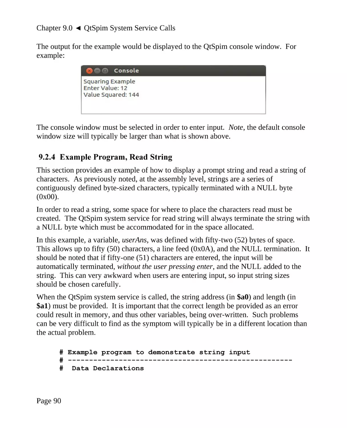
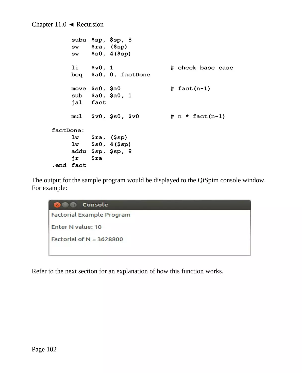
/


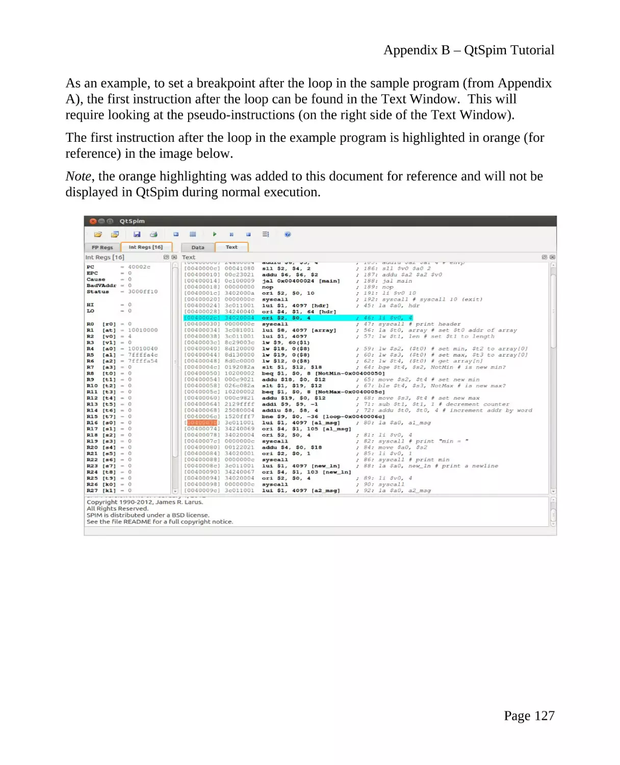
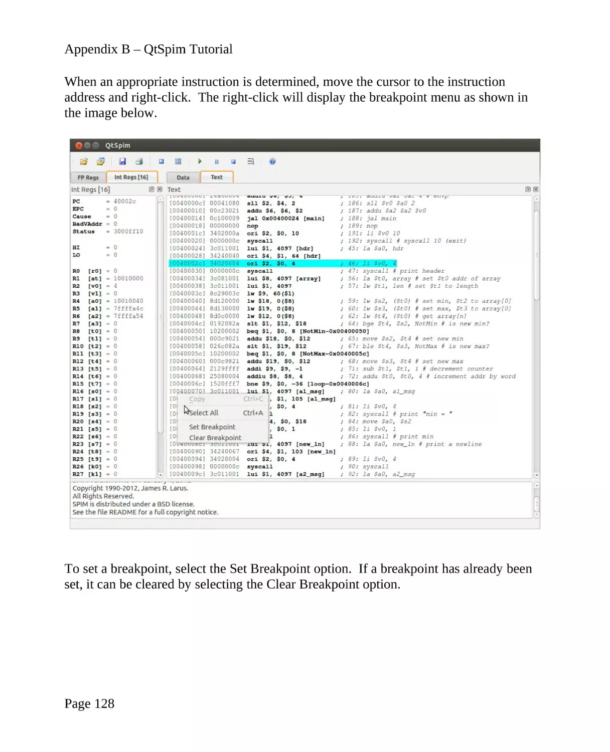
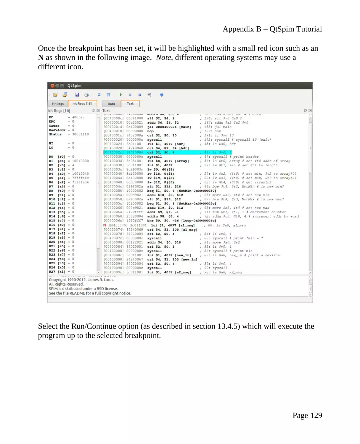
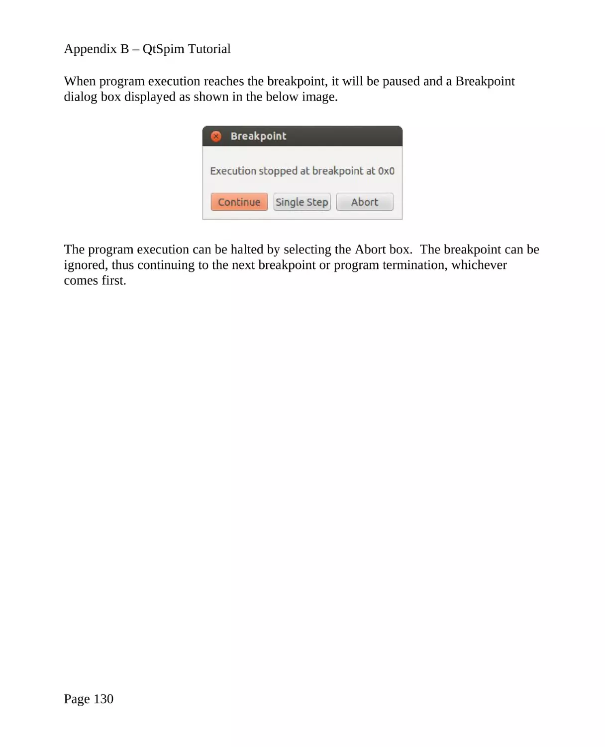


Text
MIPS
Assembly Language
Programming
using QtSpim
Ed Jorgensen, Ph.D.
Version 1.1.50
July 2019
Cover image:
MIPS R3000 Custom Chip
http://commons.wikimedia.org/wiki/File:RCP-NUS_01.jpg
Spim is copyrighted by James Larus and distributed under a BSD license.
Copyright (c) 1990-2011, James R. Larus. All rights reserved.
Copyright © 2013, 2014, 2015, 2016, 2017 by Ed Jorgensen
You are free:
To Share — to copy, distribute and transmit the work
To Remix — to adapt the work
Under the following conditions:
Attribution — you must attribute the work in the manner specified by the author
or licensor (but not in any way that suggests that they endorse you or your use of
the work).
Noncommercial — you may not use this work for commercial purposes.
Share Alike — if you alter, transform, or build upon this work, you may
distribute the resulting work only under the same or similar license to this one.
Table of Contents
1.0 Introduction...........................................................................................................1
1.1 Additional References.........................................................................................1
2.0 MIPS Architecture Overview..............................................................................3
2.1 Architecture Overview........................................................................................3
2.2 Data Types/Sizes.................................................................................................4
2.3 Memory...............................................................................................................4
2.4 Memory Layout...................................................................................................6
2.5 CPU Registers.....................................................................................................6
2.5.1 Reserved Registers......................................................................................7
2.5.2 Miscellaneous Registers..............................................................................8
2.6 CPU / FPU Core Configuration..........................................................................9
3.0 Data Representation...........................................................................................11
3.1 Integer Representation.......................................................................................11
3.1.1 Two's Complement....................................................................................13
3.1.2 Byte Example............................................................................................13
3.1.3 Halfword Example.....................................................................................13
3.2 Unsigned and Signed Addition.........................................................................14
3.3 Floating-point Representation...........................................................................14
3.3.1 IEEE 32-bit Representation.......................................................................14
3.3.1.1 IEEE 32-bit Representation Examples..............................................15
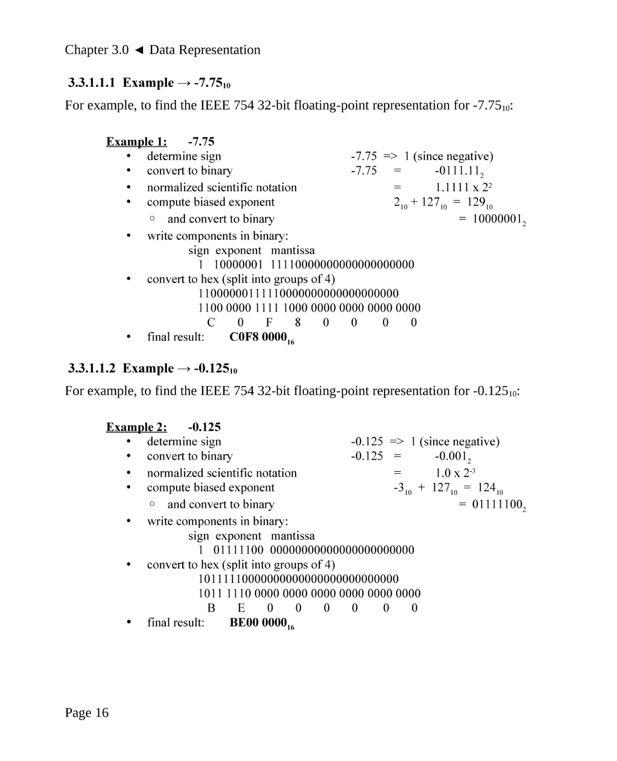
3.3.1.1.1 Example → -7.7510.....................................................................16
3.3.1.1.2 Example → -0.12510...................................................................16
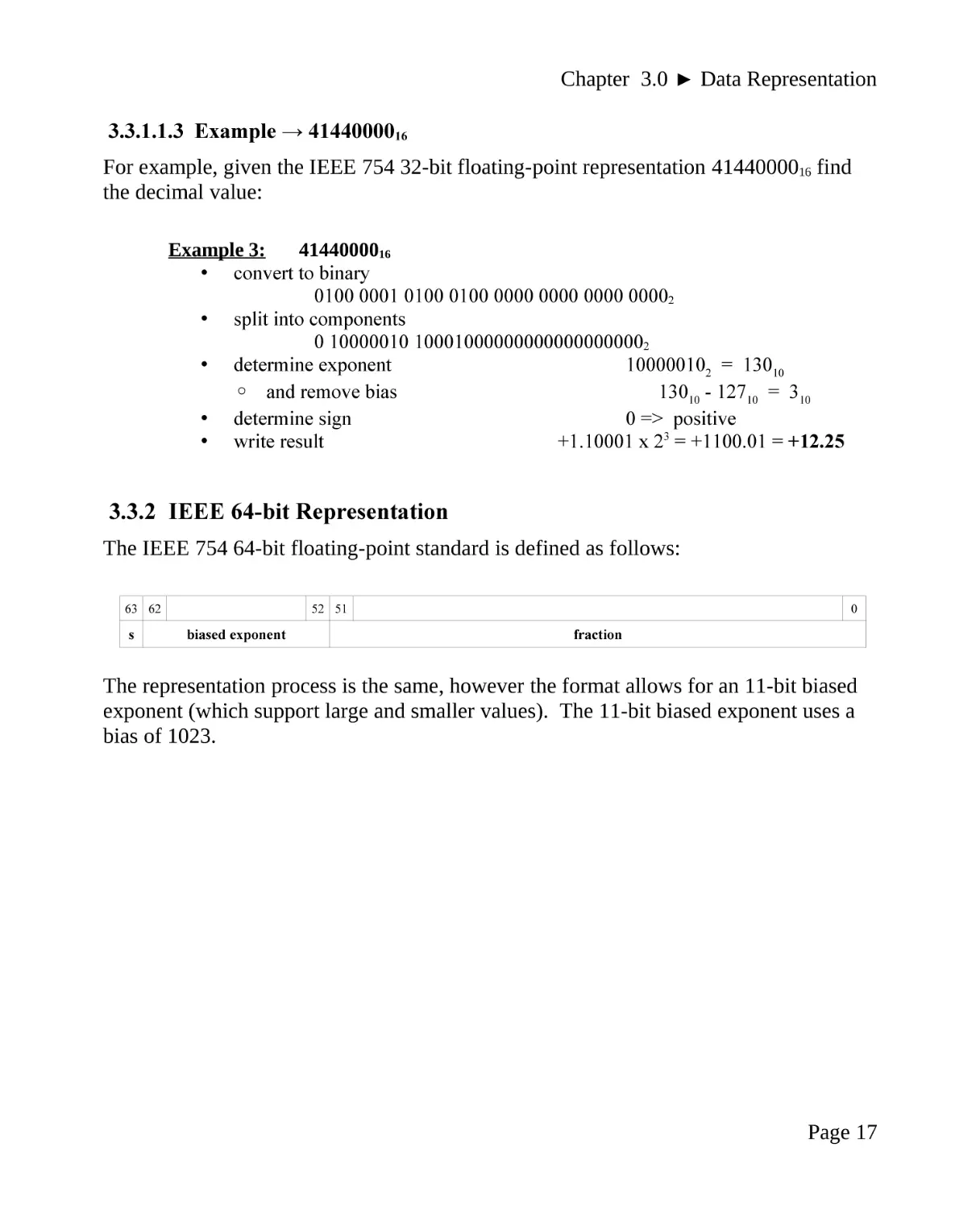
3.3.1.1.3 Example → 4144000016.............................................................17
3.3.2 IEEE 64-bit Representation.......................................................................17
4.0 QtSpim Program Formats.................................................................................19
4.1 Assembly Process..............................................................................................19
4.2 Comments..........................................................................................................19
4.3 Assembler Directives........................................................................................19
4.4 Data Declarations..............................................................................................20
4.4.1 Integer Data Declarations..........................................................................20
4.4.2 String Data Declarations............................................................................21
4.4.3 Floating-Point Data Declarations..............................................................22
4.5 Constants...........................................................................................................22
4.6 Program Code....................................................................................................23
4.7 Labels................................................................................................................23
4.8 Program Template.............................................................................................24
Table of Contents
5.0 Instruction Set Overview....................................................................................25
5.1 Pseudo-Instructions vs Bare-Instructions..........................................................25
5.2 Notational Conventions.....................................................................................25
5.3 Data Movement.................................................................................................26
5.3.1 Load and Store...........................................................................................26
5.3.2 Move..........................................................................................................28
5.4 Integer Arithmetic Operations...........................................................................29
5.4.1 Example Program, Integer Arithmetic......................................................32
5.5 Logical Operations............................................................................................33
5.5.1 Shift Operations.........................................................................................35
5.5.1.1 Logical Shift......................................................................................36
5.5.1.2 Arithmetic Shift.................................................................................37
5.5.1.3 Shift Operations, Examples...............................................................37
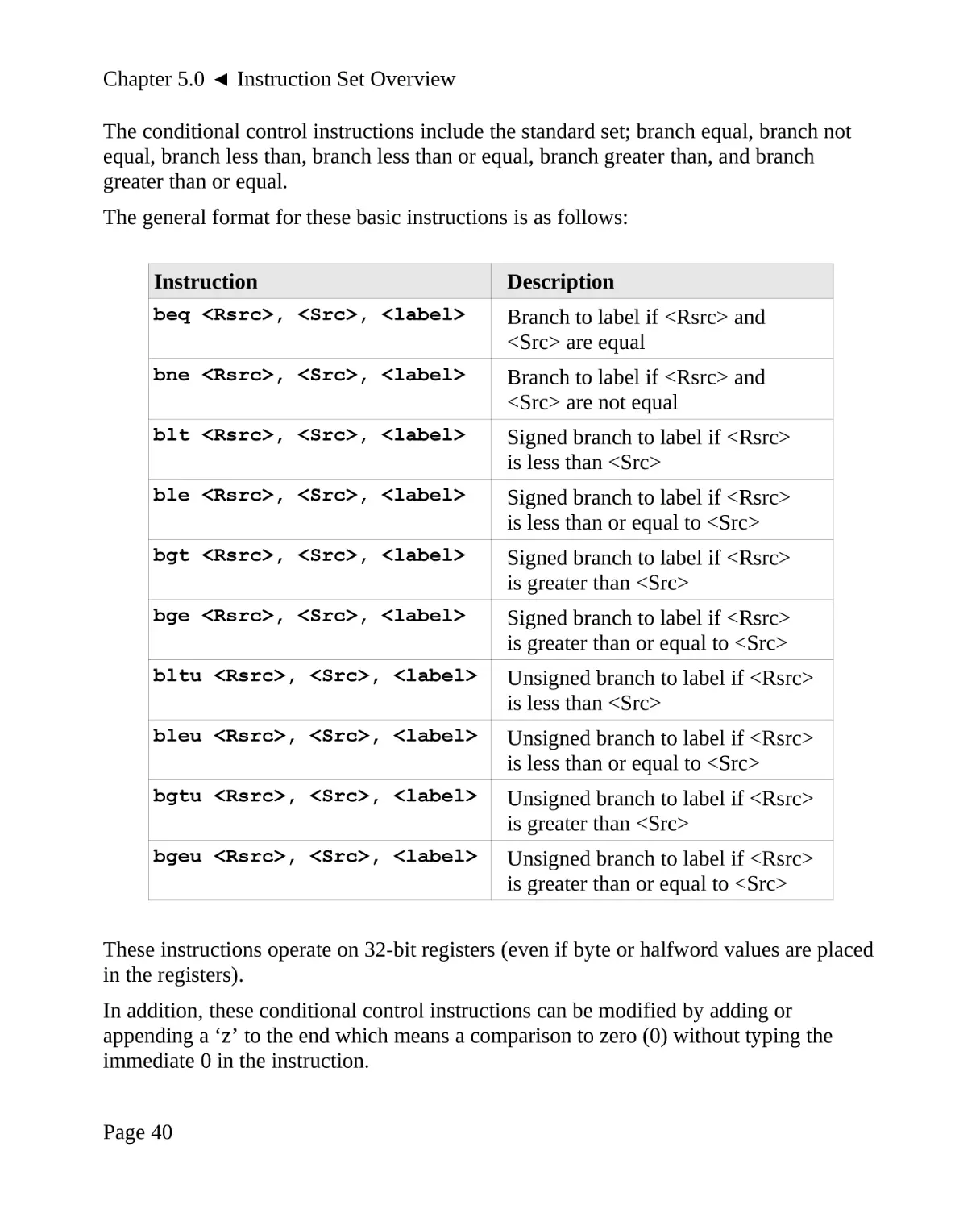
5.6 Control Instructions...........................................................................................39
5.6.1 Unconditional Control Instructions...........................................................39
5.6.2 Conditional Control Instructions...............................................................39
5.6.3 Example Program, Sum of Squares...........................................................41
5.7 Floating-Point Instructions................................................................................42
5.7.1 Floating-Point Register Usage...................................................................42
5.7.2 Floating-Point Data Movement.................................................................43
5.7.3 Integer / Floating-Point Register Data Movement....................................44
5.7.4 Integer / Floating-Point Conversion Instructions......................................45
5.7.5 Floating-Point Arithmetic Operations.......................................................47
5.7.6 Example Programs.....................................................................................48
5.7.6.1 Example Program, Floating-Point Arithmetic...................................49
5.7.6.2 Example Program, Integer / Floating-Point Conversion...................50
6.0 Addressing Modes...............................................................................................53
6.1 Direct Mode.......................................................................................................53
6.2 Immediate Mode...............................................................................................53
6.3 Indirection.........................................................................................................54
6.3.1 Bounds Checking.......................................................................................54
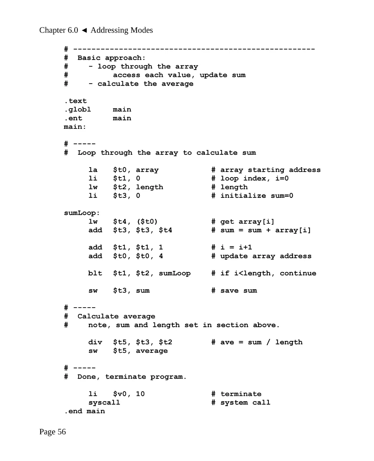
6.4 Examples...........................................................................................................55
6.4.1 Example Program, Sum and Average.......................................................55
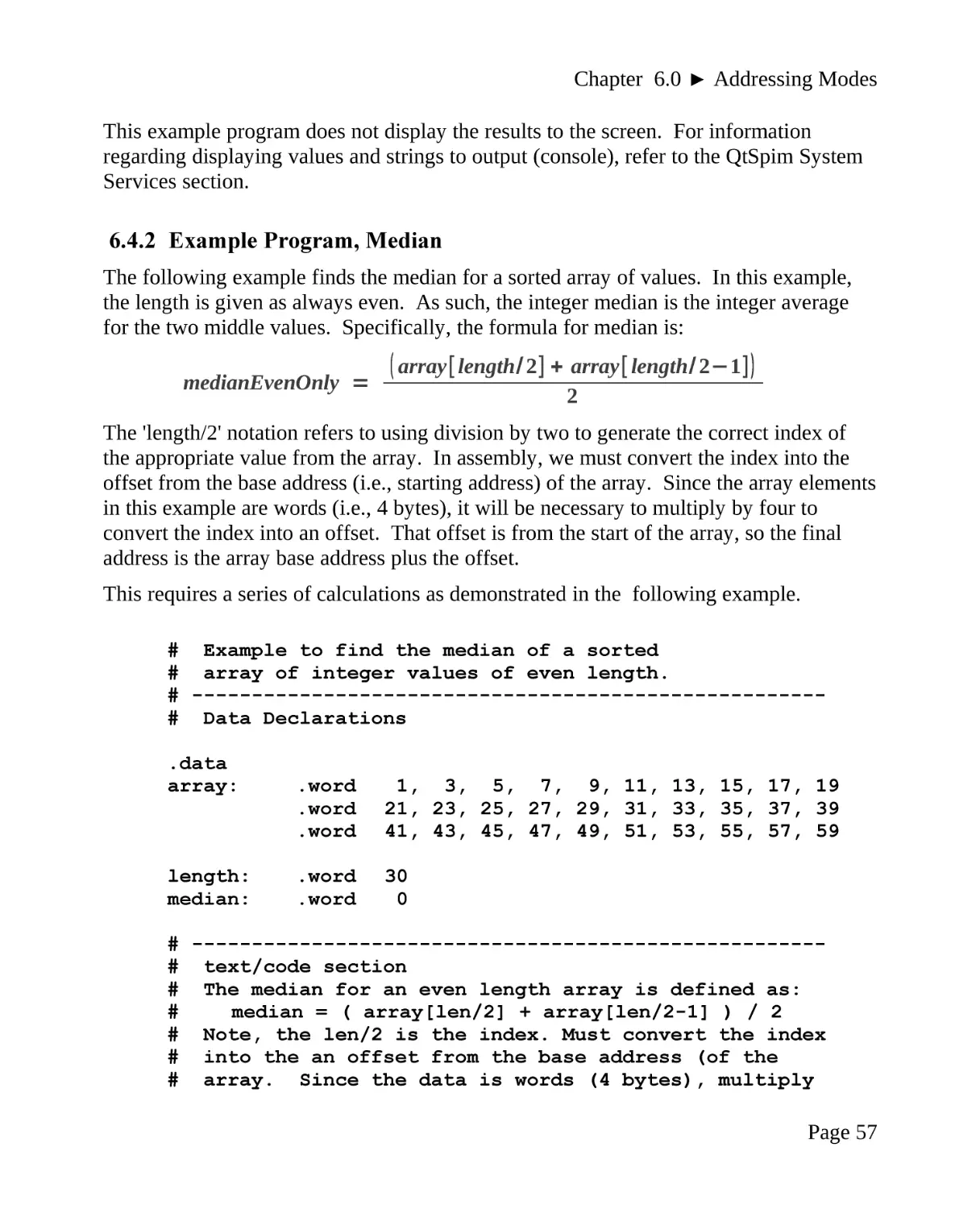
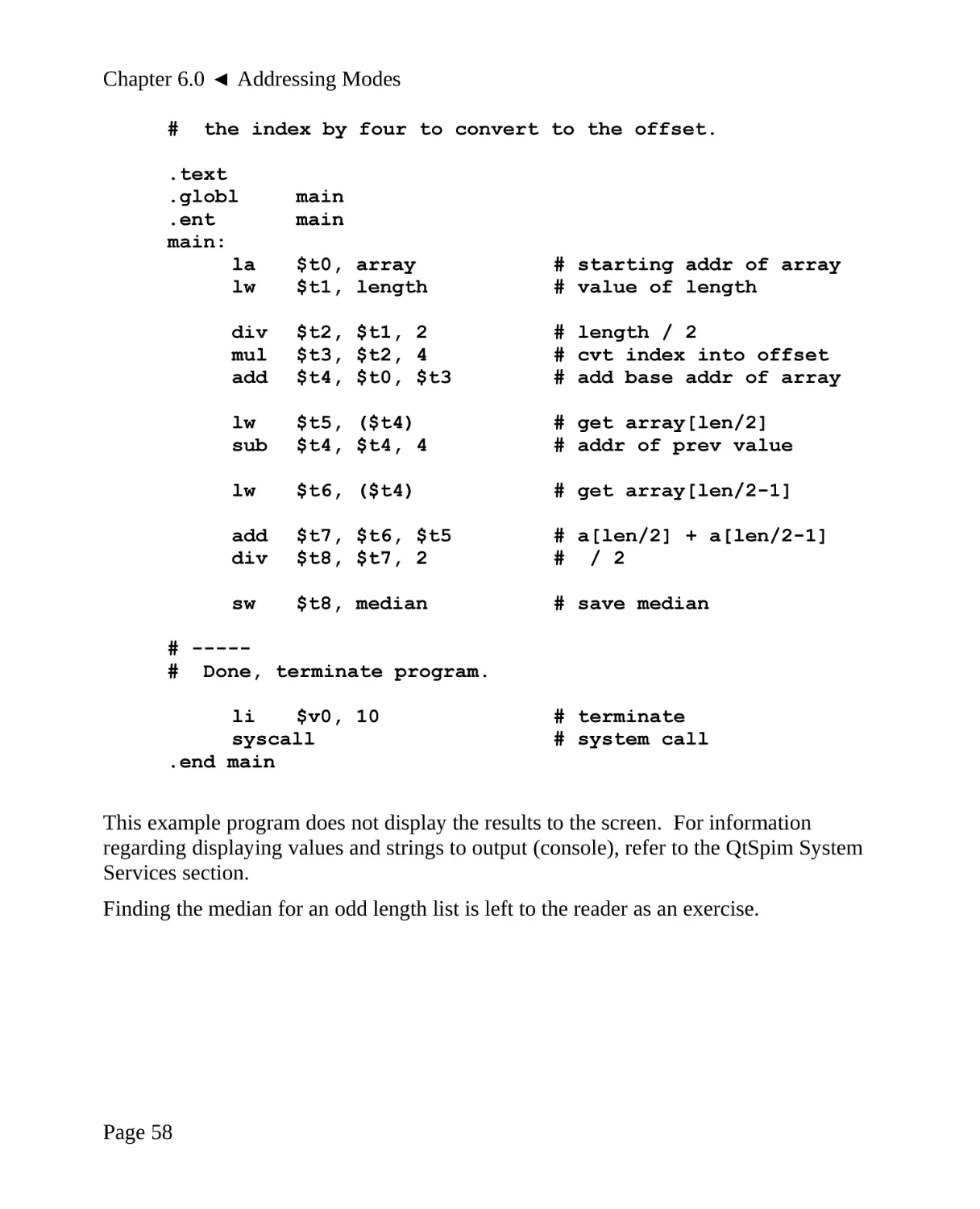
6.4.2 Example Program, Median........................................................................57
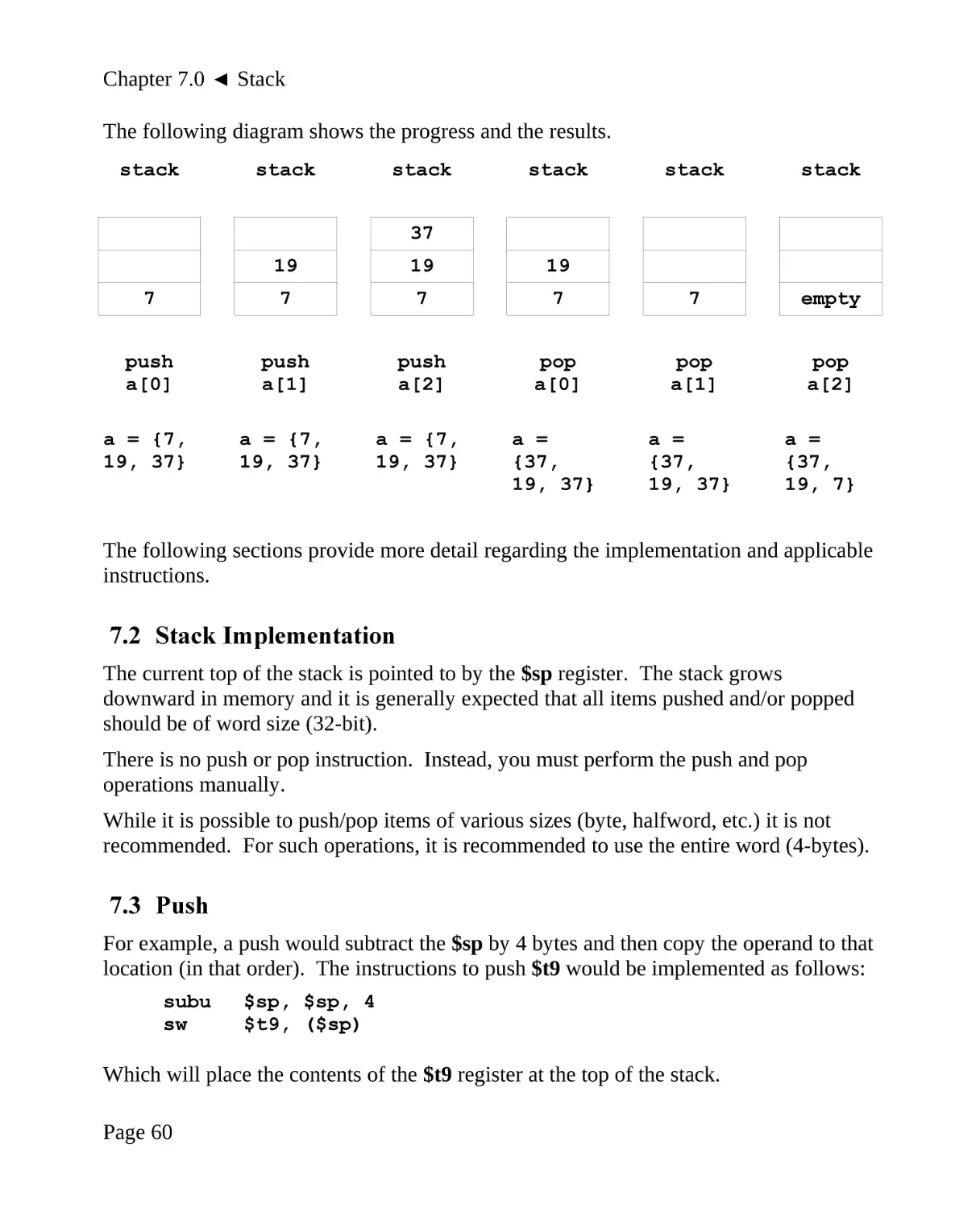
7.0 Stack.....................................................................................................................59
7.1 Stack Example...................................................................................................59
7.2 Stack Implementation........................................................................................60
Page ii
Table of Contents
7.3
7.4
7.5
7.6
Push...................................................................................................................60
Pop.....................................................................................................................61
Multiple push's/pop's.........................................................................................61
Example Program, Stack Usage........................................................................61
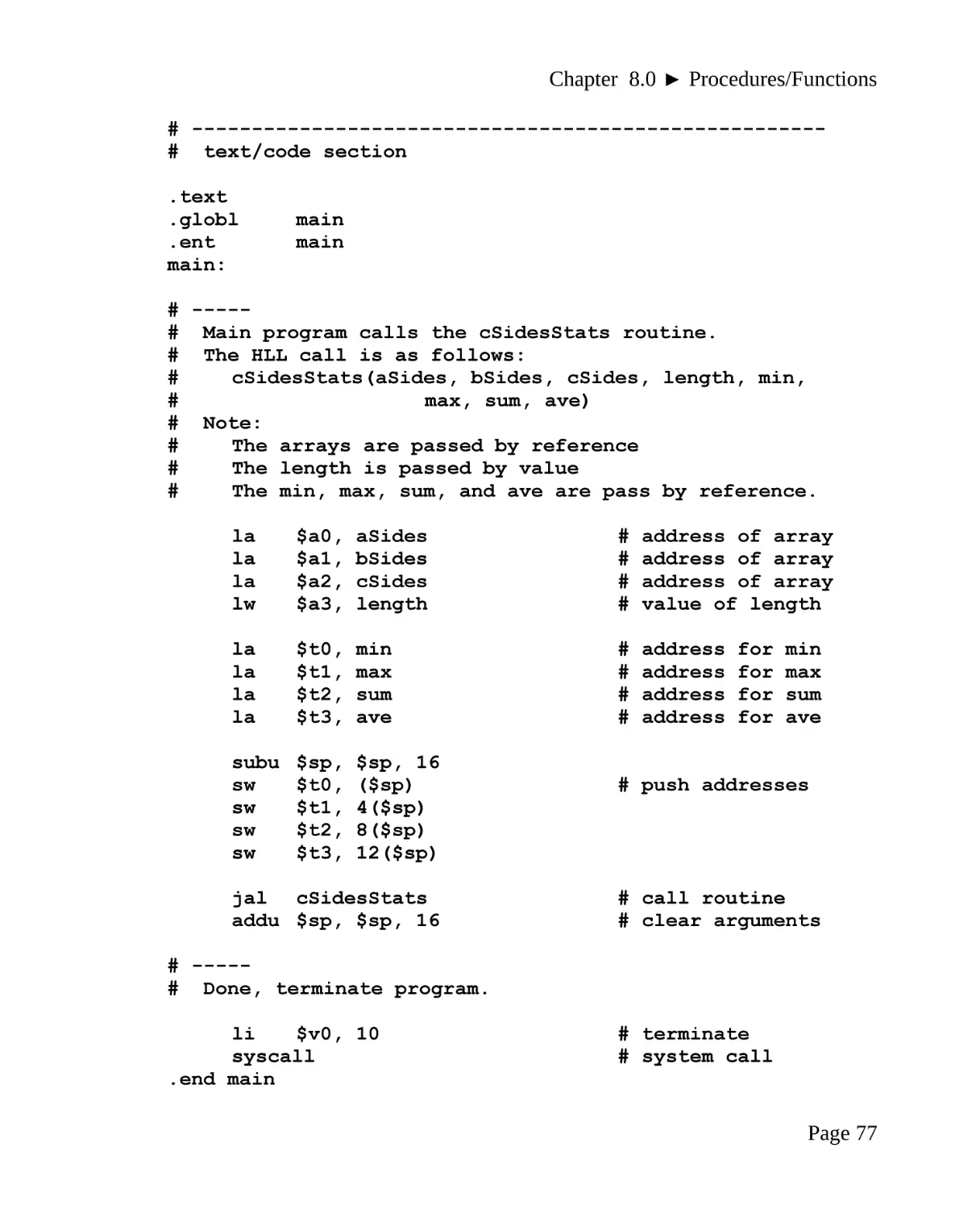
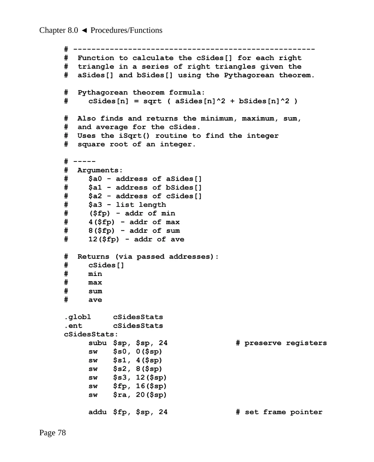
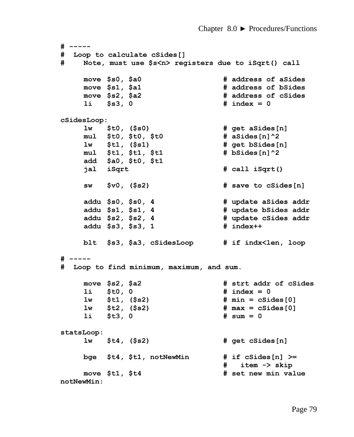
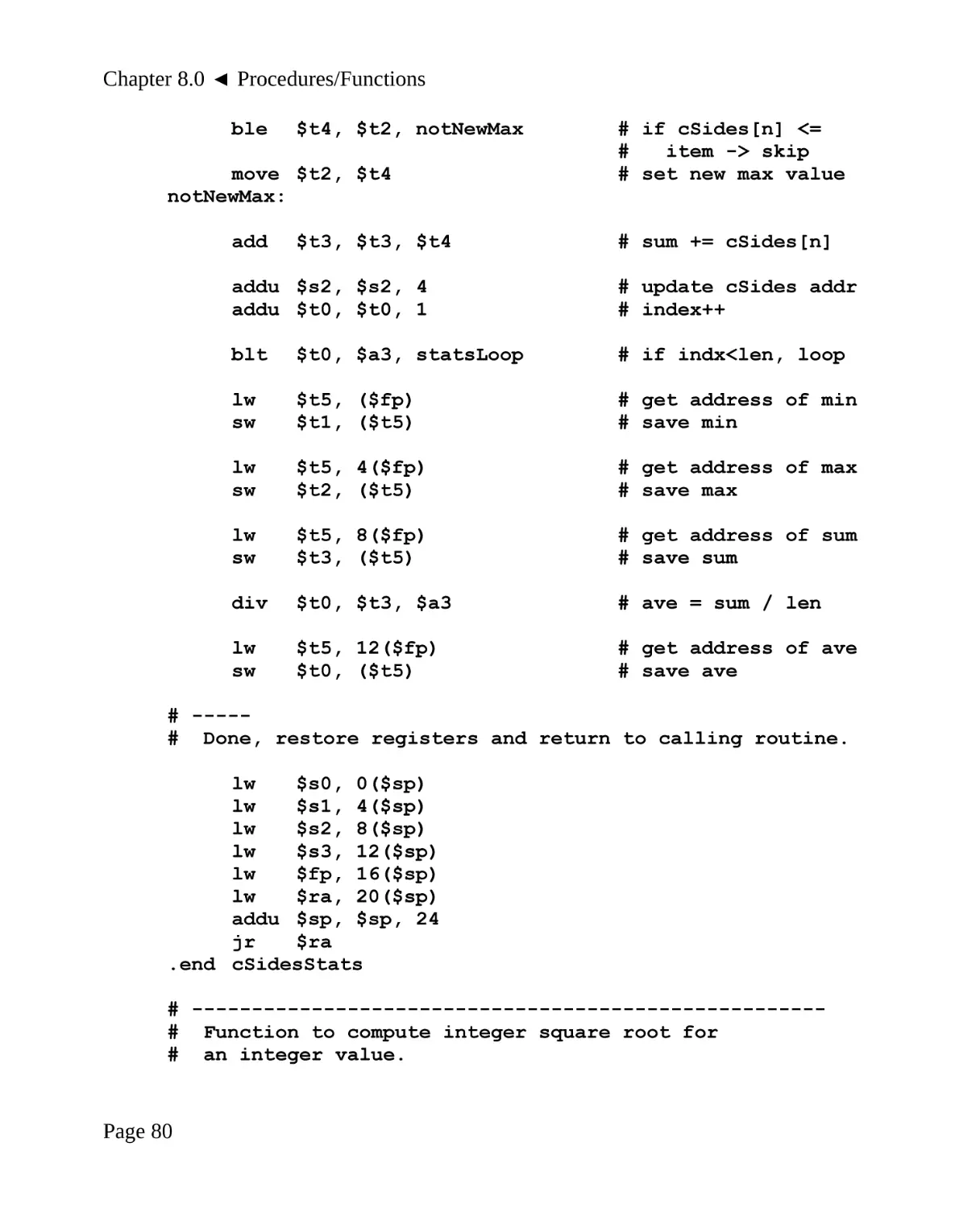
8.0 Procedures/Functions.........................................................................................65
8.1 MIPS Calling Conventions................................................................................65
8.2 Procedure/Function Format...............................................................................66
8.3 Caller Conventions............................................................................................66
8.4 Linkage..............................................................................................................67
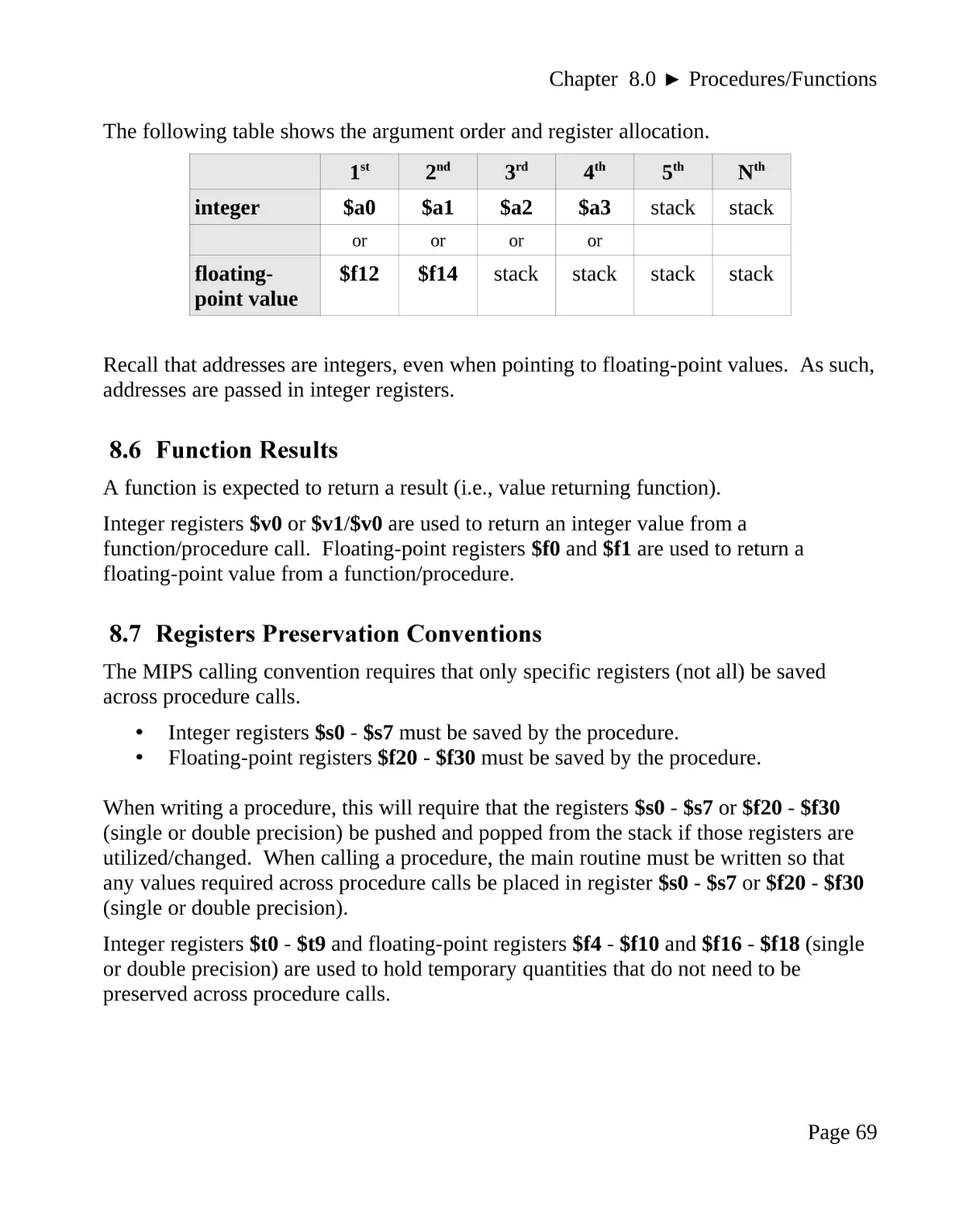
8.5 Argument Transmission....................................................................................68
8.5.1 Call-by-Value............................................................................................68
8.5.2 Call-by-Reference......................................................................................68
8.5.3 Argument Transmission Conventions.......................................................68
8.6 Function Results................................................................................................69
8.7 Registers Preservation Conventions..................................................................69
8.8 Miscellaneous Register Usage..........................................................................70
8.9 Summary, Callee Conventions..........................................................................70
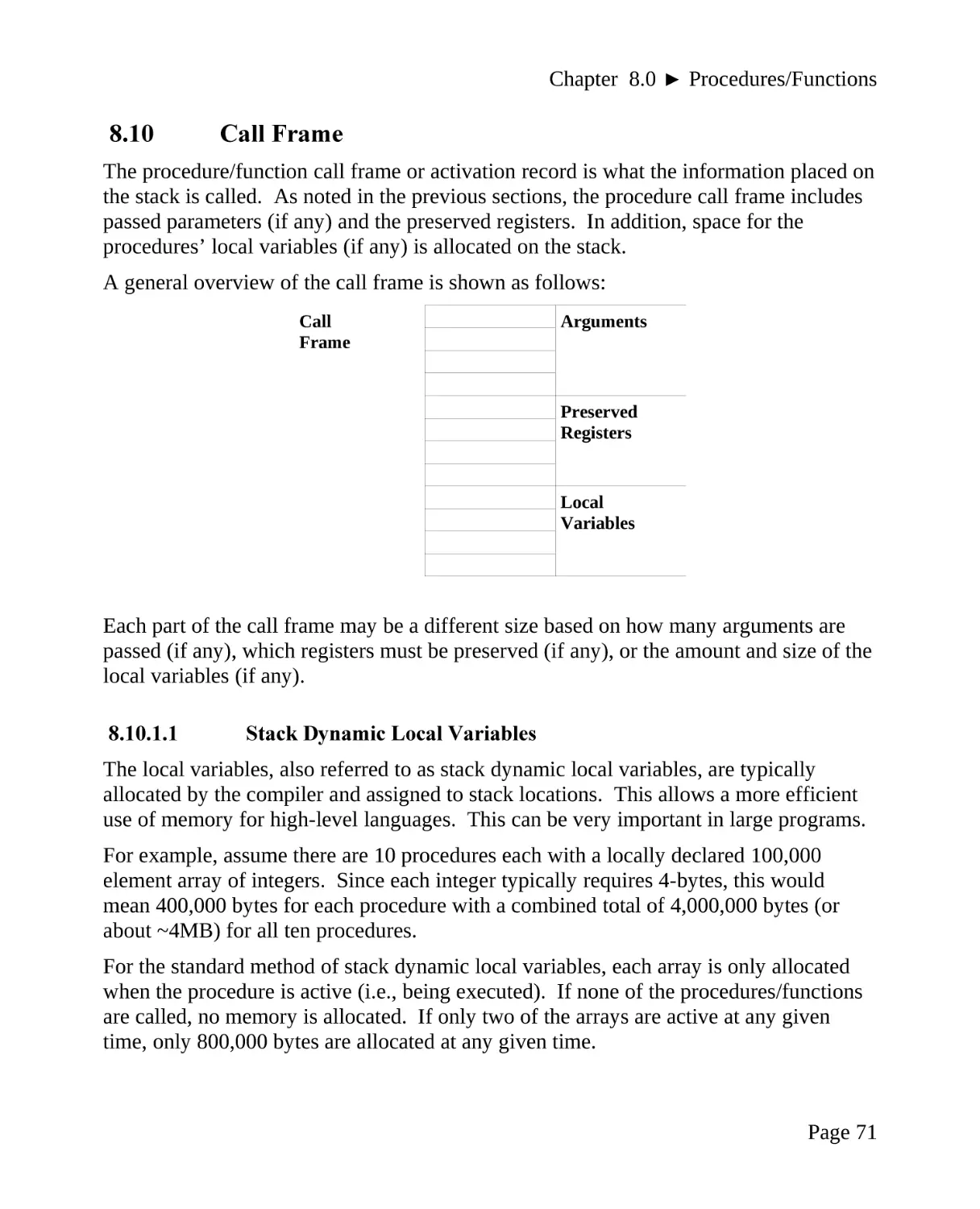
8.10 Call Frame.......................................................................................................71
8.10.1.1 Stack Dynamic Local Variables......................................................71
8.11 Procedure Examples........................................................................................72
8.11.1 Example Program, Power Function.........................................................72
8.11.2 Example program, Summation Function.................................................73
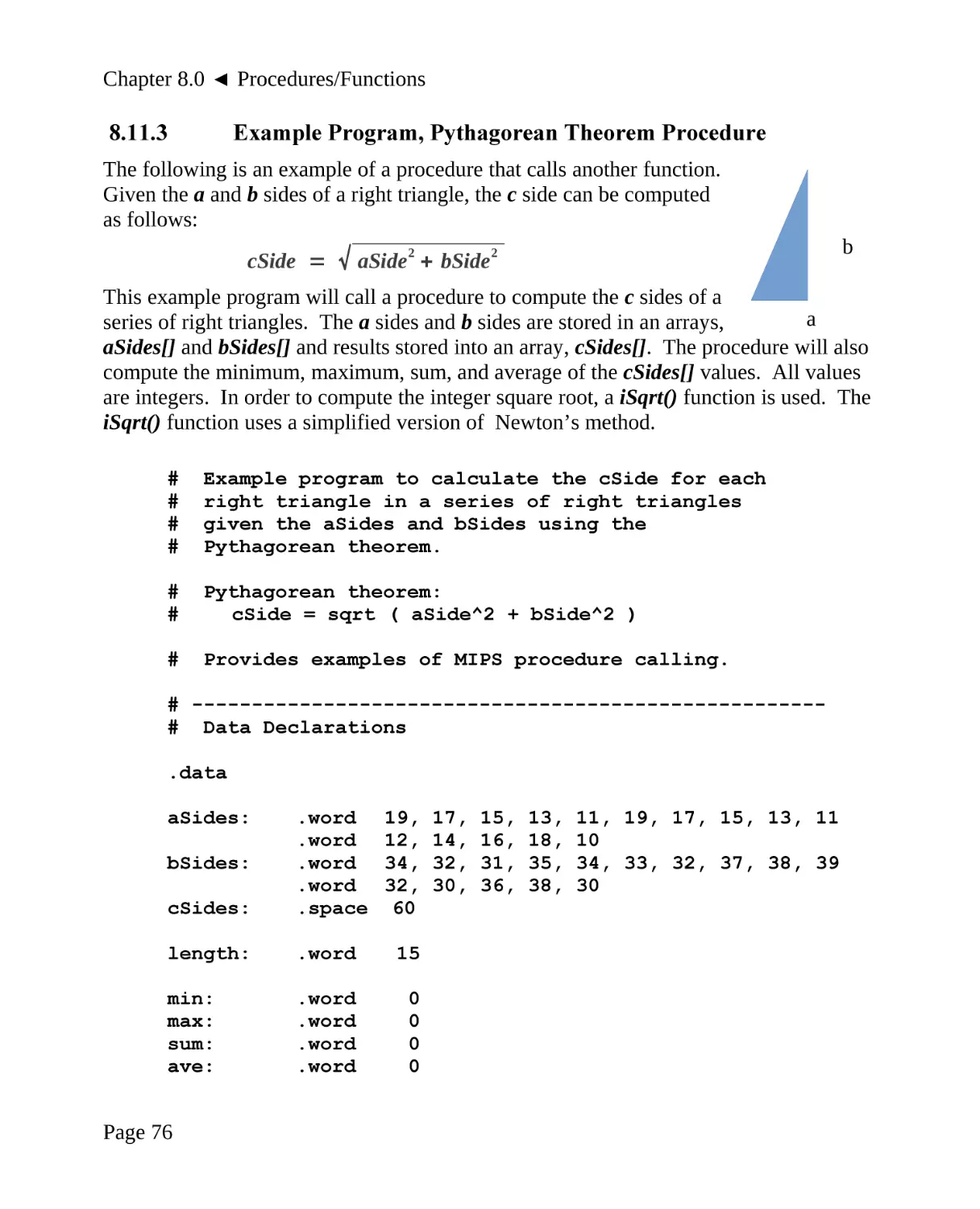
8.11.3 Example Program, Pythagorean Theorem Procedure.............................76
9.0 QtSpim System Service Calls.............................................................................82
9.1 Supported QtSpim System Services..................................................................82
9.2 QtSpim System Services Examples..................................................................85
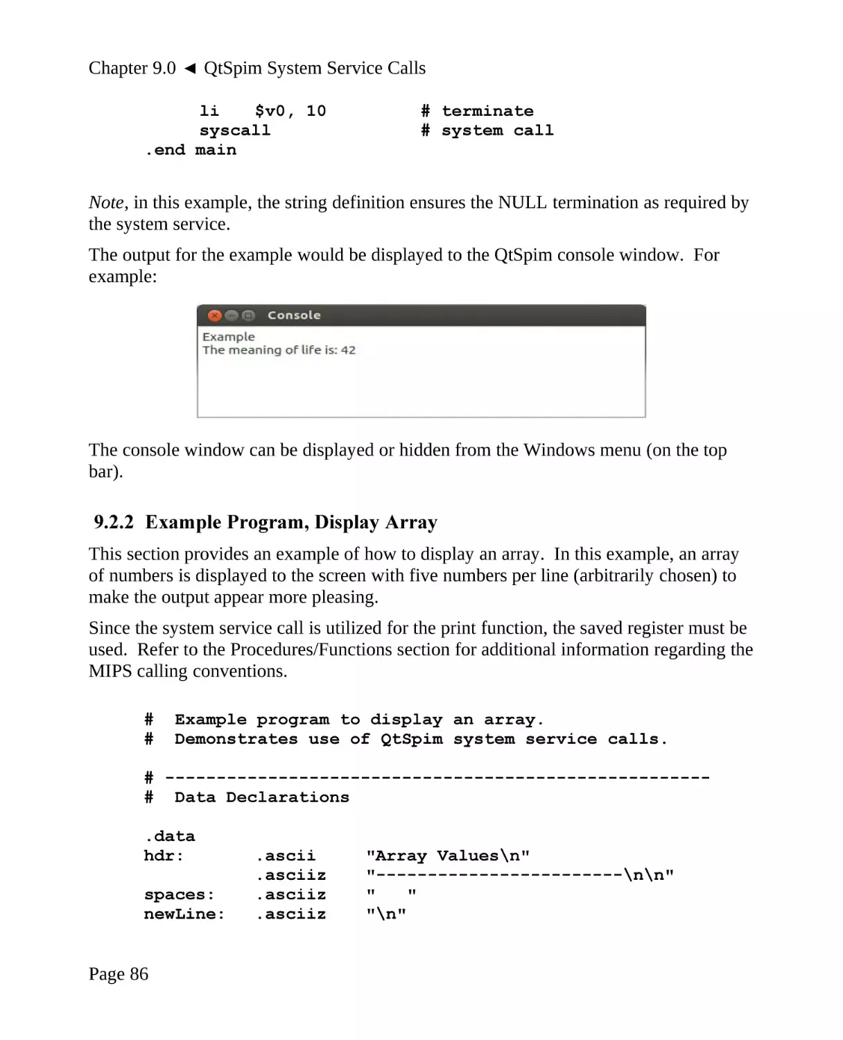
9.2.1 Example Program, Display String and Integer..........................................85
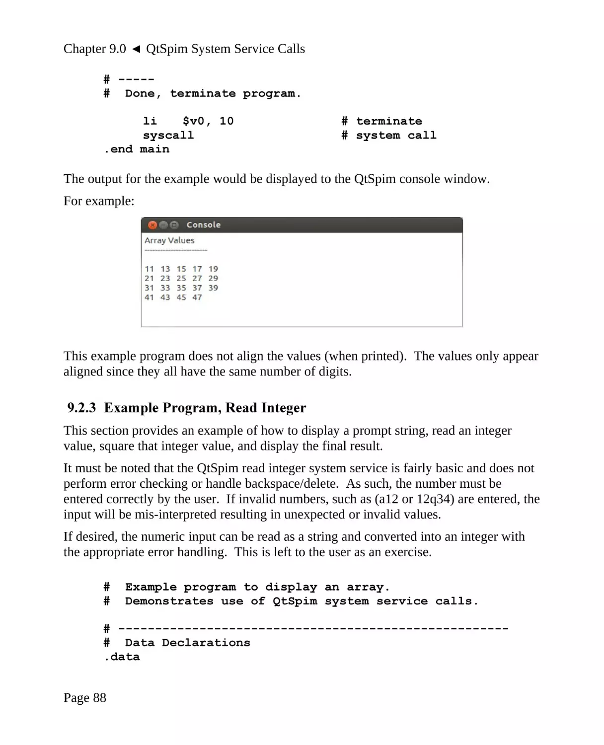
9.2.2 Example Program, Display Array.............................................................86
9.2.3 Example Program, Read Integer................................................................88
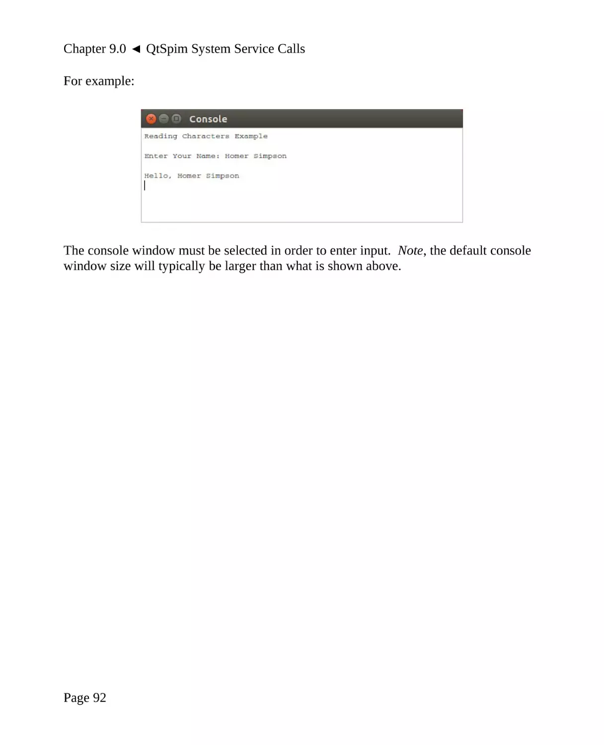
9.2.4 Example Program, Read String.................................................................90
10.0 Multi-dimension Array Implementation........................................................93
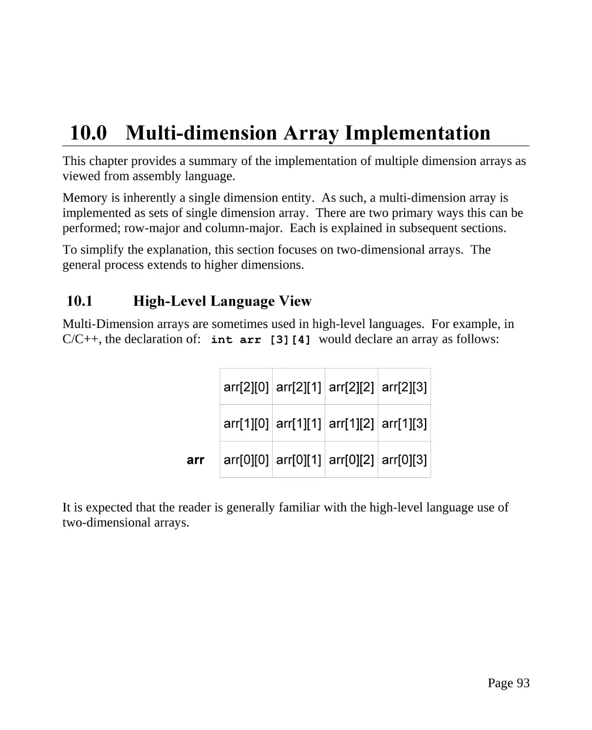
10.1 High-Level Language View............................................................................93
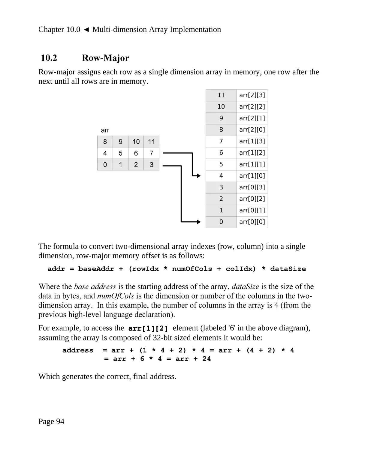
10.2 Row-Major......................................................................................................94
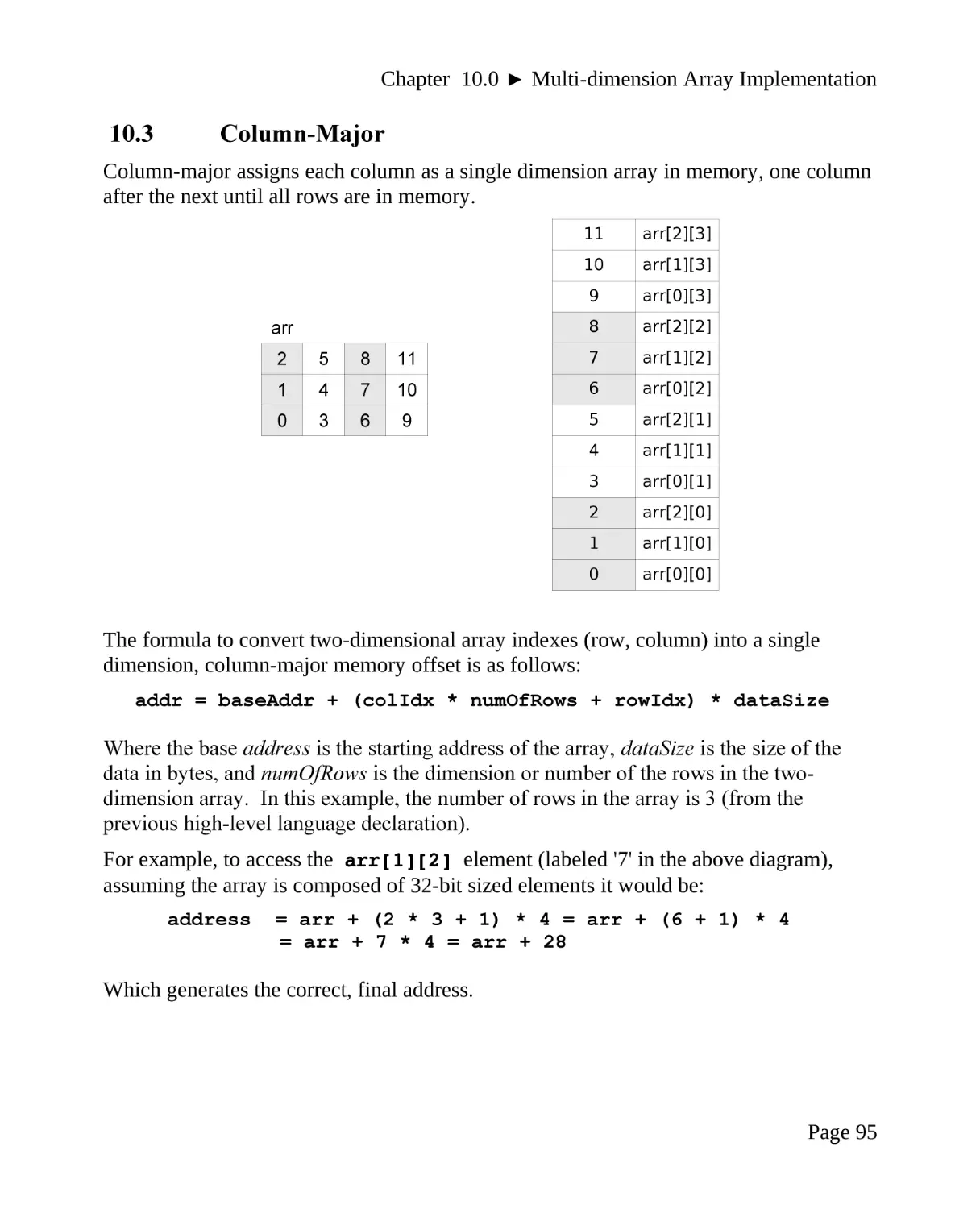
10.3 Column-Major.................................................................................................95
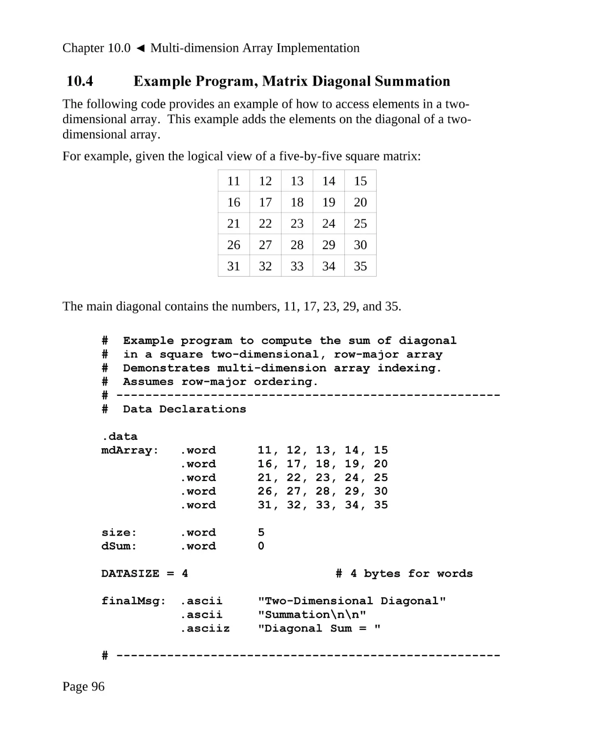
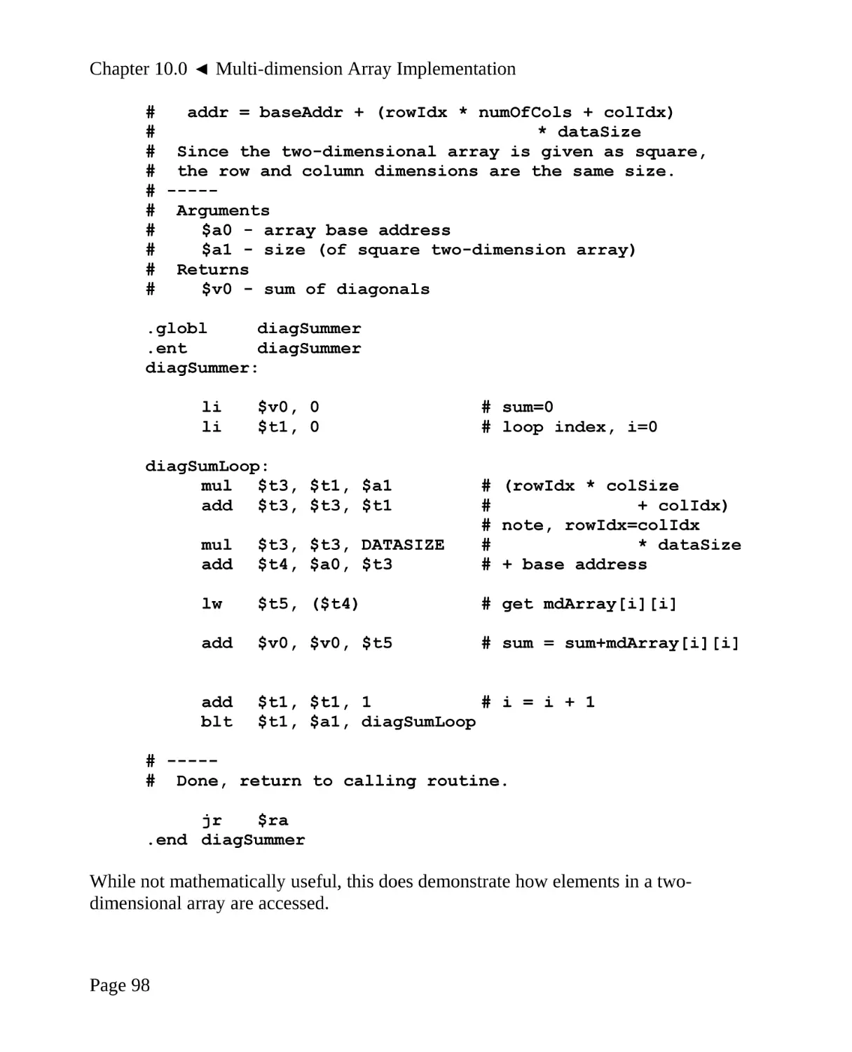
10.4 Example Program, Matrix Diagonal Summation............................................96
11.0
Recursion...........................................................................................................99
Page iii
Table of Contents
11.1 Recursion Example, Factorial.........................................................................99
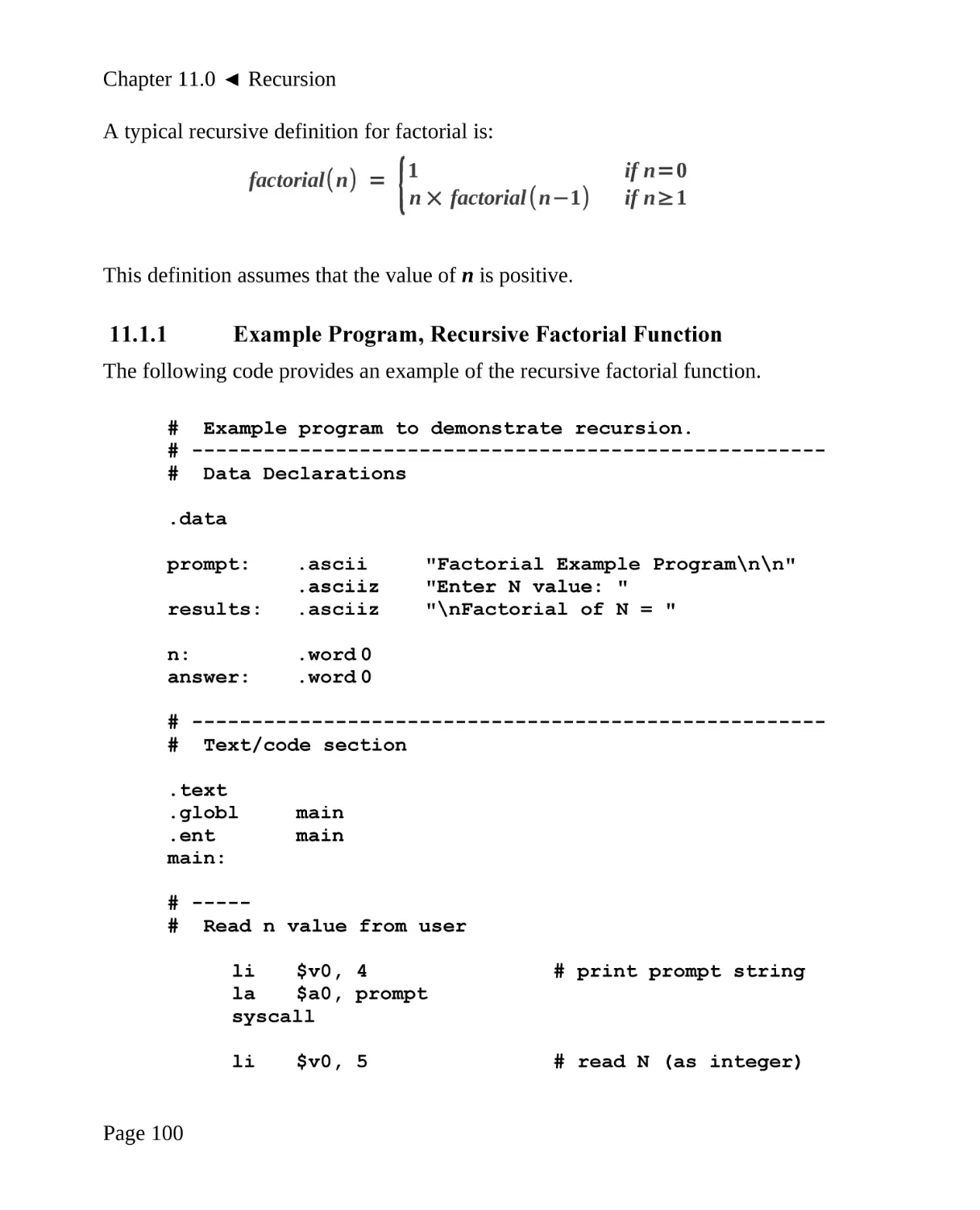
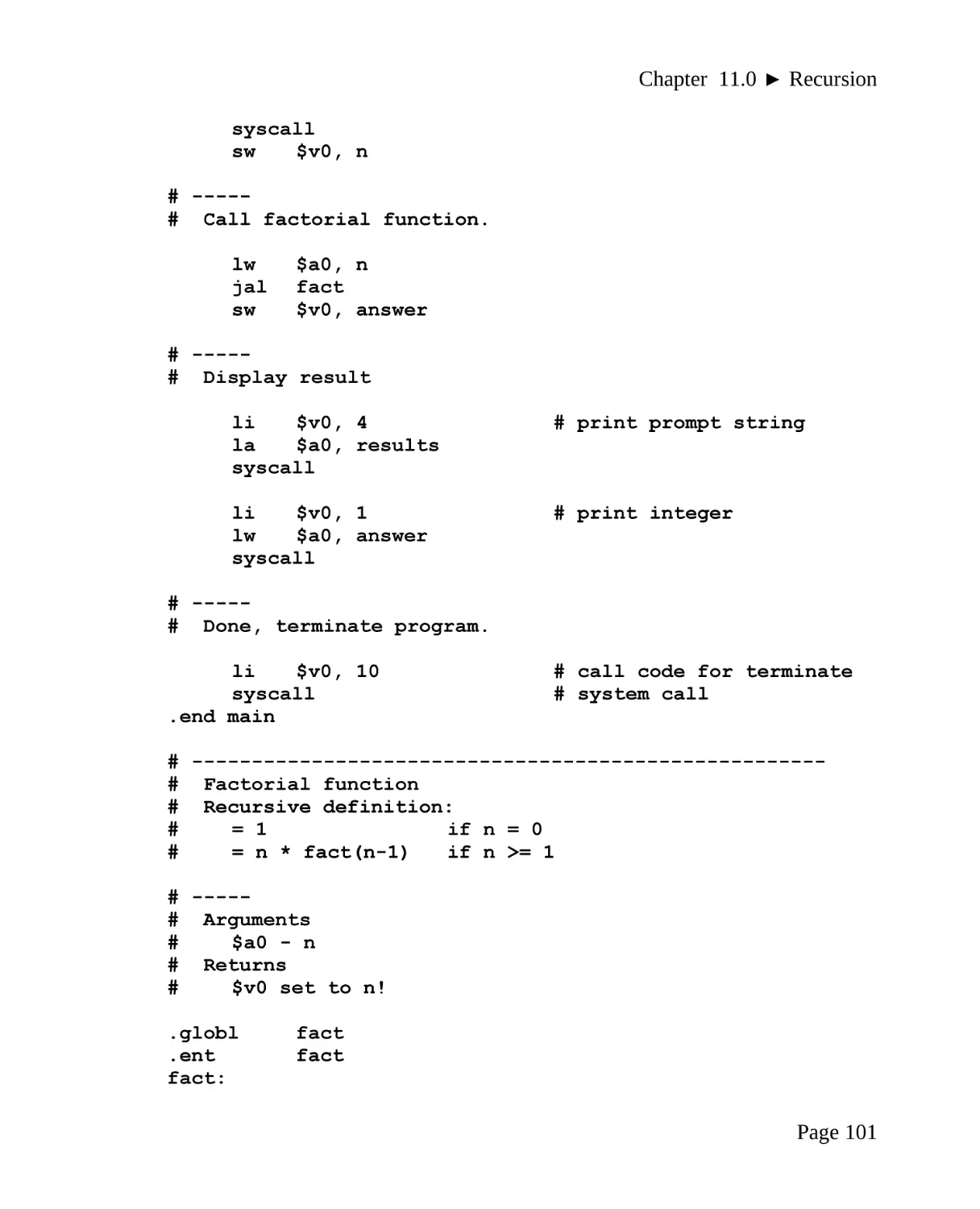
11.1.1 Example Program, Recursive Factorial Function..................................100
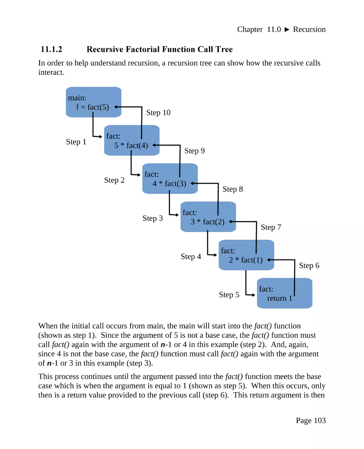
11.1.2 Recursive Factorial Function Call Tree.................................................103
11.2 Recursion Example, Fibonacci......................................................................104
11.2.1 Example Program, Recursive Fibonacci Function................................105
11.2.2 Recursive Fibonacci Function Call Tree...............................................108
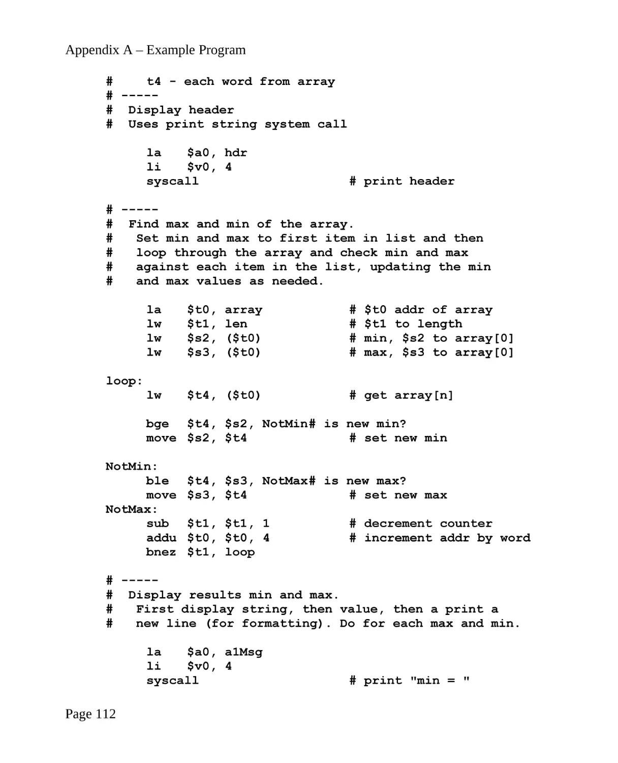
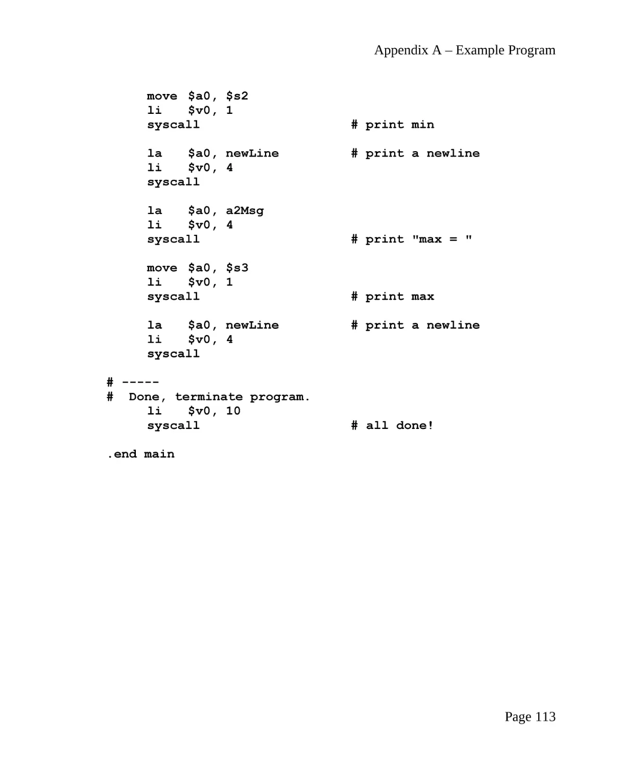
12.0
Appendix A – Example Program...................................................................111
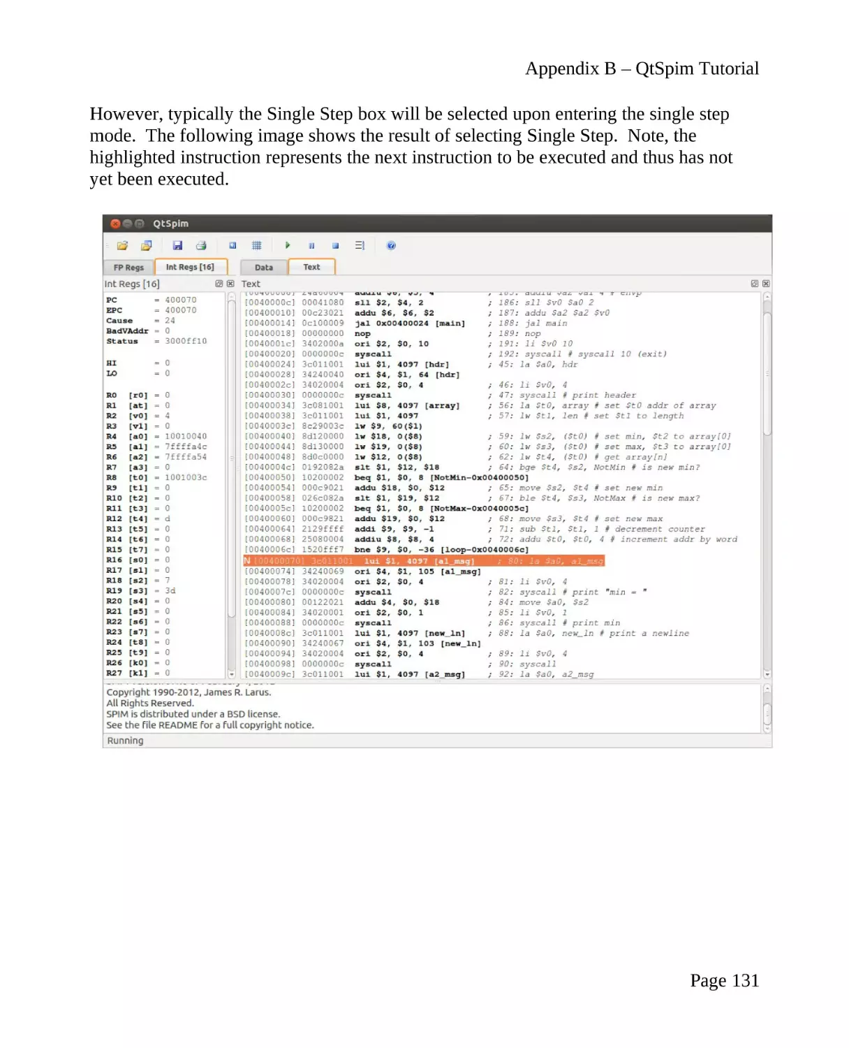
13.0 Appendix B – QtSpim Tutorial......................................................................115
13.1 Downloading and Installing QtSpim.............................................................115
13.1.1 QtSpim Download URLs......................................................................115
13.1.2 Installing QtSpim...................................................................................115
13.2 Working Directory........................................................................................116
13.3 Sample Program............................................................................................116
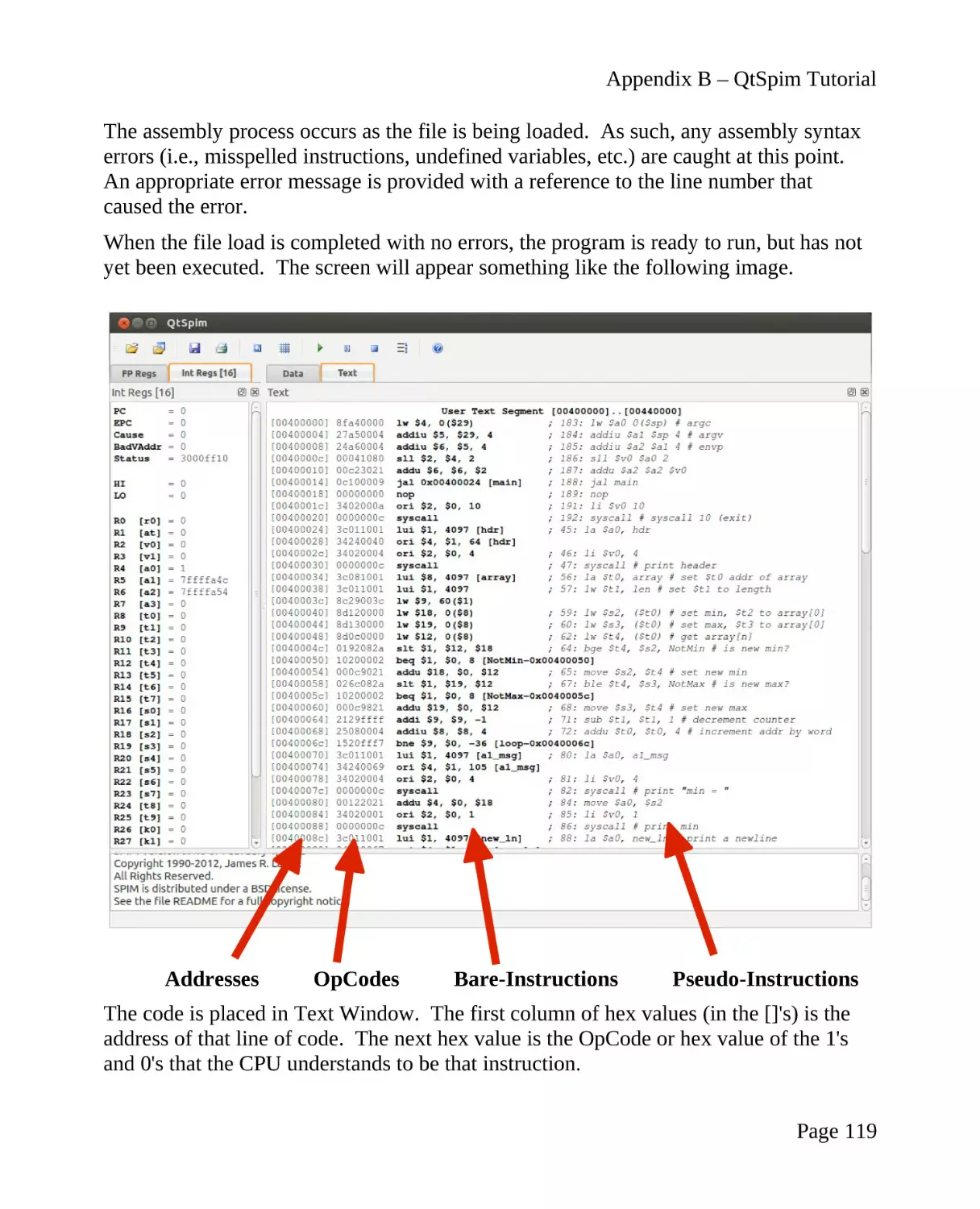
13.4 QtSpim – Loading and Executing Programs.................................................116
13.4.1 Starting QtSpim.....................................................................................116
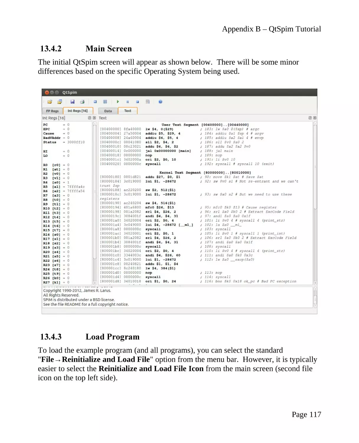
13.4.2 Main Screen...........................................................................................117
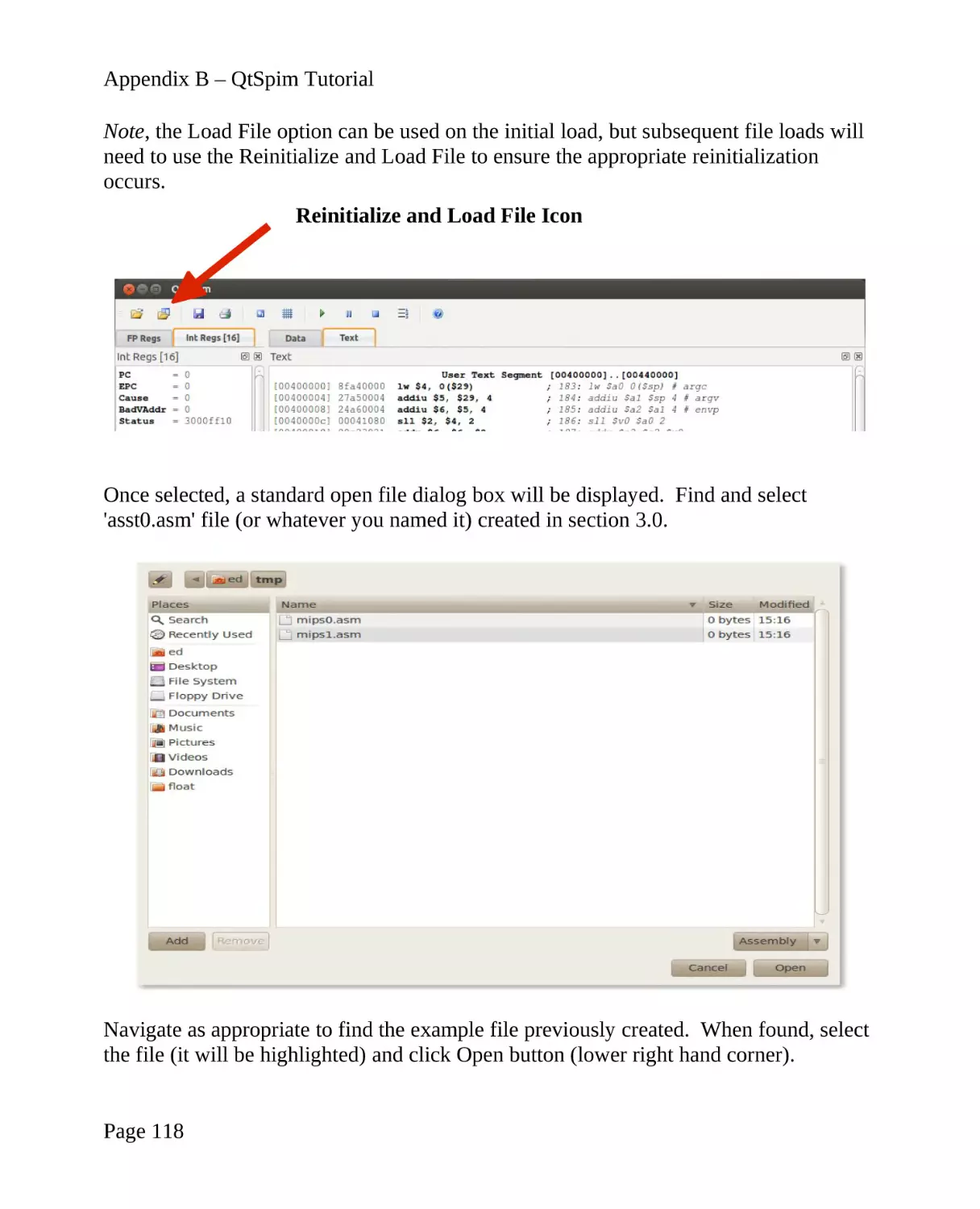
13.4.3 Load Program........................................................................................117
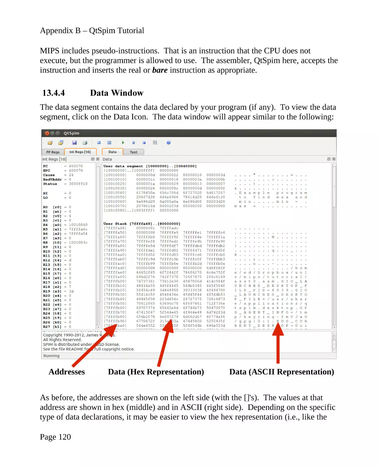
13.4.4 Data Window.........................................................................................120
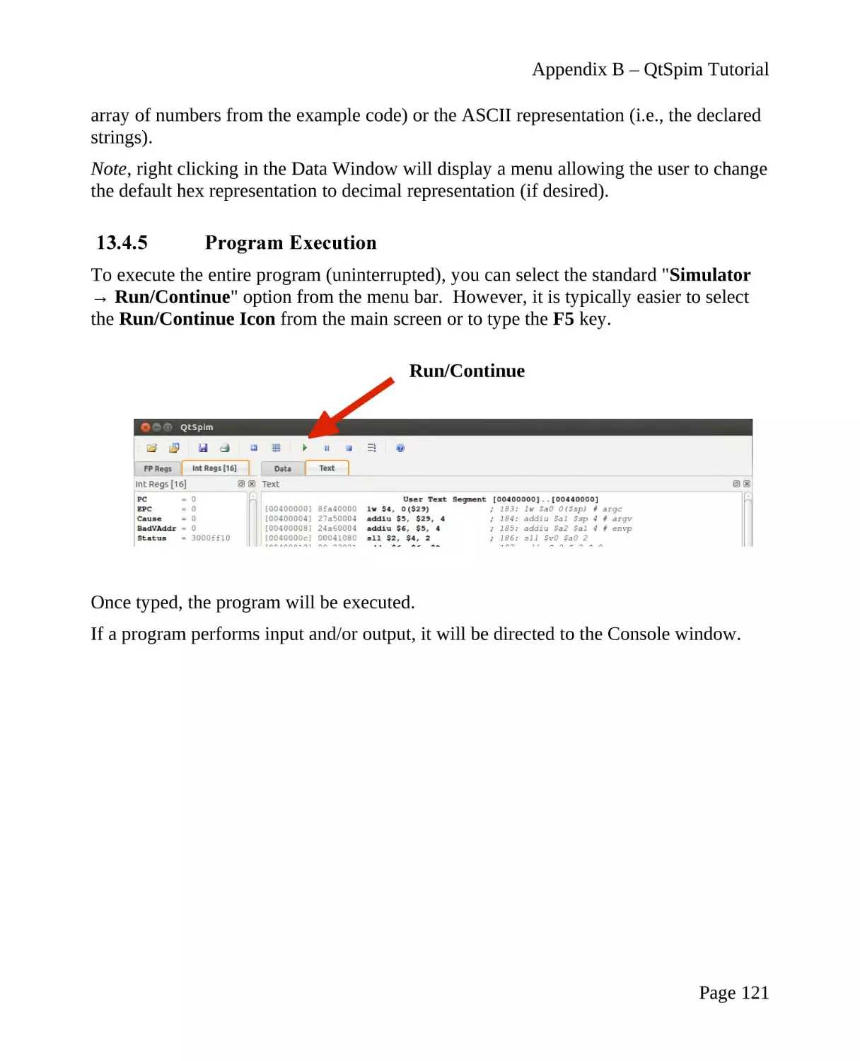
13.4.5 Program Execution................................................................................121
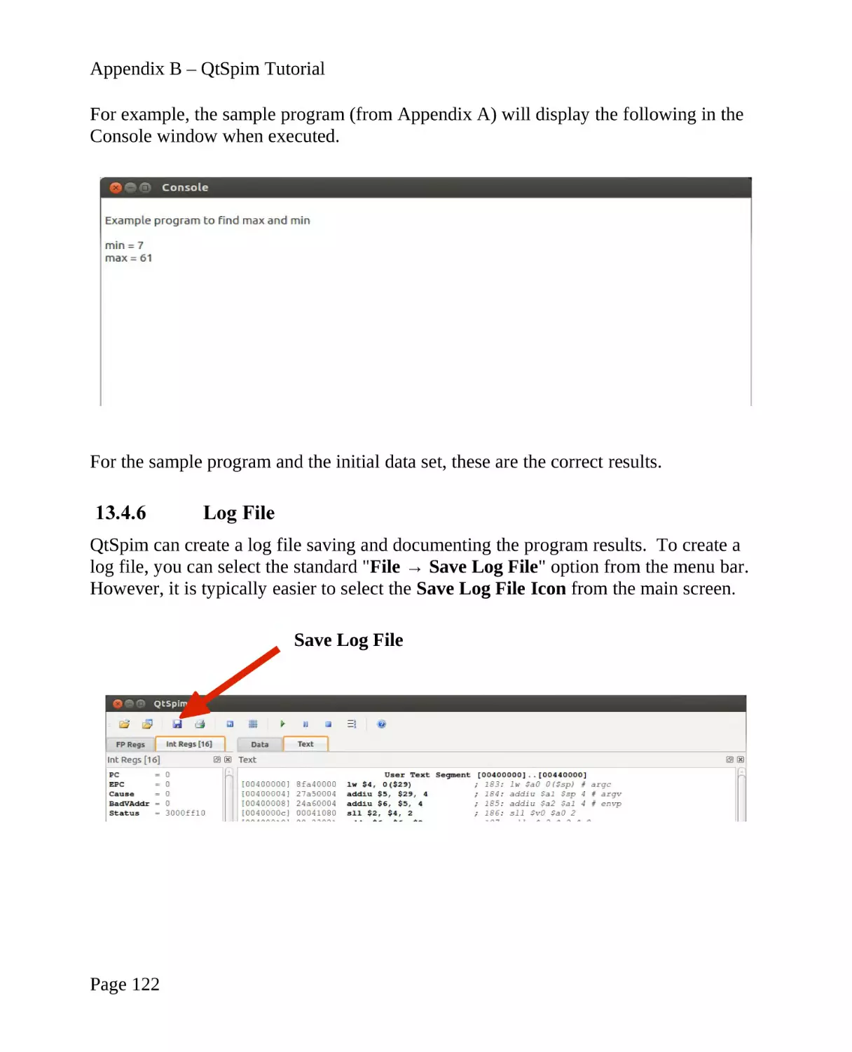
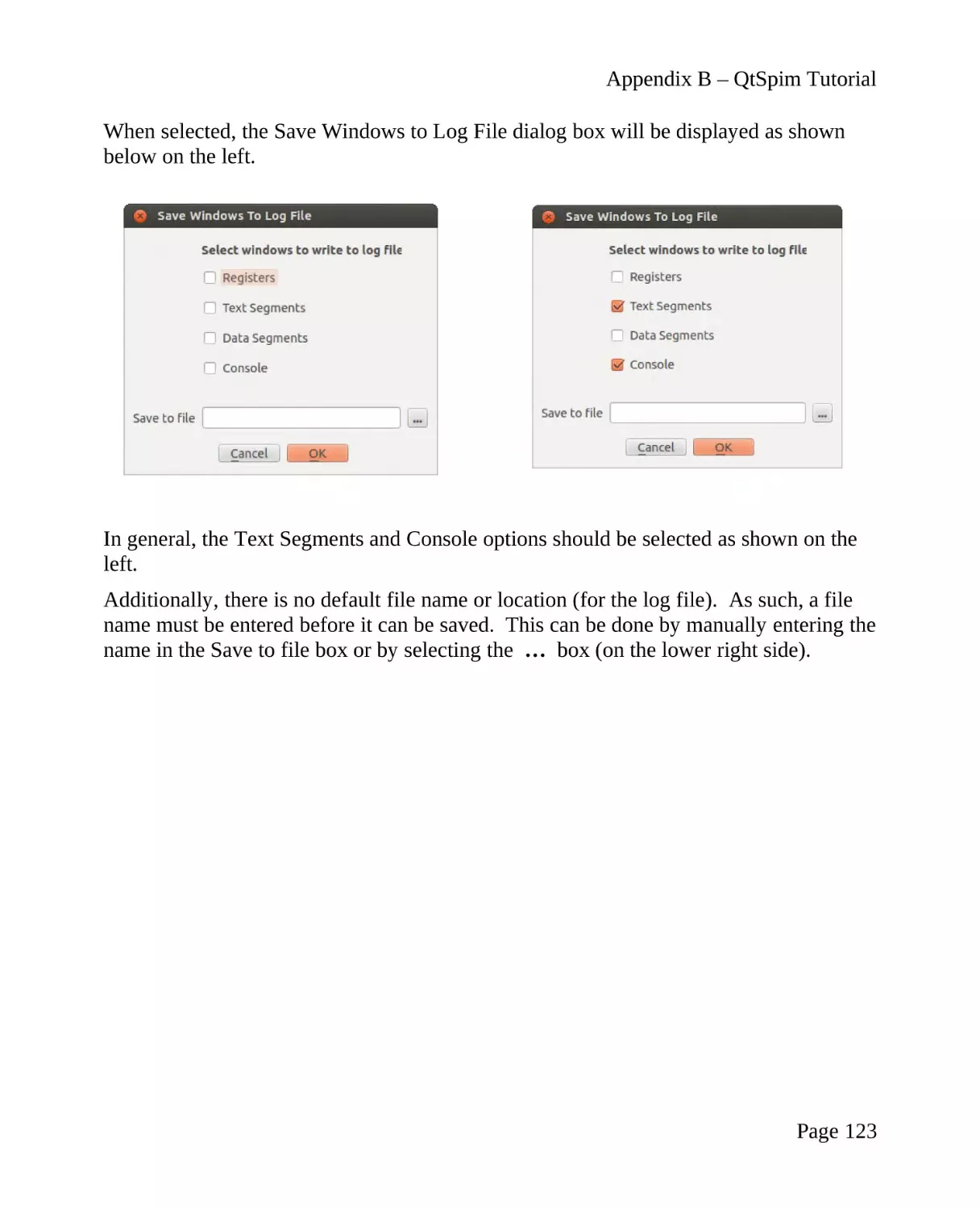
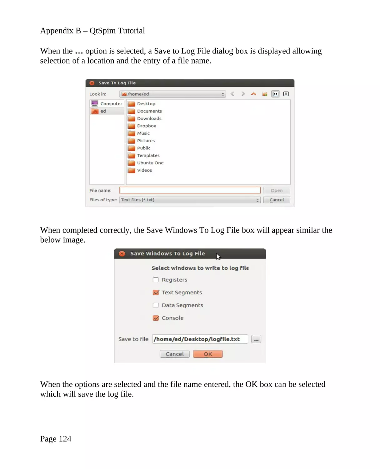
13.4.6 Log File.................................................................................................122
13.4.7 Making Updates.....................................................................................125
13.5 Debugging.....................................................................................................125
14.0 Appendix C – MIPS Instruction Set..............................................................133
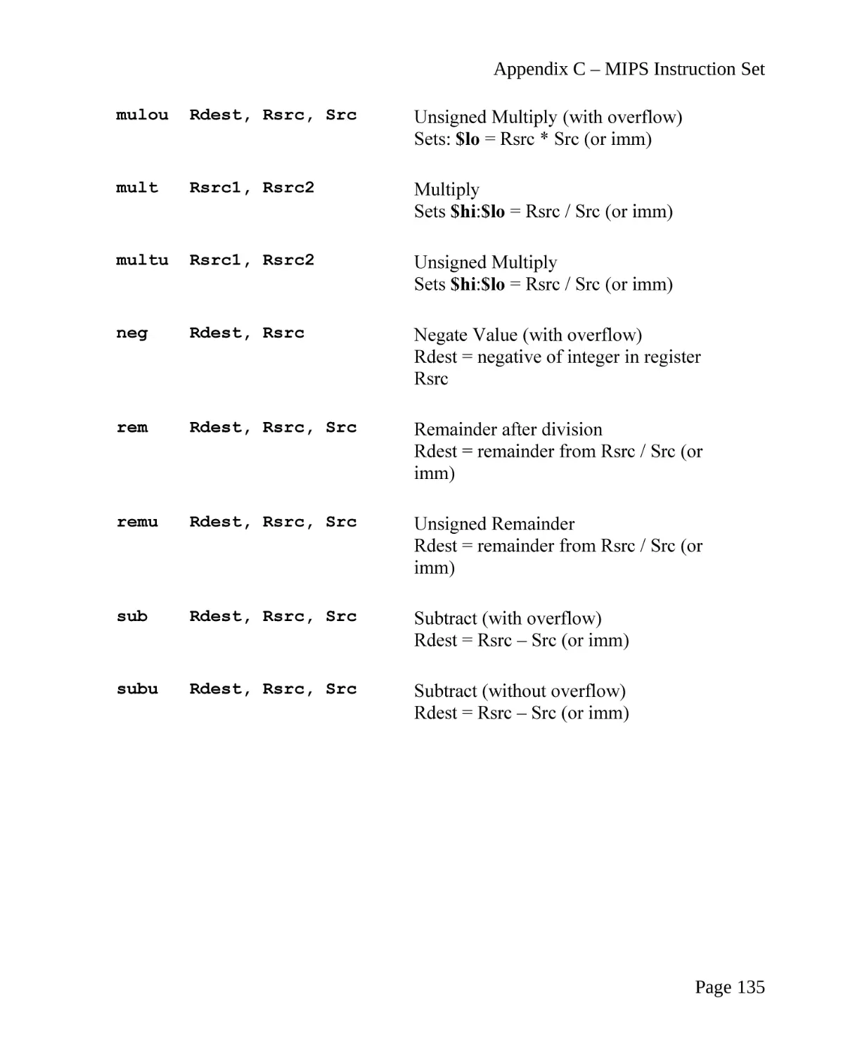
14.1 Arithmetic Instructions..................................................................................134
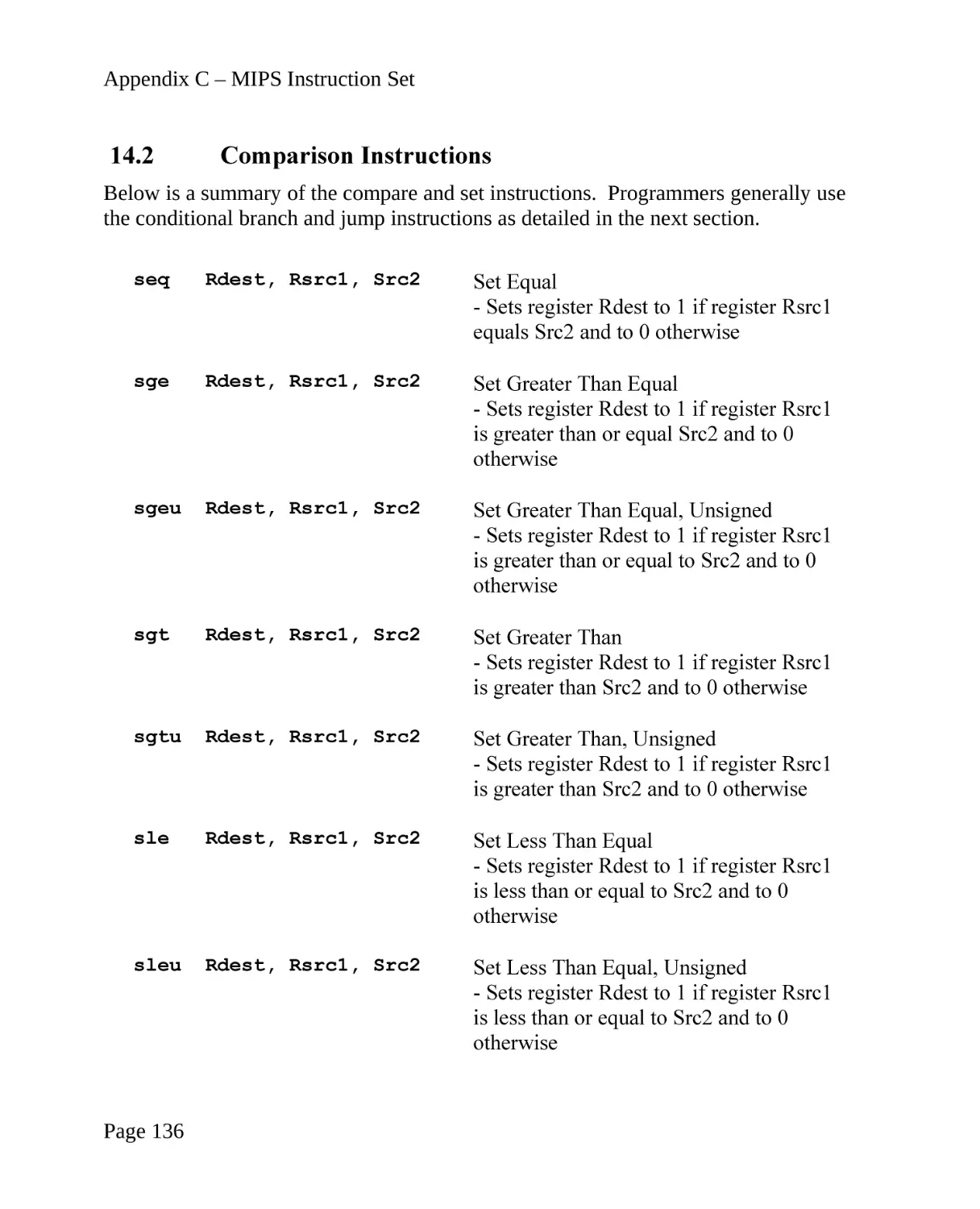
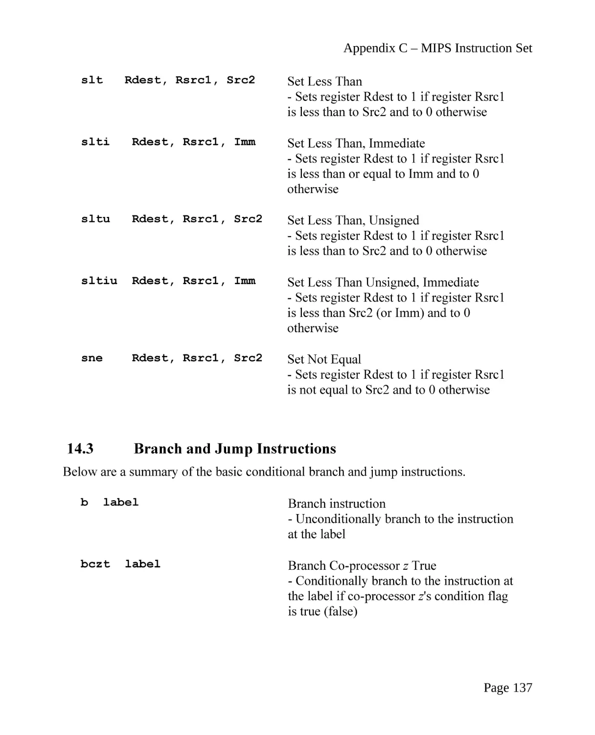
14.2 Comparison Instructions...............................................................................136
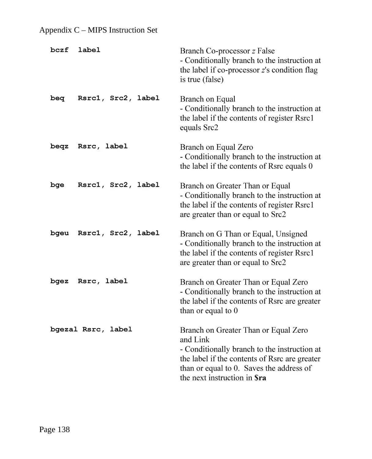
14.3 Branch and Jump Instructions.......................................................................137
14.4 Load Instructions...........................................................................................141
14.5 Logical Instructions.......................................................................................143
14.6 Store Instructions...........................................................................................145
14.7 Data Movement Instructions.........................................................................146
14.8 Floating-Point Instructions............................................................................148
14.9 Exception and Trap Handling Instructions....................................................152
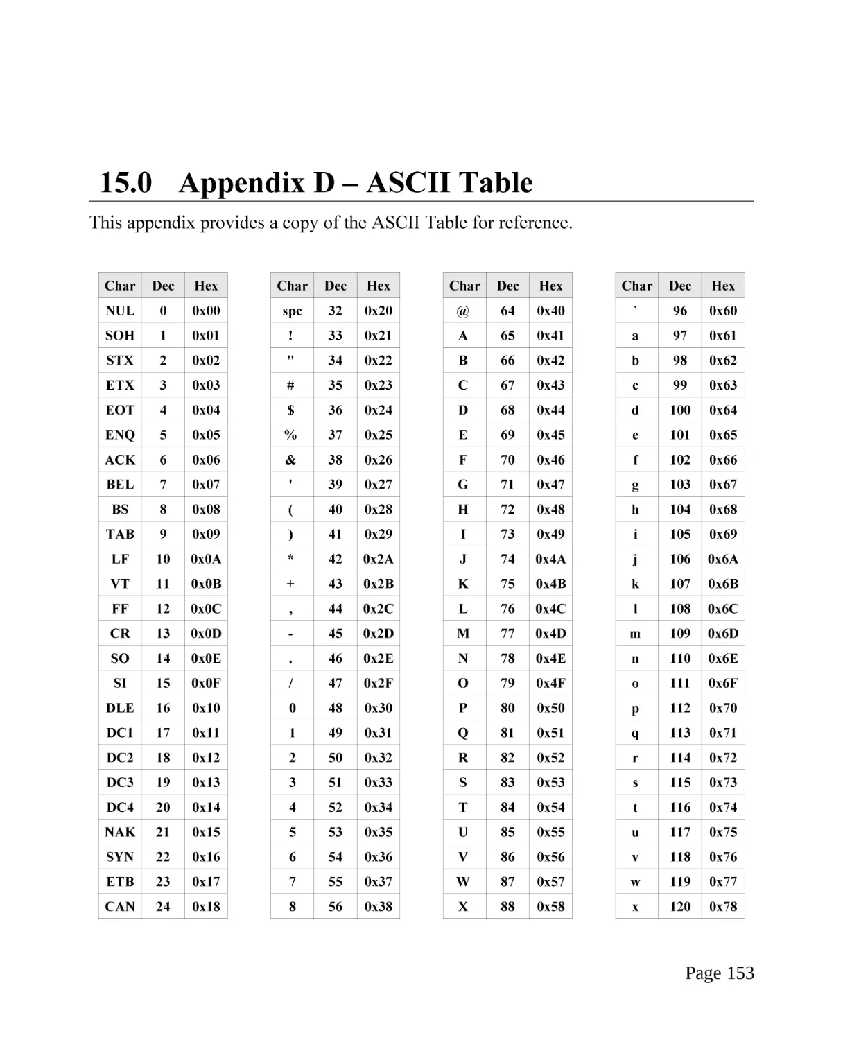
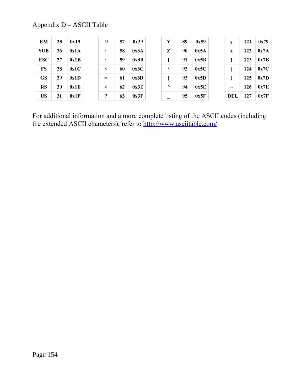
15.0
Appendix D – ASCII Table............................................................................153
16.0
Alphabetical Index..........................................................................................155
Page iv
1.0
Introduction
There are a number of excellent, comprehensive, and in-depth texts on MIPS assembly
language programming. This is not one of them.
The purpose of this text is to provide a simple and free reference for university level
programming and architecture units that include a brief section covering MIPS assembly
language programming. The text assumes usage of the QtSpim simulator. An appendix
is included that covers the download, installation, and basic use of the QtSpim
simulator.
The scope of this text addresses basic MIPS assembly language programming including
instruction set usage, stacks, procedure/function calls, QtSpim simulator system
services, multiple dimension arrays, and basic recursion.
1.1 Additional References
Some key references for additional information are listed below:
•
MIPS Assembly-language Programmer Guide, Silicon Graphics
•
MIPS Software Users Manual, MIPS Technologies, Inc.
•
Computer Organization and Design: The Hardware/Software Interface,
Hennessy and Patterson
More information regarding these references can be found on the Internet.
Page 1
Chapter 1.0 ◄ Introduction
Page 2
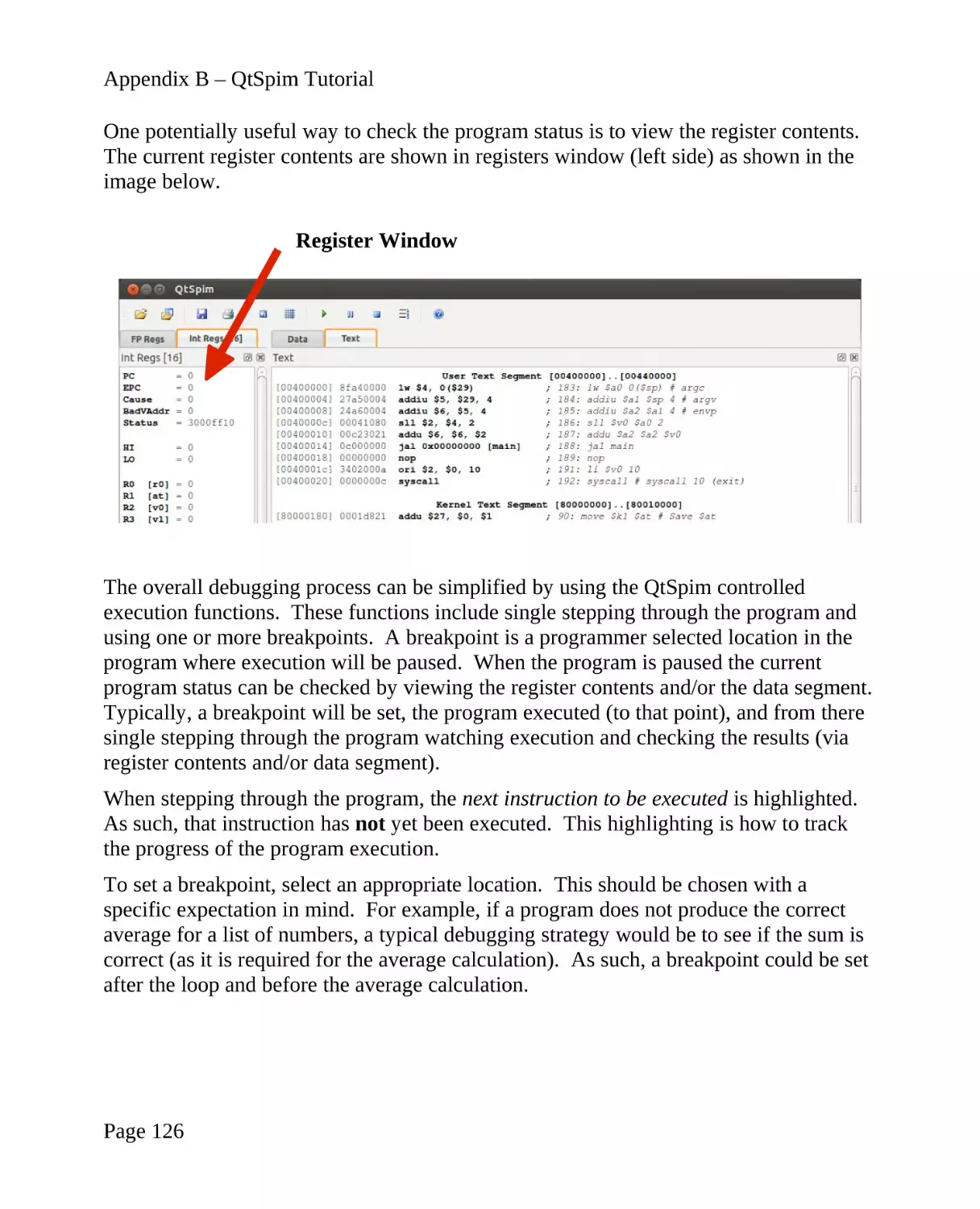
2.0
MIPS Architecture Overview
This chapter presents a basic, general overview of the architecture of the MIPS
processor.
The MIPS architecture is a Reduced Instruction Set Computer (RISC). This means that
there is a smaller number of instructions that use a uniform instruction encoding format.
Each instruction/operation does one thing (memory access, computation, conditional,
etc.). The idea is to make the lesser number of instructions execute faster. In general
RISC architectures, and specifically the MIPS architecture, are designed for high-speed
implementations.
2.1 Architecture Overview
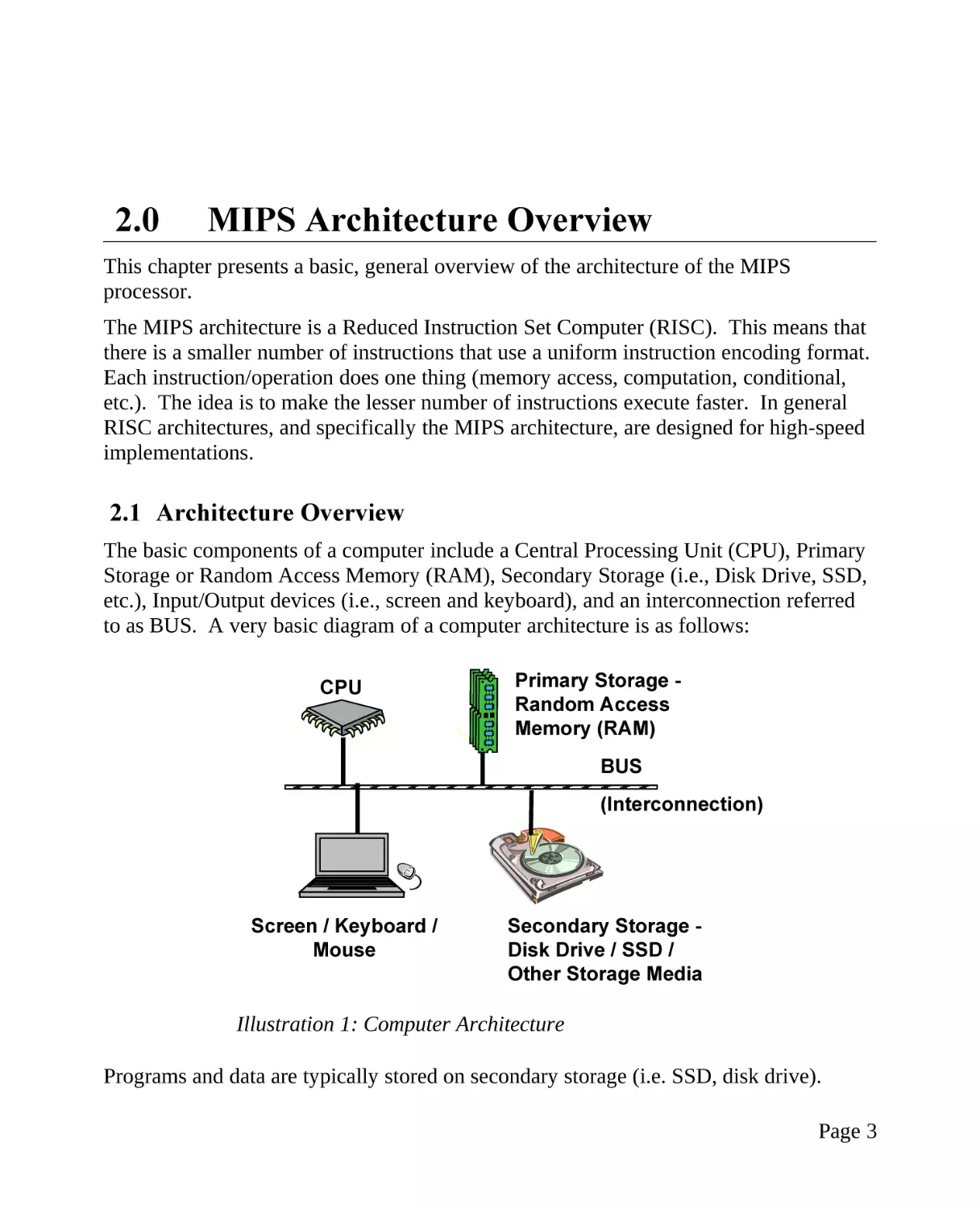
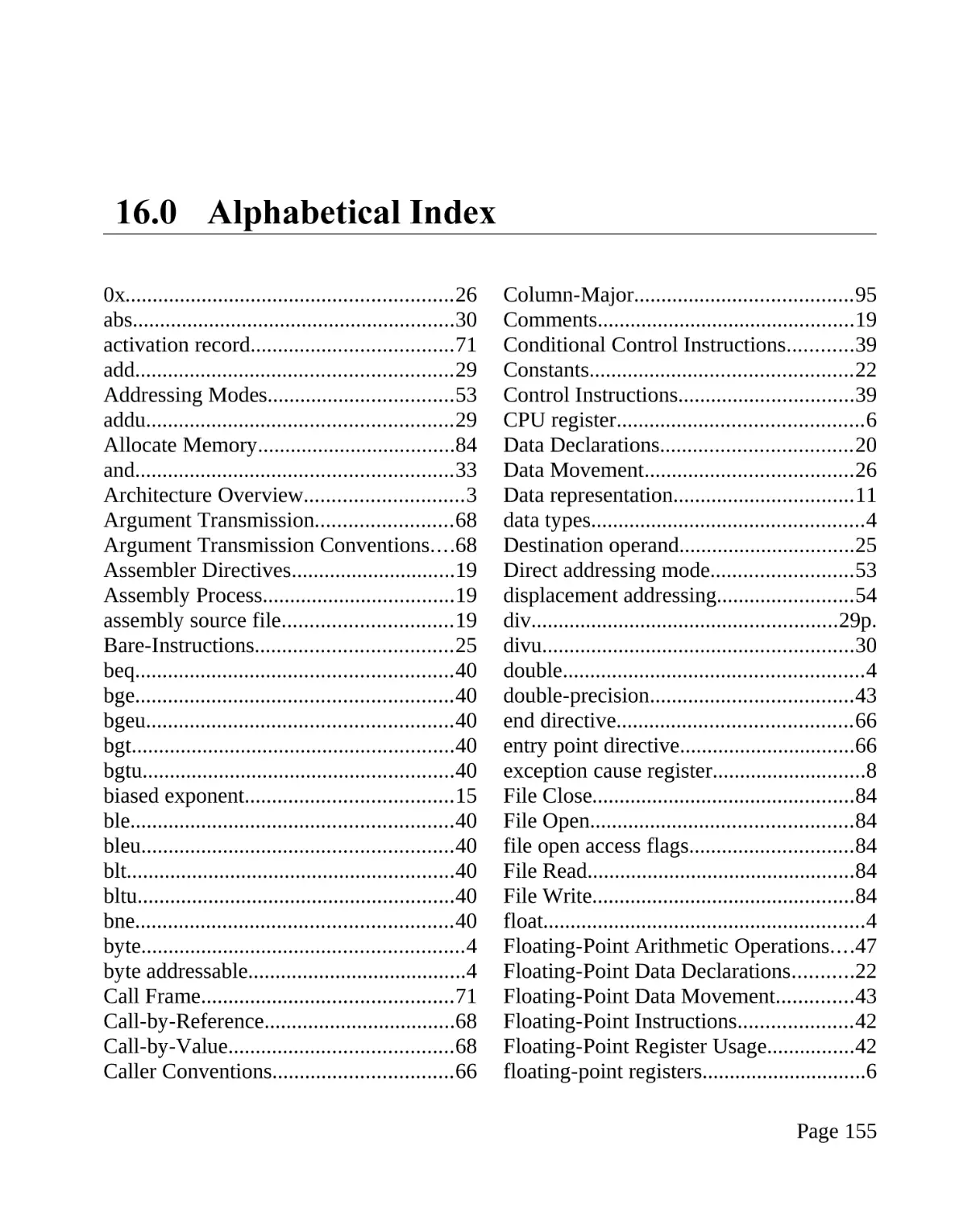
The basic components of a computer include a Central Processing Unit (CPU), Primary
Storage or Random Access Memory (RAM), Secondary Storage (i.e., Disk Drive, SSD,
etc.), Input/Output devices (i.e., screen and keyboard), and an interconnection referred
to as BUS. A very basic diagram of a computer architecture is as follows:
CPU
Primary Storage Random Access
Memory (RAM)
BUS
(Interconnection)
Screen / Keyboard /
Mouse
Secondary Storage Disk Drive / SSD /
Other Storage Media
Illustration 1: Computer Architecture
Programs and data are typically stored on secondary storage (i.e. SSD, disk drive).
Page 3
Chapter 2.0 ◄ MIPS Architecture Overview
When a program is executed, it must be copied from the disk drive into the RAM
memory. The CPU executes the program from RAM. This is similar to storing a term
paper on the disk drive, and when writing/editing the term paper, it is copied from the
disk drive into memory. When done, the updated version is stored back to the disk
drive.
2.2 Data Types/Sizes
The basic data types include integer, floating-point, and characters.
This architecture supports data storage sizes of byte, halfword (sometimes referred to as
just half), or word sizes. Floating-point must be of either word (32-bit) size or double
word (64-bit) size. Character data is typically a byte and a string is a series of sequential
bytes.
The MIPS architecture supports the following data/memory sizes:
Name
Size
byte
8-bit integer
halfword
16-bit integer
word
32-bit integer
float
32-bit floating-point number
double
64-bit floating-point number
The halfword is often referred to as just 'half '. Lists or arrays (sets of memory) can be
reserved in any of these types. In addition, an arbitrary number of bytes can be defined
with the ".space" directive.
2.3 Memory
Memory can be viewed as a series of bytes, one after another. That is, memory is byte
addressable. This means each memory address holds one byte of information. To store
a word, four bytes are required which use four memory addresses.
Additionally, the MIPS architecture as simulated in QtSpim is little-endian. This means
that the Least Significant Byte (LSB) is stored in the lowest memory address. The Most
Significant Byte (MSB) is stored in the highest memory location.
Page 4
Chapter 2.0 ► MIPS Architecture Overview
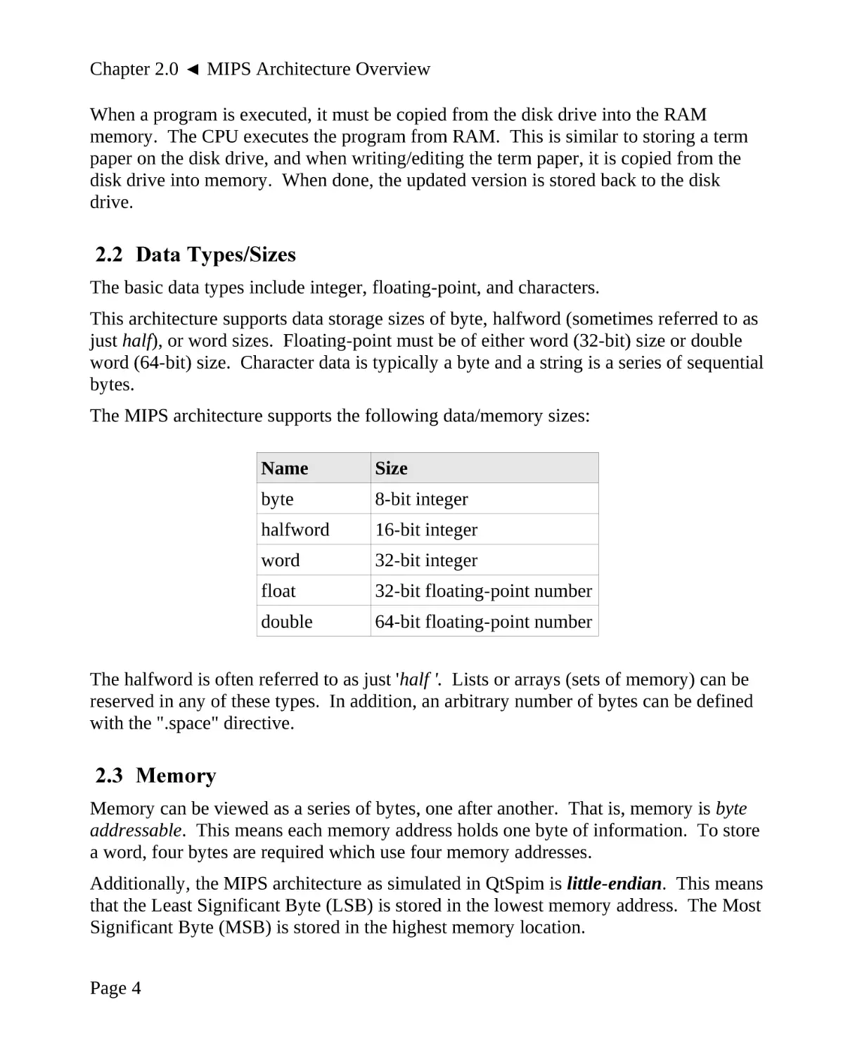
For a word (32-bits), the MSB and LSB are allocated as shown below.
31 30 29 28 27 26 25 24 23 22 21 20 19 18 17 16 15 14 13 12 11 10
9
8
7
6
5
MSB
4
3
2
1
0
LSB
For example, assuming the following declarations:
num1:
num2:
.word
.word
42
5000000
Recall that 4210 in hex, word size, is 0x0000002A and 5,000,00010 in hex, word size, is
0x004C4B40.
For a little-endian architecture, the memory picture would be as follows:
variable
name
Num2 →
Num1 →
value
address
?
0x100100C
00
0x100100B
4C
0x100100A
4B
0x1001009
40
0x1001008
00
0x1001007
00
0x1001006
00
0x1001005
2A
0x1001004
?
0x1001003
Based on the little-endian architecture, the LSB is stored in the lowest memory address
and the MSB is stored in the highest memory location.
Page 5
Chapter 2.0 ◄ MIPS Architecture Overview
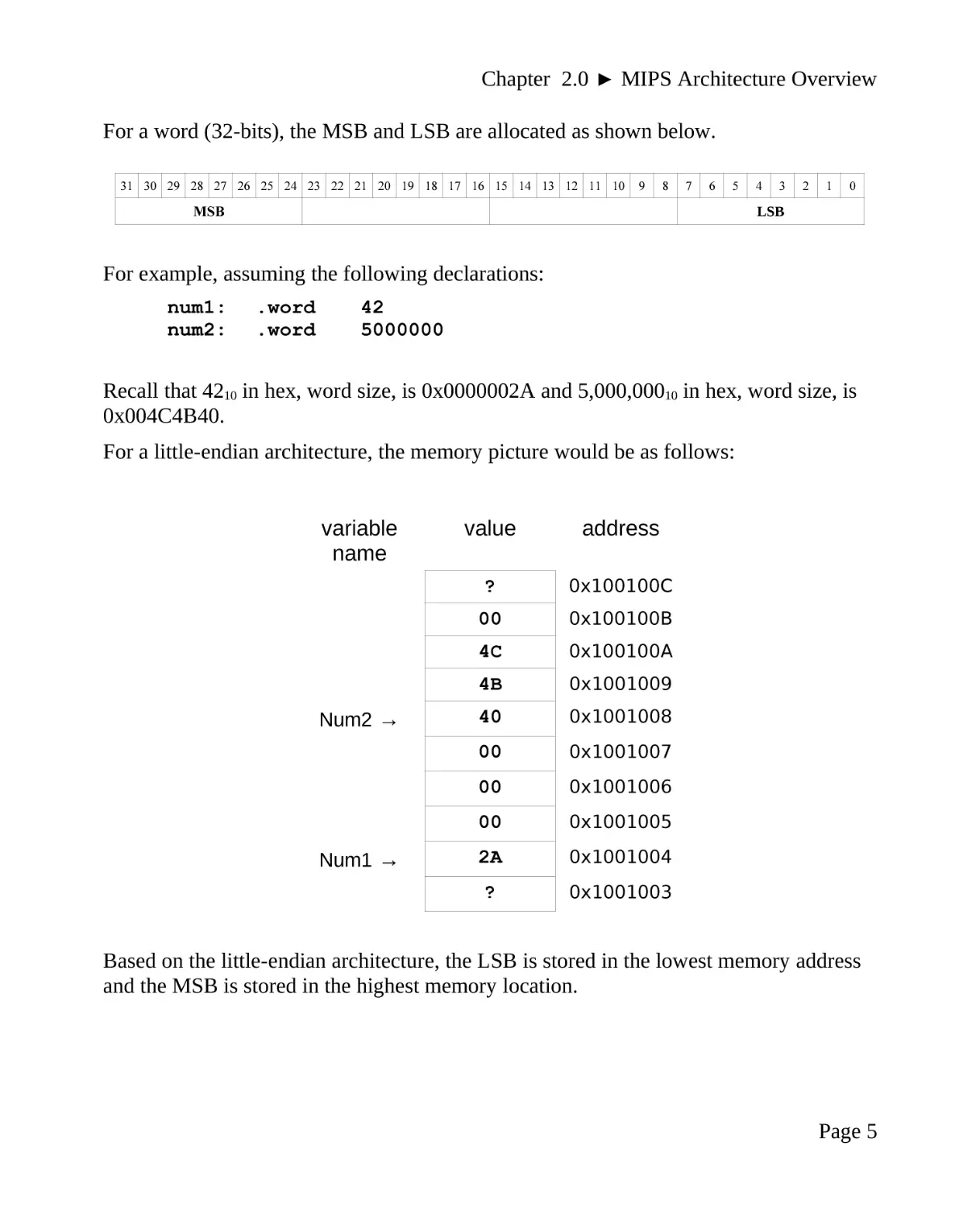
2.4 Memory Layout
The general memory layout for a program is as shown:
high memory
stack
heap
uninitialized data
data
text (code)
low memory
reserved
The reserved section is not available to user programs. The text (or code) section is
where the machine language (i.e., the 1's and 0's that represent the code) is stored. The
data section is where the initialized data is stored. This includes declared variables that
have been provided an initial value at assemble time. The uninitialized data section is
where declared variables that have not been provided an initial value are stored. If
accessed before being set, the value will not be meaningful. The heap is where
dynamically allocated data will be stored (if requested). The stack starts in high
memory and grows downward.
The QtSpim simulator does not distinguish between the initialized and uninitialized data
sections. Later sections will provide additional detail for the text and data sections.
2.5 CPU Registers
A CPU register, or just register, is a temporary storage or working location built into the
CPU itself (separate from memory). Computations are typically performed by the CPU
using registers.
The MIPS has 32, 32-bit integer registers ($0 through $31) and 32, 32-bit floating-point
registers ($f0 through $f31). Some of the integer registers are used for special purposes.
For example, $29 is dedicated for use as the stack pointer register, referred to as $sp.
Page 6
Chapter 2.0 ► MIPS Architecture Overview
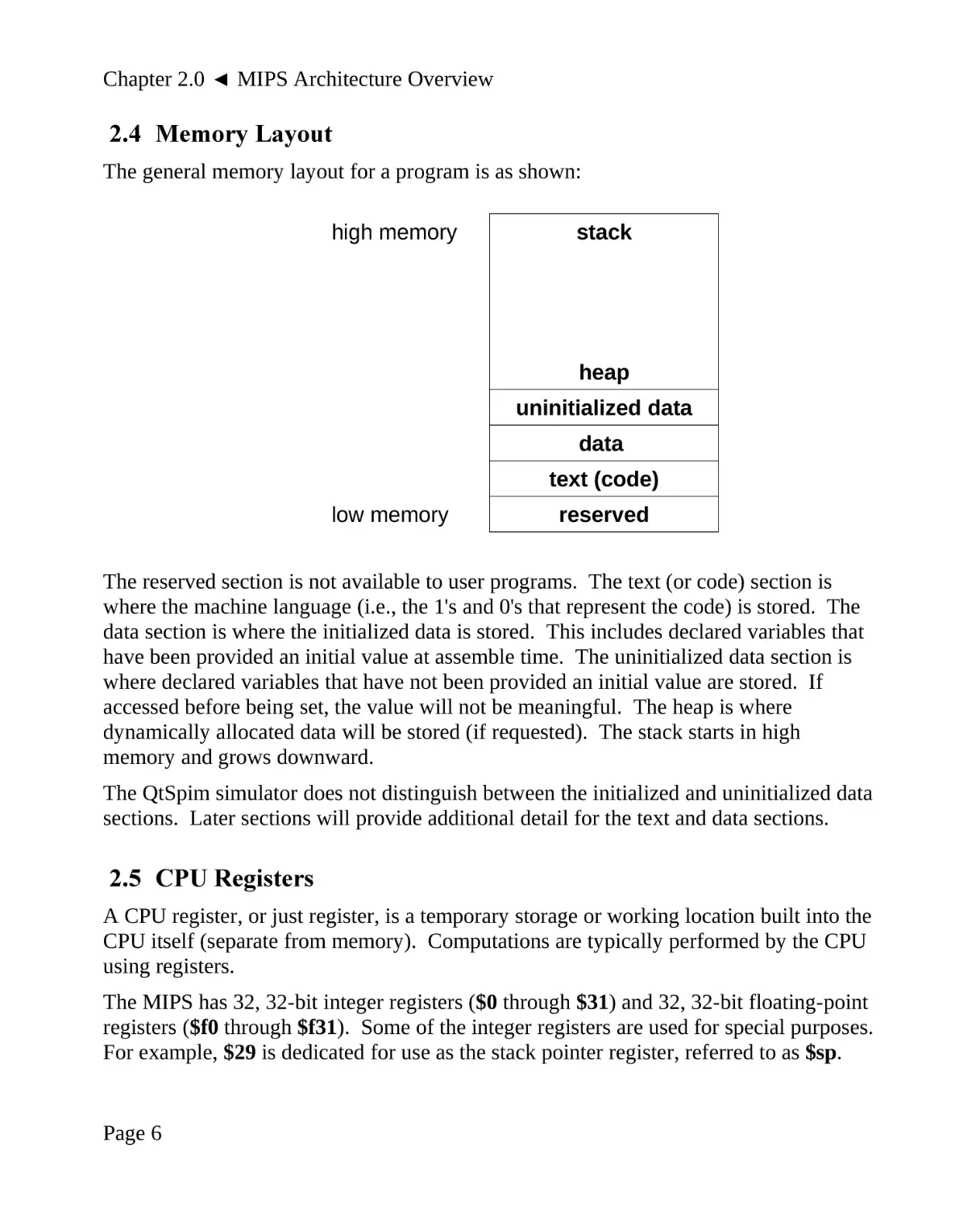
The registers available and typical register usage is described in the following table.
Register
Name
Register
Number
Register Usage
$zero
$0
Hardware set to 0
$at
$1
Assembler temporary
$v0 - $v1
$2 - $3
Function result (low/high)
$a0 - $a3
$4 - $7
Argument Register 1
$t0 - $t7
$8 - $15
Temporary registers
$s0 - $s7
$16 - $23
Saved registers
$t8 - $t9
$24 - $25
Temporary registers
$k0 - $k1
$26 - $27
Reserved for OS kernel
$gp
$28
Global pointer
$sp
$29
Stack pointer
$fp
$30
Frame pointer
$ra
$31
Return address
The register names convey specific usage information. The register names will be used
in the remainder of this document. Further sections will expand on register usage
conventions and address the 'temporary' and 'saved' registers.
2.5.1 Reserved Registers
The following reserved registers should not be used in user programs.
Register Name
Register Usage
$k0 - $k1
Reserved for use by the
Operating System
$at
Assembler temporary
$gp
Global pointer
$epc
Exception program counter
Page 7
Chapter 2.0 ◄ MIPS Architecture Overview
The $k0 and $k1 registers are reserved for use by the operating system and should not
be used in user programs. The $at register is used by the assembler and should not be
used in user programs. The $gp register is used as a pointer to global data (as needed)
and should not be used in user programs.
2.5.2 Miscellaneous Registers
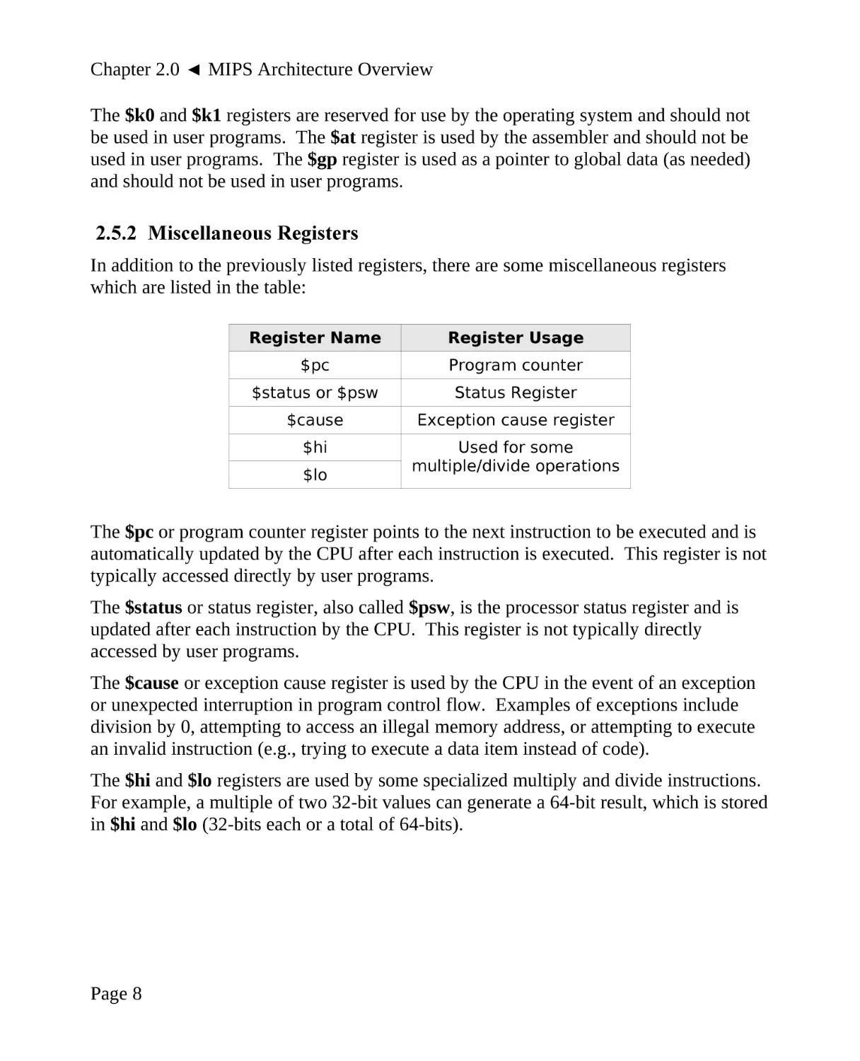
In addition to the previously listed registers, there are some miscellaneous registers
which are listed in the table:
Register Name
Register Usage
$pc
Program counter
$status or $psw
Status Register
$cause
Exception cause register
$hi
Used for some
multiple/divide operations
$lo
The $pc or program counter register points to the next instruction to be executed and is
automatically updated by the CPU after each instruction is executed. This register is not
typically accessed directly by user programs.
The $status or status register, also called $psw, is the processor status register and is
updated after each instruction by the CPU. This register is not typically directly
accessed by user programs.
The $cause or exception cause register is used by the CPU in the event of an exception
or unexpected interruption in program control flow. Examples of exceptions include
division by 0, attempting to access an illegal memory address, or attempting to execute
an invalid instruction (e.g., trying to execute a data item instead of code).
The $hi and $lo registers are used by some specialized multiply and divide instructions.
For example, a multiple of two 32-bit values can generate a 64-bit result, which is stored
in $hi and $lo (32-bits each or a total of 64-bits).
Page 8
Chapter 2.0 ► MIPS Architecture Overview
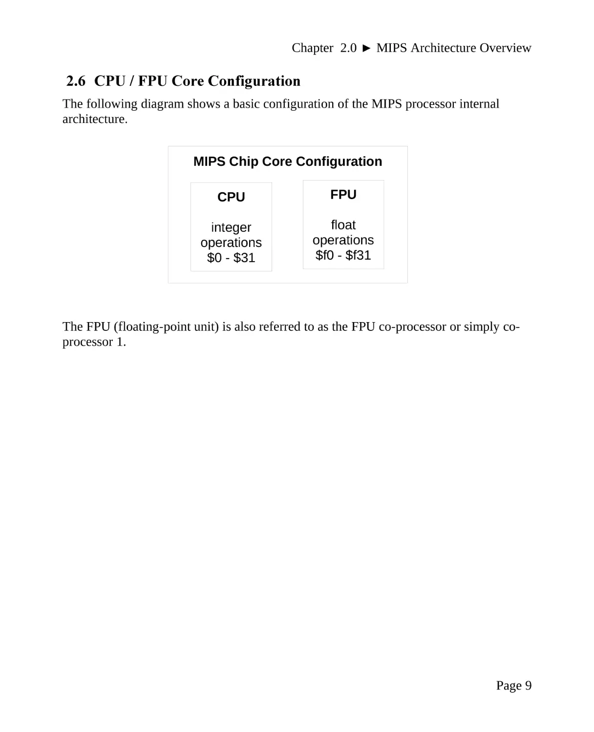
2.6 CPU / FPU Core Configuration
The following diagram shows a basic configuration of the MIPS processor internal
architecture.
MIPS Chip Core Configuration
CPU
FPU
integer
operations
$0 - $31
float
operations
$f0 - $f31
The FPU (floating-point unit) is also referred to as the FPU co-processor or simply coprocessor 1.
Page 9
Chapter 2.0 ◄ MIPS Architecture Overview
Page 10
3.0
Data Representation
Data representation refers to how information is stored within the computer. There is a
specific method for storing integers which is different than storing floating-point values
which is different than storing characters. This chapter presents a brief summary of the
integer, floating-point, and ASCII representation schemes. It is assumed the reader is
already generally familiar with the binary, decimal, and hexadecimal numbering
systems.
3.1 Integer Representation
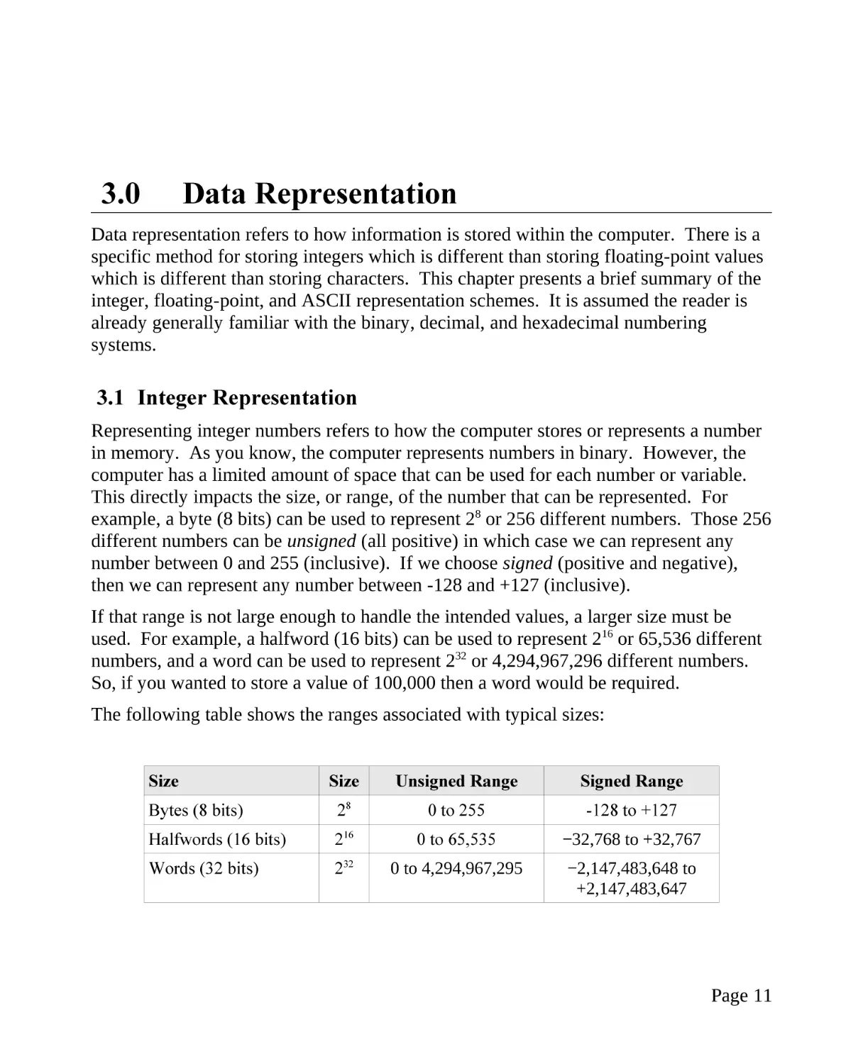
Representing integer numbers refers to how the computer stores or represents a number
in memory. As you know, the computer represents numbers in binary. However, the
computer has a limited amount of space that can be used for each number or variable.
This directly impacts the size, or range, of the number that can be represented. For
example, a byte (8 bits) can be used to represent 28 or 256 different numbers. Those 256
different numbers can be unsigned (all positive) in which case we can represent any
number between 0 and 255 (inclusive). If we choose signed (positive and negative),
then we can represent any number between -128 and +127 (inclusive).
If that range is not large enough to handle the intended values, a larger size must be
used. For example, a halfword (16 bits) can be used to represent 216 or 65,536 different
numbers, and a word can be used to represent 232 or 4,294,967,296 different numbers.
So, if you wanted to store a value of 100,000 then a word would be required.
The following table shows the ranges associated with typical sizes:
Size
Size
8
Unsigned Range
Signed Range
Bytes (8 bits)
2
0 to 255
-128 to +127
Halfwords (16 bits)
216
0 to 65,535
−32,768 to +32,767
0 to 4,294,967,295
−2,147,483,648 to
+2,147,483,647
Words (32 bits)
2
32
Page 11
Chapter 3.0 ◄ Data Representation
In order to determine if a value can be represented, you will need to know the size of
storage element (byte, halfword, word) being used and if the values are signed or
unsigned values.
•
•
For representing unsigned values within the range of a given storage size,
standard binary is used.
For representing signed values within the range, two's complement is used.
Specifically, the two's complement encoding process applies to the values in the
negative range. For values within the positive range, standard binary is used.
Additional detail regarding two's complement is provided in the next section.
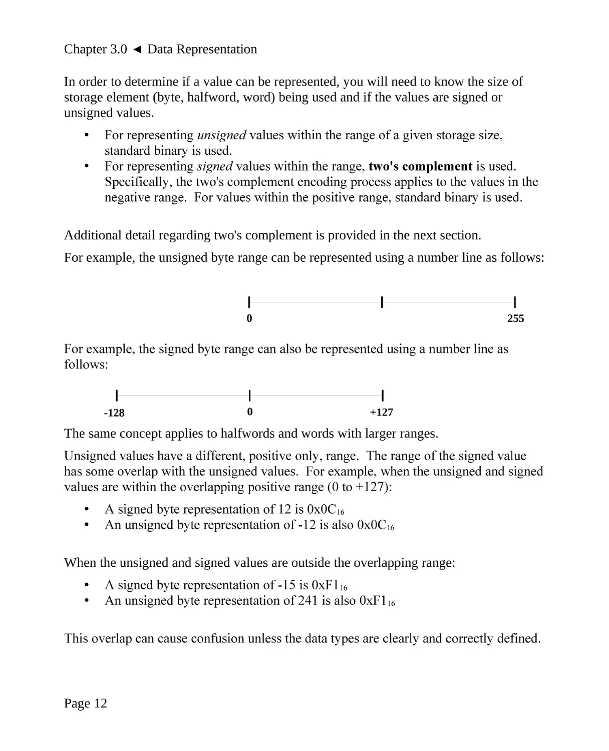
For example, the unsigned byte range can be represented using a number line as follows:
0
255
For example, the signed byte range can also be represented using a number line as
follows:
-128
0
+127
The same concept applies to halfwords and words with larger ranges.
Unsigned values have a different, positive only, range. The range of the signed value
has some overlap with the unsigned values. For example, when the unsigned and signed
values are within the overlapping positive range (0 to +127):
•
•
A signed byte representation of 12 is 0x0C16
An unsigned byte representation of -12 is also 0x0C16
When the unsigned and signed values are outside the overlapping range:
•
•
A signed byte representation of -15 is 0xF116
An unsigned byte representation of 241 is also 0xF116
This overlap can cause confusion unless the data types are clearly and correctly defined.
Page 12
Chapter 3.0 ► Data Representation
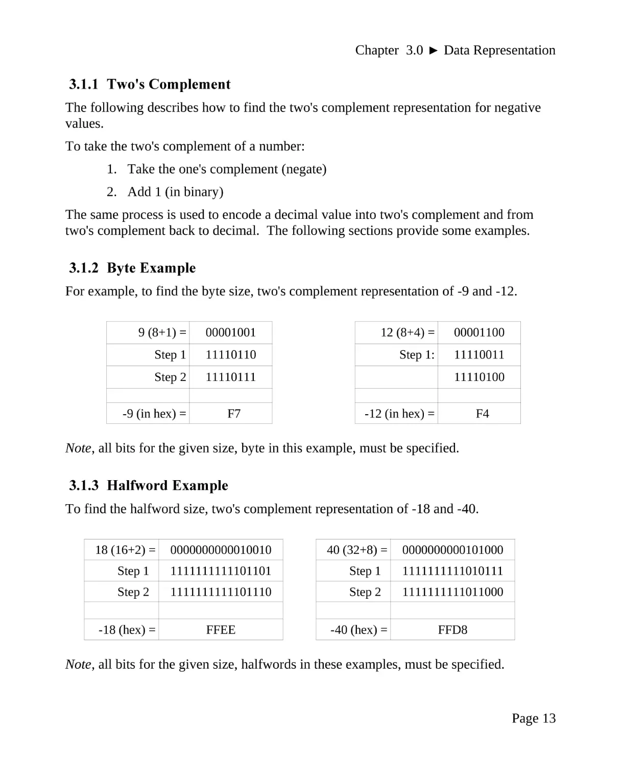
3.1.1 Two's Complement
The following describes how to find the two's complement representation for negative
values.
To take the two's complement of a number:
1. Take the one's complement (negate)
2. Add 1 (in binary)
The same process is used to encode a decimal value into two's complement and from
two's complement back to decimal. The following sections provide some examples.
3.1.2 Byte Example
For example, to find the byte size, two's complement representation of -9 and -12.
9 (8+1) =
00001001
12 (8+4) =
00001100
Step 1
11110110
Step 1:
11110011
Step 2
11110111
-9 (in hex) =
F7
11110100
-12 (in hex) =
F4
Note, all bits for the given size, byte in this example, must be specified.
3.1.3 Halfword Example
To find the halfword size, two's complement representation of -18 and -40.
18 (16+2) =
0000000000010010
40 (32+8) =
0000000000101000
Step 1
1111111111101101
Step 1
1111111111010111
Step 2
1111111111101110
Step 2
1111111111011000
-18 (hex) =
FFEE
-40 (hex) =
FFD8
Note, all bits for the given size, halfwords in these examples, must be specified.
Page 13
Chapter 3.0 ◄ Data Representation
3.2 Unsigned and Signed Addition
As previously noted, the unsigned and signed representations may provide different
interpretations for the final value being represented. However, the addition and
subtraction operations are the same. For example:
241
11110001
7
00000111
248
11111000
+
248 =
-15
11110001
7
00000111
-8
11111000
+
F8
-8 =
F8
The final result of 0xF8 may be interpreted as 248 for unsigned representation and -8 for
a signed representation.
Additionally, 0xF816 is the º (degree symbol) in the ASCII table.
As such, it is very important to have a clear definition of the sizes (byte, halfword, word,
etc.) and types (signed, unsigned) of data for the operations being performed.
3.3 Floating-point Representation
The representation issues for floating-point numbers are more complex. There are a
series of floating-point representations for various ranges of the value. For simplicity,
we will only look primarily at the IEEE 754 32-bit floating-point standard.
3.3.1 IEEE 32-bit Representation
The IEEE 754 32-bit floating-point standard is defined as follows:
31 30 29 28 27 26 25 24 23 22 21 20 19 18 17 16 15 14 13 12 11 10
s
biased exponent
9
8
7
6
5
4
3
2
1
0
fraction
Where s is the sign (0 => positive and 1 => negative). When representing floating-point
values, the first step is to convert floating-point value into binary.
Page 14
Chapter 3.0 ► Data Representation
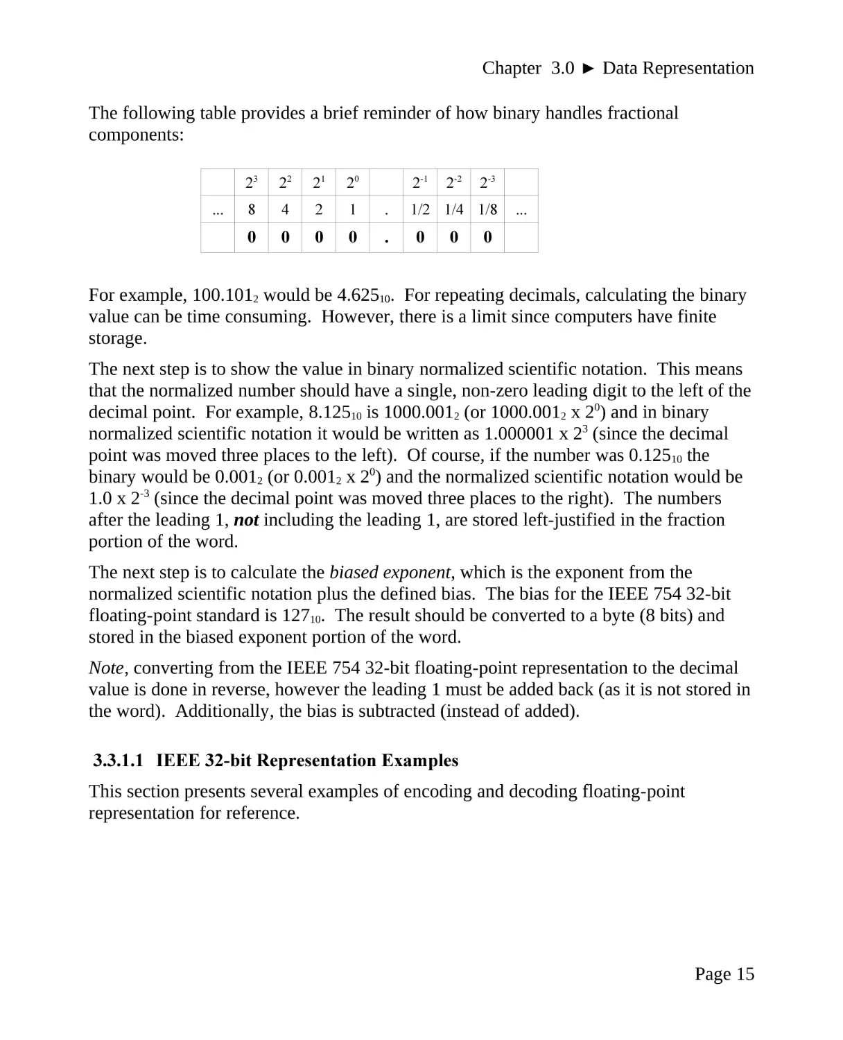
The following table provides a brief reminder of how binary handles fractional
components:
...
23
22
21
20
2-1
8
4
2
1
.
0
0
0
0
.
2-2
2-3
1/2 1/4 1/8
0
0
...
0
For example, 100.1012 would be 4.62510. For repeating decimals, calculating the binary
value can be time consuming. However, there is a limit since computers have finite
storage.
The next step is to show the value in binary normalized scientific notation. This means
that the normalized number should have a single, non-zero leading digit to the left of the
decimal point. For example, 8.12510 is 1000.0012 (or 1000.0012 x 20) and in binary
normalized scientific notation it would be written as 1.000001 x 23 (since the decimal
point was moved three places to the left). Of course, if the number was 0.12510 the
binary would be 0.0012 (or 0.0012 x 20) and the normalized scientific notation would be
1.0 x 2-3 (since the decimal point was moved three places to the right). The numbers
after the leading 1, not including the leading 1, are stored left-justified in the fraction
portion of the word.
The next step is to calculate the biased exponent, which is the exponent from the
normalized scientific notation plus the defined bias. The bias for the IEEE 754 32-bit
floating-point standard is 12710. The result should be converted to a byte (8 bits) and
stored in the biased exponent portion of the word.
Note, converting from the IEEE 754 32-bit floating-point representation to the decimal
value is done in reverse, however the leading 1 must be added back (as it is not stored in
the word). Additionally, the bias is subtracted (instead of added).
3.3.1.1 IEEE 32-bit Representation Examples
This section presents several examples of encoding and decoding floating-point
representation for reference.
Page 15
Chapter 3.0 ◄ Data Representation
3.3.1.1.1 Example → -7.7510
For example, to find the IEEE 754 32-bit floating-point representation for -7.7510:
Example 1:
-7.75
• determine sign
-7.75 => 1 (since negative)
• convert to binary
-7.75 =
-0111.112
• normalized scientific notation
=
1.1111 x 22
• compute biased exponent
210 + 12710 = 12910
◦ and convert to binary
= 100000012
• write components in binary:
sign exponent mantissa
1 10000001 11110000000000000000000
• convert to hex (split into groups of 4)
11000000111110000000000000000000
1100 0000 1111 1000 0000 0000 0000 0000
C
0
F
8
0
0
0
0
• final result:
C0F8 000016
3.3.1.1.2 Example → -0.12510
For example, to find the IEEE 754 32-bit floating-point representation for -0.12510:
Example 2:
-0.125
• determine sign
-0.125 => 1 (since negative)
• convert to binary
-0.125 =
-0.0012
• normalized scientific notation
=
1.0 x 2-3
• compute biased exponent
-310 + 12710 = 12410
◦ and convert to binary
= 011111002
• write components in binary:
sign exponent mantissa
1 01111100 00000000000000000000000
• convert to hex (split into groups of 4)
10111110000000000000000000000000
1011 1110 0000 0000 0000 0000 0000 0000
B
E
0
0
0
0
0
0
• final result:
BE00 000016
Page 16
Chapter 3.0 ► Data Representation
3.3.1.1.3 Example → 4144000016
For example, given the IEEE 754 32-bit floating-point representation 4144000016 find
the decimal value:
Example 3:
4144000016
• convert to binary
0100 0001 0100 0100 0000 0000 0000 00002
• split into components
0 10000010 100010000000000000000002
• determine exponent
100000102 = 13010
◦ and remove bias
13010 - 12710 = 310
• determine sign
0 => positive
• write result
+1.10001 x 23 = +1100.01 = +12.25
3.3.2 IEEE 64-bit Representation
The IEEE 754 64-bit floating-point standard is defined as follows:
63 62
s
52 51
biased exponent
0
fraction
The representation process is the same, however the format allows for an 11-bit biased
exponent (which support large and smaller values). The 11-bit biased exponent uses a
bias of 1023.
Page 17
Chapter 3.0 ◄ Data Representation
Page 18
4.0
QtSpim Program Formats
The QtSpim MIPS simulator will be used for programs in this text. The QtSpim
simulator has a number of features and requirements for writing MIPS assembly
language programs. This includes a properly formatted assembly source file.
A properly formatted assembly source file consists of two main parts; the data section
(where data is placed) and the text section (where code is placed). The following
sections summarize the formatting requirements and explain each of these sections.
4.1 Assembly Process
The QtSpim effectively assembles the program during the load process. Any major
errors in the program format or the instructions will be noted immediately. Assembler
errors must be resolved before the program can be successfully executed. Refer to
Appendix B regarding the use of QtSpim to load and execute programs.
4.2 Comments
The "#" character represents a comment line. Anything typed after the "#" is considered
a comment. Blank lines are accepted.
4.3 Assembler Directives
An assembler directive is a message to the assembler, or the QtSpim simulator, that tells
the assembler something it needs to know in order to carry out the assembly process.
This includes noting where the data is declared or the code is defined. Assembler
directives are not executable statements.
Assembler directives start with a ".". Assembler directives are required to define the
start and end of data declarations and to define the start and end of procedures/functions.
For example, ".data" or ".text".
Additionally, directives are used to declare data. The following sections provide some
examples of data declarations using the directives.
Page 19
Chapter 4.0 ◄ QtSpim Program Formats
4.4 Data Declarations
The data must be declared in the ".data" section. All variables and constants are placed
in this section. Variable names must start with a letter followed by letters or numbers
(including some special characters such as the "_"), and terminated with a ":" (colon).
Variable definitions must include the name, the data type, and the initial value for the
variable. In the definition, the variable name must be terminated with a ":".
The data type must be preceded with a "." (period). The general format is:
<variableName>:
.<dataType>
<initialValue>
Refer to the following sections for a series of examples using various data types.
The supported data types are as follows:
Declaration
.byte
8-bit variable(s)
.half
16-bit variable(s)
.word
32-bit variable(s)
.ascii
ASCII string
.asciiz
NULL terminated ASCII string
.float
32 bit IEEE floating-point number
.double
64 bit IEEE floating-point number
.space <n>
<n> bytes of uninitialized memory
These are the primary assembler directives for data declaration. Other directives are
referenced in different sections.
4.4.1 Integer Data Declarations
Integer values are defined with the .word, .half, or .byte directives. Two's complement
is used for the representation of negative values. For more information regarding two's
complement, refer to the Data Representation section.
Page 20
Chapter 4.0 ► QtSpim Program Formats
The following declarations are used to define the integer variables "wVar1" and
"wVar2" as 32-bit word values and initialize them to 500,000 and -100,000.
wVar1:
wVar2:
.word
.word
500000
-100000
The following declarations are used to define the integer variables "hVar1" and "hVar2"
as 16-bit word values and initialize them to 5,000 and -3,000.
hVar1:
hVar2:
.half
.half
5000
-3000
The following declarations are used to define the integer variables "bVar1" and "bVar2"
as 8-bit word values and initialize them to 5 and -3.
bVar1:
bVar2:
.byte
.byte
5
-3
If a variable is initialized to a value that can not be stored in the allocated space, an
assembler error will be generated. For example, attempting to set a byte variable to 500
would be illegal and generate an error.
4.4.2 String Data Declarations
At the assembly level, a string is a series of sequentially defined byte-sized characters,
typically terminated with a NULL byte (0x00).
Strings are defined with .ascii or .asciiz directives. Characters are represented using
standard ASCII characters. Refer to Appendix D for a copy of the ASCII table for
reference.
The C/C++ style new line, "\n", and tab, "\t" tab are supported within strings.
The following declarations are used to define a string "message" and initialize it to
"Hello World".
message:
.asciiz
"Hello World\n"
In this example, the string is defined as NULL terminated (i.e., after the new line). The
NULL is a non-printable ASCII character and is used to mark the end of the string. The
NULL termination is standard and is required by the print string system service (to work
correctly).
Page 21
Chapter 4.0 ◄ QtSpim Program Formats
To define a string with multiple lines, the NULL termination would only be required on
the final or last line. For example:
message:
.ascii
.ascii
.ascii
.asciiz
"Line 1:
"Line 2:
"for all
"Line 3:
Goodbye World\n"
So, long and thanks "
the fish.\n"
Game Over.\n"
When printed, using the starting address of 'message', everything up-to (but not
including) the NULL will be displayed. As such, the declaration using multiple lines is
not relevant to the final displayed output.
4.4.3 Floating-Point Data Declarations
Floating-point values are defined with the .float (32-bit) or .double (64-bit) directives.
The IEEE floating-point format is used for the internal representation of floating-point
values.
The following declarations are used to define the floating-point variables "pi" a 32-bit
floating-point value initialized to 3.14159 and "tao" a 64-bit floating-point values
initialized them to 6.28318.
pi:
tao:
.float
.double
3.14159
6.28318
For more information regarding the IEEE format, refer to the Data Representation
section.
4.5 Constants
Constant names must start with a letter, followed by letters or numbers including some
special characters such as the "_" (underscore). Constant definitions are created with an
"=" sign.
For example, to create some constants named TRUE and FALSE and set them to 1 and
0 respectively:
TRUE = 1
FALSE = 0
Constants are also defined in the data section. The use of all capitals for a constant is a
convention and not required by the QtSpim program. The convention helps
programmers more easily distinguish between variables (which can change values) and
Page 22
Chapter 4.0 ► QtSpim Program Formats
constants (which can not change values). Additionally, in assembly language constants
are not typed (i.e., not predefined to be a specific size such as 8-bits, 16-bits, 32-bits, or
64-bits).
4.6 Program Code
The code must be preceded by the ".text" directive.
In addition, there are some basic requirements for naming a "main" procedure (i.e., the
first procedure to be executed). The ".globl name" and ".ent name" directives are used
to define the name of the initial or main procedure. The ".ent" is optional for the QtSpim
simulator. Note, the globl spelled incorrectly is the correct directive. Also, the main
procedure must start with a label with the procedure name. The main procedure (as all
procedures) should be terminated with the ".end <name>" directive.
In the program template, the <name> would be the name of the main
function/procedure, which is "main".
4.7 Labels
Labels are code locations, typically used as a function/procedure name or as the target of
a jump. The first use of a label is the main program starting location, which must be
named 'main' which is a specific requirement for the QtSpim simulator.
The rules for a label are as follows:
•
•
•
•
Must start with a letter
May be followed by letters, numbers, or an "_" (underscore).
Must be terminated with a ":" (colon).
May only be defined once.
Some examples of a label include:
main:
exitProgram:
Characters in a label are case-sensitive. As such, Loop: and loop: are different labels.
This can be very confusing initially, so caution is advised.
Page 23
Chapter 4.0 ◄ QtSpim Program Formats
4.8 Program Template
The following is a very basic template for QtSpim MIPS programs. This general
template will be used for all programs.
#
Name and general description of program
# ---------------------------------------# Data declarations go in this section.
.data
#
program specific data declarations
# ---------------------------------------# Program code goes in this section.
.text
.globl
.ent
main:
main
main
# ----#
your program code goes here.
# ----# Done, terminate program.
li
$v0, 10
syscall
.end main
# all done!
The initial header (".text", ".globl main", ".ent main", and "main:") will be the same for
all QtSpim programs. The final instructions ("li $v0, 10" and "syscall") terminate the
program.
A more complete example, with working code, can be found in Appendix A.
Page 24
5.0
Instruction Set Overview
In assembly-language, instructions are how work is accomplished. In assembly the
instructions are simple, single operation commands. In a high-level language, one line
might be translated into a series of instructions in assembly-language.
This chapter presents a summary of the basic, most common instructions. The MIPS
Instruction Set Appendix presents a more comprehensive list of the available
instructions.
5.1 Pseudo-Instructions vs Bare-Instructions
As part of the MIPS architecture, the assembly language includes a number of pseudoinstructions. A bare-instruction is an instruction that is directly executed by the CPU.
A pseudo-instruction is an instruction that the assembler, or simulator, will recognize
but then convert into one or more bare-instructions. This text will focus primarily on
the pseudo-instructions.
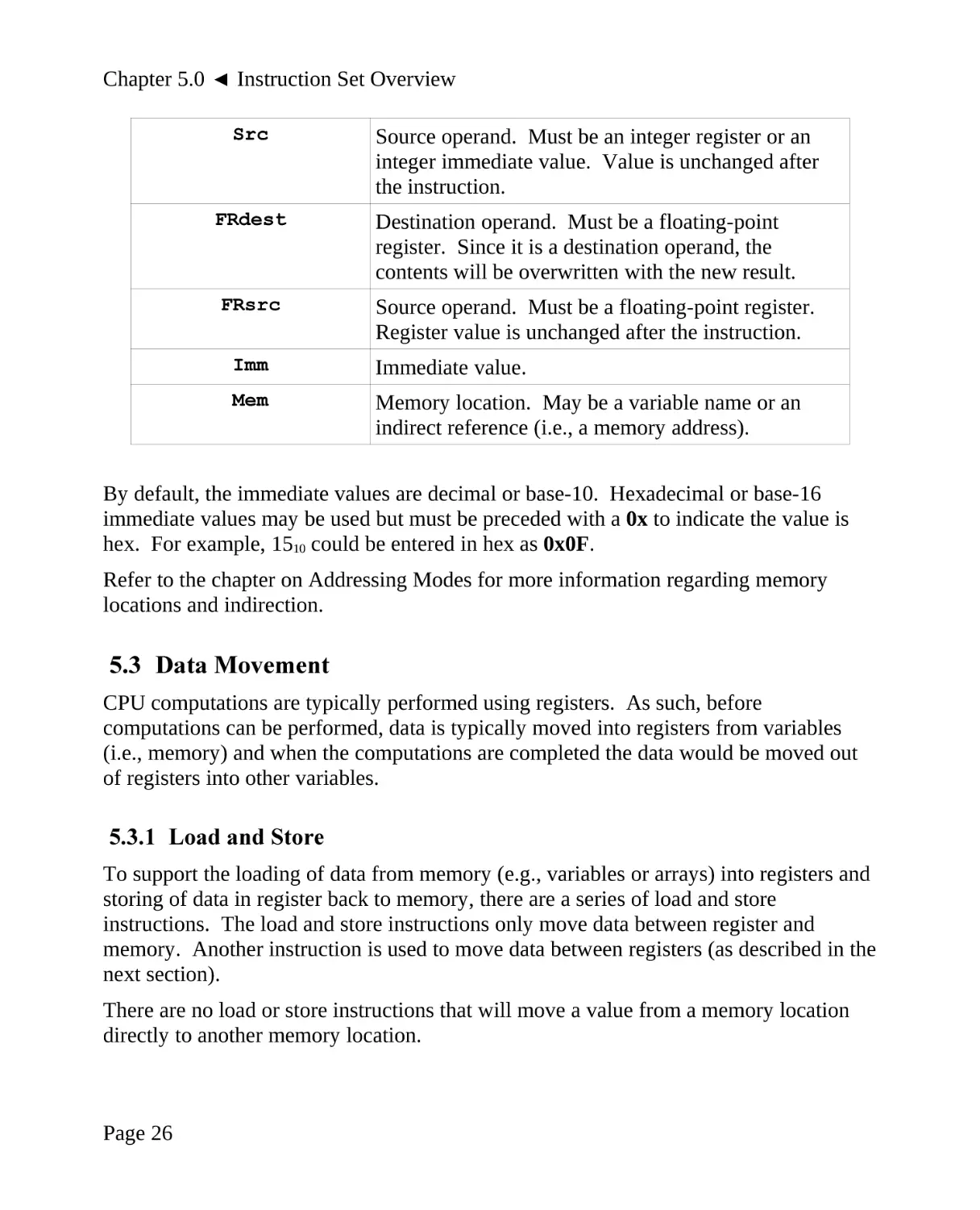
5.2 Notational Conventions
This section summarizes the notation used within this text which is fairly common in the
technical literature. In general, an instruction will consist of the instruction or operation
itself (i.e., add, sub, mul, etc.) and the operands. The operands refer to where the data
(to be operated on) is coming from, or where the result is to be placed.
The following table summarizes the notational conventions used in the remainder of the
document.
Operand Notation
Rdest
Rsrc
Description
Destination operand. Must be an integer register.
Since it is a destination operand, the contents will be
over written with the new result.
Source operand. Must be an integer register.
Register value is unchanged after the instruction.
Page 25
Chapter 5.0 ◄ Instruction Set Overview
Src
Source operand. Must be an integer register or an
integer immediate value. Value is unchanged after
the instruction.
FRdest
Destination operand. Must be a floating-point
register. Since it is a destination operand, the
contents will be overwritten with the new result.
FRsrc
Source operand. Must be a floating-point register.
Register value is unchanged after the instruction.
Imm
Immediate value.
Mem
Memory location. May be a variable name or an
indirect reference (i.e., a memory address).
By default, the immediate values are decimal or base-10. Hexadecimal or base-16
immediate values may be used but must be preceded with a 0x to indicate the value is
hex. For example, 1510 could be entered in hex as 0x0F.
Refer to the chapter on Addressing Modes for more information regarding memory
locations and indirection.
5.3 Data Movement
CPU computations are typically performed using registers. As such, before
computations can be performed, data is typically moved into registers from variables
(i.e., memory) and when the computations are completed the data would be moved out
of registers into other variables.
5.3.1 Load and Store
To support the loading of data from memory (e.g., variables or arrays) into registers and
storing of data in register back to memory, there are a series of load and store
instructions. The load and store instructions only move data between register and
memory. Another instruction is used to move data between registers (as described in the
next section).
There are no load or store instructions that will move a value from a memory location
directly to another memory location.
Page 26
Chapter 5.0 ► Instruction Set Overview
The general forms of the load and store instructions are as follows:
Instruction
Description
l<type>
Rdest, mem
Load value from memory location
into destination register.
li
Rdest, imm
Load specified immediate value
into destination register.
la
Rdest, mem
Load address of memory location
into destination register.
s<type>
Rsrc, mem
Store contents of source register
into memory location.
Assuming the following data declarations:
num:
wnum:
hnum:
bnum:
wans:
hans:
bans:
.word
.word
.half
.byte
.word
.half
.byte
0
42
73
7
0
0
0
To perform, the basic operations of:
num = 27
wans = wnum
hans = hnum
bans = bnum
The following instructions could be used:
li
sw
lw
sw
lh
sh
lb
sb
$t0,
$t0,
$t0,
$t0,
$t1,
$t1,
$t2,
$t2,
27
num
wnum
wans
hnum
hans
bnum
bans
# num = 27
# wans = wnum
# hans = hnum
# bans = bnum
Page 27
Chapter 5.0 ◄ Instruction Set Overview
For the halfword and byte instructions, only the lower 16-bits or the lower 8-bits are
used.
5.3.2 Move
The various forms of the move instructions are used to move data between registers.
Both operands must be registers. The most basic move instruction, move, copies the
contents of an integer register into another integer register. Another set of move
instructions are used to move the contents of registers into or out of the special registers,
$hi and $lo.
In addition, different move instructions are required to move values between integer
registers and floating-point registers (as discussed on the floating-point section).
There is no move instruction that will move a value from a memory location directly to
another memory location.
The general forms of the move instructions are as follows:
Instruction
Description
move
Rdest, RSrc
Copy contents of integer source
register into integer destination
register.
mfhi
Rdest
Copy the contents from the $hi
register into Rdest register.
mflo
Rdest
Copy the contents from the $lo
register into Rdest register.
mthi
Rdest
Copy the contents to the $hi
register from the Rdest register.
mtlo
Rdest
Copy the contents to the $lo register
from the Rdest register.
For example, the following instructions:
li
$t0, 42
move $t1, $t0
will move the contents of register $t0, 42 in this example, into the $t1 register.
Page 28
Chapter 5.0 ► Instruction Set Overview
The mfhi, mflo, mtho, and mtlo instructions are required only when performing 64-bit
integer multiply and divide operations.
The floating-point section will include examples for moving data between integer and
floating-point registers.
5.4 Integer Arithmetic Operations
The arithmetic operations include addition, subtraction, multiplication, division,
remainder (remainder after division), logical AND, and logical OR. The general format
for these basic instructions is as follows:
Instruction
Description
add
Rdest, Rsrc, Src
Signed addition
Rdest = Rsrc + Src or Imm
addu
Rdest, Rsrc, Src
Unsigned addition
Rdest = Rsrc + Src or Imm
sub
Rdest, Rsrc, Src
Signed subtraction
Rdest = Rsrc – Src or Imm
subu
Rdest, Rsrc, Src
Unsigned subtraction
Rdest = Rsrc – Src or Imm
mul
Rdest, Rsrc, Src
Signed multiply with no overflow
Rdest = Rsrc * Src or Imm
mulo
Rdest, Rsrc, Src
Signed multiply with overflow
Rdest = Rsrc * Src or Imm
mulou
Rdest, Rsrc, Src
Unsigned multiply with overflow
Rdest = Rsrc * Src or Imm
mult
Rsrc1, Rsrc2
Signed 64-bit multiply
$hi/$lo = Rsrc1 * Rsrc2
multu
Rsrc1, Rsrc2
Unsigned 64-bit multiply
$hi/$lo = Rsrc1 * Rsrc2
div
Rdest, Rsrc, Src
Signed divide
Rdest = Rsrc / Src or Imm
Page 29
Chapter 5.0 ◄ Instruction Set Overview
divu
Rdest, Rsrc, Src
Unsigned divide
Rdest = Rsrc / Src or Imm
div
Rsrc1, RSrc2
Signed divide with remainder
$lo = Rsrc1 / RSrc2
$hi = Rsrc1 % RSrc2
divu
Rsrc1, RSrc2
Unsigned divide with remainder
$lo = Rsrc1 / RSrc2
$hi = Rsrc1 % RSrc2
rem
Rdest, Rsrc, Src
Signed remainder
Rdest = Rsrc % Src or Imm
remu
Rdest, Rsrc, Src
Unsigned remainder
Rdest = Rsrc % Src or Imm
abs
Rdest, Rsrc
Absolute value
Rdest = | Rsrc |
neg
Rdest, Rsrc
Signed negation
Rdest = - Rsrc
These instructions operate on 32-bit registers (even if byte or halfword values are placed
in the registers).
Assuming the following data declarations:
wnum1:
wnum2:
wans1:
wans2:
wans3:
hnum1:
hnum2:
hans:
bnum1:
.word
.word
.word
.word
.word
.half
.half
.half
.byte
651
42
0
0
0
73
15
0
7
bnum2:
bans:
.byte
.byte
9
0
Page 30
Chapter 5.0 ► Instruction Set Overview
To perform, the basic operations of:
wans1
wans2
wans3
hans
bans
=
=
=
=
=
wnum1
wnum1
wnum1
hnum1
bnum1
+
*
%
*
/
wnum2
wnum2
wnum2
hnum2
bnum2
The following instructions could be used:
lw
lw
add
sw
$t0,
$t1,
$t2,
$t2,
wnum1
wnum2
$t0, $t1
wans1
# wans1 = wnum1 + wnum2
lw
lw
mul
sw
$t0,
$t1,
$t2,
$t2,
wnum1
wnum2
$t0, $t1
wans2
# wans2 = wnum1 * wnum2
lw
lw
rem
sw
$t0,
$t1,
$t2,
$t2,
wnum1
wnum2
$t0, $t1
wans3
# wans = wnum1 % wnum2
lh
lh
$t0, hnum1
$t1, hnum2
mul
sh
$t2, $t0, $t1
$t2, hans
# hans = hnum1 * hnum2
lb
lb
div
sb
$t0,
$t1,
$t2,
$t2,
# bans = bnum1 / bnum2
bnum1
bnum2
$t0, $t1
bans
For the halfword load or store instructions, only the lower 16-bits are used. For the byte
instructions, only the lower 8-bits are used.
Page 31
Chapter 5.0 ◄ Instruction Set Overview
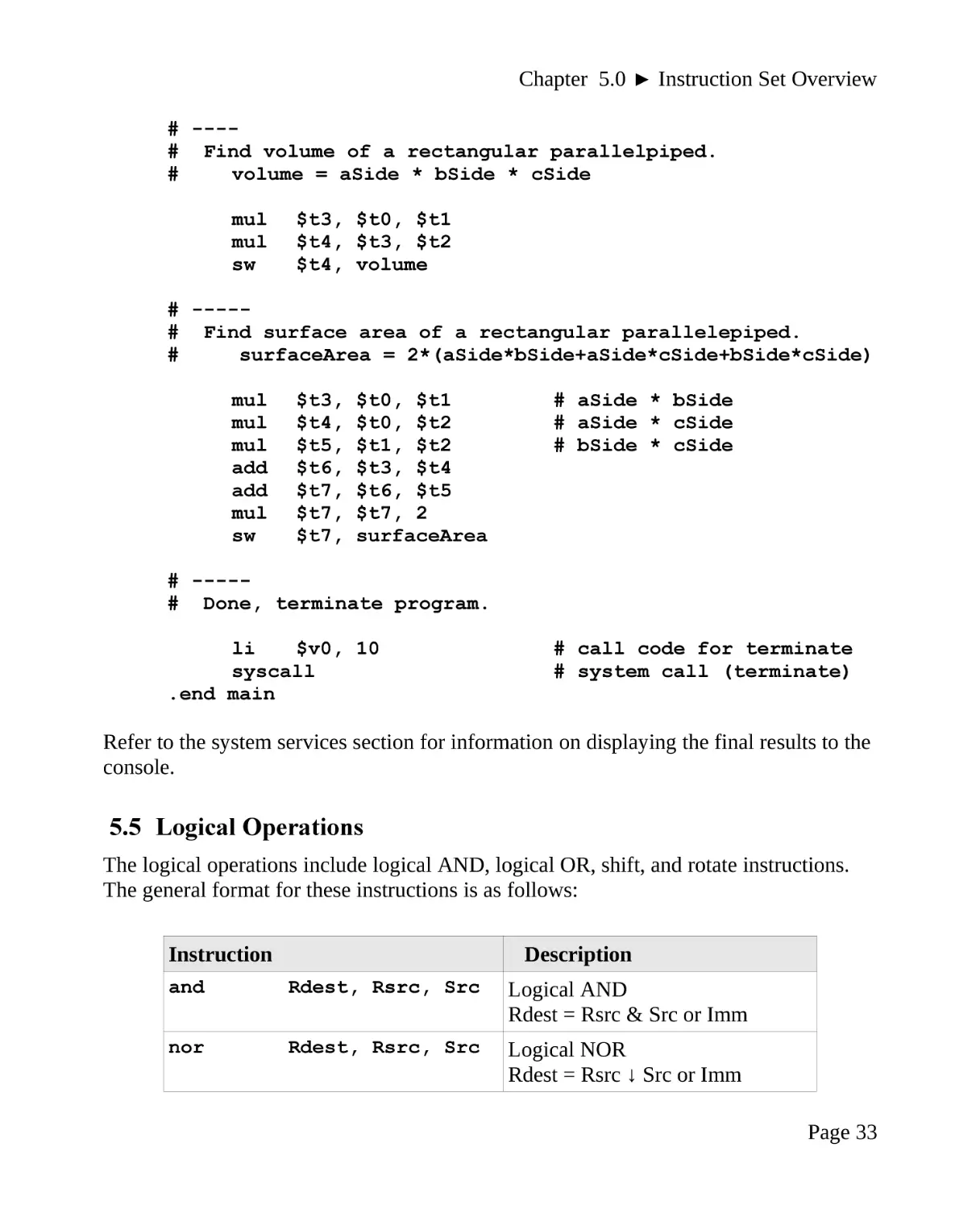
5.4.1 Example Program, Integer Arithmetic
The following is an example program to compute the
volume and surface area of a rectangular parallelepiped.
The formulas for the volume and surface area are as
follows:
volume = aSide∗bSide∗cSide
surfaceArea = 2( aSide∗bSide + aSide∗cSide + bSide∗cSide)
This example main initializes the a, b, and c sides to arbitrary integer values.
#
#
Example to compute the volume and surface area
of a rectangular parallelepiped.
# ----------------------------------------------------# Data Declarations
.data
aSide:
bSide:
cSide:
.word
.word
.word
73
14
16
volume:
surfaceArea:
.word
.word
0
0
# ----------------------------------------------------# Text/code section
.text
.globl
.ent
main:
main
main
# ----# Load variables into registers.
lw
lw
lw
Page 32
$t0, aSide
$t1, bSide
$t2, cSide
Chapter 5.0 ► Instruction Set Overview
# ---# Find volume of a rectangular parallelpiped.
#
volume = aSide * bSide * cSide
mul
mul
sw
$t3, $t0, $t1
$t4, $t3, $t2
$t4, volume
# ----# Find surface area of a rectangular parallelepiped.
#
surfaceArea = 2*(aSide*bSide+aSide*cSide+bSide*cSide)
mul
mul
mul
add
add
mul
sw
$t3,
$t4,
$t5,
$t6,
$t7,
$t7,
$t7,
$t0, $t1
$t0, $t2
$t1, $t2
$t3, $t4
$t6, $t5
$t7, 2
surfaceArea
# aSide * bSide
# aSide * cSide
# bSide * cSide
# ----# Done, terminate program.
li
$v0, 10
syscall
.end main
# call code for terminate
# system call (terminate)
Refer to the system services section for information on displaying the final results to the
console.
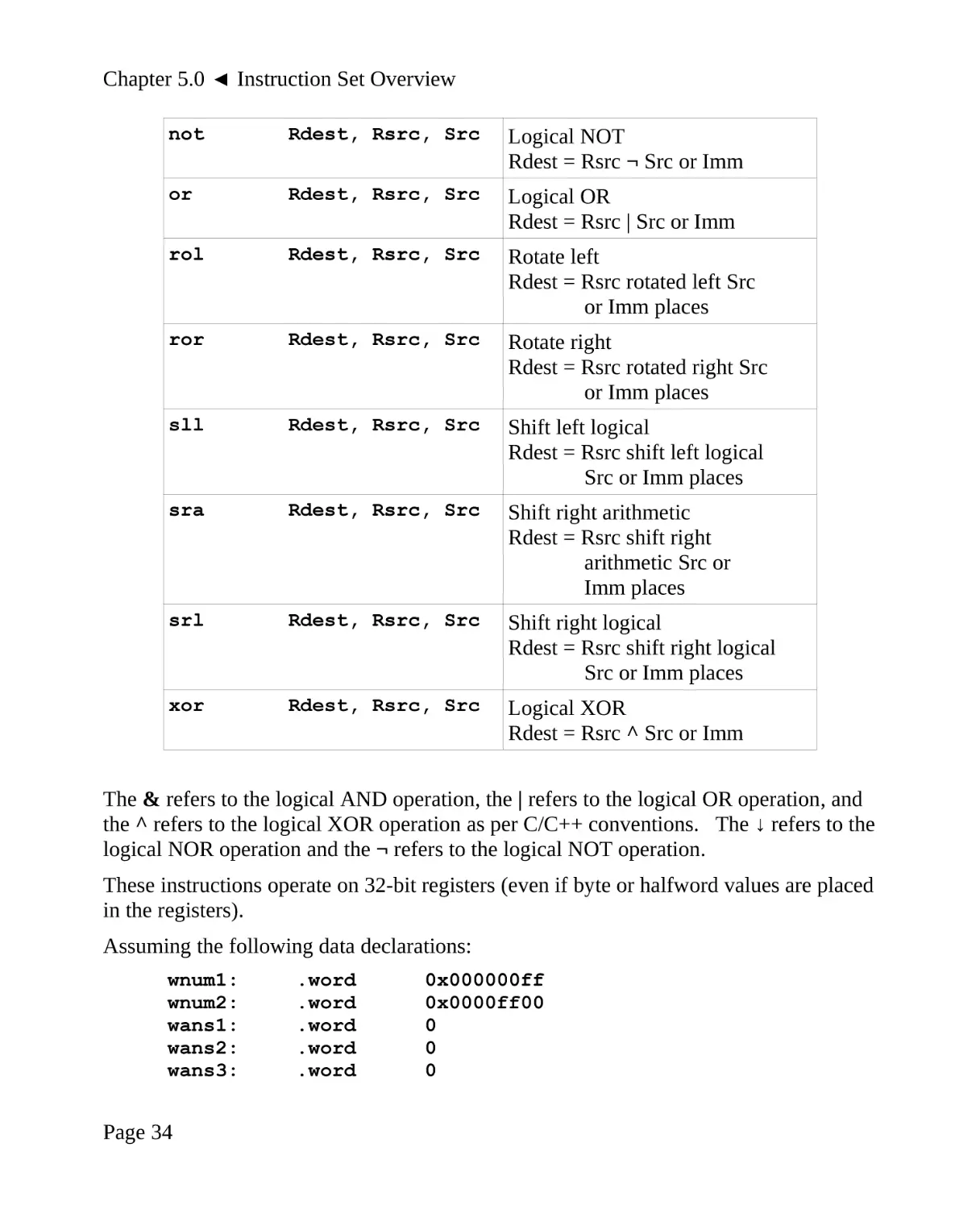
5.5 Logical Operations
The logical operations include logical AND, logical OR, shift, and rotate instructions.
The general format for these instructions is as follows:
Instruction
Description
and
Rdest, Rsrc, Src
Logical AND
Rdest = Rsrc & Src or Imm
nor
Rdest, Rsrc, Src
Logical NOR
Rdest = Rsrc ↓ Src or Imm
Page 33
Chapter 5.0 ◄ Instruction Set Overview
not
Rdest, Rsrc, Src
Logical NOT
Rdest = Rsrc ¬ Src or Imm
or
Rdest, Rsrc, Src
Logical OR
Rdest = Rsrc | Src or Imm
rol
Rdest, Rsrc, Src
Rotate left
Rdest = Rsrc rotated left Src
or Imm places
ror
Rdest, Rsrc, Src
Rotate right
Rdest = Rsrc rotated right Src
or Imm places
sll
Rdest, Rsrc, Src
Shift left logical
Rdest = Rsrc shift left logical
Src or Imm places
sra
Rdest, Rsrc, Src
Shift right arithmetic
Rdest = Rsrc shift right
arithmetic Src or
Imm places
srl
Rdest, Rsrc, Src
Shift right logical
Rdest = Rsrc shift right logical
Src or Imm places
xor
Rdest, Rsrc, Src
Logical XOR
Rdest = Rsrc ^ Src or Imm
The & refers to the logical AND operation, the | refers to the logical OR operation, and
the ^ refers to the logical XOR operation as per C/C++ conventions. The ↓ refers to the
logical NOR operation and the ¬ refers to the logical NOT operation.
These instructions operate on 32-bit registers (even if byte or halfword values are placed
in the registers).
Assuming the following data declarations:
wnum1:
wnum2:
wans1:
wans2:
wans3:
Page 34
.word
.word
.word
.word
.word
0x000000ff
0x0000ff00
0
0
0
Chapter 5.0 ► Instruction Set Overview
To perform, the basic operations of:
wans1 = wnum1 & wnum2
wans2 = wnum1 | wnum2
wans3 = wnum1 ¬ wnum2
The following instructions
lw
lw
and
sw
$t0,
$t1,
$t2,
$t2,
wnum1
wnum2
$t0, $t1
wans1
# wans1 = wnum1 & wnum2
lw
lw
or
sw
$t0,
$t1,
$t2,
$t2,
wnum1
wnum2
$t0, $t1
wans2
# wans2 = wnum1 | wnum2
lw
lw
not
sw
$t0,
$t1,
$t2,
$t2,
wnum1
wnum2
$t0, $t1
wans3
# wans3 = wnum1 ¬ wnum2
For halfword load or store instructions, only the lower 16-bits are used. For the byte
instructions, only the lower 8-bits are used.
5.5.1 Shift Operations
The shift operations shift or move bits within a register. Two typical reasons for shifting
bits include isolating a subset of the bits within an operand for some specific purpose or
possibly for performing multiplication or division by powers of two. The two shift
operations are a logical shift and an arithmetic shift.
Page 35
Chapter 5.0 ◄ Instruction Set Overview
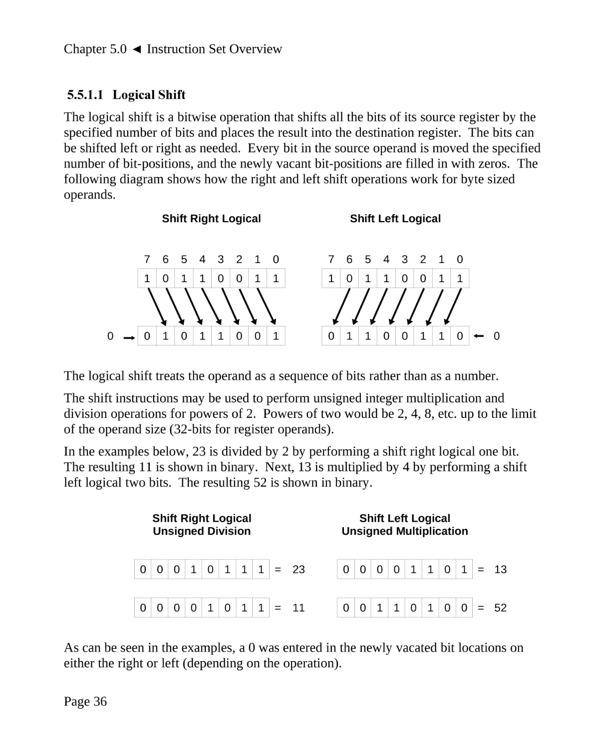
5.5.1.1 Logical Shift
The logical shift is a bitwise operation that shifts all the bits of its source register by the
specified number of bits and places the result into the destination register. The bits can
be shifted left or right as needed. Every bit in the source operand is moved the specified
number of bit-positions, and the newly vacant bit-positions are filled in with zeros. The
following diagram shows how the right and left shift operations work for byte sized
operands.
Shift Right Logical
0
Shift Left Logical
7
6
5
4
3
2
1
0
7
6
5
4
3
2
1
0
1
0
1
1
0
0
1
1
1
0
1
1
0
0
1
1
0
1
0
1
1
0
0
1
0
1
1
0
0
1
1
0
0
The logical shift treats the operand as a sequence of bits rather than as a number.
The shift instructions may be used to perform unsigned integer multiplication and
division operations for powers of 2. Powers of two would be 2, 4, 8, etc. up to the limit
of the operand size (32-bits for register operands).
In the examples below, 23 is divided by 2 by performing a shift right logical one bit.
The resulting 11 is shown in binary. Next, 13 is multiplied by 4 by performing a shift
left logical two bits. The resulting 52 is shown in binary.
Shift Right Logical
Unsigned Division
Shift Left Logical
Unsigned Multiplication
0 0 0 1 0 1 1 1 =
23
0 0 0 0 1 1 0 1 = 13
0 0 0 0 1 0 1 1 =
11
0 0 1 1 0 1 0 0 = 52
As can be seen in the examples, a 0 was entered in the newly vacated bit locations on
either the right or left (depending on the operation).
Page 36
Chapter 5.0 ► Instruction Set Overview
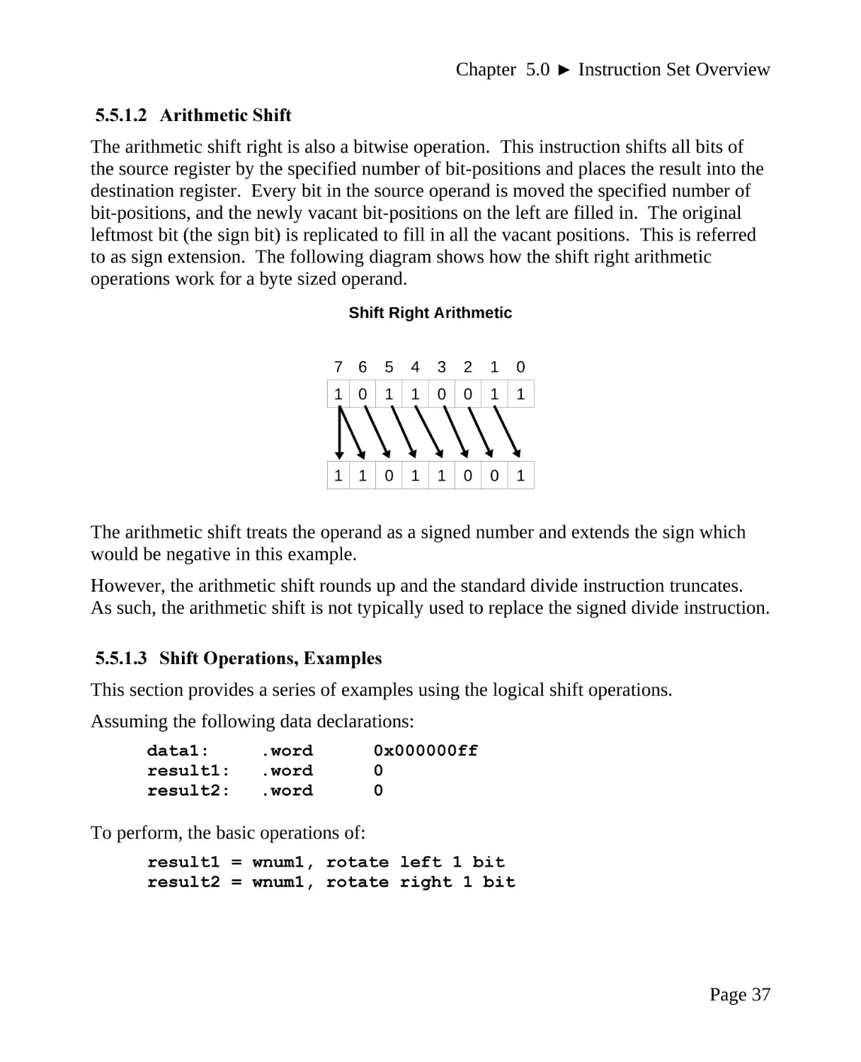
5.5.1.2 Arithmetic Shift
The arithmetic shift right is also a bitwise operation. This instruction shifts all bits of
the source register by the specified number of bit-positions and places the result into the
destination register. Every bit in the source operand is moved the specified number of
bit-positions, and the newly vacant bit-positions on the left are filled in. The original
leftmost bit (the sign bit) is replicated to fill in all the vacant positions. This is referred
to as sign extension. The following diagram shows how the shift right arithmetic
operations work for a byte sized operand.
Shift Right Arithmetic
7 6
5
4
3
2
1
0
1 0
1
1
0
0
1
1
1 1
0
1
1
0
0
1
The arithmetic shift treats the operand as a signed number and extends the sign which
would be negative in this example.
However, the arithmetic shift rounds up and the standard divide instruction truncates.
As such, the arithmetic shift is not typically used to replace the signed divide instruction.
5.5.1.3 Shift Operations, Examples
This section provides a series of examples using the logical shift operations.
Assuming the following data declarations:
data1:
result1:
result2:
.word
.word
.word
0x000000ff
0
0
To perform, the basic operations of:
result1 = wnum1, rotate left 1 bit
result2 = wnum1, rotate right 1 bit
Page 37
Chapter 5.0 ◄ Instruction Set Overview
The following instructions
lw
lw
rol
sw
$t0,
$t1,
$t2,
$t2,
wnum1
wnum2
$t0, $t1
wans3
# wans3 = wnum1, rotate left 1 bit
lw
lw
ror
sw
$t0,
$t1,
$t2,
$t2,
wnum1
wnum2
$t0, $t1
wans4
# wans3 = wnum1, rotate right 1 bit
For halfword instructions, only the lower 16-bits are used. For the byte instructions,
only the lower 8-bits are used.
To perform the operation, value * 8, it would be possible to shift the number in the
variable one bit for each power of two, which would be three bits in this example.
Assuming the following data declarations:
value:
answer:
.word
.word
17
0
The following instructions could be used to multiply a value by 8.
lw
sll
sw
$t0, value
$t1, $t0, 3
$t1, answer
# answer = value * 8
The final value in answer would be 17 * 8 or 136.
In the context of an encoded MIPS instruction, the upper 6-bits of a 32-bit word
represent the OP or operation field. If a program was analyzing code, it might be
desirable to isolate these bits for comparison. One way this can be performed is to use a
logical right shift to move the upper six bits into the position of the lower 6-bits.
The instruction:
add
$t1, $t1, 1
will be translated by the assembler into the hex value of 0x2129001.
Assuming the following data declarations:
inst1:
inst1Op1:
Page 38
.word
.word
0x2129001
0
Chapter 5.0 ► Instruction Set Overview
To mask out the OP field (upper 6-bits) for inst1 and place it in the variable instOp1
(lower 6-bits), the following instructions could be used:
lw
srl
sw
$t0, inst1
$t1, $t0, 26
$t1, instOp1
This can be done in one step since the logical shift will insert all 0's into the newly
vacated bit locations.
5.6 Control Instructions
Program control refers to basic programming structures for iteration and comparisons
such as IF statements and looping. All of the high-level language control structures
must be performed with the limited assembly-language control structures. For example,
an IF-THEN-ELSE statement does not exist at the assembly-language level. Assemblylanguage provides an unconditional branch (or jump), and a conditional branch or an IF
statement that will jump to a target label or not jump (as per the conditional expression).
The control instructions refer to unconditional and conditional branching. Branching is
required for basic conditional statements (i.e., IF statements) and looping.
5.6.1 Unconditional Control Instructions
The unconditional instruction provides an unconditional jump to a specific location.
Instruction
Description
j <label>
Unconditionally branch to the
specified label.
The "b" (branch) may be used instead of the "j" (jump). Both are encoded as the same
instruction (an unconditional jump). An error is generated by QtSpim if the label is not
defined.
5.6.2 Conditional Control Instructions
The conditional instruction provides a conditional jump based on a comparison. In
high-level language terms, this is a basic IF statement.
Page 39
Chapter 5.0 ◄ Instruction Set Overview
The conditional control instructions include the standard set; branch equal, branch not
equal, branch less than, branch less than or equal, branch greater than, and branch
greater than or equal.
The general format for these basic instructions is as follows:
Instruction
Description
beq <Rsrc>, <Src>, <label>
Branch to label if <Rsrc> and
<Src> are equal
bne <Rsrc>, <Src>, <label>
Branch to label if <Rsrc> and
<Src> are not equal
blt <Rsrc>, <Src>, <label>
Signed branch to label if <Rsrc>
is less than <Src>
ble <Rsrc>, <Src>, <label>
Signed branch to label if <Rsrc>
is less than or equal to <Src>
bgt <Rsrc>, <Src>, <label>
Signed branch to label if <Rsrc>
is greater than <Src>
bge <Rsrc>, <Src>, <label>
Signed branch to label if <Rsrc>
is greater than or equal to <Src>
bltu <Rsrc>, <Src>, <label>
Unsigned branch to label if <Rsrc>
is less than <Src>
bleu <Rsrc>, <Src>, <label>
Unsigned branch to label if <Rsrc>
is less than or equal to <Src>
bgtu <Rsrc>, <Src>, <label>
Unsigned branch to label if <Rsrc>
is greater than <Src>
bgeu <Rsrc>, <Src>, <label>
Unsigned branch to label if <Rsrc>
is greater than or equal to <Src>
These instructions operate on 32-bit registers (even if byte or halfword values are placed
in the registers).
In addition, these conditional control instructions can be modified by adding or
appending a ‘z’ to the end which means a comparison to zero (0) without typing the
immediate 0 in the instruction.
Page 40
Chapter 5.0 ► Instruction Set Overview
For example, the following instruction,
bne
$t0, 0, loop1
could be written as,
bnez
$t0, loop1
which does exactly the same thing. This short-handed method is used in some of the
text examples. A more complete list is included in Appendix C.
5.6.3 Example Program, Sum of Squares
The following is an example program to find the sum of squares from 1 to n. For
example, the sum of squares from 1 to 10 is as follows:
12 22 ⋯ 102 = 385
This example program initializes the n to 10 to match the example above example.
Other limits can be specified as desired.
# Example program to compute the sum of squares.
# ----------------------------------------------------# Data Declarations
.data
n:
sumOfSquares:
.word
.word
10
0
# ----------------------------------------------------# text/code section
.text
.globl
.ent
main:
main
main
# ----# Compute sum of squares from 1 to n.
lw
li
li
$t0, n
$t1, 1
$t2, 0
#
# loop index (1 to n)
# sum
Page 41
Chapter 5.0 ◄ Instruction Set Overview
sumLoop:
mul
add
$t3, $t1, $t1
$t2, $t2, $t3
add
ble
$t1, $t1, 1
$t1, $t0, sumLoop
sw
$t2, sumOfSquares
# index^2
# ----# Done, terminate program.
li
$v0, 10
syscall
.end main
# call code for terminate
# system call
Refer to the system services section for information on displaying the final results to the
console.
5.7 Floating-Point Instructions
This section presents a summary of the basic, most common floating-point arithmetic
instructions. The MIPS Instruction Set Appendix presents a more comprehensive list
of the available instructions.
5.7.1 Floating-Point Register Usage
The floating-point instructions are similar to the integer instructions, however, the
floating-point register must be used with the floating-point instructions. Specifically,
this means the architecture does not support the use of integer registers for any floatingpoint arithmetic operations.
When single-precision (32-bit) floating-point operation is performed, the specified 32bit floating-point register is used. When a double-precision (64-bit) floating-point
operation is performed, two 32-bit floating-point registers are used; the specified 32-bit
floating-point register and the next numerically sequential register is used by the
instruction. For example, a double-precision operation using $f12 will use
automatically $f12 and $f13.
Page 42
Chapter 5.0 ► Instruction Set Overview
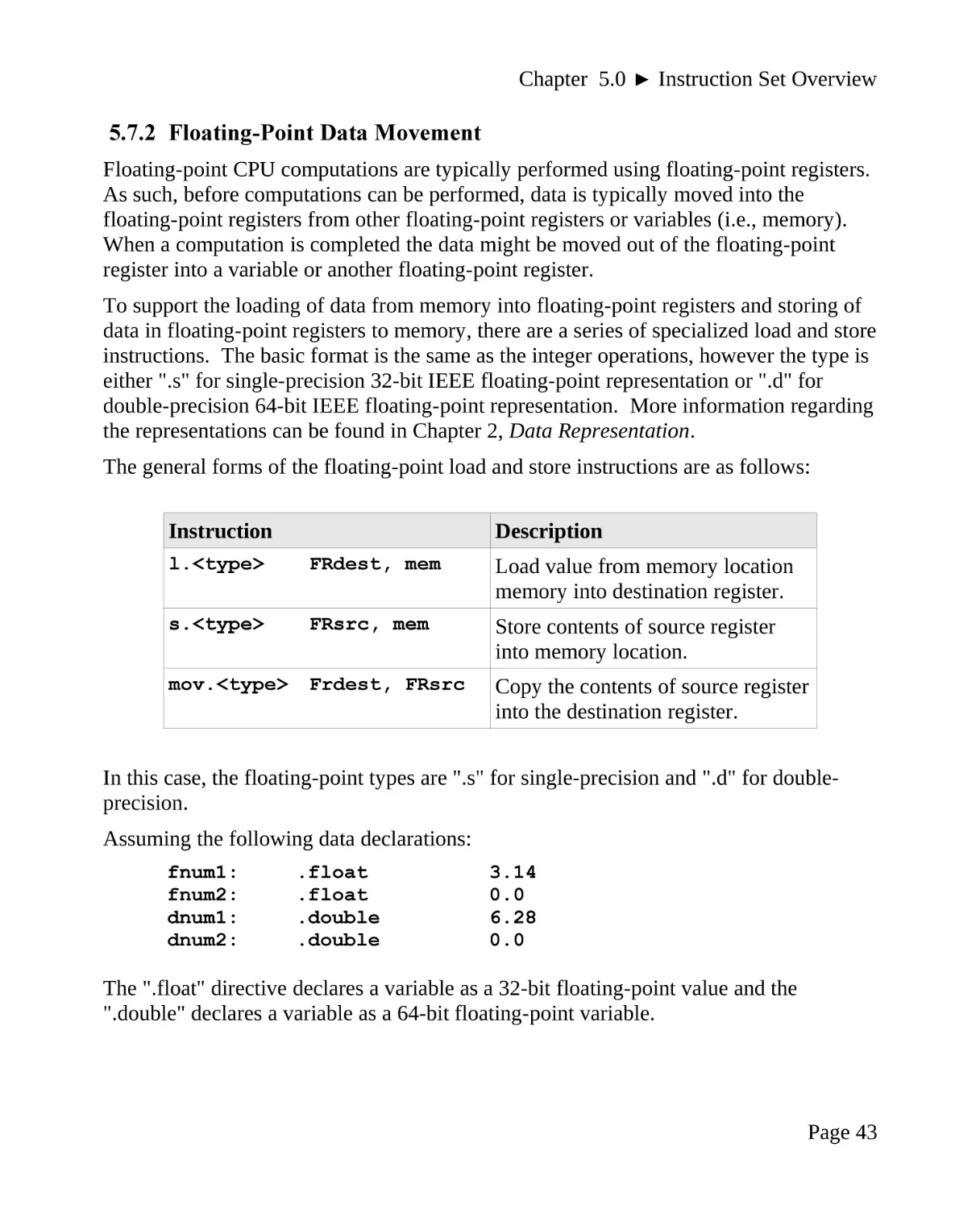
5.7.2 Floating-Point Data Movement
Floating-point CPU computations are typically performed using floating-point registers.
As such, before computations can be performed, data is typically moved into the
floating-point registers from other floating-point registers or variables (i.e., memory).
When a computation is completed the data might be moved out of the floating-point
register into a variable or another floating-point register.
To support the loading of data from memory into floating-point registers and storing of
data in floating-point registers to memory, there are a series of specialized load and store
instructions. The basic format is the same as the integer operations, however the type is
either ".s" for single-precision 32-bit IEEE floating-point representation or ".d" for
double-precision 64-bit IEEE floating-point representation. More information regarding
the representations can be found in Chapter 2, Data Representation.
The general forms of the floating-point load and store instructions are as follows:
Instruction
Description
l.<type>
FRdest, mem
Load value from memory location
memory into destination register.
s.<type>
FRsrc, mem
Store contents of source register
into memory location.
mov.<type>
Frdest, FRsrc
Copy the contents of source register
into the destination register.
In this case, the floating-point types are ".s" for single-precision and ".d" for doubleprecision.
Assuming the following data declarations:
fnum1:
fnum2:
dnum1:
dnum2:
.float
.float
.double
.double
3.14
0.0
6.28
0.0
The ".float" directive declares a variable as a 32-bit floating-point value and the
".double" declares a variable as a 64-bit floating-point variable.
Page 43
Chapter 5.0 ◄ Instruction Set Overview
To perform, the basic operations of:
fnum2 = fnum1
dnum2 = dnum1
The following instructions :
l.s
s.s
$f6, fnum1
$f6, fnum2
l.d
mov.d
$f6, dnum1
$f8, $f6
s.d
$f8, dnum2
# fnum2 = fnum1
# unnecessary use of mov
# just as an example
# dnum2 = dnum1
The two double-precision operations (l.d and mov.d) reference registers $f6 and $f8 but
use registers $f6/$f7 and $f8/$f9 to hold each of the two 64-bit values.
5.7.3 Integer / Floating-Point Register Data Movement
The arithmetic instructions require either floating-point registers or integer registers and
will not allow a combination. In order to move data between integer and floating-point
registers, special instructions are required. As noted in Chapter 2, MIPS Architecture
Overview, the floating-point operations are performed in a floating-point co-processor.
The general form of the integer and floating-point data movement instructions are as
follows:
Instruction
Description
mfc1
Rdest, FRsrc
Copy the contents from coprocessor 1 (FPU) float register
FRsrc into Rdest integer register.
mfc1.d
Rdest, FRsrc
Copy the contents from coprocessor 1 (FPU) float registers
FRsrc and FRsrc+1 into integer
registers Rdest and Rdest+1.
mtc1
Rsrc, FRdest
Copy the contents from integer Rsrc
register to co-processor 1 (FPU)
float register FRdest.
Page 44
Chapter 5.0 ► Instruction Set Overview
mtc1.d
Rsrc, FRdest
Copy the contents from integer
registers Rdest and Rdest+1 to coprocessor 1 (FPU) float registers
FRsrc and FRsrc+1.
Note, the above instructions use a 1 (number one) and not a lower-case letter L.
For example, assuming an integer value is in integer register $s0, to copy the value into
floating-point register $f12, the following instruction could be used.
mtc1
$s0, $f12
To copy the contents of $f12, into an integer register $t1, the following instruction could
be used.
mfc1
$t1, $f12
The value copied has not been converted into a different representation.
In this example, the integer value in $s0 that was copied into $f12 is still represented as
an integer in two's complement. As such, the value in $f12 is not ready for any floatingpoint arithmetic operations. The representation of the value must be converted (see next
section).
5.7.4 Integer / Floating-Point Conversion Instructions
When data is moved between integer and floating-point registers, the data representation
must be addressed. For example, when moving an integer value from an integer register
into a floating-point register, the data is still represented as an integer value in two's
complement. Floating-point operations require an appropriate floating-point
representation (32-bit or 64-bit). When data is moved between integer and floatingpoint registers, a data conversion would typically be required.
The general format for the conversion instructions is as follows:
Instruction
cvt.d.s
Description
FRdest, FRsrc
Convert the 32-bit floating-point value
in register FRsrc into a double
precision value and put it in register
FRdest.
Page 45
Chapter 5.0 ◄ Instruction Set Overview
Instruction
Description
cvt.d.w
FRdest, FRsrc
Convert the 32-bit integer in register
FRsrc into a double precision value and
put it in register FRdest.
cvt.s.d
FRdest, FRsrc
Convert the 64-bit floating-point value
in register FRsrc into a 32-bit floatingpoint value and put it in register
FRdest.
cvt.s.w
FRdest, FRsrc
Convert the 32-bit integer in register
FRsrc into a 32-bit floating-point value
and put it in register FRdest.
cvt.w.d
FRdest, FRsrc
Convert the 64-bit floating-point value
in register FRsrc into a 32-bit integer
value and put it in register FRdest.
cvt.w.s
FRdest, FRsrc
Convert the 32-bit floating-point value
in register FRsrc into a 32-bit integer
value and put it in register FRdest.
Assuming the following data declarations:
iNum:
fNum:
.word
.float
42
0.0
To convert the integer value in variable iNum and place it as a 32-bit floating-point
value in variable fNum, the following instructions could be used:
lw
mtc1
cvt.s.w
s.s
$t0,
$t0,
$f8,
$f8,
iNum
$f6
$f6
fNum
This code fragment loads the integer value in variable iNum into $t0, and then copies
the value into $f6. The integer value in $f6 is converted into a 32-bit floating-point
value and placed in $f8. The 32-bit floating-point value is then copied into the fNum
variable. The conversion instruction could have over-written the $f6 register.
Page 46
Chapter 5.0 ► Instruction Set Overview
Assuming the following data declarations:
pi:
intPi:
.double
.word
3.14
0
To convert the 64-bit floating-point value in variable pi and place it as a 32-bit integer
value in variable intPi, the following instructions could be used:
l.d
cvt.w.d
mfc1
sw
$f10, pi
$f12, $f10
$t1, $f12
$t1, intPi
This code fragment initially loads the 64-bit floating-point value into $f10. The 64-bit
floating-point value in $f10 is converted into a 32-bit integer value and placed in $f12.
The integer value in $f12 is copied into $t1 and then copied into the variable intPi.
Since conversion from floating-point truncates, the final value in intPi is 3.
5.7.5 Floating-Point Arithmetic Operations
The arithmetic operations include addition, subtraction, multiplication, division,
remainder (remainder after division), logical AND, and logical OR.
The general format for these basic instructions is as follows:
Instruction
Description
add.<type> FRdest, FRsrc, FRsrc
FRdest = FRsrc + FRsrc
sub.<type> FRdest, FRsrc, FRsrc
FRdest = FRsrc - FRsrc
mul.<type> FRdest, FRsrc, FRsrc
FRdest = FRsrc * FRsrc
div.<type> FRdest, FRsrc, FRsrc
FRdest = FRsrc / FRsrc
rem.<type> FRdest, FRsrc, FRsrc
FRdest = FRsrc % FRsrc
Assuming the following data declarations:
fnum1:
fnum2:
fans1:
fans2:
.float
.float
.float
.float
6.28318
3.14159
0.0
0.0
Page 47
Chapter 5.0 ◄ Instruction Set Overview
dnum1:
dnum2:
dans1:
dans2:
.double
.double
.double
.double
42.3
73.6
0.0
0.0
To perform, the basic operations of:
fans1
fans2
dans1
dans2
=
=
=
=
fnum1
fnum1
dnum1
dnum1
+
*
/
fnum2
fnum2
dnum2
dnum2
The following instructions:
l.s
l.s
add.s
s.s
$f4,
$f6,
$f8,
$f8,
fnum1
fnum2
$f4, $f6
fans1
mul.s
s.s
$f10, $f4, $f6
$f10, fans2
# fans2 = fnum1 * fnum2
l.d
l.d
sub.d
s.d
$f4,
$f6,
$f8,
$f8,
# dans1 = dnum1 - dnum2
div.d
s.d
$f10, $f4, $f6
$f10, dans2
dnum1
dnum2
$f4, $f6
dans1
# fans1 = fnum1 + fnum2
# dans2 = dnum1 / dnum2
For the double-precision instructions, the specified register and the next numerically
sequential register is used. For example, the l.d instruction sets the $f4 and $f5 32-bit
registers with the 64-bit value.
5.7.6 Example Programs
This section provides some example using the floating-point instructions to perform
some basic calculations.
Page 48
Chapter 5.0 ► Instruction Set Overview
5.7.6.1 Example Program, Floating-Point Arithmetic
The following is an example program to compute the surface area
and volume of a sphere.
The formulas for the surface area and volume of a sphere are as
follows:
surfaceArea = 4.0 ∗ pi ∗ radius2
volume =
4.0∗ pi
∗ radius3
3.0
This example main initializes the radius to an arbitrary floating-point value.
# Example program to calculate the surface area
# and volume of a sphere given the radius.
# ----------------------------------------------------# Data Declarations
.data
pi:
fourPtZero:
threePtZero:
radius:
surfaceArea:
volume:
.float
.float
.float
.float
.float
.float
3.14159
4.0
3.0
17.25
0.0
0.0
# ----------------------------------------------------# text/code section
.text
.globl
.ent
main:
#
main
main
Compute: (4.0*pi) which is used for both equations.
l.s
l.s
mul.s
$f2, fourPtZero
$f4, pi
$f4, $f2, $f4
# 4.0 * pi
Page 49
Chapter 5.0 ◄ Instruction Set Overview
l.s
$f6, radius
# radius
# ----# Calculate surface area of a sphere.
#
surfaceArea = 4.0 * pi * radius^2
mul.s
mul.s
s.s
$f8, $f6, $f6
$f8, $f4, $f8
$f8, surfaceArea
# radius^2
# 4.0*pi * radius^2
# store final answer
# ----# Calculate volume of a sphere.
#
volume = (4.0 * pi / 3.0) * radius^3
l.s
$f8, threePtZero
div.s
$f2, $f4, $f8
# (4.0 * pi / 3.0)
mul.s
mul.s
$f10, $f2, $f2
$f10, $f10, $f6
# radius^3
mul.s
$f12, $f6, $f10
# * 4.0*pi/3.0
s.s
$f12, volume
# store final answer
# ----# Done, terminate program.
li
syscall
.end main
$v0, 10
# terminate
# system call
Refer to the system services section for information on displaying the final results to the
console.
5.7.6.2 Example Program, Integer / Floating-Point Conversion
The following is an example program to sum an array of integer values and compute the
average as a floating-point value. This requires conversion of 32-bit integer values into
32-bit floating-point values.
Page 50
Chapter 5.0 ► Instruction Set Overview
#
#
Example program to sum an array of integers
and compute the float average.
# ----------------------------------------------------# Data Declarations
.data
iArray:
length:
.word
.word
1, 2, 3, 4, 5, 6, 7, 8, 9, 10, 11, 12
12
iSum:
fAve:
.word
.float
0
0.0
# ----------------------------------------------------# Text/code section
.text
.globl
.ent
main:
main
main
# ----# Find the sum of the integer numbers.
la
lw
li
$t0, iArray
$t1, length
$t2, 0
sumLoop:
lw
add
addu
sub
bnez
$t3,
$t2,
$t0,
$t1,
$t1,
($t0)
$t2, $t3
$t0, 4
$t1, 1
sumLoop
# array starting addr
# array length
# set sum=0
# get iArray(n)
# sum=sum+iArray(n)
# update iArray addr
sw
$t2, iSum
# save integer sum
mtc1
cvt.s.w
$t2, $f6
$f6, $f6
# move to flt reg
# cvt to flt format
lw
mtc1
cvt.s.w
$t1, length
$t1, $f8
$f8, $f8
# move to float reg
# cvt to float format
Page 51
Chapter 5.0 ◄ Instruction Set Overview
div.s
s.s
$f10, $f6, $f8
$f10, fAve
# sum / length
# ----# Done, terminate program.
li
$v0, 10
syscall
.end main
Page 52
# terminate
# system call
6.0
Addressing Modes
This chapter provides basic information regarding addressing modes and the associated
address manipulations on the MIPS architecture. The addressing modes are the
supported methods for specifying the value or address of a data item being accessed
(read or written). This might include an actual value, the name of a variable, or the
location in an array.
Since the MIPS architecture, as simulated in the QtSpim simulator, is a 32-bit
architecture, all addresses are words (32-bits).
6.1 Direct Mode
Direct addressing mode is when the register or memory location contains the actual
values.
For example:
lw
lw
$t0, var1
$t1, var2
Registers and variables $t0, $t1, var1, and var2 are all accessed in direct mode
addressing.
6.2 Immediate Mode
Immediate addressing mode is when the actual value is one of the operands.
For example:
li
add
$t0, 57
$t0, $t0, 57
The value 57 is immediate mode addressing. The register $t0 is direct mode addressing.
Page 53
Chapter 6.0 ◄ Addressing Modes
6.3 Indirection
The pair of parenthesis, ( )'s, are used to denote an indirect memory access. An indirect
memory access means the CPU will read the provided address and then go to that
address to access the value located there. This involves more work for the CPU than the
previously presented addressing modes (direct and immediate). This is typically how
elements are accessed in a list or array. For example, to get a value from a list of longs:
la
lw
$t0, lst
$s1, ($t0)
The address, in $t0, is a word size (32-bits). Memory is byte addressable. As such, if
the data items in "lst" (from above) are words, then four must be added to get the next
element.
For example, the instructions:
add
lw
$t0, $t0, 4
$s2, ($t0)
will get the next word value in array (named lst in this example).
A form of displacement addressing is allowed. For example, to get the second item
from a list of word sized values:
la
lw
$t0, lst
$s1, 4($t0)
The "4" is added to the address before the memory access. However, the register is not
changed. Thus, the location or address being accessed is displaced or temporarily
changed as needed.
6.3.1 Bounds Checking
In a high-level language, the compiler is capable of ensuring that the index for an
element in an array is legal and within the boundary of the array being accessed. Thus,
the compiler can issue an error message and help identify when and where a program is
trying to access beyond the end of an array (e.g., accessing the 110th element of a 100
element array).
This type of bounds checking is not available at the assembly-language level.
Page 54
Chapter 6.0 ► Addressing Modes
If the assembly-language program attempts to access the 110th element of an array, the
value at that memory location will be returned with no error. Of course, the value
returned is not likely to be useful.
If the memory access attempting to be accessed is outside the general scope of the
program, an exception will be generated. An exception is a run-time error, and the
QtSpim simulator will provide the line where the exception occurred. For example,
attempting to access a memory location in the reserved section would not be allowed
and thus generate an exception. This could easily occur if the programmer uses a
register with a data item instead of a correct address.
Additionally, no error is generated when a program attempts to access a word (32-bits)
in an array of halfwords (16-bits). In this case two halfwords will be read into the
registers and treated as a single value. Of course, the value will not be correct or useful.
6.4 Examples
This section provides some example using the addressing modes to access arrays and
perform basic calculations.
6.4.1 Example Program, Sum and Average
The following example computes the sum and average for an array integer values. The
values are calculated and saved into memory variables.
# Example to compute the sum and integer average
# for an array of integer values.
# ----------------------------------------------------# Data Declarations
.data
array:
length:
.word
.word
.word
.word
sum:
average:
.word
.word
1, 3, 5, 7, 9, 11, 13, 15, 17, 19
21, 23, 25, 27, 29, 31, 33, 35, 37, 39
41, 43, 45, 47, 49, 51, 53, 55, 57, 59
30
0
0
Page 55
Chapter 6.0 ◄ Addressing Modes
# ----------------------------------------------------# Basic approach:
#
- loop through the array
#
access each value, update sum
#
- calculate the average
.text
.globl
.ent
main:
main
main
# ----# Loop through the array to calculate sum
la
li
lw
li
sumLoop:
lw
add
$t0,
$t1,
$t2,
$t3,
array
0
length
0
#
#
#
#
array starting address
loop index, i=0
length
initialize sum=0
$t4, ($t0)
$t3, $t3, $t4
# get array[i]
# sum = sum + array[i]
add
add
$t1, $t1, 1
$t0, $t0, 4
# i = i+1
# update array address
blt
$t1, $t2, sumLoop
# if i<length, continue
sw
$t3, sum
# save sum
# ----# Calculate average
#
note, sum and length set in section above.
div
sw
$t5, $t3, $t2
$t5, average
# ave = sum / length
# ----# Done, terminate program.
li
$v0, 10
syscall
.end main
Page 56
# terminate
# system call
Chapter 6.0 ► Addressing Modes
This example program does not display the results to the screen. For information
regarding displaying values and strings to output (console), refer to the QtSpim System
Services section.
6.4.2 Example Program, Median
The following example finds the median for a sorted array of values. In this example,
the length is given as always even. As such, the integer median is the integer average
for the two middle values. Specifically, the formula for median is:
medianEvenOnly =
( array[ length/ 2] + array[ length/ 2−1] )
2
The 'length/2' notation refers to using division by two to generate the correct index of
the appropriate value from the array. In assembly, we must convert the index into the
offset from the base address (i.e., starting address) of the array. Since the array elements
in this example are words (i.e., 4 bytes), it will be necessary to multiply by four to
convert the index into an offset. That offset is from the start of the array, so the final
address is the array base address plus the offset.
This requires a series of calculations as demonstrated in the following example.
# Example to find the median of a sorted
# array of integer values of even length.
# ----------------------------------------------------# Data Declarations
.data
array:
length:
median:
.word
.word
.word
1, 3, 5, 7, 9, 11, 13, 15, 17, 19
21, 23, 25, 27, 29, 31, 33, 35, 37, 39
41, 43, 45, 47, 49, 51, 53, 55, 57, 59
.word
.word
30
0
# ----------------------------------------------------# text/code section
# The median for an even length array is defined as:
#
median = ( array[len/2] + array[len/2-1] ) / 2
# Note, the len/2 is the index. Must convert the index
# into the an offset from the base address (of the
# array. Since the data is words (4 bytes), multiply
Page 57
Chapter 6.0 ◄ Addressing Modes
#
the index by four to convert to the offset.
.text
.globl
.ent
main:
la
lw
main
main
$t0, array
$t1, length
# starting addr of array
# value of length
div
mul
add
$t2, $t1, 2
$t3, $t2, 4
$t4, $t0, $t3
# length / 2
# cvt index into offset
# add base addr of array
lw
sub
$t5, ($t4)
$t4, $t4, 4
# get array[len/2]
# addr of prev value
lw
$t6, ($t4)
# get array[len/2-1]
add
div
$t7, $t6, $t5
$t8, $t7, 2
# a[len/2] + a[len/2-1]
# / 2
sw
$t8, median
# save median
# ----# Done, terminate program.
li
$v0, 10
syscall
.end main
# terminate
# system call
This example program does not display the results to the screen. For information
regarding displaying values and strings to output (console), refer to the QtSpim System
Services section.
Finding the median for an odd length list is left to the reader as an exercise.
Page 58
7.0
Stack
In a computer, a stack is a type of data structure where items are added and then
removed from the stack in reverse order. That is, the most recently added item is the
very first one that is removed. This is often referred to as Last-In, First-Out (LIFO).
A stack is heavily used in programming for the storage of information during procedure
or function calls. The following chapter provides information and examples regarding
procedure and function calls.
Adding an item to a stack is referred to as a push or push operation. Removing an item
from a stack is referred to as a pop or pop operation.
It is generally expected that the reader will be familiar with the general concept of a
stack.
7.1 Stack Example
To demonstrate the usage of the stack, given an array, a = {7, 19, 37}, consider
the operations:
push a[0]
push a[1]
push a[2]
Followed by the operations:
pop
pop
pop
a[0]
a[1]
a[2]
The initial push will push the 7, followed by the 19, and finally the 37. Since the stack
is last-in, first-out, the first item popped off the stack will be the last item pushed, or 37
in this example. The 37 is placed in the first element of the array (over-writing the 7).
As this continues, the order of the array elements is reversed.
Page 59
Chapter 7.0 ◄ Stack
The following diagram shows the progress and the results.
stack
stack
stack
stack
stack
stack
37
19
19
19
7
7
7
7
7
empty
push
a[0]
push
a[1]
push
a[2]
pop
a[0]
pop
a[1]
pop
a[2]
a = {7,
19, 37}
a = {7,
19, 37}
a = {7,
19, 37}
a =
{37,
19, 37}
a =
{37,
19, 37}
a =
{37,
19, 7}
The following sections provide more detail regarding the implementation and applicable
instructions.
7.2 Stack Implementation
The current top of the stack is pointed to by the $sp register. The stack grows
downward in memory and it is generally expected that all items pushed and/or popped
should be of word size (32-bit).
There is no push or pop instruction. Instead, you must perform the push and pop
operations manually.
While it is possible to push/pop items of various sizes (byte, halfword, etc.) it is not
recommended. For such operations, it is recommended to use the entire word (4-bytes).
7.3 Push
For example, a push would subtract the $sp by 4 bytes and then copy the operand to that
location (in that order). The instructions to push $t9 would be implemented as follows:
subu
sw
$sp, $sp, 4
$t9, ($sp)
Which will place the contents of the $t9 register at the top of the stack.
Page 60
Chapter 7.0 ► Stack
7.4 Pop
A pop would copy the top of the stack to the operand and then add 4 bytes (in that
order). To pop the stack into $t2, the instructions would be as follows:
lw
addu
$t2, ($sp)
$sp, $sp, 4
Which will copy the contents of the top of the stack into the $t2 register.
7.5 Multiple push's/pop's
The preferred method of performing multiple pushes or pops is to perform the $sp
adjustment only once. For example, to push registers, $s0, $s1, and $s2:
subu
sw
sw
sw
$sp,
$s0,
$s1,
$s2,
$sp, 12
($sp)
4($sp)
8($sp)
And, the commands to pop registers, $s0, $s1, and $s2 as follows:
lw
lw
lw
addu
$s0,
$s1,
$s2,
$sp,
($sp)
4($sp)
8($sp)
$sp, 12
By performing the stack adjustment only once, it is more efficient for the architecture to
execute.
7.6 Example Program, Stack Usage
The following example uses a stack to reverse the elements in an array. The program
will push all elements of the array to the stack and then pop all elements back into the
array. This will place the elements back into the array in reverse order based on the
basic functionality of the stack.
# Example to reverse values in an array
# by using the stack.
# ----------------------------------------------------# Data Declarations
Page 61
Chapter 7.0 ◄ Stack
.data
array:
length:
.word
.word
.word
.word
1, 3, 5, 7, 9, 11, 13, 15, 17, 19
21, 23, 25, 27, 29, 31, 33, 35, 37, 39
41, 43, 45, 47, 49, 51, 53, 55, 57, 59
30
# ----------------------------------------------------# Text/code section
#
#
#
#
Basic approach:
- loop to push each element onto the stack
- loop to pop each element off the stack
Final result is all elements reversed.
.text
.globl
.ent
main:
main
main
# ----# Loop to read items from array and push to stack.
la
li
lw
pushLoop:
lw
$t0, array
$t1, 0
$t2, length
# array starting address
# loop index, i=0
# length
$t4, ($t0)
# get array[i]
subu $sp, $sp, 4
sw
$t4, ($sp)
# push array[i]
add
add
$t1, $t1, 1
$t0, $t0, 4
# i = i+1
# update array address
blt
$t1, $t2, pushLoop
# if i<length, continue
# ----# Loop to pop items from stack and write into array.
la
li
Page 62
$t0, array
$t1, 0
# array starting address
# loop index, i=0
Chapter 7.0 ► Stack
lw
$t2, length
popLoop:
lw
$t4, ($sp)
addu $sp, $sp, 4
# length (redundant line)
# pop array[i]
sw
$t4, ($t0)
# set array[i]
add
add
$t1, $t1, 1
$t0, $t0, 4
# i = i+1
# update array address
blt
$t1, $t2, popLoop
# if i<length, continue
# ----# Done, terminate program.
li
$v0, 10
syscall
.end main
# terminate
# system call
It must be noted that there are easier ways to reverse a set of numbers, but they would
not help demonstrate stack operations.
Page 63
Chapter 7.0 ◄ Stack
Page 64
8.0
Procedures/Functions
This chapter provides an overview of using assembly language procedures/functions. In
C/C++ a procedure is referred to as a void function. Other languages refer to such
functions as procedures. A function returns a single value in a more mathematical
sense. C/C++ refers to functions as value returning functions.
With regard to calling a procedure/function, there are two primary activities; linkage and
argument transmission. Each is explained in the following sections. Additionally, using
procedures/functions in MIPS assembly language requires the use of a series of special
purpose registers. These special purpose registers are part of the basic integer register
set but have a dedicated purpose based upon standardized and conventional usage.
8.1 MIPS Calling Conventions
When writing MIPS assembly-language procedures, the MIPS standard calling
conventions should be utilized. This ensures that the code can be more effectively reused, can interact with other compiler-generated code or mixed-language programs, and
utilize high-level language libraries.
The calling conventions address register usage, argument passing and register
preservation.
There are two categories of procedures as follows:
•
•
Non-leaf procedures
◦ These procedures call other procedures.
Leaf procedures
◦ These procedures do not call other procedures (or themselves).
The standard calling convention specifies actions for the caller (routine that is calling)
and the callee (routine that is being called). The specific requirements for each are
detailed in the following sections.
Page 65
Chapter 8.0 ◄ Procedures/Functions
8.2 Procedure/Function Format
The basic format for a procedure/function declaration uses a global declaration directive
(".globl <procName>"), an entry point directive (".ent <procName>"), and an entry label
for the procedure. Generally, a procedure declaration is terminated with an end
directive (".end <procName>"). The general syntax is as follows:
.globl functionName
.ent
functionName
functionName:
# code goes here
.end
functionName
The use of the ".end <functionName>" directive is optional in the QtSpim simulator.
8.3 Caller Conventions
The calling convention addresses specific requirements for the caller or routine that is
calling a procedure.
•
•
The calling procedures are expected to save any non-preserved registers ($a0 $a3, $t0 - $t9, $v0, $v1, $f0 - $f10 and $f16 - $f18) that are required after the
call is completed.
The calling procedure should pass all arguments.
◦ The first argument is passed in either $a0 or $f12 ($a0 if integer or $f12 if
float single or double precision).
◦ The second argument is passed in either $a1 or $f14 ($a1 if integer or $f14 if
float single or double precision).
◦ The third argument is passed in $a2 (integer only).
◦ If the third argument is float, it must be passed on the stack.
◦ The fourth argument is passed in $a3 (integer only).
◦ If the fourth argument is float, it must be passed on the stack.
Remaining arguments are passed on the stack. Arguments on the stack should be placed
on the stack in reverse order. Call-by-reference arguments load address (la instruction)
and call-by-value load the value.
Calling procedure should use the "jal <proc>" instruction.
Page 66
Chapter 8.0 ► Procedures/Functions
Upon completion of the procedure, the caller procedure must restore any saved nonpreserved registers and adjust the stack point ($sp) as necessary if any arguments were
passed on the stack.
Note, for floating-point arguments appearing in registers you must allocate a pair of
registers (even if it's a single precision argument) that start with an even register.
8.4 Linkage
The term linkage refers to the basic process of getting to a procedure and getting back to
the correct location in the calling routine. This does not include argument transmission,
which is addressed in the next section.
The basic linkage operation use the jal and jr instructions. Both instructions utilize the
$ra register. This register is set to the return address as part of the procedure call.
The call to a procedure/function requires the procedure/function name, generically
labeled as <procName>, as follows:
jal
<procName>
The jal, or jump and link, instruction, will copy the $pc into the $ra register and jump
to the procedure <procName>. Recall that the $pc register points to the next instruction
to be executed. That will be the instruction immediately after the call, which is the
correct place to return to when the procedure/function has completed.
If the procedure/function does not call any other procedures/functions, nothing
additional is required with regard to the $ra register.
A procedure that does not call another procedure is referred to as a "leaf procedure". A
procedure that calls another procedure is referred to as a "non-leaf procedure".
The return from procedure is as follows:
jr
$ra
If the procedure/function calls yet another procedure/function, the $ra must be
preserved. Since $ra contains the return address, it will be changed when the procedure/
function calls the next procedure/function. As such, it must be saved and restored from
the stack in the calling procedure. This is typically performed only once at the
beginning and then at the end of the procedure (for non-leaf procedures).
Refer to the example programs for a more detailed series of examples that demonstrate
the linkage.
Page 67
Chapter 8.0 ◄ Procedures/Functions
8.5 Argument Transmission
Based on the context, parameters may be transmitted to procedures/functions as either
values or addresses. These basic approaches are implemented in high-level languages.
The basic argument transmission is accomplished via a combination of registers and the
stack.
8.5.1 Call-by-Value
Call-by-value involves passing a copy of the information being passed to the procedure
or function. As such, the original value can not be altered.
8.5.2 Call-by-Reference
Call-by-reference involves passing the address of the variables. Call-by-reference is
used when passing arrays or when passing variables that will be altered or set by the
procedure or function.
8.5.3 Argument Transmission Conventions
The basic argument transmission is accomplished via a combination of registers and the
stack.
Integer arguments can be passed in registers $a0, $a1, $a2, and $a3 and floating-point
values passed in $f12 and $f14 (single or double precision floating-point).
•
•
•
•
•
•
The first argument is passed in either $a0 or $f12 ($a0 if integer or $f12 if float
single or double precision).
The second argument is passed in either $a1 or $f14 ($a1 if integer or $f14 if
float single or double precision).
The third argument is passed in $a2 (integer only).
If the third argument is float, it must be passed on the stack.
The fourth argument is passed in $a3 (integer only).
If the fourth argument is float, it must be passed on the stack.
If the first argument is integer, $a0 is used and $f12 should not be used at all. If the first
argument is floating-point value, $f12 is used and $a0 is not used at all. Any additional
arguments are passed on the stack.
Page 68
Chapter 8.0 ► Procedures/Functions
The following table shows the argument order and register allocation.
integer
floatingpoint value
1st
2nd
3rd
4th
5th
Nth
$a0
$a1
$a2
$a3
stack
stack
or
or
or
or
$f12
$f14
stack
stack
stack
stack
Recall that addresses are integers, even when pointing to floating-point values. As such,
addresses are passed in integer registers.
8.6 Function Results
A function is expected to return a result (i.e., value returning function).
Integer registers $v0 or $v1/$v0 are used to return an integer value from a
function/procedure call. Floating-point registers $f0 and $f1 are used to return a
floating-point value from a function/procedure.
8.7 Registers Preservation Conventions
The MIPS calling convention requires that only specific registers (not all) be saved
across procedure calls.
•
•
Integer registers $s0 - $s7 must be saved by the procedure.
Floating-point registers $f20 - $f30 must be saved by the procedure.
When writing a procedure, this will require that the registers $s0 - $s7 or $f20 - $f30
(single or double precision) be pushed and popped from the stack if those registers are
utilized/changed. When calling a procedure, the main routine must be written so that
any values required across procedure calls be placed in register $s0 - $s7 or $f20 - $f30
(single or double precision).
Integer registers $t0 - $t9 and floating-point registers $f4 - $f10 and $f16 - $f18 (single
or double precision) are used to hold temporary quantities that do not need to be
preserved across procedure calls.
Page 69
Chapter 8.0 ◄ Procedures/Functions
8.8 Miscellaneous Register Usage
Registers $at, $k0, and $k1 are reserved for the assembler and operating system and
should not be used by programs. Register $fp is used to point to the procedure call
frame on the stack. This can be used when arguments are passed on the stack.
Register $gp is used as a global point (to point to globally accessible data areas). This
register is not typically used when writing assembly programs directly.
8.9 Summary, Callee Conventions
The calling convention addresses specific requirements for the callee or routine that is
being called from another procedure (which includes the main routine).
•
•
•
Push any altered "saved" registers on the stack.
◦ Specifically, this includes $s0 - $s7, $f20 - $f30, $ra, $fp, or $gp.
◦ If the procedure is a non-leaf procedure, $ra must be saved.
◦ If $fp is altered, $fp must be saved which is required when arguments are
passed on the stack
◦ Space for local variables should be created on the stack for stack dynamic
local variables.
Note, when altering the $sp register, it should be done in a single operation
(instead of a series).
If arguments are passed on the stack, $fp should be set as follows:
◦ $fp = $sp + (frame size)
◦ This will set $fp pointing to the first argument passed on the stack.
The procedure can access first 4 integer arguments in registers $a0 - $a3 and the first
two float registers $f12 - $f14.
Arguments passed on the stack can be accessed using $fp. The procedure should place
returned values (if any) into $v0 and $v1.
•
Restore saved registers
◦ Includes $s0 - $s7, $fp, $ra, $gp if they were pushed.
◦ Return to the calling procedure via the jr $ra instruction.
The procedures example section provides a series of example procedures and functions
including register usage and argument transmission.
Page 70
Chapter 8.0 ► Procedures/Functions
8.10
Call Frame
The procedure/function call frame or activation record is what the information placed on
the stack is called. As noted in the previous sections, the procedure call frame includes
passed parameters (if any) and the preserved registers. In addition, space for the
procedures’ local variables (if any) is allocated on the stack.
A general overview of the call frame is shown as follows:
Call
Frame
Arguments
Preserved
Registers
Local
Variables
Each part of the call frame may be a different size based on how many arguments are
passed (if any), which registers must be preserved (if any), or the amount and size of the
local variables (if any).
8.10.1.1
Stack Dynamic Local Variables
The local variables, also referred to as stack dynamic local variables, are typically
allocated by the compiler and assigned to stack locations. This allows a more efficient
use of memory for high-level languages. This can be very important in large programs.
For example, assume there are 10 procedures each with a locally declared 100,000
element array of integers. Since each integer typically requires 4-bytes, this would
mean 400,000 bytes for each procedure with a combined total of 4,000,000 bytes (or
about ~4MB) for all ten procedures.
For the standard method of stack dynamic local variables, each array is only allocated
when the procedure is active (i.e., being executed). If none of the procedures/functions
are called, no memory is allocated. If only two of the arrays are active at any given
time, only 800,000 bytes are allocated at any given time.
Page 71
Chapter 8.0 ◄ Procedures/Functions
However, if the arrays were to be declared statically (i.e., not the standard local
declaration in the previous examples), the ~4MB of memory is allocated even if none of
the procedures are ever called. This can lead to excessive memory usage which can
slow a program down.
8.11
Procedure Examples
This section presents a series of example procedures of varying complexity.
8.11.1
Example Program, Power Function
This section presents a very simple example of a function call. The example includes a
simple main procedure and a simple function that computes xy (i.e., x to the y power).
The high-level language call, shown in C/C++ here, would be:
answer = power(x, y);
Where x and y are passed by value and the result is returned to the variable answer. The
main passes the arguments by value and receives the result in $v0 (as per the
convention). The main then saves the result into the variable answer.
#
#
Example function to demonstrate calling conventions
Function computes power (i.e., x to y power).
# ----------------------------------------------------# Data Declarations
.data
x:
y:
answer:
.word
.word
.word
3
5
0
# -----------------------------------# Main routine.
# Call simple procedure to add two numbers.
.text
.globl
.ent
main:
Page 72
main
main
Chapter 8.0 ► Procedures/Functions
lw
lw
jal
sw
$a0, x
$a1, y
power
$v0, answer
li
$v0, 10
syscall
.end main
# pass arg's to function
# terminate
# -----------------------------------# Function to find and return x^y
# ----# Arguments
#
$a0 – x
#
$a1 – y
# Returns
#
$v0 - x^y
.globl
.ent
power:
li
li
powLoop:
mul
add
blt
power
power
$v0, 1
$t0, 0
$v0, $v0, $a0
$t0, $t0, 1
$t0, $a1, powLoop
jr
$ra
.end power
Refer to the next section for a more complex example.
8.11.2
Example program, Summation Function
The following is an example program to demonstrate a procedure call.
# Example function to demonstrate calling conventions.
# Simple function to sum six arguments.
# ------------------------------------
Page 73
Chapter 8.0 ◄ Procedures/Functions
#
Data Declarations
.data
num1:
num2:
num3:
num4:
num5:
num6:
sum:
.word
.word
.word
.word
.word
.word
.word
3
5
3
5
3
5
0
# -----------------------------------# Main routine.
# Call function to add six numbers.
#
First 4 arguments are passed in $a0-$a3.
#
Next 2 arguments are passed on the stack.
.text
.globl
.ent
main:
lw
lw
lw
lw
lw
lw
subu
sw
sw
jal
sw
addu
main
main
$a0, num1
$a1, num2
$a2, num3
$a3, num4
$t0, num5
$t1, num6
$sp, $sp, 8
$t0, ($sp)
$t1, 4($sp)
addem
$v0, sum
$sp, $sp, 8
li
$v0,10
syscall
.end main
# pass arg's
# clear stack
# terminate
# -----------------------------------# Example function to add 6 numbers
Page 74
Chapter 8.0 ► Procedures/Functions
# ----# Arguments
#
$a0 - num1
#
$a1 - num2
#
$a2 - num3
#
$a3 - num4
#
($fp) - num5
#
4($fp) - num6
#
#
Returns
$v0 – num1+num2+num3+num4+num5+num6
.globl
.ent
addem:
addem
addem
subu
sw
$sp, $sp, 4
$fp, ($sp)
# preserve registers
addu
$fp, $sp, 4
# set frame pointer
# ----# Perform additions.
li
add
add
add
add
lw
add
lw
add
$v0,
$v0,
$v0,
$v0,
$v0,
$t0,
$v0,
$t0,
$v0,
0
$v0, $a0
$v0, $a1
$v0, $a2
$v0, $a3
($fp)
$v0, $t0
4($fp)
$v0, $t0
#
#
#
#
#
num1
num2
num3
num4
num5
# num6
# ----# Restore registers.
lw
addu
$fp, ($sp)
$sp, $sp, 4
jr $ra
.end addem
Refer to the next section for a more complex example.
Page 75
Chapter 8.0 ◄ Procedures/Functions
8.11.3
Example Program, Pythagorean Theorem Procedure
The following is an example of a procedure that calls another function.
Given the a and b sides of a right triangle, the c side can be computed
as follows:
cSide =
b
√ aSide2 + bSide2
This example program will call a procedure to compute the c sides of a
a
series of right triangles. The a sides and b sides are stored in an arrays,
aSides[] and bSides[] and results stored into an array, cSides[]. The procedure will also
compute the minimum, maximum, sum, and average of the cSides[] values. All values
are integers. In order to compute the integer square root, a iSqrt() function is used. The
iSqrt() function uses a simplified version of Newton’s method.
#
#
#
#
Example program to calculate the cSide for each
right triangle in a series of right triangles
given the aSides and bSides using the
Pythagorean theorem.
#
#
Pythagorean theorem:
cSide = sqrt ( aSide^2 + bSide^2 )
#
Provides examples of MIPS procedure calling.
# ----------------------------------------------------# Data Declarations
.data
aSides:
cSides:
.word
.word
.word
.word
.space
19,
12,
34,
32,
60
length:
.word
15
min:
max:
sum:
ave:
.word
.word
.word
.word
0
0
0
0
bSides:
Page 76
17,
14,
32,
30,
15,
16,
31,
36,
13,
18,
35,
38,
11, 19, 17, 15, 13, 11
10
34, 33, 32, 37, 38, 39
30
Chapter 8.0 ► Procedures/Functions
# ----------------------------------------------------# text/code section
.text
.globl
.ent
main:
main
main
# ----# Main program calls the cSidesStats routine.
# The HLL call is as follows:
#
cSidesStats(aSides, bSides, cSides, length, min,
#
max, sum, ave)
# Note:
#
The arrays are passed by reference
#
The length is passed by value
#
The min, max, sum, and ave are pass by reference.
la
la
la
lw
$a0,
$a1,
$a2,
$a3,
aSides
bSides
cSides
length
#
#
#
#
address of array
address of array
address of array
value of length
la
la
la
la
$t0,
$t1,
$t2,
$t3,
min
max
sum
ave
#
#
#
#
address
address
address
address
subu
sw
sw
sw
sw
$sp,
$t0,
$t1,
$t2,
$t3,
$sp, 16
($sp)
4($sp)
8($sp)
12($sp)
jal cSidesStats
addu $sp, $sp, 16
for
for
for
for
min
max
sum
ave
# push addresses
# call routine
# clear arguments
# ----# Done, terminate program.
li
$v0, 10
syscall
.end main
# terminate
# system call
Page 77
Chapter 8.0 ◄ Procedures/Functions
# ----------------------------------------------------# Function to calculate the cSides[] for each right
# triangle in a series of right triangles given the
# aSides[] and bSides[] using the Pythagorean theorem.
#
#
Pythagorean theorem formula:
cSides[n] = sqrt ( aSides[n]^2 + bSides[n]^2 )
#
#
#
#
Also finds and returns the minimum, maximum, sum,
and average for the cSides.
Uses the iSqrt() routine to find the integer
square root of an integer.
# ----# Arguments:
#
$a0 - address of aSides[]
#
$a1 - address of bSides[]
#
$a2 - address of cSides[]
#
$a3 - list length
#
($fp) - addr of min
#
4($fp) - addr of max
#
8($fp) - addr of sum
#
12($fp) - addr of ave
#
#
#
#
#
#
Returns (via passed addresses):
cSides[]
min
max
sum
ave
.globl
cSidesStats
.ent
cSidesStats
cSidesStats:
subu $sp, $sp, 24
sw
$s0, 0($sp)
sw
$s1, 4($sp)
sw
$s2, 8($sp)
sw
$s3, 12($sp)
sw
$fp, 16($sp)
sw
$ra, 20($sp)
addu $fp, $sp, 24
Page 78
# preserve registers
# set frame pointer
Chapter 8.0 ► Procedures/Functions
# ----# Loop to calculate cSides[]
#
Note, must use $s<n> registers due to iSqrt() call
move
move
move
li
$s0,
$s1,
$s2,
$s3,
$a0
$a1
$a2
0
cSidesLoop:
lw
$t0, ($s0)
mul $t0, $t0, $t0
lw
$t1, ($s1)
mul $t1, $t1, $t1
add $a0, $t0, $t1
jal iSqrt
#
#
#
#
address
address
address
index =
of aSides
of bSides
of cSides
0
#
#
#
#
get aSides[n]
aSides[n]^2
get bSides[n]
bSides[n]^2
# call iSqrt()
sw
$v0, ($s2)
# save to cSides[n]
addu
addu
addu
addu
$s0,
$s1,
$s2,
$s3,
#
#
#
#
blt
$s3, $a3, cSidesLoop
$s0,
$s1,
$s2,
$s3,
4
4
4
1
update aSides addr
update bSides addr
update cSides addr
index++
# if indx<len, loop
# ----# Loop to find minimum, maximum, and sum.
move
li
lw
lw
li
$s2,
$t0,
$t1,
$t2,
$t3,
$a2
0
($s2)
($s2)
0
statsLoop:
lw
$t4, ($s2)
bge
$t4, $t1, notNewMin
move $t1, $t4
notNewMin:
#
#
#
#
#
strt addr of cSides
index = 0
min = cSides[0]
max = cSides[0]
sum = 0
# get cSides[n]
# if cSides[n] >=
#
item -> skip
# set new min value
Page 79
Chapter 8.0 ◄ Procedures/Functions
ble
$t4, $t2, notNewMax
move $t2, $t4
notNewMax:
add
$t3, $t3, $t4
# if cSides[n] <=
#
item -> skip
# set new max value
# sum += cSides[n]
addu $s2, $s2, 4
addu $t0, $t0, 1
# update cSides addr
# index++
blt
$t0, $a3, statsLoop
# if indx<len, loop
lw
sw
$t5, ($fp)
$t1, ($t5)
# get address of min
# save min
lw
sw
$t5, 4($fp)
$t2, ($t5)
# get address of max
# save max
lw
sw
$t5, 8($fp)
$t3, ($t5)
# get address of sum
# save sum
div
$t0, $t3, $a3
# ave = sum / len
lw
sw
$t5, 12($fp)
$t0, ($t5)
# get address of ave
# save ave
# ----# Done, restore registers and return to calling routine.
lw
$s0, 0($sp)
lw
$s1, 4($sp)
lw
$s2, 8($sp)
lw
$s3, 12($sp)
lw
$fp, 16($sp)
lw
$ra, 20($sp)
addu $sp, $sp, 24
jr
$ra
.end cSidesStats
# ----------------------------------------------------# Function to compute integer square root for
# an integer value.
Page 80
Chapter 8.0 ► Procedures/Functions
#
#
#
#
#
Uses a simplified version of Newtons method.
x = N
iterate 20 times:
x' = (x + N/x) / 2
x = x'
# ----# Arguments
#
$a0 - N
# Returns
#
$v0 - integer square root of N
.globl
.ent
iSqrt:
move
li
sqrLoop:
div
add
div
add
blt
iSqrt
iSqrt
$v0, $a0
$t0, 0
# $v0 = x = N
# counter
$t1, $a0, $v0
$v0, $t1, $v0
$v0, $v0, 2
# N/x
# x + N/x
# (x + N/x)/2
$t0, $t0, 1
$t0, 20, sqrLoop
jr
$ra
.end iSqrt
This example uses a simplified version of Newton's method. Further improvements are
left to the reader as an exercise.
Page 81
9.0
QtSpim System Service Calls
The operating system must provide some basic services for functions that a user
program can not easily perform on its own. Some key examples include input and
output operations. These functions are typically referred to as system services. The
QtSpim simulator provides a series of operating system like services by using a syscall
instruction.
To request a specific service from the QtSpim simulator, the 'call code' is loaded in the
$v0 register. Based on the specific system service being requested, additional
information may be needed which is loaded in the argument registers (as noted in the
Procedures/Functions section).
9.1 Supported QtSpim System Services
A list of the supported system services is listed in the below table. A series of examples
are provided in the following sections.
Service Name
Call Input
Code
Output
Print Integer (32-bit)
1
$a0 → integer to be printed
Print Float (32-bit)
2
$f12 → 32-bit floating-point
value to be printed
Print Double (64-bit)
3
$f12 → 64-bit floating-point
value to be printed
Print String
4
$a0 → starting address of
NULL terminated string to be
printed
Read Integer (32-bit)
5
$v0 → 32-bit integer
entered by user
Read Float (32-bit)
6
$f0 → 32-bit floatingpoint value entered by user
Chapter 9.0 ◄ QtSpim System Service Calls
Read Double (64bit)
7
$f0 → 64-bit floatingpoint value entered by user
Read String
8
$a0 → starting address of
buffer (of where to store
character entered by user)
$a1 → length of buffer
Allocate Memory
9
$a0 → number of bytes to
allocate
Terminate
10
Print Character
11
Read Character
12
File Open
13
$a0 → file name string,
NULL terminated
$a1 → access flags
$a2 → file mode, (UNIX
style)
File Read
14
$a0 → file descriptor
$v0 → number of bytes
$a1 → buffer starting address actually read from file (-1
$a2 → number of bytes to
= error, 0 = end of file)
read
File Write
15
$a0 → file descriptor
$v0 → number of bytes
$a1 → buffer starting address actually written to file (-1
$a2 → number of bytes to
= error, 0 = end of file)
read
File Close
16
$a0 → file descriptor
$v0 → starting address of
allocated memory
$a0 → character to be printed
$v0 → character entered
by user
$v0 → file descriptor
The file open access flags are defined as follows:
Read = 0x0, Write = 0x1, Read/Write = 0x2
OR Create = 0x100, Truncate = 0x200, Append = 0x8
OR Text = 0x4000, Binary = 0x8000
For example, for a file read operation, the 0x0 would be selected. For a file write
operation, the 0x1 would be selected.
Page 84
Chapter 9.0 ► QtSpim System Service Calls
9.2 QtSpim System Services Examples
This section provides a series of examples using system service calls.
The system service calls follow the standard calling convention in that the temporary
registers ($t0 - $t9) may be altered and the saved registers ($s0 - $s7, $fp, $ra) will be
preserved. As such, if a series of values is being printed in a loop, a saved register
would be required for the loop counter and the current array address/index.
9.2.1 Example Program, Display String and Integer
The following code provides an example of how to display a string and an integer.
# Example program to display a string and an integer.
# Demonstrates use of QtSpim system service calls.
# ----------------------------------------------------# Data Declarations
.data
hdr:
number:
.ascii
.asciiz
.word
"Example\n"
"The meaning of life is: "
42
# ----------------------------------------------------# text/code section
.text
.globl
.ent
main:
la
main
main
$a0, hdr
li
$v0, 4
syscall
# addr of NULL
#
terminated string
# call code, print string
# system call
li
$v0, 1
lw
$a0, number
syscall
# call code, print int
# value for int to print
# system call
# ----# Done, terminate program.
Page 85
Chapter 9.0 ◄ QtSpim System Service Calls
li
$v0, 10
syscall
.end main
# terminate
# system call
Note, in this example, the string definition ensures the NULL termination as required by
the system service.
The output for the example would be displayed to the QtSpim console window. For
example:
The console window can be displayed or hidden from the Windows menu (on the top
bar).
9.2.2 Example Program, Display Array
This section provides an example of how to display an array. In this example, an array
of numbers is displayed to the screen with five numbers per line (arbitrarily chosen) to
make the output appear more pleasing.
Since the system service call is utilized for the print function, the saved register must be
used. Refer to the Procedures/Functions section for additional information regarding the
MIPS calling conventions.
#
#
Example program to display an array.
Demonstrates use of QtSpim system service calls.
# ----------------------------------------------------# Data Declarations
.data
hdr:
spaces:
newLine:
Page 86
.ascii
.asciiz
.asciiz
.asciiz
"Array Values\n"
"------------------------\n\n"
"
"
"\n"
Chapter 9.0 ► QtSpim System Service Calls
array:
length:
.word
.word
.word
.word
.word
11,
21,
31,
41,
19
13,
23,
33,
43,
15,
25,
35,
45,
17, 19
27, 29
37, 39
47
# ----------------------------------------------------# text/code section
.text
.globl
main
.ent
main
main:
li
$v0, 4
la
$a0, hdr
syscall
la
li
lw
# print header string
$s0, array
$s1, 0
$s2, length
printLoop:
li
$v0, 1
lw
$a0, ($s0)
syscall
# call code for print int
# get array[i]
# system call
li
$v0, 4
la
$a0, spaces
syscall
# print spaces
addu $s0, $s0, 4
add $s1, $s1, 1
# update addr (next word)
# increment counter
rem $t0, $s1, 5
bnez $t0, skipNewLine
li
$v0, 4
la
$a0, newLine
syscall
skipNewLine:
bne $s1, $s2, printLoop
# print new line
# if cnter<len -> loop
Page 87
Chapter 9.0 ◄ QtSpim System Service Calls
# ----# Done, terminate program.
li
$v0, 10
syscall
.end main
# terminate
# system call
The output for the example would be displayed to the QtSpim console window.
For example:
This example program does not align the values (when printed). The values only appear
aligned since they all have the same number of digits.
9.2.3 Example Program, Read Integer
This section provides an example of how to display a prompt string, read an integer
value, square that integer value, and display the final result.
It must be noted that the QtSpim read integer system service is fairly basic and does not
perform error checking or handle backspace/delete. As such, the number must be
entered correctly by the user. If invalid numbers, such as (a12 or 12q34) are entered, the
input will be mis-interpreted resulting in unexpected or invalid values.
If desired, the numeric input can be read as a string and converted into an integer with
the appropriate error handling. This is left to the user as an exercise.
#
#
Example program to display an array.
Demonstrates use of QtSpim system service calls.
# ----------------------------------------------------# Data Declarations
.data
Page 88
Chapter 9.0 ► QtSpim System Service Calls
hdr:
ansMsg:
value:
.ascii
.asciiz
.asciiz
.word
"Squaring Example\n"
"Enter Value: "
"Value Squared: "
0
# ----------------------------------------------------# text/code section
.text
.globl
main
.ent
main
main:
li
$v0, 4
la
$a0, hdr
syscall
# call code for print string
# addr of NULL terminated str
# system call
li
$v0, 5
syscall
# call code for read integer
# system call (result in $v0)
mul
sw
# square answer
# save to variable
$t0, $v0, $v0
$t0, value
li
$v0, 4
la
$a0, ansMsg
syscall
# call code for print string
# addr of NULL terminated str
# system call
li
$v0, 1
lw
$a0, value
syscall
# call code for print integer
# value for integer to print
# system call
# ----# Done, terminate program.
li
$v0, 10
syscall
.end main
# terminate
# system call
Page 89
Chapter 9.0 ◄ QtSpim System Service Calls
The output for the example would be displayed to the QtSpim console window. For
example:
The console window must be selected in order to enter input. Note, the default console
window size will typically be larger than what is shown above.
9.2.4 Example Program, Read String
This section provides an example of how to display a prompt string and read a string of
characters. As previously noted, at the assembly level, strings are a series of
contiguously defined byte-sized characters, typically terminated with a NULL byte
(0x00).
In order to read a string, some space for where to place the characters read must be
created. The QtSpim system service for read string will always terminate the string with
a NULL byte which must be accommodated for in the space allocated.
In this example, a variable, userAns, was defined with fifty-two (52) bytes of space.
This allows up to fifty (50) characters, a line feed (0x0A), and the NULL termination. It
should be noted that if fifty-one (51) characters are entered, the input will be
automatically terminated, without the user pressing enter, and the NULL added to the
string. This can very awkward when users are entering input, so input string sizes
should be chosen carefully.
When the QtSpim system service is called, the string address (in $a0) and length (in
$a1) must be provided. It is important that the correct length be provided as an error
could result in memory, and thus other variables, being over-written. Such problems
can be very difficult to find as the symptom will typically be in a different location than
the actual problem.
# Example program to demonstrate string input
# ----------------------------------------------------# Data Declarations
Page 90
Chapter 9.0 ► QtSpim System Service Calls
.data
hdr:
hiMsg:
userAns:
.ascii
.asciiz
.asciiz
.space
"Reading Characters Example\n\n"
"Enter Your Name: "
"\nHello, "
52
# ----------------------------------------------------# text/code section
.text
.globl
main
.ent
main
main:
li
$v0, 4
la
$a0, hdr
syscall
# call code, print string
# addr of string
# system call
li
$v0, 8
la
$a0, userAns
li
$a1, 52
syscall
#
#
#
#
li
$v0, 4
la
$a0, hiMsg
syscall
# call code, print string
# address string
# system call
li
$v0, 4
la
$a0, userAns
syscall
# call code, print string
# address string
# system call
li
$v0, 10
syscall
.end main
call code, read string
addr, where to put chars
max chars for string
system call
# call code for terminate
# system call
The output and input for the example would be displayed to the QtSpim console
window.
Page 91
Chapter 9.0 ◄ QtSpim System Service Calls
For example:
The console window must be selected in order to enter input. Note, the default console
window size will typically be larger than what is shown above.
Page 92
10.0 Multi-dimension Array Implementation
This chapter provides a summary of the implementation of multiple dimension arrays as
viewed from assembly language.
Memory is inherently a single dimension entity. As such, a multi-dimension array is
implemented as sets of single dimension array. There are two primary ways this can be
performed; row-major and column-major. Each is explained in subsequent sections.
To simplify the explanation, this section focuses on two-dimensional arrays. The
general process extends to higher dimensions.
10.1
High-Level Language View
Multi-Dimension arrays are sometimes used in high-level languages. For example, in
C/C++, the declaration of: int arr [3][4] would declare an array as follows:
arr[2][0] arr[2][1] arr[2][2] arr[2][3]
arr[1][0] arr[1][1] arr[1][2] arr[1][3]
arr
arr[0][0] arr[0][1] arr[0][2] arr[0][3]
It is expected that the reader is generally familiar with the high-level language use of
two-dimensional arrays.
Page 93
Chapter 10.0 ◄ Multi-dimension Array Implementation
10.2
Row-Major
Row-major assigns each row as a single dimension array in memory, one row after the
next until all rows are in memory.
arr
11
arr[2][3]
10
arr[2][2]
9
arr[2][1]
8
arr[2][0]
8
9
10
11
7
arr[1][3]
4
5
6
7
6
arr[1][2]
0
1
2
3
5
arr[1][1]
4
arr[1][0]
3
arr[0][3]
2
arr[0][2]
1
arr[0][1]
0
arr[0][0]
The formula to convert two-dimensional array indexes (row, column) into a single
dimension, row-major memory offset is as follows:
addr = baseAddr + (rowIdx * numOfCols + colIdx) * dataSize
Where the base address is the starting address of the array, dataSize is the size of the
data in bytes, and numOfCols is the dimension or number of the columns in the twodimension array. In this example, the number of columns in the array is 4 (from the
previous high-level language declaration).
For example, to access the arr[1][2] element (labeled '6' in the above diagram),
assuming the array is composed of 32-bit sized elements it would be:
address
= arr + (1 * 4 + 2) * 4 = arr + (4 + 2) * 4
= arr + 6 * 4 = arr + 24
Which generates the correct, final address.
Page 94
Chapter 10.0 ► Multi-dimension Array Implementation
10.3
Column-Major
Column-major assigns each column as a single dimension array in memory, one column
after the next until all rows are in memory.
arr
11
arr[2][3]
10
arr[1][3]
9
arr[0][3]
8
arr[2][2]
2
5
8
11
7
arr[1][2]
1
4
7
10
6
arr[0][2]
0
3
6
9
5
arr[2][1]
4
arr[1][1]
3
arr[0][1]
2
arr[2][0]
1
arr[1][0]
0
arr[0][0]
The formula to convert two-dimensional array indexes (row, column) into a single
dimension, column-major memory offset is as follows:
addr = baseAddr + (colIdx * numOfRows + rowIdx) * dataSize
Where the base address is the starting address of the array, dataSize is the size of the
data in bytes, and numOfRows is the dimension or number of the rows in the twodimension array. In this example, the number of rows in the array is 3 (from the
previous high-level language declaration).
For example, to access the arr[1][2] element (labeled '7' in the above diagram),
assuming the array is composed of 32-bit sized elements it would be:
address
= arr + (2 * 3 + 1) * 4 = arr + (6 + 1) * 4
= arr + 7 * 4 = arr + 28
Which generates the correct, final address.
Page 95
Chapter 10.0 ◄ Multi-dimension Array Implementation
10.4
Example Program, Matrix Diagonal Summation
The following code provides an example of how to access elements in a twodimensional array. This example adds the elements on the diagonal of a twodimensional array.
For example, given the logical view of a five-by-five square matrix:
11
12
13
14
15
16
17
18
19
20
21
22
23
24
25
26
27
28
29
30
31
32
33
34
35
The main diagonal contains the numbers, 11, 17, 23, 29, and 35.
# Example program to compute the sum of diagonal
# in a square two-dimensional, row-major array
# Demonstrates multi-dimension array indexing.
# Assumes row-major ordering.
# ----------------------------------------------------# Data Declarations
.data
mdArray:
size:
dSum:
.word
.word
.word
.word
.word
11,
16,
21,
26,
31,
.word
.word
5
0
DATASIZE = 4
finalMsg:
.ascii
.ascii
.asciiz
12,
17,
22,
27,
32,
13,
18,
23,
28,
33,
14,
19,
24,
29,
34,
15
20
25
30
35
# 4 bytes for words
"Two-Dimensional Diagonal"
"Summation\n\n"
"Diagonal Sum = "
# -----------------------------------------------------
Page 96
Chapter 10.0 ► Multi-dimension Array Implementation
#
Text/code section
.text
.globl
.ent
main:
main
main
# ----# Call function to sum the diagonal
#
(of square two-dimensional array)
la
lw
$a0, mdArray
$a1, size
jal
sw
diagSummer
$v0, dSum
# base address of array
# array size
# ----# Display final result.
li
$v0, 4
la
$a0, finalMsg
syscall
# print prompt string
li
$v0, 1
lw
$a0, dSum
syscall
# print integer
# ----# Done, terminate program.
li
$v0, 10
syscall
.end main
# terminate
# system call
# ----------------------------------------------------# Simple function to sum the diagonals of a
# square two-dimensional array.
#
#
#
#
Approach
loop i = 0 to len-1
sum = sum + mdArray[i][i]
Note, for two-dimensional array:
Page 97
Chapter 10.0 ◄ Multi-dimension Array Implementation
#
addr = baseAddr + (rowIdx * numOfCols + colIdx)
#
* dataSize
# Since the two-dimensional array is given as square,
# the row and column dimensions are the same size.
# ----# Arguments
#
$a0 - array base address
#
$a1 - size (of square two-dimension array)
# Returns
#
$v0 - sum of diagonals
.globl
diagSummer
.ent
diagSummer
diagSummer:
li
li
$v0, 0
$t1, 0
diagSumLoop:
mul $t3, $t1, $a1
add $t3, $t3, $t1
# sum=0
# loop index, i=0
mul
add
$t3, $t3, DATASIZE
$t4, $a0, $t3
# (rowIdx * colSize
#
+ colIdx)
# note, rowIdx=colIdx
#
* dataSize
# + base address
lw
$t5, ($t4)
# get mdArray[i][i]
add
$v0, $v0, $t5
# sum = sum+mdArray[i][i]
add
blt
$t1, $t1, 1
# i = i + 1
$t1, $a1, diagSumLoop
# ----# Done, return to calling routine.
jr
$ra
.end diagSummer
While not mathematically useful, this does demonstrate how elements in a twodimensional array are accessed.
Page 98
11.0 Recursion
The Google search result for recursion, shows "Did you mean: Recursion".
Recursion is the idea that a function may call itself (which is the basis for the joke).
Recursion is a powerful general-purpose programming technique and is used for some
important applications including searching and sorting.
Recursion can be very confusing in its simplicity. The simple examples in this section
will not be enough in themselves for the reader to obtain recursive enlightenment. The
goal of this section is to provide some insight into the underlying mechanisms that
support recursion. The simple examples here which are used to introduce recursion are
meant to help demonstrate the form and structure for recursion. More complex
examples (than will be discussed here) should be studied and implemented in order to
ensure a complete appreciation for the power of recursion.
The procedure/function calling process previously described supports recursion without
any changes.
A recursive function must have a recursive definition that includes:
1. Base case, or cases, that provide a simple result (that defines when the recursion
should stop).
2. Rule, or set of rules, that reduce toward the base case.
This definition is referred to as a recursive relation.
11.1
Recursion Example, Factorial
The factorial function is mathematically defined as follows:
n
n! =
∏k
k= 1
Or more familiarly, you might see 5! as:
5! = 5 × 4 × 3 × 2 × 1
It must be noted that this function could easily be computed with a loop. However, the
reason this is done recursively is to provide a simple example of how recursion works.
Page 99
Chapter 11.0 ◄ Recursion
A typical recursive definition for factorial is:
factorial( n) =
{
1
n × factorial ( n−1)
if n=0
if n≥1
This definition assumes that the value of n is positive.
11.1.1
Example Program, Recursive Factorial Function
The following code provides an example of the recursive factorial function.
# Example program to demonstrate recursion.
# ----------------------------------------------------# Data Declarations
.data
prompt:
results:
.ascii
.asciiz
.asciiz
n:
answer:
.word 0
.word 0
"Factorial Example Program\n\n"
"Enter N value: "
"\nFactorial of N = "
# ----------------------------------------------------# Text/code section
.text
.globl
.ent
main:
main
main
# ----# Read n value from user
Page 100
li
$v0, 4
la
$a0, prompt
syscall
# print prompt string
li
# read N (as integer)
$v0, 5
Chapter 11.0 ► Recursion
syscall
sw
$v0, n
# ----# Call factorial function.
lw
jal
sw
$a0, n
fact
$v0, answer
# ----# Display result
li
$v0, 4
la
$a0, results
syscall
# print prompt string
li
$v0, 1
lw
$a0, answer
syscall
# print integer
# ----# Done, terminate program.
li
$v0, 10
syscall
.end main
# call code for terminate
# system call
# ----------------------------------------------------# Factorial function
# Recursive definition:
#
= 1
if n = 0
#
= n * fact(n-1)
if n >= 1
# ----# Arguments
#
$a0 - n
# Returns
#
$v0 set to n!
.globl
.ent
fact:
fact
fact
Page 101
Chapter 11.0 ◄ Recursion
subu $sp, $sp, 8
sw
$ra, ($sp)
sw
$s0, 4($sp)
li
beq
$v0, 1
$a0, 0, factDone
# check base case
move $s0, $a0
sub $a0, $a0, 1
jal fact
# fact(n-1)
mul
# n * fact(n-1)
factDone:
lw
lw
addu
jr
.end fact
$v0, $s0, $v0
$ra, ($sp)
$s0, 4($sp)
$sp, $sp, 8
$ra
The output for the sample program would be displayed to the QtSpim console window.
For example:
Refer to the next section for an explanation of how this function works.
Page 102
Chapter 11.0 ► Recursion
11.1.2
Recursive Factorial Function Call Tree
In order to help understand recursion, a recursion tree can show how the recursive calls
interact.
main:
f = fact(5)
Step 1
Step 10
fact:
5 * fact(4)
Step 2
Step 9
fact:
4 * fact(3)
Step 3
Step 8
fact:
3 * fact(2)
Step 4
Step 7
fact:
2 * fact(1)
Step 5
Step 6
fact:
return 1
When the initial call occurs from main, the main will start into the fact() function
(shown as step 1). Since the argument of 5 is not a base case, the fact() function must
call fact() again with the argument of n-1 or 4 in this example (step 2). And, again,
since 4 is not the base case, the fact() function must call fact() again with the argument
of n-1 or 3 in this example (step 3).
This process continues until the argument passed into the fact() function meets the base
case which is when the argument is equal to 1 (shown as step 5). When this occurs, only
then is a return value provided to the previous call (step 6). This return argument is then
Page 103
Chapter 11.0 ◄ Recursion
used to calculate the previous multiplication which is 2 times 1 which will return a value
to the previous call (as shown in step 7).
These returns will continue (steps 8, 9, and 10) until the main has a final answer.
Since the code being executed is the same, each instance of the fact() function is
different from any other instance only in the arguments and temporary values. The
arguments and temporary values for each instance are different since they are
maintained on the stack as required by the standard calling convention.
For example, consider a call to factorial with n = 2 (step 4 on the diagram). The return
address, $ra, and previous contents of $s0 are preserved by pushing them on the stack in
accordance with the standard calling convention. The base case is checked and since n
≠ 1 it continues to save the original value of 1 into $s0, decrements the original
argument, n, by 1 and calls the fact() function (with n = 1). The call for the fact()
function (step 5 in the diagram) is like any other function call in that it must follow the
standard calling convention, which requires preserving $ra and $s0 (since they are
changed). This is when the function returns an answer, 1 in this specific case, that
answer in $v0 is then multiplied by the original n value in $s0 and returned to the
calling routine.
As such, the foundation for recursion is the procedure call frame or activation record. In
general, it can be simply stated that recursion is stack-based.
It should also be noted that the height of the recursion tree is directly associated with the
amount of stack memory used by the function.
11.2
Recursion Example, Fibonacci
The Fibonacci function is mathematically defined as follows:
Fn = F n−1 + Fn−2
for positive integers with seed values of F0 = 0 and F1 = 1 by definition.
As such, starting from 0 the first 14 numbers in the Fibonacci series are:
0, 1, 1, 2, 3, 5, 8, 13, 21, 34, 55, 89, 144, 233
It must be noted that this function could easily be computed with a loop. However, the
reason this is done recursively is to provide a simple example of how recursion works.
Page 104
Chapter 11.0 ► Recursion
For example, a typical recursive definition for Fibonacci is:
fib( n) =
{
0
1
fib( n−1) + fib( n−2)
if n=0
if n=1
if n> 1
This definition assumes that the value of n is positive.
11.2.1
Example Program, Recursive Fibonacci Function
The following code provides an example of the recursive Fibonacci function.
# Recursive Fibonacci program to demonstrate recursion.
# ----------------------------------------------------# Data Declarations
.data
prompt:
.ascii
.asciiz
"Fibonacci Example Program\n\n"
"Enter N value: "
results:
.asciiz
"\nFibonacci of N = "
n:
answer:
.word 0
.word 0
# ----------------------------------------------------# Text/code section
.text
.globl
.ent
main:
main
main
# ----# Read n value from user
li
$v0, 4
la
$a0, prompt
syscall
# print prompt string
Page 105
Chapter 11.0 ◄ Recursion
li
$v0, 5
syscall
sw
$v0, n
# read N (as integer)
# ----# Call Fibonacci function.
lw
jal
sw
$a0, n
fib
$v0, answer
# ----# Display result
li
$v0, 4
la
$a0, results
syscall
# print prompt string
li
$v0, 1
lw
$a0, answer
syscall
# print integer
# ----# Done, terminate program.
li
$v0, 10
syscall
.end main
# terminate
# system call
# ----------------------------------------------------# Fibonacci function
# Recursive definition:
#
= 0
if n = 0
#
= 1
if n = 1
#
= fib(n-1) + fib(n-2)
if n > 2
# ----# Arguments
#
$a0 - n
# Returns
#
$v0 set to fib(n)
.globl
.ent
Page 106
fib
fib
Chapter 11.0 ► Recursion
fib:
subu $sp, $sp, 8
sw
$ra, ($sp)
sw
$s0, 4($sp)
move $v0, $a0
ble $a0, 1, fibDone
# check for base cases
move $s0, $a0
sub $a0, $a0, 1
jal fib
# get fib(n-1)
move
sub
move
jal
$a0, $s0
$a0, $a0, 2
$s0, $v0
fib
# set n-2
# save fib(n-1)
# get fib(n-2)
add
$v0, $s0, $v0
# fib(n-1)+fib(n-2)
fibDone:
lw
lw
addu
jr
.end fib
$ra, ($sp)
$s0, 4($sp)
$sp, $sp, 8
$ra
The output for the example would be displayed to the QtSpim console window.
For example:
Refer to the next section for an explanation of how this function works.
Page 107
Chapter 11.0 ◄ Recursion
11.2.2
Recursive Fibonacci Function Call Tree
The Fibonacci recursion tree appears more complex than the previous factorial tree since
the Fibonacci function uses two recursive calls. However, the general process and use
of the stack for arguments and temporary values is the same.
As noted in the factorial example, the basis of recursion is the stack. In this example,
since two recursive calls are made, the first call will make another call, which may make
yet another call. In this manner, the call sequence will follow the order shown in the
following diagram.
Page 108
Chapter 11.0 ► Recursion
The following is an example of the call tree for a Fibonacci call with n = 4.
main:
fib(4)
step 16
step 1
fib:
fib(3) +
fib(2)
step 2
fib:
fib(2) +
fib(1)
step 5
step 10
step 9
step 3
step 8
fib:
fib(1) +
fib(0)
fib:
return 1
step 4
fib:
fib(1) +
fib(0)
step 11
fib:
return 1
step 14
step 13
fib:
return 0
step 7
step 6
fib:
return 1
step 12
step 15
step 7
fib:
return 0
The calls are shown with a solid line and the returns are shown with a dashed line.
Page 109
Chapter 11.0 ◄ Recursion
Page 110
12.0 Appendix A – Example Program
Below is a simple example program. This program can be used to test the simulator
installation and as an example of the required program formatting.
#
#
Example program to find the minimum and maximum from
a list of numbers.
# ---------------------------------------------------# data segment
.data
array:
len:
hdr:
newLine:
a1Msg:
a2Msg:
.word
.word
.word
.word
13, 34, 16, 61, 28
24, 58, 11, 26, 41
19, 7, 38, 12, 13
15
.ascii
.asciiz
.asciiz
.asciiz
.asciiz
"\nExample program to find max and"
" min\n\n"
"\n"
"min = "
"max = "
# ---------------------------------------------------# text/code segment
# QtSpim requires the main procedure be named "main".
.text
.globl
.ent
main:
#
#
#
#
#
This
t0
t1
s2
s3
main
main
program will use pointers.
- array address
- count of elements
- min
- max
Page 111
Appendix A – Example Program
#
t4 - each word from array
# ----# Display header
# Uses print string system call
la
$a0, hdr
li
$v0, 4
syscall
# print header
# ----# Find max and min of the array.
#
Set min and max to first item in list and then
#
loop through the array and check min and max
#
against each item in the list, updating the min
#
and max values as needed.
la
lw
lw
lw
$t0,
$t1,
$s2,
$s3,
array
len
($t0)
($t0)
lw
$t4, ($t0)
#
#
#
#
$t0 addr of array
$t1 to length
min, $s2 to array[0]
max, $s3 to array[0]
loop:
# get array[n]
bge $t4, $s2, NotMin# is new min?
move $s2, $t4
# set new min
NotMin:
ble
move
NotMax:
sub
addu
bnez
$t4, $s3, NotMax# is new max?
$s3, $t4
# set new max
$t1, $t1, 1
$t0, $t0, 4
$t1, loop
# decrement counter
# increment addr by word
# ----# Display results min and max.
#
First display string, then value, then a print a
#
new line (for formatting). Do for each max and min.
la
$a0, a1Msg
li
$v0, 4
syscall
Page 112
# print "min = "
Appendix A – Example Program
move $a0, $s2
li
$v0, 1
syscall
la
$a0, newLine
li
$v0, 4
syscall
# print min
# print a newline
la
$a0, a2Msg
li
$v0, 4
syscall
# print "max = "
move $a0, $s3
li
$v0, 1
syscall
# print max
la
$a0, newLine
li
$v0, 4
syscall
# ----# Done, terminate program.
li
$v0, 10
syscall
# print a newline
# all done!
.end main
Page 113
Appendix A – Example Program
Page 114
13.0 Appendix B – QtSpim Tutorial
This QtSpim Tutorial is designed to prepare you to use the QtSpim simulator and
complete your MIPS assignments more easily.
13.1
Downloading and Installing QtSpim
The first step is to download and install QtSpim for your specific machine. QtSpim is
available for Windows, Linux, and MAC OS's.
13.1.1
QtSpim Download URLs
The following are the current URLs for QtSpim.
The QtSpim home page is located at:
http://spimsimulator.sourceforge.net/
The specific download site is located at:
http://sourceforge.net/projects/spimsimulator/files/
At the download site there are multiple versions for different target machines. These
include Windows (all versions), Linux/Ubuntu (32-bit), Linux/Ubuntu (64-bit), and Mac
OS (all versions). Download the latest version for your machine.
These URLs are subject to change. If they do not work, a Google search will find the
correct URLs.
13.1.2
Installing QtSpim
Once the package is downloaded, follow the standard installation process for the
specific OS being used. This typically will involve double-clicking the downloaded
installation package and following the instructions. You will need administrator
privileges to perform the installation. Additionally, some installations will require
Internet access during the installation.
Page 115
Appendix B – QtSpim Tutorial
13.2
Working Directory
Create a working directory for the QtSpim assembly source files. This directory can be
named anything, but must be legal on the chosen operating system.
13.3
Sample Program
Copy or type the provided example program (from Appendix A) to a file in your
working directory. This file will be used in the remainder of the tutorial. It
demonstrates assembler directives, procedure calls, console I/O, program termination,
and good programming practice. Notice in particular the assembler directives '.data' and
'.text' as well as the declarations of program constants. Understanding the basic flow of
the example program will help you to complete your SPIM assignment quickly and
painlessly. Once you have created the file and reviewed the code, it is time to move
onto the next section.
13.4
QtSpim – Loading and Executing Programs
After the QtSpim application installation has been complete and the sample program has
been created, you can execute the program to view the results. The use of QtSpim is
described in the following sections.
13.4.1
Starting QtSpim
For Windows, this is typically performed with the standard "Start Menu -> Programs ->
QtSpim" operation. For macOS, enter LaunchPad and click on QtSPim. For Linux,
find the QtSpim icon (location is OS distribution dependent) and click on QtSpim.
Page 116
Appendix B – QtSpim Tutorial
13.4.2
Main Screen
The initial QtSpim screen will appear as shown below. There will be some minor
differences based on the specific Operating System being used.
13.4.3
Load Program
To load the example program (and all programs), you can select the standard
"File→Reinitialize and Load File" option from the menu bar. However, it is typically
easier to select the Reinitialize and Load File Icon from the main screen (second file
icon on the top left side).
Page 117
Appendix B – QtSpim Tutorial
Note, the Load File option can be used on the initial load, but subsequent file loads will
need to use the Reinitialize and Load File to ensure the appropriate reinitialization
occurs.
Reinitialize and Load File Icon
Once selected, a standard open file dialog box will be displayed. Find and select
'asst0.asm' file (or whatever you named it) created in section 3.0.
Navigate as appropriate to find the example file previously created. When found, select
the file (it will be highlighted) and click Open button (lower right hand corner).
Page 118
Appendix B – QtSpim Tutorial
The assembly process occurs as the file is being loaded. As such, any assembly syntax
errors (i.e., misspelled instructions, undefined variables, etc.) are caught at this point.
An appropriate error message is provided with a reference to the line number that
caused the error.
When the file load is completed with no errors, the program is ready to run, but has not
yet been executed. The screen will appear something like the following image.
Addresses
OpCodes
Bare-Instructions
Pseudo-Instructions
The code is placed in Text Window. The first column of hex values (in the []'s) is the
address of that line of code. The next hex value is the OpCode or hex value of the 1's
and 0's that the CPU understands to be that instruction.
Page 119
Appendix B – QtSpim Tutorial
MIPS includes pseudo-instructions. That is an instruction that the CPU does not
execute, but the programmer is allowed to use. The assembler, QtSpim here, accepts the
instruction and inserts the real or bare instruction as appropriate.
13.4.4
Data Window
The data segment contains the data declared by your program (if any). To view the data
segment, click on the Data Icon. The data window will appear similar to the following:
Addresses
Data (Hex Representation)
Data (ASCII Representation)
As before, the addresses are shown on the left side (with the []'s). The values at that
address are shown in hex (middle) and in ASCII (right side). Depending on the specific
type of data declarations, it may be easier to view the hex representation (i.e., like the
Page 120
Appendix B – QtSpim Tutorial
array of numbers from the example code) or the ASCII representation (i.e., the declared
strings).
Note, right clicking in the Data Window will display a menu allowing the user to change
the default hex representation to decimal representation (if desired).
13.4.5
Program Execution
To execute the entire program (uninterrupted), you can select the standard "Simulator
→ Run/Continue" option from the menu bar. However, it is typically easier to select
the Run/Continue Icon from the main screen or to type the F5 key.
Run/Continue
Once typed, the program will be executed.
If a program performs input and/or output, it will be directed to the Console window.
Page 121
Appendix B – QtSpim Tutorial
For example, the sample program (from Appendix A) will display the following in the
Console window when executed.
For the sample program and the initial data set, these are the correct results.
13.4.6
Log File
QtSpim can create a log file saving and documenting the program results. To create a
log file, you can select the standard "File → Save Log File" option from the menu bar.
However, it is typically easier to select the Save Log File Icon from the main screen.
Save Log File
Page 122
Appendix B – QtSpim Tutorial
When selected, the Save Windows to Log File dialog box will be displayed as shown
below on the left.
In general, the Text Segments and Console options should be selected as shown on the
left.
Additionally, there is no default file name or location (for the log file). As such, a file
name must be entered before it can be saved. This can be done by manually entering the
name in the Save to file box or by selecting the … box (on the lower right side).
Page 123
Appendix B – QtSpim Tutorial
When the … option is selected, a Save to Log File dialog box is displayed allowing
selection of a location and the entry of a file name.
When completed correctly, the Save Windows To Log File box will appear similar the
below image.
When the options are selected and the file name entered, the OK box can be selected
which will save the log file.
Page 124
Appendix B – QtSpim Tutorial
13.4.7
Making Updates
In the highly unlikely event that the program does not work the first time or the program
requirements are changed, the source file will need to be updated in a text editor. After
the program source file is updated, it must be explicitly reloaded into QtSpim. The
Reinitialize and Load File option must be used as described in section 13.4.3. Every
change made to the source file must be re-loaded into QtSpim.
Once re-loaded, the program can be re-executed as noted in section 13.4.5. Refer to
section 5.0 for information regarding debugging and controlling program execution.
13.5
Debugging
Often, looking at program source code will not help to find errors. The first step in
debugging is to ensure that the file assembles correctly (or "reads" in the specific case of
QtSpim). However, even if the file assembles, it still may not work correctly. In this
case, the program must be debugged. In a broad sense, debugging is comparing the
expected program results to actual program results. This requires a solid understanding
of what the program is supposed to do and the specific order in which it does it → that
is understanding the algorithm being used to solve the program. The algorithm should
be noted in the program comments and can be used as a checklist for the debugging
process.
Page 125
Appendix B – QtSpim Tutorial
One potentially useful way to check the program status is to view the register contents.
The current register contents are shown in registers window (left side) as shown in the
image below.
Register Window
The overall debugging process can be simplified by using the QtSpim controlled
execution functions. These functions include single stepping through the program and
using one or more breakpoints. A breakpoint is a programmer selected location in the
program where execution will be paused. When the program is paused the current
program status can be checked by viewing the register contents and/or the data segment.
Typically, a breakpoint will be set, the program executed (to that point), and from there
single stepping through the program watching execution and checking the results (via
register contents and/or data segment).
When stepping through the program, the next instruction to be executed is highlighted.
As such, that instruction has not yet been executed. This highlighting is how to track
the progress of the program execution.
To set a breakpoint, select an appropriate location. This should be chosen with a
specific expectation in mind. For example, if a program does not produce the correct
average for a list of numbers, a typical debugging strategy would be to see if the sum is
correct (as it is required for the average calculation). As such, a breakpoint could be set
after the loop and before the average calculation.
Page 126
Appendix B – QtSpim Tutorial
As an example, to set a breakpoint after the loop in the sample program (from Appendix
A), the first instruction after the loop can be found in the Text Window. This will
require looking at the pseudo-instructions (on the right side of the Text Window).
The first instruction after the loop in the example program is highlighted in orange (for
reference) in the image below.
Note, the orange highlighting was added to this document for reference and will not be
displayed in QtSpim during normal execution.
Page 127
Appendix B – QtSpim Tutorial
When an appropriate instruction is determined, move the cursor to the instruction
address and right-click. The right-click will display the breakpoint menu as shown in
the image below.
To set a breakpoint, select the Set Breakpoint option. If a breakpoint has already been
set, it can be cleared by selecting the Clear Breakpoint option.
Page 128
Appendix B – QtSpim Tutorial
Once the breakpoint has been set, it will be highlighted with a small red icon such as an
N as shown in the following image. Note, different operating systems may use a
different icon.
Select the Run/Continue option (as described in section 13.4.5) which will execute the
program up to the selected breakpoint.
Page 129
Appendix B – QtSpim Tutorial
When program execution reaches the breakpoint, it will be paused and a Breakpoint
dialog box displayed as shown in the below image.
The program execution can be halted by selecting the Abort box. The breakpoint can be
ignored, thus continuing to the next breakpoint or program termination, whichever
comes first.
Page 130
Appendix B – QtSpim Tutorial
However, typically the Single Step box will be selected upon entering the single step
mode. The following image shows the result of selecting Single Step. Note, the
highlighted instruction represents the next instruction to be executed and thus has not
yet been executed.
Page 131
Appendix B – QtSpim Tutorial
Page 132
14.0 Appendix C – MIPS Instruction Set
This appendix presents a summary of the MIPS instructions as implemented within the
QtSpim simulator. The instructions are grouped by like-operations and presented
alphabetically.
The following table summarizes the notational conventions used.
Operand Notation
Description
Rdest
Destination operand. Must be a register. Since it is a
destination operand, the contents will be over written
with the new result.
FRdest
Destination operand. Must be a floating-point
register. Since it is a destination operand, the
contents will be over written with the new result.
Rsrc
Source operand. Must be a register. Register value
is unchanged.
FRsrc
Source operand. Must be a floating-point register.
Register value is unchanged.
Src
Source operand. Must be a register or an immediate
value. Value is unchanged.
Imm
Immediate value
Mem
Memory location. May be a variable name or an
indirect reference.
Refer to the chapter on Addressing Modes for more information regarding indirection.
Page 133
Appendix C – MIPS Instruction Set
14.1
Arithmetic Instructions
Below are a summary of the basic integer arithmetic instructions.
abs
Rdest, Rsrc
Absolute Value
Sets Rdest = absolute value of integer in
Rsrc
add
Rdest, Rsrc, Src
Addition (with overflow)
Sets Rdest = Rsrc + Src (or imm)
addu
Rdest, Rsrc, Src
Addition (without overflow)
Sets Rdest = Rsrc + Src (or imm)
div
Rsrc1, Rsrc2
Divide (with overflow)
Set $lo = Rsrc / Src (or imm)
Remainder is placed in $hi
divu
Rsrc1, Rsrc2
Divide (without overflow)
Set $lo = Rsrc / Src (or imm)
Remainder is placed in $hi
div
Rdest, Rsrc, Src
Divide (with overflow)
Sets: Rdest = Rsrc / Src (or imm)
divu
Rdest, Rsrc, Src
Divide (without overflow)
Sets: Rdest = Rsrc / Src (or imm)
mul
Rdest, Rsrc, Src
Multiply (without overflow)
Sets: Rdest = Rsrc ( Src (or imm)
mulo
Rdest, Rsrc, Src
Multiply (with overflow)
Sets: Rdest = Rsrc * Src (or imm)
Page 134
Appendix C – MIPS Instruction Set
mulou
Rdest, Rsrc, Src
Unsigned Multiply (with overflow)
Sets: $lo = Rsrc * Src (or imm)
mult
Rsrc1, Rsrc2
Multiply
Sets $hi:$lo = Rsrc / Src (or imm)
multu
Rsrc1, Rsrc2
Unsigned Multiply
Sets $hi:$lo = Rsrc / Src (or imm)
neg
Rdest, Rsrc
Negate Value (with overflow)
Rdest = negative of integer in register
Rsrc
rem
Rdest, Rsrc, Src
Remainder after division
Rdest = remainder from Rsrc / Src (or
imm)
remu
Rdest, Rsrc, Src
Unsigned Remainder
Rdest = remainder from Rsrc / Src (or
imm)
sub
Rdest, Rsrc, Src
Subtract (with overflow)
Rdest = Rsrc – Src (or imm)
subu
Rdest, Rsrc, Src
Subtract (without overflow)
Rdest = Rsrc – Src (or imm)
Page 135
Appendix C – MIPS Instruction Set
14.2
Comparison Instructions
Below is a summary of the compare and set instructions. Programmers generally use
the conditional branch and jump instructions as detailed in the next section.
seq
Rdest, Rsrc1, Src2
Set Equal
- Sets register Rdest to 1 if register Rsrc1
equals Src2 and to 0 otherwise
sge
Rdest, Rsrc1, Src2
Set Greater Than Equal
- Sets register Rdest to 1 if register Rsrc1
is greater than or equal Src2 and to 0
otherwise
sgeu
Rdest, Rsrc1, Src2
Set Greater Than Equal, Unsigned
- Sets register Rdest to 1 if register Rsrc1
is greater than or equal to Src2 and to 0
otherwise
sgt
Rdest, Rsrc1, Src2
Set Greater Than
- Sets register Rdest to 1 if register Rsrc1
is greater than Src2 and to 0 otherwise
sgtu
Rdest, Rsrc1, Src2
Set Greater Than, Unsigned
- Sets register Rdest to 1 if register Rsrc1
is greater than Src2 and to 0 otherwise
sle
Rdest, Rsrc1, Src2
Set Less Than Equal
- Sets register Rdest to 1 if register Rsrc1
is less than or equal to Src2 and to 0
otherwise
sleu
Rdest, Rsrc1, Src2
Set Less Than Equal, Unsigned
- Sets register Rdest to 1 if register Rsrc1
is less than or equal to Src2 and to 0
otherwise
Page 136
Appendix C – MIPS Instruction Set
slt
Rdest, Rsrc1, Src2
Set Less Than
- Sets register Rdest to 1 if register Rsrc1
is less than to Src2 and to 0 otherwise
slti
Rdest, Rsrc1, Imm
Set Less Than, Immediate
- Sets register Rdest to 1 if register Rsrc1
is less than or equal to Imm and to 0
otherwise
sltu
Rdest, Rsrc1, Src2
Set Less Than, Unsigned
- Sets register Rdest to 1 if register Rsrc1
is less than to Src2 and to 0 otherwise
sltiu
Rdest, Rsrc1, Imm
Set Less Than Unsigned, Immediate
- Sets register Rdest to 1 if register Rsrc1
is less than Src2 (or Imm) and to 0
otherwise
sne
Rdest, Rsrc1, Src2
Set Not Equal
- Sets register Rdest to 1 if register Rsrc1
is not equal to Src2 and to 0 otherwise
14.3
Branch and Jump Instructions
Below are a summary of the basic conditional branch and jump instructions.
b
label
bczt
label
Branch instruction
- Unconditionally branch to the instruction
at the label
Branch Co-processor z True
- Conditionally branch to the instruction at
the label if co-processor z's condition flag
is true (false)
Page 137
Appendix C – MIPS Instruction Set
bczf
label
Branch Co-processor z False
- Conditionally branch to the instruction at
the label if co-processor z's condition flag
is true (false)
beq
Rsrc1, Src2, label
Branch on Equal
- Conditionally branch to the instruction at
the label if the contents of register Rsrc1
equals Src2
beqz
Rsrc, label
Branch on Equal Zero
- Conditionally branch to the instruction at
the label if the contents of Rsrc equals 0
bge
Rsrc1, Src2, label
Branch on Greater Than or Equal
- Conditionally branch to the instruction at
the label if the contents of register Rsrc1
are greater than or equal to Src2
bgeu
Rsrc1, Src2, label
Branch on G Than or Equal, Unsigned
- Conditionally branch to the instruction at
the label if the contents of register Rsrc1
are greater than or equal to Src2
bgez
Rsrc, label
Branch on Greater Than or Equal Zero
- Conditionally branch to the instruction at
the label if the contents of Rsrc are greater
than or equal to 0
bgezal Rsrc, label
Page 138
Branch on Greater Than or Equal Zero
and Link
- Conditionally branch to the instruction at
the label if the contents of Rsrc are greater
than or equal to 0. Saves the address of
the next instruction in $ra
Appendix C – MIPS Instruction Set
bgt
Rsrc1, Src2, label
Branch on Greater Than
- Conditionally branch to the instruction at
the label if the contents of register Rsrc1
is greater than Src2
bgtu
Rsrc1, Src2, label
Branch on Greater Than, Unsigned
- Conditionally branch to the instruction at
the label if the contents of register Rsrc1
are greater than Src2
bgtz
Rsrc, label
Branch on Greater Than Zero
- Conditionally branch to the instruction at
the label if the contents of Rsrc are greater
than 0
ble
Rsrc1, Src2, label
Branch on Less Than or Equal
- Conditionally branch to the instruction at
the label if the contents of register Rsrc1
are less than or equal to Src2
bleu
Rsrc1, Src2, label
Branch on Less Than or Equal, Unsigned
- Conditionally branch to the instruction at
the label if the contents of register Rsrc1
are less than or equal to Src2
blez
Rsrc, label
Branch on Less Than or Equal Zero
- Conditionally branch to the instruction at
the label if the contents of Rsrc are less
than or equal to 0
blezal
Rsrc, label
Branch on Less Than Equal or Zero And
Link
- Conditionally branch to the instruction at
the label if the contents of Rsrc are greater
or equal to 0 or less than 0, respectively.
Saves the address of the next instruction
in register $ra
Page 139
Appendix C – MIPS Instruction Set
bltzal
Rsrc, label
Branch on Less Than And Link
- Conditionally branch to the instruction at
the label if the contents of Rsrc are less
than 0 or less than 0, respectively. Save
the address of the next instruction in
register $ra
blt
Rsrc1, Src2, label
Branch on Less Than
- Conditionally branch to the instruction at
the label if the contents of register Rsrc1
are less than Src2
bltu
Rsrc1, Src2, label
Branch on Less Than, Unsigned
- Conditionally branch to the instruction at
the label if the contents of register Rsrc1
are less than Src2
bltz
Rsrc, label
Branch on Less Than Zero
- Conditionally branch to the instruction at
the label if the contents of Rsrc are less
than 0
bne
Rsrc1, Src2, label
Branch on Not Equal
- Conditionally branch to the instruction at
the label if the contents of register Rsrc1
are not equal to Src2
bnez
Rsrc, label
Branch on Not Equal Zero
- Conditionally branch to the instruction at
the label if the contents of Rsrc are not
equal to 0
j
label
Jump
- Unconditionally jump to the instruction
at the label
Page 140
Appendix C – MIPS Instruction Set
jal
label
Jump and Link
- Unconditionally jump to the instruction
at the label or whose address is in register
Rsrc. Saves the address of the next
instruction in register $ra
jalr
Rsrc
Jump and Link Register
- Unconditionally jump to the instruction
at the label or whose address is in register
Rsrc. Saves the address of the next
instruction in register $ra
jr
Rsrc
Jump Register
- Unconditionally jump to the instruction
whose address is in register Rsrc
14.4
Load Instructions
Below are a summary of the basic load instructions.
la
Rdest, address
Load Address
- Load computed address, not the contents
of the location, into register Rdest
lb
Rdest, address
Load Byte
- Load the byte at address into register
Rdest. The byte is sign-extended by the
lb, but not the lbu, instruction
lbu
Rdest, address
Load Unsigned Byte
- Load the byte at address into register
Rdest. The byte is sign-extended by the
lb, but not the lbu, instruction
ld
Rdest, address
Load Double-Word
- Load the 64-bit quantity at address into
registers Rdest and Rdest + 1
Page 141
Appendix C – MIPS Instruction Set
lh
Rdest, address
Load Halfword
- Load the 16-bit quantity (halfword) at
address into register Rdest. The halfword
is sign-extended
lhu
Rdest, address
Load Unsigned Halfword
- Load the 16-bit quantity (halfword) at
address into register Rdest. The halfword
is not sign-extended
lw
Rdest, address
Load Word
- Load the 32-bit quantity (word) at
address into register Rdest
lwcz
Rdest, address
Load Word Co-processor z
- Load the word at address into register
Rdest of co-processor z (0-3)
lwl
Rdest, address
Load Word Left
- Load the left bytes from the word at the
possibly-unaligned address into register
Rdest
lwr
Rdest, address
Load Word Right
- Load the right bytes from the word at the
possibly-unaligned address into register
Rdest
ulh
Rdest, address
Unaligned Load Halfword
- Load the 16-bit quantity (halfword) at
the possibly-unaligned address into
register Rdest. The halfword is signextended.
Page 142
Appendix C – MIPS Instruction Set
ulhu
Rdest, address
Unaligned Load Halfword Unsigned
- Load the 16-bit quantity (halfword) at
the possibly-unaligned address into
register Rdest. The halfword is not signextended
ulw
Rdest, address
Unaligned Load Word
- Load the 32-bit quantity (word) at the
possibly-unaligned address into register
Rdest
li
Rdest, imm
Load Immediate
- Move the immediate imm into register
Rdest
lui
Rdest, imm
Load Upper Immediate
- Load the lower halfword of the
immediate imm into the upper halfword of
register Rdest. The lower bits of the
register is set to 0
14.5
Logical Instructions
Below are a summary of the basic logical instructions.
and
Rdest, Rsrc1, Src2
AND
andi
Rdest, Rsrc1, Imm
AND Immediate
- Put the logical AND of the integers from
register Rsrc1 and Src2 (or Imm) into
register Rdest
nor
Rdest, Rsrc1, Src2
NOR
- Put the logical NOR of the integers from
register Rsrc1 and Src2 into register Rdest
Page 143
Appendix C – MIPS Instruction Set
not
Rdest, Rsrc
NOT
- Put the bitwise logical negation of the
integer from register Rsrc into register
Rdest
or
Rdest, Rsrc1, Src2
OR
- Put the logical OR of the integers from
register Rsrc1 and Src2 into register Rdest
ori
Rdest, Rsrc1, Imm
OR Immediate
- Put the logical OR of the integers from
register Rsrc1 and Imm into register Rdest
rol
Rdest, Rsrc1, Src2
Rotate Left
- Rotate the contents of register Rsrc1 left
by the distance indicated by Src2 and put
the result in register Rdest
ror
Rdest, Rsrc1, Src2
Rotate Right
- Rotate the contents of register Rsrc1 left
(right) by the distance indicated by Src2
and put the result in register Rdest
sll
Rdest, Rsrc1, Src2
Shift Left Logical
- Shift the contents of register Rsrc1 left
by the distance indicated by Src2 and put
the result in register Rdest
sra
Rdest, Rsrc1, Src2
Shift Right Arithmetic
- Shift the contents of register Rsrc1 right
by the distance indicated by Src2 and put
the result in register Rdest
srl
Rdest, Rsrc1, Src2
Shift Right Logical
- Shift the contents of register Rsrc1 right
by the distance indicated by Src2 and put
the result in register Rdest
Page 144
Appendix C – MIPS Instruction Set
xor
Rdest, Rsrc1, Src2
XOR
- Put the logical XOR of the integers from
register Rsrc1 and Src2 into register Rdest
xori
Rdest, Rsrc1, Imm
XOR Immediate
- Put the logical XOR of the integers from
register Rsrc1 and Imm into register Rdest
14.6
Store Instructions
Below are a summary of the basic store instructions.
sb
Rsrc, address
Store Byte
- Store the low byte from register Rsrc at
address
sd
Rsrc, address
Store Double-Word
- Store the 64-bit quantity in registers Rsrc
and Rsrc + 1 at address
sh
Rsrc, address
Store Halfword
- Store the low halfword from register
Rsrc at address
sw
Rsrc, address
Store Word
- Store the word from register Rsrc at
address
swcz
Rsrc, address
Store Word Co-processor z
- Store the word from register Rsrc of coprocessor z at address
swl
Rsrc, address
Store Word Left
- Store the left bytes from register Rsrc at
the possibly-unaligned address
Page 145
Appendix C – MIPS Instruction Set
swr
Rsrc, address
Store Word Right
- Store the right bytes from register Rsrc
at the possibly-unaligned address
ush
Rsrc, address
Unaligned Store Halfword
- Store the low halfword from register
Rsrc at the possibly-unaligned address
usw
Rsrc, address
Unaligned Store Word
- Store the word from register Rsrc at the
possibly-unaligned address
14.7
Data Movement Instructions
Below are a summary of the basic data movement instructions. The data movement
implies data movement between registers.
move
Rdest, Rsrc
Move the contents of Rsrc to Rdest.
- The multiply and divide unit produces its
result in two additional registers, $hi and
$lo. These instructions move values to and
from these registers. The multiply, divide,
and remainder instructions described
above are pseudo-instructions that make it
appear as if this unit operates on the
general registers and detect error
conditions such as divide by zero or
overflow.
mfhi
Rdest
Move from $hi
- Move the contents of the hi register to
register Rdest
mflo
Rdest
Move from $lo
- Move the contents of the lo register to
register Rdest
Page 146
Appendix C – MIPS Instruction Set
mthi
Rdest
Move to $hi
- Move the contents register Rdest to the
hi register.
- Note, Co-processors have their own
register sets. This instruction move values
between these registers and the CPU's
registers.
mtlo
Rdest
Move to $lo
- Move the contents register Rdest to the
lo register.
- Note, Co-processors have their own
register sets. This instruction move values
between these registers and the CPU's
registers.
mfc1
Rdest, FRsrc
Move From Co-processor 1
- Move the contents of co-processor 1 float
register FRsrc to CPU integer register
Rdest
mfc1.d
Rdest, FRsrc1
Move Double From Co-processor 1
- Move the contents of floating-point
registers FRsrc1 and FRsrc1+1 to CPU
integer registers Rdest and Rdest + 1
mtc1
Rsrc, FRdest
Move To Co-processor 1
- Move the contents of CPU integer
register Rsrc to co-processor 1 float
register FRdest
mtc1.d
Rsrc, FRdest
Move To Co-processor 1
- Move the contents of CPU integer
registers Rsrc and Rsrc+1 to co-processor
1 float registers Frdest and FRdest+1.
Page 147
Appendix C – MIPS Instruction Set
14.8
Floating-Point Instructions
The MIPS has a floating-point co-processor (numbered 1) that operates on single
precision (32-bit) and double precision (64-bit) floating-point numbers. This coprocessor has its own registers, which are numbered $f0 - $f31. Because these registers
are only 32-bits wide, two of them are required to hold doubles. To simplify matters,
floating-point operations only use even-numbered registers - including instructions that
operate on single floats. Values are moved in or out of these registers a word (32-bits)
at a time by lwc1, swc1, mtc1, and mfc1 instructions described above or by the l.s, l.d,
s.s, and s.d pseudo-instructions described below. The flag set by floating-point
comparison operations is read by the CPU with its bc1t and bc1f instructions. In all
instructions below, FRdest, FRsrc1, FRsrc2, and FRsrc are floating-point registers.
abs.d
FRdest, FRsrc
Floating-point Absolute Value, Double
- Compute the absolute value of the
floating-point double in register FRsrc and
put it in register FRdest
abs.s
FRdest, FRsrc
Floating-point Absolute Value, Single
- Compute the absolute value of the
floating-point single in register FRsrc and
put it in register FRdest
add.d
FRdest, FRsrc1,
FRsrc2
Floating-point Addition, Double
- Compute the sum of the floating-point
doubles in registers FRsrc1 and FRsrc2
and put it in register FRdest
add.s
FRdest, FRsrc1,
FRsrc2
Floating-point Addition, Single
- Compute the sum of the floating-point
singles in registers FRsrc1 and FRsrc2 and
put it in register FRdest
c.eq.d
FRsrc1, FRsrc2
Compare Equal, Double
- Compare the floating-point double in
register FRsrc1 against the one in FRsrc2
and set the floating-point condition flag
true if they are equal
Page 148
Appendix C – MIPS Instruction Set
c.eq.s
FRsrc1, FRsrc2
Compare Equal, Single
- Compare the floating-point single in
register FRsrc1 against the one in FRsrc2
and set the floating-point condition flag
true if they are equal
c.le.d
FRsrc1, FRsrc2
Compare Less Than or Equal, Double
- Compare the floating-point double in
register FRsrc1 against the one in FRsrc2
and set the floating-point condition flag
true if the first is less than or equal to the
second
c.le.s
FRsrc1, FRsrc2
Compare Less Than or Equal, Single
- Compare the floating-point single
precision in register FRsrc1 against the
one in FRsrc2 and set the floating-point
condition flag true if the first is less than
or equal to the second
c.lt.d
FRsrc1, FRsrc2
Compare Less Than, Double
- Compare the floating-point double in
register FRsrc1 against the one in FRsrc2
and set the condition flag true if the first is
less than the second
c.lt.s
FRsrc1, FRsrc2
Compare Less Than, Single
- Compare the floating-point single in
register FRsrc1 against the one in FRsrc2
and set the condition flag true if the first is
less than the second
cvt.d.s
FRdest, FRsrc
Convert Single to Double
- Convert the single precision floatingpoint number in register FRsrc to a double
precision number and put it in register
FRdest
Page 149
Appendix C – MIPS Instruction Set
cvt.d.w
FRdest, FRsrc
Convert Integer to Double
- Convert the integer in register FRsrc to a
double precision number and put it in
register FRdest
cvt.s.d
FRdest, FRsrc
Convert Double to Single
- Convert the double precision floatingpoint number in register FRsrc to a single
precision number and put it in register
FRdest
cvt.s.w
FRdest, FRsrc
Convert Integer to Single
- Convert the integer in register FRsrc to a
single precision number and put it in
register FRdest
cvt.w.d
FRdest, FRsrc
Convert Double to Integer
- Convert the double precision floatingpoint number in register FRsrc to an
integer and put it in register FRdest
cvt.w.s
FRdest, FRsrc
Convert Single to Integer
- Convert the single precision floatingpoint number in register FRsrc to an
integer and put it in register FRdest
div.d
FRdest, FRsrc1,
FRsrc2
Floating-point Divide, Double
- Compute the quotient of the floatingpoint doubles in registers FRsrc1 and
FRsrc2 and put it in register FRdest.
div.s
FRdest, FRsrc1,
FRsrc2
Floating-point Divide, Single
- Compute the quotient of the floatingpoint singles in registers FRsrc1 and
FRsrc2 and put it in register FRdest.
Page 150
Appendix C – MIPS Instruction Set
l.d
FRdest, address
Load Floating-point, Double
- Load the floating-point double at address
into register FRdest
l.s
FRdest, address
Load Floating-point, Single
- Load the floating-point single at address
into register FRdest
mov.d
FRdest, FRsrc
Move Floating-point, Double
- Move the floating-point double from
register FRsrc to register FRdest
mov.s
FRdest, FRsrc
Move Floating-point, Single
- Move the floating-point single from
register FRsrc to register FRdest
mul.d
FRdest, FRsrc1,
FRsrc2
Floating-point Multiply, Double
- Compute the product of the floatingpoint doubles in registers FRsrc1 and
FRsrc2 and put it in register FRdest
mul.s
FRdest, FRsrc1,
FRsrc2
Floating-point Multiply, Single
- Compute the product of the floatingpoint singles in registers FRsrc1 and
FRsrc2 and put it in register FRdest
neg.d
FRdest, FRsrc
Negate, Double
- Store the floating-point double in register
FRdest at address
neg.s
FRdest, FRsrc
Negate, Single
Store the floating-point single in register
FRdest at address
s.d
FRdest, address
Store Floating-point Double
- Store the floating-point double in register
FRdest at address
Page 151
Appendix C – MIPS Instruction Set
s.s
FRdest, address
Store Floating-point, Single
- Store the floating-point single in register
FRdest at address
sub.d
FRdest, FRsrc1,
FRsrc2
Floating-point Subtract, Double
- Compute the difference of the floatingpoint doubles in registers FRsrc1 and
FRsrc2 and put it in register FRdest
sub.s
FRdest, FRsrc1,
FRsrc2
Floating-point Subtract, Single
- Compute the difference of the floatingpoint singles in registers FRsrc1 and
FRsrc2 and put it in register FRdest
14.9
Exception and Trap Handling Instructions
Below are a summary of the exception and trap instructions.
rfe
Return From Exception
- Restore the Status register
syscall
System Call
- Transfer control to system routine.
Register $v0 contains the number of the
system call
break
Break
- Cause exception n.
- Note, Exception 1 is reserved for the
debugger
nop
Page 152
n
No operation
- Do nothing
15.0 Appendix D – ASCII Table
This appendix provides a copy of the ASCII Table for reference.
Char
Dec
Hex
Char
Dec
Hex
Char
Dec
Hex
Char
Dec
Hex
NUL
0
0x00
spc
32
0x20
@
64
0x40
`
96
0x60
SOH
1
0x01
!
33
0x21
A
65
0x41
a
97
0x61
STX
2
0x02
"
34
0x22
B
66
0x42
b
98
0x62
ETX
3
0x03
#
35
0x23
C
67
0x43
c
99
0x63
EOT
4
0x04
$
36
0x24
D
68
0x44
d
100
0x64
ENQ
5
0x05
%
37
0x25
E
69
0x45
e
101
0x65
ACK
6
0x06
&
38
0x26
F
70
0x46
f
102
0x66
BEL
7
0x07
'
39
0x27
G
71
0x47
g
103
0x67
BS
8
0x08
(
40
0x28
H
72
0x48
h
104
0x68
TAB
9
0x09
)
41
0x29
I
73
0x49
i
105
0x69
LF
10
0x0A
*
42
0x2A
J
74
0x4A
j
106
0x6A
VT
11
0x0B
+
43
0x2B
K
75
0x4B
k
107
0x6B
FF
12
0x0C
,
44
0x2C
L
76
0x4C
l
108
0x6C
CR
13
0x0D
-
45
0x2D
M
77
0x4D
m
109
0x6D
SO
14
0x0E
.
46
0x2E
N
78
0x4E
n
110
0x6E
SI
15
0x0F
/
47
0x2F
O
79
0x4F
o
111
0x6F
DLE
16
0x10
0
48
0x30
P
80
0x50
p
112
0x70
DC1
17
0x11
1
49
0x31
Q
81
0x51
q
113
0x71
DC2
18
0x12
2
50
0x32
R
82
0x52
r
114
0x72
DC3
19
0x13
3
51
0x33
S
83
0x53
s
115
0x73
DC4
20
0x14
4
52
0x34
T
84
0x54
t
116
0x74
NAK
21
0x15
5
53
0x35
U
85
0x55
u
117
0x75
SYN
22
0x16
6
54
0x36
V
86
0x56
v
118
0x76
ETB
23
0x17
7
55
0x37
W
87
0x57
w
119
0x77
CAN
24
0x18
8
56
0x38
X
88
0x58
x
120
0x78
Page 153
Appendix D – ASCII Table
EM
25
0x19
9
57
0x39
Y
89
0x59
y
121
0x79
SUB
26
0x1A
:
58
0x3A
Z
90
0x5A
z
122
0x7A
ESC
27
0x1B
;
59
0x3B
[
91
0x5B
{
123
0x7B
FS
28
0x1C
<
60
0x3C
\
92
0x5C
|
124
0x7C
GS
29
0x1D
=
61
0x3D
]
93
0x5D
}
125
0x7D
RS
30
0x1E
>
62
0x3E
^
94
0x5E
~
126
0x7E
US
31
0x1F
?
63
0x3F
_
95
0x5F
DEL
127
0x7F
For additional information and a more complete listing of the ASCII codes (including
the extended ASCII characters), refer to http://www.asciitable.com/
Page 154
16.0 Alphabetical Index
0x............................................................26
abs...........................................................30
activation record.....................................71
add..........................................................29
Addressing Modes..................................53
addu........................................................29
Allocate Memory....................................84
and..........................................................33
Architecture Overview.............................3
Argument Transmission.........................68
Argument Transmission Conventions....68
Assembler Directives..............................19
Assembly Process...................................19
assembly source file...............................19
Bare-Instructions....................................25
beq..........................................................40
bge..........................................................40
bgeu........................................................40
bgt...........................................................40
bgtu.........................................................40
biased exponent......................................15
ble...........................................................40
bleu.........................................................40
blt............................................................40
bltu..........................................................40
bne..........................................................40
byte...........................................................4
byte addressable........................................4
Call Frame..............................................71
Call-by-Reference...................................68
Call-by-Value.........................................68
Caller Conventions.................................66
Column-Major........................................95
Comments...............................................19
Conditional Control Instructions............39
Constants................................................22
Control Instructions................................39
CPU register.............................................6
Data Declarations...................................20
Data Movement......................................26
Data representation.................................11
data types..................................................4
Destination operand................................25
Direct addressing mode..........................53
displacement addressing.........................54
div........................................................29p.
divu.........................................................30
double.......................................................4
double-precision.....................................43
end directive...........................................66
entry point directive................................66
exception cause register............................8
File Close................................................84
File Open................................................84
file open access flags..............................84
File Read.................................................84
File Write................................................84
float...........................................................4
Floating-Point Arithmetic Operations....47
Floating-Point Data Declarations...........22
Floating-Point Data Movement..............43
Floating-Point Instructions.....................42
Floating-Point Register Usage................42
floating-point registers..............................6
Page 155
Alphabetical Index
Floating-point Representation................14
FPU co-processor.....................................9
FRdest.....................................................26
FRsrc.......................................................26
Function Results.....................................69
global declaration directive....................66
halfword....................................................4
heap...........................................................6
IEEE 32-bit Representation....................14
IEEE 64-bit Representation....................17
IEEE 754 32-bit floating-point standard 14
IF statement............................................39
Immediate addressing mode...................53
Immediate value.....................................26
indirect memory access..........................54
Indirection...............................................54
Integer / Floating-Point Conversion
Instructions.............................................45
Integer / Floating-Point Register Data
Movement...............................................44
Integer Data Declarations.......................20
integer numbers......................................11
integer registers........................................6
j <label>..................................................39
jal <procName>......................................67
jr $ra........................................................67
l<type>....................................................27
la.............................................................27
Labels.....................................................23
lb.............................................................27
Leaf procedures......................................65
Least Significant Byte..............................4
lh.............................................................27
li..............................................................27
Linkage...................................................67
little-endian............................................4p.
Load and Store........................................26
logical AND operation...........................34
Page 156
logical NOR operation............................34
logical NOT operation............................34
logical OR operation...............................34
logical XOR operation............................34
lw............................................................27
main function/procedure.........................23
Memory....................................................4
memory layout..........................................6
mfc1........................................................44
mfc1.d.....................................................44
mfhi.........................................................28
mflo.........................................................28
MIPS Calling Conventions.....................65
miscellaneous registers.............................8
Most Significant Byte...............................4
move.......................................................28
Move.......................................................28
mtc1........................................................44
mtc1.d.....................................................45
mthi.........................................................28
mtlo.........................................................28
mul..........................................................29
mulo........................................................29
mulou......................................................29
mult.........................................................29
Multi-dimension Array Implementation.93
Multiple push's/pop's..............................61
multu.......................................................29
neg..........................................................30
Non-leaf procedures...............................65
nor...........................................................33
normalized scientific notation................15
not...........................................................34
Notational Conventions..........................25
Operand Notation...................................25
operands..................................................25
operation.................................................25
or.............................................................34
Alphabetical Index
Pop..........................................................61
pop operation..........................................59
Primary Storage........................................3
Print Character........................................84
Print Double............................................82
Print Float...............................................82
Print Integer............................................82
Print String..............................................82
Procedure/Function Format....................66
Procedures/Functions.............................65
Program Code.........................................23
program counter........................................8
Program Template..................................24
Pseudo-Instructions................................25
Push........................................................60
push operation........................................59
QtSpim Program Formats.......................19
QtSpim System Services........................82
RAM.........................................................3
Random Access Memory.........................3
Read Character.......................................84
Read Double...........................................84
Read Float...............................................82
Read Integer............................................82
Read String.............................................84
Recursion................................................99
recursive relation....................................99
register......................................................6
register names...........................................7
register usage............................................7
Registers Preservation Conventions.......69
rem..........................................................30
remu........................................................30
reserved registers......................................7
rol............................................................34
ror...........................................................34
Row-Major.............................................94
s<type>...................................................27
sb.............................................................27
Secondary Storage....................................3
sh.............................................................27
signed......................................................11
single-precision.......................................43
sll............................................................34
Source operand.......................................25
sra...........................................................34
srl............................................................34
Stack.......................................................59
Stack Dynamic Local Variables.............71
Stack Implementation.............................60
stack pointer register.................................6
status register............................................8
String Data Declarations.........................21
sub...........................................................29
subu.........................................................29
sw............................................................27
Terminate................................................84
two's complement................................12p.
Unconditional Control Instructions........39
uninitialized data......................................6
unsigned..................................................11
void function...........................................65
word..........................................................4
xor...........................................................34
.ascii........................................................20
.asciiz......................................................20
.byte........................................................20
.d.............................................................43
.data........................................................20
.double....................................................20
.end <functionName>.............................66
.ent..........................................................23
.float........................................................20
.globl.......................................................23
.half.........................................................20
.s..............................................................43
Page 157
Alphabetical Index
.space <n>...............................................20
.text.........................................................23
.word.......................................................20
$cause.......................................................8
$hi.............................................................8
Page 158
$lo.............................................................8
$pc............................................................8
$psw..........................................................8
$status.......................................................8