Geometry of differential forms. American Mathematical Society - Morita Shigeyuki

1.2 Definition and examples of manifolds
1.3 Tangent vectors and tangent spaces
23
23
1.5 Fundamental facts concerning manifolds
2.2 Various operations on differential forms
69
3.2 Integral of differential forms and the Stokes theorem
Chapter 5 Vector Bundles and Characteristic Classes
5.2 Geodesics and parallel translation of vectors
5.3 Connections in vector bundles and
185
5.7 Applications of characteristic classes
Chapter 6 Fiber Bundles and Characteristic Classes
$Chem class Chern number Chern-Simons form classes $C^r$, $C^\infty$ classifying space closed form closed manifold cobordant coboundary cochain complex cocycle cocycle condition coherent orientation cohomologous cohomology commutative vector fields compact complement of a knot complete completely integrable complex Lie group complex manifold complex projective space complex vector bundle complexification conjugacy conjugate bundle connection for a complex vector bundle in a general bundle in a principal bundle connection form contractible contractible open covering coordinate change coordinate functions coordinate neighborhood cotangent bundle cotangent space covariant derivative covariant exterior differential covering covering manifold covering map curvature form cycle D algebra group de Rham complex de Rham theorem concerning the product for triangulated manifolds derivation diffeomorphism diffeomorphism group differentiate manifolds differential differential form coordinate-independent definition differential ideal directional derivative discrete group distance distribution divergence double complex dual bundle dual space embedding Euclidean simplicial complex Euclidean space Euler characteristic Euler class Euler form Euler number Euler-Poincare characteristic exact form existence and uniqueness of the solution of ODEs existence of partitions of unity exterior algebra exterior differentiation exterior power bundle exterior product F fiber fiber bundle flat connection flat $G$ bundle frame field$
$free Frobenius theorem fundamental class fundamental vector field G Gaussian plane general linear group general position geodesic gradient graph Grassmann algebra Green's operator H harmonic function Hausdorff separation axiom Hausdorff space Hirzebruch signature theorem Hodge decomposition Hodge operator $\ast$ Hodge theorem holomorphic mapping holonomy homomorphism homeomorphism homogeneous coordinate homologous homology group homology theory of cell complexes of simplicial complexes homotopy invariance of de Rham cohomology homotopy type Hopf invariant Hopf index theorem Hopf line bundle Hopf map horizontal lift horizontal vector hyperbolic space I index induced bundle induced connection integrability condition integral curve integral manifold interior product intersection form intersection number invariant polynomial function inverse function theorem involutive isomorphic bundles isolated singular point J Jacobian Jacobian matrix K Kronecker product Kiinneth formula L Laplacian left-hand system lens space Levi-Civita connection Lie algebra Lie derivative Lie group lift line bundle link with two components linking number local chart local coordinate system positive locally finite M mapping degree Massey products triple Maurer-Cartan equation Maurer-Cartan form maximal atlas maximal integral curve metric connection metric space multilinear N Newton's formula nonzero section$
normal bundle
null cobordant
O
one parameter group of transformations
open covering
open neighborhood
open set
open simplex
open star
open submanifold
orbit
orbit space
ordered basis
orientable
orientation
orientation preserving
oriented manifold
orthogonal group
P
parallel along a curve
parallel displacement
partition of unity
Pfaffian
Poincare disk
Poincare' duality
Poincare' lemma
polar coordinates
polyhedron
Pontrjagin class
Pontrjagin form
Pontrjagin number
primary obstruction
principal bundle
principal $G$-bundle
product bundle
product manifold
projection
proof of the de Rham theorem
properly discontinuous
pullback
Q
quotient space
R
reducible
refinement
regular submanifold
restriction of a bundle
Riemannian manifold
Riemannian metric
in a vector bundle
right-hand system
S
section
self-adjoint
signature
simplicial complex
singular $k$-chain
singular $k$-simplex
singular chain complex
singular homology group
singular homology theory
singular point of the vector field
special orthogonal group
stabilizer
standard $k$-simplex
Stiefel-Whitney class
Stokes theorem
on chains
structure constant
structure equation
structure group
subbundle
submanifold
submersion
support
symbol
symplectic form
system of Pfaffian equations
T
tangent frame bundle
tangent space
tangent vectors
topological manifold
topological space
topologically invariant
torsion tensor
total Chern class
total differential
total Pontrjagin class
total space
transition function
triangle inequality
triangulation
trivial bundle
trivial connection
trivialization
U
unitary group
universal covering manifold
universal $G$-bundle
upper half space
V
vector field
vector space
velocity vector
vertical vector
volume element
volume form
W
Weil homomorphism
Whitney formula
Whitney sum
Whitney's embedding theorem
Z
$Index $\mathbb{C}P^n$ $C^r$ function $C^r$ map $\mathbb{C}^\infty$ atlas $\mathbb{C}^\infty$ diffeomorphism $\mathbb{C}^\infty$ differentiate homeomorphism $\mathbb{C}^\infty$ differentiable manifold $\mathbb{C}^\infty$ function $\mathbb{C}^\infty$ manifold $\mathbb{C}^\infty$ map $\mathbb{C}^\infty$ singular $k$ chain $\mathbb{C}^\infty$ singular $k$-simplex $\mathbb{C}^\infty$ singular cochain complex $\mathbb{C}^\infty$ structure $\mathbb{C}^\infty$ triangulation $\mathbb{C}^\infty$ vector field Diff $M$ Exp $tX$ $G$-structure $\mathbb{H}^n$ $k$ cochain $k$-form $l$-chain $l$-simplex $n$-dimensional numerical space $n$-dimensional sphere $n$-dimensional torus $n$-dimensional vector space $n$-sphere $P^n$ $\mathbb{R}$, $\mathbb{R}^2$, $\mathbb{R}^3$ $\mathbb{R}^n$ $\mathbb{R}P^n$ $T_x\mathbb{R}^n$ $\epsilon$-neighborhood A action of a group adjoint operator admissible Alexander-Whitney map algebra alternating alternating form anti-derivation associated bundle atlas automorphism group B Betti number Bianchi's identity boundary boundary cycle boundary operator bracket bundle map C Cartan-Eilenberg theorem Cech cohomology cell chain complex characteristic class characteristic number E$ $Chem class Chern number Chern-Simons form classes $C^r$, $C^\infty$ classifying space closed form closed manifold cobordant coboundary cochain complex cocycle cocycle condition coherent orientation cohomologous cohomology commutative vector fields compact complement of a knot complete completely integrable complex Lie group complex manifold complex projective space complex vector bundle complexification conjugacy conjugate bundle connection for a complex vector bundle in a general bundle in a principal bundle connection form contractible contractible open covering coordinate change coordinate functions coordinate neighborhood cotangent bundle cotangent space covariant derivative covariant exterior differential covering covering manifold covering map curvature form cycle D algebra group de Rham complex de Rham theorem concerning the product for triangulated manifolds derivation diffeomorphism diffeomorphism group differentiate manifolds differential differential form coordinate-independent definition differential ideal directional derivative discrete group distance distribution divergence double complex dual bundle dual space embedding Euclidean simplicial complex Euclidean space Euler characteristic Euler class Euler form Euler number Euler-Poincare characteristic exact form existence and uniqueness of the solution of ODEs existence of partitions of unity exterior algebra exterior differentiation exterior power bundle exterior product F fiber fiber bundle flat connection flat $G$ bundle frame field$ $free Frobenius theorem fundamental class fundamental vector field G Gaussian plane general linear group general position geodesic gradient graph Grassmann algebra Green's operator H harmonic function Hausdorff separation axiom Hausdorff space Hirzebruch signature theorem Hodge decomposition Hodge operator $\ast$ Hodge theorem holomorphic mapping holonomy homomorphism homeomorphism homogeneous coordinate homologous homology group homology theory of cell complexes of simplicial complexes homotopy invariance of de Rham cohomology homotopy type Hopf invariant Hopf index theorem Hopf line bundle Hopf map horizontal lift horizontal vector hyperbolic space I index induced bundle induced connection integrability condition integral curve integral manifold interior product intersection form intersection number invariant polynomial function inverse function theorem involutive isomorphic bundles isolated singular point J Jacobian Jacobian matrix K Kronecker product Kiinneth formula L Laplacian left-hand system lens space Levi-Civita connection Lie algebra Lie derivative Lie group lift line bundle link with two components linking number local chart local coordinate system positive locally finite M mapping degree Massey products triple Maurer-Cartan equation Maurer-Cartan form maximal atlas maximal integral curve metric connection metric space multilinear N Newton's formula nonzero section$
Author: Morita Shigeyuki
Tags: mathematics geometry
ISBN: 0-8218-1045-6
Year: 2001
Similar
Topology and Geometry
Vector calculus, linear algebra and differential forms a unified approach
Cluster Algebras and Poisson Geometry
Differential geometry of curves and surfaces
Text
                    Translations of
MATHEMATICAL
MONOGRAPHS
Volume 201
Geometry of
Differential Forms
Shigeyuki Morita
'•' 11- American Mathematical Society

Translations of
MATHEMATICAL
MONOGRAPHS
Volume 201
Geometry of
Differential Forms
Shigeyuki Morita
Translated by
Teruko Nagase
Katsumi Nomizu
, American Mathematical Society
M Providence. Rhode Island

Editorial Board
Shoshichi Kobayashi (Chair)
Masamichi Takesaki
BIBUN KEISHIKI NO KIKAGAKU
(GEOMETRY OF DIFFERENTIAL FORMS)
by Shigeyuki Morita
Copyright © 1997, 1998 by Shigeyuki Morita
Originally published in Japanese
by Iwanami Shoten, Publishers, Tokyo, 1997,1998
Translated from the Japanese by Teruko Nagase and Katsurni Nomizu
2000 Mathematics Subject Classification. Primary 57Rxx, 58Axx.
Abstract. This book is a comprehensive introduction to differential forms. It
begins with a quick introduction to the notion of differentiable manifolds, and
then develops basic properties of differential forms as well as fundamental results
concerning them, such as the de Rham and FVobenius theorems. The second
half of the book is devoted to more advanced material, including Laplacians and
harmonic forms on manifolds, the concepts of vector bundles and fiber bundles,
and the theory of characteristic classes. Among the less traditional topics treated
is a detailed description of the Chern-Weil theory.
The book can serve as a textbook for an undergraduate or graduate course in
geometry.
Library of Congress Cataloging-in-Publication Data
Morita, S. (Shigeyuki), 1946-
(Bibun keishiki no kikagaku. English]
Geometry of differential forms / Shigeyuki Morita ; translated by Teruko
Nagase, Katsurni Nomizu.
p. cm. — (Translations of mathematical monographs, ISSN 0065-9282 ;
v. 201)
(Iwanami series in modern mathematics)
Includes bibliographical references and index.
ISBN 0-8218-1045-6 (softcover : alk. paper)
1. Differential forms. 2. Differentiable manifolds. I. Title. II. Series.
III. Series: Iwanami series in modern mathematics.
QA381 M67 2001
51.V.37—dc21 2001022608
© 2001 by the American Mathematical Society. All rights reserved.
The American Mathematical Society retains all rights
except those granted to the United States Government
Printed in the United States of America
(x) The paper used in this book is acid-free and falls within the guidelines
established to ensure permanence and durability.
Information on copying and reprinting can be found in the back of this volume.
Visit the AMS home page at URL: http://www.ams.org/
10 9 8 7 6 5 4 3 2 1 06 05 04 03 02 01

Contents
Preface xiii
Preface to the English Edition xvii
Outline and Goal of the Theory xix
Chapter 1 Manifolds 1
1.1 What is a manifold? 2
(a) The n-dimensional numerical space Rn 2
(b) Topology of Rn 3
(c) C°° functions and diffeomorphisms 4
(d) Tangent vectors and tangent spaces of Rn 6
(e) Necessity of an abstract definition 10
1.2 Definition and examples of manifolds 11
(a) Local coordinates and topological manifolds 11
(b) Definition of differentiable manifolds 13
(c) Rn and general surfaces in it 16
(d) Submanifolds 19
(e) Projective spaces 21
(f) Lie groups 22
1.3 Tangent vectors and tangent spaces 23
(a) C°° functions and C°° mappings on manifolds 23
(b) Practical construction of C°° functions on a
manifold 25
(c) Partition of unity 27
(d) Tangent vectors 29
(e) The differential of maps 33
(f) Immersions and embeddings 34
1.4 Vector fields 36
(a) Vector fields 36
(b) The bracket of vector fields 38

viii CONTENTS
(c) Integral curves of vector fields and one-parameter
group of local transformations 39
(d) Transformations of vector fields by diffeomorphism 44
1.5 Fundamental facts concerning manifolds 44
(a) Manifolds with boundary 44
(b) Orientation of a manifold 46
(c) Group actions 49
(d) Fundamental groups and covering manifolds 51
Summary 54
Exercises 55
Chapter 2 Differential Forms 57
2.1 Definition of differential forms 57
(a) Differential forms on Rn 57
(b) Differential forms on a general manifold 61
(c) The exterior algebra 61
(d) Various definitions of differential forms 66
2.2 Various operations on differential forms 69
(a) Exterior product 69
(b) Exterior differentiation 70
(c) Pullback by a map 72
(d) Interior product and Lie derivative 72
(e) The Car tan formula and properties of Lie
derivatives 73
(f) Lie derivative and one-parameter group of local
transformations 77
2.3 Frobenius theorem 80
(a) Frobenius theorem — Representation by vector
fields 80
(b) Commutative vector fields 82
(c) Proof of the Frobenius theorem 83
(d) The Frobenius theorem Representation by
differential forms 86
2.4 A few facts 89
(a) Differential forms with values in a vector space 89
(b) The Maurer-Cartan form of a Lie group 90
Summary 92
Exercises 93
Chapter 3 The de Rham Theorem 95
3.1 Homology of manifolds 96

CONTENTS ix
(a) Homology of simplicial complexes 96
(b) Singular homology 99
(c) C°° triangulation of C°° manifolds 100
(d) C°° singular chain complexes of C°° manifolds 103
3.2 Integral of differential forms and the Stokes theorem 104
(a) Integral of n-forms on n-dimensional manifolds 104
(b) The Stokes theorem (in the case of manifolds) 107
(c) Integral of differential forms on chains, and the
Stokes theorem 109
3.3 The de Rham theorem 111
(a) de Rham cohomology 111
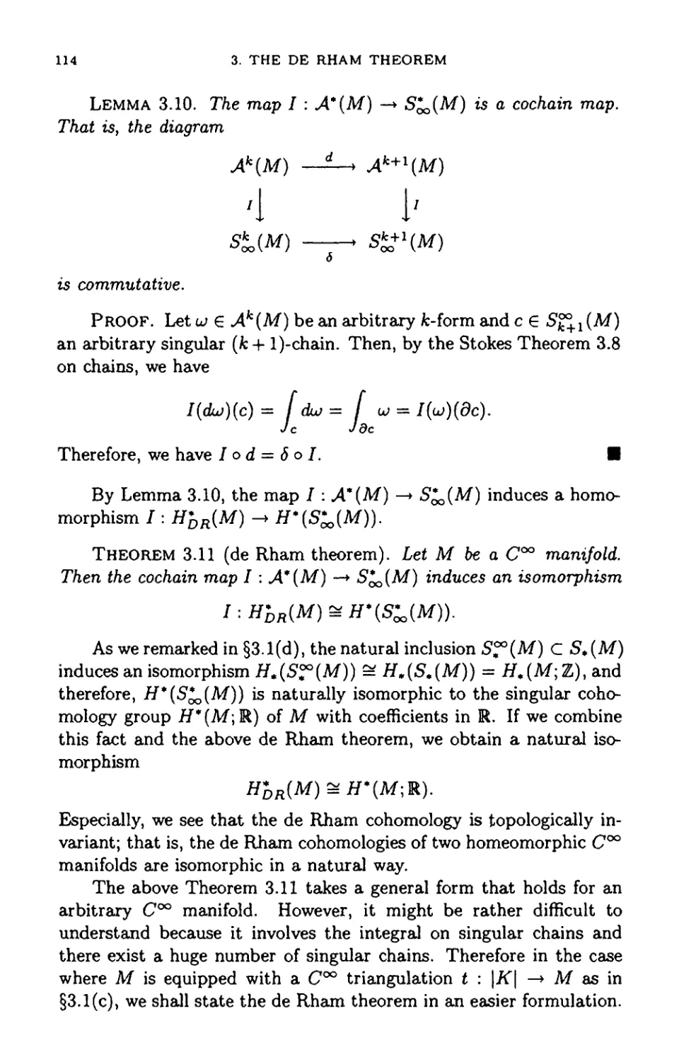
(b) The de Rham theorem 113
(c) Poincare lemma 116
3.4 Proof of the de Rham theorem 119
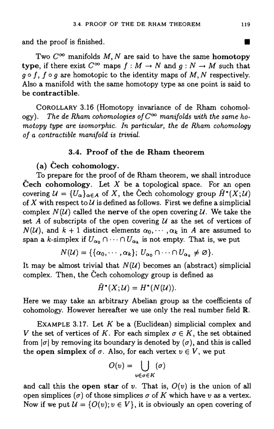
(a) Cech cohomology 119
(b) Comparison of de Rham cohomology and Cech
cohomology 121
(c) Proof of the de Rham theorem 126
(d) The de Rham theorem and product structure 131
3.5 Applications of the de Rham theorem 133
(a) Hopf invariant 133
(b) The Massey product 136
(c) Cohomology of compact Lie groups 137
(d) Mapping degree 138
(e) Integral expression of the linking number by Gauss 140
Summary 142
Exercises 142
Chapter 4 Laplacian and Harmonic Forms 145
4.1 Differential forms on Riemannian manifolds 145
(a) Riemannian metric 145
(b) Riemannian metric and differentieal forms 148
(c) The *-operator of Hodge 150
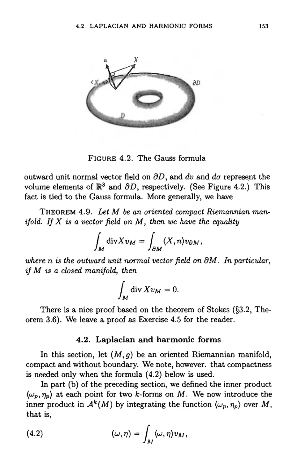
4.2 Laplacian and harmonic forms 153
4.3 The Hodge theorem 158
(a) The Hodge theorem and the Hodge decomoposi-
tion of differential forms 158
(b) The idea for the proof of the Hodoge
decomposition 160
4.4 Applications of the Hodge theorem 162

x CONTENTS
(a) The Poincare duality theorem 162
(b) Manifolds and Euler number 164
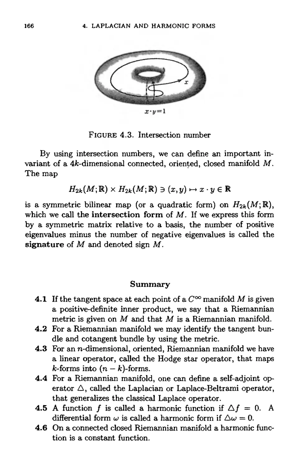
(c) Intersection number 165
Summary 166
Exercises 167
Chapter 5 Vector Bundles and Characteristic Classes 169
5.1 Vector bundles 169
(a) The tangent bundle of a manifold 169
(b) Vector bundles 170
(c) Several constructions of vector bundles 173
5.2 Geodesics and parallel translation of vectors 180
(a) Geodesics 180
(b) Covariant derivative 181
(c) Parallel displacement of vectors and curvature 183
5.3 Connections in vector bundles and 185
(a) Connections 185
(b) Curvature 186
(c) Connection form and curvature form 188
(d) Transformation rules of the local expressions for a
connection and its curvature 190
(e) Differential forms with values in a vector bundle 191
5.4 Pontrjagin classes 193
(a) Invariant polynomials 193
(b) Definition of Pontrjagin classes 197
(c) Levi-Civita connection 201
5.5 Chern classes 204
(a) Connection and curvature in a complex vector
bundle 204
(b) Definition of Chern classes 205
(c) Whitney formula 207
(d) Relations between Pontrjagin and Chern classes 208
5.6 Euler classes 211
(a) Orientation of vector bundles 211
(b) The definition of the Euler class 211
(c) Properties of the Euler class 214
5.7 Applications of characteristic classes 216
(a) The Gauss-Bonnet theorem 216
(b) Characteristic classes of the complex projective
space 223

CONTENTS xi
(c) Characteristic numbers 225
Summary 228
Exercises 229
Chapter 6 Fiber Bundles and Characteristic Classes 231
6.1 Fiber bundle and principal bundle 231
(a) Fiber bundle 231
(b) Structure group 233
(c) Principal bundle 236
(d) The classification of fiber bundles and
characteristic classes 238
(e) Examples of fiber bundles 239
6.2 S1 bundles and Euler classes 240
(a) S1 bundle 241
(b) Euler class of an S1 bundle 241
(c) The classification of S1 bundles 246
(d) Defining the Euler class for an Sl bundle by using
differential forms 249
(e) The primary obstruction class and the Euler class
of the sphere bundle 254
(f) Vector fields on a manifold and Hopf index
theorem 255
6.3 Connections 257
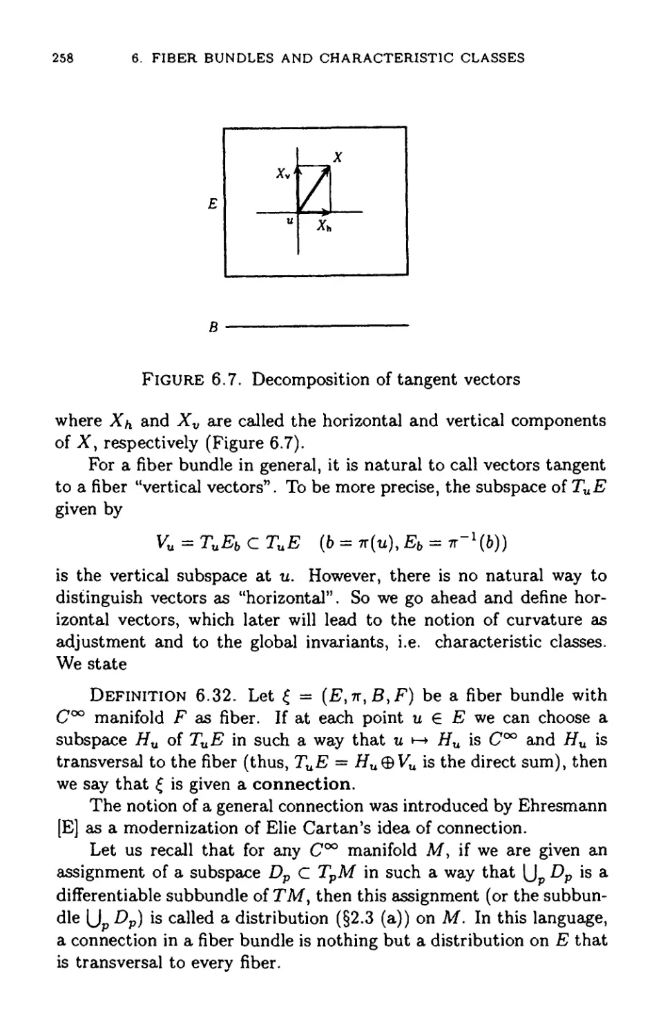
(a) Connections in general fiber bundles 257
(b) Connections in principal bundles 260
(c) Differential form representation of a connection in
a principal bundle 262
6.4 Curvature 265
(a) Curvature form 265
(b) Weil algebra 268
(c) Exterior differentiation of the Weil algebra 270
6.5 Characteristic classes 275
(a) Weil homomorphism 275
(b) Invariant polynomials for Lie groups 279
(c) Connections for vector bundles and principal
bundles 282
(d) Characterisric classes 284
6.6 A couple of items 285
(a) Triviality of the cohomology of the Weil algebra 285
(b) Chern-Simons forms 287

xii CONTENTS
(c) Flat bundles and holonomy homomorphisms 287
Summary 291
Exercises 292
Perspectives 295
Answers to Exercises 299
Chapter 1 299
Chapter 2 302
Chapter 3 305
Chapter 4 308
Chapter 5 310
Chapter 6 311
References 315
Index 317

Preface
As the title indicates, this book is an exposition of differential
forms. What is a differential form? The aim of this book is to answer
that question.
To explain differential forms, we have to comment on the
differentiable manifolds over which they are defined. In brief, a differentiable
manifold is a modern representation of a figure as a geometric
object, and is an important notion in modern mathematics. Therefore
many textbooks on differentiable manifolds have been published. The
reader may have seen or even already studied some of them. In these
textbooks, without exception, differential forms are defined. However,
in many cases only the definition and the fundamental properties are
presented, while only a brief description is given of how they are used
to analyze the structure of the differentiable manifold. This is because
so many fundamental facts already take up a lot of space.
Now that the notion of differentiable manifold is completely
established, this situation is in a sense inevitable. However, an
inconvenience arises. That is, the reader will be busy studying the
fundamental facts of differentiable manifolds, and will be left with
little time for practical manifolds. Also, as a theoretically reasonable
description is frequently not in the order of historical development,
the excitement of the discovery often gets lost.
Modern mathematics is now progressing dynamically. In
geometry a revolutionary change started in the 1980s, and it continues
today with no sign of halting. In such an era of progress, it is very
important to understand mathematics as a living system that is ready
for new advances, rather than as a completely established system.
In this series there is no book entitled "Manifolds". This may
be because the series editors took the above facts into account, and
desired to lead the readers to the scene of current active mathematical
research as quickly as possible.

xiv PREFACE
When I started to write this book, I found it much more difficult
than I had expected. Since mathematics stands on logic, vague
descriptions are not allowed. On the other hand, if I tried to base my
explanations on the historical motivations, the book would quickly
grow too long. I have tried to find a reasonable compromise, and will
leave it to the reader to judge how close I have come to the goal.
The contents of this book can be summarized as follows. In
Chapter 1 we begin with the definition of differentiate manifolds and the
fundamental ideas connected with them, such as tangent vectors,
tangent spaces, etc. The description, although minimal, should be
sufficient for understanding the rest of this book.
In Chapter 2 we introduce differential forms, define their
fundamental operations, and then prove the theorem of Frobenius. This
theorem gives a necessary and sufficient condition for the integrability
of "fields of directions" given at every point of a manifold, which are
described by either differential forms or vector fields, and its
importance has been increasing recently.
The theme of Chapter 3 is the theorem of de Rham. The reader
may have heard the name of this theorem. In fact it is a very
important result, and we may even say that it serves as the basis of the
theory of manifolds. In addition to the ordinary proof, we give an
explanation to clarify its relation to the integration of differential forms.
Also, several applications of this theorem are given at the end of the
chapter. Although they may be somewhat difficult, the author hopes
that they will show the reader some of the power of this theorem.
The second part of this book begins in Chapter 4, in which we
study the relationship between Riemannian metrics and differential
forms. We then explain the beautiful theory of harmonic forms, due
to Hodge and also to Kodaira and de Rham. Briefly, this theory may
be said to give a refinement of de Rham's theorem in the context of
Riemannian manifolds.
In Chapter 5, we introduce the notion of vector bundles. This is
the notion obtained by generalizing the tangent bundle of a manifold,
and it is a crucial tool in modern mathematics. We also explain the
concepts of connection and curvature, which are used to measure how
vector bundles are twisted.
In the last chapter, Chapter 6, we explain the theory of
characteristic classes, which I would say is one of the highest summits of
modern geometry. By virtue of this theory, the structure of figures,
namely manifolds, can be expressed in terms of differential forms,

PREFACE xv
which are local objects; and if we integrate them, the global structure
appears as concrete numbers, called characteristic numbers. Here
almost all of the previous material will be used.
Those readers who want to know the details of manifolds or
homology theory that are used in this book are invited to consult
textbooks on those subjects. If this book leads the reader to such a study,
or if it awakens an interest in deeper theories, the author will be very
happy indeed.
Shigeyuki Morita
July 1996

Preface to the English Edition
This is a translation of my book originally published in Japanese
by Iwanami Shoten, Publishers. It aims at introducing the reader to
the theory and practice of differential forms on manifolds, assuming
only a minimum of knowledge such as linear algebra, calculus, and
elementary topology. It also includes a quick introduction to the
concept of differentiate manifolds. I hope that this book will provide
the reader with a flavor of modern geometry and encourage him or
her to proceed to a study of deeper theories.
The original Japanese edition was published in two volumes. I am
grateful to Mrs. Teruko Nagase for translating the first part (Chapters
1,2,3) while keeping close contact with the author during the work.
The second part (Chapters 4,5,6) was translated by Professor Kat-
sumi Nomizu, who also suggested several improvements on the text.
I would like to express my deep gratitude to him. Finally, I would
like to thank the American Mathematical Society for publishing this
English edition, and their staff for providing excellent support.
Shigeyuki Morita
January 2001

Outline and Goal of the Theory
Geometry is the science of figures. We study various properties
of figures, and classify given figures according to the results. We
have the notion of invariants, which can serve as the most effective
method of classification. We may briefly say that invariants describe
geometric structures in terms of numbers. For example, as is well
known, the condition for congruence of triangles is described by such
invariants as the length of edges and angles at vertices.
However, in geometry we are not always studying given figures.
Sometimes we ask what kind of figures can exist at all, and also
enumerate conditions for their existence. It may be an eternal problem,
both in physics and in mathematics, for humans to imagine the figure
and shape of the universe where we live, and to study those
conditions. In geometry, in some cases, we can even surprise people by
constructing unknown figures practically. This is one of the pleasures
of studying geometry. The appearance of non-Euclidian geometry is
surely a typical example, which shows that the axiom of parallels is
not true in general.
The figures that are treated in modern geometry are called
manifolds. It is usually said that the notion of manifolds was introduced
by Riemann in his inaugural lecture at Gottingen University in 1854.
In this talk, the geometry of manifolds with Riemannian metrics -
namely, differential geometry - was also initiated. This was an epoch-
making lecture, in advance of its time. We also owe a great deal to
a series of work by Whitney, begun in the 1930's, for the formulation
of manifolds that we are now using.
Although they are all called "manifolds", there are various kinds
of manifolds. The simplest are the topological manifolds, which we
only require to be locally homeomorphic to a Euclidean space.
However, a manifold usually means a differentiable manifold, which has
smoothness; examples include curves and surfaces with beautiful
xix

xx OUTLINE AND GOAL OF THE THEORY
curved shapes. There are also complex manifolds and algebraic
manifolds (or varieties), which have finer structures. Nowadays each kind
of manifold is studied by its own methods. However, we should not
forget the origin of all manifolds, back in the days when mathematics
was not separated into branches like today. That is, we must consider
those manifolds that were considered by our great predecessors such
as Gauss, Riemann and Poincare.
As a simple but very important example, let us consider ori-
entable closed surfaces. While we shall give an exact definition later
on, for the present just imagine a smooth surface in space which is
bounded and has no boundary, as in Figure 0.1. The classification of
Figure 0.1. Orientable closed surface
these surfaces was already completed at the beginning of this century.
There is an invariant which comes to mind from a first glance at the
figure, namely the number of holes, which is called the genus. Then
a necessary and sufficient condition that two closed surfaces be the
same (in modern language, homeomorphic or diffeomorphic) is that
their genera are equal. So if E9 denotes a genus g closed surface, then
the infinite sequence
Eo, Ei, E2,....
exhausts all the orientable closed surfaces. Eo is the sphere and Ei
is the surface called a torus. Usually they are denoted by S2 and
T2, respectively. It is not an exaggeration to say that all the essence
of geometry is contained in the above classification of closed surfaces
and in the Gauss-Bonnet theorem mentioned below. Actually, one
goal of 20th century geometry was to try to extend these facts to
general manifolds in higher dimensions.
By the way, even if we consider only surfaces where the conclusion
is extremely simple and clear, if we think about its meaning a little
more deeply, we find that the problem is not so simple. It may appear
that the meaning of the genus g is so obvious from the figure that there
is no difficulty in defining it. However, this is only because, in this
picture, the figure is positioned in such a way that its genus is clearly

OUTLINE AND GOAL OF THE THEORY xxi
shown. In the case of a complicated surface, it is impossible to be sure
of the genus at sight, no matter how small it is. Moreover, there is
the intrinsically more important point that manifolds are not always
located in the well-known Euclidean spaces. In fact, it is characteristic
of modern geometry that manifolds are independent of the framework
of Euclidean spaces, and became quite free objects. Therefore, when
we study them, we cannot always utilize their relative relation to the
whole space. Moreover, in the cases of higher dimensional manifolds,
it is impossible to observe them directly with our eyes, no matter
how much we try to stretch our imagination. So how can we manage
them?
One possible method would be a combinatorial one where we take
certain items as units and decompose manifolds into these items. As
the items, we can use points, lines, triangles, and what are called
simplices, which are their generalizations to general dimensions. Also
we could use cells, which have more flexible shapes. This method is
very practical, and historically the first geometric invariant, the Euler
number, was found by this combinatorial method. If we decompose
a given figure into several triangles and take the alternating sum of
the numbers of vertices, edges and triangles, then the total is
independent of the method of decomposition, and it constitutes a specific
quantity of figures. Many readers may know that in the case of a
genus g closed surface, it is equal to 2 - 2g, and this fact in turn
indicates that the genus could be defined by a combinatorial method.
This is homology theory, introduced by Poincare about 100 years ago,
which extended these ideas and became an important means to study
figures by combinatorial methods. This theory enables us to count
the number of "holes" in each dimension (called the Betti number).
Thus the Euler number was given a theoretical basis for the first time
by Poincare, and so it is sometimes also called the Euler-Poincare
characteristic. In the 20th century, cohomology groups were defined
as the dual of homology groups, and, with both of them, a branch of
geometry called algebraic topology flourished.
Another method originated from the theory of surfaces due to
Gauss, as well as the Gauss-Bonnet theorem which followed it, and it
uses differentiation and integration to study figures. Although we say
simply a genus g closed surface, there are various ways of realizing it
in the space. In more mathematical terms, there are various kinds of
Riemannian structures on Eg, and we can bend it quite freely. What
Gauss showed in his theory of surfaces is that how curved a surface is,

xxii OUTLINE AND GOAL OF THE THEORY
now called the curvature, is an intrinsic quantity of the surface and
can be defined apart from the space where it lies. Because of this, it
may be said that he set the stage for the above-mentioned work of
Riemann. The Gauss-Bonnet theorem claims that if we integrate the
curvature K of a genus g closed surface S, which is curved arbitrarily,
over the whole surface, then the result is a constant independent of
how it is curved, and that constant is 2ir times the Euler number x(S)-
If we express this in mathematical terms, we obtain the following
beautiful equation:
f Kda = 2nX(S).
Now if we try to describe the goal of modern geometry in one
sentence, we may say that this goal is to extend the classification of
closed surfaces and also the Gauss-Bonnet theorem to manifolds of
arbitrary dimension in various ways. Here differential forms played a
fundamental role.
First of all, the theorem of de Rham claims that the homology
as well as the cohomology groups, which are defined by
combinatorial methods, can be obtained using differential forms in the case
of differentiable manifolds. But then, how does it go? Elements in
the fc-dimensional homology group of a manifold are represented by
so-called fc-dimensional cycles. A cycle is literally a figure without
boundary which returns to itself. In the cases where k = 0,1,2, a
cycle may be understood to be a point with ± signs, an oriented closed
curve, and an oriented closed surface, respectively (see Figure 0.2).
On the other hand, what is a fc-form on a manifold? When k — 0, it
Figure 0.2. Cycles
is simply a function. Therefore it takes a value on any 0-dimensional
cycle. For general k > 0, it may be said that a fc-form is a kind of
function that has a value on any ordered ^-directions (that is, tangent
vectors) at each point of a manifold. Therefore we can integrate it
over any fc-dimensional cycle, and we obtain a certain quantity. We
can repeat the theorem of de Rham by saying that we can obtain the
(co)homology groups, with coefficients from R. of any differentiable
manifold completely by such an operation of integrating differential

OUTLINE AND GOAL OF THE THEORY xxiii
forms on cycles. As above, since differential forms are something like
functions defined on any ordered directions at each point, it might be
easy to understand that they can describe various geometric
structures on manifolds. In the case of surfaces, although the curvature,
which tells how much it is curved, is a function on the surface, it
will be more natural to consider it as a differential form Kda of
degree 2 - that is, a combination of the curvature K and da which is
called the areal element. It is this 2-form that can be generalized to
the cases of higher dimensional Riemannian manifolds. It is called
the Riemannian curvature form, and it expresses how a manifold is
curved explicitly.
Going back a little bit, we have the tangent space and the tangent
bundle, which provide the most important tool to analyze the
structure of manifolds. The collection of all the tangent vectors at a point
is the tangent space, which gives the first approximation describing
the state of neighborhoods of that point, and the collection of all these
tangent spaces over the whole manifold is the tangent bundle.
Therefore, we can say that the tangent bundle is a space made of vector
spaces, which are flat spaces, over each point of a manifold. The way
these spaces are connected to each other is controlled by the group
of all the automorphisms of the vector space, which is a Lie group
called the general linear group. Generalizing this idea, we obtain the
notion of fiber bundles, which is motivated mainly by the great work
of E. Cartan in the first half of the 20th century. Briefly speaking,
a fiber bundle is a manifold obtained by tying together a family of
manifolds, called fibers, which stand systematically over each point of
another manifold (see Figure 0.3). In fiber bundles, the group (called
the structure group) that controls connections between fibers is an
infinite-dimensional group in general, but the cases where it becomes
Figure 0.3. Fiber bundle

xxiv OUTLINE AND GOAL OF THE THEORY
a Lie group are especially important. Then there arose an important
method for studying the structure of differentiable manifolds, and
that is to consider various fiber bundles over a given manifold with
various Lie groups as their structure groups, and to investigate them
from a synthetic point of view.
Now, how many fiber bundles, with a given Lie group as the
structure group, are there on a manifold? This is a fundamental question,
and it is the theory of characteristic classes that answers it. Roughly
speaking, characteristic classes are a certain description of how fiber
bundles are twisted over a manifold in terms of its cohomology groups.
The characteristic classes called Chern classes or Pontrj agin classes
are typical examples. There are various approaches to this theory;
among them the Chern-Weil theory is important. There is a general
method, where we give a relation between the fibers of a fiber bundle
in terms of a certain differential form of degree 1, called the
connection, and then differentiate it to obtain a quantity called the
curvature, which describes how the fiber bundle is curved. The Chern-Weil
theory gives a beautiful framework for research by systematically
applying this method to fiber bundles with arbitrary Lie groups as their
structure groups.
We cannot overestimate the important roles which Chern classes
and Pontrjagin classes played in classifying and analyzing the
structure of differentiable manifolds. For example, we have characteristic
numbers that are obtained by integrating polynomials in them over
manifolds, which are generalizations of the Euler number. They can
express global structures of manifolds in terms of numbers quite
explicitly.
In modern geometry, the importance of characteristic classes is
still increasing. Moreover, they are going to play a deeper role through
detailed analysis of differential forms, rather than merely
cohomology classes, which express the above classes. For example, in the
21st century, there will be grand attempts to generalize the theory of
harmonic integrals, which describes the relationship between the de
Rham cohomology and Riemannian metrics, in wider frameworks. In
these new developments, it is not too much to say that, so to speak,
differential forms play the role of water and air for life.

CHAPTER 1
Manifolds
In this chapter, we give an exposition of differentiable
manifolds, on which our leading characters, differential forms, are defined
and act. Roughly speaking, a differentiable manifold is a smooth
figure or space. For example, curves and surfaces are differentiate
manifolds. Since a point on a curve can be described by a single
parameter, it is called a 1-dimensional manifold. Similarly, every
surface can be locally obtained by slightly rounding a small domain in a
plane. Then a point can be denoted by the ordinary xy coordinates
in the plane. Thus, a point on a surface can be described by 2
parameters. So, a surface is called a 2-dimensional manifold. In general,
it is impossible to obtain the whole given surface, however skillfully
we round a domain in the plane. To obtain it, we must glue several
domains. In other words, the above-mentioned coordinates are not
always defined over the whole surface, unlike the planar case. These
coordinates are called local coordinates. Smoothness of a surface
is reflected in the relationship between different local coordinates.
Differentiable manifolds are defined by extending those properties
of curves and surfaces to general dimension. That is, a differentiable
manifold is a topological space such that any point on it has a
neighborhood whose points can be described by local coordinates consisting
of n independent parameters, and the relationship among different
local coordinates can be described by differentiable functions.
Now, unlike a curve or surface, a manifold does not always
appear in a well known space. In many cases it is rather difficult to
think of it as a geometric figure, since it is born in an extremely
abstract framework. However, it often happens that when we find local
coordinates on such a set and study the relationship among them, a
hidden geometric structure gradually comes to light. Since we try to
include as many objects as possible, it is inevitable for the definition
of manifolds to be abstract. However, once an object is recognized
to be a manifold by virtue of this abstract definition, it appears in

2 1. MANIFOLDS
a known space through the coordinates, and turns out to be a very
practical object.
In the study of not only manifolds but also modern mathematics
in general, it is important to connect abstract ideas with concrete
examples so that they mutually enrich each other. We will carry out
our exposition with this fact in mind.
1.1. What is a manifold?
(a) The n-dimensional numerical space Rn.
Before we define manifolds, we shall give some fundamental
examples. First, let R be the set of real numbers. If we consider it
geometrically as the real line, it is a 1-dimensional manifold. Next,
the set
R2 = {(x,y); x,yeR}
of all points with coordinates (x,y) (that is, the xy-plane R2) is a
2-dimensional manifold. In the same way, the set
R3 = {(x,y,z);x,y,zeR}
of all points with coordinates (x,y,z) (that is, xyz-space R3) is a
3-dimensional manifold (Figure 1.1). Generally, the set
Rn = {x= (x1,x2>--- ,xn); Xi eR}
of all the n-tuples (xi,X2,--- ,xn) of real numbers is called an n-
dimensional numerical space .
Rn is the most fundamental n-dimensional manifold. As for its
geometric image, it is a space extending boundlessly in n independent
R3
S
<*».«>
w
(x.y)
Figure 1.1. R, R2,R3
directions. A general n-dimensional manifold is formed by smoothly
glueing, one by one, some (in general, infinitely many) domains in
Rn (we shall give the details later). Therefore, let us first review the
geometric properties of Rn and the fundamental facts of differentiable
functions defined on Rn which are to be used as the glueing maps.

1.1. WHAT IS A MANIFOLD?
(b) Topology of Rn.
For two given points x = (xi,X2, • • • , xn), y — (yi,y2,
Rn, the distance d(x,y) between them is defined by
d(xty) = >/(*! - ViJ + {X2 - y2J + ¦ • ¦ + (xn - ynJ-
The distance d(x, 0) between the point x and the origin is sometimes
written ||x|| for short. In the cases of n = 1,2 and 3, d(x,y) is the
ordinary length of the line segment xy connecting 2 points x,y, and
the above formula is the natural extension of this to general n. It
is easy to see that d(x,y) satisfies the following three fundamental
properties:
(i) d(x, y) > 0 if x ^ y, and d(x, x) = 0.
(ii) d(x,y) =d(y,x).
(iii) For 3 arbitrary points x,y, z,
d(x,y) + d{y,z) > d(x,z) (triangle inequality).
Thus, Rn is a metric space with distance d. The distance d also
defines a topology on Rn as follows, and with this topology, Rn is a
topological space. For a point x in Rn and a positive number e > 0,
the set
t/(x,e) = {y GRn; d(x,y) < e)
of all points whose distance from x is less than € is called the e-
neighborhood of x (Figure 1.2). A subset U of Rn is called an
open set, if, for an arbitrary point x in U, we can take a sufficiently
small c-neighborhood of x so that it is entirely contained in U. For
example, all e-neighborhoods are open sets. An open set containing
x is sometimes called an open neighborhood of x.
U(x,e) l v--'' \
Figure 1.2. e-neighborhood and open set
Let U be the set of all open sets of Rn. Note that the empty
set 0 is considered to be an open set. Then, it is easy to see that U
satisfies the following three conditions:

4 1. MANIFOLDS
(i) Rn, 0 € U. That is, the whole space Rn and the empty set 0
are open sets,
(ii) If Uu #2, • • • , Uk € W, then CA n U2 n • • • n t/* € W. That is,
the intersection of a finite number of open sets is an open set.
(iii) For an arbitrary family {Ua}Q€A (Ua € U) of sets belonging
to U, their union [Ja€A Ua G U. That is, the union of an
arbitrary number of open sets is an open set.
In general, when a family U of subsets of X satisfies the above
three conditions (where Rn is replaced by X), we say that a
topology is defined on X and call the sets in li open sets. Thus, our
n-dimensional numerical space Rn turns out to be a topological space
that is prerequisite to a manifold.
(c) C°° functions and diffeomorphisms.
When we overlap parts of two small pieces of paper and glue them
together, we obtain a larger piece of paper. Also, when we paste two
parts of a piece of paper nicely, we can make various surfaces. For
example, when we roll up a rectangular sheet of paper and glue both
ends together, we have either a cylindrical ring or a surface called a
Mobius strip (Figure 1.3). As mentioned before, roughly speaking, a
manifold is a figure obtained by repeating the above kind of operations
with open sets in Rn as parts. We shall formulate these operations of
overlapping and glueing mathematically.
Figure 1.3. Forming surfaces by glueing
"Overlapping and gluing" two open sets U, V in Rn is read as
identifying U and V by a homeomorphism <p : U —> V. Here, <p
being a homeomorphism means that it is a one to one and onto map,
and both (p and <p_1 are continuous. Then U and V may be considered

1.1. WHAT IS A MANIFOLD? 5
to have the same shape, as topological spaces. Next, to construct a
differentiable (that is, smooth) manifold, the glueing maps have to be
smooth. This role will be played by diffeomorphisms, to be defined
below.
A function / : U —> R defined on an open set U of Rn is said to
be of class Cr if all the partial derivatives
up to order r exist and are continuous. Such a function is called a Cr
function. Functions which are of class Cr for all r are said to be of
class C°° and are called C°° functions. Thus, a C°° function is a
function which can be differentiated freely.
Next, consider a map <p : U —¦ Rm defined on an open set U of
Rn and with values in Rm. This map can be described by m functions
tpi : U -» R (i = 1, • • • , m) as follows:
<p(x) = {<pl{x),--- ,v>m(x)) {xeU).
If all <pi are of class Cr (or class C°°), <p is called a Cr map (or a C°°
map). The composition of two C°° maps is also a C°° map. This
follows from the chain rule of composite functions.
Definition 1.1 (Diffeomorphism). Let U,V be open sets in Rn.
A homeomorphism <p : U —* V from U onto V is called a C°°
differentiable homeomorphism, or simply a diffeomorphism, if both
(p and <p~l are of class C°°.
It is the inverse function theorem that plays an important
role in judging whether a given map is a diffeomorphism, and also
in practical construction of diffeomorphisms. To describe it, we shall
prepare a term. For a map ip = (</?i, • • • , ipm) defined on an open set
U with values in Rm, the matrix
few few ¦¦•few
V^fW few -fe(»v
is called the Jacobian matrix of the map <p at the point x € U.
When m = n, the determinant of the Jacobian matrix is called the
Jacobian.

6 1. MANIFOLDS
Theorem 1.2 (Inverse function theorem). Let ip be a C°° map
from an open set U of Rn to Rn. If the Jacobian at a point x in U is
not 0, then there exists an open neighborhood V C U of x such that
if{V) is an open set and if is a diffeomorphism from V onto <p{V)-
Even if a given C°° map from Rn to Rn happens to be known, for
some reason, to be a one to one map on an open set C/, it is generally
difficult to get the inverse map practically. However, if we calculate
the Jacobian of this map and find out that it is not 0 at each point on
U, by virtue of the above theorem the inverse map is also a C°° map,
and we can conclude that this is a diffeomorphism. In this sense, the
inverse function theorem is important.
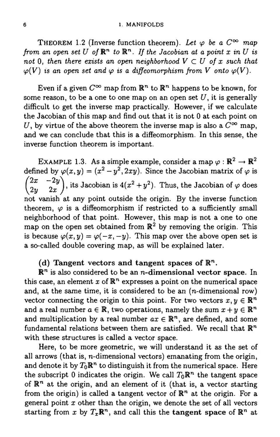
Example 1.3. As a simple example, consider a map i/>: R2 -» R2
defined by <p(x,y) = (x2 - y2,2xy). Since the Jacobian matrix of <p is
J, its Jacobian is 4(x2 + y2). Thus, the Jacobian of <p does
not vanish at any point outside the origin. By the inverse function
theorem, y? is a diffeomorphism if restricted to a sufficiently small
neighborhood of that point. However, this map is not a one to one
map on the open set obtained from R2 by removing the origin. This
is because <p{x,y) = <p(-x, -y). This map over the above open set is
a so-called double covering map, as will be explained later.
(d) Tangent vectors and tangent spaces of Rn.
Rn is also considered to be an n-dimensional vector space. In
this case, an element x of Rn expresses a point on the numerical space
and, at the same time, it is considered to be an (n-dimensional row)
vector connecting the origin to this point. For two vectors x, y G Rn
and a real number a € R, two operations, namely the sum x + y € Rn
and multiplication by a real number ax € Rn, are defined, and some
fundamental relations between them are satisfied. We recall that Rn
with these structures is called a vector space.
Here, to be more geometric, we will understand it as the set of
all arrows (that is, n-dimensional vectors) emanating from the origin,
and denote it by ToRn to distinguish it from the numerical space. Here
the subscript 0 indicates the origin. We call TbRn the tangent space
of Rn at the origin, and an element of it (that is, a vector starting
from the origin) is called a tangent vector of Rn at the origin. For a
general point x other than the origin, we denote the set of all vectors
starting from x by TxRn, and call this the tangent space of Rn at

1.1. WHAT IS A MANIFOLD?
x and its elements the tangent vectors at x. A structure of an
n-dimensional vector space over R is induced on TxRn naturally.
Figure 1.4. Tangent vectors
We now choose a basis of the tangent space TqW1. The unit vector
of length 1 starting from the origin in the direction of positive Xj is
written
_d_
dXi
The reason for using this symbol should be made clear by the following
explanation. By definition, -— is a tangent vector to Rn at the origin,
axi
that is, an element of TbRn. It is easy to see that -—, • • • , -— is a
ox i dxn
basis of ToRn. Then, an arbitrary tangent vector v at the origin can
be uniquely written as a linear combination
d d
v = oi^— + ••• + an-—.
oxi oxn
For a general point x in Rn, the parallel translation of the tangent
vector -— to x as the initial point is written as
OXi
\dxiJx
This turns out to be a tangent vector at the point x, and it is obvious
that ( -— ) >¦••,( ~— ) forms a basis of the tangent space TxRn at
\OX\/x \oxnJx
x. With this notation, the tangent vector -— at the origin should be
OXi
written precisely as (-z— ) . However in the case where the relevant
V OXi ' o
point is clear in advance, we sometimes simply write ^— instead of
OXi
(—)
\dXiJx
It may seem that the above description, which is meant to
distinguish the two aspects of Rn, that is, Rn as a geometric figure and

8 1. MANIFOLDS
Rn as a vector space, makes the matter difficult. However, this is
because Rn is originally a "straight" space, so that the tangent space
at an arbitrary point on it looks the same as the original space Rn.
In the case of a general curved manifold, the tangent space (see §1.3
for the definition) at a point is often far different from the whole
figure. However the tangent space is locally a good approximation
of a neighborhood of each point on the manifold, and gives us an
important foothold to study the structure of manifolds.
Here, we shall cite two important roles played by a tangent vector.
These two roles, each of them characterizing the tangent vectors,
give a guideline to defining the tangent vectors of a general manifold
(where it is not always possible to draw arrows like on Rn). The
first role is as a velocity vector to a curve. A smooth curve on Rn is
expressed by a C°° map c : R —> Rn. Then the velocity vector at a
point c(t) (t € R) on the curve is denoted by
S«-(?«••••¦?«)•
where c = (ci, • • • , Cn). It is also written as c(t). This velocity vector
is read to be a tangent vector at the point c(t) (Figure 1.5). When
we move the point over the curve and also consider various curves, a
variety of tangent vectors appear at each point of Rn.
Figure 1.5. Velocity vector
The second role of the tangent vector is as a directional
derivative. For example, let a function /(xi,--- ,xn) of n variables be
given. Then various partial derivatives -— (i = 1, • • • , n) are con-
oxx
sidered, and each of these is thought of as a partial derivative in
the positive direction of each axis x». Generalizing this idea, for an
arbitrary tangent vector
A.1) v = a!— + ... + an__
oxx dxn
at the origin of Rn, it will be natural to define the partial derivative
v(f) of the function / at the origin in the direction of v by
v(/)=ai^@)+*,+an^:@)-

1.1 WHAT IS A MANIFOLD? 9
This tangent vector v can be regarded as a tangent vector not only
at the origin but also at a general point x in Rn. To distinguish this
from the original v, let us write vx. Then vx(f) is thought of as a
description of the partial derivative
Vx(/)=a1^-(x) + .-- + an^-(x)
of / at x in the direction of vx. If we let vf(x) — vx(f), then vf
is a function on Rn, and its value at x is vx(f), that is, the partial
differential coefficient of / at the point in the direction of v. Thus
vf is nothing but the partial derivative of / with respect to v. From
the explanation so far, the reason why the notations of the partial
derivatives are used to describe the tangent vectors should be clear.
Above, we cited two roles of the tangent vectors; and, in general,
the velocity vector of a curve widely varies in both direction and size
depending on the point. Also, when we consider the partial derivative
of a function, we need not keep the direction of differentiation
constant. In some cases it is convenient to consider the partial derivative
of a function in a direction which depends on the place. Thus the
notion of vector field arises. Practically it is defined as follows.
A vector field X on Rn is an assignment of a tangent vector
Xx € TxRn to each point' x in Rn. Here we use the usual notation
Xf instead of v, to describe vector fields. Since the unit vectors
-— {i = 1, • • • , n) in the positive direction of each Xj-axis form a
OXi
basis of the tangent space TxRn at each point x, an arbitrary vector
field X can be written as
(L2) * = />z?r+-+'«sl;-
This formula is formally the same as A.1). However, while in A.1)
each coefficient is constant, in A.2) fc is a function on Rn, and the
direction and size of X change on each point depending on the value
of fi. When all the /t are C°° functions, X is called a C°° vector
field. We illustrate a simple example of a C°° vector field on the
plane (Figure 1.6). So far we have seen that for a function / and a
vector field X on Rn, the derivative Xfolf'va the direction X is
defined.

10 1. MANIFOLDS
Figure 1.6. Vector field on the plane
(e) Necessity of an abstract definition.
In the next section we shall give a practical definition of manifolds
which may seem to be quite abstract. As we mentioned before,
manifold is a notion obtained to generalize curves and surfaces in space to
higher dimensions. Therefore one might think it enough to work only
in the numerical space Rn. Actually, all manifolds, even if they are
defined abstractly, can be realized as generalized surfaces (called sub-
manifolds) in Rn after all (Whitney's embedding theorem). However,
there is a reason to give an abstract definition. The reason is that
even if it is embeddable in Rn, the embedding is not always a natural
one and does not always reveal the structure of the manifold. Rather,
there is a danger that it may conceal symmetry or other things that
might have existed in the manifolds.
For example, the sets of (i) all lines in the plane, (ii) all planes
in space, (iii) some particular patterns on a surface, and (iv) special
curvatures of a surface, turn out to be manifolds with a beautiful and
rich structure. These manifolds may not come out if we stick only to
Rn.
As an example which is simple but full of interesting suggestions,
we consider the set of all triangles. However, this is too vague to
capture as it stands. For instance, for, say, equilateral triangles with
sides 10 centimeter long, it is too much if we distinguish one on the
blackboard from a copy on our notebook. We should identify
congruent ones. Here we also identify similar ones, and consider the set T
of all classes of similar triangles.
An equivalence class of similar triangles is determined if three
angles are specified. If a,0 and 7 are the angles, they satisfy the
conditions
a + /? + 7 = 7r, a,/?,7>0.
Then T is realized as a domain such that x,y,z > 0 over the plane
x + y + z = n inR3. This domain is the interior of an equilateral

1.2. DEFINITION AND EXAMPLES OF MANIFOLDS 11
triangle in that plane. Actually, we should consider the exchange of
names of the three angles, for instance a and C. It is easy to see that
this corresponds to the action of the group of congruences (consisting
of rotations around the origin by 0°, 120° and 240° and reflections
with respect to the three axes of line symmetry) of the equilateral
triangle.
We now realize T in another way. We apply a similarity to expand
or shrink a given triangle so that the two vertices A, B are in the
position of 0 and 1 in the complex plane and the third vertex is at
the point z in the upper half plane H = {z — x + iy\ y > 0}. Thus
an arbitrary point on H represents an equivalence class of similar
triangles. If we put B, C in the position of 0 and 1 instead of A, B,
then a brief computation shows that A is at . In the same way,
if we put C, A in the position of 0 and 1, then B is at . Also if
we exchange A and B, C is at 1 - z, and if we exchange two other
vertices, we obtain similar formulae.
Thus T is realized as a figure obtained by identifying complex
numbers in H which are transformed into each other by the above
operations (the number of identified points is 6 for a general point, less
than 6 for special points, and just one for , which corresponds
to the equilateral triangle). Although, because of this identification,
T itself cannot be a manifold, we can represent T nicely using H.
This example shows that various coordinates can be considered
on the same object, depending on the purpose.
1.2. Definition and examples of manifolds
(a) Local coordinates and topological manifolds.
Let M be a topological space, that is, a figure in the broadest
sense. We begin by listing, one by one, the conditions for M to be a
manifold.
First, let M satisfy the Hausdorff separation axiom. That is,
for any two distinct pointsp,q e M, there exist an open neighborhood
U of p and an open neighborhood V of q such that U and V do not
intersect. Such a space M is called a Hausdorff space. Although
there are some important topological spaces that fail to satisfy this
separation axiom, it can be said that almost all ordinary figures which
are the object of geometry satisfy it. For example, the numerical space
Rn and all its subspaces are obviously Hausdorff spaces.

12 1. MANIFOLDS
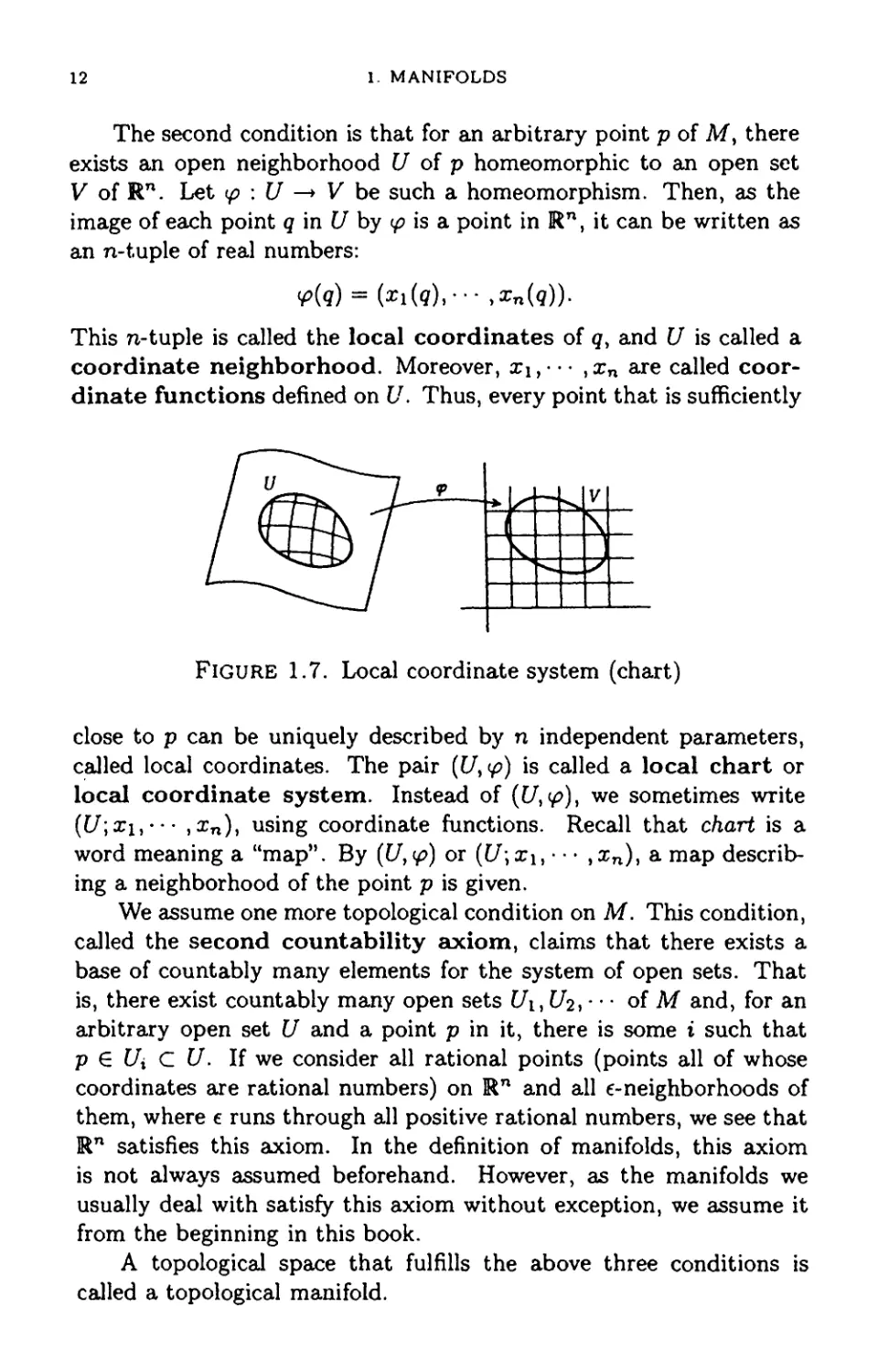
The second condition is that for an arbitrary point p of M, there
exists an open neighborhood U of p homeomorphic to an open set
V of Rn. Let <p : U —* V be such a homeomorphism. Then, as the
image of each point q in U by </? is a point in Rn, it can be written as
an n-tuple of real numbers:
?>(<?) = (*i (<?),••• ,xn(q)).
This n-tuple is called the local coordinates of q, and U is called a
coordinate neighborhood. Moreover, xi, • • • , xn are called
coordinate functions defined on U. Thus, every point that is sufficiently
Figure 1.7. Local coordinate system (chart)
close to p can be uniquely described by n independent parameters,
called local coordinates. The pair (U, <p) is called a local chart or
local coordinate system. Instead of (U,(p), we sometimes write
(U;xi,--- ,xn), using coordinate functions. Recall that chart is a
word meaning a "map". By {U,<p) or (U;x\, ¦ ¦ • ,xn), a map
describing a neighborhood of the point p is given.
We assume one more topological condition on M. This condition,
called the second countability axiom, claims that there exists a
base of countably many elements for the system of open sets. That
is, there exist countably many open sets U\, U2, ¦ • ¦ of M and, for an
arbitrary open set U and a point p in it, there is some i such that
p G Ui C U. If we consider all rational points (points all of whose
coordinates are rational numbers) on Rn and all e-neighborhoods of
them, where € runs through all positive rational numbers, we see that
Rn satisfies this axiom. In the definition of manifolds, this axiom
is not always assumed beforehand. However, as the manifolds we
usually deal with satisfy this axiom without exception, we assume it
from the beginning in this book.
A topological space that fulfills the above three conditions is
called a topological manifold.

1.2. DEFINITION AND EXAMPLES OF MANIFOLDS 13
Definition 1.4 (Topological manifolds). A Hausdorff space M
which satisfies the second countability axiom is said to be an n-
dimensional topological manifold if an arbitrary point on it has
an open neighborhood that is homeomorphic to an open set of Rn.
Example 1.5. Here is a simple example of a topological space
where, among the above three conditions, only the Hausdorff
separation axiom is not fulfilled. Define a subset M of the plane R2 by
M = {(x,0); x<0}u{(x,l); x > 0 } U {(x, -1); x>0}
(Figure 1.8). We give M the following topology, which is different
Figure 1.8
from the topology as a subspace of the plane. For every point p € M
except the two pointsp+ = @,1), p_ = @,-1), consider the ordinary
e-neighborhood Ue{p) — {q € M; d{p,q) < e } and for the exceptional
two points, let
U?(p±) = {(x,0); -e<x<0}U{(x,±l); 0 < x < e}
(with the convention that the double signs are taken in the same
order). Now, we invest M with the topology defined by the base of
open sets which consists of U€(p) for all points p on M and all positive
numbers e. By definition, any open neighborhoods of the two points
p+,p~ necessarily intersect, no matter how these neighborhoods are
chosen. Thus M is not a Hausdorff space. However, it is obvious that
M satisfies the other two conditions.
(b) Definition of differentiable manifolds.
Let M be a topological manifold. By Definition 1.4, at an
arbitrary point on M, there exists a "map" which describes its
neighborhood; that is, there exists a local coordinate system that gives an
identification of its neighborhood with an open set of Rn. Now, there
are rrfany maps, but not all of them are necessary for studying the
structure of M. For example, consider the maps which describe the
surface of the earth. While we can make all sort of maps according
to the purposes in hand, from the viewpoint of studying the whole

14 1. MANIFOLDS
surface of the earth, the important thing is whether the several sheets
of maps cover all the points of the earth. We call a system of maps
satisfying this condition an atlas of the earth. Once an atlas is given,
(in theory) we can make all maps. The same is true for manifolds.
Thus the following definition is natural.
Definition 1.6. Let M be a topological manifold. A family of
local coordinate systems <S = {(Ua, <pa)}aeA is said to be an atlas of
M if {Ua}a?A is an open covering of M, that is, if the open sets Ua
cover the whole of M.
In the above setting, we write Va for the image of the homeomor-
phism <pa from Ua into Rn. M is covered by coordinate neighborhoods
Ua in the atlas «S, and on the other hand, each Ua can be identified
with an open set VQ of Rn via the homeomorphism <pa. If we see this
the other way, it can be said that a manifold M can be made of open
sets VQ of Kn by glueing these parts one by one. We remark that even
if we cut off from Rn the part Va used to make M, Rn fills the gap
soon and is again complete, so that if the next part Vp intersects "the
imaginary hole", Vp can be taken out with complete shape. Rn is, so
to speak, a "fountain" from which the parts of manifolds spring.
We now study how to glue parts together. Suppose two
coordinate neighborhoods UayUp in the atlas S intersect. Then the
corresponding two open sets Va,Vp in Rn are to overlap in part to make
M. Look at Figure 1.9. In this figure, it is seen that the open sets
ipa{Ua H Up) in Va and <pp{Ua n Up) in Vp are glued to each other by
the homeomorphism
fCa =^o <Pal : <Pa{Ua O Up) -+ fp(Ua fl Up)
between them.
Figure 1.9. Coordinate change

1.2. DEFINITION AND EXAMPLES OF MANIFOLDS 15
Now, as fpa is a map from an open set of Rn to Rn, it is
described as fpa = (/jQ,--,/^a) by n continuous functions f0ct. If
we write the local coordinates of an arbitrary point p on Ua 0 17/3,
(xi(p),--- ,xn(p)) with respect to {Uay<pa) and (yi(p),--- ,yn(p))
with respect to {Up,tpp), then there is a relation
Vi(p) = fpaiziiPh--- ,xn{p))
between them. Thus the homeomorphism fpQ describes the
relationship between two local coordinates, so it is called the coordinate
change.
In the case of topological manifolds, it is enough that coordinate
changes or glueing maps are homeomorphisms, and there are no other
conditions. So as a figure, it may be said that they do not have a
rich structure. Against this, differentiable manifolds are defined by
claiming that all coordinate changes are diffeomorphisms. By virtue
of this they become globally smooth figures, and it is possible to
study them in detail using differentiation and integration. We state
the definition.
Definition 1.7. Let M be a topological manifold. An atlas S =
{(^o» &*)}<*€ a of M is called a C°° atlas if all its coordinate changes
fpa = <Pp ° <Pa1 are C°° maps. We also say that the atlas determines
a C°° structure on M. A manifold with a C°° structure is called a
C°° differentiable manifold or simply a C°° manifold.
Although in the above definition the coordinate changes are only
claimed to be C°° maps, by the inverse function theorem they are, of
course, C°° diffeomorphisms.
Two C°° atlases S, T given on a topological manifold M are said
to be equivalent if the union SuT is also a C°° atlas. It is easy to see
that the union of all C°° atlases equivalent to S is also a C°° atlas.
This atlas is called the maximal atlas determined by S.
A necessary and sufficient condition for two atlases to be
equivalent is that the maximal atlases determined by them coincide. So it
will be natural to identify C°° structures on M given by equivalent
C°° atlases. To show that a given figure is a C00 manifold, it is
preferable to construct an atlas of as small a number of local coordinate
systems as possible. However, once this is done, it is convenient to
use the maximal atlas collecting all the possible coordinate systems,
so that we can exchange the local coordinate systems freely according
to our purposes.

16 1. MANIFOLDS
Let p be a point on M. A local coordinate system (U, y?) belonging
to a maximal atlas of M is called a coordinate system around p, if
p belongs to U. We present a simple example of a local coordinate
system.
Example 1.8 (Polar coordinates). Let U be the domain obtained
by removing the nonpositive part of the x-axis {(x,0); x < 0} from
the xy-plane R2. Let r be the distance of a given point p — (x,y) in
U from the origin, and 0 (—•tt < 9 < -n) the angle from the positive
direction of the x-axis measured in the counterclockwise direction. If
we define a map y? : U —» R2 by y?(p) = (r,0), then (U,tp) is a local
coordinate system of R2. y?(p) is called the polar coordinates of the
point p. While here we consider the domain obtained by removing
the nonpositive part of the x-axis from R2, we sometimes consider
polar coordinates in other domains according to our purposes.
Generally a C°° structure does not always exist on a topological
manifold, and even if it exists it is not unique (except for the case of
dimension 0). However, the failure of the uniqueness here is due to the
uninteresting reason that an arbitrary difFeomorphism can be made
to be a homeomorphism which is not a diffeomorphism by a small
local perturbation. The essential classification of C°° structures is
given in terms of diffeomorphisms, and will be mentioned in §1.4.
Hereafter, the manifolds that we deal with in this book will be
C°° manifolds. We sometimes call a C°° manifold simply a
manifold. In the next subsection, we give some important examples of C°°
manifolds.
(c) Rn and general surfaces in it.
Example 1.9. The numerical space Rn is an n-dimensional C°°
manifold. As an atlas we can take only one local coordinate system,
(Rn,id). Here id denotes the identity map of Rn. Note that, in this
case, the coordinate has a meaning on the whole of Rn. We mention
another way to look at Rn, namely, to consider Rn as the product of
n copies of R. This is a special case of the next example.
Example 1.10. Let M, N be C°° manifolds, and let <S, T be their
atlases respectively. To begin with, it is easy to see that the product
space M x N is a topological manifold. Let
SxT = {{UxV1<px V); (?/,?>) € «S, (V,V) e T}.
We can see that S x T determines a natural C°° structure on M x TV.
We call this the product manifold of M and TV.

1.2. DEFINITION AND EXAMPLES OF MANIFOLDS 17
Example 1.11 (n-dimensional sphere). The set of points in Rn+1
whose distance from the origin is 1,
Sn = {x = (xi,--. ,in+i)an+1; x2i + --- + xl+i = 1},
is called the n-dimensional sphere (n-sphere). S1 is the unit circle
in the plane and S2 is the unit sphere in space. Let us check that
Sn is naturally an n-dimensional C°° manifold. We consider the two
points p+ = ((),••• ,0,1), v- = @, ¦•• ,0,-1) on Sn. Let U+ =
Sn - p_, U- = Sn - p+; then U+ and U- cover the whole of Sn.
The stereographic projection (p+ : U+ —* Rn from the point p_ is a
homeomorphism, as we can easily see (Figure 1.10). Similarly, the
stereographic projection ip- : U- —> Rn from the point p+ is also a
homeomorphism. Then we see that the two local coordinates systems,
(?/+,?>+), (*7-,?>-), form a C°° atlas of Sn.
p.
Figure 1.10. The stereographic projection </?+
Example 1.12. The product Sl x ; • • x Sl of n copies of S1 is
denoted by Tn and is called the n-dimensional torus. T2 is the
surface of a doughnut, shown in Figure 1.11. The n-dimensional torus
is one of the most important manifolds.
Figure 1.11. 2-dimensional torus
EXAMPLE 1.13 (General surfaces in Rn). The (n -
^-dimensional sphere 5n_1 is defined by the equation x\ H h x\ — 1 = 0 in

18 1. MANIFOLDS
Rn. It is natural to generalize this and consider a figure Z consisting
of all the points that satisfy m equations
fi(xi,--- >*n) =0 (t = l,--- ,m).
Here, each fi is assumed to be of class C°°. We put / = (/i, • • • , /m)-
Z takes various shapes according to the properties of /. In the
extreme case, it may happen to be the empty set. Under what conditions
will Z be a smooth figure, that is, a manifold in Rn? We will give
one sufficient condition.
We are given m equations, each of them considered as imposing
a restriction on the n variables X, which are essentially independent
parameters in Rn. The m equations give m restrictions, and the
degree of freedom decreases by m. As a result, a point on Z is expected
to be described by n - m parameters. However, if we consider the
case of /i = /2, it is easy to see that this is not always true. The
following condition is sufficient to guarantee this:
The rank of the Jacobian matrix of / has the maximal value m
at each point on Z.
We see that, under this condition, Z is an (n - m)-dimensional
C°° manifold as follows. By the assumption, for any given point p on
Z we can choose Xir, • • • , Xim such that the matrix
'&M - %?V>\
is regular. We remove x^,• • • , x,m from the n variables x\, • • • , xn,
and let the remaining variables be Xj1, • • • , Xjn_m. Then we see that
there exists an open neighborhood U of p such that the coordinates
Xj1,..., Xjn_m of an arbitrary point q on ZnU can move freely around
the corresponding coordinate values of p, while the other m
coordinates X{x, • • • , Xim are determined uniquely as C°° functions of them
by virtue of the inverse function theorem 1.2 as follows.
To show this, for simplicity, we assume that Xjx = Xi,--- ,
Xjn_m = xn-m. Consider Rn = Rn~m x Rm and define a map
F : Rn -* Rn
by F(x) = (xi,-- ,xn_m,/(x)). Then by the assumption, the
Jacobian of F at p is not 0. Thus, by the inverse function theorem,
there exists an open neighborhood U of p such that F induces a dif-
feomorphism from U onto V = F(U). If we write the coordinates

1.2. DEFINITION AND EXAMPLES OF MANIFOLDS 19
of the point p as p = (pi,P2) (pi G Rn_m, p2 G Rm), then there
exist open neighborhoods U\, U2 of pi and p2 in Rn-m and Rm
respectively, and we may assume that U = U\ x(/2. Then the inverse
function F-1 : V —» U is described as
F-1(x) = (x1,---,xn_m,/i(x)).
Here /i : V —> U2 is a C°° map. Now let q € Z n L7 be an arbitrary
point on Z near p\ then F(^) = (91,0). Therefore,
Q = (9i,92) = F~l o F(9) = (gi,%i,0)).
From this we obtain q2 = h(qi,0), and surely we see that the first
n — m coordinates (previously Xjlt- ¦ ¦ ,Xjn_m) of q are free to move
around pi, while the remaining m coordinates (previously ?*,,••• ,
Xim) are determined as their functions.
From the above discussion, we can use Xjx,• •• ,?Jn_m as the
coordinates of a point on Z n U (see Figure 1.12). That is, Z f\U
has the shape of a graph of a C°° map /i(<7i,0) defined on an open
set U\ containing the point p\ in Rn-m with values in an open set
Ui containing the point p2 in Rm. When p moves over Z, we have
to change the local coordinates. However, it is easy to see that the
transformations among the local coordinates are of class C°°. While
we leave the details to the reader, we see in this way that Z is an
(n — m)-dimensional C°° manifold.
Figure 1.12. A general surface
(d) Submanifolds.
Example 1.14 (Open submanifold). An arbitrary open subset U
of a C°° manifold M is a C°° manifold in a natural way, because if

20 1. MANIFOLDS
S = {(UQ,<Pa)}a€A is a C°° atlas of M, then S' = {((/Qn[/,^)}a6/,
is a C°° atlas of U. Here ip'Q denotes the restriction of ipatoUanU.
We call U an open submanifold of M. At first sight, these
manifolds may look worthless; however, actually they are very important.
We will present two examples.
The first example is the general linear group GL{n\ R), defined
as the set of all regular n x n real matrices. The set M(n;R) of
all real square matrices of order n can be identified with Rn in a
natural way, and thus it is a C°° manifold. Since the determinant is
obviously a continuous function on it, the set of all matrices whose
determinants are not 0, that is, GL(n; R), forms an open submanifold
of M(n;R). Moreover, GL(n;R) also has a Lie group structure that
will be mentioned later.
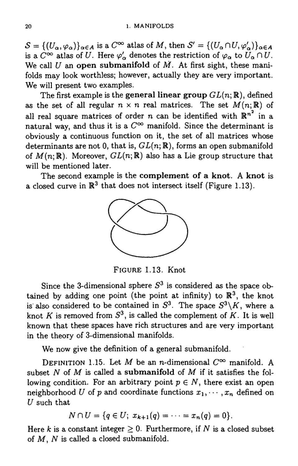
The second example is the complement of a knot. A knot is
a closed curve in R3 that does not intersect itself (Figure 1.13).
Figure 1.13. Knot
Since the 3-dimensional sphere S3 is considered as the space
obtained by adding one point (the point at infinity) to R3, the knot
is also considered to be contained in S3. The space S3\K, where a
knot K is removed from S3, is called the complement of K. It is well
known that these spaces have rich structures and are very important
in the theory of 3-dimensional manifolds.
We now give the definition of a general submanifold.
Definition 1.15. Let M be an n-dimensional C°° manifold. A
subset N of M is called a submanifold of M if it satisfies the
following condition. For an arbitrary point p € N, there exist an open
neighborhood U of p and coordinate functions Xi, • • • ,xn defined on
U such that
N n U = {qe U; xk+1(q) = • • • = xn(q) = 0}.
Here A: is a constant integer > 0. Furthermore, if N is a closed subset
of M, N is called a closed submanifold.

1.2. DEFINITION AND EXAMPLES OF MANIFOLDS 21
In this case, it is easily seen that N has the structure of a k-
dimensional C°° manifold in a natural way, and the inclusion map
N C M is a C°° map. Example 1.13, above, shows that Z is a
submanifold of Rn. In some books, the definition of submanifold
requires weaker conditions. In that case, a subset satisfying the above
condition is called a regular submanifold.
(e) Projective spaces.
Example 1.16. We write Pn for the set of all lines in Rn+1
through the origin and call it the n-dimensional real projective
space. To distinguish Pn from the complex projective space which
will be defined below, we sometimes write RPn. On Pn, a C°°
manifold structure is induced as follows. Given a point (xi, • • • ,xn+i) on
the space Rn+1 - {0} (that is Rn+l with the origin removed), the line
passing through this point and the origin defines an element of Pn.
This defines a projection
7T : Rn+1 - {0} - Pn,
which is obviously a surjection.
We put the quotient topology on Pn. That is, a subset U of Pn
is defined to be an open set if tt~1{U) is an open set of Rn+1 - {0}.
For two points x = (xi,--- ,in+i), y = (yi,--- ,yn+i) in Rn+1 -{0},
their images by it are the same if and only if there exists a nonzero
number a € R such that y^ = ax{ (i = 1, • • • , n+1). In this case, if we
denote this by x ~ y, we see that ~ gives an equivalence relation on
Rn+1 - {0}. In other words, Pn is the quotient space of Rn+1 - {0}
by this equivalence relation.
We denote tc(x\,--- ,xn+i) by [xi,--- ,xn+i]. This is called the
homogeneous coordinate of Pn. For i = 1, • • • ,n + 1, let
[/i = {[x1,---,xn+1]€Pn; xt^0}.
These are obviously open sets. Next we define pi : Ui —» Rn by
VXi Xi Xj Xi /
Then, after a brief consideration, we see that w is a homeomorphism.
Moreover, if i ^ j, an explicit calculation shows that <pj o tp'1 :
<Pi{Ui CiUj) -> <pj{Ui n Uj) is a C°° map. Thus, we see that P71 is a
C°° manifold.
Here we mention complex manifolds very briefly. We write C
for the set of complex numbers. C is a field under the usual four basic

22 1. MANIFOLDS
operations of arithmetic. Geometrically, we can identify C with R2
by the correspondence C9z = i + iy^ (x,y) € R2 (this is called
the Gaussian plane). Therefore we can consider C as a 2-dimensional
C°° manifold. The product Cn of n copies of C is a 2n-dimensional
C°° manifold. However, actually Cn has a deeper structure, that
of an n-dimensional complex manifold. In the definition of complex
manifolds, a holomorphic mapping defined over an open set of Cn
plays the role of a C°° map in C°° manifolds. Roughly speaking, a
holomorphic mapping is a differentiable function with respect to each
complex variable. If in the definition of a C°° manifold we replace
Rn and C°° maps by Cn and holomorphic mappings, we obtain the
definition of a complex manifold. Since holomorphic mappings are,
of course, C°° maps, all n-dimensional complex manifolds are
automatically 2n-dimensional C°° manifolds. However, it is known that
holomorphic mappings have much finer properties than C°° maps,
and this gives rise to deeper geometric structures on complex
manifolds. On the other hand, compared with the holomorphic case, we
can use various constructions for C°° maps freely, and the same is
true for C°° manifolds.
Example 1.17. In the definition of real projective spaces, if we
replace R by C, we obtain the definition of complex projective
spaces. That is, we denote the set of all complex lines through
the origin in Cn+1 by CPn and call this the n-dimensional complex
projective space. CPn is an n-dimensional complex manifold and
therefore a 2n-dimensional C°° manifold.
(f) Lie groups.
Lie groups are by themselves a big research field. We briefly
summarize aspects of Lie groups that we will need for this book.
Definition 1.18. If a group G is also a C°° manifold, and both
the multiplication G x G 3 (g>h) h-> gh e G of the group and the
map G 3 g h-» g~l e G of taking the inverse are of class C°°, then
G is called a Lie group. Furthermore, if G is a complex manifold
and the above two maps are holomorphic mappings, then G is called
a complex Lie group.
Example 1.19. The set GL(n\C) of regular complex square
matrices of order n is a complex Lie group, called the general linear
group over C.
Example 1.20. The set 0(n) of orthogonal matrices of order n
is a Lie group, called the orthogonal group of order n. 0(n) is

1.3. TANGENT VECTORS AND TANGENT SPACES 23
defined by the equation lX X = E {lX is the transpose of X and E
is the identity matrix) in the set M(n\ R) of all real square matrices
of order n. Then we can see that the condition of Example 1.13 is
satisfied (we put the case n = 2 as Exercise 1.2), and 0(n) is a C°°
manifold. It is easy to verify the other conditions.
The subgroup SO(n) of all elements of 0{n) with determinant
1 is called the special orthogonal group of order n. SO(n) is a
connected component of the identity of 0{n), and the quotient group
0(n)/SO(n) is a finite group of order 2. 0(n) and SO(n) are compact
Lie groups.
Example 1.21. The set U(n) of all unitary matrices of order n
is a Lie group, called the unitary group of order n. U{n) is defined
by the equation X*X = E in the set M(n;C) of all complex square
matrices of order n. Here, we denote by X* the matrix whose (i,j)
entry is the complex conjugate of the (j,i) entry of X. Also in this
case, the condition of Example 1.13 is satisfied and U(n) is a compact
Lie group.
1.3. Tangent vectors and tangent spaces
(a) C°° functions and C°° mappings on manifolds.
C°° functions on manifolds give an important hint for studying
the structure of C°° manifolds.
Definition 1.22. Let M be a C°° manifold and / : M -» R a
real valued function on M. If, for all locaL coordinate systems [U,ip)
in an atlas that defines the C°° structure of M, / o <p~l : </?(?/) —> R
is a C°° function on the open set <p{U) of Rn, then / is said to be a
C°° function on M.
In the above definition the phrase "all local coordinate systems
in an atlas" may be replaced by "all local coordinate systems in the
maximal atlas". This is because once the above condition is satisfied
for one atlas, it is satisfied for all equivalent atlases. Next we consider
the local description of C°° functions. Let A7, </>) be an arbitrary local
coordinate system. Then a point p on U is identified with a point
ip{xi(p), ¦ • ¦ yxn(p)) on Rn. Hence the function / o ip~l defined on
<p(U) can be described as
fo<p-l(x) = F(xu--- ,xn) {xe<p(U))
using the coordinate functions x\, • • • ,xn. This is the description of
/ on U by the C°° function F.

24 1 MANIFOLDS
If U is an arbitrary open set of M, then U is naturally a C°°
manifold (see Example 1.14). Hence we can consider C°° functions
on U. For example, if A7, <p) is an arbitrary coordinate system of M,
each coordinate function x* : U —* R is obviously a C°° function.
We denote by C°°{M) the set of all C°° functions on M. For
two functions / and g in C0C(M), the sum / + <?, the product fg and
the multiplication af (a 6 R) by a real number are also elements in
C°°(M). Equipped with these operations, Cco(M) has the structure
of what is called an algebra over R. As the term algebra used here
will appear frequently, we define it now.
Definition 1.23. Let K be a field (in this book K may be
thought of as R). If a vector space A over K has a ring structure
by a product operation AxA3(A,/i)hA^A and the condition
a(A/z) = (aA)/x = X(afi) (a € K, A,/i e A) is satisfied, then A is called
an algebra over K.
Example 1.24. Any real valued polynomial f(xi, ¦ • ¦ ,xn) of n
variables defines a function on Rn. Hence all those polynomials form
a subalgebra Pn of C°°(Rn). By restriction to 5n_1, these are also
considered to be C°° functions on Sn-1.
By extending the notion of C°° functions on manifolds, we obtain
that of C°° maps between manifolds.
Definition 1.25. Let M, N be C°° manifolds. A continuous
mapping / : M —> N is said to be a C°° map, if the
composition tp o f o ip~l is of class C°° wherever it has meaning (that is, on
<p(?/n/-1(V))) for an arbitrary local coordinate system (U,<p) of M
and an arbitrary local coordinate system (V}i>) of N.
Although the above definition is natural, it is easy to see that
we may rephrase it as follows. A necessary and sufficient condition
for a map / : M —* N to be a C°° map is that for an arbitrary C°°
function h on N, h o f is a C°° function on M. Theoretically, this
definition may be said to be more straightforward.
From the definition of a C°° map, it is easy to check that the
composition go f of two C°° maps / : M —¦ N and g : N —* P is also
a C°° map.
Definition 1.26. Let M,N be C°° manifolds. A one to one C°°
map / : M —» N from M onto N is called a C°° diffeomorphism or
simply a diffeomorphism if the inverse mapping of / is also of class

1.3. TANGENT VECTORS AND TANGENT SPACES 25
C°°. If a diffeomorphism from M to N exists, M and N are said to
be mutually diffeomorphic.
The classification problem of C°° manifolds by diffeomorphisms
is a fundamental problem in the field called differential topology.
Example 1.27 (Hopf map). We define a map h : Sz -> S2 from
the 3-dimensional sphere to the 2-dimensional sphere as follows.
Consider S3 as the unit sphere
S3 = {(zuz2)eC2; |*i|2 + M2 = l}
in C2 and S2 as 1-dimensional complex projective space CP1 (see
Example 1.17 and Exercise 1.3). Then we set .
h(z1,z2) = [zuz2], {zi,z2)eS3.
It is easy to see that this is a C°° map. This map, called the Hopf
map after its discoverer H. Hopf, is a very important map with a rich
structure.
(b) Practical construction of C°° functions on a
manifold.
On a C°° manifold, there are a huge number of C°° functions.
By handling those functions quite freely, we can also change them so
that they will have various properties. Here we will introduce a well
known and fundamental technique.
We denote by D(r) the open disk
{ar = (n,--- ,xn)€Rn; x\ + • • • + x2 < r2}
of radius r > 0 with center at the origin in Rn, and by D(r) its
closure. We choose a C°° function b : Rn —¦ R such that for all points
x e Rn we have 0 < 6(x) < 1 and
A.3) W-f1' X€^A)'
When n = 1 the graph of b(x) is shown in Figure 1.14. Since its
shape looks like a bump, we use the notation b(x). Such a function is
constructed, for instance, as follows. We define a function h : R —¦ R
(e-1/*, x>0,
' ~ \0, x < 0.
h{x) = <
It is easy to see that this function is of class C°°. Then, letting

1. MANIFOLDS
,f~
-2 -I
~\
1 2
b(x)
Figure 1.14. Graph of b{x)
h{4 - x\ xj)
h{4 - x\ x2n) + h{x\ + ... + x*-iy
we can show that the required conditions are satisfied. Now, using
the function b(x), we can construct various kinds of C°° functions on
a manifold.
Lemma 1.28. Let M be a C°° manifold. Let U be an open
neighborhood of a point p of M, and f : U —> R an arbitrary C°° function
defined on U. Then there exist an open neighborhood V ofp such that
V C U and a C°° function f defined on the whole of M satisfying the
condition
'«> = {o(,)' qYv
PROOF. We take a coordinate system (W, <p) around p
satisfying W c U and <p(p) = 0, tp(W) D DC). Recall that DC) is an
open disk of radius 3 with center at the origin of Rn. Such a local
coordinate system is easily constructed, if necessary, by composing a
homothety with the origin of Rn as the center. Let b = bcxpy using the
function b of A.3). Then b is a C°° function on W and is 0 outside
of <p~l(DB)) c W. Then, defining it to be 0 in the complement of
Wy we can consider b as a C°° function defined on the whole of M.
Now, if we let V = y>_1(D(l)), then V is an open neighborhood ofp,
and obviously V C U and the value of b on V is 1. Hence, letting
[0, q & W,
we can see that / satisfies the required property. ¦
Applying this lemma to an arbitrary local coordinate system
(U\x\, — - ,in) of My we can say the following. While each
coordinate function ?» has meaning originally only on U, if we cut down

1.3. TANGENT VECTORS AND TANGENT SPACES 27
the domain a little it can be extended to a C°° function defined on
the whole of M. However, of course, the extended functions no longer
play the role of coordinate functions on the whole of M.
(c) Partition of unity.
To study the structure of manifolds, it is necessary to construct
functions on them with various properties, vector fields and
differential forms that will be defined later, and Riemanninan metrics, etc.
On the other hand, C°° manifolds are constructed by glueing open
sets in Rn by diffeomorphisms one by one. Accordingly, to construct
the above items on manifolds, it is necessary to glue the constructed
things on each coordinate neighborhood. In this process, it is the
partition of unity that plays an important role.
Let X be a topological space (not necessarily a manifold). A
family of subsets {Ua} of X is called a covering of X if the union
U Ua is the whole of X. If all the Ua are open sets, we call {Ua} an
open covering. A covering {t/a} is said to be locally finite if, for
each point on X, there exists an open neighborhood U such that the
number of a with U n UQ ^ 0 is finite. A covering {Vp} is called a
refinement of {Ua} if for an arbitrary C, there exists an a such that
v0 C ua.
Recall that a topological space X is said to be compact if an
arbitrary open covering has a finite refinement. Relaxing this condition,
if an arbitrary open covering of X has a locally finite refinement, X
is said to be paracompact. The following proposition shows that all
manifolds are not only paracompact but also have better properties.
Proposition 1.29. Let M be a topological manifold. Then for
an arbitrary open covering of M there exists a locally finite open
covering {Vi,i = 1,2, •••} that is a refinement of it and has countably
many elements with all V* being compact. In particular, M is
paracompact. If necessary, we can make it satisfy the following stronger
condition: each (V*,^) is a coordinate neighborhood, ipi(Vi) = DC),
and {^t_1(^(l))} is already an open covering of M.
Proof. Since M satisfies the second countability axiom, there
exists a base {Oi\i = 1,2,-••} of open sets with countably many
elements. Moreover, since M is a manifold, it is of course a locally
compact Hausdorff space. From these facts, we see that the collection
of all Oi such that Oi is compact is a base of the open sets. So, from
the start, let us assume that the O, are all compact.

28 1. MANIFOLDS
We construct a sequence of open sets E\, E2, • • • that grows with
i as follows. In the first place, let E\ = 0\. By induction we assume
that Ei, • • • , Ek are defined, and have the form
Ek = OiU02U---UOifc.
Then, since Ek is compact, for sufficiently large i, we have
?fccOiU02U---uOi.
Among those i such that ik < i, let ik+i be the smallest and let
Ek+i=OiU02U---UOik+l.
Then obviously, for arbitrary k each Ek is compact and Ek C Ek+i.
Moreover [)k Ek = M (Figure 1.15) (if M is compact, this operation
terminates in a finite number of steps). Now let {?/a}a€A be an
arbitrary open covering of M. Fix an arbitrary i > 1. For each point
p € Ei — Ei-i, choose ap such that p € Uapt and take a local
coordinate system (VJ,, 0P) around p that satisfies ipp{p) — 0, tpp(Vp) = DC)
and Vp C ?/Qp n (Ei+i - E{-2) (we set E_i = E0 = 0). Let
W = i>~l(D(l)). Since Ej - Ei-i is compact, we can choose a
finite number of points p in it so that the corresponding open sets Wp
cover Ei - -E^-i. We apply this operation to all i, and line up the
local coordinate systems (Vp,ipp) corresponding to the finite number
of points p chosen at each stage to have {(Vii^i)}t=:i,2."-- Then, {Vi}
Figure 1.15
is a refinement of {Ua} and a locally finite open covering of M. Each
Vi is compact, and obviously also satisfies the stronger conditions of
the last part of the proposition. ¦
For a continuous function / : X —» R on a topological space X,
the closure of the set of all the points where the value of / is not 0,
suppf = {x€X;f(x) /0},

1.3. TANGENT VECTORS AND TANGENT SPACES 29
is called the support of /.
Definition 1.30. Let M be a C°° manifold. A family {/* ;t =
1,2, • • • } of at most countably many C°° functions on M is called a
partition of unity on M if it satisfies the following two conditions:
(i) For each t, fi(p) >0(p€ M) and {supp fj} is locally finite.
(ii) At all points p on M, J2i fiip) ~ 1-
Furthermore, if {supp /»} is a refinement of an open covering {Ua},
the partition of unity {fi\i = 1,2, • • • } is said to be subordinate to
the open covering {Ua}.
THEOREM 1.31 (Existence of partitions of unity). Let M be a C°°
manifold and {UQ} an open covering of M. Then there exists a
partition of unity {/t ; i = 1,2, • • • } that is subordinate to {Ua}-
Proof. Let {VJ be a locally finite refinement of {Ua} satisfying
the stronger condition of Proposition 1.29. In particular, (V*,-^) is
a local coordinate system such that ipi{Vi) — DC). Now, for each i,
using the function 6 of A.3), let
-{r
«,)-<;'*«• \\l
Then b, is a C°° function defined on the whole of M (see the proof
of Lemma 1.28). Moreover, since supp 6» C K, we can set
/ = X>
Then / is a C°° function defined on the whole of M. Furthermore,
if we let Wi = Vt_1('C)(l))> as {Wi} is already an open covering of
M, for an arbitrary point q € M there exists j such that bj(q) — 1.
Consequently, the value of / is never 0. Then, if we let
for each i, then {/i, /2, • • • } is a partition of unity subordinate to the
open covering {Ua}- ¦
(d) Tangent vectors.
We will review the case of En (see § 1.1(d)). A tangent vector at
a point x on Rn is a vector with starting point x, and the set TxRn
of all of them forms an n-dimensional vector space. We can take

30 1. MANIFOLDS
-—, • • • , -— as its standard basis, and an arbitrary tangent vector
dxi dxn
v G TzRn can be described uniquely as their linear combination
d d
, = ai__ + ... + an_
Among the roles played by tangent vectors, the following two are
fundamental, namely, the role of the velocity vector along a curve
and the role of the directional derivative that gives the direction of
the partial derivative of functions. The second role for the above
tangent vector v gives a map
t; : C°°(Rn) - R
defined by
v(/)=ai^(x)+",+anl{:(:r) (/€C,°°(Rn))-
That is, v(f) is the partial derivative of the function / at x in the
direction of v. It is easy to see that this map v has the following two
properties:
(i) v(f + g) = v(f) + v{g), v(af) = «;(/),
(ii) v(fg)=v(f)g(x) + f(x)v(g).
The first property simply says that v is linear. The important one is
the second property, and it shows directly that v is a differentiation.
We now introduce the notion of tangent vectors to a general C°°
manifold M. In this case, a vector with the starting point p on M
has no meaning in general. While, as in Example 1.13, if M is in Rn
we can consider a vector with starting point p and tangents to M, a
general manifold is defined intrinsically and is not always embedded
in Rn beforehand. Then, we define tangent vectors on the basis of
the above two properties.
Definition 1.32. Let M be a C°° manifold and p a point of M.
If a map v : C°°(M) —> R satisfies the conditions
(i) v(f + g) = v(f) + v{g), v(af) = av(f),
(ii) v(fg) = v(f)g(p) + f(p)v(g),
for arbitrary functions f,g G C°°{M) and o € R, then v is said to be
a tangent vector to M at p.
We denote by TPM the set of all the tangent vectors at the point
p of M, and call this the tangent space at the point p of M. If

1.3. TANGENT VECTORS AND TANGENT SPACES 31
we define the sum v + v' of two tangent vectors v,v' ?TPM and the
multiplication by a real number av as
(v + t/)(/)=v(/) + t/(/), M(/) = av{f),
these are also tangent vectors and thus TPM is a vector space.
For the function 1 G C°°(M) that is identically 1, v(l) = 0 for
arbitrary v € TPM. The reason is that if we let / = g = 1 in
condition (ii) of tangent vectors as differentials, we have v(l) = 2v(l).
Furthermore, for the constant function a € C°°(M) (o G R), by the
condition (i), we have v(a) = av(l) = 0.
The operation of tangent vectors on C°°(M) is local in the
following sense. If two functions /, g € C°°(M) coincide on an open
neighborhood of p, we have v(f) = v(g) for arbitrary v e TPM. We
can see this as follows. By the proof of Lemma 1.28, there exists
a C°° function b that is identically 1 in a neighborhood of p and 0
outside of this open neighborhood. Then (/ - g)b = 0. Therefore,
0 = v((f - g)b) = v(f - g)b(p) + (/ - g)(p)v(b) = v(f - g).
Thus v(f) = v{g).
Now, let (U, 4>) be a coordinate system around the point p, and
x\, ¦ • • ,xn its coordinate functions. Then it is easy to see that the
correspondence
C°°(MKf~d-^fl(v(p))
defines a tangent vector at p. We denote this tangent vector by
eTpM. If the point p is clear beforehand, we sometimes
dxi
THEOREM 1.33. Let M be an n-dimensional C°° manifold. Then
the tangent space TpM at an arbitrary point p on M is an n-
dimensional vector space. Moreover, if (U;x\, ¦ • • }xn) is a local
coordinate system around p, then the tangent vectors
\dxxJp 'KdXnJp
form a, basis ofTpM.
PROOF. First of all, ( -—) , • • • , ( -—J are linearly indepen-
\OX\/p \OXn/p
dent, because if we apply these tangent vectors on each coordinate
Uxjp

1. MANIFOLDS
function Xj (extended to be a C°° function on the whole of M, see
Lemma 1.28), obviously we have
Next, we show that TPM is generated by the. above n tangent
vectors. We identify the coordinate neighborhood U of p and <p{U) C
Rn by ip, and assume that y(p) = 0 and that <p{U) is a convex set in
Rn. For an arbitrary function / € C°°(M), the restriction of / to U
is, under the above identification, described as a C°° function F(x)
defined on <p{U). Explicitly, F = fof~l. Now since, for an arbitrary
x e <p(U),
fl dF
if we let <?i(x) = / -z—{tx)dt, this is a C°° function and we have
Jo OXi
n
A.4) F(x) = F@) + ^xi9t(x).
i=l
Obviously, pj(O) = -—@). We will apply an arbitrary tangent vector
OXi
v e TPM to A.4). Paying attention to the conditions of a tangent
vector, we have
n
v{f) = v{F)=Y,v(xi)gi@)
n <9
Since / was arbitrary, it follows that v = Y^ v(xi)-—. The proof is
. OX4
complete. ¦
Next, we mention another role of the tangent vector as the
velocity vector of curves. A C°° map from an open interval to a C°°
manifold is called a C°° curve on M. Let c : (a, 6) —¦ M be a C°°
curve passing through the point p = c{to) {to € {a,b)) of M. Then

1.3. TANGENT VECTORS AND TANGENT SPACES 33
the velocity vector c(to) of c at the point p is defined as follows. For
/ € C°°(M), we put
A.5) c((„)(/) = ^| .
at \t=to
It is easy to check that this satisfies the conditions of a tangent vector,
and so we have c(io)(/) € TPM. We sometimes write -r-(io) or —
at at 110
instead of c(to)- If we consider the velocity vector of various curves,
we see that all the elements in TPM appear.
In the case of Rn and general surfaces (Example 1.13) in Rn, the
tangent space at a point on it has an explicit geometric meaning.
In the case of a general manifold, since the definition of the tangent
space is abstract, its image might be difficult to grasp. However, we
may understand it as a first-order approximation of neighborhoods of
each point on the manifold by a vector space of the same dimension.
Finally, we will see how the expression of the tangent vector
changes under a coordinate change.
Proposition 1.34. Let (U;xir- ¦ ,xn) and (V;yi,--- ,yn) be
two local coordinate systems around a point p on a C°° manifold M.
Then,
dxi ^dx^'dyj'
As the proof is easy, we leave it to the reader.
(e) The differential of maps.
Let M and N be C°° manifolds and / : M — N a C°° map.
Then for each point p of M, a linear map
/,:TpM->T/(p)/V
is defined as follows. This is called the differential of / at p. We
sometimes write dfp for /¦. Let v e TPM be a. tangent vector to M
at the point p; then the correspondence
C°°(iV)9/iHt,(fto/) eR
is a linear map; and moreover it is easy to see that it satisfies the
property of differential at the point f(p) on TV. We denote this by
f*{v) e Tf(p)N'. It is easy to see that /„ is a linear map.
As for the differential of the composition g o / : M —> P of
two C°° maps / : M —> N and g : N —* P, it is easy to see that

34 1. MANIFOLDS
(9 ° /)¦ = 9* ° /¦ • TPM -+ Tgof{p)P. That is, the differential of the
composition is the composition of the differentials of each map.
We describe the differential of a map explicitly by local
coordinates. Let / : M —> TV be a C°° map and let f(p) = q (p €
M). Let (U\x\, ¦ • ¦ ,xm) be a local coordinate system around p and
{V'i yi» • • • ,Ifn) a local coordinate system around q. Then it is easy to
check that
A-6) f(±\=Y?VL±.
K } J'\dxJ ^dXi dVj
Using A.6) and the formula for the differential of a composition, we
obtain the following proposition. We leave the detailed proof to the
reader as Exercise 1.8.
Proposition 1.35. Let M and N be C°° manifolds and f : M -*
N a C°° map. Then, for an arbitrary tangent vector v € TPM at the
point p on M and an arbitrary function h 6 C°°(N) on N,
v(W) = /.(tOfc.
(f) Immersions and embeddings.
For a C°° map / : M -* TV, its differential /¦ : TPM — T/(p)/V
reflects the geometric properties of /. We give the following definition.
Definition 1.36. Let / : M — N be a C°° map.
(i) If at each point p € M the differential /» : TPM —> Tf(p)N of
/ is an injection, we call / an immersion.
(ii) If / : M —> N is an immersion and also / is a homeomorphism
from M onto the image f{M) of /, we call / an embedding.
Note that we give f{M) the relative topology as a subset of
N.
(iii) If / : M -* N is a surjection and at each point p the
differential /» : TPM —» Tf(p)N of / is a surjection, we call / a
submersion.
The difference between immersions and embeddings concerns
whether M intersects itself in its image f{M) or whether it approaches
itself repeatedly or not, and is a global matter. We show their
conceptual figure in Figure 1.16. A typical example of a submersion
is the Hopf map (Example 1.27). Embedding is closely related to
the concept of submanifolds (Definition 1.15). Actually the following
theorem holds.

1.3. TANGENT VECTORS AND TANGENT SPACES
Figure 1.16. Immersion and Embedding
THEOREM 1.37. Let f : M -* N be an embedding from a C°°
manifold M to N. Then, f{M) is a submanifold of N and f gives a
diffeomorphism from M onto f{M). Conversely, if M is a
submanifold of N, the inclusion map i : M —» N is an embedding.
PROOF. Let the dimensions of M and Nbem and n respectively.
By assumption, for an arbitrary point q € f(M) on /(M), there
exists a unique point p G M such that f(p) = q. If we choose a
local coordinate system (V;y,\, ¦ ¦ ¦ ,yn) around q such that V is small
enough, then U = f~l{V) is a coordinate neighborhood containing
p. Let xi, • • • , xm be the coordinate functions defined on U. For the
sake of simplicity, we will identify U and V with open sets in Rm and
Rn respectively, and also let p and f(p) be the origins respectively.
Then the restriction of / to U is described by n C°° functions fi as
follows:
Vi = /t(*i,--- ,xm) (t = l,--- ,n).
Since / is an embedding, the rank of the Jacobi matrix of / at the
point p is m. If m = n, by the inverse function theorem 1.2, / is
a diffeomorphism in a neighborhood of p. Thus, the claim of the
theorem follows easily. Let m < n. Then, if necessary changing the
order of the variables y\, • • • , yn, we may assume that
"(if
H,=,..
7^0.
Now, if we define a function F = (F1, • • • , F„) : U x Rn~n
(x,tu) = (xi,--- ,xm,u;i,--- ,wn-m) e U x Rn-m, by
» Rn, for
Fi{x,w)
/t(x) + lUi_
(t = 1,- • • ,m),
(i = m + 1, • • • ,
we see that the Jacobian of F does not vanish at the origin. Again by
the inverse function theorem, F is a diffeomorphism in a neighborhood
of the origin. Therefore, for a sufficiently small neighborhood V CV
of q = /(p), if we consider F : V -» {7 x R"-m c Rn, (V^F)

36 1. MANIFOLDS
is a local coordinate system around q. Then, while the coordinate
functions on V are xi,--- ,xm,wi,--- ,tun_m, by the definition of
F, obviously f{M) r\V = {q* e V']Wi{q') = • • • = wn.m{q') = 0}.
This shows that f{M) is a submanifold of TV. Since the proof of
the remaining claims of the theorem is easy, we will leave it to the
reader. ¦
Next we prove that an arbitrary compact C°° manifold can be
embedded into RN for a sufficiently large N. By this (although there
is the assumption of being compact), it is shown that an abstractly
defined arbitrary manifold is realized as a submanifold of RN.
THEOREM 1.38. An arbitrary compact C°° manifold can be
embedded into RN for a sufficiently large N
Proof. Let M be a compact n-dimensional manifold. Let
{Ui,(pi}i=i>...,r be an atlas of M with a finite number (r) of
coordinate neighborhood systems satisfying the following conditions. The
image <Pi{Ui) of each <pi : U —> Rn is an open disk DB) of radius
2 with center at the origin, and if we put V* = (p^1{D{l)I {Vi} is
already a covering of M. The existence of such an atlas follows
immediately from the compactness of M (see the proof of Proposition 1.29).
Then, we construct a C°° map fi:M-*SnC Rn+1 from M to the n-
dimensional sphere 5n to satisfy the following two conditions: (i) the
restriction of / to V, is a diffeomorphism from Vi onto the southern
hemisphere {x € 5n; xn+\ < 0} of 5n, and (ii) / maps the
complement of Vi to the northern hemisphere. Intuitively, the existence of
this map seems obvious. As the proof is not so difficult, we wish the
reader to try it. Now, if we define a map / : M —» Rr(n+1) as
/(p) = (/l(p),..-,/r(p)) (P€M),
it is easy to check that / is an embedding. ¦
In fact, more generally, it is known that an arbitrary
n-dimensional C°° manifold can be embedded in R2n+1 as a closed
submanifold (Whitney's embedding theorem).
1.4. Vector fields
(a) Vector fields.
In §l.l(d), we defined vector fields on Rn. In this section, we
consider vector fields over general manifolds.

1.4. VECTOR FIELDS 37
Let M be a C°° manifold. A vector field X on M is an
assignment, to each point p € M, of a tangent vector Xp eTpM in such a
way that Xp is of class C°° with respect to p. If we let A7; X\, • • • , xn)
be a local coordinate system of M, for each point p € U, X is
described as follows:
A-7) *P = X>(P)^-.
where a* is a function defined on U. This is called a local expression
of X. Xp is said to be of class C°° with respect to p, if each coefficient
a,i is a C°° function. Let yi, • • • , yn be another system of coordinate
functions defined around p. Then by Proposition 1.34, we have
*'-g(?*w?w)?-
Therefore, the condition of each coefficient di being a C°° function
does not depend on the choice of local coordinates.
We shall denote the set of all vector fields on M by X{M). When
two vector fields X, Y e X(M) are given, by putting (X + Y)p =
Xp+Yp we can define their sum X+Y € X(M). Also, for an arbitrary
real number a € R, by putting {aX)p = a(Xp) we can define the
multiplication aX € X(M) of X by a. As is easily seen, with these
two operations X(M) becomes a vector space over R. Moreover, when
/ € C°°{M) is an arbitrary C°° function on M, fX e X{M) is defined
by {fX)p = f(p)Xp. Therefore, X{M) has a structure of module not
only over R but also over C°°(M). Briefly, as for vector fields, we
can do operations such as multiplication by function, addition and
subtraction freely.
Recall that one important role of the tangent vector is the
directional differentiation of functions. Using this role, we can make the
vector field X act on any function / € C°°(M). That is, if we put
(Xf)(p) = xp(f) (j>eM),
we obtain a function XfonM. If we give a local expression of X as
A.7), then
(Xf)(p)=J2ai(p)^-(p),

38 1. MANIFOLDS
so that Xf is also a C°° function on M. Xf is called the derivative
of / by the vector field X. In this way, we obtain a map
X{M) x C°°{M) 3 (XJ) ^Xf? C°°(M).
While this map is obviously linear with respect to X, as for / it is
easy to see that it satisfies the following two conditions:
(i) X{af + bg) = aXf + bXg (a, 6 G R, f,g € C°°{M))\
(ii) X(fg) = (Xf)g + f(Xg).
Generally, we call a map C°°(M) —* C°°(M) satisfying these two
properties a derivation of the algebra C°°(M) over K.
The derivation of functions by vector field characterizes it
completely. That is, the following proposition holds.
Proposition 1.39. Let M be a C°° manifold and X,Y vector
fields on M. If Xf = Yf for an arbitrary C°° function f on M, then
X = Y.
Proof. It is enough to show that Xp = Yp at an arbitrary point
p on M. We choose a local coordinate system (U\x\, ...,i„) around
p. Let
*-§«•?• Y=pi
be the local expressions of X, Y with respect to this local coordinate
system. By Lemma 1.28, there exists a C°° function X{ defined on M
and coinciding with each coordinate function X{ in a neighborhood of
p. Then, since o^ip) = XpXi = YpXi — 6i(p), we obtain Xp = Yp, and
the proof is finished. ¦
(b) The bracket of vector fields.
Let X,Y € X{M) be two vector fields on a C°° manifold M.
Then, both XtY act on C°°(M) as derivations. Consider a map
A.8) C°°{M) 3 f -> X{Yf) - Y{Xf) € C°°(M).
By an easy calculation, we can check that this map also has the two
properties of the derivation. If we rewrite it as X(Yf) - Y{Xf) =
(XY - YX)f, it indicates that XY - YX expresses a vector field
on M. Actually, using the symbol [X, Y] instead of XY - YX, we
consider the correspondence
A.9) C°°(M) 3 f - [XtY]pf = Xp(Yf) - Yp(Xf) € R
at each point p 6 M. From the fact that A.8) satisfies the properties
of a derivation, we immediately see that the correspondence A.9)

1.4. VECTOR FIELDS 39
satisfies the condition (see Definition 1.32) of tangent vectors at the
point p. That is, we can consider [X, Y]p as a tangent vector to M
at p. If it is shown that [X, Y]p is of class C°° with respect to />, we
can conclude that [X, Y) is a vector field on M. In order to check it,
we give X, Y the local expressions
x = Ta°, y = y>#-.
f^ dxt ^ dxi
By an easy calculation, we have
tj=i J
Prom this, we see that [X, Y] is a vector field on M, and
simultaneously its local expression is given by
The vector field [X, Y] defined in this way is called the bracket of X
and Y. We will cite some properties of the bracket.
PROPOSITION 1.40. The bracket of vector fields has the following
properties.
(i) [aX + bX\ Y] = a[X, Y) + b[X', Y) (a, b e R), and the same
forY.
(n) [Y,x] = -(x,n
(iii) (Jacobi identity) ([A",y],Z] + [[K,Z],X] + [[Z,X],y] = 0.
(iv) lfX,gY] = fg[X,Y] + f(Xg)Y-g{Yf)X (f,g e C°°(M)).
If we calculate carefully, the proof is not so difficult. We leave it
as Exercise 1.7. We call a vector space with operation [, ] satisfying
the above conditions (i)-(iii) a Lie algebra. Accordingly, X(M), the
set of all vector fields on M, becomes a Lie algebra over R with respect
to the bracket operation defined above. In fact, we can see that X(M)
is naturally isomorphic to the set of all derivations (in which the Lie
algebra structure is also introduced) of C°°{M) as Lie algebras. The
interested reader may consider the proof.
(c) Integral curves of vector fields and one-parameter
group of local transformations.
Let M be a C°° manifold and X a vector field on M. A curve
c : (a, 6) —» M in M is called the integral curve of X if the velocity

40 1. MANIFOLDS
vector c{t) e TC(()M (t € (a, 6)) at each point coincides with the value
of X at that point. Imagine that X expresses the velocity vector of
a smooth flow of water over M. Then if we float a small grain at a
point p on M, it drives down the flow and draws a curve on M. This
kind of curve is the integral curve. If we change the point to float the
grain, its curve will be different in general. However, no matter how
we choose those two curves, they never cross each other (Figure 1.17).
Figure 1.17. Integral curves
We shall find equations that should be satisfied by the integral
curve through an arbitrary point p on M. Let (U;xi,-- ¦ ,xn) be a
local coordinate system around p. Then X is locally expressed as
on U. Let c : (a, 6) -¦ M be the required integral curve, and for
simplicity, choose a parameter such that c@) = p. If we describe the
position of c(t) by the local coordinate system as c(t) = (xi{t), • • • , x„(i)),
we have
Hence the required equation is
dx
A.11) -~@ = a<(*i@.-",*n@) (; = !,•••,n).
The condition of passing through the point p at t = 0 is expressed as
the initial condition; Xi@) = Xi(p). Note that if we choose another
point for p, only the initial condition changes; the equation itself is
the same.
By the way, A.11) is a system of ordinary differential equations of
first order, and, as is well known, for this type of differential equations
the following theorem of existence and uniqueness of the solution
holds.

1.4. VECTOR FIELDS 41
Theorem 1.41 (Existence and uniqueness of the solution of
ODEs). For the ordinary differential equations A.11), the following
hold.
(i) (Existence) For an arbitrary initial condition Xi@) = x»(p) (p €
U), if we choose € > 0 small enough, A.11) has a solution of
class C°° defined on — c < t < e.
(ii) (Uniqueness) // two solutions of A.11) have the same value
at a point t = to on their domains, they coincide all over the
intersection of their domains.
(iii) (Differentiability of the solution with respect to the initial
condition) For an arbitrary point p € U, if we choose a
neighborhood V (C U) of p small enough, there exists an e > 0 such
that for all q € V a solution satisfying the initial condition
Xi(to) = %i(q) is defined on to - e < t < to + e. Furthermore,
if we consider the family of these solutions as a function of t
and X\, • • • ,x„, it is of class C°°.
By Theorem 1.41 (i), we see that there exists an integral curve
through an arbitrary point p when t = 0 anyway. We shall
consider extending the (domain of the) integral curve as long as possible.
Since, by Theorem 1.41 (ii), if two integral curves pass through the
same point at the same time, then they are connected as a single
integral curve; the way of extension is unique. If it is going out of the
coordinate neighborhood U, we can continue the discussion by
choosing a new coordinate neighborhood. The reason is that, even if we
change the coordinate neighborhood, the form of the equation does
not change. In this way, for each point p e M there exists an integral
curve c(p) that passes through the point when t = 0, and it cannot
be extended any more. We call this integral curve the maximal
integral curve through p. By Theorem 1.41 (i), c(p) is a curve of class
C°°. Let (ap, bp) be the domain of c(p). Of course, — oo < ap < 0 and
0 < bp < +oo. For an arbitrary point q on c(p), c(q) is different from
c(p) only by a translation of the parameter, and is the same curve.
That is, if it starts from p and arrives at q at the time s, we have
A.12) c(q)(t)=c{p)(t + s) (<? = c(p)(s)).
We can see this fact, if we fix s and calculate the velocity vector of
c(p)(* + s) and apply Theorem 1.41(h) (see Figure 1.18).
In this way, M is covered completely by all the maximal integral
curves that are pairwise disjoint. Though it is still called an integral
curve, the integral curve through a point where the value of the vector

42 1. MANIFOLDS
0 = c(p)(s)
Figure 1.18
field is the zero vector (such a point is called a singular point of the
vector field) consists of a single point.
Let
W = {(t,p) e R x M\av < t < bp}
and define a map $ : W — M by $(t,p) = c(p){t) {{typ) e W). That
is, $(?,p) is the point at which we arrive, at the time t, after starting
from the point p and going through the integral curve.
By Theorem 1.14(i), (iii), we see that W is an open set of R x M
containing 0 x M, and the map $ is of class C°°. For an arbitrary
i, let Mt = {p e M\ ap < t < bp}. Then Mt is an open set (empty
in some cases) of M. We define the C°° map tpt '¦ Mt —¦ M by
<Pt(p) = ${t,p) (p G M). Of course, Mo = M and <^0 = idw-
PROPOSITION 1.42. For an arbitrary t, <pt '• Mt —* M is a diffeo-
morphism onto an open submanifold of M. Furthermore for arbitrary
t, s E 1R and p G M, the equation
A.13) <Pt°<Ps(p) = <Pt+s(p)
holds as long as both sides are defined (that is, if p e Ms, <ps{v) €
Mt, p € Mt+a).
PROOF. We prove the latter part. By the definition ift+s(p) =
c(p)(t 4- s), and on the other hand, if we write y?5(p) = c(p)(s) = q,
the left hand side of A.13) is c{q){t). Then by A.12), the equation
A.13) holds.
The former part can be proved as follows. First, by the definition
of Mt, we see that M_t = y?t(Mt). Next, by the above facts we have
(pto<p-t = <P-t ° <Pt = id, so that </?t is a diffeomorphism from Mt onto
M-t and ip-t serves as its inverse. ¦
Definition 1.43. Let X be a vector field on a C°° manifold M.
The set of all diffeomorphisms {y?(; t € R} constructed above is called
the one parameter group of local transformations generated by
X.
In the above notation, the reason why we say "group of local
transformations" is that yt is not always defined on the whole of M.

14. VECTOR FIELDS 43
Definition 1.44. A vector field X on a C°° manifold M is called
a complete vector field if an arbitrary element <pt of the associated
one parameter group of local transformations {</?*} is defined on the
whole of M (that is, if Mt — M or equivalently W = R x M). In
other words, X is complete if the integral curve through an arbitrary
point on M is defined on the whole of R.
Now we shall denote the group of all diffeomorphisms of M by
DiffM. We define the multiplication by the composition of
diffeomorphisms. This group is an infinite-dimensional group called the
diffeomorphism group of M, and it is a very important group
whose global structure remains mostly unknown.
If a vector field X on M is complete, by Proposition 1.42, the
correspondence R 3 t >-> <pt G DiffM is a group homomorphism. That is,
the vector field X generates a one-parameter commutative subgroup
in DiffM. In this case, we call {</><; t e R} a one parameter group
of transformations generated by X. We sometimes write Exp tX
for it.
The following theorem gives a sufficient condition for X to be
complete.
THEOREM 1.45. Let M be a compact C°° manifold. Then an
arbitrary vector field X on M is complete.
Proof. Consider W = {{t,p) e R x M;ap < t < bp}. As we
have seen above, W is an open set containing 0 x M. Since M is
compact by the assumption, we can choose c > 0 small enough so
that (-e, e) x M C W. That is, the integral curve c{p) going through
p when t = 0 is defined for -e < t < e. In this case, we can see that
the domain of c(p) can be actually extended to - §e < i < |e for any
p. This is because if we start from p and go along c(p) till time |t| = ^e
(let q be that point), then we can keep going along c(q) (= c(p)) for
\t\ < e. But then, by the discussion in A.12), we can conclude that we
started from p and went along c(p) till the time |f| < |e. Repeating
this discussion, we can go along c(p) for an arbitrary time, and the
theorem is proved. ¦
Example 1.46. As a simple example of a noncomplete vector
field, we have M = R2 - {0}, X = —. In this case, the integral
ox
curve through the point A,0) € M, for example, is defined only
for -1 < t < oo.

44 1. MANIFOLDS
(d) Transformations of vector fields by difFeomorphism.
Let M,N be C°° manifolds and /:M-»iVa difFeomorphism
from M to N. Then, for an arbitrary vector field X on M, a vector
field f+X on N is defined by
{f.X)q = f.{Xf-Hq)) (q<EN).
Or equivalently we can write f*(Xp) = (f*X)f(p) (p € M). Then, for
an arbitrary function h e C°°(N) on N, we have
A.14) (f.X)h = X(hof)of-\
This holds because, for a point q € N, we have
((/.x)/i)(<?) = {f.x)qh = /•(x/-i(„)/i,
and on the other hand, by Proposition 1.35, we have
f.{Xf-Hq))h = Xf-iM(h o /) = (X(h o /) o /-%).
1.5. Fundamental facts concerning manifolds
(a) Manifolds with boundary.
Up to now, we have defined a manifold as a figure that is
locally homeomorphic to an open set in JRn. Therefore, whatever point
we choose on a manifold, its neighborhood looks the same.
However, when we construct a surface B-dimensional manifold) by
glueing sheets of paper, for instance, it is not always a manifold at each
step in the construction. To begin with, a slip of paper has corners
and boundaries, and disks and cylinders also have boundaries.
Similarly, in the study of manifolds, manifolds with corners and
boundaries often play important roles. We now introduce manifolds with
boundaries.
First, we define "the upper half space" Hn of Rn, by
Hn = {x = (xi,--- ,in) eRn; xn > 0}.
Its subset
dUn = {x € Hn; xn = 0}
is called the boundary of Hn. It can naturally be identified with
Rn_1. Here Hn\dHn is called the interior of Hn. The case n = 2 is
illustrated in Figure 1.19.
A continuous map </? : U —> V between two open sets U and V
in Mn is called a C°° map from U to V if it can be extended to a
C°° map from an open set U' of Rn containing U to an open set V
of Rn containing V. We call ip : U —> V a diffeomorphism if it is a
homeomorphism and both y? and ip~l are C°° maps. In this case, it

1.5. FUNDAMENTAL FACTS CONCERNING MANIFOLDS 45
<?H2
Figure 1.19. The upper half plane H2
is easy to see that the restriction of ip to U n dMn is a diffeomorphism
from UndWn to VnMn.
Now, everywhere in the definition of C°° manifolds (Definitions 1.4
and 1.7), let us replace Rn by Hn. That is, for a HausdorfF space
M satisfying the second countability axiom, let an open covering
{Ua}a€A of M and a homeomorphism tpa : Ua —» Va from UQ onto
an open set Va of Hn be given, and for arbitrary a, 0, assume that
h<x = V/3 ° V^1 : VaiUcc H U0) -»<p0(Ua C\ Up)
is a C°° map. Let S = {{Ua,<Pa)}aeA- We denote by dM the set
of all the points p in Ua that are mapped by (pa to dMn, where a
moves arbitrarily. If dM ^ 0, we say that S defines a structure of a
C°° manifold with boundary on M. In this case, we call dM the
boundary of M. We see that dM has an (n — l)-dimensional C°°
manifold structure in a natural way. Local coordinate systems,
atlases, maximal atlases, etc. are defined in the same way as in the case
without boundary. Disks, cylinders and the Mobius strip (Fig. 1.20),
which will appear in the next subsection, etc. are all 2-dimensional
manifolds with boundary.
Figure 1.20. Mobius strip and cylinder
Example 1.47. The n-dimensional disk Dn = {x e Rn; x\ +
H x2 < 1} is a manifold with boundary, and dDn = 5n_1.

46 1. MANIFOLDS
A compact C°° manifold without boundary is called a closed
manifold. Closed manifolds are the most important objects in the
study of manifolds.
(b) Orientation of a manifold.
We now compare a Mobius strip, which is a famous surface where
we cannot distinguish the two faces, with a cylinder, where we can
distinguish them.
How can we formulate the difference in the properties of these
two surfaces mathematically? Since both are 2-dimensional
manifolds, we can construct them by glueing some small pieces that are
homeomorphic to open sets of K2 one by one. Specifying the two
faces of the pieces beforehand, we consider the construction of
surfaces using only identifications that preserve the right side and the
reverse side respectively. Though cylinders, spheres, tori, etc. can be
constructed in this way, the Mobius strip cannot. However it is only
for convenience that we mention the two faces. For example, when a
cylinder is constructed from several pieces, even if there is one that
is inside out, we need only reverse it to settle the case. The
essential point is whether, when a surface is constructed by glueing some
pieces, we can distinguish the two faces of each piece so that they can
be well connected as a whole. A surface on which this can be done is
called an orientable surface. Non-orientable surfaces include, besides
the Mobius strip, the projective plane RP2 and the Klein bottle.
While here we used the word orientation, we shall present it
somewhat differently from the distinction of two faces. We can define
orientations at each point on a surface, and there are exactly two. We shall
present them by two kinds of arrows, clockwise and counterclockwise.
We call them opposite orientations. When an orientation is specified
at a point, the "same" orientation is specified at an arbitrary point in
a neighborhood of the point. This is called the coherent
orientation (Figure 1.21). We specify an orientation at a point on a surface,
and choose the coherent orientation at each point on a curve
starting from the point. If the curve goes back to the starting point, the
original orientation at that point may or may not coincide with the
orientation propagated along the curve. Now a surface is orientable if
the orientation propagated along any curve always comes back to the
starting orientation. In this case we can assign an orientation to all
points on the surface in such a way that near points have mutually
coherent orientations.

1.5. FUNDAMENTAL FACTS CONCERNING MANIFOLDS
Figure 1.21. Orientation on a surface
We shall generalize the above facts to an n-dimensional manifold
Mn. In the same way as in the case of a surface, we wish to define
exactly two orientations at each point p € M. While for general n
we cannot use an arrow, its role is played by an ordered basis of
the tangent space TPM at p. Let tii, • • • ,un and t>i, • • • ,vn be two
ordered bases of TPM. Then they can be transformed into each other
by a regular linear transformation T of TVM. We say that two ordered
bases are equivalent if the determinant of T is positive. It is easy to
see that this is an equivalence relation. Then we call an equivalence
class of ordered bases of TVM an orientation at p.
As this definition is somewhat abstract, we shall examine the
case of R3. If we use the ordinary coordinates x,yyz, we can take
7T-1 7T-. tt as a basis of the tangent space TVR3 at each point p e
ox ay oz
K3. If we consider this as an ordered basis, we call the resulting
orientation the right-hand system. The reason is this: with respect
to the usual coordinate axes, if we point the thumb and the index
finger of the right hand in the positive directions of the x axis and the
y axis respectively, then the middle finger is pointing in the positive
direction of the z axis. Against this, for example, both —, —, —
oz ay ox
and - —, —, — determine another orientation (called the left-hand
ox oy oz
system). If we observe the reflection of ourselves in a mirror, we
see that the right hand and the left hand are reflected to the opposite
hands. Mathematically speaking, this means that an arbitrary planar
symmetry is a transformation that reverses orientation.

I. MANIFOLDS
If an orientation is specified at a point p on M, the coherent
orientation is determined at an arbitrary point near p. Therefore it
is natural to define the orientation as follows.
Definition 1.48. If we can assign an orientation to each point
on a manifold M in such a way that the orientations at any two
sufficiently near points on M are coherent, we say that M is orientable.
If such an orientation is specified, we call it the orientation of M and
call M an oriented manifold.
We see that there are exactly two orientations on a connected
orientable manifold. We call them opposite orientations. We
sometimes denote by —M the manifold with the opposite orientation for
an oriented manifold M.
In the case of a differentiable manifold, there is an easy method
to judge the orientability by the glueing maps. We give Rn the
natural orientation obtained from the usual coordinates - that is, the
orientation obtained by the ordered basis ——, • • • , ——. We shall
oxi oxn
call this the positive orientation. Let U, V be open sets of Rn, and
let <p : U -+ V be a difTeomorphism. How does <p transform the
orientation? By the differential of <p
<p. : TpRn - r„(p)Rn
at a point p e U, the above canonical basis in TpRn is mapped to the
basis
d d
<p'dxl'"','Pmdxn
of T^(p)Rn. The matrix which transforms the canonical basis of
Ty(P)Rn to the above basis is just the Jacobian matrix of <p at p.
Therefore, the positive orientation at p is transformed by </?* to the
positive or negative orientation at y?(p) according to the sign of the
Jacobian of <p at p. From this consideration and Definition 1.48, it is
easy to see that the following proposition holds.
PROPOSITION 1.49. A C°° manifold M is orientable if and only if
there exists an atlas <S = {{Ua,<pa)}a€A of M such that the Jacobians
of all coordinate changes fpa = tpp o ip~ * are positive at all the points
on<pa(Uaf)Up).
Usually, on a C°° manifold, the orientation is given by an atlas S
satisfying the above condition. In that case, we call a local coordinate

1.5. FUNDAMENTAL FACTS CONCERNING MANIFOLDS 49
system (U, <p) of this manifold a positive local coordinate system
if it belongs to «S or if adding it to S preserves the same condition.
Let M, N be connected oriented C°° manifolds and / : M —* N a
diffeomorphism. The orientation given at a point p of M is mapped by
the differential of / to a certain orientation at a point f(p) of N that
may coincide with the assigned orientation of N or may not. Since M
is connected, the situation is determined independently of the choice
of p. If the former holds, we call / an orientation preserving
diffeomorphism.
Next we shall consider an n-dimensional C°° manifold with
boundary. The boundary dM of M is an (n- 1)-dimensional C°° manifold.
The orientability of M is defined in almost the same way as in the
cases without boundary. Let M be orientable and specify an
orientation. Then an orientation is induced to dM in the following way.
Let p € dM and let xi,¦ ¦ • ,xn be the positive local coordinates
defined in a neighborhood of p. For any point on dM, xn = 0. Then,
xi, • ¦ • ,xn-i serve as the local coordinates of dM in a neighborhood
of p. We define the induced orientation of dM (at p) to be the one
determined by the ordered basis
dx\ <9x2' ' dxn-i
oiTp(dM). By this definition it is relatively easy to see that an
orientation is determined on dM independently of the choice of the point
p. We encourage our readers to try it by themselves (Exercise 1.9).
Although the sign (-l)n may look artificial, it is for compatibility
with the definition (see §3.1) of the boundary of an oriented simplex,
and it also has the advantage of putting Stokes' theorem (Theorem
3.6) in an elegant form. More geometrically, an equivalent definition
is obtained in the following way. Let v be the "outward" normal
vector at the point p 6 dM. With respect to the above local
coordinates Xi, • • • ,xn, we have v = --—. Then we say that an ordered
dxn
basis vi, ¦ • ¦ ,fn-i of Tp(dM) is the induced orientation of dM when
V)^i? • • • ,vn-\ coincides with the orientation of M at p.
(c) Group actions.
On a set or figure X, let a kind of structure be given. For example,
let X be a C°° manifold, and as the structure we can consider the
Riemannian metric, which will be defined later in §4.1, or a complex
structure, etc. Then if G denotes the set of all the transformations

50 1. MANIFOLDS
of X that preserve the structure, generally G becomes a group. This
will be called the automorphism group of X with respect to this
structure. Conversely, let a group G act on X from the left in the
following sense. That is, a map
f:GxX->X
is given, and if we denote f{g,x) (p,/i € G) simply by gx, the
following two conditions are satisfied:
(i) ex = x (e is the identity of G),
(ii) {gh)x = g{hx) {g,heG).
Then for an arbitrary element g € G, if we define f9 : X —» X by
fg{x) = gx, we see that this is a one to one correspondence from X
onto X. Here, the following question naturally arises: what is the
structure of X that is invariant under this action of G? For x € X,
if we put Gx = {g € G\gx = x}, Gx is a subgroup of G. This
is called the stabilizer at x. The action such that, for all x, Gx
consists of only the identity element is called a free action. Also we
call Gx = {gx\ g e G} the orbit through x. If we define two points
x,y on X to be equivalent provided they lie on the same orbit, X is
endowed with an equivalence relation. We write X/G for the quotient
space of X by this equivalence relation, and call it the orbit space
or quotient space of this action. Although we described the left
action above, the right action X x G —¦ X is essentially the same.
In the case where X is a C°° manifold M, we consider differen-
tiable group actions. The largest one among all such groups is the
group DifTM of all diffeomorphisms of M, which we already defined
in § 1.4(c). Corresponding to diverse geometric structures on M,
various subgroups of DiffM appear. A specially important one is the
differentiate action of a Lie group G on M, that is, an action such
that /:GxM—»M is a C°° map. In this case, we usually give the
orbit space the quotient topology. As a special case of Lie groups,
there is the action of a discrete group.
Definition 1.50. Let a group r act differentiablly on a G°°
manifold M. If for an arbitrary compact set K C M there are only a finite
number of 7 € T such that 7/f D K ^ 0, we say that this action is
properly discontinuous.
As a trivial example of a properly discontinuous action, there is
the action of a finite group.

1.5. FUNDAMENTAL FACTS CONCERNING MANIFOLDS 51
(d) Fundamental groups and covering manifolds.
Let M be a C°° manifold. One method of constructing a new
manifold from M is to take covering manifolds.
Definition 1.51. Let M, N be connected C°° manifolds, and
7r : N —» M a C°° map. If, for an arbitrary point p e M, there exists
an open neighborhood U of p such that each connected component
of 7r-1(t/) is mapped difFeomorphically onto U by it, we call n a
covering map. Also we say that TV is a covering manifold of M.
Obviously, the dimension of a covering manifold is the same as the
dimension of the original manifold. By virtue of the general theory
for covering maps in a broad sense, which is developed in the context
of general topological spaces, the homomorphism
7T* : ITiN —» 1X\M
induced by n : N —> M between the fundamental groups is an
injection, and consequently niN can be considered as a subgroup of
7TiM. Conversely, an arbitrary subgroup of it\M determines the
corresponding covering space over M, and it is easy to see that this
has a natural C°° manifold structure. Thus, the set of all conjugacy
classes of subgroups of -k\M and the set of all isomorphism classes
of covering manifolds of M can be naturally identified by the above
correspondence.
Among the covering manifolds of a connected C°° manifold, the
most important one is the manifold M called the universal covering
manifold. While the universal covering manifold is characterized
as being the simply connected one among all covering manifolds, it
can be practically constructed as follows. We fix a base point po of
M. Two C°° curves c» : [0,1] -* M (i = 0,1) on M with terminal
point po and the same starting point are said to be homotopic (with
fixed end points), if they are connected by a family of C°° curves
cs : [0,1) —¦ M (s € [0,1]) on M with the same starting and terminal
points.
We denote by M the set of all homotopy classes, with end points
fixed, of C°° curves on M whose terminal points are pq. The
projection 7r : M —>• M is defined by putting 7r([c]) = c@). Here, [c]
denotes the homotopy class containing the C°° curve c. Now, let
S — {(J7a, <pa)}a€A be an atlas of M such that each coordinate
neighborhood UQ is contractible. Let pQ ? UQ be a point on a coordinate
neighborhood Ua and let ca be a curve connecting pa and the base

52 1. MANIFOLDS
point po € M. Then for an arbitrary point p on UQ, we choose a
curve Cp connecting p and pQ in Uay and put
Ua(ca) = {[cP-ca]\peU0t}
(see Figure 1.22). Here, Cp ¦ ca denotes the path obtained by
connecting two curves cp)ca in this order. Then, while Ua is a subset of M,
the restriction of the projection ix to Ua(ca) obviously induces a one
to one map n : Ua(ca) —> UQ.
Figure 1.22. Construction of universal covering manifold
Then, if we put
«S = {(^(cJ.^ott); ae4, ca € P(p<>,Po)}>
we can check that this is an atlas of M, and moreover we see that
¦n : M —> M is a covering map. Here P(pa,po) denotes the set of all
(homotopy classes of) paths connecting pa to po-
Now, the universal covering manifold M of M is simply connected
and the fundamental group if\M of M acts on M naturally (from the
right) as follows. That is,
M xitiM 3 ((c],7) *-* [c-7] € M ([c] € M, 7 € ttjM).
This action is easily seen to be a properly discontinuous and free
action, and its quotient space is naturally identified with M. Therefore,
more generally, an arbitrary subgroup T of ttiM acts on M
properly discontinuously and freely. We shall prove the following general
proposition.
PROPOSITION 1.52. Let a group T act differentiably on a
connected C°° manifold M, and suppose that it is a properly
discontinuous and free action. Then a natural C°° manifold structure is induced
on the quotient space M/T, and the projection it : M —* M/T is a
covering map of class C°°.

1.5. FUNDAMENTAL FACTS CONCERNING MANIFOLDS 53
Proof. First, we shall show that the quotient space is a Haus-
dorff space. Let p,q be two points on M lying on distinct orbits.
We choose compact neighborhoods F and G of p and q such that
F n G = 0 and F and G do not intersect the orbits of q and p
respectively. Then, since K = F U G is compact, by the assumption there
are only a finite number of 7 6 T such that K D 7/f ^ 0. Hence,
putting
F' = F\\J1K} G' = G\{JiK,
we see that these are neighborhoods of p and q respectively. The
projections of F' and G' to the quotient space are disjoint neighborhoods
of the images of p and q by n.
Next, by the assumption, we see that for an arbitrary point p €
M, we can choose a sufficiently small open neighborhood U of it
so that all 7C/ G € T) are pairwise disjoint. Therefore, each yU
is mapped homeomorphically onto the projection image of U in the
quotient space. It follows easily that a natural C°° manifold structure
is induced on the quotient space and the projection -n : M —> M/T is
a covering map. ¦
In this way, we see that the properly discontinuous and free action
on a manifold and the concept of covering manifold are essentially the
same.
Example 1.53. Consider the unit sphere
S2n+1 = {(z0, ¦¦-,*„)€ Cn+1; \z0\2 + ¦¦• + \zn\2 = 1}
in Cn+1. Let p be an arbitrary natural number, and let q\, ¦ • • ,qn be
n integers prime to p. We define an action of the cyclic group Zp of
order p on Sn+1 by
^0,---^n) = (^0,C<?l^l,---,C<7^n),
where t is its generator and C, = expBni/p). It is easy to see that
this action is (obviously properly discontinuous and) free. We call the
quotient manifold 52n+1 /Zp = L(p; qi, ¦ ¦ • ,qn) a lens space.
EXAMPLE 1.54. By addition of vectors or, what is the same thing,
by translation, an abelian group Rn acts on itself. By restricting this
action to a subgroup
Zn = {{mi,-- ,mn);mi € Zn}
of Rn, the free abelian group Zn of rank n acts on Rn. It is easy
to see that this action is properly discontinuous and free. Moreover,

54 1. MANIFOLDS
the quotient manifold Rn/Zn can be naturally identified with the n-
dimensional torus Tn. Since Rn is simply connected, the universal
covering manifold of T1 is Rn and T^r71 S Zn.
The 2-dimensional torus T2 is the genus 1 orientable closed
surface Ei that we mentioned in "Outline and Goal of the Theory".
Therefore the universal covering manifold of Ei is R2. It is known
that for g > 2, the universal covering manifold of E5 is also R2. In
this case, although 7TiEp is not an abelian group any more, it acts on
R2 properly discontinuously and freely.
Summary
1.1 A Hausdorff space satisfying the second countability axiom
and locally homeomorphic to an open set of Rn is called an
n-dimensional topological manifold.
1.2 If a homeomorphism </? : U —¦ Rn from an open set U of a
topological manifold into Rn is given, we call the pair A7, <p) a
local coordinate system and U a coordinate neighborhood.
1.3 A family of coordinate neighborhood systems of a topological
manifold M is called an atlas if its coordinate neighborhoods
cover all of M.
1.4 A topological manifold with an atlas whose coordinate changes
are all of class C°° is called a C°° manifold.
1.5 If a group structure is defined on a C°° manifold and the
operations of multiplication and taking the inverse are both of
class C°°, this is called a Lie group.
1.6 A tangent vector at a point on an n-dimensional C°° manifold
gives "a direction to partially differentiate" functions defined
around that point. The set of all tangent vectors at each point
forms an n-dimensional vector space. We call this the tangent
space at that point.
1.7 A C°° map from a C°° manifold to a C°° manifold is called
an immersion if its differential is an injection at any point.
1.8 A C°° map that is an immersion and a homeomorphism onto
its image is called an embedding.
1.9 If at each point of a C°° manifold a tangent vector which moves
smoothly depending on the point is given, it is called a vector
field.
1.10 A vector field acts on the commutative algebra of all C°°
functions as a derivation.

EXERCISES 55
1.11 An orientation on a manifold is an assignment of an ordered
basis to the tangent space of each point so that they are
coherent along all the paths.
Exercises
1.1 For a natural number ra, define a map fm : C —¦ C from the
complex plane C to C by fm(z) = zm (z € C). Let z = x + iy
(x, y e R), and consider fm as a function of x and y. Compute
the Jacobian matrix of fm.
1.2 Prove that the set of all the orthogonal matrices of order 2,
denoted 0B) (the orthogonal group of order 2), becomes a
C°° manifold in a natural way (Example 1.20).
1.3 Show that 1-dimensional complex projective space CP1 is dif-
feomorphic to S2.
1.4 Show that 50C) is diffeomorphic to the 3-dimensional real
projective space RP3.
1.5 Let M, TV be C°° manifolds and / : M — N a C°° map. Then,
show that Tf = {(p, /(p)); p € M} is naturally a submanifold
of the product manifold M x N. We call Tf the graph of /.
1.6 Show that a linear map L : Rm -> Rn from Rm to Rn is of
class C°°. Moreover, if the tangent space at an arbitrary point
on Rm is naturally identified with Rm and the same is done for
Rn, prove that the differential L* of L at an arbitrary point
on Rm coincides with L itself.
1.7 Prove Proposition 1.40.
1.8 Prove Proposition 1.35.
1.9 Let M be an orientable manifold with boundary. Prove that
its boundary dM is also orientable.
1.10 Prove that the real projective space RPn is orientable if n is
odd and non-orientable if n is even.

CHAPTER 2
Differential Forms
In this chapter, we shall define the leading character of this book,
the differential forms on differentiate manifolds.
Differential forms have two main roles. One is that they describe
various system of partial differential equations on manifolds, and, ever
since the pioneering work by Pfaff in the 18th and 19th centuries,
they have played an important role in analysis. The other is that
they are used to express various geometric structures on manifolds.
By applying appropriate operations on those differential forms,
various kind of differential forms are induced, and by integrating them on
manifolds, certain geometric "invariants" are obtained. These
invariants are quantities that reflect the global structure of manifolds, and
are very important- in fact, indispensable - in the study of manifolds.
The above two roles of differential forms are deeply related to
each other, rather than independent. However, in this book, keeping
mainly the second role in mind, we shall introduce differential forms.
That is, we consider differential forms to be something "which should
be integrated on manifolds".
2.1. Definition of differential forms
(a) Differential forms on Rn.
We start with differential forms on Rn, for the sake of simplicity.
Recall that if an associative product is defined on a vector space
A over the real number field R so that a ring structure is given and
for arbitrary oGR and A, /i € A the condition
a(Xfi) — (a\)n = X(afj.)
is satisfied, then A is called an algebra over R (Definition 1.23). An
algebra generated by dxi, ¦ • ¦ ,dxn over R with unity 1, that satisfies
the equation
B.1) cte, A dxj = -dxj A dxi
57

58 2. DIFFERENTIAL FORMS
for arbitrary i,j, is denoted by A*. Here A is a symbol that stands
for the product of this algebra. We call A* the exterior algebra
generated by dx\, • • • ,dxn. By B.1), we see that dxi A dxj = 0 for
arbitrary i. By taking the degree of dxi to be 1, for each monomial of
A* the degree is defined. For example, the degree of dx\ /\dx2?\dx$ is
3. If we denote by A? the set of all linear combinations of monomials
of degree k, the direct sum decomposition
A; = 0An = A^eAie---eA^
Jt=0
holds. It is easy to see that as a basis of A? we can take
B.2) dxix A • • • A dxik, 1 < ii < • • • < ik < n,
and hence dim A? = (?). Also if k > n, then A* = 0 and dim A* = 2n.
A linear combination
U = >J /»i -tfc(xl> * * " yxn)dXil A • • • A dXjfc
tl< <ik
of each element of B.2) with C°° functions on Rn as coefficients is
called a degree k differential form on Rn, or simply a fc-form. The
above description is sometimes simply denoted by
>J // (x)dxil A • • ¦ A dxik.
i
We usually express differential froms by Greek letters. We denote the
set of all /e-forms on Rn by Ak{Rn). More precisely,
Ak{Rn) = {u;: Rn -» A?; C^map}
or
Ak{Rn) = C°°{Rn)®A*.
Collecting differential forms of each degree, we can consider the
algebra of all differential forms on Rn,
n
A*{Rn) = Q)Ak{Rn).
fc=0
In particular, .4°(Rn) = C°°(Rn). That is, differential forms of degree
0 are simply C°° functions. The product u>At) G .4fc+i(Rn) of a fc-form
u € .4*(Rn) and an /-form t? e Al{Rn) is defined by
u) A 77 = 2^, fl9J dxix A • • • A dxik A dxjt A • • • A dxjt
1,J

2.1. DEFINITION OF DIFFERENTIAL FORMS 59
if they are expressed as
u) = Y^ fi(x)dxi1 A • • • A dxik, 77 = \J9j{x)dXjl A • • • A dxj,.
/ J
We call this the exterior product of u; and 77.
In the above description, if we replace Rn by an open set U in
Rn, we can consider the algebra A*{U) of all differential forms on U.
Example 2.1. Put U = R2 - {0}. Then,
-5-—i>dx + -5——jdy
x2 + y2 x2 + y2
is a 1-form on U: However it is not a 1-form on R2, because it is not
defined at the origin.
The exterior differentiation, which is an important operation
applied to differential forms, is a linear map
d:^(Rn)-^^fc+1(Rn),
defined as follows. That is, for u> = f(x\,-•¦ ,xn) dxix A• • • Adxik, let
B.3) duj = J2^-(x)dx3,Adxi} A--- Adxik.
For a function / e .4°(Rn) on Rn, its exterior differentiation df €
^x(Rn) is df = Y^ -—dxi and is equal to so-called total differential.
Z—' OX{
For practice, let u> be the 1-form in Example 2.1; if we calculate its
exterior differentiation <ko by definition, we have
V — x y — x
^ = t 2 ¦ i\i dyAdx + dxAdy = 0.
[x2 + y2J {x2 + y2J
Lemma 2.2. // we repeatedly operate the exterior differentiation
twice, it is identically 0. That is, do d = 0.
Proof. If we operate d again on dw in B.3), we have
n n d2 f
d(dw) = Y,Y, ^rir dxtAdxjAdXi, A • • • Adxik.
Then the facts that the order 2 partial differentiation with respect to
Xj and xi does not depend on the order and dxi A dxj = -dxj A dxi
immediately imply d{duj) = 0. ¦

60 2. DIFFERENTIAL FORMS
A differential form u> such that du> — 0 is called a closed form,
and a differential form 77 that can be written 77 = du for some u
is called an exact form. The above Lemma 2.2 claims that exact
forms are always closed forms. Conversely, there arises a natural
question whether closed forms of degree k are always exact, and we
will find later that in the case of Kn, this is true for k > 0 (§3.3,
Poincare lemma (Corollary 3.14)). However, in the case of general
C°° manifolds, a closed form is not always exact, and the "gap" will
reflect the global structure of manifolds. This is the content of the
theory of de Rham cohomology, which is the theme of Chapter 3.
Since the proof of the following proposition is easy, we leave it to
the reader (Exercise 2.1).
Proposition 2.3. Foru e .4*(Rn) and 77 e .4'(Rn), we have
(i) t)/\uj = (-l)klu A 77,
(ii) d{uj A 77) = ch A 77 + {-l)ku> A drj.
Now let U, U' be two open sets in Rn and v? : U —> U' a diffeo-
morphism. Then a homomorphism
<p*:A*{U')—*A'{U)
from the algebra A*{U') of all differential forms on U' to the algebra
A*(U) of all differential forms on U is defined as follows. For an
arbitrary function / € A°(U'), let ^(/) = /o^e A°{U) and let
(p*(dxi) = d(<p*(xi)). We extend this to differential forms of general
degree in such a way that
V?*(wA77) =?>*((*;) A ^G7)
for an exterior product a; A 77 of two differential forms. Practically, we
proceed as follows. Let the coordinates of U' be xi, ¦ • • ,xn and the
coordinates of U be y\, • • • , yn (to distinguish these from the
coordinates of U'). Then each Xi is written as a function x» = X{(y\, ¦ • ¦ ,yn)
of 2/1, • • • ,Vn- Then we have </?*(dxi) = > —— dj/,-, and from this we
see that
B.4)
</(<irtlA...AdxtJ= J2 nf!i|,!",!<*|d^A---Ady>-

2.1. DEFINITION OF DIFFERENTIAL FORMS 61
D(Xi ¦ ¦ ¦ ,Xi )
Here ^, lI> T\ denotes the Jacobian of xv,, • • • , xvt with re-
spect to j/jj, • • • ,y^^. Then we see (verification is Exercise 2.2) that
do<p* = tp* od,
and by the consideration of v?-1, we can verify that <p* is in fact an
isomorphism.
Henceforth, </?*(u;) will sometimes be denoted simply by <p*v.
(b) Differential forms on a general manifold.
Let M be an n-dimensional C°° manifold and {(?/<*. <Pa)} an atlas
of it. In brief, a degree k differential form on M is a family {u>a}
of /c-forms u>a on each coordinate neighborhood UQ (which can be
considered as an open set of Rn) such that for arbitrary a,/3 with
UaC\Up ^ 0, ua and up are transformed to each other in the sense
of B.4) by the coordinate change. We denote the set of all /c-forms
on M by Ak(M), and we put
A*(M) = ®Ak[M).
k=0
As we saw in the previous subsection (a), the homomorphism (f* :
A*{U') —> A*(U) between algebras of all differential forms induced
by a coordinate change preserves the exterior products and commutes
with the operation of exterior differentiation. Prom this, we see that
the exterior products and the exterior differentiation d : Ak(M) —>
Ak+l(M) are defined also on A*(M), and d o d = 0. Furthermore,
Proposition 2.3 holds for differential forms on M.
Although this definition is right, the formula B.4) is fairly
complicated, and from the standpoint of studying the whole M it may
not give a good insight. Therefore, we shall define these differential
forms independently of the local coordinates. We need to prepare
some abstract facts for it. It is not appropriate to ask which of these
two definitions is better, and the important thing is that we learn
from them what differential forms are after all.
(c) The exterior algebra.
We shall start by giving the relationship between the exterior
algebra A* generated by dx\, ¦ • ¦ , dxn and the tangent space ToRn of
Kn at the origin. ToR" is an n-dimensional vector space with a basis
d d
"^—»•••) -z—• On the other hand, each dxi can be considered as an
ox i dxn

62 2. DIFFERENTIAL FORMS
element of the dual space
Tq Rn = {a : T0Rn -+ R ; a a linear map}
of TbRn. This is because x{ can be considered as a C°° function
Xi : Rn -+ R and the differential dx{ : T0Rn -> T0R = R of this
function at the origin is linear. Then obviously
B.5) "Kj-H-
From another point of view, since -— is a unit tangent vector in the
OXj
direction of Xj, we can consider that B.5) reflects the fact that if we
integrate the constant function 1 with respect to Xi from 0 to 1 along
the Xj-axis, the value is 6ij. Thus A^ is identified with ToRn:
Ai = T0*Rn.
In general, an arbitrary element in A J is described as a linear
combination of the elements of the form u> = cn\ A • • • A ajt {cti G A\),
while such an u> defines a map
B.6) w : T0Rn x • • • x TpR^ — R
k
as follows. That is, for Xi € T0Rn (i = 1, • • • , k), we put
B.7) u{Xu~- ,Xfc) = idet(ai(Xj)).
Here, (ai{Xj)j denotes a matrix whose (i,j)-entry is oti(Xj). Using
the properties of determinant, it is easy to see that the above value
is uniquely determined, independently of the expression of u>. For
example, if we write u> = -a^ A c*i A a^ A • • • A ctk, the value is the
same. The geometric meaning of this value is roughly as follows. For
example, dx\ A ^2(^1,^2) is the (signed) area of the orthogonal
projection of the triangle spanned by two tangent vectors X\, X2 in
7bRn onto the (xi,^-direction, and in general, B.7) is considered to
present "the (signed) volume in the direction of (a\}- • • ,0^)" of the
/c-dimensional simplex (a generalization of triangle, see §3.1) spanned
by ^i, • • • , Xk. If we recall these facts when we define the integration
of differential forms on manifolds later in Chapter 3, it may help our
understanding. For a general element ueAj, the map B.6) is also
defined by extending the above definition linearly.

2.1. DEFINITION OF DIFFERENTIAL FORMS 63
We see that the map u> of B.6) has the following two
properties. Since the proof can be given easily by using the properties of
determinant, we leave it to the reader.
(i) u) is multilinear. That is, for an arbitrary Xj, it satisfies the
linearity condition
uj{Xu--- ,Xi-UaXi + bX'i,Xi+u--- ,Xk)
= au(Xu--- ,XU-- ,Xk) + bu){Xu--- ,X;,--. ,Xk).
(ii) u) is alternating. That is, for arbitrary i < j, if we
interchange Xi and Xj, its sign changes. Therefore for an arbitrary
permutation a € 6n of n letters,
<*>(*<7(i)»'" >*a(n)) =sgncrw(Xi,--- ,Xn).
Here sgn a denotes the sign of a.
We call the map T0Rn x • • • x T0Rn (n-fold direct product) -> R
satisfying the above two conditions an alternating form of degree
k on 7oRn. As a result, by the correspondence B.6), a map
B.8) A? = all alternating forms of degree k on T0Rn
is defined, and this turns out to be a one to one correspondence. Here,
the right-hand side of B.8) does not contain the coordinates Xj of Rn
and is presented purely in terms of linear algebra. With this in mind
as a clue to go on, we shall give a definition of differential forms on
general manifolds which is independent of the coordinates. We
shall describe it without worrying about some repetition.
Let V be a vector space over R. Since we need only the case of
tangent space ToM at a point p on a C°° manifold M, it may be read
as V = TPM. The dual space V* of V is a vector space defined as
V* = {a : V —> R; a a linear map }.
Definition 2.4. Let V be a vector space over R. An algebra
with unit 1 generated by the elements of V over R satisfying the
relation
B.9) X AY = -Y AX
for arbitrary X, Y € V is denoted by A*V and called an exterior
algebra of V or a Grassmann algebra. Here A stands for the
product of this algebra.
By condition B.9), X A X = 0 for an arbitrary X € V.
Conversely, it is easy to see that B.9) follows from this condition. The

64 2. DIFFERENTIAL FORMS
previous A* is nothing but A*ToRn. In the same way as in the case
of A*, if dim V = n, we have a direct sum decomposition
A*V = 0AfcV.
fc=0
Here AfcV is the subspace of A* V consisting of all elements of degree
k. Let ei, • • • , en be a basis of V. Then we can take
B.10) eix A • • • A eik, 1 < »i < • • - < iik < n
as a basis of AkV} and therefore dimAfcV = (?). Also, A°V = R
and AlV can be naturally identified with V. While we defined the
exterior algebra of V, the exterior algebra A* V* of V* is also defined
similarly. It is this case that we use later.
Next we shall define alternating forms on V.
Definition 2.5. Let V be a vector space over R. A multilinear
map
w : V x • • ¦ x V —> R
k
from fc-fold direct product of V to R that is alternating, namely
u{Xo{l) ¦ •¦*<,(*>) = sgn ou{Xu- ¦ • ,Xk) (Xi € V)
for an arbitrary permutation a of k letters, is called an alternating
form of degree k on V.
The set of all alternating forms of degree k on V is denoted by
Ak(V). Ak(V) is a vector space with respect to the natural sum and
the multiplication of alternating forms by real numbers. We shall
consider all alternating forms
A*(V) = ($Ak(V)
fc=0
with different degrees on V. Here we define A°(V) = R, and it is easy
to see that Ak(V) = 0 for k > dim V, by the alternating condition.
A degree preserving linear map
l: A*V* —^A'{V)
from the exterior algebra A* V* of the dual space V* of V to the vector
space A*{V) of all alternating forms on V is defined as follows. It is
enough to define
tfc : AkV* —+ Ak{V)

2.1. DEFINITION OF DIFFERENTIAL FORMS 65
for each k. For an element of the form u> = ai A- • ¦ Aajt G AkV* (a, G
V*), we set
tk(u){Xu--.,Xk) = ±det(ai{Xi))
and extend it linearly for general elements. It is easy to see that
tfc is well defined independently of the expression of cj, by using the
properties of determinant in the same way as before.
PROPOSITION 2.6. The map i : A*V —> A*{V) is an
isomorphism. That is, the exterior algebra A*V* of V* and the vector space
A*{V) of all alternating forms on V can be identified by i. Using
this, a product is defined on A* (V) which is described as follows. If
for u> G AkV* ,n € A*V*, we consider their exterior product uj An as
an element of Ak+l{V) by the identification l, we have
B.11)
w A77 {Xu--- ,Xku)
= (k + nj S SSn ° ^Xo{\).' • ' >Xo(k)) ^(^<r(fc+l).-" ^a(k+l))
(Xt G V).
Here a runs over the set &k+i of all permutations of k + I letters
1,2,--- ,k + l.
Proof. First, we show that t* is an isomorphism. Let e\, ¦ • • , en
be a basis of V and ai, • • • , an its dual basis of V. They satisfy
a»(Cj) = 6ij. Then by B.10) we can take
a^j A • • • A Qjk, 1 < i\ < ¦ • ¦ < ik < n
as a basis of AkV*. We can check that the images of elements of this
basis by t are linearly independent as elements of Ak(V) by applying
them to
(ej!,--- .e>j€ V x---xV, ji < ¦•¦ < jfc.
Next, let u) G Ak{V) be an arbitrary element. Then if we set
u;(et,, • • • ,eik) — a^...^ and, using these constants, define
? = fc! ^2 an ik<*ii A'-- Aan e AkV,
we see that t;t(eD) = u. Therefore, tfc is a surjection and hence an
isomorphism.

66 2. DIFFERENTIAL FORMS
Next, we prove the latter half of the claim. It is enough to prove
it for the elements a;, 77 of the form
uj — o.ix A • • • A (Xik, 77 = ctjj A • • • A (Xjl
by the linearity of i^. Furthermore, we may assume that
Ji > • • • , 31 are all distinct, because otherwise we have u> A 77
we rearrange these numbers in order of size so that mi < •
If we let the permutation of rearrangement be r, we have
uj A 77 = sgn TCtmx A •
Therefore,
tfc+i(wA»7)(eTOl,--- ,emjt+l)
On the other hand, if we calculate
X^sgncr tfc(w)(cma(l),.-- ,emc(M)t!()))(em,(H1I'-' >erna(k+l)),
we see that it is sgn r. In this way, we see that the claim is true
for (em,, • • • ,emfc+l).,But since for every other element of the form
(eni»• • • , Cnfc+j) the value is 0, the proof finishes. ¦
The above isomorphism 1 : A*V* = A*{V) is not the unique
natural one. Actually, if we let t'k = k\tk, we obtain another isomorphism
l' : A*V* = Am{V), and this defines another product on A*(V)
(however, the difference between the two products is only up to scalars
and is not essential). This is equivalent to considering the volume
of the parallelotope spanned by each vector instead of the volume of
the fc-dimensional simplex defined by the origin and the end point of
each vector in the description following B.7). While these two
methods have their own merits, we use t in this book because there are
some inconveniences with 1' when we describe the general theory of
characteristic classes in Chapter 6. However, since 1' is defined over
Z, it has the advantage of eliminating fractional constants in various
formulae. For example, the coefficient in the formula of exterior
k + 1
differentiation (Theorem 2.9) is not necessary if we use l'.
(d) Various definitions of differential forms.
While we have already defined differential forms on general C°°
manifolds in subsection (b), in this subsection we shall give a more
intrinsic definition without using local coordinates.
= 0. Then
¦ Aamk + l-
(k + l)\
sgn r.

dxA
2.1. DEFINITION OF DIFFERENTIAL FORMS 67
The dual space T*M of the tangent space TPM at a point p on
M is called the cotangent space at p. By the description in the
previous subsection, we can consider its exterior algebra A'T*M.
Definition 2.7. Let M be a C°° manifold. We say that u> is a
fc-form on M if it assigns ujp € A*T*M to each point p € M and uip
is of class C°° with respect to p.
Let U be an arbitrary coordinate neighborhood, and x\, • • • ,xn
coordinate functions defined on U. Then, for any point p G U,
\dxx)p \dxn)p
become a basis of the tangent space TVM. We shall find the dual basis
for the dual space T*M. Each xt can be regarded as a C°° function
x{ : U -> R. Consider the differential (dxi)p : TPM -* TXi(p)R of this
map at p. Since TIt(p)R can be naturally identified with R, we can
consider {dxi)p as an element in T*M. Then obviously,
(see B.5)). Therefore,
(dx^p,--- }(dxn)p
become the dual basis of T*M. It follows from this fact that u;p in
the above Definition 2.7 is presented as
B.12) up= J2 ft, ¦xMdxilA---Adxik.
ii<-<ik
u)p is said to be of class C°° if each coefficient f^-..^ (p) is of class C°°
as a function of p. The expression B.12) is called the local expression
of the A;-form u> on M. Thus, Definition 2.7 and the definition in
subsection (b) are related.
If we use the terminology of vector bundles which will appear in
Chapter 5, we can interpret the above as follows. If we set
t-m = \Jt;m,
p
it is easy to see that this is a vector bundle over M. We call this the
cotangent bundle of M. Similarly, if we set
Afcr*M = (J Afcr;M,

68 2. DIFFERENTIAL FORMS
this is also a vector bundle over M. Note that A.lT*M = T*M. In
these terms, k-forms on M are nothing but sections of AkT*M of
class C°°. That is,
Ak{M) = all sections of AkT*M of class C°°.
Finally, we mention another view of differential forms. Let u be
a fc-form on M. Then the value u>p of u at each point p determines
an alternating form TPM x • • • x TPM —> R of degree k. Putting all
p together, u> induces a multi-linear and alternating map
B.13) a; : X(M) x • • • x X(M)—> C°°(M).
Here X(M) denotes the set of all vector fields on M and C°°{M)
denotes the algebra of all C°° functions on M. It is important here
that X(M) is not only a vector space over R but also a module over
C^iM). That is, for / G C°°{M) and X e X(M), fX is also a
vector field on M. Then the meaning of B.13) being multilinear is
that it is also linear with respect to the multiplication of vector fields
by functions. More precisely,
u(Xu--- JXt+gX'i1--- ,Xk)
=M^i,"- ,*»,¦•• ,xk) + guj(Xu--- .x;,--- }Xk)
for arbitrary Xi e X(M) and f,g € C°°(M). Conversely, we see that
any map B.13) with these two properties (that is, multilinear as a
C°°(M) module and alternating) defines a differential form. Namely,
the following theorem holds.
Theorem 2.8. Let M beaC°° manifold. Then the set Ak{M) of
all k-forms on M can be naturally identified with that of all multilinear
and alternating maps, as C°°(M) modules, from k-fold direct product
ofX{M) toC^iM).
Proof. Suppose that a map Zj : X(M) x • • • x X{M) -> C°°(M)
with the above conditions is given. First of all, we shall see that
for arbitrary vector fields Xi € X, the value uj(X\,--- ,Xk){p) at a
point p is determined depending only on the values Xi(p) of each
vector field Xi at p. For that, by linearity, it is enough to show that
if Xi(p) = 0 for some i, then the above value is 0. For the sake
of simplicity, assume that i = 1, and let (U;xi,--- ,xn) be a local
coordinate system around p. Then we can write X\ = V^ /{ -— on
Z—' OXi
U with fi(p) = 0. We choose an open neighborhood V of p such that
V C U, and a C°° function h € C°°(M) such that it is identically 1

2.2. VARIOUS OPERATIONS ON DIFFERENTIAL FORMS 69
on V and 0 outside of [/(see Lemma 1.28). Let Yi = h -—. Then we
axi
have Yi € ?(M), and if we set fi = h fit then we have U € C°°{M).
Now it is easy to see that
*i=?/in + (l-/i2)Xi-
Therefore, we have
?(Xi,--- ,Xfc)(p)
= SA(p)S(yn^2.---,^fc)(p) + (i-%J)S(xll--.>A:fc)(p) = ol
and the claim is proved.
Now we define a fc-form u> as follows. At each point p e M,
if tangent vectors X\, • ¦ • , Xk € TPM are given, we choose vector
fields Xi over M such that X{(p) = Xx. If we let uip{Xu • • ¦ ,Xk) =
uj(Xi, • • • , Xfc)(p), then, as we saw above, this is determined
independently of the choice of Xi. Since it is easy to see that u>p is of class
C°° with respect to p, u; is the required differential form. ¦
2.2. Various operations on differential forms
Let M be an n-dimensional C°° manifold. We denote all k-forms
on M by Ak(M) and consider their direct sum
X(M) = ® Ak(M)
Jfc=0
with respect to k, that is, the set of all differential forms on M. In
this section, we shall define various operations on A*{M).
(a) Exterior product.
The exterior product u>Atj € Ak+l(M) of a fc-form uj € Ak(M)
and an /-form rj G Al(M) on M is defined as follows. Since at each
point p € M we have up G AkT*M, r\p e AlT*M, their product
wp A r)p e Ak+lT*M is defined. Then, we put
(w A t?)p =wpA 77p.
By definition, the exterior product is obviously associative. That
is, if r ? Am(M), we have (w A r/) A r = u> A G7 A r). Therefore

70 2. DIFFERENTIAL FORMS
we do not need the parentheses. If they are locally expressed as
u) = / dxir A • • • A dxik ,77 = g dxjl A • • • A dxjt, we have
u) A 77 = fg dx^ A • • • A dxik A dxjl A • • • A dxj,.
The exterior product induces a bilinear map
Ak{M) x .4Z(M) 9 (W,T7) ~ w A 77 e Ak+l(M)
and it has the following properties,
(i) 77 Aw = (-l)fc/WA77.
(ii) For arbitrary vector fields Xi, • • • , Xk+i € ?(M),
B.14)
u Ar)(Xi,--- ,Xfc+0
= (fe ¦ ni S sgno'u;(^a(l),--- >*»(*)) ^(^(fc+l).--' •^(fc+o)-
Property (i) is obvious from the description above, and (ii) follows
from B.11).
(b) Exterior differentiation.
For a fc-form u> G Ak{M) on M, its exterior differentiation
dw € Ak+1(M) is the operation defined by
du) = > -— dxi A dxi, A • • • A dxi. ;
^ OXj J
j J
here u> is locally expressed asw = / dx^ A • • • A ekc^. In view of the
fact that for the isomorphism (p* : A*{U') —» «4*(?/) induced by an
arbitrary diffeomorphism (p : U -+ U' between two open sets U, U' of
Rn, the equation doip* = ip* od holds (see the description following
B.4)), we see that the above d does not depend on the local
expression. Therefore, the operation of taking the exterior differentiation
defines a degree 1 (that is, increasing the degree by 1) linear map
d:Ak{M)—+Ak+l{M),
and from Lemma 2.2 and Proposition 2.3, we see that it has the
following properties.
(i) dod = 0.
(ii) For u) € Ak{M), d{u A 77) = dw A 77 + (-1)* u A d-q.
Next, we shall characterize the exterior differentiation without
using the local expression. Namely, we have the following theorem.

2.2. VARIOUS OPERATIONS ON DIFFERENTIAL FORMS 71
Theorem 2.9. Let M be a C°° manifold and u> e Ak(M) an
arbitrary k-form on M. Then for arbitrary vector fields X\, • • • , Xk+i
€ X{M), we have
du){Xi,--- ,Xk+i)
+]?(-i)i+M[*i.*J-].*i,"- ,?,¦¦¦ .*;,¦•¦ .A-fc+,)}.
/fere ?/ie symbol Xi means Xi is omitted. In particular, the often-used
case of k — 1 is
dw{X,y) = ^PM^) - Yu>{X) - o>{[XyY))} (w G ^(M)).
Proof. If we consider the right-hand side of the formula to be
proved, as a map from the (k + l)-fold direct product of 3C(M) to
C°°(M), we see that it satisfies the conditions of degree k + 1
alternating form as a map between modules over C°°(M). Since it is easy
to verify this fact by using Proposition 1.40 (iv), we leave it to the
reader. Therefore, by Theorem 2.8, we see that the right-hand side is
a (k + l)-form on M.
If two differential forms coincide in some neighborhood of an
arbitrary point, they coincide on the whole. Then, consider a local
coordinate system (?/; x\, ¦ ¦ ¦ .xn) around an arbitrary point p € M.
Let the local expression of uj with respect to this local coordinate
system be u; = Y^ /u • tfc dxiv A • • • A dxilc. Then, we have
B.15) dw = ^ dfi^.^dx^ A--- /\dxik.
h<-<ik
From the linearity of differential forms with respect to the functions
on M, it is enough to consider only vector fields Xi such that Xi —
-— (t = 1, ¦¦¦ ,k -r 1) in a neighborhood of p. Then [XitXj] = 0
near p. Moreover, by the alternating property of differential forms,
we may assume that ji < • • • < jk+\- Then, if we apply B.15) to

72 2. DIFFERENTIAL FORMS
{Xi,-- ¦ ,Xk+i), we have
On the other hand, when we calculate the right hand side of the
formula using [Xi, Xj) = 0, we obtain the same value. This finishes
the proof. ¦
We can consider Theorem 2.9 as a definition of the exterior
differentiation that is independent of the local coordinates.
(c) Pullback by a map.
We shall study the relationship between differential forms and
C°° maps. Let
be a C°° map from a C°° manifold M to N. Consider the differential
/, : TPM -* Tf(p)N of / at each point p € M. /. induces its dual
map /* : Tj{p)N -* T'M, that is, the map defined by f(a){X) =
a(/.(X)) for a 6 T}{p)N, X € TPM. Furthermore, /* defines a linear
map /* : A.kTJ^N -* AkT*M for an arbitrary k, and they induce
an algebra homomorphism
For a differential form u € Ak(N) on N, f*u> € Ak{M) is called the
pullback by /. Explicitly, for Xu • • • , Xk € TPM,
fu>(Xu--- tXk)=u{fmXw- ,f.Xk).
Proposition 2.10. Let M, N be C°° manifolds. Let f : M -> N
be a C°° map and f* : A*{N) —> A*{M) the map induced by f. Then
f* is linear and has the following properties.
(i) /•(c;Aij)=/*u;A/*i7 (w € Ak(N), tj 6 AL(N)).
(ii) d(f*u) = r{dw) (u, € Ak{M)).
Since the proof can be given easily by using the previous results,
we leave it to the reader.
(d) Interior product and Lie derivative.
Let M be a C°° manifold and X € 3C(M) a vector field on M.
Then a linear map
i{X):Ak{M)—>Ak-\M)

2.2. VARIOUS OPERATIONS ON DIFFERENTIAL FORMS 73
is defined by
(i(X)u)(Xu--- ,Xk-l) = ku>{X,Xu--- ,**.,)
for u> e Ak(M), Xu ¦ • ¦ , Xk-i e X{M). Note that if k = 0, we define
i(X) = 0. We call i{X)u) the interior product of u by X. By
definition, x(X) is obviously linear with respect to functions. That is,
i(X)(fu) = fi(X)u>. Using Proposition 2.6, we see that i(X) is an
anti-derivation of degree -1, that is,
i(*)(wAT7)
B'16) =i{X)ujAr} + {-l)kujAi(X)r) {u> e Ak{M), -q e Al{M)).
Next, we shall define a linear operator
Lx :Ak{M)^Ak{M),
called the Lie derivative, also concerning the vector field X € X(M).
This is defined by
B.17)
(Lxuj)(Xu.-,Xk)
k
= Xo;(X1,---,Xfc)-^u;(X1,---,[X)Xi])-..,X,).
It is easy to see that the right-hand side of this formula satisfies the
condition of Theorem 2.8, so that Lxu is definitely a differential form.
Obviously Lx is linear. This definition B.17) is extremely algebraic.
Although we may say that the formula is neat and beautiful, it is
not clear what it means geometrically. We shall give a definition that
makes the meaning clearer in the next subsection.
Similar things can be said also for the exterior product and the
exterior differentiation. We first introduced both exterior product and
exterior differentiation with geometric definitions in terms of local
expressions. However, leaving them aside, we can use the formula
B.14) for exterior product and Theorem 2.9 for exterior differentiation
as algebraic definitions.
As for the Lie derivative, we use B.17) as its definition for the
moment, and proceed.
(e) The Cartan formula and properties of Lie derivatives.
The following theorem represents the relationship between two
operators concerning a vector field X, namely, the interior product
i{X) and the Lie derivative Lx, and is sometimes called the Cartan
formula.

74 2. DIFFERENTIAL FORMS
Theorem 2.11 (Cartan formula),
(i) Lxi(Y)-i(Y)Lx = i([X>Y}).
(ii) Lx =i{X)d + di(X).
Proof. First we prove (i). It is obvious for k — 0, so let u> be an
arbitrary /c-from with k > 0. Then, for any Xi, • • • , Afc-i € 3C(M),
(Lx^M^h-.^-i)
= X((t(KH(X1)...,Xfc_1))
fc-1
-^(yM^-.ix,^],-,^.,)
B.18) »=i
= k{x(uJ(Y,Xu.--,Xk.l))
Jt-i
On the other hand,
(i(Y)Lxu>)(Xl,--.,Xk-1)
= kLx^{Y,Xu---,Xk-l)
B.19) =fc{x(o;(K,X1,--.,Xfc_1))-a;([X,r],X1,-..)Xfc-1)
t=i
Subtracting B,19) from B.18), we have
Lxi{Y)u> - i{Y)Lxu = i([X,Y])uj,
and the proof is finished.
Next we shall prove (ii). When k = 0, since Lxf = Xf for a
function / and on the other hand i{X)f = 0 and i(X)df = df(X)
= Xf, (ii) holds. Thus, let k > 0, and let w be a /c-form and

2.2. VARIOUS OPERATIONS ON DIFFERENTIAL FORMS 75
Xi, • • • ,Xk vector fields. Then, we have
B.20)
(i(X)dw)(Xu--- ,Xk)
= (fc+l)cM*,*i. ••¦,**)
= x{u>{Xi,- ¦ •, **)) + ^(-lyx.Mx, xlt • • •, xt, ¦ ¦ •, xk))
it
+ ^(-i)M[^^].^i,--,^.-".-X'fc)
3=1
«<;
and on the other hand we have
B.21)
(di(X)w)(Xlr--,Xk)
^(-ir+^Mx,*!, ••-,?, •••,**))
t=i
+X>ir+M*> [*<>*,], *!>••• ¦*»•¦• »**•¦••,Xfc)-
Summing up B.20) and B.21), we have
(i(X)d + di(X))u>(Xly--- ,Xk)
k
= xmx1,-.. ,xfc)) + E(-i)M[^.^]>Xi,--- ,*,,.¦• fA-fc)
= (Lxu/)(Xi, ••¦,**),
and (ii) is proved. ¦
Using the Cartan formula (Theorem 2.11), we can prove some
properties of the Lie derivative Lx-
Proposition 2.12.
(i) Lx(wAjj) = LxwAt] + wALx'J (w € Ak{M),Tj e Al{M)).
(ii) Lxdu; = dLx<*> (u> e .4fc(M)).
(Hi) L*Ly - LyLx = L,Xlyj (*> ^ € 2(M)).

76 2. DIFFERENTIAL FORMS
PROOF. Since the proofs of (i) and (ii) are easily done by using
the Cartan formula, we put them as Exercise 2.3. We shall prove (iii).
We use induction on k. First, if k = 0, since L[x,y]/ = [X, Y]f =
{LxLy - LyLx)f for a function /, it certainly holds. Next assume
that it is true up to k (> 0), and we shall prove the case of k + 1. Let
u> be an arbitrary (k + l)-form. Then since, for an arbitrary vector
field Z, i(Z)u) is a fc-form, by the assumption of induction we have
B.22) Llx,Y)i{Z)v = {LxLy - LYLx)i{Z)u.
On the other hand, by the Cartan formula (i), we have
B.23) L[x,Y)i(Z) = i(Z)L[x,Y] + t([[X, Y], Z\)t
and, again using (i),
B.24)
LxLYi(Z)
= Lx{i{Z)LY + i{%Z)))
= i{Z)LxLY + i([X, Z))LY + i({Y, Z))LX + i([X, [Y, Z})),
and similarly,
B.25)
LYLxi{Z)
= i(Z)LYLx + t([Y, Z\)LX + i([X, Z})LY + t((Y, [X, 2]]).
Subtracting B.25) from B.24), we have
LxLYi(Z) - LYLxi(Z)
{- } =i(Z)(LxLY~LYLx)+i(\X,[YyZ}))-i([Y>[X,Z}}).
Also subtracting B.26) from B.23), we have
B.27)
{L[x,Y) - LxLy + LyLx)z(Z) = i(Z)(L[X,Y) ~ LxLy + LyLx).
Here we used the Jacobi identity [[X, Y], Z] + [[Y, Z], X] + \\Zy X], Y)
= 0. If we substitute B.27) in B.22), we have
i{Z)(L[XtY) ~ LXLY + LYLx)u = 0.
Here, since Z was an arbitrary vector field, we obtain
(L[X,Y] - ^xLy + LyLx)u = 0,
and the proof is finished. ¦

2.2. VARIOUS OPERATIONS ON DIFFERENTIAL FORMS 77
(f) Lie derivative and one-parameter group of local
transformations.
Here, as we promised in the previous subsection, we shall give a
more geometric definition of the Lie derivative.
Suppose a vector field X is given on a C°° manifold M. We can
consider X as an assignment of a direction Xp € TPM at each point
p on M. Therefore, for instance, if a C°° function / E C°°{M) on
M is given, we can "differentiate / in the direction of X". This is
nothing but Xf. Now what would happen if a differential form is
given on M instead of a function? Since a function is a special case
(the case of degree 0) of differential forms, it will be natural to try
to "differentiate" also a general differential form u> in the direction of
X. Actually, such a natural operation is defined, and furthermore it
operates not only on differential forms but also on so-called tensors,
which is a notion including vector fields on a manifold. We call this a
(general) Lie derivative. The geometric definition of a Lie derivative
is given using the one-parameter group {<pt} of local transformations
on M generated by X (see § 1.4(c)) rather than the vector field X
itself.
At first, we shall study the relationship between the differential
Xf of a function/ € C°°(M) by X and the one-parameter group of
local transformations. The result is
B.28) W)(P) = lim^LQM^iM (peM)
(here iplf stands for / oipt). This follows because, by the notation of
§1.4 (c), tpt(p) = c(p)(t) and c(p)@) = Xp, we have
lim (v»f/)(p)-/(rt = lim MHW = x/_
t-o t t-0 t p
Though (ft is not always defined on the whole of M, for each point
p € M, (ft is defined in a neighborhood of p for sufficiently small t,
and there is no problem in the above calculation.
Next we shall see that the bracket [X, Y] of vector fields can be
considered as the Lie derivative of Y by X (the symbol LxY is used).
That is,
B.29) [X, Y) = lim ^-t)*^~Y
Here, the equation B.29) means that the values of both sides are
equal at each point p on M, and then the limit of the right-hand side
is taken with respect to the usual topology of TPM as a vector space.

78 2. DIFFERENTIAL FORMS
We shall prove B.29). By Proposition 1.39, it is enough to show that
the operations of both sides on an arbitrary C°° function / € C°°(M)
on M are equal. We shall calculate the operation of the right-hand
side on /. Since, by A.14),
({<P-t).Y)f = Y(f O y,_t) O ypt = tf (y (/ O <p_t)),
we have
Um (jPzlhLzlf = iim y?(W°y-t)) ~ <PtiYf) + Vt(Yf) ~ Yf
= Y(-Xf) + X(Yf) = [X,Y]f.
Here we have used B.28), the fact that the functions which appear in
the calculation are all of class C°° so that we can change the order of
differentiation, and also the fact that {v-t} is the one-parameter
group of local transformations generated by -X. Thus B.29) is
proved.
As for the Lie derivative of differential forms, the following
proposition holds.
PROPOSITION 2.13. Let X be a vector field on a C°° manifold M,
and {(pt} the one-parameter group of local transformations generated
by X. Then for an arbitrary k-form u € Ak(M), we have
<p*tu - u
Lyu = hm —= .
t—o t
PROOF. First, we shall show that if <p : M —¦ M is an arbitrary
diffeomorphism, we have
B.30) {<p*u))p(Xi,--- ,Xk) = <p*(u){(p+Xi,--- ,<p*Xk))
for vector fields X\, • • • ,Xk on M. By the definition of pullback of
differential forms, we have
{<p*u))p(Xi,'-> ,Xk) = ^(pj^.Xi,--- ,<p.Xk)
for an arbitrary point p € M. B.30) immediately follows from this.
If we calculate the right-hand side on X\y • • ¦ , Xk using B.30), we

2.2. VARIOUS OPERATIONS ON DIFFERENTIAL FORMS 79
obtain
lim(y^)(*i>--- ,xk)-u>{xu-'- ,xk)
*-o t
= ]lm(ptM((Pt)*Xi1--- y{<pt)*Xk))-u>{Xu--- ,Xk)
t-+o t
= lirn y>?(^((y>t)*-X~i. — ,(<Pt)*xk))-<p*t{u{xu--- ,xk))
?—0 t
<pI{lj(Xi%--- ,Xk)) -u;(Xu--- }Xk)
+ am .
t-*o t
Let A be the first term and B the second term in this last formula.
Then by B.28) we have
B.31) B = X(j{Xi,--- ,Xk).
On the other hand, we have
= lim </?? (
¦w{{<Pt)*Xi,--- y{ipt)*Xk) -uj(Xi,--- ,Xk)^
t
+ (u{kPt)*Xw- ,(y?f)>Xfc)
t
w(Xit{<pt)*X2,--- ,(y>t)*ATfc)\
+ te^l }
uj(X1,X2,(<pt).X3,---,(<Pt)*Xk)\
m fuj{Xi,X2,-'- ,Xk-i,((pt).Xk) -u>{Xi,--- ,Xk)\
k
= Y,"(Xu---A-X,Xi}r--,Xk).
t=i
Therefore we have
k
A + B = Xuj(Xly-- ,**)-]? uf{Xw- ,[X,Xi\,---Xk)
= (Lxuj)(Xu--.,Xk)
and the proof is completed. I

2. DIFFERENTIAL FORMS
2.3. Frobenius theorem
(a) Frobenius theorem— Representation by vector fields.
Let M be a C°° manifold. If a vector field X is given on M, an
integral curve through each point p 6 M is determined. Integral
curves with the most extended domain (that is, the maximal integral
curves) do not intersect each other and completely cover the whole
of M (§ 1.4(c)). Then in the case where two vector fields are given on
M, how does it go? Is it possible to construct, so to speak, "integral
surfaces" by integrating them? How about the cases with 3, 4 or
more vector fields? When we consider these questions, the following
definition naturally arises.
Definition 2.14. Let M be a C°° manifold. An r-dimensional
distribution V on M is an assignment of an r-dimensional subspace
Vp of TPM at each point p of M such that Vv is of class C°° with
respect to p. Here Vv is said to be of class C°° with respect to p
if there exist vector fields X\, • • • , Xr, defined in a neighborhood of
each point p (of course, of class C°°) such that X\, ¦ • • , Xr become a
basis of Vq at all points q in the neighborhood. A submanifold N of
M is called an integral manifold of V if TpN = Vp for an arbitrary
point p on N. If an integral manifold exists through each point of M,
V is said to be completely integrable.
As is easily seen by using the integral curves of a vector field, a
1-dimensional distribution is always completely integrable. To study
higher dimensional distributions, we define a term. A vector field X
on M is said to belong to V if Xp ? Vp for any point p e M.
Proposition 2.15. Let V be a distribution on a ^°° manifold
M. I/Vis completely integrable, then for any two vector fields X, Y
belonging to V, the bracket [X, Y] also belongs to V.
PROOF. It is enough to show that [X, Y)p e Vp at an arbitrary
point p on M. By the assumption, there exists an integral manifold
N through p. Let the dimensions of M and V be n and r respectively.
Choose a local coordinate system (?/; ii, ¦ • • ,xn) around p such that
p corresponds to the origin and the submanifold N is given by xr+i =
• • = xn = 0. Then for an arbitrary point q on TV, Vq is the span of
-—, • • • , 7t—. If the local expressions of X, Y with respect to this
OXi OXr

2.3. FROBENIUS THEOREM 81
local coordinate system are
then, since X, Y belong to ?>, we have
B.32)
di{xi,--- ,zr,0,--- ,0) = 6i(x1)--- ,xr,0, ••• ,0) =0 (i > r).
It follows immediately that
B.33) |^@) = ||@)=:0 (i<r,j>r).
On the other hand, if the local expression of the bracket [X, Y] is
[X,Y] = Yjcid~' then by A-1°) we have
j j
db3 daj\
-?Kt->€)
and by B.32) and B.33) we see that Cj@) = 0 for arbitrary j > r.
Therefore we have [X, Y]p € Vp, and the proof is finished. ¦
Based on Proposition 2.15, we make the following definition.
Definition 2.16. A distribution V on a C°° manifold is said to
be involutive, if the bracket [X, Y] of two arbitrary vector fields X, Y
belonging to V also belongs to V.
It is easy to see that if a distribution V on a C°° manifold M is
involutive, then for an arbitrary open submanifold U, the restriction
V\u of V to U is also involutive.
Theorem 2.17 (Frobenius theorem). A necessary and sufficient
condition for a distribution V on a C°° manifold to be completely
integrable is that T> is involutive.
This Frobenius theorem is very important for theory as well as
applications. The proof of this theorem is given in subsection (c),
after we study commutative vector fields in the next subsection.

82 2. DIFFERENTIAL FORMS
(b) Commutative vector fields.
Let M be a C°° manifold. Two vector fields X,Y on M are
called mutually commutative vector fields if their bracket [X, Y)
is 0. For example, on R2, — and — are commutative but — and
ox oy ox
x— are not commutative. Mutually commutative vector fields have
oy
geometrically good properties. Here is an example of it. Let {<?*} and
{tpt} be the one parameter groups of local transformations generated
by X and Y respectively. Then the following proposition holds.
PROPOSITION 2.18. The following three conditions for two vector
fields X,Y on a C°° manifold M are equivalent.
(i) X and Y are commutative. That is, [X, Y] = 0.
(ii) Y is invariant by <pt. That is, for an arbitrary t, (<Pt)*Y = Y
holds whenever it is defined.
(iii) ipt and rpt are mutually commutative. That is, for arbitrary
t, s, the equality <pt o t/>s = t/>9 o <pt holds whenever they are
defined.
Proof. First we shall show that (ii) follows from (i). Considering
t as a variable, if we differentiate a family of vector fields (ipt)*Y on
M at t = to, we have
?((w).n| .u (<*.*).y-(«*.).*•
dt \t-t0 t—o t
.. . . (pt).y - y
= hm(vO* -t
= (v>to)*[-*,n = o.
Here the last equality follows from B.29). This shows that {ft)*Y
does not depend on t, and hence (<ft).Y = (<po)»Y = Y.
Next we prove that (iii) follows from (ii). In general, given a
(local) diffeomorphism <p of M, the vector field (p+Y of Y transformed
by ip is defined (§ 1.4(d)), and it is easy to see that the integral curve of
(p+Y through a point p on M has the form y?oc, where c is the integral
curve of Y through tp~l(p). Hence, we see that the one parameter
group of local transformations generated by tp*Y is {(p o rpt o y?-1}.
If we apply the above fact to (tpt)*Y for each t, the one parameter
group of local transformations generated by the vector field (<pt)* Y is
given by <Pt°ips0(P7l w*tn 5 as a parameter. Therefore, if we assume
(ii), we have <Pt°ips° fT1 = ^s* and hence tpt°ips = i>s°<Pt-

2.3. FROBENIUS THEOREM 83
Finally, we prove that (i) follows from (iii). By assumption we
have <pt o ips o <p~l = tps. For each point p on M, since rps{p) is the
integral curve of Y through p, clearly we have
4:Mp)\ =Yp.
as ls=o
On the other hand, when t is fixed, since <pt°i>s° ft^^iP) ls tne
integral curve of the vector field {<ft)*Y through p, we have
as U=o
Therefore, if we assume the condition (iii), we obtain (<pt),Y = Y.
Then by B.29), we have
[x.yi-ibn-fr-'^-^o,
1 J t^O t
and the proof is finished. ¦
(c) Proof of the Frobenius theorem.
We now prove the Frobenius Theorem 2.17, which claims that a
distribution on a C°° manifold is completely integrable if and only if it
is involutive. The only if part was already shown in Proposition 2.15.
Here we show that if a distribution is involutive, it is completely
integrable.
PROOF. Let V be an r-dimensional distribution on an n-dimen-
sional C°° manifold M, and assume that it is involutive. Then it is
enough to construct an integral manifold through an arbitrary point p
on M. If we choose a sufficiently small coordinate neighborhood U of
p, we can take vector fields Y\, • • • , Yr that are linearly independent
at each point on U and such that each Y{ belongs to V. Let the
local expression of Yi with respect to coordinate functions xi, • • • ,xn
defined over U be
Then, since the V* (i = 1,- • • ,r) are linearly independent, by
changing the order of the Xi if necessary, we may assume that
<kt(ayfo)) ^0 (qeU).

84 2. DIFFERENTIAL FORMS
Define functions bij on U by
(M<?)) = (M<7))_1 (9 €17)
and let
r
Xx = ^jYj (i = l,.--,r).
3 = 1
Then it has the form
Here the c^- are functions on 17. X\, • • • , Xr are, clearly, linearly
independent and form a basis of V at an arbitrary point on U. Since
V is involutive by the assumption, there exist functions /jt on U so
that we can write
[XuXA-j^fkXt.
fc=l
On the other hand, [Xi, XA is a linear combination of - , • • , ——
OXr+l oxn
by B.34). Therefore, we have fk = 0 (k = 1, • • • , r), namely [Xi,Xj] =
0. This shows that the vector fields X\, ¦ • ¦ ,Xr are mutually
commutative.
Now, let {ip\} be the one parameter group of local
transformations of U generated by Xi. By Proposition 2.18, we see that the <p\
commute. That is, for arbitrary t, s,
H>\ ° "Pi = v{ ° f] (*»J = 1'--' >r)>
whenever they are defined. Then let V be a sufficiently small open
neighborhood of the origin of Rr, and define a map
<p: V —* U C M
by
?>(*1,--- >*r) =<fltl O-'-O^Cp).
Obviously, y? is a C°° map, and if we consider the differential of <p at
the origin of Rr, we have
Since X\,--- ,Xr are linearly independent, v?» : ToRr —> TPM is
an injection. Therefore, we may assume that y? : V —> M is an

2 3. FROBENIUS THEOREM 85
embedding, by taking a smaller V if necessary. Then, the image
N = Imtp of if becomes a submanifold of M. We now prove that N is
the integral manifold of P. It is obvious that TPN = T>p. It is enough
to show that TqN = Vq also, at an arbitrary point q on N. By the
definition of <p, we can write
q = <p(tu- ¦¦ , tr) = (pltl o • • • o <prtr(p)
for some (<i, • • • , tr) e V. Since the </?J commute, we can rewrite this
as
B.35) q = <p\. o^c-o c^-i o $+1 o ¦ ¦ ¦ o <prtr(p)
for arbitrary i = 1, • • • ,r (this is the most essential part of the whole
discussion). In B.35), if we fix all tj but U, and vary U by a small
amount, a curve on N through q is defined and is an orbit of <p\
through q\ that is, none other than an integral curve of X{.
Therefore, we see that the velocity vector of this curve at q is Xi(q), and
Xi(q) €TqN. Since this fact is valid for all i, we have TqN = Vq as
a conclusion. That is, N is an integral manifold of Z>.
Now, the existence of the integral manifold of V through an
arbitrary point on M is shown, and the proof of Probenius theorem is
finished. ¦
Although the proof is completed, we show that a stronger fact can
be deduced by refining the last part of the above discussion. Assume
first that the point p corresponds to the origin of a local coordinate
system xi,-- ,xn, and let W = {q e U;xi(q) = • • • = xr{q) = 0}.
Then W is an (n - r)-dimensional submanifold of U intersecting N
transversally at p. We shall define a map (p : V x W —» M by
?(*i,--- ,tr,q) = ?>t\ ° '• ¦ °<PtM) (<?€ W)-
Then we see that </? is an embedding in the same way as above and,
for an arbitrary q € W, <p(V x q) c U is exactly the integral manifold
through q (see Figure 2.1).
In the case of an involutive distribution of general dimension, we
can also obtain the notion of a maximal integral manifold by
considering the union of all connected integral manifolds through a point,
just in the same way as in the case of integral curves. Furthermore
we can prove that a natural C°° manifold structure is induced on
any maximal integral manifold and the inclusion of it in the original
manifold is a one to one immersion. (We omit the details, because
it is not very difficult. The interested reader is encouraged to try

86 2. DIFFERENTIAL FORMS
FIGURE 2.1. Integral manifold of an involutive distribution
it.) However this map is not an embedding in general, so a maximal
integral manifold is not always a submanifold (in the definition of this
book). (Some authors define an embedding and a submanifold to be
a one to one immersion and its image; those definitions are weaker
than the ones adopted in this book.)
(d) The Frobenius theorem Representation by
differential forms.
Here we describe the Frobenius theorem in terms of differential
forms instead of vector fields and distributions. These two
representations of the Frobenius theorem are equivalent, and both are
important.
Suppose that an r-dimensional distribution V is given on an
Tridimensional C°° manifold M. That is, at each point p € M, an
r-dimensional subspace Vp of TPM is assigned. In order to give a
presentation of V in terms of differential forms, we proceed as follows.
For an arbitrary k > 1, let
Ik{T>) = {ueAk{M); u{Xu--- ,XJfc) = 0forXieP}
and let
/(P) = 0/fc(P).
fc=i
I(V) is the set of all differential forms on M which "vanish on V".
Lemma 2.19.
(i) I(V) is an ideal of A*{M). That is, 1(D) is a linear subspace
ofA*(M), and we have 9 A u> e I(V) for arbitrary 9 e A*{M)
andu> e I{V).

2.3. FROBENIUS THEOREM 87
(ii) Locally 1(D) is generated by s = n — r linearly independent
1-forms. That is, for an arbitrary point p e M, there exist
an open neighborhood U of p and 1 -forms u>\, • • • , ujs that are
linearly independent at each point on U such that an arbitrary
u> € 1(D) can be written as
u) = y_] Ot Aoji.
t=i
Here the $i are differential forms onU. In this case we clearly
have
Vq = {Xe TqM- u>x(X) = • • • = u>s{X) = 0}
for an arbitrary point q € U.
Proof. Obviously (i) follows from the property B.14) of the
exterior product. We shall prove (ii). If we choose a sufficiently small
open neighborhood U of p, there exist vector fields Xs+i, • • • ,Xn that
are linearly independent at each point on U, such that V is spanned
by the Xi (i = s + 1, • • • , n) on U. We add vector fields X\, • • • , Xs
on U so that X\, • • • , Xn become a basis of the tangent space at
each point. Let u\y • • • ,u>n be 1-forms dual to X\, ¦ ¦ • , Xn. That is,
they satisfy Ui(Xj) = 6{j. Then an arbitrary fc-form u> on U can be
described uniquely as a linear combination of /c-forms of the form
cJi, A • • • A ujlk (ii < •¦• < ifc),
with functions as its coefficient. Now such an u belongs to Ik{T>)
if and only if all coefficients in the above description corresponding
to i\, • • • , ik which are all different from 1, • • • , s, become 0. In other
words, this is nothing other than that w belongs to the ideal generated
by a>i, • • • , u>s. This is what we needed to prove. ¦
Proposition 2.20. Let V be a distribution on a C°° manifold
M, and 1(D) the ideal of A*(M) consisting of all differential forms
that vanish on V. Then a necessary and sufficient condition for V to
be involutive is that 1(D) becomes a differential ideal in the sense
that it is closed with respect to the operation of exterior differentiation:
dI(D) C 1(D).
PROOF. First we shall show that the condition is necessary. Let
w e Ik(D) be an arbitrary element. Then, for any vector fields
Xi, • • • > ^Jt+i belonging to ?\ since V is involutive, [Xi, Xj) also
belongs to V. Then by Theorem 2.9, we have dw(A"i,¦ • • ,Xk+i) = 0.

88 2. DIFFERENTIAL FORMS
Therefore du € Ik+l(T>), and we see that 1(D) is closed with respect
to the exterior differentiation; that is, it becomes a differential ideal.
Next we assume that I{V) is a differential ideal, and we show that
for arbitrary vector fields X, Y belonging to V, [X, Y] also belongs to
V. For this, it is enough to show that u>([X, Y)) = 0 for an arbitrary
element u e Il{V). By assumption we have du{X, Y) — 0, and again
by Theorem 2.9 we have
MX,Y) = \{X(w(Y)) - Y{u(X)) -u,([X,F])}.
Since w(X) = v(Y) = 0 here, we obtain uj([X, Y]) = 0, and the proof
is finished. ¦
We shall write the above result more practically. An arbitrary
r-dimensional distribution on an n-dimensional manifold M is
represented locally by equations
B.36) u>x = • • • = u>s = 0,
where u>i, • • • ,u>s are s = n — r 1-forms that are linearly independent
on a neighborhood U of a given point p e M. That is, we have Vq =
{X e TqM;u)i(X) = • • • = ujg(X) = 0} at an arbitrary point q € U.
B.36) is sometimes called a system of Pfafflan equations. Then
we can interpret Proposition 2.20 another way. Namely, a necessary
and sufficient condition for V to be involutive (on U) is that there
exist 1-forms u>ij on U such that
5
B.37) du>i = ^,^3 Awi (i = 1,-*- .«)-
This condition B.37) is called the integrability condition.
From the above facts, we can formulate the Frobenius theorem
in terms of differential forms as follows.
Theorem 2.21 (Frobenius theorem). A necessary and sufficient
condition for a distribution V on a C°° manifold M to be completely
integrable is that if we represent T> as
Vq = {X e TqM-^x{X) = ¦-.= us{X) = 0}
by linearly independent l-forms u>\,- ¦ ¦ ,a>s on an open neighborhood
of each point on M, they satisfy the integrability condition B.37).

2.4. A FEW FACTS
2.4. A few facts
(a) Differential forms with values in a vector space.
Let M be a C°° manifold. Then a fc-form w 6 Ak{M) on M
assigns to each point peMan element u>p in hkT*Mt that is, an
alternating multilinear map
B.38) ujp : TPM x • • • x TVM —» R
which varies differentially with respect to p. Generalizing this, for a
vector space V, we can define a V-valued fc-form on M by replacing
R in B.38) by V. We denote the vector space of all V-valued fc-forms
on M by Ak{M;V). When we choose a basis vi, • • • ,vr of V, an
arbitrary element u> € Ak{M; V) is expressed as
ijj = \_] tc'it;*
i=l
in terms of usual fc-forms u\, • • • , ur. The exterior differentiation of u>,
dw € ^4fc+1 (M; V), is defined in a natural way as du> = Y~] du;^. For
a V-valued fc-form u> € Ak(M; V) on M, and an /-form 77 e Al{M; W)
with values in another vector space W', their exterior product wAtN
>-+'(M; V ® W) is defined by
wAr?^,-- ,Xfc+j)
= (fc.nj ]C sgnau;(X<T(l)»--- >XG(k))^77(Xa(k+1))-- ,X<r(k+1))
(see B.14)). If we express 77 as 77 = /JfyWj with respect to a basis
;
w\, • • • , u>s of W, then we have u> A 77 = yj ^t A ^j vt ® wj ¦ Then, by
m
Proposition 2.3 and its generalization, it is easy to see that
B.39) d{u> A 77) = du A 77 + (- l)fcw A cty.
Next assume that a bilinear map V x V —* V is given on V and V
is a Lie algebra with respect to this. The most important case is the
one where V is the Lie algebra g of a Lie group G; this case will appear
in the next subsection. Then for u> ? Ak{M;V) and 77 e Al{M\ V)}
their product {^,77] e Ak+l(M; V) is defined by the composite
Ak{M; V) x Al{M; V) —¦ Ak+l(M\ V <g> V) —¦ ^+'(M; V).

90 2. DIFFERENTIAL FORMS
Here the first map is the above defined exterior product and the
second map is induced by the bracket V <g> V —> V of the Lie algebra
V. If we express u> = NJ^t^i? V — z_]'njvj w*th respect to a basis
* 3
v\ i • • • , vr of V, we have [cj, -q] = Y^ tJi A rjj [vi, Vj]. Therefore we have
»,>
h,u;] = (-l)w+1K»?].
Practically, for example, for o> G A1{M; V) we have
B.40)
ku;](Xf y) = ^{MX),u;(F)] - [W(y),"P0]} = MX),^)]
(X, y € X(M)). Also, as for the exterior differentiation, we see from
B.39) that
B.41) d[w,rj\ = \dw,rj\ + (-l)*^,^].
Moreover, by using the Jacobi identity of the Lie algebra V, it is easy
to see that
B.42) [[u>,u>],u;]=0,
for an arbitrary u> e A1{M; V).
(b) The Maurer-Cartan form of a Lie group.
Let G be a Lie group. Readers not familiar with the general
theory of Lie groups may assume it to be a matrix group such as
G = GL(n;R), GL(n;C), 0(n), C/(n), etc. ft is only these cases
that are used in this book.
The tangent space TeG at the identity e of G is called the Lie
algebra of G and usually denoted by the corresponding German letter
0. For an element g of G, we shall denote the left action of g by
Lg : G —» G. That is, it is a map defined by Lg(h) = gh (h € G).
An arbitrary element X € 0 can be considered to be a vector field
on G by putting X{g) = (Lg)*X. Here (Lg). : TeG — TgG is the
differential of Lg at e. The vector field X obtained in this way is
left-invariant, that is, (Lg)*X = X for an arbitrary g € G. Since it is
obvious that all left-invariant vector fields on G are obtained in this
way, 0 can be considered as the set of all left-invariant vector fields
on G. For X, Y e 0, their bracket [X,Y] belongs to 0, since it is also
left-invariant. Equipped with this product, 0 becomes a Lie algebra.

2.4. A FEW FACTS 91
Example 2.22. In the case of G = GL(n;R), its Lie algebra
gl(n;R) can be identified with the set M(n;R) of all real square
matrices of order n in a natural way. Practically, for any X € M(n;R),
exptX (t € R) is a C°° curve through the identity of GL(n;R), and
so we can associate its velocity vector. Then we see that the bracket
is given by \X}Y) = XY - YX. It is known that we have, similarly,
gl(n;C) = M(n;C) (the set of all complex square matrices of
order n),
o(n) = {X e 0l(n;R); X + lX = 0} (the set of all alternating
matrices of order n),
u(n) = {Xe gl(n;C);X + <X = 0} (the set of all skew Her-
mitian matrices of order n).
Let G be an m-dimensional Lie group and B\, • • • , Bm a basis
of g. Then, since the bracket [Bi,Bj] is also left-invariant, we can
describe it uniquely as
B-43) (Bi.B,-] = ?<$?*.
k
The constants c^ are collectively called the structure constant of
the Lie algebra g with respect to the above basis.
Example 2.23. As a basis of g((n;R), we can take all matrices
XXj {i,j = l,--- ,n) such that its (i,jf)-entry is 1 and the others are
all 0. The structure constant for this basis is immediately obtained
from X) X* = Sjk X\.
A differential form w on G is called a left-invariant differential
form, if L*g u> = u> for an arbitrary g G G. It is obvious that the
left-invariant differential forms are determined only by the value at
the identity e. Now we can consider an arbitrary element u> in the
dual space g* of the Lie algebra g as a left-invariant 1-form on G.
Practically, it is enough to set u>(X) = u>{{L~l).X) for X € TgG.
Moreover, it might be obvious that they exhaust all the left-invariant
1-forms on G. That is, we have
0* = the set of all left-invariant 1-forms on G.
A left-invariant 1-form on G is called a Maurer-Cartan form.
Given u € g*, since u>(X)>lj(Y) are constant functions on G for
arbitrary XyY e g, we have Y{w(X)) = X{u>{Y)) = 0. Therefore, by

92 2. DIFFERENTIAL FORMS
Theorem 2.9 we obtain
B.44) MX,Y) = -±u>([X,Y]).
Now let u)\, • • • , ujm be the dual basis (to the above basis of g) of
g*. Then by comparing B.43) and B.44), we obtain the following
Maurer-Cartan equation:
B.45) <^i = -^ c)k ujj A u)k.
1 3,k
The above facts can be described more simply by using g-valued
differential forms as follows. Let u € A1(G;q) be a g-valued 1-form
on G such that w(A) = A for A e g. Using the above basis, it is
described as
This w is also called a Maurer-Cartan form. Then the Maurer-Cartan
equation has the following form:
B.46) dLj = --[w,w].
Here, [u)}u>] denotes, as in B.40), a g-valued 2-form defined by
[u,uj)(X>Y) = [«>(X)MY)\
for arbitrary vector fields X, Y.
Example 2.24. We shall find the Maurer-Cartan equation of
GL(n; R). We denote by u) the dual basis of the basis {X) } of Ql(n\ R)
given in Example 2.23. Then, by the structure constants determined
there, we immediately see that the required equation is
k
Summary
2.1 A /c-form on a C°° manifold is an assignment at each point
of an alternating form from the A:-fold direct product of its
tangent space to R in such a way that it varies in a C°° manner
with respect to the points.
2.2 In other words, a /c-form on a C°° manifold M is a multilinear
and alternating map from the fc-fold direct product of the set
X{M) of all vector fields on M to C°°{M) as C°°(M)-modules.

EXERCISES 93
2.3 The exterior differentiation d is a linear map of degree 1
operating on all differential forms, and it satisfies d o d = 0.
2.4 A differential form that vanishes under the exterior
differentiation is called a closed form, and a differential form that can be
expressed as an exterior differential of some other differential
form is called an exact form.
2.5 A vector field on a C°° manifold operates on differential forms
by the interior product as well as the Lie derivative. The
interior product is an anti-derivation of degree -1, and the
Lie derivative is a derivation of degree 1.
2.6 A distribution on a C°° manifold is an assignment at each
point of a subspace of its tangent space with a fixed dimension
in such a way that it varies in a C°° manner with respect to
the points.
2.7 A necessary and sufficient condition for a distribution on a
manifold to be completely integrable is that it be involutive,
that is, the bracket of any two vector fields belonging to V
always belongs to V. This is called the Frobenius theorem.
Exercises
2.1 Verify directly that, for u; G Ak{Rn), rj e Al{Rn),
A) T)Auj = {-l)kl UJAT),
B) d(u A 77) = dw A 77 4- (-\)ku A drj.
2.2 Let U, U' be open sets of Rn, and let tp : U —> U' be a diffeo-
morphism. Then, verify directly that d(tp*u>) = <p*(duj) for an
arbitrary <*/ € Ak{U').
2.3 Prove Proposition 2.12(i),(ii) using the Cartan formula
(Theorem 2.11).
2.4 Define a 2-form on R2n by u = dx\ A dx2 + dx^ A dx^ 4- • • • +
dx2n-\ A dx2n- This is called the standard symplectic form
on R2n. Then compute u>n.
2.5 Let Nbea closed submanifold of a C°° manifold M, and let
i : N —¦ M be the inclusion map. Then show that the map
¦i* : A*{M) —» A*(N) induced by i is a surjection.
2.6 Let / : M —* N be a submersion (see Definition 1.36). Then
show that the map /* : A*(N) —» A*{M) induced by / is an
injection.

94
2. DIFFERENTIAL FORMS
2.7 Define an (n - l)-form u) on the space Rn - {0}, obtained from
Rn by removing the origin, by
u> = X^(-1)t-1 xi ^1 A ¦ • ¦ A do:* A • • • A (ix„
\\x\\ i=1
Then prove that dw — 0.
2.8 Let X be a vector field on a C°° manifold M, and let {<?><} be
the one-parameter group of local transformations generated
by X. A necessary and sufficient condition for a differential
form u> € A*(M) on M to be invariant under {<pt} (that is,
(p*tu — u for all t) is that Lx^> = 0. Prove this fact.
2.9 Let (r,0) be the polar coordinates defined on R2 outside of
the origin. Then describe the 1-forms dr, d9 in terms of the
ordinary coordinates x,y.
2.10 Find the Maurer-Cartan equation of the 3-dimensional Lie
group SU{2) = {Ae UB)- detA = 1}.

CHAPTER 3
The de Rham Theorem
We have a quantity called the homology group which can express
global structure of figures. It was created by Poincare, and at present,
about one hundred years later, it is a completely established theory.
Roughly speaking, the homology group measures the essential'number
of "holes", called cycles, in a given figure of each dimension. It is
an important problem in the study of manifolds to determine their
homology groups. The de Rham theorem guarantees that the
homology groups of difFerentiable manifolds can be "detected" by
differential forms. More precisely, by integrating closed forms on cycles, we
can investigate their non-triviality and the relationships among them.
Furthermore, we can also describe homology within the framework of
differential forms. The description of the homology (or its dual, co-
homology) of manifolds in terms of differential forms opened a way to
study the deeper structure of manifolds by analytical methods, and
we cannot overestimate its influence on the later development of the
theory of manifolds.
The de Rham theorem was proved by de Rham, as its name
indicates. Among differential forms, the history of degree one differential
forms is old, and, for instance in Abelian integrals, the integral values
on cycles (namely periods) were already considered at the beginning
of the nineteenth century. However it may be said that the global
study of general differential forms of higher degrees was begun in E.
Cartan's extensive research, which started in the 1920's. E. Cartan
conjectured the de Rham theorem in a 1928 paper, and it was not long
before de Rham gave a proof. As cohomology theory developed, more
sophisticated proofs have been published, and among them the proof
by Weil is elegant and well compatible with the sheaf cohomology
theory developed thereafter.
In this book, while we use Weil's method, we shall give a proof
whose geometric meaning will be easy to grasp, at the cost of slightly
decreasing its theoretical beauty.
95

96 3 THE DE RHAM THEOREM
3.1. Homology of manifolds
(a) Homology of simplicial complexes.
Here we briefly summarize homology theory, which is
fundamental in studying the global structure of figures, and we also fix
notations.
Let X be a topological space. Roughly speaking, the /-dimensional
homology group Hi(X) of X measures the essential quantity of
structures called "/-dimensional cycles" in X. There are several methods of
defining the homology, depending on the shape of X. The homology
theory of simplicial complexes is the method that is historically
the oldest, and intuitively easy to understand. In this method, we
decompose X into points, line-segments, triangles, • • •, and in general,
fundamental items called /-simplices (such a decomposition is called a
triangulation), and define homology using their combinatorial
structure. If we generalize simplices to cells for fundamental items (thus
admitting n-polygons rather than simply triangles), then we obtain
the homology theory of cell complexes. On the other hand, if we
use singular simplices, which are, so to speak, the ultimate
generalization of the usual simplices, then we obtain the singular homology
theory. Though each of these homology theories has its own merits
as well as demerits, the important thing is that they are all equivalent
for reasonable spaces (including differentiable manifolds).
Although it is possible to define simplicial complexes in an
abstract fashion, here we consider them in RN for a sufficiently large
N. I + 1 points t>o, vi- • ¦ • . v/ in RN are said to be in general position
if the vectors v\ - vq,V2 — vq, ¦ ¦ • , vi — vo are linearly independent.
For a set a = {vo,fi- • • • ,vi] of / + 1 points in general position, the
smallest convex set
|a| = {a0VQ H h aivr, a» > 0, a0 H h ai = 1}
including those points is called an /-simplex. It is also written \cr\ =
l^o^i •••vi\- Each Vi is called a vertex of the simplex, and I is called
its dimension. For I = 0,1,2 and 3, an /-simplex is a point, a line
segment, a triangle and a tetrahedron respectively. For an arbitrary
non-empty subset r of the set a of vertices of an /-simplex |<r|, \r\ is
also a simplex, and such a simplex is called a face of |<j|.
Definition 3.1. A set K of simplices in RN is called a
Euclidean simplicial complex if it satisfies the following conditions,
(i) If \a\ G K, then an arbitrary face of \a\ belongs to K.

3.1. HOMOLOGY OF MANIFOLDS 97
(ii) If two simplices |<r|, \r\ € K intersect, then their intersection
|<j| H \t\ ^ 0 is a common face of \<j\ and \r\.
(iii) For an arbitrary point x on an arbitrary simplex \a\ in K, we
can choose an open neighborhood U of x such that there are
only a finite number of simplices in K that intersect U.
For a simplicial complex K, the union of all simplices belonging
to K is denoted by \K\. A subset of RN obtained in this way is
called a polyhedron. For a topological space X, if we can choose an
appropriate simplicial complex K and a homeomorphism t : \K\ —> X,
it is called a triangulation of X.
If we extract only combinatorial structure from the above
Euclidean simplicial complex, we obtain the notion of abstract simplicial
complex. That is, given a set V of elements called vertices, a subset
K of the power set 2v (the set of all subsets of V) is called an abstract
simplicial complex if the following two conditions are satisfied:
(i) for all v € V, {v} G K, and 0#K,
(ii) if a e K then for all t c o such that t ^= 0, t e K.
A Euclidean simplicial complex is obviously an abstract simplicial
complex. Conversely, for instance if V is a finite set, we can prove that
any abstract simplicial complex with V as the set of vertices can be
realized as a Euclidean simplicial complex. Hereafter, Euclidean
simplicial complexes or abstract simplicial complexes are simply called
simplicial complexes.
For a simplicial complex K, its homology group H+{K) is
defined as follows. To begin with, we consider an ordering of the vertices
fo>Vi, • • • ,vi of each /-simplex |a| = |vot;i • • • v/|. Two orderings are
said to be equivalent if they can be transformed into each other by
even permutations. An equivalence class of orderings of vertices is
called an orientation of that simplex. If / > 1, there are exactly two
orientations in each Z-simplex; we call them opposite orientations. A
simplex with a specified orientation is called an oriented simplex, and
we write it as (a). If the vertices are ordered as v^i;^, • • • , Vit, the
corresponding oriented simplex is.denoted by {viovil ¦¦¦vil).
We now assign an orientation to each /-simplex \ai\ of a simplicial
complex K, and write it as (<7t). We denote the free abelian group
generated by {&{) by Ci(K), and call any element of this group an
/-chain of K. We denote |<7i| with the opposite orientation by -(cr,).
A homomorphism
d'.Ci{K)-^Ci^{K)

98 3. THE DE RHAM THEOREM
called the boundary operator is defined by setting
i
d(v0vi ¦¦¦vl) - Y2 {-iy(v0---Vi---vi)
i=0
on each oriented /-simplex and extending it linearly. Here Vi means
that V{ is omitted. The important thing here is that if we apply the
boundary operators twice, the value is always 0; that is, d o d = 0.
This may be phrased as "a boundary has no boundary", and this is
the starting point where Poincare created the notion of homology. By
virtue of this fact, if we let
Zi{K) = {ceCi{K)\ dc = 0},
Bl(K) = {dc;ceCl+l(K)},
then Bi{K) C ZL{K). We denote the quotient group Zt(K) /Bi{K)
by Hi{K) and call it the /-dimensional homology group of K. Any
element of Z\{K) is called an /-dimensional cycle, and any element
of Bi{K) is called a boundary cycle of K. The homology class
represented by a cycle z 6 Zi(K) is usually denoted by \z\ € Hi(K).
Also the two cycles z, z' € Zi(K) are called homologous if they
represent the same homology class, in other words, if there exists a
chain c € C\+\{K) such that z' — z = dc.
The above fact can be stated simply as follows: the homology
group Hm(K) of K is the homology group of the chain complex
C.(K) = {a(K),d}.
The above homology group H,(K) refers to the integral
homology group, and when we want to emphasize this fact it is denoted
by H*(K\Z). The homology group with coefficients in a general
abelian group A is defined as the homology group of the chain complex
C+(K) <8> A and is denoted by H*(K; A). If L is a subcomplex of K,
the relative homology group Ht(K,L;A) is defined as the homology
group of the chain complex C.(K) <g> A/C.(L) <8> A.
Next we give a brief description of the cohomology. In a single
word, cohomology is the dual of homology. If a chain complex C* =
{Ci,d} is given, its dual cochain complex C* = {Cl,6} (although
it is often written Hom(C»,Z), here we simply denote it by C*) is
defined as follows. First, let
C' = Hom(C/,Z)
be the set of all homomorphisms from Ci to Z; the dual boundary
operator is defined by setting Sf(c) = f{dc), c € C\+\ for / € Cl =

3.1. HOMOLOGY OF MANIFOLDS 99
Hom(C{, Z). It is easy to see that 6 o S = 0. If we let
Zl(C*) = {feCl;6f = 0),
Bl(C*) = {6f]feC1-1},
we see that Bl(C*) C Zl(C*). Then we denote the quotient group
Zl{C*)/Bl(C*) by Hl{C*) and call it the /-dimensional cohomology
group of C*. (In the case of C. = C.{K) as above, Hl{C*{K)) is
called the /-dimensional cohomology group of the simplicial complex
K.) Any element of Zl(C*) and Bl(C*) are called an /-dimensional
cocycle and coboundary of C* respectively. The cohomology class
represented by a cocycle / € Zl(C*) is usually denoted by [/] 6
Hl{C*). Also two cocycles /, /' € Z[{C*) are called cohomologous if
they represent the same cohomology class - in other words, if there
exists a cochain g € Cl~l such that f — f = 6g. Between the
homology group H» (C.) of a chain complex C+ and the cohomology group
H*(C*) of its dual cochain complex C*, there exists a bilinear map
Hi{C,)®Hl{C*)-*Zy
called the Kronecker product, which is defined by ([z], [/]) h-> f(z).
The Kronecker product shows that cohomology classes have the
function of detecting homology classes.
(b) Singular homology.
We now recall the singular homology, which is defined for general
topological spaces. We consider
Ak = {rr = (xi,--- ,xfc) € Rk\ x4 > 0, xx + • ¦ • + xk < 1}
as a representative of all fc-simplices. This is called a standard k-
simplex. (Although in the previous subsection we used subscript /
Figure 3.1. A3

100 3. THE DE RHAM THEOREM
to avoid confusion with the symbol K of simplicial complex, hereafter
we use k to match the subscript of differential forms.)
For a topological space X, an arbitrary continuous map
a : Afc -> X
is called a singular fc-simplex of X. The free abelian group
generated by all singular fc-simplices of X is denoted by Sk(X), and an
element of it is called a singular A:-chain. For i = 0,1, • • • ,k, we define
continuous maps e* : Afc_1 —> A* by
fc-i
C.1) €0(X!,--- ,Ifc_i) = (l - ^Xi.Xi,--- .Xfc-ij,
t=i
C.2)
e*(*i»--- ,Xk-i) = {x\y--- ,xt_i,0)xi,--- ,Xfc_i) (i = l,--- ,fc).
Using these, the boundary operator
0:Sfc(X)-Sfc_i(X)
is defined by da — /"](—1)* ° ° e*- Here a^so we see tnat ^ ° ^ = 0,
t=0
and hence Sm{X) = {Sk{X),d} is a chain complex. This is called
the singular chain complex of X. Its homology group is denoted by
H*(X) and called the singular homology group of X.
In the case where X is a polyhedron \K\ of a simplicial complex K,
it is known that the simplicial homology group H* (K) of K and the
singular homology group H»(\K\) of X = \K\ are naturally
isomorphic. In particular, the simplicial homology group is topologically
invariant. That is, homology groups of polyhedra are determined
independently of the choice of triangulations.
Definitions of the singular homology group H*(X; A) with
coefficients in a general abelian group A and the relative homology group
H* {X, Y; A) for a subspace Y of X can be given similarly as in the case
of simplicial complexes. Also, the cochain complex Hom(S*(X), Z) is
usually denoted by S*(X) and its cohomology group H*(S*(X)) is
called the singular cohomology group of X.
(c) C°° triangulation of C°° manifolds.
Generally in the study of given figures, it is often convenient to
consider triangulations of them. However, it is not an easy problem
to decide whether a given figure is triangulable or not, and in fact
the problem of existence and uniqueness (in the combinatorial sense)

3.1. HOMOLOGY OF MANIFOLDS 101
of triangulations of topological manifolds was one of major themes in
the 1960's, in the field called topology. In the case of differentiable
manifolds, existence was known early (in the 1930's).
Definition 3.2. Let M be an n-dimensional C°° manifold. A
triangulation t : \K\ —> M of M by an n-dimensional simplicial
complex K is called a C°° triangulation, if, for an arbitrary n-simplex
|a| of K, the restriction t\\g\ o( t to \o\ is a. C°° embedding. Here t\\a\
is a C°° embedding if it can be extended to a C°° embedding from an
open neighborhood U of |a| in the n-dimensional subspace spanned
by \cr\ (in RN where \K\ is contained) to M.
THEOREM 3.3 (Cairns, J.H.C.Whitehead). Any C°° manifold
has a C°° triangulation, and any triangulation of the boundary of
a C°° manifold can be extended to a triangulation of the whole
manifold.
We cannot give the proof of this theorem here, since it is
technically rather complicated. However, the relationship between
quantities combinatorially denned using triangulations of C°° manifolds and
those defined by making essential use of differentiable structures such
as integrating differential forms has been one of the main themes
of the geometry of manifolds until now. Recent progress seems to
indicate that the importance of the combinatorial viewpoint using
triangulations will increase in the future.
Using the above theorem, we can prove an important fact
concerning the homology of compact C°° manifolds.
Let M be an n-dimensional closed C°° manifold that is connected
and oriented. Let t : \K\ —¦ M be a C°° triangulation. Now we shall
see that on each n-simplex |cr* | of K, an orientation is induced from
the orientation of M. Let the vertices of |<7j| be vo, ¦ ¦ • , vn and denote
the point t(vo) on M by po- For i — 1, • • • , n, let the unit vector from
vQ toward Vi be Ui. We can consider u* a tangent vector to |o-t| at
vq. Then, if we let Wi = t»(ul), w\, • • • ,wn form an ordered basis of
TPoM. Here, if necessary, by exchanging vo and v\ for instance, we
can make the orientation determined by this ordered basis coincide
with the orientation (at po) of M. We now give |<7j| an orientation
determined by the ordering vq, vi, • • • , vn of vertices and denote the
oriented n-simplex obtained in this way by (<7t) (Figure 3.2).
Now, we define an n-dimensional chain Co € Cn{K) of K by
co = X>>-

102 3. THE DE RHAM THEOREM
Figure 3.2
Then we can see that cq is a cycle (that is, 8cq — 0), in the
following manner. 6cq = 2J dfai) 1S a linear combination of appropriately
oriented (n - l)-dimensional simplices of K. Now let |r| be an
arbitrary (n — l)-simplex of K. By the definition of C°° triangulation,
we see that there exist exactly two n-simplices of K with \r\ as their
face. Let them be \at\ and |<7j|. In the boundaries d{<Ji), d{aj) of
the oriented n-simplices (&{), (oj), a term of |r| with an orientation
appears.
As we see in Figure 3.3, where the case of n = 2 is illustrated, it is
easy to check that these orientations are in fact opposite. Therefore,
dc0 = 0.
Figure 3.3
Next, let c= yja,(Gt) (a* € Z) be an arbitrary n-dimensional
cycle of K. Then, by a similar argument as above showing dc =
Yjaid(<7j) = 0, we see that each coefficient a» has to be independent
of t, so it is a constant. That is, it has the form c = aco- On
the other hand, since K is an n-dimensional simplicial complex, its

3.1. HOMOLOGY OF MANIFOLDS 103
n-dimensional boundary is trivial. In this way, we see that the n-
dimensional homology group Hn{K; Z) of K is an infinite cyclic group
generated by the homology class represented by Cq.
H^{K\Z) and H*(M\Z) can be naturally identified, and the
homology class represented by c0 is denoted by [M] e H*(M;Z). This
is because the topological invariance of the homology group and the
definition of cq imply that [M] is determined independently of the
choice of C°° triangulations. We call [M] the fundamental class of
M. If we reverse the orientation of M, the fundamental class changes
its sign and we have [-M] = —\M). We summarize the above facts
as follows.
THEOREM 3.4. Let M be an n-dimensional closed C°° manifold,
and assume that it is connected and orientable. Then
tfn(M;Z)^Z.
Furthermore, the fundamental class \M] which is. determined if we
specify an orientation on M is a generator of this group.
This theorem says that an arbitrary orientable closed manifold is
itself a cycle. Although it is surely a simple fact, this is an origin of
the notion of homology, and what it means is indispensable. Actually,
in the 1950's, Thorn proved that a certain multiple of any homology
class of an arbitrary figure can be realized as the "image" of the
fundamental class of an oriented closed manifold.
(d) C°° singular chain complexes of C°° manifolds.
Let M be a C°° manifold. Since M is also a topological space,
its singular chain complex S*(M) = {Sk{M),d} is defined. However,
this is inconvenient for the consideration of integration of differential
forms on cycles. Thus the necessity of C°° singular chains comes out,
and that will be introduced below.
A C°° map
a : Ak — M
from the standard fc-simplex Ak to M is called a C°° singular k-
simplex of M. Here a- is a C°° map if it can be extended to a C°°
map from an open neighborhood of Ak in Rk to M. The free abelian
group generated by all C°° singular fc-simplices of M is denoted by
S^(M), and an element of it is called a C°° singular fc-chain of M.
For an arbitrary c 6 S^{M), we see that dc € SgL^M). Therefore,
Sr(M) = {S?(M),d}

104 3 THE DE RHAM THEOREM
is a subcomplex of the singular chain complex 5»(M) of M. We
call Sf{M) the C°° singular chain complex of M. Also we denote
its dual complex HomEf>(M),R) by S^{M) and call this the C°°
singular cochain complex of M with coefficients in R. An important
fact here is that the inclusion map S^°(M) C S*(M) induces a natural
isomorphism
^E~(M))Si/,E.(M)).
Although we do not prove this fact here, we point out that an
argument similar to that in the proof of the de Rham theorem (§3.4) can
be utilized.
In this way, in the case of C°° manifolds, the homology group can
be discussed using only C°° singular chains.
3.2. Integral of differential forms and the Stokes theorem
(a) Integral of n-forms on n-dimensional manifolds.
We wrote, at the beginning of Chapter 2, that differential forms
should be integrated on manifolds. We shall clarify that statement in
this section.
For a C°° function f(x) on Rn with compact support, its Riemann
integral
C.3) / f(x)dXl---dxn= limn ?/(*,) k,|
is defined. Here the Oj are n-dimensional small cubes which altogether
cover supp/, Xj is a point on Oj, and \<jj\ is the volume of &j. Usually
in such a formula, the function f(x) to be integrated is the main
part and dx\ ¦ • -dxn sitting behind it just means the n-dimensional
Riemann integral, or in the computation of it by iterated integral, it
also symbolizes the n-fold multiple integral
v'-oo J -c
f(x) dx\ ¦ ¦ dxn
However, here we change the viewpoint slightly and consider them as
a whole (putting in the symbols A also), and set
C.4) iA) = f(x) dxi A--- Adxn.
Then this is nothing but an n-form on Rn. We may consider that the
integral / u> of u> on Rn is defined by C.3). However, two problems
arise. One is that if we change the order of dx\ and dx2, for example,
in the formula of a;, the sign changes, while in C.3) the integral does

32. INTEGRAL OF DIFFERENTIAL FORMS; STOKES THEOREM 105
not change. Another one is that as long as we write / us, its value
must be a quantity independent of the choice of coordinates of Rn.
Is this true? Let us verify these points.
Let yi,-•• ,yn be another coordinate system of Rn. Strictly
speaking, we are given a C°° diffeomorphism <p : Rn —¦ Rn from
Rn with coordinates y\, • • • >yn to Rn with the former coordinates
X\, ¦ ¦ ¦ ,xn. However, we identify two Rn,s by </? to simplify the
notation. Then, the former coordinate Xj can be expressed as a C°°
function of t/i, • • • , yn. That is, we can write
Xi =Xi{yu-- ,yn) (i = l,--- ,rt).
We put these together and write x = x{y). The Jacobian matrix of
dxi
this coordinate change is denoted simply by ( -^- ). Then, if we
express u> with respect to new coordinates yi,--- , yn, by B.4) we
have
C.5) w = /(x(y)) det ( -^ )dyx A • • • A dyn.
On the other hand, by the formula of variable change, we have
C.6) / f(x)dxl--dxn= f f(x(y))\det{p^)\dyi--dyn.
./Rn jRn Oyj
dx
Here the term I det ( 7—^- ) I appears, because if we transform a small
dyj
area by the coordinate change v?, the volume changes approximately
by that ratio. Comparing the four formulae C.3),C.4),C.5) and C.6),
we see that, if we consider only those coordinate changes the
determinant of whose Jacobian matrices (Jacobian) are positive, then the
above two problems are solved simultaneously.
If we recall here the definition of the orientation of manifolds
(§1.5(b)), we reach the following conclusion: If we specify an
orientation on Rn, the integral of u> on Rn is determined uniquely and
independently of the choice of coordinates. Also, in the above
argument, we assumed that the coordinate change v? is defined on the
entire Rn, but in fact we do not need to do so and it is enough to
define it on an open set U containing supp/. We leave the verification
of this fact to the reader as an exercise.
Now the preparation is completed, we define the integral of
differential forms on a manifold M. In general, for a differential form u>

106 3. THE DE RHAM THEOREM
on M, the set
suppu; = {p€M;wp/ 0}
is called the support of u>. That is, suppu; is the smallest closed set
such that u; is 0 outside of it. Now let M be an oriented n-dimensional
C°° manifold, and u an n-form on M with compact support. Then
the integral of w on M,
/"•
Jm
is defined as follows. By Theorem 1.31, we can choose a locally finite
open covering {Ui} of M consisting of coordinate neighborhoods, and
a partition of unity {/*} subordinate to it. Then we set
Jm t JUi
Here, the meaning of the right-hand side is as follows. The support
of fiU is contained in a coordinate neighborhood U^ Therefore, if we
choose positive coordinate functions xi, • • • ,xn on ?/», the integral
/ A"
is determined. As we observed at the beginning of this subsection, this
is independent of the choice of positive coordinate functions. Also,
since the support of u is compact and the open covering {f/i} is locally
finite, the above integral is 0 except for a finite number of i, and the
value of the total sum over i is settled.
Proposition 3.5. The definition of the above integral fMto is
independent of the choice of the open covering {Ui} consisting of
coordinate neighborhoods and the partition of unity {/»} subordinate to
it.
PROOF. Let {V^} be another locally finite open covering of M
consisting of coordinate neighborhoods, and {$,} a partition of unity
subordinate to it. Then since Y^9j = 1, by the linearity of the
i
integral, we have
/ & w = J2 I fi9iw-
JUi ^ J Ui

3.2 INTEGRAL OF DIFFERENTIAL FORMS; STOKES THEOREM 107
On the other hand, the support of figjUJ is contained in ?/»n Vj. Then
we have
/ fi9j"= fi 9j v-
JUi JVj
Hence
Y, f fi" = Y, I fi9iUJ = Yl I /* fc " = H / 9);UJ>
i JVi ijJu* ijJv> jJvi
and the proof is finished. ¦
The above definition of / u> can be applied to the case of mani-
Jm
folds with boundaries without much change. Also it is easy to see the
linearity of the integral
/ auj + bv = a w + b n (a,b€R, u>,rj e AT
Jm Jm Jm
(M)).
(b) The Stokes theorem (in the case of manifolds).
The Stokes theorem is a fundamental formula concerning the
integral of differential forms, and will serve as a base of the de Rham
theorem. First we describe the case of manifolds.
Theorem 3.6 (Stokes theorem). Let M be an oriented n-
dimensional C°° manifold, andu an (n-l)-form on M with compact
support. Then
du> = u>.
Jm JdM
Here the right-hand side is the integral of oj on the boundary dM of
M, and we assume that dM is equipped with an orientation induced
from that of M.
Proof. If we choose a locally finite open covering {Ui} of M
consisting of coordinate neighborhoods and a partition of unity {fi}
subordinate to it, then we have u) = Y^ fi u>. Since the Stokes
theorem is obviously linear with respect tow, it is enough to prove the
theorem for each fiU>. By the way, the support of fcco is contained in
a coordinate neighborhood Ui. Therefore we may carry out the proof
under the assumption that M = Rn or Hn. In this case we can write
u) = V^aj(x) dx\ A • • • A dxi-i A dxi+i A • • • Adxn.

108 3. THE DE RHAM THEOREM
Hence we have
dw = (JT, (-1I ^ )dxi A • • • A dxn.
In the case of M = Rn, by Pubini's theorem, we have
Since di(x) has compact support, we have
r
J —c
= aj(xi,--- ,Xi_i,oo,Xi+i,-• • ,x„)
— Oi(xi,--- ,Xj_i, —oo,Xi4-i, • • • ,a
= 0.
Therefore, we have
/.
eta = 0.
Since Rn has no boundary, the Stokes theorem holds for Rn.
Next, let M = W1. In this case, it is enough to change the domain
of integration of x„ from 0 to oo in the above consideration, and it is
easily seen that only the term including an(x) remains, as follows:
/ du> = (-l)n / an (xi,- • • ,xn_i,0) dx\ ¦ • -dxn_i.
On the other hand, if we restrict u> to c?Hn, obviously only the term
including an(x) remains. Recalling the orientation induced on dWn,
we have
/ duj = (-l)n / an (xi,-- • ,x„_i,0) dxi • --dxn-i
and the proof of this case is also complete. ¦
Here we wish the reader to tackle Exercises 3.2 and 3.8.
The next corollary follows immediately from Theorem 3.6. We
state it here because of its importance.

32. INTEGRAL OF DIFFERENTIAL FORMS; STOKES THEOREM 109
Corollary 3.7. Let M be an oriented n-dimensional C°°
manifold without boundary. Then for an arbitrary (n — \)-form u> on M
with compact support, we have
J
Jm
da> = 0.
(c) Integral of differential forms on chains, and the Stokes
theorem.
Let M be a C°° manifold and 5f(M) = {S?{M),d} the C°°
singular chain complex of M (see §3.1(d)). Recall that a C°° singular
fc-simplex a : A* —> M of M is a C°° map from (an open
neighborhood of) the standard simplex A* in Rk to M. Therefore, for a
fc-form u> € Ak(M) on M, the pullback o*w of u; by a is defined. Now
we define the integral of cj on a by
I uj = I a*u>.
Jo M*
For a general chain c ? S?°(M), we extend this definition linearly.
That is, if it is expressed as c = ^at<7i, we set
h'^Lr
With regard to this integral on chains, the Stokes theorem takes the
following form.
THEOREM 3.8 (Stokes theorem on chains). ForaC00 singular k-
chain c G S?°(M) of a C°° manifold M and a (k - \)-form u> on M,
the equality
faw= f
Jc Jdc
holds.
PROOF. By the linearity of the integral, it is enough to prove the
case where c is a single singular ^-simplex a. Furthermore, since a*u
is a (k - l)-form on A*, we can write
k
a*u) = 2_. ai{%) dx\ A • • • A dxi-i A dxi+i A • • • A dxk-
t=i
Again by the linearity of the integral, it is enough to prove the case
of
a*u = a(x) dx\ A • • • A dXj-\ A dXj+\ A • • • A dxk-

110 3. THE DE RHAM THEOREM
Then we have
o*du> = (-lV"-1-—dx\ A ••• Adxk,
OXj
and also
Jt
da = ]?^(-lI croet,
i=0
so that the formula to be proved is
C.7)
k f
= y(-iy I e* {a(x) dx\ A • • • Adxj-i /\dxj+\ A • • • A dxk).
Now by the definition C.1), C.2) of €,, we can express e* dxi easily.
If we substitute this, only the terms with i = 0, j remain and we see
that the right hand side of C.7) is
C.8)
r k~l
(-ly-1 / a(l -Vxi,xi,-- ^k-Adxi-dxk-i
+(-l)J / a(xXl-- ,Xj_i,0,a:j,--- ,xk-i)dxi---dxk-i.
Here, if we define a diffeomorphism ip : Rfc_1 -*Rk l of Rfc 1 by
fc-i
<f{Xi,--- ,Xk-l) = [x2,-- ,*j-l,l -^Xi,Xj,-- ,Xjt-iJ,
i=i
(p transforms Afc_1 onto itself, and since the determinant of its Ja-
cobian matrix is (-1)-7-1, its absolute value is 1. Therefore, if we
compute the integral of the first term of C.8) by the variable
transformation by tpt we obtain
. fc-i
{-iy~l / a(xu--- tXj-itl-'STxiyXj,--- ,xk-i)dxi '-dxh-i-

3.3. THE DE RHAM THEOREM
As a result, the right-hand side of C.7) is
C.9)
t k~l
(-I)' / {a\xi>'" »xi-i»1 - X^Xi'xJ'"" »xfe-i)
-a(xi,- • • >Xj-i,0,Xj, • • • ,Xk-i)?dxi • • dxk-i-
On the other hand, the integral of the left hand side of C.7) can be
expressed as
/.
—- dxi ¦ • dxk
J{A')k~l Wo
-— dxjjdxi ¦¦•dxj-idxj+i •••dxfc
= / ^a(xi,--- ,Xj-i,l - y^i^Xj+u--- >Xk)
—a(xi, • • -,?j_i,0,Xj+i, • • • ,Xk) fdx\ • • • dxj-\dXj+\ • • • dxk-
Here (A')fc_1 is the standard (k — l)-simplex in (k — l)-dimensional
space obtained by omitting the x^-direction from R*. Here again, if
we apply an appropriate change of variables via which (A')fc_1 and
Afc_1 are identified, we see that the above integral is equal to
f k~l
\ \a(xu-- ,Xj_i,l -Tii,!;,"- ,ar*-i)
C.10) •/**-» L V fef '
-a(xi,--- .Xj-i.O.Xj,--- ,xjt_i)|dxi---dxfc_i.
If we compare C.7), C.9), and C,10), we see that the proof is
completed. ¦
3.3. The de Rham theorem
(a) de Rham cohomology.
Let M be an n-dimensional C°° manifold. Recall that if we denote
the set of all fc-forms on M by Ak{M), a linear map
d:Ak{M)—+ Ak+l{M)
called the exterior differential operator is defined. A fc-form u G
Ak(M) is called a closed form if <Lj = 0, and an exact form if
there exists a (k — l)-form 77 such that u> = drj. Since d o d = 0, any

112 3. THE DE RHAM THEOREM
exact form is a closed form. Let us denote the set of all closed k-forms
on M by Zk(M) and the set of all exact fc-forms by Bk{M). That is,
Zk{M) = Ker(d : Ak{M) - Ak+l{M)),
Bk{M) = lm(d : Ak'\M) -* Ak{M)).
Here Ker and Im stand for the kernel and the image of a linear map.
Both Zk(M) and Bk(M) are linear subspaces of Ak{M).
Definition 3.9. Let M be an n-dimensional C°° manifold. The
quotient space H^R(M) — Zk{M)/Bk{M) of the space of all degree
k closed forms Zk{M) on M by the space of all degree k exact forms
Bk(M) is called the fc-dimensional de Rham cohomology group of M.
For a closed fc-form u> € Ak(M)y we denote the class it represents in
the de Rham cohomology group by [u>] € H^^M), and call this the
de Rham cohomology class represented by u>. Also we call the direct
sum
n
fc=0
the de Rham cohomology group of M.
In other words, the de Rham cohomology group of M is the
cohomology of the cochain complex
0 - A°(M) 4 A\M) 4 A2(M) -i ¦ • • -i An(M) - 0.
Thus if we set A*{M) = (&nk=0Ak{M), we have H*DR{M) =
H*(A*(M);d). This cochain complex is called the de Rham
complex.
On the other hand, A*(M) is equipped with a product structure
defined by the exterior product. This product structure induces that
on H*DR{M) in the following way. If x 6 #?,fl(M), y G HlDR(M)
are represented by closed forms u 6 Zk(M), rj e Zl(M) respectively,
then we set
Here, since d(u/ A 77) = du A 77 + (-l)fcu> A dry = 0, u> A 77 is certainly a
closed form. Also, if we let u/ = u; + d?, 7/ = 77 + dr, then
w'Arj' = (o; + d?) A G7 + dr)
= u A 77 + <2((-l)fcu> Ar + ?A77 + ?A dr).

3.3. THE DE RHAM THEOREM 113
Hence the product xy is determined independently of the choice of
closed forms representing x, y. Also, obviously,
yx = {-l)klxy.
H*DR{M) equipped with the product structure is called the de Rham
cohomology algebra.
Let M, N be C°° manifolds and / : M -> N a C°° map. Then,
the pullback /* : A*{N) —> A*{M) of differential forms by / induces
a homomorphism /* : HpR(N) —> H*DR{M) of de Rham cohomology
algebras. In practice, if x e HpR(N) is represented by a degree k
closed form u> on N as x = [u>], then /*cj is a degree fc closed form on
M, and we set /*(x) = [/*cj]. It is easy to see that this is well defined
independently of the choice of u>, by Proposition 2.10. Concerning the
product, we have f*{xy) = f*(x)f*(y) for x,y € H^R(N). Also if
we let g : N —» P be a C°° map, for the composition p o / : M —> P,
we have {go f)* = f* o g*.
(b) The de Rham theorem.
Since the de Rham cohomology of a C°° manifold is defined using
differential forms, it would seem to depend essentially on the differ-
entiable structure of M. However, in reality, it is determined only by
the properties of M as a topological space. It is the de Rahm theorem
that expresses this fact concretely.
Let M be a C°° manifold. Then, two cochain complexes are
defined for M, namely the de Rham complex {A*{M)f d} and the C°°
singular cochain complex {S^M), 8}. It is the integral of differential
forms on chains which gives a relationship between these two. We
define a map
C.11) I:Ak{M)-^S^{M)
as follows. First, for u> € Ak{M) and each C°° singular fc-simplex
a : Ak -¦ M (e Sg°(M)), let
I(u)){cr) — / <7*u>,
and for an arbitrary singular /c-chain c € S^{M) define /(w)(c) by
extending this linearly. Let us denote the collection of maps C.11)
for each degree k by the same symbol / : A*(M) —» 5^(M).

114 3. THE DE RHAM THEOREM
Lemma 3.10. The map I : A*{M) -* S^(M) is a cochain map.
That is, the diagram
Ak{M) —i-» Ak+l{M)
'I I'
is commutative.
PROOF. Let u) e Ak{M) be an arbitrary fc-form and c e S^^M)
an arbitrary singular (A: + l)-chain. Then, by the Stokes Theorem 3.8
on chains, we have
I{aw)(c)= [dw= [ u = I{u){dc).
Jc Jdc
Therefore, we have I od = 6o I. ¦
By Lemma 3.10, the map / : A*{M) —> 5^(M) induces a homo-
morphism / : H*DR{M) -¦ H*{S^(M)).
Theorem 3.11 (de Rham theorem). Let M be a C°° manifold.
Then the cochain map I: A*{M) —* 5^0(M) induces an isomorphism
I:HhR{M)&H*{Sroo(M)).
As we remarked in §3.1(d), the natural inclusion 5J°(Af) C 5* (M)
induces an isomorphism H.(S?(M)) S H*(S.{M)) = H.(M; Z), and
therefore, H*(S^H(M)) is naturally isomorphic to the singular coho-
mology group H*(M\R) of M with coefficients in R. If we combine
this fact and the above de Rham theorem, we obtain a natural
isomorphism
H*DR(M)*H*(M;R).
Especially, we see that the de Rham cohomology is topologically
invariant; that is, the de Rham cohomologies of two homeomorphic C°°
manifolds are isomorphic in a natural way.
The above Theorem 3.11 takes a general form that holds for an
arbitrary C°° manifold. However, it might be rather difficult to
understand because it involves the integral on singular chains and
there exist a huge number of singular chains. Therefore in the case
where M is equipped with a C°° triangulation t : \K\ —> M as in
§3.1(c), we shall state the de Rham theorem in an easier formulation.

3.3. THE DE RHAM THEOREM 115
Let (a) = (v0 ¦ ¦ ¦ vi) be an arbitrary oriented /-simplex of K, and
uj E Al(M) an arbitrary Worm on M. Then, the integral of uj on (<t),
ho)
is defined as follows. Assume that the polyhedron \K\\s realized in
RN for a sufficiently large JV, and let L be the /-dimensional subspace
spanned by \a\ in RN. L is diffeomorphic to R', and an orientation
is given on it which is induced by the orientation of (a). By the
definition of C°° triangulation, t||a| : \a\ —* M can be extended to a
C°° map from an open neighborhood U of \a\ in L to M. Hence we
can consider t*u as an /-form on U. Therefore, the integral
/ t*u
J\a\
is defined, and, using this, we set
/ cj = / t*u>.
J(c) J\o\
If we define a map
I:A*(M)—>C*{K;R)
by
/(a;)«a» = / u/,
J(a)
we see that / is a cochain map in the same way as Lemma 3.10. Then
the following theorem holds.
THEOREM 3.12 ( de Rham theorem for triangulated manifolds ).
Let M be a C°° manifold and suppose that a C°° triangulation t :
\K\ —> M is given. Then, the cochain map I : A*{M) —> C*(K\R)
induces an isomorphism
I:HbR(M)*Sr{KiR).
For triangulated manifolds, Theorem 3.11 (the de Rham theorem)
can be deduced from Theorem 3.12 as follows. We give a total order
on the set of vertices of the simplicial complex K, and for an arbitrary
/-simplex a = {vo, • • • , vi} of K we consider only the order of vertices
such that vo < ••• < v/. Then a chain map C+(K) —» S?°(M) is
defined, and it is known that this is a chain homotopy equivalence.
This chain map induces a cochain map S^(M) —» C*(K;R), which
gives an isomorphism H*(SZo(M)) = H*(K\R) in cohomology. Also,

116 3. THE DE RHAM THEOREM
by the definition of the map /, it is easy to verify that the following
diagram is commutative:
HhRW -+-* H^S^M))
II I
Hdr(M) —7- JH*;R)
Therefore Theorem 3.11 follows from Theorem 3.12.
Here, we shall explain the geometric meaning of the de Rham
theorem. In general, the dimension of Hk{M\R) is denoted by 0k
and called the fc-dimensional Betti number of M. This number
expresses the essential number of fc-dimensional cycles in M, and is an
important quantity that reflects the global structure of M. In some
cases, the de Rham theorem not only determines this Betti number
but also describes the way cycles are distributed in M. In order to
"detect" a certain ^-dimensional cycle z in M, it is enough to
construct a closed fc-form wonM such that jz u) ^ 0. An important fact
here is that even if we replace 2 by an arbitrary cycle z' homologous to
it, or replace u by an arbitrary closed form u/ cohomologous to it, the
value of the integral never changes. In some cases, we can guess the
place z occupies from the form of appropriately chosen u. Now the de
Rham theorem claims the following. Let z\, • • • , zr (r = /3k) be
linearly independent cycles which generate Hk{M',R)» and let oi, • • • , aT
be arbitrary real numbers. Then there exists a closed form u> such
that fz u) = a» for any i which is unique except for the ambiguity of
adding exact forms. If we state it like this, we can understand how
fundamental the de Rham theorem is.
(c) Poincare lemma.
The proof of the de Rham theorem 3.11 will be given in the next
section. In this subsection we study the case of Rn as a preparation
for it. Also we encourage the reader to solve Exercises 3.5 and 3.6
which will help understanding of the general case.
Proposition 3.13. Let M be a C°° manifold. Let-n : M xR-*
M be the projection to the first factor, and i:M-+MxRo map
defined by i(p) = (p,0) (pG M). Then the map
7T- : HhR(M) —> H*DR(M x R)
induced by rr is an isomorphism, and i* : H*DR(M x R) —> H*DR{M)
is its inverse.

3.3. THE DE RHAM THEOREM 117
PROOF. Since obviously Trot = id^, we have i* on* = id.
Therefore, it is enough to prove that it* oi* = id on H*DR{M x R). For this,
it is enough to construct a linear map (such a map is called a cochain
homotopy)
$ : Ak{M x R) —> Ak~\M x R)
connecting the identity map id and it* o i* in such a way that id -
it* o i* — (d$ + $d) holds on Ak(M x R). The reason is that d$ + $d
maps closed forms to exact forms and therefore becomes the 0 map
on cohomology. Let uj € Ak(M x R) be an arbitrary Ar-form. For a
local coordinate system A7; X\, • • • , xn) of M and a coordinate t of R,
we can write uj as
u) = 22 aii-ik(x>t) dxn A • • • Adxik
ii< <tfc
+ Y^ ^ji-jk-i (x,t)dt A dXjx A • • • A dXjk_x,
ji<-<jk-i
where the latter term contains dt while the former does not. Now,
paying attention to the second term, we define
*" = Yl ( / bi* Jk-Ax^)dt)dxh A-.-Ada^.,.
Then, for an arbitrary u> e Ak{M x R) it is enough to show that
C.12) d{$u) + ${dw) = uj - it* o i*u).
By linearity, it is enough to verify the following two cases.
(i) uj = a(x, t)dxiv A • • • A dxik.
(ii) uj = b{x, t)dt A dxJt A • • • A dxjk_l.
In the case of (i), since $uj = 0 and
rt q
${<kj) - / — dt dxix A • • • A dxik
Jo vt
= (a(x, 0 - a(x, 0))dxil A • • • A dxik
— uj — tt* o i*u,

3. THE DE RHAM THEOREM
C.12) holds. Next, in the case where u> is of the form (ii), since
i*w = 0, we have (id - tt* oi*)uj — u>. On the other hand,
d{$uj) - d( ( / 6(x,t)dt\ dxh A • ¦ • Adxjk_x\
dt) dxm A dxjx A • • • A dxjk
dx.
*(dw) = $(- ]P -— dt A dxm A dxh A • • • A dxjk_x\
= -]?(/ ¦^-dt^dxmAdxjlA---Adxjk_l.
Therefore d($uj) + ${dw) — u>, and in this case C.12) also holds.
Although in the above computation the local expression of u; is used,
it is easy to see that $u; is determined independently of the choice of
the local coordinate. Hence, $o> is a differential form defined on the
whole of M, and C.12) holds for it. This completes the proof. ¦
By induction on n, we obtain the following corollary.
Corollary 3.14 (Poincare lemma). The de Rham cohomology
of Rn is trivial. That is,
Hk(Rn) = Hk(one point) =r> * = °'
In other words, if u> € ,4fc(Rn) (k > 0) is an arbitrary closed form,
there exists a (k - I)-form n such that u> = dn.
Corollary 3.15. Let M,N be C°° manifolds. If two C°° maps
from M to N are homotopic, then the homomorphisms HqR(N) —>
H*DR{M) induced by them are the same.
PROOF. Let f,g : M —> N be homotopic C°° maps. Then there
exists a C°° map F : M xR —> N such that
-C
™- S.';"'
If we take io,ii : M —¦ M x R to be i0(p) = (p>0), i\{p) = (p, 1),
obviously we have / = Foi0) g = F o ix. Now by the proof of
Proposition 3.13, we see that Zq = i\ = (n*). Therefore,
/* = {Foi0y =i*oF* =t*oF* = (Foi1)* =g\

3.4. PROOF OF THE DE RHAM THEOREM 119
and the proof is finished. ¦
Two C°° manifolds M, N are said to have the same homotopy
type, if there exist C°° maps / : M -> N and g : N -* M such that
9 ° /) f ° 9 are nomotopic to the identity maps of M, N respectively.
Also a manifold with the same homotopy type as one point is said to
be contractible.
Corollary 3.16 (Homotopy invariance of de Rham cohomol-
ogy). The de Rham cohomologies ofC°° manifolds with the same
homotopy type are isomorphic. In particular, the de Rham cohomology
of a contractible manifold is trivial.
3.4. Proof of the de Rham theorem
(a) Cech cohomology.
To prepare for the proof of de Rham theorem, we shall introduce
Cech cohomology. Let X be a topological space. For an open
covering U = {Ua}aeA of X, the Cech cohomology group H*{X\U)
of X with respect to li is defined as follows. First we define a simplicial
complex N(U) called the nerve of the open covering U. We take the
set A of subscripts of the open covering U as the set of vertices of
N(U), and k + 1 distinct elements ao, • • • ,ctk in A are assumed to
span a /c-simplex if Uao D • • • fl Uak is not empty. That is, we put
JV(W) = {{a0,•••,<*}; uaon---nuak*0}.
It may be almost trivial that N(U) becomes an (abstract) simplicial
complex. Then, the Cech cohomology group is defined as
H*{X;U) = H*{N{U)).
Here we may take an arbitrary Abelian group as the coefficients of
cohomology. However hereafter we use only the real number field R.
Example 3.17. Let K be a. (Euclidean) simplicial complex and
V the set of vertices of K. For each simplex o € K, the set obtained
from \cr\ by removing its boundary is denoted by (a), and this is called
the open simplex of a. Also, for each vertex v € V, we put
0(v)= |J (a)
v?o€K
and call this the open star of v. That is, 0(v) is the union of all
open simplices (a) of those simplices a of K which have v as a vertex.
Now if we put U = {0(v)\v e K}, it is obviously an open covering of

120 3. THE DE RHAM THEOREM
\K\. A brief consideration shows that we have a natural identification
N{U) = K. This is because, given any distinct 1+1 vertices vq, • • • , vi
of K, it is easy to see that a necessary and sufficient condition for them
to span a simplex of K is
O(u0)nO(ui)n-.-nO(vi) 7^0
(see Figure 3.4). Therefore, in this case the Cech cohomology group
H*(\K\\U) of \K\ with respect to U can be identified with the ordinary
cohomology group H*(K) of K.
Figure 3.4. Intersection of open stars
In order to define the Cech cohomology group directly without
using the notion of nerve, we can proceed as follows. That is, to
any ordered set c*o, - • • , a* of fc + 1 distinct elements of A, we assign
a real number c(oto, • • • ,a/c) such that for an arbitrary permutation
c(a<0,--- ,aik) = sgn i c(a0, • • • ,<**),
and we call it a /c-cochain of X with respect to U. The set Ck{X;U)
of all fc-cochains naturally becomes a vector space. The coboundary
operator
S:Ck(X-U)~>Ck+l{X\U)
is defined by putting
fc+i
<5c(a0,--- ,<*fc+i) =X^-1)lc(a°>"*' »<*«»••• '^+1)
i=0
for c € ^(X;^/). Then it is easy to see that 5 o 5 = 0, and therefore
C*(X;?/) = {Ck(X;U)}6} becomes a cochain complex. The
cohomology of this cochain complex is nothing but the Cech cohomology
group H*{X\U).

3.4. PROOF OF THE DE RHAM THEOREM 121
(b) Comparison of de Rham cohomology and Cech coho-
mology.
In this subsection, as the first step of the proof of the de Rham
theorem, we prove Theorem 3.19 below by the method of Weil. In
general, an open covering U = {Ua} of a topological space X is called
a contractible open covering, if the intersections of a finite number
of open sets belonging to U
are all contractible.
PROPOSITION 3.18. An arbitrary C°° manifold M has a
contractible open covering.
PROOF. We shall give two different methods of constructing
contractible open coverings. First let t : |jFsT| —> M be a C°° triangulation
of M, and identify \K\ with M via t. Then it is easy to see that the
set {0(v);v € V} of all open stars of each vertex of K is a contractible
open covering of M. In the second method, elementary Riemannian
geometry is used. If a Riemannian metric (see §4.1(a)) is given on
M, we can take a geodesically convex open neighborhood around each
point. The open covering consisting of such open neighborhoods is
contractible, because the intersection of geodesically convex open sets
obviously has the same property and therefore is contractible. ¦
THEOREM 3.19. Let M be a C°° manifold. Then, for an
arbitrary contractible open covering U of M, there exists a natural
isomorphism
HhR(M)^H"(M;U).
For the proof of this theorem, we prepare a few matters. First of
all, to make a connection between the de Rham cohomology and the
Cech cohomology, we consider the following. Let U = {Ua\cx € A},
and denote by Ak'l{U) the set of all assignments of an element
w(a0, • • •,*k) e Al(Uao n • • • n /yQ,)
to any ordered set Qo, • • • , ctk of k + 1 distinct elements of A, such
that, for an arbitrary permutation ct{0, ¦ • ¦ ,aik of Qo, • • • , Qfc,
o/(a<0,--- ,aifc) =sgniu{a0,--- ,ak).

122 3. THE DE RHAM THEOREM
This has a natural structure of a vector space. We define two
boundary operators
6 : Ak'l{U) —» Ak+U{U),
d:Ak\U)—>Ak*+l{U)
by setting
fc+i
(<5w)(o:o,--- ,afc+i) = 5^(-l)Mtto,--- ,3i,--- ,ak+i),
t=0
(du;)(Q0)---,afc)=d(a;(ao,---,afc))G^+1(^aon---nGaJ,
for u> G •4fc,i(lY). Here u;(ao,--- ><*i,-•• ,a:jfc+i) means precisely the
Z-form restricted to UQo n • • • n UQk+l. By a brief consideration, we
see that
8o6 = 0, dod = 0> Sod = do6.
Now let us consider the following commutative diagram:
C.13)
4
Al(M) —
4
4
A\M) —
4
^°(M) —
4 4
'—+ A°'l(U) —5—* ^-'(W)
4 4
4 4
^— .A0-1^) —^-» ^1-1(W)
4 4
^ «4°'°(W) —-*—» .4X'0(W)
4 4
C°(W) —*—» C!(W)
J
5
6
a
6
<5
s
6
4
,4fc''(W)--.
4
4
Ak-x(U)---
4
>tfc"°(W)---
4
Ck(U)-
Here r : ^(M) —* A0,l{U) is the map determined by restricting any
/-form u) € ^(M) that is defined on the whole of M to each open set

3.4 PROOF OF THE DE RHAM THEOREM 123
Ua. Also Ck(U) stands for Ck{M\U), and t : Ck{U) - Ak>°{U) is
the natural inclusion map.
In the above diagram, the left column is the de Rham complex
and the bottom row is the Cech complex. If we remove these two,
it becomes a commutative diagram such that Ak,l{U) (kj > 0) are
sitting side by side in the first quadrant, and each row and column
is a complex with respect to the boundary operator 6 or d. Such a
complex is called a double complex.
PROPOSITION 3.20. For arbitrary k,l>0,
C.14) 0 —- Al(M) -% A°'l(U) -!>...-!. Ak'l(U) -^ • • • ,
C.15) 0 —> Ck{U) -U Akfi(U) -** • • • -±> Ak\U) -^- • • •
are exact sequences. That is, the kernel of an arbitrary homomor-
phism in each sequence coincides exactly with the image of the
preceding homomorphism.
PROOF. We shall see that the first sequence is exact. First, it
is obvious that r : Al{M) —* A0,l(U) is an injection. Next, assume
that cu € A0,l(U) satisfies 6(u>) = 0. This means that for arbitrary
ce,{3 e A, the restrictions of u)(a) and u>(@) to Uq D Up coincide.
Therefore a; is a differential form defined on the whole of M. That
is, w is in the image of the map r. For general k > 0, we define
$:Ak>l{U)—+Ak~u{U)
as follows. We choose a partition of unity {fa} subordinate to the
open covering U = {UQ}, and for w € Ak'l{U) we set
D>w)(a0, • • • ,arfc_i) = ^faw{a,a0,• • • ,ajk-i).
a
Here, although fau(a,ao,- • • ,ctk-\) is a differential form on Ua f)
Ua0 H • • • n C/afc-i > ^ putting 0 outside of UQ, we can consider it as
an element of Al(Uao D • • • D C/afc_J. Then for an arbitrary element
u> € Ak'l{U), we see that
C.16)
8($u)) + $Fu>) = u>.

124
3. THE DE RHAM THEOREM
In fact, since
k
<5($cj)(a0,--- ,afc) =^2 (-1I ($w)(a0l--- ,5;,- • ,afc)
t=0
z=0 a
and
$Eu>)(a0,--- ,«fc)
= ]T]/a (<M(or,a0,--- >a*)
a
= (X^/a Mao,--- ,ojk)
a
fc
+ ^(-ir+1/aW(a1a0l-,5),..,4
a t=0
C.16) holds. Now if w G .A*''(W) satisfies <5u; = 0, C.16) implies that
w = E($u>). Hence the first sequence is exact.
Next we shall show that the second sequence is also exact. First,
it is obvious that the map i : Ck{U) —» Ak'°(U) is an injection. Next,
assume that u € Ak'l{U) satisfies du) = 0. This means that the
function u>(giq, • ¦ ¦ , a*) on Uao A • • • n Uait becomes 0 if we take the
exterior differentiation. On the other hand, since U is a contractible
open covering, in particular Uao D • • • n Uait are all connected.
Therefore uj(ao,--- ,ak) is a constant function, and we see that uj is in
the image of i. Next, let I > 0, and assume that cj € Ak,l{U)
satisfies du = 0. Then, by applying Corollary 3.16 on each contractible
manifold UaQ n • • • n Uak, we see that the second sequence is exact. ¦
Proof of Theorem 3.19. We prove the theorem using the
commutative diagram C.13). First of all, we shall construct a candidate
for the isomorphic correspondence
C.17) ip : HlDR{M) —¦ H\M\U)
which the theorem claims. For a given de Rham cohomology class
x € HlDR(M)t we have to define tp(x) € Hl{M\U). For it, we choose
a closed form u e Al(M) on M representing x, and put r(u>) = u>q €
A°'l(U). Now, since duj0 = d(r(u>)) = r{du>) = 0, by Proposition 3.20

3.4. PROOF OF THE DE RHAM THEOREM 125
there exists an tj0 G A°'l~l(U) such that dfjo = oi0- Then we put
<*>i = 6vo- Since du>i = dErjo) = 6(dr)o) = 6u>q = 6(r(u)) = 0,
again by Proposition 3.20, there exists an 771 G A1,l~2(U) such that
dr)i = u>i. Then we put u>2 = 6rji. Now assume that w< G Ai,l~i(U)
has been constructed successively by similar operations. Then, since
du>i = 0 inductively, there exists r)i G Al'l~x~l(U) such that u>i = di)i.
Then we put vi+l = Stj, g •4i+u~i~1(^0 (see diagrams C.18), and
C.19)):
<T
••• —i— A^-'iU)
C.18) d|
>li'/-<-1(W)
0
4
<5 6 A
C19) 4 4
4
In this way, we finally reach ^ G Al,0{U). Since du^ = 0, by
Proposition 3.20 there exists c G <?*(?/) such that uji = i(c). Since 5c = 0 by
construction, c is a cocycle. Then we put <p(x) — [c] G Hl(U).
Now we shall prove that (p(x) is uniquely determined,
independently of various choices made in the definition. Assume that we
start from another closed form u/ G Al{M) representing x, and by
the same discussion as above u>[ G Ax,l~x{U) and 77^ G Ax'l~x~l{U)
are determined and finally we reached a cochain d G Cl{U). We
have to prove that c and d are cohomologous. Now there exists
an element 70 G Al~l(M) such that u/ = <*> + d^o. Therefore we
have u>'0 = ujq + r(^7o) = wo + d(rGo)). Now we shall show
inductively that for an arbitrary i = 0, !,-•• }l, there exists an element
Ai+1'l-{{U)
A

126 3. THE DE RHAM THEOREM
7» e A1-1'1-*-1^) such that
C.20) u/J = u)i + d{6-yi).
(Here if i = 0, 6 is replaced by r and ^-1-'_1(W) stands for Al~l{M)\
and if i = I, d is replaced by i and «4'~1,_1(ZY) stands for Cl~l(JA).)
Since the case of i = 0 is already shown, we assume that it is
true up to i and prove the case of i + 1. Since u>i = drji, u[ = dr^ by
definition, we have
d{Vi — Vi ~ ^7t) = <*>( — Wj — <2(<$7i) = 0.
Thus, by Proposition 3.20 there is an element ji+i e Ai'l~i~2 {U)
such that d7j+i = tj • — t?j - 57^. Then we have
wi+i = Srj'i = Srji + <5(d7i+i)
-u)i+i +d(^7i+i),
and we see that C.20) holds. Now in C.20), if we put i = I, we see
that there exists 7* 6 Cl~x{U) such that u/[ = 07 + i(<S7f). On the
other hand, since u/{ = t(c') and w/ = i(c), we have c' = c + $7;, so
that c' and c are indeed cohomologous. In this way we have defined
a map <p : H*DR{M) - H*{M;U).
In the above discussion, starting from .4'(M) we followed a zigzag
course down and to the right in the diagram C.13) and reached Cl{U).
Conversely, if we start from Cl(U), and by a similar discussion as
above we follow a zigzag course up and to the left in the same diagram
C.13), we can reach Al{M). By this operation, a map
1>:&*{M-tU)—*HhR{M)
is defined. Then it is easy to see that the above two operations are
inverse to each other. Hence <p and ip are each other's inverses, so
that C.17) is an isomorphism. ¦
(c) Proof of the de Rham theorem.
In the previous subsection, we proved that for an arbitrary con-
tractible open covering U of a C°° manifold M, there exists a natural
isomorphism
C.21) <p:H*DR(M)*H*(M;U)
(Theorem 3.19) between the de Rham cohomology group and the
Cech cohomology group. However, the integral of differential forms,
which is the essence of the de Rham theorem, is hidden in this proof.
In this subsection, we supply this point and prove the de Rham
theorem in the form stated in §3.3(b). We prove Theorem 3.12 for C°°

3.4. PROOF OF THE DE RHAM THEOREM 127
triangulated manifolds, rather than Theorem 3.11 in the general form.
This is because the idea of the former is easier to understand, and
also because Theorem 3.11 can be deduced from Theorem 3.12, as
was already remarked after Theorem 3.12.
Let M be a C°° manifold and t : \K\ —» M a C°° triangulation of
it. Hereafter we identify \K\ with M. Let V be the set of vertices of
K; as in the proof of Proposition 3.18, if we put U = {0(v)\ v G V},
this is a contractible open covering of M. Furthermore, the Cech
cohomology group H*(M;U) of M with respect toU can be naturally
identified with the real cohomology group H*(K;R) of the simplicial
complex K and so further with H*(M\R):
H*{M\U) = H*{K;R) = H*(M;R)
(see Example 3.17). Then recall that the degree I part
<p : HlDR{M) —* Hl{M-U) = Hl{K;R)
of the isomorphism C.21) is given explicitly as follows. For x G
HlDR{M), we first choose a closed form u> e Al(M) representing x.
Next, we choose 770 € A°'l~l(U) so that cfyo = r(u>), and, inductively,
we choose r)i € At'l~'t~1(U) so that ^_i = drji. Finally if we choose
c 6 Cl(U) — Cl(K\'R) such that <5t7j_i = i(c), c becomes a cocycle
and we define ip(x) = [c] <E Hl{K;R) = Hl{M;R).
On the other hand, the map / : HlDR(M) -» Hl(K;R) in
Theorem 3.12 is given as follows. As above we assume that x € HlDR(M)
is represented by a closed form u>. Then, for an arbitrary oriented
/-simplex (cr) = (v0 • • • vi) of K, if we put
co((<7» = / w,
ho)
Co € Cl{K; R) becomes a cocycle. Then, we define I{x) — [co]. Now to
prove Theorem 3.12, it is enough to show that if we naturally identify
Hl{M\U) and Hl(K;R)y the two maps / : HlDR{M) - Hl(K\R)
and ip : HlDR(M) —* Hl{M\U) essentially coincide. The following
proposition guarantees this fact, and with it the proof of Theorem 3.12
will be finished.

3. THE DE RHAM THEOREM
Proposition 3.21. The diagram
HlCD{M) —L- Hl(K;R)
HlDR{M) —^ Hl{M-M)
is commutative up to sign. That is, if we put €i = (-1) a , we have
I = ei<p.
PROOF. As above, if x € HlDR{M) is represented by a closed
form u> € Al(M), then I(x) is the cohomology class represented by a
cocycle cq e Cl{K;R) and <p(x) is the cohomology class represented
by a cocycle c G Cl(K;R). Therefore to prove the proposition, it is
enough to show that Co and ejc are cohomologous.
First, we can see by the Stokes Theorem 3.8 that, for an arbitrary
oriented /-simplex (vq- • -vi) of Kf
co{(v0 ¦¦¦v[))= u)= I drH(v0)
J(v0-vi) J(v0---vi)
C.22)
,-n J(v0 ¦¦Oi-vi)
i=0 J{v0 •¦¦Oi-vl)
Now we shall define a cochain do € CZ_1(A";R) by putting
d0({v0vi •v/_i)) = / 77o(t>o)
J{vQvi -v,_i)
for an arbitrary oriented (I — l)-simplex (voi>i • • ¦ v<-i)- Then, we have
i
6d0((v0---vl))=Yl(-iydo((vo---Vi---vi))
i=0
= / VoM + Y^i-lY J Voivo)-
J(ViVt) i=1 J{VQ--Vi--Vl)

3.4. PROOF OF THE DE RHAM THEOREM 12
Hence
c0{(vo---vi))-Sd0{(vo---vi))= VoM- *7oM
J(vi-vt) J(vi---vi)
= - drji{voVi)
J{Vi--Vt)
1=1 J{v0—X>i~-Vi}
The reader should check this by referring to Figure 3.5.
Figure 3.5
Next we define a cochain d\ € Cl~l(K\R) by putting
di{(v0vi---vi-i)) = / Vi%vi)
J(vi---vi-i)
for an arbitrary oriented (/ - l)-simplex (vo^i ¦¦•vi-i) of K. Then
we have
6di{(v0 ¦ ¦ ¦ vi)) = ^2(-iydi{{v0---Vi---vi))
i=0
= / m{v\V2) - / mivov*)
J{v2-vi) J(v2-vi)
i=2 J(v0-Vi-vt)

130 3. THE DE RHAM THEOREM
Therefore we have
(c0 -Sd0 - 6di){(v0 ¦ ¦ • vt)) = / Vi(voV2) - mivovi) - r)i(viV2)
drJ{voViv2)
L
{Vi-Vl)
= -^(-i)' / m{vQViv2).
i=2 J(v2- Vi- vt)
In general we define a cochain di € C'-^K'jR) (i = 0,1, •••,/- 1)
by putting
didvovi • • • vi-i)) = / ^(v0vi---Vt
= / '¦
JiVi-Vl.x))
for an arbitrary oriented (/ — l)-simplex (i>oUi • ¦ • v/-i) of if. Then,
repeating the above discussion, we see finally that
i-i
CO + J^Ct+l&Ji = €jC.
i=0
Here tj = (-1) 2~^. We wish the reader might try the next step
where di appears. Then one may understand how signs are attached
in the above formula. In this way, it is shown that the two cocycles
co,c are surely cohomologous up to sign, and the proof is finished.
However, strictly speaking the above discussion has a problem.
That is, while we used the Stokes theorem in formula C.22), the
differential form rH is only defined on an open star 0(v) of each vertex
v, so that it is not clear at all whether the values of such integrals
/ drH(v0), / Tto(v0)
J(v0-Vt) J {Vo -Vi-Vl)
exist. The situation is the same later in the discussion, using r)x.
However, this problem can be easily solved as follows. First, instead
of the open star 0(v) of each vertex v we choose a slightly larger open
set 0'(v) containing 0(v) such that
O,{v0)n---nO,{vk)
are always contractible. Next we argue in the same way using U' =
(O'(v)} instead of the open covering U = {0(v)}. Then the values
of integrals as above are determined, and the Stokes theorem can
be applied without any problem. To show that we can choose U' =

3.4. PROOF OF THE DE RHAM THEOREM 131
{0'(v)} satisfying the above properties, we need a discussion using an
operation called the barycentric subdivision of a simplicial complex.
However, we omit it here. It is not hard to see intuitively that such
a matter is possible. ¦
(d) The de Rham theorem and product structure.
As we saw in §3.3(a), the exterior product of differential forms
induces a natural product structure on the de Rham cohomology of
manifolds, and equipped with this H*DR(M) becomes an algebra. On
the other hand, a product called the cup product is denned on the
ordinary (singular) cohomology H*(M;R). If M is triangulated by
t : \K\ —> M, the cup product is defined also on H*(K\R).
The de Rham theorem has a good consequence with respect to
this product structure. Namely, the following theorem holds.
THEOREM 3.22 (de Rham theorem concerning the product). Let
M be a C°° manifold. Then the isomorphism
I:H'DR(M)*H'(M;R)
in Theorem 3.11 preserves the product structure. Hence it becomes
an isomorphism of algebras. If a triangulation t : \K\ —> M is given
on M, the isomorphism
I : H*DR{M) * H*{K;R) = H*(M;R)
in Theorem 3.12 is similarly an isomorphism of algebras.
Proof. Here we shall prove only the latter half of the claim,
because in this case the idea of the proof seems easier to understand
than in the general case. First let us recall the definition of the cup
product of the cohomology of the polyhedron \K\. If a, r are two
arbitrary simplices of K, their product \a\ x |r| is naturally a cell of
the product space \K\ x \K\. A cellular decomposition of \K\ x \K\
is obtained by considering all such cells. Now let c,d € C*(K;R)
be cochains of K of degrees k and / respectively. Then their cross
product ex c\ defined below, is a degree k +1 cellular cochain of the
cell complex K x K. Practically, if we let (a), (r) be a, r equipped
with orientations, the product (a) x (r) becomes an oriented cell of
\K\ x \K\ and for this we put
c x c'((a) x <r» = c((a))c'((r)).
Concerning the boundary operator, it is easy to check that the
equality S(c x d) = 6c x d + (-l)kc x 6c' holds. Therefore, if both c, d
are cocycles, c x d is also a cocycle. Then the cohomology class

132 3. THE DE RHAM THEOREM
[c x c') 6 Hk+l(\K\ x \K\]R) is called the cross product of [c] and [c'\
and is denoted by [c] x (c']. Now let d : \K\ -+ \K\ x \K\ be the
diagonal map, that is, a map defined by d(p) = (p,p) (p ? |/f|), and let
d* : H*{\K\ x |tf|;R) -»'/f(|if|-;R) be the homomorphism induced
by d. Then recall that the cup product [c] U [c'] € Hk+l(\K\\R) of
two cohomology classes [c], [c'] is defined by
[c]u[c'j=<f([c]x[c']).
With the above preparation, we shall prove the claim of the theorem.
We assume that two de Rham cohomology classes x G HpR(M), y e
HlDR(M) are represented by closed forms u),r) € A*(M) respectively.
Then their product xy 6 H^Rl(M) is represented by the closed form
u> A 77. On the other hand, with respect to the isomorphism
I:H*DR(M)—*H'(K-R)
of the de Rham theorem, I(x) € Hk{K;R), I{y) € Hl{K;R) are
represented by the following cocycles c, d € C*(if;R) respectively.
That is, for an arbitrary oriented fc-simplex (a) and an {-simplex (r),
c((a)) = / c, </«r» = / r,.
Next we consider the product manifold M x M. If we let pi :
M x M —* M (i = 1,2) be the projection to the ith component, then
p\u> A P27? is a (fc + /)-form on M x M, and obviously it is a closed
form. We denote it by u) x t] and call it the cross product of u and 77.
The cross product induces a homomorphism
Hhn(M) ® H*DR(M) B (H, [rj]) H[uq]6 JFT^CAf x M)
of de Rham cohomologies. We call this the cross product of de Rham
cohomology and write [a; x 77] = [uj] x [77]. Now if we let d : M —> M x M
be the diagonal map as above, obviously <T(pJu>Ap2*?) = ^A77, because
Pi o d = id. Therefore, we have d*([w) x [77]) = [uj A 77]. Here let us
consider the following commutative diagram:
H*DR(M x M) -i— JT(|ff| x |ff|;R)
C.23) d*{ |d*
^dh(M) —y- H*(\K\;R)
The commutativity of this diagram follows easily from the de Rham
theorem in its general form, that is, Theorem 3.11. Now we can
choose the following cocycle as a cocycle c of the cell complex K xK

35. APPLICATIONS OF THE DE RHAM THEOREiM 133
representing I([uj} x [77]). That is, an arbitrary oriented {k + l)-ce\\ of
K x K has the form of (o) x (r) (a, r e K) and the value for this is
given by
C.24) c((a) x <r» = / w x 77.
J(a)x(r)
This fact can be seen easily if we subdivide the cell complex K x. K so
that it becomes a simplicial complex and recall the definition of I for
the manifold M x M. Now the integral of the right-hand side of C.24)
is obviously 0 if the dimensions of o, r differ from k, I respectively,
and otherwise it is exactly equal to
/ w tj,
J{<r) J(t)
namely c x d{{a) x (r)). Therefore, we have c — c x d. By the
commutativity of the diagram C.23), we have I{\u) A 77]) = d*([c\) =
d*{\c x c'\) = [c] U [c7] = 7(H) U 7((t?]), and the proof is finished. ¦
It might be a little hard to understand the definition of the cup
product of ordinary cohomology compared with the natural definition
of the product of de Rham cohomology. This is because, although the
direct product K x K of a simplicial complex K naturally becomes
a cell complex as mentioned above, a kind of artificial operation is
necessary to make it be a simplicial complex. This is a theoretically
inevitable fact. Actually, a deeper structure than the cup product,
called cohomology operations, can be defined on cohomology from it.
The so-called Alexander-Whitney map is one of the above
artificial operations, and by it the cup product is defined at the cocycle
level. It is possible to prove Theorem 3.22 using this, and it is enough
to follow the discussion of the previous subsection keeping in mind
the cup product of cocycles. Although it is necessary to pay attention
to the sign, it should not be so difficult, and we hope the interested
reader will try it.
3.5. Applications of the de Rham theorem
(a) Hopf invariant. For an arbitrary C°° map / : S3 —> S2
from the 3-dimensional sphere to the 2-dimensional sphere, we define a
real number H(f) € R as follows. First we choose a 2-form 6 € A2(S2)
on S2 such that Js2 $ = 1. Then since d{f*6) = f*{d$) = 0, f*6 is a
closed 2-form on S3. Since H2{S3;R) = 0, by the de Rham theorem

134 3. THE DE RHAM THEOREM
there exists a 1-forrn 77 e A1{S3) such that f*9 = dr\. Then we define
H(f) = [ r,Adrj.
Js*
H{f) is called the Hopf invariant of /.
Theorem 3.23.
(i) The value of H{f) is determined independently of the choices
of 9 and 77, and thus it depends only on f.
(ii) The value of H(f) depends only on the homotopy class of f.
That is, if two C°° maps /o, f\ : S3 —» S2 are homotopic,
thenH{fQ) = H{h).
(iii) Let h : S3 — S2 be the Hopf map (§i.3, Example 1.27). Then
H(h) = 1.
PROOF. First we prove (i). Let 9' be another 2-forra on S2 such
that Jsj 9' — 1 and let f"B' = dn'. We have to show that
C.25) / rjAdr) = f n' A dn'.
Js3 Js*
Now since H2(S2\R) = R, by the de Rham theorem, there exists a
r € A1{S2) such that 9' = 9 + dr. Then since d(n' - 77 - f*r) =
f*{9' - 9 - dr) = 0 and also H1^3;*) = 0, again by the de Rham
theorem, there exists a g E A°(S3) such that
V = r] + f'r + dg.
Therefore, we have
77' A dr) = G7 + /*r + dp) A (dr? + f*dr)
= 77 A dn + 77 A d(/V) +/'(tA@ + dr)) + d(s(dr7 + f*dr))
= 77 A dT? + 77 A d(/*r) + d(p(d77 + f'dr)).
The last equality follows because S2 is a 2-dimensional manifold, so
that the 3-form r A (9 + dr) on it becomes 0. Next, since 77 A d{f*r) =
-d(n A fr) + dn A /*r = -^G7 A /*r) + /*@ A r)) = -dfa A /*t),
we have
77' A dr)' = 77 A dn + d(—77 A fr + 5(^77 -f- fdr))}
and C.25) is shown.
Next we prove (ii). By the assumption, there exists a continuous
map F: S3xR-* S2 such that F{p, 0) = /0(p), F(p, 1) = /i(p) (p €
53). As we know, a continuous map can be approximated by a C°°
map, so we may assume that F is of class C°°. Since H2(S3 x R; R) =

3.5. APPLICATIONS OF THE DE RHAM THEOREM 135
0, there exists a 1-form rj e A^S3 x R) such that drj = F*9. Let
to : 53 x {0} -* 53 x R, tx : S3 x {1} -» S3 xR be the natural inclusion
maps and let itf = 770, ij77 = 771. Then drH = f?9, drji = f{0. If we
apply the Stokes theorem to the manifold S3 x [0,1] with boundary
and the 3-form rj A drj on it, we have
/ d(rj A drj) = I rj A drj
JS3x\0,l) Jd(S*x[0A))
= / ViKdoi- T?0 Adrjo.
^S3x{l} «/S3x{0}
Since ^G7 A drT) = F*9 A F*0 = F*(9 A 0) = 0, we have
/ r?o Adr;o = / 771 Adr/i,
./S3x{0} 7s3x{i}
and (ii) is proved.
Finally, we prove (iii). Here, instead of arguing directly, we shall
give a proof using the Euler class which will be introduced in Chapter
6. The Hopf map has the structure of a principal S1 bundle and its
Euler class is exactly -1 € H2(s2;Z) = Z, as will be shown there.
On the other hand, the Euler class of principal S1 bundles can be
computed using differential forms as follows. First a 1-form u €
A1(S3) called the connection form is defined, and then we can show
that there exists a 2-form CI € A2(S2) called the curvature form such
that
Since the Euler class is defined as the de Rham cohomology class
represented by the closed 2-form - — fi, in the present case we have
2tt
2ir jS2
/n-
Js*
Therefore, to compute the Hopf invariant H(/i), we can put 9 — — Cl.
2ir
Then, since if we put 77 = — w, drj = h*9, we have
2n
H{h)= I 77 A d-q
Js*
*2 JS*
4tt2
= 1

136 3. THE DE RHAM THEOREM
and the proof is finished. Here we used the fact that the integral
of the connection form u; on the fiber is equal to the length of Sl,
namely 2ir. fl
(b) The Massey product.
The differential forms contain complete information on the real
cohomology of manifolds, as the de Rham theorem shows. More
precisely, this information includes both the vector space structure of
real cohomology and the algebra structure defined by the cup
product. In this subsection, we show that differential forms can measure
a deeper structure defined on cohomology. While this structure
contains an infinite sequence of higher degree products called Massey
products, here we will introduce only the simplest one.
Let M be a C°° manifold. We assume that certain de Rham
cohomology classes x,y,z of degrees kj,m respectively are given on
M and they satisfy the relation
xy = yz = 0.
Then a cohomology class
(xty,z,)eHkD^+m-\M)/I(x,z)y
called the Massey triple product of x, y, z, is defined as follows.
Here
I(x,z) = x • Hl+?-\M) + z • HkD+?-\M)
expresses the subspace of Hkj?+m~l(M) consisting of all cohomology
classes of the forms xu + zv {u e Hl^~l(M), v e tf??_1(M)).
Now let us choose closed forms a, 0, 7 € A*(M) on M representing
x, y, z respectively. Then by the assumption, there exist differential
forms A,/z e A*{M) such that
a/\0 = dX, P A 7 = dfx.
Then, since
d{Xj - {-l)ka A^)=aA/9A7-aA/0A7 = O,
A7 - (-l)fco; A [i is a closed form. Now we set
<x,y,*) = [A7-(-l)fcaA/z].
It is easy to verify that this cohomology class is uniquely determined
as an element in the quotient space by the subspace /(x, 2),
independently of the choice of differential forms used in the definition. We
will leave it to the reader to verify the details.

3.5 APPLICATIONS OF THE DE RHAM THEOREM 137
Example 3.24. Let M be an S1 bundle on the 2-dimensional
torus T2 such that its Euler class is 1 € H2(T2;Z) (see Chapter 6
for the terminology). M becomes an oriented 3-dimensional closed
manifold. Practically we can also construct M in the following way.
We define a 3-dimensional Lie group N by
N has u,v,w as its (local) coordinate and can be identified with R3.
Let T be a subgroup of N consisting of all elements whose entries
are all integers. Then T acts naturally on N by the multiplication of
matrices, and we see that this action is free and properly
discontinuous. Therefore, by Proposition 1.52 of §1.5, the quotient space N/T
becomes a 3-dimensional C°° manifold, and this is the above M. A
simple computation shows that the left-invariant 1-forms on N are
generated by
du, dv, 7 = dw + udv.
Therefore, they can be thought of as 1-forms on M. In this case, we
see that HXDR{M), HpR(M) are 2-dimensional, and we can choose
x = [du], y = [dv] and [du/\-y], [dv/\*f] as their generators respectively.
Since dj = du A dv, we have xy = 0. Therefore the Massey product
(x,x,y) € H2DR(M) /I{x,y) is defined. Obviously I{x,y) = 0 and
(x,x,y) = [duA1]^0eH2DR(M).
Thus this is a simple example where the Massey product is non-trivial.
(c) Cohomology of compact Lie groups.
Let G be a Lie group and g its Lie algebra. By §2.4(b), we can
identify the dual space g* of g with the set of all left-invariant 1-forms
on G. Particularly, there is a natural inclusion map i : g* —> A1(G).
By taking exterior products of these left invariant 1-forms, we see
that i induces a homomorphism
i:AV — A"(G)
(we use the same symbol). If we consider the values on the
tangent space TeG at the identity of G, we see that i is an injection
and furthermore its image coincides with the set of all left-invariant
differential forms on G. Hereafter, we consider that
A*g* = the set of all left-invariant differential forms on G.

138 3. THE DE RHAM THEOREM
The exterior differentiations of left-invariant differential forms are also
left-invariant. Practically it is computed by the Maurer-Cartan
equation B.45). Therefore A*g* is closed in the de Rham complex A*(G)
of G with respect to the operation of exterior differentiation. That
is, it becomes a subcomplex. In general the homomorphism
t* : JT(AV) —> H*{A*(G))^Hm{G\R)
induced by i is neither an injection nor a surjection. However, in the
case where G is compact, the following theorem holds.
Theorem 3.25 (Cartan-Eilenberg). Let G be a connected
compact Lie group. Then the natural inclusion map i : A*g* —> A*(G)
from the set of all left-invariant differential forms A*g* on G induces
an isomorphism H*(A*q*) = H*(G;R).
The proof can be given by averaging differential forms in the
same way as the proof of Exercise 3.10 using the Haar measure on G.
However, here we omit it.
Example 3.26. Since the n-dimensional torus Tn can also be
regarded as the n-fold product of 50B), it is a connected compact Lie
group. Its Lie algebra is commutative and can be naturally identified
with Rn. Therefore, by Theorem 3.25, we have
/T(rn;R)^A*(R)\
(d) Mapping degree.
First of all, we shall consider how the orientability of C°°
manifolds can be expressed by means of differential forms. Let M be an
n-dimensional C°° manifold. Then, since dim hnT*M = 1, if an n-
form u> which does not vanish at any point on an open set U of M
is given, an arbitrary n-form on U can be uniquely expressed as a
multiple of u; by a function. In particular, the "ratio" wi/u>2 of two
n-forms ui, c^2 that are not 0 at any point is defined as a function on
U. Therefore, if U is connected, we can classify all those n-forms into
two classes. That is, if oj\/uj2 has positive value all over U, we let w\
and u>2 belong to the same class. Now the n-form u> = dx\ A • • • A dxn
on Rn obviously does not become 0 on Rn. Let C/, V be connected
open sets of Rn, and let <p : U —* V be a diffeomorphism. Then, by
§2.1 B.4), we have
(p'cj = Jy> uj.
Here J<p stands for the Jacobian of </?. Therefore, a necessary and
sufficient condition for two n-forms (p*u> and u> on U to belong to

35. APPLICATIONS OF THE DE RHAM THEOREM 139
the same class in the above sense is that the Jacobian of <p is always
positive on U. Prom the above observation, the following proposition
may be thought to be natural.
PROPOSITION 3.27. A necessary and sufficient condition for an
n-dimensional C°° manifold M to be orientable is that there exists an
n-form that does not vanish at any point on M.
Proof. First let us assume that there exists an n-form u> that
does not vanish at any point on M. Then, the collection of local
coordinate systems ([/, f) of M such that <p*{dx\ A • • • A dxn) belongs
to the same class as u; is obviously an atlas of M, and the Jacobians of
its coordinate changes are always positive. Therefore M is orientable.
Conversely, assume that M is orientable. Then there exists an
atlas S = {{Ua> V?a)}a€v4 sucn that the Jacobians of coordinate changes
are always positive. By taking a locally finite refinement if necessary,
we may assume that the open covering {Ua} consists of countably
many elements and there exists a partition of unity {/Q} subordinate
to it having the same subscripts. Then, if we put
u> = 2_J fa<p*Q(dxi A • • • A dxn),
this is an n-form that does not vanish at any point on M. ¦
It is obvious from the above proof that, if we give an n-form
which does not vanish anywhere on an n-dimensional C°° manifold,
an orientation associated to it is determined; and conversely, on an
oriented n-dimensional manifold, we can take a nowhere vanishing
n-form that is coherent to its orientation. Such an n-form is called a
volume form.
Now let M, TV be oriented connected closed manifolds of the
same dimension (say n), and let / : M —> N be a C°° map. Let
/* : Hn(M; Z) —> Hn(N\ Z) be the homomorphism induced by / on n-
dimensional homology groups. By assumption, Hn(M;Z), Hn(N\Z)
are infinite cyclic groups generated by the fundamental classes [M],
[./V] of M, N respectively. Therefore, there exists an integer d € Z
such that
f.([M}) = d\N}.
This is called the mapping degree of / and denoted by deg /.
Intuitively, the mapping degree counts the number of windings of M
round TV by /.

140 3. THE DE RHAM THEOREM
Example 3.28.
A) Let Sl = {ze C; \z\ = 1} and define fn : S1 - Sl (n € Z)
by /n(z) = *n- Then deg/ = n.
B) Let tt : S'2n+1 —> L(p;gi,--- ,qn) be the natural projection
from S2n+1 to a lens space (see §1.5, Example 1.53). Then deg-n- = p.
The following proposition gives the relation between mapping
degree and de Rham cohomology. As the proof is not so difficult, we
leave it to the reader as an exercise.
Proposition 3.29. Let M, N be n-dimensional oriented
connected closed manifolds, and let f : M —* N be a C°° map. Let
u € An(N) be an arbitrary n-form on N. Then
/ f*u> = degf / u>.
Jm Jn
In particular, if u is a volume form of N such that Jnuj = 1, we have
deg/= / f*u).
Jm
(e) Integral expression of the linking number by Gauss.
Assume that two disjoint knots (that is, embedded S1 's) K, L are
given in R3. Such a set-up is called a link with two components.
As in Figure 3.6, there are various cases. If we try to explain the
difference between (a) and (b) intuitively, we can say that in case (a)
the two S^'s are intrinsically linking, while in case (b) they are not.
We shall formulate this fact mathematically.
(a) (b)
Figure 3.6. Various links
First we give orientations on K, L, and let
f:Sl—+ R3, g : S1 —> R3

35. APPLICATIONS OF THE DE RHAM THEOREM 141
be their expressions by parameters. Then a map
F : S1 x Sl —> R3
is defined by F{s,t) = g{t) - f{s) (s,t € Sl = R/Z). Here g(t) -
f(s) expresses the subtraction as vectors of R3. If we denote the
space obtained from R3 by removing the origin by R3 - {0}, then the
image of F is contained in R3 - {0} by assumption. Now we define a
projection n : R3 - {0} -* S2 by n(x) = x/||x||, and put F = n o F.
Then we set
Lk(tf,L)=degF
and call this the linking number of K and L. Since the mapping
degree is a homotopy invariant, we see that the above number is
determined independently of the choice of parameters of K, L. We
intend to measure the way of linking of two knots by the mapping
degree, which is a fundamental invariant of mappings.
We shall look for a concrete expression of the linking number in
terms of an integral. First of all, we put
oj = ,, {x\dx2 A dx3 - x2dxi A dxz + x^dx\ A dx2),
\\x\\*
and furthermore we denote the restriction of u to S2 by u>o- Then by
a simple computation we see that du = 0 (Chapter 2, Exercise 2.7),
and that / u>q = 47r (Exercise 3.8). Therefore, we have
C.26) Lk(K,L) = ^- f F*u.
47T yT2
Now /, g are 3-dimensional vector valued functions defined on S1; let
/i> 9i (i = 1,2,3) be their components. Then we have
C.27) F'dxi = fi(s)ds + g\{t)dt (i = 1,2,3).
From the formulae C.26) and C.27), a simple computation finally
yields the following theorem.
Theorem 3.30. The linking number of two disjoint oriented knots
K, L in R3 is given by the integral
Lk(K, L)
Here f, g are the expressions of K, L by parameters, respectively.

142 3. THE DE RHAM THEOREM
The above integral expression of the linking number was obtained
by Gauss. Also the linking number can be defined more generally for
two disjoint oriented submanifolds in an oriented n-dimensional closed
manifold, such that the sum of their dimensions is exactly n - 1.
Summary
3.1 The homology of a simplicial complex is the quotient of the
module consisting of ail cycles by the submodule consisting of
all the boundaries.
3.2 An arbitrary C°° manifold has a C°° triangulation.
3.3 The n-dimensional homology group of an n-dimensional
connected orientable closed manifold is isomorphic to Z. A
generator of this group, which is determined if an orientation is
specified, is called the fundamental class.
3.4 Assume that an (n - l)-form u> with compact support is given
on an oriented n-dimensional C°° manifold M. Then the
integral of dw on M is equal to the integral of uj on dM. This
is called the Stokes theorem. In particular, the integral of
exterior differentiation of an arbitrary (n - l)-form on an n-
dimensional closed manifold is always 0.
3.5 For an arbitrary (k - l)-form u; and an arbitrary singular k-
chain c on a C°° manifold, the integral value of do; on c is
equal to the integral value of u> on dc. This is called the Stokes
theorem (with respect to chains). In particular, the integral
of an exact form on a cycle is always 0.
3.6 The quotient space of the space consisting of all closed forms on
a C°° manifold divided by the subspace consisting of all exact
forms is called the de Rham cohomology group. Equipped
with a product induced by the exterior product of differential
forms, the de Rham cohomology group becomes an algebra.
This is called the de Rham cohomology algebra.
3.7 The map from the de Rham cohomology of a C°° manifold to
the singular cohomology induced by the integral of differential
forms on chains is an isomorphism of algebras. This is called
the de Rham theorem.
Exercises
3.1 Referring to the proof of Theorem 3.4, show the following facts.

A) Let M be an n-dimensional closed C°° manifold and
suppose that it is connected and unorientable. Then, we have
tfn(M;Z) = 0.
B) Let M be an n-dimensional compact C°° manifold with
boundary and suppose that it is connected and orientable. Then we
have#n(M,dM;Z) = Z.
C) If M is a connected n-dimensional closed manifold, then we
have#n(M;Z2) = Z2.
3.2 Show that the fundamental theorem of calculus:
r
f(x)dx = f(b) - f(a)
can be regarded as a special case of the Stokes theorem.
3.3
A) Let M, N be oriented n-dimensional C°° manifolds and / :
M —> N an orientation-preserving diffeomorphism. Then for
an arbitrary n-form u> with compact support on N, show that
/ /*U>= / w.
JM JN
B) Let M be an oriented n-dimensional C°° manifold, and u> an
n-form with compact support on M. Prove that / uj =
J-M
u> (here —M is the manifold M with the reversed orien-
JM
tation).
3.4 Let M be a connected n-dimensional closed manifold and uj €
Ak(M), T) e An~k{M) closed forms on M. Prove that if a; An
is not 0 at any point on M, the de Rham cohomology class
[u;] € H^R{M) represented by u> is not 0.
3.5 Prove that
HkDRm = i% fc = 0'
DRK } \0, Jfc>0,
by the definition of de Rham cohomology.
3.6 Prove that
^*(s') = {R' fc = 0,1'
DRK } @, fc>l,
by the definition of de Rham cohomology.

44 3 THE DE RHAM THEOREM
3.7 We denote the space obtained from R2 by removing the origin
byR2-{0}. Then, compute H*DR{R2-{0}). Also, find a closed
1-form that represents a non-zero element of HpR(R2 — {0}).
3.8 For a 2-form u> = x\dx2 A dx% — X2dx\ A dx$ + x$dxi A dx^ on
R3, find the value of the integral
Js*
Here S2 is the unit sphere in R3.
3.9 Let M be a connected oriented n-dimensional closed manifold.
Then, prove that for an arbitrary integer d, there exists a C°°
map / : M —» Sn whose mapping degree is d.
3.10 Assume that a finite group G acts freely on a C°° manifold
M. Then, show that the de Rham cohomology of the quotient
manifold M/G is given by
HhR(M/G) s* HhR(Mf.
Here the right-hand side denotes the set of all the invariant
elements of H*DR{M) under the action of G.

CHAPTER 4
Laplacian and Harmonic Forms
In this chapter we discuss differential forms on Riemannian
manifolds. Roughly speaking, a Riemannian manifold is a differentiable
manifold such that the length is defined for each tangent vector.
The notion of differentiable manifold originates from a surface in
R3 as a model. But the notion is abstract, and thus it may not be
imbedded or immersed in Rn. Hence the concept of length or that of
curvature for a curve on the manifold is not defined. Rather it was
Riemann's epoch-making idea to define these notions as structures
on a differentiable manifold. To speak more concretely, we simply
assume that we have the notion of length of each tangent vector; then
as consequences we get the notions of volume of the manifold and its
shape, including the way it is curved. In this age, such ideas are
accepted as commonplace, but at the time such facts were recognized,
by Gauss for surfaces in R3, they were startling discoveries even for
Gauss himself.
Now that the length of tangent vector is defined, the magnitude
of a differential form is also determined. By making use of this fact we
can give a more precise statement to the theorem of de Rham. That
is, from the point of view of magnitude, we may prove that within
the set of all closed forms representing a de Rham cohomology class,
there is one and only one differential form that has the best shape.
Such a form is called a harmonic form, and it can be characterized by
using a differential operator called the Laplacian. This is the theory
of harmonic forms (or harmonic integrals) due to Hodge. In this book
our aim is to explain the ideas that will lead up to this theory. For
the details, the reader is referred to [War] or [deR] in the References.
4.1. Differential forms on Riemannian manifolds
(a) Riemannian metric.
We now state the definition of a Riemannian manifold.
145

146 4. LAPLACIAN AND HARMONIC FORMS
Definition 4.1. Let M be a C°° manifold. If for each point
p e M the tangent space TPM is provided with a positive-definite
inner product
gp : TPM x TPM -* R
in such a way that gp is of class C°° in p, we say that g = {gp\ p € M}
is a Riemannian metric on M. We also say that M is a Riemann-
ian manifold.
More precisely, an inner product on a real vector space V (it is
TPM in the present case) means a symmetric bilinear map /i: V x V —*
R; it is said to be positive-definite if /x(t>,t>) > 0 for all v € V and if
fj.(v, v) = 0 implies that v = 0. Whenever we say an inner product
from now on, we shall assume that it is positive-definite.
Let (U; x\,..., xn) be a local coordinate system for M. If we set
^ = *(?'?) (pe?/)'
then pi, is a function of X\,..., xn. We say that g is of class C°° if
the functions p^ are of class C°° in all local coordinates. (In fact,
we shall see in a moment that this is the case if it holds for any
single local coordinate system around each point p.) Indeed, suppose
(V; V\ > • • • > Vn) is another local coordinate system around p. Then the
formula in Proposition 1.34 of §1.3 gives rise to
from which it follows that hke{p) are also of class C°°. We may also
write
ds2 = V^ gijdxidxj,
t,j=i
which is a classical way of expressing the Riemannian metric as a
quadratic form, that is, a symmetric tensor of degree 2. Here for
another coordinate system we have the same expression
ds2 - ^jT hijdyidyj.

4.1. DIFFERENTIAL FORMS ON RIEMANNIAN MANIFOLDS 147
Example 4.2. Relative to the canonical coordinates x\,... , xn,
in Rn, ds2 = dx\ H h <?r2 is a Riemannian metric. This space Rn
with the metric is called an n-dimensional Euclidean space. In
other words, ds2 is a metric such that
dx\' " ' dxn
is an orthonormal basis.
Example 4.3. The upper half-plane H2 = {(x.y) e R2;y > 0}
provided with a Riemannian metric
,2 dx2 + dy2
ds = 5
y2
is called the hyperbolic plane. Using this, we can develop non-
Euclidean (hyperbolic) geometry.
EXAMPLE 4.4. An arbitrary submanifold of a Riemannian
manifold has the induced Riemannian metric. It is called a Riemannian
submanifold.
Let (M,g) be a Riemannian manifold. For each tangent vector
X € TPM, its length ||X|| is defined by
\\X\\=y/j(X^C).
Since the metric is positive-definite, we see that ||X|| is 0 if and only
if X = 0. Suppose a curve C of class C°° on M is given by a C°°
map: c : [a, b] —* M. Then its length L{C) is defined by
L(C) = [ \\c(t)\\dt
Ja
This means that the length attained is given by integrating the speed
(i.e. the length of the velocity vector). We can easily verify that the
integral is independent of parametrization.
The next proposition will show that any differentiable manifold
admits a Riemannian metric. There is a lot of freedom in choosing
a Riemannian metric, as can be imagined by changing around the
shape of a surface (without changing the differentiable structure).
PROPOSITION 4.5. On an arbitrary C00manifold there exists a
Riemannian metric.

148 4. LAPLACIAN AND HARMONIC FORMS
Proof. Let J7» (i = 1,2,...) be a locally-finite open covering
with a partition of unity {/*}. Since we can regard each Ui as an
open submanifold in the Euclidean space Rn, there is an induced
metric, say &, on it. By setting g = ?V /t0t, we can verify that it is
a Riemannian metric on M. ¦
(b) Riemannian metric and differential forms.
Let {M,g) be a Riemannian manifold. For each point p 6 M,
there is a positive-definite inner product gp : TPM x TPM -* R. By
setting
gp(X)(Y)=gp(X)Y)
we get a linear map
gp:TpM-+T;M.
To show that this linear map is injective, assume that gp{X) = 0.
Then we have gp(X)(X) = 0, that is, g(X,X) = 0, showing that
X = 0 because g is positive-definite. On the other hand, we have
dim TPM = dim T*M. Hence gp is an isomorphism, that is, by means
of the metric gp we can identify the tangent space TPM and the
cotangent space T*M. We may then extend this identification to
the space X(M) of all vector fields on M and the space A1(M) of all
differential forms of degree lonM. For example, for each C°°function
/ on M, df is a 1-form. By the isomorphism Al(M) = X(M), there
is a unique vector field, denoted by grad/ and called the gradient of
/, such that
g(gcaAf,X)=df(X)=Xf,
for every vector-field X on M. For a function / = /(xi,... ,xn) on
the Euclidean space Rn, we have
(See Exercise 4.3.)
Again in the general case, suppose grad/ has no zero point in M.
Then we have the notion of "level hypersurface", namely, a hypersur-
face on which / is constant and grad/ is perpendicular to each level
hypersurface (see Figure 4.1).
As we showed earlier, the Riemannian metric induces an
isomorphism Al{M) = X(M). For any two 1-forms u and rj, we have their
inner product (u>p,-qp) at each point p, and so we have a function
(u>,77) on M. We shall generalize this fact to the case of k-forms.

4.1. DIFFERENTIAL FORMS ON RIEMANNIAN MANIFOLDS 149
Figure 4.1. grad/
(Here we are using the symbol (,) to distinguish it from (,) that will
result by integration of (,) in §4.2.)
We need to go through some linear algebra. Let V be a vector
space. Using a positive-definite inner product given on V, we may
induce an isomorphism V = V* and hence an inner product in V*
as well. Let k > 1. For two elements of the form ai A • • • A ak and
Pi A • • • A 0k {oci,0j 6 V*), we define the value of their inner product
to be (qi A • • • A ak, Pi A • • • A pk) = det ((a*, Pj)). That this value is
independent of the way the two elements are represented follows from
the properties of exterior product and determinant. We now extend
the inner product so defined to the whole space A^V* by linearity. If
t\,..., en is an orthonormal basis of V and 9\t... ,$n the dual basis,
then all the elements of the form
0iyK--A0ik, 1 <ti < ••• < tfc <n,
form an orthonormal basis of AfcV*, as the reader may easily verify.
In this way, for any two fc-forms u> and 77 on M, we have the inner
product {up,r}p) for each p ? M, and thus the function @^,77) on
M. Note that in the special case k = 0, we define the inner product
between functions / and g at each point p simply as the product of
the values of / and g at p. We also define the inner product between
two differential forms of different degrees to be 0.
Example 4.6. For two 2-forms on R3
a; = a dxi A dx2 + b dx2 A dx$ + c dx$ A dxi,
77 = edxi A dx2 + f dx-i A dxz + gdx^ /\dx\,

150 4. LAPLACIAN AND HARMONIC FORMS
we have (u;, 77) = ae + bf + eg.
(c) The *-operator of Hodge.
Let M be an n-dimensional C°° manifold. For any integer k
@ < k < n), hkT*M and hn^kT*M have the same dimension as
vector spaces, and so they are isomorphic. If M has a Riemannian
metric and also is oriented, there is a natural isomorphism
*: kkT;M ^An~kT;M,
for each point p e M. By varying p e M, we get a linear isomorphism
* : Ak{M) - An~k{M),
where Ak{M) (resp. An~k{M)) is the vector space of all k-forms
(resp. (n - fc)-forms) on M. The first part of definition (for a fixed
point p) follows the same line of linear algebra. So write V instead
of TPM. The inner product in V induces an inner product in V*
and also in AfcV*. Furthermore, a given orientation in M induces
a natural orientation in V and V*. Let 0i,...,0*,&k+i, • • • 0n be an
arbitrary positively oriented orthonormal basis. Then we can get a
linear map
* : AkV* -» An~kV
by setting
In particular, we have
*1 =01 A---A0„, *@i A---A0„) = 1.
In this way, * is defined as a linear isomorphism in the natural fashion.
(The reader may want to verify our assertion.)
Now the Hodge operator * : Ak{M) —* An~k{M) can be defined
globally. In other words, if u € Ak{M), then *w is an element in
An~k(M) whose value at p is equal to *up for every p. Only one
thing is not quite obvious. If u> 6 Ak{M), how does one know that
*u> is of class C°°? To clarify this matter, let us find a concrete
expression for *uj. Let {U;x\,... ,xn) be a local coordinate system
that is positive relative to the orientation. Thus we may assume
that X{ = ?- form a positive frame field. Take the Gram-Schmidt
orthogonalization process and get an orthonormal frame ei,...,en.

4.1. DIFFERENTIAL FORMS ON RIEMANNIAN MANIFOLDS 151
Specifically, we let e\ = Xi/\\Xi\\ and inductively define
Yi = Xi-Y^g{Xl>ej)eh « = VIMI-
for i = 2,3,..., n. We let 6if 1 < i < n, be the dual basis of e*, 1 <
i < n. Now if
"= ? /ii-iAA-'-A^,
then we have
D.1) *u; = ? sgn(I,J)fix...ik6hA---A9jn_k.
Here ji < • • • < jn_fc is the rearrangement of the complement of
«i < • • • < ijt in the set {1,..., n} in ascending order, and sgn(J, J) is
the sign of the permutation ti,...,ijt.ii • • • Jn-k- The fact that *u>
is of class C°° follows from this representation.
We have *1 G An(M), which is called the volume form or
volume element and which will be denoted by vm- A concrete
expression is given by
t>M = 0i A • • • A 0n.
In terms of the metric components gij we have
vm = \/det(pij)(ixi A • • • A dxn}
which the reader might want to verify (as Exercise 4.4). For a domain
D C M, JD vm is the volume of D. In particular, if M is compact,
fM vm is called the volume of M.
PROPOSITION 4.7. The *-operator of Hodge has the following
properties. For any f and g in C°°(M) and for any u and n in
Ak{M) we have
(i) *{fuj + gn) = f*u>-rg*r).
(ii) **u = {-l)k(n-Vu>.
(iii) o> A *r) = n A *w = (u;, t])vm ¦
(iv) *(oj A *rj) = +G7 A *uj) = (uj,n).
(v) (*uj,*v) = (w,T7).

152 4. LAPLACIAN AND HARMONIC FORMS
PROOF. It suffices to prove each identity at every point p. (i) is
obvious. To show (ii), let 9\,..., 9n be a positive orthonormal basis in
T*M and assume that u = 9\ A • • • A 9k- In this case, we have *u>p =
6k+i A • • • A 9n. Applying * once more, we get * * up = (~\)k^n~k^u>p.
Next we show (iii). Since each term is linear in 77, we may assume,
in the argument above, that r)p = #», A • • • A 9ik. In this case, we
have *r)p = sgnG, J)9jx A • • • A 9jn_k by using the notation in D.1).
Therefore the only time u>p A *t?p ^ 0 holds is when {ii,..•,i/J =
{1,..., k}, and then we have u>p A *r)p = sgn I9\ A ... 0n, where sgn J
is the sign of the permutation i\}.. -ik-
On the other hand, we have {ujp, r)p) ^ 0 only when {ii,..., t*} =
{l,...,fc}, in which case we have (up,r)p) = sgn/. We have thus
proved that u> A *t? = {u),tj)vm- The remaining equality can be proved
in a similar way.
The proof of (iv) can be done by applying * to (iii) and using
*vm = 1. Finally, (v) follows from (ii) and (iv). ¦
Now let M be an oriented Riemannian manifold. For any X €
X(M)} let ux be the 1-form corresponding to X by the isomorphism
X{M)^Al{M). We set
divX = *d *u>x-
It is called the divergence of X. If M comes with opposite
orientation, * changes to (-*). Since * appears twice in the definition
of div, it follows that divX is defined independently of the choice of
orientation.
Example 4.8. On a Euclidean space Rn, to X = J2ifi& tnere
corresponds ux = J2i fidxi. Hence we get
by direct computation.
The physical meaning of divergence is this. If for n = 3 we
assume that a vector field X represents a motion of incompressible
liquid, then divX expresses the amount of spring-up at each point.
If D is a domain with smooth boundary in the space, then the total
amount JD divXdv of spring-up within D is equal to the total amount
JdD(X,n)da that is going out of the boundary 3D. Here n is the

4.2. LAPLACIAN AND HARMONIC FORMS
Figure 4.2. The Gauss formula
outward unit normal vector field on dD, and dv and da represent the
volume elements of R3 and dD, respectively. (See Figure 4.2.) This
fact is tied to the Gauss formula. More generally, we have
Theorem 4.9. Let M be an oriented compact Riemannian
manifold. If X is a vector field on M, then we have the equality
/ (MvXvm = / {X,n)vdM,
Jm JdM
where n is the outward unit normal vector field on dM. In particular,
if M is a closed manifold, then
/ div Xvm — 0.
Jm
There is a nice proof based on the theorem of Stokes (§3.2,
Theorem 3.6). We leave a proof as Exercise 4.5 for the reader.
4.2. Laplacian and harmonic forms
In this section, let {M,g) be an oriented Riemannian manifold,
compact and without boundary. We note, however, that compactness
is needed only when the formula D.2) below is used.
In part (b) of the preceding section, we defined the inner product
{ojp,rjp) at each point for two A;-forms on M. We now introduce the
inner product in Ak(M) by integrating the function {ujp,t)p) over M,
that is,
D.2) (W|i7)= /
(uj,t])vm,

154 4. LAPLACIAN AND HARMONIC FORMS
where vm is the volume element of M. The following properties hold,
(i) (linearity) (au> + bu',77) = a(u;,T?) + 6(u/, 77).
(ii) (symmetry) A^,77) = G7,u>).
(iii) (positive-definite) (w,a>) > 0; (w,u;) = 0 if and only if w = 0.
This is certainly an inner product on the vector space Ak(M). In
particular, the length ||u>|| = y/(uj,uj) is defined.
According to Proposition 4.7 (iii), the inner product D.2) can
also be written in the form
D.3) (w,t|) = / u> A *r? = / r)/\*u).
Jm Jm
We have also, from Proposition 4.7 (v),
(*u>,*77) = (a;, 77),
which means that the Hodge operator * : Ak(M) —> An~k{M) is
isometric relative to the inner product above. By convention, we
define the inner product between differential forms of two different
degrees to be zero, so that the entire space A"{M) is provided with
an inner product.
Next we study how exterior differentiation d : A*{M) —* A*{M)
is transformed by the Hodge operator. For this purpose, we define a
linear operator
6 = (-l)fc *~x d* = (-i)»(k+D+i * d*
by requiring that the following diagram be commutative:
Ak{M) —-i—> An~k(M)
4 I-
Ak~l(M) > An~k+1{M).
(-Dfc*
From the definition, we immediately see that
*6 = {-l)kd*> 6* = {-l)k+l * d, 6o6 = 0.
PROPOSITION 4.10. Relative to the inner product ( , ) in A*{M),
6 is an adjoint operator of exterior differentiation d; that is, we
have
D.4) (dw,i?) = (w,ET7).
Conversely, d is an adjoint operator of 6.

4.2. LAPLACIAN AND HARMONIC FORMS 155
PROOF. It suffices to prove D.4) when u> and rj are k- and (fc + 1)-
forms, respectively. In this case, we have
duj A*r) = d(u> A +77) - (-l)fcu; Ad*r)
= d(u> A *rj) + uj A *6rj.
Integrating each side over M, we get from D.3)
{dw,r}) = / d{u A +77) + (u>,6rj).
Jm
By the theorem of Stokes (§3.2, Corollary 3.7) we get JM d{ujA*r}) = 0
and hence D.4). ¦
Here we are using the term adjoint operator. It can also be called
the conjugate operator. In general, for any linear operator T : V —* V
of a vector space V, the linear operator T* satisfying
(Tv,w) = (v,T*w) (v,w€V)
is called the adjoint of T. In the case where T* = T, it is said to be
self-adjoint or self-conjugate.
Definition 4.11. For a Riemannian manifold M, the operator
defined by
A = dS + 6d : Ak{M) -» Ak{M)
is called the Laplacian or Laplace-Beltrami operator. A form
uj € A*{M) such that Au; = 0 is called a harmonic form. In
particular, a function such that A/ = 0 is called a harmonic function.
Example 4.12. Let us compute the Laplacian on an n-dimen-
sional Euclidean space Rn. It is sufficient to compute Acj for a fc-form
written
uj = fdxi1 A • • • A dxik,
where x\,...,xn are the ordinary coordinates in Rn. First, choose
ji,... ,jn-k such that
dxix A • • • A dxik A dxjx A • • • A dxJn_k = dx\ A • • • A dxn.
Then we get
*u> — fdxji A • • • A dxjn_k,
by the definition of *. By carrying out computation following the
definition:

156 4. LAPLACIAN AND HARMONIC FORMS
we get
v1- df
d*u) = > ——dxii A dXjl A • • • A dxJn_k,
5=1 la
6u> = ^(-l)s—^-dxi, A ••• AdxT, A---/\dxik.
3 = 1 **
Therefore we obtain
D.5)
dSu = - ^ -—- d^i, A • •• A dxik
s=l **
+ EE(-1M^-?-^Acte^A,-Ad^A--Adx'-
5=i t=i oxXtaxjt
On the other hand, we have
dw = V^ dxjt A d^i, A • • • A Xifc,
and thus
1-* Or
*du; = ^(-l)'14^-^ A-'-AdXj-, A---Adijn_fc.
5=1 •*«
Further, we have
n~k q2 r
d*da; = ^(-l)fc^fdxJ1A.-.ACbjn_(c
5 = 1 ¦?»
+ E ^(-l)^3 ^ dxit A dlj, A • • • A dxU A • • • A dXjn_k.
5=1 t=i C2rj,^a:it
With careful attention to signs we can compute
D.6)
n~k d2f
6du) = - E "aT"^*1 A " " A ^i*
s=i dxi>
n~k k rp f
+ J2 Y] °i {-l)t+1dxjs A dxu A • • • A dxlt A • • • A dxik.
s=l (=1 °XJ*dxU

4 2. LAPLACIAN AND HARMONIC FORMS 157
Finally, adding D.5) and D.6), we arrive at
\^ & j
5=1 ox*
In this way, we have seen that for a differential form on a Euclidean
space the Laplacian acts (with opposite sign) on the coefficients just
like the classical operator Yl*=i ^F5"- ^ *s rather the other way
around; that is, the Laplacian is an extension of the classical Laplace
operator to the case of a general Riemannian manifold.
PROPOSITION 4.13. The Laplacian A has the following
properties:
(i) *A = A * . If u is a harmonic form, so is *u>.
(ii) A is self-adjoint, that is,
(Aw, r/) = (uj,Arj) for allu>,r) e A*{M).
(iii) A necessary and sufficient condition for Aw = 0 is that dw = 0
and 5w = 0.
Proof. The proof of (i) is easy and is left to the reader, (ii)
follows from the fact that d and 5 are adjoint to each other (Proposition
4.10). Let us prove (iii). If du> = 5u> = 0, then clearly Aw = 0. To
show the converse, we need the assumption that M is compact. In
this case, the equality
(Aw, w) = ((dS + 6d)uj,u>) = (<5w, 6u) + (duj, du) = 0
shows that Acj = 0 implies ||<M| = I l*M I = 0, that is, du> — 5u> = 0.
Corollary 4.14. Suppose M is a connected, oriented, compact
Riemannian manifold. Then a harmonic function on M is a
constant function. If n = dimM, then a harmonic n-form is a constant
multiple of the volume element vm ¦
PROOF. If a function on M satisfies A/ = 0, then (iii) of the
proposition above' implies df — 0. Hence / is a constant function if
M is connected. Now any n-form on M must be a function times the
volume element: u> = /%. If Aw = 0, (i) of Proposition 4.13 shows
¦u; = *(fvM) = / is a harmonic function, hence a constant / = c,
that is, w = cvm. ¦

158 4. LAPLACIAN AND HARMONIC FORMS
Now let M be an oriented n-dimensional compact Riemannian
manifold. If r is the number of connected components, then both
H°DR{M) and /fpfi(M) are naturally isomorphic to the direct sum
of r copies of R (see Theorems 3.4 and 3.11 of Chapter 3). From
Corollary 4.14, it follows that, for k = 0 and for k = n, every element
of HqR is represented by a uniquely determined harmonic form. As
a matter of fact, this fact remains valid for every k, as we see in the
theorem of Hodge in the next section.
4.3. The Hodge theorem
In this section we continue the assumption that M is an oriented
compact Riemannian manifold without boundary.
(a) The Hodge theorem and the Hodge decomposition of
differential forms.
We consider the set Ak{M) of all k-forms on M and denote it
simply by Ak. Denote by Hfc(M), or simply Hfc, the set of all harmonic
/c-forms on M, that is,
Uk{M) = {u e Ak{M)\ Au> = 0}.
Since every harmonic form is closed by Proposition 4.13 (iii), we get
a linear map
Hfc(M) - HkDR(M)
by taking the de Rham cohomology.
Lemma 4.15. The map
Uk(M) - HkDR{M)
is an injection.
PROOF. It is sufficient to prove that if a harmonic form u) is
exact, then u> = 0. Now if u> = dn, then by Proposition 4.10, we get
(w,w) = (cty.w) = (r?,<M = G7,0) = 0.
Hence o> = 0. ¦
It follows from the theorem of de Rham that HpR(M) is
isomorphic to Hk(M;R)\ hence HqR(M) is finite-dimensional.
Combining this and the lemma above, we see that Hk(M) is also finite-
dimensional. As a matter of fact, we have indeed the following result.

4.3. THE HODGE THEOREM 159
Theorem 4.16 (Hodge theorem). An arbitrary de Rham coho-
mology class of an oriented compact Riemannian manifold can be
represented by a unique harmonic form. In other words, the natural map
Mk{M) —> H^R{M) is an isomorphism.
The essence of this theorem lies in the assertion on the existence
of a harmonic form, and existence theorems are generally difficult.
A complete proof of the Hodge theorem requires more preparations
from analysis and, unfortunately, cannot be included in this book.
We shall instead give the reader an outline of the proof. First, choose
an orthonormal basis fii,..., 0r for Mk(M) and define the projection
H :Ak{M)-+Mk{M)
by setting
t=i
Ifw € Hfc, then Hu - u>.
Lemma 4.17. The following three subspaces of Ak(M) are
orthogonal to each other: Hk,dAk~1,SAk+l. Therefore we have the
direct sum
Mk 0 dAk~l © 8Ak+1 C Ak{M),
and dAk~i (&5Ak+l is contained in KerH. Furthermore, an element
of Ak orthogonal to the direct sum above must be 0.
Proof. For u e Ek,r] e Ak~\0 e Ak+\ we have
(w.dr?) = (<5w,77) = 0, (w,<S0) = {<L>,9) = 0, {dn,69) = {d\$) = 0.
The first half of the lemma has been proved. Next, if u> e Ak is
orthogonal to dAk~l, then for any rj e Ak~l we have 0 = {u,dr)) =
{5u>, 77) and hence 6u> — 0. Similarly, if u> is orthogonal to <5-4fc+1, then
we get du> = 0. Thus if u> is orthogonal to dAk~l 0 &Ak+l, then
dw — Su = 0, that is, u) G Mk. If u is also orthogonal to Hfc, then
(uj,u) = 0 and hence u> = 0. The second half of the lemma is now
proved. ¦
If we could assume that Ak{M) is finite-dimensional, then the
lemma above would imply that Ak(M) coincides with the direct sum
of the three subspaces. But since Ak(M) is infinite-dimensional, we
need hard work before we can actually prove the following result as
formulated by Kodaira and de Rham.

160 4. LAPLACIAN AND HARMONIC FORMS
Theorem 4.18 (Hodge decomposition). On an oriented compact
Riemannian manifold, an arbitrary k-form can be uniquely ivritten as
the sum of a harmonic form, an exact form, and a dual exact form;
%n other words,
Ak{M) =Mk{M)®dAk-\M)®5AkJr\M).
Proof of the Hodge theorem based on the Hodge
decomposition. It suffices to show that the natural map Uk(M) -»
HpR(M) is surjective. Let u> e Ak(M) be any closed form and let
oj = (jjh + dn + 59
be the Hodge decomposition of a;. Of course, a>// = Hu. By
assumption, we have 0 = aw = d59. Therefore 0 = {d59,9) = {69,59) implies
59 = 0. In this case, we have u> = uh -r dn. Thus cj is cohomologous
to the harmonic form o>//, as we wanted to show. ¦
(b) The idea for the proof of the Hodge decomposition.
For any ui e Ak(M), u> - Hu is clearly orthogonal to Hfc, and we
expect
u-HujedAk-x®5Ak+l.
We start with any element cjq € (H*)-1 and ask for a solution of the
equation for n
D.7) A77 = u)q.
We know that it has always a solution, say n. Thus for uio = uj — Hu
the solution n gives rise to
uj-Hu = d{5n) + 5{dn) e dAk~x © 5Ak+\
namely, the Hodge decomposition for u>. We can furthermore modify
v. First, let nx = n - Hn e (H*I. Then
A^ = Afa - Hr)) = At?l = u> - Hu.
Second, it is easy to see that 771 satisfying 771 6 (Mk)± and u) - Hu =
Ar/i is uniquely determined. For this reason we can define a map
G : Ak{M) - (H*I = dAk~l © 5Ak+1

4.3. THE HODGE THEOREM 161
in such a way that for any u € Ak(M) its Hodge decomposition is
given by
w = Hu + A(Gw)
= Hu + d6{Gu;) + 5d{Gu>).
This map G is called Green's operator. Clearly, KerG = Hfc. We
also see that
G : (H*I = dAk~l © 6Ak+i -> (H*I = dAk~l © 6Ak+1
is bijective and equal to A-1.
The projection operator H : Ak —> Mk is self-adjoint and satisfies
H2 — H. It also has the properties
dH = Hd = 0, 6H = H8 = 0, AH = //A = 0.
The proof is left to the reader. We also have
Proposition 4.19. Green's operator G commutes with A, d, and
8.
The proof is left to the reader.
Thus we have seen that the fundamental problem is to solve the
equation D.7), which is a typical example of what is called an
elliptic partial differential equation of the second order. Several
methods that apply to this problem are now available; the reader is
referred to the references [deRh] and [Wa]. Here we shall only explain
the meaning of the term "elliptic".
In general, we consider a partial differential operator of order k
that acts on Cm-valued C°°functions defined on Rn
' tj=i...
where
r- *¦'
It is said to be of elliptic type if for every ? = (flf... ,?n) ^ 0 € Rn,
the matrix
*@)(O= ( X>a(*K°
\|a|=fc

162 4. LAPLACIAN AND HARMONIC FORMS
where
f^ff1 ¦¦¦?-.
is non-singular. Let us note that cr(D) depends only on the highest
order portion of D. It is called the symbol of D. For example, the
classical Laplace operator Yli ~§p ys clearly of elliptic type. We can
see that for D to be of elliptic type, it is necessary and sufficient
that at every point x the following condition holds: for all functions
/ : Rn -- Cm(/(x) ^ 0) and all h : Rn -» R (/i(x) = 0,dhx ? 0),
we have D(hkf){x) ^ 0. For if we set dhx = ^dxx + • • • + Zndxn,
then Da{hkf){x) = k\?af{x) and hence D{hkf)(x) = k\o{D){?)f{x).
From this observation we see that ? € T?Rn. In this way, the symbol
gives a linear map a(D)(?) : Cm —» Cm for each point. To say that D
is of elliptic type means that these maps are isomorphisms for ? ^ 0.
The notion of partial differential operator can be generalized so
that it acts on sections of a complex vector bundle over a manifold.
The definition of ellipticity is also naturally defined; that is, such
notions can be reduced, by using local trivialization, to the case of a
vector-valued function on a Euclidean space. If we use a formulation
without using coordinates as in the discussions above, everything
becomes transparent. For example, we easily see that the Laplacian
A is a partial differential operator of second order acting on Ak(M)
(see Example 5.10). We also see that it is elliptic by showing that the
symbol of the Laplacian at p € M
a(A)@:Afcr;(M)-Afcr;(M)
is an isomorphism for each ? / 0. Just as in the case of functions
on Rn we treated, this condition is equivalent to A(h2u>)p ^ 0 for
each u) e Ak(M) (with u>p ^ o) and each function h € C^iM) (with
h(p) = 0,dhp t? 0). We can verify this by concrete computation based
on the definition of the Laplacian.
4.4. Applications of the Hodge theorem
(a) The Poincare duality theorem.
Let M be a connected, compact oriented n-dimensional C°°
manifold. For each k @ < k < n), we define a bilinear map
HkDR{M) x HnD-Rk(M) - R

4.4. APPLICATIONS OF THE HODGE THEOREM
by setting
Jm
>-* u> A 77,
where u> and 77 are closed k- and (n - fc)-forms, and [u;] and [77] the de
Rham cohomology classes represented by uj and 77, respectively. This
map is obviously bilinear. That the image is independent of the choice
of closed forms representing the de Rham cohomology classes follows
from computation for Corollary 3.7 of Stokes' theorem, namely,
/
Jm
A0 + da) A G7 + dE)
= / WA77+ / d(af\r}+{-l)kuj A0 + a/\dC)
Jm Jm
u) A 77.
Jm
Theorem 4.20 (Poincare duality theorem). For a connected,
compact oriented n-dimensional C°° manifold, the bilinear map
HkDR(M)xHnD~Rk(M)^R
defined above is nondegenerate and hence induces an isomorphism
Hl-Rk{M)~HkDR{M)\
Proof. Non-degeneracy of the map means that for any
nonzero cohomology class [w] € HdR(M), there exists a certain [77] €
Hp~R(M) such that JM u A 77 ^ 0. In order to prove this, let us
choose a Riemannian metric. By Theorem 4.16 we may assume that
u> is a harmonic form relative to the metric that is not zero identically.
If 77 = *u>, then Proposition 4.13 (i) shows that 77 is also a harmonic
form, which is closed. Since
/.
u,A77 = |MIVO,
M
we conclude the proof.
Here we derived the Poincare theorem from the theorem of Hodge.
As the name suggests, the essential content of the theorem was found
by Poincare. Back then there was no concept of cohomology group, so
the result was formulated only within the framework of the homology
group of a triangulated manifold.

164 4. LAPLACIAN AND HARMONIC FORMS
(b) Manifolds and Euler number.
Suppose a figure K is triangulated with cti as the number of i-
dimensional simplices. Then the alternate sum
is an invariant regardless of the way K is triangulated. Behind this
fact there is a long history, going back to Euler in the 18-th century.
Based on the work of Betti, Poincare' formulated this result together
with the foundation of homology groups. That is, the invariant
mentioned above is equal to the alternate sum of Betti numbers, namely
XW = ?(-!)'&, Pi=dimHi(K;R).
Here x(/C) is usually called the Euler number or Euler
characteristic or Euler-Poincare characteristic. For an n-dimensional
C°° manifold M, we have
x(M) = ?>l)Mim/WM).
The next theorem is a simple application of the Poincare duality
theorem.
THEOREM 4.21. The Euler characteristic of an odd-dimensional
closed manifold is 0.
PROOF. Although this theorem holds for any topological
manifold, we shall prove it for C°° manifolds. It is clear that we have
only to prove it for a connected manifold. So let M be a Bn + 1)-
dimensional connected closed manifold. If M is not orientable, let
M be the set of all pairs (p,<r), where p is a point on M and a is
an orientation in the tangent space TVM. Then we can see that M
naturally becomes a connected and orientable C°° manifold and the
natural projection re : M —> M is a double covering map. Now, using
the triangulation of M induced from that of M, we find that
X(M) = 2X(M).
Therefore we may assume that M is oriented. In this case, by the
Poincare duality theorem 4.20, we find that there is an isomorphism
C'"W = A(M))*

4.4. APPLICATIONS OF THE HODGE THEOREM 165
for each k. Therefore we get
dim HKDR(M) = dim(//?R(M)r = dimg?l-*(M),
from which we conclude that
2n+l
X(M)= ?(-l)MimflWM) = 0.
i=0
(c) Intersection number.
Let us now have a second look at the Poincare duality theorem
from a different angle. Let M be an n-dimensional, connected,
oriented closed C°° manifold. The natural identification Hk(M;R) =
{Hk{M)Y induces an isomorphism Hk{M\W) = {HkDR{M\R)*. By
composing this isomorphism and the isomorphism due to Poincare's
duality theorem we have
D.8) Hk{M;m)^H?-Rk{M).
Now let N C M be a fc-dimensional, oriented, closed submanifold
of M. Then the fundamental class of N determines a A;-dimensional
homology class [N] e Hk{M;Z). Denote by [N]* e H%~R{M) the
cohomology class that corresponds to [N] by the isomorphism D.8)
above. In this case, what shape is the closed (n - fc)-form on M that
represents [N}*1 For example, if we take a Riemannian metric on M,
we can pick a harmonic form relative to the metric. But it does not
necessarily follow that such a form represents the geometric properties
of [N\*. As an answer to these questions, it can be proved that for
any open subset containing N there is a closed form representing
[N)*have that has its support inside U. For the details, the reader
might consult [BT].
Next, let N\ and N2 be oriented closed submanifolds of
dimensions k and n — k, respectively, in M. Then the number
[Ni\ ¦ [N2] = [HiY U [N2]m € HnDR(M) = R
is called the intersection number of N\ and N2. This number is
actually an integer that is the number of intersections of the
submanifolds N\ and iV2 together with signs. See Figure 4.3.

4. LAPLACIAN AND HARMONIC FORMS
Figure 4.3. Intersection number
By using intersection numbers, we can define an important
invariant of a 4/c-dimensional connected, oriented, closed manifold M.
The map
H2*(Af;R) x H2k(M;R) 3 (x,y) ~ x • y 6 R
is a symmetric bilinear map (or a quadratic form) on H2k(M\R),
which we call the intersection form of M. If we express this form
by a symmetric matrix relative to a basis, the number of positive
eigenvalues minus the number of negative eigenvalues is called the
signature of M and denoted sign M.
Summary
4.1 If the tangent space at each point of a C°° manifold M is given
a positive-definite inner product, we say that a Riemannian
metric is given on M and that M is a Riemannian manifold.
4.2 For a Riemannian manifold we may identify the tangent
bundle and cotangent bundle by using the metric.
4.3 For an n-dimensional, oriented, Riemannian manifold we have
a linear operator, called the Hodge star operator, that maps
fc-forms into (n — fc)-forms.
4.4 For a Riemannian manifold, one can define a self-adjoint
operator A, called the Laplacian or Laplace-Beltrami operator,
that generalizes the classical Laplace operator.
4.5 A function / is called a harmonic function if A/ = 0. A
differential form a> is called a harmonic form if Au; = 0.
4.6 On a connected closed Riemannian manifold a harmonic
function is a constant function.

4.7 For a connected, closed Riemannian manifold, every de Rham
cohomology class is represented by a unique harmonic form.
This is called the Hodge theorem.
4.8 For an oriented n-dimensional closed manifold, the fc-dimen-
sional de Rham cohomology group and the (n-/c)-dimensional
de Rham cohomology group are dual to each other. This is
the Poincare duality theorem.
4.9 The Euler number of an odd-dimensional closed manifold is 0.
4.10 The signature of the intersection form of a 4fc-dimensional
closed manifold is called the signature of the manifold.
Exercises
4.1 Show that the space of all Riemannian metrics on a C°°
manifold is connected.
4.2 Let
D = {ze C;|z| < 1}, H = {z e C,lmz > 0}.
H is naturally identified with the hyperbolic plane H2 of
Example 4.3. Prove that the map
H3z^ — eD
2 + Z
is a diffeomorphism and that the Riemannian metric induced
on D by this diffeomorphism is given by
¦ 2 _ 4|«fa)'
-(i-M2J'
This metric is called the Poincar? metric and D the Poincare'
disk.
4.3 On an n-dimensional Euclidean space Kn, prove that the
gradient of a function / is given by
At STdf d
4.4 Show that the volume element vm of a Riemannian manifold
(M, g) can be expressed by
vm = \Jdet(pij) dxi A • - • dxn

168
4. LAPLACIAN AND HARMONIC FORMS
where (U; X\,..., dxn) is a local coordinate system and gij is
the local representation of g (or the components of g).
Compute also the volume element of the hyperbolic plane H2
(Example 4.3).
4.5 Let M be a compact Riemannian manifold. Assume that X
is a vector field on M and n a unit normal vector field on the
boundary dM. Show that
/ divXvM = / (X, n)vdM
Jm JdM
4.6 For a function / on a Riemannian manaifold M, prove that
A/ = -divgrad/.
4.7 Let M be an oriented closed C°° manifold. Assume that
relative to a certain Riemannian metric the exterior product of
any two harmonic forms is also a harmonic form. Show that
Massey products are all 0. (See §3.5 (b).)
4.8 Let M and N be oriented compact Riemannian manifolds.
Introduce inMxiV the direct product orientation and direct
product Riemannian metric. Show that for a harmonic form
u> on M and a harmonic form 77 on N} the exterior product
tx\lj A n^V is a harmonic form on M x N. Here n\ and txi are
projections M x N -> M and M x N —> N. Using this result,
prove that the map
? tf{^(M) ® #i*(A0 - HkDR(M x N)
is injective. As a matter of fact, the map is an isomorphism
(called the Kunneth formula).
4.9 Let M be an odd-dimensional compact manifold. Show that
X(M) = |x@M).
4.10 Show that
sign S2 x S2 = 0, sign CP2 = 1.

CHAPTER 5
Vector Bundles and
Characteristic Classes
In this chapter we study vector bundles. For the study of dif-
ferentiable manifolds, the tangent space at each point plays a
fundamental role, as we have seen from Chapter 1 on. Neither vector fields
nor differential forms could be defined without tangent spaces. On
the other hand, a look at a manifold immersed in a Euclidean space
clearly shows that the tangent spaces do not exist in isolation but
move smoothly as points move on the manifold. Thus it is natural to
consider the set of all tangent spaces put together - this is called the
tangent bundle of a manifold. A vector bundle is a generalization.
Roughly speaking, a vector bundle is what we get by lining up vector
spaces of a fixed dimension for all points of the manifold.
For a given manifold, we construct not only the tangent bundle
but also other vector bundles in order to study the structure of the
manifold itself. For research in the theory of vector bundles the
characteristic classes are important because they express, in the language
of cohomology, the way the bundles are curved. We put off the study
of characteristic classes in general until Chapter 6, and study the
characteristic classes of vector bundles in this chapter.
5.1. Vector bundles
(a) The tangent bundle of a manifold.
Let M be a C°° manifold and consider the set of all tangent
spaces at all points of M:
TM = (J TPM.
p€A/
We define the projection
7T : TM — M
169

170 5. VECTOR BUNDLES AND CHARACTERISTIC CLASSES
by sending X G TPM to n(X) = p. Of course, we have 7r_1(p) = TPM.
The bundle TM is the most fundamental example of a vector bundle,
and is called the tangent bundle.
Let us verify that TM admits a natural structure of C°° manifold
such that the projection n is of class C°°. In the case where M = Rn,
TM is naturally identified with the product manifold Rn x Rn. Also
in the case where M is a submanifold of Rn, we may write
TM = {{p,v) e TRn = Rn x Rn;p € Myv e TPM C TpRn},
from which it is easy to see that TM is a manifold of class C°°. In
the general case, we proceed as follows. Let S be an atlas on M and
([/, <p) a local coordinate system belonging to S. We have <p(U) C Rn,
where n is the dimension of M. For any tangent vector v E TPU, its
image ip.{v) can be written in the form
MwHai_ + ... + flB_
Now define a map
(lp:7r-1(f/)-<^(^)xRncR2n
by setting, for v E TPU,
V(v) = MP),a,,...,on) € <p(U) x Rn.
Obviously, <p is one-to-one and onto. Now we introduce a topology
in TM by declaring that each n~l(U) is open and <p a homeomor-
phism. The collection
S = {(n~l(U),^(U^)eS}
is then an atlas for TM. Furthermore, from the transformation
formula for tangent vectors (§1.3, Proposition 1.34) the coordinate
transformations are all of class C°°. It follows that TM is a C°° manifold.
In the case where M is an n-dimensional complex manifold, the
tangent space TPM at each point p € M is an n-dimensional complex
vector space, and the bundle TM has the structure of a complex
vector bundle of complex dimension n.
(b) Vector bundles.
With the tangent bundle of a C°° manifold as a model we now
define an n-dimensional vector bundle as follows.

5.1. VECTOR BUNDLES 171
Definition 5.1. Let M be a C°° manifold. By an n-dimensional
real vector bundle f = (E,n,M) over M we mean that tt : E —*
M is a C°° map from a C°° manifold E onto M that satisfies the
following conditions:
(i) for each p 6 M, 7r_1(p) has the structure of an n-dimensional
real vector space;
(ii) local triviality: for each p e M there are an open
neighborhood U and a diffeomorphism <pu : ir~l{U) = U x Rn such
that for each point q € U its restriction to ^~l(q) gives a linear
isomorphism: <py : n~l{q) —» {<?} x Rn.
If we replace R by C in the above definition we get what is called an
n-dimensional complex vector bundle. If n = 1 in the definition,
we get what is called a line bundle.
For a bundle f, we call E, n, and M the total space, the
projection, and the base space, respectively. Also 7r-1(p) is called
the fiber over p and is often denoted by Ep. Sometimes, we write
¦n : E —> M or simply E and call it a vector bundle. For any sub-
manifold N of My not necessarily an open subset, a diffeomorphism
<^n : n~l(N) = TV x Rn that satisfies the condition of local triviality
is called a trivialization over N.
Now suppose there are given two open subsets UQ and Up with
trivializations ipa : it~l{Ua) = Ua x Rn and <pp : tt~1(U0) = Upx Rn.
We can see that the composite map
<Pa ° Vp1 ¦ (UQ n Up) x Rn ¦-¦ (Ua n Up) x Rn
can be written in the form
<Pa o<Ppl{p,v) = (p,ga0{p)v) {peUanUp,v6Rn).
Here gap : Ua^Up —» GL(n\R) is a certain C°° map that expresses
the shift of the two trivializations on UaC\Up. It is called the
transition function. If we take another trivialization <^7 on an open set
t/7, we obtain transition functions gp^ and ga~,. It is easy to verify
that gap(p)9p'r(p) = 9a-y(p) for p € UQnUpC\Uy, which is called the
cocycle condition. Conversely, given an open covering {UQ}a?A
of M and a family of mappings {ga0}a,0€A that satisfies the
cocycle condition, then by patching together Ua x Rn we can construct
a vector bundle. We shall give the details in §6.1, Proposition 6.2,
Chapter 6.
If rr : E —» M and ir' : F —» jV are both n-dimensional vector
bundles, a bundle map is, by definition, a C°° map / : E —* F such

172 5 VECTOR BUNDLES AND CHARACTERISTIC CLASSES
that the diagram
E —L-> F
-i I"'
M > N
f
is commutative and such that for each point p € M the map / : Ep —*
Ff(p) is a linear isomorphism. In this case, / is a bundle map over
/. For example, if / : M —> N is a diffeomorphism, its differential
/« : TM —> TN is a bundle map over /.
Two vector bundles ?t = (Ei,7Tt, M), i = 1,2, over the same base
M are said to be isomorphic if there is a bundle map E\ —» E2 over
the identity map of M. In this case, we write f i = ?2 or E\ = E-2- The
product M xRn is obviously a vector bundle over M, which we call the
product bundle. A vector bundle isomorphic to the product bundle
is called a trivial bundle. For example, the tangent bundle TRn is
clearly a trivial bundle. We can simply observe that being isomorphic
defines an equivalence relation in the set of all n-dimensional vector
bundles over M. Given a manifold M, the set of all isomorphism
classes is denoted by Vectn(M). For example, if m = dimM, then
[TM] ? Vectm(M), where [TM] denotes the isomorphism class of the
tangent bundle TM. It is important for the study of M to consider
not only the tangent bundle but also various elements of Vectn(M)
for varying n.
Definition 5.2. For a given vector bundle 7r : E -> M, a C°°
map s : M —> E such that 7r o s = id^ is called a section. In other
words, a section associates to each p a certain point s{p) € Ep that is
of class C°° relative to p. The section s such that s(p) = 0 € Ep for
every p is called the zero section. A section s such that s(p) ^ 0 is
said to be non-zero or non-vanishing.
By using the term section it is easy to explain local trivialization
of a vector bundle. For example, giving a trivialization </? : ix~l (U) =
U x Rn on an open subset U is equivalent to choosing sections Si : U —>
E,i = 1,..., n, over U such that for any point p € U, $\(p),..., sn(p)
form a basis of Ep. Such a set of sections S* is called a frame field
over U.
We denote by T(E) the set of sections of a vector bundle E.
We can make it into a vector space by defining addition and scalar
multiplication as follows:

5.1. VECTOR BUNDLES
FIGURE 5.1. Sections of a vector bundle
For s,s' ? T{E) and a € R,
(s + s'){p) = ${p) + s'{p)\ {as){p) = as{p).
For 5 € T(B) and for / e C°°{M), we can define (/s)(p) = f{p)s(p),
making T(B) into a module over C°°(M). Let us remark that if E
is a complex vector bundle, we can make T(E) into a complex vector
space as well as a module over C°° complex-valued functions.
Example 5.3. Sections of the tangent bundle TM of a C°°
manifold M are nothing but vector fields on M. Hence X(M) — T(TM).
(c) Several constructions of vector bundles.
Restrictions and induced bundles
Let 7r : E —» M be a vector bundle over a C°° manifold M.
For an arbitrary submanifold N, we set E\n = ¦n~1(N) and define a
projection 7r : E\n —> AT to be the restriction of 7r to E\n. Then we
get a vector bundle over N, which is called the restriction of E to
TV.
Again start with a vector bundle -n : E —> M and let / : N —> M
be a C°° map. Set
/^=={(P,«)€MxE;/(p) = *(*)}
and define the projection it : /*E —> iV by 7r(p, u) = p. In this way, we
get a vector bundle over N (verify this in Exercise 5.1). This bundle
is called the bundle induced by / or the pull-back. The natural
map f*E 3 (p,u) —» u G E is a bundle map over f : N -* M. In
particular, if TV is a submanifold and i the inclusion map: i : N —> M,

174 5. VECTOR BUNDLES AND CHARACTERISTIC CLASSES
then the pull-back i*S is naturally isomorphic to the restriction E\w,
as we can easily see.
Subbundles and quotient bundles
Let 7r : E —> M be a vector bundle over M. A vector bundle
7r : F —+ M is called a subbundle if F is a submanifold of i? such
that, for each point p e M, the fiber Fp is a vector subspace of the
fiber Ep of F.
Example 5.4. Let Af be a submanifold of M. Then T7V is a
subbundle of TM.
Now suppose that F is a subbundle of a vector bundle -k : E —¦ M.
For each point p € M, consider the quotient subspace Ep/Fp and set
E/F= \JEP/FP.
p€M
We can verify that the natural projection ir : E/F —¦ M is a vector
bundle, called the quotient bundle of E by F. (See Exercise 5.2.)
If n and m are the dimensions of E and F, then the dimension of
E/F is n - m.
Example 5.5. By Example 5.4, 7W is a subbundle of TM|^.
The corresponding quotient bundle is called the normal bundle of
NinM.
Example 5.6. We construct a complex line bundle L over the
complex projective space CPn as follows. First consider the trivial
(n + l)-dimensional complex vector bundle CPn x Cn+1. An arbitrary
point I on CPn is a complex line through the origin of Cn+1, that is,
a 1-dimensional complex subspace. Now we set
L={(^)GCPnxCn+1;z^}.
By simple observation we see that L is a 1-dimensional subbundle
of CPn x Cn+1 and hence a complex line bundle over CPn. This
bundle is sometimes called the Hopf line bundle . By the same
construction we get the Hopf line bundle over RPn.
Complexification of a real vector bundle
An n-dimensional complex vector space is naturally a 2n-dimen-
sional real vector space. It follows that an arbitrary n-dimensional

5.1. VECTOR BUNDLES 175
Figure 5.2. Normal bundle
complex vector bundle can be regarded as a 2n-dimensional real
vector bundle. This corresponds to the fact that GL(n; C) can be realized
as a Lie subgroup of GLBn;R).
Conversely, given any n-dimensional real vector bundle E we can
construct an n-dimensional complex vector bundle T5<g>C by
complexifying each fiber Ep (that is, by taking Ep <S> C). This is called the
complexification. The situation is similar to the fact that GL(n\ R)
is naturally a Lie subgroup of GL(n; C).
The definition of a quotient bundle we gave above is somewhat
abstract and difficult to understand. By using the idea of a metric in
a vector bundle we can obtain a more intuitive picture. For example,
when TV is a submanifold of a C°° manifold M, the normal bundle of
TV in M (see Example 5.5) can be described as a subbundle of TM\s
by making use of a Riemannian metric on M. That is, for each point
p e TV, if (TpNI is the orthogonal complement of the subspace TPTV
in the space TPM, then
U cw1
is a subbundle of TM\^. On the other hand, there exists a natural
isomorphism {TpNI = TPM/TPN that gives an isomorphism of the
vector bundle above to the normal bundle of TV. (See Figure 5.2.)
If we recall the definition of Riemannian metric on a C°° manifold
(§4.1 (a)), it will be natural to give the following definition.
Definition 5.7. By a Riemannian metric on a vector bundle
¦n : E —> M we mean that each fiber Ep,p G M, is given a positive-
definite inner product gp : Ep x Ep —¦ R in such a way that gp depends

176 5 VECTOR BUNDLES AND CHARACTERISTIC CLASSES
on p in a C°° manner. We often simplify and say a metric or an inner
product. For a complex vector bundle, we use a Hermitian inner
product.
Here we say that gp depends on p in a C°° manner if the following
holds. For a frame field
Si : U -» E A < t < n)
on an open subset U,
9PMp),Sj{p))
is a C°° function for every pair i,j.
The following proposition can be proved in a manner similar to
the case of a Riemannian metric (Proposition 4.5). So the proof is
omitted.
PROPOSITION 5.8. An arbitrary vector bundle admits a metric.
Various constructions such as direct sum, tensor product, dual
vector space, exterior algebra, etc., for vector spaces can be extended
to the case of vector bundles. We shall take up some of them.
Whitney sum
Suppose two vector bundles 7Tj : Ei —* M, i = 1,2, over the same
base space are given. Then the set
Ei®E2 = {{uuu2) eEiX E2\iri(ui) =7r2(u2)}
with the projection
7r : Ei © E2 3 {u\,u2) »-» tti(ui) € M
is the Whitney sum of E\ and E2. If dimEi = niy i — 1,2, then
dim(?'i © E2) = n\ + n2.
Example 5.9. Let E be a vector bundle and F an arbitrary
subbundle. Then there is an isomorphism E = F © E/F.
Dual bundle and exterior power bundle
Let 7r : E —> M be a real vector bundle. If we set
p€M
then this is a vector bundle whose dimension is the same as that of
E. Here ?* is the dual vector space of Ep, namely, Hom(?p,R). We
call E* the dual bundle. If we pick a Riemannian metric, then for

5.1. VECTOR BUNDLES 177
each point p € M there is an induced isomorphism E* = Ep. Hence
E* is isomorphic with E. For a C°° manifold M, the dual bundle of
the tangent bundle TM is written T*M and called the cotangent
bundle.
For a complex vector bundle n : E —> M, we get
E* = (J Homc(^p,C),
which is a complex vector bundle of the same dimension and is called
the dual bundle. We should remark, however, that in general E*
and E are not isomorphic. This is due to the fact that the Hermitian
inner product Ep x Ev —> C is complex-linear in one component but
conjugate-linear in the other component. Indeed, the dual bundle L*
of the Hopf line bundle L on CPn is not isomorphic to L, as can be
verified by using Chern classes in §5.5.
From a vector space V we may get the fc-th exterior power AfcV
(see §2.1 (c)). By applying this process to each fiber of a vector
bundle, we get the fc-th exterior power bundle.
Example 5.10. A differential form of fc-th degree over a
manifold M of class C°° is nothing but a section of the exterior power
bundle hkT*M of degree fc, where we recall that T*M is the
cotangent bundle. In other words, we have
Ak{M) = r(AfcT*M),
as we already stated in §2.1(d).
The tangent bundle of the projective space
In order to get used to various constructions of vector bundles, we
shall now obtain a concrete description of the tangent bundle of the
projective space. First we deal with the real projective space RPn.
Let L be the Hopf line bundle over RPn from Example 5.6. The
usual inner product on Rn+1 x Rn+1 defines a Riemannian metric on
the trivial bundle RPn x Rn+1. Since L is a subbundle of this trivial
bundle, the orthogonal-complement bundle L1 (with fibers that are
the orthogonal complements to the fibers of L) turns out to be an
n-dimensional vector bundle over RPn. Now recall that each point of
RPn is represented by a certain line t that goes through the origin of
Rn+1. Then for the Hopf line bundle L its fiber over the point I, say
Le, is I itself, and Lj- is nothing but the orthogonal complement ?L.
Now the line t meets the n-dimensional sphere Sn at two points, say,

178 5. VECTOR BUNDLES AND CHARACTERISTIC CLASSES
Figure 5.3. Tangent vectors to the projective space
x and -x. In other words, RPn is the space obtained by identification
of pairs of points that are symmetric to each other with respect to the
origin. Therefore the tangent space TeRPn is obtained by identifying
TxSn and T-xSn by the correspondence TxSn 3 v *-* -v e T-xSn.
If we regard TxSn and T-xSn as linear subspaces of Rn+1 by
parallel displacement, then any tangent vector X 6 T(RPn is expressed
by the pair {(x, v), (—x, —v)}, x € 5n, v € ?L. Such pairs induce a
linear map
by the correspondence
? 3 ax >-* av € tL (a ? R).
Conversely, the linear map fx determines a pair {(x,d), (-x, -v)}
uniquely. In this way, we may write
TeRPn = Hom(?J±).
By moving the point ? on RPn we obtain the following proposition.
Proposition 5.11. Let L be the Hopf line bundle over the real
projective space RPn and let L1 be the orthogonal complement of the
subbundle L in the product bundle RPn x Rn+1. Then we have a
natural bundle isomorphism
TRPn^Hom(LyL-L).

51. VECTOR BUNDLES 179
Corollary 5.12. Let e be the trivial line bundle over RPn.
Then there is an isomorphism
TRPn © e ? L © • • • © L
(the Whitney sum ofn+l copies of L).
Proof. For any line bundle f, Hom(?,f) is trivial. In fact,
using a non-vanishing section, a trivialization of the bundle can be
constructed. Together with Proposition 5.11 this implies
TRPn © c ss Hom(L, LL) © Hom(L, L) S Hom(L, L^ © L).
Since LL © L is clearly the (n + l)-dimensional trivial bundle, we get
Hom(L, L1 © L) ^ Hom(L, e © • • • © e)
S Hom(L, c)©---© Hom(L, c).
As we have seen before, the dual bundle of a real vector bundle is
isomorphic to the original bundle. In particular,
Hom(L,e)=*L.
Hence
TRPn © e S* L © • • • © L,
as we wanted to show. ¦
If we apply the argument above to the complex projective space
CPn, we get the following.
PROPOSITION 5.13. Let L be the Hop/line bundle overCPn and
€ the trivial complex line bundle. Then there is an isomorphism
TCPn © e ^ V © • • • © L*
(the Whitney sum of(n+ 1) copies of L*).
The difference from the case of the real projective space is that the
dual bundle of a complex vector bundle is not necessarily isomorphic
to the original bundle. These results, in particular Proposition 5.13,
will later be useful for Theorems 5.48 and 5.49.

180 5. VECTOR BUNDLES AND CHARACTERISTIC CLASSES
5.2. Geodesics and parallel translation of vectors
In this section we review various well-known facts about a surface
in R3, and motivate the definition of a connection in a vector bundle
that will be given in the next section.
(a) Geodesics.
The shortest curve that joins two given points in the plane is
obviously the segment joining the two points. We obtain the notion of
a geodesic naturally if we consider a surface or a more general Rie-
mannian manifold. To keep our discussions simple, we shall consider
only a surface lying in a 3-dimensional Euclidean space. It will be
relatively easy to extend our considerations to the case of a general
hypersurface in Rn.
Let M be a surface in R3. Then M has an induced Riemannian
metric from R3. We shall consider an appropriate condition under
which a given curve c : (a, 6) —* M can be thought of as a
generalization of a line segment on the plane. We think of riding a certain
vehicle moving along c. It is desirable if we can avoid any side-swing
and if we can keep constant speed. However, it would be difficult to
avoid vertical shift, due to the curved surface. From physics, these
things can be expressed in terms of the acceleration vector. First,
the velocity vector c(t) of the curve (as motion) is contained in the
tangent plane at c{t), that is,
6{t)eTc{t)M, te{a,b).
But the acceleration vector c(t) = dc/dt goes out of the tangent plane
at c(t) in general. Denoting by Np the orthogonal complement of the
tangent space TPM in TPR3, we have TPR3 = TpM®Np. Accordingly
we get
c{t) = (Dhc)(t) + (Dvc)(t),
where Dhc and Dnc denote the components of c{t) in Tp and in 7Vp,
respectively. In fact, we have
Dh6 = c — {c,n)n,
where n is a unit normal field at c(t).
Definition 5.14. A curve c:(o,b)-+Mona surface M in R3
is said to be a geodesic if its acceleration vector is perpendicular to
the tangent plane to M, that is, (Dhc)[t) = 0.

52. GEODE5ICS AND PARALLEL TRANSLATION OF VECTORS 181
Figure 5.4. Decomposition of the acceleration vector
In terms of our ride, if the acceleration vector is always in the
normal direction, then there is no side-swing. In this case, it is easy
to verify that (c(t),c(t)) = 0, which in turn implies that (c,c), and
hence the speed of c(i), is constant. As simple examples, a great
circle c on a sphere M is a geodesic in the sense of Definition 5.14;
on the other hand, a small circle on M has constant speed but is not
a geodesic.
(b) Covariant derivative.
To continue the preceding discussions, we proceed as follows.
A) In the case where we view R3 as a manifold, let X be a tangent
vector at a point p. Then for any vector field Y defined in a
neighborhood U of p, the covariant derivative Dx Y is the tangent vector at
p defined as follows. Let (Y\, V2, V3) be the components of Y relative
to any Cartesian coordinate system (x 1,22.?3) in R3. Then DxY is
the tangent vector with the components {XY\, XY2, XY$). Here each
XYi is the derivative of the function Y{ taken in the direction of X
at p. It is easily verified that DxY is independent of the choice of
the coordinate system. This idea of covariant derivative is just an
extension of differentiation of a function / in the direction of a tangent
vector at p.
B) Let M be a surface in R3 and let p € M. If X € TPM and
if Y is a vector field defined on a neighborhood U of p in M, then
we have the covariant derivative DxY at p as in the above, and its

182 5. VECTOR BUNDLES AND CHARACTERISTIC CLASSES
orthogonal decomposition
DxY = {Dh)xY + {Dn)xY,
where {Dh)xY € TPM is the eovariant derivative within the
surface M and (Dn)XY is a normal vector to M, that is, a vector in the
normal space Np. If we are interested only in the tangential
component, we denote it by V XY. Note that if X and Y are tangent vector
fields on an open subset, then the eovariant derivative VXY makes
sense as a vector field on U.
C) Generally, given a manifold M, eovariant differentiation is a
mapping
{X,Y) e X{M) x X{M) ~ VXY e X(M)
that satisfies the following properties:
(I)
Vx1+X3y = vXly + vXly, v/xy = /vxy;
(ii)
VX{YX + Y2) = VxKi + Vxy2, Vx(/y) = fVxY + (Xf)Y,
where / is any differentiable function on M and X,Y>Xi,X2,Y\,Y2
are vector fields on M.
PROPOSITION 5.15. Covariant differentiation defined on a
surface M C R3 satisfies the properties (I) and (II) above.
The proof is left as an exercise to the reader.
D) We may further define a somewhat more general concept of
covariant differentiation. Let / : M —> M be a differentiable map
between two manifolds M and M. By a vector field along the
map / we mean a differentiable map Y : M —* TM such that
*(Y(P)) = f(p), PeM.
We shall denote by 3t/ the set of all vector fields along the map /.
In this set-up, suppose M has covariant differentiation denoted by V.
Then we can obtain covariant differentiation along the map / which
essentially gives rise to the covariant derivative of each vector field
Y e Xj relative to a vector field X on M.
Actually, the discussion we had on a curve being a geodesic
depends on the general concept of covariant differentiation. Suppose
c(t) is a curve on a surface M in R3. Then Dh6 is nothing but the co-
variant derivative Va/©tc(t), whose vanishing defines a geodesic. We

5.2 GEODESICS AND PARALLEL TRANSLATION OF VECTORS 183
>K>
FIGURE 5.5. Parallel transport of tangent vectors
may also consider a vector field, say, Y(t) on M along a curve c(t). If
the covariant derivative (Va/atY)(t) is identically zero, then we say
that Y is parallel along c(t).
Definition 5.16. A vector field Y along the curve c(t) on M is
said to be parallel along the curve if V^^Y = 0.
Thus a geodesic is a curve whose velocity vector is parallel along
the curve.
(c) Parallel displacement of vectors and curvature.
We continue to deal with a curve c(t) on the surface M in R3.
How do the tangent planes TPM move and relate to each other as the
point p moves on the curve c{t)l If M were a plane, this would be
just parallel transporting of a vector at c@) along the curve c. See
Figure 5.5.
We now define the notion of parallel displacement. For any
two points p and q on M, let c(t),0 < t < 1, be a curve joining
p — c@) and q = c(l). We define a linear map r : TPM —> TqM
as follows. Take any Yq 6 TPM as initial value, construct a parallel
vector field Y(t),0 < t < 1, on M along c, and set r{Y0) = ^A).
The parallel vector field exists by the unique existence theorem for
the solution of the kind of ordinary differential equation of first order
mentioned in Theorem 1.41. Explicitly, we can first assume that
the curve c(t),0 < t < 1, lies in a coordinate neighborhood U in M
with local coordinates u\,U2- Then c{t) = (ui(t),U2{t)) The equation
D^Y = 0 (or more generally V^/dtY = 0) can be expressed by using

184 5. VECTOR BUNDLES AND CHARACTERISTIC CLASSES
FIGURE 5.6. Parallel displacement and curvature
the functions $ijk such that
2
where Xi = ¦?-. Now the equation that expresses that Y(t) is parallel
along c is
dYk 2
-IT + E *«>(«i@.t*2(t))(dtiiM) V*@ = 0 (fc = 1,2).
By linearity of this equation it also follows that r is a linear map.
It is also isometric. If the curve c(t) is not contained in a
coordinate neighborhood, we divide c(t) into a finite number of coordinate
neighborhoods and get the result in a piecewise fashion.
Along a geodesic con M, the velocity vector c(t) is parallel along
c. For any parallel vector Y(t), the angle between Y and c is constant.
This leads to a geometric construction of parallel vector fields along
a geodesic.
For any curve on the surface, parallel displacement depends on
the choice of a curve between the two points depending on the way
the surface is curved. See Figure 5.6, and observe how parallel
displacement behaves depending on whether the surface has positive or
negative curvature.

5.3 CONNECTIONS IN VECTOR BUNDLES AND CURVATURE 185
5.3 Connections in vector bundles and curvature
(a) Connections.
Motivated by the properties of covariant derivative in §5.2, we
are naturally led to the following.
Definition 5.17. By a connection in a vector bundle n : E —>
M over a C°° manifold M, we mean a bilinear map
V : X{M) x T(E) -> T(E)
satisfying the following conditions:
@ V/X.s = /Vxs
and
(ii) Vx(/s) = /Vxs + (X/M,
where / 6 C°°{M),X e X{M),s e T{E). We call Vxs the
covariant derivative of s relative to X.
We shall see that any vector bundle admits a connection. First
consider the product bundle M x Rn. Let x\>...,xn be the canonical
coordinates in Rn. We take a frame field (s\}..., sn), where s,(p) =
d/dxi, and set Vx^t = 0 (i — 1,... ,n), for every vector field X. For
any s — ?V a^ and every vector field X, we set
i=i
For this connection, V^s is just the partial derivative in the direction
of X if s is considered as an Rn-valued function on M. We call it a
trivial connection in the product bundle.
For an arbitrary vector bundle tt : E —» M, we take a locally
finite open covering {Ua}a€A such that 7r-1([/a) is trivial and denote
by V° a trivial connection in each n~l(Ua). Let {/Q} be a partition
of unity for the covering UQ, and define
V*5 = X>Vxs.
It is easy to verify that this defines a connection in E. As is obvious
from this construction, there are infinitely many connections. Recent
research indicates that the study of the space of all connections in a
given vector bundle is gaining in importance. We shall state just one
property of the space of connections.

186 5. VECTOR BUNDLES AND CHARACTERISTIC CLASSES
Figure 5.7. Space of all connections
Proposition 5.18. Let Vj A < i < k) be k connections in a
given vector bundle. Then every linear combination X)i=i U^it where
ti -H h tk = 1, is a connection.
The proof is easy, and is left as Exercise 5.5. We may express the
property above as follows. If we consider k connections as k points
in the space of connections, then ail rectilinear figures generated by
these points as vertices are contained in the space.
(b) Curvature. Assume that a vector bundle n : E —* M has
a connection V. Then for any vector field X € X(M)y there is an
associated covariant derivation V* : T(J5) —» T{E). When V is the
trivial connection in the product bundle, Vx is nothing but the action
of X on Rn-valued functions. Hence for the trivial connection, from
the definition of bracket we have obviously
VxVy-VyVx=V[x,y].
For a general connection in an arbitrary vector bundle, the formula
above does not hold, but the deviation from the above leads to the
following.
Definition 5.19. Let V be a connection in a vector bundle -n :
E —* M. Then the map that assigns to a pair of vector fields {X, Y}
the operator
R(X,Y) = i{VxVy - VyV* - V,x,y]}
is called the curvature of the connection.

5.3 CONNECTIONS IN VECTOR BUNDLES AND CURVATURE 187
Lemma 5.20. The curvature R has the following properties. For
any X, Y € X{M), f,g,h€C°°(M), and s € T{E), we have
(i) R{Y,X) = -R{X,Y);
(ii) R(fX,gY)(hs) = fghR(X,Y)(s).
Proof, (i) easily follows from [Y,X] = -[X,Y]. To show (ii),
first assume that f,g are constant and equal to 1. Then
E.1)
VXVy(/ls) = VX(/lVyS + (Yh)s)
= KVxVys + {Xh)VYs + (Yh)Vxs + (XYh)s.
Similarly we get
E.2)
Vy Vx{hs) = Vy(/iVX5 + {Xh)s)
= hVYVxs + {Yh)Vxs + (Xh)VYs + {YXh)s.
We also have
E.3) V\x,Y)(h8) = hV{x>Y]s + ([X, Y]h)s.
Subtracting E.2) and E.3) from E.1), we obtain
R{X,Y){hs) = hR{X,Y){s).
Next, in the general case, we have
E.4)
2R[fXtgY)
= V/^Vjy - V9yV/x ~ V(/X>9yj
= /V*((?Vy) - ^Vy(/VX) - V(/Xl,y]
= /((X9)Vy + pVxVy) - g((Yf)VX + /VyVX) - V\fX,9Y)-
Now, using the formula in Proposition 1.40 (iv) in §1.4,
[fX,gY] = fg\X,Y] 4- f(Xg)Y - g{Yf)X,
we obtain
V[/x,<,y] = /5V,Xly] + /(*<?) Vy - g{Yf)Vx.
Substituting this in E.4), we have
2R(fX,gY) = fg(VxVy - VyVx - V[x,y)) = 2fgR{XtY).

188 5. VECTOR. BUNDLES AND CHARACTERISTIC CLASSES
This, together with the discussion of the first half, leads to
R(fXygY)(hs) = fghR(X,Y)(s),
completing the proof. ¦
(c) Connection form and curvature form.
Let V be a connection in a vector bundle n : E —* M', and
R its curvature. In this subsection we discuss how we can locally
represent V and R by differential forms. Suppose we take a frame
field s\,...,5„ G T(Eu), where U is a certain open subset of M. For
any vector field X on U, we may write down
n
i=l
with u^X) e C^iU). Since w)(fX) = fu){X) by Definition 5.17
(ii), it follows from Theorem 2.8 in §2.1 that each w] is a 1-form on U.
In fact, these n2 1-forms contain all the information on the connection
V on U. So, denoting them collectively as
" = K),
we call u> the connection form of V on U. We might consider oj as
a 1-form on U with values in the set gl(n, R) of all real nxn matrices.
We now look at the curvature R from the same point of view.
For any vector fields X, Y on U, we define Q){X,Y) € C°°{U) by
writing
R(X,Y)(Sj) = jrn)(X,Y)si.
By Lemma 5.20 we have
Sl){Y,X) = -Q){X,Y), n)(fX,gY) = f9n){X,Y).
Again by Theorem 2.8 we see that each QJ is a 2-form on U. Putting
them together, we get a 2-form
on U with values in g((n,R). We call it the curvature form.
The following theorem describes the relationship between the
connection form and the curvature form, and is called the structure
equation.

5.3 CONNECTIONS IN VECTOR BUNDLES AND CURVATURE 189
Theorem 5.21. For a vector bundle the connection form uj =
(ui'j) and the curvature form Q = (ft*) are related by
da; = -wAw + fi.
Componentwise, this is
<S = -]Tu4.Au;;fc + ft}.
Proof. From the definition of the curvature form we get
E.5) 2R{X, Y)(sj) = ]? 2Q){Xy Y)Si.
i=i
On the other hand, the definition of curvature gives us
E.6)
2R(X,Y)(Sj) = (VxVy - VyVx - V{XtY])8,
= VxCtu)(Y)st) - Vy?W;(X)s,) - J2u)([X,Y})Si
i=i i=i t=i
= jr{Xu,){Y))Si + JT u*(YH(X)Si
t=l i,fc=l
- f)(yw}(X)Mi - ? u,${X)u>i(Y)8i - JTuililX.Y])*.
t=l t,fc=l i=l
Now if we substitute
2u,){xtY) = x*j(y) - ywj(X) -u,;([x,y)),
2u/fc A u/J(X, y) = u>UX)«>${Y) - L>i{Y)u,${X)f
in E.6), we get
E.7) 2H(x,y)Ei) = 2^{^(x,y) + ^^A^(x,y)}5t.
i=l fc=l
Now, comparing E.5) and E.7), we obtain the structure equation. ¦

190 5. VECTOR BUNDLES AND CHARACTERISTIC CLASSES
(d) Transformation rules of the local expressions for a
connection and its curvature.
Let V be a connection in a vector bundle -n : E —> M. Given two
open subsets Ua and Up in M and trivializations
<pa:7r-1(C/a) = C/QxRn,
<Pp ¦ n~\Up) = ^x Rn,
let gap : UQ D Up —> GL(n\R) be the transition function (see §5.1
(b)). We denote by
cjq, Cta; up, Sip
the connection and curvature forms on Ua and Up relative to the
frame fields induced by <pa and <pp. Then
PROPOSITION 5.22. We have the transformation rules
@ up = g'pWagop + 9llpdgap,
(») fy = 9lp^a9ap-
Proof, (i) Let slt... ,sn be the frame field on Ua induced by
<pa, and ii,..., tn the field induced on Up by <pp . On Ua fl [/^ we
have
E.8) *j=X>5*'
t=i
where the components of gap are denoted by <?}. Applying V* to
E.8), we obtain
n n n
E.9) $>(/?)j(x)«fc = J2d9)(x)si + ? $M«)i(*)*.
where the components of wa and u>/j are denoted by u>(a)*- and <*>(/?)*.
Substituting in t* of the left-hand side of E.9) the expression E.8),
with j replaced by k, and comparing the coefficients of Si, we obtain
X>(/?)J(X)ri = dg){X) + J2g^(aYk(X).
Jt=i k=i
Since this holds for arbitrary X and t,j, we can write
gQpup = dgap + oJagap.

5.3 CONNECTIONS IN VECTOR BUNDLES AND CURVATURE 191
Multiplying by <?~j on the left, we obtain the desired equation.
Now we prove (ii). From Theorem 5.21 we have
Qp = dwp + up A u)p.
Now we take the exterior derivative of each side of (i). Here functions
and 1-forms appear as matrices, but their exterior derivatives can be
easily handled by the usual rules. For instance, if we write g for gQp
for simplicity, then exterior differentiation of g~*g = J, where / is
the unit matrix, gives rise to dg~lg + g~1dg = 0, from which we get
dg~l — -g~ldgg~l. Now we can compute as follows:
ftp = du>p +u>p Aujp
= -g~ldgg~l Awaj + g~ldu>ag - g~lua Adg - g~ldgg~x A dp
+ {g~lu)ag + g~ldg) A {g~luag + g~ldg)
= g~l{dwQ+ujaAuja)g = g~l?lag.
(e) Differential forms with values in a vector bundle. Our
explanation of connection and curvature in a vector bundle is just
about over. Some readers might think the description could be a bit
cleaner, particularly in E.9) in the proof of Proposition 5.22. As a
matter of fact, we may use the notion of differential form with values
in a vector bundle and offer a logically cleaner presentation.
First let us deal with a trivial line bundle E = M x R. In this
case, a section of E is nothing more than a C°° function and hence
T(E) = CCG{M). For a vector field X on M, we may set
Vx/ = X/ (feT(E))
and obtain a trivial connection on E. On the other hand, if we use a
1-form df e Al(M), then we can write
Vxf = Xf = df(X).
Now suppose we are given an arbitrary vector bundle E with a
connection V. We think of Vs as a 1-form on M whose value on X € 3t(M)
is Vxs, which is a section of E. More generally, we have
Definition 5.23. Let E be a vector bundle over a Cx manifold
M. By a fc-form on M with values in E we mean a section of AkT*M<2>

192 5 VECTOR BUNDLES AND CHARACTERISTIC CLASSES
E. If we denote by Ak(M\ E) the set of all fc-forms with values in ?,
then
Ak{M;E) = T{AkT*M®E).
This is a generalization of the equation Ak{M) = T(hkT*M)
stated in Example 5.10 of §5.1. Corresponding to Theorem 2.8 in
§5.1, we have a natural identification
Ak(M; E) = {X{M) x • • • x X(M) - T{E)},
where the map is alternating and multilinear relative to C°°(M)-
modules X{M) x • • • x X{M) and T{E).
An arbitrary element of Ak(M;E) can be written as a linear
combination of elements of the form 6 <g> s {6 e Ak{M),s € T(E) =
A°(M;E)). Also the usual exterior product induces a natural map
Ak{M) x Ae{M- E) - Ak+e(M\ E).
Now with the definition above let us review connections. First, for
any section s G T(E) the map
X{M) 3Xm Vxs e T{E)
is linear as Coc(M)-modules by condition (i) in Definition 5.17. By
writing V s for this map, we can consider it as an element of A1 (M; E).
Thus a connection induces a linear map
V:T{E)-^Al{M\E)
for which condition (ii) for connections appears in the form
V(/s) = df ® s + /Vs.
Next, we consider the curvature R of a given connection. For any
vector fields X, Y, and s 6 T(?), R{X,Y){s) is also a section. We
take the fiber EndEp over a point p € M and consider a vector bundle
EndE over M with fiber End?p, the set of all endomorphisms of Ep)
for each point p € M. Then R induces a map
R : X(M) x X{M) - T(EndE).
From Lemma 5.20 we see that the map above is alternating and
multilinear over C°°(M)-modules. Hence we can write R € A2(M; EndE).
Recall that the differentiation d : C°°(M) -* Al{M) can be
considered as a trivial connection on M x R. In this case, exterior
differentiation Ak(M) —» Ak+1(M) is defined for all k. For a general

5.4 PONTRJAGIN CLASSES 193
connection V : T(E) -» Al{M\E), a linear map D : Ak{M\E) -»
Ak+l(M; E) is defined if we set
DF <g> s) = d0 ® s + {-l)k6 A Vs F> 6 Ak{M), s € T(E)).
For k — 0, we have D = V. We leave it to the reader to verify that
the definition of D is independent of the way elements of the form
0®s are written. This differential operator D is called the covariant
exterior differential. Unlike the well-known formula d o d = 0, it is
not true that D o D = 0. In fact, we have
PROPOSITION 5.24. Let V be a connection in a vector bundle E
and R G A2(M; EndE) its curvature. Then the linear map
R:T{E)-^A2(M]E)
coincides with the composite map D o V.
The proof is left as Exercise 5.6.
5.4 Pontrjagin classes
(a) Invariant polynomials.
Let 7r : E —¦ M be an n-dimensional vector bundle. To study
its properties we introduce a connection V and get the curvature R.
Recall that this means that M has an open covering {UQ} such that
V is trivial over Ua and R is expressed by a gl(n; Revalued 2-form
fta = (n(a)j)
over Ua. Furthermore, the curvature forms Qa are related by
E.10) Ct0 = g:l0na9a0.
Let us start with these forms and try to define a global form on
M. If we succeed, we can integrate such a form on M and obtain a
global invariant of E. The key lies in the formula E.10). That is, the
forms ?la and H^ are similar to each other in UaC\U0. This means
that if we consider only those polynomials in the components of Qa
that are invariant by similarity, then we obtain consistent quantities
in UanU0, thus getting a globally defined form on M. We state
Definition 5.25. If a polynomial function
/:gl(n;R)-R

194 5. VECTOR BUNDLES AND CHARACTERISTIC CLASSES
is invariant by similarity, that is,
f(X) = f(A-1XA) (X = (x*)egl(n;R)),
/ is called an invariant polynomial. The totality of invariant
polynomials In is a commutative algebra relative to the usual operations
on polynomials.
It is easy to see that invariance is equivalent to the condition
f{XY) = f{YX) for any two matrices X,Y. Simple examples
include detX and TvX\ the former has degree n and is equal to the
product of all the eigenvalues (counted with multiplicities), and the
latter has degree 1 and is equal to the sum of all the eigenvalues (as
well as to the sum of all the diagonal components). It is a well-known
result on symmetric polynomials that an arbitrary symmetric
polynomial in n variables can be uniquely expressed as a polynomial of
elementary symmetric functions ct\,... ,<7„. If we denote by Oi{X)
the i-th elementary symmetric function of the eigenvalues of a matrix
X, then
det(J + tX) = 1 + t<n{X) + t2a2(X) + ¦¦¦ + tnan{X),
where / is the unit matrix. By writing this equation it becomes clear
that cri(X) is an invariant polynomial.
THEOREM 5.26. The algebra In of invariant polynomials is a
polynomial ring generated 6y ai,... ,crn, that is,
Proof. Let t be the Abelian Lie subalgebra of gl(n; R) consisting
of all diagonal matrices of degree n. If the i-th diagonal component
of a general diagonal matrix X is denoted by x^ then polynomials
in xi,... ,xn can be thought of as polynomial functions on t. Since
the restriction of any / € In is a polynomial function on t, it can be
expressed as a polynomial of Xi,..., xn, which we denote by p(f). On
the other hand, for any i, j and X e t, the matrix X' obtained from X
by interchanging the (i,i) component and (j, j)-component is similar
to X. Since f(X') = f(X) by definition of invariant polynomial,
we have f(X') = f{X). Hence we see that p(f) is a symmetric
polynomial. Accordingly, writing Sn for the totality of symmetric
polynomials in X\,... ,xn, we see that the correspondence / >-» p(f)
induces a homomorphism
p:In-*Sn.

5.4 PONTRJAGIN CLASSES 195
By applying an invariant polynomial cr, to diagonal matrices, we
see that p(ai) € S» is an elementary symmetric function on xi,..., xn.
Therefore we conclude that p is onto. It remains to prove that p is
one-to-one.
For this purpose, it suffices to show that the map
PC : 7„(C) - S„(C)
over C is one-to-one. Here 7n(C) is the totality of C-valued, invariant
polynomial functions on gl(n;C), and 5n(C) is the totality of
symmetric polynomials with n complex coefficients. Then Jn and Sn are
subspaces of /n(C) and Sn(C), respectively. Now assume Pc{f) = 0.
Then / is 0 on an arbitrary complex diagonal matrix of degree n. By
invariance of /, / vanishes on matrices similar to diagonal matrices,
in particular, on any upper triangle matrix with all distinct diagonal
components. Further, by continuity of /, / is 0 on an arbitrary upper
triangle matrix. As is well-known, any square matrix is similar to an
upper triangle matrix and hence / is 0 on arbitrary matrices. We
have just proved that p is one-to-one.
FYom the description above we see that an arbitrary invariant
polynomial / e In is uniquely written as a polynomial of <7i,..., an.
However, there are cases where it is more convenient to use a basis
that we define now. For each i, let us define S; G In by
si(X) = TrXi.
Obviously, we have
p(si) =x\ + -- + x'n.
By simple computations we get
5i=^i, s2=aj-2a2, s3 = aj - 3<7i(T2 + 3a3.
More generally, it is relatively easy to obtain what is called Newton's
formula, namely,
5i-a1Si_i+a25j_2 \-{-l)l~lOi-iSi + (-iyi(Ti =0 (i = 1,. ..,n)
Si -<7iSi_i +cr2Sj_2 1- (-l)nanSi-n =0 (t = n+ l,n + 2,...).
For the proof, see Exercise 5.7. By induction on i, we see that s,
can be written as a polynomial of a\,..., at, and conversely, a, as a
polynomial of s\,..., s». Thus we conclude that In — R[si,..., sn\.

196 5. VECTOR BUNDLES AND CHARACTERISTIC CLASSES
Now for any invariant polynomial / € 7n of degree A;, /(fta) is a
2fc-form on Ua and f{?la) — /(fy?) on U^ nfi/j by invariance. Hence
we have a globally defined B/c)-form, say /(fi) € A2k(M).
PROPOSITION 5.27. For any invariant polynomial f G In of
degree k, f(Q) ? A2k(M) is a closed form.
Proof. For the proof, let us first compute the exterior
differential of the curvature form H = (ft*). By the structure equation
(Theorem 5.21), we have H = a\o + u> A u;. By taking the exterior
derivative of each side we obtain
d?l = du> Au> — u) Adu)
= QAw-wAuAu-u)An + wAwAw,
and therefore
E.11) dn = QAu>-ujAfty
which is called Bianchi's identity. In components it is expressed
by
In view of the discussion following the proof of Theorem 5.26, we have
/»SR|«i 4
Thus it is sufficient to show that e//(Q) is closed for the case where
/ = Si. In this case, we have Si(Q) = Tr(Q,1). Using Bianchi's identity
E.11), we compute
dsl(Q) = dTr{ni) = TT{dQi)
= Tr(dQ A ft*-1 + Q A dQ A ft1-2 + • • • + fii_1 A dQ)
= Tr((ftu; - wft) A Q1 + Q A (fiu; - uQ) A fii-2
+ --- + ni_1 A(fiw-^fi))
= TV(-wAn, + fi'Aa;)= 0.
The last equality follows from componentwise commutativity of the
two matrices u> and Q and the fundamental property Tr(XY) =
Tr(YX). ¦

5.4 PONTRJAGIN CLASSES 197
(b) Definition of Pontrjagin classes.
If we choose a connection V in a vector bundle -n : E —» M,
then the curvature form ft of V is defined. If furthermore / is an
invariant polynomial of degree k, then a 2/c-form /(ft) is defined.
Since it is a closed form, we may consider the de Rham cohomology
class [/(ft)] e HlkR{M).
Proposition 5.28. The de Rham cohomology class H2^R{M) is
independent of the choice of a connection V.
Proof. The idea for the proof is simple. Suppose V° and V1
are two connections with curvature forms ft0 and ft1. The natural
map
7rxid:ExR->MxR
gives a vector bundle over MxR. On the bundle E x 1R we define
a connection V as follows. For any arbitrary section s G T(E x R)
that is independent of the coordinate t in the direction of R (thus
s{p, t) = s{p) as a section of E —> M now regarded as a section of
E x R -> M x R), we set
(i) V?5 = 0,
(ii) Vxs = A - t)V°xs + tVxs, where X e T{Pit)(M) x {*}.
An arbitrary section of E x R can be written as a linear
combination with functions as coefficients for vector fields independent of
t. An arbitrary vector field on M x R can be expressed as a linear
combination with function coefficients of the vector field ^ and of
a vector field tangent to M x {t}. This means that we can define
a certain connection V by the conditions imposed by (i) and (ii).
Using the curvature form ft, we get the deRham cohomology class
\m)\ € HgR.
Using this setup, we define, for e = 0,1, a natural inclusion map
it : M —» M x R, where i((p) = {p,e).
By the definition of V, we obtain t*ft = ft*. Therefore we get
iim) = m°), ii/(ft) = /(ft1).
On the other hand, io and i\ are obviously homotopic, and from
Corollary 3.15 in §3.3 we obtain
im0)} = WW]) = t;([/(n)D = (/(ft1)],
completing the proof.
¦

198 5. VECTOR BUNDLES AND CHARACTERISTIC CLASSES
We have thus found that the cohomology class [f(Ct)] € HffR
depends only on E and not on the connection we take. Hence we denote
it by f{E) and call it the characteristic class of E corresponding
to/.
Proposition 5.29. (Naturality of the characteristic class
relative to the bundle map). For a bundle map from a vector bundle E
into a vector bundle E':
E -i— E'
¦1 1*
M » M'
h
we have
f(E) = h*(f(E')) e HfR{M).
In particular, for any arbitrary C°° map g : N —> M, we have
f(g*E) = g*(f(E))eH2DkR(N).
Proof. Let V be a connection on E'. Then we can define a
connection /i*V on E, called the induced connection by a bundle
map, in the following way. If s is a section on E', it naturally induces
a section of E, which we denote by h*s. Any arbitrary section of
E can be locally expressed as a linear combination of those induced
sections where coefficients are functions on M. So for any tangent
vector X e TPM we set
(h*V)x(h*s)=h*(VhmXs)
to define h*V. We leave it to the reader to work out the details
showing that a connection can be defined in this way. If u = (u>*-) is
the connection form for V, then h*u> = {h*u>j) is the connection form
for h*V. Hence if 0. = (ft}) is the curvature form for ?", then h*Q, =
{h*Q,lj) is the curvature form of E. The assertion in the proposition
follows immediately. ¦
PROPOSITION 5.30. If an invariant polynomial f has odd degree,
then[f{tl)] = 0eH2DkR{M).

5.4 PONTRJAGIN CLASSES 199
PROOF. Again from the discussion following Theorem 5.26 we
recall that In = R[si,... ,sn]. It is thus sufficient to show that
(sfc(ft)] = 0. For this purpose, we introduce a Riemannian metric
(see Definition 5.7) in E. Then we shall construct a connection V in
E that satisfies the condition
E.12) XE,s') = (Vx5,5,) + (s,Vxs/)
for all X € X{M) and all s,s' G Y{E).
Such a connection V is said to be compatible with the given
Riemannian metric, and is also called a metric connection. In
order to obtain a metric connection, we use the idea of Gram-Schmidt
orthogonalization and get a locally finite open covering {Ua} of M
together with a C°° orthonormal frame field S\,... ,sn on Ua, as in
§4.1, (c). The trivial connection Va on Ua x Rn satisfies E.12) on
Ua- To see this, write
n n
5 = Y^at5j, s' = y^6jSj;
t=l t=l
we have (s, s') = Y^i=i a»^- Therefore we get
n
E.13) X{s,s') = ]T((Xai)&i + ai(;r&i)).
t=i
On the other hand, we have
n n
E.14) V?s = ?(**)*, V?s'= ?(***)*•
i=i t=i
Therefore we get
E.15) (Vaxs,s') = ^(Xoi)fci, E, Vaxs') = ^MX&i).
i=l :=1
The equation E.12) for VQ follows from E.13) and E.15). Now by
using a partition of unity {/Q} associated to the covering {Ua} with
Va we can obtain V = X^/oV01, which is a connection defined
globally that satisfies E.12).
Next we show that the connection form u> — (w]) on UQ
corresponding to V is a skew-symmetric matrix, that is, w] + <jj{ = 0. By

200 5. VECTOR BUNDLES AND CHARACTERISTIC CLASSES
definition, we have
Substituting s = Si,s' = Sj in E.12), we find that
fc=l fc=l
= wj'(X)+o;j(A:).
We also see that the curvature form ft = (ftp is also skew-symmetric,
as follows:
n
ft;=du) + ^wiAwj
= -du>l +5^0/,* Au;J
fc=i
- _^ _ ^Z^i Awf
= -nj.
Now if X is a skew-symmetric matrix, so is Xfc for any odd integer
k > 0, and Tr(JTfc) = 0. Hence
sfc(ft) = TY(ft*) = 0,
completing the proof. ¦
We are now ready to define the Pontrjagin classes.
Definition 5.31. For an n-dimensional vector bundle E —> M,
the characteristic class that corresponds to the invariant polynomial
1
r*2fc € In
BttJ<
is written
Pk(E)eH4DkR(M) = H4k(M;R),
and is called the Pontrjagin class of degree k. Using the curvature
form ft, we may write
[d€t G + 2^I = l+Pi(E)+P2(E) + ¦ ¦ ¦ +P[n/2)(E) € Hhi
:(M),

5.4 PONTRJAGIN CLASSES 201
or briefly, p{E), and call it the total Pontrjagin class. The closed
form that can be written using any particular connection is called the
Pontrjagin form.
The reader might be a little perplexed about the constant
attached to the invariant polynomial for any Pontrjagin class. The
reason is that, with our choice of constant, the Pontrjagin class can
be well-defined topologically and also matches the Pontrjagin class
Pk(E)eH4k(M;Z).
(c) Levi-Civita connection.
In §5.2 we observed that the tangent bundle of a surface in R3
has a natural connection. The argument there is certainly applicable
to a general submanifold of Rn. We shall now deal with the general
situation that the tangent bundle TM of an arbitrary Riemannian
manifold has a uniquely determined natural connection called the
Levi-Civita connection. It is also called the Riemannian
connection. We first prove the following proposition.
Proposition 5.32. Let M be a Riemannian manifold and U any
coordinate neighborhood. Let s\,..., sn be an orthonormal frame field
and 01,..., 8n e Al(U) the dual frame field. Then there is a unique
l-formu) = (u>*) with values in gl(n\R) satisfying the conditions
(i) u){ = -u)),
(n) ^ = -e;=i^a^
Proof. First we can find the coefficients ax-k such that
n n
E.16) d$i = Yl a)k9j A 9k = 2 ? a)k9j A 0k
j,k=l j<k
subject to oj.• = — a*fc, 1 < i, j, k < n.
We also write
n
E.17) 4=E65^'
k=i
where bljk are to be determined so as to satisfy the conditions of the
proposition. From condition (i) it is necessary to have
& = -bw

202 5. VECTOR BUNDLES AND CHARACTERISTIC CLASSES
From E.17) we have
- ? w< a & = - ? b)kek a & = JT b)kv a ek.
j=l j.k=l j,k=l
This equation must be equal to E.16). Comparing the coefficients of
0i A 9k, we must have
E.18) 2a;fc = 6jfc-^.
Interchanging i, j as well as i,k, we obtain
E.19) 24 = bik- *?.,
as well as
E.20) 24 = ^-6*..
Using 6jfc = -6jfc, we compute E.18)-E.19)+E.20) and obtain
Now it is clear that u>* obtained from these bl-k is the desired form. ¦
Now we can define the Levi-Civita connection by using
Proposition 5.32. For any coordinate neighborhood U and an orthonormal
frame si,..., s„ on U we set
i=l
where a; = (a;j) is determined by Proposition 5.32. The connection so
defined in TU is compatible with the metric if and only if condition
(i) is satisfied.
We shall now rephrase condition (ii) in Proposition 5.32 so as to
make it independent of the choice of orthonormal frame field. In
general, a connection V given in a vector bundle E induces a connection
V* in the dual vector bundle E*. In the terminology of connection
forms, if u> = (u;*) is the connection form for V, then V* has the
connection form — lu> = (-u^) relative to the dual frame field. The
reader should verify this (Exercise 5.9). In our case, we have

5 4 PONTRJAGIN CLASSES 203
Therefore condition (ii) is satisfied if and only if the composite map
T(T*U) = A'iU) ^ T{T*U®T*U) A T{A2T*U) = A2{U)
maps each 9l to its exterior derivative d$l.
From this we can prove the following:
Theorem 5.33 (Levi-Civita connection). The tangent bundle of
a Riemannian manifold has a unique metric connection such that the
composite map A o V* coincides with exterior differentiation d.
The reader may wish to carry out the proof. In a slightly different
approach, we can proceed as follows. Suppose that V is a connection
in the tangent bundle TM of a manifold M. By setting
T(X, Y) = VXY- VyX - (X, Y) (X, Y € X(M))
we see that T is bilinear over C°°(M) and hence it is a tensor field,
called the torsion tensor.
Now for any differential form 9 of degree 1, the exterior derivative
is given by
(i) d$(X,Y) = \{X9{Y) - Y9(X) - 9([X,Y}))
as in the special case of Theorem 2.9 of Chapter 2. On the other
hand, the covariant exterior differential of 9 is given by
(ii) V0(X, Y) = X9(Y) - 9(VXY),
and its alternation by
(hi) i{(v-0)(x,r)-(v*0)(r,x)}
= \{X{9(Y)) - YF(X)) - 9(VXY - VYX)}
= Ud0{X, Y) - 9{[X, Y] + T{X, Y)}
= d9(X,Y)-1-9(T(X,Y)).
It follows therefore that d9 is equal to the alternation of the covariant
differential of 9 if and only if 0(T{X, Y)) = 0 for all vector fields X, Y
on M, that is, if and only if the torsion tensor of V is identically 0.
Theorem 5.33 can be interpreted as asserting that, given a
Riemannian metric on a manifold, there is a unique, metric linear connection
with zero torsion.

204 5. VECTOR BUNDLES AND CHARACTERISTIC CLASSES
5.5. Chern classes
(a) Connection and curvature in a complex vector
bundle.
It is possible to talk about connections, curvature, and Chern
classes for a complex vector bundle in a parallel fashion to the case
of a real vector bundle. However, Chern classes are more important
than Pontrjagin classes in that they are indispensable in the study of
complex manifolds. Here we will have brief discussions of both, even
though there is some repetition.
Suppose tv : E —> M is an n-dimensional complex vector bundle.
The set of all sections T(E) is not only a module over the ring of
all real-valued functions C°°{M) but also a module over the set of
all complex-valued C°° functions, which we denote by C°°(M;C).
Obviously, C°°(M;C) = C°°(M) <8>C. Also, for differential forms we
set
Ak{M;C)=Ak{M)®C
and call its elements complex A;-forms. By definition, an arbitrary
complex fc-form can be uniquely written in the form u + ir) (u;,t? €
Ak{M)), where i is the imaginary unit. Exterior differentiation
Ak{M;C) - Ak+l{M;C)
is defined by simply extending ordinary d linearly over C. The cochain
complex {Ak{M;C);d} is called the complex de Rham complex and
its cohomology is denoted H*DR{M\C). By virtue of the de Rham
theorem we clearly have
HhR(M;C) = HhR(M)®C^ /T(M;C).
Definition 5.34. Given a complex vector bundle E —> M, a
connection is a connection
V : 3i(M) x T(E) -» T{E)
for the underlying real vector bundle E that furthermore satisfies the
condition
Vx(ts)=iVxs.
The additional condition is equivalent to condition (ii) in
Definition 5.17 being satisfied not only for every / € C°°(M) but also for
every / € C^iM; C). If we use the description in terms of differential

5.5. CHERN CLASSES 205
forms with values in vector bundles (see §5.3 (e)), we can say that a
connection V : T(E) —> Al(M; E) is a complex linear map such that
V(/s) = df <g> s + /Vs,
for all / € C°°(M;C) and for all s € T{E). The curvature of a
connection in a complex vector bundle is defined by using the same
formula (Definition 5.19) as in the case of a real vector bundle.
Let us now consider the connection form and curvature form. If,
in an open subset U, we are given a frame field si,... sn € T(E\u),
then writing
n
vxs; = ;>>}(;o5l (XeX(U))
i=l
we get complex 1-forms w* € Al{U;C) over U. Put them together,
uj = (wj),
and we obtain a 1-form on U with values in gl(n;C); we call it the
connection form for V. Similarly, we can get the curvature form
ft = (fij)
as a 2-form with values in g[(n;C). The structure equation
(Theorem 5.21) and the Bianchi identity hold in the same form. The
transformation formulas (Proposition 5.22) for the connection and
curvature forms remain the same except that the transition functions
gap '• UaC]Up —* GL(n;C) now have values in GL(n;C).
(b) Definition of Chern classes.
A connection V in a complex bundle n : E —> M leads to
curvature R; locally, we have the connection form u> = (a;*) and the
curvature form Q = (ftp, which are related by transition functions
gQp, namely
top = 9aptoagap,
in any non-empty intersection UQnUp.
In order to construct differential forms globally on M, we make
the same definition as in the case of a real vector bundle. That is, a
polynomial function
/:0l(n;C)-C
such that
f(X) = f{A~lXA)

206 5. VECTOR BUNDLES AND CHARACTERISTIC CLASSES
for every A G GL(n; C) is called an invariant polynomial function on
GL(n\C). The set of all invariant polynomials is denoted by 7n(C).
As stated already in the proof of Theorem 5.46, there is an
isomorphism
/n(C) * 5n(C),
where Sn(C) is the commutative algebra of all symmetric polynomials
with complex coefficients in n variables.
Again by a parallel process we can prove the following sequence
of results. For any invariant polynomial / G /n(C) of degree fc, we
have /(ft) G A2k(M\C), and it is a closed form (Proposition 5.27);
the corresponding de Rham cohomology class [/(ft)] G H2k(M;C) is
determined independently of the choice of the connection (Proposition
5.28). We call it the characteristic class of E corresponding to /,
and denote it by f(E). The characteristic class is natural with respect
to bundle maps; namely, if / is a C°° map g : N —» M and g*E is
the induced bundle, then
f(9*E) = g'(f(E))eH2k(N-X)
(Proposition 5.29).
The situation of a complex vector bundle is entirely different from
the real case in that Proposition 5.30 does not hold. As we shall see in
a concrete example in §5.7(b), the characteristic class corresponding
to an invariant polynomial of odd degree is not trivial.
Definition 5.35. For an n-dimensional complex vector bundle
7r : E —* M, the characteristic class corresponding to
(_±)\€/„(C)
is written
ck{E) G H2k{M;R)
and called the Chern class of degree k. In terms of the curvature
form ft we have
detG - -Ln)l = 1 + c,(?) + c2(E) + • • • cn(E) G /T(M;R),
Ztci J
which we call the total Chern class and denote by c(E). A closed
form representing each Chern class corresponding to a chosen
connection is called a Chern form.

5.5. CHERN CLASSES 207
From our discussions so far, the Chern class Ck(E) is an element
of the complex cohomology group H2k(M\C). But as stated in the
definition above, it can be defined as a real cohomology class, in
fact, as a cohomology class with integral coefficients, namely, Ck(E) e
H2k{M;Z).
Proposition 5.36. Each Chern class Ck is a real cohomology
class.
Proof. The proof of this proposition is almost parallel to that
of Proposition 5.30, for which we introduced a Riemannian metric in
the real vector bundle, chose a metric connection, and made use of
the facts that the connection form and the curvature form are both
skew-symmetric matrices for any metric connection. In the present
case of a complex vector bundle, we make use of a Hermitian metric.
We recall here that a Hermitian metric is positive-definite in each
fiber Ep and C°° in p € E. We also note that the Hermitian metric
is conjugate linear in the second component, namely,
(at;, bv) = ab{v, v') (a, b e C, v, v' € Ep).
We can introduce a Hermitian metric on E and then construct a
connection that is compatible with the metric, that is,
X(s, s') = <Vxs, s') + E, Vxs') (X € ?(M), s, s' e T(E)).
This can be done by an argument similar to the proof of Proposition
5.30. It is also easy to show that the corresponding connection form
u = (u;j) and the curvature form ft = (ft*-) are both skew-Hermitian,
namely,
u,* + q{ =0, ft* + Ci{: = 0.
Now if X is a skew-Hermitian matrix, then I - ^-{X is a
Hermitian matrix, so that its determinant is a real number. If we use this
fact in the defining equation of each Chern class, then we can easily
verify that the differential form defining each d is real. ¦
(c) Whitney formula.
The characteristic classes of the Whitney sum (§5.1) of two vector
bundles is given by the following Whitney formula.

208 5 vector bundles and characteristic classes
Theorem 5.37.
(i) // E and F are complex vector bundles, then
k
c.(EeF)=^ct(E)cfc_t(F),
t=0
namely, c{E®F) = c(E)c(F).
(ii) // E and F are real vector bundles, then
k
Pk(EeF) = Y/ME)Pk-l(F),
t=0
namely, p(E © F) = p{E)p{F).
Proof. We first prove (i). Clearly, T{E®F) = T{E) x T(F). It
follows that if V and V are the connections of E and F, then there
is a natural direct sum connection V 0 V on E © F. If fi and Q'
are the curvature forms of V and V, then the curvature form f2 of
V © V is the direct sum matrix of H and Ct':
Ho ?)¦
Hence
c(E©F) = det[/-^]
= det [/ - —ft] det [/ - -±-n'\ ,
proving (i). The proof of (ii) is similar. ¦
(d) Relations between Pontrjagin and Chern classes.
If E is an n-dimensional real vector bundle, its Pontrjagin class
p(E) € H*(M;R) is defined. On the other hand, since the complex-
ification E (g> C of E is an n-dimensional complex vector bundle, its
Chern class c{E <8> C) G H*(M;R) is defined. There is a close
relationship between these characteristic classes. (It is possible to use
the relations to define the Pontrjagin classes in terms of the Chern
classes.)

5.5. CHERN CLASSES 209
PROPOSITION 5.38. Let E be a real vector bundle and ?<8>C its
complexification. Then
pk(E) = (-l)kc2k(E®C) € H2k(M;Z).
PROOF. Our proof depends on using differential forms and is
limited to the real case. A connection V in E naturally induces the
connection V <8> C. The connection and curvature forms u> and Cl
extend to the corresponding forms for V ® C. Therefore we have
Pk(E) = [(-^JW@)] = (-1)* [(^JWn)]
= (-l)kc2k(E®C).
If k is odd, then o2k = 0. Thus we get
ck{E <8> C) = 0 € H2k{M; R) (fc = 1,3,...).
Next let E be an n-dimensional vector bundle. We may think
of it as a 2n-dimensional real vector bundle. How are the Chern
classes of E and the Pontrjagin classes of E related to each other?
For this purpose, let us define what is called the conjugate bundle
- a complex vector bundle of the same dimension, denoted E. On
each fiber Epy p € M, we define multiplication by a complex number
a + hi € C (a, 6 6 R) by setting (a + bi)v = av — biv for every v € Ep.
We take Ep as a new complex vector space and define E = IJ Ep as
the conjugate bundle.
Lemma 5.39. The conjugate bundle E of a complex vector bundle
E is isomorphic to the dual bundle E* of E.
PROOF. Introduce a Hermitian metric in E and consider on each
fiber the map
v € Ep >-> ?{v) 6 E*; ?{v) :u6 Ep ^ l(v)u = (u, v) € C.
It is easy to verify that we get an isomorphism E = E*. ¦

210 5. VECTOR BUNDLES AND CHARACTERISTIC CLASSES
PROPOSITION 5.40. The Chem classes of the conjugate bundle
E of a complex vector bundle are given by
ck{E) = (-l)kck(E).
We have also for the dual bundle
ck(E*) = (-l)kck(E).
Proof. A connection V for E remains a connection for E. If V
has the curvature form ft, then V for E has ft as curvature form. On
the other hand, we may assume that ft is skew-Hermitian from the
proof of Proposition 5.36. Hence ft = -'ft. By putting this into the
definition of the Chem class, we get the formula we want. Combining
it with Lemma 5.39, we get the second formula. ¦
Proposition 5.41. Let E be an n-dimensional complex vector
bundle. Then, writing pi for Pi(E) and Ci for Ci(E), we have
I-P1+P2 + (-l)nPn
= A + Ci + C2 + ¦ • ¦ C„)(l -C1+C2 + (-l)UCn)-
For example, we have
pi=ci2-2c2; pi = c22 -2dc3 + 2c4.
PROOF. We write ?r when E is regarded as a real vector bundle.
Then J5r <g> C is a 2n-dimensional complex vector bundle, and there
is a natural isomorphism
ER <g> C ^ E © E.
To see this we consider the correspondence for each fiber
{Ey^<S>C)p^u + v®i
(u -f iv u — iv\
—5-,—2~J eEp®Ep (u,v,iveEp = Ep).
Because
i(u+v ® i) = -v + u <S> i
(-v + iu -v — iu\ .fu + iv u-iv\
we see that the correspondence above induces an isomorphism over
C.

5.6. EULER CLASSES 211
By Proposition 5.38 we have pk = (-l)*C2fc(?it ® C). On the
other hand, by applying the Whitney formula (Theorem 5.37) to the
isomorphism above, we obtain
c(?r <g> C) = c(E ®E) = c{E)c{E).
Now we can complete the proof by using Proposition 5.40. ¦
5.6. Euler classes
(a) Orientation of vector bundles.
We defined the notion of orientation of a manifold based on the
idea of orientation of the tangent space at each point, namely,
equivalence classes of ordered bases. We can generalize this idea to define
orientation for a vector bundle.
Definition 5.42. Let it : E —> M be an n-dimensional vector
bundle. To define the notion of orientation for E> we go back to
Definition 5.1. In addition to condition (i), we assume that for each
point p G M the fiber it~1(q) is given an orientation (as a real vector
space). Furthermore, in the notation in condition (ii), we assume that
the linear isomorphism <pu : it~l(q) —» {q} x Rn takes the orientation
in Tt~~1{q) to the fixed orientation in Rn (standard fiber). (In the last
statement, it does not matter how the standard fiber Rn is oriented.)
When we can orient all fibers Eqyq € M, in the manner above, we
say that the vector bundle E is orientable. If E is orientable and
oriented, we can reverse the orientations in the fibers and get an
opposite orientation for E.
The notion of orientation is the same for a C°° manifold M and
for its tangent bundle TM.
Any complex vector space V, as a real vector space Vr, is
orientable and, in fact, it has a natural orientation. If we take any basis
v\,..., vn of V, then an ordered basis t>i, iv\,..., vn, ivn for V over
R defines an orientation. Moreover, if w\,..., wn is another basis of
V over C, then the transformation between vi,ivi,..., vn,ivn and
w\,iw\,... ,Wn,iwn has positive determinant. Thus Vr has a
natural orientation. It follows that every complex manifold is naturally
oriented.
(b) The definition of the Euler class.
Let 7r : E —* M be a real oriented vector bundle. If we
introduce a Riemannian metric in E and select a metric connection, then

212 5. VECTOR BUNDLES AND CHARACTERISTIC CLASSES
the curvature form is represented by a skew-symmetric matrix. In
particular, the Pontrjagin class of the highest degree is given by
E.21) pn(E) = jdet (J-njj = (~5^[detn] € H4n(M : R).
The conclusion will be that if E is oriented, it is possible to get the
"square root"of pn{E); that is to say, we can find a certain cohomology
class
e{E) = H2n(M;R)
such that e(EJ = pn{E). We call e{E) the Euler class of E. In
order to find the square root, we start with an alternating matrix
X — (xlj) (that is, lX = -X) of degree 2n. For example, if
then detX = x2. In general, it is known that if we set
where a runs through the permutation group &2n on 2n letters, then
detX = Pf(XJ\ Pf{X) is called the Pfaffian of X. It satisfies
Pf{T-1XT)=detTPf{X),
where T G 0Bn) is arbitrary. In particular, Pf is invariant by T €
SOBn), because detT = 1. We shall, later in Chapter 6, consider
the algebra of invariant polynomials 1(G) for a general Lie group G.
Here Pf € J(SOBn)).
By applying the invariance property of Pf to the curvature form,
we can construct a 2n-form on the whole of M:
Pfip) e A2n{M).
More specifically, we proceed as follows. In a neighborhood U of each
point, we choose an orthonormal frame field s\,..., sn € T(E\u) with
the given orientation. Then for the corresponding curvature form
0 = (ft})> we have

5.6. EULER CLASSES 213
Since P/(ftJ = detfi, we set
«*(n) = ~p/m
and obtain from E.21)
E.22) pn(E) = [eu(ftJ].
We call eu(Q.) the Euler form.
As we have shown in §5.4 (a) and §5.5 (b), all differential forms
obtained by substituting the curvature in arbitrary invariant
polynomials of the general linear groups GL(n; R) and GL(n; C) are closed.
We naturally expect the same result for the Euler form and can
actually prove it by using the Pfaffian, but we are not going to proceed in
that manner, because in Chapter 6 the reader will find that the result
above is a very special case of a much more general result
(Proposition 6.46). The reader might appreciate the fact that from the
accumulation of concrete individual results a powerful general theory is
established with a higher point of view.
We now define the Euler class e(E) by setting
e{E) = [eu(n)]eH2n{M;R);
then from E.22) we get
pn(E) = e(EJ.
That this definition depends neither on the choice of a Riemannian
metric nor on that of a compatible connection can be seen as follows.
First, suppose a metric g is fixed. If two connections Vo and Vi are
metric, then A - t)Vo -f tV\ is also metric. By arguments similar to
those for Proposition 5.28, we can complete the proof. Second, if go
and pi are two metrics, they can be joined by a family A - t)go + tg\
of metrics (see Exercise 4.1). Using similar arguments as before, we
can finish the proof.
It should be clear at this point that the Euler class is natural
with respect to an orientation-preserving bundle map; that is, for an
arbitrary C°° map g : N —> M we get
e(g*E) = g'(e(E))
provided we give g*E the orientation induced by E.
Actually, it is known, as with Chern and Pontrjagin classes, that
the Euler class can be defined over integer coefficients, namely, e(E) €

214 5. VECTOR BUNDLES AND CHARACTERISTIC CLASSES
H2n(M\ Z). Roughly speaking, if S{E) denotes the set of all vectors of
length 1, then the projection ?r : S(E) —> M is an oriented fiber bundle
with S2n~l as fiber (see §6.1 for terminology). Since 52n_1 is Bn-2)-
connected and since 7r2„_i(S2n-1) = Z, the primary obstruction class
is defined as an element of H2n (M; Z) (see §6.2). This is how the Euler
class is defined topologically. If n is an odd number, an n-dimensional
oriented vector bundle as well as an oriented fiber bundle with 52n-1
as fiber have a topologically defined Euler class in Hn(M;Z). That
class, however, has order 2 and is thus a torsion element; it restricts
to 0 as a class with real coefficients.
(c) Properties of the Euler class.
An n-dimensional complex bundle E is a real 2n-dimensional
vector bundle with a natural orientation, as we saw in (a). Hence it has
both Chern classes and the Euler class, which bear a simple, clear
relationship to each other. To emphasize that we look upon E as a
real, oriented vector bundle and we denote it by ?r as before.
PROPOSITION 5.43. For an n-dimensional complex vector bundle
E we have e(Ex) = Cn(E).
Proof. The proposition is valid with coefficients in Z, but here
we prove the assertion over R by using differential forms. We
introduce a Hermitian metric in E, consider a compatible connection V,
and denote by R the curvature of V. If S\,..., sn is a local orthonor-
mal frame field, then the equation
E.23) R(sk) = f2nisi
j=i
determines the curvature form ft = (ft^), which is skew-Hermitian.
On the other hand, we can think of the Hermitian metric on E as
a Riemannian metric on Ejt and the connection V as a Riemannian
connection in Er. Furthermore, S\,isi,... ,sn>isn becomes a local
orthonormal frame field with positive orientation. Now writing
and observing that R is linear over C, we get from E.23)
R(sk) = a\s\ + 6fct5i + h a%sn + b?isn,
R(isk) = -&fcSi + o?isi + 6?sn + a^iSn.

5.6. EULER CLASSES
It then follows that the curvature form Qr of ?r is given by
-b\ ... aln -bl \
a] ... bi al
1 b)
\ 
\b?
-K
Here we have
e(?R) = [eu(nR)], cn(^) = [det f-^")] •
prove is
^P/(fiR) = det(-^n).
So the formula to prove is
E.24)
This is, however, a purely algebraic identity between Pf and det as
polynomials with matrix entries as variables. So suppose Q from here
on is an arbitrary skew-Hermitian matrix and ffo the corresponding
real alternating matrix. Then, as is well known in linear algebra,
there is a unitary matrix U such that U~lQU is the diagonal matrix
with ib\,..., ibn as diagonal entries. Then we obviously have
E.25) det(-^n) .^(-irto) = g)V-6„.
On the other hand, if Ur € SOBn) is the orthogonal matrix naturally
induced by t/, then
Uxln*uR =
/0 -&i
6i 0
, 0
Vo
0
bn
0 \
-bn
0 /
By invariance of P/, we get
E.26)
iSF'-'iw-iSr "<".-'">¦*>'
(sy
Our proof is complete in view of E.24), E.25), and E.26).
The next proposition can be proved similarly, and is left as
Exercise 5.8.

216 5. VECTOR BUNDLES AND CHARACTERISTIC CLASSES
Proposition 5.44. Let E and F be two oriented vector bundles
over a C°° manifold M with dimensions 2m and 2n, respectively. Then
the Whitney sum E © F is an oriented vector bundle of dimension
2(m + n), and its Euler class is given by
e{E®F) = e{E)e{F) e //2(m+n)(M;R).
5.7. Applications of characteristic classes
(a) The Gauss-Bonnet theorem.
The following result was originally proved independently by Al-
lendoerfer [A] and Fenchel [F] in the case of Riemannian manifolds
embedded in a Euclidean space, and by Allendoerfer and Weil [A-W]
in the general case. See also Chern's paper [Ch] for a modern proof.
Here we shall give a proof from a topological point of view.
Theorem 5.45 (Gauss-Bonnet theorem). Let M be an oriented
2n-dimensional closed C°° manifold. Then we have
(e(TMI[M)) = X(M).
Hence for the curvature form Q of a connection compatible with any
Riemannian metric in TM (in particular, for the Levi-Civita
connection on TM for a Riemannian manifold M ), we have
( eu(n) = X(M).
Jm
In order to prove this theorem we prove the following general fact.
Lemma 5.46. Let ix : E —» M be an oriented, 2n-dimensional
vector bundle. If there exists a section s € T(e) that is never 0, then
e{E) = 0.
Proof. Introduce a Riemannian metric, and assume ||s(p)|| = 1
at every point by dividing by the length of s. We can easily construct
a metric connection V in E such that Vs = 0. Whenever we choose a
local orthonormal frame field si,..., s„, we may assume si = s. Then
the corresponding connection form has entries 0 on the first row and
on the first column. From the structure equation the curvature form
Q has the same form. It follows that Pf{Q) = 0, and hence the Euler
form is identically 0. Now the assertion is clear. ¦

5.7. APPLICATIONS OF CHARACTERISTIC CLASSES 217
Figure 5.8
Proof of the Gauss-Bonnet theorem. We shall provide an
intuitively easier proof at the expense of rigor.
Let t : \K\ —> M be a triangulation. We want to construct a
vector field X over M that has a zero (also called a singularity) only
at the barycenter of each simplex. Let K' be the complex obtained
by barycentric subdivision of K and let K" be the result of applying
the procedure twice. We define a simplicial map
<p:K"-> K'
as follows. An arbitrary vertex v of K" lies in the interior of a uniquely
determined simplex a € K. We denote this simplex by a(v) and its
barycenter by 6<7(v). From the set V(K") to V{K') (the set of vertices
of K') we have a map
V{K") 3vm <p(v) = ba(v) e V{K').
It is easy to show that this is a simplicial map, that is, for any simplex
{vo, ¦ ¦ ¦, vi} of K"y {<p{vo),..., f{ve)} is a simplex of K'. This is the
map <p : K" —* K' we want. The continuous map <p : \K"\ = M —>
\K'\ is also denoted by <p. The action of the map on the 2-simplex
is depicted in Figure 5.8. Around each of the three vertices, it is an
expanding map with each vertex as center, and all points near the
barycenter go to the barycenter. Also around the midpoint of any of
the three edges the behavior is somewhat complicated, that is, points
on the segment go to the corresponding midpoint but other points go
to the barycenter.
The situation appears mostly the same in the case where
dimensions of simplices are general. The set of all points that are fixed by

218 5. VECTOR BUNDLES AND CHARACTERISTIC CLASSES
Figure 5.9
ip coincides with the set of all barycenters of simplices of K, namely,
the set V(K'). Using this fact we shall define a vector field X. For
each point p E M, the segment pip{p) that joins the two points p
and (p(p) within a simplex of K has an image by the map t that is a
curve through t{p). Now we define Xp to be the velocity vector of the
curve at t{p). As parameter of the curve we normalize the length of
the segment as 1, independently of p. (In this way, as p approaches
a singularity, the length of Xp approaches 0.) By setting Xp = 0 at
each point p € V{K'), we obviously have a continuous vector field.
However, it is not C°°. Here we need the well-known fact that
continuous maps between C°° manifolds, and more generally, continuous
sections of vector bundles, can be approximated by C°° objects. In
the present situation we may deform X slightly and make it C°°
without changing singularities. In the 2-dimensional case, X appears as
in Figure 5.9
Next we observe the situation around each singularity. A
singularity is the barycenter ba of a certain simplex a G K. Assume
dim a = i. If i = 0, that is, if q is a vertex of K, then X is a
vector field that diverges away from the center q. If i = 2n, that is, if
q is the barycenter of a simplex of K of highest dimension, A" is a
vector field that converges toward the center q. For the general case

5.7. APPLICATIONS OF CHARACTERISTIC CLASSES 219
Figure 5.10
0 < i < 2n, X converges in i directions tangent to a and diverges
toward the barycenters of some 2n-dimensional simplexes in the
remaining 2n - i orthogonal dimensions. Figure 5.11 will show how X
behaves.
From the discussions above we find that
E.27) Yi = -(*,
dx\
. + *, —) + xt+1
dxi+i
¦+X2:
d
ldX2n
is the model for a vector field with isolated singularity q. More
precisely, as we deform X to be C°°, as we mentioned before, the
situation around the singularity looks like the restriction of Yi above. The
vector field Yi is the gradient field ^grad/t (see §4.1 (b)) for
/i = -
-*i+xt
•+*2n>
- an important function that appears in Morse theory. Actually, we
must take orientation into consideration, but this causes no problem
since reversing orientation for the model is compensated by reversing
the orientation of the vector bundle.
Now let us denote by S the set of all singularities of X (previously
denoted by V{K')). We shall show that if we take a nice connection
in TMy then the corresponding Euler form eti(fi) will be identically

220 5. VECTOR BUNDLES AND CHARACTERISTIC CLASSES
0 except in a neighborhood U(q) for each q € «S, and furthermore
E.28) f eu(fi) = (-l)*«.
JU(q)
Here, of course, iq is the dimension of the simplex of K of which q is
the barycenter. When all this is proved, we shall get
/ eu(n) = W cii(ft) = ?>l)l« = ?(-l)dimcr = X(M),
Jm qzsJu^ qes aeK
which will complete the proof. In §6.2 (f) we shall interpret the
quantity in E.28) as the index ind(X, q) for X at the singular point
q. The number iq is called the index at the critical point (i.e. the
origin) of the standard form of Morse function.
We begin by introducing a Riemannian metric in TM. Each
point p e S has a neighborhood U(q) that can be identified with a
neighborhood of the origin of R2n, say, an open unit disk D(l) of
radius 1. We introduce the metric induced by the Euclidean metric
of R2n and extend it to M. We set
M' = M\[jU(q)
qes
and modify X so that ||X|| = 1 on M'. Then we introduce a
connection V on TM compatible with the metric above and such that
VX = 0 on M'. The construction is the same as that in Lemma 5.46.
We now take care of E.28) in the 2-dimensional case, the essential
result that will imply the general case. There are three vector fields
to consider on R2, namely, Vb>^i»^2- First normalize Yq to length 1
and write
x d yd
r0 — "—I—IT"'
r ox r ay
where r = yjx2 + y2. We are interested in constructing a connection
V on TR2 compatible with the ordinary Euclidean metric and
satisfying VVq = 0 away from the origin. Consider the connection form u>
relative to ^, ?~. Since u> is alternating (skew-symmetric), we can
consider u>\ = -w2 only. In concrete form we can write
^d , d „d , d

5.7 APPLICATIONS OF CHARACTERISTIC CLASSES
Then we have
*«-'G)«»5 + ;*5+'(?K + ?*1
o*^+H)«l+(^
dy
xydx x ,\ d
" ^ a--
ay
Therefore, we get a unique solution
. .1 _ -y
dx+ -
* x2+y2 x*+y* *
Passing to the polar coordinates tan 9 = *, we obtain
uj\ = dd.
This expression of the connection form is valid away from the origin.
The curvature form fi is also alternating, and only Vt\ nas to De dealt
with. The structure equation shows that
From the theorem of Stokes (Theorem 3.6 in §3.2) we find that
/ Q\= [ d9 = 2tt,
and hence
/ «»(fi) = / ^p/(fi) = / i-nj = i.
JD(\) JD(i)Zn jd(i) Zn
So the equality E.28) is valid. For the vector fields Y\ and V2 the
computation above goes through with sign changes, and the values
are -1 and 1. Hence the proof for the 2-dimensional case is complete.
In the general case of dimension 2n we proceed as follows. We
have to show that for a connection V on TR2n satisfying the condition
Vy/ = 0 away from the origin for Y- — n~nYi> the value of the
corresponding integral
an,i = / eu{Q)
J?>{\)
is (-1I. First, the value of the integral does not depend on the
choice of V, as we see by using the fact that if connections satisfy
the condition above then a linear combination of them (in the sense

222 5. VECTOR BUNDLES AND CHARACTERISTIC CLASSES
Figure 5.11
of Proposition 5.18) also satisfies the same condition. Now for any n,
we can prove that
a>n,i = (-l)laTi,o>
as we already saw in the case where n = 2. For the proof, we use the
following fact. For example, the correspondence
dx\ dxi
defines an automorphism of TR2n (over the identity map of R2n) that
preserves the metric and reverses the orientation. The curvature form
ft' of the pull-back connection satisfies Pf{Sl') = —Pf(Q). In view
of this, it suffices to prove that an,o = 1. Let Z be a vector field on
S2, as shown in Figure 5.11.
So Z has singularities at the north and south poles only. We take
the direct product
Mn = S2 x---xS2,
and denote by iXi : Mn —> S2 the projection onto the i-th component.
Let & denote the pull-back of the tangent bundle TS2 by 7^; then
obviously we have
TMn =fi0 ••¦0?„.
Therefore we can define a vector field Zn by
Zn{Pu...,Pn) = Z{Pl)®---(&Z{pn).
Clearly, Zn has singularities only at the 2n points that are the north
and south poles of each component sphere S2. Furthermore, the

5.7. APPLICATIONS OF CHARACTERISTIC CLASSES 223
vector field Y2j provides a local model for Zn at those singularities.
Therefore we get
E.29) (e(TMn), [Mn]) = / eu{ty = 2nan>0.
On the other hand, by repeatedly using the formula for the Euler
class of the Whitney sum (Proposition 5.44) we obtain
(e(TMn)y \Mn)) = Gr*e(T52) • • • <e(rS2), [Mn]>
E.30) =(e(TS2),[S2))n = 2n.
Here we used the already proven fact the for n = 2 the contribution
to the integral from each of the north and south poles is 1. We have
an.o = 1 by E.29) and E.30), thus completing the proof. ¦
(b) Characteristic classes of the complex projective space.
For the tangent bundle of a C°° manifold M of dimension n we
write the Pontrjagin classes in the form
p(M) = 1 +Pl(M) +p2{M) + ¦ ¦ ¦ +p(n/4)(M) € iT(M;Z).
If M is an n-dimensional complex manifold, we write the Chern classes
of the complex vector bundle TM in the form
c{M) = 1 + Cl (M) + c2(M) + • • • + Cn(M) € H* (M; Z)
and call it the Chern class of M. The determination of Pontrjagin
or Chern classes is an important step for the study of the structure
of the manifold. Here we take up an important example, namely, the
complex projective space.
First we state simple facts on the cohomology of the n-dimensional
projective space. As is well-known, CPn can be decomposed into cells
by picking one each for i = 0,2,..., 2n. Thus the homology group
(and the cohomology group) is Z at each even dimension and 0 at
odd dimensions. We take a generator of the 2-dimensional
cohomology group
xeH2{CPi;Z)^Z
as the one that is 1 on [CPl] e #2(CPn; Z) determined by the natural
orientation. In this case, the cohomology ring of CPn is given by
i/*(CPn;Z)^Z[x]/(xn+1).
This fact can also be derived from what we did, as will be seen in the
discussions below.

224 5 VECTOR BUNDLES AND CHARACTERISTIC CLASSES
Proposition 5.47. If L is the Hopf line bundle overCPn, then
cx{L) = -x.
PROOF. It is easy to provide a direct proof starting from the
definition. The reader should try (see Exercises 6.5 and 6.6). However,
we provide a round-about proof so that we can see relationships
between various results obtained so far. We hope it will serve as a good
review.
Let i : CP1 —* CPn be the natural inclusion; then clearly i*L =
L. Hence it suffices to prove the case n = 1, by virtue of the natu-
rality of the pull-back of the Chern class. Since C\{L") = -c\{L) by
Proposition 5.40, it is now sufficient to show that C\{L*) = x. Setting
C\(L*) = kx, we shall show that k = 1. By Proposition 5.13, we have
TCP1 © c 5* L* © L*. Hence by Whitney's formula (Theorem 5.37),
we obtain
dOCP1) = c^TCP1 © e) = ci(L* © L*) = 2kx.
On the other hand, Proposition 5.43 and the Gauss-Bonnet
theorem imply
c^CP1) = e(TS2) = X{S2)x = 2x,
which implies k = 1. ¦
Theorem 5.48. The Chern classes of the complex projective
space are given by the following formulas:
c(CPn) = (l + i)n+1, cfc(CPn) =
Proof. By using Proposition 5.13, Whitney's formula (Theorem
5.37), and Proposition 5.47 above we get
c(CPn) = c(TCPn © c) = c({n + 1)L*) = A + x)n+1.
From this theorem we get what we announced at the beginning
of this section, that is, that xn is a generator of Hn(CPn,Z) = Z, as
follows. First, from the theorem above we have
cry-
Cn(CPn) =(n+l)xn.

5.7. APPLICATIONS OF CHARACTERISTIC CLASSES 225
On the other hand, from Proposition 5.43 and the Gauss-Bonnet
theorem, we obtain
(cn(CPn), [CPn]) = <e(TCPn), [CP"]> = x(CPn) = n + 1.
Therefore we have (xn,[CPn]) = 1, completing the proof.
THEOREM 5.49. The Pontrjagin classes of the complex projective
space are given as follows:
p(cp») = (i+x2r+\ Pfc(cp") = (n +k iy>k.
PROOF. Substitute TCPn for the complex vector bundle E within
Proposition 5.41 and use Theorem 5.48. Then we get
1 - Pl(CPn) + p2(CPn) - • • • = A + x)n+1(l - x)n+1 = A - x2)n+1.
Therefore p(CPn) = A + z2)n+1, which completes the proof. ¦
(c) Characteristic numbers.
Let M be a 4n-dimensional, oriented closed manifold. While
regarding each Pontrjagin class pk as a variable of degree k, suppose
there is given a homogeneous polynomial
/(Pi.P2,.-.)
of degree n. If we substitute Pk{M) in each variable p/c, we obtain an
element of the cohomology of M
/(p1(M),p2(M),...)G//4n(M;R),
which we denote by f{p(M)). The number that is determined as
</(p(M)),[M])
is called the Pontrjagin number and simply denoted by f(p(M))[M].
Example 5.50. The Pontrjagin numbers of the complex
projective space are easily found from Theorem 5.49. For example,
Pi[CP2] = 3, P2[CP4] = 10, p2(CP4] = 25.
For a complex manifold we can use the Chern classes instead of
the Pontrjagin classes and define the Chern numbers.

226 5. VECTOR BUNDLES AND CHARACTERISTIC CLASSES
Figure 5.12. Cobordant manifolds
Example 5.51. The Chern numbers of the complex projective
space are easily obtainable from Theorem 5.48. For example,
c1[CP1] = 2, c2[CP2] = 3, c2[CP2] = 9.
All these numbers are called characteristic numbers. They
represent the global curving properties. Characteristic numbers
played a central role in the work of the great topologist R. Thorn.
In the early 1950s he used them to create cobordism theory, which
is a way of classifying differentiable manifolds. We shall now briefly
sketch the ideas of cobordism theory.
Definition 5.52. Let M and N be two oriented closed C°°
manifolds of the same dimension. We say that they are cobordant if
there is a compact C°° manifold W of one higher dimension such
that dW = M U -N (see Figure 5.12). Here II denotes
topological sum and —N is N with reversed orientation. In particular, if
dW = M, we say that M is null cobordant.
Proposition 5.53 (Pontrjagin). Two cobordant closed
manifolds have the same Pontrjagin numbers. In particular, a null
cobordant manifold has all vanishing Pontrjagin numbers.
Proof. By definition, the Pontrjagin numbers of —N are the
same as those of N with the signs reversed. Therefore it suffices to
show that dW = M implies that all the Pontrjagin numbers are equal
to 0. Let i: M —> W be the inclusion map. In this case, it is easy to
prove that there is an isomorphism
i*TW ^ TM © e

5.7. APPLICATIONS OF CHARACTERISTIC CLASSES 227
by considering outward tangent vectors at each point of the boundary
of W. It follows that i*p{W) = p{M). By using the Stokes theorem,
we find, for any polynomial /,
f(pi,P2,..-)[M)= f f(p(M))= ( i*f(p(W))
JM JdW
= / df(p(W)) = 0,
Jw
which concludes the proof. Here p{W) and p{M) are the Pontrjagin
forms relative to suitable connections in the tangent bundles TW and
TM, respectively. ¦
Prom this theorem and Theorem 5.49 it follows that none of the
spaces CP2n is null cobordant; that is, each of them cannot be the
boundary of a higher-dimensional, oriented closed manifold.
We had no time to discuss the Stiefel-Whitney classes, which
are important together with the Chern and Pontrjagin classes. They
are cohomology classes with coefficients in the cyclic group Z2 of order
2. For a closed manifold, the Stiefel-Whitney number is defined as an
element of Z2. A particularly simple and clear result by Thorn now
takes the following form, thanks to contributions by Milnor [M] and
Wall [Wal].
Theorem 5.54 ([T], [M], [Wal]). Two oriented closed manifolds
of the same dimension are cobordant if and only if all the Pontrjagin
numbers and all the Stiefel- Whitney numbers coincide. In particular,
a closed manifold is null cobordant if and only if its characteristic
numbers are 0.
Oriented, 4fc-dimensional manifolds have an important invariant,
the signature, that we discussed in §4.4 (c). Hirzebruch, in the same
year 1953 when Thorn published his cobordism theory, used it to prove
that the signature can be concretely expressed in terms of
Pontrjagin numbers. This result is now called the Hirzebruch signature
theorem. Its content can be simply explained as follows. Consider
*i,..., tk as indeterminates and form the formal power series
k
n
t=i

228 5. VECTOR BUNDLES AND CHARACTERISTIC CLASSES
It turns out that the homogeneous components are polynomials of the
elementary symmetric functions a\,..., crfc of t\,..., ?*. For
components of degree k, substitute pt in place of Oi and obtain the
polynomial Lfc(pi,... ,pfc), which is called the L polynomial. For example,
Ly = -pi, L2 = —Gp2 - p2), L3 = g^F2p3 - 13p2P! + 2p\).
Theorem 5.55 (Hirzebruch signature theorem). Let M
be a Ak-dimensional, oriented, closed C°° manifold. Then
sign M = Lfc(pi,...,pfc)[M].
Example 5.6. Clearly, sign CP2k = 1. On the other hand, by
Example 5.50 we have
sign CP2 = iPl[CP2] = 1, L2[CP4] = ^Gp2 - p2)[CP4] = 1.
So the signature theorem holds for these manifolds.
Summary
5.1 A vector bundle comes with a manifold called the base space,
to each point of which there is associated a vector space of a
fixed dimension in such a way that locally it appears like a
direct product of the base space and the vector space.
5.2 The tangent bundle is a vector bundle that is formed by putting
the tangent spaces of a C°° manifold together.
5.3 A curve is called a geodesic if its acceleration vector is parallel
along the curve.
5.4 To give a connection to a vector bundle E is to define the
derivative Vxs of an arbitrary section s of E in the direction
of an arbitrary tangent vector X to the base space.
5.5 The curvature is obtained by taking the covariant exterior
derivative of the connection, and it measures the curving of
the vector bundle.
5.6 A connection and its curvature are locally expressed by the
connection form of degree 1 and the curvature form of degree
2 with values in gl(n,R); they are related by the structure
equation.
5.7 A characteristic class of a vector bundle associates to the
bundle a cohomology class of the base space satisfying the natu-
rality condition relative to any bundle map.

EXERCISES 229
5.8 Substituting the curvature form into an invariant polynomial
of degree k, we get a closed form of degree 2k on the base
space; its cohomology class does not depend on the choice of
a connection, and is called a characteristic class.
5.9 The Pontrjagin class is a characteristic class of a real vector
bundle, and the Chern class is a characteristic class of a
complex vector bundle. An even-dimensional, oriented, real vector
bundle also has an Euler class as its characteristic class.
5.10 On a closed C°° manifold, characteristic numbers are obtained
by integrating various polynomials of characteristic classes.
5.11 For an oriented, even-dimensional compact Riemannian
manifold, the integral of the Euler form is equal to the Euler number
of the manifold. This is called the Gauss-Bonnet theorem.
Exercises
5.1 Let 7r : E —» M be a vector bundle over a C°° manifold M
and / : N — M a C°° map. Set
rE = {(p,u)eNxE;f(p) = w(u)}
and show that the natural projection ir : /* E —> N is a vector
bundle over N. {f*E is called the pull-back of E by /.)
5.2 Let it : E —¦ M be a vector bundle and F a subbundle. Show
that the natural projection
7r : E/F = (J Ep/Fp -> M
is a vector bundle.
5.3 Give a concrete description of the set Vecti (S1) of equivalence
classes of 1-dimensional real vector bundles over Sl.
5.4 Let € be the trivial line bundle over the n-dimensional sphere
Sn. Show that TSn © € is a trivial bundle.
5.5 Let Vj,l < i < k, be connections in a vector bundle. Show
that for arbitrary real numbers A*,l < i < k, such that
Yli=\ ^i = 1> X)i=i ^i^i ls a connection.
5.6 Prove Proposition 5.24; that is, if V is a connection in a vector
bundle E, R its curvature, and D : Al(M; E) -* A2{M\ E) is
covariant exterior differentiation, prove that i? = DoV.
5.7 Prove Newton's formula (see §5.4 (a)).
5.8 For two oriented vector bundles, show that e(E(BF) = e(E)e(F).

230 5. VECTOR BUNDLES AND CHARACTERISTIC CLASSES
5.9 Let V be a connection in a vector bundle E and u> = (cjj) its
connection form. Prove that there is a natural connection V*
in the dual bundle B* with -1uj = {-u){) as its connection
form.
5.10
A) Find all the Pontrjagin numbers of CP2 x CP2.
B) Find all the Chern numbers of CP1 x CP2.

CHAPTER 6
Fiber Bundles and
Characteristic Classes
It is hoped that the description of the preceding chapters has
helped the reader understand that the tangent bundles play an
important role in the analytic study of the structures of C°° manifolds.
The tangent bundle has a unified structure in the arrangement of one
vector space for each point of the manifold. As we discussed in detail
in Chapter 5, we obtain the notion of a vector bundle by generalizing
the tangent bundle. The way this bundle is curved can be expressed
by the Pontrjagin and Chern classes.
In this chapter we further generalize the notion of a vector bundle
to that of a fiber bundle. A fiber bundle, roughly speaking, assembles
one manifold for each point of the manifold. Of particular importance
is a principal bundle, which assembles Lie groups that are controlled
by the standard Lie group itself.
The main theme of the chapter is the Chern-Weil theory, which
is also the final goal of our book. This theory describes the way a
principal bundle is curved by using the ideas of a connection and
curvature in the language of de Rham cohomology. This is a general
theory with a wide view, and it includes the characteristic classes of
vector bundles.
6.1. Fiber bundle and principal bundle
(a) Fiber bundle.
Let F be a C°° manifold. A very simple example of copies of F
attached to all points of another manifold B is the product B x F.
If we denote by n : B x F —> B the natural projection, then for
each b € B we have n~l(b) = F. We call this structure a product
bundle. In general, we may fairly freely change the way we arrange
copies of F, and that means we can construct various different figures.
We give
231

232 6 FIBER BUNDLES AND CHARACTERISTIC CLASSES
Definition 6.1. Let F be a C°° manifold. Suppose there are
given C°° manifolds E and B and a C°° map tt : E -» B. We call
? = (E,-n,B}F) a differentiable fiber bundle (or a differentiable
F bundle) if it satisfies the following condition:
(local triviality) For each point b of B there are an open
neighborhood U and a diffeomorphism <p : tt~1(U) = U x F such that for an
arbitrary u € n~l(U) we have tt(u) = -nio<p(u), where -n\ : ?/ x F —> ?/
denotes the projection onto the first component.
We call E the total space, B the base space or base, F the
fiber, and -n the projection. We call Et, = tt-1F) the fiber over b.
Instead of (?,7r,?,F) we may call n : E —> B or simply ? a fiber
bundle.
In the definition above, E, B, F are C°° manifolds. We may just
assume that they are topological spaces and n is a continuous map and
if a homeomorphism; then we obtain the definition of a fiber bundle
in general. But in this book we shall always work with differentiable
fiber bundles. Let & = (Ei,iTi,Bi,F) (i = 1,2) be two fiber bundles
with the same fiber. By a bundle map from ?i to ?2. w« mean C°°
maps / : E\ —> E2, f : B\ —¦ ?2 such that the diagram
Ei * Ei
-1 1-
Bi > ?2
/
is commutative (that is, fl^o/ = fom) and such that the restriction
of / to an arbitrary fiber 7r—1F),6 € B\, is a diffeomorphism. If
furthermore / is a diffeomorphism, so is / (and vice versa). Also
(/-1, /-1) is a bundle map. The proof is easy.
Two fiber bundles & = (Ei, 7rt, ?, F) over the same base space B
and with the same fiber F are said to be isomorphic if there exists a
bundle map / : Ei —> ?2 together with the identity map / : B —> ?.
We write ?i = ?2- A bundle that is isomorphic to the product bundle
B x F is called a trivial bundle.
Let ? = (?\ 7r, B, F) be a fiber bundle. For any submanifold M
of the base ?, the collection
^|M = Gr-1(M),7rU-1(M))M,F)

61. FIBER BUNDLE AND PRINCIPAL BUNDLE
233
is also a fiber bundle with fiber F. Here 7r|^-i(M) is the restriction of
it to 7r_1(M). We call ?|m the restriction of ? to M. We also write
E\m for 7r_1(M). If there exists an isomorphism E\m = M x F,
we say that ? is trivial over M. By a cross section or simply a
section of ? = (?, 7r, #, F) we mean a C°° map s : B —> E such that
7r o s = id. In other words, it is a map that associates to each point 6
of B a point in the fiber over 6. Whether a given fiber bundle has a
cross section or not often becomes an important question.
(b) Structure group.
Let ? = (?\7r, B,F) be a fiber bundle. By definition, there exist
an open covering {UQ} of the base space B and a trivialization
Then the map
ifia o if~l : (Ua nU0)xF* (Ua HU0)xF
gives an isomorphism of the trivial F bundle over (UQ C\ Up). Assume
be UanUC and p € F. Then <pQ o <p~l(b,p) is of the form (b,q),
where q can be written as gap(b)(p). This means that there exists a
map
9ap :Uar)U0-> DiffF
such that
^oV?-1F,p) = F,9Q/3F)(p)) {beUanU0,PeF).
Here gap is differentiate in the sense that the map
(Ua nU0)xF3 (b,p) ~ 9ap(b)(p) e F
is C°°. We call gQp the transition functions of the fiber bundle.
The family of transition functions gap clearly satisfies
F-1) 9a0{b)9fiy(b) = W>) (beUQr)Up(lUy),
called the cocycle condition. Conversely, we have
Proposition 6.2. Given an open covering {UQ} of a Cx
manifold B and a family of differentiate functions {gaff} satisfying the
cocycle condition F.1), there is a fiber bundle ? = (E,tt,B,F) with
B as the base, with F as the fiber, and with gap o.s the transition
functions.

234 6. FIBER BUNDLES AND CHARACTERISTIC CLASSES
Proof. From the cocycle condition F.1) we find that
9*a(b) = id, 9(ja{b) = gap{b)-1.
Let us assume that the open covering {Ua} is indexed by A = {a}.
For each a € A consider Ua x F and let E be the topological disjoint
union: UaUQ x F. Thus an arbitrary element of E can be represented
.in the form (a,6,p), where a C A,b e Ua> p € F. We introduce
an equivalence relation in E by saying that two elements (a,b,p)
and (/?, c, q) are equivalent if and only if b = c and furthermore p =
9ap{b){q)- We denote by E the quotient space of E with respect to the
equivalent relation above. For each a, Ua x F is naturally a subspace
of E. It is easy to see that E admits a C°° structure such that
Ua x F is an open submanifold. The projection n : E —* B defined
by ir(a,b,p) = b is a C°° map. Now we see that ? = (F,7r,B, F) is
the fiber bundle satisfying the conditions. ¦
We have seen that an arbitrary F bundle can be constructed by
pasting together the product bundles Ua x F by means of the
transition functions. Here we may use any element of the group Diff F of all
difFeomorphisms of F; but Diff F is too large. Thus it is necessary to
use smaller subgroups of DiffF. Most important are the cases where
a certain Lie group G acts on F, namely, the cases where G is a Lie
group whose action on F is a natural C°° map G x F —> F. For
example, SO{n + 1) C DiffSn.
Definition 6.3. Let (F,7r,B,F) be a fiber bundle. Suppose
B admits an open covering {Ua} and each Ua admits a trivialization
V?Q : 7T_1 (Ua) -+[/QxF. Furthermore, assume that the corresponding
transition functions gap —> DiffF define C°° maps of UaC\Up into a Lie
transformation group G C DiffF. In this case, we say that {Ua,<pa}
defines a G structure in (E,tt,B, F) with structure group G. We
denote the fiber bundle by (F, 7r, B, F, G) in this case.
We make the following remark. First, suppose a family of
transitions gap defines a G structure. We say that a trivialization </? :
¦n~l{U) —* U x F is admissible or compatible with the G
structure if there is a map ga : U f) Ua —¦ DiffF such that <p o <p~l (b,p) =
{b,9a{b){p)) {b € U fi Ua,P € F) and such that the image of every gQ
is contained in G and the map ga : U nUa —* G is C°°. If we adjoin
an admissible trivialization {U,<p), we get the same G structure. Thus
we can talk about a maximal family of transition functions for a given

6.1. FIBER BUNDLE AND PRINCIPAL BUNDLE 2 33
G structure. This situation is analogous to what we have seen about
a Cx structure by means of an atlas of charts.
Various definitions pertaining to fiber bundles can be adapted to
fiber bundles with structure group. We will briefly discuss them. Let
? = (?'t,7rt,Bj,F,G) {i = 1,2) be two fiber bundles with the same
fiber F and the structure group G. By a bundle map from ?1 to ?2
we mean a bundle map as F bundles:
-1 1-
Si > Bi
f
that satisfies the following condition. If p : Ti]{U) ~* U x F is an
arbitrary admissible trivialization and if xp : n^*(V) —> V x F is an
arbitrary admissible trivialization, then, y\> o / o <f>~x being a bundle
map from the product bundle (?/n/-1 (V)) x F to V x F, there exists
a map h : U n f~l{V) -* DiffF such that
Tpofo<p-l(b>P) = (f(b),h(b)(p)) (beUnf-](V),P€F).
The condition we require is that the image of /i lies in G and the map
ft : U n /-! (V) -* G is of class Cx.
Suppose two bundles & = (jE^tt.^.F.G) B = 1,2) have the
same base B, the same fiber F and the same structure group G that
admits a bundle map / : E\ —> F2 over the identity map of B. Then
we say they are isomorphic, and write ?1 = ?•>•
Next let ? = (F, 7r, B, F, G) be a fiber bundle with structure group
G. If the images of all transition functions pa,g lie in a Lie subgroup
H of G, then we may regard ? as a fiber bundle with structure group
i/. In this case, we say that the structure group G of ? is reducible
to H. In this terminology we may state that a fiber bundle ? is trivial
if and only if the structure group is reducible to the trivial subgroup
(i.e. the identity subgroup).
In the same way as Proposition 6.2 we may prove
PROPOSITION 6.4. Given an open covering {?/«} °f a Cx
manifold B and a G°° family of functions gatj : U0 O Uj -* G
satisfying the cocycle condition F.1), we can construct a fiber bundle
? = (E, n, B, F, G) urith structure group G whose transition functions
are exactly the given {gQp}.

236 6 FIBER BUNDLES AND CHARACTERISTIC CLASSES
In this proposition, there is no condition imposed on the fiber F.
If G acts on a different manifold F' as a Lie transformation group,
then we have a fiber bundle ?' = (E,n,B,F',G) with the same
transition functions but different fiber. In this case, we say that ? and ?'
are mutually associated bundles. The most important associated
bundle is the one with G as fiber on which the group G acts naturally
(as left translations) on G. This is the idea of a principal bundle in
the next subsection (c).
As an application of Proposition 6.4 we shall define the notion of
induced bundle, an important method of constructing new bundles.
Let ? = (E, 7r, B, F, G) be a fiber bundle, {Ua} an open covering, y?Q :
n~1{Ucx) -* Ua x F a trivialization over UQ, and gQp : UQ f) Up —> G
the transition functions. Now let / be a C°° map M —> B. In
this case, {f~l{Ua)} is an open covering of M. The map gap o / :
f~l{Ua) n f~l{Up) -+ G is of class C°° and satisfies the cocycle
condition. By Proposition 6.4, there is a fiber bundle over M with
{pa/?} as transition functions. This bundle is called the induced
bundle or the pull-back, and is denoted by /*(?)• By definition,
there is a natural bundle map /*(?) —> ?. A concrete description is
given by noticing that the total space f*E of /*? can be put in the
form
rE={(p,u)eMxE;f(p) = n(u)}.
A detailed verification is left as Exercise 6.2.
(c) Principal bundle.
Among the fiber bundles a principal bundle plays the most
important role.
Definition 6.5. Let G be a Lie group. Then a fiber bundle
(P, 7r,M, G,G) with fiber G and structure group G is called a
principal bundle if the action of G on itself is left translation, that is,
La : x —» ax, where a,x 6 G. It is also called a principal G bundle.
Here we used P instead of E to emphasize " principal bundle".
We shall use (P,rr, M,g), n : P —> M, or simply P, to denote a
principal bundle. We have
Proposition 6.6. Let? = (P, it, M, G) be a principal G bundle.
Then we can define an action of G on the total space P to the right,
that is, a map P x G 3 {u,g) ¦-» ug € P such that {ug)h = u(gh),
where g,h e G. This action takes each fiber onto itself, and is free,

6.1. FIBER BUNDLE AND PRINCIPAL BUNDLE 237
that is, if ug = u for some u € P, then g = e, the identity of G.
Further, the quotient space P/G is identified with the base space M.
Proof. We define the action PxG-»Pas follows. Let {UQ}
be an open covering of M with trivialization <p : ir~l(Ua) —* Ua x G,
and gap • Ua n Up —* G the transition functions for the G structure.
Now let u e P and g € G. Pick a such that n(u) € UQ, and assume
that <pa(u) = (p, h) {p = ir{u),heG). We set
ug = <^a1(P»/lP)
and show that this element is independent of the choice of a such that
¦n{u) € UQ. It follows that the action of G on P to the right is defined,
and the rest of the proposition is easy to prove. Now going back to
the definition of ug above, suppose n(u) is also contained in Up, and
set <pp{u) = {p,h'). Then by definition of transition functions we get
h' = gpa(p)h and also ^>p{ug) = (p,gpa(p)(hg)). By associativity of
multiplication in the group G we have
90<*{p){hg) = {gpa{p)h)g = h'g.
Hence
ug = Vpl{p,tig),
which proves our assertion. ¦
Conversely, suppose we are given a C°° map tt : P —> M and
right action of G on P. Assume that for any point p € M there are
an open neighborhood U and a diffeomorphism <p : n~l(U) = U x G
satisfying
n{ug) = 7r(u), <p(ii0) = <p(u)$ (u € fr (?/),$ € G).
Then we can make (P,n,M,G) into a principal G bundle. All this
can be taken as another definition of principal G bundle.
PROPOSITION 6.7. For a principal bundle to be trivial it is
necessary and sufficient that it admits a section.
Proof. Let ? = (P,7r,M,G) be a principal G bundle. If it is
trivial, it clearly admits a section. Conversely, suppose a section
s : M —¦ P exists. By Proposition 6.6, G acts on P to the right.
From this construction of the action we see that, given two points u
and v on one fiber 7r_1(p),p € M, there is a unique element g € G
such that v = ug. Now define a map / : P —¦ M x G as follows. For
each point u € P consider sGr(u)); the two points u and s(tt(u)) lie

238 0 FIBER BUNDLES AND CHARACTERISTIC CLASSES
on the same fiber. Hence there is a unique element g € G such that
u = s{n(u))g. Now set f{u) = (n(u),g). It is easily checked that / is
an isomorphism as principal bundles. ¦
Example 6.8. Let t\ : P -* M be a principal G bundle. The
bundle induced by the projection ir* P —> P is trivial. In fact, P 3
u »-> (u,u) e 7r*P is a section. (See Exercise 6.2.)
(d) The classification of fiber bundles and characteristic
classes.
Given two Cx manifolds F and ?, it is a fundamentally
important problem to classify all isomorphism classes of all fiber bundles
with base B and fiber F. It is in general an extremely difficult
problem. Complete solutions for an arbitrary manifold B are known only
in a couple of cases including F = Sl, as we discuss in the
following subsection. As is shown in Theorem 6.22, S1 bundles have Euler
classes as characteristic classes and as complete invariants. We now
define for an arbitrary F the characteristic classes of a fiber bundle
with fiber F.
Definition 6.9. Let A be an abelian group. Suppose for an
arbitrary fiber bundle ? = (E,n,B,F) with fiber F an element a(?)
of the cohomology group Hk(B\ A) of the base B with coefficients A is
defined and is natural relative to a bundle map in the following sense.
Then a(?) is called a characteristic class of the F bundle (of degree
k with coefficients .4). Here naturality relative to a bundle map means
that for any bundle map between two F bundles &(?»>^i, Bx, F) (i =
1.2)
E) > ?2
?i » B2
f
we have c*(?,) = /•(<*(&))•
By definition, any two isomorphic F bundles over the same base
space have the same characteristic classes. However, the hope of
classifying fiber bundles by characteristic classes is difficult to fulfill,
due to the fact that Diff F is essentially infinite-dimensional.
On the other hand, if we restrict structure groups to Lie groups,
we get a relatively satisfactory theory concerning the classification

6.1. FIBER BUNDLE AND PRINCIPAL BUNDLE 239
of fiber bundles and the construction of characteristic classes. The
characteristic classes of vector bundles (Pontrjagin classes and Chern
classes) are typical examples. In the remaining part of this chapter
we use differential forms to build the theory of characteristic classes
of fiber bundles whose structure groups are Lie groups.
Let us briefly mention the classifying space of fiber bundles. It
is a little removed from the main theme of our book, but merely
knowing that it exists might be useful. Let G be a Lie group. Then
there exists a principal G bundle tt : EG —> BG, called a universal
G-bundle, for which the following is valid.
Theorem 6.10. Let M be a C°° manifold and ? an arbitrary
principal G bundle over M. Then there is a differentiable map f :
M —» BG, unique in the sense of homotopy, such that the pull-back
by f of the universal G bundle is isomorphic to f. Hence there exists
a one-to-one natural correspondence between the set of isomorphism
classes of principal G bundles ocuie M and the set of all homotopy
classes \M, BG) of the maps of M into BG.
The space BG above is called the classifying space. As a
matter of fact, BG and EG are not ordinary but infinite-dimensional
manifolds, although we do not go into the matter. We only mention
that the characteristic classes of a principal G bundle are nothing but
elements of the cohomology group of the classifying space BG.
(e) Examples of fiber bundles.
Example 6.11 (Vector bundle). A real n-dimensional vector
bundle is a fiber bundle with fiber Rn and structure group GL(n,R).
Similarly, an n-dimensional complex vector bundle has fiber C" and
structure group GL(n,C). By introducing a metric in each vector
bundle, we may reduce the structure group to 0(n) and ?/(n),
respectively.
Example 6.12 (The tangent frame bundle of a Cx manifold
M). Let M be an n-dimensional manifold. By a frame at p € M we
mean an ordered basis [v\,..., vn] of the tangent space TPM. Denote
by Fp the set of all frames at p. We also consider the space F(M) of
all frames at all points of M. The general linear group GL(n; R) acts
on each fiber Fp on the right:
FpxGX(n;R)-»Fp;

240 6. FIBER BUNDLES AND CHARACTERISTIC CLASSES
namely, for a frame u = [v\,..., vn] e Fp and for a regular matrix
g = (gi}) € GL(n\R) we set
wi=5Z^iVJ' U0= [wi,...,twn].
3
In particular, this action is free (that is, if up = u for some u G Fp,
then g is the identity matrix) and the orbit space is a single point.
The action F(M) x GL(n;R) —> F(M) is also free, and the quotient
space is M.
The natural projection -n : F(M) —¦ M is defined by 7r(tz) = p if
u € Fp. It is easy to check that F(M) is naturally a C°° manifold
as in the case of TM. That is, if ((/, xi,..., x„) is a local coordinate
system and if for a frame u = [vi,..., vn] we write each V{ G TPM in
the form
^ = L^ax~.
j j
and define the map
tt-1(U)->UxGL{ti-R)
by u € Fp —> (p, (pij)) € C/ x GZ/(n;R), then it is obviously bijective.
Now it is easy to check that it : F(M) —¦ M is a principal bundle with
structure group GL(n; R). We call it the tangent frame bundle. In
other words, it is a principal bundle associated to the tangent bundle.
If M is given a Riemannian metric, we can get a principal bundle
with s structure group 0{n) by considering only orthonormal frames.
If M is furthermore oriented, we get a principal bundle with
structure group SO(n) by considering only positively oriented orthonormal
frames.
By taking a general vector bundle other than the tangent bundle
we can obtain its associated principal bundle.
Example 6.13 (Covering manifold). The covering map ir : N -*
M of manifolds (see §1.5 (d)) becomes a fiber bundle with zero-
dimensional manifold as fiber. In particular, the universal covering
7r : M —> M is a principal bundle with zero-dimensional Lie group
7TiM with discrete topology acting on M as universal covering group.
6.2 S1 bundles and Euler class
Before we begin the theory of characteristic classes for general
principal bundles we shall discuss the details on the Euler class for

6 2 S1 BUNDLES AND EULER CLASS 241
an S1 bundle, which is the starting point of all characteristic classes,
so to speak.
(a) S1 bundle.
Definition 6.14. By an S1 bundle we mean a fiber bundle with
fiber Sl. If we can orient each fiber in such a way that locally we get
a unique sense, then we say that the Sl bundle is orientable. If we
have chosen an orientation, we say that S1 is oriented.
The structure group of S1 bundles is DiffS1 and that of an
oriented S1 bundle is the subgroup Diff+S1 of DiffS1 consisting of all
orientation-preserving difFeomorphisms of 5l. An S1 bundle that is
not orientable is, for example, the so-called Klein bottle obtained from
the cylinder Sl x I by identifying both boundaries with orientation
reversed. An important example of oriented bundles S1 is, for
example, a principal Sl bundle. Here S is the Lie group U(l) of all
complex numbers of absolute value 1, which can also be expressed as
the rotation group 50B) of the plane around the origin.
PROPOSITION 6.15. Every oriented S1 bundle admits the
structure of principal Sl bundle.
PROOF. Let n : E —> B be an oriented S1 bundle. By
introducing a Riemannian metric in the total space E we can induce a metric
on each fiber and hence define the length of a curve along a fiber. For
each point b G B we denote by ?b the length of the fiber Eb = n~l F).
Now we define the right action of Sl on E}
ExS1 3{u,z)^uze E{ze S1),
as follows. If 7r(u) = 6 and z = ex6f then uz is the point we reach
when we proceed in the direction of orientation a distance -^(.b on
Et, from u. It is simple to verify that this action gives rise to the
structure of principal Sl bundle. ¦
PROPOSITION 6.16. An oriented Sl bundle is trivial if and only
if it admits a section.
Proof. Direct from Propositions 6.15 and 6.7. ¦
(b) Euler class of an Sl bundle.
In order to see if a given S1 bundle ? = (P,7r,M, S1) is trivial
or not by appealing to Proposition 6.16, we shall try to construct a

242 6. FIBER BUNDLES AND CHARACTERISTIC CLASSES
Figure 6.1. Constructing a section
section. We consider a C°° triangulation t : \K\ —¦ M of the base
M. From the general theory of fiber bundles, it is known that a fiber
bundle over any contractible base is trivial. Therefore the
restriction of ? to any simplex of K is trivial. This fact is understandable
without the general theory by subdividing K sufficiently so that each
simplex is contained in an open subset of an open covering giving
local trivialization of f. Thus, at each vertex of K, pick any point
from its fiber and call it s(v) 6 Pv. Next, for each 1-simplex |t>oi>i|
use the trivialization vr-1(|voVi|) = |^oviI x Sl to choose a section
s : |vo^i| —> n~1(\voV\\) C P that coincides with the previous one at
both ends of \voV\ |. In this way, we can get a section on the 1-skeleton,
that is, on the union of all O-simplices and 1-simplices. In the
following we denote by K1 the 1-skeleton of the simplicial complex K. (See
Figure 6.1.)
Now let a = |t>oUit>2| be an oriented 2-simplex and choose a
trivialization (/?„ : tt-1(G) x 51. If we strictly follow the notation in
Chapter 3, we should write <pa ¦ 7r~J(|cr|) = \cr\ x Slt but we simply
write a in place of \a\. We also write a in place of (a). Since the
section s : da —¦ 7r-1(a) is already defined on the boundary da of a,
we can compose it with the trivialization y>a and obtain
So :da -> 7r'(a) =axS'.

6.2 S1 BUNDLES AND EULER CLASS
243
Figure 6.2. The sum of degrees from the 1-skeleton of r into S1
is zero
Since a is oriented, its boundary do can be uniquely identified with
Sl. Hence by composing the map sa above and the projection to the
second component a x S1 we obtain the map
sa:dcr = Sl -taxS1 - Sl.
Let degsa be the degree of this map (see §3.5 (d)). If it is 0, we can
extend the section s to all of a.
Lemma 6.17. The correspondence that associates to each
oriented 2-simplex a the number degsa defines a 2-cochain of K : cs €
C2(K\Z). It is, in fact, a cocycle, that is, 6cs = 0.
PROOF. We have only to show that cs(dr) — 0 for any oriented
3-simplex r. But this is clear from Figure 6.2. ¦
Now let s' be a different section of ? above on a 1-skeleton Kl of
K, and let cs' G Z2(K;Z) be the corresponding 2-cocycle. Then we
have
Lemma 6.18. cs and cs> are mutually cohomologous.
PROOF. We define a 1 cochain d € Cl{K\Z) as follows. First
for an arbitrary vertex v we choose an oriented path ?v that joins
two points s(v) and s'(v) on the fiber Pv within Pv. For example,
start at s(v) and proceed in the given direction of Pv to s'(v) - that
is the path tv. Now for any oriented 1-simplex k = |uoVi|, choose a

6. FIBER BUNDLES AND CHARACTERISTIC CLASSES
Figure 6.3. tK
trivialization
<fK -.TT'1^) ^KX S1
and get the composite map with the projection to the second
component tK : 7t-1(k) = k x S1 -* Sl. Let us write ?K for the oriented path
iVQ • s'(k) ¦ ?~* • s(k)~1. Here • denotes composition of paths, and _1
after an oriented path indicates reversing the path. (See Figure 6.3.)
Now lK can be naturally identified with S, and the degree of the
map tK —» S1 is well defined. We define a 1-cochain d by
d(n) = degi*.
By simple observation we can verify that cs>(a) = cs(a) + d{da).
Therefore
cs> — cs = 8d,
completing the proof. ¦
We can prove the following lemma by slightly modifying the proof
of Lemma 6.18. The detail is left as Exercise 6.4.
Lemma 6.19. Let s be a section on K1 of an S1 bundle, and let
c3 € Z2(K;Z) be the corresponding 2-cocycle. Then for an arbitrary
2-cocycle c € Z2(K;Z) that is cohomologous to cs there is a section
s' on Kl such that cs> = c.
Now since cs is a 2-cocycle of K by Lemma 6.17, its cohomology
class [cs] € H2(K\Z) = H2{M\Z) is defined. Since this class does
not depend on the choice of a section s by Lemma 6.18, it looks as if
the classes would be determined by the bundle f itself. But there is a

6.2 S1 BUNDLES AND EULER CLASS 245
^^
Figure 6.4. Decomposing a
problem before we can actually finish. We have fixed a C°°
triangulation t : \K\ —» M in our discussion, but of course a triangulation is not
unique. However, this problem can be settled by using the uniqueness
of triangulation in the following sense. That is, any two C°° trian-
gulations of a C°° manifold admit a C°° triangulation as a common
refinement (a result due to S.S. Cairns and J.H.C Whitehead (§3.1,
Theorem 3.3).
Now let L be a simplicial complex that is a refinement of a
Euclidean simplicial complex K. Namely, the polyhedron \L\ determined
by L coincides with \K\, and furthermore for an arbitrary simplex
a of L there is a simplex r of K such that a C r. In this case,
t : \L\ = \K\ -* M becomes a C°° triangulation of M. Under these
circumstances we have
Lemma 6.20. Let s be a section defined on a l-skeleton of K and
extend it arbitrarily to a section s on the l-skeleton of L. Then the
two cohomology classes [cs] € H2(K\Z) and [c$] e H2(L\Z) coincide
under a natural isomorphism H*(K;Z) = H"(L;Z).
PROOF. Let a be an arbitrary 2 simplex. By definition of a
refinement, there exist 2-simplices t{ (i = l,...,r) such that a =
Ui t%- If we assign one orientation to a, it induces orientation on each
T{. Now a natural isomorphism H*(K;Z) = //*(L;Z) is induced by
the chain map C*{K\Z) -> C.(L;Z) that is defined by
C2{K;Z) 3 a ^Y^rx € C2(L;Z).
(See Figure 6.4.)

246 6. FIBER BUNDLES AND CHARACTERISTIC CLASSES
On the other hand, by definition of cs, c$ and from Figure 6.4,
we easily get
C5(cr) = ^cs(rt),
which implies the assertion of the lemma. ¦
These discussions also show that the cohomology class [ca] €
H2(M;Z) does not depend on triangulation of M.
Definition 6.21. For an S1 bundle ? = (P,tt, M, S1), the
cohomology class defined as above is written
e(Oetf2(M;Z)
and called the Euler class of f.
(c) The classification of S1 bundles.
The next theorem will show that the Euler classes defined in
the previous section are complete invariants in the classification of
oriented S1 bundles. It is irrelevant which structure group, Diff+S1
or f/(l), we choose to consider.
THEOREM 6.22. The Euler class is a characteristic class for an
oriented 51 bundle; that is, if & = (P^tt^M^S1) (i = 1,2) are two
oriented S1 bundles with a bundle map
Pi -1— P2
Mx » M2
f
between the two, then the equality /"(efo)) = e(?i) holds. In
particular, two isomorphic Sl bundles have the same Euler class.
Furthermore for any C°° manifold M, the correspondence between the
isomorphism classes of Sl bundles over M and H2(M\Z),
F.2) K]-e(fle#2(A#;Z),
is one-to-one and onto.

6.2 S1 BUNDLES AND EULER CLASS 247
Proof. We prove the first part that the Euler class is a
characteristic class of S1 bundles. Let t{ : \Ki\ -* M{ (i = 1,2) be a
triangulation of the base space Mt. Let s be a section of ?2 over
the 1-skeleton of K2 and cs e Z2(K2;Z) the corresponding 2-cocycle.
Then |c,| = e(?2) € H2{M2\Z). As is well known in the homology
theory of simplicial complex, we may take a sufficiently fine
subdivision L of K\ and find a simplicial map g : \L\ —» \K2\ that is
homotopic to / : M\ —> M2. Here by saying that g is a simplicial
map, we mean that it is a continuous map that takes any simplex of
L to a certain simplex of K2 by an affine map. In this case, by pulling
back a section s of ?2 on the 1-skeleton of K2 by a simplicial map g we
can define a section g*s of ?1 on the 1-skeleton of L. In other words,
if g : P\ —» P2 is a bundle map over p, we have ff(p*s(p)) = s(g(p))
for any p € Mi. In this case, obviously, we get cp.(a)(a) = c4(^(a)),
that is, Cg'S = <?*(c5). Therefore
e«i) = [c,-.]=^([c.]) = /(c(ft)),
which shows that the Euler class is a characteristic class of an S1
bundle.
To prove the second part of the theorem, we first show that the
correspondence F.2) is injective, that is, if two S1 bundles over the
same base space have the same Euler class, then they are isomorphic.
Assume & = (P^tt^M,.?1) (i = 1,2) satisfy efo) = e(fc)- By
Proposition 6.15, we can'assume that f, are principal bundles. Let
t : \K\ -> M be a C°° triangulation of M, and let Si (s = 1,2) be
sections of & on the 1 skeleton of K. By assumption, the two cocycles
cs, and c32 are mutually cohomologous. By suitably modifying s\ or
s2 we may, by virtue of Lemma 6.19, assume that cSl coincides with
cS2. Now an isomorphism
?il|KM - 6l|/<M
on the 1-skeleton K1 of K can be defined by the correspondence
itiWK1]) 3 Sl(p)z - s2(p)z € Tr^dff1!) (P € l^l.z € 51)-
(See Figure 6.5.)
Since we have cSl (a) = c52(cr) for any oriented 2-simplex a of /C',
the bundle isomorphism ?i|da — ?2 |<9a on the boundary of a can be
extended to an isomorphism ?1 \a = &U- Here we use the well-known
result that two maps fi : S1 —¦ 51 (i = 1,2) are homotopic if and
only if deg f\ = deg /2. Next let r be an arbitarily oriented 3-simplex.

248 6. FIBER BUNDLES AND CHARACTERISTIC CLASSES
Figure 6.5. Isomorphism over Kl
We already have an isomorphism </?: i\\ar — ^Idr- We try to extend
it to the interior of r. We identify ^~l{r) with r x Sl by using the
trivialization of (j on r. Then it is sufficient if we can construct an
isomorphism (p so that the following diagram is commutative:
TrfV) ?* r x S1 —i-> 7r^(r) 3? r x S1
5r x S1 » dr x Sl.
Since r is oriented, we can identify the pair (r, dr) with (?>3, S2).
Now let us define a map h : dr = S2 —» S1 by setting
y>(p,i) = (p>Mp)) (PG52,1G51).
It is well known that the 2-dimensional homotopy group ^(S1) is
0, that is, every continuous map S2 —» S1 can be extended to a
continuous map D3 —* S1. Without knowing anything about the 2-
dimensional homotopy group, we can prove the above fact using only
the facts that S2 is simply connected and that the universal covering
space of S1 is R. Therefore there exists h : D3 —> S1 such that
h|5a = h. Hence by setting <p{p,z) = (p, h(p)z) (p € D3,z € S1), we
get a desired isomorphism.
By similar arguments using ^(S1) = 0 (i > 2) we can show that
?i and ?2 are isomorphic on the (? 4- l)-skeleton for every I. It now
follows that ?1 =&•

6.2 S1 BUNDLES AND EULER CLASS 249
Finally, we shall show that F.2) is surjective. Let x e H'2(M;Z)
be an arbitrary element, and choose a 2-cocycle c € Z2{K\Z). We
start with the product bundle \Kl\ x Sl on the 1-skeleton. For each
oriented 2-simplex a we identify its boundary da with Sl and paste
a x Sl onto IK1! x S1 by using the isomorphism
da x S2 = S1 x S1 3 (iu,z) -» (w, uTc(<7)z) e da x S1 c |K!| x Sl.
Performing this procedure for every 2-simplex, we get an Sl bundle
over the 2-skeleton K2 of K. Next let t be an oriented 3-simplex. We
already have an S1 bundle on dr. Since c is a cocycle, the bundle is
trivial, as we can see from the proof that F.2) is injective. Therefore
using this triviality we can paste r x S1. In this way, we can get an S1
bundle over K3. For an oriented 4-simplex p, we have constructed an
S1 bundle on dp^S3. Because #2(S3; Z) = 0, the proof of injectivity
will show that the bundle is trivial. Continuing these discussions, we
finally obtain an S1 bundle over M whose Euler class is equal to the
element x € H2(M\Z) by construction.
We have worked with S1 bundles in the differentiate category.
Rigorously speaking, we need to use an appropriate open
neighborhood in place of each skeleton Kl, and so on. We skip the technical
details.
(d) Defining the Euler class for an Sl bundle by using
differential forms.
The content of our discussions in this subsection is a special case
and a preview of the general theory taken up in §6.3 and thereafter.
Let #o € .^(S1) be a left invariant 1-form on the Lie group
S1 = 17A) such that /s, #o = 27r; namely, #0 = d6 in terms of the
polar coordinates. Let ? = (P,n,M,Sl) be a principal Sl bundle
over a C°° manifold M. For each p € M, we have an identification
ip : S1 ^ 7r-1(p) c P, namely, identifying S1 with the fiber over
p. Thus ip is unique up to rotation. For each element z in Sl, let
Rz : P -* P denote action on the right:
R2{u)=uz (z€Sl,ueP).
Definition 6.23. A 1-form cj on the total space P is called a
connection form if it satisfies the following two conditions:
(i) For each p€ M, i^u = #o;
(ii) For each z € Sl, R*zu) = w.

250 6. FIBER BUNDLES AND CHARACTERISTIC CLASSES
M—
Figure 6.6. Horizontal tangent vectors
Given a connection form a\ we may define at each point u e P
Keru;u = {X e TuP;uju{X) = 0}.
We might say that it is the set of all " horizontal" tangent vectors.
See Figure 6.6.
PROPOSITION 6.24. Any Sl principal bundle admits a
connection form.
Proof. Let {Ua}a be an open covering of the base space M such
that for each or there is a local trivialization <pa : ix~l{Ua) = UaxSl.
If q : UQ x S1 —» S1 denotes the projection onto the second component,
then (q o tpa)*9q is a. connection form on the trivial bundle 7r_1([/a).
Using a partition of unity {/«}<>> w© get a connection form
uj = ]P(/a ° t)(9 o <pay$0.
PROPOSITION 6.25. Given a connection form in a principal Sl
bundle, there is a unique 2-form Q € A2(M) on the base such that
PROOF. First, some local considerations. If we identify n'1^^
with the product bundle Ua x S1 by using a local trivialization t«7a,
condition (i) in Definition 6.23 says that u> is of the form

6.2 S1 BUNDLES AND EULER CLASS 251
where x = (x\,... ,xn) and 9 are coordinate functions of Ua and Sl.
Next, u} is invariant by the action of Sl (condition (ii) in Definition
6.23) and therefore fi is independent of 6: fi(x,6) = ft{x). Hence du>
can be written on 7r-1(?/a) in the form
F.3) Y^^T.dxjKdx,.
This is, however, a 2-form on the base Ua. The projection -n : P —> M
is obviously a submersion. We hence conclude that n* : ,4*(M) —*
A*{P) is injective (see Exercise 2.6). It follows from this that the
2-forms F.3) on Ua for each a make up a 2-form Ct and that the
equation du> — 7r*Q holds on M. ¦
Proposition 6.26. The 2-form Cl formed as indicated above is
a closed form. Its de Rham cohomology class [Q] € HpR{M) is
independent of the choice of a connection form u).
PROOF. By taking the exterior derivatives of both sides of the
equation duj = -n*Q. we obtain n'dCl = 0. Since 7r* is an injection, we
conclude that dQ = 0, which proves the first half of the proposition.
To show the second half, suppose u/ is another connection form. We
find that there is a 1-form r e A1 (M) such that
<J = U) + 7T*T,
as follows. As in the proof of Proposition 6.25, the connection forms
u) and u/ can locally be written in the form
u> = ^2fi(x)dxi + e0, J = ]T#(x)dxi + 0o,
and hence
J -u) = J2^(x) - ft{x))dxi,
which is clearly a 1-form on Ua. By a similar argument these 1-forms
determine a 1-form r on M such that u/ - u> = tt't. In this case, if
dw — tt*Q, dcv' = n*Q',
then
7T*(n - fi) = a\J - duj = ix*dr.
Since 7r* is injective, we get
Q' - Q, = dr,

252 6. FIBER BUNDLES AND CHARACTERISTIC CLASSES
and finally, [O'] = (ft] € HpR, completing the proof. ¦
Definition 6.27. The 2-form ft on the base M determined from
a connection form of a principal S1 bundle is called the curvature
form. Also the de Rham cohomology class
is called the real Euler class of ? and is denoted cr(?).
The next theorem shows that the two definitions of Euler class,
namely, the one using sections and the other using differential forms,
essentially coincide.
Theorem 6.28. For a principal S1 bundle f, we have
eR@ = e@®K€tf2(M;R).
PROOF. By using a triangulation t : \K\ —> M we identify M
and \K\. First, as we did at the beginning of the previous section,
we construct a section of (an open neighborhood of) the 1-skeleton
\Kl\ of K. Using this, we define a trivialization ?||KM = \KX\ x S1,
which in turn determines a connection form on \Kl\. Extend it to a
connection form u> on all of P. This can be done just as we did using
a partition of unity in the proof of Proposition 6.24.
Now let a be an oriented 1-simplex. Again if we choose a
trivialization
as at the beginning of the previous section, then we can write the
section a on da in the form
s<r : da B p >-> (p, sa(p)) e da x Sl.
Here
sa:da = S1 ^Sl.
If we set cs(a) — degsa, then this is a 2-cocycle, and e(?) = [cs] €
H2(M;Z), as we know. Let
ip:da xSl -^da x S1
be the trivialization by s, that is, an isomorphism defined by ip(p, z) =
(p, Scrip), z) (p e da, z € SY). Then by construction of u) we have
F.4) ^(/^-¦(aa)) = (^r0o,

6.2 S1 BUNDLES AND EULER CLASS 253
where N(ir~l(dcr)) is a suitable open neighborhood of ir~y(da), and
#o = d6 is an invariant 1-form on S1. From the definition, du = ir*Cl
and d$o = 0. Hence we get
^|NGr-i(da)) = 0j
that is, Q vanishes identically in a neighborhood of da. In this case
we have
1
/ du A 0o
47T2 JdaxS*
Here in the last equality we used du) A#o = d(u A#o) and the theorem
of Stokes (Theorem 3.6). On the other hand, F.4) implies
W Jdaxs* 47r27aaxS1
which is equal to
-degs = degsa =cs{o),
where we use i/,_1(P>z) = (P> S^HpJ) (p € ^ ^ € 51). We now have
eR(?) = e(f), ending the proof. ¦
Example 6.29. The Hopf map h : 53 -» S2 (§1.3, Example
1.27) has the structure of a principal 51 bundle ?, as can easily be
verified. It is called the Hopf Sl bundle (see Exercise 6.1). We shall
now find that
e@ = -l€tf2(S2;Z) = Z.
Here the orientation of S2 is one that is naturally determined by the
identification S2 = CP1. See Exercise 1.3. Now let
Vi = {[2i,*2];*i * 0}, U2 = {[zuz2];z2 * 0}.
Then S2 = CP1 = Ux n ?/2- The trivialization y? : h-l{Ux) = Ux x S1
of the Hopf bundle over U\ can be given by
F.5) h-\UlK{zuz2)~{[zuz2),^).

254 6. FIBER BUNDLES AND CHARACTERISTIC CLASSES
Now we define a section s : U-i —¦ h~l(U2) by
Now by setting ?> = {[1,*] ? Ui\\z\2 < 1}, we have dD S S1 =
{z; |z| = 1}. For any z € Sl = 5.D we have
5(Z) = S([1)Z]) = SA,-1I]) = (^-^).
Hence if </)os = (id,s), then we get $(z) = z~l. Since degs = — 1, we
have completed the proof.
Suppose 7r : E —> M is an oriented 2 dimensional-vector bundle.
In §5.6 we defined the Euler class e(E) e H2{M\R). On the other
hand, by fixing a Riemannian metric in E and setting P = {u €
E\\\u\\ = 1} we see that the natural projection -n : P —> M is an
oriented S1 bundle, as can easily be seen. As such, the Euler class
can be defined and coincides with the first one, as expected. The
verification of this fact is left as Exercise 6.5.
(e) The primary obstruction class and the Euler class of
the sphere bundle.
In this subsection we generalize the definition of the Euler class of
an S1 bundle and introduce the characteristic class called the primary
obstruction class.
Let F be an (? - l)-connected C°° manifold, so that ir^F = 0
for i = !,...,? - 1. We assume I > 1 for simplicity. By a well-
known theorem of Hurewicz, we have i\t F = He(F\ Z). A fiber bundle
? = (E, 7r, B, F) with fiber F is called an oriented F bundle if for
each 6 G B it is provided with an isomorphism H((Eb\Z) = Hi(F\Z)
and they locally are concordant in the sense each point has an open
neighborhood U and a trivialization v? : 7r-1([/) = U x F such that
for an arbitrary point c € U the composite map
He{Ec;Z) -» He(*-l(U)\Z) -» He{U x F;Z) - Ht{F;Z)
coincides with the designated isomorphism. For instance, an F bundle
is orientable if B is simply connected or if the structure group is
connected.
Now assume that we have an F bundle f = {E,rc.B,F). Start
with a triangulation t : \K\ —> B and try to construct a section of ?.
In the same way as in the case of an Sl bundle, we can construct a

62 S1 BUNDLES AND EULER CLASS 255
section s on the ^-skeleton Kl. Now for any (? + l)-oriented simplex
<x, choose a trivialization <p : n~l{a) = a x F. We already have a
section denned on the boundary da of a. Composing it with <py we
get a map
sa : da = Se -> a x F -* F,
where the last map is a projection. Let us denote the homotopy class
of this map by \sa] e ireF. Then we see that the correspondence
Ci+i{K\Z) 3 a >-> [sa] e neF
determines a cocycle c e Ze+1(K\7T(F), and it is known that the
following theorem holds.
THEOREM 6.30. Let F be an (? - I)-connected C°° manifold.
For an oriented F bundle ? = (E,7r,B,F) the cohomology class
[c] € Hi+l(M]ireF) of the cocycle defined as above is uniquely
determined independently of the choice involved in the process. It becomes
a characteristic class of the oriented F bundles.
The characteristic class defined above is called the primary
obstruction. In particular, the primary obstruction
e(E)eHn(B\Z)
of the Sn_1 bundle ix : E —> B is called the Euler class. This
is a topological definition. For the characteristic classes of vector
bundles such as the Pontrjagin classes and the Chern classes, we can
find topological definitions as the primary obstructions of appropriate
associated fiber bundles. They are meaningful with coefficients in Z.
(f) Vector fields on a manifold and Hopf index theorem.
We proved the Gauss-Bonnet theorem in §5.7 (a) as follows, we
first constructed a vector field with a nice property by using triangu-
lation of the manifold. Then we chose a good connection so that the
Euler form is concentrated around the singularity of the vector field.
Finally, we determined the value of the integral. In this subsection
we discuss singularities of a vector field in general.
Let X be a vector field on an n-dimensional C°° manifold. A
singular point q € M is said to be an isolated singular point
if there is a sufficiently small neighborhood of q which has no zero
point of X other than q itself. In this case, we can take a closed
neighborhood N of q and a diffeomorphism N = Dn so that for each

256 6. FIBER BUNDLES AND CHARACTERISTIC CLASSES
peiVwe can identify TPM with Rn. Let tt : Rn - 0 -* 5n_1 be the
natural projection and consider the map
ixoX-.dN^ S71'1 -> Rn - {0} - Sn~l,
and, using its degree, set
md{X,q) = degiroX € Z.
We can easily verify that this number is independent of the choice
of diffeomorphism N = Dn by using the property of the degree of
mapping. This number is called the index of X at q. Now we have a
result called the Hopf index theorem. It is also called the Poincare-
Hopf theorem, since Poincare" already had it for the case of surfaces.
Theorem 6.31 (Hopf index theorem). Let M be a closed C°°
manifold and let X be a vector field on M with the singularities all
isolated. Then we have
^ind(X^) = X(M),
q?S
where S is the set of singularities of X.
Sketch of the proof. We may assume that M is connected.
If M is not orient able, we can consider the double covering M -+ M
as in the proof of Theorem 4.21 in §4.4. Then x(M) = 2*(M). On
the other hand, the vector field X on M naturally induces a vector
field X. If S = n-l{S), then obviously
J2 ind(X, q) = 2 ^ ind(X, q).
Therefore it is sufficient to prove the theorem for the case where M
is oriented.
If we introduce a Riemannian metric and set
TlM = {XeTM;\\X\\ = l},
then
tt : TiM -> M
becomes an oriented 5n_1 bundle, which we call the unit sphere
bundle. Let e{TxM) e Hn(M;Z) be its Euler class. We want to
prove that
(e{TlM),[M})=X(M).

6.3. CONNECTIONS
257
Now let A" be a vector field with isolated singular points. From the
definition of the Euler class as the primary obstruction class, we have
((eT1M),lM]) = Y,'md(X>ti-
q€S
Hence in order to prove the theorem, it is sufficient to construct just
one vector field X such that
?ind(X)G) = x(M).
q€S
For example, we may take the vector field constructed by means of
triangulation in the proof of the Gauss-Bonnet theorem recalled at
the beginning of this subsection. Indeed, in this case, X has a singular
point at the barycenter of each i-dimensional simplex of K. But its
index at the barycenter is equal to the index of the vector field V*,
considered on Rn of E.27) in §5.7 at the origin. Then we obviously
have
ind(yi,0) = (-l)i,
and hence
X>d(X,g)=?(-l)dim*=X(M).
q?S creK
¦
6.3. Connections
(a) Connections in general fiber bundles.
Let ? = {E}ir,ByF) be a fiber bundle with a C°° manifold F
as fiber. By definition, ? is locally like a direct product but globally
may not be; that is, globally it may be twisted. One measure for such
twisting is given by the notion of connection.
Let us consider the case of a direct product E — B x F. In this
case, at any point u = (b,p) € E, the tangent space TUE is written
TuE = TbB®TpF,
namely, the direct sum of two subspaces, one in the base direction
and the other in the fiber direction. According to this direct sum
decomposition, any tangent vector X € TUE is decomposed as
X = Xh + Xv (Xh e TbBy Xv e TPF),

258 6. FIBER BUNDLES AND CHARACTERISTIC CLASSES
X
X*
B ¦
Figure 6.7. Decomposition of tangent vectors
where Xh and Xv are called the horizontal and vertical components
of X, respectively (Figure 6.7).
For a fiber bundle in general, it is natural to call vectors tangent
to a fiber "vertical vectors". To be more precise, the subspace of TUE
given by
Vu = TuEbcTuE F = 7r(u),Eb = 7r-1F))
is the vertical subspace at u. However, there is no natural way to
distinguish vectors as "horizontal". So we go ahead and define
horizontal vectors, which later will lead to the notion of curvature as
adjustment and to the global invariants, i.e. characteristic classes.
We state
Definition 6.32. Let ? = (E,tt,B,F) be a fiber bundle with
C°° manifold F as fiber. If at each point u e E we can choose a
subspace Hu of TUE in such a way that u ¦-» Hu is C°° and Hu is
transversal to the fiber (thus, TUE = HU(BVu is the direct sum), then
we say that ? is given a connection.
The notion of a general connection was introduced by Ehresmann
[E] as a modernization of Elie Cartan's idea of connection.
Let us recall that for any C°° manifold M, if we are given an
assignment of a subspace Dp C TpM in such a way that \J Dp is a
differentiate subbundle of TM, then this assignment (or the subbun-
dle \JpDp) is called a distribution (§2.3 (a)) on M. In this language,
a connection in a fiber bundle is nothing but a distribution on E that
is transversal to every fiber.

63. CONNECTIONS 259
Proposition 6.33. An arbitrary fiber bundle admits a
connection.
Proof. Give the total space E a Riemannian metric and define
for each u G E, the subspace Hu to be the orthogonal complement of
vu. m
If a connection is given, an arbitrary tangent vector X G TUE is
uniquely decomposed as
x = xh + xv (xheHu,xveVu).
We call Xh and Xv the horizontal and vertical components of X,
respectively. Vectors in Hu are said to be horizontal. Using horizontal
vectors, we may relate points lying on different fibers in a certain way,
as we now explain.
Let c : [a,b] —» B be a smooth curve in the base B. A curve
c : [0,6] -¦ E is called a lift if tt(c@) = c{t) for each t G [a, &]. If the
velocity vector c(t) is horizontal for every t, we call c(t) a horizontal
lift.
Proposition 6.34. Let ? = {E,-n,B,F) be a fiber bundle with
a compact C°° manifold F as fiber, and fix a connection in ?. Let
c : [a, b] —* B be a piecewise C°° curve (that is, a continuous curve,
C°° except at a finite number of points) such that &o = c(o) and
b\ = cF). Then for any point uq G EbQ there is a unique horizontal
lift c : [a, b] —¦ E such that c(a) = uq.
PROOF. By dividing the curve c into pieces by taking a finite
number of points, if necessary, we may assume that c is contained
in some open subset U of B on which ? is trivial, and furthermore
c has no self-intersection. In the general case, we may find a finite
number of horizontal lifts that can be connected successively. Now
if the image of c is denoted by C, then n~l(C) is isomorphic to
[a, 6] x F, on which a connection is given. We define a vector field X on
7r-1(C) in such a way that Xu is horizontal for every u G n~l(C) and
7r*Xu = c{t), where 7r(u) = c(t). This is clearly a nonsingular vector
field. Let us consider the maximal integral curve -y(t) of X through
u0. By definition of X we see that 7 starts at 7@) = u0 G Ebo,
proceeds transversally to each fiber, and produces a horizontal curve.
Moreover, if F is compact, then we can show that 7 reaches the fiber
E^ over 61. We now prove this final assertion as follows.

260 6. FIBER BUNDLES AND CHARACTERISTIC CLASSES
We assume that 7 does not reach E^ and derive a contradiction.
Thus we assume that there exists to <b such that 7 is defined for all
t < to but not at to. Choose a monotone increasing sequence {?„}
such that limn-^oo tn = to- By composing the trivialization 7r_1(C) =
(a, b] x F and the projection [a, 6] x F —> F we obtain a map q :
7r-1(C) —> F. Let pn = <jG(tn)). By assumption, F is compact. By
taking a subsequence if necessary we may suppose there is a point
p € F such that p = limn_o0pn. Let u € Fc(t0) De fc^e Point sucn
that g(ii) = p. Then 7 passes through an arbitrary neighborhood
of u but does not reach ?c(t0)- ^n tne other hand, by definition
of X an integral curve of X that goes through a sufficiently small
neighborhood must pass through Fc(t0)- This *s a contradiction. ¦
From Proposition 6.34 we can obtain a map hc : E6o —> Fbj by
moving uo through 2?&0. This is called the parallel displacement
along a piece wise smooth curve cm B. The map hc is constructed by
using integral curves of a vector field X, which in turn are obtained
by solutions of an ordinary differential equation. By using
differentiability of solutions on the initial values we find that hc is a C°° map.
The map does not depend on the choice of parametrization t for the
curve c. For the curve c-1 obtained from c by reversing the direction,
we have hc-i = hc~l. It follows that hc is a difFeomorphism. If two
curves c and c' are such that the endpoint of c coincides with the
initial point of c', then the parallel displacement along the composite
curve co c' is the composite of hc> and hc.
Finally, we remark that if the fiber F is not compact, parallel
displacement many not be defined (up to the last point of the curve
c). See Figure 6.8. One gives a conceptual illustration of parallel
displacement, and the other shows an example in which parallel
displacement is not defined beyond the interval Fo»^)-
(b) Connections in principal bundles.
A principal bundle has its structure group G acting on the
entire space to the right. It is then natural to relate a connection to
the action of G. It becomes possible to define parallel displacement
without assuming that G is compact. We start with
Definition 6.35. Let ? = (P,-n,M,G) be a principal bundle
with structure group G. A connection on f is a rule to assign a
subspace Hu of TUP at each point u G P in such a way that the
following conditions are satisfied:
(i) Hu is transversal to the fiber, that is, TUP = Hu © Vu;

6.3 CONNECTIONS
FIGURE 6.8. Parallel displacement
(ii) {Hu} is invariant by the right action of G, that is, if Rg :
P -> P{g € G) is defined by #s(u) = ug {u e P), then
#ttS = (Rg)*Hu;
(iii) //u is differentiable in u.
The only difference from the definition in the case of general fiber
bundles is adding the second condition on invariance by the structure
group G acting on the right. But it is a strong condition that makes it
possible to develop the theory of characteristic classes for a principal
bundle. At present, we do not know of any appropriate substitute
condition for a general fiber bundle. The following proposition
illustrates the power of this invariance condition.
Proposition 6.36. Let ? = (P, vrt Af, G) be a principal G bundle.
Given a piecewise smooth curve c : [a, 6] —> M and an arbitrary point
uq € 7r-1(c(a)), there is a unique horizontal lift c : [a, b\ —» P of c
such that c(a) = uo. It is thus possible to define parallel displacement
hc ¦ Pc(a) -» Pc(b) o-long c.
Proof. If G is compact, we already have Proposition 6.34. If G
is not compact, we replace the second half of the proof of Proposition
6.34 as follows. As before, n~l(C) is isomorphic to the direct product
bundle [a, 6] x G on which we considered integral curves of a nonsin-
gular vector field X. We now want to derive a contradiction from the

262 6. FIBER BUNDLES AND CHARACTERISTIC CLASSES
assumption that a maximal integral curve ^(t) ceases to be defined
at t = tot where to < b. In the current situation G acts on 7r_1(C) to
the right, and the horizontal direction for the connection is invariant.
It follows that, for each g E G, the curve i(t)g is a horizontal lift
of c. Hence each integral curve j{t)g cannot reach 7r_1(c(?o))- This
is, however, a contradiction to the fact that an integral curve of X
through an arbitrary point of the fiber Pc(t0) over c(*o) is transversal
to the fiber. ¦
Thus, given a connection in a principal bundle, arbitrary smooth
curves in the base space M can be lifted to horizontal curves in the
space P, by means of which parallel displacement of each point on the
fiber is defined. Now what can we say about a smooth surface with
boundary, or more generally, a submanifold N in M? A submanifold
N in P is called a lift of N if the restriction of the projection tc to N
is a diffeomorphism N = N. Furthermore we say that N is horizontal
if the tangent space TUN at each point u € N is contained in Hu.
With these definitions, the problem is this. Let p be a point of N
and choose a point uq in the fiber n~x{p) over p. Can we then find
a submanifold N in P going through p that is a horizontal lift of N7
If we try to copy the proof of Proposition 6.34, we would need an
integrable distribution of a higher dimension. For higher dimensions,
a distribution is integrable if and only if it is involutive (Frobenius
theorem, §2.3). This condition is further equivalent to the condition
of zero curvature. So much for the digression.
(c) Differential form representation of a connection in a
principal bundle.
We shall now discuss how we represent a connection in a principal
bundle ? = (P, 7r, M, G) by using a differential form. Let g be the Lie
algebra of the structure group G. Consider the Maurer-Cartan form
u>o, namely, a g-valued 1-form on G such that uq{A) = A for every
A e g (§2.4 (b)). For each g e G, we define
Lg '. G —> Gy Rg '. G —* G
by
L9{h) = gh, R9(h) = hg
for all h 6 G.
Of course, we have L*u>o = ^o- To find H*u>o, we observe that,
for A e g
(R9).A=:(RgULg-r).A = (tg->).A,

6.3. CONNECTIONS 263
where tg-\ is an automorphism of G given by G 3 h *-* g~lhg e
G. The differential (tff-0* of Lg~l is usually denoted by Ad(p-1) g
GL{q). Here Ad : G —» GL(g) is a homomorphism called the adjoint
representation. Hence (jRff)»A = Ad(g~l)A. Therefore we get
F.6) R*guo = Ad{g-l)uo.
Since ? is locally trivial, we may take for an arbitrary fiber 7r_1 (p)
(p G M) a trivialization of ? over an open neighborhood of p, and find
a diffeomorphism
ip:G^7r-\p)
such that
F.8) ip(hg) = ip(k)g (heG).
This diffeomorphism is unique up to an element of G acting on the left.
That is to say that the diffeomorphism determined by another
trivialization is indeed given as the composite map ip o Lg : G —> 7r_1(p)
for some g G G. Therefore by letting the differential of ip act on
left invariant vector fields, i.e., on elements of g, we can conclude the
following. For any point u G 7r_1(p) an isomorphism Tu{n~x{p)) = g
is uniquely determined. But TuGr-1(p)) is nothing but the set of all
vertical vectors Vu = {X G TuP;tt*X = 0}. In this way we are now
led to the natural identification
Vu ^ g for any u G P.
This also means that an arbitrary element A G Q induces a vector
field A* on P. Such vector fields are called fundamental vector
fields. In other words, they are vector fields that correspond to one-
parameter transformation groups RexptA-
Now if ? is given a connection, then at each point u G P the
horizontal subspace Hu is assigned together with a direct sum
decomposition TUP = Vu 0 Hu, which induces the projection
F.9) TUP ->Vu=g.
We can define anwe Al{P;g), that is, a 9-valued 1-form on P, by
F.9). If we know v G A1{P; g), then we can get
^ = {X6TuP;w(X) = 0}.

264 6. FIBER BUNDLES AND CHARACTERISTIC CLASSES
Since Hu depends differentiably on u, it follows that u> is also differ-
entiable. The form w thus defined is called a connection form. By-
definition and F.7) we clearly have
F.10) ipU - u0
or, equivalently,
F.11) <v(A*) = A (Aeg).
The action of G on P to the right, Rg : P —» P, Rg{u) = ug, and the
condition Hug = (Rg),Hu for the connection imply that R*u> is 0 on
an arbitrary horizontal vector. For vertical vectors, F.6) and F.8)
determine the relation between R*gu and u>. In summing up, we have
F.12) R*gu = Ad{g-l)u.
Conversely, F.11) and F.12) together characterize the connection
form; that is,
Theorem 6.37. // a connection is given in a principal bundle
(P,7r,M, G), then a g-valued l-form u, called the connection form,
satisfying the following two conditions is determined on P:
(i) uj(A*) = A for an arbitrary A € g;
(ii) RJu; = Ad{g~x)u>.
Conversely, for a Q-valued l-formu) on P satisfying the two conditions
above, there is a unique connection whose connection form coincides
with ijj.
Proof. We already proved the first half. To prove the second
half, we set
Hu = {X € TuP;u{X) = 0} (u € P).
Now we can show that the distribution u« Hu satisfies the conditions
for a connection as follows. From condition (i), we see that u{X) = X
for any vertical tangent vector X € Vu = g. Thus Hu is transversal to
the fiber, and a direct sum decomposition TUP = Vu©//U holds. From
condition (ii) we see that Hug = (i?9)»Hu. Since u is differentiate,
we see that Hu depends differentiably on u. ¦
PROPOSITION 6.38. A principal G bundle admits a connection.

§6.4 CURVATURE 265
Proof. First, a product bundle M xG admits a trivial
connection, as we saw in (a) of §6.3. The corresponding connection form
is given by <?*u>o, where uq is the Maurer-Cartan form of G and
q : M x G —>• G is the projection to the second component. Now
for a principal G bundle, we take an open covering {Ua} such that
7r_1(t/0) is a trivial bundle. Let u>a be an arbitrary connection form
and let {/a} be a partition of unity subordinate to {UQ}. Then
w = 53(/a ° f )wQ
a
is a connection form. ¦
§6.4 Curvature
(a) Curvature form.
Suppose a principal bundle n : P —* M with structure group G is
given, and let u> G .^(Pifl) be a connection form. If P is the product
bundle M x G and if w coincides with the trivial connection cj = <?*cjo,
then the Maurer-Cartan equation §2.4 B.46) says
F.13) duj = --|w,w].
In the case where P is general, F.13) is valid when restricted to each
fiber but uncertain when evaluated in horizontal vectors. Thus we
simply define a g-valued 2 form Q by
F.14) du) = --[u,u] + Q.
The form Cl is called the curvature form and F.14) the structure
equation.
Let us choose a basis B\,..., Bm in g. The connection form u; is
expressed by
u = y^utjBj,
iary 1-forms. Lil
m
where u>i,... ,u/m are ordinary 1-forms. Likewise, Q can be expressed
by

266 6. FIBER BUNDLES AND CHARACTERISTIC CLASSES
where f2i,..., fim are ordinary 2-forms. Let c? be the structure
constants (see§2.4 B.43)) of g with respect to the above basis. Then the
structure equation F.14) can be written
F.15) d^ =--^w,-Awit+fij
2 M
by §2.4 B.45).
We study the properties of the curvature form Q.
PROPOSITION 6.39. Let u> be a connection form on a principal
G bundle n : P —» M, and Q the curvature form. Then we have the
following.
(i) For an arbitrary geG, R*g?l = Ad(p-1)n.
(ii) For arbitrary vectors X,Y e TUP, Sl{X,Y) = dw{Xh,Yh).
Hence for any vertical vector field Z, i(Z)Cl — 0.
(iii) // X, Y are horizontal vector fields on P, then ?1{X, Y) =
-iw([x,y]).
(iv) (Bianchi's identity) dCl = [ft,u>].
PROOF. In order to prove (i), we let R* operate on the structure
equation F.14) and note that R*uj = Ad(y_1)cj. Since Ad(g_1) is
a Lie algebra automorphism of g, we get [Ad(G-1)u>, Ad(<7_1)u>] =
Ad(g~l)[uj,u)}. Now (i) follows from these equations.
To prove (ii), let us write X — Xh + Xv and Y = Yh + Yv using
horizontal and vertical components. Then
Q(X, Y) = Cl{Xh, Yh) + tl(Xhy Yv) + Q(XVi Yh) + Q(XV, Yv).
From the structure equation F.14) we get
Q(Xh,Yh) = MXh,Yh) + ±[u>(Xh)MYh)] = MXh,Yh).
Thus it is sufficient to show that ft(X, Y) = 0 if X or Y is vertical.
Since ?1(Y, X) = — 0(y, X), we may assume that X is vertical and
prove Q.(X, Y) = 0. We do this in two cases (a) and (b).
Case (a): X and Y are vertical. There exist A,Bea such that
X = ^4* and Y = ?*. In general, for two fundamental vector fields
A* and B* we have [j4*,?*| = [j4,?]*. (We shall prove this in a

§6.4 CURVATURE 267
moment.) Using F.14), we get
Q{A\ B") = dw{A\ B*) + huj{A*),u>{B*)}
= i{^*w(B*) - B*uj(A')-l>{\A\B*]) + \A,B}}
= \{A\B) - B*{A) - [A,B] + \AtB}} = 0.
At this point, we prove the assertion [y4*,B*] = [.A, B]* we used in
case (a) above. By virtue of local triviality, it is sufficient to show
this formula for the case P = M x (?, but then a fundamental vector
field is nothing but a left invariant vector field on G as the second
component of P. Thus the formula is valid. We now turn to
Case (b): Assume X vertical and Y horizontal. As in (ii), we can
write X = A^ (A € fl). Then choose a horizontal vector field Y on P
such that Y = YU. In this case, we get
?1{A\Y) = dxj{A*,Y) + hu>(A')MY))
= l{AWY)-MA*)-u>([A\Y))}
= 1-{Y(A)-uj([A\Y})}
= -\u}{\A\Y)Y
It suffices therefore to show that |j4*,yr] is a horizontal vector
field. As we remarked in §6.3 (c), the 1-parameter transformation
group generated by the vector field A* is R9t, where gt = exptA
Therefore the formula B.29) for Lie differentiation in §2.2 (f) says
1 J t-*o t
By definition of a connection, if Y is horizontal, then so is (R9_t)*Y
and hence [A*, Y) as well. This completes the proof of (ii).

268 6. FIBER BUNDLES AND CHARACTERISTIC CLASSES
Now to prove (iii), let X,Y be horizontal vector fields. Then by
(ii) we get
Q{X,Y)=duj{X,Y)
= ^{Xuj(Y)-YuJ(X)-oJ([X,Y))}
= -\u([X,Y)).
Finally, we prove (iv). After exterior differentiation of both sides
of the structure equation F.14), and using B.41) and B,42) of §2.4,
we obtain
dd, =-d[u>,u;] = -([dw,cj] - {ui,du>})
= {du>,(jj\ — --[[w,u;],cj] + [Cl,u>]
=[Q,u;].
(b) Weil algebra.
Let 7r : P —> M be a principal G bundle. If a connection is given in
P, its connection form cj and curvature form 0, are determined. They
are g valued 1- and 2-forms on P. They induce a certain system of
ordinary differential forms on P in the following way.
First suppose we are given an element of the dual space g* of g,
namely, a linear map a : g —» R. For each point u € P the composite
map
OLOu :TuP-+g -> R
is obviously an element of T*P that is of class C°°. Hence it is a
1-form on P, which we shall denote by w(a). By allowing all a € g*,
we get a linear map
As in the previous section, we choose a basis Bi,...,Bm of g and
write a> = ?V wtBi, where o»t are 1-forms on P. If 6\,... 0m form the
dual basis of g*, then u>@,) = u^. By extending F.16) to exterior
products we obtain a linear map
F.17) w: AV->^*(P).
Specifically, we have
w@j, A--A^)=w,1A-"Awij,.

§6.4 CURVATURE
269
The meaning of the symbol uj in F.16) and F.17) should be clear
For instance, A*g* denotes the set of all left invariant differential
forms on G, and a given connection in P induces a linear map from
A*g* to the set of all differential forms A*(P). However, in general
this linear map F.17) does not commute with exterior differentiation
- the deviation from being commutative is indeed expressed by the
curvature.
Now in the discussions above let us see what happens if we replace
the role played by the connection form w by that of the curvature form
Q. Then a linear map
F.18) n : 0* -» A2(P)
is defined by setting
Q(a) =Qofi: TUP x TUP — g -» R.
If we write SI = QiBi + ¦¦¦ + nmSm, then fit = Q(^). From the
Maurer-Cartan equation B.45) and F.15), we get
Q{ = du)i - u){ddi) = (d o uj - u> o d)[6i).
Thus for any element a6g" we get
F.19) CL(a) = {dw-ujd){a).
This means that Q shows the difference between dou> and uj od. On
the other hand, the images by F.18) are 2-forms on P and hence
commutative. Here we want to consider the polynomial algebra
fc=i
generated by g*.
Specifically, this algebra is described as follows. Although we
have S1g* = g, we define its degree as an element of S1q* to be 2.
To distinguish these elements, we write a for the element in 5Jg*
that corresponds to a € g*. Accordingly, #i,... ,6>m form a basis of
S1^. Now a map / : g —> R is called a polynomial function if it can
be expressed as a polynomial of ^i,..., 6m. This definition does not
depend on the choice of a basis, as we can easily see. We have
S*q* = {/ : polynomial function g -+ R}.

270 6. FIBER BUNDLES AND CHARACTERISTIC CLASSES
If we choose a basis as above, then S*g" can be identified with the
ring of polynomials R[9\,..., 9m\. In this case, if we set
tofa .. jik) = Sl^ A---Aftu,
F.18) can be extended to a linear map
F.20) H:SV -»-4*(P).
We now define
which is called the Weil algebra. We combine the two linear maps
F.17) and F.20). Then w = u <g> Vt is a linear map
F.21) w:W{q)->A*(P)
that preserves degree and product. The image of w is the subalge-
bra generated by the connection forms w, and curvature forms f^ in
A*(P).
(c) Exterior differentiation of the Weil algebra.
The Weil algebra W(q) defined in the preceding subsection can
be regarded as a universal model for a differential system generated
by the connection and curvature forms of a principal G bundle. If a
connection is given on a concrete principal G bundle, it induces by
F.21) a linear map from W(q) to A*{P). Now it is natural to define
a linear map 6 : W(g) —» W(q) that raises degree by 1 and also makes
the following diagram commutative:
F.22)
W(9) -^ A*{P)
4 1-
Wfo) > A*(P).
w
To do this, we shall define the following three actions that exist
in^'(P):
(i) Interior product by a fundamental vector field i( A*) : A*(P) -*
A*(P) (Ae&);
(ii) right action R*g : A*(P) -* A*{P) {g e G)\
(iii) Lie differentiation LA> : A*{P) —* A*(P) by a fundamental
vector field A* (A e g),

§6.4 CURVATURE
271
on the algebra W(g) in such a way that they are preserved by the
maptu : W(g) -> A*{P).
(i) Interior product i(A) : W(g) —» W(g). For any element
a € g* C W(g), a property of connection form requires i(A)a = ct(A).
Also for the corresponding a € Slg C W(g) properties of the
curvature form (Proposition 6.39 (ii)) require i(A)a = 0. Now i(A) is to
be an extension to the whole W(g) as antiderivation of degree -1.
Lemma 6.40. For any A € g the following diagram commutes:
W(g) -?-» A*(P)
W(g) —- A*{P).
PROOF. Since w is a linear map that preserves product and since
i(A) and i(A') are antiderivations of degree -1, it is sufficient to prove
that
w(i(A)a) = i(A*)w(a), w(i(A)a) = i(A*)w(a)
for any a G g. The first identity follows from w(i(A)a) = w(a(A)) =
a{A) and i(A*)w(a) = i{A*) = a(A). The second identity follows
from i{A)a = 0 and i{A*)w(a)Q = 0. ¦
(ii) Defining the action g* : VV(g) —> W(g) by an element g G G.
Let Ad(o-1)* : g* —» g* be the dual map of Ad{g~l) : g —> g. Also, we
denote the corresponding automorphism of S*g* by the same notation
Ad((?-1)*. Now set
g*a = Ad(g~1)*ay g*a = Ad(p-1)*d.
Lemma 6.41. For an arbitrary element g ? G, the following
diagram is commutative:
W(fl) —^ ^(P)
W(g) > .4*(P).

272 6. FIBER BUNDLES AND CHARACTERISTIC CLASSES
Proof. Since w is a linear map that preserves product and since
both g* and Rg also preserve product, it is sufficient to show that for
any a € g we have
w{g*a) = R*gw{a), w{g*a) = R*gw{a).
The first identity immediately follows from the property
R*goj = Ad{g~l)u
of the connection. The second identity follows from
R-gn = Ad(g-l)?l,
which is obtained as follows. Let Rg operate on the structure equation
F.14) and use the property above for the connection form u as well
as the fact that Ad(p_1) is an automorphism of the Lie algebra g. ¦
(iii) Defining Lie differentiation LA : VV(g) —> W(g). From the
definition of Lie differentiation §2.2 (d) we set, for any a G g*,
LAa{B) = -«{[A,B}) (Beg).
Also, for the corresponding d € 5!fl* we set
LAa = LAa.
We then extend these to all of W(g) as derivation of degree 0.
LEMMA 6.42. For any element a € g, the following diagram is
commutative:
W(fl) -^ A*{P)
LA[ [LA.
W{q) -—- A*{P).
PROOF. Since Lie differentiation by an element of g is an
infinitesimal version of the action of G, that is,
LA.n = hm t '- (n e A*{P))t
commutativity of the diagram follows from Lemma 6.41. ¦

§6.4 CURVATURE 273
With these preparations we proceed to define exterior
differentiation 6 : W{q) -* W{g) so that F.22) becomes commutative. First
of all, for a 6 9*, F.19) implies
dw{a) = w(da) + H(a) = w{da + a).
By defining
F.23) 6a = da + a
we get d o w(a) — w o <5(a). As for $i € g*, we have
Next we define 6a for each a € 51g*. Letting 6 operate on both
sides of F.23), we realize that we should define
F.24) 6a = -6{da).
Therefore we should have, for 6i,
F.25) 60i = -5{dBi) = -6{-\Y,<?i*9i A *0
1 i.k
j.k j,k
Here we used d(d$i) = 0. Also we skipped the sign <g> in denoting
elements of W(q). Since elements of A*g* and S*g* commute with each
other, we changed the order of their products in an arbitrary fashion.
For instance, the last term of F.25) can be handled as follows. From
LB,0i{Bk) = -0i{[Bj,Bk]) = -c)k we obtain
F.26) LBi6i = -Y,J3k0k-
k
Comparing F.25) and F.26), we get
6§i = ^20j<S>LB^9i.
j
Because of linearity of this equation in 6i we find that we should
define
F.27) <5d = ]T 0* <g> L^~a {a € SV).

274 6. FIBER BUNDLES AND CHARACTERISTIC CLASSES
What this means is that we extend the definition of <5 on g* and Slg*
given by F.23) and F.27) onto the whole of W{q) as antiderivation of
degree +1; that is, we require two homogeneous elements x,y € W(q)
to satisfy
F.28) 6(xy) = {6x)y + (-l)degxx6y,
where degx denotes the degree of x. It is easily shown that 5 is now
defined without contradiction.
PROPOSITION 6.43. Exterior differentiation 6 of the Weil algebra
W{g) -» W(g) satisfies 6oS = 0.
PROOF. Let S operate on both sides of F.28); we get
62(xy) = F2x)y + (-l)d'**xF2y).
Thus it is sufficient to show
S2a = 62a = 0.
The first result follows from F.23) and F.24). To show the second
result, we let 6 operate on both sides of F.27), and get
F.29)
62a = ^(Mi ®LBla-0i® 5LBia)
= ^{(e#i + 0i)®LBia -J2e*Aej® LB}LBia}
» i
= ]T0xLBta + J2d6l®LBia-,^20iA Bi <g> LB}LBia.
i i i,j
We already have F.26), in which i,j can be interchanged. Therefore
we get
F.30) X^iW* = -^24k^k = 0.
t i,k
Here we have used commutativity of 0* and §j as well as c\k — -c?ki-
By linearity of F.30) in §j, we get
F.31) 53^LBia = 0.

6.5. CHARACTERISTIC CLASSES
275
Next we obtain
F.32)
]T dOi ® LBla = - Y, r Y] c)kd} A $k <g> LB.a
= -J2Y,cU9JA0><®LBi«-
i j<k
Finally, since we have
LBiLBj ~ LBjLBi = L[Bi,Bj) = z2cijBk,
k
we obtain
F.33) 53 ^ A 9i ® LBiLBxot = - 53h A ei ® 53c?L^d-
From F.29), F.31), F.32), and F.33), we finally get
62a = 0,
concluding the proof. ¦
6.5. Characteristic classes
(a) Weil homomorphism.
Given a connection in a principal G bundle n : P —¦ M, there is
determined a homomorphism
F.34) w:W{q)-*A*{P)
from the Weil algebra W(q) of the Lie algebra g into the de Rham
complex A*{P), and it is commutative with exterior differentiation.
In general, when a fiber bundle 7r : E -* B is given, the map
7r* : .4*(B) -+ «4*(?) turns out to be injective (see Exercise 6.3). If
a differential form n e A* (E) is the pull-back of a differential form
on the base, that is, if 77 = tt'tj, where f) € A*{B), we say that n is
basic.
Lemma 6.44. Let n : P —» M be a principal G bundle. A form
n € A*(P) is basic if and only if the following two conditions hold:
(i) i(A*)n = 0 for an arbitrary A € 0.
(ii) R*n = 77 for an arbitrary g G G.

276 6. FIBER BUNDLES AND CHARACTERISTIC CLASSES
If G is connected, condition (ii) can be replaced by
(iV): La'V = 0 for an arbitrary A e g.
Proof. It is clear that the two conditions above are satisfied
if t) e Ak{P) is basic. We prove the converse. Let xi,...,xn and
V\, ¦ ¦ •, Vm be local coordinates for M and G. We may express v ?
Ak(P) locally in the form
F.35) 77 = 2ja/j(x,y)dXi1 A • • • A dxlr A dyn ¦ ¦ ¦ A dyjs,
where / = (ii,..., ir) and J = (j\}..., js) run through all
combinations with r + s = k and ajj(x,y) are functions of Xj, Vj- If 77 satisfies
condition (i), then all s in F.35) are 0 and hence
V = ^ a/(z,2/)<&tj A • • • A dxik.
/
Next, condition (ii) implies that each coefficient a/(x,y) is a function
of Xi's only and is independent of j/j's. We thus conclude that 7? =
Y^j a[(x)dxil A • • • dxik, which is basic.
When G is connected, we show how condition (ii) follows from
(ii'). From Exercise 2.8 in Chapter 2, we see that La*V = 0 implies
^expt>4?7 = 77. Since G is connected, we also know that an arbitrary
element g G G can be written as a product expAi ¦ • expAk, where
A\,...Ak eg. Hence R*n = 77. ¦
In view of Lemma 6.44 it is natural to make the following
definition.
Definition 6.45. Let G be a Lie group and q its Lie algebra. An
element x of the Weil algebra W(g) is said to be basic if it satisfies
the following two conditions:
(i) i(A)x = 0 for all elements A € g.
(ii) g*x = x for all elements g G G.
We denote by 1(G) the set of all basic elements in W(g). We note
that if G is connected, condition (ii) is equivalent to
(ii): Lax — 0 for all A e g.
By condition (i) above, no element of 1(G) contains a component
of A*g*. Therefore 1(G) is a subalgebra of the set S*g of all
polynomial functions on g. From the definition of the action of G on S*q*,
we may rewrite 1(G) as follows. First, it is the set of all / € 5*g* such
that g* f — f ¦ Second, it is the set of all polynomial maps / € 5*g

6.5 CHARACTERISTIC CLASSES 277
such that f(AdgA) - f(A) for all g e G and for all A G g. So we call
elements of 1(G) invariant polynomials and I{G) the algebra of
invariant polynomials. Denoting by Ik(G) the set of all homogeneous
elements of degree 2k we have
J(C) = fV(G), (Ik(G) c SV).
fc=0
PROPOSITION 6.46. For an arbitrary element f e 1(G) we have
<5/ = 0.
PROOF. First for an arbitrary element a € S1^* we recall we
defined
Set = J^0t <8> ?#<<*
(see F.27)). Now set
?> = ^ 0i ® Lb, •
Think of it as an operator and write 8a = Da. Since 8 is an-
tiderivation, we have
8(xy) = (8x)y+(-\)d^xxEy)
for any elements x,y € S*g*. Since degx is even, we get 8(xy) =
(Sx)y + x(8y). On the other hand, L^ is differentiation, we get
D(xy) = f^Oi ® {(LBtx)y + x(LB<y)} = (?>x)y + x(?>y).
i=l
Since E and D coincide on S1g* and obey the same rules, we
conclude that <5 = D on the entire space S*g*. Now for / e /(G),
condition (ii') in Definition 6.45 implies that LBl/ = 0. Hence
which finishes the proof. ¦
Now observe that the homomorphism w : W(g) —> A*(P), when
restricted to 1(G), induces a homomorphism w : 1(G) —> .4*(M),
because w takes basic elements to basic elements by virtue of Lemma

278 6. FIBER BUNDLES AND CHARACTERISTIC CLASSES
6.40 and 6.41. Furthermore, since any / e 1(G) is closed relative to
<5, we can take cohomology and obtain a homomorphism
F.36) w : 1(G) -* H"DR{M) = H*(M : R),
which is called the Weil homomorphism.
Theorem 6.47. (Principal theorem of Chern-Weil theory) Let
? = (P, 7r, M, G) be a principal G bundle. If we choose a connection in
?, then the Weil homomorphism w : 1(G) —¦ i/*(M;R) is determined.
This is independent of the choice of connection. If we set
f@ = w(f)eM2k(M;R)
for an arbitrary element f € Ik(G), then we get a characteristic class
of the principal G bundle.
PROOF. We first prove that the Weil homomorphism does not
depend on the choice of connection. Let uq and u>\ be two connections
on ?. Set J = [0,1] and write ? x / for the pull-back of f by the natural
projection p : M x I —* M. Then f x / is a principal G bundle over
M x I. Let Co be a connection on f x / such that cj|m><{o} = ^o
and oj\mx{i} = wi- To see that such a connection Q in f exists, we
may, for example, apply the construction of connections in the proof
of Proposition 6.38, in the open covering M x [0,1/2], M x A/3,2/3),
M x A/2,1]. More concretely, we set ut = A - t)cj0 + tu)\ (t € /)
and see that each ut is a connection on ?. Let H^ C TUP (u G P) be
the horizontal subspace relative to the connection u>t. Now we set at
each point (u, ?) € P x I
Hiult)=Htu®TtIcT{Utt)(PxI),
and get a connection we wanted. In this case, the following diagram
is obviously commutative:
¦* #*(Mx{0};R)
- //*(Mx/;R)
- ff*(Mx{l});R).
1(G)
II
1(G)
II
1(G)

6.5. CHARACTERISTIC CLASSES 279
Here wo>wi,w axe the Weil homomorphisms defined by the
connections u>o,uji,u>, respectively. The maps i0 and ii are natural
inclusions. If we naturally identify M x {0} and M x {1} with M, then
the composite map i\ o ig ] is the identity map and hence vjq = t^j,
showing that the Weil homomorphism is independent of the choice of
a connection.
Next we show that w(f) (/ € I{G)) is a characteristic class of
the principal G bundle. Let
Pi —*— P2
I I
Mi » M2
h
be a bundle map of principal G bundles. If u> is any connection on
P2, we see that h*u> is a connection on Pi. Thus w\(f) = h*(w2{f)),
which concludes the proof. ¦
(b) Invariant polynomials for Lie groups.
We are giving a concrete description of the Weil homomorphism
F.37) w:I(G)-^H*{M;R)
of a principal G bundle ? = (P, 7r, M,G). For a given connection on
?, let u> and ft be the connection form and curvature form. For a
fixed basis B\,..., Bm of g we write w = u>iPi + h u}mBm, Q =
Q1B1 H 1- fim5m. On the other hand, we know that if 0i,... ,0m
is the dual basis of 9*, then S*g* is nothing but the polynomial ring
R[$i,... ,$m) generated by the corresponding elements 9\,...,0m €
S1q*. Therefore it follows that any element / G Ik{G) can be written
in the form
In this case, C.67) is given by
F.38) w{f) = (%2 ajili, A • • • A Oik] e H2k(M- R).
1
On the right-hand side of the last equation, the differential form
between the braces is a basic closed 2k form on P. We think of it as a
closed form on the base space M and take its deRham cohomology
class.

280 6. FIBER BUNDLES AND CHARACTERISTIC CLASSES
At this point we want to introduce a somewhat different view
point of I{G). Let us denote by Skg* the set of all multi-linear maps
/ : g x ••• x g -> R,
that are symmetric, that is,
f(Aa{l),--- ,Aa{k)) = f{Au-- ,Ak)
for any A\y..., Ak G g and any permutation a of A,..., k).
Given two elements / G Skg* and g € S'g*, we want to define a
product fg e Sk+eg* by
F.39) fg(Au...,Ak+e) =
77—TTf Yl f(A^ih---tAaik))g{A<r{k+i)l...tAa{k+e)).
In this way, S*g* = ®kSkg* becomes a graded algebra.
Proposition 6.48. For f e Skg* we define f e Skg* by
f(A) = f(A,...,A) (A eg).
Then this correspondence: Skg* —* Skg* gives an isomorphism
S*g* * sv
between graded algebras.
Proof. We can easily see that Skg* 3 / ¦-»€ fSkg* preserves
product, namely, fg = fg. Next for any monomial / = 9{l ... >0lk €
SkQ* we define / € Skg* by setting
F.40) f(Au...,Ak) = ± ? A,(V))-.^Ma(fc))
* aeek
This linear map Skg* —* Skg* turns out to be the inverse of the first
map. ¦
Henceforth we identify Skg* and 5*g* by the isomorphism in
Proposition 6.48. In particular, an invariant polynomial / € Ik{G)
on G is characterized as a symmetric multi-linear map
/ : g x ••• x g -> R

6.5. CHARACTERISTIC CLASSES 281
that is invaxiant by Ad G: f(AdgAi,..., AdgA^) = /(A1(..., Ak) for
all g e G and Ai e g. We shall have another look at Weil homomor-
phisms F.37) from our new point of view. For each / € /fc(G), as we
know, its image w(f) € H2k(M;R) is represented by the closed form
on M between the brackets on the right-hand side of F.38). On the
other hand, the exterior power of the curvature form ft 6 A2k{P\$)
is written
ft* = ft A • • • A ft € A2k{P; 0 ® • • • <g> g) = A2k(P; g®*).
If / is a symmetric, AdG invariant multi-linear map: g® —> R, the
composite map / o (ft10), written also /(ftfc), is a 2k form on P. To
be specific, we have for X\,..., X2k € TUP
F.41) /(ftfc)(X1,...,X2Jt) =
—— ]T SgnG/(fi(^a(l).^<7B)).---»^(^<7Bfc-l),^aBfc)))-
^ '' a€S2fc
As a matter of fact, we shall see that /(ftfc) coincides with the
differential form (that should be written /(ft) in the notation of §5.4)
within the brackets on the right-hand side of F.38) and hence it is a
closed form on M expressing w{f).
Lemma 6.49. The two 2k forms on P defined above coincide,
that is,
mk) = w(f).
PROOF. More generally we shall prove that the diagram below is
commutative:
SV -^ A*(P)
5*g* -JL- A'{P).
Here the homomorphism w is defined by F.41). By linearity it is
sufficient to prove the assertion for the elements of the form
f = $il ¦¦¦§'* eSkg\
By computation using F.40) and F.41) we obtain for Xi,..., X2k €
TUP

6. FIBER BUNDLES AND CHARACTERISTIC CLASSES
= 7^! E Sgn^/(«(^tl),^B)),.--,n(^Bfc-l),A:aBJfc,)
<76©2k
a662fc * TG©»e
t2>(/)(x1)...,x2fc) = /(nfc)(x1,...)x2,)
1
B*)!
_ _1_
~ Bky
= T2k)\ ^ sgna'^ii^'7A)'^?7B))---fiifc^B;t-1)'^Bfc))
= (nllA---Anlk)(xl,...,x2k)
= w(f)(Xu...yX2k),
which finishes the proof. In the above equations, T°,..., T% are
shorthand for n(xffA)lxaB)),... ,n(^Bfc-i),^Bfc))- ¦
(c) Connections for vector bundles and principal
bundles.
We now compare the bundle connections for vector bundles in
Chapter 5 and the connections for general principal bundles. The
conclusion: they are exactly equivalent. For simplicity, we deal with
real vector bundles and the principal bundles that are associated. The
case of a complex vector bundle differs slightly.
THEOREM 6.50. Let n : E —» M be an n-dimensional vector
bundle and n : P —+ M the associated principal GL(n;R) bundle.
Then there is a natural one-to-one correspondence between the set of
connections on E and the set of connections on P.
Proof. For simplicity we write G and g for GL(n\ R) and gl{n; R),
respectively. We prove the assertion in the case where E is trivial.
Choose a trivialization <p : E = M x Rn and let si,... ,sn be the
corresponding frame field. Now for a given connection V on ?, we
write
Vsj = y^} ® 5»>
as in §5.3. In this way, a g valued 1-form, namely, the connection
form u = u>* is determined so as to contain all information on the
connection. Conversely, given an arbitrary g valued 1-form u> can be
chosen as the connection form of a certain connection. In this way,

6.5. CHARACTERISTIC CLASSES 283
we may say that the totality of connections on E is identical with
Next we shall determine a connection in the principal bundle P
by using a connection form iv € A1{M;q). A trivialization <p : E =
M x Rn induces a section s : M —> P, and furthermore a trivialization
ofP
is determined by the correspondence M x G 3 {p,q) *-* s{p)g e P.
Set .
u> = v*(Ad(g~l)Lj + uJo) e A^P.g) {g € G).
Here u>0 is the Maurer-Cartan form of G, and <I> turns out to be a
connection of P. In fact, condition (i) in Theorem 6.37 is clearly
satisfied because an equivalent condition F.10) is satisfied by <I>, and
(ii) is easily verified. In this way, a map i is defined from the set
of all connections on E into the set of all connections on P. The
map is obviously injective, and it is surjective, because an arbitrary
connection on P is completely determined by the 1-form on M that
is the pull-back by the section s and it is also the image by i.
We show next that l does not depend on the trivializations </? :
E = M x Rn. This will complete the proof of the theorem. Indeed,
each of the connections on E and P can be thought of as
successively pasting connections on open subsets ?/, over which the bundle
is trivial, so that on each U i is bijective.
Suppose i> : E = M x Rn is another trivialization with
corresponding connection form u'. We follow the same construction as
above and let
ij' = ^*(Ad(<7-1)u/ +u>o)
be the resulting connection on P. We want to prove that
Cj — u>.
Let g^ : M -+ G be the transition functions between trivializations
V and rp (§5.1 (b) and §6.1 (b)). Then by Proposition 5.22, §5.3, we
get
F.42) J = g'l^n, + g'^dg^
Now we consider the following commutative diagram:

284 6. FIBER BUNDLES AND CHARACTERISTIC CLASSES
P —?—> M xG
II TidxL,
P —^— MxG.
Here id x Lg(p,g) = {p,g^{p)g) (p € M,g e G). It suffices to
prove
F.43) (id x Lg)*{Ad{g-l)uj + u;0) = Ad(g~l)u>' + u0.
Clearly, we have
F.44) (id x LpJ'Adfo-1)* = Ad(g-l)(g-lujg^).
On the other hand, the Maurer-Cartan form can concretely be
written
cj0 = 9~ldg {g e G).
(Verify this in Exercise 6.8.) Therefore we get
<* ac\ (id x Lfl)*w<> = {9^9)~^d{g^g)
F.45) , ,
= Ad(p l)g^,dg^+uo.
Comparing F.42), F.44) and F.45), we see that F.43) follows
and the proof is over. ¦
We have just finished showing that the characteristic classes for
vector bundles in Chapter 5 and the characteristic classes of
associated principal bundles in this chapter are totally equivalent.
(d) Characteristic classes.
Our discussions so far show that, for a given Lie group G, any
element of the algebra 1(G) of invariant polynomials plays the role of
a characteristic class of the principal G bundle. As we proved in §5.4
(Theorem 5.26), we have
I{GL(n;R)) = R[au...,an\.
/(GL(n;C))=R[c1,...,cn].
We mention several more examples without proof.
Example 6.51. I{0{n)) = R[pi,p2,• • • ,P[n/2\\-
Example 6.52. I{SOBn)) = R[pll...,pn_llett].

§6.6 A COUPLE OF ITEMS 285
Example 6.53. I(SO{2n+ 1)) = R[pi,...,pn].
Example 6.54. I(U(n)) = R(ci,...,c„].
These four examples are compact Lie groups. In general, for a
compact group, it has been proved by H. Cartan that the set 1(G) of
all invariant polynomials and the set of real-coefficients characteristic
classes of the principal G bundle can naturally be identified.
§6.6 A couple of items
(a) Triviality of the cohomology of the Weil algebra.
Let g be the Lie algebra of a Lie group G. When the principal G
bundle is given a connection, the Weil algebra W(g) is to serve as a
model of the subcomplex of the de Rham complex of the total space
generated by the connection form and the curvature form. Therefore
we could say that its cohomology group H*(W(q)\$) represents the
cohomology of the entire space of the principal G bundle. Our next
theorem asserts that it is indeed trivial. In the language of the
classifying space BG for G, this corresponds to the fact that the total
space of the universal principal G bundle is contractible to 0.
THEOREM 6.55. The cohomology group of the Weil algrebra W(q)
relative to exterior differentiation 5 is trivial, that is,
(R (fc = 0)
"•™ = {o (*>0).
Proof. Choose a basis B\,..., Bm of g and let 6i,..., 6m be the
dual basis in g*. Recall that we have
W(g) = AV ® SV = ?@i, ¦ ¦ ¦, *m) ® R[0i, • • •, 0m}.
Here E denotes the exterior algebra. Now for each homogeneous
element x we define its 'weight' f(x) as the largest integer A; such that
x has a non-zero component in A*g* ® Skg*. For example, iFi) =
0J{6iej) = l,l{et6j) = 2, etc. We also set ?@) = -1. We also define
a linear map
k : W(g) - W(g)
by setting k(qc) = 0 for any a in g*, /c(a) = a for any a G Slg*, and
extending it to the whole space W(q) as antiderivation of degree -1.
If we set
?> = «S + <5k : W(g) - W{g),

286 6. FIBER BUNDLES AND CHARACTERISTIC CLASSES
then this is a derivation of degree 0, because for any x, y € W(fl) we
have
D{xy) = k{6x ¦ y + (-l)degIx • 6y} + 6{kx ¦ y + (-l)degIx • «y}
= (/c<5x)y + x{K6y) + {Snx)y + x(<5/cy)
= (Z>x)y + x(Dy).
Now for any a 6 9* we show
F.46) Da = a, Da = a - da.
As for a, we have
Da = (k6 + 5n)a = n(da 4- a) = a.
As for d, we get
Da = *(]?^0i <S> Laid) + 5a
= - ^ 9i ® /c(L #. d) + da + a
= — >J #t A Lj5,a + da + d = a - da,
completing the proof of F.46). We have used J2i ^t A ^BcC* = 2da.
Suppose x is a homogeneous element of degree m > 0. Then
Dx is also a homogeneous element of the same degree. Obviously,
?{x) < m. Set
x' = x -—-tDx.
m - ?{x)
We can show
F.47) ?{x') < ?{x).
as follows. We know that x is a linear combination of elements of the
forms
0ir--9lkeh--9jt {k + 2? = m).
If we introduce the notation
ej=0i,•¦¦***. §./= **¦¦¦**.
then we can write
D(eIeJ) = D(eI)eJ + eID(Qj)
= {k + ?)QiQj + terms with weight less than ?,

§6.6 A COUPLE OF ITEMS 287
by using the properties F.46) of the derivation D. If we set ? = ?{x),
then k + ? = m - ?(x). Hence ?{x') < ?(x), which proves F.47).
Let us furthermore assume Sx = 0. Then
X' = X rrr-rDx = X - 6 { TT-rKX J
m-?{x) \m-?{x) )
so that Sx' = 0 and x' is cohomologous to x. If we do the same
argument starting with x', we get an element x" cohomologous to x'
such that ?{x") < ?{x'). By repeating this procedure a finite number
of times, we arrive at an element with ? = — 1, that is, 0. This shows
that the original element x is cohomologous to 0, thus proving the
theorem. ¦
Remark 5.56.. The proof above is constructive in the following
sense. Namely, for any cocycle x G W(q) with positive degree, we can
actually construct an element y €.W(g) such that Sy = x.
(b) Chern-Simons forms.
As we have seen by now, given an invariant polynomial / G Ik{G)
for a Lie group G, any principal G bundle f = (P,n,M) gets a
characteristic class /(?) G H2k(M;R). Furthermore, this characteristic
class is represented by a basic, closed form f{?lk) induced by the
curvature form Cl of an arbitrary connection in P.
Now what happens if we take the de Rham cohomology not on
the base manifold M but on the total space P? The answer: we
get 0. This can be seen as follows. The pull-back n*? of f itself by
the projection tc : P —¦ M is a trivial principal bundle by Example
6.8, thus f(n*?) = 0. On the other hand, relative to the pull-back
connection from ? onto 7r*f we see that f{n*?) is represented precisely
by f{?lk). Therefore the cohomology is 0, that means that it is an
exact form on P. This fact also follows from Theorem 6.55. Because
Sf = 0, Theorem 6.55 says that there is an element Tf G W{q)
such that STf = /. Therefore the image w{Tf) G A2k'l{P) satisfies
dw(Tf) = /(Hfc). It was Chern and Simons that gave a concrete
expression for such a differential form Tf. Nowadays they are called
Chern-Simons forms. They are indispensable tool in research of
low-dimensional topology and gauge theory. Unfortunately, we have
no more space to go into any of these topics. Interested readers are
referred to the original paper Ann. of Math. 99A974), pp.48-69.
(c) Flat bundles and holonomy homomorphisms.
We start with flat bundles.

288 6. FIBER BUNDLES AND CHARACTERISTIC CLASSES
Definition 6.57. Let ? = (P,7r,M,G) be a principal G bundle
over a C°° manifold M. A connection w on ? is said to be a flat
connection if its curvature form fi is identically 0 (H = 0). A
principal G bundle is called a flat G bundle if it has a flat connection.
Two flat G bundles ?i and ?2 over the same base space M are to be
isomorphic if there exists a bundle isomorphism / : P\ —> P2 such
that /*u>2 = u)\. Here, of course, Pi is the total space of ?u, and u^ is
a flat connection in &, with i = 1,2.
As an example of flat bundle, the product bundle M x G has a
trivial connection, which is uninteresting. However, depending on the
base M and the structure group G, there can be many non-obvious
flat G bundles, whose study is often an important problem.
The geometric meaning for a connection u; to be flat can be
explained by using the theorem of Frobenius (§2.3, Theorems 2.17, 2.21)
as follows. For each point u € P, we define
Hu = {XeTuP;uj{X)=0}.
Then H is a ditribution consisting of all horizontal vectors relative to
u>. We have
Proposition 6.58. For a connection u on a principal G bundle
? to be flat it is necessary and sufficient for the distribution H to be
completely integrable.
PROOF. By Theorem 2.17, H is completely integrable if and only
if it is involutive. Hence it suffices to show that u> is flat if and only
if H is involutive.
Denote by T(H) the set of sections of H, that is, the set of all
horizontal vector fields on P. If X and Y are arbitrary horizontal
vector fields on P and X/, and Yh their horizontal components, then
Proposition 6.39 (ii) implies
2Q.{X,Y) = 2du{Xh,Yh)
= Xh{u{Yh)) - YhMXh)) - u([Xh, Yh})
=-u(lXh,Yh)).
It follows that Q = 0 if and only if [Xh,Yh] € T{H), that is, H is
involutive. ¦
We study the structure of flat bundles by using Proposition 6.58
and its terminology. Suppose ? is a flat connection on P. Choose a

5.6 A COUPLE OF ITEMS
Figure 6.9
point po 6 M as reference point and pick a point uo € 7r_1(Po)- Let
LU0 be the maximal integral manifold of H through u0. We denote
the restriction of ir to LUo by ttq : LUoM. For any point on LUo, 7r0 is
obviously a diffeomorphism on a certain neighborhood. This means
that 7r0 is a covering map. Hence for any closed curve a in M with
starting point po, there is a unique lift d starting at uq and lying in
the integral manifold Luo. (See Figure 6.9.) The end point of a lies in
the same fiber 7r_1(po) as uo- Therefore there exists an element g € G
such that the end point of d can be expressed as uog. Furthermore it
is easy to show that the end point of d does not vary if we continously
move a while fixing po- Therefore the element g above depends only
on the element (written, say a for simplicity) of the fundamental
group ttiM relative to the reference point po determined by the curve
a. Thus by setting p(a) = g~r we can define a map
p : n\M —* G.
We now show that p is a homomorphism, which we call a holo-
nomy homomorphism.
PROPOSITION 6.59. The map p : tk\M —> G is a homomorphism.
PROOF. Let a,P € tt\M and let a,C be their lifts starting at u0
into LUo. By definition of p, we see .that the end point of a is uop(a) ~l
and the end point of/? is uop(fi)~l. Since H is invariant by the action
of G, we see that 0p(a)~l is the lift of 0 with initial point uop(or)-1
into LUo — LuoP(a)-i. Hence we may take d • @p(a)~l) as the lift
of a/3. Now the end point of 0p{a)~l is equal to uop{0)~lp(a)~l.

290 6. FIBER BUNDLES AND CHARACTERISTIC CLASSES
uop@)-yp(a)-1
uop(a)'1
uop(/3)~l
Figure 6.10
Therefore
that is, p is a homomorphism. ¦
Next, we shall see how the holonomy p will change if we replace
the point uo € tt-1(Po) by another point in the same fiber u'0 €
7r_1(po)- Then we can write u'0 = uoh. Let p' be the holonomy
corresponding to u'0. Let a (resp. a') be the lift of a (resp. a')
into LUo (resp. L^) with initial point uo (resp.u0). Then, obviously,
a' = ah. Hence
u'op(ot)-1 = u0p(a)_1/i.
On the other hand, we have
u'op'ict)'1 =«oV(a)_1-
We conclude
p'(a) = h~lp{a)-lh,
namely,
p'(a) = /i"V(a)/i.
That is, p' and p are conjugate homomorphisms.
FVom the discussions above we see that if two flat G bundles over
the same base space M are isomorphic, then their holonomy
homomorphisms are conjugate to each other. Hence for each isomorphism

class of a flat G bundle over M, the homomorphism, called the ho-
lonomy, p : ttiM —> G, is defined up to conjugacy class. In fact, the
structure of a flat bundle is completely defined by its holonomy as
follows.
Theorem 6.60. Let M be a C°° manifold and G a Lie group.
Then the map that associates to any flat G bundle over M its
holonomy is a one-to-one correspondence between the set of isomorphism
classes of flat G bundles and the set of conjugacy classes of homo-
morphisms p : 7TiM —» G.
For the proof of this theorem and its applications, see the sequel
to this volume, S. Morita, Geometry of Characteristic Classes, AMS,
2001
Summary
6.1 A fiber bundle is made up by manifolds, called fibers, one to
each point of a manifold, called the base space, in such a way
that lcally it is a product. The way the fibers are arranged
is described by a transformation group, called the structure
group.
6.2 A fiber bundle is called a principal bundle if the structure
group is a Lie group together with its natural action on the
fibers to the left.
6.3 An oriented Sl bundle is completely classified by its Euler
class.
6.4 For a vector field with a finite number of singular points on a
closed C°° manifold, the sum of the indices at singular points
is equal to the Euler number. This is called the Hopf Index
Theorem.
6.5 A connection in a principal bundle is a distribution of
horizontal subspaces at each point of the total space that is invariant
by the action of the structure group to the right.
6.6 The curvature is defined as the derivative of a connection. It
describes the way a principal bundle is curved.
6.7 For a Lie group G with Lie algebra g, W(q) = A*g* <g> S*q*
is called the Weil algebra of g. W(g) plays the role of the de
Rham complex of the total space of the principal G bundle.
6.8 For a Lie group G the subalgebra I{G) of all basic elements of
the Weil algebra is called the algebra of invariant polynomials
of G. For any principal G bundle, there is a homomorphism

292 6. FIBER BUNDLES AND CHARACTERISTIC CLASSES
from 1(G) into the cohomology algebra of the base space. It
is called the Weil homomorphism. Elements that are images
of the Weil homomorphism are characteristic classes of the
principal G bundle.
6.9 The notion of a connection of a vector bundle and that of
a connection in an associated principal GL(n;R) bundleare
equivalent.
6.10 A principal bundle with a connection is called a flat bundle if
the curvature is 0.
Exercises
6.1 We define a generalization of the Hopf map h : S2n+l —* CPn
of the Hopf map h : 53 -> S2 (Example 1.27) as follows. For
52n + 1 = {(zlf..., *n+1); ?. |z,|2 = 1}, set h(zu..., zn+1) =
[z\,..., ?n+i]. Prove that this is a principal 51 bundle. It is
called the Hopf 51 bundle.
6.2 Let ? = (?, n, ?, F, G) be a fiber bundle. Let M be a C°°
manifold and / : M -* B a C°° map. Set f*E = {(p, u) e M x E :
f(p) = 7r(u)}. Prove that f"E is naturally a C°° manifold.
Define f'rc{p,u) = p, and show that /*@ = (/*?\/*7r, M,
F, G) is a fiber bundle.
6.3 Let 7r : E -> S be a fiber bundle. Show that tt* : .4*(?) —
A*(E) is injective.
6.4 Prove Lemma 6.19.
6.5 Prove that the Euler classes of an oriented 2-dimensional
vector bundle and those of an oriented S1 bundle coincide.
6.6 Directly from the definition by means of differential forms,
prove that the Euler class of the Hopf S1 bundle is equal to
-1 € H2(S2,Z). (See Example 6.29 and Exercise 6.1.)
6.7 Give a concrete description of the Weil algebra W(soB))) of
SO{2).
6.8 Show that the Maurer-Cartan form u> of GL(n; R) can be
written in the form ui = g~ldg.
6.9 In the Weil algebra W(su{2)) of 51/B), find the Chern-Simons
form of C2 € I(SU{2)), namely, an element Tc2 such that
STc2 = c2.

EXERCISES 293
6.10 Construct a non-trivial flat connection for the product bundle
7r : S1 x S1 —> Sl (where n is the projection onto the first
component).

Perspectives
We shall briefly summarize the roles played by the theories of
differential forms and characteristic classes in geometry today.
The starting point was the introduction of characteristic classes
such as Stiefel-Whitney classes and Pontrjagin classes that describe,
in the language of cohomology, the way a differentiate manifold is
globally bent. Prom the point of view of differential forms, we may
say that the de Rham theorem and the Chern-Weil theory are two
pillars. That is, we grasp the cohomology of the manifold by using
differential forms and then express the way the manifold is bent in
terms of the curvature of a connection we introduce in the tangent
bundle. Finally, by integrating the curvature form over various cycles
we obtain characteristic classes and characteristic numbers as global
invariants.
We touched slightly upon the cobordism theory initiated by
Pontrjagin and Rohlin and completed by Thorn. The idea of cobordism
is quite natural, and has appeared time and again in various forms in
topology. Thorn had the epoch-making idea of classifying all closed
manifolds by an equivalence class called cobordism, reduced it to the
computation of the homotopy groups of a space called the Thorn
complex, and finally solved the problem by the techniques of
algebraic topology. The final answer, as stated in Theorem 5.54 of §5.7,
is that the Pontrjagin numbers and the Stiefel-Whitney numbers are
complete invariants.
This work of Thorn was a pioneering achievement and a model of
progress in the field called differential topology that flourished in the
1950s and 1960s. First, Milnor constructed a non-standard differen-
tiable structure on S7. Shortly after, Smale achieved the /i-cobordism
theorem and the solution of the general Poincare conjecture. Around
the same time, Milnor and Kervaire built the classification theory
for homotopy spheres. Novikov and Browder started the theory of
295

296 PERSPECTIVES
surgery, by which they concretely built and classified diffentiable
manifolds. The theory was completed by Sullivan and Wall. Pontrjagin
classes played important roles in these flows. In fact, the basic
technique was to freely modify manifolds by process called surgery while
keeping global structures in mind. And the work by Kirby and Sieben-
mann in 1969 reached the pinnacle in differential topology: the final
achievement on triangulation of topological manifolds.
As stated in the text, Hirzebruch used the work by Thorn almost
immediately to prove the signature theorem that bears his name.
It says that the signature, which is a cohomological invariant of a
manifold, can be expressed by the Pontrjagin numbers. This result
itself belongs to differential topology, but its idea turned out to be
far-reaching. That is, right after the signature theorem, Hirzebruch
himself proved the Riemann-Roch theorem for algebraic varieties, and
Atiyah and Hirzebruch generalized it to differentiable manifolds. The
famous Atiyah-Singer theorem was published in 1963. It says that an
invariant called the analytic index can be defined for a certain system
of elliptic differential operator acting on various vector bundles, and
equals the topological index that can be described by the
characteristic class. It is a truly beautiful result - a model of a theorem in
mathematics.
Hirzebruch's Riemann-Roch theorem has since been deeply
generalized by Grothendieck so as to include maps for algebraic varieties.
We might say that it is one of the deepest theorems in mathematics
of the 20th century. In its formulation as well as in various index
theorems, /(-theory, also created by Grothendieck, plays an important
role. Very briefly, /(-theory is a theory dealing with an abelian group
structure in the set of certain equivalence classes of vector bundles
over a manifold. With this theory we can clearly explain Bott's
periodicity theorem and a deep theorem of Adams on topology of spheres.
What we mentioned as Grothendieck's work is only a portion of his
huge amount of achievement, most of which belongs to algebraic
geometry. For these results, see K. Ueno, Algebraic Geometry 1,2,3 in
this series. In any case, Grothendieck's work is unparallelled in its
depth and magnitude.
Let us go back to the relationship between the geometry of
manifolds and characteristic classes. As we already said, Pontrjagin classes
play an important role, but it is as a cohomology class and not as a
differential form itself. So we cannot quite say that Chern-Weil theory

PERSPECTIVES 297
itself plays a direct role. However, the appearance of Bott's
vanishing theorem and Gel'fand-Fuks cohomology theory in around 1969
changed all that. By using connection theory in vector bundles, Bott
proved the existence of a new topological obstruction for a
distribution on a manifod to be completely integable. On the other hand,
Gel'fand and Fuks constructed the cohomology theory for an infinite-
dimensional Lie algebra formed by all vector fields on a manifold.
Both of these are applied to geometry by a certain design formed
by a foliation structure. By a concrete refinement of the classical
Chern-Simons work, the theory of secondary characteristic classes for
foliated structures was born. The theory of general secondary
characteristic classes and the geometry of flat bundles are among the themes
currently being pursued actively. See my book Geometry of
Characteristic Classes, in this series.
As we entered the 1980s, the geometry of manifolds saw a
radical change, which was triggered by Donaldson's famous work. He
considered principal bundles over 4-dimensional manifolds, and by
studying the space of all connections he drew a startling conclusion
about the topology of smooth 4-manifolds. Then by combining it
with Freedman's solution of the 4-dimensional Poincare conjecture,
it was proved that on R4 there exist many differentiable structures
different from the usual one. This was followed by the work of Floer,
Jones, and Witten. At this time of writing, 1997, the research goes
on as vigorously as ever.
As a common feature of all these works, we see attention to
infinite-dimensional objects and global analysis of concrete partial
differential equations on manifolds. Beyond these, substantial roles
are played by Riemannian metrics, connections, curvature, and
differential forms. The Atiyah-Singer index theorem, and in particular,
the index theorem for families of elliptic operators on fiber bundles,
is being seriously applied.
Where are we going with such vigorous research? It is hard to
tell. When you try to get a finite number from an infinite-dimensional
object, what seems to work most effectively is physical ideas, as in
Witten's work. The attempt to take out combinatorial sides and
reconstruct mathematical objects has been fairly successful and has
produced a large amount of topological invariants for 3-dimensional
manifolds. However, the geometric meaning of such invariants remains

298 PERSPECTIVES
unclear. If we think back and realize that it took 150 years from Eu-
ler numbers to Euler-Poincare characteristic number, we might have
to say that the story has just begun.
In any case, there is no doubt that the true value of geometry,
and of mathematics, is being seriously sought out. It is possible, just
as Riemannian geometry in the early 1920s provided the theory of
relativity a good foundation, that there may be a serious move under
way to find a concept of space that can resolve various difficulties
now encountered in physics. If so, what changes will manifolds and
differential forms undergo?

Solutions to Exercises
Chapter 1.
1.1 The function fm(z) can be written as fm{z) = gm{z)+ihm{z),
where gm{z), hm(z) are the real part and the imaginary part of it
respectively. On the other hand, since
— (x + iy)m = m{x + iy)m~ \ q~(x + **/)"* = im(x + iv)™' l>
we have
?5m = mReC^), ?-gm = -mlm^-1).
Similarly for the partial derivatives of hm. Therefore the required
Jacobian matrix is
/mRe(zm-1) -mlm(zm-1)\
\mlm(zm-1) mRe^'1) )'
1.2 The set MB; R) of all real matrices of order 2 can be naturally
identified with R4. Then 0B) is defined by the equation lAA = E
{A € MB;R)). Here E is the identity matrix. If we let
¦C %
the equation becomes
a2 + b2 - 1 = 0, ac + bd = 0, c2 + d2 - 1 = 0.
That is, 0B) is defined by the above 3 equations in R4. Then, the
corresponding Jacobian matrix is
Ba 26 0 0>
dab
v0 0 2c 2d J
If we compute its four minors of order 3, they are
Aa(ad-bc), Ab(ad-bc), 4c(ad-6c), 4d{ad-bc).

300 SOLUTIONS TO EXERCISES
Since these do not vanish simultaneously on 0B), the rank of the
Jacobian matrix on 0B) is constantly 3. Therefore by Example 1.13,
we see that 0B) is a 1-dimensional C°° manifold. More precisely, we
can prove that 0B) is the disjoint union of two circles 51.
1.3 CP1 is obtained from two copies of C by glueing each subset
C - {0}, where we remove the origin, by the correspondence z *-> j.
Now we define two maps f± : C —* 52 C R3 by
/±B)" VTTW TTW ±TTffl)
(with the double signs the same order). Then it is easy to verify that
f+(z) = /_( i ) for an arbitrary non-zero complex number z € C.
Therefore, a C°° map from CP1 to 52 is obtained from this. We
leave it to the reader to verify that this map is in fact one to one and
onto and its inverse map is also of class C°°.
1.4 An arbitrary element of 50C) which is not the identity is
a rotation around a line through the origin in R3 by an appropriate
angle, as is well known. Using this fact, we try to assign an element
in 50C) to an arbitrary element in 53 that is a unit 4-dimensional
vector (a, 6, c, d). If d = ±1, we let it correspond to the identity of
50C). If d ^ ±1, since (a, 6, c) is a non-zero vector of R3, a line of
R3 through the origin in the direction of it is determined. Let the
rotation angle be it if d = 0, and as d approaches ±1, let it approach
0 or 27r. If we specify an orientation of R3, the rotation angle can be
determined for example by the right-hand system. In this way, a map
from 53 to 50C) will be determined, and furthermore it is easy to
see that ±(a, b, c, d) are mapped to the same element by this map, so
that we would finally obtain a map RP3 —> 50C). Here we used the
fact that RP3 is obtained by identifying every pair ±(a,b, c,d) in 53.
To verify that this conjecture is actually right, we argue as follows.
First of all, consider the case of (a,0,0,d) (that is, the case where it
can be written (sin 9,0,0, cos 9)). In this case we let it rotate around
the x-axis by the angle 29. Then it goes well, because, if a = 0,1,
29 = 0,7r. The corresponding matrix is
1 0 0
0 d2 - a2 -2ad
0 2ad d2 - a2
by a special case of the addition formula in trigonometry. If we argue
in the same way for the cases of a = b — 0 and a = c = 0 and
compare the corresponding matrices, we see finally that a general

SOLUTIONS TO EXERCISES
element (a, 6, c, d) should correspond to the matrix
(a2 - 62 - c2 + d2 2ab - 2cd 2ac + 2bd
2ab + 2cd -a2 + b2 - c2 + d2 -2ad + 26c
\ 2ac - 2bd 2ad + 26c -a2 - 62 + c2 + d2)
belonging to 50C). We leave it to the reader to check that the map
thus obtained becomes a diffeomorphism.
1.5 If we define a map / : M —> M x N by f(p) = (p, /(p)) (p g
M), obviously Tj = Im/. Let n : M x N —» M be the projection
to the first factor. Then we have n o / = id^. Therefore the
differential of / is an injection and we see that / becomes an immersion.
Furthermore, it should be easy to check that / is an embedding.
1.6 We use the fact that each component of the map L is
expressed by a linear function in the coordinates xi, • • • ,xm of Rm.
1.7 If one uses the local expression A.10) of the bracket, the proof
of (i), (ii) may be easy. The proof of (iv) is not so difficult. Here we
prove only the Jacobi identity (iii). By the linearity of (i), it is enough
to prove the case where the local expressions of X,Y, Z are
X = f— Y = g— Z = h d
dxi dxj dxk
respectively. Then we have
[[X,YIZ]
=(ffrhj ~ 9fA)-^~k ~ Wk9i + hf9ik)-^ + (hgkfj + h9fjk)-^--
Here, for example, & stands for -—g. If we sum up all those expres-
OXi
sions, each of which is obtained by applying a cyclic permutation on
f,g, h and i, j, fc, we see that the given formula becomes zero.
1.8 Let xi, • • • , xm and yi, • ¦ • , yn be coordinate functions around
the points p and f(p) respectively. By the linearity of the problem,
we may assume that v = -—. Then we have
OXi
dh
Mv)hssym.™
On the other hand, by the formula for the differential of a
composition, we see that -z—(h o f) is also equal to the r
OXi
above formula, so that the given formula holds.

302 SOLUTIONS TO EXERCISES
1.9 Let X\, • • • , xn and y\, • • • , yn be two positive local coordinate
systems defined near the point p € M. Then the Jacobian detf —- J
is positive. Here if p € dM, then xn = yn = 0, so that the Jacobian
matrix is
/ M ... fr/i flvi \
/ 0u ai„_i ain \
V o - o f?/
Since obviously -^— > 0, we have detf ^—) > 0. There-
OXn \OXj' l<t,j<n-l
fore, all such xi, •• • ,xn_i give an orientation on dM.
1.10 First of all, we shall see that RPn is a manifold obtained
by identifying each point p 6 Sn with its antipodal point -p in an n-
dimensional sphere Sn. Next, if we define / : Sn —» 5n by /(p) = -p,
we see that this is an orientation reversing or preserving diffeomor-
phism according to n being even or odd respectively. This is because
/ can be extended to a diffeomorphism / of the whole Rn+1 by the
same formula, and since /, ( -—) = — -—, / preserves the orienta-
V dxi / oxi
tion if n is odd, and reverses the orientation if it is even. On the
other hand, / obviously maps the outward normal vector of Sn to
the outward normal vector. From this fact, the above property of /
follows easily, and we leave it to the reader to deduce the claim from
it.
Chapter 2.
2.1 By the linearity, it is enough to prove the assertion for
u> = fdxil A ¦ • • A dxH., 77 = gdxji A • • • A dxj,.
If we use the equation dxj/\dx{ = —dxiAdxj repeatedly, A) is proved.
On the other hand, from
u> A 1) = fgdXi} A • • • A dxik. A dxjl A • • • A dXj,
we obtain
d{u) A 77) = (dfg + fdg)dXii A • • • A dxik. A dxjx A • • • A dxj,.
B) follows from this.
2.2 Since <p*{b}/\-q) = y>*ujA<p*r), it is enough to prove the assertion
in the cases where a; is a function / and dx{. First in the case of a

SOLUTIONS TO EXERCISES 303
function, since <p*{f) = / o <p, we have
On the other hand, since df = V^ -—dxi, we have
. OXi
*>•(*) = Eg g%,
and the claim is shown. Next we let w = dx^. Then obviously dw = 0,
while we have
^•((fal)> - <e g*,) = E(E ggfe-*) a *, = o,
and the claim is shown. Here we used the facts that the partial
differential does not depend on the order of differentiation and that
dyk Adt/j = -dy3 Adyk.
2.3 By the Cartan formula,
Lx{u) A r?) = {i(X)d + di{X)){u> A 77).
Here, using the fact that d and i(X) are anti-derivations of degree 1
and -1 respectively, we decompose the right-hand side of the above
formula and arrange the result. Then (i) is proved, (ii) follows from
Lxdoj = {i(X)d + di{X))dw = di{X)dw
= d{i{X)d + di{X))w = dLxuj.
2.4 If n = 2, a direct computation shows that
J1 = 2dx\ A dx2 A dx3 A dx^.
Also, in the case of general n, a brief consideration tells us that
un = n\dx\ A • • • A dx2n-
2.5 It is enough to show that an arbitrary fc-form on N can be
extended to a fc-form on M. If we put Uo = M \ TV, this is an open
set by the assumption. Also, by the definition of a submanifold, if we
let the dimensions of M, TV be m, n respectively, then there exists a
family {Ui}i>\ of open sets of M such that each Uj is diffeomorphic
to Rm, UiHN = R" C R™, and {t/, D N}i>{ is an open covering of
N. In this case we may assume further that {t/t},>o is a locally finite
open covering of M. Let {/,} be a partition of unity subordinate to

304 SOLUTIONS TO EXERCISES
this open covering. Now we put u>o = 0, and for i > 1 we choose
eAk{Ut) such that
It is clear from the form of Ui that this is possible. If we put
t=0
this is the required extension of u to M.
2.6 It is enough to show that if /*w = 0, then u> = 0. By the
definition of submersion, for an arbitrary point q € N and a point
p e M such that /(p) = qf the map /* : TPM —> T^AT is a surjection.
Therefore, the map /* : A*T*N -* A*T*M induced from it is an
injection. Since f*v{p) = 0 by the assumption, we have u)(q) = 0. As
q can be taken arbitrarily, we conclude that ut = 0.
2.7 Since ||x|| = y/x\ H hi^, we have
<*IMI = TnT(xid:ri + • • • + xndxn).
11*11
Therefore,
^ = ~n l ii nWJ.o n^i A • • • A dxn + -r—r-ndxi A • • • A din = 0.
||x||n+2 j|x||n
2.8 By Proposition 2.13,
A) LxW = iim*L^.
Therefore if <p*tu) — u for all t, obviously we have Lxw = 0.
Conversely, suppose Lxu = 0. Since the problem is local, we may assume
that ip^uj is expressed as
(p\u) = V^ fi(t, x)dxil A • • • A dx{k
ti<--<tfc
in a coordinate neighborhood. Here / = {i\, — - ,ik}- Then by A),
we have
Lxu = Y, ^¦@,x)dxil/\--'Adxik.
ti<-<u
Again by A), we see that Lx<p*su = <p*sLxw = 0 for an arbitrary s.
Therefore, replacing ui by </?*u> in the above discussion, we see that
f(...)-o

SOLUTIONS TO EXERCISES 305
for an arbitrary J. Since s was arbitrary, //(t,x) does not depend on
t and thus is a function only in x, so that <p^u) = u>.
2.9 By the definition of the polar coordinates, we can write r =
\Jx2 -f y2, 6 = arctan -. By a direct computation we have
x
dr = / o, o(xdx + vdy)' de = 12TT2(xdy ~»<&)¦
Observe further that rdr Ad9 = dx Ady.
2.10 We choose
as a basis of the Lie algebra of SU{2). Then [BUB2] = 2B3,
[B2, B3] = 2BU and [B3, BJ = 2B2. Therefore, if we let wi,w2,W3 be
its dual basis, the required Maurer-Cartan equations are
du>i = —a;2 A u;3, du>2 — —<^3 A u/i, du>^ = —c^i A u^-
Chapter 3.
3.1 For B), if we pay attention to the boundary, the proof of
Theorem 3.4 can be used without much change. Furthermore, if we
refine the discussion there a little, we see that the non-triviality of
Hn(M;Z) is equivalent to the orientability of M. A) follows from
this. C) is easy.
3.2 A bounded closed interval [a, 6] is a 1-dimensional
differentiate manifold with boundary, and f(x) is a 0-form on it. Since
df = f'dx and d[a,b] = {6} - {a}, by the Stokes theorem
/ f'(x)dx = f
J[a,b) Jd\a
f{x) = f(b) - /(a).
¦*1
3.3 If we recall the definition of the integral of n-forms on oriented
n-dimensional C°° manifolds, A) and B) are easy.
3.4 Since ujAt] does not vanish everywhere on M, M is orientable.
We specify an orientation. Then fMu> A 77 ^ 0. Now if [u>] = 0, there
exists an element 6 e Ak~l(M) such that dd = u. On the other hand,
since u; A 77 = d(8 A 77), by the Stokes theorem,
/ u;A77= /
Jm Jm
d{6 A r?) = 0.
This is a contradiction.

SOLUTIONS TO EXERCISES
3.5 It is easy to see that, in general, if a C°° manifold M is
connected, HpR(M) = R. Next, while an arbitrary 1-form f(x)dx on
R is a closed form, if we put
f{x) = r
Jo
f(x)dx
we have dF = fdx, so HlDR{R) = 0. It is clear that H^,R(R) = 0 for
fc>l.
3.6 We shall prove only that H^^S1) = R. If we define a map
/ : Hl,R(Sl) -* R by I(u>) — /sl u>, it is easy to see that this is
a surjection. This is because an arbitrary 1-form u> on Sl can be
expressed asw = fdx by a function / : R —¦ R such that f(x 4- 1) =
f(x) for an arbitrary x G R, and then we have /([o»]) = / f(x)dx.
Jo
Now let us assume that I{[u>]) = 0; that is, / f(x)dx = 0. Then, if
./o
we put
F(x)= f*f(x)dxt
Jo
F(x) becomes a function on Sl, because clearly F(x 4- 1) = F(x).
Also, since it is obvious that dF = fdx = u>, we have [u>] = 0, and
the claim is proved.
3.7 By using the polar coordinates, we see that R2 - {0} is dif-
feomorphic to Sl x R. Therefore, by the homotopy invariance of the
de Rham cohomology, we have
HbR(R2-{0}) = HhR(Sl),
and Hp^S1) is determined by the previous problem. Also, for
example,
jr-^(xdy-ydx)
is a closed 1-form on R- {0}, and we see that its de Rham cohomology
class is not 0 (see Exercise 2.9 of Chapter 2).
3.8 If we denote the unit disk in R3 by D3, then 3D3 = S2.
Therefore, by the Stokes theorem,
/ <jj = / du> = 3 / dx\ A dx2 A dx$ = 4tt.
Js2 Jd3 Jd*
4
Here we used the fact that the volume of D3 is -it.

SOLUTIONS TO EXERCISES m
3.9 If d = 0, we can take a constant map. Assume that d ^ 0
Then we take \d\ distinct points pt (i = 1, • • • , |d|) on M, and let U{ be
mutually disjoint small coordinate neighborhoods around them. Then
we can construct a C°° map / : M -* Sn such that it maps each point
Pi to the north pole of Sn and each ?/* to the northern hemisphere
preserving or reversing orientation according to whether d is positive
or negative respectively, and, furthermore, all the remaining part of
M to the southern hemisphere. Practically, we can use an appropriate
finite open covering of M and a partition of unity subordinate to it.
Now let a; be an n-form on Sn such that supp u> is in the northern
hemisphere and furthermore /s„ u> = 1. Then obviously JM fu> = d.
Therefore by Proposition 3.29, the mapping degree of / is exactly d.
3.10 Let 7r : M —> M/G be the natural projection. If w is a
closed fc-form on M/G, then tx'uj is a closed fc-form on M invariant
under G. The correspondence u> ¦-» ir*u) induces a natural linear map
B) tt* : H*Dr{M/G) - H*DR(Mf.
It is enough to show that this map is in fact a bisection. Since it
obviously is for k = 0, we assume that k > 0. First we shall see that
it is an injection. Assume that 7r*([u>]) = 0. Then there exists an
element 77 € Ak~l{M) such that n*u; = drj. Now we put
'¦AS'*
Here |G| stands for the order of the group G. Then we have drf = tt*u>.
On the other hand, since it is easy to see that 7/ is invariant under
the action of G, there exists an element f) e Ak~1(M/G) such that
7r*77 = rf. Therefore n*(dfj - a;) = 0. Now, since n* : A*{M/G) —»
A*{M) is obviously an injection, we have u> = dfj, and so [u>] = 0.
Next we shall see that the map B) is a surjection. Assume that
a de Rham cohomology class [a;] represented by a closed fc-form u on
M is invariant under the action of G. Then if we put
this is also a closed form and we see that [u/] = [u>]. On the other
hand, since u/ is invariant under the action of G, a similar argument
as above implies that there exists an element u> € Ak{M/G) such
that 7r*u> = u)'. Since <I> is obviously a closed form, we can write
n*([Q}) = [u/] = [u;], and the proof is finished.

308 SOLUTIONS TO EXERCISES
Chapter 4.
4.1 Let V be a vector space and fx{ : V x V —> R (i = 1,2)
two positive-definite inner products. It is simple to see that, for any
t € @,1], A - ?)pq 4- tfi) is a positive inner product. Now the proof
should be easy. We can similarly show that the set of all Riemannian
metrics is contractible.
4.2 The inverse of the correspondence given in the problem is
.1+w „
\—w
dz
dw
3t
- ^ \d~\
"A-ti;)" '^l~
\dz\ 2\dw\
y ~ l-H2
*-??*•
2|dn;l
ll-wp-
In this case, we have
From these we get
4.3 We have
On other hand, in the isomorphism T*Rn = TzRn induced by the
Eucliean metric it is clear that dxi corresponds to -^.
4.4 If the local representation of g is hij relative to another
positive local coordinate system (V; y\,..., yn), then we have
detfoy) = [det(^)]2det(^),
dxi
dx\ A • • • A dxn = det(-5—-)dy\ A • • • A dyn.
oyj
Prom these two equations we have
Jdet{gij)dxi A • • • A dxn = Jdet{hij)dyi A • • • A dyn.
If for a point p we choose yt such that det(/ii;) = 1, then we get
% = dj/i A • • • A dyn at p, proving the first half. It also follows that
the volume element of H2 can be written in the form dx^ffi.
4.5 By definition, we have
divXi>M = (*d * ujx)vm = *2d * ujx = d*uix-

SOLUTIONS TO EXERCISES 309
Hence by the Stokes theorem we have
/ divXVA, = / *ojx.
JM JdM
Now at an arbitrary point p e dM we choose a positive orthonormal
basis ei,..., en in TPM such that e\ = n, and we let 9\,..., 0n be
the dual basis. In this case, (X,n)vdM = (X} ei)#2 A • • • A 6n. On the
other hand, X = Yli(x>ei)ei implies ux = ^(X.e,)^. Therefore if
i : dM cMis the inclusion map, we get i*(*u>x) = {X, eiH2A- • -A0n.
It now follows that
/ *"x = / {X,n)vdM,
JdM JdM
completing the proof.
4.6 By definition, we get
A/ = {d6 + $d)f = 6df = -*d*df = -divgrad/.
4.7 Consider, for example, Massey products arising from the
relation xy = yz of three cohomology classes. If a, 0,7 are harmonic
forms representing x, y, 2, then by assumption a A 0 and 0 A 7 are
both harmonic forms. By the Hodge theorem, they coincide with each
other and the corresponding Massey product is 0. The proof in the
general case is similar.
4.8 Denote by m,n, *m,*n the dimensions of M,N and the
Hodge operators for MtN. For uj e Al(M),rj € Aj(N) we get
*{tt*1uj A 7^77) = (-l)(m_l);7rf (*Mu;) A ir^NV)-
If 6uj = 6t) = 0, it follows that 6(n[u A 7r*77) = 0. If u>, 77 are both
harmonic forms, then, of course, we get d{it{uj A 7^77) = 0. Hence in
any case, we have AGrju/ A tt^) = 0. The second half follows by
applying the Hodge theorem to what we just proved.
4.9 Get two copies of M and let DM be the manifold obtained
by pasting them along the common boundary dM. Then DM is an
odd-dimensional closed manifold, and \(DM) = 0 by Theorem 4.21.
On the other hand, think of the naturally induced triangulation of
DM induced by that of M. Then we get x{DM) = 2\{M) - x(dM),
and hence x(M) = ^x(dM).
4.10 The matrices representing the two intersection forms are A)
and
{(? !)}¦

310 SOLUTIONS TO EXERCISES
Chapter 5.
5.1 For a trivialization <p : E\u = U x Rn over an open subset
U of M, let f*E\f-HU) ^ (p,u) - (?,</>(")) € /_1(^) x Rn- This
correspondence is a trivialization of f*'E over ef~l{U).
5.2 Let n and r (n > r) be the dimensions of E and F. Choose
an open subset U so that E\y and F|t/ are both trivial. Then we can
take a frame Si,..., sn of E over [/ such that its subframe Si,..., sr
forms a frame of F\u- Now the n - r sections U 9 p »-+ [sj(p)] G
Ep/Fp (i = r -f 1,..., n) form a trivialization of E/F over [/.
5.3 It consists of two line bundles, one trivial line bundle and one
non-trivial line bundle. The second is obtained by pasting the two
ends of [0,1] x R so as to identify x *-+ -x.
5.4 The normal bundle of Sn in Rn+1 is obviously a trivial line
bundle. Hence we can combine the facts that TSn @e = rRn+1|5n
and TRn+1 are trivial.
5.5 It suffices to verify directly that Yli ^*Vj satisfies the two
conditions for connections.
5.6 For u) e A1(M) and s e T{E) we have D{u <g> s) = du> <8> s -
u <g> Vs. Hence for X,Y € ?(M) we have
D{u ® s){X, Y) = )-{Xu}{Y) - Yu{X) - u([X, Y))}s
-±{u,(X)VYs-u,(Y)Vxs}
=\{Vx(u>(Y)s) - VyMX)s) - »{IX,Y])8}.
Since Vs can be written as a linear combination of elements in the
form above, we have
D(Vs)(X, Y) = i{Vx(Vy5) - Vy(VXs) - V(x,y]s}.
Therefore we get D(Vs)(X,Y) = R(X,Y)s, completing the proof.
5.7 If we set h(t) = A + txi){l + tx2) • ¦ • A + txn), then we
get h(t) = 1 + to\ + t2a2 + • • • + tnan. On the other hand, from
ft{\ogh{t)) = jfch'{t), we obtain h{t)±{\ogh{t)) = h'{t). Formally
we have
jt(\ogh(t)) = x,(l - ix, + t2x\ -...) + ...
+ xn(l - txn + t2xl ).

SOLUTIONS TO EXERCISES 3
Finally we end up with
— (log/i@) = si - ts2 + t2s3
and
A + tax + t2a2 + ¦ ¦ • + tnan){si - ts2 + t2s3 )
= Gi + 2ta2 + ¦¦• + ntn~1(Trx.
By comparing the coefficients of t{ we get Newton's formula.
5.8 Use a known property of Pfaff polynomials, namely, the fact
that for two alternating matrices X and Y
pf{o y) = pfmpf(yy
5.9 For s 6 T(E') and t e T{E), there is a function (s,t) on M.
We define a connection V* such that
X(s,t) = (V*xstt) + {syVxt).
If si,..., sn is a loal frame field on E and 01,..., 0n the corresponding
dual frame. If we write Vsj = J2iuj ® 5»> tnen tne condition above
implies V*#* = ]T^ —u>*-0J'. This shows the meaning of the problem.
5.10 A) p2 = 9,p? = 18; B) c3 = 6,C!C2 = 24,c? = 54.
Chapter 6.
6.1 Over an open subset Ui = {[z\,... ,zn'?l]\Zi ^ 0} a triv-
ialization can be given by the correspondence /i_1(C/i) 3 {zj) *-*
([zj),Zi/\zi\) eUiX Sl. The action of Sl on the total space 52n+1 is
given by (z,) -» (Zjz) (z € S1).
6.2 Let U C ? be a coordinate neighborhood and let y>: n 1(U)
= G x F be a trivialization over U. In this case, the map that
takes (p,u) € (/-ir)-1^1^)) to ?(p,ti) = (/(p),v>(«)) € 17 x F
is a bijection. By postulating such <p to be diffeomorphisms, we can
define a C°° structure on f*E. Furthermore, (p gives a trivialization
of f*E over f'l{U).
6.3 By definition of a fiber bundle, the projection n : E —> B is
clearly a submersion. By Exercise 2.6 in Chapter 2, -n* : A*(B) —>
«4*(?) is an injection.
6.4 Pick a 1-cochain d e C^/f.Z) such that c - cs = 6d. Next
take a section s' with s' = s at each vertex and satisfying the following
condition. For any 1-simplex ac, there is a map from the oriented path

312 SOLUTIONS TO EXERCISES
s'(k) -s(k)~1 into 51, by the same argument as in the proof of Lemma
6.18. Now we determine s'(k) so that its degree coincides with s'(k).
In this case, we get cs> = cs + 5d = c.
6.5 For an oriented 2-dimensional vector bundle 7r : E —* M,
introduce a Riemannian metric and choose a connection V compatible
with the metric. If u — (o>j) and ft = (ft*) are the connection and
curvature forms, we can write
--(.J "»')¦
-U ?)¦
Moreover, we have
u\ = -wj, ft? = -ftj, ftj = dwj.
Now if P(E) denotes the principal GLB; R) bundle associated to E,
then V determines a connection u) by virtue of Theoorem 6.50. On the
other hand, if we set S(E) = {u G E; ||u|| = 1}, then the projection
5(E) —> E is an oriented 51 bundle. We can also consider S(E) as
a submanifold of P{E). That is, for u e S(E) let u' be the vector
obtained by -n/2 rotation of u in the positive direction. We associate
the frame [u,u'\ to u. In this case, the B,1) component of the 1-
form that is the restriction of u> to 5(E), namely, the portion u)\, is
a connection form of the principal 51 bundle S(E), because
exp((? "M-f"' """A
\1 0 / \sin< cost J
Now by definition the Euler class of E as an oriented
2-dimensional vector bundle is represented by the closed 2-form j^ty- On
the other hand, the Euler class of the 51 bundle S(E) is represented
by -^rftf- This concludes the proof.
6.6 On 53 = {z = {zi,z2)\\z\\2 + \z2\2 = 1}, consider a 1-form
u) = Xidyi — yidx\ + x2dy2 - y2dx2. For each point z = [z\, z2) € 53,
define a map /, : 51 -» 53 by /z(e*) = (zicw,z2eifl). A direct
computation shows that /*a> = dO. Also, w is invariant by the action
of 51 on 53 (cf. Exercise 6.1). It follows that uj is a connection form on
the 51 bundle h : 53 -» CP1. Since cL> = 2(<fai Ady! +ctr2 Ady2), the
Euler class can be determined by computing — ^ /cpl do;. Now we

SOLUTIONS TO EXERCISES 313
identify U = {[reie, 1]} C CP1 with C and define a section s : C — S3
by
s{rei0) = (-7=L=reie, , * J.
VT+75 n/TTT2^
Then 5* (da;) = i^^drdd. Now we can finish the proof by using:
2irJCP, 27rJc(l + r2J
6.7 A*(so)B)* is an exterior algebra E{6) . Hence W(so)B) as
E@)®R[0].
6.8 First, that g~ldg is a left invariant 1-form with values in
gl(n;R) follows from
(9o9)~'ld(gog) = g^g^godg = g~ldg
for any g0 e GL(n;R). Second, for any left invariant vector field
A = (a*) € fll(n;R) the value g~ldg(A) at e is equal to (g~ldg)A = A,
since {g~ldg)e = {dg)) and A = Eaj^r.
6.9 Let Bi, B2, B3 be an arbitrary basis in g = suB) and 0i, 02,03
the dual basis. Set
0 = ]T 9{ ® Bi € W(g) <8> g
and 1 2
Tc2 = s-^Tr@ A E0 + -0 A 0 A 0).
Verify that STC2 = c2 by direct computation.
6.10 For example, the pull-back /j.*(d9) of dO by the map fj,: S1 x
S1 —» S1 that defines multiplication is a connection form satisfying
the condition in the problem.

References
Some of the books and research articles listed here are original,
historical, or highly recommended. Others are quoted in the text as
useful or convenient references on the subjects.
[A] Allendoerfer, C.B., The Euler number of a Riemannian
manifold, Amer. J. Math. 62 A940), 243-248
[AW] Allendoerfer, C. B. and Weil, A., The Gauss-Bonnet
theorem for Riemannian polyhedra, Trans. Amer. Math. Soci.
53A943), 101-129
[BT] Bott, R. and Tu, W., Differential Forms in Algebraic Topology,
Springer, 1982
(C) Chern, S.S., A simple intrinsic proof of the Gauss-Bonnet
formula for closed Riemannian manifolds, Ann.of Math. 45A944),
747-752
[Ca] Cartan, H., Notion d'algebre differentielle; application aux
groupes de Lie et aux varietis ou opere un groupe de Lie, 15-
27; La transgression dans un groupe de Lie et dans un espace
fibre principal, 57-71; Colloque de Topologie, Bruxelles, Mas-
son, Paris, 1951
(deR] de Rham, G., Varietes Differentiables, Hermann, 1955
[DFN] B.A. Dubrovin, B.A., Fomenko, A.T., and Novikov, S.P.,
Modern Geometry-Methods and Applications, Part I, The
geometry of surfaces, transformation groups, and fields, Part II. The
geometry and topology of manifolds, Part III. Introduction to
homology theory, Springer, 1984, 1985, 1990
[E] Ehresmann, C, Les connexions infinitesimales dans un espace
fibri differentiable, Colloque de Topologie, Bruxelles, Masson,
Paris, 1951 A950), 29-55
[Fj Fenchel, W., On total curvatures of Riemannian manifolds I,.
London Math. Soc. 62 A940), 243-248
315

316 REFERENCES
[Fl] Flanders, H., Differential Forms with Applications to the
Physical Sciences, Academic Press, 1963
[GP] Guillemin,V. and Polack, A., Differential Topology, Prentice
Halll, 1974
[H] Helgason, S.,Differential Geometry, Lie Groups and
Symmetric Spaces, Academic Press, 1978
[KN] Kobayashi, S. and Nomizu, K., Foundations of Differential
Geometry, I, II (Interscience), John Wiley, 1963, 1969
[M] Milnor, J.,On the cobordism ring Cl* and a complex analogue,
Amer.J. Math. 82A960), 505-521
[MS] Milnor, J.W. and Stasheff, J.D., Characteristic Classes,
Princeton University Press, 1976
[Mu] Munkres, J. R. Elementary Differential Topology, Revised
Edition, Princeton University Press, 1966
[NS] Nash, C. and Sen, S., Topology and Geometry for Physicists,
Academic Press, 1983
[S] Steenrod, N., The Topology of Fiber Bundles, Princeton
University Press, 1951
[T] Thorn, R., Quelques proprietes globales des varietes differentiables,
Comm.Math.Helv. 28A954), 17-86
(W] Whitney, H.,Geometric Integration Theory, Princeton
University Press, 1951
[Wal] Wall, C.T.C., Determination of the cobordism ring, Ann. of
Math. 72 A960), 292-311
(War] Warner, F.W., Foundations of Differentiate Manifolds and
Lie Groups, Springer, 1983
[We] Wells, R.O. Jr., Differential Geometry on Complex Manifolds,
Prentice Hall, 1973; Springer, 1979

Index
C , 21
CPn , 22
Cr function , 5
Cr map , 5
C°° atlas , 15
C°° diffeomorphism , 24
C°° differentiate homeomorphism ,
5
C°° differentiable manifold , 15
C°° function , 5 , 23
C°° manifold , 15
C°° map , 5 , 24
C°° singular k chain , 103
C°° singular ^-simplex , 103
C°° singular cochain complex , 104
C°° structure , 15
C°° triangulation , 101
C°° vector field , 9
Diff M , 43
ExptX , 43
G-structure , 234
GL(n;C) , 22
GL(n; R) , 20
Hn , 44
k cochain , 120
fc-form , 58
/-chain , 97
/-simplex , 96
n-dimensional numerical space , 2
n-dimensional sphere , 17
n-dimensional torus , 17
n-dimensional vector space , 6
n-sphere , 17
0{n) , 22
Pn , 21
R , R2 , R3 , 2
Rn , 2 , 6
RPn , 21
SO{n) , 23
TxRn , 6
c-neighborhood , 3
abstract simplicial complex , 97
action of a group , 50
adjoint operator , 154
admissible , 234
Alexander-Whitney map , 133
algebra , 24 , 57
alternating , 63
alternating form , 63
anti-derivation , 73
associated bundle , 236
atlas , 14
automorphism group , 50
base space , 171
basic element (in a Weil algebra) ,
276
Betti number , 116
Bianchi's identity , 196
boundary , 45
boundary cycle , 98
boundary operator , 98
bracket , 39
bundle map , 232 , 235
Cartan formula , 74
Cartan-Eilenberg theorem , 138
Cech cohomology , 119
cell , 96
chain complex , 98
characteristic class , 198 , 238
characteristic number , 226

318
INDEX
Chem class , 206
Chern number , 225
Chern-Simons form , 287
classes Cr , C°°t 5
classifying space , 239
closed form , 60 , 111
closed manifold , 46
cobordant , 226
coboundary , 99
cochain complex , 98
cocycle , 99
cocycle condition , 171 , 233
coherent orientation , 46
cohomologous , 99
cohomology , 98
commutative vector fields , 82
compact , 27
compatible (with a metric) , 199
complement of a knot , 20
complete , 43
completely integrable , 80
complex Lie group , 22
complex manifold , 21
complex projective space , 22
complex vector bundle , 171
complexification , 175
conjugacy , 290
conjugate bundle , 209
connection , 185
for a complex vector bundle , 205
in a general bundle , 258
in a principal bundle , 260
connection form , 185 , 264
contractible , 119
contractible open covering , 121
coordinate change , 15
coordinate functions , 12
coordinate neighborhood , 12
cotangent bundle , 67 , 177
cotangent space , 67
covariant derivative , 181 , 185
covariant exterior differential , 193
covering , 27
covering manifold , 51
covering map , 51
curvature form , 186 , 188 , 252 , 264
cycle , 98
de Rham cohomology , 111
algebra , 113
group , 112
de Rham complex , 112
de Rham theorem , 114
concerning the product , 131
for triangulated manifolds , 115
derivation , 38
diffeomorphism , 5 , 24
diffeomorphism group , 43
differentiate manifolds , 1
differential , 33
differential form , 58
coordinate-independent definition ,
63
differential ideal , 87
directional derivative , 8
discrete group , 50
distance , 3
distribution , 80 , 258
divergence , 152
double complex , 123
dual bundle , 176
dual space , 63
elliptic PDE , 161
embedding , 34
Euclidean simplicial complex , 96
Euclidean space , 147
Euler characteristic , 164
Euler class , 212 , 246 , 254
Euler form , 213
Euler number , 164
Euler-Poincare characteristic , 164
exact form , 60 , 111
existence and uniqueness of the
solution of ODEs , 41
existence of partitions of unity , 29
exterior algebra , 58 , 63
exterior differentiation , 59 , 70
exterior power bundle , 177
exterior product , 59 , 69
face , 96
fiber , 171 , 232
fiber bundle , 232
fiat connection , 288
flat G bundle , 288
frame field , 172

INDEX
319
free , 50
Frobenius theorem , 81 , 88
fundamental class , 103
fundamental vector field 119
Gauss-Bonnet theorem , 216
Gaussian plane , 22
general linear group , 20
general position , 96
geodesic , 180
gradient , 148
graph , 55
Grassmann algebra , 63
Green's operator , 161
harmonic form , 155
harmonic function , 155
Hausdorff separation axiom , 11
Hausdorff space , 11
Hirzebruch signature theorem , 227
Hodge decomposition , 160
Hodge operator * , 150
Hodge theorem , 159
holomorphic mapping , 22
holonomy homomorphism , 289
homeomorphism , 4
homogeneous coordinate , 21
homologous , 98
homology group , 97
homology theory
of cell complexes , 96
of simplicial complexes , 96
homotopy invariance of de Rham
cohomology , 119
homotopy type , 119
Hopf invariant , 134
Hopf index theorem , 256
Hopf line bundle , 174
Hopf map , 25 , 34
horizontal lift , 259
horizontal vector , 259
hyperbolic space , 147
immersion , 34
index , 256
induced bundle , 236
induced connection , 198
integrability condition , 88
integral curve , 39
integral manifold , 80
interior product , 73
intersection form , 166
intersection number , 165
invariant polynomial function , 194
inverse function theorem , 5 , 6
involutive , 81
isomorphic bundles , 172 , 235
isolated singular point , 255
Jacobi identity , 39
Jacobian , 5
Jacobian matrix , 5
knot , 20
Kronecker product , 99
Kiinneth formula , 168
Laplace-Bertrami operator , 155
Laplacian , 155
left-hand system , 47
lens space , 53
Levi-Civita connection , 201
Lie algebra , 39 , 90
Lie derivative , 77
Lie group , 22
lift , 259
line bundle , 171
link with two components , 140
linking number , 141
local chart , 12
local coordinate system , 1 , 12
positive , 49
locally finite , 27
manifold with boundary , 45
mapping degree , 139
Massey products , 136
triple , 136
Maurer-Cartan equation , 92
Maurer-Cartan form , 91
maximal atlas , 15
maximal integral curve , 41
metric connection , 199
metric space , 3
multilinear , 63
nerve , 119
Newton's formula , 195
nonzero section , 172

320
INDEX
normal bundle , 174
null cobordant , 226
one parameter group of local
transformations , 42
one parameter group of
transformations , 43
open covering , 27
open neighborhood , 3
open set , 3
open simplex , 119
open star , 119
open submanifold , 20
orbit , 50
orbit space , 50
ordered basis , 47
orientable , 46 , 48 , 211
orientation , 47 , 97
orientation preserving , 49
oriented manifold , 48
orthogonal group , 22
paracompact , 27
parallel along a curve , 183
parallel displacement , 183
partition of unity , 29
Pfaffian , 212
Poincare disk , 167
Poincare' duality , 163
Poincare' lemma , 118
polar coordinates , 16
polyhedron , 97
Pontrjagin class , 200
Pontrjagin form , 201
Pontrjagin number , 225
primary obstruction , 255
principal bundle , 236
principal G-bundle , 236
product bundle , 171
product manifold , 16
projection , 171
proof of the de Rham theorem , 126
properly discontinuous , 50
pullback , 72 , 236
quotient bundle , 174
quotient space , 50
real projective space , 21
reducible , 235
refinement , 27
regular submanifold , 21
restriction of a bundle , 173
Riemannian manifold , 146
Riemannian metric , 146
in a vector bundle , 175
right-hand system , 47
second countability axiom , 12
section , 172 , 233
self-adjoint , 155
signature , 166
simplicial complex , 97
singular fc-chain , 100
singular fc-simplex , 100
singular chain complex , 100
singular homology group , 100
singular homology theory , 96
singular point of the vector field , 42
special orthogonal group , 23
stabilizer , 50
standard /c-simplex , 99
Stiefel-Whitney class , 227
Stokes theorem , 107
on chains , 109
structure constant , 91
structure equation , 188 , 265
structure group , 234
subbundle , 174
submanifold , 20
submersion , 34
support , 29 , 106
symbol , 162
symplectic form , 93
system of Pfaffian equations , 88
tangent bundle , 170
tangent frame bundle , 240
tangent space , 6 , 30
tangent vectors , 7 , 30
topological manifold , 13
topological space , 3
topologically invariant , 100
torsion tensor , 203
total Chern class , 206
total differential , 59
total Pontrjagin class , 201
total space , 171 , 232

INDEX
321
transition function , 171
triangle inequality , 3
triangulation , 97
trivial bundle , 232
trivial connection , 185
trivialization , 171
unit sphere bundle , 256
unitary group , 23
universal covering manifold , 51
universal G-bundle , 239
upper half space , 44
vector bundle , 171
vector field , 9 , 37
vector space , 6
velocity vector , 8
vertical vector , 259
volume element , 151
volume form , 139 , 151
Weil algebra , 268
Weil homomorphism , 275 , 278
Whitney formula , 207 -8
Whitney sum , 176
Whitney's embedding theorem , 10 ,
36
zero section , 172