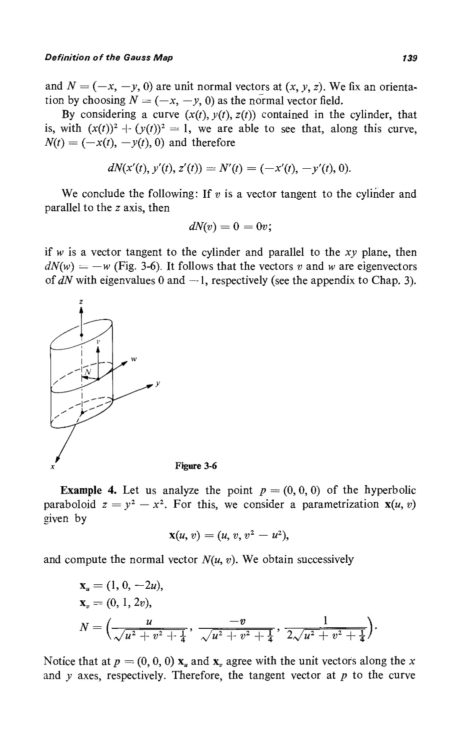
/


Text
pifferential Geometry
of
Curves and Surfaces
Manfredo P. do rmo
Instituto de Matematica Pura e Aplicada (IMP:4)
R;o de land"', Br.,U 1 V _1- C{1 Y1E.--
UP COLLEGE OF SCIENCE
. 11111 ililiilllllllll I lilil liilillll'''11 ilililililllill
UDSCB0013255
Prentice-Ha lnc., Englewood Cliffs, New Jersey
Carmo, Manfredo Perdigao do.
Differential geometry of curves and surfaces
"A free translation, with additional material, of a
book and a set of notes, both published originally in
Portuguese. "
Bibliography: p.
Includes index.
1. Geometry, Differential. 2. Curves. 3. Surfaces.
T. Title
QA641.C33
ISBN: 0-13-212589-7
75-22094
23149 1
Q
10'\ \
t 1
To Leny
@ 1976 -by Prentice-Hall, Inc.
Englewood Cliffs, New Jersey
All rights reserved. No part of this
book may be reproduced in any form,
or by any means, without permission
in writing from the publisher
Current printing:
10 9 8 7 6 5 4 3 2
Printed III the United States of America
Prentice-Hall International, Inc., London
Prentice-Hall of Australia pty., Limited, Sydney
Prentice-Hall of Canada, Ltd., Toronto
Prentice-Hall of India Private Ltd., New Delhi
Prentice-Hall of Japan, Inc., Tokyo
Prentice-Hall of Southeast Asia Private Limited, Singapore
Contents
Preface v
Some Remarks on Using this Book vii
1. Curves 1
I-I Introduction 1
1-2 Parametrized Curves 2
1-3 Regular Curves; Arc Length 5
1-4 The Vector Product in R3 11
1-5 The Local Theory of Curves Parametrized by Arc Length 16
1-6 The Local Canonical Form 27
1-7 Global Properties of Plane Curves 30
2. Regular Surfaces 51
2-1 Introduction 51
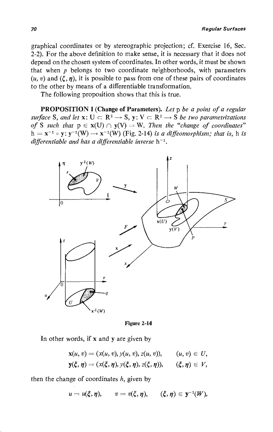
2-2 Regular Surfaces; Inverse Images of Regular Values 52
2-3 Change of Parameters; Differential Functions on Surfaces 69
2-4 The Tangent Plane; the Differential of a Map 83
2-5 The First Fundamental Form; Area 92
2-6 Orientation of Surfaces 102
2-7 A Characterizat;on of Compact Orientable Surfaces 109
2-8 A Geometric Definition of Area 114
Appendix: A Brief Review on Continuity
and Differentiability 118
iii
iv Contents
3. The Geometry of the Gauss Map 134
3-1 Introduction 134
3-2 The Definition of the Gauss Map and
Its Fundamental Properties 135
3-3 The Gauss Map in Local Coordinates 153
3-4 Vector Fields 175
3-5 Ruled Surfaces and Minimal Surfaces 188
Appendix: Self-Adjoint Linear Maps and Quadratic Forms 214
4. The Intrinsic Geometry of Surfaces 217
4-1 Introduction 217
4-2 Isometries; Conformal Maps 218
4-3 The Gauss Theorem and the Equations of Compatibility 231
4-4 Parallel Transport; Geodesics 238
4-5 The Gauss-Bonnet Theorem and its Applications 264
4-6 The Exponential Map. Geodesic Polar Coordinates 283
4-7 Further Properties of Geodesics. Convex Neighborhoods 298
Appendix: Proofs of the Fundamental Theorems of
The Local Theory of Curves and Surfaces 309
5. Global Differential Geometry 315
5-1 Introduction 315
5-2 The Rigidity of the Sphere 317
5-3 Complete Surfaces. Theorem of Hopf-Rinow 325
5-4 First and Second Variations of the Arc Length;
Bonnet's Theorem 339
5-5 Jacobi Fields and Conjugate Points 357
5-6 Covering Spaces; the Theorems of Hadamard 371
5-7 Global Theorems for Curves; the Fary-Milnor Theorem 380
5-8 . Surfaces of Zero Gaussian Curvature 408
5-9 Jacobi's Theorems 415
5-10 Abstract Surfaces; Further Generalizations 425
5-11 Hilbert's Theorem 446
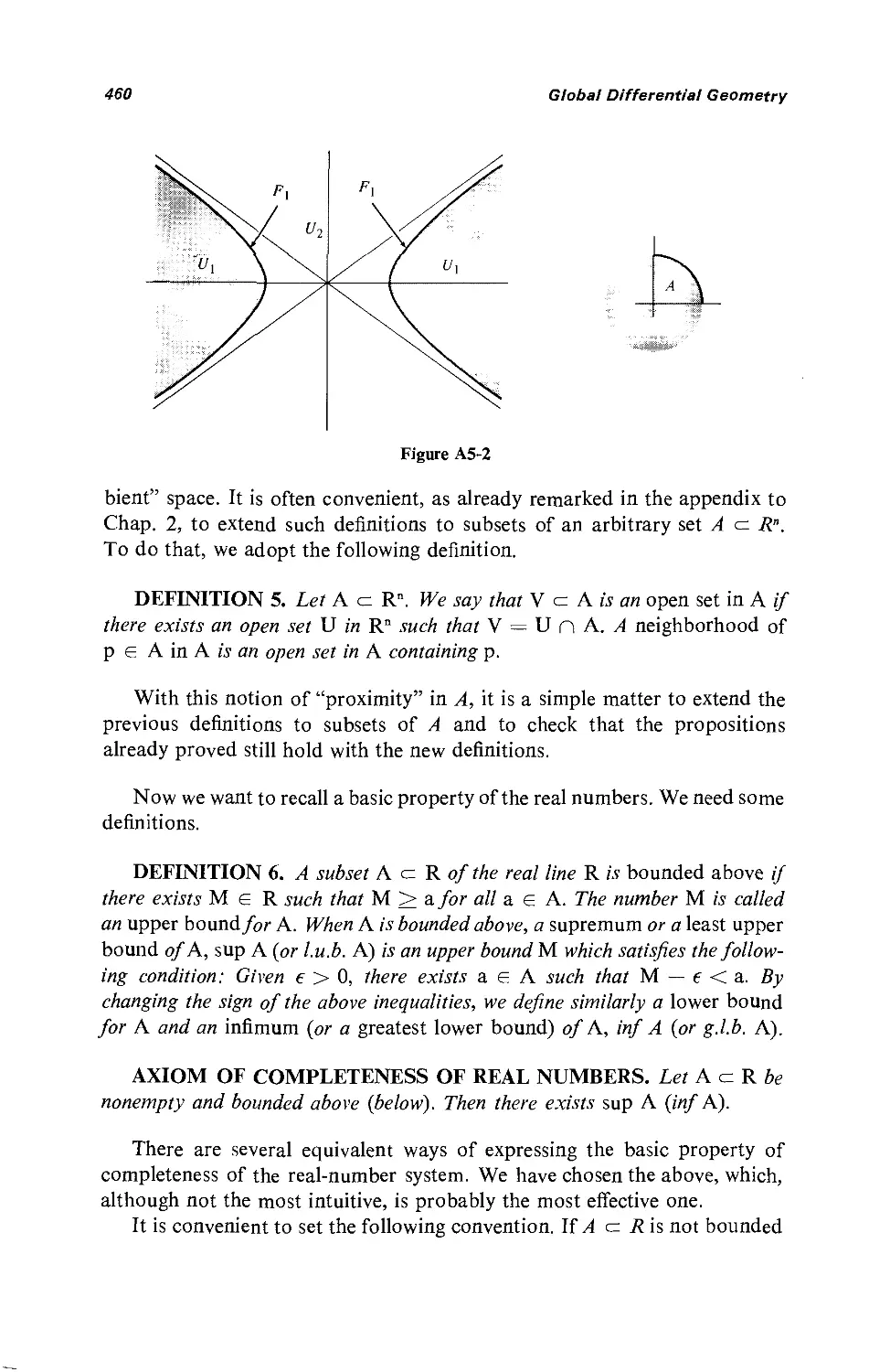
Appendix: Point-Set Topology of Euclidean Spaces 456
Bibliography and Comments 471
Hints and Answers to Some Exercises 475
Index 497
Preface
This book is an introduction to the differential geometry of curves and
surfaces, both in its local and global aspects. The presentation differs from
the traditional ones by a more extensive use of elementary linear algebra
and bya certain emphasis placed on bas.icgeometrical facts, rather than
on machinery or random details.
We have tried to build each chapter of the book around some simple
and fundamental idea. Thus, Chapter 2 develops around the concept of a
regular surface in R3; when this concept is properly developed, it is prob-
ably the best model for differentiable manifolds. Chapter 3 is built on the
Gauss normal map and contains a large amount of the local geometry of
surfaces in R3. Chapter 4 unifies the intrinsic geometry of surfaces around
the concept of covariant derivative; again, our purpose was to prepare the
reader for the basic notion of connection in Riemannian geometry. Finally,
in Chapter 5, we use the first and second variations of arc length to derive
some global properties of surfaces. Near the end of Chapter 5 (Sec. 5-10),
we show how questions on surface theory, and the experience of Chapters 2
and 4, lead naturally to the consideration of differentiable manifolds and
Riemannian metrics.
To maintain the proper balance between ideas and facts, we have
presented a large number of examples that are computed in detail. Further-
more, a reasonable supply of exercises is provided. Some factual material
of classical differential geometry found its place in these exercises. Hints or
answers are given for the exercises that are starred.
The prerequisites for reading this book are linear algebra and calculus.
From linear algebra, only the most basic concepts are needed, and a
v
vi
Preface
standard undergraduate course on the subject should suffice. From calculus,
a certain familiarity with calculus of several variables (including the state-
ment of the implicit function theorem) is expected. For the reader's con-
venience, we have tried to restrict our references to R. C. Buck, Advancd
Calculus, New York: McGraw-Hj]j, 1965 (quoted as Buck, Advanced
Calculus). A certain knowledge of differential equations will be useful but
it is not required.
This book is a free translation, with additional material, of a book and
a set of notes, both published originally in Portuguese. Were it not for the
enthusiasm and enormous help of Blaine Lawson, this book would not
have come into English. A large part of the translation was done by Leny
Cavalcante. I am also indebted to my colleagues and students at IMP A
for their comments and support. In particular, Elon Lima read part of the
Portuguese version and made valuable comments.
Robert Gardner, Jiirgen Kern, Blaine Lawson, and Nolan Wallach read
critically the English manuscript and helped me to avoid several mistakes,
both in English and Mathematics. Roy Ogawa prepared the computer pro-
grams for some beautiful drawings that appear in the book (Figs. 1-3, 1-8,
1-9,1-10,1-11,3-45 and 4-4). Jerry Kazdan devoted his time generously
and literally offered hundreds of suggestions for the improvement of the
manuscript. This final form of the book has benefited greatly from his
advice. To all these people-and to Arthur Wester, Editor of Mathematics
at Prentice-Hall, and Wilson Goes at IMPA-I extend my sincere thanks.
Rio de Janeiro
Manfredo P. do Carmo
Some Remarks on
Using This Book
We tried to prepare this book so it could be used in more than one type of
differential geometry course. Each chapter starts with an introduction that
describes the material in the chapter and explains how this material will be
used later in the book. For the reader's convenience, we have used footnotes
to point out the sections (or parts thereof) that can be omitted on a first
reading.
Although there is enough material in the book for a full-year course (or
a topics course), we tried to make the book suitable for a first course on
differential geometry for students with some background in linear algebra
and advanced calculus.
For a short one-quarter course (10 weeks), we suggest the use of the
following material: Chapter 1: Secs. 1-2, 1-3, 1-4, 1-5 and one topic of
Sec. 1-7-2 weeks. Chapter 2: Secs. 2-2 and 2-3 (omit the proofs), Secs.
2-4 and 2-5-3 weeks. Chapter 3: Secs. 3-2 and 3-3-2 weeks. Chapter 4:
Secs. 4-2 (omit conformal maps and Exercises 4, 13-18, 20), 4-3 (up to
Gauss theorem a egregium), 4-4 (up to Prop. 4; omit Exercises 12, 13, 16,
18-21), 4-5 (up to the local Gauss-Bonnet theorem; include applications
(b) and (f) )-3 weeks.
The lO-week program above is on a pretty tight schedule. A more re-
laxed alternative is to allow more time for the first three chapters and to
present survey lectures, on the last week of the course, on geodesics, the
Gauss theorema egregium, and the Gauss-Bonnet theorem (geodesics can
then be defined as curves whose osculating planes contain the normals to
the surface).
In a one-semester course, the first alternative could be taught more
vii
viii
some Remarks on Using this Book
leisurely and the instructor could probably include additional material (for
instance, Secs. 5-2 and 5-10 (partially), orSecs. 4-6, 5-3 and 5-4).
Please also note that an asterisk attached to an exercise does not mean
the exercise is either easy or hard. It only means that a solution or hint is
provided at the end of the book. Second, we have used for parametrization
a bold-faced x and that might become clumsy when writing on the black-
board. Thus we have reserved the capital X as a suggested replacement.
Where letter symbols that would normally be italic appear in italic con-
text, the letter symbols are set in roman. This has been done to distinguish
these symbols from the surrounding text.
1 Curves
1-1. Introduction
The differential geometry of curves and surfaces has two aspects. One, which
may be called classical differential geometry, started with the beginnings of
calculus. Roughly speaking, classical differential geometry is the study of
local properties of curves and surfaces. By local properties we mean those
properties which depend only on the behavior of the curve or surface in the.
neighborhood of a point. The methods which have shown themselves to be
adequate in the study of such properties are the methods of differential
calculus. Because of this, the curves and surfaces considered in differential
geometry will be defined by functions which can be differentiated a certain
number of times.
The other aspect is the so-called global differential geometry. Here one
studies the influence of the local properties on the behavior of the entire
curve or surface. We shall come back to this aspect of differential geometry
later in the book.
Perhaps the most interesting and representative part of classical differen-
tial geometry is the study of surfaces. However, some local properties of
curves appear naturally while studying surfaces. We shall therefore use this
first chapter for a brief treatment of curves.
The chapter has been organized in such a way that a reader interested
mostly in surfaces can read only Secs. 1-2 through 1-5. Sections 1-2 through
1-4 contain essentially introductory material (parametrized curves, arc
length, vector product), which will probably be known from other courses
and is included here for completeness. Section 1-5 is the heart of the chapter
1
2
Curves
and contains the material of curves needed for the study of surfaces. For
those wishing to go a bit further on the subject of curves, we have included
Secs. 1-6 and 1-7.
1-2. Parametrized Curves
We denote by R3 the set of triples (x, y, z) of real numbers. Our goal is to
characterize certain subsets of R3 (to be called curves) that are, in a certain
sense, one-dimensional and to which the methods of differential calculus
can be applied. A natural way of defining such subsets is through differenti-
able functions. We say that a real function of a real variable is differentiable
(or smooth) ifit has, at all points, derivatives of all orders (which are automa-
tically continuous). A first definition of curve, not entirely satisfactory but
sufficient for the purposes of this chapter, is the following.
DEFINITION. A parametrized differentiable curve is a differentiable
map (J,: I ---> R 3 of an open interval I = (a, b) of the real line R into R 3 .t
The word differentiable in this definition means that (J, is a correspondence
which maps each tEl into a point (J,(t) = (x(t), yet), z(t)) E R3 in such a
way that the functions x(t), yet), z(t) are differentiable. The variable t is called
the parameter of the curve. The word interval is taken in a generalized sense,
so that we do not exclude the cases a = -00, b = +00.
If we denote by x'(t) the first derivative of x at the point t and use similar
notations for the functions y and z, the vector (x'(t), y'(t), z'(t)) = (J,'(t) E R3
is called the tangent vector (or velocity vector) of the curve (J, at t. The image
set (J,(I) c R3 is called the trace of (J,. As illustrated by Example 5 below, one
should carefully distinguish a parametrized curve, which is a map, from its
trace, which is a subset of R3.
A warning about terminology. Many people use the term "infinitely
differentiable" for functions which have derivatives of all orders and reserve
the word "differentiable" to mean that only the existence of the first deriva-
tive is required. We shall not follow this usage.
Example 1. The parametrized differentiable curve given by
(J,(t) = (a cos t, a sin t, bt),
t E R,
has as its trace in R3 a helix of pitch 2nb on the cylinder x 2 + y2 = a 2 . The
parameter t here measures the angle which the x axis makes with the line
joining the origin 0 to the projection of the point (J,(t) over the xy plane (see
Fig. 1-1).
t In italic context, letter symbols will not be italicized so they will be clearly distin-
guished from the surrounding text.
Parametrized Curves
3
y
o
x
Figure 1-1
Figure 1-2
Example 2. The map rt,: R --> R2 given by rt,(t) = (t 3 , t 2 ), t E R, is a
parametrized differentiable curve which has Fig. 1-2 as its trace. Notice that
rt,'(0) = (0, 0); that is, the velocity vector is zero for t = O.
Example 3. The map rt,: R --> R2 given by rt,(t) = (t 3 - 4t, t 2 - 4),
t E R, is a parametrized differentiable curve (see Fig. 1-3). Notice that
rt,(2) = rt,( - 2) = (0, 0); that is, the map rt, is not one-to-one.
y
x
y
o
x
Figure 1-3
Figure 1-4
Example 4. The map rt,: R --> R2 given by rt,(t) = (t, I t I), t E R, is not a
parametrized differentiable curve, since I t I is not differentiable at t = 0
(Fig. 1-4).
Example 5. The two distinct parametrized curves
rt,(t) = (cos t, sin t),
pet) = (cos 2t, sin 2t),
4
Curves
where t E (0 - f, 2n + f), f > 0, have the same trace, namely, the circle
x 2 + y2 = 1. Notice that the velocity vector of the second curve is the
double of the first one (Fig. 1-5).
y
Figure 1-5
We shall now recall briefly some properties of the inner (or dot) product
of vectors in R3. Let U = (u I' U 2' U 3) E R3 and define its norm (or length) by
I u I = u1 + u + u .
Geometrically, I u I is the distance from the point (u l , u 2 , u 3 ) to the origin
o = (0, 0, 0). Now, let u = (u I , u 2 , u 3 ) and v = (VI' v 2 , V3) belong to R3, and
let e, 0 < e < n, be the angle formed by the segments Ou and Ov. The inner
product u. V is defined by (Fig. 1-6)
u. v = I u II v I cos e.
U3
o "3 Vl / =t: /'
I /' ul
v2 --1/
u2
.. y
x
The following properties hold:
Figure 1-6
1. Assume that u and v are nonzero vectors. Then u. v = 0 if and
only if u is orthogonal to v.
Regular Curves: Arc Length
5
2. u.v = v.u.
3. l(u.v) = lu.v = u.lv.
4. u.(v + w) = u.v + u.w.
A useful expression for the inner product can be obtained as follows.
Let e l = (I, 0, 0), e 2 = (0, 1,0), and e 3 = (0, 0, I). It is easily checked that
ei.e j = 1 jf i = j and that ei.e j = ° if i"* j, where i,j = 1,2,3. Thus, by
writing
u = ule l + u 2 e 2 + u 3 e 3 ,
v = vle l + V2e2 + v 3 e 3 ,
and using properties 3 and 4, we obtain
u.v = UIV I + U 2 V 2 + U3V3'
From the above expression it follows that if u(t) and vet), tEl, are
differentiable curves, then u(t). vet) is a differentiable function, and
; (u(t).v(t)) = u'(t).v(t) + u(t).v'(t).
EXERCISES
1. Find a parametrized curve lX(t) whose trace is the circle x 2 + y2 = 1 such that
lX(t) runs clockwise around the circle with IX(O) = (0, 1).
2. Let 1X(t) be a parametrized curve which does not pass through the origin. If lX(t o )
is the point of the trace of IX closest to the origin and 1X'(t0) =I=- 0, show that the
position vector lX(t 0) is orthogonal to 1X'(t 0)'
3. A parametrized curve lX(t) has the property that its second derivative 1X"(t) is
identically zero. What can be said about IX ?
4. Let IX: 1---4 R3 be a parametrized curve and let v E R3 be a fixed vector. Assume
that 1X'(t) is orthogonal to v for all tEl and that IX(O) is also orthogonal to v.
Prove that lX(t) is orthogonal to v for all tEl.
5. Let IX: 1---4 R3 be a parametrized curve, with 1X'(t) =I=- 0 for all tEl. Show that
JIX(t) I is a nonzero constant if and only if lX(t) is orthogonal to 1X'(t) for all tEl.
1-3. Regular Curves; Arc Length
Let IX: 1---4 R3 be a parametrized differentiable curve. For each tEl where
1X'(t) "* 0, there is a well-defined straight line, which contains the point lX(t)
and the vector 1X'(t). This line is called the tangent line to IX at t. For the study
6
Curves
of the differential geometry of a curve it is essential that there exists such a
tangent line at every point. Therefore, we call any point t where 1X'tt) = 0
a singular point of IX and restrict our attention to curves without singular
points. Notice that the point t = 0 in Example 2 of Sec. 1-2 is a singular
point.
DEFINITION. A parametrized differentiable curve IX: 1---4 R 3 is said to
be regular if 1X'(t) =1= 0 for all tEl.
From now on we shall consider only regular parametrized differentiable
curves (and, for convenience, shall usually omit the word differentiable).
Given tEl, the arc length of a regular parametrized curve IX: I ---4 R3,
from the point to, is by definition
set) = s:. \ 1X'(t) I dt,
where
11X'(t) I = ,J(x'(t»)2 + (y'(t»2 + (Z'(t»2
is the length of the vector 1X'(t). Since 1X'(t) =1= 0, the arc. length s is a differen-
tiable function of t and dsjdt = 11X'(t) I.
In Exercise 8 we shall present a geometric justification for the above
definition of arc length.
It can happen that the parameter t is already the arc length measured from
some point. In this case, dsjdt = 1 = IIX'(t) I; that is, the velocity vector has
constant length equal to 1. Conversely, if 11X'(t) 1 = 1, then
s = f dt = t - to;
to
i.e., t is the arc length of IX measured from some point.
To simplify our exposition, we shall restrict ourselves to curves para-
metrized by arc length; we shall see later (see Sec. 1-5) that this restriction is
not essential. In general, it is not necessary to mention the origin of the arc
length s, since most concepts are defined only in terms of the derivatives of
IX(S ).
It is convenient to set still another convention. Given the curve IX para-
metrized by arc length s E (a, b), we may consider the curve P defined in
(-b, -a) by P( -s) = IX(S), which has the same trace as the first one but is
described in the opposite direction. We say, then, that these two curves
differ by a change of orientation.
Regular Curves; Arc Length
7
EXERCISES
1. Show that the tangent lines to the regular parametrized curve lX(t) = (3t, 2t 2 ,
2t 3 ) make a constant angle with the line y = 0, z = x.
2. A circular disk of radius 1 in the plane xy rolls without slipping along the x
axis. The figure described by a point of the circumference of the disk is called a
cycloid (Fig. 1-7).
y
x
Figure 1-7. The cycloid.
*a. Obtain a parametrized curve IX: R ---4 R2 the trace of which is the cycloid,
and determine its singular points.
b. Compute the arc length of the cycloid corresponding to a complete rotation
of the disk.
3. Let OA = 2a be the diameter of a circle 8 1 and 0 Yand A V be the tangents to 8 1
at 0 and A, respectively. A half-line r is drawn from 0 which meets the circle 8 1
at C and the line A Vat B. On OB mark off the segment Op = CB. If we rotate r
about 0, the point p will describe a curve called the cissoid of Diocles. By taking
OA as the x axis and 0 Y as the y axis, prove that
a. The trace of
( 2at2 2at 3 )
lX(t) = 1 + t2 ' 1 + t 2 '
is the cissoid of Diocles (t = tan (); see Fig. 1-8).
b. The origin (0, 0) is a singular point of the cissoid.
c. As t ---4 00, lX(t) approaches the line x = 2a, and 1X'(t) ---4 (2a, 0). Thus, as
t ---4 co, the curve and its tangent approach the line x = 2a; we say that
x = 2a is an asymptote to the cissoid.
t E R,
4. Let IX: (0, n) ---4 R2 be given by
lX(t) = (cos t, cos t + log tan ),
where t is the angle that the y axis makes with the vector lX(t). The trace of IX is
called the tractrix (Fig. 1-9). Show that
8
Curves
y
y
x
x
Figure 1-8. The cissoid of Diocles.
Figure 1-9. The tractrix.
a. rt, is a differentiable parametrized curve, regular except at t = n12.
b. The length of the segment of the tangent of the tractrix between the point of
tangency and the y axis is constantly equal to 1.
5. Let rt,: (-1, +co) --> R2 be given by
( 3at 3at 2 ) .
rt,(t) = 1 + t3 ' 1 + t 3
Prove that:
a. For t = 0, rt, is tangent to the x axis.
b. As t --> + co, rt,(t) --> (0, 0) and rt,'(t) --> (0, 0).
c. Take the curve with the opposite orientation. Now, as t --> -1, the curve
and its tangent approach the line x + y + a = O.
The figure obtained by completing the trace of rt, in such a way that it
becomes symmetric relative to the line y = x is called the folium of Descartes
(see Fig. 1-10).
6. Let 0:(1) = (ae bt cos t, ae bt sin t), t E R, a and b constants, a> 0, b < 0, be a
parametrized curve.
Regular Curves; Arc Length
9
x
Figure 1-10. Folium of Descartes.
a. Show that as t ---> +=, lX(t) approaches the origin 0, spiraling around it
(because of this, the trace of IX is called the logarithmic spiral; see Fig. 1-11).
b. Show that 1X'(t) ---> (0, 0) as t ---> +00 and that
, oo S:. [1X'(t) I dt
is finite; that is, IX has finite arc length in [to, 00).
y
x
Figure 1-11. Logarithmic spiral.
10
Curves
7. A map a: [ ---> R3 is called a curve of class Ck if each of the coordinate func-
tions in the expression aCt) = (x(t), yet), z(t) has continuous derivatives up to
order k. If a is merely continuous, we say that a is of class Co. A curve a is
called simple if the map a is one-to-one. Thus, the curve in Example 3 of Sec. 1-2
is not simple.
Let a: [---> R3 be a simple curve of class Co. We say that a has a weak
tangent at t = to E [if the line determined bya(to + h) and aCto) has a limit
position when h ---> O. We say that a has a strong tangent at t = to if the line
determined by aCto + h) and a(to + k) has a limit position when h, k ---> O.
Show that
a. aCt) = (t 3 , t 2 ), t E R, has a weak tangent but not a strong tangent at t = O.
*b. If a: [ ---> R3 is of class C 1 and regular at t = to, then it has a strong tangent
at t = to.
c. The curve given by
{ (t2, t2),
aCt) =
(t 2 , -t 2 ),
t > O,
t ::;; 0,
is of class C 1 but not of class C 2. Draw a sketch of the curve and its tangent
vectors.
*8. Let a: [ ---> R3 be a differentiable curve and let [a, b] c [be a closed interval.
For every partition
a = to < t l < .,. < t n = b
of [a, b], consider the sum L7 1 I a(t,) - a(tH) I = {(a, P), where P stands
for the given partition. The norm I P [ of a partition P is defined as
I P I = max(t; - t;-l), i = 1, . . . , n.
Geometrically, lea, P) is the length of a polygon inscribed in a([a, b]) with
vertices in a(t,.) (see Fig. 1-12). The point of the exercise is to show that the arc
length of a([a, b]) is, in some sense, a limit of lengths of inscribed polygons.
a(t,)
a(tn)
Figure 1-12
The Vector Product in R3
11
Prove that given f > 0 there exists t5 > 0 such that if [ P [ < t5 then
\ S>X'(t) \ dt - I(IX, P) I < f.
9. a. Let IX: 1--7 R3 be a curve of class Co (cf. Exercise 7). Use the approximation
by polygons described in Exercise 8 to give a reasonable definition of arc
length of IX.
b. (A Nonrectifiable Curve.) The following example shows that, with any reason-
able definition, the arc length of a Co curve in a closed interval may be un-
bounded. Let IX: [0, 1] --7 R2 be given as IX(!) = (t, t sin(n/t)) if t *- 0, and
a:(0) = (0, 0). Show, geometrically, that the arc length of the portion of the
curve corresponding to I/(n + 1) ::;; t < l/n is at least 2/(n + -i} Use this to
show that the length of the curve in the intervall/N::;; t::;; 1 is greater than
2 L;; I I/(n + 1), and thus it tends to infinity as N --7 co.
l{}. (Straight Lines as Shartest.) Let 0:: I --'> R3 be '" param triz d \.:urv . L t {a, b)
c I and set a:(a) = p, a:(b) = q.
a. Show that, for any constant vector v, I v I = 1,
(q-p).v= f:a:'(t).vdt::;;S:Ia:'(t)ldt.
b. Set
q-p
v= [q_pl
and show that
I IX(b) - a:(a) \ < f: I a:'(t) \ dt;
that is, the curve of shortest length from a:(a) to a:(b) is the straight line join-
ing these points.
1-4. The Vector Product in R3
In this section, we shall present some properties of the vector product in R3.
They will be found useful in our later study of curves and surfaces.
It is convenient to begin by reviewing the notion of orientation of a vector
space. Two ordered bases e = {eJ andf = {J,}, i = 1, . . . ,n, of an n-dimen-
sional vector space V have the same orientation if the matrix of change of
basis has positive determinant. We denote this relation by e f From ele-
mentary properties of determinants, it follows that e f is an equivalence
relation; i.e., it satisfies
1. e '" e.
2. If e f, thenf e.
3. If e f,f g, then e g.
12
Curves
The set of all ordered bases of V is thus decomposed into equivalence classes
(the elements of a given class are related by ) which by property' 3 are
disjoint. Since the determinant of a change of basis is either positive or
negative, there are only two such classes.
Each of the equivalence classes determined by the above relation is called
an orientation of V. Therefore, V has two orientations, and if we fix one of
them arbitrarily, the other one is called the opposite orientation.
In the case V = R3, there exists a natural ordered basis e I = (I, 0, 0),
e z = (0, 1,0), e 3 = (0, 0, 1), and we shall call the orientation corresponding
to this basis the positive orientation of R3, the other one being the negative
orientation (of course, this applies equally well to any Rn). We also say that a
given ordered basis of R3 is positive (or negative) if it belongs to the positive
(or negative) orientation of R3. Thus, the ordered basis e I' e 3 , e z is a negative
basis, since the matrix which changes this basis into e l , e z , e 3 has determinant
equal to -1.
We now come to the vector product. Let u, v E R3. The vector product
of u and v (in that order) is the unique vector u ;\ v E R3 characterized by
(u ;\ v). w = dettu, v, w)
for all w E R3.
Here det(u, v, w) means that if we express u, v, and w in the natural basis {e,},
U = L: U; e;, v = L: v. e.
, "
w=L:we i=I,2,3,
, "
then
U 1 U z U 3
det(u, v, w) = VI Vz V 3 ,
WI W z W 3
where I au I denotes the determinant of the matrix (a;j). It is immediate from
the definition that
l u z U3 !el _j ul
u;\v=
V z V 3 VI
u 3 ! I UI
e z +
V 3 VI
u z !
e 3 .
Vz
(1)
Remark. It is also very frequent to write u ;\ v as u X v and refer to it 'as
the cross product.
The following properties can easily be checked (actually they just express
the usual properties of determinants):
1. u ;\ v = -v ;\ u (anticommutativity).
2. u ;\ v depends linearly on u and v; i.e., for any real numbers a, b,
we have
The Vector Product in R3
13
(au + bw) 1\ v = au 1\ v + bw 1\ v.
3. u 1\ v = 0 if and only if u and v are linearly dependent.
4.- (u 1\ v).u = 0, (u 1\ v).v = o.
It follows from property 4 that the vector product u 1\ v"* 0 is normal to
a plane generated by u and v. To give a geometric interpretation of its norm
and its direction, we proceed as follows.
First, we observe that (u 1\ v).(u 1\ v) = lu 1\ vi 2 > O. This means that
the determinant of the vectors u, v, u 1\ v is positive; that is, {u, v, u 1\ v} is a
positive basis.
Next, we prove the relation
j u.X v.x l,
(u 1\ v).(x 1\ y) =
u.y v.y
where ll, v, X, yare arbitrary vectors. This can easily be done by observing
that both sides are linear in u, v, x, y. Thus, it suffices to check that
j ej.e k ej.ek j
(e j 1\ eJ.(e k 1\ e/) =
ei.ef ej.e f
for all i,j, k, I = 1,2,3. This is a straightforward verification.
It follows that
i u.u u.V (
lu 1\ vl 2 = = lul 2 lvl 2 (1 - cos 2 0) = A2,
u.v v.v
where 0 is the angle of u and v, and A is the area of a parallelogram generated
by u and v.
In short, the vector product of u and v is a vector u 1\ v perpendicular to
a plane generated by u and v, with a norm equal to the area of a parallelogram
generated by u and v and a direction such that {u, v, u 1\ v} is a positive basis
(Fig. I-B).
1/1\ v
Figure 1-13
14
Curves
The vector product is not associative. In fact, we have the following
identity:
(u 1\ v) 1\ w = (u.w)v - (v.w)u,
(2)
which can be proved as follows. First we observe that both sides are linear
in 1I, v, w; thus, the identity will be true if it holds for all basis vectors. This
last verification is, however, straightforward; for instance,
(e l 1\ e z ) 1\ e l = e z = (e l .el)e z - (e z .el)e l .
Finally, let u(t) = (ul(t), uz(t), u 3 (t)) and vet) = (vl(t), vz(t), v 3 (t)) be
differentiable maps from the interval (a, b) to R3, t EO (a, b). It follows im-
mediately from Eq. (1) that u(t) 1\ vet) is also differentiable and that
(u(t) 1\ vet)) = 1\ vCt) + u(t) 1\ .
Vector products appear naturally in many geometrical constructions.
Actually, most of the geometry of planes and lines in R3 can be neatly ex-
pressed in terms of vector products and determinants. We shall review some
of this material in the following exercises.
EXERCISES
1. Check whether the following bases are positive:
a. The basis r(l, 3), (4, 2)} in RZ.
b. The basis r(l, 3, 5), (2,3,7), (4, 8, 3)} in R3.
*2. A plane P contained in R3 is given by the equation ax + by + cz + d = O.
Show that the vec tor v = (a, b, c) is perpendicular to the plane and that
[d I/ a Z + b Z + C Z measures the distance from the plane to the origin (0, 0, 0).
*3. Determine the angle of intersection of the two planes 5x + 3y + 2z - 4 = 0
and 3x + 4y - 7z = O.
*4. Given two planes aix + biy + ciz + d i = 0, i = 1, 2, prove that a necessary
and sufficient condition for them to be parallel is
al b l CI
- - - - -,
Oz - b z - Cz
where the convention is made that if a denominator is zero, the corresponding
numerator is also zero (we say that two planes are parallel if they either coin-
cide or do not intersect).
5. Show that the equation of a plane passing through three noncolinear points
PI = (XI, Yb ZI), pz = (xz, yz, zz), P3 = (X3, Y3, Z3) is given by
The Vector Product in R3
75
(p PI) !\ (p - pz)-(p P3) = 0,
where p = (x, y, z) is an arbitrary point of the p]ane and p - Ph for instance,
means the vector (x Xb Y - Yb Z - ZI).
*6. Given two nonparallel planes aix + biy + CiZ + d i = 0, i = 1,2, show that
their line of intersection may be parametrized as
x - Xo = Ult,
Y - Yo = uzt,
Z - Zo = U3t,
where (xo, Yo, zo) belongs to the intersection and U = (Ub liz, 1I3) is the vector
product 1I = VI !\ Vz, Vi = (ai, bi, Ci), i = 1,2.
*7. Prove that a necessary and sufficient condition for the plane
ax + by + cz + d= 0
and the line x - Xo = lilt, Y - Yo = lIzt, Z - Zo = 1I3t to be parallel is
aliI + bll z + C1I3 = O.
*8. Prove that the distance p between the nonparallel lines
x - Xo = lilt,
Y - Yo = lIzt,
Y - YI = vzt,
Z - Zo = 1I3t,
x - XI = vlt,
Z - ZI = v3t
is given by
l(lI!\v).rl
p= 11I!\v[ ,
where 1I = (lib liz, 1I3), V = (Vb Vz, V3), r = (Xo - Xb Yo - Yb Zo - ZI)'
9. Determine the angle of intersection of the plane 3x + 4y + 7z + 8 = 0 and
the line x - 2 = 3t, Y - 3 = 5t, Z - 5 = 9t.
10. The natural orientation of RZ makes it possible to associate a sign to the area A
ofa paraJIelogram generated by two linearly independent vectors u, V E RZ. To
do this, let {eJ, i = 1,2, be the natural ordered basis of RZ, and write
U = 1I1el + uzez, V = Vlel + vzez. Observe the matrix relation
( U'U u'V ) = ( III
V'U V'V VI
lIZ )( 1I1 VI )
Vz Uz Vz
and conclude that
AZ= ! UI uz j z.
VI Vz
Since the ]ast determinant has the same sign as the basis [1I, v}, we can say that A
is positive or negative according to whether the orientation of {1I, v} is positive
or negative. This is called the oriented area in RZ.
76
Curves
11. a. Show that the volume V of a parallelepiped generated by three linearly inde-
pendent vectors u, v, W E R3 is given by V = I( u !\ v). w I, and introduce an
oriented volume in R3.
b. Prove that
u.u u.v u'w
vz = v.u v.v v.w.
w.u w.v w.w
12. Given the vectors v -=I=- 0 and w, show that there exists a vector u such that
u !\ v = w if and only if v is perpendicular to w. Is this vector u uniquely deter-
mined? If not, what is the most general solution?
13. Let u(t) = (Ui(t), uz(t), U3(t)) and vet) = (Vi(t), vz(t), V3(t)) be differentiable
maps from the interval (a, b) into R3. If the derivatives u'(t) and v'(t) satisfy the
conditions
u'(t) = au(t) + bv(t),
v'(t) = cu(t) - av(t),
where a, b, and c are constants, show that u(t) !\ vet) is a COnstant vector.
14. Find all unit vectors which are perpendicular to the vector (2, 2, 1) and parallel
to the plane determined by the points (0, 0, 0), (1, -2,1), (-1,1,1).
1-5. The Local Theory of Curves
Parametrized by Arc Length
This section contains the main results of curves which will be used in the
later parts of the book.
Let a: J = (a, b) -----> R3 be a curve parametrized by arc length s. Since
the tangent vector OG'(s) has unit length, the norm I OG"(s) I of the second deriva-
tive measures the rate of change of the angle which neighboring tangents make
with the tangent at s. I OG"(s) I gives, therefore, a measure of how rapidly the
curve pulls away from the tangent line at s, in a neighborhood of s (see
Fig. 1-14). This suggests the following definition.
DEFINITION. Let a: I -----> R3 be a curve parametrized by arc length
s E I. The number I OG"(s) I = k(s) is called the curvature of OG at s.
If OG is a straight line, OG(s) = us + v, where u and v are constant vectors
(I u I = I), then k - O. Conversely, if k = I a"(s) 1 0, then by integration
OG(s) = us + v, and the curve is a straight line.
Notice that by a change of orientation, the tangent vector changes its
direction; that is, if p( -s) = OG(s), then
dp ( _ _ _dOG
d(-s) s) - ds (s).
Curves Parametrized by Arc Length
17
o:'(s)
a"(s)
Figure 1-14
Therefore, OG"(s) and the curvature remain invariant under a change of
orientation.
At points where k(s) "* 0, a unit vector n(s) in the direction OG"(s) is well
defined by the equation OG"(s) = k(s)n(s). Moreover, OG"(s) is normal to a'(s),
because by differentiating OG'(s).OG'(s) = I we obtain OG"(s).OG'(s) = O. Thus,
n(s) is normal to OG'(s) and is called the normal vector at s. The plane deter-
mined by the unit tangent and normal vectors, OG'(s) and n(s), is called the
osculating plane at s. (See Fig. 1-15.)
At points where k(s) = 0, the normal vector (and therefore the osculating
plane) is not defined (cf. Exercise 10). To proceed with the local analysis of
curves, we need, in an essential way, the osculating plane. It is therefore
Figure 1-15
18
Curves
convenient to say that s EO I is a singular point of order I if 1Xf/(s) = 0 (in this
context, the points where IX'(S) = 0 are called singular points of order 0).
In what follows, we shall restrict ourselves to curves parametrized by arc
length without singular points of order 1. We shall denote by t(s) = IX'(S)
the unit tangent vector of IX at s. Thus, t'(s) = k(s)n(s).
The unit vector b(s) = t(s) 1\ n(s) is normal to the osculating plane and
will be called the binormal vector at s. Since b(s) is a unit vector, the length
I b'(s) I measures the rate of change of the neighboring osculating planes with
the osculating plane at s; that is, b'(s) measures how rapidly the curve pulls
away from the osculating plane at s, in a neighborhood of s (see Fig. 1-15).
To compute b'(s) we observe that, on the one hand, b'(s) is normal to b(s)
and that, on the other hand,
b'(s) = t'(s) 1\ n(s) + t(s) 1\ n'(s) = t(s) 1\ n'(s);
that is, b'(s) is normal to t(s). It follows that b'(s) is parallel to n(s), and we
may write
b'(s) = T(s)n(s)
for some function T(S). (Warning: Many authors write -T(S) instead of our
r(s).)
DEFINITION. Let IX: I ---> R3 be a curve parametrized by arc length s
such that 1Xf/(s) * 0, S EO I. The number T(S) defined by b'(s) = T(s)n(s) is called
the torsion of IX at s.
If IX is a plane curve (that is, IX(I) is contained in a plane), then the plane
of the curve agrees with the osculating plane; hence, T - O. Conversely, if
T - 0 (and k * 0), we have that b(s) = b o = constant, and therefore
(lX(s).b o )' = 1X'(s).b o = O.
It follows that lX(s).b o = constant; hence, IX(S) is contained in a plane normal
to boo The condition that k * 0 everywhere is essential here. In Exercise 10
we shall give an example where T can be defined to be identically zero and
yet the curve is not a plane curve.
In contrast to the curvature, the torsion may be either positive or nega-
tive. The sign of the torsion has a geometric interpretation, to be given later
(Sec. 1-6).
Notice that by changing orientation the binormal vector changes sign,
since b = t 1\ n. It follows that b'(s), and, therefore, the torsion, remains
invariant under a change of orientation.
Curves Parametrized by Arc Length
19
Let us summarize our position. To each value of the parameter s, we have
associated three orthogonal unit vectors t(s), n(s), b(s). The trihedron thus
formed is referred to as the Frenet trihedron at s. The derivatives t'(s) = kn,
b'(s) = rn of the vectors t(s) and b(s), when expressed in the basis {t, n, b},
yield geometrical entities (curvature k and torsion r) which give us infor-
mation about the behavior of rx in a neighborhood of s.
The search for other local geometrical entities would lead us to compute
n'(s). However, since n = b 1\ t, we have
n'(s) = b'(s) 1\ t(s) + b(s) 1\ t'(s) = -rb - kt,
and we obtain again the curvature and the torsion.
For later use, we shall call the equations
t' =kn,
n' = -kt - rb,
b' = rn
the Frenetformulas (we have ommited the s, for convenience). In this context,
the following terminology is usual. The tb plane is called the rectifying plane,
and the nb plane the normal plane. The lines which contain n(s) and b(s) and
pass through rx(s) are called the principal normal and the binormal, respecti-
vely. The inverse R = Ilk of the curvature is called the radius of curvature at
s. Of course, a circle of radius r has radius of curvature equal to r, as one can
easily verify.
Physically, we can think of a curve in R3 as being obtained from a straight
line by bending (curvature) and twisting (torsion). After reflecting on this
construction, we are led to conjecture the following statement, which, roughly
speaking, shows that k and r describe completely the local behavior of the
curve.
FUNDAMENTAL THEOREM OF THE LOCAL THEORY OF
CURVES. Given differentiable functions k(s) > 0 and r(s), s E I, there
exists a regular parametrized curve rx: I ---> R3 such that s is the arc length, k(s)
is the curvature, and res) is the torsion of rx. Moreover, any other curve fi,
satisfying the same conditions, differs from rx by a rigid motion; that is, there
exists an orthogonal linear map p ofR 3 , with positive determinant, and a vector
c such that fi = porx + c.
The above statement is true. A complete proof involves the theorem of
existence and uniqueness of solutions of ordinary differential equations and
will be given in the appendix to Chap. 4. A proof of the uniqueness, up to
20
Curves
rigid motions, of curves having the same s, k(s), and res) is, however, simple
and can be given here.
Proof of the Uniqueness Part of the Fundamental Theorem. We first remark
that arc length, curvature, and torsion are invariant under rigid motions;
that means, for instance, that if M: R3 ---> R3 is a rigid motion and rx = rx(t)
is a parametrized curve, then
J: I I dt = J: I d( torx) I dt.
That is plausible, since these concepts are defined by using inner or vector
products of certain derivatives (the derivatives are invariant under transla-
tions, and the inner and vector products are expressed by means of lengths
and angles of vectors, and thus also invariant under rigid motions). A careful
checking can be left as an exercise (see Exercise 6).
Now, assume that two curves rx = rx(s) and ti = tiCs) satisfy the conditions
k(s) = k(s) and res) = res), s E I. Let to, no, b o and to, iio, b o be the Frenet tri-
hedrons at s = So E I of rx and ti, respectively. Clearly, there is a rigid motion
which takes fi(so) into rx(so) and to, iio, b o into to, no, boo Thus, after perform-
ing this rigid motion on fi, we have that fi(so) = rx(so) and that the Frenet
trihedrons t(s), n(s), b(s) and i(s), ii(s), b(s) of (j, and ti, respectively, satisfy
the Frenet equations:
dt = kn
ds
dn = -kt - rb
ds
db
ds = rn
di = kii
ds
dii k - -
- = - t - rn
ds
db -
ds = rn,
with t(s 0) = i(s 0)' n(s 0) = ii(s 0), b(s 0) = b(s 0)'
We now observe, by using the Frenet equations, that
1-!£{lt - fl2 + In - iil 2 + Ib - bn
2 ds
= <t - i, t' - i') + <b - b, b' - b') + <n - ii, n' - ii')
= k<t - i, n - ii) + r<b - b, n - ii) - k<n - ii, t - f)
- r<n - ii, b - b)
=0
for all s E I. Thus, the above expression is constant, and, since it is zero for
Curves Parametrized by Arc Length
27
s = So, it is identically zero. It follows that t(s) = res), n(s) = n(s), b(s) = b(s)
for all s E I. Since
d(1._ _ -_dfi
- - t - t - -,
ds ds
we obtain (djds) ((1. - fi) = O. Thus, (1.(s) = fi(s) + a, where a is a constant
vector. Since (1.(so) = fi(so), we have a = 0; hence, (1.(s) = fi(s) for all s E [.
Q.E.D.
Remark I. In the particular case of a plane curve (1.: I -> RZ, it is possible
to give the curvature k a sign. For that, let {e!, e z } be the natural basis (see
Sec. 1-4) of RZ and define the normal vector n(s), s E I, by requiring the basis
{t(s), n(s)} to have the same orientation as the basis {e!, e z }. The curvature k
is then defined by
dt
-=kn
ds
and might be either positive or negative. It is clear that I k I agrees with the
previous definition and that k changes sign when we change either the
orientation of (1. or the orientation of RZ (Fig. 1-16).
n
"L
ez
Figure 1-16
It should also be remarked that, in the case of plane curves (r = 0), the
proof of the fundamental theorem, refered to above, is actually very simple
(see Exercise 9).
Remark 2. Given a regular parametrized curve (1.: 1-> R3 (not neces
sarily parametrized by arc length), it is possible to obtain a curve p: J -> R3
parametrized by arc length which has the same trace as (1.. In fact, let
22
Curves
s = set) = I ' I ex'(t) I dt,
'0
t, to E I.
Since ds/dt = I ex'(t) 1"* 0, the function s = set) has a differentiable inverse
t = t(s}. s E sf!) = J; where; by an abuse of notation; t also denotes the
inverse function $-1 of S. Now set p = exot: J --> R3. Clearly, P(l) = ex(I)
and I P'(s) I = I ex'(t). (dt/ds) I = 1. This shows that P has the same trace as ex
and is parametrized by arc length. It is usual to say that P is a reparametriza-
lion of ex(I) by arc length.
This fact allows us to extend all local concepts previously defined to
regular curves with an arbitrary parameter. Thus, we say that the curvature
k(t) of ex: 1--> R3 at tEl is the curvature of a reparametrization p: J --> R..3
of ex(I) by arc length at the corresponding point s = set). This is clearly
independent of the choice of P and shows that the restriction, made at the
end of Sec. 1-3, of considering only curves parametrjzed by arc length is not
essential.
In applications, jt is often convenient to have explicit formulas for the
geometrical entities in terms of an arbitrary parameter; we shall present SOlbe
of them in Exercise 12.
EXERCISES
Unless explicity stated, ex: I --> R 3 is a curve parametrized by arc length s, With
curvature k(s) *- 0, for all s E I.
1. Given the parametrized curve (helix)
exes) = ( a cas ..£, a sin ..£, b..£ ) ,
c c c
S E R,
where c 2 = a 2 + b 2 ,
a. Show that the parameter s is the arc length.
b. Determine the curvature and the torsion of ex.
c. Determine the osculating plane of ex.
d. Show that the lines containing n(s) and passing through exes) meet the z a)(is
under a constant angle equal to n/2.
e. Show that the tangent lines to ex make a constant angle with the z axis.
*2. Show that the torsiop. 'r of ex is given by
ex'(s) !\ ex"(s).ex"'(s)
'res) = - Ik(s)12 .
3. Assume that ex(I) c R2 (i.e., ex is a plane curve) and give k a sign as in the te)(t.
Transport the Vectors t(s) parallel to themselves in such a way that the origins of
Curves Parametrized by Arc Length
23
t(s) agree with the origin of RZ; the end points of t(s) then describe a parame-
trized curve s ---> t(s) called the indicatrix of tangents of (j,. Let O(s) be the angle
from el to t(s) in the orientation of RZ. Provc (a) and (b) (notice that we are
assuming that k oF 0).
a. The indicatrix of tangents is a regular parametrized curve.
b. dt(ds = (dO(ds)n, that is, k = dO(ds.
*4. Assume that all normals of a parametrized curve pass through a fixed point.
Prove that the trace of the curve is contained in a circle.
5. A regular parametrized curve (j, has the property that all its tangent lines pass
through a fixed point.
a. Prove that the trace of (j, is a (segment of a) straight line.
b. Does the conclusion in part a still hold if (j, is not regular?
6. A translation by a vector v in R3 is the map A: R3 ---> R3 that is given by
A(p) = p + v, P E R3. A linear map p: R3 ----> R3 is an orthogonal transfor-
mation when pu. pv = u. v for all vectors u, v E R3. A rigid motion in R3 is the
result of composing a translation with an orthogonal transformation with posi-
tive determinant (this last condition is included because we expect rigid motions
to preserve orientation).
a. Demonstrate that the norm of a vector and the angle 0 between two vectors,
o < 0 < n, are invariant under orthogonal transformations with positive
determinant.
b. Show that the vector product of two vectors is invariant under orthogonal
transformations with positive determinant. Is the assertion stilI true if we
drop the co'ndition on the determinant?
c. Show that the arc length, the curvature, and the torsion of a parametrized
curve are (whenever defined) invariant under rigid motions.
*7. Let IX: 1---> RZ be a regular parametrized plane curve (arbitrary parameter), and
define n = net) and k = k(t) as in Remark 1. Assume that k(t) oF 0, t E I. In
this situation, the curve
I
ft(t) = (j,(t) + k(t) n(t),
tEl,
is called the evolute of (j, (Fig. 1-17).
a. Show that the tangent at t of the evolute of (j, is the normal to (j, at t.
b. Consider the normal lines of (j, at two neighboring points tb tz, t 1 oF t z . Let
t 1 approach t z and show that the intersection points of the normals converge
to a point on the trace of the evolute of (j,.
8. The trace of the parametrized curve (arbitrary parameter)
(j,(t) = (t, cosh t),
t E R,
is caIled the catenary.
Figure 1-17
a. Show that the signed curvature (cf. Remark 1) of the catenary is
I
k ( t ) --.
- cosh 2 t
b. Show that the evolute (cf. Exercise 7) of the catenary is
Pet) = (t - sinh t cosh t, 2 cosh t).
9. Given a differentiable function k(s), s E I, show that the parametrized plane
curve having k(s) = k as curvature is given by
exes) = (f cos O(s) ds + a, f sin O(s) ds + b),
where
O(s) = f k(s) ds + rp,
and that the curve is determined up to a translation of the vector (a, b) and a
rotation of the angle rp.
10. Consider the map
{ (t, 0, e- 1 / r '), t > 0
ex(t)= (t,e-1/r',0), t<O
(0, 0, 0), t = 0
a. Prove that ex is a differentiable curve.
b. Prove that ex is regular for all t and that the curvature k(t) *" 0, for t *" 0,
t *" ::!: ../ 2/3 , and k(O) = O.
Curves Parametrized by Arc Length
25
c. Show that the limit of the osculating planes as t --+ 0, t > 0, is the plane
y = 0 but that the limit of the osculating planes as t --+ 0, t < 0, is the plane
z = 0 (this implies that the normal vector is discontinuous at t = 0 and
shows why we excluded points where k = 0).
d. Show that 'r can be defined so that 'r == 0, even though rt is not a plane curve.
11. One often gives a plane curve in polar coordinates by p = p(()), a :<:::: () < b.
a. Show that the arc length is
s: -vi p2 + (p')2 d(),
where the prime denotes the derivative relative to ().
b. Show that the curvature is
2(p')2 - P p" + p2
k(()) = {(p')2 + p2}3/2 .
12. Let rt: 1--+ R3 be a regular parametrized curve (not necessarily by arc length)
and let p: J --+ R3 be a reparametrization of rt(I) by the arc length s = set),
measured from to E I (see Remark 2). Let t = t(s) be the inverse function of s
and set drt/dt = rt', d 2 rt/dt 2 = rt", etc. Prove that
a. dt/ds = 1/lrt'l, d 2 t/ds 2 = -(rt'4'/lrt'14).
b. The curvature of rt at tEl is
I rt' /\ rt" I
k(t) = 1 rt' 1 3 .
c. The torsion of rt at tEl is
(rt' /\ rt").rt'"
'r(t) = - 1 rt' /\ rt" 1 2 .
d. If rt: 1--+ R2 is a plane curve rt(t) = (x(t), yet)), the signed curvature (see
Remark 1) of rt at tis
x'y" - xllyl
k(t) = ((x')2 + (y')2)3/2
13. Assume that 'res) oF 0 and k'(s) oF 0 for all s E I. Show that a necessary and
sufficient condition for rt(l) to lie on a sphere is that
R2 + (R')2T2 = const.,
where R = l/k, T = I/'r, and R' is the derivative of R relative to s.
14. Let rt: (a, b) --+ R2 be a regular parametrized plane curve. Assume that there
exists to, a < to < b, such that the distance I rt(t) I from the origin to the trace of
26
Curves
rt will be a maximum at to. Prove that the curvature k of rt at to satisfies
I k(t 0) I > 1/1 rt(t 0)1.
*15. Show that the knowledge of the vector function b = b(s) (binormal vector) of a
curve rt, with nonzero torsion everywhere, determines the curvature k(s) and the
absolute value of the torsion 'res) of rt.
*16. Show that the knowledge of the vector function n = n(s) (normal vector) of a
curve rt, with nonzero torsion everywhere, determines the curvature k(s) and the
torsion 'res) of rt.
17. In general, a curve rt is called a helix if the tangent lines of rt make a constant
angle with a fixed direction. Assume that 'res) oF 0, s E I, and prove that:
*a. rt is a helix if and only if k/'r = const.
*b. rt is a helix if and only if the lines containing n(s) and passing through rt(s)
are parallel to a fixed plane.
*c. rt is a helix if and only if the lines containing b(s) and passing through rt(s)
make a constant angle with a fixed direction.
d. The curve
rt(s) = ( J sin O(s) ds, J cos O(s) ds, s ),
where a 2 = b 2 + c 2 , is a helix, and that k/'r = b/a.
*18. Let rt: 1---> R3 be a parametrized regular curve (not necessarily by arc length)
with k(t) oF 0, 'r(t) oF 0, tEl. The curve rt is called a Bertrand curve if there
exists a curve : I ---> R3 such that the normal lines of rt and at tEl are
equal. In this case, is called a Bertrand mate of rt, and we can write
(t) = rt(t) + met).
Prove that
a. r is constant.
b. rt is a Bertrand curve if and only if there exists a linear relation
Ak(t) + B'r(t) = 1,
tEl,
where A, B are nonzero constants and k and 'r are the curvature and torsion
of rt, respectively.
c. If rt has more than one Bertrand mate, it has infinitely many Bertrand mates.
This case occurs if and only if rt is a circular helix.
The Local Canonical Form
27
1-6. The Local Canonical Formt
One of the most effective methods of solving problems in geometry consists
of finding a coordinate system which is adapted to the problem. In the study
of local properties of a curve, in the neighborhood of the point s, we have a
natural coordinate system, namely the Frenet trihedron at s. It is therefore
convenient to refer the curve to this trihedron.
Let IX: I ---> R3 be a curve parametrized by arc length without singular
points of order 1. We shall write the equations of the curve, in a neighborhood
of So, using the trihedron t(so), n(so), b(so) as a basis for R3. We may assume,
without loss of generality, that So = 0, and We shall consider the (finite)
Taylor expansion
2 3
a.(s) = a.(0) + sa.'(O) + a."(0) + a.'''(O) + R,
where lim Rfs3 = 0. Since IX'(O) = t, IX"(O) = kl1, and
.-0
IXI/,(O) = (kn)' = k'n + kn' = k'n - k 2 t - k7:b,
we obtain
( k2S3 ) ( s2k S3k' ) S3
IX(S) -IX(O) = S - 3T t + 2 + 3T n - TIk7:b + R,
where all terms are computed at s = 0.
Let us now take the system Oxyz in such a way that the origin 0 agrees
with IX(O) and that t = (1, 0, 0), n = (0, 1,0), b = (0, 0, 1). Under these
conditions, IX(S) = (x(s), yes), z(s)) is given by
k 2 s 3
xes) = s - 6 + R""
k k'S3
yes) = T S2 + 6 + Ry,
z(s) = - 7: S3 + R"
(1)
where R = (Rx, Ry, RJ. The representation (1) is called the local canonical
form of IX, in a neighborhood of s = 0. In Fig. 1-18 is a rough sketch of the
projections of the trace of IX, for s small, in th tn, tb, and nb planes.
tThis section may be omitted on a first reading.
28
Curves
b
,
\
\
\
\
\
\
\
n
Projection over the plane tn
b
b
Projection over the plane t b
Projection over the plane n b
Figure 1-18
Below we shall describe some geometrical applications of the local can-
onical form. Further applications will be found in the Exercises.
A first application is the following interpretation of the sign of the torsion.
From the third equation of (1) it follows that if'l' < 0 and s is sufficiently
small, then z(s) increases with s. Let us make the convention of calling the
"positive side" of the osculating plane that side toward which b is pointing.
Then, since z(O) = 0, when we describe the curve in the direction of increasing
arc length, the curve will cross the osculating plane at s = 0, pointing toward
the positive side (see Fig. 1-19). If, on the contrary, 'l' > 0, the curve (described
in the direction of increasing arc length) will cross the osculating plane
pointing to the side opposite the positive side.
Negative torsion
Positive torsion
Figure 1-19
The Local Canonical Form
29
The helix of Exercise 1 of Sec. 1-5 has negative torsion. An example of a
curve with positive torsion is the helix
rt ( s ) = ( a cos a sin -b )
c' c' c
obtained from the first one by a reflection in the xz plane (see Fig. 1-19).
Remark. It is also usual to define torsion by b ' = -'m. With such a
definition, the torsion of the helix of Exercise 1 becomes positive.
Another consequence of the canonical form is the existence of a neighbor-
hood J c I of s = 0 such that rt(J) is entirely contained in the one side of the
rectifying plane toward which the vector n is pointing (see Fig. 1-18). In fact,
since k > 0, we obtain, for s sufficiently small, y(s) > 0, and y(s) = 0 if and
only if s = O. This proves our claim.
As a last application of the canonical form, we mention the following
property of the osculating plane. The osculating plane at s is the limit position
of the plane determined by the tangent line at s and the point rt(s + h) when
h O. To prove this, let us assume that s = O. Thus, every plane containing
the tangent at s = 0 is of the form z = cy or y = O. The plane y = 0 is the
rectifying plane that, as seen above, contains no points near rt(O) (except
rt(O) itself) and that may therefore be discarded from our considerations. The
condition for the plane z = cy to pass through s + h is (s = 0)
_ 7:h3 + ...
c = z(h) _ 6
y(h) - .!5.... h 2 + k 2 h 3 + . . .
2 6
Letting h 0, We see that c O. Therefore, the limit position of the plane
z(s) = c(h)y(s) is the plane z = 0, that is, the osculating plane, as we wished.
EXERCISES
*1. Let rt: I R3 be a curve parametrized by arc length with curvature k(s) *- 0,
S E I. Let P be a plane satisfying both of the following conditions:
1. P contains the tangent line at s.
2. Given any neighborhood J c I of s, there exist points of rt(J) in both
sides of P.
Prove that P is the osculating plane of rt at s.
2. Let rt: I R3 be a curve parametrized by arc length, with curvature k(s) *- 0,
S E I. Show that
30
Curves
*a. The osculating plane at s is the limit position of the plane passing through
exes), ex(s + hI)' ex(s + h 2 ) when hI, h 2 --+ O.
b. The limit position of the circle passing through exes), ex(s + hI)' ex(s + h 2 )
when hI> h 2 --+ 0 is a circle in the osculating plane at s, the center of which is
on the line that contains n(s) and the radius of which is the radius of curvature
l(k(s); this circle is called the osculating circle at s.
3. Show that the curvature k(t) * 0 of a regular parametrized curve ex: 1--+ R3 is
the curvature at t of the plane curve noex, where n is the normal projection of ex
over the osculating plane at t.
1-7. Global Properties of Plane Curvest
In this section we want to describe some results that belong to the global
differential geometry of curves. Even in the simple case of plane curves, the
subject already offers examples of nontrivial theorems and interesting
questions. To develop this material here, we must assume some plausible
facts without proofs; we shall try to be careful by stating these facts precisely.
Although we want to come back later, in a more systematic way, to global
differential geometry (Chap. 5), we believe that this early presentation of the
subject is both stimulating and instructive.
This section contains three topics in order of increasing difficulty: (A)
the isoperimetric inequality, (B) the four-vertex theorem, and (C) the Cauchy-
Crofton formula. The topics are entirely independent, and some or all of
them can be omitted on a first reading.
A differentiable function on a closed interval [a, b] is the restriction of a
differentiable function defined on an open interval containing [a, b].
A closed plane curve is a regular parametrized curve ex: [a, b] --+ R2 such
that ex and all its derivatives agree at a and b; that is,
ex(a) = ex(b),
ex'(a) = ex'(b),
ex"(a) = ex"(b), . . . .
The curve ex is simple if it has no further self-intersections; that IS, if
t lo t 2 E [a, b), t l * t 2 , then ex(t l ) * ex(t 2 ) (Fig. 1-20).
We usually consider the curve ex: [0, I] --+ R2 parametrized by arc length
s; hence, I is the length of ex. Sometimes we refer to a simple closed curve C,
meaning the trace of such an object. The curvature of ex will be taken with a
sign, as in Remark 1 of Sec. 1-5 (see Fig. 1-20).
We assume that a simple closed curve C in the plane bounds a region of
this plane that is called the interior of C. This is part of the so-called Jordan
tThis section may be omitted on a first reading.
Global Properties of Plane Curves
(a) A simple closed curve
(a) A simple closed curve C on a
torus T; C bounds no region on T
31
(b) A (nonsimple) closed curve
Figure 1-20
Interior of C
(b) C is positively oriented
Figure 1-21
curve theorem (a proof will be given in Sec. 5-6, Theorem 1), which does not
hold, for instance, for simple curves on a torus (the surface of a doughnut;
see Fig. 1-21(a)). Whenever we speak of the area bounded by a simple closed
curve C, we mean the area of the interior of C. We assume further that the
parameter of a simple closed curve can be so chosen that if one is going along
the curve in the direction of increasing parameters, then the interior of the
curve remains to the left (Fig. 1-21(b)). Such a Curve will be called positively
oriented.
A. The Isoperimetric Inequality
This is perhaps the oldest global theorem in differential geometry and is
related to the following (isoperimetric) problem. Of all simple closed curves
in the plane with a given length I, which one bounds the largest area? In this
form, the problem was known to the Greeks, who also knew the solution,
namely, the circle. A satisfactory proof of the fact that the circle is a solution
to the isoperimetric problem took, however, a long time to appear. The main
32
Curves
reason seems to be that the earliest proofs assumed that a solution should
exist. It was only in 1870 that K. Weierstrass pointed out that many similar
questions did not have solutions and gave a complete proof of the existence
of a solution to the isoperimetric problem. Weierstrass' proof was somewhat
hard, in the sense that it was a corollary of a theory developed by him to
handle problems of maximizing (or minimizing) certain integrals (this theory
is called calculus of variations and the isoperimetric problem is a typical
example of the problems it deals with). Later, more direct proofs were found.
The simple proof we shall present is due to E. Schmidt (1939). For another
direct proof and further bibliography on the subject, one may consult
Reference r1O] in the Bibliography.
We shall make use of the fOllowing formula for the area A bounded by a
positively oriented simple closed curve /X(t) = (x(t), ylt)), where t E [a, b]
is an arbitrary parameter:
f b f b I f b
A = - a y(t)x'(t) dt = a x(t)y'(t) dt = 2 a (xy' - yx') dt
(1)
Notice that the second formula is obtained from the first one by observing
that
S: xy' dt = S: (xy)' dt - S: x'y dt = [xy(b) - xy(a)] - S: x'y dt
= S: x'y dt,
since the curve is closed. The third formula is immediate from the first two.
To prove the first formula in Eq. (1), we consider initially the case of
Fig. 1-22 where the curve is made up of two straight-line segments parallel
y
1=11
t = a. 1= b
t = "
1=13
I
I
o
x
Xo
Xl
Figure 1-22
to the J axis and two arcs that can be written in the form
y = fl (x) and y = f2(x), X .E [xo, XI], fl > f2.
Global Properties of Plane Curves
33
Clearly, the area bounded by the curve is
A = f Xj\(x) dx - f X 'f2(x) dx.
xo xo
Since the curve is positively oriented, we obtain, with the notation of Fig. 1-22,
f " f " f b
A = - a y(t)x'(t) dt "y(t)x'(t) dt = - a y(t)x'(t) dt,
since x'(t) = 0 along the segments parallel to the y axis. This proves Eq. (1)
for this case.
To prove the general case, it must be shown that it is possible to divide
the region bounded by the curve into a finite number of regions of the above
type. This is clearly possible (Fig. 1-23) if there exists a straight line E in the
y
p(t)
E
x
o
Figure 1-23
plane such that the dist'ance p(t) of !X(t) to this line is a function with finitely
many critical points (a critical point is a point where p'(t) = 0). The last
assertion is ,true, but we shall not go into its proof. We shall mention, how-
ever, that Eq. (1) can also be obtained by using Stokes' (Green's) theorem in
the plane (see Exercise 15).
THEOREM 1 (The Isoperimetric Inequality). Let C be a simple closed
plane curve with length 1, and let A be the area of the region bounded by C. Then
f2 - 4nA > 0,
(2)
and equality holds if and only ifC is a circle.
34
Curves
Proof Let E and E' be two parallellin s which do not meet the closed
curve C, and move them together until they first meet C. We thus obtain two
parallel tangent lines to C, Land L', so that the curve is entirely contained in
the strip bounded by Land L', Consider a circle Sl which is tangent to both
L andL' and does not meet C. Let 0 be the Center of Sl and take a coordinate
system with origin at 0 and the x axis perp ndicular to Land L' (Fig. 1-24).
E'
x
E
s=O
Figure 1-24
Parametrize C by arc length, a(s) = (x(s), Y(.Ii», so that it is positively oriented
and the tangency points of Land L' are s =e,0 and s = Sj> respectively.
We can assume that the equation of Sl is
a(s) = (x(s), yes» = (x(s), yes» , s E [0, f]
where 2r is the distance between Land L'. Eiy using Eq. (1) and denoting by
A the area bounded by Sl, we have
A = s: xy' ds,
- f l
A = nr z = - oyx'ds.
Thus,
A + nr 2 = s: ( xy' - yx') ds s: ,flXy' - yx')2 ds
< s: ,J(x 2 + PX(X')2 + (y')2)ds = s: ,Jx 2 + P ds (3)
= fr.
Global Properties of Plane Curves
35
We now notice the fact that the geometric mean of two positive numbers is
smaller than or equal to their arithmetic mean, and equality holds if and only
if they are equal. It follows that
,JA < -teA + nr 2 ) < Fr. (4)
Therefore, 4nAr 2 < f2r 2 , and this gives Eq. (2).
Now, assume that equality holds in Eq. (2). Then equality must hold
everywhere in Eqs. (3) and (4). From the equa.lity in Eq. (4) it follows that
A = nr 2. Thus, I = 2nr and r does not depend on the choice of the direction
of L. Furthermore, equality in Eq. (3) implies that
(xy' - jix')2 = (x 2 + P)((X')2 + (y')2)
or
{xx' + }y')2 = 0;
that is,
x y
---, == -,- ==
y x
,Jx 2 +P
,J(y')2 + (X')2 = :!::r.
Thus, x = :!::ry'. Since r does not depend OQ the choice of the direction of
L, we can interchange x and y in the last re1atioll and obtain y = :!::rx'. Thus,
x 2 + y2 = r 2 ((x')2 + (y')2) = r2
and C is a circle, as we wished.
Q.E.D.
Remark 1. It is easily checked that the above proof can be applied to
CI curves, that is, curves a(t) = (x(t), yet» , t E:; [a, b], for which we require
only that the functions x(t), yet) have continuous first derivatives (which, of
course, agree at a and b if the curve is closed).
Remark 2. The isoperimetric inequality hC)lds true for a wide class of
curves. Direct proofs have been found that work as long as we can define arc
length and area for the curves under consideration. For the applications, it is
convenient to remark that the theorem holds for piecewise CI curves, that is,
continuous curves that are made up by a finite number of CI arcs. These
curves can have a finite number of corners, where the tangent is discontinu-
ous (Fig. 1-25).
A piecewise C 1 curve
Figure 1'25
36
B. The Four-Vertex Theorem
Curves
We shall need further general facts on plane closed curves.
Let /X: [0, I] R2 be a plane closed curve given by /X(s) = (x(s), yes)).
Since s is the arc length, the tangent vector t(s) = (x'(s), y'(s)) has unit
length. It is convenient to introduce the tangent indicatrix t: [0, l] R2 that is
given by t(s) = (x'(s), y'(s)); this is a differentiable curve, the trace of which is
contained in a circle of radius 1 (Fig. 1-26). Observe that the velocity vector
Figure 1-26
of the tangent indicatrix is
= (x"(s),y"(s))
= IX "(s) = kn,
x
where n is the normal vector, oriented as in Remark 2 of Sec. 1-5, and k is
the curvature of IX.
Let O(s), 0 < O(s) < 2n, be the angle that t(s) makes with the x axis; that
is, x'es) = cos O(s), y'(s) = sin O(s). Since
O(s) = arc tan ', '
o = O(s) is locally well defined (that is, it is well defined in a small interval
about each s) as a differentiable function and
dt = (cos 0 sin 0)
ds ds '
= 0'( -sin 0, cos 0) = O'n.
Global Properties of Plane Curves
37
This means that O'(s) = k(s) and suggests defining a global differentiable
function 0: [0, I] ----+ R by
O(s) = s: k(s) ds.
Since
0' = k = x'y" - x "y' = (arc tan : )' ,
this global function agrees, up to constants, with the previous locally defined
O. Intuitively, O(s) measures the total rotation of the tangent vector, that is,
the total angle described by the point t(s) on the tangent indicatrix, as we run
the curve IX from 0 to s. Since IX is closed, this angle is an integer multiple I
of 2n; that is,
S: k(s) ds = O(l) - 0(0) = 2nl.
The integer I is called the rotation index of the curve IX.
In Fig. 1-27 are some examples of curves with their rotation indices.
Observe that the rotation index changes sign when we change the orientation
of the curve. Furthermore, the definition is so set that the rotation index of a
positively oriented simple closed curve is positive.
An important global fact about the rotation index is given in the following
theorem, which will be proved later in the book (Sec. 5-6, Theorem 2).
THE THEOREM OF TURNING TANGENTS. The rotation index of a
simple closed curve is ::!: I, where the sign depends on the orientation of the
curve.
A regular, plane (not necessarily closed) curve IX: [a, b] ----+ R2 is convex
if, for all t E [a, b], the trace 1X([a, b]) of IX lies entirely on one side of the closed
half-plane determined by the tangent line at t (Fig. 1-28).
A vertex of a regular plane curve IX: [a, b] ----+ R2 is a point t E [a, b]
where k'(t) = O. For instance, an ellipse with unequal axes has exactly four
vertices, namely the points where the axes meet the ellipse (see Exercise 3).
It is an interesting global fact that this is the least number of vertices for all
closed convex curves.
THEOREM 2 (The Four-Vertex Theorem). A simple closed convex
curve has at least four vertices.
Before starting the proof, we need a lemma.
LEMMA. Let IX: [0, I] ----+ R 2 be a plane closed curve parametrized by arc
length and let A, B, and C be arbitrary real numbers. Then
38
Curve
/ Tangent indicatrix
Curve
Tangent indicatrix
Figure 1-27
Curves
5=0
s=O
Global Properties of Plane Curves
39
o
Convex curves
Noncom'ex curves
Figure 1-28
J I dk
o (Ax + By + C) ds ds = 0,
where the functions x = xes), y = yes) are given by OG(s) = (x(s), yes)), and k is
the curvature of OG.
(5)
Proof of the Lemma. Recall that there exists a differentiable function
e: [0, I] ----> R such that x'es) = cos e, y'(s) = sin e. Thus, k(s) = e'(s) and
x" = -ky',
y"= kx'.
Therefore, since the functions involved agree at ° and I,
s: k' ds = 0,
f: xk' ds = - f: kx' dx = - f: y" ds = 0,
f>k'dS = - (kY' ds = f: x" ds = 0.
Q.E.D.
Proof of the Theorem. Parametrize the curve by arc length, OG: [0, I] ----> RZ.
Since k = k(s) is a continuous function on the closed interval [0, I], it reaches
a maximum and a minimum on [0, l] (this is a basic fact in real functions; a
proof can be found, for instance, in the appendix to Chap. 5, Prop. 10).
Thus, OG has at least two vertices, OG(s!) = p and OG(sz) = q. Let L be the
straight line passing through p and q, and let p and r be the two arcs of C
which are determined by the points p and q.
40
Curves
We claim that each of these arcs lies on a definite side of L. Otherwise, it
meets L in a point r distinct from p and q (Fig. 1-29(a)). By convexity, and
since p, q, r are distinct points on C, the tangent line at the intermediate
point, say p, has to agree with L. Again, by convexity, this implies that L is
tangent to C at the three points p, q, and r. But then the tangent to a point
\ L
(b)
(a)
Figure 1-29
near p (the intermediate point) will have q and r on distinct sides, unless the
whole segment rq of L belongs to C (Fig. 1-29(b)). This implies that k = 0
at p and q. Since these are points of maximum and minimum for k, k - 0 on
C, a contradiction. .
Let Ax + By + C = 0 be the equation of L. If there are no further
vertices, k'(s) keeps a constant sign on each of the arcs {3 and y. We can then
arrange the sign of all the coefficients A, B, C so that the integral in Eq. (5)
is positive. This contradiction shows that there is a third vertex and that
k'(s) changes sign on p or y, say, on p. Since p and q are points of maximum
and minimum, k'(s) changes sign twice on p. Thus, there is a fourth vertex.
Q.E.D.
The four-vertex theorem has been the subject of many investigations. The
theorem also holds for simple, closed (not necessarily convex) curves, but the
proof is harder. For further literature on the subject, see Reference [10].
Later (Sec. 5-6, Prop. I) we shall prove that a plane closed curve is convex
if and only if it is simple and can be oriented so that its curvature is positive or
zero. From that, and the proof given above, we see that we can reformulate
the statement of the four-vertex theorem as follows. The curvature function
of a closed convex curve is (nonnegative and) either constant or else has at least
two maxima and two minima. It is then natural to ask whether such curvature
functions do characterize the convex curves. More precisely, we can ask the
following question. Let k: [a, b] ----> R be a differentiable nonnegative function
such that k agrees, with all its derivatives, at a and b. Assume that k is either
Global Properties of Plane Curves
41
constant or else has at least two maxima and two minima. Is there a simple
closed curve (J.,: [a, b] ----> R2 such that the curvature of IX at t is k(t)?
For the case where k(t) is strictly positive, H. Gluck answered the above
question affirmatively (see H. Gluck, "The Converse to the Four Vertex
Theorem," L'Enseignement MathtJmatique T. XVII, fasc. 3-4 (J 971),295-309).
His methods, however, do not apply to the case k > O.
C. The Cauchy-Crofton Formula
Our last topic in this section will be dedicated to finding a theorem which,
roughly speaking, describes the following situation. Let C be a regular curve
in the plane. We look at all straight lines in the plane that meet C and assign
to each such line a multiplicity which is the number of its interesection points
with C (Fig. 1-30).
n=3
Figure 1-30. n is the multiplicity of the
correspondi ng straight line.
c
x
Figure 1-31 L is determined
by p and e.
We first want to find a way of assigning a measure to a given subset of
straight lines in the plane. It should not be too surprising that this is possible.
After all, we assign a measure (area) to point subsets of the plane. Once we
realize that a straight line can be determined by two parameters (for instance,
p and () in Fig. 1-31), we can think of the straight lines in the plane as points
in a region of a certain plane. Thus, what we want is to find a "reasonable"
way of measuring "areas" in such a plane.
fla ving chosen this measure, we want to apply it and find the measure of
the set of straight lines (counted with multiplicities) which meet C. The result
is quite interesting and can be stated as follows.
THEOREM 3 (The Cauchy-Crofton Formula). Let C be a regular plane
curve with length I. The measure of the set of straight lines (counted with
multiplicities) which meet C is equal to 21.
42
Curves
Before going into the proof we must define what we mean by a reasonable
measure in the set of straight lines in the plane. First, let us choose a conve-
nient system of coordinates for such a set. A straight line L in the plane is
determined by the distance p > 0 from L to the origin 0 of the coordinates
and by the angle e, 0 < e < 2n, which a half-line starting at 0 and normal to
L makes with the x axis (Fig. 1-31). The equation of L in terms of these param-
eters is easily seen to be
x cos e + y sin e = p.
Thus we can replace the set of all straight lines in the plane by the set
£ = {(P, e) EO R2; P > 0, 0 < e < 2n}.
We will show that, up to a choice of units, there is only one reasonable
measure in this set.
To decide what we mean by reasonable, let us look more closely at the
usual measure of areas in R2. We need a definition.
A rigid motion in R2 is a map F: R2 ----> R2 given by (x, ji) ----> (x, y),
where (Fig. 1-32)
Figure 1-32
x = a + x cos (jJ - ji sin (jJ
y = b + x sin (jJ + ji cos (jJ.
(6)
Now, to define the area of a set S c R2 we consider the double integral
f Is dx dy;
that is, we integrate the "element of area" dx dy over S. When this integral
exists in some sense, we say that S is measurable and define the area of S as
the value of the above integral. From now on, we shall assume that all the
integrals involved in our discussions do exist.
Notice that we could have chosen some other element of area, say,
xy2 dx dy. The reason for the choice of dx dy is that, up to a factor, this is
Global Properties of Plane Curves
43
the only element of area that is invariant under rigid motions. More precisely,
we have the following proposition.
PROPOSITION 1. Let f(x, y) be a continuous function defined in R2. For
any set S c R 2 , define the area A of S by
A(S) = f f s f(x, y) dx dy
(of course, we are considering only those sets for which the above integral
exists). Assume that A is invariant under rigid motions; that is, zf S is any set
and S = F-l(S), where F is the rigid motion (6), we have
A(S) = f f s f(x, y) dx dy = f f s f(x, y) dx dy = A(S).
Then f(x, y) = const.
Proof We recall the formula for change of variables in multiple integrals
(Buck, Advanced Calculus, p. 301, or Exercise 15 of this section):
f fsf(x,y)dXd y = f fsf(X(X,ji),y(x,ji)) : dXdji. (7)
Here, x = x(x, ji), y = y(x, ji) are functions with continuous partial deriva-
tives which define the transformation of variables T: R2 -> R2, S = T-j (S),
and
a(x, y)
a(x, ji) =
ax ax
ax aji
ay ay
ax aji
is the Jacobian of the transformation T. In our particular case, the transfor-
mation is the rigid motion (6) and the Jacobian is
a(x, y) I cos rp
a(x, ji) = sin rp
- sin rp I = 1.
cas rp
By using this fact and Eq. (7), we obtain
JLf(x(x,ji),y(x,ji»dxdji = fLf(x,ji)dxdji.
Since this is true for all S, we have
f(x(x, ji),y(x, ji» = f(x, ji).
44
Curves
We now use the fact that for any pair of points (x, y), (x, y) in RZ there
exists a rigid motion F such that F(x, y) = (x, y). Thus,
f(x, y) = (f of)(x, y) = f(x, y),
and f(x, y) = const., as we wished.
Q.E.D.
Remark 3. The above proof rests upon two facts: first, that the Jacobian
of a rigid motion is I, and, second, that the rigid motions are transitive on
points of the plane; that is, given two points in the plane there exists a rigid
motion taking one point into the other.
With these preparations, we can finally define a measure in the set.£;. We
first observe that the rigid motion (6) induces a transformation on .£;. In
fact, Eq. (6) maps the line x cos () + y sin () = p into the line
x cos(() - rp) + Y sin(() - rp) = p - a cos () - b sin ().
This means that the transformation induced by Eq. (6) on .£; is
p = p - a cos () - b sin (),
e = () - rp.
It is easily checked that the Jacobian of the above transformation is I and
that such transformations are also transitive on the set of lines in the plane.
We then define the measure of a set S c .£; as
f Is dp d().
In the same way as in Prop. 1, we can then prove that this is, up to a constant
factor, the only measure on .£; that is invariant under rigid motions. This
measure is, therefore, as reasonable as it can be.
We can now sketch a proof of Theorem 3.
Sketch of Proof of Theorem 3. First assume that the curve C is a segment
of a straight line with length /. Since our measure is invariant under rigid
motions, we can assume that the coordinate system has its origin 0 in the
middle point of C and that the x axis is in the direction of C. Then the measure
of the set of straight lines that meet C is (Fig. 1-33)
II J zn (J lcoser (I/Z) ) J zn /
dp d() = 0 0 dp d() = 0 2" I cos () I d() = 2/.
Global Properties of Plane Curves
45
x
x
y
Figure 1-33
Next, let C be a polygonal line composed of a finite number of segments
C i with length Ii (2: Z. = I). Let n = n(p, e) be the number of intersection
points of the straight line (p, e) with C. Then, by summing up the results for
each segment C i , we obtain
J J n dp de = 2 2f Z. = 21,
(8)
which is the Cauchy-Crofton formula for a polygonal line.
Finally, by a limiting process, it is possible to extend the above formula to
any regular curve, and this will prove Theorem 3. Q.E.D.
It should be remarked that the general ideas of this topic belong to a
branch of geometry known under the name of integral geometry. A survey
of the subject can be found in L. A. Santal6, "Integral Geometry," in
Studies in Global Geometry and Analysis, edited by S. S. Chern, The Mathe-
matical Association of America, 1967, 147-193.
The Cauchy-Crofton formula can be used in many ways. For instance,
if a curve is not rectifiable (see Exercise 9, Sec. 1-3) but the left-hand side of
Eq. (8) has a meaning, this can be used to define the "length" of such a curve.
Equation (8) san also be used to obtain an efficient way of estimating lengths
of curves. Indeed, a good approximation for the integral in Eq. (8) is given
as follows.t Consider a family of parallel straight lines such that two con-
secutive lines are at a distance r. Rotate this family by angles of n/4, 2n/4,
3n/4 in order to obtain four families of straight lines. Let n be the number of
intersection points of a curve C with all these lines. Then
1 1£
2 nr 4
tI want to thank Robert Gardner for suggesting this application and the example that
follows.
46
Curves
is an approximation to the integral
J J n dp dO = length of C
and therefore gives an estimate for the length of C. To have an idea of how
good this estimate can be, let us work out an example.
Example. Figure 1-34 is a drawing of an electron micrograph of a
circular DNA molecule and we want to estimate its length. The four families
I'-. A / I'-. n /' V A V "v 1/ IV
V y '\ ?- -, L "\ / b( X
IX >( ..;x.
)< <- IX f )<\ )' "'K » )(
I\.- 7f / IV '" /' Y A Y\ fy fA-, /
V >< '>< >< k\ X tx )< I
V / )\ y '- / >(' / ""
'" ." V Ix "\ / X '\ "xl X t><'
)< K 7- -V I'-. ) K ;< V
V V /'-. V 'y V 1\1 /' V 'X "
)< .'\ K rx " X II >( X > X
"" A D( '- 1)< / t>< /' "V /'- V
/ X '> ?X-. V rx ')< K )< "
Figure 1-34. Reproduced from H. Ris and B. C. Chandler, Cold Spring Harbor
Symp. Quant. Bioi. 28, 2 (1963), with permission.
of straight lines at a distance of 7 millimeters and angles of n/4 are drawn
over the picture (a more practical way would be to have this family drawn
once and for all on transparent paper). The number of interesection points
is found to be 153. Thus,
1-n!£ = 1- 153 3 .14 ", 60
2 4 2 4 .
Since the reference line in the picture represents 1 micrometer (= 10- 6 meter)
and measures, in our scale, 25 millimeters, r = V , and thus the length of
this DNA molecule, from our values, is approximately
60 e:?) '" 16.6 micrometers.
The actual value is 16.3 micrometers.
Global Properties of Plane Curves
47
EXERCISES
*1. Is there a simple closed curve in the plane with length equal to 6 feet and bound-
ing an area of 3 square feet?
*2. Let AB be a segment of straight line and let I > length of AB. Show that the
curve C joining A and B, with length I, and such that together with AB bounds
the largest possible area is an arc of a circle passing through A and B (Fig. 1-35).
L
A
T
p
Figure 1-35
Figure 1-36
3. Compute the curvature of the ellipse
x = a cos t,
y = b sin t,
t EO [0, 2n], a "* b,
and show that it has exactly four vertices, namely, the points (a, 0), (-a, 0),
(0, b), (0, -b).
*4. Let C be a plane curve and let T be the tangent line at a point p E C. Draw a
lineL parallel to the normal line atp and at a distance d ofp (Fig. 1-36). Let h be
the length of the segment determined on L by C and T (thus, h is the "height" of
C relative to T). Prove that
I k(p) \ = lim d 2 ,
d O
where k(p) is the curvature of C atp.
*5. If a closed plane curve C is contained inside a disk of radius r, prove that there
exists a point pEe such that the curvature k of Cat p satisfies I k I > l/r.
6. Let OC(s), s E [0, I] be a closed convex plane curve positively oriented. The curve
Pes) = OC(s) - rn(s),
where r is a positive constant and n is the normal vector, is called a parallel
curve to OC (Fig. 1-37). Show that
a. Length of P = length of oc + 2nr.
b. A(P) = A(OC) + rl + nr 2 .
c. kp(s) = kis)/(1 + r).
48
Curves
Figure 1-37
For (a)-(c), A( ) denotes the area bounded by the corresponding curve, and
koc, kp are the curvatures of (t and fJ, respectively.
7. Let (t: R ---> R2 be a plane curve defined in the entire real line R. Assume that (t
does not pass through the origin 0 = (0, 0) and that both
lim I (t(t) I = 00 and Jim I (t(l) I = 00.
t.......+oo t_-oo
a. Prove that there exists a point to E R such that [(t(t o ) 1 I (t(t) I for all
t E R.
b. Show, by an example, that the assertion in part a is false if one does not as-
sume that both lim t _+ oo I (t(t) I = DO and lim H _ oo I (t(t) I = 00.
8. *a. Let (t(s), s E [0, IJ, be a plane simple closed curve. Assume that the curva-
ture k(s) satisfies 0 < k(s) c, where c is a constant (thus, (t is less curved
than a circle of radius lie). Prove that
2n
length of (t > C .
b. In part a replace the assumption of being simple by "(t has rotation index
N." Prove that
2nN
length of (t > ----c- .
*9. A set K c R2 is convex if given any two points p, q E K the segment of straight
line pq is contained in K (Fig. 1-38). Prove that a simple closed convex curve
bounds a convex set.
10. Let C be a convex plane curve. Prove geometrically that C has no self-intersec-
tions.
*11. Given a nonconvex simple closed plane curve C, we can consider its convex hull
H (Fig. 1-39), that is, the boundary of the smallest convex set containing the
interior of C. The curve H is formed by arcs of C and by the segments of the
tangents to C that bridge "the nonconvex gaps" (Fig. 1-39). It can be proved
that His a CI closed convex curve. Use this to show that, in the isoperimetric
problem, we can restrict ourselves to convex Curves.
Global Properties of Plane Curves
Figure 1-38
49
c
Figure 1-39
*12. Consider a unit circle 51 in the plane. Show that the ratio MdM2 = t, where
M 2 is the measure of the set of straight lines in the plane that meet 51 and M 1 is
the measure of all such lines that determine in 51 a chord of length> ,Jj.
Intuitively, thi ratio is the probability that a straight line that meets 51 deter-
mines in 51 a chord longer than the side of an equilateral triangle inscribed in
51 (Fig. 1-40).
y
Figure 1-40
x
T'
Figure 1-41
13. Let C be an oriented plane closed curve with curvature k > O. Assume that C
has at least one point p of self-intersection. Prove that
a. There is a point p' E C such that the tangent line T' at p' is parallel to some
tangent at p.
b. The rotation angle of the tangent in the positive arc of C made up by pp'p is
> n (Fig. 1-41).
c. The rotation index of C is > 2.
50
Curves
14. a. Show that if a straight line L meets a closed convex curve C, then either L is
tangent to C or L intersects C in exactly two points.
b. Use part a to show that the measure of the set of lines that meet C (without
multiplicities) is equal to the length of C.
15. Green's theorem in the plane is a basic fact of calculus and can be stated as
follows. Let a simple closed plane curve be given by ex(t) = (x(t), y(t)), t E [a, b].
Assume that ex is positively oriented, let C be its trace, and let R be the interior
of C. Let p = p(x, y), q = q(x, y) be real functions with continuous partial deriv-
atives Px, Py, qx, qy. Then
IR (qx - py)dx dy = Ie (p ; + q ) dt,
(9)
where in the second integral it is understood that the functions p and q are
restricted to ex and the integral is taken between the limits t = a and t = b. In
parts a and b below we propose to derive, from Green's theorem, a formula for
the area of R and the formula for the change of variables in double integrals
(cL Eqs. (1) and (7) in the text).
a. Set q = x and p = -y in Eq. (9) and conclude that
A(R) = I IR dx dy = r (X(t) Z - y(t) ) dt.
b. Let f(x, y) be a real function with continuous partial derivatives and T:
R2 --> R2 be a transformation of coordinates given by the functions
x = x(u, v), y = y(u, v), which also admit continuous partial derivatives.
Choose in Eq. (9) p = 0 and q so that qx = f Apply successively Green's
theorem, the map T, and Green's theorem again to obtain
SS f(x, y) dx dy = S q dy = SS (qo T)(Yuu'(t) + yvv'(t)) dt
R e T-'(e)
= II { a a «qo T)yv) - a a «qo T)Yu) } du dv.
T-'(R) U V
Show that
a a
au (q(x(u, v), y(u, v))Yv) - av (q(x(u, v), y(u, tlnyu)
a(x, y)
= f(x(u, v), y(u, 'IJ))(xuYv - xvYu) = f a - ) '
(u, v
Put that together with the above and obtain the transformation formula for
double integrals:
II f(x, y) dx dy = I f(x(u, v), y(u, v)) a a « X' y) ) du dv.
R r'(R) u, v
2 Regular
Surfaces
2-1. Introduction
In this chapter, we shall begin the study of surfaces. Whereas in the first
chapter we used mainly elementary calculus of one variable, we shall now
need some knowledge of calculus of several variables. Specifically, we need
to know some facts about continuity and differentiability of functions and
maps in R2 and R3. What we need can be found in any standard text of
advanced calculus, for instance, Buck Advanced Calculus; we have included
a brief review of some of this material in an appendix to Chap. 2.
In Sec. 2-2 we shall introduce the basic concept of a regular surface in
R3. In contrast to the treatment of curves in Chap. 1, regular surfaces are
defined as sets rather than maps. The goal of Sec. 2-2 is to describe some
criteria that are helpful in trying to decide whether a given subset of R3 is a
regular surface.
In Sec. 2-3 we shall show that it is possible to define what it means for a
function on a regular surface to be differentiable, and in Sec. 2-4 we shall
show that the usual notion of differential in R2 can be extended to such func-
tions. Thus, regular surfaces in R3 provide a natural setting for two-dimen-
sional calculus.
Of course, curves can also be treated from the same point of view, that is,
as subsets of R3 which provide a natural setting for one-dimensional calculus.
We shall mention them briefly in Sec. 2-3.
Sections 2-2 and 2-3 are crucial to the rest of the book. A beginner may
find the proofs in these sections somewhat difficult. If so, the proofs can be
omitted on a first reading.
51
52
Regular Surfaces
In Sec. 2-5 we shall introduce the first fundamental form, a natural instru-
ment to treat metric questions (lengths of curves, areas of regions, etc.) on a
regular surface. This will become a very important issue when we reach Chap.
4.
Sections 2-6 through 2-8 are optional on a first reading. In Sec. 2-6, we
shall treat the idea of orientation on regular surfaces. This will be needed
in Chaps. 3 and 4. For the benefit of those who omit this section, we shall
review the notion of orientation at the beginning of Chap. 3.
2-2. Regular Surfaces;
Inverse Images of Regular Valuest
In this section we shall introduce the notion of a regular surface in R3. Rough-
ly speaking, a regular surface in R3 is obtained by taking pieces of a plane,
deforming them, and arranging them in such a way that the resulting figure
has no sharp points, edges, or self-intersections and so that it makes sense to
speak of a tangent plane at points of the figure. The idea is to define a set
that is, in a certain sense, two-dimensional and that also is smooth enough
so that the usual notions of calculus can be extended to it. By the end of Sec.
2-4, it should be completely clear that the following definition is the right one.
DEFINITION 1. A subset S c R 3 is a regular surface if, for each p E' S,
there exists a neighborhood V in R3 and a map x: U --+ V n S of an open set
U c R 2 onto V n S c R3 such that (Fig. 2-1)
1. x is differentiable. This means that if we write
x(u, v) = (x(u, v), y(u, v), z(u, v»,
(u, v) E' U,
thefunctions x(u, v), y(u, v), z(u, v) have continuous partial derivatives
of all orders in U.
2. x is a homeomorphism. Since x is continuous by condition 1, this
means that x has an inverse X-I: V n S --+ U which is continuous;
that is, X-I is the restriction of a continuous map F: W c R 3 --+ R 2
defined on an open set W containing V n S.
3. (The regularity condition.) For each q E' U, the differential
dx q : R2 --+ R3 is one-to-one.t.
We shall explain condition 3 in a short while.
tProofs in this section may be omitted on a first reading.
:tIn italic context, letter symbols are roman so they can be distinguished from the sur-
rounding text.
v
v
p V()S
{/:sq
I i I
\ /
I ."-
I ,-
,(x(u, v),y(u, v), z(u, v))
I
I
I
11
o
y
x
Figure 2-1
The mapping x is called a parametrization or a system of(1ocal) coordinates
in (a neighborhood of) p. The neighborhood V II S of pin S is called a coor-
dinate neighborhood.
To give condition 3 a more familiar form, let us compute the matrix of the
linear map dX q in the canonical bases e l = (1,0), e2 = (0, I) of R2 with
coordinates (u, v) and!! = (1, 0, 0),[2 = (0,1, 0),!3 = (0, 0, I) of R3, with
coordinates {x, y, z).
Let q = (u o , vo)' The vector e l is tangent to the curve u ---> (u, vo) whose
image under x is the CUrve
u ----+ (x(u, vo), y(u, vo), z(u, vo»'
This image curve (called the coordinate curve v = vo) lies on S and has at
x(q) the tangent vector (Fig. 2-2)
( ax ay az ) _ ax
au' au' au - au '
where the derivatives are computed at (u o , vo) and a vector is indicated by its
components in the basis £I1,[2,[3}' By the definition of differential (appendix
to Chap. 2, Def. I),
( ( ax ay az ) ax
dx q e l ) = au ' au ' au = au '
Similarly, using the coordinate curve u = U o (image by x of the curve
v -> (u o , v», we obtain
( ( ax ay az ) ax
dx q e 2 ) = av ' av ' av = av '
v U = Uo
dX q
-
v = Vo
U
Thus, the matrix of the linear map dX q in the referred basis is
Figure 2-2
dX q =
ax
au
ay
au
az
au
ax
av
ay
av
az
av
Condition 3 of Def. I may now be expressed by requiring the two column
vectors of this matrix to be linearly independent; or, equivalently, that the
vector product axjau /\ axjav:::l= 0; or, in still another way, that one of the
minors of order 2 of the matrix of dXq, that is, one of the Jacobian determi-
nants
ax ax
a(x, y) au av
a(u, v) = ay ay
au av
be different from zero at q.
a(y, z)
a(u, v) ,
a(x, z)
a(u, v) '
Remark 1. Definition 1 deserves a few comments. First, in contrast to our
treatment of curves in Chap. 1, we have defined a surface as a subset S of
R3, and not as a map. This is achieved by covering S with the traces of
parametrizations which satisfy conditions I, 2, and 3.
Condition I is very natural if we expect to do some differential geometry
on S. The one-to-oneness in condition 2 has the purpose of preventing self-
Regular Surfaces
55
intersections in regular surfaces. This is clearly necessary if we are to speak
about, say, the tangent plane at a pointp E 8 (see Fig. 2-3(a». The continuity
of the inverse in condition 2 has a more subtle purpose which can be fully
understood only in the ne){t section. For the time being, we shall mention
that this condition is essential to proving that certain objects defined in terms
of a parametrization do not depend on this parametrization but only on the
set 8 itself. Finally, as we shall show in Sec. 2.4, condition 3 will guarantee
the existence of a "tangent plane" at all points of 8 (see Fig. 2-3(b».
p /
,AI .. .. . . .. . . : . . . . . . . : . : . . .. : . . . . . . . u..
(b)
Figure 2-3. Some situations to be avoided in the definition of a regular surface.
Example 1. Let us show that the unit sphere
8 2 = {(x,y, z) E R3; x 2 + y2 + Z2 = I}
is a regular surface.
We first verify that the map Xl : U c R2 -> R3 given by
Xl(x,y) = (x,y, +,./1 - (x 2 + y2»,
(x,y) E U,
where R2 = {(x, y, z) E R3; Z = O} and U = {(x, y) E R2; x 2 + y2 < I}, is
a parametrization of 8 2 . Observe that Xl (U) is the (open) part of 8 2 above the
xy plane.
Since x 2 + y2 < I, the function +,./1 - (x 2 + y2) has continuous
partial derivatives of all orders. Thus, Xl is differentiable and condition I
holds.
Condition 3 is easily verified, since
a(x,y) = I
a(x,y)- .
To check condition 2, we observe that Xl is one-to-one and that xi! is
the restriction of the (continuous) projection n(x, y, z) = (x, y) to the set
x!(U). Thus, Xii is continuous in x!(U).
56
Regular Surfaces
We shall now cover the whole sphere with similar parametrizations as
follows. We define X 2 : U c R2 --> R3 by
X 2 (x,y) = (x,y, - l - (x 2 + y2»,
check that X 2 is a parametrization, and observe that xl(U) U x 2 (U) covers
8 2 minus the equator
{(x, y, z) E R3; x 2 + y2 = 1, z = OJ.
Then, using the xz and zy planes, we define the parametrizations
X 3 (x, z) = (x, + l - (x 2 + Z2) , z),
xix, z) = (x, - l - (x 2 + Z 2), z),
xs(Y, z) = (+ l - (y2 + Z2), y, z),
x 6 (y, z) = (- l - (y2 + Z2), y, z),
which, together with Xl and X 2 , cover 8 2 completely (Fig. 2-4) and show that
8 2 is a regular surface.
6
jB
/(R" @ .
, 0 ,0$'0
z
Figure 2-4
For most applications, it is convenient to relate parametrizations to the
geographical coordinates on 8 2 . Let V = {CO, rp); 0 < 0 < n, 0 < rp < 2n}
and let x: V --> R3 be given by
X(O, rp) = (sin 0 cos rp, sin 0 sin rp, cos 0).
Clearly, xCV) c 8 2 . We shall prove that x is a parametrization of 8 2 .0 is
Regular Surfaces
57
z
y
Figure 2-5
usually called the colatitude (the complement of the latitude) and rp the
longitude (Fig. 2-5).
It is clear that the functions sin e cos rp, sin e sin rp, cos e have continuous
partial derivatives of all orders; hence, x is differentiable. Moreover, in order
that the Jacobian determinants
a(x, y) e . e
a(e, rp) = COS SIll ,
a(y, z) = sin 2 e cos rp,
a(e,rp)
a(x, z) = sin 2 e sin rp
ace, rp)
vanish simultaneously, it is necessary that
cos 2 e sin 2 e + sin 4 e cos 2 rp + sin 4 e sin 2 rp = sin 2 e = o.
This does not happen in V, and so conditions 1 and 3 of Def. I are satisfied.
Next, we observe that given (x, y, z) E 8 2 - C, where C is the semicircle
c = {(x,y, z) E 8 2 ;y = 0, X > O},
e is uniquely determined by e = cos- l z, since 0 < e < It. By knowing e,
we find sin rp and cos rp from x = sin e cos rp, y = sin e sin rp, and this
determines rp uniquely (0 < rp < 21t). It follows that x has an inverse X-I.
To complete the verification of condition 2, we should prove that X-I is
continuous. However, since we shall soon prove (Prop. 4) that this verifica-
tion is not necessary provided we already know that the set 8 is a regular sur-
face, we shall not do that here. . .
We remark that xCV) only omits a semicircle of 8 2 (including the two
poles) and that 8 2 can be covered with the coordinate neighborhoods of two
parametrizations of this type.
58
Regular Surfaces
In Exercise 16 we shall indicate how to cover S2 with another useful set
of coordinate neighborhoods.
Example I shows that deciding whether a given subset of R3 is a regular
surface directly from the definition may be quite tiresome. Before going into
further examples, we shall present two propositions which will simplify this
task. Proposition I shows the relation which exists between the definition of a
regular surface and the graph of a function z = f(x, y). Proposition 2 uses
the inverse function theorem and relates the definition of a regular surface
with the subsets of the form f(x, y, z) = constant.
PROPOSITION 1. If f: U -> R is a differentiable function in an open
set U of R 2, then the graph of f, that is, the subset of R3 given by (x, y, f(x, y))
for (x, y) E U, is a regular surface.
Proof: It suffices to show that the map x: U -> R3 given by
x(u, v) = (u, v, feu, v))
is a parametrization of the graph whose coordinate neighborhood covers
every point of the graph. Condition I is clearly satisfied, and condition 3
also offers no difficulty since a(x, y)ja(u, v) = 1. Finally, each point (x, y, z)
of the graph is the image under x of the unique point (u, v) = (x, y) E U.
x is therefore one-to-one, and since X-I is the restriction to the graph of f
of the (continuous) projection of R3 onto the xy plane, X-I is continuous.
Q.E.D.
Before stating Prop. 2, we shall need a definition.
DEFINITION 2. Given a differentiable map F: U c Rn -> Rm defined in
an open set U ofRn we say that p E U is a critical point ofF if the differential
dF J): R n -> R m is not a surjective (or onto) mapping. The image F(p) E R m
of Cl critical point is called a critical value of F. A point of Rm which is not a
critical value is called a regular value of F.
The terminology is evidently motivated by the particular case in which
f: U c R -> R is a real-valued function of a real variable. A point Xo E U
is critical if f'(x o ) = 0, that is, if the differential dfxo carries all the vectors in
R to the zero vector (Fig. 2-6). Notice that any point a $. feU) is trivially a
regular value off
If f: U c R3 -> R is a differentiable function, then df;, applied to the
vector (1, 0, 0) is obtained by calculating the tangent vectOr at f(p) to the
curve
X -----+ f(x, Yo, zo).
Regular Surfaces
59
y
Critical f(x)
value 0
dfxo(v)
y = f(x)
df x I (v)
x
Regular f(x I )
value
o
Xo
Critical point
Figure 2-6
It follows that
dli l , 0, 0) = 1x (X o , Yo, Zo) = fx
and analogously that
dfiO, 1,0) = fy,
dliO,O, I) = fz.
We conclude that the matrix of dfp in the basis (1,0,0), (0, 1,0), (0, 0, I) is
given by
dfp = Ux,fy,fz).
Note, in this case, that to say that dfp is not surjective is equivalent to
saying that fx = Iy = fz = 0 at p. Hence, a E feU) is a regular value of
f: U c R3 ----> R if and only if Ix,fy, and fz do not vanish simultaneously at
any point in the inverse image
I-l(a) = {(x,y, z) E U: I(x,y, z) = aJ.
PROPOSITION 2. If f: U c R3 ----> R is a differentiable function and
a E feU) is a regular value off, then f-I(a) is a regular surface in R3.
Proof Let p = (x o , Yo, zo) be a point of f-l(a). Since a is a regular value
of f, it is possible to assume, by renaming the axis if necessary, that Iz :::1= 0 at
p. We define a mapping F: U c R3 ----> R3 by
F(x, y, z) = (x, y, f(x, y, z»,
and we indicate by (u, v, t) the coordinates of a point in R3 where F takes its
\alues. The differential of F at p is given by
60
Regular Surfaces
dF p = (
fx fy
) ,
fz
whence
det(dF p ) = fz =F O.
We can therefore apply the inverse function theorem (cf. the appendix to
Chap. 2), which guarantees the existence of neighborhoods V of p and Wof
F(p) such that F: V --> W is invertible and the inverse F-l: W --> V is differ-
entiable (Fig. 2-7). It follows that the coordinate functions of F-l, i.e., the
functions
x = u,
y = v,
z = g(u, v, t),
(u, v, t) E W,
a
f-l(a)n V
'
I I J I
I I I I
I I I I
I I I I
I I I I
I: : I y
I
I
I I
V
F
f=a
" gr
: : F(r): :
I I I
I I I
[ I I
I J
I I
I I I
I I I J
v ' : V
- :
I I
I I
V
Figure 2-7
are differentiable. In particular, z = g(u, v, a) = hex, y) is a differentiable
function defined in the projection of V onto the xy plane. Since
F(f-l(a) n V) = W n {(u, v, t); t = a},
we conclude that the graph of his f-l(a) n V. By Prop. I, f-l(a) n V is a
coordinate neighborhood of p. Therefore, every p E f- I (a) can be covered
by a coordinate neighborhood, and so f-l(a) is a regular surface. Q.E.D.
Remark 2. The proof consists essentially of using the inverse function
theorem "to solve for z" in the equation f(x, y, z) = a, which can be done
in a neighborhood of p iffz(p) =F O. This fact is a special case of the general
implicit function theorem, which follows from the inverse function theorem
and is, in fact, equivalent to it.
Regular Surfaces
61
Example 2. The ellipsoid
x 2 y2 Z2
2" + b 2 + 2" = 1
a c
is a regular surface. In fact, it is the set f-I (0) where
x 2 y2 Z2
f(x, y, z) = 2" + b 2 + 2" - I
a c
is a differentiable function and 0 is a regular value off This follows from the
fact that the partial derivatives fx = 2x/a 2 , fy = 2y/b 2 , fz = 2z/c 2 vanish
simultaneously only at the point (0,0,0), which does not belong to f-I(O).
This example includes the sphere as a particular case (a = b = c = I).
The examples of regular surfaces presented so far have been connected
subsets of R3. A surface S c R3 is said to be connected if any two of its points
can be joined by a continuous curve in S. In the definition of a regular surface
we made no restrictions on the connectedness of the surfaces, and the follow-
ing example shows that the regular surfaces given by Prop. 2 may not be con-
nected.
Example 3. The hyperboloid of two sheets -x 2 - y2 + Z2 = I is a
regular surface, since it is given by S = f-I (0), where 0 is a regular value of
f(x, y, z) = -x 2 - y2 + Z2 - I (Fig. 2-8). Note that the surface S is not
connected; that is, given two points in two distinct sheets (z > 0 and z < 0)
it is not possible to join them by a continuous curve t>:(t) = (x(t), yet), z(t))
contained in the surface; otherwise, z changes sign and, for some to, we have
.::(t o ) = 0, which means that t>:(t o ) $. s.
Incidentally, the argument of Example 3 may be used to prove a property
of connected surfaces that we shall use repeatedly. If f: S c R3 -> R is a
nonzero continuous function defined on a connected surface S, then f does not
change sign on S.
To prove this, we use the intermediate value theorem (appendix to Chap.
2, Prop. 4). Assume, by contradiction, that f(p) > 0 and f(q) < 0 for
some points p, q E S. Since S is connected, there exists a continuous curve
'Y. : [a, b] -> S with t>:(a) = p, t>:(b) = q. By applying the intermediate value
theorem to the continuous functionf 0 t>:: [a, b] -> R, we find that there exists
c E (a, b) withf 0 t>:(c) = 0; that is,fis zero at t>:(c), a contradiction.
Example 4. The torus T is a "surface" generated by rotating a circle SI
of radius r about a straight line belonging to the plane of the circle and at a
distance a > r away from the center of the circle (Fig. 2-9).
62
Regular Surfaces
z
x
y
Figure 2-8. A nonconnected surface:
_y2 - x 2 + Z2 = 1.
Let Sl be the circle in the yz plane with its center in the point (0, a, 0).
Then Sl is given by (y - a)2 + Z2 = r 2 , and the points of the figure T ob-
tained by rotating this circle about the z axis satisfy the equation
Z2 = r 2 _ (,.jx 2 + y2 - a)2,
Therefore, T is the inverse image of r 2 by the function
j(x,y, z) = Z2 + (,.jx 2 + y2 -:a)2,
This function is differentiable for (x, y) *- (0,0), and since
aj
az = 2z,
aj _ 2y( ,.j x 2 + y2 - a)
-- ,
ay ,.j x 2 + y2
aj 2x(,.j x 2 + y2 - a)
ax = ,.j x 2 + y2 '
r 2 is a regular value of f It follows that the torus T is a regular surface.
Proposition I says that the graph of a differentiable function is a regular
surface. The following proposition provides a local converse of this; that is,
any regular surface is locally the graph of a differentiable function.
z
y
x
Figure 2-9
PROPOSITION 3. Let S c R3 be a regular surface and pES. Then there
exists a neighborhood V of p in S such that V is the graph of a differentiable
function which has one of the following three forms: z = f(x, y), Y = g(x, z),
x = hey, z).
Proof Let x: U c R2 ---> S be a parametrizatiol1 of S in p, and write
x(u, v) = (x(u, v), y(u, v), z(u, v)), (u, v) E U. By condition 3 of Def. 1, one
of the Jacobian determinants
a(x, y)
a(u, v) '
a(y, z)
a(u, v) '
a(z, x)
a(u, v)
is not zero at x-I(p) = q.
Suppose first that (a(x, y)ja(u, v))(q) -=1= 0, and consider the map no x:
U ---> R2, where n is the projection n(x, y, z) = (x, y). Then no x(u, v) =
(x(u, v), y(u, v)), and, since (a(x, y)ja(u, v))(q) -=1= 0, we can apply the inverse
function theorem to guarantee the existence of neighborhoods VI of q, V 2 of
n 0 x(q) such that n 0 x maps VI diffeomorphically onto V 2 (Fig. 2-10). It fol-
lows that n restricted to x( VI) = V is one-to-one and that there is a differenti-
able inverse (n 0 xt I: V 2 ---> VI' Observe that, since x is a homeomorphism,
V is a neighborhood of pin S. Now, if we compose the map (n 0 xt I: (x, y)--->
(u(x, y), vex, y)) with the function (u, v) ---> z(u, v), we find that V is the graph
of the differentiable function z = z(u(x, y), vex, y)) = I(x, y), and this settles
the first case.
The remaining cases can be treated in the same way, yielding x = hey, z)
and y = g(x, z). Q.E.D.
The next proposition says that if we already know that S is a regular
surface and we have a candidate x for a parametrization, we do not have to
x
-
Regular Surfaces
64
II
--
I I
I I
V2
o
I
I
Figure 2-10
check that X-I is continuous, provided that the other conditions hold. This
remark was used in Example 1.
PROPOSITION 4. Let PES be a point of a regular surface S and leT
x: U c R Z --> R 3 be a map with p E xCV) such that conditions I and 3 of Def
I hold. Assume that X is one-to-one. Then X-I is continuous.
Proof The first part of the proof is similar to the proof of Prop. 3. Write
x(u, v) = (x(u, v), y(u, v), z(u, v)), (u, v) E U, and let q E U. By conditions 1
and 3 we may assume, interchanging the coordinate axis of R3 if necessary,
that (a(x, y)/a(u, v))(q) *- O. Let n: R3 --> RZ be the projection n(x, y, z) =
(x, y). From the inverse function theorem, we obtain neighborhoods VI of q
in U and V z of n 0 x(q) in RZ such that n 0 X maps VI diffeomorphicallyonto
V z .
Assume now that x is one-to-one. Then, restricted to X(VI),
X-I = (n 0 xt Ion
(see Fig. 2-10). Thus, X-I is continuous as a composition of continuous
maps. Since q is arbitrary, x- j is continuous in x( U). Q.E.D.
Example 5. The one-sheeted cone C, given by
z = +.Jx z + yZ,
(x, y) E RZ,
is not a regular surface. Observe that we cannot conclude this from the fact
alone that the "natural" parametrization
(x,y) (x,y, +.Jx z + yZ)
is not differentiable; there could be other parametrizations satisfying DeL 1.
To show that this is not the case, we use Prop. 3. If C were a regular
surface, it would be, in a neighborhood of (0, 0, 0) E C, the graph of a
Regular Surfaces
65
differentiable function having one of three forms: y = hex, z), x = g(y, z),
:: = I(x, y). The two first forms can be discarded by the simple fact that the
projections of C over the xz and yz planes are not one-to-one. The last form
would have to a gree, in a neighborhood of (0, 0, 0), with z = +,Jx 2 + y2.
Since z = + ,J x 2 + y2 is not differentiable at (0, 0), this is impossible.
Example 6. A parametrization for the torus T of Example 4 can be given
by (Fig. 2-9)
x(u, v) = ((r cos u + a) cas v, (r cos u + a) sin v, r sin u),
where 0< u < 2n, ° < v < 2n.
Condition I of Def. I is easily checked, and condition 3 reduces to a
straightforward computation, which is left as an exercise. Since we know that
T is a regular surface, condition 2 is equivalent, by Prop. 4, to the fact that x
is one-to-one.
To pro ve that x is one-to-one, we first observe that si n u = zlr; also, if
v'X2 + y2 < a, then nl2 < u < 3n12, and if ,Jx 2 + y2 > a, then either
° < u < nl2 or 3nl2 < l1 < 2n. Thus, given (x, y, z), this determines u,
° < u < 2n, uniquely. By knowing u, x, and y we find cos v and sin v. This
determines v uniquely, ° < v < 2n. Thus, x is one-to-one.
It is easy to see that the torus can be covered by three such coordinate
neighborhoods.
EXERCISESt
1. Show that the cylinder [(x, y, z) E R3; x 2 + y2 = I} is a regular surface, and
find parametrizations whose coordinate neighborhoods cover it.
2. Is the set [(x, y, z) E R3; Z = 0 and x 2 + y2 :<::::: I} a regular surface? Is the set
[(x, y, z) E R3; Z = 0, and x 2 + y2 < I} a regular surface?
3. Show that the two-sheeted cone, with its vertex at the origin, that is, the set
[(x, y, z) E R3; x 2 + y2 - Z2 = OJ, is not a regular surface.
4. Letf(x, y, z) = Z2. Prove that 0 is not a regular value of/and yet thatf-l(O) is
a regular surface.
*5. Let P = [(x, y, z) E R3; X = y} (a plane) and let x: U c R2 -> R3 be given by
x(u, v) = (u + v, u + v, uv),
where U = [(u, v) E R2; U > v}. Clearly, x( U) c P. Is x a pq.rametrization of
P?
+Those who have omitted the proofs in this section should also omit Exercises 17-19.
66
Regular Surfaces
6. Give another proof of Prop. I by applying Prop. 2 to hex, y, z) = f(x, y) - z.
7. Letf(x, y, z) = (x + y + z - 1)2.
a. Locate the critical points and critical values off
b. For what values of c is the setf(x, y, z) = c a regular surface?
c. Answer the questions of parts a and b for the functionf(x, y, z) = xyz2.
8. Let x(u, v) be as in Def. 1. Verify that dx q : R2 ---+ R3 is one-to-one if and only if
ax II ax =F O.
au av
9. Let V be an open set in the xy plane. Show that the set
{(x, y, z) E R3; Z = 0 and (x, y) E V}
is a regular surface.
10. Let C be a figure "8" in the xy plane and let S be the cylindrical surface over C
(Fig. 2-11); that is,
S = ((x, y, z) E R3; (x, y) E C}.
Is the set S a regular surface?
s
Figure 2-11
11. Show that the set S = ((x, y, z) E R3; Z = x 2 - y2} is a regular surface and
check that parts a and bare parametrizations for S:
a. x(u, v) = (u + v, u - v, 4uv), (u, v) E R2.
*b. x(u, v) = (u cosh v, u sinh v, u 2 ), (u, v) E R2, U =F O.
Which parts of S do these parametrizations cover?
12. Show that x: U c R2 ---+ R3 given by
x(u, v) = (a sin u cos v, b sin u sin v, c cas u),
a, b, c =F 0,
where 0 < u < 'It, 0 < v < 2'1t, is a parametrization for the ellipsoid
x2 y2 Z2
a2 + b2 + CZ = 1.
Describe geometrically the curves u = canst. on the ellipsoid.
Regular Surfaces
67
*13. Find a parametrization for the hyperboloid of two sheets [(x, y, Z) E R3;
-X 2 - y2 + Z2 = I}.
14. A half-line [0, =) is perpendicular to a line E and rotates about E from a given
initial position while its origin 0 moves along E. The movement is such that
when [0, =) has rotated through an angle e, the origin is at a distance
d = sin 2 (e/2) from its initial position on E. Verify that by removing the line E
from the image of the rotating line we obtain a regular surface. If the movement
were such that d = sinCe /2), what else would need to be excluded to have a
regular surface?
*15. Let two points pet) and q(t) move with the same speed, p starting from (0, 0, 0)
and moving along the z axis and q starting at (a, 0, 0), a =F 0, and moving par-
allel to the y axis. Show that the line joining pet) to q(t) describes a set in R3
given by y(x - a) + zx = O. Is this a regular surface?
16. One way to define a system of coordinates for the sphere S2, given by
x 2 + y2 + (z - 1)2 = 1, is to consider th(,': so-called stereographic projection
n: S2 [N} ----> R2 which carries a point p = (x, y, z) of the sphere S2 minus
the north pole N = (0, 0, 2) onto the intersection of the xy plane with the
straight line which connects N to p (Fig. 2-12). Let (u, v) = n(x, y, z), where
(x, y, z) E S2 [N} and (u, v) E xy plane.
a. Show that n- 1 : R2 ----> S 2 is given by
n- 1
4u
x = u2 + v2 + 4'
4v
y = u 2 + v 2 + 4'
2(u 2 + v 2 )
Z = u2 + v2 + 4.
z
N
x
Figure 2-12. The stereographic projection.
68
Regular Surfaces
b. Show that it is possible, using stereographic projection, to cover the sphere
with two coordinate neighborhoods.
17. Define a regular curve in analogy with a regular surface. Prove that
a. The inverse image of a regular value of a differentiable function
I: U c R2 ---> R
is a regular plane curve. Give an example of such a curve which is not con-
nected.
b. The inverse image of a regular value of a differentiable map
F: U c R3 ---> R2
is a regular Curve in R3. Show the relationship between this proposition and
the classical way of defining a curve in R3 as the intersection of two surfaces.
*c. The set C = {(x, y) E R2; x 2 = y3} is not a regular curve.
*18. Suppose that I(x, y, z) = u = const., g(x, y, z) = v = const.,
hex, y, z) = w = const.,
describe three families of regular surfaces and assume that at (xo, Yo, zo) the
J aco bian
au, g, h) =F O.
a(x, y, z)
Prove that in a neighborhood of (xo, Yo, zo) the three families will be described
by a mapping F(u, v, w) = (x, y, z) of an open set of R3 into R3, where a local
parametrization for the surface of the family I(x, y, z) = u, for example, is
obtained by setting u = const. in this mapping. Determine Ffor the case where
the three families of surfaces are
I(x, y, z) = x 2 + y2 + Z2 = U = const.;
g(x, y, z) = 1:'.. = v = const.,
x
(spheres with center (0, 0, 0));
(planes through the z axis);
x2 + y2
hex, y, z) = ------z- = w = const.,
*19. z
(cones with vertex at (0, 0, 0)).
Let : ( - 3, 0) ---> R2 be defined by (Fig. 2-13)
= (0, -(I + 2)), if 1 E (-3, -1),
= regular parametrized curve joining p = (0, -1) to q = ( ' 0)'
if 1 E (-I, - ),
(t)
= ( -I -sin )
, t '
if 1 E ( - 0 )
1t' .
Change Qr Parameters
ee
y
o
x
fJ = (0,-))
Horizon tal scale distinct from vertical scale
Figure 2-13
It is possible to define the curve joining p to q so that all the derivatives of ty., are
continuous at the corresponding points and ty., has no self'intersections. Let C
be the trace of ty.,.
a. Is C a regular curve?
b. Let a normal line to the plane R2 run through C so that it describes a "cylin-
der" S. Is S a regular surface?
2 3. Change of Parameters;
DiFferentiable Functions on Surfacest
Differential geometry is concerned with those properties of surfaces which
d pend on their behavior in a neighborhood of a point. The definition of a
regular surface given in Sec. 2-2 is adequate for this purpose. According to
this definition, each point p of a regular surface belongs to a coordinate
n ighborhood. The points of such a neighborhood are characterized by their
coordinates, and we should be able, therefore, to define the local properties
which interest us in terms of these coordinates.
For example, it is important that we be able to define what it means for a
function f: S --> R to be differentiable at a point p of a regular surface S.
A natural way to proceed is to choose a coordinate neighborhood of p, with
coordinates u, v, and say that f is differentiable at p if its expression in the
coordinates u and v admits continuous partial derivatives of all orders.
The same point of S can, however, belong to various coordinate neigh-
borhoods (in the sphere of Example I of Sec. 2-2 any point of the interior of
the first octant belongs to three of the given coordinat neighborhoods).
Moreover, other coordinate systems could be chosen in a neighborhood of p
(the points referred to on the sphere could also be para.metrized by geo-
tProofs in this section may be omitted on a first reading.
70
Regular Surfaces
graphical coordinates or by stereographic projection; cf. Exercise 16, Sec.
2-2). For the above definition to make sense, it is necessary that it does not
depend on the chosen system of coordinates. In other words, it must be shown
that when p belongs to two coordinate neighborhoods, with parameters
(u, v) and (C;, 11), it is possible to pass from one of these pairs of coordinates
to the other by means of a differentiable transformation.
The following proposition shows that this is true.
PROPOSITION 1 (Change of Parameters). Let p be a point of a regular
surface S, and let x: U c R2 ----> S, y: V c R2 ----> S be two parametrizations
of S such that p E x(V) n y(V) = W. Then the "change of coordinates"
h = X-I 0 y: y-I(W) -, x-I(W) (Fig. 2-14) is a diffeomorphism; that is, his
differentiable and has a differentiable inverse h -I.
u
z
17 y-l(W)
W
0
Y y
..
/
q
Figure 2-14
In other words, if X and yare given by
x(u, v) = (x(u, v), y(u, v), z(u, v)),
y(C;, 11) = (x(C;, 11),Y(C;, 11), z(C;, 11)),
(u, v) E U,
(C;,I1) E V,
then the change of coordinates h, given by
u = u(c;, 11),
v = v(C;, 11),
(C;,I1) E y-I(W),
Change of Parameters
71
has the property that the functions u and v have continuous partial derivatives
of all orders, and the map h can be inverted, yielding
= (u, v),
1/ = 1/(u, v),
(u, v) EO X-I(W),
where the functions and 1/ also have partial derivatives of all orders. Since
a(u, v) . a( , 1/) - I
a( , 1/) a(u, v) - ,
this implies that the Jacobian determinants of both hand h- I are nonzero
everywhere.
Proof of Prop. 1. h = x-Ioy is a homeomorphism, since it is composed
of homeomorphisms (cf. the appendix to Chap. 2, Prop. 3). It is not possible
to conclude, by an analogous argument, that h is differentiable, since X-I is
defiJ,_ed in an open subset of S, and we do not yet know what is meant by a
differentiable function on S.
We proceed in the following way. Let r E y-I(W) and set q = her).
Since x(u, v) = (x(u, v), y(u, v), z(u, v)) is a parametrization, we can assume,
by renaming the axis if necessary, that
a(x, Y) (q) "* O.
a(u, v)
We extend x to a map F: U X R -> R3 defined by
F(u, v, t) = (x(u, v), y(u, v), z(u, v) + t),
(u, v) EO U, t E R.
Geometrically, F maps a vertical cylinder Cover U into a "vertical cylinder"
over x(U) by mapping each section of C with height t into the surface x(u, v)
+ te 3 , where e3 is the unit vector of the z axis (Fig. 2-14).
It is clear that F is differentiable and that the restriction F[ U X {O} = x.
Calculating the determinant of the differential dFq, we obtain
ax ax 0
au av
ay ay o = a(x, Y) (q) "* O.
au av a(u, v)
az az
au av
It is possible therefore to apply the inverse function theorem, which guaran-
tees the existence of a neighborhood M of x(q) in R3 such that F-I exists and
is differentiable in M.
72
Regular Surfaces
By the continuity of y, there exists a neighborhood N of r in V such that
yeN) c M (appendix to Chap. 2, Prop. 2). Notice that, restricted to N,
hi N = F-l 0 y I N is a composition of differentiable maps. Thus, we can apply
the chain rule for maps (appendix to Chap. 2, Prop. 8) and conclude that h
is differentiable at r. Since r is arbitrary, h is differentiable on y-l(W).
Exactly the same argument can be applied to show that the map h- 1 is
differentiable, and so h is a diffeomorphism. Q.E.D.
We shall now give an explicit definition of what is meant by a differentiable
function on a regular surface.
DEFINITION 1. Let f: V c S ----> R be a function defined in an open
subset V of a regular surface S. Then f is said to be differentiable at p E V if,
for some parametrization x: U c R2 ----> S with.p E x(V) c V, the composi-
tion fox: U c R 2 ----> R is differentiable at x- t (p). f is differentiable in V if it is
differentiable at all points ofV.
It follows immediately from the last proposition that the definition given
does not depend on the choice of the parametrization x. In fact, if
y: V c R2 ----> S is another parametrization withp E xCV), and if h = x-loy,
thenf 0 y = fox 0 h is also differentiable, whence the asserted independence.
Remark 1. We shall frequently make the notational abuse of indicating
fandf 0 x by the same symbol feu, v), and say that feu, v) is the expression
of f in the system of coordinates x. This is equivalent to identifying x(U)
with U and thinking of (u, v), indifferently, as a point of U and as a point of
x(U) with coordinates (u, v). From now on, abuses of language of this type
will be used without further comment.
Example 1. Let S be a regular surface and V c R3 be an open set such
that S c V. Let f: V c R3 ----> R be a differentiable function. Then the
restriction off to S is a differentiable function on S. In fact, for any pES
and any parametrization x: U c R2 ----> Sin p, the functionf 0 x: U ----> R is
differentiable. In particular, the following are differentiable functions:
1. The height function relative to a unit vector v E R3, h: S ----> R,
given by h(p) = p.v, pES, where the dot denotes the usual inner
product in R3. h(p) is the height of pES relative to a plane normal to
v and passing through the origin of R3 (Fig. 2-15).
2. The square of the distance from a fixed point Po E R3, f(p) =
Ip - Po 1 2 , pES. The need for taking the square comes from the
fact that the distance [p - Po I is not differentiable at p = Po'
Remark 2. The proof of Prop. I makes essential use of the fact that the
inverse of a parametrization is continuous. Since we need Prop. I to be able
Change of Peremeters
73
L 1 (
/
Figure 2-15
to define differentiable functions on surfaces (a vital concept), we cannot
dispose of this condition in the definition of a regular surface (cf. Remark I
of Sec. 2-2).
The definition of differentiability can be easily extended to mappings
between surfaces. A continuous map cp: VI c Sl ----> S2 of an open set VI
of a regular surface Sj to a regular surface Sz is said to be differentiable at
p E VI if, given parametrizations
Xj:U I CRZ SI
Xz: U z c RZ S2,
withp E xl(U) and CP(XI(U I )) C xz(U z ), the map
XZI 0 cp 0 Xl: U l U 2
is differentiable at q = xil(P) (Fig. 2-16).
<P
I X2
V2
VI
xiI 0 <p 0 x I
U2
III
Figure 2-16
74
Regular Surfaces
In other words, rp is differentiable if when expressed in local coordinates
as rp(u I , VI) = (rpl(UI> VI), rp2(U I , VI)) the functions rpl and rp2 have continuous
partial derivatives of all orders.
The proof that this definitions does not depend on the choice of para-
metrizations is left as an exercise.
We should mention that the natural notion of equivalence associated with
differentiability is the notion of diffeomorphism. Two regular surfaces SI
and S2 are diffeomorphic if there exists a differentiable map rp: SI --> S2 with
a differentiable inverse rp-1: S2 --> SI' Such a rp is called a diffeomorphism
from SI to S2' The notion of diffeomorphism plays the same role in the study
of regular surfaces that the notion of isomorphism plays in the study of
vector spaces or the notion of congruence plays in Euclidean geometry. In
other words, from the point of view of differentiability, two diffeomorphic
surfaces are indistinguishable.
Example 2. If x; U c R2 --> S is a parametrization, x- 1 : x(U) --> R2
is differentiable. In fact, for any p E x(U) and any parametrization
y: V c R2 --> Sinp, we have that X-I 0 y: y-1(W) --> x-1(W), where
W = x(U) n y(V),
is differentiable. This shows that U and x( U) are diffeomorphic (i.e., every
regular surface is locally diffeomorphic to a plane) and justifies the identi-
fication made in Remark I.
Example 3. Let SI and S2 be regular surfaces. Assume tha t SI eVe R3,
where V is an open set of R3, and that rp: V --> R3 is a differentiable map such
that rp(SI) c S2' Then the restriction rp I SI : SI --> S2 is a differentiable map.
In fact, given p E Sl and parametrizations XI: U 1 --> SI, x 2 : U 2 --> S2, with
p E XI (U I ) and rp(x 1 (U I )) c x 2 ( U 2 ), we have that the map
Xii 0 rp 0 XI: U I ----+ U 2
is differentiable. The following are particular cases of this general example:
1. Let S be symmetric relative to the xy plane; that is, if (x, y, z) E
S, then also (x, y, -z) E S. Then the map a: S --> S, which takes
pES into its symmetrical point, is differentiable, since it is the
restriction to S of a; R3 --> R3, a(x, y, z) = (x, y, -z). This, of
course, generalizes to surfaces symmetric relative to any plane of R3.
2. Let R z . B : R3 --> R3 be the rotation of angle e about the z axis, and
let S c R3 be a regular surface invariant by this rotation; i.e., if
pES, Rz,B(P) E S. Then the restriction R z . B : S --> S is a differen-
tiable map.
Change of Parameters
75
3. Let rp: R3 --> R3 be given by rp(x, y, z) = (xa, yb, zc), where a, b,
and c are nonzero real numbers. rp is clearly differentiable, and the
restriction rp I sz is a differentiable map from the sphere
SZ = {(x, y, z) E R3; x 2 + yZ + ZZ = I}
into the ellipsoid
{ X2 yZ ZZ }
(x, y, z) E R3; a 2 + b 2 + ? = 1
(cf. Example 6 of the appendix to Chap 2).
Remark 3. Proposition I implies (cf. Example 2) that a parametrization
x; U c R2 --> S is a diffeomorphism of U onto x(U). Actually, we can now
characterize the regular surfaces as those subsets S c R3 which are locally
diffeomorphic to R2; that is, for each point PES, there exists a neighbor-
hood V of P in S, an open set U c R2, and a map x: U --> V, which is a
diffeomorphism. This pretty characterization could be taken as the starting
point of a treatment of surfaces (see Exercise B).
At this stage we could return to the theory of curves and treat them from
the point of view of this chapter, i.e., as subsets of R3. We shall mention only
certain fundamental points and leave the details to the reader.
The symbol I will denote an open interval of the line R. A regular curve
in R3 is a subset C c R3 with the following property: For each point pEe
there is a neighborhood V of p in R3 and a differentiable homeomorphism
a: I c R --> V n C such that the differential da t is one-to-one for each
tEl (Fig. 2-17).
It is possible to prove (Exercise 15) that the change of parameters is given
(as with surfaces) by a diffeomorphism. From this fundamental result, it is
possible to decide when a given property obtained by means of a parametriza-
tion is independent of that parametrization. Such a property will then be a
local property of the set C.
For example, it is shown that the arc length, defined in Chap. I, is inde-
pendent of the parametrization chosen (Exercise 15) and is, therefore, a
property of the set C. Since it is always possible to locally parametrize a
regular curve C by arc length, the properties (curvature, torsion, etc.) deter-
mined by means of this parametrization are local properties of S. This shows
that the local theory of curves developed in Chap. 1 is valid for regular curves.
Sometimes a surface is defined by displacing a certain regular curve in a
specified way. This occurs in the following example.
76
Regular Surfaces
Figure 2-17. A regular curve.
Example 4 (Surfaces of Revolution). Let S c R3 be the set obtained by
rotating a regular plane curve C about an axis in the plane which does not
meet the curve; we shall take the xz plane as the plane of the curve and the
z axis as the rotation axis. Let
x = f(v),
z = g(v),
a < v < b, f(v) > 0,
be a parametrization for C and denote by u the rotation angle about the z
axis. Thus, we obtain a map
x(u, v) = (f(v) cos u, f(v) sin u, g(v))
from the open set U = feu, v) E R2; 0 < u < 2n, a < v < b} into S (Fig.
2-18) .
We shall soon see that x satisfies the conditions for a parametrization in
the definition of a regular surface. Since S can be entirely covered by similar
parametrizations, it follows that S is a regular surface which is called a
surface of revolution. The curve C is called the generating curve of S, and the
z axis is the rotation axis of S. The circles described by the points of Care
called the parallels of S, and the various positions of C on S are called the
meridians of S.
To show that x is a parametrization of S we must check conditions I,
2, and 3 of Def. I, Sec. 2-2. Conditions 1 and 3 are straightforward, and we
leave them to the reader. To show that x is a homeomorphism, we first show
that x is one-to-one. In fact, since (f(v), g(v)) is a parametrization of C,
given z and x 2 + y2 = (f(V))2, we can determine v uniquely. Thus, x is one-
to-one.
Change of Parameters
77
z
y
Figure 2-18. A surface of revolution.
We remark that, again because (f (v), g(v) ) is a parametrization of C, v
is a continuous function of z and of .-} x 2 + y2 and thus a continuous func-
tion of (x, y, z).
To prove that X-I is continuous, it remains to show that u is a continuous
function of (x, y, z). To see this, we first observe that if u *- 'It, we obtain,
since f(v) *- 0,
. U
Slll-
U 2
tanT=-U=
cosT
2 sin.!:!.... cos .!:!....
2 2
u
2 cos 2 2
sin u
l+cosu
y
](V) _ y .
x - x + .-} x 2 + y2 '
1 + f(v)
hence,
u = 2tan- 1 y .
x+.-}X 2 +y2
Thus, if u *- 'It, U is a continuous function of (x, y, z). By the same token,
if u is in a small interval about 'It, we obtain
u = 2 cotan- I y
-x + .-}x 2 + y2
Thus, u is a continuous function of (x, y, z). This shows that X-I is con-
tinuous and completes the verification.
Remark 4. There is a slight problem with our definition of surface of
revolution. If C c R2 is a closed regular plane curve which is symmetric
relative to an axis r of R3, then, by rotating C about r, we obtain a surface
78
Regular Surfaces
which can be proved to be regular and should also be called a surface of
revolution (when C is a circle and r contains a diameter of C, the surface is a
sphere). To fit it in our definition, we would have to exclude two of its points,
namely, the points where r meets C. For technical reasons, we want to main-
tain the previous terminology and shall call the latter surfaces extended
surfaces of revolution.
A final comment should now be made on our definition of surface. We
have chosen to define a (regular) surface as a subset of R3. If we want to
consider global, as well as local, properties of surfaces, this is the correct
setting. The reader might have wondered, however, why we have not defined
surface simply as a parametrized surface, as in the case of curves. This can
be done, and in fact a certain amount of the classical literature in differential
geometry was presented that way. No serious harm is done as long as only
local properties are considered. However, basic global concepts, like orienta-
tion (to be treated in Secs. 2-6 and 3-1), have to be omitted, or treated inade-
quately, with such an approach.
In any case, the notion of parametrized surface is sometimes useful and
should be included here.
DEFINITION 2. A parametrized surface x:. Dc R2 ---> R3 is a differ-
entiable map xfrom an open set D c R2 into R3. The set xeD) c R3 is called
the trace of x. x is regular if the differential dX q : R 2 ---> R 3 is one-to-one for all
q E D (i.e., the vectors ax/au, ax/av are linearly independent for all q ED).
A point p E D where dX q is not one-to-one is called a singular point of x.
Observe that a parametrized surface, even when regular, may have self-
intersections in its trace.
Example 5. Let rx: 1---> R3 be a regular parametrized curve. Define
x(t, v) = rx(t) + vrx'(t),
(t, v) E I x R.
x is a parametrized surface called the tangent surface of rx (Fig. 2-19).
Assume now that the curvature k(t), tEl, of rx is nonzero for all tEl,
and restrict the domain of x to U = {(t, v) E I x R; v =F- OJ. Then
= rx'(t) + vrx"(t),
ax = rx'(t)
av
and
1\ : = vrx"(t) 1\ rx'(t) =F- 0,
(t, v) E U,
Change of Parameters
79
Figure 2-19. The tangent surface.
since, for all t, the curvature (cf. Exercise 12 of Sec. 1-5)
k(t) _ I aO(t) A a'(t) I
- 1 a'(t) 1 3
is nonzero. It follows that the restriction x: U ---> R3 is a regular parametrized
surface, the trace of which consists of two connected pieces whose common
boundary is the set a(I).
The following proposition shows that we can extend the local concepts
and properties of differential geometry to regular parametrized surfaces.
PROPOSITION 2. Let x: U c R2 ---> R3 be a regular parametrized
surface and let q E U. Then there exists a neighborhood V of q in R 2 such
that xCV) c R3 is a regular surface.
Proof This is again a consequence of the inverse function theorem. Write
x(u, v) = (x(u, v), y(u, v), z(u, v)).
By regularity, we can assume that (a(x, y)/a(u, v))(q) =F- O. Define a map
F: U x R ---> R3 by
F(u, v, t) = (x(u, v), y(u, v), z(u, v) + t),
(u, v) E U, t E R.
80
Regular Surfaces
Then
det(dF) = a(x, Y) (q) =F- O.
q a(u, v)
By the inverse function theorem, there exist neighborhoods WI of q and W 2
of F(q) such that F: WI ----> W 2 is a diffeomorphism. Set V = WI n U and
observe that the restriction FI V = x I V. Thus, xCV) is diffeomorphic to V,
and hence a regular surface. Q.E.D.
EXERCISESt
*1. Let S2 = [(x, y, z) E R3; x 2 + y2 + Z2 = I} be the unit sphere and let
A: S2 ----> S2 be the (antipodal) map A(x, y, z) = (-x, -y, -z). Prove that A
is a diffeomorphism.
2. Let S c R3 be a regular surface and 11:: S ----> R2 be the map which takes each
pES into its orthogonal projection over R2 = [(x, y, z) E R3; Z = OJ. Is 11:
differentiable?
3. Show that the paraboloid z = x 2 + y2 is diffeomorphic to a plane.
4. Construct a diffeomorphism between the ellipsoid
x2 y2 Z2
a2 + b2 + c 2 = 1
and the sphere x 2 + y2 + Z2 = 1.
*5. Let S c R3 be a regular surface, and let d: S -> R be given by d(p) = I p - Po I,
wherep E S,Po E R3,po $ S; that is, dis the distance fromp to a fixed point
Po not in S. Prove that d is differentiable.
6. Prove that the definition of a differentiable map between surfaces does not
depend on the parametrizations chosen.
7. Prove that the relation "SI is diffeomorphic to S2" is an equivalence relation in
the set of regular surfaces.
*8. Let S2 = [(x, y, z) E R3; x 2 + y2 + Z2 = I} and H = ((x, y, z) E R3;
x 2 + y2 - Z2 = I}. Denote by N = (0,0, 1) and S = (0,0, -1) the north and
south poles of S2, respectively, and let F: S2 - [N} U is} ---> Hbe defined as
follows: For each p E S2 - [N} U is} let the perpendicular from p to the z
axis meet Oz at q. Consider the half-line I starting at q and containing p. Then
F(p) = In H (Fig. 2-20). Prove that Fis differentiable.
9. a. Define the notion of differentiable function on a regular curve. What does
one need to prove for the definition to make sense? Do not prove it now. If
tThose who have omitted the proofs of this section should also omit Exercises 13-16.
Change of Parameters
81
Figure 2-20
you have not omitted the proofs in this section, you will be asked to do it in
Exercise 15.
b. Show that the map E: R ---> S' = {(x, Y) E R2; x 2 + y2 = I} given by
E(t) = (cos t, sin t),
t E R,
is differentiable (geometrically, E "wraps" R around S I).
10. Let C be a plane regular curve which lies in one side of a straight line r of the
plane and meets r at the points p, q (Fig. 2-21). What conditions should C sat-
isfy to ensure that the rotation of C about r generates an extended (regular)
surface of revolution?
Figure 2-21
11. Prove that the rotations of a surface of revolution S about its axis are diffeo-
morphisms of S.
12. Parametrized surfaces are often useful to describe sets which are regular sur-
faces except for a finite number of points and a finite number of lines. For in-
stance, let C be the trace of a regular parametrized curve a: (a, b) ---> R3 which
does not pass through the origin 0 = (0, 0, 0). Let be the set generated by the
82
Regular Surfaces
o
Figure 2-22
displacement of a straight line I passing through a moving point pEe and the
fixed point 0 (a cone with vertex 0; see Fig. 2-22).
a. Find a parametrized surface x whose trace is .
b. Find the points where x is not regular.
c. What should be removed from so that the remaining set is a regular sur-
face?
*13. Show that the definition of differentiability of a function f: V c S ----> R given
in the text (Def. 1) is equivalent to the following: f is differentiable in p E V if
it is the restriction to V of a differentiable function defined in an open set of R3
containing p. (Had we started with this definition of differentiability, we could
have defined a surface as a set which is locally diffeomorphic to R2; see Remark
3.)
14. Let A c S be a subset of a regular surface S. Prove that A is itself a regular
surface if and only if A is open in S; that is, A = U n S, where U is an open set
in R3.
15. Let C be a regular curve and let a: I c R ---> C, p: J c R ---> C be two para-
metrizations of C in a neighborhood of p E a(I) n P(I) = W. Let
h = a-lop: P-I(W) ---+ a-I(W)
be the change of parameters. Prove that
a. h is a diffeomorphism.
b. The absolute value of the arc length of C in W does not depend on which
parametrization is chosen to define it, that is,
If:. \a'(t)ldt! = 1J:.IP'(T)\dTI,
t = h(T), t EO I, T E J.
*16. Let R2 = [(x, y, z) E R3; Z = -I} be identified with the complex plane <C by
setting (x, y, -1) = x + iy =, EO <C. Let P: <C ----> <C be the complex polyno-
mial
The Tangent Plane
83
P(') = ao" + al,.-I + .. . + am
ao "*- 0, aj E (C, i = 1, . . . , n.
Denote by 7t N the stereographic projection of 8 2 = [(x, y, z) E R3;
x 2 + y2 + Z2 = I} from the north pole N = (0,0, 1) onto R2. Prove that the
map F: 8 2 --> 8 2 given by
F(p) = 7tiV I 0 po 7t N (p),
F(N) = N
if p E 8 2 - [N},
is differentiable.
2-4. The Tangent Plane;
The Differential of a Map
In this section we shall show that condition 3 in the definition of a regular
surface S guarantees that for every pES the set of tangent vectors to the
parametrized curves of S, passing through p, constitutes a plane.
By a tangent vector to S, at a point pES, we mean the tangent vector
IX'(O) of a differentiable parametrized curve IX: (-E, E) --> S with IX(O) = p.
PROPOSITION 1. Let x: U c R 2 --> S be a parametrization of a
regular surface S and let q E U. The vector subs pace of dimension 2,
dx q (R2) C R3,
coincides with the set of tangent vectors to S at x( q).
Proof Let w be a tangent vector at x(q), that is, let w = IX'(O), where
IX: (-E, E) --> x(U) c S is differentiable and IX(O) = x(q). By Example 2 of
Sec. 2-3, the curve P = X-I 0 IX: (-E, E) --> U is differentiable. By definition
of the differential (appendix to Chap. 2, Def. I), we have dxiP'(O)) = w.
Hence, w E dx q (R2) (Fig. 2-23).
On the other hand, let w = dxiv), where v E R2. It is clear that v is the
velocity vector of the curve Y: (-E, E) --> U given by
yet) = tv + q,
t E (-E, E).
By the definition of the differential, w = IX'(O), where IX = X 0 y. This shows
that w is a tangent vector. Q.E.D.
By the above proposition, the plane dx q (R2), which passes through x(q) =
p, does not depend on the parametrization x. This plane will be called the
84
Regular Surfaces
/
c
o
)
f
ex
---
'(O)
11
Figure 2-23
tangent plane to S at p and will be denoted by T peS). The choice of the
parametrization x determines a basis {(axjau(q), (axjav)(q)} of TiS), called
the basis associated to x. Sometimes it is convenient to write axjau = Xu
and axj av = Xv'
The coordinates of a vector W E Tp(S) in the basis associated to a
parametrization x are determined as follows. W is the velocity vector IX'(O)
of a curve IX = X 0 p, where p: ( -E, E) --> U is given by P(t) = (u(t), vet» ,
with P(O) = q = x-!(p). Thus,
IX'(O) = ; (x 0 P)(O) = ; x(u(t), v(t»(O)
= xuCq)u'(O) + xv(q)v'(O) = w.
Thus, in the basis {xu(q), xvCq)}, W has coordinates (u'(O), v'(O», where
(u(t), vet» is the expression, in the parametrization x, of a curve whose velocity
vector at t = 0 is w.
With the notion of a tangent plane, we can talk about the differential of a
(differentiable) map between surfaces. Let S! and Sz be two regular surfaces
and let rp: V c S! --> Sz be a differentiable mapping of an open set V of S!
into Sz. If p E V, we know that every tangent vector W E TiS!) is the veloc-
ity vector IX'(O) of a differentiable parametrized curve IX: (-E, E) --> V with
IX(O) = p. The curve P = rp 0 IX is such that P(O) = rp(p), and therefore P'(O) is
a vector of T (p)(Sz) (Fig. 2-24).
PROPOSITION 2. In the discussion above, given w, the vector P'(O) does
not depend on the choice of IX. The map drpp: Tp(S!) --> T (p)(Sz) defined by
drpp(w) = P'(O) is linear.
The Tangent Plane
85
<jJ
-
Figure 2-24
Proof The proof is similar to the one given in Euclidean spaces (cf.
Prop. 4, appendix to Chap. 2). Let x(u, v), x(li, if) be parametrizations in
neighborhoods of p and rp(p), respectively. Suppose that rp is expressed in
these coordinates by
rp(u, v) = (rpl(U, v), rpiu, v))
and that a is expressed by
aCt) = (u(t), vet)),
t E (-f, f .
Then pet) = (rpl(U(t), vet)), rpz(u(t), vet))), and the expression of P'(O) in the
basis {xa, Xii} is
P'(O) = ( arpl u'(O) + alp I v'(O), arpz u'(O) + arpz V'(O) ) .
au av au av
The relation above shows that P'(O) depends only on the map rp and the
coordinates (u'(O), v'(O)) of w in the basis {xu, xu}, P'(O) is therefore indepen-
dent of a. Moreover, the same relation shows that
( arpl arpl ) ( u'(O) )
P'(O) = drpiw) = a dU a av ;
...!I!..J, ...!I!..J, v'(O)
au av
that is, drpp is a linear mapping of Tp(SI) into T (p)(Sz) whose matrix in the
bases {xu, xv} of Tp(SI) and {xa, Xii} of T (p)(Sz) is just the matrix given above.
Q.E.D.
The linear map drpp defined by Prop. 2 is called the differential of rp at
pES!. In a similar way we define the differential of a (differentiable) func-
tion f: U c S --> Rat p E U as a linear map dfp: Tp(S) --> R. We leave the
details to the reader.
86
Regular Surfaces
Example 1. Let v EO R3 be a unit vector and let h: 5 --> R, h(p) = v.p,
P EO S, be the height function defined in Example 1 of Sec. 2-3. To compute
dhp(w), w EO Tp(5), choose a differentiable curve IX: (-E, E) --> 5 with IX(O) =
p, IX'(O) = w. Since h(lX(t)) = lX(t). v, we obtain
dhp(w) = d d h(lX(t))lt-o = IX'(O).V = w.v.
t -
Example 2. Let 52 C R2 be the unit sphere
52 = {(x, y, z) EO R3; x 2 + y2 + Z2 = I}
and let R Z ,9: R3 --> R3 be the rotation of angle () about the z axis. Then R z ,9
restricted to 52 is a differentiable map of 52 (cf. Example 3 of Sec. 2-3). We
shall compute (dR z ,9)p(w), P EO 52, W EO T p (5 2 ). Let IX: (-E, E) --> 52 be a
differentiable curve with IX(O) = p, IX'(O) = w. Then, since R z ,9 is linear,
(dRz,o)iw) = (R Z ,9 0 lX(t)) = Rz,oClX'(O)) = Rz.oCw).
Observe that R z ,9 leaves the north pole N = (0, 0, 1) fixed, and that
(dR z ,9)N: TN(5) --> TN(5) is just a rotation of angle () in the plane T N (5).
In retrospect, what we have been doing up to now is extending the notions
of differential calculus jn R2 to regular surfaces. Sjnce calculus is essentially
a local theory, we defined an entity (the regular surface) which locally was a
plane, up to diffeomorphisms, and this extension then became natural. It
might be expected therefore that the basic inverse function theorem extends
to differentiable mappings between surfaces.
We shall say that a mapping rp: U c 51 --> 52 is a local diffeomorphism
at p EO U if there exists a neighborhood V c U of p such that rp restricted to
V is a diffeomorphism onto an open set rp(V) c 52' In these terms, the
version of the inverse of function theorem for surfaces is expressed as follows.
PROPOSITION 3. IjSI andS 2 are regular surfaces and rp: U c SI --> S2
is a differentiable mapping of an open set V c SI such that the differential
drpp of rp at p EO U is an isomorphism, then rp is a local diffeomorphism at p.
The proof is an immediate application of the inverse function theorem in
R2 and will be left as an exercise.
Of course, all other concepts of calculus, like critical points, regular
values, etc., do extend naturally to functions and maps defined on regular
surfaces.
The Tangent Plane
87
The tangent plane also allows us to speak of the angle of two intersecting
surfaces at a point of intersection.
Given a point p on a regular surface S, there are two unit vectors of R3
that are normal to the tangent plane TiS); each of them is called a unit
normal vector at p. The straight line that passes through p and contains a
unit normal vector at p is called the normal line at p. The angle of two inter-
secting surfaces at an intersection point p is the angle of their tangent planes
(or their normal lines) atp (Fig. 2-25).
\ p /
\ I
\ I
l_______-'
Figure 2-25
By fixing a parametrization x: U c R2 -> S at pES, we can make a
definite choice of a unit normal vector at each point q E x(U) by the rule
N(q) = l : ; : I (q).
Thus, we obtain a differentiable map N: x(U) -> R3. We shall see later (Secs.
2-6 and 3-1) that it is not always possible to extend this map differentiably
to the whole surface S.
Before leaving this section, we shall make some observations on questions
of differentiability.
The definition given for a regular surface requires that the parametriza-
tions be of class C=, that is, that they possess continuous partial derivatives
of all orders. For questions in differential geometry we need in general the
existence and continuity of the partial derivatives only up to a certain order,
which varies with the nature of the problem (very rarely do we need more
than four derivatives).
For example, the existence and continuity of the tangent plane depends
only on the existence and continuity of the first partial derivatives. It could
happen, therefore, that the graph of a function z = j(x, y) admits a tangent
88
Regular Surfaces
plane at every point but is not sufficiently differentiable to satisfy the defini-
tion of a regular surface. This occurs in the following example.
Example 3. Consider the graph of the function z = ,..l(x 2 + y2)2,
generated by rotating the curve z = X 4 / 3 about the z axis. Since the curve is
symmetric relative to the z axis and has a continuous derivative which van-
ishes at the origin, it is clear that the graph of z = ,..l(x 2 + y2)2 admits the
xy plane as a tangent plane at the origin. However, the partial derivative Zxx
does not exist at the origin, and the graph considered is not a regular surface
as defined above (see Prop. 3 of Sec. 2-2).
We do not intend to get involved with this type of question. The hypothe-
sis C= in the definition was adopted precisely to avoid the study of the
minimal conditions of differentiability required in each particular case.
These nuances have their place, but they can eventually obscure the geometric
nature of the problems treated here.
EXERCISES
*1. Show that the equation of the tangent plane at (xo, Yo, zo) of a regular surface
given by f(x, y, z) = 0, where 0 is a regular value of/, is
fx(xo, Yo, zo)(x - xo) + fy(xo, Yo, zo)(Y - Yo) + fz(xo, Yo, zo)(z - zo) = o.
2. Determine the tangent planes of x 2 + y2 - Z2 = 1 at the points (x, y, 0) and
show that they are all paraJlel to the z axis.
3. Show that the equation of the tangent plane of a surface which is the graph of a
differentiable function z = f(x, y), at the point Po = (xo, Yo), is given by
z = f(xo, Yo) + fx(xo, Yo)(x -- xo) + fy(xo, Yo)(y - Yo).
Recall the definition of the differential dfof a functionf: R2 --> R and show that
the tangent plane is the graph of the differential dfp.
*4. Show that the tangent planes of a surface given by z = xf(yfx), x *- 0, wherefis
a differentiable function, all pass through the origin (0, 0, 0).
5. If a coordinate neighborhood of a regular surface can be parametrized in the
form
x(u, v) = IX I (u) + 1X 2 (v),
where IX I and 1X 2 are regular parametrized curves, show that the tangent planes
along a fixed coordinate curve of this neighborhood are all parallel to a line.
6. Let IX: 1--> R3 be a regular parametrized curve with everywhere nonzero curva-
ture. Consider the tangent surface of IX (Example 5 of Sec. 2-3)
The Tangent Plane
89
x(t, v) = ex(t) + vex'(t),
tEl, v *- O.
Show that the tangent planes along the curve xU, const.) are all equal.
7. Letf: S --> R be given by f(p) = I P - Po 1 2 , whcre pES and Po is a fixed point
of R3 (see Example 1 of Sec. 2-3). Show that dfp(w) = 2w . (p - Po),
W E TiS).
8. Prove that if L: R3 --> R3 is a linear map and S c R3 is a regular surface
invariant under L, i.e., L(S) c S, then the restriction LIS is a differentiable map
and
dLp(w) = L(w),
PES, W E Tp(S).
9. Show that the parametrized surface
x(u, v) = (v cos u, v sin u, au),
a*- 0,
is regular. Compute its normal vector N(u, v) and show that along the coordi-
nate line u = Uo the tangent plane ofx rotates about this line in such a way that
the tan gent of its angle with the z axis is proportional to the distance
v ( = .v x 2 + y2) of the point x(uo, v) to the z axis.
10. (Tubular Surfaces.) Let ex: 1--> R3 be a regular parametrized curve with nonzero
curvature everywhere and arc length as parameter. Let
xes, v) = exes) + r(n(s) cos v + b(s) sin v),
r = const. *- 0, s E I,
be a parametrized surface (the tube of radius r around ex), where n is the normal
vector and b is the binormal vector of ex. Show that, when x is regular, its unit
normal vector is
N(s, v) = -(n(s) cos v + b(s) sin v).
II. Show that the normals to a parametrized surface given by
x(u, v) = (f(u) cos v, feu) sin v, g(u)),
feu) *- 0, g' *- 0,
all pass through the z axis.
'12. Show that each of the equations (a, b, c *- 0)
x 2 + y2 + Z2 = ax,
x 2 + y2 + Z2 = by,
x 2 + y2 + Z2 = cz
define a regular surface and that they all intersect orthogonally.
13. A critical point of a differentiable function f: S R defined on a regular sur-
face S is a point pES such that dfp = O.
*a. Let f: S --> R be given by f(p) =! p - Po I, PES, Po 1: S (cf. Exercise 5,
90
Regular Surfaces
Sec. 2-3). Show that pES is a critical point of fif and only if the line joining
p to Po is normal to S at p.
b. Let h: S --> R be given by h(p) = p'V, where v E R3 is a unit vector (cf.
Example 1, Sec. 2-3). Show that pES is a critical point off if and only if v is
a normal vector of S at p.
*14. Let Q be the union of the three coordinate planes x = 0, y = 0, Z = O. Let
p = (x, y, z) E R3 - Q.
a. Show that the equation in I,
x2 y2 Z2
a - 1 + b - I + c - I == f(t) = 1,
a > b > c > 0,
has three distinct real roots: 11> t 2 , 13'
b. Show that for each p E R3 - Q, the sets given by f(/l) - 1 = 0, f(1 2 ) - 1
= 0, f(t 3) - 1 = 0 are regular surfaces passing through p which are pairwise
orthogonal.
15. Show that if all normals to a connected surface pass through a fixed point, the
surface is contained in a sphere.
16. Let w be a tangent vector to a regular surface S at a pointp E S and let x(u, v)
and x(u, v) be two parametrizations at p. Suppose that the expressions of w in
the bases associated to x(u, v) and x(u, v) are
w = IXIX u + IX 2 X v
and
w = PIX u + P2Xv.
Show that the coordinates of ware related by
au au
PI = IX l au + IX2 av
av av
P2 = IX l au + IX 2 av '
where u = u(u, v) and v = v(u, v) are the expressions of the change of coordi-
nates.
*17. Two regular surfaces SI and S2 intersect Iransversally if whenever p E SI (I S2
then Tp(SI) *- T p (S2)' Prove that if SI intersects S2 transversally, then SI (I S2
is a regular curve.
18. Prove that if a regular surface S meets a plane P in a single point p, then this
plane coincides with the tangent plane of S atp.
19. Let S c R3 be a regular surface and P c R3 be a plane. If all points of S are on
the same side of P, prove that P is tangent to S at all points of P (I S.
*20. Show that the perpendicular projections of the center (0, 0, 0) 01 the ellipsoid
The Tangent Plane
91
x2 y2 Z2
2: + b 2 + 2" = 1
a c
onto its tangent planes constitute a regular surface given by
[(x, y, z) E R3; (x 2 + y2 + Z2)2 = a 2 x 2 + b 2 y2 + C 2 Z 2 } - [(0, 0, O)}.
'11. Let f: S --> R be a differentiable function on a connected regular surface S.
Assume that dfp = 0 for allp E S. Prove thatfis constant on S.
'12. Prove that if all normal lines to a connected regular surface S meet a fixed
straight line, then S is a surface of revolution.
23. Prove that the map F: S2 --> S2 defined in Exercise 16 of Sec. 2-3 has only a
finite number of critical points (see Exercise 13).
24. (Chain Rule.) Show that if rp: Sl --> S2 and If!: S2 --> S 3 are differentiable maps
and p E Sh then
d(1f! 0 rp)p = dlf! (p) 0 drpp.
15. Prove that if two regular curves C 1 and C 2 of a regular surface S are tangent at
a point pES, and if rp: S --> S is a diffeomorphism, then rp( C 1) and rp( C 2) are
regular curves which are tangent at rp(p).
16. Show that if p is a point of a regular surface S, it is possible, by a convenient
choice of the (x, y, z) coordinates, to represent a neighborhood of pin S in the
form z = f(x, y) so that f(O, 0) = 0, fAD, 0) = 0, fy(O, 0) = O. (This is equiva-
lent to taking the tangent plane to S atp as the xy plane.)
17. (Theory of Contact.) Two regular surfaces, Sand S, in R3, which have a pointp
in common, are said to have contact of order > 1 at p if there exist parametriza-
tions with the same domain x(u, v), x(u, v) at p of Sand S, respectively, such
that Xu = Xu and Xv = Xv at p. If, moreover, some of the second partial deriva-
tives are different at p, the contact is said to be of order exactly equal to 1. Prove
that
a. The tangent plane TiS) of a regular surface S at the point p has contact of
order 2: 1 with the surface at p.
b. If a plane has contact of order;;::: 1 with a surface Sat p, then this plane coin-
cides with the tangent plane to S at p.
c. Two regular surfaces have contact of order;;::: 1 if and only if they have a
common tangent plane at p, i.e., they are tangent at p.
d. If two regular surfaces Sand S of R3 have contact of order 2: 1 at p and if
F: R3 --> R3 is a diffeomorphism of R3, then the images F(S) and F(S) are
regular surfaces which have contact of order;;::: 1 at f(p) (that is, the notion of
contact of order 2: 1 is invariant under diffeomorphisms).
e. If two surfaces have contact of order;;::: 1 at p, then limr_o (d/r) = 0, where
d is the length of the segment which is determined by the intersections with
the surfaces of some parallel to the common normal, at a distance r from this
normal.
92
Regular Surfaces
28. a. Define regular value for a differentiable function!: S -> R on a regular sur-
face S.
b. Show that the inverse image of a regular value of a differentiable function on
a regular surface S is a regular curve on S.
2-5. The First Fundamental Form; Area
So far we have looked at surfaces from the point of view of differentiability.
In this section we shall begin the study of further geometric structures carried
by the surface. The most important of these is perhaps the first fundamental
form, which we shaH now describe.
The natural inner product of R3 :::J S induces on each tangent plane
TiS) of a regular surface San inn'er product, to be denoted by < )p: If
WI' Wz EO Tp(S) C R3, then <WI' wZ)p is equal to the inner product of WI and
Wz as vectors in R3. To this inner product, which is a symmetric bilinear
form (i.e., <WI' w z ) = <W Z , WI) and <WI' w z ) is linear in both WI and w z ),
there corresponds a quadratic form Ip: Tp(S) -> R given by
IiW) = <w, w)p = Iwlz > o.
(1)
DEFINITION 1. The quadratic form Ip on T q(S), defined by Eq. (1), is
called the first fundamental form of the regular surface S c R3 at p EO S.
Therefore, the first fundamental form is merely the expression of how the
surface S inherits the natural inner product of R3. Geometrically, as we shall
see in a while, the first fundamental form allows us to make measurements
on the surface (lengths of curves, angles of tangent vectors, areas of regions)
without referring back to the ambient space R3 where the surface lies.
We shall now express the first fundamental form in the basis {X., xv}
associated to a parametrization x(u, v) at p. Since a tangent vector W EO Tp(S)
is the tangent vector to a parametrized curve rt(t) = x(u(tJ; v(t», t E (- , ),
with p = /X(O) = x(u o , vo), we obtain
Ii/X'(O» = </X'(O), /X'(O»p
= <xuu' + xvv', xuu' + xvv')p
= <xu, xu)iu')Z + 2<xu, xv)pu'v' + <xv, xv)p(v')Z
= E(u')Z + 2Fu'v' + G(v')Z,
where the values of the functions involved are computed for t = 0, and
E(u o , vo) = <xu, xu)p,
F(u o , vo) = <xu, xv)p,
G(u o , vo) = <xv> xv)p
The First Fundemental Form
93
are the coefficients of the first fundamental form in the basis {xu, xv} of
T/S). By letting P run in the coordinate neighborhood corresponding to
x(u, v) we obtain functions E(u, v), F(u, v), G(u, v) which are differentiable
in that neighborhood.
From now on we shall drop the subscript P in the indication of the inner
product < )p or the quadratic form Ip when it is clear from the context
which point we are referring to. It will also be convenient to denote the
natural inner product of R3 by the same symbol < , ) rather than the
previous dot.
Example 1. A coordinate system for a plane P c R3 passing through
Po = (xo, Yo, zo) and containing the orthonormal vectors WI = (a" a z , a 3 ),
W z = (b l , b z , b 3 ) is given as follows:
x(u, v) = Po + UW I + VW z ,
(u, v) E RZ.
To compute the first fundamental form for an arbitrary point of P we observe
that Xu = W" Xv = W z ; since WI and W z are unit orthogonal vectors, the
functions E, F, G are constant and given by
E = I,
F=O,
G=1.
In this trivial case, the first fundamental form is essentially the Pythagorean
theorem in P; i.e., the square of the length of a vector W which has coordinates
a, b in the basis {xu, xv} is equal to a Z + b Z .
Example 2. The right cylinder over the circle xZ + yZ = I admits the
parametrization x: U ---> R3, where (Fig. 2-26)
x(u, v) = (cos u, sin u, v),
U = feu, v) E RZ; 0 < u < 2n,
-00 <v< oo}.
f z
I
p
r
.. y
Figure 2-26
94
Regular Surfaces
To compute the first fundamental form, we notice that
Xu = (-sin u, cos u, 0),
Xv = (0, 0, 1),
and therefore
E = sin 2 u + cos 2 U = 1,
F=O,
G=1.
We remark that, although the cylinder and the plane are distinct surfaces,
we obtain the same result in both cases. We shall return to this subject later
(Sec. 4-2).
Example 3. Consider a helix that is given by (see Example 1, Sec. 1-2)
(cos u, sin u, au). Through each point of the helix, draw a line parallel to
the xy plane and intersecting the z axis. The surface generated by these lines
is called a helicoid and admits the following parametrization:
X(u, v) = (v cos u, v sin u, au),
o < u < 2n,
-00 < v < 00.
X applies an open strip with width 2n of the uv plane onto that part of the
helicoid which corresponds to a rotation of 2n along the helix (Fig. 2-27).
x
Figure 2-27. The helicoid.
The verification that the helicoid is a regular surface is straightforward and
left to the reader.
The computation of the coefficients of the first fundamental form in the
above parametrization gives
E(u, v) = v 2 + a2,
F(u, v) = 0,
G(u, v) = 1.
The First Fundamental Form
95
As we mentioned before, the importance of the first fundamental form I
comes from the fact that by knowing I we can treat metric questions on a
regular surface without further references to the ambient space R3. Thus,
the arc length s of a parametrized curve a: I -> S is given by
set) = s: [a'(t) I dt = f: I(a'(t)) dt.
In particular, if aCt) = x(u(t), vet)) is contained in a coordinate neighborhood
corresponding to the parametrization x(u, v), we can compute the arc length
of a between, say, 0 and t by
set) = s: E(U')2 + 2Fu'v' + G(v')Z dt.
(2)
Also, the angle () under which two parametrized regular curves a: I -> S,
p; 1-> S intersect at t = to is given by
() _ (a'(to), P'(to»
cos -, a' (to) I [P'(to) ,.
In particular, the angle rp of the coordinate curves of a parametrization
x(u, v) is
( X X ) F
cos rp = u' v - _'
I Xu II Xv I - EG '
it follows that the coordinate curves of a parametrization are orthogonal if
and only if F(u, v) = 0 for all (u, v). Such a parametrization is called an
orthogonal parametrization.
Remark. Because of Eq. (2), many mathematicians talk about the "ele-
ment" of arc length, ds of S, and write
ds 2 = E du 2 + 2F du dv + G dv 2 ,
meaning that if aCt) = x(u(t), vet») is a curve on Sand s = set) is its arc
length, then
( ds ) 2 = E ( du ) 2 + 2F du dv + G ( dV ) 2.
dt dt dt dt dt
Example 4. We shall compute the first fundamental form of a sphere at
a point of the coordinate neighborhood given by the parametrization (cf.
Example 1, Sec. 2-2)
x((), rp) = (sin () cos rp, sin () sin rp, cos ()).
96
Regular Surfaces
First, observe that
XeC(), rp) = (cos () cos rp, cos () sin rp, -sin (),
xi(), rp) = (-sin () sin rp, sin () cos rp, 0).
Hence,
E((), rp) = (xe, xe) = 1,
F((), rp) = (xe, x ) = 0,
G((), rp) = (x , x ) = sin 2 ().
Thus, if w is a tangent vector to the sphere at the point x((), rp), given in the
basis associated to x((), rp) by
w = aXe + bx ,
then the square of the length of w is given. by
I W 1 2 = J(w) = Ea 2 + 2Fab + Gb 2 = a 2 + b 2 sin 2 ().
As an application, let us determine the curves in this coordinate neigh-
borhood of the sphere which make a constant angle p with the meridians
rp = const. These curves are called loxodromes (rhumb lines) of the sphere.
We may assume that the required curve aCt) is the image by X of a curve
(()(t), rp(t» of the ()rp plane. At the point x((), rp) where the curve meets the
meridian rp = const., we have
_ <xe, a'(t» _ (J'
cosP- lxella'(t)l - (()1)2+(rp')2sin2() '
since in the basis {x e , x } the vector a'(t) has coordinates (()', rp') and the
vector Xe has coordinates (1, 0). It follows that
(()')2 tan 2 p - (rp')2 sin 2 () = 0
or
()' rp'
-=::!::-,
sin () tan p
whence, by integration, we obtain the equation of the loxodromes
log tan( ) = ::!::(rp + c) cotan p,
where. the constant of integration c is to be determined by giving one point
x(()o, rpo) through which the curve passes.
Tlte First Fundamental Form
97
Another metric question that can be treated by the first fundamental
form is the computation (or definition) of the area of a bounded region of a
regular surface S. A (regular) domain of S is an open and Connected subset of
S such that its boundary is the image of a circle by a difi'erentiable homeo-
nlOrphism which is regular (that is, its differential is nonzero) except at a
finite number of points. A region of S is the union of a domain with its
boundary (Fig. 2-28). A region of S c R3 is bounded if it is contained in some
ball of R3.
Figure 2-28
We shall consider bounded regions R which are contail1ed in a coordinate
neighborhood x(U) of a parametrization x: U c R2 ---> S. In other words,
R.. is the image by x of a bounded region Q c U.
The function I Xu 1\ XV I, defined in U, measures the area of the parallelo-
gram generated by the vectors Xu and Xv' We first show that the integral
f Q 1 Xu 1\ Xv du dv
does not depend on the parametrization x.
In fact, let x: fj c R2 ---> S be another parametrization with R c xeD)
and set Q = x-I(R). Let a(u, v)ja(ii, v) be the Jacobian of the change of
Parameters h = X-loX. Then
J J Q I Xu 1\ Xv I dii dv = J J Q I Xu 1\ XV II : I dii dv
= J J.o I Xu 1\ Xv I du dv,
where the last equality comes from the theorem of change of variables in
multiple integrals (cf. Buck Advanced Calculus, p. 304). The asserted indepen-
dence is therefore proved and we can make the following definition.
98
Regular Surfaces
DEFINITION 2. Let ReS be a bounded region of a regular surface con-
tained in the coordinate neighborhood of the parametrization x: U c R 2 --> S.
The positive number
f f Q I Xu 1\ Xv I du dv = A(R),
Q = x- 1 (R),
is called the area of R.
There are several geometric justifications for such a definition, and one
of them will be presented in Sec. 2-8.
It is convenient to observe that
Ixu 1\ x v l 2 + <xu, xv)2 = Ix.l 2 .l x vI 2 ,
which shows that the integrand of A(R) can be written as
Ixu 1\ xvi = EG - P.
We should also remark that, in most examples, the restriction that the
region R is contained in some coordinate neighborhood is not very serious,
because there exist coordinate neighborhoods which cover the entire surface
except for some curves, which do not contribute to the area.
Example 5. Let us compute the area of the torus of Example 6, Sec. 2-2.
For that, we consider the coordinate neighborhood corresponding to the
parametrization
x(u, v) = ((a + r cos u) cos v, (a + r cos u) sin v, r sin u),
o < u < 2n, 0 < v < 2n,
which covers the torus, except for a meridian and a parallel. The coefficients
of the first fundamental form are
E= r 2 ,
F=O,
G = (r cos u + a)2;
hence,
EG - P = r(rcos u + a).
Now, consider the region R, obtained as the image by x of the region
Q, (Fig. 2-29) given by (E > 0 and small),
Q, = feu, v) E R2; 0 + E < u < 2n - E, 0 + E < V < 2n - d.
Using Def. 2, we obtain
The First Fundamental Form
99
E,
21T
"E
Q.
/-
E\
"E 11
0 21T
y
Figure 2-29
A(R.) = f f r(r cos u + a) du dv
Q,
= f zn-. (rZ COS u + ra) du f zn-. dv
0+(;" O+E"
= r Z (2n - 2fXsin(2n - f) - sin f) + ra(2n - 2f)z.
Letting f ---> 0 in the above expression, we obtain
A(T) = lim A(R.) = 4n z ra.
. o
This agrees with the value found by elementary calculus, say, by using the
theorem of Pappus for the area of surfaces of revolution (cf. Exercise 11).
EXERCISES
1. Compute the first fundamental forms of the following parametrized surfaces
where they are regular:
a. x(u, v) = (a sin u cos v, b sin u sin v, c cos u); ellipsoid.
b. x(u, v) = (au cos v, bu sin v;"u Z ); elliptic paraboloid.
c. x(u, v) = (au cosh v, bu sinh v, U Z ); hyperbolic paraboloid.
d. x(u, v) = (a sinh u cos v, b sinh u sin v, c cosh u); hyperboloid of two sheets.
2. Let x(u, v) = (sin () cos rp, sin () sin rp, cos () be a parametrization of the unit
sphere 8 z . Let P be the plane x = z cotan (1", 0 < (I" < n, and p be the acute
angle which the curve P n 8 z makes with the semimeridian rp = rpo. Compute
cos p.
3. Obtain the first fundamental form of the sphere in the parametrization given by
stereographic projection (cf. Exercise 16, Sec. 2-2).
100
Regular Surfaces
4. Given the parametrized surface
X(u, v) = (u cos v, u sin v, log cos v + u),
n n
-2 <v <2'
show that the two curves X(Uh v), x(uz, v) determine segments of equal lengths
on all curves x(u, const.).
5. Show that the area A of a bounded region R of the surface z = f(x, y) is
A = f f Q.v 1 + n + J; dx dy,
where Q is the normal projection of R onto the xy plane.
6. Show that
X(u, v) = (u sin (I" cos v, u sin (I" sin v, u cos (1,,)
o < u < co, 0 < v < 2n,
(I" = const.,
is a parametrization of the cone with 2(1" as the angle of the vertex. In the corre-
sponding coordinate neighborhood, prove that the curve
X(c exp(v sin (I" cotan p), v),
c = const., p = const.,
intersects the generators of the cone (v = const.) under the constant angle p.
7. The coordinate curves ofa parametrization x(u, v) constitute a Tchebyshefnet if
the lengths of the opposite sides of any quadrilateral formed by them are equal.
Show that a necessary and sufficient condition for this is
aE = aG = 0
av au .
*8. Prove that whenever the coordinate curves constitute a Tchebyshef net (see
Exercise 7) it is possible to reparametrize the coordinate neighborhood in such a
way that the new coefficients of the first quadratic form are
E= 1,
F = cos (),
G = 1,
where () is the angle of the coordinate curves.
*9. Show that a surface ofrevolution can always be parametrized so that
E = E(v),
F=O,
G=1.
10. Let P = [(x, y, z) E R3; Z = O} be the xy plane and let x: U -> P be a para-
metrization of P given by
x(P,8) = (p cos (), p sin ()),
The First Fundamental Form
101
where
u = [(p, ()) E R2; P > 0, 0 < () < 2n}.
Compute the coefficients of the first fundamental form of P in this parametriza-
tion.
11. Let S be a surface of revolution and C its generating curve (cf. Example 4, Sec.
2-3). Let s be the arc length of C and denote by p = pes) the distance to the rota-
tion axis of the point of C corresponding to s.
a. (Pappus' Theorem.) Show that the area of S is
2n L pes) ds,
where I is the length of C.
b. Apply part a to compute the area of a torus of revolution.
12. Show that the area of a regular tube of radius r around a curve (I" (cf. Exercise
10, Sec. 2-4) is 2nr times the length of (1".
13. (Generalized Helicoids.) A natural generalization of both surfaces of revolution
and helicoids is obtained as follows. Let a regular plane curve C, which does not
meet an axis E in the plane, be displaced in a rigid screw motion about E, that
is, so that each point of C describes a helix (or circle) with E as axis. The set S
generated by the displacement of C is called a generalized helicoid with axis E
and generator C. If the screw motion is a pure rotation about E, S is a surface of
revolution; if C is a straight line perpendicular to E, S is (a piece of) the stan-
dJ:Jrd heJjcojd (cf. Example 3).
Choose the <.:oordinate axes so that E is the z axis and C lies in the yz plane.
Prove that
a. If (f(s), g(s» is a parametrization of C by arc length s, a < s < b, f(s) > 0,
then x: U -> S, where
U = ((s, u) E R2; a < s < b, 0 < u < 2n}
and
xes, u) = (f(s) cos u, f(s) sin u, g(s) + cu),
c = const.,
is a parametrization of S. Conclude that S is a regular surface.
b. The coordinate lines of the above parametrization are orthogonal (i.e.,
F = 0) if and only if x( U) is either a surface of revolution or (a piece of) the
standard helicoid.
14. (Gradient on Surfaces.) The gradient of a differentiable function f: S --> R is a
differentiable map grad f: S --> R3 which assigns to each point pES a vector
grad f(p) E Tp(S) C R3 such that
<grad f(p), v)p = dfp(v)
for all v E Tp(S).
102
Regular Surfaces
Show that
a. If E, F, G are the coefficients of the first fundamental form in a parametriza-
tion x: U c RZ ----> S, then gradfon x(U) is given by
d f luG - /vF + /vE - luF
gra = EG _ FZ XU EG _ FZ XV'
In particular, if S = RZ with coordinates x, y,
gradf=fxel +fyez,
where {e" ez} is the canonical basis of Rz (thus, the definition agrees with the
usual definition of gradient in the plane).
b. If you let pES be fixed and v vary in the unit circle I v I = 1 in Tp(s), then
dfiv) is maximum if and only if v = gradf71 grad f I (thus, grad f(p) gives
the direction of maximum variation off at p).
c. If grad f* 0 at all points of the level curve C = {q E S; f(q) = const.},
then C is a regular curve on Sand gradfis normal to C at all points of C.
15. (Orthogonal Families of Curves.)
a. Let E, F, G be the coefficients of the first fundamental form of a regular sur-
face S in the parametrization x: U c RZ ----> S. Let rp(u, v) = const. and
If/(u, v) = const. be two families of regular curves on x(U) c S (cf. Exercise
28, Sec. 2-4). Prove that these two families are orthogonal (i.e., whenever two
curves of distinct families meet, their tangent lines are orthogonal) if and
only if
Erpvlf/ v - F(rpulf/ v + rpvlf/ u) + Grpulf/ u = O.
b. Apply part a to show that on the coordinate neighborhood x( U) of the heli-
coid of Example 3 the two families of regular curves
v cos u = const.,
(V Z + a Z ) sinzu = const.,
v "1':- 0,
v'''1':- 0,
u "1':- n,
are orthogonal.
2-6. Orientation of Surfacest
In this section we shall discuss in what sense, and when, it is possible to orient
a surface. Intuitively, since every point p of a regular surface S has a tangent
plane TiS), the choice of an orientation of TiS) induces an orientation in a
neighborhood of p, that is, a notion of positive movement along sufficiently
tThis section may be omitted on a first reading.
Orientation of Surfaces
103
,mall closed curves about each point of the neighborhood (Fig. 2-30). If it is
;:,ossible to make this choice for eachp E S so that in the intersection of any
two neighborhoods the orientations coincide, then S is said to be orientable.
If this is not possible, S is called nonorientable.
n ,)
('U0
o
Figure 2-30
We shall now make these ideas precise. By fixing a parametrization x(u, v)
of a neighborhood of a point p of a regular surface S, we determine an
orientation of the tangent plane Tp(S), namely, the orientation of the asso-
ciated ordered basis {xu, xv}, If p belongs to the coordinate neighborhood of
another parametrization x(u, v), the new basis {xa, xv} is expressed in terms of
the first one by
- au av
Xa = xu au + Xv au '
au av
Xv = xu av + xv av '
where u = u(u, v) and v = v(u, v) are the expressions of the change of coor-
dinates. The bases {xu, xv} and {xu, xv} determine, therefore, the same orienta-
tion of Tp(S) if and only if the Jacobian
a(u, v)
a(u, v)
of the coordinate change is positive.
DEFINITION 1. A regular surface S is called orientable if it is possible
to cover it with a family of coordinate neighborhoods in such a way that if a
104
Regular Surfaces
point pES belongs to two neighborhoods of this family, then the change of
coordinates has positive Jacobian at p. The choice of such afamily is called an
orientation of S, and S, in this case, is called oriented. If such a choice is not
possible, the surface is called nonorientable.
Example 1. A surface which is the graph of a differentiable function
(cf. Sec. 2-2, Prop. I) is an orientable surface. In fact, all surfaces which can
be covered by one coordinate neighborhood are trivially orientable.
Example 2. The sphere is an orientable surface. Instead of proceeding to
a direct calculation, let us resort to a general argument. The sphere can be
covered by two coordinate neighborhoods (using stereographic projection;
see Exercise 16 of Sec. 2-2), with parameters (u, v) and (ii, v), in such a way
that the intersection W of these neighborhoods (the sphere minus two points)
is a connected set. Fix a point p in W. If the J aco bian of the coordinate change
atp is negative, we interchange u and v in the first system, and the Jacobian
becomes positive. Since the Jacobian is different from zero in Wand positive
at pEW, it follows from the connectedness of W that the Jacobian is every-
where positive. There exists, therefore, a family of coordinate neighborhoods
satisfying Def. I, and so the sphere is orientable.
By the argument just used, it is clear that if a regular surface can be covered
by two coordinate neighborhoods whose intersection is connected, then the
surface is orientable.
Before presenting an example of a nonorientable surface, we shall give a
geometric interpretation of the idea of orientability of a regular surface in R3.
As we have seen in Sec. 2-4, given a system of coordinates x(u, v) at p, we
have a definite choice of a unit normal vector N at p by the rule
N = Xu 1\ Xv (p).
IXul\xvl
(1)
Taking another system of local coordinates xCii, v) at p, we see that
- - _ ( ) a(u, v)
Xa 1\ Xii - Xu 1\ Xv a(ii, v) '
(2)
where a(u, v)ja(ii, v) is the Jacobian of the coordinate change. Hence, N will
preserve its sign or change it, depending on whether a(u, v)ja(ii, v) is positive
or negative, respectively.
By a differentiable field of unit normal vectors on an open set U c S, we
shall mean a differentiable map N: U -> R3 which associates to each q E U
a unit normal vector N(q) E R3 to S at q.
Orientation of Surfaces
105
PROPOSITION 1. A regular surface S c R3 is orientable if and only if
there exists a differentiable field of unit normal vectors N: S -> R 3 on S.
Proof If S is orient able, it is possible to cover it with a family of coor-
dinate neighborhoods so that, in the intersection of any two of them, the
change of coordinates has a positive Jacobian. At the points p = x(u, v)
of each neighborhood, we define N(p) = N(u, v) by Eq. (I). N(p) is well
defined, since if p belongs to two coordinate neighborhoods, with parameters
(u, v) and (ii, v), the normal vector N(u, v) and N(ii, v) coincide by Eq. (2).
Moreover, by Eq. (I), the coordinates of N(u, v) in R3 are differentiable
functions of (u, v), and thus the mapping N: S -> R3 is differentiable, as
desired.
On the other hand, let N: S -> R3 be a differentiable field of unit normal
vectors, and consider a family of connected coordinate neighborhoods cover-
ing S. For the points p = x(u, v) of each coordinate neighborhood x(U),
U c R2, it is possible, by the continuity of Nand, if necessary, by interchang-
ing u and v, to arrange that
N(p) = Xu 1\ Xv
IXul\xvl
In fact, the inner product
I N(p), Xu 1\ Xv ) = f(p) = :f:l
\ lxu 1\ xvi
is a continuous function on x(U). Since x(U) is connected, the sign of f is
constant. Iff = -I, we interchange u and v in the parametrization, and the
assertion follows.
Proceeding in this manner with all the coordinate neighborhoods, we have
that in the intersection of any two of them, say, x(u, v) and x(ii, v), the
J aco bian
a(u, v)
a(ii, v)
is certainly positive; otherwise, we would have
Xu 1\ Xv _ N( ) _ xa 1\ Xv - N( )
I 1\ 1 - p -- 1 - 1\ -- 1 -- p,
Xu Xv Xa Xv
which is a contradiction. Hence, the given family of coordinate neighborhoods
after undergoing certain interchanges of u and v satisfies the conditions of
Def. I, and S is, therefore, orientable. Q.E.D.
106
Regular Surfaces
Remark. As the proof shows, we need only to require the existence of a
continuous unit vector field on S for S to be orientable. Such a vector field
will be automatically differentiable.
Example 3. We shall now describe an example of a nonorientable surface,
the so-called Mobius strip. This surface is obtained (see Fig. 2-31) by consider-
ing the circle Sl given by x 2 + y2 = 4 and the open segment AB given in the
yz plane by y = 2, I z 1< 1. We move the center c of AB along Sl and turn
AB about c in the cz plane in such a manner that when c has passed through
an angle u, AB has rotated by an angle u/2. When c completes one trip around
the circle, AB returns to its initial position, with its end points inverted.
z
; 1
47T
I :
A
y
x
Figure 2-31
From the point of view of differentiability, it is as if we had identified the
opposite (vertical) sides of a rectangle giving a twist to the rectangle so that
each point of the side AB was identified with its symmetric point (Fig. 2-31).
It is geometrically evident that the Mobius strip M is a regular, non-
orientable surface. In fact, if M were orientable, there would exist a differen-
tiable field N: M --> R3 of unit normal vectors. Taking these vectors along
the circle x 2 + y2 = 4 we see that after making one trip the vector N returns
to its original position as - N, which is a contradiction.
We shall now give an analytic proof of the facts mentioned above.
A system of coordinates x: U --> M for the Mobius strip is given by
x(u, v) = ((2 - v sin ) sin u, (2 - v sin ) cos u, v cos ),
where 0 < u < 2n and -1 < v < I. The corresponding coordinate neigh-
borhood omits the points of the open interval u = O. Then by taking the
Orientation of Surfaces
107
origin of the u's at the x axis, we obtain another parametrization i(ii, v)
given by
x = {2 - v sin( + )} cos ii,
{2 -. ( n ii ) } . -
y = - - v SIll 4 + 2 SIll U,
- ( n U )
z = v cos 4 + 2 '
whose coordinate neighborhood omits the interval u = n12. These two
coordinate neighborhoods cover the Mobius strip and can be used to show
that it is a regular surface.
Observe that the intersection of the two coordinate neighborhoods is not
connected but consists of two connected components:
WI = {X(U, v): < u < 2n},
W 2 = {X(U, v): 0 < u < }.
The change of coordinates is given by
- n }
=u-2
v=v
in WI>
and
- 3n }
=T+u
v =-v
in W 2 .
It follows that
a(ii, v) = I > 0
a(u, v)
in WI
and that
a(ii, v) = _ I <0 W
.. in 2.
a(u, v)
To show that the Mobius strip is nonorientable, we suppose that it is
possible to define a differentiable field of unit normal vectors N: M ---> R3.
Interchanging u and v if necessary, we can assume that
N(p) = Xu 1\ Xv
IXul\xvl
108
Regular Surfaces
for any p in the coordinate neighborhood of x(u, v). Analogously, we may
assume that
N(p) = u 1\ ii
I Xu 1\ Xii I
at all points of the coordinate neighborhood ofx(u, v). However, the Jacobian
of the change of coordinates must be -I in either WI or W z (depending on
what changes of the type u --> v, U --> v has to be made). If p is a point of
that component of the intersection, then N(p) = - N(p), which is a contradic-
tion.
We have already seen that a surface which is the graph of a differentiable
function is orientable. We shall now show that a surface which is the inverse
image of a regular value of a differentiable function is also orientable. This is
one of the reasons it is relatively difficult to construct examples of non-
orientable, regular surfaces in R3.
PROPOSITION 2. If a regular surface is given by S = {(x, y, z) E R3;
f(x, y, z) = a}, where f: U c R3 --> R is differentiable and a is a regular
value off, then S is orientable.
Proof Given a point (xo, Yo, zo) = pES, consider the parametrized
curve (x(t), yet), z(t)), tEl, on S passing through p for t = to. Since the
curve is on S, we have
f(x(t), yet), z(t)) = a
for all tEl. By differentiating both sides of this expression with respect to
t, we see that at t = to
fx(p)( )to + fip)( CZ )to + flP)( : )to = O.
This shows that the tangent vector to the curve at t = to is perpendicular to
the vector Ux,fy,f') at p. Since the curve and the point are arbitrary, we
conclude that
N ( X y z ) - ( f< fy fz )
" - f; + f; + f;' f; + f; + f;' f; + f; + f;
is a differentiable field of unit normal vectors on S. Together with Prop. I,
this implies that S is orientable as desired. Q.E.D.
A final remark. Orientation is definitely not a local property of a regular
surface. Locally, every regular surface is diffeomorphic to an open set in the
plane, and hence orientable. Orientation is a global property, in the sense
Compact Orientable Surfaces
109
that it involves the whole surface. We shall have more to say about global
properties later in this book (Chap. 5).
EXERCISES
1. Let S be a regular surface covered by coordinate neighborhoods VI and V z .
Assume that VI n V z has two connected components, W b W z , and that the
Jacobian of the change of coordinates is positive in WI and negative in W z . Prove
that S is nonorientable.
2. Let Sz be an orientable regular surface and rp: SI ---> Sz be a differentiable map
which is a local diffeomorphism at every p E Sl' Prove that Sl is orientable.
3. Is it possible to give a meaning to the notion of area for a Mobius strip? If so, set
up an integral to compute it.
4. Let S be an orientable surface and let {Va,} and {V p } be two families of coordinate
neighborhoods which cover S (that is, U U = S = U V p ) and satisfy the condi-
tions of Def. 1 (that is, in each of the families, the coordinate changes have posi-
tive Jacobian). We say that {V } and {V p } determine the same orientation of S if
the union of the two families again satisfies the conditions of Def. 1.
Prove that a regular, connected, orientable surface can have only two dis-
tinct orientations.
5. Let rp: Sl ---> Sz be a diffeomorphism.
a. Show that SI is orientable if and only if Sz is orientable (thus, orientability is
preserved by dijJeomorphisms).
b. Let SI and Sz be orientable and oriented. Prove that the diffeomorphism rp
induces an orientation in Sz. Use the antipodal map of the sphere (Exercise 1,
Sec. 2-3) to show that this orientation may be distinct (cf. Exercise 4) from the
initial one (thus, orientation itself may not be preserved by dijJeomorphisms;
note, however, that ifSI and Sz are connected, a diffeomorphism either preserves
or "reverses" the orientation).
6. Define the notion of orientation of a regular curve C c R3, and show that if Cis
connected, there exist at most two distinct orientations in the sense of Exercise 4
(actually there exist exactly two, but this is harder to prove).
7. Show that if a regular surface S contains an open set diffeomorphic, to a Mobius
strip, then S is nonorientable.
2-7. A Characterization
of Compact Orientable Surfacest
The converse of Prop. 2 of Sec. 2-6, namely, that an orientable surface in R3
is the inverse image of a regular value of some differentiable function, is true
tThis section may be omitted on a first reading.
110
Regular Surfaces
and nontrivial to prove. Even in the particular case of compact surfaces
(defined in this section), the proOf is instructive and offers an interesting
example of a global theorem in differential geometry. This section will be
dedicated entirely to the proof of this converse statement.
Let S c R3 be an orientable surface. The crucial point of the proof
consists of showing that one may choose, on the normal line through pES,
an open interval Ip around p of length, say, 2f p (f p varies with p) in such a
way that if p *- q E S, then Ip (J Iq = cpo Thus, the union Ulp, pES,
constitutes an open set V of R3, which contains S and has the property that
through each point of V there passes a unique normal line to S; V is then
called a tubular neighborhood of S (Fig. 2-32).
Iq
Figure 2-32. A tubular neighborhood.
Let us assume, for the moment, the existence of a tubular neighborhood
V of an orientable surface S. We can then define a function g: V -> R as
follows: Fix an orientation for S. Observe that no two segments Ip and Iq,
p *- q, of the tubular neighborhood V intersect. Thus, through each point
P E V there passes a unique normal line to S which meets S at a point p; by
definition, g(P) is the distance from p to P, with a sign given by the direction
of the unit normal vector at p. If we can prove that g is a differentiable func-
tion and that 0 is a regular value of g, we shall have that S = g-l(O), as we
wished to prove.
We shall now start the proof of the existence of a tubular neighborhood
of an orientable surface. We shall first prove a local version of this fact; that
is, we shall show that for each point p of a regular surface there exists a
neighborhood of p which has a tubular neighborhood.
PROPOSITION 1. Let S be a regular surface and x: V -> S be a para-
metrization of a neighborhood of a point p = x(u o , v o ) E S. Then there exists
a neighborhood W c xCV) of p in S and a number f > 0 such that the segments
of the normal lines passing through points q E W, with center at q and length
2f, are disjoint (that is, W has a tubular neighborhood).
Proof Consider the map F: U X R -> R3 given by
F(u, v; t) = x(u, v) + tN(u, v),
(u, v) E U,
t E R,
Compact Orientable Surfaces
111
where N(u, v) = (N x , Ny, N z ) is the unit normal vector at
x(u, v) = (x(u, v), y(u, v), z(u, v)).
Geometrically, F maps the point (u, v; t) of the "cylinder" U X R in the
point of the normal line to S at a distance t from x(u, v). F is clearly differ-
entiable and its Jacobian at t = 0 is given by
ax ay az
au au au
ax ay az = I Xu 1\ Xv I =1= o.
av av av
N x Ny N z
By the inverse function theorem, there exists a parallelepiped in U X R,
say,
U o - J < u < U o + J,
V o - J < v < V o + J,
-E < t <E,
restricted to which F is one-to-one. But this means that in the image W by F
of the rectangle
U o - J < u < U o + J,
V o - J < v < V o + J
the segments of the normal lines with centers q E Wand of length < 2E do
not meet. Q.E.D.
At this point, it is convenient to observe the following. The fact that the
function g: V --> R, defined above by assuming the existence of a tubular
neighborhood V, is differentiable and has 0 as a regular value is a local fact
and can be proved at once.
PROPOSITION 2. Assume the existence of a tubular neighborhood
V c R3 of an orientable surface S c R3, and choose an orientation for S. Then
the function g: V --> R, defined as the oriented distance from a point of V to
the foot of the unique normal line passing through this point, is differentiable
and has zero as a regular value.
Proof Let us look again at the map F: U X R --> R3 defined in Prop. I,
where we now assume that the parametrization X is compatible with the
given orientation. Denoting by x, y, z the coordinates of F(u, v, t) = x(u, v)
+ tN(u, v) we can write
F(u, v, t) = (x(u, v, t), y(u, v, t), z(u, v, t)).
112
Regular Surfaces
Since the Jacobian a(x, y, z)ja(u, v, t) is different from zero at t = 0, we can
invert F in some parallelepiped Q,
U o - J < u < U o + J,
V o - J < v < V o + J,
-E < t < E,
to obtain a differentiable map
F-l(X, y, z) = (u(x, y, z), vex, y, z), t(x, y, z)),
where (x, y, z) E F(Q) = V. But the function g: V --> R in the statement of
Prop. 2 is precisely t = t(x, y, z). Thus, g is differentiable. Furthermore, 0
is a regular value of g; otherwise
_ at _ at = 0
ax - ay - az
for some point where t = 0; hence, the differential dF- 1 would be singular
for t = 0, which is a contradiction. Q.E.D.
To pass from the local to the global, that is, to prove the existence of a
tubular neighborhood of an entire orientabIe surface, we need some topo-
logical arguments. We shall restrict ourselves to compact surfaces, which we
shall now define.
Let A be a subset of R3. We say th t p E R3 is a limit point of A if every
neighborhood of p in R3 contains a point of A distinct from p. A is said to be
closed if it contains all its limit points. A is bounded if it is contained in some
ball of R3. If A is closed and bounded, it is called a compact set.
The sphere and the torus are compact surfaces. The paraboloid of revolu-
tion z = x 2 + y2, (x, y) E R2, is a closed surface, but, being unbounded, it
is not a compact surface. The disk x 2 + y2 < I in the plane and the Mobius
strip are bounded but not closed and therefore are noncompact.
We shall need some properties of compact subsets of R3, which we shall
now state. The distance between two points p, q E R3 will be denoted by
d(p, q).
PROPERTY 1 (Bolzano-Weierstrass). Let A c R3 be a compact set.
Then every infinite subset of A has at least one limit point in A.
PROPERTY 2 (Heine-Borel). Let A c R3 be a compact set and {U.}
be a family of open sets of A such that U. U. = A. Then it is possible to choose
a finite number Uk" U k2 , . . . , Uk" of U. such that U Uk, = A, i = I, . . . , n.
PROPERTY 3 (Lebesgue). Let A c R3 be a compact set and {U.} afamily
of open sets of A such that U. U. = A. Then there exists a number J> 0
Compact Orientabla Surfaces
113
(the Lebesgue number of the family {V,,}) such that whenever two points
p, q E A are at a distance d(p, q) < 0 then p and q belong to some V".
Properties I and 2 are usually proved in courses of advanced calculus. For
completeness, we shall now prove Property 3. Later in this book (appendix to
Chap. 5), we shall treat compact sets in Rn in a more systematic way and shall
present proofs of Properties 1 and 2.
Proof of Property 3. Let us assume that there is no 0 > 0 satisfying the
conditions in the statement; that is, given l/n there exist points Pn and qn
such that d(p., qn) < l/n but Pn and qn do not belong to the same open set of
the family {U,,}. Setting n = 1,2, . . . , we obtain two infinite sets of points
[Pn} and {qn} which, by Property I, have limit points p and q, respectively.
Since d(p., qn) < l/n, we may choose these limit points in such a way that
P = q. But P E U" for some rt, because pEA = U" U", and since U" is an
open set, there is an open ball BE(p), with center in p, such that BE(p) C U".
Since p is a limit point of {Pn} and {qn}' there exist, for n sufficiently large,
points Pn and qn in BE(p) C U,,; that is, Pn and qn belong to the same U",
which is a contradiction. Q.E.D.
Vsing Properties 2 and 3, we shall now prove the existence of a tubular
neighborhood of an orientable compact surface.
PROPOSITION 3. Let S c R3 be a regular, compact, orientable surface.
Then there exists a number E > 0 such that whenever p, q E S the segments of
the normal lines of length 2E, centered in p and q, are disjoint (that is, S has a
tubular neighborhood).
Proof By Prop. I, for eachp E S there exists a neighborhood W p and a
number E p > 0 such that the proposition holds for points of W p with E = E po
Letting p run through S, we obtain a family {W p } with UPES W p = S. By
compactness (Property 2), it is possible to choose a finite number of the
Wp's, say, Wj, . . . , W k (corresponding to E j , . . . , E k ) such that U Wi = S,
i = I, . . . , k. We shall show that the required E is given by
E < min (Ej' . . . , E k , ) ,
where 0 is the Lebesgue number of the family {Wi} (Property 3).
In fact, let two points p, q E S. If both belong to some Wi' i = I, . . . , k,
the segments of the normal lines with centers in p and q and length 2E do not
meet, since E < E i . If p and q do not belong to the same Wi' then d(p, q) > 0;
were the segments of the normal lines, centered in p and q and of length 2E,
to meet at point Q E R3, we would have
174
Regular Surfacas
2E > d(p, Q) + d(Q, q) > d(p, q) > 0,
which contradicts the definition of E.
Q.E.D.
Putting together Props. 1,2, and 3, we obtain the following theorem,
which is the main goal of this section.
THEOREM. Let S c R3 be a regular compact orientable surface. Then
there exists a differentiable function g: V R, defined in an open set V c R3,
with V :::J S (precisely a tubular neighborhood ofS), which has zero as a regular
value and is such that S = g-l(O).
Remark 1. It is possible to prove the existence of a tubular neighborhood
of an orient able surface, even if the surface is not compact; the theorem is
true, therefore, without the restriction of compactness. The proof is, however,
more technical. In this general case, the E(p) > 0 is not constant as in the
compact case but may vary with p.
Remark 2. It is possible to prove that a regular compact surface in R3 is
orientable; the hypothesis of orientability in the theorem (the compact case)
is therefore unnecessary. A proof of this fact can be found in H. Samelson,
"Orientability of Hypersurfaces in Rn," Proc. A.M.S. 22 (1969), 301-302.
2-8. A Geometric Definition of Areat
In this section we shall present a geometric justification for the definition of
area given in Sec. 2-5. More precisely, we shall give a geometric definition of
area and shall prove that in the case of a bounded region of a regular surface
such a definition leads to the formula given for the area in Sec. 2-5.
To define the area of a region ReS we shall start with a partition 6' of
R into a finite number of regions R i , that is, we write R = Ui R i , where the
intersection of two such regions R i is either empty or made up of boundary
points of both regions (Fig. 2-33). The diameter of R i is the supremum of the
distances (in R3) of any two points in R i ; the largest diameter of the R/s of a
given partition (p is called the norm Ii of (P. If we now take a partition of each
R i , we obtain a second partition of R, which is said to refine 6'.
Given a partition
R=UR i
i
of R, we choose arbitrarily points Pi E R i and project R i onto the tangent
tThis section may be omitted on a first reading.
Geometric Definition of Area
N
115
Ri
Figure 2-33
plane at Pi in the direction of the normal line at Pi; this projection is denoted
by j{ and its area by A(R i ). The sum 2:; A(R;) is an approximation of what
we understand intuitively by the area of R.
If, by choosing partItions (p l' . . . , (p no . . . more and more refined and
such that the norm /in of (p n converges to zero, there exists a limit of 2:i A(R;)
and this limit is independent of all choices, then we say that R has an area
A(R) defined by
A(R) = lim 2: A(RJ
J.ln-O i
An instructive discussion of this definition can be found in R. Courant,
Differential and Integral Calculus, Vol. II, Wiley-Interscience, New York,
1936, p. 311.
We shall show that a bounded region of a regular surface does have an
area. We shall restrict ourselves to bounded regions contained in a coordinate
neighborhood and shall obtain an expression for the area in terms of the
coefficients of the first fundamental form in the corresponding coordinate
system.
PROPOSITION. Let x: V ----> S be a coordinate system in a regular
surface S and let R = x(Q) be a bounded region of S contained in xCV). Then
R has an area given by
A(R) = f t I Xu /\ Xv I du dv.
Proof Consider a partition, R = Ui R i , of R. Since R is bounded and
closed (hence, compact), we can assume that the partition is sufficiently
refined so that any two normal lines of R i are never orthogonal. In fact,
because the normal lines vary continuously in S, there exists for each pER
a neighborhood of P in S where any two normals are never orthogonal;
these neighborhoods constitute a family of open sets covering R, and consid-
176
Regular Surfaces
ering a partition of R the norm of which is smaller than the Lebesgue number
of the covering (Sec. 2-7, Property 3 of compact sets), we shall satisfy the
required condition.
Fix a region R i of the partition and choose a point Pi E R i = x(QJ We
want to compute the area of the normal projection R i of R i onto the tangent
plane at Pi' To do this, consider a new system of axes p/xyz in R3, obtained
from Oxyz by a translation 0pi' followed by a rotation which takes the z
axis into the normal line at Pi in such a way that both systems have the same
orientation (Fig. 2-34). In the new axes, the parametrization can be written
x(u, v) = (i(u, v), y(u, v), Z(u, v)),
where the explicit form of i(u, v) does not interest us; it is enough to know
that the vector i(u, v) is obtained from the vector x(u, v) by a translation
followed by an orthogonal linear map.
We observe that a(i, y)ja(u, v) oF 0 in Qi; otherwise, the z component of
some normal vector in R i is zero and there are two orthogonal normal lines
in R i , a contradiction of our assumptions.
o
x
Figure 2-34
The expression of A(RJ is given by
A(R;) = f f 11, di dy.
Since a(i, y)ja(u, v) oF 0, we can consider the change of coordinates i =
i(u, v), Y = Y(u, v) and transform the above expression into
- II a(i, y)
A(R i ) = Q, a(u, v) du dv.
Geometric Definition of Area
177
We remark now that, at Pi' the vectors Xu and Xv belong to the iji plane;
therefore,
az _ az - 0 t
au - av - a Pi;
hence,
I z : ;j I = I z !\ z: I at Pi.
It follows that
I a(i, ji) I I ax ax 1 - ( )
a(u, v) - au !\ av - E i U, V ,
(u, v) E Qi'
where Ei(U, v) is a continuous function in Q{ with £lX- 1 (Pi)) = O. Since the
length of a vector is preserved by translations and orthogonal linear maps, we
obtain
I ax !\ ax I = I ax !\ ax I = a(i, ji) 1 - E.(X, ).
au av au av a(u, v) ,y
Now let M i and m i be the maximum and the minimum of the continuous
function E;(U, v) in the compact region Qi; thus,
.< ] a(i,ji) l _ j ax !\ ax l <M.'
m, - a(u, v) au av - "
hence,
m i f f Q, du dv < A(RJ - f f Q, I Z !\ Z: I du dv < M i f f Q, du dv.
Doing the same for all R i , we obtain
m{A(Qf) < A(R f ) - f f Q I Xu !\ Xv I du dv < MiA(Qi).
Now, refine more and more the given partition in such a way that the
norm Ii ----> O. Then M i ----> mi' Therefore, there exists the limit of I:i A(R i ),
given by
A(R) = f f J Z !\ Z: I du dv,
which is clearly independent of the choice of the partitions and of the point
Pi in each partition. Q.E.D.
Appendix A Brief Review
of Continuity and
Differen tiability
Rn will denote the set of n-tuples (Xl> . . . , x n ) of real numbers. Although we
use only the cases Rl = R, R2, and R3, the more general notion of Rn unifies
the definitions and brings in no additional difficulties; the reader may think
in R2 or R3, if he wishes so. In these particular cases, we shall use the follow-
ing more traditional notation: X or t for R, (x, y) or (u, v) for R2, and (x, y, z)
for R3.
A. Continuity in Rn
We start by making precise the notion of a point being {-close to a given
point Po EO Rn.
A ball (or open ball) in Rn with center Po = (x?, . . . , x ) and radius f> 0
is the set
B.(po) = {(Xl> ... , x n ) EO Rn; (Xl - x?P + ... + (x n - x ) < f2}.
Thus, in R, BE(po) is an open interval with center Po and length 2f; in R2,
B.(po) is the interior of a disk with center Po and radius f; in R3, BE(po) is the
interior of a region bounded by a sphere of center Po and radius f (see Fig.
A2-1).
A set U c:::: Rn is an open set if for each p EO U there is a ball BE(p) c:::: U;
intuitively this means that points in U are entirely surrounded by points of U,
or that points sufficiently close to points of U still belong to U.
For instance, the set
{(x, y) EO R2; a < x < b, c < y < d}
118
Appendix: Continuity and Differentiability
119
G
R2
@ --- -.Y -
- --
Po -
R3
Figure A2-1
is easily seen to be open in R2. However, if one of the strict inequalities, say
x < b, is replaced by x < b, the set is no longer open; no ball with center at
the point (b, (d + c)j2), which belongs to the set, can be contained in the set
(Fig. A2-2).
It js convenjent to say that an open set jn Rn containmg a point p EO Rn
is a neighborhood of p.
From now on, U c Rn will denote an open set in Rn.
We recall that a real function f: U c R -. R of a real variable is con-
tinuous at Xo EO U if given an E > 0 there exists aD> 0 such that if
I x - Xo I < D, then I I( ) ( I
x - I xo) < f.
d
d
c
c
a
b
a
b
Figure A2-2
120
Regular Surfaces
Similarly, a real function f: U c R2 ----> R of two real variables is continuous
at (xo, Yo) E U if given an E> 0 there exists a 0> 0 such that if
(x - XO)2 + (y - YoY < 0 2 , then
I f(x, y) - f(xo, Yo) I < E.
The notion of ball unifies these definitions as particular cases of the following
general concept:
A map F: U c Rn ----> Rm is continuous at p E U if given E > 0, there
exists a 0 > 0 such that
F(Bo(p)) c B.(F(p)).
In other words, F is continuous at p if points arbitrarily close to F(p) are
images of points sufficiently close to p. It is easily seen that in the particular
cases of n = 1,2 and m = I, this agrees with the previous definitions. We
say that F is continuous in U if F is continuous for all p E U (Fig. A2-3).
R2
F
R3
Figure A2-3
Given a map F: U c Rn ----> Rm, we can determine m functions of n
variables as follows. Let p = (Xl' . . . , x n ) E U and f(p) = (Yl, . . . , Ym).
Then we can write
Yl =fl(X p "" x n ),... 'Ym =fm(x p .", x n ).
The functions j,: U ----> R, i = 1, . . . , m, are the component functions of F.
Appendix: Continuity and Differentiability
121
Example 1 (Symmetry). Let F: R3 R3 be the map which assigns to
each p E R3 the point which is symmetric to p with respect to the origin
o E R3. Then F(p) = -p, or
F(x, y, z) = (-x, -y, -z),
and the component functions of Fare
fleX, y, z) = -x,
f2(X, y, z) = -y,
f3(X, y, z) = -z.
Example 2 (Inversion). Let F: R2 - (CO, O)} R2 be defined as follows.
Denote by jp I the distance to the origin (0,0) = 0 of a point p E R2. By
definition, F(p), p oF 0, belongs to the half-line Op and is such that I F(p) 1.lp I
= 1. Thus, F(p) = p/lp 1 2 , or
_ ( x Y )
F(x, y) - x 2 + y2 ' x2 + y2 '
(x, y) oF (0, 0),
and the component functions of Fare
fleX, y) = 2 2 '
X Y
f2(X, y) = x 2 y2 '
Example 3 (Projection). Let n: R3 R2 be the projection n(x, y, z) =
(x, y). Thenfl(x, y, z) = X,f2(X, y, z) = y. -
The following proposition shows that the continuity of the map F is
equivalent to the continuity of its component functions.
PROPOSITION 1. F: U c Rn Rm is continuous if and only if each
component function f i : U c Rn R, i = I, . . . , m, is continuous.
Proof Assume that F is continuous at p E U. Then given E > 0, there
exists 0 > 0 such that F(BoCp)) c B,(F(p)). Thus, if q E BoCp), then
F(q) E B.(F(p)),
that is,
U/q) - f,(p))Z + .,. + Um(q) - fm(p))2 < E 2 ,
which implies that, for each i = I, . . . , m, j !;(q) - flp) I < E. Therefore,
given E > 0 there exists 0 > 0 such that if q E S6(P), then jl(q) - fi(P) 1< E.
Hence, each fj is continuous at p.
Conversely, let l, i = 1, . . . , m, be continuous at p. Then given E > 0
there exists 0; > 0 such that if q E S6'(P), then [l(q) - l(p)1 < Ej,.jm. Set
122
Regular Surfaces
D < min D i and let q E So(p). Then
(/i(q) - fi(p))Z + ... + (/m(q) - fm(P))Z < E 2 ,
and hence, the continuity of F at p.
Q.E.D.
It follows that the maps in Examples 1,2, and 3 are continuous.
Example 4. Let F: U c R Rm. Then
F(t) = (xi(t), . . . , xm(t)),
t E U.
This is usually called a vector-valued function, and the component functions
of F are the components of the vector F(t) E Rm. When F is continuous, or,
equivalently, the functions xlt), i = I, . . . , m, are continuous, we say that
F is a continuous curve in Rn.
In most applications, it is convenient to express the continuity in terms of
neighborhoods instead of balls.
PROPOSITION 2. A map F: U c Rn Rm is continuous at p E U if
and only if, given a neighborhood V of F(p) in R m there exists a neighborhood
W. of p in R n such that F(W) c V.
Proof Assume that F is continuous at p. Since V is an open set containing
F(p), it contains a ball B,(F(p)) for some E > O. By continuity, there exists a
ball Bo(p) = W such that
F(W) = F(BoCp)) c B.(F(p)) c V,
and this proves that the condition is necessary.
Conversely, assume that the condition holds. Let 8 > 0 be given and set
V = B,(F(p)). By hypothesis, there exists a neighborhood W of pin Rn such
that F(W) c V. Since W is open, there exists a ball Bo(p) c W. Thus,
F(Blp)) c F(W) c V = B.(F(p)),
and hence the continuity of F at p.
Q.E.D.
The composition of continuous maps yields a continuous map. More
precisely, we have the following proposition.
PROPOSITION 3. Let F: U c Rn Rm and G: V c Rm Rk be
continuous maps, where U and V are open sets such that F(U) c V. Then
Go F: U c Rn Rk is a continuous map.
Appendix: Continuity and Differentiebility
123
Proof Let p E U and let V be a neighborhood of Go F(p) in Rk. By
continuity of G, there is a neighborhood Q of F(p) in Rm with G(Q) c V.
By continuity of F, there is a neighborhood W of pin Rn with F(W) c Q.
Thus,
G 0 F(W) c G(Q) c V,
and hence the continuity of G 0 F.
Q.E.D.
It is often necessary to deal with maps defined on arbitrary (not neces-
sarily open) sets of Rn. To extend the previous ideas to this situation, we shall
proceed as follows.
Let F: A c Rn ---> Rm be a map, where A is an arbitrary set in Rn. We say
that F is continuous in A if there exists an open set U eRn, U::J A, and a
continuous map F: U ---> Rm such that the restriction F I A = F. In other
words, F is continuous in A if it is the restriction of a continuous map defined
in an open set containing A.
It is clear that if F: A c Rn ---> Rm is continuous, given a neighborhood
V of F(p) in Rm, pEA, there exists a neighborhood W of pin Rn such that
F(W n A) c V. For this reason, it is convenient to call the set W n A a
neighborhood of p in A (Fig. A2-4).
A
wnA
w
wnA
Figure A2-4
Example 5. Let
_ { 3 . x 2 y2 Z2 _ }
E - (x, y, z) E R , a 2 + b 2 + ? - 1
be an ellipsoid, and let 7C: R3 ---> R2 be the projection of Example 3. Then the
restriction of 7C to E is a continuous map from E to R2.
We say that a continuous map F: A c R" ---> Rn is a homeomorphism
onto F(A) if Fis one-to-one and the inverse F- 1 : F(A) c Rn ---> Rn is continu-
ous. In this case A and F(A) are homeomorphic sets.
124
Reguler Surfaces
Example 6. Let F: R3 ----+ R3 be given by
F(x, y, z) = (xa, yb, zc).
Fis clearly continuous, and the restriction of F to the sphere
52 = {(x, y, z) E R3; x 2 + y2 + Z2 = I}
is a continuous map i: 52 ----+ R 3 . Observe that i(5 2 ) = E, where E is the
ellipsoid of Example 5. It is also clear that F is one-to-one and that
F-I(X, y, z) = ( ' ' ; ).
Thus, i-I = F-I I E is continuous. Therefore, i is a homeomorphism of the
sphere 52 onto the ellipsoid E.
Finally, we want to describe two properties of real continuous functions
defined on a closed interval [a, b],
[a, b] = {x E R; a < x < b}
(Props. 4 and 5 below), and an important property of the closed interval
[a, b] itself. They will be used repeatedly in this book.
PROPOSITION 4 (The Intermediate Value Theorem). Let f: [a, b] ----> R
be a continuous function defined on the closed interval [a, b]. Assume that
f(a) and f(b) have opposite signs; that is, f(a)f(b) < O. Then there exists a
point c E (a, b) such that f(c) = O.
PROPOSITION 5. Let f: [a, b] be a continuous function defined in the
closed interval [a, b]. Then f reaches its maximum and its minimum in [a, b];
that is, there exist points XI' X 2 E [a, b] such that f(x l ) < f(x) < f(x 2 ) for all
X E [a, b].
PROPOSITION 6 (Heine-Borel). Let [a, b] be a closed interval and let
la, (J., E A, be a collection of open intervals in [a, b] such that Ua la = [a, b].
Then it is possible to choose a finite number lk j , lk,' . . . , Ik. of la such that
U lki = I, i = I, . . . , n.
These propositions are standard theorems in courses on advanced
calculus, and we shall not prove them here. However, proofs are provided in
the appendix to Chap. 5 (Props. 6, 13, and 11, respectively).
Appendix: Continuity and Differentiability
125
B. Differentiability in Rn
Letf: U c R ----+ R. The derivative I'(x o ) off at Xo E U is the limit (when
i t exists)
f ' ( ) - I . f(xo + h) - f(x o )
Xo - 1m h '
h O
Xo + h E U.
When f has derivatives at all points of a neighborhood V of Xo, we can
consider the derivative of 1': V ----+ R at Xo, which is called the second derivative
f"(x o ) off at Xo, and so forth. f is differentiable at Xo if it has continuous
derivatives of all orders at XO' f is differentiable in U if it is differentiable at
all points in U.
Remark. We use the word differentiable for what is sometimes called
infinitely differentiable (or of class C=). Our usage should not be confused
with the usage of elementary calculus, where a function is called differentiable
if its first derivative exists.
Let F: U c RZ ----+ R. The partial derivative of f with respect to x at
(xo, Yo) E U, denoted by (afjax)(x o , Yo), is (when it exists) the derivative at
Xo of the function of one variable: x ----+ f(x, Yo)' Similarly, the partial deriva-
tive with respect to y at (xo, Yo), (af/ay)(x o , Yo), is defined as the derivative at
Yo of y ----+ f(x o , y). Whenfhas partial derivatives at all points of a neighbor-
hood V of (x o , Yo), we can consider the second partial derivatives at (x o , Yo):
1x ( rx ) = ,
a ( a f ) _ aZf
ayax - ayax '
a ( a f ) aZf
ax ay = axay '
a ( a f ) _ aZf
ay ay - ayZ '
and so forth.fis differentiable at (x o , Yo) if it has continuous partial derivatives
of all orders at (xo, y o).fis differentiable in U if it is differentiable at all points
of U. We sometimes denote partial derivatives by
af _
ax - fx,
af _
ay - fy,
a Z { _
axz - fxx,
a2j _
ax ay - fxy,
aZf _
ayZ - fyy.
It is an important fact that whenfis differentiable the partial derivatives
of f are independent of the order in which they are performed; that is,
aZf _ aZf
ax ay - ayax '
a 3 f _ a 3 f
azx ay - ax ay ax'
etc.
126
Regular Surfaces
The definitions of partial derivatives and differentiability are easily extend-
ed to functionsj: U c Rn ----'> R. For instance, (af/ax 3 )(xL x , . . . ,x2) is the
derivative of the function of one variable
x 3 --+ f(x , x , x 3 , x , . . . , x2).
A further important fact is that partial derivatives obey the so-called
chain rule. For instance, if x = x(u, v), y = y(u, v), z = z(u, v) are real differ-
entiable functions in U c R2 and f(x, y, z) is a real differentiable function in
R3, then the composition f(x(u, v), y(u, v), z(u, v)) is a differentiable function
in U, and the partial derivative of fwith respect to, say, u is given by
af = afax + af ay + af az .
au ax au ay au az au
We are now interested in extending the notion of differentiability to maps
F: U c Rn ----'> Rm. We say that F is differentiable at p E U if its component
functions are differentiable at p; that is, by writing
F(xl> . . . , x n ) = (fl(x I , . . . , x n ), . . . ,fm(xl> . . . , x n )),
the functions J;, i = I, . . . ,m, have continuous partial derivatives of all
orders at p. F is differentiable in U if it is differentiable at all points in U.
For the case m = I, this repeats the previous definition. For the case
n = 1, we obtain the notion of a (parametrized) differentiable curve in Rm.
In Chap. 1, we have already seen such an object in R3. For our purposes,
we need to extend the definition of tangent vector of Chap. 1 to the present
situation. A tangent vector to a map (J.,: U c R ----'> Rm at toE U is the vector
in Rm
(J.,'(to) = (X'I(t O ), . . . , x (to))'
Example 7. Let F: U c R 2 ----'> R3 be given by
F(u, v) = (cos u cos v, cos u sin v, cos 2 v),
(u, v) E U.
The component functions of F, namely,
fl(u, v) = cos u cos v,
fzCu, v) = cos u sin v,
fiu, v) = cos 2 v
have continuous partial derivatives of all orders in U. Thus, F is differentiable
in U.
Example 8. Let (J.,: U c R ----'> R4 be given by
(J.,(t) = (t 4 , t 3 , t 2 , t),
t E U.
Appendix: Continuity and Differentiability
127
Then (I., is a differentiable curve in R4, and the tangent vector to (I., at t is
a'(t) = (4t3, 3t 2 , 2t, I).
Example 9. Given a vector w E Rm and a point Po E U c Rm, we can
always find a differentiable curve (1.,: (-E, E) ----'> Uwith (1.,(0) = Po and (1.,'(0) =
w. Simply define (I.,(t) = Po + tw, t E (-E, E). By writing Po = (x?, . . . , x )
and w = (WI' . . . , w m ), the component functions of (I., are xlt) = x? + tw i ,
i = 1, . . . , m. Thus, (I., is differentiable, (1.,(0) = Po and
(1.,'(0) = (X'I(O), ... , x;"(O)) = (WI> ... , w m ) = w.
We shall now introduce the concept of differential of a differentiable
map. It will play an important role in this book.
DEFL ITION 1. Let F: U c Rn ----'> Rm be a differentiable map. To each
p E U we associate a linear map dF p : R n ----'> Rm which is called the differential
of F at p and is defined as follows. Let w E Rn and let (1.,: (-E, E) ----'> U be a
differentiable curve such that (1.,(0) = p, (1.,'(0) = w. By the chain rule, the curve
[3 = F 0 (1.,: (-E, E) ----'> Rm is also differentiable. Then (Fig. A2-5)
dFp(w) = [3'(0).
dFp(w)
F
F(p)
'\
" y
u
x
Figure A2-5
PROPOSITION 7. The above definition of dF p does not depend on the
choice of the curve which passes through p with tangent vector w, and dF pis,
in fact, a linear map.
Proof To simplify notation, we work with the case F: U c R 2 ---> R3.
Let (u, v) be coordinates in R2 and (x, y, z) be coordinates in R3. Let
128
Regular Surfaces
e l = (1, 0), e 2 = (0, 1) be the canonical basis in R2 and fl = (1, 0, 0),
12 = (0, 1, 0), f3 = (0, 0, 1) be the canonical basis in R3. Then we can write
(X(t) = (u(t), vet» , t E (-E, E),
(X'(O) = w = u'(O)e l + v'(0)e 2 ,
F(u, v) = (x(u, v), y(u, v), z(u, v», and
pet) = F 0 (X(t) = (x(u(t), vet» , y(u(t), vet» , z(u(t), vet» ).
Thus, using the chain rule and taking the derivatives at t = 0, we obtain
P'(O) = ( aX du + ax dV ) f + ( a y du + ay dV ) f
au dt av dt I au dt av dt 2
+ ( aZ du + az dV ) f
au dt av dt 3
ax ax du
au av dt
ay ay
au dv = dFiw).
az az dv
au av dt
This shows that dF p is represented, in the canonical bases of R2 and R3,
by a matrix which depends only on the partial derivatives at p of the com-
ponent functions x, y, z of F. Thus, dF p is a linear map, and clearly dFp(w)
does not depend on the choice of (x.
The reader will have no trouble in extending this argument to the more
general situation. Q.E.D.
The matrix of dF p : Rn ----+ Rm in the canonical bases of Rn and Rm, that
is, the matrix (afJax j ), i = 1, . . . , m, j = I, . . . , n, is called the Jacobian
matrix of F at p. When n = m, this is a square matrix and its determinant is
called the Jacobian determinant; it is usual to denote jt by
det ( aJ; ) = aup ... ,fn) .
aX j a(xp...,x n )
Remark. There is no agreement in the literature regarding the notation
for the differential. It is also of common usage to call dF p the derivative of
Fat p and to denote it by F'(p).
Example 10. Let F: R2 ----+ R2 be given by
F(x, y) = (X2 - y2, 2xy),
(x, y) E R2.
Appendix: Continuity and Differentiability
129
F is easily seen to be differentiable, and its differential dF p at p = (x, y) is
dF = ( 2X
p 2y
-2 Y ) .
2x
For instance, dF(j. 1)(2, 3) = ( - 2, 10).
One of the advantages of the notion of differential of a map is that it
allows us to express many facts of calculus in a geometric language. Consider,
for instance, the following situation: Let F: U c R2 ----> R3, G: V c R3 ----> R2
be differentiable maps, where U and V are open sets such that F(U) c V.
Let us agree on the following set of coordinates,
U C R2 V C R3
(u, v) (x, y, z)
G
----r
R2
( , 1/)
and let us write
F(u, v) = (x(u, v), y(u, v), z(u, v)),
G(x, y, z) = ( (x, y, z), 1'f(x, y, z)).
Then
Go F(u, v) = ( (x(u, v), y(u, v), z(u, v)), 1'f(x(u, v), y(u, v), z(u, v))),
and, by the chain rule, we can say that G 0 F is differentiable and compute the
partial derivatives of its component functions. For instance,
a _ a ax + a ay + a az .
au - ax au ay au az au
Now, a simple way of expressing the above situation is by using the fol-
lowing general fact.
PROPOSITION 8 (The Chain Rule for Maps). Let F: U c Rn ----> Rm
and G: V c RID ----> Rk be differentiable maps, where U and V are open sets
such that F(U) c V. Then Go F: U ----> R k is a differentiable map, and
d(G 0 F)p = dGF(p) 0 dF p'
P E: U.
Proof The fact that G 0 F is differentiable is a consequence of the chain
rule for functions. Now, let WI E: R" be given and let us consider a curve
IX: (-C2' C2) ----> U, with IX(O) = p, IX'(O) = WI' Set dFiw 1 ) = W 2 and observe
that dG p (plw2) = (djdt)(G 0 F 0 1X)lt o' Then
d
d(G 0 FMw 1 ) = d/ G 0 F 0 lX)t o = dG p (plw2) = dGp(p) 0 dFiwl)'
Q.E.D.
130
Regular Surfaces
Notice that, for the particular situation we were considering before, the
relation d(G 0 F)p = dGp(p) 0 dF p is equivalent to the following product of
Jacobian matrices,
ac; aC; aC; aC; ac;' ax ax
au av ax ay az au av
ay ay
au av '
al'f al'f al'f al'f al'f az az
au av ax ay az au av
which contains the expressions of all partial derivatives aC;/au, aC;/av, al'f/au,
al'f/av. Thus, the simple expression of the chain rule for maps embodies a
great deal of information on the partial derivatives of their component func-
tions.
An important property of a differentiable function f: (a, b) c R ----+ R
defined in an open interval (a, b) is that if f'(x) 0 on (a, b), thenfis con-
stant on (a, b). This generalizes for differentiable functions of several variables
as follows.
We say that an open set U c R" is connected if give!). two points p, q E U
there exists a continuous map rx: [a, b] ----+ U such that rx(a) = p and rx(b) = q.
This means that two points of U can be joined by a continuous curve in U or
that U is made up of one single "piece."
PROPOSITION 9. Let f: U c Rn ----+ R be a differentiable function
defined on a connected open subset U of R n. Assume that df p : R n ----+ R is zero
at every point p E U. Then f is constant on U.
Proof Let p E U and let Bo(p) cUbe an open ball around p and con-
tained in U. Any point q E B.(p) can be joined to p by the "radial" segment
p: [0, I] ----+ U, where pet) = tq + (1 - t)p, t E [0, I] (Fig. A2-6). Since U
is open, we can extend P to (0 - E, I + E). Now,f 0 p: (0 - E, I + E) ----+ R
is a function defined in an open interval, and
d(f 0 P), = (df 0 dP), = 0,
since df O. Thus,
d
-(f 0 P) = 0
dt
for all t E (0 - E, I + E), and hence (f 0 P) = const. This means that
f(P(O)) = f(p) = f(P(I)) = f(q); that is,fis constant on BoCp).
Thus, the proposition is proved locally; that is, each point of U has a
Appendix: Continuity and Differentiability
131
-
b
Figure A2-6
neighborhood such that f is constant on that neighborhood. Notice that so
far we have not used the connectedness of U. We shall need it now to show
that these constants are all the same.
Let r be an arbitrary point of U. Since U is connected, there exists a
continuous curve 0(;: [a, b] ----> U, with IX(a) = p, IX(b) = r. The function
f 0 IX: [a, b] ----> R is continuous in [a, b]. By the first part of the proof, for
each t E [a, b], there exists an interval I" open in [a, b], such that f 0 IX is
constant on It. Since Ut It = [a, b], we can apply the Heine-Borel theorem
(Prop. 6). Thus, we can choose a finite number II, . . . , Ik of the intervals It
so that Ui Ii = [a, b], i = 1, . . . , k. We can assume, by renumbering the
intervals, if necessary, that two consecutive intervals overlap. Thus, f 0 IX is
constant in the union of two consecutive intervals. It follows thatfis constant
on [a, b]; that is,
f(IX(a)) = f(p) = f(IX(b)) = fer).
Since r is arbitrary, f is constant on U.
Q.E.D.
One of the most important theorems of differential calculus is the so-
called inverse function theorem, which, in the present notation, says the
following. (Recall that a linear map A is an isomorphism if the matrix of A
is invertible.)
INVERSE FUNCTION THEOREM. Let F: U c Rn ----> Rn be a differ-
entiable mapping and suppose that at p E U the differential dF p: R n ----> R n is
an isomorphism. Then there exists a neighborhood V of p in U and a neigh-
borhood W of F(P) in Rn such that F: V ----> W has a differentiable inverse
F-I: W ----> V.
A differentiable mapping F: V c Rn ----> We Rn, where Vand Ware open
sets, is called a diffeomorphism of V with W if F has a differentiable inverse.
132
Regular Surfaces
The inverse function theorem asserts that if at a point p E U the differential
dF p is an isomorphism, then F is a diffeomorphism in a neighborhood of p.
In other words, an assertion about the differential of F at a point implies a
similar assertion about the behavior of F in a neighborhood of the point.
This theorem will be used repeatedly in this book. A proof can be found,
for instance, in Buck, Advanced Calculus, p. 285.
Example 11. Let F: R 2 --> R2 be given by
F(x, y) = (eX cosy, eX siny),
(x, y) E R2.
The component functions of F, namely, u(x, y) = eX cos y, v(x, y) = ex
sin y, have continuous partial derivatives of all orders. Thus, F is differenti-
able.
It is instructive to see, geometrically, how F transforms curves of the
xy plane. For instance, the vertical line x = Xo is mapped into the circle
u = eX' cos y, v = eX' sin y of radius ex" and the horizontal line y = Yo is
mapped into the half-line u = eX cosYo, v = eX sin Yo with slope tan Yo. It
follows that (Fig. A2-7)
v
(xo'Y o )
(1,0)
Y = Yo
u
y x = Xo
(0,1)
o
x
Figure A2-7
dF(x.,y.)(1, 0) = fx (e X cosYo, eX sin Yo) Ix-x.
= (eX' cOSYo, eX' sin Yo),
dF(x.,yJl, 0) = (eX' cos y, eX. sin y) !y_y.
= (-eX, sin Yo, eX. cos Yo).
Tills can be most easily checked by computing the Jacobian matrix of F,
Appendix: Continuity and Differentiability
133
( au au ) (
ax ay eX cos y
dF - -
, - a a -
--.:!:: ---.!!. eX sin y
ax ay
-eX sin Y ) ,
eX cos y
and applying it to the vectors (1, 0) and (0, I) at (xo, Yo)'
We notice that the Jacobian determinant det(dF(x,y) = eX 7"= 0, and thus
dF p is nonsingular for allp = (x, y) E R2 (this is also clear from the previous
geometric considerations). Therefore, we can apply the inverse function
theorem to conclude that F is locally a diffeomorphism.
Observe that F(x, y) = F(x, y + 2n). Thus, F is not one-to-one and has
no global inverse. For each p E R2, the inverse function theorem gives
neighborhoods V of p and W of F(p) so that the restriction F: V ----> W is a
diffeomorphism. In our case, V may be taken as the strip {-oo < X < 00,
0< y < 2n} and Was R2 - (CO, O)}. However, as the example shows, even
if the conditions of the theorem are satisfied everywhere and the domain of
definition of F is very simple, a global inverse of F may fail to exist.
3 The
of the
Geometry
Gauss Map
3-1. Introduction
As we have seen in Chap. I, the consideration of the rate of change of the
tangent line to a curve C led us to an important geometric entity, namely, the
curvature of C. In this chapter we shall extend this idea to regular surfaces;
that is, we shall try to measure how rapidly a surface S pulls away from the
tangent plane Tp(S) in a neighborhood of a point pES. This is equivalent to
measuring the rate of change at p of a unit normal vector field N on a neigh-
borhood of p. As we shall see shortly, this rate of change is given by a linear
map on Tp(S) which happens to be self-adjoint (see the appendix to Chap. 3).
A surprisingly large number of local properties of S at p can be derived from
the study of this linear map.
In Sec. 3-2, we shall introduce the relevant definitions (the Gauss map,
principal curvatures and principal directions, Gaussian and mean curvatures,
etc.) without using local coordinates. In this way, the geometric content of the
definitions is clearly brought up. However, for computational as well as for
theoretical purposes, it is important to express all concepts in local coordi-
nates. This is taken up in Sec. 3-3.
Sections 3-2 and 3-3 contain most of the material of Chap. 3 that will be
used in the remaining parts of this book. The few exceptions will be explicitly
pointed out. For completeness, we have proved the main properties of self-
adjoint linear maps in the appendix to Chap. 3. Furthermore, for those who
have omitted Sec. 2-6, we have included a brief review of orientation for
surfaces at the beginning of Sec. 3-2.
Section 3-4 contains a proof of the fact that at each point of a regular
134
Definition of the Gauss Map
135
surface there exists an orthogonal parametrization, that is, a parametrization
such that its coordinate curves meet orthogonally. The techniques used here
are interesting in their own right and yield further results. However, for a
short course it might be convenient to assume these results and omit the
section.
In Sec. 3-5 we shall take up two interesting special cases of surfaces,
namely, the ruled surfaces and the minimal surfaces. They are treated inde-
pendently so that one (or both) of them can be omitted on a first reading.
3-2. The Definition of the Gauss Map
and Its Fundamental Properties
We shall begin by briefly reviewing the notion of orientation for surfaces.
As we have seen in Sec. 2-4, given a parametrization x: U c R2 - S of
a regular surface S at a point pES, we can choose a unit normal vector at
each point of x( U) by the rule
x 1\ x
N(q) = u v (q),
I Xu 1\ Xv I
q E x(U).
Thus, we have a differentiable map N: x(U) - R3 that associates to each
q E x(U) a unit normal vector N(q).
More generally, if V c S is an open set in Sand N: V - R3 is a differ-
entiable map which associates to each q E V a unit normal vector at q, we
say that N is a differentiable field of unit normal vectors on V.
It is a striking fact that not all surfaces admit a differentiable field of unit
normal vectors defined on the whole surface. For instance, on the Mobius
strip of Fig. 3-1 one cannot define such a field. This can be seen intuitively by
Figure 3-1. The Mobius strip.
136
The Geometry of the Gauss Map
going around once along the middle circle of the figure: After one turn, the
vector field N would come back as - N, a contradiction to the continuity of
N. Intuitively, one cannot, on the Mobius strip, make a consistent choice of
a definite "side"; moving around the surface, we can go continuously to the
"other side" without leaving the surface.
We shall say that a regular surface is orientable if it admits a differentiable
field of unit normal vectors defined on the whole surface; the choice of such
a field N is called an orientation of S.
For instance, the Mobius strip referred to above is not an orientable sur-
face. Of course, every surface covered by a single coordinate system (for
instance, surfaces represented by graphs of differentiable functions) is triv-
ially orientable. Thus, every surface is locally orientable, and orientation is
definitely a global property in the sense that it involves the whole surface.
An orientation N on S induces an orientation on each tangent space
TiS), pES, as follows. Define a basis {v, w} E Tp(S) to be positive if
<v 1\ w, N) is positive. It is easily seen that the set of all positive bases of
Tp(S) is an orientation for Tp(S) (cf. Sec. 1-4).
Further details on the notion of orientation are given in Sec. 2-6. How-
ever, for the purpose of Chaps. 3 and 4, the present description will suffice.
Throughout this chapter, S will denote a regular orientable surface in
which an orientation (i.e., a differentiable field of unit normal vectors N) has
been chosen; this will be simply called a surface S with an orientation N.
DEFINITION 1. Let S c R3 be a surface with an orientation N. The map
N: S -> R 3 takes its values in the unit sphere
S2 = {(x, y, z) E R3;
The map N: S -> S2, thus defined, is called the Gauss map ofS (Fig. 3-2).t
It is straightforward to verify that the Gauss map is differentiable. The
differential dN p of N at pES is a linear map from TiS) to T N (p)(S2). Since
Tp(S) and T N (plS2) are parallel planes, dN p can be looked upon as a linear
map on Tp(S).
The linear map dN p : TiS) -> Tp(S) operates as follows. For each para-
metrized curve !X(t) in S with !X(O) = p, we consider the parametrized curve
N o!X(t) = N(t) in the sphere S2; this amounts to restricting the normal vector
N to the curve !X(t). The tangent vector N'(O) = dNp(!X'(O» is a vector in TiS)
(Fig. 3-3). It measures the rate of change of the normal vector N, restricted to
the curve !X(t), at t = O. Thus, dN p measures how N pulls away from N(p) in
tIn italic context, letter symbols set in roman rather than italics.
Definition of the Gauss Map
137
/'
N(P\
Figure 3-2. The Gauss map.
N(t) N(p)
V +_t /?O) = v
,.
a{t) "'
Figure 3-3
a neighborhood of p. In the case of curves, this measure is given by a number,
the curvature. In the case of surfaces, this measure is characterized by a
linear map.
Example 1. For a plane P given by ax + by + cz + d = 0, the unit
normal vector N = (a, b, c)/..j a 2 + b 2 + c 2 is constant, and therefore
dN 0 (Fig. 3-4).
Example 2. Consider the unit sphere
8 2 = {(x, y, z) E R3; x 2 + y2 + Z2 = I}.
If (X(t) = (x(t), yet), z(t» is a parametrized curve in 8 2 , then
2xx' + 2yy' + 2zz' = 0,
which shows that the vector (x, y, z) is normal to the sphere at the point
138
The Geometry of the Gauss Map
N
Figure 3-4. Plane: dN p = O.
(x, y, z). Thus, if = (x, y, z) and N = (-x, -y, -z) are fields of unit nor-
mal vectors in S2. We fix an orientation in S2 by choosing N = (-x, -y, -z)
as a normal field. Notice that N points toward the center of the sphere.
Restricted to the curve /X(t), the normal vector
N(t) = (-x(t), -yet), -z(t))
is a vector function of t, and therefore
dN(x'(t), y'(t), z'(t)) = N'(t) = (-x'(t), -y'(t), -z'(t));
that is, dNp(v) = -v for all P E 8 2 and all v E T p (S2). Notice that with the
choice of if as a normal field (that is, with the opposite orientation) we would
have obtained dN)v) = v (Fig. 3-5).
Example 3. Consider the cylinder {(x, y, z) E R3; x 2 + y2 = l}. By an
argument similar to that of the previous example, we see that if = (x, y, 0)
N
Figure3-5. Unit sphere: dNp(v) = v.
Definition of the Gauss Map
139
and N = (-x, -y, 0) are unit normal vectors at (x, y, z). We fix an orienta-
tion by choosing N = (-x, -y, 0) as the normal vector field.
By considering a curve (x(t), yet), z(t)) contained in the cylinder, that
is, with (x(tW + (y(t))2 = 1, we are able to see that, along this curve,
N(t) = (- x(t), - yet), 0) and therefore
dN(x'(t), y'(t), z'(t)) = N'(t) = (-x'(t), -y'(t), 0).
We conclude the following: If v is a vector tangent to the cylinder and
parallel to the z axis, then
dN(v) = 0 = Ov;
if w is a vector tangent to the cylinder and parallel to the xy plane, then
dN(w) = -w (Fig. 3-6). It follows that the vectors v and ware eigenvectors
of dN with eigenvalues 0 and -1, respectively (see the appendix to Chap. 3).
y
x
Figure 3-6
Example 4. Let us analyze the point p = (0, 0, 0) of the hyperbolic
paraboloid z = y2 - x 2 . For this, we consider a parametrization x(u, v)
gIven by
X(u, v) = (u, v, v 2 - u 2 ),
and compute the normal vector N(u, v). We obtain successively
Xu = (1,0, -2u),
Xv = (0, 1, 2v),
( u -v 1 )
N = -Ju2 + v2 + t ' -Ju 2 + v 2 + t ' 2-Ju 2 + v 2 + t .
Notice that at p = (0,0, 0) Xu and Xv agree with the unit vectors along the x
and y axes, respectively. Therefore, the tangent vector at p to the curve
140
The Geometry of the Gauss Map
/X(t) = x(u(t), vet» , with /X(O) = p, has, in R3, coordinates (u'(O), v'(O), 0)
(Fig. 3-7). Restricting N(u, v) to this curve and computing N'(O), we obtain
N'(O) = (2u'(0), -2v'(0), 0),
z
Figure 3-7
and therefore, at p,
dNp(u'(O), v'(O), 0) = (2u'(0), -2v'(0), 0).
It follows that the vectors (1, 0, 0) and (0, 1, 0) are eigenvectors of dN p with
eigenvalues 2 and - 2, respectively.
Example 5. The method of the previous example, applied to the point
p = (0, 0, 0) of the paraboloid z = x 2 + ky2, k > 0, shows that the unit
vectors of the x axis and the y axis are eigenvectors of dN p , with eigenvalues
2 and 2k, respectively (assuming that N is pointing outwards from the region
bounded by the paraboloid).
An important fact about dN p is contained in the following proposition.
PROPOSITION 1. The differential dN p : Tp(S) ----> Tp(S) of the Gauss
map is a self-adjoint linear map (cf. the appendix to Chap. 3).
Proof Since dN p is linear, it suffices to verify that <dNp(w I ), w 2 ) =
<WI' dN p (w 2 » for a basis {WI' W2} ofTp(S). Let x(u, v) be a parametrization of
S at p and {xu, xv} the associated basis of Tp(S). If /X(t) = x(u(t), vet» is a
parametrized curve in S, with /X(O) = p, we have
dN //X'(O» = dN /xuu'(O) + xvv'(O»
= N(u(t), vet» t o
= Nuu'(O) + Nvv'(O);
in particular, dNp(x.) = N u and dNixJ = N v . Therefore, to prove that dN p
Definition of the Gauss Map
141
is self-adjoint, it suffices to show that
<N u , xv) = <xu, N v ).
To see this, take the derivatives of <N, xu) = 0 and <N, xv> = 0, relative
to v and u, respectively, and obtain
<N v , xu> + <N, xuv) = 0,
<N u , xv> + <N, xvu) = o.
Thus,
<N u , xv> = -<N, xuv> = <N v , xu>.
Q.E.D.
The fact that dN p : Tp(S) ----> Tp(S) is a self-adjoint linear map allows us
to associate to dN p a quadratic form Q in Tp(S), given by Q(v) = <dNiv), v),
t' E Tp(S) (cf. the appendix to Chap. 3). To obtain a geometric interpretation
of this quadratic form, we need a few definitions. For reasons that will be
clear shortly, we shall use the quadratic form - Q.
DEFINITION 2. The quadratic form IIp, defined in Tp(S) by IIp(v)
= -<dNp(v), v) is called the second fundamental form ofS at p.
DEFINITION 3. Let C be a regular curve in S passing through pES, k
the curvature of Cat p, and cos () = <n, N), where n is the normal vector to
C and N is the normal vector to S at p. The number k n = k cos () is then called
the normal curvature ofC c S at p.
In other words, k n is the length of the projection of the vector kn over the
normal to the surface at p, with a sign given by the orientation N of S at p
(Fig. 3-8).
N
Figure 3-8
142
The Geometry of the GausS Map
Remark. The normal curvature of C does not depend on the orientation
of C but changes sign with a change of orientation for the surface.
To give an interpretation of the second fundamental form IIp, consider a
n gu1a.r C\1f'-ie C c. S })a.ra.metrired b)' oc(s), where s if, the a.rc length of C, a.nd
with (X(O) = p. If we denote by N(s) the restriction of the normal vector N to
the curve (X(s), we have <N(s), (X'(s» = O. Hence,
<N(s), (X"(s» = -<N'(s), (X'(s».
Therefore,
IIp((X'(O)) = -<dNp((X'(O», (X'(O»
= -<N'(O), (X'(O» = <N(O), (X"(O»
= <N, kn)(p) = kn(p).
In other words, the value of the second fundamental form IIp for a unit
vector v E T/S) is equal to the normal curvature of a regular curve passing
throughp and tangent to v. In particular, we obtained the following result.
PROPOSITION 2 (Meusnier). All curves lying on a surface S and having
at a given point pES the same tangent line have at this point the same normal
curvatures.
The above proposition allows us to speak of the normal curvature along
a given direction at p. It is convenient to use the following terminology. Given
a unit vector v E Tp(S), the intersection of S with the plane containing v and
N(p) is called the normal section of S atp along v (Fig. 3-9). In a neighborhood
of p, a normal section of S at p is a regular plane curve on S whose normal
vector n at pis -:1:.N(p) or zero; its curvature is therefore equal to the absolute
value of the normal curvature along v at p. With this terminology, the above
Figure 3-9. Meusnier theorem: C and
C n have the same normal curvature at
p along v.
Definition of the Gauss Map
143
proposition says that the absolute value of the normal curvature at p of a
curve a(s) is equal to the curvature of the normal section of S atp along a'(O).
Example 6. Consider the surface of revolution obtained by rotating the
curve z = y4 about the z axis (Fig. 3-10). We shall show that at p = (0, 0, 0)
the differential dN p = O. To see this, we observe that the curvature of the
curve z = y4 at p is equal to zero. Moreover, since the xy plane is a tangent
plane to the surface alp, the normal vector N(P) is parallel to the z axis.
Therefore, any normal section at p is obtained from the curve z = y4 by
rotation; hence, it has curvature zero. It follows that all normal curvatures
are zero atp, and thus dN p = O.
y
Figure 3-10
Example 7. In the plane of Example I, all normal sections are straight
Jines; hence, all normal curvatures are zero. Thus, the second fundamental
form is identically zero at all points. This agrees with the fact that dN = O.
In the sphere S2 of Example 2, with N as orientation, the normal sections
through a point p EO S2 are circles with radius I (Fig. 3-11). Thus, all normal
curvatures are equal to I, and the second fundarvental form is IIp(v) = I
for allp EO S2 and all v EO Tp(S).
Figure 3-11. Normal sections on a sphere.
144
The Geometry of the Gauss Map
In the cylinder of Example 3, the normal sections at a point p vary from
a circle perpendicular to the axis of the cylinder to a straight line parallel to
the axis of the cylinder, passing through a family of ellipses (Fig. 3-12). Thus,
the normal curvatures varies from I to O. It is not hard to see geometrically
that I is the maximum and 0 is the minimum of the normal curvature at p.
Figure 3-12. Normal sections on a
cylinder.
However, an application of the theorem on quadratic forms of the appendix
to Chap. 3 gives a simple proof of that. In fact, as we have seen in Example 3,
the vectors wand v (corresponding to the directions of the normal curvatures
I and 0, respectively) are eigenvectors of dN p with eigenvalues -I and 0,
respectively. Thus, the second fundamental form takes up its extreme values
in these vectors, as we claimed. Notice that this procedure allows us to check
that such extreme values are I and O.
We leave it to the reader to analyze the normal sections at the point
p = (0, 0, 0) of the hyperbolic paraboloid of Example 4.
Let us come back to the linear map dNp- The theorem of the appendix to
Chap. 3 shows that for eachp E S there exists an orthonormal basis {e 1 , e z }
of TiS) such that dNiel) = -k 1 e 1 , dNiez) = -kze z . Moreover, k 1 and
k z (k 1 > k z ) are the maximum and minimum of the second fundamental
form II p restricted to the unit circle of Tp(S); that is, they are the extreme
values of the normal curvature at p.
DEFINITION 4. The maximum normal curvature k 1 and the minimum
normal curvature k z are called the principal curvatures at p; the corresponding
directions, that is, the directions given by the eigenvectors e 1 , e z , are called
principal directions at p.
For instance, in the plane all directions at all points are principal direc-
Definition of the Gauss Map
145
tions. The same happens with a sphere. In both cases, this comes from the
fact that the second fundamental form at each point is constant (cf. Example
7); thus, all directions are extremals for the normal curvature.
In the cylinder of Example 3, the vectors v and w give the principal direc-
tions at p, corresponding to the principal curvatures 0 and I, respectively.
In the hyperbolic paraboloid of Example 4, the x and y axes are along the
principal directions with principal curvatures -2 and 2, respectively.
DEFINITION 5. If a regular connected curve C on S is such that for all
pEe the tangent line of C is a principal direction at p, then C is said to be a
line of curvature of C.
PROPOSITION 3 (Olinde Rodrigues). A necessary and sufficient condi-
tion for a connected regular curve C on S to be a line of curvature of S is that
N'(t) = A(t)a'(t),
for any parametrization aCt) of C, where N(t) = N oa(t) and A(t) is a differen-
tiable function oft. In this case, - A(t) is the (principal) curvature along a'(t).
Proof It suffices to observe that if a'(t) is contained in a principal direc-
tion, then a'(t) is an eigenvector of dN and
dN(a'(t» = N'(t) = A(t)a'(t)._
The converse is immediate.
Q.E.D.
The knowledge of the principal curvatures atp allows us to compute easily
the normal curvature along a given direction of TiS). In fact, let v E TiS)
with I v I = 1. Since e 1 and e z form an orthonormal basis of TiS), we have
v = e, cos () + e z sin (),
where () is the angle from e, to v in the orientation of TiS). The normal
curvature k n along v is given by
k n = JIiv) = -<dNiv), v)
= -<dNp(e, cos () + e z sin (), e, cos () + e z sin ()
= <elk, cos () + ezk z sin (), e, cos () + e z sin ()
= k, cos z () + k z sin z ().
The last expression is known classically as the Euler formula; actually, it is
just the expression of the second fundamental form in the basis {e" e z }.
146
The Geometry of the Gauss Map
Given a linear map A: V -> V of a vector space of dimension 2 and given
a basis {VI' v 2 } of V, we recall that
determinant of A = a ll a22 - al2a2l,
trace of A = all + a22,
where (aij) is the matrix .of A in the basis {VI' v 2 }. It is known that these
numbers do not depend on the choice of the basis {VI' V2} and are, therefore,
attached to the linear map A.
In our case, the determinant of dN is the product (-k l )( -k 2 ) = k l k 2 of
the principal curvatures, and the trace of dN is the negative -(k l + k 2 ) of
the sum of principal curvatures. If we change the orientation of the surface,
the determinant does not change (the fact that the dimension is even is
essential here); the trace, however, changes sign.
DEFINITION 6. Let p EO S and let dN p : Tp(S) -> Tp(S) be the differ-
ential of the Gauss map. The determinant of dN p is the Gaussian curvature K
of S at p. The negative of half of the trace of dN p is called the mean curvature
H ofS at p.
In terms of the principal curvatures we can write
K = k l k 2 ,
H= k 1 +k 2 .
2
DEFINITION 7. A point of a surface S is called
1. Elliptic if det(dN p ) > O.
2. Hyperbolic if det(dN p ) < O.
3. Parabolic if det(dN p ) = 0, with dN p =F O.
4. Planar if dN p = O.
It is clear that this classification does not depend on the choice of the
orientation.
At an elliptic point the Gaussian curvature is positive. Both principal
curvatures have the same sign, and therefore all curves passing through this
point have their normal vectors pointing toward the same side of the tangent
plane. The points of a sphere are elliptic points. The point (0, 0, 0) of the
paraboloid z = x 2 + ky2, k > 0 (cf. Example 5), is also an elliptic point.
At a hyperbolic point, the Gaussian curvature is negative. The principal
curvatures have 9site signs, and therefore there are curves through p
whose normal vectors at p point toward any of the sides of the tangent plane
at p. The point (0, 0, 0) of the hyperbolic paraboloid z = y2 - x 2 (cf. Exam-
ple 4) is a hyperbolic point.
At a parabolic point, the Gaussian curvature is zero, but one of the prin-
Definition of the Gauss Map
147
cipal curvatures is not zero. The points of a cylinder (cf. Example 3) are
parabolic points.
Finally, at a planar point, all principal curvatures are zero. The points of
a plane trivially satisfy this condition. A nontrivial example of a planar point
was given in Example 6.
DEFINITION 8. If at p EO S, k, = k 2 , then p is called an umbilical point
of S; in particular, the planar points (k, = k 2 = 0) are umbilical points.
All the points of a sphere and a plane are umbilical points. Using the
method of Example 6, we can verify that the point (0, 0, 0) of the paraboloid
:: = x 2 + y2 is a (nonplanar) umbilical point.
We shall now prove the interesting fact that the only surfaces made up
entirely of umbilical points are essentially spheres and planes.
PROPOSITION 4. If all points of a connected surface S are umbilical
points, then S is either contained in a sphere or in a plane.
Proof Let pES and let x(u, v) be a parametrization of S at p such that
the coordinate neighborhood V is connected.
Since each q E V is an umbilical point, we have, for any vector w =
a1x u + a 2 x" in TiS),
dN(w) = A(q)W,
where A = A(q) is a real differentiable function in V.
We first show that A(q) is constant in V. For that, we write the above
equation as
Nua, + Nva2 = A(xua, + X v a 2);
hence, since w is arbitrary,
N u = AX u ,
N v = AXv.
Differentiating the first equation in u and the second one in v and subtract-
ing the resulting equations, we obtain
Aux" - AvXu = O.
Since Xu and Xv are linearly independent, we conclude that
Au = Av = 0
for all q E V. Since V is connected, A is constant in V, as we claimed.
148
The Geometry of the Gauss Map
If A 0, N" = N v = 0 and therefore N = No = constant in V. Thus,
<x(u, v), No>. = <x(u, v), No>v = 0; hence,
<x(u, v), No> = const.,
and all points x(u, v) of V belong to a plane.
If A 7"= 0, then the point x(u, v) - (l/A)N(u, v) = y(u, v) is fixed, because
1 1
(x(u, v) - ;:N(u, v»" = (x(u, v) - ;:N(u, v»v = O.
Since
Ix(u, v) - y[2 = }2 '
all points of V are contained in a sphere of center y and radius l/[ A [.
This proves the proposition locally, that is, for a neighborhood of a point
pES. To complete the proof we observe that, since S is connected, given
any other point rES, there exists a continuous curve a: [0, I] -----+ S with
a(O) = p, a(l) =r. For each point aCt) E S of this curve there exists a
neighborhood V, in S contained in a sphere or in a plane and such that
a-I(V,) is an open interval of [0, I]. The union U a-I(V,), t E [0, I], covers
[0, I] and since [0, I] is a closed interval, it is covered by finitely many ele-
ments of the family {a-I(V,)} (cf. the Heine-Borel theorem, Prop. 6 of the
appendix to Chap. 2). Thus, c([O, I]) is covered by a finite number of the
neighborhoods V,.
If the points of one of these neighborhoods are on a plane, all the others
will be on the same plane. Since r is arbitrary, all the points of S belong to
this plane.
If the points of one of these neighborhoods are on a sphere, the same
argument shows that all points on S belong to a sphere, and this completes
the proof. Q.E.D.
DEFINITION 9. Let p be a point in S. An asymptotic direction of S at p
is a direction of T peS) for which the normal curvature is zero. An asymptotic
curve of S is a regular connected curve C c S such that for each p E C the
tangent line of C at p is an asymptotic direction.
It follows at once from the definition that at an elliptic point there are no
asymptotic directions.
A useful geometric interpretation of the asymptotic directions is given by
means of the Dupin indicatrix, which we shall now describe.
Let p be a point in S. The Dupin indicatrix at p is the set of vectors w of
Tp(S) such that IIp(w) = ::1::1.
Definition of the Gauss Map
149
To write the equations of the Dupin indicatrix in a more convenient
form, let ( , 11) be the cartesian coordinates of TiS) in the orthonormal
basis {el' e 2 }, where e l and e2 are eigenvectors of dNp- Given W E Tp(S), let
p and () be "polar coordinates" defined by w = pv, with I v [ = 1 and v =
e j cos () + e 2 sin (), if P oj::. O. By Euler's formula,
:::!: I = JIiw) = p2JIiv)
= k l P2 cos 2 () + k 2p 2 sin 2 ()
= kl 2 + k 2 11 2 ,
where w = el + l1e2' Thus, the coordinates ( , 11) of a point of the Dupin
indicatrix satisfy the equation
kl 2 + k 2 11 2 = :::!:l;
(1)
hence, the Dupin indicatrix is a union of conics in TiS). We notice that the
normal curvature along the direction determined by w is kn(v) = IIp(v)
= :::!:(1/ p2).
For an elliptic point, the Dupin indicatrix is an ellipse (k j and k 2 have
the same sign); this ellipse degenerates into a circle if the point is an umbilical
nonplanar point (k 1 = k 2 oj::. 0).
For a hyperbolic point, k l and k 2 have opposite signs. The Dupin indica-
trix is therefore made up of two hyperbolas with a common pair of asymptotic
lines (Fig. 3-13). Along the directions of the asymptotes, the normal curva-
ture is zero; they are therefore asymptotic directions. This justifies the
terminology and shows that a hyperbolic point has exactly two asymptotic
directions.
2
P e
P el
e2
Elliptic point
Hyperbolic point
Figure 3-13. The Dupin indicatrix.
For a parabolic point, one of the principal curvatures is zero, and the
Dupin indicatrix degenerates into a pair of parallel lines. The common direc-
tion of these lines is the only asymptotic direction at the given point.
In Example 5 of Sec. 3-4 we shall show an interesting property of the
Dupin indicatrix.
Closely related with the concept of asymptotic direction is the concept of
conjugate directions, which we shall now define.
150
The Geometry of the Gauss Map
DEFINITION 10. Let p be a point on a surface S. Two nonzero vectors
WI' W 2 E Tp(S) are conjugate if <dNp(w I ), w 2 ) = <WI' dN p (w 2 » = O. Two
directions r l , r 2 at p are conjugate if a pair of nonzero vectors WI' W 2 paral-
lel to r I and r 2 , respectively, are conjugate.
It is immediate to check that the definition of conjugate directions does
not depend on the choice of the vectors WI and W2 on r l and r 2 .
It follows from the definition that the principal directions are conjugate
and that an asymptotic direction is conjugate to itself. Furthermore, at a
nonplanar umbilic, every orthogonal pair of directions is a pair of conjugate
directions, and at a planar umbilic each direction is conjugate to any other
direction.
Let us assume thatp E S is not an umbilical point, and let {e l , e 2 } be the
orthonormal basis of TiS) determined by dNie l ) = -kle l , dN p (e 2 ) =
-k 2 e 2 . Let () and cp be the angles that a pair of directions r 1 and r 2 make with
e l . We claim that r l and r 2 are conjugate if and only if
k l cos () cos cp = -k 2 sin () sin cpo
(2)
In fact, r l and r 2 are conjugate if and only if the vectors
WI = e l cos () + e 2 sin (),
W 2 = e l cos cp + e 2 sin cp
are conjugate. Thus,
o = <dNiwl), W2) = -k l COS () cos cp - k 2 sin () sin cpo
Hence, condition (2) follows.
When both k I and k 2 are nonzero (i.e., p is either an elliptic or a hyperbolic
point), condition (2) leads to a geometric construction of conjugate directions
Figure 3-14. Construction of conjugate directions.
Definition of the Gauss Map
151
in terms of the Dupin indicatrix at p. We shall describe the construction at an
elliptic point, the situation at a hyperbolic point being similar. Let r be a
straight line through the origin of TiS) and consider the intersection points
q 1> q 2 of r with the Dupin indicatrix (Fig. 3-14). The tangent lines of the
Dupin indicatrix at q I and q 2 are parallel, and their common direction r' is
conjugate to r. We shall leave the proofs of these assertions to the Exercises
(Exercise 12).
EXERCISES
1. Show that at a hyperbolic point, the principal directions bissect the asymptotic
directions.
2. Show that if a surface is tangent to a plane along a curve, then the points of this
curve are either parabolic or planar. .
3. Let C c S be a regular curve on a surface S with Gaussian curvature K> O.
Show that the curvature k of Cat p satisfies
k:2: min([kll, Ik 2 1),
where k l and k 2 are the principal Curvatures of S atp.
4. Assume that a surface S has the property that I k I I < 1, I k 2 1 < 1 everywhere.
Is it true that the curvature k of a curve on S also satisfies I k I .:s:: 1 ?
5. Show that the mean curvature Hat pES is given by
H = J: knee) de,
where knee) is the normal curvature at p along a direction making an angle e
with a fixed direction.
6. Show that the sum of the normal curvatures for any pair of orthogonal direc-
tions, at a point pES, is constant.
7. Show that if the mean curvature is zero at a nonplanar point, then this point has
two orthogonal asymptotic directions.
8. Describe the region of the unit sphere covered by the image of the Gauss map of
the following surfaces:
a. Paraboloid of revolution z = x 2 + y2.
b. Hyperboloid of revolution x 2 + y2 - Z2 = 1.
c. Catenoid x 2 + y2 = cosh 2 Z.
9. Prove that
a. The image No(J, by the Gauss map N: S -> S2 of a parametrized regular
152
The Geometry of the Gauss Map
curve IX: 1---+ S which contains no planar or parabolic points is a para-
metrized regular curve on the sphere S2 (called the spherical image of IX).
b. If C = IX(I) is a line of curvature, and k is its curvature at p, then
k = IknkNI,
where k n is the normal curvature atp along the tangent line of C and k N is the
curvature of the spherical image N(C) c S2 at N(p).
10. Assume that the osculating plane of a line of Curvature C c S, which is no-
where tangent to an asymptotic direction, makes a constant angle with the
tangent plane of S along C. Prove that C is a plane curve.
11. Let p be an elliptic point of a surface S, and let rand r' be conjugate directions
at p. Let r vary in Tp(S) and show that the minimum of the angle of r with r' is
reached at a. unique pair of directions in Tp(S) that are symmetric with respect
to the principal directions.
12. Let p be a hyperbolic point of a surface S, and let r be a direction in Tp(S).
Describe and justify a geometric construction to find the conjugate direction r'
of r in terms of the Dupin indicatrix (cf. the construction at the end of Sec. 3-2).
*13. (Theorem of Beltrami-Enneper.) Prove that the absolute value of the torsion 1: at
a point of an asymptotic curve, whose curvature is nowhere zero, is given by
11: I = ..,; - K,
where K is the Gaussian Curvature of the surface at the given point.
*14. If the surface SI intersects the surface S2 along the regular curve C, then the
curvature k of C at p E C is given by
k 2 sin 2 () = ,q + A - 2.1 1 .1 2 COS (),
where Al and .1 2 are the normal curvatures at p, along the tangent line to C, of
SI and S2, respectively, and () is the angle made up by the normal vectors of SI
and S2 at p.
15. (Theorem of Joachimstahl.) Suppose that SI and S2 intersect along a regular
curve C and make an angle ()(p), p E C. Assume that C is a line of curvature of
SI' Prove that ()(p) is constant if and only if C is a line of curvature of S2.
*16. Show that the meridians of a torus are lines of curvature.
17. Show that if H = 0 on Sand S has no planar points, then the Gauss map
N: S ---+ S2 has the following property:
<dNiWI), dN p (W2» = -K(P)<WI, W2>
for all pES and all WI> W2 E Tp(S). Show that the above condition implies
that the angle of two intersecting curves on S2 and the angle of their spherical
images (cf. Exercise 9) are equal up to a sign.
The Gauss Map in Local coordinatas
153
-18. Let AI> . . . , Am be the normal curvatures at PES along directions making
angles 0, 2n/m, . . . , (m - 1)2n/m with a principal direction. Prove that
Al + ... + Am = mH,
where H is the mean curvature at p.
t19. Let C c S be a regular curve in S. Let pEe and exes) be a parametrization of
C in p by arc length so' that ex(O) = p. Choose in TAS) an orthonormal positive
basis [t, h}, where t = ex'(O). The geodesic torsion T g of C c Sat p is defined by
Tg = ( (O),h).
Prove that
a. T g = (k 1 - k 2) cas rp sin rp, where rp is the angle from e 1 to t.
b. If 1: is the torsion of C, n is the (principal) normal vector of C and cos ()
= <N, n), then
dO
ds = T - T g'
c. The lines of curvature of S are characterized by having geodesic torsion
identically zero.
'20. (Dupin's Theorem.) Three families of surfaces are said to form a triply orthogonal
system in an open set U c R3 if a unique surface of each family passes through
each point p E U and if the three surfaces that pass through p are pairwise
orthogonal. Use part c of Exercise 19 to prove Dupin's theorem: The surfaces of
a triply orthogonal system intersect each other in lines of curvature.
3-3. The Gauss Map
in Local Coordinates
In the preceding section, we introduced some concepts related to the local
behavior of the Gauss map. To emphasize the geometry of the situation,
the definitions Were given without the USe of a coordinate system. Some
simple examples were then computed directly from the definitions; this pro-
cedure, however, is inefficient in handling general situations. In this section,
we shall obtain the expressions of the second fundamental form and of the
differential of the Gauss map in a coordinate system. This will give us a
systematic method for computing specific examples. Moreover, the general
expressions thus obtained are essential for a more detailed investigation of
the concepts introduced above.
All parametrization x: V c R2 --> S considered in this section are
assumed to be compatible with the orientation N of S; that is, in xCV),
754
Tha Gaomatry of the Gauss Map
N = Xu 1\ Xu .
I Xu 1\ Xv I
Let x(u, v) be a parametrization at a point pES of a surface S, and let
ex(t) = x(u(t), vet)) be a parametrized curve on S, with ex(O) = p. To simplify
the notation, we shall make the convention that all functions to appear below
denote their values at the point p.
The tangent vector to ex(t) at p is ex' = xuu' + xvv' and
dN(ex') = N'(u(t), vet)) = Nuu' + Nvv'.
Since N u and N v belong to TiS), we may write
N u = a 11 x u + azlx v ,
N v = au x u + anXv,
(1)
and therefore,
dN(ex') = (al1u' + alzV')x u + (aHu' + azzV')x v ;
hence,
dN ( u: ) = ( a 11
v aH
a l z ) ( u: ) .
azz v
This shows that in the basis {xu, xv}, dN is given by the matrix (aiJ,
i, j = I, 2. Notice that this matrix is not necessarily symmetric, unless
{xu, xv} is an orthonormal basis.
On the other hand, the expression of the second fundamental form in the
basis {xu, xv} is given by
IIiex') = -<dN(ex'), ex') = -<Nuu' + Nvv', xuu' + xvv')
= e(u')Z + 2Iu'v' + g(v')Z,
where, since <N, xu> = <N, xv> = 0,
e = -<N u , xu> = <N, xuu>,
1 = -<N v , xu> = <N, xuv> = <N, x"u> = -<N u , xv>,
g = -<N v , xv> = <N, xvv>'
We shall now obtain the values of aij in terms of the coefficientes e, f, g.
From Eq. (I), we have
-1= <N u , xv> = a 11 F + aZ1G,
-1= <N v , xu> = alzE + an F ,
-e = <N u , xu> = allE + azlF,
-g = <N v , xv> = auF + anG,
(2)
The Gauss Map in Local Coordinates
755
where E, F, and G are the coefficients of the first fundamental form in the
basis {xu, xv} (cf. Sec. 2-5). Relations (2) may be expressed in matrix form by
hence,
_ ( e f ) = ( all a21 ) ( E F ) ;
f g a'2 a 22 F G
( all a21 ) = _ ( e f ) ( E F ) -I,
a'2 a 2 2 f g F G
(3)
where ( t I means the inverse matrix of ( ). It is easily checked that
( E F'\ -1 I ( G -F )
F G) = EG - P -FE '
whence the following expressions for the coefficients (au) of the matrix of
dN in the basis {xu, xv}:
_ fF-eG
a" - EG _ F2'
_ gF - fG
a 12 - EG _ F2'
_ eF - fE
a 21 - EG _ F2'
fF - gE
a22 = EG _ F2 .
For completeness, it should be mentioned that relations (I), with the above
values, are known as the equations of Weingarten.
From Eq. (3) We immediately obtain
_ _ eg - j2 .
K - det(aij) - EG _ P
(4)
To compute the mean curvature, we recall that -klJ -k 2 are the eigenvalues
of dN. Therefore, k l and k 2 satisfy the equation
dN(v) = -kv = -klv
for some v E Tp(S), v "* 0,
where I is the identity map. It follows that the linear map dN + kI is not
invertible; hence, it has zero determinant. Thus,
det ( a" + k a12 ) =0
a21 a2 2 + k
or
k 2 + k(a" + a22) + a l1 a22 - a2la12 = O.
756
The Geometry of the Gauss Map
Since k! and k z are the roots of the above quadratic equation, we conclude
that
_ I _ I _ I eG - 2fF + gE.
H - 2:(k! + k z ) - -2:(a!! + azz) - 2: EG _ FZ , (5)
hence,
k Z - 2Hk + K = 0,
and therefore,
k=H::I::-JHz-K.
(6)
From this relation, it follows that if we choose k j (q) > kz(q), q E S,
then the functions k! and k z are continuous in S. Moreover, k! and k z are
differentiable in S, except perhaps at the umbilical points (HZ = K) of S.
In the computations of this chapter, it will be convenient to write for
short
(u 1\ v, w> = (u, v, w)
for any u, v, W E R3.
We recall that this is merely the determinant of the 3 X 3 matrix whose
columns (or lines) are the components of the vectors u, v, w in the canonical
basis of R3.
Example 1. We shall compute the Gaussian curvature of the points of
the torus covered by the parametrization (cf. Example 6 of Sec. 2-2)
x(u, v) = «a + r cos u) cos v, (a + r cos u) sin v, r sin u),
o < u < 2n, 0 < v < 2n.
F or the computation of the coefficients e, f, g, we need to know N (and
thus Xu and xv), Xuu, Xuv, and Xvv:
Xu = (-r sin u cos v, -r sin u sin v, r cos u),
Xv = (-(a + r cos u) sin v, (a + r cos u) cos v, 0),
Xuu = (-r cos u cos v, -r cos u sin v, -r sin u),
Xuv = (r sin u sin v, -r sin u cos v, 0),
Xvv = (-(a + r cos u) cos v, -(a + r cos u) sin v, 0).
From these, we obtain
E = <xu, xu> = r Z , F = <xu, xv> = 0,
G = <xv, xv> = (a + rcos u)z.
Intro ducing th e values just obtained in e = (N, xuu>, we have, since I Xu !\ Xv I
= -JEG - P,
The Gauss Map in Local Coordinates
757
_ / Xu /\ Xv ) _ (Xu, Xv, Xu.) _ r 2 (a + r CoS u) _
e - \Ix u /\ xvi' Xuu -,JEG _ P - rea + rcosu) - r.
Similarly, we obtain
f = (xu, Xv, xu,) = 0,
rea + r cos u)
( X X X )
g = u' v' vv = cos u( a + r cos u).
rea + rcosu)
Finally, since K = (eg - f2)/(EG - P), we have that
K= cosu
r( a + r cos u)
From this expression, it follows that K = 0 along the parallels u = nl2
and u = 3n12; the points of such parallels are therefore parabolic points.
In the region of the torus given by nl2 < u < 3n12, K is negative (notice that
r> 0 and a> r); the points in this region are therefore hyperbolic points.
In the region given by 0 < u < nl2 or 3nl2 < u < 2n, the curvature is
positive and the points are elliptic points (Fig. 3-15).
As an application of the expression for the second fundamental form in
coordinates, we shall prove a proposition which gives information about the
position of a surface in the neighborhood of an elliptic or a hyperbolic point,
relative to the tangent plane at this point. For instance, if we look at an
elliptic point of the torus of Example I, we find that the surface lies on one
side of the tangent plane at such a point (see Fig. 3-15). On the other hand,
if p is a hyperbolic point of the torus T and VeT is any neighborhood of p,
we can find points of V on both sides of TiS), however small V may be.
Rotation
axis
K=O
Generating
circle
n
K«OUK>O
Figure 3-15
758
The Geometry of the Gauss Map
This example reflects a general local fact that is described in the following
proposition.
PROPOSITION 1. Let pES be an elliptic point of a surface S. Then
there exists a neighborhood V of p in S such that all points in V belong to the
same side of the tangent plane TiS). Let pES be a hyperbolic point. Then
in each neighborhood ofp there exist points ofS in both sides ofTp(S).
Proof Let x(u, v) be a parametrization in p, with x(O,O) = p. The dis-
tance d from a point q = x(u, v) to the tangent plane TiS) is given by (Fig.
3-16)
d = <x(u, v) - x(O, 0), N(p).
Figure 3-16
Since x(u, v) js differentiable, we have Taylor's formula:
x(u, v) = x(O, 0) + xuu + xvv + -i-(x uu u 2 + 2xuvuv + x vv v 2 ) + R,
where the derivatives are taken at (0, 0) and the remainder R satisfies the
condition
lim 2 R 2 = O.
(u,v)-(O,O) u + v
It follows that
d = <x(u, v) - x(O, 0), N(p)
= -i-f<xuu' N(p)u 2 + 2<xuv, N(p)uv + <xvv, N(p)v 2 } + R
= -i-(eu 2 + 2fuv + gv 2 ) + R = -tJ1iw) + R,
where w = xuu + xvv, R = <R, N(p), and limw_o (R/I w 12) = O.
The Gauss Map in Local Coordinates
159
For an elliptic point p, IIiw) has a fixed sign. Therefore, for all (u, v)
sufficiently near p, dhas the same sign as lIiw); that is, all such (u, v) belong
to the same side of TiS).
For a hyperbolic point p, in each neighborhood of p there exist points
(u, v) and (u, v) such that IIp(w/1 w I) and IIp(w/1 w I) have opposite signs (here
iv = xuu + x.v); such points belong therefore to distinct sides of TiS).
Q.E.D.
No such statement as Prop. I can be made in a neighborhood of a para-
bolic or a planar point. In the above examples of parabolic and planar points
(cf. Examples 3 and 6 of Sec. 3-1) the surface lies on one side of the tangent
plane and may have a line in common with this plane. In the following exam-
ples we shall show that an entirely different situation may occur.
Example 2. The "monkey saddle" (see Fig. 3-17) is given by
x =u,
y =v,
z = u 3 - 3v 2 u.
A direct computation shows that at (0, 0) the coefficients of the second
fundamental form are e = f = g = 0; the point (0,0) is therefore a planar
point. In any neighborhood of this point, however, there are points in both
sides of its tangent plane.
z
y
z = 1
y
x
Figure 3-17
Figure 3-18
Example 3. Consider the surface obtained by rotating the curve z = y3,
-1 < z < I, about the line z = I (see Fig. 3-18). A simple computation
shows that the points generated by the rotation of the origin 0 are parabolic
points. We shall omit this computation, because we shall prove shortly
(Example 4) that the parallels and the meridians of a surface of revolution
760
The Geometry of the Gauss Map
are lines of curvature; this, together with the fact that, for the points in
question, the meridians (curves of the form y = x 3 ) have zero curvature and
the parallel is a normal section, will imply the above statement.
Notice that in any neighborhood of such a parabolic point there exist
points in both sides of the tangent plane.
The expression of the second fundamental form in local coordinates is
particularly useful for the study of the asymptotic and principal directions.
We first look at the asymptotic directions.
Let x(u, v) be a parametrization at pES, with x(O,O) = p, and let
e(u, v) = e, feu, v) = f, and g(u, v) = g be the coefficients of the second
fundamental form in this parametrization.
We recall that (see Def. 9 of Sec. 3-2) a connected regular curve C in the
coordinate neighborhood of x is an asymptotic curve if and only if for any
parametrization ex(t) = x(u(t), vet)), tEl, of C we have Il(ex'(t)) = 0, for
all tEl, that is, if and only if
e(u')2 + 2fu'v' + g(V')2 = 0,
tEl.
(7)
Because of that, Eq. (7) is called the differential equation of the asymptotic
curves. In the next section we shall give a more precise meaning to this
expression. For the time being, we want to draw from Eq. (7) only the follow-
ing useful conclusion: A necessary and sufficient condition for a parametriza-
tion in a neighborhood of a hyperbolic point (eg - f2 < 0) to be such that the
coordinate curves of the parametrization are asymptotic curves is that e = g
=0.
In fact, if both curves u = const., v = vet) and u = u(t), v = const.
satisfy Eq. (7), we obtain e = g = O. Conversely, if this last condition holds
andf::f::- 0, Eq. (7) becomesfu'v' = 0, which is clearly satisfied by the coordi-
nate lines.
We shall now consider the principal directions, maintaining the notations
already established.
A connected regular curve C in the coordinate neighborhood of x is a
line of curvature if and only if for any parametrization ex(t) = x(u(t), vet)) of
C, tEl, we have (cf. Prop. 3 of Sec. 3-2)
dN(ex'(t)) = A(t)ex'(t).
It follows that the functions u'(t), v'(t) satisfy the system of equations
fF - eG , + gF - fG ,_ ,
EG _ F2 u EG _ F2 v - AU ,
eF - fE, fF - gE , _ 1 ,
EG - F2 u + EG _ F2 v - AV .
The Gauss Map in Local Coordinates
161
By eliminating A in the above system, we obtain the differentia! equation of
the lines of curvature,
(f E - eF)(u')2 + (gE - eG)u'v' + (gF - fG)(v')2 = 0,
which may be written, in a more symmetric way, as
(V')2
E
, , (U')2
-uv
F G =0.
f g
(8)
e
Using the fact that the principal directions are orthogonal to each other,
it follows easily from Eq. (8) that a necessary and sufficient condition for the
coordinate curves of a parametrization to be lines of curvature in a neighbor-
hood of a nonumbilical point is that F = f = O.
Example 4 (Surfaces of Revolution). Consider a surface of revolution
parametrized by (cf. Example 4 of Sec. 2-3; we have changed f and g by rp
and 1fI, respectively)
x(u, v) = (rp(v) cos u, rp(v) sin u, lfI(v»,
o < u < 2n, a < v < b,
rp(v) "* O.
The coefficients of the first fundamental form are given by
E = rp2,
F=O,
G = (rp')2 + (1fI')2.
It is convenient to assume that the rotating curve is parametrized by arc
length, that is, that
(rp')2 + (1fI')2 = G = 1.
The computation of the coefficients of the second fundamental form is
straightforward and yields
(xu, xv, xu'> I
e = EG _ F2 = EG - Pz
-rp sin u
rp cos u
o
rp' cos u
rp' sin u
1fI'
-rp cos u
-rp sin u
o
= -rplfl'
f=O,
g = lfI'rp" - 1fI" rp'.
Since F = f = 0, we conclude that the parallels (v = const.) and the
762
The Geometry of the Gauss Map
meridians (u = const.) of a surface of revolution are lines of curvature of
such a surface (this fact was used in Example 3).
Because
_ eg - f2 _ 1fI'(IfI'rp" - lfI"rp')
K - EG _ Pz - - rp
and rp is always positive, it follows that the parabolic points are given by
either 1fI' = 0 (the tangent line to the generator curve is perpendicular to the
axis of rotation) or rp'IfI" - lfI'rp" = 0 (the curvature of the generator curve
is zero). A point which satisfies both conditions is a planar point, since these
conditions imply that e = f = g = O.
It is convenient to put the Gaussian curvature in still another form. By
differentiating (cp')Z + (1fI')2 = I we obtain cp'cp" = -1fI'1fI". Thus,
K= _1fI'(IfI'rp" -1fI"rp') = _(IfI')2rp" + (rp')2rp" = _ rp" .
rp rp rp 00
Equation (9) is a convenient expression for the Gaussian curvature of a
surface of revolution. It can be used, for instance, to determine the surfaces
of revolution of constant Gaussian curvature (cf. Exercise 7).
To compute the principal curvatures, we first make the following general
observation: If a parametrization of a regular surface is such that F = f = 0,
then the principal curvatures are given by ejE and gjG. In fact, in this case,
the Gaussian and the mean curvatures are given by (cf. Eqs. (4) and (5))
K= eg ,
EG
H= eG-gE .
2 EG
Since K is the product and 2H is the sum of the principal curvatures, our
assertion follows at once.
Thus, the principal curvatures of a surface of revolution are given by
.!!...- _ _ lfI'rp _ _ 1fI' ,
E - rp2 - rp
= lfI'rp" -1fI"rp';
(10)
hence, the mean curvature of such a surface is
H = -1fI' + rp(IfI'rp" -1fI"rp') .
2 rp
(11)
Example 5. Very often a surface is given as the graph of a differentiable
function (cf. Prop. 1, Sec. 2-2) z = hex, y), where (x, y) belong to an open set
U c R2. It is, therefore, convenient to have at hand formulas for the relevant
concepts in this case. To obtain such formulas let us parametrize the surface
The Geuss Map in Locel Coordinates
163
by
X(u, v) = (u, v, h(u, v)),
(u, v) EO U,
where u = x, v = y. A simple computation shows that
Xu = (l, 0, hJ, Xv = (0, I, h v ), Xuu = (0, 0, h u .)'
Xuv = (0, 0, huv), Xvv = (0, 0, hvv).
Thus
N ( ) - (-h x , -h y , 1)
x,y - (I + h; + h;)1/2
is a unit normal field on the surface, and the coefficients of the second fun-
damental form in this orientation are given by
_ hxx
e - (1 + h; + h;)1!2'
f - h xy
- (l + h; + h;)1/2'
_ h yy
g - (1 + h; + h];)I/2
From the above expressions, any needed formula can be easily computed.
For instance, from Eqs. (4) and (5) we obtain the Gaussian and mean
curvatures:
K - hxxh yy - h;y
- (1 + h; + h;)2'
H = (1 + h;)h yy - 2h x h y h xy + (1 + h;)h xx .
(1 + h; + h;)3/2
There is still another, perhaps more important, reason to study surfaces
given by z = hex, y). It comes from the fact that locally any surface is the
graph of a differentiable function (cf. Prop. 3, Sec. 2-2). Given a point p of a
surface S, we can choose the coordinate axis of R3 so that the origin 0 of the
coordinates is at p and the z axis is directed along the positive normal of S
at p (thus, the xy plane agrees with TiS)). It follows that a neighborhood of
pin S can be represented in the form z = hex, y), (x,y) EO U c R2, where U
is an open set and h is a differentiable function (cf. Prop. 3, Sec. 2-2), with
h(O,O) = p, hx(O,O) = 0, hiO,O) = 0 (Fig. 3-19).
The second fundamental form of S at p applied to the vector (x, y) EO R2
becomes, in this case,
hxx(O, 0)x 2 + 2hxiO, O)xy + hyiO, 0)y2.
164
The Geometry of the Geuss Mep
z
Figure 3-19. Each point of S has a
neighborhood that can be written as
z = hex, y).
In elementary calculus of two variables, the above quadratic form is known
as the Hessian of h at (0, 0). Thus, the Hessian of h at (0, 0) is the second
fundamental form of Sat p.
Let us apply the above considerations to give a geometric interpretation
of the Dupin indicatrix. With the notation as above, let ( > ° be a small
number such that
c = {(x, Y) EO TiS); hex, y) = f}
is a regular curve (we may have to change the orientation of the surface to
achieve ( > 0). We want to show that if p is not a planar point, the curve Cis
"approximately" similar to the Dupin indicatrix of S at p (Fig. 3-20).
To see this, let us assume further that the x and y axes are directed along
the principal directions, with the x axis along the direction of maximum
principal curvature. Thus, f = hxiO, 0) = ° and
k/p) = = hxx(O, 0),
k 2 (p) = = hyiO, 0).
By developing hex, y) into a Taylor's expansion about (0, 0), and taking into
account that hx(O, 0) = ° = hiO, 0), we obtain
hex, y) = t(hxx(O, 0)x 2 + hxiO, O)xy + hyiO, 0)y2) + R
= !(k 1 x 2 + k2y2) + R,
where
lim 2 R 2 = 0.
(x,y) (O,o) x + y
Thus, the curve C is given by
k 1 x 2 + k 2y 2 + 2R = 2(.
The Gauss Map in Local Coordinates
165
A plane parallel to Tp(S)
Figure 3-20
Now, if p is not a planar point, we can consider klx z + kzyZ = 2f" as
a first-order approximation of C. By using the similarity transformation,
x = x..j 2f",
y = y..j 2f",
we have that kzx z + k z y2 = 2f" is transformed into the curve
kIP + k 2 y Z = I,
which is the Dupin indicatrix at p. This means that if p is a nonplanar point,
the intersection with S of a plane parallel to TiS) and close to p is, in ajirst-
order approximation, a curve similar to the Dupin indicatrix at p.
If p is a planar point, this interpretation is no longer valid (cf. Exercise
II).
To conclude this section we shall give a geometrical interpretation of the
Gaussian curvature in terms of the Gauss map N: S ---> SZ. Actually this
was how Gauss himself introduced this curvature.
To do this, we first need a definition.
Let Sand S be two oriented regular surfaces. Let rp: S ---> S be a differ-
entiable map and assume that for some pES, dipp is nonsingular. We say
that rp is orientation-preserving at p if given a positive basis {WI> w z } in Tp(S),
166
The Geometry of the Gauss Map
then {dqJiw l ), dqJp(w z )} is a positive basis in T (p)(S). If {dqJp(w 1 ), dqJp(w z )}
is not a positive basis, we say that qJ is orientation-reversing at p.
We now observe that both 8 and the unit sphere 8 z are embedded in R3.
Thus, an orientation N on 8 induces an orientation N in 8 z . Let p EO 8 be
such that dN p is nonsingular. Since for a basis {WI' w z } in Tp(8)
dNiW1) /\ dNiwz) = det(dNp)(w 1 /\ w z ) = KW 1 /\ W z ,
the Gauss map N will be orientation-preserving at p EO 8 if K(p) > 0 and
orientation-reversing atp EO 8 if K(p) < O. Intuitively, this means the follow-
ing (Fig. 3-21): An orientation of Tp( 8) induces an orientation of small
closed curves in 8 around p; the image by N of these curves will have the
same or the opposite orientation to the initial one, depending on whether p
is an elliptic or hyperbolic point, respectively.
To take this fact into account we shall make the convention that the
area of a region contained in a connected neighborhood V, where K oF 0,
and the area of its image by Nhave the same sign if K > 0 in V, and opposite
signs if K < 0 in V (since V is connected, K does not change sign in V).
-
N
....
...
...
...
,
...
...
...
,
,
...
,
\
\
\
y
Figure 3-21. The Gauss map preserves orientation at an elliptic point and reverses
it at a hyperbolic point.
The Gauss Map in Local Coordinates
167
Now we can state the promised geometric interpretation of the Gaussian
curvature K, for K oF 0.
PROPOSITION 2. Let p be a point of a surface S such that the Gaussian
curvature K(P) oF 0, and let V be a connected neighborhood ofp where K does
'JOt change sign. Then
A'
K(p) = lim A '
A O
where A is the area of a region B c V containing p, A' is the area of the image
of B by the Gauss map N; S ---> 8 2 , and the limit is taken through a sequence of
regions Bn that converges to p, in the sense that any sphere around p contains
all Bn' for n sufficiently large.
Proof The area A of B is given by (ef. Sec. 2-5)
A = f L I Xu !\ Xv I du dv,
where x(u, v) is a parametrization in p, whose coordinate neighborhood
contains V (V can be assumed to be sufficiently small) and R is the region in
the uv plane corresponding to B. The area A' of N(B) is
A' = ff)N u !\ Nvldudv.
Using Eq. (1), the definition of K, and the above convention, we can write
A' = f L KI XU !\ Xv I du dv.
(12)
Going to the limit and denoting also by R the area of the region R, we obtain
lim A' = lim A'IR = i_ (lIR) f f R KI XU !\ Xv I du dv
A O A R O AIR l im(1I R ) ff Ixu!\ xvl dudv
R O R
_ K I Xu !\ Xv I = K
- I Xu !\ Xv I
(notice that we have used the mean value theorem for double integrals), and
this proves the proposition. Q.E.D.
Remark. Comparing the proposition with the expression of the curvature
k = lim !!..-
s o s
168
The Geometry of the Gauss Map
of a plane curve C at p (here s is the arc length of a small segment of C
containing p, and (J is the arc length of its image in the indicatrix of tangents;
cf. Exercise 3 of Sec. 1-5), we see that the Gaussian curvature K is the ana-
logue, for surfaces, of the curvature k of plane curves.
EXERCISES
1. Show that at the origin (0, 0, 0) of the hyperboloid z = axy we have K = -a 2
and H = O.
*2. Determine the asymptotic curves and the lines of curvature of the helicoid
x = v cos u, y = v sin u, z = cu, and show that its mean curvature is zero.
*3. Determine the asymptotic Curves of the catenoid
x(u, v) = (cosh v cos u, cosh v sin u, v).
4. Determine the asymptotic curves and the lines of curvature of z = xy.
5. Consider the parametrized surface (Enneper's surface)
( U3 v 3 )
x(u, v) = u - 3" + uv 2 , v - 3" + vu 2 , u 2 - v 2
and show that
a. The coefficients of the first fundamental form are
E = G = (1 + u 2 + v 2 )2,
F=O.
b. The coefficients of the second fundamental form are
e = 2,
g = -2,
f=O.
c. The principal curvatures are
2
k 1 = (1 + u 2 + v 2 )2 '
2
k 2 = - (1 + u 2 + V 2 )2
d. The lines of curvature are the coordinate curves.
e. The asymptotic curves are u + v = const., u - v = const.
6. (A Surface with K == -1; the Pseudosphere.)
*a. Determine an equation for the plane curve C, which is such that the segment
of the tangent line between the point of tangency and some line r in the plane,
which does not meet the curve, is constantly equal to 1 (this curve is called
the tractrix; see Fig. 1-9).
b. Rotate the tractrix C about the line r; determine if the "surface" of revolution
thus obtained (the pseudosphere; see Fig. 3-22) is regular and find out a para-
metrization in a neighborhood of a regular point.
The Gauss Map in Local Coordinates
169
C<l
Figure 3-22. The pseudosphere.
Figure 3-23
c. Show that the Gaussian Curvature of any regular point of the pseudosphere is
-1.
7. (Surfaces of Revolution with Constant Curvature.) (rp(v) cos u, rp(v) sin u, lfI(v»
is given as a surface of revolution with constant Gaussian curvature K. To
determine the functions rp and 1fI, choose the parameter v in such a way that
(rp')2 + (1fI')2 = 1 (geometrically, this means that v is the arc length of the gen-
erating curve (rp(v), lfI(v))). Show that
a. rp satisfies rp" + Krp = 0 and IfI is given by IfI = f 1 - (rp')2 dv; thus,
o < u < 2n, and the domain of v is such that the last integral makes
sense.
b. All surfaces of revolution with constant curvature K = 1 which intersect per-
pendicularly the plane xOy are given by
rp(v)= C cos v,
lfI(v) = S: l - C2 sin 2 v dv,
where C is a constant (C = rp(O». Determine the domain of v and draw a
rough sketch of the profile of the surface in the xz plane for the cases C = 1,
C> 1, C < 1. Observe that C = 1 gives a sphere (Fig. 3-23).
c. All surfaces of revolution with constant curvature K = -1 may be given by
one of the following types:
1. rp(v) = C cosh v,
lfI(v) = S: 1 - C2 sinh 2 vdv.
170
The Geometry of the Gauss Map
2. rp(v) = C sinh v,
lfI(v) = S:.v1 - C2 cosh 2 vdv.
3. rp(v) = e V ,
lfI(v) = S: .v I - e 2v dv.
Determine the domain of v and draw a rough sketch of the profile of the sur-
face in the xz plane.
d. The surface of type 3 in part c is the pseudosphere of Exercise 6.
e. The only surfaces of revolution with K =' 0 are the right circular cylinder,
the right circular cone, and the plane.
8. (Contact of Order:? 2 of Surfaces.) Two surfaces Sand S, with a common point
p, have contact of order:? 2 at p if there exist parametrizations x(u, v) and
x(u, v) in p of Sand S, respectively, such that
Xu:::::: Xu,
Xv == Xv,
Xuu == XU",
Xuv ::::::: xuv,
Xvv := xvv
at p. Prove the following:
*a. Let Sand S have contact of order:? 2 at p; x: U ---> S and x: U ---> S be
arbitrary parametrizations inp of Sand S, respectively; andf: V c R3 ---> R
be a differentiable function in a neighborhood V of p in R3. Then the partial
derivatives of order::;: 2 off 0 x: U ---> R are zero in i-I (p) if and only if the
partial derivatives of order < 2 of fox: U ---> R are zero in x-I(p).
*b. Let Sand S have contact of order:? 2 at p. Let z = f(x,y), z = j(x,y) be the
equations, in a neighborhood of p, of Sand S, respectively, where the
xy plane is the common tangent plane at p = (0, 0). Then the function
f(x, y) - j(x, y) has all partial derivatives of order < 2, at (0, 0), equal to
zero.
c. Let p be a point in a surface S c R3. Let 0 xyz be a cartesian coordinate sys-
tem for R3 such that 0 = p and the xy plane is the tangent plane of S at p.
Show that the paraboloid
z = 3;(x 2 lxx + 2xy fxy + y2 fyy),
(*)
obtained by neglecting third- and higher-order terms in the Taylor devel-
opment around p = (0, 0), has contact of order:? 2 at p with S (the surface
(*) is called the osculating paraboloid of S at p).
*d. If a paraboloid (the degenerate cases of plane and parabolic cylinder are
included) has contact of order:? 2 with a surface Sat p, then it is the osculat-
ing paraboloid of S at p.
e. If two surfaces have contact of order:? 2 at p, then the osculating parabo-
loids of Sand Sat p coincide. Conclude that the Gaussian and mean curva-
tures of Sand Sat p are equal.
f. The notion of contact of order:? 2 is invariant by diffeomorphisms of R3;
The Gauss Map in Local Coordinates
171
that is, if Sand S have contact of order > 2 at p and rp: R3 --> R3 is a dif-
feomorphism, then rp(S) and rp(S) have contact of order > 2 at rp(p).
g. If Sand S have contact of order:? 2 at p, then
lim =0,
r.......O r
where d is the length of the segment cut by the surfaces in a straight line
normal to TP(S) = Tp(S), which is at a distance r fromp.
9. (Contact of Curves.) Define contact of order:? n (n integer > 1) for regular
curves in R3 with a common point p and prove that
a. The notion of contact of order:? n is invariant by diffeomorphisms.
b. Two curves have contact of order > 1 at p if and only if they are tangent at p.
10. (Contact of Curves and Surfaces.) A curve C and a surface S, which have a com-
mon point p, have contact of order:? n (n integer:? 1) at p if there exists a
curve C c S passing through p such that C and C have contact of order > n at
p. Prove that
a. If f(x, y, z) = 0 is a representation of a neighborhood of p in Sand
(X(t) = (x(t), y(t), z(t» is a parametrization of C in p, with (X(O) = p, then C
and S have contact of order:? n if and only if
f(x(O), y(O), z(O» = 0,
df d n f
dt = 0, . . . , dt n = 0,
where the derivatives are computed for t = O.
b. If a plane has contact of order:? 2 with a curve Cat p, then this is the oscu-
lating plane of Cat p.
c. If a sphere has contact of order:? 3 with a curve Cat p, and (X(s) is a para-
metrization by arc length of this curve, with (X(O) = p, then the center of the
sphere is given by
1 k'
(X(O) + Tn + k2'r b .
Such a sphere is called the osculating sphere of C at p.
11. Consider the monkey saddle S of Example 2. Construct the Dupin indicatrix at
p = (0, 0, 0) using the definition of Sec. 3-2, and compare it with the curve
obtained as the intersection of S with a plane parallel to Tp(S) and close to p.
Why are they n01 "approxim tely similar" (cf. Example 5 of Sec. 3-3)? Go
through the argument of Example 5 of Sec. 3-3 and point out where it breaks
down.
12. Consider the parametrized surface
x(u, v) = (sin u cos v, sin u sin v, cos u + log tan + rp(v»),
172
The Geometry of the Gauss Map
where rp is a differentiable function. Prove that
a. The curves v = const. are contained in planes which pass through the z axis
and intersect the surface under a constant angle () given by
- rp'
cos ()- - 1 + (rp'p
Conclude that the curves v = const. are lines of curvature of the surface.
b. The length of the segment of a tangent line to a curve v = const., determined
by its point of tangency and the z axis, is constantly equal to 1. Conclude
that the curves v = const. are tractrices (cf. Exercise 6).
13. Let F: R3 ---> R3 be the map (a similarity) defined by F(p) = cp, P E R3, c a
positive constant. Let 8 c R3 be a regular surface and set F(8) = S. Show that
S is a regular surface, and find formulas relating the Gaussian and mean curva-
tures, K and H, of 8 with the Gaussian and mean curvatures, if and ii, of S.
14. Consider the surface obtained by rotating the curve y = x3, -1 < x < 1,
about the line x = 1. Show that the points obtained by rotation of the origin
(0, 0) of the curve are planar points of the surface.
*15. Give an example of a surface which has an isolated parabolic point p (that is, no
other parabolic point is contained in some neighborhood of p).
*16. Show that a surface which is compact (i.e., it is bounded and closed in R3) has an
elliptic point.
17. Define Gaussian curvature for a nonorientable surface. Can you define mean
curvature for a nonorientable surface?
18. Show that the Mobius strip of Fig. 3-1 can be parametrized by
x( u, v) = (( 2 - v sin ) sin u, (2 - v sin ) cos u, v cos )
and that its Gaussian curvature is
K- _ 1
- av2 + (2 - v sin (uj2))2}2
*19. Obtain the asymptotic curves of the one-sheeted hyperboloid x 2 + y2 - Z2
=1.
*20. Determine the umbilical points of the elipsoid
x2 y2 Z2
2: + b 2 + 2 = 1.
a c
*21. Let 8 be a surface with orientation N. Let V c 8 be an open set in 8 and let
/: V c 8 ---> R be any nowhere-zero differentiable function in V. Let VI and V2
be two differentiable (tangent) vector fields in V such that at each point of V,
VI and V2 are orthonormal and VI II V2 = N.
The Geuss Map in Locel Coordinetes
173
a. Prove that the Gaussian curvature K of V is given by
K - <d(JN)(vj) 1\ d(JN)(vz), fN>
- f3 .
The virtue of this formula is that by a clever choice of f we can often
simplify the computation of K, as illustrated in part b.
b. Apply the above result to show that iff is the restriction of
/X2 y2 Z2
Y a 4 + b 4 + c 4
to the ellipsoid
x2 y2 Z2
a2 + b2 + c 2 = 1,
then the Gaussian curvature of the e11ipsoid is
1 1
K=--.
a 2 b 2 c Z f4
22. (The Hessian). Let h: S ---> R be a differentiable function on a surface S, and let
pES be a critical point of h (i.e., dh p = 0). Let W E Tp(S) and let
a: (-E, E) ---> S
be a parametrized curve with a(O) = p, a'(O) = w. Set
H h ( ) = dZ(hoa) I .
p W dt2 t O
a. Let x: U ---> S be a parametrization of Sat p, and show that (the fact thatp
is a critical point of h is essential here)
Hph(u'xu + v'xv) = huuCp)(u')Z + 2huvCp)u'v' + hvvCp)(v')2.
Conclude that Hph: TP(S) ---> R is a well-defined (i.e., it does not depend on
the choice of a) quadratic form on Tp(S). Hph is called the Hessian of h at p.
b. Let h: S ---> R be the height function of S relative to Tp(S); that is, h(q)
= <q - p, N(p», q E S. Verify that p is a critical point of h and thus that
the Hessian Hph is well defined. Show that if W E TiS), I w I = 1, then
Hph(w) = norma] curvature at p in the direction of w.
Conclude that the Hessian at p of the height function relative to T peS) is the
second fundamental form of S at p.
23. (Morse Functions on Surfaces.) A critical point pES of a differentiable function
h: S ---> R is nondegenerate if the self-adjoint linear map Aph associated to the
174
The Geometry of the Gauss Map
quadratic form Hph (cf. the appendix to Chap. 3) is nonsingular (here Hph is the
Hessian of h atp; cf. Excercise 22). Otherwise,p is a degenerate critical point. A
differentiable function on S is a Morse function if all its critical points are non-
degenerate. Let h,: S c R3 ---> R be the distance function from S to r; i.e.,
hrCq) = .yI <q - r, q - r),
q E S,
r E R3,
r $. S.
a. Show that pES is a critical point of h r if and only if the straight line pr is
normal to S at p.
b. Let p be a critical point of h r : S ---> R. Let w E TiS), I w I = 1, and let
IX: (-f,f) ---> S be a curve parametrized by arc length with IX(O) = p, IX'(s) = w.
Prove that
1
Hph,(w) = hr(p) - k.,
where k n is the normal curvature at p along the direction of w. Conclude that
the orthonormal basis {ei> ez}, where el and ez are along the principal direc-
tions of Tp(S), diagonalizes the self-adjoint linear map A ph,. Conclude fur-
ther that p is a degenerate critical point of h r if and only if either hr(p) = 1/ k 1
or hr(p) = l/k z , where k 1 and k z are the principal curvatures at p.
c. Show that the set
B = {r E R3; h r is a Morse function}
is an open and dense set in R3; here dense in R3 means that in each neigh-
borhood of a given point of R3 there exists a point of B (this shows that on
any regular surface there are "many" Morse functions).
24. (Local Convexity and Curvature). A surface S c R3 is locally convex at a point
pES if there exists a neighborhood V c S of p such that V is contained in one
of the closed half-spaces determined by Tp(S) in R3. If, in addition, V has only
one common point with Tp(S), then S is called strictly locally convex at p.
a. Prove that S is strictly locally convex at p if the principal curvatures of Sat p
are nonzero with the same sign (that is, the Gaussian curvature K(p) satisfies
K(p) > 0).
b. Prove that if S is locally convex at p, then the principal curvatures at p'do not
have different signs (thus, K(p) ;:::: 0).
c. To show that K;:::: 0 does not imply local convexity, consider the surface
f(x, y) = x 3 (1 + yZ), defined in the open set U = [(x, y) E RZ; yZ <.n
Show chat the Gaussian curvature of this surface is nonnegative on U and yet
the surface is not locally convex at (0, 0) E U (a deep theorem, due to R.
Sacksteder, implies that such an example cannot be extended to the entire
RZ if we insist on keeping the curvature nonnegative; cf. Remark 3 of Sec.
5-6).
*d. The example of part c is also very special in the following local sense. I"et p
be a point in a surface S, and assume that there exists a neighborhood V c S
Vector Fields
175
of p such that the principal curvatures on V do not have different signs (this
does not happen in the example of part c). Prove that S is locally convex at p.
3-4. Vector Fieldst
In this section we shall use the fundamental theorems of ordinary differential
equations (existence, uniqueness, and dependence on the initial conditions)
to prove the existence of certain coordinate systems on surfaces.
If the reader is willing to assume the results of Corollaries 2, 3, and 4 at
the end of this section (which can be understood without reading the section),
this material may be omitted on a first reading.
We shall begin with a geometric presentation of the material on differ-
ential equations that we intend to use.
A vector field in an open set U c R2 is a map which assigns to each
q EO U a vector w(q) EO R2. The vector field w is said to be differentiable if
writing q = (x, y) and w(q) = (a(x, y), b(x, y)), the functions a and bare
differentiable functions in U.
Geometrically, the definition corresponds to assigning to each point
(x, y) EO U a vector with coordinates a(x, y) and b(x, y) which vary differ-
entiably with (x, y) (Fig. 3-24).
y
x
o
Figure 3-24
In what follows we shall consider only differentiable vector fields.
In Fig. 3-25 some examples of vector fields are shown.
Given a vector field w, it is natural to ask whether there exists a trajectory
of this field, that is, whether there exists a differentiable parametrized curve
rl(t) = (x(t), y(t)), t EO I, such that lX'(t) = W(lX(t)).
For instance, a trajectory, passing through the point (xo, Yo)' of the
vector field w(x, y) = (x, y) is the straight line lX(t) = (xoe', yoe'), t EO R,
and a trajectory of w(x, y) = (y, - x), passing through (xo, Yo), is the circle
fJ(t) = (r sin t, r cos t), t EO R, r 2 = x + Y5.
tThis section may be omitted on a first reading.
176
w = (y.-x)
Figure 3-25
The Geometry of the Gauss Map
w = (x,y)
In the language of ordinary differential equations, one says that the vector
field w determines a system of differential equations,
dx
dt = a(x, y),
dy )
dt = b(x,y,
(1)
and that a trajectory of w is a solution to Eq. (I).
The fundamental theorem of (local) existence and uniqueness of solutions
of Eq. (1) is equivalent to the following statement on trajectories (in what
follows, the letters I and J will denote open intervals of the line R, containing
the origin 0 E R).
THEOREM 1. Let w be a vector field in an open set U c R2. Given
p E U, there exists a trajectory (1,,: I ---> U of w (i.e., (1,,'(t) = w((1,,(t», tEl)
with (1,,(0) = p. This trajectory is unique in the following sense: Any other
trajectory [3: J ---> U with 13(0) = p agrees with (1" in I n J.
An important complement to Theorem I is the fact that the trajectory
passing through p "varies differentiably with p." This idea can be made
precise as follows.
THEOREM 2. Let w be a vector field in an open set U c R2. For each
p E U there exist a neighborhood V c U of p, an interval I, and a mapping
(1,,: V X 1---> U such that
1. For a fixed q E V, the curve (1,,(q, t), tEl, is the trajectory of w
passing through q; that is,
(1,,(q, 0) = q,
(q, t) = w((1,,(q, t».
Vector Fields
177
2. rx is differentiable.
Geometrically Theorem 2 means that all trajectories which pass, for
t = 0, in a certain neighborhood V of p may be "collected" into a single
differentiable map. It is in this sense that we say that the trajectories depend
differentiably on p (Fig. 3-26).
Figure 3-26
The map rx is called the (local) flow of w at p.
Theorems I and 2 will be assumed in this book; for a proof, one can
consult, for instance, W. Hurewicz, Lectures on Ordinary Differential Equa-
tions, M.LT. Press, Cambridge, Mass., 1958, Chap. 2. For our purposes, we
need the following consequence of these theorems.
LEMMA. Let w be a vector field in an open set U c R 2 and let p EO U
be such that w(p) * O. Then there exist a neighborhood W c U of p and a
differentiable function f: W ---> R such that f is constant along each trajectory
ofw and df q * Ofor all q EO W.
Proof Choose a cartesian coordinate system in R2 such that p = (0, 0)
and w(p) is in the direction of the x axis. Let rx: V X 1---> U be the local flow
at p, V c U, t EO I, and let fi be the restriction of rx to the rectangle
(V X I) n [(x, y, t) EO R3; X = O}.
(See Fig. 3-27.) By the definition of local flow, dfi p maps the unit vector
of the t axis into wand maps the unit vector of the y axis into itself. There-
fore, dfi p is nonsingular. It follows that there exists a neighborhood We U
of p, where fi- I is defined and differentiable. The projection of fi-I(X, y)
onto the y axis is a differentiable function c; = f(x, y), which has the same
178
The Geometry of the Gauss Map
v
Figure 3-27
value c; for all points of the trajectory passing through (0, c;). Since d p is
nonsingular, W may be taken sufficiently small so that dh * 0 for all
q EO W. f is therefore the required function. Q.E.D.
The function f of the above lemma is called a (local) first integral of w
in a neighborhood of p. For instance, if w(x, y) = (y, -x) is defined in R2,
a first integralf: R2 - {CO, O)} ---> R is f(x, y) = x 2 + y2.
Closely associated with the concept of vector field is the concept of field
of directions.
Afield of directions r in an open set U c R2 is a correspondence which
assigns to each p EO U a line r(p) in R2 passing through p. r is said to be
differentiable at p EO U if there exists a nonzero differentiable vector field w,
defined in a neighborhood V c U of p, such that for each q EO V, w(q) * 0
is a basis of r(q); r is differentiable in U if it is differentiable for every p EO U.
To each nonzero differentiable vector field win U c R2, there corresponds
a differentiable field of directions given by r(p) = line generated by w(p),
p EO U.
By its very definition, each differentiable field of directions gives rise,
locally, to a nonzero differentiable vector field. This, however, is not true
globally, as is shown by the field of directions in R2 - {CO, O)} given by the
tangent lines to the curves of Fig. 3-28; any attempt to orient these curves in
order to obtain a differentiable nonzero vector field leads to a contradiction.
A regular connected curve C c U is an integral cune of a field of direc-
tions r defined in U c R2 if r(q) is the tangent line to Cat q for all q EO C.
By what has been seen previously, it is clear that given a differentiable
field of directions r in an open set U c R2, there passes, for each q EO U, an
integral curve C of r; C agrees locally with the trace of a trajectory through q
Vector Fields
179
Figure 3-28. A nonorientable field of
directions in RZ - (O,O)}.
of the vector field determined in U by r. In what follows, we shall consider
only differentiable fields of directions and shall omit, in general, the word
differentiable.
A natural way of describing a field of directions is as follows. We say
that two nonzero vectors WI and W z at q E RZ are equivalent if WI = AW z for
some A E R, A * O. Two such vectors represent the same straight line pass-
ing through q, and, conversely, if two nonzero vectors belong to the same
straight line passing through q, they are equivalent. Thus, a field of directions
r on an open set U c RZ can be given by assigning to each q E U a pair of
real numbers (r l , rz) (the coordinates of a nonzero vector belonging to r),
where we consider the pairs (r 1 , r z ) and (Ar l , Ar z ), A * 0, as equivalent.
In the language of differential equations, a field of directions r is usually
given by
( dx ( ) dy
ax,y) dt +bx,y dt =O,
(2)
which simply means that at a point q = (x, y) we associate the line passing
through q that contains the vector (b, -a) or any of its nonzero multiples
(Fig. 3-29). The trace of the trajectory of the vector field (b, -a) is an integral
curve of r. Because the parametrization plays no role in the above considera-
tions, it is often used, instead of Eq. (2), the expression
a dx + b dy = 0
with the same meaning as before.
The ideas introduced above belong to the domain of the local facts of
RZ, which depend only on the "differentiable structure" of RZ. They can,
therefore, be transported to a regular surface, without further difficulties, as
follows.
DEFINITION 1. A vector field w in an open set U c S of a regular surface
S is a correspondence which assigns to each p E U a vector w(p) E Tp(S).
The vector field w is differentiable at p E U if, for some parametrization
180
The Geometry of the Gauss Map
y
x
Figure 3-29. The differential equation adx + bdy = O.
x(u, v) at p, the functions a(u, v) and b(u, v) given by
w(p) = a(u, v)x u + b(u, v)x v
are differentiable functions at p; it is clear that this definition does not depend
on the choice of x.
We can define, similarly, trajectories, field of directions, and integral
curves. Theorems I and 2 and the lemma above extend easily to the present
situation; up to a change of R2 by S, the statements are exactly the same.
Example 1. A vector field in the usual torus T is obtained by parametriz-
ing the meridians of T by arc length and defining w(p) as the velocity vector
of the meridian through p (Fig. 3-30). Notice that I w(p) I = 1 for all p EO T.
It is left as an exercise (Exercise 2) to verify that w is differentiable.
Example 2. A similar procedure, this time on the sphere S2 and using the
semimeridians of S2, yields a vector field w defined in the sphere minus the
Figure 3-30
Vector Fields
181
two poles Nand S. To obtain a vector field defined in the whole sphere,
reparametrize all the semimeridians by the same parameter t, -1 < t < I,
and define v(p) = (1- t 2 )w(p) forp EO S2 - {N} u is} and v(N) = v(S) = 0
(Fig. 3-31).
Figure 3-31
Example 3. Let S = {(x, y, z) EO R3; Z = x 2 - y2} be the hyperbolic
paraboloid. The intersection with S of the planes z = const. * 0 determines
a family of CUrves {C<x} such that through each point of S - (CO, 0, O)} there
passes one curve C<x' The tangent lines to such curves give a differentiable
field of directions r on S - {CO, 0, O)}. We want to find a field of directions
r' on S - {CO, 0, O)} that is orthogonal to r at each point and to determine
the integral curves of r'. r ' is called the orthogonal field to r, and its integral
curves are called the orthogonal family of r (cf. Exercise 15, Sec. 2-5).
We begin by parametrizing S by
x(u, v) = (u, v, u 2 - v 2 ),
u =x,
v =y.
The family {C<x} is given by u 2 - v 2 = const. * 0 (or rather by the image
under x of this set). If U'xu + V'xv is a tangent vector of a regular parametriza-
tion of some curve C<x, we obtain, by differentiating u 2 - v 2 = const.,
2uu ' - 2vv ' = O.
Thus, (u ' , v') = (-v, -u). It follows that r is given, in the parametrization
x, by the pair (v, u) or any of its nonzero multiples.
Now, let (a(u, v), b(u, v)) be an expression for the orthogonal field r ' , in
the parametrization x. Since
E = I + 4u 2 ,
F = -4uv,
G = I + 4v 2 ,
and r ' is orthogonal to r at each point, we have
182
The Geometry of the Gauss Map
Eav + F(bv + au) + Gbu = 0
or
(1 + 4u Z )av - 4uv(bv + au) + (1 + 4v Z )bu = O.
It follows that
va + ub = O.
(3)
This determines the pair (a, b) at each point, up to a nonzero multiple, and
hence the field r'.
To find the integral curves of r', let u'x u + v'x v be a tangent vector of
some regular parametrization of an integral curve of r'. Then (u', v') satisfies
Eq. (3); that is,
vu' + uv' = 0
or
uv = const.
It follows that the orthogonal family of {Co,} is given by the intersections with
S of the hyperbolic cylinders xy = const. * O.
The main result of this section is the following theorem.
THEOREM. Let WI and Wz be two vector fields in an open set U c S,
which are linearly independent at some point p EO U. Then it is possible to
parametrize a neighborhood V c U of p in such a way that for each q EO V
the coordinate lines of this parametrization passing through q are tangent to
the lines determined by wl(q) and wz(q).
Proof Let W be a neighborhood of p where the first integrals fl and fz
of WI and W z , respectively, are defined. Define a map fP.: W -----> RZ by
qJ(q) = (fl(q),fz(q»,
qEOW.
Sincefl is constant on the trajectories of WI and (dfl) * 0, we have at p
dqJiw l ) = ((dfIMw l ), (dfzMw l » = (0, a),
where a = (dfz)iw l ) * 0, since WI and W z are linearly independent. Similarly,
dqJiw z ) = (b, 0),
where b = (dfIMw z ) * o.
It follows that dqJ p is nonsingular, and hence that qJ is a local diffeomor-
phism. There exists, therefore, a neighborhood (j c RZ of qJ(p) which is
Vector Fields
183
mapped diffeomorphically by x = rp-I onto a neighborhood V = x(U) of
p; that is, x is a parametrization of Sat p, whose coordinate curves
fl(q) = const.,
f2(q) = const.,
are tangent at q to the lines determined by wl(q), W2(q), respectively. Q.E.D.
It should be remarked that the theorem does not imply that the coor-
dinate curves can be so parametrized that their velocity vectors are W j (q)
and w 2 (q). The statement of the theorem applies to the coordinate curves as
regular (point set) curves; more precisely, we have
COROLLARY 1. Given two fields of directions rand r' in an open set
DeS such tJiat at p E D, r(p) * r'(p), there exists a parametrization x in
a neighborhood ofp such that the coordinate curves ofx are the integral curves
ofrandr'.
A first application of the above theorem is the proof of the existence of
an orthogonal parametrization at any point of a regular surface.
COROLLARY 2. For all pES there exists a parametrization x(u, v) in
a neighborhood V ofp such that the coordinate curves u = const., v = const.
intersect orthogonally for each q E V (such an x is called an orthogonal
parametrization).
Proof Consider an arbitrary parametrization x: U ----> S at p, and define
two vector fields WI = x"' W2 = -(F/E)x" + Xv in x(U), where E, F, G are
the coefficients of the first fundamental form in X. Since WI (q), W2(q) are
orthogonal vectors, for each q E x(U), an application of the theorem yields
the required parametrization. Q.E.D.
A second application of the theorem (more precisely, of Corollary I) is
the existence of coordinates given by the asymptotic and principal directions.
As we have seen in Sec. 3-3, the asymptotic curves are solutions of
e(u')2 + 2fu'v' + g(v')2 = O.
In a neighborhood of a hyperbolic point p, we have eg - p < 0, and the
left-hand side of the above equation can be decomposed into two distinct
linear factors, yielding
(Au' + Bv')(Au' + Dv') = 0,
(4)
where the coefficients are determined by
A2 = e,
A(B + D) = 2j,
BD=g.
184
The Geometry of the Gauss Map
The above system of equations has real solutions, since eg - J2 < O. Thus,
Eq. (4) gives rise to two equations:
Au' -+ Bv' = 0,
Au' -+ Dv' = O.
(4a)
(4b)
Each of these equations determines a differentiable field of directions (for
instance, Eq. (4a) determines the direction r which contains the nonzero
vector (B, - A», and at each point of the neighborhood in question the
directions given by Eqs. (4a) and (4b) are distinct. By applying Corollary I,
we see that it is possible to parametrize a neighborhood of p in such a way
that the coordinate curves are the integral curves of Eqs. (4a) and (4b). In
other words,
COROLLARY 3. Let pES be a hyperbolic point ofS. Then it is possible
to parametrize a neighborhood of p in such a way that the coordinate curves of
this parametrization are the asymptotic curves of S.
Example 4. An almost trivial example, but one which illustrates the
mechanism of the above method, is given by the hyperbolic paraboloid z =
x 2 - y2. As usual we parametrize the entire surface by
x(u, v) = (u, v, u 2 - v 2 ).
A simple computation shows that
2
e = (l -+ 4u 2 -+ 4V 2 )lIZ'
f= 0,
g=
2
(l -+ 4u z -+ 4v Z )1/Z
Thus, the equation of the asymptotic curves can be written as
(l -+ 4u z2 -+ 4v Z )'/2 ((u')2 - (v')2) = 0,
which can be factored into two linear equations and give the two fields of
directions:
r,: u' -+ v' = 0,
rz: u' - v' = O.
The integral curves of these fields of directions are given by the two families
of curves:
r,: U -+ v = const.,
rz: u - v = const.
Vector Fields
185
Now, the functions fl(u, v) = u + v, fz(u, v) = U - v are clearly first
integrals of the vector fields associated to r l and r2, respectively. Thus, by
setting
it = u + v,
v = u - v,
we obtain a new parametrization for the entire surface z = x 2 - y2 in which
the coordinate curves are the asymptotic curves of the surface.
In this particular case, the change of parameters holds for the entire
surface. In general, it may fail to be globally one-to-one, even if the whole
surface consists only of hyperbolic points.
Similarly, in a neighborhood of a nonumbilical point of S, it is possible
to decompose the differential equation of the lines of curvature into distinct
linear factors. By an analogous argument we obtain
COROLLARY 4. Let pES be a nonumbilical point ofS. Then it is possi-
ble to parametrize a neighborhood ofp in such a way that the coordinate curves
of this parametrization are the lines of curvature of S.
EXERCISES
1. Prove that the differentiability of a vector field does not depend on the choice of
a coordinate system.
2. Prove that the vector field obtained on the torus by parametrizing all its merid-
ians by arc length and taking their tangent vectors (Example 1) is differentiable.
3. Prove that a vector field w defined on a regular surface S c R3 is differentiable
if and only if it is differentiable as a map w: S --> R3.
4. Let S be a surface and x: V --> S be a parametrization of S. Then
a(u, v)u' + b(u, v)v' = 0,
where a and b are differentiable functions, determines a field of directions r on
xCV), namely, the correspondence which assigns to each x(u, v) the straight line
containing the vector bxu - axv. Show that a necessary and sufficient condition
for the existence of an orthogonal field r' on xCV) (cf. Example 3) is that both
functions
Eb - Fa,
Fb - Ga
are nowhere simultaneously zero (here E, F, and G are the coefficients of the first
fundamental form in x) and that r' is then determined by
(Eb - Fa)u' + (Fb - Ga)v' = O.
186
The Geometry of the Gauss Map
5. Let S be a surface and x: U ----> S be a parametrization of S. If ac - b 2 < 0,
show that
a(u, V)(U')2 + 2b(u, v)u'v' + c(u, v)(v')2 = 0
can be factored into two distinct equations, each of which determines a field of
directions on x( U) c S. Prove that these two fields of directions are orthogonal
if and only if
Ec - 2Fb + Ga = O.
6. A straight line r meets the z axis and moves in such a way that it makes a con-
stant angle I]., "* 0 with the z axis and each of its points describes a helix of pitch
c "* 0 about the z axis. The figure described by r is the trace of the parametrized
surface (see Fig. 3-32)
x(u, v) = (v sin I]., cos u, v sin I]., sin u, v cos I]., + cu).
x is easily seen to be a regular parametrized surface (cf. Exercise 13, Sec. 2-5).
Restrict the parameters (u, v) to an open set U so that x( U) = S is a regular
surface (cf. Prop. 2, Sec. 2-3).
a. Find the orthogonal family (cf. Example 3) to the family of coordinate curves
u = const.
b. Use the curves u = const. and their orthogonal family to obtain an orthog-
onal parametrization for S. Show that in the new parameters (u, v) the coef-
ficients of the first fundamental form are
G = 1,
F=O,
E = tC2 + (v - cu cos I].,)!} sin 2 1].,.
C<
o
y
x
Figure 3-32
7. Define the derivative w(f) of a differentiable function f: U c S ----> R relative to a
vector field w in U by
w(f)(q) = d (f 01].,) La'
q E U,
where 1].,: 1----> S is a curve such that 1].,(0) = q, 1].,'(0) = w(q). Prove that
Vector Fields
187
a. w is differentiable in V if and only if w(f) is differentiable for all differentiable
fin V.
b. Let A and p, be real numbers and g: V c S -> R be a differentiable function
on V; then
w(Af + p,f) = Aw(f) + p,w(f),
w(fg) = w(f)g + fw(g).
8. Show that if w is a differentiable vector field on a surface Sand w(p) "* 0 for
some pES, then it is possible to parametrize a neighborhood of p by x(u, v)
in such a way that Xu = w.
9. a. Let A: V -> W be a nonsingular linear map of vector spaces V and Wof
dimension 2 and endowed with inner products < , > and ( , ), respectively. A
is a similitude if there exists a real number A "* 0 such that (AVl, Avz)
= A< VI, vz) for all vectors VI, Vz E V. Assume that A is not a similitude and
show that there exists a unique pair of orthonormal vectors el and ez in V
such that Ael> Aez are orthogonal in W.
b. Use part a to prove Tissot's theorem: Let rp: VI c Sl -> Sz be a diffeomor-
phism from a neighborhood VI of a point p of a surface S I into a surface Sz.
Assume that the linear map drp is nowhere a similitude. Then it is possible to
parametrize a neighborhood of p in S 1 by an orthogonal parametrization
Xl: V -> Sl in such a way that rp 0 Xl = Xz: U -> Sz is also an orthogonal
parametrization in a neighborhood of rp(p) E Sz.
10. Let T be the torus of Example 6 of Sec. 2-2 and define a map rp: RZ -> T by
<p(u, v) = ((r cos u + a) cos v, (r cos u + a) sin v, r sin u),
where u and V are the cartesian coordinates of RZ. Let u = at, V = bt be a
straight line in RZ, passing by (0,0) E RZ, and consider the curve in T
(X(t) = rp(at, bt). Prove that
a. rp is a local diffeomorphism.
b. The curve (X(t) is a regular curve; (X(t) is a closed curve if and only if bla is a
rational number.
"'c. If bla is irrational, the curve (X(t) is dense in T; that is, in each neighborhood
of a point pET there exists a point of (X(t).
*11. Use the local uniqueness of trajectories of a vector field win U c S to prove the
following result. Given p E V, there exists a unique trajectory (X: I -> V of w,
with (X(O) = p, which is maximal in the following sense: Any other trajectory
fi: J -> U, with fiCO) = p, is the restriction of (X to J (i.e., J c I and (X I J = fi).
*12. Prove that if w is a differentiable vectOr field on a compact surface Sand (X(t) is
the maximal trajectory of w with (X(O) = pES, then (X(t) is defined for all
t E R.
13. Construct a differentiable vector field on an open disk of the plane (which is not
compact) such that a maximal trajectory (X(t) is not defined for all t E R (this
shows that the compactness condition of Exercise 12 is essential).
188
The Geometry of the Gauss Map
3-5. Ruled Surfaces
and Minimal Surfaces t
In differential geometry one finds quite a number of special cases (surfaces
of revolution, parallel surfaces, ruled surfaces, minimal surfaces, etc.) which
may either become interesting in their own right (like minimal surfaces),
or give a beautiful example of the power and limitations of differentiable
methods in geometry. According to the spirit of this book, we have so far
treated these special cases in examples and exercises.
It might be useful, however, to present some of these topics in more
detail. We intend to do that now. We shall use this section to develop the
theory of ruled surfaces and to give an introduction to the theory of minimal
surfaces. Throughout the section it will be convenient to use the notion of
parametrized surface defined in Sec. 2-3.
If the reader wishes so, the entire section or one of its topics may be
omitted. Except for a reference to Sec. A in Example 6 of Sec. B, the two
topics are independent and their results will not be used in any essential way
in this book.
A. Ruled Surfaces
A (differentiable) one-parameter family of (straight) lines {l>:(t), wet)} is a
correspondence that assigns to each tEl a point l>:(t) E R3 and a vector
wet) E R3, wet) =F- 0, so that both l>:(t) and wet) depend differentiably on t.
For each tEl, the line L, which passes through l>:(t) and is parallel to wet)
is called the line of the family at t.
Given a one-parameter family of lines {l>:(t), wet)}, the parametrized
surface
x(t, v) = l>:(t) + vw(t),
t E J,
V E R,
is called the ruled surface generated by the family {l>:(t), wet)}. The lines L,
are called the rulings, and the curve l>:(t) is called a directrix of the surface x.
Sometimes we use the expression ruled surface to mean the trace of x. It
should be noticed that we also allow x to have singular points, that is, points
(t, v) where x, 1\ Xv = 0.
Example 1. The simplest examples of ruled surfaces are the tangent
surfaces to a regular curve (cf. Example 4, Sec. 2-3), the cylinders and the
cones. A cylinder is a ruled surface generated by a one-parameter family of
lines {l>:(t), wet)}, tEl, where l>:(I) is contained in a plane P and wet) is parallel
tThis section may be omitted on a first reading.
Ruled Surfaces and Minimal Surfaces
189
to a fixed direction in R3 (Fig. 3-33(a)). A cone is a ruled surface generated by
a family {l>:(t), wet)}, tEl, where l>:(I) c P and the rulings L, all pass through
a point p rt P (Fig. 3-33(b )).
IV
c<(I)
(a)
c<(I)
(b)
Figure 3-33
Example 2. Let Sl be the unit circle x 2 + y2 = I in the xy plane, and let
xes) be a parametrization of Sl by arc length. For each s, let w(s) = l>:'(s) + e 3 ,
where e 3 is the unit vector of the z axis (Fig. 3-34). Then
xes, v) = l>:(s) + v(l>:'(s) + e3)
X 2 +y2-z2=!
z
x
y
Figure 3-34. x 2 + y2 - z2 = 1 as a ruled surface.
I
is a ruled surface. It can be put into a more familiar form if we write
xeS, v) = (cos S - v sin s, sin s + v cos s, v)
and notice that x 2 + y2 - Z2 = I + v 2 - v 2 = 1. This shows that the trace
of x is a hyperboloid of revolution.
190
The Geometry of the Gauss Map
It is interesting to observe that if we take w(s) = -l):'(s) + e 3 , we again
obtain the same surface. This shows that the hyperboloid of revolution has
two sets of rulings.
We have defined ruled surfaces in such a way that allows the appearance
of singularities. This is necessary if we want to include tangent surfaces and
cones. We shall soon show, at least for ruled surfaces that satisfy some
reasonable condition, that the singularities of such a surface (if any) will
concentrate along a curve of this surface.
We shall now start the study of general ruled surfaces. We can assume,
without loss of generality, that I w(t) [ = I, tEl. To be able to develop the
theory, we need the nontrivial assumption that w'(t) "* 0 for all tEl. If the
zeros of w'(t) are isolated, we can divide our surface into pieces such that
the theory can be applied to each of them. However, if the zeros of w'(t)
have cluster points, the situation may become complicated and will not be
treated here.
The assumption w'(t) "* 0, tEl, is usually expressed by saying that the
ruled surface x is noncylindrical.
Unless otherwise stated, we shall assume that
x(t, v) = l):(t) + vw(t)
(1)
is a noncylindrical ruled surface with I w(t) I = I, tEl. Notice that the
assumption' wet) I = I implies that <w(t), w'(t» = 0 for all tEl.
We first want to find a parametrized curve P(t) such that <P'(t), w'(t»
= 0, tEl, and P(t) lies on the trace of x; that is,
P(t) = l):(t) + u(t)w(t),
(2)
for some real-valued function u = u(t). Assuming the existence of such a
curve P, one obtains
P' = l):' + u'w + uw';
hence, since <w, w') = 0,
0= <P', w') = <l):', w') + u<w', w').
It follows that u = u(t) is given by
<l):', w')
u = - <w', w')
(3)
Thus, if we define P(t) by Eqs. (2) and (3), we obtain the required curve.
We shall now show that the curve P does not depend on the choice of the
Ruled Surfaces and Minimal Surfaces
191
directrix rx for the ruled surface. P is then called the line of striction, and its
points are called the central points of the ruled surface.
To prove our claim, let a be another directrix of the ruled surface; that
is, let, for all (t, v),
X(t, v) = rx(t) + vw(t) = aCt) + sw(t)
(4)
for some function s = set). Then, from Eqs. (2) and (3) we obtain
< -' " )
P P - _ ( - ) + rx - rx , w
- - rx - rx < ' ' ) w,
w,w
where p is the line of striction corresponding to a. On the other hand, Eq.
(4) implies that
rx - a = (s - v)w(t).
Thus,
P - jJ = {(s - v) + «v 0/);:> w'> }w = 0,
since <w, w') = O. This proves our claim.
We now take the line of striction as the directrix of the ruled surface and
write it as follows:
X(t, u) = pet) + uw(t).
(5)
With this choice, we have
X, = P' + uw',
Xu = w
and
X, !\ Xu = P' !\ w + uw' !\ w.
Since <w', w) = 0 and <w', P') = 0, we conclude that P' !\ w = AW'
for some function A = A(t). Thus,
[X, !\ X.[2 = [AW' + uw ' !\ W [2
= A2Jw'J2 + u 2 Jw'i 2 = (A 2 + u 2 )[W'J2.
It follows that the only singular points of the ruled surface (5) are along the
line of stricti on u = 0, and they will occur if and only if A(t) = O. Observe
also that
1 _ (P', w, w')
A, - I W' 1 2 '
where, as usual, (P', w, w') is a short for <P' !\ w, w').
192
The Geometry of the Gauss Map
Let us compute the Gaussian curvature of the surface (5) at its regular
points. Since
P " + "
x" = uw ,
X tu == w',
xuu = 0,
we have, for the coefficients of the second fundamental form,
g= 0,
f - (x" xu, xu,) _ (P', w, w') .
- I x, !\ Xu I -- I x, !\ Xu 1 2 '
hence (since g = 0 we do not need the value of e to compute K),
eg - P A? I w' 1 4
K = EG - p2 = - (.P + u 2 Y I W' 1 4
.P
(A? + U 2 )2
(6)
This shows that, at regular points, the Gaussian curvature K of a ruled surface
satisfies K < 0, and K is zero only along those rulings which meet the line of
striction at a singular point.
Equation (6) allows us to give a geometric interpretation of the (regular)
central points of a ruled surface. Indeed, the points of a ruling, except perhaps
the central point, are regular points of the surface. If A "* 0, the function
I K(u) I is a continuous function on the ruling and, by Eq. (6), the central
point is characterized by the fact that I K(u) I has a maximum there.
For another geometrical interpretation of the line of stricti on see Exer-
cise 4.
We also remark that the curvature K takes up the same values at points
on a ruling that are symmetric relative to the central point (this justifies the
name central).
The function A(t) is called the distribution parameter of x. Since the line
of stricti on is independent of the choice of the directrix, it follows that the
same holds for A. If x is regular, we have the following interpretation of A.
The normal vector to the surface at (t, u) is
N(t, u) = x,!\ Xu _ AW' + uw' !\ w
Ix,!\ Xu I - ,JA 2 + u 2 lw'l
On the other hand (A "* 0),
N(t,O)_= I:: I .
Therefore, if 0 is the angle formed by N(t, u) and N(t, 0),
tanO= .
(7)
Ruled Surfaces and Minimal Surfaces
193
Thus, if () is the angle which the normal vector at a point. of a ruling makes
with the normal vector at the central point of this ruling, then tan () is propor-
tional to the distance between these two points, and the coefficient of propor-
tionality is the inverse of the distribution parameter.
Example 3. Let S be the hyperbolic paraboloid z = kxy, k * O. To show
that S is a ruled surface, we observe that the lines y = zltk, x = t, for each
t * 0 belong to S. If we take the intersection of this family of lines with the
plane z = 0, we obtain the curve x = t, Y = 0, z = O. Taking this curve as
directrix and vectors wet) parallel to the lines y = zltk, x = t, we obtain
aCt) = (t, 0, 0),
wet) = (0, k ' t) .
This gives a ruled surface (Fig. 3-35)
x(t, v) = a(t) + vw(t) = (t, % , vt).
the trace of which clearly agrees with S.
t E R, v E R,
z
y
..
Figure 3-35. z = xy as a ruled surface.
x
Since a'(t) = (1, 0, 0), we obtain that the line of striction is a itself. The
distribution parameter is
I + k 2 t 2
,1,= P .
We also remark that the tangent of the angle () which w(t) makes with
w(O) is tan () = tk.
194
The Geometry of the Gauss Map
The last remark leads to an interesting general property of a ruled surface.
If we consider the family of normal vectors along a ruling of a regular ruled
surface, this family generates another ruled surface. By Eq. (7) and the last
remark, the latter surface is exactly the hyperbolic paraboloid x = kxy,
where Ilk is the value of the distribution parameter at the chosen ruling.
Among the ruled surfaces, the developables play a distinguished role.
Let us start again with an arbitrary ruled surface (not necessarily non-
cylindrical)
X(t, v) = aCt) + vw(t),
(8)
generated by the family {aCt), wet)} with I wet) I - 1. The surface (8) is said to
be developable if
(w, w', a') - O.
(9)
To find a geometric interpretation for condition (9), we shall compute the
Gaussian curvature of a developable surface at a regular point. A computa-
tion entirely similar to the one made to obtain Eq. (6) gives
g= 0,
f - (w, w', a') .
- I X, !\ Xv 1 2
By condition (9), f - 0; hence,
_ eg - J2 _
K - EG _ Pz = O.
This implies that, at regular points, the Gaussian curvature of a developable
surface is identically zero.
For another geometric interpretation of a developable surface, see Exer-
cise 6.
We can now distinguish two nonexhaustive cases of developable surfaces:
1. wet) !\ w'(t) O. This implies that w'(t) _ O. Thus, wet) is con-
stant and the ruled surface is a cylinder over a curve obtained inter-
secting the cylinder with a plane normal to wet).
2. wet) !\ w'(t) *- 0 for all tEl. In this case w'(t) *- 0 for all tEl.
Thus, the surface is noncylindrical, and we can apply our previous
work. Thus, we can determine the line of striction (2) and check that
the distribution parameter
1= (P',W,W') = 0
I\, [w'1 2 -.
(10)
Ruled Surfaces and Minimal Surfaces
195
Therefore, the line of striction will be the locus of singular points of
the developable surface. If P'(t) '* 0 for all t E: I, it follows from Eq.
(10) and the fact that <P', w') = 0 that w is parallel to p'. Thus, the
ruled surface is the tangent surface of p. If P'(t) = 0 for all t E: I,
then the line of striction is a point, and the ruled surface is a cone
with vertex at this point.
Of course, the above cases do not exhaust all possibilities. As usual, if
there is a clustering of zeros of the functions involved, the analysis may
become rather complicated. At any rate, away from these cluster points, a
developable surface is a union of pieces of cylinders, cones, and tangent
surfaces.
As we have seen, at regular points, the Gaussian curvature of a develop-
able surface is identically zero. In Sec. 5-8 we shall prove a sort of global
converse to this which implies that a regular surface S c R3 which is closed
as a subset of RJ and has zero Gaussian curvature is a cylinder.
Example 4. (The Envelope of the Family of Tangent Planes Along a Curve
of a Surface). Let S be a regular surface and rx = rx(s) a curve on S para-
metrized by arc length. Assume that rx is nowhere tangent to an asymptotic
direction. Consider the ruled surface
_ N(s) 1\ N'(s)
xes, v) - rx(s) + v I N'(s) I '
(11)
where by N(s) we denote the unit normal vector of S restricted to the curve
xes) (since rx'(s) is not an asymptotic direction, N'(s) '* 0 for all s). We shall
show that x is a developable surface which is regular in a neighborhood of
v = 0 and is tangent to S along v = O. Before that, however, let us give a
geometric interpretation of the surface x.
Consider the family [T",«)(S)} of tangent planes to the surface S along the
curve rx(s). If Lls is small, the two planes T",(s)(S) and T",(s+As)(S) of the family
will intersect along a straight line parallel to the vector
N(s) 1\ N(s + Lls) .
Lls
If we let Lls go to zero, this straight line will approach a limiting position
parallel to the vector
lim N(s) 1\ N(s + Lls) = lim N(s) 1\ (N(s + Lls) - N(s))
As O Lls As O Lls
= N(s) 1\ N'(s).
196
The Geometry of the Gauss Map
This means intuitively that the rulings of x are the limiting positions of the
intersection of neighboring planes of the family [T (s)(S)}. x is called the
envelope of the family of tangent planes of S along a(s) (Fig. 3-36).
T"(s+ils) (5)
Figure 3-36
For instance, if a is a parametrization of a parallel of a sphere S2, then
the envelope of tangent planes of S2 along a is either a cylinder, if the parallel
is an equator, or a cone, if the parallel is not an equator (Fig. 3-37).
Nonequatorial
parallel
Figure 3-37. Envelopes of families of tangent planes along parallels of a sphere.
To show that x is a developable surface, we shall check that condition (9)
holds for x. In fact, by a straightforward computation, we obtain
Ruled Surfaces and Minimal Surfaces
197
IN /\ N' ( N /\ N' ) ' ,\ _ IN /\ N' (N /\ N')' ,\
\ I N' I /\ I N' I ' IX I - \ I N' I /\ I N' I ' IX I
= IJ'lz «N /\ N', N")N, IX') = O.
This proves our claim.
We shall now prove that x is regular in a neighborhood of v = 0 and
that it is tangent to S along IX. In fact, at v = 0, we have
/\ , /\ (N /\ N') (N ' ' ) N (N " ) N
Xs Xv - IX I N' I = , IX I N' I = - , IX I N' I
(k.N)
= -TN'T'
where k. = k.(s) is the normal curvature of IX, Since k.(s) is nowhere zero,
this shows that x is regular in a neighborhood of v = 0 and that the unit
normal vector of x at xes, 0) agrees with N(s). Thus, x is tangent to S along
v = 0, and this completes the proof of our assertions.
We shaH summarjze our conclusions as foHows. Let !X(s) be a curve para-
metrized by arc length on a surface S and assume that a is nowhere tangent to
an asymptotic direction. Then the envelope (9) of the family of tangent planes
to S along a is a developable surface, regular in a neighborhood of IX(S) and
tangent to S along a(s).
B. Minimal Surfaces
A regular parametrized surface is called minimal if its mean curvature
vanishes everywhere. A regular surface S c R3 is minimal if each of its
parametrizations is minimal.
To explain why we use the word minimal for such surfaces, we need to
introduce the notion of a variation. Let x: U c RZ -----y R3 be a regular
parametrized surface. Choose a bounded domain D c U (cf. Sec. 2-5) and a
differentiable function h: D -----y R, where D is the union of the domain D
with its boundary aD. The normal variation of xeD), determined by h, is
the map (Fig. 3-38) given by,
rp: D X (f, f) R3
rp(u, v, t) = x(u, v) + th(u, v)N(u, v), (u, v) E D, t E (-f, f).
For each fixed t E (-f, f), the map x': D -----y R3
X'(U, v) = rp(u, v, t)
198
The Geometry of the Gauss Map
thN
o
-thN
(x + thN)(D)
x(D)
(x - thN)(D)
Figure 3-38. A normal variation of x(D).
is a parametrized surface with
ax'
au = Xu + thN u + thu N ,
ax'
av = Xv + thN v + thvN.
Thus, if we denote by E', F', G' the coefficients of the first fundamental form
of x', we obtain
E' = E + th(xu, N u ) + (xu, N u ») + t 2 h 2 (N u , N u ) + t2huhu,
F' = F + th(xu, N v ) + (xv, N u ») + t 2 h 2 (N u , N v ) + t2huhv,
G' = G + th(x v , N v ) + (xv, N v ») + t 2 h 2 (N v , N v ) + t2hvhv.
By using the fact that
(xu, N u ) = -e,
(xu, N v ) + (xv, N u ) = -2f,
(xv, N v ) = -g
and that the mean curvature H is (Sec. 3-3, Eq. (5))
H _ ..l Eg - 2[F + Ge
- 2 EG - F2 '
we obtain
E'G' - (P)2 = EG - P - 2th(Eg - 2Ff + Ge) + R
= (EG - F2)(l - 4thH) + R,
where lim H (R/t) = O.
It follows that if f is sufficiently small, x' is a regular parametrized sur-
face. Furthermore, the area A(t) of x'(D) is
Ruled Surfaces and Minimal Surfaces
199
A(t) = f D E'G' - (P)2 du dv
= f D 1 - 4thH + R EG - P du dv,
where R = Rj(EG - P). It follows that if f is small, A is a differentiable
function and its derivative at t = 0 is
A'(O) = - f D 2hH EG - P du dv
(12)
We are now prepared to justify the use of the word minimal in connection
with surfaces with vanishing mean curvature.
PROPOSITION 1. Let x: U --> R3 be a regular parametrized surface
and let D cUbe a bounded domain in U. Then x is minimal if and only If
N(O) = Ofor all such D and all normal variations ofx(D).
Proof If x is minimal, H _ 0 and the condition is clearly satisfied.
Conversely, assume that the condition is satisfied and that H(q) :#- 0 for some
q E D. Choose h: D --> R such that h(q) = H(q) and h is identically zero
outside a small neighborhood of q. Then A'(O) < 0 for the variation deter-
mined by this h, and that is a contradiction. Q.E.D.
Thus, any bounded region xeD) of a minimal surface x is a critical point
for the area function of any normal variation of xeD). It should be noticed
that this critical point may not be a minimum and that this makes the word
minimal seem somewhat awkward. It is, however, a time-honored termi-
nology which was introduced by Lagrange (who first defined a minimal
surface) in 1760.
Minimal surfaces are usually associated with soap films that can be
obtained by dipping a wire frame into a soap solution and withdrawing it
carefully. If the experiment is well performed, a soap film is obtained that
has the same frame as a boundary. It can be shown by physical considerations
that the film will assume a position where at its egular points the mean
curvature is zero. In this way we can "manufacture" beautiful minimal
surfaces, such as the one in Fig. 3-39.
Remark 1. It should be pointed out that not all soap films are minimal
surfaces according to our definition. We have assumed minimal surfaces to
be regular (we could have assumed some isolated singular points, but to go
beyond that would make the treatment much less elementary). However,
soap films can be formed, for instance, using a cube as a frame (Fig. 3-40),
that have singularities along lines.
200
The Geometry of the Gauss Map
Figure 3-39
Figure 3-40
Remark 2. The connection' between minimal surfaces and soap films
motivated the celebrated Plateau's problem (Plateau was a Belgian physicist
who made careful experiments with soap films around 1850). The problem
can be roughly described as follows: to prove that for each closed curve
C c R 1 there exists a surface S of minimum area with C as boundary. To
make the problem precise (which curves and surfaces are allowed and what
is meant by C being a boundary of S) is itself a nontrivial part of the prob-
lem. A version of Plateau's problem was solved simultaneously by Douglas
and Rad6 in 1930. Further versions (and generalizations of the problem for
higher dimensions) have inspired the creation of mathematical entities which
include at least as many things as soap-like films. We refer the interested
reader to the Chap. 2 of Lawson [20] (references are at the end of the book)
for further details and a recent bibliography of Plateau's problem.
It will be convenient to introduce, for an arbitrary parametrized regular
Ruled Surfaces and Minimal Surfaces
201
surface, the mean curvature vector defined by H = HN. The geometrical
meaning of the direction of H can be obtained from Eq. (12). Indeed, if we
choose h = H, we have, for this particular variation,
A'(O) = -2 f D (H, H),.jEG - P du dv < O.
This means that if we deform xeD) in the direction of the vector H, the area
is initially decreasing.
The mean curvature vector has another interpretation which we shall
now pursue, since it has important implications for the theory of minimal
surfaces.
A regular parametrized surface x = x(u, v) is said to be isothermal if
(xu, xu) = (xv, xv) and (xu, xv) = O.
PROPOSITION 2. Let x = x(u, v) be a regular parametrized surface
and assume that x is isothermal. Then
xuu + Xvv = 21 2 H,
where 1 2 = (xu, xu) = (xv, xv).
Proof Since x is isothermal, (xu, xu) = (xv, xv) and (xu, xv) = O. By
differentiation, we obtain
(xuu, xu) = (xvu, xv) = -<xu, x vv )'
Thus,
(xuu + Xvv, xu) = O.
Similarly,
(xuu + Xvv, xv) = O.
It follows that Xuu + Xvv is parallel to N. Since x is isothermal,
H=l.. g+e .
2 1 2
Thus,
21 2 H = g + e = (N, Xuu + xvv);
hence,
xuu + Xvv = 21 2 H.
Q.E.D.
The Laplacian f of a differentiable function f: U c R2 -> R is defined
by f = (a 2 f/au 2 ) + (a 2 fjav 2 ), (u, v) E U. We say thatfis harmonic in U if
I1f = O. From Prop. 2, we obtain
202
The Geometry of the Gauss Map
COROLLARY: Let x(u, v) = (x(u, v), y(u, v), z(u, v)) be a parametrized
surface and assume that x is isothermal. Then x is minimal if and only if its
coordinate functions x, y, z are harmonic.
Example 5. The catenoid, given by
x(u, v) = (a cosh v cos u, a cosh v sin u, av),
0< u < 2n, -00 < v < 00,
This is the surface generated by rotating the catenary y = a cosh(zja) about
the z axis (Fig. 3-41). It is easily checked that E = G = a 2 cosh 2 v, F = 0,
and that X UII + Xvv = O. Thus, the catenoid is a minimal surface. It can be
characterized as the only surface of revolution which is minimal.
z
y = a cosh( z/a)
y
.t
Figure 3-41
The last assertion can be proved as follows. We want to find a curve
)' = f(x) such that, when rotated about the x axis, it describes a minimal
surface. Since the parallels and the meridians of a surface of revolution are
lines of curvature of the surface (Sec. 3-3, Example 4), we must have that the
curvature of the curve y = f(x) is the negative of the normal curvature of
the circle generated by the pointf(x) (both are principal curvatures). Since
the curvature of y = f(x) is
y"
(1 + (y')2)3/2
and the normal curvature of the circle is the projection of its usual curvature
(= Ijy) over the normal N to the surface (see Fig. 3-42), we obtain
y" 1
(1 + (y')2)3/2 = - Y cos qI.
But -cos qI = cos () (see Fig. 3-42), and since tan () = y', we obtain
" 1 1
y -
(1 + (y')Z)3/2 - Y (1 + (y')2)1/2
as the equation to be satisfied by the curve y = f(x).
Ruled Surfaces and Minimal Surfaces
203
y
y = [(x)
x
Figure 3-42
Clearly, there exists a point x where I'(x) *- O. Let us work in a neighbor-
hood of this point where I' *- O. Multiplying both members of the above
equation by 2y', we obtain,
2y"y' _ 2y' .
1 + (y')2 - Y
Setting I + (y')2 = z (hence, 2y"y' = z'), we have
z' 2y'
-=:=-,
z y
which, by integration, gives (k is a constant)
log z = logy2 + log k 2 = log(yk)2
or
I + (y')2 = z = (yk)2.
The last expression can be written
k dy = k dx
"j(yk)2 - 1 '
which, again by integration, gives (c is a constant)
cosh- 1 (yk) = kx + c
or
I
y = k cosh(kx + c).
Thus, in the neighborhood of a point where I' *- 0, the curve y = f(x)
is a catenary. But then y' can only be zero at x = 0, and if the surface is to
be connected, it is by continuity a catenoid, as we claimed.
204
The Geometry of the Geuss Mep
Example 6 (The Helicoid). (cf. Example 3, Sec. 2-5.)
x(u, v) = (a sinh v cos u, a sinh v sin u, au).
It is easily checked that E = G = a 2 cosh 2 v, F = 0, and Xuu + xvv = O.
Thus, the helicoid is a minimal surface. It has the additional property that it
is the only minimal surface, other than the plane, which is also a ruled
surface.
We can give a proof of the last assertior. if we assume that the zeros of
the Gaussian curvature of a minimal surface are isolated (for a proof, see,
for instance, the survey of Osserman quoted at the end of this section, p. 76).
Granted this, we shall proceed as follows.
Assume that the surface is not a plane. Then in some neighborhood W
of the surface the Gaussian curvature K is strictly negative. Since the mean
curvature is zero, W is covered by two families of asymptotic curves which
intersect orthogonally. Since the rulings are asymptotic curves and the sur-
face is not a plane, we can choose a point q E W such that the asymptotic
curve, other than the ruling, passing through q has nonzero torsion at q.
Since the osculating plane of an asymptotic curve is the tangent plane to the
surface, there is a neighborhood V c W such that the rulings of Vare prin-
cipal normals to the family of twisted asymptotic curves (Fig. 3-43). It is an
interesting exercise in curves to prove that this can occur if and only if the
twisted curves are circular helices (cf. Exercise 18, Sec. 1-5). Thus, Vis a part
of a helicoid. Since the torsion of a circular helix is constant, we easily see
that the whole surface is part of a helicoid, as we claimed.
'\onrectilinear
asymptotic curves
Figure 3-43
Ruled Surfaces and Minimal Surfaces
205
The helicoid and the catenoid were discovered in 1776 by Meusnier, who
also proved that Lagrange's definition of minimal surfaces as critical points
of a variational problem is equivalent to the vanishing of the mean curva-
ture. For a long time, they were the only known examples of minimal sur-
faces. Only in 1835 did Scherk find further examples, one of which is described
in Example 8. In Exercise 14, we shall describe an interesting connection
between the helicoid and the catenoid.
Example 7 (Enneper's Minimal Surface). Enneper's surface is the para-
metrized surface
x(u, v) = (u - 3 + uv2, v _ 3 + vu z , U Z - v z ),
(u, v) EO: RZ,
which is easily seen to be minimal (Fig. 3-44). Notice that by changing (u, v)
into (-v, u) we change, in the surface, (x, y, z) into (-y, x, -z). Thus, if
we perform a positive rotation of nl2 about the z axis and follow it by a
symmetry in the xy plane, the surface remains invariant.
y
Figure 3-44. Enneper's surface. Reproduced, with modifications, from K. Leicht-
weiss, "Minimalfliichen im Grossen," Oberblicke Math. 2 (1969), 7-49, Fig. 4,
with permission.
206
The Geometry of the Gauss Map
An interesting feature of Enneper's surface is that it has self-intersections.
This can be shown by setting u = P cos 0, v = P sin 0 and writing
X(p, 0) = (p cos 0 - j3 cos 30, P sin 0 + j3 sin 30, pZ cos 20) .
Thus, if X(Pl, 0 1 ) = X(Pz, Oz), a straightforward computation shows that
XZ + yZ = PI + p1 - cos 40 2pt
9 3
= (PI + j ) z - j (PI cos 20 1 )Z
= (pz + j r - j (p cos 20 z )z.
Hence, since PI cos Z 20 1 = P cos z 20 z , we obtain
P pI
PI + 3 = pz + 3'
which implies that PI = pz. It follows that cos 20 1 = COS 20 z .
If, for instance, PI = pz and 0 1 = 2n - Oz, we obtain from
y(p!> 0 1 ) = y(pz, Oz)
that y = -Yo Hence, y = 0; that is, the points (PI,OZ) and (pz,Oz)
belong to the curve sin 0 + (pZj3) sin 30 = O. Clearly, for each point (p,O)
belonging to this curve, the point (p, 2n - 0) also belongs to it, and
x(p, 0) = x(p, 2n - 0), z(p, 0) = z(p, 2n - 0).
Thus, the intersection of the surface with the plane y = 0 is a curve along
which the surface intersects itself.
Similarly, it can be shown that the intersection of the surface with the
plane x = 0 is also a curve of self-intersection (this corresponds to the case
PI = pz, 0 1 = n - Oz). It is easily seen that they are the only self-intersec-
tions of Enneper's surface.
I want to thank A1cides Lins Neto for having worked out this example in
order to draw a first sketch of Fig. 3-44.
Before going into the next example, we shall establish a useful relation
between minimal surfaces and analytic functions of a complex variable. Let
It denote the complex plane, which is, as usual, identified with RZ by setting
, = u + iv, , E It, (u, v) E RZ. We recall that a function f: U c It ---+ It
Ruled Surfaces and Minimal Surfaces
207
is analytic when, by writing
f(O = fl(u, v) + ifzCu, v),
the real functions fl and f2 have continuous partial derivatives of first order
which satisfy the so-called Cauchy-Riemann equations:
afl _ af2
au - av '
afl af2
av = - au .
Now let x: U c R2 -> R3 be a regular parametrized surface and define
complex functions rpl' rp2, rp3 by
ax .ax
rpl(O = au - I av '
) ay .ay
rp2(' = au - I av '
Y ) az .az
rp3(" = au - l av '
where x, y, and z are the component functions of x.
LEMMA. x is isothermal if and only if rpt + rp + rp O. If this last
condition is satisfied, x is minimal if and only if rp I' rp 2' and rp 3 are analytic
functions.
Proof By a simple computation, we obtain that
rpt + rp + rp = E - G + 2iF,
whence the first part of the lemma. Furthermore, Xuu + xvv = 0 if and only if
tu ( ) = - :J )'
:u ( ) = - tv ( ) ,
a ( aZ ) a ( aZ )
au au = - av av '
which give one-half of the Cauchy-Riemann equations for rpl' rp2, rp3' Since
the other half is automatically satisfied, we conclude that Xuu + xvv = 0 if
and only if rp!, rp2' and rp3 are analytic. Q.E.D.
Example 8 (Scherk's Minimal Surface). This is given by
_ ( , + i , + 1 1 '2 + I I)
x(u, v) - ar g , _ i' ar g , _ I ' log '2 _ 1 '
'*::!::l,'*::!::i,
where' = u + iv, and arg , is the angle that the real axis makes with'.
208
The Geometry of the Gauss Map
We easily compute that
, + i t -I 2u
arg -y--; = an 2 + 2 1 '
.. -I U v-
, + 1 t -I -2v
ar g , _ 1 = an u 2 + v 2 - I
1 '2 + 1 1 _ I (u 2 - v 2 + 1)2 + 4U 2 V 2 .
log '2 _ I - Tlog (u2 _ v 2 _ 1)2 + 4U2V2 '
hence,
ax .ax 2
({Jl = au - 1 av = - 1 + '2 '
2i
({J2 = - 1 _ '2 '
m- .
.,.3 - I _ r4
..
Since ({Jt + ({J + ({J = 0 and ({JI' ({J2, and ({J3 are analytic, x is an isothermal
parametrization of a minimal surface.
It is easily seen from the expressions of x, y, and z that
cos y
z = log-.
cos x
This representation shows that Scherk's surface is defined on the chess-
board pattern of Fig. 3-45 (except at the vertices of the squares, where the
surface is actually a vertical line).
Minimal surfaces are perhaps the best-studied surfaces in differential
geometry, and we have barely touched the subject. A very readable introduc-
tion can be found in R. Osserman, A Survey of Minimal Surfaces, Van
Nostrand Mathematical Studies, Van Nostrand Reinhold, New York, 1969.
The theory has developed into a rich branch of differential geometry in
which interesting and nontrivial questions are still being investigated. It
has deep connections with analytic functions of complex variables and
partial differential equations. As a rule, the results of the theory have the
charming quality that they are easy to visualize and very hard to prove. To
convey to the reader some flavor of the subject we shall close this briefaccount
by stating without proof one striking result.
THEOREM (Osserman). Let S c R3 be a regular, closed (as a subset of
R3) minimal surface in R3 which is not a plane. Then the image of the Gauss
map N: S ---+ S2 is dense in the sphere S2 (that is, arbitrarily close to any
point ofS2 there is a point ofN(S) c S2).
A proof of this theorem can be found in Osserman's survey, quoted
above. Actually, the theorem is somewhat stronger in that it applies to com-
plete surfaces, a concept to be defined in Sec. 5-3.
Ruled Surfaces and Minimal Surfaces
209
-11"
(a)
(c)
Figure 3-45. Scherk's surface.
EXERCISES
1. Show that the helicoid (d. Example 3, Sec. 2-5) is a fllied smface, its line of
striction is the z axis, and its distribution parameter is constant.
2. Show that on the hyperboloid ofrevolution x 2 + y2 - Z2 = 1, the parallel of
least radius is the line of striction, the rulings meet is under a constant angle, and
the distribution parameter is cOnstant.
210
The Geometry of the Gauss Map
3. Let (1.,: I -> S C R3 be a curve on a, regular surface S and consider the ruled
surface generated by the family {(I.,(t), N(t)}, where N(t) is the normal to the
surface at (I.,(t). Prove that (1.,(1) c S is a line of curvature in S if and only if this
ruled surface is developable.
4. Assume that a noncylindrical ruled surface
x(t, v) = (I.,(t) + vw(t),
Iwl = 1,
is regular. Let w(td, W(t2) be the directions of two rulings of x and let x(t" VI),
X(t2, V2) be the feet of the common perpendicular to these two rulings. As
t2 -> t" these points tend to a point x(t" v). To determine (t" v) prove the
following:
a. The unit vector of the common perpendicular converges to a unit vector
tangent to the surface at (t I, v). Conclude that, at (t I, v),
<w' 1\ w, N) = O.
b. v = -«(1.,', w')/<w', w'»).
Thus, (t I, v) is the central point of the ruling through t I, and this gives
another interpretation of the line of striction (assumed nonsingular).
5. A right conoid is a ruled surface whose rulings L, intersect perpendicularly at
fixed axis r which does not meet the directrix (1.,: 1-> R3.
a. Find a parametrization for the right conoid and determine a condition that
implies it to be noncylindrical.
b. Given a noncylindrical right conoid, find the line of striction and the distri-
bution parameter.
6. Let
x(t, v) = (I.,(t) + vw(t)
be a developable surface. Prove that at a regular point we have
<N v , xv) = <N v , x,) = O.
Conclude that the tangent plane of a developable surface is constant along (the
regular points of) a fixed ruling.
7. Let S be a regular surface and let C c S be a regular curve on S, nowhere tan-
gent to an asymptotic direction. Consider the envelope of the family of tangent
planes of S along C. Prove that the direction of the ruling that passes through a
point pEe is conjugate to the tangent direction of Cat p.
8. Show that if C c S2 is a parallel of a unit sphere S2, then the envelope of tan-
gent planes of S2 along C is either a cylinder, if C is an equator, or a cone, if C
is not an equator.
9. (Focal Surfaces.) Let S be a regular surface without parabolic or umbilical
points. Let x: U -> S be a parametrization of S such that the coordinate curves
Ruled Surfaces and Minimal Surfaces
211
are lines of curvature (if U is small, this is no restriction. cf. Corollary 4, Sec.
3-4). The parametrized surfaces
y(u, v) = x(u, v) + PIN(u, v),
z(u, v) = x(u, v) + PzN(u, v),
where PI = l/k!> pz = l/k z , are called focal surfaces of x(U) (or surfaces of
centers of x( U); this terminology comes from the fact that y(u, v), for instance,
is the center of the osculating circle (cf. Sec. 1-6, Exercise 2) of the normal sec-
tion at x(u, v) corresponding to the principal curvature k l ). Prove that
a. If (kl)u and (kz)v are nowhere zero, then y and z are regular parametrized
surfaces.
b. At the regular points, the directions on a focal surface corresponding to the
principal directions on x(U) are conjugate. That means, for instance, that
Yu and Yv are conjugate vectors in y( U) for all (u, v) E U.
c. A focal surface, say y, can be constructed as follows: Consider the line of
curvature x(u, const.) on x(U), and construct the developable surface gener-
ated by the normals ofx(U) along the curve x(u, const.) (cf. Exercise 3). The
line of striction of such a developable lies on y(U), and as x(u, const.)
describes x(U), this line describes y(U) (Fig. 3-46).
Figure 3-46. Construction of a focal surface.
212
The Geometry of the Gauss Map
10. Example 4 can be generalized as follows. A one-parameter differentiable family
of planes {/X(t), N(t)} is a correspondence which assigns to each tEl a point
/X(t) E R3 and a unit vector N(t) E R3 in such a way that both /X and N are
differentiable maps. A family {/X(t), N (t)}, tEl, is said to be a family of tangent
planes if /X'(t) "* 0, N'(t) "* 0, and </X'(t), N(t» = 0 for all t E 1.
a. Give proof that a differentiable one-parameter family of tangent planes
{/X(t), N(t)} determines a differentiable one-parameter family of lines
{/X(t), (N 1\ N')/IN' I} which generates a developable surface
N 1\ N'
x(t, v) = /X(t) + v IN'I .
(*)
The surface (*) is called the envelope of the family {/X(t), N(t)}.
b. Prove that if /X'(t) 1\ (N(t) 1\ N'(t)) "* 0 for all tEl, then the envelope (*)
is regular in a neighborhood of v = 0, and the unit normal vector of x at
(t,O) is N(t).
c. Let /X = /X(s) be a curve in R3 parametrized by arc length. Assume that the
curvature k(s) and the torsion T(S) of /X are nowhere zero. Prove that the
family of osculating planes [/X(s), b(s)} is a one-parameter differentiable
family of tangent planes and that the envelope of this family is the tangent
surface to /X(s) (cf. Example 5, Sec. 2-3).
11. Let x = x(u, v) be a regular parametrized surface. A parallel surface to x is a
parametrized surface
y(u, v) = x(u, v) + aN(u, v),
where a is a constant.
a. Prove that Yu 1\ Yv = (1 - 2Ha + Ka 2 )(x u 1\ xv), where K and H are the
Gaussian and mean curvatures of x, respectively.
b. Prove that at the regular points, the Gaussian curvature of y is
K
1 - 2Ha + Ka 2
and the mean curvature of y is
H-Ka
1 - 2Ha + Ka 2
c. Let a surface x have constant mean curvature equal to c "* 0 and consider
the parallel surface to x at a distance 1/2c. Prove that this parallel surface has
constant Gaussian curvature equal to 4c 2 .
12. Prove that there are no compact (i.e., bounded and closed in R3) minimal sur-
faces.
13. a. Let 8 be a regular surface without umbilical points. Prove that 8 is a mini-
mal surface if and only if the Gauss map N: 8 -> 8 2 satisfies, for all p E 8
Ruled Surfeces and Minimal Surfeces
213
and all WI> W2 EO T p (8),
<dNp(wl)' dN p (w2»N(P) = A(p)<WI> W2)p,
where A(p) =F 0 is a number which depends only onp.
b. Let x: U 8 2 be a parametrization of the unit sphere 8 2 by (0, ip) EO U,
where 0 is the colatitude (cf. Example 1, Sec. 2-2) and ip is the arc length of
the parallel determined by O. Consider a neighborhood V of a point p of the
minimal surface 8 in part a such that N: 8 8 2 restricted to V is a diffeo-
morphism (since K(p) = det(dN p ) =F 0, such a V exists by the inverse func-
tion theorem). Prove that the parametrization y = N-l 0 x: U 8 is
isothermal (this gives a way of introducing isothermal parametrizations on
minimal surfaces without planar points).
14. When two differentiable functions f, g: U c R2 R satisfy the Cauchy-Rie-
mann equations
af ag
au = av '
af ag
av = - au '
they are easily seen to be harmonic; in this situation, f and g are said to be
harmonic conjugate. Let x and y be isothermal parametrizations of minimal
surfaces such that their component functions are pairwise harmonic conjugate;
then x and yare called conjugate minimal surfaces. Prove that
a. The helicoid and the catenoid are conjugate minimal surfaces.
b. Given two conjugate minimal surfaces, x and y, the surface
z = (cos t)x + (sin t)y
(*)
is again minimal for all t EO R.
c. All surfaces of the one-parameter family (*) have the same fundamental
form: E = <xu, xu) = <Yv, Yv), F = 0, G = <Xv, Xv) = <Yu, Yu)'
Thus, any two conjugate minimal surfaces can be joined through a one-
parameter family of minimal surfaces, and the first fundamental form of this
family is independent of t.
Appendix Self-Adjoint Linear Maps
and Quadratic Forms
In this appendix, V will denote a vector space of dimension 2, endowed with
an inner product ( , ). All that follows can be easily extended to a finite
n-dimensional vector space, but for the sake of simplicity, We shall treat
only the case n = 2.
We say that a linear map A: V ->- V is self-adjoint if (Av, w) = (v, Aw)
for all v, w EO V.
Notice that if {el, e z } is an orthonormal basis for V and (a-ij), i,j = 1,2,
is the matrix of A relative to that basis, then
(Ae/, e j ) = a-ij = (e/, Ae j ) = (Ae j , e t ) = a- j /;
that is, the matrix (a-ij) is symmetric.
To each self-adjoint linear map we associate a map B: V x V ->- R defined
by
B(v, w) = <Av, w).
B is clearly bilinear; that is, it is linear in both v and w. Moreover, the fact
that A is self-adjoint implies that B(v, w) = B(w, v); that is, B is a bilinear
symmetric form in V.
Conversely, if B is a bilinear symmetric form in V, we can define a linear
map A: V ->- V by <Av, w) = B(v, w) and the symmetry of B implies that A
is self-adjoint.
On the other hand, to each symmetric, bilinear form B in V, there corre-
sponds a quadratic form Q in V given by
Q(v) = B(v, v),
V E V,
214
Appendix: Lineer Meps end Quedratic Forms
215
and the knowledge of Q determines B completely, since
B(u, v) = i[Q(u + v) - Q(u) - Q(v)].
Thus, a one-to-one correspondence is established between quadratic
forms in V and self-adjoint linear maps of V.
The goal of this appendix is to prove that (see the theorem below) given
a self-adjoint linear map A: V ----> V, there exists an orthonormal basis for
V such that relative to that basis the matrix of A is a diagonal matrix. Fur-
thermore, the elements on the diagonal are the maximum and the minimum
of the corresponding quadratic form restricted to the unit circle of V.
LEMMA. If the function Q(x, y) = ax Z + 2bxy + cyZ, restricted to the
unit circle XZ + yZ = 1, has a maximum at the point (1,0), then b = O.
Proof Parametrize the circle XZ + yZ = I by x = cos t, Y = sin t,
t EO: (0 - €, 2n + E). Thus, Q, restricted to that circle, becomes a function
of t:
Q(t) = a cos z t + 2b cos t sin t + c sin z t.
Since Q has a maximum at the point (1, 0) we have
( d Q ) = 2b = O.
dt t O
Hence, b = 0 as we wished.
Q.E.D.
PROPOSITION. Given a quadratic form Q in V, there exists an orthonor-
mal basis {el> e z } of V such that ifv EO: V is given by v = xe l + ye z , then
Q(v) = AjX Z + Azyz,
where AI and Az are the maximum and minimum, respectively, ofQ on the unit
circle I v I = 1.
Proof Let AI be the maximum of Q on the unit circle I v I = 1, and let e j
be a unit vector with Q(e l ) = AI' Such an e l exists by continuity of Q on the
compact set I v I = 1. Let e z be a unit vector that is orthogonal to e l , and
set Az = Q(ez). We shall show that the basis {ej, e z } satisfies the conditions
of the proposition.
Let B be the symmetric bilinear form that is associated to Q and
set v = xe l + ye z " Then
Q(v) = B(v, v) = B(xe j + ye z , xe j + ye z )
= AjX Z + 2bxy + AzYz,
216
The Geometry of the Gauss Map
where b = B(el> e 2 ). By the lemma, b = 0, and it only remains to prove that
..1. 2 is the minimum of Q in the circle I v I = 1. This is immediate because, for
any v = xe l + ye 2 with x 2 + y2 = 1, we have that
Q(v) = A l x 2 + A2y2 > A2(X 2 + y2) = A2,
since A2 < AI'
Q.E.D.
We say that a vector v "* 0 is an eigenvector of a linear map A: V V
if Av = AV for some real number A; A is then called an eigenvalue of A.
THEOREM. Let A: V V be a self-adjoint linear map. Then there
exists an orthonormal basis {e l , e 2 } of V such that A(e l ) = AIel> A(e 2 ) = A2e2
(that is, e l and e 2 are eigenvectors, and AI> A2 are eigenvalues of A). In the
basis {el> e 2 }, the matrix of A is clearly diagonal and the elements AI' A2,
Al > A2, on the diagonal are the maximum and the minimum, respectively, of
the quadratic form Q(v) = <Av, v) on the unit circle ofV.
Proof Consider the quadratic form Q(v) = <Av, v). By the proposition
above, there exists an orthonormal basis {e l , e 2 } of V, with Q(e l ) = A l ,
Q(e 2 ) = A2 < AI, where Al and A2 are the maximum and minimum, respec-
tively, of Q in the unit circle. It remains, therefore, to prove that
A(e l ) = AIel,
A(e 2 ) = A2(e 2 ).
Since B(e l , e2) = <Ae l , e 2 ) = 0 (by the lemma) and e 2 "* 0, we have that
either Ae l is parallel to e l or Ae l = O. If Ae l is parallel to e l , then Ae l = a-e l ,
and since <Ae l , e l ) = AI = <a-e l , e l ) = a-, we conclude that Ae l = AIel;
if Ae l = 0, then AI = <Ael> e l ) = 0, and Ae l = 0 = AIel' Thus, we have
in any case that Ae l = AIel'
Now using the fact that
B(e l , e 2 ) = <Ae 2 , e l ) = 0
and that
<Ae 2 , e2) = A2,
we can prove in the same way that Ae 2 = A2e2'
Q.E.D.
Remark. The extension of the above results to an n-dimensional vector
space, n > 2, requires only the following precaution. In the previous proposi-
tion, we choose the maximum Al = Q(e j ) of Q in the unit sphere, and then
show that Q restricts to a quadratic form QI in the subspace VI orthogonal
to e l . We choose for A2 = QI(e 2 ) the maximum of QI in the unit sphere of
V l , and so forth.
4 The Intrinsic
Geometry of Surfaces
4-1. Introduction
In Chap. 2 we introduced the first fundamental form of a surface Sand
showed how it can be used to compute simple metric concepts on S (length,
angle, area, etc.). The important point is that such computations can be made
without "leaving" the surface, once the first fundamental form is known.
Because of this, these concepts are said to be intrinsic to the surface S.
The geometry of the first fundamental form, however, does not exhaust
itself with the simple concepts mentioned above. As we shall see in this
chapter, many important local properties of a surface can be expressed only
in terms of the first fundamental form. The study of such properties is called
the intrinsic geometry of the surface. This chapter is dedicated to intrinsic
geometry.
In Sec. 4-2 we shall define the notion of isometry, which essentially makes
precise the intuitive idea of two surfaces having "the same" first fundamental
forms.
In Sec. 4-3 we shall prove the celebrated Gauss formula that expresses
the Gaussian curvature K as a function of the coefficients of the first funda-
mental form and its derivatives. This means that K is an intrinsic concept,
a very striking fact if we consider that K was defined using the second funda-
mental form.
In Sec. 4-4 we shall start a systematic study of intrinsic geometry. It turns
out that the subject can be unified through the concept of covariant deriva-
tive of a vector field on a surface. This is a generalization of the usual deriva-
tive of a vector field on the plane and plays a fundamental role throughout
the chapter.
217
218
Inttinsic Geometry of Surfaces
Section 4-5 is devoted to the Gauss-Bonnet theorem both in its local and
global versions. This is probably the most important theorem of this book.
Even in a short course, one should make an effort to reach Sec. 4-5.
In Sec. 4-6 we shall define the exponential map and use it to introduce two
special coordinate systems, namely, the normal coordinates and the geodesic
polar coordinates.
In Sec. 4-7 We shall take up some delicate points on the theory of geodesics
which were left aside in the previous sections. For instance, we shall prove the
existence, for each point p of a surface S, of a neighborhood of p in S which
is a normal neighborhood of all its points (the definition of normal neigh-
borhood is given in Sec. 4-6). This result and a related one are used in Chap.
5; however, it is probably convenient to assume them and omit Sec. 4-7 on a
first reading. We shall also prove the existence of convex neighborhoods,
but this is used nowhere else in the book.
4-2. Isometries; Conformal Maps
Examples I and 2 of Sec. 2-5 display an interesting peculiarity. Although the
cylinder and the plane are distinct surfaces, their first fundamental forms are
"equal" (at least in the coordinate neighborhoods that we have considered).
This means that insofar as intrinsic metric questions are concerned (length,
angle, area), the plane and the cylinder behave locally in the same way.
(This is intuitively clear, since by cutting a cylinder along a generator we may
unroll it onto a part of a plane.) In this chapter we shall see that many other
important concepts associated to a regular surface depend only on the first
fundamental form and should be included in the category of intrinsic con-
cepts. It is therefore convenient that we formulate in a precise way what is
meant by two regular surfaces having equal first fundamental forms.
Sand S will always denote regular surfaces.
DEFINITION 1. A diffeomorphism rp: S ----> S is an isometry if for all
pES and all pairs WI' W2 E Tp(S) we have
<WI' W2)p = <drpp(wl), drpp(w2)\(p)'
The surfaces Sand S are then said to be isometric.
In other words, a diffeomorphism rp is an isometry if the differential drp
preserves the inner product. It follows that, drp being an isometry,
Iiw) = <w, w)p = <drpiw), drpiw) (p) = I (p)(drpiw))
for all w E Tp(S). Conversely, if a diffeomorphism rp preserves the first
Isometries: Conformal Maps
219
fundamental form, that is,
liw) = l (p)(drpiw))
for all w E Tp(S),
then
2<w p W2) = Ip(w 1 + w 2 ) - Iiw 1 ) - Iiw 2 )
= I (p)(drpiwl + W2)) - I (pldrpp(Wl)) - I (p)(drpiw2))
= 2<drpiw 1 ), drpiw 2 ),
and rp is, therefore, an isometry.
DEFINITION 2. A map rp: V ---> S of a neighborhood V of pES is a
local isometry at p if there exists a neighborhood V of rp(p) E S such that
rp: V ---> V is an isometry. If there exists a local isometry into S at every pES,
the surface S is said to be locally isometric to S. Sand S are locally isometric
if S is locally isometric to Sand S is locally isometric to S.
It is clear that if rp: S ---> S is a diffeomorphi m and a local isometry for
every pES, then rp is an isometry (globally). It may, however, happen that
two surfaces are locally isometric without being (globally) isometric, as shown
in the following example.
Example 1. Let rp be a map of the coordinate neighborhood X(V) of the
cylinder given in Example 2 of Sec. 2-5 into the Diane X(R2) of Example I of
Sec. 2-5, defined by rp = x 0 x- 1 (we have changed x to x in the parametriza-
tion of the cylinder). Then rp is a local isometry. In fact, each vector w, tangent
to the cylinder at a point p E x(V), is tangent t() a curve x(u(t), vet)), where
(u(t), vet)) is a curve in V c R2. Thus, W can be written as
W = xuu' + xvv'.
On the other hand, drp(w) is tangent to the CUrve
rp(x(u(t), vet))) = x(u(t), vet)).
Thus, drp(w) = xuu' + xvv'. Since E = E, F = t, G = G, we obtain
Ip(w) = E(u'F + 2Fu'v' + G(V')2
= E(U')2 + 2Fu'v' + G(V')2 = l (p)(drpiw)),
as we claimed. It follows that the cylinder x 2 + y2 = I is locally isometric
to a plane.
The isometry cannot be extended to the entire cylinder because the
cylinder is not even homeomorphic to a plane. A r,jgorous proof of the last
220
Intrinsic Geometry of Surfaces
assertion would take us too far afield, but the following intuitive argument
may give an idea of the proof. Any simple closed curve in the plane can be
shrunk continuously into a point without leaving the plane (Fig. 4-1). Such a
property would certainly be preserved under a homeomorphism. But a paral-
lel of the cylinder (Fig. 4-1) does not have that property, and this contradicts
the existence of a homeomorphism between the plane and the cylinder.
p
s
c'
Figure 4-1. C c P can be shrunk continuously into p without leaving P. The
same does not hold for C' c S.
Before presenting further examples, we shall generalize the argument
given above to obtain a criterion for local isometry in terms of local coordi-
nates.
PROPOSITION 1. Assume the existence of parametrizations x: U S
andi: U S such that E = E, F = F, G = d in U. Then the map rp = iox- I :
x(U) S is a local isometry.
Proof Let p E xCV) and W E TiS). Then w is tangent to a curve x(a(t))
at t = 0, where aCt) = (u(t), vet)) is a curve in V; thus, w may be written
(t = 0)
w = xuu' + xvv'.
By definition, the vector d rp p( w) is the tangent vector to the curve
i 0 X-I 0 i(a(t)), i.e., to the curve i(a(t)) at t = 0 (Fig. 4-2). Thus,
drplw) = iuu' + ivv'.
Since
llw) = E(U')2 + 2Fu'v' + G(V')2,
l (p)(drplw)) = E(U')2 + 2Eu'v' + G(v')Z,
we conclude that Iiw) = l (p}(drpiw)) for all p E xCV) and all w E Tp(S);
hence, rp is a local isometry. Q.E.D.
Isometries: Conformal Maps
221
<I> =;(0 x-I
x oCX
\
y
Figure 4-2
Example 2. Let S be a surface of revolution and let
xCv, v) = (f(v) cos u, I(v) sin u, g(v)),
a < v < b, 0 < u < 2n,
I(v) > 0,
be a parametrization of S (cf. Example 4, Sec. 2-3). The coefficients of the
first fundamental form of S in the parametrization x are given by
E = (f(V))2,
F= 0,
G = (f'(V))2 + g'(v))2.
In particular, the surface of revolution of the catenary,
x = a cosh v,
z = av,
-00 < v < 00,
has the following parametrization:
x(u, v) = (a cosh v cos u, a cosh v sin u, av),
0< u < 2n, -00 < v < 00,
relative to which the coefficients of the first fundamental form are
E = a 2 cosh 2 v,
F=O,
G = a 2 (1 + sinh 2 v) = a 2 cosh 2 v.
This surface of revolution is called the catenoid (see Fig. 4-3). We shall show
that the catenoid is locally isometric to the helicoid of Example 3, Sec. 2-5.
A parametrization for the helicoid is given by
x( ii, if) = (v cos ii, v sin ii, aii),
0< ii < 2n, -00 < v < =.
222
Intrinsic Geometry of Surfeces
z
y
x
Figure 4-3. The catenoid.
Let us make the following change of parameters:
u = u,
v = a sinh v,
0< u < 2n, -00 < v < 00,
which is possible since the map IS clearly one-to-one, and the Jacobian
a ( - - )
= acoshv
a(u, v)
is nonzero everywhere. Thus, a new parametrization of the helicoid is
i(u, v) = (a sinh v cos u, a sinh v sin u, au),
relative to which the coefficients of the first fundamental form are given by
E = a 2 cosh2 v,
F=O,
G = a 2 cosh2 v.
Using Prop. 1, we conclude that the catenoid and the helicoid are locally
isometric.
Figure 4-4 gives a geometric idea of how the isometry operates; it maps
"one turn" of the helicoid (coordinate neighborhood corresponding to
o < u < 2n) into the catenoid minus one meridian.
Remark 1. The isometry between the helicoid and the catenoid has already
appeared in Chap. 3 in the context of minimal surfaces; cr. Exercise 14, Sec.
3-5.
Isometries: Conformal Maps
223
Example 3. We shall prove that the one-sheeted cone (minus the vertex)
z = +k,Jx 2 + y2,
(x, y) -=1= (0, 0),
is locally isometric to a plane. The idea is to show that a cone minus a genera-
tor can be "rolled" onto a piece of a plane.
Let U c R2 be the open set given in polar coordinates (p, (J) by
o < p < 00,
o < (J < 2n sin IX,
(a)
(b)
(c)
(d)
Figure 4-4. Isometric deformation of helicoid to catenoid. (a) Phase 1 .
(b) Phase 2. (c) Phase 3. (d) Phase 4'
224
Intrinsic Geometry of Surfaces
(f)
(e)
(g)
Figure 4-4. (e) Phase 5. (f) Phase 6. (g) Phase 7.
where 21X (0 < 21X < n) is the angle at the vertex of the cone (i.e., where
cotan IX = k , and let F: U ------'> R3 be the map (Fig. 4-5)
F(p, (}) = ( p sin IX cos ( -L- ) , p sin IX sin ( -L- ) , p cos IX ) .
sm IX SIll IX
It is clear that F( U) is contained in the cone because
k,Jx Z + yZ = cotan IX,J pZ sin z IX = P cos IX = z.
Furthermore, when () describes the interval (0, 2n sin IX), (}jsin IX describes the
Isometries: Conformal Maps
z
x
225
F
y
Figure 4-5
interval (0, 2n). Thus, all points of the cone except the generator (J = a are
covered by F(U).
It is easily checked that F and dF are one-to-one in U; therefore, F is a
diffeomorphism of U onto the cone minus a generator.
We shall now show that F is an isometry. In fact, U may be thought
of as a regular surface, parametrized by
i(p, (J) = (p cos (J, p sin B, 0),
a < p < 00, a < (J < 2n sin (1,.
The coefficients of the first fundamental form of U in this parametrization
are
E= I,
F=O,
G = p2.
On the other hand, the coefficientes of the first fundamental form of the cone
in the parametrization Fox are
E= I,
F=O,
G = p2.
From Prop. I we conclude that F is a local isometry, as we wished.
Remark 2. The fact that we can compute lengths of curves on a surface
S by using only its first fundamental form allows us to introduce a notion of
"intrinsic" distance for points in S. Roughly speaking, we define the (intrin-
sic) distance d(p, q) between two points of S as the infimum of the length of
curves on S joining p and q. (We shall go into that in more detail in Sec. 5-3.)
This distance is clearly greater than or equal to the distance lip - q II of p to
q as points in R3 (Fig. 4-6). We shall show in Exercise 3 that the distance d
is invariant under isometries; that is, if rp: S ----> S is an isometry, then
d(p, q) = d(rp(p), rp(g)), p, q E S.
226
Intrinsic Geometry of Surfaces
Figure 4-6
The notion of isometry is the natural concept of equivalence for the
metric properties of regular surfaces. In the same way as diffeomorphic
surfaces are equivalent from the point of view of differentiability, so isometric
surfaces are equivalent from the metric viewpoint.
It is possible to define further types of equivalence in the study of surfaces.
Prom our point of view, diffeomorphisms and isometries are the most
important. However, when dealing with problems associated with analytic
functions of complex variables, it is important to introduce the conformal
equivalence, which we shall now discuss briefly.
DEFINITION 3. A diffeomorphism rp: S ------'> S is called a conformal map
iffor all pES and all VI' V z E Tp(S) we have
(drpp(v 1 ), drpp(v z ) = 2Z(p)(v j , vz)p,
where 2 z is a nowhere-zero differentiable function on S; the surfaces Sand S
are then said to be conformal. A map rp: V S of a neighborhood V of pES
into S is a local conformal map at p if there exists a neighborhood V of rp(p)
such that rp: V ------'> V is a conformal map. Iffor each pES, there exists a local
conformal map at p, the surface S is said to be locally conformal to S.
The geometric meaning of the above definition is that the angles (but
not necessarily the lengths) are preserved by conformal maps. In fact, let
IX: 1------'> Sand p: 1------'> S be two curves in S which intersect at, say, t = O.
Their angle (J at t = 0 is given by
_ (IX', P')
cos (J - I IX' II PT
o < (J < n.
A conformal map rp: S ------'> S maps these curves into curves rpolX: I ------'> S,
rpoP: 1------'> S, which intersect for t = 0, making an angle (j given by
- _ (drp(IX'), drp(P') _ 2 Z (IX', p,> _
cos (J - I drp(IX') II drp(P') I - 2 zllX' II P' I - cos (J,
Isometries; Conformal Maps
227
as we claimed. It is not hard to prove that this property characterizes the
locally conformal maps (Exercise 14).
The following proposition is the analogue of Prop. 1 for conformal maps,
and its proof is also left as an exercise.
PROPOSITION 2. Let x: V ---> S and X:: V ---> S be parametrizations
such that E = ,FE, F = ,FF, G = ,FG in U, where ;'2 is a nowhere-zero
differentiable function in V. Then the map rp = xox- I : xCV) ---> S is a local
conformal map.
Local conformality is easily seen to be an equivalence relation; that is,
if SI is locally conformal to S2 and S2 is locally conformal to S3, then SI
is locally conformal to S3'
The most important property of conformal maps is given by the following
theorem, which we shaff not prove.
THEOREM. Any two regular surfaces are locally conformal.
The proof is based on the possibility of parametrizing a neighborhood of
any point of a regular surface in such a way that the coefficients of the first
fundamental form are
E = ;'2(U, v) > 0,
F=O,
G = ;'2(U, v).
Such a coordinate system is called isothermal. Once the existence of an
isothermal coordinate system of a regular surface S is assumed, S is clearly
locally conformal to a plane, and by composition locally conformal to any
other surface.
The proof that there exist isothermal coordinate systems on any regular
surface is delicate and will not be taken up here. The interested reader may
consult L. Bers, Riemann Surfaces, New York University, Institute of Mathe-
matical Sciences, New York, 1957-1958, pp. 15-35.
Remark 3. Isothermal parametrizations already appeared in Chap. 3 in
the context of minimal surfaces; cf. Prop. 2 and Exercise 13 of Sec. 3-5.
EXERCISES
1. Let F: U c R2 ---> R3 be given by
F(u, v) = (u sin IX cos v, u sin (>: sin v, u cos IX),
(u, v) EO U = feu, v) EO R2; u> O}, IX = const.
228
Intrinsic Geometry of Surfaces
a. Prove that F is a local diffeomorphism of U onto a cone C with the vertex at
the origin and 21X as the angle of the vertex.
b. Is F a local isometry?
2. Prove the following "converse" of Prop. 1: Let rp: S ----> S be an isometry and
x: U ----> S a parametrization at pES; then i = rp 0 x is a parametrization at
rp(P) and E = E, F = ft, G = G.
*3. Show that a diffeomorphism rp: S ----> S is an isometry if and only if the arc
length of any parametrized curve in S is equal to the arc length of the image
curve by rp.
4. Use the stereographic projection (cf. Exercise 16, Sec. 2-2) to show that the
sphere is locally conformal to a plane.
5. Let IXI : 1----> R3, 1X 2 : 1----> R3 be regular parametrized curves, where the para-
meter is the arc length. Assume that the curvatures k I of IX I and k 2 of 1X 2 satisfy
kl(s) = k 2 (s) =I=- 0, S E I. Let
XI(S, v) = IXI(s) + VIX'I(S),
X2(S, v) = 1X 2 (S) + vlXi(s)
be their (regular) tangent surfaces (cf. Example 5, Sec. 2-3) and let Vbe a neigh-
borhood of (to, so) such that XI (V) c R3, X2(V) C R3 are regular surfaces (cf.
Prop. 2, Sec. 2-3). Prove that Xl 0 xZ;!: X2(V) ---> XI (V) is an isometry.
*6. Let rt: 1----> R3 be a regular parametrized curve with k(t) =I=- 0, tEl. Let
x(t, v) be its tangent surface. Prove that, for each (to, va) E I X (R - {O}),
there exists a neighborhood V of (to, va) such that xCV) is isometric to an open
set of the plane (thus, tangent surfaces are locally isometric to planes).
7. Let Vand W be (finite-dimensional) vector spaces with inner products denoted
by < , > and let F: V -> W be a linear map. Prove that the following conditions
are equivalent:
a. <F(VI)' F(V2» = (VI> V2> for all VI> V2 E VI'
b. IF(v) I = Ivl for all v E V.
c. If {VI> . . . , v n } is an orthonormal basis in V, then {F(VI)' . . . , F(v n )} is an
orthonormal basis in W.
d. There exists an orthonormal basis {VI, . . . , v n } in V such that
{F(VI)' . . . , F(vnn is an orthonormal basis in W.
If any of these conditions is satisfied, F is called a linear isometry of V into W.
(When W = V, a linear isometry is often called an orthogonal transformation.)
*8. Let G: R3 ----> R3 be a map such that
IG(p) - G(q) I = Ip - ql
for all p, q E R3
(that is, G is a distance-preserving map). Prove that there exists Po E R3 and a
linear isometry (cf. Exercise 7) F of the vector space R3 such that
G(p) = FCP) + Po
for all p E R3.
Isometries: Conformal Maps 229
9. Let 8 10 8 2 , and 8 3 be regular surfaces. Prove that
a. If qJ: 8 1 --> 8 2 is an isometry, then qJ-l : 8 2 --> 8 1 is also an isometry.
b. If qJ: 8 1 --> 8 2 , If/: 8 2 8 3 are isometries, then If/ 0 qJ: 8 1 --> 8 3 is an
isometry.
This implies that the isometries of a regular surface 8 constitute in a natural way
a group, called the group of isometries of 8.
10. Let 8 be a surface of revolution. Prove that the rotations about its axis are
isometries of 8.
*11. a. Let 8 c R3 be a regular surface and let F: R3 --> R3 be a distance-pre-
serving map of R3 (see Exercise 8) such that F(8) c 8. Prove that the restric-
tion of F to 8 is an isometry of 8.
b. Use part a to show that the group of isometries (see Exercise 10) of the unit
sphere x 2 + y2 + Z2 = 1 is contained in the group of orthogonal linear
transformations of R3 (it is actually equal; see Exercise 23, Sec. 4-4).
c. Give an example to show that there are isometries qJ: 8 1 --> 8 2 which cannot
be extended into distance-preserving maps F: R3 --> R3.
*12. Let C = {(x, y, z) E R3; x 2 + y2 = l} be a cylinder. Construct an isometry
qJ: C --> C such that the set of fixed points of qJ, i.e., the set {p E C; qJ(p) = p},
contains exactly two points.
13. Let Vand Wbe (finite-dimensional) vector spaces with inner products <,). Let
G: V --> W be a linear map. Prove that the following conditions are equivalent:
a. There exists a real constant A =I=- 0 such that
<G(Vt), G(V2» = A 2 <Vh V2)
for all VI, V2 E V.
b. There exists a real constant A > 0 such that
I G(v») = A)vl
for a]] V E V.
c. There exists an orthonormal basis {vI,..., v n } of V such that
{G(Vl)' . . . , G(v n )} is an orthogonal basis of Wand, also, the vectors
G(v(), i = 1, . . . , n, have the same (nonzero) length.
If any of these conditions is satisfied, G is called a linear conformal map (or a
similitude).
14. We say that a differentiable map qJ: 8 1 --> 8 2 preserves angles when for every
p E 8 1 and every pair VI, v 2 E TA8 j ) we have
cos(vI, V2) = cos(dqJp(vl)' dqJp(v2»'
Prove that qJ is locally conformal if and only if it preserves angles.
15. Let qJ: R2 --> R2 be given by qJ(x, y) = (u(x, y), vex, y», where u and V are dif-
ferentiable functions that satisfy the Cauchy-Riemann equations
U x = V y ,
u y = -v x .
230
Intrinsic Geometry of Surfaces
Show that rp is a local conformal map from R2 - Q into R2, where
Q = {(x, y) EO: R2; u;: + u; = OJ.
16. Let x: U c R2 --> R3, where
U = reO, rp) EO: R2; 0 < 0 < n, 0 < rp < 2n},
x(O, rp) = (sin 0 cos rp, sin 0 sin rp, cos 0),
be a parametrization of the unit sphere S2. Let
log tan ttl = u,
rp = v,
and show that a new parametrization of the coordinate neighborhood x(U) = V
can be given by
y(u, v) = (sech u cos v, sech u sin v, tanh u).
Prove that in the parametrization y the coefficients of the first fundamental
form are
E = G = sech 2 u,
F=O.
Thus, y-l: V c::: S2 --> R2 is a conformal map which takes the meridians and
parallels of S2 into straight lines of the plane. This is called Mercator's pro-
jection.
*17. Consider a triangle on the unit sphere so that its sides are made up of segments
of loxodromes (Le., curves which make a constant angle with the meridians; cr.
Example 4, Sec. 2-5), and do not contain poles. Prove that the sum of the interior
angles of such a triangle is n.
18. A diffeomorphism rp: S --> S is said to be area-preserving if the area of any
region ReS is equal to the area of rp(R). Prove that if rp is area-preserving and
conformal, then rp is an isometry.
19. Let S2 = {(x, y, z) EO: R3; x 2 + y2 + Z2 = I} be the unit sphere and C
= {(x, y, z) EO: R3; x 2 + y2 = I} be the circumscribed cylinder. Let
rp: S2 - {(O,O, 1) u (0,0, -I)} = M --> C
be a map defined as follows. For each p EO: M, the line passing through p and
perpendicular to Oz meets Oz at the point q. Let I be the half-line starting from q
and containingp (Fig. 4-7). By definition, rp(p) = en I.
Prove that rp is an area-preserving diffeomorphism.
20. Let x: U c R2 --> S be the parametrization of a surface of revolution S:
x(u, v) = (f(v) cos u,/(v) sin u, g(v», f(v) > 0,
U = leU, v) EO: R2; 0 < U < 2n, a < v < b}.
a. Show that the map rp: U --> R2 given by
The Gauss Theorem and the Equations of Compatibility
231
z
F(p)
£
Figure 4-7
rp(u, v) = (U, J ,v(f'(V)j( (g'(V»2 dV)
is a local diffeomorphism.
b. Use part a to prove that a surface of revolution S is locally conformal to a
plane in such a way that each local conformal map 0: V c S ---> R2 takes the
parallels and the meridians of the neighborhood V into an orthogonal sys-
tem of straight lines in O(V) c R2. (Notice that this generalizes Mercator's
projection of Exercise 16.)
c. Show that the map If!: U ---> R2 given by
If!(U, v) = (u, f f(v),vU'(v»)2 + (g'(v))2 dv)
is a local diffeomorphism.
d. Use part c to prove that for each point p of a surface of revolution S there
exists a neighborhood V c S and a map {j: V ---> R2 of V into a plane that
is area-preserving.
4-3. The Gauss Theorem and the Equations
of Compatibility
The properties of Chap. 3 were obtained from the study of the variation of
the tangent plane in a neighborhood of a point. Proceeding with the analogy
with curves, we are going to assign to each point of a surface a trihedron (the
analogue of Frenet's trihedron) and study the derivatives of its vectors.
S will denote, as usual, a regular, orientable, and oriented surface. Let
x: U c R2 ----> S be a parametrization in the orientation of S. It is possible
to assign to each point of x( U) a natural trihedron given by the vectors Xu,
xv, and N. The study of this trihedron will be the subject of this section.
232
Intrinsic Geometry of Surfaces
By expressing the derivatives of the vectors Xu, Xv, and N in the basis
{XII' Xv, N}, we obtain
X IIU = rLxu + rLxv + L]N,
Xuv = n 2 X u + rt 2 X v + L 2 N,
Xvu = rLx u + rLx v + L 2 N,
Xvv = ri2 X u + r 2Xv + L 3 N,
N u = all Xv + a 2 ]x v '
N v = a 12 x u + a 22 x v '
(1)
where the a;j, i,j = 1,2, were obtained in Chap. 3 and the other coeffici-
ents are to be determined. The coefficients rt, i, j, k = I, 2, are called the
Christoffel symbols of S in the parametrization x. Since Xuv = Xvu, we
conclude that n2 = rL and n2 = rL; that is, the Christoffel symbols are
symmetric relative to the lower indices.
By taking the inner product of the first four relations in (1) with N, we
immediately obtain L] = e, L 2 = L 2 = f, L3 = g, where e, f, g are the
coefficients of the second fundamental form of S.
To determine the Christoffel symbols, we take the inner product of the
first four relations with Xu and Xv, obtaining the system
{ nIE + nIF = <xuu, xu> = !Eu,
rLF + rLG = <xuu, xv> = Fu - !E..
{ n2 E + n2 F = <xuv, xu> = !Ev,
n2 F + n2G = <Xu v' xv> = !G u ,
{ rizE + rLF = <xvv, XII> = Fv - !G u ,
n2 F + n2 G = <X,'V, xv> = !G v .
(2)
Note that the above equations have been grouped into three pairs of equa-
tions and that for each pair the determinant of the system is EG - F2 -=F- O.
Thus, it is possible to solve the above system and to compute the Christoffel
symbols in terms of the coefficients of the first fundamental form, E, F, G, and
their derivatives. We shall not obtain the explicit expressions of the rt, since
it is easier to work in each particular case with the system (2). (See Example
I below.) However, the following consequence of the fact that we can solve
the system (2) is very important: All geometric concepts and properties ex-
pressed in terms of the Christoffel symbols are invariant under isometries.
Example 1. We shall compute the Christoffel symbols for a surface of
revolution parametrized by (cf. Example 4, Sec. 2-3)
The Geuss Theorem end the Equetions of Compatibility 233
X(u, v) = (f(v) cos u, f(v) sin u, g(v)), f(v) =1= 0.
Since
E = (f(V))2,
F=O,
G = (f'(V))2 + (g'(v))2,
we obtain
Eu = 0,
Fu = Fv = 0,
Ev = 2ff',
G u = 0,
G v = 2(f'f" + g'g"),
where prime denotes derivative with respect to v. The first two equations of
the system (2) then give
nl=O,
p _ _ ff'
II - (f')2 + (g')2
Next, the second pair of equations in system (2) yield
n2= "
rL =0.
Finally, from the last two equations in system (2) we obtain
n2=0,
2 _ f'f" + g'g"
r 22 - (f')2 + (g')2 '
As we have just seen, the expressions of the derivatives of Xu, Xv, and N
in the basis {xu, XV, N} involve only the knowledge of the coefficients of the
first and second fundamental forms of S. A way of obtaining relations
between these coefficients is to consider the expressions
(xuu)v - (xuv)u = 0,
(x vv ). - (xvu)v = 0,
N uv - N vu = 0.
(3)
By introducing the values of (1), we may write the above relations in the
form
Alx u + Blx v + CIN = 0,
A 2 x u + B 2 "Xv + C 2 N = 0,
A3Xu + B3Xv + C 3 N = 0,
(3a)
where Ai' B i , C i , i = 1,2,3, are functions of E, F, G, e,f, g and of their
234
Intrinsic Geometry of Surfaces
derivatives. Since the vectors Xu, Xv, N are linearly independent, (3a) implies
that there exist nine relations:
Ai =0,
B i =0,
C i =0,
i = 1,2, 3.
As an example, we shall determine the relations Al = 0, BI = 0, C 1 = O.
By using the values of (1), the first of the relations (3) may be written
rLx uv + rLxvv + eNv + (rL)vxu + (ndvxv + evN
= rJzXuu + nzX vu + fN u + (rJz)uXu + (nz)uXv + fuN.
(4)
By using (1) again and equating the coefficients of Xv, we obtain
rJlnZ + rLnz + ea zz + (nl)v
= rJZnl + nznz + fa z1 + (ru u '
Introducing the values of au already computed (cf. Sec. 3-3) it follows that
(nz)u - (rL)v + rJZnl + nznz - rLnz - rLnz
eg - J2
= - E EG _ Pz
= -EK. (5)
At this point it is convenient to interrupt our computations in order to
draw attention to the fact that the above equation proves the following
theorem, due to K. F. Gauss.
THEOREMA EGREGIUM (Gauss). The Gaussian CUrvatUre K of a
surface is invariant by local isometries.
In fact if x: U c R 2 S is a parametrization at pES and if cp: V c S S,
where V c x( U) is a neighborhood of p, is a local isometry at p, then y = xorp
is a parametrization of Sat cp(p). Since cp is an isometry, the coefficients of the
first fundamental form in the parametrizations X and y agree at corresponding
points q and cp(q), q E V; thus, the corresponding Christoffel symbols also agree.
By Eq. (5), K can be computed at a point as a function of the Christoffel symbols
in a given parametrization at the point. It follows that K(q) = K(cp(q) for all
q E V.
The above expression, which yields the value of K in terms of the coeffici-
ents of the first fundamental form and its derivatives, is known as the Gauss
formula. It was first proved by Gauss in a famous paper [I].
The Gauss theorem is considered, by the extension of its consequences,
The Gauss Theorem and the Equations of Compatibility
235
one of the most important facts of differential geometry. For the moment we
shall mention only the following corollary.
As was proved in Sec. 4-2, a catenoid is locally isometric to a helicoid. It
follows from the Gauss theorem that the Gaussian curvatures are equal at
corresponding points, a fact which is geometrically nontrivial.
Actually, it is a remarkable fact that a concept such as the Gaussian
curvature, the definition of which made essential use of the position of a
surface in the space, does not depend on this position but only on the metric
structure (first fundamental form) of the surface.
We shall see in the next section that many other concepts of differential
geometry are in the same setting as the Gaussian curvature; that is, they
depend only on the first fundamental form of the surface. It thus makes sense
to talk about a geometry of the first fundamental form, which we call intrinsic
geometry, since it may be developed without any reference to the space that
contains the surface (once the first fundamental form is given).
tWith an eye to a further geometrical result we come back to our com-
putations. By equating the coefficients of Xu in (4), we see that the relation
Al = 0 may be written in the form
(r:z)u - (rL)v + nzr:z - rLnz = FK.
(Sa)
By equating also in Eq. (4) the coefficients of N, we obtain C I = 0 in the
form
e v - lu = erlz + I(nz - rL) - grL.
(6)
Observe that relation (Sa) is (when F =1= 0) merely another form of the
Gauss formula (5).
By applying the same process to the second expression of (3), we obtain
that both the equations Az = 0 and Bz = 0 give again the Gauss formula (5).
Furthermore, C z = 0 is given by
Iv - gu = enz + I(nz - ru - grL.
(6a)
Finally, the same process can be applied to the last expression of (3), yielding
that C 3 = 0 is an identity and that A3 = 0 and B3 = 0 are again Eqs. (6) and
(6a). Equations (6) and (6a) are called Mainardi-Codazzi equations.
The Gauss formula and the Mainardi-Codazzi equations are known
under the name of compatibility equations of the theory of surfaces.
tThe rest of this section will not be used until Chap. 5. If omitted, Exercises 7 and 8
should also be omitted.
236
Intrinsic Geometry of Surfaces
A natural question is whether there exist further relations of compatibility
between the first and the second fundamental forms besides those already
obtained. The theorem stated below shows that the answer is negative. In
other words, by successive derivations or any other process we would obtain
no further relations among the coefficients E, F, G, e,/, g and their deriva-
tives. Actually, the theorem is more explicit and asserts that the knowledge
of the first and second fundamental forms determines a surface locally. More
precisely,
THEOREM (Bonnet). Let E, F, G, e, f, g be differentiable functions,
defined in an open set V c RZ, with E > 0 and G > O. Assume that the given
functions satisfy formally the Gauss and Mainardi-Codazzi equations and that
EG - Pz > O. Then, for every q E V there exists a neighborhood V c V of
q and a diffeomorphism x: V ----> xCV) c R 3 such that the regular surface
xCV) c R3 has E, F, G and e, f, g as coefficients of the first and second funda-
mental forms, respectively. Furthermore, if V is connected and if
x: V ----> xCV) C R3
is another diffeomorphism satisfying the same conditions, then there exist a
translation T and a proper linear orthogonal transformation p in R3 such
that x = Top 0 x.
A proof of this theorem may be found in the appendix to Chap. 4.
For later use, it is convenient to observe how the Mainardi-Codazzi
equations simplify when the coordinate neighborhood contains no umbilical
points and the coordinate curves are lines of curvature (F = 0 = f). Then,
Eqs. (6) and (6a) may be written
e v = erJz - grL,
gu = gnz - eriz.
By taking into consideration that F = 0 implies that
rL = - ,
nz = - ,
rJ z = 1- Ev ,
2 E
nz = 1- G u ,
2 G
we conclude that the Mainardi-Codazzi equations take the following form:
_ Ev ( e + g )
e v - 2 E G '
gu = u ( + ).
(7)
(7a)
The Gauss Theorem and the Equations of Compatibility
237
EXERCISES
1. Show that if x is an orthogonal parametrization, that is, F = 0, then
K=- f ( ) + ( ) } .
2"; EG 1 ,,; EG v ,,; EG u
2. Show that if x is an isothermal parametrization, that is, E = G = A(U, v) and
F= 0, then
1
K = - 2A A(log A),
where Arp denotes the Laplacian (a 2 rpjau 2 ) + (a 2 rpjav 2 ) of the function rp. Con-
clude that when E = G = (u 2 + v 2 + C)-2 and F = 0, then K = con st. = 4c.
3. Verify that the surfaces
x(U, v) = (u cos v, U sin v, log u),
i(u, v) = (u cos v, u sin v, v),
have equal Gaussian curvature at the points x(u, v) and i(u, v) but that the map-
ping i 0 X-I is not an isometry. This shows that the "converse" of the Gauss
theorem is not true.
4. Show that no neighborhood of a point in a sphere may be isometrically mapped
into a plane.
5. If the coordinate curves form a Tchebyshef net (cf. Exercises 7 and 8, Sec. 2-5),
then E = G = 1 and F = cos (). Show that in this case
K = _ ()uv .
sin ()
6. Use Bonnet's theorem to show that there exists no surface x(u, v) such that
E = G = 1, F = 0 and e = 1, g = -1,/ = O.
7. Does there exist a surface x = x(u, v) with E = 1, F = 0, G = cos 2 u and
e = cos 2 U, f = 0, g = 1 ?
8. Compute the Christoffel symbols for an open set of the plane
a. In cartesian coordinates.
b. In polar coordinates.
Use the Gauss formula to compute K in both cases.
9. Justify why the surfaces below are not pairwise locally isometric:
a. Sphere.
b. Cylinder.
c. Saddle z = x 2 - y2.
238
Intrinsic Geometry of Surfaces
4-4. Parallel Transport. Geodesics.
We shall now proceed to a systematic exposition of the intrinsic geom.etry.
To display the intuitive meaning of the concepts, we shall often give defini-
tions and interpretations involving the space exterior to the surface. However,
we shall prove in each case that the concepts to be introduced depend only on
the first fundamental form.
We shall start with the definition of covariant derivative of a vector field,
which is the analogue for surfaces of the usual differentiation of vectors in
the plane. We recall that a (tangent) vector field in an open set U c S of a
regular surface S is a correspondence w that assigns to each p E U a vector
w(p) E Tp(S). The vector field w is differentiable at p if, for some parame-
trization x(u, v) in p, the components a and b of w = ax u + bxv in the basis
{x u ,l'v1 are differentiable functions at p. w is differentiable in U if it is differen-
tiable for every p E U.
DEFINITION 1. Let w be a differentiable vector field in an open set
U c Sand p E U. Let Y E Tp(S). Consider a parametrized curve
a: (-E, E)--> U,
with a(O) = p and a'(O) = y, and let wet), t E (-E, E), be the restriction
of the vector field w to the curve a. The vector obtained by the normal pro-
jection of (dw/dt)(O) onto the plane TiS) is called the covariant derivative
at p of the vector field w relative to the vector y. This covariant derivative is
1enoted by (Dw/dt)(O) or (Dyw)(p) (Fig. 4-8).
Figure 4-8. The covariant derivative.
Parallel Transport. Geodesics
239
The above definition makes use of the normal vector of S and of a particu-
lar curve (x, tangent to y at p. To show that covariant differentiation is a
concept of the intrinsic geometry and that it does not depend on the choice
of the curve (x, we shall obtain its expression in terms of a parametrization
x(u, v) of S inp.
Let x(u(t), vet» = (X(t) be the expression of the curve (X and let
wet) = a(u(t), v(t»x u + b(u(t), v(t»xv
= a(t)x u + b(t)"",
be the expression of wet) in the parametrization x(u, v). Then
7 = a(xuuu' + xuv v ') + b(xvu u ' + xvvv') + a'x u + b'x v ,
where prime denotes the derivative with respect to t.
Since Dw/dt is the component of dw/dt in the tangent plane, we use the
expressions in (1) of Sec. 4-1 for Xuu, Xuv, and Xvv and, by dropping the normal
component, we obtain
= (a' + rJzau' + rJzav' + rJzbu' + nzbv')xu
+ (b' + n1au' + nzav' + nzbu' + nzbv')x v .
(1)
Expression (I) shows that Dw/dt depends only on the vector (u', v') = y
and not on the curve (x. Furthermore, the surface makes its appearance in
Eq. (I) through the Christoffel symbols, that is, through the first fundamental
form. Our assertions are, therefore, proved.
If, in particular, S is a plane, we know that it is possible to find a parame-
trization in such a way that E = G = I and F = O. A quick inspection of the
equations that give the Christoffel symbols shows that in this case the rt
become zero. In this case, it follows from Eq. (1) that the covariant derivative
agrees with the usual derivative of vectors in the plane (this can also be seen
geometrically from Def. I). The covariant derivative is, therefore, a genera-
lization of the usual derivative of vectors in the plane.
Another consequence of Eq. (1) is that the definition of covariant deriva-
tive may be extended to a vector field which is defined only at the points of a
parametrized curve. To make this point clear, we need some definitions.
DEFINITION 2. A parametrized curve (X: [0, I] ---> S is the restriction to
[0, I] of a differentiable mapping of (0 - E, I + E), E > 0, into S. Ij(X(O) = P
and (X(l) = q, we say that (X joins p to q. (X is regular if (X'(t) * 0 for t E [0,1].
240
Intrinsic Geometry of Surfaces
In what follows it will be convenient to use the notation [0, I] = I whenev-
er the specification of the end point I is not necessary.
DEFINITION 3. Let (X: I ---> S be a parametrized CUrve in S. A vector field
w along (X is a correspondence that assigns to each tEl a vector
wet) E T (t) (S).
The vector field w is differentiable at to E I if for some parametrization
x(u, v) in (X(t o ) the components aCt), bet) ofw(t) = ax u + bxv are differentiable
functions of t at to. w is differentiable in I if it is differentiable for every
t E I.
An example of a (differentiable) vector field along (X is given by the field
(X'(t) of the tangent vectors of (X (Fig. 4-9).
Figure 4-9. The field of tangent vectors along a curve IX.
DEFINITION 4. Let w be a differentiable vector field along (X: I ---> S.
The expression (I) of(Dw/dt)(t), tEl, is well defined and is called the covariant
derivative of w at 1.
From a point of view external to the surface, in order to obtain the
covariant derivative of a field w along (X: I ---> S at tEl we take the usual
derivative (dw/dt)(t) of w in t and project this vector orthogonally onto the
tangent plane T (t)(S). It follows that when two surfaces are tangent along a
parametrized curve (X the covariant derivative of a field w along (X is the same
for both surfaces.
If (X(t) is a curve on S, we can think of it as the trajectory of a point which
is moving on the surface. (X'(t) is then the speed and (X"(t) the acceleration of
(x. The covariant derivative D(X'/dt of the field (X'(t) is the tangential compo-
nent of the acceleration (X"(t). Intuitively D(X'/dt is the acceleration of the
point (X(t) "as seen from the surface S."
Parallel Transport. Geodesics
241
DEFINITION 5. A vector field w along a parametrized curve (X: 1---> S
is said to be parallel if Dw jdt = ° for every tEL
In the particular case of the plane, the notion of parallel field along a
parametrized curve reduces to that of a constant field along the curve; that
is, the length of the vector and its angle with a fixed dir ction are constant
(Fig. 4-10). Those properties are partially reobtained on any surface as the
following proposition shows.
p
Figure 4-10
PROPOSITION 1. Let wand v be parallel vector fields along (X: I ---> S.
Then < wet), v(t) is constant. In particular, I wet) I and I vet) I are constant, and
the angle between vet) and wet) is constant.
Proof To say that the vector field w is parallel along (X means that dwjdt
is normal to the plane which is tangent to the surface at (X(t); that is,
<vet), w'(t) = 0,
tEl.
On the other hand, v'(t) is also normal to the tangent plane at (X(t). Thus,
<vet), w(t)' = <v'(t), w(t) + <v(t), w'(t) = 0;
that is, <vet), w(t) = constant.
Q.E.D.
Of course, on an arbitrary surface parallel fields may look strange to our
R3 intuition. For instance, the tangent vector field of a meridian (parametrized
by arc length) of a unit sphere S2 is a parallel field on S2 (Fig. 4-11). In fact,
since the meridian is a great circle on S2, the usual derivative of such a field
is normal to S2. Thus, its covariant derivative is zero.
The following proposition shows that there exist parallel vector fields
along a parametrized curve (X(t) and that they are completely determined by
their values at a point to.
242
Intrinsic Geometry of Surfaces
Figure 4-11. Parallel field on a sphere.
PROPOSITION 2. Let (X: I ---> S be a parametrized curve in S and let
W o E T"'(t'/S), to E 1. Then there exists a unique parallel vector field wet)
along (X(t), with w(t o ) = woo
An elementary proof of Prop. 2 will be given later in this section. Those
who are familiar with the material of Sec. 3-6 will notice, however, that
the proof is an immediate consequence of the theorem of existence and
uniqueness of differential equations.
Proposition 2 allows us to talk about parallel transport of a vector along
a parametrized curve.
DEFINITION 6. Let (X: I ---> S be a parametrized curve and WoE T "'(to)(S),
to E 1. Let w be the parallel vector field along (x, with w(t o ) = WOo The vector
wet!), t j E I, is called the parallel transport of W o along (X at the point t!.
It should be remarked that if (X: 1---> S, tEl, is regular, then the parallel
transport does not depend on the parametrization of (X(I). As a matter offact,
if p: J ---> S, a E J is another regular parametrization for (X(I), it follows
from Eq. (I) that
Dw Dw dt
da - dt da '
tEI,aEI.
Since dt/da *- 0, wet) is parallel if and only if w(a) is parallel.
Proposition I contains an interesting property of the parallel transport.
Fix two points p, q E S and a parametrized curve (X: 1---> S with (X(O) = p,
(X(1) = q. Denote by P",: TiS) ---> Tq(S) the map that assigns to each
v E Tp(S) its parallel transport along (X at q. Proposition I says that this map
is an isometry.
Parallel Transport. Geodesics
243
Another interesting property of the parallel transport is that if two sur-
faces Sand S are tangent along a parametrized curve IX and W o is a vector of
T (to)(S) = T (to)(S), then wet) is the parallel transport of W o relative to the
surface S if and only if wet) is the parallel transport of W o relative to S.
Indeed, the covariant derivative Dwldt of w is the same for both surfaces.
Since the parallel transport is unique, the assertion follows.
The above property will allow us to give a simple and instructive example
of parallel transport.
Example 1. Let C be a parallel of colatitude rp (see Fig. 4-12) of an
oriented unit sphere and let W o be a unit vector, tangent to C at some point
p of C. Let us determine the parallel transport of W o along C, parametrized
by arc length s, with s = 0 at p.
Figure 4-12
..:J orientation
s=O
w(s)
Figure 4-13
Consider the cone which is tangent to the sphere along C. The angle IfI at
the vertex of this cone is given by IfI = (nI2) - rp. By the above property, the
problem reduces to the determination of the parallel transport of w o , along
C, relative to the tangent cone.
The cone minus one generator is, however, isometric to an open set
U c R2 (cf. Example 3, Sec. 4-2), given in polar coordinates by
0< p < +00,
0< () < 2n sin 1fI.
Since in the plane the parallel transport coincides with the usual notion.
we obtain, for a displacement s of p, corresponding to the central angle ()
(see Fig. 4-13) that the oriented angle formed by the tangent vector t(s) with
the parallel transport w(s) is given by 2n - ().
It is sometimes convenient to introduce the notion of a "broken curYe,"
which can be expressed as follows.
244
Intrinsic Gaometry of Surfaces
DEFINITION 7. A map rt: [0, I] S is a parametrized piecewise regular
curve if rt is continuous and there exists a subdivision
o = to < t l < ... < t k < t k + 1 = I
of the interval [0, I] in such a way that the restriction rt I [t;, t i + 1], i = 0, . . . , k,
is a parametrized regular curve. Each rt I[t i , t i + I] is called a regular arc of rt.
The notion of parallel transport can be easily extended to parametrized
piecewise regular curves. If, say, the initial value W o lies in the interval
[t i , t;+I]' we perform the parallel transport in the regular arc rt I [t;, t i + 1 ] as
usual; if t H 1 *- I, we take w(t i + I) as the initial value for the parallel transport
in the next arc rt I [t i + 1 , t;+2]' and so forth.
Example 2. t The previous example is a particular case of an interesting
geometric constructi n of the parallel transport. Let C be a regular curve on
a surface S and assume that C is nowhere tangent to an asymptotic direction.
Consider the envelope of the family of tangent planes of S along C (cf.
Example 4, Sec. 3-5). In a neighborhood of C, this envelope is a regular
surface L which is tangent to S along C. (In Example I, L can be taken as a
ribbon around C on the cone which is tangent to the sphere along C.) Thus,
the parallel transport along C of any vector w E TiS), pES, is the same
whether we consider it relative to S or to L. Furthermore, L is a developable
surface; hence, its Gaussian curvature is identically zero.
Now, we shall prove later in this book (Sec. 4-6, theorem of Minding)
that a surface of zero Gaussian curvature is locally isometric to a plane.
Thus, we can map a neighborhood VeL of p into a plane P by an isometry
rp: V P. To obtain the parallel transport of w along V Ii C, we take the
usual parallel transport in the plane of drpiw) along rp(C) and pull it back to
L by drp (Fig. 4-14).
This gives a geometric construction for the parallel transport along small
arcs of C. We leave it as an exercise to show that this construction can be
extended stepwise to a given arc of C. (Use the Heine-Borel theorem and
proceed as in the case of broken curves.)
The parametrized curves y: I R2 of a plane along which the field of
their tangent vectors y'(t) is parallel are precisely the straight lines of that
plane. The parametrized curves that satisfy an analogous condition for a
surface are called geodesics.
tThis example uses the material on ruled surfaces of Sec. 3-5.
Parallel Transport. Geodesics
245
dq,p(W)
q,(V) tI>(p)
Figure 4-14. Parallel transport along C.
DEFINITION 8. A nonconstant, parametrized curve y: I ---> S is said to be
geodesic at tEl if the field of its tangent vectors y'(t) is parallel along y at
t; that is,
Dy'(t) = O.
dt '
\
Y is a parametrized geodesic if it is geodesic for all tEl.
By Prop. 1, we obtain immediately that I y'(t) I = const. = c *- O. There-
fore, we may introduce the arc length s = ct as a parameter, and we conclude
that the parameter t of a parametrized geodesic y is proportional to the arc
length of y.
Observe that a parametrized geodesic may admit self-intersections.
(Example 6 will illustrate this; see Fig. 4-20.) However, its tangent vector is
never zero, and thus the parametrization is regular.
246
Intrinsic Geometry of Surfaces
The notion of geodesic is clearly local. The previous considerations allow
us to extend the definition of geodesic to subsets of S that are regular curves.
DEFINITION 8a. A regular connected curve C in S is said to be a geodesic
if, for every pES, the parametrization /X(s) of a coordinate neighborhood of
p by the arc length s is a parametrized geodesic; that is, /X'(s) is a parallel
1-ector field along /X(s).
Observe that every straight line contained in a surface satisfies Def. Sa.
From a point of view exterior to the surface S, Def. Sa is equivalent to
saying that /X"(s) = kn is normal to the tangent plane, that is, parallel to the
normal to the surface. In other words, a regular curve C c S (k *- 0) is a
geodesic if and only if its principal normal at each point pEe is parallel to
the normal to Sat p.
The above property can be used to identify some geodesics geometrically,
as shown in the examples below.
Example 3. The great circles of a sphere S2 are geodesics. Indeed, the
great circles C are obtained by intersecting the sphere with a plane that
passes through the center 0 of the sphere. The principal normal at a point
pEe lies in the direction of the line that connects p to 0 because C is a circle
of center O. Since S2 is a sphere, the normal lies in the same direction, which
verifies our assertion.
Later in this section we shall prove the general fact that for each point
pES and each direction in TiS) there exists exactly one geodesic C c S
passing through p and tangent to this direction. For the case of the sphere,
through each point and tangent to each direction there passes exactly one
great circle, which, as we proved before, is a geodesic. Therefore, by unique-
ness, the great circles are the only geodesics of a sphere.
Example 4. For the right circular cylinder over the circle x 2 + y2 = 1, it
is clear that the circles obtained by the intersection of the cylinder with
planes that are normal to the axis of the cylinder are geodesics. That is so
because the principal normal to any of its points is parallel to the normal to
the surface at this point.
On the other hand, by the observation after Def. Sa the straight lines of
the cylinder (generators) are also geodesics.
To verify the existence of other geodesics on the cylinder C we shall
consider a parametrization (cf. Example 2, Sec. 2-5)
x(u, v) = (cos u, sin u, v)
of the cylinder in a point pEe, with x(O, 0) = p. In this parametrization,
Parallel Transport. Geodesics
247
a neighborhood of p in C is expressed by x(u(s), v(s)), where s is the arc
length of C. As we saw previously (cf. Example 1, Sec. 4-2), x is a local
isometry which maps a neighborhood U of (0, 0) of the uv plane into the
cylinder. Since the condition of being a geodesic is local and invariant by
isometries, the curve (u(s), v(s)) must be a geodesic in U passing through
(0, 0). But the geodesics of the plane are the straight lines. Therefore, exclud-
ing the cases already obtained,
u(s) = as,
v(s) = bs,
a 2 + b 2 = 1.
It follows that when a regular curve C (which is neither a circle or a line)
is a geodesic of the cylinder it is locally of the form (Fig. 4-15)
(cos as, sin as, bs),
and thus it is a helix. In this way, all the geodesics of a right circular cylinder
are determined.
x
Geodesic
Local
isometry
Figure 4-15. Geodesics on a cylinder.
Observe that given two points on a cylinder which are not in a circle
parallel to the xy plane, it is possible to connect them through an infinite
number of helices. This fact means that two points of a cylinder may in
general be connected through an infinite number of geodesics, in contrast to
the situation in the plane. Observe that such a situation may occur only with
geodesics that make a "complete turn," since the cylinder minus a generator
is isometric to a plane (Fig. 4-16).
Proceeding with the analogy with the plane, we observe that the lines,
that is, the geodesics of a plane, are also characterized as regular curves of
curvature zero. Now, the curvature of an oriented plane curve is given by
the absolute value of the derivative of the unit vector field tangent to the
curve, associated to a sign which denotes the concavity of the curve in
relation to the orientation of the plane (cf. Sec. 1-5, Remark 1). To take the
sign into consideration, it is convenient to introduce the following definition.
248
Intrinsic Geometry of Surfaces
Figure 4-16. Two geodesics on a cylinder joining p and q.
DEFINITION 9. Let w be a differentiable field of unit vectors along a
parametrized curve rt: I S on an oriented surface S. Since wet), tEl, is a
unit vector field, (dwjdt)(t) is normal to wet), and therefore
Dw
(If = A(N !\ wet» .
The real number A = A(t), denoted by [Dwjdt], is called the algebraic value of
the covariant derivative ofw at 1.
Observe that the sign of [Dwjdt] depends on the orientation of S and that
[Dwjdt] = <dwjdt, N !\ w).
We should also make the general remark that, from now on, the orienta-
tion of S will play an essential role in the concepts to be introduced. The
careful reader will have noticed that the definitions of parallel transport and
geodesic do not depend on the orientation of S. In constrast, the geodesic
curvature, to be defined below, changes its sign with a change of orientation
of S.
We shall now define, for a curve in a surface, a concept which is an ana-
logue of the curvature of plane curves.
DEFINITION 10. Let C be an oriented regular curve contained on an
oriented surface S, and let rt(s) be a parametrization of C, in a neighborhood
of pES, by the arc length s. The algebraic value of the covariant derivative
[Drt'(s)jds] = kg ofrt'(s) at p is called the geodesic curvature ofC at p.
The geodesics which are regular curves are thus characterized as curves
whose geodesic curvature is zero.
From a point of view external to the surface, the absolute value of the
geodesic curvature kg of Cat p is the absolute value of the tangential com-
ponent of the vector rt"(s) = kn, where k is the curvature of C at p and II
is the normal vector of C at p. Recalling that the absolute value of the normal
component of the vector kn is the absolute value of the normal curvature
Parallel Transport. Geodesics
249
Figure 4-17
k n of C c 8 in p, we have immediately (Fig. 4-17)
k 2 = k; + k;.
For instance, the absolute value of the geodesic curvature kg of a parallel
C of colatitude rp in a unit sphere 8 2 can be computed from the relation (see
Fig. 4-18)
that is,
sin 2 rp = k; + k; = sin 4 rp + k;;
k; = sin 2 rp(l - sin 2 rp) = t sin 2 2rp.
The sign of kg depends on the orientations of 8 2 and C.
A further consequence of that external interpretation is that when two
surfaces are tangent along a regular curve C, the absolute value of the geodesic
curvature of C is the same relatively to any of the two surfaces.
Figure 4-18. Geodesic curvature of a
parallel on a unit sphere.
250
Intrinsic Geometry of Surfaces
Remark. The geodesic curvature of C c S changes sign when we change
the orientation of either C or S.
We shall now obtain an expression for the algebraic value of the covariant
derivative (Prop. 3 below). For that we need some preliminaries.
Let v and w be two differentiable vector fields along the parametrized
curve rt: I S, with I vet) I = I wet) I = I, tEl. We want to define a differ-
entiable function rp: I R in such a way that rp(t), tEl, is a determination
of the angle from vet) to wet) in the orientation of S. For that, we consider
the differentiable vector field v along rt, defined by the condition that
{vet), vet)} is an orthonormal positive basis for every tEl. Thus, wet) may
be expressed as
wet) = a(t)v(t) + b(t)V(t),
where a and b are differentiable functions in I and a 2 + b 2 = 1.
Lemma 1 below shows that by fixing a determination rpo of the angle from
v(to) to w(t o ) it is possible to "extend it" differentiably in I, and this yields the
desired function.
LEMMA 1. Let a and b be differentiable functions in I with a 2 + b 2 = I
and 'Po be such that aCto) = cos rpo, b(t o ) = sin 'Po. Then the differentiable
function
rp = rpo + r (ab' - ba') dt
to
is such that cos rp(t) = aCt), sin rp(t) = bet), tEl, and rp(t o ) = rpo.
Proof It suffices to show that the function
(a - cos rp)2 + (b - sin rp)2 = 2 - 2(a cos rp + b sin rp)
is identically zero, or that
A = a cos rp + b sin rp = 1.
By using the fact that aa' = -bb' and the definition of rp, we easily obtain
A' = -a(sin rp)rp' + b(cos 'P)rp' + a' cos rp + b' sin rp
= -b'(sin rpXa 2 + b 2 ) - a'(cos rpXa 2 + b 2 )
+ a' cos rp + b' sin rp = o.
Therefore, A(t) = const., and since A(to) = 1, the lemma is proved. Q.E.D.
We may now relate the covariant derivative of two unit vector fields along
a curve to the variation of the angle that they form.
Parallel Transporj. Geodesics
251
LEMMA 2. Let v and w be two differentiable vector fields along the curve
: I S, with I w(t) I = Iv(t) I = I, tEl. Then
[ ] - [ ;] = ,
where rp is one of the differentiable determinations of the angle from v to w,
as given by Lemma 1.
Proof We introduce the vectors v = N /\ v and w = N /\ w. Then
w = (cos rp)v + (sin rp)v,
(2)
w = N /\ w = (cos rp)N /\ v + (sin rp)N /\ v
= (cos rp)V - (sin rp )v.
(3)
By differentiating (2) with respect to t, we obtain
w' = -(sin rp)rp'v + (cos rp)v' + (cos rp)rp'v + (sin rp)v'.
By taking the inner product of the last relation with w, using (3), and
observing that (v, v) = 0, (v, v') = 0, we conclude that
(w', iV) = (sin 2 rp)rp' + (cos 2 rp)(v', v) + (cos 2 rp)rp'-(sin2 rp)(v', v)
= rp' + (cos 2 rp)(v', v) - (sin 2 rp)(v', v).
On the other hand, since (v, v) = 0, that is,
(v', v) = -(v, v'),
we conclude that
(w', w) = rp' + (cos 2 rp + sin 2 rp)(v', v) = rp' + (v', v).
It follows that
[ DW ] ( ' - ) , + ( , _ ) drp [ Dv ]
dt = w,w =rp v, v = dt + dt '
since
(w', w) = ( , w) = [ ; J(N /\ w, w) = [ }
which concludes the proof of the lemma.
Q.E.D.
An immediate consequence of the above lemma is the following observa-
tion. Let C be a regular oriented curve on S, (s) a parametrization by the
252
Intrinsic Geometry of Surfaces
arc length s of Cat pEe, and v(s) a parallel field along /X(s). Then, by taking
w(s) = /X'(s), we obtain
k (s) = [ D/X'(S) ] = drp .
g ds ds
In other words, the geodesic curvature is the rate of change of the angle
that the tangent to the curve makes with a parallel direction along the curve.
In the case of the plane, the parallel direction is fixed and the geodesic curva-
ture reduces to the usual curvature.
We are now able to obtain the promised expression for the algebraic
value of the covariant derivative. Whenever we speak of a parametrization of
an oriented surface, this parametrization is assumed to be compatible with
the given orientation.
PROPOSITION 3. Let x(u, v) be an orthogonal parametrization (that
is, F = 0) of a neighborhood of an oriented surface S, and wet) be a differen-
tiable field of unit vectors along the curve x(u(t), vet)). Then
[ DW ] _ { G dv _ E dU } drp ,
dt - 2,J EG Udt v dt + dt
where rp(t) is the angle from Xu to wet) in the given orientation.
Proof Let e I = xu!,J E , e z = Xv /,JG be the unit vectors tangent to
the coordinate curves. Observe that e l /\ e z = N, where N is the given
orientation of S. By using Lemma 2, we may write
[ DW ] = [ Del ] + drp ,
dt dt dt
where el(t) = el(u(t), vet)) is the field e j restricted to the curve x(u(t), vet)).
Now
[Dftl ] = (d;/ , N /\ e l ) = ( I , e z ) = «el)u, ez> + «elL ez) '
On the other hand, since F = 0, we have
<xuu, xv) = --!-Ev,
and therefore
«elL e z ) = (( JE ): JG ) = - ,J7:G '
Similarly,
«el)v, e z ) = JEG '
Parallel Transport. Geodesics
253
By introducing these relations in the expression of [Dwfdt], we finally
obtain
[ DW ] _ { G dv _ E du } drp ,
dt - 2../ EG u dt v dt + dt
which completes the proof.
Q.E.D.
As an application of Prop. 3, we shall prove the existence and uniqueness
of the parallel transport (Prop. 2).
Proof of Prop. 2. Let us assume initially that the parametrized curve
rt.,: 1---> S is contained in a coordinate neighborhood of an orthogonal para-
metrization x(u, v). Then, with the notations of Prop. 3, the condition of
parallelism for the field w becomes
drp _ - { G dv _ E du } = B ( t )
dt - 2../ EG U dt v dt .
Denoting by rpo a determination of the oriented angle from Xu to w o , the field
w is entirely determined by
rp = rpo + r B(t) dt,
ta
which proves the existence and uniqueness of w in this case.
If rt.,(I) is not contained in a coordinate neighborhood, we shall use the
compactness of I to divide rt.,(I) into a finite number of parts, each contained
in a coordinate neighborhood. By using the uniqueness of the first part of
the proof in the nonempty intersections of these pieces, it is easy to extend the
result to the present case. Q.E.D.
A further application of Prop. 3 is the following expression for the geode-
sic curvature, known as Liouville's formula.
PROPOSITION 4 (Liouville). Let rt.,(s) be a parametrization by arc length
of a neighborhood of a point pES of a regular oriented curve C on an oriented
surface S. Let x(u, v) be an orthogonal parametrization ofS in p and rp(s) be the
angle that Xu makes with rt.,'(s) in the given orientation. Then
kg = (kg)! cos rp + (kg)2 sin rp + ,
where (kg)! and (kg)2 are the geodesic curvatures of the coordinate curves
v = const. and u = const. respectively.
254
Intrinsic Geometry of Surfaces
Proof By setting w = '(s) in Prop. 3, we obtain
k = { G dv _ E du } drp .
g 2.) EG uds vds + ds
Along the coordinate curve v = const. u = u(s), we have dvlds = 0 and
dulds = II.) E ; therefore,
(kg)! = - 2:!;G '
Similarly,
(kg)z = 2G) E
By introducing these relations in the above formula for kg, we obtain
_ /-du /-dv drp
kg - (kg)!,,-/, E ds + (kg)z,,-/, G ds + ds .
Since
.)E = ( '(S), :IF) = cos rp and -J G = sin rp,
we finally arrive at
kg = (kg)! COS rp + (kg)z sin rp + '
as we wished.
Q.E.D.
We shall now introduce the equations of a geodesic in a coordinate
neighborhood. For that, let y: 1---> S be a parametrized curve of S and let
x(u, v) be a parametrization of S in a neighborhood V of y(to), to E I. Let
J c I be an open interval containing to such that y(J) c V. Let x(u(t), vet)),
t E J, be the expression of y: J ---> S in the parametrization x. Then, the
tangent vector field y'(t), t E J, is given by
w = u' (t)xu + v' (t)xv.
Therefore, the fact that w is parallel is equivalent to the system of differential
equations
u" + n!(u')Z + 2nzu'v' + nzCv')Z = 0,
v" + rL(u')Z + 2nzu'v' + rMv')Z = 0,
(4)
obtained from Eq. (1) by making a = u' and b = v', and equating to zero
the coefficients of Xu and XV' .
Parallel Transport. Geodesics
255
In other words, y: 1----> S is a geodesic if and only if system (4) is satisfied
for every interval J c I such that y(J) is contained in a coordinate neighbor-
hood. The system (4) is known as the differential equations of the geodesics of
S.
An important consequence of the fact that the geodesics are characterized
by the system (4) is the following proposition.
PROPOSITION 5. Given a point pES and a vector w E Tp(S), w =1= 0,
there exist an £ > 0 and a unique parametrized geodesic y: (-£, £) ----> S such
that y(O) = p, y'(O) = w.
In Sec. 4-5 we shall show how Prop. 5 may be derived from theorems on
vector fields.
Remark. The reason for taking w *'0 in Prop. 5 comes from the fact
that we have excluded the constant curves in the definition of parametrized
geodesics (cf. Def. 8).
We shall use the rest of this section to give some geometrical applications
of the differential equations (4). This material can be omitted if the reader
wants to do so. In this case, Exercises 18, 20, and 21 should also be omitted.
Example 5. We shall use system (4) to study. locally the geodesics of a
surface of revolution (cf. Example 4, Sec. 2-3) with the parametrization
x = f(v) cos u,
y = f(v) sin u,
z = g(v).
By Example 1 of Sec. 4-1, the Christoffel symbols are given by
nl=O,
r2 - ff' p - ff'
II - - (/')2 + (g')2' 12 - f2 '
2 f'f" T g'g"
n2 = 0, r 22 = (/')2 + (g')2 .
rL =0,
With the values above, system (4) becomes
" + 2ff' ' , - 0
U f2 U V - ,
" ff' '2 f'f" + f'g" '2_
V - (/')2 + (g')2 (u) + (/')2 + (g')2 (v) - O.
(4a)
We are going to obtain some conclusions from these equations.
First, as expected, the meridians u = const. and v = v(s), parametrized
by arc length s, are geodesics. Indeed, the first equation of (4a) is trivially
satisfied by u = const. The second equation becomes
256
Intrinsic Geometry of Surfaces
" f'f" + g'g" '2_
V + (f')Z + (g')2 (V) - O.
Since the first fundamental form along the meridian u = const. V = v(s)
yields
((f')2 + (g')2XV')Z = 1,
we conclude that
( ' ) 2 _ 1
v - (f')2 + (g')2
Therefore, by derivation,
, ,,_ _2(f'f" + g'g") ,_ _2(f'f" + g'g") '3
2v v - ((f'Y + (g')2)2 v - (f')2 + (g')Z (v),
or, since v' * 0,
,,_ _f'f" + g'g" '2.
V - (f'Y + (g')2 (v) ,
that is, along the meridian the second of the equations (4a) is also satisfied,
which shows that in fact the meridians are geodesics.
Now we are going to determine which parallels v = const. u = u(s),
parametrized by arc length, are geodesics. The first of the equations (4a)
gives u' = const. and the second becomes
ff' ( ' ) 2 - 0
(f')2 + (g')Z U - .
In order that the parallel v = const., u = u(s) be a geodesic it is necessary
that u' * O. Since (f')2 + (g')2 * 0 and f * 0, we conclude from the above
equation that f' = O.
In other words, a necessary condition for a parallel of a surface of revolu-
tion to be a geodesic is that such a parallel be generated by the rotation of a
point of the generating curve where the tangent is parallel to the axis of
revolution (Fig. 4-19). This condition is clearly sufficient, since it implies
that the normal line of the parallel agrees with the normal line to the surface
(Fig. 4-19).
We shall obtain for further use an interesting geometric consequence
from the first of the equations (4a), known as Clairaut's relation. Observe
that the first of the equations (4a) may be written as
(pu')' = f 2 u" + 2ff'u'v' = 0;
hence,
f 2 u' = const. = c.
Parallel Transport. Geodesics
257
Not a
geodesic
Geodesic
Figure 4-19
On the other hand, the angle e, 0 < e < n12, of a geodesic with a parallel
that intersects it is given by
cos e = I <xu, xuu' + xvv') I = I l'u' I
Ixul J' ,
where {xu, xv} is the associated basis to the given parametrization. Since
f = r is the radius of the parallel at the intersection point, we obtain
Clairaut's relation:
r cos e = const. = I c I.
In the next example we shall show how useful this relation is. See also
Exercises 18,20, and 21.
Finally, we shall show that system (4a) may be integrated by means of
primitives. Let u = u(s), v = v(s) be a geodesic parametrized by arc length,
which we shall assume not to be a meridian or a parallel of the surface. The
first of the equations (4a) is then written as pu' = const. = c *- O.
Observe initially that the first fundamental form along (u(s), v(s)),
1= P ( dU ) 2 + ((f')2 + (g')2) ( dV ) 2
ds ds '
(5)
together with the first of the equations (4a), is equivalent to the second of the
equations (4a). In fact, by substituting flu' = c in Eq. (5), we obtain
258
Intrinsic Geometry of Surfaces
( r ((1')2 + (g')2) = - ;22 + I;
hence, by differentiating with respect to s,
2 dv d 2 v ((I')2 + ( ')2) + ( dV ) 2 (2f' f" + 2g'g,,) dv = 2ff' c 2 dv ,
ds ds 2 g ds ds f4 ds
which is equivalent to the second equation of (4a), since (u(s), v(s)) is not a
parallel. (Of course the geodesic may be tangent to a parallel which is not a
geodesic and then v'(s) = O. However, Clairaut's relation shows that this
happens only at isolated points.)
On the other hand, since c*-O (because the geodesic is not a meridian),
we have u'(s) *- O. It follows that we may invert u = u(s), obtaining s = s(u),
and therefore v = v(s(u)). By multiplying Eq. (5) by (ds/du) 2, we obtain
( ds ) 2 = f2 + ((1')2 + (g')2) ( dV ds ) 2,
du ds du
or, by using the fact that (ds/du)2 = f4/C 2 ,
f2 = c2 + c2 (1')2 + (g')2 ( dv ) 2,
f2 du
that is,
dv _ 1- / f2 - c 2 .
du - c f'Y (1')2 + (g')2 ,
hence,
u = c f 1- / (1')2 + (g')2 dv + const
f 'V f2 - c 2 .
(6)
which is the equation of a segment of a geodesic of a surface of revolution
which is neither a parallel nor a meridian.
Example 6. We are going to show that any geodesic of a paraboloid of
revolution z = x 2 + y2 which is not a meridian intersects itself an infinite
number of times.
Let Po be a point of the paraboloid and let Po be the parallel ofradius ro
passing through Po. Let y be a parametrized geodesic passing through Po
and making an angle 0 0 with Po. Since, by Clairaut's relation,
r cos 0 = const. = [ c I,
0 < 0 < ,
we conclude that 0 increases with r.
Parallel Transport. Geodesics
259
Therefore, if we follow in the direction of the increasing parallels, e
increases. It may happen that in some revolution surfaces y approaches
asymptotically a meridian. We shall show in a while that such is not the case
with a paraboloid of revolution. That is, the geodesic y intersects all the
meridians, and therefore it makes an infinite number of turns around the
paraboloid.
On the other hand, if we follow the direction of decreasing parallels,
the angle e decreases and approaches the value 0, which corresponds to a
parallel of radius I c I (observe that if eo *- 0, I c I < r). We shall prove later.
in this book that no geodesic of a surface of revolution can be asymptotic to
a parallel which is not itself a geodesic (Sec. 4-7). Since no parallel of the
paraboloid is a geodesic, the geodesic y is actually tangent to the parallel of
radius I c I at the point PI' Because 1 is a maximum for cos e, the value of r
will increase starting from PI' We are, therefore, in the same situation as
before. The geodesic will go around the paraboloid an infinite number of
turns, in the direction of the increasing r's, and it will clearly intersect the
other branch infinitely often (Fig. 4-20).
Figure 4-20
Observe that if eo = 0, the initial situation is that of the point PI'
It remains to show that when r increases, the geodesic y meets all the
meridians of the paraboloid. Observe initially that the geodesic cannot be
tangent to a meridian. Otherwise, it would coincide with the meridian by the
uniqueness part of Prop. 5. Since the angle e increases with r, if y did not cut
all the meridians, it would approach asymptotically a meridian, say M.
Let us assume that this is the case and let us choose a system of local
coordinates for the paraboloid z = x 2 + y2, given by
x = v cos u,
y = v SIn u, z = v 2 ,
0< V < +00, 0 < u < 2n,
260
Intrinsic Geometry of Surfaces
in such a way that the corresponding coordinate neighborhood contains M
as U = U O ' By hypothesis u ---> U o when v ---> =. On the other hand, the equa-
tion of the geodesic y in this coordinate system is given by (cf. Eq. (6),
Example 5 and choose an orientation on y such that c > 0)
f I 1 1 + 4v 2 f dv
u = c -' 2 2 dv + const. > c - + const.,
v v -c v
sInce
I + 4v 2 > 1
v 2 - c 2 .
It follows from the above inequality that as v ---> =, u increases beyond
any value, which contradicts the fact that y approaches M asymptotically.
Therefore, y intersects all the meridians, and this completes the proof of the
assertion made at the beginning of this example.
EXERCISES
1. a. Show that if a curve C c S is both a line of curvature and a geodesic, then C
is a plane curve.
b. Show that if a (nonrectilinear) geodesic is a plane curve, then it is a line of
curvature.
c. Give an example of a line of curvature which is a plane curve and not a
geodesic.
2. Prove that a curve C c S is both an asymptotic curve and a geodesic if and only
if C is a (segment of a) straight line.
3. Show, without using Prop. 5, that the straight lines are the only geodesics of a
plane.
4. Let v and w be vector fields along a curve rx: I ---> S. Prove that
d / Dv \ / Dw\
dt <v(t), w(t) = \ dt ' w(t) / + \ v(t), di /.
5. Consider the torus of revolution generated by rotating the circle
(x - a)2 + Z2 =r 2 ,y = 0,
about the z axis (a > r > 0). The parallels generated by the points (a + r, 0),
(a - r, 0), (a, r) are called the maximum parallel, the minimum parallel, and the
upper parallel, respectively. Check which of these parallels is
a. A geodesic.
b. An asymptotic curve.
c. A line of curvature.
Parallel Transport. Geodesics
261
*6. Compute the geodesic curvature of the upper parallel of the torus of Exercise 5.
7. Intersect the cylinder xZ + yZ = 1 with a plane passing through the x axis and
making an angle () with the xy plane.
a. Show that the intersecting curve is an ellipse C.
b. Compute the absolute value of the geodesic curvature of C in the cylinder at
the points where C meets their axes.
*8. Show that if all the geodesics of a connected surface are plane curves, then the
surface is contained in a plane or a sphere.
*9. Consider two meridians of a sphere C 1 and C z which make an angle rp at the
point PI. Take the parallel transport of the tangent vector Wo of C 1> along C 1
and C z , from the initial point PI to the point pz where the two meridians meet
again, obtaining, respectively, WI and wz. Compute the angle from WI to wz.
*10. Show that the geodesic curvature of an oriented curve C c S at a point P E C
is equal to the curvature of the plane curve obtained by projecting C onto the
tangent plane TiS) along the normal to the surface at p.
11. State precisely and prove: The algebraic value of the covariant derivative is
invariant under orientation-preserving isometries.
*12. We say that a set of regular curves on a surface S is a differentiable family of
curves on S if the tangent lines to the curves of the set make up a differentiable
field of directions (see Sec. 3-4). Assume that a surface S admits two differen-
tiable orthogonal families of geodesics. Prove that the Gaussian curvature of S
is zero.
*13. Let V be a connected neighborhood of a point P of a surface S, and assume that
the parallel transport between any two points of V does not depend on the curve
joining these two points. Prove that the Gaussian curvature of V is zero.
14. Let S be an oriented regular surface and let a: 1-> S be a curve parametrized
by arc length. At the point P = a(s) consider the three unit vectors (the Darboux
trihedron) T(s) = a'(s), N(s) = the normal vector to S at P, V(s) = N(s) 1\ T(s).
Show that
dT
ds = 0 + aV + bN,
dV
ds = -aT + 0 + cN,
dN
-=-bT-cV+O
ds '
where a = a(s), b = b(s), c = c(s), S E I. The above formulas are the ana-
logues of Frenet's formulas for the trihedron T, V, N. To establish the geomet-
rical meaning of the coefficients, prove that
a. c = -<dNjds, V); conclude from this that a(l) c S is a line of curvature if
and only if c==,O (c is called the geodesic torsion of a; cf. Exercise 19, Sec.
3-2).
262
Intrinsic Geometry of Surfaces
b. b is the normal curvature of (1,,(1) c S at p.
c. a is the geodesic curvature of (1,,(1) c S at p.
15. Let Po be a pole of a unit sphere S2 and q, r be two points on the corresponding
equator in such a way that the meridians PDq and por make an angle () at po.
Consider a unit vector v tangent to the meridian PDq at Po, and take the parallel
transport of v along the closed curve made up by the meridian PDq, the paraIJel
qr, and the meridian rpo (Fig. 4-21).
Figure 4-21
a. Determine the angle of the final position of v with v.
b. Do the same thing when the points p, q instead of being on the equator are
taken on a parallel of colatitude rp (cf. Example 1).
"'16. Let p be a point of an oriented surface S and assume that there is a neighborhood
of p in S all points of which are parabolic. Prove that the (unique) asymptotic
curve through p is an open segment of a straight line. Give an example to show
that the condition of having a neighborhood of parabolic points is essential.
17. Let (1,,: I ---> S be a curve parametrized by arc length s, with nonzero Curvature.
Consider the parametrized surface (Sec. 2-3)
xes, v) = (1,,(s) + vb(s), s E I, -E < v < E, E > 0,
where b is the binormal vector of (1". Prove that if E is small, xCI x (-E, E)) = S
is a regular surface over which (1,,(1) is a geodesic (thus, every curve is a geodesic
on the surface generated by its binormals).
"'18. Consider a geodesic which starts at a point p in the upper part (z > 0) of a
hyperboloid of revolution x 2 + y2 - Z2 = 1 and makes an angle () with the
parallel passing through p in such a way that cos () = 1/ r, where r is the distance
from p to the z axis. Show that by following the geodesic in the direction of
decreasing parallels, it approaches asymptotically the parallel x 2 + y2 = 1,
z = 0 (Fig. 4-22).
"'19. Show that when the differential equations (4) of the geodesics are referred to
the arc length then the second equation of (4) is, except for the coordinate
curves, a consequence of the first equation of (4).
Parallel Transport. Geodesics
263
z
y
x
Figure 4-22
*20. Let T be a torus of revolution which we shall assume to be parametrized by (cf.
Example 6, Sec. 2-2)
x(u, v) = «r cos u + a) cos v, (r cos u + a) sin v, r sin u).
Prove that
a. If a geodesic is tangent to the parallel u = 17./2, then it is entirely contained
in the region of T given by
- <u< .
2 - - 2
b. A geodesic that intersects the parallel u = 0 under an angle () (0 < () < 17./2)
also intersects the parallel u = 17. if
cos () < a - r .
a+r
21. Surfaces of Liouville are those surfaces for which it is possible to obtain a system
of local coordinates x(u, v) such that the coefficients of the first fundamental
form are written in the form
E=G=U+V,
F=O,
where U = U(u) is a function of u alone and V = V(v) is a function of valone.
Observe that the surfaces of Liouville generalize the surfaces of revolution and
prove that (cf. Example 5)
a. The geodesics of a surface of Liouville may be obtained by primitivation in
the form
264
Intrinsic Geometry of SurfeceS
J du J dv
"';U - C =:f: ...;V + C + c/,
where c and Cl are constants that depend on the initial conditions.
b. If e, 0::;; e ::;; 17./2, is the angle which a geodesic makes with the curve
v = canst., then
U sin 2 e - V cos 2 e = const.
(Notice that this is the analogue of Clairaut's relation for the surfaces of
Liouville.)
22. Let S2 = {(x, y, z) E R3; x 2 + y2 + Z2 = I} and let p E S2. For each piece-
wise regular parametrized curve a: [0, I] -> S2 with a(O) = a(l) = p, let
p : T p (S2) -> TiS 2 ) be the map which assigns to each v E TiS2) its parallel
transport along a back to p. By Prop. 1, p is an isometry. Prove that for every
rotations R of TiS) there exists an a such that R = P .
23. Show that the isometries of the unit sphere
S2 = {(x, y, z) E R3; x 2 + y2 + Z2 = I}
are the restrictions to S2 of the linear orthogonal transformations of R3.
4-5. The Gauss-Bonnet Theorem
and Its Applications
In this section, we shall present the Gauss-Bonnet theorem and some of its
consequences. The geometry involved in this theorem is fairly simple, and the
difficulty of its proof lies in certain topological facts. These facts will be
presented without proofs.
The Gauss-Bonnet theorem is probably the deepest theorem in the differ-
ential geometry of surfaces. A first version of this theorem was presented by
Gauss in a famous paper [I] and deals with geodesic triangles on surfaces
(that is, triangles whose sides are arcs of geodesics). Roughly speaking, it
asserts that the excess over 17. of the sum of the interior angles 'PI' 'P2, 'P3 of a
geodesic triangle T is equal to the integral of the Gaussian curvature Kover
T; that is (Fig. 4-23),
t (jJ/ - 17. = II K da.
1=1 T
For instance, if K - 0, we obtain that 1: 'Pi = 17., an extension of Thales'
theorem of high school geometry to surfaces of zero curvature. Also, if
K = I, we obtain that 1: 'Pi - 17. = area (T) > O. Thus, on a unit sphere, the
sum of the interior angles of any geodesic triangle is greater than 17., and the
The Gauss-Bonnet Theorem, and Its Applications
265
Figure 4-23. A geodesic triangle.
excess over 'It is exactly the area of T. Similarly, on the pseudosphere (Exercise
6, Sec. 3-3) the sum of the interior angles of any geodesic triangle is smaller
than 'It (Fig. 4-24).
The extension of the theorem to a region bounded by a nongeodesic
simple curve (see Eq. (1) below) is due to O. Bonnet. To extend it even further,
say, to compact surfaces, some topological considerations will come into
play. Actually, one of the most important features of the Gauss-Bonnet
theorem is that it provides a remarkable relation between the topology of a
compact surface and the integral of its curvature (see Corollary 2 below).
K=-I,'L<Pi<1r
K=I,'L<Pi>1r
Figure 4-24
We shall now begin the details of a local version of the Gauss-Bonnet
theorem. We need a few definitions.
Let a: [0, I] --> S be a continuous map from the closed interval [0, I]
into the regular surface S. We say that a is a simple, closed, piecewise regular,
parametrized curve if
1. a(O) = a(/).
266
Intrinsic Geometry of Surfaces
2. t l 7"= t 2 , t l , t 2 EO [0, I), implies that a(t l ) 7"= a(t2)'
3. There exists a subdivision
o = to < t l < ... < t k < tk+1 = I,
of [0, I] such that a is differentiable and regular in each [(, t j + I],
i =0,... ,k.
Intuitively, this means that a is a closed curve (condition 1) without self-
intersections (condition 2), which fails to have a well-defined tangent line
only at a finite number of points (condition 3).
The points a(t j ), i = 0, . . . , k, are called the vertices of a and the traces
a([ti' t i + I]) are called the regular arcs of a. It is usual to call the trace a([O, I])
of a a closed piecewise regular curve.
By the condition of regularity, for each vertex aCt) there exist the limit
from the left, i.e., for t < t i
lim a'(t) = a'(( - 0) 7"= 0,
t---"'tt
and the limit from the right, i.e., for t > ti'
lim a'(t) = a'(ti + 0) 7"= O.
t-+t,
Assume now that S is oriented and let [Oi I, 0 < I OJ I < n, be the smallest
determination of the angle frDm a'(( - 0) to a'(t j + 0). If I OJ I 7"= n, we give
OJ the sign of the determinant (a'(t j - 0), a'(t j + 0), N). This means that if
the vertex a(t;) is not a "cusp" (Fig. 4-25), the sign of OJ is given by the
orientation of S. The signed angle OJ' -n < OJ < n, is called the external
angle at the vertex a(().
In the case that the vertex aCt) is a cusp, that is, I Oi I = n, we choose the
sign of Oi as follows. By the condition of regularity, we can see that there
exists a number f' > 0 such that the determinant (a'(( - f), a'(t j + f), N)
Figure 4-25
()
The Gauss-Bonnet Theorem and Its Applications
267
",Ui)
Oi =-11"
n
""(Ij + E)
Figure 4-26. The sign of the external angle in the case of a cusp.
OJ =..".
does not change sign for all 0 < f < f'. We give (}j the sign of this determi-
nant (Fig. 4-26).
Let x: U c R2 ---> S be a parametrization compatible with the orientation
of S. Assume further that U is homeomorphic to an open disk in the plane.
Let a: [0,1]---> x(U) c S be a simple closed, piecewise regular, para-
metrized curve, with vertices a(t;) and external angles OJ, i = 0, . . . , k.
Let rpi: [tj' fr+ 1] ---> R be differentiable functions which measure at each
t EO [fr, t i + 1 J the positive angle from Xu to a'(t) (cf. Lemma 1, Sec. 4-4).
The first topological fact that we shall present without proof is the follow-
ing.
THEOREM (of Turning Tangents). With the above notation
k k
:E (rp/t i + 1) - rpi(tJ) + :E (}i = ::J::2n,
i=O 1=0
where the sign plus or minus depends on the orientation of a.
The theorem states that the total variation of the angle of the tangent
vector to a with a given direction plus the "jumps" at the vertices is equal to
2n.
An elegant proof of this theorem has been given by H. Hopf, Compositio
Math. 2 (1935), 50-62. For the case where a has no vertices, Hopf's proof can
be found in Sec. 5-7 (Theorem 2) of this book.
Before stating the local version of the Gauss-Bonnet theorem we still
need some terminology.
Let S be an oriented surface. A region ReS (union of a connected open
set with its boundary) is called a simple region if R is homeomorphic to a disk
and the boundary aR of R is the trace of a simple, closed, piecewise regular,
parametrized curve a: I ---> S. We say then that a is positively oriented if
268
Intrinsic Geometry of Surfaces
for each a(t), belonging to a regular arc, the positive orthogonal basis
{a'(t), h(t)} satisfies the condition that h(t) "points toward" R; more precisely,
for any curve p: 1-> R with P(O) = a(t) and P'(O) oF a'(t), we have that
<P'(O),h(t) > O. Intuitively, this means that if one is walking on the curve
a in the positive direction and with one's head pointing to N, then the region
R remains to the left (Fig. 4-27). It can be shown that one of the two
possible orientations of a makes it positively oriented.
Figure 4-27. A positively oriented boundary curve.
Now let x: U c R2 -> S be a parametrization of S compatible with its
orientation and let R c x(U) be a bounded region of S. Iffis a differentiable
function on S, then it is easily seen that the integral
f L-'(R) f(u, v)..jEG - Pz du dv
does not depend on the parametrization x, chosen in the class of orientation
of x. (The proof is the same as in the definition of area; cf. Sec. 2-5.) This
integral has, therefore, a geometrical meaning and is called the integral off
over the region R. It is usual to denote it by
f L f dO".
With these definitions, we now state the
GAUSS-BONNET THEOREM (Local). Let x: U -> S be an orthogonal
parametrization (that is, F = 0), of an oriented surface S, where U c R 2 is
homeomorphic to an open disk and x is compatible with the orientation of S.
The Gauss-Bonnet Theorem and Its Applications
269
Let R c x(U) be a simple region ofS and let a: I -> S be such that aR = a(T).
Assume that a is positively oriented, parametrized by arc length s, and let
a(so), . . . , a(sk) and (}o, . . . , (}k be, respectively, the vertices and the external
angles of a. Then
5::<1 kg{s) ds + 5 t K dO' + (}i = 2n,
(1)
where kg(s) is the geodesic curvature of the regular arcs of a and K is the
Gaussian curvature ofS.
Remark. The restriction that the region R be contained in the ima.ge set
of an orthogonal parametrization is needed only to simplify the proof. As
we shall see later (Corollary 1 of the global Gauss-Bonnet theorem) the
above result still holds [or any simple region of a regular surface. This is
quite plausible, since Eq. (1) does not involve in any way a particular para-
metriza ti on. t
Proof Let u = u(s), v = v(s) be the expression of a in the parametriza-
tion x. By using Prop. 3 of Sec. 4-4, we have
1 { dv E du } dqJi
kcC s ) = 2..) EG G u ds - v cis + ds '
where qJi = qJJs) is a differentiable function which measures the positive
angle from Xu to a'(s) in [Si' Si+1]' By integrating the above expression in
every interval [Si' S;+I] and adding up the results,
k J "'I k J S"1 ( Gu dv Ev dU )
SI k is) ds = si 2..) EG ds - 2..) EG ds ds
k J "" dqJ
+ d/ ds.
Si
Now we use the Gauss-Green theorem in the uv plane which states the
following: If P(u, v) and Q(u, v) are differentiable functions in a simple region
A c R2, the boundary of which is given by u = u(s), v = v(s), then
k J "" ( du dv ) IJ ( aQ ap )
Si P ds + Q ds ds = A au - av du dv.
tIf the truth of this assertion is assumed, applications 2 and 6 given below ::an be pre-
sented now.
270
Intrinsic Geometry of Surfaces
It follows that
r:+ 1 kg{s)ds = I IX-'(R) {( 2JEG )v + C3EG )J dudv
k I "+l drpi
+ ds ds.
SI
From the Gauss formula for F = 0 (cf. Exercise 1, Sec. 4-3), we know that
II {( E ) ( G )} II . I-
v + U du dv = - Kv EG du dv
x-1(R) 2,jEG v 2,jEG x-1(R)
= -ILKdO'.
On the other hand, by the theorem of turning tangents,
k I "+l d k
:Is t ds = (rp;(Si+l) - rp;(sJ)
"
k
= =:I::2n - L: Ot.
i=O
Since the curve (f., is positively oriented, the sign should be plus, as can
easily be seen in the particular case of the circle in a plane.
By putting these facts together, we obtain
k I "+l II k
31 kg{s) ds + R K dO' + Ot = 2n.
Q.E.D.
Before going into a global version of the Gauss-Bonnet theorem, we
would like to show how the techniques used in the proof of this theorem may
also be used to give an interpretation of the Gaussian curvature in terms of
parallelism.
To do that, let x: U -> S be an orthogonal parametrization at a point
p EO S, and let R c x(U) be a simple region without vertices, containing p
in its interior. Let (f.,: [0, I] -> x(U) be a curve parametrized by arc length s
such that the trace of (f., is the boundary of R. Let W o be a unit vector tangent
to S at (f.,(0) and let w(s), s EO [0, I], be the parallel transport of W o along (f.,
(Fig. 4-28). By using Prop. 3 of Sec. 4-4 and the Gauss-Green theorem in the
uv plane, we obtain
0= I: [ ; Jds
I I I { dv _ dU } I I drp
= 0 2,jEG G u ds E v ds ds + 0 ds
The Gauss-Bonnet Theorem and Its Applications
271
w(l)
w(s)
Figure 4-28
= - f fR K dO' + rp(l) - rp(O),
where rp = rp(s) is a differentiable determination of the angle from Xu to w(s).
It follows that rp(l) - rp(O) = I:1rp is given by
I:1rp = f L K dO'.
(2)
Now, I:1rp does not depend on the choice of w o , and it follows from the
expression above that I:1rp does not depend on the choice of oc(O) either. By
taking the limit (in the sense of Prop. 2, Sec. 3-3)
) = K(p),
where A(R) denotes the area of the region R, we obtain the desired interpreta-
tion of K.
To globalize the Gauss-Bonnet theorem, we need further topological
preliminaries.
Let S be a regular surface. A region ReS is said to be regular if R is
compact and its boundary aR is the finite union of (simple) closed piecewise
regular curves which do not intersect (the region in Fig. 4-29(a) is regular,
but that in Fig. 4-29(b) is not). For convenience, we shall consider a compact
surface as a regular region, the boundary of which is empty.
A simple region which has only three vertices with external angles oc( oF 0,
i = l, 2, 3, is called a triangle.
A triangulation of a regular region ReS is a finite family 3 of triangles
T" i = I, . . . , n, such that
1. U7 1 T, = R.
2. If T, Ii Tj oF cp, then T i Ii Tj is either a common edge of T( and TJ
or a common vertex of T; and TJ"
Given a triangulation :J of a regular region ReS of a surface S, we shall
denote by Fthe number of triangles (faces), by E the number of sides (edges),
272
Intrinsic Geometry of Surfaces
(b)
and by V the number of vertices of the triangulation. The number
Figure 4-29
F-E+V=X
is called the Euler-Poincare characteristic of the triangulation.
The following propositions are presented without proofs. An exposition
of these facts may be found, for instance, in L. Ahlfors and L. Sario, Riemann
Surfaces, Princeton University Press, Princeton, N.J., 1960, Chap. 1.
PROPOSITION 1. Every regular region of a regular surface admits a
triangulation.
PROPOSITION 2. Let S be an oriented surface and {x"J, (f., EO A, a
family of parametrizations compatible with the orientation of S. Let ReS
be a regular region of S. Then there is a triangulation :J of R such that every
triangle T EO :J is contained in some coordinate neighborhood of the family
{x }. Furthermore, if the boundary of every triangle of:J is positively oriented,
adjacent triangles determine opposite orientations in the common edge (Fig.
4-30).
Figure 4-30
PROPOSITION 3. IfR c S is a regular region of a surface S, the Euler-
Poincare characteristic does not depend on the triangulation of R. It is con-
venient, therefore, to denote it by X(R).
The Gauss-Bonnet Theorem end Its Applicetions
273
The latter proposition shows that the Euler-Poincare characteristic is a
topological invariant of the regular region R. For the sake of the applications
of the Gauss-Bonnet theorem, we shall mention the important fact that this
invariant allows a topological classification of the compact surfaces in R3.
It should be observed that a direct computation shows that the Euler-
Poincare characteristic of the sphere is 2, that of the torus (sphere with one
"handle"; see Fig. 4-31) is zero, that of the double torus (sphere with two
Sphere with one handle X = 0 Sphere with two handles X = -2
Sphere X = 2
€} ":'\: \ \
------ . . . . . .. . ..
-- ..:-:-
'".Ii.:'.'":'
.:.;.: h::::'
..... _:r:
"-:.. ;:;:.;.\ .f, -'
..
.' .J';" ':":';'"'''"''':':;.i..:.:, : \
"' >'; "_ ',' ,". :._.....,..;:l .!. ; .
..;>. ::-. ..:"': : .'-'<'.j- '::"1. ;,,' ,.
Torus
Figure 4-31
2-Torus
handles) is -2, and, in general, that of the n-torus (sphere with n handles) is
-2(n - I).
The following proposition shows that this list exhausts all compact
surfaces in R3.
PROPOSITION 4. Let S c R3 be a compact connected surface; then one
of the values 2,0, -2, . . . , -2n, . . .. is assumed by the Euler-Poincare
characteristic XeS). Furthermore, if Sf c R3 is another compact surface and
xeS) = xeS'), then S is homeomorphic to S'.
In other words, every compact connected surface S c R3 is homeomor-
phic to a sphere with a certain number g of handles. The number
g = 2 - XeS)
2
is called the genus of S.
Finally, let ReS be a regular region of an oriented surface S and let ::I
be a triangulation of R such that every triangle Tj EO ::I, j = I, . . . , k, is
contained in a coordinate neighborhood x/U j ) of a family of parametriza-
tions [x..], x EO A, compatible with the orientation of S. Letf be a differen-
tiable function on S. The following proposition shows that it makes sense to
talk about the integral off over the region R.
274
Intrinsic Geometry of Surfaces
PROPOSITION 5. With the above notation, the sum
I I x('(T j ) f(u i , vJ,JEpj - Ff dU j dV j
does not depend on the triangulation ::I or on the family {x;} of parametriza-
tions of S.
This sum has, therefore, a geometrical meaning and is called the integral
0/ f over the regular region R. It is usually denoted by
IL/dO".
We are now in a position to state and prove the
GLOBAL GAUSS-BONNET THEOREM. Let ReS be a regular
region of an oriented surface and let Cl> . . . , C n be the closed, simple, piecewise
regular curves which form the boundary aR of R. Suppose that each C i is
positively oriented and let (}l, . . . , (}p be the set of all external angles of the
curves C 1 , . . . , Cn. Then
ii Ie, kg(s) ds + I IRK dO" + i1 (}l = 2nx(R),
where s denotes the arc length of C i , and the integral over C i means the sum of
integrals in every regular arc ofC i .
Proof Consider a triangulation ::I of the region R such that every triangle
T j is contained in a coordinate neighborhood of a family of orthogonal
parametrizations compatible with the orientation of S. Such a triangulation
exists by Prop. 2. Furthermore, if the boundary of every triangle of ::I is
positively oriented, we obtain opposite orientations in the edges which are
common to adjacent triangles (Fig. 4-32).
By applying to every triangle the local Gauss-Bonnet theorem and adding
up the results we obtain, using Prop. 5 and the fact that each "interior"
side is described twice in opposite orientations,
Ie! kg(s)ds + J J R K dO" + j' l (}jk = 2nF,
where F denotes the number of triangles of ::I, and () jl, () j2, () j3 are the external
angles of the triangle Tj'
We shall now introduce the interior angles of the triangle Tj' given by
rp jk = n - () jk' Thus,
The Gauss-Bonnet Theorem and Its Applications
275
Figure 4-32
L: OJk = L: n - L: (jJJk = 3nF - L: (jJjk'
J,k J,k J,k J,k
We shall use the following notation:
E. = number of external edges of ::I,
E i = number of internal edges of ::I,
V. = number of external vertices of ::I,
Vi = number of internal vertices of ::I.
Since the curves C i are closed, E. = V.. Furthermore, it is easy to show by
induction that
3F = 2E i + Ee
and therefore that
L: ejk = 2nE i + nEe - L: (jJjk'
hk hk
We observe now that the external vertices may be either vertices of some curve
C i or vertices introduced by the triangulation. We set V e = V ec + V e "
where V ec is the number of vertices of the curves C i and Vet is the number of
external vertices of the triangulation which are not vertices of some curve Ci'
Since the sum of angles around each internal vertex is 2n, we obtain
L: ejk = 2nEi + nEe - 2nV i - nV" - L: (n - Oi)'
hk I
By adding nEe to and subtracting it from the expression above and taking
into consideration that Ee = V" we conclude that
L: Ojk = 2nEi + 2nEe - 2nV i - nV. - nV et - nV,c + L: 0 1
j,k J
= 2nE - 2nV + L: 0 1 ,
I
276
Intrinsic Geometry of Surfaces
By putting things together, we finally obtain
t1 fe, kis) ds + f L K dO' + t/ J / = 2n(F - E + V)
= 2nx(R).
Q.E.D.
Since the Euler-Poincare characteristic of a simple region is clearly I,
we obtain (cf. Remark I)
COROLLARY 1. ffR is a simple region ofS, then
f::+ 1 kg(s) ds + f f R K dO' + (Ji = 2n.
By taking into account the fact that a compact surface may be considered
as a region with empty boundary, we obtain
COROLLARY 2. Let S be an orientable compact surface; then
f f s K dO' = 21tX(S).
Corollary 2 is most striking. We have only to think of all possible shapes
of a surface homeomorphic to a sphere to find it very surprising that in each
case the curvature function distributes itself in such a way that the "total
curvature," i.e., f f K dO', is the same for all cases.
We shall present some applications of the Gauss-Bonnet theorem below.
For these applications (and for the exercises at the end of the section), it is
convenient to assume a basic fact of the topology of the plane (the Jordan
curve theorem) which we shall use in the following form: Every piecewise
regular curve in the plane (thus without self-intersections) is the boundary of a
simple region.
1. A compact surface of positive curvature is homeomorphic to a sphere.
The Euler-Poincare characteristic of such a surface is positive and the
sphere is the only compact surface of R3 which satisfies this condition.
2. Let S be an orientable surface of negative or zero curvature. Then two
geodesics YI and Yz which start from a point pES cannot meet again at a
point q E S in such a way that the traces ofYI and Yz constitute the boundary
of a simple region R of S.
Assume that the contrary is true. By the Gauss-Bonnet theorem (R is
simple)
fLKdO' + (JI + (Jz = 2n,
The GausS-Bonnet Theorem and Its Applications
277
where 0 1 and O 2 are the external angles of the region R. Since the geodesics
Yl and Y2 cannot be mutually tangent, we have OJ < n, i = 1,2. On the other
hand, K < 0, whence the contradiction.
When 0 1 = O 2 = 0, the traces of the geodesics Yl and Y2 constitute a
simple closed geodesic of S (that is, a closed regular curve which is a geodesic).
It follows that on a surface of zero or negative curvature, there exists no
simple closed geodesic which is a boundary of a simple region of S.
3. Let S be a surface homeomorphic to a cylinder with Gaussian curvature
K < O. Then S has at most one simple closed geodesic.
Suppose that S contains one simple closed geodesic r. By application 2,
and since there is a homeomorphism rp of S with a plane P minus one point
q E P, rp(r) is the boundary of a simple region of P containing q.
Assume now that S contains another simple closed geodesic r'. We claim
that r' does not intersect r. Otherwise, the arCS of rp(r) and rp(r') between
two "consecutive" intersection points, r 1 and r2' would be the boundary of a
simple region, contradicting application 2 (see Fig. 4-33). By the above argu-
<P(r')
Figure 4-33
ment, rp(ff) is again the boundary of a simple region R of P containing q,
the interior of which is homeomorphic to a cylinder. Thus, XCR) = O. On the
other hand, by the Gauss-Bonnet theorem,
SS K da = 2nx(R) = 0,
-l(R)
which is a contradiction, since K < O.
4. If there exist two simple closed geodesics r 1 andr 2 on a compact surface
S of positive curvature, then r 1 and r 2 intersect.
By application 1, S is homeomorphic to a sphere. If r 1 and r 2 do not
intersect, then the set formed by r 1 and r 2 is the boundary of a region R,
the Euler-Poincare characteristic of which is X(R) = O. By the Gauss-Bonnet
theorem,
278
Intrinsic Geometry of Surfaces
f L K da = 0,
which is a contradiction, since K > O.
5. We shall prove the following result, due to Jacobi: Let (X: I -> R3 be
a closed, regular, parametrized curve with nonzero curvature. Assume that the
curve described by the normal vector n(s) in the unit sphere S2 (the normal
indicatrix) is simple. Then n(l) divides S2 in two regions with equal areas.
We may assume that (X is parametrized by a.rc length. Let s denote the arc
length of the curve n = n(s) on S2. The geodesic curvature kg of n(s) is
kg = <ii, n /\ n),
where the dots denote differentiation with respect to s. Since
n = dnd = (-kt - 7:b) d ,
ds ds ds
ii = (-kt - 7:b) ;; + (-k't - 7:'b)( : r - (k 2 + 7:2)n( : r,
and
( ds ) 2 1
ds = k 2 + 7: 2 '
we obtain
kg = <n /\ n, ii) = : «kb - 7:t), ii) = ( : r (-h' - k'7:)
7:'k - h'ds = _!itan-l ( ) ds .
k 2 + 7: 2 ds ds k ds
Thus, by applying the Gauss-Bonnet theorem to one of the regions R
bounded by n(I) and using the fact that K = I, we obtain
2n = f K da + f kg ds = f da = area of R.
R aR R
Since the area of S2 is 4n, the result follows.
6. Let T be a geodesic triangle (that is, the sides of T are geodesics) in an
oriented surface S. Let (}l, (}2, (}3 be the external angles of T and let ({Jl =
n - (}l, ({J2 = n - (}2, ({J3 = n - (}3 be its interior angles. By the Gauss-
Bonnet theorem,
f L K da + (}j = 2n.
The Gauss-Bonnet Theorem and Its Applications
279
Thus,
f f T K da = 2n - tl (n - 'fJJ = -n + tl 'fJi'
It follows that the sum of the interior angles, 2:1 1 'fJi' of a geodesic triangle
IS
I. Equal to n if K = O.
2. Greater than n if K > O.
3. Smaller than n if K < O.
Furthermore, the difference 2:1 1 'fJi - n (the excess of T) is given pre-
cisely by f t K da. If K "* 0 on T, this is the area of the image N(T) of T by
the Gauss map N: S -----> S2 (cf. Eq. (12), Sec. 3-3). This was the form in which
Gauss himself stated his theorem: The excess of a geodesic triangle T is
equal to the area of its spherical image N(T).
The above fact is related to a historical controversy about the possibility
of proving Euclid's fifth axiom (the axiom of the parallels), from which it
follows that the sum of the interior angles of any triangle is equal to n. By
considering the geodesics as straight lines, it is possible to show that the
surfaces of constant negative curvature constitute a (local) model of a geome-
try where Euclid's axioms hold, except for the fifth and the axiom which
guarantees the possibility of extending straight lines indefinitely. Actually,
Hilbert showed that there does not exist in R3 a surface of constant negative
curvature, the geodesics of which can be extended indefinitely (the pseudo-
sphere of Exercise 6, Sec. 3-3, has an edge of singular points). Therefore, the
surfaces of R3 with constant negative Gaussian curvature do not yield a
model to test the independence of the fifth axiom alone. However, by using
the notion of abstract surface, it is possible to bypass this inconvenience and
to build a model of geometry where all of Euclid's axioms but the fifth are
valid. This axiom is, therefore, independent of the others.
In Secs. 5-10 and 5-11, we shall prove the result of Hilbert just quoted and
shall describe the abstract model of a noneuclidean geometry.
7. Vector fields on surfaces.t Let v be a differentiable vector field on an
oriented surface S. We say that pES is a singular point of v if v(p) = O.
The singular point p is isolated if there exists a neighborhood V of p in S such
that v has no singular points in V other than p.
To each isolated singular point p of a vector field v, we shall associate an
tThis application requires the material of Sec. 3-4. If omitted, then Exercises 6--9 of this
section should also be omitted.
280
Intrinsic Geometry of Surfaces
integer, the index of v, defined as follows. Let x: U -----> S be an orthogonal
parametrization at p = x(O, 0) compatible with the orientation of S, and let
(t: [0, I] -----> S be a simple, closed, piecewise regular parametrized curve such
that (t([0, I]) c x(U) is the boundary of a simple region R containing p as its
only singular point. Let v = v(t), t E [0, I], be the restriction of v along (t,
and let rp = rp(t) be some differentiable determination of the angle from Xu
to vet), given by Lemma I of Sec. 4-4 (which can easily be extended to piece-
wise regular curves). Since (t is closed, there is an integer I defined by
J I d
2nI = rp(l) - rp(O) = 0 J: dt.
I is called the index of v at p.
We must show that this definition is independent of the choices made,
the first one being the parametrization x. Let W o E T (o)(S) and let wet) be the
parallel transport of W o along (t. Let 1jI(t) be a differentiable determination of
the angle from Xu to wet). Then, as we have seen in the interpretation of K in
terms of parallel transport (cf. Eq. (2»,
1jI(l) - 1jI(0) = J L K dO'.
By subtracting the above relations, we obtain
J L K dO' - 2nI = (1jI - rp)(/) - (1jI - rp)(O) = tJ.(1jI - rp) (3)
Since IjI - rp does not depend on Xu, the index I is independent of the parame-
trization x.
The proof that the index does not depend on the choice of (t is more
technical (although rather intuitive) and we shall only sketch it.
Let (to and (tl be two curves as in the definition of index and let us show
that the index of v is the same for both curves. We first suppose that the traces
of (to and (tl do not intersect. Then there is a homeomorphism of the regior
bounded by the traces of (to and (tl onto a region of the plane bounded by twc
concentric circles Co and C I (a ring). Since we can obtain a family ofconcen-
tric circles C t which depend continuously on t and deform Co into Cl> we
obtain a family of curves (t" which depend continuously on t and deform
(to into (tl (Fig. 4-34). Denote by It the index of v computed with the curve
(tt. Now, since the index is an integral, It depends continuously on t, t E [0, I].
Being an integer, It is constant under this deformation, and 10 = II, as we
wished. If the traces of (to and (tl intersect, we choose a curve sufficiently
small so that its trace has no intersection with both (to and (tl and then apply
the previous result.
The Gauss-Bonnet Theorem and Its Applications
281
Figure 4-34
It should be noticed that the definition of index can still be applied when
p is not a singular point of v. It turns out, however, that the index is then
zero. This follows from the fact that, since I does not depend on x,,, we can
choose x. to be v itself; thus, rp(t) _ O.
In Fig. 4-35 we show some examples of indices of vector fields in the xy
plane which have (0, 0) as a singular point. The curves that appear in the
drawings are the trajectories of the vector fields.
V=(X.y)
/ = 1
v = (-X,y)
1=1
V=(X,-y)
1=-1
v = (x2 - y2.-2xy)
1=-2
Figure 4-35
Now, let S c R3 be an oriented, compact surface and v a differentiable
vector field with only isolated singular points. We remark that they are finite
in number. Otherwise, by compactness (cf. Sec. 2-7, Property I), they have a
limit point which is a nonisolated singular point. Let {x } be a family of
orthogonal parametrizations compatible with the orientation of S. Let J be
a triangulation of S such that
I. Every triangle T E 3 is contained in some coordinate neighbor-
hood of the family {x }.
2. Every T E 3 contains at most one singular point.
3. The boundary of every T E J contains no singular points and is
positively oriented.
If we apply Eq. (1) to every triangle T E 3, sum up the results, and take
into account that the edge of each T E ;:I appears twice with opposite orienta-
tions, we obtain
282
Intrinsic Geometry of Surfaces
fIsK dO' - 2n ii Ii = 0,
where Ii is the index of the singular point Pi' i = I, . . . , k. Joining this with
the Gauss-Bonnet theorem (cf. Corollary 2), we finally arrive at
L Ii = in f f s K dO' = XeS).
Thus, we have proved the following:
POINCARE'S THEOREM. The sum of the indices of a differentiable
vector field v with isolated singular points on a compact surface S is equal to
the Euler-Poincare characteristic of S.
This is a remarkable result. It implies that L Ii does not depend on v
but only on the topology of S. For instance, in any surface homeomorphic to
a sphere, all vector fields with isolated singularities must have the sum of
their indices equal to 2. In particular, no such surface can have a differentiable
vector field without singular points.
EXERCISES
1. Let S c R3 be a regular, compact, orientable surface which is not home-
omorphic to a sphere. Prove that there are points on S where the Gaussian curva-
ture is positive, negative, and zero.
2. Let T be a torus of revolution. Describe the image of the Gauss map of T and
show, without using the Gauss-Bonnet theorem, that
f L K dO' = O.
Compute the Euler-Poincare characteristic of T and check the above result with
the Gauss-Bonnet theorem.
3. Let S c R3 be a regular surface homeomorphic to a sphere. Let reS be a
simple closed geodesic in S, and let A and B be the regions of S which have r as
a common boundary. Let N: S S2 be the Gauss map of S. Prove that N(A)
and N(B) have the same area.
4. Compute the Euler-Poincare characteristic of
a. An ellipsoid.
*b. The surface S = {(x, y, z) E R3; x 2 + y4 + Z6 = I}.
5. Let C be a parallel of colatitude rp on an oriented unit sphere S2, and let Wo be
a unit vector tangent to C at a point pEe (cf. Example 1, Sec. 4-4). Take the
The Exponential Map
283
parallel transport of Wo along C and show that its position, after a complete
turn, makes an angle I::1rp = 2n(1 - cos rp) with the initial position woo Check
that
lim I::1 A rp = 1 = curvature of 8 2 ,
R p
where A is the area of the region R of 8 2 bounded by C.
6. Show that (0, 0) is an isolated singular point and compute the index at (0, 0) of
the following vector fields in the plane:
*a. v = (x, y).
b. v = (-x,y).
c. v = (x, -y).
*d. v = (x 2 - y2, -2xy).
e. v = (x 3 - 3 xy 2, y3 - 3x 2 y).
7. Can it happen that the index of a singular point is zero? If so, give an example.
8. Prove that an orientable compact surface 8 c R3 has a differentiable vector field
without singular points if and only if 8 is homeomorphic to a torus.
9. Let C be a regular closed curve on a sphere 8 2 . Let v be a differentiable vector
field on 8 2 such that the trajectories of v are Dever tangent to c. Prove that each
of the two regions determined by C contains at least one singular point of v.
4-6. The Exponential Map.
Geodesic Polar Coordinates
In this section we shall introduce some special coordinate systems with an
eye toward their geometric applications. The natural way of introducing such
coordinates is by means of the exponential map, which we shall now describe.
As we learned in Sec. 4-4, Prop. 5, given a point p of a regular surface S
and a nonzero vector v E Tp(S) there exists a unique parametrized geodesic
y: (- f, f) --> S, with y(O) = p and y' (0) = v. To indicate the dependence of
this geodesic on the vector v, it is convenient to denote it by yet, '1.') = y.
LEMMA 1. If the geodesic yet, v) is defined for t E (-f, f), then the
geodesic yet, AV), A E R, A -=1= 0, is defined for t E (-f/ A, f/ A), and
yet, AV) = y(At, v).
Proof Let rt: ( -f / A, f / A) --> S be a parametrized curve defined by
rt(t) = y(At). Then rt(O) = y(O), rt/(O) = Ay'(O), and, by the linearity of D (cf.
Eq. (I), Sec. 4-2),
D",(t)rt/(t) = A 2 Dr'(t)y'(t) = O.
284
Intrinsic Geometry of Surfaces
If follows that a is a geodesic with initial conditions y(O), AY'(O), and by
umqueness
aCt) = yet, AV) = Y(At, v)
Q.E.D.
Intuitively, Lemma I means that since the speed of a geodesic is constant,
we can go over its trace within a prescribed time by adjusting our speed
appropriately.
We shall now introduce the following notation. If v = TiS), v -=1= 0, is
such that y(1 v I, vii v I) = y(1, v) is defined, we set
expiv) = y(1, v) and expiO) = p.
Geometrically, the construction corresponds to laying off (if possible)
a length equal to \ v \ along the geodesic that passes through p in the direction
of v; the point of S thus obtained is denoted by expiv) (Fig. 4-36).
Figure 4-36
Figure 4-37
For example, expiv) is defined on the unit sphere S2 for every v E T p (S2).
The points of the circles of radii n, 3n, . . . , (2n + l)n are mapped into the
point q, the antipodal point of p. The points of the circles of radii 2n,
4n, . . . ,2nn are mapped back into p.
On the other hand, on the regular surface C formed by the one-sheeted
cone minus the vertex, expiv) is not defined for a vector v E TiC) in the
direction of the meridian that connects p to the vertex, when I v I > d and d
is the distance from p to the vertex (Fig. 4-37).
If, in the example of the sphere, we remove from S2 the antipodal point
of p, then expiv) is defined only in the interior of a disk of TiS 2 ) of radius n
and center in the origin.
The important point is that exp p is always defined and differentiable in
some neighborhood of p.
The Exponential Map
285
PROPOSITIONl. Given pES there exists an ( > 0 such that expp is
defined and differentiable in the interior B. of a disk of radius ( ofTp(S), with
center in the origin.
Proof It is clear that for every direction of TiS) it is possible, by Lemma
I, to take v sufficiently small so that the interval of definition of yet, v) con-
tains I, and thus y(1, v) = expiv) is defined. To show that this reduction can
be made uniformly in all directions, We need the theorem of the dependence
of a geodesic on its initial conditions (see Sec. 4-7) in the following form:
Given pES there exist numbers (1 > 0, (2 > 0 and a differentiable map
y: (-(2' (2) X B.. ----> S
such that, for v E B.., v"* 0, t E (-(2' (2), the curve yet, v) is the geodesic
ofS with y(O, p) = p, y'(O, v) = v, and for v = 0, y(t,O) = p.
From this statement and Lemma I, our assertion follows. In fact, since
yet, v) is defined for I t I < (2' I v I < (1' we obtain, by setting A = (2/2 in
Lemma I, that yet, (( 2/2)V) is defined for I t I < 2, I v I < (1' Therefore, by
taking a disk B, c TiS), with center at the origin and radius ( < (1(2/2,
we have that y(1, w) = exp p w, w E Bo is defined. The differentiability of
exp p in B. follows from the differentiability of y. Q.E.D.
An important complement to this result is the following:
PROPOSITION 2. exp p : B. c T peS) ----> S is a diffeomorphism in a
neighborhood U c B. of the origin 0 of TiS).
Proof We shall show that the differential d(exp p ) is nonsingular at
o E TiS). To do this, we identify the space of tangent vectors to TiS) at
o with Tp(S) itself. Consider the curve o:(t) = tv, V E Tp(S). It is obvious
that 0:(0) = 0 and 0:'0) = v. The curve (exp p 0 o:)(t) = expp(tv) has at t = 0
the tangent vector
; (expi tv )) 1,=0 = ; (y(t, v)) 1,=0 = v.
It follows that
(d expp)o(v) = v,
which shows that d exp p is nonsingular at O. By applying the inverse function
theorem (cf. Prop. 3, Sec. 2-4), we complete the proof of the proposition.
Q.E.D.
It is convenient to call V c S a normal neighborhood of pES if V is the
image V = expp(U) of a neighborhood U of the origin of Tp(S) restricted to
which exp p is a diffeomorphism.
286
Intrinsic Geometry of Surfaces
Since the exponential map at pES is a diffeomorphism on U, it may be
used to introduce coordinates in V. Among the coordinate systems thus
introduced, the most usual are
I. The normal coordinates which correspond to a system of rectan-
gular coordinates in the tangent plane TiS).
2. The geodesic polar coordinates which correspond to polar coordi-
nates in the tangent plane TiS) (Fig. 4-38).
s
A geodesic
circle
A radial
geodesic
Figure 4-38 Polar coordinates.
We shall first study the normal coordinates, which are obtained by
choosing in the plane TiS), pES, two orthogonal unit vectors e 1 and e z .
Since exp p : U ----> V C S is a diffeomorphism, it satisfies the conditions for a
parametrization inp. If q E V, thenq = expp(w), where w = ue 1 + vez E U,
and we say that q has coordinates (u, v). It is clear that the normal coordinates
thus obtained depend on the choice of e 1 , e z .
In a system of normal coordinates centered in p, the geodesics that pass
through p are the images by expp of the lines u = at, v = bt which pass
through the origin of TiS). Observe also that at p the coefficients of the first
fundamental form in such a system are given by E(p) = G(p) = I, F(p) = O.
Now We shall proceed to the geodesic polar coordinates. Choose in the
plane Tp( S), pES, a system of polar coordinates (p, 0), where p is the polar
The Exponential Map
287
radius and 0, 0 < 0 < 2n, is the polar angle, the pole of which is the origin
o of Tp(S). Observe that the polar coordinates in the plane are not defined in
the closed half-line I which corresponds to 0 = O. Set expp(l) = L. Since
exp p : U - I ---> V - L is still a diffeomorphism, we may parametrize the
points of V - L by the coordinates (p, 0), which are called geodesic polar
coordinates.
We shall use the following terminology. The images by exp p : U ---> Vof
circles in U centered in 0 will be called geodesic circles of V, and the images
of exp p of the lines through 0 will be called radial geodesics of V. In V - L
these are the curves p = const. and 0 = const., respectively.
We shall now determine the coefficients of the first fundamental form in a
system of geodesic polar coordinates.
PROPOSITION 3. Let x: U - I ---> V - L be a system of geodesic
polar coordinates (p, 0). Then the coefficients E = E(p, 0), F = F(p, 0), and
G = G(p, 0) of the first fundamental form satisfy the conditions
E = I,
F =0,
lim G = 0,
p O
lim (,J G) p = 1.
p O
Proof By definition of the exponential map, p measures the arc length
along the curve 0 = const. It follows immediately that E = 1.
By introducing in the differential equation of a geodesic (Eq. (4), Sec. 4-4)
the fact that 0 = const. is a geodesic, We conclude that n I = O. By using the
first of the relations (2) of Sec. 4-3 that define the Christoffel symbols, we
obtain
0= -tEp = nlE = nl'
By introducing this relation in the second of the equations (2) of Sec. 4-3, we
conclude that Fp = 0, and, therefore, F(p, 0) does not depend on p.
For each q E V, we shall denote by iX(O') the geodesic circle that passes
through q, where 0' E [0,2n] (if q = p, iX(O') is the constant curve iX(O') = p).
We shall denote by y(s), where s is the arc length of y, the radial geodesic that
passes through q. With this notation we may write
O - j diX cJ1. \
F(p, ) - \ dO" ds ('
The coefficient F(p, 0) is not defined at p. However, if we fix the radial
geodesic 0 = const., the second member of the above equation is defined for
every point of this geodesic. Since at p, iX(O') = p, that is, diXjdO' = 0, we
obtain
lim F(p, 0) = lim j d d iX , d d Y \ = o.
p O p O \ 0' S I
Together with the fact that F does not depend on p, this implies that F = O.
288
Intrinsic Geometry of Surfaces
To prove the last assertion of the proposition, we choose a system of
normal coordinates (ii, v) inp in such a way that the change of coordinates is
given by
ii = P cos (),
v = p sin (),
P -=1= 0, ° < () < 2n.
By recalling that
,.,j EG - pz = ,.,jEG _ Pz a(ii, v) ,
a(p, ())
where a( ii, v)ja(p, ()) is the Jacobian of the change of coordinates and
E, F, G, are the coefficients of the first fundamental form in the normal
coordinates (ii, v), we have
,.,j G = p,.,j EG - F Z ,
p-=l=o.
(1)
Since at p, E = G = I, F = ° (the normal coordinates are defined at p), we
conclude that
lim ,.,j G = 0,
p O
lim(,JG\ = I,
p O
which concludes the proof of the proposition.
Q.E.D.
Remark I. The geometric meaning of the fact that F = ° is that in a
normal neighborhood the family of geodesic circles is orthogonal to the
family of radial geodesics. This fact is known as the Gauss lemma.
We shall now present some geometrical applications of the geodesic
polar coordinates.
First, we shall study the surfaces of constant Gaussian curvature. Since in
a polar system E = I and F = 0, the Gaussian curvature K can be written
K = _ (,.,jG)PP .
,.,jG
This expression may be considered as the differential equation which
,J G (p, ()) should satisfy if we want the surface to have (in the coordinate
neighborhood in question) curvature K(p, ()). If K is constant, the above
expression, or, equivalently,
(-v G )pp + Kft = 0,
(2)
is a linear differential equation of second order with constant coefficients.
We shall prove
THEOREM (Minding). Any two regular surfaces with the same constant
Gaussian curvature are locally isometric. More precisely, let SI, Sz be two
The Exponential Map
289
regular surfaces with the same constant curvature K. Choose points PI E S!>
pz E Sz, and orthonormal basis {el, e z } E Tp/S I ), {f!> fz} E Tp,(Sz). Then
there exist neighborhoods VI of PI' V z ofpz and an isometry If/: VI --> V z such
that dlf/(el) = C, dlf/(ez) = fz.
Proof Let us first consider Eq. (2) and study separately the cases (1)
K = 0, (2) K > 0, and (3) K < O.
1. If K = 0, (,v' G ) pp = O. Thus, (,v G )p = g(O), where g(O) is a function
of O. Since
lim (,v' G ) p = 1,
p-o
we conclude that (,v'G\ - 1. Therefore, ,v'G = p + f(O), where f(O) is
a function of O. Since
f(O) = lim,v'G = 0,
p-o
we finally have, in this case,
E= I,
F=O,
G(p, 0) = pZ.
2. If K> 0, the general solution of Eq. (2) is given by
,v'G = A(O) cos(,v' K p) + B(O) sin(,v' K p),
where A(O) and B(O) are functions of O. That this expression is a solution
of Eq. (2) is easily verified by ditferentiatiop.
Since lim,.}G = 0, we obtain A(O) = O. Thus,
p-o
(,v'G)p = B(O),v' K cos(,.} K p),
and since lim (.JG\ = I, we conclude that
p-o
I
B(O) = ,.} K '
Therefore, in this case,
E= 1,
F=O,
I /-
G = K sinZ(,y K p).
3. Finally, if K < 0, the general solution of Eq. (2) is
,JG = A(O) cosh(,v' -Kp ) + B(O) sinh(,J=Kp).
By using the initial conditions, we verify that in this case
E= I,
F= 0,
I -
G = _ K sinhZ(,v' - K p).
290
Intrinsic Geometry of Surfaces
We are now prepared to prove Minding's theorem. Let VI and V l be
normal neighborhoods of PI and Pl, respectively. Let rp be the linear isometry
of Tp,(SI) onto Tp,(Sl) given by rp(e l ) = fl, rp(e l ) = fl' Take a polar coordi-
nate system (p, 0) in TpJSI) with axis I and set LI = eXPPI(I), Ll =
exp p , (rp(l)). Let If/: VI ---> V l be defined by
If/ = exp p , 0 rp 0 exp p /'
We claim that If/ is the required isometry.
In fact, the restriction r[I of If/ to VI - LI maps a polar coordinate
neighborhood with coordinates (p, 0) centered in PI into a polar coordinate
neighborhood with coordinates (p, 0) centered in Pl' By the above study of
Eq. (2), the coefficients of the first fundamental forms at corresponding points
are equal. By Prop. I of Sec. 4-2, r[I is an isometry. By continuity, If! still
preserves inner products at points of LI and thus is an isometry. It is imme-
diate to check that dlf!(e l ) = fl, dlf/(e l ) = fl, and this concludes the proof.
Q.E.D.
Remark 2. In the case that K is not constant but maintains its sign, the
expression ,.jG K = -(.JG\p has a nice intuitive meaning. Consider the
arc length L(p) of the curve p = const. between two close geodesics 0 = 0 0
and 0 = 0 I :
L(p) = f OI .J G(p, 0) dO.
0 0
Assume that K < O. Since
lim (.JG\ = I and (y'G)pp = -K.JG > 0,
p O
the function L(p) behaves as in Fig. 4-39(a). This n:eans that L(p) increases
with p; that is, as p increases, the geodesics 0 = 0 0 and 0 = 0 1 get farther
and farther apart (of course, we must remain in the coordinate neighborhood
in question).
On the other hand, if K > 0, L(p) behaves as in Fig. 4-39(b). The geodesics
L
L
o
o
p
p
(a) K<O
(b) K>O
Figure 4-39. Spreading of close geodesics in a normal neighborhood.
The Exponential Map
291
e = eo and e = e! may (case I) or may not (case II) come closer together
after a certain value of p, and this depends on the Gaussian curvature. For
instance, in the caSe of a sphere two geodesics which leave from a pole start
coming closer together after the equator (Fig. 4-40).
Figure 4-40
In Chap. 5 (Secs. 5-4 and 5-5) we shall come back to this subject and shall
make this observation more precise.
Another application of the geodesic polar coordinates consists of a
geometrical interpretation of the Gaussian curvature K.
To do this, we first observe that the expression of K in geodesic polar
coordinates (p, e), with center pES, is given by
K = _ (.j7J)pp ,
.jG
and therefore
a3 ) = _ K(.j7J\ - K/.j G ).
Thus, recalling that
lim .j G = 0,
p o
we obtain
a 3 .j G
-K(p) = lim----"3'
p o a p
On the other hand, by defining .jG and its successive derivatives with
respect to p at p by its limit values (cf. Eq. (I)), we may write
292
Intrinsic Geometry of Surfaces
" G(p, e) = fleo, e) + p(fl)/o, e) + (,JG)piO, e)
p3
+ 3! (fl)ppi O , e) + R(p, e)
where
lim R(p, e) = °
p o p3 '
uniformly in e. By substituting in the above expression the values already
known, we obtain
/_ p3
AI G (p, e) = p - 3! K(p) + R.
With this value for fl, we compute the arc length L of a geodesic circle
of radius p = r:
J 2n-<
- 11:
L = l! . 0+< ,JG(r, e) de = 211:r - 3r3K(p) + R I ,
where
lim R} = 0.
T O r
It follows that
v: ( ) _ I . 3 211:r - L
1\.1 P - 1m - 3 '
T O 11: r
which gives an intrinsic interpretation of K(p) in terms of the radius r of a
geodesic circle STep) around p and the arc lengths Land 211:r of STep) and
exp;I(ST(P)), respectively.
An interpretation of K(p) involving the area of the region bounded by
SrCp) is easily obtained by the above process (see Exercise 3).
As a last application of the geodesic polar coordinates, we shall study
some minimal properties of geodesics. A fundamental property of a geodesic
is the fact that, locally, it minimizes arc length. More precisely, we have
PROPOSITION 4. Let p be a point on a surface S. Then, there exists a
neighborhood W c S of p such that if y: 1--> W is a parametrized geodesic with
yea) = p, y(tl) = q, t l E I, and (t :[0, t l ] --> S is a parametrized regular curve
joining p to q, we have
I, < la.,
where Ia. denotes the length of the curve (t. Moreover, if I, = 'a., then the trace
of (t coincides with the trace of (t between p and q.
The Exponential Map
293
Proof Let V be a normal neighborhood of p, and let W be the closed
region bounded by a geodesic circle of radius r contained in V. Let (p, 0) be
geodesic polar coordinates in W - L centered in p such that q E L.
Suppose first that a((O, t 1» c W - L, and set aCt) = (p(t), O(t».
Observe initially that
,J(p')Z + G(O')2 > ,J (p')2,
and equality holds if and only if 0' _ 0; that is, 0 = const. Therefore, the
length I (E) of a between E and t 1 - E satisfies
lif) = r- E ,J(p')Z + G(O')2 dt > r- E ,J (p')2 dt
> r- E p' dt = I,. - 2E,
and equality holds if and only if 0 = const. and p' > O. By making E ----> 0
in the expression above, we obtain that I" > I,. and that equality holds if and
only if a is the radial geodesic 0 = const. with a parametrization p = pet),
where p'(t) > O. It follows that if I" = I,., then the traces of a and y between
p and q coincide.
Suppose now that a((O, t 1» intersects L, and assume that this occurs for
the first time at, say, a(t 2)' Then, by the previous argument, I" > I,. between to
and t 2 , and I" = I,. implies that the traces of (1., and y coincide. Since a([O, 'ID
and L are compact, there exists a 1 > t 2 such that either (1.,(1) is the last point
where a((O, t 1 » intersects Lor a([[, t 1 ]) c L (Fig. 4-41). In any case, applying
the above case, the conclusions of the proposition follow.
w
Figure 4-41
Figure 4-42
Suppose finally that a([O, t d) is not entirely contained in W. Let
to E [0, t 1 ] be the first value for which aCto) = x belongs to the boundary
of W. Let y be the radial geodesic px and let a be the restriction of the curve
a to the interval [0, to]. It is clear then that I" > I (see Fig. 4-42).
By the previous argument, I > Iy. Since q is a point in the interior of W,
1,. > I,.. We conclude that 1" > I,., which ends the proof. Q.E.D.
294
Intrinsic Geometry of Surfaces
Remark 3. For simplicity, we have proved the proposition for regular
curves. However, it still holds for piecewise regular curves (cf. Def. 7, Sec.
4-4); the proof is entirely analogous and will be left as an exercise.
Remark 4. The proof also shows that the converse of the last assertion of
Prop. 4 holds true. However, this converse does not generalize to piecewise
regular curves.
The previous proposition is not true globally, as is shown by the example
of the sphere. Two nonantipodal points of a sphere may be connected by two
meridians of unequal lengths and only the smaller one satisfies the conclu-
sions of the proposition. In other words, a geodesic, if sufficiently extended,
may not be the shortest path between its end points. The following proposi-
tion shows, however, that when a regular curve is the shortest path between
any two of its points, this curve is necessarily a geodesic.
PROPOSITION 5. Let a: I ---+ S be a regular parametrized CUrve with a
parameter proportional to arc length. Suppose that the arc length of a between
any two points t, -r E I, is smaller than or equal to the arc length of any regular
parametrized curve joining aCt) to aC-r). Then a is a geodesic.
Proof Let to E I be an arbitrary point of I and let W be the neighbor-
hood of a(t 0) = p given by Prop. 4. Let q = a(t 1) E W. From the case of
equality in Prop. 4, it follows that a is a geodesic in (to, t 1 ). Otherwise a
would have, between to and t 1 , a length greater than the radial geodesic
joining aCto) to aCt!), a contradiction to the hypothesis. Since a is regular, we
have, by continuity, that a still is a geodesic in to. Q.E.D.
EXERCISES
1. Prove that on a surface of constant curvature the geodesic circles have constant
geodesic curvature.
2. Show that the equations of the geodesics in geodesic polar coordinates CE = 1,
F = 0) are given by
pI' _ ; Gp(O')2 = 0
0" + % p'O' + ; C;; CO')2 = O.
3. If p is a point of a regular surface S, prove that
X( ) - 1 ' 121lr2-A
p - 1m - 4 '
r O 1l r
The Exponential Map
295
where K(p) is the Gaussian curvature of S at p, r is the radius of a geodesic circle
STep) centered inp, and A is the area of the region bounded by STep).
4. Show that in a system of normal coordinates centered in p, all the Christoffel
symbols are zero at p.
5. For which of the pair of surfaces given below does there exist a 10cal isometry?
a. Torus of revolution and cone.
b. Cone and sphere.
c. Cone and cylinder.
6. Let S be a surface, let p be a point of S, and let Sl(p) be a geodesic circle around
p, sufficiently small to be contained in a normal neighborhood. Let rand s be
two points of Sl(p), and C be an arc of Sl(p) between rand s. Consider the
curve exp l(C) c Tp(S). Prove that S1(p) can be chosen sufficient1y small so
that
a. If K > 0, then l(exp;1(C)) > I(C), where l( ) denotes the arc length of the
corresponding curve.
b. If K < 0, then l(exp 1(C)) < l(C).
7. Let (p, 0) be a system of geodesic polar coordinates (E = 1, F = 0) on a surface,
and let y(p(s), e(s)) be a geodesic that makes an angle rp(s) with the curves
e = const. For definiteness, the curves e = const. are oriented in the sense of
increasing p's and rp is measured from e = const. to y in the orientation given by
the parametrization (p, e). Show that
drp + (.v G ) de =0.
ds pds
*8. (Gauss Theorem on the Sum of the Internal Angles of a "Small" Geodesic Tri-
angle.) Let A be a geodesic triangle (that is, its sides are segments of geodesics)
on a surface S. Assume that A is sufficiently small to be contained in a normal
neighborhood of some of its vertices. Prove directly (i.e., without using the
Gauss-Bonnet theorem) that
f f K dA = Ct 1 a i ) - n,
where K is the Gaussian curvature of S, and 0 < a i < n, i = 1,2,3, are the
internal angles of the triangle A.
9. (A Local Isoperimetric Inequality for Geodesic Circles.) Let PES and let STep)
be a geodesic circle of center p and radius r. Let L be the arc length of STep) and
A be the area of the region bounded by STep). Prove that
4nA - V = n 2 r 4 K(p) + R,
where K(p) is the Gaussian curvature of S at p and
lim = O.
r O r
296
Intrinsic Geometry of Surfaces
Thus, if K(p) > 0 (or < 0) and r is small, 4nA - £2 > 0 (or < 0). (Compare
the isoperimetric inequality of Sec. 1-7.)
10. Let 5 be a connected surface and let rp, If/: 5 ---> 5 be two isometries of 5.
Assume that there exists a point P E 5 such that rp(p) = If/(p) and drpp(v)
= dlf/ p(v) for all v E T p (5). Prove that rp(q) = If/(q) for all q E 5.
11. (Free Mobility of 5mall Geodesic Triangles.) Let S be a surface of constant
Gaussian curvature. Choose points PI> P'I E 5 and let V, V' be normal neigh-
borhoods of PI> p'J> respectively. Choose geodesic triangles PI> P2, P3 in V
-----. -----. -----.
(geodesic means that the sides PIP2, P2P3, P3PI are geodesic arcs) andp'), p'z, pj
in V' in such a way that
l(pl> P2) = l(pl' pi),
I(P2,P3) = l(p'z,pj),
l(p3,pI) = l(pj,p'1)
(here I denotes the length of a geodesic arc). Show that there exists an isometry
e: V ---> V' which maps the first triangle onto the second. (This is the local ver-
sion, for surfaces of constant curvature, of the theorem of high school geometry
that any two triangles in the plane with equal corresponding sides are con-
gruent.)
12. A diffeomorphism rp: 51 ---> 52 is said to be a geodesic mapping if for every
geodesic C c 51 of 51, the regular curve rp( C) c 52 is a geodesic of 52' If U is a
neighborhood of p E 51> then rp: U ---> 52 is said to be a local geodesic map-
ping in p if there exists a neighborhood V of rp(p) in 52 such that rp: U ---> V is
a geodesic mapping.
a. Show that if rp: 5 I ---> 52 is both a geodesic and a conformal mapping, then
rp is a similarity; that is,
<v, w>p = A<drpp(v), drpp(w»,
P E 51> v, W E T p (5 1 ),
where A is constant.
b. Let 52 = {(x, y, z) E R3; x 2 + y2 + Z2 = I} be the unit sphere, 5-
= {(x, y, z) E 52; Z < O} be its lower hemisphere, and P be the plane
Z = -1. Prove that the map (central projection) rp: 5- ---> P which takes a
point p E 5- to the intersection of P with the line that connects p to the cen-
ter of 52 is a geodesic mapping.
*c. Show that a surface of constant curvature admits a local geodesic mapping
into the plane for every P E 5.
13. (Beltrami's Theorem.) In Exercise 12, part c, it was shown that a surface 5 of
constant curvature K admits a local geodesic mapping in the plane for every
p E 5. To prove the converse (Beltrami's theorem)-If a regular connected sur-
face S admits for every PES a local geodesic mapping into the plane, then S has
constant curvature, the following assertions should be proved:
The ExponenualA4ap
297
a. If v = v(u) is a geodesic, in a coordinate neighborhood of a surface para-
metrized by (u, v), which does not coincide with u = const., then
d 2 v r 1 ( dV ) 3 + ( 2 r l r 2 ) ( dv ) 2 + t 2r 2 ) dv r 2
du2 = 22 du 12 - 22 du (rtt - 12 du - II'
*b. If S admits a local geodesic mapping rp: V ----> R2 of a neighborhood V of a
point PES into the plane R2, then it is possible to parametrize the neigh-
borhood V by (u, v) in such a way that
r L = rL = 0,
n2 = 2r12,
rll = 2rT2'
*c. If there exists a geodesic mapping of a neighborhood V of PES into a
plane, then the curvature K in V satisfies the relations
KE = rTzrTz - (rU/J
KF = rl2rT2 - (rT 2 )v
KG = rl2rlz - (rlJv
KF = rT2r12 - (rl2)u
(a)
(b)
(c)
(d)
*d. If there exists a geodesic mapping of a neighborhood V of PES into a
plane, then the curvature K in V is constant.
e. Use the above, and a standard argument of connectedness, to prove Belt-
rami's theorem.
14. (The Holonomy Group.) Let S be a regular surface and pES. For each piece-
wise regular parametrized curve a: [0, I] ___ S with a(o) = a(l) = p, let
P,,: TiS) ---> TiS) be the map which assigns to each v E Tp(S) its parallel trans-
port along a back to p. By Prop. 1 of Sec. 4-4, P" is a linear isometry of Tp(S).
If fJ: [I, iJ is another piecewise regular parametrized curve with fJ(l) = fJ(i) = p,
define the curve P 0 a: [0, I + i] --> S by running successively first iX and then
P; that is, P 0 a(s) = a(s) if s E [0, I], and P 0 !X(s) = pes) if s E [I, i].
a. Consider the set
Hp(S) = £P,,: Tp(S) --> Tp(S); all ajoiningp top},
where iX is piecewise regular. Define in this set the operation P poP" = P p',,;
that is, P poP" is the usual composition of performing first P" and then P p.
Prove that, with this operation, Hp(S) is a group (actually, a subgroup of the
group of linear isometries of Tp(S)). Hp(S) is called the holonomy group of S
atp.
b. Show that the holonomy group at any point of a surface with K == 0 reduces
to the identity.
c. Prove that if S is connected, the hoJonomy groups Hp(S) and HiS) at two
arbitrary points p, q E S are isomorphic. Thus, we can talk about the
(abstract) holonomy group of a surface.
298
Intrinsic Geometry of Surfa[;es
d. Prove that the holonomy group of a sphere is isomorphic to the group of
2 x 2 rotation matrices (cf. Exercise 22, Sec. 4-4).
4-7. Further Properties of Geodesics;
Convex Neighborhoodst
In this section we shall show how certain facts on geodesics (in particular,
Prop. 5 of Sec. 4-4) follow from the general theorem of existence, uniqueness,
and dependence on the initial condition of vector fields.
The geodesics in a parametrization x(u, v) are given by the system
u" + r11(U')Z + 2r1 z u'v' + nz(v')Z = 0,
v" + rL(u')Z + 2n z u'v' + nzCv')Z = 0,
(1)
where the rt are functions of the local coordinates u and v. By setting
u' = and v' = 11, we may write the above system in the general form
' = F 1 (u, v, , 11),
11' = Fz(u, v, , 11),
u' = F3(U, v, , 11),
v' = F 4 (u, v, , 11),
(2)
where F 3 (u, v, , f/) = , F 4 (u, v, , 11) = 11.
It is convenient to use the following notation: (u, v, , 11) will denote a
point of R4 which will be thought of as the cartesian product R4 = RZ X RZ;
(u, v) will denote a point of the first factor and ( , 11) a point of the second
factor.
The system (2) is equivalent to a vector field in an open set of R4 which
is defined in a way entirely analogous to vector fields in RZ (cf. Sec. 3-4). The
theorem of existence and uniqueness of trajectories (Theorem I, Sec. 3-4)
still holds in this case (actually, the theorem holds for R"; cf. S. Lang, Analy-
sis I, Addison-Wesley, Reading, Mass., 1968, pp. 383-386) and is stated as
follows:
Given the system (2) in an open set U c R 4 and given a point
(u o , vo, o, 110) E U
there exists a unique trajectory a: (-f, f) ---> U of Eq. (2), with
a(O) = (u o , Vo, o, 110)'
tThis section may be omitted on a first reading. Propositions 1 and 2 (the statements of
which can be understood without reading the section) are, however, used in Chap. 5.
Further Properties of Geodesics
299
To apply this result to a regular surface S, we should observe that, given
a parametrization x(u, v) in pES, of coordinate neighborhood V, the set
of pairs (q, v), q E V, V E TiS), may be identified to an open set V X Rl =
U C R4. For that, we identify each TiS), q E V, with Rl by means of the
basis [xu, xv}, Whenever we speak about differentiability and continuity in
the set of pairs (q, v) we mean the differentiability and continuity induced by
this identification.
Assuming the above theorem, the proof of Prop. 5 of Sec. 4-4 is trivial.
Indeed, the equations of the geodesics in the parametrization x(u, v) in
pES yield a system of the form (2) in U c R4. The fundamental theorem
implies then that given a point q = (u o , vo) E Vand a nonzero tangent vector
v = (C;o, 110) E TiS) there exists a unique parametrized geodesic
y = no a: (-E, E) -> V
in V (where n(q, v) = q is the projection V X Rl -> V).
The theorem of the dependence on the initial conditions for the vector
field defined by Eq. (2) is also important. It is essentially the same as that for
the vector fields of Rl: Given a point p = (u o , v o , C;o, 110) E D, there exist a
neighborhood V = V I X V 1 of P (where V I is a neighborhood of (u o , v 0) and
V 1 is a neighborhood of (C;o, 110)), an open interval I, and a differentiable
mapping a: I X VI X V 1 -> D such that, fixed (u, v, C;, 11) = (q, v) E V,
then aCt, q, v), t E I, is the trajectory of (2) passing through (q, v).
To apply this statement to a regular surface S, we introduce a parametri-
zation in pES, with coordinate neighborhood V, and identify, as above,
the set of pairs (q, v), q E V, V E Tq(S), with V X Rl. Taking as the initial
condition the pair (p,O), we obtain an interval (-El' El)' a neighborhood
VI c V of p in S, a neighborhood V 1 of the origin in Rl, and a differentiable
map
Y:(-E1,El) x VI X V1->V
such that if (q, v) E VI X V 1 , V *- 0, the curve
t -> yet, q, v),
t E (-El' El)'
is the geodesic of S satisfying y(O, q, v) = q, y'(O, q, v) = v, and if v = 0, this
curve reduces to the point q. Here y = n 0 a, where n(q, v) = q is the projec-
tion U = V X Rl -> V and IX is the map given above.
Back in the surface, the set VI X V 1 is of the form
{(q, v),p E VI' V E ViO) c TiS)},
where Vq(O) denotes a neighborhood of the origin in Tq(S). Thus, if we restrict
300
Intrinsic Geometry of Surfaces
Y to (-E2' E2) X {p} X V 2 , we can choose {p} X V 2 = BE, C Tp(S), and
obtain
THEOREM 1. Given pES there exist numbers El > 0, E2 > 0 and a
differentiable map
y: (-E2' E2) X BEl ---> S,
BEl C Tp(S)
such that for v E BEl' V *- 0, t E (-E2' E2) the curve t ---> yet, v) is the
geodesic ofS with y(O, v) = p, y'(0, v) = v, andfor v = 0, yet, 0) = p.
This result was used in the proof of Prop. I of Sec. 4-6.
The above theorem corresponds to the case where p is fixed. To handle the
general case, let us denote by B,(q) the domain bounded by a (small) geodesic
circle of radius r and center q, and by B,(q) the union of B,(q) with its bound-
ary.
Let E > 0 be such that BE(p) C VI' Let Bb(q)(O) c Vq(O) be the largest
open disk in the set Vq(O) formed by the union of Vq(O) with its limit points,
and set E 1 = inf o(q), q E B.(p). Clearly, E 1 > O. Thus, the set
'U = {(q, v); q E BE(p), v E BEI(O) c TiS)}
is contained in VI X V 2 , and we obtain
THEOREM la. Given pES, there exist positive numbers E, E l' E2 and a
differentiable map
y: (-E2' E2) X 'U ---> S,
where
'U = {(q, v); q E BE(p), v E BEJO) c Tq(S)},
such that yet, q, 0) = q, and for v*-O the curve
t yet, q, v),
t E (-E 2 , E 2 )
is the geodesic of S with y(O, q, v) = q, y'(O, q, v) = v.
Let us apply Theorem la to obtain the following refinement of the exist-
ence of normal geodesics.
PROPOSITION 1. Given pES there exist a neighborhood W of p in S
and a number r5 > 0 such that for every q E W, expq is a diffeomorphism 011
BoCO) c Tq(S) and eXPq (Bb(O)) W; that is, W is a normal neighborhood
of all its points.
Further Properties of Geodesics
301
Proof Let V be a coordinate neighborhood of p. Let E, EJ> Ez and
y: (- Ez, Ez) X 'U ---> V be as in Theorem la. By choosing E I < Ez, we can
make sure that, for (q, v) E 'U, expiv) = y(1 v I, q, v) is well defined. Thus,
we can define a differentiable map rp: 'U ---> V X V by
rp(q, v) = (q, expiv».
We first show that drp is nonsingular at (p, 0). For that, we investigate
how rp transforms the curves in 'U given by
t --+ (p, tw),
t --+ (a(t), 0),
where W E TiS) and aCt) is a curve in S with a(O) = p. Observe that the
tangent vectors of these curves at t = 0 are (0, w) and (a'(O), 0), respectively.
Thus,
drp(p.o)(O, w) = d d (p, e XP/wl) ! = (0, w),
I t O
drp(p. O)(a'(O), 0) = (a(t), exp"'(t)(O» 1,=0 = (a'(O), a'(O»,
and drp (p, 0) takes linearly independent vectors into linearly independent vec-
tors. Hence, drp(p,o) is nonsingular.
It follows that we can apply the inverse function theorem, and conclude
the existence of a neighborhood '0 of (p, 0) in 'U such that rp maps '0 diffeo-
morphically onto a neighborhood of (p, p) in V X V. Let U c B.(p) and
r5 > 0 be such that
'0 = {(q, v) E 'U; q E U, V E BoCa) c TiS)}.
Finally, let We U be a neighborhood of p such that W X We rp('O).
We claim that r5 and Wthus obtained satisfy the statement of the theorem.
In fact, since rp is a diffeomorphism in '0, expq is a diffeomorphism in Bo(O),
q E W. Furthermore, if q E W, then
rp({q} X BoCa» =:J {q} X W,
and, by definition of rp, expq(Bo(O» =:J W.
Q.E.D.
Remark 1. From the previous proposition, it follows that given two
points qJ> qz E W there exists a unique geodesic y of length less than r5
joining qj and qz. Furthermore, the proof also shows that y "depends differ-
entiably" on ql and qz in the following sense: Given (qj' qz) E W X W, a
unique v E TqJS) is determined (precisely, the v given by rp-l(qJ> qz) = (ql, v»
which depends differentiably on (ql, qz) and is such that y'(O) = v.
302
Intrinsic Geometry of Surfaces
One of the applications of the previous result consists of proving that 2.
curve which locally minimizes arc length cannot be "broken." More precisely.
we have
PROPOSITION 2. Let ('f,: I ----> S be a parametrized, piecewise regular
curve such that in each regular arc the parameter is proportional to the arc
length. Suppose that the arc length between any two of its points is smaller
than or equal to the arc length of any parametrized regular curve joining these
points. Then a is a geodesic; in particular, a is regular everywhere.
Proof Let 0 = to < t l < .,. < t k < t HI = I be a subdivision of[O, I]
= I in such a way that a [ [t i , t i + I], i = 0, . . . , k, is regular. By Prop. 5 of
Sec. 4-6, a is geodesic at the points of (t i , t i + I)' To prove that a is geo-
desic in t;, consider the neighborhood W, given by Prop. I, of a(t;). Let
ql = a(t; - f), q2 = a(t; + f), f > 0, be two points of W, and let y be the
radial geodesic of BoCql) joining ql to q2 (Fig. 4-43). By Prop. 4 of Sec.
4-6, extended to the piecewise regular curves, ley) < lea) between ql ane
q2' Together with the hypothesis of the proposition, this implies tha:
ley) = lea). Thus, again by Prop. 4 of Sec. 4-6, the traces of y and rJ.
coincide. Therefore, a is geodesic in t 1 , which ends the proof. Q.E.D.
;y
Figure 4-43
Figure 4-44
In Example 6 of Sec. 4-4 we have used the following fact: A geodesic
yet) of a surface of revolution cannot be asymptotic to a parallel Po which is not
itself a geodesic. As a further application of Prop. I, we shall sketch a proof
of this fact (the details can be filled in as an exercise).
Assume the contrary to the above statement, and let p be a point in the
parallel Po' Let Wand r5 be the neighborhood and the number given by
Prop. I, and let q E Po (J W, q "* p. Because yet) is asymptotic to Po, the
point p is a limit of points yeti)' where {t,} ----> 00, and the tangents of y at "
converge to the tangent of Po at p. By Remark I, the geodesic yet) with length
smaller than 15 joining p to q must be tangent to Po at p. By Clairaut's relation
Further Properties of Geodesics
303
(cf. Example 5, Sec. 4-4), a small arc of yet) around p will be in the region of
W where yet) lies. It follows that, sufficiently close to p, there is a pair of
points in W joined by two geodesics of length smaller than (see Fig. 4-44).
This is a contradiction and proves our claim.
One natural question about Prop. I is whether the geodesic of length less
than which joins two points ql, q2 of W is contained in W. If this is the
case for every pair of points in W, we say that W is convex.
We say that a parametrized geodesic joining two points is minimal if its
length is smaller than or equal to that of any other parametrized piecewise
regular curve joining these two points.
When W is convex, we have by Prop. 4 (see also Remark 3) of Sec. 4-6
that the geodesic y joining qj E W to q2 E W is minimal. Thus, in this case,
we may say that any two points of Ware joined by a unique minimal geodesic
in W. In general, however, W is not convex.
We shall now prove that W can be so chosen that it becomes convex. The
crucial point of the proof is the following proposition, which is interesting
in its own right. As usual, we denote by Br(P) the interior of the region bound-
ed by a geodesic circle Sip) of radius r and center p.
PROPOSITION 3. For each point pES there exists a positive number
f with the following property: If a geodesic yet) is tangent to the geodesic circle
Seep), r < f, at y(O), then, for t =1= 0 small, yet) is outside BrCp) (Fig. 4-45).
Br(p)
Figure 4-45
Sr(P)
Proof Let W be the neighborhood of p given by Prop. 1. For each pair
(q, v), q E W, V E TiS), I v 1 = 1, consider the geodesic yet, q, v) and set.
for a fixed pair (q, v) (Fig. 4-46),
exp; 1 yet, q, v) = u(t),
F(t, q, v) = I u(t) 1 2 = F(t).
Thus, for a fixed (q, v), F(t) is the square of the distance of the point
304
Intrinsic Geometry of Surfeces
u'(t)
o
exp p
Tp(S)
Figure 4.46
yet, q, v) to p. Clearly, F(t, q, v) is differentiable. Observe that F(t, p, v) =
I vI /2.
Now denote by 'ill the set
'ill = {(q, v), q E W, V E TiS), Ivl = I},
and define a function Q: 'il I ----> R by
a 2 F I
Q(q, v) = .
at t O
Since F is differentiable, Q is continuous. Furthermore, since
= 2<u(t), u'(t»,
2/: = 2<u(t), u /I(t» + 2<u'(t), u'(t»,
and at (p, v)
u'(t) = v,
ul/(t) = 0,
we obtain
Q(p, v) = 21 V 1 2 = 2 > 0
for all v E Tp(S), 1 vi = 1.
It follows, by continuity, that there exists a neighborhood V c W such
that Q(q, v) > 0 for all q E Vand v E TiS) with I v I = I. Let f > 0 be such
that BE(p) c V. We claim that this f satisfies the statement of the proposition.
In fact, let r < f and let yet, q, v) be a geodesic tangent to Sr(P) at y(O) =
q. By introducing geodesic polar coordinates around p, we see that
<u(O), u'(O» = 0 (see Fig. 4-47). Thus, aFjat(O) = O. Since F(O, q, v) = r 2 ,
and (a 2 Fjat 2 )(0) > 0, we have that F(t) > r 2 for t*-O small; hence, yet) is
outside Br(p). Q.E.D.
Further Properties of Geodesics
305
---
exp p
Figure 4-47
We can now prove
PROPOSITION 4 (Existence of Convex Neighborhoods). For each point
pES there exists a number c > 0 such that Be(P) is convex; that is, any two
points of Be(P) can be joined by a unique minimal geodesic in Be(P).
Proof Let f be given as in Prop. 3. Choose and W in Prop. I in such a
way that < f/2. Choose c < and such that Be(P) C W. We shall prove
that Be(P) is convex.
Let q I, q 2 E Be(P) and let "I: I -> S be the geodesic with length less that
< f/2 joining ql to q2' y(I) is clearly contained in B,(p), and we want to
prove that y(I) is contained in Be(P). Assume the contrary. Then there is a
point m E B,(p) where the maximum distance v of y(I) to p is attained
(Fig. 4-48). In a neighborhood of m, the points of "1(1) will be in Br(p). But this
contadicts Prop. 3. Q.E.D.
Figure 4-48
EXERCISES
*1. Let y and w be differentiable vector fields on an open set U c S. Letp E Sand
let IX: 1-> U be a curve such that IX(O) = p, IX'(O) = y. Denote by Pa.,,:
Ta.(o)(S) -> Ta.(t)(S) the parallel transport along IX [rom IX(O) to IX(t), t E 1. Prove
that
306
Intrinsic Geometry of Surfaces
(Dyw)(p) = :r (P;;,lt(W( (t)))t o'
where the second member is the velocity vector of the curve p;;,l{(W( (t») in
TiS) at t = O. (Thus, the notion of covariant derivative can be derived from the
notion of parallel transport.)
2. a. Show that the covariant derivative has the following properties. Let v, w, and
y be differentiable vector fields in U c S, f: U --> R be a differentiable func-
tion in S, y(f) be the derivative of f in the direction of y (cf. Exercise 7, Sec.
3-4), and A, j.t be real numbers. Then
1. Dy{AV + j.tw) = AD/v) + j.tD/w); D,\y+Jw(w) = ADy{w) + j.tDvCw).
2. Dy{fv) = y(f)v + fDy{v); DrY{v) = fDy{v).
3. y«v, w» = <Dyv, w) + <v, Dyw).
4. Dx,xu = Dx,xv, where x(u, v) is a parametrization of S.
*b. Show that property 3 is equivalent to the fact that the parallel transport along
a given piecewise regular parametrized curve : 1--> S joining two points
p, q E S is an isometry between Tp(S) and TiS). Show that property 4 is
equivalent to the symmetry of the lower indices of the Christoffel symbols.
*c. Let 'D(U) be the space of (differentiable) vector fields in U c S and let
D:'D x '0--> '0 (where we denote D(y,v) = Dy{v» be a map satisfying properties
1-4. Verify that Dy{v) coincides with the covariant derivative of the text. (In
general, a D satisfying properties 1 and 2 is called a connection in U. The point
of the exercise is to prove that on a surface with a given scalar product there
exists a unique connection with the additional properties 3 and 4).
*3. Let : I = [0, I] --> S be a simple, parametrized, regular curve. Consider a unit
vector field vet) along , with < '(t), v(t» = 0 and a mapping x: R x 1--> S given
by
xes, t) = exp (r) (sv(t)),
S E R, tEl.
a. Show that x is differentiable in a neighborhood of I in R x I and that dx is
nonsingular in (0, t), t E 1.
b. Show that there exists f > 0 such that x is one-to-one in the rectangle tEl,
Isl < f.
c. Show that in the open set t E (0, I), I s I < f, x is a parametrization of S, the
coordinate neighborhood of which contains ((O, 1)). The coordinates thus
obtained are called geodesic coordinates (or Fermi's coordinates) of basis rx..
Show that in such a system F = 0, E = 1. Moreover, if is a geodesic para-
metrized by the arc length, G(O, t) = 1 and GlO, t) = O.
d. Establish the following analogue of the Gauss lemma (Remark 1 after Prop. 3.
Sec. 4-6). Let : 1--> S be a regular parametrized curve and let y,(s), tEl, be
a family of geodesics parametrized by arc length s and given by; y,(O) = (t I.
{y;(O), '(t)} is a positive orthogonal basis. Then, for a fixed s, sufficientl!
small, the curve t --> y,(S), tEl, intersects all y, orthogonally (such curves
are called geodesic parallels).
Further Properties of Geodesics
307
4. The energy E of a curve (t: [a, b] -----> S is defined by
E«(t) = S: I (t'(t) 1 2 dt.
*a. Show that (I«(t))2 ::;; (b - a)E«(t) and that equality holds if and only if t is
proportional to the arc length.
b. Conclude from part a that ify: (a, bJ -----> Sis a minimal geodesic with yea) = p,
y(b) = q, then for any curve (t: [a, bJ -----> S, joining p to q, we have
E(y) ::;; E«(t) and equality holds if and only if (t is a minimal geodesic.
5. Let y: [0, IJ -> S be a simple geodesic, parametrized by arc length, and denote by
u and v the Fermi coordinates in a neighborhood of y«(O, IJ) which is given as
u = 0 (cf. Exercise 3). Let u = y(v, t) be a family of curves depending on a param-
eter t, -f < t < f, such that y is differentiable and
y(O, t) = y(O) = p,
y(l, t) = y(l) = q,
y(v,O) = y(v) == o.
Such a family is called a variation of y keeping the end points p and q fixed. Let
E(t) be the energy of the curve y(v, t) (cf. Exercise 4); that is,
E(t) = J: ( (v, t) r dv.
*a. Show that
E'(O) = 0,
£"(0) = J: {( ; r - KId dv,
where 1'f(v) = ay/at It O' K = K(v) is the Gaussian curvature along y, and'
denotes the derivative with respect to t (the above formulas are called the
first and second variations, respectively, of the energy of y; a more complete
treatment of these formulas, including the case where y is not simple, will be
given in Sec. 5-4).
b. Conclude from part a that if K < 0, then any simple geodesic y: [0, I] -----> S is
minimal relatively to t he curves sufficiently close to y and joining y(O) to y(i).
6. Let S be the cone z = k..j x 2 + y2, k > 0, (x, y) 7=- (0,0), and let V c R2 be the
open set of R2 given in polar coordinates by 0 < P < co, 0 < () < 2nn sin p,
where cotan p = k and n is the largest integer such that 2nn sin p < 2n (cf.
Example 3, Sec. 4-2). Let rp: V -----> S be the map
rp(p, ()) = (p sin p cos Ci p ), p sin p sin C p ), p cos p)-
a. Prove that rp is a local isometry.
308
Intrinsic Geometry of Surfaces
*b. Let q E S. Assume that P < n/6 and let k be the largest integer such that
2nk sin P < n. Prove that there exist at least k geodesics that leaving from q
return to q. Show that these geodesics are broken atq and that, therefore, none
of them is a closed geodesic (Fig. 4-49).
(p,€ + 21T sin 13) = r]
rjJ
y
x
Figure 4-49
*c. Under the conditions of part b, prove that there are exactly k such geodesics.
7. Let rt: 1---> R3 be a parametrized regular curve. For each tEl, let pet) c R3 be
a plane through rt(t) which contains rt'(t). When the unit normal vector N(t) of
pet) is a differentiable function of t and N'(t) *- 0, tEl, we say that the map
t ---> [rt(t), N(t)} is a differentiable family of tangent planes. Given such a family,
we determine a parametrized surface (cf. DeL 2, Sec. 2-3) by
N(t) 1\ N'(t)
xU, v) = rt(t) + v I N'(t) I .
The parametrized surface x is called the envelope of the family [rt(t), N(t)}
(cf. Example 4, Sec. 3-5).
a. Let S be an oriented surface and let y: I ---> S be a geodesic parametrized by
arc length with k(s) *- 0 and -res) *- 0, s E I. Let N(s) be the unit norma!
vector of S along y. Prove that the envelope of the family of tangent planes
[yes), N(s)} is regular in a neighborhood of y, has Gaussian curvature K '= 0,
and is tangent to S along y. (Thus, we have obtained a surface locally isometric
to the plane which contains y as a geodesic.)
b. Let rt: 1---> R3 be a curve parametrized by arc length with k(s) *- 0 and
-res) *- 0, s E I, and let [rt(s), n(s)} be the family of its rectifying planes. Prove
that the envelope of this family is regular in a neighborhood of rt, has Gaussian
curvature K '= 0, and contains rt as a geodesic. (Thus, every curve is a geodesic
in the envelope of its rectifying planes; since this envelope is locally isometric to
the plane, this justifies the name rectifying plane.)
Appendix Proofs of the
Fundamental Theorems of the
Local Theory of Curves and Surfaces
In this appendix we shall show how the fundamental theorems of existence
and uniqueness of curves and surfaces (Secs. 1-5 and 4-2) may be obtained
from theorems on differential equations.
Proof of the Fundamental Theorem of the Local Theory of Curves (cf. state-
ment in Sec. 1-5). The starting point is to observe that Frenet's equations
dt
- =kn
ds '
dn
- = - kt - Tb
ds '
db
ds = Tn
(1)
may be considered as a differential system in I X R9,
I = fl(s, 1>' .., 9)
S E I,
(Ia)
9 = f9(s, I' . . . , 9)
where ( I' 2' 3) = t, ( 4' 5' 6) = n, ( 7' 8' 9) = b, and/;, i = I, . . . , 9,
are linear functions (with coefficients that depend on s) of the coordinates i'
309
310
Intrinsic Geometry of Surfaces
In general, a differential system of type (la) cannot be associated to a
"steady" vector field (as in Sec. 3-4). At any rate, a theorem of existence and
uniqueness holds in the following form:
Given initial conditions So E I, ( 1)0, . . . , ( 9)0, there exist an open interval
J ::::: I containing So and a unique differentiable mapping 0:: J -> R9, with
o:(so) = « 1)0' ..., ( 9)0) and o:'(s) = (C, ..., f 9 ),
where each C i = I, . . . ,9, is calculated in (s, o:(s)) E J X R9. Furthermore,
if the system is linear, J = I (cf. S. Lang, Analysis I, Addison-Wesley,
Reading, Mass., 1968, pp. 383-386).
It follows that given an orthonormal, positively oriented trihedron
[to, no, b o } in R3 and a value So E I, there exists a family of trihedrons
{t(s), n(s), b(s)}, s E I, with t(so) = to, n(so) = no, b(so) = boo
We shall first show that the family {t(s), n(s), b(s)} thus obtained remains
orthonormal for every s E I. In fact, by using the system (1) to express the
derivatives relative to s of the six quantities
<t, n),
<t, b),
<n, b),
<t, t),
<n, n),
<b,b)
as functions of these same quantities, we obtain the system of differential
equations
d
ds <t, n) = k<n, n) - k<t, t) - T<t, b),
d
ds <t, b) = k<n, b) + T<t, n),
d
ds <n, b) = -k<t, b) - T<b, b) + T<n, n),
d
ds <t, t) = 2k<t, n),
d
ds <n, n) = -2k<n, t) - 2T<n, b),
d
ds <b, b) = 2T<b, n).
It is easily checked that
<t, n) - 0,
< b, b) = 0,
<n,b) - O,
t 2 _ I, n 2 = I, b 2 = I,
is a solution of the above system with initial conditions 0, 0, 0, I, I, I. By
uniqueness, the family {t(s), n(s), b(s)} is orthonormal for every s E I, as we
claimed.
Appendix: Fundamental Theorems of Curves and Surfaces
311
From the family {res), n(s), b(s)} it is possible to obtain a curve by setting
(X(s) = f t(s) ds,
S E I,
where by the integral of a vector we understand the vector function obtained
by integrating each component. It is clear that (X'(s) = t(s) and that (X"(s) =
kn. Therefore, k(s) is the curvature of (X at s. Moreover, since
(X"'(s) = k'n + kn' = k'n - k 2 t - hb,
the torsion of (X will be given by (cf. Exercise 3, Sec. 1-5)
«(X' 1\ (x", (X"'> _ (t 1\ kn, (-k 2 t + k'n - hb» _ .
- k2 - - k 2 - 7:,
(X is, therefore, the required curve.
We still have to show that (X is unique up to translations and rotations of
R3. Let Ii: 1-> R3 be another curve with k(s) = k(s) and -res) = 7:(s), s E I,
and let {fo, no, bo} be the Prenet trihedron of Ii at So. It is clear that by a
translation A and a rotation p it is possible to make the trihedron {fo, no, bo}
coincide with the trihedron {to, no, b o } (both trihedrons are positive). By
applying the uniqueness part of the above theorem on differential equations,
we obtain the desired result. Q.E.D.
Proof of the Fundamental Theorem of the Local Theory of Surfaces (cr. state-
ment in Sec. 4-3). The idea of the proof is the same as the one above; that
is, we search for a family of trihedrons {xu, xV, N}, depending on u and v,
which satisfies the system
xuu = rl1x u + rLx" + eN,
Xuv = rJ2 X u + rI2 X v + fN = Xvu,
XV" = n2 X u + rLxv + gN,
N u = al1 x u + a 2l x v '
N v = a I2Xu + a 22 x",
(2)
where the coefficients rt, aij' i, j = 1,2, are obtained from E, F, G, e,f, g
as if it were on a surface.
The above equations define a system of partial differential equations in
V X R9,
( l)u = fl(u, V, l"'" 9)'
(2a)
( 9)" = fls(u, V, l" .. , 9)'
312
Intrinsic Geometry of Surfaces
where = ( 1' 2' 3) = Xu, 1] = ( 4' 5' 6) = Xv, = ( 7' 8' 9) = N,
and J; = I, . . . , 15, are linear functions of the coordinates j' j = I, . . . , 9,
with coefficients that depend on u and v.
In contrast to what happens with ordinary differential equations, a system
of type (2a) is not integrable, in general. For the case in question, the condi-
tions which guarantee the existence and uniqueness of a local solution, for
given initial conditions, are
uv = vu'
1]uv = 1]vu'
'uv = 'vu.
A proof of this assertion is found in J. Stoker, Differential Geometry, Wiley-
Interscience, New York, 1969, Appendix B.
As we have seen in Sec. 4-3, the conditions of integrability are equivalent
to the equations of Gauss and Mainardi-Codazzi, which are, by hypothesis,
satisfied. Therefore, the system (2a) is integrable.
Let { , 1], Q be a solution of (2a) defined in a neighborhood of (u o , vo) E V,
with the initial conditions (uo, vo) = o, 1](u o , vo) = 1]0' '(Uo, Vo) = '0,
Clearly, it is possible to choose the initial conditions in such a way that
= E(u o , vo),
1] = G(u o , vo),
< o, 1]0> = F(u o , Vo),
'5 = I,
< o, '0) = <1]0, '0> = o.
(3)
With the given solution we form a new system,
Xu = ,
Xv = 1],
(4
which is clearly integrable, since v = 1]u. Let x: V ---> R3 be a solution of
(4), defined in a neighborhood V of (u o , v o ), with x(u o , vo) = Po E R3. We
shall show that by contracting V and interchanging v and u, if necessar)
xCV) is the required surface.
We shall first show that the family { , 1], Q, which is a solution of (2a).
has the following property. For every (u, v) where the solution is defined, we
have
2 = E,
1]2 = G,
< , 1"f> = F
'2 = I,
< ,,> = <1],'> = o.
(5)
Appendix: Fundementel Theorems of Curves and Surfeces
313
Indeed, by using (2) to express the partial derivatives of
2,
11Z,
,z,
< , 11),
< ,o,
<11,0
as functions of these same 6 quantities, we obtain a system of 12 partial
differential equations:
( 2)u = BI( 2, 11 2 , . . . , <11, 0),
( 2)u = Bz( 2, 11 2 , . . . , <11, 0),
(6)
<11, Ov = BI2( 2, 112, ..., <11, 0).
Since (6) was obtained from (2a), it is clear (and may be checked directly)
that (6) is integrable and that
2 = E,
11 2 = G,
<11, ) = F,
'2 = I,
( ,')= <11,')= 0
is a solution of (6), with the initial conditions (3). By uniqueness, we obtain
our claim.
It follows that
IXu 1\ xvl 2 = x;x; - <x,,, xv)2 = EG - p2 > O.
Therefore, if x: P ---> R3 is given by
X(u, v) = (x(u, v), y(u, v), z(u, v)),
(u, v) E P,
one of the components of Xu 1\ Xv, say a(x, y)/a(u, v), is different from zero
in (u o , vo)' Therefore, we may invert the system formed by the two first com-
ponent functions of x, in a neighborhood U c P of (u o , vo), to obtain a
map F(x, y) = (u, v). By restricting X to U, the mapping x: U ---> R3 is one-
to-one, and its inverse X-I = F 0 n (where n is the projection of R3 on the xy
plane) is continuous. Therefore, x: U ---> R3 is a differentiable homeomor-
phism with Xu 1\ Xv *- 0; hence, x(U) c R3 is a regular surface.
From (5) it follows immediately that E, F, G are the coefficients of the
first fundamental form of x(U) and that' is a unit vector normal to the
surface. Interchanging v and u, if necessary, we obtain
,= Xu 1\ Xv = N
I Xu 1\ Xv I .
314
Intrinsic Geometry of Surfeces
From this, the coefficients of the second fundamental form of x(u, v)
are computed by (2), yielding
<" xuu> = e,
«, xuv> = f,
<" xvv> = g,
which shows that those coefficients are e, f, g and concludes the first part of
the proof.
It remains to show that if U is connected, x is unique up to translations
and rotations of R3. To do this, let x: U ---> R3 be another regular surface
with E = E, F = F, G = G, e = e,j = f, and g = g. Since the first and
second fundamental forms are equal, it is possible to bring the trihedron
{Xu(U a , va), xv(U a , va), N(ua, va)}
into coincidence with the trihedron
{xuCU a , va), xv(u a , va), N(u a , va)}
by means of a translation A and a rotation p.
The system (la) is satisfied by the two solutions.
= xu,
11 = Xv,
11 = xv,
'=N;
,= N.
,= Xu,
Since both solutions coincide in (u a , va), we have by uniqueness that
Xu = Xu,
Xv = Xv,
N=N,
(7)
in a neighborhood of (U a , va)' On the other hand, the subset of U where (7)
holds is, by continuity, closed. Since U is connected, (7) holds for every
(u, v) E U.
From the first two equations of (7) and the fact that U is connected, we
conclude that
x(u, v) = x(u, v) + c,
where C is a constant vector. Since x(u a , va) = x(u a , va), we have that C = 0,
which completes the proof of the theorem. Q.E.D.
5 Global
Differential Geometry
5-1. Introduction
The goal of this chapter is to provide an introduction to global differential
geometry. We have already met global theorems (the characterization of
compact orientable surfaces in Sec. 2-7 and the Gauss-Bonnet theorem in
Sec. 4-5 are some examples). However, they were more or less encountered
in passing, our main task being to lay the foundations of the local theory of
regular surfaces in R3. Now, with that out of the way, we can start a more
systematic study of global properties.
Global differential geometry deals with the relations between local and
global (in general, topological) properties of curves and surfaces. We tried to
minimize the requirements from topology by restricting ourselves to subsets
of euclidean spaces. Only the most elementary properties of connected and
compact subsets of euclidean spaces were used. For completeness, this
material is presented with proofs in an appendix to Chap. 5.
In using this chapter, the reader can make a number of choices, and with
this in mind, we shall now present a brief section-by-section description of
the chapter. At the end of this introduction, a dependence table of the
various sections will be given.
In Sec. 5-2 we shall prove that the sphere is rigid; that is, if a connected,
compact, regular surface S c R3 is isometric to a sphere, then S is a sphere.
Except as a motivation for Sec. 5-3, this section is not used in the book.
In Sec. 5-3 we shall introduce the notion of a complete surface as a
natural setting for global theorems. We shall prove the basic Hopf-Rinow
315
316
Global Differential Geometry
theorem, which asserts the existence of a minimal geodesic joining any two
points of a complete surface.
In Sec. 5-4 we shall derive the formulas for the first and second variations
of arc length. As an application, we shall prove Bonnet's theorem: A com-
plete surface with Gaussian curvature positive and bounded away from zero
is compact.
In Sec. 5-5 we shall introduce the important notion of a Jacobi field along
a geodesic y which measures how rapidly the geodesics near y pull away
from y. We shall prove that if the Gaussian curvature of a complete surface
S is nonpositive, then exp p : Tp(S) -> S is a local diffeomorphism.
This raises the question of finding conditions for a local diffeomorphism
to be a global diffeomorphism, which motivates the introduction of covering
spaces in Sec. 5-6. Part A of Sec. 5-6 is entirely independent of the previous
sections. In Part B we shall prove two theorems due to .Hadamard: (1) If S
is complete and simply connected and the Gaussian curvature of S is non-
positive, then S is diffeomorphic to a plane. (2) If S is compact and has
positive Gaussian curvature, then the Gauss map N: S -> S2 is a diffeomor-
phism; in particular, S is diffeomorphic to a sphere.
In Sec. 5-7 we shall present some global theorems for curves. This section
depends only on Part A of Sec. 5-6.
In Sec. 5-8 we shall prove that a complete surface in R3 with vanishing
Gaussian curvature is either a plane or a cylinder.
In Sec. 5-9 we shall prove the so-called Jacobi theorem: A geodesic arc
is minimal relative to neighboring curves with the same end points if and
only if such an arc contains no conjugate points.
In Sec. 5-10 we shall introduce the notion of abstract surface and extend
to such surfaces the intrinsic geometry of Chap. 4. Except for the Exercises,
this section is entirely independent of the previous sections. At the end of
the section, we shall mention possible further generalizations, such as differ-
entiable manifolds and Riemannian manifolds.
In Sec. 5-11 we shall prove Hilbert's theorem, which implies that there
exists no complete regular surface in R3 with constant negative Gaussian
curvature.
In the accompanying diagram we present a dependence table of the
sections of this chapter. For instance, for Sec. 5-11 one needs Secs. 5-3, 5-4.
5-5, 5-6, and 5-10; for Sec. 5-7, one needs Part A of Sec. 5-6; for Sec. 5-8 one
needs Secs. 5-3, 5-4, and 5-5 and Part A of Sec. 5-6.
The Rigidity of the Sphere
317
5-3
5-4
5-5
U
'"
'"
00
"0
'"
'"
"
'" 5-7
"
0
5-8
5-9
5-10
5-11
For Sec.
5-5 5-6,A5-6,B 5-7 5-8 5-9 5-10 5-] I
5-2. The Rigidity of the Sphere
It is perhaps convenient to begin with a typical, although simple, example of
a global theorem. We choose the rigidity of the sphere.
We shall prove that the sphere is rigid in the following sense. Let
rp : ----+ S be an isometry of a sphere c R3 onto a regular surface
S = rp( ) C R3. Then S is a sphere. Intuitively, this means that it is not
possible to deform a sphere made of a flexible but inelastic material.
Actually, we s.hall prove the following theorem.
THEOREM 1. Let S be a compact, connected, regular surface with con-
stant Gaussian CUrvature K. Then S is a sphere.
The rigidity of the sphere follows immediately from Theorem 1. In fact,
let rp: ----> S be an isometry of a sphere onto S. Then rp( ) = S has con-
stant curvature, since the curvature is invariant under isometries. Further-
more, rp( ) = S is compact and connected as a continuous image of the
compact and connected set (appendix to Chap. 5, Props. 6 and 12). It
follows from Theorem 1 that S js a sphere.
The first proof of Theorem I is due to H. Liebmann (1899). The proof we
shall present here is a modification by S. S. Chern of a proof given by D.
Hilbert (S. S. Chern, "Some New Characterizations of the Euclidean
318
Global Differential Geometry
Sphere," Duke Math. J. 12 (1945), 270-290; and D. Hilbert, Grundlagen der
Geometrie, 3rd ed., Leipzig, 1909, Appendix 5).
Remark 1. It should be noticed that there are surfaces homeomorphic
to a sphere which are not rigid. An example is given in Fig. 5-1. We replace
the plane region P of the surface S in Fig. 5-1 by a "bump" inwards so that
the resulting surface S' is still regular. The surface S" formed with the
"symmetric bump" is isometric to S', but there is no linear orthogonal
transformation that takes S' into S". Thus, S' is not rigid.
s
--
/
\ I
" I
....-/
s'
Figure 5-1
We recall the following convention. We choose the principal curvatures
k 1 and k 2 so that k1(q) > k 2 (q) for every q E S. In this way we obtain k 1
and k 2 as continuous functions in S which are differentiable except, perhaps,
at the umbilical points (k 1 = k 2 ) of S.
The proof of Theorem I is based on the following local lemma, for which
We shall use the Mainardi-Codazzi equations (Sec. 4-3).
LEMMA 1. Let S be a regular surface and pES a point of S satisfying
the following conditions:
1. K(p) > 0; that is, the Gaussian curvature in p is positive.
2. p is simultaneously a point of local maximum for the function k 1 an
a point of local minimum for the function k 2 (k 1 > k 2 ).
Then p is an umbilical point of S.
Proof Let us assume that p is not an umbilical point and obtain a con-
tradiction.
If p is not an umbilical point of S, it is possible to parametrize a neighbor-
hood of p by coordinates (u, v) so that the coordinate lines are lines of
curvature (Sec. 3-4). In this situation, F = f = 0, and the principal curvatures
are given by el E, giG. Since the point p is not umbilical, we may assume, by
interchanging u and v if necessary, that in a neighborhood of p
The Rigidity of the Sphere
319
kl= '
E
k - g.
2-7J
(1)
In the coordinate system thus obtained, the Mainardi-Codazzi equations are
written as (Sec. 4-3, Eqs. (7) and (7a»
e v = V (kl + k 2 ),
gu = U (kl + k 2 ).
(2)
(3)
By differentiating the first equation of (I) with respect to v and using Eq. (2),
we obtain
E(kl)v = V ( -k l + k 2 ).
(4)
Similarly, by differentiating the second equatj,on of (I) with respect to 1/ and
using Eq. (3),
G(k 2 )u = U (kl - k 2 ).
(5)
On the other hand, when F = 0, the Gauss formula for K reduces to
(Sec. 4-3, Exercise I)
K-- {( ) + ( )} .
- 2 EG EG v EG U '
hence,
-2KEG = Evv + G uu + MEv + NG u ,
(6)
where M = M(u, v) and N = N(u, v) are functions of (u, v), the expressions
of which are immaterial for the proof. The same remark applies to if, ii,
£1, and N, to be introduced below.
From Eqs. (4) and (5) we obtain expressions for Ev and G u which, after
being differentiated and introduced in Eq. (6), yield
2E 2G - -
-2KEG = - k k (kl)vv + k _ k (k 2 L + M(kl)v + N(k 2 )u;
1 - 2 1 2
hence,
-(k l - k 2 )KEG = -2E(k l )vv + 2G(k 2 L + M(k 1 )v + N(k2)U' (7)
Since K > 0 and k j > k 2 at p, the first member of Eq. (7) is strictly nega-
320
Global Differential Geometry
tive at p. Since k 1 reaches a local maximum at p and k z reaches a local mini-
mum at p, we have
(kl)v = 0,
(kz)u = 0,
(kl)vv < 0,
(kzL > 0
at p. However, this implies that the second member of Eq. (7) is positive or
zero, which is a contradiction. This concludes the proof of Lemma I. Q.E.D.
It should be observed that no contradiction arises in the proof if we
assume that k l has a local minimum and k z has a local maximum at p. Actu-
ally, such a situation may happen on a surface of positive curvature without
p being an umbilical point, as shown in the following example.
Example 1. Let S be a surface of revolution given by (cf. Sec. 3-3, Exam-
ple 4)
x = rp(v) cos u,
y = rp(v) sin u,
Z = ljI(v),
o < u < 2n,
where
rp(v) = C cos v,
ljI(v) = f l - CZ sin z v dv,
C> I,
1jI(0) = O.
We take I v I < sin -I (1 I C), so that ljI(v) is defined.
By using expressions already'known (Sec. 3-3, Example 4), we obtain
E = CZ cos z v,
F=O,
G = I,
e = -C cos v( l - CZ sin z v),
f= 0,
Ccosv .
g= - ,
l - CZ sin z v
hence,
k = = _ l - CZ sin z v ,
1 E Ccosv
k z = JL = _ C cos v
G l - CZ sin z v
Therefore, S has curvature K = k1k z = I > 0, positive and constant (cf.
Exercise 7, Sec. 3-3).
It is easily seen that k l > k z everywhere in S, since C> 1. Therefore, S
has no umbilical points. Furthermore, since k l = -(I/C) for v = 0, and
The Rigidity of the Sphere
321
k = _ ,.jl - CZ sin z V > _
I C cos V C
for V *- 0,
we conclude that k l reaches a minimum (and therefore k z reaches a maxi-
mum, since K = I) at the points of the parallel v = O.
Incidentally, this example shows that the assumption of compactness in
Theorem I is essential, since the surface S (see Fig. 5-2) has constant positive
curvature but is not a sphere.
Figure 5-2
In the proof of Theorem 1 we shall use the following fact, which we
establish as a lemma.
LEMMA 2. A regular compact surface S c R3 has at least one elliptic
point.
Proof Since S is compact, S is bounded. Therefore, there are spheres of
R3, centered in a fixed point 0 E R3, such that S is contained in the interior
of the region bounded by any of them. Consider the set of all such spheres.
Let r be the infimum of their radii and let c R3 be a sphere of radius r
centered in O. It is clear that and S have at least one common point, say p.
The tangent plane to at p has only the common point p with S, in a neigh-
borhood of p. Therefore, and S are tangent at p. By observing the normal
sections at p, it is easy to conclude that any normal curvature of S at p is
greater than or equal to the corresponding curvature of at p. Therefore,
Ks(p) > K"E(p) > 0, and p is an elliptic point, as we wished. Q.E.D.
Proof of Theorem 1. Since S is compact, there is an elliptic point, by
Lemma 2. Because K is constant, K > 0 in S.
By compactness, the continuous function k l on S reaches a maximum at
a point p EO: S (appendix to Chap. 5, Prop. 13). Since K = k1k z is a positive
322
Global Differential Geometry
constant, k 2 is a decreasing function of k j , and, therefore, it reaches a mini-
mum at p. It follows from Lemma I that p is an umbilical point; that is,
kj(p) = k 2 (p).
Now let q be any given point of S. Since we assumed kj(q) > k 2 (q),
we have that
k1(p) > k1(q) > k 2 (q) > k 2 (p) = k1(p).
Therefore, k1(q) = k 2 (q) for every q E S.
It follows that all the points of S are umbilical points and, by Prop. 5
of Sec. 3-2, S is contained in a sphere or a plane. Since K > 0, S is con-
tained in a sphere . By compactness, S is closed in , and since S is a regular
surface, S is open in . Since is connected and S is open and closed in ,
S = (appendix to Chap. 5, Prop. 5).
Therefore, the surface S is a sphere. Q.E.D.
Observe that in the proof of Theorem I the assumption that K = k 1 k 2
is constant is used only to guarantee that k 2 is a decreasing function of k 1 .
The same conclusion follows if we assume that the mean curvature H =
!(k 1 + k 2 ) is constant. This allows us to state
THEOREM la. Let S be a regular, compact, and connected surface with
Gaussian curvature K > 0 and mean curvature H constant. Then S is a sphere.
The proof is entirely analogous to that of Theorem 1. Actually, the
argument applies whenever k 2 = f(k 1 ), where f is a decreasing function of
k 1 . More precisely, we have
THEOREM lb. Let S be a regular, compact, and connected surface of
positive Gaussian curvature. If there exists a relation k 2 = f(k 1 ) in S, where f
is a decreasing function ofki> k j > k 2 , then S is a sphere.
Remark 2. The compact, connected surfaces in R3 for which the Gaussian
curvature K > 0 are called ovaloids. Therefore Theorem la may be stated as
follows: An ovaloid of constant mean curvature is a sphere.
On the other hand, it is a simple consequence of the Gauss-Bonnet theo-
rem that an ovaloid is homeomorphic to a sphere (cf. Sec. 4-5, application I).
H. Hopf proved that Theorem la still holds with the following (stronger)
statement: A regular surface of constant mean curvature that is homemorphic
to a sphere is a sphere. A theorem due to A. Alexandroff extends this result
further by replacing the condition of being homeomorphic to a sphere by
compactness: A regular, compact, and connected surface of constant mean
curvature is a sphere.
An exposition of the above-mentioned results can be found in Hopf [11].
(References are listed at the end of the book.)
The Rigidity of the Sphere
323
Remark 3. The rigidity of the sphere may be obtained as a consequence
of a general theorem of rigidity on ovaloids. This theorem, due to Cohn-
V ossen, states the following: Two isometric ovaloids differ by an orthogonal
linear transformation of R3. A proof. of this result may be found in Chern [10].
Theorem I is a typical result of global differential geometry, that is,
information on local entities (in this case, the curvature) together with weak
global hypotheses (in this case, compactness and connectedness) imply strong
restrictions on the entire surface (in this case, being a sphere). Observe that
the only effect of the connectedness is to prevent the occurrence of two or
more spheres in the conclusion of Theorem I. On the other hand, the hypoth-
esis of compactness is essential in several ways, one of its functions being to
ensure that we obtain an entire sphere and not a surface contained in a
sphere.
EXERCISES
1. Let S c R3 be a compact regular surface and fix a point Po EO R3, Po Ef. S. Let
d: S R be the differentiable function defined by d(q) = -! [q - Po 1 2 , q EO S.
Since S is compact, there exists qo EO S such that d(qo) > d(q) for all q EO S.
Prove that qo is an elliptic point of S (this gives another proof of Lemma 1).
2. Let S c R3 be a regular surface with Gaussian curvature K> 0 and without
umbilical points. Prove that there exists no point on S where H is a maximum and
K is a minimum.
3. (Kazdan-Warner's Remark.) Let S c R3 be an extended compact surface ofrevo-
lution (cf. Remark 4, Sec. 2-3) obtained by rotating the curve
exes) = (0, rp(s), If/(s»,
parametrized by arc length s EO [0, I], about the z axis. Here rp(O) = rp(/) = 0
and rp(s) > 0 for all s EO [0, I]. The regularity of S at the poles implies further
that rp'(O) = 1, rp'(/) = -1 (cf. Exercise 10, Sec. 2-3). We also know that the
Gaussian curvature of S s given by K = -rpl/(s)frp(s) (cf. Example 4, Sec. 3-3).
*a. Prove that
f K'rp2 ds = 0,
K,= dK .
ds
b. Conclude from part a that there exists no compact (extended) surface ofrerolu-
tion in R 3 with monotonic increasing curvature.
The following exercise outlines a proof of Hopf's theorem: A regular surface
with constant mean curvature which is homeomorphic to a sphere is a sphere (cf.
Remark 2). Hopf's main idea has been used over and over again in recent work.
The exercise requires some elementary facts on functions of complex variables.
324
Global Differential Geometry
4. Let U c R3 be an open connected subset of R2 and let x: U -> S be an isother-
mal parametrization (i.e., E = G, F = 0; cf. Sec. 4-2) of a regular surface S. We
identify R2 with the complex plane (C by setting u + iv = " (u, v) E R2, , E (C.
, is called the complex parameter corresponding to x. Let ifJ: x( U) -> (C be the
complex-valued function given by
ifJ(') = ifJ(u, v) = e ;- g - if = ifJI + iifJ2,
where e,f, g are the coefficients of the second fundamental form of S.
a. Show that the Mainardi-Codazzi equations (cf. Sec. 4-3) can be written, in the
isothermal parametrization x, as
( e -g )
u +fv =EHu,
( e -g )
v - fu = - EHv
and conclude that the mean curvature H of x(U) c S is constant if and only
if ifJ is an analytic function of' (i.e., (ifJI)u = (ifJ2)v, (ifJI)v = -(ifJ2)U)'
b. Define the "complex derivative"
;, = ; ( ;u - i ;J ,
and prove that ifJ(') = -2<xc, N c >, where by X{, for instance, we mean the
vector with complex coordinates
( ax ay aZ )
Xc = a( a( a, .
c. Let I: U c (C -> v c (C be a one-to-one complex function given by I(u + iv)
= x + iy = 1"/. Show that (x, y) are isothermal parameters on S (i.e., 1"/ is a
complex parameter on S) if and only if lis analytic andf'(') -=I=- 0, , E U. Let
Y = x 0 I-I be the corresponding parametrization and define 1f/(1"/) =
-2<Yq, N q >. Show that on x(U) n y(V),
ifJ(') = 1f/(1"/)( t) 2.
(*)
d. Let S2 be the unit sphere of R3. Use the stereographic projection (cf. Exercise
16, Sec. 2-2) from the poles N = (0, 0, 1) and S = (0, 0, -1) to cover S 2 by
the coordinate neighborhoods of two (isothermal) complex parameters, , and
1"/, with' (S) = 0 and 1"/(N) = 0, in such a way that in the intersection Wof
these coordinate neighborhoods (the sphere minus the two poles) 1"/ = '-I.
Assume that there exists on each coordinate neighborhood analytic functions
rp('), 1f/(1"/) such that (*) holds in W. Use Liouville's theorem to prove that
rp(') == 0 (hence, 1f/(1"/) == 0).
Complete Surfaces
325
e. Let 8 c R3 be a regular surface with constant mean curvature homeomorphic
to a sphere. Assume that there exists a conformal diffeomorphism rp: 8 --> 8 2
of 8 onto the unit sphere 8 2 (this is a consequence of the uniformization theo-
rem for Riemann surfaces and will be assumed here). Let/; and fj be the com-
plex parameters corresponding under rp to the parameters' and 17 of 8 2 given
in part d. By part a, the function ifJ(/;) = ((e - g)J2) - if is analytic. The
similar function lfI(fj) is also analytic, and by part c they are related by (*).
Use part d to show that ifJ(/;) == 0 (hence, lfI(fj) == 0). Conclude that 8 is made
up of umbilical points and hence is a sphere. This proves Hopf's theorem.
5-3. Complete Surfaces.
Theorem of Hopf-Rinow
All the surfaces to be considered from now on will be regular and connected,
except when otherwise stated.
The considerations at the end of Sec. 5-1 have shown that in order to
obtain global theorems we require, besides the connectedness, some global
hypothesis to ensure that the surface cannot be "extended" further as a
regular surface. It is clear that the compactness serves this purpose. How-
ever, it would be useful to have a hypothesis weaker than compactness which
could still have the same effect. That would allow us to expect global theorems
in a more general situation than that of compactness.
A more precise formulation of the concept that a surface cannot be
extended is given in the following definition.
DEFINITION 1. A regular (connected) surface S is said to be extendable
if there exists a regular (connected) surface S such that S c S as a proper
subset. If there exists no such S, S said to be nonextendable.
Unfortunately, the class of nonextendable surfaces is much too large to
allow interesting results. A more adequate hypothesis is given by
DEFINITION 2. A regular surface S is said to be complete when for every
point pES, any parametrized geodesic y: [0, f) --> S of S, starting from
p = y(O), may be extended into a parametrized geodesic y: R --> S, defined
on the entire line R.
In other words, S is complete when for every pES the mapping exp p :
TiS) --> S (Sec. 4-6) is defined for every VET p(S).
We shall prove later (Prop. I) that every complete surface is non extend-
able and that there exist nonextendable surfaces which are not complete
(Example I). Therefore, the hypothesis of completeness is stronger than that
326
Global Differential Geometry
of nonextendability. Furthermore, we shall prove (prop. 5) that every closed
surface in R3 is complete; that is, the hypothesis of completeness is weaker
than that of compactness.
The object of this section is to prove that given two points p, q E S of a
complete surface S there exists a geodesic joining p to q which is minimal
(that is, its length is smaller than or equal to that of any other curve joining
p to q). This fundamental result was first proved by Hopf and Rinow (H.
Hopf, W. Rinow, "Uber den Begriff der vollstiindigen differentialgeometri-
schen FIiichen," Comm. Math. Helv. 3 (1931),209-225). This theorem is the
main reason the complete surfaces are more adequate for differential geome-
try than the nonextendable Ones.
Let us now look at some examples. The plane is clearly a complete sur-
face. The cone minus the vertex is a noncomplete surface, since by extending
a generator (which is a geodesic) sufficiently we reach the vertex, which does
not belong to the surface. A sphere is a complete surface, since its para-
metrized geodesics (the traces of which are the great circles of the sphere)
may be defined for every real value. The cylinder is also a complete surface
since its geodesics are circles, lines, and helices, which are defined for all real
values.
On the other hand, a surface S - [p} obtained by removing a point p
from a complete surface S is not complete. In fact, a geodesic y of S should
pass through p. By taking a point q, nearby p on y (Fig. 5-3), there exists a
parametrized geodesic of S - [p} that starts from q and cannot be extended
through p (this argument will be given in detail in Prop. I). Thus, a sphere
minus a point and a cylinder minus a point are not complete surfaces.
Figure 5-3
PROPOSITION 1. A complete surface S is nonextendable.
Proof Let us assume that S is extendable and obtain a contradiction. To
say that S is extendable means that there exists a regular (connected) surface
8 with S c 8. Since S is a regular surface, S is open in 8. The boundary
(appendix to Chap. 5, Def. 4) Bd S of S in 8 is nonempty; otherwise 8 =
S U (8 - S) would be the union of two disjoint open sets Sand 8 - S,
which contradicts the connectedness of S (appendix to Chap. 5, Def. 10).
Complete Surfaces
327
Therefore, there exists a point P E Bd S, and since S is open in S, P rf S.
Let V c S be a neighborhood of P in S such that every q E V may be
joined to P by a unique geodesic of S (Sec. 4-6, Prop. 2). Since p E Bd S,
some qo E V belongs to S. Let y: [0, I] --> S be a geodesic of S, with y(O)
= p and y(1) = qo. It is clear that ex: [0, f) --> S, given byex(t) = y(I - t), is
a geodesic of S, with ex(O) = qo, the extension of which to the line R would
pass through p for t = I (Fig. 5-4). Since p rf S, this geodesic cannot be
extended, which contradicts the hypothesis of completeness and concludes
the proof. Q.E.D.
Figure 5-4
Figure 5-5
The converse of Prop. I is false, as shown in the following example.
Example 1. When we remove the vertex Po from the one-sheeted cone
given by
z = XZ + yZ,
(x, y) E RZ,
we obtain a regular surface S. S is not complete since the generators cannot
be extended for every value of the arc length without reaching the vertex.
Let us show that' S is nonextendable by assuming that S c S, where
S =t= S is a regular surface, and by obtaining a contradiction. The argument
consists of showing that the boundary of S in S reduces to the vertex Po and
that there exists a neighborhood W of Po in S such that W - [Po} c S. But
this contradicts the fact that the cone (vertex Po included) is not a regular
surface in Po (Sec. 2-2, Example 5).
First, we observe that the only geodesic of S, starting from a point pES.
that cannot be extended for every value of the parameter is the meridian
(generator) that passes through p (see Fig. 5-5). This fact may easily be seen
by using, for example, Clairaut's relation (Sec. 4-4, Example 5) and will be
left as an exercise (Exercise 2).
328
Global Differential Geometry
Now let P E Bd S, where Bd S denotes the boundary of S in S (as we
have seen in Prop. I, Bd S =1= cp). Since S is an open set in S, P rf S. Let V
be a neighborhood of P in S such that every point of V may be joined to P by
a unique geodesic of S in V. Since P E Bd S, there exists q E V Ii S. Let
ji be a geodesic of S joining P to q. Because S is an open set in S, ji agrees
with a geodesic y of S in a neighborhood of q. Let Po be the first point of ji
that does not belong to S. By the initial observation, ji is a meridian and Po
is the vertex of S. Furthermore, Po = p; otherwise there would exist a neigh-
borhood of p that does not contain Po. By repeating the argument for that
neighborhood, we obtain a vertex different from Po, which is a contradiction.
It follows that Bd S reduces to the vertex Po.
Now let TV be a neighborhood of Po in S such that any two points of TV
may be joined by a geodesic of S (Sec. 4-7, Prop. I). We shall prove that
TV - {Po} c S. In fact, the points of y belong to S. On the other hand, a
point r E TV which does not belong to y or to its extension may be joined to
a point t of y, t =1= Po, t E TV, by a geodesic IX, different from y (see Fig. 5-6).
By the initial observation, every point of IX, in particular r, belongs to S.
Finally, the points of the extension of y, except Po, also belong to S; other-
wise, they would belong to the boundary of S which we have proved to be
made up only of Po.
Figure 5-6
In this way, our assertions are completely proved. Thus, S is nonextend-
able and the desired example is obtained.
For what follows, it is convenient to introduce a notion of distance
between two points of S which depends only on the intrinsic geometry of S
and not on the way S is immersed in R3 (cf. Remark I, Sec. 4-2). Observe
that, since S c R3, it is possible to define a distance between two J:oints of
S as the distance between these two points in R3. However, this distance
Complete Surfaces
329
depends on the second fundamental form, and, thus, it is not adequate for
the purposes of this chapter.
We need some preliminaries.
A continuous mapping ex: [a, b] S of a closed interval [a, b] c R of
the line R onto the surface S is said to be a parametrized, piecewise differ-
entiable curve joining ex(a) to ex(b) if there exists a partition of [a, b] by points
a = to < t l < t 2 < ... < t k < t k + 1 = b such that ex is differentiable in
[t i , t i + I], i = 0, . . . , k. The length l(ex) of ex is defined as
l(ex) = 'to r:+ 1 I ex'(t) I dt.
PROPOSITION 2. Given two points p, q E S of a regular (connected)
surface S, there exists a parametried piecewise differentiable curve joining p
to q.
Proof: Since S is connected, there exists a continuous curve ex: [a, b] S
with ex(a) = p, ex(b) = q. Let t E [a, b] and let It be an open interval in
[a, b], containing t, such that ex(Jt) is contained in a coordinate neighborhood
of ex(t). The union U I" t E [a, b], covers [a, b] and, by compactness, a finite
number II, . . . , In still covers [a, b]. Therefore, it is possible to decompose
I by points a = to < t 1 < ... < t k < t k + 1 = b in such a way that [!;, t i + l ]
is contained in some Ij, j = I, . . . , n. Thus, ex(!;, t/+ I) is contained in a
coordinate neighborhood.
Since p = ex(to) and ex(t l ) lie in a same coordinate neighborhood x(U)
c S, it is possible to join them by a differentiable curve, namely, the image
by x of a differentiable curve in U c R2 joining x-I(ex(to)) to x-I(ex(t l )). By
this process, we join ex(t;) to ex(t i + 1), i = 0, . . . , k, by a differentiable curve.
This gives a piecewise differentiable curve, joining p = ex(to) and q = ex(t k + I),
and concludes the proof of the proposition. Q.E.D.
Now let p, q E S be two points of a regular surface S. We denote by
exp,q a parametrized? piecewise differentiable curve joining p to q and by
l(exp,q) its length. Proposition 2 shows that the set of all such exp,q is not empty.
Thus, we can set the following:
DEFINITION 3. The (intrinsic) distance d(p, q) from the point p EO S
to the point q E S is the number
d(p, q) = infl(exp,q),
where the inf is taken over all piecewise differentiable curves joining p to q.
PROPOSITION 3. The distance d defined above has the following prop-
erties,
330
Global Differential Geometry
1. d(p, q) = d(q, p),
2. d(p, q) + d(q, r) > d(p, r),
3. d(p, q) > 0,
4. d(p, q) = 0 if and only if p = q,
where p, q, r are arbitrary points of S.
Proof Property I is immediate, since each parametrized curve
a: [a, b] S,
with a(a) = p, a(b) = q, gives rise to a parametrized curveiX: [a, b] S,
defined by iX(t) = a(a - t + b). It is clear that iX(a) = q, iX(b) = p,
and l(ap,q) = l(fip,q). .
Property 2 follows from the fact that when A and B are sets of real num-
bers and A s; B then inf A > inf B.
Property 3 follows from the fact that the infimum of positive numbers is
positive or zero.
Let us now prove property 4. Let p = q. Then, by taking the constant
curve a: [a, b] S, given by aCt) = p, t E [a, b], we get lea) = 0; hence,
d(p, q) = O.
To prove that d(p, q) = 0 implies that p = q we proceed as follows. Let
us assume that d(p, q) = inf l(ap,q) = 0 and p *- q. Let V be a neighborhood
of p in S, with q 1:- V, and such that every point of V may be joined to p by
a unique geodesic in V. Let Br(P) C V be the region bounded by a geodesic
circle of radius r, centered in p, and contained in V. By definition of infimum,
given f > 0, 0 < f < r, there exists a parametrized, piecewise differentiable
curve a: [a, b] S joining p to q and with lea) < f. Since a([a, b]) is con-
nected and q 1:- Bn there exists a point to E [a, b] such that aCto) belongs to
the boundary of BrCp). It follows that lea) > r > f, which is a contradiction.
Therefore, p = q, and this concludes the proof of the proposition. Q.E.D.
COROLLARY. I d(p, r) - d(r, q) I < d(p, q).
It suffices to observe that
d(p, r) :::; d(p, q) + d(q, r),
d(r, q) :::; d(r, p) + d(p, q);
hence,
-d(p, q) :::; d(p, r) - dCr, q) :::; d(p, q).
PROPOSITION 4. If we let Po E S be a point of S, then the function
f: S R given by f(p) = d(po, p), pES, is continuous on S.
Proof We have to show that for each pES, given f > 0, there exists
0> 0 such that if q E BoCp) II S, where Bli(p) C R3 is an open ball of R3
centered at p and of radius 0, then I f(p) - f(q) I = I d(po, p) - d(po, q) 1< f.
Complete Surfaces
331
Let f' < f be such that the exponential map exp p = TiS) S is a
diffeomorphism in the disk B.,(O) c Tp(S), where 0 is the origin of Tp(S),
and set exp(B.,(O)) = V. Clearly, V is an open set in S; hence, there exists
an open ball BoCp) in R3 such that Bo(p) II S c V. Thus, if q E BoCp) II S,
I d(po, p) - d(po, q) I < d(p, q) < f' < f,
which completes the proof.
Q.E.D.
Remark 1. The readers with an elementary knowledge of topology will
notice that Prop. 3 shows that the function d: S X S R gives S the structure
of a metric space. On the other hand, as a subset of a metric space, S c R3
has an induced metric d. It is an important fact that these two metrics deter-
mine the same topology, that is, the same family of open sets in S. This
follows from the fact that exp p : U c TiS) S is a local diffeomorphism,
and its proof is analogous to that of Prop. 4.
Having finished the preliminaries, we may now make the following
observation.
PROPOSITION 5. A closed surface S c R 3 is complete.
Proof Let y: [0, f) S be a parametrized geodesic of S, y(O) = pES,
which we may assume, without loss of generality, to be parametrized by arc
length. We need to show that it is possible to extend y to a geodesic y: R S,
defined on the entire line R. Observe first that when y(so), So E R, is defined,
then, by the theorem of existence and uniqueness of geodesics (Sec. 4-4,
Prop. 5), it is possible to extend y to a neighborhood of So in R. Therefore,
the set of all s E R where y is defined is open in R. If we can prove that this
set is closed in R (which is connected), it will be possible to define y for all
of R, and the proof will be completed.
Let us assume that.y is defined for s < So and let us show that y is defined
for s = so. Consider a sequence [s.} so, with s. < so, n = 1,2, . . . .
We shall first prove that the sequence [y(s.)} converges in S. In fact, given
f > 0, there exists no such that if n, m > no, then I Sn - Sm I < f. Denote by
d the distance in R3, and observe that if p, q E S, then d(p, q) < d(p, q).
Thus,
d(y(sn)' y(sm)) < d(y(s.), y(sm)) < Is. - Sm I < f,
where the second inequality comes from the definition of d and the fact that
I Sn - Sm I is equal to the arc length of the curve y between s. and Sm' It follows
that [y(s.)} is a Cauchy sequence in R3; hence, it converges to a pointq E R3
(appendix to Chap. 5, Prop. 4). Since q is a limit point of [y(s.)} and S is
closed, q E S, which proves our assertion.
332
Global Differential Geometry
Now let W and be the neighborhood of q and the number given by
Prop. 1 of Sec. 4-7. Let YCsn), y(sm) E W be points such that I Sn - Sm I < ,
and let y be the unique geodesic with ley) < joining y(sn) to y(sm)' Clearly,
Y agrees with y. Since expy(sn) is a diffeomorphism in BoCO) and expy(sn)(BoCO))
:::J W, Y extends Y beyond q. Thus, y is defined at S = So, which completes
the proof. Q.E.D.
COROLLARY. A compact surface is complete.
Remark 2. The converse of Prop. 5 does not hold. For instance, a right
cylinder erected over a plane curve that is asymptotic to a circle is easily seen
to be complete but not closed (Fig. 5-7).
Figure 5-7. A closed noncom-
plete surface.
Figure 5-8
We say that a geodesic y joining two points p, q E S is minimal if its
length ley) is smaller than or equal to the length of any piecewise regular
curve joining p to q (cf. Sec. 4-7). This is equivalent to saying that ley) =
d(p, q), since, given a piecewise differentiable curve rt joining p to q, we can
find a piecewise regular curve joining p to q that is shorter (or at least not
longer) than rt. The proof of the last assertion is left as an exercise.
Observe that a minimal geodesic may not exist, as shown in the following
example.
Let S2 - {p} be the surface formed by the sphere S2 minus the point
p E S2. By taking, on the meridian that passes through p, two points PI
and P2' symmetric relative to p and sufficiently near to p, we see that there
exists no minimal geodesic joining PI to P2 in the surface S2 - {p} (see Fig.
5-8).
On tne other hand, there may exist an infinite number of minimal geodes-
ics joining two points of a surface, as happens, for example, with two anti-
Complete Surfaces
333
podal points of a sphere; all the meridians that join these antipodal points
are minimal geodesics.
The main result of this section is that in a complete surface there always
exists a minimal geodesic joining two given points.
THEOREM (Hopf-Rinow). Let S be a complete surface. Given two points
p, q E S, there exists a minimal geodesic joiniflg p to q.
Proof Let l' = d(p, q) be the distance between the points p and q. Let
Bo(O) E TiS) be a disk of radius , centered in the origin 0 of the tangent
plane Tp(S) and contained in a neighborhood U c Tp(S) of 0, where exp p is
a diffeomorphism. Let Blp) = expiBlO)). Observe that the boundary
Bd Blp) = is compact since it is the contimlOUS image of the compact set
Bd BlO) c TiS).
If x E 1:., tl\ c<mtimlQU'i, fUIlctiQIl d(x, q) reacb e"- a miIlimum at a 9QitlJ.
Xo of the compact set . The point Xo may be written as
Xo = exp p (c5v),
Iv I = I, v E TiS).
Let y be the geodesic parametrized by arc length, given by (see Fig. 5-9)
yes) = expisv).
X
8 -__
--
Xo -__
.r -...-.....
L q .... .......
Figure 5-9
Since S is complete, y is defined for every s E R. In particular, y is defined
in the interval [0,1']. If we show that y(r) = q, then y must be a geodesic
joining p to q which is minimal, since ley) = r = d(p, q), and this will con-
clude the proof.
To prove this, we shall show that if s E [c5,1'], then
d(y(s),q) = r - s.
(1)
Equation (I) implies, for s = 1', that Y(1') = q, as desired.
To prove Eq. (1), we shall first show that it holds for s = . Now the set
A = {s E [ , 1']; where Eq. (1) holds} is clearly closed in [0,1']. Next we
show that if So E A and so< 1', then Eq. (1) holds for So + ', where ' > 0
and ' is sufficiently small. It follows that A = [ , 1'] and that Eq. (1) will
be proved.
We shall now show that Eq. (1) holds for s = . In fact, since every curve
334
Global Differential Geometry
joiningp to q intersects , we have, denoting by x an arbitrary point of ,
d(p, q) = inf l(rxp,q) = inf {inf l(rtp,J + inf l(rtx,q)}
(f. xE1: (f. ct
= inf (d(p, x) + d(x, q» = inf (c5 + d(x, q»
xE:E xE:E
= c5 + d(xo, q).
Hence,
d(y(c5), q) = r - c5,
which is Eq. (I) for S = c5.
Now we shall show that if Eq. (1) holds for So E [c5, r], then, for c5' > 0
and sufficiently small, it holds for So + c5'.
Let Bo'(O) be a disk in the tangent plane Ty(s,)(S), centered in the origin
o of this tangent plane and contained in a neighborhood U', where expy(s,)
is a diffeormophism. Let Bo'(Y(so» = expy(so)Bo,(O) and ' = Bd(Bo'(Y(so»,
If x' E E', the continuous function d(x', q) reaches a minimum at x E '
(see Fig. 5-10). Then, as previously,
d(y(so), q) = inf {d(y(so), x') + d(x', q)}
x'E!:'
= c5' + d(x'o, q).
Since Eq. (1) holds in So, we have that d(y(so), q) = r - So' Therefore,
d(x , q) = r - So - c5'.
(2)
Furthermore, since
d(p, x'o) > d(p, q) - d(q, x'o),
we obtain from Eq. (2)
d(p, x ) > r - (r - so) + c5' = So + 6'.
--
...
....
.....
.....
"-
'1.....,
"
Figure 5-10
Complete Surfaces
335
Observe now that the curve that goes from p to y(so) through y and from
yes 0) to x through a geodesic radius of Bo'(Y(so)) has length exactly equal to
So + '. Since d(p, x'o) > So + ', this curve, which joins p to x , has mini-
mal length. It follows (Sec. 4-6, Prop. 2) that it is a geodesic, and hence
regular in all its points. Therefore, it should coincide with y; hence, x =
yes + '). Thus, Eq. (2) may be written as
d(y(so + '), q) = r - (so + '),
which is Eq. (1) for s = So + '.
This proves our assertion and concludes the proof.
Q.E.D.
COROLLARY 1. Let S be complete. Then for every point pES the map
exp p : T peS) -> S is onto S.
This is true because if q E Sand d(p, q) = r, then q = exp p rv, where
v = y'(O) is the tangent vector of a minimal geodesic y parametrized by the
arc length and joining p to q.
COROLLARY 2. Let S be complete and bounded in the metric d (that is,
there exists r > 0 such that d(p, q) < r for every pair p, q E S). Then S is
compact.
Proof By fixing pES, the fact that S is bounded implies the existence
of a closed ball B c TiS) of radius r, centered at the origin 0 of the tangent
plane Tp(S), such that expiB) = expiTp(S)). By the fact that exp p is onto,
we have S = expiTiS)) = expp(B). Since B is compact and exp p is con-
tinuous, we conclude that S is compact. Q.E.D.
From now on, the metric notions to be used will refer, except when
otherwise stated, to the distance din Def. 3. For instance, the diameter peS)
of a surface S is, by definition,
pes) = sup d(p, q).
p,qES
With this definition, the diameter of a unit sphere S2 is p(S2) = n.
EXERCISES
1. Let S c R3 be a complete surface and let F c S be a nonempty, closed subset
of S such that the complement S - F is connected. Show that S - F is a non-
complete regular surface.
336
Global Differential Geometry
2. Let S be the one-sheeted cone of Example 1. Show that, given P EO S, the only
geodesic of S that passes through P and cannot be extended for every value of
the parameter is the meridian of S through p.
3. Let 5 be the one-sheeted cone of Example 1. Use the isometry of Example 3 of
Sec. 4-2 to show that any two points P, q EO S (see Fig. 5-11) can be joined by a
minimal geodesic on S.
\sO'"
Figure 5-11
4. We say that a sequence [Pn} of points on a regular surface S c: R3 converges to
a point Po EO S in the (intrinsic) distance d if given E > 0 there exists an index
no such that n ;:;::: no implies that d(Pm Po) < E. Prove that a sequence [Pn} of
points in S converges in d to Po EO S if and only if {Pn} converges to Po as a
sequence of points in R3 (i.e., in the euclidean distance).
*5. Let S c: R3 be a regular surface. A sequence [Pn} of points on S is a Cauchy
sequence in the (intrinsic) distance d if given E > 0 there exists an index no such
that when n, m ;:;::: no then d(Pm Pm) < E. Prove that S is complete if and only if
every Cauchy sequence on S converges to a point in S.
*6. A geodesic y: [0, (0) S on a surface S is a ray issuing from y(O) if it realizes
the (intrinsic) distance between y(O) and yes) for all s EO [0, (0). Let P be a point
on a complete, noncom pact surface S. Prove that S contains a ray issuing from
p.
7. A divergent curve on S is a differentiable map rt: [0, (0) S such that for every
compact subset K c: S there exists a to EO (0,00) with rt(l) rf. Kfor t > to (i.e.,
rt "leaves" every compact subset of S). The length of a divergent curve is defined
as
! s: I rt'(t) I dt.
Prove that S c: R3 is complete if and only if the length of every divergent curve
is unbounded.
Complete Surfaces
337
*8. Let 5 and S be regular surfaces and let rp: 5 --> S be a diffeomorphism. Assume
that S is complete and that a constant c > 0 exists such that
Iiv) :2:: ci (p)(drp p(v»
for all p E 5 and all v E T p (5), where I and j denote the first fundamental
forms of 5 and S, respectively. Prove that 5 is complete.
*9. Let S1 c R3 be a (connected) complete surface and S2 c R3 be a connected
surface such that any two points of 52 can be joined by a unique geodesic. Let
rp: 51 --> 52 be a local isometry. Prove that rp is a global isometry.
*10. Let 5 c R3 be a complete surface. Fix a unit vector v E R, and let h: S --> R be
the height function h(p) = <p, v), P E 5. We recall that the gradient of h is the
(tangent) vector field grad h on 5 defined by
<grad h(p), w)p = dhp(w)
for all w E TiS)
(cf. Exercise 14, Sec. 2-5). Let !X(t) be a trajectory of grad h; i.e., !X(l) is a curve on
S such that !X'(t) = grad h(!X(t». Prove that
a. I grad h(p) I < 1 for all pES.
b. A trajectory !X(l) of grad h is defined for all t E R.
The following exercise presumes the material of Sec. 3-5, part, B and an ele-
mentary knowledge of functions of complex variables.
11. (Osserman' s Lemma.) Let D 1 = t' E (C; I' I ::;;: I} be the unit disk in the com-
plex plane (C. As usual, we identify (C "'" R2 by' = u + iv. Let x: D 1 --> R3 be
an isothermal parametrization of a minimal surface x(DJ c R3. This means
(cf. Sec. 3-5, Part B) that
<xu, xu) = <xv, xv),
<xu, xv) = 0
and (the minimality condition) that
xuu + Xvv = o.
Assume that the unit normal vectors of x(D 1 ) omit a neighborhood of a unit
sphere. More precisely, assume that for some vector w E R3, I w I = 1, there
exists an f > 0 such that
<Xu, W)2 > f2 and <xv, W)2 > f2.
IX u l 2 - IX v l 2 -
(*)
The goal of the exercise is to prove that xeD) is not a complete surface. (This is
the crucial step in the proof of Osserman's theorem quoted at the end of Sec.
3-5.) Proceed as follows:
338
Global Differential Geometry
a. Define rp: D 1 -> (C by
rp(u, v) = rp(() = <xu, w) + i<xv, w).
Show that the minimality condition implies that rp is analytic.
b. Define (): Dl -> (C by
()(O = f: rp(() d( = 11.
By part a, () is an analytic function. Show that ()(O) = 0 and that the
condition (*) implies that ()'(() -=I=- O. Thus, in a neighborhood of 0, () has itn
analytic inverse ()-1. Use Liouville's theorem to show that ()-1 cannot be
analytically extended to all of (C.
c. By part b there is a disk
DR = In Eo ; \'1\ R}
and a point 110, with 1110 I = R, such that ()-1 is analytic in D and cannot be
analytically extended to a neighborhood of 110 (Fig. 5-12). Let L be the seg-
ment of DR that joins 110 to 0; i.e., L = [tl1o E (C; 0 < t < I}. Set IX =
()-l(L) and sbow that the arc length I Ofx(lX) is
1= J 2< xu, X u ){ (f/f) 2 + ( ) 2} dt
::;; f .v<X u , W)2 + <xv, w)2Id(1 = L !rp(Olld(1
R
= f < +00.
Use Exercise 7 to conclude that xeD) is not complete.
e
'1 plane
plane
Figure 5-12
Variations of Arc Length
339
5-4. First and Second Variations
of Arc Length: Bonnet's Theorem
The goal of this section is to prove that a complete surface S with Gaussian
curvature K > 0 > 0 is compact (Bonnet's theorem).
The crucial point of the proof is to show that if K > 0 > 0, a geodesic y
joining two arbitrary points p, q E S and having length 1(1') > n/,,)ef is no
longer minimal; that is, there exists a parametrized curve joining p and q,
the length of which is smaller than 1(1').
Once this is proved, it follows that every minimal geodesic has length
I < n/"J(f; thus, S is bounded in the distance d. Since S is complete, S is
compact (Corollary 2, Sec. 5-3). We remark that, in addition, we obtain an
estimate for the diameter of S, namely, peS) < n/,,) .
To prove the above point, we need to compare the arc length of a para-
metrized curve with the arc length of "neighboring curves." For this, we
shall introduce a number of ideas which are useful in other problems of
differential geometry. Actually, these ideas are adaptations to the purposes
of differential geometry of more general concepts found in calculus of varia-
tions. No knowledge of calculus of variations will be assumed.
In this section, S will denote a regular (not necessarily complete) surface.
We shall begin by making precise the idea of neighboring curves of a
given curve.
DEFINITION 1. Let (X: [0, I] --> S be a regular parametrized curve, where
the parameter s E [0, l] is the arc length. A variation of (X is a differentiable
map h: [0, I] X (-f, f) C R2 --> S such that
h(s, 0) = (X(s),
s E [0, I].
For each t E (-f, f), the curve h,: [0, I] --> S, given by h,es) = h(s, t), is
called a curve of the variation h. A variation h is said to be proper if
h(O, t) = (X(O),
h(/, t) = (X(!),
t E (-f, f).
Intuitively, a variation of (X is a family h, of curves depending differenti-
ably on a parameter t E (-f, f) and such that ho agrees with (X (Fig. 5-13).
The condition of being proper means that all curves h, have the same initial
point (X(O) and the same end point (X(l).
It is convenient to adopt the following notation. The parametrized curves
in R2 given by
s --> (s, to),
t --> (so, t),
340
Global Differential Geometrv
J
I e
Figure 5-13
pass through the point Po = (so, to) E R2 and have (1,0) and (0, I) as
tangent vectors at (so, to)' Let h: [0, I] X (-f, f) C R2 -> S be a differentiable
map and let Po E [0, I] X (-f, f). Then dh po (1, 0) is the tangent vector to
the curve s -> h(s, to) at h(po), and dhp,(O, I) is the tangent vector to the
curve t -> h(so, t) at h(po). We shall denote
ah
dh po (1, 0) = as (Po),
ah
dhpo(O, 1) = at (Po).
We recall (cf. Sec. 4-4, Def. 2) that a vector field w along a curve IX: 1-> S
is a correspondence that assigns to each tEl a vector wet) tangent to the
surface S at IX(t). Thus, ah/as and ah/at are differentiable tangent vector
fields along IX.
It follows that a variation h of IX determines a differentiable vector field
V(s) along IX by
ah
V(s) = as (s, 0),
S E [0, I].
V is called the variational vector field of h; we remark that if h is proper, then
V(O) = V(/) = O.
This terminology is justified by the following proposition.
PROPOSITION 1. If we let V(s) be a differentiable vector field along
a parametrized regular curve IX: [0, l] -> S then there exists a variation
Variations of Arc Length
341
h: [0, l] X (-f, f) -> S of (I., such that V(s) is the variational vector field of
h. Furthermore, if V(O) = V (l) = 0, then h can be chosen to be proper.
Proof We first show that there exists a 0> 0 such that if I v I < 0,
V E T,,(,)(S), then exp,,(,) v is well defined for all s E [0, I]. In fact, for each
p E (1.,([0, l]) c S consider the neighborhood W p (a normal neighborhood of
all of its points) and the number op > 0 given by Prop. I of Sec. 4-7. The
union UpW p covers (1.,([0, I]) and, by compactness, a finite number of them,
say, WI> . . . , W n , still covers (1.,([0, I]). Set 0 = min (0 1 , . . . , On)' where Oi is
the number corresponding to the neighborhood Wi' i = I, . . . , n. It is
easily seen that 0 satisfies the above condition.
Now let M = max'E[O,1J I V(s) I, f < olM, and define
h(s, t) = exp,,(,) tV(s),
S E [0, I], t E (-f, f).
h is clearly well defined. Furthermore, since
exp,,(,) tV(s) = y(I, (I.,(s), tV(s)),
where y is the (differentiable) map of Theorem 1 of Sec. 4-7 (i.e., for t"* 0,
and V(s)"* 0, y(1, (I.,(s), tV(s)) is the geodesic y with initial conditions
y(O) = (I.,(s), y'(O) = V(s)), h is differentiable. It is immediately checked
that h(s, 0) = (I.,(s). Finally, the variational vector field of h is given by
ah d I
_ a (s, 0) = dhc"olO, 1) = - d (exp,,(,) tV(s))
t t ,=0
= y(l, (I.,(s), tV(S))Lo = y(t, (I.,(s), V(S))I, o = V(s),
and it is clear, by the definition of h, that if V(O) = V(l) = 0, then h is proper.
Q.E.D.
We want to compare the arc length of (I., (= ho) with the arc length of h,.
Thus, we define a function L: (-f, f) -> R by
L(t) = J: I ; (s, t) IdS,
t E (-f, f).
(1)
The study of L in a neighborhood of t = 0 will inform us of the "arc length
behavior" of curves neighboring (1."
We need some preliminary lemmas.
LEMMA 1. The function L defined by Eq. (1) is differentiable in a neigh-
borhood oft = 0; in such a neighborhood, the derivative ofL may be obtained
by differentiation under the integral sign.
342
Global Differential Geometry
Proof Since IX: [0, l] -> S is parametrized by arc length,
I ; I = I ; (S,O)I = 1.
It follows, by compactness of [0, l], that there exists a 0> 0,0 < f, such that
I ; (s, t) I * 0,
S E [0, l], 't' < o.
Since the absolute value of a nonzero differentiable function is differentiable,
the integrand of Eq. (1) is differentiable for I t I < O. By a classical theorem of
calculus (see R. C. Buck, Advanced Calculus, 1965, p. 120), we conclude that
L is differentiable for I t I < 0 and that
, J I a l ah I
L (t) = 0 at as (s, t) ds.
Q.E.D.
Lemmas 2, 3, and 4 below have some independent interest.
LEMMA 2. Let wet) be a differentiable vector field along the parametrized
curve IX: [a, b] -> S and let f: [a, b] -> R be a differentiable function. Then
D Dw df
dt (f(t)w(t)) = f(t)df + dt wet).
Proof It suffices to use the fact that the covariant derivative is the tan-
gential component of the usual derivative to conclude that (here ( )T denotes
the tangential component of ( ))
D f ) ( df dw ) df ( dw )
dt ( w = dt w + f dt T = dt w + f . dt T
df Dw
=-w+f-.
dt dt
Q.E.D.
LEMMA 3. Let v1(t) and wet) be differentiable vector fields along the
parametrized curve IX: [a, b] -> S. Then
;t <vet), w(t) = ; , wet)) + V(t), ).
Proof Using the remarks of the above proof, we obtain
<v, w) = , w) + v, ) = (( ) r' w) + v, ( :) )
= J ' w) + (v, ).
Q.E.D.
Variations of Arc Length
343
Before stating the next lemma it is convenient to introduce the following
terminology. Let h: [0, I] X (-E, E) ----> S be a differentiable map. A differ-
entiable vector field along h is a differentiable map
V: [0, I] x (-E, E) --* S c R3
such that V(s, t) E Th(s.t)(S) for each (s, t) E [0, l] X (-E, E). This generalizes
the definition of a differentiable vector field along a parametrized curve (Sec.
4-4, Def. 2).
For instance, the vector fields (ahjas)(s, t) and, (ahjat)(s, t), introduced
above, are vector fields along h.
Ifwe restrict V(s, t) to the curves s = const., t = const., we obtain vector
fields along curves. In this context, the notation (DVjat)(s, t) means the
covariant derivative, at the point (s, t), of the restriction of V(s, t) to the curve
s = const.
LEMMA 4. Let h: [0, I] x (-E, E) c RZ ----> S be a differentiable mapping.
Then
D ah D ah
as at (s, t) = at as (s, t).
Proof. Let x: U ----> S be a parametrization of S at the point h(s, t), with
parameters u, v, and let
u = h 1 (s, t),
v = his, t)
be the expression of h in this parametrization. Under these conditions, when
(s, t) E h- 1 (x(U)) = W, the curve h(s, to) may be expressed by
u = h 1 (s, to),
v = hz(s, to)'
Since (ahjas)(so, to) is tangent to the curve h(s, to) at s = so, we have that
ah ( ) ahl ( ) ahz ( )
as so, to = as so, to Xu + as so, to XV'
By the arbitrariness of (so, to) E W, we conclude that
ah _ ah 1 + ahz y
as - as Xu as "'V'
where we omit the indication of the point (s, t) for simplicity of notation.
Similarly,
ah ah 1 ah z
at = at XU + at Xv .
344
Global Differentiel Geometry
We shall now compute the covariant derivatives (Djas)(ahjat) and
(Djat)j(ahjas) using the expression of the covariant derivative in terms
of the Christoffel symbols rt (Sec. 4-4, Eq. (1)) and obtain the asserted
equality. For instance, the coefficient of Xu in both derivatives is given by
a 2 h] + p ah] ah] + p ah] ah 2 + p ah 2 ah] + p ah 2 ah 2 .
asat ]] at as ]2 at as ]2 at as 22 at as
The equality of the coefficientes of Xv may be shown in the same way, thus
concluding the proof. Q.E.D.
We are now in a position to compute the first derivative of L at t = 0
and obtain
PROPOSITION 2. Let h: [0, I] X (-E, E) be a proper variation of the
curve !X: [0, I] --+ S and let yes) = (ahjat)(s, 0), s E [0, 1]1, be the variational
vector field ofh. Then
'I
L/(O) = - f 0 <A(s), Y(s» ds,
where A(s) = (Djas)(ahjas)(s, 0).
(2)
Proof If t belongs to the interval (-8,8) given by Lemma I, then
L'(t) = J I { .!£./ ah , ah V / 2 } ds.
o dt \as as!
By applying Lemmas 3 and 4, we obtain
I D ah ah\ I D ah ah \
L'(t) r\ atl I", 1 ili J: \ a;-l la;- l d,
Since I (ahjas)(s, 0) I = I, we have that
L'(O) = J I / ah , ah \ ds,
o \as at as /
where the integrand is calculated at (s, 0), which is omitted for simplicity of
notation.
According to Lemma 3,
1- Jah , ah \ _ / D ah , ah \ -L / ah , ah \.
as \ds at / - \as as at / I \as as at /
Variations of Arc Length
345
Therefore,
L'(O) = I I 1-l ah , ah \ ds _ I I 1 D ah , ah \ ds
o as \as at 1 0 \as as at 1
= _ I I 1!2.- ah , ah \ ds,
o \as as at!
since (ahjat)(O, 0) = (ahjat) (I, 0) = 0, due to the fact that the variation is
proper. By recalling the definitions of A(s) and V(s), we may write the last
expression in the form
L'(O) = - ( <A(s), V(s) ds.
Q.E.D.
Remark 1. The vector A(s) is called the acceleration vector of the curve ex,
and its norm is nothing but the absolute value of the geodesic curvature of rx.
Observe that L'(O) depends only on the variational field V(s) and not on the
variation h itself. Expression (2) is usually called the formula for the first
variation of the arc length of the curve rx.
Remark 2. The condition that h is proper was only used at the end of the
proof in order to eliminate the terms
lah ah\ lah ah\
\ as ' at 1(1, 0) - \ as ' at /0, 0).
Therefore, if h is not proper, we obtain a formula which is similar to Eq. (2)
and contains these additional boundary terms.
An interesting consequence of Prop. 2 is a characterization of the geo-
desics as solutions of a "variational problem." More precisely,
PROPOSITION 3. A regular parametrized curve rx: [0, l] ----> S, where the
parameter s E [0, I] is the arc length of rx, is a geodesic if and only if, for every
proper variation h: [0, I] X (-E, E) ----> S ofrx, L'(O) = O.
Proof The necessity is trivial since the acceleration vector A(s) =
(Djas)(arxjas) of a geodesic rx is identically zero. Therefore, L'(O) = 0 for
every proper variation.
Suppose now that L'(O) = 0 for every proper variation of rx and consider
a vector field V(s) = f(s)A(s), where f: [0, I] ----> R is a real differentiable
function, with f(s) > 0, f(O) = f(/) = 0, and A(s) is the acceleration
vector of rx. By constructing a variation corresponding to V(s), we have
346
Global Differential Geometry
L'(O) = -I: <f(s)A(s), A(s» ds
= - S: f(s) I A(s) 1 2 ds = O.
Therefore, since f(s) 1 A(s) 1 2 > 0, we obtain
f(s) I A(s) 1 2 - O.
We shall prove that the above relation implies that A(s) = 0, S E [0, 1].
In fact, if I A(so) I :::/= 0, So E (0, I), there exists an intervall = (so - E, So + E)
such that I A(s) 1:::/= 0 for s E I. By choosing f such that f(so) > 0, we con-
tradict f(so) I A(so) I = O. Therefore, I A(s) I = 0 when s E (0, I). By con-
tinuity, A(O) = A(l) = 0 as asserted.
Since the acceleration vector of IX is identically zero, IX is geodesic.
Q.E.D.
From now on, we shall only consider proper variations of geodesics
y: [0, IJ ----> S, parametrized by arc length; that is, we assume L'(O) = O. To
simplify the computations, we shall restrict ourselves to orthogonal variations;
that is, we shall assume that the variational field V(s) satisfies the condition
<V(s), y'(s» = 0, s E [0, l]. To study the behavior of the function L in a
neighborhood of 0 we shall compute L"(O).
For this computation, we need some lemmas that relate the Gaussian
curvature to the covariant derivative.
LEMMA 5. Let x: U ----> S be a parametrization at a point pES of a
regular surface S, with parameters u, v, and let K be the Gaussian curvature
ofS. Then
DD DD
av au Xu - au av xu = K(x u 1\ xv) 1\ xu.
Proof By observing that the covariant derivative is the component of
the usual derivative in the tangent plane, we have that (Sec. 4-3)
D _ r l r 2
au xu- llXu+ llXv'
By applying to the above expression the formula for the covariant derivative
(Sec. 4-4, Eq. (1)), we obtain
( Xu) = {(nl)v + n2nl + n2 r L}x u
+ Hnl)v + n2nl + n2nd x v.
We verify, by means of a similar computation, that
Variations of ArC Length
347
( Xu) = {(nz). + nZnl + nZn2}X u
+ {(n2)u + rLn2 + nZn2}X v '
Therefore,
Xu - Xu = {(nl)v - (nZ)u + n2 r L - n2 r fz}X u
+ {(nl)v - (nZ)u + n2nl + n2nl
- nlnZ - nznz1 x v.
We now use the expressions of the curvature in terms of Christoffel symbols
(Sec. 4-3, Eqs. (5) and (5a) and conclude that
DD DD
av au xu - au av xu = -FKx u + EKx v
= K{<xu, xu)xv - <xu, xv)xu}
= K(x u /\ xv) /\ xu'
Q.E.D.
LEMMA 6. Let h: (0, I] X (-E, f) ----> S be a differentiable mapping and
let yes, t), (s, t) E (0, I] X (-E, E), be a differentiable vector field along h.
Then
D D D D ( ah ah )
at as v -- as at v = K(s, t) as /\ at /\ v,
where K(s, t) is the curvature ofS at the point h(s, t).
Proof Let x(u, v) be a system of coordinates of S around h(s, t) and let
V(s, t) = a(s, t)xu + b(s, t)x v
be the expression of V(s, t) = V in this system of coordinates. By Lemma 2,
we have
D D
as v = as (axu + bx v )
D D aa ab
= a as Xu + b as Xv + as Xu + as Xv'
Therefore,
D D D D D D aa D
at as v = a at as Xu + b at as Xv + as at Xu
ab D X aa D X ab D X aZa x aZb x
+ as at v + at as u + at as v + at as u + at as v'
348
Global Differential Geometry
By a similar computation, we obtain a formula for (Djas)(Djat) V, which
is given by interchanging sand t in the last expression. It follows that
D D D D ( D D D D )
at as V - as at v = a at as xu - as at XU
( D D D D )
+ b at as Xv - as at Xv .
(3)
To compute (Djat)(Djas)x u , we shall take the expression of h,
u = hl(s, t),
v = h 2 (s, t),
in the parametrization x(u, v) and write
X.(u, v) = xu(hl(s, t), h 2 (s, t)) = Xu.
Since the covariant derivative (Djas)x u is the projection onto the tangent
plane of the usual derivative (djds)xu, we have
D _ { d } _ { ahl ah 2 }
as Xu - ds xu T - xuuas + xuvas T
ah l { } ah2 { }
= as Xuu T + as Xuv T
ah l D ah 2 D
= as au Xu + as av xu ,
where T denotes the projection of a vector onto the tangent plane.
With the same notation, we obtain
D D { d ( ah l D ah 2 D )} a2hl D
at as Xu = dt as au xu + as av xu T = at as au Xu
a 2 h 2 D X ah l ( ah l D D ah 2 D D )
+ at as av u + as at au au Xu + at av au Xu
ah 2 ( ah l D D ah 2 D D )
+ as at au av xu + at av au Xu .
In a similar way, we obtain (Djas)(Djat)xu, which is given by interchanging
sand t in the above expression. It follows that
D D D D ah 2 ah l ( D D D D )
at as Xu - as at Xu = as at au av xu - avau xu
ah l ah 2 ( D D D D )
+ (]Sat av au xu - au av xu
( D D D D )
=..1 av au xu - au av xu '
Variations of Arc Length
349
where
A = ( ah 1 ahz _ ah z ahl ) .
as at as at
By replacing Xu for Xv in the last expression, we obtain
D D D D ( D D D D )
h - h =A - .
By introducing the above expression in Eq. (3) and using Lemma 5, we
conclude that
D D D D
at as v - as at v = a AK(x u /\ xv) /\ Xu + b AK(x u /\ xv) /\ Xv
= K(Ax u /\ xv) /\ (axu + bx v ).
On the other hand, as we saw in the proof of Lemma 4,
ah _ ah 1 + ahz
as - as Xu as xv,
ah ah j ah z .
at = ---at Xu + ---at Xv ,
hence,
ah ah
as /\ at = Axu /\ XV'
Therefore,
D .Q V _ D D V = K ( ah /\ ah ) /\ V.
at as as at as at
Q.E.D.
We are now in a position to compute L"(O).
PROPOSITION 4. Let h: [0, I] X (-E, E) ----> S be a proper orthogonal
variation of a geodesic r: [0, l] ----> S parametrized by the arc length s E [0, I].
Let yes) = (ahjat)(s, 0) be the variational vector field ofh. Then
L"(O) = J: (I V(S)r - K(S)!V(S)!z) ds,
(4)
where K(s) = K(s, 0) is the Gaussian curvature ofS at res) = h(s, 0).
Proof As we saw in the proof of Prop. 2,
j D ah ah \
, J I \ as at' as I
L (t) = 0 j ah , ah Vlz ds
\as as I
350
Global Differential Geometry
for t belonging to the interval (-8,8) given by Lemma 1. By differentiating
the above expression, we obtain
( diD ah ah\ ) /ah ah\1/2
L"(t) = I I di \ as at' as ! \ as' as ! d
o l ah , ah \ s
\as as!
( I D ah ah\ ) 2
- I I \ asai' as ! d
o I ; r/ 2 s.
Observe now that for t = 0, I (ahjas)(s, 0) I = 1. Furthermore,
d lah ah\ 1 D ah ah\ lah D ah\
ds \ as ' at ! = \ as as ' at ! + \ as ' as at r
Since y is a geodesic, (Djas)(ahjas) = 0 for t = 0, and since the variation is
orthogonal,
( ah , ah \ = 0
as at!
for t = O.
It follows that
L"(O) = I I 3-1.Q ah , ah ) ds
o dt \as at as '
(5)
where the integrand is calculated at (s, 0).
Let us now transform the integrand of Eq. (5) into a more convenient
expression. Observe first that
diD ah ah\ ( D D ah ah\ 1 D ah D ah\
dt \ as at ' as ! = at as at ' as ! + \ as at ' at as !
IDDah ah\ ( DDah ah\
= \ at as at ' as ! - as at at ' as I
1 D D ah ah \ \ D ah 1 2
+ \ as at at ' as ! + as at .
On the other hand, for t = 0,
d ( D ah ah\ ( D D ah ah\
ds at at ' as I = as at at ' as f'
since (Djas)(ahjas)(s,O) = 0, owing to the fact that y is a geodesic. More-
over, by using Lemma 6 plus the fact that the variation is orthogonal, we
Variations of Arc Length
351
obtain (for t = 0)
I D D ah , ah \ _1!2. D ah , ah \ -!(Is I ( ah . ah ) ah , ah \
\at as at as I \as at at as I - (\ as /\ at /\ at as I
= -K(s)(IV(s)12 ; , ; )
= -KI V(s)l2.
By introducing the above values in Eq. (5), we have
L"(O) = I: ( -K(s) I V(s)12 + I V(s) n ds
+ I D ah , ah \cl 0) _ I D ah , ah \co 0).
\at at as I' \ at at as I '
Finally, since the variation is proper, (ahjat)(O, t) = (ahjat)(l, t) = 0,
t E (- , ). Thus,
L"(O) = { (I V(S)12 - KI V(s)l2) ds. Q.E.D.
Remark 3. Expression (4) is called theformulafor the second variation of
the arc length ofT. Observe that it depends only on the variational field of h
and not on the variation h itself. Sometimes it is convenient to indicate this
dependence by writing L (O).
Remark 4. It is often convenient to have the formula (4) for the second
variation written as follows:
L"(O) = = fa ( ; + KV, V)ds.
(4a)
Equation (4a) comes from Eq. (4), by noticing that V(O) = V(l) = 0 and that
/v DV \ = I DV , DV \ + Iv, D2V \.
ds \ ' ds I \ ds ds I \ ds 2 I
Thus,
. I: (( , ) - K<V, v» ds = [(V, )l
I I ID2V \
- a \ ds 2 + KV, V Ids
I IID 2 v )
= - a \ ds 2 + KV, V ds.
352
Global Differential Geometry
The second variation L"(O) of the arc length is the tool that we n ed to
prove the crucial step in Bonnet's theorem, which was mentioned in the
beginning of this section. We may now prove
THEOREM (Bonnet). Let the Gaussian curvature K of a complete surface
S satisfy the condition
K > > O.
Then S is compact and the diameter p of S satisfies the inequality
:n;
P <,J .
Proof Since S is complete, given two points p, q E S, there exists, by the
Hopf-Rinow theorem, a minimal geodesic l' of S joining p to q. We shall
prove that the length I = d(p, q) of this geodesic satisfies the inequality
1< re .
-,J
We shall assume that I > rej,J"J" and consider a variation of the geodesic
y: [0, l] ----> S, defined as follows. Let W o be a unit vector of Ty(o)(S) such
that (w o , 1"(0» = 0 and let w(s), s E [0, I], be the parallel transport of W o
along T. It is clear that I w(s) I = I and that (w(s), T'(s» = 0, s E [0, l].
Consider the vector field V(s) defined by
V(s) = w(s) sin 7 s,
S E [0, I].
Since V(O) = V(l) = 0 and < V(s), T'(s» = 0, the vector field V(s) determines
a proper, orthogonal variation of T. By Prop. 4,
L (O) = f: (I £ V(S)12 - K(s)! V(sW) ds.
Since w(s) is a parallel vector field,
£ V(s) = ( 7 cas 7 s)w(S).
Thus, since 1> rej,J"F, so that K > > re 2 jP, we obtain
L (O) = J: ( 7: cos 2 7 s - Ksin 2 7 s) ds
Variations of Arc Length
353
J I 2 ( )
n 2n . 2n
< - CoS -S - SIll -S ds
o 1 2 1 1
n 2 J I 2n
= p: 0 cos T S ds = O.
Therefore, there exists a variation of y for which L"(O) < O. However,
since y is a minimal geodesic, its length is smaller than or equal to that of
any curve joining p to q. Thus, for every variation of y we should have L'(O)
= 0 and L"(O) > O. We obtained therefore a contradiction, which shows
that I = d(p, q) < n/",JT, as we asserted.
Since d(p, q) < n/",J for any two given points of S, we have that S is
bounded and that its diameter p < n/",J . Moreover, since S is complete
and bounded, S is compact. Q.E.D.
Remark 5. The choice of the variation V(s) = w(s) sin (n/I)s in the above
proof may be better understood if we look at the second variation in the
form (4a) of Remark 4. Since K> f2 /n2, we can write
J I J D2 V 2 ) J I ( 2 )
L (O) = - 0 \ V, ds2 + 72 V ds - 0 K - 72 I V /2 ds
J I J D2 V n 2 )
< - 0 \ V, ds2 + p: V ds.
Now it is easy to guess that the above V(s) makes the last integrand equal to
zero; hence, L (O) < O.
Remark 6. The hypothesis K > J > 0 may not be weakened to K > O.
In fact, the paraboloid
{(x, y, z) EO R3; Z = x 2 + y2}
has Gaussian curvature K> 0, is complete, and is not compact. Observe
that the curvature of the paraboloid tends toward zero when the distance of
the point (x, y) EO R2 to the origin (0,0) becomes arbitrarily large (cf. Remark
8 below).
Remark 7. The estimate of the diameter p < n/",J given by Bonnet's
theorem is the best possible, as shown by the example of the unit sphere:
K - I and p = n.
Remark 8. The first proof of the above theorem was obtained by O.
Bonnet, "Sur quelquer proprietes des lignes geodesiques," C.R.Ac. Sc. Paris
XL (1850), 1331, and "Note sur les lignes geodesiques," ibid. XLI (1851),
354
Global Differential Geometry
32. A formulation of the theorem in terms of complete surfaces is found in
the article of Hopf-Rinow quoted in the previous section. Actually, it is not
necessary that K be bounded away from zero but only that it not approach
zero too fast. See E. Calabi, "On Ricci Curvature and Geodesics," Duke
Math. J. 34 (1967), 667-676; or R. Schneider, "Konvexe Flachen mit lang-
sam abnehmender Kriimmung," Archiv der Math. 23 (1972), 650-654 (cf.
also Exercise 2 below).
EXERCISES
1. Is the converse of Bonnet's theorem true; Le., if S is compact and has diameter
p < nj.../J, is K::2: J?
*2. (Kazdan-Warner's Remark. cf. Exercise 10, Sec. 5-10.) Let S = {z =f(x,y);
(x, y) E R2} be a complete noncompact regular surface. Show that
lim ( inf K(x, y» < o.
T-HX' x2+y2 r
3. a. Derive a formula for the first variation of arc length without assuming that
the variation is proper.
b. Let S be a complete surface. Let y(s), s E R, be a geodesic On S and let d(s) be
the distance d(y(s), p) from y(s) to a point PES not in the trace of y. Show
that there exists a point So E R such that d(so) < d(s) for all s E R and that
the geodesic r joiningp to y(so) is perpendicular to y (Fig. 5-14).
p
Figure 5-14
c. Assume further that S is homeomorphic to a plane and has Gaussian curva-
ture K O. Prove that So (hence, n is unique.
4. (Calculus of Variations.) Geodesics are particular cases of solutions to variational
problems. In this exercise, we shall discuss some points of a simple, although
Vadations of Arc Length
355
quite representative, vanational problem. In the next exercise we shall make some
applications of the ideas presented here.
Let y = y(x), X E [XI> X2] be a differentiable curve in the xy plane and let a
variation of y be given by a differentiable map y = y(x, t), t E (-f, f). Here
y(x, 0) = y(x) for all X E [XI> X2], and y(xl> t) = Y(XI)' y(X2, t) = y(X2) for all
t E (-f, f) (i.e., the end points of the variation are fixed). Consider the integral
I X'
l(t) = F(x, y(x, t), y'(x, t)) dx,
Xl
t E (-f, f),
where F(x, y, y') is a differentiable function of three variables and y' = ayjax.
The problem of finding the critical points of let) is called a variational problem
with integrand F.
a. Assume that the curve y = y(x) is a critical point of let) (i.e., dljdt = 0 for
t = 0). Use integration by parts to conclude that U = dljdt)
. I x, ( ay a y ' )
let) = Xl F Yat + Frat dx
[ a y J X' J X' ay ( d )
= at Fy Xl + Xl at Fy - dx Fy ' dx.
Then, by using the boundary conditions, obtain
0= i(o) = f:: {l1(Fy - fx Fy)} dx,
(*)
where 11 = (ayjat)(x, 0). (The function 11 corresponds to the variational vector
field of y(x, t).)
b. Prove that if i(O) = 0 for all variations with fixed end points (i.e., for all 11 in
(*) with l1(xI) = 11(x2) = 0), then
d
Fy - dx Fy. = O.
(**)
Equation (**) is called the Euler-Lagrange equation for the variational problem
with integrand F.
c. Show that if F does not involve explicitly the variable x, i.e., F = F(y, y'),
then, by differentiating y'F y ' - F, and using (**) we obtain that
y' Fy' - F = const.
5. (Calculus of Variations; Applications.)
a. (Surfaces of Revolution of Least Area.) Let S be a surface of revolution ob-
tained by rotating the curve y = f(x), x E [Xl> X2], about the X axis. Suppose
356
Global Differential Geometry
that S has least area among all surfaces of revolution generated by curves
joining (Xl, f(x!)) to (X2, f(x2))' Thus, Y = f(x) minimizes the integral (cf.
Exercise 11, Sec. 2-5)
I x,
let) = Xl y 1 + (y')2 dx
for all variations y(x, t) o f y with fixed end points Y(XI)' Y(X2)' By part b of
Exercise 4, F(y, y') = y 1 + (y')2 satisfies the Euler-Lagrange equation (**).
Use part c of Exercise 4 to obtain that
'F F Y 1
y y' - = - 1 + (y')2 = -c'
c = const.;
hence,
1
y = - cosh(cx + Cl),
c
Cl = const.
Conclude that if there exists a regular surface of revolution of least area con-
necting two given parallel circles, this surface is the catenoid which contains the
two given circles as parallels.
b. (Geodesics of Surfaces of Revolution.) Let
x(u, v) = (I(v) cos u,f(v) sin u, g(v))
be a parametrization of a surface of revolution S. Let u = u( v) be the equation
of a geodesic of S which is neither a parallel nor a meridian. Then u = u(v) is
a critical point for the arc length integral (F = 0)
I E(U')2 + G dv,
du
u' - dv '
Since E = j2, G = (1')2 + (g')2, we see that the Euler-Lagrange equation for
this variational problem is
d
Fu - dv Fu' = 0,
F = j2(u') 2 + (1')2 + (g')2.
Notice that F does not depend on u. Thus, (dJdv)Fu' = 0, and
u'f2
C = const. = Fu' = j2(u')2 + (1')2 + (g')2
From this, obtain the following equation for the geodesic u = u(v) (cf.
Example 5, Sec. 4-4):
u = c I .l (I')2 + (g')2 dv + const.
f f2 - c 2
Jacobi Fields and Conjugate Points
357
5-5. Jacobi Fields
and Conjugate Points
In this section we shall explore some details of the variational techniques
which were used to prove Bonnet's theorem.
We are interested in obtaining information on the behavior of geodesics
neighboring a given geodesic y. The natural way to proceed is to consider
variations of y which satisfy the further condition that the curves of the
variation are themselves geodesics. The variational field of such a variation
gives an idea of how densely the geodesics are distributed in a neighborhood
of y.
To simplify the exposition we shall assume that the surfaces are complete,
although this assumption may be dropped with further work. The notation
y: [0, l] -----> S will denote a geodesic parametrized by arc length on the
complete surface S.
DEFINITION 1. Let y: [0, I] -----> S be a parametrized geodesic on Sand
let h: [0, l] X (-E, E) -----> S be a variation ofy such that for every t E (-E, E)
the curve ht(s) = h(s, t), s E [0,1], is a parametrized geodesic (not necessarily
parametrized by arC length). The variational field (ahjat)(s, 0) = J(s) is called
a Jacobi field along y.
A trivial example of a Jacobi field is given by the field y'(s), s E [0, I], of
tangent vectors to the geodesic y. In fact, by taking h(s, t) = yes + t), we
have
J(s) = (s, 0) = .
We are particularly interested in studying the behavior of the geodesics
neighboring y: [0, I] -----> S, which start from y(O). Thus, we shall consider
variations h: [0, I] X (-E, E) -----> S that satisfy the condition h(O, t) = y(O),
t E (-E, E). Therefore, the corresponding Jacobi field satisfies the condi-
tion J(O) = 0 (see Fig. 5-15).
Before presenting a nontrivial example of a Jacobi field, we shall prove
that such a field may be characterized by an analytical condition.
PROPOSITION 1. Let J(s) be a Jacobifield along y: [0, l] -----> S, S E [0, I].
Then J satisfies the so-called Jacobi equation
DD
ds ds J(s) + K(sXy'(s) 1\ J(s» 1\ y'(s) = 0,
(1)
where K(s) is the Gaussian curvatUre of S at yes).
358
Global Differential Geometry
Figure 5-15
Proof By the definition of J(s), there exists a variation
h:[O,I] X (-c,c)----+S
of I' such that (ahjat)(s, 0) = J(s) and h,(s) is a geodesic, t e (-c, c). It
follows that (Djas)(ahjas)(s, t) = O. Therefore,
D D ah
at as as (s, t) = 0,
(s, t) e [0, I] x (-c, c).
On the other hand, by using Lemma 6 of Sec. 5-4 we have
D .!2 ah = .!2 D ah + K(s O ( ah 1\ ah ) 1\ ah = O.
at as as as at as ' as at as
Since (Djat)(ahjas) = (Djas)(ahjat), we have, for t = 0,
ffs ffs J(S) + K(s)(y'(s) 1\ J(s)) 1\ y'(s) = O.
Q.E.D.
To draw some consequences from Prop. I, it is convenient to put the
Jacobi equation (1) in a more familiar form. For that, let e 1 (0) and e 2 (0) be
unit orthogonal vectors in the tangent plane Ty(o}(S) and let el(s) and e 2 (s)
be the parallel transport of ej(O) and e 2 (0), respectively, along yes).
Assume that
J(s) = aj(s)ej(s) + a2(s)e2(s)
for some functions al = aleS), a 2 = a 2 (s). Then, by using Lemma 2 of the
last section and omitting s for notational simplicity, we obtain
D J ' + '
as = alej a2 e 2 ,
Jacobi Fields and Conjugate Points
359
D D J " + "
as as = aiel aze z .
On the other hand, if we write
(y' 1\ J) 1\ y' = Aiel + Azez,
we have
Aiel + Aze z = (y' 1\ (aiel + aze z ) 1\ y'
= al(y' 1\ e l ) 1\ y' + az(y' 1\ e z ) 1\ y',
Therefore, by setting «y' 1\ eJ 1\ y', e) = rx ij , i,j = 1,2, we obtain
Al = alrx ll + aZrxZI'
Az = GlrxlZ + azrx zz .
It follows that Eq. (1) may be written
a ' { + K(rxllal + rxzlaz) = 0,
a + K(rxI2a l + rxzzaz) = 0,
(1a)
where all the elements are functions of s. Note that (1a) is a system oflinear,
second-order differential equations. The solutions (a I (s), az(s)) = J(s) of
such a system are defined for every s E [0, I] and constitute a vector space.
Moreover, a solution J(s) of (1a) (or (1)) is completely determined by the
initial conditions J(O), (DJjas)(O), and the space of the solutions has 2 X 2
= 4 dimensions.
One can show that every vector field J(s) along a geodesic y: [0, l] --+ S
which satisfies Eq. (1) is, in fact, a Jacobi field. Since we are interested only
in Jacobi fields J(s) which satisfy the condition J(O) = 0, we shall prove the
proposition only for this particular case.
We shall use the following notation. Let TiS),p E S, be the tangent plane
to S at point p, and denote by (TiS))v the tangent space at v of TiS) con-
sidered as a surface in R3. Since exp p : TiS) ---> S,
d(expp)v: (Tp(S))v -+ Texpp(v)(S),
We shall frequently make the following notational abuse: If v, w E TiS),
then w denotes also the vector of (T is))v obtained from w by a translation of
vector v (see Fig. 5-16). This is equivalent to identifying the spaces TiS) and
(Tp(S»)v by the translation of vector v.
LEMMA 1. Let pES and choose v, w E Tp(S), with I v I = l. Let
y: [0, I] --+ S be the geodesic on S given by
yes) = expp(sv),
S EO [0, I].
360
Global Differential Geometry
o
(d exppMw)
Figure 5-16
Then, the vector field J(s) along y given by
J(s) = sed expp)sv(W),
s e [0, l],
is a Jacobi field. Furthermore, J(O) = 0, (DJjds)(O) = w.
Proof Let t ----> vet), t e (-E, E), be a parametrized curve in TiS) such
that v(O) = v and (dvjdt)(O) = w. (Observe that we are making the notational
abuse mentioned above.) Define (see Fig. 5-17)
h(s, t) = expp(sv(t»),
t e (-E, E), S e [0, l].
The mapping h is obviously differentiable, and the curves s ----> h,(s) =
h(s, t) are the geodesics s ----> expp(sv(t)). Therefore, the variational field of h
is a Jacobi field along y.
To compute the variational field (ahjat)(s, 0), observe that the curve of
TiS), s = so, t = t, is given by t ----> So vet) and that the tangent vector to this
curve at the point t = 0 is
dv
So dt (0) = SoW.
It follows that
ah
at (s,O) = (dexpptvC sw ) = s(dexpp)sv(w).
Jacobi Fields and Conjugate Points
361
'Y
exp p
-
a
Figure 5-17
The vector field J(s) = sed expp)sv(W) is, therefore, a Jacobi field. It is imme-
diate to check that J(O) = O. To verify the last assertion of the lemma, we
compute the covariant derivative of the above expression (cf. Lemma 2,
Sec. 5-4), obtaining
D D
as sed expp)sv(W) = (d expp)sv(w) + s as (d expp)..(w).
Hence, at s = 0,
DJ
as(O) = (d exppMw) = w.
Q.E.D.
PROPOSITION 2. If we let J(s) be a differentiable vector field along
1'; [0, l]-c> S, s e [0,1], satisfying the Jacobi equation (1), with J(O) = 0,
then J(s) is a Jacobi field along y.
Proof Let w = (DJ/ds)(O) and v = 1"(0). By Lemma I, there exists a
Jacobi field sed expp)sv(W) = j(s), s e [0, I], satisfying
j(O) = 0, ( ; )(O) = w.
Then, J and j are two vector fields satisfying the system (1) with the same
initial conditions. By uniqueness, J(s) = j(s), s e [0, I]; hence, J is a Jacobi
field. Q.E.D.
We are now in a position to present a nontrivial example of a Jacobi
field.
362
Global Differential Geometry
Example. Let 52 = {(x, y, z) e R3; X 2 + y2 + Z2 = I} be the unit
sphere and X(e, rp) be a parametrization at p e 5, by the colatitude () and the
longitude rp (Sec. 2-2, Example I). Consider on the parallel () = nl2 the
segment between qJo = nl2 and qJI = 3nj2. This segment is a geodesic y,
which we assume to be parametrized by rp - qJo = s. Let w(s) be the parallel
transport along y of a vector w(O) e T y (o)(5), with I w(O) I = I and
<w(O), y'(O) = O. We shall prove that the vector field (see Fig. 5-18)
J(t) = (sin s)w(s),
s e [0, n],
is a_ Jacobi field along y.
Figure S-18. A Jacobi field on a sphere.
In fact, since J(O) = 0, it suffices to verify that J satisfies Eq. (1). By using
the fact that K = I and w is a parallel field we obtain, sucessively,
DJ
ds = (cos s)w(s),
.Q DJ = (-sin s)w(s),
ds ds .
Z ; + K(y' 1\ J) 1\ y' = (-sin s)w(s) + (sin s)w(s) = 0,
which shows that J is a Jacobi field. Observe that J(n) = O.
DEFINITION 2. Let y: [0, I] --> S be a geodesic of S with y(O) = p. We
say that the point q = y(so), So e [0, 1], is conjugate to p relative to the geo-
desic y if there exists a Jacobi field J(s) which is not identically zero along y
with J(O) = J(so) = O.
As we saw in the previous example, given a point p e 52 of a unit sphere
52, its antipodal point is conjugate to p along any geodesic that starts from p.
Jacobi Fields end Conjugete Points
363
However, the example of the sphere is not typical. In general, given a point p
of a surface S, the "first" conjugate point q to p varies as we change the
direction of the geodesic passing through p and describes a parametrized
curve. The trace of such a curve is called the conjugate locus to p and is
denoted by C(p).
Figure 5-19 shows the situation for the ellipsoid, which is typical. The
geodesics starting from a point p are tangent to the curve C(p) in such a way
that when a geodesic }i near y approaches y, then the intersection point of}i
and y approaches the conjugate point q of p relative to y. This situation was
expressed in classical terminology by saying that the conjugate point is the
point of intersection of two "infinitely close" geodesics.
Figure 5-19. The conjugate locus of an ellipsoid.
Remark 1. The fact that, in the sphere SZ, the conjugate locus of each
point p E SZ reduces .to a single point (the antipodal point of p) is an excep-
tional situation. In fact, it can be proved that the sphere is the only such sur-
face (cf. L. Green, "Aufwiedersehenfliiche," Ann. Math. 78 (1963), 289-300).
Remark 2. The conjugate locus of the general ellipsoid was determined
by A. Braunmiihl, "Geodiitische Linien auf dreiachsigen Flachen zweiten
Grades," Math. Ann. 20 (1882), 557-586. Compare also H. Mangoldt,
"Geodatische Linien auf positiv gekriimmten Flachen," Crelles Journ. 91
(1881), 23-52.
A useful property of Jacobi fields J along y: [0, I] ----> S is the fact that
when J(O) = J(/) = 0, then
<J(s), y'(s) = 0
for every s E [0, l]. Actually, this is a consequence of the following properties
of Jacobi fields.
PROPOSITION 3. Let J [(s) and Jz(s) be Jacobifields along y: [0, l] ----> S,
S E [0, l]j. Then
364
Globel Differential Geometry
(Dfsl ,J2(S)) - (J 1 (s), Dfs2 ) = const.
Proof. It suffices to differentiate the expression of the statement and
apply Prop. 1 (s is omitted for notational convenience):
.!{ { I DJ I J ) _IJ DJ 2 )}
ds \ ds' 2 \ I' ds
= /!2. DJI ,J ) _I J .!2. DJ 2 ) + I DJ I , DJ 2 ) _I DJ I , DJ 2 )
\ds ds 2 \ l' ds ds \ ds ds \ ds ds
= -K{<JI' !\ J I ) !\ )1',]2) - «JI' !\ J 2 ) !\ JI',J I )} = o.
Q.E.D.
PROPOSITION 4. Let J(s) be a Jacobifield along JI: [0, lJ -> S, with
<J(s), JI'(SI) = <J(S2)' JI'(S2) = 0,
sp S2 E'[O, l], Sl =t= S2'
Then
<J(s), JI'(s» = 0,
S E [0, I] .
Proof. We set JI(s) = J(s) and JzCs) = JI'(s) (which is a Jacobi field) in
the previous proposition and obtain
( ; , JI'(S)) = const. = A.
Therefore,
<J(s), JI'(s) = ( : ' JI'(S)) = A;
hence,
(J(s), JI'(s) = As + B,
where B is a constant. Since the linear expression As + B is zero for
Sl, S2 E [0, I], Sl =t= S2, it is identically zero. Q.E.D.
COROLLARY. Let J(s) be a Jacobi field along JI: [0, I] -> S, with J(O)
= J(j) = O. Then <J(s), JI'(s) = 0, S E [0, lJ.
We shall now show that the conjugate points may be characterized by the
behavior of the exponential map. Recall that when rp: SI -> S2 is a differ-
entiable mapping of the regular surface SI into the regular surface S2, a point
p E SI is said to be a critical point of rp if the linear map
Jacobi Fields and Conjugate Points
365
drpp: Tp(Si) -----+ T (P)(S2)
is singular, that is, if there exists v E Tp(SI)' V =F- 0, with drpp(v) = O.
PROPOSITION 5. Let p, q E S be two points of S and let 1'; [0, I] ----> S
be a geodesic joining p = 1'(0) to q = expily'(O)). Then q is conjugate to p
relative to I' if and only if v = II" (0) is a critical point of exp p : T peS) ----> S.
Proof As we saw in Lemma l, for every w E TiS) (which we identify
with (Tp(S))v) there exists a Jacobi field J(s) along I' with
and
J(O) = 0,
DJ
-(0) = w
ds
J(l) = I{(d expp)v(w)}.
If v E TiS) is a critical point of exp p , there exists w E Tp(S))v, w =F- 0,
with (d expp).{w) = O. This implies that the above vector field J(s) is not
identically zero and that J(O) = J(/) = 0; that is, 1'(/) is conjugate to 1'(0)
relative to y.
Conversely, if q = y(l) is conjugate to p = 1'(0) relative to 1', there exists
a Jacobi field J(s), not identically zero, with J(O) = J(l) = O. Let (DJjds)(O)
= w =F- O. By constructing a Jacobi fieldJ(s) as above, we obtain, by unique-
ness, J(s) = J(s). Since
J(/) = I{(d expp)v(w)} = i(l) = 0,
we conclude that (d expp)v(w) = 0, with w =F- O. Therefore v is a critical point
of exp p' Q.E.D.
The fact that Eq. (I) of Jacobi fields involves the Gaussian curvature K
of S is an indication that the "spreading out" of the geodesics which start
from a point pES is closely related to the distribution of the curvature in S
(cf. Remark 2, Sec. 4-6). It is an elementary fact that two neighboring geo-
desics starting from a point pES initially pull apart. In the case of a sphere
or an ellipsoid (K > J > 0) they reapproach each other and become tangent
to the conjugate locus C(p). In the case of a plane they never get closer again.
The following theorem shows that an "infinitesimal version" of the situation
for the plane occurs in surfaces of negative or zero curvature. (See Remark 3
after the proof of the theorem.)
THEOREM. Assume that the Gaussian curvature K of a surface S satisfies
the condition K < O. Then,for every pES, the conjugate locus ofp is empty.
In short, a surface of curvature K < 0 does not have conjugate points.
366
Global Differential Geometry
Proof Let pES and let y: [0, I] ---> S be a geodesic of S with y(O) = p.
Assume that there exists a nonvanishing Jacobi field J(s), with J(O) = J(l)
= O. We shall prove that this gives a contradiction.
In fact, since J(s) is a Jacobi field and J(O) = J(/) = 0, we have, by the
corollary of Prop. 4, that (J(s), y'(s» = 0, s E [0, l]. Therefore,
D DJ
-- + KJ=O,
ds ds
I D DJ )
\ ds ds ' J = - K(J, J) > 0,
since K < O.
It follows that
e
I DJ J\ = I D DJ J\ + I DJ , DJ \ > o.
ds \ ds' 1 \ds ds' 1 \ ds ds 1 -
Therefore, the function (DJ/ds, J) does not decrease. in the interval [0, 1].
Since this function is zero for s = 0 and s = I, we conclude that
( : ' J(s») = 0, s E [0, l].
Finally, by observing that
d I DJ \
ds (J, J) = 2\ ds ' J 1 = 0,
we have I J 1 2 = const. Since J(O) = 0, we conclude that I J(s) 1 = 0, S E [0, I];
that is, J is identically zero in [0, I]. This is a contradiction. Q.E.D.
Remark 3. The theorem does not assert that two geodesics starting from
a given point will never meet again. Actually, this is false, as slwwn by the
closed geodesics of a cylinder, the curvature of which is zero. The assertion
is not true even if we consider geodesics that start from a given point with
"nearby directions." It suffices to consider a meridian of the cylinder and to
observe that the helices that follow directions nearby that of the meridian
meet this meridian. What the proposition asserts is that the intersection point
of two "neighboring" geodesics goes to "infinity" as these geodesics approach
each other (this is precisely what occurs in the cylinder). In a classical ter-
minology we can say that two "infinitely close" geodesics never meet. In
this sense, the theorem is an infinitesimal version of the situation for the plane.
An immediate consequence of Prop. 5, the above theorem, and the inverse
function theorem is the following corollary.
Jacobi Fields and Conjugate Points
367
COROLLARY. Assume the Gaussian curvature K of S to be negative or
zero. Then for every pES, the mapping
exp p : TiS) -----+ S
is a local diffeomorphism.
We shall use later the following lemma, which generalizes the fact that,
in a normal neighborhood of p, the geodesic circles are orthogonal to the
radial geodesics (Sec. 4-6, Prop. 3 and Remark I).
LEMMA 2 (Gauss). Let pES be a point of a (complete) surface Sand
let u E TiS) and w E (Tp(S))u. Then
(u, w) = «(d exppMu), (d exppMw),
where the identification T peS) = (T p(S))u is being used.
Proof Let I = I u I, v = ull u I and let y: [0, I] ---> S be a geodesic of 5
given by
yes) = expp(sv),
S E [0, 1].
Then y'(O) = v. Furthermore, if we consider the curve s ---> sv in Tp(S) which
passes through u for s = I with tangent vector v (see Fig. 5-20), we obtain
y'(/) = (expp SV)IS l = (d expp).(v).
(d expp)u(v)
Figure 5-20
Consider now a Jacobi field J along y, given by J(O) = 0, (DJ/ds)(O) = w
(cf. Lemma 1). Then, since yes) is a geodesic,
(y'(s), J(s) = \y'(S), : ),
368
Global Differential Geometry
and since J is a Jacobi field,
\Y'(S), : ) = \Y'(S), : ) = o.
It follows that
(y'(s), J(s» = (y'(s), : ) = const. = C;
(2)
hence (since J(O) = 0)
(y'(s), J(s» = Cs.
(3)
To compute the constant C, set s equal to I in Eq. (3). By Lemma 1,
J(/) = I(d exppMw).
Therefore,
CI = (y'(l), J(/» = «d exppMv), I(d exppMw».
From Eq. (2) we conclude that
(y'(l), : (l)) = C = (y'(O), : (O») = (v, w).
By using the value of C, we obtain from the above expression
(u, w) = «d expp)u(u), (d exppMw».
Q.E.D.
EXERCISES
1. a. Let y: [0, I] ---> S be a geodesic parametrized by arc length on a surface Sand
let J(s) be a Jacobi field along y withJ(O) = 0, <F(O), y'(O» = O. Prove that
<J(s), y'(s» = 0 for all s E [0, I].
b. Assume further that IJ'(O) I = 1. Take the parallel transport of el(O) = y'(O)
and of ez(O) = F(O) along y and obtain orthonormal bases {el (s), ez(s)} for all
Ty(s)(S), s E [0, I]. By part a, J(s) = u(s)ez(s) for some function u = u(s).
Show that the Jacobi equation for J can be written as
u"(s) + K(s)u(s) = 0,
with initial conditions u(O) = 0, u'(O) = 1.
2. Show that the point p = (0, 0, 0) of the paraboloid z = Xz + yZ has no conju-
gate point relative to a geodesic yes) with y(O) = p.
Jacobi Fields and Conjugate Points
369
3. (The Comparison Theorems.) Let Sand S be complete surfaces. Let PES,
pES and choose a linear isometry i: Tp(S) ---+ Tp(S). Let }': [0, co) ---+ S be a
geodesic on S with }'(O) = p, 1}"(O)j = 1, and let J(s) be a Jacobi field along}'
with J(O) = 0, < reO), }"(O) = 0, I reO) I = 1. By using the linear isometry i, con-
struct a geodesic y: [0, co) ---+ S with y(O) = p, 'ji'(0) = i(}"(O)), and a Jacobi field
J along y with J(O) = 0, J'(O) = i(J'(O)) (Fig. 5-21). Below we shall describe two
theorems (which are essentially geometric interpretations of the c1assical Sturm
comparison theorems) that allow us to compare the Jacobi fields J and J from a
"comparison hypothesis" on the curvatures of Sand S.
-
5
Tp(i;)
Figure 5-21
a. Use Exercise 1 to show that J(s) = v(s)e2(s), J(s) = u(s)e2(s), where u = u(s),
v = v(s) are differentiable functions, and e2(s) (respectively, e2(s)) is the par-
allel transport along}' (respectively, y) of reO) (respectively, J'(O)). Conclude
that the Jacobi equations for J and J are
v"(s) + K(s)v(s) = 0,
u"(s) + K(s)u(s) = 0,
v(O) = 0, v'(O) = 1,
u(O) = 0, u'(O) = 1,
respectively, where K and K denote the Gaussian curvatures of Sand S.
*b. Assume that K(s) ::;; K(s), s E [0, co]. Show that
o = J: [u(v" + Kv) - v(u" + Ku)}ds
J s -
= [uv' - vu']{; + 0 (K - K)uv ds.
(*)
Conclude that if a is the first zero of u in (0, co) (Le., u(a) = 0 and u(s) > 0 in
370
Global Differential Geometry
(0, a» and b is the first zero of v in (0, co), then b 2: a. Thus, if K(s) ::;;; K(s) for
all s, the first conjugate point of p relative to }' does not occur before the first
conjugate point ofp relative to y. This is called the first comparison theorem.
*c. Assume that K(s)::;;; K(s), s E [0, a). Use (*) and the fact that u and v are
positive in (0, a) to obtain that [uv' - vu']t 2: O. Use this inequality to show
that v(s) 2: u(s) for all s E (0, a). Thus, ifK(s) ::;;; K(s) for all s before the first
conjugate point ofy, then I J(s) I > IJ(s) I for all such s. This is called the second
comparison theorem (of course, this includes the first one as a particular case;
we have separated the first case because it is easier and because it is the one
that we use more often).
d. Prove that in part c the equality v(s) = u(s) holds for all s E [0, a) if and only
if K(s) = K(s), s E [0, a).
4. Let S be a complete surface with Gaussian curvature K::;;; Ko, where Ko is a
positive constant. Compare S with a sphere S 2(Ko) with curvature Ko (that is, set,
in Exercise 3, S = S2(Ko) and use the first comparison theorem, Exercise 3, part
b) to conclude that any geodesic}': [0, co) ---> Son S has no point conjugate to
}'(O) in the interval (0, n/"'; Ko) .
5. Let S be a complete surface with K 2: Kl > 0, where K is the Gaussian curvature
of Sand K J is a constant. Prove that every geodesic }': [0, 00) ---> S has a point
conjugate to }'(O) in the interval (0, n/"'; Kd .
*6. (Sturm's Oscillation Theorem.) The following slight generalization of the first
comparison theorem (Exercise 3, part b) is often useful. Let S be a complete
surface and}': [0, co) ---> S be a geodesic in S. Let J(s) be a Jacobi field along}'
with J(O) = J(so) = 0, So E (0,00) and J(s) oF- 0, for s E (0, so). Thus, J(s) is a
normal field (corollary of Prop. 4). It follows that J(s) = v(s)e2(s), where v(s) is
a solution of
v"(s) + K(s)v(s) = 0,
S E [0, 00),
and e2(s) is the parallel transport of a unit vector at Ty(o)(S) normal to t(O).
Assume that the Gaussian curvature K(s) of S satisfies K(s) < L(s), where L is a
differentiable function on [0, co). Prove that any solution of
u"(s) + L(s)u(s) = 0,
S E [0, 00),
has a zero in the interval (0, so] (i.e., there exists SJ E (0, so] with u(sJ) = 0).
7. (Kneser Criterion for Conjugate Points.) Let S be a complete surface and let
}': [0, 00) ---> S be a geodesic on S with }'(O) = p. Let K(s) be the Gaussian curva-
ture of S along}'. Assume that
J = 1
, K(s) ds ::;;; 4(1 + 1)
for all t > 0
(*)
in the sense that the integral converges and is bounded as indicated.
Covering Spaces; The Theorems of Hadamard
371
a. Define
J 1
wet) = t K(s) ds + 4(t + 1) '
and show that w'(t) + (W(t))2 :::;:; - K(t).
b. Set, for t 0, w'(t) + (W(t))2 = -L(t) (so that L(t) K(t)) and define
t 0,
vet) = eXP(f w(s) ds),
Show that v"(t) + L(t)v(t) = 0, v(O) = 1, v'(O) = O.
c. Notice that vet) > 0 and use the Sturm oscillation theorem (Exercise 6) to
show that there is no Jacobi field J(s) along yes) with J(O) = 0 and J(so) = 0,
So E (0, co). Thus, if(*) holds, there is no point conjugate to p along y.
*8. Let y: [0, l) --> S be a geodesic on a complete surface S, and assume that y(l) is
not conjugate to y(O). Let Wo E Ty(o)(S) and WI E Ty(l)(S). Prove that there
exists a unique Jacobi fieldJ(s) along y withJ(O) = wo, J(l) = WI.
9. Let J(s) be a Jacobi field along a geodesic y: [0, I] --> S such that <J(O), y'(O) = 0
and 1'(0) = O. Prove that <J(s), y'(s) = 0 for all s E [0, I].
t O.
5-6. Covering Spaces;
The Theorems of Hadamard
We saw in the last section that when the curvature K of a complete surface
S satisfies the condition K < 0 then the mapping exp p : TP(S) --> S, pES,
is a local diffeomorphism. It is natural to ask when this local diffeomorphism
is a global diffeomorphism. It is convenient to put this question in a more
general setting for which we need the notion of covering space.
A. Covering Spaces
DEFINITION 1. Let Band B be subsets of R 3 . We say that n: B --> B
is a covering map if
1. n is continuous and neB) = B.
2. Each point p E B has a neighborhood U in B (to be called a distin-
guished neighborhood of p) such that
n-I(U) = U V ,
where the V ' s are pairwise disjoint open sets such that the restriction of
n to V (J. is a homeomorphism of V (J. onto U.
372
Global Differential Geometry
B is then called a covering space of B.
Example 1. Let P c R3 be a plane of R3. By fixing a point qo E P and
two orthogonal unit vectors e t , e z E P, with origin in qo, every point q E P
is characterized by coordinates (u, v) = q given by
q - U o = ue j + vez'
Now let S = {(x, y, z) E R3; XZ + yZ = l} be the right circular cylinder
whose axis is the z axis, and let n: P ---+ S be the map defined by
n(u, v) = (cos u, sin u, v)
(the geometric meaning of this map is to wrap the plane P around the cylinder
S an infinite number of times; see Fig. 5-22)
(u o .vo)
'.
p
lio -1r
"o
"o +"
Figure 5.22
We shall prove that n is a covering map. We first observe that when
(u o , vo) E P, the mapping n restricted to the band
R = feu, v) E P; U O - n < u < U o + n}
covers S entirely. Actually, n restricted to the interior of R is a parametriza-
tion of S, the coordinate neighborhood of which covers S minus a generator.
It follows that n is continuous (actually, differentiable) and that n(P) = S,
thus verifying condition 1.
To verify condition 2, let pES and U = S - r, where r is the generator
opposite to the generator passing through p. We shall prove that U is a
distinguished neighborhood of p.
Let (u o , vo) E P be such that n(u o , vo) = p and choose for V n the band
given by
V n = feu, v) E P; U o + (2n - l)n < u < U o + (2n + l)n},
n=O,:f:l,:f:2, ....
It is immediate to verify that if n *- m, then V n Ii V m = ifJ and that UX"
Covering Spacas; Tha Theorams of Hadamard
373
= n-I(U). Moreover, by the initial observation, n restricted to any V n is a
homeomorphism onto U. It follows that U is a distinguished neighborhood
of p. This verifies condition 2 and shows that the plane P is a covering space
of the cylinder S.
Example 2. Let H be the helix
H = {(x, y, z) E R3; X = cos t, Y = sin t; z = bt, t E R}
and let
SI = {(x, y, 0) E R3; x 2 + y2 = I}
be a unit circle. Let n; H -> SI be defined by
n(x, y, z) = (x, y, 0).
We shall prove that n is a covering map (see Fig. 5-23).
p Figure 5.23
It is clear that n is continuous and that n(H) = SI. This verifies condition 1.
To verify condition 2, let p E SI. We shall prove that U = SI - [q},
where q E SI is the point symmetric to p, is a distinguished neighborhood of
p. In fact, let to E R be such that
n(cos to, sin to, bt o ) = p.
Let us take for V n the arc of the helix corresponding to the interval
(to + (2n - l)n, to + (2n + l)n) c R,
n = 0, ::!:: 1, ::!::2, . . . .
Then it is easy to show that n-I(U) = Un Vn> that the Vn's are pairwise dis-
joint, and that n restricted to V n is a homeomorphism onto U. This verifies
condition 2 and concludes the example.
Now, let n: B -> B be a covering map. Since neB) = B, each point
p E B is such that jj E n-I(p) for some p E B. Therefore, there exists a
374
Global Diffarential Geometry
neighborhood V", of p such that n restricted to V", is a homeomorphism. It
follows that n is a local homeomorphism. The following example shows,
however, that there exist local homeomorphisms which are not covering
maps.
Before presenting the example it should be observed that if U is a dis-
tinguished neighborhood of p, then every neighborhood U of p such that
U c U is again a distinguished neighborhood of p. Since n-I(U) c U", V",
and the V", are pairwise disjoint, we obtain
n-I(U) = U W""
'"
where the sets W'" = n-I(U) Ii V", still satisfy the disjointness condition 2 of
Def. 1. In this way, when dealing with distinguished neighborhoods, we may
restrict ourselves to "small" neighborhoods.
Example 3. Consider in Example 2 a segment H of the helix H corre-
sponding to the interval (n, 4n) c R. It is clear that the r striction ft of n to
this open segment of helix is still a local homeomorphism and that ft(H) =
SI. However, no neighborhood of
n(cos 3n, sin 3n, b3n) = (-1,0,0) = p E SI
can be a distinguished neighborhood. In fact, by taking U sufficiently small,
ft-I( U) = VI U V z , where VI is the segment of helix corresponding to
t E (n, n + E) and V z is the segment corresponding to t E (3n - E, 3n + E).
Now ft restricted to VI is not a homeomorphism onto U since ft(V I ) does not
even contain p. It follows that ft: H -> S is a local homeomorphism onto SI
but not a covering map.
We may now rephrase the question we posed in the beginning of this
chapter in the following more general form: Under what conditions is a local
homeomorphism a global homeomorphism?
The notion of covering space allows us to break up this question into two
questions as follows:
1. Under what conditions is a local homeomorphism a covering
map?
2. Under what conditions is a covering map a global homeomor-
phism?
A simple answer to question J is given by the following proposition.
PROPOSITION 1. Let n: B -> B be a local homeomorphism, B compact
and B connected. Then n is a covering map.
Covering Spaces; The Theorems of Hadamard
375
Proof Since n is a local homeomorphism neB) c B is open in B. More-
over, by the continuity of n, neB) is compact, and hence closed in B. Since
neB) c B is open and closed in the connected set B, neB) = B. Thus condition
I of Def. I is verified.
To verify condition 2, let b E B. Then n- 1 (B) c B is finite. Otherwise,
it would have a limit point ij E B which would contradict the fact that
n: B ---> B is a local homeomorphism. Therefore, we may write n- 1 (b) =
{bl> . . . , b k }.
Let WI be a neighborhood of bl, i = I, . . . , k, such that the restriction of
n to WI is a homeomorphism (n is a local hom omorphism). Since n- 1 (b) is
finite, it is possible to choose the W/s sufficiently small so that they are pair-
wise disjoint. Clearly there exists a neighborhood U of b such that
U c n(n(WJ) (see Fig. 5-24). By setting Vi = 1!;-I(U) n Wi we have that
1(-I(U) = U Vi
i
and that the V/s are pairwise disjoint. Moreover, the restriction of n to Vi
is clearly a homeomorphism onto U. It follows that U is a distinguished neigh-
borhood of p. This verifies condition 2 and concludes the proof. Q.E.D.
3 w 3
2 w 2
bl Wl
t 1(
Figure 5-24
When B is not compact there are few useful criteria for asserting that a
local homeomorphism is a covering map. A special case will be treated later.
For this special case as well as for a treatment of question 2 we need to return
to covering spaces.
The most important property of a covering map is the possibility of
"lifting" into jj continuous curves of B. To be more precise we shall introduce
the following terminology.
Let B c R3. Recall that a continuous mapping rt: [0, I] ---> B, [0, l] c R,
is called an arc of B (see the appendix to Chap. 5, Def. 8). Now, let jj and B
376
Global Differential Geometry
be subsets of R3. Let n; B -> B be a continuous map and ("t: [0, l] -> B be
an arc of B. If there exists an arc of B,
fi: [0, l] ----+ B,
with n 0 fi = ("t, fi is said to be a lifting of ("t with origin in fiCO) E B. The situa-
tion is described in the accompanying diagram.
/f.
[0, l] . B
With the above terminology a fundamental property of covering spaces
is expressed by the following proposition of existence and uniqueness.
PROPOSITION 2. Let n; B -> B be a covering map, ("t: [0, l] ----> B all
arc in B, and Po E B a point of 13 such that n(po) = ("t(0) = Po. Then there
exists a unique lifting fi: [0, I] -> B of ("t with origin at Po, that is, with
fiCO) = Po.
Proof We first prove the uniqueness. Let fi, p: [0, l] -> B be two liftings
of ("t with origin at Po. Let A c [0, l] be the set of points t E [0, l] such that
fi(t) = Pet). A is nonempty and clearly closed in [0, l].
We shall prove that A is open in [0, l]. Suppose that fi(t) = Pet) = p.
Consider a neighborhood V of p in which n is a homeomorphism. Since fi
and P are continuous maps, there exists an open interval I, c [0, l] containing
t such that fi(I,) c V and P(I,) c V. Since n 0 fi = n 0 P and n is a homeo-
morphism in V, fi = P in I" and thus A is open. It follows that A = [0, l],
and the two liftings coincide for every t E [0, l].
We shall now prove the existence. Since ("t is continuous, for every ("t(t) E B
there exists an interval I, c [0, l] containing t such that ("t(I,) is contained
in a distinguished neighborhood of ("t(t). The family I" t E [0, l], is an open
covering of [0, l] that, by compactness of [0, l], admits a finite subcovering,
say, 1 0 , . . . , In.
Assume that 0 E 10' (If it did not, we would change the enumeration of
the intervals.) Since ("t(Io) is contained in a distinguished neighborhood U o
of p, there exists a neighborhood V o of Po such that the restriction no of n to
V o is a homeomorphism onto U o . We define, for t E 10 (see Fig. 5-25),
fi(t) = no' 0 /X(t),
where no' is the inverse map in U o of the homeomorphism no. It is clear that
Covering Spaces; The Theorems of Hadamard
377
! u
Figure 5-25
1i(0) = Po,
n 0 Ii(t) = !X(t),
t E /0'
Suppose now that /1 Ii /0 * cP (otherwise we would change the order of
the intervals). Let t l E /1 Ii /0' Since !X(II) is contained in a distinguished
neighborhood U I of !X(t I), we may define a lifting of !X in /1 with origin at
Ii(t I)' By uniqueness, this arc agrees with Ii in /1 Ii /0' and, therefore, it is an
extension of Ii to /0 U /1' Proceeding in this manner, we build an arc
Ii: [0, I] -> E such that 1i(0) = Po and n 0 Ii(t) = !X(t), t E [0, l]. Q.E.D.
An interesting consequence of the arc lifting property of a covering map
n: E -> B is the fact that when B is arcwise connected there exists a one-to-
one correspondence between the sets n-I(p) and n-I(q), where p and q are
two arbitrary points of B. In fact, if B is arcwise connected, there exists an
arc !X: [0, I] -> B, with !X(O) = p and !X(l) = q. For every p E n-I(p), there is
a lifting lip: [0, I] -> E, with Iip(O) = p. Now define rp: n-I(p) -> n-I(q) by
rp(p) = Ii il); that is, let rp(p) be the extremity of the lifting oh with origin
p. By the uniqueness of the lifting, rp is a one-to-one correspondence as
asserted.
It follows that the "number" of points of n-1(p), pE B, does not depend
on p when B is arcwise connected. If this number is finite, it is called the
number of sheets of the covering. If n-I(p) is not finite, we say thatthe cover-
ing is infinite. Examples I and 2 are infinite coverings. Observe that when E
is compact the covering is always finite.
Example 4. Let
st = {(x, Y) E R2; X = cos t, Y = sin t, t E R}
378
Global Differential Geometry
be the unit circle and define a map n: SI -> SI by
n(cos t, sin t) = (cos kt, sin kt),
where k is a positive integer and t E R. By the inverse function theorem, n
is a local diffeomorphism, and hence a local homeomorphism. Since SI is
compact, Prop. I can be applied. Thus, n: SI -> SI is a covering map.
Geometrically, n wraps the first SI k times onto the second SI. Notice
that the inverse image of a point p E SI contains exactly k points. Thus, n
is a k-sheeted covering of SI,
For the treatment of question 2 we also need to make precise some
intuitive ideas which arise from the following considerations. In order that a
covering map n: B -> B be a homeomorphism it suffices that it is a one-
to-one map. Therefore, we shall have to find a condition which ensures that
when two points PI' pz of B project by n onto the same point
p = n(PI) = n(pz)
of B, this implies that PI = pz. We shall assume B to be arcwise connected
and project an arc fi of B, which joins PI to pz, onto the closed arc rt of B,
which joins p to p (see Fig. 5-26). If B does not have "holes" (in a sense to be
made precise), it is possible to "deform rt continuously to the pointp." That
is, there exists a family of arcs rt" continuous in t, t E [0, 1], with rt o = rt
and rt l equal to the constant arc p. Since fi is a lifting of rt, it is natural to
expect that the arcs rt, may also be lifted in a family fi" continuous in t,
t E [0, l], with rt o = fi. It follows that fil is a lifting of the constant arc p and,
therefore, reduces to a single point. On the other hand, fi l joins PI to pz and
hence we conclude that PI = pz.
P2
p
PI
Figure 5-26
To make the above heuristic argument rigorous we have to define a "con-
tinuous family of arcs joining two given arcs" and to show that such a family
may be "lifted."
DEFINITION 2. Let B c R3 and let rt o : [0, I] -> B, rt 1 : [0, l] -> B be
two arcs ofB,joining the points
P =rto(O) =rtl(O) and q = rtolf) = rtl(f).
Covering Spaces; The Theorems of Hadamard
379
We say that (Xo and (Xl are homotopic if there exists a continuous map
H: [0, I] X [0, I] -> B such that
1. H(s,O) = (Xo(s), H(s, I) = (Xj(s), S E [0, I].
2. H(O, t) = p, H(l, t) = q, t E [0, I].
The map H is called a homotopy between (Xo and (X J.
For every t E [0, I], the arc (X,: [0, I] -> B given by (X,(s) = H(s, t) is
called an arc of the homotopy H. Therefore, the homotopy is a family of
arcs (X" t E [0, 1], which constitutes a continuous deformation of (xo into (Xl
(see Fig. 5-27) in such a way that the extremities p and q of the arcs (x, remain
fixed during the deformation (condition 2).
q
H
£
p
o
Figure 5-27
The notion of lifting of homotopies is entirely analogous to that of lifting
of arcs. Let n: fJ -> B be a continuous map and let (Xo, (Xl: [0, I] -> B be two
arcs of B joining the points p and q. Let H: [0, I] X [0, I] -> B be a homotopy
between (Xo and (Xl' If there exists a continuous map
fi: [0, l] X [0, IJ -> fJ
such that n 0 fi = H, we say that fi is a lifting of the homotopy H, with origin
at fiCo, 0) = ft E fJ.
We shall now show that a covering map has the property of lifting
homotopies. Actually, we shall prove a more general proposition. Observe
that a covering map n: fJ -> B is a local homeomorphism and, furthermore,
that every arc of B may be lifted into an arc of fJ. For the proofs of Props.
3, 4, and 5 below we shall use only these two properties of covering maps,
and so, for future use, we shall state these propositions in this generality.
380
Global Differential Geometry
Thus, we shall say that a continuous map n: jj ---+ B has the property of
lifting arcs when every arc of B may be lifted. Notice that this implies that n
maps jj onto B.
PROPOSITION 3. Let n: B ---+ B be a local homeomorphism with the
property of lifting arcs. Let 1X0, IX I : [0, I] ---+ B be two arcs ofB joining the points
p and q, let
H: [0, l] X [0, I] -----+ B
be a homotopy between 1X0 and lXI, and let P E B be a point of B such that
n(p) = p. Then there exists a unique lifting H of H with origin at p.
Proof The proof of the uniqueness is entirely analogous to that of the
lifting of arcs. Let ill and il 2 be two liftings of H with ill(O, 0) = il 2 (0, 0)
= ft. Then the set A of points (s, t) E [O,/J >< [0, IJ = Q such that ilJ(s, t)
= il 2 (s, t) is nonempty and closed in Q. Since ill and il 2 are continuous
and n is a local homeomorphism, A is open in Q. By conne<;tedness of Q,
A = Q; hence, ill = il 2 .
To prove the existence, let IX,(S) = H(s, t) be an arc of the homotopy H.
Define il by
il(s, t) = ,(s),
s E [0, I], t E [0, I],
where fi, is the lifting of IX" with origin at ft. It is clear that
'It 0 il(s, t) = IX,(S) = H(s, t),
il(O,O) = 0(0) = ft.
s E [0, I], t E [0, I],
Let us now prove that il is continuous. Let (so, to) E [0, I] X [0, I]. Since
'It is a local homeomorphism, there exists a neighborhood V of il(so, to) such
that the restriction 'lto of 'It to V is a homeomorphism onto a neighborhood U
of H(so, to). Let Qo c H-I(U) C [0, l] X [0,1] be an open square given by
So - E < s < So + E,
to - E < t < to + E.
It suffices to prove that il restricted to Qo may be written as il = 'It 0 I 0 H to
conclude that il is continuous at (so, to). Since (so, to) is arbitrary, il is con-
tinuous in [0, I] X [0, I], as desired.
For that, we observe that
'lto I (H(s 0' t)),
t E (to - E, to + E),
is a lifting of the arc H(so, t) passing through il(so, to)' By uniqueness,
'It 0 I (H(so, t)) = il(so, t). Since Qo is a square, for every (Sl, t l ) E Qo there
exists an arc H(s, t l ) in U, s E (so - E, SO + E), which intersects the arc
Covering Spaces; The Theorems of Hadamard
381
H(so, t). Since 'ltol(H(so, t 1 )) = H(so, t l ), the arc 'ltol(H(s, t l )) is the lifting of
H(s, t l ) passing through H(so, t l ). By uniqueness, 'ltol(H(s, t l )) = H(s, t l );
hence, 'ltol(H(sl> t l )) = H(sl' t l ). By the arbitrariness of (Sl, t l ) E Qo we
conclude that 'lto I (H(s, t)) = H(s, t), (s, t) E Qo, which ends the proof.
Q.E.D.
A consequence of Prop. 3 is the fact that if 'It: E -> B is a covering map,
then homotopic arcs of B are lifted into homotopic arcs of E. This may be
expressed in a more general and precise way as follows.
PROPOSITION 4. Let 'It: B -> B be a local homeomorphism with the
property of lifting arcs. Let (Xo, (XI: [0,1]-> B be two arcs of B joining the
points p and q and choose p E B such that'lt(p) = p. If (Xo and (X I are homotopic,
then the liftings fio and fi I of (Xo and (XI, respectively, with origin p, are homo-
topic.
Proof Let H be the homotopy between (Xo and (XI and let H be its lifting,
with origin at p. We shall prove that H is a homotopy between fio and fi l
(see Fig. 5-28).
In fact, by the uniqueness of the lifting of arcs,
H(s, 0) = fio(s),
H(s, I) = fil(S),
S E [0, I],
which verifies condition I of Def. 2. Furthermore, H(O, t) is the lifting of the
"constant" arc H(O, t) = p, with origin at p. By uniqueness,
H(O, t) = p,
t E [0, I].
/
H
ij
Figure 5-28
382
Global Differential Geometry
Similarly, fi(l, t) is the lifting of H(l, t) = q, with origin at &'0(1) = q; hence,
fi(l, t) = q = (t1(l),
t E [0, I].
Therefore, condition 2 of Def. 2 is verified, showing that fi is a homotopy
between &'0 and &'1' Q.E.D.
Returning to the heuristic argument that led us to consider the concept
of homotopy, we see that it still remains to explain what it is meant by a space
without "holes." Of course we shall take as a definition of such a space
precisely that property which was used in the heuristic argument.
DEFINITION 3. An arcwise connected set B c R3 is simply connected
if given two points p, q E B and two arcs (to: [0, I] -> B, (t1: [0, I] -> B
joining p to q, there exists a homotopy in B between (to and (t J. In particular,
any closed arc of B, (t: [0, l] -> B (closed means that (t(0) = (t (/)= p), is
homotopic to the "constant" arc (t(s) = p, S E [0, l](in Exercise. 5 it is indicated
that this last property is actually equivalent to the first one).
Intuitively, an arcwise connected set B is simply connected if every closed
arc in B can be continuously deformed into a point. It is possible to prove
that the plane and the sphere are simply connected but that the cylinder and
the torus are not simply connected (cf. Exercise 5).
We may now state and prove an answer to question 2 of this section. This
will come out as a corollary of the following proposition.
PROPOSITION 5. Let 1T.: B -> B be a local homeomorphism with the
property of lifting arcs. Let B be arcwise connected and B simply connected.
Then 1T. is a homeomorphism.
Proof The proof is essentially the same as that presented in the heuristic
argument.
We need to prove that 1T. is one-to-one. For this, let PI and pz be two
points of E, with 1T.(P1) = 1T.(pz) = p. Since E is arcwise connected, there
exists an arc &'0 of E, joining PI to pz. Then 1T. 0 &'0 = (to is a closed arc of B.
Since B is simply connected, (to is homotopic to the constant arc (t)(s) = p,
S E [0, l]. By Prop. 4, &'0 is homotopic to the lifting &'1 of (tl which has origin
in p. Since &'1 is the constant arc joining the points PI and pz, we conclude
that PI = pz. Q.E.D.
COROLLARY. Let 1T.: B -> B be a covering map, B arcwise connected,
and B simply connected. Then 1T. is a homeomorphism.
The fact that we proved Props. 3,4, and 5 with more generality than was
Covering Speces; The Theorems of Hadamard
383
strictly necessary will allow us to give another answer to question 1, as
described below.
Let n: fJ -----> B be a local homeomorphism with the property of Jifting
arcs, and assume that fJ and B are locally "well-behaved" (to be made pre-
cise). Then n is, in fact, a covering map.
The required local properties are described as follows. Recall that B c R3
is locally arcwise connected if any neighborhood of each point contains an
arcwise connected neighborhood (appendix to Chap. 5, Def. 12).
DEFINITION 4. B is Jocally simply connected if any neighborhood of
each point contains a simply connected neighborhood.
In other words, B is locally simply connected if each point has arbitrarily
small simply connected neighborhoods. It is clear that if B is locally simply
connected, then B is locally arcwise connected.
We remark that a regular surface S is locally simply connected, since
pES has arbitrarily small neighborhoods homeomorphic to the interior of
a disk in the plane.
In the next proposition we shall need the following properties of a locally
arcwise connected set B c R3 (cf. the Appendix to Chap. 5, Part D). The
union of all arcwise connected subsets of B which contain a point p E B
is clearly an arcwise connected set A to be called the arcwise connected
component of B containing p. Since B is locally arcwise connected, A is open
in B. Thus, B can be written as a union B = U"A" of its connected com-
ponents A", which are open and pairwise disjoint.
We also remark that a regular surface is locally arcwise connected. Thus,
in the proposition below, the hypotheses on Band fJ are satisfied when both
Band fJ are regular surfaces.
PROPOSITION 6. Let n: B -----> B be a local homeomorphism with the
property of lifting arcs. Assume that B is locally simply connected and that B
is locally arcwise connected. Then n is a covering map.
Proof Let p E B and let V be a simply connected neighborhood of p
in B. The set n- 1 (V) is the union of its arcwise connected components; that is,
n-l(V) = U V"'
"
where the V,,'s are open, arcwise connected, and pairwise disjoint sets.
Consider the restriction n: V" -----> V. If we show that n is a homeomorphism
of V" onto V, n will satisfy the conditions of the definition of a covering map.
We first prove that n(V,,) = V. In fact, nC-V,,) c V. Assume that there is
a point p E V, p tf: n(V,,). Then, since V is arcwise connected, there exists an
384
Global Differential Geometry
arc IX: [a, b] -----> V joining a point q E n(fl ) to p. The lifting fi: [a, b] -----> jj
of IX with origin at ij E fl , where n(ij) = q, is an arc in fl , since fl is an
arcwise connected component of B. Therefore,
n(fi(b)) = p E n(fl ),
which is a contradiction and shows that n(fl ) = V.
Next, we observe that n: fl -----> V is still a local homeomorphism, since
fl is open. Furthermore, by the above, the map n: fl -----> V still has the
property of lifting arcs. Therefore, we have satisfied the conditions of Prop.
5; hence, n is a homeomorphism. Q.E.D.
B. The Hadamard Theorems
We shall now return to the question posed in the beginning of this section,
namely, under what conditions is the local diffeomorphism exp p: T peS) -----> S,
where p is a point of a complete surface S of curvature K < 0, a global dif-
feomorphism of Tp(S) onto S. The following propositions, which serve to
"break up" the given question into questions I and 2, yield an answer to the
problem.
We shall need the following lemma.
LEMMA 1. Let S be a complete surface of curvature K < O. Then
exp p : Tp(S) -----> S, pES, is length-increasing in the following sense: If
u, wET peS), we have
<Cd exppMw), (d exppMw) > <w, w),
where, as usual, w denotes a vector in (T p(S)L that is obtained from w by the
translation u.
Proof For the case u = 0, the equality is trivially verified. Thus, let
v = u/l u I, u "* 0, and let y: [0, I] -----> S, I = I u I, be the geodesic
yes) = exp p sv,
S E [0, I].
By the Gauss lemma, we may assume that <w, v) = O. LetJ(s) = sed expp)sv(w)
be the Jacobi field along y given by Lemma 1 of Sec. 5-5. We know that
J(O) = 0, (DJ/ds)(O) = w, and <J(s), y'(s) = 0, S E [0, I].
Observe now that, since K < 0 (cf. Eq. (1), Sec. 5-5),
!£ j J, DJ \ = j DJ , DJ \ + j J, D2J \ = I DJ 1 2 - KIJI 2 > O.
ds \ ds / \ ds ds / \ ds 2 / ds
Covering Spaces; The Theorems of Hadamard
385
This implies that
(J, ; ) > 0;
hence,
!{j DJ DJ ) = 2 j DJ D2 J ) = _2Kj DJ J ) > O. (1)
ds \ ds' ds \ ds' ds 2 \ ds ' -
It follows that
jDJ DJ ) jDJ DJ )
\ ds ' ds > \ ds (0), ds (0) = <w, w) = C;
(2)
hence,
d 2 jDJ DJ\ j D2J\ jDJ DJ\
ds2 <J, J) = 2\ ds ' ds / + 2\J, ds2 / > 2\ ds ' di / > 2C.
(3)
By integrating both sides of the above inequality, we obtain
<J, J) > 2Cs + ( <J,J) )'-0 = 2Cs + 2( ; (0), J(O)) = 2Cs.
Another integration yields
<J, J) > CS2 + <J(O), J(O) = CS2.
By setting s = I in the above expression and noticing that C = <w, w), we
obtain
(1(/), J(/) > f2<w, w).
Since J(l) = led expp)/v(w), we finally conclude that
<Cd expp)/v(W), (d exp)/v(w) > <w, w).
Q.E.D.
For later use, it is convenient to establish the following consequence of the
above proof.
COROLLARY (of the proof). Let K O. Then exp p : Tp(S) -----> S, pES,
is a local isometry.
It suffices to observe that if K _ 0, it is possible to substitute " > 0" by
" _ 0" in Eqs. (1), (2), and (3) of the above proof.
PROPOSITION 7. Let S be a complete surface with Gaussian curvature
K < O. Then the map exp p : Tp(S) -----> S, pES, is a covering map.
386
Global Differential Geometry
Proof Since we know that exp p is a local diffeomorphism, it suffices
(by Prop. 6) to show that exp p has the property of lifting arcs.
Let ("/.,: [0, I] -----> S be an arc in S and also let v E TiS) be such that
exp p v = ("/.,(0). Such a v exists since S is complete. Because exp p is a local
diffeomorphism, there exists a neighborhood U of v in Tp(S) such that exp p
restricted to U is a diffeomorphism. By using exp in expp(U), it is possible to
define fi in a neighborhood of O.
Now let A be the set of t E [0, I] such that fi is defined in [0, t]. A is non-
empty, and if fi(to) is defined, then fi is defined in a neighborhood of to; that
is, A is open in [0, l]. Once we prove that A is closed in [0, l], we have, by
connectedness of [0, l], that A = [0, I] and ("/., may be entirely lifted.
The crucial point of the proof consists, therefore, in showing that A is
closed in [0, l]. For this, let to E [0, I] be an accumulation point of A and
{tn} be a sequence with {tn} -----> to, t n E A, n = 1,2, . . .. We shall first prove
that fi(tn) has an accumulation point.
Assume that a:(tn) has no accumulation point in Tp(S). Then, given a
closed disk D of Tp(S), with center a:(0), there is an no such that a:(t n ,) tf: D.
It follows that the distance, in Tp(S), from a:(0) to a:(tn) becomes arbitrarily
large. Since, by Lemma I, exp p : Tp(S) -----> S increases lengths of the vectors,
it is clear that the intrinsic distance in S from ("/.,(0) to ("/.,(tn) becomes arbitrarily
large. But that contradicts the fact that the intrinsic distance from ("/.,(0) to
("/.,(t o ) = limtn t, ("/.,(tn) is finite, which proves our assertion.
We shall denote by q an accumulation point of fi(t n ).
Now let V be a neighborhood of q in Tp(S) such that the restriction of
exp p to V is a diffeomorphism. Since q is an accumulation point of {a:(t n )},
there exists an n l such that a:(tn) E V. Moreover, since ("/., is continuous,
there exists an open interval Ie [0, l], to E I, such that ("/.,(I) c expp(V) = U.
By using the restriction of exp; 1 in U it is possible to define a lifting of ("/., in I,
with origin in a:(tn). Since exp p is a local diffeomorphism, this lifting
coincides with a: in [0, to) n I and is therefore an extension of fi to an interval
containing to. Thus, the set A is closed, and this ends the proof of Prop. 7.
Q.E.D.
Remark 1. It should be noticed that the curvature condition K < 0 was
used only to guarantee that exp p : Tp(S) -----> S is a length-increasing local dif-
feomorphism. Therefore, we have actually proved that if rp: SI -----> S2 is a
local diffeomorphism of a complete surface SI onto a surface S2, which is
length-increasing, then rp is a covering map.
The following proposition, known as the Hadamard theorem, describes
the topological structure of a complete surface with curvature K < O.
Covering Spaces; The Theorems of Hadamard
387
THEOREM 1 (Hadamard). Let S be a simply connected, complete surface,
with Gaussian curvature K < O. Then exp p : Tp(S) -----> S, pES, is a diffeo-
morphism; that is, S is diffeomorphic to a plane.
Proof By Prop. 7, exp p : Tp(S) -----> S is a covering map. By the corollary
of Prop. 5, exp p is a homeomorphism. Since exp p is a local diffeomorphism,
its inverse map is differentiable, and exp p is a diffeomorphism. Q.E.D.
We shall now present another geometric application of the covering
spaces, also known as the Hadamard theorem. Recall that a connected,
compact, regular surface, with Gaussian curvature K > 0, is called an ovaloid
(cf. Remark 1, Sec. 5-2).
THEOREM 2 (Hadamard). Let S be an ovaloid. Then the Gauss map
N: S -----> S2 is a diffeomorphism. In particular, S is diffeomorphic to a sphere.
Proof Since for every pES the Gaussian curvature of S, K = det(dN p ),
is positive, N is a local diffeomorphism. By Prop. I, N is a covering map.
Since the sphere S2 is simply connected, we conclude from the corollary of
Prop. 5 that N: S -----> S2 is a homeomorphism of S onto the unit sphere 52.
Since N is a local diffeomorphism, its inverse map is differentiable. Therefore,
N is a diffeomorphism. Q.E.D.
Remark 2. Actually, we have proved somewhat more. Since the Gauss
map N is a diffeomorphism, each unit vector v of R3 appears exactly once as
a unit normal vector to S. Taking a plane normal to v, away from the surface,
and displacing it parallel to itself until it meets the surface, we conclude that
S lies on one side of each of its tangent planes. This is expressed by saying
that an ovaloid S is locally convex. It can be proved from this that S is actually
the boundary of a convex set (that is, a set K c R3 such that the line segment
joining any two points p, q E K belongs entirely to K).
Remark 3. The fact that compact surfaces with K > 0 are homeomorphic
to spheres was extended to compact surfaces with K > 0 by S. S. Chern and
R. K. Lashof ("On the Total Curvature of Immersed Manifolds," Michigan
Math. J. 5 (1958), 5-12). A generalization for complete surfaces was first
obtained by J. J. Stoker ("Uber die Gestalt der positiv gekrumnten offenen
FHiche," Compositio Math. 3 (1936), 58-89), who proved, among other
things, the following: A complete surface with K> 0 is homeomorphic to a
sphere or a plane. This result still holds for K > 0 if one assumes that at some
point K> 0 (for a proof and a survey of this problem, see M. do Carmo and
E. Lima, "Isometric Immersions with Non-negative Sectional Curvatures,"
Boletim da Soc. Bras. Mat. 2 (1971), 9-22)
388
Global Differential Geometry
EXERCISES
1. Show that the map n: R ---> 8 1 = {(x, y) E R2; x 2 + y2 = I} that is given
by net) = (cos t, sin t), t E R, is a covering map.
.. Show that the map n: R2 - to, O} ---> R2 - to, O} given by
n(x, y) = (x 2 - y2, 2xy),
(x, y) E R2,
is a two-sheeted covering map.
3. Let 8 be the helicoid generated by the normals to the helix (cos I, sin I, bl).
Denote by L the z axis and let n: 8 - L ---> R2 - to, O} be the projection
n(x, y, z) = (x, y). Show that n is a covering map.
4. Those who are familiar with functions of a complex variable will have noticed
that the map n in Exercise 2 is nothing but the map n(z) = Z2 from (C - {OJ
onto (C - {OJ; here (C is the complex plane and z E (C. Generalize that by prov-
ing that the map n: (C - {OJ ---> (C - {OJ given by n(z) = zn is an n-sheeted cov-
ering map.
5. Let B c R3 be an arcwise connected set. Show that the following two properties
are equivalent (cf. Def. 3):
1. For any pair of points P, q E B and any pair of arcs IXo: [0, l] ---> B,
IX 1 : [0, I] ---> B, there exists a homotopy in B joining IXo to IX I'
2. For any p E B and any arc IX: [0, I] ---> B with IX(O) = IX(l) = P (that is,
IX is a closed arc with initial and end point p) there exists a homotopy
joining IX to the constant arc IX(S) = p, S E [0, 1].
6. Fix a point Po E R2 and define a family of maps rp,: R2 ---> R2, t E [0, 1], by
rp,(p) = Ipo + (1 - t)p,p E R2. Notice that rpo(p) = p, rpl(P) = Po. Thus, rp,
is a continuous family of maps which starts with the identity map and ends with
the constant map Po. Apply these considerations to prove that R2 is simply con-
nected.
7. a. Use stereographic projection and Exercise 6 to show that any closed arc on a
sphere 8 2 which omits at least one point of 8 2 is homotopic to a constant arc.
b. Show that any closed arc on 8 2 is homotopic to a closed arc in 8 2 which
omits at least one point.
c. Conclude from parts a and b that 8 2 is simply connected. Why is part b nec-
essary?
8. (Klingenberg's Lemma.) Let 8 c R3 be a complete surface with Gaussian cur-
vature K < Ko, where Ko is a nonnegative constant. Letp, q E 8 and let Yo and
YI be two distinct geodesics joining p to q, with l(yo)::;: I(YI); here l( ) denotes
the length of the corresponding curve. Assume that Yo is homotopic to YI; i.e.,
there exists a continuous family of curves IX" I E [0, 1], joining p to q with
Covering Spaces; The Theorems of Hadamard
389
(Xo = Yo, (X 1 = Y I. The aim of this exercise is to prove that there exists a
to E [0, 1] such that
2n
l(yo) + 1((X,,) > "j Ko .
(Thus, the homotopy has to pass through a "long" curve. See Fig. 5-29.) Assume
that l(yo) < n/"j Ko (otherwise there is nothing to prove) and proceed as fol-
lows.
'Yo
Figure 5-29. Klingenberg's lemma.
a. Use the first comparison theorem (cf. Exercise 3, Sec. 5-5) to prove that
exp p : Tp(S) ----> S has no critical points in an open disk B of radiu n/"j Ko
about p.
b. Show that, for t small, it is possible to lift the curve (X, into the tangent plane
TP(S); i.e., there exists a curve ,joining exp;l(p) = 0 to exp;l(q) = q and
such that exp p 0 , = (X,.
c. Show that the lifting in part b cannot be defined for all t E [0, 1]. Conclude
that for every f > 0 there exists a t(f) such that (X,(.) can be lifted into '«)
and ,«) contains points at a distance <f from the boundary of B. Thus,
2n
l(yo) + 1((X,(<») :2 "j Ko - 2f.
d. Choose in part c a sequence of f'S, £ f n} ----> 0, and consider a converging sub-
sequence of [t(fn)}' Conclude the existence of a curve (X", to E [0, 1], such
that
390
Global Differential Geometry
2n
l(yo) + l(rt to ) :2 Ko '
9. a. Use Klingenberg's lemma to prove that if S is a complete, simply connected
surface with K < 0, then exp p : TiS) --> S is one-to-one.
b. Use part a to give a simple proof of Hadamard's theorem (Theorem 1).
*10. (Synge's Lemma.) We recall that a differentiable closed curve on a surface S is
a differentiable map rt: [0, I] ----> S such that rt and all its derivatives agree at 0
and I. Two differentiable closed curves rto, rt l : [0, l] --> S are freely homotopic if
there exists a continuous map H: [0, I] X [0, 1] ----> S such that H(s, 0) = lXo(s),
H(s, 1) = IXI(s), S E [0, I]. The map H is called afree homotopy (the end points
are not fixed) between lXo and IXI' Assume that S is orientable and has positive
Gaussian curvature. Prove that any simple closed geodesic on S is freely homo-
topic to a closed curve of smaller length.
11. Let S be a complete surface. A point pES is called a pole if every geodesic
y: [0, co) --> S with y(O) = p contains no point conjugate to p relative to y. Use
the techniques of Klingenberg's lemma (Exercise 8) to prove that if S is simply
connected and has a pole p, then exp p : Tp(S) ----> S is a diffeomorphism.
5-7. Global Theorems for Curves;
The Fary-Milnor Theorem
In this section, some global theorems for closed curves will be presented.
The main tool used here is the degree theory fOf continuous maps of the
circle. To introduce the notion of degree, we shall use some properties of
covering maps developed in Sec. 5-6.
Let SI = {(x, Y) E R2; x 2 + y2 = I} and let n: R ----> SI be the covering
of Sl by the real line R given by
n(x) = (cos x, sin x),
X E R.
Let cp: Sl --> Sl be a continuous map. The degree of cp is defined as follows.
We can think of the first SI in the map cp: SI --> SI as a closed interval [0, 1]
with its end points 0 and 1 identified. Thus, cp can be thought of as a con-
tinuous map cp: [0, l] --> SI, with cp(O) = cp(l) = P E SI. Thus, cp is a closed
afC at p in SI which, by Prop. 2 of Sec. 5-6, can be lifted into a unique arc
rp: [0, I] ----> R, starting at a point x E R with n(x) = p. Since n(rp(O)) =
n(rp(l)), the difference rp(l) - rp(O) is an integral multiple of 2n. The integer
deg cp given by
rp(l) - rp(O) = (deg cp )2n
is called the degree of cp.
Intuitively, deg cp is the number of times that cp: [0, l] --> SI "wraps"
[0, 1] around Sl (Fig. 5-30). Notice that the function rp: [0, I] --> R is a con-
Global Theorems for Curves
391
R
I
o
211"
I
x = (O)
411"
611"
I
x + 211"
J 11"
x +411"
/
5-
P =<1>(0)
o
I
£
Figure 5-30
tinuous determination of the positive angle that the fixed vector 91(0) - 0
makes with 91(t) - 0, t E [0, I], 0 = (0, O)-e. g., the map n: SI -> Sl
described in Example 4 of Sec. 5-6, Part A, has degree k.
We must show that the definition of degree is independent of the choices
of P and x.
First, deg 91 is independent of the choice of x. In fact, let XI > X be a point
in R such that n(x l ) = P, and let fPI(t) = fP(t) + (XI - x), t E [0, I]. Since
XI - X is an integral multiple of 2n, fPI is a lifting of 91 starting at XI' By the
uniqueness part of Prop. 2 of Sec. 5-6, fP I is the lifting of 91 starting at X I' Since
fPI(l) - fPl(O) = fP(l) - fP(O) = (deg 91)2n,
the degree of 91 is the same whether computed with X or with X I'
Second, eg 91 is independent of the choice of P E SI. In fact, each point
PI E SI, except the antipodal point of P, belongs to a distinguished neigh-
borhood VI of p. Choose Xu in the connected component ofn-I(V I ) contain-
ing x, such that n(x l ) = PI' and let fPI be the lifting of
91: [0, I] -> SI, 91(0) = PI'
starting at XI' Clearly, I fPI(O) - fP(O) I < 2n. It follows from the stepwise
process through which liftings are constructed (cf. the proof of Prop. 2, Sec.
5-6) that I fP I (I) - fP(l) I < 2n. Since both differences fP(l) - fP(O), fP I (I) - fP I (0)
must be integral multiples of 2n, their values are actually equal. By continuity,
the conclusion also holds for the antipodal point of p, and this proves our
claim.
The most important property of degree is its invariance under homotopy.
More precisely, let 911, 912: SI -> SI be continuous maps. Fix a point p E SI,
thus obtaining two closed arcs at p, 911,912: [0, l] -> SI, 911(0) = 91zCO) = p.
If 911 and 912 are homotopic, then deg 911 = deg 912' This follows immediately
392
Global Differential Geometry
from the fact that (Prop. 4, Sec. 5-6) the liftings of rpl and rp2 starting from
a fixed point x E R are homotopic, and hence have the same end points.
It should be remarked that if rp: [0, I] -----> SI is differentiable, it determines
differentiable functions a = aCt), b = bet), given by rp(t) = (a(t), bet)), which
satisfy the condition a 2 + b 2 = 1. In this case, the lifting qJ, starting at qJo = x,
is precisely the differentiable function (cf. Lemma 1, Sec. 4-4)
qJ(t) = qJo + S: (ab' - ba') dt.
This follows from the uniqueness of the lifting and the fact that cos qJ(t) = aCt),
sin qJ(t) = bet), qJ(O) = qJo. Thus, in the differentiable case, the degree of
rp can be expressed by an integral,
1 J I d-
deg rp = 2n o :t dt.
In the latter form, the notion of degree has appeared repeatedly in this
book. For instance, when v: U c R2 -----> R2, U Sl, is a vector field, and
(0, 0) is its only singularity, the index of v at (0, 0) (cf. Sec. 4-5, Application 5)
may be interpreted as the degree of the map rp: SI -----> SI that is given by
rp(p) = v(p)/I v(p) I, p E SI.
Before going into further examples, let us recall that a closed (differenti-
able) curve is a differentiable map /X: [0, l] -----> R3 (or R2, if it is a plane curve)
such that the components of /x, together with all its derivatives, agree at 0 and
I. The curve /X is regular if /X'(t) =1= 0 for all t E [0, I], and /X is simple if when-
ever t 1 =1= t 2 , t I' t 2 E [0, I), then /X(t I) =1= /X(t 2 ). Sometimes it is convenient to
assume that /X is merely continuous; in this case, we shall say explicitly that
/X is a continuous closed curve.
Example 1 (The Winding Number of a Curve). Let /X: [0, I] -----> R2 be a
plane, continuous closed curve. Choose a point Po E R 2 , Po $ /X([O, I]), and
let rp: [0, l] -----> SI be given by
( t ) _ /X(t) - Po
rp - I /X(t) - Po I'
t E [0, I].
Clearly rp(O) = rp(l), and rp may be thought of as a map of SI into SI; it is
called the position map of /X relative to Po. The degree of rp is called the winding
number (or the index) of the curve /X relative to Po (Fig. 5-31).
Notice that by moving Po along an arc p which does not meet /X([O, I])
the winding number remains unchanged. Indeed, the position maps of /X
relative to any two points of p can dearly be joined by a homotopy. It follows
that the winding number of /X relative to q is constant when q runs in a con-
nected component of R2 - /X([O, I]).
Global Theorems for Curves
393
Po
Figure 5-31
Example 2 (The Rotation Index of a Curve). Let OG: [0, I] ---> RZ be a regular
plane closed curve, and let rp: [0, I] ---> 51 be given by
0G/et)
rp(t) = I 0G/(t) I '
t E [0, l].
Clearly rp is differentiable and rp(O) = rp(l). rp is called the tangent map of OG,
and the degree of rp is called the rotation index of OG. Intuitively, the rotation
index of a closed curve is the number of complete turns given by the tangent
vector field along the curve (Fig. 1-27, Sec. 1-7).
It is possible to extend the notion of rotation index to piecewise regular
curves by using the angles at the vertices (see Sec. 4-5) and to prove that the
rotation index of a simple, closed, piecewise regular curve is ::!:: 1 (the theorem
of turning tangents). This fact is used in the proof of the Gauss-Bonnet
theorem. Later in this section we shall prove a differentiable version of the
theorem of turning tangents.
Our first global theorem will be a differentiable version of the so-called
Jordan curve theorem. For the proof we shall presume some familiarity with
the material of Sec. 2-7.
THEOREM 1 (Differentiable Jordan Curve Theorem). Let OG: [0, I] ---> R Z
be a plane, regular, closed, simple curve. Then R Z - OG'([O, I]) has exactly two
connected components, and OG([O, I]) is their common boundary.
Proof Let N.(OG) be a tubular neighborhood of OG([O, I]). This is con-
structed in the same way as that used for the tubular neighborhood of a com-
pact surface (cf. Sec. 2-7). We recall that N,(OG) is the union of open normal
segments I,(t), with length 2f and center in OG(t). Clearly, N,(OG) - OG([O, I])
has two connected components TI and Tz. Denote by w(p) the winding num-
ber of OG relative to p E RZ - OG([O, I]). The crucial point of the proof is to
show that if both PI and Pz belong to distinct connected components of
NiOG) - OG([O, I]) and to the same I,(t o ), to E [0, I], then W(PI) - w(pz) = ::!:: I,
the sign depending on the orientation of OG.
394
Global Differential Geometry
Choose points A = OG(t l ), D = OG(t z ), t l < to < t z , so close to to that the
arc AD of OG can be deformed homotopically onto the polygon ABCD of
Fig. 5-32. Here BC is a segment of the tangent line at OG(t), and BA and CD
are parallel to the normal line at OG(t o ).
Tubular
neighborhood
P2
) Orientation of the plane
PI
Figure 5-32
Let us denote by p: [0, I] ----> RZ the curve obtained from OG by replacing the
arc AD by the polygon ABCD, and let us assume that P(O) = P(/) = A and
that P(t 3 ) = D. Clearly, W(PI) and w(pz) remain unchanged.
Let fIJI, flJz: [0, I] ----> SI be the position maps of P relative to PI> pz, respec-
tively (cf. Example I), and let ;PI' ;pz: [0, f] ----> R be their liftings from a fixed
point, say 0 EO R. For convenience, let us assume the orientation of P to be
given as in Fig. 5-32.
We first remark that if t EO [t 3 , i], the distances from OG(t) to both PI and P2
remain bounded below by a number independent of t, namely, the smallest
of the two numbers dist(PI' Bd N,(OG)) and dist(pz, Bd N,(OG)). It follows that
the angle of OG(t) - PI with OG(t) - pz tends uniformly to zero in [t 3, f] as PI
approaches Pz.
Now, it is clearly possible to choose PI and pz so close to each other that
Global Theorems for Curves
395
fPj(t 3 ) - fPj(O) = n - E j , and fPzCt 3 ) - fPzCO) = -en + Ez), with E j and Ez
smaller than n/3. Furthermore,
2n(w(pj) - w(pz)) = (fPj(l) - fPj(O)) - (fPz(l) - fPz(O))
= {(fPj - fPz)(l) - (fPj - fPz)(t 3 )}
+ {(fPj - fPz)(t 3 ) - (fPj - fPz)(O)}.
By the above remark, the first term can be made arbitrarily small, say equal to
f 3 < n/3, if pj is sufficiently close to Pz' Thus,
2n(w(pj) - w(pz)) = E3 + n - f j - (-n - fz) = 2n + f,
where f < n if Pt is sufficiently close to pz- It follows that Wept) - w(pz) = 1,
as we had claimed.
It is now easy to complete the proof. Since w(p) is constant in each con-
nected component of RZ - OG([O, I]) = W, it follows from the above that there
are at least two connected components in W. We shall show that there are
exactly two such components.
In fact, let C be a connected component of W. Clearly Bd C *- cp and
Bd C c OG([O, I]). On the other hand, if P E OG([O, I]), there is a neighborhood
of p that contains only points of OG([O, I]), points of T j , and points of Tz (T j
and Tz are the connected components of N,((/,) - OG([O, I])). Thus, either Tt
or Tz intersect C. Since C is a connected component, C :::J T j or C :::J Tz.
Therefore, there are at most two (hence, exactly two) connected components
of W. Denote them by C t and C z . The argument also shows that
Bd C j = &:([0, ID = Bd C z . Q.E.D.
The two connected components given by Theorem I can easily be dis-
tinguished. One starts from the observation that if Po is outside a closed disk
D containing OG([O, I]) (since [0, I] is compact, such a disk exists), then the
winding number of OG relative to Po is Zero. This comes from the fact that the
lines joining Po to OG(t), t E [0, 1], are all within a region containing D and
bounded by the two tangents from Po to the circle Bd D. Thus, the connected
component with winding number zero is unbounded and contains all points
outside a certain disk. Clearly the remaining connected component has
winding number::!:: I and is bounded. It is usual to call them the exterior and
the interior of OG, respectively.
Remark 1. A useful complement to the above theorem, which was used in
the applications of the Gauss-Bonnet theorem (Sec. 4-5), is the fact that the
interior of OG is homeomorphic to an open disk. A proof of that can be found
in J. J. Stoker, Differential Geometry, Wiley-Interscience, New York, 1969,
pp.43-45.
396
Global Differential Geometry
We shall now prove a differentiable version of the theorem of turning
tangents.
THEOREM 2. Let p: [0, I] ---> R 2 be a plane, regular, simple, closed
curve. Then the rotation index of p is :J: I (depending on the orientation of P).
Proof Consider a line that does not meet the curve and displace it parallel
to itself until it is tangent to the curve. Denote by I this position of the line
and by p a point of tangency of the curve with I. Clearly the curve is entirely
on one side of I (Fig. 5-33). Choose a new parametrization OG: [0, l] ---> R2
for the curve so that OG(O) = p. Now let
T= {(t"t 2 ) E [0,1] X [O,I];O < t, < t 2 < /}
be a triangle, and define a "secant map" If/: T ---> 5' by
) OG(t2) - OG(t ,)
If/(t" t 2 = I OG(t 2 ) _ OG(t,) I for t, * t 2 , (t 1 , t 2 ) E T - {CO, I)}
OG' (t) OG' (0)
If/(t, t) = I OG'(t) I ' If/(O, l) = - I OG'(O) I .
B = (0,£)
C= (£,£)
A = (0,0)
Figure 5-33
Since OG is regular, If/ is easily seen to be continuous. Let A = (0, 0),
B = (0, I), C = (I, I) be the vertices of the triangle T. Notice that If/ restricted
to the side AC is the tangent map of OG, the degree of which is the rotation
number of OG. Clearly (Fig. 5-33), the tangent map is homotopic to the restric-
tion of If/ to the remaining sides AB and BC. Thus, we are reduced to show
that the degree of the latter map is :J: I.
Global Theorems for Curves
397
Assume that the orientations of the plane and the curve are such that the
oriented angle from OG/(O) to -OG/(O) is n. Then the restriction of IjI to AB
covers half of 51 in the positive direction, and the restriction of IjI to BC
covers the remaining half also in the positive direction (Fig. 5-33). Thus, the
degree of IjI restricted to AB and BC is + I. Reversing the orientation, we shall
obtain -I for this degree, and this completes the proof. Q.E.D.
The theorem of turning tangents can be used to give a characterization of
an important class of curves, namely the convex curves.
A plane, regular, closed curve OG: [0, I] ---> R2 is convex if, for each t E [0, /],
the curve lies in one of the closed half-planes determined by the tangent line
at t (Fig. 5-34; cf. also Sec. 1-7). If OG is simple, convexity can be expressed in
terms of curvature. We recall that for plane curves, curvature always means
the signed curvature (Sec. 1-5, Remark I).
(a)
(b)
(c)
Convex curve
Nonconvex curves
Figure 5-34
PROPOSITION 1. A plane, regular, closed curve is convex if and only if
it is simple and its curvature k does not change sign.
Proof Let rp: [0, I] ---> 51 be the tangent map of OG and rp: [0, I] ---> R be
the lifting of rp starting at 0 E R. We first remark that the condition that k
does not change sign is equivalent to the condition that rp is monotonic (non-
decreasing if k > 0, or nonincreasing if k < 0).
Now, suppose that OG is simple and that k does not change sign. We can
orient the plane of the curve so that k > O. Assume that OG is not convex. Then
there exists to E [0, I] such that points of OG([O, l]) can be found on both sides
of the tangent line Tat OG(to). Let n = n(to) be the normal vector at to, and set
h.Ct) = <OG(t) - OG(t o ), n),
t E [0, I].
Since [0, I] is compact and both sides of T contain points of the curve, the
"height function" h. has a maximum at t l ::;t: to and a minimum at t 2 ::;t: to.
398
Global Differential Geometry
The tangent vectors at the points to, t l , t z are all parallel, so two of them, say
OG'(t o ), OG'(t I), have the same direction. It follows that rp(to) = rp(t I) and, by
Theorem 2 (OG is simple), (j(to) = (j(t l ). Let us assume that t l > to. By the
above remark, (j is monotonic nondecreasing, and hence constant in [to, td.
This means that OG([to, t 1]) c T. But this contradicts the choice of T and shows
that OG is convex.
Conversely, assume that OG is convex. We shall leave it as an exercise to
show that if OG is not simple, at a self-intersection point (Fig. 5-35(a)), or
nearby it (Fig. 5-35(b )), the convexity condition is violated. Thus, OG is simple.
(a)
(b)
Figure 5-35
We now assume that OG is convex and that k changes sign in [0,1]. Then
there are points tl> t z E [0, I], t l < t z , with (j(t l ) = (j(tz) and (j not constant
in [t 1, t z].
We shall show that this leads to a contradiction, thereby concluding the
proof. By Theorem 2, there exists t 3 E [0, I) with rp(t 3 ) = -rp(t l ). By con-
vexity, two of the three parallel tangent lines at OG(t I), OG(t z ), OG(t 3) must coin-
cide. Assume this to be the case for OG(t l ) = p, OG(t 3 ) = q, t 3 > t l . We claim
that the arc of OG between p and q is the line segment pq.
In fact, assume that r *- q is the last point for which this arc is a line
segment (r may agree with p). Since the curve lies in the same side of the line
pq, it is easily seen that some tangent T near p will cross the segment pq in an
interior point (Fig. 5-36). Then p and q lie on distinct sides of T. That is a con-
tradiction and proves our claim.
It follows that the coincident tangent lines have the same directions; that
p
q
Figure 5-36
Global Theorems for Curves
399
is, they are actually the tangent lines at (X(t 1) and (X(t 2)' Thus, fP is constant in
[t 1> t 2 ], and this contradiction proves that k does not change sign in [0, l].
Q.E.D.
Remark 2. The condition that (X is simple is essential to the proposition,
as shown by the example of the curve in Fig. 5-34(c).
Remark 3. The proposition should be compared with Remarks 2 and 3 of
Sec. 5-6; there it is stated that a similar situation holds for surfaces. It is to be
noticed that, in the case of surfaces, the nonexistence of self-intersections is
not an assumption but a consequence.
Remark 4. It can be proved that a plane, regular, closed curve is convex
if and only if its interior is a convex set K c R2 (cf. Exercise 4).
We shall now turn our attention to space curves. In what follows the word
curve will mean a parametrized regular curve (X: [0, I] ----> R3 with arc length s
as parameter. If (X is a plane curve, the curvature k(s) is the signed curvature of
(X (cf. Sec. 1-5); otherwise, k(s) is assumed to be positive for all s E [0, l]. It is
convenient to call
S: I k(s) Ids
the total curvature of (x.
Probably the best-known global theorem on space curves is the so-called
Fenchel's. theorem.
THEOREM 3 (Fenchel's Theorem). The total curvature of a simple closed
cUrve is > 2n, and equality holds if and only if the CUrve is a plane convex
curve.
Before going into the proof, we shall introduce an auxiliary surface which
is also useful for the proof of Theorem 4.
The tube of radius r around the curve (X is the parametrized surface
xes, v) = (X(s) + r(n cos v + b sin v),
S E [0, I], v E [0, 2n],
where n = n(s) and b = b(s) are the normal and the binormal vector of Ct.,
respectively. It is easily checked that
lx, /\ xvi = EG - Pz = r 2 (1- rkcosv)2.
We assume that r is so small that rko < I, where ko < max I k(s) I, s E [0, l].
Then x is regular, and a straightforward computation gives
400
Global Differential Geometry
N = -en cos V + b sin v),
Xs /\ Xv = r(1 - rk cos v)N,
N s /\ N v = k cos v(n cos v + b sin v) = -k N cos v
k cos v /\
r(1 - rk cos v) Xv Xs'
It follows that the Gaussian curvature K = K(s, v) of the tube is given by
K s v _ _ k cos v
(, ) - r(l - rk cos v)
Notice that the trace T of X may have self-intersections. However, if IX is
simple, it is possible to choose r so small that this does not occur; we use the
compactness of [0, l] and proceed as in the case of a tubular neighborhood
constructed in Sec. 2-7. If, in addition, IX is closed, T is a regular surface
homeomorphic to a torus, also called a tube around IX. In what follows, we
assume this to be the case.
Proof of Theorem 3. Let Tbe a tube around IX, and let R c T be the region
of T'where the Gaussian curvature of T is nonnegative. On the one hand,
ILK d/1 = I L K,J EG - P ds dv
= I I k ds I 3 "/2 cos v dv = 2 I I k(s) ds.
o ,,/2 0
On the other hand, each half-line L through the origin of R3 appears at
least once as a normal direction of R. For if we take a plane P perpendicular
to L such that P (J T = cp and move P parallel to itself toward T (Fig. 5-37),
it will meet T for the first time at a point where K > O.
It follows that the Gauss map N of R covers the entire unit sphere S2 at
least once; hence, I IRK d/1 > 4n. Therefore, the total curvature of IX is > 2n,
and we have proved the first part of Theorem 3.
Observe that the image of the Gauss map N restricted to each circle
s = const. is one-to-one and that its image is a great circle r. c S2. We
shall denote by r: c rs the closed half-circle corresponding to points where
K > O.
Assume that IX is a plane convex curve. Then all r: have the same end
points p, q, and, by convexity, L, (J L, = {p} u {q} for SI *- S2, SI' S2 EO
[0, I). By the first part of the theorem, it follows that I IRK d/1 = 4n; hence,
the total curvature of IX is equal to 2n.
Assume now that the total curvature of IX is equal to 2n. By the first part
Global Theorems for Curves
401
L
Figure 5-37
of the theorem, f f R K drT = 4n. We claim that all rt have the same end
points p and q. Otherwise, there are two distinct great circles C., C" 51
arbitrarily close to 52, that intersect in two antipodal points which are not in
N(R Ii Q), where Q is the set of points in T with nonpositive curvature. It
follows that there are two points of positive curvature which are mapped by
N into a single point of S2. Since N is a local diffeomorphism at such points
and each point of S2 is the image of at least one point of R, we conclude that
f f R KrT > 4n, a contradiction.
By observing that the points of zero Gaussian curvature in T are the in-
tersections of the binormal of IX with T, we see that the binormal vector of IX
is parallel to the line pq. Thus, IX is contained in a plane normal to this line.
We finally prove that IX is convex. We may assume that IX is so oriented
that its rotation number is positive. Since the total curvature of IX is 2n, we
have
402
Global Differential Geometry
2n = s: I kids > S: k ds.
On the other hand,
L k ds > 2n,
where J = {s E [0, I]; k(s) > OJ. This holds for any plane closed curve and
follows from an argument entirely similar to the one used for R c T in the
beginning of this proof. Thus,
s: k ds = s: [k I ds = 2n.
Therefore, k > 0, and IX is a plane convex curve.
Q.E.D.
Remark 5. It is not hard to see that the proof goes through even if IX is not
simple. The tube will then have self-intersections, but this is irrelevant to the
argument. In the last step of the proof (the convexity of IX), one has to observe
that we have actually shown that IX is non negatively curved and that its rota-
tion index is equal to 1. Looking back at the first part of the proof of Prop.
I, one easily sees that this implies that IX is Convex.
We want to use the above method of proving Fenchel's theorem to obtain
a sharpening of this theorem which states that if a space curve is knotted (a
concept to be defined presently), then the tota.l curvature is actually greater
than or equal to 4n.
A simple closed continuous curve C c R3 is unknotted if there exists a
homotopy H: 51 X 1--> R3, I = [0, I], such that
H(5 1 X {O}) = 51
H(5 1 X {I}) = C;
and H(5 1 X {t}) = C, C R3
is homeomorphic to 51 for all t E [0, 1]. Intuitively, this means that C can
be deformed continuously onto the circle 51 so that all intermediate positions
are homeomorphic to 51. Such a homotopy is called an isotopy; an unknotted
curve is then a curve isotopic to 51. When this is not the case, C is said to be
knotted (Fig. 5-38).
THEOREM 4 (Fary-Milnor). The total curvature of a knotted simple
closed curve is greater than or equal to 4n.
Proof Let C = IX([O, I]), let T be a tube around IX, and let R c T be the
region of T where K > O. Let b = b(s) be the binormal vector of IX, and let
Global Theorems for Curves
403
@
Unknotted
Knotted
Figure 5-38
V E: R3 be a unit vector, v "* b(s), for all s E: [0, l]. Let hv: [0, I] ---+ R be the
height function of rt in the direction of v; that is, hv(s) = <rt(s) - 0, v),
s E: [0, l]. Clearly, s is a critical point of hv if and only if v is perpendicular to
the tangent line at rt(s). Furthermore, at a critical point,
d JdZrt )
dsz (h v ) = \ ds z ' v = k<n, v)"* 0,
since v "* b(s) for all sand k > O. Thus, the critical points of hv are either
maxima or minima.
Now, assume the total curvature of rt to be smaller than 4n. This means
that
f f R K dO" = 2 f k ds < 8n.
We claim that, for some Va $. b([O, 1]), hv o has exactly two critical points
(since [0, I] is compact, such points correspond to the maximum and minimum
of h v .). Assume that the contrary is true. Then, for every v $. b([O, I]), hv has
at least three critical points. We shall assume that two of them are points of
minima, Sl and Sz, the case of maxima being treated similarly.
Consider a plane P perpendicular to v such that P (] T = ifJ, and move it
parallel to itself toward T. Either hv(SI) = hvCsz) or, say, hv(SI) < hv(sz). In
the first case, P meets T at points qj "* qz, and since v $. b([O, 1]), K(qj) and
K(qz) are positive. In the second case, before meeting rt(Sj), P will meet Tat
a point ql with K(ql) > O. Consider a second plane P, parallel to and at a
distance r above P (r is the radius of the tube T). Move P further up until it
reaches rt(sz); then P will meet T at a point qz "* qj (Fig. 5-39). Since Sz is a
point of minimum and v $. b([O, I]), K(qz) > O. In any case, there are two
distinct points in T with K > 0 that are mapped by N into a single point of
SZ. This contradicts the fact that f f R K dO" < 8n, and proves our claim.
Let S I and Sz be the critical points of h"., and let PI and P z be planes per-
pendicular to Va and passing through rt(SI) and rt(sz), respectively. Each plane
parallel to Va and between PI and P z will meet C in exactly two points. Joining
these pairs of points by line segments, we generate a surface bounded by C
404
Global Differential Geometry
hv (SI)
41
Figure 5-39
which is easily seen to be homeomorphic to a disk. Thus, Cis unknotted, and
this contradiction completes the proof. Q.E.D.
EXERCISES
1. Determine the rotation indices of curves (a), (b), (c), and (d) in Fig. 5-40.
(a)
(b)
(c)
(d)
Figure 5-40
Global Theorems for Curves
405
2. Let !X(t) = (x(t), yet)), t E [0, I], be a differentiable plane closed cUrie. Let
Po = (xo, Yo) E R2, (xo, Yo) 1= !X([O, I]), and define the functions
( ) x(t) - Xo
a t = {(x(t) - xo)2 + (y(t) - yo)2}1/2'
bet) - y(t) - Yo
- ((x(t) - xoP + (y(t) - yo)2}1/2
a. Use Lemma 1 of Sec. 4-4 to show that the differentiable function
rp(t) = rpo + f (ab' - ba')dt,
, = da b' = db ,
a dt' dt
is a determination of the angle that the x axis makes with the position vector
(!X(t) - Po)/I !X(t) - Po I.
b. Use part a to show that when !X is a differentiable closed plane curve, the
winding number of !X relative to Po is given by the integral
w = in r (ab' - ba') dt.
3. Let !X: [0, I] ----+ R2 and p: [0, I] ----+ R2 be two differentiable plane closed curves,
and let Po E R2 be a point such that Po 1= !X([O, I]) and Po 1= P([O, I]). Assume
that, for each t E [0, l], the points !X(t) and Pet) are closer than the points !X(t)
and Po; i.e.,
I !X(t) - pet) I < 1 !X(t) - Po I.
Use Exercise 2 to prove that the winding number of !X relative to Po is equal to
the winding number of P relative to Po.
4. a. Let C be a regular plane closed convex curve. Since C is simple, it determines,
by the Jordan curve theorem, an interior region K c R2. Prove that K is a
convex set (i.e., given P, q E K, the segment of straight line pq is contained in
K; cf. Exercise 9, Sec. 1-7).
b. Conversely, let C be a regular plane curve (not necessarily closed), and assume
that C is the boundary of a convex region. Prove that C is convex.
5. Let C be a regular plane, closed, convex curve. By Exercise 4, the interior of Cis
a convex set K. Let Po E K, Po 1= c.
a. Show that the line which joins Po to an arbitrary point q E C is not tangent
to Cat q.
b. Conclude from part a that the rotation index of C is equal to the winding num-
ber of C relative to Po.
c. Obtain from part b a simple proof for the fact that the rotation index of a
closed convex curve is :i:: 1.
406
Global Differential Geometry
6, Let !X: [0, I] -> R3 be a regular closed curve parametrized by arc length. Assume
that 0 -=I=- I k(s) I ::;: 1 for all s E [0, I]. Prove that 1:2: 2n and that I = 2n if and
only if !X is a plane convex curve.
7. (Schur's Theorem for Plane Curves.) Let !X: [0, I] -> R2 and a: [0, I] -> R2 be two
plane convex curves parametrized by arc length, both with the same length I.
Denote by k and k the Curvatures of !X and a, respectively, and by d and J. the
lengths of the chords of !X and a, respectively; i.e.,
des) = 1!X(s) - !X(O) I,
des) = I a(s) - a(O) I.
Assume that k(s) :2: k(S), s E [0, 1]. We want to prove that des) ::;: des), s E [0, I]
(i.e., if we stretch a curve, its chords become longer) and that equality holds for
s E [0, I] if and only if the two curves differ by a rigid motion. We remark that
the theorem can be extended to the case where a is a space curve and has a num-
ber of applications. Compare S. S. Chern [10].
The following outline may be helpful.
a. Fix a point s = s,. Put both curves !X(s) = (x(s), yes)), a(s) = (x(s), yes)) in
the lower half-plane y::;: 0 so that !X(O), !X(s,), a(O), and a(s,),lie on the x
axis and xes,) > x(O), x(s,) > x(O) (see Fig. 5-41). Let So E [0, sd be such
that !X'(so) is parallel to the x axis. Choose the function O(s) which gives a dif-
ferentiable determination of the angle that the x axis makes with !X'(s) in such a
way that O(so) = O. Show that, by convexity, -n ::;: 0 ::;: n.
y
o
X(O)
X(Sl) -':(0)
x(S, )
x
",(so)
Figure 5-41
b. Let (J(s), (J(so) = 0, be a differentiable determination of the angle that the x
axis makes with !X'(s). (Notice that a'(so) may no longer be parallel to the x
axis.) Prove that (J(s) < O(s) and use part a to conclude that
des,) = S:' cos O(s) ds ::;: J:' cos (J(s) ds::;: des,).
For the equality case, just trace back your steps and apply the uniqueness
theorem for plane curves.
8. (Stoker's Theorem for Plane Curves.) Let !X: R -> R2 be a regular plane Curve
parametrized by arc length. Assume that !X satisfies the following conditions:
Global Theorems for Curves
407
1. The curvature of rt is strictly positive.
2. lim I rt(s) I = co; that is, the curve extends to infinity in both directions.
s-:t oo
3. rt has no self-intersections.
The goal of the exercise is to prove that the total curvature of rt is < 7t.
The following indications may be helpful. Assume that the total curvature
is > 7t and that rt has no self-intersections. To obtain a contradiction, proceed as
follows:
a. Prove that there exist points, say, p = rt(O), q = rt(SI), Sl > 0, such that the
tangent lines TN T q at the points p and q, respectively, are parallel and there
exists no tangent line parallel to Tp in the arc rt([O, sID.
b. Show that as S increases, rt(s) meets Tp at a point, say, r (Fig. 5-42).
c. The arc rt(( -co, 0)) must meet Tp at a point t betweenp and r.
d. Complete the arc tpqr of rt with an arc p without self-intersections joining r to
t, thus obtaining a closed curve C. Show that the rotation index of C is :2: 2.
Show that this implies that rt has self-intersections, a contradiction.
Tq
Figure 5-42
'9. Let rt: [0, I] --> S 2 be a regular closed curve on a sphere S 2 = [(x, y, z) E R3;
x 2 + y2 + Z2 = I}. Assume that rt is parametrized by arc length and that the
curvature k(s) is nowhere zero. Prove that
s: -res) ds = O.
(The above integral is actually a sufficient condition for a non planar curve to lie
on the surface of a sphere. For this and related results, see H. Geppert, "Sopra
408
Global Differential Geometry
una caractterizzazione dell a sfera," Ann. di Mat. Pura ed App. XX (1941),59-66;
and B. Segre, "Una nuova caracterizazzione dell a sfera," Atti Accad. Naz. dei
Lincei 3 (1947), 420-422.)
5-8. Surfaces of Zero Gaussian Curvature
We have already seen (Sec. 4-6) that the regular surfaces with identically zero
Gaussian curvature are locally isometric to the plane. In this section, we shall
look upon such surfaces from the point of view of their position in R3 and
prove the following global theorem.
THEOREM. Let S c R 3 be a complete surface with zero Gaussian
curvature. Then S is a cylinder or a plane.
By definition, a cylinder is a regular surface S such that through each
point pES there passes a unique line R(p) c S (the generator through p)
which satisfies the condition that if q "* p, then the lines R(p) and R(q) are
parallel or equal.
It is a strange fact in the history of differential geometry that such a
theorem was proved only somewhat late in its development. The first proof
came as a corollary of a theorem of P. Hartman and' L. Nirenberg ("On
Spherical Images Whose Jacobians Do Not Change Signs," Amer. J. Math.
81 (1959), 901-920) dealing with a situation much more general than ours.
Later, W. S. Massey ("Surfaces of Gaussian Curvature Zero in Euclidean
Space," Tohoku Math. J. 14 (1962), 73-79) and J. J. Stoker ("Developable
Surfaces in the Large," Comm. Pure and Appl. Math. 14 (1961), 627-635)
obtained elementary and direct proofs of the theorem. The proof we present
here is a modification of Massey's proof. It should be remarked that Stoker's
paper contains a slightly more general theorem.
We shall start with the study of some local properties of a surface of zero
curvature.
Let S c R3 be a regular surface with Gaussian curvature K -- O. Since
K = k[k 2 , where k[ and k 2 are the principal curvatures, the points of S are
either parabolic or planar points. We denote by P the set of planar points and
by U = S - P the set of parabolic points of S.
P is closed in S. In fact, the points of P satisfy the condition that the
mean curvature H = t(k[ + k 2 ) is zero. A point of accumulation of P has,
by continuity of H, zero mean curvature; hence, it belongs to P. It follows
that U = S - P is open in S.
An instructive example of the relations between the sets P and U is given
in the following example.
Surfaces of Zero Gaussian Curvature
409
Example 1. Consider the open triangle ABC and add to each side a
cylindrical surface, with generators parallel to the given side (see Fig. 5-43).
It is possible to make this construction in such a way that the resulting
surface is a regular surface. For instance, to ensure regularity along the open
segment BC, it suffices that the section FG of the cylindrical band BCDE by a
plane normal to BC is a curve of the form
ex p ( - x 12 ) .
Observe that the vertices A, B, C of the triangle and the edges BE, CD, etc.,
of the cylindrical bands do not belong to S.
Figure 5-43
The surface S so constructed has curvature K _ O. The set P is formed by
the closed triangle ABC minus the vertices. Observe that P is closed in S
but not in R3. The set U is formed by the points which are interior to the
cylindrical bands. Through each point of U there passes a unique line which
will never meet P. The boundary of P is formed by the open segments AB,
BC, and CA.
In the following, we shall prove that the relevant properties of this example
appear in the general case.
First, let p E U. Since p is a parabolic point, one of the principal direc-
tions at p is an asymptotic direction, and there is no other asymptotic direc-
tion at p. We shall prove that the unique asymptotic curve that passes through
p is a segment of a line.
PROPOSITION 1. The unique asymptotic line that passes through a
parabolic point p E U c S of a surface S of curvature K 0 is an (open)
segment of a (straight) line in S.
410
Global Differential Geometry
Proof Since p is not umbilical, it is possible to parametrize a neighbor-
hood V c U of p by x(u, v) = x in such a way that the coordinate curves are
lines of curvature. Suppose that v = const. is an asymptotic curve; that is, it
has zero normal curvature. Then, by the theorem of Olinde Rodrigues (Sec.
3-2, Prop. 4), N u = 0 along v = const. Since through each point of the
neighborhood V there passes a curve v = const., the relation N u = 0 holds
for every point of V.
It follows that in V
<x, N)u = <xu, N) + <x, N u ) = O.
Therefore,
<x, N) = rp(v),
(1)
where rp(v) is a differentiable function of valone. By differentiating Eq. (1)
with respect to v, we obtain
<x, N v ) = rp'(v).
(2)
On the other hand, N v is normal to N and different from zero, since the
points of V are parabolic. Therefore, Nand N v are linearly independent.
Furthermore, N vu = N uv = 0 in V.
We now observe that along the curve v = const. = Vo the vector N(u) =
No and Nv(u) = (Nv)o = const. Thus, Eq. (1) implies that the curve x(u, vo)
belongs to a plane normal to the constant vector No, and Eq. (2) implies that
this curve belongs to a plane normal to the constant vector (Nv)o. Therefore,
the curve is contained in the intersection of two planes (the intersection exists
since No and (Nv)o are linearly independent); hence, it is a segment of a
line. Q.E.D.
Remark. It is essential that K 0 in the above proposition. For instance,
the upper parallel of a torus of revolution is an asymptotic curve formed by
parabolic points and it is not a segment of a line.
We are now going to see what happens when we extend this segment of
line. The following proposition shows that (cf. Example I) the extended line
never meets the set P; either it "ends" at a boundary point of S or stays indefi-
nitely in U.
It is convenient to use the following terminology. An asymptotic curve
passing through a point p E' S is said to be maximal if it is not a proper
subset of some asymptotic curve passing through p.
PROPOSITION 2 (Massey, loco cit.). Let r be a maximal asymptotic line
passing through a parabolic point p E' U c S of a surface S of curvature
K 0 and let PeS be the set of planar points of S. Then r n P = ifJ.
Surfaces of Zero Gaussian Curvature
411
The proof of Prop. 2 depends on the following local lemma, for which we
use the Mainardi-Codazzi equations (cf. Sec. 4-3).
LEMMA 1. Let s be the arc length of the asymptotic curve passing through
a parabolic point p of a surface S of zero curvature and let H = H(s) be the
mean curvature of S along this curve. Then, in U,
d 2 ( I )
ds2 H = O.
Proof of Lemma 1. We introduce in a neighborhood V c U of p a system
of coordinates (u, v) such that the coordinate curves are lines of curvature
and the curves v = const. are the asymptotic curves of V. Let e,f, and g be
the coefficients of the second fundamental form in this parametrization. Since
f = 0 and the curve v = const., u = u(s) must satisfy the differential equa-
tion of the asymptotic curves
e ( dU ) 2 + 2f du dv + ( dV ) 2 = 0,
ds ds ds g ds
we conclude that e = O. Under these conditions, the mean curvature His
given by
H = k 1 ; k 2 = ( + ) = .
(3)
By introducing the values F = f = e = 0 in the Mainardi-Codazzi
equations (Sec. 4-1, Eq. (7) and (7a)), we obtain
o = gEv
2 G'
_ I gOu
gU-2G'
(4)
From the first equation of (4) it follows that Ev = O. Thus, E = E(u) is a
function of u alone. Therefore, it is possible to make a change of parameters:
v= v,
ii = f ,j E(u) duo
We shall stilI denote the new parameters by u and V. u now measures the arc
length along v = const., and thus E = 1.
In the new parametrization (F = 0, E = I) the expression for the Gaus-
sian curvature is
I /-
K= - ,jG (Y G)uu = O.
412
Global Differential Geometry
Therefore,
,jG = Cj(V)U + civ),
(5)
where Cj(v) and c 2 (v) are functions of valone.
On the other hand, the second equation of (4) may be written (g"* 0)
gu _ 1 G u _ (,jG)uo
g 2,jG,jG - ,jG '
hence,
g = C3(V),jG,
(6)
where c 3 (v) is a function of v. By introducing Eqs. (5) and (6) into Eq. (3) we
obtain
H - _1. C3(V) ,j G _ -L C3(V)
- 2 ,jG ,jG - 2 Cj(v)u + C2(V)
Finally, by recalling that U = S and differentiating the above expression with
respect to s, we conclude that
d 2 ( 1 )
ds2 H = 0,
Q.E.D.
Proof of Prop. 2. Assume that the maximal asymptotic line r passing
through p and parametrized by arc length s contains a point q E P. Since r is
connected and U is open, there exists a point Po of r, corresponding to So,
such that Po E P and the points of r with s < So belong to U.
On the other hand, from Lemma I, we conclude that along r and for
s < So,
I
H(s) = -,
as + b
where a and b are constants. Since the points of P have zero mean curvature,
we obtain
H(po) = 0 = Hm H(s) = 1im _ + 1 b '
a-so &-80 as
which is a contradiction and concludes the proof.
Q.E.D.
Let now Bd(U) be the boundary of U in S; that is, Bd(U) is the set of
points pES such that every neighborhood of p in S contains points of U
and points of S - U = P. Since U is open in S, it follows that Bd(U) c P.
Furthermore, since the definition of a boundary point is symmetric in U
Surfaces of Zero Gaussian Curvature
413
and P, we have that
Bd(U) = Bd(P).
The following proposition shows that (just as in Example I) the set
Bd(U) = Bd(P) is formed by segments of straight lines.
PROPOSITION 3 (Massey). Let p E Bd(U) c S be a point of the
boundary of the set U of parabolic points of a surface S of curvatUre K - O.
Then through p there passes a unique open segment of line C(p) c S. Further-
more, C(p) c 'Bd(U); that is, the boundary of U is formed by segments of
lines.
Proof Let p E Bd(U). Since p is a limit point of U, it is possible to
choose a sequence {Pn}, Pn E U, with lim n _ oo Pn = p. For every Pm let C(Pn)
be the unique maximal asymptotic curve (open segment of a line) that passes
through Pn (cf. Prop. I). We shall prove that, as n ----> 00, the directions of
C(Pn) converge to a certain direction that does not depend on the choice of
the sequence {Pn}'
In fact, let L c R3 be a sufficiently small sphere around p. Since the sphere
L is compact, the points {qn} of intersection of C(Pn) with L have at least one
point of accumulation q E L, which occurs simultaneously with its antipodal
point. If there were another point of accumulation r besides q and its antipo-
dal point, then through arbitrarily near points Pn and Pm there should pass
asymptotic lines C(Pn) and C(Pm) making an angle greater than
e = t ang(pq, pr),
thus contradicting the continuity of asymptotic lines. It follows that the
lines C(Pn) have a limiting direction. An analogous argument shows that
this limiting direction does not depend on the chosen sequence {Pn} with
lim n _ oo Pn = P, as previously asserted.
Since the directions of C(Pn) converge and Pn ----> P, the open segments
of lines C(Pn) converge to a segment C(p) c S that passes through p. The
segment C(p) does not reduce itself to the point p. Otherwise, since C(Pn) is
maximal, pES would be a point of accumulation of the extremities of
C(Pn), which do not belong to S (cf. Prop. 2). By the same reasoning, the
segment C(p) does not contain its extreme points.
Finally, we shall prove that C(p) c Bd(U). In fact, if q E C(p), there
exists a sequence
{qn}' qn E C(Pn) c U, with lim qn = q.
n_ oo
Then q E U u Bd(U). Assume that q rt Bd(U). Then q E U, and, by the
continuity of the asymptotic directions, C(p) is the unique asymptotic line
414
Global Differential Geometry
that passes through q. This implies, by Prop. 2, that p E U, which is a con-
tradiction. Therefore, q E Bd(U), that is, C(p) c Bd(U), and this concludes
the proof. Q.E.D.
We are now in a position to prove the global result stated in the beginning
of this section.
Proof of the Theorem. Assume that S is not a plane. Then (Sec. 3-2,
Prop. 5) S contains parabolic points. Let U be the (open) set of parabolic
points of Sand P be the (closed) set of planar points of S. We shall denote by
int P, the interior of P, the set of points which have a neighborhood entirely
contained in P. int P is an open set in S which contains only planar points.
Therefore, each connected component of int P is contained in a plane (Sec.
3-2, Prop. 5).
We shall first prove that if q E Sand q 1= int P, then through q there
passes a unique line R(q) c S, and two such lines are either equal or do not
intersect.
In fact, when q E U, then there exists a unique maximal asymptotic line
r passing through q. r is a segment of line (thus, a geodesic) and r Ii P = if>
(cf. Props. I and 2). By parametrizing r by arc length we see that r is not a
finite segment. Otherwise, there exists a geodesic which cannot be extended
to all values of the parameter, which contradicts the completeness of S.
Therefore, r is an entire line R(q), and since r Ii P = if>, we conclude that
R(q) c U. It follows that when p is another point of U, p 1= R(q), then
R(p) Ii R(q) = if>. Otherwise, through the intersection point there should
pass two asymptotic lines, which contradicts the asserted uniqueness.
On the other hand, if q E Bd(U) = Bd(P), then (cf. Prop. 3) through q
there passes a unique open segment of line which is contained in Bd(U). By
the previous argument, this segment may be extended into an entire line
R(q) c Bd(U), and if p E Bd(U), p 1= R(q), then R(p) Ii R(q) = if>.
Clearly, since U is open, if q E U and p E Bd(U), then R(p) Ii R(q) = if>.
In this way, through eayh point of S - int P = U u Bd(U) there passes a
unique line contained in S - int P, and two such lines are either equal or do
not intersect, as we claimed. If we prove that these lines are parallel, we shall
conclude that Bd(U) (= Bd(P)) is formed by parallel lines and that each
connected component of int P is an open set of a plane, bounded by two
parallel lines. Thus, through each point t c int P there passes a unique line
R(t) c int P parallel to the common direction. It follows that through each
point of S there passes a unique generator and that the generators are parallel,
that is, S is a cylinder, as we wish.
To prove that the lines passing through the points of U u Bd(U) are
parallel, we shall proceed in the following way. Let q E U u Bd(U) and
p E U. Since S is connected, there exists an arc rx: [0, l] ----> S, with rx(O) = p,
Jacobi's Theorems
415
rx(l) = q. The map exp p : TiS) ---> S is a covering map (Prop. 7, Sec. 5-6) and
a local isometry (corollary of Lemma 2, Sec. 5-6). Let fi: [0, I] ---> TiS) be
the lifting of rx, with origin at the origin 0 E TiS). For each fi(t), with
exp p fi(t) = rx(t) E U U Bd(U), let rt be the lifting of R(rx(t)) with origin at
fi(t). Since expp is a local isometry, rt is a line in TiS).
We shall prove that when rx(t l ) oF rx(tz), t 1 , t z E [0, I], the lines rt , and rt,
are parallel. In fact, if v E rt , n rt" then
expiv) E R(rx(t l )) n R(rx(tz)),
which is a contradiction.
So far we have not defined R(rt,(t)) when rx(t) E int P. This will now be
done. When fi(t) is such that exp p fi(t) = rx(t) E int P, we draw through fi(t)
a line r in TiS) parallel to the common direction we have just obtained. It is
clear that expir) c int P, and since expir) is a geodesic, expir) is an entire
line contained in S. In this way, the line R(rx(t)) is defined for every t E [0, 1].
We shall now prove that the lines R(rx(t)), t E [0, I], are parallel lines. In
fact, by the usual compactness argument, it is possible to cover the interval
[0, I] with a finite number of open intervals II, . . . , In such that fi(I i ) is con-
tained in a neighborhood Vi of rx(O, t i E (, where the restriction of exp p is
an isometry in Vi' Observe now that when t 1 , t z E Ii and rx(t l ) oF rx(tz) then
R(rx(t l )) is parallel to R(rx(tz)). In fact, since r t, is parallel to rt, and expp is an
isometry in Vi' the open segment expirt l n VJ is parallel to expirt, n Vi);
this means that the lines exp p rt , = R(IX(t l )) and exp p rt, = R(IX(t z )) have
parallel open segments and are therefore parallel. By then using the decom-
position qf [0, I] by II> . . . , In> we shall prove, step by step, that the lines
R(rx(t)) are parallel.
In particular, the line R(q) is parallel to R(p). If s is another point in
U u Bd(U), then, by the same argument, R(s) is parallel to R(p) and hence
parallel to R(q). In this way, it is proved that all the lines that pass through
U u Bd(U) are parallel, and this concludes the proof of the theorem.
Q.E.D.
5-9. Jacobi's Theorems
It is a fundamental property of a geodesic r (Sec. 4-6, Prop. 4) that when two
points p and q of r are sufficiently close, then r minimizes the arc length
between p and q. This means that the arc length of r between p and q is smaller
than or equal to the arc length of any curve joining p to q. Suppose now that
we follow a geodesic y starting from a point p. It is then natural to ask how
far the geodesic y minimizes arc length. In the case of a sphere, for instance,
a geodesic r (a meridian) starting from a point p minimizes arc length up to
416
Global Differential Geometry
the first conjugate point of p relative to r (that is, up to the antipodal point of
p). Past the antipodal point of p, the geodesic stops being minimal, as we may
intuitively see by the following considerations.
A geodesic joining two points p and q of a sphere may be thought of as a
thread stretched over the sphere and joining the two given points. When the
arc pq is smaller than a semimeridian and the points p and q are kept fixed,
it is not possible to move the thread without increasing its length. On the
other hand, when the arc pq is greater than a semimeridian, a small displace-
ment of the thread (with p and q fixed) "loosens" the thread (see Fig. 5-44).
Figure 5-44
In other words, when q is farther away than the antipodal point of p, it is
possible to obtain curves joining p to q that are close to the geodesic arc pq
and are shorter than this arc. Clearly, this is far from being a mathematical
argument.
In this section we shall begin the study of this question and prove a result,
due to Jacobi, which may be roughly described as follows. A geodesic r
starting from a point p minimizes arc length, relative to "neighboring"
curves of r, only up to the "first" conjugate point of p relative to r (more
precise statements will be given later; see Theorems I and 2).
For simplicity, the surfaces in this section are assumed to be complete and
the geodesics are parametrized by arc length.
We need some preliminary results.
The following lemma shows that the image by exp p : TiS) ---> S of a
segment of line of TiS) with origin at 0 E TiS) (geodesic starting from
p) is minimal relative to the images by expp curves of TiS) which join the
extremities of this segment.
More precisely, let
pES,
U E TiS),
I = I u I oF- 0,
Jacobi's Theorems
417
and let r: [0, I] -> TiS) be the line of TiS) given by
res) = sv,
S E [0, I],
u
v=-.
JuJ
Let fi: [0, 1] -> TiS) be a differentiable parametrized curve of TiS), with
fiCO) = 0, fi(l) = u, and fi(s) oF 0 if s oF O. Furthermore, let (Fig. 5-45)
IX(S) = expp fi(s) and yes) = expp res).
r
Figure 5-45
LEMMA 1. With the above notation, we have
I. I(rt) > l(y), where I ( ) denotes the arc length of the corresponding
curve.
In addition, if fie s) is not a critical point of exp p , S E [0, I)], and if the traces
of IX and I' are distinct, then
2. I(IX) >' 1(1').
Proof Let fi(s)/I fi(s) I = r, and let n be a unit vector of TiS), with
<r, n) = O. In the basis [r, n} of Tp(S) we can write (Fig. 5-45)
fi'(s) = ar + bn,
where
a = <fi'(s), r),
b = <fifes), n).
418
Global Differential Geometry
By definition
/X'(s) = (d expp),;;(s)(&'(s»
= a(d expp)';;(S)(r) + bed expp),;;(s) (n).
Therefore, by using the Gauss lemma (cf. Sec. 5-5, Lemma 2) we obtain
<oc'(s), /X'(s» = a 2 + c 2 ,
where
c 2 = b 2 1(dexp p ),;;(s)(n)1 2 .
It follows that
</X'(s), /X'(s» > a 2 .
On the other hand,
d < - ( ) - ( » 1/2 _ <&'(s), &(s» _ < -' ( ) )
ds /X S , /X S - <&(s), &(S»I/2 - /X s, r - a.
Therefore,
I(/X) = J: </X'(s), /X'(S»I/2 ds > J: a ds
= J I <&(s), &(S»1/2 ds = 1&(/)1 = 1= I(y),
ods
and this proves part 1.
To prove part 2, let us assume that I(/X) = I(y). Then
s: </X'(s), /X'(s»112 ds = S ads,
and since
</X'(s), /X'(S»I/2 > a,
the equality must hold in the last expression for every s E [0, I]. Therefore,
c = I b II (d expp),;;(s)(n) I = O.
Since &(s) in not a critical point of expp, we conclude that b O. It follows
that the tangent lines to the curve & all pass through the origin 0 of Tp(s).
Thus, & is a line of TiS) which passes through O. Since &(l) = r(l), the lines
& and r coincide, thus contradicting the assumption that the traces of IX and
yare distinct. From this contradiction it follows that I(/X) > I(y), which proves
part 2 and ends the proof of the lemma. Q.E.D.
Jacobi's Theorems
419
We are now in a position to prove that if a geodesic arc contains no con-
jugate points, it yields a local minimum for the arc length. More precisely,
we have
THEOREM 1 (Jacobi.) Let y: [0,1]--> S, y(O) = p, be a geodesic withollt
conjugate points; that is, exp p : TiS) ----+ S is regular at the points of the line
res) = sy'(O) of Tp(S), s E [0, I]. Let h: [0, l] X (-f, f) ----+ S be a proper
variation of y. Then
1. There exists a 0> 0, 0 < f, such that if t E (-0, 0),
L(t) > L(O),
where L(t) is the length of the curve ht: [0, l] ----+ S that is given by
ht(s) = h(s, t).
2. JJ, in addition, the trace of ht is distinct from the trace of y,
L(t) > L(O).
Proof. The proof consists essentially of showing that it is possible, for
every t E (-0,0), to lift the curve h, into a curve h, of TiS) such that
h,(O) = 0, h,(/) = r(/) and then to apply Lemma I.
Since exp p is regular at the points of the line r of TiS), for each s E [0, I]
there exists a neighborhood Us of res) such that exp p restricted to Us is a
diffeomorphism. The family {Us}, s E [0, I], COvers r([O, 1]), and, by compact-
ness, it is possible to obtain a finite subfamily, say, U I , . . . , Un which still
covers r([O, 1]). It follows that we may divide the interval [0, I] by points
0= Sl < S2 < . .. < Sn < Sn+1 = I
in such a way that r([Si, SI+I]) CUi' i = 1, . . . ,n. Since h is continuous and
[Si' SI+I] is compact, there exists Oi > 0 such that
h([si' Sk+ I] X (-Oi' Oi)) c exp p (U i ) = Vi'
Let 0 = min(OI"'" on)' For t E (-0,0), the curve h,: [0, l] ----+ S may be
lifted into a curve h,: [0, I] ----+ TiS), with origin h,(O) = 0, in thefollowing
way. Let S E [s\) S2]' Then
h,(s) = exp;l(h,(s)),
where exp;1 is the inverse map of expp: U I --> VI' By applying the same
technique we used for covering spaces (cf. Prop. 2, Sec. 5-6), we can extend
h, for all s E [0, I] and obtain h,(/) = r(/).
In this way, we conclude that y(s) = exp p res) and that h,(s) = exp p h:(s),
420
Global Differential Geometry
t E (- , ), with h,(O) = 0, h,(l) = r(l). We then apply Lemma I to this
situation and obtain the desired conclusions. Q.E.D.
Remark 1. A geodesic r containing no conjugate points may well not be
mjnjmal re1a6ve to tbe curves wbjcb are not jn a neighborbood of ')I. Sucb a
situation occurs, for instance, in the cylinder (which has no conjugate points),
as the reader will easily verify by observing a closed geodesic of the cylinder.
This situation is related to the fact that conjugate points inform us only
about the differential of the exponential map, that is, about the rate of
"spreading out" of the geodesics nieghboring a given geodesic. On the other
hand, the global behavior of the geodesics is controlled by the exponential
map itself, which may not be globally one-to-one even when its differential is
nonsingular everywhere.
Another example (this time simply connected) where the same fact occurs
is in the ellipsoid, as the reader may verify by observing the figure of the
ellipsoid in Sec. 5-5 (Fig. 5-19).
The study of the locus of the points for which the geodesics starting from
p stop globally minimizing the arc length (called the cut locus of p) is of
fundamental importance for certain global theorems of differential geometry,
but it will not be considered in this book.
We shall proceed now to prove that a geodesic r containing conjugate
points is not a local minimum for the arc length; that is, "arbitrarily near" to
r there exists a curve, joining its extreme points, the length of which is smaller
than that of y.
We shall need some preliminaries, the first of which is an extension of the
definition of variation of a geodesic to the case where piecewise differentiable
functions are admitted.
DEFINITION 1. Let r: [0, l] ----+ S be a geodesic of S and let
h: [0, I] X (-f, f) ----+ S
be a continuous map with
h(s,O) = res),
s E [0, l] .
h is said to be a broken variation of r if there exists a partition
0= So < Sl < Sz < . . . < Sn-l < Sn = I
of [0, l] such that
h: [S;, Sl+l] X (-f, f) ----+ S, i = 0, I, .." n - 1,
Jacobi's Theorems
421
is differentiable. The broken variation is said to be proper if h(O, t) = 1'(0),
h(l, t) = y(l)for every t E (-E, E).
The curves h,(s), s E [0, 1], of the variation are now piecewise differenti-
able curves. The variational vector field yes) = (ahjat)(s, 0) is a piecewise
differentiable vector field along 1'; that is, V: [0, l] ----+ R3 is a continuous map,
differentiable in each [ti' t i + 1]' The broken variation h is said to be orthogonal
if <yes), y'(s) = 0, S E [0, I].
In a way entirely analogous to that of Prop. 1 of Sec. 5-4, it is possible
to prove that a piecewise differentiable vector field V along I' gives rise to a
broken variation of 1', the variational field of which is V. Furthermore, if
V(O) = Vel) = 0,
the variation can be chosen to be proper.
Similarly, the function L: (-E, E) ----+ R (the arc length of a curve of the
variation) is defined by
L(t) = n r:" I ; (s, t) I ds
= I: I ; (s, t) Ids.
By Lemma I of Sec. 5-4, each summand of this sum is differentiable in a
neighborhood of O. Therefore, L is differentiable in (- , ) if is sufficiently
small.
The expression of the second variation of the arc length (L"(O)), for
proper and orthogonal broken variations, is exactly the same as that obtained
in Prop. 4 of Section 5-4, as may easily be verified. Thus, if V is a piecewise
differentiable vector field along a geodesic 1': [0, I] ----+ S such that
. <V(s), y'(s) = 0,
S E [0, I],
and V(O) = V(/) = 0,
we have
L (O) = I: ( , ; ) - K(s)<V(s), V(S)) ds.
Now let 1': [0, I] ----+ S be a geodesic and let us denote by '0 the set of
piecewise differentiable vector fields along I' which are orthogonal to 1'; that
is, if V E '0, then <yes), y'(s) = 0 for all s E [0, !]. Observe that '0, with the
natural operations of addition and multiplication by a real number, forms a
vector space. Define a map I: '0 X '0 ----+ R by
422
Global Differential Geometry
leV, W) = J: (( ' 7' ) - K(s)(V(s), W(S)) ds,
where V, WE '0.
It is immediate to verify that I is a symmetric bilinear map; that is, I is
linear in each variable and leV, W) = [(W, V). Therefore, [ determines a
quadratic form in '0, given by leV, V). This quadratic form is called the
index form of y.
Remark 2. The index form of a geodesic was introduced by M. Morse,
who proved the following result. Let y(so) be a conjugate point of 1'(0) = p,
relative to the geodesic 1': [0, I] -> S, SO E [0, 1]. The multiplicity of the
conjugate point y(so) is the dimension of the largest subspace E of Tp(S)
such that (d expp),(so)(u) = 0 for every u E E. The index of a quadratic form
Q: E -> R in a vector space E is the maximum dimension of a subspace L
of E such that Q(u) < 0, u E L. With this terminology, the Morse index
theorem is stated as follows: Let 1': [0, I] -> S be a geodesic. Then the index of
the quadratic form [ of I' is finite, and it is equal to the number of .conjugate
points to 1'(0) in 1'((0, I]), each one counted with its multiplicity. A proof of this
theorem may be found in J. Milnor, Morse Theory, Annals of Mathematics
Studies, Vol. 51, Princeton University Press, Princeton, N. J., 1963.
For our purposes we need only the following lemma.
LEMMA 2. Let V E '0 be a Jacobi field along a geodesic 1': [0, I] -> S
and W E '0. Then
I(V, W) = ( (I), W(I)) - ( (0), W(O)).
Proof By observing that
.i.j DV W\ = j D 2 V , w\ + j DV , DW \,
ds \ ds' I \ ds 2 I \ ds ds I
we may write [in the form (cf. Remark 4, Sec. 5-4)
leV, W) = ( , w)11o - J: (( :; + K(s)V(s), W(S))) ds.
From the fact that V is a Jacobi field orthogonal to 1', we conclude that the
integrand of the second term is zero. Therefore,
leV, W) = ( (!), we!)) - ( (O), W(O)).
Q.E.D.
Jacobis Theorelns
423
We are now in a position to prove
THEOREM 2 (Jacobi). If we let y: [0, /] ----> S be a geodesic ofS and we let
y(so) E y((O, I) be a point conjugate to y(O) = p relative to y, then there exists
a proper broken variation h: [0, I] X (-E, E) ----> S ofy and a real number 0 > 0,
o < E, such that if t E (-0,0) we have L(t) < L(O).
Proof Since y(so) is conjugate to p relative to y, there exists a Jacobi
field J along y, not identically zero, with J(O) = J(so) = O. By Prop. 4 of Sec.
5-5, it follows that <J(s), y'(s» = 0, s E [0, I]. Furthermore, (DJ/ds)(so) =1= 0;
otherwise, J(s) O.
Now let Z be a parallel vector field along y, with Z(so) = -(DJ/ds)(so),
and f: [0, I] ----> R be a differentiable function with f(O) = f(l) = 0, f(s 0) = 1.
Define Z(s) = f(s)Z(s), s E [0, I].
For each real number 17 > 0, define a vector field Y q along y by
Y q = J(s) + 17Z(S),
= 17 Z (s)
S E [0, so],
S E [so, 1].
Y q is a piecewise differentiable vector field orthogonal to y. Since Y/O) =
Y/l) = 0, it gives rise to a proper, orthogonal, broken variation of y. We
shall compute L"(O) = I( Yq, Y q ).
For the segment of geodesic between 0 and so, we shall use the bilinearity
of I and Lemma 2 to obtain
Is.(Yq, Y q ) = Is.(J + 17Z, J + 1]Z)
= Is.(J, J) + 21]Is.(J, Z) + 1]2Is.(Z, Z)
= 217( : (so), Z(so») + 172Is.(Z, Z)
I DJ 1 2
= -217 ds (so) + 17 2I s.(Z, Z),
where Is. indicates that the coresponding integral is taken between 0 and so.
By using Ito denote the integral between 0 and I and noticing that the integral
is additive, we have
I DJ 1 2
I(Y q , Y q ) = -217 ([S(so) + 17 2 [(Z, Z).
Observe now that if 17 = 170 is sufficiently small, the above expression is
negative. Therefore, by taking Y q ., we shall obtain a proper broken variation,
with L"(O) < O. Since L'(O) = 0, this means that 0 is a point of local maxi-
mum for L; that is, there exists 0 > 0 such that if t E (-0,0), t =1= 0, then
L(t) < L(O). Q.E.D.
424
Global Differential Geometry
Remark 3. Jacobi's theorem is a particular case of the Morse index theo-
rem, quoted in Remark 2. Actually, the crucial point of the proof of the index
theorem is essentially an extension of the ideas presented in the proof of
Theorem 2.
EXERCISES
1. (Bonnet's Theorem.) Let S be a complete surface with Gaussian curvature
K 0 > O. By Exercise 5 of Sec. 5-5, every geodesic y: [0, (0) --> S has a point
conjugate to y(O) in the interval (0, n/-v!JJ. Use Jacobi's theorems to show that
this implies that S is compact and that the diameter peS) :S; n/-v!b (this gives a
new proof of Bonnet's theorem of Sec. 5-4).
2. (Lines on Complete Surfaces.) A geodesic y: [-00, (0) --> S is called a line if its
length realizes the (intrinsic) distance between any two of its points.
a. Show that through each point of the complete cylinder x 2 + y2 = 1 there
passes a line.
b. Assume that S is a complete surface with Gaussian curvature K> O. Let
y:(-oo, (0) --> Sbe a geodesic onSandletJ(s) be a Jacobi field alongy given
by <J(O), y'(O» = 0, I J(O) I = 1, 1'(0) = O. Choose an orthonormal basis
[el(O) = y'(O), e2(0)} at Ty(o)(S) and extend it by parallel transport along y to
obtain a basis [el (s), e2(s)} at each Ty(s)(S). Show that J(s) = u(s)e2(s) for some
function u(s) and that the Jacobi equation for J is
u" + Ku = 0,
u(O) = 1,
u'(O) = O.
(*)
c. Extend to the present situation the comparison theorem of part b of Exercise
3, Sec. 5-5. Use the fact that K > 0 to show that it is possible to choose E > 0
sufficiently small so that
U(E) > 0,
U(-E) > 0,
U'(E) < 0,
u'( -E) > 0,
where u(s) is a solution of(*). Compare (*) with
v"(s) = 0,
v(E) = U(E),
v'(E) = u'(E)
for s E [E, (0)
and with
w"(s) = 0,
w( -E) = u( -E),
w'( -E) = u'( -E)
for s E (-00, -E]
to conclude that if So is sufficiently large, then J (s) has two zeros in the interval
(-so, so).
d. Use the above to prove that a complete surface with positive Gaussian curvature
contains no lines.
Abstract Surfaces
425
5-10. Abstract Surfaces;
Further Generalizations
In Sec. 5-11, we shall prove a theorem, due to Hilbert, which asserts that
there exists no complete regular surface in R3 with constant negative Gaussian
curvature.
Actually, the theorem is somewhat stronger. To understand the correct
statement and the proof of Hilbert's theorem, it will be convenient to intro-
duce the notion of an abstract geometric surface which arises from the follow-
ing considerations.
So far the surfaces we have dealt with are subsets S of R3 on which differ-
entiable functions make sense. We defined a tangent plane TiS) at each
pES and developed the differential geometry around p as the study of the
variation of Tp(S). We have, however, observed that all the notions of the
intrinsic geometry (Gaussian curvature, geodesics, completeness, etc.) only
depended on the choice of an inner product on each Tp(S). If we are able to
define abstractly (that is, with no reference to R3) a set S on which differenti-
able functions make sense, we might eventually extend the intrinsic geometry
to such sets.
The definition below is an outgrowth of our experience in Chap. 2.
Historically, it took a long time to appear, probably due to the fact that the
fundamental role of the change of parameters in the definition of a surface
in R3 was not clearly understood.
DEFINITION 1. An abstract surface (differentiable manifold of dimension
2) is a s t S together with a family of one-to-one maps x,,: U" -> S of open sets
U" c R 2 into S such that
1. U" x,.(U,,) = S.
2. For each pair a, P with x,,(U,,) n xP(U p ) = W =1= r/>, we have that
x;; 1 (W), xi 1 (W) are open sets in R 2 , and xi loX", x;; 1 0 x p are dif-
ferentiable maps (Fig. 5-46)
The pair (U", x,,) with p E xiU,,) is called a parametrization (or coordi-
nate system) of S aroundp. x,.(U,,) is called a coordinate neighborhood, and if
q = x"(u,,, v,,) E S, we say that (u", v,,) are the coordinates of q in this coor-
dinate system. The family {U", x,,} is called a differentiable structure for S.
It follows immediately from condition 2 that the "change of parameters"
X-lOX. x - 1 ( W ) x - 1 ( W )
P "." P
is a diffeomorphism.
426
Global Differential Geometry
W xaJUc<) n x{3(Up)
'\;
X-J(W)
;:
X-J. x
X{3-1(W)
Figure 5-46
Remark I. It is sometimes convenient to add a further axiom to Def. I
and say that the differentiable structure should be maximal relative to condi-
tions I and 2. This means that any other family satisfying conditions I and 2
is already contained in the family {U"" x"j.
A comparison of the above definition with the definition of a regular
surface in R3 (Sec. 2-2, Def. I) shows that the main point is to include the
law of change of parameters (which is a theorem for surfaces in R3, cf. Sec.
2-3, Prop. I) in the definition of an abstract surface. Since this was the pro-
perty which allowed us to define differentiable functions on surfaces in R3
(Sec. 2-3, Def. I), we may set
DEFINITION 2. Let SI and S2 be abstract surfaces. A map rp: SI --> S2
is differentiable at p E SI if given a parametrization y: VcR 2 --> S2 around
rp(p) there exists a parametrization x: V c R2 --> SI around p such that
rp(x(V)) c y(V) and the map
y-I 0 rp 0 x: X-I (V) c R2 R2
(1)
is differentiable at x-I(p). rp is differentiable on SI ifit is differentiable at every
pES I (Fig. 5-47).
It is clear, by condition 2, that this definition does not depend on the
Abstract Surfaces
427
tfJ(x(V»
xCV)
tfJ(p)
I '
p
tfJ
f '
y-1otfJox
Figure 5-47
choices of the parametrizations. The map (1) is called the expression of rp in
the parametrizations x, y.
Thus, on an abstract surface it makes sense to talk about differentiable
functions, and we have given the first step toward the generalization of
intrinsic geometry.
Example 1. Let 8 2 = {(x, y, z) EO R3; x 2 + y2 + Z2 = I} be the unit
sphere and let A: 8 2 -----> 8 2 be the antipodal map; i.e., A(x, y, z) =
(-x, -y, -z). Let p2 be the set obtained from 8 2 by identifying p with A(p)
and denote by :n:: 8 2 -----> p2 the natural map :n:(p) = {p, A(p)}. Cover 8 2 with
parametrizations x : U -----> 8 2 such that x (U ) n A 0 x (U ) = <p. Prom the
fact that 8 2 is a regular surface and A is a diffeomorphism, it follows that p2
together with the family {U , :n: 0 x } is an abstract surface, to be denoted again
by P2. p2 is called the real projective plane.
Example 2. Let T c R3 be a torus of revolution (Sec. 2-2, Example 4)
with center in (0,0,0) EO R3 and let A: T -----> T be defined by A(x, y, z) =
(-x, -y, -z) (Pig. 5-48). Let K be the quotient space of T by the equiva-
lence relation p A(p) and denote by:n:: T -----> K the map :n:(p) = {p, A(p)}.
Cover T with parametrizations x : U -----> T such that xiU ) n A 0 x (U ) =
<p. As before, it is possible to prove that K with the family {U , :n: 0 x } is an
abstract surface, which is called the Klein bottle.
428
Global Differential Geometry
Figure 5-48
Now we need to associate a tangent plane to each point of an abstract
surface S. It is again convenient to use our experience with surfaces in R3
(Sec. 2-4). There the tangent plane was the set of tangent vectors at a point,
a tangent vector at a point being defined as the velocity at that point of a
curve on the surface. Thus, we must define what is the tangent vector of a
curve on an abstract surface. Since we do not have the support of R3, we
must search for a characteristic property of tangent vectors to curves which is
independent of R3.
The following considerations will motivate the definition to be given
below. Let IX: (-E, E) -> R2 be a differentiable curve in R2, with IX(O) = p.
Write IX(t) = (u(t), vet)), t EO (-E, E), and IX'(O) = (u'(O), v'(O)) = w. Letfbe
a differentiable function defined in a neighborhood of p. We can restrict f
to IX and write the directional derivative off relative to w as follows:
d(f 0 IX) I = ( a f du + af dV ) I = { u'(O) + v'(O) } f.
dt t O au dt av dt t O au av
Thus, the directional derivative in the direction of the vector w is an operator
on differentiable functions which depends only on w. This is the characteristic
property of tangent vectors that we were looking for.
DEFINITION 3. A differentiable map IX: (-E, E) -> S is called a curve
on S. Assume that IX(O) = P and let D be the set of functions on S which are
differentiable at p. The tangent vector to the curve IX at t = 0 is the function
IX'(O): D -> R given by
IX'(O)(f) = d(folX) ! '
dt t O
f EO D.
A tangent vector at a point p EO S is the tangent vector at t = 0 of some curve
IX: (-E, E) -> S with IX(O) = p.
Abstract Surfaces
429
By choosing a parametrization x: U --> S around p = x(O, 0) we may
express both the functionf and the curve IX in x by feu, v) and (u(t), vet» ,
respectively. Therefore,
IX'(OXf) = (f 0 IX) 't O = (f(u(t), vet» It o
= u'(O)( % ) 0 + v'(O)( ) 0 = {u'(O)( :J 0 + v '(0) ( :J 0 }(f).
This suggests, given coordinates (u, v) around p, that we denote by (a/au)o
the tangent vector at p which maps a functionfinto (af/au)o; a similar mean-
ing will be attached to the symbol (a/av)o. We remark that (a/au)o, (a/av)o
may be interpreted as the tangent vectors at p of the "coordinate curves"
U -----+ x(u, 0),
V -----+ x(O, v),
respectively (Fig. 5-49).
u
v
v = Vo
u =uo
Figure 5-49
From the above, it follows that the set of tangent vectors at p, with the
usual operations for functions, is a two-dimensional vector space TiS) to be
called the tangent space of S at p. It is also clear that the choice of a parame-
trization x: U --> S around p determines an associated basis {(a/au)q, (a/av)q}
of Tq(S) for any q E xCV).
With the notion of tangent space, we can extend to abstract surfaces the
definition of differential.
DEFINITION 4. Let SI and S2 be abstract surfaces and let rp: SI --> S2 be
a differentiable map. For each p E SI and each w E Tp(SI)' consider a differ-
430
Global Differential Geometry
entiable curve IX: (-E, E) SI, with IX(O) = p, IX'(O) = w. Set p = rpolX.
The map drpp: Tp(SI) Tp(Sz) given by drpp(w) = P'(O) is a well-defined
linear map, called the differential of rp at p.
The proof that drp p is well defined and linear is exactly the same as the
proof of Prop. 2 in Sec. 2-4.
We are now in a position to take the final step' in our generalization of
the intrinsic geometry.
DEFINITION 5. A geometric surface (Riemannian manifold of dimension
2) is an abstract surface S together with the choice of an inner product < , )p
at each T peS), p EO S, which varies differentiably with p in the following sense.
For some (and hence all) parametrization x: U S around p, the functions
E(u, v) = \ tu ' tu )'
F(u, v) = \ tu ' tv )'
G(u, v) = \ tv ' tv )
are differentiable functions in U. The inner product < , > is often called a
(Riemannian) metric on S.
It is now a simple matter to extend to geometric surfaces the notions of
the intrinsic geometry. Indeed, with the functions E, F, G we define Christoffel
symbols for S by system 2 of Sec. 4-3. Since the notions of intrinsic geometry
were all defined in terms of the Christoffel symbols, they can now be defined
in S.
Thus, covariant derivatives of vector fields along curves are given by
Eq. (1) of Sec. 4-4. The existence of parallel transport follows from Prop. 2
of Sec. 4-4, and a geodesic is a curve such that the field of its tangent vectors
has zero covariant derivative. Gaussian curvature can be either defined by
Eq. (5) of Sec. 4-3 or in terms of the parallel transport, as in done in Sec.
4-5.
That this brings into play some new and interesting objects can be seen by
the following considerations. We shall start with an example related to Hil-
bert's theorem.
Example 3. Let S = RZ be a plane with coordinates (u, v) and define an
inner product at each point q = (u, v) EO RZ by setting
/ , ) =E=l,
\au au q
\ tv ' )q = G = e Zu .
I , ) = F= 0,
\au av q
Abstract Surfaces
431
RZ with this inner product is a geometric surface H called the hyperbolic
plane. The geometry of H is different from the usual geometry of RZ. For
instance, the curvature of H is (Sec. 4-3, Exercise I)
K= - {( ) + ( ) } - _ -.L ( 2e ZU ) --I
2 EG EG v EG U - 2e u e U U - .
Actually the geometry of H is an exact model for the non-euclidean geometry
of Lobachewski, in which all the axioms of Euclid, except the axiom of
parallels, are assumed (cf. Sec. 4-5). To make this point clear, we shall com-
pute the geodesics of H.
If we look at the differential equations for the geodesics when E = I,
F = 0 (Sec. 4-6, Exercise 2), we see immediately that the curves v = const.
are geodesics. To find the other ones, it is convenient to define a map
if>: H ----+ R = {(x, y) E RZ; y > O}
by if>(u, v) = (v, e- u ). It is easily seen that if> is differentiable and, since
y > 0, that it has a differentiable inverse. Thus, if> is a diffeomorphism, and
we can induce an inner product in R; by setting
<dif>(w j ), dif>(wz) (q) = <WI> wz)q.
To compute this inner product, we observe that
a a
ax = av '
a ua
- = -e-,
ay au
hence,
\ :x ' :) = e Zu = ;z '
\ :x ' ) = 0,
\ :y ' :) = ;z '
R; with this inner product is isometric to H, and it is sometimes called the
Poincare half-plane.
To determine the geodesics of H, we work with the Poincare half-plane
and make two further coordinate changes.
First, fix a point (xa, 0) and set (Fig. 5-50)
x - Xo = P cos (),
y = p sin (),
0< () < n, 0 < p < +00. This is a diffeomorphism of R; into itself, and
fa a ) 1
\ a p , a p = pZ sin Z 0 '
\ :p ' to ) = 0,
fa a ) 1
\ ao ' a() = sin Z 0 .
432
Global Differential Geometry
Parallels to
'Y through p
Xo
Figure 5-50
Next, consider the diffeomorphism of R given by (we want to cha.nge ()
into a parameter that measures the arc length along P = const.)
PI = p,
f o I
8 1 = -;-- d()
o SIll () ,
which yields
ja a ) I
\ apl ' apl = pfsin 2 ()'
\ a I ' a ) = 0,
\ a l ' a ) = 1.
By looking again at the differential equations for the geodesics (F = 0,
G = I), we see that Pl = P = const. are geodesics. (Another way of finding
the geodesics of R is given in Exercise 8.)
Collecting our observations, we conclude that the lines and the half-
circles which are perpendicular to the axis y > 0 are geodesics of the Poincare
half-plane R . These are all the geodesics of R , since through each point
q EO R and each direction issuing from q there passes either a circle tangent
to that line and normal to the axis y = 0 or a vertical line (when the direction
is vertical).
The geometric surface R is complete; that is, geodesics can be defined for
all values of the parameter. The proof of this fact will be left as an exercise
(Exercise 7; cf. also Exercise 6).
It is now easy to see, if we define a straight line of R to be a geodesic,
that all the axioms of Euclid but the axiom of parallels hold true in this
geometry. The axiom of parallels in the Euclidean plane P asserts that from
a point not in a straight line r c P one can draw a unique straight line
Abstract Surfacas
433
r' c P that does not meet r. Actually, in R;, from a point not in a geodesic
y we can draw an infinite number of geodesics which do not meet y.
The question then arises whether such a surface can be found as a regular
surface in R3. The natural context for this question is the following definition.
DEFINITION 6. A differentiable map rp: S ---> R 3 of an abstract surface
S into R 3 is an immersion if the differential drpp: T peS) ---> T peR 3) is injective.
If, in addition, S has a metric < , ) and
(drpp(v), drpp(w)\(p) = (v, w)p,
v, W E Tp(S),
rp is said to be an isometric immersion.
Notice that the first inner product in the above relation is the usual inner
product of R3, whereas the second one is the given Riemannian metric on S.
This means that in an isometric immersion, the metric "induced" by R3 on
S agrees with the given metric on S.
Hilbert's theorem, to be proved in Sec. 5-11, states that there is no isome-
tric immersion into R3 of the complete hyperbolic plane. In particular, one
cannot find a model of the geometry of Lobachewski as a regular surface in
R3.
Actually, there is no need to restrict ourselves to R3. The above definition
of isometric immersion makes perfect sense when we replace R3 by R4 or,
for that matter, by an arbitrary Rn. Thus, we can broaden our initial question,
and ask': For what values ofn is there an isometric immersion of the complete
hyperbolic plane into Rn? Hilbert's theorem say that n > 4. As far as we know,
the case n = 4 is still unsettled.
Thus, the introduction of abstract surfaces brings in new objects and
illuminates our view of important questions.
In the rest of this section, we shall explore in more detail some of the
ideas just introduced and shall show how they lead naturally to further
important generalizations. This part will not be needed for the understanding
of the next section.
Let us look into further examples.
Example 4. Let R2 be a plane with coordinates (x, y) and T m, n: R2 ---> R2
be the map (translation) Tm,n(x, y) = (x + m, y + n), where m and n are
integers. Define an equivalence relation in R2 by (x, y) '" (Xl' y 1) if there exist
integers m, n such that T m, n(x, y) = (XI' y I)' Let T be the quotient space of
R2 by this equivalence relation, and let n: R 2 ----> T be the natural projection
map n(x, y) = {Tm,nCx, y); all integers m, n}. Thus, in each open unit square
whose vertices have integer coordinates, there is only one representative of
434
Global Diffarential Geometry
T, and T may be thought of as a closed square with opposite sides identified.
(See Fig. 5-51. Notice that all points of R2 denoted by x represent the same
point p in T.)
Let icr.: Ucr. C R2 ----+ R2 be a family of parametrizations of R2, where icr.
is the identity map, such that Ucr. n T m, .(Ucr.) = cf> for all m, n. Since T m,. is a
diffeomorphism, it is easily checked that the family (Ucr., noicr.) is a differenti-
able structure for T. T is called a ( differentiable) torus. From the very defini-
tion of the differentiable structure on T, n: R2 ----+ T is a differentiable map
and a local diffeomorphism (the construction made in Fig. 5-51 indicates
that T is diffeomorphic to the standard torus in R3).
Now notice that T m,' is an isometry of R2 and introduce a geometric
(Riemannian) structure on T as follows. Let pET and v E TiT). Let
ql, q2 E R2 and WI, W2 E R2 be such that n(ql) = n(q2) = p and dnq1(w l ) =
dn q ,(w 2 ) = v. Then ql q2; hence, there exists T m,' such that T m, .(q I) = q2,
d(Tm,.)q,(w I ) = W2' Since Tm,. is an isometry, I WI I = I w 2 1. Now, define the
length of v in TiT) by I v I = I dnq(wa I = I WI I. By what we have seen, this is
well defined. Clearly this gives rise to an inner product < ' )p on TiT)
for each pET. Since this is essentially the inner product of R2 and n is a
local diffeomorphism, < , )p varies differentiably with p.
y
x x x
x x x
x x x
0
!
D )
(}"" ",." ,,(:
x
/
Figure 5-51 The torus.
Abstract Surfaces
435
Observe that the coefficients of the first fundamental form of T, in any of
the parametrizations of the family [U"" no i",}, are E = G = I, F = O. Thus,
this torus behaves locally like a Euclidean space. For instance, its Gaussian
curvature is identically zero (cf. Exercise I, Sec. 4-3). This accounts for the
name flat torus, which is usually given to T with the inner product just
described.
Clearly the flat torus cannot be isometrically immersed in R3, since, by
compactness, it would have a point of positive curvature (cf. Exercise 16,
Sec. 3-3, or Lemma I, Sec. 5-2). However, it can be isometrically immersed
in R4.
In fact, let F: R2 ----+ R 4 be given by
F(x, y) = }n (cos 2nx, sin 2nx, cos 2ny, sin 2ny).
Since F(x + m, y + n) = F(x, y) for all m, n, we can define a map rp: T ----+ R4
by rp(p) = F(q), where q EO n- 1 (p). Clearly, rp 0 n = F, and since n: R2 ----+ T
is a local diffeomorphism, rp is differentiable. Furthermore, the rank of drp
is equal to the rank of dF, which is easily computed to be 2. Thus, rp is an
immersion. To see that the immersion is isometric, we first observe that if
e 1 = (1,0), e 2 = (0, I) are the vectors of the canonical basis in R 2 , the vectors
dn q (e 1 ) = fl, dn q (e 2 ) = f2, q EO R 2 , form a basis for Tn(q)(T). By definition of
the inner product on T, (f;,fj) = (e;, e j ), i,j = 1,2. Next, we compute
: = dF(el) = (-sin 2nx, cos 2nx, 0, 0),
= dF(e2) = (0, 0, -sin 2ny, cos 2ny),
and obtain that
<dF(e;), dF(e) = (e;, e j ) = (/;,fj)'
Thus,
(drp(/;), drp(f) = (drp(dn(e;)), drp(dn(e j ))) = (/;, f).
It follows that rp is an isometric immersion, as we had asserted.
It should be remarked that the image rp(S) of an immersion rp: S ----+ Rn
may have self-intersections. In the previous example, rp: T ----+ R4 is one-to-
one, and furthermore rp is a homeomorphism onto its image. It is convenient
to use the following terminology.
DEFINITION 7. Let S be an abstract surface. A differentiable map
rp: S ---> R n is an embedding if rp is an immersion and a homeomorphism onto
its image.
436
Global Differential Geometry
For instance, a regular surface in R3 can be characterized as the image of
an abstract surface 8 by an embedding rp: 8 ---> R3. This means that only
those abstract surfaces which can be embedded in R3 could have been
detected in our previous study of regular surfaces in R3. That this is a serious
restriction can be seen by the example below.
Example 5. We first remark that the definition of orientability (cf. Sec.
2-6, Def. 1) can be extended, without changing a single word, to abstract
surfaces. Now consider the real projective plane p2 of Example 1. We claim
that p2 is nonorientable.
To prove this, we first make the following general observation. Whenever
an abstract surface 8 contains an open set M diffeomorphic to a Mobius
strip (Sec. 2-6, Example 3), it is nonorientable. Otherwise, there exists a
family of parametrizations covering 8 with the property that all coordinate
changes have positive Jacobian; the restriction of such a family to M will
induce an orientation on M which is a contradiction.
Now, p2 is obtained from the sphere 8 2 by identifying antipodal points.
Consider on 8 2 a thin strip B made up of open segments of meridians whose
centers lay on half an equator (Fig. 5-52). Under identification of antipodal
points, B clearly becomes an open Mobius strip in P2. Thus, p2 is nonorient-
able.
Figure 5-52. The projective plane contains a Mobius strip.
Bya similar argument, it can be shown that the Klein bottle K of Example
2 is also nonorientable. In general, whenever a regular surface 8 c R3 is
symmetric relative to the origin of R3, identification of symmetric points gives
rise to a nonorientable abstract surface.
It can be proved that a compact regular surface in R3 is orientable (cf.
Remark 2, Sec. 2-7). Thus, p2 and K cannot be embedded in R3, and the
same happens to the compact orientable surfaces generated as above. Thus,
we miss quite a number of surfaces in R3.
p2 and K can, however, be embedded in R4. For the Klein bottle K, con-
sider the map G: R2 ---> R4 g;iven by
G(u, v) = ((r cos v + a) cos u, (r cos v + a) sin u,
. u.. U )
r SIll v cos T' r SIll v SIll T .
Abstract Surfaces
437
Notice that G(u, v) = G(u + 2mn, 2nn - v), where m and n are integers.
Thus, G induces a map IjI of the space obtained from the square
[0, 2n] X [0, 2n] c R2
by first reflecting one of its sides in the center of this side and then identi-
fying opposite sides (see Fig. 5-53). That this is the Klein bottle, as defined
in Example 2, can be seen by throwing away an open half of the torus in
which antipodal points are being identified and observing that both processes
lead to the same surface (Fig. 5-53).
I /'
I /'
1,/
,/1
1
8==J= ==5==1 )
e
1
Klein bottle
immersed in R 3
with self-intersections
Figure 5-53
Thus, IjI is a map of K into R4. Observe further that
G(u + 4mn, v + 2mn) = G(u, v).
It follows that G = IjI 0 n lon, where n: R2 ---> T is essentially the natural
projection on the torus T (cf. Example 4) and nl: T ---> K corresponds to
identifying "antipodal" points in T. By the definition of the differentiable
structures on T and K, nand n 1 are local diffeomorphisms. Thus, 1jI: K ---> R4
is differentiable, and the rank of dljl is the same as the rank of dG. The
latter is easily computed to be 2; hence, IjI is an immersion. Since K is compact
and IjI is one-to-one, 1jI-1 is easily seen to be continuous in rp(K). Thus, IjI is an
embedding, as we wished.
For the projective plane p2, consider the map F: R3 ---> R 4 given by
F(x, y, z) = (x 2 - y2, xy, xz, yz).
Let 8 2 C R3 be the unit sphere with center in the origin of R3. It is clear that
the restriction rp = F/8 2 is such that rp(p) = rp( - p). Thus, rp induces a map
438 Global Differential Geometry
{ft: p2 -+ R4 by (ft({p, -p}) = rp(p).
To see that rp (hence, (ft) is an imme rsion, consid er the parametrization x
of 8 2 given by x(x, y) = (x, y, + ,Jl - x 2 - y2), where x 2 + y2 < 1.
Then
rp a x(x, y) = (x 2 - y2, xy, xD, yD),
D = ,J 1 - x 2 - y2.
It is easily checked that the matrix of d(rpox) has rank 2. Thus, {ft is an immer-
SIOn.
To see that {ft is one-to-one, set
x 2 - y2 = a,
xy = b,
xz = c,
yz = d.
(2)
It suffices to show that, under the condition x 2 + y2 + Z2 = I, the above
equations have only two solutions which are of the form (x, y, z) and
(-x, -y, -z). In fact, we can write
x 2 d = bc,
z 2 b = cd,
y 2 c = bd,
x 2 - y2 = a,
(3)
x 2 + y2 + Z2 = I
where the first three equations come from the last three equations of (2).
Now, if one of the numbers b, c, d is nonzero, the equations in (3) will
give x 2 , y2, and Z2, and the equations in (2) will determine the sign of two
coordinates, once given the sign of the remaining one. If b = c = d = 0,
the equations in (2) and the last equation of (3) show that exactly two coordi-
nates will be zero, the remaining one being ::!:: I. In any case, the solutions
have the required form, and (ft is one-to-one.
By compactness, rp is an embedding, and that concludes the example.
If we look back to the definition of abstract surface, we see that the
number 2 has played no essential role. Thus, we can extend that definition to
an arbitrary n and, as we shall see presently, this may be useful.
DEFINITION la. A differentiable manifold of dimension n is a set M
together with afamity of one-to-one maps x",: U", ---+ M of open sets U", c Rn
into M such that
1. UX",(U",) = M.
'"
2. For each pair (1." P with x",(U",) n xP(U p ) = W *- cf>, we have that
X l(W), xli 1 (W) are open sets in R n and that xli I ox"" x 1 oX p are differ-
entiable maps.
Absrtact Surfaces
439
3. The family {Va, Xa} is maximal relative to conditions I and 2.
A family {U a , xa} satisfying conditions I and 2 is called a differentiable
structure on M. Given a differentiable structure on M we can easily complete
it into a maximal one by adding to it all possible parametrizations that,
together with some parametrization of the family {U a , xa}, satisfy condition
2. Thus, with some abuse of language, we may say that a differentiable mani-
fold is a set together with a differentiable structure.
Remark. A family of open sets can be defined in M by the following
requirement: V c M is an open set iffor every IX, X;;l(V n xa(U a )) is an open
set in Rn. The readers with some knowledge of point set topology will notice
that such a family defines a natural topology on M. In this topology, the maps
Xa are continuous and the sets xa(U a ) are open in M. In some deeper theorems
on manifolds, it is necessary to impose some conditions on the natural
topology of M.
The definitions of differentiable maps and tangent vector carryover,
word by word, to differentiable manifolds. Of course, the tangent space is
now an n-dimensional vector space. The definitions of differential and orien-
tability also extend straightforwardly to the present sitllation.
In the following example we shall show how questions on two-dimensional
manifolds lead naturally into the consideration of higher-dimensional
manifolds.
Example 6 (The Tangent Bundle). Let S be an abstract surface and let
T(S) = {(p, w), pES, W E TiS)}. We shall show that the set T(S) can be
given a differentiable structure (of dimension 4) to be called the tangent
bundle of S.
Let {U a , xa} be a differentiable structure for S. We shall denote by (u a , va)
the coordinates of U>, and by {a/au>, a/av a } the associated bases in the
tangent planes of xa(U a ). For each IX, define a map Ya: U a X R2 ---> T(S) by
Ya(U>, v>, x, y) = (xa(u>, va), x a a + y a )
(x, y) E R2.
Geometrically, this means that we shall take as coordinates of a point
(p, w) E T(S) the coordinates U>, Va of p plus the coordinates of w in the basis
{a/aua> a/av a }.
We shall show that {U a X R2, Ya} is a differentiable structure for T(5).
Since Ua xaCUa) = Sand (dxaMR2) = Txa(q)(S), q E Ua> we have that
U YaCUa X R2) = T(S),
a
440
Global Differential Geometry
and that verifies condition I of Def. la. Now let
(p, w) E y"(U,, X RZ) n Yp(U p X RZ).
Then
(p, w) = (x,,(q,,), dx,,(w,,)) = (Yp(qp), dxp(w p )),
where q" E U", qp E Up, W", w p E RZ. Thus,
Ypl 0 y"(q,,, w,,) = Ypl(X,,(q,,), dx,,(w,,))
= ((x p l 0 x,,)(q,,), d(x p 1 0 x,,)(w,,)).
Since x p loX" is differentiable, so is d(x p loX,,). It follows that YP 1 0 y" is dif-
ferentiable, and that verifies condition 2 of Def. la.
The tangent bundle of S is the natural space to work with when one is
dealing with second-order differential equations on S. For instance, the
equations of a geodesic on a geometric surface S can be written, in a coordi-
nate neighborhood, as (cf. Sec. 4-7)
U" ===/I(U, V, u', v'),
v" = fz(U, v, u', v').
The classical "trick" of introducing new variables x = u', y = v' to reduce
the above to the first-order system
x' = fl(u, v, x, y),
y' = fz(u, v, x, y),
U' = flu, v, x, y),
v' = flu, v, x, y)
(4)
may be-interpreted as bringing into consideration the tangent bundle T(S),
with coordinates (u, v, x, y) and as looking upon the geodesics as trajectories
of a vector field given locally in T(S) by (4). It can be shown that such a vector
field is well defined in the entire T(S); that is, in the intersection of two coor-
dinate neighborhoods, the vector fields given by (4) agree. This field (or rather
its trajectories) is called the geodesic flow on T( S). It is a very natural object to
work with when studying global properties of the geodesics on S.
By looking back to Sec. 4-7, it will be noticed that we have used, in a
disguised form, the manifold T(S). Since we were interested only in local
properties, we could get along with a coordinate neighborhood (which is
essentially an open set of R 4 ). However, even this local work becomes neater
when the notion of tangent bundle is brought into consideration.
Of course, we can also define the tangent bundle of an arbitrary n-dimen-
Abstract Surfaces
441
sional manifold. Except for notation, the details are the same and will be
left as an exercise.
We can also extend the definition of a geometric surface to an arbitrary
dimension.
DEFINITION Sa. A Riemannian manifold is an n-dimensional differenti-
able manifold M together with a choice, for each p E M, of an inner product
< , )p in T p(M) that varies differentiably with p in the following sense. For
some (hence, all) parametrization X : U ---> M with p E x (U ), the functions
gij(U\, . . . , un) = ( a:/ a }
i,j = I,..., n,
are differentiable at X,;l(p); here (u l , . . . , un) are the coordinates ofU eRn,
The differentiable family {< > p' p E M} is called a Riemannian structure
(or Riemannian metric) for M.
Notice that in the case of surfaces we have used the traditional notation
gll =E,gI2 =g21 =F,g22 =G.
The extension of the notions of the intrinsic geometry to Riemannian
manifolds is not so straightforward as in the caSe of differentiable manifolds.
First, we must define a notion of covariant derivative for Riemannian
manifolds. For this, let x: U ---> M be a parametrization with coordinates
(u l , . . . , un) and set Xi = a/au;. Thus, gij = <Xi' x j ).
We want to define the covariant derivative Dwv of a vector field v relative
to a vector field w. We would like Dwv to have the properties we are used to
and that have shown themselves to be effective in the past. First, it should
have the distributive properties of the old covariant derivative. Thus, ifu, v, IV
are vector fields on M and f, g are differentiable functions on M, we want
Dfu+gw(v) = fDuv + gDwv,
_ af ag
Du(fv + gw) -fDu v + au v + gDuw + au IV,
(5)
(6)
where af/au, for instance, is a function whose value at p E M is the derivative
(f 0 a)'(O) of the restriction of f to a curve a: (-E, E) ---> M, !X(O) = p,
!X'(O) = u.
Equations (5) and (6) show that the covariant derivative D is entirely
determined once we know its values on the basis vectors
Dx,x j = t r Xk'
k 1
i, j, k = I, . ., , n,
where the coefficients r are functions yet to be determined.
442
Global Differential Geometry
Second, we want the n j to be symmetric in i and j(rt. = rJi); that is,
Dx,x j = DXjx i
for all i,j.
(7)
Third, we want the law of products to hold; that is,
a
_ a <Xi' X j ) = <DX,x i , X j ) + <Xi' Dx,x j ).
Uk
(8)
From Eqs. (7) and (8), it follows that
a a a
_ a <Xi X) + _ a <Xj' Xk) - _ a <Xk' X) = 2<D x ,x k , X j ),
Uk
or, equivalently,
a: k gij + a:/ jk - a:/ ki = 2 nk glj'
Since det(gij) ;1:0 0, we can solve the last system, and obtain the r as
functions of the Riemannian metric gij and its derivatives (the reader should
compare the system above with system (2) of Sec. 4-3). If we think of gij as a
matrix and write its inverse as gij, the solution of the above system is
r = I: gkl ( a g il + ag jl _ aUij ) .
2 I aU j aU i aU I
Thus, given a Riemannian structure for M, there exists a unique covariant
derivative on M (also called the Levi-Civita connection of the given Riemannian
structure) satisfying Eqs. (5)-(8).
Starting from the covariant derivative, we can define parallel transport,
geodesics, geodesic curvature, the exponential map, completeness, etc. The
definitions are exactly the same as those we have given previously. The notion
of curvature, however, requires more elaboration. The following concept,
due to Riemann, is probably the best analogue in Riemannian geometry of
the Gaussian curvature.
Let p E M and let a c Tp(M) be a two-dimensional subspace of the
tangent space TiM). Consider all those geodesics of M that start from p and
are tangent to a. From the fact that the exponential map is a local diffeo-
morphism at the origin of TiM), it can be shown that small segments of such
geodesics make up an abstract surface S containing p. S has a natural geome-
tric structure induced by the Riemannian structure of M. The Gaussian
curvature of S at p is called the sectional curvature K(p, a) of M at p along a.
It is possible to formalize the sectional curvature in terms of the Levi-
Civita connection but that is too technical to be described here. We shall only
Abstract Surfaces
443
mention that most of the theorems in this chapter can be posed as natural
questions in Riemannian geometry. Some of them are true with little or no
modification of the given proofs. (Tbe Hopf-Rinow theorem, the Bonnet
theorem, the first Hadamard theorem, and the Jacobi theorems are all in this
class.) Some others, however, require further assumptions to hold true (the
second Hadamard theorem, for instance) and were seeds for further develop-
ments.
A full development of the above ideas would lead us into the realm of
Riemannian geometry. We must stop here and refer the reader to the biblio-
graphy at the end of the book.
EXERCISES
1. Introduce a metric on the projective plane p2 (cf. Example 1) so that the natural
projection n: S2 --> p2 is a local isometry. What is the (Gaussian) curvature of
such a metric?
2. (The Infinite Mobius Strip.) Let
C = {(x, y, z) E R3; x 2 + y2 = I}
be a cylinder and A: C --> C be the map (the antipodal map) A(x, y, z) =
(-x, -y, -z). Let M be the quotient of C by the equivalence relation
p A(p), and let n: C --> M be the map n(p) = {p, A(p)}, p E C.
a. Show that M can be given a differentiable structure so that n is a local diffeo-
morphism (M is then called the infinite Mobius strip).
b. Prove that Mis nonorientable.
c. Introduce on M a Riemannian metric so that n is a local isometry. What is
the curvature of such a metric?
3. a. Show that the projection n: S 2 --> p2 from the sphere onto the projective
plane has the following properties: (1) n is continuous and n(S2) = p2; (2)
each point p E p2 has a neighborhood U such that n- I ( U) = VI U V 2 ,
where VI and V 2 are disjoint open subsets of S2, and the restriction of n to
each V;, i = 1,2, is a homeomorphism onto U. Thus, n satisfies formally the
conditions for a covering map (see Sec. 5-6, Def. 1) with two sheets. Because
of this, we say that S2 is an orientable double covering of P2.
b. Show that, in this sense, the torus T is an orientable double covering of the
Klein bottle K (cf. Example 2) and that the cylinder is an orientable double
covering of the infinite Mobius strip (cr. Exercise 2).
4. (The Orientable Double Covering). This exercise gives a general construction for
the orientable double covering of a nonorientable surface. Let S be an abstract,
connected, nonorientable surface. For each pES, consider the set B of all
bases of Tp(S) and call two bases equivalent if they are related by a matrix with
444
Global Differential Geometry
positive determinant. This is clearly an equivalence relation and divides B into
two disjoint sets (cf. Sec. 1-4). Let fJ p be the quotient space of B by this equiva-
lence relation. fJ p has two elements, and each element OpE fJ p is an orientation
of Tp(S) (cf. Sec. 1-4). Let S be the set
S = [(p, Op); pES; Op E fJ p }.
To give S a differentiable structure, let [U , x } be the maximal differentiable
structure of S and define x : U ---> S by
xiu , v ) = (x (u , V )'[ a: ' a:J )'
where (u , v ) E U and [a/au , a/av ] denotes the element offJ p determined by
the basis [a/au , aJav }. Show that
a. [U , x } is a differentiable structure on S and that S with such a differentiable
structure is an orientable surface.
b. The map n: S ---> S given by n(p, 0 p) = p is a differentiable surjective map.
Furthermore, each point pES has a neighborhood U such that n-I(U)
= VI U V 2 , where VI and V 2 are disjoint open subsets of Sand n restricted
to each Vi, i = 1, 2, is a diffeomorphism onto U. Because of this, S is called
an orientable double covering of S.
5. Extend the Gauss-Bonnet theorem (see Sec. 4-5) to orientable geometric sur-
faces and apply it to prove the following facts:
a. There is no Riemannian metric on an abstract surface T diffeomorphic to a
torus such that its curvature is positive (or negative) at all points of T.
b. Let T and S 2 be abstract surfaces diffeomorphic to the torus and the sphere,
respectively, and let rp: T --> S2 be a differentiable map. Then rp has at least
one critical point, i.e., a point pET such that drp p = O.
6. Consider the upper half-plane R; (cf. Example 3) with the metric
E(x, y) = 1,
F(x, y) = 0,
1
G(x, y) = -,
y
(x, y) E R;.
Show that the lengths of vectors become arbitrarily large as we approach the
boundary of R; and yet the length of the vertical segment
x =0,
0< f::;;: Y < 1,
approaches 2 as f --> O. Conclude that such a metric is not complete.
*7. Prove that the Poincare half-plane (cf. Example 3) is a complete geometric
surface. Conclude that the hyperbolic plane is complete.
8. Another way of finding the geodesics of the Poincare half-plane (cf. Example 3)
is to use the Euler-Lagrange equation for the corresponding variational problem
(cf. Exercise 4, Sec. 5-4). Since we know that the vertical lines are geodesics, we
Abstract Surfaces
445
can restrict ourselves to geodesics of the form y = y(x). Thus, we must look for
the critical points of the integral (F = 0)
f .../ E + G(yl)2 dx = f .../l (y')2 dx,
since E = G = IJy2. Use Exercise 4, Sec. 5-4, to show that the solution to this
variational problem is a family of circles of the form
(x + kIP + y2 = k1,
kj, k 2 = const.
9. Let Sand S be connected geometric surfaces and let n: S --> S be a surjective
differentiable map with the following property: For each pES, there exists a
neighborhood U of p such that n-I(U) = U V , where the V 's are open dis-
joint subsets of Sand n restricted to each V is an isometry onto U (thus, n is
essentially a covering map and a local isometry).
a. Prove that S is complete if and only if S is complete.
b. Is the metric on the infinite Mobius strip, introduced in Exercise 2, part c, a
complete metric?
10. (Kazdan- Warner's Results.)
a. Let a metric on R2 be given by
E(x, y) = 1,
F(x, y) = 0,
G(x, y) > 0,
(x, y) E R2.
Show that the curvature of this metric is given by
a ::) + K(x, y),J G = O.
(*)
b. Conversely, given a function K(x, y) on R2, regard y as a parameter and let
.../ G be the solution of (*) with the initial conditions
,JG(xo, y) = 1,
a,J G
-a;- (xo, y) = O.
Prove that G is positive in a neighborhood of (xo, y) and thus defines a metric
in this neighborhood. This shows that every differentiable function is locally
the curvature of some (abstract) metric.
*c. Assume that K(x, y) < 0 for all (x, y) E R2. Show that the solution of part b
satisfies
,J G (x, y) > ,J G (xo, y) = 1
for all x.
Thus, G(x, y) defines a metric on all of R2. Prove also that this metric is com-
plete. This shows that any nonpositive differentiable function on R2 is the cur-
vature of some complete metric on R2. If we do not insist on the metric being
complete, the result is true for any differentiable function K on R2. Compare
446
Global Differential Geometry
J. Kazdan and F. Warner, "Curvature Functions for Open 2-Manifolds,"
Ann. of Math. 99 (1974), 203-219, where it is also proved that the condition
on K given in Exercise 2 of Sec. 5-4 is necessary and sufficiept for the metric
to be complete.
5-11. Hilbert's Theorem
Hilbert's theorem can be stated as follows.
THEOREM. A complete geometric surface S with constant negative
curvature cannot be isometrically immersed in R 3 .
Remark 1. Hilbert's theorem was first treated in D. Hilbert, "Uber
FHichen von konstanter Gausscher Kriimung," Trans. Amer. Math. Soc. 2
(1901), 87-99. A different proof was given shortly after by E. Holmgren,
"Sur les surfaces a courbure constante negative," C. R. A cad. Sci. Paris 134
(1902), 740-743. The proof we shall present here follows Hilbert's original
ideas. The local part is essentially the same as in Hilbert's paper; the global
part, however, is substantially different. We want to thank J. A. Scheinkman
for helping us to work out this proof and M. Spivak for suggesting Lemma 7
below.
We shall start with some observations. By multiplying the inner product by
a constant factor, we may assume that the curvature K -I. Moreover,
since exp p : Tp(S) --> S is a local diffeomorphism (corollary of the theorem of
Sec. 5-5), it induces an inner product in Tp(S). Denote by S' the geometric
surface Tp(S) with this inner product. If 1jI: S --> R3 is an isometric immersion,
the same holds for rp = ljIo exp p: S' --> R3. Thus, we are reduced to proving
that there exists no isometric immersion rp: S' --> R3 of a plane S' with an
inner product such that K - -1.
LEMMA 1. The area ofS' is infinite.
Proof We shall prove that S' is (globally) isometric to the hyperbolic
plane H. Since the area of the latter is (cf. Example 3, Sec. 5-10)
f += f +=
_= _= e" du dv = 00,
this will prove the lemma.
Let p E H, p' E S', and choose a linear isometry 1jI: Tp(H) --> Tp'(S') be-
tween their tangent spaces. Define a map rp: H --> S' by rp = exp p ° IjI ° exp; 1.
J1Hberts Theorer.n
447
Since each point of H is joined to p by a unique minimal geodesic, qJ is well
defined.
We now use polar coordinates (p, 0) and (p', 0') around p and p', respec-
tively, requiring that rp maps the axis 0 = 0 into the axis 0' = O. By the results
of Sec. 4-6, rp preserves the first fundamental form; hence, it is locally an
isometry. By using the remark made after Hadamard's theorem, we conclude
that rp is a covering map. Since S' is simply connected, rp is a homeomorphism,
and hence a (global) isometry. Q.E.D.
For the rest of this section we shall assume that there exists an isometric
immersion rp: S' --> R3, where S' is a geometric surface homeomorphic to a
plane and with K -I.
To avoid the difficulties associated with possible self-intersections of
rp(S'), we shall work with S' and use the immersion rp to induce on S' the local
extrinsic geometry of rp(S') c R3. More precisely, since rp is an immersion,
for each pES' there exists a neighborhood V' c S' of p such that the
restriction rp IV' = ip is a diffeomorphism. At each ip(q) E ip(V'), there exist,
for instance, two asymptotic directions. Through ip, these directions induce
two directions at q E S', which will be called the asymptotic directions on
S' at q. In this way, it makes sense to talk about asymptotic curves on S',
and the same procedure can be applied to any other local entity of rp(S').
We now recall that the coordinate curves of a parametrization constitute
a Tchebyshef net if the opposite sides of any quadrilateral formed by them
have equal length (cf. Exercise 7, Sec. 2-5). If this is the case, it is possible to
reparametrize the coordinate neighborhood in such a way that E = 1,
F = cos 0, G = I, where 0 is the angle formed by the coordinate curves, (Sec.
2-5, Exercise 8). Furthermore, in this situation, K = -(Ouv/sin 0) (Sec. 4-3,
Exercise 5).
LEMMA 2. For each pES' there is a parametrization x: V c R2 --> S',
P E X (V), such that the coordinate curves of x are the asymptotic curves
of xCV) = v' and form a Tchebyshef net (we shall express this by saying
that the asymptotic curves of V' form a Tchebyshef net).
Proof Since K < 0, a neighborhood V' c S' of p can be parametrized
by x(u, v) in such a way that the coordinate CUrves of x are the asymptotic
curves of V'. Thus, if e,f, and g are the coefficients of the second fun-
damental form of S' in this parametrization, we have e = g = O. Notice
that we are using the above convention of referring to the second fundamental
form of S' rather than the second fundamental form of rp(S') c R3.
Now in rp(V') c R3, we have
448
Global Differential Geometry
N u 1\ N v = K(x u 1\ Xv);
hence, setting D = "j EG - F2,
(N 1\ Nv)u - (N 1\ Nu)v = 2(N u 1\ N v ) = 2KDN.
Furthermore,
I I
N 1\ N u = D {(xu 1\ xv) 1\ N u } = D {<xu, Nu)xv - (xv, Nu)x u }
1
= D (fx u - ex v )'
and, similarly,
1
N 1\ N v = D (gxu - fx.).
Since K = -I = -(f2/D2) and e = g = 0, we obtain
N 1\ N u = ::!::x u ,
N 1\ N v = ::!::xv;
hence,
2KDN = -2DN = ::!::xuv::!:: Xvu = ::!::2xuv.
It follows that Xuv is parallel to N; hence, Ev = 2(xuv, xu> = 0 and G u =
2(xuv, xv) = O. But Ev = G u = 0 implies (Sec. 2-5, Exercise 7) that the coor-
dinate curves form a Tchebyshef net. Q.E.D.
LEMMA 3. Let V' c S' be a coordinate neighborhood of S' such that
the coordinate curves are the asymptotic curves in V'. Then the area A of any
quadrilateral formed by the coordinate curves is smaller than 2n.
Proof Let (ii, v) be the coordinates of V'. By the argument of Lemma 1,
the coordinate curves form a Tchebyshef net. Thus, it is possible to repara-
metrize V' by, say, (u, v) so that E = G = I and F = cos (). Let R be
a quadrilateral that is formed by the coordinate curves with vertices
(UI> VI), (u 2 , VI), (u 2 , v 2 ), (UI, v 2 ) and interior angles lXI, 1X2, 1X 3 , 1X4, respectively
(Fig. 5-54). Since E = G = 1, F = cos (), and f)uv = sin (), we obtain
A = L dA = L sin () du dv = L () uv du dv
= ()(UI, VI) - ()(U2, VI) + ()(U2, v 2 ) - ()(u l , v 2 )
4
= IX I + 1X3 - (n - 1X 2 ) - (n - 1X 4 ) = .L: <Xi - 2n < 2n,
i=l
since lX i < n.
Q.E.D.
Hilbert's Theorem
449
U=Ul
U =UZ
v = Vz
R
Figure 5-54
So far the considerations have been local. We shall now define a map
x: R Z -> S' and show that x is a parametrization for the entire S'.
The map x is defined as follows (Fig. 5-55). Fix a point 0 E S' and choose
orientations on the asymptotic curves passing through O. Make a definite
choice of one of these asymptotic curves, to be called aI, and denote the
other one by a z . For each (s, t) E RZ, layoff on a l a length equal to s starting
from 0_ Let p' be the point thus obtained. Through p' there pass two asympto-
tic curves, one of which is a l . Choose the other one and give it the orientation
obtained by the continuous extension, along aI, of the orientation of az-
Over this oriented asymptotic curve layoff a length equal to t starting from
p'. The point so obtained is xes, t).
xCs,t)
Figure 5-55
xes, t) is well defined for all (s, t) E RZ. In fact, if xes, 0) is not defined,
there exists SI such that ales) is defined for all s < SI but not for s = 5."
Let q = lims Sl a l (s). By completeness, q E S'. By using Lemma 2, we see
that a l (8 1) is defined, which is a contradiction a.nd shows that xes, 0) is defined
for all s E R. With the same argument we shc)w that xes, t) is defined for ail
t E R.
450
Global Differential Geometry
Now we must show that x is a parametrization of S'. This will be done
through a series of lemmas.
LEMMA 4. For afixedt, the curve xes, t), -00 < s < 00, is an asympto-
tic curve with s as arc length.
Proof For each point xes', t') E S', there exists by Lemma 2 a "rectan-
gular" neighborhood (that is, of the form t a < t < t b , Sa < S < Sb) such that
the asymptotic curves of this neighborhood form a Tchebyshef net. We
first remark that if for some to, t a < to < t b , the curve xes, to), Sa < s < Sb,
is an asymptotic curve, then we know the same holds for every curve xes, i),
t a < i < t b . In fact, the point xes, i) is obtained by laying off a segment of
length i from xes, 0) which is equivalent to laying off a segment of length
i-to from xes, to)' Since the asymptotic curves form a Tchebyshef net in this
nejghborhood, the asser60n foUows.
a]
Figure 5-56
Now, let xes I' t I) E S' be an arbitrary point. By compactness of the
segment X(SI' t), 0 < t < t l , it is possible to Cover it by a finite number of
rectangular neighborhoods such that the asymptotic curves of each of them
form a Tchebyshef net (Fig. 5-56). Since xes, 0) is an asymptotic curve, we
iterate the previous remark and show that xes, t l ) is an asymptotic curve in a
neighborhood of St. Since (Sl> t l ) was arbitrary, the assertion of the lemma
follows. Q.E.D.
LEMMA 5. x is a local diffeomorphism.
Proof This follows from the fact that on the one hand x(so, t), xes, to)
are asymptotic curves parametrized by arc length, and on the other hand S'
can be locally parametrized in such a way that the coordinate curves are the
asymptotic curves of S' and E = G = I. Thus, x agrees locally with such a
parametrization. Q.E.D.
J1ilberts Theorer.n
451
LEMMA 6. x is surjective.
Proof Let Q = X(R2). Since x is a local diffeomorphism, Q is open in
S', We also remark that if p' = x(so, to), then the two asymptotic curves
which pass through p' are entirely contained in Q.
Let us assume that Q oF- S'. Since S' is connected, the boundary Bd Q oF- rp.
Let p E Bd Q. Since Q is open in S', p tf- Q. Now consider a rectangular
neighborhood R of p in which the asymptotic curves form a Tchebyshef net
(Fig. 5-57). Let q E Q n R. Then one of the asymptotic curves through
q intersects one of the asymptotic curves through p. By the above remark,
this is a contradiction. Q.E.D.
Figure 5-57
LEMMA 7. On S' there are two differentiable linearly independent vector
fields which are tangent to the asymptotic curves of S'.
Proof Through each point of S' there pass two distinct asymptotic
curves. Fix a point pES' and choose two unit vectors, vI(p) and v 2 (p),
tangent to the asymptotic curves through p. Let q E S' be an arbitrary point
and let 0: 0 : [0, l] -> S' be an arc such that 0: 0 (0) = p, O:o(l) = q. Define
vI(O:o(s»), s E [0, l], as the (unique) continuous extension of vl(p) along 0: 0
which is tangent to an asymptotic curve. Define similarly v 2 (0:0(s», s E [0, I].
We claim that vl(q) and v 2 (q) do not depend on the choice of the arc joining
p to q. Thus, VI and V 2 are well-defined continuous vector fields on S' which
are tangent to the asymptotic curves. Hence, VI and V 2 are differentiable, and
the lemma will be proved.
To prove our claim, let us work with VI' the case of V2 being similar. Let
a l : [0, IJ ---+ S' be another arc with al(O) = p, al(l) = q. Since S' (which is
homeomorphic to a plane) is simply connected (cf. Sec. 5-6, Def. 3), there
exists a homotopy at(s) = H(s, t), s E [0, IJ, t E [0, I], between a o and a l
(cf. Sec. 5-6, Def. 2); that is, at(s) is a continuous family of arcs joining p to
q. From the continuity of the asymptotic directions and the compactness of
[0, IJ, it follows that given E > 0 there exists to E [0, I J such that if t < to,
then IV I (arC/») - VI (ao(l)1 < E. Thus, if to is small enough, we have VI (a t ( I) =
VI (ao(l» for t < to. Since [0, IJ is compact, we can extend this argument
stepwise to all t E [0, 1 J. Hence, VI (a l (l)) = VI (ao(l)) .
452
Global Differential Geometry
This proves our claim and concludes the proof of the lemma.
Q.E.D.
LEMMA 8. x is injective.
Proof. We want to show that x(so, to) = X(SI, t l ) implies that (so, to) =
(SI' t l ).
We first assume that x(so, to) = X(SI, to), SI > so, and show that this
leads to a contradiction. By Lemma 7, an asymptotic curve cannot intersect
itself unless the tangent lines agree at the intersection point. Since x is a local
diffeomorphism, there exists an E > 0 such that
X(So, t) = xes!> t), to - f < t < to + f.
By the same reason, the points of the curve x(so, t) for which
x(So, t) = X(SI, t)
form an open and closed set of this curve; hence, xes 0, t) = xes l' t) for all t.
Moreover, by the construction of the map x, x(so + a, to) = X(SI + a, to),
o < a < SI - So; hence, x(so + a, t) = X(SI + a, t) for all t. Thus, either
1. x(so, to) oF- x(so, t) for all t > to, or
2. There exists t = t l > to such that x(so, to) = x(so, t l ); by a similar
argument, we shall prove that xes, to + b) = xes, t l + b) for all s,
o < b < t l - to.
. In case I, x maps each strip of R2 between two vertical lines at a distance
Sl - So onto S' and identifies points in these lines with the same t. This implies
that S' is homeomorphic to a cylinder, and this is a contradiction (Fig. 5-58).
In case 2, x maps each square formed by two horizontal lines at a distance
Sl - So and two vertical lines at a distance t l - to onto S and identifies
R2
s'
x
----
Figure 5-58
Hilbert's Theorem
453
corresponding points on opposite sides of the boundary. This implies that
Sf is homeomorphic to a torus, and this is a contradiction (Fig. 5-59).
By a similar argument, we show that x(so, to) = x(so, t j ), t 1 > to, leads
to the same contradiction.
R2
s
0
x
-
s'
Figure 5-59
We now consider the case x(so, to) = X(SI, t 1 ), SI > So, t l > to. By using
the fact that x is a local diffeomorphism and the connectedness of Sf, we see
that x maps onto Sf a strip of R2 between two li nes perpendicular to th e vector
(Sl - So, t l - to) E R 2 and at a distance ,-,/ (SI - so)2 + (tl - t o )2 apart.
We can now consider cases I and 2 as in the previous argument and show that
Sf is then homeomorphic either to a cylinder or to a torus. In any case, this
is a contradiction. Q.E.D.
The proof of Hilbert's theorem now follows easily.
Proof of the Theorem. Assume the existence of an isometric immersion
1fI: S ---+ R3, where S is a complete surface with K = -1. Let pES and
denote by Sf the tangent plane Tp(S) endowed with the metric induced by
exp p : TiS) ---+ S. Then rp = lfIoexp p : Sf ---+ R3 is an isometric immersion and
Lemmas 5, 6, and 8 show the existence of a parametrization x: R2 ---+ Sf of
the entire Sf such that the coordinate curves of x are the asymptotic curves
of Sf (Lemma 4). Thus, we can cover Sf by a union of "coordinate quadrila-
terals" Qn, with Qn c Qn+ I' By Lemma 3, the area of each Qn is smaller
than 2n. On the other hand, by Lemma I, the area of Sf is unbounded. This
is a contradiction and concludes the proof. Q.E.D.
Remark 2. Hilbert's theorem was generalized by N. V. Efimov, "Appear-
ance of Singularities on Surfaces of Negative Curvature," Math. Sb. 106
(1954). A.M.S. Translations. Series 2, Vol. 66, 1968, 154--190, who proved the
following conjecture of Cohn- Vossen; Let S be a complete surface with
curvature K satisfying K < 0 < O. Then there exists no isometric immersion of
S into R 3 . Efimov's proof is very long, and a shorter proof would be desirable.
454
Global Diffarentiel Geometry
An excellent exposition of Efimov's proof can be found in a paper by T.
Klotz Milnor, "Efimov's Theorem About Complete Immersed Surfaces of
Negative Curvature," Advances in Mathematics 8 (1972), 474--543. This
paper also contains another proof of Hilbert's theorem which holds for sur-
faces of class C2.
For further details on immersion of the hyperbolic plane see M. L.
Gromov and V. A. Rokhlin, "Embeddings and Immersions in Riemannian
Geometry," Russian Math. Surveys (1970), 1-57, especially p. 15.
EXERCISES
1. (Stoker's Remark.) Let S be a complete geometric surface. Assume that the
Gaussian curvature K satisfies K < 0 < O. Show that there is no isometric im-
mersion rp: S ---> R3 such that the absolute value of the mean curvature H is
bounded. This proves Efimov's theorem quoted in Remark 2 with the additional
condition on the mean curvature. The following outline may be useful:
a. Assume such a rp exists and consider the Gauss map N: rp(S) c R3 ---> S2,
where S2 is the unit sphere. Since K -=I=- 0 everywhere, N induces a new metric
( , ) on S by requiring that No rp: S ---> S2 be a local isometry. Choose
coordinates on S so that the images by rp of the coordinate curves are lines of
curvature of rp(S). Show that the coefficients of the new metric in this coor-
dinate system are
gjj = (k j )2E,
gj2 = 0,
g22 = (k 2 )2G,
where E, F (= 0), and G are the coefficients of the initial metric in the same
system.
b. Show that there exists a constant M> 0 such that ky ::;: M, k < M. Use the
fact that the initial metric is complete to conclude that the new metric is also
complete.
c. Use part b to show that S is compact; hence, it has points with positive curva-
ture, a contradiction.
2. The goal of this exercise is to prove that there is no regular complete surface of
revolution Sin R3 with K::;: 0 < 0 (this proves Efimov's theorem for surfaces
of revolution). Assume the existence of such an S c R3.
a. Prove that the only possible forms for the generating curve of S are those in
Fig. 5-60(a) and (b), where the meridian curve goes to infinity in both direc-
tions. Notice that in Fig. 5-60(b) the lower part of the meridian is asymptotic
to the z axis.
b. Parametrize the generating curve (rp(s), If/(s)) by arc length S E R so that
If/(O) = O. Use the relations rp" + Krp = 0 (ct. Example 4, Sec. 3-3, Eq. (9»
and K < 0 < 0 to conclude that there exists a point So E [0, + co) such that
(rp'(so))2 = 1.
}filberts Theoren7
455
c. Show that each of the three possibilities to continue the meridian (rp(s), lfI(s»
of 8 past the point Po = (rp(so), lfI(so) (described in Fig. 5-60(c) as I, II, and
III) leads to a contradiction. Thus, 8 is not complete.
z
TIl
z
z
o
II
Po
I
o
y
y
y
o
(a)
(b)
(c)
Figure 5-60
3. (T. K. Milnor's Proof of Hilbert's Theorem.) Let 8 be a plane with a complete
metric g 1 such that its curvature K == -1. Assume that there exists an isometric
immersion rp: 8 ---> R3. To obtain a contradiction, proceed as follows:
a. Consider the Gauss map N: rp(8) c R3 ---> 8 2 and let g2 be the metric on 8
obtained by requiring that No rp: 8 ---> 8 2 be a local isometry. Choose local
coordinates on 8 so that the images by rp of the coordinate curves are the asym-
ptotic curves of rp(8). Show that, in such a coordinate system, gl can be written
as
du 2 + 2 cos e du dv + dv 2
and that g2 can be written as
du 2 - 2 cos e du dv + dv 2 .
b. Prove that g 3 = j-(g 1 + g 2) is a metric on 8 with vanishing curvature. Use the
fact that gl is a complete metric and 3g 3 ;?:: gl to conclude that the metric g3
is complete.
c. Prove that the plane with the metric g3 is globally isometric to the standard
(Euclidean) plane R2. Thus, there is an isometry rp: 8 ---> R2. Prove further
that rp maps the asymptotic curves of 8, parametrized by arc length, into a
rectangular system of straight lines in R2, parametrized by arc length.
dO. Use the global coordinate system on 8 given by part c, and obtain a contra-
diction as in the proof of Hilbert's theorem in the text.
Appendix Point-Set Topology
of Euclidean Spaces
In Chap. 5 we have used more freely some elementary topological properties
of Rn. The usual properties of compact and connected subsets of Rn, as they
appear in courses of advanced calculus, are essentially all that is needed. For
completeness, we shall make a brief presentation of this material here, with
proofs. We shall assume the material of the appendix to Chap. 2, Part A, and
the basic properties of real numbers.
A. Preliminaries
Here we shall complete in some points the material of the appendix to
Chap. 2, Part A.
In what follows U c Rn will denote an open set in Rn. The index i varies
in the range 1,2,..., m, . . ., and if p = (Xl> . . . , x n ), q = (YI, . . . , Yn),
I p - q I will denote the distance from p to q; that is,
Ip - q[2 = L: (x j - Yj)2,
j
j = I,..., n.
DEFINITION 1. A sequence PI' . . . , Pi> . . . E Rn converges to Po E Rn
if given E > 0, there exists an index io of the sequence such that Pi E B,(po)
for all i > io. In this situation, Po is the limit of the sequence {pJ, and this is
denoted by {Pi} ---> Po.
Convergence is related to continuity by the following proposition.
456
Appendix: Point-Set Topology of Euclidean Spaces
457
PROPOSITION 1. A map F: U c Rn ---> Rm is continuous at Po E U if
and only if for each converging sequence {Pi} ---> Po in U, the sequence {F(pi)}
converges to F(po)'
Proof Assume F to be continuous at Po and let f > 0 be given. By con-
tinuity, there exists 0 > 0 such that F(B(j(Po» c B. (F(p 0))' Let {Pi} be a
sequence in U, with {pJ ---> Po E U. Then there exists in correspondence with
o an index io such that Pi E B(j(po) for i > io. Thus, for i > io,
F(p;) E F(BoCpo» c B.(F(po»,
which implies that {F(p;)} ---> F(po)'
Suppose now that F is not continuous at Po. Then there exists a num-
ber E > 0 such that for every 0 > 0 we can find a point p E B(j(Po), with
F(p) 1:- B.(F(po». Fix this E, and set 0 = I, 1/2, . . . , Iii, . . . , thus obtaining
a sequence {Pi} which converges to Po. However, since F(p;) 1:- B.(F(po»,
the sequence {F(p;)} does not converge to F(po). Q.E.D.
DEFINITION 2. A point pER n is a limit point of a set A eRn if every
neighborhood ofp in Rn contains one point of A distinct from p.
To avoid some confusion with the notion of limit of a sequence, a limit
point is sometimes called a cluster pofnt or an accumulation point.
Definition 2 is equivalent to saying that every neighborhood V of p
contains infinitely many points of A. In fact, let q I =1= p be the point of A
given by the definition, and consider a ball B.(p) c V so that ql 1:- B.(p).
Then there is a point q2 =1= p, q2 E A n B.(p). By repeating this process, we
obtain a sequence {qJ in V, where the qi E A are all distinct. Since {qJ ---> p,
the argument also shows that p is a limit point of A if and only if p is the
limit of some sequence of distinct points in A.
Example 1. The sequence I, 1/2, 1/3, . . . , Iii, . . . converges to O. The
sequence 3/2, 4/3, . . . , i + Iii, . ., converges to 1. The "intertwined"
sequence I, 3/2, 1/2,4/3, 1/3, . . . , I + (IIi), Iii, . . . does not converge and
has two limit points, namely 0 and I (Fig. A5-1).
1 1 I 1. 3
0 4 3 2 3 2 2
. . . . -
Figure A5-1
It should be observed that the limit Po of a converging sequence has the
property that any neighborhood of Po contains all but a finite number of
458
Global Differential Geometry
points of the sequence, whereas a limit point p of a set has the weaker property
that any neighborhood of p contains infinitely many points of the set. Thus, a
sequence which contains no constant subsequence is convergent if and only
if, as a set, it contains only one limit point.
An interesting example is given by the rational numbers Q. It can be
proved that Q is countable; that is, it can be made into a sequence. Since
arbitrarily near any real number there are rational numbers, the set of limit
points of the sequence Q is the real line R.
DEFINITION 3. A set FeRn is closed if every limit point of F belongs
to F. The closure of A c Rn denoted by A, is the union of A with its limit
points.
Intuitively, F is closed if it contains the limit of all its convergent se-
quences, or, in other words, it is invariant under the operation of passing to
the limit.
It is obvious that the closure of a set is a closed set. It is convenient to
make the convention that the empty set if> is both open and closed.
There is a very simple relation between open and closed sets.
PROPOSITION 2. FeRn is closed if and only if the complement
Rn - F ofF is open.
Proof Assume F to be closed and let p E Rn - F. Since p is not a limit
point of F, there exists a ball BE(p) which contains no points of F. Thus,
BE C Rn - F; hence Rn - F is open.
Conversely, suppose that Rn - F is open and that p is a limit point of F.
We want to prove that p E F. Assume the contrary. Then there is a ball
BE(p) C Rn - F. This implies that BE(p) contains no point of F and contra-
dicts the fact that p is a limit point of F. Q.E.D.
Continuity can also be expressed in terms of closed sets, which is a con-
sequence of the following fact.
PROPOSITION 3. A map F: U eRn - R m is continuous if and only
iffor each open set V c Rm, F-l(V) is an open set.
Proof Assume F to be continuous and let V c Rm be an open set in Rm.
If P-l(V) = if>, there is nothing to prove, since we have set the convention
that the empty set is open. If F-l(V) *- if>, let p E P-l(V). Then F(p) E V,
and since V is open, there exists a ball BE(F(p)) c V. By continuity of F,
there exists a ball Bo(p) such that
Appendix: Point-Set Topology of Euclidean Spaces
459
F(Bo(p)) c B.(F(p)) c V.
Thus, B(j(p) c F-I(V); hence, F-1(V) is open.
Assume now that F-I(V) is open for every open set V c Rm. Let p E U
and E> 0 be given. Then A = F-I(B.(F(p))) is open. Thus, there exists
0> 0 such that BoCp) c A. Therefore,
F(B(j(p)) c F(A) c B.(F(p));
hence, F is continuous in p.
Q.E.D.
COROLLARY. F: U c Rn ---> Rm is continuous if and only if for every
closed set A c Rm, F-I(A) is a closed set.
Example 2. Proposition 3 and its corollary give what is probably the best
way of describing open and closed subsets of Rn. For instance, letf: RZ ---> R
be given by f(x, y) = (xz/a Z ) - (yz/b Z ) - 1. Observe that f is continuous,
o E R is a closed set in R, and (0, + 00) is an open set in R. Thus, the set
FI = {(x, y); f(x, y) = O} = f-I(O)
is closed in R 2 , and the sets
U 1 = {(x, y); f(x, y) > O},
U z = {(x, y); f(x, y) < O}
are open in RZ. On the other hand, the set
A = {(x, y) E R2, x 2 + yZ < I}
U {(x, y) E R2; x 2 + y2 = I, x> 0, y > O}
is neither open nor closed (Fig. A5-2).
The last example suggests the following definition.
DEFINITION 4. Let A eRn. The boundary Bd A of A is the set of
points p in R n such that every neighborhood of p contains points in A and
points in R n - A.
Thus, if A is the set of Example 2, Bd A is the circle x 2 + y2 = 1. Clearly,
A c Rn is open if and only if no point of Bd A belongs to A, and BeRn is
closed if and only if all points of Bd B belong to B.
A final remark on these preliminary notions: Here, as in the appendix to
Chap. 2, definitions were given under the assumption that Rn was the "am-
460
Global Differential Geometry
Figure AS-2
bient" space. It is often convenient, as already remarked in the appendix to
Chap. 2, to extend such definitions to subsets of an arbitrary set A eRn.
To do that, we adopt the following definition.
DEFINITION 5. Let A eRn. We say that V c A is an open set in A if
there exists an open set U in R n such that V = UnA. A neighborhood of
pEA in A is an open set in A containing p.
With this notion of "proximity" in A, it is a simple matter to extend the
previous definitions to subsets of A and to check that the propositions
already proved still hold with the new definitions.
Now we want to recall a basic property of the real numbers. We need some
definitions.
DEFINITION 6. A subset A c R of the real line R is bounded above if
there exists MER such that M > a for all a E A. The number M is called
an upper bound for A. When A is bounded above, a supremum or a least upper
bound of A, sup A (or l.u.b. A) is an upper bound M which satisfies the follow-
ing condition: Given E > 0, there exists a E A such that M - E < a. By
changing the sign of the above inequalities, we define similarly a lower bound
for A and an infimum (or a greatest lower bound) of A, inf A (or g.l.b. A).
AXIOM OF COMPLETENESS OF REAL NUMBERS. Let A c R be
non empty and bounded above (below). Then there exists sup A (inf A).
There are several equivalent ways of expressing the basic property of
completeness of the real-number system. We have chosen the above, which,
although not the most intuitive, is probably the most effective one.
It is convenient to set the following convention. If A c R is not bounded
Appendix: Point-Set Topology of Euclidean Spaces
461
above (below), we say that sup A = +00 (inf A = --00). With this con-
vention the above axiom can be stated as follows: Every nonempty set of real
numbers has a sup and an info
Example 3. The sup of the set (0, I) is I, which does not belong to the set.
The sup of the set
B = {x E R; 0 < x < I} u {2}
is 2. The point 2 is an isolated point of B; that is, it belongs to B but is not a
limit point of B. Observe that the greatest limit point of B is I, which is not
sup B. However, if a bounded set has no isolated points, its sup is certainly a
limit point of the set.
One important consequence of the completeness of the real numbers is
the following "intrinsic" characterization of convergence, which is actually
equivalent to completeness (however, we shall not prove that).
LEMMA 1. Call a sequence {Xi} of real numbers a Cauchy sequence if
given E < 0, there exists io such that I Xi - x j I < E for all i, j > io. A sequence
is convergent if and only if it is a Cauchy sequence.
Proof Let {xJ ----> Xo. Then, if E > 0 is given, there exists io such that
I Xi - Xo I < EI2 for i > io. Thus, for i, j > io, we have
IX i - xii < IX i - xol + [Xi - xol < E;
hence, {xJ is a Cauchy sequence.
Conversely, let {xJ be a Cauchy sequence. The set {Xi} is clearly a bounded
set. Let a I = inf{xJ, b l = sup{xJ Either, one of these points is a limit point
of {xJ and then {xJ converges to this point, or both are isolated points of the
set {xJ In the latter case, consider the set of points in the open interval
(aI' bl)' and let a z and b z be its inf and sup, respectively. Proceeding in this
way, we obtain that either {xJ converges or there are two bounded sequences
a l < a z < ... and b l > b z > .... Let a = sup{a i } and b = inf{bJ Since
{Xi} is a Cauchy sequence, a = b, and this common value Xo is the unique
limit point of {xJ Thus, {xJ ----> Xo. Q.E.D.
This form of completness extends naturally to Euclidean spaces.
DEFINITION 7. A sequence {Pi}, Pi ERn, is a Cauchy sequence if given
E > 0, there exists an index io such that the distance I Pi - Pi I < E for all
i,j > io.
462
Global Differential Geometry
PROPOSITION 4. A sequence {pJ, Pi ERn, converges if and only if it is a
Cauchy sequence.
Proof A convergent sequence is clearly a Cauchy sequence (see the
argument in Lemma I). Conversely, let {p;} be a Cauchy sequence, and
consider its projection on thej axis of Rn,j = I, . . . , n. This gives a sequence
ofreal numbers {Xj;} which, since the projection decreases distances, is again
a Cauchy sequence. By Lemma I, {Xj;} ---> X jo ' It follows that {Pi} ---> Po =
{X iO ' X zo , . . . ,x nO }. Q.E.D.
B. Connected Sets
DEFINITION 8. A continuous curve (1.:: [a, b] --> A eRn is called an
arc in A joining a( a) to a(b).
DEFINITION 9. A eRn is arcwise connected if, given two points
p, q E A, there exist,f an arc in A joining p to q.
Earlier in the book we have used the word connected to mean arcwise
connected (Sec. 2-2). Since we were considering only regular surfaces, this
can be justified, as will be done presently. For a general subset of Rn, however,
the notion of arcwise connectedness is much too restrictive, and it is more
convenient to use the following definition.
DEFINITION 10. A c Rn is connected when it is not possible to write
A =U 1 u Uz,whereUlandUzarenonemptyopensetsinAandU I n U z =
cpo
Intuitively, this means that it is impossible to decompose A into disjoint
pieces. For instance, the sets U 1 and F 1 in Example 2 are not connected. By
taking the complements of U 1 and U z , we see that we can replace the word
"open" by "closed" in Def. 10.
PROPOSITION 5. Let A eRn be connected and let B c A be simulta-
neously open and closed in A. Then either B = cp or B = A.
Proof Suppose that B *- cp and B *- A and write A = B U (A - B).
Since B is closed in A, A - B is open in A. Thus, A is a union of disjoint,
nonvoid, open sets, namely B and A-B. This contradicts the connectedness
of A. Q.E.D.
The next proposition shows that the continuous image of a connected set
is connected.
Appendix: Point-Set Topology of Euclidean Spaces
463
PROPOSITION 6. Let F: A c Rn --> Rm be continuous and A be con-
nected. Then F(A) is connected.
Proof Assume that F(A) is not connected. Then F(A) = U I U U 2 , where
U I and U 2 are disjoint, nonvoid, open sets in F(A). Since F is continuous,
FI(U I ), F-I(U 2 ) are also disjoint, nonvoid, open sets in A. Since A =
F- I (U I) U F-I (U 2), this contradicts the connectedness of A. Q.E.D.
For the purposes of this section, it is convenient to extend the definition of
interval as follows:
DEFINITION 11. An interval of the realUne R is any of the sets a < x < b
a :=:; x :=:; b, a < x :=:; b, a:=:; x < b, x E R. The cases a = b, a = - x.
b = +00 are not excluded, so that an interval may be a point, a half-line, 01
R itself
PROPOSITION 7. A c R is connected if and only if A is an intenal.
Proof Let A c R be an interval and assume that A is not connected. We
shall arrive at a contradiction.
Since A is not connected, A = U I U U 2 , where U I and U 2 are nonvoid.
disjoint, and open in A. Let a l E U I , b l E U 2 and assume that a l < b l . By
dividing the closed interval [aj> b l ] = II by the midpoint (a I + b l )/2, we
obtain two intervals, one of which, to be denoted by 1 2 , has one of its end
points in U I and the other end point in U 2 . Considering the midpoint of 1 2
and proceeding as before, we obtain an interval 13 c 1 2 C II' Thus, we
obtain a family of closed intervals II => 1 2 => '" => In => .. . whose lengths
approach zero. Let us rewrite Ii = [Ci' dJ. Then C I < C z < . . . < en < . . "
and d l > d 2 > ... > d n > .... Let c = SUP{CI} and d = inf{dJ Since
d i - C i is arbitrarily small, c = d. Furthermore, any neighborhood of c
contains some Ii for i sufficiently large. Thus, c is a limit point of both U I
and U z . Since U I and U z are closed, c E U I n U z , and that contradicts the
disjointness of U I and U 2 .
Conversely, assume that A is connected. If A has a single element, A is
trivially an interval. Suppose that A has at least two elements, and let a =
inf A, b = sup A, a *- b. Clearly, A c [a, b]. We shall show that (a, b) c A,
and that implies that A is an interval. Assume the contrary; that is, there
exists t, a < t < b, such that t 1. A. The sets A n (-=, t) = VI'
A n (t, + =) = V 2 are open in A = VI U V 2 . Since A is connected, one of
these sets, say, V 2 , is empty. Since b E (t, + =), this implies both that b 1. A
anu b is not a limit point of A. This contradicts the fact that b = sup A. In
the same way, if V j = ifJ, we obtain a contradiction with the fact that
a = inf A. Q.E.D.
464
Global Differential Geometry
PROPOSITION 8. Let f: A eRn --> R be continuous and A be con.
nected. Assume that f(q) "* a for all q E A. Then f does not change sign in A.
Proof By Prop. 5, f(A) c R is connected. By Prop. 7, f(A) is an interval.
By hypothesis, f(A) does not contain zero. Thus, the points in f(A) all have
the same sign. Q.E.D.
PROPOSITION 9. Let A eRn be arcwise connected. Then A is con-
nected.
Proof Assume that A is not connected. Then A = U I U U z , where
Uj> U z are nonvoid, disjoint, open sets in A. Let P E U I , q E U z . Since A
is arcwise connected, there is an arc IX: [a, b] --> A joining p to q. Since IX is
continuous, B = IX([a, b]) c A is connected. Set VI =B nUl, V z = B n
U z . Then B = VI U V z , where VI and V z are nonvoid, disjoint, open sets in
B, and that is a contradiction. Q.E.D.
The converse is, in general, not true. However, there is an important
special case where the converse holds.
DEFINITION 12. A set A eRn is locally arcwise connected if for each
pEA and each neighborhood V of p in A there exists an arcwise connected
neighborhood V c V of p in A.
Intuitively, this means that each point of A has arbitrarily small arcwise
connected neighborhoods. A simple example of a locally arcwise connected
set in R3 is a regular surface. In fact, for each pES and each neighborhood
W of pin R3, there exists a neighborhood V c W of pin R3 such that V n S
is homeomorphic to an open disk in RZ; since open disks are arcwise con-
nected, each neighborhood W n S of pES contains an arcwise connected
neighborhood.
The next proposition shows that our usage of the word connected for
arcwise connected surfaces was entirely justified.
PROPOSITION 10. Let A eRn be a locally arcwise connected set. Then
A is connected if and only if it is arcwise connected.
Proof Half of the statement has already been proved in Prop. 9. Now
assume that A is connected. Let pEA and let A I be the set of points in A
that can be joined to p by some arc in A. We claim that A I is open in A.
In fact, let q E A I and let IX: [a, b] --> A be the arc joining p to q. Since
A is locally arcwise connected, there is a neighborhood V of q in A such that
q can be joined to any point rEV by an arc 13: [b, c] --> V (Fig. A5-3).
Figure A5-3
It follows that the arc in A,
rx, 0 fJ = { rx,(t),
fJ(t),
tE[a,b],
t E [b, c],
joins q to r, and this proves our claim.
By a similar argument, we prove that the complement of A I is also open
in A. Thus, A I is both open and closed in A. Since A is locally arcwise con-
nected, Al is not empty. Since A is connected, Al = A. Q.E.D.
Example 4. A set may be arcwise connected and yet fail to be locally
arcwise connected. For instance, let A c R2 be the set made up of vertical
lines passing through (l/n, 0), n = I, . . . , plus the x and y axis. A is clearly
arcwise connected, but a small neighborhood of (0, y), y "* 0, is not arcwise
connected. This comes from the fact that although there is a "long" arcjoining
any two points p, q E A, there may be no short arc joining these points
(Fig. A5-4).
y
(O,y) q
P
x
0 1/4 1/3 1/2
Figure A5-4
466
Global Differential Geometry
C. Compact Sets
DEFINITION 13. A set A c Rn is bounded if it is contained in some ball
ofR". A set KeRn is compact ifit is closed and bounded.
We have already met compact sets in Sec. 2-7. For completness, we shall
prove here properties I and 2 of compact sets, which were assumed in Sec.
2-7.
DEFINITION 14. An open cover of a set A eRn is afamily of open sets
{U }, EO a such that U U = A. When there are only finitely many U in
the family, we say that the cover is finite. If the subfamily {Up}, fJ EO CB c a,
still covers A, that is, Up Up = A, we say that {Up} is a subcover of {U }.
PROPOSITION 11. For a set K eRn the following assertions are
equivalent:
I. K is compact.
2. (Heine-Borel). Every open cover of K has a finite subcover.
3. (Bolzano-Weierstrass). Every infinite subset ofK has a limit point
in K.
Proof We shall prove 1=>2 => 3 => 1.
1 => 2: Let {U }, EO a, be an open cover of the compact K, and assume
that {U } has no finite subcover. We shall show that this leads to a contra-
diction.
Since K is compact, it is contained in a closed rectangular region
B = {(XI' . . ., x") EO R"; a j < x j < b j ,
j=l,...,n}.
Let us divide B by the hyperplanes x j = (a j + bJ/2 (for instance, if K c R2,
B is a rectangle, and we are dividing B into 2 2 = 4 rectangles). We thus
obtain 2" smaller closed rectangular regions. By hypothesis, at least one of
these regions, to be denoted by B I' is such that BIn K is not covered by a
finite number of open sets of {U }. We now divide BI in a similar way, and,
by repeating the process, we obtain a sequence of closed rectangular regions
(Fig. A5-5)
BI =:>B 2 =:> ... =:>B i =:> ...
which is such that no B i n K is covered by a finite number of open sets of
{U } and the length of the largest side of B i converges to zero.
We claim that there exists pEOn B i . In fact, by projecting each B i on the
j axis of R", j = I, . . . , n, we obtain a sequence of closed intervals
Appendix: Point-Set Topology of Euclidean Spaces
467
B3 B4
B2
B
Figure A5-5
[a jp b jl ] :::J [ajz, b jz ] :::J ... :::J [a ji , bjJ :::J
Since (b ji - a ji) is arbitrarily small, we see that
a j = sup[a j ,} = inf[b j ,} = b j ;
hence,
a i EO n [a ji , bjJ
i
Thus, P = (aI' . . . , an) EO ni B i , as we claimed.
N ow, any neighborhood of P contains some B i for i sufficiently large;
hence, it contains infinitely many points of K. Thus, P is a limit point of K,
and since K is closed, P EO K. Let U o be an element of the family {U } which
contains p. Since U o is open, there exists a ball BE(p) C U o . On the other
hand, for i sufficiently large, B i C BE(p) C U o . This contradicts the fact
that no B i n K can be covered by a finite number of Uoc's and proves that
I => 2.
2 => 3. Assume that A c K is an infinite subset of K and that no
point of K is a limit point of A. Then it is possible, for each P EO K, P 1. A,
to choose a neighborhood V p of p such that V p n A = rp and for each q EO A
to choose a neighborhood W q of q such that W q n A = q. Thus, the family
{V p , W q }, P EO K - A, q EO A, is an open cover of K. Since A is infinite and
the omission of any W q of the family leaves the point q uncovered, the family
{V p , W q } has no finite subcover. This contradicts assertion 2.
3 => I: We have to show that K is closed and bounded. K is closed, be-
cause if p is a limit point of K, by considering concentric. balls B1/i(p) = B i , we
obtain a sequence PI EO BI - Bz, pz EO Bz - B 3 , . . . , Pi EO B i - B i + l , . . .
which has p as a limit point. By assertion 3, p EO K.
K is bounded. Otherwise, by considering concentric balls Blp), of radius
I, 2, . . . , i, . . . , we will obtain a sequence PI EO Bj, pz EO Bz - B I , . . . ,
Pi EO B i - B i - I , . . . with no limit point. This proves that 3 => 1. Q.E.D.
468
Global Differential Geometry
The next proposition shows that a continuous image of a compact set is
compact.
PROPOSITION 12. Let F: KeRn --> Rm be continuous and let K be
compact. Then F(K) is compact.
Proof If F(K) is finite, it is trivially compact. Assume that F(K) is not
finite and consider an. infinite subset {F(p )} c: F(K), P E K. Clearly the set
{p } c K is infinite and has, by compactness, a. limit point q E K. Thus, there
exists a sequence PI' . . . , Pi' . . . , --> q, Pi E {p }. By the continuity of F,
the sequence F(p;) --> F(q) E F(K) (Prop. 1). Thus, {F(p )} has a limit point
F(q) E F(K); hence, F(K) is compact. Q.E.D.
The following is probably the most important property of compact sets.
PROPOSITION 13. Let f: K eRn --> R be a continuous function defined
on a compact set K. Then there exists PI' pz E K such that
f(pz) < f(p) < f(pl)
for all p E K;
that is, f reaches a maximum at PI and a minimum at Pz'
Proof We shall prove the existence of Pl; the case of minimum can be
treated similarly.
By Prop. 12, f(K) is compact, and hence closed and bounded. Thus,
there exists sup f(K) = Xl' Since f(K) is clof;ed, Xl E f(K). It follows that
there exists Pl E K with Xl = f(PI)' Clearly, f(p) < f(PI) = Xl for all
P E K. Q.E.D.
Although we shall make no use of it, the notion of uniform continuity
fits so naturally in the present context that we should say a few words about
it.
A map F: A c Rn --> Rm is uniformly continuous in A if given E > 0,
there exists b > 0 such that F(Bo(p)) c B,(F(p)) for all pEA.
Formally, the difference between this definition and that of (simple)
continuity is the fact that here, given E, the number b is the same for all
P E B, whereas in simple continuity, given E, the number b may vary with p.
Thus, uniform continuity is a global, rather than a local, notion.
It is an important fact that on compact sets the two notions agree. More
precisely, let F: KeRn --> R m be continuous and K be compact. Then F is
uniformly continuous in K.
The proof of this fact is simple if we rec<tll the notion of the Lebesgue
number of an open cover, introduced in Sec. -7. In fact, given E > 0, there
exists for each P E K a number b(p) > 0 such that F(Bo(p/p)) c B'/2(F(p)).
Appendix: Point-Set Topology of Euclidean Spaces
469
The family {B/j(p)(p), p EO K} is an open cover of K. Let 0> 0 be the Lebesgue
number of this family (Sec. 2-7, property 3). If q EO Blp), p EO K, then q andp
belong to some element of the open cover. Thus, I F(p) - F(q) 1< E. Since q
is arbitrary, F(B/j(p)) c B,(F(p)). This shows that 0 satisfies the definition of
uniform continuity, as we wished.
D. Connected Components
When a set is not connected, it may be split into its connected compo-
nents. To make this idea precise, we shall first prove the following proposition.
PROPOSITION 14. Let C" eRn be a family of connected sets such that
n C" '* rp.
"
Then U C" = C is a connected set.
"
Proof Assume that C = U I U U z , where U I and U z are nonvoid, dis-
joint, open sets in C, and that SOme pointq EO n"c belongs to U I . Letq EO U z .
Since C = U"C", and p EO n",C"" there exists some C" such that p, q EO C".
Then C" n U I and C n U z are nonvoid, disjoint, open sets in C". This
contradicts the connectedness of C" and shows that C is connected. Q.E.D.
DEFINITION 15. Let A eRn and p EO A. The union of all connected
subsets of A which contain p is called the connected component of A containing
p.
By Prop. 14, a connected component is a connected set. Intuitively the
connected component of A containing p EO A is the largest connected subset
of A (that is, it is contained in no other connected subset of A that contains p).
A connected component of a set A is always closed in A. This is a con-
sequence of the following proposition.
PROPOSITION 15. Let C cAe Rn be a connected set. Then the closure
C of C in A is connected.
Proof Let us suppose that C = U I U U z , where U I , U z are nonvoid,
disjoint, open sets in C. Since C :::J C, the sets C n U I = Vi> C h U z = V z
are open in C, disjoint, and VI U V z = C. We shall show that VI and V z
are nonvoid, thus reaching a contradiction with the connectedness of C.
Letp EO U I . Since U I is open in C, there exists a neighborhood W of pin
A such that W n C CUI' Since p is a limit of C, there exists q EO W n C c
W n C CUI' Thus, q EO en U I = VI' and VI is not empty. In a similar
way, it can be shown that V z is not empty. Q.E.D.
470
Global Differential Geometry
COROLLARY. A connected component C cAe R n of a set A is closed
in A.
In fact, if C "* C, there exists a connected subset of A, namely C, which
contains C properly. This contradicts the maximality of the connected com-
ponent C.
In some special cases, a connected component of set A is also an open set
in A.
PROPOSITION 16. Let C cAe R n be a connected component of a
locally arcwise connected set A. Then C is open in A.
Proof Let pEe c A. Since A is locally arcwise connected, there exists
an arcwise connected neighborhood V of pin A. By Prop. 9, V is connected.
Since C is maximal, C:::J V; hence, C is open in A. Q.E.D.
Bibliography and
Comments
The basic work of differential geometry of surfaces is Gauss' paper "Disqui-
sitiones generales circa superficies curvas," Comm. Soc. G6ttingen Bd 6,
1823-1827. There are translations into several languages, for instance,
1. Gauss, K. F., General Investigations of Cur.ved Surfaces, Raven Press,
New York, 1965.
We believe that the reader of this book is now in a position to try to
understand that paper. Patience and open-mindedness will be required, but
the experience is most rewarding.
The classical source of differential geometry of surfaces is the four-volume
treatise of Darboux:
2. Darboux, G., Theorie des Surfaces, Gauthier-Villars, Paris, 1887, 1889,
1894, 1896. There exists a reprint published by Chelsea Publishing Co.,
Inc., New York.
This is a hard reading for beginners. However, beyond the wealth of
information, there are still many unexplored ideas in this book that make it
worthwhile to come to it from time to time.
The most influential classical text in the English language was probably
3. Eisenhart, L. P. A Treatise on the Differential Geometry of Curves and
Surfaces, Ginn and Company, Boston, 1909, reprinted by Dover, New
York, 1960.
An excellent presentation of some intuitive ideas of classical differential
geometry can be found in Chap. 4 of
471
472
Bibliography and Comments
4. Hilbert, H., and S. Cohn-Vossen, Geometry and Imagination, Chelsea
Publishing Company, Inc., New York, 1962 (translation of a book in
German, first published in 1932).
Below we shall present, in chronological order, a few other textbooks.
They are more or less pitched at about the level of the present book. A more
complete list can be found in [9], which, in addition, contains quite a number
of global theorems.
5. Struik, D. J., Lectures on Classical Differential Geometry, Addison-
Wesley, Reading, Mass., 1950.
6. Pogorelov, A. V., Differential Geometry, Noordhoff, Groningen, Nether-
lands, 1958.
7. Willmore, T. J., An Introduction to Differential Geometry, Oxford Uni-
versity Press, Inc., London 1959.
8. O'Neill, B., Elementary Differential Geometry, Academic Press, New
York, 1966.
9. Stoker, J. J., Differential Geometry, Wiley-Interscience, New York, 1969.
A clear and elementary exposition of the method of moving frames, not
treated in the present book, can be found in [8]. Also, more details on the
theory of curves, treated briefly here, can be found in [5], [6], and [9].
Although not textbooks, the following references should be included.
Reference [10] is a beautiful presentation o(some global theorems on curves
and surfaces, and [II] is a set of notes which became a classic on the subject.
10. Chern, S. S., Curves and Surfaces in Euclidean Spaces, Studies in Global
Geometry and Analysis, MAA Studies in Mathematics, The Mathe-
. matical Association of Amerka, 1967.
11. Hopf, H., Lectures on Differential Geometry in the Large, notes pub-
lished by Stanford University, 1955.
For more advanced reading, one should probably start by learning some-
thing of differentiable manifolds and Lie groups. For instance,
12. Spivak, M., A Comprehensive Introduction to Differential Geometry, Vol.
I, Brandeis University, 1970.
13. Warner, F., Foundations of Differentiable Manifolds and Lie Groups,
Scott, Foresman, Glenview, Ill., 1971.
Reference [12] is a delightful-reading. Chapters 1-4 of [13] provide a short
and efficient account of the basics of the subject.
After that, there is a wide choice of reading material, depending on the
reader's tastes and interests. Below we include a possible choice, by no means
unique. In [16] and [17] one can find extensive lists of books and papers.
Bibliography and Comments
473
14. Berger, M., P. Gauduchon, and E. Mazet, Le Spectre d'une Variete
Riemannienne, Lecture Notes 194, Springer, Berlin, 1971.
15. Bishop, R. L., and R. J. Crittenden, Geometry of Manifolds, Academic
Press, New York, 1964.
16. Cheeger, J., and D. Ebin, Comparison Theorems in Riemannian Geometry,
North-Holland, Amsterdam, 1974.
17. Helgason, S., Differential Geometry and Symmetric Spaces, Academic
Press, New York, 1963.
18. Kobayashi, S., and K. Nomizu, Foundations of Differential Geometry,
Vols. I and II, Wiley-Interscience, New York, 1963 and 1969.
19. Klingenberg, W., D. Gromoll, and W. Meyer, Riemannsche Geometrie
im Grossen, Lecture Notes 55, Springer-Verlag, Berlin, 1968.
20. Lawson, B., Lectures on Minimal Submanifolds, Monografias de Mate-
matica, IMPA, Rio de Janeiro, 1973.
21. Milnor, J., Morse Theory, Princeton University Press, Princeton, N. J.,
1963.
22. Spivak, M., A Comprehensive Introduction to Differential Geometry, Vol.
II, Brandeis University, 1970.
The theory of minimal submanifolds, [20] and the references therein; the
problems associated with the spectrum, [14]; and the topological behavior
of positively curved manifolds, [16] and [19], are only three of the many
interesting topics of present-day differential geometry.
Hints and Answers
SECTION 1-3
2. a. aCt) = (t - sin t, 1 - cos t); see Fig. 1-7. Singular points: t = 2nn, where n
is any integer.
7. b. Apply the mean value theorem to each of the functions x, y, z to prove that the
vector (a(t + h) - a(t + k»j(h - k) converges to the vector a'(t) as h, k
-> O. Since a'(t) *- 0, the line determined by a(t + h), a(t + k) converges to
the line determined by a'(t).
8. By the definition of integral, given € > 0, there exists a fJ' > 0 such that if
IPI < fJ', then
I (f: la'(b) I dt) - }: (t i - ti-l) la'(t i ) II < .
On the other hand, since a' is uniformly continuous in [a, b], given € > 0, there
exists fJ" > 0 such that if t, S E [a, b] with It - S I < fJ", then
la'(t) - a'(s) I < €j2(b - a).
Set fJ = min(fJ', fJ"). Then if I P I < fJ, we obtain, by using the mean value
theorem for vector functions,
I}: la(t i - I ) - a(ti)l- }: (t i - 1 - ti)la'(ti)11
< I }: (t i - I - t i ) sup la'(sJ I - }: (ti-I - t i ) la'(t i ) II
Sj
< I }: (ti-I - ti) s p [a'(Si) - a'(t i ) II < '
where ti-I < Si < ti' Together with the above, this gives the required inequality.
475
476
Hints and Answers
SECTION 1-4
2. Let the points Po = (xo, Yo, zo) and p = (x, y, z) belong to the plane P. Then
axo + byo + cZo + d = 0 = ax + by + cz + d. Thus, a(x - xo) + bey - Yo)
+ c(z - zo) = O. Since the vector (x - Xo, Y - Yo, z - zo) is parallel to P, the
vector (a, b, c) is normal to P. Given a point p = (x, y, z) E P, the distance p
from the plane P to the origin 0 is given by p = [p [ cos e = (p . v)/1 v I, where e
is the angle of Op with the normal vector v. Since p . v = -d,
p. v d
P = lVT = -TVl.
3. This is the angle of their normal vectors.
4. Two planes are parallel if and only if their normal vectors are parallel.
6. Vj and Vz are both perpendicular to the line of intersection. Thus, Vj 1\ Vz is par-
allel to this line.
7. A plane and a line are parallel when a normal vector to the plane is perpendicular
to the direction of the line.
8. The direction of the common perpendicular to the given lines is the direction of
u 1\ v. The distance between these lines is obtained by projecting the vector
r = (xo - x!, Yo - Yb Zo - Zj) onto the common perpendicular. Such a projec-
tion is clearly the inner product of r with the unit vector (u 1\ v)/1 u 1\ v I.
SECTION 1-5
2. Use the fact that (J,' = t, (J," = kn, (J,'" = kn' + k'n = -kZt + k'n - k7:b.
4. Differentiate (J,(s) + A(s)n(s) = const., obtaining
(1 - Ak)t + kn - A7:b = O.
It follows that 7: = 0 (the curve is contained in a plane) and that A = const.
= Ilk.
7. a. Parametrize (J, by arc length.
b. Parametrize (J, by arc length s. The normal lines at Sj and Sz are
pj(t) = (J,(Sj) + tn(sj),
pz(7:) = (J,(sz) + 7:n(sz),
t E R, 7: E R,
respectively. Their point of intersection will be given by values of t and 7:
such that
(J,(Sz) - (J,(Sj) = tn(sj) - 7:n(sz) .
Sz - Sj Sz - Sj
Use Taylor's formula n(sz) = n(sj) + (sz - sj)n'(sj) + R, and let Sz -> Sj
to conclude that (J,'(Sj) = -{n'(sl), where { is the limiting common value of
t and 7: as Sz -> Sl. It follows that { = Ilk.
Hints and Answers
477
13. To prove that the condition is necessary, differentiate three times I !X(s) 1 2 =
const., obtaining !X(s) = -Rn + R'Tb. For the sufficiency, differentiate
Pes) = !X(s) + Rn - R'Tb, obtaining
fi'(s) = t + R( -kt - 7:b) + R'n - (TR'Yb - R'n = -(R7: + (TR')')b.
On the other hand, by differentiating R2 + (TR')2 = const., one obtains
o = 2RR' + 2(TR')(TR'Y = 2:' (R7: + (TR')'),
since k' =F 0 and 7: =F O. Hence, Pes) is a constant Po, and
I !X(s) - Po [2 = R2 + (TR')2 = const.
15. Since b' = 7:n is known, /7: I = / b' /. Then, up to a sign, n is determined. Since
t = n 1\ b and the curvature is positive and given by t' = kn, the curvature can
also be determined.
16. First show that
k
n 1\ n' . nn --:r
In'12 = ( ; r + 1 =a(s).
Thus, f a(s) ds = arc tan (kjr:); hence, kj7: can be determined; since k is posi-
tive, this also gives the sign of 7:. Furthermore, In' 1 2 = [ - kt - 7: b [2 = k 2 + -r 2
is also known. Together with kj-r, this suffices to determine k 2 and 7: 2 .
17. a. Let a be the unit vector of the fixed direction and let e be the constant angle.
Then t. a = cos e = const., which differentiated gives n . a = O. Thus,
a = t cos e + b sin e, which differentiated gives k cos e + 7: sin e = 0,
or kj7: = -tan e = const. Conversely, if kj-r = const. = -tan e =
-(sin ejcos e), we can retrace our steps, obtaining that t cos e + b sin e is a
constant vector a. Thus, t . a = cos e = const.
b. From the argument of part a, it follows immediately that t . a = const.
implies that n . a = 0; the last condition means that n is parallel to a plane
normal to a. Conversely, if n . a = 0, then (dtjds) . a = 0; hence, t . a =
const.
c. From the argument of part a, it follows that t . a = const. implies that
b . a = const. Conversely, if b . a = const., by differentiation we find that
n. a = O.
18. a. Parametrize !X by arc length s and differentiate fi = !X + rn with respect to s,
obtaining
= (1 - rk)t + r'n - r-rb.
Since dfijds is tangent to fi, (dfijds).n = 0; hence, r' = O.
478
Hints and Answers
b. Parametrize rt by arc length s, and denote by sand i the arc length and the
unit tangent vector of a. Since dijds = (dijds)(dsjds), we obtain that
d - di dt -
-(t. t) = t . - + - . t = O.
ds ds ds '
hence, t . 1 = const. = cos e. Thus, by using that a = rt + rn, we have
e - dads ds
cos = t . t = - ----0. . t = ----0.(1 - rk)
ds ds ds '
[sin 91 = Ii /\ t I = I : ((t + rn') /\ tl = I : r !.
From these two relations, it follows that
1 - rk B
- = const. = -.
r r
Thus, setting r = A, we finally obtain that Ak + B = 1.
Conversely, let this last relation hold, set A = r, and define a = rt + rn.
Then, by again using the relation, we obtain
da
ds = (1 - rk)t - r b = (Bt - rb).
Thus, a unit ve ctor i o f a is (Bt - rb)j v B2 +r 2 = i. It follows that dijds
= ((Bk - r )j v B2 + r 2 )n. Therefore, lies) = ::J:::n(s), and the normal lines of a
and rt at s agree. Thus, rt is a Bertrand curve.
c. Assume the existence of two distinct Bertrand mates a = rt + in, fi =
rt + rn. By part b there exist constants Cl and C2 so that 1 - ik = Cl (r ),
1 - f'k = C2(f' ). Clearly, Cl *- C2' Differentiating these expressions, we
obtain k' = 'CI, k' = 'C2, respectively. This implies that k' = ' = O.
Using the uniqueness part of the fundamental theorem of the local theory of
curves, it is easy to see that the circular helix is the only such curve.
SECTION 1-6
1. Assume that s = 0, and consider the canonical form around s = O. By condition
1, P must be of the form z = cy, or y = O. The plane y = 0 is the rectifying
plane, which does not satisfy condition 2. Observe now that if I s I is sufficiently
small, yes) > 0, and z(s) has the same sign as s. By condition 2, C = zjy is simul-
taneously positive and negative. Thus, P is the plane z = O.
2. a. Consider the canonical form of rt(s) = (x(s), yes), z(s)) in a neighborhood of
s = O. Let ax + by + cz = 0 be the plane that passes through rt(O), rt(O + hI)'
rt(O + h 2 ). Define a function F(s) = axes) + byes) + cz(s) and notice that
F(O) = F(h 1 ) = F(h 2 ) = O. Use the canonical form to show that P(O) = a,
Hints and Answers
479
F"(O) = bk. Use the mean value theorem to show that as hj, h 2 --> 0, then
a --> 0 and b --> O. Thus, as hj, h 2 --> 0 the plane ax -I- by = cz = 0
approaches the plane z = 0, that is, the osculating plane.
SECTION 1-7
1. No. Use the isoperimetric inequality.
2. Let S 1 be a circle such that AB is a chord of S 1 and one of the two arcs rt and p
determined by A and B on S 1, say rt, has length I. Consider the piecewise C 1
closed curve (see Remark 2 after Theorem 1) formed by p and C. Let p be fixed
and C vary in the family of all curves joining A to B with length I. By the isoperi-
metric inequality for piecewise C I curves, the curve of the family that bounds
the largest area is S 1. Since p is fixed, the arc of circle rt is the solution to
our problem.
4. Choose coordinates such that the center 0 is at p and the x and y axes are
directed along the tangent and normal vectors at p, respectively. Parametrize C
by arc length, rt(s) = (x(s), yes» , and assume that rt(O) = p. Consider the (fi-
nite) Taylor's expansion
2
rt(s) = rt(O) -I- rt'(O)s -I- rt"(O) -I- R,
where lims o R/S2 = O. Let k be the curvature of rt at s = 0, and obtain
xes) = s -I- Rx,
ks 2
yes) = f:T -I- Ry,
where R = (Rx, Ry) and the sign depends on the orientation of rt. Thus,
[k[ = r 2Jy(s)[ - r 2h .
s S2 - d d 2
5. Let 0 be the center of the disk D. Shrink the boundary of D through a family of
concentric circles until it meets the curve C at a point p. Use Exercise 4 to show
that the curvature k of C atp satisfies I k [ > l/r.
8. Since rt is simple, we have, by the theorem of turning tangents,
s: k(s) ds = O(l) - 0(0) = 2n.
Since k(s) < c, we obtain
2n = s: k(s) ds < c s: ds = d.
9. By the Jordan curve theorem, a simple closed curve C bounds a set K. If K is
not convex, there are points p, q c K such that the segment pq contains points
480
Hints and Answers
that do not belong to K, andpq meets C at a point r, r *- p, q. Use the argument
given in the middle of the proof of the four-vertex theorem to show that the line
L determined by p and q is tangent to C at the points p, q, r and that the segment
pq is contained in C c K. This is a contradiction.
11. Observe that the area bounded by H is greater than or equal to the area bounded
by C and that the length of H is smaller than or equal to the length of C. Expand
H through a family of curves parallel to H (Exercise 6) until its length reaches the
length of C. Since the area either remains the same or has been further in-
creased in this process, we obtain a convex curve H' with the same length as C
but bounding an area greater than or equal to the area of C.
12.
f 2" (f 1/3 ) 2n
M 1 = 0 0 dp de = T'
M 2 = f:" (f dP) de = 2n.
(See Fig. 1-40.)
SECTION 2-2
5. No. x is not one-to-one.
11. b. To see that x is one-to-one, observe that from z one obtains f:u. Since
cosh v> 0, the sign of u is the same as the sign of x. Thus, sinh v (and hence
v) is determined.
13. x(u, v) = (sinh u cos v, sinh u sin v, cosh v).
15. Eliminate t in the equations xja = yjt = -(z - t)jt of the line joining
pet) = (0, 0, t) to q(t) = (a, t, 0).
17. c. Extend Prop. 3 for plane CUrves and apply the argument of Example 5.
18. For the first part, use the inverse function theorem. To determine F, set u = p2,
V ==;.-1an rp, w = tan 2 e. Write x = f(p, e) cos rp, y = f(p, e) sin rp, where f is
t6be determined. Then
x 2 + y2 + Z2 = f2 + Z2 = p2,
j2
2 = tan 2 e.
z
It follows thatf = p cos e, z = p sin e. Therefore,
_ ( .jli v.jli .jUW )
F(u, v, w) - ,v(1 + w)(1 + v 2 ) ' ,v(1 + w)(1 + v 2 ) ' ,vI + w .
19. No. For C, observe that no neighborhood in R2 of a point in the vertical arc can
be written as the graph of a differentiable function. The same argument applies
to S.
Hints and Answers
481
SECTION 2-3
1. Since A2 = identity, A = A-I.
5. d is the restriction to 8 of a function d; R3 R;
d(x, y, z) = [(x - xo)2 + (y - YO)2 + (z - zo)2}1!2,
(x, y, z) *- (xo, Yo, zo).
8. If p = (x, y, z), F(p) lies in the intersection with H of the line t ---+ (tx, ty, z),
t > O. Thus,
_ ( .v I + Z2 .v I + Z2 )
F(p) - .vx 2 + y2 X , .vx 2 + y2 Y ' z .
Let U be R3 minus the z axis. Then F: U c R3 ---+ R3 as defined above is
differentiable.
13. If I is such a restriction, I is differentiable (Example 1). To prove the converse,
let x: U ---+ R3 be a parametrization of 8 in p. As in Prop. 1, extend x to
F: U x R ---+ R3. Let W be a neighborhood of p in R3 on which F-I is a
diffeomorphism. Defineg: W ---+ R by g(q) = 10 x 0 1r 0 F-I(q), q E W, where
1r; U x R ---+ U is the natural projection. Then g is differentiable, and the
restriction g I W n 8 = f
16. F is differentiable in 8 2 - [N} as a composition of differentiable maps. To
prove that Fis differentiable at N, consider the stereographic projection 1rs from
the south pole 8 = (0,0, -1) and set Q = 1rs 0 F 0 1r;SI: (C ---+ (C (of course, we
are identifying the plane z = 1 with (C). Show that 1r N 0 1r;SI; (C - [OJ ---+ (C is
given by 1rN 0 1r;SI(O = 4/'. Conclude that
'n
Q(') = - - , - , ;
ao + al +... + an n
hence, Q is differentiable at , = O. Thus, F = 1r;S1 0 Q 0 1rs is differentiable at
N.
SECTION 2-4
1. Let /X(t) = (x(t), yet), z(t» be a curve on the surface passing through Po =
(xo, Yo, zo) for t = O. Thus, I(x(t), yet), z(t» = 0; hence, Ixx'(O) + f y'(O) +
hz'(O) = 0, where all derivatives are computed atpo. This means that all tangent
vectors at Po are perpendicular to the vector (Ix, J;" h), and hence the desired
equation.
4. Denote by I' the derivative of l(y/x) with respect to t = y/x. Then Zx =
1- (yfx)l', Zy = 1'. Thus, the equation of the tangent plane at (xo, Yo) is
z = xol + (f - (Yo/xo)f')(x - xo) + I'(y - Yo), where the functions are com-
puted at (xo, Yo). It follows that if x = 0, y = 0, then z = O.
482
Hints and Answers
12. For the orthogonality, consider, for instance, the first two surfaces. Their
normals are parallel to the vectors (2x - a, 2y, 2z), (2x,2y - b, 2z). In the
intersection of these surfaces, ax = by; introduce this relation in the inner pro-
duct of the above vectors to show that this inner product is zero.
13. a. Let aCt) be a curve on S with a(O) = p, a'(O) = w. Then
dlp(w) = :, «a(t) - Po, aCt) - PO>l/l)lt o = <1 P_ :I> '
It follows that P is a critical point of I if and only if <w, p - Po> = 0 for all
W E Tp(S).
14. a. I(t) is continuous in the interval (-00, c), and limt _=/(t) = 0, limt c,t<J(t)
= +00. Thus, for some t 1 E (-00, c), l(tl) = 1. By similar arguments, we
find real roots t l E (c,b),t 3 E (b,a).
b. The condition for the surfaces/(t 1 ) = l,/(t l ) = 1 to be orthogonal is
Ix(tl)/x(tl) + ly(tl)/vCt l ) + IzCt1)fz(t l ) = O.
This reduces to
Xl y1 Zl
+ + =0
(a - !l)(a - t1) (b - t1)(b - t1) (c - t1)(c - t 1 ) ,
which follows from the fact that t 1 *- t 1 and/(t 1 ) - l(t 1 ) = O.
17. Since every surface is locally the graph of a differentiable function, S 1 is given
by I(x, y, z) = 0 and Sl by g(x, y, z) = 0 in a neighborhood of p; here 0 is a
regular value of the differentiable functions I and g. In this neighborhood of p,
Sl n Sl is given as the inverse image of (0, 0) of the map F: R3 ---> R1: F(q) =
U(q), g(q». Since Sl and Sl intersect transversally, the normal vectors
Ux,/y,fz) and (gx, gy, gz) are linearly independent. Thus, (0,0) is a regular value
of F and Sin Sl is a regular curve (cf. Exercise 17, Sec. 2-2).
20. The equation of the tangent plane at (xo, Yo, zo) is
xXo + yYo + zZo = 1
a 1 b 1 c l .
The line through 0 and perpendicular to the tangeQt plane is given by
xa 1 yb 1 zc 1
Xo Yo Zo
From the last expression, we obtain
x1a 1
xXo
y1b 1
yYo
ZlC 1
zZo
a1x1 + b1y1 + C1Z 1
xXo + yYo + zZo
From the same expression, and taking into account the equation of the ell ips-
Hints and Answers
483
oid, we obtain
XXo _ YYo _ zZo _ XXo + YYo + ZZo
x5Ja 2 - y5Jb 2 - z5Jc 2 - 1
Again from the same expression and using the equation of the tangent plane, we
obtain
X2 _ y2 _ Z2 _ X2 + y2 + Z2
(xox)/a 2 - (yoy)/b 2 - (zoz)/c 2 - 1
The right-hand sides of the three last equations are therefore equal, and hence
the asserted equation.
21. Imitate the proof of Prop. 9 of the appendix to Chap. 2.
22. Let r be the fixed line which is met by the normals of Sand letp E S. The plane
P b which contains p and r, contains all the normals to S at the points of PIn S.
Consider a plane P 2 passing throughp and perpendicular to r. Since the normal
through p meets r, P 2 is transversal to Tp(S); hence, P 2 n S is a regular plane
curve Cin a neighborhood of p (cf. Exercise 17, Sec. 2-4). Furthermore PI n P 2
is perpendicular to Tp(S) n P 2 ; hence, PI n P 2 is normal to C. It follows that
the normals of C all pass through a fixed point q = r n P 2 ; hence, C is con-
tained in a circle (cf. Exercise 4, Sec. 1-5). Thus, every pES has a neighborhood
contained in some surface of revolution with axis r. By connectedness, S is con-
tained in a fixed one of these surfaces.
SECTION 2-5
8. Since aE/av = 0, E = E(u) is a function of u alone. Set it = f ..; E duo Similarly,
G = G(v) is a function of valone, and we can set v = f ..; G dv. Thus, it and v
measure arc lengths along the coordinate curves, whence E = {; = 1, F = cos e.
9. Parametrize the generating curve by arc length.
SECTION 3-2
13. Since the osculating plane is normal to N, N' = 'm and, therefore, 7: 2 =
I N'I2 = kf cos 2 e + k sin 2 e, where e is the angle of el with the tangent to the
curve. Since the direction is asymptotic, we obtain cos 2 e and sin 2 e as functions
of k l and k 2 , which substituted in the expression above yields 7: 2 = -k l k 2 .
14. By setting "'I = A1N2 and "'2 = A2Nl we have that
1"'1 - "'21 = kl <n,N 1 )N 2 - <n,N 2 )N 1 1
= Af + A - 2A1A2 cos e.
484
Hints end Answers
On the other hand,
[sin 01 = IN 1 1\ N 2 ! = In 1\ (N 1 1\ N 2 )!
= I (n, N 2 )N 1 - (n, N 1 )N 2 [.
16. Intersect the torus by a plane containing its axis and use Exercise 15.
18. Use the fact that if 0 = 2n/m, then
a(O) = 1 + cos 2 0 + ... + cos 2 (m - 1)1) = m ,
2
which may be proved by observing that
a(O) = 1- ( V f-l e 2vi8 + 2m + 1 )
4 v -(m-!)
and that the expression under the summation sign is the sum of a geometric
progression, which yields
sin(2mO - 0) = -1
sin 0 .
19. a. Express t and h in the basis {el, e2} given by the principal directions, and
compute (dN(t), h).
b. Differentiate cos 0 = (N, n), use that dN(t) = -knt + 7: g h, and observe
that (N, b) = (h, N) = sin 0, where b is the binormal vector.
20. Let 8j, 8 2 , and 8 3 be the surfaces that pass throughp. Show that the geodesic
torsions of C 1 = 8 2 (I 8 3 relative to 8 2 and 8 3 are equal; it will be denoted by
7: l' Similarly, 7:2 denotes the geodesic torsion of C 2 = 8 1 (I 8 3 and 7: 3 that of
8 1 '(18 2 , Use the definition of7: g to show that, since Cj, C 2 , C 3 are pairwise
orthogonal, 7:1 + 7:2 = 0, 7:2 + 7:3 = 0,7:3 + 7:1 = O. It follows that 7:1 = 7:2
= 7:3 = O.
SECTION 3-3
2. Asymptotic curves: u = const., v = const. Lines of curvature:
log (v + "; v 2 + c 2 ) ::!: u = const.
3. u + v = const. u - v = const.
6. a. By taking the line r as the z axis and a normal to r as the x axis, we have that
, "; 1 - x 2
z = .
x
Hints and Answers
4IJ5
By setting x = sin (J, we obtain
(J f COS2 (J (J (J (J
z( ) = sin (J d = log tan 2 + cos + c.
If z(nj2) = 0, then C = O.
8. a. The assertion is dearly true if x = Xl and x = Xl are parametrizations that
satisfy the definition of contact. If X and i are arbitrary, observe that x =
Xl 0 h, where h is the change of coordinates. It follows that the partial deriva-
tives of lox = I 0 Xl 0 h are linear combinations of the partial derivatives
of 1 0 Xl' Therefore, they become zero with the latter ones.
b. Introduce parametrizations x(x, y) = (x, y,f(x, y)) and x(x, y) =
(x, y,j (x, y)), and define a function hex, y, z) = I(x, y) - z. Observe that
h 0 X = 0 and h 0 X = I - j. It follows from part a, applied the function h,
that I - j has partial derivatives of order < 2 equal to zero at (0, 0).
d. Since contact of order > 2 implies contact of order > 1, the paraboloid
passes through p and is tangent to the surface at p. By taking the plane
Tp(S) as the xy plane, the equation of the paraboloid becomes
j(x, y) = ax 2 + 2bxy + cy2 + dx + ey.
Let z = I(x, y) be the representation of the surface in the plane Tp(S). By using
part b, we obtain that d = c = 0, a = ilxx, b = Ixy, c = i.l;,y.
15. If there exists such an example, it may locally be written in the form z = I(x, y),
with 1(0,0) = 0, Ix(O, O) = .1;,(0,0) = O. The given conditions require that
I;x + J;y =1= 0 at (0, 0) and thatlxx.l;,y - I;y = 0 if and only if (x, y) = (0,0).
By setting, tentatively, f(x, y) = iX(x) + p(y) + xy, where iX(x) is a func-
tion of x alone and p(y) is a function of y alone, we verify that iXxx = cos x,
pyy = cos y satisfy the conditions above. It follows that
I(x, y) = cos x + cos y + xy - 2
is such an example.
16. Take a sphere containing the surface and decrease its radius continuously. Study
the normal sections at the point (or points) where the sphere meets the surface
for the first time.
19. Show that the hyperboloid contains two one-parameter families of lines which
are necessarily the asymptotic lines. To find such families of lines, write the
equation of the hyperboloid as
(x + z)(x - z) = (1 - y)(1 + y)
and show that, for each k =1= 0, the line x + z = k(1 + y), x - z =
(ljk)(l - y) belongs to the surface.
486
Hints and Answers
20. Observe that (x/a 2, y/b 2 , Z/C 2 ) = fN for some function f and that an umbilical
point satisfies the equation
j d(fN) II d(J, N ) = 0
\ dt dt '
for every curve (J,(t) = (x(t), yet), z(t» on the surface. Assume that z "* 0, multi-
ply this equation by z/c 2 , and eliminate z and dz/dt (observe that the equation
holds for every tangent vector on the surface). Four umbilical points are found,
namely,
y = 0,
a 2 - b 2
x 2 = a 2
a 2 - c 2 '
b 2 - c 2
Z2 = c 2 -.
a 2 - c 2
The hypothesis z = 0 does not yield any further umbilical points.
21. a. Let dN(vI) = aVI + bV2, dN(v2) = CVI + dV2' A direct computation yields
(d(fN)(vI) II d(fN)(v2),fN) = f3 det(dN).
b. Show thatfN = (x/a 2, y/b 2 , z/c 2 ) = W, and observe that
( (J,. p. y. )
d(fN)(vi) = a ' b ' c '
where Vi = ((J,i' Pi' yJ,
i = 1,2. By choosing Vi so that VI II V2 = N, conclude that
(W, X) 1
(d(fN)(vI) II df(N)(v2),fN) = a 2 b 2 c 2 7'
where X = (x, y, z), and therefore (W, X) = 1.
24. d. Choose a coordinate system in R3 so that the origin 0 is at pES, the xy
plane agrees with Tp(S), and the positive direction of the z axis agrees with
the orientation of S at p. Furthermore, choose the x and y axes in Tp(S)
along the principal directions at p. If V is sufficiently small, it can then be
represented as the graph of a differentiable function
z = f(x, y),
(x, y) E D C R2,
where D is an open disk in R2 and
fx(O, 0) = J;,(O, 0) = fxy(O, 0) = 0,
j xCO, 0) = k l ,
J;,y(O,O) = k 2 .
We can assume, without loss of generality, that k l 0 and k 2 0 on
D, and we want to prove thatf(x, y) ?: 0 on D.
Assume that, for some (x, y) E D, f(x, y) < O. Consider the function
ho(t) = f(tx, ty), 0 < t::;;: 1. Since h (O) = 0, there exists a t 1> 0::;;: t I < 1,
such that h (tl) < 0, Let PI = (tlx, t1:9,f(t l x, t1:9» E S, and consider the
height function hI of Vrelative to the tangent plane Tp,(S) at PI' Restricted to
Hints and Answers
487
the curve IX(t)=(tx, ty,[(tx, ty)), this height function is hI (t)=<IX(t) - PI, N I ),
where N I is the unit normal vector at PI' Thus, h'{(t) = <IX"(t), N I ), and, at
1 = tj,
h'{(/I) = «0, 0, h (tl))' (-j (PI), J;,(PI)' I) = h (tl) < O.
But h'{(tl) = <IX"(t l ), N I ) is, up to a positive factor, the normal curvature at P
in the direction of Q:'(t l ). This is a contradiction.
SECTION 3-4
10. c. Reduce the problem to the fact that if A is an irrational number and m and n
run through the integers, the set [Am + n} is dense in the real line. To prove
the last assertion, it suffices to show that the set [Am + n} has arbitrarily
small positive elements. Assume the contrary, show that the greatest lower
bound of the positive elements of [Am + n} still belongs to that set, and
obtain a contradiction.
11. Consider the set [IX i : Ii -> I} of trajectories of W," with IXlO) = p, and set
I = Ui Ii' By uniqueness, the maximal trajectory IX: 1-> U may be defined by
setting IX(t) = IXi(t), where 1 E 1;.
12. For every q E S, there exist a neighborhood U of q and an interval (-f, f),
f > 0, such that the trajectory IX(t), with IX(O) = q, is defined in (-f, f). By com-
pactness, it is possible to cover S with a finite number of such neighborhoods.
Let fo = minimum of the corresponding f'S. If IX(t) is defined for 1 < 10 and is
not defined for to, take tIE (0, to), with It 0 - t I I < f 0/2. Consider the trajec-
tory pet) of w, with p(t l ) = IX(t l ), and obtain a contradiction.
SECTION 4-2
3. The "only if" part is immediate. To prove the "if" part, let pES and v E Tp(S),
v "* O. Consider a curve IX: (-f, f) -> S, with IX'(O) = v. We claim that
I dtpp(IX'(O)) I = I IX '(0) I. Otherwise, say, I dtpp(IX'(O)) I> I IX'(O) [, and in a neigh-
borhood J of 0 in (-f, f), we have I dtpp(IX'(t)) 1 > 1 IX'(t) I. This implies that the
length of IX(J) is greater than the length of tp a IX(J), a contradiction.
6. Parametrize IX by arc length s in a neighborhood of to. Construct in the plane a
curve with curvature k = k(s) and apply Exercise 5.
8. Set 0 = (0, 0, 0), G(O) = Po, and G(p) - Po = F(p). Then F: R3 -> R3 is a map
such that F(O) = 0 and I F(p) I = I G(p) - G(O) [ = Ip I. This implies that F pre-
serves the inner product of R3. Thus, it maps the basis
[(1,0,0) = fl, (0, 1,0) = f2, (0,0, 1) = f3}
onto an orthonormal basis, and if p = ad;, i = 1,2,3, then F(p) = aiF(j;).
Therefore, F is linear.
488
Hints and Answers
11. a. Since F is distance-preserving and the arc length of a differentiable curve is
the limit of the lengths of inscribed polygons, the restriction F I S preserves
the arc length of a curve in S.
c. Consider the isometry of an open strip of the plane onto a cylinder minus a
generator.
12. The restriction of F(x, y, z) = (x, -y, - z) to C is an isometry of C (cf. Exercise
11), the fixed points of which are (1, 0, 0) and ( -1, 0, 0).
17. The loxodromes make a constant angle with the meridians of the sphere. Under
Mercator's projection (see Exercise 16) the meridians go into parallel straight
lines in the plane. Since Mercator's projection is conformal, the loxodromes
also go into straight lines. Thus, the sum of the interior angles of the triangle in
the sphere is the same as the sum of the interior angles of a rectilinear plane
triangle.
SECTION 4-4
6. Use the fact that the absolute value of the geodesic curvature is the absolute
value of the projection onto the tangent plane of the usual curvature.
8. Use Exercise 1, part b, and Prop. 5 of Sec. 3-2.
9. Use the fact that the meridians are geodesics and that the parallel transport
preserves angles.
10. Apply the relation k; + k?; = k 2 and the Meusnier theorem to the projecting
cylinder.
12. Parametrize a neighborhood of pES in such a way that the two families of
geodesics are coordinate curves (Corollary 1, Sec. 3-4). Show that this implies
that F = 0, Ev = 0 = G u . Make a change of parameters to obtain that F = 0,
E=G=1.
13. Fix two orthogonal unit vectors v(p) and w(p) in TiS) and parallel transport
them to each point of V. Two differentiable, orthogonal, unit vector fields are
thus obtained. Parametrize V in such a way that the directions of these vectors
are tangent to the coordinate curves, which are then geodesics. Apply Exercise
12.
16. Parametrize a neighborhood of pES in such a way that the lines of curvature
are the coordinate curves and that v = const. are the asymptotic curves. It
follows that eo = 0, and from the Mainardi-Codazzi equations, we conclude
that Ev = O. This implies that the geodesic curvature of v = const. is zero. For
the example, look at the upper parallel of the torus.
18. Use Clairaut's relation (cf. Example 5).
19. Substitute in Eq. (4) the Christoffel symbols by their values as functions of E, F,
and G and differentiate the expression of the first fundamental form:
1 = E(u')2 + 2Fu'v' + G(V')2.
20. Use Clairaut's relation.
Hints and Answers
489
SECTION 4-5
4. b. Observe that the map x = x, y = ()i)2, z = (z)3 gives a homeomorphism of
the sphere x 2 + y2 + Z2 = 1 onto the surface (X)2 + (ji)4 + (Z)6 = 1.
6. a. Restrict v to the curve (t(t) = (cos t, sin t), t E [0, 2n]. The angle that vet)
forms with the x axis is t. Thus, 2nI = 2n; hence, I = 1.
d. By restricting v to the curve (t(t) = (cos t, sin t), t E [0,2n], we obtain
vet) = (cos 2 t sin 2 t, -2 cos t sin t) = (cos 2t, -sin 2t). Thus, 1= -2.
SECTION 4-6
8. Let (p, B) be a system of geodesic polar coordinates such that its pole is one of
the vertices of and one of the sides of corresponds to B = O. Let the two
other sides be given by B = Bo and p = h(B). Since the vertex that corresponds
to the pole does not belong to the coordinate neighborhood, take a small circle
of radius f around the pole. Then
ff - f OD ( f h(O) - )
",KvGdpdB= odB < KVGdp.
Observing that KV G = -(V G )pp and that lim (V G )p = 1, we have that the
<-0
limit enclosed in parentheses is given by
1 a(t G \h(B), B).
By using Exercise 7, we obtain
ff - f OD f OD 3
'" KV G dpdB = 0 dB - 0 drp = (t3 - (n - (t2 - (tl) = (ti - n.
12. c. For K == 0, the problem is trivial. For K> 0, use part b. For K < 0, con-
sider a coordinate neighborhood V of the pseudosphere (cf. Exercise 6, part
b, Sec. 3-3), parametrized by polar coordinates (p, (); that is, E = 1, F = 0,
G = sinh 2 p. Compute the geodesics of V; it is convenient to use the change
of coordinates tanh p = l/w, p eft 0, B = B, so that
1
E = (w2 - 1)2'
r l _ 2w
II - - w2 -1 '
1
G = w 2 _ l ' F = 0,
r l - w r l
12 - - w 2 _ l ' 22 = W,
and the other Christoffel symbols are zero. It follows that the nonradial
geodesics satisfy the equation (d 2 w/dB2) + w = 0, where w = w(B). Thus,
490
Hints and Answers
W = A cos e + B sin e; that is
A tanh p cos e + B tanh p sin e = 1.
Therefore, the map of V into R2 given by
= tanh p cos e,
1'/ = tanh p sin e,
( , 1'/) E R2, is a geodesic mapping.
13. b. Define x = rp-I: rp(U) c R2 ---4 S. Let v = v(u) be a geodesic in U. Since rp
is a geodesic mapping and the geodesics of R2 are lines, then d 2 v/du 2 == O. By
bringing this condition into part a, the required result is obtained.
c. Equation (a) is obtained from Eq. (5) of Sec. 4-3 using part b. From Eq.
(5a) of Sec. 4-3 together with part b we have
KF = (ri2)u - 2(rt2)v + rt2r!2'
By interchanging u and v in the expression above and subtracting the results,
we obtain (r!2)U = (rt2)v, whence Eq. (b). Finally, Eqs. (c) and (d) are
obtained from Eqs. (a) and (b), respectively, by interchanging u and v.
d. By differentiating Eq. (a) with respect to v, Eq. (b) with respect to u, and sub-
tracting the results, we obtain
EKv - FKu = -K(E v - Fu) + K( -Frt2 + Er!2).
By taking into account the values of rt, the expression above yields
EKv - FKu = -K(E v - Fu) + K(E v - Fu) = O.
Similarly, from Eqs. (c) and (d) we obtain FKv - GKu = 0, whence
Kv = Ku = O.
SECTION 4-7
1. Consider an orthonormal basis {el> e2} at T«(o)(S) and take the parallel transport
of el and e2 along (1." obtaining an orthonormal basis {el(t), e2(t)} at each Ta.(t)(S).
Set w((I.,(t)) = wI(t)el(t) + w2(t)e2(t). Then Dyw = w'j(O)el + w;(0)e2 and the
second member is the velocity of the curve WI (t)e I + W2(t)e2 in Tp(S) at t = O.
2. b. Show that if (t I, t 2) C I is small and does not contain "break points of (1.,," then
the tangent vector field of (I.,((t I> t 2)) can be extended to a vector field y in a
neighborhood of (I.,((t l , t 2 )). Thus, by restricting v and w to (1." property 3
becomes
d / Dv \ / DW )
dt <vet), w(t) = \ dt ' wI + \v, (j{ ,
which implies that parallel transport in (I., I (tl> t 2 ) is an isometry. By compactness,
Hints and Answers
491
this can be extended to the entire 1. Conversely, assume that parallel transport is
an isometry. Let (J., be the trajectory of y through a point p EO S. Restrict v and W
to (J.,. Choose orthonormal basis relet), e2(t)} as in the solution of Exercise 1, and
set vet) = Vje, + V2e2, wet) = w,e, + W2e2' Then property 3 becomes the "pro-
duct rule" :
d ( '" ) '" dVi '" dWi
dt t ViWi = t dt WI + "'f Vldt'
i = 1,2.
c. Let D be given and choose an orthogonal parametrization x(u, v). Let y =
y,x u + YlX v , W = W'X u + W2Xv' From properties 1, 2, and 3, it follows that
Dyw is determined by the knowledge of Dx.xu, DxuXv, Dx,Xv. Set Dxuxu =
A!,x u + AT'xv, Dxuxv = A!2Xu + At2xv, Dx,xv = Ai2Xu + A!2Xv. From
property 3 it follows that the A j satisfy the same equations as the it (cf. Eq.
(2), Sec. 4-3). Thus, At = it, which proves that Dyv agrees with the opera-
tion 'Take the usual derivative and project it onto the tangent plane."
3. a. Observe that
dXro,c)(1,O) = ( a aX ) = d d yes, (J.,(t), vet)) I = vet),
s s=o s s=o
dxro,c)(O, 1) = ( a a X ) = (J.,'(t).
t s= 0
b. Use the fact that x is a local diffeomorphism to cover the compact set I with
a family of open intervals in which x is one-to-one. Use the Heine-Borel
theorem and the Lebesgue number of the covering (cf. Sec. 2-7) to globalize
the result.
c. To show that F = 0, we compute (cf. property 4 of Exercise 2)
d F _ d/ax aX ) _/DaX aX ) +/ax DaX ) _/ax DaX )
ds - ds \ as ' at - \ as as ' at \ as ' as at - \ as ' at as '
because the vector field ax/as is parallel along t = const. Since
0= !i./ ax aX ) = 2/ D ax aX ) ,
dt \as' as \at as' as
F does not depend on s. Since F(O, t) = 0, we have F = O.
d. This is a consequence of the fact that F = O.
4. a. Use Schwarz's inequality,
U>gdtY < f>2dt f>2 dt ,
with!= 1 and g = I d(J.,/dt I.
5. a. By noticing that E(t) = s: [(au/aV) 2 + G(y(v, t), v)} dv, we obtain (we write
y(v, t) = u(v, t), for convenience)
492
Hints and Answers
E'(t) = f t { 2 au a 2 u + aG u, } dv.
o av avat au
Since, for t = 0, aujav = 0 and aGjau = 0, we have proved the first part.
Furthermore,
E"(t) = f t { 2 ( a2u ) 2 + 2 au + a 2 G (u'P + aG u,, } dv.
o avat av av a 2 t au 2 au
Hence, by using G uu = - 2K..j G and noting that ..j G = 1 for t = 0, we obtain
E"(O) = 2 { {( Z )2 - K1J2} dv.
6. b. Choose f > 0 and coordinates in R3 ::J S so that rp(p, f) = q. Consider the
points (p, f) = TO, (p, f + 2n sin p) = TI> . . . , (p, f + 2nk sin p) = k'
Taking f sufficiently small, we see that the line segments rOT! , . . . , rOrk belong
to Vif 2nk sin P < n (Fig. 4-49). Since rp is a local isometry, the images of
these segments will be geodesics joining q to q, which are clearly broken at q
(Fig. 4-49).
c. It must be proved that each geodesic y: [0, I] -> S with y(O) = y(l) = q is the
image by rp of one of the line segments rOrl, . . . , rOrk referred to in part b.
For some neighborhood U c V of ro, the restriction rp I U = ip is an isometry.
Thus, ip-I 0 Y is a segment of a half-line L starting at roo Since rp(L) is a geode-
sic which agrees with y([O, I]) in an open interval, it agrees with y where y is
defined. Since y(l) = q, L passes through one of the points rt, i = 1, . . . , k,
say rj> and so y is the image of rOrj .
SECTION 5-2
3. a. Use the relation rp" = - Krp to obtain (rp'2 + Krp2)' = K'rp2. Integrate both
sides of the last relation and use the boundary conditions of the statement.
SECTION 5-3
5. Assume that every Cauchy sequence in d converges and let yes) be a geodesic
parametrized by arc length. Suppose, by contradiction, that yes) is defined for
S < So but not for s = So. Choose a sequence iSn} -> So. Thus, given f > 0,
there exists no such that jf n, m > no, I Sn - Sm I < f. Therefore,
d(Y(Sm), y(sn» I Sn - Sm I < f
and {y(sn)} is a Cauchy sequence in d. Let {y(sn)} -> Po E S and let W be a
neighborhood of Po as given by Prop. 1 of Sec. 4-7. If m, n are sufficiently large,
Hints and Answers
493
the small geodesic joining y(sm) to y(sn) clearly agrees with y. Thus, y can be
extended through Po, a contradiction.
Conversely, assume that S is complete and let {Pn} be a Cauchy sequence in
d of points on S. Since d is greater than or equal to the Euclidean distance d,
{Pn} is a Cauchy sequence in d. Thus, {Pn} converges to Po E R3. Assume, by
contradiction, that Po 1: S. Since a Cauchy sequence is bounded, given f > 0
there exists an index no such that, for all n > no, the distance d(Pn" Pn) < f.
By the Hopf-Rinow theorem, there is a minimal geodesic Yn joiningpno to Pn with
length < f. As n ----> 00, Yn tends to a minimal geodesic Y with length:::;: f. Para-
metrize Y by arc length s. Then, since Po 1: S, Y is not defined for S = f. This
contradicts the completeness of S.
6. Let [Pn} be a sequence of points on S such that d(p, Pn) ----> 00. Since S is com-
plete, there is a minimal geodesic y.(s) (parametrized by arc length)joining P to
Pn with Yn(O) = p. The unit vectors y (O) have a limit point v on the (compact)
unit sphere of Tp(S). Let yes) = exp p sv, s > O. Then yes) is a ray issuing fromp.
To see this, notice that, for a fixed So and n sufficiently large, limn = y.(so) =
y(so). This follows from the continuous dependence of geodesics from the initial
conditions. Furthermore, since d is continuous,
lim d(p, Yn(SO)) = d(p, y(so)).
But if n is large enough, d(p, ynCso) = So. Thus, d(p, y(so)) = So, and y is a ray.
8. First show that if d and d denote the intrinsic distances of Sand &, respectively,
then d(p, q) > cd(rp(p), rp(q) for allp, q E S. Now let [Pn} be a Cauchy sequence
in d of points on S. By the initial remark, [rp(Pn)} is a Cauchy sequence in d.
Since S is complete, [rp(Pn)} ----> rp(po). Since rp-I is continuous, [Pn} ----> Po. Thus,
every Cauchy sequence in d converges; hence S is complete (cf. Exercise 5).
9. rp is one-to-one: Assume, by contradiction, that PI "* P2 E SI are such that
rp(PI) = rp(P2) = q. Since SI is complete, there is a minimal geodesic y joining
PI to P2' Since rp is a local isometry, rp 0 y is a geodesic j6ining q to itself with the
same length as y. Any point distinct from q on rp 0 y can be joined to q by two
geodesics, a contradiction.
rp is onto: Since rp is a local diffeomorphism, rp(SI) C S2 is an open set in 8 2 ,
We shall prove that rp(St) is also closed in S2; since S2 is connected, this will
imply that rp(SI) = S2' If rp(SI) is not closed in S2, there exists a sequence
{rp(Pn)}, Pn E SI> such that [rp(Pn)} ----> Po $- rp(SI)' Thus, {rp(Pn)} is a noncon-
verging Cauchy sequence in rp(SI)' Since rp is a one-to-one local isometry, [Pn} is
a nonconverging Cauchy sequence in S I, a contradiction to the completeness of
SI'
10. a. Since
(horp(t)) = <rp(t), v) = <rp'(t), v) = <grad h, v)
and
d
dt (horp(t)) = dh(rp'(t)) = dh(grad h) = <grad h, grad h),
494
Hints and Answers
we conclude, by equating the last members of the above relations, that
I grad hi < 1.
b. Assume that rp(t) is defined for t < to but not for t = to. Then there exists a
sequence {tn} --+ to such that the sequence {rp(tn)} does not converge. If m and
n are sufficiently large, we use part a to obtain
d(rp(tm), rp(tm» < J: I grad h(rp(t» I dt < It m - tnl,
where d is the intrinsic distance of S. This implies that {rp(tn)} is a none on-
verging Cauchy sequence in d, a contradiction to the completeness of S.
SECTION 5-4
2. Assume that
lime inf K(x, y» = 2c > o.
T--'>OO x 2 + y2;;:::r
"-
Then there exists R > 0 such that if (x, y) 1: D, where
D = {(x, y) E R2; x 2 + y2 < R2},
then K(x, y) :::::: c. Thus, by taking points outside the disk D, we can obtain arbi-
trarily large disks where K(x, y) :::::: c > O. This is easily seen to contradict Bon-
net's theorem.
SECTION 5-5
3. b. Assume that a > b and set s = b in relation (*). Use the initial conditions and
the facts v'(b) < 0, u(b) > 0, uv > 0 in [0, b) to obtain a contradiction.
c. From [uv' - vu'] > 0, one obtains v'jv > u'ju; that is, (log v)' :::::: (log u)'.
Now, let 0 < So s < a, and integrate the last inequality between So and s
to obtain
log v(s) - log v(so) :::::: log u(s) - log u(so);
that is, v(s)ju(s) :::::: v(so)ju(so). Next, observe that
Iim v(so) = lim v:(so) = 1.
so o u(so) so o U (so)
Thus, v(s) > u(s) for all s E [0, a).
6. Suppose, by contradiction, that u(s) "* 0 for all s E (0, so]. By using Eq. (*) of
Exercise 3, part b (with K = Land s = so), we obtain
I so
o (K - L)uv ds + u(so)v'(so) - u(O)v'(O) = O.
Hints and Answers
495
Assume, for instance, that u(s) > 0 and v(s) < 0 on (0, sol Then v'(O) < 0 and
v'(so) > O. Thus, the first term of the above sum is > 0 and the two remaining
terms are> 0, a contradiction. All the other cases can be treated similarly.
8. Let'/:! be the vector space of Jacobi fields J along y with the property that J(l) = O.
'/:! is a two-dimensional vector space. Since y(l) is not conjugate to y(O), the linear
map (): '/:! --> Ty(o)(S) given by ()(J) = J(O) is injective, and hence, for dimen-
sional reasons, an isomorphism. Thus, there exists J E '/:! with J(O) = Wo0 By the
same token, there exists a Jacobi field 1 along y with 1(0) = 0, 1(l) = WI' The
required Jacobi field is given by J + 1.
SECTION 5-6
10. Let y: [0, l] --> S be a simple closed geodesic on S and let v(O) E Ty(o)(S) be
such that Iv(O)1 = 1, <v(O), y'(0) = O. Take the parallel transport v(s) ofv(O)
along y. Since S is orientable, v(l) = v(O) and v defines a differentiable vector
field along y. Notice that v is orthogonal to y and that Dv/ds = 0, s E [0, l].
Define a variation (with free end points) h: [0, I] x (-f, f) --> S by
h(s, t) = expy(s) tv(s).
Check that, for t small, the curves of the variation h,(s) = h(s, t) are closed.
Extend the formula for the second variation of arc length to the present case,
and show that
L (O) = - f l K ds < O.
J 0
Thus, yes) is longer than all curves h,(s) for t small, say, I t I < 0 < f. By chang-
ing the parameter t into t/o, we obtain the required homotopy.
SECTION 5-7
9. Use the notion of geodesic torsion T g of a curve on a surface (cf. Exercise 19, Sec.
3-2). Since
de
ds = T - T g,
where cos () = <N, n) and the curve is closed and smooth, we obtain
f> ds - f>g ds = 2nn,
where n is an integer. But on the sphere, all curves are lines of curvature. Since
the lines of curvature are characterized by having vanishing geodesic torsion (cf.
496
Hints and Answers
Exercise 19, Sec. 3-2), we have
s: T ds = 2nn.
Since every closed curve on a sphere is homotopic to zero, the integer n is easily
seen to be zero.
SECTION 5-10
7. We have only to show that the geodesics yes) parametrized by arc length which
approach the boundary of R1;. are defined for all values of the parameter s. If the
contrary were true, such a geodesic would have a finite length I, say, from a
fixed point Po. But for the circles of R1;. that are geodesics, we have
I II ' J E dO 1>1 1 ' I E C OSOd() !
= 1m - 1m = CXJ
",--+0 9 0 >n,'2 sin () f'-+O (Ju>n/2 sin () ,
and the same holds for the vertical lines oflR1;..
10. c. To prove that the metric is complete, notice first that it dominates the
Euclidean metric on R2. Thus, if a sequence is a Cauchy sequence in the
given metric, it is also a Cauchy sequence in the; Euclidean metric. Since
the Euclidean metric is complete, such a sequence converges. It follows that
the given metric is complete (cL Exercise 1, Sec. 5-3).
Index
Acceleration vector, 345
Accumulation point, 457
Angle:
between two surfaces, 87
external, 266
interior, 274
Antipodal map, 80
Arc, 462
regular, 266
Arc length, 6
in polar coordinates, 25 (Ex. 11)
reparametrization by, 22 ,
Area, 98
geometric definition of, 115
of a graph, 100 (Ex. 5)
oriented, 15 (Ex. 10), 166
of surface of revolution, 101 (Ex. 11)
Area-preserving diffeomorprusms, 230 (Ex.
18), 231 (Ex. 20)
Asymptotic curve, 148
Asymptotic direction, 148
Ball, 118
Beltrami-Enneper, theorem of, 152 (Ex. 13)
Beltrami's theorem on geodesic mappings,
296 (Ex. 13)
Bertrand curve, 26
Bertrand mate, 26
Binormal line, 19
Binormal vector, 18
Bolzano- Weierstrass theorem, 112, 124, 466
Bonnet, 0., 535
Bonnet's theorem, 352, 424
Boundary of a set, 459
Braunmtih1, A., 363
Buck, R. C., 43, 97, 132
Calabi, E., 354
Catenary, 23 (Ex. 8)
Catenoid, 221
asymptotic curves of, 168 (Ex. 3)
local isometry of, with a helicoid, 213
(Ex. 14), 223
as a minimal surface, 202
Cauchy-Crofton formula, 41
Cauchy sequence, 461
in the intrinsic distance, 336 (Ex. 5)
Chain rule, 91 (Ex. 24), 126, 129
Chern, S. S., 318
and Lashof, R., 387
Christoffel symbols, 232
in normal coordinates, 295 (Ex. 4)
for a surface of revolution, 232
Cissoid of Diocles, 7 (Ex. 3)
Clair aut's relation, 257
Closed plane curve, 30
Closed set, 458
Closure of a set, 458
Compact set, 112, 465
Comparison theorems, 369 (Ex. 3)
Compatibility equations, 235
Complete surface, 325
Cone, 64, 65 (Ex. 3), 327
geodesics of, 307 (Ex. 6)
local isometry of, with plane, 223
as a ruled surface, 189
Conformal map, 226
linear, 229 (Ex. 13)
local, 226, 229 (Ex. 14)
of planes, 229 (Ex. 15)
of spheres into planes, 230 (Ex. 16)
Conjugate directions, 150
Conjugate locus, 363
497
498
Conjugate minimal surfaces, 213 (Ex. 14)
Conjugate points, 362
Kneser criterion for, 370 (Ex. 7)
Connected, 462
arcwise, 462
locally, 464
component, 469
simply, 382
locally, 383
Connection, 306 (Ex. 2), 442
Conoid, 210 (Ex. 5)
Contact of curves, 171 (Ex. 9)
Contact of curves and surfaces, 171 (Ex. 10)
Contact of surfaces, 91 (Ex. 27), 170 (Ex.
8)
Continuous map, 120
uniformly, 468
Convergence, 456
in the intrinsic distance, 336 (Ex. 4)
Convex curve, 37
Convex hull, 48 (Ex. 11)
Convex neighborhood, 303
existence of, 305
Convex set, 48 (Ex. 9)
Convexity and curvature, 40, 174 (Ex. 24),
387, 397
Coordinate curves, 53
Coordinate neighborhood, 53
Coordinate system, 52
Courant, R., 115
Covariant derivative, 238
algebraic value of, 248
along a curve, 240
expression of, 239
properties of, 306 (Ex. 2)
in terms of parallel transport, 305 (Ex. 1)
Covering space, 371
number of sheets of, 377
orientable double, 443 (Exs. 3, 4)
Critical point, 58, 89 (Ex. 13)
nondegenerate, 173 (Ex. 23)
Critical value, 58
Cross product, 12
Curvature:
Gaussian, 146, 155 (see also Gaussian
curvature)
geodesic, 248, 253
lines of, 145
differential equations of, 161
mean, 146, 156, 163
vector, 201
normal, 141
of a plane curve, 21
principal, 144
radius of, 19
sectional, 442
of a space curve, 16
in arbitrary parameters, 25 (Ex. 12)
Curve:
asymptotic, 148
differential equations for, 160
maximal, 410
of class Ck, 10 (Ex. 7)
closed, 30
Index
Curve (Cant.)
closed (Cant.)
continuous, 392
piecewise regular, 266
simple, 30
coordinate, 53
divergent, 336 (Ex. 7)
knotted, 402
level, 102 (Ex. 14)
parametrized, 3
piecewise differentiable, 329
piecewise regular, 244
regular, 6
piecewise 0, 35
simple, 10 (Ex. 7)
Cut locus, 420
Cycloid, 7
Cylinder, 65 (Ex. 1)
first fundamental form of 93
isometries of, 229 (Ex. Ii)
local isometry of, with plane, 219
normal sections of, 144
as a ruled surface, 188
Darboux triheJron, 261 (Ex. 14)
Degree of a map, 390
Developable surface, 194, 210 (Ex. 3)
classification of, 194
as the envelope of a family of tangent
planes, 195
tangent plane of a, 210 (Ex. 6)
Diffeomorphism, 74
area-preserving, 230 (Exs. 18, 19)
local, 86
orientation-preserving, 165
orientation-reversing, 166
Differentiable function, 72, 80 (Ex. 9), 82
(Ex. 13), 125
Differentiable manifoJd, 438
Differentiable map, 73, 126, 426
Differentiable structure, 425, 439
Differential of a map, 86, 127, 430
Direction:
asymptotic, 148
principal, 144
Directions:
conjugate, 150
field of, 178
Directrix of a ruled surface, 188
Distance on a surface, 329
Distribution parameter, 192
do Carmo, M. and E. Lima, 387
Domain, 97
Dot product, 4
Dupin indicatrix, 148
geometric interpretation of, 164
Dupin's theorem on triply orthogonal sys-
tems, 153
Edges of a triangulation, 271
Efimov, N. V., 453
Eigenvalue, 216
Eigenvector, 216
Ellipsoid, 61, 80 (Ex. 4), 90 (Ex. 20)
Index
Ellipsoid (Cant.)
conjugate locus of, 263
first fundamental form of, 99 (Ex. 1)
Gaussian curvature of, 173 (Ex. 21)
parametrization of, 66 (Ex. 12)
umbilical points of, 172 (Ex. 20)
Embedding, 435
of the Klein bottle into R4 436
of the projective plane into' R4, 437
of the torus into R4, 435
Energy of a curve, 307 (Ex. 4)
Enneper's surface, 168 (Ex.5)
as a minimal surface, 205
Envelope of a family of tangent planes, 195,
210 (Ex. 8), 212 (Ex. 10), 244, 308
(Ex. 7)
Euclid's fifth axiom, 279, 431, 432
Euler formula, 145
Euler-Lagrange equation, 365
Euler-Poincare charactedstic 272
Evolute, 23 (Ex. 7) ,
Exponential map, 284
differentiability of, 285
Faces of a tdangu!ation, 271
Fary-Milnor Theorem, 402
Fenchel's theorem, 399
Fermi coordinates, 306 (Ex. 3)
Field of directions, 178
differential equation of, 179
integral curves of, 178
Field of unit normal vectors, 104
First fundamental form, 92
Flat torus, 435
Focal surfaces, 210 (Ex. 9)
Folium of Descartes, 8 (Ex. 5)
Frenet formulas, 19
Frenet trihedron, 19
Function:
analytic, 207
component, 120
continuous, 119
differentiable, 72, 125
harmonic, 201
height, 72
Morse, 173 (Ex. 23)
Fundamental theorem for the local theory
of curves, 19, 309
Fundamental theorem for the local theory
of surfaces, 236, 311
Gauss-Bonnet theorem (global), 274
application of, 276
Gauss-Bonnet theorem (local), 268
Gauss formula, 234
in orthogonal coordinates, 237 (Ex. 1)
Gauss lemma, 288
Gauss map, 136
Gauss theorem egregium, 234
Gaussian curvature, 146, 155
geometric interpretation of, 167
for graphs of differentiable functions, 163
in terms of parallel transport, 270, 271
Genus of a surface, 273
499
Geodesic:
circles, 287
coordinates, 306 (Ex. 3)
curvature, 248, 253
flow, 440
mapping, 296 (Ex. 12)
paral1els, 306 (Ex. 3)
polar coordinates, 286
first fundamental form in, 287
Gaussian curvature in, 288
geodesics in, 295 (Ex. 7)
torsion, 153 (Ex. 19), 261 (Ex. 14)
Geodesics, 307
of a cone, 306 (Ex. 6)
of a cylinder, 246, 247
differential equations of, 254
existence of, 255
minimal, 303, 332
minimizing properties of, 292
of a paraboloid of revolution, 258-260
of the Poincare half-plane, 431, 432, 444
(Ex. 8)
radial, 287
as solutions to a variational problem, 345
of a sphere,. 246
of surfaces of revolution, 255-258, 356
(Ex. 5)
Geppert, H., 407
Gluck, H., 41
Gradient on surfaces, 101 (Ex. 14)
Graph of a differentiable function, 58
area of, 100 (Ex. 5)
Gaussian curvature of, 163
mean curvature of, 163
second fundamental form of, 163, 164
tangent plane of, 88 (Ex. 3)
Green, L., 363
Gromov, M. L., and V. A. Rokhlin, 454
Group of isometries, 229 (Ex. 9)
Hadamard's theorem on complete surfaces
with K 0, 387, 390 (Ex. 9)
Hadamard's theorem on ovaloids, 387
Hartman, P. and L. Nirenberg, 408
Heine-Borel theorem, 112, 124
Helicoid, 94
asymptotic curves of, 168 (Ex. 2)
distribution parameter of, 209 (Ex. 1)
generalized, 101 (Ex. 13), 186 (Ex. 6)
line of striction of, 209 (Ex. 1)
lines of curvature of, 168 (Ex. 2)
local isometry of, with a catenoid, 213
(Ex. 14), 223
as a minimal surface, 204
as the only minimal ruled surface, 204
tangent plane of, 89 (Ex. 9)
Helix, 3, 22 (Ex. 1)
generalized, 26 (Ex. 17)
Hessian, 164, 173 (Ex. 22)
Hilbert, D., 318, 446
Hilbert's theorem, 446
Holmgren, E., 446
Holonomy group, 297 (Ex. 14)
Homeomorphism, 123
500
Homotopic arcs, 378
Homotopy of arcs, 378
free, 390 (Ex. 10)
lifting of, 379
Hopf, H. and W. Rinow, 326, 354
Hopf-Rinow's theorem, 333
Hopf's theorem on surfaces with H = cons!.,
234 (Ex. 4)
Hurewicz, W., 177
Hyperbolic paraboloid (saddle surface), 66
(Ex. 11), Fig. 3-7
asymptotic curves of, 184
first fundamental form of, 99 (Ex. 1)
Gauss map of, 139
parametrization of, 66 (Ex. 11)
as a ruled surface, 193
Hyperbolic plane, 431
Hyperboloid of one sheet, 88 (Ex. 2), Fig.
3-34
Gauss map of, 151 (Ex. 8)
as a ruled surface, 189, 209 (Ex. 2)
Hyperboloid of two sheets, 61
first fundamental form of, 99 (Ex. 1)
parametrization of, 67 (Ex. 13), 99 (Ex. 1)
Immersion, 433
isometric, 433
Index form of a geodesic, 422
Index of a vector field, 280
Infimum (g.l.b.), 460
Integral curve, 178
Intermediate value theorem, 124
Intrinsic distance, 225, 329
Intrinsic geometry, 217, 235, 238
Inverse function theorem, 131
Inversion, 121
Isometry, 218
linear, 228 (Ex. 7)
local, 219
in local coordinates, 220, 228 (Ex. 2)
of tangent surfaces to planes, 228 (Ex.
6)
Isoperimetric inequality, 33
for geodesic circles, 295 (Ex. 9)
Isothermal coordinates, 201, 227
for minimal surfaces, 213 (Ex. 13(b»
Jacobi equation, 357
Jacobi field, 357
on a sphere, 362
Jacobian determinant, 128
Jacobian matrix, 128
Jacobi's theorem on the normal indicatrix,
278
Jacobi's theorems on conjugate points, 419,
423
Joachimstahl, theorem of, 152 (Ex. 15)
Jordan curve theorem, 393
Kazdan, J. and F. Warner, 446
Klein bottle, 427
embedding of, into R4, 436, 437
non-orientability of, 436
Klingenberg's lemma, 388 (Ex. 8)
Index
Kneser criterion for conjugate points, 370
(Ex. 7)
Knotted curve, 402
Lashof, R. and S. S. Chern, 387
Lebesgue number of a family, 113
Levi-Civita connection, 442
Lifting:
of an arc, 376
of a homotopy, 379
property of, arcs, 380
Lima, E. and M. do Carmo, 387
Limit point, 457
L;m;t of a sequence, 456
Line of curvature, 145
Liouville:
formula of, 253
surfaces of, 263
Local canonical form of a curve, 27
Locally convex, 174 (Ex. 24), 387
strictly, 174 (Ex. 24)
Logarithmic spiral, 9
Loxodromes of a sphere, 96, 230
Mainardi-Codazzi equations, 235
Mangoldt, H., 363
Map:
antipodal, 80 (Ex. 1)
conformal, 226
linear, 229 (Ex. 13)
continuous, 120
covering, 371
differentiable, 73, 126, 426
distance-preserving, 228 (Ex. 8)
exponential, 284
Gauss, 136
geodesic, 296 (Ex. 12)
self-adjoint linear, 214
Massey, W., 408
Mean curvature, 146, 156, 163
Mean curvature vector, 201
Mercator projection, 230 (Ex. 16), 231 (Ex.
20)
Meridian, 76
Meusnier theorem, 142
Milnor, T. Klotz, 454
Minding's theorem, 288
Minimal surfaces, 197
conjugate, 213 (Ex. 14)
Gauss map of, 212 (Ex. 13)
isothermal parameters on, 202, 213 (Ex.
13(b»
of revolution, 202
ruled, 204
as solutions to a variational problem,
199
Mobius strip, 106
Gaussian curvature of, 172 (Ex. 18)
infinite, 443 (Ex. 2)
nonorientability of, 107, 109 (Exs. 1,7)
parametrization of, 106
Monkey saddle, 159, 171 (Ex. 11)
Morse index theorem, 422
Index
Neighborhood, 119, 123
convex, 303
coordinate, 53
distinguished, 371
normal, 285
Nirenberg, L. and P. Hartman, 408
Norm of a vector, 4
Normal:
coordinates, 286
curvature, 141
indicatrix, 278
line, 87
plane to a curve, 19
principal, 19
section, 142
vector to a curve, 17
vector to a surface, 87
Olinde Rodrigues, theorem of, 145
Open set, 118
Orientation:
change of, for curves, 6
for curves, 109 (Ex. 6)
positive, of Rn, 12
for surfaces, 103, 136
of a vector space, 12
Oriented:
area in R2, 15 (Ex. 10)
positively, boundary of a simple region,
267
positively, simple closed plane curve,
31
surface, 103, 106
volume in R3, 16 (Ex. II)
Orthogonal:
families of curves, 102 (Ex. 15), 181, 186
(Ex. 6)
fields of directions, 181, 185 (Ex. 4), 186
(Ex. 5)
parametrization, 95, 183
projection, 80 (Ex. 2), 121
transformation, 23 (Ex. 6), 228 (Ex. 7)
Osculating:
circle to a curve, 30 (Ex. 2(b))
paraboloid to a surface, 170 (Ex. 8(c»)
plane to a curve, 17, 29, 29 (Ex. 1), 30
(Ex.2)
sphere to a curve, 171 (Ex. 1O(c)
Osserman's theorem, 208, 337 (Ex. 11)
Ovaloid, 322, 387
Paraboloid of revolution, 80 (Ex. 3)
conjugate points on, 368 (Ex. 2)
Gauss map of, 140
geodesics of, 258
Parallel:
curves, 47 (Ex. 6)
surfaces, 212 (Ex. 11)
transport, 242
existence and uniqueness of, 242, 253
geometric construction of, 244
vector field, 241
501
Parallels:
geodesic, 306 (Ex. 3(d»
of a surface of revolution, 76
Parameter:
of a curve, 3
distribution, 192
ParameterS:
change of, for curves, 82 (Ex. 15)
change of, for surfaces, 70
isothermal, 227
existence of, 227
existence of, for minimal surfaces, 213
(Ex. 13 (b) )
Parametrization of a surface, 52
by asymptotic curves, 184
by lines of curvature, 185
orthogonal, 95
existence of, 183
Partition, 10 (Ex. 8), 114
Plane:
hyperbolic, 431
normal, 19
osculating, 17, 29, 29 (Ex. I), 30 (Ex. 2)
real projective, 427
rectifying, 19
tangent, 84
Planes, one-parameter family of tangent, 212
(Ex. 10), 308 (Ex. 7)
Plateau's problem, 200
Poincare half-plane, 431
completeness of, 444 (Ex. 7)
geodesics of, 432, 444 (Ex. 8)
Poincare's theorem on indices of a vector
field, 282
Point:
accumulation, 457
central, 191
conjugate, 362
critical, 58, 89 (Ex. 13), 364
elliptic, 146
hyperbolic, 146
isolated, 461
limit, 457
parabolic, 146
umbilical, 147
Pole, 390 (Ex. 11)
Principal:
curvature, 144
direction, 144
normal, 19
Product:
cross, 12
dot, 4
inner, 4
vector, 12
Projection, 80 (Ex. 2), 121
Mercator, 230 (Ex. 16), 231 (Ex. 20)
stereographic, 67 (Ex. 16), 228 (ExA)
Projective plane, 427
embedding of, into R4, 437
nonorientability of, 436
orientable double covering of, 443 (Ex.
3)
Pseudo-sphere, 168 (Ex. 6)
502
Radius of curvature, 19
Ray, 336 (Ex. 6)
Rectifying plane, 19
envelope of, 308 (Ex.7(b»
Region, 97
bounded, 97
regular, 271
simple, 267
Regular:
curve, 68 (Ex. 17), 75
parametrized curve, 6
parametrized surface, 78
surface, 52
value, 58, 92 (Ex. 28)
inverse image of, 59, 92 (Ex. 28)
Reparametrization by arc length, 22
Riemannian:
manifold, 441
covariant derivative on, 442
metric, 441
on abstract surfaces,' 430
structure, 442
Rigid motion, 23 (Ex. 6), 42
Rigidity of the sphere, 317
Rinow, W. and H. Hopf, 326, 354
Rokhlin, V. A. and M. L. Gromov, 454
Rotation, 74, 86
Rotation axis, 76
Rotation index of a curve, 37, 393
Ruled surface, 188
central points of, 191
directrix of, 188
distribution parameter of, 192
Gaussian curvature of, 192
line of striction of, 191
noncylindrical, 190
rulings of, 188
Ruling, 188
Samelson, H., 114
Santal6, L., 45
Scherk's minimal surface, 207
Schneider, R., 54
Schur's theorem for plane curves, 406 (Ex.
8)
Second fundamental form, 141
Segre, B., 408
Set: .
arcwise connected, 462
bounded, 112
closed, 458
compact, 112, 466
connected, 462
convex, 48 (Ex. 9)
locally simply connected, 383
open, 118
simply connected, 382
Similarity, 296 (Ex. 12)
Similitude, 187 (Ex. 9), 229 (Ex. 13)
Simple region, 267
Singular point:
of a parametrized curve, 6
of a parametrized surface, 78
of a vector field, 279
Index
Smooth function, 2
Soap films, 199
Sphere, 55
conjugate locus on, 362-363
as double covering of projective plane,
443 (Ex. 2) ,
first fundamental form of, 95
Gauss map of, 137
geodesics of, 246
isometries of, 229 (Ex. 11), 264 (Ex. 23)
isothermal parameters on, 228 (Ex. 4)
Jacobi field on, 362
orientability of, 104
parametrizations of, 55-58, 67 (Ex. 16)
rigidity of, 317
stereo graphic projection of, 67 (Ex. 16)
Spherical image, 152 (Ex. 9), 279
Stereo graphic projection, 67 (Ex. 16), 228
(Ex. 4)
Stoker, J. J., 387, 408
Stoker's remark on Efimov's theorem, 454
(Ex. 1)
Stoker's theorem for plane curves, 406 (Ex.
8)
Striction, line of, 191
Sturm's oscillation theorem, 370 (Ex. 6)
Supremum (l.u.b.), 460
Surface:
abstract, 425
complete, 325
connected, 61
developable, 194, 210 (Ex. 3)
focal, 210 (Ex. 9)
geometric, 430
of Liouville, 263
minimal, 197
parametrized, 78
regular, 78
regular, 52
of revolution (see Surfaces of revolution)
rigid, 317
ruled (see Ruled surface)
tangent, 78
Surfaces of revolution, 76
area of, 101 (Ex. 11)
area-preserving maps of, 231 (Ex. 20)
Christoffel symbols, 232
conformal maps of, 231 (Ex. 20)
with constant curvature, 169 (Ex. 7), 320
extendeO, 78
Gaussian curvature of, 162
geodesics of, 255-258
isometries of, 229 (Ex. 10)
mean curvature of, 162
minimal, 202-203
parametrization of, 76
principal curvatures of, 162
Symmetry, 74, 121
Synge's lemma, 390 (Ex. 10)
Tangent:
bundle, 439
indicatrix, 23 (Ex. 3), 36
line to a curve, 5
. Index
Tangent (Cant.)
map of a curve, 393
plane, 84, 88 (Exs. 1, 3)
of abstract surfaces, 429
strong, 10 (Ex. 7)
surface, 78
vector to an abstract surface, 428
vector to a curve, 2
vector to a regular surface, 83
weak, 10 (Ex. 7)
Tangents, theorem of turning, 267, 396
Tchebyshef net, 100 (Exs. 3, 4),237 (Ex. 5),
447
Tissot's theorem, 187 (Ex. 9)
Topological properties of surfaces, 271-273
Torsion:
in an arbitrary parametrization, 25 (Ex.
12)
geodesic, 153 (Ex. 19), 261 (Ex. 14)
in a parametrization by arc length, 22
(Ex. 12)
sign of, 28
Torus, 61
abstract, 434
area of, 98
flat, 435
Gaussian curvature of, 157
implicit equation of, 62
as orient able double covering of Klein
bottle, 443 (Ex. 3)
parametrization of, 65
Total curvature, 399
Trace of a parametrized curve, 2
Trace of a parametrized surface, 78
Tractrix, 7 (Ex. 4)
Translation, 23 (Ex. 6)
Transversal intersection, 90 (Ex. 17)
Triangle on a surface, 271
geodesic, 264, 278
free mobility of small, 295 (Ex. 8)
Triangulation, 271
Trihedron:
Darboux, 261 (Ex. 14)
Frenet, 19
Tubular:
neighborhood, 110, 400
surfaces, 89 (Ex. 10), 399
503
Umbilical point, 147
Uniformly continuous map, 468
Unit normal vector, 87
Variation:
first, of arc length, 345
second, of arc length, 351
second, of energy for simple' geodesics.
307 (Ex. 5)
Variations:
broken, 420
calculus of, 354-356 (Exs.A,5)
of curves, 339
orthogonal, 346
proper, 339
of simple geodesics, 307
of surfaces, 197
Vector:
acceleration, 345
length of, 4
norm of, 4
tangent (see Tangent, vector)
velocity, 2
Vector field along a curve, 240
covariant derivative of, 240
parallel, 241
variational, 340
Vector field along a map, 343
Vector field on a plane, 175
local first integral of, 178
local flow of, 177
trajectories of, 175
Vector field on a surface, 179, 238
covariant derivative of, 238
derivative of a function relative to, 186
(Ex, 7)
maximal trajectory of, 187 (Ex. 11)
singular point of, 279
Vertex:
the four, theorem, 37
of a plane curve, 37
Vertices of a piecewise regular curve, 266
Vertices of a triangulation, 271
Warner, F. and J. Kazdan, 446
Weingarten, equations of, 155
Winding number, 392