Cluster Algebras
and Poisson
Geometr
Michael Gekhtman
Michael Shapiro
AlekVainshtein
American Mathematical Society

Cluster Algebras
and Poisson
Geometry

Mathematical
Surveys
and
Monographs
Volume 167
°NDED y
Cluster Algebras
and Poisson
Geometry
Michael Gekhtman
Michael Shapiro
AlekVainshtein
American Mathematical Society
Providence, Rhode Island

EDITORIAL COMMITTEE
Ralph L. Cohen, Chair Michael A. Singer
Eric M. Friedlander Benjamin Sudakov
Michael I. Weinstein
2010 Mathematics Subject Classification. Primary 13F60, 53D17;
Secondary 05E40, 14M15, 16T30.
The first author was supported in part by NSF Grants DMS #0400484 and DMS
#0801204 and BSF Grant #2002375. The second author was supported in part
by NSF Grants DMS #0401178, DMS #0800671, PHY #0555346, and BSF
Grant #2002375. The third author was supported in part by ISF Grant
#1032/08 and BSF Grant #2002375.
Key words and phrases. Cluster algebras, Poisson structures, networks on
surfaces, Grassmannians, double Bruhat cells, Coxeter-Toda lattices.
For additional information and updates on this book, visit
www.ams.org/bookpages/surv-167
Library of Congress Cataloging-in-Publication Data
Gekhtman, Michael, 1963-
Cluster algebras and Poisson geometry / Michael Gekhtman, Michael Shapiro, Alek Vainshtein.
p. cm. — (Mathematical surveys and monographs ; v. 167)
Includes bibliographical references and index.
ISBN 978-0-8218-4972-9 (alk. paper)
1. Cluster algebras. 2. Poisson algebras. I. Shapiro, Michael, 1963- II. Vainshtein, Alek,
1958- III. Title.
QA251.3.G45 2010
512/.44—dc22
2010029529
Copying and reprinting. Individual readers of this publication, and nonprofit libraries
acting for them, are permitted to make fair use of the material, such as to copy a chapter for use
in teaching or research. Permission is granted to quote brief passages from this publication in
reviews, provided the customary acknowledgment of the source is given.
Republication, systematic copying, or multiple reproduction of any material in this publication
is permitted only under license from the American Mathematical Society. Requests for such
permission should be addressed to the Acquisitions Department, American Mathematical Society,
201 Charles Street, Providence, Rhode Island 02904-2294 USA. Requests can also be made by
e-mail to reprint-permission@ams.org.
© 2010 by the American Mathematical Society. All rights reserved.
The American Mathematical Society retains all rights
except those granted to the United States Government.
Printed in the United States of America.
@ The paper used in this book is acid-free and falls within the guidelines
established to ensure permanence and durability.
Visit the AMS home page at http://www.ams.org/
10 9 8 7 6 5 4 3 2 1 15 14 13 12 11 10

Dedicated to the memory of Vladimir Igorevich Arnold

Contents
Preface ix
Chapter 1. Preliminaries 1
1.1. Flag manifolds, Grassmannians, Plucker coordinates and Plucker
relations 1
1.2. Simple Lie algebras and groups 3
1.3. Poisson-Lie groups 8
Bibliographical notes 13
Chapter 2. Basic examples: Rings of functions on Schubert varieties 15
2.1. The homogeneous coordinate ring of G2(m) 15
2.2. Rings of regular functions on reduced double Bruhat cells 24
Bibliographical notes 36
Chapter 3. Cluster algebras 37
3.1. Basic definitions and examples 37
3.2. Laurent phenomenon and upper cluster algebras 43
3.3. Cluster algebras of finite type 49
3.4. Cluster algebras and rings of regular functions 60
3.5. Conjectures on cluster algebras 63
3.6. Summary 64
Bibliographical notes 65
Chapter 4. Poisson structures compatible with the cluster algebra structure 67
4.1. Cluster algebras of geometric type and Poisson brackets 67
4.2. Poisson and cluster algebra structures on Grassmannians 73
4.3. Poisson and cluster algebra structures on double Bruhat cells 92
4.4. Summary 98
Bibliographical notes 99
Chapter 5. The cluster manifold 101
5.1. Definition of the cluster manifold 101
5.2. Toric action on the cluster algebra 102
5.3. Connected components of the regular locus of the toric action 104
5.4. Cluster manifolds and Poisson brackets 107
5.5. The number of connected components of refined Schubert cells in real
Grassmannians 109
5.6. Summary 110
Bibliographical notes 110

viii CONTENTS
Chapter 6. Pre-symplectic structures compatible with the cluster algebra
structure 111
6.1. Cluster algebras of geometric type and pre-symplectic structures 111
6.2. Main example: Teichmuller space 115
6.3. Restoring exchange relations 127
6.4. Summary 130
Bibliographical notes 130
Chapter 7. On the properties of the exchange graph 133
7.1. Covering properties 133
7.2. The vertices and the edges of the exchange graph 135
7.3. Exchange graphs and exchange matrices 138
7.4. Summary 139
Bibliographical notes 139
Chapter 8. Perfect planar networks in a disk and Grassmannians 141
8.1. Perfect planar networks and boundary measurements 142
8.2. Poisson structures on the space of edge weights and induced Poisson
structures on Matfc?m 147
8.3. Grassmannian boundary measurement map and induced Poisson
structures on Gk{n) 159
8.4. Face weights 165
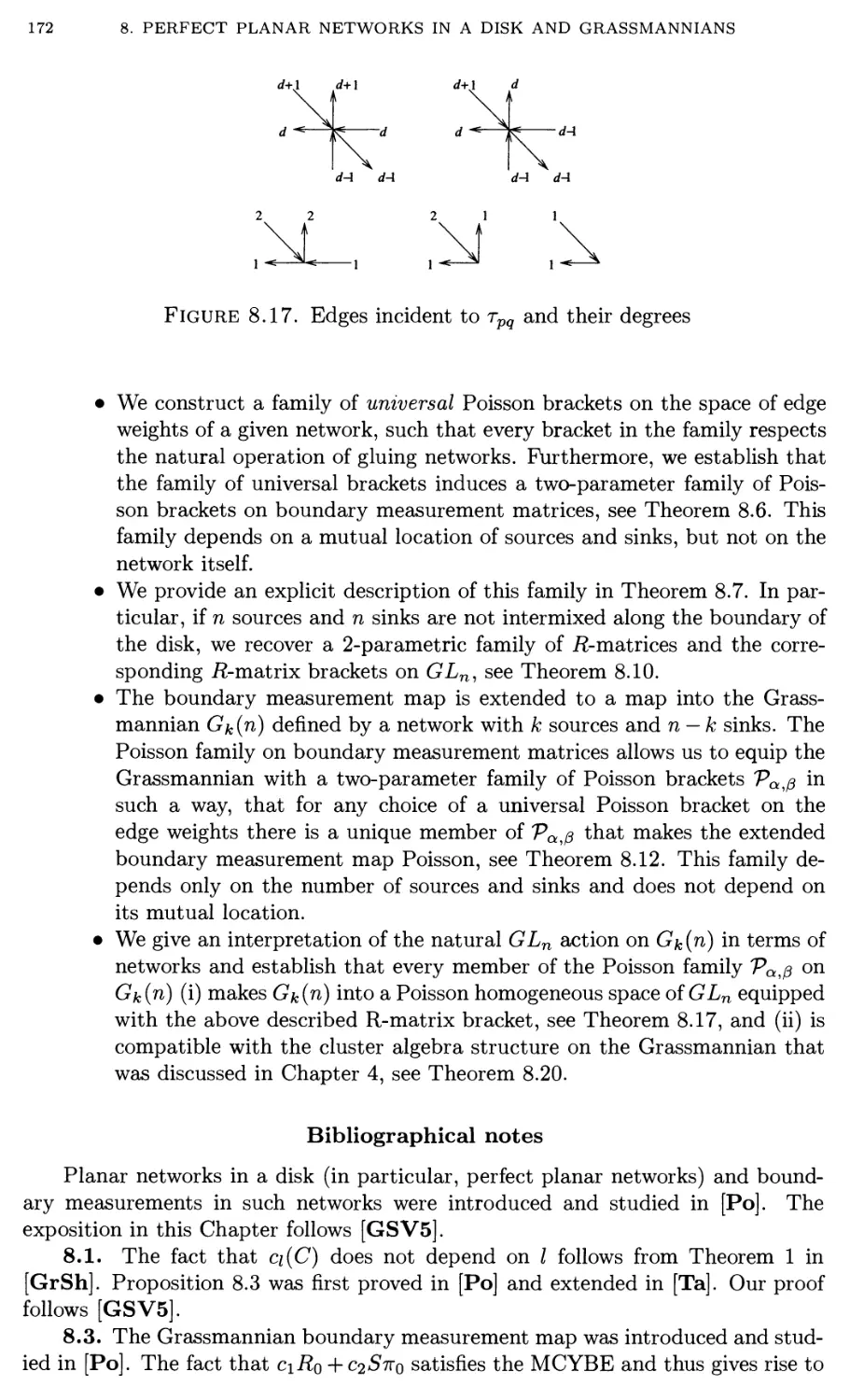
8.5. Summary 171
Bibliographical notes 172
Chapter 9. Perfect planar networks in an annulus and rational loops in
Grassmannians 175
9.1. Perfect planar networks and boundary measurements 175
9.2. Poisson properties of the boundary measurement map 181
9.3. Poisson properties of the Grassmannian boundary measurement map 191
9.4. Summary 196
Bibliographical notes 197
Chapter 10. Generalized Backlund-Darboux transformations for Coxeter-
Toda flows from a cluster algebra perspective 199
10.1. Introduction 199
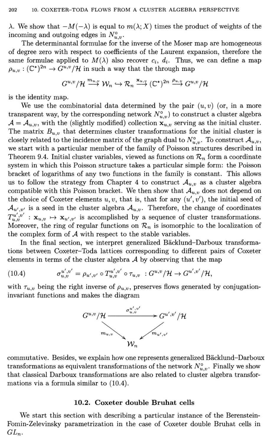
10.2. Coxeter double Bruhat cells 202
10.3. Inverse problem 207
10.4. Cluster algebra 214
10.5. Coxeter-Toda lattices 228
10.6. Summary 237
Bibliographical notes 237
Bibliography 239
Index
243

Preface
Cluster algebras introduced by Fomin and Zelevinsky in [FZ2] are
commutative rings with unit and no zero divisors equipped with a distinguished family
of generators (cluster variables) grouped in overlapping subsets (clusters) of the
same cardinality (the rank of the cluster algebra) connected by exchange relations.
Among these algebras one finds coordinate rings of many algebraic varieties that
play a prominent role in representation theory, invariant theory, the study of total
positivity, etc. For instance, homogeneous coordinate rings of Grassmannians,
coordinate rings of simply-connected connected semisimple groups, Schubert varieties,
and other related varieties carry (possibly after a small adjustment) a cluster
algebra structure. A prototypic example of exchange relations is given by the famous
Plucker relations, and precursors of the cluster algebra theory one can observe in
the Ptolemy theorem expressing product of diagonals of inscribed quadrilateral in
terms of side lengths and in the Gauss formulae describing Pentagrama Myrificum.
Cluster algebras were introduced in an attempt to create an algebraic and
combinatorial framework for the study dual canonical bases and total positivity in
semisimple groups. The notion of canonical bases introduced by Lusztig for
quantized enveloping algebras plays an important role in the representation theory of
such algebras. One of the approaches to the description of canonical bases
utilizes dual objects called dual canonical bases. Namely, elements of the enveloping
algebra are considered as differential operators on the space of functions on the
corresponding group. Therefore, the space of functions is considered as the dual
object, whereas the pairing between a differential operator D and a function F is
defined in the standard way as the value of DF at the unity. Elements of dual
canonical bases possess special positivity properties. For instance, they are regular
positive-valued functions on the so-called totally positive subvarieties in reductive
Lie groups, first studied by Lusztig. In the case of GLn the notion of total
positivity coincides with the classical one, first introduced by Gantmakher and Krein:
a matrix is totally positive if all of its minors are positive. Certain finite
collections of elements of dual canonical bases form distinguished coordinate charts on
totally positive varieties. The positivity property of the elements of dual canonical
bases and explicit expressions for these collections and transformations between
them were among the sources of inspiration for designing cluster algebra
transformation mechanism. Transitions between distinguished charts can be accomplished
via sequences of relatively simple positivity preserving transformations that served
as a model for an abstract definition of a cluster transformation. Cluster
algebra transformations construct new distinguished elements of the cluster algebra
from the initial collection of elements. In many concrete situations all constructed
distinguished elements have certain stronger positivity properties called Laurent
ix

χ PREFACE
positivity. It is still an open question whether Laurent positivity holds for all
distinguished elements for an arbitrary cluster algebra. All Laurent positive elements
of a cluster algebra form a cone. Conjecturally, for cluster algebras arising from
reductive semisimple Lie groups extremal rays of this cone form a basis closely
connected to the dual canonical basis mentioned above.
Since then, the theory of cluster algebras has witnessed a spectacular growth,
first and foremost due to the many links that have been discovered with a wide
range of subjects including
• representation theory of quivers and finite-dimensional algebras and cat-
egorification;
• discrete dynamical systems based on rational recurrences, in particular,
F-systems in the thermodynamic Bethe Ansatz;
• Teichmuller and higher Teichmuller spaces;
• combinatorics and the study of combinatorial polyhedra, such as the
Stasheff associahedron and its generalizations;
• commutative and non-commutative algebraic geometry, in particular,
— Grassmannians, projective configurations and their tropical analogues,
— the study of stability conditions in the sense of Bridgeland,
— Calabi-Yau algebras,
— Donaldson-Thomas invariants,
— moduli space of (stable) quiver representations.
In this book, however, we deal only with one aspect of the cluster algebra
theory: its relations to Poisson geometry and theory of integrable systems. First of all,
we show that the cluster algebra structure, which is purely algebraic in its nature,
is closely related to certain Poisson (or, dually, pre-symplectic) structures. In the
cases of double Bruhat cells and Grassmannians discussed below, the corresponding
families of Poisson structures include, among others, standard R-matrix Poisson-
Lie structures (or their push-for wards). A large part of the book is devoted to the
interplay between cluster structures and Poisson/pre-symplectic structures. This
leads, in particular, to revealing of cluster structure related to integrable systems
called Toda lattices and to dynamical interpretation of cluster transformations, see
the last chapter. Vice versa, Poisson/pre-symplectic structures turned out to be
instrumental for the proof of purely algebraic results in the general theory of cluster
algebras.
In Chapter 1 we introduce necessary notions and notation. Section 1.1 provides
a very concise introduction to flag varieties, Grassmannians and Plucker
coordinates. Section 1.2 treats simple Lie algebras and groups. Here we remind to the
reader the standard objects and constructions used in Lie theory, including the
adjoint action, the Killing form, Cartan subalgebras, root systems, and Dynkin
diagrams. We discuss in some detail Bruhat decompositions of a simple Lie group, and
double Bruhat cells, which feature prominently in the next Chapter. Poisson-Lie
groups are introduced in Section 1.3. We start with providing basic definitions of
Poisson geometry, and proceed to define main objects in Poisson-Lie theory,
including the classical R-matrix. Sklyanin brackets are then defined as a particular
example of an R-matrix Poisson bracket. Finally, we treat in some detail the case
of the standard Poisson-Lie structure on a simple Lie group, which will play an
important role in subsequent chapters.

PREFACE
χι
Chapter 2 considers in detail two basic sources of cluster-like structures in rings
of functions related to Schubert varieties: the homogeneous coordinate ring of the
Grassmannian G2{m) of 2-dimensional planes and the ring of regular functions on
a double Bruhat cell. The first of the two rings is studied in Section 2.1. We show
that Plucker coordinates of C?2(m) can be organized into a finite number of groups
of the same cardinality (clusters), covering the set of all Plucker coordinates. Every
cluster corresponds to a triangulation of a convex m-gon. The system of clusters
has a natural graph structure, so that adjacent clusters differ exactly by two Plucker
coordinates corresponding to a pair of crossing diagonals (and contained together
in exactly one short Plucker relation). Moreover, this graph is a 1-skeleton of the
Stasheff poly tope of m-gon triangulations. We proceed to show that if one fixes
an arbitrary cluster, any other Plucker coordinate can be expressed as a rational
function in the Plucker coordinates entering this cluster. We prove that this rational
function is a Laurent polynomial and find a geometric meaning for its numerator
and denominator, see Proposition 2.1.
Section 2.2 starts with the formulation of Arnold's problem: find the number of
connected components in the variety of real complete flags intersecting transversally
a given pair of flags. We reformulate this problem as a problem of enumerating
connected components in the intersection of two real open Schubert cells, and proceed
to a more general problem of enumerating connected components of a real double
Bruhat cell. It is proved that components in question are in a bijection with the
orbits of a group generated by symplectic transvections in a vector space over the
field F2, see Theorem 2.10. As one of the main ingredients of the proof, we provide
a complete description of the ring of regular functions on the double Bruhat cell.
It turns out that generators of this ring can be grouped into clusters, and that they
satisfy Plucker-type exchange relations.
In Chapter 3 we introduce cluster algebras and prove two fundamental results
about them. Section 3.1 contains basic definitions and examples. In this book we
mainly concentrate on cluster algebras of geometric type, so the discussion in this
Section is restricted to such algebras, and the case of general coefficients is only
mentioned in Remark 3.13. We define basic notions of cluster and stable variables,
seeds, exchange relations, exchange matrices and their mutations, exchange graphs,
and provide extensive examples. The famous Laurent phenomenon is treated in
Section 3.2. We prove both the general statement (Theorem 3.14) and its sharpening
for cluster algebras of geometric type (Proposition 3.20). The second fundamental
result, the classification of cluster algebras of finite type, is discussed in Section 3.3.
We state the result (Theorem 3.26) as an equivalence of three conditions, and
provide complete proofs for two of the three implications. The third implication is
discussed only briefly, since a complete proof would require exploring intricate
combinatorial properties of root systems for different Cartan-Killing types, which goes
beyond the scope of this book. In Section 3.4 we discuss relations between cluster
algebras and rings of regular functions, see Proposition 3.37. Finally, Section 3.5
contains a list of conjectures, some of which are treated in subsequent chapters.
Chapter 4 is central to the book. In Section 4.1 we introduce the notion of
Poisson brackets compatible with a cluster algebra structure and provide a complete
characterization of such brackets for cluster algebras with the extended exchange
matrix of full rank, see Theorem 4.5. In this context, mutations of the exchange
matrix are explained as transformations of the coefficient matrix of the compatible

Xll
PREFACE
Poisson bracket induced by a basis change. In Section 4.2 we apply this result to
the study of Poisson and cluster algebra structures on Grassmannians. Starting
from the Sklyanin bracket on SLn, we define the corresponding Poisson bracket
on the open Schubert cell in the Grassmannian Gk(n) and construct the cluster
algebra compatible with this Poisson bracket. It turns out that this cluster algebra
is isomorphic to the ring of regular functions on the open cell in Gfc(n), see
Theorem 4.14. We further investigate this construction and prove that an extension of
the obtained cluster algebra is isomorphic to the homogeneous coordinate ring of
the Grassmannian, see Theorem 4.17.
The smooth part of the spectrum of a cluster algebra is called the cluster
manifold and is treated in Chapter 5. The definition of the cluster manifold is
discussed in Section 5.1. In Section 5.2 we investigate the natural Poisson toric
action on the cluster manifold and provide necessary and sufficient conditions for
the extendability of the local toric action to the global one, see Lemma 5.3. We
proceed to the enumeration of connected components of the regular locus of the toric
action in Section 5.3 and extend Theorem 2.10 to this situation, see Theorem 5.9. In
Section 5.4 we study the structure of the regular locus and prove that it is foliated
into disjoint union of generic symplectic leaves of the compatible Poisson bracket,
see Theorem 5.12. In Section 5.5 we apply these results to the enumeration of
connected components in the intersection of η Schubert cells in general position in
Gk(n), see Theorem 5.15.
Note that compatible Poisson brackets are defined in Chapter 4 only for
cluster algebras with the extended exchange matrix of a full rank. To overcome this
restriction, we present in Chapter 6 a dual approach based on pre-symplectic rather
than on Poisson structures. In Section 6.1 we define closed 2-forms compatible with
a cluster algebra structure and provide a complete characterization of such forms
parallel to Theorem 4.5, see Theorem 6.2. Further, we define the secondary cluster
manifold and a compatible symplectic form on it, which we call the Weil-Petersson
form associated to the cluster algebra. The reason for such a name is explained
in Section 6.2, which treats our main example, the Teichmuller space. We briefly
discuss Penner coordinates on the decorated Teichmuller space defined by fixing
a triangulation of a Riemann surface Σ, and observing that Ptolemy relations for
these coordinates can be considered as exchange relations. The secondary cluster
manifold for the cluster algebra *4(Σ) arising in this way is the Teichmuller space,
and the Weil-Petersson form associated with this cluster algebra coincides with the
classical Weil-Petersson form corresponding to Σ, see Theorem 6.6. We proceed
with providing a geometric meaning for the degrees of variables in the denominators
of Laurent polynomials expressing arbitrary cluster variables in terms of the initial
cluster, see Theorem 6.7; Proposition 2.1 can be considered as a toy version of this
result. Finally, we give a geometric description of *4(Σ) in terms of triangulation
equipped with a spin, see Theorem 6.9. In Section 6.3 we derive an axiomatic
approach to exchange relations. We show that the class of transformations satisfying
a number of natural conditions, including the compatibility with a closed 2-form,
is very restricted, and that exchange transformations used in cluster algebras are
simplest representatives of this class, see Theorem 6.11.
In Chapter 7 we apply the results of previous chapters to prove several
conjectures about exchange graphs of cluster algebras listed in Section 3.5. The
dependence of a general cluster algebra on the coefficients is investigated in Section 7.1.

PREFACE
Xlll
We prove that the exchange graph of the cluster algebra with principal coefficients
covers the exchange graph of any other cluster algebra with the same exchange
matrix, see Theorem 7.1. In Section 7.2 we consider vertices and edges of an
exchange graph and prove that distinct seeds have distinct clusters for cluster
algebras of geometric type and for cluster algebras with arbitrary coefficients and
a non-degenerate exchange matrix, see Theorem 7.4. Besides, we prove that if a
cluster algebra has the above cluster-defines-seed property, then adjacent vertices
of its exchange graph are clusters that differ only in one variable, see Theorem 7.5.
Finally, in Section 7.3 we prove that the exchange graph of a cluster algebra with a
non-degenerate exchange matrix does not depend on coefficients, see Theorem 7.7.
In the remaining three chapters we develop an approach to the interaction of
Poisson and cluster structures based on the study of perfect networks—directed
networks on surfaces with boundary having trivalent interior vertices and univalent
boundary vertices. Perfect planar networks in the disk are treated in Chapter 8.
Main definitions, including weights and boundary measurements, are given in
Section 8.1. We prove that each boundary measurement is a rational function of the
edge weights, see Proposition 8.3, and define the boundary measurement map from
the space of edge weights of the network to the space of к χ πι matrices, where к
and m are the numbers of sources and sinks. Section 8.2 is central to this chapter;
it treats Poisson structures on the space of edge weights of the network and Poisson
structures on the space of к х πι matrices induced by the boundary measurement
map. The former are defined axiomatically as satisfying certain natural conditions,
including an analog of the Poisson-Lie property for groups. It is proved that such
structures form a 6-parametric family, see Proposition 8.5. For fixed sets of sources
and sinks, the induced Poisson structures on the space of к χ га matrices form a
2-parametric family that does not depend on the internal structure of the network,
see Theorem 8.6. Explicit expressions for this 2-parametric family are provided
in Theorem 8.7. In case к — πι and separated sources and sinks, we recover on
к χ к matrices the Sklyanin bracket corresponding to a 2-parametric family of
classical R-matrices including the standard R-matrix, see Theorem 8.10. In Section 8.3
we extend the boundary measurement map to the Grassmannian Gk(k + πι) and
prove that the obtained Grassmannian boundary measurement map induces a 2-
parametric family of Poisson structures on Gk(k + πι) that does not depend on the
particular choice of к sources and ra sinks; moreover, for any such choice, the
family of Poisson structures on к χ πι matrices representing the corresponding cell of
Gk(k-\-m) coincides with the family described in Theorem 8.7 (see Theorem 8.12 for
details). Next, we give an interpretation of the natural GLk+m action on Gk(k + m)
in terms of networks and establish that every member of the above 2-parametric
family of Poisson structures on Gk(k + πι) makes it into a Poisson homogeneous
space of GLk+m equipped with the Sklyanin R-matrix bracket, see Theorem 8.17.
Finally, in Section 8.4 we prove that each bracket in this family is compatible with
the cluster algebra constructed in Chapter 4, see Theorem 8.20. An important
ingredient of the proof is the use of face weights instead of edge weights.
In Chapter 9 we extend the constructions of the previous chapter to perfect
networks in an annulus. Section 9.1.1 is parallel to Section 8.1; the main difference
is that in order to define boundary measurements we have to introduce an auxiliary
parameter λ that counts intersections of paths in the network with a cut whose end-
points belong to distinct boundary circles. We prove that boundary measurements

xiv PREFACE
are rational functions in the edge weights and λ, see Corollary 9.3 and study how
they depend on the choice of the cut. Besides, we provide a cohomological
description of the space of face and trail weights, which is a higher analog of the space
of edge weights used in the previous chapter. Poisson properties of the obtained
boundary measurement map from the space of edge weights to the space of rational
к χ πι matrix functions in one variable are treated in Section 9.2. We prove an
analog of Theorem 8.6, saying that for fixed sets of sources and sinks, the induced
Poisson structures on the space of matrix functions form a 2-parametric family
that does not depend on the internal structure of the network, see Theorem 9.4.
Explicit expressions for this family are much more complicated than those for the
disk, see Proposition 9.6. The proof itself differs substantially from the proof of
Theorem 8.6. It relies on the fact that any rational к χ πι matrix function belongs
to the image of the boundary measurement map for an appropriated perfect
network, see Theorem 9.10. The section is concluded with Theorem 9.15 claiming that
for a specific choice of sinks and sources one can recover the Sklyanin bracket
corresponding to the trigonometric R-matrix. In Section 9.3 we extend these results
to the Grassmannian boundary measurement map from the space of edge weights
to the space of Grassmannian loops. We define the path reversal map and prove
that this map commutes with the Grassmannian boundary measurement map, see
Theorem 9.17. Further, we prove Theorem 9.22, which is a natural extension of
Theorem 8.12; once again, the proof is very different and is based on path reversal
techniques and the use of face weights.
In the concluding Chapter 10 we apply techniques developed in the previous
chapter to providing a cluster interpretation of generalized Backlund-Darboux
transformations for Coxeter-Toda lattices. Section 10.1 gives an overview of the chapter
and contains brief introductory information on Toda lattices, Weyl functions of the
corresponding Lax operators and generalized Backlund-Darboux transformations
between phase spaces of different lattices preserving the Weyl function. A Coxeter
double Bruhat cell in GLn is defined by a pair of Coxeter elements in the symmetric
group Sn. In Section 10.2 we have collected and proved all the necessary technical
facts about such cells and the representation of their elements via perfect networks
in a disk. Section 10.3 treats the inverse problem of restoring factorization
parameters of an element of a Coxeter double Bruhat cell from its Weyl function. We
provide an explicit solution for this problem involving Hankel determinants in the
coefficients of the Laurent expansion for the Weyl function, see Theorem 10.9. In
Section 10.4 we build and investigate a cluster algebra on a certain space 7£n of
rational functions related to the space of Weyl functions corresponding to Coxeter
double Bruhat cells. We start from defining a perfect network in an annulus
corresponding to the network in a disk studied in Section 10.2. The space of face weights
of this network is equipped with a particular Poisson bracket from the family
studied in Chapter 9. We proceed by using results of Chapter 4 to build a cluster algebra
of rank 2n — 2 compatible with this Poisson bracket. Theorem 10.27 claims that
this cluster algebra does not depend on the choice of the pair of Coxeter elements,
and that the ring of regular functions on 7£n is isomorphic to the localization of this
cluster algebra with respect to the stable variables. In Section 10.5 we use these
results to characterize generalized Backlund-Darboux transformations as sequences of
cluster transformations in the above cluster algebra conjugated by by a certain map
defined by the solution of the inverse problem in Section 10.3, see Theorem 10.36.

PREFACE xv
We also show how one can interpret generalized Backlund-Darboux
transformations via equivalent transformations of the corresponding perfect networks in an
annulus. In conclusion, we explain that classical Darboux transformations can be
also interpreted via cluster transformations, see Proposition 10.39.
The process of writing spread over several years. We would like to thank all
individuals and institutions that supported us in this undertaking. The project
was started in Summer 2005 during our visit to Mathematisches Forschunginstitut
Oberwolfach in the framework of Research in Pairs program. Since then we
continued to work on the book during our joint visits to Institut des Hautes Etudes
Scientifiques (Bures-sur-Yvette), Institut Mittag-Leffler (Djursholm), Max-Planck-
Institut fur Mathematik (Bonn), University of Stockholm, Royal School of
Technology (Stockholm), University of Haifa, Michigan State University, and University
of Michigan. We thank all these institutions for warm hospitality and excellent
working conditions. During the process of writing, we had numerous discussions
with A. Berenstein, L. Chekhov, V. Fock, S. Fomin, R. Kulkarni, A. Postnikov,
N. Reshetikhin, J. Scott, B. Shapiro, M. Yakimov, A. Zelevinsky and others that
helped us to understand many different facets of cluster algebras. It is our pleasure
to thank all of them for their help.

CHAPTER 1
Preliminaries
In this chapter we collect necessary terms and notation that will be used
throughout the book.
1.1. Flag manifolds, Grassmannians, Plucker coordinates and Plucker
relations
1.1.1. Recall that the Grassmannian Gfc(ra) is the set of all fc-dimensional sub-
spaces in an m-dimensional vector space V over a field F. Any fc-dimensional sub-
space W of V can be described by a choice of к independent vectors w\,..., Wk G W,
and, vice versa, any choice of к independent vectors w\,..., Wk G V determines a
fc-dimensional subspace W = span{it;i,..., w^}. Fix a basis in V. Any к
independent vectors in V give rise to а к χ πι matrix of rank к whose rows are coordinates
of these vectors. Hence any element X of the Grassmannian can be represented
(non-uniquely) as а к χ πι matrix X of rank к. Two к χ πι matrices represent the
same element of the Grassmannian G^(m) if one of them can be obtained from the
other one by the left multiplication with a nondegenerate к х к matrix.
Let / be a fc-element subset of [1, m] = {1,..., πι}. The Plucker coordinate xj
is a function on the set of к χ πι matrices which is equal to the value of the minor
formed by the columns of the matrix indexed by the elements of /. Note that for
any к χ πι matrix Μ and any nondegenerate к х к matrix A, the Plucker coordinate
xi(AM) is equal to det A · xj(M). The Plucker embedding is an embedding of the
Grassmannian into the projective space of dimension (™) — 1 that sends X G Gfc(m)
to a point with homogeneous coordinates
X m — k-l· 1 ,m — k+2,... ,ra
(X).
Plucker coordinates are subject to quadratic constraints called Plucker
relations. Fix two fc-element subsets of the set [l,m], / = {ii,...,^} and J =
{jb · · · ,jk}- In what follows, we will sometimes use notation
(1.1) I(ia -> /) = {гь ... ,iQ_i,/,iQ+i,... ,i/J
for a G [1, k] and / G [1, πι].
Then for every /, J and a Plucker coordinates satisfy a quadratic equation
к
(!·2) xixJ = Σ xnia^j0)xJUp^ia).
/3=1
If /, J are of the form / = {Γ,i,j), J = {/',p, q}, where Γ is a (k — 2)-subset
of [l,m] and i,j,p, q are distinct indices not contained in /', then (1.2) reduces to
a 3-term relation
^l.oj Xj'ijXI'pq — Xj'pjXI'iq ι XI'qjxI'pi
1

2
1. PRELIMINARIES
called the short Plucker relation, which will be of special interest to us.
The Plucker embedding shows that the Grassmannian Gk{m) is a smooth
algebraic projective variety. Its homogeneous coordinate ring C[Gfc(m)] is the quotient
of the ring of polynomials in Plucker coordinates by the ideal of homogeneous
polynomials vanishing on Gk(m). The latter ideal is generated by Plucker relations.
1.1.2. Grassmannians Gk(m) are particular examples of {partial) flag
varieties. More generally, the {partial) flag variety Fl(V,d) associated to the data
d = (di,..., dn) with l<di<---<dn<m = dim V is defined as the set of all
flags f = ({0} С f1 С · · · С fn) of linear subspaces of V with dim/·7' = dy, it can
be naturally embedded into the product of Grassmannians Gdx (τη) χ · · · χ Gdn(m).
The image of this embedding is closed, thus F1(F, d) is a projective variety. If
d=(l,2,...,ra — 1), then F1(V, d) is called the complete flag variety and denoted
F\(V).
Let us choose a basis (ei,..., em) in V and a standard flag
/o(d) = {{0} С span{ei,..., edl} С ··· С span{eb ... ,edn}}
in Fl(V,d). The group SL(V) acts transitively on Fl(V,d). We can use the chosen
basis to identify V with Fm. The stabilizer of the point /o(d) under this action is
a parabolic subgroup V С 5Lm(F) of elements of the form
(Ax • · · · • \
0 A2 .
I I '
• I
\ 0 · · · 0 An )
where A{ are d{ χ d{ invertible matrices. Thus, as a homogeneous space, Fl(V,d) =
SLrn(¥)/V. In particular, the complete flag variety is isomorphic to
Flm(F) := SLm(¥)/B+,
where B+ is the subgroup of invertible upper triangular matrices over F.
Two complete flags / and g in Flm(F) are called transversal if
dim(/2 Π gJ) = max (г + j — m, 0)
for any г, j G [l,m]. When two flags are transversal, we often say that they are in
general position.
Fix two transversal flags / and g and consider the set ΙΙψ (¥) С Flm(F) of all
flags that are transversal to both / and g. The set UTд(Щ serves as one of our
main motivational examples and will be studied in great detail in the next chapter.
For now, note that, since SLm(¥) acts transitively on the set of pairs of transverse
flags, we may assume without loss of generality that gi = spanjei,... ,ej} and
/г = span{em_;+i,... ,em}. Then any flag h transversal to / can be naturally
identified with a unipotent upper triangular matrix Η whose first г rows span the
subspace hl. In order for h to be also transversal to g, the matrix Η must satisfy
an additional condition: for every 1 < к < m, the minor of Η formed by the first
к rows and the last к columns must be non-zero.

1.2. SIMPLE LIE ALGEBRAS AND GROUPS
3
1.2. Simple Lie algebras and groups
1.2.1. Let Q be a connected simply-connected complex Lie group with an
identity element e and let g = TeQ be the corresponding Lie algebra. We will often use
notation Q = expg and g = Lie Q. The dual space to g will be denoted by g* and
the value of I G g* at ξ G g will be denoted by (ί, ξ).
Recall the definitions of the adjoint (resp. co-adjoint) actions of Q and g on g
(resp. g*):
Ad*£ = ^(x 1ехР(#И
асЦ ξ = [τ/, ξ]
dt \t=o
and
(Ad; i, ξ) = (£, Adx ξ), (ad; £, ξ) = (£, ad, ξ)
for any ξ G g.
The Killing form on g is a bilinear symmetric form (·, ·)0 defined by
(1.4) (^r/^trtad^ad^),
where ad^ ad^ is viewed as a linear operator acting in the vector space g.
1.2.2. Let now g be a complex simple Lie algebra of rank r with a Cart an
subalgebra () = αθΐο. Recall that f) is a maximal commutative subalgebra of g
of dimension r, and that the adjoint action of f) on g can be diagonalized. More
precisely, for a G f)*, define
0a = {£ G g : [ft, ξ] = a(ft)£ for any Λ G f)}.
Clearly, go = f). A nonzero α such that ga 7^ 0 is called a root of g, and a collection
Φ of all roots is called the root system of g. Then:
(i) For any a G Φ, dimga = 1, and
(ii) g has a direct sum decomposition
0 = ϊ)θ(θα£Φ0α),
which is graded by Φ, that is, [0а,0/з] = да+/з, where the right hand side is zero if
a -f β is not a root.
The Killing form (1.4) is nondegenerate on the simple algebra g, and so is its
restriction to f), which we will denote by (·,·). Thus f)* and f) can be identified via
ί)*3α t-> ha G f) : α(/ι) = (fta, /1)
for all h G f). Moreover, the restriction of (·,·) to the real vector space spanned
by ha,a G Φ is real-valued and positive definite. Thus, the real vector space f)o
spanned by a G Φ is a real Euclidean vector space with the inner product (·,·).
In particular, a reflection with respect to the hyperplane normal to a G f)J can be
defined by
(1.5) 3αβ = β - (β\α)α,
where </3|a>=2gg.
We can now summarize the properties of the root system Φ:
(i) Φ contains finitely many nonzero vectors that span f)g;
(ii) for any a G Φ, the only multiples of a G Φ are ±a;
(iii) Φ is invariant under reflections sa, a e Φ;
(iv) for any α, β G Φ, the number (β\α) is an integer.

4
1. PRELIMINARIES
The second property above allows one to choose a polarization of Φ, i.e., a
decomposition Φ = Φ+ U Φ_, where Φ_ = —Φ+. Elements of Φ+ (resp. Φ_) are
called positive (resp. negative) roots. The set Π = {αχ,... , ar} of positive simple
roots is a maximal collection of positive roots that can not be represented as a
positive linear combination of other roots. Every positive root is a nonnegative
linear combination of elements of Π with integer coefficients. The sum of these
coefficients is called the height of the root.
The Cartan matrix of g is defined by
A = (aij)lj=1 = ((<*j\<*i))iJ=1
and is characterized by the following properties:
(i) A is an integral matrix with 2's on the diagonal and non-positive off-diagonal
entries.
(ii) A is symmetrizable, i.e. there exists an invertible diagonal matrix D (e.g.
D = diag((ai,ai))[=1) such that DA is symmetric. In particular, A is sign-
symmetric^ that is, a^aji > 0 and a^aji = 0 implies that both a^ and a^ are
zero.
(iii) DA defined as above is positive definite. This implies, in particular, that
The information contained in the Cartan matrix can also be encoded in the
corresponding Dynkin diagram, defined as a graph on r vertices with ith and jth
vertices joined by an edge of multiplicity аца^. If аца^ > 1 then an arrow is
added to the edge. It points to j if (а^^г) > (aj,aj)-
A simple Lie algebra is determined, up to an isomorphism, by its Cartan matrix
(or, equivalently, its Dynkin diagram). Namely, it has a presentation with the so-
called Chevalley generators {hi,e±i}ri=l and relations
(1.6) [h%,hj] = 0, [hi,e±j] = ±c^e±j, [ej,e_j] = Sijhj,
and
«£-0« e±j = 0.
The latter are called the Serre relations. In terms of positive simple roots and
Chevalley generators, the elements of the Cartan matrix can be rewritten as a^ —
OLj{hi), г J e [l,r].
The classification theorem for simple Lie algebras states that every Dynkin
diagram is of one of the types described in Fig. 1.1.
It is clear from relations (1.6) that for every г G [l,r], one can construct an
embedding pi of the Lie algebra 5/2 into g by assigning
*(o 1 )=л<- л(о l)=eh *( 1 o)=e-i'
which can be integrated to an embedding (also denoted by pi) of the group SL2
into the group Q. In particular,
(1-7) Pi ί 0 г J=exp(tei), pi I t χ )=exp(te-i)
for any t G С One-parameter subgroups
(1.8) xf(t) = exp(te±l)
generated by e±i will play an important role in what follows.

1.2. SIMPLE LIE ALGEBRAS AND GROUPS 5
Figure 1.1. The list of Dynkin diagrams
1.2.3. The Borel (resp., opposite Borel) subalgebra b+ (resp., b_) of g relative
to f) is spanned by f) and vectors ea, a G Φ+ (resp., ea, a G Φ-). Let n+ = [b+, b+]
and n_ = [b_, b_] be the corresponding maximal nilpotent subalgebras of g. The
connected subgroups that correspond to g, f), b+, b_, n+, n_ will be denoted by Q,
The weight lattice Ρ consists of elements 7 G f)* such that 7(^*2) £ ^ f°r
г G [l,r]. The basis of fundamental weights cji, ... ,cjr in Ρ is defined by ujj(hi) =
{u)j\oLi) = &ij, i,j G [l,r]. Every weight 7 G Ρ defines a multiplicative character
α Η α7 of Я as follows: let α = exp(h) for some /1 G f), then a7 = e7^. Positive
simple roots, fundamental weights and entries of the Cart an matrix are related via
r r
(1.9) oti — У. ajiUj = 2ω{ + \^ ajiUJj.
The PFei// ^rowp W is defined as a quotient W = Norm^H/H. For each of the
embeddings pi'. SL2 —> ^, i G [l,r], defined in (1.7), put
5г = />г ί г q j G Norm^ Η
and 5г = 5гН G W. All 5^ are of order 2, and together they generate W. We
can identify Si with the elementary reflection sai, oti G П, in f)J defined by (1.5).
Consequently, W can be identified with the Coxeter group generated by reflections
si,..., sr. The Weyl group acts on the weight lattice. For any w G W and 7 G Ρ the
action 7 ь-> г/;7 is defined by expanding it; into a product of elementary reflections
and applying the reflections one by one to 7.
A reduced decomposition of an element w G W is a representation of it; as a
product w = six- ·· Sit of the smallest possible length. A reduced decomposition is
not unique, but the number / of reflections in the product depends only on w and
is called the length of w and denoted by l(w). The sequence of indices (г'1,..., г'/)
that corresponds to a given reduced decomposition of w is called a reduced word for
w. The unique element of W of maximal length (also called the longest element of
W) will be denoted by wo· Braid relations for s~i guarantee that the representative
w G Norm^H can be unambiguously defined for any w G W by requiring that

6
1. PRELIMINARIES
ΰν = ΰν whenever l(uv) — l(u)+l(v). In what follows we will slightly abuse notation
by denoting an element of the Weyl group and its representative in Norm^ Ή with
the same letter.
We will also need a notion of a reduced word for an ordered pair (u,v) of
elements in W. It is defined as follows: if (ii,..., щи)) 1S a reduced word for и and
(i[,..., i'uv\) is a reduced word for v, then any shuffle of sequences (ii,... ,щи))
and (—i[,..., —i'uv\) is called a reduced word for (г/, ν).
Every ξ G 0 can be uniquely decomposed
(1-10) ξ = ξ-+ξ0+ξ+,
where (+ Ε n+, ^_ G n_ and £o £ f)· Consequently, for every χ in an open Zarisky
dense subset
д°=АГ_ШГ+
of Q there exists a unique Gauss factorization
χ = x_xqx+, x+ G Λ/Υ, X- G Λί-, xo G %.
For any χ Ε Q° and a fundamental weight ω ι define
Ai(x) = xp;
this function can be extended to a regular function on the whole Q. In particular,
for Q — 5Lr+i, Ai(x) is just the principal г х г minor of a matrix x. For any pair
u,v G W, the corresponding generalized minor is a regular function on Q given by
(1.11) АиШг,УШ{(х) = Аг(и~1ху).
These functions depend only on the weights ηωι and vuji, and do not depend on
the particular choice of и and v.
1.2.4. The Bruhat decompositions of Q with respect to S+ and B- are defined,
resp., by
Q = ииецгВ+иВ+, Q = UveWB-vB-.
The sets B+uB+ (resp. B-vB-) are disjoint. They are called Bruhat cells (resp.
opposite Bruhat cells). The generalized flag variety is defined as a homogeneous
space
G/B+ = UuewB+u.
Clearly, this is a generalization of the complete flag variety in a finite dimensional
vector space.
Finally, for any u,v G W, the double Bruhat cell is defined as
gu'v =B+uB+C\B-vB-,
and the reduced double Bruhat cell, as
Double Bruhat cells and reduced double Bruhat cells will be the subject of our
discussion in the next chapter. Here we will only mention that the variety Qu,v is
biregularly isomorphic to a Zariski open subset of сг+/(и)+/(г;)5 where r = rankC/.
A corresponding birational map from cr+l(u)+l(v) to Qu,v can be constructed quite
explicitly, though not in a unique way.
Namely, let j = (ji,... ,ji(u)+i(v)+r) be a shuffle of a reduced word for (u,v)
and any re-arrangement of numbers i,... ,ir with i2 = — 1; we define θ{1) — + if

1.2. SIMPLE LIE ALGEBRAS AND GROUPS
7
jt > 0, θ(1) = - if ji < 0 and 0(Z) = 0 if ji G iZ. Besides, for г G [l,r] and ί G C,
put
x?(0 = p»(diag(i,r1)).
Then one defines a map xy Cz(u)+z(v)+r -> £^ by
/(u)+/(v)+r
(1-12) Sj(t)= J] **'>&),
/ = 1
where elements xf(t) are defined as in (1.8). This map is a biregular
isomorphism between (C*)^u^+^^+r and a Zariski open subset of Qu>v. Parameters
£ъ · · · > ^(u)+Z(v)+r constituting t are called factorization parameters. Note that
setting £/ = 1 in the definition of Xj for all I such that θ (I) = 0, one gets a parametriza-
tion for a Zariski open set in Lu,v, and so Lu,v is biregularly isomorphic to a Zariski
open subset inC'M+'W. In this case, we replace the factorization map above by
i(u)+i(v)
(1.13) 4(t) = J] *2?('0,
/ = 1
where now j is a reduced word for (u, v) and t = (£i,..., i/(u)+z(v))· We retain
notations j and t, since it will be always clear from context which of the factorizations
(1.12), (1.13) is being used.
Remark 1.1. It will be sometimes convenient to interpret θ as taking values
±1 instead of ±. The proper interpretation will be clear from the context.
It is possible to find explicit formulae for the inverse of the map (1.12) in terms
of the so-called twisted generalized minors. We will not review them here, but
instead conclude the subsection with an example.
Example 1.2. Let Q — SLn and (u,v) = (wo,wq), where wq is the longest
element of the Weyl group Sn. Then Qw°^w° is open and dense in SLn and consists
of elements such that all minors formed by several first rows and last columns as well
as all minors formed by several last rows and first columns are nonzero. A generic
element of Qw°'w° has nonzero leading principal minors, and by right multiplying
by an invertible diagonal matrix D~l can be reduced to a matrix A G Qw°^w° with
all leading principal minors equal to 1. Subtracting a multiple of the (n — l)st row
of A from its nth row we can ensure that the (n, l)-entry of the resulting matrix
is 0, while (generically) all other entries are not. Applying similar elementary
transformations to rows η — 2 and η — 1, then η — 3 and η — 2, and so on up to
1 and 2, we obtain a matrix with all off-diagonal entries in the first column equal
to 0. Starting from the bottom row again and proceeding in a similar manner, we
will eventually reduce Л to a unipotent upper triangular matrix B. Applying (in
the same order) the corresponding column transformations to B, we will eventually
reduce it to the identity matrix. If one now translates operations above into the
matrix multiplication, they can be summarized as a factorization of A into
A = (l + iien>n_i) · · · (1 + *n-ie2,i)(l + tnenin-i) - · (1 + hn-г^га)'''
)(l+*n(n-l) ,,
(n— 1)^71— 1,71 /·
2 2 "t"1 Ч
Furthermore, denote m — n{n — 1) and factor D as
D = diag(*m+b ^+1,1,..., 1) · · · diag(l,..., 1, *m+n-i, *™+η-ι)·

8
1. PRELIMINARIES
The resulting factorization for X — AD is exactly formula (1.12) corresponding to
the word j = (-(n - 1), -(n - 2),..., -1, -(n - 1), -(n - 2),..., -2,..., -(n -
l),n — l,n — 2,n — l,...,l,...,n — l,i,... ,i(n — 1)).
1.3. Poisson-Lie groups
The theory of Poisson-Lie groups and Poisson homogeneous spaces serves as
a source of many important examples that will be considered below. This section
contains a brief review of the theory.
1.3.1. We first recall basic definitions of Poisson geometry.
A Poisson algebra is a commutative associative algebra # equipped with a
Poisson bracket defined as a skew-symmetric bilinear map {·,·}: # x $ —» $ that
satisfies, for any /i, /2, /з G #, the Leibniz identity
{/1/2,/3} = /i{/2,/3} + {/ъ/з}/2
and the Jacobi identity
{/l, {/2,/3}} + {/2, {/3,/l}} + {/3, {/l,/2}} = 0.
An element с G # such that {c, /} = 0 for any / G # is called a Casimir element
A smooth real manifold Μ is called a Poisson manifold if the algebra C°°(M)
of smooth functions on Μ is a Poisson algebra. In this case we say that Μ is
equipped with a Poisson structure.
Let (Mb {·, -}г) and (M2, {·, ·}2) be two Poisson manifolds. Then Μι χ M2 is
equipped with a natural Poisson structure: for any /1, /2 G C°°(Mi χ M2) and any
χ G Mi, у e M2
{fij2}(x,y) = {fi(-,y)j2(-,y)h(x) + {fi(xr)j2(xr)h(y).
Let F : Mi —» M2 be a smooth map; it is called a Poisson map if
{/ioF,/2oF}i = {/b/2}2oF
for every /i,/2 G C°°(M2). A submanifold TV of a Poisson manifold (M, {·,·}) is
called a Poisson submanifold if it is equipped with a Poisson bracket {·, ·}Ν such
that the inclusion map i : N —» Μ is Poisson.
A bracket {·, ·} on C°°(M) is called поп-degenerate if there are no non-constant
Casimir elements in C°°(M) for {·,·}. Otherwise, {·,·} is called degenerate. Every
symplectic manifold, that is, an even-dimensional manifold Μ equipped with a
non-degenerate closed 2-form ω2, gives rise to a nondegenerate Poisson bracket
(1-14) {f1J2}=oj2(Idf1,Idf2),
where / : T*M Э ω1 t-> Ι ω1 G Τ Μ is an isomorphism defined by
{ω\·)=ω2(·,Ιω1).
Conversely, if a Poisson bracket {·, ·} on Μ is nondegenerate, then Μ is a symplectic
manifold and the Poisson bracket is defined by (1.14).
Fix a smooth function φ on a Poisson manifold M. By the Leibniz rule, the
map {φ, ·} : C°°(M) —» C°°(M) is a differentiation. This implies an equation
{φ,/} = (ά/,νφ),
which defines a vector field νφ even if the Poisson bracket on Μ is degenerate. νφ
is called a Hamiltonian vector field generated by φ. If Μ is a symplectic manifold,
then νφ = Ιάφ.

1.3. POISSON-LIE GROUPS
9
The Poisson bivector field π is a section of T2M defined by
{/ΐ,/2} = (#ΐΛ#2)Μ·
In terms of the Poisson bivector field, a Poisson submanifold can be defined as a
submanifold N С М such that π\χ G T2N. The rank of the Poisson structure at
a point of Μ is defined to be the rank of π at that point.
Now, we are ready to review the notion of a symplectic leaf. First, introduce an
equivalence relation ~ on M: for x, у G Μ, χ ~ у if χ and у can be connected by a
piecewise smooth curve whose every segment is an integral curve of a Hamiltonian
vector field. Then it can be shown that
(i) equivalence classes of ~ are Poisson submanifolds of M;
(ii) the rank of the Poisson structure at every point of such submanifold N is
equal to the dimension of N.
An equivalence class, MX1 of a point χ G Μ is called a symplectic leaf through
x. It is clear that Mx is a symplectic manifold with respect to the restriction of
{·, ·} to Mx. Casimir functions of {·, ·} are constant on symplectic leaves.
Example 1.3. An important example of a degenerate Poisson bracket is the
Lie-Poisson bracket on a dual space g* to a Lie algebra g defined by
{fuf2}(a) = (a,[df1(a),df2(a)})
for any /ι,/г G C°°(g*) and a G g*. Casimir functions for the Lie-Poisson bracket
are functions invariant under the co-adjoint action on g* of the Lie group Q — expg.
Symplectic leaves of the Lie-Poisson bracket are co-adjoint orbits of Q.
1.3.2. Let Q be a Lie group equipped with a Poisson bracket {·,·}. Q is called
a Poisson-Lie group if the multiplication map
m : Q χ Q Э (x, y) >-> xy G Q
is Poisson. This condition can be re-written as
(1-15) Uij2}(xy) = {pyfi,Pyf2}(x) + {bxfi,bxf2}(y),
where py and \x are, respectively, right and left translation operators on Q:
(pyf)(x) = (Xxf)(y) = f(xy).
Example 1.4. A dual space g* to a Lie algebra g equipped with a Lie-Poisson
bracket (Example 1.3) is an additive Poisson-Lie group.
To construct examples of non-abelian Poisson-Lie groups, one needs a closer
look at the additional structure induced by property (1.15) on the tangent Lie
algebra g of Q. First, we introduce right- and left-invariant differentials, D and D',
on£:
(1.16) (Df(x)^)= ^/(exp(fOz)
, (D'f(x),t)= -£/(*exp(fO)
t=o dt
t=0
where / G C°°(G), ξ G g. The Poisson bracket {·, ·} on Q can then be written as
{/ъ/2}(*) = (n(x)Df1(x),Df2(x)) = {it'{x)D'h{x),D'f2{x)),
where π,π' map Q into Hom(g*,g). Then property (1.15) translates into the 1-
cocycle condition for π and π' :
(1.17) n(xy) = Adx n(y) Ad^-i +π(χ), π'{xy) = Ad^-i тг'(ж) Ad* +n'(y).

10
1. PRELIMINARIES
Using the identification Hom(g*,g) = g 0 g, we conclude from (1.17) that the
map δ : g —» g 0 g defined by
(1.18) *(0=4π(βχρ(ί0)|
d* lt=o
satisfies
δ([ξ,η]) = К ® 1 + 1 ®f,5(ry)] - [r/0 1 + 1 ® ту, 5(01-
In other words, 5 is a 1-cocycle on g with values in the g-module q® q.
Another consequence of (1.17) is that the Poisson operators π, π' vanish at the
identity element e of Q and, thus, any Poisson-Lie bracket is degenerate at the
identity. The linearization of {·,·} at the identity equips g* = T*Q with a Lie
algebra structure:
[aba2]* = άΒ{φι,φ2},
where φ^ г = 1,2 are any functions such that deipi — a*. Comparison with (1.18)
gives
([αι,α2]*,0 = (αϊ Λα2,5(0>·
To summarize, if Q is a Poisson-Lie group then the pair (q,Q*) satisfies the
following conditions:
(i) g and g* are Lie algebras,
(ii) the map δ dual to the commutator [·,·]* '·&*&&* —>· 0* is a 1-cocycle on g
with values in g® g.
A pair (q,Q*) satisfying the two conditions above is called a Lie bialgebra and
the corresponding map δ is called a cobracket.
Theorem 1.5. (Drinfeld) If (q,Q*) is a Lie bialgebra and Q is a connected
simply-connected Lie group with the Lie algebra $, then there exists a unique Poisson
bracket on Q that makes Q into a Poisson-Lie group with the tangent Lie bialgebra
(0,0*)·
If 7ί is a Lie subgroup of Q, it is natural to ask if it is also a Poisson-Lie subgroup,
i. e. if % is a Poisson submanifold of Q such that property (1.15) remains valid for
the restriction of the Poisson-Lie bracket on Q to Ή,. The answer to this question
is also conveniently described in terms of the tangent Lie bialgebra of Q. Let ()Cg
be the Lie algebra that corresponds to 7ί.
Proposition 1.6. % is a Poisson-Lie subgroup of Q if and only if the annihi-
lator of\) in g* is an ideal in the Lie algebra g*.
1.3.3. Next, we discuss an important class of Lie bialgebras, called factorizable
Lie bialgebras.
A Lie bialgebra (g.Q*) is called factorizable if the following two conditions hold:
(i) g is equipped with an invariant bilinear form (·,·), so that g* can be identified
with g via
g* Э α^ξα eg : (a, ·) = (£a,·);
(ii) the Lie bracket on g* = g is given by
(ΐ·ΐ9) [ξ,η]. = \(№),4] + [ξ,η(ι)]),
where R G End(g) is a skew-symmetric operator satisfying the modified classical
Yang-Baxter equation (MCYBE)
(1.20) [Щ), R(V)] - R ([Я(0, η] + [ξ, ϋ(η)]) = -[ξ, η};

1.3. POISSON-LIE GROUPS
11
R is called a classical R-matrix.
The invariant bilinear form (·, ·) can be represented by a Casimir element t G
g®g. Let r be the image of R under the identification $&$ = $&$* = End(g) and
let rij (1 < г < j < 3) denote the image of r under the embedding 0®0—>·0®0®0
such that the first (resp. second) factor in g 0 g is mapped into the ith (resp. jth)
factor in g ® g ® g. Define
[[r,r]] := [ri2,ri3] + [ri2,r23] + [г1з,г2з].
Then condition (1.20) in the definition of a factorizable Lie bialgebra can be equiv-
alently re-phrased as a condition on the cobracket δ:
where r± = \ (r ± t) G g ® g satisfy
[[r±,r±]]=0.
Let £ be a Poisson-Lie group with a factorizable tangent Lie bialgebra (Q,g*).
The corresponding Poisson bracket whose existence is guaranteed by Theorem 1.5
is called the Sklyanin bracket. To provide an explicit formula for the Sklyanin
bracket, we first define, in analogy to (1.16), right and left gradients for a function
/ e c°°(gy.
(V7(*U)=|/(*exp(tO)
i=0
(1.21) (V/(*),0=^/(exp(*0*)
Then the Sklyanin bracket has a form
(1.22) {/i,/2} = ^WV7i),V72)-^(fl(V/i),V/2).
1.3.4. Standard Poisson-Lie structure on a simple Lie group. We now
turn to the main example of a Poisson-Lie group to be used in this exposition. Let
Q be a connected simply-connected Lie group with the Lie algebra g. The Killing
form is a bilinear nondegenerate form on g = g*. Define R G End(g) by
(1.23) Я(0 =£+-£-,
where ξ± are defined as in (1.10). It is easy to check that R satisfies (1.20) and thus
(1.22), (1.23) endow Q with a Poisson-Lie structure, called the standard Poisson-Lie
structure and denoted by {·, -}g. Furthermore, the Lie bracket (1.19) on g* = g in
this case is given by
(1.24) [£,77]* = K+ + -£ο,?7+ + 2Щ] ~ [ί" + 2ξθ'η- + 2^'
It follows from (1.24), that subalgebras n± of g are ideals in g*. Since n± = b^
with respect to the Killing form, Proposition 1.6 implies that Borel subgroups B±
are Poisson-Lie subgroups of Q.
Example 1.7. Let us equip Q = SLn and g = sln with the trace-form
(ξ, η) = ίτξη.
Then the right and left gradients (1.21) are
Vf(x) = x grad/(x), Vf(x) = grad/(x) x,

12
1. PRELIMINARIES
where
Thus the standard Poisson-Lie bracket becomes
(1.25)
{h,h}sLn{x) = -(^(grad/i(x)x),grad/2(x)x)--(i?(xgrad/i(x)),xgrad/2(x)),
where the action of the R-matrix (1.23) on ξ = (^ij)fj=i £ sln is given by
Щ) = (sign(j-%j)^=i·
Substituting into (1.25) coordinate functions x^, x^i, we obtain
{x%j, xki}sLn = 2 (siSn(^ ~ 0 + siSnG ~ Л) xuxkj-
In particular, the standard Poisson-Lie structure on
SL*={(ac d) : «*-bc=l}
is described by the relations
{a, b}SL2 = |ab, {a, c}sl2 = ^ac, {a, d}SL2 = 6c,
{c, d}5L2 = ±cd, {6, d}5L2 = \bd, {6, c}5L2 = 0.
Note that the Poisson bracket induced by {-,-}sl2 on upper and lower Borel
subgroups of SL2
«♦-{Μ}· ·4(:;·)}
has an especially simple form:
The example of SL2 is instrumental in an alternative characterization of the
standard Poisson-Lie structure on Q. Fix г G [1,/], I = rankg, and consider an
annihilator of the subalgebra g2 = span{e^, e_i, hi} with respect to the Killing
form:
(β*) = Κ Θ (θα£φ\{α±,}0α) ,
where /ι^- is the orthogonal complement of hi in f) with respect to the restriction
of the Killing form. Though (g2)-1 is not even a subalgebra in g, it is an ideal in
g* equipped with the Lie bracket (1.24). It follows that for every г, the image of
the embedding pi : SL2 —» G defined in (1.7) is a Poisson-Lie subgroup of Q. The
restriction {',-}pjsl2) °f the Sklyanin bracket (1.22), (1.23) to pi(SL2) involves
only the restriction of the standard R-matrix to дг = piish)- It is not difficult to
check then, that
{•'•}^(5L2) = (aiiai){'i'}sL2'
Thus the standard Poisson-Lie structure is characterized by the condition that for
every г G [1, /], the map
(1-26) Pi : (5Ь2,(аг,аг){-,-Ьь2) "> (βΛ;·}β)
is Poisson.

BIBLIOGRAPHICAL NOTES
13
Bibliographical notes
1.1. For a detailed treatment of Grassmannians and Plucker relations we
address the reader to [HdP] or [GrH].
1.2. The standard material about simple Lie algebras and groups can be found
in [Hu2] and [OV]. For a good introduction to Coxeter groups, including reduced
words for pairs of elements, Bruhat decompositions and Bruhat cells, see [Hu3].
Double Bruhat cells were introduced and studied in [FZ1], as well as generalized
minors and their twisted counterparts.
1.3. The bulk of the material reviewed in this section, including Drinfeld's
theorem and Proposition 1.6, can be found in [ES] and [ReST]. For an introduction
to symplectic manifolds and Hamilton vector fields, see [A2]. The description of
the standard Poisson-Lie structure on a simple Lie group follows [HKKR] and
[KoZ].

CHAPTER 2
Basic examples: Rings of functions on Schubert
varieties
We start with a few basic examples which motivate the notion of a cluster
algebra.
2.1. The homogeneous coordinate ring of G2(m)
In this section we consider the problem of constructing an additive monomial
basis in the homogeneous coordinate ring of the Grassmannian of two-dimensional
planes in the m-dimensional space, and introduce the cluster structure of Plucker
coordinates.
2.1.1. Cluster structure of Plucker coordinates. While Plucker
coordinates provide a convenient system of generators for the homogeneous coordinate
ring of G2(m), these generators are not independent: Plucker coordinates satisfy
short Plucker relations (1.3). In G2{m) Plucker relations take the form
(2.1) XijXki = XikXji + xuXkj for 1 < i < к < j < I < m.
A classical question of the invariant theory is to choose an additive basis of
the homogeneous coordinate ring C[G2(m)} formed by monomials in Plucker
coordinates.
More exactly, all homogeneous degree d polynomials in Plucker coordinates
form a vector space, and the question is to describe explicitly a subsystem of
monomials of degree d that forms a basis in this vector space.
The answer to this question has been known for a long time. Consider a
convex m-gon Rm. Enumerate its vertices counterclockwise from 1 torn. A pair
(ij)i i < h is called a diagonal of Rm; it is a proper diagonal if j — г > 1 and a
side otherwise. Any diagonal (ij) encodes the Plucker coordinate хц. We call two
diagonals (ij) and (kl) (and the corresponding Plucker coordinates xij and Xki)
crossing if i < к < j < l. In other words, both diagonals should be proper and
should intersect inside Rm.
Note that by definition, the pair of Plucker coordinates in the left hand side of
Plucker relations (2.1) is crossing, and for any pair of crossing diagonals (ij) and
(kl), the Plucker relation (2.1) expresses the product of these crossing Plucker
coordinates as a sum of monomials containing only non-crossing Plucker coordinates.
We see therefore that non-crossing monomials form a linear generating set in the
homogeneous coordinate ring C[G2(m)]. Let us check now that all such monomials
are linearly independent.
Given a linear relation between non-crossing monomials, we say that a Plucker
coordinate is labeled if it enters at least one of the monomials involved in the
relation. Next, if хц is labeled, we say that both indices i and j are labeled.
15

16 2. BASIC EXAMPLES: RINGS OF FUNCTIONS ON SCHUBERT VARIETIES
From all the linear relations between the non-crossing monomials choose those
with the minimal number of distinct labeled indices. Among the obtained set
of relations, choose those with the minimal number of distinct labeled Plucker
coordinates (observe that the left hand side of such a relation is an irreducible
polynomial). Take an arbitrary relation as above, and let г and j be two labeled
indices such that any к, г < к < j, is not labeled. Consider a new relation obtained
from the chosen one by replacing each хц by Xji, each хц by хц, and хц by 0.
By the non-crossing property, this is indeed a relation, and by the irreducibility, it
includes monomials with non-zero coefficients. It is easy to see that this relation
is nontrivial, and hence we obtained a relation with a smaller number of labeled
indices, a contradiction. Therefore the set S of all monomials each containing only
non-crossing Plucker coordinates forms a basis in C[G2(m)].
Let us study the maximal families of non-crossing Plucker coordinates. Any
such family gives rise to an infinite set of monomials from S formed by products
of powers of Plucker coordinates from this family. The basis S is covered by the
union of these families.
We call a maximal family of non-crossing Plucker coordinates an extended
cluster. Adding any extra Plucker coordinate to such an extended cluster violates the
non-crossing property.
Below we describe all extended clusters for Сг(4) and 6Υ2(5). Note that each
maximal non-crossing subset contains all sides of the m-gon Rm. The sides of
Rm (or, equivalently, cyclically dense minors X12,... ,xm_iim, x\,m) play a special
role in the construction. We call them stable Plucker coordinates, and consider
C[G2{m)} as an algebra over К = C[xi2,#23, · · · , #m-i,m,#i,m]·
For the sake of simplicity we will discuss below only how the proper diagonals
are distributed among extended clusters, keeping in mind that all sides of Rm are
common for all extended clusters. A maximal set of non-crossing proper diagonals
of Rm we call a cluster. The corresponding extended cluster is obtained by adding
to the cluster all sides of Rm.
2.1.2. Grassmannian Сг(4). If m = 4 then i?m becomes a quadrilateral
with two proper diagonals. We have two clusters {х\з} and {^24}· Each
cluster contains exactly one proper diagonal. The only Plucker relation is X13X24 =
#i2#34 + #i4#23· The homogeneous coordinate ring С[Сг(4)] has an additive basis
over К = C[xi2,#23,#34,#i4] formed by powers of either one of the variables χχ3
and x24- As a vector space, С[Сг(4)] = Щ#1з] + K[x24], with Κ[χχ3] ΠΚ[χ24] = Κ.
2.1.3. Grassmannian G2(J>) and the Stasheff pentagon. In a convex
pentagon we have five proper diagonals: (13), (14), (24), (25), (35). It is easy to check
that there are five clusters:
{#13, #14}, {#24, #25}, {#13, #35}, {#24, #14}, {#25, #35},
and five Plucker relations. These clusters exhibit nice combinatorial properties.
Each of them describes a triangulation of the pentagon into three triangles. Each
one contains exactly two proper diagonals. It is well known that any
triangulation can be transformed into another one by a sequence of Whitehead moves (see
Fig. 2.1).
If we represent triangulations as a vertices of a graph and connect two vertices
by an edge when the corresponding triangulations are connected by a Whitehead
move, then we obtain the Stasheff pentagon (see Figure 2.2).

2.1. THE HOMOGENEOUS COORDINATE RING OF G2(m)
17
Figure 2.1. Whitehead move
2
1 ^ X 3
. - xx=xx + xx
4 \ 13 24 14 23 12 34
\ X X =X X + X X
χ Π 25 15 23 12 35
Figure 2.2. Stasheff pentagon
Edges of the Stasheff pentagon correspond to Plucker relations. Note also that
adjacent clusters always contain one common proper diagonal and the second proper
diagonal is replaced according to the Whitehead move.
2.1.4. Grassmannian G<i{m) and Stasheff polytopes. A convex m-gon
has m(m — 3)/2 proper diagonals {(ij) : 1 < г < j < m, \j — i\ > 1}. The number
of clusters coincides with the number of all possible triangulations and equals to
the Catalan number Cm_2 = ^τγ (2 m-2 ) · Each cluster contains exactly m — 3
proper diagonals (since each triangulation contains m — 3 proper diagonals).
The Stasheff pentagon is replaced by the Stasheff polytope, also known as the
associahedron. To define the latter we need some preparations.
Recall that an abstract poly tope is a partially ordered set (*p, -<) with the
following properties:

18 2. BASIC EXAMPLES: RINGS OF FUNCTIONS ON SCHUBERT VARIETIES
(i) φ contains the least element p_i and the greatest element p^;
(ii) each maximal chain between p_i and ρ<χ> has the same finite length, and
hence the rank of each element ρ £ φ can be defined as the length of the maximal
chain between p_ ι and p;
(iii) for any two elements p, q £ φ distinct from p_i, p^, there exists a sequence
Ρ — Ро>Ръ · · · ,Pk — Q such that for each г £ [0, fc — 1],
a) either p; -< pi+1 or pi+1 -< p;,
b) ρ^ -< r for any r such that ρ ^r, q <r, and
c) r -< pi for any r such that r -< ρ and r -< q\
(iv) if ρ -< q and the ranks of ρ and ς differ by two, then there exist exactly
two elements r £ φ such that ρ -< r -< q and rank ρ < rankr < rank q.
The elements in φ of rank г are called its (г — l)-dimensional faces; faces of
dimension 0 are known as vertices, those of dimension 1, as edges.
We now define the associahedron Sm as an abstract poly tope. The ground
set of 5m is formed by sets of noncrossing diagonals containing all the sides of
i?m; we will call them subtriangulations. The order relation is given by inverse
inclusion. Clearly, the set of sides of Rm is the greatest element p^ of this partial
order; the least element p_i should be added artificially, to satisfy condition (i)
above. Any maximal chain between p_i and p^ corresponds to a sequence of
deletions of proper diagonals one by one from a triangulation, until only the sides
of Rm remain; clearly, the length of such a chain equals the number of proper
diagonals in a triangulation, and is therefore the same for all chains. Condition (iii)
for triangulations follows immediately from the fact that any two triangulations
can be connected by a sequence of Whitehead moves. Verifying this condition for
subtriangulations is left to the the reader. Finally, condition (iv) just says that if
one subtriangulation is obtained from another one by deleting two proper diagonals,
there are exactly two ways to perform this deletion.
Vertices of the associahedron thus defined correspond to triangulations of Rm,
and its edges correspond to subtriangulations having exactly one quadrilateral;
therefore, each edge corresponds to the Plucker relation defined by this
quadrilateral. In other words, adjacent clusters contain m — 2 common proper diagonals
and differ in only one proper diagonal. These two diagonals are the only crossing
diagonals in the corresponding Plucker relation. Two-dimensional faces of Sm
correspond to subtriangulations obtained from a triangulation by deleting a pair of its
proper diagonals. These diagonals are either disjoint, or have a common endpoint.
In the former case the subtriangulation has exactly two quadrilaterals, while in the
latter case it has exactly one pentagon. Consequently, there are two types of 2-
dimensional faces: those corresponding to disjoint diagonals are quadrilaterals, and
those corresponding to diagonals with a common endpoint are Stasheff pentagons.
Finally, the facets of the associahedron correspond to subtriangulations with only
one proper diagonal left; therefore, there is a bijection between the set of facets of
Sm and the set of proper diagonals of Rm.
It is worth to note for future applications that the associahedron Sm can be
realized as a simple convex poly tope in JRm_3; the proof of this fact is elementary
but rather tedious, and falls beyond the scope of this book. The convex polytope
Sq in M3 corresponding to triangulations of the hexagon is shown in Fig. 2.3.
Each triangulation Τ of Rm defines a directed graph Γ(Τ) in the following way.
The vertices of Г(Т) are the proper diagonals in T. The vertices di and dj are joined

2.1. THE HOMOGENEOUS COORDINATE RING OF G2(m)
19
Figure 2.3. Stasheff polytope 56
by an edge if d{ and dj share a common endpoint ν and di immediately precedes dj
in the counterclockwise order around v. For example, "snake-like" triangulations
(see Fig. 2.4) lead to an orientation of the Dynkin diagram Аш-^.
12 3 4 5 6 7 8
Figure 2.4. Snake-like triangulation and its graph
Consider the (m — 3) χ (m — 3) incidence matrix of Γ(Τ). Extend it to a (ra —
3) χ (2m — 3) matrix by adding an additional column for each side of i?m describing
the counterclockwise adjacency between this side and proper diagonals. It is easy to
see that the rows of this extended matrix correspond to the Ρ Kicker relations (2.1)

20 2. BASIC EXAMPLES: RINGS OF FUNCTIONS ON SCHUBERT VARIETIES
in the following sense. For an arbitrary diagonal d G T, let d! denote the unique
proper diagonal that intersects d and is disjoint from all the other diagonals in T.
Then the left hand side of the corresponding Plucker relation is XdXd' · One of the
monomials in the right hand side is the product of the diagonals corresponding to
l's in the dth row of the extended matrix, while the other monomial is the product
of the diagonals corresponding to —l's in the same row.
Consider for example the uppermost pentagon in Fig. 2.2. Assume that the
diagonals are ordered as follows: {13,14,12,23,34,45,15}. Then the extended
counterclockwise adjacency matrix is
0-11-1 10 0
1 0 0 0-11-1
and we immediately read off both Plucker relations shown on Fig. 2.2.
2.1.5. Transformation rules. It is known that any two triangulations are
connected by a sequence of Whitehead moves, and each Whitehead move replaces
one of the Plucker coordinates by a new one, which is expressed as a rational
function of the replaced coordinate and the remaining ones. Therefore, fixing some
initial cluster, one can express all other Plucker coordinates (and hence, any element
in C[G2(m)]) as rational functions in the Plucker coordinates from this cluster. We
will describe how to compute these rational functions.
Let us introduce the following notation. Let us fix a triangulation Τ of our m-
gon consisting of non-crossing proper diagonals di,... ,dm_3. The corresponding
cluster contains Plucker coordinates Xd1,..., #dm_3; together with the "sides" Xi,i-\-i
they form the extended cluster.
Given an arbitrary proper diagonal d £ T, let us express Xd as a rational
function of {xt : t G T} (slightly abusing notation we assume that Τ also includes
all sides of the m-gon).
Let T" denote the subset of diagonals from Τ intersecting d, and let pt>, t' eT',
denote the corresponding intersection point. In a neighborhood of pt> one can
resolve the intersection in two different ways to produce smooth nonintersecting
curves (see Figure 2.5).
Figure 2.5. Resolutions of an intersection
Let us choose a resolution for each intersection point; we obtain a number of
non-intersecting curves inside the m-gon. Replace each curve with distinct end-
points by the diagonal (or the side) connecting the same endpoints. If a curve is
closed, we replace it by 0. Denote the set of all possible resolutions of Τ U {d}

2.1. THE HOMOGENEOUS COORDINATE RING OF G2(m)
21
by Res(T, d), and the set of sides and proper diagonals (including 0 if necessary)
obtained from a resolution ζ G Res(T, d) by E(z). For any subset A of Τ U {0}
denote by χ a the product ПгеАх*' where x0 = 0. In particular, the monomial
xE{z) — Пге£(г) xt vanishes if E(z) contains 0; we call such a resolution ζ
degenerate.
Proposition 2.1. All diagonals obtained by a resolution ofTu{d} belong to T.
The Plucker coordinate Xd equals to the following rational expression in xt, t G T:
Xd = У2 Xe(z)·
XT' ^—'
zGRes(T,d)
Example 2.2. Take a triangulation Τ of a pentagon as in Figure 2.6.
5
Figure 2.6. Transformation rules
Let us express X35 as a rational function of χγι, х2з, £34, £45, xis, £14, £24· By
Plucker relations,
^35 = (^23^45 + ^25^34) , ^25 = (^12^45 + ^15^24) ·
X24 ХЫ
After substitution we obtain
^14^23^45 + ^12^45^34 + ^15^24^34
^35 =
X24^14
The monomial in the denominator is determined by the intersection. The
numerator coincides with the decomposition into the sum over all possible resolutions,
as seen in the Figure 2.7.
Proof. The proof goes by induction. The case m = 4 follows immediately
from the Plucker relations. Assume that the statement holds true for any η between
4 and m, and consider the case η = m + 1. Without loss of generality one may
assume that the new diagonal d connects the vertices m + 1 and к G [2, m — 1]. If
there exists at least one initial diagonal d' not intersecting properly with d, we are
done, since we can cut our (m + l)-gon along d! and thus reduce the problem to
the case η < m. Therefore, we assume that all initial diagonals are intersected by
d. In particular, this implies that the first diagonal met by d upon leaving vertex
m + 1 is J connecting 1 and m. The corresponding Plucker relation reads
(2.2)
Consider other initial diagonals incident to 1 or m. Since all such diagonals
intersect d and do not intersect each other, we immediately infer that either all of

22 2. BASIC EXAMPLES: RINGS OF FUNCTIONS ON SCHUBERT VARIETIES
+ ι
XXX
15 24 34
+ ι
X
12
X
34
\
) λ'ϊ
X
45
+ ι
XXX
14 23 45
Figure 2.7. Resolutions for the pentagon
them are incident to 1 or all of them are incident to m. Assume without loss of
generality that they all are incident to m.
There are two possible cases: к = m — 1 and 2 < к < m — 2.
In the first case, all the initial diagonals are incident to m. Relation (2.2)
implies
%l,m%m — l,m-)rl%T — 3Cl,m — l%m,m + l%T ' ^Ι,τη+Ι^τη — l,m%Ti
where Τ = T\{d}. The decomposition into two summands in this formula evidently
corresponds to the two possible resolutions of the intersection of d and d. The first
summand corresponds to the resolution in which the side (га, га + 1) is cut off.
All the m — 3 remaining intersections can be resolved independently, and each
(m — 3)-tuple of such resolutions corresponds bijectively to a certain resolution of
all intersections of the diagonal (1, m — 1) with the diagonals (г,т), 2 <i <m — 2
in an m-gon spanned by the vertices 1,..., m (see Fig. 2.8).
The second summand corresponds to the resolution in which the side (1, m +1)
is cut off. It is easy to see that in this case there exists a unique nondegenerate
resolution of the remaining m — 3 intersections (see Fig. 2.9).
In the second case, relation (2.2) implies
Xl,mxk,m+1XT = Xl,kxm,m+1XT ' xl,m + l%m — l,mxT'
Here again the two summands correspond to the two different resolutions of the
intersection of d and d. The first summand correspond to the resolution in which
the side (m, m + 1) is cut off. All the m — 3 remaining intersections can be resolved
independently, and each (n — 3)-tuple of such resolutions corresponds bijectively to
a certain resolution of all intersections of the diagonal (1, k) with the corresponding
diagonals in an m-gon spanned by the vertices l,...,m. Similarly, the second
summand corresponds to the resolution in which the side (l,m + 1) is cut off.
All the m — 4 remaining intersections can be resolved independently, and each
(m — 4)-tuple of such resolutions corresponds bijectively to a certain resolution

2.1. THE HOMOGENEOUS COORDINATE RING OF G2(m) 23
m+1 m+1
Figure 2.8. Cutting off (m, m + 1)
m+1 m+1
Figure 2.9. Cutting off (1, m + 1)
of all intersections of the diagonal (k, m) with the corresponding diagonals in an
(m — l)-gon spanned by the vertices 2,..., m. D
2.1.6. Summary. Let us summarize what we have learned about С[Сг(^)]·
• Plucker coordinates of G^^) can be organized into a system of Cm_2
extended clusters (where Cm = ^p[(2™) is the mth Catalan number)
covering the set of all Plucker coordinates. Any extended cluster contains
all "cyclically dense" Plucker coordinates (corresponding to the sides of
a convex m-gon) and exactly m — 3 other Plucker coordinates encoding
a maximum set of non-crossing diagonals and forming the corresponding
cluster. In other words, every (extended) cluster corresponds to a trian-
gulation of a convex m-gon.
• The system of clusters has a natural graph structure. Namely, two clusters
are connected by an edge if and only if they have exactly 2m — 4
common Plucker coordinates. Adjacent clusters exchange exactly two Plucker

24 2. BASIC EXAMPLES: RINGS OF FUNCTIONS ON SCHUBERT VARIETIES
coordinates corresponding to the crossing diagonals. (These Plucker
coordinates are contained together in exactly one short Plucker relation.)
• The "exchange" graph described above is a 1-skeleton of the Stasheff poly-
tope of m-gon triangulations. In particular, it is a 1-skeleton of a convex
poly tope whose faces are quadrilaterals and pentagons.
• Fix an arbitrary extended cluster. Its Plucker coordinates are generators
of the field of meromorphic functions С(Сг(^))· In particular, any other
Plucker coordinate can be expressed as a rational function in the Plucker
coordinates of the initial extended cluster. This rational function is a
Laurent polynomial whose denominator equals to the product of initial
Plucker coordinates corresponding to the diagonals crossing the diagonal
of the coordinate in question. Moreover, the numerator is the sum of non-
negative monomials over all possible resolutions of the diagonal diagram.
• We can assign a directed graph Г(Т) to each triangulation of the
convex m-gon. The graph corresponding to a "snake-like" triangulation is
an orientation of the Dynkin diagram Лт_з. Note that there is only a
finite number (a Catalan number) of different triangulations of the m-
gon. These two facts (the existence of a diagram of a finite Dynkin type
and finiteness of the number of clusters) are related to each other in the
general theory of cluster algebras, see Chapter 3.
2.2. Rings of regular functions on reduced double Bruhat cells
In this Section we describe a geometric problem of counting connected
components of a double Bruhat cell. Our solution to this problem is based on the
construction of cluster-like structures in the ring of regular functions on the
double Bruhat cell. This example was one of the initial motivations for Fomin and
Zelevinsky to introduce the cluster algebra formalism.
2.2.1. Intersection of Schubert cells. In early 1980's, V.I.Arnold asked
the following question. Given two real η-dimensional complete flags / and g in
general position, what can one say about the variety Щ (Ж) of real complete flags
intersecting these two fixed flags transversally? In particular, what is the
topology of this variety and how many connected components this variety has? The
latter question is equivalent to the following problem: "What is the number of
connected components of the complement of the train of a complete flag in W1 in
a neighborhood of this flag?"
This problem can be reformulated in terms of Schubert calculus. Namely, the
variety of all real complete flags intersecting transversally a fixed flag is the maximal
Schubert cell B+woB+. The variety of all real flags intersecting transversally two
fixed flags in general position is the intersection of two generic maximal Schubert
cells B+wqB+ Π wqB+wqB+. If two flags are not in general position then we obtain
the intersection B+wB+C\wqB+wqB+. Hence, the problem is to compute the number
of connected components of B+wB+ Π wqB+wqB+.
Example 2.3. Let the dimension η be equal to 2. We use projective spaces
instead of vector ones, to decrease the dimensions and to facilitate visualization.
The vector space M2 becomes MP1, complete flags become points on RP1. Flags
that intersect transversally two other fixed flags in general position become points

2.2. RINGS OF REGULAR FUNCTIONS ON REDUCED DOUBLE BRUHAT CELLS 25
on RP1 avoiding two fixed points on RP1. The variety of such flags consists of two
disjoint intervals and has two connected components.
Figure 2.10.
flags in R2
Intersection of opposite Schubert cells in complete
Example 2.4. Consider the case η = 3. The three-dimensional vector space
becomes RP2, a complete flag is represented as a pair consisting of a projective line
in RP2 and a point on it.
It is easy to see that the are six different pairs "point G line" that are disjoint
(belong to different connected components) (see Figure 2.11) in the class of complete
flags transversal to the two fixed flags.
Figure 2.11. Six flags in RP2 that can not be deformed one into
another in the class of flags transversal to the two fixed flags. Fixed
flags are represented by dashed lines and empty circles.
To prove that the number of connected components is indeed 6, consider the
following general setting. Let e* be a standard basis in Rn. Following our explanation
in Section 1.1.2, denote by / the complete flag
{span{en} С span{en_i,en} ... span{e2,..., en_b en} Cln},

26 2. BASIC EXAMPLES: RINGS OF FUNCTIONS ON SCHUBERT VARIETIES
and by g the "opposite" flag
{span{ei} С span{eb e2} ... span{eb ..., en_2, en_i} С Шп} .
Recall that the maximal Schubert cell of flags transversal to / can be identified with
the set of unipotent upper triangular matrices (we consider the rows of a matrix as
vectors in Mn, the corresponding /c-dimensional subspace is generated by the first к
rows). The condition that flags are transversal to g is transformed into inequalities
Ak φ 0, where Δ& is the dense upper-right к х к minor. Hence, for the dimension
three the intersection of the maximal generic Schubert cells is
(2.3) | 10 1 y\ : ζφ^χν-ζφΛ.
In other words, we have to find the number of connected components of the
complement to the union of two surfaces ζ = 0 and ζ = xy in the standard three-
dimensional space with coordinates x, y, z.
From Figure 2.12 we see that there are totally six components with
representatives as in Figure 2.11.
In dimension 4, the number of connected components was computed by V.I.
Arnold; the answer is 20. The case η = 5 was studied by B. Shapiro and A. Vainshtein,
and the number of connected components is equal to 52. However, ad hoc
computations did not seem to work in dimensions higher than 5. The progress in this
problem was made only several years later; the same approach applies also to double
Bruhat cells.
2.2.2. Double Bruhat cells. The notion of a double Bruhat cell in a semisim-
ple Lie group Q was introduced as a geometrical framework for the study of total
positivity. Recall that given a pair (u,v) of elements in the Weyl group of Q,
the double Bruhat cell Qu'v is the intersection Qu'v — B+uB+ Π B-vB-, see
Section 1.2.4 for details. Besides, the corresponding reduced double Bruhat cell Lu,v is
the intersection Lu*v = Λί+ηΛί+ Π B-vB-. The maximal torus acts on Qu"v by left
multiplication. This action makes Qu,v into a trivial fiber bundle over Lu,v with
the fiber (C*)r, where r is the rank of Q. Taking real parts, we get
GU'V(R)~LU'V(R) χ (M*)r.
Therefore, the number of connected components in the real part of Qu,v equals Τ
times the number of components in the real part of Lu,v.
We will explain how to compute the number of connected components in the
real part LU'V(R) of a reduced double Bruhat cell Lu,v. In particular, this solves
the initial Arnold's problem, since Le'w° is isomorphic to the intersection of the two
opposite Schubert cells B+woB+ Π wqB+woB+ in the flag variety SLn/B+.
The answer is given in the following terms. The reduced double Bruhat cell
Lu'v is biregularly isomorphic to an open subset of an afnne space of dimension m =
l(u) +l(v). For example, we have already seen above that Le'w° in the case Q = SLn
is an open subset of the set of unipotent upper triangular matrices; the latter set is
an afnne space of dimension l(wo) = n(n — l)/2. In the general case, every reduced
word i of (u, v) G W χ W gives rise to a subgroup Γι(¥2) С GLm(F2) generated by
symplectic transvections (to be defined below). Connected components of LU,V(R)
are in a natural bijection with the Ti(F2)-orbits in F^.

2.2. RINGS OF REGULAR FUNCTIONS ON REDUCED DOUBLE BRUHAT CELLS 27
V
Figure 2.12. Connected components in the intersection of generic
Schubert cells in 3D flags
The idea of the proof is as follows. We construct a set of toric charts (that is,
isomorphic to (R*)m) covering LU,V(M) except for a codimension 2 locus. More
exactly, given a reduced word i for (u, v), we consider the corresponding factorization
of the elements in Lu,v to the product of elementary matrices, as in Section 1.2.4.
The toric chart associated with i is the subset T\ of LU,V(R) defined as the
image of the product map (1.13) for all nonzero values of factorization parameters.
The analysis of the inverse problem (restoring factorization parameters U from the
product x) shows that ti are reconstructed uniquely from any χ G 7Ϊ.
Therefore, T\ ~ (R \ 0)m and ti are coordinates for the toric chart 71. Note that we
have constructed a toric chart for every reduced word of (u,v). Moreover,
elementary transformation of reduced words lead to the corresponding transformations
of factorization parameters. Even more convenient to make a monomial change of

28 2. BASIC EXAMPLES: RINGS OF FUNCTIONS ON SCHUBERT VARIETIES
variables and replace factorization parameters t{ by collection of monomial
functions Mi, which have the following nice properties: Mi are regular functions on the
whole Lu,v, and transformations of M^'s induced by elementary transformations of
reduced words have an especially simple form.
Clearly, the union U(№) of the toric charts has the same number of connected
components as LU'V(R). Each chart is dense in U(M) and consists of 2m disjoint
connected pieces called orthants. The orthants belonging to the same chart are
naturally encoded by vectors in F™. Consider two orthants whose encoding vectors
differ only in one coordinate. We prove that they are connected in U(№) if and only
if there exists an orthant of a different chart that intersects the above two orthants
nontrivially. Moreover, this happens if and only if there exists a transvection in
Ti(F2) that maps one of the encoding vectors into the other. Therefore the number
of connected components can be computed as the number of Ti(F2)-orbits.
To see how orthants are glued together, it is enough to consider all charts
obtained from a fixed one by one "exchange" transformation similar to short Plucker
relations discussed in Section 2.1. Note that even in the case of SLn, the coordinates
in these charts are no longer minors of the standard matrix representation, unlike
the case of 02(τη) discussed above.
It is possible to compute the number of Ti(F2)-orbits explicitly for a vast
majority of pairs (u,v). In particular, for dimension η > 6, the number of connected
components in the intersection of open opposite Schubert cells equals 3 · 2n_1.
This observation accomplishes the solution of Arnold's problem discussed above in
Section 2.2.1.
2.2.3. Computation of the number of connected components. Let Π
be the Dynkin diagram of Q, and A = (a^i) be its Cartan matrix. We associate
with ianmxm matrix C\ = С = (cki) in the following way: set Cki = 1 if |г&| = \ii\
and Cki = ~a\ik\,\it\ if Nfcl Φ \ч\- The diagonal entries сц do not play any role in
what follows.
For / G [l,m], we denote by /~ = /Г the maximal index к such that к G [1,/]
and \ik\ = \ii\. If \гк\ ф \ц\ for all к G [1,/] then /~ = 0.
Definition 2.5. We call an index q G [1, m] i-bounded if q~ > 0.
Example 2.6. Let W = 54 and i = (1 3 2 - 3 - 2 1), hence и = sis3s2si =
(3 2 4 1), ν = s3s2 = (134 2), whereas l(u) = 4, l(v) = 2. Next, 1" = 0, 2" =
0, 3~ =0, 4~ = 2, 5~ = 3, 6~ = 1, and so 4, 5 and 6 are i-bounded. Finally,
/ * 0 1 0 1 1 \
0*1110
11*111
011*10'
1111*1
\ 1 0 1 0 1 * /
Let us associate to i a directed graph Ei on the set of vertices [1, m]. The edges
of Ei are defined as follows.
Definition 2.7. A pair {k, 1} с [1, га] with к < I is an edge of Ei if it satisfies
one of the following three conditions:
(i) к = Г;
(ii) k~ <Г < k, {|tfc|, |г/|} G П, and Θ(Γ) = в{к);

2,2. RINGS OF REGULAR FUNCTIONS ON REDUCED DOUBLE BRUHAT CELLS 29
(iii) I' <k~ < k, {\ik\, \ii\} G Π, and 0(Ar) ф в(к).
The edges of type (i) are called horizontal, and those of type (ii) and (iii) inclined.
A horizontal (resp. inclined) edge {k, 1} with к < I is directed from к to / if and
only if 9(k) = -f (resp. в(к) = -). We write (k -» /) G Σ{ if & -» / is a directed
edge of Σι.
Example 2.8. The reduced word i = (1 3 2 -3 -2 1) from the previous
example gives rise to the graph in Figure 2.13. The corresponding Dynkin diagram
is shown on the left.
03
Figure 2.13. The graph associated to reduced word
i = (1 3 2 - 3 - 2 1). Indices к for which 0(fc) = +
correspond to bold circles, those for which в(к) = — correspond to gray
circles.
To each q G [l,m] we associate a transvection rq = rgj : Zw -» Zw defined as
follows. Let τς(ξι,..., £m) = (ft, · · · > C)> then €lk = ^ for a11 * Φ 9, and
(2.4)
£ς = £*~ Σ Cfc9&+ ^ с/<7£/.
(fc->ijr)GEi (q-+l)eZi
Let Γι denote the group of linear transformations of Zm generated by the
transvections rq for all i-bounded indices q G [l,m]. Similarly, Tj^) denotes
the group of linear transformations of the F2-vector space F2n obtained from Тх by
reduction modulo 2.
Example 2.9. For W = S% the pair (u>o,e) gives rise to the reduced word
i = (1 2 1), which corresponds to the following graph:
^
Figure 2.14. The graph associated to reduced word i = (1 2 1)
The only bounded index is 3. The group Ti^) is generated by the unique
symplectic transvection T3 : (£ь£2>£з) *-> (£ъ£2>£з + &2 — £з)· The linear space F|
is subdivided into six Fi(F2)-orbits:
{(0,0,0)}, {(0,0,1)}, {(1,1,0)}, {(1,1,1)}, {(0,1,0), (0,1,1)}, {(1,0,0), (1,0,1)}.

30 2. BASIC EXAMPLES: RINGS OF FUNCTIONS ON SCHUBERT VARIETIES
In the above example, the number of orbits coincides with the number of
connected components in the intersection of two open opposite Schubert cells in SL3.
Let us formulate a general result.
Theorem 2.10. For every reduced word i of (u,v) G W χ W, the connected
components of LU,V(R) are in a natural bisection with the Γ{(¥2)-orbits in F™.
To prove this theorem we need the following lemma.
Lemma 2.11. For any fixed i there exist regular functions Μχ,... Mm on Lu,v
with the following properties:
(i) If к G [l,m] is not i-bounded then Mk vanishes nowhere on Lu,v.
(ii) The map (Mi,..., Mm) : Lu,v —> Cm restricts to a biregular isomorphism
U\ -> (C*)m, where U\ is the locus of all χ G Lu'v such that Mk(x) φ 0 for all
к G [l,m].
(iii) For every i-bounded q G [l,m], the rational function M'q defined by
(2.5) MqMq = Ц Mckk«+ JJ M^
(fc-^GEi (<7->Z)№
is regular on Lu,v.
(iv) For every i-bounded η G [l,m], the map
(мь... ,мп_ьм;,мп+1,... мт): lu>v -> cm
restricts to a biregular isomorphism Un^ —>· (C*)m? where Un^ is the locus of all
χ G Lu'v such that М'пф{) and Mk(x) φ 0 for all к G [1, m] \ {n}.
(v) The functions Mk and M'n take real values on LU,V(R), and the biregular
isomorphisms in (2) and (4) restrict to biregular isomorphisms U{(№) —>> (M*)m and
t/n,i(R) -> (M*)m.
Regular functions Mn,..., Mrs for unbounded indices rj play a special role in
what follows.
The proof of Lemma 2.11 is rather technical, and will be omitted. Instead, we
would like to illustrate the lemma by providing the construction of Mk in 5Ln-case.
Recall that a reduced word gives rise to a pseudoline arrangement as in the
following example (each entry i of i produces a crossing in the zth level counting
from the bottom).
Example 2.12. The reduced decomposition ν = S1SSS2S1 produces the
pseudoline arrangement shown in Fig. 2.15.
χ
rxr^S
13 2 1
Figure 2.15. The pseudoline arrangement associated to the
reduced word i = (1 3 2 1)

2.2. RINGS OF REGULAR FUNCTIONS ON REDUCED DOUBLE BRUHAT CELLS 31
Given a reduced word i for (u, v) G Snx Sn, with the subword Ε corresponding
to и and the subword F corresponding to n, we construct a double pseudoline
arrangement, superimposing pseudoline arrangements for Ε and F, aligning them
closely in the vertical direction, and placing the intersections so that tracing them
left-to-right would produce the same shuffle of Ε and F that appears in i.
Say, the reduced word i = (2 —1 3 —3 —2 1 2 —1 1) for the pair of permutations
(u,v), where и = (3 2 4 1) and ν = (3 4 2 1), gives the pseudoline arrangement
shown in Fig. 2.16.
00
Figure 2.16. Double pseudoline arrangement associated to the
reduced word i = (2 -1 3 -3 -2 1 2 -1 1)
The pseudoline arrangement for F = (—1 —3 —2 — 1) is shown in bold lines,
the one for F = (2 3 1 2 1), in thin lines. Each E-E (F-F) intersection corresponds
to a letter of Ε (F) in i; E-F intersections are of no interest. The pseudolines of
the F-part (F-part) are numbered from 1 to η bottom-up at the left (right) end.
Note that reading off the labels of Ε bottom-up at the right end we obtain u~l,
while reading off the labels of F bottom-up at the left end we obtain v.
The arrangement has clearly visible horizontal strips of levels 1 to η — 1. (The
bottom strip is numbered 1, the top strip is η — 1.) Each strip of the pseudoline
arrangement is divided into closed chambers. We take into account also chambers at
the ends of the strips. The leftmost (rightmost) endpoint of a chamber correspond
to an E-E or an F-F intersection. Given г G [l,m], C(i) stands for the chamber
whose rightmost point is the ith intersection point counting from left to right.
We assign to each chamber two sets of indices: indices of pseudolines of the
F-part (F-part) below the chamber (see Figure 2.16). For a chamber C, we denote
these sets by 1(C) and «/(C), respectively. The cardinalities of /(C) and in J(C)
coincide and are equal to the level of C.
For an η χ η matrix X, denote by Aj/W (X) the minor of X consisting of rows
/(C) and columns J(C). Finally, put Μ.(Χ) = AJjf°$j(X).
Example 2.13. Consider the reduced double Bruhat cell Le'™° in SL5. As
we have discussed above, it is isomorphic to the following set of unipotent upper

32 2. BASIC EXAMPLES: RINGS OF FUNCTIONS ON SCHUBERT VARIETIES
Δ? φ 0, Α?2 φ 0, Δ£§ ,έ 0, Δ^£ ?έ 0.
triangular matrices:
(2.6)
{ /l Xi2 X13 ^14 ^1δ\
0 1 X23 #24 #25
0 0 1 X34 #35
0 0 0 1 Х45
\0 0 0 0 1 /
Take i = (123412312 l). Figure 2.17 presents the corresponding double
pseudoline arrangement. Note that since the E'-part of this arrangement is trivial,
we omit the corresponding ^-indices.
12345
2345
1234
345
234
123
Figure 2.17. Double pseudoline arrangement associated to
reduced word i = (123412312 1)
It follows immediately from the definition that all M^'s are regular functions on
SL5. Moreover, M4,M7,M9,Mio do not vanish on Le'w° (see inequalities (2.6)).
Let us check the behavior of M[. The graph induced by the reduced
decomposition i is shown in Fig. 2.18.
2345
Figure 2.18. Oriented graph associated to reduced word i = (123412312 1)
Consider for instance Mg = Ms+M6. Since M9 does not vanish on Le'™°, the
function Mg is regular. The function
M2M7M8 + M4M5M9 245 345
M6 = ^ = ^ΐ3Δ123 - χι2Δ123
is evidently regular on the whole SL$. Finally, the function
, _ M3M5 + MiM6 _ 24
Mk
M2
= A
12

2.2. RINGS OF REGULAR FUNCTIONS ON REDUCED DOUBLE BRUHAT CELLS 33
is also regular on SL^.
Remark 2.14. Functions Mi arise in a natural way from the factorization
problem discussed in Section 1.2.4. Namely, factorization parameters U are mero-
morphic functions on Lu'v. Functions M{ are regular functions on Lu'v and are
monomials in t{. Vice versa, it can be shown that factorization parameters are
expressed monomially in terms of M{S. Factorization parameters are naturally
associated with intersection points of pseudolines, while functions M{ are labeled by
chambers formed by pseudolines. Another collection of functions τ* monomial in U
and Mi can be defined as follows. Functions т$ are associated with chambers as well.
If a chamber i is bounded by an intersection point pr of pseudolines from the right
and by an intersection point pi from the left then τι = t(pr)/t(pi). Generalizations
of these functions in a more general context of cluster algebras will be discussed in
Section 4.1.
Remark 2.15. It is not true that functions M{ are minors of the matrix X for
an arbitrary reduced decomposition. For a generic reduced decomposition, Mi are
generalized minors of the so-called twisted matrix X', where the twist is a birational
map between Lu,v and Lu 'v .
Now we derive Theorem 2.10 from Lemma 2.11. In fact, we provide an explicit
bijection between connected components and orbits.
For every ξ = (ξι,..., £m) G Fg\ denote by Щ£) the set of all χ G U{{R) such
that (-l)*kMk(x) > 0 for all fc, and by ТЩ) its closure in ЩЩ.
Theorem 2.16. For any reduced word i for (u,v), the correspondence Q ь->
U$eQt/i(£), where Q is а Г\(¥2)-огЬй, is a bijection between Ti(F2)-orbits in F™
and connected components of LU,V(R).
Proof. Let U = U\ (J (Unt/n,i) С Lu,v, where the inner union is taken over all
i-bounded n. We are going to prove first that the number of connected components
of LU,V(R) coincides with the number of connected components of U(M) by showing
that the complement of U(№) in LU,V(R) has codimension two. As a second step,
we are going to label connected components in U(M) by the orbits of Г^Рг).
Let us start with the first step. We show that the complement of U(M) can be
described as a finite union of common zero sets of at least two irreducible polynomial
functions. Then the codimension two statement follows immediately.
From Lemma 2.11 we know that all Mn and M'n are regular functions on Lu'v.
Let χ G Lu,v be a common zero of Mn and M^ (or of Mn and M^), where η and к
are i-bounded. Then χ 0 U.
Conversely, suppose χ G Lu,v \ U. Since χ £ U\, property (i) in Lemma 2.11
implies that Mn(x) = 0 for some i-bounded n. Since χ £ Un,\, it follows that either
Mfn(x) = 0, or Mk(x) = 0 for some i-bounded к φ η.
We see that that LU,V(R) \U(M) is the union of finitely many subvarieties, each
given by two (distinct) equations. Since Lu,v is a Zariski open subset in Cm, it
remains to prove that these equations are irreducible, and the codimension 2 result
will follow.
More exactly, we need to show that Mn are irreducible functions for all i-
bounded n, whereas each М'п is equal to an irreducible element МЩ G 0(LU'V)
times a Laurent monomial in Mi,..., Mn,..., Mm.

34 2. BASIC EXAMPLES: RINGS OF FUNCTIONS ON SCHUBERT VARIETIES
We start with the irreducibility of Mn. Assume that Mn = Ρ · Q, where Ρ and
Q are some regular functions on Lu,v. Restrict all functions to U{. Since Ρ and Q
are regular functions on U{, they are Laurent polynomials in M\,..., Mm. Equality
Mn = PQ implies that both Ρ and Q are in fact monomials. However, a monomial
χ · · · χ M^m is regular on Lu,v if and only if all di corresponding to i-bounded г
are nonnegative. Indeed, the product Мг * χ · · · χ M^m must be a regular function
on C4,i, i-e-5 it must be a Laurent polynomial in Mi,..., M'k,... , Mm, which is
possible in view of (2.5) only for a nonnegative value of dk- In particular, it means,
that either Ρ or Q is a monomial containing only unbounded variables M;, i.e., it
is an invertible element of 0(LU,V). Hence, Mn is irreducible.
Assume now that M'n — Ρ · Q, where P,Q G 0(LU,V) are as above. Restriction
to Un,\ shows that both Ρ and Q must be Laurent monomials in Mi,..., Mn_i, M'n,
Mn+i,..., Mm. Moreover, since both Ρ and Q may contain only positive powers
of M^, we can conclude that one of them, say P, contains Mfn in some nonnegative
power times a Laurent monomial in Mi,..., Mn,..., Mm, whereas Q is a Laurent
monomial in Mi,..., Mn,..., Mm.
This accomplishes the first step in the proof of Theorem 2.16.
We illustrate this on the following example.
Example 2.17. Let W = S3. Then Le'™° is given by (2.3). Choosing i = (121)
we obtain U\ = (C*)3 with toric coordinates Mi = ζ φ О, М2 = xy — ζ ^0,
Ms = χ φ 0. As we have seen above, the only bounded index is 3. The open set
C/3,i is (C*)3 with coordinates Mi = ζ φ 0, M2 = xy - ζ φ 0, Μ'ζ = у ф 0. The
complement
Г/1 о Л I
Le,w0 \ ([Г, и £/31) = < 0 1 0 :г/0
(\о о ι) )
has codimension 2 in Le,w°.
In particular, the above codimension 2 result gives rise to the following
statement.
Corollary 2.18. For any reduced word i for (u, v), the ring 0(LU,V) of regular
functions on the reduced double Bruhat cell Lu,v coincides with 0(U), where U =
£AU(un£/n,i).
Proof. Indeed, the inclusion 0(LU'V) ^> 0(U) follows immediately from the
embedding U ^> Lu>v. On the other hand, let / be a regular function on U that is
not regular on Lu'v. Recall that Lu,v is biregularly isomorphic to the complement of
a finite union of irreducible hypersurfaces Di in Cm. Therefore, the divisor of poles
of / has codimension 1 in Cm. Since / is not regular on Lu,v, this latter divisor
does not lie entirely in the union of Di, and hence its intersection with Lu,v has
codimension 1 in Lu,v. Therefore, it intersects U nontrivially, a contradiction. D
To accomplish the second step of the proof of Theorem 2.16, let us note that
U\ and all the C/n,i are dense in U. Moreover, U{(M) consists of 2m connected
orthants f/i(£)> ζ £ ЩГ· То finish the proof it is enough to find out which of the
orthants £/i(£) are connected in U(R). We say that two orthants £Д(£) and U\(^)
are adjacent if υ{(ξ) Π U{(?) φ 0.
Let us prove that two orthants are connected in U(№) if and only if there
exists a sequence of adjacent orthants starting at one of them and ending at the

2.2. RINGS OF REGULAR FUNCTIONS ON REDUCED DOUBLE BRUHAT CELLS 35
other one. The if statement is evident. Let ϋΊ(ξ) and £Л(£') be adjacent, and let
χ G f/i(£) Π f7i(£')· RecaU that all M; are regular functions on ΖΛυ. Therefore,
there exists к G [l,m] such that Mfc(x) = 0, while Mk(U^)) and Mfc(f7i(£')) have
different signs, and hence £*. ^ ££.. Observe that it follows from the first part of the
proof that such к is unique, that is, ξj = £'· for j фк.
Since χ G U(№) and all f7i(£) are disjoint for distinct £, we see that x G t4?i and
χ £ U\(Q as well as χ £ f7i(£')· In particular, M'k(x) φ 0, which means that f7i(£)
and f7i(£') are indeed connected in t/(]R). Moreover, it follows that two monomials
on the right hand side of transformation formula (2.5) must have opposite signs at
x. We thus have
fit ~ €fc = 1 = 2^ cr-fcir - 2^ csfc£s
(fc-^r)GEi (s-^fc)GEi
(since all the expressions in the latter formula are defined over F2, subtraction signs
are used for illustrative purposes only). Comparing this with (2.4), we conclude
that £' = Tfc(£), and hence ξ' and ξ belong to the same Ti(F2)-orbit. Conversely, if
ξ and ξ* are connected by a transvection, we see that the corresponding orthants
are adjacent. D
2.2.4. Summary. Let us summarize what we had learned about 0(LU,V).
• The ring of regular functions on a reduced double Bruhat cell 0(LU,V)
coincides with the ring О (U\ U (Uni/n,i)), where U\,Un^ are toric charts
isomorphic to (C*)m.
• The latter ring is an algebra over К generated by 26 generators M\,..., Μ5,
M{,..., M'h, where 6 is the number of bounded indices in i.
• For a bounded index q, generators Mq and Mq satisfy Plucker-type
relations (2.5).
• The generators of 0(LU,V) are organized into 6+1 groups ("clusters")
numbered 0 to 6. Group 0 corresponds to the toric chart U{, group q
is associated with the toric chart Uqj. Cluster 0 contains Μι,.,.,Μ^,
cluster q contains Mi,..., Mq_i,Mq, Mq+i,..., Μ5. These clusters form
a star-like graph with 6+1 labeled vertices and edges connecting vertex
0 with all other vertices (see Fig. 2.19). The edge number q corresponds
to the unique Plucker-type relation (2.5).
6 5
Figure 2.19. Star on 7 clusters
An algebra with such a special structure of generators is an example
of the so called upper cluster algebra.

36 2. BASIC EXAMPLES: RINGS OF FUNCTIONS ON SCHUBERT VARIETIES
Bibliographical notes
2.1. For the description of an additive basis in the homogeneous coordinate
ring of С?г(М), and other related questions, see [KR]. Stasheff's pentagon, and,
in general, Stasheff's polytopes (associahedra) were first introduced in [St] as CW-
complexes. The realization theorem for associahedra is proved, e.g., in [Le]. Our
definition of abstract polytopes follows [McMS].
Triangulations of polygons and Whitehead moves (also called diagonal flips) are
discussed, e.g., in [SITTh]. Proposition 2.1 is a particular case of an unpublished
result due to D. Thurston (see also [GSV3]).
2.2. The problem stated at the beginning of Section 2.2.1 appears as Problem
1987-7 in [Al]. The solution for η = 5 was obtained in [SV]. The complete solution
in any dimension mentioned at the end of Section 2.2.2 is given in [SSV1, SSV2].
For the generalization of the same approach to double Bruhat cells, see [SSVZ, Z,
GSV1].
Double Bruhat cells for semisimple Lie groups are introduced in [FZ1], reduced
double Bruhat cells and the inverse problem of restoring factorization parameters
are studied in [BZ2]. In Section 2.2.3 we follow [SSVZ, Z]. Lemma 2.11 is proved
in [Z]. The construction of functions Mi in the SLn-case based on pseudoline
arrangements is borrowed from [BFZ1, FZ1].
Monomial expressions for factorization parameters via M{ mentioned in
Remark 2.14 are obtained in [FZl]. Functions τ* are introduced and studied in
[SSV2]. Change of Τ{ under elementary transformations of reduced
decompositions was computed in the same paper.
For a more detailed definition of the twist mentioned in Remark 2.15, see [BZ2]
and [FZl].

CHAPTER 3
Cluster algebras
3.1. Basic definitions and examples
The goal of this chapter is to introduce cluster algebras and to study their
basic properties. To make the exposition more transparent, and to emphasize
the connections to geometry, we decided to restrict our attention to the so-called
cluster algebras of geometric type. However, in the text we have indicated possible
extensions to general cluster algebras.
Let us start from several technical definitions.
Definition 3.1. Let В be an η χ η integer matrix. We say that
В is skew-symmetric if bij = —bji for any i,j G [l,n];
В is skew-symmetrizable if there exists a positive integer diagonal matrix D
such that DB is skew-symmetric; in this case D is called the skew-symmetrizer of
B, and В is called D-skew-symmetrizable-,
В is sign-skew-symmetric if bijbji < 0 for any i,j G [1, n] and bijbji = 0 implies
bij = bji = 0.
Evidently, each skew-symmetric matrix is skew-symmetrizable, and each skew-
symmetrizable matrix is sign-skew-symmetric.
The coefficient group V is a free multiplicative abelian group of a finite rank m
with generators Q\,..., gm. An ambient field in our setting is the field Τ of rational
functions in η independent variables with coefficients in the field of fractions of the
integer group ring ΈΡ = Ъ\д^х,... ,^1] (here and in what follows we write x±x
instead of x,x~l).
Definition 3.2. A seed (of geometric type) in J7 is a pair Σ = (χ, Β), where
χ = (χι,... ,xn) is a transcendence basis of F over the field of fractions of ΈΡ
and В is an η χ (η + га) integer matrix whose principal part В (that is, the η χ η
submatrix formed by the columns 1,..., n) is sign-skew-symmetric.
In what follows χ is called a cluster, and its elements called
cluster variables. Denote xn+i = g% for i G [l,m]. We say that χ = (χι,... ,xn+m) is
an extended cluster, and xn+i, · · · ,Xn+m are stable variables. It will be sometimes
convenient to think of Τ as of the field of rational functions inn + m independent
variables with rational coefficients. The square matrix В is called the exchange
matrix, and B, the extended exchange matrix. Slightly abusing notation, we
denote the entries of В by bij, i G [l,n], j G [l,n + m]; besides, we say that В
is skew-symmetric (D-skew-symmetrizable, sign-skew-symmetric) whenever В
possesses this property.
Definition 3.3. Given a seed as above, the adjacent cluster in direction к G
[l,n] is defined by
xfc = (x\{xk})U{x'k},
37

38
3. CLUSTER ALGEBRAS
where the new cluster variable x'k is defined by the exchange relation
(3.1) xkx'k= J] ***·+ Π
-Ькг
х- кг;
1<г<п+га 1<г<п+т
Ъкъ>Ъ Ькг<0
here, as usual, the product over the empty set is assumed to be equal to 1.
Remark 3.4. It is important to note that most papers use a different
correspondence between the (extended) exchange matrix and the exchange relations.
Namely, their exchange relations correspond to the columns of the matrix, and not
to its rows as above; respectively, the extended exchange matrix has η columns
and η + m rows. Clearly, these two approaches are equivalent up to taking the
transpose.
Occasionally we will be interested in separating cluster and stable variables in
(3.1) by rewriting it in the form
(3.2) xkx'k=P+k Π Xi'n+Pk Π x7bkt>
1<г<п 1<г<п
Ькг>0 Ькг<0
where the coefficients p^ G V are given by
(3.3) vl= Π 4ϊΓ. Pk= Π χ
.+ _ TT ->"+· „- - TT -г."6*»
п+г
1<г<га 1<г<га
Ькп+г>0 Ькп+г<0
Definition 3.5. Let A and A! be two matrices of the same size. We say that
A! is obtained from Л by a matrix mutation in direction к and write A' = μΐς{Α) if
i—dij, if г = к or j = k\
aij+\aik\akj+aik\akj\^ ^^
It can be easily verified that μις(μις(Α)) = A.
We say that two matrices В and Bf are mutation equivalent, and write В ~ В'\
if each of them can be obtained from the other by a sequence of matrix mutations.
It is easy to see that the property of a matrix to be sign-skew-symmetric is not
necessarily preserved under mutation equivalence. For example, the matrices
0 1 -2 \ /0-12
-3 0 1 and 3 0-5
1-20/ \ -1 -1 0
are connected by a matrix mutation in direction 1. However, the first of these
matrices is sign-skew-symmetric, while the second is not. This brings us to the
following definition: a matrix is said to be totally sign-skew-symmetric if any matrix
that is mutation equivalent to it is sign-skew-symmetric.
An important class of totally sign-skew-symmetric matrices is furnished by the
following proposition.
Proposition 3.6. Skew-symmetrizable matrices are totally
sign-skew-symmetric.
Proof. The proof follows immediately from Definition 3.1 and Definition 3.5.
Moreover, it is easy to see that if В с^ Bf and DB is skew-symmetric for some
integer diagonal matrix D, then DB' is skew-symmetric as well. D

3.1. BASIC DEFINITIONS AND EXAMPLES
39
Given a seed Σ = (χ, Β), we say that a seed Σ' = (x', B') is adjacent to Σ (in
direction k) if x' is adjacent to χ in direction к and Β' = μ^Β)* Two seeds are
mutation equivalent if they can be connected by a sequence of pair wise adjacent
seeds.
To get better acquainted with the introduced objects, let us study the change
of the 2n-tuple of coefficients ρ = (pf,... ,p^) after a transition to an adjacent
seed.
Proposition 3.7. Let the seeds Σ and Σ' be adjacent in direction k. Then the
coefficients (pf)' in the exchange relations of the seed Σ' satisfy relations (pjr)' = p^
<v+
<«> Щ - <
(Pi У
pi
+
(Pfc)"3*, ifbjk<0.
Ь ln-sb.
Proof. The case j = к follows immediately from (3.3) and the definition of
matrix mutations. Let j φ к, then by (3.3) and Definition 3.5 one has
ш
Π (Ό41-- = Π *«#' Π *fti|b*"+'+^|b*"+'l)/a.
3 ' 1<г<т 1<г<т 1<г<т
since stable variables in the cluster Σ' remain the same. The first factor in the
latter product equals p^ /p~. Let bj^ > 0, then the second factor equals
Π
b3k(bkn+x + \bkn+t\)/2
xn+i
l<i<m
Π ^r
\Ькп+г>0 )
= (pt)b'k
Similarly, for bj^ < 0 the second factor equals (p^)bjk, and the result follows. D
Now we are ready to define the main object of our studies.
Definition 3.8. Let Σ = (χ, Β) be a seed with a skew-symmetrizable matrix
β, A be a subring with unity in ZV containing all the coefficients p^ for all seeds
mutation equivalent to Σ. The cluster algebra (of geometric type) Λ = A(B) over
A associated with Σ is the A-subalgebra of Τ generated by all cluster variables in
all seeds mutation equivalent to Σ. The number η of rows in the matrix В is said
to be the rank of A. The ring A is said to be the ground ring of A.
In what follows we usually assume that for cluster algebras of geometric type
the ground ring is the polynomial ring Z[xn+i,..., xn+m]5 and do not mention the
ground ring explicitly.
A convenient tool in dealing with cluster algebras is the η-regular tree Tn. Its
vertices correspond to seeds, and two vertices are connected by an edge labeled by
к if and only if the corresponding seeds are adjacent in direction k. The edges of Tn
are thus labeled by the numbers 1,..., η so that the η edges emanating from each
vertex receive different labels. The distance <Ζ(Σ, Σ') between the seeds Σ and Σ' is
the length of the path between the corresponding vertices in Tn; when this does not
lead to a confusion, we will write ^(χ,χ') instead of ^(Σ,Σ'). Two seeds obtained

40 3. CLUSTER ALGEBRAS
one from the other by an arbitrary permutation of cluster (or stable) variables and
the corresponding permutation of the rows and columns of В are called equivalent
The exchange graph of a cluster algebra is defined as the quotient of the tree Tn
modulo this equivalence relation.
Example 3.9. Let η = 1. The matrix В is a vector (&i,... , 6m+i), and the
skew-symmetrizability condition boils down to b\ = 0. The initial cluster χ contains
one cluster variable χχ, and the unique exchange relation reads x\x\ = pf + pj~,
where pf are monomials in stable variables X2,. · ·, Xm+i with exponents prescribed
by B. The adjacent cluster consists of x[, and the corresponding exchange relation
coincides with the above one, with pf and pj~ interchanged. The two adjacent
clusters exhaust the class of mutation equivalence of x. The exchange graph coincides
with the 1-regular tree Ti and is the path of length 1.
Though trivial, this example serves for the description of the homogeneous
coordinate ring of 6?2(4) and of the ring of regular functions on Le'w° in SL3. In the
former case one takes m = 4 and В = (0,1,1,—1,-1), which leads to the Plucker
exchange relation from Section 2.1.2. The ring С[(?2(4)] is obtained by tensoring
the corresponding cluster algebra with C. In the latter case one takes m = 2 and
В = (0,1, -1), which leads to relation M3M3 = Mx + M2 from Example 2.17. The
ring O(Le,W0) is obtained by tensoring the corresponding cluster algebra over the
ground ring ZV with C. Instead of changing the ground ring, one can take the
localization of the cluster algebra (over the standard polynomial ring) with respect
to the stable variables.
Let η = 2. Since T2 is an infinite path, its quotient can be either an infinite
path or a cycle. Instead of trying to provide a complete classification of cluster
algebras of rank 2, we give several examples.
Example 3.10. Let us start from the matrix
5/010-11-1 о \
у —1 ο ι oo l-i у*
The two possible exchange relations are x\x\ = X2X5+X4X6 and ^2^2 — #ι#7+#3#β;
recall that the variables x3,..., χ 7 are stable, so pf = X5, p^ = x^xq, pf = ^3^6>
P2 = X7. Applying matrix mutation in direction 1 we get
д,= / 0 -1 0 1-11 0 λ
\1 0 1-1 0 0 -1 J *
The corresponding cluster variables are (^2^5 + ^4^б)/^1 and #2·
On the next step we mutate the obtained matrix in direction 2, then again in
direction 1, and so on. The matrices obtained on the four consecutive steps are
0 1 0 0—1 1 —1 Л
-10-11 0 0 I )
/01-1 0 0 -1 1 \
V -1 0 1-11 о о у
/0-1 0 0 1 -1 1 λ
\ ι 0-11-1 о о у
/0-11 00 1 -1 λ
\ ι 00-11-1 о у

3.1. BASIC DEFINITIONS AND EXAMPLES
41
the corresponding pairs of cluster variables are
Х2Хъ + ^4^6 X\X±Xl + 3?2^3^5 + 3?3^4^6 λ
X\ ' X\X2 ) '
(χ\Χη +Хз^6 XjX4^7 + ^2^3^5 + ^3^4^6 \
\ X2 ' ^1^2 / '
{хгх7 + х3х6 \
(x2,^i)·
Observe that the last matrix coincides with the original matrix В up to the
transposition of rows and columns, and that the same is true for the elements of
the corresponding cluster. Therefore, the sixth cluster is equivalent to the initial
one, and hence the total number of nonequivalent clusters in this case is equal to 5.
Comparing the exchange relations with the Plucker relations (2.1), one concludes
that the arising cluster algebra tensored with С is isomorphic to the homogeneous
coordinate ring of the Grassmannian G2(5). The corresponding exchange graph is
the Stasheff pentagon described in Section 2.1.3. It is convenient to identify the
initial cluster with the triangulation in the lower left corner of the pentagon, and
the variables χχ,..., Χγ with the Plucker coordinates x24, ^25, ^12, ^23, £34, £45, #15.
Our next example shows that the number of nonequivalent clusters in a cluster
algebra is not necessarily finite.
Example 3.11. Let again η = 2 and let
s-*-(-S2)-
Here m = 0, so we are dealing with a coefficient-free cluster algebra (that is, all the
coefficients in the exchange relations are equal to 1). The two possible exchange
relations are x\x\ = x2 + 1 and x2x2 = 1 + #?· Applying matrix mutation in
direction 1 we get B' = —B. The corresponding cluster variables are (x| + l)/#i
and Χ2.
On the next step we mutate the obtained matrix in direction 2, then again in
direction 1, and so on. The matrices obtained this way are equal to ±B, so the
exchange relations remain the same all the time. The new cluster variables are
rational functions in x\ and x2- Given a rational function /, write it as / = p/q
where ρ and q are polynomials and define 6(f) = degp — deg# (evidently, 6(f)
depends only on / and does not depend on the specific choice of ρ and q). Let
now (жь^г) be one of the clusters obtained by the above process. Assume that
δ(χι) > δ (χ 2) > 0; it is easy to see that for x2 = (1 + x\)/x2 one has δ(χ2) =
3ί(χι) — δ(χ2) > δ(χι). Since δ (χ ι) = <5(χ2) = 1, this means that δ is not bounded
from above on the set of cluster variables, and hence the number of nonequivalent
clusters in the cluster algebra A(B) is infinite. The corresponding exchange graph
is a path infinite in both directions.
Though the cluster algebra in the previous example has an infinite number of
nonequivalent clusters, it is not difficult to prove that it is finitely generated; in
fact, each cluster algebra of rank 2 is generated by four cluster variables subject to
two relations, see Lemma 3.17 below. Our next example shows that already cluster
algebras of rank 3 can be much more complicated.

42
3. CLUSTER ALGEBRAS
Example 3.12. Consider the coefficient-free cluster algebra of rank 3 defined
by the matrix
/ 0 2 -2 \
B= -2 0 2 1.
\ 2 -2 0 /
Similarly to the previous example, the only other matrix that is mutation equivalent
to В is —B. Therefore, all the exchange relations are the same as in the initial
cluster, namely Xix\ = xj + x\, where {г, j, k} = {1,2,3}.
All cluster variables are rational functions in xi,x2,X3. Let / be an arbitrary
rational function in xi,x2,X3, and αϊ, 0:2,0:3 be arbitrary integers. Define the
valuation ^αια2α3(/) as the multiplicity at point 0 of / restricted to the curve
[xi = ία*}ί=ι?2,3· It is easy to see that ^αια2α3 has the following properties:
1/ΟίΐΟί2Οί3 \J9) = 1/ΟίιΟί2Οί3\}) + 1/ΟίιΟί2Οί3\9)ΐ
"a^asif + g) > min{z/QlQ2Q3(/),Z/QlQ2Q3(^)},
provided f + g does not vanish identically; the latter relation turns to an
equality if both / and g can be represented as ratios of polynomials with nonnegative
coefficients.
Let Xi,Xj,Xk form a cluster x, and let x\ belong to the cluster adjacent to χ in
direction г; we denote ^αια2α3(χ) = min{z/aia2a3(:r;): г = 1,2,3}. For a particular
choice of ol\ = ot2 = 1, аз = 2 one infers from (3.5) by induction on the distance
d(x,x) that
(3.6) ϊΊ,ι,2(£·) =2min{i/i>i,2(^),^i,i,2(xfc)}-^i,i,2(*i) < ^1,1,2(^2),
provided d(x,x') > d(x,x), and the inequality is strict if the path between χ and
x' in T3 contains at least one mutation in direction 3. Define
vr = min{z/i?i?2(x)· d(x,x) = r}.
It follows from the above inequality that the sequence щ, v\,... is strictly
decreasing.
Let us first prove that the cluster algebra A(B) has an infinite number of
clusters. To do this, consider the so-called Markov equation
tl + t2 + t% = St^ts;
positive integer triples (£1, t2, £3) satisfying this equation are called Markov triples. l
It is easy to check that if ^, tj and tk form a Markov triple, then so do U, tk and
Stitk — tj. Moreover, if ti > tj > tk then Stitk — tj > U > tk, and hence proceeding
in this way we can get an infinite number of different Markov triples. Finally,
Markov equation stipulates 3Utk — tj = (tf + t2k)/tj.
Let us assign to each cluster χ a triple of integer numbers by expressing cluster
variables Xi,2:2,^3 via the initial cluster variables χι,#2,^3 and substituting x\ =
£2 = ^3 = 1· Evidently, the triple (1,1,1) assigned to the initial cluster is a Markov
triple. It follows from the above discussion that the triple of integers assigned to
Markov triples appear mysteriously in different areas of mathematics, such as mathematical
physics, algebraic geometry, theory of triangulated categories, etc. Connections of these areas
with the cluster algebra theory became a subject of active study in recent years. One of the most
intriguing problems involving Markov triples is a Markov conjecture stating that any triple is
determined uniquely by its largest element.

3.2. LAURENT PHENOMENON AND UPPER CLUSTER ALGEBRAS 43
any cluster is a Markov triple, and that in such a way we get the same infinite set
of Markov triples as above. Therefore, the number of clusters in A(B) is infinite.
Assume now that A(B) is finitely generated, and choose r to be the
maximum among the distances from χ to generators of A(B). Then the valuation
^i-i/r,i-i/r,2-i/r possesses the following properties:
(i) v\-Vr,\-Vr2-Vr(^) > 0 for any χ such that d(x,x) < r;
(ii) v\-Vr^-Vr^-vri^) < 0 for some χ such that d(x,x) = r + 1.
Property (i) together with the inequality in (3.5) implies, in particular, that
^i-i/r,i-i/r,2-i/r is nonnegative on the whole cluster algebra A(B), which contradicts
property (ii).
Let A = A{B) be a cluster algebra of rank n. We can declare some of the
cluster variables to be stable. The corresponding exchange relations are discarded.
Assuming without loss of generality that only the variables X\,..., Xk remain in the
initial cluster for some к < η, we get a subalgebra of the original cluster algebra,
which is called the restriction of A. The corresponding extended exchange matrix
is the submatrix of В in the rows 1,..., к and columns 1,..., η + га. The tree T^
is obtained from Tn by deleting all the edges labeled by к + 1,..., η and chosing
the connected component containing the initial seed. For example, restricting the
algebra from Example 3.10 to any one of its cluster variables we get an algebra
from Example 3.9.
In a similar way, we can declare some of the stable variables to be equal to one.
Assuming without loss of generality that only the stable variables хп+ъ · · · ·> xn+k
remain in the initial extended cluster for some к < га, we get a quotient algebra of
the original cluster algebra; we say that it is obtained from A by freezing variables
xn+fc+i5... ,xn+m. The corresponding extended exchange matrix is the submatrix
of В in the rows 1,..., η and columns 1,..., n + к. For example, the algebra related
to Le,w° in SL3 is obtained from the algebra related to С?г(4) by freezing stable
variables xs and £4, see Example 3.9.
Remark 3.13. To define a general cluster algebra, we have to consider, as a
coefficient group, an arbitrary multiplicative abelian group without torsion. A seed
is defined as a triple Σ = (χ, ρ, Β), where x has the same meaning as above, ρ =
(pf,... ,pj), pf G V is a 2n-tuple of coefficients, В is a totally sign-skew-symmetric
exchange matrix. Exchange relations are defined by (3.2). The adjacent seed in
a given direction г consists of the new cluster x' obtained via the corresponding
exchange relation, new matrix Β' = μι(Β) and the new tuple of coefficients p';
the new coefficients are required to satisfy relations (3.4) given in Proposition 3.7.
Observe that these relations do not define the coefficients uniquely. The way to
overcome this problem consists in turning V into a semifield by introducing an
additional operation 0, and in requiring the normalization condition p^ 0p~ = 1
for all j. In case of cluster algebras of geometric type the operation 0 is given by
3.2. Laurent phenomenon and upper cluster algebras
3.2.1. Laurent phenomenon. Let us look once again at the Example 3.10.
We have listed there the cluster variables in all the five distinct clusters expressed via
the stable variables and the initial cluster variables. The obtained rational functions
possess a remarkable feature: all the denominators are monomials in the initial

44
3. CLUSTER ALGEBRAS
cluster variables. It turns out that that this feature is not specific for the cluster
algebra from Example 3.10, but rather is characteristic for all cluster algebras.
More precisely, the following statement, known as the Laurent phenomenon holds
true.
Theorem 3.14. Any cluster variable is expressed via the cluster variables from
the initial (or any other) cluster as a Laurent polynomial with coefficients in the
group ring ZV.
Proof. Since the nature of coefficients is irrelevant in the proof, we assume
that our cluster algebra is general, as defined in Remark 3.13.
Given a seed Σ = (χ, ρ, Ρ), consider the ring ZV\x.±l] of Laurent polynomials
in variables χχ,..., xn. In fact, Theorem 3.14 claims that the whole cluster algebra
is contained in the intersection of such rings over all seeds mutation equivalent to Σ.
We will prove that under certain mild restrictions the cluster algebra is contained
already in the polynomial ring
W(x) = ZV[n±l] Π ZV[xf 4 Π · · · Π ZT^x*1],
where χι,... ,xn are all the clusters adjacent to x. The latter polynomial ring is
called the upper bound associated with the cluster x.
The main idea of the proof is as follows. It is easy to see that the cluster algebra
is contained in the subalgebra of Τ generated by the union of upper bounds over all
seeds. Therefore, it suffices to prove that under certain mild conditions all upper
bounds coincide. It is worth to note that all the computations are done for cluster
algebras of ranks 1 and 2.
We start from analyzing the following simple situation. Consider an arbitrary
cluster algebra of rank 1. Let χ = (χ ι) be the initial cluster and xi = (x[) be the
adjacent cluster. The exchange relation is x\x\ = Pi, where Pi G ZV. Observe
that even in this simple case Pi is a sum of two elements of V, and hence itself does
not belong to V.
Lemma 3.15. ZV[xfx] Π ZV^x^1] = ZV[xi,x'1].
Proof. The "Э" inclusion is obvious. To prove the opposite inclusion, consider
an arbitrary у G ZV[x1 } and observe that each monomial in у can be written as
ckx\ = ^/(χί )fc with ck G ZV and dk = ckPf. Additional condition у G Ζν[(χΊ)±ι}
implies c'k G ZV, which means that C-k is divisible by Pf if к > 0 (since Pi £V).
Evidently, for any к > 0, both ckx\ and d_kP^jx\ = c'_k(x[)k belong to Ζν[χι,χ[],
and hence the same holds for y. D
Remark 3.16. Observe that we can add an arbitrary tuple ζ of independent
variables to both sides of the above relation; in other words, the following is true:
ZV[xt1,z]nZV[(x'1)±1,z]=ZV[xi,x'1,z].
The proof follows immediately from Lemma 3.15 by changing the ground ring from
ZV to ZP[z].
As a next step, consider an arbitrary cluster algebra of rank 2. Let χ = (x1? x2)
be the initial cluster, xi = (x^a^) and X2 = (xi,xf2) be the two adjacent clusters
(in directions 1 and 2, respectively), and xi?2 = (χ'ι,χ'2) be the cluster adjacent to
xi in direction 2.
Lemma 3.17. ZV X\ , 3?i, X2-, %2
] = Ζν[χι,χΊ,Χ2,Χ2]'

3.2. LAURENT PHENOMENON AND UPPER CLUSTER ALGEBRAS
45
Proof. It is enough to show that x2 £ ZV\x\,χ'^χι,χ1^. Consider the 2x2
exchange matrix В corresponding to x.
Assume first that &i2 = &21 = 0. Then the exchange relations in direction 2
for the clusters χ and Χχ are #2^2 = P2 + P2 an<^ ^2^2 = (Р2У + (P2Y ·> w^n
{ptУ/(Р2~У — P2 IP2 · Therefore, x'2' = px2 for some ρ eV, and we are done.
Assume now that 612 = b and 621 = —c, so that be > 0. Without loss of
generality, we may assume that both b and с are positive (the opposite case is
symmetric to this one). The exchange relations for the cluster χ are x\x\ = p^x2 +
ΡΪ and X2X2 — Ρ2χι + P2" f°r some Pi 5P2 ^ ^· Similarly, the exchange relations
for cluster χχ are x\x\ = ρ\χ\ + ΡΪ and ^2^2 = (piY(xiY + {P2Y ·> where by
Proposition 3.7 {piY /{P2Y — P2 /P2~(P^Y- Therefore,
,, _ (ptY(x'i)c + (P2)' _ (Pty(x'x)c(x2x'2-P2^) , (Pi")'
x2 — — + "I
^2 P2 ^2 ^2
= (p£)V1)V2 f(pt)'P2 (xix[)c (ft Г
Pi \ P2 χ2 χ2
(pjyVi)c4 (ft)' («+рГ)с-(рГ)с
Ρί (Pl)C X2
Evidently, both terms in the last expression belong to ZV\x\ , X^ , Χ25 %2
L and the
Lemma is proved. D
In fact, Lemma 3.17 completes the proof of the Theorem for cluster algebras
of rank 2. Indeed, an immediate corollary of Lemma 3.17 is that the whole cluster
algebra is generated by X\ , Χγ , X2-, X2·
However, to get the proof for cluster algebras
of an arbitrary rank, we have to further study cluster algebras of rank 2.
In the same situation as above, let Pi and P2 denote the right hand sides of
the exchange relations corresponding to the initial cluster x.
Lemma 3.18. Assume that Pi and P2 are coprime in ZV[x\,X2}· Then
ZV[x1,x'1,x2tl}nZV[xf1,X2,x2] =Ζν[χ1,χ'1,Χ2,χ2]'
Proof. Consider the same two cases as in the proof of Lemma 3.17.
In the first case, both Pi and P2 lie in ZV. Therefore,
ZV[xu χΊ, χ2, χ,2] = ZV[xi,x2] + ZV[xi, xf2] + ZV[x[, x2] + ZV[x[, x'2\.
Applying the same reasoning as in the proof of Lemma 3.15, we see that any
у G ZV\x\,x'i,X2,x,2\ is the sum of monomials of the four following types:
(i) Ck,lXiXl2\
(ii) Ος,-ιΧ^χ^1 with Ck,-i divisible by P2\
(iii) c-kjXi kxl2 with c-k,i divisible by Pf;
(iv) c-k,-ix^hX2~l with c-k,-i divisible by ΡχΡ2.
In all the listed cases к, I > 0.
On the other hand, the proof of Lemma 3.15 together with Remark 3.16
provides a similar description for the monomials of any element in ZV[ X\ , Хл , X<2 I I I
,x2,x2]. The only difference is that the coefficient of хг х2 should be
divisible by Pi and P2. However, this condition is equivalent to divisibility by ΡχΡ2,
since Pi and P2 are coprime.
In the second case, let us start with proving that
(3.7) ΖνΙχ^χΊ,χ^1] =ZV[x1,x'1,x2,x2]+ZV[x1,x2tl].

46
3. CLUSTER ALGEBRAS
As before, the "D" inclusion is obvious. To prove the opposite inclusion, observe
that each monomial у G ZV\x\ , Χι, χ<2 ι can be written as
У = Ckuk2,k3(Pi4 +Pi)klXi2X23,
where k\ > 0, k\ + k2 > 0, while &2,&з have arbitrary signs. If k% > 0 then
2/ G Ζ7?[χι, χ'1? x2> #2]· If Лз < 0 and /c2 > 0 then у G ZV[xi,x^1}. In the remaining
case &2 < 0, ks < 0, and у can be rewritten as
у = cklM,kMx\+PT)kl+k2{Ark243-
It is therefore enough to prove that
(3.8) (х'г)-к2х%3 G ZV[x1,x'1,x2,x'2] +ЯР[х1,х5г].
Indeed, the exchange relation for x2 implies (1 — t)/x2 G ZV[xi,x2], where
t = -(р2/р^)хсг G ZV[xi,xf2]. Multiplying (1 - t)/x2 by tl and summing the
obtained products for i = 0,..., — k2 — 1 we get (1 —t~k2)/x2 G ZV[xi,x'2]. Raising
the left hand side of this inclusion to power — k% we get x%3 — x{ 2w £ ΈΡ\χ\,χ'2\
where w G ΈΡ\χ\,χ^λ\ It remains to multiply the left hand side of the latter
inclusion by (x[)~h2 and to use the exchange relation for x\ to get (3.8), and hence
(3.7).
It is now easy to complete the proof of the lemma. Indeed, by (3.7) and an
obvious inclusion I/P[x\ , Χγ , Χ2) X2 ] С 1/Р[х^г,х2,х2] we get
ZV[x1,x'1,x2tl]r\ZV[xf\x2,x'2] =ZV[x1,x[,x2,x2]+ZV[x1,x2tl]r\ZV[xf\x2lx2].
It is easy to see that the second term in the above sum equals ZV[xi,x2,xf2] С
ZV\ X\ , Χγ , X2, X2 1, and the result follows. D
The last statement concerning cluster algebras of rank 2 claims that under the
coprimality condition, the intersection of three Laurent polynomial rings defined
by a cluster and its two neighbors does not depend on the cluster. More precisely,
recall that the upper bound associated with χ is
U(x) = ZV[yi±l} Π ZV[xfг] П Z^IxJ1],
where χχ and X2 are the clusters adjacent to x. Besides, let Pi, P2 be the exchange
polynomials for x, and P[, P2 be the exchange polynomials for xi.
Lemma 3.19. Assume that Pi and P2 are coprime in ZV\x\,x2\ and P{ and
P2 are coprime in ZV\x\,x2\. ThenU(x) = W(xi).
Proof. First of all, using Lemma 3.15 and Remark 3.16 we get
W(x) = ZV[xi,x,llx21]nZV[xf\x2lx2}1
which by Lemma 3.18 is equal to ZV[xi,x[,x2lx2]. Similarly,
W(xi) = ZV[xi,x[,x2,x2].
The latter two expressions are equal by Lemma 3.17, which completes the proof. D
The statement of Lemma 3.19 can be immediately extended to cluster algebras
of an arbitrary rank by applying the argument of Remark 3.16 to Lemmas 3.17

3.2. LAURENT PHENOMENON AND UPPER CLUSTER ALGEBRAS 47
and 3.18. Assuming that all the exchange polynomials Pi,...,Pn are pairwise
coprime in ZP[x], and the same is true for P{,..., P'n in ΖΡ[χχ], we get
W(x) = Π (ZP^')n Z^xf1,...,^.^)*1,^1!.···,^1])
г=1
η
= I \^r[xl i---iXi—li%iiXiiXi+li-'-iXn J
г=1
η
= [ I ( ^l-Xl'xi'x2 > · · ·' xn jHZP[x1 ,..., xi_l^Xi^ a^,:ri+1,
г=2
η
= | \^r[xlixlix2 i-'-iXi—lixiixiixi^-li---iXn J
г=2
η
= \ \^r[xl,xl-lx2 ι · ' ' > Xi-l"> Xii xi ι Xi + li · · · > Xn \= ^*(xl)·
г=2
As it is explained at the beginning of the proof, the claim of the theorem follows
immediately from this equality.
Finally, to lift the coprimality assumption we use the following argument: we
regard the coefficients p~ of the exchange polynomials Pi as indeterminates. Then
all the coefficients in all exchange polynomials become "canonical" (i.e.
independent of the choice of V) polynomials in these indeterminates, with positive integer
coefficients. D
For the cluster algebras of geometric type one can sharpen Theorem 3.14 as
follows.
Proposition 3.20. Any cluster variable in a cluster algebra of geometric type
is expressed via the cluster variables from the initial (or any other) cluster as a
Laurent polynomial whose coefficients are polynomials in stable variables.
Proof. Fix an arbitrary stable variable x. Let χ be a cluster variable belonging
to a seed Σ. We will use induction on d(2, Σ) to show that χ, as a function of x,
is a polynomial whose constant term is a subtraction-free rational expression in χ
and all stable variables except for x.
This statement is trivial when d(S,E) = 0. If d(E, Σ) > 0, then, by the
definition of the distance, χ can be expressed via the cluster variables belonging to
a seed whose distance to Σ is smaller than d(E,E). Therefore, by the inductive
assumption, χ is a ratio of two polynomials in x. Moreover, since χ enters at most
one of the two monomials in the exchange relation (3.1), both these polynomials
have nonzero constant term. It remains to notice that if a ratio of two polynomials
with nonzero constant terms a and b is a Laurent polynomial, then it is, in fact, a
polynomial, and its constant term equals a/b. D
3.2.2. Upper cluster algebras. Let Λ = A(B) be a cluster algebra of
geometric type. The upper cluster algebra U =U(B) is defined as the intersection of
the upper bounds U(x) over all clusters χ in A. Upper cluster algebras are
especially easy to describe in the case of extended exchange matrices of the maximal
rank.
,^1])

48
3. CLUSTER ALGEBRAS
Theorem 3.21. Let В be an η χ (η + га) skew-symmetrizable matrix of rank
n. Then the upper bounds do not depend on the choice of x, and hence coincide
with the upper cluster algebra U{B).
Proof. For cluster algebras of geometric type, the extension of Lemma 3.19 to
cluster algebras of an arbitrary rank discussed in Section 3.2.1 can be summarized
as follows.
Corollary 3.22. // the exchange polynomials Pi,..., Pn are coprime in the
ring Z[xi,..., Xn+m] for any cluster χ in A(B) then the upper bounds do not depend
on the choice o/x, and hence coincide with the upper cluster algebra U(B).
Therefore, to prove the theorem it suffices to check the coprimality condition
of Corollary 3.22. We start from the following observation.
Lemma 3.23. //rank В = η, and Bf is obtained from В by mutation in direction
г then rankB' = n.
Proof. Indeed, apply the following sequence of row and column operations to
the matrix B. For any / such that Ьц < 0, subtract the ith column multiplied by
Ьц from the Ith column. For any к such that bki > 0, add the ith row multiplied
by bki to the kth row. Finally, multiply the ith row and column by —1. It is easy
to see that the result of these operations is exactly Bf, and the lemma follows since
the elementary row and column operations do not change the rank of a matrix. D
It remains to check that the maximal rank condition implies the coprimality
condition.
Lemma 3.24. Exchange polynomials Pi,..., Pn are coprime in Ъ\х\,..., Xn+m]
if and only if no two rows of В are proportional to each other with the proportionality
coefficient being a ratio of two odd integers.
Proof. Let Bi and Bj be two rows of В such that Bi = ±^Bj with a and
b odd coprime positive integers. Then Pi = Mf + Μξ, Pj = M\ + M\ for some
monomials Mi, M2 G Z[xi,..., xn+m]5 and so M\ + M2 is a common factor of Pi
and Pj.
Assume now that Pi and Pj are not coprime. Let Pi = Mi + M2. Since Mi
and M2 do not share common factors, we can rename the variables entering Mi
as 2/1,..., ι/ρ, and those entering M2 as z\,...,zq, so that Mi = Π«=ι Vss an<^
M2 = Пг=1 zrr- Clearly, ds and 6r constitute positive and negative elements of Bi.
Assume that Pi can be factored as Pi = P'P"\ then each of P' and P" contain
exactly one monomial in y-variables and exactly one monomial in z-variables.
Consider P' and denote these monomials M[ and M2, and the corresponding exponents
d's and 5'r, respectively. We want to prove the following fact:
(3.9) d'8/d8 = 6'r/6r = c{Pi) for any 1 < s < p, 1 < r < q.
Let us assign to the variables у ι,..., yp and z\,..., zq nonnegative weights
wi,..., wp and cji, ... ,cjg, respectively. The weight of a monomial is defined as
the sum of the weights of the variables; for example, the weight of Mi is equal to
Σ«=ι wsds- A polynomial is called quasihomogeneous with respect to the weights
as above if the weights of all monomials are equal. It is easy to see that if a
polynomial is quasihomogeneous with respect to certain weights then all its factors

3.3. CLUSTER ALGEBRAS OF FINITE TYPE
49
are quasihomogeneous with respect to the same weights as well. To prove (3.9)
assign weights ws = l/ds, ωΓ = l/ir, Wg = ω? — 0 for any s φ s and f φ r. This
makes Pi into a quasihomogeneous polynomial, hence P' is quasihomogeneous as
well. The weights of the monomials M[ and M2 are d's/ds and Sfr/Sr, respectively,
and (3.9) follows with c{Pi) φ 0. Consequently, the row Bi of В can be restored
up to the sign from the vector of exponents of the variables in Pf by dividing it by
с(Рг).
Assume now that P' is a common factor of Pi and Pj. Then the row Bj can
be restored up to the sign from the same vector by dividing it by c(Pj). Therefore,
c{Pi)Bi = ±c(Pj)Bj. Represent the rational number c(Pj)/c(Pi) as 6/a, where a
and b are coprime positive integers. It remains to prove that a and b are both odd.
Indeed, Pi = M$ + M% and Pj = M| + M\ for some monomials M3 and
M4. Consider polynomials ta + 1 and tb + 1 in one variable. If either a or b is
even then ta + 1 and tb + 1 are coprime in Z[i], and hence there eixst /, g G Z[t]
such that f{t)(ta + 1) + g(t)(tb + 1) = 1. Substituting t = M4/M3 we obtain
F(M£ + Ml) + G(Ml + Af|) = M| in Z[x1,..., xn+m] for some nonnegative integer
c. Therefore the common factor of Pi and Pj is a monomial, a contradiction. D
D
It follows from the discussion in the previous section that A{B) С U(B). The
following example shows that in general these two algebras are different.
Example 3.25. Consider the coefficient-free cluster algebra Л introduced in
Example 3.12 and the corresponding upper cluster algebra Ы. This time we make
use of valuation ^а1а2а3(/) for ql\ = 0*2 = &з = 1. Similarly to (3.6) we can prove
that
*Ί,ι,ι(£·) =2mm{ulilil(xj)i ^ι,ι,ι(^)} - ^i,i,i(^i) = *Ί,ι,ι(£ί),
and hence ιί,ι,ι(χ) = 1 for any cluster variable x. This defines a grading on Д, and
the zero-degree component in this grading consists of the elements of the ground
ring.
On the other hand, consider the element
_ хг + x2 + x3 —
X\X2
Using the exchange relations, one can rewrite it as
_ χι + x\ _ x2 +x'2 _ (x\ + χΙ){χ2ι +xl + (хз)2)
X2 X\ X\X2{xlz)2
so у G U. Clearly, ^1,1,1(2/) = 0 and у does not lie in the ground ring, so у £ Л,
and hence ЛфЫ.
3.3. Cluster algebras of finite type
We say that a cluster algebra Λ is of finite type if the number of nonequivalent
clusters in Λ is finite, or, which is the same, if the exchange graph of Λ is finite.
Surprisingly, the classification of these algebras is very similar to the Cartan-Killing
classification of semisimple Lie algebras. To formulate a precise statement we need
to introduce several definitions.
Let A be an integer symmetrizable square matrix. We say that A is quasi-
Cartan if all the diagonal entries of A are equal to 2, and Cartan if, in addition, all

50
3. CLUSTER ALGEBRAS
off-diagonal entries of A are non-positive. A (quasi)-Cartan matrix is called positive
if all its principal minors are positive.
Given an integer skew-symmetrizable square matrix B, its quasi-Cartan
companion is a quasi-Cartan matrix A such that \aij\ = \bij\. Observe that В has
2N quasi-Cartan companions, where N is the number of nonzero entries in В
lying above the main diagonal. Exactly one of these quasi-Cartan companions is a
Cart an matrix, called the Cartan companion of B.
Let В be an integer skew-symmetrizable square matrix. We say that В is
2-finite if for any matrix Bf mutation equivalent to В one has
(3.10) Mjb'jtl < 3
for all pairs of indices г, j.
Theorem 3.26. Let В be a sign-skew-symmetric matrix and В be its principal
part, then the following statements are equivalent.
(1) The cluster algebra A(B) is of finite type.
(2) В is 2-finite.
(3) There exists a matrix B' mutation equivalent to В such that the Cartan
companion of B1 is positive.
Furthermore, the Cartan-Killing type of the Cartan matrix in (3) is uniquely
determined by B.
Remark 3.27. As follows from the definitions above, it is implicit in (2) and
(3) that В is skew-symmetrizable.
3.3.1. Proof of the implication (1) ==> (2). Assume to the contrary that
there exist B' mutation equivalent to В and indices i,j such that l^j^J — 4.
Without loss of generality, we may restrict ourselves to the case Bf = В and г = 1,
j = 2. We want to prove that already the rank 2 subalgebra of A(B) obtained
by the restriction to the first two cluster variables possesses an infinite number of
clusters.
Let b= I&12I, c= \b21\.
The case 6, с > 2, be φ 4 is quite similar to Example 3.11 above. Indeed, let
(2/1,2/2) be a cluster obtained from the initial one by applying mutations in
directions 2 and 1 alternatively, the total number of mutations being even. Write y\, y2
as rational functions in the initial cluster variables X\,x2 and define £(2/1), 5(2/2) as
in Example 3.11. Assume that S(yi) > £(2/2) > 0; after applying the mutation in
direction 2 followed by the mutation in direction 1 we get a cluster (21,2:2) such
that
φι) = bc5(yi) - b6(y2) - 5(2/ι), δ(ζ2) = cS(yi) - 6(y2).
It is easy to see that δ(ζ\) > δ(ζ2) provided bc> b + c, and δ(ζ\) > S(yi) provided
be > b + 2. In our case both inequalities are satisfied, so we get at infinite number
of clusters.
The case b = с = 2 follows immediately from the Example 3.12 above. Indeed,
it suffice to notice that that all the Markov triples obtained from (1,1,1) by the
process described in Example 3.12 are of the form (£1,^2,1)·
The remaining case 6=l,c>4(orb>4,c=l)is similar to the first
one, though slightly more subtle. Consider (2/1,2/2) and (zi,z2) as above, and, in
addition, the cluster (wi,w2) obtained from (zi,z2) by the mutation in direction 2

3.3. CLUSTER ALGEBRAS OF FINITE TYPE
51
followed by the mutation in direction 1. It is easy to see that
δ(ζι) = с5(уг) - 5(2/ι) - 6(y2), δ(ζ2) = с6{уг) - 6(y2);
assume that
(3.11) φι) > <%i) > 0, δ(ζ2) > <%2) > 0.
The first inequality in (3.11) is equivalent to (c — 2)S(yi) > S(y2), the second one,
to
(3.12) cS(yi) > 2S(y2).
Consequently, the first inequality in (3.11) follows from (3.12), provided c—2 > c/2,
which is equivalent to с > 4.
Let us check that οδ(ζι) > 2δ(ζ2), which by the above is equivalent to
c(c-3)5(yi)>(c-2)S(y2).
Indeed, by (3.12),
c(c - 3)6(У1) > 2(c - 3)<%2) > (c - 2)%2),
since с > 4. We therefore see that (3.11) implies S(wi) > δ{ζ{) > 0, S(w2) >
δ(ζ2) > 0. To get an infinite number of distinct clusters, it suffices to check (3.11)
for (2/1,2/2) = (xi,x2)- In this case we have £(2/1) = S(y2) = 1, δ{ζ\) = с — 2,
δ(ζ2) = с — 1, and the result follows from с > 4. In the case b > 4, с = 1 it suffices
to interchange the order of mutations.
Now, when the inequality (3.10) in the definition of 2-finiteness has been already
proved, it remains to check that В is skew-symmetrizable. It is known that a sign-
skew-symmetric matrix В is skew-symmetrizable if
(3.13) aia2---afc = (-l)fcbib2---bfc
for any к χ к principal submatrix
/θ αχ *
В
*
0
0
*
dk-1
\ak * * ... bk-i * /
of В (recall that we do not distinguish between matrices obtained by a simultaneous
permutation of rows and columns).
For к = 3 we have, in fact, to check a statement concerning 3x3 integer
matrices. By (3.10), the number of such matrices is finite (and does not exceed 140),
so this can be done by direct computer-aided inspection. This inspection reveals
that the only cases when a 3 χ 3 sign-skew-symmetric integer matrix together with
three adjacent matrices satisfy (3.10) are
(3.14)
Clearly, all these matrices satisfy (3.13) with к = 3.
Assume now that (3.13) is already established for к = 3,...,/ — 1, and we want
to check it for к = l. We may assume that all a^s and Vs are nonzero, since
0
1
1
1
0
-1
-1 \
1
0/
and
/
±
V
0
-1
1
2
0
-2
-1
1
0

52
3. CLUSTER ALGEBRAS
otherwise (3.13) holds trivially. Suppose that b^ = с φ 0, where 1 < j — г < I — 1,
and let d = b^. Consider two submatrices of B, one formed by rows and columns
1,..., г, j,..., Z, and the other by rows and columns г,..., j. Then by induction
αϊ · · · ai-icaj --ai = (—1)ζ+ϊ_·7+16ι · · · bi-idbj · · · 6/,
dj · · · dj-id = {—1)3~г+1Ь^ - - - bj-ic,
and (3.13) follows since cd φ 0.
Finally, if all the asterisques in В are equal to zero, we apply the following
procedure called shrinking of cycles. Consider the mutation in direction j, 1 < j <
I. It is easy to see that all the entries off the principal 3x3 submatrix in the rows
and columns j — l,j,j' + 1 remain intact, while this submatrix is transformed as
follows:
(0 dj-i 0\ / 0 -dj-i (|α^_ι|α^+α^_ι|α^|)/2\
bj-i 0 dj J >-» —bj-i 0 — dj J
0 bj 0/ Vflb^lb,·+ *,·_! |b,-|)/2 -6,- 0 /
It follows that if α^_ι and dj have the same sign then (3.13) for В follows from (3.13)
for the (I — 1) χ (I — 1) submatrix of μ^(Β) obtained by deleting the jth row and
column. Finally, if the signs of a^'s alternate, it suffices to apply first μ^-ι (or
/Xj+i) followed by μ у
3.3.2. Proof of the implication (2) ==> (3). The main tool we are going to
use in this section is the weighted directed graph Г(В) called the diagram of B. It
is defined for a skew-symmetrizable nxn matrix В as follows: Г(В) has η vertices,
and an edge goes from г to j if and only if b^ > 0; the weight Wij of this edge is
set to be y/\bijbji\. The weights thus defined are strictly positive. Slightly abusing
notation, we will say that the weight w^ of an edge from i to j is negative (and
equals —Wji) whenever the edge is directed from j to г, and equals zero whenever
there are no edges between i and j in either direction.
The following proposition describes how T(B) changes with matrix mutations.
Lemma 3.28. Let В be skew-symmetrizable, Г = Г (В) and Г' = Γ(μίς(Β)).
Then Γ' is obtained from Γ as follows:
(1) the orientations of all edges incident to к are reversed, their weights remain
intact;
(2) for any vertices i and j such that both Wik and Wkj are positive, the direction
of the edge between i and j in Tl and its weight are uniquely determined by the rule
Wij +w'ij =WikWkj',
(3) the rest of the edges and their weights remain intact.
Proof. Let D be a skew-symmetrizer for B, then S(B) = D1I2BD~1I2 is
evidently skew-symmetric. Moreover, it is easy to check that its entries can be
written as sij = sgnfr^·\/\bijbji\ — sgn(hj)\wij\- Therefore the diagram T(S(B))
coincides with T(B)1 including the weights of the edges. Besides, S^k(B)) =
μΐς(8(Β)) for any k, since mutation rules are invariant under conjugation by a
diagonal matrix with positive entries. Translating this statement into the language
of diagrams we obtain all three assertions of the Lemma. D

3.3. CLUSTER ALGEBRAS OF FINITE TYPE
53
Let us consider abstract diagrams (weighted directed graphs), without relating
them to skew-symmetrizable matrices. In view of Lemma 3.28, it is natural to define
the diagram mutation in direction к by μ&(Γ) = Γ(μ&). The notions of mutation
equivalence and 2-finiteness are readily carried to diagrams.
To proceed with the proof, recall that indecomposable positive Cartan matrices
are classified via their Dynkin diagrams (see Sectionl.2.2). Given a Dynkin diagram
Π, the corresponding Dynkin graph G(U) is an undirected weighted graph on the
same set of vertices. Two vertices г and j of the graph G(II) are connected by an
edge if and only if (ij) or (j, г) is an edge in П. The weight of an edge in G(II) equals
the square root of the number of edges between the corresponding vertices of П.
Figure 3.1 below presents the list of Dynkin diagrams for indecomposable positive
Cartan matrices together with the corresponding Dynkin graphs; all unspecified
weights are equal to 1. Observe that the same Dynkin graph corresponds to Dynkin
diagrams Bn and Cn.
• · · · · · · · · · · ·
• · · · » >#
A/2
• · ·· · ·
Figure 3.1. Dynkin diagrams and Dynkin graphs
By Lemma 3.28, all we need to prove is the following result.

54
3. CLUSTER ALGEBRAS
Theorem 3.29. Any connected 2-finite diagram is mutation equivalent to an
orientation of a Dynkin graph. Furthermore, all orientations of the same Dynkin
graph are mutation equivalent to each other.
Proof. Let us introduce several useful notions. Recall that a subgraph is
called induced if it is obtained from the original graph by deleting an arbitrary
subset of vertices together with all the edges incident to these vertices. When
referring to diagrams, we will write subdiagram instead of induced subdiagram. It
is clear that any subdiagram of a 2-finite diagram is 2-finite as well.
We say that a diagram is tree-like if it is an orientation of a tree. An edge e of
a connected diagram Γ is called a tree edge if the diagram Г\{е} has two connected
components and at least one of them is tree-like.
Lemma 3.30. Let Г be a connected diagram, e be a tree edge, and Г' be the
diagram obtained from Г by reversing the direction of e. Then Г" and Г are mutation
equivalent.
Proof. Let Γι be a tree-like component of Γ \ {e}, and i £ Γι, j G Γι be the
endpoints of e. Without loss of generality assume that e is directed from г to j.
Denote by У+ (resp., VL) the set of vertices к G Γι such that the last edge in the
unique path from j to к is directed from к (resp., to k). To reverse the direction
of e it suffices to apply first mutations at the vertices of V- in the decreasing order
of the distance to j, then the mutation at j, and then mutations at the vertices
of V+ in the increasing order of the distance to j (in both cases ties are resolved
arbitrarily). Indeed, to see that no new edges arise and that the existing edges do
may only change direction, it is enough to notice that each mutation is applied at a
vertex that currently has no outcoming edges, and to use Lemma 3.28. Moreover,
each edge except for e retains its direction, since we apply mutation once at each
vertex of Γι. D
Observe that Lemma 3.30 immediately implies the second assertion of
Theorem 3.29.
We say that a diagram is cycle-like if it is an orientation of a cycle.
Lemma 3.31. (i) Any 2-finite cycle-like diagram is an oriented cycle.
(ii) The only 2-finite cycle-like diagrams with weights distinct from 1 are the
three-cycle with weights (л/2, л/2,1) and the four-cycle with weights (л/2,1, л/2,1).
Proof . The proof of this Lemma is basically a translation of the proof of (3.13)
to the language of diagrams. The cycles of length 3 correspond to the matrices
listed in (3.14), and the validity of the assertions for these matrices follows from
inspection. The shrinking of cycles described in the proof of (3.13) immediately
implies the first assertion of the Lemma. Next, the product of the edge weights
along the cycle, called the total weight of the cycle, is preserved under shrinking,
so (3.14) imply that this product equals either 1 or 2. In the latter case the initial
cycle-like diagram contains two edges of weight л/2. If the number of edges in the
cycle is at least 5, the shrinking process leads to the four-cycle (л/2, л/2,1,1), which
is discarded by applying mutation at the vertex incident to both edges of weight
л/2. If there are four edges, the only other possibility is the four-cycle described in
Lemma. D
Observe that the property of a diagram to be tree-like or cycle-like is not
preserved under diagram mutations.

3.3. CLUSTER ALGEBRAS OF FINITE TYPE
55
Example 3.32. For any positive integer p, s and any tree-like diagrams 7\,
T2 denote by Cs,p,Ti,T2 the diagram on Figure 3.2,a. Applying mutations at
vertices αχ, (22, . .
A,k
'2,- ··
, bp we arrive at the tree-like diagram Ts^Ti,t2i see
Figure 3.2,b. Moreover, if an additional leave α$ is connected by a directed edge to
αχ, then the same sequence of mutations results in Tg^^^ with ao connected to
d{ bp b2 bx
CJ^- Ti
as as_j a2 ax
# # ·
b
Figure 3.2. Transforming a cycle of total weight 1
Example 3.33. For any tree-like diagrams 7\, T2 denote by Ср^т^т2 the
diagram on Figure 3.3,a. Applying mutations at vertices &i, 62,..., bp we arrive at the
tree-like diagram ΤΡιΤι,Τ2> see Figure 3.3,b.
<Ί
*<2
bp-ibp
a
d ι
Figure 3.3. Transforming a cycle of total weight 2

56
3. CLUSTER ALGEBRAS
We can now prove the following weaker version of Theorem 3.29.
Lemma 3.34. Any 2-finite tree-like diagram is mutation equivalent to an
orientation of a Dynkin graph.
Proof. A weighted tree is called critical if it is not a Dynkin graph itself, and
each of its proper induced subgraphs is a disjoint union of Dynkin graphs. The
complete list of critical trees is given on Figure 3.4; here w can take any value in
{1,л/2,л/3}.
о
о +-
V2
о о ·-
V2
-· # о
о
о о
• # # # ·
v7
W
Figure 3.4. Critical trees
То prove the Lemma, it is enough to check that any orientation of a critical
tree is 2-infinite. By Lemma 3.30, it suffices to consider one particular orientation.
For the first three critical trees, direct the edges top-down or leftwards, and apply
mutations consecutively at all non-leaves from right to left.
For the first tree, the diagram induced by the white vertices is a non-oriented
cycle, in a contradiction with Lemma 3.31. For the second tree, the diagram
induced by the white vertices is the three-cycle (л/2, л/2,2), in a contradiction with
Lemma 3.31. For the third tree, uppend the above sequence by the mutation at
the rightmost vertex; the diagram induced by the white vertices is the four-cycle
(л/2, л/2,1,1), in a contradiction with Lemma 3.31.
The forth tree is T2,2,p2,Pi> where P{ is a path on i vertices. By
Example 3.32, any its orientation is mutation equivalent to C2,2,p2,Pi, which contains
an instance of the first critical tree as an induced subgraph (for a reference see
vertices as, 6Ь 62, сь d\ and a neighbour of c\ in 7\ on Figure 3.2).
The fifth tree is Τι?2,ρ3,ρ2. By the same example, any its orientation is mutation
equivalent to Ci,2,p3?p2, which contains an instance of the fourth critical tree as an
induced subgraph (for a reference see vertices hx, 62, c\, d\, d2 and a path of length 2
in T\ starting at c\ on Figure 3.2).
The sixth tree is Ti^,p2,p3- By the same example, its every orientation is
mutation equivalent to Ci?3?p2?p3, which contains an instance of the fourth critical
tree as an induced subgraph (for a reference see vertices 6Ь 62, 63, сь di, a neighbor
of c\ in T\ and a path of length 2 in T2 starting at d\ on Figure 3.2).

3.3. CLUSTER ALGEBRAS OF FINITE TYPE
57
For the remaining two trees the claim follows easily from inspection. D
To complete the proof of Theorem 3.29 we need the following statement.
LEMMA 3.35. Any connected 2-finite diagram is mutation equivalent to a
treelike diagram.
Proof. Assume that assertion of the Lemma is wrong, and let Γ be a
counterexample with the minimal number of vertices. This number is at least 4, since
for diagrams on three vertices the assertion can be checked easily. Let ν be a vertex
in Γ such that Γ" = Γ \ {v} is connected. We may assume that Γ" is tree-like,
and hence, by Lemma 3.34, is an orientation of a Dynkin graph. In particular, Γ"
contains at most one edge of weight л/2, which we denote by e.
If the degree of ν in Γ equals 1, then Γ is already tree-like.
If the degree of ν in Γ is at least 3, direct all the edges of the Dynkin graph
corresponding to Γ' leftwards and top-down (cp. Fig. 3.1). It is easy to see that we
immediately get a non-oriented cycle, in a contradiction with Lemma 3.31.
Let the degree of ν in Γ be 2, so that Γ contains a unique cycle С passing
through v. By Lemma 3.31, the total weight of С is either 1, or 2.
Assume first that the total weight of С equals 1. If С is a three-cycle, the
mutation at ν turns Γ into a tree-like diagram. Otherwise, Γ is an instance of
Cs,p,Ti,t2 (possibly, with an additional edge incident to a\) for some suitable choice
of the parameters. By Example 3.32, any such diagram is mutation equivalent to
a tree-like diagram.
Assume now that the total weight of С equals 2. By Lemma 3.31, С is either the
three-cycle with weights (л/2, у/2,1), or the four-cycle with weights (л/2,1, %/2,1).
In the former case, Г is an instance of Ср^тит2 f°r some suitable choice of the
parameters; by Example 3.33, any such diagram is mutation equivalent to a
treelike diagram. To discard the remaining case, it suffices to notice that e belongs to
C, and that connecting a new vertex by an edge of weight 1 with a vertex of the
four-cycle (\/2,1, \/2,1) immediately produces an instance of the first critical tree
(cp. Figure 3.4). D
Now the proof of Theorem 3.29 is complete. D
3.3.3. Proof of the implication (3) => (1). We start from the following
general construction. Let φ be a simple convex polytope in En. Assume that
the vertices of φ are labeled by η-tuples of elements of some finite ground set in
such a way that г-dimensional faces of φ correspond bijectively to maximal sets
of η-tuples having exactly η — г elements in common. Besides, an integer η χ η
sign-skew-symmetric matrix Bv is attached at each vertex ν of φ. The rows and
columns of Bv are labeled by the elements of the η-tuple at v. Moreover, for every
edge (v, v) of φ, the matrices Bv and Βϋ satisfy the following condition: let 7 and
7 be the unique elements of the labels at ν and v, respectively that are not common
to these two labels, the Βϋ is obtained from Bv by a matrix mutation in direction
7 followed by replacing the label 7 by 7.
Next, fix an arbitrary 2-dimensional face F of φ. The label at any vertex in
F contains exactly two elements that are not common to the labels of all other
vertices in F; denote these element a and β. It is trivial to check that the integer
\ЬaβЬβa\ does not depend on the choice of the vertex in F; we call this number the
type of F.

58
3. CLUSTER ALGEBRAS
Proposition 3.36. Let φ be a simple convex polytope and {B} be a family
of matrices as above. Assume that 2-dimensional faces of φ are quadrilaterals,
pentagons, hexagons and octagons of types 0, I, 2 and 3, respectively. Then the
cluster algebra A = A(B) is of finite type for any vertex ν of φ and any В such
that its principal part coincides with Bv.
Proof. We will prove that the 1-skeleton of φ covers the exchange graph of
A. Let Σ = (χ, Β) be a seed of A and let В be the principal part of B. It is
convenient to regard the rows and columns of В as being labeled by the entries of
x. An attachment of Σ at г; is a bijection between the labels at ν and the cluster
variables entering x; such an attachment provides an identification of В and Bv.
The transport of a seed attachment along and edge (v,v) is defined as follows: the
seed Σ attached at ν is obtained from Σ by the mutation in direction ж (7), and the
new bijection at ν is uniquely determined by χ (α) = χ (a) for all а ф 7. Clearly, the
transport of Σ attached at ν backwards to ν recovers the original seed attachment.
Let us fix an arbitrary vertex ν of φ and attach a seed of Л at v. Clearly,
we can transport the initial attachment to any other vertex v' along a path from
ν to v'. To show that the resulting attachment does not depend on the choice of
a path, it suffice to prove that transporting the attachment along a loop brings it
back unchanged. Since all loops in φ are generated by 2-dimensional faces, it is
enough to prove this fact for quadrilaterals, pentagons, hexagons and octagons of
types 0, —1, —2 and —3, respectively. This is a simple exercise on cluster algebras
of rank 2, which we leave to the interested reader.
Take an arbitrary seed of A. It is obtained from the seed attached at ν by
a sequence of mutations. This sequence is uniquely lifted to a path on φ such
that transporting the initial seed attachment at ν along the edges of this path
produces the chosen sequence of mutations. Therefore, the vertices of φ are mapped
surjectively onto the set of all seeds of A.
Let now vf and v" be two vertices of φ such that their labels contain a common
element a. Clearly, they can be connected by a path such that each vertex on
this path possesses the same property. Therefore, x'(a) = x"(a), and hence the
attachment of cluster variables to the elements of the ground set does not depend on
the choice of the vertex. It follows from above that this attachment is a surjection.
Thus, A is of finite type, since the ground set is finite. D
The proof of the implication (3) ==> (1) consists of the construction of the
polytopes φ for all each of the Cartan-Killing types. In the case of An we are
in fact done for the following reasons. Let φ be the associahedron described in
Section 2.1.4. It was already explained there that φ is a simple convex polytope,
and that its 2-dimensional faces are quadrilaterals and pentagons. Moreover, let
Bf be the matrix mentioned in statement (3), then l^-b'-J is either 0, or 1. Recall
that the rows and columns of B' are labeled by the cluster variables, that is, by
the diagonals of Rm. It follows immediately from the structure of the Plucker
relations that b[j = 0 if the diagonals corresponding to г and j are disjoint, and
b[- = ±1 otherwise. Therefore, quadrilateral 2-faces of φ are of type 0, while
pentagonal 2-faces are of type 1. So, the associahedron satisfies all the assumptions
in Proposition 3.36, and hence the implication (3) ==> (1) holds true for Cartan-
Killing type An.

3.3. CLUSTER ALGEBRAS OF FINITE TYPE
59
The above construction for type An can be described in the following terms. Let
Φ be the corresponding root system, Δ be the set of simple roots, Φ+ be the set of
all positive roots (see Section 1.2.2). Define the set of almost positive roots Φ>_ι as
the union of —Δ and Φ+. The elements of Φ>_ι correspond to the proper diagonals
of i?n+3, and hence to the cluster variables of the corresponding cluster algebra.
Indeed, consider the snake-like triangulation of i?n+3 formed by the diagonals (1, n+
2), (2, n + 2), (2, n + 1), (3, n + 1),..., see Fig. 2.4 in Section 2.1.4. This diagonals are
identified with —αϊ, —α2,... for α* £ П. The diagonal intersecting initial diagonals
labeled by — aj, —α^+ι,..., — a^ is identified with the positive root Qj -ha^+i Η l·
a^. A collection of almost positive roots is called compatible if the corresponding
collection of diagonals is non-crossing. So, the faces of the associahedron are labeled
by collections of compatible almost positive roots. In particular, the facets are
labeled by the almost positive roots themselves, and the vertices are labeled by
maximal compatible collections.
The same construction goes through for other Cartan-Killing types as well. The
two main problems are to define the notion of compatibility and to prove that the
resulting abstract polytope can be realized as a simple convex polytope satisfying
the assumptions of Proposition 3.36. Consequently, the cluster variables of the
cluster algebra are identified with the almost positive roots of the corresponding
root system. The concrete details of the construction rely on intricate combinatorial
properties of finite root systems. Since we will not need these results in the following
chapters, they are not going to be reproduced here.
3.3.4. Proof of the uniqueness. Let B" be another matrix mutation
equivalent to В such that its Cartan companion is positive. Denote the Cartan
companions of Bf and B" and the corresponding root systems by A!, A" and Φ', Ф",
respectively. It follows from the explanations in the previous section that the sets
Ф>0 and Ф>0 are isomorphic, hence Ф' and Ф" have the same rank and the same
cardinality. A direct check shows that the only different Cartan-Killing types with
this property are Bn and Cn for all η > 3, and also E^, which has the same data as
Bq and Cq. To distinguish between these types, note that mutation-equivalent
matrices share the same skew-symmetrizer D. Furthermore, D is a skew-symmetrizer
for a skew-symmetrizable matrix, it is also a symmetrizer for its Cartan companion.
Therefore, the diagonal entries of D are given by di = (αι,αι), see Section 1.2.2.
Since the root system of type Bn has one short simple root and η — 1 long ones,
while that of type Cn has one long root and η — 1 short ones, the corresponding
matrices cannot be mutation equivalent. The same is true for Eq and B§ or Cq
since all simple roots for Eq are of the same length. Therefore, A! and A!1 have the
same Cartan-Killing type.
Let now B' and B" be two sign-skew-symmetric matrices such that their
Cartan companions A! and A" are of the same Cartan-Killing type. Clearly, the
corresponding diagrams T{B') and T{B") are tree-like. By Lemma 3.30, we may assume
that T(B') = Y(B") = Γ. It is easy to see that any D that serves a symmetrizer for
A! (and hence for A") is also a skew-symmetrizer for B' and B". By the proof of
Lemma 3.28, the skew-symmetric matrices Dl/2B'D~1/2 and Dl/2B"D~1/2 have
the same diagram Γ, hence they coincide. Therefore, B' and B" coincide as well.

60
3. CLUSTER ALGEBRAS
3.4. Cluster algebras and rings of regular functions
As we have seen in Chapter 2, one can find cluster-like structures in the rings
of functions related to Schubert varieties, such as the ring of regular functions on a
double Bruhat cell, or a homogeneous coordinate ring of a Grassmannian. The goal
of this section is to establish a corresponding phenomenon in a context of general
Zariski open subsets of the affine space.
Let V be a Zariski open subset in Cn+m, Ac be a cluster algebra of geometric
type tensored with C. We assume that the variables in some extended cluster are
identified with a set of algebraically independent rational functions on V. This
allows us to identify cluster variables in any cluster with rational functions on V
as well, and thus to consider Ac as a subalgebra of C(V). Finally, we denote
by A^ the localization of Ac with respect to the stable variables that do not
vanish on V; assuming that the latter variables are xn+i,... ,χη+&, taking the
localization is equivalent to changing the ground ring A from Z[xn+i,..., xn+m] to
^lXn+li · · · > Xn+ki Xn+k+li · · · 5 xn+m\'
Proposition 3.37. Let V and A as above satisfy the following conditions:
(i) each regular function on V belongs to A^;
(ii) there exists an extended cluster χ = (χχ,... ,xn+m) in Ac consisting of
algebraically independent functions regular on V;
(iii) any cluster variable х'к, к G [l,n], obtained by the cluster transformation
(3.1) applied to χ is regular on V.
Then A£ coincides with the ring 0(V) of regular functions on V.
Proof. All we have to prove is that any element in Aq is a regular function
on V. The proof consists of three steps.
Lemma 3.38. Let ζ = (ζχ,..., zn+rn) be an arbitrary extended cluster in Ac-
If a Laurent monomial Μ = zdl · · · z^+ш ^s regular on V then d{ > 0 for г G [1, n].
Proof. Indeed, assume that dk < 0 and consider the cluster zk. By (3.1), Μ
can be rewritten as Μ = M'(z'k)~dk/B~dk, where Mf is a Laurent monomial in
common variables of ζ and z^, and В is the binomial (in the same variables) that
appears in the right hand side of (3.1). By condition (i) and Theorem 3.14, Μ can
be written as a Laurent polynomial in the variables of zk. Equating two expressions
for M, we see that B~dk times a polynomial in variables of zk equals a Laurent
monomial in the same variables. This contradicts the algebraic independence of
variables in zk, which follows from the algebraic independence of variables in x. D
Lemma 3.39. Let ζ be a cluster variable in an extended cluster z, and assume
that ζ is a regular function on V. Then ζ is irreducible in the ring of regular
functions on V.
Proof. Without loss of generality, assume that zn+\ = xn+i,... ,2n+m/ =
xn+m/ do not vanish on V, and zn+m/+i = xn+m/+b ..., zn+m = хп+ш may vanish
on V. Moreover, assume to the contrary that ζ = fg, where / and g are non-
invertible regular functions on V. By condition (i) and Proposition 3.20, both /
and g are Laurent polynomials in z\,..., zn+rn> whose coefficients are polynomials
in 2n+m/+i,..., 2n+m. Applying the same argument as in the proof of Lemma 3.38,
we see that both / and g are, in fact, Laurent monomials in z\,..., zn+m and
that 2n+i,..., zn+m/ enter both / and g with a non-negative degree. Moreover,

3.4. CLUSTER ALGEBRAS AND RINGS OF REGULAR FUNCTIONS 61
by Lemma 3.38, each cluster variable z\,..., zn enters both / and g with a non-
negative degree. This can only happen if one of / and g is invertible in 0(V), a
contradiction. D
Denote by t/0 С V the locus of all ί G У such that Xi(t) Φ 0 for all г G [1, n].
Besides, denote by Uk С V the locus of all t G V such that Xi(t) Φ 0 for all
г G [1, n] \ к and x'k{t) Φ 0. Note a similarity between sets Uq, Ui and sets U\, Unj
defined in Lemma 2.11. The following statement is a straightforward generalization
of the codimension 2 result implicitly comprising the first part of Theorem 2.16.
Lemma 3.40. Let U = U^=0Ui9 then codimV\U >2.
Proof. Follows immediately from Lemma 3.39 and conditions (ii) and (iii).
D
We can now complete the proof of Proposition 3.37. Inclusion Aq С 0(U) is
an immediate corollary of Proposition 3.20. The rest of the proof follows literally
the proof of Corollary 2.18. D
In some situations condition (i) of Proposition 3.37 is difficult to check. In
this case one may attempt prove a weaker result, with cluster algebras replaced
by upper cluster algebras, by imposing additional conditions on the variables X{,
г G [l,n + ra] and x'k, к G [l,n]. As an example, consider reduced double Bruhat
cells Lu>v studied in Section 2.2. In Section 2.2.3 we associated to each reduced
word i a symmetric (l(u) +l(v)) x (l(u) + l(v)) matrix С = С\ and a directed graph
Ei. Based on C\ and Ei, we define a matrix В = B\ as follows. The rows of В
correspond to i-bounded indices, and the columns of В correspond to all indices.
For an i-bounded index к and an arbitrary index /, bki = Cki if (&—»/)£ Ej and
Hi — ~cki if (I —> k) G Σι; all the other entries of В are equal to zero. So, В
can be considered as a submatrix of the incidence matrix of Ei weighted by the
corresponding elements of C\.
Proposition 3.41. The matrix B\ satisfies the assumptions of Theorem 3.21.
Proof. Clearly, B\ is skew-symmetric. To see that it has a full rank, consider
the square submatrix В of B\ formed by the columns indexed by all ρ such that
ρ = q~ for some i-bounded index q. Let us rearrange the rows of В in such a
way that its diagonal represents the one-to-one correspondance q >-> q~. It follows
immediately from Definition 2.7 that the rearranged В is upper-triangular and all
its diagonal entries equal ±1. D
Choose functions M^, 1 < г < l(и) + l(v), discussed in Lemma 2.11 (and
described explicitly in the SLn case immediately after that Lemma) as an initial
cluster and denote by U\ the corresponding upper cluster algebra IA(B\). In these
terms, Corollary 2.18 can be restated as follows.
Theorem 3.42. For any reduced word i for the pair (u, v), the ring 0(LU'V) of
regular functions on the reduced double Bruhat cell Lu,v coincides with the upper
cluster algebra IA\ tensored with C.
Proof. Indeed, by Corollary 2.18, 0(LU'V) coincides with the ring of regular
functions on U = U\ U t/ij U · · · U Un,\. The latter is, by definition, the upper bound
corresponding to the initial cluster, which in view of Theorem 3.21 coincides with
the upper cluster algebra U\. D

62
3. CLUSTER ALGEBRAS
The case of double Bruhat cells Qu'v can be treated in a similar way. More
exactly, given a reduced word i for (u, v), define i as i written in the reverse direction
appended with the word — 1 — 2 · · · — r, where r is the rank of Q. Define the
(l(u)+l(v)+r) x (l(u)+l(v)+r) matrix C\ and the directed graph Σ· on l(u)+l(v)+r
vertices similarly to C\ and Ej. The graph Σ( is obtained from Σγ via the following
modifications:
(i) erase all inclined edges with both endpoints lying in [l(u) + l(v) + 1, l(u) +
/(v)+r];
(ii) reverse the direction of all remaining edges;
(iii) reverse the ordering of the vertices as folows: к ь-> к with
- _ U(u) + l[v) + 1 - * if Л G [1, l(u) + Z(v)],
~ \l(u) + l(v) -k like [l(u) + l(v) + 1, l(u) + Ι (υ) + r].
As a result, the vertex set of Σ| is [—r, — 1] U [1, l(u) + l(v)].
Example 3.43. Let i = (1 2 1 -1 -2 -1). Then! = (-1 -2-1121-1 -2),
and the corresponding graph Σγ is shown on Fig. 3.5a. To get the graph Σ( we delete
the edge between the vertices 7 and 8, reverse the directions of eges and reorder the
vertices. Since the vertices in Σ· are ordered from left to right, the latter operation
can be represented as the symmetry with respect to the vertical axes. The resulting
graph Σj is shown on Fig. 3.5b.
Figure 3.5. Transforming Σγ to Σ{
An index к is called i-exchangeable if the corresponding index к is i-bounded.
Based on this combinatorial data, define the matrix B[ similarly to B\\ its rows
correspond to i-exchangeable indices among in [1, l(u) + l(v)], and its columns
correspond to all indices. It follows immediately from Proposition 3.41 that B[ satisfies
the assumptions of Theorem 3.21.
For к e [1, l(u) + l(v)} denote
i-g(Q i + e(0
(3.15) u<k =u<k(i) = [[ S\uf , v>k=v>k(i)= υ S|ii|2
1 = 1,...,k /=/(u) + Z(u),...,fc+l
(see Remark 1.1 for notation). Besides, for к G —[l,r] set u<k to be the identity
and Vyk to be equal to v~l. For к G [—r, —1] U [1, l(u) + l(v] put
(3·16) МЬ'1) = Аи<ки>\гк\,У>кШ^кГ
where the right hand side is a generalized minor defined by (1.11). Take the
functions Δ(&; i) as the initial cluster and define the corresponding upper cluster algebra
U[ = U(B[). An analog of Theorem 3.42 can be stated as follows.

3.5. CONJECTURES ON CLUSTER ALGEBRAS
63
Theorem 3.44. For any reduced word i for the pair (u,v), the ring 0(QU,V)
of regular functions on the double Bruhat cell Qu,v coincides with the upper cluster
algebra U[ tensored by C.
3.5. Conjectures on cluster algebras
Besides the general results on cluster algebras presented in the previous two
sections, there are also many general conjectures. One can divide the conjectures
into several groups.
The conjectures in the first group deal with the structure of the exchange graph
of a cluster algebra.
Conjecture 3.45. The exchange graph of a cluster algebra depends only on
the initial exchange matrix B.
The vertices and the edges of the exchange graph are conjecturally described
as follows.
Conjecture 3.46. (i) Every seed is uniquely defined by its cluster; thus, the
vertices of the exchange graph can be identified with the clusters, up to a permutation
of cluster variables.
(ii) Two clusters are adjacent in the exchange graph if and only if they have
exactly η — 1 common cluster variables.
The last conjecture in the first group says that if two clusters contain the same
variable then they can be reached one from the other without changing this variable.
Conjecture 3.47. For any cluster variable x, the seeds whose clusters contain
χ form a connected subgraph of the exchange graph.
The second group of conjectures treats in more detail the Laurent phenomenon
described in Section 3.2. Recall that by Theorem 3.14, any cluster variable χ can
be uniquely expressed via the initial cluster variables xi,..., xn as
r\X\, . . . , Xn j
d\ dn
X-i . . . Xr,
(3.17)
where Ρ is a polynomial not divisible by any of x^s. The exponent di as defined
above may depend on the choice of the cluster containing χ and on the choice of
the initial cluster. The first conjecture in the second group says that there is no
such dependence.
Conjecture 3.48. The exponent di depends only on χ and X{.
The following conjecture deals with the properties of the exponents di.
Conjecture 3.49. (i) The exponents di, г G [l,n], are nonnegative for any
cluster variable χ φ Xi.
(ii) The exponent di vanishes if and only if there exists a cluster containing
both χ and Xi.
The third, and the most interesting group of conjectures deal with cluster
monomials. A cluster monomial is a monomial in cluster variables all of which
belong to the same cluster; in other words, if χ = (χι,...,χη) is a cluster then
ΠΓ=ι ^T ls a c^uster nionomial for any choice of nonnegative exponents сц, г G [1, n].

64
3. CLUSTER ALGEBRAS
Conjecture 3.50. Cluster monomials in any cluster algebra are linearly
independent over the ground ring.
Writing down each variable in a cluster monomial in form (3.17), one can extend
the definition of exponents di to cluster monomials.
Conjecture 3.51. // the exponents di for two cluster monomials coincide for
all i G [l,n] then the monomials themselves coincide.
We say that a nonzero element in a cluster algebra Λ is positive if its Laurent
expansion in terms of the variables from any seed in Λ has nonnegative coefficients.
Further, a positive element is called indecomposable if it cannot be written as a
sum of two positive elements.
Conjecture 3.52. Every cluster monomial is an indecomposable positive
element.
Conjectures 3.45-3.50 are known to be true for the algebras of finite type. In
what follows we exhibit several other classes of cluster algebras for which some of
these conjectures hold. Conjectures 3.51 and 3.52 are even less accessible. They
are known to be true for cluster algebras of classical type, that is, for the cluster
algebras of finite type corresponding to classical semisimple Lie algebras.
3.6. Summary
• A seed of geometric type is a pair (x, B), where χ is an (n + m)-tuple
of variables called an extended cluster and В is an η χ (η + га) integer
matrix such that its principal part B[n;n] is skew-symmetrizable. The
first η entries of χ are called cluster variables, and the last ra entries are
called stable variables. _
• Two seeds (x, B) and (x', B') are adjacent in direction к if x^ and x'k are
related by exchange relation (3.1), χι = x\ for i φ к, and В' is obtained
from В by the matrix mutation in direction k. By iterating this procedure
we obtain an η-regular tree Tn whose vertices correspond to seeds and
edges connect adjacent clusters.
• The cluster algebra of geometric type A(B) over a ground ring A is the
A-subalgebra of the ambient field generated by all cluster variables at all
the vertices of Tn.
• Two seeds are equivalent if they are obtained one from another by a
permutation of cluster variables and the corresponding permutation of
rows and columns of the exchange matrix. The exchange graph of a cluster
algebra is the quotient of Tn by this equivalence relation.
• Any cluster variable is a Laurent polynomial in the initial cluster variables
(the Laurent phenomenon, Theorem 3.14).
• The ring of functions that can be written as Laurent polynomials in the
variables of a given cluster x, as well as in the variables of any of the
adjacent clusters, is called the upper bound associated with x. The upper
cluster algebra U is the intersection of all upper bounds. If the exchange
matrix В has a full rank then the upper bounds do not depend on the
choice of x, and hence coincide with U(B) (Theorem 3.21). The upper
cluster algebra U(B) contains A(B), and in general these two algebras do
not coincide (Example 3.25).

BIBLIOGRAPHICAL NOTES
65
• The classification of cluster algebras having a finite exchange graph (called
algebras of finite type) coincides with the Cartan-Killing classification of
semisimple Lie algebras (Theorem 3.26).
Bibliographical notes
Our exposition in this chapter is based on the three consecutive papers [FZ2,
FZ4, BFZ2], which laid the foundation of the theory of cluster algebras.
3.1. For the complete classification of cluster algebras of rank 2, see [FZ2,
ShZ]. Example 3.12 involving Markov triples is borrowed from [BFZ2]. For
relations of Markov numbers to various mathematical problems see [CuFl] and
references therein. The definition of general cluster algebras in Remark 3.13 follows
[FZ2]. The approach based on normalization condition is suggested in [FZ4].
3.2. Theorem 3.14 was proved in [FZ2] (see also [FZ3] for an extended
discussion of this subject, going beyond the context of cluster algebras). Our proof
here follows, with minor modifications, that of [BFZ2]. To lift the coprimality
assumption at the end of the proof, we use the argument suggested in [FZ2], p.507.
Proposition 3.20 can be found in [FZ4]. The treatment of upper cluster algebras
follows [BFZ2]. Lemma 3.23 is borrowed from [GSV2].
3.3. The classification theorem for cluster algebras of finite type was obtained
in [FZ4].
Exposition in Section 3.3.1 follows [BaGZ] with some deviations. For
condition (3.13) see, e.g., Theorem 4 in [PY] or Theorem 4 in [Ma]. Section 3.3.2
follows [BaGZ] with certain modifications. For the complete proof of the
implication (3)=^(1) in Theorem 3.26 based on the notion of generalized associahedra,
see [FZ4]. Theory of generalized associahedra was developed in [FZ5, CFZ]. For
further generalizations of associahedra see [FRe, HLT] and references therein.
3.4. Proposition 3.37 can be found in [GSV7]. Theorem 3.42, apparently, has
not appeared in literature in this form. Theorem 3.44 is proved in [BFZ2] based
on an analog of Lemma 2.11.
3.5. The list of conjectures is borrowed from [FZ6].

CHAPTER 4
Poisson structures compatible with the cluster
algebra structure
The first goal of this chapter is to give a geometric explanation for cluster
algebra matrix mutation rules from the Poisson point of view. Namely, we introduce
the notion of a Poisson structure compatible with the cluster algebra structure.
Compatibility means that in any set of cluster variables, the Poisson structure is
given by the simplest possible kind of a homogeneously quadratic bracket. Then
exchange relation are related to simple transvections with respect to the Poisson
structure. In particular, matrix mutations (see Definition 3.5) can be simply
explained as transformations of the coefficients of a compatible Poisson structure
under a transvection. In the first section we give a complete description of all
Poisson brackets compatible with a given cluster algebra A = A(B), provided В is of
full rank.
The second goal of this chapter is to restore the cluster algebra structure on
a Grassmannian starting from the standard Poisson structure. This is done in the
second section.
Finally, in the third section, we show that the restriction of the standard
Poisson-Lie structure on a simple Lie group to a double Bruhat cell is
compatible with the cluster algebra structure on this cell defined at the end of Section 3.4.
4.1. Cluster algebras of geometric type and Poisson brackets
In this Section we assume that the basic field F is R or C, however the results
are true for any field of characteristic 0.
4.1.1. Compatible Poisson brackets. Let {·, ·} be a Poisson bracket on the
ambient field Τ considered as the field of rational functions inn + m independent
variables with rational coefficients. We say that functions /i,...,/n+m are log-
canonical with respect to {·, ·} if {/*, fj} = ^ijfifj^ where ω^ G Ζ are constants for
all г, j G [l,n + m]. The matrix Ω^ = (ω^) is called the coefficient matrix of {·, ·}
(in the basis /); evidently, Ω^ is skew-symmetric.
Given a cluster algebra of geometric type A = A(B), we consider the following
question: is there a Poisson structure on Τ such that all extended clusters in A
are log-canonical with respect to it? Such a Poisson structure (if any) is called
compatible with A. The importance of this definition for the cluster algebra theory
follows from Example 4.1 and Theorem 4.5 below.
Example 4.1. Consider the cluster algebra of Example 3.10 that corresponds
to the homogeneous coordinate ring of the Grassmannian Сг(5). Define a Poisson
67

68
4. COMPATIBLE POISSON STRUCTURES
bracket by the coefficient
matrix
I °
nx =
-1
1
1
-1
-1
I 0
1
0
1
1
0
-1
1
-1
-1
0
-1
-2
-2
-1
-1
-1
1
0
-1
-2
0
1
0
2
1
0
-1
0
1
1
2
2
1
0
1
0
-1
1
0
0
-1
0
/
in the initial variables χι,.,.,χγ. Let us check that both adjacent clusters are
log-canonical with respect to the above bracket. Indeed, the adjacent cluster in
direction 1 contains a new cluster variable x[ = (x2xs + X4Xe)/xi- Therefore, to
check that {x[, χι) is proportional to x[xi for г G [2, 7], it suffices to verify that the
sum of the second and fifth rows of flx differs from the sum of the fourth and the
sixth rows only in the first column, which corresponds to the initial cluster variable
x\. To compute the actual value of {x[^Xi}/x[xi one has to subtract the first row
of flx from the above sum. We thus get the coefficient matrix of our bracket in the
new basis:
/
nx
\
0
1
2
1
1
-1
1
-1
0
1
1
0
-1
1
-2
-1
0
-1
-2
-2
-1
-1
-1
1
0
-1
-2
0
-1
0
2
1
0
-1
0
1
1
2
2
1
0
1
-1
-1
1
0
0
-1
0
\
/
Similar calculations for all the five clusters convince us that the bracket in question
is compatible with the cluster algebra structure. We will see later that this bracket
is, in fact, a Poisson homogeneous bracket on G2(5).
Note that a compatible Poisson structure does not necessarily exist if rank(B) <
Example 4.2. Consider a seed consisting of a cluster χ = (χι, x2, хз) and a 3x3
I ° l Л
skew-symmetric matrix В = В = I — 1 0 II. Note that В is degenerate.
V 1 -1 0/
The exchange relations imply x[ = X2^x^, x2 = #2> х'з — ^3·
Let {·, ·} be a Poisson structure compatible with the coefficient free cluster
algebra A(B). Then, by the definition of compatibility, {xi,x2} — λχιΧ2ι {^2,^3} —
μχ2Χ3, {^ъ^з} = г^хгхз- Besides, {x[,x2} — — Axl/^i-/^2^3/^1 — \х2хз/х\. On
the other hand, the compatibility yields {х[,х2} — ах[х2 = ax2/xi + ax2xs/xi.
Comparing these two expressions we immediately get μ = 0, which means that
{^2,^3} = 0. Similarly, {xi,x2} = {^1,3:3} = 0. Hence we see that the only
Poisson structure compatible with this cluster algebra is the trivial one.
4.1.2. τ-coordinates. Keeping in mind Example 4.2 we assume for the rest
of this chapter that matrix В has the maximal rank n. Such an assumption is
justified by Lemma 3.23.
For our further purposes it is convenient to consider, along with cluster and
stable variables x, another (n + m)-tuple of rational functions. In what follows this

4.1. CLUSTER ALGEBRAS OF GEOMETRIC TYPE AND POISSON BRACKETS 69
(n + m)-tuple is denoted r = (τι,..., rn+m) and called r-coordinates. It is related
to the initial (n + m)-tuple (χχ,..., xn, xn+i? · · · ? ^n+m) as follows.
Let D = diag(di,... ,dn) be a skew-symmetrizer of B. Define an (n + ra) χ
(n + ra) diagonal matrix D = diag(di,..., dn, 1,..., 1) and fix an arbitrary D-skew-
symmetrizable matrix В such that В[щп+т] = В (here and in what follows A\p; q]
stands for the ρ χ q submatrix of A whose entries lie in the first ρ rows and the first
q columns). As before, we slightly abuse notation and denote the entries of В by
bij, I < i,j < n + m. Finally, put
n + ra
(4.1) Т1=х?ЦхЬк>\
k=l
where Xj is an integer, x3; = 0 for 1 < j < n. We say that the entries т*, г G
[1, η + га], form a r-cluster.
The transformation χ ь-> т is nondegenerate if
(4.2) det(B + K)^0,
where К = diag(xi,..., xn+m). It is easy to see that if the transformation χ ь-> т
is nondegenerate and the entries of the extended cluster χ are functionally
independent, then so are the entries of the r-cluster.
Lemma 4.3. An (n + m)-tuple of χι such that transformation χ ь-> т is
nondegenerate exists if and only if rank В = п.
Proof. The "only if" part is trivial. To prove the "if" part, assume that
rank В = η and rank В = к < η, where В = B[n;n] as before. Then there exists
a nonzero η χ η minor Q of В consisting of the columns j\ < J2 < · · · < jn such
that jk < n, jfc+i > η (here jo = 0, jn+i = η + га + 1). Without loss of generality
assume that j% = г for г G [1, к]. Define
(0 for j = l,...,n,
1 for j =jk+1,...,jn,
χ otherwise.
Let us prove that there exists an integer χ such that det(B + Κ) φ 0. Indeed, the
leading coefficient of Q (regarded as a polynomial in x) is equal to the (2n—k) χ (2η—
k) minor consisting of the rows and columns with numbers 1,2,..., n, jk+i, · · ·, jn-
It is easy to see that applying the same sequence of elementary operations to rows
and columns of В one can make it into a matrix
'вг о о
Μ = I 0 B2 B3
0 B\ £?5y
where B\ is just В[к;к], B2 is an (n — к) χ (η — к) matrix depending only on
the entries of B, £3, £4, B$ are (n — к) χ (η — к) matrices. Moreover, B2 = 0,
since otherwise rank В would exceed /c, and hence detM = det Β ι det B% det B4.
On the other hand, condition rank Β = η implies det Β ι det B% φ 0, while the
skew-symmetrizability of В implies det В4 φ 0. Therefore, the leading coefficient
of det(B + K) is not zero, and we are done. D

70
4. COMPATIBLE POISSON STRUCTURES
Exchange relation in direction г for χ induces a transformation Τι : τ »-> τ'. This
transformation has a rather simple form. First, we extend the mutation rules 3.5
to all entries of B. Observe that for any В as above, one has B'[n;n + m] = B'.
Moreover, the coordinate change x7 ь-> τ' remains nondegenerate, due to Lemma 4.3
and Lemma 3.23.
Exchange relations for coordinates τ are described by the following statement.
Lemma 4.4. Letie[l,n]andletTj=Ti(Tj)forje[l,n + m]. Thenr[ = Ι/τ»
and Tj = Tjtpji(Ti), where
-bji
for bji > 0,
<ыо = <
ι
for bji < 0,
for bji = 0 and j фг.
Proof. Let us start from the case j = i. Since г G [1, тг] and Ьц = О, we have
, , . , , . * г
кфг
as required.
Now, let j φι. Then
кфг
-^(n^+iL·
кфг
~ьзг
Лг
\Ьгк>0
bik<0
LKkLl·
кфг кфг
J\bjt\bik+bjt\btk\)/2
-bji
Π & + Π ^ Π
A\bJl\blk+bji\blk\)/2
\Ьгк>0
bik<0
кфг
If bji = 0, then evidently rj = Tj.
If б^г > 0, then
Π & + Π
-bji
U>*fc>0
blfc<0
π
bik>0
bjtbtk
-bji
= Ъ\ П хьЬгк + 1\ =г,-(1/п + 1)-^·.
If bji < 0, then
rj = Ti
Π*** + Π *;
^*fc>0
bifc<0
Η Π ■
/ bik<0
-b3ibik
-bji
= 4 ( Π 4" + 1 Π ^"^ = 'Л* + 1)~Ч
as required.
D

4.1. CLUSTER ALGEBRAS OF GEOMETRIC TYPE AND POISSON BRACKETS 71
4.1.3. Characterization of compatible Poisson brackets. We say that
a square matrix A is reducible if there exists a permutation matrix Ρ such that
PAPT is a block-diagonal matrix, and irreducible otherwise; r(A) is defined as the
maximal number of diagonal blocks in PAPT. The partition into blocks defines an
obvious equivalence relation ~ on the rows (or columns) of A.
Now we are ready to formulate the existence result for compatible Poisson
brackets.
THEOREM 4.5. Assume that В is D-skew-symmetrizable and rank В = п.
Then all compatible with A(B) Poisson brackets form a vector space of dimension
r(B) + (™), where В = В[щп]. Moreover, the coefficient matrices of these Poisson
brackets in the basis r are characterized by the equation flT[n;n + m] = KBD~l,
where Л = diag(Ai,..., λη) with Χι = Xj whenever г ~ j. In particular, if В is
irreducible, then Ωτ[η; η + га] = XBD~l.
Proof. Let us note first that τ-coordinates are expressed in a monomial way
in terms of initial extended cluster x, and by Lemma 4.3 this transformation is
invertible. It is easy to check that all extended clusters in A(B) are log-canonical
w.r.t. some bracket {·, ·} if and only if so are all τ-clusters. Simple computation
shows that Ωτ = (Β + Κ)Ω*{Β + K)T. By definition, the exchange relation in
direction г preserves the log-canonicity if and only if for any j φ i,
(4.3) {x,i,x'j}=Jijx'ix'j
for some constant ω'^ provided {xi,Xj} = UijXiXj. Using (3.1) we get
l г \Ьгк>0 bik<0 / )
= J Π xkik ( Σ ь*ши " w<0 + τ* Π xkik - Σ b*uv - ων '
1 bik>0 \bik>0 J l bik<0 \ bik<0 J
and hence conditions (4.3) are satisfied if and only if
/ v bikUJkj — uj{j = — 2^ bikUkj — Wij
bik>0 Ьгк<0
for j φ г. This means that
(4.4) (В + К)П*[щп + т] = ВП*= (Δ θ),
where Δ is a diagonal matrix. Consequently, we get Qr[n;n + m] = AB[n +
ra;n]T, and hence ABT = 0,Т[щп] is skew-symmetric. Therefore, Δ = — AD"1
where Λ = diag(Ai,... ,λη) with λ^ = Xj whenever г ~ j. It remains to notice
that В = —D~1BTD, and therefore B[n + ra;n] = —D~lBTD, and the equation
Ωτ[η; η + га] = KBD~l follows. The entries ω* for η + 1 < i < j < η + га are free
parameters. D

72
4. COMPATIBLE POISSON STRUCTURES
Example 4.6. Let us proceed with the cluster algebra considered above in
Examples 3.10 and 4.1. Define 6^
/ 0
-1
0
B + K =\ 1
-1
1
V о
0 for г J G [3,7], then
0
1
χ
0 0
о о
0
0
-1 1
о о
о о
χ 0
0 χ
о о
о о
-1
1
0
0
0
X
0
о \
-1
0
0
0
0
It is easy to see that χ = 1 implies rank(В + К) = 7. We therefore can define
X\X§
ГЪ =
Г2 =
^3^6
Χ\Χγ
тз
ι
χι
Тб
Х2
- ΐΐ
х2
τι =
т4 — χ1 χ41
Χ2χΊ·
( °
-2
0
2
-2
2
V ο
2
0
-2
0
0
-2
2
0
2
0
-4
0
-2
-3
-2
0
4
0
-1
-2
-2
2
0
0
1
0
0
1
-2
2
2
2
0
0
0
0 \
-2
3
2
-1
0
ο/
Evidently, coordinates τ\,..., τγ are log-canonical for the compatible bracket
defined above in Example 4.1. A simple computation shows that the coefficient
matrix of this bracket in coordinates r\,..., τη equals
Ωτ
We thus see that Ωτ[2; 7] = 2B[2; 7] = В, as predicted by Theorem 4.5.
In conclusion, we want to point out that mutations of В can be viewed as
linear transformations of a skew-symmetric bilinear form on an (n + m)-dimensional
vector space under a certain basis change. Since mutations commute with a skew-
symmetrization, it is sufficient to consider only mutations of skew-symmetric
matrices. Consider an (n + m)-dimensional vector space L spanned by logr^. We
treat log as a formal expression subject to the relations \og( fg) = log / + log g and
d\ogf/df = i/f.
A compatible Poisson bracket {·,·} can be identified with a skew-symmetric
form ω on L defined by u;(logr^, logTj) = {logr^, log tj} = ω^ G Z. For any element
ν G L define a symplectic transvection σν : L -> L as the linear transformation that
maps χ to χ — ω(χ,υ) · v. Given a basis {e; = logr^} in L, we define its mutation
in direction j as a set of η vectors e^,
tj if г = j,
ti if u)(ej,ei) > 0 and г ф j,
^ej(ei) iiui(ej,ei) < 0.
Note that e[ also form a basis in L. It is easy to check that the matrix obtained
from В by mutation in direction j coincides with the coefficient matrix of the form
ω with respect to the basis e\.

4.2. POISSON AND CLUSTER ALGEBRA STRUCTURES ON GRASSMANNIANS 73
4.2. Poisson and cluster algebra structures on Grassmannians
In this section we consider examples of varieties that admit a maximal family
of regular functions log-canonical with respect to a given (quadratic) Poisson
structure. These examples are provided by the theory of Poisson-Lie groups and Poisson
homogeneous spaces and include our running example, real Grassmannians. We
will use the latter to show how a structure of a Poisson homogeneous space leads to
a construction of a cluster algebra. Slightly abusing terminology, we will say that
this cluster algebra is compatible with the corresponding Poisson structure.
4.2.1. Poisson structure and log-canonical coordinates. Let V be a Lie
subgroup of a Poisson-Lie group Q. A Poisson structure on the homogeneous space
V\Q is called Poisson homogeneous if the action map V\Q x Q -» V\Q is Poisson.
In particular, if V is a parabolic subgroup of a simple Lie group Q equipped with
the standard Poisson-Lie structure, then V\Q is a Poisson homogeneous space. We
will be interested in the case when Q = SLn equipped with the bracket (1.25) and
V = Vk = {(i £) :AeSLk,CeSLn-k\.
The resulting homogeneous space is the Grassmannian Gk(n).
We will need an explicit expression of the Poisson homogeneous brackets on
an open cell G°k(ri) in Gk(n) characterized by non-vanishing of the dense Plucker
coordinate X[\^y Elements of G°k{n) are parametrized by к χ (η — к) matrices in the
following way: if W G SLn admits a factorization into block-triangular matrices
then Υ = Y(W) represents an element of the cell GQk(n).
It is easy to check that Plucker coordinates x/, / = {zi,..., ik : 1 < i\ < · · · <
ik < n), and minors УД1/.'.'»/ = det(yai^j)lij=1 of Υ are related via
γβι·..βι _ / ι \fc/-/(/-l)/2-(a1 + ---+Q/) x([l,fc]\{tti---M)U{/3i+fc.../3,+fc}
x[iM
Note that, if the row index set {αϊ ... α/} in the above formula is contiguous then
the sign in the right hand side can be expressed as (—l)(fe-a')'.
It will be convenient to extend the Sklyanin bracket (1.25) from SLn to the
Poisson bracket on the associative algebra Matn of η χ η matrices given by the
same formula:
(4-6) {/b/2}Mat„(W0
= i(fl(grad/i(W) W0,grad/2(W) W) - ±(R(W grad/i(W0),W grad/2(^)),
where R is the standard i?-matrix (1.23).
For any function / on Mat„, denote by Δ/ its variation in the direction AW:
Af(W) = jtf(W + tAW)\t=0.
We can view Υ in (4.5) as a function of W. Then it is not hard to see that the
variation of Υ = Y(W) is given by
AY=(lk 0)V-1AWU-1(1°_Y

74 4. COMPATIBLE POISSON STRUCTURES
and, therefore, for any function / on G\{n) (or, equivalently, on the space of all
к χ (η — к) matrices), the gradient of a superposition / ο Υ at W can be computed
as
grad(/ ο Υ) = U-1 Γ Μ grad/ ο Υ (lk θ) V~l
and
grad(/ о Y)W = kdu-ι ((ln°_fe) grad/ ο У (lfc 0)) = Λ~Η grad/ о У (lfc У),
Wgrad(/ о У) = kav ((ln°_fc) g^d/ о У (lfc θ) V
In particular, we see that VKgrad(/ о У) is strictly lower triangular.
Thus we obtain from (4.6)
{(/i°^,/2oy}Matn(W0
1 ((-R{YgvBah{Y)) -ygradA (Y)Y\ f-Ygradf2(Y) -ygrad/2(y)y\
2\\ -grad/i(F) ^(grad/!(У)У); ' ^ grad/2(y) grad/2(y)y;
= \ (R(graAf1(Y)Y), grad/2(y)y) + \ (fl(ygrad/i(y)), Fgrad/2(y)).
It follows that the last expression defines a Poisson bracket on G\{n) (which,
to avoid cumbersome notations we will simply denote by {·,·}) such that
{/1°У,/2оУ}Ма4п={/ь/2}оУ.
In terms of matrix elements yij of Y, this bracket looks as follows:
(4.7) 2{yi:j,y^} = (sign(a - г) - sign(/3 - j)^yaj.
Next, we will introduce new coordinates on G°k(n), log-canonical with respect
to {·,·}. This will require some preparation.
Let / = {zi,... , zr}, J = {ji,...,jr} be two multi-indices. As in (1.1), we
denote by I(ip -» a) the result of replacing ip with a in I Furthermore, I \ip
is the multi-index obtained by deleting ip from / and al is the multi-index / =
{a,ii,...,ir}. Then the Laplace expansion formula implies
r
(4.8) Σ^ρΛρ-*") = w"*Wi ~ W«l·
p=l
We will say that a < I (resp. a > I), if a is less than the minimal index in /
(resp., the maximal index in / is less than a). We define sign(a — I) = — sign(7 — a)
to be — 1,0 or 1, if a < /, a G / or a > /, resp. Otherwise, sign(a — I) is not defined.
Lemma 4.7. 7/sign(a — I) and sign(/3 — J) are defined and
(4.9) |sign(a-/)-sign(/?-J)|<l,
then
(4.10) {ναβ,Υ/} = - (sign(a - /) - sign(/3 - J)) yafiY/.
Proof. It is evident from (4.7) that {ya/3, Y/} = 0 if a < /, β < J, or a > /,
β > J, so in these cases (4.10) holds true.

4.2. POISSON AND CLUSTER ALGEBRA STRUCTURES ON GRASSMANNIANS 75
In general, one obtains from (4.7)
{ya0,Y/}= Σ(-νρ+4ναβ,νϊρ}Υ№
p,q=l
ЛЗя
= ^sign(ip - α)ν1ρβ ^2{-l)p^qyajqYlVp
p=l «?=1
- £sign(ig - P)yajq Σί-Ι^Χ^ν*
«7=1 p=l
= J2sign(ip - a)ylp0Y/{lp^a) - 5>gn(jg ~ β)ν«ί4Υ/ϋ^β) ■
p=l «7=1
Assume that β Ε J. Then, in the second sum above, Yj ^9-w can be nonzero
only if sign(j(? — β) = 0, which implies that the sum is zero. If in addition a e I,
the first sum is equal to zero as well, and thus {yap, Y/} = 0 if a G Ι, β G J,
which is consistent with (4.10). Otherwise, by our assumptions, sign(zp — a) does
not depend on ρ and is equal to sign(/ — a). In this case, (4.8) implies
{ya0, Υ/} = sign(/ - α)(ναβΥ/ - Υ*}) = sign(/ - α)ν*βΥ/.
This agrees with (4.10). The remaining case a G /, sign(J — β) = ±1 can be treated
in the same way. D
The following Corollary drops out immediately from Lemma 4.7 together with
the Leibniz rule for Poisson brackets.
Corollary 4.8. Let A = {ab ..., α/}, Β = {/?i,..., βι} be such that for every
pair (αρ,βς), p, q G [I J], condition (4.9) is satisfied. Then
(4.11) {Yf,Y/} = ~ (l>Sn(aP - 7) - si§n№ - J))J ΥΛΥ/-
For every (г, j)-entry of Υ define
(4.12) l(i,j)=mm(i-l,n-k-j)
and
(4·13) *i3 ~ Y[i-l(i,j),i] '
see Fig. 4.1 where the diagonal line separates two regions in which /(г, j) is calculated
via distinct linear expressions.
Note that Гц depends only on y^ with a < i , /3 > j and dependence of Fij
on y^ is linear, which implies that the change of coordinates {yij) ь-> (i7^·) is a
birational transformation.
Lemma 4.9. Put
(4.14) Uj = l^—
Fi-l,j + l
Then
(4.15) {lntij,lnt^} = sign(j - β)δία - sign(i - a)£j/3.

76
4. COMPATIBLE POISSON STRUCTURES
Υ
F
V
/
/
/
/
X
F.,.,
' J
/
Figure 4.1. To the definition of Fit
Proof. First, we will show that coordinates F^ are log-canonical. For this one
needs to check that conditions of Corollary 4.8 are satisfied for every pair F^, F^.
One has the following seven cases to consider.
(i) ol < i, β < j, г + j < η — к + 1;
(ii) a < i, β > j, max(a + β, г + j) < η — к + 1;
(iii) a < i, β < j, a + β > η — /c + 1;
(iv) a <i, β > j, min(a + β, г + j) > η - к + 1;
(ν) α < г, β < j, a + β < η - к + 1 < г + j;
(vi) a<i, P>j,a + P<n-k + l<i+j;
(vii) a<i, β>ί,ι + ί<η — k + l<a + fi.
Direct inspection shows that choosing Уд = F^, Y/ = Fa/3 in case 3 and Y^ =
— Fij in all the remaining cases ensures that conditions of Corollary 4.8
hold true. Moreover, one can use (4.11) to compute {lnFa/3,lnF^} in each of these
cases; the answers are
(i) -min(a,j -β);
(ii) max(a + β, г + j) - max(/3, г + j);
(iii) г — max(a, i + j + к — η — 1));
(iv) min(a, i + j + k — η — 1) — min(a + β + к — η — l,i+j + /c — η — 1);
(ν) η + 1 — j — к + max(a, i + j + к — η— 1) — max(a + β, г);
(vi) -(η + 1 - к - тах(^, г + j));
(vii) — min(a, i + j + к — η — 1).
Note that formulae above remain valid if we replace all strict inequalities used
to describe cases (i) through (vii) by non-strict ones. Now (4.15) can be derived
from the formulae above via the case by case verification, simplified by noticing
that due to the previous remark, for any (i,j) and (a,/3), all the four quadruples
(z,i),(a,^);(i-l,j>l),(a,^);(i,j),(a-l,^+l)and(i-l,i + l),(a-l,^ + l)
satisfy the same set of conditions out of (i)-(vii) (with inequalities relaxed). D
Denote η — к by т. If we arrange variables ln£^ into a vector
(4.16)
t = (In tи,..., In tlm,..., In ifci,..., In tkm),

4.2. POISSON AND CLUSTER ALGEBRA STRUCTURES ON GRASSMANNIANS 77
the coefficient matrix Ω km of Poisson brackets (4.15) will look as follows:
(4.17) Пкт =
where A\ = 0 and
m J-Tn J-T?
J-ТП. -'Τ-777. J-77
Lm rxm
-im -ι
Lm χτη
\ J-ТП J-ТП J-7
Am/
Ar
'4
/0 -1 -1
1 0 -1
ω£
1 1
0
-1
-1
\1 1 1 ... 0/
We now proceed to compute a maximal dimension of a symplectic leaf of the
bracket (4.7).
First note that left multiplying (Alm + A^) by Cm = lm + eim - ^г™2 eM-i,
where e^· is a (0, l)-matrix with a unique 1 at position (г, j), results in the following
matrix:
BmW
( λ-1 0 0
-λ-1 λ-l О
0 -λ-1 λ-1
V о
о
о
о
о
о
λ + ΐ\
о
о
-λ-1 λ-1/
Since the determinant of Β7η(λ) is easily computed to be equal to (λ—l)m+(A+l)m,
it follows that the spectrum of Аш is given by
(4.18)
A + l
λ-1
-1.
Next, we observe that using block row transformations similar to row
transformations applied to (Alm + A^) above, one can reduce Ω km to a matrix Вк(Агп)
obtained from Bk(X) by replacing λ with Аш and 1 with lm. Since (Am —lm) is invert-
ible by (4.18), we can left multiply Bk(Am) by diag((Am-lm)-1,..., (Am-lm)_1)
and conclude that the kernel of Ω^τη coincides with that of the matrix
/lm 0 0 .·. Q\
-Q im о ... о
0 -Q lm ... 0
v°
0 '·· lm)
The kernel consists of vectors of the form
where Q = (Am + lm)(Am - lm)'1
(yT QvT ... Qk~1vT) , where ν satisfies condition (Qk + 1т)г>Т = О. In
other words, the kernel of Ω^τη is parametrized by the (—l)-eigenspace of Qk. Due
to (4.18), the dimension of this eigenspace is equal to

78
4. COMPATIBLE POISSON STRUCTURES
IS
Moreover, it is not hard to check that
m
(4.19) Q = (Am + lm)(Am - lm)_1 = -eml + ^ e;_M,
i=2
and therefore Qk = Y™=k+l ei-k,i - Σϊ=ι ег+т-м· A (-l)-eigenspace of Qk
non-trivial if and only if there exist natural numbers p, q such that (2p — l)k =
(2q — l)ra (we can assume (2p — 1) and (2q — 1) are co-prime). Let / = gcd(fc, ra),
then every non-trivial (—l)-eigenvector of Qk is a linear combination of vectors
v(i) = (v(i)j)'jL1, г G [1,/], that can be described as follows: v(i)i+ai = (—l)a
for a = 0,..., ™ — 1, and all the other entries of v(i) vanish. To analyze the
corresponding element of the kernel of Р^т, we represent it as а к х т matrix
/ v(i) \
v(i)QT
V(i) =
\v(i)(Qk-YJ
From the form of Q one concludes that V(i) is a matrix of 0's and ±l's that
has a Hankel structure, i.e. its entries do not change along anti-diagonals. More
precisely,
_J(-l)a ifp + <7 = i + a/,
V{l)pq ~ \ 0 otherwise
Here a changes from 0 to j — 1. Since to each element V of the kernel of Ω^7η
(represented as а к χ m matrix) there corresponds a Casimir function Iy of {·, ·}
given by Iy = Пг=7,^=1 Uj3'tne observation above together with (4.14) implies that
on an open dense subset of G°k(n) the algebra of Casimir functions is generated by
monomials in
(4.20) J\ = Fn,..., Jk = Ffci, Jk+i = Fk2,..., Jn-\ = Fkrn.
In particular,
(4.21) IvW = Π №
a=0
(we assume that Jn = 1).
Thus we have proved
Theorem 4.10. Let I = gcd(fc,n). The codimension of a maximal symplectic
leaf of GQk(n) is equal to 0 if j is even or ILf^ is even, and is equal to I otherwise.
In the latter case, a symplectic leaf via a point in general position is parametrized
by values of Casimir functions 1у{%), i £ [M]? defined in (4.21).
We call a symplectic leaf in G°k(n) generic if it contains a point Υ such that
Ji(r)...Jn_!(r)^0.
Recall now that right multiplication of а к χ η matrix X that represents an
element X G Gk(n) by elements of GLn defines the natural action of GLn on
Gk(n). In particular, the action of the maximal torus Τ ~ {diag(£i,... ,£n)} of
GLn on Gk(n) amounts to multiplying the г-th column of X by U. This action

4.2. POISSON AND CLUSTER ALGEBRA STRUCTURES ON GRASSMANNIANS 79
descends to an action of the torus (C*)n l in G\{n): for t = {t\,..., tn) such that
tx χ ... χ tn = 1 and Υ G Gl(n)
(4.22) (tY)ij = t-lyijtk+j 1 < t < *, 1 < j < m .
Then (i) the action (4.22) restricts to the action of (M*)n_1 = {diag(£i,..., tn) :
t\ x · · · x tn = ±1} of G^(^)0; (ϋ) the latter action is Poisson with respect to the
bracket (4.7). Indeed,
{t~ Vijtk+jit^yafitk+fi} =t~ t~ {2/ij,2/a/3}*fc+j*fc+/3
= 2 (siSn(a ~ 0 - sign(/3 - JW^yoLjtk+fiit^yifitk+fi)·
Proposition 4.11. The locus Sk{n) = {Y e G°k(n) : JX(F) · · · Jn_i(F) ^ 0}
is the union of generic symplectic leaves and the action (4.22) is locally transitive
on Sk(n).
Proof. Recall that by (4.13) and (4.20),
Ji
V[1,i] i < к
J[l,i] г - K'
УЦм+1Л к<г<т,
*it*:a] rn<i<n.
Thus, for all г,а,/3 conditions of the Lemma 4.7 are satisfied for Ji and y^. As
a result, the locus {Ji = 0} is a Poisson submanifold in G\{n). Therefore, any
generic symplectic leaf lies in Sk(n).
Clearly, the toric action (4.22) preserves Sk(n). By Theorem 4.10, if the codi-
mension of a generic symplectic leaf in G\(ri) is /, then к = (2r + 1)/, η = 2pl for
some integers r, / such that gcd(2r + l,p) = 1. We can rewrite Casimir functions
in (4.21) as
p-l
7V(*) = Π
Ji+2al
a=0 <Λ+(2α+1)/
Using relations between minors of Υ and Plucker coordinates of the element X G
G°k(n) that is represented by У, on can see that, up to a sign, Ιν(ϊ) coincides with
j. _ TT X[JJ + k-l]
j=i mod 21 XiJ+U+l+k-l] '
where, as usual, indices defining Plucker coordinates are considered mod n. Then,
since under the toric action on Gk(n) every Xii—ifc changes to Xib... ^Ui x * * * x tik >
/i are transformed under the action (4.22) as follows:
/,«У) = /,(У) Π Π ψ
P=0j=i+P mod 21 ■?
Denote К/з = Π~=β mo(j 2/ tj+i/tj· Then /s^+j = l/я/з, and we have for г G [1, /]
г-1 /
/3=1 β=ΐ
Define
ί Д(Щ+1(У) »e[i,i-i],
0i^j-\ Ii(Y)h(Y) i = l.

80
4. COMPATIBLE POISSON STRUCTURES
Then
(4.23) d(tY) = K^ditY)
for г G [1,1]. Note that the map (Μ*)η_1 Э t ь-> к
surjective: the preimage of к contains, e.g., an element t with t
(«i,...,«z) G (R*)z is
\/\kA for
г G [1, /], ^ = κ>ι-ΐ/\/\κί-ι\ for г G [Ζ + 1, 21] and ^ — 1 for i > 2/. This means that
any point Υ in Sk(n) can be moved by the the action (4.22) into a point tY such
that Ci(tY) = ±1, г€ [1,/]. Π
4.2.2. Cluster algebra structures on Grassmannians compatible with
the standard Poisson-homogeneous structure. Our next goal is to build a
cluster algebra A°k^ associated with the Poisson bracket (4.7). The initial
extended cluster consists of functions
(4.24) fi3 = (_1)(*-0С«,Л-1)^. =
_ x([l,k]\[i-l(iJ), i]MJ + kj + l(ij) + k]
x[i,fc]
ie [1,*], jG[l,m];
(here m = η — k as above, and /(г, j) is defined by (4.12)). We designate functions
/ib /21 j · · · 5 Ль /fc2, · · ·, Am (cf. (4.20)) to serve as stable coordinates. This choice
is motivated by the last statement of Theorem 4.10 and by the following
observation: let /, J be the row and column sets of the minor that represents one of the
functions (4.20), then for any pair (α,/З), a G [1,&], β G [l,m], condition (4.9) is
satisfied and thus, functions (4.20) have log-canonical brackets with all coordinate
functions υαβ.
Now we need to define the matrix В that gives rise to cluster transformations
compatible with the Poisson structure. We want to choose В in such a way that the
submatrix of В corresponding to cluster coordinates will be skew-symmetric and
irreducible. According to (4.4) and to our choice of stable coordinates, this means
that В must satisfy
ΒΩ1 = const · (diag(P,..., P) 0)
where Ρ = Σ™=ι e^+i is a (m — 1) χ m matrix and Ω^ is the coefficient matrix of
Poisson brackets {·, ·} in the basis /^.
Let t be defined as in (4.16), and let
/= (b/и,..., In/im,.
Then t = MfT, where
/lm 0
Mfi
kl,
Mfkrn)·
Μ =
-s ir
0
V о о .·. -s im/
and S = Σ?=2 ei-i,i- Then Ω' = MQkrnMT
Define a (k — l)m x km block bidiagonal matrix
/Im-Q'1 Q^-lm ·'· 0
0 lm-Q-1 ··· 0
V
0
0
Q-1 Q~
ImJ

4.2. POISSON AND CLUSTER ALGEBRA STRUCTURES ON GRASSMANNIANS 81
Observe that Ρ is the upper (m - 1) χ m submatrix of 5, and PQ г = PST.
Since by (4.17), (4.19),
УПкт = 2
/lm -Q-1 0
0 lm -Q-1
\ о о о
о о \
о о
-О"1/
we obtain
Define
(4.25)
: diag(P,..., Р)УПкгп = (diag(P,..., P) 0) MT.
B = diag(P,...,P)VrM =
/ Po Pi 0
P_i Pq Pi
0 P-i P0
0\
0
0
\ 0 0 0 ... Pi/
where P0 = P(lm - Q^Klm + S), Pi = -P(lm - Q"1), and P_i = -P(lm -
Q"1)5. Then
ΡΩ' = diag(P,..., P)Vtlkrn(MT)-1 = 2 (diag(P,..., P) 0) ,
as needed. Note that for ζ = (zu,..., zi?m,..., 2^1,..., Zk,m) one has
{Bz)ij = Zi+ij + ^ij-l + zi-lJ + l — zi+lj-l ~ zi,j + l ~ zi-l,j-
It is easy to see that the submatrix Β οϊ Β corresponding to the non-stable
coordinates is indeed skew-symmetric and irreducible.
The matrix Ρ thus obtained can be conveniently represented by its diagram
Γ(Ρ). The latter is defined similarly to the definition of the diagram of a square
skew-symmetrizable matrix (see Section 3.3.2). The only difference is that the
vertices of Г(Р) correspond to all columns of P, and hence there are no edges
between the vertices corresponding to stable variables. In our case, Г(Р) is a
directed graph with vertices forming a rectangular к χ πι array and labeled by
pairs of integers (ij), and edges (ij) -» (г, j + 1), (г + 1, j) -» (ij) and (г, j) -»
(i + lj-l) (cf. Fig. 4.2).
1 -# Μ Μ *4f Μ
/л /л /л /л /л
2 Л ^Л ^Л ^Λ *Л
/\ /Л /\ /Л /\
3 Jf ^Jf ж/f ^Jf >jI
/л /л /л /л /л
4 W ^М ^м ^м ^М
т-4 т-3 т-2 т-1 т
Figure 4.2. Diagram corresponding to G°k(n)

82
4. COMPATIBLE POISSON STRUCTURES
Cluster transformations can now be "read off" the diagram:
[ fi + lj-lfij + lfi-lj + fi+l,jfi,j-lfi-l,j + l, г > 1, j < Ш,
/i,i-i/2j + /i,i+i/2,i-i, г = 1, J = яг,
Ji,m — lji+l,m ι Ji+l,m — lJi — l,m-> 2 >· 1, J = 772,
l/l,m-l/2m + /г.т-1, * = 1, j = ™>.
(4.26) /(,£,■ = ^
The following proposition can be considered as an analog of the third claim in
Lemma 2.11.
Lemma 4.12. For every г G [1, к — 1] and even/ j G [2, η — &], a cluster variable
//· obtained via the cluster transformation from the initial cluster (4.24) is a regular
function on Gfc(n).
Proof. The proof is based on Jacobi's determinantal identity
(4.27) Al%AJ = аЦа% - Α%Α}ί ■
We will consider the following cases:
(i) 1 < г < m+l-j. In this case/^ = (-1)(^"ф^'+*~1], and (4.27), (4.24)
imply
/_i#+i) f f f _ \r[3-^d+i-l]v\j,j+i-2]v\j-\-l,j-\-i]
\ i; Ji+i,j-ijij+iji-i,j — J[i,i+i] [i,*-i] [i,*]
_ fV[jJ+i-l]v[j-lJ+i-2] _ v\j-l,j+i-2]v\jj+i-l]\ v\j + lJ+i]
~ \r[l,i+l]\i Г[1,г] Г[1,г+1]\г Г[1,г] J Г[1,г]
and
\ 1) Ji + l,jJi,j-lJi-l,j + l — J[l,i+1] [1,г-1] J[l,i]
_ /vy + l,j+i]v[i,j+i-l] _ vy,i+i-l]vb' + l,j+i]\ ytj + lj+i]
- \/[l,t + l]\i Г[1,г] Г[1,г+1]\г Г[1,г] ) Г[1,г]
Therefore, by (4.26),
м __ fi+lj-lfij + lfi-lj + fi+ljfij-lfi-lj + l
*ι3 ~ f. .
Jij
_ vb"+i,i+*]vb"-i.i+*-2] _ yb"-i,j+i-2]vb"+i.j+»]
- J[l,i+l]\i *[l,i] J[l,i+l]\i J[l,i]
Other cases can be treated similarly. Below, we present corresponding
expressions for f[y
(ii) m + 1 — г < j < ra. Then
f _ y-b'-i>™]Y?VL?>m] _ v^_1,m^-7V^,m^
•/г? ~~ 2[а+1,г+1] 2[а-1,г-1] 2[а-1,г-1] * [с*+1,г+1]'
where α = г + j — т.
(iii) га + 1 — г = j < т. Then
/*/ _ / i\fc-i /vb'-1'm]vb' + 1'm-1l _ vb'-1'm-1]vb' + 1'm]>\
Jij ~ l Ч \/[l,i+l] *[2,г-1] Г[2,г + 1] *[Μ"1] у/ *
(iv) г = 1, j < га. Then /^ = yg"1>i+1.
(v) i > 1, j = m. Then /J,- = -Y£^.
(vi) t = 1, j = ra. Then Л?т = (-l)fcy2,m-i.
In all six cases, f^ is a polynomial in variables i/ρς, which proves the assertion.
D

4.2. POISSON AND CLUSTER ALGEBRA STRUCTURES ON GRASSMANNIANS 83
Lemma 4.13. For every i G [l,к — 1] and every j G [2,η — к], the coordinate
function yij belongs to some cluster obtained from the initial one.
Proof. Let У be the matrix obtained from Υ by deleting the first row and
the last column. Denote by F{j, Д?, i G [2, k], j G [l,ra — 1], the functions defined
by (4.13), (4.24) with Υ replaced by У. Define also / = (fi3) and / = (fi3).
Let us consider the following composition of cluster transformations:
(4.28) Γ = ΓΛ_ιο...οΓι,
where
T7 = Tfc_i?m_7 + i О · · · О T7 + i?m_7 + i О T7 2 О · · · О T7?m_7 + 1
for 7 £ [1, & — 1]. Note that every cluster transformation T^·, г G [2, &], j G [1, m — 1],
features in (4.28) exactly once.
We claim that
(T/)y- = /y, te[l,*-l]; j=2,m-l,
(4.29) (TB)(ii)>(a/3) = Ь(у),(а/3), t,a G [1,* - 1]; j,/3 = 2,m - 1;
j + β > 2; г + a < 2fc.
In particular, (Т/)ъ = F2,fc-i^i G [2>mh and (т/)гш = ii+i,m-i, j € [2,m].
Applying the same strategy to У etc., we will eventually recover all matrix entries
ofy.
To prove (4.29), it is convenient to work with diagrams Г(В), rather than with
matrices themselves. Using the initial graph given on Fig. 4.2 and Lemma 3.28, it
is not hard to convince oneself that at the moment when Тц (considered as a part
of the composition (4.28)) is applied, the corresponding graph changes according
to Fig. 4.3. In the latter figure, the white circle denotes the vertex (г, j) and only
the vertices connected with (i,j) are shown. If г = 1 (resp., j = m) then vertices
above (resp. to the right of) (г, j) and edges that connect them to (г, j) should be
ignored.
Figure 4.3. Mutations
It follows from Fig. 4.3 that
(i) the direction of an edge between (α,/З) and (a + 1,/3 — 1) changes when
Ταβ is applied and is restored when Τα+ι?/3_ι is applied;

84
4. COMPATIBLE POISSON STRUCTURES
(ii) a horizontal edge between (α, β) and (a, /3+ 1) is erased when Τα_ι?/3_ι is
applied and is restored with the original direction when Τα+ι,β is applied;
(iii) a vertical edge between (α, β) and (a + 1, β) is erased when Ta^+i is
applied and is restored with the original direction when Τα_ι?/3+ι is applied;
(iv) an edge between (α,β + 1) and (a + l,/3 — 1) is introduced when Ταβ is
applied and is erased when Τα+ι?/3 is applied;
(v) an edge between (a — 1, β) and (a + 1, β — 1) is introduced when Ταβ is
applied and is erased when Ta^-\ is applied.
Thus, after applying all transformations that constitute Τ in (4.28), one obtains
a directed graph whose upper right (k — 1) χ (m — 1) part (not taking into account
edges between the vertices in the first column and the last row) coincides with that
of the initial graph on Fig. 4.2. This proves the second equality in (4.29).
To prove the first equality in (4.29), note that, by the definition of (4.28), a
cluster coordinate fij changes to (Tf)ij at the moment when Тц is applied and
stays unchanged afterwards. In particular, on Fig. 4.3, coordinates that correspond
to vertices above and to the right of (г, j) are coordinates of T/, while coordinates
that correspond to vertices above and to the right of (i,j) are coordinates of /.
Thus, (4.29) will follow if we show that
fij fij = /i+lj-l/i-lj + l + fi,j-lfi+l,j, i+j = Ш+ 1,
fij fij — fi+l,j-lfi-l,j + l + fi,j-lfi,j + l, г + j < Ш + 1,
fij fij = /z + lj-l/i-lj + l + fi+l,jfi-l,j, i + j > ГП+1.
But referring to definitions of / and /, one finds that the three equations above
are just another instances of Jacobi's identity (4.27). The proof is complete. D
We are now in a position to prove the following
Theorem 4.14. AGk^ tensored with С coincides with the ring of regular
function on GQk(n).
Proof. The proof is based on Proposition 3.37. First of all, observe that every
stable variable attains zero value at some point in G^n), hence, there is no need
to use localization, and Ack is just A°k^ tensored by C. Second, G®k(n) is
isomorphic to Ck(n~k\ so Proposition 3.37 applies with V = G®k(n). Condition (i)
in Proposition 3.37 follows from Lemma 4.13. Condition (ii) holds by construction
of the initial cluster. Finally, condition (iii) is guaranteed by Lemma 4.12. D
Next, we will modify our construction of AGk^ by replacing the initial cluster
(4.24) with the collection of all Plucker coordinates involved in the definition of fij,
that is with the collection
(4.30)
Х = Х(&,П) = {Χ[ΐ,/φ £([1,/с]\[г-/(г,Л, i])u[j + k,j+l(ij) + k], i G [l,fc], j G [l,m]},
where l(i,j) is defined by (4.12). It will be convenient to denote the index set
([1, k]\[i- l(i,j), i]) U [j + к J + l(i,j) + *]
by Iij = I{j(k, m). In what follows we usually write хц instead of xj . Besides, we
write xo,m+i instead of χμ,/ф since /(0,m+ 1) = —1, and hence /o,m+i — [1>&]·
Now, there is only one natural way to also modify the set of stable coordinates
and the integer matrix that defines initial cluster transformations in AGk^ (we will

4.2. POISSON AND CLUSTER ALGEBRA STRUCTURES ON GRASSMANNIANS 85
denote this matrix B). Stable coordinates now are xo,m+1,^11, · · · , #/cb^/c2, · · · ,Xkm
Note that 1ц = [г + 1, к + г] for г G [1, к] and
fcj \[l,k + j-m-l]U[k+ j, n], if j G [ra - & + 2, m];
in other words, stable coordinates coincide with cyclically dense Pliicker
coordinates. To define the (к — l)(m — 1) x (km + 1) matrix B, note that for
every initial transformation Тц in AGk^n\ one has fijTij(fij) = Pij/^om+i, where
Pij is a binomial in variables χαβ not divisible by хо,т+ь and r = 2 if г = 1
or j = m and r = 3 otherwise. The exponent of every χαβ in P^ coincides
with the exponent of /αβ in fijTij(fij). Moreover, only Pim contains xo,m+i:
Pirn = ^i,m-i^2,m + ^2,m-i^o,m+i· Thus, В = B(k,n) is obtained from В by
attaching one column that contains a single non-zero entry. Equivalently, the
diagram T(B) is obtained from T(B) by attaching a single vertex to the upper-right
vertex in Fig. 4.2 with an edge directed towards the added vertex (for convenience,
we will think of this additional vertex as also being part of the grid and having
coordinates (0, m + 1):
Figure 4.4. Diagram corresponding to Gk(n)
Denote the cluster algebra with the initial seed (χ, Β) by AGk^. It follows
from the above discussion that AGk^ is obtained from AGk^ by freezing the
stable variable xo,m+i·
Note that, similar to the case of AGk^n\ each cluster variable хц is associated
with (placed at) the vertex with coordinates (г, j) of the grid in Fig. 4.4 for г G
[1,/c], j G [l,m], while an additional vertex in Fig. 4.4 corresponds to the cluster
variable xo,m+i·
Proposition 4.15. Every Pliicker coordinate in (4.30) is a cluster variable in
AGk(n\
Proof. We use a strategy similar to one employed in the proof of Lemma 4.13
and look at the result of applying two specially designed sequences, R and 5, of
cluster transformations to the initial cluster (4.30). As in Lemma 4.13, each cluster
transformation T^ appears in both R and S exactly once:
R = Rto--oR1, t = min{/c,m} — 1,
where
Ri = (Tk-l,m + l-i О · · · О Ti+i?m + i_i) О (Ti2 О · · · О Ti>m + i_i),

86
4. COMPATIBLE POISSON STRUCTURES
and
S = S3 О · · · О Sk + m-li
where
о _ \Ti-m,m О · · · О Tk-i4-k + i if г > 771,
[TM_i о · · · οΧ·_2,2 if г < га.
In other words, R consists of applying cluster transformations to variables
associated with vertices of the grid depicted in Fig. 4.4 going right to left along the first
row, then down along the last column starting from the second vertex, then right
to left along the second row starting from the second vertex etc., while to obtain
S we apply transformations going up along anti-diagonals of the grid starting with
the rightmost and ending with the leftmost anti-diagonal.
We are interested in the seeds i?(x, B) and 5(x, B), where (χ, Β) is the initial
cluster in AGk^ described by (4.30). In order to describe T(R(B) we will place,
for every г G [l,&], j G [l,m], the new cluster variable R{xij) at (i,j)-vertex of
the grid and keep xo,m+i at the additional vertex. However, when dealing with
the seed 5(x,B), it will be more convenient to place S(xij) at (г, j)-vertex of the
grid only for г G [1, к — 1], j G [2,m], while rotating the stable cluster variables
counterclockwise, i.e. placing xo,m+i at (1, l)-vertex, x\\ at (2,1)-vertex, ..., and
finally Xkm at the vertex (0, ra + 1).
Next, we define , for every г G [1, к], j G [1, ra], fc-element subsets R{hj), S(Iij)
as follows:
• For г G [1,/c — 1], j G [2,m], R(hj) is the union of {1} and the (к — 1)-
element subset of [2,n— 1] obtained by shifting every element of Iij-i(k —
1, m — 1) up by 1.
• For г = к or j = 1, or (г, j) = (0, m + 1), R{hj) = Uj.
• For every pair г, j, S(Iij) is obtained from I^ by shifting (mod n) every
index in 1ц down by 1.
Clearly, for any cyclically dense index set /, S(I) is also cyclically dense.
Lemma 4.16. (i) All cluster variables in the cluster i?(x) are Plucker
coordinates, moreover, for every pair i,j
R(xii3) = xr(i13)·
(ii) The diagram obtained from F(R(B)) by deleting vertices (i,j) with г = к
or j = 1 coincides with Г(В(к — l,m — 1)) (recall that a diagram is defined up to
edges between stable variables).
(iii) All cluster variables in the cluster 5(x) are Plucker coordinates, moreover,
for every pair i,j
S(xiJ = xS(il3)·
(iv) The diagrams T(S(B)) and T(B) coincide.
Proof. We will argue inductively to see that at the moment when we reach a
transformation Тц in the sequence of transformations prescribed by the definition
of R (resp. 5) the following conditions are satisfied:
(i) all of the already transformed variables are Plucker coordinates (i.e. to every
vertex of the grid there corresponds a fc-element subset of [l,n]);
(ii) the vertex ν with coordinates (г, j) is connected to precisely four other
vertices of the grid, и1,и2,из,щ',

4.2. POISSON AND CLUSTER ALGEBRA STRUCTURES ON GRASSMANNIANS 87
(iii) exactly two of these edges are directed towards ν (we assume those are the
edges connecting ν with U2 and щ) ;
(iv) an intersection, J, of the index set 1ц that corresponds to ν with four index
sets that correspond to the neighbors of ν has (k — 2) elements;
(v) if one writes 1ц as J U {α,/З} for some α, β G [l,n], then there exist such
7,£ G [l,n] that index sets corresponding to и\,и2,щ,и± are JU{a,7}, JU{/3,7},
J U {/3, δ} and J U {α, £}, respectively.
Then it will follow from the short Plucker identity that an application of Тц to
хц will produce the Plucker coordinate £ju{7,<5}·
Let us first concentrate on R. Note that for every г G [1, к — 1], j G [2, ra], index
sets 1ц and Я(1ц) have a (A; — 2)-element intersection
_ ( [г + 2, к] U [fc + j, к + j + г - 2] if г + j < га + 1,
г^ ~ \[1,г+ j -m- 1]U [г + 2,&]и [& +j,n- 1] if г +j > ra+ 1.
The first transformation to be applied is Tim. It is easy to check that conditions
(i)-(v) above are met with щ = (0,ra + 1), U2 = (2,m), щ = (2,m — 1), u± =
(l,ra — 1), J = [3, fc], α = 2, β = n, 7 = 1 and 5 = η — 1, and so
R(xhm) = Tlm(xiim) = Z[3,fc]U{l,n-l} = xR(Ilrn)-
The corresponding transformation of the diagram Γ(Β) consists in reversing
directions of four edges incident to (l,m), erasing edges (2,m — 1) —> (l,m — 1)
and (2,m — 1) —» (2,m) and introducing edges (l,m — 1) —> (0,m + 1) and
(2,m) -> (0,m + l).
Proceeding further, we see that prior to applying T^·, j G [2, m — 1], the vertex
(l,j) satisfies conditions (i)-(v) with ^i = (0,m + l), ^2 = (1, J +1), ^з = (2,j —1),
ΐ/4 = (1, j — 1), J = [3, k], a = 2, /3 = к + j, 7 = 1 and 5 = к + j — 1. Moreover,
R(xiij) = x[3,k]u{i,k+j-i} — xR{h )j and the corresponding transformations of
the diagram are as follows: all edges incident to (1, j) reverse their directions (in
particular, the edge joining (l,j) and (1, j + 1) is restored to its original direction,
which was reversed at the previous step), edges (0, ra+1) —» (1, j+1) and (2, j —1) —>
(1, j- 1) are erased and new edges (1, j — 1) -» (0,m + l) and (1, j + l) —» (2, j — 1)
are introduced. Therefore, after applying transformations Tim,... ,Τχ2 we get the
diagram that differs from the original one in that
• the edge (l,m) —» (0,m + 1) has been erased and new edges (1,2) —>
(0, m + 1) and (2, m) —» (0, m + 1) has been added;
• the edge (2,m) —> (l,m) and the edges (2,j —1) —> (l,j), j G [2,m], have
changed their directions;
• every vertical edge (2, j) —» (l,j), j G [2,m - 1], has been erased;
• new edges (1, j) —» (2,j — 2), j G [3,m], has been introduced.
Moving to the last column of the grid, we find that conditions (i)-(v) are now
valid for the vertex (2, m) with u\ = (0, m + 1), U2 = (3, m), щ = (3, m — 1), щ =
(l,m), J = {1}U[4, k], a = 3, /3 = n, 7 = 2 and δ = η—I. Applying T2m, we obtain
R(xh,m-i) = x[4,fc]u{i,2,n-i} = xR(i2m)i while the diagram is transformed as follows:
all edges incident to (2, m) reverse their directions (in particular, the edge joining
(2, m) and (1, m) is restored to its original direction), edges (2, m — 2) —» (2, m — 1)
and (2,m —2) —» (l,m —2) are erased, a new edge (l,m) —» (3,m— 1) is introduced
and the edge (1, m) —» (0, ra+1) is restored (with its original orientation). Similarly
to the above, we see that prior to applying Tim, i G [3,& — 1], the vertex (г,га)

88
4. COMPATIBLE POISSON STRUCTURES
satisfies conditions (i)-(v) with u\ = (0, m + 1), u2 = (i + 1, га), щ = (г + 1, πι — 1),
ΐ/4 = (г — 1, га), J = [1, /с] \ [г, г + 1], α = г + 1, β = η, η = i and 5 = η — 1.
Moreover, R(xjirn) = xju{i,n-i) — xR{h )·> and the corresponding transformations
of the diagram are similar to those described above.
Figure 4.5 below presents the above transformations for the Grassmannian
£4(9). Note that the edges between the stable variables are omitted.
Figure 4.5. Transformations of the diagram of £4(9): acting by R\
Now the first two claims of the Lemma follow by induction if we assume that
at the moment when Тц is applied, the index sets associated with vertices (p, q)
located above and to the right from (г, j) are R(Ipq) and then show that conditions
(i)-(v) are satisfied with J = J^· and
• u1 = (i- 1J + 1), u2 = (г, j + 1), u3 = (i + 1, j - 1), щ = (г J - 1),
a = i + l,P = k + j + i — l,j = l,6 = k+j — I iii+j<m + l,i>l,
j <ra;
• U! = (i- l,j + 1), u2 = (i + 1, j), u3 = (i + 1, j - 1), щ = (i - 1, j),
a = i + l, β = η, j = i+j — πι, δ = к + j — lifi + j>m + l,i>l,
j < m.
To do this we discern the pattern in transformations of the diagram. Namely,
for i,j such that г G [2,k], j G [l,m — 1] and г + j φ πι + 1, let us consider
a parallelogram CDEF in in the initial diagram T(B) with vertices С = (г, j),
D = (i,j + 1), Ε = (г - l,j + 2), F = (t - 1, j + 1) if t + j < m + 1 and С = (г, j),
D = (i - l,j), Ε = (г- 2,з + 1), F = (г - l,j + 1) if г + j > m + 1 and edges
С -» Д Ε -> D, F -» E, F -> С and D -> F in both cases. The order in

4.2. POISSON AND CLUSTER ALGEBRA STRUCTURES ON GRASSMANNIANS 89
which cluster transformations enter the definition of R guarantees that these edges
are affected only when transformations that correspond to vertices of CDEF are
applied. These transformations enter R in the following order : first, Те, then Тр,
then To, then Tc (here, we slightly abuse notation by replacing T^· with T^j) etc.)
As a result, first the edge D —» F is erased, then the edge Ε —» С is introduced,
then the edge E1 -> С is erased and, finally, the edge D —» F is restored, while every
side of CDEF changes direction twice. Thus, restrictions of T(B) and T{R{B)) to
CDEF coincide (see Fig. 4.6 for details in the case of C?4(9)). A straightforward
though tedious check shows that these transformations are consistent with induction
assumptions above. Furthermore, a direct inspection shows that in T(R(B))1 the
vertex (0,ra + 1) is connected to, in addition to (l,m), only two other vertices :
(1,2) and (k— 1, m). This establishes the claims of the Lemma concerning R. Claim
(ii) of the Lemma is illustrated on Fig. 4.6: the part of the last diagram enclosed in
the box coincides with the diagram for the Grassmannian С?з(7), up to the edges
between the stable variables of the new diagram.
Figure 4.6. Transformations of the diagram of £4(9): acting by
R2 and Rs
Similar reasoning can be applied to transformation 5. In this case, one should
pay attention to how transformations that form S affect rectangles in the grid with
vertices (i,j), (i,j + l), (г — l,j + l), (г — l,j). We illustrate this construction below
in two figures that describe transformations S in the case of £4(9).
α
Now we can finish the proof of the Proposition 4.15 using an induction on
η and k. Indeed, for к = 2, the statement was shown to be true in Chapter
2. Now, consider a fc-element subset / of [l,n]. Suppose first that 1 Ε / and
η £ /, that is / = {l,ji + l,...,jfc_i + 1}, where J = {ji,..., j*-i} Ξ [Ι,η-2].
For every such /, define yj to be equal to xj. Clearly, the family {yj} forms
a collection of Plucker coordinates of an element in Gk-i{n — 2). Consider the
cluster R(x.(k,n)) G AGk^n\ Due to claim (i) of Lemma 4.16, for г < к or j > 1 ,
the variable R(xit (k,n)) coincides with yii_l -(k-i,n-2)· Moreover, by claim (2) of

90 4. COMPATIBLE POISSON STRUCTURES
Figure 4.7. Transformations of the diagram of £4(9): acting by
5g, S7 and Sq
Figure 4.8. Transformations of the diagram of £4(9): acting by
S5, 54 and S3
Lemma 4.16 the restriction of AGk^ obtained by fixing, in addition to all cyclically
dense Plucker coordinates, cluster variables R(xj..(k^) for г = к — 1 or j = 2 has
the same initial exchange matrix as ,4Gfc-i(n-2)t Then, by the induction hypothesis,

4.2. POISSON AND CLUSTER ALGEBRA STRUCTURES ON GRASSMANNIANS 91
for any J С [l,n - 2], yj is a cluster variable of ,4^-1 (*-2) c j\Gk{n)^ Thus we
proved the proposition for any / С [1, η] such that lei and η £ I.
If / = {ii,..., ik} is not of this kind, let us fix an index i £ I such that (г +
l)(modn) ^ /. For any L = {/1,... ,lk} С [l,n] define L = {(h — i)(mod n),..., (/*.—
г)(mod n)}. Clearly, 1 G / and η £ I. Define also zl = #£, then the family zl
forms a collection of Plucker coordinates of an element in Gk(n). Claims (iii) and
(iv) of Lemma 4.16 imply that
5*((х(Л,п),В)) = ({*[ιϊ4, */(<ϊ,),ι G [l,fc] , j G [l,m]},B)
and so, by the argument above, Zj = xj is a cluster variable in AGk^n\
D
We conclude this section with the following statement.
Theorem 4.17. AGk^ tensored with С coincides with the homogeneous
coordinate ring of Gk{n).
Proof. Slightly abusing notation, denote AGk{n) ®q С by A^k{n). Direct
application of Proposition 3.37 is impossible, since Gk(n) is not a Zariski open
subset of an affine space. To circumvent this problem, consider the standard Plucker
embedding Gk(n) -> CP^-1, and denote by C(Gk(n)) С OfcJ the affine cone over
the image of this embedding. Starting with the initial extended cluster in AGk^
given by (4.24) and the corresponding initial extended cluster χ in AGk^ given
by (4.30), define the sets Uq С G°k(n) and Uo С C(Gk{n)) as the nonzero loci
for all the cluster variables constituting these two clusters, respectively. Similarly,
define the corresponding nonzero loci Щ and Ui for all the neighboring clusters X;,
i £ [1, (k - l)(m - 1)]. Finally, put
(fc-l)(m-l) (fc-l)(m-l)
(4.31) U= [j Uu U= [j Ui
г=0 г=0
(ср. with Lemma 3.40).
Proposition 4.15 means that the ring 0(C(Gk(n))) of regular functions on
C(Gk(n)) (which is generated by Plucker coordinates) is contained in Ack .
Similarly to the proof of Proposition 3.37, we would like to check that Ack is
contained in the ring 0(U) of regular functions on U, and that the latter coincides
with 0(C(Gk(n))).
Indeed, by Proposition 3.20, for any г G [0, (k — l)(m — 1)], any element φ in
Ack is a Laurent polynomial in the cluster variables of X;, whose coefficients are
polynomials in the stable variables. Therefore, at any point of U one can find a
suitable cluster that guarantees the regularity of φ at this point, which means that
AGk(n) ς 0фу ^
Let us prove, similarly, to Lemma 3.40, that the complement W to U in
C(Gk(n)) is of codimension at least 2 in C(Gk(n)). Indeed, W = W U W", where
W' is the affine cone over W = G°k(n) \ U and W" = W Π {x[hk] = 0}. Clearly,
codimVT' > 2, since codimVT' > 2 in G°k(n) (the latter fact is true since, as we
have checked in the proof of Theorem 4.14, V = G\(ri) satisfies all the conditions
of Proposition 3.37, and hence Lemma 3.40 applies).

92
4. COMPATIBLE POISSON STRUCTURES
Further, let Wo be the complement to Щ in C(Gk(n)), and Wq = WoD{x[i^] =
0}. It is easy to see that Wq is the affine cone over a proper closed subvariety of a
hyperplane section of Gk(n). This subvariety is given by vanishing of at least one
Plucker coordinate involved in x. Since Plucker coordinates are irreducible, we see
that codimЙ^' > 2, and hence coaimW" > 2, since W" С W^. So, coaimW > 2,
and, hence Лск coincides with 0(C(Gk{n))), since the Grassmannian is
project ively normal in the Plucker embedding. It remains to recall that the ring of
regular functions on C(Gk(n)) is isomorphic to the homogeneous coordinate ring of
Gk(n). D
4.3. Poisson and cluster algebra structures on double Bruhat cells
To illustrate the concept of compatible Poisson brackets, let us consider the
example that was discussed at the end of Section 3.4. Recall that with a double
Bruhat cell Qu,v and a fixed reduced word i for (u, v) we have associated an (l(u) +
l(v))x(l(u)+l(v)+r) matrix B[ of rank l(u)+l(v) and an initial cluster Xk = A(fc;i),
к G [—r, —l]u[l, l(u)+l(v)]. This data defines a cluster algebra A(B[) (in Section 3.4
we were interested only in the corresponding upper cluster algebra U(B[)). We will
prove
Theorem 4.18. For any reduced word i for a pair (u,v) G W χ W, the
restriction of the standard Poisson-Lie structure {·, -}g to Qu,v is compatible with the
cluster algebra structure A(B[).
Proof. First, we will show that functions x^, к G [—r, — 1] U [1, l(u)+l(v)], are
log-canonical with respect to the restriction of the standard Poisson-Lie structure
{·, -}g to Qu,v. This will require some preparation.
For any u, ν G W and ξ G f) define a function on Q by the formula
(4.32) ψΙυ(χ) = (\ое[и-гху]о^),
where (·, ·) is the Killing form that identifies f)* with f), and then also serves as a
VT-invariant inner product on f)*, see Section 1.2.2. Note that for any generalized
minor AUUJ^VUJi(x) defined in (1.11), one has log(Aua,t|t;a,t(:r)) = ψί)υ(χ)-
Proposition 4.19. For any u,u',ν,ν' G W such that l(uu') = l(u) + l(u') and
l(vv') = l(v) + l(v') and for any ξ, η G \),
(4-33) {<PZtw»<pL',v } =
(77,Ad^O-(AaVr7,0
Proof. We start with the following
Lemma 4.20. (i) Left and right gradients of φ^ν are given by
ν'φί,ν = Adv[u_la.v]-i ξ, V<p£|V = Adu[u_la.v]-i ξ.
In particular,
(4.34) (VVt„)0 = Ad„ ξ, (V<J0 = Adu ξ.
(ii) VV|,„ -L Ad„ n+, 4ψΙ<υ ± Adu n_.

4.3. POISSON AND CLUSTER ALGEBRA STRUCTURES ON DOUBLE BRUHAT CELLS 93
Proof. To simplify notation, we will prove part (i) viewing Q as a subgroup of
a matrix group with the Killing form proportional to the trace-form. The function
<^4 ν can ke written as a superposition φ^ = £ξθψη^ν of a map ipu,v(x) — [и~гху]о
from Q to 7ί and a function ίξ(Η) = (log/ι,ξ) on 7ί. Let δχ G д. Define
δ. = ^[u-lxet6xv]-
at
t=o
δο and δ+ are defined similarly.
It easy to see that V^(ft) = V'^(ft) = ξ. Therefore,
Further,
d —ι tSx
—u Lxetoxv
dt
t=o
νίξ(ψη,ν(χ)),ψη,ν{χ)-1 -ψη,ν(χβίδχ)
t=0
= (ξ,ψη,ν(χ) 1δθ)
δ-[и гху]о[и 1xv] ++[u 1xv}-6o[u гху] ++[и 1xv]-[u 1χν]οδ+.
t=0
Clearly, the left hand side equals η~ιχδχν, which implies
Ad[u-ia.t,]+t,-i δχ = Ad[u_la.v]-i ([η^χν^δ-) + [гг-1^]^1^ + δ+[υ,~1χυ]+1.
The first, the second and the third terms in the right-hand side of the above equality
belong to n_, f) and n+, respectively, therefore
[гг"1^]^1^ = (Ad[u-ia.t;]+t;-i δχ) .
Thus,
dt
φίΑ™ίδχ)
t=o
(ξ,ΦηΑχ) ^o) = (ξ,(Αά[η-ιχυ]+υ-ιδχ)0).
Since ( G f), the latter expression is equal to (Ad r _x ,-ι £, δχ), and hence
V<pliV(x) = ^dv[u-ixv]-i ξ, as required. Furthermore,
which coincides with (4.34). The formulas for V<p£ υ(χ) can be obtained similarly.
To prove part (ii), observe that for any у G vN+v~l, and ζ G uN~u~l,
[^-1(;г::гу)г>]о = [(^~1г^)^~1:гг>(г>~1уг>)]о = [гг_1:гг;]о,
hence φ^ ν is right-invariant with respect to vN+v~l and left-invariant with respect
to uN-u~l. Now the claim follows from the definition (1.21) of the right and left
gradients. D
Now we can complete the proof of Proposition 4.19. Denote φηη, ν by g and
tfU' by /· ву t1·22)we have
2{f,g}g = (R(Vf),Vg) - (R(Vf),Vg) = -(Vf,R(Vg)) - (R(Vf),Vg).
By (1.23), the first term in the right hand side can be rewritten as — (V/, R(Vg)) =
- (V/, (V'ff)+ - (V'ff)_). We claim that
(4.35)
(V/, (V'ff)-) = 0.

94
4. COMPATIBLE POISSON STRUCTURES
For an arbitrary w G W define the following subgroups of Q:
Mw =Af+nwJ\f+w~1, M'w =N+c\wM-w-1,
Mw =M-C\wM-W-1, N'w =Af-nwAf+w-\
and the corresponding Lie subalgebras
nw = n+ Π Adwn+, n'w = n+ Π Adwn-,
xiw = n_ Π Adw n_, nfw = n_ Π Adw n+.
Clearly
n+ = nw 0 nw , n_ = t^ Θ nw.
Therefore, ππ_ = π„ω + π^ , where 7Γπω,7Γπ/ are natural projections. Set w = vv'.
Then, by Lemma 4.20(H), V'/ J_ n'w, and hence
(V'/,(V'<7)-) = (V7,7Tn_(V'3)) = (V'f^jVg)).
Since (fiw)1- = ni Θ Ad^rr!: = n_ 0 Ad^ri-, one has
(ν7,^ν'5)) = (πη„(ν7),ν'5).
It is well-known that l(vvf) = l(v) + l(v') implies
(4.36) tw С tv
By Lemma 4.20(H) and (4.36), Vg is orthogonal to n^ С ηυ, and (4.35) follows.
Using (4.35), one can write
(Vf, R(V'g)) = (Vf, Vg) - 2 (V7, (V'ff)-) - (V7, (V'ff)o)
= (v7,v'5)-(v7,(Vff)o).
Since (V'(?)o G f), this implies
(V7, fl(V'p)) = (V7, Vg) - ((V7)o, (V'ff)o) ·
Similarly,
(fl(V/), Vfl) = - (V/, Vfl) + ((V/)0, (Vfl)o) ·
Recall that (V/, Vg) = (Adx-i V/, Ad^-i Vg) = (V/, V'#), and hence
4f,9h = ((V/)0, (Vfl)o) - ((V7)o, (Vg)0).
Now (4.33) follows from (4.34). D
As an immediate corollary of Proposition 4.19 we get the log-canonicity of the
functions Xk with respect to {·, -}g.
Corollary 4.21. The standard Poisson-Lie structure induces the following
Poisson brackets for functions xk = A(fc;i) : for j < к,
ίχ Xu\r ~ Ω .uX Tu - (^<^lbl^<fe^fc|) ~ (У>1"М,У>ки\гк\)
Proof. Recall that by (3.15), for j < к we have l(u<k) = Ku<j) + Чи<]и<к)
and l(v>j) = l(v>k) + Kv>lv>j)' Therefore, we can apply (4.33) with ξ = u\ik\,
η = ω\ΐ \, и = u<j, uu1 = u<k, ν = v>k, vv' = v>j. D

4.3. POISSON AND CLUSTER ALGEBRA STRUCTURES ON DOUBLE BRUHAT CELLS 95
To complete the proof of Theorem 4.18, we need to check that the matrix
Ω = Ωί = (ftjk) satisfies condition (4.4) in the proof of Theorem 4.5. Let us
introduce some additional notation:
Vk = u<kLd\ik\, vk = v>kcj\ik\, Pjk = (μ^-,μ*;), jjk = (uj,uk), zjk = Pjk-jjk.
Then 2Ω = Z+ — Z_, where Ζ = (zjk) and, as usual, subscripts ± refer to strictly
upper/strictly lower triangular parts of a matrix.
Let m = l(u) + l(v) + r, and let b'kl denote the elements of the matrix B[.
Lemma 4.22. For any i-exchangeable index k,
m m
(4.37) ΣΧ^ = Σ6'^ = °·
1=1 1=1
Proof. Fix an i-exchangeable index k. We will assume that 6(k) = 1. The
other case can be treated in exactly the same way.
For any /, define l~ as in Section 2.2.3 and /+ by (/+)~ = /. Denote ρ = \ik\,
and for any q G [1, r], q φ ρ, define
Iq = {l :\ц\=Ч, Ъ'ыфО}.
Let lq and rq be the leftmost and the rightmost elements in Iq, respectively. Note
that by construction of Σ(, the arrow is directed from к to lq.
We will treat the cases 6(k+) = ±1 separately. First, suppose 6(k+) = 1.
Then 6{rq) = 1, and the arrow in the graph Σ J is directed from rq to k. Moreover,
rq < k+, and for all I e [rq + 1, k+] such that |i/| = q, one has θ(1) = — 1. Careful
inspection reveals that Iq has the following properties:
(i) the number of elements in Iq is even;
(ii) the arrows in Έχ are directed from к to even elements of Iq and from odd
elements of Iq to k\
(iii) let j and f be two consequent elements in Iq, then for all / G [j,/ — 1]
such that \ii\ = q, θ (I) = 0(j) = -6(f).
For any j put
ν™ = Σ άΜμι' σ4ν = Σ dk[Vu
l€lq, 1<J l€lq, 1>J
where D = (dki) is the incidence matrix of the graph Σ(. Let χ = x(j) be the
number of elements in Iq that are less or equal than j.
Lemma 4.23. Let 0(fc) = в(к+) = 1, then
(4.38)
qj = |0, if κ is even, qj = \(v>k+ - v>j)uq, if κ is even,
μ 1— u<jUq, if κ is odd, v \у>к+^я^ if κ is odd.
Proof. Let Iq = {ji < · · · < jt}. Properties (ii) and (iii) of Iq imply
s=l s=*t+l
Recall that by (1.5), elementary reflections s^ act on fundamental weights ujk as
(4.39) Situk = ujk - (ujk\ai)ai = ujk - 6ikai.

96
4. COMPATIBLE POISSON STRUCTURES
Π
l=J2s-l-
J2s + l
■ Π
1-
5I^
-Ы
i+g(
SM
\ ω4
11
LJq =
= U<J2s
■ V>hs + l
-l"Q
<JUq =
= μ28-
^2s+l·
-1
We therefore conclude from property (iii) of Iq that
μ28 =u<j2au)q = u<hs_l
and
Vis = V>j2sUq = V>j2s + 1
l=32s + l
Now the first relation in (4.38) follows from property (i) immediately, whereas σ^
equals vTq — Vj„+l for χ even and vTq for χ odd. Moreover, using properties of
rq, property (iii) and (4.39), one obtains vTq = v>rquq = v>k+ujq and Vj„+1 =
ν>3*+\ω4 — v>jUq, which completes the proof. D
Denote the sums in (4.37) by σμ and σ^, respectively. Then
σμ = μ*- - μι<+ - ]Γ α<?ρσ/Γς' σ» = vk- ~ "k+ - Σ аяра1'1ч~г1
where A = (aqp) is the Cartan matrix. Recall that x(rq) = \Iq\ is even by property
(i), and hence Lemma 4.23 yields
/ hi 1-θ(1) \
σμ= μ^ - μ^ =u<k-\l- [[ s^2 Jup = 0,
^ i=k-+i '
since the only reflection in the product above that acts nontrivially on ωρ is Sik+,
and it enters the product with degree 0.
On the other hand, x(lq — 1) = 0 is even as well, and hence by the proof of
Lemma 4.23, σΙ' q~ = vk+ — v\q. Moreover, using properties of lq and (4.39), one
obtains v\q = v>iqcjq = v>kujq, and hence
σγ4~χ = (v>k+ -v>k)uq.
For a similar reason, vk- = v>k-ujp = v>kspujp and vk = v>kujp = v>k+spujp,
thus
°v = (V>k~ ~ V>k) Up - (V>k+ - V>k) ( ωρ + ^2 α4Ρω4 ) ·
Taking into account (1.9), we get
°v = (v>k- ~ v>k) up ~ (v>k+ - v>k) (-up + ap)
= (V>k~ - v>k) Up + (v>k+ - V>k) SpUJp
= (v>k- -v>kSp)up + (v>k+sp -v>k)ujp = 0.
This completes the proof for the case 6(k+) = 1.
If 0(fc+) = — 1, then 9(rq) = — 1, and the arrow in the graph Σ( is directed from
к to rq. Moreover, rq < fc+, and for all / G [rq + 1, &+] such that |г'/| = q, one has
θ (I) = 1. A similar argument as above shows that Iq has the following properties:
(i) the number of elements in Iq is odd;
(ii) the arrows in Έ\ are directed from к to odd elements of Iq and from even
elements of Iq to k;
(iii) let j and f be two consequent elements in Iq, then for all / G [j + l,j']
such that \it\ = q, θ(1) = 0(j') = -0(j).

4.3. POISSON AND CLUSTER ALGEBRA STRUCTURES ON DOUBLE BRUHAT CELLS 97
In this case Lemma 4.23 is replaced by the following
Lemma 4.24. Let в(к) = -9(k+) = 1, then
(4.40)
aqj = fo, ifx(j) is even, ^qj = (-v>jU)q, ifx(j) is even,
μ 1 — u<jUJq, if x(j) is odd, v 1 0, if x(j) is odd.
Proof. The proof is similar to that of Lemma 4.23 and is left to the reader. D
Consequently, aV q~ = -v>iquuq = -v>kuoq and σ4μ4 = -u<rquq = -u<k+ujq.
Using (1.9) and (4.39) as above, we get
= μ*;- + μι<+ + ^2aqpu<k+uq = u<k-Lup + u<k+ Ιωρ + }] α4Ρω4 \
яфр чФр
= U<k-Up-U<k+SpUp=U<k-[iup-[ JJ 5|i;|2 \spSpLup\=0
"l=k~ + l
and
0~v = Vk- + Vk+ + V>k 22 aqpU<k+UJq = V>k-LOp + V>k ( ίϋρ + ^J dqp^q j
яфр яфр
= ν>ίς-ωρ — v>kspujp = v>kspujp — v>kspujp = 0.
D
Now we are ready to complete the proof of Theorem 4.18. We need to show
that (B'{n)kj = dk6kj for any i-exchangeable index k. Lemma 4.22 implies
m / m \ m • m \
Σ Ь'ь№ = ( Σ bkiM>M ) = °ι Σ bkifc = ( Σ ььМ>"з ) = °·
1=1 M=l ' 1=1 M=l '
Besides,
βιι = (yuv{) = (слм,слы) = (μι, μι) = 7//·
Therefore,
2
/=1 l<j l>j
or
(4.41) (B(n)fci = (ΣΧ^,/ъ) + (Σ^^^Λ
M<j ' ^l>j '
Let us fix an i-exchangeable index к with \ik\ = p. Once again, it suffices to
consider the case 6(k) = 1. Since b'kl = 0 for / > k+, one gets (Β(Ω)^ = 0 for
j > k+, and we only need to consider the case j < fc+.
Let j > k. First, assume that 0(fc+) = 1. Denote \ij\ by p* and consider
σμ = Σ6**/"= ^*- ~ Σα^σ^ σ^ = Σ6*/^ = -^+ - Σα^σ^·
/<?' <?^p />j <?^p
Since //j = u<jujp*, Vj = VyjUjy*, Lemma 4.23 gives

98
4. COMPATIBLE POISSON STRUCTURES
Therefore,
= ( - "k+ ~ v>k+ Σ α4Ρω4ΐ ν3) + ( Σ α<ινω4^ ωΡ* J + Ь*к- , Η)·
Mimicking the proof of Lemma 4.22, we can rewrite the last expression as
{B[Q)kj = {v>k+SpUp,v>jujp*) + (ap - 2ωρ,ωρ*) + (u<k-Lup,u<jiup*).
Since between k~ and j there are no indices / with θ(1) = — 1 and |i/| = p, and
between j and k+ — 1 there are no indices / with θ(1) = 1 and |i/| = ρ , the first
term and the third term are both equal to (ωρ,ωρ*). Thus,
(B[ri)kj = (αρ,ωρ*) = -6kj(ap,ap).
If 6(k+) = — 1, a similar argument applies, with Lemma 4.24 replacing
Lemma 4.23. The resulting formula for (£?(Ω)^ reads
(B[il)kj = {vk+,Vj) + ί Y^dqp^q^p* J + (/**",/*j)
= ("k+,Vj) + {aP -2ωΡ,ωρ*) + (μ*-,μ^)
1
2
= (ωρ,ωρ*) + (ap - 2ωρ,ωρ*) + (ωρ,ωρ*) = {αρ,ωρ*) = -6kj(ap,ap).
Now, let j < к. The proof in this case does not depend on 6(k+). Similarly
to (4.41), we can write
(B[n)kj = (ΣνΜνι,νλ - (^ъ'кшн) =Σ^((^^)-(μ^))·
^ Kj ' ^ Kj ' Kj
Note that for each q G [1, r] there is at most one / < к such that \ii \ = q and b'kl φ 0.
In notation of the proof of Lemma 4.22, / = lq. Moreover, there is no other index /
between lq and к with |i/| = q. This means that for lq < j < к one has
{WqiVj) = (U<lqUq,U<jLup*) = (u<jU)q,U<jU)p*) = (uq,UJp*)
= (v>jUq,V>jLJp*) = (v>lqUJq,V>jUJp*) = (viq,Vj),
and the corresponding contribution to (B[Q)kj equals zero.
This completes the proof of the theorem. D
4.4. Summary
• For any cluster algebra with an exchange matrix of full rank, we define
and describe the set of Poisson structures compatible with a given cluster
algebra structure. Moreover, we establish that in τ-coordinates obtained
from cluster variables via a suitable monomial transformation, the Poisson
bracket is given by a skew-symmetrization of the extended exchange
matrix, see Theorem 4.5. In this setting, matrix mutations can be interpreted
as transformations of Poisson brackets under coordinate changes.

BIBLIOGRAPHICAL NOTES
99
• For Grassmannians, the Poisson structure induced by the Sklyanin Poisson
bracket on GLn is compatible with the natural cluster algebra structure
on the open cell. In this case, the non-vanishing locus of stable
cluster coordinates coincides with the union of generic symplectic leaves, see
Proposition 4.11. We provide a complete description of generic symplectic
leaves in Theorem 4.10.
• Furthermore, it is shown that the cluster algebra we constructed coincides
with the ring of regular functions on the open cell in the Grassmannian,
see Theorem 4.14. We extend the cluster algebra structure from this ring
to the homogeneous coordinate ring of the Grassmannian and show that
the resulting cluster algebra, in fact, coincides with the latter ring, see
Theorem 4.17.
• Finally, we prove that the restriction of the standard Poisson-Lie structure
on a simple Lie group to any double Bruhat cell is compatible with the
cluster algebra structure described in Section 3.4.
Bibliographical notes
4.1. Exposition in this section closely follows [GSV2].
4.2. For cited results in theory of Poisson homogeneous spaces, see e.g. [ReST].
Section 4.2.1 is borrowed from [GSV2], as well as Theorem 4.14 and its proof.
Symplectic leaves of the standard Poisson-Lie structure on GLn and the
corresponding Poisson homogeneous structure on the Grassmannian were comprehensively
studied in [BGY] within a unifying framework of matrix affine Poisson spaces.
Theorem 4.17 was first proved in a different way in [Sc] based on the Postnikov's
combinatorial model for the Grassmannian derived in [Po]. Our proof is new.
Projective normality of the Grassmannian in the Plucker embedding was proved by
Severi in 1915, see [HdP], Chapter XIV, §7, Theorem 1.
4.3. A system of log-canonical coordinates for a double Bruhat cell was first
constructed in [KoZ]. However, it consisted of twisted generalized minors, which
do not extend to regular functions on the entire group. To the best of our
knowledge, the results of this section have not appeared in the literature. A proof of
inclusion (4.36) follows easily from Lemma 7 in Chapter IV. 12 of [Hul].

CHAPTER 5
The cluster manifold
Basic examples in Chapter 2 show that cluster algebras originate from
(homogeneous) coordinate rings of some classical geometrical varieties, e.g., intersections
of Schubert cells or double Bruhat cells.
In this Chapter we construct an algebraic variety X (which we call the cluster
manifold) related to an abstract cluster algebra А (В).
Further, we extend calculations of the number of connected components in
real reduced double Bruhat cells (see Section 2.2 and references therein) to a more
general setting of geometric cluster algebras and compatible Poisson structures. We
introduce an F*-action compatible with the cluster algebra A (here F is С or R).
Compatibility of the F*-action means that all exchange relations of Л are preserved
under this action. The union X° of generic orbits with respect to this F*-action
"almost coincides" with the union of generic symplectic leaves of a compatible
Poisson structure in Spec(«4). We compute the number of connected components
of X° for a cluster algebra over R.
Finally we apply the previous result to the case of refined open Bruhat cells
in the Grassmannian Gk(n). Namely, the famous Sklyanin Poisson-Lie bracket
on SLn(R) induces a Poisson bracket on the open Bruhat cell in Gk(n). This
Poisson bracket is compatible with the structure of a special cluster algebra, one of
whose clusters consists only of Plucker coordinates. The corresponding R*-action
determines the union of generic orbits, which is simply described as a subset of
the Grassmannian defined by inequalities Zi,i+i,...,x+fc-i Φ 0, where
is the (cyclically dense) minor containing the ith, (г + l)-st, ..., (г + к — l)-st
columns (here the indices are taken modulo n). We call this subset a refined open
Bruhat cell in the Grassmannian <2*(η); indeed, this subset is the intersection of η
open Bruhat cells in general position. In the last part we compute the number of
connected components of a refined open Bruhat cell in Gk(n) over R. This number
is equal to 3 · 2n~l if к > 3 and η > 7.
5.1. Definition of the cluster manifold
A natural way to associate a variety with an algebra is suggested by
algebraic geometry. One can naturally define the cluster manifold as Spec(A(B)), (or
Pro'](A(B)) in the (quasi)-homogeneous case), since it is the maximal manifold Μ
satisfying the following two universal conditions:
(i) all the cluster functions are regular functions on M;
(ii) for any pair pi, p2 of two distinct points on Μ there exists an element
feA(B) such that /(pi)^/(p2).
However, as we have already seen, the Markov cluster algebra introduced in
Example 3.12 is not finitely generated. This observation shows that Spec(A(B))
101

102
5. THE CLUSTER MANIFOLD
might be a rather complicated object. Therefore we define the cluster manifold
X = X(A) as a "handy" nonsingular part of Spec(A(B)).
We will describe X by means of charts and transition functions. Let us denote
by Tn the universal covering of the exchange graph of A(B). Clearly, Tn is the
η-regular tree introduced in Section 3.1. Vertices of Tn are equipped with ordered
(n+ra)-tuples of extended cluster variables and with nx(n+m) exchange matrices.
Abusing notation, we will denote the (n+ra)-tuple and the matrix at vertex ν by Siv
and Bv. Observe that the tuples at two vertices of Tn covering the same extended
cluster, consist of the same elements and differ only in the order of the elements,
while the matrices are obtained one from the other by an appropriate rearrangement
of rows and columns. For each vertex ν of Tn we define a chart, that is, an open
subset Uv С X by
U* = SpeciFK*?)*1,..., «)±1, <+1,..., <+J)
(as before, F is a field of characteristic 0, and stable variables x^+i — Xn+i, · · · ?
Xn+m — xn+m do not depend on v). An exchange relation in direction г between
extended clusters χ and x7 induces an edge (v,vf) G Tn, where ν covers χ and v'
covers x7. This edge defines an elementary transition map Uv -» Uv via
(5.1) x)'=x) iij^i, x«x\ = MV+N?,
where Mf and N? are monomials in x\,..., iv,..., xvn+m forming the right hand
side of the exchange relation in direction i.
Note that any pair of vertices of Tn is connected by a unique path. Therefore,
the transition map between the charts corresponding to two arbitrary vertices can
be computed as the composition of the elementary transitions along this path.
Finally, put
X = UV£jnUv.
It follows immediately from the definition that X С Spec(A(B)). More exactly,
X contains the points ρ G Spec(*4(B)) for which there exists a vertex ν of Tn
such that x\,..., x^, xn+i, · · ·, Xn+m form a coordinate system in a neighborhood
Uv Эр.
Example 5.1. Consider a cluster algebra A over С of rank 1 given by two
extended clusters {хг,Х2,Хз} and {х[,Х2,Хз} subject to the relation: xix[ = x\ +
x\. Clearly, Spec(«4) = Spec(C[x,y, z,t]/{xy — z2 — t2 = 0}) is a singular affine
hypersurface Η С С4 given by the equation xy = z2 +12 and containing a singular
point x = y = z = t = 0. On the other hand, X = H \ {x = у = ζ2 + t2 = 0} is
nonsingular.
In the general case, the following result stems immediately from the above
definitions.
Lemma 5.2. The cluster manifold X is a nonsingular rational manifold.
5.2. Toric action on the cluster algebra
Assume that an integer weight wv = (w\,..., w^+m) is given at any vertex ν of
the tree Tn. We define a local toric action at vertex ν as the map F(xv) xF* -> F(xv)
given on the generators of F(xv) by the formula x.v ь-> χυ · tw , i.e.,
\χ1' * * * ' xn+m) ^ Vxl L ι * · · ι xn+m L )·>

5.2. TORIC ACTION ON THE CLUSTER ALGEBRA
103
and extended naturally to F(xv). We say that two local toric actions at ν and и
are compatible if the following diagram is commutative:
F(xv) > F(xu)
«-Ι Η
¥(xv) > F(xu)
where the horizontal arrows are induced by transitions along the path from и to ν
in Tn. If all local toric actions are compatible, they determine a global toric action
on A(B). This toric action is said to be an extension of the local toric action at v.
A toric action on the cluster algebra gives rise to a well-defined F*-action on
X. The corresponding flow is called a toric flow.
Lemma 5.3. Let wv be an arbitrary integer weight. The local toric action at ν
defined by χυ ь-> χυ · ϊ™ν can be extended to a global toric action on A(B) if and
only if Bv(wv)T = 0. Moreover, if such an extension exists, then it is unique.
Proof. Given a monomial g = Π хр-э, we define its weighted degree by deg# =
Y^jPjWj. It is easy to see that local toric actions are compatible if and only if all
the monomials in the right hand sides of all exchange relations for all clusters have
the same weighted degree.
Consider an edge (v,vf) G Tn in direction i. The equality degM? = degiV? in
the exchange relation (5.1) implies, by virtue of (3.1),
Σ *м = Σ -<μ·
%>o %<o
The above equalities written for all г G [l,n] are equivalent to the matrix equality
Bv(wv)T = 0. Therefore, the latter condition is necessary for the existence of a
global toric action.
Assume now that Bv(wv)T = 0. We claim that there is a unique weight w^
that makes the local toric action at v' compatible with the one at v. Note first
that identities χ J = χ J immediately incur Wj = Wj for j φ i. Next, the exchange
relation in direction г implies
™f= Σ«-<·
bL>v
Hence, the compatible weight w^ is unique (if it exists). To complete the proof it
remains to check that Bv(wv)T = 0 implies Bv\wv')T = 0.
For к Ф i, the feth entry of Bv'(wv')T is
n+m
(^'(^')Τ),= Σ<<
= Σ<м + \Σ ш*ъ+«·ικ - ьы ΙΣ b>i - <
n+m
= Σ ь№ = °·

104
5. THE CLUSTER MANIFOLD
Finally,
(^Vf^ = ϊ>^/ = - E*W = °·
since bi = 0. Hence, ^'(w^T = 0. D
Note that the main source of examples of cluster algebras are coordinate rings
of homogeneous manifolds. Toric actions on such cluster algebras are induced by
the natural toric actions on these manifolds.
For example, the toric action on the Grassmannian Gfc(n) described in
Section 4.2.1 is compatible with the cluster algebra A(Gk(n)) defined in Section 4.2.2.
By Lemma 5.3, it suffices to check that each short Plucker relation involved in the
transformations of the initial cluster (4.30) is homogeneous with respect to this
action. Write this relation in form (1.3); it is easy to see that an arbitrary index r
either belongs to /', or belongs to {г, j, &, /}, or to neither of them, in the first case
relation (1.3) is of degree 2, in the second case it is of degree 1, and in the third
case, of degree 0. Similarly, action (4.22) in G°k(ri) is compatible with the cluster
algebra A(G(k(n)). This follows form the fact that the transformations of the initial
cluster (4.24) are obtained from short Plucker relations by division of each
monomial by the same power of Х[\д, which is, in its turn, homogeneous with respect
to the toric action on Gk(n). It follows that both X(A(Gk(n))) and X (A(G°k(ri)))
are endowed with a toric action compatible with the corresponding cluster algebra.
5.3. Connected components of the regular locus of the toric action
We are going to extend the results of Section 2.2.3 on the number of connected
components in the real part of a reduced double Bruhat cell to general cluster
manifolds. Let us denote by Xq = Xo(A) the open part of X given by the conditions
of nonvanishing of stable variables: Χι φ 0 for г G [n + 1, η + га]. Recall that stable
variables are the same for all extended clusters, and hence Xq is well defined. We
call Xq the regular locus of the toric action described in the previous section; Xq is
a union of isomorphic orbits of the toric action. Moreover, we will see in the next
section that in the presence of a compatible Poisson structure on X, Xq is the union
of generic symplectic leaves.
Denote Щ = Uv Π Xq, then we have a decomposition Xq = УуетпЩ.
In what follows we assume that F = Ш. A natural generalization of Arnold's
problem discussed in Section 2.2.1 is to find the number #(Xq) of connected
components of Xq . In the current section we answer this question following the approach
developed in Chapter 2.
Given a vertex и G Tn, we define an open subset S(v) С Xq by
S(v) = USu (J Щ';
note that in the context of double Bruhat cells, S(v) corresponds to U\ (J (Uni7n?i)
studied in the proof of Theorem 2.16.
Recall that Щ ~ (M*)n+m. We can decompose Щ as follows. For every
ξ = (£ъ--.,£п+т) e F£+m, define υ$(ξ) as the orthant (-l)^xj > 0 for all
j G [l,n + m]. Two orthants υβ(ξ) and Щ(ξ) are called adjacent if the following
two conditions are fulfilled:
(i) there exists г G [1, n] such that & φϊί, and ξj = ^ for all j φ г;

5.3. CONNECTED COMPONENTS OF THE REGULAR LOCUS 105
(ii) there exists ρ G S(v) that belongs to the intersection of the closures of
US (ξ) and US (ξ) in S(v).
The second condition can be restated as follows:
(ii') there exists ρ G S(v) and a neighbor ν of ν in direction г such that x\
vanishes at p, x\ does not vanish at p, and χ J = χ J does not vanish at ρ for j φ г.
Lemma 5.4. Let (v,vf) G Tn, ξ, ξ G F^+m? and ί/^ξ) 6e adjacent to υ$(ξ).
Then Uq (ξ) and Uq (ξ) are adjacent as well.
Proof. Assume that (v,vf) is labeled by i. To simplify notation, we will
denote coordinates xj by Xj, and xj by x'j. Let us consider the case £j φ \j. Then
ν in condition (ii') coincides with ν', and hence
(5.2) Xix'^Mi+Ni,
where Mi, Ni are two monomials entering the right hand side of exchange relations.
By condition (ii'), there exists a point z* G Uq such that Xi(z*) = 0, χ\{ζ*) Φ 0.
Hence, M{(z*) + Ni(z*) = 0. Recall that Mj + Nj does not depend on x{. Choose
a point z** G Uv such that Xj(z**) = Xj(z*) for j φ г, х'{(г**) = 0, but Xi(z**) φ 0.
Such a point г** exists by virtue of (5.2). Therefore, condition (ii') holds for Uq (ξ)
and Uq (ξ), and they are adjacent.
Assume now that £j φ £j for some j φ г. As before, we have Mj(z)+Nj(z) = 0
for any ζ G Uv U Uv such that Xi(z) = xi{z*) for Ι φ j. Consider the edge
(г/, г/') G Tn in direction j; by the above assumption, ν" φ v. Without loss of
generality assume that x\ does not enter Nj. Then one has
(5.3) m, + Nj = Nj (^ +1) = Щ (^ +1) I ,
г х^
where R = M, + ^1^=0- Therefore, for any г** such that
x'iiz'*) = R(z*)/Xi(z'),
x'j(z**)=0,
one has
Mfr") + N'j(z**) = Μό{ζ*) + Nt{z*) = 0,
and hence one can choose xfj(z**) φ 0. D
Corollary 5.5. Ι/υ$(ξ) апаЩ{() are adjacent, then Щ' (ξ) апаЩ'(£) are
adjacent for any vertex v' G Tn.
Proof. Since the tree Tn is connected, one can pick up the path connecting
υ and г/. Then the corollary follows immediately from Lemma 5.4. D
Let φν denote the number of connected components in S(v).
Theorem 5.6. The number #v does not depend on ν and is equal to #(Xo).
Proof. Indeed, since S(v) is dense in Xq, one has #(ΑΌ) < #v Conversely,
assume that there are points z\,z2 G Xq that are connected by a path in Xq.
Therefore their small neighborhoods are also connected in Xq, since Xq is a topological
manifold. Since Щ is dense in Xq, one can pick ξ, ξ G F2+m such that the
intersection of the first of the above neighborhoods with C/q (£) and the intersection of the

106
5. THE CLUSTER MANIFOLD
second one with Щ (£) are both nonempty. Thus, Щ{£) and Щ (ξ) are connected
in Xq. Hence, there exist a loop 7 in Tn with the initial point v, a subset vi,...,vp
of vertices of this loop, and a sequence ξ1 = £, £2,..., ξρ+1 = ξ G F£+m such that
Щ1 (ξ1) is adjacent to Щ1 (£/+1) for all / e [l,p]. Then by Corollary 5.5, US (ξ1) and
Щ(ζί+1) are adjacent. Hence all Uq(£1) are connected with each other in S(v). In
particular, Щ (ξ) and i/g (0 are connected in S(v). This proves the assertion. D
Fix a basis {ej in F^+m. Let Β = (^)^Γι and D = diag{db... ,dn+m} be
the same as in Section 4.1.2, and let η = ην be a (skew)-symmetric bilinear form
on F£+m given by 7/(е»,е^·) = d^·. Define a linear operator t* : F£+m -> F^+m
by the formula U{Q = ζ — η{ζ,£%)£%, and let Γ = Γν be the group generated by t*,
г e [l,n].
The following lemma is a minor modification of Theorem 2.10.
Lemma 5.7. The number of connected components #v is equal to the number
of Τ-orbits in ¥^m.
The proof follows the pattern already discussed in Section 2.2.3.
Lemma 5.8. Let ξ and ξ be two distinct vectors mFJ+m. The closures о}Щ{£)
and of υβ(ξ) intersect in S(v) if and only if ξ = U(Q for some г G [1, n].
Proof. The proof repeats the corresponding part of the proof of Theorem 2.16.
D
Now we are ready to complete the proof of Lemma 5.7. Let Ξ be a Γ-orbit
in F^+rn, and let Ι70υ(Ξ) С S(v) be the union U^e^o (0· Each υ$(ξ) is a copy
of M>^m, and is thus connected. Using the "if" part of Lemma 5.8, we conclude
that Щ (Ξ) is connected (since the closure of a connected set and the union of two
non-disjoint connected sets are connected as well). On the other hand, by the "only
if" part of the same lemma, all the sets Uq(E) are pairwise disjoint. Thus, they are
the connected components of S(v), and we are done.
Theorem 5.6 and Lemma 5.7 imply the following result.
Theorem 5.9. The number of connected components in X$ equals the number
of Τ-orbits in F£+m.
The number of Γ-orbits in F£+m in many cases can be calculated explicitly.
A finite undirected graph is said to be E6-compatible if it is connected and
contains an induced subgraph with 6 vertices isomorphic to the Dynkin diagram
Eq. A directed graph is said to be uVcompatible if the corresponding undirected
graph obtained by forgetting orientations of edges is ^-compatible.
Theorem 5.10. Suppose that the diagram of В is E6-compatible. Then the
number of Γ-orbits in F^+n is equal to
Om . (O _l odim(F.f Dker 77) \
where F.f is the n-dimensional subspace of i^+m induced by cluster variables.
The proof of this result falls beyond the scope of this book.

5.4. CLUSTER MANIFOLDS AND POISSON BRACKETS 107
5.4. Cluster manifolds and Poisson brackets
In this section we assume that the rank of the exchange matrix В is equal to
n. Our goal is to interpret Xq in terms of symplectic leaves of a Poisson bracket.
Lemma 5.11. Let rank Β = η, then the cluster manifold X possesses a Poisson
bracket compatible with the cluster algebra A(B).
Proof. Definitions and Theorem 4.5 imply immediately the existence of a
compatible Poisson bracket defined on rational functions on X. This bracket is
extended naturally to a compatible Poisson bracket on C°°(X). D
Let {·, ·} be one of these Poisson brackets. The smooth manifold X is foliated
into a disjoint union of symplectic leaves of {·, ·}. In this section we are interested
in generic symplectic leaves.
We start with the description of genericity conditions. Recall that a Casimir
element of {·, ·} is a function that is in involution with all the other functions on X.
All rational Casimir functions form a subfield Fc in the field of rational functions
F(X). Fix some generators <?i,..., qs of Fc, where s is the corank of {·, ·}. They
define a map Q : X —> Fs, Q(x) = (qi(x), ·. · ,qs(x))· Let £ be a symplectic leaf.
We say that С is generic if there exist s vector fields щ in a neighborhood of С
such that
(i) at every point x* G £, the vector щ(х*) is transversal to the surface qi(x) =
qi{x*), i.e., VUlqi(x*) ^ 0;
(ii) the translation along щ for a sufficiently small time t determines a diffeo-
morphism between С and a close symplectic leaf Ct.
Theorem 5.12. Xq is a regular Poisson manifold foliated into a disjoint union
of generic symplectic leaves of the Poisson bracket {·,·}.
Proof. First note that for any χ € Xq there exists a chart Uv such that χ J
does not vanish at χ for all j G [1, n+ra]. Therefore we can consider functions log χ J
as a local coordinate system on Uv. The Poisson structure {·, ·} written in these
coordinates becomes a constant Poisson structure. Since the rank of a constant
Poisson structure is the same at every point, we conclude that {·, ·} has a constant
rank on Xq. In other words, Xq is a regular Poisson submanifold of X.
If a Poisson structure on X is generically symplectic, i.e. when its rank equals
the dimension of X at a generic point of X, the observation above shows that every
point χ of Xq is generic. Moreover, note that the complement X \ Xq consists of
degenerate symplectic leaves of smaller dimensions. Hence, if the Poisson structure
is generically symplectic then Xq is the union of its generic symplectic leaves.
Let us assume that the rank of {·,·} equals r < n. In this case, there exist
s = n — r Casimir functions that generate the field Fc. The following proposition
describes Fc-
Lemma 5.13. Fc = F(//i,... ,μ8), where μ^ has a monomial form
η
Mi= Π x°"
i=m+l
for some integer a^.

108
5. THE CLUSTER MANIFOLD
Proof. Fix a vertex ν G Tn. For the sake of simplicity, we will omit the
dependence on ν when it does not cause confusion. Define the τ-coordinates as in
Section 4.1.2 and note that each r« is distinct from 0 and from oo in U0. Therefore,
logr^ form a coordinate system in i/0, and {logT^logT^} = ωτς, where Ωτ = (ωτ )
is the coefficient matrix of {·, ·} in the basis r. The Casimir functions of {·, ·} that
are linear in {logr^} are given by the left nullspace Ν\(ΩΤ) in the following way.
Since Ωτ is an integer matrix, its left nullspace contains an integral lattice L. For
any vector и = (ui,..., un+m) G L, the sum J2i ui l°gTz is m involution with all
the coordinates log ту. Hence the product П™=™ т™г belongs to Fc; moreover Fc
is generated by the monomials μη = Πΐ^ι™ TT ^or s distinct vectors и G L.
Let us calculate log//w = ulogrT, where log τ = (log τι,... ,logTn+m). Recall
that by (4.1), logTT = (B + K) logxT, where К is a diagonal matrix whose first η
diagonal entries are equal to zero, and log χ = (logxi,..., logxn+m). So ulogrT =
alogxT, where a = u(B + K). Further, consider the decompositions
5 _ ( Bi BA nr-f Ωι ПА
*-\-BjD BA)> U ~\-ίϊξ Ω4>/'
where B\ and Ωχ are nxn submatrices (and hence B\ = B). By Theorem 4.5, B\ =
Λ-1ΩιΖ) and B2 = Λ_1Ω2; moreover it is easy to check that Λ and Ωι commute.
Let и = (и1 u2>) and a = (a1 a2) be the corresponding decompositions of и and
a. Since uflr = 0, one has ια1Ωι — η2Ω% = 0. Therefore α1 = uxB\ — u2BjD =
(ΐ^Ωι - u2^l)K~lD = 0, and hence μη = П-=т+11?'. Finally, U0 = Щ is
open and dense in Uv, so the above defined meromorphic Casimir functions can be
extended to the whole Uv, and hence to X. D
Following Lemma 5.13, choose an integer vector и in the left nullspace Λ^(ΩΤ)
and take the corresponding monomials μη. Observe that if и = (и1 и2) G Ν\(ΩΤ)
and и' = [D~lul ϊζ2), then (u')T G Nr(B). Therefore, by Lemma 5.3, v! as
above defines a toric flow on Л\ То accomplish the proof it is enough to show
that the toric flow corresponding to the vector v! is transversal to the level surface
{y £ <*o : Ци(у) — И>и(х)}, and that a small translation along the trajectory of the
toric flow transports one symplectic leaf to another one.
We will first show that if x(t) is a trajectory of the toric flow corresponding to
v! with the initial value x(l) = χ and the initial velocity vector
ν = dx(t)/dt\t=i = {u[xu ..., ν!η+Ύηχη+ηι)
then άμη{ν)/άί φ 0. Indeed, by Lemma 5.13,
n+m ττη+m a3
<ίμ»/Λ= Σ a* j 'ηίχί=μηα2{η2)τ.
i=n+l г
Since 1 G ΑΌ, one has μη{χ) φ 0. To find a2(u2)T recall that by the proof of
Lemma 5.13, a2 = u1 B2 + u2B4 + u2K', where K' is the submatrix of К whose
entries lie in the last η rows and columns. Clearly, u2B±{u2)T = 0, since B4 is
skew-symmetric. Next,
u1B2(u2)T = ulA-ltl2(u2)T = u'A-'nJiuY = 0,
since η2Ω,2 = иг^1 and Λ_1Ω^ is skew-symmetric. Thus, a2(u2)T = u2Kf(u2)T φ
0, since K' can be chosen to be a diagonal matrix with positive elements on the
diagonal, see the proof of Lemma 4.3.

5.5. CONNECTED COMPONENTS OF REFINED SCHUBERT CELLS 109
Consider now another basis vector й G Ν\(Ω,Τ) and the corresponding Casimir
function μη. It is easy to see that άμη(ν)/άί = μηά2(η2)τ. Note that the latter
expression does not depend on the point x, but only on the value μη{χ) and on
the vectors a and u. Therefore the value of the derivative άμη jdt is the same for
all points χ lying on the same symplectic leaf, and the toric flow transforms one
symplectic leaf into another one. D
Example 5.14. It is not true, in general, that Xq coincides with the union of
all "generic" symplectic leaves. A simple counterexample is provided by the cluster
algebra of rank 1 containing two clusters {хь^^з} and {х[,Х2,Хз} subject to
the relation: x\x\ = x\x\ + 1. By Theorem 4.5 we can choose a compatible
Poisson bracket on X as follows: {x\,X2\ — X\X2, {^ъ^з} = Х\Хъ-> {х2,Хъ\ =
0. Equivalently, {x[,X2} = —x[x2, {х[,Хз} = —х[хз, {х2,^з} = 0. Generic
symplectic leaves of this Poisson structure are solutions of the equation Ax2+Bx3 =
0 where (A : B) is a homogeneous coordinate on P1. Thus, the set of all generic
symplectic leaves is Pl. In particular, two leaves (1:0) and (0 : 1) (equivalently,
subsets X2 = 0,хз φ Ο,Χι^Ί = 1 and Xs = 0,^2 φ §,X\x\ = 1) are generic
symplectic leaves in X. According to the definition of Xq these leaves are not
contained in Xq.
5.5. The number of connected components of refined Schubert cells in
real Grassmannians
Let Sf(n) be the real part of the locus Sk(n) defined in Proposition 4.11.
Since Sf(n) is an intersection of η Schubert cells in general position, we call it a
real refined Schubert cell According to Proposition 4.11, it is the union of generic
symplectic leaves of the real toric action (4.22). Below we explain how to find the
number of connected components of a real refined Schubert cell.
Theorem 5.15. The number of connected components of a real refined Schubert
cell Sf(n) is equal to 3 · 2n~l ifk>3,n-k>3.
Proof. Note that regular orbits of action (4.22) in GjJ(rc) and X0(A(G%(n)))
are given by the same nonvanishing conditions for the dense minors as Sk{n). Let
U be given by (4.31), then U С X{G°k{n) с G°k{n). By the proof of Theorem 4.14
we know that the complement to U in G^(n) has codimension 2. codimension
Therefore, Xo(A(G(l(n))) c-^ Sk(n), and its complement has codimension 2 in Sk(n).
It follows that the number of connected component of Sf(n) equals the number of
connected components of the real part of X0(A(G(l(n))).
By Theorem 5.9 we know that the number of connected components of the real
part of Xo(A(G(l(n))) equals the number of orbits of Γ-orbits in F2 , where Г is
defined by the graph shown on Fig. 4.2 and the cluster variables correspond to all
vertices except for the first column and the last row. Since in the case к > 4, η > 8
the subgraph spanned by these vertices is evidently uVcompatible, Theorem 5.10
implies that to prove the statement it is enough to show that Ff Dker η = 0; in other
words, that there is no nontrivial vector in ker η with vanishing stable components.
Indeed, let us denote such a vector by h G Ff, and let 6{j be the (z,j)-th basis
vector in F2 . Note that the condition 7/(/i, #fc,n-fc) — 0 implies that hk-i,n-k =
0. Further, assuming hk-\,n-k = 0 we see that the condition η(Η, Sk,n-k-i) — 0
implies hk-i,n-k-i — 0 and so on. Since η(Ιι,δ^) = 0 for any j G [l,n — к], we

по
5. THE CLUSTER MANIFOLD
conclude that hk-ij = 0 for any j G [l,n — к]. Proceeding by induction we prove
that hij = 0 for any г G [l,fc] and any j G [I, n — к]. Hence h = 0. Note that
the number of stable variables equals η — 1, which accomplishes the proof of the
statement. D
By the standard duality between Gk(n) and Gn-k(n) we can make a conclusion
that the number of connected components for Sf(n) equals the number of connected
components for S^_k(n). Therefore, taking in account Theorem 5.15, in order to
find the number of connected components for real refined Schubert cells for all
Grassmannians we need to consider only two remaining cases: G2(n) and Gs(n).
To accomplish our investigation let us mention the following result.
Proposition 5.16. The number of connected components of a real refined
Schubert cell equals to (n — 1) · 2n~2 for G2{n), η > 3, and equals to 3 · 2n_1
for G3(n) for η > 6.
5.6. Summary
• We define a cluster manifold for a general cluster algebra of geometric
type. It is a smooth (generally speaking, non-compact) rational manifold
endowed with toric actions compatible with the cluster algebra. These
actions correspond to integer vectors in the right nullspace of the exchange
matrix, see Lemma 5.3.
• The number of connected components of the regular locus of the toric
action over R can be computed as the number of orbits of a linear group
action in a finite dimensional vector space over the finite field F2, see
Theorem 5.9.
• If the exchange matrix is of the full rank, the cluster manifold can be
endowed with a compatible Poisson structure, while the nonsingular locus
of the toric action is foliated into a union of generic symplectic leaves of
this structure, see Theorem 5.12.
• As an application of these ideas, we calculate the number of connected
components of a real refined Schubert cell, see Theorem 5.15.
Bibliographical notes
Exposition in this chapter closely follows [GSV2]. Relation (5.3) in the proof
of Lemma 5.4 is borrowed from [FZ2]. Theorem 5.10 is proved in [SSVZ]; for a
further generalization of this result see [Se]. Proposition 5.16 is proved in [GSV2]
based on techniques from [GSV1].

CHAPTER 6
Pre-symplectic structures compatible with the
cluster algebra structure
In Chapter 4 we have discussed Poisson properties of cluster algebras of
geometric type with exchange matrices of full rank. Now we are going to relax the
maximal rank condition for exchange matrix. Example 4.2 shows that in
degenerate case a compatible Poisson structure may not exist. The main idea is that
the relevant geometric object in this case is a pre-symplectic structure compatible
with the cluster algebra structure. We also make efforts to restore cluster algebra
exchange relations given such a pre-symplectic structure as "canonical"
transformations satisfying some "natural" conditions.
6.1. Cluster algebras of geometric type and pre-symplectic structures
6.1.1. Characterization of compatible pre-symplectic structures. Let
ω be a pre-symplectic structure (that is, a closed differential 2-form) on an (n + ra)-
dimensional rational manifold. We say that functions #i,..., gn+rn are log-canonical
with respect to ω if
n+m j j
dgi a dgj
ujij— Λ
where ω^ are constants. The matrix Ω9 = (со^) is called the coefficient matrix οϊω
(with respect to g)\ evidently, Ω9 is skew-symmetric. We say that a pre-symplectic
structure uona rational manifold is compatible with the cluster algebra A(Z) if
all clusters in A{Z) are log-canonical with respect to ω.
Example 6.1. Consider the same seed as in Example 4.2 above. Recall that it
consists of a cluster χ = (х\^Х2^хз) and a 3 χ 3 skew-symmetric matrix Β = Β =
О 1 -1N
-1 0 1 Ι , and that the exchange relations imply
1 -1
x2 = x2, хз = хз-
χι
Let ω be a closed 2-form compatible with the coefficient free cluster algebra
A{B). Then, by the definition of compatibility,
Besides,
λ dx\ dx2 dx2 ахз dx\ ахз
ω = λ Λ h μ Λ h ν Λ .
X\ X2 %2 ХЗ χ1 ХЗ
dx\ dx[ dx2 ахз
X\ X\ X2 + ХЗ Х2+ ХЗ
111

112
6. COMPATIBLE PRE-SYMPLECTIC STRUCTURES
and hence
λ dx\ dx2 ( Ххз — νχ<χ \ dx2 dxs dx\ dx%
ω = —A—-1- Λ Η μ Η Λ ν—г Λ ·
Χ\ Χ2 \ Χ2+Χ3 J Χ2 Χ3 Χ\ Χ3
By the compatibility, μ+Λ^3~^2 is a constant, which is only possible when λ = —v.
In a similar way one gets λ = μ, and hence the coefficient matrix of a compatible
2-form with respect to χ is given by Ωχ = XB.
Recall that a square matrix A is reducible if there exists a permutation matrix
Ρ such that PAPT is a block-diagonal matrix, and irreducible otherwise; ρ (A) is
defined as the maximal number of diagonal blocks in PAPT. The partition into
blocks defines an obvious equivalence relation ~ on the rows (or columns) of A.
The following result, which can be considered as a natural analog of
Theorem 4.5, shows that the answer in Example 6.1 is not just a coincidence.
Theorem 6.2. Assume that В is D-skew-symmetrizable and does not have zero
rows. Then all pre-symplectic structures compatible with A(B) form a vector space
of dimension p{B) + (™), where В = В[щ п]. Moreover, the coefficient matrices of
these pre-symplectic structures with respect to χ are characterized by the equation
Ωχ[η; n + m]= ADB, where Λ = diag(Ai,..., λη) with Χι = Xj whenever г ~ j. In
particular, if В is irreducible, then flx[n;n + m] = XDB.
Proof. Indeed, let wbea 2-form compatible with A(B). Then
Σ axj dxk v^ / axi dxh
jtk=i 3 k jtk=i J Xk
where x'j is given by (3.1) and Ujk are the coefficients of ω with respect to x7. Recall
that the only variable in the extended cluster x7 different from the corresponding
variable in χ is x^, and
dx\ _ dx^ ^ bik dxk _ \r-y bik dxk
~^~~~^ bL·1+п£г^bik ^ ~ bL·l+n£r^ ~*'
Thus, for any jE [l,n + m] we immediately get
(6.1) ω[ά = -uji:j.
Next, consider any pair j,k φ % such that both b^ and b{k are nonnegative, and
at least one of the two is positive. Then
This equality can only hold if u'ikbij + u^bik = 0, which by (6.1) is equivalent to
Uijbik = coikbij. If both bij and bik are positive, this gives
(6.2) -± = — = μί.
Oij Oik
Otherwise, if, say, b^ = 0, one gets ω^ = 0. Besides, in any case
(6.3) Jjk = ujk.

6.1. CLUSTER ALGEBRAS AND PRE-SYMPLECTIC STRUCTURES
113
Similarly, if both 6^ and bik are nonpositive, and at least one of the two is
negative, then
"'* = "*-1 + ΠΕΓ^'
and hence the same relations as above hold.
Finally, let 6^· · bik < 0, say, bij > 0 and bik < 0; then
, , шгкЬг, Пк=1 Хк ~ ω}Μ
"jk = "jk+ ι + ΠΕΓ»** '
which again leads to (6.2); the only difference is that in this case
(6.4) Jjk = u>jk+ujikbij.
We have thus obtained that Ωχ[η; n + m] = diag(//i,..., μη)Β. Recall that Ωχ
is skew-symmetric; however, any skew-symmetrizer for В can be written as AD,
where Л = diag(Ai,..., λη) and λ^ = λ^ whenever г ~ j, which completes the
proof. D
It is worth mentioning that relations (6.1), (6.3),(6.4) are equivalent to the
matrix mutation rules from Definition 3.5.
6.1.2. Secondary cluster manifold and the Weil-Petersson form. In
this section we restrict ourself to the skew-symmetric case with no stable variables,
i.e., m = 0 and the exchange matrix is a square η χ η skew-symmetric matrix.
Consider the cluster manifold X introduced and studied in Chapter 5; recall that by
Lemma 5.2, X is rational. Let ω be one of the forms described in Theorem 6.2. Note
that ω is degenerate whenever r = rank В < n. Kernels of ω form an integrable
distribution (since it becomes linear in the coordinates logx), so one can define
the quotient mapping πω. Observe that this mapping does not depend on the
choice of ω, provided ω is generic (that is, the corresponding diagonal matrix Λ is
nonsingular), since the kernels of all generic ω coincide. The image of the quotient
mapping is called the secondary cluster manifold and denoted y.
Proposition 6.3. The secondary cluster manifold is a rational manifold of
dimension r.
Proof. Indeed, note that by construction X is covered by a collection of open
dense charts {Ui}. Each chart Ό ι is isomorphic to a torus U{ ~ (С \ 0)n, which is
fibered by kernels of ω in such a way that the quotient Uf — (С \ 0)r is well defined.
Since every chart Ui is dense in Λ*, the intersection of any two charts Ui Π Uj is an
open dense subset of X as well. We claim that a well defined global quotient space
У is obtained by gluing open charts Uf. To see that let us show that for any г no
two distinct points of Щ are identified by the gluing procedure.
Note first that it is enough to prove that no two distinct fibers of Ui that
intersect a fixed dense subset V of Ui are identified. Then the claim follows by
continuity. Define V as the intersection C\jUj. Clearly, V is dense in Ui as the
intersection of countably many open dense subsets of Ui. Assume that we can find
a sequence of charts Uj0 = Ui, Ujx,..., Ujs = Щ and two distinct fibers f\ and
/2 of Ui such that fi Π V φ 0, /гПУ ф 0, and f\ is identified with /2 after
consecutive identifications of fibers in Ujk and Ujk+l, к = 0,..., s — 1. Choose a

114
6. COMPATIBLE PRE-SYMPLECTIC STRUCTURES
point ρ G /ι Π V. By the definition of V, ρ G C/j for all j, and hence the fiber of Uj
identified with Д via the consecutive gluing procedure is the one that contains p.
By construction, if a fiber / of the whole X has a nonempty intersection with
a chart Uj, then / Π Uj coincides with / up to real codimension 2. It follows that if
two points pi,p2 £ Uj Π Uι belong to the same fiber of U\ (i.e., represent the same
element of Uf), then they both belong to the same fiber of Uj (i.e., represent the
same element of U"). Therefore, the consecutive identification of the fiber of Ujk
containing ρ G V with the corresponding fiber of Ujk+1 can not identify points of
two distinct fibers in U{, meaning that У is well defined.
Finally, we note that any chart Uf is an open dense subset of У, which implies
rationality ofy. D
Clearly, the symplectic reduction π"ω of ω is well defined; moreover, π"ω is a
symplectic form on У.
Let us introduce coordinates on the secondary cluster manifold У that are
naturally related to the initial coordinates χ on Л\ То do this, we use the r-
coordinates introduced in Chapter 4. Recall that by (4.1),
η
*-:,· = Π***. ie[i,4
fc=l
It is easy to see that elements of the τ-cluster are no longer functionally independent.
To get a functionally independent subset one has to choose at most r entries in such
a way that the corresponding rows of В are linearly independent.
Clearly, any choice of r functionally independent coordinates τ provides log-
canonical coordinates for the 2-form π"ω. Besides, π"ω is compatible with the
cluster algebra transformations. Moreover, if 7 is any other 2-form on У compatible
with the cluster algebra transformations, then its pullback is a compatible 2-form
on the preimage X. Thus, we get the following result.
Corollary 6.4. Let В be irreducible, then there exists a unique, up to a
constant factor, closed 2-form on the secondary cluster manifold У compatible with
A(B). Moreover, this form is symplectic.
The unique symplectic form described in the above corollary is called the Weil-
Petersson form associated with the cluster algebra A(B). The reasons for this
name will become clear in Section 6.2.3 below.
Let us discuss the relation between the Poisson brackets and closed 2-forms
compatible with the cluster algebra structure. Fix a multiindex I of length r such
that the rank of the corresponding r χ η submatrix equals r and consider the
restriction Ai(B) of A(B) obtained by declaring all the variables Xi, i £ I, stable.
By Theorem 4.5, there exists a linear space of Poisson structures compatible with
Ai(B). To distinguish a unique, up to a constant factor, Poisson structure, we
consider the restriction of the form ω to an affine subspace χ ι = const, г £ I.
This restriction is a symplectic form, since the kernels of ω are transversal to the
above subspace, and it is compatible with Ai(B) С А(В). Its dual is therefore
a Poisson structure on this affine subspace, compatible with Ai(B). By the same
transversality argument, we can identify each affine subspace χ ι = const, г £ /, with
the secondary cluster manifold, and hence each of the obtained Poisson structures
can be identified with the dual to the Weil-Petersson symplectic form.

6.2. MAIN EXAMPLE: TEICHMULLER SPACE
115
In Chapter 4 we have considered an alternative description of the Poisson
structure dual to π"ω. It follows from the proof of Theorem 4.5 that it is the unique
(up to a nonzero scalar factor) Poisson structure {·, ·} on У satisfying the following
condition: for any Poisson structure on X compatible with any reduced cluster
algebra Ai(B), the projection p: X —»· У is Poisson. The basis т$ is log-canonical
with respect to {·,·}, and {т$, Tj} = Xz^tiTj for some constant λ.
6.2. Main example: Teichmuller space
Let Σ be a smooth closed orientable 2-dimensional surface of genus g, 5 be a
finite set of marked points, \S\ = s > 2 — 2g. For technical reasons we also exclude
the case g = 0, s = 3.
6.2.1. Teichmuller space, horocycles, decorated Teichmuller space.
Let Tg denote the Teichmuller space of complex structures on Σ degenerating
at marked points modulo the action of the connected component of identity in
the group of diffeomorphisms of Σ. We require a tubular neighborhood of each
marked point to be isomorphic as a complex manifold to a punctured disc; in what
follows we call these marked points punctures. By the uniformization theorem, Σ is
identified with the quotient of the complex upper half-plane EI modulo the action
of a Fuchsian group Γ. A horocycle centered at a point ρ on the real axis дШ is a
circle orthogonal to any geodesic passing through p.
If ρ is a puncture of Σ, then the stabilizer of ρ is generated by a parabolic
element φ G Γ. Let 7 be a geodesic in EI through p, then φ(η) is a geodesic through
ρ as well. Denote the interval of a horocycle h centered at ρ between geodesies 7
and φ(η) by h. Note that h is orthogonal to both 7 and ^(7). After taking the
quotient modulo Γ, the interval h becomes a closed curve on Σ around ρ—the image
of the horocycle on Σ that we, abusing notation, will also denote h. The length of
h with respect to the hyperbolic metric is denoted by L(h). Finally, two horocycles
hi and /12 centered at the same puncture ρ are called conjugate if L{h\) · L{h,2) = 1.
The decorated Teichmuller space Tgs classifies hyperbolic metrics on Σ with a
chosen horocycle centered at each of the marked points; Tgs is a fiber bundle over
Tgs whose fiber is ]R+.
Let us recall here a construction of coordinates on the decorated Teichmuller
space. An ideal arc is a simple (possibly closed) curve in Σ considered up to isotopy
relative S with endpoints at marked points such that its relative interior is disjoint
from S. A trivial ideal arc is the isotopy class of a marked point. Two ideal
arcs are compatible if there exist two curves in the corresponding isotopy classes
that do not intersect outside 5. An ideal triangulation Δ is a maximal collection
of distinct pairwise compatible nontrivial ideal arcs. It is well-known that if two
ideal arcs are compatible, then the corresponding geodesies do not intersect outside
5. These geodesies are called the edges of Δ. The edges of Δ cut Σ into ideal
triangles, which are images of ideal triangles in the complex upper-half plane under
the uniformization map; observe that two sides of an ideal triangle on Σ may
coincide (see the punctured monogon on Fig. 6.1).
Any edge e G Edge(A) has an infinite hyperbolic length, however the hyperbolic
length of its segment between a pair of horocycles centered at the endpoints of e
is finite. Let us denote by /(e) the signed length of this segment, i.e., we take the

116
6. COMPATIBLE PRE-SYMPLECTIC STRUCTURES
Figure 6.1. Punctured monogon: a triangle with two coinciding sides
length of e with the positive sign if the horocycles do not intersect, and with the
negative sign if they do, and define /(e) = exp(/(e)/2).
The following result is well known.
Theorem 6.5. For any ideal geodesic triangulation Δ and any choice of
horocycles around the punctures, the functions f{e), e G Edge(A), define a homeomor-
phism between the decorated Teichmuller space ТУ and Ш+~ s.
J?he coordinates described in Theorem 6.5 are called the Penner coordinates
01177.
6.2.2. Whitehead moves and the cluster algebra structure. Given a
triangulation of Σ, one can obtain a new triangulation via a sequence of simple
transformations called flips, or Whitehead moves, see Fig. 6.2 (a very simple
particular case of Whitehead moves was already discussed in Section 2.1.3). Note that
some of the sides a, 6, c, d can coincide, while ρ is distinct from any of them.
Figure 6.2. Whitehead move
Under such a transformation the Penner coordinates undergo the following
change described by the famous Ptolemy relation:
(6-5) f(p)f(q) = f(a)f(c) + f(b)f(d).
Note that this transformation looks very much like a cluster algebra
transformation; we would like to make this statement more precise. Let us call an ideal
triangulation of Σ nice if all the edges of any triangle are pairwise distinct. We call
a nice triangulation perfect if, moreover, all vertices have at least three incident
edges (it is assumed that loops are counted with multiplicity 2). We will consider
Penner coordinate systems only for nice triangulations. Note that every edge in a
perfect triangulation borders two distinct triangles with different edges. So, a and
с can coincide with each other, but not with any of b and d\ similarly, b and d can
coincide as well.

6.2. MAIN EXAMPLE: TEICHMULLER SPACE
117
Therefore in this situation the Ptolemy relation holds for any edge. In general,
flips do not preserve the perfectness of a triangulation; however, the result of a flip
of a perfect triangulation is a nice one.
Given a perfect triangulation Δ, we construct the following coefficient-free
cluster algebra A(A): the Penner coordinates are cluster coordinates, and the
transformation rules are defined by Ptolemy relations. The transformation matrix В (A)
is determined by Δ in the following way.
Let vp(a, b) be the number of occurrences of the edge b immediately after a in
the counterclockwise order around vertex P. For any pair of edges a,b Ε Edge(A),
put
(6.6) B(A)ab = Σ ^α'6) ~ Vp^a))'
PGVert(A)
and define A(A) = A(B(A)).
For example, the left part of Fig. 6.3 shows a triangulation of the sphere with
four marked points. Here vp(a,b) = vp(b,a) = 1 and v(a,b) = v(b, a) = 0 at
all other marked points, hence В(А)аъ = 0. The right part of Fig. 6.3 shows a
triangulation of the torus with one marked point. Here vp(a, b) = 0, vp(b, a) = 2,
and hence B(A)ab = —2.
Figure 6.3. To the definition of В (A)
Let Δ t-> Δ' be a flip shown on Fig. 6.2. By the definition of A(A) we see that
cluster variables in A(A) corresponding to the cluster obtained from the initial one
by the transformation T: f(p) ь-> f(q) coincide with Penner coordinates for the
flipped triangulation Δ'. To check that the flip is indeed a cluster algebra
transformation, it is enough to check that the transformation matrix B' is determined by
the adjacency of edges in Δ' in the same way as В = В (A) above.
To prove this, recall that the new transformation matrix B' is obtained from
В by the matrix mutation rules from Definition 3.5. Assume first that the degrees
of both endpoints of ρ are at least three; the Whitehead move in this case is shown
on Fig. 6.2.
Note that the image of the diagonal ρ under the flip is the diagonal q. Using
Definition 3.5 we obtain B'ad = Bad-1, B'ba = £ba + l, B'cb = Bcb-1, B'dc = Bdc + 1,
B'xq = —Bxp, where χ runs over {a, 6, c, d}.
For instance, substituting the values Bda = Bap = Bpd = Bcp = Bpb = Bbc = 1,
Bab = Bcd = 0 into the mutation rule we obtain Bfab = B'bq = Bqa = Bfdq = Bqc =
B'cd = 1 and B'ad = Bbc = 0 which corresponds to the adjacency rules of Fig. 6.2.
Similarly, one can easily check that the adjacency rules hold for other triangulations
containing the rectangle ABCD.

118
6. COMPATIBLE PRE-SYMPLECTIC STRUCTURES
This shows that Penner coordinates for two perfect triangulations related by a
Whitehead move form two sets of cluster coordinates for adjacent clusters in A(A).
A problem arises in the case of non-perfect triangulations, as shown in Fig. 6.4,
where edge PR is replaced by a loop QQ.
Figure 6.4. Prohibited Whitehead move
Indeed, Ptolemy relation (6.5) implies
(6.7) f(PR)f(QQ) = f(PQ)(f(Q ^ R) + f(Q - R)).
However, by the definition of cluster algebras, the right part of the cluster algebra
relation must be an irreducible polynomial, and in fact the cluster algebra relation
would be
(6.8) f(PR)f(QQ) = f(Q~R) + f(Q^R).
We thus see that the flip with respect to the edge ВС breaks the cluster algebra
rules, meaning that Penner coordinates after the flip differ from the coordinates
prescribed by the cluster algebra rules.
To overcome this problem we are going to prohibit flips of certain diagonals in
non-perfect triangulations. Namely, we call a Whitehead move allowed only if both
endpoints of the flipped diagonal before the move have degrees at least three. As we
have already mentioned, the transformation rule for Penner coordinates coincides
with the transformation rule for the corresponding cluster algebra, and we are
guaranteed that Penner coordinates of triangulations obtained by a sequence of
such flips form clusters in the same cluster algebra A(A).
Observe that all nice triangulations might be obtained one from another by
a sequence of allowed flips. This can be proved by an immediate modification of
the known proofs for a similar statement in the case of ideal triangulations, or all
triangulations; another proof follows from the fact that nice triangulations label
maximal simplices of triangulations of the Teichmuller space. Therefore, cluster
algebras A(A) defined by all perfect triangulations Δ of a fixed punctured surface
are isomorphic to the same cluster algebra, which we denote by Α(Σ).
The clusters of *4(Σ) corresponding to nice triangulations are called Teichmuller
clusters. Let A*(E) be the cluster manifold for the cluster algebra *4(Σ). It is easy
to see that the decorated Teichmuller space Tgs coincides with the positive part of
any toric chart defined by a Teichmuller cluster.
6.2.3. The Weil-Petersson form. Recall that if Δ is a perfect triangulation,
then flips of all edges are allowed. Let us define the star of Δ as the subset of clusters
in Α(Σ) formed by Δ itself and all the clusters obtained by flips with respect to
all edges of Δ; we denote the star of Δ by *(Δ). It follows immediately from the
proof of Theorem 6.2f and the connectedness of the graph of Δ that there exists
a unique (up to a constant) closed 2-form on A*(E) compatible with all clusters in

6.2. MAIN EXAMPLE: TEICHMULLER SPACE
119
*(Δ); moreover, this form is compatible with the whole algebra «4(Σ). Recall that
this form is given in coordinates /(e), e G Edge(A), by the following expression:
, .χ v- dfla) Λ df(b)
(6.9) "-«-Sw·
where Ь r\ a means that edge b follows immediately after a in the counterclockwise
order around some vertex of Δ.
It is well-known that the Teichmuller space Tgs is a symplectic manifold with
respect to the Weil-Petersson symplectic form W. Let us recall here the definition
of W. The cotangent space T£Tgs is the space of holomorphic quadratic
differentials φ(ζ)άζ2. Define the Weil-Petersson nondegenerate co-metric by the following
formula:
where Λ(^)|g?^2| is the hyperbolic metric on Σ. The Weil-Petersson metric is defined
by duality. It is known to be Kahler, hence its imaginary part is a symplectic 2-form
W, which is called the Weil-Petersson symplectic form.
As we have already mentioned above, the decorated Teichmuller space is fibered
over Tg with a trivial fiber M>0. The projection π: Tgs —» Tgs is given by forgetting
the horocycles.
Given a geodesic triangulation, we introduce Thurston shear coordinates on the
Teichmuller space. Namely, we associate to each edge of the triangulation a real
number in the following way. Choose an edge e and two triangles incident to it
and lift the resulting rectangle to the upper half plane. Vertices of this geodesic
quadrilateral lie on the real axis. Therefore, we obtain four points on the real
axis, or more precisely, on RP1. Among the constructed four points there are two
distinguished ones, which are the endpoints of the edge e we have started with.
Using the Mobius group action on the upper half plane, we can shift these points to
zero and infinity, respectively, and one of the remaining points to —1. Finally, we
assign to e the logarithm of the coordinate of the fourth point (the fourth coordinate
itself is a suitable cross-ratio of those four points).
To show that we indeed obtained coordinates on the Teichmuller space, it is
enough to reconstruct the surface. We will glue the surface out of ideal hyperbolic
triangles. The lengths of the sides of ideal triangles are infinite, and therefore we
can glue two triangles in many ways which differ by shifting one triangle w.r.t.
another one along the side. The ways of gluing triangles can be parametrized by
the cross-ratio of four vertices of the obtained quadrilateral (considered as points
of MP1).
The projection ρ is written in these natural coordinates as follows:
(6.10) g(e) =log/(ei) +log/(e3) -log/(e2) -log/(e4),
where {g(e): e G Edge(A)} and {/(e): e G Edge(A)} are Thurston shear
coordinates on the Teichmuller space and Penner coordinates on the decorated
Teichmuller space, respectively, with respect to the same triangulation Δ; notation a
is explained in Fig. 6.5.
We see that exp(7r) coincides with the transition from cluster variables to
τ-coordinates in the cluster algebra «4(Σ). Therefore, the pullback of the Weil-
Petersson symplectic form determines a degenerate 2-form of corank s on the
decorated Teichmuller space. For any nice triangulation Δ its expression in terms of

120
6. COMPATIBLE PRE-SYMPLECTIC STRUCTURES
Figure 6.5. Notation for neighboring edges
Penner coordinates /(e), e G Edge(A), is as follows:
(6.11) ω = - ^ (dxei Λ dxe — dxe2 Λ dxe + dxe3 Λ dxe — dxe4 Λ dxe),
eGEdge(A)
where xe = log/(e).
Comparing this expression with (6.9) we can summarize the previous discussion
as follows.
Theorem 6.6. (i) The decorated Teichmiiller space Tgs is the subset of the
cluster manifold A*(E) given by the positive part of the toric chart defined by any
Teichmiiller cluster.
(ii) The projection to the secondary cluster manifold is the forgetful map from
the decorated Teichmiiller space to the Teichmiiller space.
(iii) The corank of the corresponding transformation matrix equals s.
(iv) The unique compatible symplectic structure induced on the Teichmiiller
space is the classical Weil-Peters son symplectic structure.
6.2.4. Denominators of transformation functions and modified
geometric intersection numbers. In this Section we provide an interpretation of
denominators of transition functions in terms of certain intersection numbers on
the surface Σ. Let us express all cluster variables in *4(Δ) as rational functions in
the cluster variables of the initial cluster. Recall that all the clusters in A(A) are
related to nice triangulations of Σ, while cluster variables correspond to edges of
a triangulation. Abusing notation, we denote an edge of a triangulation and the
corresponding cluster variable by the same letter. For a cluster variable ρ and an
initial cluster variable χ we denote by δχ(ρ) the exponent of χ in the denominator of
ρ written as an irreducible rational function in the initial cluster variables. Besides,
let a and b be two distinct edges possibly belonging to different nice triangulations.
We define the modified geometric intersection number [a, b] as the sum of
contributions of all inner intersection points of a and b (that is, the ones distinct from their
ends). The contribution of an intersection point equals 1 in all the cases except
for the following one: if b is a loop based at a point P, Al and A 2 are intersection
points of a and b consecutive along a, and the triangle PA1A2 is contractible in Σ,
then the contributions of both Αχ and A2 to [a, b] equal 1/2; if this is the case we
say that Αχ and A2 are conjugate and that b is in the exceptional position w.r.t. a,
otherwise it is in the regular position. Observe that in general, [a, b] φ [6, a].
For example, consider the edges a and b presented on Fig. 6.6; they form
two triangles with one vertex at Ρ and two others being intersection points of

6.2. MAIN EXAMPLE: TEICHMULLER SPACE
121
a and b consecutive along a. In the left part of the figure, both these triangles
are not contractible, and hence in this case b is in a regular position w.r.t. a and
[a, b] = [6, a] = 4. In the middle part, the smaller triangle is contractible, while the
larger one is not, hence b is in the exceptional position w.r.t. a, there exists one
pair of conjugate points, and [a, b] = 3, [6, a] = 4. Finally, in the right part of the
figure both triangles are contractible. Here again b is in the exceptional position
w.r.t. a, but the number of conjugate pairs is 2, and hence [a, b] = 2, [6, a] = 4.
Figure 6.6. To the definition of the modified geometric
intersection number
We extend the definition of the modified geometric intersection number by
setting [a, a] = — 1 for any edge a.
Theorem 6.7. δχ(ρ) = [ρ,χ].
Proof. The claim is trivial for ρ = χ, so in what follows we assume that ρ φ χ.
Consider two triangles bordering on ρ (see Fig. 6.7) and denote by q the edge
obtained by flipping p. We want to prove the following two relations:
(6.12) δχ(ρ) + 5x(q) = max{5x(a) + Sx(c),Sx(b) + Sx(d)}.
(6.13) [p, x] + [q, x] = max{ [a, x] + [c, x], [6, x] + [d, x]}.
To prove (6.12), consider an arbitrary cluster variable, say p, as a function of
the initial cluster variable x, provided all the other initial cluster variables are fixed
to 1. Then ρ = P(x)/xk, where P(x) is a polynomial in χ with a nonzero constant
term, and к > 0. It is easy to notice that the above constant term is positive.
Indeed, by Theorem 6.5, ρ > 0 for any choice of positive values of the initial
cluster coordinates. On the other hand, the sign of ρ coincides with the sign of
the constant term under consideration, provided χ is sufficiently small. Therefore,
5x{ac + bd) = maxj^a + 6xc, 6xb + 6xd}, and (6.12) follows immediately from this
fact and the exchange relation pq = ac + bd.
To prove (6.13), we consider all the inner intersection points of χ with the sides
a, 6, c, d. These points break χ into consecutive segments, each either lying entirely
inside the quadrangle abed (internal segments), or entirely outside this quadrangle
(external segments). We are going to partition the set of all internal segments into
pairs and singletons such that the following two claims hold true.
Claim 1. For each part (pair or singleton) x; of x,
\p,Xi] + [q,Xi] = max{[a,Xi] + [c,x;], [b,Xi] + [d,Xi]}
(here and in what follows we extend the notation for the modified geometric
intersection number to parts of x).

122
6. COMPATIBLE PRE-SYMPLECTIC STRUCTURES
Claim 2. If there exists a part X{ such that [a, X{] + [c, Xi] > [6, X{] + [d, X{], then
[a,Xj] + [c,Xj] > [b,Xj] + [d,Xj] for any other part Xj.
Evidently, (6.13) will follow from the above two claims by summing up the
contributions of all parts.
Assume first that χ is not a loop. In this case the partition consists only of
singletons. We distinguish three types of inner segments. The segments of the first
type intersect two adjacent sides of the quadrangle and exactly one of the diagonals
ρ and q (see Fig. 6.7). Thus, for any such segment X{ one has [p, Xj\ + [q,x^ =
[a,Xi] + [c, x^ = [b,Xi] + [d, Xi] = 1. Therefore, Claim 1 for the segments of the
first type holds true. The segments of the second type intersect two opposite sides
of the quadrangle and both diagonals. Thus, for any such segment Xi one has
[p,Xi] + [q, Xi] = max{[a,Xi] + [c,Xi], [b,Xi] + [d,£i]} = 2, and hence Claim 1 holds
true. Finally, the segments of the third type start at a vertex and intersect the
opposite diagonal and one of the opposite sides of the quadrangle. They are treated
in the same way as the segments of the second type, the only difference being that
their contribution to both sides of (6.13) equals 1. To prove Claim 2 it suffices to
notice that all segments of the second and the third types contribute to the same
pair of the opposite sides, otherwise χ would have a self-intersection.
Figure 6.7. Types of segments
Assume now that χ is a loop based at a point lying outside the quadrangle. If
χ is in the regular position w.r.t. the sides of the quadrangle, then it is also in the
regular position w.r.t. its diagonals, and we proceed exactly as in the previous case.
Otherwise, χ is in the exceptional position w.r.t. at least one of the sides of the
quadrangle. Consider a pair of conjugate points on the boundary of the quadrangle
and the corresponding pair of internal segments of x, one starting at one of the
conjugate points and the other ending at the other conjugate point. We say that
these segments are conjugate. The partition consists of pairs of conjugate internal
segments and of remaining single internal segments.
Consider a part Xi consisting of an arbitrary pair of conjugate internal segments
of x. We can distinguish four possible cases.
Case 1. Both segments in Xi are of the second type. Therefore, χ is in the
exceptional position w.r.t. both diagonals, and hence [p, Xi] + [q, Xj\ = max{[a, Xi] +
[c, Xi], [b,Xi] + [d,Xi]} — 2, so Claim 1 holds true.
Case 2. Both segments in Xi are of the first type, and their other endpoints
belong to the same side of the quadrangle. Therefore, χ is in the exceptional
position w.r.t. one of the diagonals, and hence [p, X{] + [q, Xi] = [a, Xj\ + [c, Xi] =
[b,Xi] + [d,Xi] = 1, so Claim 1 holds true.

6.2. MAIN EXAMPLE: TEICHMULLER SPACE
123
Case 3. Both segments in χι are of the first type, and their other endpoints
belong to distinct sides of the quadrangle. Therefore, χ is in the regular position
w.r.t. both diagonals, and hence \p,Xi] + [q,Xi] = max{[a,Xi] + [с,Хг],[Ь,Х{] +
[d,X{]} = 2, so Claim 1 holds true.
Case 4. One of the segments in χι is of the first type, and the other one is
of the second type. Therefore, χ is in the exceptional position w.r.t. one of the
diagonals, and hence \p,Xi] + [q,Xi] = max{[a,Xi] + [c,#i]? [b,Xi] + [d,#i]} — 2, so
Claim 1 holds true.
Internal segments of χ not included in conjugate pairs are treated as before;
observe that they all are of the first or of the second type.
Claim 2 follows once again from the absence of self-intersections.
Finally, let χ be a loop based at a vertex of the quadrangle. All pairs of
internal conjugate segments of the first and the second types are treated as in the
previous case. If both segments in a pair X{ are of the third type (and thus are
incident to the same vertex of the quadrangle and intersect the same side of the
quadrangle), χ is in the exceptional position w.r.t. one of the diagonals and hence
\p,Xi] + [q,Xi] = max{[a,χι] + [c,X{], [b,X{] + [d, χι]} = 1, so Claim 1 holds true.
Internal segments of a: of the first and the second types not included in conjugate
pairs are treated as before. The remaining case to be considered occurs when two
segments of the third type are incident to the same vertex of the quadrangle, and
their endpoints lie on its distinct sides. In this case these two segments together
form a part Xi, though they are not conjugate. It is easy to see that χ is in
the exceptional position w.r.t. one of the diagonals, and hence [ρ, χι] + [ς, χι] =
[a,Xi] + [c, X{] = [b,Xi] + [d,Xi] = 1, so Claim 1 holds true. Claim 2 is treated as
before.
Thus, we have proved that both δχ(ρ) and \p,x] satisfy the same relation with
respect to flips. To get the statement of the theorem it suffices to notice that it
obviously holds when ρ and χ belong to two adjacent clusters. D
We illustrate the theorem with the following example, see Fig. 6.8. Consider the
triangulation of the sphere with 6 marked points presented on the upper left part of
the figure (two additional marked points and four edges lie inside the dashed part
of the figure). After the first move we have χ = (ас + bd)/x, and hence δχ(χ) = 1,
which corresponds to the unique intersection point of the edges χ and x. After
the second move we have a = (abc + b2d + cex)/ax, and hence δχ(α) = 1, which
corresponds to the unique intersection point of the edges χ and a. After the third
move we have d = (acg + bdg + bfx)/dx, and hence δχ(3) = 1, which corresponds to
the unique intersection point of the edges χ and d. Finally, after the fourth move
we have b = (2abcdg + b2dg + a2c2g + abcfx + cdegx)/abdx, and hence 6x(b) = 1,
which corresponds to the two conjugate intersection points of χ and b.
6.2.5. Geometric description of the algebra *4(Σ). Recall that in
Section 6.2.2 we have prohibited flips that do not preserve the perfectness of the
triangulation. The reason for this was that the corresponding Ptolemy relations (6.7)
deviate from the cluster algebra framework. Here we explain how to overcome this
difficulty by introducing an additional geometric structure.
Consider a punctured monogon pictured on Fig. 6.1. Assume that Penner
coordinates f(PQ) and f(QQ) are calculated with respect to some pair of horocycles,
and let f*(PQ) be the Penner coordinate obtained when the horocycle around Ρ is

124
6. COMPATIBLE PRE-SYMPLECTIC STRUCTURES
Figure 6.8. Denominators and the modified geometric
intersection number
replaced by the conjugate one (defined in Section 6.2.1 above). One can show that
in this case
(6.14) f(QQ) = f(PQ)f*(PQ).
Therefore, (6.7) can be rewritten as
f(PR)r(PQ) = f(Q ~R) + f(Q w R),
which means that the cluster algebra relation (6.8) will be preserved with f(QQ)
replaced by f*(PQ). In other words, the prohibited Whitehead move presented
on Fig. 6.4 should be replaced by a new one that, instead of introducing a loop
QQ with the corresponding variable f{QQ), makes use of the conjugate horocycle
at the point Ρ and introduces an additional variable f*(PQ) corresponding to the
edge PQ.
To be more precise, we fix at each puncture an ordered pair of distinct conjugate
horocycles. Therefore, any geodesic arc e joining two distinct marked points Ρ and
Q defines four different variables fij(e), i,j £ {—1,1}, depending on the choice of a
horocycle at each of its endpoints. Similarly, any geodesic loop e based at a marked
point Q defines two different variables fu(e), г £ {—1,1}.
Given an ideal triangulation Δ, define 5'(Δ) С 5 as the subset of marked
points having degree at least 2 in Δ. Clearly, for a nice triangulation 5'(Δ) = 5.

6.2. MAIN EXAMPLE: TEICHMULLER SPACE
125
We say that a geodesic arc e G Edge(A) is a special edge of Δ if one of its endpoints
does not belong to S'(A). Note that the same geodesic arc on Σ may be a special
edge in one triangulation and a regular edge in another one. Further, we say that a
geodesic loop is a noose if it cuts off a single marked point (see Fig. 6.1). Clearly, any
triangulation containing a noose contains also the special edge joining the base of
the loop with the point inside it. The situation when two special edges correspond
to the same noose never occurs, since it corresponds to the case of a sphere with
three marked points, which was prohibited from the very beginning.
For an ideal triangulation Δ, a spin σ is defined as a function σ: 5'(Δ) ->
{—1,1}. The pair (Δ,σ) is called a spun triangulation. A spun geodesic arc is a
pair (e,£), where e is a geodesic arc and ξ maps the endpoints of e to {—1,1}. We
say that (e, ξ) is a spun edge of (Δ, σ) if e is an edge of Δ distinct from a noose and
the values of σ and ξ coincide at the endpoints of e lying in S'(A). Therefore, to
each regular edge e G Edge(A) distinct from a noose corresponds a spun edge (e, £)
of (Δ, σ) with ξ being the restriction of σ to the endpoints of e. To each special edge
e = PQ G Edge(A), Ρ £ S'(A), correspond two spun edges (e,£) and (e,£) with
£(Q) — £(Q) — a(Q) and ζ{Ρ) = —ζ{Ρ)· There are no spun edges corresponding
to nooses.
Given a spun triangulation (Δ,σ), we define spun Whitehead moves (or spun
flips) for all its spun edges. Let (e = PQ, ξ) be a spun edge of (Δ, σ). If the degrees
of both Ρ and Q in Δ are at least 3, then the spun flip coincides with the usual one,
and the spin σ remains unchanged. If the degree at one of the endpoints, say at P,
equals 2, then the spun flip is the prohibited move presented on Fig. 6.4; observe
that after the spun flip Ρ does not belong to S'(A), and hence σ is not defined
at P. Finally, if the degree at one of the endpoints, say at P, equals 1, then the
spun flip is the inverse of the prohibited move. Observe that after the spun flip
Ρ belongs to 5'(Δ), and hence we have to define σ at P; this is done by setting
σ(Ρ) = -ξ(Ρ).
Define the graph G(E) as follows: the vertices of G(E) are all spun triangula-
tions (Δ, σ), and two vertices are connected by an edge if they differ by a spun flip.
A simple modification of the standard argument proves the following result.
Proposition 6.8. The graph G(E) is connected for s > 1 and consists of two
isomorphic components for s = 1.
Finally, define the adjacency matrix Β (Α, σ). Let (α, £), (6, ζ) be a pair of spun
edges in (Δ, σ); this means that ξ and ζ coincide with σ at any point in 5'(Δ). Put
5(Δ,σ)(α,ξ),(ί),0-|ο otherw.se;
where B(A)ab is defined by (6.6). Clearly, for a nice triangulation Δ the matrices
В (A) and Β(Α,σ) coincide.
Theorem 6.9. (i) Clusters of Λ(Έ) are labeled by the spun tnangulations.
(ii) Cluster variables of *4(Σ) are labeled by spun geodesic arcs distinct from
nooses.
(iii) The exchange graph о/Л(Е) coincides with a connected component o/G(E).
(iv) The exchange matrix for the cluster labeled by a spun triangulation (Δ, σ)
coincides with the adjacency matrix Β(Α,σ).

126
6. COMPATIBLE PRE-SYMPLECTIC STRUCTURES
Proof. A spun triangulation defines a cluster in the following way: to each
spun edge (e,£) corresponds a cluster variable /(e,£) = /$(P),£(Q)(e)· It follows
from the above discussion that adjacent clusters correspond bijectively to the spun
triangulations obtained from (Δ,σ) by spun Whitehead moves, and that the
exchange relations are governed by the adjacency matrix Β(Α,σ). Indeed, the only
situations that are new as compared to the proof of Theorem 6.6(i) arise when we
apply the spun flip to an arc adjacent to a noose or to a loop adjacent to two nooses.
Both these situations are pictured in Fig. 6.9.
Figure 6.9. Spun flips adjacent to a noose
In the first of them, the usual Ptolemy relation reads f(a)f(a) = f(b)f(m) +
f(c)f(n). Recall that f(m) = /(*)/*(*) and f(n) = /(0/*(0i hence for апУ fixed
spin σ,
/(α, σ)/(α, σ) = /(6, a)f(k+)f(k.) + /(с, σ)/(Ζ+)/(Ζ_),
where k+ = (Μ,σ(<?)), *- = (*,-1,σ(<?)), /+ = (Ζ,1,σ(<?)), /_ = (Z,-l,a(Q)).
This corresponds to the fact that, by the definition of Β (Α, σ),
£(Δ,σ)(α,σ),(6,σ) = Β(Δ, σ)(α>σ)|Λ.+ = Β(Α, σ)^σ)^_ = 1,
£(Δ,σ)(α?σ)^σ) = Β(Δ,σ)(βϊσ)ϊΖ+ = £(Δ,σ)Κσ)?/_ = -1.
Similarly, in the second situation, the usual Ptolemy relation reads f(b)f(b) =
f(a)f(d) + /(e)/(n), which leads to
f(b, a)f(b, σ) = /(α, a)f(d, σ) + f(e, <r)/(J+)/(i_),
in agreement with
^(Δ,σ)(6?σ)?(α?σ) = Β(Δ,σ)(6?σ)?(^σ) = 1,
Β(Δ,σ)(6?σ)?(β?σ) = Β(Δ,σ)(6?σ)?/+ = Β(Δ, σ)(6?σ)?/_ = -1.

6.3. RESTORING EXCHANGE RELATIONS
127
Therefore, claims (i), (iii) and (iv) hold true, and the only statement which
remains to be proven is (ii). More exactly, since we have assigned a cluster variable
to each spun geodesic arc, it remains to show that distinct spun geodesic arcs define
distinct cluster variables.
For two spun geodesic arcs (e, ξ) and (e', ξ') define the spun intersection number
[(e,0,(eU')]by
(6.15) [(e,ξ), (e',ξ')} = [e, e'} + £ \ξ(Ρ) - £(P)\l(e),
Ρ
where [e, ef] is the modified geometric intersection number defined in the previous
section, the sum is taken over all common endpoints of e and e', and /(e) equals 1
if e is a loop and 1/2 otherwise. To complete the proof, we need the following
statement is a straightforward generalization of Theorem 6.7 and can be proved
similarly.
Proposition 6.10. The exponent of /(e,£) in the denominator of /(e',£')
written via any cluster containing (e,£) equals [(e',£'), (e, £)].
Assume now that (e, ξ) and (e\ £') are two distinct spun geodesic arcs such that
/(e,£) = /(e',£'). Then the exponent of a /(e,£) in the denominator of /(e',£')
written via any cluster containing (e,£) equals —1, and hence by Proposition 6.10,
[(e',£'), (e,£)] — —1· It follows immediately from (6.15) and the definition of the
modified geometric intersection number that the spun intersection number is non-
negative unless (e,£) and (e',£') coincide. The obtained contradiction proves the
statement. D
6.3. Restoring exchange relations
In this section we suggest an axiomatic approach to exchange relations (3.1).
Namely, we start from a list of properties which these relations should have and
derive from this list the corresponding expressions. In what follows we confine
ourselves to the skew-symmetric case.
Consider an infinite bi-indexed sequence of maps
Тщк : (5;xi,...,xn) ь-> (£'; a^,... ,x'n), ne[l,oo), ie[l,n],
where B,B' G son(Z), Х{,х[ G T. We assume that this sequence satisfies the
following conditions:
(i) (locality) x^ = Xj for all j φ к, x'k depends on χ = (χι,...,χη) and
bfc = (bfci,.. .,bfcn);
(ii) (involutivity) T% k = id;
(iii) (polynomiality) x'k is a nontrivial polynomial in Xj, j φ к not divisible by
any of Xj;
(iv) (compatibility) the 2-forms ω = Σ^~i Λ ^ and ω' = EKjlf л <^L
coincide;
(v) (Sn-invariance) Тп,а{к)(аВ;ха{1),... ,χσ(η)) = И';^(1),...,^(п)) for
any permutation σ G Sn, where σΒ stands for the matrix obtained from В by
applying σ to its rows and columns;
(vi) (universality) for any j G [l,n + 1],
ln,k\B ; Xi, . . . , Xj, . . . , Xn+l) — -Mi+l,fcJ V-^*? ХЪ · · · ι xji - - - ·> χη+1)\χ3=1ι

128
6. COMPATIBLE PRE-SYMPLECTIC STRUCTURES
where BJ is obtained from В by deleting the jth row and the jth column, к3 = к
if к < j and k3' = к + 1 if к > j.
It is easy to see that the identical map, as well as the map that changes the
sign of xk and preserves £?, trivially satisfy conditions (l)-(6).
Theorem 6.11. LetTn^k be a sequence ofnontrivial maps satisfying conditions
(i)-(vi). Then x'k is given by
(6.16) 4 = "(*Ь»)'Р(,(х;Ь»))
where
η
z(x; bfc) = Π χϊ", v(x; bfc) = Ц x*«,
г=1 Ькг<0
and Ρ is a reciprocal polynomial of degree d.
Proof. Let us write down ω' using the locality condition:
,e.i7) j - £.{,« л dA _ Σ ^ A & + E4,fe д |k.
* 3 Ьэфк г 3 гфк г к
Since by locality, x'k = Fk(x;hk), we get
lg dx^ = y^<9Ffc(x;bfc) gj- # dx^
Therefore, compatibility implies
, dFk(x;hk) xk
b%k, i€[l,n].
<fc 0xfc Ffc(x;bfc)
If there exists г G [1, n] such that 6^ ^ 0 then b'ik φ 0 as well, and hence the above
first-order equation is solved to
Рк(х;Ък) = Фк(х;Ък)хскк
with ck = bik/b'ik and Фк not depending on xk. Since x'k G J*, ck should be an
integer; by involutivity, this integer is either 1 or —1. Observe that by polynomiality,
Фк is a polynomial in x\,..., xk,..., χη·
Assume first that ck = 1. Then b'ik = b{k for г G [1, n], and hence T% k takes x^
to Ф|(х;Ь/ь)х&. By involutivity, this means that Фк = ±1, which contradicts the
nontriviality assumption.
Therefore, ck = —1, and hence b'ik = —bik for г G [l,n]. Note that by Sn-
invariance, neither ck nor Фк depend on /c, and hence
(6.19) 4 = teM.
Xk
In case 6^ = 0 for all г G [1, n] we extend β by adding one additional row and
column and setting bn+i^ = 1. For the obtained matrix all the above reasoning is
valid. To get back to the initial matrix it suffices to use the universality condition.
Substituting (6.19) into (6.18) and (6.17) and using compatibility, we get
аФ(х;Ь.) <?Ф(х;Ь,)
°гкх3 о.. °пкхг
ik 3 dXj * 1 dXj _
ф(х;Ы
(6.20) 6L + J ! =Ьу, *,ie[l,n], z,j^fc.

6.3. RESTORING EXCHANGE RELATIONS
129
The polynomial Φ can be rewritten as
Φ(χ; bfc) = ]T c(r; hk)x\l · · · xrnn,
r>0
where r = (74,..., rn). Taking into account that 6Jfc = —6/^ for any I G [l,n], we
can rewrite (6.20) as
Ег>о(ЬзкГг - bikrj)c(r; hk)x\l ...xrj m ш
' Er>_oc(r;hk)x?···^ = b»-b* г^еЫ г^фк'
Since the right hand side of the above equality does not depend on x, the same
holds true for the left hand side. This is only possible if all points r for which
c(r; bfc) φ 0 lie on the same affine line parallel to hk. We thus get
(6.21) Φ(χ; bfc) = M(x; hk)P(z(x; bk); bfc),
where M(x; b^) is a monomial in (χχ,..., xk,..., xn) and Ρ is a polynomial in one
variable with a nonzero constant term. Polynomiality condition implies
immediately that the only possible choice for the monomial Μ is v(x; hk)d^bk\ where d(hk)
is the degree of P.
Lets us prove that the polynomial Ρ in (6.21) does not depend on b^. Indeed,
extend the matrix В by two rows and columns and set &/c,n+i = — 1, &/c,n+2 = 1 (the
values of other additional entries of the extended matrix are irrelevant). Denote by
hk the extended row of В and by χ the corresponding (n + 2)-tuple of variables.
Then, by the above reasoning,
Ф(х;Ь,) = ь(*;Ък)аЫР(г(х;Ък);Ък),
е) = v(xk, Хп+1, ^n+2i
e)d^P(z(xk e);e)
with e = (0, —1,1). Besides,
v(xfc,xn+i,xn+2;e) = v(x;hk)\Xl=...=Xn=1 = xn+i,
z(xk,xn+i,xn+2;e) = z(x;bk)\Xl=...=Xn=i = xn+2/xn+i,
and hence by universality,
x%*)1P(xn+2/xn+1;e) = x^i)P(xn+2/xn+i;bfc),
which amounts to P(z;e) = P(z;bk).
On the other hand,
Ф(х;Ь*) = v(x;bk)dMp(z(x;bk);bk)
and
v(x;bfc) = v(x;bfc)Un+1=*n+2=i, z(x;hk) = *(x;bfc)Un+1=*n+2=i.
Therefore, universality implies
v(x; bk)d^P(z(x; Ък);Ък) = v(x; bfc)d<b*> P(z(x; bfc); bfe),
which amounts to P(z;hk) = P(z-,bk).
We thus get that P(z;hk) = P(z;e) for any hk. Therefore, P(z;hk) does not
depend on b^, and in what follows we write just P(z). It remains to prove that Ρ
is reciprocal, that is, P(z) = zdP(l/z), where d is the degree of P.
Consider a 3 x 3 matrix В with the first row bi = (0, —1,1). By the above
reasoning, Ф(хьх2,^з;0, — 1,1) = Х2Р(хз/х2)· Besides, the 53-invariance condition

130
6. COMPATIBLE PRE-SYMPLECTIC STRUCTURES
for σ = (132) yields Φ(χι,χ3,χ2;0,1, —1) = Φ(χι,χ2,^3;0, —1,1). We therefore get
ХзР(х2/^з) = ^2^(хз/х2), and the reciprocity follows. D
It is easy to see that the simplest case of transformations (6.16) obtained for
P(z) = 1 + ζ is equivalent to exchange relations (3.1).
6.4. Summary
• We define a pre-symplectic structure compatible with a cluster algebra
structure. Unlike the compatible Poisson structure, a compatible pre-
symplectic structure exists even in the case of a degenerate exchange
matrix. We provide a complete description of all compatible pre-symplectic
structures in Theorem 6.2. In the non-degenerate case, the
compatible pre-symplectic structure is dual to the compatible Poisson structure.
The compatible pre-symplectic structure reduces to the symplectic (Weil-
Peter sson) form on the secondary cluster manifold, see Corollary 6.4.
• As an example of the general construction we give a cluster algebra
interpretation to the classical Weil-Petersson form on the Teichmuller space. In
this case, the Penner coordinates associated with nice geodesic triangula-
tions of a surface Σ serve as cluster variables of a cluster algebra *4(Σ), and
cluster transformations are induced by Whitehead moves. Furthermore,
we express exponents in denominators of cluster variables as modified
geometric intersection numbers for geodesic arcs, see Theorem 6.7.
• Nice geodesic triangulations correspond to a subset of all clusters in Λ(Σ).
We provide a geometric description of Λ(Σ) based on the notion of the
spin of a triangulation, see Theorem 6.9.
• Finally, we use the notion of compatible pre-symplectic structure to
describe, in the skew-symmetric case, a set of axioms that allows one to
restore cluster algebra exchange relations, see Theorem 6.11.
Bibliographical notes
6.1. Theorem 6.2 is proved in [GSV4]. It expands a similar result in [GSV3]
proved for skew-symmetric matrices. The Weil-Petersson form associated with an
arbitrary cluster algebra and the secondary cluster manifold were introduced in
[GSV3].
6.2. For more details on uniformization, Fuchsian groups and hyperbolic
geometry, see Chapter 9 in [Sp] and Chapter 4 in [Ka]. Penner coordinates on the
decorated Teichmuller space are introduced in [Pel]. The proof of Theorem 6.5
and Ptolemy relation for Penner coordinates can be found in the same paper.
Connectivity for the set of ideal triangulations is proved in [Ha], and for the set of
all triangulations in [Bu]. For the correspondence between nice triangulations and
maximal simplices of triangulations of the Teichmuller space see [Iv] and references
therein. For the definition of the classical Weil-Petersson form, see e.g. [Pe2].
Thurston shear coordinates are described, e.g., in [Th, Pel, Fo]. Relation (6.10)
is borrowed from [Pel, Fo]. Expression (6.11) can be found, e.g., in [FoR].
Theorems 6.6 and 6.7 are proved in [GSV3]. Relation (6.14) can be derived from
Corollary 3.4 in [Pel]. Theorem 6.9 is a slight modification of one of the results
in [FST], where tagged triangulations were used instead of spun triangulations.

BIBLIOGRAPHICAL NOTES 131
6.3. The results in this section are new. A similar but weaker result involving
Poisson brackets instead of closed 2-forms can be found in [GSV2].

CHAPTER 7
On the properties of the exchange graph
In this Chapter we prove, under certain nondegeneracy conditions, two
conjectures about the structure of the exchange graph of a cluster algebra formulated in
Section 3.5.
7.1. Covering properties
In this Section we consider in more detail general cluster algebras over an
arbitrary semifield Ρ as defined in Remark 3.13. It will be more convenient to
consider, instead of the 2n-tuple p, an η-tuple у = (г/ι,...,yn), Уг G Ρ, defined
by yj = p+ /pj for all j. Consequently, a seed is defined as a triple Σ = (χ, у, Б).
It is easy to see that the two settings are equivalent since the coefficients p^ are
recovered via
+ Уз - l
Pi = —i-r> Pi =
(7.2) y' = {
Using this new notation one can rewrite exchange relations (3.2) as
УК ^ Ькг>0 УК ^ bki<0
Correspondingly, relations (3.4) now become
fVkl if j = fc,
У,Укк{Ук®1)-Ьзк ifj^k*ndbjk>0,
{Уз(Ук θ I)"6'* if j φ к and bjk < 0.
In what follows we assume that the initial cluster χ and the initial exchange
matrix В are fixed, and the η-tuple у varies; denote by ЩВ) the family of all cluster
algebras thus obtained. Let Bpr be the η χ 2η matrix whose principal part equals
В and the remaining part is the η χ η identity matrix. The corresponding algebra
of geometric type A(Bpr) G ЩВ) is called the algebra with principal coefficients
and is denoted by Apr(B). Note that for this algebra initial coefficients г/ι,..., yn
coincide with the stable variables xn+i,..., x^n-
Recall that the exchange graph of a cluster algebra was defined in Section 3.1
as the quotient of the η-regular tree Τ modulo the equivalence relation that
identifies two seeds obtained one from the other by an arbitrary permutation of cluster
variables and the corresponding permutation of the rows and columns of B. Let
Λ and Af be two cluster algebras in ЩВ). The exchange graph of A! covers the
exchange graph of A if the equivalence of two seeds in A! implies the equivalence of
the corresponding two seeds in A. It follows immediately from the definition that
the exchange graph of any cluster algebra in 21(5) covers the exchange graph of the
133

134
7. ON THE PROPERTIES OF THE EXCHANGE GRAPH
со efficient-free cluster algebra Aci(B) over the one-element semifield {1} defined by
the seed (x, 1, B). The corresponding map takes all elements of V to 1.
Theorem 7.1. The exchange graph of any cluster algebra Λ G 21(B) is covered
by the exchange graph of the cluster algebra with principal coefficients Apr(B).
Proof. Define Xi-t(x\,..., xn; г/ι,..., yn) as a rational function expressing the
cluster variable X{.t in Apr(B); further, define rational functions F^t by
F%\t{yi,- -,Уп) = Xi-A1' · · ·, 1; 2/i, · · ·, 2/n).
Observe that by (3.1) Xi-t, and hence F^t, can be written as subtraction-free
rational expressions in χι,..., xn, yi,..., yn. For any subtraction-free rational
expression G(z\,..., Zk) and arbitrary elements щ,..., щ G V denote by G\-p(ui,..., щ)
the evaluation of G at щ,..., щ; this operation is well-defined since any subtraction-
free identity in the field of rational functions remains valid in any semifield.
Lemma 7.2. Let Л be a cluster algebra over an arbitrary semifield V defined
by a seed (x, y,B) at the initial vertex t$. Then the cluster variables at a vertex t
can be expressed as follows:
(7.3) Xi-t = . ( г , ге l,n.
Proof. Let (х4,у4,Б*) be the seed of Л at a vertex t G T. Introduce a new
η-tuple yt = (yi;t,..., 2/n;t) ^ ^*n by
(7.4) yj;t = yi;i Π ^
4*
fc=l
Observe that for the algebra with principal coefficients the initial η-tuple у coincides
with the η-tuple of τ-coordinates defined in Section 4.1.2 (see (4.1)). The following
proposition is a straightforward generalization of Lemma 4.4.
Proposition 7.3. Assume that у and yf are calculated at a pair of vertices
adjacent in direction к, then they are related by (7.2) with 0 replaced by the usual
addition in Τ.
Proof. The proof is similar to the proof of Lemma 4.4 and is based on the
coefficient relations (7.2) and exchange relations (7.1) which can be rewritten as
./ _ Ук +x π т-ькг
(7-5) хкх'к = У-^ Π
α
Define Yi-t(yi,... ,yn) as a rational subtraction-free expression for the
coefficient yi;t- Note that the functions Yi;t are defined for general coefficients, while X^t
and Fi-t are defined for principal coefficients. The evaluation of Y^t over a semifield
V gives the value of yi-t in the cluster algebra over V. In particular, for the cluster
algebra with principal coefficients this evaluation equals Π?=ι У/,п+3 · Using this
notation, Proposition 7.3 can be restated as
(7.6) yj;t = Yj;t\Ayi,-">yn)·
We can now prove (7.3) by induction on the distance between t and to. The
base of the induction is trivial since for t = to both sides of (7.3) are equal to X{.

7.2. THE VERTICES AND THE EDGES OF THE EXCHANGE GRAPH
135
Assume now that xi-t, г G [1, n], satisfy (7.3) and that t' is adjacent to t in direction
k. We have to prove that x^t' satisfies (7.3) as well.
Indeed, by Proposition 7.3, exchange relation (7.5) can be rewritten as
(П;* + 1)1ИУ1,...,£п) -1 TT -bki
(П, + 1)|р(уь...,уп)^ь11о^ *
(7 7) xu „ - УУ^^Ч\АУи---,Уп) -ι тт
Applying the above formula to the algebra Apr(B) we obtain
(7.8) Xfc;t' = (n;t + l)(»b...,yn) Π Vi k,n+iXk't Π 4
ькг
t
Further specializing all χ ι in (7.8) to 1 and evaluating the resulting expression in
V we get
Fk;t>\p = (Yk;t + l)\Ayu---,yn) Π vr*U+1*W Π ВД***·
biU+i<0 i>k«<o
Therefore,
Xk-Ατ = (П;« + 1)Ь(У1,---,Уп) Fk,t\V π /Xj;tb4 "**'
Fm'Ip (*fe;t + 1)к(Уь · · · ,Уп) Xk-Ar }*n \ Fiit\v
_ (^+%fc^i) ι π -bfci _ Tu f
~ (П;* + 1)|7>(У1 УЛ)^* biio S*
by (7.7). D
We can now complete the proof of the theorem. Indeed, assume that the seeds
at the vertices t\ and £2 of Τ are equivalent in Apr(B). This means that there
exists a permutation σ G Sn such that Xi-t2 — ^σ(ί);*ι f°r аи * G [l,n]. Therefore,
Fi;t2 = Fa(i).tl by the definition of F, and hence by Lemma 7.2, χ;;ί2 = χσ^;ίι in
A To prove that ^;ί2 = Уσ{i)·м m «4? observe that specializing χχ = · · · = xn = 1
in (7.4) and (7.6) gives
Уць\т(Уи · · · ,Уп) = У%м Π Fj;t
i=i
For the algebra with principal coefficients this translates to
«*= Π yi<n+kflF&'
The latter equality yields Y^2 — ^σ(*);*ι f°r aU * G [1, n], and the result follows. D
7.2. The vertices and the edges of the exchange graph
By the definition, the vertices of the exchange graph are seeds considered up
to an arbitrary permutation and if two such seeds are adjacent then they have
exactly η — 1 common cluster variables. In this Section we prove that under certain
conditions, Conjecture 3.46 holds true, namely, the vertices of the exchange graph
are, in fact, clusters considered up to an arbitrary permutation, and two such
clusters are adjacent if and only if they have exactly η — 1 common variables.

136
7. ON THE PROPERTIES OF THE EXCHANGE GRAPH
Theorem 7.4. Let a cluster algebra Λ G 21(B) satisfy one of the following two
conditions:
(i) Λ is of geometric type;
(ii) Λ is arbitrary and В is nondegenerate.
Then every seed in Л is uniquely defined by its cluster (in other words,
Conjecture 3.46(i) holds true for A).
Proof. Observe that Conjecture 3.46(i) is equivalent to the following one:
suppose that the seeds at the vertices t\ and t<i of Τ satisfy relations
(7.9) Xi-t2 = Χσ(%)·Μ
for some σ G Sn and any г G [1, n], then
(7-Ю) yi;t2 =Уа(г);и
for г G [l,n] and
(7·11) Щ = £Wu>
for any i,j G [l,n].
Consider case (i) and assume first that the initial extended matrix В does not
have zero rows. Then by Theorem 6.2 we can pick a closed 2-form ω compatible
with A so that at any vertex t of Τ holds
(7.12) Bt = D-1Qf[n;n + m]
where D is a skew-symmetrizer of B. Since (7.9) implies uj*J2 = Ла,л, we get
Let us show that d\ = da^y Indeed, relation (7.13) implies that aD is a skew-
symmetrizer for В along with D. If В is irreducible then any two skew-symmetrizers
coincide up to the multiplication by a positive constant, hence d{ = Xda^ for some
λ > 0. Iterating this equality we get Xk = 1 for some integer к > 1, and hence
λ = 1. If В is reducible then the same holds for any matrix mutation equivalent
to В with the same partition into blocks, and hence σ cannot permute cluster
variables from different blocks. Inside each block the previous reasoning remains
valid. We thus proved that (7.11) holds true for any г, j G [l,n]. Similarly, taking
into account (7.12) and d{ = da{i) we get b^n+j = b^(i)jn+i for any ij G [l,n].
It remains to recall that for cluster algebras of geometric type the η-tuple y^ is
completely defined by the initial η-tuple у and the matrix Bl.
Assume now that В has к zero rows. In this case Л is a direct product of к copies
of the simplest cluster algebra of rank 1 (see Example 3.9 with 61 = · · · = 6m+i = 0)
and a cluster algebra defined by a (n — k) χ (η + m)-submatrix of В with no zero
rows, for which the above reasoning applies.
Consider now case (ii). Evidently, (7.9) for the algebra Л implies the same
relation for the coefficient-free cluster algebra Acf(B). Since the latter is of geometric
type, the result of case (i) applies, and hence relation (7.11) holds true. Therefore
τ-coordinates defined by (4.1) at the vertices t\ and t^ coincide up to σ. Observe
that for the coefficient-free cluster algebra, the η-tuple of τ-coordinates at a vertex
t of Τ coincides with yt. Therefore, by (7.6), Yi]t2 (ть ..., rn) = Ya^)-tl (n,..., rn).
Since В is nondegenarate, Lemma 4.3 implies that the transformation χ ь-> г is a

7.2. THE VERTICES AND THE EDGES OF THE EXCHANGE GRAPH
137
bijection, and hence Yi;t2(zii · · · ? zn) = ^σ(ί);*ι (^ι? · · · ? ^n) f°r апУ set of variables
2?i,..., zn. Therefore, (7.10) holds for any cluster algebra Л G 21(B). D
Theorem 7.5. Let every seed in a cluster algebra Л G ЩВ) be uniquely defined
by its cluster. Then two clusters are adjacent in the exchange graph of Л if and
only if they have exactly n — 1 common variables. In particular, Conjecture 3.46(H)
holds true for Л satisfying one of the conditions (i) or (ii) of Theorem 7.4-
Proof. Denote by xi,...,xn-i the common variables in the two clusters and
by χ and χ the remaining variables; the clusters themselves will be denoted χ
and x, respectively. By Theorem 3.14, χ can be written as a Laurent polynomial
in xi,... , xn_i,x. Since each cluster transformation is birational, χ enters this
polynomial with exponent 1 or — 1; we write this as χ = Co + L\x±l where L0 and
L\ are Laurent polynomials in χχ,... , χη-ι· Denote by x' the cluster variable in
the cluster adjacent to χ that replaces x, then
(7.14) Γ, " + "
Lo + Lii*1'
where Μ and N are monomials in xi,..., χη-ι· Since x! is a Laurent polynomial
in xi,..., xn-i, x, we immediately get Lq = 0.
We have to consider two cases: χ = L\x and χ = L\/x. In the first case
we write down X — J-j-t X and apply once again Theorem 3.14 to see that L\ is a
Laurent monomial M+. In the second case we use (7.14) to get x' = M-x for some
Laurent monomial M_. It remains to prove that both M+ and M_ are identically
equal to 1. In the first case this would mean χ and χ have η common cluster
variables, a contradiction. In the second case this would mean that χ is adjacent
to χ as required.
Assume that a variable χ ι enters M+ with a negative exponent —к, к > 0. Let
x[ denote the cluster variable that replaces χ ι in the cluster adjacent to χ in the
corresponding direction. Then Х{х[ = Mi + N{, where Mi and iV* are monomials
in x\,..., xn-\, x. Therefore,
х(х[)кМ'+
X~ (Mi+Ni)*'
where M'+ is a Laurent monomial. We may assume that В does not have zero rows;
for the case of nondegenerate В this condition holds trivially, and the geometric
type is treated as before. Hence, the denominator in the above expression is a
nontrivial polynomial, which contradicts the Laurent property. To handle the case
of a positive exponent к > 0 we write χ = M+lx and proceed in a similar way using
the variable x'( that replaces χ ι in the cluster adjacent to χ in the corresponding
direction. We thus obtained that M+ is a constant. It is an easy exercise to prove
that the constant is equal to 1. The case of M_ is handled similarly. D
Remark 7.6. Note that we do not claim that the whole cluster complex is
determined by set-theoretic combinatorics of subsets (clusters) of the ground set
of all cluster variables, although we strongly believe that it is true. Theorem 7.5
states only that the exchange graph of a cluster algebra is determined by this
combinatorics. In other words, we can restore which maximal simplices are adjacent
by a codimension one face.

138
7. ON THE PROPERTIES OF THE EXCHANGE GRAPH
7.3. Exchange graphs and exchange matrices
In this Section we prove that all cluster algebras in ЩВ) share the same
exchange graph, provided В is nondegenerate, thus establishing Conjecture 3.45 for
nondegenerate initial exchange matrices.
Theorem 7.7. Let В be nondegenerate, then the exchange graphs of all cluster
algebras in ЩВ) coincide.
Proof. In view of Theorem 7.1, it suffices to prove that the exchange graphs
for Apr(B) and Act(B) coincide.
Define rational functions G^t by Gi;t(xi,...,xn) — Xi;t{xi, · · · ιχη, 1, · · ·, 1);
it stems immediately from (7.3) that G^t express the variables x^t via the initial
variables in the coefficient-free algebra Acf(B). By Theorem 7.4, we have to prove
the following implication: if
(7.15) Gi;t2 = Gff(t);ii
for some σ G 5n, some ίχ, £2 £ Τ and any г G [1, n] then
(7-16) Xi-t2 = Χσ{%)·Μ
for any г G [1, n]. The proof is based on the following lemma.
Lemma 7.8. For any t G Τ there exist Laurent monomials M^t such that
(7.17) Xi-t(xi,..., xn\ 2/1,. ·., yn)
= Mi;t(zi,..., 2n)Gi;t(:riMi (zi,..., zn),..., xnMn(z!,..., zn)), г G [1, n],
w/iere M^ = Mi;to and Zi = y{ .
Proof. Consider toric actions on Apr(B) similar to those introduced in
Section 5.2. A slight modification of Lemma 5.3 guarantees that if w1 = (w\,..., w^n),
..., wn = (ιυγ,..., г^2п) are integer weights at the initial vertex ίο then the local
toric action at ίο given by χ 4 χ · if ... t™n can be extended to a global toric
action. Define the weights w* as follows: the first η entries of w* constitute the ith
row of the matrix B~l multiplied by det B, while its last η entries constitute the ith
row of the η χ η-matrix diag(— det £,...,— det B). The corresponding monomials
Mi are defined by M^(ii,..., tn) = Π?=ι tj ° · Then the compatibility condition of
Section 5.2 gives
Х-Лтл^1 tw* τ tw" tw«-mt-detB и f-detB)
^•г;Дх1^1 · · · Ln 5·· чхп1'1 · · · Ln 1 ylLi ·> · · · ·> Уп1п )
= Ni;t(ti,..., tn)Xi-t(xu ..., xn\ yi,..., yn).
Relation (7.17) follows from the above condition with ti = Z{ and M^t = N^. D
From (7.15) and (7.17) we get Xi;t2 = Mi^2M~}iyt^X(T^yM. Let us prove that
the monomial M(yi,..., yn) = Mi;t2M~}yt is, in fact, trivial.
Indeed, assume that there exists a variable, say, г/ι, that enters Μ with a
negative exponent. Consider the (n + 1) χ 2n-matrix Btl obtained from (BpY)tl by
adding the (n + l)th row (di&^n+1,... ,4^,0,... ,0), where db.. .,dn are the
diagonal entries of D. Clearly, Apr(B) is the restriction of A(Btl) to the first η
variables; therefore, xl;t2 = ^^M'^,...,^)^^ in A(Btl), where xn+i;tl

BIBLIOGRAPHICAL NOTES
139
is naturally identified with y\. The rest of the proof proceeds exactly as the proof
of the second part of Conjecture 3.46 in Theorem 7.5. D
7.4. Summary
• We discuss general cluster algebras (not necessary of geometric type) and
study the dependence of the exchange graph on coefficients. We define
principal coefficients and prove that the exchange graph of a cluster
algebra with principal coefficients covers the exchange graph of any other
cluster algebra with the same exchange matrix, see Theorem 7.1.
• Using properties of compatible 2-forms, we prove that every seed of a
cluster algebra Л is completely determined by the collection of cluster
variables in this seed, i.e., by its cluster, in the following two cases: (i) A
is a cluster algebra of geometric type, or (ii) the exchange matrix of A is
nondegenerate, see Theorem 7.4.
• We deduce then that if every seed of a cluster algebra A of rank η is
determined by its cluster, then the exchange graph of A is determined by
clusters of A. Namely, two clusters are adjacent in the exchange graph if
and only if the clusters share exactly η — 1 common variables, see
Theorem 7.5. In particular, this holds for both cluster algebras of geometric
type and cluster algebras with a nondegenerate exchange matrix.
• Finally, we prove that if the exchange matrix is nondegenerate, then any
two cluster algebras sharing this exchange matrix have isomorphic
exchange graphs, see Theorem 7.7.
Bibliographical notes
7.1. All results in this Section are borrowed from [FZ7]. The fact that any
subtraction-free identity in the field of rational functions remains valid in any semi-
field is proved in [BFZ1], Lemma 2.1.6.
7.2. Theorems 7.4 and 7.5 are proved in [GSV4]. Theorem 7.4(i) for cluster
algebras with no stable variables with a skew-symmetric exchange matrix
satisfying an additional acyclicity condition was proved in [BMRT]. The proof of
Theorem 7.4(ii) is similar to the proof of Proposition 2.7 in [FoG].
7.3. Theorem 7.7 is proved in [GSV4].

CHAPTER 8
Perfect planar networks in a disk and
Grassmannians
We have already seen in Section 2.2.2 that to describe connected components
in the real part of a reduced double Bruhat cell LU'V(R) с SLn(R), u,v e Sn, one
makes use of a factorization of upper triangular matrices into a product of
elementary bidiagonal matrices of a special form. Each elementary matrix depends on
one parameter t{ called a factorization parameter. This factorization is not unique;
all possible factorizations are labeled by reduced words for the pair (u, v) (see
Section 1.2.3). Each reduced word gives rise to its own toric chart, and the union of
all such charts covers LU,V(R) up to a codimension two subset. In Section 2.2.3
we introduce regular functions M{ on LU'V(R), which are expressed monomially in
terms of ti, and use them to find the number of connected components of LU'V(M).
Most importantly, there are elementary transformations of reduced words that
do not change the resulting product of simple transpositions. An elementary
transformation of a reduced word leads to the elementary transformation of the matrix
factorization. We change factorization parameters in such a way that the resulting
product remains unchanged; this condition determines a birational transformation
of factorization parameters. The change of factorization parameters leads to a
cluster algebra type change of the corresponding system of regular functions M{.
Poisson structures compatible with the arising cluster algebra include the famous
Sklyanin bracket, see Chapter 4.
Factorizations discussed above can be visualized via representing an elementary
bidiagonal matrix by a simple weighted directed planar graph. The product of
elementary bidiagonal matrices is given by the concatenation of graphs corresponding
to factors. This tool has been used a lot in the study of totally positive matrices.
It turns out that Poisson brackets mentioned above also enjoy a natural graphical
interpretation.
In this Chapter we develop a similar construction for Grassmannians. In order
to achieve our goal we utilize the notion of perfect planar networks. Such a network
is a directed planar trivalent graph satisfying certain conditions. The edges of the
network are equipped with weights. The boundary measurement map provides a
parametrization of cells in a certain cell decomposition of the Grassmannian by edge
weights, more exactly, by edge weights modulo gauge transformations. The edge
weights can be viewed as analogs of factorization parameters discussed above. A
more convenient parametrization invariant under gauge transformations is provided
by face weights. Face weights are restored from the boundary measurements, and
are, in a sense, similar to the functions τ* (see Remark 2.14).
141

142 8. PERFECT PLANAR NETWORKS IN A DISK AND GRASSMANNIANS
Next, we introduce a natural family of Poisson brackets on the space of edge
weights. These brackets induce, via the boundary measurement map, a two-
parameter family of Poisson structures on Ma,tk,n-k- The map from edge weights
to matrices is then extended to a map into the Grassmannian Gk(n) that is Poisson
with respect to a certain two-parameter family of Poisson bracket on the
Grassmannian. Every Poisson bracket in this family is compatible with the cluster algebra
on the Grassmannian described in Chapter 4.
Furthermore, for a special class of networks the boundary measurement map
extends to a Poisson map to GLn equipped with a family of R-matrix Poisson-
Lie structures. The corresponding R-matrices form a two-dimensional linear space,
which contain the standard R-matrix. The resulting families of Poisson structures
on Gk(n) and on GLn do not depend on a particular network. Every Poisson
bracket in the former family is Poisson homogeneous with respect to the natural
right action of GLn equipped with the R-matrix Poisson-Lie bracket with matching
parameters.
8.1. Perfect planar networks and boundary measurements
8.1.1. Networks, paths and weights. Let G = (V, E) be a directed planar
graph drawn inside a disk (and considered up to an isotopy) with the vertex set V
and the edge set E. Exactly η of its vertices are located on the boundary circle of
the disk. They are labelled counterclockwise &i,..., bn and called boundary vertices;
occasionally we will write &o f°r bn and 6n+i for b\. Each boundary vertex is marked
as a source or a sink. A source is a vertex with exactly one outcoming edge and no
incoming edges. Sinks are defined in the same way, with the direction of the single
edge reversed. The number of sources is denoted by k, and the corresponding set
of indices, by / С [1, η]; the set of the remaining m = n — k indices is denoted by J.
All the internal vertices of G have degree 3 and are of two types: either they have
exactly one incoming edge, or exactly one outcoming edge. The vertices of the first
type are called (and shown on figures) white, those of the second type, black.
Let xi,..., Xd be independent variables. A perfect planar network N = (G, w)
is obtained from G as above by assigning an edge weight we G Z(xi,..., Xd) to each
edge e G E. In what follows we occasionally write "network" instead of "perfect
planar network". Each network defines a rational map w : Rd —> M^l; the space
of edge weights Sn is defined as the intersection of the image of (Μ \ 0)d under w
with (R \ 0)'^'. In other words, a point in Sn is a, graph G as above with edges
weighted by nonzero reals obtained by specializing the variables χχ,... ,Xd in the
expressions for we to nonzero values.
An example of a perfect planar network is shown in Fig. 8.1. It has two sources:
&i and 62, and two sinks 63 and 64. Each edge e* is labelled by its weight. The
weights depend on four independent variables xi,x2,X3,X4 and are given by
wi = χί/(χ2 + 1), ^2 = ^2, w3 = x2 + 1, W4 = χι + X31
W5=X3, W6=X3, W7=X3, w8=X4,
W9 = 1, U7io = 1, Wu = 1.
The space of edge weights is the 4-dimensional subvariety in (Ш \ 0)11 given by
equations ^1^3 = (w^ — W5)2, w3 = w2 + 1, w^ = wq = W7, w$ = ww = wn = 1
and condition 1^3 φ 1.

8.1. PERFECT PLANAR NETWORKS AND BOUNDARY MEASUREMENTS 143
Figure 8.1. A perfect planar network in a disk
A path Ρ in N is an alternating sequence (i>i, eb v2,..., er, vr+i) of vertices
and edges such that e^ = (vi, Vi+i) for any г G [1, r]. Sometimes we omit the names
of the vertices and write Ρ = (ei,..., er). A path is called a cycle if vr+i = v\ and
a simple cycle if additionally vi Φ Vj for any other pair г ф j.
To define the weights of the paths we need the following construction. Consider
a closed oriented polygonal plane curve C. Let e' and e" be two consequent oriented
segments of C, and let ν be their common vertex. We assume for simplicity that for
any such pair (e', e"), the cone spanned by e' and e" is not a line; in other words, if
ef and e" are collinear, then they have the same direction. Observe that since С is
not necessary simple, there might be other edges of С incident to ν (see Figure 8.2
below). Let / be an arbitrary oriented line. Define c\(e!\ e") G Z/2Z in the following
way: ci(e',e") = 1 if the directing vector of / belongs to the interior of the cone
spanned by ef and e" and ci(e',e") = 0 otherwise (see Figure 8.2 for examples).
Define ci(C) as the sum of cz(e',e") over all pairs of consequent segments in C.
One can check that q(C) does not depend on /, provided / is not collinear to any of
the segments in С The common value of q(C) for different choices of / is denoted
by c(C) and called the concordance number of C. In fact, c(C) equals mod 2 the
rotation number of C; the definition of the latter is similar, but more complicated.
In what follows we assume without loss of generality that N is drawn in such a
way that all its edges are straight line segments and all internal vertices belong to
the interior of the convex hull of the boundary vertices. Given a path Ρ between
a source hi and a sink 6j, we define a closed polygonal curve С ρ by adding to Ρ
the path between bj and bi that goes counterclockwise along the boundary of the
convex hull of all the boundary vertices of N. Finally the weight of Ρ is defined as
wP = (-l)<c^-1l[we.
The weight of an arbitrary cycle in N is defined in the same way via the concordance
number of the cycle.
If edges e^ and ej in Ρ coincide and г < j, the path Ρ can be decomposed
into two parts: the path Pf = (ei,..., e^-i, e^ = e^·, ej+i,..., er) and the cycle
C° = (e*, бг+ι,..., ej-ι). Clearly, c(Cp) = c(Cp/) + c(C°), and hence
(8.1)
Wp = —Wp'Wco.

144 8. PERFECT PLANAR NETWORKS IN A DISK AND GRASSMANNIANS
Figure 8.2. To the definition of the concordance number:
Q(ei,e2) = Q(e5,e2) =0; c/(e2,e3) = l,c/(e2,e6) = 0; c/(e6,e7) =
l,c/(e7,e8) =0
Example 8.1. Consider the path Ρ = (ei,e2,e3, en,e7,ei0,e3, ец,е8) in
Figure 8.1. Choose / as shown in the Figure; / is neither collinear with the edges of
Ρ nor with the relevant edges of the convex hull of boundary vertices (shown by
dotted lines). Clearly, c/(e', e") = 0 for all pairs of consecutive edges of Ср except
for the pairs (ею, e3) and (e8, e), where ё is the additional edge joining 63 and 64.
So, c(Cp) = 0, and hence wp = —w\W2'w1wijw^wiqw21. The same result can be
obtained by decomposing Ρ into the path P' = (ei, e2,e3, en, e8) and the cycle
C° = (e3,en,e7,eio).
Remark 8.2. Instead of closed polygonal curves Cp, one can use curves Ср
obtained by adding to Ρ the path between bj and b{ that goes clockwise along
the boundary of the convex hull of all the boundary vertices of N. It is a simple
exercise to prove that the concordance numbers of Cp and Ср coincide. Therefore,
the weight of a path can be defined also as
wp = (-l)<c^-lY[we.
8.1.2. Boundary measurements. Given a perfect planar network as above,
a source &;, i £ I, and a sink bj, j G J, we define the boundary measurement M(i,j)
as the sum of the weights of all paths starting at bi and ending at bj. Clearly, the
boundary measurement thus defined is a formal infinite series in variables we, e G E.
However, this series possesses certain nice properties.
Recall that a formal power series g G Z[[we, e G E]] is called a rational function
if there exist polynomials p, q G Z[we, e G E] such that ρ = qg in Z[[we, e G E]]. In
this case we write g = p/q. For example, 1 — ζ + ζ2 — ζ3 Η = (1 + ζ)~ι in Ζ[[ζ\].
Besides, we say that g admits a subtraction-free rational expression if it can be
written as a ratio of two polynomials with nonnegative coefficients. For example,
x2 — xy + y2 admits a subtraction-free rational expression since it can be written
as (x3 + y3)/(x + y).
Proposition 8.3. Let N be a perfect planar network in a disk, then each
boundary measurement in N is a rational function in the weights we admitting a
subtraction-free rational expression.

8.1. PERFECT PLANAR NETWORKS AND BOUNDARY MEASUREMENTS 145
Proof. We prove the claim by induction on the number of internal vertices.
The base of induction is the case when there are no internal vertices at all, and
hence each edge connects a source and a sink; in this case the statement of the
proposition holds trivially.
Assume that N has r internal vertices. Consider a specific boundary
measurement M(i,j). The claim concerning M(i,j) is trivial if bj is the neighbor of bi. In
the remaining cases b{ is connected by an edge eo to its only neighbor in G, which
is either white or black.
Assume first that the neighbor of bi is a white vertex v. Create a new network
N by deleting bi and the edge (bi,v) from G, splitting ν into 2 sources 6^, &*" (so
that г — 1 -< i'v -< i" -< г + 1 in the counterclockwise order) and replacing the edges
ei = (v,vf) and e2 = (ν, ν") by (Ь^ ,v') and (б^г/'), respectively, both of weight 1
(see Figure 8.3). Clearly, to any path Ρ from bi to bj corresponds either a path Pf
from bi'v to bj or a path Pn from b^ to bj. Moreover, c(Cp) = c(Cpt) = c(Cp»).
Therefore _ _
M(iJ) =weo(weiM(i'vJ) +wetM(%J)),
where Μ means that^the measurement is taken in N. Observe that the number of
internal vertices in N is r — 1, hence the claim follows from the above relation by
induction.
bi-u
bi \
bi-н
··' bi+1
·' bi+i
Ν Ν
Figure 8.3. Splitting a white vertex
Assume now that the neighbor of bi is a black vertex u. Denote by u+ the
unique vertex in G such that (u,u+) G E, and by u- the neighbor of и distinct
from u+ and bi. Create a new network N by deleting bi and the edge (bi,u)
from G, splitting и into one new source biu and one new sink bju (so that either
г — 1 -< гu -< ju -< г + 1 or г — 1 -< ju -< ги -< г + 1 in the counterclockwise order)
and replacing the edges e+ = (u,u+) and e_ = (u_,u) by new edges e+ and e_ in
the same way as in the previous case, see Figure 8.4.
Let us classify the paths from bi to bj according to the number of times they
traverse e+. Similarly to the previous case, the total weight of the paths traversing
e+ only once is given by weowe+M(iv,j), where Μ means that the measurement
is taken in N. Any path Ρ traversing e+ exactly twice can be represented as
Ρ = (eo,e+,Pi,e_,e+,P2) for some path Pi = (e+,Pi,e_) from iu to ju in N
and a path P2 — (e+,P2) from iu to bj in N. Clearly, C\ — (e+,Pl5e_) is a

146 8. PERFECT PLANAR NETWORKS IN A DISK AND GRASSMANNIANS
cycle in iV, and c(C\) = ο(Ορλ). Besides, c(Cp>) = c(Cp2) for P' = (e0,e+,P2)·
Therefore, by (8.1), wp = —w^wpf. Taking into account that wcx = we_we+wpi
and wpi = weowe+wp , we see that the total contribution of all paths traversing
e+ exactly twice to M(i,j) equals
-weowe+M(iuJ)we_ we+ M(i
uiJu)·
In general, the total contribution of all paths traversing e+ exactly 5 + 1 times to
M(i,j) equals
{-l)sweowe+M(iuJ)(we_we+M{i
Therefore, we find
weowe+M(iu,j)
(8.2)
M(iJ)
1 +we_we+M(iuJu)
and the claim follows by induction, since the number of internal vertices in N is
r- 1.
α
bi-U
bi-Ы
bi-U
.■■'' bi+1
..··*' bi+i
Figure 8.4. Splitting a black vertex: cases г — 1 -< iu -< ju -< г +1
(upper part) and г — 1 -< ju -< iu -< г + 1 (lower part)
Boundary measurements can be organized into а к х т boundary measurement
matrix Mn in the following way. Let I = {i\ < 12 < · · · < h} and J = {j\ < j2 <
··· < jrn}- We define MN = (Mp<7), ρ e [l,fc], q G [l,m], where Mpq = M(ipJq).
Each network N defines a rational map Sn —> Matfc?m given by Mn and called the
boundary measurement map corresponding to N.

8.2. POISSON STRUCTURES ON EDGE WEIGHTS AND MATRICES 147
EXAMPLE 8.4. Consider the network shown in Figure 8.1
boundary measurement matrix is a 2 χ 2 matrix given by
/ W3W4W5W6Wiq W3W5W6WsWn
I 1 + г^з^г^ю^и 1 + W3W7WioWii ι
WiW3W±(w2 + W6W9Wiq) W1W3WsWn(w2 + W6W9Ww)
\ 1 + W3W7W10Wn 1 + W3W7WioWU /
8.2. Poisson structures on the space of edge weights and induced
Poisson structures on Matfc?m
8.2.1. A natural operation on networks is their concatenation, which
consists, roughly speaking, in gluing some sinks/sources of one network to some of
the sources/sinks of the other. We expect any Poisson structure associated with
networks to behave naturally under concatenation. To obtain from two planar
networks a new one by concatenation, one needs to select a segment from the boundary
of each disk and identify these segments via a homeomorphism in such a way that
every sink (resp. source) contained in the selected segment of the first network
is glued to a source (resp. sink) of the second network. We can then erase the
common piece of the boundary along which the gluing was performed and identify
every pair of glued edges in the resulting network with a single edge of the same
orientation and with the weight equal to the product of two weights assigned to the
two edges that were glued.
As an illustration, let us review a particular but important case, in which
sources and sinks of the network do not interlace. In this case, it is more convenient
to view the network as located in a square rather than in a disk, with all sources
located on the left side and sinks on the right side of the square. It will be also handy
to label sources (resp. sinks) 1 to к (resp. 1 to m) going from the bottom to the top.
This results in a different way of recording boundary measurements into a matrix.
Namely, if Μ is the boundary measurements matrix we defined earlier, then now
we associate with the network the matrix A = MWq, where Wo = №,m+i-.?)ij=i
is the matrix of the longest permutation wq .
We can now concatenate two networks of this kind, one with к sources and m
sinks and another with m sources and / sinks, by gluing the sinks of the former to the
sources of the latter. If A\, A2 are matrices associated with the two networks, then
it is clear that the matrix associated with their concatenation is A\A2. Note that
this "visualization" of the matrix multiplications is particularly relevant when one
deals with factorization of matrices into products of elementary bidiagonal matrices
that was mentioned in Section 1.2.4, in particular, in Example 1.2. Indeed, a n χ η
diagonal matrix diag(di,..., dn) and elementary bidiagonal matrices
(8.3) E~(l) = 1 + /ei+i,i, E+(u) = l+uejJ+1
correspond to planar networks shown in Figure 8.5 a, b and c, respectively; all
weights not shown explicitly are equal to 1.
The construction of Poisson structures we are about to present is motivated by
the way in which the network representation of the bidiagonal factorization reflect
the standard Poisson-Lie structure (1.25) on SLn.
Let us take another look at the explicit formulas for the standard Poisson-Lie
structure on SL2, which, when restricted to upper and lower Borel subgroups of
The corresponding

148 8. PERFECT PLANAR NETWORKS IN A DISK AND GRASSMANNIANS
d2 2
1 dx ι
i+U
ι ·-
1
-5** 1+1
1

Μι.
•7+1
-э-7
1
a) b) с)
Figure 8.5. Three networks used in matrix factorization
B± С SL2
Ή(^·)}·
has an especially simple - log-canonical -
{p,q}
B-
form
1
= A
~{G p°V
Recall now that Poisson embeddings pi : 5Z/2 -* S'^n (i £ [l,n — 1]) that are
used to characterize the standard Poisson-Lie structure on SLn map SL2 into SLn
as a diagonal 2x2 block occupying rows and columns г and г + 1.
Note that the network that represents pi(B-) looks like the second network in
the figure above with the weights p,p_1 and q attached to edges (г — 1) -+ (г — 1),
г -+ г and г -+ (г — 1) resp., while a network that represents Pj(B+) looks like the
third network in the figure above with the weights p,p_1 and q attached to edges
(j — 1) -+ (j — 1), j -+ j and (j — 1) -+ j resp. Concatenation of several networks
N1,··· , iVr, r = n(n — 1), of these two kinds, with appropriately chosen order
and with each diagram having its own pair of nontrivial weights Ci, di, describes a
generic element of SLn.
As we explained in Section 1.2.4, the order is prescribed by a reduced word for
the pair (wo, wo)· For example, the network in Figure 8.6 corresponds to the reduced
word(-l -2-1 -3 -2 -l...-(n-l)...-2 -1 12...(n-l)...123 12 1).
*л-1л-1
Λ-1. ^o зА
X-*
SHI =*>—3
"„-12
"TV ;\ ^—у >d γ * -
'*-2l\ *„-п\ /«„-11 /«„-21
5*- =»* sab эО =»0—S>- 3*
"*-!„-!
y—
Figure 8.6. Generic planar network
On the other hand, due to the Poisson-Lie property, the Poisson structure on
SLn is then inherited from simple Poisson brackets for parameters a, di, which can
be described completely in terms of networks: (i) the bracket is log-canonical; (ii)
the only pairs of weights having nonzero brackets are those that correspond to two

8.2. POISSON STRUCTURES ON EDGE WEIGHTS AND MATRICES 149
edges having a common source/sink; (iii) the constant entering the definition of a
log-canonical bracket is ±| if the corresponding edges follow one another around
the source/sink in the counterclockwise direction. The corresponding Poisson-Lie
structure on GLn is obtained by requiring the determinant to be a Casimir function.
This example motivates conditions we impose below on a natural Poisson
structure associated with a 3-valent planar directed network.
8.2.2. Poisson structures on the space of edge weights. Let G be a
directed planar graph in a disk as described in Section 8.1.1. A pair (v,e) is called
a flag if ν is an endpoint of e. To each internal vertex ν of G we assign a 3-
dimensional space (M\0)^ with coordinates x\,x\,x\. We equip each (R \ 0)v with
a Poisson bracket {·, ·}ν. It is convenient to assume that the flags involving ν are
labelled by the coordinates, as shown in Figure 8.7.
Figure 8.7. Edge labelling for (R \ 0)*
Besides, to each boundary vertex bj of G we assign a 1-dimensional space
(R \ 0) · with the coordinate xj (in accordance with the above convention, this
coordinate labels the unique flag involving bj). Define 71 to be the direct sum of
all the above spaces; thus, the dimension of 71 equals twice the number of edges in
G. Note that 71 is equipped with a Poisson bracket {·, ·}π, which is defined as the
direct sum of the brackets {·,·}υ; that is, {х,у}-к = 0 whenever χ and у are not
defined on the same (R \ 0)v. We say that the bracket {·, ·}π is universal if each
of {·, ·}ν depends only on the color of the vertex v.
Define the weights we by
(8.4) we = xlxi,
provided the flag (v,e) is labelled by xlv and the flag (u, e) is labelled by xJu. In other
words, the weight of an edge is defined as the product of the weights of the two flags
involving this edge. Therefore, in this case the space of edge weights En coincides
with the entire (R\0)' , and the weights define a weight map w: (R\0)2'£;' —»
(R\0)1"1. We require the pushforward of {·, ·}π to (R \ 0)1 'by the weight map
to be a well defined Poisson bracket; this can be regarded as an analog of the
Poisson-Lie property for groups.
Proposition 8.5. Universal Poisson brackets {·,·}ιι such that the weight map
w is Poisson form a ^-parametric family defined by relations
(8.5) {xlv,xl}v = aijXlvx3v, г J G [1,3], i Φ j,
at each white vertex ν and
(8.6) {xlv,xi}v = PijXlvxJv, i J e [1,3], i Φ j,
at each black vertex v.

150 8. PERFECT PLANAR NETWORKS IN A DISK AND GRASSMANNIANS
Proof. Indeed, let ν be a white vertex, and let e = (v,u) and ё = (ν, и) be
the two outcoming edges. By definition, there exist г, jf, k, I G [1,3], г Ф j, such that
we = x%vxku, we = xJvxlu. Therefore,
{we, we}N = {xlvxku, x3vxlu)n = xkuxlu{xlv,x3v}v,
where {·, -}jv stands for the pushforward of {·, ·}π· Recall that the Poisson bracket
in (Μ\0)υ depends only on x\, x\ and x%. Hence the only possibility for the
right hand side of the above relation to be a function of we and we occurs when
{xlv,x{}v = aijXlvx{, as required.
Black vertices are treated in the same way. D
Let ν be a white vertex. A local gauge transformation at ν is a transformation
(R\0)3V -> (R\Q)l defined by {χ^χ^χΐ) -> (xlv = xlvtv,x2v = xfc\x3v = x^"1),
where tv is a Laurent monomial in x*, x\, x\. A local gauge transformation at a
black vertex is defined by the same formulas, with tv replaced by t~l.
A global gauge transformation t: К —» 11 is defined by applying a local gauge
transformation tv at each vertex v. The composition map wot defines a network
tN\ the graph of tN coincides with the graph of N, and the weight we of an edge
e = (u,v) is given by we = tvwet~l. Therefore, the weights of the same path in N
and tN coincide. It follows immediately that
(8.7) MtN ° w о t = MN о w,
provided both sides of the equality are well defined.
8.2.3. Induced Poisson structures on Ма^?т. Our next goal is to look at
Poisson properties of the boundary measurement map. Fix an arbitrary partition
I U J = [1, η], Ι η J = 0, and let к = |/|, m = n — к = \J\. Let Net/?j stand for
the set of all perfect planar networks in a disk with the sources 6^, г G /, sinks 6j,
j G J, and edge weights we defined by (8.4). We assume that the space of edge
I F\
weights £n = (Ш\0у is equipped with the Poisson bracket {-,-}jv obtained as
the pushforward of the 6-parametric family {·, -}тг. described in Proposition 8.5.
Theorem 8.6. There exists a 2-parametric family of Poisson brackets on Matfc?rr
with the following property: for any choice of parameters otij, β^ in (8.5), (8.6)
this family contains a unique Poisson bracket on Ма^?т such that for any network
N G Net/,j the map MN: (M\0)|£;| -> Matfc?m is Poisson.
Proof. Relation (8.7) suggests that one may use global gauge transformations
in order to decrease the number of parameters in the universal 6-parametric family
described in Proposition 8.5. Indeed, for any white vertex ν we consider a local
gauge transformation (χ^,χ^,χ^) ь-> (χ^,χ^,χ^) with tv = \jx\. Evidently,
(o.oj \xv,xv)v = axvxv1 \χυ,χυ\ν = \χυ,χυ\ν = (J
with
(8.9) a = а2з + ai3 - a12.
Similarly, for each black vertex ν we consider a local gauge transformation
(xl,xl,xl) ь-> (χΐ,χΐ,χΐ) with tv = x\. Evidently,
(o.lUj \xv1xvjv = ρχνχν, \xv,xvfv = \xv,xvjv = U

8.2. POISSON STRUCTURES ON EDGE WEIGHTS AND MATRICES
151
with
(8.11)
0 = 02з+013-А2.
From now on we consider the 2-parametric family (8.8), (8.10) instead of the
6-parametric family (8.5), (8.6).
To define a Poisson bracket on Mat^jm, it suffices to calculate the bracket for
any pair of matrix entries and to extend it further via bilinearity and the Leibniz
identity. To do this we will need the following two auxiliary functions: for any
г, г' G /, j,j' G J define
(8.12)
and
(8.13)
s=(ij,i'j') = {
Sx(iJ,i'j') = {
1
-1
1
2
1
2
0
1
-1
1
2
1
2
if г -<г' <j' -<j,
if i' <i -< j -<j\
if г = i' -< j' -< j or г -< i' -< j' = j,
if г' = г -< j -< j' or %' -< г -< j = f
otherwise,
if г' <i<i' <j,
if г <%' < j -<j',
if г' = г -< jf -< j or г' -< г -< j' = j,
if г = i' -< j -< j' or г -< г' -< j = f
0 otherwise.
Note that both s= and sx are skew-symmetric:
s=(ij,i'j') + s=(i'j',i,j) = sx(i, j,i'j') + sx(i'j',ij) = 0
for any г, г' G /, j,f G J. Quadruples (i,j,i',jf) such that at least one of
s={i,j,ir,3*) and sx(i,j,i',j') is distinct from zero are shown in Figure 8.8. For a
better visualization, pairs г, j and i',j' are joined by a directed edge; these edges
should not be mistaken for edges of N.
s_= s„=l/2
Figure 8.8. Nontrivial values of s= and sx

152 8. PERFECT PLANAR NETWORKS IN A DISK AND GRASSMANNIANS
Theorem 8.6 is proved by presenting an explicit formula for the bracket on
Matfc,m. D
Theorem 8.7. The 2-parametric family of Poisson brackets on Ма^?т
satisfying the conditions of Theorem 8.6 is given by
(8.14)
{Mpq,Mpq}^j = (a- P)s=(ipJq,ipJq)MPqMpq + (a + P)sx(ipJq,ipJq)MpqMPq,
where a and β satisfy (8.9), (8.11), ρ,ρ £ [1>&], Q,Q€ [1>^]·
Proof. First of all, let us check that that relations (8.14) indeed define a
Poisson bracket on Ма^?т. Since bilinearity and the Leibnitz identity are built-in
in the definition, and skew symmetry follows immediately from (8.12) and (8.13),
it remains to check the Jacobi identity.
Lemma 8.8. The bracket {·,·}/,j satisfies the Jacobi identity.
Proof. The claim can be verified easily when at least one of the following five
conditions holds true: г = i' = i"; j = jf = j"\ г = %' and j = j'; г = i" and j = j";
%' = i" and j' = j". In what follows we assume that none of these conditions holds.
A simple computation shows that under this assumption, the Jacobi identity
for {·, -}/?j is implied by the following three identities for the functions s= and sx:
for any г, г', г" £ /, jJ'J" £ J,
+ вх(*,^ЛЛ*х(Л/,ЛЛ + *х(^^ЛЛвх(*,^ЛЛ
+ вх(ЛЛ*^>х(^/,ЛЛ + вх(*,^ЛЛвх(ЛЛьЯ = о,
(8.15) 5=(г^/,г^/)5=(г,^г^Л + 5=(Λ/^г,j)5=(г^/,г,Л
+ e=(u')»/j>=(»,,,/>*,j,) = oJ
^(ЛЛЛЛ^х^^ЛЛ + вх^^^Л-вх^^ЛЛ
-sx(ij,i,'j')) = 0.
The first identity in (8.15) is evident, since by (8.13), the first term is canceled
by the fifth one, the second term is canceled by the sixth one, and the third term
is canceled by the fourth one.
To prove the second identity, assume to the contrary that there exist г, г', г" £ /,
j,jf,j" £ J such that the left hand side does not vanish. Consequently, at least one
of the three terms in the left hand side does not vanish; without loss of generality
we may assume that it is the first term.
Since s=(i', j',i", j") φ 0, we get either
(8.16) %'<%" <?<i\
or
(8.17) г' У i" У j" t f-
Assume that (8.16) holds, than we have five possibilities for j:
(H)i=i";
(iii) i" ч j ■< j";
(iv) / -< j ■< г";
(v)j=f-

8.2. POISSON STRUCTURES ON EDGE WEIGHTS AND MATRICES
153
In cases (i)-(iii) condition s=(i,j,i",j') φ 0 implies i" -< г -< j. Therefore, in
case (i) we get
s=(i',f,i",j") = s=(i",j",i',j), s=(i,j,i",f) = s=(i,j,i',f),
s=(i",j",i,j)=0
provided г" ф г, and
s=(i',j',i",j") = -s=(i",j",i',j) = s=(i',j',i,f) = -s=(i,j,i',j') = 1,
s=(i,j,i",j') = s=(i",j",i,j) =-1/2
provided i" = г φ г'. In both situations the second identity in (8.15) follows
immediately.
In case (ii) we get
s=(ij,i", Л = s=(ij,i'j') = -s=(i'j',i,j") = -1, s=(i",j",ij) = 1/2,
and
e=(t'-7','j) = \l/2 if i' = i", s=^'^) = (0 if <' = <".
In both situations the second identity in (8.15) follows immediately.
In case (iii) we get
s=(i',j',i",j") =s=(i',j',i,j"), s=(i,j,i",j') = -s=(i",j",i,j),
s=(i",j",i',j)=0
provided г' ф i", and
s=(i"J",i,j) = -s=(i,j,i",f) = s=(i',j',i,j") = -s=(i,j,i',f) = 1,
s=(i',j,,i",j") = s=(i",j",i',j) = 1/2
provided if = i" φ i. In both situations the second identity in (8.15) follows
immediately.
Case (iv), in its turn, falls into three cases depending on the location of г; these
three cases are parallel to the cases (i)-(iii) above and are treated in the same way.
Finally, in case (v) we have to distinguish two subcases: i" -< % -< %' and
if -< г X г". In the first subcase we have
s=(i',j',i", j") = -s=(i",j",i',j), s=(i,j,i",f) = s=(i,j,i',j'),
МЛ/,г,.7>=(Л/,м") = 0,
while in the second subcase,
s=(i',j',i",j") = s=(i',j',i,j") = s=(i",j",i',j) = -1, s=(i,j,i',f) = -1/2
and
-1 ίΐΐφί", . .„ .,, il/2 ifi^i",
-1/2 if г = г", 5=^'^г'^-|0 if * = *".
In both situations the second identity in (8.15) follows immediately.
If the points are ordered counterclockwise as prescribed by (8.17), the proof is
very similar, with -< and ^ replaced by У and У, correspondingly.
To prove the third identity in (8.15), assume to the contrary that there exist
%,%',%" G /, j,j',j" G J such that the left hand side does not vanish. Consequently,
s={if,j',i",j") φ 0, and hence once again one of (8.16) and (8.17) holds.
-(i",3",iJ)

154 8. PERFECT PLANAR NETWORKS IN A DISK AND GRASSMANNIANS
'"'V---------V;" /'V- - ------- ---p/y
Figure 8.9. To the proof of Lemma 8.8
Denote by S the sum in the left hand side of the identity. If i' = i" or f = j"
then S vanishes due to the skew-symmetry of 5 x. The remaining case amounts to
checking all possible ways to insert a chord ij in the configurations presented in
Figure 8.9. The check itself in each case is trivial. For example, if the inserted chord
is as shown by the dotted line in the left part of Figure 8.9, then the last two terms
of S vanish, while the first two terms have opposite signs and absolute value 1. If
the inserted chord is as shown by a dotted line in the right part of Figure 8.9, then
one of the last two terms in S vanishes and one of the first two terms has absolute
value 1. The two remaining terms have absolute value 1/2; besides, they have the
same sign, which is opposite to the sign of the term with absolute value 1. Other
cases are similar and left to the reader. D
To complete the proof of Theorem 8.7, it remains to check that
(8.18) {Mpq, Mpq}N = {Mpq, Mpg}ItJ
for any pair of matrix entries Mpq and Mpq. The proof is similar to the proof
of Proposition 8.3 and relies on the induction on the number of inner vertices in
TV G Net/,./.
Assume first that N does not have inner vertices, and hence each edge of N
connects two boundary vertices. It is easy to see that in this case the Poisson
bracket computed in (M\0)' ' vanishes identically. Let us prove that the bracket
given by (8.14) vanishes as well.
We start with the case when both (bip,bjq) and {bip,bjq) are edges in N. Then
ρ φ ρ and q φ q, since there is only one edge incident to each boundary vertex.
Therefore Mpq = Mpq = 0, and the first term in the right hand side of (8.14)
vanishes. Besides, since N is planar, sx(ip,jq,ip,jq) = 0, and the second term
vanishes as well.
Next, let (bip,bjq) be an edge of N, and (biP,bj-) be a non-edge. Then Mpq =
Mpq = 0, and hence both terms in the right hand side of (8.14) vanish.
Finally, let both (bip,bjq) and (biP,bj-) be non-edges. Then Mpq = Mpq = 0,
and the second term in the right hand side of (8.14) vanishes. The first term can be
distinct from zero only if both (bip,bj-) and (biP,bjq) are edges in N. Once again
we use planarity of N to see that in this case s=(ip,jq,ip,jq) = 0, and hence the
right hand side of (8.14) vanishes.
Now we may assume that N has r inner vertices, and that (8.18) is true for all
networks with at most r — 1 inner vertices and any number of boundary vertices.
Consider the unique neighbor of bip in N. If this neighbor is another boundary
vertex then the same reasoning as above applies to show that {Mp<7, Mpq}j^j vanishes

8.2. POISSON STRUCTURES ON EDGE WEIGHTS AND MATRICES
155
identically for any choice of ip G /, jq,jq G J, which agrees with the behavior of
Assume that the only neighbor of bip is a white inner vertex v. Define
П = (π Θ (R \ 0).,v θ (R \ 0)f„) θ ((R \ 0)* θ (R \ 0)ip) ,
which corresponds to a network N obtained from N by deleting vertices bip, ν and
the edge (bip,v) from G and adding two new sources i'v and i" so that ip — 1 -<
iy -< i'l -< ip + 1, see Figure 8.3. Let Ι,χ',χ" be the coordinates in (R\0)^ after
the local gauge transformation at v, so that {x',x"}v = ax'x". Then
(8.19) M(ipJ) = x^jI+i^j·), M(ipJ) = M(ipJ)
for any j G J and any ρ ^ p. Since iV has r — 1 inner vertices, M(i,j) satisfy
relations similar to (8.18) with N replaced by N and I replaced by I \ ip U iv U i".
Relations (8.18) follow immediately from this fact and (8.19), provided ρ φ p. In
the latter case we have
{Mpq,Mpq}N = {x,^,vJq)+x'^C3q)^,^vJq)+^,^vJq)}^
+ {xflXff}vM(ifvJq)M(i^jq) + (хУ{Щ'М,Щ'Ш}я-
The first term in the right hand side of the expression above equals
{{a-P)s={ivJqJvJq-) + {a + P)sx{ivJqJvJq-))x,M(iv^
Since s=(i'v,jq,i'v,jq) = sx(i'v,jq,iv,jq) = ±\ (the sign^is negativeJf ip < jq -< jq
and positive if ip -< jq -< j^), the first term equals ±ax'M(iv,jq)x" M(i'v,jq).
Similarly, the second term equals
-(a - ^)x'M{i'v,3q)xnM{inv,3q) if ip -< jq -< jq
(a + P)x,M{i,vJq)x,,M(i,^jq) if ip -< ^ -< jg,
the fourth term equals
-(a + P)x/M(i/vJq)x//M{i/^jq) if ip -< jq -< jq
(a - P)x,M{i,vJq)xf,M(i,^jq) if ip -< jq -< jg,
and the sixths term equals ±axnM(ifl,jq)xnM(i",jq) with the same sign rule as
for the first term. We thus see that
{Mpq,Mpq}N = ±a(x'M(ivJq)+x"M(i':jq))(x'M
= ±aMpqMpq = {Mpq, Mpqj^j,
Since S={lpiJqilp,Jq) = Sxylpijqilpijq) — ^2'
Assume now that the only neighbor of bip is a black inner vertex u. Define
П = (π θ (R \ 0)iu Θ (R \ 0)ju) θ ((R \ 0)3„ Θ (R \ 0)ip) ,
which corresponds to a network N obtained from N by deleting vertices bip, и and
the edge (bip, u) from G and adding a new source iu and a new sink ju so that either
ip - 1 < iu < ju -< ip + 1, or ip - 1 -< iu -< ju -< ip + 1, see Figure 8.4. Applying

156 8. PERFECT PLANAR NETWORKS IN A DISK AND GRASSMANNIANS
the local gauge transformation at u, we obtain new coordinates in (Ш \ 0)u: in the
first case, Ι,χ',χ" with {x',x"}u = βχ'χ", and in the second case, l,x",xf with
1 X , X \U — fJ JU X ·
Lemma 8.9. Boundary measurements in the networks TV and N are related by
M(W)= Х%Л.,
1 +x"M(iu,ju)
M(W) = M(W) ± *'ЯЬ>>^>\ ρ φ κ
1 +x"M{iu,ju)
in the second formula above, sign + corresponds to the cases
ip - 1 -< ju -< iu -< ip + 1 r< j -< ip or ip -< j r< ip - 1 -< iu -< ju -< ip + 1,
and sign — corresponds to the cases
iP - 1 -< iu -< ju -< h + 1 r< j -< ip or ip -< j ^ ip - 1 -< ju -< iu ·< ip + 1.
Proof. The first formula above was, in fact, already obtained in the proof of
Lemma 8.3; one has to take into account that after the local gauge transformation
at и we get we+ = 1, we_ = x" and weo = xf.
To get the second formula, we apply the same reasoning as in the proof of
Lemma 8.3. The paths from biP to bj in N are classified according to the number of
times they traverse the edge e+. The total contribution of the paths not traversing
e+ at all to M(ip,j) equals M(ip,j). Each path Ρ that traverses e+ exactly once
can be decomposed as Ρ = (Ρχ, e_, e+, P^) so that P\ = (Pi, e_) is a path from bip
to bju in N and P2 = (e+, P2) is a path from biu to bj in TV. Define Ρ = {P\,e, P2),
where e is the edge between ju and iu belonging to the convex hull of the boundary
vertices of iV (see Figure 8.10). Clearly, c(Cp) = c(Cp).
Assume first that
ip ~< j r< ip - 1 ~< ju -< iu ~< ip + 1,
which corresponds to the upper part of Figure 8.10. Then c(Cp ) = cp + ciu + с1\
where cpi is the contribution of all vertices of Pi, including bip and bju, ciu is the
contribution of two consecutive edges of the convex hull of boundary vertices of TV
calculated at biu, and c' is the total contribution calculated at the vertices of the
convex hull lying between biu and bip. Similarly, c(Cp ) = с ρ +Cju +c", where с р
is the contribution of all vertices of P2, including biu and 67, Cju is the contribution
of two consecutive edges of the convex hull of boundary vertices of TV calculated
at bju, and c" is the total contribution calculated at the vertices of the convex hull
lying between bj and bju. Finally,
c(Cp) = cPi + cp2 + c" + cju + ciu + c',
and so c(Cp) = c{Cp) + c(Cp2). Therefore, in this case wp = —wp1we_we+wp2,
and the contribution of all such paths to M(ip,j) equals —x"M(ip,ju)M(iu,j).
Each additional traversing of the edge e+ results in multiplying this expression by
—x"M{iu,ju); the proof of this fact is similar to the proof of Lemma 8.3. Summing
up we get the second formula with the — sign, as desired.

8.2. POISSON STRUCTURES ON EDGE WEIGHTS AND MATRICES 157
Ν Ν
Ν Ν
Figure 8.10. To the proof of Lemma 8.9
Assume now that
ip - 1 -< ju -< iu -< ip + 1 r< j -< ip,
which corresponds to the lower part of Figure 8.10. Then
c(CPi ) = cpx+ ciu + d + cj + c'",
where с р and Ciu are as in the previous case, Cj is the contribution of two
consecutive edges of the convex hull of boundary vertices of N calculated at bj, c' is
the total contribution calculated at the vertices of the convex hull lying between
biu and bj, and cf" is the total contribution calculated at the vertices of the convex
hull lying between bj and bi . Similarly,
c(Cp2) = cp2+cm + cip+c" + cju,
where cp and Cju are as in the previous case, Cip is the contribution of two
consecutive edges of the convex hull of boundary vertices of N calculated at fy., and c" is
the total contribution calculated at the vertices of the convex hull lying between bi-
and bju. Finally, c(Cp) = cpi + cp2 + c"1\ and so c(Cp) = c(Cpi) + c(Cp2) +1, since
cf + c" + c,n + Cju + ciu + Cj + CiP = 1. Therefore, in this case wp = wp1 we_ we+ wp2,
and the contribution of all such paths to M(ip,j) equals x"M(ip,ju)M(iu,j). Each

158 8. PERFECT PLANAR NETWORKS IN A DISK AND GRASSMANNIANS
additional traversing of e+ once again results in multiplying this expression by
—x"M(iu,ju). Summing up we get the second formula with the + sign, as desired.
To treat the remaining two cases one makes use of Remark 8.2 and applies the
same reasoning. D
Since N has r — 1 inner vertices, M(i,j) satisfy relations similar to (8.18) with
N replaced by TV, / replaced by I\ip\Jiv and J replaced by JUjv. Relations (8.18)
follow from this fact and Lemma 8.9 via simple though tedious computations.
For example, let ip -< jq d iP — 1 -< ju ~< i>u -< ip + 1· Then the left hand side
of (8.18) is given by
Ш Μ \ - l X'M{iui3q) T7(j A\ ^'М{%Р^и)М{%и,Зя)\
{Mpq,Mpq-\N - < - -^- —,M(2p,^) -^- —— >
[ 1 + x"M(iu,3u) 1 + x"M{iu,3u) J N
x' — —
l + x"M(iu,ju)
(l+x"M(iu,ju))2
ui3q) r / Пл
^-^ \ X , X Yu
(l+z"M(w„))2
M'W~b) {M(iuJq),M(ipJu)}R
(l+x"M(tu,ju))2
x'x"M(ip,ju) {M(iuJq)iM(iuj9)}R
(l+x"M(i„,j„))2
+ -=t7—— {М{ги,Зи),М(гр,Зи)}}}
(1+х"М(ги,зи))3
x'(x")2M(iu,jq)M(ip,ju) fi7,. j-jr
+ τψ~7.——^ {М{1и,Зи),М{1и,Зд)}$
x'(x")2M(ip, ju)M(iu,jg) ^ Ώ
+ ~rT7.—ΓΤ^ {М(ги,Зд),М{ги,3и)}я
(1+х"М(ги,Зи))3
x"M(ip,ju)M(iu,jq)M(iu,jq),M(iu,ju) , „
~Г —~-~. \Х ·) Χ \ΐ±Ί
{\ + x"M{iu,ju)Y
and the right hand side is given by
l+x"M(iu,ju) \ l+x"M(iu,ju) J
l+x"M(iu,3u) \ l+x"M{iu,Ju) J
Treating M(·, ·), α — β and α + β as independent variables and equating coefficients
of the same monomials in the above two expressions we arrive to the following

8.3. GRASSMANNIAN BOUNDARY MEASUREMENT MAP 159
identities:
S=\}ui Jqi Ipi Jq) = s=\1pi Jqi^piJq)i SX \}ui Jqi^pi Jq) = SX \}pi Jqi^piJq)i
s=\}ui Jui Ipi Jq) "T S=y>ui Jqi ^pi Ju) "T S=\}ui Jqi ^uijq) ~ *■ / Δ = S={lp, Jq, lp, Jq),
SX \}uijui %pijq) + SX (^uijqi гр1Ju) + SX \}uijqi ^uijq) + V^ = SX\lpiJqi %piJq)i
S= \1ui Jui Ipi Ju) "Г S= \lUi Jut ^ui Jq) "Г S= \lUi Jq·, ^ui Ju) *■ I ^ = *Л
SX \}ui Jui ^piju) Η" SX \}ui Jui ^uijq) Η" SX \}ui Jqi iuiju) + 1/2 = 0.
The latter can be checked easily by considering separately the following cases:
Ъ ""< Jq ~< ίρΊ Ц ~< jq ""< jq'i jq = jq'i jq ~< jq "^ V In each one of these cases all the
functions involved in the above identities take constant values. D
8.3. Grassmannian boundary measurement map and induced Poisson
structures on Gk{n)
8.3.1. Recovering the Sklyanin bracket on Mat^. Let us take a closer
look at the 2-parameter family of Poisson brackets obtained in Theorem 8.7 in the
case when vertices 61,..., bk on the boundary of the disk are sources and vertices
bfc+i, · · · 1 bn are sinks, that is, when / = [1, к] and J = [к + 1, η]. To simplify
notation, in this situation we will write {·, -}k,m and Net^?m instead of {·, ·}[ΐ,&],[&+ι,η]
and Net[i?fc]?[fc+i?n]. Therefore, formula (8.14) can be re-written as
(8.20) 2{Mih A%}fc,m = (a - β) (sign(z - г) - sign(j- j)) Μ^Μ-ιά
+ (a + β) (sign(z - г) + sign(j - j)) My A%
where M^· corresponds to the boundary measurement between 6; and bj+k- The
first term in the equation above coincides (up to a multiple) with formula (4.7) for
a Poisson bracket on the open cell G\(n) in the Grassmannian Gk{n) viewed as a
Poisson homogeneous space of the group GLn equipped with the standard Poisson-
Lie structure. This suggests that it makes sense to investigate Poisson properties
of the boundary measurement map viewed as a map into Gk (η), which will be the
goal of this section.
First, however, we will go back to the example, considered in Sect. 8.2.1, where
we associated with a network N G Net*^ a matrix An = MnWq G Mat^. Written
in terms of matrix entries Ац of A, bracket (8.20) becomes
(8.21) 2{Aij, Ajjj^m = (α-β) (sign(z - г) + sign(j- j)) Α^Αυ
+ (α + β) (sign(z - г) - sign(J- j)) А^А-г-г
If An1,An2 are matrices that correspond to networks N±,N2 G Net^ then their
product AnyAn2 corresponds to the concatenation of N\ and N2. This fact
combined with Theorem 8.6 implies that the bracket (8.21) possesses the Poisson-Lie
property.
In fact, (8.21) is the Sklyanin bracket (4.6) on Mat^ associated with a
deformation of the standard R-matrix (1.23). Indeed, it is known that if Rq is the standard
R-matrix, S is any linear operator on the set of diagonal matrices that is skew-
symmetric w.r.t. the trace-form, and πο is the natural projection onto a subspace
of diagonal matrices, then for any scalar ci, C2 the linear combination c\Rq + C2SV0
satisfies the MCYBE and thus gives rise to a Sklyanin Poisson-Lie bracket.

160 8. PERFECT PLANAR NETWORKS IN A DISK AND GRASSMANNIANS
Define S by
Siea)
к
Σ
г=1
sign(j - i)ei
1,
and put
(8.22) Rnj = {a- P)R0 + (α + /?)5тг0.
Substituting coordinate functions Ац, Αγγ into the expression (4.6) for the Sklyanin
Poisson-Lie bracket associated with the R-matrix Ra^, we recover equation (8.21).
To summarize, we obtained
Theorem 8.10. For any N G Net^ and any choice of parameters aij, β^
in (8.5), (8.6) the map An : (M\0)' ' —» Mat^ is Poisson with respect to the
Sklyanin bracket (4.6) associated with the R-matrix Ra^, where a and β satisfy
relations (8.9) and (8.11).
8.3.2. Induced Poisson structures on Gk(n). Let N be a network with
the sources &;, г G / and sinks bj, j G J. We are going to interpret the boundary
measurement map as a map into the Grassmannian Gk(n). To this end, we extend
Мдг to а к χ η matrix X^ as follows:
(i) the kxk submatrix of Χχ formed by к columns indexed by I is the identity
matrix 1^;
(ii) for ρ G [1, fc] and j = jq G J, the (p, j)-entry of XN is mlvj = (-l)s^Mpq,
where s(p,j) is the number of elements in / lying strictly between min{ip, j} and
max{ip, j} in the linear ordering; note that the sign is selected in such a way that
the minor (Xjv)mkC comc^es wrth Mpq.
We will view Xn as a matrix representative of an element X^ G Gk{n). The
corresponding rational map X^: Sn —> Gk(n) is called the Grassmannian boundary
measurement map. For example, the network presented in Figure 8.11 defines a map
of (R \ 0)8 to G2(4) given by the matrix
/ WiWAWq WXW3W4WSW7 ч
1 + W2W4W5W7
W2W4W5W6Ws
1 + W2W4W5W7
1 + W2W4W5W7
W3W5Ws
1 + W2W4W5W7 /
ь2 *··...
h
FIGURE 8.11. To the definition of the Grassmannian boundary
measurement map

8.3. GRASSMANNIAN BOUNDARY MEASUREMENT MAP 161
Clearly, Xn belongs to the cell G{(n) = {X G Gfc(n) : χ ι φ 0}; here,
as before, xi is the corresponding Plucker coordinate. Therefore, we can regard
matrix entries m^· as coordinate functions on G[(n) and rewrite (8.14) as follows:
(8.23) {mlvj,m^-}/,j = (a-/?)s=(ip, j,ip, j)ra^^
Remark 8.11. If / = [l,fc], then the 2-parametric family (8.23) of Poisson
brackets on G[(n) = G°k{n) is defined by (8.20). A computation identical to the
one presented in Sect. 4.2.1 shows that (8.20) is the pushforward to G\(n) of the
Sklyanin Poisson-Lie bracket (4.6) on Matn associated with the R-matrix Ra,p.
The following result says that the families {·, -}/?j on different cells Gk(n) can
be glued together to form the unique 2-parametric family of Poisson brackets on
Gfc(n) that makes all maps X^ Poisson.
Theorem 8.12. (i) For any choice of parameters a and β there exists a unique
Poisson bracket Ρα,β on Gk(n) such that for any network N with к sources, η — к
sinks and weights defined by (8.4), the map Xn'- (M\0)' —» Gk{n) is Poisson
ι w\
provided the parameters aij and β^ defining the bracket {·, -}дг on (Ш \ 0) satisfy
relations (8.9) and (8.11).
(ii) For any I С [l,n], \I\ = k, and J = [l,n] \I, the restriction ofVa^ to the
cell Gk(n) coincides with the bracket {·,·}/,j given by (8.23) in coordinates m1^.
Proof. Both statements follow immediately from Theorems 8.6 and 8.7, the
fact that G°k(n) is an open dense subset in G^(n), and the following proposition.
Proposition 8.13. For any ip,ip G / and any j,j G J,
(8.24) {m^·, т^Ук.п-к = {mpj, ^j}/,J·
Proof. It is convenient to rewrite (8.23) as
{ra^,ra^-}/,j = {m^,m^-}}?J + {m^,m^-}^j
and to treat the brackets {·,·}} j and {·,·}/ j separately for a suitable choice of
parameters a and β.
Let / = [1, k] and denote m\ ·' J simply by rriij. Then two independent brackets
are given by
(8.25) {rriij, гПгзУьп-к = (siSn(* - г) ~ siSn(J - j)) mijmjj.
(for a — β = 2) that coincides (up to a multiple) with the Poisson homogeneous
bracket we defined in (4.7) on G°k(n) and
(8.26) {rriij, Шц}2к)П_к = (sign(z - г) + sign(j- j)) пц0т-г-3
(for a + /3 = 2).
Let us start with the first of the two brackets above. For a generic element X
in Gk(n) represented by a matrix X = Хдт, consider any two minors, Χνμ and Xv,,
with row sets μ = (μΐ5..., μ/), μ' = (μ'ΐ5..., μ'ν), μ, μ' С [1, к] and column sets
ν = (ζ/χ,..., ζ//), ζ/ = (ι/(,..., v[,), v,v' С [к + 1, η]. Using considerations similar to

162 8. PERFECT PLANAR NETWORKS IN A DISK AND GRASSMANNIANS
those in the proof of Lemma 4.7, we obtain from (8.25)
(8.27) {x;, xi)l,n_k = Σ Σ (si*M - b)%b,^q)*Uw
p=l q=l
- sign(i/p - ν4)Χμ Χμ, J .
Plucker coordinates x/ (for / С [l,n], \l\ = k) and minors Χμ are related via
jfi/ _ / 1y(/-l)/2X([l^]V)U{^}
(The difference between this formula and the one used in Sect. 4.2.1 is due to signs
we assigned to entries of Xn-) Denote
- _ίί_ - (_iy(i-i)/2jfA[i,*]
α/-*[1ι4-( 1} ^iw
where / = |[1, к] \ I\. Then (8.27) gives rise to Poisson relations
Wi, ai'}l,n-k = EiG/n[i,fc] Σί'€/'η[ι,4 sign^ ~ Oa/(i-+i')a/'(*'-+*)
+ EiG/\[l,4 Σ»'€/'\[1,4 Sign^ " Oa/(i->i')a/'(i'->0
— X/iG/ £^ι'£ΐ' εϋ'αΙ{ΐ-+ΐ')αΓ{ΐ'-+ΐ)·>
where
0 if г < к <г or ϊ < к < i,
sign (г — г') otherwise.
Let us fix a fc-element index set / = {1 < i\ < ... < ik < n) and use (8.28)
to compute, for any p,p G [1, к] and j, J ^ /, the bracket {тп^,тру}\^п_к. Taking
into account that
mi = хШр^Л for any ρ G [1, A:], j G J,
£ii' ~ I si^
W X/
we get
/ / / \i _ 1 f r \i Q/(ip-^j) r г1
\mpj,mpj}k,n-k — ~2\ \aI(ip-+j)iaI(ip-*j)fk,n-k ~ ta/> aI(ip-+j) Jk,n-k
CLj \ a/
a/(ip-^J) /л „ il
a/
~ (Zjip + 6ipj)aI(ip-+j)aI(ip-+3))
a7
= (5iJ + ε*ρ*Ρ — £?ip — eip3)mpjrnpji
where in the third step we have used the short Plucker relation.
Relation (8.24) for the first bracket follows from
Lemma 8.14. For any ip,ip G / and any j, j (£ I,
(8.28) Sjj + SiPip — Sjip — SiPj = 2s=(ip,j, ip,j).

8.3. GRASSMANNIAN BOUNDARY MEASUREMENT MAP
163
Proof. Denote the left hand side of (8.28) by el(ip,j,j,ip). Let us prove that
this expression depends only on the counterclockwise order of the numbers гр, j, J,
ip and does not depend on the numbers themselves.
Assume first that all four numbers are distinct. In this case s1(ip,j,j,ip) is
invariant with respect to the cyclic shift of the variables, hence it suffices to verify
the identity ε1 (гр, j, j, ip) = ε1 (ip,j — 1 mod n, J, ip) provided the counterclockwise
orders of гр, j, J, ip and гр, j — 1 mod n, J, ip coincide. This is trivial unless
j = 1 or j = /г, since all four summands retain their values. In the remaining cases
the second and the fourth summands retain their values, and we have to check the
identities e\-3 - ецр = enJ - enip and ekj - ekip = £fc-ij - £fc-i,ip · The first of them
follows from the identity εη{ = ε и + 1 for г φ Ι,η, and the second one, from the
identity £/c-i,i = £ы + 1 for г φ к — 1, к.
If j = J or ip = ip (other coincidences are impossible since ip,ip G /, j,j φ /),
ε1 degenerates to a function of three variables, which is again invariant with respect
to cyclic shifts, therefore all the above argument applies as well.
To obtain (8.28) it remains to check that ε1(ζρ, 1, к, ip) = 2s=(ip, 1, ip, k), which
can be done separately in all the cases mentioned in (8.12). D
Next, let us turn to the Poisson bracket (8.26). For any two monomials in
matrix entries of Хдт, χ = ΠΡ=ι ΧμΡνΡ·> an(^ χ/ = Πσ=ι Χμ' ν' > we nave
ι V
{*, x'}fc,n-fc = Χ Χ' Σ Σ (SiSn(/4> ~ Ν) + δίβηΚ - Vq)) ·
ρ=1 q=l
Observe that the double sum above is invariant under any permutation of indices
within sets μ = (μι, . ..,μ/), μ' =_ {μ!λ,...,//{,), ν = (z/b ..., ζ//), ν1 = (^,..., ζ//,)·
This means that for minors XY., Xv, we have
μ? μ
ι ι'
Щ, х$)1,п-к = ЧЧ Σ Σ (sisnK - н)+si§nK -",)).
ρ=1 «?=1
and the resulting Poisson relations for functions a/ are
{a/,a/'}fc,n-fc = aiav ]T ]T sign(i - Ϊ)
\ге[1,/с]\/г'е[1,/с]\/'
+ Σ Σ sign(i-o
iei\[i,k]i'ei'\[i,k] J
= aiar 22 Σ Eii''
iei i'er
where ε a* has the same meaning as above. These relations imply
{mipjimipj}k,n-k = mipjmipj \Sipip ~ SiP3 ~ Eqip + 6jj) ·
Relation (8.24) for the second bracket follows now from
Lemma 8.15. For any ip,ip G / and any j,jqt I,
(8.29) £ipip ~ £ipj — £qip + £jj = 2sx (г'р, j, ip,J).
Proof. The proof of (8.29) is similar to the proof of (8.28). D

164 8. PERFECT PLANAR NETWORKS IN A DISK AND GRASSMANNIANS
This proves Proposition 8.13, and hence Theorem 8.12. D
α
8.3.3. GLn-action on the Grassmannian via networks. In this
subsection we interpret the natural action of GLn on Gk{n) in terms of planar networks.
First, note that any element of GLn can be represented by a planar network
built by concatenation from building blocks (elementary networks) described in
Fig. 8.5. To see this, one needs to observe that an elementary transposition matrix
Si = 1 - en - e;+i?i+i + e;?i+i + ei+i,i can be factored as
Si = (1 - 2ег+1,г+1)Е-+1(-1)Ег++1(1)Е-+1(-1),
which implies that any permutation matrix can be represented via concatenation of
elementary networks. Consequently, any elementary triangular matrices 1 + ue^,
1 + leji, i < j, can be factored as
1 + ueij = WijE^WWy1, 1 + 1ец = Wr'E-^HWij,
where Wij is the permutation matrix that corresponds to the permutation
(l)...(»)(t+l...j)(i + l) ···(")·
The claim then follows from the Bruhat decomposition and constructions presented
in Section 8.2.1.
Consider now a network N G Net/?j and a network N(A) representing an
element A G GLn as explained above. We will concatenate N and N(A) according
to the following rule: in N(A) reverse directions of all horizontal paths г —» г
for г G /, changing every edge weight w involved to w~l, and then glue the left
boundary of N(A) to the boundary of N in such a way that boundary vertices with
the same label are glued to each other. Denote the resulting net by Ν ο Ν(Α).
Let Хм and XnoN(A) be the signed boundary measurement matrices constructed
according to the recipe outlined at the beginning of Section 8.3.2.
Lemma 8.16. Matrices XnoN(A) and XnA are representatives of the same
element in Gk(n).
Proof. To check that XnoN(A) coincides with the result of the natural action
of GLn on Gk{n) induced by the right multiplication, it suffices to consider the
case when Л is a diagonal or an elementary bidiagonal matrix, that is when N(A)
is one of the elementary networks in Fig. 8.5. If N(A) is the first diagram in
Fig. 8.5, then the boundary measurements in Nf = NoN(A) are given by M'{i,j) =
d~lM(i,j)dj, г G I,j G J, where M(i,j) are the boundary measurements in N.
This is clearly consistent with the natural GLn action.
Now let A = E~(l) (the case A = Е*(и) can be treated similarly). Then
(8.30)
'M(ip,j) + SiiplM(ip-Uj) if г, г - 1 G I
M(ipJ) + Si-xjlM^pJ + 1) if г, г- 1 G J
M(ip,j) + Sup5i-ijl if г G J, г - 1 G J
(1 - iip|i_i)M(ip, j) + t^1^^^-! ± (1 " *p,i-i)iM(tp, ι))
if г G J, г - 1 G /
M'(ipJ) =
(in the last line above we used Lemma 8.9).

8.4. FACE WEIGHTS
165
Recall that for j G J, an entry Xpj of Xn coincides with M(ip,j) up to
the sign (—1)S(P'J). By the construction in Section 8.3.2, if г, г — 1 G /, then
(_iy(PJ) = _(_i)s(p-i,j) forj, sucri triat гр_ = г and for all j G J. Then the
first line of (8.30) shows that Xn' = E~(—1)XnE~(1), where the first elementary
matrix is к х к and the second one is η χ η.
If г, г - 1 G J, then (-l)*^"1) = (_i)*(p.<) for all ρ G [1,/c], and the second
line of (8.30) results in XN> = Х^Е~(1). The latter equality is also clearly valid
for the case г G /, г — 1 G J.
Finally, if г G J, г — 1 G /, let r G [1, fc] be the index such that г — 1 = ir, and let
Χχ denote the ith. column of Xn· Then the A: x A: submatrix of ΧχΕ~ (I) formed
by the columns indexed by / is С = Ik + IX^e^, where er = (0,..., 0,1, 0,..., 0)
with the only nonzero element in the rth position. Therefore,
X = С-'ХмЕЩ) = (lk - —L^-lX^e^ XNE~(l)
is the representative of [Х^Е~(1)] G Gfc(n) that has an identity matrix as its к х к
submatrix formed by columns indexed by /. We need to show that X = Xn'· First
note that Xri = М(гг, г) = Μ (г — 1, г) and so, for all j G J,
_(-i)*(^M(i-u) n,(rii) /r Ί .x rjP χ
x~ ~ i + iM(i-i,i) - (_1) м (г"1,J) - {Xn,)^'
rj 1 + lXri 1 + /M(
If ρ φ r, then
Λ-ηηη АП
tr^^Vp2
w ~ рз 1 + /JC,
гг
-( L) ум(1р,3) { L) l+lM(i-l,i) J'
Thus, to see that Xpj = (XN')rj, it is enough to check that the sign assignment
that was used in Lemma 8.9 is consistent with the formula — (—l)s(p^)^s(r^)-s(pj)m
This can be done by direct inspection and is left to the reader as an exercise. D
Now that we have established that the natural right action of GLn on Gk(n)
can be realized via the operation on networks described above, Theorems 8.7, 8.10
and 8.12 immediately imply the following
Theorem 8.17. For any choice of parameters α, β, the Grassmannian Gk{n),
equipped with the bracket Va$ is a Poisson homogeneous space for GLn equipped
with the "matching" Poisson-Lie bracket (8.21).
8.4. Face weights
In Section 4.2.2 we constructed the cluster algebra Λο°(η) οη the open cell
Gj!(n) in the Grassmannian Gk(n). By construction, *4<2°(η) is compatible with the
Sklyanin Poisson structure on Gk (n) induced by the standard Sklyanin Poisson-Lie
structure on SLn.
The main goal of this section is to use networks in order to show that, in fact,
every Poisson structure in the 2-parameter family να,β described in Theorem 8.12
is compatible with Aqo (n).

166 8. PERFECT PLANAR NETWORKS IN A DISK AND GRASSMANNIANS
8.4.1. Face weights and boundary measurements. Let N = (G,w) be a
perfect planar network in a disk. Graph G divides the disk into a finite number
of connected components called faces. The boundary of each face consists of edges
of G and, possibly, of several arcs bounding the disk. A face is called bounded if
its boundary contains only edges of G and unbounded otherwise. In this Section
we additionally require that each edge of G belongs to a path from a source to a
sink. This is a technical condition that ensures that the two faces separated by an
edge are distinct. Clearly, the edges that violate this condition do not influence the
boundary measurement map and may be eliminated from the graph.
Given a face /, we define its face weight yf as the Laurent monomial in the
edge weights we, e G E, given by
(8.31) yf= ]Jw2%
eedf
where je = 1 if the direction of e is compatible with the counterclockwise orientation
of the boundary df and je = — 1 otherwise. For example, the face weights for the
network shown in Figure 8.11 are wiw^w^, w^1w^1w^11 w6Wj1ws1 Wi1w^1Wq1
for four unbounded faces and W2W4W5W7 for the only bounded face.
Similarly to the space of edge weights En, we can define the space of face weights
Tn ; a point of this space is the graph G as above with the faces weighted by real
numbers obtained by specializing the variables xi,..., Xd in the expressions for we
to nonzero values and subsequent computation via (8.31) (recall that by definition,
we do not vanish on En)- By the Euler formula, the number of faces of G equals
\E\ — \V\ + 1, and so Tn is a semialgebraic subset in ]Rl£;l-lKl+1. In particular, the
product of the face weights over all faces equals 1 identically, since each edge enters
the boundaries of exactly two faces in opposite directions.
In general, the edge weights can not be restored from the face weights. However,
the following proposition holds true.
Lemma 8.18. The weight wp of an arbitrary path Ρ between a source bi and a
sink bj is a monomial in the face weights.
Proof. Assume first that all the edges in Ρ are distinct. Extend Ρ to a
cycle С ρ by adding the arc on the boundary of the disk between bj and bi in the
counterclockwise direction. Then the product of the face weights over all faces lying
inside С ρ equals the product of the edge weights over the edges of P, which is wp.
Similarly, for any simple cycle С in G, its weight wc equals the product of the
face weights over all faces lying inside C. It remains to use (8.1) and to care that
the cycles that are split off are simple. The latter can be guaranteed by the loop
erasure procedure that consists in traversing Ρ from bi to bj and splitting off the
cycle that occurs when the first time the current edge of Ρ coincides with the edge
traversed earlier. D
It follows from Lemma 8.18 that one can define boundary measurement maps
Μ χ: Fn —» Matfc,m and X^: Fn —» Gk(n) so that
Mfioy = MN, Xfioy = XN,
where y: En —» Fn is given by (8.31).
Our next goal is to write down the 2-parametric family of Poisson structures
induced on Τ ν by the map y. Let N = (G, w) be a perfect planar network. In this
section it will be convenient to assume that boundary vertices are colored in gray.

8.4. FACE WEIGHTS
167
Define the directed dual network N* = (G*,w*) as follows. Vertices of G* are the
faces of N. Edges of G* correspond to the edges of N with endpoints of different
colors; note that there might be several edges between the same pair of vertices in
G*. An edge e* of G* corresponding to e is directed in such a way that the white
endpoint of e (if it exists) lies to the left of e* and the black endpoint of e (if it
exists) lies to the right of e. The weight w*(e*) equals a — β if the endpoints of
e are white and black, a if the endpoints of e are white and gray and — β if the
endpoints of e are black and gray. An example of a planar network and its directed
dual network is given in Fig. 8.12.
Figure 8.12. Planar network and its directed dual
Lemma 8.19. The 2-parametric family {·, -}jrN is given by
Proof. Let e = (u, v) be a directed edge. We say that the flag (щ е) is positive,
and the flag (i>, e) is negative. The color of a flag is defined as the color of the vertex
participating in the flag.
Let / and /' be two faces of N. We say that a flag (i>, e) is common to /
and /' if both ν and e belong to df Π df. Clearly, the bracket {y/, yf>}rN can be
calculated as the sum of the contributions of all flags common to / and /'.
Assume that (v, e) is a positive white flag common to / and /', see Fig. 8.13.
Then yf = —%у/ and yf> = х\х\у$>, where xlv are the weights of flags involving
xv
ν and {хгу,у/}п = {χ1ινί'}κ = 0, see Section 8.2.2. Therefore, by (8.5), the
contribution of (v, e) equals (ai2 — #13 — &2з)у/У/'1 which by (8.9) equals —otyfyf.
Assume now that (v,e) is a negative white flag common to / and /', see
Fig. 8.13. In this case y/ = χ 3y/ and yj> = х\х\у]>, so the contribution of
xvxv
(v, e) equals (a13 + а2з - <*\2)У!УГ = <*у/уу.
In a similar way one proves that the contribution of a positive black flag common
to / and /' equals —fiyfyf, and the contribution of a negative black flag common
to / and /' equals fiyfyf. Finally, the contributions of positive and negative gray
flags are clearly equal to zero.
The statement of the lemma now follows from the definition of the directed
dual network. D

168 8. PERFECT PLANAR NETWORKS IN A DISK AND GRASSMANNIANS
• i' ν
a) b)
Figure 8.13. Contribution of a white common flag: a) positive
flag; b) negative flag
8.4.2. Compatibility theorem. The main result of this section is the
following theorem.
Theorem 8.20. Any Poisson structure in the two-parameter family Τα,β is
compatible with the standard cluster algebra structure on the Grassmannian Gk(n).
Proof. By Theorem 4.5, it is enough to choose an initial extended cluster and
to compare the coefficient matrix οΐΤα,β in the basis τ with the exchange matrix
for this cluster.
For the initial extended cluster we take the cluster fy, г G [l,fc], j G [l,m],
defined by (4.24). The corresponding exchange matrix (more exactly its diagram
T(B)) is presented on Fig. 4.2. Recall that Д, are cluster variables for г G [1, k — 1],
j G [2, m] and stable variables otherwise.
To find the coefficient matrix of Va$ we define a special network N(k,m) with
к sources and m sinks. The graph of N(k, m) has km + 1 faces. Each bounded face
is a hexagon; all bounded faces together form a (k — 1) χ (га — 1) parallelogram on
the hexagonal lattice. Edges of the hexagons are directed North, South-East and
South-West. Each vertex of degree 2 on the left boundary of this parallelogram
is connected to a source, and each vertex of degree 2 on the upper boundary of
this parallelogram is connected to a sink. The remaining vertices of degree 2 on
the lower and the right boundaries of the parallelogram are eliminated: two edges
u\ —» ν —» U2 are replaced by one edge u\ —» U2 and the intermediate vertex
υ is deleted. The sources are labelled counterclockwise from 1 to k, sinks from
к + 1 to n. The faces are labelled by pairs (ij) such that г G [1, fc], j G [k + l,n].
The unbounded faces are labelled (lj) and (in) except for one face, which is not
labelled at all. The network N(k,m) is defined by assigning a face weight yij to
each labelled face (ij). Consequently, the directed dual network N*(k, m) forms the
dual triangular lattice. All edges of N*(k, m) incident to the vertices (ij), г G [2, fc],
j G [k + 1, η — 1] are of weight a — β.
For an example of the construction for к = 3, m = 4 see Fig. 8.14. The edge
weights of the dual network that are not shown explicitly are equal to a — β.
As the first step of the proof, we express the cluster variables Д? via the face
weights of N(k, m).
Lemma 8.21. For any г G [1, k], j G [l,m], one has
г п
(8.32) /ύ=±Π Π у£™«-™-*-к\

8.4. FACE WEIGHTS
169
17 16 15 14
_β/Γα"7Γα"7Γα7
-β' \ / \ / \ ι
37 --,..β6 35 344
Figure 8.14. The graph of N(3,4) and its directed dual ΛΓ*(3,4)
Proof. Since the graph of N(k,m) is acyclic, one can use the Lindstrom
lemma to calculate the minors of the boundary measurement matrix. Assume first
that г+j < n +1 — k. By (4.13) and the Lindstrom lemma, fij equals to the sum of
the products of the path weights for all г-tuples of nonintersecting paths between the
sources &i, 62,..., bi and the sinks fy+fc, bj+k+i,..., bj+k+i-i, each product being
taken with a certain sign. Note that there exists a unique path from 61 to &;+j+fc-i
in N(k,m). After this path is chosen, there remains a unique path from 62 to
&;+j+fc-25 and so on. Moreover, a path from 61 to any sink bp with ρ < i + j + k — 1
cuts off the sink bi+j+k-i- Therefore, there exists exactly one г-tuple of paths as
required. Relation (8.32) for i + j < η + 1 — к now follows from the proof of
Lemma 8.18.
The case г+j > n+1 — к is similar and relays on the uniqueness of an (n+1 — к —
j)-tuple of nonintersecting paths between the sources bi+j+ь-п, fri+j+fc-n+i, · · · > Ы
and the sinks &?+*;, fy+fc+i,..., bn. Here we start with the unique path from bi to
6n, then choose the unique remaining path between 6^_i and 6n_i, and so on. D
The next step is the calculation of τ-coordinates for the initial extended
cluster (4.24) via face weights.
Lemma 8.22. The τ-coordinates corresponding to the cluster variables of the
initial extended cluster (4.24) are given by
(8.33) nj = ±2/i+i,j+*-b г G [l,fc - 1], j G [2,m].
Proof. Combining the definition of τ-coordinates via (4.1) and the description
of the exchange matrix in the basis {fij} provided by Fig. 4.2, we conclude that
/г+lj'-l ^ Jij
— fi+lj-lfhj + lfi-lj _ fij fi-lj + l
fij-lfi+ljfi-lj + l
Jij
fi
г+lj
fij-l
JiJ + 1 Ji-lJ
ie [i,fc-i], je [2,m];
here we assume that fij = 1 if г = 0 or j = m + 1. Next, by (8.32),
Jij
fi-lj
+1
= ±П П Ъч
p=lq=j+k

170 8. PERFECT PLANAR NETWORKS IN A DISK AND GRASSMANNIANS
for г G [1, к — 1], j G [2, m], and the result follows. D
Remark 8.23. The operation that expresses τ-coordinates in terms of face
weights is an analog of the twist mentioned in Section 1.2.
The expressions for the τ-coordinates that correspond to the stable variables of
the initial extended cluster (4.24) are somewhat cumbersome. Recall that by (4.1),
each stable variable enters the expression for the corresponding τ-coordinate with
some integer exponent нц. Let us denote
'г j — 'iJJij
for г = к, j G [1, m] and г G [1, fc], j = 1.
Lemma 8.24. The τ-coordinates corresponding to the stable variables of the
initial extended cluster (4.24) are given by
f k-l min{nj + k-p-l}
±П П Уря
η min{n,i—q+k+2}
(8.34)
Π Π
Vpq
fori = k, j G [2,m- 1],
/orte[2,fc-l],j = l,
q=k+2
k-l
±Y[yPn
p=l
р=г
Π УЪ
q=k+2
к п
±π π
ρ=1q=k+l
Proof. It suffices to note that
У>
— m'm{k— p,q—k — 1}
pq
fk-lj/fk-lj + 1 ^
halh-ia for
Jk — l,7n
/l2 for
ч1/Л-1,2 fori
and to apply Lemma 8.21.
Tij = <
for г = к, j = m,
fori = l,j = 1,
/or г = к, j = 1.
= fc, jG [2,m-l],
G[2,fc-l],j = l,
for i = k, j = m,
= 1, J = 1,
= k, j = 1,
D
To conclude the proof of the theorem we build the network Га?/з representing
the family of Poisson brackets Va^ in the basis r. The vertices of Га?/з are r-
coordinates т^·, г G [1, fc], j G [l,m]. An edge from r^· to τρς with weight с means
that {Tij,TpqJTN(ktm) — CTijTpq.
It follows immediately from Lemmas 8.19 and 8.22 that the induced subnetwork
Γ^β of Γα?/3 spanned by the vertices т^·, г G [1, /c — 1], j G [2, m] is isomorphic to
the subnetwork iV0*(/c, m) of N*(k,m) spanned by the vertices (ρς), ρ G [2, fc],
ς G [fc +1, η — 1]. We thus get an isomorphism between Г^д and the corresponding
induced subgraph of T(B), see Fig. 8.15. Under this isomorphism each edge of
weight a — β is mapped to an edge of weight 1.
For the remaining vertices of Γα,β, that is, т^, г G [l,fc], j = 1 or г = к,
j G [l,m], we have to check the edges connecting them to the vertices of Г°>/3.

8.5. SUMMARY
171
Γ(Β)
2
к.
N*(k,m)
i'.
J
VSfi=Ng(k,m)
m η η-\
k+1
Figure 8.15. The isomorphisms between induced subgraphs of
Γα,β and T{B)
Consider for example the case г = к, j G [2,ra — 1]. Then, by Lemma 8.24, the
bracket {т£ ·, Tpq}jrN{krn) for rpq G Г° ?/3 is defined by the edges incident to the vertex
subset of N*(k,m) corresponding to the factors in the right hand side of the first
formula in (8.34), see Fig. 8.16. Clearly, any vertex (p,q) G Щ(к,т) other than
(k, j + k) and (fc, j + к — 1) is connected to this subset by an even number of edges
(more exactly, 0, 2, 4 or 6), all of them of weight a — β. Since exactly half of the
edges are directed to (pq), the bracket between ypq and r£ vanishes by Lemma 8.19.
The remaining two edges connecting the contracted set to the vertices (k,j + k) and
(k,j + k — l) correspond to the two edges connecting the vertex (k,j) to (к — 1, j)
and (fc - 1, j + 1) in Г(В), see Fig. 8.16.
Г(в)
N*(k,m)
Figure 8.16. The isomorphisms in the neighborhood of rkj
^eit
Finally, factor fkj commutes with all rpq ΕΓ^. Indeed, given an edge between
and yrs, define its degree as the exponent of yrs in expression (8.32) for
fkj- We have to prove that the sum of the degrees of all edges entering rpq equals
the sum of the degrees of all edges leaving rpq. This fact can be proved by analyzing
all possible configurations of edges, see Fig. 8.17 presenting these configurations up
to reflection.
Other cases listed in Lemma 8.24 are treated in the same way. D
8.5. Summary
• We introduce a notion of a perfect planar network in a disk and
associate with every such network a matrix of boundary measurements.
Each boundary measurement is a rational function in the weights of the
edges (edge weights) and admits a subtraction-free rational expression,
see Proposition 8.3.

172 8. PERFECT PLANAR NETWORKS IN A DISK AND GRASSMANNIANS
d+1 d+1
\ A
" fV
-i
d+l d
dA dA
2 2 2
1
-<м
dA dA
Figure 8.17. Edges incident to rpq and their degrees
We construct a family of universal Poisson brackets on the space of edge
weights of a given network, such that every bracket in the family respects
the natural operation of gluing networks. Furthermore, we establish that
the family of universal brackets induces a two-parameter family of
Poisson brackets on boundary measurement matrices, see Theorem 8.6. This
family depends on a mutual location of sources and sinks, but not on the
network itself.
We provide an explicit description of this family in Theorem 8.7. In
particular, if η sources and η sinks are not intermixed along the boundary of
the disk, we recover a 2-parametric family of /^-matrices and the
corresponding i?-matrix brackets on GLn, see Theorem 8.10.
The boundary measurement map is extended to a map into the Grass-
mannian Gk(n) defined by a network with к sources and η — к sinks. The
Poisson family on boundary measurement matrices allows us to equip the
Grassmannian with a two-parameter family of Poisson brackets Va$ in
such a way, that for any choice of a universal Poisson bracket on the
edge weights there is a unique member of Va^ that makes the extended
boundary measurement map Poisson, see Theorem 8.12. This family
depends only on the number of sources and sinks and does not depend on
its mutual location.
We give an interpretation of the natural GLn action on Gk{n) in terms of
networks and establish that every member of the Poisson family Τα,β on
Gk{n) (i) makes Gk(n) into a Poisson homogeneous space of GLn equipped
with the above described R-matrix bracket, see Theorem 8.17, and (ii) is
compatible with the cluster algebra structure on the Grassmannian that
was discussed in Chapter 4, see Theorem 8.20.
Bibliographical notes
Planar networks in a disk (in particular, perfect planar networks) and
boundary measurements in such networks were introduced and studied in [Po]. The
exposition in this Chapter follows [GSV5].
8.1. The fact that ci(C) does not depend on / follows from Theorem 1 in
[GrSh]. Proposition 8.3 was first proved in [Po] and extended in [Та]. Our proof
follows [GSV5].
8.3. The Grassmannian boundary measurement map was introduced and
studied in [Po]. The fact that c\Rq + C2Sn0 satisfies the MCYBE and thus gives rise to

BIBLIOGRAPHICAL NOTES 173
a Sklyanin Poisson-Lie bracket can be found in [ReST]. Formula (8.22) in [GSV5]
contains a superfluous factor 1/2.

CHAPTER 9
Perfect planar networks in an annulus and rational
loops in Grassmannians
In this Chapter, we continue the line of investigation started in Chapter 8 and
build a parallel theory for directed weighted networks in an annulus (or, equiv-
alently, on a cylinder). First, we have to modify the definition of the boundary
measurement map, whose image now consists of rational valued matrix functions of
an auxiliary parameter Λ associated with the notion of a cut We then show that the
analogue of Postnikov's construction leads to a map into the space of loops in the
Grassmannian. Universal Poisson brackets for networks in an annulus are defined
in exactly the same way as in the case of a disk. We show that they induce a two-
parameter family of Poisson brackets on rational-valued boundary measurement
matrices. In particular, when sources and sinks belong to distinct circles
bounding the annulus, one of the generators of these family coincides with the Sklyanin
R-matrix bracket associated with the trigonometric solution of the classical Yang-
Baxter equation in sl(n). Moreover, we prove that the two-parameter family of
Poisson brackets can be further pushed forward to the space of loops in the
Grassmannian. In proving the latter, we depart from the approach of Chapter 8 where
a similar result is obtained via a more or less straightforward calculation. Such an
approach would have been too cumbersome in our current setting. Instead, we find
a way to utilize face weights and their behavior under path-reversal maps.
9.1. Perfect planar networks and boundary measurements
9.1.1. Networks, cuts, paths and weights. Let G = (V,E) be a directed
planar graph drawn inside an annulus with the vertex set V and the edge set
E. Exactly η of its vertices are located on the boundary circles of the annulus
and are called boundary vertices', n\ > 0 of them lie on the outer circle, and
ri2 = η — ri\ > 0 on the inner circle. The graph is considered up to an isotopy
relative to the boundary (with fixed boundary vertices).
Each boundary vertex is marked as a source or a sink. Sources, sinks and black
or white internal vertices are defined exactly in the same way as in the case of planar
networks in a disk. That is, sources are vertices of degree 1 with one outcoming
edge, sinks are vertices of degree 1 with one incoming edge, and all internal vertices
have degree 3 and either have exactly one incoming edge (white vertices), or exactly
one outcoming edge (black vertices).
A cut ρ is an oriented non-selfintersecting curve starting at a base point on
the inner circle and ending at a base point on the outer circle considered up to an
isotopy relative to the boundary (with fixed endpoints). We assume that the base
points of the cut are distinct from the boundary vertices of G. For an arbitrary
oriented curve 7 with endpoints not lying on the cut ρ we denote by ind(7) the
175

176
9. PERFECT PLANAR NETWORKS IN AN ANNULUS
algebraic intersection number of 7 and p. Recall that each transversal intersection
point of 7 and ρ contributes to this number 1 if the oriented tangents to 7 and ρ
at this point form a positively oriented basis, and —1 otherwise. Non-transversal
intersection points are treated in a similar way.
Let χι,..., Xd be independent variables. A perfect planar network in an annulus
N = (G,p,w) is obtained from a graph G equipped with a cut ρ as above by
assigning a weight we G Z(xi,... ,Xd) to each edge e G E. In this chapter we
occasionally write "network" instead of "perfect planar network in an annulus".
Each network defines a rational map w : Rd —» М'^'; the space of edge weights Sn
is defined as the intersection of the image of w with (R \ 0)'^'. In other words, a
point in Ejq is a graph G as above with edges weighted by nonzero real numbers
obtained by specializing the variables a?i,..., x^ in the expressions for we.
Paths and cycles in N are defined exactly in the same way as in the case
of perfect planar networks in a disk. In what follows we assume without loss of
generality that N is drawn in such a way that all its edges and the cut are smooth
curves. Moreover, any simple path in N is a piecewise-smooth curve with no cusps,
at any boundary vertex of N the edge and the circle intersect transversally, and the
same holds for the cut at both of its base points. Given a path Ρ between a source
b' and a sink 6", we define a closed piecewise-smooth curve С ρ in the following way:
if both b' and b" belong to the same boundary circle, Ср is obtained by adding to
Ρ the path between b" and b' that goes counterclockwise along the boundary of
the corresponding circle. Otherwise, if bf and b" belong to distinct circles, Cp is
obtained by adding to Ρ the path that starts at b", goes counterclockwise along
the corresponding circle to the base point of the cut, follows the cut to the other
base point and then goes counterclockwise along the other circle up to b'. Clearly,
the obtained curve Ср does not have cusps, so its concordance number c(Cp) can
be defined in a straightforward manner via polygonal approximation. Finally the
weight of Ρ is defined as
(9.1) wP = wP(X) = (_i)c(CP)-iAind(P) "Q w^
eEP
where λ is an auxiliary independent variable. Occasionally, it will be convenient
to assume that the internal vertices of G do not lie on the cut and to rewrite the
above formula as
(9.2) wP = (-l)^-)-1 Ц we,
eEP
where we = weXmd^ are modified edge weights. Observe that the weight of a path
is a relative isotopy invariant, while modified edge weights are not. The weight of
an arbitrary cycle in N is defined in the same way via the concordance number of
the cycle. As in the case of the disk, if Ρ can be decomposed into a path P' and a
cycle C°, relation (8.1) holds true.
An example of a perfect planar network in an annulus is shown in Fig. 9.1 on
the left. It has two sources, b on the outer circle and b" on the inner circle, and one
sink b' on the inner circle. Each edge ег· is labelled by its weight. The cut is shown
by the dashed line. The same network is shown in Fig. 9.1 on the right; it differs
from the original picture by an isotopic deformation of the cut.
Consider the path Pi = (eb e2,e3,e4) from b to bf. Its algebraic intersection
number with the cut equals 0 (in the left picture, two intersection points contribute 1

9.1. PERFECT PLANAR NETWORKS AND BOUNDARY MEASUREMENTS 177
Figure 9.1. A perfect planar network in an annulus
each, and two other intersection points contribute —1 each; in the right picture there
are no intersection points). The concordance number of the corresponding closed
curve Cpx equals 1. Therefore, (9.1) gives wpY = W1W2W3W4. On the other hand, the
modified weights for the left picture are given by w\ = wi, Щ = λΐϋ2, W3 = A-11^3,
W4 = W4, and hence, computation via (9.2) gives wpl = W1W2W3W4 = W1W2W3W4.
Finally, the modified weights for the relevant edges in the right picture coincide
with the original weights, and we again get the same result.
Consider the path P2 = (в7,е8,ез,е4) from b" to bf. Its algebraic intersection
number with the cut equals —1, and the concordance number of the corresponding
closed curve Cp2 equals 1. Therefore, wp2 = \~lW3W4Wjw%. The same result can
be obtained by using modified weights.
Finally, consider the path P3 = (ei, ег, ез, es, ее, eg, ез, β4) from b to b'. Clearly,
wp3 = —X~1WiW2wIw4W^wqWs- The path P3 can be decomposed into the path Pi
as above and a cycle C° = (ез, e5,ee,es) with the weights wp1 = W1W2W3W4 and
wco = \~1W3WsW6Wg, hence relation (8.1) yields the same expression for Wp3 as
before.
Let us see how moving a base point of the cut affects the weights of paths. Let
N = (G,p,w) and Nf = (G,p',w) be two networks with the same graph and the
same weights, and assume that the cuts ρ and p' are not isotopic. More exactly, let
us start moving a base point of the cut in the counterclockwise direction. Assume
that b is the first boundary vertex in the counterclockwise direction from the base
point of ρ that is being moved. Clearly, nothing is changed while the base point
and b do not interchange. Let p' be the cut obtained after the interchange, and
assume that no other interchanges occurred. Then the relation between the weight
wp of a path Ρ in N and its weight w'P in Nf is given by the following proposition.
Proposition 9.1. For N and N' as above,
w'P(X) = ((-l)Q<p>A)W>u,P,

178
9. PERFECT PLANAR NETWORKS IN AN ANNULUS
where a(P) equals 0 if the endpoints of Ρ lie on the same circle and 1 otherwise,
and
1 ifbis the sink of P,
— 1 if b is the source of P,
0 otherwise.
Proof. The proof is straightforward.
D
N N'
Figure 9.2. Moving the base point of the cut
For example, consider the networks N and Nf shown in Fig. 9.2. The base
point of the cut lying on the inner circle interchanges positions with the sink b'.
The path Pi from the previous example goes from the outer circle to the inner
circle, so α(Ρι) = 1; besides, b' is the sink of Pi, so /3(6', Pi) = 1. Therefore, by
Proposition 9.1, w'Pi = —Xwp1 = —\w1W2W3W4, which coincides with the value
obtained via (9.2). The path P2 from the previous example starts and ends at the
inner circle, so a(P2) = 0. Besides, /?(&', P2) = 1, and hence, by Proposition 9.1,
w'p2 = Xwp2 = W1W2W3W4; once again, this coincides with the value obtained
via (9.2).
9.1.2. Boundary measurements. Given a perfect planar network in an an-
nulus as above, we label its boundary vertices 61,..., bn in the following way. The
boundary vertices lying on the outer circle are labelled 61,... ,6ni in the
counterclockwise order starting from the first vertex that follows after the base point of the
cut. The boundary vertices lying on the inner circle are labelled 6ni+i,... ,6n in
the clockwise order starting from the first vertex that follows after the base point
of the cut. For example, for the network N in Fig. 9.2, the boundary vertices are
labelled as 61 = 6, b2 = b", 63 = &', while for the network N\ one has 61 = 6,
b2 = &', 63 = V.
The number of sources lying on the outer circle is denoted by h\, and the
corresponding set of indices, by Д С [1, щ]; the set of the remaining т\=п\ — к\
indices is denoted by J\. Similarly, the number of sources lying on the inner circle
is denoted by fe, and the corresponding set of indices, by /2 Q [n\ + l,n]; the
set of the remaining 7712 = n2 — k2 indices is denoted by J2. Finally, we denote

9.1. PERFECT PLANAR NETWORKS AND BOUNDARY MEASUREMENTS 179
I = I\\J I2 and J = Ji U J2; the cardinalities of / and J are denoted к = k\ + fe
and m = mi + rri2.
Given a source bi, г G /, and a sink 6j, j G J, we define the boundary
measurement M(i,j) as the sum of the weights of all paths starting at bi and ending at bj.
Assume first that the weights of the paths are calculated via (9.2). The boundary
measurement thus defined is a formal infinite series in variables we, e G E. The
following analog of Proposition 8.3 holds true in Z[[we, e G E}}.
Proposition 9.2. Let N be a perfect planar network in an annulus, then each
boundary measurement in N is a rational function in the modified weights we,
eeE.
Proof. The proof by induction on the number of internal vertices literally
follows the proof of Proposition 8.3. The only changes are that modified weights
are used instead of original weights and that the counterclockwise cyclic order -< is
replaced by the cyclic order mod η induced by the labeling. D
Taking into account the definition of the modified weights, we immediately get
the following corollary.
Corollary 9.3. Let N be a perfect planar network in an annulus, then each
boundary measurement in N is a rational function in the parameter A and the
weights we, e G E.
For example, the boundary measurement Μ(1,2) in the network N' shown in
Fig. 9.2 equals
W\W^W^{WqW%Wq — XW2)
1 -\-X~1WsW^WqWs
Boundary measurements can be organized into а к х т boundary measurement
matrix Μ ν exactly as in the case of planar networks in the disk: let / = {i\ < г 2 <
• · · < ik) and J = {ji < J2 < "· < jm}, then MN = (Mpq), ρ G [1, fc], q G [1, m],
where Mpq = M(ip,jq). Let Rat^?m stand for the space of real rational к х т matrix
functions in one variable. Then each network N defines a map Sn —> Rat^?m given
by M/v and called the boundary measurement map corresponding to N.
The boundary measurement matrix has a block structure
MN =
Μι Μ2
M3 M4
where Mi is k\ χ m\ and M4 is A^ x Шг· Moving a base point of the cut changes the
weights of paths as described in Proposition 9.1, which affects Mjq in the following
way. Define
/ 0 1 ... 0\ /0 1 ... 0\
Л+ =
л_ =
0 0 ... 1
\λ~ι 0 ... 0/
then interchanging the base point of the cut with 61 implies transformation
0
-A"1
1
0/
Mi
M3
M2
M4
t->
Λ+Μι
M3
л_м2
м4

180
9. PERFECT PLANAR NETWORKS IN AN ANNULUS
if 61 is a source and
/Mi M2\ /MiA;1 M2\
\M3 M4) ^ \MsAZ1 M4J '
if 61 is a sink, while interchanging the base point of the cut with bn yields
/Μι M2\ /Μι Μ2 \
^м3 м4у ^ va^m3 л^м4у *
if bn is a source and
/Mi м2\ /Mi m2(a;x)t\
^m3 м4; ^ ^м3 м4(л:1)77'
if 61 is a sink. Note that Л+ and Л_ are k\ χ k\ in the first case, m\ χ m\ in the
second case, fc2 χ fc2 in the third case and m2 χ m2 in the fourth case.
9.1.3. The space of face and trail weights. Let N = (G, p, w) be a perfect
network. Consider the Z-module ЪЕ generated by the edges of G. Clearly, points
of En can be identified with the elements of Hom(Z£;,IR*) via w(^ni£i) — П^еЛ
where M* is the abelian multiplicative group Ш \ 0. Further, consider the Z-module
Zv generated by the vertices of G and its Z-submodule Zv° generated by the
internal vertices. An arbitrary element φ G Hom(ZK,IR*) acts on En as follows: if
e = (u, v) then
φ(ν)
We b-> We—7— .
φ(ύ)
Therefore, the weight of a path between the boundary vertices b{ and bj is multiplied
by (^(fy )/(^(6;). It follows that the gauge group <S, which preserves the weights of
all paths between boundary vertices, consists of all φ G Hom(ZK,IR*) such that
φ(ο) = 1 for any boundary vertex 6, and can be identified with Hom(ZKo,IR*).
Thus, the boundary measurement map En —> Ratfc?m factors through the quotient
space Tn = En/® as follows: Μ ν = Mjy* о у, where у : Ε ν —> Fn is the projection
and Μ]γ is a map Τ ν —> Rat^?m. The space .F/v is called the space of face and trail
weights for the following reasons.
First, by considering the cochain complex
0 -> в -> 5N -> 0
with the coboundary operator δ : <8 -* En defined by i(<p)(e) = φ(ν)/φ(ύ) for
e = (u,υ), we can identify Tn with the first relative cohomology Hl(G,dG;R*) of
the complex, where dG is the set of all boundary vertices of G.
Second, consider a slightly more general situation, when the annulus is replaced
by an arbitrary Riemann surface Σ with the boundary <9Σ, and G is embedded into
Σ in such a way that all vertices of degree 1 belong to 0Σ (boundary vertices).
Then the exact sequence of relative cohomology with coefficients in R* gives
0 -> H°(G U <9Σ, <9Σ) ->Я°(С U <9Σ) -> Н°(ΘΣ) ->
Я1 (G U <9Σ, ΘΣ) -> Я1 (G U <9Σ) -> Я1 (<9Σ) -> 0.
Evidently, Hl(G,dG) ~ ^((ϊυ9Σ,9Σ). Next, Я°(С U <9Σ,<9Σ) = 0, since
each connected component of G is connected to at least one connected component
of <9Σ, and hence
Hl(G, dG) ~Hl{G\J 0Σ)/Η1(δΣ) Θ H°(dE)/H°(G U ΘΣ) =^0^.

9.2. POISSON PROPERTIES OF THE BOUNDARY MEASUREMENT MAP 181
If the genus of Σ equals zero, the space TJ^ can be described as follows. Graph G
divides Σ into a finite number of connected components called faces. The boundary
of each face consists of edges of G and, possibly, of several arcs of <9Σ. A face is
called bounded if its boundary contains only edges of G and unbounded otherwise.
Given a face /, we define its face weight yf as the function on Ejq that assigns
to the edge weights we, e £ E, the value
(9.3) yf= l[w2%
eedf
where je — 1 if the direction of e is compatible with the counterclockwise orientation
of the boundary df and 7e = — 1 otherwise. It follows immediately from the
definition that face weights are invariant under the gauge group action, and hence
are functions on J1*^, and, moreover, form a basis in the space of such functions.
Consider now the space J7^. If Σ is a disk, then J7^ = 0, and hence Tn and
F*N coincide. This case was studied in the previous Chapter, and the space Tn was
called there the space of face weights. If Σ is an annulus, there are two possible
cases. Indeed, dim#°(<9E) = 2. The dimension of H°(G U ΘΣ) is either 2 or 1,
depending on the existence of a trail connecting the components of 0Σ. Here a trail
is a sequence (vi,..., Vk+i) of vertices such that either (v{, ^+i) or (vi+ι, V{) is an
edge in G for all г £ [l,fc] an the endpoints v\ and Vk+ι are boundary vertices of
G. Given a trail t, the trail weight yt is defined as
к
yt = Y[w(vi,vi+1),
г=1
where
I we if e = (vi,vi+i) £ E,
w{vi,vw) = i
[weL if e= (Vi+uVi) £ E.
Clearly, the trail weights are invariant under the action of the gauge group.
If G does not contain a trail connecting the inner and the outer circles, then
dim H°(G U <9Σ) = 2, and hence F^ = 0. Otherwise, dimtf^G U ΘΣ) = 1, and
hence dim F^ = 1. The functions on J^· are generated by the weight of any
connecting trail.
9.2. Poisson properties of the boundary measurement map
9.2.1. Induced Poisson structures on Rat^?m. Fix an arbitrary pair of
partitions Д U J\ = [1, ni], Д Π J\ = 0, /2 U J2 = [n\ + 1, η], /2 Π J2 = 0, and
denote к = |Д| + |/г|, т = η — к = |Ji| + IJ2I· Let Net/1?j1?/2?j2 stand for the set
of all perfect planar networks in an annulus with the sources b{, г £ Д and sinks
bj, j £ Ji, on the outer circle, sources 6^, г £ /2 and sinks bj, j £ J2, on the inner
circle, and edge weights we defined by (8.4). We assume that the space of edge
weights Sдт = (Ш \ 0)'^' is equipped with the Poisson bracket {·, -}дт obtained as
the pushforward of the 6-parametric family {·, -}r described in Proposition 8.5.
Theorem 9.4. There exists a 2-parametric family of Poisson brackets on Rat*;?m,
denoted {·,·}/ j /2,J2' ш^ ^е f°^ow^n9 property: for any choice of parameters
otij, Pij in (8.5), (8.6) this family contains a unique Poisson bracket on Rat^?m
such that for any network N £ Net/1?j1?/2?j2 the map Мдг: (Ш \ 0)'^' —> Rat^,m is
Poisson.

182
9. PERFECT PLANAR NETWORKS IN AN ANNULUS
Proof. First of all, we use the factorization Mjq = M^ о у to decrease the
number of parameters.
Lemma 9.5. The 6-parametric family {·, ·}Ν induces a 2-parametric family of
Poisson brackets {·, -}j?N on T^ with parameters a and β given by
(9.4) a = a23 + «13 - «12, β = Дгз + Лз - /?ΐ2·
Proof. The proof literally follows the proof of Lemma 8.19. D
By the above lemma, it suffices to consider the 2-parametric family (8.8), (8.10)
instead of the 6-parametric family (8.5), (8.6).
The rest of the proof consists of two major steps. First, we compute the induced
Poisson bracket on the image of the boundary measurement map. More exactly,
we show that the bracket {·, -}N of any pair of pullbacks of coordinate functions
on the image can be expressed in terms of pullbacks of other coordinate functions,
and that for fixed Д, Ji, /2, J2 these expressions do not depend on the network N G
Net/1?j1?/2?j2. Second, we prove that any rational matrix function belongs to the
image of the boundary measurement map (for a sufficiently large Ν G Net/1?j1?/2?j2),
and therefore {·, ·}Ν induces {·,·}/ j1 i2 j2 on Rat^?m. This approach allows us to
circumvent technical difficulties one encounters when attempting to prove an analog
of Lemma 8.8.
To compute the induced Poisson bracket on the image of the boundary
measurement map, we consider coordinate functions val*: / >-> f(t) that assign to any
/ G Rati?i its value at point t. Given a pair of two matrix entries, it suffices to
calculate the bracket between arbitrary pair of functions val* and vals defined on
two copies of Rati?i representing these entries. Since the pullback of vdlt is the
corresponding component of Μχ(ί), we have to deal with expressions of the form
{Mpq(t),Mpq(s)}N.
To avoid overcomplicated formulas we use the same trick as in the proof of
Proposition 8.13 and consider separately two particular representatives of the
family (8.8), (8.10): 1) a = —β = 1, and 2) a = β = 1. Any member of the family can
be represented as a linear combination of the above two.
Denote by {-,·}^ the member of the 2-parametric family (8.8), (8.10)
corresponding to the case a = —β = 1 (ср. to the bracket (8.25) in the proof of
Proposition 8.13). Besides, define a=(i,j, i',jf) = sign(i/ — г) — sign(j' — j); clearly,
a=(i,j,i',f) is closely related to s=(i,j,i',f) defined in (8.12). The bracket
induced by {-,-}дг on tne image of the boundary measurement map is completely
described by the following statement.
Proposition 9.6. (i) Let ip,ip G [Ι,ηχ] and 1 < max{ip,ip} < jq < jq < n,
then
! 2
(9.5) {Mpq(t),MPq-(s)}lN = a=(ipJq,ipJq)Mpq{s)Mpq(t) - -^—^ppqq(t,s),
where
( (Mpq(t)-Mpq(s))(sMpq(t)-tMpq(s)), jq<jq<nu
Φρ2(Μ)= \ sMpq(t)(Mpq(t)-Mpq(s)), Эя<П\ <3q,
{ s(Mpq(t)Mpq(s) - Mpq{s)Mpq(t)), Щ < jq < jq.
(ii) Let jq,jq G [n\ + l,n] and 1 < ip < ip < mm{jq,jq} < n, then
(9.6) {Mpq(t),Mpq{s)}lN = a=(ipJq,ip,jq)Mpq(t)Mpq(s) - ^-ig'(M),
ζ s

9.2. POISSON PROPERTIES OF THE BOUNDARY MEASUREMENT MAP 183
where
{t(Mpq(t)Mpq(s) - Mpq(s)Mpq(t)), lp < lp < UU
-tMpq-(t)(MPq(t) - MPq(s)), ip < m < ip,
-(tMpq(t) - sMpq(s))(Mpq(t) - Mpq(s)), ni<ip< ip.
(iii) Let 1 < ip = ip < jq = jq < n, then
(9.7)
{Mpq{t),MPq{s)YN
—£-s(Mpq{t) - Mpq(s))(sMpq(t) - tMpq(s)), ip < jq < щ,
0, ip < ni < jq.
(iv) Let 1 < ip < mm{ip,jq,jq}, then
(9.8)
{Mpq(t)MPq(s)yN
^(Mpq{t) - Mpq(s)) (Mpq(t) - Mpq(s)), jq < ip < jq < m,
—^(Mpq(t)Mpq(t) - Mpq(s)Mpq(s)), jq <rn<ip< jq,
0, jq < Πι < ip < jq.
Proof. Let us first make sure that relations (9.5)-(9.8) indeed allow to
compute {Mpq(t),Mpq(s)}lN for any p,p G [l,fc] and q, q G [l,m]. This is done by
employing the following three techniques:
- moving a base point of the cut;
- reversing the direction of the cut;
- reversing the orientation of boundary circles.
The first of the above techniques has been described in detail in Section 9.1.1.
For example, let 1 < jq < ip < ip < jq < n\. This case is not covered explicitly
by relations (9.5)-(9.8). Consider the network Nf obtained from N by moving the
base point of the cut on the outer circle counterclockwise and interchanging it with
jq. In this new network one has 1 < ip> < ipi < j^ < jq = щ, so the conditions of
Proposition 9.6(i) are satisfied and (9.5) yields
{Mpfqf(t),Mp,q,(s)}lNt = 2Mp,q,(s)Mp,q,(t)
~ JZrsiMP'^^) ~ Mpfqf{s))(sMpfqf(t) ~ tMp,q,(s)).
By Lemma 9.1,
Mp,q>(t)=tMpq(t), Mpfqf(t) = Mpq(t), Mpfq,{t)=Mpq{t), Mp,q> (t) = tMp,q> (t).
Finally, {·, -}N = {·, ·}Ν, for any pair of edge weights, so we get
{Mpq(t), Mpqis)}^ = 2Mpq{s)Mpq(t) ~ j-^ (Mpq-(t) ~ Mpq-(s)) (Mpq{t) ~ Mpq{s)) .
Reversing the direction of the cut transforms the initial network N to a new
network N'; the graph G remains the same, while the labeling of its boundary
vertices is changed. Namely, the n[ = n2 boundary vertices lying on the inner circle are
labelled b\,..., 6n/ in the clockwise order starting from the first vertex that follows
after the base point of the cut. The boundary vertices lying on the outer circle are
labelled 6n/+i,... ,6n in the counterclockwise order starting from the first vertex
that follows after the base point of the cut. The transformation N ь-> Ν' is better

184
9. PERFECT PLANAR NETWORKS IN AN ANNULUS
visualized if the network is drawn on a cylinder, instead of an annulus. The
boundary circles of a cylinder are identical, and reversing the direction of the cut simply
interchanges them. Clearly, the boundary measurements in N and Nf are related
by Mr/e/(i) = Mrs(l/t) for any ir G I, js G J. Besides, {;-}N = {·,·}#/ for any
pair of edge weights. Therefore, an expression for {Mpq(t), MPq(s)}1N via Mpq-(t),
Mpq(s), Mpq(t), Mpq{s) is transformed to the expression for {Mptq>(t),Mptq-t{s)}lN,
via Mp'q'(t), Mp'q'(s), Mp'q'(t), Mp'q'(s) by the substitution t ь-> 1/t and 5 ь-> 1/5
in coefficients. For example, let 1 < ip < jq < jq < ηχ < ip < n. This case
is not covered explicitly by relations (9.5)-(9.8). Consider the network N'
obtained from N by reversing the direction of the cut. In this new network one has
1 < V < η[ < ip* < jq < jq' < n, so the conditions of Proposition 9.6(ii) are
satisfied and (9.6) yields
{Mp,q,(t),Mpfqf(s)YN, = -2Mpfqf(t)Mp,qf(s) + J^K'q' (0 (MPV (*) " Щ A8))'
Applying the above described rule one gets
{Mpq{t),Mpq{s)}lN = -2Mpq(t)Mpq(s) + ^ _ §_ χ Μρξ (t) (Mpq (t) ~ Mpq(S))
= -2Mpq{t)Mpq(s) ~ -J-Mpq(t)(Mpq(t) ~ Mpq(s)).
Finally, reversing the orientation of boundary circles also retains the graph G
and changes the labeling of its boundary vertices. Namely, the ri\ boundary vertices
of Nf lying on the outer circle are labelled 61,..., bni in the clockwise order starting
from the first vertex that follows after the base point of the cut. The boundary
vertices lying on the inner circle are labelled 6ni+i,..., 6n in the counterclockwise
order starting from the first vertex that follows after the base point of the cut.
The transformation N ь-> Ν' may be visualized as a mirror reflection. Clearly,
the boundary measurements in N and N' are related by Mr*3t(t) = Mrs(l/t) for
any ir G /, js G J. Besides, {-,-}дг = — {·?·}#/ for any pair of edge weights.
Therefore, the transformation of the expressions for the brackets differs from the
one for the case of cut reversal by factor —1. For example, let 1 < jq < ip <
Ц < jq < ^1· This case is not covered explicitly by relations (9.5)-(9.8). Consider
the network N' obtained from N by reversing the orientation of boundary circles.
In this new network one has 1 < ip> < jq/ < ip/ < jq < ni, so the conditions of
Proposition 9.6(iv) are satisfied and (9.8) yields
{Mptqt{t),Mp,q,(s)}lN, = -^-(Mp,q,(t) - Mp,q,(s))(Mp,qt(t) - Mp,q,(s)).
Applying the above described rule one gets
2t~l
{Mpq{t),Mpq{s)}lN = -—r—-T(Mpq(t) ~ Mpq(s)) (Mpq(t) - Mpq(s))
= -fT-s{MP^) ~ Mpq(s))(Mpq(t) ~ Mpq(s)).
Elementary, though tedious, consideration of all possible cases reveals that
indeed any quadruple (гр, j9, ip,jq) can be reduced by the above three transformations
to one of the quadruples mentioned in the statement of Proposition 9.6.
It is worth to note that cases (i) and (ii) are not independent. First, they both
apply if 1 < ip < ip < ni < jq < jq < n; the expressions prescribed by (9.5)

9.2. POISSON PROPERTIES OF THE BOUNDARY MEASUREMENT MAP 185
and (9.6) are distinct, but yield the same result:
2Mpq{s)MPq{t) - j-^(MPq(t)MPq(s) - Mpq(s)MPq(t))
2t
= 2Mpq(t)MPq(s) - j—s(Mpq{t)Mpq{s) - Mpq(s)MPq(t)).
Besides, the expression for n\ < ip < ip < jq < jq < η in case (ii) can be
obtained from the expressions for 1 < ip < ip < jq < jq < n\ in case (i) by
reversing the direction of the cut. However, we think that the above presentation,
though redundant, better emphasizes the underlying symmetries of the obtained
expressions.
The proof of relations (9.5)-(9.8) is similar to the proof of Theorem 8.7 and is
based on the induction on the number of internal vertices in N. The key ingredient
of the proof is the following straightforward analog of Lemma 8.9.
Let N be the network obtained from N by splitting a black neighbor of a
boundary vertex (see Figure 8.4). We may assume without loss of generality that
the cut ρ in N does not intersect the edge eo, and hence ρ remains a valid cut in
N.
Lemma 9.7. Boundary measurements in the networks N and N are related by
WeQWe+M(iu,j)
U·) Ju)
Ti/ГС Λ λΐί· л _l ™e-We+M(ip,ju)M(iu,j) _
1 +we_we+M(iu,ju)
in the second formula above, sign + corresponds to the cases
ip or ip -< j ^ ip — 1 -< iu -< ju -< ip + 1,
and sign — corresponds to the cases
ip - 1 -< iu -< ju -< ip + 1 r< j -< ip or ip -< j r< ip - 1 -< ju ·< iu -< ip + 1,
where -< is the cyclic order modn.
We leave the details of the proof to the interested reader. D
Denote by {*,*}дг the member of the 2-parametric family (8.8), (8.10)
corresponding to the case a = β = 1 (ср. to the bracket (8.26) in the proof of
Proposition 8.13). Besides, define σχ(г, j,г',/) = sign(i/ — г) +sign(j/ — j); clearly,
Vxihjii'if) is closely related to sx(i,j,i,,jf) defined in (8.12). The bracket
induced by {-,-}дг on the image of the boundary measurement map is completely
described by the following statement.
Proposition 9.8. (i) Let 1 < тах{гр, ip} < jq < jq < n, then
(9.9) {Mpq(t),Mpq(s)}l, = ax(ipJq,ipJq)Mpq(t)M
where
{0, jq<ni,
-sMpq(t)M^{s), j-q < щ < jq,
tM'pq(t)MPq(s) - sMpq(t)M'pq(s), тах{гр, ip] < щ < j-q,
tMpq(t)Mpq(s), ip < щ < ip,

186
9. PERFECT PLANAR NETWORKS IN AN ANNULUS
and Mpq, Mpy are the derivatives of Mpq and MPq-.
(ii) Let I < ip < jq < ip < jq < η and either jq <n\<ip or jq < n\, then
(9.10)
{Mpq(t),Mpq(s)}2N = Q.
(iii) Let 1 < ip < jq < ip < jq < η and either jq <n\<ip or jq < n\, then
(9.11) {Mpq(t),Mpq(s)}2N=0.
Proof. The proof is similar to the proof of Proposition 9.6. We leave the
details to the interested reader. D
Remark 9.9. It is worth to mention that bracket (8.14) can be considered as a
particular case of (9.5)-(9.8) (for a = -β = 1) or (9.9)-(9.11) (for a = β = 1). To
see this it suffices to consider only networks without edges that intersect the cut p,
and to cut the annulus along ρ in order to get a disk.
9.2.2. Realization theorem. To conclude the proof of Theorem 9.4 we need
the following statement. We say that F G Rat^?m is represented by a network N if
F belongs to the image of Mjq.
Theorem 9.10. For any F G Rat^?m there exists a network N G Net/1?j1?/2,j2
such that F is represented by N.
Proof. We preface the proof by the following simple observation concerning
perfect planar networks in a disk.
Lemma 9.11. Let η = 4, I = {1,2}, J = {3,4}. There exists a network
N[d G Net/,j such that the 2x2 identity matrix is represented by Ν-ι(\.
Proof. The proof is furnished by the network depicted in Fig. 9.3. The
corresponding boundary measurement matrix is given by
^W1Ws(w3Wn(w2 + WQWgWio) + W6W7Wg) WiW3W4(w2 + WqWqWw)\
WiWqWs (W7 + W3W10W11) W3W4W5W6W10 /'
which yields the identity matrix for 1^5 = ww = — 1 and Wi = 1 for г ф 5,10.
Figure 9.3. Network iVid
D

9.2. POISSON PROPERTIES OF THE BOUNDARY MEASUREMENT MAP 187
Effectively, Lemma 9.11 says that the planarity restriction can be omitted in
the proof of Theorem 9.10. Indeed, if F G Rat^,m is represented by a nonplanar
perfect network in an annulus, one can turn it to a planar perfect network in annulus
by replacing each intersection by a copy of N·^.
In what follows we make use of the concatenation of planar networks in an
annulus. Similarly to the case of networks in a disk (see Section 8.2.1), the most
important particular case of concatenation arises when the sources and the sinks
are separated, that is, all sources lie on the outer circle, and all sinks lie on the
inner circle. We can concatenate two networks of this kind, one with к sources
and m sinks and another with m sources and / sinks, by gluing the sinks of the
former to the sources of the latter. More exactly, we glue together the inner circle
of the former network and the outer circle of the latter in such a way that the
corresponding base points of the cuts are identified, and the ith sink of the former
network is identified with the (m+ 1 — i)th source of the latter. The erasure of the
common boundary and the identification of edges are performed exactly as in the
case of a disk.
Let us start with representing any rational function F G Rati?i by a network
with the only source on the outer circle and the only sink on the inner circle.
Lemma 9.12. Any rational function F G Rati?i can be represented by a network
WeNeti,0,0,2.
Proof. First, if networks Ni,N2 G Neti,0,0,2 represent functions F\ and F2
respectively, their concatenation N1 о N2 G Neti,0,0,2 represents F1F2.
FIGURE 9.4. The direct sum of two networks (left) and a network
representing the sum of two functions (right)
Second, define the direct sum Ni®N2 G Net[i?2],0,0,[3,4] as shown in the left part
of Fig. 9.4. The shadowed annuli contain networks iVi and iV2. The intersections of
the dashed parts of additional edges with the edges of N1 and N2 are resolved with
the help of N-^ (not shown). Note that the direct sum operation is not commutative.
Clearly, Ni®N2 represents the 2x2 matrix I „ J" J. The direct sum of networks
is used to represent the sum F\ + F2 as shown in the right part of Fig. 9.4.

188
9. PERFECT PLANAR NETWORKS IN AN ANNULUS
Third, Ίΐ Ν e Neti?0?0?2 represents F, the network shown in Fig. 9.5 represents
F/(l + F), and, with a simple adjustment of weights, can also be used to represent
—F/(l + F). Taking the direct sum with the trivial network representing 1, we get
a representation for 1/(1 + F).
Figure 9.5. Representing F/(l + F)
Finally, functions aXk for any integer к can be represented by networks in
Neti?0?0?2· The cases к = 2 and к = — 2 are shown in Fig. 9.6. Other values of к
are obtained in the same way.
Figure 9.6. Representing a\k for к = 2 (left) and fc = -2 (right)
We now have all the ingredients for the proof of the lemma. Any rational
function F can be represented as F(A) = ΣΓ=ο ai^d+VQM, where d is an integer
and Q is a polynomial satisfying Q(0) = 1. Therefore, it suffices to represent each
of the summands, and to use the direct sum construction. Each summand, in its
turn, is represented by the concatenation of a network representing сц\а+г with a
network representing 1/Q = 1/(1 + (Q — 1)). The latter network is obtained as
explained above from a network representing Q — 1 = Σ?=ι tyX-* via the direct sum
construction. Π
To get an analog of Lemma 9.12 for networks with the only source and the only
sink on the outer circle, one has to use once again Lemma 9.11.

9.2. POISSON PROPERTIES OF THE BOUNDARY MEASUREMENT MAP 189
Lemma 9.13. Any rational function F G Rati?i can be represented by a network
iVeNeti,2,0,0.
PROOF. Such a representation is obtained from the one constructed in the
proof of Lemma 9.12 by replacing the edge incident to the sink with a new edge
sharing the same tail. The arising intersections, if any, are resolved with the help
of iVid. For example, representation of α(1 + 6Λ)-1 obtained this way is shown in
Fig. 9.7 on the right. It makes use of the network N\& described in Lemma 9.11;
the latter is shown in thin lines inside a dashed circle. Note that the network on
the left, which represents α(1 + 6λ)_1 in Neti?0?0?2, is not the one built in the proof
of Lemma 9.12.
Figure 9.7. Representing a(l + 6A) l by a network in Neti?0?0?2
(left) and Net 1,2,0,0 (right)
α
Representation of rational functions by networks in Net2,1,0,0 and Net0? 1,2,0
is obtained in a similar way. In the latter case one has to replace also the edge
incident to the source with a new one sharing the head.
The next step is to prove Theorem 9.10 in the case when all sources lie on the
outer circle and all sinks lie on the inner circle.
Lemma 9.14. For any rational matrix F G Rat^?m there exists a network N G
Net[1?fc]?0?0?[fc+1?fc+m] such that F is represented by N.
Proof. First of all, we represent F as F = AFB, where A = {a^} is the
к χ km constant matrix given by
_ Г 1, if (k — i)m < j < (k — i + l)m,
u _ \ 0, otherwise,
F is the km x km diagonal matrix
F = diag{Ffcm, Ffc,m_i,..., Fku Ffc_i,m,..., Fn},

190
9. PERFECT PLANAR NETWORKS IN AN ANNULUS
and В is the km x m constant matrix
B =
\w0/
with Wo = №,m+i-j)ij=i· Similarly to the case of networks in a disk (see
Section 8.2.1), the concatenation of networks representing matrices Fi and F2 produces
a network representing F1W0F2. Therefore, in order to get F as above, we have to
represent matrices A> W$F and WqB.
The first representation is achieved trivially as the disjoint union of networks
representing the 1 χ m matrix (1 1 ... 1); in fact, since A is constant, it can be
represented by a network in a disk. The second representation is obtained as the
direct sum of networks representing each of Fij. Finally, the third representation
can be also achieved by a network in a disk, via a repeated use of the network Λ^.
Observe that in order to represent а к х т matrix we have to use intermediate
matrices of a larger size. □
To complete the proof of Theorem 9.10 we rely on Lemma 9.14 and use the same
idea of replacing edges incident to boundary vertices as in the proof of Lemma 9.13.
So, Theorem 9.10 has been proved, and hence the proof of Theorem 9.4 is
completed. D
As we already mentioned in the proof, the 2-parametric family of Poisson
brackets on Ratfc?m induced by (a - /?){·, ·γΝ + (α + /?){·, ·}%, where {·, ·}* and {·, ·}*
are described in Propositions 9.6 and 9.8, respectively, is denoted {·, *}i1,j1j2 j2-
9.2.3. Recovering the trigonometric R-matrix bracket on Rat*,*. As
an application of results obtained in Section 9.2.1, consider the set N\i^\,0,0 ,[k+i,2k\
of perfect networks with к sources on the outer circle and к sinks on the inner circle.
Clearly, in this case the boundary measurement map takes En to Rat^. Just as
we did in Section 8.2.1 and in the proof of Theorem 9.10, we can replace Mn
with An = MnWq and observe that the concatenation N of networks Ni,N2 G
N[i,/c],0,0,[/c+i,2fc] leads to An = AnxAn2- We would like to take a closer look at
the bracket {·, -}N in this case.
First, recall that the space Rat*^ can be equipped with an R-matrix (Sklyanin)
Poisson bracket
(9.12) {A(t), A(s)} = [R(t, s), A(s) ® A(t)},
where the left-hand side should be understood as
{A(t),A(s)rp$ = {apq(t),aPt(s)}
and the R-matrix R(t> s) is an operator acting in R2k <g> R2k that depends on
parameters ty s and solves the classical Yang-Baxter equation. Of interest to us is a
bracket (9.12) that corresponds to the so-called trigonometric R-matrix
(9.13)
β(*> 5) = J~t Σ Ekk ® Ekk + JZ~t Σ (tElrn ® Eml + sEml ® Elm) .
k=l l<l<m<2k

9.3. GRASSMANNIAN BOUNDARY MEASUREMENT MAP
191
Bracket (9.12), (9.13) can be re-written in terms of matrix entries of A(t) as
follows (we only list non-zero brackets): for ρ < ρ and q < q,
(9.14) {apq(t),aPq(s)} = 2tap9^ap9^ ~_ заРя^аРя(8) _
(9.15) {apq(t), aPq(s)} = a^^^W^wW^W,
(9.16) {apq(t),apq(s)} = ^'^^-^^W.
(9.17) {apq(t),apq(s)} = 2*Ή(«>°*(«) -(* + s)apq(t)aPq(s)
It is now straightforward to check that for N G N[i,fc],0,0,[fc+i,2fc]» the Pois-
son algebra satisfied by the entries of An coincides with that of the Sklyanin
bracket (9.12), (9.13). More exactly, relations (9.14) and (9.16) are equivalent
to (9.5) with Ф|!|(£, s) calculated according to the third case, while (9.15) and (9.17)
are equivalent to (9.6) with Φ^(ί, 5) calculated according to the first case. Finally,
the brackets that vanish identically, correspond exactly to the situations listed in
the second case in (9.7) and in the third case in (9.8).
To summarize, we obtained the following statement.
Theorem 9.15. For any N G Ν[ι,&],0,0,[&+ι,2&] and апУ choice of parameters
ctij,fiij in (8.5), (8.6) such that a = 1 and β = — 1 in (8.9), (8.11), the map
An ' (Μ \ 0)'^' —> Rat^ is Poisson with respect to the Sklyanin bracket (9.12)
associated with the R-matrix (9.13).
Remark 9.16. Equations (9.14)-(9.17) can be also used to define a Poisson
bracket in the "rectangular" case of Rat^1?/c2· In this case, a concise
description (9.12) of the bracket should be modified as follows:
{A(t)yA(s)} = Rkl (f, s) (A(t) 0 A(8)) - (A(t) ® A(s)) Rk2(f, s),
where Rki(t,s) denotes the R-matrix (9.13) acting in Rk% ®Rki.
9.3. Poisson properties of the Grassmannian boundary measurement
map
9.3.1. Grassmannian boundary measurement map and path reversal.
Let N G Net/bjb/2?j2 be a perfect planar network in an annulus. Similarly to
Section 8.3.2, we are going to provide a Grassmannian interpretation of the boundary
measurement map defined by N. To this end, we extend the boundary
measurement matrix Μ ν to а к χ η matrix Χ ν = (jn1 A exactly in the same way as it
was done in Section 8.3.2, that is, by inserting а к х к identity submatrix in the
columns indexed by / = Д U I2 and setting m^· = (—l)3^p^Mpq for ρ G [1, k] and
j = jq G J, where s(p, j) is the number of elements in / lying strictly between
min{ip, jf} and max{ip, j} in the linear ordering; recall that the sign is selected in
such a way that the minor (^n)m £~* coincides with Mpq.
We will view XN as a matrix representative of an element Xn in the space
LGk(n) of rational functions X: R -> Gk(n). The latter space is called the space

192
9. PERFECT PLANAR NETWORKS IN AN ANNULUS
of Grassmannian loops, and the corresponding rational map Хдг: Sn —* LGk(n) is
called the Grassmannian boundary measurement map.
Given a network N and a simple path Ρ from a source b{ to a sink bj in N, we
define the reversal of Ρ as follows: for every edge e G P, change its direction and
replace its weight we by l/we; equivalently, the modified weight we is replaced by
l/we. Clearly, after the reversal of Ρ all vertices preserve their color.
Denote by Np the network obtained from N by the reversal of P, and by
Rp the corresponding path reversal map Sn —> S^p. Besides, put tp = 1 if
both endpoints of Ρ belong to the same boundary circle, and tp = — 1 otherwise.
Define two maps from LGk{n) to itself: S\ is the identity map, while 5_i takes
any X(t) G LGk(n) to X(—t). Our next goal is to prove that the path reversal
map for paths not intersecting the cut commutes with the Grassmannian boundary
measurement map up to Stp.
Theorem 9.17. Let Ρ be a simple path from a source b{ to a sink bj in N such
that M(i,j) does not vanish identically and Ρ does not intersect the cut Then
SfP О Xjy = XfqP О R .
Proof. Let I be the index set of the sources in N. The statement of the
Theorem is equivalent to the equality Stp(xK)xf = ^к f°r апУ subset К С [Ι,η]
of size k. Here and in what follows the superscript Ρ means that the corresponding
value is related to the network Np. The signs of the elements m1· are chosen in
such a way that xp = Mp(j, г), so we have to prove
(9.18) StP(xK)Mp(j,i) = xp.
The proof of (9.18) is similar to the proof of Proposition 8.3 and relation (8.18)
and relies on the induction on the number of inner vertices in N.
Let us start with the case when N does not have inner vertices. In this case it
suffices to prove (9.18) with К = I(ir -» I) for all edges e = (6г-г,6/). Assume first
that the intersection index of each edge with the cut ρ equals ±1 or 0; consequently,
after a suitable isotopy, each edge either intersects ρ exactly once, or does not
intersect it at all. Let e* = (b{ybj) be the edge to be reversed, and hence ind(e*) = 0.
If both bi and bj belong to the same boundary circle, then exactly the following
two cases are prohibited:
min{ir,/} < min{i,j} < тах{гг,/} < тах{г, j},
min{i, j} < min{ir,/} < тах{г, j} < тах{гг,/}.
Consequently, reversing e* does not change (—l)^r^, which corresponds to the
map Si. If 6г· and bj belong to distinct boundary circles, then the above two cases
are prohibited whenever e does not intersect the cut. If e intersects the cut then
the above two cases are the only possibilities. Consequently, reversing e* does not
change (—l)s(rO for the edges not intersecting the cut and reverses it for the edges
intersecting the cut, which corresponds to the map 5_i.
It remains to lift the restriction on the intersection index of edges with p. If
there exists an edge e' such that | ind(e/)| > 1 then the endpoints of e' belong to
distinct boundary circles, and for any other edge with the endpoints on distinct
boundary circles, the intersection index with ρ does not vanish. Consequently, only
edges with the endpoints on the same boundary circle can be reversed, and the
above reasoning applies, which leads to S\.

9.3. GRASSMANNIAN BOUNDARY MEASUREMENT MAP
193
Let now N have inner vertices, and assume that the first inner vertex ν on Ρ is
white. Denote by e and ef the first two edges of P, and by e" the third edge incident
to v. In what follows we assume without loss of generality that the cut in N does
not intersect e. To find Mp(j,i) consider the network Np that is related to Np
exactly in the same way as the network N defined as in the proof of Proposition 8.3
is related to N. Similarly to the first relation in Lemma 9.7, we find
Taking into account that w^ = l/we, -ωζ, = l/we>, ιυζ„ = we», we finally get
(9.19)
Af(j,i) =
wewe> +wewe"Mp(ivJv)
To find Χχ we proceed as follows.
Lemma 9.18. Let the first inner vertex ν of Ρ be white, then
[ we,(xp)Kuiv + we»(xp)Kujv
we> +we»Mp(ivJv)
xK
if i£ К
(хр)к
(i-*jv)Uiy
ifieK.
\wewe> +wewe»Mp(ivJv)
Proof. The proof utilizes explicit formulas (similar to those provided by
Lemma 9.7) that relate boundary measurements in the networks Np and Np. What is
important, the sign ± in the second formula in Lemma 9.7 and the sign (—1)s(p>j)
defined at the beginning of this Section interplay in such a way that any submatrix
of Xjqp is the sum of the corresponding submatrix of Xffp and a submatrix of the
rank 1 matrix that is equal to the tensor product of the ith column of X^p and
the jvth row of Xj^p. D
To find хкУ create a new network N by deleting b{ and the edge e from G,
splitting ν into 2 sources b^, b^ (so that either г — 1 < i'v < i" < i + 1 or i — 1 <
i" < i'v < г + 1) and replacing the edges e' = (v,vf) and e" = (v,v") by (Ь^,г/)
and (Ьщуу")у respectively (see Figure 8.3).
Lemma 9.19. Let the first inner vertex ν of Ρ be white, then
(wewefXKuin + wewe»xKui,v if г φ Κ
хк = I
[xK(i-H'v)Ui'J ifieK.
Proof. The proof is a straightforward computation. D
By (9.19) and Lemmas 9.18 and 9.19, relation (9.18) boils down to
Stp(weiXKuin +WeffXKui,v)MP(j,jv) = We'(xP)KUiv +We"(xP)Kujv
for г ^ К and
Stp(xK{i-+i,v)uin)Mp(jJv) = (xp)K(i-+jv)uiv

194
9. PERFECT PLANAR NETWORKS IN AN ANNULUS
for г G K. To prove these two equalities, we identify b^ with bjv and Ьщ with b{v.
Under this identification we have Np = Np, where Ρ is the path from 6^ to bj in
N induced by P. Observe that N has less inner vertices than iV, and that the index
set of the sources in N is I(i -» i'v) U i". Therefore, by the induction hypothesis,
(9.20) Stp^K)Xl{i-+i'v)Ui't = %κ
for any К of size fc + 1. Besides, zf(i_^)(Ji// = Mp(j,i'v) = Mp(jJv) and tp = tp.
Therefore, using (9.20) for К = К U ϊυ = К U jVy К = К U i% = К U iv and
К = К (г -» i'v) U г" = АГ(г -ϊ jv)L) iv we get both equalities above.
Assume now that the first inner vertex ν on Ρ is black. Denote by e and
e' the first two edges of P, and by e" the third edge incident to v. Once again
we assume without loss of generality that the cut does not intersect e. To find
Mp(jyi)y consider the network Np similar to the one defined immediately before
Lemma 9.19, the difference being that the two new boundary vertices j'v and j" are
sinks rather than sources. Clearly,
(9.21) Mp(j,i) = — (mP{JJ'v) + We<>we,Mt(j,j':)) .
WeWef \ /
To find Χχ we proceed as follows.
Lemma 9.20. Let the first inner vertex ν of Ρ be black, then
[(х*)к ifitK
*к = <
Proof. The proof is a straightforward computation. D
To find xk we consider the network N defined as in the proof of Proposition 8.3.
Lemma 9.21. Let the first inner vertex ν of Ρ be black, then
wewe,xK
xK
1 + wettwe<M(iVyjv)
ifi£K
ifieK.
XK{i-+iv) + ™e"™e>XK{i-+jv)
1 +we„we,M(ivJv)
Proof. The proof is similar to the proof of Lemma 9.18.
By (9.21) and Lemmas 9.20 and 9.21, relation (9.18) boils down to
D
Str(xK)Mp(j,j'v)[l+we/,we
Mp(j,j'v),
for г ф К and
Stp (xk(%-hv) +we„we>xK(i^jv)) Mp(jj'v) l + we»we.
(xp)KStp (l-\-wenwefM(ivJv)j
_ MpUJ'v)J
= \(χρ)κ{ί-+3>υ) +we»we,(xp)K{i_+j,v,)) Stp (l+weffwefM(ivJv))

9.3. GRASSMANNIAN BOUNDARY MEASUREMENT MAP
195
for г G K. To prove these two equalities, we identify by with biv and bjn with bjv.
Under this identification we have Np = Npy where Ρ is the path from biv to bj
in N induced by P. Observe that N has less inner vertices than N, and that the
index set of the sources in N is I(i —> iv). Therefore, by the induction hypothesis,
(9-22) StP{xR)x%^iv)=x%
for any К of size k. Taking into account that xi(i->jv) = M(iVyjv),
xf(^iv) = mp(jJv) = M*U,tf), ϊ/U*,) = Mp(j,iv) = MP(jJi)9
and using (9.22) for К = К, К = К{г -> iv) = К (г -> j'v), К = К (г -> jv) =
К (г -» j") and К = 1(г -» jv) we get both equalities above. D
9.3.2. Induced Poisson structures on LG/^n). Let us consider a subspace
LGj[(n) С LGk(n) consisting of all X G LGk(n) such that the Plucker coordinate
χ ι does not vanish identically; clearly, Xjq G LGl(n). Therefore, we can identify
LG^ri) with the space Rat^?m equipped with the 2-parametric family of Poisson
brackets {.,.}/iJi/2j2.
The following result says that for any fixed n\ = \I\\ + |Ji|, the families
{'>'}/i Ji i2 J2 on different subspaces LG^n) can be glued together to form the
unique 2-parametric family of Poisson brackets on LGk(n) that makes all maps
Xn Poisson.
Theorem 9.22. (i) For any fixedni, 0 < n\ < η, and any choice of parameters
a and β there exists a unique Poisson bracket Ρ^β οη ^Gk (ft) such that for any
network N with n\ boundary vertices on the outer circle, η — n\ boundary vertices
on the inner circle, k sources, η — k sinks and weights defined by (8.4), the map
Xn\ (Ш \ 0)'^' -» LGk{n) is Poisson provided the parameters otij and β^ defining
the bracket {·,·}λγ on (R\0)\E\ satisfy relations (8.9) and (8.11).
(ii) For any I С [l,n], \I\ = k, and any nb 0 < пг < η, the restriction ofV^
to the subspace LG^n) coincides with the bracket {·, -}i1,j1,i2,J2 w^ ^1 = ^Π[1, rii]^
Ji = [l,ni] \ h, /2 = / \ h, J2 = Κ + Ι,η] \ /2.
Proof. This result is an analog of Theorem 8.12, and one may attempt to
prove it in a similar way. The main challenge in implementing such an approach is
to check that the Poisson structures defined for two distinct subspaces LG^ (n) and
LGlk (n) coincide on the intersection LG^njHLG^ (n) (cp. with Proposition 8.13).
For the case of networks in an annulus, the direct check becomes too cumbersome.
We suggest to bypass this difficulty in the following way.
Assume first that |/ Π Γ\ = k - 1 and take iel\l\jel'\l. Denote by
Net^ j j j2 the set of networks in Net/bj1?/2?j2 satisfying the following two
conditions: M(i,j) does not vanish identically and there exists a path from b{ to bj
that does not intersect the cut. The set Netl) v T, v is defined similarly, with the
roles of i and j interchanged. Clearly, the path reversal introduced in Section 9.3.1
establishes a bijection between Net^ j 7 Js and Net j* Jf v Jt. Moreover, a
suitable modification of Theorem 9.10 remains true for networks in Net^ j 7 Js: these
networks represent all rational matrix function such that corresponding component
of the matrix does not vanish identically. To see that we use the following
construction. Let υ be the neighbor of bi in N and и be the neighbor of bj in N. Add two new

196
9. PERFECT PLANAR NETWORKS IN AN ANNULUS
white vertices v' and v" and two new black vertices uf and u". Replace edge (biyv)
by the edges {bi,v') and (г/, v) so that the weight of the obtained path is equal to the
weight of the replaced edge. In a similar way, replace (uybj) by (u,uf) and (u',bj).
Besides, add edges (v1\v") and (u"yuf) of weight 1 and two parallel edges (v'\u"),
one of weight 1, and the other of weight — 1. Finally, resolve all the arising
intersections with the help of the network iVid. Since the set of functions representable via
networks in Net^ j 7 j2 is dense in the space of all rational matrix functions, the
2-parametric family {·, -}i1,j1j2,J2 ^s defined uniquely already by the fact that Μ ν
is Poisson for any N G Net)* j 7 j . Recall that the boundary measurement map
Мдг factors through Fjq\ clearly, the same holds for the Grassmannian boundary
measurement map X^· Besides, the path reversal map Rp commutes with the
projection y: En —> Fn and commutes with Xjq up to Stp. Finally, Poisson
brackets satisfying relations (9.5)-(9.8) and (9.9)-(9.11) commute with Stp. Therefore,
Poisson structures {·, '}i1,j1,i2,j2 an<^ {*> '}i[,J{,i2,J2 coincide on LG^n) Π LGlk (n).
If |/ Π Γ\ = г < к - 1, we consider a sequence \l = Ι^0\ΐ^\... ,/(*"г> = Γ)
such that |/(^ Π /(ί+1)| = к — 1 for alH = 0,..., к — г — 1 and apply to each pair
(/(*)/(*+!)) the same reasoning as above. D
9.4. Summary
• We extend the notion of a perfect planar network in a disk to the case of
an annulus. An adequate description of boundary measurements requires
introducing a cut with the endpoints on distinct connected components of
the boundary of the annulus. Boundary measurements in this extended
setting are rational functions in edge weights and a parameter associated
to the cut, see Corollary 9.3.
• We introduce the space of face and trail weights and provide its cohomo-
logical interpretation, see Section 9.1.3.
• The family of universal Poisson brackets on the space of edge weights of
a given network constructed in Chapter 8 induces a two-parameter family
of Poisson brackets on boundary measurement matrices, see Theorem 9.4.
This family depends on a mutual location of sources and sinks, but not
on the network itself.
• We provide an explicit description of this family in Propositions 9.6 and 9.8.
In particular, if all sources lie on the outer circle and all sinks lie on the
inner circle, we recover a 2-parametric family of trigonometric i?-matrices
and the corresponding i?-matrix brackets, see Theorem 9.15. An
important tool in the proof of Theorem 9.4 is the realization theorem (see
Theorem 9.10); it claims that any rational matrix function can be realized
as the boundary measurement matrix of a perfect planar network.
• The boundary measurement map is extended to a map into the space of
Grassmannian loops LGk(n) defined by a network with к sources, η — к
sinks, and exactly щ < η boundary vertices on the outer circle. The
Poisson family on boundary measurement matrices allows us to equip the
Grassmannian with a two-parameter family of Poisson brackets 7*2le m
such a way, that for any choice of a universal Poisson bracket on the edge
weights there is a unique member of V^o that makes the extended
boundary measurement map Poisson, see Theorem 9.22. This family depends
only on the number of sources and sinks and on the number of boundary

BIBLIOGRAPHICAL NOTES
197
vertices on the outer circle, and otherwise does not depend on its mutual
location.
• The main ingredient in the proof of Theorem 9.22 is the path reversal
operation on networks. We prove that under certain conditions this
operation preserves the Grassmannian boundary measurement map up to the
action λ ь-> — A, see Theorem 9.17.
Bibliographical notes
Our exposition in this Chapter is based on [GSV6].
9.2. For a discussion of R-matrix Poisson brackets on Rat^ see [FT]. The
trigonometric R-matrix is defined in [BeD].
9.3. Theorem 9.17 for perfect networks in a disk is proved (in a different way)
in [Po]. Observe that for the networks in a disk, there is no cut and tp = 1
identically, hence in this case Xn and Rp always commute.

CHAPTER 10
Generalized Backlund-Darboux transformations
for Coxeter-Toda flows from a cluster algebra
perspective
In this chapter we consider an example that ties together objects and concepts
from the theory of cluster algebras, Poisson geometry of directed networks discussed
in Chapter 9 and the theory of integrable systems.
10.1. Introduction
We will start by reviewing basic facts about Toda flows on GLn. These are
commuting Hamiltonian flows generated by conjugation-invariant functions on GLn
with respect to the standard Poisson-Lie structure. Toda flows (also known as
characteristic Hamiltonian systems) are defined for an arbitrary standard semi-
simple Poisson-Lie group, but we will concentrate on the GLn case, where as a
maximal algebraically independent family of conjugation-invariant functions one
can choose Fk : GLn Э X »-> £ trXky к = Ι,.,.,η — 1. The equation of motion
generated by Fk has a Lax form:
(10.1)
dX/dt =
1
X, --(п+(Хк)-^(Хк))
where π+ (A) and π_ (A) denote strictly upper and lower parts of a matrix A.
Any double Bruhat cell Gu'vy iz, ν G Sny is a regular Poisson submanifold in
GLn invariant under the right and left multiplication by elements of the maximal
torus (the subgroup of diagonal matrices) 7ί С GLn. In particular, Gu,v is invariant
under the conjugation by elements of Ή. The standard Poisson-Lie structure is also
invariant under the conjugation action of H on GLn. This means that Toda flows
defined by (10.1) induce commuting Hamiltonian flows on Gu,v/Ή where H acts on
qu,v ky conjugation. In the case when ν = u~l = (n 1 2... η — 1), Gu,v consists of
tridiagonal matrices with nonzero off-diagonal entries, Gu,v/7ί can be conveniently
described as the set Jac of Jacobi matrices of the form
L =
f h
аг
\ о
1
b2
0
1
bn-1
«71-1
0 \
0
1
bn )
аг
-ι ^0, detL^O.
Lax equations (10.1) then become the equations of the finite nonperiodic Toda
hierarchy:
dL/dt= [L,7r_(L*)],
199

200 10. COXETER-TODA FLOWS FROM A CLUSTER ALGEBRA PERSPECTIVE
the first of which, corresponding to к = 1, is the celebrated Toda lattice
ddj/dt = cij(bj+i — 6j), j = 1,...,η — 1,
dbj/dt = (dj-dj-i), j = l,...,n,
with the boundary conditions ao = an = 0. Recall that det L is a Casimir function
for the standard Poisson-Lie bracket. The level sets of the function det L foliate
Jac into 2(n — l)-dimensional symplectic manifolds, and the Toda hierarchy defines
a completely integrable system on every symplectic leaf. Note that although Toda
flows on an arbitrary double Bruhat cell Gu,v can be exactly solved via the so-called
factorization method, in most cases the dimension of symplectic leaves in Gu,v /7ί
exceeds 2(n — 1), which means that conjugation-invariant functions do not form a
Poisson commuting family rich enough to ensure Liouville complete integrability.
An important role in the study of Toda flows is played by the Weyl function
(10.2) m(A) = τη{λ;Χ) = ((Al - Х)-геиег) = ^
where ρ (A) is the characteristic polynomial of χ and q (A) is the characteristic
polynomial of the (n—1) χ (n — 1) submatrix of χ formed by deleting the first row and
column. Differential equations that describe the evolution of m(\\X) induced by
Toda flows do not depend on the initial value x(0) and are easy to solve: though
nonlinear, they are also induced by linear differential equations with constant
coefficients on the space
(10.3) |м(А) = ^ : degP = degQ + 1 = n, P, Q coprime, P(0) φ θ|
by the map M(A) ь-> ra(A) = -^-Μ(-λ), where H0 = ϋπΐλ-юо AM (λ) Φ 0.
It is easy to see that m(A; X) is invariant under the action of 7ί on Gu,v by
conjugation. Thus we have a map from Gu,v/Ή into the space
Wn = \ m(X) = -~-{ : degp = deg<? + 1 = n, p, q monic and coprime, p(0) Φ 0 > .
Ι Ρ(λ) J
In the tridiagonal case, this map, sometimes called the Moser map, is invertible:
it is a classical result in the theory of moment problems that matrix entries of an
element in Jac can be restored from its Weyl function m(A; X) via determinantal
formulas for matrix entries of χ in terms of Hankel determinants built from the
coefficients of the Laurent expansion of m(X;X).
In this Chapter, we study double Bruhat cells Gu,v that share common features
with the tridiagonal case:
(i) the Toda hierarchy defines a completely integrable system on level sets of
the determinant in Gu,v/Ή, and
(ii) the Moser map T7iu,v '· Gu,v/Ή, —у Wn defined in the same way as in the
tridiagonal case is invertible.
We will see that double Bruhat cells Gu,v associated with any pair of Coxeter
elements uyv G Sn enjoy these properties. (Recall that a Coxeter element in Sn is
a product of η — 1 distinct elementary transpositions.) We will call any such double
Bruhat cell a Coxeter double Bruhat cell. Integrable equation induced on Gu,v/7ί
by Toda flows will be called Coxeter-Toda lattices.

10.1. INTRODUCTION
201
Since Coxeter-Toda flows associated with different choices of (uy v) lead to the
same evolution of the Weyl function, and the corresponding Moser maps are invert-
ible, one can construct transformations between different Gu,v /7ί that preserve the
corresponding Coxeter-Toda flows and thus serve as generalized Backlund-Darboux
transformations between them. Our goal is to describe these transformations from
the cluster algebra point of view. To this end, we construct a cluster algebra of
rank 2n — 2 associated with an extension of the space (10.3)
Kn = < ^-j : degP = n, degQ < n, P, Q are coprime, P(0) φ 0
(Note that Wn is embedded into 7Zn as a codimension 1 subspace.) Distinguished
clusters xu,v in this algebra correspond to Coxeter double Bruhat cells, and are
formed by certain collections of Hankel determinants built out of coefficients of
the Laurent expansion of an element in ΊΖη. Sequences of cluster transformations
connecting these distinguished clusters are then used as the main ingredient in the
construction of generalized Backlund-Darboux transformations.
The insight necessary to implement this construction is drawn from two sources:
(i) the procedure for the inversion of the Moser map, that can be viewed as a
generalization of the inverse moment problem, and
(ii) interpretation of functions in 7Zn as boundary measurement functions
associated with a particular kind of networks in an annulus.
The chapter is organized as follows.
First, we describe a parametrization of a Coxeter double Bruhat cell. This is
a particular case of the Berenstein-Fomin-Zelevinsky parametrization that we
discussed in Section 1.2.4: for a generic element X in Gu,v, we consider a factorization
of X into elementary bidiagonal factors consistent with the Gauss factorization of
Xy that is X = X-XoX+y where Xq is the diagonal matrix diag(di,..., dn), X+ is
the product of η — 1 elementary upper bidiagonal factors Ef(cf), г = 1,..., η — 1,
with the order of factors in the product prescribed by vy and X- is the product of
η — 1 elementary lower bidiagonal factors E~(c~), г = 1,... ,n — 1, with the order
of factors in the product prescribed by u.
Elements in Gu,v/Ή, are parametrized by d{ and a = cfc~y г = 1,..., η — 1. We
show that these parameters can be restored as monomial expressions in terms of an
appropriately chosen collection of Hankel determinants built from the coefficients
of the Laurent expansion of the Weyl function ra(A). Both the choice of Hankel
determinants and exponents entering monomial expressions for d{, c\ are uniquely
determined by the pair (uyv).
Next, the map X ь-> ra(A; X) is given a combinatorial interpretation in terms
of weighted directed planar networks. To an elementary bidiagonal factorization
of X G Gu,v there corresponds a network NUiV in a square (disk) with η sources
located on one side of the square and η sinks located at the opposite side, both
numbered bottom to top (cp. to Section 8.2.1). By gluing opposite sides of the
square containing sinks and sources in such a way that each sink is glued to the
corresponding source and adding two additional edges, one incoming and one outgoing,
one obtains a weighted directed network in an annulus (outer and inner boundary
circles of the annulus are formed by the remaining two sides of the square). The
network we just described, N° υ, has one sink and one source on the outer
boundary of an annulus and, according to Sect. 9.1.2, the boundary measurement that
corresponds to this network is a rational function Μ (λ) in an auxiliary parameter

202 10. COXETER-TODA FLOWS FROM A CLUSTER ALGEBRA PERSPECTIVE
λ. We show that — M(—λ) is equal to m(\\X) times the product of weights of the
incoming and outgoing edges in N° .
The determinantal formulae for the inverse of the Moser map are homogeneous
of degree zero with respect to coefficients of the Laurent expansion, therefore the
same formulae applied to Μ (λ) also recover c$, d{. Thus, we can define a map
pu,v · (C*)2n -» Gu,v/7ί in such a way that the through map
Gu,v/n ^ Wn ^ Пп ^ (C*)2n Рщ Gu,v/n
is the identity map.
We use the combinatorial data determined by the pair (uyv) (or, in a more
transparent way, by the corresponding network N°^v) to construct a cluster algebra
A = Au,vi with the (slightly modified) collection xu?i; serving as the initial cluster.
The matrix Bu^v that determines cluster transformations for the initial cluster is
closely related to the incidence matrix of the graph dual to N° v. To construct Au,v>
we start with a particular member of the family of Poisson structures described in
Theorem 9.4. Initial cluster variables, viewed as functions on ΊΖη form a coordinate
system in which this Poisson structure takes a particular simple form: the Poisson
bracket of logarithms of any two functions in the family is constant. This allows
us to follow the strategy from Chapter 4 to construct Au,v as a cluster algebra
compatible with this Poisson bracket. We then show that Au,v does not depend on
the choice of Coxeter elements uyvy that is, that for any (u,,v,)y the initial seed of
Au',v' is a seed in the cluster algebra Au,v- Therefore, the change of coordinates
Tujv '· xu,v >-> Xu'.v' is accomplished by a sequence of cluster transformations.
Moreover, the ring of regular functions on 7Zn is isomorphic to the localization of
the complex form of A with respect to the stable variables.
In the final section, we interpret generalized Backlund-Darboux
transformations between Coxeter-Toda lattices corresponding to different pairs of Coxeter
elements in terms of the cluster algebra A by observing that the map
(10.4) σ«/ = Pu,y ο Τ:'/ ο τ„,„ : G»·"/Η -► σ»'·"'/Η,
with ru,v being the right inverse of pu,Vy preserves flows generated by conjugation-
invariant functions and makes the diagram
Gu,v/n ^ ^ Gu''v'/H
commutative. Besides, we explain how one represents generalized Backlund-Darboux
transformations as equivalent transformations of the network N° v. Finally we show
that classical Darboux transformations are also related to cluster algebra
transformations via a formula similar to (10.4).
10.2. Coxeter double Bruhat cells
We start this section with describing a particular instance of the Berenstein-
Fomin-Zelevinsky parametrization in the case of Coxeter double Bruhat cells in

10.2. COXETER DOUBLE BRUHAT CELLS
203
Denote S[p?9] = spsp+i · · · sq-i for 1 < ρ < q < η and recall that every Coxeter
element ν G Sn can be written in the form
(10·5) v = s[ik-x,ik]-"s[ii,i2]s[l,ii]
for some subset / = {1 = %q < i\ < ... < ik = n} С [l,n]. Besides, define
L = {1 = ίο < h < ... < ln-k = n) by {h < ... < /n-fc-i} = [1, η] \ I.
Lemma 10.1. Let ν be given by (10.5), then
V~l = S[in_k_uin_k] · · · S[iui2]S[lM.
Proof. We use induction on n. Denote the right-hand side of the above
relation by v. The index η — 1 belongs either to / or to L. In the latter case ln-k-i =
n-1, and we have υ = s[ik_un] · · · s[iui2]S[Ul] = S[ifc_1|Tl_i] · · · S[2bi2]5[i,u] sn_i and
ν = sn-1s[in_k_2,iri_k_l] · · · S[lui2]S[lM. Then ν = v'sn-i and ν = sn-iv\ where г/,
v1 are Coxeter elements in 5n_i corresponding to index sets / \ {n} U {n — 1} and
L \ {n}, and hence vv = v'v' = 1 by the induction hypothesis. Otherwise, if η — 1
belongs to /, we interchange the roles of ν and ν and use the same argument. D
Lemma 10.2. The permutation matrix that corresponds to a Coxeter element
ν is
к п—к
3 = 1 3 = 1
Proof. We use the same inductive argument as in the proof of Lemma 10.1.
Assuming that η — 1 G L, the relation ν = ν1sn-i and the induction hypothesis
imply ν = (eUl +.. . + eifc_in_i +е/х1 + .. . + en_i/n_fc_2 +enn)(en +.. . + en_2n-2 +
enn_i+en_in) = eH1+... + eifc_in + e/1i + ... + en_i/n_fc_2+enn_i as claimed. D
Let now (uyv) be a pair of Coxeter elements and
1+ = {1 = *o < it < - < **+ = ™}>
/~ = {1 = Iq < %ϊ < ... < г~_ = η},
(1° L+ = {1 = ί+ < ί+ < ... < C-,+ -i < C-*+ = nh
L~ = {1 = I- < I- < ... < Г_,__1 < Г_к_ = n}
be subsets of [l,n] that correspond to ν and w-1 in the way just described. For
a set of complex parameters c]~,..., c~_x; c|,..., с^_г; du ..., dn, define matrices
jD = diag(db...,dn),
(Ю.7) C+= Σ c+ea,a+1, jG[l,fc+], Cr= ^ c"ea+1,a, j G [1,/T],
and
C/ = Σ ^V+bj'HM-^i C7 = Σ 4ea+l,a, j £ Μ-^Ί-
α^^ α=/7-ι
Lemma 10.3. Л generic element X G G1^ can 6e written as
(10.8) X = (1 - СГГ1 ··.(!- С"-)"1 Д1 - С^Г1 ···(!- C+)"1,

204 10. COXETER-TODA FLOWS FROM A CLUSTER ALGEBRA PERSPECTIVE
and its inverse can be factored as
(10.9) X-1 = (1 + C+_fc+)-x · · · (1 + C+)-1D-1(l + С^Г1 · · · (1 + С"-)"1.
Proof. It is easy to see that
(l-Cp-^E-^y-E-ic-),
(l + C+)-1=E+ (-c+ )···£+ ^-с* χ),
{i + cj)-' = e;__(-c"_1)···^-- ("V )
with £7f defined by (8.3). Then, by (1.12) and (10.5), a generic X e Gu'v can
be written as in (10.8). Next, the same reasoning as in the proof of Lemma 10.1
implies that
/Λί-ι
(10.10)
(l-C1+)..-(l-C+)
Π #(<*) ··· n^(ci)
Vs
lk-l
5=1
\
/
/ «+-*-!
Π s+(-c+>
\«=C-*-i
= fl
C'n-fe+)
and, similarly,
(1-^-)·
Π #(-o
5=1
-C+)-1
(i-c1-) = (i + c1-)-1
Therefore,
x-^a-c^.-.a-c+ju-ni-^-)...(i-en
= (i + c+_fc+)-1-..(i + cD-1u-1(i + cD-1 ···(! +cfc-_r
D
The network iVUiU that corresponds to factorization (10.8) is obtained by the
concatenation (left to right) of 2n — 1 building blocks (as depicted in Fig. 8.5) that
correspond to elementary matrices
Е7._1(с^_1),...,ЕГ(сТ),Е7._1(с^_1),...,Е-_(с^),...,
£--ι(^-ι),··.,ίΓ_ (с" ),ДЯ++ (с+ ),...,S+_i(4-i).
fc--l fc--l fc+-l fc+-l
...,£+(c++),...£+ ,(c+ J.S+icD···^ ,(ct+ ,).
2jV2j/ 2j—lV2j—1/7 IV 1/ 2J_1V2J_1/
This network has 4(n — 1) internal vertices and 5n — 4 horizontal edges. One can
use the gauge group action described in Section 9.1.3 to change the weights of all
horizontal edges except for those belonging to block D to 1. Note that the weights
on the remaining edges become Laurent monomials in the initial weights of the
network.
Let us now introduce some combinatorial data that will be useful in the
following sections.

10.2. COXETER DOUBLE BRUHAT CELLS 205
Let us fix a pair (u, v) of Coxeter elements, and hence, fix the sets /± given
by (10.6). For any г G [l,n] define integers ef and (f by setting
ε± = ( 0 if г = if for some 0 < j < k±
^ ' ' г \ 1 otherwise
and
2-1
(Ю.12) Ct=i{l-ef)-Yje
±.
/3'
1
note that by definition, ef = 1, (f = 0· (Here and in what follows a relation
involving variables with superscripts ± is a shorthand for two similar relations:
the one obtained by simultaneously replacing each ± by +, and the other, by —.)
Further, put Mf = {ζ± : a = 1,..., г} and
(10.13) kf = max{j : if < г}.
Finally, put
(10.14) 6i = £f+£7
and
г
(10.15) Xi = ί + 1-Σεβ·
/3=1
Remark 10.4. It is easy to see that there exist distinct pairs (u, v) and (u\ v')
that produce the same n-tuple e. The ambiguity occurs when ei = 1 for some
г G [2, η — 1]. By (10.14), this situation corresponds either to ε/" = 1, ε2~ = 0, or to
ef — 0, ε~ = 1. Consequently, the number of pairs (u, v) with the identical n-tuple
ε equals 2 power the number of times ei takes value 1.
Lemma 10.5. (i) The η-tuples e± = (ef) and (^ = ((f) uniquely determine
each other.
(ii) For any г G [l,n],
, J j г/ г = if for some 0 < j < k±
1 | — Y^^=i sf otherwise
(iii) For any г G [1, n],
/3=1
(iv) For any г G [l,n],
М± = [А:±-» + 1,*±] = [1-24<-Е^·
/3=1 /3=1
Proof, (i) Follows form the fact that the transformation e± >-> C± defined
by (10.12) is given by a lower-triangular matrix with a non-zero diagonal,
(ii) By (10.12), the first equality is equivalent to
•±
(Ю.16) b±=i+E
1
±
ε
= 1

206 10. COXETER-TODA FLOWS FROM A CLUSTER ALGEBRA PERSPECTIVE
By (10.11), the latter can be interpreted as counting the first if elements of {ef):
exactly j of them are equal to 0, and all the other are equal to 1.
The second equality follows trivially from (10.11) and (10.12).
(iii) For г = if, follows immediately from (10.13) and (10.16). For г ф if, the
same counting argument used in (10.16) gives
ef.
/3=1
(iv) Follows from parts (ii) and (iii). D
Remark 10.6. (i) If ν = sn_i · · ·si, then X is a lower Hessenberg matrix, and
if и = si · · · 5n_i, then X is an upper Hessenberg matrix.
(ii) If υ = 5n_i · · · 5i and и = 5χ · · · sn_i, then Gu'v consists of tri-diagonal
matrices with non-zero off-diagonal entries (Jacobi matrices). In this case /+ =
I~ = [1, n], ef = 1 and ef = 0 for г = 2,..., η.
(iii) If и = ν = sn-i"-si (which leads to /+ = [l,n],/~ = {l,n}), then
elements of Gu,v have a structure of recursion operators arising in the theory of
orthogonal polynomials on the unit circle.
(iv) The choice и = ν = (sis^ · · · )(«2«4 · · ·) (the so-called bipartite Coxeter
element) gives rise to a special kind of pentadiagonal matrices X (called CMV
matrices), which serve as an alternative version of recursion operators for orthogonal
polynomials on the unit circle.
Example 10.7. Let η = 5, ν = 54535152 and и = S3S2S1S4. The network Nu,v
that corresponds to factorization (10.8) is shown in Figure 10.1.
5 -
4 *.
С А
съ
dA
Cl
Figure 10.1. Network representation for elements in Gs*S2SiSa>SaS3SiS2
X12C2 0 0
X22CJ 0 0
+ C2X23 d3c^ 0
C3X33 d>4 + C3X34 d4cf
0 C4CI4 d5 +С^Ж45 /
One finds by a direct observation that k+ = 3 and /+ = {^,г^,г^,г^} =
{1,3,4,5}, and hence L+ = {l^JfJ^} = {1? 2,5}. Next, u~l = 545^53,
therefore, k~ = 2 and I~ = {ίο,ίϊ,ί^} — {1,4, 5}, and hence L~ = {Iq ,/f ,/^,1%} =
{ generic element X G
/ di
\Xij)i,j = l =
C^Xll
C2X2I
c3 x3i
V 0
Gu'v has a form
xucf
d2 + c[x\2
C2X22 d3
C3X32
0

10.3. INVERSE PROBLEM
207
{1,2,3,5}. Further,
ε+ = (1,1,0,0,0), ε- = (1,1,1,0,0),
and hence
Therefore,
and hence
C+ = (0,-1,1,2,3), С = (0,-1,-2,1,2).
(kfYi=i = (0,0,1,2,3), (kr)Li = (0,0,0,1,2),
(M+)f=1 = ([0,0], [-1,0], [-1,1], [-1, 2], [-1,3]),
(Mr)Li = ([0,0], [-1,0], [-2,0], [-2,1], [-2,2]).
Finally, ε = (2,2,1,0,0) and χ = (0,-1,-1,0,1). By Remark 10.4, there is one
more pair of Coxeter elements such that produces the same 5-tuples: v' = S4S1S2S3
and v! = S2S1S3S4. We will use this example as our running example in the next
section.
10.3. Inverse problem
10.3.1. In this section we show how an element X of a Coxeter double Bruhat
cell Gu,v that admits factorization (10.8) can be restored from its Weyl function
(10.2) up to a conjugation by a diagonal matrix.
Recall various useful representations for the Weyl function ra(A; X):
(10.17) m(A;X) = ((Al - X)^euex) = ^ = Σ ^ΤΓ·
Here ei denotes the vector (5ία)α=ι of the standard basis in Cn, ( ·, ·) is the standard
inner product, p(X) is the characteristic polynomial of X, q(X) is the characteristic
polynomial of the (n — 1) χ (n — 1) submatrix of X formed by deleting the first row
and column, and
^(Χ) = (Χήη= (Xjeuei), jGZ,
is the jth moment of X. (Only moments with nonnegative indices are present in
(10.17), however, hj(X) for j < 0, that we will need below, are also well-defined,
since X is invertible.) In what follows, when it does not lead to a confusion, we
occasionally omit the argument and write hj instead of hj(X).
To solve the inverse problem, we generalize the approach used previously in
the cases of symmetric or Hessenberg X. The main idea stems from the classical
moments problem: one considers the space C[A, A-1]/det(A — X) equipped with the
so-called moment functional — a bi-linear functional ( , ) on Laurent polynomials
in one variable, uniquely defined by the property
(10.18) (\\Х') = Ы+,.
X is then realized as a matrix of the operator of multiplication by A relative to
appropriately selected bases {^(A)}^1, {p^(X)}™=o bi-orthogonal with respect
to the moment functional:
<p-(A),p+(A)) = <V
For example, the classical tridiagonal case corresponds to the orthogonalization of
the sequence 1, A,..., A71"1. Elements of G8"-1'"81'*"-1'"81 (cf. Remark 10.6(iii))
result from the bi-orthogonalization of sequences 1, A,..., An_1 and A-1,..., A1_n,

208 10. COXETER-TODA FLOWS FROM A CLUSTER ALGEBRA PERSPECTIVE
while CMV matrices (Remark 10.6(iv)) correspond to the bi-orthogonalization of
sequences 1, λ, λ-1, λ2,... and 1, λ-1, λ, λ-2, —
For any Ζ G Ζ, г G N define Hankel matrices
Hi = (/iQ+/M-i-i-l)L,/3=l'
and Hankel determinants
(10.19) Af] =detnf];
we assume that Δ0 = 1 for any !eZ.
Remark 10.8. (i) Let X be an η χ η matrix, then it follows from the Cayley-
Hamilton theorem that, for г > η, the columns of щ are linearly dependent and
so Δ<° = 0.
(ii) In what follows we will frequently use the identity
(10.20) д^а^аГЧ^-К)2'
which is a particular case of Jacobi's determinantal identity (4.27). In particular,
for г = η, (10.20) and the first part of the Remark imply Д#_1)Д#+1) = (а^Л
for any /.
The main result of this Section is
Theorem 10.9. If X e Gu'v admits factorization (10.8), then
* = Δ<*·>Δ<ν1+1)'
г ^-*г— 1
(ΐθ·2ΐ) + _ _ А(~Г)Д(:Г) (а%г^\^ (д£г^\2-ε·
с с,
(д(«.+цу
for any г G [Ι,η].
Remark 10.10. Formulae (10.21) allow us to restore an element X G Gu>v
from its Weyl function m(X;X) only modulo the diagonal conjugation. Indeed,
it is clear from (10.2) that m(X;X) = m(X\TXT~l) for any invertible diagonal
matrix Τ = diag(£i,..., tn). On the other hand, under the action X ь-> TXT~l,
factorization parameters di,cf in (10.8) are transformed as follows: d{ ь-> d{, q »->
(ti/ti+i)±lcf, thus leaving the left-hand sides in (10.21) unchanged.
10.3.2. The rest of the section is devoted to the proof of Theorem 10.9. The
proof relies on properties of polynomials of the form
Г hi-i+ι Ы-г+2 · · · Ы+i
(10.22) 7>i°(A) = det ',' , ,"
; г v \ Ы hi+1 ··· hi+i
[ 1 λ ··· λ4
To prove the first equality in (10.21) we need two auxiliary lemmas.
Lemma 10.11. Let me [1, η — 1] and Xm be the mxm submatrix of X G Gu,v
obtained by deleting η — m last rows and columns. Then
(10.23) ha(Xm) = ha(X)

10.3. INVERSE PROBLEM
209
for a G [xm -т + 1,ят+т].
Proof. It is enough to prove the claim for X G Gu'v that admits
factorization (10.8). It is clear that Хш does not depend on parameters cm,..., cf_x,
dm+i,... ,dn. Moreover, Хш G GUm'Vm, where иш and уш are obtained from и
and v, respectively, by deleting all transpositions S{ with г > m. Consequently, the
network NUrn,Vrn can be obtained from the network NUjV by deleting all the edges
above the horizontal line joining the mth source with the mth sink. Note also that
if a > 0 then ha(X) is the sum of path weights over all paths from the first source
to the first sink in the network obtained by the concatenation of a copies Nu^v.
Thus, ha(Xm) — ha(X) as long as none of the paths involved reaches above the
mth horizontal level. The smallest positive power of X such that in the
corresponding network there is a path joining the first source to the first sink and reaching
above the mth horizontal level is r = r+ + r~, where r± = min{j : if > m + 1}.
By (10.13), r± = km + 1. Therefore, (10.23) holds for a G [0, fc+ + /с" + 1]. By
Lemma 10.5(iii), (10.14) and (10.15), the latter interval coincides with [0, хш + m].
Next, consider the network Nu-\^v-\ that represents X~l corresponding to
factorization (10.9). Note that this network differs from Nu-iiV-i. In particular,
in N all "north-east" edges are to the left of any "south-east" edge. Once again,
the network Nu-i v-i is obtained from the network Nu-iiV-i by deleting all the
edges above the horizontal line joining the mth sink with the mth source. The
smallest positive power of X~l such that in the corresponding network obtained by
concatenation of copies of Nu-\ v-\ there is a path joining the first source to the
first sink and reaching above the mth horizontal level is f = f+ + f~ — 1, where
f+ = min{j : if > m + 1} and f~ = min{j : l~ > m + 1}. The difference in the
formulas for r and f stems from the difference in the structure of the networks N
and N: the latter already contains paths from the first source to the first sink that
reach above the first horizontal level. Consequently, it is possible that f = 1 for
some m > 1, whereas r > 1 for any m > 1.
One can define combinatorial parameters ef and kf similarly to (10.11) and
(10.13) based on the sets L± rather than on /± (cp. (10.6)). It follows immediately
from definitions that ef = 1 — ef for г G [2, η — 1] and ef = ef = 1. One can
prove, similarly to Lemma 10.5(iii), that k{ = г — Y^\=1ef, which translates to
kf = Σ/3=ιε/3 ~ 1· Since f± = kfl-\- 1, we get f = Σ™=1εβ - 1, and hence,
by (10.15), r = m — хш. If f = 1, then хш — m + 1 = 0, and the interval
[0, хш + m] coincides with [ят — m + 1, хш + m]. Otherwise we can concatenate
uptof— 1 =m— 1 — хш networks Nu-\^v-\, and hence (10.23) holds additionally
for a G [xm - m + 1, —1]. Π
Lemma 10.12. Let m G [1, η - 1], then
(10.24) det(A - Xm) = -^-yV%™\\).
In particular,
(10.25) d1-..drn= m .
Δ\-Κτη)
m

210 10. COXETER-TODA FLOWS FROM A CLUSTER ALGEBRA PERSPECTIVE
Proof. Let det (λ - Xm) = Am + Σϋο* α™*λ*. Then the Hamilton-Cayley
theorem implies
771—1
г=0
for any a G Z. By Lemma 10.11, this relation remains valid if we replace ha+i(Xm)
with ha+i = ha+i(X) for г = 0,..., га, as long as xm—ra+1 < a < xm. This means
that, after the right multiplication of the matrix used in the definition (10.22) of
Vm by the unipotent matrix 1 + Y^JrZq ат/зе/з+1,т+ъ one gets a matrix of the
form
7*i*m) 0
1 λ ··· λ™"1 det(A-Xm)
and (10.24) follows. Since det Xm = d\ · · -dm, (10.25) drops out immediately from
(10.24) and (10.22) after substitution λ = 0. D
Remark 10.13. Combining Remark 10.8(H) with (10.25) for m = η and taking
into account that det X = d\ · · · dn, we see that for any /
δ£+1)
= detX,
which implies that for any /
(10.26) Δ« = Δΐη-1} detX/+1"n.
Now, the first formula in (10.21) is an easy consequence of (10.25). To be
in a position to prove the second formula in (10.21), we first need the following
statement. For any г G [l,n] define subspaces
Cf = span{ef,..., ef}, C~ = span{eb ..., ej.
Besides, put
(10.27) 7± = (-lf-^td7^ l[cfdf-£\ г G [2,n],
3 = 1
where sf are defined in the proof of Lemma 10.11, and 7^ = 1.
Lemma 10.14. For any г G [l,n] one has
(10.28) 7+ef = ejxtf mod £+_i
and
(10.29) 7rei = Х^ег mod C~_v
In particular,
Cf = span{ef X^,..., e\X&}, C~ = span{Xci"eb ..., Xе*"ei}.
Proof. We prove here only (10.28). The case of (10.29) can be treated
similarly.
For any X given by (10.8), consider an upper triangular matrix
v = z?(i-c++)-1(i-c++_1)-1..-(i-c1+r1.
Note that V is the upper triangular factor in the Gauss factorization of X.

10.3. INVERSE PROBLEM
211
By (10.7), е5ГС+ = 0 for r < г^_г and r > i+, and hence
eTr(i-c+rl = { T e?:r+ r<Av
3 \ e; mod £;_!, r^lJ·
Thus, for j e [l,fc+],
= 4i;.ie^i(l-C;)-1 mod^
= d*ucb-i'''cb-^l· mod £c-i·
A similar argument shows that e^V e C\ for r < г^_г. This implies
^ = (Π d*jc5 ···c5+l-i Ι βξ- mod *<}-i
r=l
Besides, e*+ XV~J = e'j+ mod C++ , hence the above relation can be re-writ ten
гз-1 гз-1 Ь-i
as
Λ+_1 Λ
(10.30) efX^ = Д c+d?*· е£ mod £+ _χ.
On the other hand, for I € [ίί_ι> *t — 1], define m > 0 so that I + m + 1 is the
smallest index greater than I that belongs to the index set L+. Then
efV-1 = ef(l - C+) · · · (1 - C++)JT * mod £+m
= ((-l)m+1c(+ · · · c^r+Ui) еГ+то+1 mod £++m.
The latter equality implies
(10.31) eJV~a = ((-lY'-'ct · ■ · 4./Г+1''' d7t) el· mod Cti-i
for any /+ G L+ distinct from 1 and n. Note now that la = г if and only if
a = Υ^Γ=ιεΊ (this can be considered as an analog or (10.16)). Furthermore,
dZ1 · · · d~+ = Π}=2 dj 3 · Thus, one can re-write (10.31) as
e?V-Ei-i«r = (-1Г1 Π c+dT^ef mod £+_i-
Together with efVX~l = ej mod £^т this leads to
етХ-Ъ-\< = {-irl^d-^eJ mod CU.
3 = 1
Combining this relation with (10.30) and Lemma 10.5(H), one gets (10.28). D

212 10. COXETER-TODA FLOWS FROM A CLUSTER ALGEBRA PERSPECTIVE
Example 10.15. We illustrate (10.28) using Example 10.7 and Fig. 10.1. If
j > 0 then to find г such that ejX7 = 7+ ef mod Cf_x it is enough to find the
highest sink that can be reached by a path starting from the source 1 in the network
obtained by concatenation of j copies of Nu,v. Thus, we conclude from Fig. 10.1,
that
ejX = dic+cjej mod ^J, ejX2 = dicf c%а3с% ej mod £3",
ej X3 = diCi C2 (I3C3 d±c\ej mod L\.
Similarly, using the network Nu-iiV-i shown in Fig. 10.2, one observes that e\X~x =
—Cid^eJ mod Cf. These relations are in agreement with (10.28).
•—
•—
-СУ*
3^.
:!
?
-у
^7?
d?
d?
d2~l
-^
4
->·-
' -K
^4. *
—5»*·
—=>»
d?
Figure 10.2. Network Nu-iiV-i for the double Bruhat cell Gu'v
from Example 10.7
Define Laurent polynomials
rfW = ίΐ£^λ'ί·±"ί+1^-ι"1"ε·±)(λ), i € [l,n].
h ^г — 1
Corollary 10.16. (i) One has
eJpf(X) = ef, р-(Х)ег = eu ie [l,n].
(ii) For any eigenvalue X of X, the column-vector (pf(X))^=1 and the row-vector
(p~(X))f=1 are, respectively, right and left eigenvectors of X corresponding to X.
Proof, (i) We will only give a proof for pf(X). By Lemma 10.14, eJX^,
α = 1,..., г — 1, form a basis of Cf_x, hence, taking into account (10.28), we get
for some coefficients πα. By Lemma 10.5(iv), this can be re-written as
where either щ = 1 (if ef = 0), or πι = 1 (if ef = 1). Define a polynomial p(X) =
Σα=ι ^αλα_1. By Lemma 10.14, vectors Xaei, a G М~_г, span the subspace С~_г.

10.3. INVERSE PROBLEM 213
Therefore, by Lemma 10.5(iv), (хк*-*+1р(Х)Хаег, еЛ = 0 for a e [к~_г - г +
2, к~_г]. This system of linear equations determines p(X) uniquely as
(_1)«-1)еГ (kt+k^-i+1)
P{X) = д^^Г-,-^!^)^-1 (Л)'
which by (10.15) and Lemma 10.5(iii) gives
It remains to notice that 7+ e[ = eJXhi ~г+1р(Х), and the result follows.
(ii) Let zx — (zx)f=1 be a right eigenvector of X corresponding to an eigenvalue
λ. Then efpf(X)zx = e[zx, which means that z\ = pf(X)eJzx = pf(X)z$.
Therefore, zx φ 0, pf(X) = fv and (pf(X))f=1 is a right eigenvector of X. The
case of (ρ~(λ))™=1 can be treated in the same way.
α
Remark 10.17. The statement of Corollary 10.16(i) is equivalent to saying
that Laurent polynomials pf(X) form a bi-orthonormal family with respect to the
moment functional (10.18) obtained by the Gram process applied to the sequences
1, λ^ι , λ^2 ,... and 1, λ^1 , λ^2 , Indeed,
(ρ+(λ),ρ-(λ)} = eJpt(X)PJ(X)e1 = (е4)е,·) = <%.
Finally, we can complete the proof of Theorem 10.9. To prove the second
relation in (10.21), observe that by Lemma 10.14 and Corollary 10.16(i),
it = (JtfprWei,*) = iZSS (^·++*Γ'<+1^Γ,_'Γ)(^ι.«ι) ·
Since by (10.12), (10.14), (10.15) and Lemma 10.5(iii), C^+fcf-i+l = Xi-(i-l)s+,
the above equality gives
(-1)μ-ΐ)Τ + ^
% 7-Δΐ-Γ0 ( } l '
and so
7+7Γ = (-l)^1^
Consider the ratio
^2-1
+ - д(Ж1_1)д(х1 + 1)
Taking into account (10.27), we obtain
д(:хг_1)д(*гг+1) ,ei+l
which together with the first relation in (10.21) gives the second one.

214 10. COXETER-TODA FLOWS FROM A CLUSTER ALGEBRA PERSPECTIVE
10.4. Cluster algebra
10.4.1. Let Nu,v be the network associated with X G GLn and the
factorization scheme (1.12). We will now construct a network iV° in an annulus as
follows:
(i) For each г G [l,n], add an edge that is directed from the ith sink on the
right to the ith source on the left in such a way that moving from the ith source to
the ith sink in Nu,v and then returning to the ith source in along the new edge, one
traverses a closed contour in the counter-clockwise direction. These η new edges
do not intersect and to each of them we assign weight 1.
(ii) Place the resulting network in the interior of an annulus in such a way that
the cut intersects η new edges, and the inner boundary of the annulus is inside the
domain bounded by the top horizontal path in Nu,v and the nth new edge.
(iii) Place one source and one sink on the outer boundary of the annulus, the
former slightly to the right and the latter slightly to the left of the cut. Split the
first (the outermost) new edge into three similarly directed edges by adding two
vertices, a black one slightly to the right and a white one slightly to the left of the
cut. Add an edge with weight Win directed from the source to the new black vertex
and another edge with weight wout directed from the new white vertex to the sink.
It is important to note that the gauge group is rich enough to assure the
possibility of assigning weights as described above, with unit weights at prescribed
edges.
Example 10.18. The network N°^v that corresponds to Nu,v discussed in
Example 10.7 is shown in Figure 10.3.
We equip the space JjvU)1; (respectively, Tn% v) with the Poisson bracket from
the 2-parametric family described in Proposition 8.19 (respectively, Proposition 9.5)
with a = 1/2 and β = —1/2. In what follows we call this Poisson bracket standard,
since by Theorem 8.10, the corresponding Sklyanin bracket on square matrices is
associated with the standard R-matrix.
Now let X be an element in a Coxeter double Bruhat cell Gu,v, Nu,v be the
network that corresponds to the factorization (10.8) and N° v be the corresponding
network in an annulus. Then N° v has 2(n— 1) bounded faces /oi, /и, i £ [1, n — 1],
which we enumerate as follows: each face /oi contains a piece of the cut and each
face fu does not, and the value of г is assigned according to the natural bottom to
top order inherited from NUiV. There are also three unbounded faces: two of them,
adjacent to the outer boundary of the annulus, will be denoted /oo, fw, where the
first index is determined using the same convention as for bounded faces. The third
unbounded face is adjacent to the inner boundary. It will be denoted by /on-
Recall that faces of N°^v correspond to the vertices of the directed dual network
(N°^v)* (in Section 8.4.1 we have defined the directed dual network for networks in
a disk; the definition for networks in an annulus is completely similar). To describe
adjacency properties of (N°^v)*, let us first consider inner vertices of N° . There
are altogether 4n — 2 inner vertices. For every г G [1, η — 1], the ith level contains
two black and two white vertices. One of the black vertices is an endpoint of an
edge directed from the (г + l)th level; it is denoted v^(i). The other one is an
endpoint of an edge directed from the (г — l)th level (or from the source, for г = 1);
it is denoted v£(i). Similarly, white vertices are startpoints of the edges directed
towards the (г + l)th and the (г — l)th levels (or towards the sink, for г = 1); they

10.4. CLUSTER ALGEBRA
215
Wouti
Ji
(''
\""~""~— "'л "*
с A d5 ic'4
L d*
cj\ d3
'c3
nc2
Figure 10.3. Network N°v for Nu,v from Example 10.7
are denoted v+(i) and vw(i), respectively. The nth level contains only v£(n) and
ν~(η).
Now we can describe faces foi, i £ [0, n], and fu, г G [0, η — 1], by listing their
vertices in the counterclockwise order. Below we use the following convention: if
a vertex appears in the description of a face with the exponent 0, this means that
this vertex does not belong to the boundary of the face. With this in mind, we
obtain
fu = (v;(i)v-(ir~v+(i)^v+(i)v+(i + l)v+(i + l)^1 «Π* + lf'^v-{i + 1)) ,
foi = [vl{i)v+(i)^v-(i)^v^{i)v-{i + l)v~{i + l)e."+iv+(i + l)<i«+(г + 1))

216 10. COXETER-TODA FLOWS FROM A CLUSTER ALGEBRA PERSPECTIVE
for г G [2, η — 2] and
/ю = (source v+(l)v+(l)v-(l)v~(l) sink) ,
/oo = (sink v~(l))v£(l) source) ,
/и = (^-(1)^(1)^(2)^(2Г2\ь-(2)^^-(2)) ,
/οι = (*£(1)*Л1)^
/in_i = (V(n - l)v~(n - l)en-i^(n - 1)ε--^+(η - l)v£(n)v~(n)) ,
/on-i = (v+(n - l)v£(n - l)E"-iv-(n - 1)^-ιν-(η - l)v-(n)v+(n)^) ,
/on = (v£(n)v-(n)).
Example 10.19. Vertices and faces of iV° from Example 10.18 are shown in
Figure 10.4. Consider face /13. As we have seen before in Example 10.7, £3" = ε£ =
ε4 = 0 and ε% = 1, so the above description yields
/13 = fa" (3)^" (3)^(3)^(4)^(4)^" {4)v- (4)) .
Figure 10.4. Vertices and faces of N°^v for Example 10.18
In our description of (N° v)* below we use the following convention: whenever
we say that there are a < 0 edges directed from vertex / to vertex /', it means that
there are \a\ edges directed from /' to /. It is easy to see that for any г G [0, n— 1],
faces foi and fu have two common edges: v~(i + l) -» v^(i) and v+(i) -l· v£(i + l).

10.4. CLUSTER ALGEBRA
217
The startpoints of each one of the edges are white, the endpoints are black, and in
both cases face fu lies to the right of the edge. This means that in (N°v)* there
are two edges directed from /o* to fw Similarly, the description above shows that
(Κ,νΥ has
(i) 1 — ε;+ι edges directed from fu+i to fu,
(ii) 2 — £i+i edges directed from fu to /oi+i,
(iii) 1 — Si+ι edges directed from /ог+ι to /ог,
(iv) ε;+ι edges directed from /н+ι to /ог
for г G [1, η — 2], one edge directed from /in-i to /on and one edge directed from
/on to /on-i. Finally, for \i - j\ > 1 and a, 6 G {0,1}, vertices fai, hj in (#£„)*
are not connected by edges.
Next, we associate with every face fst in N°v a face weight yst. We will see
below that yst are related to parameters cf, d; via a monomial transformation. At
this point, however, let us examine the standard Poisson bracket on Fn° · Since
N°v has one source and one sink, both lying on the same connected component
of the boundary, and the other connected component of the boundary does not
carry boundary vertices, we have Tn° v = F^o in the notation of Section 9.1.3.
Therefore, the standard Poisson bracket on Tn° v is completely described by
Proposition 8.19. Together with the above description of (N°^v)* this implies the following
Poisson relations for face weights:
{yoi,Vii} = tyoiVii, {yu,yu+i} = -(1 - £i+i)2/ii2/ii+i,
(10.32) {yu,yoi+i} = (2-£i+i)2/ii2/oi+b {Уог^Уог+г} = -(1 - £i+i)2/oi2/oi+b
{УОгтУи+г} = -£г+ШгУ1г+1
for г G [2, η - 2] and
{2/oo,2/io} = 2/002/10, {2/10,2/01} = 22/102/01,
(10.33) {2/10,2/11} = -2/102/11, {2/00,2/01} = -2/002/01,
{2/On,2/On-i} = 2/On2/On-i, {2/on,2/in-i} = -2/on2/in-i,
and the rest of the brackets are zero.
Denote by M(X) the boundary measurement for the network iV° , and put
#0 — WinWout- We have the following
Proposition 10.20. Let X e Gu>v be given by (10.8), then
Μ(λ) = #ο ((λΐ + Х)~1еъ ei) = -Я0ш(-А; X).
Proof. Clearly, Μ(λ) is a power series in λ-1 with the coefficient of X~k equal
to (—l)k~l times the sum of weights of all paths from the source to the sink that
cross the cut exactly к times. Moreover, the leading term of Μ(λ) is H$\~l. Denote
^"(λ) = Σ£1ο(—^)kHk^~k~l. Since the weight of every path has a factor #0,
computing Hk/Ho is equivalent to computing the boundary measurement between
the first source and the first sink in the planar network obtained by concatenation

218 10. COXETER-TODA FLOWS FROM A CLUSTER ALGEBRA PERSPECTIVE
of к copies of Nu,v. Therefore, Hk/Ho = (Xkei,ei) = /i^, and
oo / oo \
Μ(λ) = H0 ^Г(-1)к^Х-к-г = Ho λ"1 £(-АХ)*еь ei
k=0 \ k=0 J
= Ho((M + X)-1eue1).
D
Let 7Zn denote the space of rational functions of the form Q/P, where Ρ is a
monic polynomial of degree n, Q is a polynomial of degree at most η — 1, Ρ and Q
are co-prime and P(0) φ 0.
Proposition 10.21. The space of boundary measurements associated with the
network N° v is dense in ΊΖη.
PROOF. Let us first prove that any boundary measurement indeed belongs to
1Zn. By Proposition 10.20, the roots of Ρ are exactly the eigenvalues of —X, hence
the degree of Ρ equals to n. Next, since Μ(λ) = Σ&=ο(~~1)кНкХ~к~г, the value
of Μ (λ) at infinity equals zero, and hence the degree of Q is at most η — 1.
By Proposition 10.20 and (10.17), the coprimality statement is equivalent to
saying that X and its submatrix obtained by deleting the first row and column have
no common eigenvalues. Suppose this is not true, and λ is a common eigenvalue.
Denote X = X — XI. Then detX = X\2n\ = ^' anc*' ky the Jacobi determinantal
identity,
A[l,n-l]A[2,n] - A[2,n-1] detA + A[2,n]A[l,n-l] ~ U*
Thus either xf2'^l] or X$£]_ ι, is zero. Assume the latter is true (the other case
can be treated similarly). Consider the classical adjoint ί of I. Since X is
degenerate, X has rank one. Since Хц = X\n = 0, either the first row or the
first column of X has all zero entries. Assume the latter is true. This means that
every (n — 1) χ (n — 1) minor based on the last η — 1 rows of X equals zero, and
so the η χ (η — I) submatrix of X obtained by deleting the first column does not
have the full rank. Then there is a non-zero vector w with w\ = 0 such that
Xw = 0. Therefore, w is linearly independent with the eigenvector (ρ+(λ))^=1
of X constructed in Corollary 10.16(ii), whose first component is equal to 1. We
conclude that the dimension of the eigenspace of X corresponding to λ is greater
than one. However, due to Lemma 10.14 and invertibility of X, e\ is a cyclic vector
for X, which implies that all eigenspaces of X are one-dimensional. This completes
the proof of coprimality by contradiction. The case when the first row of X is zero
can be treated similarly.
To prove that P(0) φ 0, we denote Ρ(λ) = λη + ρη_ιλη_1 + · · · + p0. Then
relation Q(X) = Μ(λ)Ρ(λ) yields
η
(10.34) ^(-l)*p2tffc+2 = 0, ^°'
2 = 0
with pn = 1. Relations (10.34) for к G [0, n— 1] provide a system of linear equations
for po? · · · ,Pn-i- The determinant of this system equals ЩАп · It is well-known
that the coprimality of Ρ and Q is equivalent to the non-vanishing of Δη · So,

10.4. CLUSTER ALGEBRA
219
Po = P(0) can be restored uniquely as (—1)ηΔη /Δη , which by Remark 10.13
is equal to (—l)ndetX. It remains to recall that detX = d\ · · · dn φ 0.
The density statement follows easily from Theorem 10.9: given Μ(λ), one
builds Hankel determinants (10.19) and makes use of formulas (10.21) to restore
X, provided Hq and all determinants in the denominator do not vanish. D
Remark 10.22. (i) Since p0 φ 0, equations (10.34) extended to к = -1, -2,...
can be used as a recursive definition of /f_i, #_2,
(ii) Since m(—X;X) = 4^4, where p(A) = Σ™=0(—1)гРгАг is the characteristic
polynomial of —X, the Cay ley-Hamilton theorem implies that for any к G Z,
η η
Σί-ΐΥρώΜ-ί = С52(-1ГРгХк+*еи ei) = (Χ*ρ(-*Κ βχ) = 0.
г=0 г=0
Therefore,
(10.35) Hk = hkH0
for any к G Z.
(iii) Denote Q(A) = ςη-ιΑη Η l· ςο· Similarly to (10.34) one gets
η
(10.36) ("l)j+4- = Σ (-1)гРгЯг_,_ь j G [0, η - 1].
The following proposition is a particular case of Proposition 9.6.
Proposition 10.23. The standard Poisson bracket on Tn° induces a Poisson
bracket on 7Zn. This bracket is given by
(10.37) {Μ (λ), Μ(μ)} = - (Α Μ(λ) - μ Μ (μ)) M(A)~M^.
л — μ
Remark 10.24. Using Proposition 10.20, one can deduce from (10.37) the
Poisson brackets for the Weyl function ra(A) = m(A; X):
(10.38) {m(A), τη(μ)} = - (Am(A) - μπι(μ)) /"m(A)-mM + т(Л)т(//)') .
Thus a combination of Theorem 2.1 and Propositions 10.20 and 10.23 provides a
network-based proof of the fact that the standard Poisson-Lie structure on GLn
induces the Poisson bracket (10.38) on Weyl functions. This fact plays a useful role
in the study of a multi-Hamiltonian structure of Toda flows.
10.4.2. To compute face weights in terms of factorization parameters c~,di ,
we introduce new notation that makes formulas (10.21) more convenient. First of
all, for any / G Z, i G N define, similarly to (10.19), Hankel determinants
(Ю.39) Δ\1) = det^^^-!)^;
we assume that Δι0 = 1 for any leZ.lt follows from (10.35) that Δ$1) = ЩА$1).
Let us fix a pair of Coxeter elements (u, v) and denote ε = (si)f=1 and
(10.40) х0г = хог{е) = Δ{^\ х1г = хи(е) = Δ^Λ1\ сг = с+с~.
Then formulae (10.21) become
(Ю.41) di=XuX(*-1, ц = *«-if»+i (Ξΐΐ±ΐΥί+1 (^1ζΐΫ~ε\
XQiXli-1 Xu \Xoi+lJ \Xoi-iJ

220 10. COXETER-TODA FLOWS FROM A CLUSTER ALGEBRA PERSPECTIVE
We now compute the face weights for N° v:
7/n· - r~l — г1-егг£1 + 1-1г2 ret-2 -ει+ι
УОг — Ч — х0г-1х0г+1 Х1гх1г-1х1г+1 '
(10.42) _c1d±_ x_ei £г+1_! _2 β| 2_£г+1
УН — ι — ^li-l^li+l X0i ^Oi-l^Oi+l '
#г+1
for г G [Ι,η — 1] and
(10.43)
1 _ Η2
y00 = — = χ-*, y10 = —О- = Χοι^ΓΛ Уоп = dn = χχηΧοη-χχΰηΧΪη^.
We will re-write (10.42) for г = η — 1 in a slightly different way. Recall that
en = 0. Due to (10.26),
x2nx^ = Δ^-V = ^-«(detX)"»-",
x0n = A^ = A^-l\aetX)^-n^1.
(10.44)
Thus, (10.42) yields
un 1 - rl~£n-lr2 τεη-1-2 (a^-^Y1 ( l \
2/On-l — x0n-2 xln-lxln-2 \^η J I Λ et X I
УСп—П-\-\
yin-l — xln-2 x0n-lx0n-2^n
1
detX
Define
(10.45)
χ = χ(ε) = (Xi)j=i = 1 д?оь д?1Ь ..., a?0w-b a?iw_b Л^~1\ п{п_г) = ^^ I
and у = у(е) = (УгШг = (зЛньУиь · · · ,2/Оп-ъ 2/in-i). Then од = Π?=ι^' where
Л = (aij)22i is an η χ η block lower-triangular matrix with 2x2 blocks:
A =
/ Vi 0 0 0 0 \
U V2 0 0 0
-y2T и v3 о о
о "·. "·. "·. о
V о о -vnT_! c/ vn /
with
t/ =
(10.46)
0 2
Vi
-1 0
2 -1
, Кг
— 1 κη — η+1
1 η — κη
-2 0,
The matrix Л is invertible, since det V* = 1, г G [1, η — 1] and det Vn = — 1.
Remark 10.25. Note that the expression for x2n in terms of face weights is
independent of ε:
X2n = (УооУю)п(Уо1Уп)п l''' (2/on-i2/in-i).

10.4. CLUSTER ALGEBRA
221
10.4.3. Given a pair of Coxeter elements (u,v), we want to define a cluster
algebra with the compatible Poisson bracket given by (10.37). To this end, we
use the strategy developed in Chapter 4. The first step consists in finding a
coordinate system on 7Zn such that written in terms of their logarithms, the Poisson
bracket (10.37) becomes constant. Having in mind Proposition 3.37, we require this
coordinate system to be given by a collection of regular functions on ΊΖη. Clearly,
Ни i > 0, are regular on 7£n, and hence so are Δη * and Δη · Besides, it
was explained in the proof of Lemma 10.21 that Δη and Δη do not vanish
on ΊΖη, hence (Δη )_1 and (Δη)-1 are regular as well. Consequently, by
Remark 10.22(i), Hi are regular functions on 1Zn for г < 0, and hence so are Hankel
determinants (10.39) for any I G Z, г G N. Therefore, components of χ(ε) are
regular functions on 1Zn and they are connected by an invertible monomial
transformation to face weights у (ε) that satisfy Poisson relations (10.32), (10.33) of the
required kind. Therefore we can use χ (ε) as an initial extended cluster (this
notation deviates slightly from that used in the previous chapters, where χ was reserved
for the cluster, and the corresponding extended cluster was denoted x; however,
this should not cause any confusion). Now, following Theorem 4.5, we have to
compute the matrix that defines cluster transformations, based on the coefficient
matrix of the bracket (10.37).
Define a 2n χ 2n matrix
(10.47)
B(e) = -
( U
-у?
о
V о
v2
и
о
Уз
\
0 -VJ -\U )
with 2x2 block coefficients given by (10.46). Denote by Β (ε) the (2n — 2) χ 2n
submatrix of Β (ε) formed by the first 2n — 2 rows and consider the cluster algebra
Λε of rank 2n — 2 with the initial seed Σ(ε) = (χ(ε), Β (ε)), so that χι, г G [1, 2n — 2],
are cluster variables and X2n-i, #2n are stable variables.
A.
Lemma 10.26. Poisson structure (10.37) is compatible with the cluster algebra
Proof. Let us first revisit standard Poisson structure on Tno described by
(10.32), (10.33). It is easy to see that in terms of the components of the vector
у = у (ε), this bracket can be written as {yi,Vj} = ^ijUiVj, where the matrix
Ω = Ω(ε) = (wij)?5=1 is given by
(10.48)
Ω
/
V
\u
-vf
0
0
Vi
и
0
0
v2
-v;T_!
0 \
0
и )
Therefore, the matrix of coefficients of the Poisson bracket (10.37) written in
coordinates χ(ε) is Ωχ = A-1Q(AT)-1.
Note that Ω defined by (10.48) is invertible. To see that, observe that the
block-entries of Ω satisfy relations V^UVi = U, г G [1, η — 1], and U2 = 41г, which

222 10. COXETER-TODA FLOWS FROM A CLUSTER ALGEBRA PERSPECTIVE
implies that Ω can be factored as
/ i2 о
\V?U 12
(10.49)
Ω =
0 \
0
V
0 \V^U 12 /
V
\u
0
0
0
VX
\u
0
0
Vi
0
0 \
0
\u }
Therefore, άβΐΩ = 1, and hence Ωχ is invertible.
To find its inverse ΑτΩ~ι A, observe that if we define
/ 0 12 0 0 \
0 0 12 0
J =
0 '·. '·. *
\ 0 0 0 0 /
then A = flJT + Vn ® Enn with Enn = (#mijn)™j=i· We then have
АтП~гА = mTJT -J(Vn® Enn) + (FnT <g> £nn) JT
+ (FnT <g> Enn) Ω"1 (Fn 0 Enn) = Β(ε),
since by (10.49), the lower-right 2x2 block of Ω"1 equals -\U and V%UVn = -U.
So, Β (ε) is non-degenerate and skew-symmetric. Thus we can invoke
Theorem 4.5. According to (4.4), compatibility will follow from the condition £?(ε)Ωχ =
(D 0), where D is a (2n — 2) χ (2n — 2) diagonal matrix. Since Β~ι(ε) = Ωχ, this
condition is obviously satisfied with D = I271-2· Π
Our goal is to prove
Theorem 10.27. (i) The cluster algebra Λε does not depend on ε.
(ii) The localization of Λε with respect to the stable variables Χ2η-\ι χ2η
coincides with the ring of regular functions on ΊΖη.
Proof. First, we will compute cluster transformations of the initial extended
cluster χ(ε) in directions (0г) and (1г). The transformed variables are denoted xqi
and хц, respectively. By (10.47), for г G [l,n — 2] the transformations in question
are determined by the matrix
2-ει 0 -2 1-εί+ι
St-I 2 0 ε,+ι-2
Therefore, we have to consider the following cases.
Case 1: ε* = ε*+ι = 0. Then by (10.15), Хг+ι = Щ + 1 and Щ-\ = щ — 1, so
Xqi = А^г) is transformed into
л^г1)(А("+1))2 + л^+1)И-)2
ε%-1
-£i
1 - <Ч+1
Х0г —
\("г)
Using (10.20) and (10.35), we re-write the numerator as
= Л^г) Л^~1) л(^+2)
лг-1
+ <-1)((л^))2-л|-Т1)^-\+1
д("г) /Л(^г-1)Л(^г+2) Д (*, ) Д (хг + 1) \

10.4. CLUSTER ALGEBRA
223
and so
(10.50) x0i = At\l)A{r+2) - Δ^Δ%\+1\
Similarly, χ и = Λ[κχ+ ' is transformed into
xu
which can be re-written as
(10.51) *„ = Δ^Δ^ - Δ£·}Δ&+1\
Case 2: ε, = Si+ι = 2. This case is similar to Case 1. We have щ+ι = x« — 1
and щ-ι = yti + 1, hence
(10.52)
Х0г - "|—j - ^i ^г+1 ~ ni-l ^г+2
and
(10.53)
д(хгг + 1) ^г-1 ^г ^г-2 ^г+1 *
2
(Ж1+2) д(^-1) Л(^г + 1) л("г)
Case 3: ε$ = 0, ε*+ι = 2. We have x^+i = Щ-\ — Щ — 1> and so Хог is
transformed into
_ (лй'л&У + лЙ-"^.-" (4"«>)2
* - jp ·
The numerator of the above expression can be re-written as
= ((Α(-·Μί:\})2 - (Λ(κί+1)4κ·-υ)2)+4κ,) α("-2) (α("+1))2
= α(-} (л<-"2) (л<-+1))2 - л^ (δ£1δ№ + 4^+1Чк_1))) ,
and so
(10.54) x0i = ^Г2) (4"+1))2 - А^° (Д-МЙ + 4κ'+1) Α(κ,_1)) ·
On the other hand,
(10.55) '^ ^ = Δ\^\
Case 4: ε* = 2, ε^+ι — 0. This case is similar to Case 3. We have щ+\ =
Щ-\ = Яг + 1, hence
д(*< + 1)л(*< + 1) /л(>,г + 1)\2
A) l)

224 10. COXETER-TODA FLOWS FROM A CLUSTER ALGEBRA PERSPECTIVE
and
(α(?ι+1)45+1))'+4-\+2) 4:i+2) (аК)У
Xu =
\(*i + l)
(10.57) 4}
Case 5: ε* = 1, ε^ι = 2. We have x^+i — Щ — 1> >^г-1 — Щ-> so Хог is
transformed via (10.52) and Хц via (10.55).
Case 6: ει = 2, £i+1 = 1. We have x^+i — >*ή >^г-1 = Щ + 1, so х0г is
transformed via (10.56) and xu via (10.53).
Case 7: ε* = 0, ε*+ι = 1. We have x^+i — xu Щ-\ = щ — 1, so x^ is
transformed via (10.50) and хц via (10.55).
Case 8: Si = 1, ε*+ι = 0. We have x;+i — Щ + 1, >^-i — >^, so Хог is
transformed via (10.56) and хц via (10.51).
Case 9: Si = ει+ι = 1. We have щ+\ = Щ-\ = щ, so Xqi is transformed
via (10.56) and Хц via (10.55).
Now, let г = η — 1. In this situation transformations of the initial cluster are
determined by the matrix
εη-ι - 1 2-εη_ι 0-2 1 η - κη - 1
-εη-ι εη-ι - 1 2 0 -1 χη - η
Note that χη does not exceed η — 1, so the last two elements in the first row
are always nonnegative, and the last two elements in the second row are always
negative. By (10.44), they contribute to the corresponding relations A"n and
Δη , respectively. Therefore, we have to consider the following cases.
Case Юг sn—\ = 0. Then xn—\ = xn— 1 = xn_2 + l, and Xon-i is transformed
into
#0n-l —
(Ati) Δΐ^ + Δ^(Δΐ%^γ
/i(^n-l)
Similarly to Case 1, this gives (10.50) for г = η — 1.
On the other hand,
Zln-l
f Λ(κη-1)\ , Λ(κη-1) Λ{κη-1)
^n-l
which gives (10.55) for г = η— 1. We thus see that the transformations in this case
are exactly the same as in Case 7.
Case 11: εη_ι = 1. Then xn-\ = xn — 1 = xn-2, and hence
, 2
(Л№) +^Ч-П2}
Х°п-г ~ л(-п-1)
which gives (10.56) for г = η — 1.
Similarly,
(^"Γυ) + 4ГП~1)4,-Т1)

10.4. CLUSTER ALGEBRA
225
which gives (10.55) for г = η — 1. We thus see that the transformations in this case
are exactly the same as in Case 9.
Case 12: εη_ι = 2. Then xn-i = ^n — 1 = Xn-2 — 1, and Xon-i transforms
exactly as in the previous case.
On the other hand,
X0n-1 - {κη)
^n-l
Similarly to Case 2, this gives (10.53) for г = η — 1. We thus see that the
transformations in this case are exactly the same as in Case 6.
Let (v!,v') be an arbitrary pair of Coxeter elements, ε' be the corresponding
η-tuple built by (10.11) and (10.14).
Lemma 10.28. For any Coxeter elements uf, ν', the seed Σ(ε') = (χ(ε/),5(ε/))
belongs to A£.
PROOF. First we will show that, in certain cases, mutations of the seed Σ (ε)
transform it into a seed equivalent to Σ (ε') for an appropriately chosen ε'. These
situations are listed in the table below. In this table, only the entries at which ε and
ε' differ are specified. In the first four rows г is assumed to be less than η — 1. The
second column describes the direction of the seed mutation: under the mutation
in direction (з,г), the cluster variable xSi is being transformed. It should also be
understood that each mutation is followed by the permutation of variables with
indices (0, г) and (1,г) in the new cluster, which results in permuting columns and
rows 2г — 1 and 2 г in the matrix obtained via the corresponding matrix mutation. In
particular, if χ(ε') is obtained from χ (ε) via the cluster transformation in direction
(5, г), then χ(ε) is obtained from χ(ε') via the cluster transformation in direction
(1-*,*)·
£
ει =0,εί+ι =2
S{ = 2, £i+l = 0
Si = 1,ε*+ι = 0
Si = 2,εΐ+ι = 1
εη-ι = 0
εη-ι — 1
Direction
(ι,Ο
(ο,Ο
(ο,Ο
(ο,Ο
(0,η-1)
(l,n-l)
ε'
e'i = l,e,i+i = l
^ = 1,^+1 = 1
εί = 0,ε<+1 = 1
e/i = l,e'i+1 = 2:
4-i = 1
4-i = 2
We will only provide justification for rows one and five of the table. The
remaining cases can be treated similarly. If ε* = 0,ε*+ι = 2, let s' be defined by
s'i = I, sfi+l = 1 and s'j = Sj for j φ г, г + 1 Then it is easy to check that the matrix
mutation in the direction (1,г) followed by the permutation of rows and columns
2г — 1 and 2г transforms Β (ε) into Β (ε'). Note also that when ε is replaced by ε',
the corresponding sequence χ = (щ)?=1 transforms into a sequence x1 that differs
from χ only in the component x[ = Xi — 1. This means, that χ' = χ(ε') differs from
χ(ε) only in components хы(е') = Λ\κί~ ' = хц(е) (cf. (10.54) in Case 3) and
Xii{z') = Δ* — #οί(ε)· Thus, we see that the seed mutation in direction (1,г) of
the initial seed of A£ transforms it into a seed equivalent to the initial seed of Αε*.
Now consider the case εη_ι = 0, ε'η_1 = 1. Then xn-\ = κ>η — 1, >^-i =
xn-i — 1 and x'n = xn — 1. The fact that the matrix mutation in direction (1, η — 1)

226 10. COXETER-TODA FLOWS FROM A CLUSTER ALGEBRA PERSPECTIVE
followed by the permutation of rows and columns 2n — 1 and 2n transforms Β (ε)
into Β {ε') becomes easy to check once we recall that, by (10.15), n— 1 — κη is always
nonnegative. As was shown in Case 11 above, Χ\η-\(ε) = A^{~ * = Α*™{λ —
Χθη-ι(ε'). Also χοη-ι(ε) = Α^{ι) = Α*"{1* = Χιη-ι(ε'), which completes the
check.
To complete the proof of the lemma, it suffices to show that, for any ε', the
seed Σ(ε') is a seed in Λε(ο) for ε^ = (2,0, ...,0). This can be done by
induction on Y^I2 ε'ι· Indeed, if ε'η_1 φ 0, then Σ (ε') can be obtained via a
single mutation from Σ(ε), where ε differs from ε1 only in the (n — l)st
component: εη_ι = ε'η_! — 1 (see the last two rows of the above table). Otherwise, if
г G [2, η — 2] is the largest index such that ε\ φ 0, then, using the table again,
we see that Σ (ε') can be obtained via a sequence of mutations from Σ (ε), where
ε = (ει,..., ε\_λ, ε\ — 1,0,..., 0). The intermediate transformations of the η-tuple ε
in this case are (ε'χ,..., ε\_λ, ε\ - 1,0,..., 0,1,0), (ε'χ,..., ε[_λ, ε\ - 1,0,..., 1,0,0),
..., (ε/1,...,ε^_1,ε^-1,1,0,...,0,0). D
The first statement of Theorem 10.27 follows immediately. We can now drop
the dependence on ε in the cluster algebra Λε and denote it simply by Λ.
Lemma 10.29. For any к <2п — 2, Hk is a cluster variable in A.
Proof. Consider the extended cluster χ(ε) that corresponds to ε = (2,0,..., 0).
In this case X23-1 = Aj , j G [l,n], and x2j = Aj\ j G [l,n — 1]. The matrix
Β (ε) can be conveniently represented by a planar graph Γ, whose vertices are
represented by nodes of a 2 χ η rectangular grid. Vertices in the top row (listed left to
right) correspond to cluster variables χι, £3,..., Ж2п-ъ and vertices in the bottom
row correspond to cluster variables :r2, £4,..., X2n- We will label the jth vertex in
the 5th row by (5, j), 5 = 0,1, j G [2, n] (5 = 0 corresponds to the top row, and
5 = 1 to the bottom row). In accordance with (10.47), Г has edges (г, j) —> (s,j — l)
for 5 = 0,1 and any j G [2, η — 1], edges (0, n) -> (0, η — 1), (1, η — 1) -> (1, η),
(Ι,τι- 1) -> (0,n), (Ι,η) -> (Ο,η) and double edges (0, j) ->· (1, j) for j G [l,n- 1]
and (1, j) -> (0, j + 1) for j G [1, η - 2]:
• -< · -< · -^ · -< ·
l/l
l/l
1 ^
1 /* t
• -< · -< · -< ··· — · >· ·
Denote by Tp the cluster transformation in direction p. Let us consider the result
of the composition
T(1) = T2n_4 о · · · о Т4 о Т2 о Т2п_3 о ... о Т3 о Τι.
An application of Τχ transforms X\ = Ho into x\ = -^-(Щ + A2 ) = H2 and the
graph Г into
• >· · -< · -< ··· — · -< ·
l/l
1 ^1
1 /* h
• -< · -< · ■< ■■■ — · >· ·

10.4. CLUSTER ALGEBRA
227
Next, an application of T3 transforms x% into £3 = Δ2 (here we use (10.20) with
г = 1 = 2) and the graph Γ into
^
Continuing in the same fashion and using on the jth step relation (10.20) with
г = I = j, we conclude that an application of Т2п_з о · · · о T3 o Τχ to the initial
cluster transforms Γ into
'4
with the variable X2i-i replaced with X2i-\ = Δ}1* for all г G [1, n— 1]. Similarly,
the subsequent application of T2n_4 о · · · о Т4 о T2 transforms Г into
l/l
1/1
1 ^1
i 1
ϊ / *
1 ^ ... — · .
and replaces х2г with X2i = Δ^ for all г G [l,n — 2].
Note that the transformation for г G [1, 2n — 3] is described by the shift
Hi ь-> #/+2 in the corresponding formulas. In particular, x\ = uf2 and X2 = H3.
Moreover, the subgraph of the resulting graph spanned by vertices (0,1),..., (0, n —
l),(l,l),...,(l,n — 2) is obtained from the corresponding subgraph in Γ by deleting
the double edge between (l,n — 2) and (0,n — 1). This means that applying the
composition
T(2) = T2n_6 о · · · о T4 о Т2 о Т2п_5 о ... о Гз о Γι.
to the cluster we just obtained will result in another shift Hi -> /f/+2 in the formulas
defining χι for г G [1, 2n — 5]. In particular, we will recover #4 and #5. Similarly,
continuing with transformations
Ϊι(^Τ2Μ_2ο...οΤ4οΓ2οΤ2Μ_1ο·..οΓ3οΤ1, s = 3,...n-l,
we will recover Hi for / < 2n — 2.
To recover Hi for / < 0, we act in an analogous fashion, starting with the
cluster corresponding to ε = (2, 2,..., 2,0) and repeatedly applying a composition
of cluster transformations
Т2п-3 О · · · О T3 О Ti О T2n_2 О · . . О T4 О T2.
D
Remark 10.30. The strategy of the proof of Lemma 10.29 can be also used to
show that HkX2n2~2n ^s a cluster variable in Λ for any к > 2n — 2.
To prove the second statement of Theorem 10.27, we would like to apply
Proposition 3.37 in the situation when V = 7Zn, Л is the cluster algebra discussed above
and χ is given by (10.45). Clearly ΊΖη is Zariski open in C2n, as the complement
to the union of hypersurfaces Δη = 0 and p0 = 0. Condition (ii) is satisfied

228 10. COXETER-TODA FLOWS FROM A CLUSTER ALGEBRA PERSPECTIVE
by construction and by the invertibility of Ω, and condition (iii) follows from Cases
1-12 discussed above. It remains to check condition (i).
Observe that the ring of regular functions on 1Zn is generated by 2(n + 1)
functions po? · · · ,Pn-i, (to? · · · ? Qn-i, Pq1 , (4n )_1. Clearly, the last two generators
belong to A*. Recall that coefficients pi satisfy relations (10.34). These relations
for к G [—2, η — 3] provide a system of linear equations, and by Lemma 10.29,
the coefficients of this system belong to Л*. The determinant of the system
is Δη = Δη /Ρο, so it does not vanish on ΊΖη. Therefore, coefficients
Po, · · · ,Pn-i belong to A*. Finally, coefficients qo,..., qn-\ belong to A* due to
relations (10.36) that involve po, · · · ,Pn-i and H^ for к < n. D
10.5. Coxeter-Toda lattices
10.5.1. The goal of this section is to establish a connection between the cluster
algebra A defined above and transformations of Coxeter-Toda flows. First, we
review the basic facts about the Toda flows on GLn.
Double Bruhat cells are regular Poisson submanifolds of GLn equipped with
the standard Poisson-Lie structure (1.22). Furthermore,
(i) any symplectic leaf of GLn is of the form Su,va, where Su'v С Gu'v is a
certain distinguished symplectic leaf and a is an element of the Cart an subgroup,
and
(ii) the dimension of symplectic leaves in Gu,v equals Z(iz)+Z(i>)+corank(m>_1 —
Id).
Conjugation-in variant functions on GLn form a Poisson-commuting family.
Any such function F generates a Hamiltonian flow described by the Lax equation
(10.58) dX/dt =
X, -±R(XVF(X))
The resulting family of equations is called the hierarchy of Toda flows If one
chooses F(X) = Fk(X) = £tr(Xfc), then equation (10.58) becomes (10.1).
Functions Fi,..., Fn-\ form a maximal family of algebraically independent conjugation-
invariant functions on GLn.
For an element h G GLn, denote by Ch the action of h on GLn by conjugation:
Ch(X) = hXh~l. For any smooth function / on GLn we have
V(foCh) = Adh-1(Vf).
Furthermore, if h belongs to H, then it is easy to see that
R(Adh-i(t)) = Adh->{R(t))
for any ξ G gln- Together, these observations imply that for any h G Ή and any
pair of smooth functions /ь /2 on GLn,
{fioCh,f2oCh} = {f1,f2}oCh.
In other words, the action of 7ί on GLn by conjugation is Poisson with respect to
the standard Poisson-Lie structure. Since the action preserves double Bruhat cells,
the standard Poisson-Lie structure induces a Poisson structure on Gu,v/H, and the
Toda hierarchy induces the family of commuting Hamiltonian flows on Gu,v/H.
Remark 10.31. (i) The Lax equation (10.58) can be solved explicitly via the
factorization method, which we will not review here.

10.5. COXETER-TODA LATTICES
229
(ii) Written in terms of matrix entries, equations (10.58) have exactly the
same form as equations of the Toda hierarchy on gln, where the relevant Pois-
son structure is the Lie-Poisson structure associated with the R-matrix Lie bracket
[ZiVIr — \ ([ЩО^] + [ζιΚ(ν)])' Ιη facti viewed as equations on the algebra of
nx η matrices, the Toda hierarchy becomes a family of bi-Hamiltonian flows with
compatible linear and quadratic Poisson brackets given by, respectively, Lie-Poisson
and the extension of the Poisson-Lie brackets. However, we will not need the linear
Poisson structure in the current paper.
Now, consider the Toda hierarchy defined by (10.1). Equations on χ induce an
evolution of the corresponding Weyl function m(X;X), which can be most
conveniently described in terms of its Laurent coefficients hi. The following proposition
is well known in the case of the usual (tridiagonal) Toda flows.
Proposition 10.32. If χ = X(t) satisfies the Lax equation (10.1), then
coefficients hi(X) = (X2ei,ei) of the Laurent expansion of the Weyl function m(X;X)
evolve according to equations
dhi(X)/dt = hi+k(X) - hk(X)hi(X).
Proof. If χ satisfies (10.1), then so does x\ By rewriting xk as n+(Xk) +
n-(Xk)+n0(Xk), we get
dhi(X)
dt
Х\-\(>к+{Хк)-ъ_{Хк))
ei,ei
= \ {Хг {Xk - 2^{Xk) - n0(Xk)) еиег)
- I ((-Xk + 2π_(Λ*) + π0(Χ*)) Хгеи ег)
= (Xi+fcebei) - ЫХ^е^ег) (Х*еиег) = hi+k(X) - hk(X)hi(X).
Π
Now, let (u,v) be a pair of Coxeter elements. Coxeter-Toda flows on Gu,v/Ή
are induced by the restriction of the Toda hierarchy to Gu,v. To get a more
detailed description of Coxeter-Toda flows, we choose parameters q = c^c~, di that
correspond to the factorization (10.8) of a generic element in Gu,v as coordinates
on the open dense set in Gu,v/H. Indeed, q, di are invariant under conjugation by
diagonal matrices (cf. Remark 10.10) and are clearly independent as functions on
Gu'v/H.
Lemma 10.33. The standard Poisson-Lie structure on GLn induces the
following Poisson brackets for variables Ci,dii
(10.59)
{q,ci+i} = (Si+i-lJCfCi+i, {di,dj} = 0, {ci,di} = -Cidi, {q,di+i} = qd;+i,
and the rest of the brackets are zero.
Proof. In view of Theorem 8.10, it is sufficient to compute Poisson brackets for
Ci,di induced by Poisson brackets (10.32), (10.33) for face weights of the network
N°v. The first equation is an easy consequence of the equality yoi = c~l, г G
[l,ra - 1], (cf. (10.42)) and Poisson relations for y0i described in (10.32), (10.33).
By (10.42), (10.43), уогУи = di/di+1 for г e [0,n- 1] (here d0 = 1). Therefore,
{logdi/di+blogdj/dj+i} = {logy0iyu,logyojy^}, i,j e [0,n- 1],

230 10. COXETER-TODA FLOWS FROM A CLUSTER ALGEBRA PERSPECTIVE
which equals the sum of the entries of the 2x2 block of Ω in rows 2г + 1,2г + 2 and
columns 2j + 1,2j + 2. By (10.48), each such block is proportional either to U, or
to Vfc, or to Vj[, к G [1, η — 1], given by (10.46). It is easy to see that the sum of
the entries for each of these matrices equals zero, and hence {di/di+i,dj/dj+i} =
0 for all i,j G [0, η — 1]. In particular, this holds for г = 0, which can be
rewritten as {di,dj/dj+i} = 0 for all j G [0,n — 1]. Taking into account that dj =
di(d2/di) · - - (di/di-ι), we get the second formula in (10.59).
Similarly,
{logCi^ogdj+x/dj} = {logl/Ci,log^/^+i} = {Iog2/0i,bg2/0j2/ij},
for г G [1, η — 1], j G [0, η — 1], which equals the sum of the two upper entries of the
2x2 block of Ω in rows 2г +1, 2г + 2 and columns 2j +1, 2j + 2. By (10.48), if such a
block is nontrivial, it is equal either to U, or to V*, or to — V£, к G [1, η — 1], given
by (10.46). Since the sum of the two upper entries equals 2 for U and —1 in the
other two cases, we conclude that {logc^logdj+i/dj·} = 2^,j — uj+i — <^,j-i for
г G [l,n—l], j G [0,n — l]. In particular, for j = 0 one gets {logc^logdi} = — 6ц for
г G [l,7i — 1]. Re-writing dj via d\ and di+i/di as before, one gets {log q, log dj} =
—διj + iij-ъ * £ [1?n — 1]? J £ [1? n]> which is equivalent to the last two equations
in (10.59). D
Due to their invariance under conjugation by elements of Ή, Hamiltonians
Fk(X) = \ tvXk of the Toda flows, when restricted to a Coxeter double Bruhat cell
Gu*v, can be expressed as functions of Ci,di, which, in turn, serve as Hamiltonians
for Coxeter-Toda flows on Gu,v/7ί. The easiest way to write down Fk as a function
of Ci,di explicitly is to observe that tvXk is equal to the sum of weights of all
paths that start and end at the same level in the planar network obtained by
concatenation of к copies of Nu,v. In the case к = 1, we only need to use Nu,v
itself, which leads to the following formula for Fi: define /~ and /+ by (10.6) and
denote I~ U /+ = {1 = ζχ,..., гт = η}, then
fc-l ii + i
(10.60) Fi =Fi(c,d) = di+]T ]T (dj + Cj^dj^ + .. .Cj-г · · - cudu).
J=l j=ii + l
One can use (10.60), (10.59) to write equations of the first Coxeter-Toda flow
generated by F\ on Gu,v/Ή, as a system of evolution equations for Ci,d{.
Example 10.34. (i) For our running Example 10.7, /~ U /+ = {1,3,4,5},
so (10.60) becomes
F\ = di + d2 + c\d\ + d3 + c2d2 + c2cxdi + d4 + c3d3 + d5 + c4d4.
(ii) Let ν = sn-i- — si, then /~ U /+ = [l,n] and formula (10.60) reads
Fi(c, d) = di + d2 + cidi + ... + dn + cn_idn_i. If, in addition, и = у~г, then
ε = (2,0,..., 0) and F\ and (10.59) generate Hamiltonian equations
ddi/dt =; {di,Fi} = {di,Cidi + ci-idi-i] = di(cidi — Cj-idi-i)?
dCi/dt = {Q,Fi} = {Q,di + С?г + 1 + C{-\di-\ + Q^ + Q+l^+i}
= Ci(di+i — di + Ci-idi-ι — Cidi).
Then a change of variables V2%-\ = di, i e [Ι,τι], and r2i = c^di, г G [l,n — 1],
results in the equations of the open Volterra lattice:
dn/dt = η(τί+1 - n_i), г G [l,2n - 1]; r0 = r2n = 0.

10.5. COXETER-TODA LATTICES
231
Another change of variables, a; = Cidf, bi = d{ + Ci-idi-ι, leads to equations
of motion of the Toda lattice that were presented in the introduction. Note that
a,i,bi are, resp., subdiagonal and diagonal matrix entries in a lower Hessenberg
representative of an element in Gu,v/H defined by parameters c^, d{.
(iii) If и = ν = sn-i · · · si, then ε = {2,1,..., 1,0}, and Hamiltonian equations
generated by Fi and (10.59) produce the system
ddi/dt = di(cidi — Ci-idi-ι), dci/dt = Ci(di+i — di + q+i^+i — Cidi).
After the change of variables q = C{di this system turns into the relativistic Toda
lattice
ddi/dt = di(di — Ci_i), dci/dt = Ci(di+i — di + q+i — cVi)·
Proposition 10.32 combined with Theorem 10.9 suggests a method to solve
Coxeter-Toda lattices explicitly, following the strategy that was originally
applied to the usual Toda lattice. In order to find a solution with initial conditions
Ci(0), di(0) to the Coxeter-Toda equation on Gu,v/7ί generated by the Hamiltonian
Ffc, we first define
00 Λ0
т^Х)=т(Х;Х(0)) = ^2ф
г=0
to be the Weyl function of any representative x(0) G Gu,v of the element in Gu,v/Ή.
with coordinates c;(0),d;(0). Let M(X;t) = Y^10 Hi{t)X~l~l be the solution to a
linear system on ΊΖη described in terms of Laurent coefficients Hi(t) by
dHi(t)/dt = Hi+k(t), г = 0,1,...,
with initial conditions #г(0) = h®. For г < 0, define Hi(t) via (10.34), where
(—l)n~lpi are coefficients of the characteristic polynomial of x(0).
Proposition 10.35. The solution with initial conditions a(0),di(0) to the kth
Coxeter-Toda equation on Gu,v/7ί is given by formulas (10.21) with hi = hi(t) =
Hi(t)/H0(t),ieZ.
PROOF. An easy calculation shows that hi = hi(t) = Hi(t)/Ho(t), г > 0, give
the solution to the system presented in Proposition 10.32 with initial conditions
Лг(0) = h®. Thus the function m(X,t) = Х^0^(0^_г-1 evo^ves ш tne waY
prescribed by the kth Toda flow and therefore coincides with m(X;X(t)), where
x(t) is the solution of (10.1) with the initial condition x(0). Since coefficients of the
characteristic polynomial are preserved by Toda flows, Remark 10.22(ii) implies that
for г < 0 we also have hi(t) = hi(X(t)). Finally, since the Moser map is invertible
on Gu'v/%, we see that the system in Proposition 10.32 is, in fact, equivalent to
the fcth Toda flow on Gu,v/Ή, which completes the proof. D
We see that for any pair of Coxeter elements (u, v), the Coxeter-Toda flows are
equivalent to the same evolution of Weyl functions. We want to exploit this fact to
construct, for any two pairs (u, v) and (u\ v') of Coxeter elements, a
transformation between Gu'v/Ή and Gu ,υ /Ή. that is Poisson and maps the fcth Coxeter-Toda
flow into the kth. Coxeter-Toda flow. We call such a transformation a generalized
Backlund-Darboux transformation. The term "Backlund transformation" has been
used broadly over the years for any transformation that maps solutions of one
nonlinear equation into solutions of another. To justify the use of Darboux's name,
we recall that traditionally a Backlund-Darboux transformation consists in
interchanging factors in some natural factorization of the Lax operator associated with

232 10. COXETER-TODA FLOWS FROM A CLUSTER ALGEBRA PERSPECTIVE
a given integrable system. In the case of Coxeter-Toda flows, the same number and
type of elementary factors appears in the Lax matrix associated with any Coxeter
double Bruhat cell. Hence we use the term "generalized Backlund-Darboux
transformation" even though in our case, re-arrangement of factors is accompanied by a
transformation of factorization parameters.
Let us fix two pairs, (u, v) and (u\ vf), of Coxeter elements and let ε = (ei)f=1,
ε' = (ε·)™=1 ^e the corresponding η-tuples defined by (10.11), (10.14). We construct
a map σ™£ : Gu'v/Η -» Gu 'v /H using the following procedure. Consider the
cluster algebra Λ defined in Section 10.4. Fix a seed Σ(ε) = (χ(ε),Β(ε)) in Λ,
where χ(ε) is given by (10.45) and Β (ε) by (10.47). Let Τεε be the sequence of
cluster transformations defined in the proof of Lemma 10.28 that transforms Σ(ε)
into the seed Σ (ε'). Next, for an element in Gu,v /7ί with coordinates c^, d^, consider
its representative χ G Gu,v, the corresponding Weyl function m(X;X) and the
sequence of moments hi(X), г G Z. Apply transformation ru^v by assigning values
to cluster variables in the cluster χ(ε) according to formulas (10.39), (10.40), (10.45)
with Hi replaced by hi(X). Then apply transformation Τξ to χ(ε) to obtain the
cluster χ(ε'). Finally, apply transformation pu>,v> by using equations (10.41) with
ε replaced by ε1 and components of χ(ε) replaced by those of χ(ε') to compute
parameters c!b d[ that serve as coordinates of an element in Gu ,v /%. This concludes
the construction of σ™ g .
Theorem 10.36. The map σ%'/ · Gu*v/H -> Gu'*v' /H is a birational
transformation that preserves the Weyl function, maps Coxeter-Toda flows on Gu,v/Ή, into
matching Coxeter-Toda flows on Gu ,v /Ή. and is Poisson with respect to Poisson
structures on Gu,v/Ή, and Gu ,v /H induced by the standard Poisson-Lie bracket
on GLn.
Proof. Moments hj(X) are polynomial functions of Ci,di for г > 0 and
rational functions of Ci,di for г < 0. Values we assign to cluster variables in χ(ε)
are thus rational functions of Ci,d{. This, combined with the rationality of Τξ
and equations (10.41), shows that the map σ™]? is rational. It is easy to see
that its inverse is σ™ϊνυ, which implies birationality. The claim that a^tf
preserves the Weyl function is simply a re-statement of Lemma 10.28, which implies
that if clusters χ(ε) and χ(ε') are obtained from a function Μ(λ) G ΊΖη according
to (10.39), (10.40), (10.45), then T*' transforms χ(ε) into χ(ε'). The rest of the
statement of the theorem is a consequence of the invariance of the Weyl function,
since Poisson structures on Gu,v /Ή and Gu ,v /7ί induce the same Poisson bracket
on 1Zn compatible with Λ and, by Proposition 10.32, Coxeter-Toda flows generated
by Hamiltonians Fk on Gu'v/7ί and Gu'*v' /Ή. induce the same evolution of the Weyl
function.
D
To illustrate Theorem 10.36, in the table below we list elementary
generalized Backlund-Darboux transformations that correspond to cluster transformations
from a fixed cluster χ(ε) into an adjacent cluster χ(ε'). The table can be viewed in
parallel with the table in the proof of Lemma 10.28. Expressions for transformed
variables c', d' are obtained by combining formulas for cluster transformations with
equations (10.41). Variables that are not listed are left unchanged.

10.5. COXETER-TODA LATTICES
233
Inverse
latior
Q
Ε
*s
§
Tra
\>
U)
+
1
+
1
υ
ilT
II
\f
T-H
II
о
II
ύΤ
J|Y
13 |rH
II
7
<·* ·«*
+
r-H
V
II
43
(5*
+
7
43*
II
7
Нз*
+
13
"?
+
+
13
II
4?
т-Н
II
^7
см
II
7
+
1
чг1
V
+
1
7
13 +
Vlv
II
Is
+
т-Н
7
II
+
υ
+
13
сч
+
гН
13
II
\r
т-Н
II
\г
см
II
и?
^ +
V
υ
V
V ι +
IV
II
43
43*
+
7
4?
II
+
43
+
т-Н
43s
II
43*
гнГ-
■Й +
13 |тн
II
+
43*
т-Н
II
^7
о
II
7-
+
V
V
л +
4V
II
7
V|V
II
с
+
т-Н
7
о*
II
+
«υ
+
13
%.
13
II
\г
о
II
\г
т-Н
II
иТ
к*
+
V
13
υ
+
IV
II
43
4?
+
7
43
II
7
43
Μ
II
+
4?
0*
+
т-Н
43*
II
4?
т-Н
II
^7
о
II
7
+
?
л +
υιν
II
7
II
0s
..'f
υ
+
τ-Η
ι
iS
II
7
ο
и
+
13
υ
υ
+
is
II
\Γ
τ-Η
II
"uf
CM
II
uT
κ·*
+
V
V
13
V
+
IV
II
43
4ξ
+
^7
43**
II
+
43
Μ
II
+
43*
0*
+
т-Н
43
II
V
см
II
т-Н
II
7
IV
II
7
I
с
13
7
с
υ
с
13
II
1
1
т-Н
II
1
^ β
о
II
1
β
^ й
"С
гН
1
^ е
υ
+
1
7
^ β
+
т-Н
7
^ β
43
II
1
4f
-.
1
4f
^
1
+
4f
II
•ч
с
13
с
13
1
13
1
с
υ
+
с
13
II
7
Η
13
|
^
υ
+
ι
|13
II
7
ι
+
т-Н
(Ν
I
^ β
II
(Ν
Ι
β
ι
13
ι
с
υ
С
13
II
7
с
13
Ι
с
υ
I
с
13
I
с
υ
+
с
13
II
(Ν
ι
см
II
ι
<*>
τ-Η
II
ι
^ с
~е
гН
1
^ с
υ
+
1
1
+
т-Н
7
^ β
43
II
I
43
гН
1
43
^
1
+
Tf
II
*
с
13
с
13
1
13
I
+
13
II
1
Elementary generalized Backlund-Darboux transformations can be conveniently
interpreted in terms of equivalent transformations of perfect networks. The three
types of equivalent transformations are shown in Figure 10.5. Instead of attempting
to describe the general case, we will provide an example.

234 10. COXETER-TODA FLOWS FROM A CLUSTER ALGEBRA PERSPECTIVE
У^~|Ч ^—^ч
/\ νν4χ /\ 1 L νν4χ
Figure 10.5. Equivalent transformations of perfect networks
Example 10.37. Consider the network from Example 10.18. Recall that ε =
(2,2,1,0,0) and set г = 2. So, ε 2 = 2 and £3 = 1, which corresponds to the fourth
row of the above table. The corresponding transformation consists of the following
steps:
(i) Type 2 transformation with χ = г^(3), у = г£~(3) and w\ = w\ = 1,
w2 = cj, w3 = cj.
(ii) Type 3 transformation with χ = г^(3), у = υ~(3), xf = ν+(2), у' = ν~{2)
and w\ = c~2, W2 = c^", w% = ds, W4 = 1.
(iii) Type 1 transformation with χ = г>+(2), у = v~(2) and w\ = c£/(l + C2),
w2 = 1, г^з = ^2, w4 = cf.
(iv) The gauge group action at v£(3) that takes the triple of weights (d3, с^ДЦ-
c2), 1/(1 + c2)) to (1,d3c+/(l + c2), d3/(l + c2)).
(v) The gauge group action at v~{2) that takes the triple of weights (1 +
c2,l,c^) to (l,l + c2,cf (l + c2)).
(vi) The gauge group action at v+(2) that takes the triple of weights (1 +
c2,d34/(l + c2),d2) to (d2(l + c2), d34/№(l + c2)], 1).
Thus, at the end we have (c^Y = 0^/(1 + c2), (cj)' = d3C2"/[d2(l + с2)], and
hence c2 = с?зс2/[с?2(1 + c2)]. Besides, (cj~)' = cj~(l + c2), cfY = с*, and hence
c[ = ci(l + c2). Finally, d2 = d2(l + c2) and d^ = d3/(l + c2). All these expressions
coincide with those given in the fourth row of the table.
Transformations of the relevant part of the network during the first two steps
are shown in Figure 10.6.
Transformations of the relevant part of the network during the remaining four
steps are shown in Figure 10.7.
10.5.2. It is natural to ask whether the classical Darboux transformation X =
X-XqX+ h-> D(X) = XqX+X_ can also be interpreted in terms of the cluster

10.5. COXETER-TODA LATTICES 235
FIGURE 10.6. Elementary generalized Backlund-Darboux
transformation: steps (i) and (ii)
FIGURE 10.7. Elementary generalized Backlund-Darboux
transformation: steps (iii)-(vi)
algebra A. The transformation D constitutes a step in the LU-algorithm for
computing eigenvalues of a matrix x. We collect some relevant simple facts about the
transformation V in the proposition below.

236 10. COXETER-TODA FLOWS FROM A CLUSTER ALGEBRA PERSPECTIVE
Proposition 10.38. LetxeM-B+. Then
(i) for any i G Ζ, Ητ(ϋ(Χ)) = hw(X)/h1(X);
(ii) for any u,v G Sn, if χ G Gu'v then D(X) G Gu'v;
(iii) D descends to a rational Poisson map V : Gu,v/7ί —> Gu,v/H that coincides
with a time-one map of the Hamiltonian flow generated by the Hamiltonian F(X) —
\K\oiX.
Proof, (i) For i > 0, we have hi+l(X) = (Х-(Х0Х+Х-УХоХ+еиег) =
di (D(X)lei,ei) = h\(X)hi(D(X)). The case г < 0 can be treated similarly.
(ii) It suffices to observe that if Y\ G λί- and Y2 G B+ than both statements
Y1Y2 e Gu>v and Υ2Υλ G Gu'v are equivalent to Y1 G B+vB+,Y2 G B-uB-.
(iii) Claim (ii) implies that D descends to a rational map from Gu'v/H to
Gu,v/%. The rest of the claim is an immediate corollary of well-known general
results. D
For a pair of Coxeter elements (u,v), Proposition 10.38(i) allows us to
completely describe the action of V on Gu,v/7ί in terms of a simple map on ΊΖη. Namely,
define η : ΊΖη -> ΊΖη by η(Μ(λ)) = ΧΜ (λ) - Η0. Equivalently, η can be described
by η (Σ,Ζο HiX~i~1) = ίΧο^+ιλ"*"1. Then Proposition 10.38(i) implies that
on Gu'v/n
Ώ = pu,v ° xu,u °η° mu,v>
where maps pu^v, xu?i;, mu,v were defined in the Introduction.
To tie together the cluster algebra Λ and the Darboux transformation V, we
will only need to fix the stable variable X\n to be equal to 1. In view of (10.45), this
means that we are dealing with double Bruhat cells in SLn rather than in GLn.
To emphasize a similarity between the classical Darboux transformation V and
the generalized Backlund-Darboux transformation a^tf , we express the former
similarly to (10.4).
Proposition 10.39. V = pu^v ο Τχ> ο ru^v, where Τχ> is a sequence of cluster
transformations in A.
Proof. Note that in the graphical representation of the matrix Β (ε) that we
employed in the proof of Lemma 10.29, the condition xln = I amounts to erasing
the rightmost lower vertex and all corresponding edges in the graph Γ. Consider
the cluster corresponding to ε = (2,0, ...,0). Then the proof of Lemma 10.29
shows that an application of Т2П-3 ° · · · ° T\ leads from the cluster with the graph
Γ with cluster variables Л\_1У г G [l,n], associated (left to right) with vertices of
the top row and Δ^, г G [l,n — 1], associated with vertices of the bottom row to
the cluster with the same graph with cluster variables Л\г\ г G [l,n], associated
(left to right) with vertices of the top row and Δ^, г G [l,n — 1], associated with
vertices of the bottom row. (One has to take into an account that x\n = 1 implies
that Aj = Δ^_λ for any j.) This means that for ν = u~l = sn_i · · -si we can
choose Т2п_з о · · · ο Τι for Тр. Then, for arbitrary pair of Coxeter elements (u, v),
Tp can be defined as
Tv = T»'_\w о (Т2п_з о ..· ο Τ,) ο Τ?;1'»
with w = sn-i · · · 5i. D

BIBLIOGRAPHICAL NOTES
237
10.6. Summary
• Generic elements in a Coxeter double Bruhat cell Gu,v are parameterized
by 3n — 2 parameters di, г = 1,..., η, and cf, c~, г = 1,..., η — 1, see
Lemma 10.3.
• Parameters di and q = cfc~ can be restored as monomial expressions in
terms of an appropriately chosen collection of Hankel determinants built
from the coefficients of the Laurent expansion of the Weyl function, see
Theorem 10.9.
• Given a generic element in Gu,v, we build a planar network in an annulus
with one source and one sink such that its boundary measurement
coincides with the Weyl function up to a constant factor and the
transformation Ah-A, see Proposition 10.20. Together with general constructions
of Chapter 9, this gives a Poisson bracket on the space ΊΖη of degree η
rational functions in one variable vanishing at infinity and regular at the
origin, see Proposition 10.23.
• Based on general techniques developed in Chapter 4, we define a cluster
algebra so that the Poisson structure on 1Zn becomes compatible with it,
see Lemma 10.26. This cluster algebra does not depend on the choice of
u, v, and its localization with respect to the stable variables coincides with
the ring of regular functions on 1ln, see Theorem 10.27.
• Generalized Backlund-Darboux transformations between different Coxeter-
Toda lattices can be interpreted as cluster transformations in the above
cluster algebra, see Theorem 10.36. Several explicit examples of such
transformations are given in Example 10.34.
Bibliographical notes
Our exposition in this Chapter is based on [GSV7].
10.1. Toda flows for an arbitrary standard semi-simple Poisson-Lie group were
studied in [R] under the name of characteristic Hamiltonian systems. Factorization
method for the exact solution of Toda flows on an arbitrary double Bruhat cell is
presented in [ReST]. For a discussion of the Weyl function see, e.g., [DLNT, M,
BrF]. Determinantal formulas for the inversion of the Moser map go back to the
work of Stieltjes on continuous fractions [St] (see, e.g. [A] for details).
Coxeter double Bruhat cells have appeared (for an arbitrary simple Lie group)
in [HKKR] in the context of integrable systems and in [BFZ2, YZ] in connection
with cluster algebras of finite type. The term Coxeter-Toda lattices was first used
in [HKKR] in the case и = ν for an arbitrary simple Lie group, which generalizes
the relativistic Toda lattice that corresponds to the choice и = ν = sn_i · · · si in
GLn. In [FGl, FG2], the corresponding integrable systems for ν = sn-i---si
and an arbitrary Coxeter element и were called elementary Toda lattices. Bira-
tional transformations between Gu'Sn~l'"Sl/7ί and Gu 'Sn-1#"Sl/% for two different
Coxeter elements u, uf that serve as generalized Backlund-Darboux transformation
between the corresponding elementary Toda lattices were first studied in [FGl].
A cluster algebra closely related to the one we consider here appeared in [K]
and was a subject of a detailed combinatorial study in paper [DK], where cluster
mutations along the edges of a certain subgraph of its exchange graph were shown
to describe an evolution of an An type Q-system - a discrete evolution that arises
in the analysis of the XXX-model, which is an example of a quantum integrable

238 10. COXETER-TODA FLOWS FROM A CLUSTER ALGEBRA PERSPECTIVE
model. In [DK], solutions of the Q-system are represented as Hankel determinants
built from coefficients of a certain generating function, that turns out to be rational
and can be represented as a matrix element of a resolvent of an appropriate linear
operator.
10.2. Recursion operators arising in the theory of orthogonal polynomials on
the unit circle, including CMV matrices, and mentioned in Remark 10.6, are studied
in [CMV, Si].
10.3. The inverse problem studied in Section 10.3 was solved for the case
ν = sn-i · - · si, и arbitrary in [FG3]. Relation (10.28) in Lemma 10.14 was proved
in the same paper. For the equivalence between coprimality of Ρ and Q and non-
vanishing of Δη see, e.g. Theorem 8.7.1 in [Fu]. The derivation of (10.38) from
(10.37) can be found in [FG2], Proposition 3.
10.4. The cluster algebra Λ built in this section is tightly connected with the
cluster algebra studied in [K, DK]. To get the latter from Λ one has to fix the
values of the stable variables at 1. The exchange matrix of this algebra is therefore
obtained from Β (ε) by deleting the last two rows. If we take ε = (2,1,..., 1,0)
and rearrange the cluster variables as Жоъ #02?...,жоп-ъ#ш #12? · · · ? #in-i? the
exchange matrix will be given by
(с о )·
where С is the Cartan matrix for An-i, cp. with Theorem 1.2 in [DK].
10.5. For the standard Poisson-Lie structure on double Bruhat cells and its
symplectic leaves see [R, KoZ, Y]. Conjugation-invariant functions on GLn are
discussed, e.g., in [ReST].
We could have also computed brackets (10.59) by specializing general formulas
obtained in [KoZ] for Poisson brackets for factorization parameters of an arbitrary
double Bruhat cell in a standard semisimple Poisson-Lie group.
An explicit solution method to the finite non-periodic Toda lattice was first
suggested by Moser [M].
Equivalent transformations of perfect networks were introduced in [Po].
A connection of the //[/-algorithm (as well as similar numerical algorithms,
such as QR and Cholesky algorithms) to integrable systems of Toda type is well-
documented, see, e.g. [DLT, W]. For an arbitrary semisimple Lie group, a
restriction of such a transformation to a Coxeter double Bruhat cell of type Gu,u was
studied, under the name of factorization dynamics, in [HKKR].
The proof of Proposition 10.38(iii) follows immediately from general results
stated in Section 7.1 in [HKKR].
The shift Щ ь-> jffj+i plays an important role in the study of Q-systems in
[DK]. As we mentioned above, the initial cluster in [DK] corresponds to ε =
(2,1,..., 1,0), which results, e. g. from the choice и = ν = sn_i · · · si. Also,
the stable variables Хоп,Х\п are "frozen" to be equal to 1. The rest of the cluster
variables in the initial cluster are realized as Hankel determinants of the form
prescribed by (10.40). Therefore, solutions of the corresponding Q-system form a
subset of cluster variables in Л (ε), every element of which is realized as a Hankel
determinant with all indices shifted by the same integer.

Bibliography
[A] N. I. Akhiezer, The classical moment problem and some related questions in analysis. Hafner
Publishing Co., New York 1965.
[Al] V. Arnold, Arnold's problems. Springer, Berlin; PHASIS, Moscow, 2004.
[A2] V. Arnold, Mathematical methods of classical mechanics. Springer, NY, 1989.
[BaGZ] M. Barot, C. Geiss, and A. Zelevinsky, Cluster algebras of finite type and positive sym-
metrizable matrices. J. London Math. Soc. (2) 73 (2006), 545-564.
[BeD] A. Belavin, V. Drinfeld, Solutions of the classical Yang-Baxter equation for simple Lie
algebras, Functional Anal. Appl. 16 (1982), 159-180.
[BFZ1] A. Berenstein, S. Fomin, and A. Zelevinsky, Parametrizations of canonical bases and
totally positive matrices. Adv. Math. 122 (1996), 49-149.
[BFZ2] A. Berenstein, S. Fomin, and A. Zelevinsky, Cluster algebras. III. Upper bounds and double
Bruhat cells. Duke Math. J. 126 (2005), 1-52.
[BZl] A. Berenstein and A. Zelevinsky, Tensor product multiplicities and convex polytopes in
partition space. J. Geom. Phys. 5 (1988), 453-472.
[BZ2] A. Berenstein and A. Zelevinsky, Total positivity in Schubert varieties. Comment. Math.
Helv. 72 (1997), 128-166.
[BrF] R. W. Brockett, L. Faybusovich, Toda flows, inverse spectral problems and realization
theory, Systems and Control Letters, 16 (1991), 79-88.
[BGY] K. Brown, K. Goodearl, and M. Yakimov, Poisson structures on affine spaces and flag
varieties. I. Matrix affine Poisson space, Adv. Math. 206 (2006), 567-629.
[BMRRT] A. Buan, R. Marsh, M. Reineke, I.Reiten, and G. Todorov, Tilting theory and cluster
combinatorics. Adv. Math. 204 (2006), 572-618.
[BMRT] A. Buan, R. Marsh, I.Reiten, and G. Todorov, Clusters and seeds in acyclic cluster
algebras. Proc. Amer. Math. Soc. 135 (2007), 3049-3060.
[Bu] Yu. Burman, Triangulations of surfaces with boundary and the homotopy principle for
functions without critical points. Ann. Global Anal. Geom. 17 (1999), 221-238.
[CMV] M. J. Cantero, L. Moral, L. Velazquez, Five-diagonal matrices and zeros of orthogonal
polynomials on the unit circle, Linear Algebra Appl. 362 (2003), 29-56.
[CFZ] F. Chapoton, S. Fomin, and A. Zelevinsky, Polytopal realizations of generalized associahe-
dra. Canad. Math. Bull. 45 (2002), 537-566.
[CuFl] T. Cusick and M. Flahive, The Markoff and Lagrange spectra. Amer. Math. Soc,
Providence, 1989.
[DK JM] E. Date, M. Kashivara, M. Jimbo, T. Miwa, Transformation groups for soliton equations,
Proc. of RIMS Symposium on Non-Linear Integrable Systems, Singapore, World Science Publ.
Co., 1983, pp. 39-119.
[DLNT] P. A. Deift., L.-C. Li, T. Nanda and C. Tomei, The Toda lattice on a generic orbit is
integrable, Comm. Pure Appl. Math. 39 (1986), 183-232.
[DLT] P. A. Deift., L.-C. Li and C. Tomei, Matrix factorizations and integrable systems, Comm.
Pure Appl. Math. 42 (1989), 443-521.
[DK] P. Di Francesco and R. Kedem, Q-systems, heaps, paths and cluster positivity, Comm. Math.
Phys. 293 (2010), 727-802.
[ES] P. Etingof and O. Schiffmann, Lectures on quantum groups. International Press, Somerville,
MA, 2002.
[FT] L. Faddeev, L. Takhtajan, Hamiltonian methods in the theory of solitons, Springer, Berlin,
2007.
[FG1] L. Faybusovich, M. I. Gekhtman, Elementary Toda orbits and integrable lattices, J. Math.
Phys. 41 (2000), 2905-2921.
239

240
BIBLIOGRAPHY
[FG2] L. Faybusovich, M. I. Gekhtman, Poisson brackets on rational functions and multi-
Hamiltonian structure for integrable lattices, Phys. Lett. A 272 (2000), 236-244.
[FG3] L. Faybusovich, M. I. Gekhtman, Inverse moment problem for elementary co-adjoint orbits,
Inverse Problems 17 (2001), 1295-1306.
[Fo] V. Fock, Dual Teichmuller spaces. arxiv:dg-ga/9702018.
[FoG] V. Fock and A. Goncharov, Cluster ensembles, quantization and the dilogarithm, Ann. Sci.
Ec. Norm. Super., 42 (2009), 865-930.
[FoR] V. Fock and A. Rosly, Poisson structure on moduli of flat connections on Riemann surfaces
and the r-matrix. Moscow Seminar in Mathematical Physics, Amer. Math. Soc. Transl. Ser.
2, 191, Amer. Math. Soc, Providence, RI, 1999, pp. 67-86.
[FRe] S. Fomin and N. Reading, Generalized cluster complexes and Coxeter combinatorics. Int.
Math. Res. Notices (2005), 2709-2757.
[FST] S. Fomin, M. Shapiro, and D. Thurston, Cluster algebras and triangulated surfaces. I.
Cluster complexes. Acta Math. 201 (2008), 83-146.
[FZ1] S. Fomin and A. Zelevinsky, Double Bruhat cells and total positivity. J. Amer. Math. Soc.
12 (1999), 335-380.
[FZ2] S. Fomin and A. Zelevinsky, Cluster algebras.I. Foundations. J. Amer. Math. Soc. 15 (2002),
497-529.
[FZ3] S. Fomin and A. Zelevinsky, The Laurent phenomenon. Adv. in Appl. Math. 28 (2002),
119-144.
[FZ4] S. Fomin and A. Zelevinsky, Cluster algebras. II. Finite type classification. Invent. Math.
154 (2003), 63-121.
[FZ5] S. Fomin and A. Zelevinsky, Υ -systems and generalized associahedra. Ann. of Math. (2)
158 (2003), 977-1018.
[FZ6] S. Fomin and A. Zelevinsky, Cluster algebras: notes for the CDM-03 conference. Current
Developments in Mathematics, Int. Press, Somerville, MA, 2003, pp. 1-34.
[FZ7] S. Fomin and A. Zelevinsky, Cluster algebras. IV. Coefficients. Compos. Math. 143 (2007),
112-164.
[Fu] P. A. Fuhrmann, A polynomial approach to linear algebra. Universitext. Springer-Verlag,
New York, 1996.
[GLS] Ch. Geiss, B. Leclerc, and J. Schroer, Rigid modules over preprojective algebras. Invent.
Math. 165 (2006), 589-632.
[GSVl] M. Gekhtman, M. Shapiro, and A. Vainshtein, The number of connected components in
double Bruhat cells for nonsimply-laced groups. Proc. Amer. Math. Soc. 131 (2003), 731-739.
[GSV2] M. Gekhtman, M. Shapiro, and A. Vainshtein, Cluster algebras and Poisson geometry.
Mosc. Math. J. 3 (2003), 899-934.
[GSV3] M. Gekhtman, M. Shapiro, and A. Vainshtein, Cluster algebras and Weil-Petersson forms.
Duke Math. J. 127 (2005), 291-311; 139 (2007), 407-409.
[GSV4] M. Gekhtman, M. Shapiro, and A. Vainshtein, On the properties of the exchange graph
of a cluster algebra. Math. Res. Lett. 15 (2008), 321-330.
[GSV5] M. Gekhtman, M. Shapiro, and A. Vainshtein, Poisson properties of planar networks in
a disk. Selecta Math. 15 (2009), 61-103.
[GSV6] M. Gekhtman, M. Shapiro, and A. Vainshtein, Poisson properties of planar networks in
an annulus. arxiv:0901.0020.
[GSV7] M. Gekhtman, M. Shapiro, and A. Vainshtein, Generalized Backlund-Darboux
transformations of Coxeter-Toda flow from cluster algebra perspective, Acta Math., to appear.
[GrH] P. Griffiths and J. Harris, Principles of algebraic geometry. John Wiley &: Sons, NY, 1994.
[GrSh] B. Grunbaum and G. Shephard, Rotation and winding numbers for planar polygons and
curves. Trans. Amer. Math. Soc. 322 (1990), 169-187.
[Ha] A. Hatcher, On triangulations of surfaces. Topology Appl. 40 (1991), 189-194.
[HdP] W. Hodge and D. Pedoe, Methods of algebraic geometry. Vol. II. Book III: General
theory of algebraic varieties in projective space. Book IV: Quadrics and Grassmann varieties.
Cambridge University Press, 1994.
[HoL] T. Hodges and T. Levasseur Primitive ideals ofCq[SL(3)] Comm. Math. Phys. 156 (1993),
581-605.
[HKKR] T. Hoffmann, J. Kellendonk, N. Kutz, and N. Reshetikhin, Factorization dynamics and
Coxeter-Toda lattices. Comm. Math. Phys. 212 (2000), 297-321.

BIBLIOGRAPHY
241
[HLT] С. Hohlweg, С. Lange, and H. Thomas, Permutahedra and generalized associahedra.
arXiv:0709.4241.
[Hul] J. Humphreys, Arithmetic groups. Springer, NY, 1980.
[Hu2] J. Humphreys, Introduction to Lie algebras and representation theory. Springer, NY, 1978.
[Hu3] J. Humphreys, Reflection groups and Coxeter groups. Cambridge University Press,
Cambridge, 1990.
[IIKNS] R. Inoue, O. Iyama, A. Kuniba, T. Nakanishi, and J. Suzuki, Periodicities of Τ-systems
and Υ -systems. arxiv:0812.0667
[Iv] N. Ivanov, Mapping class groups, Handbook of geometric topology, North-Holland,
Amsterdam, 2002, pp. 523-633.
[Ka] S. Katok, Fuchsian groups, Univ. of Chicago Press, 1992.
[K] R. Kedem, Q-systems as cluster algebras, J. Phys. A 41 (2008), no. 19, 194011, 14 pp.
[Kel] B. Keller, On triangulated orbit categories. Doc. Math. 10 (2005), 551-581.
[Ke2] B. Keller, Cluster algebras, quiver representations and triangulated categories,
arxiv0807.1960.
[KoZ] M. Kogan and A. Zelevinsky, On symplectic leaves and integrable systems in standard
complex semisimple Poisson-Lie groups. Internat. Math. Res. Notices (2002), 1685-1702.
[KR] J. Kung and G.-C. Rota, The invariant theory of binary forms. Bull. Amer. Math. Soc.
(N.S.) 10 (1984), 27-85.
[Le] C. W. Lee, The associahedron and triangulations of the n-gon. European J. Comb. 10 (1989),
551-560.
[Li] B. Lindstrom, On the vector representations of induced matroids. Bull. London Math. Soc.
• 5 (1973), 85-90.
[MRZ] R. Marsh, M. Reineke, and A. Zelevinsky, Generalized associahedra via quiver
representations. Trans. Amer. Math. Soc. 355 (2003), 4171-4186.
[Ma] J. Maybee, Combinatorially symmetric matrices. Linear Algebra and Appl. 8 (1974), 529-
537.
[McMS] P. McMullen and E. Schulte, Abstract regular polyopes. Cambridge Univesity Press,
Cambridge, 2002.
[M] J. Moser, Finitely many mass points on the line under the influence of the exponential
potential - an integrable system. Dynamical systems, theory and applications, 467-497, Lecture
Notes in Physics 38, Springer, Berlin, 1975.
[OV] A. Onishchik and E. Vinberg, Lie groups and algebraic groups. Springer-Verlag, Berlin, 1990.
[Pel] R. Penner, The decorated Teichmller space of punctured surfaces. Comm. Math. Phys. 113
(1987), 299-339.
[Pe2] R. Penner, Weil-Petersson volumes. J. Differential Geom. 35 (1992), 559-608.
[Po] A. Postnikov, Total positivity, Grassmannians, and networks. arXiv:math/0609764.
[PY] S. Parter and J. Youngs, The symmetrization of matrices by diagonal matrices. J. Math.
Anal. Appl. 4 (1962), 102-110.
[R] N. Reshetikhin Integrability of characteristic Hamiltonian systems on simple Lie groups with
standard Poisson Lie structure, Comm. Mat. Phys. 242 (2003), 1-29.
[ReST] A. Reyman and M. Semenov-Tian-Shansky Group-theoretical methods in the theory
of finite-dimensional integrable systems. Encyclopaedia of Mathematical Sciences, vol.16,
Springer-Verlag, Berlin, 1994, pp. 116-225.
[Sc] J. Scott, Grassmannians and cluster algebras. Proc. London Math. Soc. (3) 92 (2006), 345-
380.
[Se] A. Seven, Orbits of groups generated by transvections over F2. J. Algebraic Combin. 21
(2005), 449-474.
[SV] B. Shapiro and A. Vainshtein, Euler characteristics for links of Schubert cells in the space
of complete flags, Theory of singularities and its applications, Adv. Soviet Math., 1, Amer.
Math. Soc, Providence, RI, 1990, pp. 273-286.
[SSV1] B. Shapiro, M. Shapiro, and A. Vainshtein, Connected components in the intersection of
two open opposite Schubert cells in SLn(R)/B. Int. Math. Res. Not. (1997), 469-493.
[SSV2] B. Shapiro, M. Shapiro, and A. Vainshtein, Skew-symmetric vanishing lattices and
intersections of Schubert cells. Int. Math. Res. Not. (1998), 563-588.
[SSVZ] B. Shapiro, M. Shapiro, A. Vainshtein, and A. Zelevinsky, Simply laced Coxeter groups
and groups generated by symplectic transvections. Michigan Math. J. 48 (2000), 531-551.

242
BIBLIOGRAPHY
[ShZ] P. Sherman and A. Zelevinsky, Positivity and canonical bases in rank 2 cluster algebras of
finite and affine types. Mosc. Math. J. 4 (2004), 947-974.
[Si] B. Simon, Orthogonal Polynomials on the Unit Circle, Part 1: Classical Theory, AMS
Colloquium Series, American Mathematical Society, Providence, RI, 2005.
[SITTh] D. Sleator, R. Tarjan, and W. Thurston, Rotation distance, triangulations, and hyperbolic
geometry. J. Amer. Math. Soc. 1 (1988), 647-681.
[Sp] G. Springer, Introduction to Riemann surfaces, 2nd ed., Chelsea Publ. Сотр., New York,
1981.
[St] J. Stasheff, Homotopy associativity of Η-spaces. 1,11. Trans. Amer. Math. Soc. 108 (1963),
275-312.
[St] T.J. Stieltjes, Recherches sur les fractions continues, in: Oeuvres Completes de Thomas Jan
Stieltjes, Vol. II, P. Noordhoff, Groningen, 1918, pp. 402-566.
[Та] К. Talaska, A formula for Plucker coordinates associated with a planar network. Int. Math.
Res. Not. (2008), rnn 081.
[Th] W. Thurston, Minimal stretch maps between hyperbolic surfaces. arxiv:math.GT/9801039.
[W] D. S. Watkins, Isospectral flows, SIAM Rev. 26 (1984), no. 3, 379-391.
[Y] M. Yakimov, Symplectic leaves of complex reductive Poisson-Lie groups. Duke Math. J. 112
(2002), 453-509.
[YZ] S.-W. Yang, A. Zelevinsky, Cluster algebras of finite type via Coxeter elements and principal
minors, Transform. Groups, 13 (2008), 855-895.
[Zam] Al. Zamolodchikov, On the thermodynamic Bethe ansatz equations for reflectionless ADE
scattering theories. Phys. Lett. В 253 (1991), 391-394.
[Ζ] A. Zelevinsky, Connected components of real double Bruhat cells. Int. Math. Res. Not. (2000),
1131-1154.

Index
Abstract poly tope, 17
Adjacent
clusters, 37
orthants, 104
seeds, 39
Ambient field, 37
Associahedron, 17
Backlund-Darboux transformation
(generalized), 201, 231
Borel
subalgebra, 5
subalgebra opposite, 5
Boundary measurement, 144, 179
map, 146, 179
Grassmannian, 160, 192
matrix, 146, 179
Bruhat
cell, 6
double, 6, 26
double Coxeter, 200
double reduced, 6, 26
opposite, 6
decomposition, 6
Cart an
companion, 50
matrix, 4, 49
Casimir element, 8, 107
Che valley generators, 4
Cluster, 16, 37
adjacent, 37
algebra
coefficient-free, 41
compatible with a Poisson structure,
73
general, 43
of finite type, 49
of geometric type, 39
restriction of, 43
upper, 35, 47
with principal coefficients, 133
extended, 16, 37
manifold, 102
secondary, 113
monomial, 63
variable, 37
Cobracket, 10
1-cocycle condition, 9
Coefficient
group, 37
matrix
of a Poisson structure, 67
of a pre-symplectic structure, 111
Compatibility, 127
Concordance number, 143
Conjugate
horo cycles, 115
segments, 122
Coxeter element, 200
Coxeter-Toda lattice, 200
Critical tree, 56
Cut, 175
base point of, 175
Cycle, 143
simple, 143
Cyclically dense, 16
Darboux transformation, 234
Diagram
cycle-like, 54
mutation, 53
of a mutation matrix, 52
tree-like, 54
Differential
left-invariant, 9
right-invariant, 9
Direct sum of networks, 187
Directed dual network, 167
Dynkin
diagram, 4
graph, 53
Edge weight, 142
modified, 176
Elementary reflection, 5
Exchange
graph, 40
243

244
INDEX
matrix, 37
extended, 37
relation, 38
Face, 166, 181
bounded, 166, 181
unbounded, 166, 181
weight, 166, 181
Factorization parameters, 7
Flag
standard, 2
variety, 2
complete, 2
generalized, 6
Flip, 116
spun, 125
Freezing (of variables), 43
Gauge
group,180
transformation
global, 150
local, 150
Gauss factorization, 6
Generalized minor, 6
Graph ^-compatible, 106
Grassmannian, 1
Ground ring, 39
Hamiltonian vector field, 8
Horocycle, 115
Ideal
arcs, 115
compatible, 115
triangle, 115
triangulation, 115
nice, 116
perfect, 116
Index
i-bounded, 28
i-exchangeable, 62
Induced subgraph, 54
Intersection number (modified geometric),
120
spun, 127
Sn -invar iance, 127
Involutivity, 127
Jacobi
identity, 8
matrix, 199
Killing form, 3
Lattice
Coxeter-Toda, 200
open Volterra, 230
relativistic Toda, 231
Toda, 200
Laurent phenomenon, 44
Lax equation, 199, 228
Leibniz identity, 8
Lie bialgebra, 10
factorizable, 10
Lie-Poisson bracket, 9
Locality, 127
Log-canonical basis
with respect to Poisson structure, 67
with respect to pre-symplectic structure,
111
Loop erasure, 166
Markov
equation, 42
triple, 42
Matrix
Cart an, 49
2-finite, 50
irreducible, 71, 112
Jacobi, 199
mutation, 38
quasi-Cartan, 49
reducible, 71, 112
sign-skew-symmetric, 37
totally, 38
sign-symmetric, 4
skew-symmetric, 37
skew-symmetrizable, 37
D-skew-symmetrizable, 37
Moment, 207
functional, 207
Moser map, 200
Mutation equivalent
matrices, 38
seeds, 39
Noose, 125
Normalization condition, 43
Orthant, 28
Path, 143
reversal, 192
map, 192
weight, 143
Penner coordinates, 116
Perfect planar network
in a disk, 142
in an annulus, 176
Plucker
coordinates, 1
crossing, 15
non-crossing, 15
stable, 16
embedding, 1
relations, 1
short relations, 2, 15
Poisson

INDEX
245
algebra, 8
bivector field, 9
bracket, 8
degenerate, 8
nondegenerate, 8
universal, 149
manifold, 8
map, 8
structure, 8
compatible, 67
generically symplectic, 107
homogeneous, 73
submanifold, 8
regular, 107
Poisson-Lie group, 9
Polarization, 4
Polynomiality, 127
Pre-symplectic structure, 111
compatible, 111
Pseudoline arrangement, 30
Ptolemy relation, 116
Puncture, 115
Quasi-Cartan
companion, 50
matrix, 49
positive, 50
Quasihomogeneous polynomial, 48
R-matrix
classical, 11
trigonometric, 190
Rank
of a Poisson structure, 9
of a cluster algebra, 39
Reduced
decomposition, 5
word, 5
Representation by a network, 186
Resolution, 20
degenerate, 21
Root
almost positive, 59
height, 4
negative, 4
positive, 4
simple positive, 4
system, 3
Schubert cell, 24
real refined, 109
Seed (of geometric type), 37
Seeds
adjacent, 39
distance between, 39
equivalent, 40
Serre relations, 4
Sink, 142
Skew-symmetrizer, 37
Sklyanin bracket, 11
Source, 142
Space
of edge weights, 142, 176
of face and trail weights, 180
of face weights, 166, 181
of Grassmannian loops, 191
Spin, 125
Spun
edge, 125
flip, 125
geodesic arc, 125
intersection number, 127
triangulation, 125
Whitehead move, 125
Stable variable, 37
Standard Poisson-Lie structure, 11
Star, 118
Stasheff
pentagon, 16
polytope, 17
Subdiagram, 54
Subtraction-free rational expression, 144
Subtriangulation, 18
Symplectic
leaf, 9
generic, 107
manifold, 8
r-cluster, 69
r-coordinates, 69
Teichmuller
cluster, 118
space, 115
decorated, 115
Thurston shear coordinates, 119
Toda
flow, 199
hierarchy (finite nonperiodic), 199
lattice, 200
relativistic, 231
Toric
action
extension of, 103
global, 103
local, 102
regular locus, 104
actions compatible, 103
chart, 27
flow, 103
Trail, 181
weight, 181
Transvection, 29
symplectic, 72
Transversal flags, 2
Tree edge, 54
Triangulation
ideal, 115

246
INDEX
edges of, 115
special edge of, 125
Twist, 33
Universality, 127
Upper bound, 44
Valuation, 42
Vertex
black, 142, 175
boundary, 142, 175
white, 142, 175
Weight
fundamental, 5
lattice, 5
map, 149
Weil-Petersson form, 114, 119
Weyl
function, 200
group, 5
element length, 5
longest element, 5
Whitehead move, 16, 116
allowed, 118
spun, 125
Yang-Baxter equation (modified classical,
MCYBE), 10

ISBN 978-0-8218-4972-9
SURV/167