Glen E. Bredon
Topology
and Geometry
Springer-Verlag

Graduate Texts in Mathematics
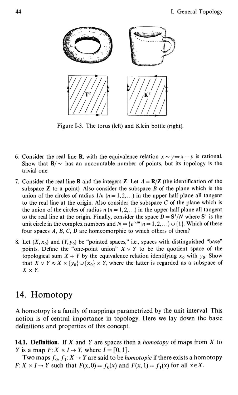
139
Editorial Board
J.H. Ewing F.W. Gehring P.R. Halmos

Graduate Texts in Mathematics
1 Takeuti/Zaring. Introduction to Axiomatic Set Theory. 2nd ed.
2 OXTOBY. Measure and Category. 2nd ed.
3 Schaeffer. Topological Vector Spaces.
4 Hilton/Stammbach. A Course in Homological Algebra.
5 Mac Lane. Categories for the Working Mathematician.
6 Hughes/Piper. Projective Planes.
7 SERRE. A Course in Arithmetic.
8 Takeuti/Zaring. Axiometic Set Theory.
9 Humphreys. Introduction to Lie Algebras and Representation Theory.
10 COHEN. A Course in Simple Homotopy Theory.
11 Conway. Functions of One Complex Variable. 2nd ed.
12 Beals. Advanced Mathematical Analysis.
13 Anderson/Fuller. Rings and Categories of Modules. 2nd ed.
14 GOLUBITSKY/GUILEMIN. Stable Mappings and Their Singularities.
15 Berberian. Lectures in Functional Analysis and Operator Theory.
16 Winter. The Structure of Fields.
17 Rosenblatt. Random Processes. 2nd ed.
18 HALMOS. Measure Theory.
19 Halmos. A Hilbert Space Problem Book. 2nd ed., revised.
20 HUSEMOLLER. Fibre Bundles. 2nd ed.
21 Humphreys. Linear Algebraic Groups.
22 Barnes/Mack. An Algebraic Introduction to Mathematical Logic.
23 GREUB. Linear Algebra. 4th ed.
24 HOLMES. Geometric Functional Analysis and Its Applications.
25 HEWITT/STROMBERG. Real and Abstract Analysis.
26 Manes. Algebraic Theories.
27 KELLEY. General Topology.
28 Zariski/Samuel. Commutative Algebra. Vol. I.
29 Zariski/Samuel. Commutative Algebra. Vol. II.
30 Jacobson. Lectures in Abstract Algebra I. Basic Concepts.
31 JACOBSON. Lectures in Abstract Algebra II. Linear Algebra.
32 JACOBSON. Lectures in Abstract Algebra III. Theory of Fields and Galois Theory.
33 Hirsch. Differential Topology.
34 Spitzer. Principles of Random Walk. 2nd ed.
35 WERMER. Banach Algebras and Several Complex Variables. 2nd ed.
36 Kelley/Namioka et al. Linear Topological Spaces.
37 Monk. Mathematical Logic.
38 Grauert/Fritzsche. Several Complex Variables.
39 ARVESON. An Invitation to C*-Algebras.
40 Kemeny/Snell/Knapp. Denumerable Markov Chains. 2nd ed.
41 APOSTOL. Modular Functions and Dirichlet Series in Number Theory. 2nd ed.
42 SERRE. Linear Representations of Finite Groups.
43 GILLMAN/JERISON. Rings of Continuous Functions.
44 Kendig. Elementary Algebraic Geometry.
45 LOEVE. Probability Theory I. 4th ed.
46 LOEVE. Probability Theory II. 4th ed.
47 MoiSE. Geometric Topology in Dimensions 2 and 3.
continued after index

Glen E. Bredon
Topology and Geometry
With 85 Illustrations
Springer-Verlag
New York Berlin Heidelberg London Paris
Tokyo Hong Kong Barcelona Budapest

Glen E. Bredon
Department of Mathematics
Rutgers University
New Brunswick, NJ 08903
USA
Editorial Board
J.H. Ewing F.W. Gehring P.R. Halmos
Department of Department of Department of
Mathematics Mathematics Mathematics
Indiana University University of Michigan Santa Clara University
Bloomington, IN 47405 Ann Arbor, MI 48109 Santa Clara, CA 95053
USA USA USA
Mathematics Subject Classification (1991): 55-01, 58A05
Library of Congress Cataloging-in-Publication Data
Bredon, Glen E.
Topology & geometry/Glen E. Bredon.
p. cm. — (Graduate texts in mathematics; 139)
Includes bibliographical references and indexes.
ISBN 3-540-97926-3.—ISBN 0-387-97926-3
1. Algebraic topology. I. Title. II. Title: Topology and
geometry. III. Series.
QA612.B74 1993
514'.2—dc20 92-31618
Printed on acid-free paper.
© 1993 Springer-Verlag New York, Inc.
All rights reserved. This work may not be translated or copied in whole or in part without the
written permission of the publisher (Springer-Verlag, 175 Fifth Avenue, New York, NY 10010,
USA), except for brief excerpts in connection with reviews or scholarly analysis. Use in
connection with any form of information storage and retrieval, electronic adaptation, computer
software, or by similar or dissimilar methodology now known or hereafter developed is forbidden.
The use of general descriptive names, trade names, trademarks, etc., in this publication, even if
the former are not especially identified, is not to be taken as a sign that such names, as
understood by the Trade Marks and Merchandise Marks Act, may accordingly be used freely by
anyone.
Production coordinated by Brian Howe and managed by Francine Sikorski; manufacturing
supervised by Vincent Scelta.
Typeset by Thomson Press (India) Ltd., New Delhi, India.
Printed and bound by R.R. Donnelley & Sons, Harrisonburg, Virginia.
Printed in the United States of America.
987654321
ISBN 0-387-97926-3 Springer-Verlag New York Berlin Heidelberg
ISBN 3-540-97926-3 Springer-Verlag Berlin Heidelberg New York

Preface
The golden age of mathematics—that was not
the age of Euclid, it is ours.
CJ. Keyser
This time of writing is the hundredth anniversary of the publication (1892)
of Poincare's first note on topology, which arguably marks the beginning
of the subject of algebraic, or "combinatorial," topology. There was earlier
scattered work by Euler, Listing (who coined the word "topology"), Mobius
and his band, Riemann, Klein, and Betti. Indeed, even as early as 1679, Leibniz
indicated the desirability of creating a geometry of the topological type. The
establishment of topology (or "analysis situs" as it was often called at the
time) as a coherent theory, however, belongs to Poincare.
Curiously, the beginning of general topology, also called "point set
topology," dates fourteen years later when Frechet published the first abstract
treatment of the subject in 1906.
Since the beginning of time, or at least the era of Archimedes, smooth
manifolds (curves, surfaces, mechanical configurations, the universe) have
been a central focus in mathematics. They have always been at the core of
interest in topology. After the seminal work of Milnor, Smale, and many
others, in the last half of this century, the topological aspects of smooth
manifolds, as distinct from the differential geometric aspects, became a subject
in its own right. While the major portion of this book is devoted to algebraic
topology, I attempt to give the reader some glimpses into the beautiful and
important realm of smooth manifolds along the way, and to instill the tenet
that the algebraic tools are primarily intended for the understanding of the
geometric world.
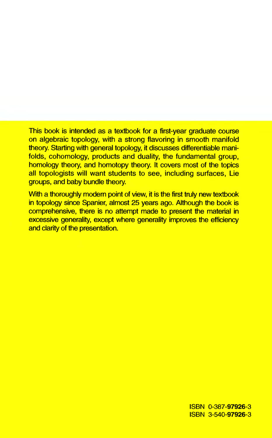
This book is intended as a textbook for a beginning (first-year graduate)
course in algebraic topology with a strong flavoring of smooth manifold
theory. The choice of topics represents the ideal (to the author) course.
In practice, however, most such courses would omit many of the subjects in
the book. I would expect that most such courses would assume previous
knowledge of general topology and so would skip that chapter, or be limited
v

VI
Preface
to a brief run-through of the more important parts of it. The section on
homotopy should be covered, however, at some point. I do not go deeply
into general topology, but I do believe that I cover the subject as completely
as a mathematics student needs unless he or she intends to specialize in that
area.
It is hoped that at least the introductory parts of the chapter on
differentiate manifolds will be covered. The first section on the Implicit
Function Theorem might best be consigned to individual reading. In practice,
however, I expect that chapter to be skipped in many cases with that material
assumed covered in another course in differential geometry, ideally concurrent.
With that possibility in mind, the book was structured so that that material
is not essential to the remainder of the book. Those results that use the
methods of smooth manifolds and that are crucial to other parts of the
book are given separate treatment by other methods. Such duplication is
not so large as to be consumptive of time, and, in any case, is desirable from
a pedagogic standpoint. Even the material on differential forms and
de Rham's Theorem in the chapter on cohomology could be omitted with
little impact on the other parts of the book. That would be a great shame,
however, since that material is of such interest on its own part as well as
serving as a motivation for the introduction of cohomology. The section on
the de Rham theory of CP" could, however, best be left to assigned reading.
Perhaps the main use of the material on dififerentiable manifolds is its impact
on examples and applications of algebraic topology.
As is common practice, the starred sections are those that could be omitted
with minimal impact on other nonstarred material, but the starring should
not be taken as a recommendation for that aim. In some cases, the starred
sections make more demands on mathematical maturity than the others and
may contain proofs that are more sketchy than those elsewhere.
This book is not intended as a source book. There is no attempt to present
material in the most general form, unless that entails no expense of time or
clarity. Exceptions are cases, such as the proof of de Rham's Theorem, where
generality actually improves both efficiency and clarity. Treatment of esoteric
byways is inappropriate in textbooks and introductory courses. Students are
unlikely to retain such material, and less likely to ever need it, if, indeed,
they absorb it in the first place.
As mentioned, some important results are given more than one proof, as
much for pedagogic reasons as for maintaining accessibility of results essential
to algebraic topology for those who choose to skip the geometric treatments
of those results. The Fundamental Theorem of Algebra is given no less than
four topological proofs (in illustration of various results). In places where
choice is necessary between competing approaches to a given topic, preference
has been given to the one that leads to the best understanding and intuition.
In the case of homology theory, I first introduce singular homology and
derive its simpler properties. Then the axioms of Eilenberg, Steenrod, and
Milnor are introduced and used exclusively to derive the computation of
the homology groups of cell complexes. I believe that doing this from the

Preface
Vll
axioms, without recourse to singular homology, leads to a better grasp of the
functorial nature of the subject. (It also provides a uniqueness proof gratis.)
This also leads quickly to the major applications of homology theory. After
that point, the difficult and technical parts of showing that singular homology
satisfies the axioms are dealt with.
Cohomology is introduced by first treating differential forms on manifolds,
introducing the de Rham cohomology and then linking it to singular
homology. This leads naturally to singular cohomology. After development
of the simple properties of singular cohomology, de Rham cohomology is
returned to and de Rham's famous theorem is proved. (This is one place
where treatment of a result in generality, for all differentiable manifolds and
not just compact ones, actually provides a simpler and cleaner approach.)
Appendix B contains brief background material on "naive" set theory.
The other appendices contain ancillary material referred to in the main text,
usually in reference to an inessential matter.
There is much more material in this book than can be covered in a one-year
course. Indeed, if everything is covered, there is enough for a two-year course.
As a suggestion for a one-year course, one could start with Chapter II,
assigning Section 1 as individual reading and then covering Sections 2 through
11. Then pick up Section 14 of Chapter I and continue with Chapter III,
Sections 1 through 8, and possibly Section 9. Then take Chapter IV except
for Section 12 and perhaps omitting some details about CW-complexes. Then
cover Chapter V except for the last three sections. Finally, Chapter VI can
be covered through Section 10. If there is time, coverage of Hopf's Theorem
in Section 11 of Chapter V is recommended. Alternatively to the coverage
of Chapter VI, one could cover as much of Chapter VII as is possible,
particularly if there is not sufficient time to reach the duality theorems of
Chapter VI.
Although I do make occasional historical remarks, I make no attempt at
thoroughness in that direction. An excellent history of the subject can be
found in Dieudonne [1]. That work is, in fact, much more than a history and
deserves to be in every topologist's library.
Most sections of the book end with a group of problems, which are
exercises for the reader. Some are harder, or require more "maturity," than
others and those are marked with a ♦. Problems marked with a <>- are those
whose results are used elsewhere in the main text of the book, explicitly or
implicitly.
Glen E. Bredon

Acknowledgments
It was perfect, it was rounded, symmetrical,
complete, colossal.
Mark Twain
Unlike the object of Mark Twain's enthusiasm, quoted above (and which
has no geometric connection despite the four geometric-topological
adjectives), this book is far from perfect. It is simply the best I could manage.
My deepest thanks go to Peter Landweber for reading the entire manuscript
and for making many corrections and suggestions. Antoni Kosinski also
provided some valuable assistance. I also thank the students in my course
on this material in the spring of 1992, and previous years, Jin-Yen Tai in
particular, for bringing a number of errors to my attention and for providing
some valuable pedagogic ideas.
Finally, I dedicate this book to the memory of Deane Montgomery in
deep appreciation for his long-term support of my work and of that of many
other mathematicians.
Glen E. Bredon
IX

Contents
Preface v
Acknowledgments ix
Chapter I
General Topology 1
1. Metric Spaces 1
2. Topological Spaces 3
3. Subspaces 8
4. Connectivity and Components 10
5. Separation Axioms 12
6. Nets (Moore-Smith Convergence) -Q- 14
7. Compactness 18
8. Products 22
9. Metric Spaces Again 25
10. Existence of Real Valued Functions 29
11. Locally Compact Spaces 31
12. Paracompact Spaces 35
13. Quotient Spaces 39
14. Homotopy 44
15. Topological Groups 51
16. Convex Bodies 56
17. The Baire Category Theorem 57
Chapter II
Differentiable Manifolds 63
1. The Implicit Function Theorem 63
2. Differentiable Manifolds 68
3. Local Coordinates 71
4. Induced Structures and Examples 72
xi

xii Contents
5. Tangent Vectors and Differentials 76
6. Sard's Theorem and Regular Values 80
7. Local Properties of Immersions and Submersions 82
8. Vector Fields and Flows 86
9. Tangent Bundles 88
10. Embedding in Euclidean Space 89
11. Tubular Neighborhoods and Approximations 92
12. Classical Lie Groups ft 101
13. Fiber Bundles ft 106
14. Induced Bundles and Whitney Sums ft Ill
15. Transversality ft 114
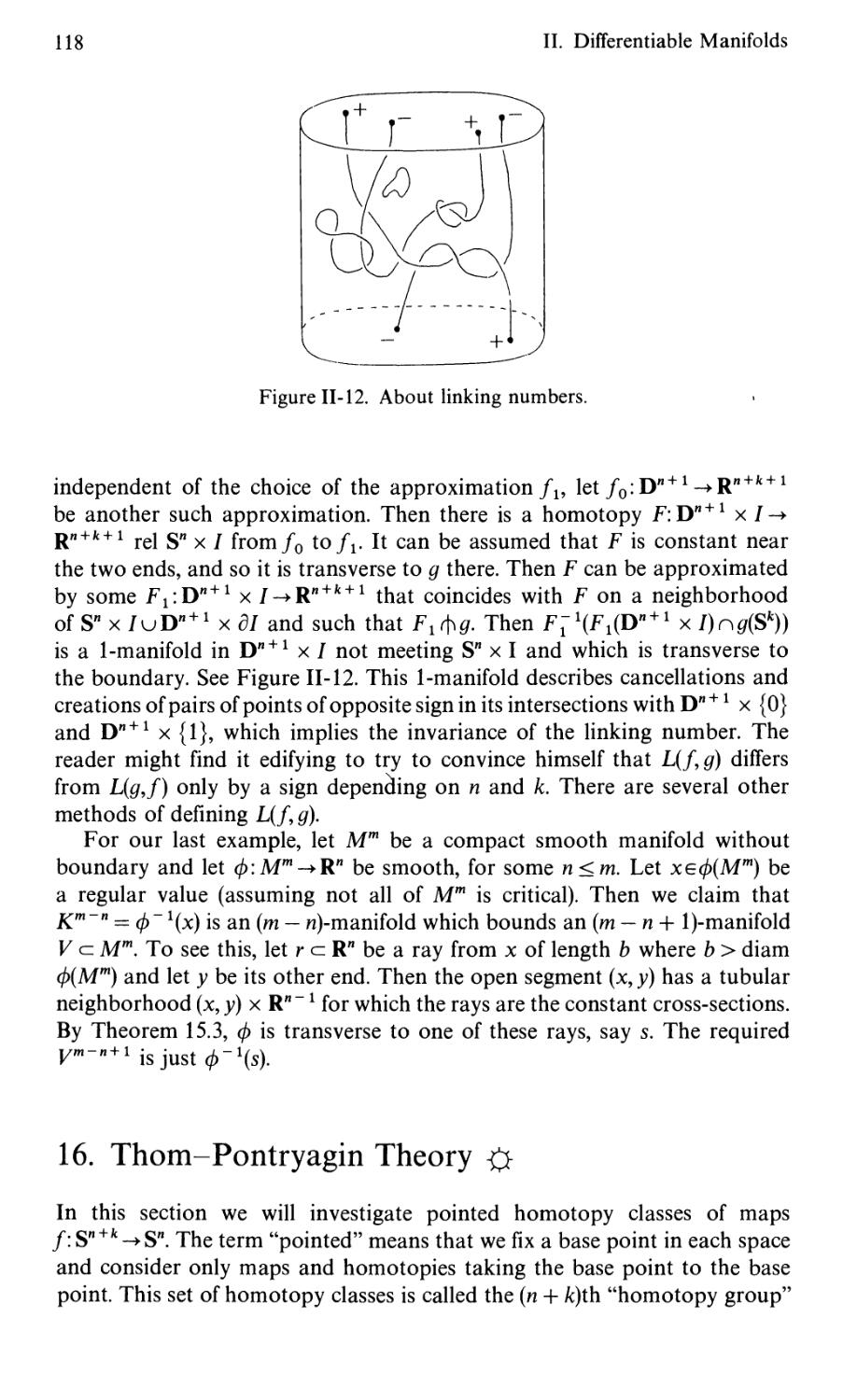
16. Thom-Pontryagin Theory ft 118
Chapter III
Fundamental Group 127
1. Homotopy Groups 127
2. The Fundamental Group 132
3. Covering Spaces 138
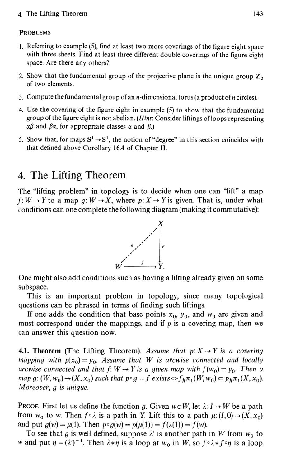
4. The Lifting Theorem 143
5. The Action of nl on the Fiber 146
6. Deck Transformations 147
7. Properly Discontinuous Actions 150
8. Classification of Covering Spaces 154
9. The Seifert-Van Kampen Theorem ft 158
10. Remarks on SO(3) ft 164
Chapter IV
Homology Theory 168
1. Homology Groups 168
2. The Zeroth Homology Group 172
3. The First Homology Group 172
4. Functorial Properties 175
5. Homological Algebra 177
6. Axioms for Homology 182
7. Computation of Degrees 190
8. CW-Complexes 194
9. Conventions for CW-Complexes 198
10. Cellular Homology 200
11. Cellular Maps 207
12. Products of CW-Complexes ft 211
13. Euler's Formula 215
14. Homology of Real Projective Space 217
15. Singular Homology 219
16. The Cross Product 220
17. Subdivision 223
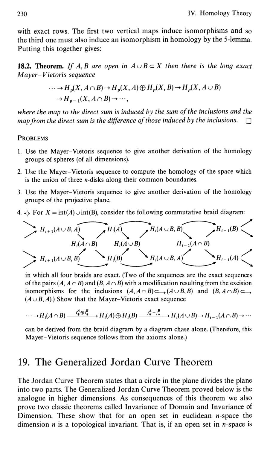
18. The Mayer-Vietoris Sequence 228
19. The Generalized Jordan Curve Theorem 230
20. The Borsuk-Ulam Theorem 240
21. Simplicial Complexes 245

Contents xiii
22. Simplicial Maps 250
23. The Lefschetz-Hopf Fixed Point Theorem 253
Chapter V
Cohomology 260
1. Multilinear Algebra 260
2. Differential Forms 261
3. Integration of Forms 265
4. Stokes' Theorem 267
5. Relationship to Singular Homology 269
6. More Homological Algebra 271
7. Universal Coefficient Theorems 281
8. Excision and Homotopy 285
9. de Rham's Theorem 286
10. The de Rham Theory of CPM #. 292
11. Hopf's Theorem on Maps to Spheres ■$. 297
12. Differential Forms on Compact Lie Groups -$ 304
Chapter VI
Products and Duality 315
1. The Cross Product and the Klinneth Theorem 315
2. A Sign Convention 321
3. The Cohomology Cross Product 321
4. The Cup Product 326
5. The Cap Product 334
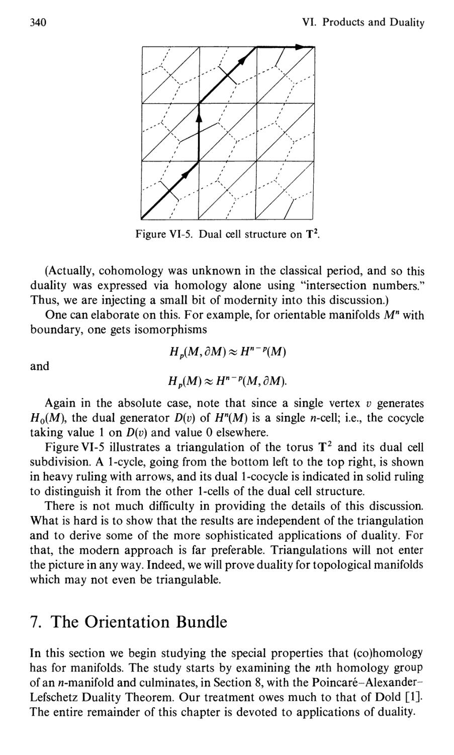
6. Classical Outlook on Duality $• 338
7. The Orientation Bundle 340
8. Duality Theorems 348
9. Duality on Compact Manifolds with Boundary 355
10. Applications of Duality 359
11. Intersection Theory ■£ 366
12. The Euler Class, Lefschetz Numbers, and Vector Fields #• 378
13. The Gysin Sequence ■$• 390
14. Lefschetz Coincidence Theory Q 393
15. Steenrod Operations ■$■ 404
16. Construction of the Steenrod Squares ty 412
17. Stiefel-Whitney Classes •# 420
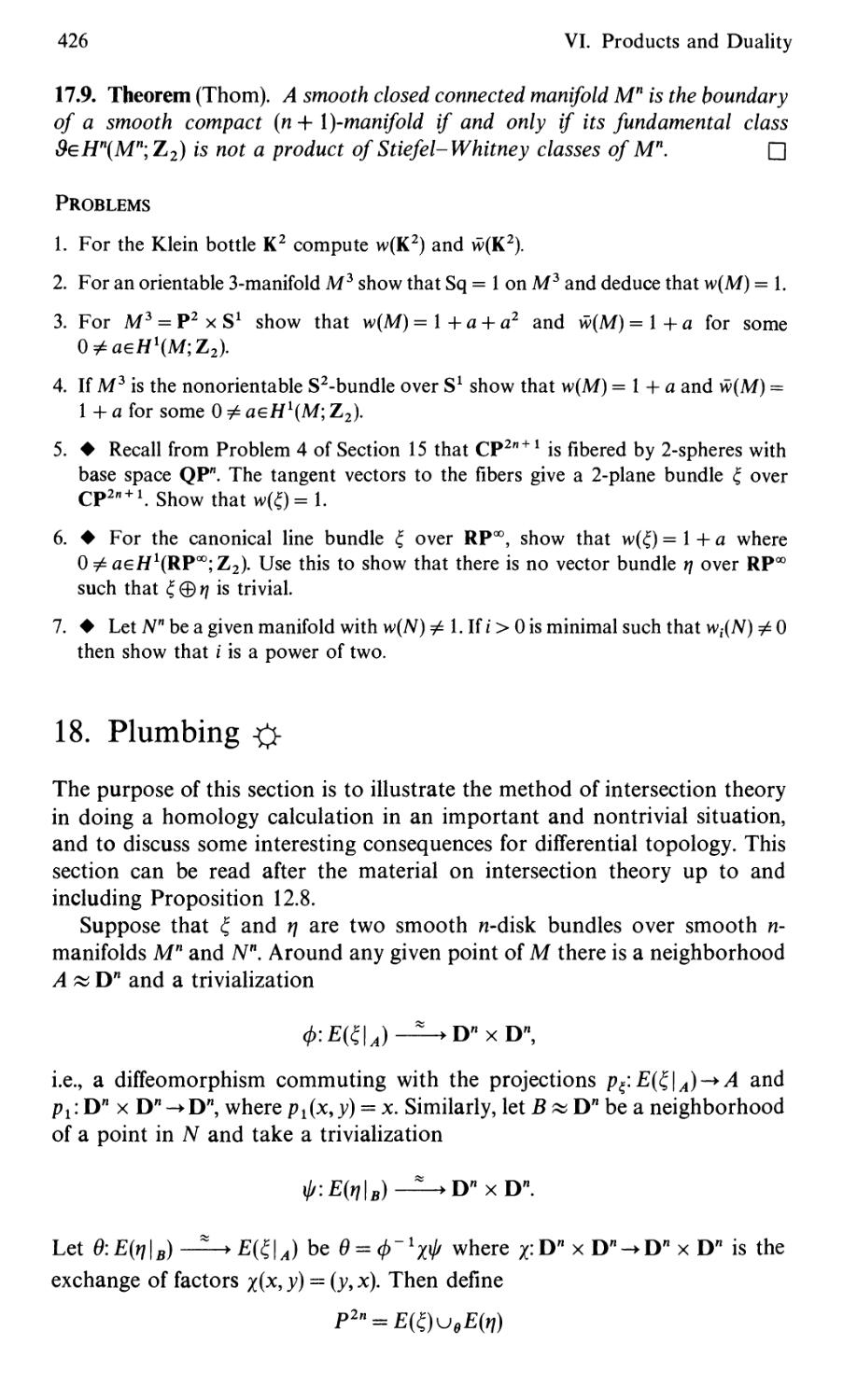
18. Plumbing # 426
Chapter VII
Homotopy Theory 430
1. Cofibrations 430
2. The Compact-Open Topology 437
3. H-Spaces, H-Groups, and H-Cogroups 441
4. Homotopy Groups 443
5. The Homotopy Sequence of a Pair 445
6. Fiber Spaces 450
7. Free Homotopy 457
8. Classical Groups and Associated Manifolds 463

xiv Contents
9. The Homotopy Addition Theorem 469
10. The Hurewicz Theorem 475
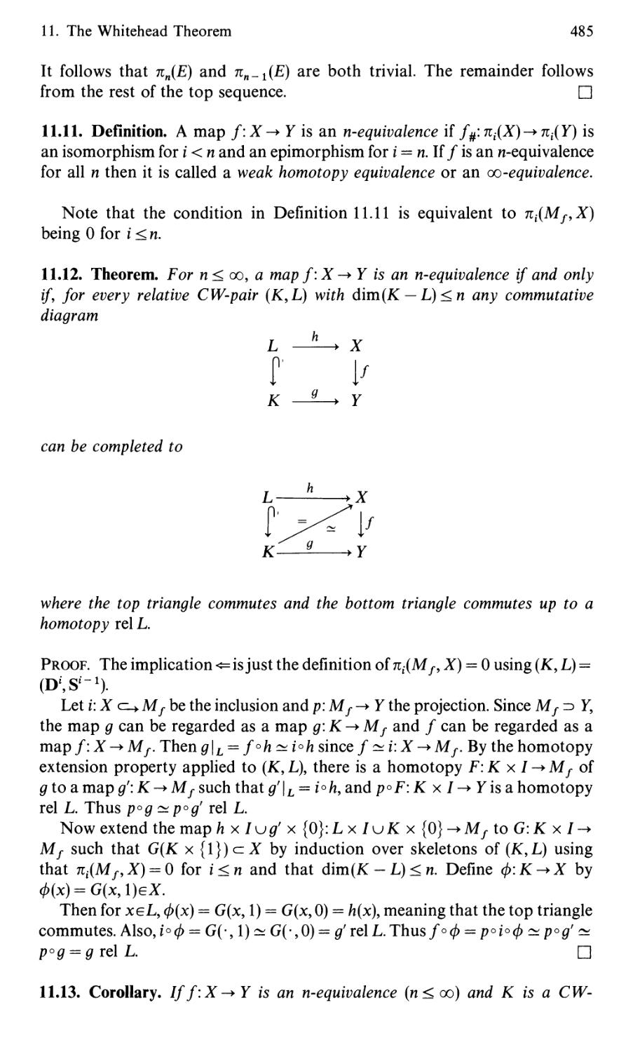
11. The Whitehead Theorem 480
12. Eilenberg-Mac Lane Spaces 488
13. Obstruction Theory # 497
14. Obstruction Cochains and Vector Bundles -$■ 511
Appendices
App. A. The Additivity Axiom 519
App. B. Background in Set Theory 522
App. C. Critical Values 531
App. D. Direct Limits 534
App. E. Euclidean Neighborhood Retracts 536
Bibliography 541
Index of Symbols 545
Index 549

CHAPTER I
General Topology
A round man cannot be expected to fit in a
square hole right away. He must have time to
modify his shape.
Mark Twain
1. Metric Spaces
We are all familiar with the notion of distance in euclidean n-space: If x and
y are points in R" then
dist(x,y) = f t(xt-;y,)2
This notion of distance permits the definition of continuity of functions from
one euclidean space to another by the usual e-S definition:
/: R"->Rk is continuous at xeR" if, given e > 0,
3d > 0adist(x,y) < S => dist(/(x),/(y)) < e.
Although the spaces of most interest to us in this book are subsets of euclidean
spaces, it is useful to generalize the notion of "space" to get away from such
a hypothesis, because it would be very complicated to try to verify that spaces
we construct are always of this type. In topology, the central notion is that
of continuity. Thus it would usually suffice for us to treat "spaces" for which
we can give a workable definition of continuity.
We could define continuity as above for any "space" which has a suitable
notion of distance. Such spaces are called "metric spaces."
1.1. Definition. A metric space is a set X together with a function
distil xX-+R,
called a metric, such that the following three laws are satisfied:
(1) (positivity) dist(x,y) > 0 with equality o x = y\
(2) (symmetry) dist(x,y) = dist(y,x); and
(3) (triangle inequality) dist(x,z) < dist(x,y) + dist(y,z).
1
1/2

2 I. General Topology
In a metric space X we define the "e-ball," e > 0, about a point xeX to be
B€(x) = {yeX\dist(x,y)<e}.
Also, a subset U aX is said to be "open" if, for each point xeU, there is
an €-ball about x completely contained in U. A subset is said to be "closed"
if its complement is open. If yeB€(x) and if S = e — dist(x,y) then Bd(y) c B€(x)
by the triangle inequality. This shows that all €-balls are open sets.
It turns out that, for metric spaces, continuity can be expressed completely
in terms of open sets:
1.2. Proposition. A function f:X-+Y between metric spaces is continuous o
f~l(U) is open in X for each open subset U of Y.
Proof. If / is continuous and U c Y is open and f(x)eU then there is an
€ > 0 such that B€(f(x)) c U. By continuity, there is a d > 0 such that / maps
the 5-ball about x into B€(f(x)). This means that Bs(x) c f~l(U). This implies
that f~l(U) is open.
Conversely, suppose f(x) = y and that e > 0 is given. By hypothesis,
f~1(B€(y)) is open and contains x. Therefore, by the definition of an open
set, there is a S > 0 such that ^(x) <=f~\B€(y)). It follows that if dist(x, x') < d
then f(x')eB€(y), and so dist(/(x),/(x')) <e, proving continuity in the e-d
sense. □
The only examples of metric spaces we have discussed are euclidean spaces
and, of course, subsets of those. Even with those, however, there are other
reasonable metrics:
n
dist2(x,y)= X \Xi-yil
i=l
dist3(x,y) = max(|x£-tt|).
It is not hard to verify, from the following proposition, that these three
metrics give the same open sets, and so behave identically with respect to
continuity (for maps into or out of them).
1.3. Proposition. If dist1 and dist2 are metrics on the same set X which satisfy
the hypothesis that for any point xeX and e > 0 there is a S>0 such that
dist1(x,y)<(5 => dist2(x,y) <€,
and
dist2(x,y)< S => dist1(x,y)<€,
then these metrics define the same open sets in X.
Proof. The proof is an easy exercise in the definition of open sets and is
left to the reader. □

2. Topological Spaces
3
Problems
1. Consider the set X of all continuous real valued functions on [0,1]. Show that
dist(/,0) =
\f(x)-g(x)\dx
defines a metric on X. Is this still the case if continuity is weakened to integrability?
2. -cj>- If X is a metric space and x0 is a given point in X, show that the function
f:X->R given by /(x) = dist(x,x0) is continuous.
3. -cj>-lf A is a subset of a metric space X then define a real valued function d on X
by d(x) = dist(x,y4) = inf{dist(x,y)|;ye,4}. Show that d is continuous. (Hint: Use the
triangle inequality to show that \d(xl) — d(x2)\ <dist(x1,x2).)
2. Topological Spaces
Although most of the spaces that will interest us in this book are metric
spaces, or can be given the structure of metric spaces, we will usually only
care about continuity of mappings and not the metrics themselves. Since
continuity can be expressed in terms of open sets alone, and since some
constructions of spaces of interest to us do not easily yield to construction
of metrics on them, it is very useful to discard the idea of metrics and to
abstract the basic properties of open sets needed to talk about continuity.
This leads us to the notion of a general "topological space."
2.1. Definition. A topological space is a set X together with a collection of
subsets of X called "open" sets such that:
(1) the intersection of two open sets is open;
(2) the union of any collection of open sets is open; and
(3) the empty set 0 and whole space X are open.
Additionally, a subset C c X is called "closed" if its complement X — C is
open.
Topological spaces are much more general than metric spaces and the
range of difference between them and metric spaces is much wider than that
between metric spaces and subspaces of euclidean space. For example, it is
possible to talk about convergence of sequences of points in metric spaces
with little difference from sequences of real numbers. Continuity of functions
can be described in terms of convergence of sequences in metric spaces. One
can also talk about convergence of sequences in general topological spaces
but that no longer is adequate to describe continuity (as we shall see later).
Thus it is necessary to exercise care in developing the theory of general
topological spaces. We now begin that development, starting with some
further basic definitions.

4
I. General Topology
2.2. Definition. If X and Y are topological spaces and/: X -► Y is a function,
then / is said to be continuous if f~l{U) is open for each open set U czY.
A map is a continuous function.
Since closed sets are just the complements of open sets and since inverse
images preserve complements (i.e., f~1(Y — B) = X — f~ 1(B)), it follows that
a function f:X-+Y is continuousof~l(F) is closed for each closed set
Fez Y.
2.3. Definition. If X is a topological space and xeX then a set N is called
a neighborhood of x in X if there is an open set U a N with xeU.
Note that a neighborhood is not necessarily an open set, and, even though
one usually thinks of a neighborhood as "small," it need not be: the entire
space X is a neighborhood of each of its points.
Note that the intersection of any two neighborhoods of x in X is a
neighborhood of x, which follows from the axiom that the intersection of
two open sets is open.
The intuitive notion of "smallness" of a neighborhood is given by the
concept of a neighborhood basis at a point:
2.4. Definition. If X is a topological space and xeX then a collection Bx of
subsets of X containing x is called a neighborhood basis at x in X if each
neighborhood of x in X contains some element of Bx and each element of Bx
is a neighborhood of x.
Neighborhood bases are sometimes convenient in proving functions to be
continuous:
2.5. Definition. A function f:X-+Y between topological spaces is said to
be continuous at x, where xeX, if, given any neighborhood N of /(x) in Y,
there is a neighborhood M of x in X such that f(M) c N.
Since f{f~l{N))aN, this is the same as saying that f~1(N) is a
neighborhood of x, for each neighborhood N of f(x). Clearly, this need only
be checked for N belonging to some neighborhood basis at /(x).
2.6. Proposition. A function f:X-+Y between topological spaces is
continuous<=> it is continuous at each point xeX.
Proof. Suppose that / is continuous, i.e., that /" 1(U) is open for each open
U czY. Let N be a neighborhood of /(x) in Y and let U be an open set such
that f(x)eU aN as guaranteed by the definition of neighborhood. Then
xef-l(U)cf-\N) and f~\U) is open. It follows that f~\N) is a
neighborhood of x. Thus / is continuous at x.

2. Topological Spaces
5
Conversely, suppose that / is continuous at each point and let U c Y be
an open set. For any xef~l(U\ f~l{U) is then a neighborhood of x. Thus
there exists an open set Vx in X with xeVx af~l(U). Hence f~l{U) is the
union of the sets Vx for x ranging over f~l(U). Since the union of any
collection of open sets is open, it follows that /" l(U) is open. But U was an
arbitrary open set in Y and, consequently, / is continuous. □
2.7. Definition. A function f:X-+Y between topological spaces is called a
homeomorphism if f~l:Y-+X exists (i.e., / is one-one and onto) and
both / and f~l are continuous. The notation X&Y means that X is
homeomorphic to Y.
Two topological spaces are, then, homeomorphic if there is a one-one
correspondence between them as sets which also makes the open sets
correspond. Homeomorphic spaces are considered as essentially the same.
One of the main problems in topology is to find methods of deciding when
two spaces are homeomorphic or not.
To describe a topological space it is not necessary to describe completely
the open sets. This can often be done more simply using the notion of a
"basis" for the topology:
2.8. Definition. If X is a topological space and B is a collection of subsets
of X, then B is called a basis for the topology of X if the open sets are
precisely the unions of members of B. (In particular, the members of B are
open.) A collection S of subsets of X is called a subbasis for the topology of
X if the set B of finite intersections of members of S is a basis.
Note that any collection S of subsets of any set X is a subbasis for some
topology on X, namely, the topology for which the open sets are the arbitrary
unions of the finite intersections of members of S. (The empty set and whole
set X are taken care of by the convention that an intersection of an empty
collection of sets is the whole set and the union of an empty collection of
sets is the empty set.) Thus, to define a topology, it suffices to specify some
collection of sets as a subbasis. The resulting topology is called the topology
"generated" by this subbasis.
In a metric space the collection of €-balls, for all € > 0, is a basis, So is
the collection of €-balls for € = 1, \, |,
Here are some examples of topological spaces:
1. (Trivial topology.) Any set X with only the empty set and the whole set
X as open.
2. (Discrete topology.) Any set X with all subsets being open.
3. Any set X with open sets being those subsets of X whose complements
are finite, together with the empty set. (That is, the closed sets are finite
sets and X itself.)

6
I. General Topology
4. X = cou{co} with the open sets being all subsets of co together with
complements of finite sets. (Here, co denotes the set of natural numbers.)
5. Let X be any partially ordered set. For aeX consider the one-sided
intervals {/?eX|a</?} and {jieX\a> /?}. The "order topology" on X is
the topology generated by these intervals. The "strong order topology" is
the topology generated by these intervals together with the complements
of finite sets.
6. Let X = I x I where / is the unit interval [0,1]. Give this the "dictionary
ordering," i.e., (x,y) < (s, £)<=> either x<sor(x = s and y < t). Let X have
the order topology for this ordering.
7. Let X be the real line but with the topology generated by the "half open
intervals" [x,y). This is called the "half open interval topology."
8. Let X = Qu{Q} be the set of ordinal numbers up to and including the
least uncountable ordinal Q; see Theorem B.28. Give it the order topology,
2.9. Definition. A topological space is said to be first countable if each point
has a countable neighborhood basis.
2.10. Definition. A topological space is said to be second countable if its
topology has a countable basis.
Note that all metric spaces are first countable. Some metric spaces are
not second countable, e.g., the space consisting of any uncountable set with
the metric dist(x,y) =1 if x / y, and dist(x,x) = 0 (which yields the discrete
topology).
Euclidean spaces are second countable since the €-balls, with e rational,
about the points with all rational coordinates, is easily seen to be a basis.
2.11. Definition. A sequence /i,/2»--- of functions from a topological space
X to a metric space Y is said to converge uniformly to a function f:X-+Y
if, for each e > 0, there is a number n such that i>n=>dist(/)(x), f(x)) < e for
all xeX.
2.12. Theorem. // a sequence fi,f2,-; of continuous functions from a
topological space X to a metric space Y converges uniformly to a function
f\X -> 7, then f is continuous.
Proof. Given e > 0, let n0 be such that
n > n0 => dist(/(x),/„(x)) < e/3 for all xeX.
Given a point x0, the continuity of fno implies that there is a neighborhood
N of x0 such that xeN => dist(/„0(x),/„0(x0)) < e/3. Thus, for any xeiVwe have
dist(/(x),/(x0)) < dist(/(x),/„0(x)) + dist(/„0(x),/„0(x0)) + dist(/BO(xo),/(x0))
< 6/3+6/3 + 6/3 = 6. □

2. Topological Spaces
7
2.13. Definition. A function f:X->Y between topological spaces is said to
be open if f(U) is open in Y for all open U c X. It is said to be closed if/(C)
is closed in Y for all closed Ccl
2.14. Definition. If X is a set and some condition is given on subsets of X
which may or may not hold for any particular subset, then if there is a
topology T whose open sets satisfy the condition, and such that, for any
topology T whose open sets satisfy the condition, then the T-open sets are
also T'-open (i.e., T c T'), then T is called the smallest (or weakest or coarsest)
topology satisfying the condition. If, instead, for any topology T whose open
sets satisfy the condition, any T'-open sets are also T-open, then T is called
the largest (or strongest or finest) topology satisfying the condition.
The terms "weak" and "strong" are the oldest historically. However, they
are used in some places to mean the opposite of the above meaning in general
topology. Even some topology books disagree on their meaning. For this
reason, the terms "coarse" and "fine" were introduced to rectify the confusion.
They are metaphors for thinking of open sets as grains in a rock (the fewer
grains, the coarser the rock). The terms "smallest" and "largest" were
introduced for the same reason, and they are mathematically more precise
as applied to the topologies as collections of open sets. We prefer the latter
terms in general.
For example (see Section 13), if/: X -> Y is a function and X is a topological
space, then there is a largest topology on Y making / continuous, namely
that topology having open sets {V c Y\f~l(V) is open in X}. There is also
a smallest such topology, the trivial topology, but it is not very interesting.
Also see Sections 8 and 13 for other examples of this concept.
If a topology is the largest one satisfying some given condition then usually
(in fact, always) there is another condition for which the given topology is
the smallest one satisfying the new condition. For example, the topology on
Y, in the example of the previous paragraph, is the smallest topology satisfying
the condition "for all spaces Z and all functions g:Y-+Z,g°f continuous => g
continuous." Thus it is meaningless to argue whether a given topology is
"weak" or "strong," etc., unless the defining condition is specified.
Problems
1. -cj>- Show that in a topological space X:
(a) the union of two closed sets is closed;
(b) the intersection of any collection of closed sets is closed; and
(c) the empty set 0 and whole space X are closed.
2. Consider the topology on the real line generated by the half open intervals [x, y)
together with those of the form (x, y]. Show that this coincides with the discrete
topology.
3. Show that the space Qu{Q} in the order topology cannot be given a metric
consistent with its topology.

8
I. General Topology
4. -^ If f:X^ Y is a function between topological spaces, and / l(U) is open for
each open U in some subbasis for the topology of 7, show that / is continuous.
5. -ty Suppose that S is a set and that we are given, for each xeS, a collection N(x)
of subsets of S satisfying:
(1) iVeN(x)=>x£iV;
(2) N,MeN(x)=>3PeN(x)9PczNnM;and
(3) xeS=>N(x)^0.
Then show that there is a unique topology on S such that N(x) is a neighborhood
basis at x, for each xeS. (Thus a topology can be defined by the specification of
such a collection of neighborhoods at each point.)
3. Subspaces
There are several techniques for producing new topological spaces out of old
ones. The simplest is the passing to a "subspace," which is merely an arbitrary
subset inheriting a topology from the mother space in a quite natural
way.
3.1. Definition. If X is a topological space and A c X then the relative
topology or the subspace topology on A is the collection of intersections of
A with open sets of X. With this topology, A is called a subspace of X.
The following propositions are all easy consequences of the definitions
and the proofs are left to the reader:
3.2. Proposition. // Y is a subspace of X then AczY is closed in Y <=> A =
YnB for some closed subset B of X. □
3.3. Proposition. IfX is a topological space and A c X then there is a largest
open set U with U a A. This set is called the "interior" of A in X and is
denoted by int(^). □
3.4. Proposition. IfX is a topological space and A a X then there is a smallest
closed set F with A a F c X. This set is called the "closure" of A in X and
is denoted by A. □
If we need to specify the space in which a closure is taken (the X), we
shall use the notation Ax. A consequence of the following fact is that this
notation need not be used very often:
3.5. Proposition. If AaYaX then AY = Axn Y. Thus, if Y is closed in X
then AY = Ax. □
3.6. Definition. If X is a topological space and AczX then the boundary or
frontier of A is defined to be dA = bdry(^) = Ar\X — A.

3. Subspaces
9
3.7. Proposition. If Y aX then the set of intersections of Y with members of
a basis of X is a basis of the relative topology of Y. □
3.8. Proposition. // X, Y, Z are topological spaces and Y is a subspace of X
and Z is a subspace of 7, then Z is a subspace of X. □
3.9. Proposition. // X is a metric space and A c X then A coincides with the
set of limits in X of sequences of points in A.
Proof. If x is the limit of a sequence of points in A then any open set about
x contains a point of A. Thus x^int(X — A). Since X — int(X — A) = A (see
the problems at the end of this section), xeA. Conversely, if xeA and n > 0
is any integer, then Bl/n(x) must contain a point in A because otherwise x
would lie in int(X — A). Take one such point and name it xn. Then it follows
immediately that x = lim(x„) is a limit of a sequence of points in A. □
3.10. Definition. A subset A of a topological space X is called dense in X if
A = X. A subset A is said to be nowhere dense in X if int(^) = 0.
Problems
1. -cj)- Let X be a topological space and A,B<^X.
(a) Show that
int(y4) = {aeX|3l/open9ae£/cz,4}
and
y4 = {xeX|Vl/open with xeU, UnA # 0}.
(b) Show that A is open<=>^4 = 'mt(A) and that A is closed o A — A.
(c) Show that X - m\(A) = X -A and that X-A = int(X - A).
(d) Show that 'mt(AnB) = int(i4)nint(B) and that AuB = AuB.
(e) Show that
fl int(/i.) => int( H /ij = int(f| int(/ij),
[]Aa<= closure( \J Aa) = closure( (J ^J,
Uint(yUcint(U>U,
(Va=> closure(f]Aa\
and give examples showing that these inclusions need not be equalities.
(f) Show A cz B => [A cz B and int(yl) c int(B)].
2. -<{)- For y4 czX, a topological space, show that X is the disjoint union of int(A\
bdry(y4), and X - A
3. -(J> Show that a metric space is second countable o it has a countable dense set
(a countable set whose closure is the whole space). (Such a metric space is called
"separable.")

10
I. General Topology
4. -<J> Show that the union of two nowhere dense sets is nowhere dense.
5. A topological space X is said to be "irreducible" if, whenever X = FkjG with F
and G closed, then either X = F or X = G. A subspace is irreducible if it is so in
the subspace topology. Show that if X is irreducible and U cz X is open, then U
is irreducible.
6. A "Zariski space" is a topological space with the property that every descending
chain Fr =5 F2 => F3 =5 ••• of closed sets is eventually constant. Show that every
Zariski space can be expressed as a finite union X — ^u^u-uy, where the
Yt are closed and irreducible and Yt <£ Y} for i ^j. Also show that this decomposition
is unique up to order.
7. Let X be the real line with the topology for which the open sets are 0 together
with the complements of finite subsets. Show that X is an irreducible Zariski space.
8. -cj> Let X — Au£, where A and B are closed. Let f:X->Y be a function. If the
restrictions off to A and B are both continuous then show that / is continuous.
4. Connectivity and Components
In a naively intuitive sense, a connected space is a space in which one can
move from any point to any other point without jumps. Another way to
view it intuitively is as the idea that the space does not fall into two or
more pieces which are separated from one another. There are two ways
of making these crude ideas precise and both of them will be important
to us. One of them, called "connectivity," is the subject of this section,
while the other, called "arcwise connectivity," is taken up in the problems
at the end.
4.1. Definition. A topological space X is called connected if it is not the
disjoint union of two nonempty open subsets.
4.2. Definition. A subset A of a topological space X is called clopen if it is
both open and closed in X.
4.3. Proposition. A topological space X is connected <=> its only clopen subsets
are X and 0. □
4.4. Definition. A discrete valued map is a map (continuous) from a
topological space X to a discrete space D.
4.5. Proposition. A topological space X is connected <=> every discrete valued
map on X is constant.
Proof. If X is connected and d: X -► D is a discrete valued map and if yeD
is in the range of rf, then d~l(y) is clopen and nonempty and so must equal
X, and so d is constant with only value y.

4. Connectivity and Components
11
Conversely, if X is not connected then X = U u V for some disjoint clopen
sets U and V. Then the map d: X -► {0,1} which is 0 on U and is 1 on V is
a nonconstant discrete valued map. □
4.6. Proposition. ///: X -+ Y is continuous and X is connected, then f(X) is
connected.
Proof. Let d:f(X)-+D be a discrete valued map. Then rf°/ is a discrete
valued map on X and hence must be constant. But that implies that d is
constant, and hence that f(X) is connected. □
4.7. Proposition. If{Y{} is a collection of connected sets in a topological space
X and if no two of the YL are disjoint, then (J Yt is connected.
Proof. Let d: (J Yt -> D be a discrete valued map. Let p, q be any two points
in \J Y{. Suppose pe Yt and qe Yj and re Yt n Y}. Then, since d must be constant
on each Yh we have d(p) = d(r) = d(q). But p and q were completely arbitrary.
Thus d is constant. □
4.8. Corollary. The relation "p and q belong to a connected subset of X9' is
an equivalence relation. □
4.9. Definition. The equivalence classes of the equivalence relation in
Corollary 4.8 are called the components of X.
4.10. Proposition. Components of space X are connected and closed. Each
connected set is contained in a component. (Thus the components are "maximal
connected subsets.") Components are either equal or disjoint, and fill out X.
Proof. The last statement follows from the fact that the components are
equivalence classes of an equivalence relation. By definition, the component
of X containing p is the union of all connected sets containing p, and that
is connected by Proposition 4.7. This also implies that a connected set lies
in a component. That a component is closed follows from the fact that the
closure of a connected set is connected (left to the reader in the problems
below). □
4.11. Proposition. The statement "d(p) = d(q) for every discrete valued map d
on X" is an equivalence relation. □
4.12. Definition. The equivalence classes of the relation in Proposition 4.11
are called the quasi-components of X.
4.13. Proposition. Quasi-components of a space X are closed. Each connected
set is contained in a quasi-component. (In particular, each component is
contained in a quasi-component.) Quasi-components are either equal or disjoint,
and fill out X.

12 I. General Topology
Proof. If peX then the quasi-component containing it is just
{qeX\d(q) = d(p) for all discrete valued mapsrf}.
But this is
(~){d~1(d(p))\d a discrete valued map}
which is an intersection of closed sets and hence is closed. The rest is obvious.
□
Problems
1. <J> If A is a connected subset of the topological space X and if A cz B cz A then
show that B is connected.
2. -cj> A space X is said to be "locally connected" if for each xeX and each
neighborhood N of x, there is a connected neighborhood V of x with V cz N.
If X is locally connected, show that its components are open and equal its
quasi-components.
3. -fy Show that the unit interval [0,1] in the real number is connected. (Hint: Assume
that [0,1] = UuV9 where U and V are disjoint nonempty open sets, and \eV.
Consider x = sup(£/). Show that x < 1 and derive a contradiction.)
4. Consider the subspace X of the unit square in the plane consisting of the vertical
line segments {1/w} x [0,1] for w= 1,2,3,..., and the two points (0,0) and (0,1).
Show that the latter two points are components of X but not quasi-components.
Show that the two point set {(0,0), (0,1)} is a quasi-component which is not
connected.
5. <J> A topological space X is said to be "arcwise connected" if for any two points
p and q in X there exists a map X: [0,1] -+X with A(0) = p and A(l) = q. A space
X is "locally arcwise connected" if every neighborhood of any point contains an
arcwise connected neighborhood. An "arc component" is a maximal arcwise
connected subset. Show that:
(a) an arcwise connected space is connected;
(b) a space is the disjoint union of its arc components;
(c) an arc component of a space is contained in some component;
(d) the arc components of a locally arcwise connected space are clopen, and
coincide with the components;
(e) the space with exactly two points p and q and open sets 0, {p}, {p,q} (only)
is arcwise connected; and
(f) the subspace of the plane consisting of {0} x [ - 1,1] u {(x, sin(l/x))|x > 0} is
connected but not arcwise connected.
5. Separation Axioms
The axioms defining a topological space are extremely general and weak. It
should be no surprise that most spaces of interest will have further restrictions
on them. We refer here not to structures like a metric, but to conditions

5. Separation Axioms
13
completely describable in terms of the topology itself, i.e., in terms of the
points and open sets. We begin with the so-called separation axioms.
5.1. Definition. The separation axioms:
(T0) A topological space X is called a T0-space if for any two points x^y
there is an open set containing one of them but not the other.
(Tx) A topological space X is called a Trspace if for any two points x^y
there is an open set containing x but not y and another open set
containing y but not x.
(T2) A topological space X is called a T2-space or Hausdorff if for any two
points x^y there are disjoint open sets U and V with xe U and ye V.
(T3) A Tx-space X is called a T3-space or regular if for any point x and closed
set F not containing x there are disjoint open sets U and V with xeU
and F czV.
(T4) A Trspace X is called a T4-space or normal if for any two disjoint
closed sets F and G there are disjoint open sets U and V with F aU
and GcK.
Axiom T0 simply says that points can be distinguished by the open sets
in which they lie.
Axiom T1 is the same as saying that one-point sets (singletons) are closed
sets, because if we single out a point x and, for each different point y we
take Uy to be an open set containing y but not x, then X — {x} = [j Uy is the
union of open sets and so is open. Conversely, if {x} is closed then the open
set X — {x} can be taken, in the axiom, as the open set containing any other
point.
Axiom T2 is the most important of these axioms and will be assumed in
the majority of the text of this book. We shall see later that it essentially
means that "limits" are unique.
5.2. Proposition. A Hausdorff space is regular <=> the closed neighborhoods of
any point form a neighborhood basis of the point.
Proof. Suppose that X is regular, let xe K, with V open, and put C = X — V.
By regularity there are open sets U9 W9 with xeU, C aW, and U nW = 0.
Then X — W is closed, and we have X — W aX — C=V, so any neighborhood
V of x contains a closed neighborhood X — W of x, as was to be shown.
Conversely, suppose that every point has a closed neighborhood basis.
Let x<£C with C closed and put V = X — C. By the assumption, there is
an open set U with U aV = X -C and xeU. Then CaX-U, and
Un(X -U) = 0. Thus X is regular. □
5.3. Corollary. A subspace of a regular space is regular.
Proof. If A c X is a subspace, just intersect a closed neighborhood basis in

14
I. General Topology
X of a point aeA with A and you get a closed neighborhood basis of a
in A. □
Problems
1. Give an example of a space that is not T0, and an example of a T0-space that
is not Tt. (/fmf: Spaces with only two points suffice.)
2. Show that a finite T{-space is discrete.
3. Consider the set to of natural numbers together with two other points named x9y.
Put a partial ordering on this set which orders co as usual and makes both x and
y greater than any integer, but does not order x against y. Give this the strong
order topology. Show it is Tx but not Hausdorff.
4. Consider the space X whose point set is the plane but whose open sets are given
by the basis consisting of the usual open sets in the plane together with the sets
{(x,)0|x2 + ;K2<a,.y^O}u{(O,O)} for all a>0. Show that X is Hausdorff but
not regular.
5. -fy Show that a subspace of a Hausdorff space is Hausdorff.
6. <J>- Show that a Hausdorff space is normal <=> for any sets U open and C closed
with C c U there is an open set V with C cz V cz V cz U.
7. Show that there is a smallest topology on the real numbers such that every singleton
is closed. Which of the separation axioms does it satisfy?
8. Show that if a Zariski space (see Section 3, Problem 6) is Hausdorff then it is finite.
9. ♦ -(J)- Show that a metric space is normal.
6. Nets (Moore-Smith Convergence) ^
In metric spaces continuity of functions can be expressed in terms of the
convergence of sequences. This is not true in general topological spaces.
However, there is a generalization of sequences that does work and permits
proofs of some things analogously to proofs using sequences in metric spaces.
This can be of great help to the intuition. The generalization of a sequence
is called a net, and we will develop this subject in this section. Although we
will use this concept in proving a couple of important results in subsequent
sections, those results will not be used in the main body of the book,
and for that reason, this section can be skipped without serious harm to
subsequent developments.
6.1. Deflnition. A directed set D is a partially ordered set such that, for any
two elements a and /? of D, there is a teD with t > a and t > /?.
6.2. Deflnition. A net in a topological space X is a directed set D together
with a function O: D -> X.

6. Nets (Moore-Smith Convergence)
15
Note that a sequence is simply a net based on the natural numbers as
indexing set.
6.3. Definition. If O: D -> X is a net in the topological space X and A a X
then we say that O is frequently in ^ if for any aeD there is a /? > a such
that 0(/?)eA It is said to be eventually in ^ if there is an aeD such that
<b{p)eA for all j8 > a.
6.4. Definition. A net <t>: D -+ X in a topological space is said to converge to
xeX if, for every neighborhood £/ c X of x, 0 is eventually in U.
Note that if a net O is eventually in two sets U and V then it is eventually
in Ur\V. Also, this is impossible if U n V = 0. This proves half of the
following fact. The remainder of the proof constructs a net which is typical
of the nets encountered with general topological spaces.
6.5. Proposition. A topological space X is Hausdorff <=> any two limits of any
convergent net are equal. (Thus one can speak o/the limit of a net in such a
space.)
Proof. The implication => follows from the preceding discussion. Thus
suppose that X is not Hausdorff, and that x,yeX are two points which
cannot be separated by open sets. Consider the directed set whose elements
are ordered pairs a = <£/, V} of open sets where xeU and yeV with the
ordering <£/, V) > (A9B)o(U c A and VaB). For any a = <£/,K>, let
0(a) be some point in U n V. This defines a net 0 which we claim converges
to both x and y.
To see this, let W be any neighborhood of x. We claim that 0 is eventually
in W. In fact, take any open set V containing y and an open set U with
xet/c Wand let a = (U,V). If j8 = (A,B) > a then A c U and B c K so
that 0(/?)e,4n£ c [/ c ^, as claimed. Thus 0 converges to x. Similarly, it
converges to y. □
Next we show that nets are "sufficient" to describe continuity.
6.6. Proposition. A function f:X-+Y between two topological spaces is
continuous<=> for every net <t> in X converging to xeX, the net /°$ in Y
converges to f(x).
Proof. First suppose that / is continuous and let O be a net in X converging
to x. Let V be any open set in Y containing f(x) and put U = f~ l(V), which
is a neighborhood of x. By definition of convergence, 0 is eventually in U,
and so /°0 is eventually in V, and thus converges to f(x).
Conversely, suppose that / is not continuous. Then there is an open set
VczY such that K=f~\V) is not open. Let xeK-int(K). Consider the
directed set consisting of open neighborhoods of x ordered by inclusion, i.e.,

16
I. General Topology
A < B means A=> B. For any such neighborhood A of x, A cannot be
completely inside K, so we can choose a point wAeA — K. Define the net 0
by putting <&(A) = wA. If N is any neighborhood of x and if B > N (i.e., B a N)
then Q>(B) = wBeB- KaN, showing that 0 is eventually in N. Thus 0
converges to x. However (f°<t>)(A)<£ V, for any A, so that /°0 is not eventually
in V, and thus does not converge to f(x). □
Given a particular net <t>: D -> X let xa = 0(a), for aeD. Then it is common
to speak of {xa} as being the net in question. This notation makes discussion
of nets similar to the notation commonly used with sequences. For example,
one can phrase the condition in Proposition 6.6 as
/(limxa) = lim(/(xa)).
6.7. Proposition. If AczX then A coincides with the set of limits of nets in A
which converge in X.
Proof. If xeA then any open neighborhood U of x must intersect A
nontrivially. Thus we can base a net on this set of neighborhoods, ordered
by inclusion and such points xveUnA. This clearly converges to x.
Conversely, if {xa} is any net of points in A which converges to a point xeX
then, by definition, this net is eventually in any given neighborhood of x.
Thus any neighborhood of x contains a point in A and so xeA (Here we
are using Problem 1(a) of Section 3.) □
In the case of ordinary sequences, a subsequence can be thought of
in two different ways: (1) by discarding elements of the sequence and
renumbering, or (2) by composing the sequence, thought of as a function
Z+->X, with a function /z:Z+->Z + , such that i > j => h{i) > h(j). The first
of these turns out to be inadequate for nets in general spaces. For the second
method, a little thought should convince the reader that the last condition
of monotonicity of h is stronger than is necessary for the usual uses of
subsequences. Modifying it leads to the more general notion of a "subnet,"
which we now define.
6.8. Definition. If D and D' are directed sets and h: D' -+ D is a function, then
h is called final if, VSeD, 38'eD'3(<x' >d'=> ft(a') > d).
6.9. Definition. A subnet of a net fi:D-+X, is the composition {i°h of \i with
a final function h: D' -+ D.
6.10. Proposition. A net {xa} is frequently in each neighborhood of a given
point xeXoit has a subnet which converges to x.
Proof. Consider the directed set D' consisting of ordered pairs (a, U) where
aeD, U is a neighborhood of x, and xaeU, ordered by the D ordering and

6. Nets (Moore-Smith Convergence)
17
inclusion. If (a, U) and (/?, V) are in D' then, since {xa} is frequently in U n V,
there is a y > a, /? with xyeU nV. Thus (y, £/ n V)eD' and (y, L/nF)> (a, U),
(/?, K), showing that D' is directed. Map D' -+D by (a, [/)»-»a. For any SeD,
we have (5, A^eD'. Now (a, U) > (S, X) implies that a > S, which means that
D' ->D is final, and so {x(a>t/)} is a subnet of {xa}. We claim that it converges
to x. Let N be any neighborhood of x. By assumption, there is some XpeN.
If (a, U)>(f3,N) then x(a[/) = xae£/ c JV. Consequently, {x(a[/)} is eventually
in JV. The converse is immediate. □
Next we treat a powerful concept for nets which has no analogue for
sequences.
6.11. Definition. A net in a set X is called universal if, for any Ac: X, the
net is either eventually in A or eventually in X — A.
6.12. Proposition. The composition of a universal net in X with a function
f: X -+ Y is a universal net in Y.
Proof. If A c Y then the net is eventually in either f~1(A) or X - f~1(A)
by definition. But X — f~1(A) = f~l(Y — A) and it follows that the composed
net is eventually in either A or Y — A, respectively. □
Except for somewhat trivial cases, the definition of a universal net may
seem so strong that the reader may reasonably doubt the existence of universal
nets. However:
6.13. Theorem. Every net has a universal subnet.
Proof. Let {xa|aeP} be a net in X. Consider all collections C of subsets of
X such that:
(1) AeC => {xa} is frequently in A; and
(2) A,BeC=>AnBeC.
For example, C = {X} is such a collection. Order the family of all such
collections C by inclusion. The union of any simply ordered set of such
collections is clearly such a collection, i.e., satisfies (1) and (2). By the
Maximality Principle, there is a maximal such collection C0.
Let P0 = {(^,a)eC0 x P|xae^} and order P0 by
(B, P)>(A9ol) o BczA and p > a.
This gives a partial order on P0 making P0 into a directed set. Map P0-+P
by taking (A, a) to a. This is clearly final and thus defines a subnet we shall
denote by {xu a)}. We claim that this subnet is universal.
Suppose S is any subset of X such that {xUa)} is frequently in S, Then,
for any (A,u)eP0, there is a (£,/?)> (.4, a) in P0 with Xp = xiB(i)eS. Then
BczA, j8>a, and x^eB. Thus xpeSnBczSnA. We conclude that {xa} is

18
I. General Topology
frequently in SnA, for any AeC0. But then we can throw S and all the sets
SnA, for AeC0, into C0 and conditions (1) and (2) will still hold. By
maximality, we must have SeC0. If {xUa)} were also frequently in X -S
then X - S would be in C0, and so 0 = Sn(X - S) would be in C0, by (2),
and this is contrary to (1). Thus we conclude that {xMa)} is not frequently
in X — S, and so is eventually in S.
We have shown that if {xu,a)} is frequently in a set S then, in fact, it is
eventually in S. This implies that {xu,a)} is universal. □
Note that this proof uses the Axiom of Choice in the guise of the Maximality
Principle. In fact, it can be shown that Theorem 6.13 is equivalent to the
Axiom of Choice.
The following fact is immediate from the definitions:
6.14. Proposition. A subnet of a universal net is universal □
Problems
1. Show that a sequence is a universal net if and only if it is eventually constant.
2. Consider the space I = Qu{Q} of ordinals up to and including the first
uncountable ordinal Q with the order topology. Show explicitly that there is a net
in Q which converges to {Q} but that there is no sequence which does so.
3. Prove Proposition 6.14.
4. ♦ Let H be a dense set in the topological space X and let /: H -» Y be a map with
Y regular. Let g:X-+ Y be a. function. Suppose that for any net {ha} in H with
h^xeX we have f(h^-*g(x). Then show that g:X-+ Y is continuous. Also show
that the condition of regularity on Y is needed by giving a counterexample
without it.
7. Compactness
The notion of compactness is one of the most important ideas in mathematics.
The reader has undoubtedly already met it in connection with some of the
fundamental facts about the real numbers used in calculus.
7.1. Definition. A covering of a topological space X is a collection of sets
whose union is X. It is an open covering if the sets are open. A subcover is
a subset of this collection which still covers the space.
If A c X then, for convenience, we sometimes use "cover A" for a collection
of subsets of X whose union contains A.
7.2. Definition. A topological space X is said to be compact if every open

7. Compactness
19
covering of X has a finite subcover. (This is sometimes referred to as the
Heine-Borel property.)
7.3. Definition. A collection C of sets has the finite intersection property if
the intersection of any finite subcollection is nonempty.
The following fact is just a simple translation of the definition of
compactness in terms of open sets to a statement about the (closed) complements of
those sets:
7.4. Theorem. A topological space X is compact <=> for every collection of closed-
subsets of X which has the finite intersection property, the intersection of the
entire collection is nonempty. □
7.5. Theorem. IfX is a Hausdorff space, then any compact subset ofX is closed.
Proof. Let A c X be compact and suppose xeX — A. For aeA let aeUa and
xeVa be open sets with UanVa = 0. Now A = [J(UanA), which implies, by
compactness of A, that there are al9 a2,..., aneA, such that A c Uai u • • • u Uan =
U. But xeVain--n Van= V, which is open, and U nV = 0. Thus xeV c
X —U cz X — A and V is open. Since this is true for any xe X — A, we conclude
that X — A is open, and so A is closed. □
7.6. Theorem. // X is compact and f:X-+Y is continuous, then f(X) is
compact.
Proof. We may as well replace Y by f(X) and so assume that / is onto.
For any open cover of Y look at the inverse images of its sets and apply the
compactness of X. □
7.7. Theorem. // X is compact, and A a X is closed, then A is compact.
Proof. Cover A by open sets in X, throw in the open set X — A and apply
the compactness of X. □
The following fact provides an easy way to check that certain constructions
yield homeomorphisms, as we shall see:
7.8. Theorem. IfX is compact and Y is Hausdorffand f:X-+Y is continuous,
one-one, and onto, then f is a homeomorphism.
Proof. We are to show that / "l is continuous. That is the same as showing
that / is a closed mapping (takes closed sets to closed sets). But if A c X is
closed, then A is compact by Theorem 7.7, so f(A) is compact by Theorem
7.6, whence f(A) is closed by Theorem 7.5. □

20
I. General Topology
7.9. Theorem. The unit interval I = [0,1] is compact.
Proof. Let U be an open covering of J. Put
S = {se/1 [0,s] is covered by a finite subcollection of U}.
Let b the least upper bound of S. Clearly S must be an interval of the form
S = [0,b) or S=[0,b]. In the former case, however, consider a set £/eU
containing the point b. This set must contain an interval of the form [a,b].
But then we can throw U in with the hypothesized finite cover of [0, a] to
obtain a finite cover of [0,b]. Thus we must have that S = [0,b] for some
be[0,1]. But if b< 1, then a similar argument shows that there is a finite
cover of [0, c] for some ob, contradicting the choice of b. Thus b = 1 and
we have found the desired finite cover of [0,1]. D
Note, of course, that any finite closed interval [a, b] of real numbers is
homeomorphic to [0,1] and hence is also compact. Any closed subset of
[a, b~\ is then compact. By looking at the covering of any subset of R by the
intervals (— n, n\ we see that a compact set in R must be bounded.
Consequently, a subset of R is compact <=> it is closed and bounded. The
reader is cautioned not to think that this holds in all metric spaces; see
Corollary 8.7 and Theorem 9.4.
7.10. Theorem. A real valued map on a compact space assumes a maximum
value.
Proof. If /: X -+ R is continuous and X is compact then f(X) is compact
by Theorem 7.6. Thus f(X) is closed and bounded. Thus sup(/(Ar)) exists,
is finite, and belongs to f(X) since f(X) is closed. □
7.11. Theorem. A compact Hausdorff space is normal.
Proof. Suppose X is compact Hausdorff. We will first show that X is regular.
For this, suppose C is a closed subset and x$C. Since X is Hausdorff, for
any point yeC there are open sets Uy and Vy with xeUr yeVy and
UynVy = 0. Since C is closed, it is compact, and the sets Vy cover it.
Thus there are points yi,...,yn9 so that Cc^u-uK^. If we put
U = Uyi n ... n Uyn and V = Vyi u ••• u Vyn then xeU,C<=: V, andUnV = 0
as desired. The remainder of the proof goes exactly the same way with C
playing the role of x and the other closed set playing the role of C. □
The following notion is mainly of use for locally compact spaces X, Y (see
Section 11), but makes sense for all topological spaces:
7.12. Definition. A map/iX-* Y between topological spaces is said to be
proper if f~l{C) is compact for each compact subset C of Y.
7.13. Theorem. If f:X -+Y is a closed map and f~1{y) is compact for each
yeY, then f is proper.

7. Compactness
21
Proof. Let C c 7 be compact and let {UJaeA} be a collection of open sets
whose union contains f~1(C). For any yeC there is a finite subset Aya A
such that
/"'(y^Uitf.l*^,}.
Put
Wy = \J{Ua\*eAy}
and
which is open. Note that f~1(Vy) <= Wy and yeKr Since C is compact and is
covered by the Vy9 there are points yi,...,yn such that C c Kyi u • • • u Kyri. Thus
/-1(C)c=/-1(Kyi)u...u/-1(KJC^1u...u^
= U{[/a|ae>4yi; i= l,2,...,w},
a finite union. □
7.14. Theorem. For a topological space X the following are equivalent:
(1) X is compact.
(2) Every collection of closed subsets of X with the finite intersection property
has a nonempty intersection.
(3) Every universal net in X converges.
(4) Every net in X has a convergent subnet.
Proof. We have already handled the equivalence of (1) and (2). For the rest:
(1)=>(3) Suppose {xa} is a universal net that does not converge. Then
given xeX, there is an open neighborhood Ux of x such that xa is not
eventually in Ux. Then xa is eventually in X — Ux by definition of universal.
That is, there is an index f}x such that <x>/3x=>xa<fcUx. Cover X by
UXlu ••• u UXn. Let a > /?x. for all i. Then xa<£Ux. for any i, which means that
xa$X, an absurdity.
(3) => (4) is clear since every net has a universal subnet.
(4)=>(2) Let F = {C} be a collection of closed sets with the finite
intersection propety. We can throw in all finite intersections and so assume
that F is closed under finite intersection. Then F, ordered byC>C'oCcC,
is directed. For each CeF let xceC, defining a net. By assumption, there is a
convergent subnet, given by a final map/:D ->F, say. Thus, for aeD,/(a)eF
and xf(a)ef(a). Suppose x/(fle)->x. Let CeF. Then there is a /?e/)3a>/? =>
/(a) a C, and so x/(a)e/(a) c C. Since C is closed it follows from Proposition 6.7
that xeC. Thus xef|{CeF}, proving (2). □
Problems
1. Give a direct proof of (1) =>(4) in Theorem 7.14 without use of universal nets.
2. <J> Let X be a compact space and let {Ca|ae^} be a collection of closed sets,
closed with respect to finite intersections. Let C = f] Ca and suppose that C a U
with U open. Show that CaczU for some a.

22
I. General Topology
3. Give an example showing that the hypothesis, in Theorem 7.13, that / is closed,
cannot be dropped.
8. Products
Let X and Y be topological spaces. Then we can define a topology (called
the "product topology") on X x Y by taking the collection of sets U x V to
be a subbase, where U aX and V a Y are open. Since
UlxVlnU2xV2 = (UlnU2)x(VlnV2\
this is, in fact, a basis. Therefore the open sets are precisely the arbitrary
unions of such "rectangles."
Similarly we can define a product topology on finite products
Xl x X2 x ••• x Xn of topological spaces.
For an infinite product X {Xa\aeA}9 we define the product topology as
the topology with a basis consisting of the sets X {UJtxeA} where the Ua
are open and where we demand that Ua = Xa for all but a finite number of
a's. Note that the collection of sets of the form Ua x X {Xp\/? / a} is a sub-
basis for the product topology. This topology is also called the "Tychonoff
topology."
8.1. Proposition. The projections nx\Xx Y-+X and nY:X x Y-+Y are
continuous, and the product topology is the smallest topology for which this is
true. Similarly for the case of infinite products.
Proof. The subbasis last described consists of exactly those sets which must
be open for the projections to be continuous, and the proposition is just
expressing that. □
8.2. Proposition. If X is compact then the projection nY\X x Y -+Y is closed.
Proof. Let C c X x Y be closed. We are to show that Y - nY(C) is open.
Let y<fcnY(C)9 i.e., <x,y><£C for all xeX. Then, for any xeX, there are open
sets Uxcz X and VX<^Y such that xeUx, yeVx, and (Ux x Vx)nC = 0.
Since X is compact there are points xu...,xneX such that
UXlv-~uUXn = X. Let V=VXln--nVXn. Then
(X x K)nC = ([/Jtlu-uC/Jx(KXln-nKJnC = 0.
Thus, yeV a Y — nY(C) and V is open. Since y was an arbitrary point of
Y — nY(C) it follows that this set is open, and so its complement nY(C)
is closed. □
8.3. Corollary. If X is compact then nY\ X x Y-+Y is proper.
Proof. This follows immediately from Theorem 7.13 and Proposition 8.2.
□

8. Products
23
8.4. Corollary. // X and Y are both compact, then X x Y is compact. □
8.5. Corollary (TychonofT Theorem for Finite Products). If the Xt are compact
then X1 x ••• x Xn is compact. □
8.6. Corollary. The cube In c R" is compact. □
8.7. Corollary. A subspace of R" is compact <=> it is closed and bounded.
Proof. Let X be the subspace in question.
(=>) Since X is compact, it is closed. Cover X by the open balls of radius
k about the origin, /c = 1,2, Since this has, by hypothesis, a finite subcover,
X must be in one of these balls, and hence is bounded.
(<=) If X is closed and bounded, then it is in some ball of radius k about
the origin, which in turn is contained in [ — k, k] x • • • x [ — /c, fc] (n times),
which is compact. Thus X is a closed subset of a compact set and so is
compact by Theorem 7.7. □
8.8. Proposition. A net in a product space X = X Xa converges to the point
(..., xa,...) <=> its composition with each projection 7ia: X -+ Xa converges to xa.
Proof. This is an easy exercise in the definition of product spaces and of
convergence of nets, which will be left to the reader. □
8.9. Theorem (Tychonoff). The product of an arbitrary collection of compact
spaces is compact.
Proof. Let X = XXa where the Xa are compact. Let /: D -> X be a universal
net in X. Then the composition na°f is also a universal net by Proposition
6.12. Therefore this composition converges, say to xa by Theorem 7.14. But
this means that the original net converges to the point whose ath coordinate
is xa by Proposition 8.8 and so X is compact by Theorem 7.14. □
TychonofFs Theorem has the reputation of being difficult. So, how can
we prove it with such ease here? The answer is that the entire difficulty has
been subsumed in the results about universal nets. The basic facts about
universal nets depend on the axiom of choice, and so it follows that so does
the Tychonoff Theorem. In fact, it is known that the Tychonoff Theorem is
equivalent to the axiom of choice. That is why we gave a separate treatment
of the finite case, which does not depend on the axiom of choice. (Also, the
finite case is all that is needed in the main body of this book.)
If X is a space and A is a set, the product of A copies of X is often denoted
by XA and can be thought of as the space of functions f:A-*X. In this
context, Proposition 8.8 takes the following form:
8.10. Proposition. A net {fa} in XA converges to feXA <=> VxeX,/a(x)->/(x).
In particular, lim(/a(x)) = (lim /a)(x). □

24
I. General Topology
When A also has a topology, the notation XA is often used for the set of
all continuous functions f:A-+X. In that context a topology is often used
on this set that differs from the product topology. There are several useful
topologies in particular circumstances, and so the context must indicate what
topology, if any, is meant by this notation.
8.11. Definition. If X and Y are spaces, then their topological sum or disjoint
union X + Y is the set X x {0} u Y x {1} with the topology making X x {0}
and Y x {1} clopen and the inclusions xi-»(x, 0) of X -+ X + Y and yi—>(y, 1)
of Y-+X + Y homeomorphisms to their images. More generally, if {XJae^}
is an indexed family of spaces then their topological sum ~\~aXa is
(J {Xa x {a} | as A) given the topology making each Xa x {a} clopen and each
inclusion xi-»(x,/?) of Xfi-+ -\-aXa a homeomorphism to its image Xfi x {/?}.
In ordinary parlance, if X and Y are disjoint spaces, one regards X + Y
asIuY with the topology making X and Y open subspaces.
Problems
1. Let X and Y be metric spaces. Define a metric on X x Y by
dist« xl9 y, >, <x2, y2» = (distfo, x2)2 + dist(yl9 y2)2)1/2.
Show that the topology induced by this metric is the product topology.
2. Do the same as Problem 1 for the metric:
dist(<x1,y1>,<^2^);2>) = max{dist(x1,X2),dist(y1,y2)}.
3. -^ For a collection of spaces Ya show that a function f:X^> X {ya} is
continuous <=> each composition X-+ Xl^}-*^, with the projection, is
continuous.
4. <)- Show that an arbitrary product of HausdorfT spaces is Hausdorff. Also show
that an arbitrary product of regular spaces is regular. (Hint: Use Proposition 5.2
for the latter.)
5. If I is a topological space, the "diagonal" of X x X is the subspace
A = {<x,x>|xgX}. Show that X is HausdorfT <=> A is closed in X x X.
6. -c^ Let /, g: X -»Y be two maps. If Y is HausdorfT then show that the subspace
A = {xeX\f(x) = g(x)} is closed in X.
7. Give an alternative proof of Proposition 8.2 using nets.
8. ♦ Let A be an uncountable set. For each cue A let Xa = {0,1} with the discrete
topology. Put X = X ^AXa. (That is, X = {0, \}A.) Let peX be the point with all
components pa = 1. Let K = {qeX\qa = 0 except for a countable number of a}.
(a) Show that p does not have a countable neighborhood basis.
(b) Show that there is no neighborhood basis for p simply ordered by inclusion.
(c) Show that K = X but that if H is a countable subset of K then H czK.
(d) Give an explicit description of a net in K which converges to p.

9. Metric Spaces Again
25
9. ♦ .<£_ Show that a product of a family of connected spaces is connected. Do the
same for arcwise connectivity.
9. Metric Spaces Again
In this section we discuss the central concept of "completeness" of a metric
space, which says, intuitively, that sequences that should converge do, in
fact, converge. We also show that certain topological conditions on a
topological space suffice for the existence of a metric on that space consistent
with the given topology.
9.1. Definition. A Cauchy sequence in a metric space is a sequence xl5 x2, x3,...
such that V€>0, 3N >0an,m> N =>dist(xw,xj <€.
9.2. Definition. A metric space X is called complete if every Cauchy sequence
in X converges in X.
9.3. Definition. A metric space X is totally bounded if, for each e > 0, X can
be covered by a finite number of €-balls.
9.4. Theorem. In a metric space X the following conditions are equivalent:
(1) X is compact.
(2) Each sequence in X has a convergent subsequence.
(3) X is complete and totally bounded.
Proof. (1) =>(2) Let {xn} be a sequence. Suppose that x is not a limit of a
subsequence. Then there is an open neighborhood Ux of x containing xn for
only a finite number of n. Since X can be covered by a finite number of the
Ux, this contradicts the infinitude of indexes n.
(2)=>(3) Let {xn} be a Cauchy sequence. It follows from (2) that some
subsequence xn.-+x for some xeX. The triangle inequality then implies that
xn-+x and hence X is complete. Now suppose that X is not covered by a
finite number of €-balls. Then one can choose points xl5x2,... such that
dist(x;,x;)>€ for all j<i. It follows that the distance between any two of
these points is greater than e. Such a sequence can have no convergent
subsequences, contrary to (2). So, in fact, X must be totally bounded.
(3) => (2) Let {x„} be an arbitrary sequence in X. Since X is totally bounded
by assumption, it can be covered by a finite number of 1-balls. Thus some
one of these 1-balls, say Bl9 must contain x„ for an infinite number of n. Next,
X, and hence Bl9 can be covered by a finite number of |-balls and so one
of these balls, say J32, must be such that B1nB2 contains x„ for an infinite
number of n. Continuing in this way we can find, for n = 1,2,3..., a (1 /n)-ball
Bn such that Bx n J32n • •• n Bn contains xt for an infinite number of i. Thus
we can choose a subsequence {x„.} such that xn.eB1 n • • • nBt for all i. If i < j

26
I. General Topology
then it follows that xfl. and xn. are both in Bt and hence dist(x„.,xMj) < 1/i.
This implies that this subsequence is Cauchy and so it must converge by
completeness.
(2)=>(1) Suppose {Ua\aeA} is an open covering of X. Since X is totally
bounded (by (2)=>(3)), we can find a dense sequence of points xl5x2,... in
X. For each x^ there is a positive integer n such that Bl/n(xi) c Ua for some
a. Denote one such Ua by Vni. Now, given xeX, there is an n such that
^2/n(x) <= Ua f°r some a. By density, there is also an i such that dist(x^, x) < 1/n.
Then Bl/n(xi)cB2/n{x)c £/a so that KMI- is defined. Thus, xeJ31/M(x;) c Vni.
Therefore the Vni cover X and this is a countable subcover of the original
cover. Let us rename this countable subcover {Vl9 V2,...}. If this has a finite
subcover then we are done. If not then the closed sets
Cx = X-Vl9
C2 = X-(VlvV2),
C3 = X-(K1uK2uK3),
are all nonempty. Also note that Cl => C2 => C3 => •••. Choose ^gQ for each
j. By our assumption, there is a convergent subsequence x„. -+ x, say. Since
x„.6C„ for all nt > n, and Cn is closed, x must be in C„, for all n. Thus
x6f|{C.} = A--U{K.} = 0.
This contradiction completes the proof. D
It clearly would be desirable to know when a given topological space can
be given the structure of a metric space, in which case the space is called
"metrizable." There are several known theorems of this nature. We shall be
content with giving one of the simpler criteria. This development will span
the rest of this section.
9.5. Definition. A Hausdorff space X is said to be completely regular, or
T3i, if, for each point xeX and closed set CaX with x<£C, there is a
ma'p /: X -> [0,1] such that f(x) = 0 and / = 1 on C.
By following such a function with a map [0,1] -> [0,1] which is 0 on [0,|]
and stretches [|, 1] onto [0,1], we see that the function / in Definition 9.5
can be taken so that it is 0 on a neighborhood of x.
9.6. Proposition. Suppose X is a metric space. Define:
(dist(x,y) i/ dist(x,y)< 1.
Then dist and dist' give rise to the same topology on X.
Proof. It is clear that the topology only depends on the open €-balls for
small €, and these are the same in the two metrics. □

9. Metric Spaces Again
27
9.7. Proposition. Let Xt, i = 1,2, 3,..., be a metric space with metric bounded
by 1 {see Proposition 9.6). Define a metric on X {Xt} by dist(x, y} = Ztdist(Xf, yt)/
2\ where xt is the ith coordinate of x, etc. Then this metric gives rise to the
product topology.
Proof. Let X denote the product space with the product topology, and X'
the same set with the metric topology. By Problem 3 of Section 8, to show
that X' -+ X is continuous, it suffices to show that its composition with the
projection to each X{ is continuous. But this projection decreases distance
and then multiplies it by the constant 21 and that clearly implies continuity.
For the converse, it suffices to show that for any point xeX, the e-ball about
x contains a neighborhood of x in the product topology. Recall that
Be(x) = |yk(dist(xi,y1.)/2i)<e
Let n be so large that 2~" < e/4 and then let ^eX,- be such that dist(x;, y{) < e/2
for i = 1,2,..., n — 1 and arbitrary for i > n. Then we compute
dist(x,y) = "x dist(xj,yi)/2i+ £ dist(xi,y,)/2i
i= 1 i = n
<i>'*'+Ki+^+")
< e/2 + e/2 = €.
Thus
xeB^ix^x ••• x B^ix^Jx Xn xX„+l x •••c=JBe(x)
and the middle term is a basic open set in the product topology. □
9.8. Lemma. Suppose that X is Hausdorff and that /f:X->[0,1] are maps
(i= 1,2,3,...) such that, for any point xeX and any closed set CaX with
x^C, there is an index i such that f(x) = 0 and f = l on C. Define
f:X-+ X {[0, l]|i= 1,2,3,...} by f(x)= X {f(x)\i= 1,2,3,...}. Then f is
an embedding, i.e., a homeomorphism onto its image.
Proof. / is continuous by Problem 3 of Section 8. It is also clear that / is
one-one (but not onto). Thus it suffices to show that: C aX closed => f(C)
is closed in f(X). Suppose we have a sequence cteC such that /(c£)->/(x).
It then suffices to show that xeC. If not, then there is an index i such that
fi(x) = 0 and f= 1 on C. Then 1 = ft(cn) -> ft(x) = 0 and this contradiction
concludes the proof. □
9.9. Lemma. Suppose that X is a second countable and completely regular
space and let S be a countable basis for the open sets. For each pair U, VeS
with U czV, select a map f: X -+ [0,1] which is 0 on U and 1 on X — V, provided
such a function exists. Call this set of maps F, possibly empty, and note that

28
I. General Topology
F is countable. Then for each xeX and each closed set C c X with x$C, there
is an feF with f = 0 on a neighborhood of x and f = 1 on C.
Proof. The whole point of the lemma is, of course, that the map / can be
chosen from the previously defined countable collection F. Given x^Cas
stated, we can find a VeS with xeV aX — C (by definition of a basis). Since
X is completely regular we can find a map#: X -► [0,1] which is 0 at x and
1 on X — V. As remarked below Definition 9.5, this can be assumed to be
0 on a neighborhood of x. This contains a neighborhood UeS and so we have
provided a triple U, V, g satisfying the initial requirements in the lemma. By
assumption, this g can be replaced by another map/eF with the same
properties and this / clearly satisfies the final requirements. □
9.10. Theorem (Urysohn Metrization Theorem). // a space X is second
countable and completely regular then it is metrizable.
Proof. Find a countable family F of functions satisfying Lemma 9.9. Apply
Lemma 9.8 to obtain an embedding of X into a countable (!) product of unit
intervals. Finally, apply Proposition 9.7 to see that this countable product
of intervals, and hence X, is metrizable. □
The following lemma will be useful to us later on in the book. The diameter,
diam(^), of a subset A of a metric space is sup{dist(p,q)\p,qeA}.
9.11. Lemma (Lebesque Lemma). Let X be a compact metric space and let
{Ua} be an open covering of X. Then there is a S>0 (a "Lebesque number"
for the covering) such that (A c X, diam(^) < d) => A c U a for some a.
Proof. For each xeX there is an e(x) > 0 such that B2€ix){x) c Ua for some
a. Then X is covered by a finite number of the balls Be(x)(x), say for
x = xu...,xn. Define 5 = mm{e(xi)\i=\,...9n}. Suppose dmm(A)<S and
pick a point a0eA. Then there is an index \<i<n such that
dist(a0,xl)<€(xi). If aeA, then dist(a,a0) <S <e(xt). By the triangle
inequality, dist(a,xt) < 2€(xf). Thus A c B2e(Xl.)(xi) c Ua for some a. □
Problems
1. Show that a countable product of copies of the real line is metrizable.
2. -<J>- Show that a subspace of a completely regular space is completely regular.
»
3. Let X be a metric space. If {xn} and {yn} are Cauchy sequences in X such that
dist(xM,yM)^0 then call {x„} and {y„} "equivalent." Let Y be the set of equivalence
classes [{x„}] of Cauchy sequences {xn} in X. Give Y the metric
dist([{xM}],[{yM}]) = limdist(xM,yM).
(a) Show that this is a metric on Y.

10. Existence of Real Valued Functions
29
(b) Show that the function f\X-*Y given by xi—►[{*}] is an isometric embedding
of X as a dense subspace of Y. ("Isometric" means "preserving distance.")
(c) Show that Y is complete. (It is called the "completion" of X)
(d) If g\X^Z is an isometry (into) and Z is complete then show that there is a
unique factorization X —?—> Y ► Z of g with h an isometry.
(e) If g(X\ in part (d), is dense in Z then show that h is onto.
4. Show that a completely regular space is regular.
5. ♦ Show that an uncountable product of unit intervals is not first countable and
hence is not metrizable.
10. Existence of Real Valued Functions
In the metrization theorem of the last section, we gave conditions for
metrizability that included complete regularity of the space. This relies on
knowing about the existence of sufficiently many, in some sense, continuous
real valued functions on the space. That leaves open the question of finding
purely topological assumptions that will guarantee such functions, and that
is what we are going to address in this section.
10.1. Lemma. Suppose that, on a topological space X, we are given, for each
dyadic rational number r = m/2" (0 < m < 2"), an open set Ur such that
r <s=>Urcz Us. Then the function f:X-+R defined by
f(x) = [{ni{r\XeUr} lf XeUl>
[1 ifx*Ul9
is continuous.
Proof. Note that, for r dyadic:
f(x)<r => xeUr hence f(x)>r <= x<fcUr,
f{x)<r <= xeUr hence f(x)>r => x$Ur => xeX — Ur.
Thus, for a real,
jr1(-^,a) = {x|/(x)<a} = U(C/,l'-<a}
which is open, and
f-HP,^)={x\f(x)>p} = [j{X-Ur\r>^ = [j{X-Us\s>P}
which is also open. Since these half infinite intervals give a subbasis for the
topology of R, / is continuous. (See Problem 4 of Section 2.) □
10.2. Lemma (Urysohn's Lemma). IfX is normal and F czU where F is closed
and U is open, then there is a map f: X -+ [0,1] which isOonF and 1 on X — U.

30 I. General Topology
Proof. Put Ul = U and use normality to find FaU0, U0aUu
U0aUl/2 and U1/2aUl9
U0czU1/4 and f/1/4c[/1/2 and L/1/2c[/3/4 and U3/4raUu
and so on. Apply Lemma 10.1. □
10.3. Corollary. Normality => Complete Regularity. D
10.4. Theorem (Tietze Extension Theorem). Let X be normal and F a X be
closed and let f:F-+R be continuous. Then there is a mapg:X->R such that
g(x) = f(x) for all xeF. Moreover, it can be arranged that
sup/(x) = sup#(x) and inf f(x) = inf g(x).
xeF xeX xeF xeX
Proof. First let us take the case in which / is bounded. Without loss of
generality, we can assume 0 </(x) < 1 with infimum 0 and supremum 1. By
the Urysohn Lemma (Lemma 10.2), there exists a function gi'.X-* [0,|] such
that
0 if xeFand/(x)<|,
3'
2
3 " -"^x """ J V*> — 3*
if xeFand/(x)>-2
Put fi=f-gl and note that 0 < /\(x) < § for all xeF.
Repeating this, find ^2;^r_)>[^i'f] sucrl triat
|0 if xeFand/^^H
2 ' Uxf if xeFand/^x)^!-!.
Put f2=f1-g2 and note that 0< f2(x)<(f)2 for all xeF.
For the inductive step, suppose we have defined a function /„ with
0 </„(x) < (f)" for xeF. Then find gn+l:X-[0,(|)(f)M] such that
fO if xGFand/„(x)<(i)(|r,
l(i)(fr if xgFand/„(x) >(|)(fr.
?Utfn+l=fn-9n+l-
Now put g(x) = Z#„(x). This series converges uniformly since 0 < gn(x) <
(i)(f)w_1- Thus # is continuous, by Theorem 2.12.
For xeF we have
/-0i=/i,
/i - 02 = A,
By adding and canceling we get
/-toi+02 + -+^) = /« and 0</„(x)<(|r,

11. Locally Compact Spaces
31
and taking the limit gives that g(x) = f(x) on F. Clearly the bounds are also
correct.
Now we consider the unbounded cases:
Case I: / is unbounded in both directions.
Case II: / is bounded below by a.
Case III: / is bounded above by b.
Let h be a homeomorphism:
(— oo, oo) -> (0,1) in Case I,
[a, oo)-> [0,1) in Case II,
(-oo,b]->(0,l] in Case III.
Then h°f is bounded by 0,1 and we can extend it to gx say. If we can
arrange that gx(x) is never 0 (resp. 1) if h°f is never 0 (resp. 1) then g = h~1°g1
would be defined and would extend /.
Thus put
C= {x\gl(x) = 0 or 1} in Case I,
C = {x\gl(x)= 1} in Case II,
C = {xlg^x) = 0} in Case III.
Then C is closed and CnF = 0, so there exists a function k:X-* [0,1] such
that k = 0 on C and k = 1 on F. Put g2 = k-gx + (1 — k)-\. Then g2 is always
between gx and \ with g2±gx on C. Also, g2 = 9i=h°f on F. Thus
g = h~log2 extends / in the desired manner. □
Problems
1. If X is a compact Hausdorff space then show that its quasi-components are
connected (and hence that its quasi-components coincide with its components).
[Hint. If C is a quasi-component, let C = f] Ca where the Ca are the clopen sets
containing C. If C is disconnected, then C = AkjB, Ar\B = 0, A, B closed. Let
/:X->[0,1] beOon^ and 1 on B. Put U = /_1([0,^)) and apply Problem 2 of
Section 7.]
2. <J>- If F is a closed subspace of the normal space X then show that any map F -»RM
can be extended to X.
11. Locally Compact Spaces
There are many spaces, the most important being euclidean spaces, which
are not compact but which contain enough compact subspaces to be important
for many properties of the space itself. One class of such spaces is the subject
of this section.
11.1. Definition. A topological space is said to be locally compact if every
point has a compact neighborhood.

32
I. General Topology
11.2. Theorem. IfX is a locally compact Hausdorff space then each
neighborhood of a point xeX contains a compact neighborhood of x. (That is, the
compact neighborhoods of x form a neighborhood basis at x.) In particular, X
is completely regular.
Proof. Let C be a compact neighborhood of x and U an arbitrary
neighborhood of x. Let V czCnU be open with xeV. Then V c C is compact
Hausdorff and therefore regular. Thus there exists a neighborhood N aV
of x in C which is closed in V and hence closed in X. Since N is closed in
the compact space C, it is compact by Theorem 7.7. Since N is a neighborhood
of x in V and since N = N n V, N is a neighborhood of x in the open set V
and hence in X. □
11.3. Theorem. Let X be a locally compact Hausdorff space. Put
X+ =Iu{oo} where oo just represents some point not in X. Define an open
set in X+ to be either an open set in X a X+ or X+ — C where C c X is
compact. Then this defines a topology on X+ which makes X + into a compact
Hausdorff space called the "one-point compactification" of X. Moreover, this
topology on X+ is the only topology making X+ a compact Hausdorff space
with X as a subspace.
Proof. The whole space X+ and 0 are clearly open. If V c X is open and
U = X + — C with C c X compact then UnV =V — C which is open in X
(C being closed in X by Theorem 7.5). The other cases of an intersection of
two open sets are trivial.
For arbitrary unions of open sets, let U = [j {Ua}. If all the Ua are open
subsets of X then the union is clearly open. If some U0 = X+ — C then
X+ -U = f]{X+ -Ua} = Cn{f){X -UJa^p}) which is closed in C
and therefore compact. Thus, this is a topology.
Suppose that {Ua} is an open cover of X + . One of these sets, say Up,
contains {oo}. Then X — Up is compact and hence is covered by a finite
subcollection of the other Ua. Therefore X+ is compact.
To see that X+ is Hausdorff, it clearly suffices to separate oo from any
point xeX. Let V be an open neighborhood of x in X such that V czX is
compact. Then xeV and coeX —V provide the required separation.
For uniqueness, let U aX+ be an open set in some such topology. Then
C = X + — U is closed and therefore compact. If C c X then U is open in the
described topology. If C <£ X then U a X and must be open in X since X is
a subspace. Thus, again U is open in the described topology. It remains to
show that we are forced to take the described open sets as open. Since X is
a subspace, if U c X is open in X then U = U'nX for some U' open in X + .
But X is an open subset of X+ since points are closed in a Hausdorff space,
so U = U' n X is open in X + . Next, if C is compact in X then it is compact
in X + , since compactness does not depend on the containing space, and thus
C is closed in X + . It follows that X+ - C is open in X + . □

11. Locally Compact Spaces 33
Note that if X is already compact, then oo is an isolated point (clopen)
in X+ and X is also clopen in X + .
11.4. Theorem. Suppose that X and Y are locally compact, Hausdorff spaces
and thatf: X -+Y is continuous. Then f is proper of extends to a continuous
f+:X+ -+Y+ by setting f + (oox)= ooy.
Proof. => :/+ exists as a function, so it suffices to check continuity of it.
Suppose U a Y+ is open. In case U c Y then (f + )~1(U) = f~1(U) is open.
In the other case, U=Y+ -C with C c Y compact. Then (f + )-\U) =
X+ — f~l(C) is open in X+ since f~l(C) is compact, and therefore closed,
by properness.
<= : If /+ exists then {f+)~\ooY) = {oox} and thus {f+y\Y) = X. If
C c Y is compact then it is closed and so /" 1(C) is closed in X+ and hence
is compact and is contained in X. Thus / is proper. □
11.5. Proposition. If f:X-+Y is a proper map between locally compact
Hausdorff spaces, then f is closed.
Proof. There is an extension f + :X+ -+Y + . If FcX is closed in X then
Fu{oo} is closed in X+ and hence compact. Consequently, / + (Fu{oo}) is
compact by Theorem 7.6 and hence closed in Y+ by Theorem 7.5. But then
f(F) = f + {Fu{oo})nY is closed in Y. □
11.6. Definition. A subspace A of a topological space is said to be locally
closed if each point aeA has an open neighborhood Ua such that UanA is
closed in Ua.
11.7. Proposition. A subspace AczX is locally closed <=> it has the form
A = CnU where U is open in X and C is closed in X.
Proof. Put U = [j {Ua\aeA}, as in Definition 11.6, which is open, and C = A
which is closed. Then
C n U = A n((J Ua) = [j {A n Ua) = [j (A n Ua) = A n U = A. □
11.8. Theorem. For a Hausdorff space X the following conditions are
equivalent:
(1) X is locally compact.
(2) X is a locally closed subspace of a compact Hausdorff space.
(3) X is a locally closed subspace of a locally compact Hausdorff space.
Proof. If X is locally compact then it is an open subspace of its one-point
compactification. Thus (1)=>(2). Clearly, (2)=>(3). If Y => X is locally compact
and X = CnU where Cc7is closed and U c Y is open, then C is locally

34
I. General Topology
compact, and X = UnC is open in C and hence is also locally compact.
Thus (3)=>(1). □
The remainder of this section is not used in the remainder of this book
and so can be skipped. It assumes knowledge of nets from Section 6.
The preceding results suggest the question of when a topological space
X can be embedded in a compact, Hausdorff space Y (as a subspace). Since
Y is normal, it is also completely regular. Since a subspace of a completely
regular space is completely regular, it follows that X must be completely
regular. This turns out to be the precise condition needed.
If X is a completely regular space, consider the set F of all maps
f:X-*[0,1]. Define
<D:X-+[0,1]F = X{[0,l]|/eF}
by <&(x)(f) = f(x). (Here we regard an element of [0,1 ]F as a function
F-[0,1].)
11.9. Definition. If X is a completely regular space, and O: X-+[0, 1]F is
defined as above then the closure of <5>(X) is called the Stone-Cech
compactification of X and is denoted by (i(X).
11.10. Theorem. If X is a completely regular space, then /3(X) is compact
Hausdorff and O: X -+ fi(X) is an embedding.
Proof. The function <& is one-one since, if O(x) = <£>(y), then f(x) = f(y) for
all maps /: X -+ [0,1] and this implies that x = y by complete regularity.
To prove continuity, let xa be a net in X converging to x. Then
Um (<D(xJ(/)) = lim (f(xx)) = f(x) = <D(x)(/)
for all maps f:X-> [0,1]. This implies that lim<&(xa)=<I>(x) by Proposition
8.8.
For continuity of the inverse, suppose that {xx} is a net in X such that
<J>(xJ converges to <I>(x). Then, for all maps/:X->[0,1],
lim {fix J) = lim (<D(xa)(/)) = <D(x)(/) =/(x).
If xa does not converge to x then there is a neighborhood U of x such that
xa is frequently in X — U. But there is a map f:X-+[0,\] which is 0 at x
and 1 on X — U. Thus/(xa) is frequently 1, while/(x) = 0 contradicting the
convergence off(xa) to f(x). □
11.11. Theorem. If X is completely regular and f:X-+R is a bounded real
valued map, then f can be extended uniquely to a map /3(X)-+R.
Proof. It suffices to treat the case in which the image of / is in [0,1].
Consider the function /: [0,1]F->R defined by/(//) = //(/). If {fia} is a net in

12. Paracompact Spaces 35
[0,1]F converging to fi then
lim (/(p.)) = lim injf)) = Of) = m,
which shows that /is continuous.
If xeX then/(<&(*)) = (<&(*))(/) =/(x), showing that / does extend / □
The problems give other properties of the Stone-Cech compactification.
Problems
1. Show that the Stone-Cech compactification /?(•) is a functor on completely regular
spaces by showing that a map f: X^Y induces a unique commutative diagram
X -U Y
1 1
such that P(fog) = P(f)op(g) and jS(l*)= l„w.
2. Show that the Stone-Cech compactification is the "largest" compactification of a
completely regular space X by showing that if g: X c; > 7 is any compactification,
then there is a unique map p(X) -► 7 factoring #.
3. Let a> be the set of natural integers and let X be its Stone-Cech compactification.
Show that the sequence given by the usual ordering of a> can have no convergent
subsequence in X. Conclude that X is not metrizable and not second countable.
(Note that this sequence does have a convergent subnet since that is always true
in a compact space.)
12. Paracompact Spaces
The notion of "paracompactness" of a space is a type of localization of
compactness. It is very different, however, from local compactness.
Paracompact spaces are very close to being metrizable, but the concept of
paracompactness is sometimes simpler to deal with than that of a metric. In this
book, most spaces in which we shall be interested are paracompact. The most
important property of paracompact spaces is the existence of "partitions of
unity," see Definition 12.7.
12.1. Definition. If U and V are open coverings of a set then U is said to
be a refinement of V if each element of U is a subset of some element of V.
12.2. Definition. A collection U of subsets of a topological space X is said
to be locally finite if each point xeX has a neighborhood N which meets,
nontrivially, only a finite number of the members of U.

36
I. General Topology
12.3. Definition. A HausdorfT space X is said to be paracompact if every
open covering of X has an open, locally finite refinement.
12.4. Proposition. A closed subspace of a paracompact space is paracompact.
Proof. If A is a closed subspace of the paracompact space X, cover A with
sets open in X. Throw in the set X — A. Take a locally finite refinement of
this open covering of X and intersect it with A. This gives a locally finite
refinement of the original covering of A. □
12.5. Theorem. A paracompact space is normal.
Proof. We will first show the paracompact space X to be regular. Thus
suppose xeX and Cclis closed with x<£C. For each point yeC there are
disjoint open sets Uy, Vy with xeUy and yeVy. Cover X by X — C together
with the sets Vr Then there is an open locally finite refinement, say by sets
Ua. Let U = \J{Ua\Uaa some Vy) and note that this contains C. Since this
is a locally finite collection, its closure U is the union of the closures of the
same UJs. But x is not in any of the Ua and so x$U. Thus U and X — U
provide the required separation.
The same argument, with C playing the role of x and the other closed set
playing the role of C, shows X to be normal. □
Thus paracompact spaces are close to being metric spaces because all that
is needed is second countability. Also, it is known that metric spaces are
paracompact. (This is very hard to prove and we will not attempt it.) However,
there are paracompact spaces that are not metrizable. There are also examples
of paracompact spaces having subspaces which are not paracompact, and,
of course, that cannot happen with metrizable spaces.
Normality implies that a paracompact space has many real valued maps,
a property that we will now exploit.
12.6. Definition. If / is a real valued map then the support of / is
support(/) = closure{x|/(x) / 0}.
12.7. Definition. Let {Ua\aeA} be an open covering of the space X. Then
a partition of unity subordinate to this covering is a collection of maps
{/,:*->[(), l]|j8eB}
such that:
(1) There is a locally finite open refinement {Vp\PeB} such that
support^) c Vp for all f}eB; and
(2) £/*//*(*) = 1 for each xeX.

12. Paracompact Spaces
37
12.8. Theorem. IfX is paracompact and U is an open covering ofX then there
exists a partition of unity subordinate to U.
Proof. Without loss of generality, we may assume that the covering
U= {UJaeA} is locally finite.
Consider a family F = {gp: X -► [0,1] |/3eAF}, where AF c A, such that if
Wp={x\gp(x)>0}, then Wfi c Ufi and {W^jSe^JuftfJae^-^J covers
X. Let F be a collection of such families F which is simply ordered by
inclusion and is a maximal such collection; see Theorem B. 18(C). Let G = (JF.
We claim that GeF. Now G = {gfi\peAG = [JAF for FeF}. If G<£F then there
is a point xeX not in any Wfi for /?e,4G or in any Ua for ae,4 - AG. Let
{a1?..., aw} be the finite nonempty set of indices for which xeUai, all I Then
each a,e,4G. Since F is simply ordered there is an FeF for which a,e,4F for
all i = l,...,w. But then x must be in some Wai, a contradiction. Therefore
GeF as claimed.
Next we claim that AG = A. If not then let aeA — AG and put
D = \J{Wfi\PeAG}u\J{Vy\yeA-AG9y**}.
Then X = Du(7a. Let C = X — D which is closed and inside Ua. Since X is
normal, there exists an open set V with C aV and K c £/a. By Urysohn's
Lemma there is a map ga:X-+[0,1] which is 1 on C and 0 outside V. Then
Wa^C and so I = Du Wa, showing that Gu{ga} is a collection of maps,
as above, properly containing G. This contradicts the maximality of F, and
so AG = A as claimed.
Thus we now have a collection {gJaeA} of maps such that the
Wa = {x\ga(x) > 0} cover X and J^a a Ua. Let # = Xa#a> which makes sense
by the local finiteness, and note that g(x) > 0 for all x. Then put fa = gjg.
This fulfills our requirements. □
Note that we proved a little more than was stated in Theorem 12.8.
Namely, if the original covering is already locally finite then it need not be
refined as in Definition 12.7. Also note that the sets Wa form a covering and
that Wa c Ua. Thus, we have:
12.9. Proposition. IfX is paracompact and {£/a} is a locally finite open covering
of X then there is an open covering {Va} such that, for each a, Kac Ua. □
Generally it is difficult to check that a space is paracompact by just using
the definition. Also, we would like to avoid using that metric spaces are
paracompact, since we have not proved it. However, the following criterion
will apply in most cases of interest to us here.
12.10. Definition. A space is called o-compact if it is the union of countably
many compact subspaces.

38
I. General Topology
12.11. Theorem. A locally compact, Hausdorff space is paracompact o it is
the disjoint union of open a-compact subsets.
Proof. => : Using local compactness, cover the space with open sets Ua
such that Ua is compact. Using paracompactness it is easy to see that this
covering can be replaced by one which is also locally finite, so assume that.
We shall inductively construct open sets Vt whose closures are compact. We
start with Vx = Up for some given /?. If Vn has been defined then consider all
the Ua which intersect Vn. By compactness of Vn and the local fmiteness of
the cover, this set of UJs is finite. Let Vn+l be the union of these Ua. Then
Vn+1 is the union of the closures of this finite set of £/a's and so it is compact.
Also Vn c Vn+l. Put V=\JVn- Then V is the union of countably many of
the £/a's. By local fmiteness V is the union of the closures of these £/a's but
each of these closures is contained in some Vn c Vn + l a V. Thus V = V is
clopen and, by construction, is a-compact. The remainder of the proof of
the implication (=>) is accomplished by a Maximality Principle argument
which will be left to the reader since this implication will not be used in this
book.
<= : It is clear that a disjoint union of open paracompact spaces is
paracompact, and so we may as well assume the space X to be a-compact;
X = CxuC2u ••• where the C, are compact. In sequence, alter the C, by
adding to each Ci+l (and to the following ones at the same time) a finite
union of compact sets (by local compactness) whose interiors cover C,. In
this way, we get C, c int(Cl+ x) for all i. Define compact sets Ax = Cl9 and
A{ = C, — int Q_! for i > 1. (Think of the C, as concentric disks and the A{
as the rings between them.) Note that each A{ intersects nontrivially with
only (at most) Ai_l and Ai+l. A little more work, using the compactness,
hence normality, of the At shows that we can enlarge the At slightly to provide
compact sets B{ whose interiors contain the A{ and which intersect only with
the two Bj with adjoining indices. Now, given an open covering, consider
the induced covering of each of the compact sets A{. We can select a finite
refinement still covering A{ and with none of the covering sets overflowing
from Bv It is then clear that these finite coverings taken together provide a
locally finite refinement of the original cover. □
12.12. Theorem. IfX is locally compact, Hausdorff, and second countable then
its one-point compactification X+ is metrizable and X is a-compact and
paracompact.
Proof. Let B be a countable basis for X and let C c X be compact. If xeC
then x has a compact neighborhood N and there is a member UxeB with
xeUx c N. Hence C is covered by a finite union UXl u ••• u UXn of such sets.
Put V = X — [J Uxr Then Ku {oo} is a neighborhood of oo in X+ contained
in the arbitrary neighborhood X+ — C. These sets V are indexed by finite
subsets of B and hence are countable in number; see the remark below
Theorem B.27. This shows that X+ is second countable, and also shows that

13. Quotient Spaces 39
X is o--compact. By Theorem 12.11, X is paracompact. By Theorem 7.11,
Corollary 10.3 and Theorem 9.10, X+ is metrizable. □
Problems
1. Without using Theorem 12.11 or the fact that metric spaces are paracompact,
show that any open subspace of euclidean space is ^-compact, and hence
paracompact by Theorem 12.11.
2. Suppose X is paracompact. For any open subset U of X x [0, 00) which contains
X x {0} show that there is a map /: X -»(0, 00) such that (x, y)eU for all y ^ f(x).
13. Quotient Spaces
The notion of a quotient space or identification space is of central importance
in topology. It gives, for example, a firm foundation for the intuitive idea of
the operation of "pasting" spaces together. It also provides many other
techniques of producing new spaces out of old ones. It can also be difficult
to understand when met for the first time, and the reader is advised to study
it fully before going further in this book.
13.1. Definition. Let X be a topological space, Y a set, and/: X -+ Y an onto
function. Then we define a topology on Y called the topology induced by f
or the quotient topology, by specifying a set Kc7to be open of~l(V) is
open in X. Note that this is the largest topology on Y which makes / continuous.
13.2. Definition. Let A" be a topological space and ~ an equivalence relation
on X. Let Y = X/ ~ be the set of equivalence classes and n: X -+ Y the
canonical map taking xeX to its equivalence class [x]eXI~. Then Y, with
the topology induced by n, is called a quotient space of X.
Quotient spaces often have very non-Hausdorff topologies. For example,
if X is the real line and x~ yox — y is rational, then Xj ~ is an uncountable
set but has the trivial topology, as the reader is asked to verify in Problem 6.
We will mostly be concerned with quotient spaces that are better
behaved.
The reader can verify the following fact directly from the definition:
13.3. Proposition. A quotient space of a quotient space ofX is a quotient space
ofX. That is, if X -+ Y ->Z are Wo onto functions and Y is given the quotient
topology from X, and Z is given the quotient topology from Y, then Z has the
quotient topology from X induced by the composition of the two functions. □
13.4. Definition. A map X -+ Y is called an identification map if it is onto
and Y has the quotient topology.

40
I. General Topology
13.5. Proposition. A surjection f:X-+Y is an identification map <=> (for all
functions g: Y-+Z, {g°fis continuous <=> g is continuous)).
Proof. The => part is clear from the definitions. For <= specialize to the
case Z = Y as sets, with the identification topology (on Z) and g the identity
function. Then the composition X -► Y —9-+Z is continuous, so the condition
demands that g be continuous. But g ~l is continuous because the composition
X-+Z-+ Y is/ which is continuous (by the case Z = Y as spaces and g = ly)
and since Z has the quotient topology. Thus g is a homeomorphism, meaning
that Y = Z as spaces. □
13.6. Example. The projective plane is often defined as the sphere S2 with
antipodal points identified. That is, it is given the quotient topology from
the relation that identifies antipodal points in a sphere. A second description
of the projective plane one often sees is that it is the unit disk D2 with
antipodal points on the boundary identified. Regard D2 as the upper
hemisphere and consider the diagram:
D2 —U S2
D2/ k-+S2/~
where the maps / and g are the identifications, i is the inclusion, and k is
induced (the only function making the diagram commute). If U c S2/ ~ is
open then g~\U) is open so (gi)~ 1(U) = i~ 1(g~l(U)) is open. But this is the
same as {kfy\U) = f'^k'^U)). Thus k~\U) is open by the definition of
the quotient topology. That means that k is continuous. But k is also clearly
one-one and onto. Moreover, D2/ ~ is compact since D2 is. Also, S2/ ~ is
easily seen to be Hausdorff, and so we finally conclude that k is a
homeomorphism from Theorem 7.8. Thus, indeed, these two ways of defining the
projective plane as a topological space are equivalent. This is a typical
argument involving spaces obtained via identifications.
An often used special case of quotient spaces is the idea of "collapsing"
a subspace:
13.7. Definition. If A" is a space and AaX, then X/A denotes the quotient
space obtained via the equivalence relation whose equivalence classes are A
and the single point sets {x}, xeX — A.
The following is an easy exercise:
13.8. Proposition. // X is regular and A is closed then X/A is Hausdorff If
X is normal and A is closed, then X/A is normal. □

13. Quotient Spaces
41
Figure 1-1. The sphere as quotient space of a disk.
13.9. Example. Consider the cylinder Sw x/. Define f:SnxI-+Dn + 1 by
f(x, t) = tx. This carries the set Sw x {0} to the origin and so / factors through
S" x J/S" x {0}. The resulting map g:Sn x J/S" x {0}->DM+1 is clearly
one-one and onto. Thus it is a homeomorphism by Theorem 7.8.
13.10. Example. Consider the n-disk Dw. This is clearly homeomorphic to
the lower n-hemisphere of radius 2 centered at 1 on the "vertical" axis. (See
Figure 1-1.) We can map this onto the n-sphere S" of radius 1 centered at
the origin by projection towards the vertical axis. It maps the boundary of
the disk to the north pole of the sphere. This function is distance decreasing
and hence continuous. Also consider the quotient space D7SW+1. One can
factor the projection of the disk to the sphere through this space. By an
argument similar to that in Example 13.9 one can show that the resulting
map Dw/S""x -> S" is a homeomorphism.
If the method in Example 13.9 is not available, the following gives a
criterion for deciding the same sort of question.
13.11. Definition. If A c X and if ~ is an equivalence relation on X then
the saturation of A is {xeX\x ~ a for some aeA}.
13.12. Proposition. IfAaX and ~ is an equivalence relation on X such that
every equivalence class intersects A nontrivially, then the induced map
k:A/~-+X/~ is a homeomorphism if the saturation of every open (res p. closed)
set of A is open (resp. closed) in X.
Proof. If /: A -+ A/ ~ and g: X -> Xj ~ are the canonical maps, and U is an
open set in A/~ then g~1(k(U)) is the saturation of f~l(U). Moreover, by
definition, it is open ok(U) is open in X/ ~. Also k is clearly one-one, onto,
and continuous. □
Another common application of the idea of a quotient space is a space
obtained by "attaching":
13.13. Definition. Let X and Y be spaces and Aa X closed. Let /: A -► Y be
a map. Then we denote by Y\jfX, the quotient space of the disjoint union

42
I. General Topology
X + Y by the equivalence relation ~ which is generated by the relations
a~ f(a) for aeA.
(To be more precise about the equivalence relation, for points u, v in
X + Y,u~v if one of the following is true: (l)u = v; (2) w, veA, and /(w) = /(i;);
(3)116.4 and t; = /(u)6y.)
Note that if Y is a one-point space then Yuf X = X/A.
The following is an easy verification left to the reader:
13.14. Proposition. The canonical map Y-+YvfX is an embedding onto a
closed subspace. The canonical map X — A-+ YufX is an embedding onto an
open subspace. □
13.15. Definition. If A is a subspace of a space X then a map f\X-+A such
that f(a) = a for all points aeA, is called a retraction, and A is said to be a
retract of A".
Special cases of attachments of importance to us are the "mapping
cylinder" and the "mapping cone." As is usual, the unit interval [0,1] will
be denoted by / here.
13.16. Definition. If /: X-+ Y is a map then the mapping cylinder of / is the
space Mf = YufoX x / where f0:X x {0}-+Y is f0(x,0) = f(x). See
Figure 1-2.
Note that A^XxjlJis embedded as a closed subset of Mf. By an abuse
of notation, we will regard this as an inclusion X c Mf. Also note then that
there is the factorization of /, X c Mf —r—* Y where r is the retraction of Mf
onto 7 induced by the projection X x I-+X x {0}.
13.17. Definition. If /: X-+ Y is a map then the mapping cone of / is the
space Cf = Mf/(Xx{l}).
Figure 1-2. Mapping cylinder.

13. Quotient Spaces
43
It is often of interest to know when a function Mf-+Z, taking a mapping
cylinder into another space Z, is continuous. This is usually quite easy to
check by use of the following simple fact. The proof is an easy application
of the definition of the quotient topology on a mapping cylinder, and is left
to the reader.
13.18. Proposition. A function M f-+Z is continuous o the induced functions
X x I-+Z and Y -+Z are both continuous. □
Here is a result we shall need later.
13.19. Proposition. If f:X-+Y is an identification map and K is a locally
compact Hausdorff space then f x \:X x K-+Y x Kisan identification map.
Proof. Suppose that g: Y x K -> W and let h = g<>(f x 1): X x K -> W. Then,
by Proposition 13.5, it suffices to prove that h continuous =>g continuous.
Let U c W be open and suppose that g(y0,k0)eU. Let f(x0) = y0. Then
h{x0,k0) = g(y0,k0)eU. Therefore there is a compact neighborhood N of k0
such that h(x0 x N)aU. Put A = {yeY\g(y x N)a U}. Then y0eA and it
suffices to show that A is open. Thus it suffices to show that /" 1(A) is open.
Now
f~\A) = {xeX\h(x xN) = g(f(x) xN)aU}
and so X - f~\A) = nx(h~ l(W-U)n(Xx N)) is closed by Proposition 8.2.
□
Problems
\.-d}-lff:X->A and g: Y -► B are open identification maps, show that f xg:X x Y ->
A x B is also an open identification map.
2. If X, Y are normal, A cz X is closed, and f: A -► Y is a map, show that YKjfX is
normal.
3. Iff: X -► Y is a map between Hausdorff spaces, show that Mf and Cf are Hausdorff.
4. There are four common definitions of the torus T2:
(1) as R2/Z2, i.e., the plane modulo the equivalence relation (x, y) — (w, w)<=>x — u
and y — w are both integers;
(2) as a square with opposite edges identified (see Figure 1-3);
(3) as the product S1 x S1; and
(4) as the "anchor ring," the surface of revolution obtained by rotating a circle
about an axis in its plane and disjoint from it.
Show that these are all homeomorphic to one another.
5. The "Klein bottle" K2 is a square with opposite vertical edges identified in the
same direction and opposite horizontal edges identified in the opposite direction
(see Figure 1-3). Consider the space (denoted by P2#P2) resulting from an annulus
by identifying antipodal points on the outer circle, and also identifying antipodal
points on the inner circle. Show that K2 ^P2#P2.

44
I. General Topology
Figure 1-3. The torus (left) and Klein bottle (right).
6. Consider the real line R, with the equivalence relation x ~ y<=>x — y is rational.
Show that R/ ~ has an uncountable number of points, but its topology is the
trivial one.
7. Consider the real line R and the integers Z. Let A = R/Z (the identification of the
subspace Z to a point). Also consider the subspace B of the plane which is the
union of the circles of radius \/n (n= 1,2,...) in the upper half plane all tangent
to the real line at the origin. Also consider the subspace C of the plane which is
the union of the circles of radius n (n = 1,2,...) in the upper half plane all tangent
to the real line at the origin. Finally, consider the space D = Sl/N where S1 is the
unit circle in the complex numbers and N = {ein/n\n = 1,2, ...}u{l}. Which of these
four spaces A, B, C, D are homeomorphic to which others of them?
8. Let (X,x0) and (Y,y0) be "pointed spaces," i.e., spaces with distinguished "base"
points. Define the "one-point union" X v Y to be the quotient space of the
topological sum X + Y by the equivalence relation identifying x0 with y0. Show
that X v F^Ix {yoW^o} x ^ where the latter is regarded as a subspace of
X xY.
14. Homotopy
A homotopy is a family of mappings parametrized by the unit interval. This
notion is of central importance in topology. Here we lay down the basic
definitions and properties of this concept.
14.1. Definition. If X and Y are spaces then a homotopy of maps from X to
Y is a map F:X x /-> 7, where / = [0,1].
Two maps fo,fi'.X-+Y are said to be homotopic if there exists a homotopy
F: X x /-> Y such that F(x,0) = /0(x) and F(x91) = f^x) for all xeX.

14. Homotopy
45
The relation "/ is homotopic to g" is an equivalence relation on the set
of all maps from X to Y (see Definition 14.11) and is denoted by / ~g. The
following is elementary:
14.2. Proposition. Iff9g:X-+Y9h:X'-+X and k: Y-> Y' then
f~g => f°h~g°h and k°f~k°g. □
14.3. Definition. A map /:AT-> Y is said to be a homotopy equivalence with
homotopy inverse g if there is a map g: Y-> A" such that #°/ ~ lxand/o#~ ly.
This relationship is denoted by X ~ Y. One also says, in this case, that X
and Y have the same homotopy type.
This is an equivalence relation between spaces, since, if h: Y ->Z is another
homotopy equivalence with homotopy inverse k then
(gk)(hf) = g(kh)f^glYf=gf^\x
and similarly for the opposite composition.
14.4. Definition. A space is said to be contractible if it is homotopy equivalent
to the one-point space.
14.5. Proposition. A space X is contractible o the identity map lx: X-+X is
homotopic to a map r.X-+X whose image is a single point.
Proof. Let Y = {x0} = im(r). Then we have the inclusion map i:Y-+X and
the retraction r\X-+Y. Now r°i=ly and i°r~lx by assumption. The
converse is also easy. □
14.6. Example. Consider euclidean space X = R" and the homotopy
F: X x I-+ X given by F(x, t) = tx. This is a homotopy between fi = lx an^
/0, which is the map taking everything to {0}. Consequently, R" is contractible.
Note that each /, is onto for t > 0 but that, suddenly, f0 is far from onto.
This may challenge the intuition of some readers.
14.7. Example. Consider the unit sphere Sw_1 in Rw and the punctured
euclidean space R" — {0}. Let f:Sw_1 ->RW — {0} be the inclusion and
r:Rn — {0}->S"-1 be the central projection r(x) = x/\\x\\. Then r°i= 1 and
i°r~ 1 where the latter homotopy is given by F: (R" —{0}) x /->R" —{0},
where F(x,t) = tx + (1 - t)x/\\x\\. Thus Sn"l ~Rw- {0}.
These two examples illustrate and suggest the following:
14.8. Definition. A subspace A of X is called a strong deformation retract of

46
I. General Topology
X if there is a homotopy F:X x I-+X (called a deformation) such that:
F(x,0) = x,
F(x, l)sA,
F(a, t) = a for aeA and all tel.
It is just a deformation retract if the last equation is required only for t = 1.
As in the examples, a deformation retract A of a space X is homotopically
equivalent to X.
Is the sphere S" contractible? Our intuition tells us the answer is "no"
but, in fact, this is quite difficult to prove. This is one type of question which
algebraic topology is equipped to answer, and we will answer it, and many
more such questions, in later pages.
14.9. Example. If /: X-+ Y is a map then the canonical map r:Mf-+ Y is a
strong deformation retraction, as the reader can verify (see the end of the
proof of Theorem 14.18). Hence Mf ~ Y. Thus, the mapping cylinder allows
replacing "up to homotopy" the arbitrary map / by the inclusion X r- > Mf.
14.10. Definition. If AczX then a homotopy F.X x I-+Y is said to be
relative to A (or rel A) if F(a, t) is independent of t for aeA. A homotopy
that is rel X is said to be a constant homotopy.
Two homotopies of X into Y can be "concatenated" if the first ends where
the second begins, by going through the first at twice the normal speed and
then the second at that speed. We will now study this construction. The
reader should note the important special case in which X is a single point
and so the homotopies are simply paths in Y. It might help the reader's
understanding if he draws pictures, in this case, for all the basic
homotopies produced in Propositions 14.13, 14.15, and 14.16.
14.11. Definition. HF.X x /-► Yand G:X x /-► Yare two homotopies such
that F(x, 1) = G(x, 0) for all x, then define a homotopy F* G: X x / -+ Y, which
is called the concatenation of F and G, by
(F*G)(x, t) = < ,
; ; {G(x,2r-1) if t>\.
(See Figure 1-4.)
One does not have to combine these homotopies at t = \. We can do it
at any point and with arbitrary speed:
14.12. Lemma (Reparametrization Lemma). Let (j)l and (j)2 be maps
(/, dl) -> (/, dl) which are equal on dl. (Note the case where one of these is the

14. Homotopy
47
Figure 1-4. Concatenation of homotopies.
identity.) Let F:XxI-+Y be a homotopy and let Gt(x,t) = F(x,(j)i(t)) for
i=l,2. ThenGl^G2Tcl X xdl.
Proof. Define H:X xl xI-+Y by tf (x,t9s) = F(x,s<f>2{t) + (1 -s)^^)).
Then
H(x, r, 0) = F(x, (j>! (0) = G! (x, r),
H(x, r, 1) = F(x, (/>2(0) = G2(x, r),
H(x,0,s) = F(x,^1(0)) = G1(x,0),
H(x,l,s) = F(x,<Ml)) = G2(x,l),
with the last two equations coming from (^(O) = 02(O) and (/^(l) = </>2(l).
n
We shall use C to denote a constant homotopy, whichever one makes
sense in the current context. For example F*C is concatenation with the
constant homotopy C for which C(x, t) = F(x, 1), but use of C*F will imply
the one for which C(x, t) = F(x, 0).
14.13. Proposition. We have F*C ~ F relX x dl, and, similarly, C*F ~ F rel
XxdI.
Proof. This follows from Lemma 14.12 by letting (j>l(t) = 2t for t<\ and
= 1 for t > \, and (j)2(t) = t in the first case, and (fr^t) = 0 for t < \ and = It — 1
for t > \ and (j)2{t) = t in the second case. D
We define the "inverse" F_1 of a homotopy F to be this homotopy with
t running backward. Note that this has nothing to do with the inverse of
the map (which probably does not exist anyway).
14.14. Definition. IfF.X x I-+ Yis a homotopy, then we define F~l:X x /-►
yby F-1(x,t) = F(x,l-r).
14.15. Proposition. For a homotopy F we have F*F_1 ~ Cyq\X x dl where
C(x, t) = F(x,0) for all x and t; i.e., C is a constant homotopy.

48
I. General Topology
Proof. This follows from Lemma 14.12 by letting (j)1(t) = 2t for t<\,
<j>x(t) = 2 - It for t > \, and <j>2(t) = 0 for all t. D
14.16. Proposition. For any homotopies F, G, H for which the concatenations
F*G and G*H are defined, we have (F*G)*H ~F*(G*H)relX x dl.
Proof. Again, this is an easy application of the Reparametrization Lemma
(Lemma 14.12). □
14.17. Proposition. For homotopies Fu F2, Gu and G2, ifF1 ~ F2 tq\X x dl
and G1 ~G2rel X x dl then F1*G1 ~F2*G2relX x dl.
Proof. If H:X x I x I-+Y and K:X x I x I-► Y are the homotopies giving
Fx ~ F2 and G1 ~ G2, respectively, then it is easy to check that H*K is the
required homotopy of homotopies. (The reader should fill in the details
here.) □
Note that all of the discussion of concatenation of homotopies goes
through with no difficulties for the cases in which all homotopies are
relative to some subspace AaX or are homotopies of pairs (X,A)-+(Y, B).
It follows from the stated results that homotopy between maps of pairs
(X9A)-+(Y, B) is an equivalence relation. The set of homotopy classes of these
maps is commonly denoted by [X, A; 7, J5], or just [X\ Y] if A = 0.
We will now prove that the homotopy type of a mapping cylinder or cone
depends only on the homotopy class of the map.
14.18. Theorem. If f0^fl:X-»Y then M/o ~ M/l rel X + Y and C/o ~ Cfl
rel Y + vertex.
Proof. The part for the cone follows from that for the mapping cylinder.
Let F\X x I-+Y be the given homotopy between f0 and f1. Define
h: M/o -+ Mfl by h(y) = y for ye Y and
h(x,t) = \F{X>2t) f°r^
l(x,2t-l) for \<t.
Note that h(x,\) = F(x, 1) = j\(x) = (x,0). To prove continuity, we only have
to show that the compositions Y-+Mfl and X x I-+Mfl are continuous by
Proposition 13.18, but this is trivial.
Define k:Mfl-+Mfo in the analogous fashion. Then the composition
kh:Mfo-+Mfo is the identity on Y and, on the cylinder portion, it is
F * (F ~ * * E) where E.X x I-+ M/o is induced by the identity onX x I-+X x I;
see Figure 1-5. This is homotopic to the identity yq\X x {1} + Y. Similarly
for hk. It remains to check the continuity of this homotopy. We have described
a homotopy M/o x 7->M/o. For continuity, it is sufficient to know that
M/o x / « Mfo x / because then we only have to check continuity of the

14. Homotopy
49
Figure 1-5. Deformation of a mapping cylinder.
composition (Xx/+7)x 7->M/o x 7->M/o, and that is trivial. (On 7x7
it is the constant homotopy and on X x 7 x 7 it results from
F*(F-1*£)~£relX x 37.) That is, it suffices to show that Mfo x 7 has the
identification topology from the map f0 x 7. But that is a consequence of
Proposition 13.19. □
We conclude this section by studying the effect on mapping cones of
changing the target space by a homotopy equivalence.
Let f:X-+Y. If <p:Y-+Y' is a map then there is the induced map
F: Mf -^M^j induced from (j> on Y and the identity on X x 7.
14.19. Theorem. 7/ (/>:Y-»Y' is a homotopy equivalence then so is
F:(Mf,X)-^(M(f)0f, X) and hence so is F: Cf -+ C^0y.
Proof. Let i/r. Y'-> 7be a homotopy inverse of (/> and let G:M0O/-»M^O(£O/
be the map induced by ijj on 7' and the identity on X x 7. The composition
GF'.Mf-^M^o^j- is induced from ^o(/>: Y-> Yand the identity on X x 7. Let
77: Y x 7-> Y be a homotopy from 1 to i^o(/>; i.e., 77(y,0) = y and 77(y, 1) = \j/(j)(y).
By the proof of Theorem 14.18 there is the homotopy equivalence
h: Mf -> M^O0O/ rel X given by h(y) = y and
l(x,2r-l) for t>\.
We claim that h ~ GF rel X. Indeed, the homotopy 77 can be extended to
Mf x 7->M^o0o/ by putting
Jf((x,s),f) =
(77(/(x),25 + 0
for 2s + t< 1,
\(x9(2s + t-l)/(t+l)) for 2s + r>l.
Then 77((x, 5), 0) = /*(x, 5), 77(>;, 0) = y9 and 77((x, 5), 1) = (x, 5), 77(>;, 1) = \jj(j)(y\ so
that 77(, 0) = h and 77(-, 1) = GF.

50
I. General Topology
We conclude that GF is a homotopy equivalence, since h is one. Likewise,
F'G is a homotopy equivalence, where F'\ M^O0O/->M0OJ/,O0O/ is defined
similarly to F.
If k is a homotopy inverse of GF then GFk ~ 1. If k' is a homotopy inverse
of F'G then k'F'G~ 1. Thus G has a homotopy right inverse R = Fk and
also a homotopy left inverse L = /c'F. That is, LG ~ 1 ~ Gfl. Then
K = 1 °K ~ (LG)/? = L(GR) ~ L°l = L, and so R ~ L is a homotopy inverse of
G. Therefore, G is a homotopy equivalence. Since G and GF are homotopy
equivalences, so is F. (Explicitly, if / is a homotopy inverse of G then
FkG ~ (lG)FkG = l(GFk)G ~ IG ~ 1 so that /cG is a homotopy inverse of F,
since /cGF ~ 1 by the definition of k) □
Problems
1. Let S2 v S1 be the "one-point union" of a 2-sphere and a circle; see Problem 8 of
Section 13. Let S2u^4 denote the union of the unit 2-sphere and the line segment
joining the north and south poles. Show that these spaces are homotopically
equivalent.
2. Show that the union of a 2-sphere and a flat unit 2-cell through the origin is
homotopically equivalent to the one-point union of two 2-spheres.
3. Show that the union of a standard 2-torus with two disks, one spanning a latitudinal
circle and the other spanning a longitudinal circle of the torus, is homotopically
equivalent to a 2-sphere.
4. Show that the projective plane is homeomorphic to the mapping cone of the map
z\—>z2 of the unit circle in the complex numbers to itself.
5. Consider the mapping cone of the map / of the unit circle in the complex numbers
to itself, given by f(z) = z4 for z in the upper semicircle and by f(z) = z2 for z in
the lower semicircle. Show that this space is contractible.
6. The "dunce cap" space is the quotient of a triangle (and interior) obtained by
identifying all three edges in an inconsistent manner. That is, if the vertices of the triangle
are p,q,r then we identify the line segment (p,q) with (q,r) and with (p,r) in the
orientation indicated by the order given of the vertices. (See Figure 1-6.) Show that
the dunce cap is contractible. (Hint: Describe this space as the mapping cone of
a certain map from S1 to itself, and study this map.)
p = q
Figure 1-6. The dunce cap.

15. Topological Groups
51
7. If <f)\X'->X and f:X->Y are maps, define an induced map F:Cf0(P->Cf.
If <f> is a homotopy equivalence then show that F is a homotopy equivalence.
8. Show that a retract of a contractible space is contractible.
9. For any two maps /, g: X -> S" such that/(x)^ -#(x) for all x, show that/~gr.
15. Topological Groups
Topological groups, spaces which are also groups in the algebraic sense,
form a rich territory for important examples in topology and geometry. Here
we shall develop the roots of the theory behind them.
15.1. Definition. A topological group is a Hausdorff topological space G
together with a group structure on G such that:
(1) group multiplication (g,h)\-*gh of G x G-+G is continuous; and
(2) group inversion g^-^g~l of G-+G is continuous.
15.2. Definition. A subgroup H of a topological group G is a subspace which
is also a subgroup in the algebraic sense.
15.3. Definition. If G and G' are topological groups then a homomorphism
f:G-+G' is a group homomorphism which is also continuous.
15.4. Definition. If G is a topological group and geG then left translation
by g is the map Lg:G-+G given by Lg(h) = gh. Similarly right translation
by g is the map Rg:G-+G given by Rg(h) = hg~1.
15.5. Proposition. In a topological group G we have Lg°Lh = Lgh and
Rg°Rh = Rgh. Moreover, both Lg and Rg are homeomorphisms as is
conjugation by g (h\-^ghg~1) and inversion (/n->/j-1).
Proof. The first statement is a trivial computation, and implies that Lg-X =
L~l and similarly for right translation, and it follows that these are homeo-
morphisms. Conjugation h\-*ghg~ is the same as Rg°Lg and so is a
homeomorphism. Inversion is continuous by assumption and is its own
inverse, and thus is a homeomorphism. □
In a topological group G, if A,B are subsets then we let AB = [ab\aeA,
beB} andA-1 = {a-1\aeA}.
15.6. Definition. A subset A of a topological group is called symmetric if
A = A~\
15.7. Proposition. In a topological group G with unity element e, the symmetric
neighborhoods of e form a neighborhood basis at e.

52
I. General Topology
Proof. If U is any neighborhood of e then so is U \ and hence so is
Un I/-1, which is symmetric. □
It is an easy exercise using the continuity of multiplication to see the
following two results:
15.8. Proposition. If G is a topological group and geG, and U is any
neighborhood ofg, then there is a symmetric neighborhood Vofe such that VgV~l c
U. □
15.9. Proposition. // G is a topological group and U is any neighborhood
of e and n is any positive integer, then there exists a symmetric neighborhood
Vofe such that Fc[/. □
15.10. Proposition. If H is any subgroup of a topological group G then H
is also a subgroup of G. // H is a normal subgroup then so is H.
Proof. It follows from continuity of inversion and multiplication that
H~1 czH and HH c H so that H is a subgroup. If H is a normal subgroup
and geG then continuity also implies that gHg~l czH and the opposite
inclusion follows by applying this formula to g~l. □
15.11. Proposition. If G is a topological group and H is a closed subgroup
then the space G/H of left cosets of H in G, with the topology induced by
the canonical map n:G-+ G/H, is a Hausdorff space. Moreover, n is open
and continuous.
Proof. If L/cG is open then n-ln{U)=UH = [j{Uh\heH} is a union of
open sets and so is open. By definition of the quotient topology it follows
that n(U) is open, proving the last statement. To see that G/H is Hausdorff,
suppose that g\H^g2H (hence representing different points in G/H). This
is the same as saying that g~lg2$H. Since G-H is an open set containing
Q\ 102> Proposition 15.8 implies that there is a symmetric open neighborhood
U of e such that (Ug~1g2U)nH = 0. Thus g~1g2UnUH = 0 which is the
same as g2Ur\glUH = 0 which implies in turn that g2UHc\gxUH = 0.
This shows that nig^eg^H which are disjoint open sets in G/H. □
15.12. Proposition. If H is a closed normal subgroup of the topological group
G then G/H, with the quotient topology, is a topological group.
Proof. G/H is Hausdorff by Proposition 15.11 and it remains to show that
the group operations are continuous. Consider the following diagram, where
the horizontal arrows are group multiplications:
G x G > G
71 X 71 7t
G/H x G/H ► G/H.

15. Topological Groups
53
An easy consequence of the fact (Proposition 15.11) that n is open is that
n x n is an identification map (see Section 13, Problem 1). Taking an open
set in G/H (the lower right), we must show its inverse image on the lower
left is open. But that is the same as showing that its inverse image in G x G
is open. But this inverse image is the same as that via the top and right
maps, and that is open since those maps are continuous. A similar argument
gives the continuity of inversion in G/H. □
The most important class of topological groups is that of the so-called
Lie groups which also carry a differentiate structure. We will discuss
differentiate structures in Chapter II. Here, we will only discuss some of the important
"classical Lie groups."
The set Mn of n x n-matrices is just a euclidean space of dimension n2.
The determinant function Mn -+ R is continuous since it is just a polynomial
in the matrix coefficients. Thus the inverse image of {0} is a closed set. Its
complement is the set of nonsingular matrices, and this forms a group under
multiplication. It is called the "general linear group" and is denoted by
Gl(n,R). It is an open subset of euclidean n2-space and that is the topology
it is given. Matrix multiplication is given by polynomials in the coefficients
and so is continuous. Matrix inversion is a rational function of the coefficients
by Cramer's rule and so that is continuous. Thus Gl(n,R) is a topological
group.
In the same way, the general linear group Gl(n, C) over the complex numbers
can be seen to be a topological group.
The special linear group Sl(n, R) is the subgroup of Gl(n, R) consisting of
matrices of determinant 1, and similarly for Sl(n, C) over the complexes.
Similarly, the general linear group Gl(n, H) over the quaternions is a
topological group, although, in this case, the argument is a little harder since quater-
nionic matrices lack a determinant function. (See Problem 12.)
The set 0(ri) of orthogonal (real) matrices forms a subgroup of Gl(n, R)
and it is a closed subset, since it is defined via continuous relations (A A1 = I).
Since the coefficients of an orthogonal matrix are bounded by 1 in absolute
value, 0(n) is a bounded closed subset of euclidean n2-space, and hence is
compact by Corollary 8.7.
Similarly, the set U(n) of unitary matrices (AA* = I) is a compact subgroup
ofGl(n,C).
The quaternionic analogue of the orthogonal and unitary groups is called
the symplectic group Sp(n). Its elements are quaternionic matrices A such
that A A* = /, where A* is the quaternionic conjugate transpose of A,
conjugation meaning reversal of all three imaginary components. This group is a
compact subgroup of Gl(n, H).
These three classes of examples are called the "classical Lie groups."
Note that the map Gl(n, R)xR"-> R" is given by polynomials in the
coefficients of the matrix and the vector, and so is continuous.
An orthogonal matrix AeO(n% as a transformation of euclidean n-space,
preserves lengths of vectors, and so it is a map of the sphere Sn_1 to itself.
We can regard 0(n — 1) as the subgroup of Q(n) fixing the last coordinate.

54
I. General Topology
Consider the point (0,0,..., 0,1). This point is left fixed by 0(n — 1). We can
map 0(n) into Sn_1 by taking a matrix into where it moves the point
(0,0,..., 0,1). That is, we define the map
f:0(n)^Sn~l by f(A) = A(0,0,...,0,1)1.
If BeO(n - 1) then clearly f(AB) = f(A). This means that the map/ factors
through the left coset space 0(n)/0(n— 1). A short computation will show
that the induced map 0(n)/0(n — 1)->SW"1 is one-one onto and continuous.
Since this is a one-one mapping of a compact space onto a Hausdorff
space it is a homeomorphism by Theorem 7.8. Let us abstract these
observations.
15.13. Definition. If G is a topological group and X is space, then an action
of G on X is a map G x X -+ X, with the image of (g9 x) being denoted by
g(x), such that:
(1) (gh)(x) = g(h(x)); and
(2) e(x) = x.
For a point xeX, the set G(x) = {g(x)\geG} is called the orbit of x, and the
subgroup Gx = {geG\g(x) = x} is called the isotropy or stability group at x.
The action is said to be transitive if there is only one orbit, the whole space
X. The action is said to be effective if (g(x) = x for all x)=>g = e, the identity
element of G.
Note that, in describing GxI->Iasa "map," we are assuming it to be
continuous. The following, then, is the general setting in which our comments
on O(w) acting onS""1 lie.
15.14. Proposition. IfG is a compact topological group acting on the Hausdorff
space X and Gx is the isotropy group at x, then the mapcj): G/Gx-+G(x) given
by QGxh-*g(x) is a homeomorphism.
Proof. If gi{x) = g2{x) then g\xg2^Gx and so g\Gx = g2Gx, showing that
(j) is one-one onto G(x). It is continuous by the definition of the quotient
topology on G/Gx, and the result then follows from Theorem 7.8. □
Just as with the case of O(w), U(w) acts on S2n~x, and it is transitive because
one can find a unitary matrix moving any vector of length 1 into any other.
The isotropy group at (0,0,..., 0,1) is U(w - 1), and so U(w)/U(w - 1) a S2n"1
Similarly SP(n)/SP(n - 1)« S4n"l.
More generally, if we let (as is usual) V„tk denote the "Stiefel manifold" of
/c-frames in n-space (a /c-frame being an orthonormal set of k vectors in
n-space), then O(n) acts transitively on Vnk with an isotropy group 0(n — /c),
and so 0(n)/0(n — k)« Vnk. The reader can make analogous observations
for the unitary and symplectic cases.

15. Topological Groups 55
Some other matrix groups are obtained by restriction to matrices of
determinant 1:
SO(n)= {AeO(ri)\det(A) = 1} = the special orthogonal group,
SU(n)= {Ae\J(n)\det(A) = 1} = the special unitary group.
There is no analogue in the symplectic case.
With appropriate restrictions, these groups also act transitively on spheres
and we get
SOinySOin-^xS"-1 for n>2,
$U(n)/$U(n - 1) w S2""l for n > 2.
Similar results can be obtained for the Stiefel manifolds, as the reader can
verify.
Problems
1. If G is a topological group and G0 is the component containing the identity
element, then show that G0 is a closed normal subgroup of G.
2. If <j>: G -> H is an onto homomorphism of topological groups, show that the kernel
K of <j) is a closed normal subgroup of G. If, moreover, G is compact, show that
G/K « H as topological groups.
3. If geG, a compact topological group, and A = {gn\n = 0,1,2,...}, then show that
A is a subgroup of G. Is this true without compactness of G?
4. If G is a compact topological group, then show that every neighborhood of e
contains a neighborhood V which is invariant under conjugation (i.e., gVg'1 = V
for all geG).
5. -c^- If G is a topological group and H is a closed subgroup, show that if H and
G/H are both connected then so is G.
6. If G is a topological group acting on the space X and if we put
H = {heG\VxeX,h(x) = x},
then show that H is a closed normal subgroup of G.
7. <> Show that SO(2)«S1, SU(2)^S3, and Sp(l)^S3 (as spaces).
8. ^> Show that SO(rc) is connected. (Hint: Use Problem 5.) Further, show that SO(n)
is the component of 0(n) containing the identity.
9. k> Show that U(n) and SU(w) are both connected and that U^/SUM^S1.
10. Show that the center {heG\MgeG,hg = gh) of a topological group G is closed.
11. Show that real projective rc-space RPM« 0(n + \)/(0(n) x O(l)) and that complex
projective n-space CPM« U(n + l)/(U(w) x U(l)).
12. ^ Show that GI(rc,H) is open in M„(H).
13. Consider the multiplicative group of all upper diagonal 2x2 matrices of deter-

56
I. General Topology
minant 1. Show that the conclusion of Problem 4 is false for this (noncompact)
topological group.
14. Show that a topological group is regular. (Hint: Let U, V be symmetric open
neighborhoods of e such that V2 cz U and deduce that Vcz U.)
15. Prove Propositions 15.8 and 15.9.
16. Convex Bodies
In topology, we often need to know that certain familiar objects are homeo-
morphic. For example, we shall have reason to want to know that a disk in
euclidean space is homeomorphic to a cube, and to a cylinder, and a simplex
(the analogue of a tetrahedron), and so on. In this section we give a general
result that provides a unified proof of these special cases and many others.
16.1. Definition. A convex body in R" is a closed set CcR" with the property
that whenever p,qeC the line segment between p and q is contained in C.
The boundary of C is dC = C — int(C).
16.2. Proposition. IfCaR" is a convex body and Oeint(C) then any ray from
the origin intersects dC in at most one point.
Proof. Suppose R is a ray from the origin and p,qeRnC, with neither p
nor q being the origin. Suppose q is further from the origin than p. Since the
origin is assumed to lie in int(C) there is a ball B about the origin completely
contained in C. Then consider the union of all line segments from points in
B to q (the cone on B subtended from q). The point p is clearly in the interior
of this cone, and the cone is contained completely in C, since C is convex,
and so p must be in int(C). □
16.3. Proposition. Let C cR" be a compact convex body with Oeint(C). Then
the function f:dC-+Sn~l given by f(x) = xj || x || is a homeomorphism.
Proof. Since / is the composition of the inclusion dC cl_> R" - {0} with the
radial retraction r:Rn — {0} ->Sn_1, it is continuous. Proposition 16.2
implies that / is one-one, and / is obviously onto. By Theorem 7.8, / is a
homeomorphism. □
16.4. Theorem. A compact convex body C in Rn with nonempty interior is
homeomorphic to the closed n-ball, and dC^S"-1.
Proof. By translation, we can assume the origin is in the interior of C. Let
D" denote the unit disk in R" and let / be as in Proposition 16.3. Then the
function k:Dn-+C given by k(x)=\\x\\f-1(x/\\x\\) for x^O and fc(0) = 0
clearly maps D" onto C and is continuous everywhere except possibly at the

17. The Baire Category Theorem
57
origin. However, since C is compact, there is a bound M for {||x|| |xeC}.
Then ||k{x)\\ <M-\\x|| which implies continuity at the origin. It is also clear
that k is one-one, and hence it is a homeomorphism by Theorem 7.8. □
17. The Baire Category Theorem
Often, one is interested in a condition on points of a space that is satisfied
by an open dense set of points. For example, if p(xx,..., x„) is a polynomial
function on R" then the condition p(x) / 0 has this property, and a special
case of that is the determinant function on square matrices. If one has two
such conditions then the set of points satisfying both conditions is still open
and dense. The same, then, is true for any finite number of such conditions.
But what of a countably infinite number of such conditions? Certainly, one
cannot expect that the set of points satisfying all the conditions is open, but
the density of this set does survive for a wide class of spaces, as we show in
this section. This fact has many important consequences in analysis as well as
in topology.
17.1. Theorem (Baire Category Theorem). Let X be either a complete metric
space or a locally compact Hausdorff space. Then the union of countably many
nowhere dense subsets of X has empty interior.
Proof. Let U be an open subset of X and suppose that A{ cXis nowhere
dense (i = 0,1,...). Construct a sequence of nonempty open sets Vl9 V2,...,
such that Vi+l c Vt-Ah where V0 = U. (In the complete metric case, this
can be achieved by taking J/-+1=J3e(x) for some xeK^-^ such that
B2e(x)czVi-Ai.)
If X is locally compact thenalso construct the Vi so that Vu and hence
each Vh is compact. Then the Vt satisfy the finite intersection property and
so0/n^c=£/-u^
If X is complete metric, then also construct the V{ so that diam(Kt) < 2~\
Then a sequence of points xt-eK; is Cauchy since, for i<j, dist(x,-, x;) <
diam(K,) < 2~\ Then xneVi for all n > i and so x = lim(xw)eKf for all i. Thus
xef]ViCU-[JA,
In both cases this shows that U £ \jAt. Since U is an arbitrary open set,
we conclude that intdj^) = 0. □
The word "category" in the theorem refers to the following definition:
17.2. Definition. A subset S of a space X is said to be of first category if it
is the countable union of nowhere dense subsets. Otherwise it is said to be
of second category. A set of second category is said to be residual if its
complement is of first category.

58 I. General Topology
Thus Theorem 17.1 can be rephrased: "An open subset of a complete
metric space, or a locally compact Hausdorff space, is of second category in
itself."
It is also worth while to state the contrapositive of Theorem 17.1:
17.3. Corollary. Let X be either a complete metric space or a locally compact
Hausdorff space. Then the intersection of any countable family of dense open
sets in X [i.e., a residual set) is dense. □
We close this section with some applications of this result. The first
application deals with pointwise limits of functions.
17.4. Corollary. //{/„} is a sequence of continuous functions fn: X -+ Yfrom a
complete metric space X to a metric space Y and iff(x) = limfn(x) exists for
each x then the set of points of continuity off is residual and hence dense.
Proof. For positive integers m, k let
t/m,t= (J {x|dist(/„(x),/m(x))>l//c}
n > m
which is open. Since
PI Um,k
m> 1
consists of points where fn(x) does not converge, it is empty. It follows that
f| ^m,*<= U (Um,k-Um,k)
m>1 m> 1
which is a countable union of nowhere dense sets. Therefore
u n um,k
k>lm>l
is also a countable union of nowhere dense sets. Thus its complement
C= n U M 0 {x|dist(/„(x),/m(x))<l//c})
k>lm>l n>m
is residual. But yeC means that
V/c > 1,3m > 1 333 > 09dist(x,y) < S => Vn > m, dist(/„(x),/m(x)) < l//c.
Hence, for such k,m,S and dist(x,y) < 3 we have that dist(/(x), fm{x)) < \/k
and also that dist(/(j;), fm{y))< \/k. By taking S smaller, if necessary, we
can also assure that dist(fm(x\ fm(y)) < \/k by the continuity of/m. Therefore
dist(/(x),/(y)) < 3/fc for these choices, showing that/is continuous at y. (We
hasten to point out that the set of points of discontinuity of/, while of first
category, can well be dense. It is not hard to produce such examples.) □

17. The Baire Category Theorem
59
17.5. Corollary. There exists a connected 2-manifold [i.e., a Hausdorff space
in which each point has a neighborhood homeomorphic to the plane) with the
following properties:
(1) it has a countable dense set;
(2) it has an uncountable discrete subset, and hence is not second countable; and
(3) it is not normal, and hence not metrizable.
Proof. We will describe a similar manifold M "with boundary." The desired
manifold can then be obtained by "doubling" M; i.e., taking two copies of
M and identifying their boundaries.
First we describe the point set of M. There are two types of points. The
first type consists of the points in the upper half space of the plane, i.e.,
{(x,y)\y >0}. The second type of point is a ray (but we are describing a
single point of M) from a point of the x-axis pointing into the upper half space.
To describe the topology on this set of points, we shall give a neighborhood
basis at each point. For points in the upper half space, we use the usual
topology of the plane. For a point corresponding to a ray r from a point x
on the x-axis, we take, for a basic neighborhood, the set of points in the
upper half plane in the "wedge" between two rays surrounding r and of
distance (in the sense of the plane) less than e from (x, 0) together with the
points of the second kind consisting of the rays from (x, 0) and lying in the
mentioned "wedge." (See Figure 1-7.)
To see that this really is a 2-manifold, consider the map (j> from the upper
half plane to itself given by (j)(x, y) = (x/y, y). It is easy to verify that this is a
homeomorphism on the upper half plane. Moreover, it maps rays from the
origin to vertical lines. Thus the point of M corresponding to a ray from
the origin can be thought of as the point on the x-axis attached to the vertical
corresponding to the ray under (j>. Under this correspondence it is evident
that the topology becomes the ordinary topology of the closed half plane.
This shows that a neighborhood of any point of M given by a ray from the
origin, is indeed homeomorphic to an ordinary neighborhood of a boundary
point in closed half space, a manifold with boundary. Rays from other points
on the original x-axis can be treated similarly.
r
x
Figure 1-7. Construction of a strange manifold.

60
I. General Topology
We now verify the claims for this space. The points in the upper half plane
with rational coordinates clearly give a countable dense set, proving (1).
Consider, for each x, the point of the second kind corresponding to a
vertical ray from (x, 0). Let S be the collection of these points. For any one
of them a "wedge" neighborhood of that point intersects S in that point
alone. Thus that point is itself an open subset of S. Thus S is discrete, and
it is in one-one correspondence with the real axis, and so is uncountable. If
M were second countable then any subspace, such as S, would also be second
countable (just intersect the basis with the subspace), and that is not true
of S.
Finally, we must show that M is not normal. In fact, let A be the subset
of S, above, corresponding to rational x, and B that corresponding to
irrational x. These are both closed subsets of M and are disjoint. We claim
that it is impossible to separate them by disjoint open supersets. Suppose
U c M is an open set containing B and disjoint from A. For a point xeS,
and integer n > 0, let Wn(x) be the wedge of angle n/n and radius 1/w about
the vertical ray from x. Then define
Tn = {xeB\Wn(x)czU}.
Then the sets Tn together with the singletons {xe^} comprise a countable
collection of sets whose union is AuB, the real axis. Since the real line in
its ordinary topology is complete metric, the closure in R of one of these
sets must contain an interval. This is not true of the singletons, so it must
be that Tn=>(a,b) for some n and interval. But then for any "rational"
qe(a, b) n S it is clear that every neighborhood in M of q must intersect U. □
The manifold just described is, in fact, a differentiable manifold (see
Chapter II) except for failure to be second countable. Indeed, it is the strange
properties of examples like this that lead to the restriction to second countable
spaces in the definition of a differentiable manifold.
Note that this manifold is a subspace of a normal space, its one-point
compactification. Thus, a subspace of a normal space need not be normal.
17.6. Corollary. In the space R1 of continuous functions 7-+R in the uniform
metric, the set of functions which are nowhere differentiable is dense. Indeed, it
is residual in R7.
Proof. For a positive integer n, consider the set
\f(t)-f(s)
i/. = UeR/
Vtel,3s^t in 13
t-s
>n
We claim that this is open. To see this, note that for a given feUn and tel,
there is an e > 0 and ans/t such that
l/(t)-/(s)L j.
> n + €.
t-s

17. The Baire Category Theorem
61
Then, for some such 5 = s(t) and e = e(t), there is an open neighborhood Vt
of t such that s(t)$Vt and such that
f(t)-f(s)
>n + e
for all t'eVv The Vt cover / so that some finite union Vtl u ••• u Vtk => /. Let
€ = min €(£,), 5 = min dist(s(tt), Vti)9 and suppose that || / — g \\ < eS/2. Then,
for any tel, we have teVt. for some i and, for 5 = s(£,), we have
n + €<
f(t)-f(s)
t-s
f(t)-g(t)
t-s
+
g(t)-g(s)
+
^)-/(s)
Since |r —s|>5, the first and third terms on the right are each at most
(e8/2)(l/8) = €/2. It follows that
g(t)-g(s)
t-s
>n + € — e = n,
and hence that gsJJn. Therefore, Un is open as claimed.
Next we claim that each Un is dense. To see this, let/eR7 and €>0 be
given. Let m be so large that 2/m < €. By uniform continuity of / there is
a k so large that
|x-y| < 1/fc
\f(x)-f(y)\<l/m.
Also, take k so large that k > nm. Let at = i/k, bt = at+ l/(3/c), ct = at + 2/(3fc),
and yi = f(ai). Consider the interval \_ahai+l]. Define a function # on this
interval whose graph consists of the three line segments (ai9 y() to (bi9 yt — (1/m))
to (ci9yt + (1/m)) to (ai+l9yi+ x); see Figure 1-8. These fit together to define g
on all of /. By construction, \\f-g\\< 2/m < e. Let te\_ai9ai + {\. If g(t) > yt
a( = i/k bt c{ a{ + {
Figure 1-8. Creating a nowhere differentiable function.

62
I. General Topology
then take 5 = bt. Otherwise, take 5 = ct. Then
\g(t)-g(s)\ 1/m k nm
> = —> — = n.
I t — s I 1/k m m
Hence geUn and \\f - g\\ < €, concluding the proof that Un is dense.
Since R7 is a complete metric space (prove it) we conclude that A = f] Un
is residual. We claim that any function feA is nowhere differentiable.
Suppose, on the contrary, that / is differentiable at some tel. Then
l(/(5)-/(0)/(5 — 01 has a limit as s-+t and so it is bounded for all 56/, s^t.
If n is larger than such a bound then it follows that/ <£ Un, a contradiction. □
Problems
1. Below is an outline of a more elegant proof of the fact that Un is open in the proof
of Corollary 17.6. Justify all statements made here.
(a) The function RJ x / -> R taking (/, t)\-+f(t) is continuous.
(b) For A = {(x,x)|xe/}, the function F:R' x (/ x /- A)->R taking (f,s,t)\-+
\(f(t) - f(s))/(t — s)\ is continuous.
(c) The map <D: RJ x (/ x / - A) -> RJ x (R - {0}) taking (/, s, t)\-+(f91 - s) is closed.
(d) The projection p.R1 x (R - {0})->RJ is open.
(e) UH = /?(RJ x (R - {0}) - (DF "l [0, w]) which is open.
2. Let X be a complete metric space and let Rx be the set of continuous functions
X->R. Let SczRx be a collection of maps f:X->R such that {f(x)\feS} is
bounded for each xeX. Show that there is an open set 0 ^ U a X and a number
B such that |/(x)| < B for all xeU and feS.
3. An upper semicontinuous function of a real variable is a real valued function /
on R such that/ " *( — 00, r) is open for all real r. If/: R -> R is upper semicontinuous,
show that there is some open interval (a,b) on which/is bounded below.
4. Show that the set of points of continuity of an upper semicontinuous function is
residual.

CHAPTER II
Differentiable Manifolds
We have here, in fact, a passage to the limit of
unexampled audacity.
F. Klein (in reference to Brook Taylor's
derivation of his famous theorem)
1. The Implicit Function Theorem
In this section we will prove the Implicit Function Theorem and the Inverse
Function Theorem in sufficient generality for our use. Readers who think
they already know these theorems, or who are willing to accept them, can
skip this section, but they are advised to at least read the statements. This
section is self-contained.
A real valued function on an open subset of euclidean space R" is said to
be Ck if it has continuous partial derivatives through order k (of all orders if
k = oo). A function from an open subset of R" to an open subset of Rm is said to
be Ck if the m coordinate functions are Ck. A function from an open subset
of R" to another open subset of R" is said to be a "diffeomorphism" if it is
C00 and has a C00 inverse.
1.1. Theorem (The Mean Value Theorem). Let f:Rn-+R be C1. Let x =
(xu..., xn) and x = (xu..., x„). Then
n df
f(x) -f(x) = X T~ (X)(xt - Xt)
i=lOXt
for some point x on the line segment between x and x.
Proof. Apply the Mean Value Theorem found in any freshman calculus
book to the function R -> R defined by t\-*f(tx + (1 — t)x) and use the Chain
Rule:
df(tx + (l -t)x)
dt
where x = t0x + (1 - t0)x. □
63
= f df ditXi + jl-tfa)
, i=idxt dt
n of =
= Z T-(x)(Xi-*i)>
, i=idxt

64 II. Differentiable Manifolds
1.2. Corollary. Letf:Rk xRm-+Rbe C\ xeRk,y,yeRm. Then
m df
f(x,y)-f(x,y)=YJ-zL(x,y)(yi-yi)
i=idyt
for some y on the line segment between y and y. □
1.3. Theorem (The Banach Contraction Principle). Let Xbea complete metric
space and T: X -+ X a contraction (i.e., for some constant K < 1 we have
dist(Tx, Ty) < Kdist(x,y) for all x,yeX). Then T has a unique fixed point
£eX. Moreover, for any xeX, £ = lim Tl(x).
Proof. Consider a given point x0eX and put x1 = Tx0, x2 = Tx1? etc. Then,
with S = dist(x0, Tx0) = dist^^), we have
dist(x0, xk) < dist(x0, xx) + dist(x1? x2) + —h dist(xk_ l5 xk)
<dist(x0,x1) + K-dist(x0,x1) + K2dist(x0,x1) + •••
= S(l+K + K2+>..)
= S/(1-K).
Also, for m>n,
dist(x„,xJ<Kdist(x„_1,xm_1)<K2dist(x„_2,xm_2)
< < K"-dist(x0,xm_„)<(5X7(1 - K)
which tends to 0 as w-> oo, since K < 1.
Thus x0,x1,x2,... is a Cauchy sequence. Put £ = lim(xt). Then we have
that T£ = lim Tx, = limxi+l= £.
If x is another fixed point then
dist(x, {) = dist(Tx, T£) < Kdist(x, {).
Since K < 1, this implies that dist(x, £) = 0 and hence that x = £. □
The following is the basic ingredient going into the Implicit Function
Theorem and the Inverse Function Theorem:
1.4. Lemma. Let £eRn and rjeRm be given. Let f: Rn xRm-+Rm be Cl and put
f= (/i» • • •»fm)- if need only be defined in a neighborhood of(£, rj).) Assume that
f{£,rj) = ri and that all the following partial derivatives off vanish at {£,rj):
^ri) = 0,
dyj
where xu...,xn are the coordinates in Rn and yu...,ym those in Rm. Then
there exist numbers a>0 and b>0 such that there exists a unique function
(j):A-+B, where A = {xeRn\ \\x- £\\ < a} and B = {yeRm\ \\y-rj\\< b), such
that (j)(^) = rj and (j)(x) = f(x,(j)(x))for all xeA. Moreover, (j> is continuous.

1. The Implicit Function Theorem
65
Proof. By a transition of coordinates, we may as well assume that £ = 0, rj = 0,
and /(0,0) - 0. [Precisely, if ${x)_= 0(£_+ *)_- f, 7(x, y) =/(x + & y +1/) -1/
then 0(x) =/(x, 0(x)) becomes (j)(x) = f(x, 0(x)) and now the situation is
centered at the origin.] We now assume this.
Applying Corollary 1.2 to each coordinate/; off and using the assumption
that dfjdyj = 0 at the origin, and hence is small in a neighborhood of 0, we
can find a > 0 and b > 0 so that for any preassigned constant 0 < K < 1,
(*) ll/(x,y)-/(x,y)ll<K||y-yll
for ||x||<a, ||y||<fr, and ||y||<fr.
Moreover, we can take a to be even smaller so that we also have, for all
l|x||<a,
(**) X6+||/(x,0)||<6.
Consider the set F of all functions (j):A-+B with 0(0) = 0. Give this the "uniform
metric": dist(0, ijj) = sup{ || (j)(x) — ij/(x) \\ \xeA}. This is a complete metric space
since ({0J Cauchy) =>({</>t-(x)} Cauchy for all x)=>(lim0t(:x) exists for all x).
[Note that if we restrict this to continuous 0, it is still complete, since uniform
limits preserve continuity.]
Define T: F-+F by putting (T0)(x)=/(x,0(x)). One must check: (i)
(T0)(O) = 0; and (ii) (T0)(x)gJ5 for xg A Now (T0)(O) = /(0,0(0)) = /(0,0) = 0,
proving (i). Next we calculate
||(T0)(x)|| = ||/(x,0(x))|| < ||/(x,0(x))-/(x,O)|| + ||/(x,0)||
<K||0(x)|| + ||/(x,O)|| by(*)
</O>+||/(x,0)||<fr by(**),
proving (ii).
We claim that T is a contraction. In fact, we compute
dist(T0, m = sup (|| (T0)(x) - (7»(x) ||)
xeA
= sup(||/(x,4>(x))-/(x,^(x))||)
xeA
<supKH(x)-il/(x)\\ by(*)
xeA
= Kdist((/>,iA).
Thus the Banach Principle (Theorem 1.3) states that there is a unique 0:
A -+ B with 0(0) = 0 and T0 = 0; i.e.,/(x, 0(x)) = 0(x) for all xeA.
It also states that 0 = lim0f where 0o is arbitrary and (j)i+1 = T0,-. Put
0o(x) = 0 for all x. Then 0x(x)=/(x, 0o(x)) is continuous, 02(x)=/(x, 0i(x))
is continuous, etc. Hence 0 = lim 0f is a uniform limit of continuous functions,
and so it is continuous. □
1.5. Theorem (The Implicit Function Theorem). Let g:Rn x Rm->Rm be C1

66
II. Differentiable Manifolds
and let £eR",rjeRm be given with g(£,n) = 0. (g need only be defined in a
neighborhood of {£,rj).) Assume that the differential of the composition
Rm-4R"xRm-^Rm,
y*->(Z,y)*->g(Z,y\
is onto at rj. [This is equivalent to the statement that the Jacobian determinant
J(9h yj) ¥"0 at (£, rj).~] Then there are numbers a > 0 and b>0 such that there
exists a unique function (j):A-+B (with A,B as in Lemma 1.4), with (j)(£) = n,
such that
g(x, (/>(*)) = 0 for all xeA.
[That is, (j) "solves" the implicit relation g(x,y) = 0.]
Moreover, if g is Cp then so is (j) (including the case p = oo).
Proof. The differential referred to is the linear map L: Rm -> Rm given by
Hy)= td^n)yP
j=iSyj
where y = (yl9...,ym) and L(y) = (Ll(y),...,Lm(y)). That is, it is the linear
map represented by the Jacobian matrix (dgjdy}) at (£, n).
The hypothesis says that L is nonsingular, and hence has a linear inverse
L_1:Rm->Rm.
Let
/:R"xRm->Rm
be defined by
f(x,y) = y-L-\g(x,y)).
Then/(£, n) = n — L~ 1(0) = n. Also, computing differentials at n of y>-»/(£, y)
gives
I-L~lL = I-I = 0.
Explicitly, this computation is as follows: Let L = (ai}) so that ai} =
(Sgi/dy^ri) and let L_1 =(bUj) so that Yhkakj = ^ij- Then
-—(£,rj) = diJ-—-
dyj dyj
Z hk9k(x,y)
.k=l
dij- Z Kkakj = Q-
Applying Lemma 1.4 to get a, b, and <j> with </>(£) = n and/(x, (j)(x)) = (j)(x)
we see that
<Kx) = f(x, <Kx)) = <Kx) - L~ \g(x, ct>(x))),
which is equivalent to g(x,(j)(x)) = 0.

1. The Implicit Function Theorem
67
We must now show that (j) is differentiable. Since the Jacobian J(gt; yj) / 0
at (£, rj\ it is nonzero in a neighborhood, say A x B. To show that <j> is
differentiable at a point xeA we can use the translation trick in the proof
of Lemma 1.4 to reduce the question to the case x = 0, and we can also take
£=rj = 0. With this assumption, which is a minor notational convenience
only, apply the Mean Value Theorem (Theorem 1.1) to g(x,y), #(0,0) = 0:
0 = gfa, 0(x)) = gfa9 <Kx)) - 0,(0,0)
n dcj- m da-
= Z -~'(Pi> It)'xj + Z -r1 (P*> It)'<l>k(x),
j=iOXj k = idyk
where (p„qi) is some point on the line segment between (0,0) and (x, </>(*)).
Let hU) denote the point (0,0,..., ft, 0,..., 0), with the ft in theyth place, in R".
Then, putting ft0) in place of x in the above equation and dividing by ft, we get
n dgi( . * dgi( Ak(hij))
o =—(p^) + Z—(p^)——•
dXj k = idyk ft
For j fixed, i = 1,..., m and k = 1,..., m these are m linear equations for the
m unknowns
UhU)) HhU))-H0)
and they can be solved since the determinant of the coefficient matrix is
J(dh yk) ^ 0 m A x B. The solution (Cramer's Rule) has a limit as ft -+ 0. Thus
(3(/>k/3x;-)(0) exists and equals this limit.
We now know that <j> is differentiable (once) in a neighborhood A x J5 of
(£, 77) and thus we can apply standard calculus to compute the derivative of
the equations g(x, </>(*)) = 0 (i.e., each gt(x, </>(*)) = 0) with respect to Xy The
Chain Rule gives
0 = ^(x,#c))+ t ^i(x,<Kx)Ax).
oXj k = idyk dxj
Again, these are linear equations (i = 1,..., m, and; fixed) with nonzero
determinant near (£, rj) and hence has, by Cramer's Rule, a solution of the form
d^(x) = FkJ(x^(x)l
OXj
where Fkj is Cp_1 when g is Cp. (Ffc></- is just an analytic function of the dgjdxj
and dgt/dyk which are Cp_1.)
If (/> is O for r < p, then the right-hand side of this equation is also Cr.
Thus the left-hand side d(j>k/dXj is C and hence the (j)k are Cr+1. By induction,
the (/>k are Cp. Consequently, <j> is Cp when g is Cp, as claimed. □
1.6. Theorem (The Inverse Function Theorem). Let 6:Rm-+Rm be C1 with
6(rj) = £> and with differential at rj which is nonsingular (i.e., ./(fy;^)/0 at

68
II. Differentiable Manifolds
y = n). Then there are numbers a > 0 and b>0 such that there is a function
(ft:A-+B, where
A = {xeRm\\\x-Z\\<a}
and
B = {yeRm\\\y-ri\\<b},
with (/)(£,) = rj and with 9((j)(x)) = xfor all xeA.
Moreover, (j) is Cp when 9 is Cp. Furthermore, 6 is a diffeomorphism of some
neighborhood ofrj onto a neighborhood of i, with inverse (/>, when 6 is C00.
Proof. Apply the Implicit Function Theorem (Theorem 1.5) to g: RmxRm-^
Rm where g(x, y) = 9(y) - x. We get (j) with g(x, #x)) = 0; i.e., 0 = 6((j)(x)) - x9
as desired. Now the Jacobian of <j> is just the inverse of that of 6 at y = n by
the Chain Rule. Thus we can apply the part of Theorem 1.6 now proved, to
(j) in place of 6.
Note that the equation 0(</>(*)) = x for xeA shows that (j) is one-one on
A and 6\B is onto A. The application of the same result to (j) in place of 6
shows that (j>:A-+B is onto some neighborhood B' of rj in B (hence in Rm).
Thus cj)\A-+B' is one-one onto, and 6((j)(x)) = x shows that 6 = (j)~l here.
If 6 is C00 then so is (j) and hence 6: B' -+A is a diffeomorphism with inverse
(j). (Technically we should pass to smaller open sets here.) □
2. Differentiable Manifolds
A "topological n-manifold" is a Hausdorff space for which each point has a
neighborhood homeomorphic to euclidean n-space (or, equivalently, an open
subset of euclidean n-space). In each of these euclidean neighborhoods one
can introduce a coordinate system. As one travels around the manifold, one
must pass from one set of such coordinates to another. This requires a change
of coordinates. The changes of coordinates are continuous functions (real
functions of several real variables). If one wants to do "calculus" on such a
space, however, the changes of coordinates will have to be differentiable
functions. This leads to the notion of a "smooth" or "differentiable" manifold
(or "C°°-manifold"). We shall now formally define this notion. Actually, we
are going to give two quite different definitions of smooth manifolds. The
first one is rather traditional. The second one is more elegant and adapts
more easily to some more general situations. We will make use of both.
2.1. Deflnition. An n-dimensional differentiable manifold (or smooth manifold
or C00-manifold) is a second countable Hausdorff space Mn together with a
collection of maps called "charts" such that:
(1) a chart is a homeomorphism (j>: U -+ V c R" where U is open in Mn and
V is open in R";

2. Differentiable Manifolds
69
(2) each point xeM is in the domain of some chart;
(3) for charts 4>:U -> [/' cR" and \jj\V -*V aW we have that the "change of
coordinates" ^"^([/n V)-><£(£/n F) is C00; and
(4) the collection of charts is maximal with properties (1), (2) and (3).
A set of charts satisfying conditions (1), (2), and (3) is often called an
"atlas." It should be noted that an atlas can be enlarged uniquely to provide
a maximal atlas as in the definition. Note that, by Theorem 12.12 of Chapter I,
a smooth manifold is paracompact and its one-point compactification is
metrizable.
2.2. Definition. Let X be a topological space. A functional structure on X is
a function Fx defined on the collection of open sets U in X, such that:
(1) FX(U) is a subalgebra of the algebra of all continuous real valued functions
on U;
(2) FX(U) contains all constant functions;
(3) VczUJeFx(U)=>f\veFx(VXand
(4) U = U Ua and f\veFx(Ua) for all a =>feFx(U).
The pair (X, Fx) is called ^functionally structured space. (See Hochschild [1].)
Note: To check item (4) in Definition 2.2 for a particular example, one needs
only check it for "small" Ua (diameter < s in some metric, for example). To
see this, compare U both to the original {Ua} and to a "small" covering
refining the original.
Some examples of functional structures are X = R" with:
(1) FX(U) = C°(£/) = all continuous real valued functions on U\
(2) FX{U) = Ck{U) = all Ck functions on U;
(3) FX(U) = C°°(lO = all C00 functions on U; and
(4) F*(L0 = C°(U) = all real analytic functions on U.
2.3. Definition. A morphism of functionally structured spaces
is a map (j>: X -+ Y such that composition /t->/°0 carries Fy(L/) into
FX((/)_1(L/)). An isomorphism is a morphism (/> such that 0-1 exists as a
morphism.
Notation. If (X, Fx) is a given functionally structured space and U c X is
open, then let F^K) = FX(K) for open KcU. Then ([/, F^) is a functionally
structured space. With scant abuse of notation, we shall simply use F to
denote Fx, Fv, etc.
We now come to our second definition of a differentiable manifold.
2.4. Definition. An n-dimensional differentiable manifold is a second countable
functionally structured Hausdorff space (M", F) which is locally isomorphic

70
II. Differentiable Manifolds
to (R", C00). That is, each point in M has a neighborhood U such that
([/, F^) a (K, C{?) for some open Fc R".
In this case a morphism is called a differentiable or smooth map, an
isomorphism is called a diffeomorphism, and members of F(£/) are called differentiable
(real valued) functions.
We shall now endeavor to show that these two definitions of a smooth
manifold are, indeed, equivalent.
(Definition 2.4 => Definition 2.1.) Let (M", F) be a given functionally
structured space satisfying Definition 2.4. Let a "chart" be a map of an open subset
U c M to an open set FcR" which is an isomorphism of functional
structures. The domains of the charts cover M by Definition 2.4. Essentially all
that needs proving, then, is that the "transition functions" 0 = (j)\jj~l between
two charts are C00. But 0 is an isomorphism of functional structures. Clearly
all we need to show, then, is that a morphism 0-.W-+W of the C00
structures on open sets Wand W in R" is the same thing as a C00 map on
such sets.
By definition, 0 is a morphism <=> (/eC00 on an open set in W'=>f°0 is
C00). Thus it suffices to show
Q\W-*W' is C00 o fo0 is C00 for all C00/
The implications is clear. For<=, let/be a coordinate function (projection
to a coordinate axis in R") and decompose 0 into its coordinate functions
0{XU. ..,*„) = (0i(*l> • • • > Xn\ • • • , 0„(*l, • • • , *«))•
Then /°0 = 0t for / = ith coordinate function. Thus each 0t is C00. But that
is exactly what it means for 0 to be C00.
(Definition 2.1 => Definition 2.4.) Suppose we are given a manifold M" in
the sense of charts. We must define F(U) for U open. By (4) of Definition 2.2
it suffices to do this for U small, and we shall do so for U the domain of a
chart. If (/>: U -+ U' c R" is a chart, put
F(l/) = {/WeC»(l/')},
that is, define F^ such that (j> is an isomorphism of functional structures. It
is then easy to verify that this gives a smooth n-manifold in the sense of
Definition 2.4.
2.5. Definition. A map/: M -> N between two smooth manifolds is said to be
smooth (or differentiable or C00) if, for any charts 0 on M and i// on N, the
function \jj°f°(j)~l is smooth where it is defined. (Also see Problem 3.)
2.6. Definition. An n-manifold together with an atlas such that, for any two
charts (/>, ijj in the atlas, the Jacobian of the change of coordinates function
(/)°^_1 has positive determinant at all points in its domain, is called an
oriented manifold. The particular atlas, maximal with this property, is called

3. Local Coordinates
71
an orientation of the manifold. An n-manifold having such an atlas is called
orientable.
Clearly a connected orientable manifold has exactly two orientations. The
charts of one have Jacobian determinants that are negative when compared
with charts from the opposite orientation. An orientation can be chosen on
a connected orientable manifold by the choice of a compatible chart or
local coordinates at any one point, which is often the way an orientation is
specified.
2.7. Definition. An n-manifold with boundary is as in Definition 2.1 except
that the target for charts is the half space {(x1,...,xw)eRw|x1 <0}. Its
boundary is the (n — 1 )-manifold consisting of all points mapped to {(x x,..., x„)
gR"|x! =0} by a chart.
Problems
1. Show that a second countable Hausdorff space X with a functional structure F
is an n-manifold o every point in X has a neighborhood U such that there are
functions fl9...9fneF(U)such that: a real valued functiong on U is in F(U)othere
exists a smooth function h(xl9...9 xn) of n real variables 3 g(p) = Ai(/i(p)»• • •»fn(p))
for all peU.
2. Complete the discussion of the two definitions of smooth manifold by showing
that if one goes from one of the descriptions to the other, as indicated, and then
back, one ends up with the same structure as at the start.
3. Show that a map f:M-*N between smooth manifolds, with functional structures
FM and FN, is smooth in the sense of Definition 2.5 o it is smooth in the sense of
Definition 2.4 (i.e., geFN(U)=>gofeFM(f-\U))).
4. Let X be the graph of the real valued function 6(x) = |x| of a real variable x. Define
a functional structure on X by taking feF(U)of is the restriction to U of a C00
function on some open set V in the plane with U = VnX. Show that X with this
structure is not diffeomorphic to the real line with usual C00 structure.
5. Consider the half open real line [0, oo). Define a functional structure F{ by taking
feFl(U)of(x) = g(x2) for some C00 function g on {x\xeU or —xeU}. Define
another functional structure F2 by taking feF2(U) of is the restriction to U of
some C00 function on an open subset of R. (Note that U is open in [0, oo) but
not necessarily in R.) Convince yourself that it is not unreasonable to believe that
these structured spaces are equal, and also try to convince yourself that this is not
a triviality; i.e., try to prove it.
3. Local Coordinates
Let Mn be a smooth manifold, let / be a real valued function on M, and let
x: U -► U'_cz R" be a chart. Let / = f°x~l which is an ordinary real valued
function f(xl9..., x„) of n real variables. Any point p in the domain U of the

72
II. Differentiable Manifolds
chart has coordinates
x{p) = (xl(p)9...,xJip)).
Thus
/(p) = 7(*i(p),---,x,,(p))-
By abuse of notation, one often blurs this distinction between / and / and,
on the domain of the chart, thinks off as a function of the "local coordinates"
x!,..., xn. One must realize, however, that this representation of/depends
on the choice of the chart. In another coordinate system (i.e., chart) this
representation would change by the change of coordinates from one chart
to another.
4. Induced Structures and Examples
Here we discuss some simple examples of manifolds, mostly with the intention
of aiding the reader's understanding of the basic definitions. We also discuss
three methods of creating new manifolds from old ones.
4.1. Definition. Suppose Fx is a functional structure on the space X and let
j>:X-+ Y be a map. Then the induced functional structure on Y is given by
FY(U)={f:U^R\fo$eFx(<fi-i(U))}.
For example, if m > n and (/>: Rm -+ R" is the projection then the induced
structure from C00 on Rm is just C00 on R" as the reader should verify.
We shall now give a number of examples of well-known manifolds defined
by both the chart method and the functional structure method.
4.2. Example. Consider the torus T2 defined as the quotient space of R2
under the equivalence relation relating points whose coordinates differ by
integer amounts. Let 7i:R2 -»T2 be the canonical projection. We wish to give
a smooth structure on T2 by means of charts. This is quite easy, since for a
small open disk U c R2 in R2, n maps U homeomorphically to its image U'.
Thus the inverse of this can be taken to be a chart. If (j> and ijj are two such
charts then (j)\jj~l is just a translation and so it is C00 (in fact, real analytic),
and so this does define a smooth structure on T2. (See Figure II-1.)
Let us now show how to define the structure by means of functional
structures. This is quite trivial in this example, since we can just take the
structure induced from the standard one on R2 by the projection n. In this
case, however, we must show that this induced structure is that of a manifold.
But this need be done only locally. Let V be a small open set in T2 whose
inverse image, as above, is the disjoint union of open sets U homeomorphic
to U' under n. Let / be a real valued function on U'. If U and Kare two of
the open sets in R2 mapping homeomorphically to V then/°7i is C00 on U

4. Induced Structures and Examples 73
/
'&
'&
Figure II-1. Differentiable structure on T2.
if and only if it is on V since the difference is merely a translation U -> V,
which is smooth. Thus we see that the map U -+U' is an isomorphism of
functionally structured spaces where 1/cR2 has the C00 structure. Therefore,
T2 is indeed locally isomorphic to R2.
4.3. Example. Consider the sphere S2. As before, we will first give a structure
via charts. For this let us take the sphere of radius \ in the upper half space
tangent to the x-y plane at the origin. Thus the north pole is the point
(0,0,1) and the south pole is the origin. We map S2 - {(0,0,1)} to the plane
by "stereographic projection," i.e., we take the line from (0,0,1) to another
point on the sphere and produce it until it intersects the x-y plane, and the
chart (j) is the map taking that point on the sphere to that intersection point
in the plane. (See Figure II-2.) For a second chart i//, we similarly take the
stereographic projection from the origin to the plane z = 1 followed by the
translation to the x-y plane. The comparison of these charts is
\jj(f)~1:R2 — {0}-»R2 — {0} and is given by xh->x/||x||2 as the reader can
Figure II-2. Stereographic projection.

74
II. Differentiable Manifolds
Figure II-3. Defining a functional structure on a sphere.
calculate. Since this map is C00 on R2 — {0}, this does define a smooth
manifold.
To define the structure on S2 by means of functional structures we will
regard the sphere as the unit sphere in R3. Consider the radial projection
n: R3 - {0} ->S2. We take the structure induced from C00 on R3 - {0} by this
map 7T.
This is a much simpler description of the structure than that given by
charts, but the difficulty is in showing that this does define a C00 manifold.
To do this, we consider a portion of the sphere cut out by a small circle and
the single sheeted open cone through that. (See Figure II-3.) The induced
structure on that open "disk" on the sphere simply consists of those functions
/ such that the function, obtained on the open cone by making / constant
along radii, is C00. We must show this to be isomorphic to C00 on some open
set in R2. To see this, we may as well just consider the case where the disk
on the sphere is taken around the north pole, since rotations in R3 are C00.
Consider the map of this open cone to an open cylinder, given by (x,y,z)i-»
(x/p, y/p, p) where p = ^/(x2 + y2 + z2). This map is clearly a diffeomorphism
of one open set in R3 to another, and it maps the spherical disk to a planar
disk (in the plane z = 1), and takes functions which are constant along radii
to those independent of the z-coordinate. But a function independent of z
and C00 as a function of x,y,z is simply a C°°-function of x,y. This shows
the small spherical disk to be isomorphic to the planar disk with the
C00-structure, as was desired.
4.4. Example. Consider the projective plane P2 as the quotient space of a
sphere by the identification of antipodal points. We can take the functional
structure on P2 induced by this quotient map from the smooth structure on
S2. Very much in the same way as with the torus in Example 4.2, one simply
has to know that the antipodal map is smooth on the sphere, to conclude
that this does define a smooth structure on P2. But that is trivial.

4. Induced Structures and Examples
75
All of these examples could have been done in n dimensions with no
further complications. We now discuss induced structures of a type opposite
to that above. Although it can be done more generally for maps X -► Y, we
will confine it to the case of inclusions.
4.5. Definition. Suppose that X is a topological space and that A a X is a
subspace. Let F be a functional structure on X. We define a functional
structure F^ on A by letting fe¥A(\Jc\A)oeach point of UnA has a
neighborhood W in X sf is the restriction to W n A of some function g e F( W).
Considering T2 and S2 to be subspaces of R3 in the usual ways, this gives
another way to define a smooth structure on these spaces. Of course, one
would have to show that the structure obtained this way is smooth, but that
will follow from general results we will give later on. On the other hand, if
we consider the surface of a cone in R3 then this definition gives a functional
structure on the cone. However, this is not a smooth structure. The cone is
homeomorphic, but not diffeomorphic to R2. Thus, functional structures give
an easy way to describe "singularities" like the vertex of a cone or of a cusp,
which would be much harder to handle with the chart type of definition.
Finally, let us define the product differential structure on a product of
two smooth manifolds.
4.6. Definition. Let Mm and Nn be smooth manifolds. If (j>: U -> Rm is a chart
for M and \jj\ K-+R" is a chart for N, then take <f> x \jj\ U x V-+Rm+n to be
a chart for M x N. This defines a smooth structure on M x N called the
product structure.
For example, take the circle S1 with a smooth structure, then this gives
a structure on the tori T2 ^S1 x S1, T3 = SX x S1 x S1, etc. It is not too
difficult to show that the smooth manifolds produced this way are diflfeo-
morphic to those described in Example 4.2.
Note that the charts described in Definition 4.6 do not satisfy axiom (4)
(maximality) of Definition 2.1, but this is not necessary, as remarked there,
since there is a unique maximal atlas containing them.
Note also that, for a product of manifolds, the projections M x N-+M
and M x N -+N are smooth.
Problems
1. Consider the 3-sphere S3 as the set of unit quaternions
{x + iy +jz + kw\x2 + y2 + z2 + w2 = 1}.
Let (/>: U ->R3 be (j)(x + iy +jz + kw) = (y,z, w)eR3 where
U = {x + iy +jz + /cweS3|x > 0}.
Consider 0 as a chart. For each qeS3, define a chart \\iq by \j/q(p) = <t>(q~lp\
Show that this set of charts is an atlas for a smooth structure on S3.

76
II. Differentiate Manifolds
2. Let X be a copy of the real line R and let (j>: X -»R be (/>(x) = x3. Taking (/> as a
chart, this defines a smooth structure on X. Prove or disprove the following
statements:
(1) X is diffeomorphic to R;
(2) the identity map X -» R is a diffeomorphism;
(3) (/> together with the identity map comprise an atlas;
(4) on the one-point compactification X+ of X, <f> and \j/ give an atlas,
where i/^(x) = 1/x, for x ^ 0, oo, and i^(oo) = 0. (\j/ is defined onX+- {0}.)
5. Tangent Vectors and Differentials
All readers are well acquainted with the notion of tangent vectors to curves
and surfaces embedded in 3-space. Perhaps, however, many readers are not
aware that this notion is intrinsic to the curve or surface and has little to
do with the particular embedding in 3-space. It is important to give the
notion of a tangent vector an intrinsic setting, not dependent on, or even
using, an embedding in euclidean space. One way to do this is to associate
the notion of tangent vectors with that of directional derivatives, or
derivatives along parametrized curves in the manifold in question. That is
the approach we take.
5.1. Definition. Let M be a smooth manifold and y:R-+M a smooth curve
with y(0) = p. (y need only be defined in a neighborhood of 0.) Let /:[/-> R
be smooth where U is an open neighborhood of p. Then the directional
derivative of / along y at p is
Dy(f) = yf(y(t))\t=0-
at
The operator Dy is called the tangent vector to y at p. For two such curves
y and / we regard Dy = Dy> if they have the same value at p on each such
function /.
5.2. Definition. If M is a smooth manifold and peM, Tp(M) denotes the
vector space of all tangent vectors to M at p. (See below for the fact that
this is a vector space.)
5.3. Definition. A germ of a smooth real valued function / at peM on a
smooth manifold M is the equivalence class of/under the equivalence relation
/i ~ fi <=>/i W = fi(x) f°r aU x m some neighborhood of p.
Note that Dy(f) is defined on the germ off. Letting D = Dy, we note two
properties of tangent vectors:
(1) D(af + bg) = aD(f) + bD(g) where a and b are constant; and
(2) D(fg) = f(p)D(g) + D(f)g(p).

5. Tangent Vectors and Differentials
77
Figure II-4. Tangent vectors.
That is, D is a "derivation" of the algebra of germs of smooth real valued
functions on M at p. We remark that one can show (in the C00 case only)
that any derivation is a tangent vector.
Let us interpret the foregoing in terms of local coordinates. Let xl5..., xn
be local coordinates at p. Then (by abuse of notation) y(t) = (y1(t),...,yn(t))
where y^t) = Xi(y(t)). Then
Dy(f) = ^-f(yi(t),...,yn(t))\t=o
at
i=i dxt dt
t = 0
Thus
Dy= 5>l
OX:
where at = dyjdt at t = 0.
Now
_d_
dx(
D„
where vt{t) = (0,..., 0, t, 0,..., 0),
where the t is in the ith place. Therefore the set TP(M) of tangent vectors to
M at p is a vector space with basis {d/dxt\i = 1,..., n). This also shows that,
for tangent vectors X and Yat p and scalars a,beR, we have
(aX + bY)(f) = a(X(f)) + b(Y(f)).
5.4. Example. We go through these definitions for the manifold R" itself.
Fix a point peR" and an ordinary n-vector v = (vl9...,v„). Let
yJ(t) = p + tv = [pl + tvl9...,pn + tvn). We then have the tangent vector Dyv,

78 II. DifTerentiable Manifolds
and wish to find its coordinates with respect to the basis {d/cbcj. As shown
above in general,
I =d(pi + tt;i)|
|r = 0 dt
Thus
*>,.(/)= t«^ where fl' = T?
i=i oxi dt
t = 0
n d
Dyv= Z Vi-Z- = <Vl>-~>Vn>=V
i=l OXi
in the d/dxt basis. That is, the correspondence
R"~Tp(R"),
is an isomorphism of vector spaces. By abuse of notation, it is often regarded
as an equality.
5.5. Definition. If </>: M -+ N is a smooth map between two smooth manifolds
then we define the differential of </> at peM to be the function
<t>*:TJLM)-+TM(N)
given by 0#(Dy) = I>0Or (The differential 0^ is also often denoted by d(/>.)
5.6. Proposition. The differential (j>^ of a smooth map (/>:M->N is well defined
and linear. It satisfies the equation
Moreover, </>„>* =(</>°iA)*-
Proof. Let g: U -> R be a smooth function where U is a neighborhood of
(j)(p). Then
<MDy)fo) = D^0y(g) = -g((t>(y(t)))\t = 0 = Dy(0°<«.
dt
Therefore ((j)^D)(g) = D(g°(j)) which shows that (j)^D is well defined and
satisfies the stated formula.
For tangent vectors X and Y at peM, we have (fr^aX + bY)(f) =
[aX + bY){fo(j)) = aX{fo(j))^bY{fo(j)) = {a^{X)^b(i)^Y)){f) and so ^ is
linear.
Also ((/>^^)(^)-(iA^)to°0) = ^o0o^)-((0o^W^))(^ gjving the
last formula. D
Note the following special case in which the smooth map 0 is a curve:
Let y: R -+ M be a smooth curve. Then
(f)=-(f°y)\t=o=Dtf)

5. Tangent Vectors and Differentials 79
so that
M^l-D,
Let us now interpret the differential in terms of local coordinates. Let
(j):M-+N be a smooth map and consider local coordinates x1?..., xm near
the point peM and yl9...9 yn near the point (j>(p)eN. Then we can write
(/>(x1,...,xj = ((/>1(x1,...,xj,...,(/)„(x1,...,xj)
and we wish to find 0#: Tp(M)-+T(t)ip)(N) in terms of the bases d/dxi and
d/dyj. The linear map 0# is represented, with respect to these bases, by a
matrix (aitj) where
+•{£)=&«■>-<
d \ A d
and so
</>*( — )()>*) = Z ^u^-tv*) = «*j-
But the left-hand side of this equation is
—OW) = — </>*•
OXj OXj
Therefore (j)^ is represented by the Jacobian matrix
dXj
5.7. Definition. If (/>: M -> JV is smooth then:
(1) if (/^ is a monomorphism at all points then (j) is an immersion;
(2) if (/^ is onto at all points then 0 is a submersion;
(3) if </> is an immersion and one-one then (M, <j>) is a submanifold; and
(4) if (M, (j>) is a submanifold and 0: M -> 0(M) is a homeomorphism for
the relative topology on </>(M), then (/> is called an embedding, and </>(M) is
called an embedded submanifold of JV.
In case (j>:M ->JV is an embedding (or just an immersion) then we may
(and often will), without confusion, identify a tangent vector veTp(M) with
0>)6T0(p)(N).
Similarly, if M and JV are smooth manifolds then so is M x JV by taking
as charts the products of those for the factors. Clearly then TiPtq)(M xJV)^
Tp(M) x Tq(N) and we will often identify them when no confusion can result.

80
II. DifTerentiable Manifolds
Problems
1. <^ If <f>\ Rm -»RM is a linear map and we identify Tp(Rfc) with Rk by identifying d/dxf
with the ith standard basis vector, show that (j)^ becomes <j>,
2. If the curve <j)\ R -» RM is an embedding then show that (jyj^d/dt) coincides with
the classical notion of the tangent vector to the curve <\> under the identification
of the tangent space to a euclidean space with the euclidean space.
3. <J> For a smooth function / defined on a neighborhood of a point peR", the
gradient V/ = grad/ of/ is the vector
(0L !!L\
\dx^ ' dxH/
For a vector veR" show that the directional derivative Dv, denoted by DYv
in Example 5.4, satisfies the equation
I z>J = <v/», I
the standard inner product of V/ with t; in RM.
4. -§■ If Mm cz RM is a smoothly embedded manifold and / is a smooth real valued
function defined on a neighborhood of peMm in RM and which is constant on M,
show that V/ is perpendicular to Tp(M) at /?.
6. Sard's Theorem and Regular Values
In this section we introduce the notion of "regular value" of a smooth map.
This is a type of "general position" concept, and is one of the most useful
tools when dealing with smooth manifolds from the topological viewpoint.
6.1. Definition. If <f>\ Mm-+Nn is a smooth map then a point peMm is called
a critical point of (/> if (j)^: Tp(M)-+Tq{p)(N) has rank < n. The image in Nn
of a critical point is called a critical value. A point of Nn which is not a
critical value is called a regular value (even though it may not be in the image
of</>).
Note that this means that a point qeNn is a regular value provided:
m > n => </>* is onto at all points pecj)~l(q), and
m < n => q$ Image ((/>).
Any point not in the image is automatically a regular value. It might seem
strange to call a point q$(j){M) a "regular value" when it is not even a "value,"
but this convention makes the statements and proofs of results concerning
regular values much simpler than if one were to exclude points not in the
image from the definition.
The following is the main result concerning regular values. Its proof
requires a small amount of measure theory. The proof contains no ideas of
particular interest to us here and so is relegated to Appendix C.

6. Sard's Theorem and Regular Values
81
6.2. Theorem (Sard's Theorem). // (j>: Mm -► R" is a smooth map then the set
of critical values has measure zero.
6.3. Corollary (A.B. Brown). // (/>: Mm -► Nn is smooth then the set of regular
values is residual in Nn.
Proof. If C is the critical set of (j> and Ka M is compact then (j)(C n K) is
compact and its interior is empty by Theorem 6.2. Therefore (j)(C n K) is
nowhere dense in N. Since M is covered by a countable number of such sets
K, </>(C) is of first category, and thus its complement is residual. □
Note that, in the case m= 1, Sard's Theorem shows that there do not
exist smooth "space filling curves," in distinction to the nonsmooth case.
The reader who wishes to examine the proof of Sard's Theorem in
Appendix C should first read Section 7 because the proof uses some elementary
items from that section.
We shall have many applications of Sard's Theorem later on in this book.
It is one of the central tools of differential topology. For now, we will rest
content with the following application to a classical result:
6.4. Corollary (Fundamental Theorem of Algebra). // p(z) is a complex
polynomial of positive degree then p(z) has a zero.
Proof. (This argument is due to Milnor [3]). Let p(x + iy) = u(x,y) + iv(x,y).
Then p'(z) = (ux + ivx) = — i(uy + ivy) as is seen by differentiating with respect
to x and y and comparing the answers (and, of course, is very well known
for all complex analytic functions). Thus the Jacobian J(u, v; x, y) = u2x + u2y
is zero if and only if p\z) = 0. There are only a finite number of points (zeros
of p') that can satisfy this. Thus, p: R2 -> R2 has only a finite number of critical
points. Let F c R2 be the finite set of critical values.
Letting p(z) = a0zn + axzn~1 + •••+«„, with a0 / 0, the equation
\p{z)\ = \z\n\a0 + alz-l + --.+anz-n\
shows that |p(z)|->oo as |z|->oo. This means that p can be extended
continuously to the one-point compactification S2 of R2 and hence that p is
a proper map. Thus p is a closed mapping by Proposition 11.5 of Chapter I.
For any ceC, p~ 1(c) consists of the zeros of the polynomial p(z) — c and
so it contains at most n points. Let k = k(c) be the number of points in p~l(c).
If c is a regular value and p~ l(c) = {zl5..., zk}, then each zt has a neighborhood
Ui mapping diffeomorphically onto a neighborhood K|cR2-Fof c. Since
R2 is Hausdorff, we can assume the Ui to be disjoint. There is an open
connected neighborhood V of c inside the open set V1n ---n Vk — f(R2 —
(l/^-ul/J). Then Wt= L/fnp_1(K) is taken diffeomorphically by p onto
V. Moreover, p~1(V)=Wl<u---vWk (disjoint) since p(z)eV=>zep~1(V)n
{UlU'-uUk)=W1U'"uWk. It follows that k(c) is locally constant on
the set R2 — F of regular values. Since R2 — F is connected, k(c) is constant on

82
II. Differentiable Manifolds
R2 — F. This constant cannot be zero since that would imply that the image
of p is F, and hence that p is constant since its image is connected, but p is
not constant. This shows that the image of p contains (R2 — F)uF = R2, so
that p takes on all values including 0. □
The ideas in the last paragraph of the proof of Corollary 6.4 will be of
importance to us in later parts of this chapter; see Theorem 11.6 and
Section 16.
Problems
1. For the map (j)(x) = xsin(x) of the real line to itself, what are the regular values?
2. For the map </>(x, y) = x2 — y2 of the plane to the line, what are the regular values?
3. For the map <p(x, y) = sin(x2 + y2) of the plane to the line, what are the regular
values?
4. Criticize the following "counterexample" of Sard's Theorem: Let M° be the real
line with the discrete topology. This is a 0-manifold. The canonical map M° -»R
then has no regular values.
5. Let y:R-»R2 be a smooth curve in the plane. Let K be the set of all reR such
that the circle of radius r about the origin is tangent to the curve y at some point.
Show that K has empty interior in R.
6. If C is a circle embedded smoothly in R4, show that there exists a three-dimensional
hyperplane H such that the orthogonal projection of C to H is an embedding.
7. Formulate and prove a "Fundamental Theorem of algebra" for quaternionic
polynomials.
7. Local Properties of Immersions and Submersions
This section is mainly a simple generalization of the Inverse Function
Theorem from the case of euclidean space to that of general smooth manifolds.
There is nothing deep about this generalization and it is mainly a matter of
notation.
First let us note that if (j>: M -> N is a smooth map and if (j)^. Tp(M) -> T^{p)(N)
is a monomorphism, then it is a monomorphism at any point of some
neighborhood of p. Also, if ^ is onto at p then it is onto at any point in
some neighborhood of p. The reason for this is that these are the cases for
which (j)^ has maximum possible rank, and the rank of a matrix (the Jacobian
in these cases) is the largest size of a square submatrix having nonzero
determinant. But the determinant is a continuous function of its entries, and
hence of the point p, so it will still be nonzero in some neighborhood of p.
7.1. Theorem. Let 9: Mm-+Nn be smooth and assume that 9*: Tp(Mm)-+Te(p)(Nn)
is a monomorphism (at the particular point p). Then there are charts (j> at p

7. Local Properties of Immersions and Submersions
83
and i// at 9(p) such that the following diagram commutes:
Mm -?-* Nn
Rm -^ R"
where 9' is the standard inclusion of Rm in R": (x x,..., xm)i-»(x x,..., xm, 0,..., 0).
(Accordingly, in these local coordinates, 9(M) is "flat" in N.)
Proof. Take arbitrary charts (j> and \\i such that the origin in euclidean space
corresponds to p and 9(p), respectively. Then 0'#: Rm = T0(Rm) -> T0(Rn) = R"
is a monomorphism. By a change of coordinates (a rotation) we can assume
that the image of 0; is RfflcR" = Rmx Rnm.
We wish to change coordinates in R" by a map (: R" -+ R" so that the
diagram
commutes, where i(x) = (x, 0). We must take £(x, 0) = 9'(x) and so the obvious
candidate for C is C(x,y) = 9'(x) + y. With this choice, note that C* takes the
tangent space of Rm x {0} onto itself by 0'^. Also, it takes the tangent space
of {0} xR""m onto itself by the identity. Consequently C* is an isomorphism.
By the Inverse Function Theorem (Theorem 1.6), C is a diflfeomorphism
in the neighborhood of the origin. We claim that if we replace the chart \j/
with C~lo*A (possibly cutting down on the domain) the new charts satisfy
the conclusion of the theorem. But the new 9' is just 1 = C~1 °9' and i(x) = (x, 0)
as desired. □
7.2. Corollary. If M cz N is an embedded submanifold then M has the induced
functional structure as a subspace on N. □
Another way to phrase the corollary is that if / is a smooth real valued
function on M, then it extends locally to a smooth function on a neighborhood
inJV.
7.3. Theorem. Let 9: Mm -> Nn be smooth and assume that 9^\ Tp{Mm) -> Te{p)(Nn)
is onto (at the particular point p). Then there are charts (/> at p and \\i at 9(p)
such that the following diagram commutes:
Mm-^Nn
where 9' is the standard projection of Rm onto R":(x1,...,xji->(x1,...,x„).

84
II. Differentiable Manifolds
Proof. Actually, in this proof, we will regard Rm as Rk x R" and the projection
in question as the map taking (x,y)eRm to yeRn. This is of no import. Let
(j) and \jj be charts at p and 8(p) with (j)(p) = 0 = iA(0(p)).
By a rotation of coordinates at peM we can assume that ker^) = Rk x {0}
at 0. We wish to change coordinates in Rm by a map £: Rm -> Rm so that the
diagram
R* xR" = Rm-^R"
RkxR" = Rm
commutes, where n(x, y) = y. Then the second coordinate of C(x, y) must be
9'{x,y), so that the obvious candidate for C is C(x,.y) = (x> fl'fo.y))- With this
choice, note that ker(CJ <= ker(0'#) = Rk x {0} since 6' = n°C. But the
composition R^R* x {0} cl_>R* xR"-^R*xR"-4RA is the identity, so
that ker(C5jc)n(Rk x {0}) = {0}. Consequently C* is monomorphic, hence
isomorphic, at 0. Therefore, C is a diffeomorphism locally at 0. Accordingly
we can change the chart (j) to C°</>. Then the new 6' is just 7i = 6'°C~l and
n(x, y) = y as desired. □
7.4. Corollary. Suppose that 6:Mm-+Nn is a smooth map and that yeN is a
regular value of 6. Then 6~1(y) is an embedded submanifold ofMm of dimension
m — n. □
7.5. Example. Consider the map ftR"->R given by 0(xi,...,xw) = Zx?. We
claim that 1 is a regular value. To see this, let p = (xl,..., xn) where £x? = 1.
Then some xt is nonzero, say x1 / 0 at p. Then d6/dxl = 2xl / 0 at p and
so 6^ is onto at p. Hence fl^l^S"-1 is a submanifold of R".
7.6. Definition. Suppose that Nl and N2 are embedded submanifolds of M.
We say that N1 intersects N2 transversely (symbolically N1r\\N2) if, whenever
peNlnN2, we have TP{Nx) + TP{N2) = TP(M). (The sum is not direct, just
the set of sums of vectors, one from each of the two subspaces of TP(M).)
7.7. Theorem. If Nlt\\N2 in Mm then N1nN2 is a submanifold of Mm of
dimension dim(N1 n N2) = dim^) + dim(N2) — dim(M). Moreover, locally
in an appropriate coordinate system, we have that Nl = Rnix{0} and
N2 = {0} x R"2.
Proof. By taking a chart at p in which N1 is "flat" (see Theorem 7.1) we can
find a coordinate neighborhood U of p and a map 4>v U-+Rm~ni having 0
as a regular value and such that UnNx= ^^(O). Similarly, perhaps cutting
down U, we can find a map (j>2: U-+Rm~"2 with 0 as a regular value and
such that UnN2 = (t)~1(0). Consider fa x <\>2\ U-+Rm~ni x Rm~"2 taking x
to (</>i(x), </>2(x))- We claim that 0 = (0,0) is a regular value. By considering

7. Local Properties of Immersions and Submersions
85
transverse transverse transverse except
everywhere nowhere at 1 point
Figure II-5. Intersection of submanifolds.
(j)l x (j)2 followed by the projections we see easily that
W>i x^2)rrp(M)-4Rm"BlxRm""2
is given by
W>1 X02)» = (01»,02»)-
It follows that ker((/>! x <j>2)+ = ker(0u)nker((/>2+) = Tp(N1)nTp(N2). But the
dimension of this is dim T^N^ + dim TP(N2) — dim Tp(M) = nl+n2 — m.
Thus d\m(im(4>l x (j)2)^) = m — (nl + n2 — m) = 2m — nl — n2 = dim(Rm_Ml x
Rm""2) and hence (<j)l x cj)2)^ is onto at p. Thus 0 is a regular value for (j>l x <j>2
on U and has (cj)l x (j>2)~x(0) = N1nN2 (locally), proving the first statement
of the theorem.
For the statement about the coordinate system consider the map
6:U-+Rm~n2 x R"i+"2-" x Rm~ni
defined by 6(x) = (</>2(x)> ^ix\ 0iW) where \\i is the projection to NlnN2 in
a coordinate system on U in which NlnN2 is flat.
Now (j)u kills TP(N1 nN2) which implies that im^) contains the middle
factor (of the tangent space of this product of euclidean spaces). By projection
to the first and third factors (together) we see that im(05j{) maps onto
im((/>2+ x (j)u) = Rm-n2 x {0} x Rm~n\ 11 follows that 0+ is onto and hence that
6 is a chart (possibly by further restricting its domain) and it clearly satisfies
our requirements. □
7.8. Example. Consider V= {(z1,z2,z3)eC3 - {0}\z\ + z\ + z23 = 0}. Note
that 0 is a regular value of (z1,z2,z3)i->zj + z\ + z\ of C3 — {0}->C, so that
V is a 4-manifold. Let S = $5 = {(z1,z2,z3)6C3| |zj2 + |z2|2 + |z3|2 = 1}.
Then we claim that Vr\\S and hence that Vc\ S is a 3-manifold.
To see this, note that we need only show that Khas a tangent vector, at
any given point (z1,z2,z3)eVnS, which is not tangent to S. For this, consider
the map (j>: R -> Va C3 given by (j)(t) = {t2zu t3z2, r3z3) and the map \j/\ C3 -> R
which is the norm squared. That is, ij/(zuz2,z3) = |zj2 + |z2|2 + |z3|2. Note
that \jj takes vectors tangent to S into 0. Accordingly, it suffices to show that

86
II. Differentiable Manifolds
the differential of the composition ^°(/> is nonzero at t = 1. But the value of
this differential on d/dt is 4\z1\2 + 6|z2|2 + 6|z3|2 /0, as desired.
Thus Vn S is a 3-manifold. It is known to be the "lens space" called L(3,1),
and, unless you already know about lens spaces, it is doubtful you have ever
seen this 3-manifold before.
Problems
1. Consider the real valued function f(x,y,z) = (2 — (x2 + y2)112)2 + z2 on R3—
{(0,0,z)}. Show that 1 is a regular value off Identify the manifold M=/-1(l).
2. Show that the manifold M of Problem 1 is transverse to the surface
JV = {(x,y,z)eR3|x2 + y2 =4}.
Identify the manifold Mr\N.
3. Show that the manifold M of Problem 1 is not transverse to the surface
JV = {(x,j;,z)eR3|x2 + j;2 = l}.
Is Mr\N a manifold?
4. Show that the manifold M of Problem 1 is not transverse to the plane
N = {(x,y,z)eR3\x=\}.
IsMnNa manifold?
5. Generalize Example 7.8 as far as you can.
8. Vector Fields and Flows
8.1. Definition. A vector field on a smooth manifold M" is a function £ on
M", such that £{p)eTp(M) and which is smooth in the following sense: Given
local coordinates xl9...,xn near peM, we can write
n
£(P)= Z ai(P)d/dxt
and smoothness of £ means that the at are smooth functions.
8.2. Definition. A (smooth) flow on a smooth manifold Mn is a smooth map
6: R x M -> M such that:
(1) 0(O,x) = xforallxeM;and
(2) 0(s + r,x) = 0(s,0(r,x)) for all xeM and s,reR.
It is easy to check that a flow is the same as what we called an "action"
of the additive topological group R of real numbers on the manifold Mn in
Definition 15.13 of Chapter I with the addition of smoothness.

8. Vector Fields and Flows
87
A flow generates a vector field by assigning to a point p the vector £(p)
which is tangent to the curve y(t) = 9(t, p) at t = 0. That is,
«P) = 0,
(0,p)
eTp{M).
This vector field £ is called the "tangent field" of the flow 6.
Conversely, given a smooth vector field and a coordinate chart in M", the
field broken up into its n coordinates is just a set of n functions
where the yt are the local coordinates. A set of "solution curves" for this field
are solutions of the first-order system of differential equations
dyi/dt = £l(yl9...,yn)9
dyjdt = ^n{yu...,yn).
For the solution going through the point p = (xl9...,x„) at time r = 0, the
existence and uniqueness theorem for first-order differential equations says
that there is a solution (smooth) in a neighborhood of (t, p) in R x R". This
means, in the coordinate free notation, that there is a function 6:U ->M, for
some neighborhood U of {0} x M in R x M, whose set of trajectories at t = 0
induces the original vector field £. By looking at the two functions 6(s + t,p)
and 6(s,6(t,p)) as functions of 5 near 5 = 0, it is not hard to show that they
give rise to the same set of differential equations. By the uniqueness theorem,
they must coincide for small 5, t. Thus a vector field induces a "local" flow
(all properties of a flow except that it is defined on some neighborhood of
{0} x M and possibly not on all of R x M). However, if M is compact then
one can see that one gets a "global" flow as in Definition 8.2. Since we have
Figure II-6. Vector field and flow.

88
II. Differentiable Manifolds
no great use for these facts, we leave it to the reader to fill in the details of
this discussion.
8.3. Example. Consider the sphere S2""1 c C" and let z = (zl9..., zn)e$2n~\
Let £(z) = fjd/dt) where f(t) = (eitzu..., eltzn). Since {d/dt)(eitz)\t = 0 = iz9 we
see that £(z) = iz. Consequently, this defines a unit vector field on S2"-1.
It is natural to ask, for a given manifold M, whether or not a vector
field exists on M which is everywhere nonzero, like the one just
produced on S2"-1. This is a question which algebraic topology is equipped
to answer, and it will be taken up again when the needed tools have been
developed.
Problems
1. On the 2-sphere, consider the flow
0(t, <x,y,z>) = <x,ycos(t) — zsin(t),ysin(t) + z-cos(t)>.
Find the vector field on S2 induced by this flow.
2. Consider the vector field £(x) = x on R. Show that £ is the tangent field to a flow,
and find the flow. (Hint: In classical notation, this vector field corresponds to the
initial value problem dy/dt = y, y(0) = x.)
3. Show that the vector field £(x) = x2 on R is not the tangent field of any (global) flow.
4. <^ If X and Y are vector fields on M then X Y makes sense as an operator on
smooth real valued functions on M. Show that [X, Y] = XY— YX is a vector
field. (This is called the "Lie bracket" of X and Y. Sometimes it is defined with
the opposite sign.) Also show that XY itself is not a vector field.
5. Show that the Klein bottle has an everywhere nonzero vector field. Describe the
resulting flow.
9. Tangent Bundles
For a smooth n-manifold M" put T(Mn) = [j{Tp(Mn)\peM}. This is the set
of all ordered pairs (p, £) where £eTp(M). There is the projection n: T(M) -> M.
Let (/>: U-> V c R" be a chart giving the local coordinates xl,...,xn near p.
Then any tangent vector at a point of U is of the form Ysiaid/dxv Therefore
n~l(U)« U x R"« U' x R" and a specific map is
{(t)°7i)x(t)x:7i-1{U)-+U' xR"
taking veTp(M) to ((j)(n(v)\ (j)Jv)) = {(j)(p\ </>*(u))- We can take this as a chart
on T(M). (Thought of in terms of local coordinates, this gives the coordinates
xl5..., x„, yl9..., yn on n~l(U) where the yt are the coordinates of the vector
Zi^3/3xf.) If *lr. K-+R" is another chart on M so that 6 = ^"^([/nK)-^
\//(U nV) is the transition function, then the corresponding transition function

10. Embedding in Euclidean Space
89
on T(M) is clearly 6 x 6^. This makes T(M) into a smooth 2rc-manifold,
called the "tangent bundle" of M.
A vector field £ on M is then just a smooth cross section of this bundle.
That is, it is a smooth map £: M -+ T(M) such that 7i°£ = 1M.
A manifold M" is called "parallelizable" if there is a diflfeomorphism 0:
T(M)-+M x R" such that each TP(M) is carried linearly isomorphically onto
{p} x R". (This is called a "bundle isomorphism" of T(M) to the trivial rc-plane
bundle.) Clearly, M" is parallelizable <=> there exist n vector fields on Mn
which are independent at each point of Mn.
An example of a parallelizable manifold is the circle S1, and one way to
produce the required nonzero vector field is as the tangent field to the flow
e{t,z) = eltz.
A less trivial example is the sphere S3. The required three independent
vector fields can be obtained by thinking of S3 as the unit quaternions and
the three fields as the tangent fields of the flows 6(t,q) = (cos(t) + ism(t))q,
obtaining the other two by replacing i with j and /c, respectively.
The sphere S7 can also be shown to be parallelizable by the same technique
using the Cayley numbers. It is known, and nontrivial, that no other spheres
are parallelizable. A proof of part of that is given in Corollary 15.16 of
Chapter VI.
Problems
1. Show that the rc-torus TM = S1 x ••• x S1 is parallelizable.
2. Is the Klein bottle parallelizable? (♦ Prove your answer.)
3. Show that the sphere S4m ~l has three vector fields that are everywhere independent.
4. Show that SM x R is parallelizable for all n.
5. ♦ If n is odd, show that SM x Sk is parallelizable for all k > 1.
10. Embedding in Euclidean Space
In this section we prove that every smooth manifold can be smoothly
embedded in an appropriate euclidean space.
First we establish a smooth version of the previous result, Theorem 12.8
of Chapter I, on partitions of unity.
10.1. Theorem. If M is a smooth manifold and {Ua} is an open covering then
there is a partition of unity {fp} subordinate to this covering such that the
functions fp are all smooth.
Proof. We may as well assume that the original covering is locally finite
and also that each member is contained in the domain of a coordinate chart

90
II. DifTerentiable Manifolds
and has compact closure. By Proposition 12.9 of Chapter I, there is a
"shrinking" {Ka}, such that Va c Ua for all a.
We shall complete the proof in a sequence of lemmas.
10.2. Lemma. There exists a smooth function B.R-+R such that B(x) > 0 on
(-1,1), and B(x) = 0for \x\ > 1.
Proof. Take B(x) = e-llix-l)2e-lKx+l)2 for |x|<l and B(x) = 0 otherwise.
n
10.3. Lemma. Let peU aM with U open. Then there is a smooth map
g:M-+ [0, oo) such that g(p) > 0 and support(g) c U. (That is, g vanishes on a
neighborhood of M — U.)
Proof. Take local coordinates x1,...,x„ at p and assume that the box
{(*!,...,x„)|all |xf|<£}
is contained inside U. Then let g(x) = B(x1/e)-.. .-B(xje). □
10.4. Lemma. Let KaU a M with K compact and U open. Then there is a
smooth function g: M-> [0, oo) such that g(x) > 0 for all xeK, and support(g)
cl/.
Proof. For each peK, take a function gp satisfying Lemma 10.3. The sets
{xeM\gp(x) > 0} are open and cover K. Thus a finite number of them cover K.
Add up the corresponding finite number of gp9 and that clearly works for g. □
Now we shall complete the proof of Theorem 10.1. For each index a use
Lemma 10.4 to get a smooth function ga:M-+R such that ga(p)>0 if peVa
and support^) c Ua. Then put fa = gJY,ga. □
10.5. Proposition. Let Ua and fa be as in Theorem 10.1. Let ga:Ua-+R be
arbitrary smooth functions. Then the function g:M-+R given by g(x) =
Y*fJ<x)gJ<x) is smooth.
Proof. Since fa vanishes on a neighborhood of M — Ua, faga is smooth on
Ua and vanishes on a neighborhood of its boundary in M. Thus faga extends
smoothly, by 0, to all of M. Any point xeM has a neighborhood on which
all but a finite number of the faga vanish and so Y^afaGa makes sense and is
smooth. □
10.6. Theorem. Let M be a smooth manifold and let K czM be closed. Let
g: K -+ R be smooth (in the induced structure; this means that g extends locally
at each point peK to a smooth function on some neighborhood of p in M).
Then g extends to a smooth function g:M-+R.

10. Embedding in Euclidean Space
91
Proof. Cover K by sets Ua which are open in M and such that there is a
smooth function ga on Ua coinciding with g on Uac\K. Throw M — K and
the zero function into this to get a covering of M. By passing to a refinement
we can assume that this is locally finite. By Theorem 10.1 there is a smooth
partition of unity {fa} subordinate to this covering. By Proposition 10.5 the
function g:M-+R given by g(x) = ^fa(x)ga(x) is smooth. For xeK we have
g(x) = Z(/«(*)0(x)) = (Z/«(*))0(x) = 1 -0(*) = 0(*). □
10.7. Theorem (Whitney Embedding Theorem). IfMn is a compact n-manifold
then there exists a smooth embedding g:Mn-+R2n + l.
Proof. We can cover M by a finite number of domains JJi of charts (f>h
i= 1,2, ,/c. We can assume there are sets V{ also covering M such that
Kf cz Ut for each i. There are also smooth functions X{. M -+ R which are 1 on
Kf and have support in Ut. This follows from Theorem 10.6. Let i/^(p) =
kkp)4>i{p) f°r Pe^i and 0 otherwise. Then each ^ is smooth. Now define
ftM-^RfxR^by
0(P) = OA i(p)> • • • > Wp), ^i(p)» • • • > >Wp))
and note that
0* = <Aux ••• x <K* x^u X ••■ x V
We claim first that 6 is an immersion. Look at a point peM which must
be in some Vh say peK;. Since Xs= 1 near p, ij/j coincides with 0; near p.
Thus ^ = 0^ near p, and the latter is monomorphic near p since $,- is a
chart. Accordingly, 0^ is monomorphic at p.
Next we claim that 6 is one-one. If 6(p) = 6(q) then X^p) = Xt(q) for each
i. Now, peKf for some i and, for that i, ^(p)= 1. Thus $,-(p) = A£(p)^(p) =
^ite)^i(^)= ^ite)- This means that p = g since 0f is one-one, being a chart.
Since M" is compact, 6 is a homeomorphism onto its image, by Theorem 7.8
of Chapter I. Thus 6 is an embedding of Mn into RN, for some large integer
N, which we will regard as an inclusion. It remains to show that we can cut
N down to 2n+ 1. For this, suppose we can find a vector weRN such that
w is not tangent to M" at any point, and such that there do not exist points
x.yeM with x-y parallel to w. Then it is clear that the projection of M into
the hyperplane w1 is still one-one and kills no tangent vector to M. Thus
it suffices to show such a vector w exists if N > In + 1. The argument is one
of "general position."
Consider the map a: T(Mn) — Mn -+ PN ~x (real projective (N — l)-space),
taking a tangent vector to a vector in RN via the embedding and then to its
equivalence class in projective (N — l)-space. Also consider the mapr:M" x
M" — A -► PN "l taking a pair (x, y\ with x / y, to the equivalence class of x-y.
Both of these are smooth maps. The dimensions of both of the source
manifolds are In which is less than the dimension N — 1 of the target manifold.
By Sard's Theorem (Corollary 6.3), it follows that the images of both

92
II. Differentiable Manifolds
maps are of first category, and hence their union is also of first category
which implies that there must be a vector w satisfying our demands. □
Actually, Whitney [1] proved that Mn can be embedded in R2", but that
is beyond our present capabilities to show.
It takes only a little more argument to remove the compactness restriction
from Theorem 10.7 and we now indicate how to do that. We will not use
this extension, so the reader can skip it if so desired.
10.8. Theorem. A smooth manifold Mn can be embedded as a submanifold, and
closed subset, ofR2n + 1.
Proof. Cover Mn by open sets with compact closures and take a smooth
partition of unity subordinate to a locally finite refinement of this covering.
The refinement must be countable and so we can index the partition by the
positive integers {Xt\i > 0}. Let h(x) = ^kkXk(x). This is a smooth proper map
M"-[l,oo)cR. Let Ut = h-l(i-±, i + £) and Cl = fc-1p--|, i + f]. Then
Ut is open, Ct is compact, and Ut c int Q. Also, all Codd are disjoint as are
the Ceven. For each i, the proof of Theorem 10.7 shows that there exists a
smooth map 0i:M"-+R2"+1 which is an embedding on Ut and is 0 outside
C{. By composing this with a diflfeomorphism from R2"+1 to an open ball,
we can also assume that gt has bounded image. Let/0 = X#odd and/e = Eleven
and/ = </0,/c, ft>:M"->R2" + 1 xR2" + 1 x R and note that im(/) c K x R
for some compact set XcR2"+1 xR2"+1 since f0 and fe have bounded
images. Then/ is proper since h is proper. Iff(x) = f(y) then h(x) = h(y) so
that x and y are in some common £/f. If i is odd then /0 is an embedding on Ut
which implies that x = y; and similarly for i even. Hence / is an embedding
to a closed subset (by properness). By repeated use of the Sard Theorem
argument in the proof of Theorem 10.7 there is a projection p of R2m + 1 x
R2m + 1 x R to a {In + l)-dimensional hyperplane H which is still a one-one
immersion on /(M). Moreover, this can be so chosen that the original h
coordinate axis is not in ker(p). That is, if ti:R2m + 1 x R2" + 1 x R-+R2" + 1 x R2m + 1
is the projection, then ker(7i)nker(p) = {0}, which implies that n x p is an
inclusion, hence proper, where (n x p)(x) = n(x) x p(x). Thus, for C czH
compact, K x Rr\p~ 1(C) = (it x p)~ l(K x C) is compact, whence p is proper
on f(M) c K x R. Therefore p°f is an embedding of M" as a c/osed subspace
ofR2" + 1. □
11. Tubular Neighborhoods and Approximations
In this section we will show that any smoothly embedded manifold has a nice
neighborhood analogous to a tube around a curve in 3-space; see Figure II-7.
This is then used to prove that continuous maps can be approximated by
smooth maps.

11. Tubular Neighborhoods and Approximations
93
Figure II-7. Tubular neighborhood.
11.1. Definition. Let Mn be a compact smooth manifold embedded in Rk.
Then the normal bundle of M" in Rk is E(M) = {(x,v)eM x R*|i;± T^M)}.
We let 7c:E(M)-> M be the projection n(x9v} = x.
11.2. Proposition. Eac/z point xeM /zas a neighborhood U such that n~l(U) «
(/ x Rk~" with the projection n:n~1(U)-+U corresponding to the canonical
projection U x Rk~"-» U.
Proof. Let <j>\ K->R*"M x R" = Rk be a chart making M flat, i.e., [/ = VnM
corresponds to {0} x R". Let Al5...,Afc_w be the first k — n coordinate
projections Rk-»R. Then the At°(/> are constant on U. Thus the vectors
V(A,°(/>), at a point of U, give a normal frame to U and provide the splitting
7r_1(£/)~ £/ x R*~"; see Problems 3 and 4 of Section 5. (These vectors are
independent since they form the first k — n rows of the Jacobian matrix of (/>.)
□
11.3. Definition. In the present situation, let 0:S(M)->R* be given by
0<x,v) = x + v. Also let Z(M,e)= {(x,v)eZ(M)\ \\v\\ <e}.
11.4. Theorem (Tubular Neighborhood Theorem). Let Mn be a compact
smooth submanifold ofRk. Then there is an € > 0 such that 9:E(M,€)-+Rk is
a diffeomorphism onto the neighborhood {yeRk\dist(M,y)<e} of Mn in Rk.
Proof. First note that there is a canonical splitting T(X>0)(3(M))« TX(M) x
NX(M) where NX(M) is the normal space to TX(M) in Rk.
Now let us compute 6+ at <x,0>eE(M). Since 6(x,v) = x + v is just a
translation for x fixed and i; variable, 9^ is the standard inclusion (identity)
on NX{M)-+Rk. Also 0^ TX{M)-+ Tx{Rk) is just the differential of the inclusion
ofMcRk and so this part of 0^ is just the standard inclusion of TX(M) in
Tx(Rk) = Rk. Thus
0„: R' = TX(R*) = T^Af) x NX(M) - R*

94
II. Differentiable Manifolds
is the identity. Therefore 9^ is an isomorphism at <x,0> for each xeM, and
so 9 is a diffeomorphism on some neighborhood of <x,0>. Consequently,
9^ is an isomorphism at {x,v} for any x and for ||i;|| small.
By compactness, there is a S > 0, such that 9^ is an isomorphism at all
points of H(M,(5). Thus 9:E(M,d)-+Rk is a local diffeomorphism. We wish
to show that 9 is one-one on H(M,e) for some 0 < e < S.
Suppose that 9 is not one-one on E(M,e) for any e > 0. Then there exist
sequences (x^v^ / (yhwt} in S(M) such that ||^||->0, ||wJ->0, and
9{xhVi} = 9{yi9wi}. Since M is compact, metrizable, there exists a
subsequence such that (by reindexing) xf->x and yt-+y. Then ^(Xf,^)-*
0<x,O> = x and 0<)^wf>->0<y,O> = y, so that x = y. But then, for i large,
both (xhVi) and <yf, wf> are close to <x,0>. Since 9 is one-one locally near
<x,0>, this is a contradiction, and thus, as claimed, 9 must be one-one on
some E(M, e).
To finish, we must prove the final contention that 9(E(M,e)) =
{y|dist(y, M) < e}. The containment c is clear, so suppose that y is such that
dist(y,M)<€ and let xeM be such that dist(y,x) is a minimum (and
hence < e). Then the-vector y-x is a normal vector, at the point x, of length
< € and so y does lie in 9(E(M,e)). □
Note that the map r = n°9~l\9(E(M,e))-^Mn is a smooth retraction of
the tubular neighborhood onto M". It is also clear that r is homotopic to
the identity via a smooth homotopy. That is, r is a smooth "deformation
retraction." Also every point of Mn is a regular value of r. We call r the
"normal retraction" of the tubular neighborhood onto M".
There are more general versions of the Tubular Neighborhood Theorem.
Such a theorem can be proved for smooth submanifolds of arbitrary smooth
manifolds, and not just euclidean space. This is done in much the same way
using geodesies in some Riemannian structure in the same way as straight
lines in euclidean space are used in the foregoing proof. A more elementary
derivation of that is given at the end of this section. Also, compactness can
be removed as a restriction, with a slight modification of the conclusion (the
€ must be allowed to vary with the point).
11.5. Corollary. Let Mn be a compact manifold and £, a nonzero vector field
on Mn. Then there is a map f: Mn -> Mn without fixed points, and withf ~ 1.
(£ is assumed to be continuous, but need not be smooth.)
Proof. Embed Mn in some Rk. Then £ is a field of tangent vectors to Mn
and, since Mn is compact, there is a constant c such that the vector field c£
has all vectors of length less than e for any given e > 0. Thus each
x + cfxe0(E(M,€)). Define f(x) = r{x + cfx). If/(x) = x then c£xeNx{M)n
TX(M) = {0}, so that £x = 0. Therefore, / has no fixed points. The homotopy
is given by F(x, t) = r(x + tc^x). □
11.6. Theorem. Let f\Rn-+Mm be a smooth map. Assume that peMm is a

11. Tubular Neighborhoods and Approximations
95
regular value, let K=f~1{p}, and assume that K is compact. Then there is
an open neighborhood N of K inside a tubular neighborhood ofK, with normal
retraction r:N-+K, and an open neighborhood E&Rm of p in Mm such that
the map r xf:N-+K x E is a diffeomorphism.
Proof. Since the critical set of/ is closed and disjoint from K, there exists
a tubular neighborhood U of K on which / has no critical points. At a point
peK, the tangent space of R" at p is the direct sum of the tangent space Tp
of K at p and the normal space N p to Tp in R". The differential r^ kills Np and
is an isomorphism (the identity) on Tp. The differential f^ kills Tp and is an
isomorphism on Np since it has maximal rank. It follows that (r x f)^ is an
isomorphism at p. Therefore we can take U small enough so that (r x f)^
is an isomorphism at each point of U. Then r x f is an immersion on U. An
easy compactness argument, similar to that in the proof of Theorem 11.4,
shows that r x f is one-one on some compact neighborhood C c U of K.
Then r x f is a homeomorphism on C to its image by Theorem 7.8 of
Chapter I. Another compactness argument shows that, for a sufficiently small
open euclidean neighborhood E of p in M, we have that N=f~1(E)nCa
int C. (Just consider the sets f~1(E)ndC for varying E.)
For xeK, let fx:r~1(x)nN-+E denote the restriction of/ to the "fiber"
r_1(x)nJV. We claim that each fx is a diffeomorphism onto E. Since r x /has
no critical points in N and r^ kills tangent vectors to r~1(x)nN, it follows
that fx has no critical points and hence is a diffeomorphism into E. Now
fx(r-\x)nN) = f(r-\x)nCnf-\E)) = f(r-\x)nC)nE9butr-\x)nC is
compact and so this set is closed, as well as open, in E. Consequently,
fx(r~1(x)nN) = E since E is connected.
This shows that r x f:N —^ K x E is onto and that finishes the proof. □
Figure II-8 illustrates the situation of Theorem 11.6. Let us rephrase
Theorem 11.6 slightly. It says that if p is a regular value whose inverse image
K is compact then, in a neighborhood of K, f has the form of a smooth
projection KxE-+E. Also note that it does not say that the product
neighborhood is the entire inverse image f~1{E) but only that they coincide
r\E)
Figure II-8. Regular value and inverse image of its neighborhood.

96
II. Differentiable Manifolds
near K. The projection (x,y)i-»x of S1 — {(0,1)} -»R is a counterexample to
that. The compactness assumption on K is necessary as is shown by simple
examples such as the projection (x,y)i-»x of {(x,y)\y < |l/x|}->R.
This result can be generalized to a smooth map from any manifold and
not just euclidean space.
The neighborhood N « K x E of Theorem 11.6 is also called a "tubular
neighborhood" although it does not quite have the form of a E(K,e). More
generally, any neighborhood of K with the structure of a vector bundle over
K (see Section 13) is called a "tubular neighborhood" of K.
We shall now turn to the question of approximating arbitrary continuous
maps between smooth manifolds by smooth maps. Note the case B = 0 of
the following result, which is all that is used in this chapter. The case B^0
is needed for an important application in Chapter IV, the Cellular
Approximation Theorem (Theorem 11.4 of Chapter IV).
11.7. Theorem. Let Mn be smooth and A,Ba Mn closed subsets. Letf: Mn -+ Rk
be continuous on Mn and smooth on A (in the induced structure). Then, given
€ > 0, there exists a map g: Mn -+ Rk which is smooth on M — B and is such
that g(a) = f{a)for all aeAvB and such that ||g(x) — f(x)\\ < e for all xeMn.
Moreover, f ~ g rel A u B via an e-small homotopy.
Proof. Let dist be any metric on M; see Theorem 12.12 of Chapter I. For
xeM, let e(x) = min(e, dist(x,£)). We remind the reader that "smooth on 4"
just means that near any point aeA, there is a function defined near a on
M which is smooth there and whose restriction to A coincides with / there.
Thus, for any xeM" — B, let Vx c Mn — B be a neighborhood of x in Mn — B
and let hx: Vx -+ Rk be such that
(1) xeA — B=>hx is a smooth local extension off\AnVx\ and
(2) x$AKjB=>VxnA = 0 and yeVx=>hx(y) = f(x) (constant in y).
We can also assume that the Vx are so small that
(3) ye Vx => || f[y) - f{x) \\ < e(x)/2, || hx(y) - f(x) \\ < e(x)/2 and dist(x, y) <
€(x)/2.
Let {Ua} be a locally finite refinement of {Vx} with index assignment
ah-*x(a), and let {Xa) be a smooth partition of unity on M — B with
support(^) c Ua. Note that Xa = 0 on A — B unless x(a)eA — B.
Put g(y) = Ela(#x(a)(y) for yeM - B and g(y) = f(y) for yeB. We claim
this has the desired properties.
First g, is smooth on M — B by Proposition 10.5.
Second, suppose ye A - B. Then g(y) = ZK(y)K(*)(y) = Z^M/OO = f(y),
since the sum need only range over the a for which x(a)eA — B, as remarked
above.
Third, for yeM — B, we calculate (the sums running over the a for which
yeUa):

11. Tubular Neighborhoods and Approximations
97
\\g(y)-f(y)\\ = \\lW)hxia)(y)-f(y)\\
= IIZ im(hxia)(y) - /(*(«)))] + Z WM/M«)) - /(y))] II
< III^)(fc^,(y)-/Wa)))|| + lllAM/Wa))-/(y))ll
<Z^(y)[ll^(a)(y)-/Wa))|| +1|/(*(«))-/(y) ||]
<Z^(y)[€(x(a))/2 + €(x(a))/2]<€.
Also,
ye £/a => e(x(a)) < dist(x(a), £) < dist(x(a), y) + dist(y, B) <
€(x(a))/2 + dist(y, B) => €(x(a)) < 2 dist(y, B).
It follows from the displayed inequalities that || g(y) — f(y) \\ < 2 dist(y, B).
This implies that g is continuous on all of M.
Finally, the standard homotopy F(x, t) = tf(x) + (1 — t)g(x) gives the desired
€-small homotopy rel AvB. □
11.8. Theorem (Smooth Approximation Theorem). Suppose Mm and Nn are
smooth manifolds with Nn compact metric. Let A c Mm be closed. Letf: Mm-»
Nn be a map with f\A smooth. Then for any given e > 0, there exists a map
h:Mm^Nn such that:
(1) h is smooth;
(2) dist(/z(x), f(x)) < e for all xeMm;
(3) h\A = f\A;and
(4) h ~ / by an e-small homotopy (rel A).
Proof. Embed Nn in some Rk. By continuity of the inverse of the embedding
map of Nn in Rk and the compactness of Nn, hence uniform continuity, we
can find a S > 0 such that \\p — q\\<S=> dist(p,q) <e. Thus it will suffice to
use the metric in Rk rather than the one given on Nn.
Take a 5/2-tubular neighborhood U of Nn in Rk (using a smaller S if
needed), and let r.U -+Nn be the related normal retraction map.
Approximate / by a smooth map g: Mm -+ Rk within 8/2 using Theorem
11.7. Then g{Mm) a U. Let h = r°g. Then:
(a) h is smooth;
(b) || h(x) - f(x) || < || r(g(x)) - g(x) \\ + || g(x) - f(x) || < 8/2 + 8/2 = 8;
(c) /z|^ = r°0|^ = r°/|^ = ./L;and
(d) hcaf rel A by the homotopy F(x, t) = r{tg{x) + (1 - t)/(x)).
To see that this homotopy is valid, recall that U = {yeRk\y is within 8/2 of
Nn}. Since || g(x) - /(x) || < 8/2 we have that for 0 < t < 1, r#(x) + (1 - f)/(^)e
L/ and is within 8/2 of/(x), showing that the given formula for F(x, t) is valid.
It also shows that the homotopy remains within 8 of f(x). □
11.9. Corollary. Suppose that Mm and Nn are smooth manifolds with Nn
compact. Then any continuous f: Mm -+ Nn is homotopic to a smooth map. Iff

98
II. Differentiable Manifolds
and g are smooth and f ~g9 then f ~g by a smooth homotopy F:I x Mm c
RxM%iV".
Proof. The first part comes directly from the theorem. Thus suppose that
F:/xM^Nisa given homotopy between two smooth maps. Extend F to
RxM->Af by making it constant on the ends. Then F is smooth on the
subspace {0,1} x M and so Theorem 11.8 implies that there is a smooth map
G:RxM->JV which coincides with F on {0,1} x M. □
We now apply the foregoing results of this section to derive some well-
known topological facts.
11.10. Theorem. If Mm is a smooth m-manifold and m<n then any map
f: Mm -> S" is homotopic to a constant map.
Proof. Approximate / by a smooth map g homotopic to it. By Sard's
Theorem (Corollary 6.3), there must be a point p which is not in the image
of g. But S" — {p} is homeomorphic to R" and so it is contractible. Composing
g with such a contraction gives a homotopy of g to a constant map. □
11.11. Theorem. A sphere S" is not a retract of the disk D" + 1.
Proof. (This proof is due to M. Hirsch.) Suppose/: D"+1 ->Sn is a retraction.
We can alter / so that it is the composition of a map /: R"+ x -> S" which
retracts the disk of radius \ onto its boundary with one which maps everything
outside the disk of radius \ to the sphere S" of radius 1 by radial projection.
This makes / smooth on a neighborhood of S". Then we can smooth /
without changing it near S", so we may as well assume that / is smooth and
that it is the radial projection near the boundary S".
Let zeS" be a regular value of/. Then/- l(z) is a 1-manifold with boundary,
and its boundary is the single point f~l(z)c\$n = {z). But any compact
1-manifold with boundary is homeomorphic to a disjoint union of circles
and closed unit intervals, and hence has an even number of boundary points,
a contradiction showing / cannot exist. □
11.12. Corollary (Brouwer's Fixed Point Theorem). Any mapf:Dn->Dn has
a fixed point (i.e., a point x such thatf(x) = x).
Proof. If/ is such a map and does not have a fixed point then we can define
a new map r:D"->S"_1 by letting r(x) be the point where the ray from the
point/(x) to the point x passes through S"~l in the direction indicated. (See
Figure II-9.) This is a retraction of D" onto S"_1 and hence contradicts
Theorem 11.11.
It is not hard to convince oneself that r is continuous, but it is unpleasant
to write down a formula that exhibits this. Instead, we will produce another
retraction for which the continuity is evident. Consider the disk D of radius

11. Tubular Neighborhoods and Approximations
99
Figure II-9. Retraction of disk.
2 and define a map g: D -> D as follows:
(X) = {(2_I|X|I)/(X/I|X|I) if I|X|1"1'
\m ifiixii<i.
It is clear that g has no fixed points since the image of each point is in the
disk of radius 1 where g and / coincide.
Then define r: £>->£> by r(x) = 2(x —g(x))/\\x —g(x)\\. This is obviously
continuous, and, if \\x\\= 2, then g(x) = 0 whence r(x) = x. □
11.13. Corollary. The sphere S" is not contractible.
Proof. If S" is contractible then there is a homotopy F: S" x I -► S" such that
F(x, \) = x and F(x, 0) = x0 for all xeS" and for some point x0eS". This factors
through the quotient space S" x //S" x {0} ^DM + 1 (by Example 13.9 of
Chapter I). The resulting map D"+1 -> D"+1 is a retraction of D"+1 onto its
boundary S", contrary to Theorem 11.11. □
Although the Tubular Neighborhood Theorem (Theorem 11.4) is sufficient
for most of our purposes, it will be convenient to have a version for
embeddings in arbitrary manifolds, instead of euclidean space. This will be
used only in Section 15, which is not used elsewhere in this book.
Let Wbe a compact manifold smoothly embedded in R" and let N be a
tubular neighborhood of W with normal retraction r:N-+W. Let M be a
compact smooth submanifold of W. Define the "normal bundle" of M in W
to be
3(M,W) = {<x,i?>eM = Rn\veTx{W) and v±Tx{M)}
and put
E(M,W,6) = {<x,v>eE{M9W)\\\v\\<5}.
There is a map 6: S(M, W) -> R" given by 6(x, v) = x + v. Then, for S sufficiently

100
II. Differentiable Manifolds
Figure 11-10. Normal vector to M in W and normal retraction.
small, 9 maps 3(M, W,S) into N. Consider the composition (j> = r°0: S(M, W,
S)-+W. At a point <x,0>, the differential of 6 is monomorphic, as seen before,
and maps to the tangent space of W. Since r^ kills only normal vectors,
</>* = (r°0)* is monomorphic at <x,0> and therefore isomorphic by a check
of dimensions. As in the proof of Theorem 11.4, there must be an e > 0 such
that (/>:E(M, W,e)-+ Wis a diffeomorphism to a neighborhood of M in W.
(See Figure 11-10.)
Although we have assumed that Wis compact, that restriction is unnecessary
since all manipulations take place in a compact subset, namely, some compact
neighborhood of M. We have shown the following generalization of
Theorem 11.4.
11.14. Theorem (Tubular Neighborhood Theorem). Let Mc^cR" be a
smooth pair of submanifolds with M compact. With the notation above, there
is an €>0 such that the mapcj)\'E(M,W,e)^W is a diffeomorphism of the
"e-normal disk bundle to M in W" to a neighborhood V of M in W. □
In a similar manner, Theorem 11.6 can be generalized so as to replace R"
by an arbitrary smooth manifold.
The compactness assumptions in Theorems 11.4 and 11.14 can be removed
if one allows e to vary with the point. This allows the compactness restrictions
in Theorem 11.8 and Corollary 11.9 to be dropped as well. We do not need
these results in that generality.
Problems
1. A "probability vector" is a vector in RM whose coordinates are all nonnegative
and add to 1. A "stochastic matrix" is an n x n matrix whose columns are
probability vectors. Use Corollary 11.12 to show that every stochastic matrix A
has a fixed probability vector under the mapping v\-+Av.

12. Classical Lie Groups
101
2. Use Corollary 11.12 to show that every nxn matrix with positive real
entries has a positive real eigenvalue.
12. Classical Lie Groups Q
In this section we develop some elementary properties of the classical groups.
This will be used mostly for the study of examples, and so is of minimal
importance in understanding the remainder of the book. The reader may
want to review parts of Section 15 of Chapter I.
12.1. Lemma. Let A = [_atj] be an n x n matrix over the complex numbers. If
c is a bound for the coefficients \ atJ \ then (nc)k is a bound for the coefficients ofAk.
Proof. The proof is by an easy induction on k which the reader can supply. □
It follows from Lemma 12.1 that the series of coefficients of
T A2 A3
are absolutely dominated by the convergent Taylor's series of enc. Thus this
series of matrices converges to a matrix called eA. Moreover, the convergence
is uniform in any compact subset of the space Mn of all n x n matrices, and
so the coefficients of eA are analytic functions of those of A. That is, the map
exp: Mn -► Mn defined by exp(/l) = eA, is analytic. Note that exp(0) = J.
Let us compute the Jacobian of exp at 0, using the usual coordinates (i.e.,
the matrix coefficients xitj) in Mn. Note that the i, j coordinate of eA is
8itj + xtj + higher degree terms.
It follows that the Jacobian at 0eM„ is the n2 x n2 identity matrix.
By the Inverse Function Theorem, exp is a diffeomorphism on some
neighborhood of 0eM„ to some neighborhood of JeGl(w,C). (Recall that
Gl(n,C) is an open subset of Mn)
Also note that for any nonsingular nxn matrix B,
BA2B~1 ( A2 \
exp(BAB~l) = I + BAB"1 + --■-- — = BU + A + —-+ ••• \B-l = BeAB~l.
For any AeMn9 there is a BeGl(n, C) such that BAB'1 has super diagonal
form with the eigenvalues Al5...,Aw of A on the diagonal. It follows that
BeAB~x — Qxp(BAB~l) is also super diagonal with ex\..., eXn on the diagonal.
It follows that
deuV) = etTace{A\
In particular, det(e^) # 0 for all A, and so the image of the map exp is in
Gl{n, C).

102
II. Differentiable Manifolds
12.2. Proposition. If A and B are n x n matrices that commute then e = eAeB.
Proof. For A and B fixed, we shall show that the two functions esA + tB and
esAetB, of the real variables 5 and r, are identical. We compute
(1) esA + tB= ^(sA + tBT^ g £ (sAy(tBT-J
n = o n\ n = oj=o j\(n-j)\
On the other hand, an easy computation of partial derivatives in 5 and t
shows that the power series expansion of esAetB is
«-.._! yW jW
^'" &T-X&7
and this is clearly formally equally to the right-hand side of (1). Since esA+tB
and esAetB are analytic functions of 5, t it follows that they are identical. □
12.3. Corollary. For a given n x n matrix A, the map t\-*etA is a homomorphism
from the additive group of reals into Gl(n, C). □
The homomorphism of Corollary 12.3 is called a "one-parameter
subgroup" of Gl(n, C). Since Gl(n, C) is an open subset of the euclidean space
Mn, tangent vectors to Gl(w, C) can be regarded as points in Mn. In particular,
the tangent vector to the curve t\->etA, at t = 0, is
- = lim( A + t— + ••• ):
t-o\ 2! ;
etA — I ( A1
lim = lim( A + t h • •• ] = A.
f-0 t
Consequently, these tangent vectors to Gl(w, C) at J fill out the tangent space.
12.4. Proposition. Letf: R -> Gl(n, C) be a one-parameter subgroup. (That is, fis
a continuous homomorphism.) Then there is a matrix AeMn such thatf(t) = etA
for all teR.
Proof. Consider an open €-neighborhood U c Mn of 0 on which the
exponential map is one-one onto a neighborhood V of J in Gl(n, C). Since
enA = (eA)n, for integers n, multiplication by n on U, where defined, becomes
raising to the nth power on V. It follows that elements in V have unique nth
roots in V. Let/, g: R->Gl(n,C) be one-parameter subgroups with/(r) = g(s)
for some parameter values t and 5. Also assume that f(t')eV for t' in the
interval between 0 and t, and similarly for g and 5. Then it follows that
f(t/q) = g(s/q) for all integers q > 0. In turn, this implies that f(tp/q) = g(sp/q)
for all rational numbers p/q. By continuity, we deduce that f(rt) = g(rs) for
all real r. Thus f(u) = g((s/t)u) for all real u. Since the one-parameter groups
of the form etA fill out a neighborhood of J in Gl(n, C), there is a matrix B
and parameters 5 and t with f(t) = esB and fulfilling the conditions above
for g(s) = esB. Consequently, f(u) = g(su/t) = e(su/t)B = euA, for all u, where
A = (s/t)B. □

12. Classical Lie Groups
103
All of the matrix groups discussed in Section 15 of Chapter I are evidently
subgroups of Gl(n, C) except for the ones defined via quaternions. To see
this for the latter, note that any quaternionic matrix P can be written as
p = A + Bj where A, B are complex matrices. Since jB = Bj, the matrix
product is given by
(A + Bj)(C + Dj) = (AC - BD) + {AD + BC)j.
For P = A + Bj, let
It is easy to calculate that <f> is an isomorphism of the algebra of quaternionic
n x n matrices into that of In x In complex matrices. Also <f)(P*) = </>(P)*, so
that P is symplectic (i.e., PP* = I)o / = (/>(/) = </)(PP*) = (/>(P)(/>(P)*, which
holds <=> (j)(P) is unitary.
It is elementary to see that a In x In complex matrix Q has the form (2)
<>jqj~1 = q where
'-(-M>
If g is also unitary, then the equation JQJ l = Q can be rewritten as
Q'JQ = J. Thus the symplectic group Sp(n) is isomorphic, via (/>, to the
subgroup of U(2n) consisting of those unitary matrices Q which preserve the
bilinear form J (i.e., Q'JQ = J). Therefore, we may, and will, consider Sp(n)
as that subgroup of U(2n).
12.5. Theorem. For a complex n x n matrix A the following statements hold:
(1) if A is real then eA is real;
(2) if A is skew symmetric (A' = —A) and real then eAeO(n);
(3) if A is skew Hermitian (A* = — A) then eAe\J(n);
(4) if A is skew Hermitian, J A + A'J = 0, and n = 2m then eA = Sp(m); and
(5) if A has trace 0 then eAeSl(n,C).
Conversely, there is a neighborhood ofO in Mn on which the reverse implications
hold.
Proof. The proofs are all similar and quite easy, so we will only give the
argument for (4). If ^4* = — A then (eA)* = eA* = e~A = (eA)~l which implies
that eA is unitary. The equation J A + A'J = 0 is equivalent to JAJ~l = — A'
and so it implies that JeAJ~1 =eJAJ~l = e~A' = (e~A)' = ((eA)')~1. For A skew
Hermitian, and hence eA unitary, this equals the complex conjugate of eA,
implying that eAeSp(m).
For the converse, restrict attention to matrices A in a neighborhood of 0
taken by the exponential homeomorphically onto a neighborhood of J. We
can assume this neighborhood to be a "ball," and hence invariant under
complex conjugation, negation, conjugation by J, and transposition. Then

104
II. Differentiable Manifolds
if eA is unitary, we have that e~A = (eA)~l = (eA)* = eA*. Since the exponential
is one-one on a neighborhood of 0 containing both A* and — A, we conclude
that A*= —A. If eA is symplectic then we also have that Qxp(JAJ~l) =
Jexp(/4)J_1 is the complex conjugate of eA. But that is Qxp(A). It follows
that JAJ~l = A = —A\ which is equivalent to J A + A' J = 0. □
12.6. Definition. A Lie group is a topological group G which also has the
structure of a smooth manifold for which the group operations (product and
inverse) are smooth maps.
We remark that it can be shown, fairly easily, that a Lie group carries a
unique structure as a real analytic manifold for which the group operations
are real analytic. It is also known (Hilbert's "fifth problem" proved by
A. Gleason, D. Montgomery, and L. Zippin; see Montgomery-Zippin [1]),
that a topological group which is locally euclidean (i.e., a topological
manifold) carries a unique structure as a Lie group. We shall need neither
of these facts.
12.7. Corollary. Let G c Gl(w, C) be one of the groups Gl(w, C), Gl(w, R), Sl(w, C),
Sl(n, R), U(w), SU(w), O(w), SO(w), or Sp(m), where n = 2m in the latter case.
Then there is a vector subspace TG of Mn such that exp: Mn -> Gl(n, C) maps
a neighborhood of 0 in TG homeomorphically onto a neighborhood of I in G.
Also, G is a closed embedded submanifold ofGl(n, C) and is a Lie group with this
structure.
Proof. We already have the first statement. The exponential map can be
regarded as the inverse of a chart at J in Gl(w, C), and so the first statement
means that G coincides with a plane in this chart near J. By left translation,
one sees that this holds at any point of G. The group operations are smooth
because they are in the big group. (The restriction of a smooth map to a
submanifold is smooth.) □
Corollary 12.7 is a special case of a general statement about closed
subgroups of Lie groups. We will state and prove this for the special case
of closed subgroups of Gl(w, C). This is not so special a case, but we won't
go into that. Since all the groups of interest to us here (those listed in
Corollary 12.7) are themselves closed subgroups of Gl(w,C), the following
development applies to them as to Gl(w, C). Indeed, the whole development
can be done starting with a Lie Group instead of Gl(w, C). Since our
applications will only concern closed subgroups of Gl(w, C), and are merely examples,
we chose this approach to get at the desired items as cheaply as possible.
12.8. Theorem. Let G be a closed subgroup o/Gl(w,C). Then G is an embedded
submanifold of Gl(n, C) and is a Lie group with this structure.
Proof. Consider Mn as a real 4n2-dimensional vector space. Let Al9...,

12. Classical Lie Groups
105
AkeMn be linearly independent and such that etAieG for all t, and assume
that k is maximal with these properties. Let Kbe the span of Al9..., Ak and
let Whs a complementary subspace of Kin Mn. Consider the map (j>:Mn-+
Gl(w,C) defined by
(*)
(t>(t1Au...,tkAk,B) = et^et^:.et*A*eB,
where Be W. By looking at the differential of (/> restricted to these k axes and
on W, one sees that cj)^ is the identity. Therefore 0 is a diffeomorphism on
any sufficiently small neighborhood of 0 in Mn to a neighborhood of J in
Gl(n, C). If the right-hand side of (*) is in G then eBeG since the other factors
are. If we can show that the image under exp of a sufficiently small
neighborhood of 0 in W contains no elements of G, other than J, then it
follows that a local inverse of (j> gives a chart on Gl(n,C) at J with G
corresponding to a vector subspace. The group operations on G are smooth
near J since they are in Gl(n, C). Smoothness elsewhere follows from an easy
argument using left and right translations.
(This latter is a general fact about Lie groups: one need only have
differentiability near the identity, and it follows elsewhere. The proof is more difficult
in general than in this special case, much more in case of disconnected groups.)
Consequently, the proof will be finished when we establish the following
lemma.
12.9. Lemma. Let S a Rm be a closed nonempty subset. Suppose that seS =>
nseSfor all integers n. If 0 is not isolated in S then S contains a line through
the origin.
Proof. For each integer n > 0 let xn # 0 be a point in B1/n(0)nS. Then there
is an integer kn > n such that knxneK, where K = {i;eRm| 1 < || v || < 2}. Let
yn = knxn9 so that yneK. Since K is compact, there is a subsequence {yn.} of
{yn} converging to some point yeK. Since the subsequence has all the
properties of the original sequence, we may as well assume that {yn} itself
converges to y. Let t^ 0 be a real number. Then there is an integer r such
that
1 1
< — <-.
k„ n
Also (r/kn)yn = (r/kn)knxn = rxneS. We conclude that
\rx„
ty\\ =
yn-ty
yn - tyn + tyn - ty
<-\\yn\\ + \t\\\yn-y\\-
n
But this approaches 0 as n-> oo and so nc„-» ty. Since rxneS and S is closed,
we have tyeS for all real t. □

106
II. Differentiable Manifolds
Although we now know that any closed subgroup G of Gl(n,C) is a Lie
group, we do not have the full force of Corollary 12.7 for it, in that we do
not know that G coincides near J with the image under the exponential of a
linear subspace of Mn. (The proof of Theorem 12.8 gives G in terms of what is
known as "canonical coordinates of the second kind" while Corollary 12.7
corresponds to "canonical coordinates of the first kind." The first kind are
natural, while the second kind are not.) If we knew that G has a neighborhood
of J that is swept out by one-parameter groups then it would follow from
the uniqueness (Proposition 12.4) of one-parameter subgroups that the
exponential map takes a neighborhood of 0 in the tangent space of G, thinking
of Mn as the tangent space of Gl(n, C), diffeomorphically onto a neighborhood
of J in G, i.e., that Corollary 12.7 holds for any closed subgroup G of Gl(n, C).
For completeness we will indicate the proof of this, but we really don't need
it, since we will be concerned only with subgroups that are products of the
classical groups, and this fact is immediate (using Corollary 12.7) for those.
12.10. Theorem. // G is a Lie group and X is a tangent vector to G at the
identity eeG, then there is a one-parameter subgroup f:R-+G whose tangent
vector at 0 is taken to X by the differential f^.
Proof. For any geG there is the left translation Lg:G-*G defined by
Lg(h) = gh. This is a diffeomorphism and so the differential of it at e takes
A" to a tangent vector at g. This gives a tangent vector field on G. By the
existence and uniqueness theorem for first-order ordinary differential equations
this has, locally at eeG, a unique solution curve /:R-»G with/(0) = e.
Suppose that f(t) = g for some t near 0. Then Lg takes e to g and takes the
vector field into itself, and hence takes solution curves to solution curves. This
implies that, for 5 near 0, f(t + s) = Lg(f(s)) = g-f(s)=f(t)f(s). Thus/is a
homomorphism locally at 0. (Of course, it is only defined near 0 at the
moment.) An easy argument, that we leave to the reader, shows that / can
be extended, uniquely, to a global homomorphism R -+ G. By construction, its
tangent vector at 0 is the original vector X. □
13. Fiber Bundles ■$-
The theory of fiber bundles, which we have already alluded to and which
will be studied in this section, is very well developed. We make no attempt
here to go into it deeply, being satisfied to introduce the relevant notions
and to discuss some of the examples that will be of use to us later in the book.
13.1. Definition. Let X,B, and F be Hausdorff spaces and p:X-+B a map.
Then p is called a bundle projection with fiber F, if each point of B has a
neighborhood U such that there is a homeomorphism (j>:U x F-+p~l(U)
such that p((j){b,y)) = b for all beU and yeF. That is, on p~l(U\ p

13. Fiber Bundles
107
corresponds to projection U x F
of the bundle over U.
U. Such a map (j> is called a trivialization
13.2. Definition. Let K be a topological group acting effectively on the
Hausdorff space F as a group of homeomorphisms. Let X and B be Hausdorff
spaces. By a fiber bundle over the base space B with total space X, fiber F, and
structure group K, we mean a bundle projection p:X-*B together with a
collection <& of trivializations (j>:U x F-*p~l{U\ of p over [7, called charts
over [/, such that:
(1) each point of B has a neighborhood over which there is a chart in O;
(2) if 0: t/ x F->p_1 (I/)is in* and Kc [/ then the restriction of <f> to K x F
is in <&;
(3) if 0, ^e<D are charts over U then there is a map 6:U->K such that
^<tt,j>> = <Ktt,0(tt)OO>; and
(4) the set O is maximal among collections satisfying (1), (2), and (3).
The bundle is called smooth if all these spaces are manifolds and all maps
involved are smooth.
Let us investigate the meaning of condition (3) of Definition 13.2. Given
charts (j> and \\i over [/, $_1^:[/xF->[/xFisa homeomorphism
commuting with the projections to U. Thus we can write
(j) 1il/(u,y) = (u,fi(u,y)),
where
\x\ U x F -> F
is the composition pF°(j)~1^ with the projection pF:U x F->F, and hence is
continuous. Then 6\U -*K is given by
6{u){y) = fi(u,y).
group = Z2||f
Figure 11-11. A fiber bundle.

108
II. Differentiable Manifolds
Therefore 6 is completely determined by the charts </> and \jj, and it is only
a matter of its continuity, and that it takes values in the structure group K,
that is of concern in condition (3).
In most cases of interest, the continuity of 6 comes free (see Section 2 of
Chapter VIII). We shall show that this is the case for "vector bundles" which
we now define.
13.3. Definition. A vector bundle is a fiber bundle in which the fiber is a
euclidean space and the structure group is the general linear group of this
euclidean space or some subgroup of that group.
A vector bundle is usually denoted by a Greek letter such as £ and its
total space by E(£) and base space by £(£). Its fiber projection is denoted by
7C£ or just by n. The following definition, given only for vector bundles, has
a fairly obvious generalization to general fiber bundles, but we need it only
for vector bundles.
13.4. Definition. If £ and n are vector bundles then a bundle map £-+rj is a
map g: E(£) -> E(rj) carrying each fiber of £ onto some fiber of rj isomorphically.
(In particular, the fibers have the same dimension and there is an induced
map B(£,) -+ B(rj).) A bundle map g is a bundle isomorphism or a bundle
equivalence if it is a homeomorphism.
13.5. Proposition. For a vector bundle, condition (3) in Definition 13.2 can'be
replaced by the weaker requirement that each 9(u):Rn->RW be linear. That is,
a vector bundle can be defined as a bundle projection p:X-+B with fiber R"
such that the changes of coordinates are linear in the fiber.
Proof. Let X = (j>~ l\jj\ U x R" -► U x R" be the change of coordinates between
any two charts <j> and if/ over U. The function \x\ U x R"-»R" given by
k(u,y} = (u,fi(u,y}} is continuous, as remarked before, and 6 is given by
6(u)(y) = fx{u,y}. Let e} be the jth standard basis vector in R" and let
pf:R"->R be the rth coordinate projection. Then the composition
U - U x {ej} d_ U x R" -^R" -^R
is continuous and is given by
wh-><w,^>h->/i<w,^> = OiuJiejiv-tpiiOiuJiej)).
But 6{u)(ej) is just the jth column of 6(u)eGl(n) and phO(u)(e$) is the i, j
element of 6(u). That is,
°(u) = ( adu) \
where aij(u) = pi(6(u)(ej)) = pi(fi(u,ej)) is continuous. Hence 6 is
continuous, n

13. Fiber Bundles
109
Note that if we only have the map X:U xRn-+U xRn in the proof of
Proposition 13.5 (commuting with the projection to U and an isomorphism
on each fiber), then \i is continuous and hence 6 is continuous. If we let
ff(u) = (9(u))~1 then 6' is also continuous. This implies that the corresponding
// and X' are also continuous. But X' = X~l and so X must, in fact, be a
homeomorphism, and a dififeomorphism in the smooth case. This gives the
following consequence.
13.6. Corollary. If £ and n are vector bundles over B and f: £(£) -> E(rj) is a
bundle map inducing the identity on B then f is a bundle isomorphism. □
13.7. Definition. A disk bundle, or sphere bundle, is a fiber bundle in which
the fiber is a metric disk or sphere in euclidean space and the structure group
is the orthogonal group of that space, or a subgroup of that group.
A disk or sphere bundle gives rise to a vector bundle with the orthogonal
group as structure group just by replacing the fibers D" or S"_1 by R" and
using the same change of coordinate functions 6. Such a vector bundle is
sometimes called a "euclidean bundle." Conversely, every vector bundle over
a paracompact base space can be given the structure of a euclidean bundle,
meaning that an atlas of charts can be selected for which the changes of
coordinates are orthogonal in each fiber. (In Steenrod's terminology, one
says that the structure group can be "reduced" to O(n).) One can see this as
follows: the changes of coordinates being orthogonal in each fiber just means
that they preserve the quadratic form £x? on fibers. That means that there
exists a map q:E(£,)-+R which is a positive-definite quadratic form on each
fiber since, given such a map q, the Gram-Schmidt construction produces
an orthonormal framing on the fibers of a coordinate chart and this is
equivalent to giving a chart for which the quadratic form is the standard one,
£x? on each fiber. Thus it suffices to produce such a q:E(£,)-*R. For any
point xeB, one can use any chart to produce such a function q locally about
x in B. One can then multiply it by a function/: £-» [0, oo) which is nonzero
at x and vanishes outside the domain of the chart. This gives a qx: E(£) -> [0, oo)
which is a positive semidefinite form on each fiber and is positive definite
over a neighborhood of x. Since a positive linear combination of positive
definite forms is positive definite, a partition of unity argument then finishes
the construction. If the base space is a smooth manifold and £ is a smooth
vector bundle (smooth 6) then one usually wants the quadratic form q to
be smooth, and that can be guaranteed by using a smooth partition of
unity.
In the case of the tangent bundle of a smooth manifold, such a smooth
quadratic form is called a "Riemannian metric" on M.
For another example, suppose Mm is a smooth manifold and that Nn is
a submanifold. The tangent bundle of M is a vector bundle over M. Its
restriction to N is a vector bundle, or "m-plane bundle" over N. For this
bundle over N the structure group can be taken to be (is said to be "reducible"

110
II. Differentiable Manifolds
to) the subgroup K of Gl(m, R) consisting of matrices of the form
where A is n x n. This is because the tangent space of M at a point of N has
a well-defined subspace, the tangent space of N, and we can restrict our
attention to charts preserving this subspace. The matrices A form the
transformations of the subspace (i.e., give the transitions for the tangent space of N).
This embeds the tangent bundle of N in that of M, restricted to N. One
can also form a bundle of the quotients of the tangent spaces to M at points
of N by this subbundle, the tangent bundle of N. One gets a vector bundle
in which the transition functions are given by the matrices denoted by C
above. This vector bundle is called the "normal bundle" of N in M.
For another example, one that will be of use to us in providing examples
of later results in algebraic topology, consider a Lie group G and closed
subgroup H. Let us assume that G is a closed subgroup of Gl(n, C). (This
assumption is not needed for the truth of what we say below, but is imposed
so as to be able to use facts we have previously proved under such an
assumption. All our examples will satisfy this.) Then we claim that the canonical
map G -> G/H is a bundle projection with fiber H. Recall that from
Corollary 12.7 and the discussion above Theorem 12.10, that the exponential map
Mn -+ Gl(n, C) takes a linear subspace TG of Mn smoothly into G and is a
diffeomorphism on a neighborhood of 0 in TG to a neighborhood of the
identity eeG. We do not care about the remainder of the exponential map
and can forget about Gl(n, C) now. Similarly, a linear subspace TH c TG is
taken into H by exp, again a diffeomorphism near 0. Let V be a linear
subspace of TG complementary to TH and consider the map <j>\V x H-+G
defined by (j>(v, h) = cxp(v)h. Recalling that the differential of exp at 0 is the
identity, we see that the differential (/>* of 0 at (0, e) is the identity on Vx {0} c
Vx TH = TG. It is also the identity on {0} x TH since 0(0, h) = h. Thus (j)^ = 1
at (0,e) and it follows that 0 is a diffeomorphism near (0,e)eV x H to a
neighborhood U of e in G. We claim that (/> is an embedding on B x H where
B c Kis a ball about the origin such that exp(J5)2 c U. Note that translation
by elements of H shows that the differential (/>* is an isomorphism at any
point of B x H. Consequently, it suffices to show that (j> is one-one on B x H.
Suppose that 4>(b, h) = (j>(b', h') where b, b'eB. This equation is ebh = eb'h\ i.e.,
e~b'eb = h'h~l. But this is in exp(B)2 n H = {e}. Thus, eb = eb\ whence b = b\
and h = h'.
Clearly, <j> induces a commutative diagram
BxH-^ G
Jproj J
defining \jj. Obviously \jj maps onto a neighborhood of eH in G/H. If i//(v) =
ij/(vf) then (j)(v,e) = (j)(v\e)h for some heH. But (j)(v',e)h = (j)(v\h\ and so this

14. Induced Bundles and Whitney Sums
111
can happen only for v = v' and h = e. Thus \jj is one-one. If we take B to be a
closed ball then ^ is a one-one map from a compact space to a Hausdorff
space and so is a homeomorphism to its image. This provides a trivialization
of the map G -> G/H over a neighborhood of eH. Trivializations near other
points are obtained simply by left translation in G and G/H. We leave the
rest of the easy verification that this is a bundle to the reader. Note that it
also follows that G/H is a smooth manifold with the structure induced by
the projection G -> G/H, and that left translation G x G/H -> G/H is a smooth
action; see Definition 15.13 of Chapter I.
Problems
1. Finish the proof at the end of this section that G->G/H is a bundle. Also show
that this is a fiber bundle with structure group N(H)/H where N(H) is the normalizer
of H in G.
2. -^ Suppose that G is a Lie group, and assume it is a closed subgroup of GI(rc, C).
Assume that K a H czG are closed subgroups. Show that the canonical map
G/K -> G/H is a fiber bundle with fiber H/K.
3. Show that the Klein bottle is a fiber bundle over S1 with fiber S1 and structure
group Z2 acting by a reflection on S1 c= R2.
4. <> A fiber bundle p: X ->B is a "principal bundle" if its fiber is its structure group
K acting on itself by right translation. Show that K acts naturally on X (on the
left) with orbit space X/K « B. If p has a continuous cross section then show that
it is a trivial bundle.
14. Induced Bundles and Whitney Sums -Q-
This section will be used only in Section 15 and in Section 17 of
Chapter VI.
If p: X -► B is a fiber bundle with fiber F and if B' c J5, then the restriction
of p to p~l(B')-+B' is also a fiber bundle. One can generalize this to
arbitrary maps/:,4-»J3 instead of inclusions as follows.
The "induced bundle" p':f*X-+A, induced from p by /, is given by
the "pullback"
f*(X)= {<a,x)eA x X\p(x) = f(a)}
andp' is given by p\a,x} = a. Withf':f*(X)-+X given by/'<a,x> =x, the
diagram
f*{x)jL,X
f
B

112
II. Differentiable Manifolds
commutes. To see that p' is a bundle projection, let (j>: U x F-+p 1(U) be a
chart over the open set U aX and define
(t>':f-\U)xF-+(p')-lf-1(U) = (fPrHU)
by
(t>\v9y) = <v9(t>(f(v\y)).
This works since p(t>(f(v),y} = f(v)eU and fp\v,(j)(f(v\y}} = f(v). The
inverse of (/>' is
A<a,x> = <a,pF0_1(x)>
for p(x) = f(a)eU, and where pF:U x F-+F is the projection onto F. To see
this, let pv\ U x F-> t/ be the projection onto U and compute
Xct>\v,y) = Kv,ct><f(v),y))
= <v,pFct>-\ct>(f(v\y)))
= <v,pF<f(v),y»
= <v,y>
and with f(a) = p(x),
(j)'X(a,x) = (j)\a,pF(j)~1(x)}
= <a,0</(a),pF(/)-1(x)>>
= <a,(/><p(x),pF(/>"1(x)>>
= <^0<Pt/0"1W5PF0~1W>>
= <£I,^-1(X)>
= <a,x>.
This shows that p' is a bundle projection with fiber F. If <f> and ^ are two
charts over U for p:X-+B and ^<w,y> = $<m,0(w)(y)> as in (3) of
Definition 13.2, then we see that
^<v,y) = (v9il/(f(v\y))
= <v,(t>(me(f(v))(y)»
= <t>\v,9(f(v))(y))
= <l>\v9ff(v){y)>,
where 9' = 9°f:f~1(U)-+K. Therefore 9' is continuous and satisfies (3) of
Definition 13.2 for p'. Consequently, p' is a fiber bundle with fiber F and
structure group K.
It is clear that if A' c A and B' aB are subspaces such that f(A') c £', then
the part of f*(X) over ,4' and the part X' of X over £' provide a pullback
diagram; i.e., the part o{f*(X) over A' is equivalent to (f\A)*{X'\ Applying
this to the case of a single point as A and its image b = f(a)eB gives the

14. Induced Bundles and Whitney Sums
113
subdiagram
/•(F)— F
1 !•
Thus/*(F)= {<a,x>e{a} x F\p(x) = f(a)} = {a} x F and this maps to F in
the obvious manner.
Now we shall specialize, for the remainder of this section, to vector
bundles. As remarked before, one commonly denotes the total space of a
vector bundle £ by E(£).
14.1. Theorem. Suppose £, is a vector bundle over A and rj is a vector bundle
over B and let f:A-+B. If (j>: E(£) -> E(rj) is a bundle map over f then £ is
isomorphic tof*rj.
Proof. Let g:E(£)-+E(f*ri)= {(a,x)eA x E{n)\f{a) = 7iT1{x)} be given by
g(v) = (n^v), (j)(v)}. Then g maps the fiber of £ over aeA to that of f*(rj) over a
by the linear isomorphism v\-+(a9(j)(v)}. By Corollary 13.6 this implies that
g is a bundle equivalence. □
If ^ and £2 are vector bundles with projections nl:E(£l)-+Bl and
n2''E(L)-+B2 and with fibers RMl and R"2, then nl x 7c2:E(£i) x £(£2)->
Bx x J52, with the obvious charts, is a vector bundle with fiber R"i+M2. In the
special case for which Bx = B = B2, the diagonal map J3-+ B x J5 then induces
a bundle from 71! x n2, This vector bundle over B with fiber R"1 +"2 is denoted
by £1 ©£2 anc* is called the "Whitney sum" of ^ and £2.
For example, if Mm is a smoothly embedded submanifold of R" then one
has its tangent bundle t and its normal bundle v. The fiber of the Whitney
sum t©v is just R". Since tangent vectors to Mm can be regarded as vectors
in R" and similarly for normal vectors, there are maps E(x) -> R" and E(y) -> R".
This induces a map £(t©v)-»R", by addition of vectors, which is an
isomorphism on each fiber. This is a bundle map if R" is thought of as the
total space of a vector bundle over a point. Therefore E(x © v) is induced
from the trivial bundle over a point and hence is itself a trivial bundle. Thus,
in a sense, v is an additive inverse to t. That the tangent bundle has an
additive inverse in this sense is not a special property of the tangent bundle,
as we now show.
14.2. Theorem. // £ is a smooth vector bundle over the smooth manifold Mm
then there exists a vector bundle rj over Mm such that £®n is isomorphic to
a trivial vector buncle over Mm.
Proof. We can, and will, regard Mm as the zero section of E(£). One can
embed some neighborhood U c E(£) of Mm in some R". If zv and v^ are the
tangent and normal bundles of U then tu@vu is a trivial bundle over U as

114
II. Differentiable Manifolds
seen above. Consider a vector in £ at xeM. This defines a ray in the fiber of
E(£) over x. The differential of the embedding U -> R" takes the tangent vector
to this ray into a tangent vector to U at x that does not lie in the tangent
space of M at x. Therefore, it projects nontrivially to the normal space to
TX(M) in TX(U), regarding both as subspaces of R". This induces an
isomorphism of £ with the normal bundle X to M in U. But X®vv\MttvM
and so X®vv\m®tm^vm®tm which is a trivial bundle. This shows that
<!; « X has an additive inverse, namely, vv\m®tm. □
Remark. The condition in Theorem 14.2, that the base space is a smooth
manifold, can be weakened considerably. Indeed, if the base space is any
space that can be embedded in euclidean space, then it can be shown that
the bundle extends over some neighborhood and can be assumed smooth
there. Then the idea of the proof of Theorem 14.2 applies. On the other hand,
the canonical line bundle over P00 (essentially the projection R00 — {0} -+P00)
does not have an inverse. (This follows from the results presented in Section 17
of Chapter VI.)
15. Transversality -$-
Transversality is a central idea in differential topology which allows "general
position" arguments. Here we prove some basic facts about it and attempt
to indicate its importance via some simple examples. This section will not
be used elsewhere in this book except for the isolated result Theorem 11.16
of Chapter VI.
The following is a generalization of the definition of transversality given
in Definition 7.6:
15.1. Definition. Let M, X, Ybe smooth manifolds and let f:X-+M and
g: Y -+ M be smooth maps with g an embedding. Then/is said to be transverse
to g (denoted by f (\\g) if, whenever/(x) = g(y), the images of the differentials
/„: Tx(X)-+Tf{x)(M) and g^ Ty(Y) - Tgiy)(M) = Tf(x)(M) span 7}(X)(M).
15.2. Theorem. In the situation of Definition 15.1, f~l(f(X)ng(Y)) is an
embedded submanifold of X of dimension dimpO + dim(Y) — dim(M).
Proof. Let pef(X)ng(Y) and take local coordinates on the open set U c M
about p for which g(Y) is flat; i.e., U &Rn xRk with g(Y) corresponding to
R" x {0}. Let q:UxRnx Rk->Rk be the projection. Then qof:f-\U)-+Rk
has 0 as a regular value and so (q°f)-\0) = f~\f(X)ng(Y))nf-\U) is an
embedded submanifold of X of codimension k = dim(M) — dim( Y). □
The elegant proof of the following result is due to Kosinski [1].

15. Transversality
115
15.3. Theorem. Let £ be a smooth vector bundle over the smooth manifold Y.
Let X be a smooth manifold and f: X -+ £(£) a smooth map. Then there is a
smooth cross section s: Y-+E(£,), as close to the zero section as desired, such
thatf(\\s.
Proof. By Theorem 14.2 there is a (smooth) vector bundle rj over Y such
that £ © rj is trivial. Consider the commutative diagram
E(f*tt®n))^->E{Z®ri)
X '- >E{£)
defining/'. A trivialization of £®rj provides a diffeomorphism (j>: Yx R" —^
E(£ © rj). Let p: E(£ ©?/)-> R" be the resulting projection. Let zeR" be a regular
value of the composition p °/':£(/*(£ ©77))-+£(£© 77)->R". By definition of
a regular value, the differential p^°/'^ maps the tangent space at any point
veE(f*(Z@r\)) with pf'(v) = z onto that of R" at z. This implies that the
image of/' must span the complement of the tangent space to Yx {z} at
(/'(f),z> and that simply means that /' is transverse to the section
s':Y-+£(£© 77), given, in terms of the trivialization, by s'(y) = <y,z>. Define
the section s:Y-+E(£) by s(y) = ns'(y); i.e., so that the following diagram
commutes:
We claim that fr\\s. To see this, let xeX, ye 7 be such that f(x) = s(y).
Then n(s'(y)) = s(y)=f(x). By the definition of the induced bundle, the point
<x,sXy)>e£(/*(<!; ©//)) has/'<x,s'(y)> = s'(y). Since f'(\\s\ the images of the
differentials/'^ at <x,s'(y)> and s' at y span the tangent space to £(£©77)
at/'<x,s'(y)> = s'(y). Since n is a submersion, this must also hold for the
images of the differentials /^ at x and s^ at y to the tangent space of E(£) at
/(x) = s(y), but that just means that fr\\s. D
For the remainder of this section we will consider submanifolds of some
fixed manifold W. We will state the results in general, but will use the
Tubular Neighborhood Theorems (Theorems 11.4 and 11.14) which we have
proved only in case W = R" or Wa compact submanifold of R". To simplify
notation in proofs, the case W— R" will be assumed, but there is no real
difficulty in extending the proofs to the general case.
15.4. Corollary. Let M and N be compact smooth manifolds. Letf: M-+W be
smooth and let g0:N -+W be a smooth embedding where W is some smooth
manifold. Then there is an arbitrarily small homotopy of g0 to a smooth

116
II. Differentiable Manifolds
embedding gx'.N -+W such thatf^\\g1. Indeed, the homotopy can be taken to
be smooth and such that each gt:N-+ Wis an embedding; i.e., it is an "isotopy."
M and N can be manifolds with boundary provided the boundaries do not meet.
Proof. Let v be the normal bundle of g0(N) in Wand let g: E(v) <r > W be a
tubular neighborhood. Then NT = f~1(E(v)) is an open submanifold of M
and Theorem 15.3 applies to/|M* :M'->E(v). □
We need to have a version of Corollary 15.4 in which the map / is the
one to be deformed. This requires the following fact.
15.5. Lemma. Let N be a compact smoothly embedded submanifold of W. Let
T be a tubular neighborhood of N as constructed in Theorems 11.4 or 11.14.
Ifs: N -+ int T is a section (i.e., p°s = 1 where p: T-+N is the normal retraction)
then there is a homeomorphism h\T -+ T which preserves fibers, is the identity
on dT, and carries s to the zero section N. If s is smooth then h is smooth on
int T Moreover, h is homotopic to the identity through such homeomorphisms.
Proof. As stated before, we will do the proof in the case W = R" which is
notationally, but not conceptually, easier. Let us first remark that a more
advanced proof can show that there is such a map h which is smooth on dT
as well; i.e., such that the extension to R"-»R" by the identity is smooth. See
Kosinski [1]. (It can be seen that the h we produce here is C1 but not C2.
It is possible to amplify the present proof to produce such a smooth h.)
For our proof, recall that Twas constructed as the image of
{{x,v)eN xRn\v±TX{N) and |M|<e}
under the map (x,v)t->x + veRn. The section s can be viewed as a map
xv->s(x)eRn where s(x) 1 TX(N) and || s{x) || < € for all x. Let (/>: [0, oo) -> [0, e)
be a diffeomorphism which is the identity near 0, and note that d(j)/dt -> 0
as t-> oo. If B is the open e-ball about 0 in R" then the map 9:B-+Rn given
by 6(v) = (t)~\\\v\\)v/\\v\\ for v^O and 6(0) = 0, is a diffeomorphism. Then
the map h: int T-nnt T given by
h(x,v) = (x,6-\6(v)-6(s(x))))
is the required map. The reason that it extends continuously to 3Tis as
follows. Note that || 6(s(x)) || is bounded. As || v || ->€ we have that || 6(v) || -+ oo.
Since 6(v) and 6(v) — 6(s(x)) are of bounded distance apart it follows that the
distance between v = 0~10(v) and 6~l(6(v) — 6(s(x))) approaches 0, basically
because d(j)/dt -> 0.
Note that the idea of h is that one uses a nice diffeomorphism 6 of B to
R", then translation in R" to move the section s to the zero section and then
the inverse of 6 to bring this back to B from R".
The reason that h carries T into itself preserving fibers is that 6 carries
all vector subspaces of R" into themselves, and, in particular, carries the
orthogonal complement of TX(N) into itself.

15. Transversality
117
The statement that h ~ 1 is obvious from the construction. □
15.6. Corollary. Let Mbea compact smooth manifold. Letf0 :M-+W be smooth
and let N c Wbe a smooth compact submanifold. Then f0 ~ fl where ft^N.
Moreover, the homotopy can be taken to be constant outside /q X(T) for a
given tubular neighborhood T of N in W.
Proof. Theorem 15.3 provides a section s of some tubular neighborhood of
N such that/0/t>s(N). Composing f0 with h of Lemma 15.5 (extended by the
identity) gives the desired/\. This/\, as constructed, is not smooth at the
boundary of the tubular neighborhood, but can then be smoothly
approximated without changing it near the intersection with N where f1 is already
smooth. □
Although we have only dealt with manifolds without boundary, it is clear
that everything goes through for manifolds with boundary as long as the
maps do not take any boundary point of one manifold to the image of the
other manifold. It is not too hard to weaken that to the case in which
transversality already exists near the boundaries. Even that restriction can
be dropped, in which case one should also demand that the approximating
maps be transverse when restricted to either boundary.
15.7. Corollary. Let Mm be any compact manifold smoothly embedded in R"
{or S"). Then any mapf: Sk -> R" - Mm can be extended to J: Bk+1 -> R" - Mm
provided k<n — m— I.
Proof. By a small homotopy (see Theorem 11.7) we can smooth / and then
we can extend it to a smooth map/0:Dk+1 ->RW. By Corollary 15.6,/0 ^/i
rel S\ with f1 r\\ Mm. But, in these dimensions (k + 1 + m < n), this implies
that/1(Dk+1)nMm = 0 so that/1:Dk+1->R"-Mm as required. □
As an example, this shows that if/'.S1 -»R4 is a smooth embedding, then
R4 — /(S1) is "simply connected," i.e., that any map S1 ->R4 — /(S1) is homo-
topic to a constant map. This is not true for nonsmooth embeddings in
general; see Rushing [1].
As another example, consider embeddings/: S" -► Rn+k+ x and g: Sk -> Rn+k+1
whose images are disjoint. One can extend/tofl:T>n+1 -► Rw+fc+1, and, by
a homotopy rel S", one can assume that fi<\\g. Then/1(Dn+1)ngf(Sfc) is a
0-manifold; a finite set of points where these maps are transverse. Let K =
/^1(/1(D" + 1)n^(Sk)), again a 0-manifold by Theorem 15.2. At any point
xeK, the differential of/x induces an (n+ l)-frame at/x(x) and that of g
induces a /c-frame at the same point. Putting these together in this order
gives an (n + k + l)-frame which may or may not be consistent with the
standard (n + k+ l)-frame of Rw+fc + 1. Assign a plus sign to x if so and a
minus sign if not. Then the sum of these signs over all such points x gives
an integer called the "linking number" L(fg) of/ and g. To see that this is

118
II. Differentiable Manifolds
Figure 11-12. About linking numbers.
independent of the choice of the approximation/\, let /0:D"+1 ->R"+k+1
be another such approximation. Then there is a homotopy F:D"+1 x /-+
R"+k+1 relS"x/ from/0 to fv It can be assumed that F is constant near
the two ends, and so it is transverse to g there. Then F can be approximated
by some F1:D"+1x/->R"+k + 1 that coincides with F on a neighborhood
of S" x /uD"+1 x dl and such that Fx(\\g. Then F^F^D"*1 x I)ng($k))
is a 1-manifold in D" + 1 x / not meeting S" x I and which is transverse to
the boundary. See Figure 11-12. This 1-manifold describes cancellations and
creations of pairs of points of opposite sign in its intersections with D"+1 x {0}
and D"+1 x {1}, which implies the invariance of the linking number. The
reader might find it edifying to try to convince himself that L(f, g) differs
from L(g,f) only by a sign depencling on n and k. There are several other
methods of defining L(f, g).
For our last example, let Mm be a compact smooth manifold without
boundary and let 4>:Mm-+Rn be smooth, for some n<m. Let xe(j)(Mm) be
a regular value (assuming not all of Mm is critical). Then we claim that
Xm~" = (j>~ l(x) is an (m — n)-manifold which bounds an (m — n + l)-manifold
V c Mm. To see this, let rcR"bea ray from x of length b where b > diam
(j)(Mm) and let y be its other end. Then the open segment (x, y) has a tubular
neighborhood (x, y)xR"_1 for which the rays are the constant cross-sections.
By Theorem 15.3, (j> is transverse to one of these rays, say s. The required
ym-n+l js just <£-l(s).
16. Thom-Pontryagin Theory -$-
In this section we will investigate pointed homotopy classes of maps
f:Sn+k-+Sn. The term "pointed" means that we fix a base point in each space
and consider only maps and homotopies taking the base point to the base
point. This set of homotopy classes is called the (n + k)th "homotopy group"

16. Thom-Pontryagin Theory
119
of S" and is denoted by nn + k(Sn). The group structure on this set will be defined
below, and in more detail in the next chapter.
By composing a pointed map/:S"+k-»S" with the end of a deformation
of S" collapsing a disk about the base point to the base point, we see that,
up to homotopy, we can assume that / takes a neighborhood of the base
point of Sn + k to the base point of S", and similarly with homotopies of such
maps.
Then by removing the base point from Sn+k we can study, instead, maps
and homotopies R"+k-»S" which are constant to the base point outside some
compact subset of Rn+k. By the Smooth Approximation Theorem we can
also restrict attention to smooth maps R"+k-»S" and smooth homotopies.
For convenience in notation we shall consider S" to be the one-point
compactification R"+ =R"u{oo} of euclidean space. Use will be made of
some constructions on S" which are not smooth at oo, but this will have no
affect on our arguments. For example, a translation of R" extends to R"+ and
is smooth except at oo.
Suppose given a smooth map f:Rn+k-+Rn+ as above. Then there is a
regular value peR". By following/by a translation in R" (which is, of course,
homotopic to the identity as a map of R"+ to itself) we can assume that p is
the origin OeR". By Theorem 11.6 there is a disk En about 0 in R" and an
embedding Mk x En-+Rn+k onto an open neighborhood N of Mk and whose
inverse N -+Mk x En is r x / where r:N-+Mk is the normal retraction. By
another homotopy of/ it can and will be assumed that En is the open unit
disk in R" about the origin. In this section, we will refer to such an embedding
g:Mk x En-+Rn+k, Mk compact, as a "fattened /c-manifold."
Now we can follow / by a smooth deformation of R"+ starting at the
identity and ending with a map 6\ Rn+ -»R"+ which takes En diflfeomorphically
onto R" and everything else to oo. For example, the homotopy
.UAl-llxpr2)1/2 for ||x||<l/t,
[X (oo for ||x||>l/r,
does this. With this map, 0(x) = x/(l - ||x||2)1/2 for ||x||<l. Then the
composition 6°f~f can be described as the map taking N « Mk x En-+En
by the projection followed by the diffeomorphism En —^ R" (the restriction
of 6) and taking everything else to oo. (See Figure 11-13.)
Therefore every fattened /c-manifold g: Mk x En -+ Rn+k gives rise to a map
(j)g: R"+k -+ R"+ of this form, and every map R"+k -> R"+, as above, is homotopic
to a map arising this way.
Now suppose we are given two fattened /c-manifolds g0:Mk0 xEn-*Rn+k
and g1:M\ x En-+Rn+k and that the associated maps are homotopic:
^go-^gr via the homotopy F:Rn+k x /->R"+.
By composing F with a map Rn+k x I-+Rn+k x / of the form 1 x i// where
^(0 = 0 for t near 0 and ^(0= 1 for t near 1, we can assume that F is a

120
II. Differentiable Manifolds
Figure 11-13. Thom-Pontryagin construction.
constant homotopy near the two ends. Also, of course, F can be assumed to
be smooth away from F_1(oo).
Let qeRn be a regular value of F and put Vk+1 = F~1({q}). Then there
is an open disk Dn about q and an embedding Vk+1 x Dn-+Rn+k x I onto a
neighborhood Wof Kand whose inverse is r x F: W-+ Vk+1 x Dn,r being the
normal retraction. Also, in R"+1 x [0,e], for some €>0, this fattened Vk+1
has the form of the composition
Mk0 x Dn x [0,6] cl_>M* x R" x [0,6] -^+M* xFx [0,e] -^i*R"+* x [0,e]
and similarly at the other end. The first inclusion can be replaced by an
isotopy (a level preserving embedding Mk0 x Dn x [0,€]-+Mq xR"x [0,6])
which first translates Dn to the origin, then expands it to the unit disk En
and then expands it to map onto R" (essentially the map O above with a
modification of the parametrization to make it constant near the ends). At the
end of this we get the diflfeomorphism Mk0 x Dn -^Mj x R" -^-» Mk0 x En.
We can use the inverse of this to reparametrize the entire fattened Vk+l to
give a fattened manifold G: Vk+l x En-+Rn+k x I which coincides with g0
near Rn+k x {0} and with gl near Rn+k x {1}. This is called a "cobordism"
of fattened manifolds in Rn+k; see Figure 11-14. Since cobordism is taken to
be constant near the ends, it is an equivalence relation between fattened
/c-manifolds in Rn+k.
Figure 11-14. A cobordism.

16. Thom-Pontryagin Theory
121
Conversely, such a cobordism of fattened manifolds determines a homo-
topy between the maps Rn+k ->RW+ associated with the ends of the cobordism.
Thus we have set up a one-one correspondence between pointed homotopy
classes of maps S"+k-»S" and cobordism classes of fattened /c-manifolds
Mk x En-+Rn+k. This is close to what we want, but not quite.
A fattened manifold Mk x £"->RM+k(or Vk+l x En-+Rn+k x /) determines
a field of normal (meaning here, independent of the tangent space) n-frames
on Mk by taking the differentials at points xeMk c Rn+k of the coordinate
axes in {x} x En. (An n-frame is a set of n independent vectors. We do not
assume that they are orthogonal, and they are not in this construction.)
Thus we have a "framed manifold" Mk c Rn+k: Similarly, the fattened Vk+1
gives a field of normal n-frames to Vk + 1 c Rn + k x /, and this is a "framed
cobordism."
Conversely, given a (compact) framed manifold MkaRn+k, we can
construct a fattening of Mk as follows. Let £i9...,£n be the vector fields in
Rn+k defined on Mk and forming an independent set of n normal vectors at
each point of Mk. Then define the map t:M* x R"->R"+k by
z(x9tl9...9tj = x + tlti{x) + "' +tH£M
At any point of M\ the differential of t is clearly onto and so, by an argument
similar to the proof of Theorem 11.4, there is an €>0 such that t maps
Mk x Be(0) diflfeomorphically onto a neighborhood of Mk in Rn+k. By
composing with a diflfeomorphism £"-»J3e(0) which is the identity near 0, we
get a fattening Mk x En-+Rn+k of Mk in our sense, and its differential gives
back the original n-frame on Mk.
We have almost proved that there is a one-one correspondence between
nn+k(Sn) and framed cobordism classes of framed /c-manifolds Mk in Rn + k.
What remains to prove is that if we start with a fattening, pass to the induced
framing, and then, by the above construction, to a fattening, we get a fattening
which is cobordant to the original one. We shall prove this formally later,
in Lemma 16.3.
The group structure on nn+k(Sn) is defined as follows. Use a base point
which is in the equator of Sn+k. If we collapse the equator to a point, we get
a map y:Sn+k-+$n+k vSn+k. If we have pointed maps/, g:$n+k-+Sn then we
can put / on the first factor of Sn+k v Sn+k and g on the second to get a map
S"+k vS"+k->S". Composing this with y then gives a new map SM+k->S"
called/*#. If we use [/] to denote the homotopy class of / then we define
[/] + [#] to be [/*#]. That this is a group structure will be proved in the
next chapter. Looking at the inverse image of a regular value (assuming /
and g are smooth) it is clear that the corresponding operation on framed
cobordism classes of framed /c-manifolds in Rn+k is as follows. Given two
framed /c-manifolds Mk and Nk9 translate Mk in Rn + k until it lies in the lower
half space (with respect to the last coordinate, although that does not really
matter), and translate Nk to the upper half space. Then Mk and Nk together
form a framed /c-manifold in R"+\ which we will denote here by Mk*Nk. If
[Mk~\ denotes the framed cobordism class of Mk then let [Mk~\ + [Nk] =

122
II. Differentiable Manifolds
[M**N*]. It is not hard to see that this latter operation does provide the
structure of an abelian group. The identity element is the cobordism class
of the empty manifold and the inverse is the class of the mirror image of a
framed /c-manifold.
Thus, subject to proving the mentioned lemma, we have shown:
16.1. Theorem (Thom-Pontryagin). The above construction gives an
isomorphism ofnn+k(Sn) with the group of framed cobordism classes of framed k-mani-
folds in Rn+k. □
As mentioned, we still must prove Lemma 16.3. By a diflfeomorphism of
R" with En which is the identity near the origin, or at least has the identity as
differential there, we may replace En by R" in the definition of "fattening."
We need the following definition:
16.2. Definition. Let (/>, ij/:MkxRn-^Rn + k be two fattenings of the same
manifold Mk9 i.e., 0(x, 0) = \j/(x9 0) for all x. Then an isotopy between them is an
embedding 0:M* x R" x I-+Rn+k x / such that ®(x9y9t)eRn+k x {t}9
0(x, 0, t) is constant in t9 and 0(x, y9 0) = (0(x, y)9 0), and 0(x, y9 1) =
Often an isotopy is denoted by 6t(x9y):Mk xRn-+Rn+k where
e(x9y9t) = (6t(x9y)9t).
An isotopy can be assumed to be constant near the ends, i.e., 6t is constant
for t near 0 and near 1. Then it is clear that isotopy is an equivalence relation
and that it implies cobordism of fattenings. Thus the following lemma suffices
to complete the proof of Theorem 16.1.
16.3. Lemma. If(j)9 ij/:Mk x R"-»R"+k are two fattenings of the same compact
manifold Mk and if they induce the same framing ofMk then they are isotopic.
Proof. We can shrink the normal disk, keeping a neighborhood of 0 fixed,
to make the images of the normal disks as small as we please, and this
constitutes an isotopy that does not change the assumptions in the lemma.
Thus it is clear that we may assume that the image of (/> is contained in the
image of \j/. Then \jj~l(j) is defined. Therefore we can define 6t(x9y) =
il/(t~1il/~1(j)(x9tv)) and we must investigate this as t approaches 0. For
simplicity, we can regard Mk as an embedded submanifold of Rn+k.
Let peMk and let xl9..., xk be local coordinates on an open neighborhood
U of p in Mk. Let yi,...,yn be coordinates in R". Then xl9...,xk9 yi,...,yn
can be taken as local coordinates in Rn+k using ij/: U x R" -+ Rn+k as a chart.
Thus ij/ is the identity in these coordinates. We can represent (j> in these
coordinates by
(j)(x9y) = (X(x9y)9^i(x9y))9

16. Thom-Pontryagin Theory
123
where
A(x, y) = (Ax(x, y),..., Ak(x, y))eRk,
//(x, y) = (^(x, y),..., //„(*, y))eRM.
Since (/>(x, 0) = (x, 0) we have that A(x, 0) = x and //(x, 0) = 0. Therefore
0,(x, y) = il/(t ~ V "x0(x, ty)) = (A(x, ty), t ~l //(*> ty))
which is defined for sufficiently small t / 0.
Now A(x, ty) is defined and smooth in x, y, £ even at t = 0. Since //(x, 0) = 0,
we can express
ufa, y) = Z «.•,/*))>.• + Z buAx> y)yjyk
J hk
via Taylor's Theorem, where the biJtk are smooth and where
aitJ{x) = (diii/dyJ)(x90).
By the assumption that (j> induces the same frame as does ij/, we have that
aitpc) = Stj. Therefore
r V,<^ ty) = yt +1Z &i,M(x, ^)y;y^
which is defined and smooth in x, y, £ even at t = 0. Also, putting £ = 0 gives
0o(x, y) = (x, y). This means that the end t = 0 of the isotopy 6t(x, y) is ^(x, y).
The end t = 1 is 0i(x,y) = </>(x,y). □
We will now look at the special case k = 0 of maps S"-»S". By Theorem 16.1
nn(Sn) is isomorphic to the group of framed cobordism classes of framed
0-manifolds in R". A (compact) 0-manifold is just a finite set of points. The
framing at each point can be assumed orthonormal by the Gram-Schmidt
process, which provides a "homotopy" of the frame, which is a framed
cobordism. Also a frame can be rotated so that its first vector agrees with
that of R", and then a rotation in the orthogonal complement of the first
vector can move the second to agree with the second standard basis vector
of R", if n > 2. (This is just a matter of knowing that the special orthogonal
group SO(n) is connected and transitive on the sphere S"_1 if n > 1. See
Problem 8 of Section 15 of Chapter I.) One can continue this until one gets
to the last vector. That finishes it since SO(l) is not transitive on the 0-sphere.
But that leaves all vectors but the last in the standard position and the last
is either standard or in the opposite direction from the nth standard vector.
One can distinguish these cases simply by the sign of the determinant of the
matrix made up of column vectors equal to the original frame, expressed in the
standard basis. Thus, we can replace the frame by the sign ± 1, and
still have the correspondence. Moreover, one can cancel two opposite signs
by a cobordism that is an arc between two such points at the end t = 0, and
empty at the end t = 1. Other points stay constant during the cobordism.
Thus, adding up the signs gives an integer, and this integer is a complete

124
II. Differentiable Manifolds
invariant for nn(Sn). This integer is known as the "degree" of the map/: S" -+ S"
whose homotopy class is in question. Thus we have:
16.4. Corollary (Hopf). There is an isomorphism nn(Sn)^Z which takes a
homotopy class [/] to the degree off. □
16.5. Corollary (Hopf). A map /:S"->Sn of degree 0 is homotopic to a
constant. □
The degree of such a smooth map is, by the discussion, determined by
taking a regular value peS" and adding up the signs of the Jacobians of/
at the (finite number of) points in f~1(p).
The method of Pontryagin and Thorn was originally intended as an
approach to the computation of homotopy groups of spheres. The groups
7i„+1(S") work out fairly easily since they correspond to framed 1-manifolds
and 1-manifolds are well known. The groups 7r„ + 2(S") also work by this
method since 2-manifolds are well understood. Even in that case, however,
the derivation of 7i„ + 2(S") is quite difficult. Indeed, Pontryagin originally
announced that 7cn + 2(Sw) is trivial; apparently because of a missed framing
on the torus. He corrected this shortly thereafter. With great difficulty, the
method has been pushed through to compute nn + 3(Sn). For higher codimen-
sions, the difficulties become overwhelming. In the meantime, other, algebraic,
methods were found for the computation of nn+k(Sn) and many computations
have been done, but the complete problem is yet to be cracked. But these
results on homotopy groups can be used, through the Thom-Pontryagin
construction, to yield information about manifolds, a method that has proved
to be highly productive.
Although we have restricted our attention in the discussion to maps from
Rn+k to S", the only place we used that the maps are from Rn+k was in the
definition of the group structure in nn + k(Sn). We mainly made that
assumption in order to simplify the argument and aid the reader's intuition. (Also
it is by far the most important case.) There is no difficulty in generalizing the
results to apply to maps from any compact manifold Mn+k to S". The upshot
of that generalization is the following:
16.6. Theorem. // Mn+k is a compact smooth manifold, then the Thom-
Pontryagin construction gives a one-one correspondence between the set
[Mn+k\ S"] of homotopy classes of maps Mn + k ->SW and the set of smooth framed
cobordism classes of smooth, compact, normally framed k-submanifolds ofMn+k.
□
Returning to smooth maps f:Sn+k-+Sn, note that there is an obvious
"suspension" of/ to a map Sf:$n+k + l-+$n+l induced from/ x 1:S"+* x/-
S" x / by passing to the quotient spaces S"+k +1 of S"+k x / and S"+1 of S" x /
identifying the ends of the cylinders to points. This is not smooth at the
poles, but has a regular value on the equator and so it can be smoothed
without changing that regular value.

16. Thom-Pontryagin Theory
125
In the viewpoint of the Thom-Pontryagin construction, it is clear that
the corresponding operation (at least up to sign) is given by considering a
given framed /c-manifold Mk in Rn+k as lying in Rn+k x {0}cR"+fc + 1 and
adding the new coordinate vector to the frame at each point. Then this
defines a homomorphism
S'-nn+k($n)-+nn+k+i(Sn+1Y
We claim that S is an isomorphism for n > k + 1 and is surjective for n = k + 1.
We will prove this in several steps.
First, note that a given framing can be altered by an isotopy of frames
(producing a framed cobordism that is a constant cobordism on the manifold
itself) so that the new framing is orthonormal and orthogonal to the manifold.
To do that, first project to the normal space. This can be filled in with an
isotopy via the standard tv + (1 — t)w method. Then use the Gram-Schmidt
process to orthogonalize. This also fills in with an isotopy.
Second, for Mk aRn+k+1,n> k, there is a unit vector v not tangent to M
anywhere and not a secant of M; see the proof of the Embedding Theorem
(Theorem 10.7). We can rotate RM+k+1 (giving a cobordism) moving v to the
last basis vector, and so we can assume that v is this basis vector e = en+k+1.
If pt-*{xl(p),...,xn+k+l(p)) represents the original embedding of Mk in
Rn+k + \ then the map (j>:Mk x /->R"+*+1 x/ given by (/>(/?, t) = (x,<p),...,
x„+k(p), txH+k+1(p)9 t) defines a cobordism of Mk to Nk c Rn+k x {0} c Rn+k+ \
not yet framed.
To see that (/> does carry the framing along, note that at each parameter
value r, the manifold pi—►(/)(/?, t) has a tangent space at each p which has an
angle < n/2 with the original tangent space of M at p and hence has trivial
intersection with the original normal space. Thus the original framing is still
a framing of the displaced manifold, even though not orthogonal to it.
Therefore, we may assume that Mk aRn+k x {0} aRn+k+l (if n > k) and
has an orthonormal framing. Now consider the frame at each point. Referring
the vector e = en+k+l to this frame at a given point xeM gives a point
0(x)eS". Since n>k, the smooth map 6:Mk-+Sn must miss a point. By
rotating the framing by an orthogonal transformation constant on M
(another cobordism) we can assume that — i;<£image(0), where v = vn+1 is the
last vector in the given frame (vl,...,vn+ x).
Now we claim that we can change the framing via a homotopy so that
the last vector v = vn+1 of the frame becomes e. This is done by rotating the
frame through the 2-plane spanned by e and v moving v to e. This rotation
can be described as follows: Let w be the unit vector half way between e and
v\ i.e. w = (e + v)/\\e + v\\. This makes sense since — v is never e. Then the
rotation in question is Rw: Rn+1 -> RM+1 given by Rw{u) = TJJJu)) where Tw
is the reflection in the line Rw; whence Tw(u) = 2<w, w>w — u. The homotopy
is given by the family RWt of rotations where
te + (l-t)w
Wt~\\te + (l-t)w\\'

126
II. Dififerentiable Manifolds
Consequently, we can assume that the framing has e as its last vector, but
that just means that the new framed /c-manifold is in the image of the
suspension S: nn+k(Sn) -+ nn+k + X(S"+ *); n > k. For a framed cobordism Vk0+1 c
Y£n+k+1 x j a sjmjiar argument shows that it can be changed into a cobordism
Vk+1 czRn + k x {0} x I czRn+k+1 x I with the last frame vector e, provided
that n > k + 1. This shows that S is an isomorphism for n > k + 1. Thus we
have proved:
16.7. Theorem (Freudenthal). For n > 1, the suspension homomorphism
^•^«+k(S")-^7r„ + k+1(S"+1)
is an isomorphism for n > k + 1 and an epimorphism for n = k + 1. □
Note that this implies that iS,:7r1(S1)->7r2(S2) is onto and that
7r2(S2) -> 7r3(S3) -+ • • • are all isomorphisms. Thus an alternative to the proof
of Corollary 16.4 is to compute rc^S^^Z (done by other means in
Chapter III), and to show that 7i2(S2) is infinite (an easy application of
Homology Theory in Chapter IV), and to then use Theorem 16.7 to conclude
that all these groups are Z.
In Chapter VII we will show that tt3(S2) a Z and tt4(S3) a Z2. Thus it will
follow from Theorem 16.7 that 7i„+1(S")^Z2 for all n>3. It is easy to
"explain" (without proof) these facts from the point of view of Thom-
Pontryagin. An element of nn + 1(Sn) is represented by a framed 1-manifold
M1 in R"+1. It is not hard to see that one can join the components of M
via a framed cobordism and similarly one can unknot M. That is, every
element of 7r„+1(S") is represented by a framed standardly embedded circle
M = Sl in R"+1. The trivial element is represented by a "trivial" framing:
embed D2 in R2 x / meeting R2 x {1} transversely in S1 =3D2; then this
can be framed and shows that the normal framing of the standard S1 c R2
is frame cobordant to 0 (i.e., 7i2(S1) = 0; similar arguments show ^(S1) = 0
for all k > 1). Suspending this adds another normal vector to S1 in R3, giving
a "trivial" framed S1 in R3. Now, given any smooth map (j>: S1 ->SO(2) « S1,
one can produce a new framing of S1 by rotating the given frame at xeS1
by (j)(x)eSO(2). It is clear that all framings come this way. A homotopy of
maps S1 x /-»SO(2) gives a cobordism (actually an isotopy) of framings.
The homotopy classes of maps S1->SO(2)^S1 are given by rc^S^^Z,
by Corollary 16.4, and each of these classes produces, by the frame change
construction, an element of 7i3(S2), and it turns out that these elements are
all distinct, which explains why 7i3(S2)^Z. For framings of S1 in R4, one
would operate on a trivial normal framing by the maps S1->SO(3). In
Chapter III we will show that there is exactly one nontrivial (up to homotopy)
map S1->SO(3) and this "explains" why 7i4(S3)^Z2. The same fact holds
for S1 -»SO(n) for all n > 3, "explaining," without using Theorem 16.7, why
7i„+1(SM)^Z2 for all n>3.

CHAPTER III
Fundamental Group
Finally, let me propose still another kind of
geometry, which, in a sense, is obtained by the
most careful sifting process of all, and which,
therefore, includes the fewest theorems. This
is analysis situs
F. Klein
1. Homotopy Groups
With this chapter we begin the study of algebraic topology. The central idea
behind algebraic topology is to associate an algebraic situation to a
topological situation, and to study the simpler resulting algebraic setup. For
example, to each topological space X there could be associated a group
G(X), such that homeomorphic (indeed, usually homotopically equivalent)
spaces give rise to isomorphic groups. Usually, also, to a map of spaces one
associates a homomorphism of the groups attached to those spaces, such that
compositions of maps yield compositions of homomorphisms of groups. Then
anything one can say about the algebraic situation, gives information about
the topological one. For example, if we have two spaces whose associated
groups are not isomorphic, then we can conclude that the spaces cannot be
homeomorphic.
Many readers will recognize that what we are talking about here is what
is known as a "functor" from the category of topological spaces and maps
to the category of groups and homomorphisms. Indeed, the whole idea of
functors arose out of the field of algebraic topology.
In this chapter we shall study the first and simplest realization of this
idea, the fundamental group (or Poincare group) of a space. This is a special
case of so-called homotopy groups, and we shall first define the latter and
then specialize, in the rest of the chapter, to the fundamental group, or "first
homotopy group."
To define a group, one must define an operation of "multiplication." The
reader may recall that we already had such a situation in the first chapter,
namely, the concatenation F*G of two homotopies. However, this operation
is only defined when the second homotopy starts where the previous one
ends. But we can restrict attention to homotopies that all start and end with
127

128
III. Fundamental Group
the same map, and the simplest such map to take is a constant map to a
point. Also, one needs certain identities in the definition of a group, such as
the associativity of multiplication. But concatenations of homotopies only
satisfy the weaker law that F*(G*H)~(F*G)*H. This suggests that the
objects making up the group should not be homotopies, but equivalence
classes of homotopies under some type of equivalence that would make
homotopic homotopies equivalent to one another. That is exactly what we
are going to do.
First let us recall the notations from Section 14 of Chapter I. If X and Y
are spaces, then [X; 7] denotes the set of homotopy classes of maps X-+Y.
If A c X and B c Y then [X, A; Y, B] denotes the set of homotopy classes of
maps X-► Y carrying A into B (denoted by (X,A)-+(Y,B)) such that,
moreover, A goes into B during the entire homotopy.
To make a group then, we can select a point y0e Yand consider the set
lXxI,XxdI; Y9{y0}l
Here, indeed, one does get a group from the operation of concatenation of
homotopies. However, it is technically better to also choose a "base point"
x0eX and consider the set
[XxJ, {x0}x/ulx^y, {y0}l
(Of course, dl = {0,1}.) For the moment let us set A = {x0} x IuX x dl.
Then note that maps X x I-+Y which carry A into {y0} are in one-one
correspondence with maps of the quotient space (X x I)/A -► Y which take
the point {A} into {y0}. Thus we define the space
SX = (X x I)/A=(X x I)/{{x0} xluX xdl) with base point {A}.
This is called the "reduced suspension" of X.
A space with a base point is often referred to as a "pointed space." We
will mostly work in the category of these pointed spaces and pointed maps
(maps taking base point to base point). Let us denote the set of homotopy
classes of pointed maps of a pointed space I to a pointed space Y, with
homotopies preserving the base points, by [X; Y]^. (We use this notation for
stress here. In most of the book we will drop the asterisk suffix, depending
on the context to make clear what is intended.)
Thus [SX; Y]^ is in a canonical one-one correspondence with [X x I, A;
Y,{y0n
If /, g:SX -+Y are pointed maps, then they induce homotopies/', g':
X x I -► Y by means of composition with the quotient map X x I-+ SX. Then
f'*g':X x /-► Yis defined and factors through SX. The resulting pointed
map SX -+ Y will be denoted by f*g with little danger of confusion. Note
that, geometrically,/*# is obtained by putting / on the bottom and g on
the top of the one-point union SX v SX and composing the resulting map
SX v SX -> Ywith the map SX -► SX v SX obtained by collapsing the middle
(parameter value |) copy of X in SX to the base point. (See Figure III-l.)

1. Homotopy Groups 129
Figure III-l. The product of two map classes SX -» Y.
For any map f:(SX9 {4})->(Y, {y0}) we denote its homotopy class in
[SX\ Y~\# by [/]. For two such maps / and g we define
Of course, we must check that [/J = [/2] and [gj = [#2] imply that
[/i*0i] = [/2*^2]» but this follows from Proposition 14.17 of Chapter I.
Let cyo: X -> 7 be the constant map to the point y0. Then, from the laws
of homotopies developed in Propositions 14.13, 14.15 and 14.16 of Chapter I,
we see easily that:
(associativity) [/]-([flf]-[fc]) = ([/]-[flf])-[fc] from 1-14.16,
(unityelement) [cyo]-[/] - [/] = [/]-[cw] fromI-14.13,
(inverse) [/]•[/"x] = [cyo] fromI-14.15.
(Recall that/-1 stands here for the "inverse" homotopy with time running
the opposite way to that in /, and not to an inverse function.)
Thus, under this operation, the set [SX; 7]^ of pointed homotopy classes
of pointed maps SX -+ Y, becomes a group.
Figure III-l illustrates the group operation. Note that the line segment
from the "north pole" in the left-hand side of the illustration to the point x0
and on to the "south pole" is, in SX, really identified to a point. For the
picture it is easier not to try to depict this. One can consider the picture as
defining a map on the "unreduced suspension" (the union along X of two
cones), which is constant on this line segment. Such a map factors through
the reduced suspension, and vice versa, so such illustrations should not lead
to problems.
The most important special case of the foregoing is that of suspensions
of spheres. To fix the ideas, let S° denote the 0-sphere {0,1} with base point
{0}. Pick any base point in the other spheres, say the north pole. We shall
use an asterisk "*" to denote base points in general.
1.1. Proposition. The reduced suspension gives 5S"_1 «SW.
Proof. Note that SS""1 - {*} ^(S""1 - {*}) x (0,1)»RM * x R^ R". Since

130
III. Fundamental Group
S$n 1 is compact Hausdorff, if follows that it is homeomorphic to the
one-point compactification of R". But the latter is just S". □
Because of this fact, we can, and will for the purposes of this chapter, define
the (pointed) n-sphere S" to be the n-fold reduced suspension of the two-point
set S°. Then we have the equality Sn = SSn~\
Thus, as a special case of the foregoing discussion, the set [Sn; y]# is a
group for n > 0. This is the "nth homotopy group," and it is denoted by
If we wish to indicate a homotopy group without specifying the "w" we will
just write n^(Y, y0), or sometimes just n^Y), the base point being understood.
Of course, the elements of nn(Y) are homotopy classes (rel base point) of
maps S" -► Y. The group operation is easily seen directly. Given maps /,
g: Sn -► 7, put them together to give a map of S"vS"-> Y, and then compose
with the map S"->S" v S" which just collapses the equator (containing the
base point) of S" to a point. (The reader may well argue here that this
description is too vague. For example, on which of the two parts of S" v S" do you
put/? As a matter of fact, however, we will see later that this only matters
when n= 1. Also, it is of little consequence just how one defines S" in the
first place. Of course, at the present time, we cannot justify these statements,
and when proving things we will have to stick to our definition.)
If you think about our definition of nn(Y) for a moment, especially the
description of S" as a repeated suspension of S°, you will note that each
suspension supplies a parameter in [0,1] and, in fact, the space S" as
constructed is actually a quotient space of the cube F obtained by collapsing
the boundary of the cube to a point (which becomes the base point). Maps
S" -► y preserving base points, are in one-one correspondence with maps
/"-> y which take dl" to the base point of Y. This is a more traditional way
of defining nn{Y). This group then becomes the set of homotopy classes of
maps (In,dIn)-+(Y,{y0}). In that context, the group operation is the one
coming from the definition:
lg(tu...,tn_u2tn-l) for tn>\.
We will see later that using the last coordinate to do the concatenation of
/and g is completely immaterial, and one gets the exact same group operation
in nn(Y) by using any other coordinate for the concatenation.
Homotopy groups are very important but they are also very difficult to
compute. The most important cases are the groups n„(Sk). Many of these
have been computed, but not all of them. Their study has long been, and
continues to be, a very important topic in algebraic topology.
Before returning to the general discussion, let us indicate some of the
known facts about these groups. Some of these things will be proved later

1. Homotopy Groups
131
in this book. The groups nn(Sn) are known to be infinite cyclic and are
generated by the homotopy class of the identity map Sn->Sn, a fact that is
probably no surprise. Indeed, this was proved in Corollary 16.4 of Chapter II.
The group nn(Sk) is trivial for n < k. In fact, this follows from Theorem 11.10
of Chapter II.
The group nn(S*) is trivial for n > 1. We will prove this later in this chapter.
The group 7i3(S2) is infinite cyclic. This may well come as a surprise.
Consider S3 as the unit sphere in C2. Then (u,v)\-*uv~l defines a map
S3 -> C+ « S2 and this represents a generator of 7i3(S2). This map, incidentally,
is called the "Hopf map" and there are several other ways to define it.
The group nn + 1(Sn) is the group Z2 of two elements for n > 2. Going back
to maps S3-»S2, note that one may "suspend" such maps to get maps
S4->S3,..., SB+1->SB. (They are obtained from the maps / x l:Xx/->
Y x I, for any /: X -+ Y by passing to the quotient spaces defining the reduced
suspensions.) Starting with the Hopf map described in the last paragraph,
these suspensions turn out to yield the generators of all the groups 7cn+1(Sn)
for n > 2.
The group nn + 2(Sn) is the group Z2 of two elements for n > 2. The group
7i4(S2) is generated by the composition of the Hopf map S3-»S2 with its
suspension S4-»S3, and the higher groups are generated by the suspensions
of this.
The group nn + 3($n)&Z24r for n>5; also 7i5(S2)^Z2, 7i6(S3)^Z12, and
7i7(S4)^Z©Z12.
As might be guessed from some of the stated facts about homotopy groups
of spheres, it turns out that nn + k(Sn) is independent of n for n sufficiently
large. This is known as "stability." Those who have read Section 16 of
Chapter II have already seen a proof of this in Theorem 16.7 of Chapter II.
Enough peeks into the future. Let us resume our general discussion of
the groups [_SX; Y]^. Let (X,x0) be a fixed pointed space, and consider
maps
lif:(SX, *)-(7, y0) is any map then (j)of:(SX,*)-+(W,w0). Also, if / -
#rel{*}, then (j)°f ~(f)°g rel{*} so that (j) induces a function
(/>#:[SX,*; Y,y0-]-+[SX,*;W,w0-]
by </>#[/] = [0°/]- It is clear (see Figure III-2) that (f)°{f*g) = {<j>°f)*{<j>og)
whence </>#(a/J) = </>#(a)(/>#(/?), i.e., 0# is a homomorphism of groups.
If 0:(y,tt))->(W>o) and ^:(W>0)->(Z,z0) then it is clear that
<A# ° </># = OA ° 0)# and Identity # = Identity,
so that [SX, *; v] is & functor.
Also, if (j) ~ \j/: (Y, y0) -> (Z, z0) then (frof^ij/ o/which implies that 0# = ij/#.
Let us rewrite these observations in terms of the special case of homotopy
groups. If <t>:(Y9y0)-+(W,w0) and \ji:(W,w0)->(Z,z0) then there are the

132
III. Fundamental Group
Figure III-2. Functoriality of the product.
homomorphisms
<t>#-nn(Y>yo)-*nn(W,w0) and *l'#:n„(W9w0)-+nn(Z9z0)9
and we have (ij/ ° 0)# = \j/#° </>#. Also, if </> ~ \j/\ (X, x0) -► (Y9 y0) then 0# = ^#.
2. The Fundamental Group
We shall now specialize to the case of tl^X.Xq), the "fundamental" or
"Poincare" group. Via the quotient map (7, d7)-»(S1,*) we had the one-one
correspondence between maps (7, dl) -> (X, x0) and maps (S1, *) -> (X, x0). Thus
the fundamental group tl^X.Xq) can be considered as [7,37; X, x0], i.e., as
the set of homotopy classes of closed paths, or "loops," in X at the base
point x0. For loops/, g in X at x0,f*g is the loop obtained by going along
/ and then along g. (This is, of course, a special case of the treatment of
homotopies. A loop is just a homotopy of maps from a point {*} to the
space X beginning and ending at the map {*} ->{x0}-)
Therefore, for each pointed space (X,x0) there is a group n1(X,x0), and
for each map (j>:(X9x0)-+(Y9y0) there is an induced homomorphism
<t>#-7Zi(X9x0)-+nl(Y9y0) such that {ty°(j))#=- *A#°</>#, and Identity# = Identity.
Finally, if 4> ~\jj\(X9x0)-+{Y9y0) then 0# = ^#. Moreover, it is clear that
ni({xo}>xo)= 1> trie trivial group.
An arcwise connected space X with nl(X9x0)=l is called "simply
connected." Presently, we will show that this does not depend on the choice
of x0eX.
As a consequence of this formalism, let us derive an application. Suppose
that X is contractible in the strong sense that there exists a homotopy
(j)\ I x (X, x0) -> (X9 x0) of pointed spaces with 0(x, 0) = x and 0(x, 1) = x0 for
all xeX. The assumption that this is a homotopy of pointed spaces means
that 0(xo, r) = x0 for all £e[0,1]. Letting c denote the constant map X-+X
with c(x) = x0 for all xeX9 we have Identity ~c. Thus Identity# = c# on
n^X,x0). But Identity^ = Identity, and c = i°k where i:{x0}-+X is the
inclusion and k: X -+ {x0} is the unique map of X into the one point space

2. The Fundamental Group
133
{x0}. Thus
Identity = Identity # = c# = i#°k#.
But the right-hand side is a composition through the group nl({x0}9x0)
which is trivial. The only way this can happen is if tl^X^Xq) = 1, the trivial
group. (One can give an easier direct proof of this, but we wished to illustrate
it as a consequence of the functoriality of the fundamental group.)
Of course, this is not of any use unless we know of spaces X for which
the fundamental group n^X, x0) is nontrivial. We will find many such spaces,
but for the present let us give a proof that this is the case for the circle. We
will compute rc^S1) later, but for now, we will just show it nontrivial using
only methods from the simpler parts of Chapter II.
2.1. Proposition. The circle S1 is not simply connected.
Proof. Consider the identity map/: S1 -> S1 as a loop in S1. Thus [/] erc^S1, p)
for some peS1. If [/] = 1, the unity element of rc^S^p), then/ ~ c (pointed)
where c: S1 -+S1 is the constant map to the base point p. But such a homotopy
is a deformation of S1 to a point and implies that S1 is contractible, contrary to
Corollary 11.13 of Chapter II. □
On the other hand, we have:
2.2. Theorem. The sphere S" is simply connected for n>2.
Proof. This almost follows from Theorem 11.10 of Chapter II, but to be a
correct proof, we have to make sure that the homotopy resulting from the
proof of Theorem 11.10 of Chapter II can be taken to preserve the base point.
(Later we will show that this is not really necessary.) But the map of the
base point to S" is smooth, and so the smooth approximations used in
Theorem 11.10 of Chapter II can be taken to not move the base point. □
These are important facts, so we will give alternative proofs. We
also do this for the reason of illustrating some other approaches to things
of this sort. For Proposition 2.1, consider S1 as the unit circle in the plane
and suppose that we have a homotopy F: Sl x / -► S1 with F(x, 0) = (1,0) and
F(x, l) = x for all xeS1. We can assume this to be a smooth map, since it
is already smooth on the ends. Composing this with the quotient map 7-+S1
gives a homotopy G:I x 7-+S1 with
G(s,0) = (l,0),
G(s, 1) = (cos (27i5), sin (2715)),
G(0,t) = (l,0),
G(U) = (1,0).
Break G into its components G(s, t) = (x(s, t), y(s, t)) and consider the

134
III. Fundamental Group
differential d9 = d(arctan(y/x)) = (x Ay - y dx)/(x2 + y2). Then consider the
line integral
= ['-(St
Jo ds
f(t) = (hdO= —(s,t)ds.
It is easy to calculate that /(0) = 0 and f(l) = 2n. If you look at the
approximating Riemann sums for this integral, you will see that they are
just sums of (signed) angles between successive points (x^y,). Any partial sum
is the angle from the x-axis to the present point (xh yt). Of course, the angle
is determined only up to a multiple of In. Since the start and end of each of the
parametrized (by 5) curves are the same, the approximating Riemann sums
must all be multiplies of In. It follows that the line integral/(t) = §d6 is itself
a multiple of In for any t. But fit) is continuous in t and a continuous
function taking values in a discrete set must be constant. This contradiction
shows that the homotopy cannot exist. Some readers may be unsure of the
rigor of this proof, and they are urged to fill in the details. This argument
was one of the precursors to algebraic topology and one of the things we
will be doing momentarily is to detail this type of argument, although with
different terminology.
Here is another proof of Theorem 2.2: Cover S" with open hemispheres. Let
/: / -+Sn be any loop and consider the covering of / by the inverse images under
/ of the hemispheres. By the Lebesque Lemma (Lemma 9.11 of Chapter I),
there is an integer n such that any interval [a, b] of length < 1/n is taken by
/ into an open hemisphere. Now we will define a homotopy of / rel dl. It
will be defined as a homotopy of the restriction of / to each interval
[i/n,(i + l)/ri] rel{i/w, (i+l)/w}. For 5 in this interval, let g(s) be any
parametrization of the line segment in Rn + 1 from f(i/n) to f(i+ l)/w), and
note that this does not go through the origin since the end points are in a
common open hemisphere. Then let
tg(s) + (l-t)f(s)
Ft(s, t) = -
\tg(s) + (l-t)f(s)\[
Combining these homotopies then gives a homotopy from / to a loop made
up of a finite number of great circle arcs. Such a loop cannot fill up S" (prove
it) and so there is a point peS" left over. Thus [/] is in the image of the
homomorphism rc^S"—{p})->7c1(Sw). But S" — {p} is contractible without
moving the base point, so its fundamental group is trivial, and [/] must be
the trivial class 1. (Where did we use that n > 1 in this argument?)
In the things we have done in this section, so far, we had to pay attention
to the base point, making sure it did not move during homotopies. This was
particularly irksome in the proof that a contractible space has a trivial
fundamental group, since we had to assume a stronger type of contractibility,
one that does not move the base point. An example of a contractible space
that does not satisfy this condition is the "comb space" Comb of Figure III-3.
Any contraction of Comb must move the point x0. On the other hand,

2. The Fundamental Group
135
XjHILJ-J 1 1 1
Figure III-3. The comb space {0} x JuJ x ({0}u{l/n|n= 1,2,3,...}).
there is a contraction that does not move the point xv Thus we know
that n^Comb, xl) = l but nothing we have said tells us anything about
n^Comb, x0). It can be shown directly that the latter group is trivial, and
the reader is encouraged to try to do so.
We now try to rectify this fault by studying change of base point. We will
restrict attention at this time to the fundamental group, but a similar
treatment can be given for homotopy groups nn(X)9 in general, and the reader
is urged to attempt to give generalizations of the things we do here for the
fundamental group. Given a space X, let p: I-+X be a path from p(0) = x0
to p(l) = x1. Then we define a function
hp:nl(X,xl)-+n1(X,x0)
by
That this is well defined (i.e., depends only on the homotopy class of /)
is clear.
This is a homomorphism since (p*f*p~l)*(p*g*p~1)~p*f*(p~1*p)*
g*p~l ~p*f*g*p~\
Also it is clear that:
(1) hpohq = hp.q;
(2) p ~ q rel dl^>hp = hq; and
(3) hCx = 1 where cx is the constant path at x.
Also, using (1) to (3) we get
(4) hpohp^ = L
Moreover, if p is a loop then hp\_f~\ = [p][/][p]-1. Thus we have:
2.3. Theorem. For a path pfrom x0toxl in a space X, we have the isomorphism
hp: n^X, xx) -^-nz^X, x0)
with inverse hp-u If p is a loop representing a = [p], then hp is the inner

136
III. Fundamental Group
automorphism
Thus, tl^X^Xq) only depends, up to isomorphism, on the path component
of x0. It must be noted, however, that the isomorphism is not natural, in that
it depends on the homotopy class of a path between the two base points. The
degree of nonnaturality is only up to inner automorphism, however. Thus, for
example, if the fundamental group is abelian then the isomorphism connecting
different base points is natural
Because of these facts, we sometimes use n^X) to represent the
fundamental group, where the base point taken is immaterial if X is arcwise
connected.
Now we take up the study of homotopies of loops which can move the base
point, which we shall call "free homotopies." To be more precise, suppose
p:I-+ X is a path as above. Suppose we have a homotopy F:I x I-+X such
that
F(0,s) = F(ls) = p(s\
F(t,0) = fM
F(t9l) = fM
Then we say that f0 is "freely homotopic" to fx along p, and we denote this
relationship by f0~pfv
2.4. Proposition. In the above situation, f0 ~ pfl <=>/*p[/i] = [/0]-
Proof. The proof is accomplished by study of the diagrams in Figure III-4.
These are pictures of homotopies / x / -+ X. In that figure, the cross hatching
represents lines along which the maps are constant. The unhatched portion is
to be filled in here. The left-hand diagram represents the proof of the => part of
the proposition. The unhatched portion can be filled in since f0 ^ pfv The
entire map is then a homotopy showing that hp[f{] = [/0]. The right-hand
Figure III-4. Basic free homotopy constructions.

2. The Fundamental Group
137
diagram represents the proof of<=. There, the unhatched portion can be
filled in since /zp[/J = [/0]. The entire map shows that f0 ~ pfv □
Now we remove the restriction from the proof that contractible spaces
have trivial fundamental group. Indeed, we prove a much stronger fact, that
homotopically equivalent, arcwise connected spaces have isomorphic
fundamental groups.
2.5. Theorem. // X and Y are arcwise connected spaces and (j>:X -+Y is a
homotopy equivalence then (j)^:7il(X,x0)-^nl(Y9(l)(x0)) is an isomorphism.
Proof. Let y0 = </>(x0). The only problem with proving this is that we
cannot assume that there is a homotopy inverse which takes y0 to x0, and we
cannot assume that homotopies preserve the base points. Let \j/:Y-+X
be a homotopy inverse to (j> and put x1 = il/{y0). Then we have the homo-
morphisms
nl(X,x0)^^nl(Y,y0)^^7il(X,xl)
whose composition is (i//0 </>)#. By assumption ^°(/> ~ 1. During the homotopy
the images of the point x0 sweep out some path, say p, from x1 to x0.
Composing on the right with a loop / gives \jj°(j)0 f ~ pf. Putting
a = \_f~\£n\{X,x0\ we have (ij/° (j))#(a) = hp(a) for all aerc^A^Xo). Thus 0A°</>)#
is an isomorphism, and it follows that (/># is a monomorphism and ^# is
onto. Applying the same discussion but starting with \\i shows that ^# is also
a monomorphism. Thus ^# is an isomorphism. Therefore (/># = ^^l°(^°(j>)#
is an isomorphism as claimed. □
2.6. Theorem. Let X and Y be spaces with base points x0 and y0 and let
ix:Xc=-+XxY and ^Yc^Ix 7 be the inclusions ix(x) = (x,y0) and
iY(y) = (x0, y). Let jx and f be the projections of X x Y onto X and Y,
respectively. Then the map
i#'il-ni(X9x0) x n^Xy^-^n^X x Y9(x09y0))9
given by i# •*'#((* x /?) = z#(a) *#(/?), is an isomorphism with inverse
7# X7#^i(^ x Y9(x09y0))-+n1(X9x0) x tt^Y,^).
Proof. Given a loop/iS1 -> X x Y, let /^ =jx°f and fY =jY°f. Consider the
map fxx fy'.S1 xSx-+X xY given by fx x fY{s, t) = (fx(s), fY(t)). Also let
a(t) = (t,0), j8(t) = (0,t), and S{t) = {t,t) as maps S'-S'xS1. Clearly
a*/?~(5~/?*a, which can be seen by thinking of d as the diagonal of the
unit square and a,/? as adjacent sides. Thus
= {(/iX/rK*{(/iX/rH}.

138
III. Fundamental Group
Computing each of these terms at t shows that (fx x fY)0& = ix°fx and
(fx x fY)°P = iY°fy Thus/ ^ {iXof^*{iY°fY) which shows that *#• J#is onto.
If f:Sl-*X and g.-S1-^ are loops, then it is easy to see that
Jx°{{ix°f)*(iY°g)}=f*cX0^f and jY°{(ix°f)*(iY°g)} = cyo*g ^g from
which it follows that j% x^(^[/]^[^f])= [/] x [#]. This means that
(j# x7#)°(*#'*#)= 1- Therefore fj£-^ is one-one onto and7^ xjY# is its inverse.
Since j# x 7'^ is a homomorphism, it is an isomorphism and hence so is
We end this section with a simple criterion for the triviality of an element
of the fundamental group, which is quite convenient at times.
2.7. Proposition. Let f\S1-^X. Then [/] = lenl(X)of extends to D2.
Proof. If [/] = len^X) then there is a homotopy S1 x /-> X starting with
/ and ending with the constant map to the base point. We can think of this
homotopy as a map from the annulus between the circles of radius 1 and \
to X, which is / on the outer circle and constant to the base point on the
inner circle. But that extends, by a constant map, over the disk of radius |,
giving the desired extension of/ to D2.
Conversely, suppose there is an extension of/ to F:D2-+X. Compose
this with the map G:I x 7-+D2 given by G(s, t) = (tcos(2ns\ £sin(27is)). This
is a free homotopy along the path p(t) = F(G(0,1 — t)) from / to a constant
loop c. Therefore, in the notation above, [/] = hp[c~] = hp(\) = 1. □
Problems
1. Let G be a topological group with unity element e. For loops/, 0:(S\*)->(G,e)
define a loop f • g(t) = f(t)g(t) by the pointwise product in G. Show that
f*g~fmg rel*.
2. Let G be a topological group with unity element e. Show that n^G.e) is
abelian. (Hint: Use Problem 1 and the idea of Problem 1 to show that
/•0~0*/)
3. If K2 is Klein bottle, show that 71 ^K2) is generated by two elements, say a and /?
obtained from the "longitudinal" and "latitudinal" loops. Also show that there is
the relation (with proper assignment of a and /?) a/fa~l = fi~l. (You are not asked
to show that this is the "only" relation, but, in fact, it is.) (Hint: Use the fact that
a smooth loop must miss a point.)
3. Covering Spaces
The spaces we shall consider in this section will all be Hausdorff, arcwise
connected, and locally arcwise connected.

3. Covering Spaces
139
Note that, in such spaces, every point has a neighborhood basis consisting
of arcwise connected sets. In turn, this implies that the arc components of
any open subset of such a space are themselves open.
3.1. Definition. A map p:X -+ Yis called a covering map (and X is called a
covering space of Y) if X and Yare Hausdorff, arcwise connected, and locally
arcwise connected, and if each point ye Yhas an arcwise connected
neighborhood U such that p~ 1(U) is a nonempty disjoint union of sets Ua (which are
the arc components of p~ 1{U)) on which p\ Ua is a homeomorphism Ua —^ U.
Such sets U will be called elementary, or evenly covered.
Note that a covering map must be onto, because that is part of
"homeomorphism." Also, it is not enough for a map to be a local homeomorphism
(meaning each point of X has a neighborhood mapping homeomor^hically
onto a neighborhood of the image point). Consider the map pi^Ij-^S1
defined by p(t) = (cos(2nt), sin(27it)). That is a local homeomorphism, but for
any small neighborhood U of leS1, some component of p~l{V) does not
map onto U.
It is clear that the number of points in the inverse image of a point, under
a covering map, is locally constant, and hence constant since the base space
is connected. This number is called the "number of sheets" of the covering.
Covering maps with two sheets are often called "double coverings" or "two
fold" coverings.
Here are some examples of covering maps. Throughout the examples, we
will consider S1 to be the unit circle in the complex numbers C.
(1) The map R-+S1 taking t\-*e2nit is a covering map with infinitely many
sheets.
(2) The map S1 -+S1 taking zi-»z" for a fixed positive integer n, is a covering
with n sheets.
(3) The canonical map S2 -+ P2, the real projective plane, is a double covering.
Figure III-5. A threefold covering space.

140
III. Fundamental Group
(4) Consider the equivalence relation on the plane R2 which is generated by
the equivalences (x,y) ~ (x,y + 1) and (x,y) ~ (x + 1, —y). The canonical
map R2-»R2/~ is a covering with infinitely many sheets. (The quotient
space is the Klein bottle.)
(5) Figure III-5 shows an interesting covering of the "figure eight" space,
with three sheets. We shall have reason to refer back to this example
later. It would be wise to try out results and proofs on this example.
(6) Let p(z) be a complex polynomial considered as a map C -> C, and let F
be the set of critical values of p(z). Then the induced map C — p~ 1{F)-+
C — F is a covering map, as follows from the proof of Corollary 6.4 of
Chapter II, and has deg(p(z)) sheets.
3.2. Lemma. Let Wbe an arbitrary space and let {Ua} be an open covering
ofWxI. Then for any point weW there is a neighborhood N ofw in Wand
a positive integer n such that N x [i/n, (i+ l)/n] c Uafor some a, for each
0<i<n.
Proof. We can cover {w} x / by a refinement of {Ua} of the form N1 x Vu
N2 x V2,..., Nk x Vk by compactness of / and the definition of the product
topology. The Lebesque Lemma (Lemma 9.11 of Chapter I) implies that there
is an n > 0 such that each [i/w, (i + l)/n] is contained in one of the Vy Just
take this n and N = f] Nt. □
3.3. Theorem (The Path Lifting Property). Let p:X-+Y be a covering map
and let f:I-+Y be a path. Let x0eX be such that p{xo)=j(0). Then there
exists a unique path g:I-+X such that p°g = f and g(G) = x0. This can be
summarized by saying that the following commutative diagram can be completed
uniquely:
{0} >X
p ''
9/ \p
/ -'—L—► y.
Proof. By the Lebesque Lemma (Lemma 9.11 of Chapter I), there is an n
such that each f[j/n,(i+l)/ri] lies in an elementary set. By the local
homeomorphisms over elementary sets we can lift by induction on i. (At each
stage of the induction, the lift is already defined at the left-hand end point,
leading to the uniqueness since it singles out the component above the
elementary set which must be used.) □
3.4. Theorem (The Covering Homotopy Theorem). Let W be a locally
connected space and let p:X-+Y be a covering map. Let F:W x I-+Y be a
homotopy and letf: W x {0} -+X be a lifting of the restriction ofF to W x {0}.
Then there is a unique homotopy G:W x I-+X making the following diagram

3. Covering Spaces
141
commute:
Wx{0}—^X
W x / £—► Y.
Moreover, if F is a homotopy rel W for some W a W, then so is G.
Proof. Define G on each {w} x / by Theorem 3.3. This is unique. For
continuity, let weW. By Lemma 3.2 we can find a connected neighborhood
N of w in Wand integer n so that each F(N x [i/n,(i+ l)/n]) is in some
elementary set Ut. Assuming that G is continuous on N x {i/n} we see that
G(N x {f/w}), being connected, must be contained in a single component, say
Kof p~ 1{Ui). But then on N x p/w,(i + l)/w], the lift G must be F composed
with the inverse of the homeomorphism p\v'V-*Ui (again using
connectivity). But that means G is continuous on all of N x [i/n,(i+ l)/w].
A finite induction then shows that G is continuous on each N x /, and hence
everywhere. The last statement follows from the construction of G. □
The condition that W be locally connected, in Theorem 3.4, can be
dropped. The proof is only slightly more difficult. The reader might try
proving that.
3.5. Corollary. Let p:X-+Ybe a covering map. Let f0 and fx be paths in Y
withf0 ~/x rel dl. Letf0 andfx be liftings off0 andfx such thatfo(0) = /i(0).
Thenf0{l) = /i(l) andfo-fi rel 31. □
3.6. Corollary. Let p:X -+Ybe a covering map. Letf:(I, dl)-+(Y,y0)be a loop.
Iff is homotopic to a constant loop rel dl then any lift off to a path is a loop
and is homotopic to a constant loop rel dl. □
3.7. Corollary. Let p: X -+ Ybe a covering map and p(x0) = y0. Then
P#ni(X>x0)-+nl(Y9y0)
is a monomorphism whose image consists of the classes of loops at y0 in Y
which lift to loops at x0 in X. □
3.8. Corollary. Let p:X-+Y be a covering map and p{x0) = y0. Iffis a loop
in Y at y0 which lifts to a loop in X at x0 then any loop homotopic to /rel dl
also lifts to a loop in X at x0. That is, lifting to a loop is a property of the
class [/]. □
3.9. Corollary. If a Hausdorff, arcwise connected, and locally arcwise connected
space Yhas a nontrivial covering space then n^Y,y0) / 1.

142
III. Fundamental Group
Proof. Take two points x0,xlep~1(y0) and let / be a path between them.
Then p°f is a loop in Yat y0 which does not lift to a loop in X at x0. By
Corollary 3.7, it follows that lp°f^^n1(Y,y0) is not in the image from 7^(AT, x0)
and hence it is a nontrivial element. □
As a consequence of Corollary 3.9 we now know several spaces having
nontrivial fundamental groups: the circle, the Klein bottle, and the projective
plane. Later, we will completely calculate these fundamental groups. We shall
start with the most important one, the circle.
Consider the exponential map p: R-+S1 defined by p(t) = e2nit which is a
covering map. Let/iZ-^S1 be any loop at leS1. Let/:/->R be a lifting off
such that/(O) = 0. Then ]{\)ep-\{\}) = Z. Let n = f(\). By Corollary 3.5,
n depends only on the homotopy class [/le^S1). This integer n is called
the "degree" of/, and we write n = deg(/).
3.10. Theorem. dGg:nl(S1)-+Z is an isomorphism.
Proof. First, we show that deg is a homomorphism. Given loops /, g, and
liftings f g, both starting at OeR we have 7(1) = deg(/) = n, say, and g(l) =
deg(gf) = m. Define g'(f) = g{t) + n. Then g'(0) = n=f(\\ and so f*g' is defined,
covers/*# and 7*<f(l) = g'{l) = g(l) + n = m + n = deg(/) + deg(#), as claimed.
Second, deg is onto since a path from 0 to n in R maps to a loop in S1
which has degree n by definition.
Third, we show that deg is a monomorphism by showing its kernel is
zero. Suppose f-.I-^S1 has degree 0. Then, for a lifting f of / we have
7(1) = 0 = 7(0) so that 7is a loop and represents an element [7]G7ri(R>0)= *>
since R is contractible. Thus [/] = p#[7] = P#(l) = 1- □
3.11. Proposition. The map z\->zn 0/S1 -+S1 has degree n. □
3.12. Corollary (Fundamental Theorem of Algebra). // p(z) is a complex
polynomial of degree n > 0 then p(z) has a zero.
Proof. We may assume that p(z) = zn + a1zn~1 + ••■ +an,n>0. Assuming p
has no zeros, consider the homotopy F: S1 x /-+S1 defined by
F(zt)=Pi{1~t)z/t) = tnp{{1~t)z/t)
[Z'} \p((l-t)z/t)\ \tnp((l -t)z/t)\'
Since
tnp((l-t)z/t) = (l-t)nzn + al(l-t)n-1zn-1t + -.-+ant\
F is defined and continuous even at t = 0. We have F(z,0) = z" and
F(z,l) = p(0)/|p(0)|. Therefore the map zh->zM of S1->S1 is freely homo-
topic to a constant map contrary to Proposition 2.4, Theorem 3.10, and
Proposition 3.11. □

4. The Lifting Theorem
143
Problems
1. Referring to example (5), find at least two more coverings of the figure eight space
with three sheets. Find at least three different double coverings of the figure eight
space. Are there any others?
2. Show that the fundamental group of the projective plane is the unique group Z2
of two elements.
3. Compute the fundamental group of an ^-dimensional torus (a product of n circles).
4. Use the covering of the figure eight in example (5) to show that the fundamental
group of the figure eight is not abelian. (Hint: Consider liftings of loops representing
a/? and /ta, for appropriate classes a and /?.)
5. Show that, for maps S1 -+S1, the notion of "degree" in this section coincides with
that defined above Corollary 16.4 of Chapter II.
4. The Lifting Theorem
The "lifting problem" in topology is to decide when one can "lift" a map
/: W-+ Y to a map g:W-+X, where p: X -+ Y is given. That is, under what
conditions can one complete the following diagram (making it commutative):
X
9 / P
/
/
/
f i
W >Y.
One might also add conditions such as having a lifting already given on some
subspace.
This is an important problem in topology, since many topological
questions can be phrased in terms of finding such liftings.
If one adds the condition that base points x0, y0, and w0 are given and
must correspond under the mappings, and if p is a covering map, then we
can answer this question now.
4.1. Theorem (The Lifting Theorem). Assume that p:X-+Y is a covering
mapping with p{x0) = y0. Assume that W is arcwise connected and locally
arcwise connected and that f:W-+Y is a given map with f(w0) = y0. Then a
map g: (W9 w0)->(AT, x0) such that p°g=f exists of^n^W, w0) c p^n^X, x0).
Moreover, g is unique.
Proof. First let us define the function g. Given we W, let /:/-> W be a path
from w0 to w. Then/° A is a path in Y. Lift this to a path //: (/,())-► (AT, x0)
and put g(w) = //(I). Then pog(w) = />(//(!)) = /(A(l)) = f(w).
To see that g is well defined, suppose X is another path in W from w0 to
w and put n = (X')~1. Then A*/y is a loop at w0 in W, so f°A*forj is a loop

144
III. Fundamental Group
at y0 in Y. Since [/°A*/°*/] =/#[A*^]eim(/#) czim(p#),/°^*/°?7 lifts to a
loop in A" at x0. The reverse of the portion of this lift corresponding to n
then is a lift //' of A', and //'(I)= /*(!)> as required.
Next, we have to show that g is continuous. This is where the condition
that W be locally arcwise connected comes in. Let we Wand put y = f(w).
Let [/cYbe an elementary neighborhood of y, and let K be an arcwise
connected neighborhood of w such that f(V) c U. For any point w'eV, we
can construct a path from w0 to w' by concatenating a given path X from
w0 to w with a path <r in Kfrom w to w'. Since f(V) is contained in an
elementary set, the lift of f°a is simply f°c composed with the inverse of p
taking U to that component of p~ 1(U) containing g(w). This same component
is used for all w'eV and it follows that g is continuous at w.
The converse is immediate from f# = p#°g#. □
To see that, in this theorem, the hypothesis that W be locally arcwise
connected cannot be dropped, consider the example illustrated in Figure
III-6. The map / there is a quotient map that collapses the "sin(l/x)" part
of W to a point. Take the point, to which this set is collapsed, as 1 on the
circle and let it be the base point. Take 0 as the base point in R. If the lift
g of/is constructed as in the proof of Theorem 4.1 (which is forced by
continuity of path lifting), then the straight part of the "sin(l/x)" set maps
to 0 under g and the wiggly part maps to 1 under g, so that g is seen to be
discontinuous.
4.2. Corollary. Let W be simply connected, arcwise connected, and locally
arcwise connected, and let p: (X, x0) -+ (Y, y0) be a covering map. Let f:{W, w0) -+
(Y,y0) be any map. Then a lift g off always exists taking w0 to any given point
in p~1(yo)- The lift g is unique if the image ofw0 is specified. □
4.3. Corollary. The homotopy group nn(Sl) is trivial for n>\. That is, any
map S"->S1 is homotopically trivial for n> 1.
0 R
Figure III-6. Discontinuous lifting.

4. The Lifting Theorem
145
Proof. Any given map f:Sn-+Sl lifts to g:Sn-+R by Corollary 4.2. But g
is homotopically trivial since R is contractible, and so f = p°g is also
homotopically trivial. □
4.4. Lemma. Let Wbe connected. Let p:X -+Ybe a covering map andf: W-+ Y
a map. Let gl and g2 be maps W-+X both of which are liftings of f. If
#i(w)= 02(w)for some point we W then gx = g2.
Proof. Let we Wbe such that gl(w) = g2(w) = x, say. Let U be an open
elementary neighborhood of/(w) in Yfor the covering map p. Let Kbe the
component of p~l{V) containing x. Then A =g~1(V)ng21(V) is an open
set in W and for aeA we have g^a) = g2(a) since the homeomorphism p:V-+U
maps them both to f(a). This shows that the set {we\V\gl(w) = g2(w)} is
open. But this set is also closed since it is the inverse image of the diagonal
under the map gx x g2. W-+ X x X, and the diagonal is closed by Problem 5
in Section 8 of Chapter I, since X is Hausdorff. Since W is connected, this
set is either empty or all of W. □
4.5. Corollary. Let p{\ Wt -> Y, i = 1,2, be covering maps such that W1 is simply
connected, and let wteWi and yeY be such that Pi{Wi) = y. Then there is a
unique map g: Wx -> W2 such that ^(wx) = w2 and p2°g = px. Moreover, g is a
covering map.
Proof. This follows directly from Lemma 4.4 except for the addendum that
g is a covering map. The latter is a simple exercise in the definition of covering
maps and is left to the reader. □
4.6. Corollary. Let pt: Wt-+ Y, i = 1,2, be covering maps such that Wl and W2
are both simply connnected. Ifw^Wi are such that Piiw^ = p2(w2) then there
is a unique map g: W1 -> W2 such that p2°g = pl and g{wY) = w2. Moreover, g
is a homeomorphism. □
Proof. Use Corollary 4.5 to produce g and to also produce a map k: W2 -> W1
going the other direction. Then k°g:W1-+W1 covers the identity map and
equals the identity map at w1. By Lemma 4.4, it equals the identity
everywhere. Similarly, with g°k, so k = g~x. □
In the situation of Corollary 4.6, g is called an "equivalence" of covering
spaces. Thus all simply connected covering spaces of a given space are
equivalent. Such covering spaces are also called "universal" covering spaces.
They do not always exist, but they do exist under a mild restriction, as we
shall see presently.
Problems
1. Show that 7i„(Pm) is trivial for 1 < n < m.

146 HI. Fundamental Group
2. Show that any map of the projective plane to the circle is homotopic to a constant
map.
3. Complete the proof of Corollary 4.5.
5. The Action of n1 on the Fiber
The next few sections are devoted to the classification of all covering spaces
of a given space. It should be clear from our previous results that this is
closely associated with the study of the fundamental groups of the spaces
involved. In this section we define and study an action of the fundamental
group of the base space of a covering map, on the "fiber," the set of points
mapping to the base point in the base space. This will play an important
role in the study of the classification problem.
Throughout this section let p: X -+ Ybe a given covering space. Also let
y0eYbe a fixed base point. To simplify notation, we define
J = nl(Y9y0) and F = p~1(y0).
The discrete set F is called the "fiber" of p. We are going to describe an
action of the group J on F as a group of permutations. For convenience the
group will act on the right of the set. This action is called the "monodromy"
action.
Let xeF and aeJ. Represent a by a loop/:/-* Y Lift / to get a path g
in W with g(0) = x. Then define
x-0L = g(l).
By Corollary 3.5, this does not depend on the choice of / and so it is a
well-defined function
FxJ >F.
Now we shall derive some properties of this function.
(1) x-l=x.
(2) (x-a)-j8 = x-(aj8).
These say that J acts as a group of permutations of F. (1) is clear. To
prove (2), lift a loop representing a to a path / starting at x. This goes
from xtox-a. Then lift a loop representing /? to a path g starting at x-a.
This goes from x-a to (x-a)-/?. But then/*g is a lift of a loop representing
a/? and starts at x and hence ends at x-(a/?), proving (2).
(3) This is a transitive action. That is, given x,x0eF, 3aeJax = x0-a.
To see this, merely choose a path in X from x0 to x. This projects to a
loop / in Y. Then a = [/] works.
(4) Put Jxo = {aeJ|x0-a = x0} (called the "isotropy subgroup" of J at x0).
Then Jxo = im{p#: n^X, x0) -> n^ Y, y0) = J}.

6. Deck Transformations 147
To see this, note that oceJXQo(oc = [/] and / lifts to a loop at x0)ooce
imp# (as shown earlier in Corollary 3.7).
(5) The map (/>:JX0\J->F taking the right coset Jxo<x to x0-(Jxoa) = x0-a is
a bijection.
This is a simple computation left to the reader.
Summarizing this, we now have:
5.1. Theorem. Let p:X-+Ybe a covering with p(x0) = y0. Then there is a
one-one correspondence between the set p#n ^X, Xq^tz^Y, y0) of right cosets,
and the fiber p "l (y0). □
Note that p^7c1(X,x0)«7c1(A',x0) since p# is a monomorphism by
Corollary 3.7.
5.2. Corollary. The number of sheets of a covering map equals the index of
P^tl^X.Xq) in Ti^y^o). □
5.3. Corollary. If p\X-+Y is a covering with X simply connected, then the
number of sheets equals the order ofn^Y^o). □
For example, since S" is simply connected for n > 1 and S" is a double
covering of the real projective n-space P", it follows that 7c1(Pw)«Z2.
Problems
1. Show that any map of the projective plane to itself which is nontrivial on the
fundamental group can be lifted to a map T:S2-»S2 such that T( —x)= — T(x)
for all xeS2.
2. Show that a map /iS1-^1 of degree 1 is homotopic to the identity. (Hint: If
7r. R1 -►S1 is the exponential map, consider the lift of f°n to a map R1 -►R1.)
6. Deck Transformations
In this section, a covering map p: X -+ Y will be fixed once and for all. Also
the notation from Section 5 will continue to be used here.
6.1. Definition. Let p:X-+Y be a covering map. A homeomorphism D.X^X
which covers the identity map on Y (i.e., p°D = p) is called a deck
transformation or automorphism of the covering.
If D is a deck transformation, then D~l is also. Also, the composition of
two deck transformations of the same covering is a deck transformation.
Thus the deck transformations form a group A = A( p) under composition.

148 HI. Fundamental Group
Note that, by Lemma 4.4, if DeA and D(x) = x for some xeX then D = 1.
6.2. Proposition. If DeA, aerc^Y,)^), and xe/T H^o) ^^ (Dx)-a = D(x-a).
Proof. Let / be a loop at y0 representing a and lift /toa path g starting
at x. Then #(1) = xa by definition. Look at the path D°g. It is a lift of/and
starts at Dx. Thus it ends at (Dx)oc by definition of the latter. But it ends at
D of the end of g, i.e., at D(x-a). □
Recall that the "normalizer" of a subgroup H of a group G is
N{H)={neG\nHn~l = H}.
6.3. Theorem. Let x0eX be such that p(x0) = y0 and let xep~ \yoy Then the
following statements are equivalent:
(1) 3DeA3D(x0) = x.
(2) 3cceN(p4fitl(X9x0))Bx = x0'<x.
(3) p#7i1(X,x0) = p#7i1(X,x).
Proof. By Theorem 4.1 a map D covering the identity and taking the point
x0 to x exists<>p#7c1(X,:x0)c:p#7c1tX',;x). Similarly, a map D' exists
covering the identity and taking x to x0othe opposite inclusion holds. If both
exist then D°D' covers the identity and has a point in common with the
identity map, so D°D' = 1 by Lemma 4.4. This proves the equivalence
(l)o(3).
Now compute
Jx0'a={P\(xo'<x)'P = (x0-ot)}
= {j8|x0-aj8a"1=x0}
= {j8|aj8a-16JX0}.
Thus
Jrxo-« = a ljx0a.
Next we prove (2)=>(3): If x = x0a and <xeN(JX0) then Jx = Jxo.a =
<x~lJxoa = Jxo, as claimed.
For (3) =>(2), Suppose Jxo = Jx and x = x0-a. (Note that such an a exists
since J is transitive on F.) Then Jxo = JX = Jxo.a = oc~ lJxoa which shows that
aeiV(JX0). □
From (2)o(l) of Theorem 6.3, and the last part of its proof, we get:
6.4. Corollary. The subgroup p^tz^X.Xq) is normal in n^Y.yoJoA is (simply)
transitive on p~1(y0). □

6. Deck Transformations 149
6.5. Corollary. Ifx ranges over p~ 1(y0) and x0 is one such point then p^n^X, x)
ranges over all conjugates of p^tz^X^Xq).
Proof. This is really a consequence of the proof of Theorem 6.3, namely, it
is contained in the formula Jxo.a = a"1 Jxoa derived there. □
6.6. Definition. A covering map p is said to be regular if A is transitive on
the fiber p~l{y0\ i.e., if p^ti^X.Xq) is normal in 7ii(Y,y0).
The examples (1) through (4) of Section 3 are all regular. Example (5) is
not regular since it is obvious that A is not transitive. (Indeed, A is clearly
the trivial group in that example.)
6.7. Definition. Define a function 0:N(Jxo)->A by 0(a) = Da where Da is
that unique deck transformation such that Da(x0) = x0-(x.
6.8. Theorem (Classification of Deck Transformations). The map 0: N(JX0) -+
A is an epimorphism with kernel Jxo. Consequently,
A^ N(p4fitl(X9x0))/p1(iLl(X9xoy
Proof. First compute DpDa(x0) = Dp(x0-<x) = (Dp(x0))'(x = (x0j8)a = x0(j8a) =
Dpa(x0). Thus DpDa = Dpa, i.e., 0 is a homomorphism.
Next note that if DeA then there is an cceN(JX0) such that Dx0 = x0a =
Da(x0). Therefore D = Da, which shows that 0 is onto.
Finally we compute the kernel of 0:Da= lox0a = x0 (since Da(x0) =
x0-a)oaeJX0, as claimed. □
6.9. Corollary. If the covering map p'.X^Yis regular, then
6.10. Corollary. If p:X-> Yis a covering map with X simply connected then
A* 71,(7, y0). □
We will now discuss some examples. The covering R->SX has, as deck
transformations, the translations of R by integer amounts. Thus rc^S1)^
A « Z, as we already know.
Similarly, the covering of the torus by the plane has the translations by
integer amounts, in both coordinates, as deck transformations, so that the
fundamental group of the torus S1 x S1 is Z©Z, as also follows from
Theorem 2.6.
Any double covering by a simply connected space has exactly two deck
transformations, the identity and one "switching the sheets." Thus the
fundamental group of the base space must be Z2. For example, 7c1(Pw)«Z2 for
n>2.

150
III. Fundamental Group
Figure III-7. A sixfold covering of the figure 8.
Note the covering illustrated in Figure III-7. The arcs labeled a, on the
left, map to the one in the figure eight at the right with the indicated
orientation. Similarly for the ones marked /?. It is easy to see, by looking at
the figure on the left, that the deck transformation group A is a3, the
permutation group on three letters. If we alter the covering map by reversing
the arrows a on the inner circle only, then the deck transformation group
becomes Z2 x Z3« Z6. In both cases the covering is regular since A is
transitive on the fiber (the six vertices on the left).
Problems
1. If p: X -» Yis a covering map with X simply connected then n^Y) acts on the fiber
F in two ways:
(1) by deck transformations via the isomorphism @ of Definition 6.7; and
(2) by the monodromy action.
Show that these actions coincide<=>n^Y) is abelian.
7. Properly Discontinuous Actions
Recall, from Section 15.13 of Chapter I, that an "action" of a group G on a
space X is a map G x X -+ X, where the image of (g, x) will be denoted by
gx, such that {gh)x = g{hx) and ex = x. In this section G will have the discrete
topology, which we mean to imply by calling it a "group" rather than a
"topological group."
For xeX, the "orbit" of x is the set G(x) = {gx\geG}. It is easy to see that
two orbits are either disjoint or identical. Thus they partition the space X.
The set of all orbits is denoted by X/G, with the quotient topology from the
map X-+X/G taking x to G(x), and is called the "orbit space." Note that
the canonical map p:X-+X/G is open since, for UaX open and U* its

7. Properly Discontinuous Actions
151
image in X/G, then
p-\U*) = [J{gU\geG}
which is a union of open sets and hence is open.
7.1. Definition. An action of a group G on a space X is said to be properly
discontinuous if each point xeX has a neighborhood U such that
gUnU / 0=>g = e, the identity element of G.
For example, if p:X-+ Y is a covering map, then the group A of deck
transformations acts properly discontinuously. Moreover, if p is regular then
AT/A « K
7.2. Proposition. // G acts properly discontinuously on the arcwise connected
and locally arcwise connected Hausdorff space X then p.X^XjG is a regular
covering map with deck transformation group A = G.
Proof. Let [/cl bean arcwise connected open set as in Definition 7.1
and put U* = p(U) which is open as remarked above. Since U-+U* is
continuous, U* is arcwise connected. Also, the sets gU are the components of
p_1(£/*). The maps gU-+ U* are continuous, open, one-one and onto, and
hence are homeomorphisms. Thus p is a covering map. Elements of G are
deck transformations and act transitively on a fiber. There are no other
deck transformations by Lemma 4.4. □
7.3. Corollary. // X is simply connected and locally arcwise connected and G
acts properly discontinuously on X, then n^X/G)« G. □
7.4. Example (Lens Spaces). Consider S2""1 c C" as {z - (zl9..., zn)\ \\ z || = 1}.
Let e = e2nl/p be a primitive pth root of unity and let qi,...,q„ be integers
relatively prime top. Consider Zp= {l,e,e2,...,ep_1} and let it act on S2"-1
by €(zl,...,zn) = (€qizl9...,€qnzn). This is properly discontinuous, as is any
action by a finite group such that gx = x =>g = e (and which the reader should
check). The orbit space is denoted by L(p\qu...,qr) and is called a "lens
space." By Corollary 7.3, the fundamental group of any of these spaces
is Zp. For the classical case n = 2, L(p;l,q) is commonly denoted by
L{p,q\
7.5. Example (Klein Bottle). Consider the group of transformations of the
plane generated by a and /?, where a(x, y) = (x+l,y) and /?(x, y) = (1 — x, y + 1).
A close inspection of this action should convince the reader that the orbit
space R2/G is the Klein bottle. The group is the group abstractly defined as
generated by elements a an /? and having the single relation /?-1a/? = a-1.
(This is easily checked geometrically.) This group is nonabelian, has a normal

152
III. Fundamental Group
infinite cyclic subgroup (generated by a) with a quotient group also infinite
cyclic generated by the image of /?. By Corollary 7.3, this group is the
fundamental group of the Klein bottle.
7.6. Example (Figure Eight). Let G be the free group on two letters a and /?.
Define a graph X = Graph(G, a, /?) as follows: The vertices of X are the
elements of G, so they are reduced words in a and /?. The edges are of two
types (g, ga) and (g, gP). (Note then that there are exactly four edges abutting
the vertex g, namely, (g, ga), (g, gP), (ga~ 1,g), and (gP~ 1,g).) The group element
heG acts on X by taking an edge {g,ga) to (hg,hga) and {g,gP) to (hg,hgP).
That is, it is the obvious action on X induced by left translation on G, the
vertex set. It is clear that this action is properly discontinuous and that X/G
is the figure eight space, whose two loops are the images of edges (g, ga) for one
loop and (g, gP) for the other loop.
(The precise description of the space X is as (G x V)/ ~ where V is the
graph with the three vertices e,a, and b and two edges (e,a) and (e,b)
and where ~ is the equivalence relation generated by g x a ~ gat. x e and
g x b ~ gfi x e)
We claim that this space X is simply connected. It suffices to show that
any finite connected subgraph is contractible (since the image of a loop is
in a finite connected subgraph). The proof will be done via the following two
lemmas.
7.7. Lemma. A finite connected graph with no cycles (a finite "tree") is
contractible.
Proof. Such a graph must have a vertex which is on only one edge (or the
graph is a single vertex). If the graph obtained by deleting that vertex and
edge (but not the other vertex of this edge) is contractible then clearly the
original graph is contractible. Thus the result follows by induction on the
number of vertices. (We remark that this lemma is true without the word
"finite." The reader might attempt to prove this.) □
7.8. Lemma. The graph X of Example 7.6 has no cycles.
Proof. Start constructing a cycle beginning at the vertex g. The vertices one
visits have to be of the form g, ga, gap, gap2,... That is, it is g followed by a
growing reduced word in a, /?. Thus, upon return to the vertex g the vertex
we stop at is gw where w is a reduced word. Thus g = gw, so w = 1. But w
is a reduced word, and in a free group no nontrivial reduced word equals 1.
□
Thus, finally, we see that the fundamental group of the figure eight is the
free group on two generators. The reader can prove similar results for more
than two circles attached at a common point. We simply state the final result:

7. Properly Discontinuous Actions
153
7.9. Theorem. IfX is the one-point union ofn circles then n^X) is a free group
on n generators. □
Theorem 7.9 holds for infinite n provided the correct topology is used on
the union. (It should be a CW-complex, see Chapter IV.)
We shall go on to find the fundamental group of any finite connected
graph in the following sequence of lemmas.
7.10. Lemma. A finite connected graph G contains a maximal tree. Any such
tree T c G contains all the vertices of G.
Proof. The existence of T is obvious. If it does not contain all vertices of G
then there must be an edge of G one of whose vertices is in Tand the other
not. But then addition of this edge to T still makes a tree, contradicting
maximality. □
7.11. Definition. If G is a finite connected graph with V vertices and E edges
then its Euler characteristic x(G) is defined to be the integer V — E.
7.12. Lemma. If Tis a finite tree then x(T) =\. If Tis a maximal tree in the
finite connected graph G then x(G) = 1 — w, where n is the number of edges of
G not in T
Proof. The first statement is an easy induction on the number of edges using
the fact that a tree that is more than a single vertex has an edge with a vertex
on no other edge. Removing such an edge leaves a tree with one less edge
and one less vertex. The second statement is even more trivial. □
7.13. Lemma. // G is a finite connected graph then G is homotopy equivalent
to the one-point union of n circles where n = 1 — #(G).
Proof. The graph G is obtained from one of its maximal trees T by attaching
edges. Each of these attachments is just the mapping cone of a map of {0,1}
to the pair of vertices of that edge. Since the vertices are in T and T is
contractible by Lemma 7.7, this mapping cone is homotopy equivalent to
the mapping cone of the map of {0,1} to a single vertex (any vertex), by
Theorem 14.18 of Chapter I. By Theorem 14.19 of Chapter I, this argument
can be repeated for subsequent attachments and so G is homotopy equivalent
to Twith n circles attached to any vertex. Since Tis contractible this space
is homotopy equivalent to the subspace consisting of the n circles joined at
a vertex by Theorem 14.19 of Chapter I again. □
The following theorem is a direct consequence of the foregoing results:
7.14. Theorem. If G is a finite connected graph then n^G) is a free group on
1 — x{G) generators. □

154 III. Fundamental Group
Problems
1. kJ>- Suppose that G is a finite group acting on the Hausdorff space X in such a
way that g(x) = x, for some xeX,=>g = e, the identity element of G. (Such an action
is called "free.") Then show that G acts properly discontinuously.
2. If G ^ {e} acts properly discontinuously on R, show that G « Z.
3. Find an example of a free, but not properly discontinuous, action of some infinite
group on some space.
4. ♦ Either prove or find a counterexample to the following statement:
If p: X-» Yis a covering map and if <j>\ X ^X is a map such that p°(j) = p, then 0
is a deck transformation.
8. Classification of Covering Spaces
Recall that two covering spaces X and X' of a given space 7 are called
equivalent if there is a homeomorphism X-+X' covering the identity on Y
There is also a stronger form of equivalence, that one for which one specifies
base points, which, of course, must correspond under the mappings.
8.1. Theorem. Let Ybe arcwise connected and locally arcwise connected, and
suppose that Yhas a simply connected covering space Y Then the equivalence
classes of covering spaces of Ywith base points mapping to y0e Y, are in one-one
correspondence with subgroups ofn^Y^o). Equivalence classes without base
points are in one-one correspondence with conjugacy classes of such subgroups.
The correspondence is given by X<r^p^n1(X) where p:X -> Y is the covering
map.
Proof. The second statement follows from the first and Corollary 6.5, so we
shall restrict our attention to the first. We are to show the function taking
a covering map, with base point, p:(X,x0)->(Y,y0), into the subgroup
Pun^X, x0) of 7^(7, y0) is a one-one correspondence. This function is one-one
by the Lifting Theorem (Theorem 4.1). To see that it is onto, suppose that
H c=7r1(7,y0) = J is an arbitrary subgroup. Since Y is simply connected,
Theorem 6.8 gives the isomorphism ©:J->A, where ©(a) = Da. Under this
map, the subgroup H goes to a subgroup AH c A. Put X = Y/AH which maps
to Y canonically. Let x0 be the image of the base point ^o °f ?• We wish to
identify p#X\(X,x0). Let / be a loop in X at x0. Lifting this to 7at ^o giyes
the same path as a lifting of the projection of / to a loop at y0 in Y. Thus
the lift ends at the point Da(y0), where aen^Y^yo) is the homotopy class of
the projection of / to Y But for / to be a loop in X = Y/AH, we must have
that y0 and Da(y0) are in the same orbit of AH. This is true if and only if
DaeAH, and this holds if and only if oceH. But a is an arbitrary element of
ptft^X,x0). Thus H = p^tz^X^Xq). □

8. Classification of Covering Spaces
155
8.2. Corollary. // G is a free group on n generators and H is a subgroup of
index p in G then H is a free group on pn — p+ 1 generators.
Proof. From Theorem 7.9 we know that G is the fundamental group of the
bouquet Y of n circles. By Theorem 8.1 and Corollary 5.2, H is isomorphic
to the fundamental group of a p-fold covering X of Y. Then x(X) = px(Y) =
p(l - n). By Theorem 7.14, H is a free group on 1 - x(X) =1 - p(l — n) =
pn-p+1 generators. □
Now we turn our attention to the question: "When does an arcwise
connected and locally arcwise connected Hausdorff space X have a simply
connected covering space?" A necessary condition is readily at hand: If a
loop is in an evenly covered subspace of X then the loop lifts to the covering
space, and if that is simply connected, the loop must be homotopically trivial
in the covering space. The homotopy can be composed with the map to X
and so the original loop must be homotopically trivial in X. That is, "small"
loops in X must be homotopically trivial in X. This leads to:
8.3. Definition. A space X is said to be semilocally {-connected or locally
relatively simply connected if each point xeX has a neighborhood U such
that all loops in U are homotopically trivial in X (i.e., for any ueU, the
homomorphism 7il(U,u)-+nl(X,u) is trivial).
It turns out that this condition is also sufficient, as we now show.
8.4. Theorem. // Y is arcwise connected and locally arcwise connected, then
Y has a simply connected covering space oY is locally relatively simply
connected.
Proof. Only the <= part is left to be proved. We must construct the simply
connected covering space Y Choose a base point y0eYonce and for all
and let
y= {[/] rel dl \f is a path in Y with /(0) = y0}
and let p: Y-> Ybe p([/]) = /(l). We are going to topologize Yand show
that p is then the desired covering map.
Let B= {U czY\U is open, arcwise connnected, and relatively simply
connected} and note that this is a basis for the topology of Y. If /(l)e£/eB
let
U[f] = {[0]ep-1([/)|0^/*a rel dl, for some path a in U}
which is a subset of Y (See Figure III-8.)
We shall now prove a succession of properties of these definitions,
culminating in the proof of the theorem. In the discussion, all homotopies

156
III. Fundamental Group
Figure III-8. The set U{
of paths starting at y0 will be assumed, to simplify notation, to be rel dl
unless otherwise indicated.
d)[ff]6l/m=>l/W=l/m.
To prove this, let [h^eU^. Then /z~g*/?, for some path /? in U. Since
g~f*a we conclude that h ~(/*a)*/?~/*(a*/?) showing that [K]eUuv
Thus ^[^^^[/j- But g ~/*a=>g*a_1 ~/*a*a_1 ~/, so [/]e[/[ff].
Consequently, L/t/] c L/M, proving the claim.
(2) p maps U[f] one-one onto U.
That this is onto is clear since U and Y are arcwise connected. To show
that it is one-one, let [g], [g']eU[f], which we now know is the same as U[g]
and U[g,y Suppose that #(1) = g'(\). Since \_g'~]e\J[g] we have that g' ~ g*ot for
some loop a in U. But then a is homotopically trivial in Y since U is relatively
simply connected in Y. Thus g' ~g*ct ~g*constant cz g. Therefore [#'] = [g],
showing the map in question to be one-one.
(3) U, KgB, l/cF,/(l)6[/^l/mcKm.
This is obvious.
(4) The U[f] for £/gB and/(l)Gt/, form a basis for a topology on Y
Suppose [/]6[/wnKb1 = U[f]nV[f]. Let W c £/n Kbe in B with/(l)eW:
Then [/jeW^j c If^n Kt/] yielding the claim.
(5) p is open and continuous.
We have p{U[f]) = U by (2), and these sets form bases, so it follows that p
is open. Also, p~1(U)= \J {U^lfep'1^)} which is open for £/gB, so p is
continuous.
(6)p:l/m-%l/.
This is because p is one-one, continuous, and open.
Now we have shown that p satisfies all the requirements to be a covering
map except for showing that the space Y is arcwise connected. To do this,
we need the next claim.
(7) Let F: I x / -> Y be a homotopy with F(0, t) = y0. Put ft{s) = F(s9 i) which

8. Classification of Covering Spaces
157
Figure III-9. Proof of item (7).
is a path starting at y0. Let fit) = [fje Y. Then f is a path in Y covering
thepath/,(l) = F(l,r)in Y.
The only thing that needs proving here is that / is continuous. Let t0el.
We shall prove continuity at t0. Let UeB be a neighborhood of/f0(l). For
t near t09ft(l)eU. Thus
7(0 = [/Jel/[/to] fort near r0
because the portion of F(-9t) for t in a small interval near t0 is a homotopy
rel{0} between fto and /, with the right end of the homotopy describing a
path a in U9 i.e., ft^ft0*<x; see^Figure III-9. Since U[ft] maps homeo-
morphically to U it follows that f(t) is continuous at t0 because it maps to
the continuous function F(l9t) in U9 for t near t0.
(8) Yis arcwise connected. (Hence p is a covering map.)
For [/]e Y, put F(s9 i) = f{st). By (7) this yields a path in Y from y0 = [lyo]
to the arbitrary point \_f]sY
(9) Y is simply connected.
Let a67c1(^!v0) and let / be a loop in Y representing a. Let F(s, r) = f(st)
and let /r(5) = Hs> 0- Then we have the path /, where f(t) = [/J. This path
covers / since /*/(*)) = p[/J = /f(l) = /(t).
Now /(O) = [/0] = y0. Also, by definition. y0a = 7(1) = [/J = [/].
If j?0,a = ^o ^en
l = [lyo]=:>5o = yoa = [/] = a
so that a = 1 in n^Y, y0). By (4) of Section 5, we conclude that
{1} = {cc\y0-a = y0} = J9o = p#ni{Y9y0).
Since p# is a monomorphism by Corollary 3.7, Ymust be simply connected.
□

158
III. Fundamental Group
Problems
1. Describe all covering spaces of the projective plane, up to equivalence.
2. Describe all covering spaces of the 2-torus, up to equivalence.
3. Describe all covering spaces of the Klein bottle, up to equivalence.
4. Find all covering spaces with three sheets of the figure eight. What are the
implications for the fundamental group of the figure eight?
5. If X is a topological group which, as a space, has a universal covering space X
then show how to define a group structure on X making it into a topological
group such that the projection X -► X is a homomorphism. Also show that this
is essentially unique.
6. If Y satisfies the hypotheses of Theorem 8.1, show that the equivalence classes,
ignoring base points, of /c-fold covering spaces of 7 are in one-one correspondence
with the equivalence classes of representations of n^Y) as a transitive permutation
group of {1,2,...,/c} modulo the equivalence relation induced by renumbering;
i.e., modulo inner automorphisms of the symmetric group on k letters. Also
interpret the correspondence geometrically.
7. The connected sum M of T2 and P2 has fundamental group {a, b,c\aba~lb~lc2 = 1}.
Find the number of regular 3-fold covering spaces of M up to equivalence.
9. The Seifert-Van Kampen Theorem Q
In this optional section we shall prove a powerful result about the
fundamental group of a union of two spaces. First, we provide some needed
group-theoretic background material on free products of groups.
Let {GJaeS} be a disjoint collection of groups. Then the "free product"
of these groups is denoted by G = + {Ga\aeS} (or by G1*G2**-, etc.). It is
defined to be the set of "reduced words"
w = xlx2" xn
where each xt is in some Ga, no xt = 1 and adjacent xt are in different Ga's.
These are multiplied by juxtaposition and then reduction (after juxtaposition,
the last xt in the first word may be in the same group as the first xt in the
second word, and they must be combined; this combination may cancel those
x's out, etc.). The unity element is the empty word which we just denote by 1.
The proof that this does, in fact, define a group is messy but straightforward
and intuitive, so we shall omit it.
There are the canonical monomorphisms ia:Ga-+G whose images
generate G.
9.1. Proposition. The free product G = +{Ga\aeS} is characterized by the
"universal property" that ifH is any group and ij/a: Ga-*H are homomorphisms
then there is a unique homomorphism f:G->H such thatf° i = ij/a for all<xeS.

9. The Seifert-Van Kampen Theorem
159
Proof. For a reduced word w — xx • • • x„ we must have/(w) = /(x^- • •/(*„) =
{j/ai(xi)" * <A «„(*„) anc* this serves as the definition of/. An easy induction on
the length of the word proves / to be a homomorphism. □
The "free group" on one generator x is Fx = {..., x2, x "*, 1, x, x2,...}. The
"free group" on a set S is Fs = + {Fx\xeS} and S generates it, since Fs is the
group of words in S. The reader may supply the proof to:
9.2. Proposition. The free group Fs on a set S satisfies the "universal property"
that if H is any group and g:S-+H is any function then there is a unique
homomorphism f:Fs-+H such thatf\s = g. □
Suppose we are given groups Gu G2, and A and homomorphisms (j>l: A -+
Gl and <\>2\A-+G2. Then we define the "free product with amalgamation"
Gl*AG2 as (Gl*G2)/N where N is the normal subgroup generated by the
words 4>\(a)(j)2(a)~l for as A. Otherwise stated, this consists of the words in
Gl and G2 with the relations 4>\(p) = (/)2(fl)« There is the commutative diagram:
Gi
G2
The notation GX*AG2 leaves something to the imagination since it does not
indicate the homomorphisms (j)1 and (j)2 explicitly, and they are, of course,
important to the construction.
9.3. Proposition. The free product with amalgamation satisfies the universal
property that a commutative diagram
.GK
-*-H
*2N
G2
induces a unique homomorphism G1*AG2-^H through which the
homomorphisms from Gl9 G2, and A to H factor.
Proof. There is a unique extension to a homomorphism G1 * G2 -> H. Words
of the form <j>i(a)(f)2(a)~l are in the kernel, and so it factors through G1*AG2.
□
9.4. Theorem (Seifert-Van Kampen). Let X = U u V with U9 V, and UnV
all open, nonempty, and arcwise connected. Let the base point of all these be
some point x0el/n V. Then the canonical maps of the fundamental groups of
U, V, and Un Vinto that of X induce an isomorphism ^'•7ii(U)*niiUnV)nl(V)

160
III. Fundamental Group
Proof. The homomorphism 0 is defined and it is a matter of showing it
to be one-one and onto. To show it is onto, let / be a loop in X (at the
base point in UnV). By the Lebesque Lemma (Lemma 9.11 of Chapter I)
there is an integer n such that / takes each subinterval [j/n,(i+ l)/n] into
either U or V. If one of these is in U and the next one is in V, or vice versa,
then the common point must map to(7nK Insert into the path at that point
a path through Ur\Vrunning to the base point and then back again. This
does not change the homotopy class of/. When that is done at all the division
points i/n where it is appropriate, we then have a path that can be broken
up into parts that are loops in U or in V. Thus the images in n^X) from
7r1(L/) and n^V) generate the whole fundamental group, proving that 0 is
onto.
Now we will prove that 0 is one-one. Suppose we have a word w =
a1j81a2-" where alenl(U) and fasTi^y). Let af be represented by the loop
fi in U and /?,- by the loop gt in V. Suppose that this word is in the kernel
of 0. That means that there is a homotopy F:IxI-+X with F(s,0) =
/i*0i*/2*'"> F(s9l) = x0, F(0,t) = xo and F(l,t) = x0. By the Lebesque
Lemma (Lemma 9.11 of Chapter I), there is an integer n so that any square
of side \/n is mapped by F into either U or V. We can assume that n is a
multiple of the number of letters in the word w so that each of the loops f
and gt consists of an integral number of paths on intervals of length 1/w.
What we must do is to show that the word w, thought of as an element of
7ri(^)*7ri(^X can be altered by the amalgamation relations (passing an
element of 7r1(L/ n V) from one element in the word to the next), so as to end
up with the trivial word. The procedure will be, after some preliminaries, to
show that one can thus pass from the word represented by F(s, i/n) to that
represented by F(s,(i-h \)/n). First, however, by a homotopy not changing
the word w illegally, we can assume that F is constant along the horizontal
(5 direction) on a neighborhood of the verticals {i/n} x /. Then it can be
made constant vertically in the neighborhood of the horizontals / x {i/n}. It
is then constant in the neighborhood of each grid point (i/nj/n). Then one
can use paths in U, V, or U n V, with preference to the latter, to replace the
constant disks by functions of the radius making the radii into paths to the
h
U
_►—
X
k
'
/
V
►-
X
m
1
/'
V
». :
-T* ' * ' T-+~
f *o 9 *o g
Figure III-10. Used in the proof of Theorem 9.4.

9. The Seifert-Van Kampen Theorem
161
base point so that the grid points all map to the base point x0. Now we will
indicate the passage from one horizontal to the next by means of a typical
example indicated in Figure III-10. In that figure/and h represent loops in
V and should be thought of as giving elements in 7r1(L/) of the word along
the horizontal. Similarly, g, g\ /, and /' represent loops in V. Now we give
the manipulation of the bottom word to the top one, taking place in
nl(U)*niiUnV)nl(V). Subscripts show what group the indicated homotopy
class is meant to be in:
[/]i/MK^]K = [fc*]i/[*"1'm]K[m-1r]K
= [hk~]v[k~lll'~]v (multiplication in n^V))
=mulk-]v)ik-lir\v
= [/z]v( [/c]v[_k ~1 //']v) (by amalgamation
of [k^en^UnV))
= [/z][/[//']K (multiplication in n^V)).
Thus we have passed from the bottom word to the top word in Figure III-10.
In such a way, we change the original word to the word along the top of F.
But the latter is the trivial word, so we have shown that the original word
w represents 1 in the amalgamated product. These remarks should make it
clear how to complete a formal proof and the details of that will be left to
the reader. □
9.5. Corollary. IfX = Uu Vwith U, V, and U n Vopen and arcwise connected
and with U n V / 0 and simply connected, then n^X)« nl(U)*7tl(V). □
For example, the figure eight is the union of two circles with whiskers
(making them open sets) and with contractible intersection. Thus its
fundamental group is the free product of Z with itself, i.e., it is the free group on
two letters (as we know by different means). Similarly, we can add another
circle making a three-petaled rose, and it follows that its fundamental group
is the free group on three letters, etc.
9.6. Corollary. Suppose X = [/ u Vwith U, V, and U n V^ 0 open and arcwise
connected, and with Vsimply connected. Then n^X) = n^UyN where N is the
normal subgroup ofn^U) generated by the image ofn^Un V). □
For example, consider Figure III-ll, which illustrates the Klein bottle K2.
If we remove a small disk from the center of the square, the result contracts
onto the "boundary," which, under the equivalences, is the figure eight. One
gets the Klein bottle back from this by pasting on a slightly larger (open)
disk, which is contractible. The fundamental group of the intersection (an
annulus) is Z generated by the obvious circle. This circle deforms to the
figure eight and represents the word aba~lb there. Then it follows from
Corollary 9.6 that tc^K2) is {a,b\aba~1b= 1}. This agrees with our earlier
calculation using a universal covering space.

162
III. Fundamental Group
Figure III-ll. The Klein bottle and a disk in it.
Problems
1. The surface Hn obtained from the sphere S2 by attaching n handles is
homeomorphic to the space obtained from a 4rc-gon by identifications on the
boundary according to the word a^b^a^b'la2b2a~lb~1'-anbna~lb~l. Similarly,
the surface H'tt obtained from the projective plane by attaching n handles is
homeomorphic to the space obtained from a (An + 2)-gon by identifications on the
boundary according to the above word with c2 added. See Figure III-12. Calculate
the fundamental groups of these surfaces. Also calculate the abelianized
fundamental groups n^Hn^.n^]. From the latter, show that none of these surfaces
are homeomorphic to any of the others. (Hn is called the surface of "genus" n.)
2. Consider the space which is obtained from a disjoint union of countably many
circles by identifying one point from each of them to a common base point (an
infinite petaled rose). Show that the fundamental group of this is the free group
on a countable set of letters. (The topology is the quotient topology with respect
to the indicated identifications and is important to the validity of the result.)
(Hint: Use the known result for a finite rose to a deduce this result directly,
instead of trying to cite a theorem.)
3. Consider an annulus. Identify antipodal points on the outer circle. Also identify
antipodal points on the inner circle. Calculate the fundamental group of this
Figure III-12. Projective plane with two handles.

9. The Seifert-Van Kampen Theorem
163
surface. Can this surface be homeomorphic to one of those in Problem 1? If not,
prove it. If so, which one?
4. Let H"n be the surface resulting from the Klein bottle by attaching n handles,
n > 0. It is known that the H"n together with the Hn and H'n of Problem 1 form
a complete list without repetitions of compact surfaces up to homeomorphism.
Let Cmn> 1, be the surface obtained from S2 by removing n disjoint open disks
and identifying antipodal points on each remaining boundary circle, giving what
are called "crosscaps." It is known that the Hn and the Cn form a complete list,
without repetition, of all compact surfaces up to homeomorphism. Granting this,
Cn must be homeomorphic to some H'k or R"r Determine this correspondence.
5. Let X be the union of the unit sphere in 3-space with the straight line segment
from the north pole to the south pole. Find n^X).
6. Let X be the union of the unit sphere in 3-space with the unit disk in the x-y
plane. Find n^X).
7. Let X be the quotient space of D2 obtained by identifying points on the boundary
that are 120° apart. Find n^X).
8. Let X be the quotient space of an annulus obtained by identifying antipodal
points on the outer circle, and identifying points on the inner circle which are
120° apart. Find n^X).
9. Let P2 = L^u --yjUn where each U( is homeomorphic to the plane. Put
Vi=Ulv-vUifor 1 < i < n. Show that there is an i < n such that Ut 0^^ is
disconnected or empty.
10. Let X = D2 xSV^1 xD2 where/iS1 xSUS1 x S1 is the map induced by
the linear map R2 ->R2 given by the matrix
CD
Compute nx(X) in terms of the integers a,b,c,d.
11. ♦ Consider S? = S1 x D2uD2 x S1. The intersection of these sets is the torus
S1 x S1. The "torus knot" Kpq, p and q relatively prime, is the curve px = qy in
R2 projected to this torus and considered as a closed curve in S3. Show that
Figure III-13. Cloverleaf knot as the torus knot K2>3.

164
III. Fundamental Group
nl(S3-KPjq) = {a, p\apPq= 1}. The knot K23 is also known as the "cloverleaf
knot." Show that the "group rc^S3 — K2,3) of the knot" is nonabelian by exhibiting
an epimorphism of it to the dihedral group of order 6 (the symmetry group of
a regular triangle), from which it follows that K2,3 is really knotted. (It can be
shown that the Kpq all have distinct groups, except, of course, that Kpq = Kqp)
See Figure III-13.
12. Construct a compact 4-manifold whose fundamental group is the free group on
k generators, k = 1,2, 3,
13. ♦ If G is finitely presented (i.e., a group defined by a finite number of generators
and relations) then show how to construct a compact 4-manifold M with
10. Remarks on SO(3) #
The special orthogonal group SO(3) in three variables is homeomorphic to
real projective 3-space P3. One way to see this is to consider the action of
S3 « Sp(l) on itself by conjugation. This action is linear and preserves norm
and so is an action by orthogonal transformations. It leaves the real axis
fixed and so operates on its perpendicular complement, the span of i, j, and
k. Thus it defines a homomorphism Sp(l)-»SO(3). It is easy to check that
the kernel of this map is {± 1}. It can be seen that this map is onto (an easy
proof is given in Section 8 of Chapter VII, relying on some results
presented in Chapter IV), and it follows that SO(3) a Sp(l)/{ ± 1} a P3. Therefore
Consider the semicircle
{cos(0 + fsin(0eSp(l)|0 < t < n}.
This maps to a loop in SO(3) and so this projection represents the nontrivial
element of 7c1(SO(3)). When it acts by conjugation on the quaternions we
see that it fixes the complex plane and so acts only on the j-Zc-plane. For
z=jx + ky we have
(cos(t) + ism(t))(jx + ky)(cos(t) + isin(t))- x
= (cos(t) + isin(t))(jx + ky)(cos(t) — isin(t))
=jl(cos2(t) - sin2(t))x - 2sin(0cos(0y]
+ /c[2sin(0cos(0* + {cos2(t) - sin2(t))y]
=j[cos(2t)x — sin(2r)y] + /c[sin(2r)x + cos(2r)y],
which means that cos(t) + isin(t) acts on the j-Zc-plane as a rotation through
It. This means that the nontrivial element of 7c1(SO(3)) is given by the path
of rotations about a given axis going from the rotation of angle 0 to that
of angle In. Let us take the axis to be the z-axis and let r(t) be the
counterclockwise rotation in the x-y-plane through the angle 2nt, so that r
is a loop in SO(3) representing the nontrivial class of 7c1(SO(3)). This group

10. Remarks on SO(3)
165
is the cyclic group of order 2, so we have that the loop r*r is homotopic to
the constant loop at eeSO(3). This loop X = r*r is the loop whose value X(t)
is the rotation of angle Ant.
The fact that X is homotopically trivial means that there is a homotopy
F:/x/->SO(3)
with
F{s,0) = e,
F(s,l) = X(s) = rotation by 4ns,
F(0,t) = e,
F(l,t) = e.
Consider the map O.R3 x 7-+R3 given by
) = JF(p-l,l-t)-x forl<p<2,
(x otherwise,
where p is the distance from x to the center. Thus
<&(x,0) = A(p-l) for l<p<2,
<D(x, 0) = x for p < 1 or p > 2,
<D(x, l) = x for all x.
Think of the parameter t as time and, for given t, think of <!>(•, t): R3 -►R3 as
representing a contortion of space. At time t = 0, the contortion is given by
the rotation of the sphere of radius p through the angle 4n(p — 1). At time
t = 1, there is no longer any contortion. For p < 1 and p > 2, there is no
contortion at any time. This can be illustrated by the following thought
experiment. Suppose we have a steel ball of radius 1. Suppose it is placed
in the center of a cavity of radius 2 in a block of steel. In the region between,
put some very flexible, but not liquid, Jello attached firmly to both ball and
block. Now rotate the ball about some axis until it has made two full rotations.
During this rotation, the Jello must move, but we suppose it does not break.
At the end, the ball is in its original position, but the Jello is all wound
around. Now clamp the ball so it cannot move and give the block a kick.
The Jello will move through the region between the stable ball and stable
block, and it will totally untangle itself. (This action is what is described by
the map 0(x, t) where t is representing time. The wound up position is <I>(x,0)
and the unwound position is 0(x, 1) = x.)
One can actually carry out such an experiment with some minor changes.
Take some strings and attach one end of them to some small object. Attach
the other ends to some fixed objects in the room, say some chairs and tables
and chandeliers. Do this carefully so that the strings are not tangled. Then
rotate the small object one complete turn. Then try to untangle the string
keeping the object stationary. You will not be able to do that. But rotate the
object one more time in the same direction. You would think this would just

166
III. Fundamental Group
A A A
^^p ^SBI ^^w
mJ-
J
■mfa
"W-
Figure III-14. Two full rotations are homotopic to the identity.

10. Remarks on SO(3)
167
tangle the strings more thoroughly, but, in fact, you can now untangle them,
while holding stationary the small object to which they are attached.
The photographs in Figure 111-14 show another illustration of this
phenomenon. In them a hand holding a cup is rotated about the vertical axis
two complete turns, with palm up at all times, and at the end the arm has
untwisted itself.
This phenomenon has been used in mechanical devices. It has also been
cited by Dirac to explain why a rotating body can have an angular momentum
of half a quantum, but of no other fraction.

CHAPTER IV
Homology Theory
Others [topological invariants] were discovered
by Poincare. They are all tied up with his
homology theory which is perhaps the most
profound and far reaching creation in all topology.
S. Lefschetz
1. Homology Groups
One necessary annoyance when dealing with the fundamental group is
keeping the base point under control. Let us discuss another approach that
does not require base points, but which leads necessarily to something other
than the fundamental group.
Instead of loops, consider paths / -+ X and "sums" of paths in a formal
sense. The sums of paths are called chains, more precisely 1-chains. We are
mostly interested in "closed" chains, defined as follows: If a is a path then
put da = o(\) — o-(O), a formal sum of signed points. Then for a chain c = £(7,
let dc = Y,d<7r A "closed" chain is a chain c with dc = 0. A closed chain is
more commonly called a "cycle." The left part of Figure IV-1 shows a 1-cycle.
Instead of using homotopies to identify different cycles, we use the relation
arising from regarding the boundary of a triangle to be trivial. (The boundary
consists of three paths oriented consistently.) The right side of Figure IV-1
indicates the sum of the boundaries of several triangles and, allowing for
cancellations of paths identical except for having the opposite orientation,
the boundary is the indicated inner cycle cx minus the outer cycle c0, if both of
those are oriented in the clockwise direction. Accordingly, cl—c0 is regarded
as zero, i.e., cx and c0 give the same equivalence class. The equivalence
relation here, resulting from making boundaries zero, is called "homology."
Note that if the paths in these chains are joined to make loops then the
loops are homotopic in this example. It is important to understand that this
need not be the case in general. For example, if the torus is divided into
triangles (it is "triangulated") and if the interior of one of the triangles is
removed, then its boundary (a chain of three paths) is still homologically
trivial since it bounds the sum of all the remaining triangles, oriented
consistently, on the torus. However, regarded as a loop, it is not homotopically
168

1. Homology Groups
Figure IV-1. Examples of chains.
trivial. Thus the relation of homology is weaker than that of homotopy. This
has the disadvantage that it yields an invariant of spaces which is less sharp
than that of homotopy, but the advantage, as we shall see, that it gives
invariants which are easier to compute and work with.
The foregoing was somewhat vague. We shall soon give a more precise
description of homology. Historically, the first method of introducing
homology was to restrict attention to spaces having a "triangulation." Then
the invariants (homology groups) one gets must be shown to be independent
of the triangulation, a difficult matter. Also, one is restricted to dealing with
spaces with such a structure. There are two ways of generalizing this to
general topological spaces: One way of generalizing is to discard the idea of
physical triangles, edges, etc., and substitute maps of a standard triangle into
the space. This leads to what is known as "singular homology" and it is the
approach we will take. The other way to generalize is to approximate the
space, in some sense, with triangulated spaces. This leads to what is known
as "Cech homology."
We now embark on the detailed description of "singular homology."
1.1. Definition. Let R00 have the standard basis e0,el9 Then the standard
p-simplex is Ap = {x = Zf= 0/,-£,• I ZAf = 1,0 < Af- < 1}. The Lx are called bary-
centric coordinates.
1.2. Definition. Given points v0,...,vn in RN, let [v0,..., vn~] denote the map
A„-»RN taking £,- Xiei -+ £;Aft. This is called an affine singular n-simplex.
Note that the image of [v0,..., vn~] is the convex span of the vt. The vt are
not assumed to be independent, so this convex object may be degenerate.
For example, the image of [e0, e1,e2, e2~] *s a triangle instead of a tetrahedron.
The notation of putting a hat over one of a group of similar symbols,
indicates that that one is omitted. Thus [e0,..., eh..., ep~] denotes the affine
singular (p — l)-simplex obtained by dropping the ith vertex (counting from
0). Note that the image of this is in Ap.
1.3. Definition. The affine singular simplex [e0,...,<?,,... ,ep]: Ap^-^Ap is
called the ith face map and is denoted by Ff.
169

170
IV. Homology Theory
Figure IV-2. Standard 2-simplex and its faces.
Note that the ith face referred to here is the face opposite vertex number
i. Figure IV-2 indicates the standard 2-simplex and its faces. Note that the
faces in the figure are not oriented consistently. That is something that will
have to be dealt with.
We have that Ff(ej) = e} for j < i, and Ff(ej) = ej+l for j > I It is easy to
see that
j>i => Fj + l°F? = |>0,..., eh..., e-p..., ep\
j<i => F>+loFf = le0,...JJ,...Ji+l,...,ep].
1.4. Definition. If A" is a topological space then a singular p-simplex of X is
a map op: Ap -+ X. The singular p-chain group Ap(X) is the free abelian group
based on the singular p-simplices.
Thus a p-chain (for short) in I is a formal finite sum c = Y,<rn<r(J °f
p-simplices a with integer coefficients na. Or you can consider this a sum
over all singular p-simplices with all but a finite number of the coefficients
zero.
1.5. Definition. If a: Ap-> X is a singular p-simplex, then the ith face of o is
a{l) = <T°Ff. The boundary of o is dpa = Y,?=o(~ l)i(jii\ a (p—l)-chain. If
c = YuanaG is a p-chain, then we put dpc = d^^n^c) = Y.ana^vG- That is, dp is
extended to Ap(X) so as to be a homomorphism
1.6. Lemma. The composition dpdp+l = 0.
Proof. This is a simple calculation as follows:
dpdp+ia = a/f (-1)v°f?+*) = "z (-1); f (- i)'(<ToFp+i)oF>
j=0 j=0 i=0
= "! £(-l)i+V°FJ+1°Ff
; = 0 i = 0

1. Homology Groups
171
Z (-l)'+V>FJ+1°Ff + Z (-l)'*+;Wj+1°Ff
0 < i <j<p+ 1 0<j<i<p
0<i<j<p+1 0<j<i<p
But, if we replace i + 1 by i, the second sum becomes the negative of the
first, so this comes out zero as claimed. □
For convenience we put Ap(X) = 0 for p < 0, and dp = 0 for p < 0. Thus
the composition
A,+ 1(*)—*,(*)—A,.^*)
is always zero. Chains in the kernel of dp are called "p-cycles," and those in
the image of dp+l are called "p-boundaries." That is,
p-cycles = ker dp = Zp(X\
p-boundaries = im dp+1 = Bp(X).
1.7. Definition. The pth singular homology group of a space X is
Hp(X) = Zp(X)/Bp(X) = (ker 3p)/(im dp+ x).
As said before, a p-chain c is called a "cycle" if dc = 0. Two chains cx and
c2 are said to be "homologous" if c1—c2 = dd for some (p + l)-chain d, and
this is indicated by cx ~ c2. The equivalence class of a cycle c under the relation
of homology is denoted by [cJeH^AT).
Homology groups are obviously invariant under homeomorphism. In fact,
even the chain groups are invariant, but they are too large to be useful
invariants.
Clearly the chain group Ap(X) is the direct sum of the chain groups of
the arc components of X. The boundary operator d preserves this and so
Hp(X) = 0Hp(Ia), where the Xa are the arc components of X. Accordingly,
if suffices to study arcwise connected spaces.
Let us compute the homology groups of a one-point space *. This is not
a complete triviality since there is a singular simplex in each dimension p > 0.
A p-simplex a has p + 1 faces, all of which are the unique (p — l)-simplex.
But they have alternating signs in dpo starting with +. Thus dpo = 0 when
p is odd, and dp is an isomorphism Ap -+ Ap_ x when p is even, p / 0. It follows
that Hp(*) = 0 for p / 0 and H0(*)« Z and is generated by the homology
class of the unique 0-simplex o of *. One of the problems with the definition
of singular homology is that the one-point space is about the only space for
which the homology groups can be computed directly out of the definition.
Rest assured, however, that we shall develop tools which will make
computation usually fairly easy, at least for simple spaces.
For a space X, the sequence of groups At(X) and homomorphisms
d:Ai(X)-^Ai_l(X) is called the "singular chain complex" of X.

172 IV. Homology Theory
If Ht(X) is finitely generated then its rank is called the ith "Betti number"
of*.
2. The Zeroth Homology Group
In this section we shall calculate H0(X) for any space X. A 0-simplex a in
X is a map from A0 to X. But A0 is a single point, so a 0-simplex in X is
essentially the same thing as a point in X. By agreement, d0 = 0.
Thus a 0-chain can be regarded as a formal sum c = Y,xnxx over points
xeX, where nx = 0 except for a finite number of x. A 0-chain is automatically
a 0-cycle.
Let us define, for c = Y.xnxx^ e(c) = Zxwxe^ Then €:A0(AT)->Z is a
homomorphism.
If g is a singular 1-simplex then da is the difference of two points. Thus
e(do) = 0. Since € is a homomorphism and any 1-chain is a sum of 1-simplices,
it follows that e(dd) = 0 for any 1-chain d.
It follows that € induces a homomorphism
€t.H0(X)-+Z.
Both € and e^ are called the "augmentation."
2.1. Theorem. If X ^ 0 is arcwise connected, then €^'-H0(X)-+Z is an
isomorphism.
Proof. That e^ is onto is clear. Choose a point x0eX. For any xeX, let kx
be a path from x0 to x. This is, of course, a 1-simplex with dXx = x — x0.
Suppose c = Y,xnxx is a 0-chain with €#[c] =e(c) = Xxwx = 0» i-e-> cekere.
Then c - S^xM* = c - Yxnx^K = Ex"^ - Z*M* - *o) = (E*n*)*o = °-
Therefore c = ^x«xlx, so that [c] = 0. □
2.2. Corollary. If X is arcwise connected then H0(X)« Z anrf is generated by
[x] /or any xeX. □
2.3. Corollary. H0(X) is canonically isomorphic to the free abelian group based
on the arc components of X. □
3. The First Homology Group
We now give ourselves the task of "finding" the first homology group HX(X)
of any space, something a good deal more difficult than for H0. As should
be suspected, the answer is in terms of the fundamental group of the space,
and provides a definite link between the present subject of homology and
our previous discussion of homotopy.

3. The First Homology Group
173
It suffices, of course, to treat the case in which X is arcwise connected.
As in the last section, we pick a point x0eX once and for all. For any point
xeX, we again let Xx denote some path from x0 to x. We shall take XXo to
be the constant path.
Let nl be the abelianized fundamental group of X at x0. That is,
itl =7il(X9x0)/[nl,7il], where the denominator stands for the normal
subgroup generated by the commutators of elements in ti^X.Xq). Recall that
this has the universal property that any homomorphism from 7c1(AT, x0) to any
abelian group can be factored through n1.
Since we shall be dealing with both homotopy classes and homology
classes in this section, we remind the reader that [/] stands for a homotopy
class, while [/] stands for a homology class. Also recall that / ~ g stands
for "/ is homotopic to g," while f ~g stands for "/ is homologous to g"
3.1. Lemma. Iff and g are paths in X such that f(X) = g(0) then the {-chain
f*g — f — gisa boundary.
Proof. On the standard 2-complex A2 put / on the edge (e0,e^) and g on
the edge (eue2). Then define a singular 2-simplex a:A2-+X to be constant
on the lines perpendicular to the edge (e0,e2). This results in the path f*g
being on the edge (e0,e2). Therefore da = g — (f*g) + / as claimed. □
Note that this lemma implies that one can replace the 1-simplex f*g by
the 1-chain f + g modulo boundaries.
3.2. Lemma. /// is a path in X thenf + / ~x is a boundary. Also the constant
path is a boundary.
Proof. The boundary of a constant 2-simplex is a constant 1-simplex since
two of the faces cancel. If we put / on the edge (e0>£i) and then define a
2-simplex a: A2 -+ X by making it constant on lines parallel to the edge (e0, e2\
then the edge (el9e2) carries /"l and we have that do = f + f~l — constant.
Since the constant edge is a boundary, so is / + /"x. □
3.3. Lemma. // / and g are paths then f ~g rel dl => f ~ g.
Proof. If F: I x / -+ X is a homotopy from f to g then, since the edge {0} x /
maps to a single point, F factors through the map / x /-> A2 which collapses
that edge to the vertex e0. This provides a singular simplex a which is / on
the edge (e0>£i) an^ g on (e0,e2) and is constant on (eue2). Then
da = f — g + constant. Since the constant edge is a boundary, so is / — g. □
Now if /: / -> X is a loop then /, as a 1-chain, is a cycle. Thus, by Lemma
3.3, we have a well-defined function
(t>:nl(X,x0)-+Hl(X),

174
IV. Homology Theory
taking [/] to [/]. We claim that this is a homomorphism. To see this, let /
and g be loops and note that </>([/][#]) = </>[/*#] = [/*flf] = [/] + [flf], by
Lemma 3.1, as claimed.
Consequently, <j> induces a homomorphism
^ITii^Xo)-►/*!(*).
3.4. Theorem (Hurewicz). The homomorphism (j)^ is an isomorphism if X is
arcwise connected.
Proof. First, we will define the function that will be the inverse of (j)^. Let
feA^X) be a path. Then put / = A/(0)*/* A^}) wmch *s a 1°°P at xo- Define
xl/{f) = [/Je^iffl. This extends to a homomorphism
(Note that this is defined since we are going into n^X) instead of n^X).)
We will need two further lemmas before completing the proof of Theorem 3.4.
3.5. Lemma. The map \\i takes the group B^X) of 1 -boundaries into 1 Eii^X).
Proof. Let o: A2 -> X be a 2-simplex. Put a(et) = y{ and / = a{2\ g = (7(0) and
fc = (ff<1>)-1. Then
^(3a) = ^(ff(0)-ff(1) + ff(2))
= Hg-h-1+f) = ^(f + g-h-')
= MfmgMh-1rl
= [/]«][((fc"1r)"1]
= [/*d*((fc"1D"1]
= [Ayo*/*Ay"i1*Ayi*gf*^"21*Ay2*ft*Ay"o1]
= [Ayo*/*^*^*Ay~1] = [constant] = 1,
since f*g*h~ constant. (See Figure IV-3.) □
Thus \\i induces the homomorphism i//^: H^X)-^^^). If / is a loop then
^*0*[/] = ^*[/] = [Axo*/*A;o1] = [/] since AXo was chosen to be a
constant path.
Thus we have shown that i//^* = 1, and it remains to show that the
opposite composition is also 1.
The assignment x\-^Xx takes O-simplices into 1-simplices and thus extends
to a homomorphism A: A0(AT)->A^AT) by AlMxJC = A(£xwxx) = Y,xnxK>
3.6. Lemma, //a fs a 1-simplex in X then the class (j)^{o) is represented by

4. Functorial Properties
175
Figure IV-3. Inverse of the Hurewicz homomorphism.
the cycle a + 2ff(0) — Aff(1) = o — Xd(J. Also, ifc is a l-chain then (j)^{c) = [c — ldcj.
Ifc is a 1-cycle then (j)^{c) = [c].
Proof. We compute
0*^) = 0*[^(O)*ff*C(l)]
= 1^0) + ^ + ^]
by Lemmas 3.1 and 3.2. The last two statements follow immediately. □
If c is a 1-cycle, then, by Lemma 3.6, (j)*^* [c] = [c], finishing the proof
of Theorem 3.4. □
Using Theorem 3.4, we can now calculate H^X) for a large number of
spaces. Here are a few such results:
3.7. Corollary. The following isomorphisms hold, where P" is real projective
n-space, and T" is the n-dimensional torus (the product of n circles):
tfiCS^z,
H^aQ for n>\,
H1(P")^Z2 /or n>2,
H\(Klein bottle) a Z©Z2,
H! (Figfwre eigrft t) a Z © Z. D
4. Functorial Properties
Suppose that /: X -► 7 is a map. For any singular p-simplex o\Ap-+X in X,
the composition f°o:Ap-+Y is a singular p-simplex in Y. This extends
uniquely to a homomorphism:
/A:AP(JD-Ap(y)

176 IV. Homology Theory
by
f^n«G) = Y.n«(fo(j)-
4.1. Proposition. For a map f:X -> 7, the induced homomorphismf^.AJ^X)-*
A5jc(7) is a "chain map." That is, f^d = d°fA.
Proof. We compute
=Z(-Di/V)
i
=E(-1)'/offof£
i
= E(-i)'(/o*)(0
i
= d(fo<j) = d(fA(G)).
This shows that fA°d = d°fAon generators, and thus these homomorphisms
must also be identical on the entire group A5jc(Ar). □
4.2. Corollary. A map f:X-+Y induces homomorphisms f^:Hp(X)-^Hp(Y)
defined byfj[c} = [/A(c)]. Moreover
(f°9)*=f*°9*
and
i* = i-
That is, H^ is a "functor"
Proof. If ceAp(X) is a cycle then so is fA(c), since dfA(c) = fA(dc) = fA(0) = 0.
If c ~ c' then c' = c + dd for some chain deAp+ X(X) and so fA(c') = fA(c + dd) =
hie) + /A(3d) = fA(c) + dfA(d). This shows that fA(cf) ~ /A(c) so that [/A(c')] =
[/A(c)J. Thus f^ is defined. The two equations follow immediately from the
definition. □
4.3. Corollary. If f\X-+Y is a homeomorphism thenf^\Hp(X)-+Hp(Y) is an
isomorphism. □
Problems
1. <> If X is arcwise connected and /: X -► X is any map, show that fa H0(X) -► H0(X)
is the identity.

5. Homological Algebra
177
2. -^ If /: X -► Y is a map and /(x0) = y0 then show that the diagram
h
tijC^xo) —■* Ti^y^o)
//,(*) -^ H^y)
commutes, where <\>x and </>y are the Hurewicz homomorphisms.
3. If f:X^ Y is a covering map then i/#:7t1CY,Xo)->rci(Y',.yo) is a monomorphism
by covering space theory. Is it true that f^:Hi(X)-^Hi(Y) is a monomorphism?
Give either a proof or a counterexample.
5. Homological Algebra
For a space X we defined the "singular chain complex" (A5jc(Ar), d) of X. From
that point, the definition of the homology groups HP(X) and some simple
properties were derived completely algebraically. Such "chain complexes"
can, and will, occur in other contexts. Accordingly, it is very useful to abstract
the algebraic part of the process, in order to apply it to future situations.
We will begin that in this section. At the end of the section are some
applications to singular homology.
5.1. Definition. A graded group is a collection of abelian groups Ci indexed
by the integers.
5.2. Definition. A chain complex is a graded group {Q} together with a
sequence of homomorphisms d: C^C^ x such that d2: Ci-^Ci_2 is zero. The
operator d is called a boundary operator or differential.
Our only example, so far, is the singular chain complex Ct = At(X) for
i > 0, and Ci = 0 for i < 0.
5.3. Definition. If C# = ({CI-},3) is a chain complex, then we define its
homology to be the graded group
ker d: C, -+ C, _ i
H^CJ^ l —.
* imd: Ci+l-+Ct
ThusHi(X) = Hi(A*(X»
5.4. Definition. If A^ and B^ are chain complexes then a chain mapf: A^ -► B^
is a collection of homomorphisms f\A{-*B{ such that f°d = d°f.
In other words, a chain map is a "ladder" of homomorphisms which
commutes:
^i+l
1'
#i+l
c
0 .
>At-
l<
►Bi-
d
0
+At.
I'
*Bt.
-1
1

178
IV. Homology Theory
A chain map /'.A^-^B^ induces a homomorphism of graded groups
/*:H^J^H^Jby/Ja] = [/(a)],suchthat(/o^=^o^andl, = l.
5.5. Definition. A sequence of groups A—-^B—'-^C is called exact if
im(0 = ker(;').
Exact sequences are common and fundamental in algebraic topology.
Note that an exact sequence of the form 0-+A ——>B ——►C-+0 means that
i is an isomorphism of A onto a subgroup of B and; induces an isomorphism
of B/i(A) onto C. Also note that to say that k:A-+B is an isomorphism
(onto), is the same as to say that 0 -+ A ► B -+ 0 is exact.
5.6. Theorem. A "short" exact sequence 0-^A^—^B^—^C^-^O of chain
complexes and chain maps induces a "long" exact sequence
where d^{c} = li~1°d°j~1(c)J and is called the "connecting homomorphism".
Proof. The arguments in this proof are of a type called "diagram chasing"
consisting, in this case, of carrying elements around in the diagram
0-+Ap+l-^Bp+l^-+Cp+l-+0
id ld id
0- Ap -U Bp -U Cp -0
ld ld ld
0-+Ap_1^Bp_1^Cp_1-+0.
We will see this one through in detail, but later such arguments will be
abbreviated, since they are almost always straightforward to one with
previous experience. We begin by checking that the definition given for d^
really does define a unique homomorphism Hp{C^)^Hp_l{A^). Suppose
given ceCp such that dc = 0. Since ;' is onto there is a beBp with c = j{b).
Then j(db) = d(j(b)) = d(c) = 0. By exactness there is a unique element aeAp_x
such that i(a) = db. Then i(da) = d(i(a)) = ddb = 0. Thus da = 0 since i is a
monomorphism. Therefore [a]eHp_1(;4:):) is defined. As indicated d^{cj is
defined to be [a].
We must show that this does not depend on the choices of b and of c
within its homology class. First suppose c = j(b'\ so that j(b — b') = 0. Then
b — b' = i(a0) for some a0eAp. Thus db — db'= d(i(a0)) = i(da0). But the
left-hand side of this equation is db — db' = i(a) — i(d) = i(a — a'). It follows
that a — a' = da0 and so a — a! as desired.
We now consider the effect of changing c within its homology class. Let
c' = c + dc". Then we can set c = j(b) and c" = j(b"). Let V = b + db". We

5. Homological Algebra
179
calculate j(b') = j(b) + j(db") = c + dc" = c'. But db' = db + ddb" = db and so
db and db\ being equal, pull back to the same thing under i"1.
One also must show that d^ is a homomorphism. But for two classes c
and c', we can trace the definition back for both and, at any stage, the
addition of the elements going into the definition work for the sum c + c',
which proves this contention.
Finally, we must show that the indicated "long" sequence is exact. First,
we show it is of "order two" (i.e., the composition of adjoining homo-
morphisms is zero). There are three cases. First, jj^ = (;°0* = 0* = 0.
Second, consider d^jj{b\ where db = 0. By definition of d^ this is obtained
by taking b, then applying d to it, giving db = 0, and pulling this back
(to 0) to 4,.
Third, consider i^d^. This is the result of taking an element of C^, pulling
it back to 2^, taking d of it, pulling that back to A^ (this being the d^ part)
and then pushing this out to B^ again. But this element of B^ is, by
construction, d of something, which has homology class 0, as claimed.
Now we must show that an element in the kernel of one of the maps
*'*> 7*> or ^* is in the image of the preceding one. Again the proof of this has
three cases.
First, we show the exactness at H^BJ. Suppose that ;*[£>] = 0. This
means that j(b) = dc for some ceC^. Let b'eB^ be such that; (b') = c. Then
j(b - db') = j(b) - j(db') = dc- d(j(b')) = dc-dc = 0.
This shows that we could have taken the representative b of its homology
class to be such that j(b) = 0. For this choice, then, b = i(a) for some aeA^
(and da = 0 since it maps, by the monomorphism z, into db = 0). Thus
\b\ = i#[a] as claimed.
Second, for the exactness at H^(A^\ suppose that i^[a\ = 0. Then i(a) = db
for some beB^. Then put c = j(b). We have dc = dj(b) = j(db) = j{i(a)) = 0.
Thus c represents a homology class, and by construction of d^9 d^{c} = {a}.
Third, for the exactness at HJCJ, suppose that d^{c} = 0. Then for an
element beB^ for which j(b) = c, there is an agA^ such that i(a) = db, by the
construction of d^9 and a must be a boundary since it represents ^[c] = 0.
Thus let a = da'. Then di(a') = i(da') = i(a) = db. Accordingly, d(b — i(a')) = 0
and j(b - i(a')) = c-0 = c. Therefore j^{b - i(a')} = [c] as required. □
A short exact sequence 0 -+ A —1—> B —^ C -+ 0 is said to "split" if there
exists an idempotent ((f)2 = (f>) endomorphism <f)\B-+B whose kernel or image
equals im(z') = ker(;'). Then 1 — <f> is also idempotent and ker(l — 0) = {b\b =
#>)} = {b\b = <f>{b')} = im((/>), since,if b = (f){b'\ then 4>{b) = 4>2{b') = <j>(b') = b.
Also fl = ker((/>)0im((/>) given by b = (1 - 4>)(b) + <t>{b). If ker(0) = im(f)
(otherwise use 1 — 0 instead) then we have {0} = im(0)nker((/)) = im(0)n
ker(;') so that ;: im(0) -+ C is injective. But j: im(0) -+ C is also surjective since
j.B^C is surjective and kills the summand ker(0) = ker(j) complementary
to im(0). Therefore B = ker(0)© im(0) = im(z) © im(0)«im(f) © C via 1 © j.

180 IV. Homology Theory
Conversely, if im(f) is a direct summand of B then the projection (j):B->im(i)
is a splitting.
If 0-+A—^B—^C-+0 is exact and if s:B-+A satisfies s°i= lA then
(j) = ios is idempotent and im(0) = im(f) so that the sequence splits.
Conversely, a splitting provides such a left inverse s of i.
If 0->A—l-^B—UC->0 is exact and if t:C-+B satisfies j°t=\c then
<f> = t°j is idempotent and ker(0) = ker(j) = im(z') so that the sequence splits.
Conversely, a splitting provides such a right inverse t of j.
Therefore, to specify a splitting, either of the maps s or t, as above, will
do. Both are called "splitting maps."
H0-+A ——► B —^—► C -+ 0 is exact and if C is free abelian, then the sequence
splits since a splitting t:C-+B can be defined by just specifying its value on
a basis element to be any preimage under j.
Similar remarks also hold in the noncommutative case as the reader should
show.
5.7. Example. Let A cz X be a pair of spaces. Clearly At(A) is a subgroup of
At(X) and the inclusion is a chain map. Let At(X, A) = A^XyA^A). Then
is an exact sequence of chain complexes and chain maps. We define the
"relative homology" of (X, A) to be
HP(X9A) = HP(A*(X9A)).
Then we have an induced "exact homology sequence of the pair (X, A)":
}^Hp(A)^Hp(X)^Hp(X9A)^Hp^(A)^-^
Note that the group Ap(X, A) = Ap(X)/Ap(A) is free abelian since it can be
seen to be isomorphic to the free group generated by the singular p-simplices
of X whose images are not completely in A. This gives a splitting
A5!5(Ar,v4)->A;!{(Ar). It is important to realize, however, that this splitting is
not a chain map (why not?) and so it does not induce a map in homology.
5.8. Example (Homology with Coefficients). Let G be an abelian group. Then
the tensor product A^(X) (x) G is a chain complex with the differential d ® 1.
[Those not familiar with tensor products can regard Ap (x) G as the group
of finite formal sums Y,aGaG witn S^eG. All the properties of the tensor product
we will use here are easily verified for this definition. Tensor products are
discussed in detail in Section 6 of Chapter V, and are not really needed until
then.]

5. Homological Algebra 181
We define homology groups with coefficients in G by
HP(X;G) = HP(*,(X)®G).
For A cz X, the sequence
(1) 0^AJ,4)(x)G^A*(Ar)(x)G^AJX,v4)(x)G-*0
is exact because of the splitting map A^(X, A)-+A^(X). Define
Hp(X9A;G) = Hp(At(X9A)®G).
Then (1) induces the long exact sequence
••-+Hp(A;G)-+Hp(X;G)-+Hp(X,A;G)-+Hp-1(A,G)-+--.
If 0 -+ G' -► G -+ G" -+ 0 is an exact sequence of abelian groups then
0 - AJX) <g> G' - A^{X) (x) G - AJX) (x) G" - 0
is exact, since A^(X) is free abelian. Consequently, there is the long exact
sequence
... - HP(X; G') - HP(X; G) - HP(X; G") - Hp_ ^ G')
and similarly for the relative groups H^(X,A,). The connecting
homomorphism Hp(X; G") -^Hp_1 (X; G') is sometimes called the "Bockstein"
homomorphism in this case, although that appellation is usually reserved
for the special cases of the coefficient sequences O-^Z-^Z-^Z^-^O and
Especially note the case of coefficients in a field F. In this case all the
groups such as HP(X, A; F) are vector spaces over F. More generally, if R is
a commutative ring, then HP{X, A; R) is an ^-module.
5.9. Example (Reduced Homology). Consider the chain complex C# where
Ct = Ai(X) for f > 0, C_! = Z, and Ct = 0 for i < - 1, and where the differential
C0-*C^l is the augmentation €: A0(Ar)-^Z. The homology of this complex
is called the "reduced homology" of X and is denoted by H*(X). This differs
from H#(X) only in degree zero where H0(X) can easily be seen to be the
kernel of the map H0(X)-+H0(point) induced by the map of XJ.0 the one-
point space. (For X = 0 it also differs in degree —1 since H_1(0)«Z.
However, one usually does not talk of reduced homology in this case.)
The following algebraic lemma is useful throughout algebraic topology:
5.10. Lemma (The 5-Lemma). // the following diagram is commutative and
has exact rows, and iy/1,/2,/4, and f5 are isomorphisms then f3 is also an

182
IV. Homology Theory
isomorphism:
A\ ► A2 ► A3 ► A4 ► A5
~ i /i ~ i fi i h * i A ~ i fs
Bx ► B2 *B3 ► B4 ► B5.
Proof. This is a fairly straightforward diagram chase. First suppose
a3eker(/3). Then a3 maps into ker(/4) = 0, so that a3 comes from some
a2eA2 by exactness. If we push a2 to b2eB2 then that goes to 0 in B3 and
thus comes from some bleBl9 and in turn that can be lifted to aleA1. But
ax maps to a2, since the images of these in B2 are equal. But then ax maps
to a3 and so the latter is 0 by exactness. This shows that/3 is a monomorphism.
Now, forgetting the above notation, let b3eB3. Map this to b4eB4 and
pull it up to a4eA4. This must map to 0 in A5 since it goes to 0 in B5. By
exactness, there is an a3eA3 mapping to a4. If we map this to B3 and subtract
it from the original b3 we conclude that this goes to 0 in B4. Accordingly,
we may as well assume that the original b3 maps to 0 in B4, and hence comes
from some b2eB2. Pulling this up to A2 and pushing it into A3 gives us an
element that maps to b3, showing that f3 is onto. □
5.11. Definition. A space X is said to be acyclic if H*{X) = 0.
Note that 0 is not acyclic since H_1(0) /0.
Problems
1. Multiplication by the prime p:Z-»Z fits in a short exact sequence
0-»Z-^>Z-»Zp-»0.
Use this to derive the natural split exact sequence
°^4rS->//«(X;Zp)^ker^://«-iW->H«-iW}->a
pHn(X)
(The splitting is not natural.)
2. ^> The proof of the 5-lemma did not really use the full strength of the assumptions.
Find the minimal assumptions on the homomorphisms /i,/2,/4, and f5 needed to
prove that f3 is a monomorphism (resp., onto). Give examples showing that further
weakening of the assumptions on these maps is not possible.
3. If 0 ^ A a X and A is acyclic then show that H^(X, A)« H*(X).
6. Axioms for Homology
We shall now temporarily abandon singular homology in order to present
the Eilenberg-Steenrod-Milnor axioms for homology. Then we shall derive

6. Axioms for Homology
183
consequences and applications directly out of the axioms. Only later will we
return to singular homology and show that it satisfies the axioms. This
illogical approach is used in order to get as quickly as possible to some of
the main applications of homology theory. It is useful, also, to force ourselves
to derive some of the main consequences of homology in the "right way"
instead of making ad hoc arguments with singular chains.
The axioms are not presented in their most general form, as we prefer to
state them for the full category of topological spaces and maps.
6.1. Definition. A homology theory (on the category of all pairs of topological
spaces and continuous maps) is a functor H assigning to each pair (X9 A) of
spaces, a graded (abelian) group {HP(X9 A)}, and to each map/: (X, A)-+(Y, B)9
homomorphisms f^:Hp(X9A)-+Hp(Y9B)9 together with a natural
transformation of functors d^:Hp(X9 A)-+Hp_1(A)9 called the connecting homomorphism
(where we use HJ^A) to denote H^(A9 0), etc.), such that the following five
axioms are satisfied:
(1) (Homotopy axiom.)
f*g:(X9A)^{Y,B) => f* = g*.H^X9A)-+H^Y9B).
(2) (Exactness axiom.) For the inclusions i: A <r > X and j:X <r >(X9A) the
sequence
...±+Hp(A)^Hp(X)^Hp(X9A)^Hp_1(A)^--
is exact.
(3) (Excision axiom.) Given the pair (X9 A) and an open set U cz X such that
L/<=int(v4) then the inclusion k\ (X — U9 A — U) <r > (X9 A) induces an
isomorphism
k*:H*(X-U9A-U)^H*(X9A).
(4) (Dimension axiom.) For a one-point space P9 Ht(P) = 0 for all i / 0.
(5) (Additivity axiom.) For a topological sum X = + a Xa the homomorphism
©(U*: ©#„(*«)-#„(*)
is an isomorphism, where ia: Xa <r > X is the inclusion.
The statement that d^ is a "natural transformation" means that for any
map f:{X9 A)-+(Y9B)9 the diagram
Hp(X9A)^Hp_1(A)
Hp(Y9B)^Hp_1(B)
is commutative. The statement that H is a functor means that for maps
f:{X9A)-*(Y9B) and g:(Y9B)-+(Z9C) we have (g°f)* = g*°U and also
1* = 1, where 1 stands for any identity mapping.

184
IV. Homology Theory
6.2. Definition. For a homology theory, H0(P) = G is called the coefficient
group of the theory, where P is a one-point space.
Note that singular theory HJ|C(AJ|C(-)) has coefficients Z and H #(&*(•) ®G)
has coefficient group G.
Singular homology clearly satisfies the additivity axiom.
It should be noted that there are important "homology theories" that do
not satisfy all of these axioms. ("Cech homology" does not satisfy the exactness
axiom, and "bordism" and "K-theories" do not satisfy the dimension axiom.)
So far, we have proved that singular homology is a functor with the
natural transformation d^ that satisfies the exactness, dimension, and
additivity axioms. Later, we shall prove the more difficult homotopy and
excision axioms. For now, we will assume we have a theory that does satisfy
all these axioms and shall derive many consequences from this assumption.
6.3. Proposition.
(X9A)~(Y9B) => H^X9A)^H^Y9B).
Proof. If/: (X, A)-+(Y, B) is a homotopy equivalence with homotopy inverse
g then g°f^\{X,A), so that g*of* = l* = l. Similarly, f*°g*=l. Thus
f^:H^(X9A)-^H^{Y9B) is an isomorphism with inverse g^. □
The following shows that the additivity axiom is needed only for infinite
disjoint unions. (However, the axiom has implications for spaces which are
not disjoint unions.)
6.4. Proposition. Ifix:X r- >X + Y and iY\ Y r- >X + Y are the inclusions,
where X + Y is the topological sum ofX and Y9 then ix^ © iY;. H*(X) © HJiY) -+
H^(X + Y) is an isomorphism for any homology theory satisfying axioms
(l)-(4).
Proof. Consider the exact homology sequence for the pair (X + Y9 X):
...^HJiX)^Hp(X + Y)^Hp(X+Y9X)^Hp.l{X)-^^.
The inclusion mapk:(Y9 0)r- >(X + Y9X) is an excision map (with U = X)
and so there is the isomorphism k^:Hp(Y)^—^Hp(X+ Y9X). But k = j°iY.
Accordingly, iY# ° k ~ * is a splitting of the long exact sequence, as claimed. □
Reduced homology was previously defined for singular homology, but it
is easy to define it from the axioms as follows: Assume that X ^ 0 and let
C.X-+P be the unique map to a one-point space P. This induces
c^H^A^-^HJP). For any map i:P-+X we have €°i= 1 so that 6^ is onto.
We define H#{X) = ker(€J|c). That is, the reduced homology group is defined

6. Axioms for Homology 185
by exactness of the sequence
0 - H0(X) - H0(X) "^ H0(P) - 0.
The group on the right is, of course, the coefficient group G. This sequence
splits via i#, but this splitting is not natural, as it depends on the inclusion
i chosen. Accordingly,
H0(X)« H0(X) 0 G (not natural).
We set Stp(X) = Hp(X) for p * 0. We also set Hp(X9 A) = Hp{X9 A) if A * 0.
Then the map (X9A)-+(P,P) induces the commutative diagram:
H0(A)-+H0(X) .
HX(X9 A) - H0(A) - H0(*) - " o(*, >4) - H- X(A)
111 1
0 = H1(P9P)^Ho(P)-+Ho(P)-+Ho(P9F) = 0.
A diagram chase shows the reduced homology sequence is exact. The
following result is immediate from Proposition 6.3 and the definition of
reduced homology.
6.5. Theorem. If X is contractible then H*{X) = 0. □
Note that this is just a convenient way of saying that Hp(X) = 0 for p ^ 0
and H0(X) = G.
Let us denote by D"+ the closed upper hemisphere of the sphere S".
6.6. Theorem. For n > 0, we have
(Sn) Ht{S")>.
(Dm) ff^S""1)*
(*„) H|(S",D"+);
Proof. The labels (Sn)9(D„)9 and (Rn) stand for these statements which will all
be proved by a recursive procedure. First we shall prove (R0). This follows
from the excision and dimension axioms giving Ht{S°9D°+) & H((P) & G for
i = 0, and 0 otherwise.
Next we shall show that (Rn)o(Sn). This follows from the exact homology
sequence of the inclusion mapD"+ -+Sn:
0 = H£(D"+)-*Hi(S")-.Hl(S",D"+)-*HI._1(D"+) = 0.
G
0
G
0
G
0
if i = n9
if i ¥> n9
if i = n9
if i jz n9
if i = w,
if i / n.

186
IV. Homology Theory
Similarly, (Dn)o(Rn) follows from
H,(S", D"+) » Ht(Sn - U9 D"+ - U) * Hf(D"_, S""1),
where U is a small disk neighborhood of the north pole of S", and the first
isomorphism is by the excision axiom and the second by the homotopy
axiom.
Next, the exact sequence of the pair (D",S"_1) in its reduced form is
Hi{Dn)^Hi{D\Sn-1)-^Hi_1(Sn-1)-^Hi_l{Dn).
The two groups on the ends are zero since D" is contractible, and so the
middle map is an isomorphism, proving (D„)<=>(S'„_1).
Finally, having proved (R0) and the following implications, all claims are
proved:
(D0)o{R0)o(S0)^(Dl)^{Rl)^(Sl)^{D2)^-. □
6.7. Corollary. The sphere Sn ~ * is not a retract of the disk D".
Proof. (This was proved by smooth manifold methods in Theorem 11.11
of Chapter II, but we now give a totally independent, and very simple, proof
via homology.) If r:D"->S"_1 is a retraction map, and z':S"_1->D" is the
inclusion, then r°i=\. Thus the composition
factors the identity map 1 =r^°i^.G-+G through the middle group which
is 0. This implies that the coefficient group G is zero. Consequently, any
homology theory with nonzero coefficients, such as the integers, gives a
contradiction. □
The Brouwer Fixed Point Theorem (Theorem 11.12 of Chapter II),
follows from this by the same simple geometric argument given in
Chapter II.
The reader should note the form of the proof of Corollary 6.7. The
geometric assumption that there is a retraction can be stated in terms of
maps and their compositions (the identity map of the sphere to itself factors
through the disk). This statement translates, by applying the homology
functor, to an analogous statement about groups and homomorphisms and
their compositions. Since the resulting statement about groups is obviously
false, the original one about spaces must also be false. This type of argument
is typical of applications of homology theory.
6.8. Definition. If f:Sn-+Sn is a map, we let deg(/) be that integer such that
fJLa) = (deg(/))fl for all aeHn(Sn; Z)« Z.
The following is a triviality:

6. Axioms for Homology 187
6.9. Proposition. Iff,g:Sn-+Sn then deg(/°#) = deg(/)degfer). D
6.10. Proposition. For S"cR"+1 with coordinates x0,...,x„, letf:Sn-+S" be
given byf(x0, xl9..., xn) = (— x0, xl5..., x„), £/ze reversal of the first coordinate
only. Then deg(/) = — 1.
Proof. First we prove the case n = 0. The zero sphere S° is just two points,
say S° = {x,j}, where x=\ and y= — \ on the real axis. Note that /
interchanges x and y. By Proposition 6.4, the inclusions induce the
isomorphism
H0({x})@H0({y})-^H0(S°)
and f^ becomes, on the direct sum, the interchange (a, b)\-^(b,a\ where we
identify the homology of all one point spaces via the unique maps between
them. The mapS°->P, to a one-point space, is, in homology, (a, b)\-^a-\-b.
Hence, under this isomorphism with the direct sum, H0{S°) becomes
{(a, -a)eH0{P)@H0{P)xH0{S0)}. Thus, in this representation, /# takes
(a, — a) to (— a, a) = — (a, — a). Accordingly, / has degree — 1 in this case as
claimed.
Suppose we know the result on Sfc for k < n. Let D"+ = {(x0,..., x„)eS"|
xn> 0} and Dn_ = {(x0,.. .,x„)eSn\x„ < 0}. Note that these are preserved by
/. Consider the commutative diagram
Hn(S") ^U HH(S",B"+) ^- HH(B"_,S"-1) ^+ JV^S""1)
Hn(Sn) ^U Hn(S\D»+) ^ ^(D^S"-1) -5U H^S-1)
in which the horizontal isomorphisms are from the proof of Theorem 6.6.
This shows that all of the vertical maps/^ are multiplication by — 1. The
one on the left establishes the induction. □
The map / in Proposition 6.10 is topologically no different from the map
reversing any other single coordinate. So all these maps have degree — 1.
OnS"cR"+1 there are n + 1 coordinates. If we compose all these n + 1 maps,
we get the antipodal map, and so that composition must have degree (— l)n+1.
Therefore we have proved:
6.11. Corollary. The antipodal map - 1:S"-^S" has degree (- 1)"+1. □
6.12. Corollary. For n even, the antipodal map on S" is not homotopic to the
identity map. □
6.13. Corollary. If n is even and f:Sn-+Sn is any map then there is a point
xeSn such that f(x) = ±x.
Proof. Suppose not. That is, suppose there is a map /: S"->S" such that

188 IV. Homology Theory
f(x) is never + x. Define two homotopies F and G as follows:
tf(x) + (1 - px -rx + (l-r)/(x)
F(x, 0 = , G(x, f) =
|r/(x) + (l-r)x|| \\-tx + (\-t)f(x)\\
Now, F(x, 0) = x, F(x, 1) = /(x), G(x, 0) = /(x), and G(x, 1) = — x.
Consequently, F*G is a homotopy between the identity and the antipodal map
on S", contrary to Corollary 6.12. □
6.14. Corollary. The sphere S", for n even, does not have an everywhere nonzero
{continuous) tangent vector field.
Proof. If £x is a tangent vector at xeS" which is nonzero and continuous,
we can divide by its length (as a vector in R"+1) to get one of length one
everywhere. Consequently, putting f(x) = £J \\ £x \\ gives a map Sn -+ Sn for
which f(x) is never ± x (since it is J_x). This contradicts Corollary 6.13. □
It follows, for example, that at any given time there is a point on the
surface of the earth where the wind velocity is zero.
Note that an odd-dimensional sphere S2"-1 does have a nonzero vector
field, the field assigning to (x1,...,x2„)eR2", the vector (x2, — xl5x4, — x3,...,
X2n> ~ X2n-l)'
We end this section by proving a stronger form of the exactness axiom,
namely, exactness for a triple (X,A,B).
6.15. Theorem. If B^A^X and we let d^:Hi(X,A)-^Hi_l(A,B) be the
composition of 5^: //£(AT, ^4)—>//£_ x(^4) with the map //i_1(i4)-+//i_1(i4,B)
induced by inclusion, then the following sequence is exact, where the maps other
than d^ come from inclusions:
• • • A>Hp(A, B) -XHP(X9 B) -!U Hp(X, A)^Hp_ X{A, B) -X • • •.
Proof. There is the following commutative diagram:
x / \ / x / ^
Ht{A) Ht(X,B) Ht-M)
y x y x / x x
- Ht{B) H((X) Ht{XtA) H.-.M^C
This is called a "braid" diagram. (This kind of diagram is due to Wall [1]
and Kervaire.) There are four braids and three of them are exact (the exact
sequences for the pairs (X,A), (X,B\ and (A,B)). The fourth is the sequence
of the triple (X9A,B) which we wish to prove exact. This sequence is easily

6. Axioms for Homology 189
seen from the commutativity to be of order two except for the composition
H£A,B)-*HIX,B)-*HIX9A).
But this composition factors through Ht(A,A) = 0 (see Problem 5), so the
entire sequence is of order two. The theorem now follows from the following
completely algebraic fact.
6.16. Lemma (Wall). Consider the following commutative braid diagram:
If all the (3) braids except the one with single subscripts are exact and the
fourth is of order two, then the fourth one is also exact.
Proof. The proof is by a diagram chase. For simplicity in doing the chase
we shall introduce some special notation for it. Elements of, for example, G\2
will be denoted by a\ 2, b\2, etc. To indicate that an element aleGl comes
from an element blj3, not yet defined, we just write 3blt3-+al. To indicate
that an element a1eG1 goes to blt2eGlt2 we just write a1-^bia, and if bla
has not yet been defined, this does so. The notation a2-+03 means that the
element a2eG2 goes to 0 in G3. Now we begin the chase. In following the
arguments the reader will find it helpful to diagram the elements and relations
as they arise.
First we prove exactness at G2 for the composition G1-+G2-+G3. Thus
suppose a2 ->03. Then if a2 -+alt2, alt2 -*0'if3 by commutativity. By exactness,
3al-+alt2. Let a1-^b2. Then a2-+al>2 and b2-+alt2 imply a2 — b2-+012.
Thus 3a23 -* #2 — b2- Since al-^b2 we have b2 -+ 03. Thus a2 — b2-+ 03, and
so a2 3-+03. Therefore 3alt3-+a2t3. Let alt3-*bl. Since alt3-+a2t3-+a2 — b2
and flif3-+bi it follows from commutativity that b1-+a2 — b2. But al-^b29
so al + bi -+b2 + (a2 — b2) = a2, as desired.
Next we prove exactness at G3. Thus let a3-+0"v Define a3-+a'[3. Then
ai,3~*0'i> so tnat ^a\,2~*a'[3. Since a3-+a"l3-+023 we have al2-+§"23.
Consequently, 3a2-+alt2. Let a2-+b3. Then a3 — b3-+0"l 3. Thus 3a23-+
a3 — b3. Let a23-+ c2. Then a2 + c2-+b3 + (a3 — b3) = a3 as claimed.
Finally we prove exactness at Gu Thus suppose al-*02. Then ax -►01 >2
so 3^!f3->fl1. Let flif3-*«2,3- Then 02,3^^2 so tnat ^ 2-x22>3. Let
fli,2~*^i,3- Then note b13^>0l. Then we have al3 — bl3-+§23 so
3a'3-xz1>3 — bif3. Now alf3 — ^1,3-^^1 — 0X =ax, so that a'3->au as claimed.
□

190
IV. Homology Theory
Problems
1. -& Define the "unreduced suspension" ZX of a space X to be the quotient space
of / x X obtained by identifying {0} x X and {1} x X to points. (This is the union
of two cones on X.) For any homology theory (satisfying the axioms) show that
there is a natural isomorphism Hi(X)—^>Hi + l(LX). Here "natural" means
that for a map /:X-> Y, and its suspension L/:LX->LY", the following diagram
commutes:
HJLX)^UHi + l&X)
iff(y)iHl+1(in
2. If /:S"->S" is a map without fixed points, show that deg(/) = (- 1)" + 1.
3. -<> Let X be a Hausdorff space and let x0eX be a point having a closed
neighborhood N in X, of which {x0} is a strong deformation retract. Let Y be a
Hausdorff space and let y0e Y. Define X v V = X x {y0} u {x0} x Y, the "one-point
union" of X and 7. Show that the inclusion maps induce isomorphisms
Ht{X) 0 Ht( Y) —^U Ht(X v 7), for any homology theory, whose inverse is induced
by the projections of X v Y to X and Y.
4. If n is even, show that any map /:P"->P" (real projective rc-space) has a fixed
point. (Hint: Use Corollary 6.13.)
5. -^ Prove from the axioms that Ht(0) = 0 for all i, and that //f(X, X) = 0 for all i
and all spaces X.
7. Computation of Degrees
In the next few sections it will be important for us to be able to compute
the degree of a map S"->S". We will give a method for doing that in this
section for any homology theory satisfying the axioms. (Degree was defined
in Definition 6.8.)
In this section, and in the remainder of the book, the coefficient group
for homology is assumed to be Z if not otherwise indicated.
7.1. Proposition. Let A be a nonsingular n x n matrix. As a map R"-*R" it
can be extended, by adding the point at infinity, to a map S" -+ S", and as such
it has degree equal to the sign of the determinant \A\.
Proof. Since A is a homeomorphism it does extend to the one-point
compactification. Clearly, if the statement on degree holds for matrices A
and B then it holds for AB. Consequently, it suffices to prove it for the
elementary matrices. The elementary matrix which is diagonal with one term
on the diagonal different from 1 (and from 0) is homotopic, as a map, through
such matrices to the identity matrix or to the matrix differing from the

7. Computation of Degrees
191
identity by the sign of one of the diagonal entries. These cases are taken care
of by Proposition 6.10. The elementary matrix differing from the identity by
having one off-diagonal entry is homotopic to the identity, taking care of
that case. The remaining case of an elementary matrix obtained by interchange
of two rows of the identity is topologically a reflection through a codimension-
one hyperplane, so this is also taken care of by Proposition 6.10. □
7.2. Proposition. Suppose that f:Sn-+Sn is differentiate and that the north
pole p is a regular value such that f~l{p) is exactly one point q. Then deg(/)
is the sign of the Jacobian determinant at q, computed from coordinate systems
at p and q that differ by a rotation of Sn, i.e., operation by an element of
SO(w+l).
Proof. By a rotation (and using that SO(n + 1) is arcwise connected) we
may as well assume that q = p. Using Proposition 7.1 we can compose /
with a (one-point compactified) linear map so that the differential at p of
the new map is the identity. Thus we can assume that to be the case for/,
and our task becomes to show that the new / has degree one. By Taylor's
Theorem, we can write f(x) = x + g(x) in some local coordinates x = (xl9..., xn)
about p9 where, for some €>0, \\g{x)\\ <j\\f{x)\\ for 0< ||x|| <2e. Define
F:S"x/-^S"by
ff{x) for 2€< ||x||,
F{x91) = | f{x) -1(2 - || x || /€)g(x) for €<\\x\\< 2e,
lf(x)-tg(x) for ||x||<€,
and put f1(x) = F(x9l). Then fx is the identity near p and maps no other
point to p because of the stipulation that \\g{x)\\ <^||/(x)|| for ||x|| < 2e.
Then there is an open disk about p so small that if D is the complementary
disk in Sn then fi(D) a D and fx is the identity on 3D. Such a map on a disk
is homotopic to the identity rel the boundary. (Considering D as D", the
homotopy G(x, t) = tx + (1 — 0/iM does this-) This homotopy extends to
give a homotopy of fx to the identity, and so deg(/) = deg^) = deg(ls„) = 1.
□
7.3. Proposition. Let X = S" v • • • v S£ be the one-point union of k copies of
the n-sphere, for n>0. Then the homomorphism H„(S") © • • • © H„(S£) -+ Hn(X)
induced by the inclusion maps, is an isomorphism whose inverse is induced by
the projections X -+ S" (obtained by collapsing all the other spheres to the base
point).
Proof. This follows from Problem 3 of Section 6 by an induction on k. □
To state our next, and main, result, we first need some notation and a
description of the situation we will be concerned with. Let Y be a space with
a base point y0. Let Eu...9Ek be disjoint open sets in Sn each homeomorphic

192
IV. Homology Theory
+- Y
= h{ v h2 v h->
Figure IV-4. Setup for Theorem 7.4.
to R", rc>0. Let f:Sn-
factors through the
S7(S" - Et):
► Y be a map which takes S" -
space SH/(SH-\JE^SH1V"
:S"-^US'; v -vS^y.
-\jEt to y0. Then /
■•vSJ where S7 =
Let ijiSj
>S\ v
^ >j.„.. >^ v • v S£ be theyth inclusion and let py.&l v ••• v SJ-*SJ be
the yth projection. Then Proposition 7.3 implies that £jij*Pu = 1 °n
/^(S? v ... vSJ). Let gj = pjog:Sn-+Snj, and let fc,.= fco^sj-* 7, *and put
/} = hjOg/.S"-* Y. See Figure IV-4. Note that /,- is just the map which is /
on Ej and maps the complement of Ej to the base point y0.
7.4. Theorem.
/n the above situation we have f^ = ]£)= x /^ Hn(Sn)-+Hn(Y).
Proof. For ae//„(S") we have g^) = Y,jiuPhOM = T.jihOjS(X) and so
/*(«) = KaM = Z A*/.0/. (a) = Z A0/.(a) = Z ;//»• O
7.5. Corollary. Le£ /: S" -+Sn be differentiable and let peSn be a regular value.
Let f~l(p) = {ql9..., qk}. Let dt= ±\be the "local degree" off at qb computed
as the sign of the Jacobian at q( using a coordinate system at qi which is a
rotation of the coordinate system at p. Let d = deg(/). Then d = £*= x dv (More
generally, f need only be smooth on f~l(U) for some neighborhood U of p.)
Proof. By definition of regular value there is a disk D about p such that
f~1{D) is a union of disjoint disks about the qt which map diffeomorphically
to D. We can follow / by the end of a deformation which stretches D so
that its interior maps diffeomorphically onto the complement of the antipode
of p and the rest of S" goes to this antipode. This composition has the same
degree as / and it falls under the situation of Theorem 7.4. The result then
follows from Theorem 7.4 and Proposition 7.2. □

7. Computation of Degrees
193
7.6. Corollary. The degree of a map f:Sn-+Sn is independent of the homology
theory (integer coefficients) used to define it. □
7.7. Example. Consider the circle S1 as the unit circle in the complex plane
and let (/^S1 -►S1 be (j)k(z) = zk. This is differentiate and all points are
regular values. The inverse image of a point is k equally spaced points around
S1 and the local degree at each of them is clearly 1. Consequently, deg(0fc) = k.
One can give another argument for this directly from Theorem 7.4: Divide
S1 into k equal arcs, which are the Et of Theorem 7.4. Let / = <f>k. The map
/•just takes one of these arcs and wraps it around S1, in the same direction,
and maps the complement to a point. It is clear that ft is homotopic to the
identity. Accordingly, deg(/£) = 1 and it follows from Theorem 7.4 that
deg(0k) = Zideg(/i) = fc.
7.8. Example. We shall calculate //JP2), where P2 is the projective plane,
even though this computation will follow easily from things we shall develop
later. Consider P = P2 as the attachment of D2 to S1 by a map /rS1 -►S1
which is (/)2 of Example 7.7. Let D denote the disk of radius \ in D2 and
let C be its boundary. Let S = S1, the circle the disk is being attached to.
Let U = P — {p} where p is the center of D2. Note that S is a deformation
retract of U9 so that these have the same homology. Consider the exact
sequence of the pair (P, U):
•^Hk+l(P,U)-+Hk(U)-+Hk(P)-+Hk(P,U)-+.-.
By excision and a homotopy Ht(P, U)« Ht(P -S9U-S)& Ht(D, C) which,
by Theorem 6.6, is Z for i = 2 and is 0 otherwise. Thus Hk(U)-+Hk(P) is an
isomorphism if k ^ 1,2. Since U is homotopy equivalent to S1 it follows that
Hk(P) = Z for k = 0 and is 0 for k> 2. It remains to compute H^P) and H2{P).
The pair (D, C) maps to the pair (P, U) by inclusion. Since this is an excision
and H2{U) = 09 H1{P9U) = 09 Ht{D) = 0 for i = 1,2, there is the following
commutative diagram with exact rows:
0-+H2(D9C)-+H1(C)-+0
i« I
0-+H2(P)-+H2(P,U)-*H1(U)-+Hl(P)-+0.
Thus the map H2(P9 U) -^H^U) is essentially the same as HX(C) -*HX(U) ^U
Hi(S), and this is induced by the inclusion C <r > U followed by the retraction
of U onto S. But this map is just <\>2 and so has degree 2. Thus the sequence
looks like O-^/Z^PHZ-Uz-*//^)-**). Accordingly, H2(P) = 0 and
Note that we could have deduced that H1(P)ssZ2 for singular theory
from the connection between it and n^P), and then the rest follows from the
exact sequence of (P, 17) alone. However, the argument we gave is the type
of idea we are going to generalize.

194
IV. Homology Theory
7.9. Corollary (Fundamental Theorem of Algebra). Ifp{z) is a complex
polynomial of positive degree then p(z) has a zero.
Proof. There was another proof in Corollary 6.4 of Chapter II and we shall
use parts of that proof here. The function p can be extended to S2->S2 and
there are only a finite number of points which are not regular values. Since
the image of p is connected and p is not constant, there must be a point in
the image which is a regular value. But the Jacobian (which was computed
to be w2 + uj) is always positive. Thus the local degree at a point mapping
into a regular value must be 1. Therefore the degree of p:S2->S2 is strictly
positive by Corollary 7.5. Hence p is not homotopic to a constant map and
so its image cannot miss a point. □
Problems
1. Give another proof of Example 7.7 for singular homology using the fact that </>k
is a /c-fold covering map, and using the relationship between rc^S1) and H^S1).
2. Consider the surface 5 of a tetrahedron. Number its vertices in any order and
number the three vertices of a triangle 1, 2, 3. Let S' be the triangle with the sides
collapsed to a point. Note that both S and S' are homeomorphic to S2. Define a
map S -► S' by taking a triangle T in S and mapping its vertices to the points 1,
2, 3 of the triangle in the order of the numbering of the vertices of T. Extend that
to an affine map of T to the triangle and then collapse to get a map to S'. Find
the degree of this map up to sign. Do the same for all regular triangulated polyhedra.
Does the answer depend on the numbering?
3. If Xk = S1 u^ D2, where </>k is the map of Example 7.7, compute H^(Xk).
8. CW-Complexes
A CW-complex is a space made up of "cells" attached in a nice way. The
"C" in "CW" stands for "closure finite" and the "W" stands for "weak
topology." It is possible to define these spaces intrinsically, but we prefer to
do it by describing the process by which they are constructed. For the most
part, we will be concerned only with "finite" complexes, meaning complexes
having a finite number of cells, but we shall give the definition in general
and we will make use of infinite complexes in parts of Chapter VII.
Let K{0) be a discrete set of points. These points are the 0-cells.
If Kin~1] has been defined, let {fd(T} be a collection of maps /5ff:S"_1->
K(n~l) where a ranges over some indexing set. Let Y be the disjoint union
of copies D" of D", one for each a, let B be the corresponding union of the
boundaries S"~ * of these disks, and put together the maps fda to produce a
map f:B-+K{"-l\ Then define
K^ = Kitt~1)ufY.
The map fda is called the "attaching map" for the cell o\

8. CW-Complexes
195
Figure IV-5. A two-dimensional CW-complex.
If K{n) has been defined for all integers rc>0, let K = {jK{n) with the
"weak" topology that specifies that a set is open <=> its intersection with each
K{n) is open in K{n\ (It follows that a set is closed <=> its intersection with
each K{n) is closed.)
For each o let /CT:D" -+K be the canonical map given by the attaching of
the cell a. This map is called the "characteristic map" of the cell a. Let Ka
be the image of fa. This is a compact subset of K which will be called a
"closed cell." (Note, however, that this is generally not homeomorphic to D"
since there are identifications on the boundary.) Denote by Ua the image in
K of the open disk D" — S"_1. This is homeomorphic to the interior of the
standard n-disk (i.e., to R"). We shall refer to Ua as an "open cell," but
remember that this is usually not an open subset of K. It is open in K{n\ See
Figure IV-5.
It is clear that the topology of each K(n\ and hence of K itself, is
characterized by the statement that a subset is open (closed) <=> its inverse
image under each fa is open (closed) o its intersection with each Ka is open
(closed) in Ka where the topology of the latter is the topology of the quotient
of D" by the identifications made by the attaching map fda.
Also note that a function g:K-+X, for any space X, is continuous if and
only if each g°fa\Wa-+X is continuous.
By a "subcomplex" we mean a union of some of the closed cells which is
itself a CW-complex with the same attaching maps. (Thus if the cell a is in
the subcomplex then Ka is contained in the subcomplex, as well as all the
open cells it touches.) It is clear that an intersection of any collection of
subcomplexes of K is a subcomplex of K. Consequently, there is usually a
minimal subcomplex satisfying any given condition.
The subcomplex K(n) of K is called the "n-skeleton" of K.
8.1. Proposition. IfK is a CW-complex then the following statements all hold:
(1) if A c K has no two points in the same open cell, then A is closed and discrete;

196
IV. Homology Theory
(2) ifC a K is compact then C is contained in a finite union of open cells; and
(3) each cell of K is contained in a finite subcomplex of K.
Proof. First, we will show that (1) => (2). If C c K is a compact set then let
A cz C be a set of points, one from each open cell touching C. By (1) A is
closed, hence compact, and discrete. Hence A is finite. But that means C is
contained in a finite union of open cells as claimed.
Second, we will prove (2) => (3). In fact, for a cell a, we will only use (2)
for the set C which is the image of the attaching map fda and the images of
attaching maps of smaller-dimensional cells. Statement (2) implies that Ka
is contained in a finite union of open cells, and by construction all of these
are of smaller dimension except for Ua itself. By the same token each of these
lower-dimensional closed cells is contained in a finite union of open cells of
even smaller dimension (except for the cell itself), and so on. This reasoning
obviously must come to an end with 0-cells in a finite number of steps, and,
at that stage, the union of the cells produced is a finite subcomplex.
Third, we will prove (3)=>(1). Consider the intersection of A with a closed
cell. By (3) this is contained in a finite subcomplex. Since A has at most one
point in common with any open cell this intersection must be finite, and
hence closed. For any point xeA, the set A — {x} satisfies the hypothesis for
A, and so it must also be closed. Hence {x} is open in A, so A is discrete.
Finally, we put all this together. Statement (1) clearly holds for K{0\
Suppose we know (1) for the n-skeleton K(n\ Then we also have (2) for K{n).
In turn, we get (3) for K{n\ But the proof of (2)=>(3) for a particular /c-cell
only used (2) for subsets of K{k~1]. Thus we actually have (3) for K{n+1). Thus
we also have (1) for K{n+1). Consequently, we have all three statements for
K{n) for all n. But any cell is in some K(n\ and so we know (3) for K itself,
and this implies (1) then (2) for K. [J
8.2. Theorem. IfK is a CW-complex then any compact subset ofK is contained
in a finite subcomplex.
Proof. Let C cz K be compact. By (2) of Proposition 8.1, C is contained in
a union of a finite number of open cells. By (3) of Proposition 8.1, each of
these is contained in a finite subcomplex. The union of this finite number of
finite subcomplexes is a finite subcomplex which contains C. □
Note that it follows that the attaching map fda for any cell o is an
attachment onto a finite subcomplex. Part (3) of Proposition 8.1 is the origin
of the term "closure finite." The notion of a CW-complex is due to J.H.C.
Whitehead [2].
Here are some examples of finite CW-complexes.
8.3. Example. The n-sphere is a CW-complex with one 0-cell and one n-cell,
where, of course, the only attaching map is the unique map S"_1 -+ point.
There are no cells at all in other dimensions.

8. CW-Complexes
197
8.4. Example. Another CW-structure on the n-sphere is obtained by starting
with two 0-cells, making K(0)^S°. To this, attach two l-cells attached by
homeomorphisms S°->K(0). This makes K^ssS1. Then attach two 2-cells
(the north and south hemispheres) again by homeomorphisms S1 -+ K{1\ This
gives K{2)« S2. The pattern is now clear. This complex has exactly two cells
in each dimension from 0 to n.
8.5. Example. In Example 8.4, we can take the two cells in dimension /, for
each U to be
Di+={(x1,...,xi + 1,0,...,0)ES"|x,+ 1>0}
and
Di_={(xl9...9xi+l909...90)eS"\xi+1^0}.
Then the antipodal map interchanges D\ and Dl_. If we identify these two
/-cells by the antipodal map for each i = 0,..., n then we get a CW-complex
structure on P", the real projective n-space. (See Example 8.9 for the complex
analogue giving another approach to the definition of this structure.)
8.6. Example. The 2-sphere has a CW-structure given by its dissection as a
dodecahedron. This has twenty 0-cells, thirty l-cells, and twelve 2-cells.
8.7. Example. The torus T2 can be considered as the space resulting from
a square by identifying opposite sides. Under this identification all four vertices
of the square are identified. Thus one can consider this as a CW-complex
with one 0-cell, two l-cells, each corresponding to one of the two pairs of
identified sides, and one 2-cell. The attaching maps for the l-cells are unique
since the 0-skeleton is a single point. The 1-skeleton K{1) is a figure eight. If
the two loops of the figure eight are named a and /? then the attaching map
of the 2-cell is given by the word a/ta-1/?-1.
8.8. Example. The Klein bottle is similar to the torus. The only difference
from Example 8.7 is that the attaching of the 2-cell is by the word a/?a~ */?.
8.9. Example. Consider complex projective n-space CP". Let (z0:zl:--zn)
denote the homogeneous coordinates of a point in CP". Let f:D2n-+CPn
be given by/(zo,...,zn_0 = (zo:---:zn-1:(l-Zl<nl^2l)1/2). Then/takes ^D"
into the points with zn = 0, i.e., into CP" *. If f0 denotes the restriction of
/ to S2""1 then / factors through CP""1 u/oD2n. The resulting map
CP"_1 u/oD2n->CPn is easily seen to be one-one and onto. Since it is from
a compact space to a Hausdorff space it is a homeomorphism by Theorem 7.8
of Chapter I. Therefore, this gives a structure as a CW-complex on CP" with
exactly one z-cell in each even dimension 0 < i < In. There are no odd
dimensional cells.
We conclude this section by showing that a covering space of a CW-complex
has a canonical structure as a CW-complex. This is rather a triviality, but

198
IV. Homology Theory
perhaps it is useful to illustrate a direct argument concerning the weak
topology. Let p: X -+ Y be a covering map and assume that Y is a CW-complex
with characteristic maps fa:Dn-+Y. Since D" is simply connected, each/a
lifts to maps fa D" -+ X which are unique upon specification of the image of
any point. Take the collection of all such liftings of all fa to define a cell
structure on X.
8.10. Theorem. With the above notation, the covering space X of the CW-
complex Y is a CW-complex with the /5 as its characteristic maps.
Proof. The only thing that really needs proving is that X has the weak
topology. That is, we must show that a set A cz X is open <=> each f^l(A)
is open in the disk which is the domain of fa The implication => is trivial
since /5 is continuous. Thus we must show that if A czX has each f^l(A)
open, then A is open. If U ranges over all components of p~x(V) where V
ranges over all connected evenly covered open sets in Y, then A = [J(AnU)
and f^1(AnU) = f^1(A)nf^1{U). This shows that it suffices to consider
the case in which A cz U for some such U.
We claim that
/;1(p(^))=U{/a"1(^)l/aalift0f/a}.
Indeed, if xef~l(p(A)) then fa{x) = p(a) for some aeA and there exists a
lifting /- of fa such that fax) = a. Thus xe/~_1(fl) c /^(A). Conversely, if
xefl \A) then fax) = aeA and so fax) = {p°fi){x) = p{a)ep(A\ giving that
xef~l{p{A)\ as claimed.
Therefore, if/~_1(v4) is open for all a, then the union above is open and
so f~l{p{A)) is open for all a. Since Y has the weak topology by definition,
p(A) is open. But A cz U and p: U-+p(U) = V is a homeomorphism by the
assumption that U is a component of p~l{V) for the evenly covered open
set V. Therefore, A is open in U and hence in X. □
Problems
1. Fill in the details of Example 8.9.
2. -fy Give the analogue of Example 8.9 for quaternionic projective spaces.
3. Let X be the union in R" of infinitely many copies of the circle which all go
through the origin, but are otherwise disjoint. Show that X does not have the
structure of a CW-complex.
9. Conventions for CW-Complexes
For the purposes of computing the homology of CW-complexes in the
following sections we need some notational conventions. For technical
reasons we will consider characteristic maps as being defined on the cubes
P rather than on D".

9. Conventions for CW-Complexes
199
For spaces X, Y with base points (pointed spaces), and using * to denote
all base points, the one-point union X v Y is the disjoint union X + Y with
base points identified. The "smash product" is X a Y = X x Y/(X x {*} u
{*} x Y) = X x Y/X v YAiX and 7 are compact then X a 7is the one-point
compactificationof(Ar - {*}) x (Y - {*}). Thus, for example, Sp a S* xSp+q.
Let / = [0,1] with base point {0}. Let P = / x • ■ • x / (w times). Thus I1 = /.
Let S1 = l1/dl1 =//{0,1}, a pointed space. Let y^I1-^1 be the quotient
map. Let S^S1 a ••• a S1 (p times) and yp:V = I x ••• x /-►S1 a ••• a S1
= Spbeyp = yl a ••• a yl9 and note that this factors through / a ••• a /. Note
that yp collapses 3F to the base point and is a homeomorphism on the
interior. (dlp cz F is the set of points with some coordinate 0 or 1.) Also note
that
yP+q = yP a yq:ip+q = v x p-s* a s* = s*+*.
The reason for using P rather than D" is that we have \p+q = \p x P, not
just homeomorphic. This will be very convenient when considering product
complexes. Note that, with these conventions dlp is homeomorphic to Sp_1
but not equal to it.
Now let H^ be a homology theory satisfying the axioms. We will assume
it to have integer coefficients, but this is not really necessary. It could have
any coefficient group G but statements about "generators" would have to
be replaced with statements about "given isomorphisms with G."
Let 1° be a singleton, so that H0(l°)« Z, the coefficients of the theory,
and take, once and for all, a generator [I°]eH0(I°). This element [I0] is often
called a "fundamental class," or an "orientation."
Take y0:I°->S° = {0,1} to be the map to {1}, {0} being the base point *
of S°. (For any space X, X/0 should be regarded as the disjoint union of
X and a base point. Thus y0:I°->S0 is the collapse 1° -* I°/5I° « S°, where
the homeomorphism is the unique pointed map. Note that 31° = 0.)
Now we shall orient F, Sp, and dlp (which, here, is not Sp_1) inductively
as follows. If F has been oriented by choice of a generator \\p~\eHp(\p,d\p)
then orient Sp by taking [Sp]eHp(SV) to correspond to [F] under the
isomorphism
y^:H,(F,3F)^>Hp(S^,*).
That is, take [Sp] = yp£lpl That y^ is an isomorphism follows from the fact
that, up to a homeomorphism, yp is the collapsing map y in the diagram
where h is a homotopy equivalence (stretching D^ to cover Sp) and the
inclusion induces an isomorphism in homology by the excision and homotopy
axioms (see Theorem 6.6).
Now we orient dlp+l: Consider the map 1 a yp:lp+1 =V x F->P a Sp.
This restricts to dlp+ * = (dl1) x Ful1 x (dlp)-+dll xSpu/x{*}-^S°aSp =
Sp. (The latter equality is the canonical homeomorphism Ar-^S°AAr

200 IV. Homology Theory
taking x to {1} a x, for any space X.) This is a map which collapses all but
the face {1} x F c I1 x F to the base point and is essentially yp on this face.
Clearly it is a homotopy equivalence. (Indeed, it is homotopic to a
homeomorphism.) This map 1 a yp:dlp+1 -+SP then induces an isomorphism
(1a^:H^F + 1,*)^Hp(S^)
and we take [3P+1]eHp(3F+1,*) to go into [Sp],
Finally, we orient F+1 via the isomorphism
^:^+i(F+1^Ip+1)^-H^F+1,*),
choosing, of course, [F+1] to go into [3F+1]. This completes the inductive
definitions.
Now, suppose given a CW-complex K. For each n-cell a of K we choose,
once and for all, a characteristic map
Its restriction to dl" is the "attaching map"
fda:dl»-*&*-».
Consider K{n)IK(n~l) (for n = 0 this is X° + {*}) as a pointed space. It is the
one-point union
K{n)/K{n-1] * V S" (one copy for each n-cell a).
There is a "projection" to the ath summand S" and the composition
j« fa ) ^(n) _^ fC{n)/K{n ~ X ] <Tthpr0JeCti0n) S"
collapses 3F to the base point and is otherwise a homeomorphism. We are
free to change this by a self-homeomorphism of S" and thus, without loss of
generality, this composition can be assumed to be the given collapse yn.
With this assumption, the ath projection X(n)-^X("VX("_1)-^S" will be
denoted by pa. Thus pa:K{n)-+Sn is that unique map such that
Pa/a = y-:I"-*S-
and
Pa fa' = constant map to base point, for n-cells a' ^ a.
10. Cellular Homology
We will now show how to compute the homology of a CW-complex using
only information about the degrees of certain maps arising from the attaching

10. Cellular Homology
201
maps. Throughout this section let K be a CW-complex and A a subcomplex.
Let K{n) denote the union of the n-skeleton of K with the entire space A.
Let + CTI" be the disjoint union of n-disks over the n-cells a of K not in
A. The characteristic maps fa fit together to give a map /: + a\n -+ K{n) which
takes +0dr-+K{tt~1\ Additivity gives
tf„( + ff(I",3F))*©fftf„(r,3P)
which is a free abelian group on the n-cells of K not in A.
10.1. Lemma. 77w? map 0ff/ffJi{: 0ffH„(P, 31") -* Hn(X(w), K<""1}) is an
isomorphism. v4/so Ht{K{n\ Kin~l)) = 0 for i * w.
Proof. This is equivalent to the map /#: H#( + ff(I", 31")) -* HJK^, X(""1})
being an isomorphism. In turn, this follows from the diagram:
H#( + (I",31")) ^HJiKi«\Ki«-l))
(homotopy axiom and 5-lemma)
ff„( + (I", I" - {0})) —> tf #(K<">, K<"> - UA(0))
3s (excision)
H„( + (intI",intl" - {0})) ^H^Kin) - Kin~1), K("> - K*~ J> - (J/CT(0)).
(7
The isomorphism on the bottom holds because the map of spaces is a
homeomorphism. □
By the naturality of the homology sequence of a pair we get the following
result.
10.2. Corollary. The following diagram commutes:
HH(KiH\ K{n~1]) -U Hn_ !(£<"-1})
©/,,
©/*
©//„(!", 3F)
©tf*
©Hn_1(3I").
n
We have seen that Hn(K{n\K{n 1]) is a free abelian group on the n-cells
of K not in A, and that Hl{Kitt\Kitt~1)) = 0 for i±n. The exact homology
sequence of {Kin\Kin~l)) then implies that H^""1*)-*//^"*) is onto for
i / n, is one-one for i ^ n — 1, and thus is an isomorphism for f ^ n, n — 1.
By induction on n with i fixed we conclude that
Hi(K{n)) = 0 for n<i (and for i<0),

202 TV. Homology Theory
and we have the exact sequence
0^Hn(K{n))^Hn(K{n\K{n-1))^Hn_1(K{n-l))^Hn_l(K{n))^0.
Consider the following diagram with exact row and column, defining f}n + l
by commutativity:
0
1
Hn+l(K(« + i))^Hn + 1(K(» + i)^^
Hn{Kin\K{"-l))
Accordingly, fitt+1 =jtt°dH+1. Since /}Jn+1 =jn-1djndn + 1 =jn_1<>0odn+l = 0,
this gives a boundary operator /?. Note that
kerj8„+1=ker^ + 1=im;n+1.
Hence
kerj8n = ker^ = im;n,
imj8n + 1=;„(im^+1)
and;„ is a monomorphism on Hn(K{n)). Consequently,^ induces isomorphisms
HJLKM)^* ker/?„
u u
imdn+1 ^imj8n+1
and hence induces
But
since Hn(K{i\K{i~1)) = 0 for i>n, and by the exact sequences. Thus, if
dim(X)< oo, we get
Hn{K9 A) * Hn(K<»+ »)« ker fijim fiH+l.
For arbitrary K, and for singular homology this also follows from the fact
that any singular chain has compact image and hence is inside some finite
subcomplex. It is proved in general from the axioms in Appendix A but the
case of finite-dimensional cell complexes is all we really need here.

10. Cellular Homology
203
The above facts then show that Hn(K, A) can be computed from the chain
complex whose nth term is Hn(K{n\ K{n~1]) and whose boundary operator
is j8. We now look more closely at this chain complex.
Let Cn(K, A) be the free abelian group based on the n-cells of K not in
A. Define the homomorphisms
CJLKM)<=*HH(K<"\K<"-1))
(D
given by
^(l^)=L^*[n
*(«) = I 0n(Pa*WK
where <f>n\ H„(S", *)-+Z is the unique homomorphism such that </>„[Sn] = 1.
Note that *F has already been shown to be an isomorphism. We claim that
O is its inverse. To show this, it suffices to show that 0°*F = 1. Thus start
with some n-cell a, i.e., a basis element of C„(K, A). The composition in
question is then 0(^)) = (D(^[r]) = IT^/jr])T. Using that
Pxfa = y„ for t = a and is constant otherwise, we see that this is
<t>n(P«J,*m)° = 4>n{y«Sri)° = <M[Sn])<T = 1 -a = a,
as claimed.
These explicit maps allow us to "compute" the homology as follows: We
define, of course, the boundary operator d on C^K, A) by commutativity of
Cn+1(K, A) — > C„(K, A)
I" I-
Hn+1(KC+1\ K<">) ^ HJLKW) ^ H„(K<">, X("- »)
I I
where the verticals are the isomorphisms given above.
For a generator GeCn+l{K,A) (ann+1 cell) we trace this diagram as
follows (where the [t:ct]eZ are the coefficients that make the diagram
commutative):
a l ►II>:<7]t
T T T
(/,)*[in+1]^(/affU3r+1]-— (/^[ai-*1].

204
IV. Homology Theory
Looking at our previous description of the right-hand vertical map we
conclude that the "incidence number" [t: <j] is
lr.&] = <l>JiptJifdaXdV + 1l))
= ^(deg(pt/flff).[S-])
= feg(Prfda)
by the definition of degree and the choice of the generators [dln+1]eHn(dln+1)
and [S"]eH„(S"). Consequently, we have shown:
10.3. Theorem. H^(K, A) is isomorphic to the homology of the chain complex
C^(K, A\ where the boundary operator d:Cn+l(K,A)-+Cn(K,A) is given by
da = Y, Lt: °"]t
where
[?:*'] = deg(pxfda). □
The boundary operator d: Cl(K9A)-+C0(K,A) is the least important one
to understand since the singular homology in this area is easy to understand.
(We already computed it in Sections 2 and 3.) However, it is perhaps the
most difficult for the student to understand from the point of view of the
present section. Thus we will work that out here. Suppose that x and y are
0-cells in K and that a is a l-cell attached by the map fda: {0,1} = dll -+ {x, y}
cz K{0) taking 0 to x and 1 to y. We wish to compute da = [y: a~]y + [x: a]x,
where [x:a] = deg(pxfda) and [y: a~] = deg(pyfda). The projections px and
py are both compositions of the form (disregarding 0-cells other than x
and y)
K^^K{0)/K^l) = Ki0)/A=(K^-A) + {*} = {^x,y}^S0
and the only difference is that px takes x to 1 and y to 0, while py does the
opposite. Thus pxfea takes 1 to 0 and 0 to 1, while pyfsa is the identity on
S° = {0,1}. Therefore [x: a~] = deg(pxfda) = — 1 (the reader may wish to verify
the details of this) and [y: a] = deg(pyfda) = 1. Hence, we can now compute
da = [y: a~]y + [x: d]x = y — x. (If either x or y is in A, just discard it.)
We shall now illustrate these results by doing some simple examples.
10.4. Example. Consider the real projective plane K = P2 as a CW-complex
with exactly one 0-cell x, one l-cell a, and one 2-cell a. There is only one
way to attach the l-cell to the 0-cell, and it makes K{1) into a circle. The
2-cell is attached to this by the map that is the quotient map of identifying
antipodal points on S1. The chain complex CJ^K) is
.. ■-*0-*C2(K)-*C1(K)-*Co(K)-*0-*-»

10. Cellular Homology
205
which is
..■-*0-*Z-*Z-*Z-*0-*-».
For the 1-cell a we have that da = x — x = 0, by the remarks above. For the
2-cell a, the attaching map is just the map that can be thought of as z\—>z2
of the unit complex numbers. This is the map pafaa up to a difference of
orientation (which only affects the sign of the incidence number [a: a]). By
Example 7.7 this map has degree 2. Our neglect of "orientation" here means
that we cannot depend on the sign, but anyway, [a: a] = + 2. Accordingly,
the chain complex looks like
...-o-z^z-^z-o---
so that H2(P2) = 0, HX(Y2) « Z2, and H0(P2) * Z.
10.5. Example. Consider the torus K = T2 as the space arising from the unit
square by identifying opposite sides. The obvious structure as a CW-complex
is to let the corners be the unique 0-cell x, the edges of the square giving
two 1-cells a,b and the interior giving the single 2-cell a. Thus C0(T2)^Z,
generated by x, C^T^^ZSZ, generated by a and b, and C2(T2)^Z,
generated by a. By the above remarks da = 0 and db = 0. The attaching map
for a is the loop in the figure eight (formed by a and b) running around a
then b then a~l then b~l. The composition pafda is this map followed by
mapping the a part of the figure eight around the circle by degree + 1, and
the b part to the base point. This is just the loop a*constant*a~ ^constant
^constant. Hence it has degree 0, and similarly for pbfea. Consequently,
[a: er] = 0 and [b\ er] = 0 so that d = 0 in degree 2, and thus in all degrees.
Therefore HJJ2)« C#(T2)« Z, Z©Z, Z in degrees 0, 1, 2, respectively.
10.6. Example. The Klein bottle K2 can be constructed similarly to the torus
but with the "b" edges identified with a flip. Thus the attaching map, up to
orientation of cells, would be the loop a*b*a~1*b. In this case the
composition phf^a becomes the loop, in S1, constant*b*constant*/? which
has degree ± 2. Thus the boundary map computation will give \b\ a] = ± 2,
where the sign depends on how one defines the attaching maps in detail.
Thus do = [a: o\a + [b\ &]b = 0a ± 2b = ± 2k It then follows that H2(K2) = 0,
H^K2) * Z 0 Z2, and H0(K2) * Z.
10.7. Example. We will define a space L as a quotient space of D3 as follows.
The only identifications will be on the boundary S2. Let relatively prime
integers p > 1 and q be given. Identify a point on the closed upper hemisphere
of S2 with the point on the lower hemisphere obtained by rotating clockwise
about the vertical axis through an angle of 2nq/p and then reflecting through
the equator. Then a point in the open upper hemisphere is identified to
exactly one other point which is in the open lower hemisphere. However, a
point on the equator is identified with all points on the equator making an

206
IV. Homology Theory
angle with it of any multiple of Inq/p. Since q is prime to p, this implies that
points on the equator 2nn/p apart are identified for all n = 1, 2,..., p — 1. We
take the class of some point on the equator to define the unique 0-cell x of
L. The equivalents ,of this point divide the equator into p intervals of angle
2n/p all equivalent to one another. Take such a (clockwise) interval to define
the unique 1-cell a of L. The upper hemisphere is then taken to define the
unique 2-cell b of L and D3 itself is taken to define the unique 3-cell c of L.
Then da = x — x = 0 and db = pa (or — pa with the opposite choice of
orientation). It is clear that dc is either + (b — b) = 0 or + (b + b) = ±2b. But
± 2b is not a cycle and so we must have dc = 0. Consequently, H0(L)« Z,
H^L)^ Zp9 H2(L) = 0 and H3(L)« Z. This space can be seen to be the lens
space L(p, q); see Example 7.4 of Chapter III. Indeed, this is the classic
description of the lens space (except for our use of a simple CW-decomposition
instead of a much more complicated simplicial decomposition).
Problems
1. Give a CW-structure on the 3-torus T3 and use it to compute the homology.
2. Consider the space X which is the union of the unit sphere S2 in R3 and the line
segment between the north and south poles. Give it a CW-structure and compute
its homology.
3. Show that the space X in Problem 2 is homotopy equivalent to the one-point
union S2 v S1 of a 2-sphere and a circle. Use this to give an easier computation
ofH*(X).
4. Compute the homology of the real projective 3-space. (Hint: Try to use
information you already have from the computation for projective 2-space.)
5. The "dunce cap" space is the space resulting from a triangle (a, b, c) and its interior
by identifying the three edges by (a, b) ~ (b, c) ~ (a, c). Compute its homology using
the induced CW-structure.
6. Compute the homology of the space obtained from a circle by attaching a 2-cell
by a map of degree 2, and another 2-cell by a map of degree 3. Generalize.
7. <> Show that
8. <$■ Show that
Z for i even, 0 < i < In,
0 otherwise.
f Z for i divisible by 4,0 < i < An,
(o otherwise.
Let K be the quotient space of the cube {(x,y,z)\ \x\ <1, |y|<l, M<l} by
the identifications (x,y, 1)~(— V,x, — 1), (x, l,z)~(z, — 1, — x), and (l,y,z)~
(— 1, — z,y)\ i.e., by identifying each face with the opposite face by a counter
clockwise rotation through 90°. Compute H^(K\ Z) and H^(K\ Z2).
10. Let X result from D3 by identifying points on S2 taken into one another by the

11. Cellular Maps
207
180° rotation about the vertical axis. Give X the structure of a CW-complex and
compute its homology.
11. Let C be the circle on the torus T2 which is the image, under the covering map
R2->T2, of the line px = qy. Let X = T2/C, the quotient space obtained by
identifying C to a point. Compute H^(X).
12. For a CW-complex, show that £T [&>: t] [t: a] = 0 for all (n + l)-cells o and
(n — l)-cells &>, and with t ranging over all rc-cells.
11. Cellular Maps
In the previous section we showed how to compute HJ^K) for a CW-complex
K. In this section we show how to compute f^:HJJK)^HJJL) for a map
f:K-+L between CW-complexes. We shall use that K x I has the structure
of a CW-complex, where / is regarded as the 3-cell complex {/, {0}, {1}}. The
cell structure of K x I is obvious (if not, see Section 12). That the product
topology coincides with the CW-topology is easy to see; a proof is given in
Theorem 12.3, not requiring the reading of the rest of Section 12.
11.1. Definition. A map f:K-+L between CW-complexes is said to be
cellular if f(K{n)) c L{n) for all n.
11.2. Lemma. Let K be a CW-complex. Then any map <f>: Dn-+K such that
0(Sn-1)<= K{n~1] is homotopic relS"-1, to a map into K{n\ The same is true
for D" replaced by a quotient space resulting from D" by some identifications
on the boundary. (Accordingly, (K, K{n)) is "n-connected")
Proof. Since any compact subset of K is contained in a finite subcomplex,
it suffices to show that if (X, Y) is a pair of spaces with X = Y u^Im, where
0: dlm -* 7, for some m > n9 and if /: (Dn, S"" *) -* (X9 Y) then / is homotopic,
rel S"" \ to a map into Y. Let U = X - Y « Rm and put M" = f~l{U) which
is an open set in R". Let E ^ 0 be an open set with E^U compact. Put
B = M — f~1(E) which is a closed subset of M. By the smooth approximation
Theorem (Theorem 11.7 of Chapter II), there is a map g:M-+U which equals
/ on B, is smooth on M — B, and is homotopic to / rel B. Since g = f on
B, and since Buf~1(Y) is a neighborhood of f~1(Y\ g extends to a map
g: D" -*X by taking g(x) = f(x) for xeD" - M = f~ l(Y). Let peE be a regular
value of g\M-B- Since m>n, this just means that p£g(M — B). But
p£g{B) = f(B\ and so p$g(Dn). However, X — {/?} deforms to Y and so there
is a homotopy relS"-1 of g, and hence of/, to a map into Y.
For the case of a map from a space Q which is D" with some identifications
on the boundary, just apply what we now have to the composition
D" -► Q -+ K. Since the resulting homotopy is rel S"~ *, it factors through Q x I
and the induced function Q x I-+K is continuous because Q x I has the
quotient topology by Proposition 13.19 of Chapter I. □

208
IV. Homology Theory
11.3. Corollary. IfK is a CW-complex then any map D" x {0} uS"~ * x / -► K
suchthatf{Sn~l x {l})c Kin~l) extends to a map D" x /-► K taking D" x {1}
into K{n\ This also holds for maps from Q x I where Q is a quotient space of
D" resulting from identifications owS"-1.
Proof. This follows from Lemma 11.2 and the evident fact that the pair
(D" x /, D" x {0} uS""l x I) is homeomorphic to the pair (D" x /, D" x {0});
see Figure VII-6 on p. 451. □
11.4. Theorem (Cellular Approximation Theorem). Let K and Y be CW-
complexes and Lc K a subcomplex. Suppose </>: K-+Y is a map such that 0|L
is cellular. Then </> is homotopic, rel L, to a cellular map if/.K-^Y.
Proof. Extend (f>u((f)Q7iL): Kx{0}vLxI-+Y by induction over the
skeletons of K — L using Corollary 11.3. Continuity of the result is a
consequence of having the weak topology on K x I. □
11.5. Corollary. If cj), if/: K -+ Y are cellular maps which are homotopic, then
they are homotopic via a cellular homotopy K x I-+Y. Also, if the original
homotopy is already cellular on L x I, for some subcomplex L of K, then the
new homotopy can be taken to be identical to the old one on L x I.
Proof. Just apply Theorem 11.4 to (K x /, K x dluL x I). {J
In the remainder of this section, we shall show, for a cellular map g:
(X, A) -+ (L, B) of pairs of CW-complexes, how to compute the induced map
g^\ Hi(K,A)-+Hi(L,B) in homology. As in the previous section, we shall
simplify the notation by letting K{n) denote the union of the n-skeleton of K
with all of A and similarly for (L, B).
Since g is cellular, it induces the commutative diagram:
<
i i
Hn(K{n\ K{n- »>) >Hn_i(K("-J)) ► ff„_ ,(K("-1], K(""2))
r* _ J9* ['*
H„(L("»,L,""1)) — >//„_1(L("-1))^ HB_1(L("-1,,L(--2))
I 1
Thus gA: C^K, A) -+ C^(L, B\ induced by this diagram, is a chain map.
(Although the notation gA for an induced chain map is derived from the
notation for the singular chain complex, we use it to denote any chain map
induced from a map. This should not cause confusion since cellular chain
maps and singular chain maps are never used at the same time in this book.)

11. Cellular Maps
209
We have shown that there is the following commutative diagram with
exact rows:
0^imdn + 1-*HH(KM)-±+HJLK,A)-*0
ker R
0-*imPm+1-* ker^ — —£---0
impn + 1
where the dotted arrow is the resulting isomorphism with which we are
concerned. (Recall that Hn(K{n + 1\ A)« Hn(K, A).) There is the same diagram
for (L,B) and its obvious naturality shows that g^ induces a map from the
diagram for K to that for L. Accordingly, the following diagram commutes:
I- I-
kerjgf g^ kerff
im/?*+1 im#+1"
The bottom of this diagram is simply the map g^: Hn{C^{K, A)) -► Hn(C^(L, B))
induced by the chain map g ±: C JJK, A)-+C JJL, B). This shows that
g^: Hn(K, A)-+ Hn(L,B) can be "computed" from the chain map gA: C^(K,A)
-► C#(L, B). It remains to get a formula for this chain map.
Consider the following commutative diagram, where the barred maps are
uniquely defined by commutativity, and gza is defined to be the composition
along the bottom. (Here a denotes an n-cell of K — A, % an n-cell of L — B,
and g:K-+L is cellular.)
D" —^-* K{n) 9- > Lin) —► S"
i* i i.i
S» -U Kin)/Kin~l) -^U Lin)/Lin-l) —^-> S"
9xta
By the discussion above, the diagram
Cn(K,A) >C„(L,B)
h I-
Hn(K{n\ Kin~l)) -^Hn(Lin\ L{n~1})
commutes (which is the definition of the chain map gA on the top). For an
rc-cell a of K — A, we can then compute gA(a) by going down, right, and up
in this diagram as follows:
0»=l^(pt*(0*A*[i"]))*

210
IV. Homology Theory
= Z«(p,^)»[r]K
T
T
= IM<U*[S"])t
T
= Z degfet,a)T
T
the sums ranging over n-cells t of L — 5. We have shown:
11.6. Theorem. If g:K-+L is cellular, and A^Kisa subcomplex of K, and
B, one of L, such that g(A)<=B, then the induced chain map g^.Cj(K,A)^»
C^(L, B) is given by
Q^) = Z deg(0T)>. □
T
We have now shown how to compute the homology groups of CW-
complexes and the induced homomorphisms in homology from cellular
maps. Also, the computations depend only on the degrees of maps of spheres
associated to the attaching maps. These degrees can be found from smooth
approximations and signs of determinants of certain Jacobian matrices. None
of this data for the computations depends at all on the particular homology
theory used. Thus we have a sort of uniqueness theorem for homology theories
satisfying the axioms as far as their values on CW-complexes is concerned.
This is not quite a proper uniqueness theorem since we should also show
how to compute the "boundary" operator d^:Hn(K,A)-^Hn_1(A) from the
same sort of data. This can be done by similar arguments as for the rest,
but we don't need it and so leave it as an exercise for the interested reader.
It is worthwhile noting here that although we have this uniqueness result,
we still do not have a corresponding existence theorem. That is, we do not
know yet that there is any homology theory that does satisfy the axioms. In
later sections we shall remedy this and show that singular theory does satisfy
the two axioms (excision and homotopy) that we have not already verified.
Only at that point will the applications we have already given be fully justified.
Problems
1. Consider the torus T2 as the quotient space of R2 by identifying points, both of
whose coordinates differ by integers. In R2 also consider the line segment from
(0,0) to (2,3). In the torus this gets embedded as a circle C. Compute, with the
methods of this section, the map HX(C) -► H^T2) induced by the inclusion C c^. T2.
2. Consider the unit sphere S2 in 3-space. Attach two handles (connected sum with

12. Products of CW-Complexes
211
two tori) away from the z-axis in such a way that the 180° rotation about the
z-axis takes one into the other. Call this space X. Define a quotient space Y of
this by identifying points that are symmetric with respect to the z-axis. (Note that
Y is homeomorphic to the torus.) Compute the homology of these spaces and the
map n^: H((X) -► Ht( Y) induced by the quotient map it:X^>Y.
3. <^- Let L be a subcomplex of the CW-complex K.
(a) If L is contractible, show that L is a retract of K.
(b) If L and K are both contractible, show that L is a deformation retract of K.
(Hint: Construct the retractions by induction over skeletons.)
4. Show that the fundamental group of a finite CW-complex is finitely generated.
5. Show that a connected finite CW-complex has the homotopy type of a CW-complex
with a single 0-cell.
12. Products of CW-Complexes -$■
Let K and L be CW-complexes and K x L the product CW-complex. This
need not have the product topology unless one of K and L is locally finite,
but it is the case L = I (a complex with cells {0}, {1}, and [0,1]) in which
we are mainly interested. The attaching maps for K x L will be described in
a moment, and that is how this space is defined. (The fact that the topology
may not be the product topology is of very little significance, since it can be
shown that the singular homology and homotopy groups are the same, in a
strong sense; see Problem 5.)
Since PxP = lp+q and Sp a Sq = Sp+q by our conventions, we can define,
for a p-cell a of K and a g-cell t of L, the p + g-cell a x t of K x L having
characteristic map
Also
pa a pt: Kip) x Kiq)-+Sp a S* = Sp+q
extends to (K x L){p+q) = (J {K(i) x LU)\i +j = p + q}. If xeF and ye\q then
(Pa A Pt){fa x r(*, )>)) = (Pff A Pr)(/ff(4 /tOO) = Pa/aW A Pt/tOO
Thus, PaxT = P(T A Pt extended trivially to (K xL){p+q\
We wish to compute the boundary operator of the chain complex
CJ^K x L) which is the free abelian group on the cells a x t, in terms of those
on CJ(K) and C*(L).
First, let c be a p-cell of K, t a (p - l)-cell of X and ju a g-cell of L. To
find d(a x ju) we need to know, in particular, the value of the incidence number
[t x fx\ a x ju] = deg(/?T x ^/a(ff x^j).

212 IV. Homology Theory
For (x,y)edlp+q = dlp xFuFx dlq9 we have
Pt x Jd(a x M)(X, y) = (pt A pfl){fa X fJ(X, y)
= {PT*Pv)(f*(x),fll{y))
= pzfa{x) a yq(y).
If one looks at this, one sees that it is the composition (\p denoting the
identity on F or Sp)
F x dVudV xlq = d(lp x V) K^q > dlp a S* pJd<jAl\sp-x a S* = Sp+q~l
where the first map is a restriction of \p a yq:lp x F->F a S*.
12.1. Lemma, [t x ju: o- x ju] = [t: c].
Proof. By the above remarks, we need to show that
deg((pt/a, a \q)o(\p a y^)) = deg(/?T/a<7).
In general, for a map #: dF->Sp_1 we will show that the composition
d(lp x F) -^3F a S* -^Sp"' a S* = Sp+^"*
has the same degree as does g. That is, deg(# a \q° lp a yq) = degg.
Recall from Problem 1 of Section 6 that there is a natural "suspension"
isomorphism Hk(X)-^-+Hk + l(2,X). Also, for pointed X, there is a canonical
map II-^IaS1 collapsing the arc between the poles through the base
point. For most X this is a homotopy equivalence, and that is true when
XxSk. (We only need that Hk + l(LX)^+Hk + l(X a S1) when XxSk and
that is an easy consequence of Theorem 7.4 by comparing both spaces to
the sphere obtained by collapsing the complement of a nice disk away from the
"base point arc") Therefore, the composition Hk(X)-+Hk + 1(X a S1), of these
two maps, is a natural homomorphism which is an isomorphism when X « Sfc.
Iterating this q times and using that S^S1 a ••• a S1, q times, gives the
natural homomorphism <f>\ Hk(X)-+Hk+q(X a Sq) which is an isomorphism
for X « Sfc. (Incidentally, a general condition on X for <f> to be an isomorphism
is that X be "well-pointed"; see Theorem 1.9 of Chapter VII.) Thus there is
the commutative diagram
Hp-^F) -^►Jw.cai'AS')
Hp_1(S"-1)^//p+,_1(S"-1aS«) = Hp+,_1(S"+«-1)
for any g.

12. Products of CW-Complexes 213
Define e=±l by ^[S""1] = e[Sp+«-1]. By definition, 0«,[dP] =
(deggJES"-1]. Hence
(g a g^[5P] = faJidV} = edeg^ES'^-1].
In the special case where g is lx a yp_1:dIp-+Sp~1, our orientation
conventions specify that deg(l x a yp_ x) = 1. Substituting 1 x a yp_ x for g in the above
equation gives
(liAyp_1Ag^E5F] = eESp+9-1].
For general g then, these two equations show that
deg(# a lq) = deg(gf)-deg(l iAyrlA lq).
(The degrees make sense only after orienting dV a Sq, but the equation is
not affected by that choice.) Composing this with \p a yq, and noting that
(li Ayp_! a lfl)°(lpAyfl)=l1 Ayp+rl in the diagram
d(V x F) -^- dV a S*
l|Ayp + ,-,j |liAyp-iAl,
SP + q-l = Sp_1aS*
we conclude that
deg(# a lflo ip A yq) = deg(gf)-deg((l x a yp_ x a lfl)o(lp A y^))
= deg(^)-deg(l1 Ayp+rl) = degfor),
where the last equation is by our orientation conventions. □
12.2. Theorem. For a product of two CW-complexes with our orientation
conventions, the boundary operators satisfy the equation
d(axfi) = daxfi + (- l)degff<7 x d/i.
Proof. It is clear, by remarks similar to those above, that [f7X^:rjxJu] =
± [0: lA where the sign + 1 depends only on the dimensions of a and fi. For
a 0-cell a, it is clear that the sign is -hi. Direct arguments can determine
this sign, as in the proof of Lemma 12.1. But this is difficult and the following
approach is much easier.
Let €p q = ± 1 be the sign defined by the equation
[^^x/i]=ej^]
where a is a p-cell of K, jj, is a g-cell of L, and 0 is a (q — l)-cell of L. We
have that e0q = 1 for all q. We compute
d(a x fi) = £ [t x ju: a x ju]t x ju + £ [a x 0: a x fi]a x 0
= (da) x fi + €M<7 x (<fy).

214
IV. Homology Theory
But we know that d2 = 0, and so
0 = dd{a x jj) = (dda) x ju + ep_ Uq(d&) x (d/j)
+ €M(3ff) X (d/i) + €M_ !€Mff X (3fy)
= €p_Uq(da) x (<fy) + €Ptq(da) x (<fy).
For this to always hold (for all K and L) we clearly must have €Ptq = —ep_lq.
Since e0tq = 1, we conclude that €p>q = (— l)p. D
For the sake of completeness, we now prove the fact, about the topology
of a product complex, alluded to at the beginning of this section.
12.3. Theorem. If K and L are CW-complexes and if L is locally finite then
the weak topology coincides with the product topology on K x L.
Proof. For each n-cell a of K, let Da be a copy of P and consider the
characteristic map fa as defined on DCT, and similarly for cells x of L. Then,
for the product topology on K x L, there is the map
+ DffxDT-*KxL,
where + denotes disjoint union over all cells a of K and t of L. It suffices
to show that this map is an identification since that is exactly what the weak
topology on K x L is. We can factor this as the composition
+ Da x Dz-+ +Da x L-+K x L.
The first map is an identification by Proposition 13.19 of Chapter I since
+ DCT is locally compact. The second map is an identification since L is
locally compact (which follows easily from local finiteness). Therefore the
composition is an identification by Proposition 13.3 of Chapter I. □
Problems
1. Compute Hi(Sp x S*).
2. Compute Ht(P2 x P2).
3. Compute the homology of the product of a Klein bottle and a real projective plane.
4. LetX = S1u/D2and Y = SX ugD2 where /: S1 ^S1 has degree p and g: S1-^1
has degree q. Compute H((X x Y).
5. Let K and L be CW-complexes. Let K x L denote the product space with the
product topology and let KOL denote K x L with the CW topology. Show that
the canonical function </>: KOL^K x L is continuous. Also show that if X is
compact then a function f:X^>KOL is continuous<^></>°/:X-► /C x L is
continuous. Conclude that (j>^:H^(KOL)^H^(K x L) (singular homology) and
(j>#: 7z^(K OL)^> 7z^(K x L) are isomorphisms.

13. Euler's Formula
215
13. Euler's Formula
Let us recall, without proof, the Fundamental Theorem of Abelian Groups.
A finitely generated free abelian group A is isomorphic to Zr for some r.
Suppose that B <= A is a subgroup. Then there exists a basis au...,ar of A
and nonzero integers nl\n2\'"\ns(each dividing the next) with s<r such that
nla1,...,nsas is a basis for B. In particular, B is free abelian of rank s and
(i) ^/5^znie-ez„sez-s.
The integer r — s > 0 is called the rank of A/B. Note that it is the dimension
of the rational vector space (A/B) (x) Q where Q is the rationals.
Thus any finitely generated abelian group has the form of (1) and if
0->£->;4->C->0isan exact sequence of finitely generated abelian groups
then rank(^) = rank(5) + rank(C).
13.1. Definition. A space X is said to be of finite type if Ht(X) is finitely
generated for each i. It is of bounded finite type if Ht(X) is also zero for all
but a finite number of i.
13.2. Definition. If X is a space of bounded finite type then its Euler
characteristic is
X(X) = YJ(-i)irankHl(X).
i
Note then that %(X) is a topological invariant of X.
13.3. Theorem (Euler-Poincare). Let X be a finite CW-complex and let at
be the number ofi-cells in X. Then x{X) is defined and
X(X) = Z(-iya,
i
Proof. Note that ^ = rank Ct(X). Let Zi^Ci = Cl{X) be the group of
/-cycles, Bt = dCi+l, the group of f-boundaries, and H{ = Ht(CJ(X))« Ht(X).
Thus Ht = Zi/Bf
The exact sequence
O-Z^-C, ^->fl^-O
shows that
rank(Q = rank(Z£) + rank (Bt_ x).
Similarly the exact sequence 0 -+ Bt -+ Z, -+ Ht;-+ 0 shows that
rank(Zf) = rank (Bt) + rank(//£).

216 IV. Homology Theory
Adding the last two equations with signs (- l)1 gives
X (- I)1'(rankC//,) + rank(^)) = £ (- l)'rank(Z;)
i i
= X(-l)i(rank(C,.)-rank(B1_1)).
i
The terms in B* cancel, leaving x(X) = X; (- 1); rank(tf,) = Z; (- 1); rank(Q
= Z«(-lK D
13.4. Corollary (Euler). For any CW-complex structure on the 2-sphere with
F 2-cells, E \-cells and V 0-cells, we have F — E + V = 2. □
13.5. Proposition. If X -+Y is a covering map with k sheets (k finite) and Y is
a finite CW-complex then X is also a CW-complex and x{X) = kx(Y).
Proof. Since the characteristic maps D1 -+ Y are maps from a simply
connected space, they lift to X in exactly k ways. This gives the structure of
a CW-complex on X with the number of z-cells exactly k times that number
for Y. (Also see Theorem 8.10.) Thus the alternating sum of these for X is k
times the same thing for Y. □
13.6. Corollary. IfS2n-+ Y is a covering map and Y is CW then the number
of sheets is either 1 or 2. □
13.7. Corollary. The Euler characteristic of real projective 2n-space P2n is 1.
□
13.8. Corollary. Iff:P2n-+ Y is a covering map and Y is a CW-complex then
f is a homeomorphism, □
The hypothesis that Y is a CW-complex in Corollaries 13.6 and 13.8 can
be dropped, but we do not now have the machinery to prove that.
Problems
1. Use the knowledge of the covering spaces of the torus, but do not use the knowledge
of its homology groups, to show that its Euler characteristic is zero.
2. If X is a finite CW-complex of dimension two, and if X is simply connected
then show that x{X) determines H2(X) completely. What are the possible values
for x(X) in this situation?
3. Let
A(t)= £ a? and B(t)= £ bf1

14. Homology of Real Projective Space
217
be formal power series. Define a relation A(t)» B(t) to mean that there is a formal
power series
C{t)=fjcfi
i = 0
with all ct > 0 such that
A(t)-B(t) = (l+t)C(t).
(a) Show that A(t)»B(t) is equivalent to the "Morse inequalities":
a0 > b0,
ax -a0>bx -b0,
a2 — al+a0>b2 — b1+ bQ,
(b) If C* is a chain complex of finite type over a field A with C{ = 0 for i < 0, let
C(r) = SIrank(CI)rI and H(t) = Z.-rank(HI.(CJ|t))t'. Show that C(t)»H(t).
(c) Derive the Euler-Poincare formula from (b).
4. If X and Y are finite CW-complexes, show that x{X x Y) = x(X)x(Y).
14. Homology of Real Projective Space
Construct a CW-complex structure on S" with exactly two cells in each
dimension i, 0<i<n,by letting the f-cells be two hemispheres of S1 c S" for
each i. For k < n denote the two /c-cells by ak and Tak. We can take the
characteristic map of the latter to be
JT<Tk ~ * J<Tk
where T:S"-^S" is the antipodal map. Note that VTJTa = vJa since both
are equal to yk. Also note that the first of these equals pTaTfa. Since the
equation pafa = yk characterizes the projection pa we conclude that
PtJ = Pa-
Now the composition p(Tk_lfd(Tk:Sk~1 -^Sfc_1 collapses a hemisphere to a
point and is otherwise a homeomorphism. This is clearly homotopic to a
homeomorphism and thus has degree + 1. (This also follows directly from
Proposition 7.2 or Corollary 7.5.)
We can choose the characteristic maps/CTk inductively so that
deg(pak_JdJ=\.
We also have that degfp^^/aj = ± 1. Thus
[jGk_l\Gk\= ± 1.

218 IV. Homology Theory
We will determine the correct sign in a moment. It follows that
(1) dak = ak.l ±To-fc_!.
Now
rTfffc - i J dTak rTak - \ J dak Pak - l J Sak
has degree 1. Similarly
Pak - tJdTah ~ P(rk - 1 ak PTak-Xfdak
has the same degree as the sign in (1). Thus
(2) d{Tak)=Tak_l±(7k_1
where the sign is the same as in (1). From (1) and (2) we see that T:C^-+C^
is a chain map.
Now dox = c0 ± Ta0, but the sign here must be " —" in order for H0 to
come out correctly. Thus dax =a0 — Ta0 = (1 — T)a0.
Similarly, do2 = (1 ± T)al. But we calculate
0 = dda2 = (1 ± T)dax = (1 ± T)(l - 7>0.
If the sign here is " — " then the result is 0 = 2(1 — T)a0, which is false. Thus
the sign must be " + ." Similar arguments establish that these signs must
alternate in order that dd = 0 on all the ak. Thus
dak = {\+{-\)kT)ak.v
Now the map7i:S"->P" induces a cell structure on P" with a single cell xk
for each k < n and with characteristic map/Tk = n°fah = nTfak = nfT(Tk.
Thus the map 7r:S"->P" induces the chain map nA: Ck(Sn) -+ Ck(Pn) taking
both uk and Tak to xk. Therefore
dTk = dnAak = nAdak = nA(\+(-\)kT)Gk-1=(\+(-\)k)Tk-1,
which is 0 if k is odd and 2zk_l if k is even. Thus we can compute the
homology groups of P" from this, with the final result:
fZ for f = 0,
n even => H^P") = \ Z2 for i odd, 0 < i < w,
10 otherwise,
fZ for f = 0,w,
n odd => Ht(Pn) =1 Z2 for / odd, 0 < i < w,
10 otherwise.
Problems
1. Use the formulas developed in this section for the CW-structure on S" to rederive
the degree of the antipodal map.
2. ♦ Let jj, = e2m,p. The map (z1,...,z„)i->(iuzl9...9 jnzn) is a map of period p on the

15. Singular Homology
219
sphere S2"-1. It defines a properly discontinuous action of Zp on S2"-1 and so
gives a p-fold covering S2""* -► L of its orbit space L (which is a special case of
what is called a "lens space"). Compute the homology groups of L.
15. Singular Homology
We now return to the study of the singular complex of a space. The reader
may wish to review the definitions and elementary properties given in
Section 1.
First we shall give some further material on homological algebra.
15.1. Definition. Let <f> and \\t be chain maps A*-►£* between chain
complexes. Then we say that they are chain homotopic, <f> ~ \jj in symbols, if there
exists a sequence of homomorphismsD:AI-^5I+1 such that dD + Dd = <f> — \j/.
15.2. Proposition. If <\> ~ iM*-*#* then <\>* = ^^.H^AJ-^H^BJ.
Proof. If da = 0 then 0Jfl] - ^Jfl] = [0(a)- ^{a)J = {(dD + Dd)a\ =
[dD(a)l = 0. □
15.3. Proposition. Chain homotopy is an equivalence relation.
Proof. If </> - \\> = 3D + Dd and \\i - n = dD' + Dd then </> -n = d(D + D) +
(D + D')3. □
15.4. Definition. A chain map (j>: A^ -+ 2?^ is called a c/iam equivalence if there
is a chain mapi^:!^-*^ such that 0^ ~ \B^ and ^0 ~ 1^.
Note that in the situation of Definition 15.4, the induced maps satisfy
0*<A* = 1 on H^(BJ and i/^* = 1 on H^AJ, and so ^ and ^ are both
isomorphisms which are inverses of one another. Clearly the relation of chain
equivalence is an equivalence relation on chain complexes.
The following theorem is basic to singular homology theory. Remember
that we do not yet know that singular theory satisfies the axioms.
15.5. Theorem. If X is contractible then H^X) = 0 for all i ^ 0.
Proof. Let F: X x I-+ X with F(x,0) = x and F(x, 1) = x0 for all xeX and
for some base point x0eX. Define Da:An-+X, for each singular simplex
a:AH.l-*X of X, by
where ££ A£ = 1 and X = YJ[ k = 1 - V (See Figure IV-6.) This is called the
"cone construction."

220 IV. Homology Theory
Figure IV-6. A chain homotopy.
Since D has been defined on a basis of the free abelian group An_1(X) it
extends uniquely to a homomorphism D\An_l(X)-+An(X).
To compute the ith face of the singular simplex Da for i > 0 just put Xt = 0
or eliminate the kt terms, and you get
(Dff)(l) = D(ff(£-1)).
Clearly also
(Dg){0) = a.
Let us compute d{Dc). For n > 1 we find
d(Da) = (Z)<7)(0) - £ (- I)'" '(^ = (Daf0) - "X (- iyZ)(<70)) = a - D(3ff).
For n = 1 (i.e., a a 0-simplex) we have
d{Da) = G — g0 where o-0: A0->{x0},
and D{da) = 0 by definition. Thus dD + D<3 = 1 - € where €: At(X) -* A^JT) is
given by € = 0 for i ?* 0 and c(2 «ffff) = (Z na)°"o ^or z' = 0 and where o-0 is the
0-simplex at x0. That is, € is the "augmentation." Thus, in homology
1 = 1^ = 6^ which is 0 in nonzero dimensions. □
16. The Cross Product
We would like to define a bilinear map (for each p,q > 0)
X:Ap{X)xAq{Y)-+Ap+q{XxY).
The image of {a,b} will be denoted by a x b. The geometric idea here is
easy to describe. If a is a singular p-simplex in X and x is a singular ^-simplex
in Y then <gt,t> is a map from the prism Ap x Aq to X x Y. Thus if we
somehow subdivide the prism into simplices we can regard that map as
defining a (p + g)-chain in X x Y. This is essentially what we do, except that
the process of subdivision is replaced by an algebraic analogue that is easier
to implement.

16. The Cross Product
221
First let us establish some notation. If xeX then we will use x to also
stand for the singular 0-simplex taking the vertex e0 into x. That is, x(e0) = x.
For a\ Aq -+ Y we let x x a be the singular ^-simplex of 1x7 taking
w\-+(x,a(w)) and similarly, for yeY and r.Ap-+X, we let xxy denote
the singular p-simplex of X x Y taking w\->(x(w\ y). This defines x on
A0(X) x Aq(Y) and on Ap(X) x A0(7).
16.1. Theorem. There exist bilinear maps X:Ap(X) x Aq(Y)-+Ap+q(X x 7)
such that:
(1) /or xeJf, yeY, o:Aq-+ 7, and t:Ap-+I, xxo- and t x y are as described
above;
(2) {naturality) if f\X-+X' and g\Y-±Y' and if </,#>: Xx Y-*X' x Y'
denotes the product map, then
<f>9 >a(« x b) = fA{a) x gA{b); and
(3) (boundary formula) d(a x b) = da x b+ (— \)degaa x db.
Proof. Note that (3) holds when either p or q is zero. The method of proof
here goes by the name of "acyclic models." One can give a general form of
it allowing the plugging in of specific situations like the present one. We much
prefer, however, to just use it as a method, as that gives one a better idea of
just what is going on.
Let ip: Ap -+ Ap be the identity map thought of as a singular p-simplex of
the space Ap.
Let p > 0 and q > 0 be given and assume that X has been defined for
smaller p + q satisfying (1), (2), and (3). The idea is this: first try to define
ip x iq (on the "models"). To do that, write down what its boundary would
have to be by (3). Then compute the boundary of that to see that it is a
cycle. Since the space Ap x Aq is contractible, and hence "acyclic," this cycle
must be a boundary. What it is a boundary of is then taken to be ip x iq.
Next we define a x x in general by applying (2) to the maps a:Ap-+X and
t: A^-^ Y. We now carry this plan out.
If ip x iq were defined then, by (3), its boundary would be
ud(ipxiqr = dipxiq + {-lYipxdiq
in Ap+q-^Ap x Aq). We compute the boundary of the right-hand side
d(rhs) = ddip x iq + (- \)p~ldip xdiq + (- \)pdip x diq + ipx ddiq = 0.
Thus the rhs is a (p + q — l)-cycle in Ap x Aq. Since this space is contractible
and p + q> 1, its homology is zero by Theorem 15.5. Thus the rhs is a
boundary of some chain. Choose any such chain to be ip x iq.
Now, if g\Ap-+X and T:A^~^7are arbitrary singular simplices then,
regarding them also as maps which then induce homomorphisms of chain
groups, we have o = oA(ip) and T = TA(iq). As before, let <<7,t>: Ap x Aq-+

222
IV. Homology Theory
X x 7 denote the product map. By (2) we must define a x % = crA(ip) x xA{iq) =
< v,i )a(ip x iq)- Then it is clear that (2) holds in general in these dimensions.
To verify property (3) we compute
3(<7XT) = fl(0,T>A(lpX lq))
= 0,*>A(dip x iq + (-l)pip x diq)
= <*tkdip) x rA(iq) + (- \)paA(ip) x xA{diq)
= d(TA(lp) X TA{lq) + ( - \)PGA{lp) X dTA{lq)
= dax t + (-1)p<tx dx.
This extends to all chains by bilinearity. □
16.2. Definition. If (X,A) and (7,5) are pairs of spaces then (X,A) *(Y,B)
denotes the pair (X x 7, X x BuA x 7).
16.3. Proposition. The cross product Ap(X) x Aq(Y)-+Ap+q{X x Y) induces a
bilinear map X : HP{X9 A) x Hq{Y, B)-Hp+q{{X, A) x (7,B)) defined by
H x lb} = {a x bl
Proof. If aeAp(X) with daeAp_l(A) (i.e., if a represents a cycle of (X,A))
and beAq(Y) with dbeA^^B) then
d{axb) = daxb + {-\)paxdbeAp+q_1{(A x Y)u{X x B))
so that ax b does represent a cycle of (X, A) x (7, B). We must show that it
does not depend on the choices of representatives a and b of the (relative)
homology classes. This is clear if they are changed by adding chains in A
and B respectively. Also, {a + da') x(b + db') = a x b -h a x db' -h da' x b
-h da' x db' = a x b ± d(a x b') + d(a' x b) + d(a' x db') + (a chain in A x 7u
1x5) when a and b are relative cycles. □
The most important case of this is X = I = [0,1]. We will also use / to
denote the affine simplex [{0}, {1}]: Ax -W and we let €0 and €x be the
0-simplices €0(e0) = {0} and e^) = {1} of /. Thus dl = €1-e0.
For a chain ceAq(X) we have / x ceAq+l(I x X\ and
d(I x c) = e1 x c — €0 x c — I x dc.
Define D:Aq{X)-+Ap+1(I x X) by D(c) = I x c. Then
{dD + Dd)(c) = d(D(c)) + D(dc) = €1xc-€0xc.
Let rj0 and rj1 be the maps X-+I x X given by rj0(x) = (0,x) and rjl(x) = (\,x).
Then rji&(c) = etx c. Thus we have
dD + Dd = rilA-ri0A.

17. Subdivision
223
16.4. Theorem. If f0~U{X9A)-*{Y9B) then fa-f^A^X,A)-+**(¥,B)
and therefore f0m = /u: H+{X9 A) - //J 7,5).
Proof. The second statement follows immediately from the first. If
F:I x (X,A)-+(Y,B) is a homotopy between f0 and /x (so that F°rj0 = f0
and F0^ =/i) then it induces FA: A#(/ x X,I x A)-+A^(Y,B). If we compose
this with dD + Dd = rjlA — rj0AWG obtain
d(FAoD) + (FAo/))5 = f Ao(aD + D3) = Fao^1a _ fao^0a =fu _ /oa,
which shows that FA°D is the desired chain homotopy. □
16.5. Corollary. Singular homology satisfies the Homotopy Axiom. [J
17. Subdivision
We wish to prove that singular homology satisfies the Excision Axiom. First
we will indicate the difficulty with doing this, and outline the remedy, and
finally we go into the detailed proof.
Suppose, for example, U cz A cz X with U cz int(A) and we wish to "excise"
U. If all singular simplices which are not completely within A miss U
completely, then we could just discard any simplex in A. Thus the problem
is with "large" singular simplices, those touching both X — A and U. These
sets are "separated," i.e., their closures do not meet. Thus if we could somehow
"subdivide" a singular simplex into smaller simplices (a chain) which satisfy
the above condition then we might be able to make excision work.
We are going to define an operator T called "subdivision" on At(X) and
a chain homotopy T from T to the identity.
Recall that the standard ^-simplex AqcR,+ 1. Let L^(Aq) be the sub-
complex of A^(A^) generated by the affine singular simplices, i.e., singular
simplices of the form o\Ap-*Aq such that erQ^kte^ = £fX-pi where Z;^= 1
and vt = a(e^. We denote such affine singular simplices by a = [i?0,..., vp~\.
Now we define the "cone operator" which takes an affine simplex and
forms the "cone" on it from some point, producing a simplex of one higher
dimension. Let veAq and let o= [i?0,...,i?p]:Ap-+Aq be affine. The cone on
a from v is then defined to be v<T=[y9v09...,vp]:Ap+1-+Aq. For a chain
c = Zffwff<reLp(Afl), let vc = Y«,navoeLp+l{Aq). Taking c^vc gives a
homomorphism
Lp(Aq)-+Lp+l(Aq).
(By definition, vO = 0.) If p > 0 then we compute
3|>,v0,..., vp~] = [v0,..., vp~\ - X(- iy|>, v0,..., vh..., vp~\
i
= [v0,...,vp]-v(d[v0,...,vp]).

224
IV. Homology Theory
If p = 0 then dva = a— [i?]. Thus, for a 0-chain c, dvc = c — e(c)[v] where €
is the augmentation, of Section 2, assigning to a 0-chain the sum of its
coefficients. Thus we have that
d{vc) =
c — v(dc) if deg(c) > 0,
c — e{c)[v] if deg(c) = 0.
We now define the "barycentric subdivision" operator Y: Lp(Aq) -+ Lp(Aq)
inductively by
T(a) =
a(T(dc)) for p > 0,
a for p = 0,
where a denotes the "barycenter" of the affine simplex <r, i.e.,
a = (Zf=0vi)/(P + 1) f°r °"= [uo? • • • »up]- This defines T on a basis of Lp(A^)
and thus we extend it linearly to be a homomorphism. See Figure IV-7.
17.1. Lemma. Y:Lp(Aq)-+Lp(Aq) is a chain map.
Proof. We shall show that Y(der) = d(Y(er)) inductively on p where a is an
affine p-simplex. If p = 0 then Y(der) = Y(0) = 0, while d(Y(er)) = da = 0, since
there are no (— l)-chains. If p = 1 then Y(do-) = da while d(Y(o-)) =
3(g(T(3ff))) = d{o{dc)) = d(T- €(da)[a] = da.
For p > 1 and assuming that the formula is true for chains of degree < p,
we have d(T(a)) = d(qT(da)) = T{d(j) - q{dTda) = T{d<r) since dTda = Yd<fo = 0
by the inductive assumption. □
Now we define T:Lp(Aq)-+Lp + 1(Aq) by induction on the formula
To = q(Ta — a — T(da)\
and T = 0 for p = 0.
We wish to show that dT + Td = Y - 1. For p = 0 we compute
<97V + Tda = d(a(Ta -g)) = 0
since Ta = a for p = 0. For the same reason (Y — \)g = 0.
C ~ C
Figure IV-7. Barycentric subdivision.

17. Subdivision 225
For p > 0 we compute
(*) dTa = (Ta-a- Tda) - a(dTa -da- dTda).
The term dTda = (T - 1 - Td){dc) = Tda - da so that the entire right-hand
term of (*) vanishes, which yields the claimed formula. Thus T is a chain
homotopy from 1 to T.
We are now done for affine chains in Aq. We now transfer these results
to general singular chains of X.
We wish to define T: Ap{X) -* Ap{X) and T:Ap{X)-+Ap+1{X) such that:
(1) (naturality) TfA(c) = fA(Tc) and T(fA(c)) = fA(T(c)) for f:X-+Y;
(2) T is a chain map and dT + Td = T — 1;
(3) T and T extend the previous definition on affine chains; and
(4) Ta and To are chains in image (a).
Note that (4) follows from (1). We list it for stress.
Thus let a: Ap-+X. Then we have o = aA(ip) and, of course, ipeLp(Ap). We
define
To- = aA{Tip\
Ta = (TA(Tip).
Of course, one must check that these coincide with the previous definitions
when o is affine, but this is obvious because T and T were defined on affine
simplices using only affine operations. Property (4) is also clear, so this settles
(3) and (4).
To show naturality (1) we compute TfAa = T(f°a)A(ip) = (f°a)A(Tip) =
/aMt*p)) = /a(to-)> and similarly for T.
It remains to prove property (2). To show that T is a chain map, we
compute
Tda = T(d(aA(ip)))
= Y(aA(dip)) (since aA is a chain map)
= aA{T{dip)) (naturality)
= aA(d(Tip)) (since ip is affine)
= d(aA(Tip)) (since aA is a chain map)
= d(Tc) (by definition).
Similarly, for the formula involving T we compute
TdG=T((TA(dip)) = GA(Tdip)
and
dTa = daA(Tip) = aA(dTip)
so that
(Td + dT)(a) = aA((Td + dT)ip) = aA((T - \)ip) = (T - \)aA(ip) = Ta - a. Q
17.2. Corollary. For k>\, Tk: Ap(X)-+Ap(X) is chain homotopic to the
identity.

226
IV. Homology Theory
Proof. This follows from Y2~Y°1~1°1 = 1, etc. Another way to show it,
which displays the chain homotopy explicitly is to note that
jk_l=Tk_Tk-i +Tk-i i=(Tfc-i_hTfc-2_h..._hT_hl)(T_1)
= G(T - 1) = G(Td + dT) = {GT)d + d{GT). D
Let us denote this chain homotopy (GT in the second proof) by Tk and
note that it is natural.
17.3. Lemma. If c= [y0,...,Vp] is an affine simplex of Aq then any simplex
in the chain Ta has diameter at most (p/(p + l))diam(o-).
Proof. A simplex in Ta has the form qx where x is a simplex of T(da\ i.e.,
t is a simplex of T(a{i)) for some i. Thus a simplex of Ta has the form
[<70, gu a2, • • ] where a = a0> a1XT2"^ using a > /? to mean that /? is a
proper face of a. Each of the barycenters at is the average of some of the vk.
If j > i then Cj is the average of some of these vk. Thus by reordering the
vertices, the lemma comes down to the following:
If wu..., wkERq with m < k < p + 1 then
1 k 1 m
7 E w* - - E wi
ki=i mi=i
<
>+l
max \\Wi — w,
Since x/(x + 1) is an increasing function and m < k < p + 1, it suffices to
show that the left-hand side of this inequality is at most ((/c — l)//c)
max || wt — Wj ||. We calculate
1 1 m
- E wr
\mi=1
1 k
— y wj
k -1
=
=
i
1 1 m
\ m I k II
wi-7Ewi-7 E W£
^ i= 1 ^ i = m+ 1 ||
\k-m™ 1 * 1
L wi— E wi
km £=i ki = m + \ \
i — m\
~k~\
1 1 m 1
\LI.»i-r- )
\mi=i k — mt=t
k 1
n+ 1 |
Both the terms in the norm of the last expression are in the convex span of
the wt and so this entire expression is at most ((/c — m)/k) max || vvt- — Wj\\ <
((k- l)//c)max||wi-wj\\. D
17.4. Corollary. Each affine simplex in Yk(ip)eLp(A ) has a diameter of at most
(p/(P + 1)) diam(A ), which approaches 0 as k-+ oo.
D
17.5. Corollary. Let X be a space and U = {Ua} an open covering of X. Let
a be a singular p-simplex ofX. Then 3k3Tk(a) is JJ-small. That is, each simplex
in Tk(a) has image in some Ua.

17. Subdivision 227
Proof. This is an easy consequence of Corollary 17.4 and the Lebesque
Lemma (Lemma 9.11 of Chapter I). □
17.6. Definition. Let U be a collection of subsets of X whose interiors cover
X. Let A^(X) cz A^(X) be the subcomplex generated by the U-small singular
simplices and let H"{X) = H^{X)).
17.7. Theorem. The map H^(X) -► H#(X) generated by inclusion is an
isomorphism.
Proof. First we show the map to be a monomorphism. Let cgA^(X) with
dc = 0. Suppose that c = de for some eeAp + 1(X). We must show that c = de'
for some e'eA%+1(X). There is a k such that rk{e)eA"+1{X) and
Tk(e) - e = Tk(de) + dTk(e) = Tk(c) + dTk{e).
Thus
dTk{e)-de = dTk{c\
so that
c = de = d(Tk(e)-Tk(c))ed(AV(X))
by the naturality of Tk.
Now we shall show the map to be onto. Let ceAp(X) with dc = 0. We
must show that there is a c'gA^(X) such that c ~ c'. There is a k such that
Tk{c)eAvp(X). Then
rk(c)-c=Tk(dc) + dTk(c) = dTk(c).
Thus c' = Tk(c) works. Q
We remark that it can be shown that the isomorphism of Theorem 17.7
is induced by a chain equivalence.
To discuss the relative case of this result, put
AV(X9A) = /S"(X)/A""A(A)
where UnA is the set of intersections of members of U with A. We have
the commutative diagram
0^A^A(A)^AvJX)^AvAX,A)^0
I I I
0- A*(A) -AJJO-AJX,/!)-<>.
This induces a commutative "ladder" in homology
^H^M)^H^{X)^H^X,A)^H^A{A)^^-^)^
- H£A) ^Hi(X)-+Hi(X,A)-+Hi_1(A)-*Hi_1(X)^.
Thus HV(X9A)-2->Hl(X9A) follows from the 5-lemma.

228 IV. Homology Theory
Now we are prepared to prove the Excision Axiom. Note that the following
statement of it is slightly stronger than the axiom itself.
17.8. Theorem (Excision). If BczAczX with 2?czint(,4) then the inclusion
(X — B,A — B)<=—+(X,A) induces an isomorphism H^(X — B, A — B)-^-+
H*(X,A).
Proof. Let U = {A, X - B}. Then X = int(^)u(X - B) = mi(A)umt(X - B).
Thus we have H^(X,A)-^H^(X,A). Note that
AV(X) = A*(A) + A*(X-B)
as a subgroup of A^X). (The sum is not direct.) Also
A.(A-B) = At(A)n*,(X-B).
By one of the Noetherian isomorphisms it follows that inclusion induces the
isomorphism
A«(A- - B)IA*{A - B) -^ A"(X)/A.(A).
Thus the inclusion maps induce
A^X-B) , A^X)
A^A-B) \M)
I )A»W( |
AM)
This diagram of chain complexes and chain maps induces the following
diagram in homology:
HJ^X -B,A-B) 2 > HV(X, A)
incl^ ~
I >H*(X9A)< '•
It follows that the map marked incl* is an isomorphism. □
This concludes the demonstration that singular theory does satisfy all the
axioms.
18. The Mayer-Vietoris Sequence
In this section we derive an exact sequence that links the homology of A, B,
AnB, and AuB directly. It is often useful in doing computations of homology
groups. It will also play a major role in the proofs of some important results.

18. The Mayer-Vietoris Sequence 229
18.1. Theorem (Mayer-Vietoris). Let A, B cz X and suppose that X = int(^)u
int(5). Let U = {A,B}. Let iA:AnBc—+A, iB:AnB c—+BJa:Ac—+AkjB,
and jB:B c- > AuB be the inclusions. Then the sequence
0- AP(A nB) *** > Ap{A)® Ap(B) ji~jl > Avp(A uB)^0
is exact and so induces the long exact sequence
• • • -Hp(AnB) '*@i* > Hp(A)® Hp(B) '*"j* > Hp(AuB)
called the "Mayer-Vietoris" sequence. IfAnB ^ 0 then the reduced sequence
is also exact.
Proof. This is all straightforward and elementary, given our present
machinery. □
The reader should note that we could just as well have taken the difference
instead of the sum in the first map and the sum in the second.
We wish to give a version of this for relative homology. Consider the
diagram
0 0 0
1 I I
0 - Ap(A n B) - Ap(A)® Ap(B) ^Avp(AuB)-+0
I I I
0^ Ap(X) ^Ap(X)®Ap(X)^ Ap(X) ^0
o^^-^^W®^)^ A^ ^o
Ap(AnB) Ap(A) Ap(B) A^AuB)
I I I
0 0 0
with exact columns. The first two nontrivial rows are exact, and an easy
diagram chase shows the third to be exact. (Another way to see that is to
regard the rows as chain complexes. The columns then provide a short exact
sequence of chain complexes and chain maps. Thus there is an induced long
exact homology sequence with every two out of three terms zero, and so the
remaining terms are also zero; which is equivalent to the third row being
exact.)
Also consider the diagram
0-+A"(AuB)-+AJX)-> TApW ->0
pK > * > Av(AuB)
i i i
0^Ap(AuB)^Ap(X)^- Ap(X) -"
AJAuB)

230 IV. Homology Theory
with exact rows. The first two vertical maps induce isomorphisms and so
the third one must also induce an isomorphism in homology by the 5-lemma.
Putting this together gives:
18.2. Theorem. If A,B are open in AkjBczX then there is the long exact
Mayer- Vietoris sequence
•. ■ - HJLX, AnB)^ HP(X, A) ® HP{X, B) - Hp(X, AuB)
where the map to the direct sum is induced by the sum of the inclusions and the
map from the direct sum is the difference of those induced by the inclusions. Q
Problems
1. Use the Mayer-Vietoris sequence to give another derivation of the homology
groups of spheres (of all dimensions).
2. Use the Mayer-Vietoris sequence to compute the homology of the space which
is the union of three rc-disks along their common boundaries.
3. Use the Mayer-Vietoris sequence to give another derivation of the homology
groups of the projective plane.
4. <!> For X = int(/4)uint(B), consider the following commutative braid diagram:
J^ H1 + 1(AvB9aT y^jiT yHJLAKjB9B) sHt-AB) <T
Ht(AnB) Ht(AuB) H^^AnB)
^ Hi+1(A^B,B) NH«(B) ^Ht(AvB,A) ^Ht^M)\.
in which all four braids are exact. (Two of the sequences are the exact sequences
of the pairs (A, AnB) and (£, A n B) with a modification resulting from the excision
isomorphisms for the inclusions (A,AnB)cz—+(AvB,B) and (5,/4n£)c_>
(AkjB, A)) Show that the Mayer-Vietoris exact sequence
■■^H^AnB)—'*e'* >Ht(A)®Hi(B)—;'*~;* > Hi(AuB)^Hi_t(>4nfl)->-
can be derived from the braid diagram by a diagram chase alone. (Therefore, this
Mayer-Vietoris sequence follows from the axioms alone.)
19. The Generalized Jordan Curve Theorem
The Jordan Curve Theorem states that a circle in the plane divides the plane
into two parts. The Generalized Jordan Curve Theorem proved below is the
analogue in higher dimensions. As consequences of this theorem we also
prove two classic theorems called Invariance of Domain and Invariance of
Dimension. These show that for an open set in euclidean n-space the
dimension n is a topological invariant. That is, if an open set in n-space is

19. The Generalized Jordan Curve Theorem
231
homeomorphic to one in m-space then n = m. This intuitively "obvious" fact
is, in fact, rather difficult to prove without the sort of advanced tools we
now have at our disposal.
First, however, we prove a result saying, in effect, that the homology of
each piece of an increasing union of open sets determines that of the union.
Although we use the terminology "direct limit" (lim) in this section, it is
not really necessary to know what a direct limit is, since we only use the
two properties listed below in Theorem 19.1. However, the reader can consult
Appendix D for this definition and its simple properties, if so desired.
19.1. Theorem. Let X be a space and let X = (J {Ut\i = 1,2,3,...} where the
Ut are open and Ut cz Ui + 1, for all i. Let in: Un c- > X and imn: Un cz—► Um be
the inclusions. Then Hp(X) = lim Hp{U^). That is:
(1) each olgHp(X) is in im(inJ for some n\ and
(2) ifccneHp(Un) and ZJaJ = 0 then *m,Ja„) = 0 for m sufficiently large.
Proof. Note that if C cz X is compact then C czUn for some n. To prove (1),
let a be represented by the singular chain aeAp(X). Since a involves only
a finite number of singular simplices and the image of each of them is compact
we must have that aeAp(Un) for some n and this implies (1). Part (2) is proved
in the same way. □
We wish to show that iff: Dr->S" is an embedding then HJS" - /(Dr)) =
0. The next theorem will be a generalization of this.
First, let us point out that the complement of the image of this r-disk in
S" need not be contractible. (If it were the result would be trivial.) One
counterexample of this is the "wild arc" of Fox and Artin illustrated in Figure
IV-8. It can be shown that the complement of this arc in R3 is not simply
connected. Although this is quite plausible, a proof is difficult, and we will
not attempt it here.
Another counterexample is the Alexander horned disk depicted in Figure
IV-9. This is an inductively constructed object in 3-space. We will briefly
describe it with no attempt at proving anything about it. One starts with an
ordinary disk (right-hand side of the figure). Embed that in 3-space in the
standard way. Then take two disks inside it and map them to "horns" on
Figure IV-8. Wild arc of Fox and Artin.

232 IV. Homology Theory
Figure IV-9. The Alexander horned disk.
the embedded disk. You now have an embedded disk shaped with horns and
a map of the standard disk to the embedded disk. In each of these two
subdisks, now take two more disks and use them to put horns on the horns
in such a way that the two pairs of horns seem to link like a chain. This
process is continued ad infinitum. If done carefully you will end up with a
one-one map (hence a homeomorphism) of the standard disk to an embedded
disk in 3-space whose complement is not simply connected. For details about
these, and similar, examples see Rushing [1].
The following theorem, and its proof, is essentially due to Alexander (see
Dieudonne [1], p. 57):
19.2. Theorem. Let n be fixed. Suppose that Y is a compact space with the
property that H^(Sn - f(Y)) = 0 for every embedding f: Y->S". Then I xY
also has this property.
Proof Let f:IxY->Sn be an embedding and suppose that O^ae
Ht(S" - /(/ x Y)). Put
t/o = S"-/([0,|]x7)
and
i/1 = S"-/([£,i]xy).
Then
UonU^S'-filxY)
and
i/0ui/1 = S"-/({£}xy).
The latter is acyclic by assumption. There is the following Mayer-Vietoris
exact sequence:
.■.^^^([/oUt/J^H^ont/J^^^eH^J^H^oUt/!)^-.-.

19. The Generalized Jordan Curve Theorem
233
The terms involving UqKjU^ are 0 by assumption. Our element
0^oieHiiU0nUx) must then map nontrivially into at least one of Hi(U0)
and HiiUt) and it is no loss of generality to suppose it is U0. Now replace
the interval / by [0, ^] and repeat the argument.
In this way we get a sequence of intervals I => ^u I2u ••• where Ik has
length 2~k and a maps to ak * 0 in H^S" - f{Ik x Y)). Let Vk = Sn - f(Ik x Y),
an open set. Then we have V0 c Vx cz V2 <= •••, Q/* = {x} for some xe/, and
Un = s«-n/(/fcxy) = s«-/({x}xn
By Theorem 19.1, we have 0 ^ {ak}e\im H£¥,,) = H£{] Vk) = H^S" -
f({x} x Y)) = 0, (i.e., a maps to afc^0 for all k and so it must map to a
nonzero element of Ht{\J Vk) by Theorem 19.1), a contradiction. □
19.3. Corollary. Iff:Dr^Sn is an embedding then H*(Sn - f{Dr)) = 0. In
particular Sn — /(Dr) is connected.
Proof. This is clearly true for r = 0. By Theorem 19.2, it follows for
r= 1,2,3,.... □
19.4. Theorem (The Generalized Jordan Curve Theorem). ///: Sr->S" is an
embedding then
fZ for i = n — r— 1,
H((S"-/(SWn J
[0 for i^n — r—1.
That is, Ht(S" -/(Sr))« /fyS"-'-x).
Proof. We use induction on r. For r = 0 we have S" - /(S°)« R" - {0} - S""x.
Suppose we know the result for r-1, i.e., that Hl(S"-/(Sr"1)) ^Z for
i = n — r and is 0 otherwise. Then for an embedding / of Sr in S" put
U+ = S" - /(D'+) and l/_ = S" - /(D1),
so that
U+ n l/_ = S" - /(Sr) and l/+ u I/_ = S" -/(Sr"x).
In the Mayer-Vietoris sequence for the pair U+ and U _,
—>HI.(t/ + )0Hi(t/_) —-
the direct sum terms are 0 by Corollary 19.3. Thus the terms between are
isomorphic and this implies the result. □
Now we shall apply the foregoing results in a sequence of propositions
culminating in two classic facts called Invariance of Domain and Invariance
of Dimension. These results are so intuitively plausible that it is very easy
to allow some unproved intuition to creep into the proofs. The reader should
keep this in mind when going through the demonstrations.

234
IV. Homology Theory
19.5. Corollary (Jordan-Brouwer Separation Theorem). Iff'.S"'1 ->S" is an
embedding then S" —/(S"_1) consists of exactly two components and both of
them are acyclic. Moreover, /(S"_1) is the topological boundary of each of
these components.
Proof. By Theorem 19.4, H0(Sn - /(S"_ x))« Z 0 Z and all other homology
groups are zero. This is equivalent to the first statement of the corollary.
For the last statement, let U and V be the two components of Sn — f{Sn~1).
Note that since/(S"_1) is compact, its complement is open and any point
in it is in an open €-ball completely contained in U or V. Thus such a point
is not in the boundary of either U or V. Therefore dU c /(S"_1) and
dKcz/(S"-1). Let peSn~l and suppose that f(p)$dU. Then some open
neighborhood N of f(p) does not touch U. Let Wbe an open ball in S"_1
about p so small that f(W) cz N. Since S""1 - W^D""1, we have that
Y = Sn - f(Sn~l- W) is an open connected set by 19.3. Now Y=UvVkj
f(W)cz Uv VvN. But Ur\(VvN) = 0zndso Y = (UnY)v{{VuN)nY)is
a disjoint union of two nonempty open sets, a contradiction. Thus f(p)edU9
and a similar argument shows that f(p)edV. □
19.6. Corollary. ///: S""l -► R", n > 2, is an embedding then Rn - f(Sn~l) has
exactly two components, one of which is bounded and the other not. The bounded
component is acyclic and the other has the homology ofS"'1.
Proof. Let Kbe a component of S" —/(S"_1) and let xeV. Then consider
the exact sequence of the pair (V, V — {x}):
The homology of Kis trivial by Corollary 19.5, so
H£(K-{x})«H£+1(K,K-{x})«Hf+1(DMy-{0})
«5I(D--{0})«5I(S""1)>
where the first isomorphism is from the sequence for (K, V — {x}\ the second
is by excision, the third is from the exact sequence for (D", D"— {0}), and
the fourth is by homotopy. □
19.7. Corollary. Iff is an embedding ofDn in Sn (or in R") thenf{Dn -Sn~1) =
f(Bn) -/(S"_1) is open in Sn {or R") and equals a component ofSn - /(S"_1)
(orR^-AS""1)).
Proof. Let U0 and U^ be the two components of S"-/(S"_1). Then
S" — /(S"_1) is the disjoint union U0 + Ul. But it is also the disjoint union
(S" - /(DB)) + /(D" - Sn~l). By Corollary 19.3, A0 = Sn- f(Dn) is open and
acyclic and therefore connected. Also Ax = f(Dn — S"~x) is connected. Now
/40csome Uh say U0. Then Ax cl/j. Since A0kjAx = U0uU1 we must
have A0 = U0 and Ax = Uv D

19. The Generalized Jordan Curve Theorem
235
19.8. Corollary. If Mn is a topological n-manifold and f: M" -+Rn is one-one
and continuous, then f is an open mapping.
Proof. Let V^Mn be open and xeV. Then there is an open neighborhood
[/cFof x and a homeomorphism g: R" -+ U such that g(0) = x. Then
g(Dn — S""1) is open in U, by Corollary 19.7, and therefore is open in M.
Consider the composition /og|Dn:D"->R", which is an embedding by
Theorem 7.8 of Chapter I. Now {f°g)(Dn - S"~ *) is open by Corollary 19.7
and contains f(x). But this set is f(g{Dn - S""1)) <=/(L0 and so f(U) is a
neighborhood of/(x). Therefore f(V) contains a neighborhood of each of its
points and so is open. □
19.9. Corollary (Invariance of Domain). // Mn and Nn are topological
n-manifolds andf:Mn-+Nn is one-one and continuous, then f is open.
Proof. It suffices to show that the image under / of a neighborhood of x is
a neighborhood of f(x). Let f{x)eV cz N" be an open set homeomorphic to
R". Then the restriction of/to/" 1(V)-+ V « R" is one-one, continuous and
hence open by Corollary 19.8. Now, if U is an open neighborhood of x then
so is U c\f~l(V). Therefore / takes this into an open neighborhood of/(x).
Hence f(U) is a neighborhood of/(x). □
19.10. Corollary (Invariance of Dimension). If an m-manifold Mm is
homeomorphic to an n-manifold Nn then n = m.
Proof. If m < n then one can embed Rm in Nn & Mm in such a way that Rm
is not open in Nn. But then this Rm is not open in Mm contrary to
Corollary 19.9.
There is also an easy direct proof of Corollary 19.10 as follows: By
embedding an m-disk Dm in Mm with 0 corresponding to x we compute
Ht(M9 M-{x))k Ht(Dm, Dm - {0}) (by excision)
« Hi- i(Dm — {0}) (by the exact sequence)
« Ht _ J (Sm "x) (by homotopy)
and we know this group to be Z for i = m and 0 otherwise. It follows that m
is a topological invariant of Mm since the groups Ht(M9M — {x}) are
topological invariants. □
In the classical situation of embeddings/'.S1 ->S2, it is also known that
the closure of each of the two components of S2 — /(S1) is homeomorphic
to D2. This is called the Schoenflies Theorem and follows from the strong
form of the Riemann Mapping Theorem in complex analysis. (See, for
example, Nehari [1].)
In higher dimensions, the analogue of this is false, in general, as is shown
by the Alexander horned sphere. However, by assuming a "bicollaring" on

236
IV. Homology Theory
the embedding, one can prove the higher-dimensional case. The rest of this
section is devoted to just that. It will not be used elsewhere in this book and
so it can be skipped. However, it does provide an exposure to some interesting
topological techniques quite different from others studied in this book.
This higher-dimensional case was first proved by Mazur [1] with an
ingenious argument. His argument assumed an additional niceness hypothesis
that was later removed by Morse [1]. Independently of Morse, M. Brown
[1] gave an elegant new proof that also avoided the additional condition.
Our treatment is based on Brown's proof.
19.11. Theorem (Generalized Schoenflies Theorem). Suppose /:S"_1 x
[— 1,1]->S" is an embedding. Then the closure of each component of
Sn - f(Sn~ * x {0}) is homeomorphic to D".
Proof. First we need the following four lemmas:
19.12. Lemma. Let Kl9...9Kk be compact sets in R", let K = \jKt and let
Rn/{Ki} denote the quotient space obtained by identifying each Kt to a point.
Ifg: Rn/{K(} -+Rnisa one-one map then it is an embedding onto an open set.
Proof. We must show that g is open. Let/:R"->R" be the composition of
g with the quotient map Rn-+Rn/{Ki}. Let D be an n-disk with K cintD.
Then f(D — dD) is contained in a component W of R" — f(dD). Note that
f(D - dD) = f(D)n W. By Invariance of Domain, f(D -dD-K) is open. But
f(D) is compact and so f(D - dD - K) = f(D)n(W- f(K)) is closed in
W — f(K). Since f(K) is a finite, W — f(K) is connected and we conclude
that f(D — dD) = W, which is open. Now g is an embedding on D/{Kt} by
Theorem 7.8 of Chapter I and so g:(mtD)/{Ki} -+ W is a homeomorphism.
Thus (int D)/{Kt}, and hence Rn/{Kt}, is an n-manifold and so g is open by
Invariance of Domain. □
19.13. Lemma. Let A and B be disjoint compact subsets ofRn. Suppose that
Figure IV-10. Avoiding B.

19. The Generalized Jordan Curve Theorem
237
the quotient space Rn/{A,B} obtained by identifying A to a point and B to
another point can be embedded in R". Then Rn/A and Rn/B can be embedded
in Rn as open sets.
Proof. (See Figure IV-10.) Let/: R"-»R" be the composition of the quotient
map Rtt-+Rtt/{A9B} with the embedding of the latter in R". Let f{A)={a}
and f{B) = {b}. By Lemma 19.12, f(R») is open in R"^
Let U <=/(ir) be an open disk with beU and a$U. Let g.Rn-+Rn be an
embedding which is the identity on U and whose image does not contain a.
(The image can be taken to be any open disk slightly larger than 0.) On
/_1(Rn — {b}) the map/_1^/is defined since a$gf(Rn). It is the identity on
f-\U)=>B. Thus the function fcRn-»R", defined by
w , (x for xeB,
h(x) = <
Xf-'gfix) for x{B,
is continuous, collapses A to a point, and is an embedding on R" — A. The
induced map h: Rn/A -► R" is one-one and hence an embedding onto an open
set in R" by Lemma 19.12. □
19.14. Lemma. If A is a compact subset ofRn and Rn/A can be embedded as
an open set in Rn then A is "cellular" meaning that each neighborhood of A
contains a neighborhood homeomorphic to D".
Proof. (See Figure IV-11.) We may assume that A a int D". Let/: R" -* R" be
the composition of the quotient map R"-»R7^4 with the hypothesized
embedding R"/^-^R". Let l) ■=> A be open. Let/(i4)= {a}, so aef(U).
Let V be a small open disk about a with V cz f(U). Let g: R"-^R" be an
embedding such that
g(x) = x for xeV,
im(g)<=f(U).
Figure IV-11. Showing A to be cellular.

238
IV. Homology Theory
Then / lgf is an embedding on R" — A and equals the identity on
f~l(V- {a}). Thus the function hRn-+Rn defined by
fx for xeA,
h(x) = <
\f~lgf(x) for x*A9
is an embedding. Then h(Bn) « D" and ^ c h(Dn) cz U, as required. □
19.15. Lemma. Let Mn be a compact topological n-manifold, possibly with
boundary. Let A^M — dM be cellular. Then M«M/A.
Proof. Give M a metric. (For our use we could assume further that M c R".)
Since A is cellular, there exist, in M- dM9 w-cells (homeomorphs of D")
Q = Q0 zd Qx zd Q2 • with ft+1c int(ft) and ^ = f]Q, Let fc0: Q -+ Q be a
homeomorphism which is the identity on dQ and is such that diam (/i0(Gi)) <
1. Then let hl:Q-*Q be a homeomorphism which equals /z0 on Q — Qx and
has diam (/ii(Q2)) < 1/2. Continue inductively to construct homeomorphisms
such that
hi(x) = hi.1(x) on Q-a
and
diam(/i,((2I+1))<l/2£.
For any xeQ, we have dist(hi + 1 (x), /if(x)) <diam(/iI(QI+ x)) < 1/2' since hi+1=ht
outside QI+1, and (hence) fcf+1(fif+i)c/i,.(g,.+ 1).
Therefore the /it- converge uniformly to a map Q -► Q which is the identity
on dQ. Also
dist(/i,(x),/*(*)) < dist(/z,(x),fci+ x(x)) + dist(fci+ x{x)9hi+2{x)) + - < l/2<"'.
Now h = hi on Q — Qi+1. Therefore h is one-one outside A. Since ft(Gf + i) =
Q-HQ-Qi+i) = Q-hi(Q-Qi+1) = hi(Qi+1)9 we have *(/l)=nMfii+i)
which has diameter at most 1/21 for all i. It follows that h(A) is a single point
which is distinct from any h(x) for x$A.
We claim that h is onto. To see this, let xeQ. Then, for any i9 there is a
point xf with fe.(x£) = x. Thus dist(x, /z(x,)) = dist^-fo), ftfo-)) < 1/21" l9 so that
/i(x;)->x. Since im(/i) is compact, we conclude that xeim(/z).
The map h extends by the identity to M and so induces a map M/A -► M
which is one-one onto, and hence a homeomorphism by Theorem 7.8 of
Chapter I. □
Now we shall prove the main theorem (Theorem 19.11). Let </>:S"_1 x
[-1,1]->S" be an embedding. Then </>(S"_1 x {0}) divides S" into two
components with common boundary 0(S"_1 x {0}), by Corollary 19.5. Let
M+ be the closure of the one of these components containing (/)(S"_1 x {1})

19. The Generalized Jordan Curve Theorem
239
Figure IV-12. Final proof of the Generalized Schoenflies Theorem.
and M_ the closure of the one containing </>(S" * x {—1}). Put
/l=(S"-0(S"-1x(-l,l)))nM + ,
B = (S" - 0(Sn_ l x (- 1, l)))nM_.
(See Figure IV-12.) Consider the map ftS""1 x [-1,1]->S" given by
0(x,t) = <xcos(7if/2),sin(7if/2)>eR" xR = R"+1.
Then 0o(/)_1 extends to a map f:Sn-+Sn taking A to the north pole, B to
the south pole, M+ onto D"+ and M_ onto D"_. In particular, / induces
homeomorphisms M + /A -^-*D + and M_/2?-—►D"_.
If peS" — (AuB) then / induces a homeomorphism (Sn — {p})/{A,B}-+
Sn-f{p). Regard R" as S"- {p}. By Lemma 19.13, Rn/A and Rn/B can be
embedded as open sets in R". By Lemma 19.14, A and B are cellular. By
Lemma 19.15, M+xM + /AxDn+ and M_ ^M_/fl^D"_. □
Problems
1. Let Y = AkjB where /4,B, and AnB are homeomorphic to closed disks. Let Xr
be a union of three r-dimensional disks along their common boundary; i.e., Xr =
{(x0,...,xr)eRr+1|EiX2 = 1, or x0 = 0 and 2>? < 1}.
(a) For any embedding/: Y^Sn show that i?„(S" - f(Y)) = 0.
(b) For any embedding g:Xr^Sn find H^(Sn - g(Xr)).
(Hint: Xr is a union of two sets each of which is homeomorphic to some Y, as
above, and with intersection Xr_x)
2. Find a cellular set in R2 which is not arcwise connected.
3. Find a manifold M2 and a compact set A a M2 such that M/A is a 2-manifold
but A is not cellular.
4. Consider the graph G consisting of the vertices and edges of A4. Show that G

240
IV. Homology Theory
cannot be embedded in S2. (Hint: Assume the Schoenflies Theorem, use Euler's
Formula, and derive the relation 3F < IE)
5. Consider the Fox-Artin wild arc A of Figure IV-8. Let C be a small circle looping
around a portion of A (one that does not obviously deform to a point in R3 — A).
Sketch a surface in R3 — A bounded by C, thereby showing directly that C is
homologous to 0 in the complement of A. Do the same for a loop C around one
of the horns of the Alexander horned disk of Figure IV-9.
6. Let A a R" be a closed set homeomorphic to Rk. Determine H*(R" — A).
7. Let A, B a S" be disjoint, with A % Sp, B * S* Find tf„(S" - (A u B)).
8. If A.BczS" are as in Problem 7 except that AnB is a single point, find
Ht{S"-(AvB)).
9. Let Gc=S" be a finite connected graph. Find H^(S" — G). Also try this for a
disconnected graph.
20. The Borsuk-Ulam Theorem
Let n: X -+ 7 be a two-sheeted covering map. Let g:X-+X be the unique
nontrivial deck transformation. We have g2 = 1. Also #(x) ^x for all xeX.
Throughout this section we will use singular homology with coefficients
in Z2. This can be regarded as the homology based on the chain complex
A^(X;Z2) = A5i5(Ar) (x) Z2 or more simply as the complex of chains Z^ff
where naeZ2.
For any simplex a:Ap-+X the simplex g°a is distinct from a. Thus the
simplices of X fall into a set of pairs (a,g°a). Any simplex x of Yean be lifted
to a simplex of X since the standard simplex is simply connected. There are
exactly two such liftings of the form a and g°a. Define a chain map
f:A5!5(y;Z2)-^A;!{(Ar;Z2) by taking x into a-\-goa = (\-\-gA)a. Clearly
nA°t = 0 since we are using mod 2 coefficients. Suppose a chain c of X is in
the kernel of nA: A5i5(Ar;Z2)-^A;|{(y;Z2). That means that c contains the
simplex go a whenever it contains a and that means that it is in the image
of t. Thus we have shown that there is the short exact sequence of chain
complexes
0 — Ajy; Z2) -U A*(X; Z2) -^ A,(Y;Z2) —+0.
The chain map t (and its induced map t^ in homology) is called the "transfer."
We have the induced long exact sequence in homology:
HP(Y;Z2)-^HP{X;Z2)^^HP(Y;Z2)-^HP.1(Y;Z2)—^-.
(This sequence is a rather trivial special case of an extensive theory due to
P.A. Smith; see Bredon [4].) The composition t°nA takes a simplex a to

20. The Borsuk-Ulam Theorem
241
(1 + Q^g and so
t*°nt={l+gj.Hp(X;Z2)-*Hp(X;Z2).
In particular, if g^ = 1 then t^n^ = 0. Note that this is always the case when
wehaveH/7(Ar;Z2)^Z2.
The exact sequences we have derived are obviously natural with respect
to equivariant maps, i.e., maps f:X-+X' between the total spaces of two
double sheeted coverings such that f°g = g'°f (using g' to denote the
nontrivial deck transformation of X').
20.1. Theorem. Let g: S"->S" be the antipodal map (and similarly for g' on Sm)
and let </>: S" -+ Sm be equivariant. Then n<m.
Proof. Suppose that n > m. The coverings in question are the double
coverings of the real projective spaces by the spheres. We claim that the
exact sequence for Sm must look like this:
0-
> HJP"; Z2) -% Hm(Sm; Z2) -^ Hm(Pm; Z2) -U Hm _, (P«; Z2) -
,H1(P-;Z2)^UH0(F»;Z2)-5UHo(Sm;Z2)^>Ho(Pm;Z2)-
► 0.
To see this, we do not need to know the homology of Pm. If the first map
marked 0 were nontrivial then the composition Hm(Sm; Z2) -+ HJPm; Z2) -+
Hm(Sm; Z2) would be nontrivial since the second map is a monomorphism.
But that composition is trivial by the remarks above (it is 1 + g'^). Thus
Hm(Pm;Z2)~Z2 and the first two markings are correct. The second 0 is
correct since Hm_1(Sm;Z2) = 0 and the same reasoning applies to the rest.
By naturality we get the commutative diagram (where ^:P"->Pm is the
map induced by </>):
H;(P";Z2) -?*— Hi.^Z,)
H£(F";Z2) -^— ^^(P-Z,).
The isomorphisms shown are true for i — 1 = 0. It follows that i/^ on the left
is also an isomorphism. Then we can look at the same diagram for i = 2,3
and so on until we no longer know that the horizontal maps are
isomorphisms, i.e., until, and including, i = m. Now look at the commutative diagram:
tfm(P";Z2) -!*— tfm(S";Z2) = 0
\j/*
</>*
Hm(P*;Z2) -^— Hm(S*;Z2).

242
IV. Homology Theory
This diagram is self-contradictory, and so we have reached the desired
contradiction. Q
20.2. Theorem (Borsuk-Ulam Theorem). Iff:Sn-+Rn is a map then there
exists a point xeSn such that f(x) = f( — x).
Proof. If not then consider the map cj)(x) = (f(x) — /(— x))/1| f(x) - /(- x) || e
Sn ~ *. This satisfies </>( — x) = — (j>{x) so that it contradicts Theorem 20.1. Q
20.3. Corollary. At any particular time there is a place on the earth where the
barometric pressure and the temperature are both equal to those at the antipodal
point. □
A ham sandwich consists of two pieces of bread and one piece of ham.
The following corollary says that one can always slice it with a straight cut
of a knife so as to cut each slice of bread exactly in two and the same for
the ham.
20.4. Corollary (The Ham Sandwich Theorem). Let A1,...,Am be Lebesque
measurable bounded subsets ofRm. Then there exists an affine (m— \)-plane
HcR"1 which divides each At into pieces of equal measure.
Proof. The proof is illustrated in Figure IV-13. Regard Rm as Rmx{l}c
Rm+1, i.e., the subset {(xl,...,xm+1)\xm+1 = 1}. Foraunit vector xeRm + 1, let
Vx = Rmx{\}n{yeRm+1\(x,y}>0}
and
Hx = Rmx{\}n{yeRm+1\(x,y) = 0}.
Let ft = measure(Kxn^t) which is continuous since A{ is bounded. Then
put /=(/!,..., /J: Sm -* Rm. By the Borsuk-Ulam Theorem (Theorem 20.2),
Figure IV-13. Ham sandwich.

20. The Borsuk-Ulam Theorem
243
there is a vector x0 such that f(x0) = /( — x0). Then Hxo is the desired
hyperplane. □
Let us discuss briefly a generalization of the Ham Sandwich Theorem due
to Stone and Tukey [1].
Suppose we are given maps f0,...,fn:Rk-+R and bounded measurable
sets A1,...,An^Rk. Suppose that the f{ are independent in the sense that
{xGRk\Ydni = oXifi(x) = 0} has measure zero unless all the X{ are zero. For
I = (A0,...,A„)eS" define
Vt=lxGRk\ tXjfJLx)2:o\
V- = lxGRk\ £ V/x)<oJ,
V° = {xeRk\i^jfj(x) = o},
and note that V~ = V^x. Define
0:S"-R"
by g = (gi, • • •, gn) where g^X) = measure( V\ n A j). That g is continuous is not
hard to prove, but requires more measure theory than we wish to assume.
It will be clear in the examples we give. Then by Theorem 20.2, there exists
a AeSn with g(X) = g(-A). That is,
measure^* n A{) = measure(K^ n At) for all i,
so that the solution set V°x = {x\Ydnj=oXjfJ{x) = 0} cuts each At in half. For
example, if/0 = 1, /i = xl9...,/„ = xw, this is the Ham Sandwich Theorem.
For f0 = x2 + y2, /\ = x, f2 = y, /3 = 1, we conclude that, given three sets
Al9A2, and v43 in R2, there is a circle or a line (the solution set
{(x,y)\k0(x2 + j2) + AjX + X2y + A3 = 0}) cutting each At in half That "or a
line" cannot be omitted is shown by Problem 5. Similarly, the functions
/o = *2> /i = ^, A = y2, h = *> f* = y> fs = ishow that any five such sets
Aj,...,^5 in R2 can be cut in half by some conic section.
20.5. Theorem (Lusternik-Schnirelmann). IfS" is covered by n + 1 closed sets
Al9...9An+l then at least one of the A{ contains an antipodal pair of points.
Proof. Suppose that A{ is disjoint from — A{ for i = l,...,n. By Urysohn's
Lemma (Lemma 10.2 of Chapter I), there is a map ft:Sn-^ [0,1] which is 0
on At and 1 on -Ah for all i=l,...,w. Let /= (/\ ,...,/„): S"-► R". By
Theorem 20.2 there exists a point x0eS" such that f(x0) = f{ — x0). If x0eAt
for some j < n then /f(x) = 0 while ft(- x0) = 1 and so /(x0) ^ /(— x0). Thus
x0^y4, for any z < n. Similarly — x0$At for any z < n. Since the ,4; cover S",
both x0 and — x0 must lie in An + 1. D

244
IV. Homology Theory
We conclude this section by giving an alternative proof of Theorem 20.1
using a combination of smooth methods and homology. If 0:S"-^Sm satisfies
(j)( — x)= — </>(*) with m < n then composing <f> with the inclusion Sm <r >Sn
gives an equivariant map/: S" -+ S" of degree zero. Thus Theorem 20.1 follows
from:
20.6. Theorem. Iff:Sn-+Sn satisfies f(-x)= - f{x) then deg(/) is odd.
Proof. Let g:Sn-+Sn be a smooth approximation to / so close that
|| f(x) - g(x)|| < 1 for all xeS". Put h(x) = (g(x)- g(-x))/2eRn+1 - {0} and
k(x) = h(x)/|| h(x) ||. Then 21| h(x) - f(x) \\ = \\g(x) -g(-x)- f(x) + /(-x) \\ <
|| g(x) - f{x) || + \\g{-x) - /(-x) || < 2 so that || h(x) - f(x) || < 1. This implies
that h(x\ and hence k(x\ is in the open half space in R"+1 with/(x) as pole
and this implies, in turn, that k: S"->S" is homotopic to / via the homotopy
F(x,t) = (tk(x) + (l-t)f(x))/\\tk(x) + (l-t)f(x)\\. Also k is smooth and
equivariant. This shows that we may assume that / is smooth. Now discard
the notation g, h, k.
Let veSn be a regular value of / and put f~1(v) = {xu...,xd};sQe Figure
IV-14. Note that d = deg(/) (mod 2) by Corollary 7.5. There is a great sphere
S"_1cS" not containing any of the points xt and hence not containing any
of the — xt. Let D+ « D" be the closure of one of the components of S" — S"_1
and D_ the closure of the other component. Let {yu...9 yd} be those points
among the + xt contained in D +. Let r: Sn -► S" be the "folding" map that is
the identity on the hemisphere with center v and the reflection taking — v
to v on the other hemisphere. Since /(S"_1)cS"-{i;,-d}, and hence
rf(S"~*) cS"- {v} « Rn, the restriction rf\D+ extends to D_ -+Sn - {v}. Let
g:S"->S" be rf on D+ and this extension on D_. Then g~l(v) = {yl9...,yd)
and so dQg(g) = d (mod 2) by Corollary 7.5. Note that —v$g(D+). Let
k: S" — {v, — v} -+Sn~x be the obvious equivariant map, which is a homotopy
equivalence, and put h = /cog:S"_1 -►S"-1 which is equivariant. The
commutative diagram
Figure IV-14. Proof of Theorem 20.6.

21. Simplicial Complexes
245
Hn(S")-^Hn(S",D_)< H„{D + ,Sn-1) ± >HH.l(S"-1)—^—^H^^S""1)
j^* I9* [9* I9* [h*
Hn(Sn)-^Hn(Sn,Sn- {»}Kr H„(S" - { - v},S" - {», -»})-%»HB_,(S" - {v, - »})-£♦//,,_ jCS""1)
shows that deg(/i) = ± deg(#) = d = deg(/) (mod 2). Since the result is clear
for n = 0, it follows from this by induction on n. [J
Problems
1. Let / be a map F»_>p« with n>m>0. Show that /#:7i1(P")->7i1(Pm) is trivial.
2. Show that P2 is not a retract of P3.
3. Show that S" can be covered by n + 2 closed sets, none containing an antipodal pair.
4. If /4!,..., /4„ are measurable subsets of S", show that there is a great S"~1 cutting
each At exactly in half.
5. It has been stated in the popular literature that, given three regions in the plane,
there is a circle dividing each into equal pieces. Show by example that this is false;
indeed, give an example of just two regions for which no such circle exists. However,
show that for any three regions on S2 there is a circle on S2 dividing each region
into equal pieces.
6. Give a simple derivation of Theorem 20.1 out of Theorem 20.2.
7. Derive Theorem 20.6 from Theorem 20.1. (Hint: From an equivariant mapS"->S"
of even degree, show how to construct one of degree zero, and from such a map
of degree zero construct an equivariant mapS" +1 ->S". There is also an easy proof
out of the proof of Theorem 20.1.)
8. Justify the statement, in the proof of Theorem 20.6, that there exists a great sphere
S"_1 not containing any of the xt.
21. Simplicial Complexes
Points i?0,..., i;„eR°° are "affinely independent" if they span an affine n-plane,
i.e., if
( ZM = 0, t Xi = o) => alU; = 0.
\i = 0 i = 0 /
If this is not the case then if, for example, X0 ^ 0 we can assume X0 = — 1
and solve the equations to get
n n
^o = Z Xiv» Z Xi = *>
i=i i = i
which means that v0 is in the affine space spanned by vu...,vn.

246
IV. Homology Theory
If i?0,..., vn are affinely independent then we put
<r = (v0,...,vtt) = < X fa.,
I^ = U;>o
which is the "affine simplex" spanned by the vv Note that this is the convex
hull of the vt. For k < n, a /c-face of a is any affine simplex of the form
(vio,..., vik) where these vertices are all distinct and so are affinely independent.
21.1. Definition. A (geometric) simplicial complex K is a collection of affine
simplices such that:
(1) geK => any face of a is in K; and
(2) a,TeK => (jot is a face of both a and t, or is empty.
Figure IV-15 illustrates two noncomplexes, and they are not complexes
because the intersection of two simplices is not a face of at least one of those
simplices. Both of these could be "subdivided" to form simplicial complexes.
If K is a simplicial complex then we put \K\ = {J{g\ggK}. This is called
the "polyhedron" of K.
21.2. Definition. A space X is a polyhedron if there exists a homeomorphism
h:\K\ -^->X for some simplicial complex K. The maph, together with the
complex X, is called a triangulation of X.
Let K be a finite simplicial complex and choose an ordering of the vertices
v0, vl9... of K. If o = (vao,..., var) is a simplex of K, where a0 < • • • < an then
let/ff:A„-.|X|be
fa =[»*<>>'••>"*»]>
in the notation of Definition 1.2. Then this gives a CW-complex structure
on | K | with the fa as characteristic maps.
In this situation we will use <i?ff0,...,i?ffn> = a to denote a as an n-cell of
this CW-complex.
Recall the boundary formula (Theorem 10.3) for cellular homology of a
CW-complex: If a is an n-cell then da = £T [t: g~\t, where [t: g~\ = deg(pT/5(T).
Figure IV-15. Not simplicial complexes.

21. Simplicial Complexes
247
In the present situation it is clear that
. f constant if t is not a face of o\
{of degree ± 1 if t is a face of er,
because, in the latter case, this map is homotopic to a homeomorphism since
it maps a face of the boundary of a simplex homeomorphically and collapses
all other faces. Therefore we get the boundary formula
n
d<V*o> • • • > O = X €n,l<V*o> • • • > K> • • • > O
i=0
where €n>i = + 1. We wish to determine this sign. The equation dd = 0 implies
that ettti = - €Hti+l. Thus €Hti = en( - 1)£ for some signs €n= + 1.
But, for homology calculations, it does not matter what the signs en are,
since the cycles and boundaries do not depend on that. Thus, we get the
correct homology if we just take en = 1. (Technically, to work this out, one
must produce a fixed homeomorphism of the n-simplex An with the n-cube
I". It is clear that one can make those choices so that the sign en comes out
any way one wants.) Thus we can arrange so that the boundary formula for
a simplicial complex is
(*) d(vao,...,vany=j:(-iy<vao,...jai,...,vany.
i = 0
This describes a chain complex we shall, temporarily, name C°(K). That
is, we order the vertices of K (which we do here by naming them v0, vu...)
and we let C°n(K) be the free abelian group on the n-simplices <uCT0,..., i?ffn>,
where a0 < ••• < <rn9 and we take the boundary formula (*). We have shown,
by way of considering this as a CW-complex, that
tf*(|K|)~tf*(C*(K))-
There is another way of describing this chain complex. It is called the
"oriented simplicial chain complex" and it is defined as follows: Let Cn(K)
be the abelian group generated by the symbols < vao,..., vGn > where the vt
are distinct vertices of a simplex of K, subject to the relations that make
these "alternating" symbols, i.e., we regard
<^o---^an> = sign(p)<i?ffp(0),...,i?ffp(n)>
for any permutation p of 0,..., n. The boundary operator is still defined by (*).
If we take an ordering of the vertices of K then any chain in C°(K) can
be regarded as an oriented chain, and, in fact, we get all oriented chains this
way. (For example, <i?l5 v0} is an oriented chain, but it is equal, as an oriented
chain, to - <u0j1?i X an^ the latter is a chain in C^K).) It is clear that this
correspondence preserves the boundary operator and so it is an isomorphism

248
IV. Homology Theory
of chain complexes. Thus, we also have that
Ht(\K\)*Ht(Ct(K))9
and this does not depend on any ordering of the vertices.
It is easy to generalize these considerations to the case of infinite simplicial
complexes as long as they are locally finite in the sense that each vertex is
the vertex of at most a finite number of simplices. The only difficulty with
general infinite complexes that are not locally finite is in comparing them to
a CW-complex, and there it is just a matter of changing the topology to the
weak topology to make the discussion go through.
The formula for the boundary operator in simplicial theory is very nice,
but it is almost always much more difficult to make computations with it
than it is for the cellular homology since there are usually many more
simplices in a triangulation than there are cells needed in a CW-complex
structure for the same space. For example, the real projective plane P2 requires
only a single cell in dimensions 0,1, and 2, while Figure IV-16 shows the
simplest triangulation of this space. It has 6 vertices, 15 edges, and 10 faces.
It is the image of the triangulation of S2 as an icosahedron.
Of course, Figure IV-16 does not describe a complex in the sense of our
definition of a simplicial complex, since we have given no embedding in
euclidean space. This can be done by taking those faces of the standard
simplex A5 c R6 which correspond to simplices in the figure. (For example,
include the simplex [el,e3,e4'] since <1,3,4> is a simplex in the figure.)
Obviously, this works for any finite complex, and that suffices for our
purposes.
There is another important variety of simplicial complex called an
"abstract simplicial complex." We will not make use of this concept in this
book, but briefly give its definition. An abstract simplicial complex is a set
K, whose elements are called vertices, and a collection K of finite subsets of
V, called simplices, such that ereK, 0 ^ x cz a => teK, and veV =>{v}eK. It
is possible to assign a topological space \K\ to such an abstract simplicial
complex which, for finite complexes, is equivalent to a geometric simplicial
Figure IV-16. Triangulation of the projective plane.

21. Simplicial Complexes
249
complex. The notion of an abstract simplicial complex is useful in a number
of ways, but we shall not have a need for it in this book.
Perhaps it is useful to do one calculation using simplicial theory, and we
shall do so with the projective plane as triangulated as in Figure IV-16. We
leave the discussion of the zeroth homology to the reader, and shall do the
first and second (oriented) homology groups. We start with the easier of the
two, the second homology group. Thus suppose we have a 2-cycle c. If c
contains a term n<0,1,3> then, this term contributes dn<0,1,3> = n<l, 3> —
h<0, 3> + h<0, 1> to the expression for dc. For c to be a cycle, these have to
be cancelled out. But, for example, the only way to cancel out n<0,3> would
be to have a term n<0,3,2> in c because that is the only 2-simplex besides
the original <0,1, 3> that has <0,3> as an edge. Reasoning in the same way
for all the "interior" 1 -simplices, we see that the cycle c must have the same
coefficient on all of the 2-simplices <0,1,3>, <0,3,2>, <1,4,3>, <3,4,5>,
<2,3,5>, <2,5,1 >< 1,2,4>, <0,4,2>, <0,5,4>, and <0,1,5>. These are just all
ten 2-simplices written with the vertices in such an order that they go
clockwise in the figure. Thus c must be a multiple of the chain which is the sum of
these 10 simplices. Computing the boundary of this chain, and just looking
at the contribution to the term in <0,1 >, we see that that is 2<0,1 >. This is
not zero, and so this 2-chain cannot be a cycle, nor can any nonzero multiple
of it. Thus, H2(P2) = 0. (If we compute with mod 2 coefficients, however, note
that this 2-chain would be a cycle, the only one, and so H2(P2;Z2) ~Z2.)
Now let us try to compute the first homology group. We shall not try to
find all 1-cycles (there are many) but shall look for representatives within a
homology class. That is, starting with an unknown 1-cycle c we allow
ourselves to change c by adding boundaries of 2-simplices, and thus will try
to get c into some standard form. In fact, let us try to get c into
a form only involving the 1-simplices <0,1>, <1,2>, and <2,0>. We will first
work on the edges around the vertex <3>. Clearly we can add a multiple,
perhaps, 0, of d<0,1,3> to c to get rid of any term involving <0, 3>. Then
we can add a multiple d<3,1,4> to get rid of a term in < 1,3> (without ruining
previous work, of course). Similarly, use <3,4,5> to get rid of <3,4>, then
use <3,5,2> to get rid of <3,5>. At this point, we have gotten rid of all the edges
around the vertex <3> except for <2,3>. But the resulting coefficient on <2,3>
must be 0 or else the boundary of this 1-cycle would have a nonzero term
h<3>. Working in the same way, we can use <1,2,4> to get rid of <1,4>;
<0,4,5> to get rid of <4,5>; <0,2,4> to get rid of <0,4> and we get rid of
<2,4> for free, because of the vertex <4>. Then use < 1,5,2> to get rid of <2,5>,
and <0,5,1> to get rid of <1,5>, and <0,5> disappears automatically because
of <5>. Now we have altered c, within its homology class, into the
form c = i<0,1> +j<\,2) + /c<2,0>. Then we calculate dc = i((\) - <0» +
;«2>-<l» + /c«0>-<2» = (/c-0<0> + (i-;)< l> + (;-/c)<2>. For this
to be 0 we must have i=j = k. Thus there is an n such that
c~h«0, 1> + <1,2> + <2,0», and this is, indeed, a 1-cycle. However, we
showed above that there is a 2-chain a (the sum of the 10 clockwise 2-simplices)
with da = 2«0,1> + <1,2> + <2,0». Thus the homology class a = [<0,1> +

250
IV. Homology Theory
<l,2> + <2,0>] generates H^P2) and 2a = 0. Hence H1(P2)xZ2. Mod 2
coefficients give the same result.
Problems
1. Triangulate the torus and use simplicial theory to compute its homology.
2. Triangulate the Klein bottle and use simplicial theory to compute its homology in
both integer and mod 2 coefficients.
3. Consider the triangulation of S2 as an octahedron. This is invariant under the
antipodal map and so gives a CW-decomposition of P2 into four triangles. Show
that this is not a triangulation of P2.
22. Simplicial Maps
For simplicial complexes K and L there is a class of mappings |K|->|L| of
the associated polyhedra which are closely related to the triangulations. These
are the "simplicial maps" studied in this section. A simplicial map induces
a homomorphism in homology that is very easy to describe. We will prove
an important result called the "Simplicial Approximation Theorem" which
says that any map \K\ -+ \L\ is homotopic to a simplicial map after, perhaps,
subdividing K.
22.1. Definition. If K and L are simplicial complexes then a simplicial map
f:K-+L is a map /:|K|-+|L| which takes vertices of any given simplex of
K into vertices of some simplex of L and is affine on each simplex, i.e.,
/(ZM,,) = Z;4f(0-
Note that such a map is characterized by its values on vertices. Also a
function / from the vertex set of K to that of L will define a simplicial map
if and only if
<X0,..., vak)eK =>f(vao\... 9f(vak) are vertices of some simplex of L
(not necessarily distinct). It follows that /: | K\ -+ \ L\ is cellular and the induced
chain map f±. CJ(K)-* C JJL) has values
{ { </(i?ff0),..., f(van) > if the latter vertices are distinct,
(O if they are not distinct.
(To see this, choose an ordering of the vertices of L such that these are in
the correct order.) Thus this formula serves to calculate the homomorphism
in oriented simplicial homology induced by any simplicial map/.
To generalize this to arbitrary maps between polyhedra we need a way
to replace an arbitrary map by a simplicial one. This is called "simplicial
approximation." It also requires subdivision of one of the complexes involved,

22. Simplicial Maps
251
and we shall deal with that first. For the rest of this section we shall deal
exclusively with finite simplicial complexes.
Suppose K to be a simplicial complex. Let K' be its "barycentric
subdivision," i.e., the complex whose vertices are the bary centers a of the simplices
a of K and the simplices are of the form (G09...9Gky where a0 < ••• <ok.
(Recall that the barycenter of <u0,...,£>„> is the average of the vb and that
the " <" relation between simplices means the first is a proper face of the
second.) Also, let K[r] denote the r-fold iterated barycentric subdivision of K.
We have that \K\ = \K'\ (proof left to the reader).
Define mesh(K) to be the maximum diameter of a simplex of K. In
Section 17 it was shown that
mesh(K') < —^- mesh(K),
n+ 1
where n = dim K9 and hence that mesh(X[r]) -* 0 as r-» oo.
22.2. Definition. For xe|K|, for a simplicial complex K, we define the carrier
of x (carr(x)) to be the smallest simplex of K containing x.
Note that
yecarr(x) <=> carr(j) c carr(x).
22.3. Definition. Let /:|K|-+|L| be continuous. A simplicial approximation
to / is a simplicial map g:K-+L such that #(x)ecarr(/(x)) for each xg\K\.
Note that this condition is equivalent to carr(#(x)) c carr(/(x)).
22.4. Corollary. If g is a simplicial approximation to f then f ~g. □
Proof. Since f(x) and g(x) are both in the simplex carr(/(x)), the line segment
between them is in carr(/(x)). Thus the homotopy F(x, t) = tg(x) + (1 — t)f(x)
works. □
22.5. Lemma. Ifg:K-+L is simplicial then #(carr(x)) = carr(#(x)).
Proof. Let (v09...9vp)eK and x = Y,f=0Aivi with all At>0. Then carr(x) =
(v09..., vp). Since g is simplicial, g(x) = ]£f= 0 X^v^). Note that some of the g(vt)
may be equal. Thus carr(g(x)) = convex hull of {g(v0\...,g(vp)} = ^(carr(x)).
□
22.6. Corollary. If f{. \K\-±\L\ and /2:|L|-+|M| are continuous and gi is a
simplicial approximation to ft then g2°Q\ is a simplicial approximation to
/2°/l.
Proof. g2gi(x)eg2(can(fl(x))) = carr(sf2(/,(x))) c carr(/2(/!(x))). D

252 IV. Homology Theory
22.7. Definition. If v is a vertex of the simplicial complex K then the open
star of v is
Stk(v) = {xe\K\ |uecarr(x)}.
Note that
xeStx(u) o ve carr(x).
22.8. Proposition. For vertices v ofK9 each StK(v) is open, and these cover \K\.
Proof. Let St = Stx. We will show that \K\ — St(u) is a union of simplices,
and hence is closed. It suffices to show that x^St(u) => carr(x) n St(u) = 0.
Thus suppose x^St(u), i.e., u^carr(x). If yecarr(x) then carr(j) c carr(x) and
hence u<£carr(y). Therefore y$St(v). That is, carr(x)n St(i?) = 0. □
22.9. Proposition. // v09..., vr are vertices of the simplicial complex K then
f]StK(Vi)^0 o (v09...9vr)eK.
Proof. A point xeQSt^^foecarrfx) for all i)o(v09...9vr) is a face of
carr(x), and the result follows. □
22.10. Theorem (The Simplicial Approximation Theorem). Let K and L be
finite simplicial complexes and let f:\K\-+\L\ be continuous. Then there is
an integer r > 0 such that there is a simplicial approximation g: K[r] -+Ltof.
Proof. Let {wj be the set of vertices of L. Let U( = f~l(StL(w$ and note
that these give an open covering of \K\. Let 3 be a Lebesque number of
this covering. Then diam(^) < 3 => A a Ut for some i. Take r such that
mesh(X[r]) < 3/2. For purposes of the proof we can now forget r and assume
that mesh(K) < 3/2.
Let v be a vertex of K. If xeStK(v) then uecarr(x) and so
dist(u, x) < mesh(K) < 3/2.
Therefore diam(Stx(i;)) < 2-5/2 = 3.
Thus Stx(u) c Ut = f~1(StL(wi)) for some i. That is, f(StK{v)) c StL(wf) for
some i. Define g(v) to be one such vertex w£. That is
/(Stx(i;))CStL(^)),
and this is the defining relation for g.
Next we show that g is simplicial. Let (v09..., vk)eK. Then Q (St^i?,.)} ^ 0.
Thus, 0 */(f| Stx(i;,)) c n/(Stx(«i)) <= 0StL(fl<^). Therefore f| StL(^,)) #
0, and it follows from Proposition 22.9 that (^(y0),. • •, g(vk)) is a simplex of L,
showing that g is simplicial.
Finally, we must show that g is a simplicial approximation to /. That is, we
must show that #(x)ecarr(/(x)) for all x. Let x = YJl=0^ivb where (v09..., vk) =

23. The Lefschetz-Hopf Fixed Point Theorem
253
carr(x). Then ^ecarr(x), so that xeStK(Vi). Thus /(^/(St^)) c Stjg^)).
This implies that gf(i;I.)Gcarr(/(x)). Therefore g(x) = Tdki = 0Aig(vi)ecarr(f(x)).
□
The Simplicial Approximation Theorem can be used to prove some things
that we have used smooth approximation to prove previously. For example,
it can be used to prove that any map Sfc->S" is homotopic to a constant if
k < n. (Because it is homotopic to such a simplicial map, and that map must
miss a point in Sn.)
Problems
1. Let K be any subdivison of A„ and let g: K -► A„ be a simplicial approximation to
the identity. Show that the number of simplices of K that map onto A„ is odd. (This
is known as "Sperner's Lemma.") (Hint'.g must carry dAn into itself.)
2. Triangulate S2 via the central projection of a regular tetrahedron T inscribed in
S2. Show that there is no simplicial approximation T -> T (without subdividing)
to the antipodal map.
3. Let K be a simplicial complex and K' its barycentric subdivision. Let
T: C^{K)-> C^(K') be the subdivision chain map and let </>:K'->K be a simplicial
approximation to the identity. Show that </>A°T= 1: C*(K)-> C*(K).
23. The Lefschetz-Hopf Fixed Point Theorem
Let W be a finite-dimensional vector space over the field A and let f:W-+W
be a linear transformation. Then the "trace" of / is the sum of the diagonal
entries in a matrix representation of /, which is the sum, with multiplicities,
of the eigenvalues of /, and is denoted by tr(/). The reader can supply the
proof to the following elementary fact.
23.1. Lemma. ///: W-+ W is linear and V ^W is a subspace such that f(V) cz
V then f induces a linear map fWjV on W/V and we have tr(fw) = tr(/K) + tT{fw/v).
□
Let C^ be any chain complex of bounded finite type over a field A (i.e.,
each C{ is finite dimensional and all but a finite number of them are zero),
and let Z{ be the z'-cycles, Bx the f-boundaries, and Hi the /-homology, all of
which are A-vector spaces. Let /: C^ -+ C^ be a chain map. Then / induces
the endomorphisms /Z.,/B., and fH. on ZbBb and Hb respectively. We have
the commutative diagram
0 ► Zf ► C, -^ Bi.1 ► 0
fz,
/c
/.,-,
ct JU Vt

254
IV. Homology Theory
and it follows from Lemma 23.1 that
titfcHtrtfz,)+ *(/*_,).
Similarly
tr(/Zl) = tr(/Bi) + tr(/Hi).
Thus Si(- lyCtrC/c.-) - tr(/fli_,)) = Sf(- lyCtrC/^.) + trC/^.)). The terms
involving Bt cancel out and so we get the following fact:
23.2. Theorem (Hopf Trace Formula). // C^ is a chain complex of bounded
finite type over afield A and f: C^-^C^ is a A-linear chain map then
B-tftrC/cHB-iytrt/^eA,
i i
where fH. is the induced map on homology. □
Note that for/ = 1 and C^ = C^(K\ for a CW-complex K, this is just the
Euler-Poincare formula (Theorem 13.3).
23.3. Definition. Let K be a finite simplicial complex, and consider homology
with coefficients in a field A. Let f:\K\-*\K\ be a map and f^.Hi(\K\\/S)-*
Hi(\K\;A) the induced map in homology and tr^/J its trace in degree i.
Then we define the Lefschetz number of / to be
M/HZl-iyt^lQeA.
i
23.4. Theorem (Lefschetz-Hopf Fixed Point Theorem). Let K be a finite
simplicial complex and f:\K\-+\K\a map. IfLA(f) ^ 0 then f has a fixed point.
Proof. Suppose that / has no fixed points. Then we must show that L(f) = 0.
Since dist(x,/(x)) is a continuous function there is a number 3 such that
dist(x,/(x)) > 3 for all xe\K\. Subdivide K so that mesh(K) < 3/2. We may
as well assume this holds for K itself. That is, we have
dist(x,/(x))>2mesh(X).
Let g:K[n]-+K be a simplicial approximation to /. Thus xe|K| =>#(*)
ecarrx(/(x)). It follows that dist(#(x), f(x)) < mesh(K). We conclude that
dist(x, g(x)) > mesh(K).
Therefore xeueK^> g(x)$a. This shows that
ang(a) = 0 for all simplices a of K.
Now g may be regarded as a cellular map K[n] -+ K[n] even though it is
not simplicial. Recall that the induced cellular chain map is given by
0a(°") = Ztdeg^Jt where, for /c-cells a and T,gtf(T:Sk-+Sk is induced by the
composition of the characteristic map for a with the collapse to V TSfc followed
by the projection to the tth sphere. Since g(\<r\) has empty intersection with

23. The Lefschetz-Hopf Fixed Point Theorem
255
| a | we have deg(goJ = 0. Therefore gA:Ck(K[n])-+Ck(K[n]) has trace 0. Since
/ ~ g, we deduce that
^/) = I(-iytr,(^) (since 0, =/J
= I(-l)'tr£(flfA) (byHopf)
= 0 (since all terms are 0). □
Now we will discuss the case of integer coefficients. Let A be an abelian
group. Then the tensor product A ® Q of A with the rationals Q is the abelian
group generated by the symbols a®q for aeA and qeQ subject to the
relations of being bilinear ((a + b)®q = a®q + b®q and a®{p + q) =
a®p + a®q). This is a rational vector space (by r(a®q) = a®rq for reQ).
If A is finitely generated, as is the case with the applications in this section,
then A ® Q is easy to understand. The torsion part T(A) of A disappears
in A®Q because if na = 0 for some integer n then a®q = a®(n)(q/n) =
na®(q/n) = 0®(q/n) = 0. But A/T(A) is free abelian and it is clear that
(A/T(A))®Q is just the rational vector space on a basis of this free abelian
group, so the same is true of ^4®Q. Unfortunately, this description is not
"natural" and so masks the fact that, for example, tensoring a commutative
diagram with Q gives a commutative diagram.
H0-+A-+B-+C-+0 is a short exact sequence of abelian groups then
0-*i4(g>Q-*fl<g>Q-*C<g>Q-*0
is also exact. (That is, ®Q is an exact functor.) We only need this for finitely
generated groups and the reader should be able to prove that case with ease.
(If not, then refer to Chapter V, Section 6, where general tensor products are
discussed in detail.) It follows that for any chain complex C^, we have
tfJC,(x)Q)*HJC,)(x)Q.
Suppose now that A is finitely generated and that f:A-+A is an endo-
morphism. Then / induces an endomorphism A/T(A) -+ A/T(A). Since A/T(A)
is free abelian with a finite basis, this has a matrix representation over the
integers, and therefore has a trace in Z. We denote this trace by tr(/).
Then f® 1 is defined on A ® Q = A/T(A) ® Q, which, as mentioned above,
is a vector space over Q with basis consisting of a basis over Z of A/T(A)
tensored with 1. Thus f® 1 has the same matrix representation as does /.
Therefore trQ(/(x) 1) = tr(/) and is an integer.
Thus if f:\K\-+\K\ is a map of a finite polyhedron to itself then one can
define the integral Lefschetz number
^(/) = Z(-l)itr(/(H,|x|)/torsion))eZ
i
but we have L(f) = LQ(/) by our remarks. Therefore L(f) can always be
computed using rational coefficients, and the result is always an integer.
We shall now make a slight generalization of Theorem 23.4 to the case
of a compact "euclidean neighborhood retract" (ENR). An ENR is a space
which is homeomorphic to a retract of some open set in some R". If X is a

256
IV. Homology Theory
compact ENR then X is a retract of a finite polyhedron K because it is the
retract of an open set U in some R" and one can triangulate R" so finely
that any simplex touching X is inside U9 and the union of those simplices
can be taken as K. Conversely, a retract of a finite polyhedron is an ENR
since the polyhedron is an ENR as is shown in Appendix E (not needed
here). It follows easily from the Tubular Neighborhood Theorem that any
smooth compact manifold is a compact ENR. In Appendix E it is shown
that any topological manifold embeddable in euclidean space, and hence any
compact topological manifold, is an ENR (not needed here).
23.5. Corollary. Let X be a compact ENR. Iff:X-+X has L(f)^0 then f
has a fixed point.
Proof. By the above remarks X is a retract of some finite polyhedron K.
Let i:X <r >K be the inclusion and r:K-+X the retraction, so that r°i = 1. It
follows from this that HJ^X) has bounded finite type since the identity map
on it factors though H^(K) which has bounded finite type. Therefore L(f) is
defined. We cannot apply Theorem 23.4 directly because we do not assume
that X can be triangulated. Put fK = i°f°r:K-+ K. On Hp(;Q\ and recalling
that tr{AB) = tr{BA\ we have
tr/>(/*) = trp('*/> J = tTpif^rJJ = tr^o i) = tr^fj,
and so L(f) = L(fK). If L{f) ^ 0 then L(fK) ^ 0 and so fK has a fixed point
xgK by Theorem 23.4. But x = fK(x) = ifr(x) shows that xeX and so
f{x) = x. □
Let us now examine a few examples and corollaries. First note that if X
is arcwise connected then, for any map f:X-+X9 f^ is the identity on H0(X).
That is so because H0(X) is generated by a singular 0-simplex, which is
essentially just a point in X, and any two of these are homologous because
there is a singular 1-simplex having the difference of the points as boundary
(a path from one to the other). Consequently, [x] = [/(*)] =/*[*].
The following result is an immediate consequence of Corollary 23.5 and
Corollary 11.5 of Chapter II. Note that L{\K) = x(K).
23.6. Corollary. If M is a compact smooth manifold with Euler characteristic
X{M) ^ 0 then any tangent vector field on M has a zero. □
The converse of Corollary 23.6 is also true but cannot be shown here. It
is proved in Corollary 14.5 of Chapter VII.
23.7. Corollary. Iff:Sn-+Sn has deg(/) ^(-l)n + 1 then f has a fixed point.
□
This implies, of course, that the degree of the antipodal map on S" is
(— l)n + 1 as seen before.

23. The Lefschetz-Hopf Fixed Point Theorem
257
23.8. Definition. A space X is said to have the fixed point property if every
map f:X-+X has a fixed point.
For example, any polyhedron X which is acyclic (H^X; A) = 0) over any
field A has the fixed point property. Thus the "dunce cap" space and the
real projective plane have the fixed point property. In fact, the real projective
space of even dimension P2m is acyclic over Q and so has the fixed point
property.
We shall give some further examples based on some results we shall have
to state without proof (all but one of which will be proved later in the book).
Consider a map /: CP" -+ CP" on complex projective n-space. Recall from
Problem 7 of Section 10 that Ht(CPn)« Z for i even with 0 < i < In. It is
known (shown in Proposition 10.2 of Chapter VI, also see Section 10 of
Chapter V), that if 0 ^ aeH2(CP") and /(a) = fca then /# is multiplication by
kl on H2|.(CP"). Thus L(f) = 1 + k + k2 + ••• + k\ This is not zero for k = 1.
For k ^ 1 we have L(f) = (1 — kn + 1)/(l — k). But this has no integer k as a
root if n is even. (For n odd, there is the single root — 1.) Consequently, CP"
has the fixed point property for n even.
A similar argument also applies to quaternionic projective space QP".
The homology of this space is Ht(QPn)« Z for i divisible by 4 and 0 < i < An.
There is also the added fact about these spaces that for n > 2, it can be shown
that there is no map /: QP" -* QP" which is multiplication by - 1 on H4(QP"),
i.e., the analogue of k here cannot be — 1. It follows that QP" has the fixed
point property for all n > 2.
The reduced suspension SCP2 is a CW-complex with single cells in
dimensions 0,3, and 5. It follows that its mod 2 homology is Z2 in these
dimensions and 0 otherwise. It is a fact that iff is a self-map in SCP2 then f ^ is
nontrivial in dimension 3 if and only if it is nontrivial in dimension 5. Thus
^z2(/) = 1 in Z2 always. Therefore SCP2 has the fixed point property. (Proofs
of the foregoing facts about QP" and SCP" can be found in Section 15 of
Chapter VI.)
A known theorem in the other direction states that if K is a simplicial
complex of dimension at least 3, with no local cut points (i.e., no point of \K\
disconnects all small connected neighborhoods), and Euler characteristic
X(K) = 0, then there is a self-map of \K\ without fixed points and homotopic
to the identity. (See R.F. Brown [1].)
23.9. Proposition. A retract A of a space X with the fixed point property has
the fixed point property.
Proof. This follows from the last part of the proof of Corollary 23.5. □
23.10. Proposition. The one-point union A v B has the fixed point property
o both A and B have the fixed point property.
Proof. Let x0 stand for the common base point. For (<=) suppose

258
IV. Homology Theory
f:A v B-+A v B and let us assume that f(x0)eA and is not x0. Let g:A^A
be pA°f where pA is the projection of A v B onto A Then g(a0) = a0 for
some a0eA
If f(a0)eA then a0 = g(a0) = pAf(a0) = f{a0) and we are done.
If f(a0)eB then a0 = g(a0) = pAf(a0) = x0 contrary to the assumption that
f(x0)eA-B.
The implication (=>) follows from Proposition 23.9. □
Putting together several of the last "results," we see that the space
X = QP3 v SCP2 v SCP2 has the fixed point property, but / x X does not.
This is because all three "factors" of X have the fixed point property by the
above remarks, but x(I x X) = x(X) = 1 + (3) - (2) - (2) = 0, so that there is
a map without fixed points on / x X by the theorem cited above. (In this
computation, the 1 represents the unique 0-cell, the others are contributions
from higher cells in the three factors.) Examples like this are rather hard to
come by. They are useful to prevent hard work being expended trying to
prove intuitively plausible guesses such as "J x X has the fixed point property
if X does" which are, in fact, false. There are more sophisticated examples
of polyhedra K and L such that K x L has a fixed point free map but every
polyhedron homotopy equivalent to either K or L has the fixed point
property; see Bredon [3].
Lefschetz originally proved his fixed point theorem for manifolds only.
That is the form appearing here in Theorem 12.6 of Chapter VI. The
version (Theorem 23.4) in the present section is due to Hopf.
Remarks on computation of homology groups. Let K be a finite CW-complex.
Since Bp_ x cz Cp_ x is free abelian by the Fundamental Theorem of Abelian
Groups (see Section 13), the exact sequence 0 -+ Zp -+ Cp -+ Bp _ t -+ 0 splits.
Thus Cp^Zp@Bp_1 and Cp+1 &Zp+l ®Bp. In this representation, dp + 1 is
just the inclusion Bp <~ > Zp. By the Fundamental Theorem of Abelian
Groups there are bases {zx,...,z„,bx,...,br} of Cp and {z\9...,z'n,9b'l9...9b'r,}
of Cp+19 such that db\ = kizi where k1\k2\---\kr>. It follows that
Hp(/C)«Zfc'0Ztl0.-eZv
where the pth Betti number bp = n — r'. (Some of the kt may be 1 in which
case Zk. is trivial.) Thus
bp = n-r' = nullity(dp) - rank{dp+l)
= rank(Cp) - rank(3p) - rank(3p + 1).
The matrix A of dp + l in these bases is diag(fcl5...,fcr.) padded with some
zero rows and/or columns.
A change of bases is given by Bh^UBV where U and V are unimodular
(integer matrices with determinant + 1). This can be achieved by a sequence
of row and column operations which are addition of an integer multiple of
a row or column to another, interchange of rows or columns, and change
of the sign of a row or column. Therefore the matrix A9 and hence the ki9

23. The Lefschetz-Hopf Fixed Point Theorem
259
can be obtained, via these operations, from the matrix of dp + l in its canonical
basis. The latter is just the matrix
([t«:^])
of incidence numbers, where the xt are the p-cells of K and the o3 are the
(p + l)-cells of K. Such matrix reductions can be given in algorithmic form
and hence can (easily) be programmed on a computer.
Problems
1. Let /:R2->R2 be the map taking (x, y) h-> (— x — y, x). Since this is linear and
preserves the integral lattice Z2, it induces a map /:T2->T2 on the torus. Let
w0eT2 be the point corresponding to the origin {0} of R2.
(a) Find /^(T^WoHtt^T2, w0) and use this to find f^\ H X{T2) ^ H X{T2).
(b) Find/,:tf2(T2HH2(T2).
(c) Show that any self-map on T2 homotopic to / has a fixed point.
2. Let 7 be the union of the cylinder {(x,y,z)eR3|x2 + y2 = 1, |z| < 1} with the disk
{(x,y,z)eR3|x2 + y2 < l,z = 0}. Let X be the quotient space of Y obtained by
identifying antipodal points on the circle {z = 1} in Y and also identifying antipodal
points on the circle {z = — 1} in Y Show that X has the fixed point property.
3. If X is a polyhedron with the property that any map f:X^X has L(f) #0, then
show that any finite polyhedron Y homotopy equivalent to X has the fixed point
property. Also show that this is false if Vis allowed to be any topological space
homotopy equivalent to X.
4. Consider the subset X of the plane consisting of the two circles A and B of radius
1 centered at (0, ± 1). Let f:X^X be the reflection in the y-axis on A and a map
£ -► £ ofdegree 2 on B. Show that L(f) = 0 but that any map g:X^X homotopic
to / has a fixed point.
5. Let X = AuBuC be the subset of R3 where A = {(1 + l/t)e2nit\l < t < oo} (a
spiral), £ = {(x,0,z)eR3|(x-l)2 + z2 = l,z>0} (a semicircle), and C = {zeC|
|z|< 1} (a disk). Show that X is compact and acyclic (whence L(f)= 1 for all
f'.X^X) but there exists a map /:X-► X without fixed points. Why does this not
contradict Corollary 23.5?
6. ♦ Let /C = {(x,y)GR2|x2 + y2<16,(x-2)2 + y2>l,(x + 2)2 + y2>l} which is
a disk with two small separated disks removed; i.e., the simplest surface with three
boundary components. If /: K -► K is a homeomorphism without fixed points, show
that / must cyclically permute the three boundary components and must reverse
orientation. Also, construct such a homeomorphism without fixed points.

CHAPTER V
Cohomology
/ shall allow myself free excursions as the
changing stimulus of surroundings may lead me
to do... .
F. Klein
1. Multilinear Algebra
Let V be a vector space over the real numbers. Denote by AP(V) the vector
space of all alternating multilinear p-forms on V. That is, a>eAp(V) is a
function which assigns to each p-tuple <Xl5...,Xp} of vectors in V, a real
number co(X x,..., Xp) such that
a)(Xffl,...,Xffp) = sgn(a)o)(X1,...,X/7)
for any permutation a of 1,2,..., p, and such that co is linear in each variable.
There is a product, the "wedge" product or "exterior" product, Ap x Aq
-+Ap+q defined by
a>An(Xl,...,Xp+q) = Yjsgn(aMXai,...,XJri(X<Tp + l,...,X<Tp + q\
where the sum is over all permutations a of 1,2,...,p + q such that
o"! < ••• < ap and erp+1 < ••• < ap+q. Note that this is the same as
(DAn(Xu...,Xp+q) = ^YsZ*(°Mx^---^
where the sum is over all permutations.
The wedge product is bilinear and associative.
For p = 0 we define A°{V) = R. Note that A\V) = V*9 the dual space to
V. It is easy to see that if col5...,o)p are 1-forms then
[ Ka-a <)(*!,• ..,XP) = detfrPjPg]. ~]
Indeed, that is essentially the definition of a determinant.
260

2. Differential Forms
261
1.1. Proposition. Ifa>1,...,oonisa basis of K* then {ooit a • • • a ooip\ix < • • • < ip}
is a basis of AP(V) over R.
Proof. Let Xl9...,Xn be the dual basis of V9 so that oo^Xj) = Sitj. Let co be
a p-form. For indices ix < ••• < ip\etait Ip = (^(X^,..., X^). Then we see that
ii < ••■ <ip
for all;*! < </p since co^ a • • • a (oip(Xjl9..., Xjp) = 1 when the;fc equal the
ik9 and is zero otherwise. It follows that these forms are identical. Thus the
forms in question span AP(V). If the above sum is zero, i.e. if co = 0, then
each of the coefficients a. . vanishes and so the forms in question are
i\,...,ip
independent. □
1.2. Corollary.
dimAp(V) = {np) = n\/{p\{n-p)\) where n = dim V. □
1.3. Corollary.
(oeAp(V\ rjeAq{V) => co a rj = (- \)pqrj a co.
Proof. Both sides of the formula are bilinear. They coincide, by direct
examination, when co and rj are from the basis given in Proposition 1.1. Thus
they coincide for all forms oo and rj. □
1.4. Corollary.
oogAp(V\p odd => co a co = 0. □
2. Differential Forms
Let Mn be a smooth manifold. Recall that TX(M) denotes the tangent space
of M at xeM.
2.1. Definition. A differential p-form co on M is a differentiable function which
assigns to each point xeM, a member ooxgAp(Tx(M)).
In this definition, "differentiable" means the following: In local coordinates
xl9...9xn about x, T*(M) has the basis dx1,..., dxn where dx^d/dXj) = dx-Jdxj =
d^. Thus oo can be written as
G) = Z/ii.....ipdx«i A '" AdxiP
and the filimmmti are required to be smooth.

262
V. Cohomology
We let QP(M) be the vector space of all smooth p-forms on M. Note that
Q°(M) is the space of all real valued smooth functions on M.
One has the wedge product on QP{M) by operating pointwise. In the case
of a function /eQ°(M) and a form coeQp(M) we use the notation/co = f acd
for short.
Note that if Xl5...,Xp are vector fields on M and a> is a p-form then
co^!,..., Xp) is a smooth real valued function on M. (It can be shown that
smoothness of a> is equivalent to the smoothness of the functions obtained
this way.)
In general, if/is smooth real valued function on M, and X is a smooth
vector field, then we define df(X) = X(f). Note that if =Zi(df/dxi)dxi.
If coe£Ip(M) then we define its "exterior derivative" dcoeQ?+l(M) as follows.
If a) = fdxix a - - - a dxi then we put dco = df a dxit a • • • a dxip. This is then
extended linearly to all forms.
Of course, it must be shown that this definition is independent of the local
coordinates used to define it. This is straightforward and will be left to the
reader. A nice way to do this is indicated in Problem 1.
Note then that the exterior derivative gives a linear map
d:Qp(M)-+Qp+l(M).
2.2. Proposition. We have that dd = 0.
Proof. It is sufficient to check this on co = fdxx a • • • a dxp. We calculate
" df
do = df a dxx a • • • a dxp = Y, — dxt a dxx a • • • a dxp.
i=i dxt
Thus
n n tf-f
ddco = Y y dx: a dx: a dx, a • • • a dxn.
• 1 • i dx dx. p
J = 1 1=1 C/Aj UXi
If we rearrange the double sum so that it ranges over; < i then we get two
terms for each pair ij. These terms are identical except for a dx3 a dxt in
one and dxt a dxj in the other. Thus it all cancels out. □
2.3. Proposition. Ifo is a p-form and rj is a q-form then
d(co a rj) = do a rj + (— Vfo a drj.
Proof. One need only check this when co = fdxx a ••• a dxp and rj =
gdxit a ••• a dxiq. This is straightforward. D
One can prove (but we will not do so here) the following invariant formula
for do:

2. Differential Forms
263
dco(X09...,XP)=£(- l)lXMX09..., f,,..., Xp))
i = 0
+ Yj(-\)i+J(D(£XhXjlX0,...Jh...Jj,...,Xp\
where [X9 Y] = XY- YX9 the so-called Lie bracket.
2.4. Definition. A p-form a> is closed if dco = 0. It is exact if co = drj for some
(p- l)-form r\.
Note that the sequence >OP~ \M) -* QP(M) -* Q" + ^M) -* • • • is of order
2 and so it is a chain complex except that the operator d raises degree instead
of lowering it. Thus what we get by taking its "homology" is called
"cohomology." more precisely:
2.5. Definition. The pth de Rham cohomology group of M is the real vector
space
_ ker(rf: QP(M) -* &p + l{M)) _ closed p-forms
" im(d:Qp-l(M)-+Qp(M)) ~ exact p-forms '
It is a classical problem in analysis to decide when a given form is exact.
It is easy to check whether or not a form is closed since that is just a
computation. Thus, if H^(M) = 0, then exact is the same as closed and so
the problem is solved in that case.
Note that there is a product H£(M) x HqQ(M)-+Hpn+q(M) given by
[co] x Mi—►[&) a r\\ This is well defined by Proposition 2.3 and it is
bilinear and associative. Moreover, the constant function 1 is a unity element.
Thus H*(M) is a graded (signed) commutative R-algebra.
Let us compute H£(M). This is the kernel of d:Q°(M)-^Q1(M). That is,
it is {f:M-+R\df=0}. But df = 0 means all partials of/ vanish and that
means that / is locally constant. Thus H£(M) is the cartesian product of
copies of R, one copy for each component of M. In particular, it is R if M
is connected.
Now we will study "induced forms." Let 8:M^N be a smooth map.
Recall that the differential 6^ of 6 at a point xeM is defined by
0*PO(/) = x(f°6) where X is a tangent vector at x of M.
2.6. Definition. If 6:M^N is smooth then 0*:Q/7(N)-^Q/7(M) is defined
by
0*(a>)(*lx,..., XpJ = (D(6*(Xlx\..., e*(XpJ\
where Xlx9..., XPx are tangent vectors to M at x. On functions 0*(/) = f°0.

264
V. Cohomology
Note that for a smooth real valued function / there are the following
identities which follow immediately from the definitions:
de*(f)(x) = d{foe){X) = x(f°e) = o,(X)(f) = d/(0,w) = 0*W)W-
Of course, we must show that the form 8*(co) is smooth. This follows
immediately from part (3) of the following result:
2.7. Proposition. If 6 and \\t are smooth mappings of manifolds then:
(1) (0o^)* = ^*o0*;
(2) 0*(co av) = 0*(co) a 9*(rj);
(3) 0*(fdyi a ••• a dyp) = foed(yio6) a ••• a d(ypo6); and
(4) 6*{da>) = d(0*(a>)).
Proof. The first two follow directly from the definitions. For the third, we
compute
0*(fdyi a • • • a dyp) = 6*(f) a 6*(dyi) a • • • a 6*(dyp)
= foed(yioe)A-"Ad(ypoe).
For part (4), and for a> = fdyx a • • • a dyp, we have
6*(d(o) = 0*{df) a 6*(dy1 a • • • a dyp)
= d{fo0) a d(yio6) a ••• a d(ypo6)
= d(foed(yioe)A--- Ad(ypo6))
= d(6*co). D
It follows from Proposition 2.7 that 8* induces a ring homomorphism
ff£(N)-*»S(A*),
taking [o] to [0*o].
Problems
1. On an open set U c R" show that the exterior derivative d is the only operator
d:Qp(U)^Qp+l(U) satisfying:
(a) d(oj + r\) = d(D + dr\\
(b) wenp(U), t]eQq(U)=>d((o At]) = d(DAfj + (- l)pco a dv\\
(c) feQ°(U)=>df(X) = X(f); and
{d)feQ°(U)=>d{df) = 0.
Deduce that d is independent of the coordinate system used to define it.
2. On the unit circle S1 in the plane, let 6 = arctan(j//x) be the usual polar coordinate.
Show that dO makes sense on S1 and is a closed 1-form which is not exact.
3. For coeQ^M), verify the special case dw(X, Y) = X(o)(Y)) - Y(a)(X))- co([X, Y])
of the invariant formula mentioned above Definition 2.4.

3. Integration of Forms 265
3. Integration of Forms
We wish to define the "integration" of an n-form on an n-manifold. First we
consider the case of an open subset U c: R" with coordinates xl5..., xn.
For a form co, define the support of co, support(co), to be the closure of
{x\cox*0}.
Let co be an n-form on U a R" with compact support. Note then that co
extends to all of Rn by 0 with support in some cube. Now co can be written
co = f(xl,...,xn)dxx a • • • a dxn
and/ = 0 outside some compact set. Thus we can define
r r r r r
co= co=\ ••• f(xl9...9xjdxldx2'-dxn9
Ju Jr« J J Jr«
where the right-hand integral is an ordinary Riemann integral. In fact,/need
only be Riemann integrable with compact support for this to make sense.
Now suppose that Wis another open set in R" and let 8.W-+U be a
diffeomorphism. Then we have the n-form 8*{co) on W where, by definition,
0*(G)) = (/o0)d(x1o0) A'" Ad{xno6).
Now
" d(x°6) n
d(xi°6)= Z\-Jdxj= ZJ^Qdxj.
where JitJ{9) is the i,j entry of the Jacobian matrix of 6. Thus
d(Xlod)A-Ad(x„od) = (yjUl(9)dxAA- A (ZJnjJftdxA
s
= Y,sgn{s)(J'itsl(0)'~Jntsn(0))dxl a ••• a dxn
s
= dQt(Jij(8))dx1 a ••• a dxn.
Therefore 0*{co) = (f°0) det(JitJ{0)) dxx a ••• a dxn and so
J J J J RM
= ± •• \f(xi,.-.,xn)dx1~'dxtt= ±
CO
by the standard Riemann change of variables rule, where the sign is the sign
of det(Jf j(6)). If U is not connected then we are assuming here the same sign
on all components.

266
V. Cohomology
Now assume that Mn is an oriented manifold and use only charts consistent
with its orientation. Let a> be an n-form on Mn whose support is contained
in the open set U where U is the domain of a chart c/>: U -► W a R".
Then (c/)_1)*a) is an n-form on W cz R". Thus we define
j
a> =
(0_1)*G).
R"
To show that this is independent of the choice of <f> let \j/ be another such
map and let 6 = i/^c/)-1. Then ^_1°0 = c/r1 so (c/>-1)* = 0*°OA-1)*- Thus
(0
1)*o>= U*(iA-1)*o)= (iA"1)*^
which proves this independence.
Now let a) be an arbitrary n-form on Mn with compact support K. Let
fi'.M-^R give a smooth partition of unity so that:
(a)/;>0;
(b) support(/) <= Ut where {[/J is a locally finite covering of M with each
l^ the domain of a chart; and
(c)Z«/« = l.
Note that the compact set X touches only a finite number of the U^ We
define
J»-zJ/*
We must show that this is well defined. Thus suppose {gj} to be another
such partition. Then 1 = ZijfiGy Hence/ = f^Qj = Hjfi Gy It follows that
|/^ = ZJ/i^
CO.
Therefore
J i J i j J j J
as claimed.
We already had a local change of variables rule which now generalizes
easily to the global fact that if 6:Mn^>Nn is a diffeomorphism of oriented
H-manifolds, which preserves orientation, then
6*oj= \
J M JN
0)
for any n-form oj on Nn with compact support.

4. Stokes' Theorem
267
4. Stokes' Theorem
Consider an n-manifold Mn with boundary. It can be shown, in a similar
manner to the Tubular Neighborhood Theorem, that such a manifold can
be embedded in an n-manifold without boundary by adding an outward
"collar" to dM. For technical reasons we shall assume this to be done. (In
this way, we do not have to redefine forms, etc.)
We also assume Mn to be oriented. Given, at a boundary point, a system
of local coordinates xl,..,xn such that Mn is defined by xx <0 (as in
Definition 2.7 of Chapter II), we have that x2,...,xn form local coordinates
for the boundary. (See Figure V-1.) We take these coordinates, renumbering
in the same order, to define an orientation on the boundary dM. (The reader
should convince himself that the boundary is, indeed, orientable.) Let B = dM
denote the boundary and i.B^M the inclusion map.
Let co be an (n — l)-form on Mn. Then i*co is an (n — l)-form on Bn~ K We
will denote this by co\B = i*co or simply by co when it is clear we are talking
about Bn~l and not Mn.
Thus, if co = Y*ifi dxx a • • • a dxi a • • • a dxn, then
o)\B = i*co = Y,fid(xi°i) a ••• a dix^i) a ••• a d(xn°i) = fx dx2 a ••• a dxn,
i
since B is given by xx = 0, whence d(x1°i) = 0.
4.1. Theorem (Stokes' Theorem). lfMn is an oriented n-manifold with boundary
dMn and co is an (n — \)-form on Mn with compact support then
J.
J M
dco =
CO.
dM
Proof. We first prove this in the case for which the support of co is in a
"cubic coordinate neighborhood" {{xl9...,x„)\\xi\<a}. (At a point on the
boundary, we assume as usual that xx<0 defines M.) We can take
Figure V-1. Coordinate patch at a boundary point.

268
V. Cohomology
/N
co = Y<ifi d*i a • • • a ax,, a • • • a dxn where support^) is in the coordinate
neighborhood. Because of the linearity of both sides of the equation in
Theorem 4.1, it suffices to prove Theorem 4.1 for the individual terms
oo = fdxx a • • • a dxi a • • • a dxn.
Then
doo = (— l)1 *(df/dxi)dx{ a -•• a dxt a "• a dxn.
Accordingly, we compute
j
Jm
doo = (-\y
■J
• • (df/dxi) dxx dx2 - • • dxn
=(-ir1 [•••[/(x1)...,x„)
dx1''dxi" dxn,
where xt = a should be replaced with xt = 0 in the case of coordinates at a
boundary point and i= 1. For an interior point this last term is zero since
/ vanishes where it is being evaluated. At a boundary point, with i ^ 1 we
also get 0. In both cases ^Moo = 0 since oo\dM = 0.
The only case remaining is that of a boundary point, and f = 1. In this case,
doo= ••• /(*!,...,;
J M J J
xt =0
dx2 ''' dxn
-H
-I-
JdM
dx7 - ••dx„
dM
as was to be shown. Now we take the general case. Let {gt} be a smooth
partition of unity with the support of each gt being compact and inside a
cubic coordinate neighborhood as above. Then
Jm Jm \ t / i Jm »' J dM J dM »
00 ■
(D.
dM
D
To close this section, we shall briefly discuss the relationship between this
material and the classical Stokes' Theorem in R3 one usually sees in a calculus
course.
In R3 a 1-form oo can be written
oo = fdx + gdy + hdz.
To this, one can associate the vector field F = (f,g,h). A 2-form n can be
written
rj = fdy a dz -\- gdz a dx -\- hdx a dy

5. Relationship to Singular Homology
269
and this too can be associated with the same vector field F = < /, #, /i >. The 3-
form fdx a dy Adz can be regarded as the function /.
Then one can compute that
dco = (gx — fy) dx a dy + (fz — hx)dz a dx + (/z^ — gz) dy a dz,
so that the form do corresponds to the vector field curl F.
Similarly, for a 2-form rj, as above, we have
d*1 = (fx + Qy + ^z) dx a dy a dz
which is identified with the function div F.
For a function /, the vector field grad / corresponds to the form df.
On a (compact smooth) solid M3 c R3 one can see that the 2-form induced
from rj by the inclusion map dM3 <r > R3, corresponds to F -7zda on dM3 where
7z is the outward normal and da is the element of surface area. This is
essentially the same calculation that is done in calculus books. In this case,
then, the formula \Mdv\ = \ dM*! °f Theorem4.1 becomes
m div FdV= FUda,
M J JdM
which is the "Divergence Theorem" or "Gauss' Theorem" in calculus books.
Similarly, if M2 is a surface with a boundary in R3 and o is a 1-form as
above, then the restriction of o to dM2 can be computed to correspond to
FT ds where T is the unit tangent vector to the curve dM2 appropriately
oriented, and ds is the element of arc length. Thus, the formula jM do = \dM o
of Theorem 4.1 becomes
curl F ~n da = (t) F T ds
)M JdM
which is the "Stokes' Theorem" in calculus books, and becomes, in case M2
is planar, what is variously called "Green's Theorem" or "Gauss' Theorem"
in the plane.
Also, of course, the formula d2 = 0 becomes, in the classical notation,
divcurlF =0 when applied to 1-forms, and curl grad/=0 when applied to
0-forms.
5. Relationship to Singular Homology
We wish to relate de Rham cohomology to singular homology. In order to
do that we must make a slight modification to singular homology (which
will be shown later to give the same groups). We will restrict attention to
smooth singular simplices cr:Ap->Mn. (Actually we require a to be defined
and smooth in a neighborhood of Ap in its p-plane, but we don't care about
its values there. This is just to avoid a separate definition of "smooth" for
nonmanifolds like Ap.)

270
V. Cohomology
Since we are going to integrate a p-form over the standard p-simplex, we
must choose an orientation for Ap. Do this by taking the positive orientation
on the 0-simplex A0 and, if an orientation has been chosen for Ap_ l5 choose
the one on dAp making the face map F0:Ap_1 -+dAp preserve orientation.
(Ignore the (p — 2)-skeleton so you can think of Ap as a manifold with
boundary.) Then orient Ap consistently with its boundary, in the way
described in the previous section. Since the face maps Ft satisfy Ft =
[ehe0,el,...9&h...9ep]°F0 it follows that ^preserves orientation if and only
if i is even.
Now suppose we have a p-form oo on Mn and a smooth singular simplex
a: Ap->Mn. Then cr*oo is a p-form on Ap. Ignoring the (p — 2)-skeleton of Ap,
we can integrate a*oo over Ap. (To be precise, one must do an approximation
in order to avoid the (p — 2)-skeleton, or expand the treatment of integration
a bit. One could, for example, multiply the form by a smooth function to
[0,1] which is 1 outside a small neighborhood of the (p — 2)-skeleton and 0
inside a smaller neighborhood, and then pass to a limit as these
neighborhoods get smaller. The result of all that is clear, however, so we shall leave
the details alone.)
Thus we define
a J Ap
(Note that Mn need not be oriented for this. It is the orientation of Ap that
matters.) Define, for a p-chain c = ^n^a,
™ = Z na\ cd.
J c a J a
This provides a homomorphism
V(to):Ap(M)^R
given by ^(^(c) = \coo. Note that this is linear in oo as well. Therefore we
have the homomorphism
¥: QP{M) - Hom(Ap(M), R),
where Hom(A,B) denotes the group of homomorphisms A^B.
Now let oo be a (p — l)-form and a a (smooth) singular p-simplex in M".
Applying Stokes' Theorem, we obtain
V(doo)(a) = \ doo =\ (T*(doo)
J a J Ap
= d((J*C0) = (7*00
J Ap J dAp
= Z(-l)'f Ffff*© = £(-l)'f (a°FL
)*G)

6. More Homological Algebra 271
= V(<o)(3ff)
=E(-i)'f <*>=[ «> = '
i J a°Fi *J da
where
3: Hom(Ap _, (M), R) - Hom(Ap(M), R)
is the transpose of d, i.e., (5f)(c) = /(3c).
Thus we have the commutative diagram
QP_!(M) -?U Hom(Ap_1(M),R)
d
5 = Hom(d,\)
ap(M) > Hom(Ap(M),R).
That is, *¥ is a chain map. We shall study it.
The groups on the right (the duals of the chain groups) are called "cochain
groups," their elements being "cochains." The (smooth) singular "cochain
complex" is
Ap(M;R) = Hom(Ap(M),R)
together with the transpose 3 of d. The singular "cohomology" of M is
HP(M;R) = HP(A*(M;R)),
that is, the kernel of 3 on Ap modulo the image of 3 from Ap 1. The chain
map *F, above, then induces a homomorphism
*¥*:H*HM) >HP(M;R).
The "de Rham Theorem" (originally conjectured by E. Cartan) states that
*F* is an isomorphism for all M. We will prove that theorem in Section 9.
First we must develop the elements of the theory of singular cohomology,
and related things.
6. More Homological Algebra
We briefly discussed the tensor product A®B of two abelian groups A and
B before. Let us take it up again a little more fully. The group A®B is
defined as the abelian group generated by the symbols a®b, aeA and beB
subject to the relations that make this bilinear, i.e., (ax + a2) ® b = ax ® b +
a2 ® b and a ® (bx + b2) = a ® bx + a ® b2. It is characterized by the "universal
property" that a bilinear map A x 5 -► C into an abelian group C factors
uniquely through A ® B where AxB^A®B taking a x b to a ® b is bilinear
and the induced map A ® B -► C is a homomorphism.

272
V. Cohomology
The tensor product is a covariant functor of both variables. That is,
homomorphisms f:A' -> A and g.B'^B induce a homomorphism/®^:
A'®B'^A®B by (f®g)(a®b) = f{a)®g{b).
If A' a A and K a A ® B is the image of i ® 1: A' ® B -► A ® B, then there
is the homomorphism {A/A')®B-► (A®B)/K taking [a]®b into \_a®b~\.
There is also the homomorphism (A®B)/K^(A/A')®B induced from the
homomorphism A ® B -► (A/A') ® B and taking [a ® b~\ \-+[a\ ® b. These two
homomorphisms are mutually inverse, and so define an isomorphism
(A/A')®B^{A®B)/K. This is equivalent to saying that the short exact
sequence
0^A'^A^A"^0
induces the sequence
A'®B^A®B^A"®B^0
which is exact at the A®B term. It is also obviously exact at the A"®B
term, and so it is exact. That means that ® is a "right exact functor."
There is the isomorphism Z®BzzB making 1 ® b correspond to b. This
covers all of Z®B because of the identity n®b = (\ + \ +•-• + \)®b =
\®b+ •■■+ \®b= \®nb.
If {Aa} is a collection of abelian groups then (Q)Aa)®B is generated by
the elements aa®b. The group @{Aa®B) is also generated by elements
aa®b. This symbol means different things in the two groups, but the
correspondence between them generates an isomorphism
(®Aa)®B*@(Aa®B).
Similarly, if A and B are abelian groups then Hom(A,B) denotes the
abelian group of all homomorphism A^B. If O^A'^A ->,4"->0 is exact
then it is very easy to see that the induced sequence
0 -► Hom(A", B) -► Hom(A, B) -► Wom{A\ B)
is exact. Thus Hom(v) is a "left exact" contravariant functor of the first
variable. It is easy to see that it is also a left exact covariant functor of the
second variable.
Now let [C^d) be a chain complex and let G be an abelian group. Then
C^®G is a chain complex with the differential d® 1. Also Uom(C^G) is a
chain complex with the differential S = Hom(d, 1), but note that this raises
degree by one instead of lowering it. (Some people call this a "cochain
complex" but we will usually not do that unless we want to stress that the
differential is of degree + 1 instead of — 1.)
If A^ and B^ are chain complexes and (f)\A^^>B^ is a chain map then,
for any abelian group G,0(x) \\A^®G^B^®G is a chain map, and <\j =
Hom((/>,l):Hom(5;!{,G)-^Hom(A;!{,G), given by <f)\f){a) = f{4>{a)\ is also a
chain map, i.e., S(j)f = (j)'d, by
5{4>\f)){a) = 4>'{f){da)= f(4>(da)) = f(d(<t>(a))) = (Sf)(4>(a)) = 4>W)H

6. More Homological Algebra
273
Thus there is an induced homomorphism
0*: H*{Hom{B^ G)) - H*{Hom{A^ G)),
and similarly
<t>*:H^®G)^H^B^®G).
Let 0-^/1^-^5^-^C^-^O be an exact sequence of chain complexes and
chain maps which is split, by a splitting C^^B^ which is not assumed to
be a chain map (and usually is not). (For example, the splitting exists if each
Ct is free abelian, e.g., C^ = AJX).) In this case we get the short exact sequence
O^Hom{C„G)^Hom(B„G)-+Hom{A„G)-+0
and therefore the induced long exact sequence
• • • - H\Uom(C^ G)) - H'flHom^, G)) - //'(Hom^, G))
^HI+1(Hom(C„G))^--
and similarly for the tensor product.
For example, in singular theory, if A cz X then there is the split exact
sequence
0^A*(A)^A*(X)^A*(X,A)^0
which induces
0 - A*(X, A; G) - A*(X; G) - A*(A; G) - 0
where, for instance, AP(X; G) = Hom(Ap(Ar), G). Note that this "cochain group"
can be thought of as the group of functions from the set of singular simplices
to G, since these simplices are a set of free generators of the chain group.
By the exact sequence, it follows that we can similarly regard AP(X, A; G) as
the set of functions on singular p-simplices of X to G which vanish on simplices
totally in A. Of course, the singular cohomology group HP(X, A; G) with
coefficients in G is defined to be
\HP{X9 A; G) = HP{A*(X, A; G)).
The last short exact sequence then induces the long exact sequence in
singular cohomology with coefficients in G:
■■ '-+Hi(X9A'9G)-+Hi(X;G)-+Hi(A;G)-+Hi+l(X9A;G)-+'~.
For another example, but one involving changing the other variable in
Horn, suppose that 0->G'->G->G"->0 is a short exact sequence of abelian
groups, and that C^ is a free chain complex. Then this induces the short
exact sequence
0-^Hom(C5!{,G,)-^Hom(C;!{,G)-^Hom(C;!{,G,,)-^0,
the exactness on the right following from the assumption that C^ is free,

274
V. Cohomology
and hence the long exact sequence
• • ^tf(Hom(C,, G'^H'CHomCC*, G)) ^ H^UomiC ^ G"))
-.HI'+1(Hom(C;!{,G,))-^••^
For singular theory, this gives, for example, the exact sequence
I •• ^Hi(X,A;G,)^Hi{X,A;G)^Hi{X,A;Gff)^Hi+1{X,A;Gf)^-.
In singular homology, the tensor product gives, similarly, the long exact
sequences
J •• ^Hi{A\G)^Hi{X\G)^HjX,A\ G)-> Ht.x(A\ G)-> —
and
| ••^Hi(X,A;G')^Hi{X,A;G)^Hi(X,A;G")^Hi_l(X,A;G')^-'. |
We shall now introduce and study the "derived functors" Ext and Tor of
Horn and (x), respectively, in the category of abelian groups.
6.1. Definition. An abelian group / is called injective if, whenever G' cz G, any
homomorphism G'->7 can be extended to a homomorphism G->7. An
abelian group D is said to be divisible if, for any element deD and any integer
n ^0, there is an element d'eD with nd! = d. An abelian group P is called
projective if, for any surjection G -► G" of abelian groups, any homomorphism
P -► G", can be factored via a homomorphism P -► G.
The group / being injective then means that the following diagram with
exact row can always be completed to be commutative:
Similarly, the group P being projective then means that the following
diagram with exact row can be completed to be commutative:
P
G ► G" ► 0.
6.2. Proposition. An abelian group I is injective <=> it is divisible.
Proof. If / is injective, then applying the definition of injective to the inclusion
ttZo_>Z and the homomorphism hZ->7 taking nk\-+kd shows that / is
divisible. If D is divisible and h'\ G'-^D is a homomorphism and G' c G then

6. More Homological Algebra
275
consider all pairs (/, H) where H is a subgroup of G containing G and
f.H^D is a homomorphism extending /z'. Order these pairs by inclusion (of
homomorphism as well as of group) and note that the union of any chain
of this partially ordered set is a member of the set. Thus, by the Maximality
Principle, there is a maximal such pair. We may as well suppose that (h\ G)
is already maximal and must then show that G = G Suppose geG -G. If
ng$G for any integer n > 1 then we can extend h! by putting h'(g) = 0. Thus
also define h'(g' + kg) = h'(g'\ for any g'eG and /ceZ. This is a proper
extension contradicting maximality. Next suppose that ngeG for some
minimal integer n > 1. Since D is divisible, there is a deD such that nd = h\ng).
Then, extend b! by putting h\g' + kg) = h\g') + kd. This is a well-defined
proper extension of h' and so this again contradicts maximality. □
6.3. Proposition. Any abelian group G is a subgroup of an injective group.
Proof. There exists an epimorphism F -► G for some free abelian group F\ e.g.,
F could be taken as the free abelian group on the elements of G. Thus G is
isomorphic to F/R for some R^F. If we take D to be the rational vector
space on a basis of F then FcD,so that G « F/K c D/R and D/K is divisible
and hence injective. □
Since the quotient of a divisible group is divisible and hence injective, it
follows that, for any abelian group G, there is an exact sequence
0->G->/->J->0
with both / and J injective. (This is called an "injective resolution of G.")
Applying the functor Hom(A, ) we get an exact sequence
0 - Hom(A, G) - Hom(A, /) - Hom(A, J).
The group Ext(^4, G) is defined to be the cokernel of the last map. That is,
it is defined so that the following sequence is exact:
| 0->HomQ4,G) -► Hom(A, /) -► Hom(A, J) -► Ext(A, G) -► 0.
Letting 1° = I and I1 = J, the resolution can be regarded as a small cochain
complex /* with augmentation G-^7*. Then C* = Hom(A, /*) is also a
cochain complex and the above exact sequence amounts to saying that
H°(C*) = Hom(A, G) and H^C*) = Ext(A, G).
6.4. Proposition. IfG-^I* and //-►J* are injective resolutions of the abelian
groups G and H respectively, and if h: G^H is a given homomorphism then
there exists a chain map h^: /*->J* extending h. Moreover, any two such
extensions are chain homotopic.
Proof. We will prove this for the resolutions of length two that we have in
the case of abelian groups, but it would extend easily to those of any length.

276
V. Cohomology
We are to show that there is a completion to a commutative diagram (with
exact rows) as shown:
The composition j°h: G^J° extends to the map h0 by injectivity of J°. This
makes the first square commute. Regarding, as we can, ij as inclusions, there
is the induced diagram with exact rows
0 ► I°/G -^ 71
1*° [hl
0 ► J°/H -^ J1.
The map/0°ft'0 extends to hl: I1 -► J1 by injectivity of J1. This completes the
construction of h0 and hl9 the desired commutativity being clear from the
construction.
Now suppose that h\:r-*J\ f = 0,1, give another extension of h. The
desired chain homotopy will be a map D: I1 -► J° (since it vanishes in other
degrees) such that D°i0 = h'0 — h0 and j0°D = h\—hv Since h'0 — h0 vanishes
on G it induces a map I°/G^J° and this extends to a map D: I1 -► J° because
J° is injective. Thus we have the commutative diagram:
which is exactly what we were after. (The commutativity of the lower triangle
follows from the surjectivity of i09 the only place we are using that these are
resolutions of length 2.) □
This shows that there is a canonical isomorphism between the versions
of Ext(^, G) obtained from two injective resolutions of G and also shows
that Ext(A, G) is a covariant functor of G. Naturality in A of the sequence
defining Ext(^, G) shows that Ext(A, G) is a contravariant functor of A.
If 0 -► A' -► A -► A" -► 0 is exact then so is
0 - Hom(/T, /) - Hom( A, /) - Hom( A\ I) - 0,
for / injective, the exactness on the right being precisely the definition of
"injective." Thus
0 -► Hom(4", /*) -► Hom(A, /*) -► Hom(A\ I*) -► 0
is a short exact sequence of cochain complexes, and hence induces the (not

6. More Homological Algebra 277
very) long exact sequence in homology:
0 -► Hom(A", G) -► Hom(A, G) -► Hom(A\ G) -> Ext(A", G)
1 -> Ext( A, G) ->Ext( A\ G) ->0
If P is projective and 0->G->/->J->0isan injective resolution of G then
Hom(P, /) -► Hom(P, J) is onto, by definition of "projective," and so
Ext(P,G) = 0. Suppose that 0->K->F->,4->0 is exact with F projective.
(Here "F" stands for "free" since a free abelian group is obviously projective,
and such a sequence always exists for any A with F free.) This gives the exact
sequence
0 -► Hom(/4, G) -► Hom(F, G) -► Hom(K, G) -► Ext(A, G) -► 0
since Ext(F, G) = 0. Thus Ext(A, G) could also be defined via this exact
sequence.
Suppose now that A is such that Ext(A, G) = 0 for all G. Let 0->R ->F -►
^ -►() be exact with F projective and let 0 -► G2 -► G{ -► G0 -►() be exact. Then
0 -► Hom(A, G J -► Hom(F, G J -► Hom(K, G J -► 0
is a short exact sequence of chain complexes. Its induced homology sequence
contains the segment
H^Hom^, GJ)^H0{Hom(A9 GJ)^H0(Hom(F, GJ).
But the right-hand term is zero since Hom(F, •) is exact because F is projective.
The left-hand term is also zero since 0 -► Hom(K, G2) -► Hom(K, Gx) -► Hom(K,
G0) is exact. Therefore the middle term is zero which means that Hom(/4, G^-*
Hom(A, G0) is onto. Since this is true for all surjections Gx ->G0, it follows
that A is projective. This shows that Ext(A, •) = 0 <=> A is projective.
For general A, and for an exact sequence 0->K->F->A->0 with F
projective, the exact sequence
0 -► Hom(A, G) -► Hom(F, G) -► Hom(K, G) -► Ext(^, G)
-►Ext(F,G)->Ext(K,G)->0
shows that Ext(K,G) = 0 for all G, since Ext(F,G) = 0. Therefore R is
automatically projective, so that we really have a projective resolution of A.
Since R is an arbitrary subgroup of F we conclude that any subgroup of a
projective group is projective.
[Of course, it is well known that a subgroup R of a free abelian group
F is free abelian. It follows easily that "projective" is the same as "free" for
abelian groups. However, we do not need these facts.]
Let O-^Pi-^Po-^A-^Obea "projective resolution" of A; e.g., take P0 = F,
PX=R as above. Then HomtP^G) is a cochain complex with
H°(Hom{P„ G)) = Hom(/4, G) and H^UomiP^ G)) = Ext(A, G) for all G. If
0->G'->G->G"->0

278 V. Cohomology
is exact then so is
0 - HomiP^ G) - Hom^*, G) - Hom^, G") -0
since P^ is projective. The induced homology sequence of this gives the exact
sequence
0 -► Hom(A, G) -► Hom(^, G) -► Hom(A, G") -► Ext(/4, G')
I -> ExtQ4, G) -> Ext(A, G") ->0. J
Similar considerations apply to the tensor product in place of Horn, as
we will briefly describe. For any abelian group A, let 0->K->F->,4->0 be
a projective resolution. Then there is the exact sequence
0^>A*B^R(g)B^F(g)B^A(g)B^0
which defines the "torsion product" A*B. This is often denoted by Tor(A,B)
or Tor^A^B). It is symmetric in the sense that A*B&B*A (in a canonical
way). (To see this, chase the diagram made up of the tensor product of a
projective resolution of A with one of B.) Also, any exact sequence 0 -► A' -►
/4-»/4"-»0 induces the (somewhat) long exact sequence
0^A'*B^A*B^A"*B^A'®B^A®B^A"®B^0.
Clearly A *B = 0 if either A or B is projective since, then, 0->K->F->,4->0
splits.
Now we shall compute Ext and Tor for finitely generated groups. Since
they commute with finite direct sums, as is easily seen by looking at split
exact sequences, it suffices to compute them for cyclic groups.
Since Z is projective we have
A * Z = 0 and Ext(Z, A) = 0 for all A.
From the exact sequence 0 -► Z ► Z -► Z„ -► 0 we have, for any G, the exact
sequence
0 -► Hom(Z„, G) -► Hom(Z, G) -^ Hom(Z, G) -► Ext(Z„, G) -► 0.
Since Hom(Z, G)« G, we conclude that
Ext(Z„, G)« G/hG.
In particular,
Ext(Z„,Z)*Z„.

6. More Homological Algebra
279
To compute Ext(Z„, Z J consider the exact sequence 0 -► Zm -► Q/Z -% Q/Z -►
0 where the map on the right is multiplication by m. This induces the exact
sequence
0 - Hom(Z„, Z J - Hom(Z„, Q/Z) ^U Hom(Z„, Q/Z) - Ext(Z„, Z J - 0
where the middle map is multiplication by m. The groups on the ends must
be cyclic, and counting orders using exactness shows they must both be Zd
for some d. Thus it suffices to compute the kernel of multiplication by m on
Hom(Z„, Q/Z)« Z„. We claim the kernel is the (cyclic) subgroup of order
d = gcd(n, m). To see this let n = dp and m = dq where p and q are relatively
prime. Then /ceker(m) <=> w|fcm <=> dp\kdq o p\kqo p\k9 whence k = p works
and is the smallest such, proving the claim. Therefore we have
Ext(Z„, ZJ « Zd« Hom(Z„, ZJ where d = gcd(n,ra).
The exact sequence 0->Z —%> Z->Z„->0 induces the exact sequence
O^Z*Zm^Z*Zm^Z„*Zm^Z(x)Zm^Z(x)Zm^Z„(x)Zm^O.
Since Z is projective, this reduces to
0^Z„*Zm^Zm^UZm^Z„(x)Zm^0
where the middle map is multiplication by n. As above this implies that the
groups on the ends are cyclic of order d = gcd(n, m). That is,
Z„*Zm^Zd^Z„(x)Zm where d = gcd(n,m).
Recall that an abelian group A is said to be "torsion free" if na = 0 for
some 0 ^ neZ implies that a = 0.
6.5. Proposition. The abelian group A is torsion free o A * B = 0 /or a// B.
Proof. <=: Suppose ^ has n-torsion and consider the exact sequence 0->
Z—%Z->Z„->0. This induces the exact sequence
0^A*Zn^A®Z^-+A®Z^A®Zn^0
where the middle map is multiplication by n. Then A *Zn « ker{n: A -►^4} ^ 0
as claimed.
=>: For arbitrary £ suppose A*B^0, with ^ torsion free. Let
0->R->F->B->0 be a projective resolution of B. This induces the exact
sequence
0^>A*B^A®R^A(g)F^A®B^0.

280
V. Cohomology
Let 0 ^ <xe A *B. Then, regarding a as an element of A ® R, a can be written
0L = J^ai®ri. Let Gc/lbe the subgroup generated by the av Consider the
commutative diagram
A/G*R^>A/G*F
I I
0->G*5-> G®R -► G®F ->G(x)5->0
1 1 1 1
0->A*5-> A®R -+ A®F ^>A®B^>0
with exact rows and columns. The element aeA*B taken into A®R comes
from some [SeG®R by construction. The image of /? in G(x)F maps to 0 in
,4® F, and so comes from (A/G)*F. But (A/G)*F = 0 since F is projective.
Thus j8 comes from G*£. But G is finitely generated and torsion free, hence
free, so G*B = 0, a contradiction. □
6.6. Proposition.
(1) A is projective o Ext(^4, G) = 0 for all G.
(2) G fs injective o Ext(A, G) = 0/or all A.
Proof. Part (1) has already been proved. For part (2), if G is injective then 0 -►
G->G->0->0isan injective resolution and Ext(A, G) = 0 from its definition.
Conversely, suppose that Ext(^, G) = 0 for all A. Then, for an exact sequence
O^A'^A^A" -►(), the induced sequence
0 - Hom( A\ G) - Hom( A; G) - Hom(i4', G) - 0
is exact. The surjectivity on the right is precisely the definition of G being
injective. □
We conclude this section with some remarks on other "base rings." If A
is a commutative ring with unity and A, B are A-modules then one can
define the tensor product A (x)A B and the module of A-homomorphisms
HomA(A,5). The only differences are the addition of the relation Xa®b =
a®Xb for the tensor product and the requirement that heHomA(A,B)
be A-linear; i.e., h(Xa) = Xh{a). Then A®AB and HornA(A,B) are A-modules.
If A is a principal ideal domain then everything done in this section, and
most of the rest of the book, goes through with no major differences. In fact,
however, the only major use made of such generalizations in this book is in
the case of a field A. Even in that case, we use only the fields Q, R, and Zp, p
prime. For a field, (x)A and HomA are exact functors and all A-modules are
both A-projective and A-injective and so the theory is a great deal simpler
for them than for the integers or for a general principal ideal domain. More
general base rings would have no impact on the ideas covered in this book.
For that reason, and for the sake of simplicity, we shall generally restrict
attention to the case of the integers, with a few special comments in the case

7. Universal Coefficient Theorems
281
of a field. Occasionally, we will state results for a principal ideal domain as
base ring, but this is only done in order to give a unified statement covering
the case of a field in addition to the case of the integers. When this is done,
(x) and Horn should be interpreted as (x)A and HomA even if those subscripts
are omitted.
7. Universal Coefficient Theorems
In this section we will show that the integral homology groups determine
the homology and cohomology groups with arbitrary coefficients. Note that
this does not mean, and it is not true, that anything you can do with these
more general groups can be done with integral homology. In the first place,
field coefficients, by their simplicity, often provide a better platform for
computation. Much more significant is the fact that cohomology can be
given extra structure which is not present in homology, as we shall see in
Chapter VI.
Assume, throughout this section, that C^ is a free chain complex, i.e., that
each Cp is free abelian. Let Zp denote the p-cycles, Bp the p-boundaries, and
Hp = Zp/Bp the pth homology group.
Since Bp_1 is projective (because Bp_l cz Cp_ x and Cp_x is free), the exact
sequence
0^Zp^Cp^Bp_^0
splits. Let (j>: Cp^Zp be a splitting homomorphism.
7.1. Theorem (Universal Coefficient Theorem). For a free chain complex C^
there is a natural, in C^ and G, exact sequence
0 -+ Ext(tf „ _ X(C J, G) - tf "(Hom(C#, G)) ^ Hom(ff B(C J, G) - 0
which splits (naturally in G but not in C#) and where 0?[/])([c|) = /(c).
Proof. The proof is just an easy diagram chase in the diagram:
0
T
0-» Hom(Bp, G) ->Hom(Cp+ „ G) Ext(tfp_ 1( G)
T U T
0^Hom(Zp,G)^ Horn(CP,G) ^Hom(Bp_„G)^0
t I 1 p t
Hom(Hp,G) Hom(Cp_1,G)->Hom(Zp_1,G)^0
r
0.

282
V. Cohomology
The diagram is, for the most part, induced by the exact sequences 0->Zp->
Cp-tBp-i-tO and 0-► Bp-► Zp-► Hp-► 0. The rows and end columns are
exact. Starting with an element /eHom(Cp, G) killed by <5, we chase left, up,
and right. Since that is <5/ = 0, and the right arrow is monomorphic, the
element goes to 0eHom(Bp, G). By exactness of the first column the element
can be pulled back to the Hom(Hp, G) term. Iff was in the image of 3 then
the first part of the chase kills it. Thus the chase describes the desired
homomorphism /?. The curved arrow is Hom((/>, 1), arising from the splitting
map <f>9 and clearly induces, by an even simpler chase, the desired splitting
homomorphism. To see the map from Ext(Hp_1,G), go down and left. To
see that this produces a cocycle, note that, starting at Hom(5p_l5G) and
going left then up is the same as going left twice then up then right, but
going left twice gives zero, as claimed. To see that it is well defined, note
that the indeterminacy comes from the Hom(Cp_1,G) term and that goes
into a coboundary in Hom(Cp, G). That the map from Ext(Hp_l,G) to
Hom(Cp, G) goes into the kernel of the map to Hom(Hp, G) is clear. To see
exactness at that point, note that any cocycle of Hom(Cp, G) mapping to
zero in Hom(Hp, G) must already map to zero in Hom(Zp, G). Thus it comes
from Hom(£p_l5G), but that implies that it comes from Ext(Hp_l,G) as
claimed. □
7.2. Corollary (Universal Coefficient Theorem). For singular homology and
cohomology there is the exact sequence
0 - Ext(H„ _ X(X9 A\ G) - Hn(X, A; G) -^ Hom(Hn(X, A)9 G) - 0
which is natural in G and in (X, A) and which splits (naturally in G but not in
(X9A)). □
7.3. Corollary. If Hn_l(X,A) and Hn(X,A) are finitely generated then so is
Hn(X, A; Z). Indeed
(not natural) where Ft and Tt are the free part and torsion part, respectively,
ofHt{X9A). □
Now we take up the dual situation of the tensor product.
7.4. Theorem (Universal Coefficient Theorem). For a free chain complex C^
there is a natural, in C^ and G, exact sequence
0-+Hn(CJ®G^Hn(C*®G)-+Hn_1(CJ*G-+0
which splits (naturally in G but not in CJ and where a([c]®0) = [c®#].
Proof. This is a dual argument to Theorem 7.1 using the analogous diagram:

7. Universal Coefficient Theorems
283
0
1
0^Bp®G^Cp+l®G Hp_,*G
1 id I
0-Zp(x)G- Cp®G -+Bp-1®G-+0
i[ ' id i
Hp®G CP-X®G^ZP-X®G^Q
1
0.
Algebraically, this diagram is identical to that of Theorem 7.1 after rotating
it 180°. (The splitting Cp®G-+Zp®G implies a splitting Bp _ x ® G -* Cp ® G.)
Thus an algebraically identical diagram chase gives the result. □
7.5. Corollary (Universal Coefficient Theorem). For singular homology there
is the exact sequence
0-+Hn(X,A)®G-+Hn(X,A;G)^Hn_i(X,A)*G-+0
which is natural in G and in (X, A) and which splits (naturally in G but not in
{X9A)). D
7.6. Example. For an abelian group G let
TG = {geG\ng = 0 for some integer n> 1}
which is called the "torsion subgroup" of G. The exact sequence 0 -+ TG -+ G -+
G/TG-+0 induces the exact sequence 0-+TG*B-+G*B-+G/TG*B which
implies that G*B& TG*B since G/TG is torsion free. The exact sequence
0->Z->Q->Q/Z->0 induces the exact sequence.
0-TG*Q/Z-TG(x)Z-TG(x)Q.
Now TG®Q = 0and so
TG « TG®Z « TG*Q/Z « G*Q/Z.
Therefore Corollary 7.5 gives the exact sequence
0 - H„(X,A) (x) Q/Z - H„(X,A; Q/Z) - THn _ x (X,A) - 0.
7.7. Example. This example shows that the splitting in Corollaries 7.2 and
7.5 cannot be natural. It is simply the map 0:P2->S2 which (regarding
P2 as a 2-disk with antipodal points on the boundary identified) collapses the
"boundary" circle P1 to a point. Since H^P2)« Z2 and H2(P2) = 0, the map
0*: H,{P2)-»fl|S2) is trivial for i = 1,2. If the splitting
H2(X; Z2) * H2(X)®Z2@H1(X)*Z2

284
V. Cohomology
were natural then the homomorphism 0^: //2(P2;Z2)-+//2(S2;Z2) wou^
have to be zero. (Both these groups are Z2.) We claim that this is not the
case, i.e., we claim that (f)^ is an isomorphism. To see that, note that <f> is
cellular for the usual CW-structures on P2 and S2. By Theorem 11.6 of
Chapter IV, the chain map 0A: C2(P2;Z2)->C2(S2;Z2) is given by 4>A{a) =
deg((/)T(T)T (mod 2) where o and t are the unique 2-cells of P2 and S2,
respectively. But (f>x a is clearly of degree +1 in this example; indeed 0T a is
a homeomorphism. Since a and t, being the only 2-cells, must generate their
respective homology groups, the contention follows.
The following is a corollary of Theorems 7.1 and 7.4:
7.8. Corollary. Let (f>: A^-^B^bea chain map of free chain complexes inducing
isomorphisms(f)^: Hp{A^)^^Hp{B^)forallp. Then((f)®\)^\ H^A^G)^-*
Hp{B^®G) and 0*: Hp(Hom(B^G))^Hp(Hom(A^G))for all p.
Proof. The Universal Coefficient Theorem (Theorem 7.1) provides the
commutative diagram
0 — Ext(H,_ !(£„), G) — H*(Hom(B„G)) — Hom(Hp(BJ,G) — 0
0 — ExtiH^M^G) — H*(Hom(A„G)) — Uom(Hp(A^G) — 0
and the second of the claimed isomorphisms follows from the 5-lemma. The
first claimed isomorphism follows the same way from the analogous diagram
from Theorem 7.4. □
7.9. Corollary. If <\>\ {X, A)-+{Y, B) is a map such that 0#: Hp{X, A)-* Hp(Y, B)
is an isomorphism for all p, then
<t>*:Hp(X,A;G)-+Hp(Y,B;G)
and
(j)*:Hp{Y,B;G)-+Hp(X,A;G)
are isomorphisms for all p and all G. □
Problems
1. Prove the analogue of Example 7.7 for cohomology with coefficients in Z2. That
is, show that </>*: tf2(S2;Z2)-> H2(P2;Z2) is an isomorphism.
2. Given that the Klein bottle K2 has H0(K2)^Z, H1(K2)^Z©Z2, and all other
integral homology groups zero, compute the homology and cohomology of K2
in all dimensions for coefficients in Z, and in Zp, all primes p.
3. If X arises from attaching a 2-disk to a circle by a map of circles of degree 9, then

8. Excision and Homotopy
285
compute the homology of X with coefficients in Z3 and in Z9 and in Z6. Do the
same in case the map was of degree 3, and of degree 6.
4. Suppose /, g: X^> Y are maps such that/* = g^:H^,(X;Z)-»#*(Y;Z). There are
cases in the literature of the Universal Coefficient Theorem being cited as implying
that then /+ = g*\ H^(X\G)->H*(Y; G) for any coefficient group G. Show by
example that this is false.
5. IfHjiX) is finitely generated then show that x{X) = £ (- 1)£ dim Ht(X; A) for any
field A.
6. Show that Hl(X) is torsion free for all X.
7. ♦ If G is finitely generated show that there is a natural exact sequence
O^Hn(X,A;Z)®G^Hn(X,A;G)^Hn + l(X,A;Z)*G^O
which splits naturally in G but not in X, A.
8. Excision and Homotopy
8.1. Theorem (Excision). IfB<^A<^X and B a 'mt(A) then the inclusion map
(X-B9A-B)c-+{X9A) induces isomorphisms HP{X,A;G)^>HP{X-B,
A-B;G) and Hp(X -B,A-B;G)^> Hp{X, A; G) for all p and G.
Proof. The Excision Theorem for integer homology (Theorem 17.8 of
Chapter IV) says that this inclusion induces, through the chain map A^(X — B,
A - B)-+A:i:(X, A\ an isomorphism in homology. Thus the present result
follows immediately from this and Corollary 7.9. □
The following result is a similar consequence of Corollary 7.9.
8.2. Theorem. // U is a collection of subsets of X whose interiors cover X,
and we put A*(X; G) = Hom(A^(X), G) then A*(X; G) -* A*(X; G) induces an
isomorphism in cohomology and A^(X)®G-+ A^(X)®G also induces an
isomorphism in homology. □
Consider the case of X = int(A) u int(£), and put U = {A, B}. Then we have
the exact sequence
0 - Ap(A n B) ^^ Ap(A) ® Ap(B) ^^ A^A uB)-+0
of Theorem 18.1 of Chapter IV. Since these groups are all free abelian,
applying Hom(-,G) or ()(x)G to this sequence yields short exact sequences.
These, in turn, induce Mayer-Vietoris long exact sequences, proving, via
Theorem 8.2:
8.3. Theorem (Mayer-Vietoris). If X = int(A) uint(B) then there is the long

286 V. Cohomology
exact sequence
• ■ ■ - HP(A u B) -^U HP{A) ® HP(B) -^U HP(A n B)
-+Hp+\AkjB)-+-
for any coefficient group G. Also Theorem 18.1 of Chapter IV holds for any
coefficients. □
8.4. Theorem. If X = + Xa (topological sum) then the inclusions and
projections induce an isomorphism HP(X; G)« X Hp(Xa; G).
Proof. This is true already on the cochain level. That is,
Hom( © AJXJ, G) * X Hom(A*(Xa), G). □
In the proof of the Homotopy Axiom for singular homology with
integer coefficients we constructed (in Section 16 of Chapter IV) a natural
chain homotopy D: Ap(X)-+Ap+1(I x X) between rj0^ and ?/lA, where niA is the
chain map induced by the inclusion X <r > I x X taking x to (z, x). That is,
dD + Dd = rju-rj0A. Putting D'= Hom(Z), 1), ff = Hom(^A, 1), and 6 =
Hom(d, 1) etc., this becomes
where D'\ AP{I x X\G)-+AP~\X\G). Thus if F: / x *-► Y is a homotopy
between/c/i:-Y-* y then, with FA = Hom(FA, 1): A*(Y;G)->A*(7 x X;G),
we have
(DTA)3 + 3(D'FA) = nA1oFA-n^FA = (Fori1f-(For,0)A = f^-f^
Consequently, /*=/*: Hp( Y; G) - HP(X; G).
The naturality of D implies that D and D' induce similar chain homotopies
on pairs (X, A). The reader can fill in these details. We state the final result.
8.5. Theorem (Homotopy). Iff0 ~/\: (X9 A)-+(Y9 B) then, for any coefficient
group G,
/*=/*: Hp( Y,B;G)-+Hp(X, A; G)
and
f0^=f^Hp(X9A;G)^Hp(Y9B;G). □
9. de Rham's Theorem
We now return to de Rham cohomology (closed forms modulo exact forms)
and its relation to singular theory. As mentioned, the relationship is through
singular theory based on smooth singular simplices. Thus we must know to
what extent the development of singular theory can be followed with the restric-

9. de Rham's Theorem
287
tion to smooth simplices. Of course, we are interested only in (co)homology
of smooth manifolds, and smooth maps and homotopies. There are a few
things we will need below for this theory. We will need the long exact
sequences, the Mayer-Vietoris sequences (for open subsets), and the triviality
of the homology of contractible manifolds (like euclidean space). All of this
goes along quite easily for smooth simplices with two exceptions. First, one
must talk about chains in the standard simplices, but these spaces are not
manifolds. They do, however, carry a functional structure as subspaces of
euclidean space, and so smoothness makes sense for them. This is really a
nonissue. More serious is the proof of Theorem 15.5 of Chapter IV that a
contractible space has trivial homology. It does no good to cite the
Homotopy Axiom for this, as it is a crucial ingredient of the proof of that
axiom. The problem is the "cone" construction of a (p + l)-simplex from a
given p-simplex and the contracting homotopy. This construction simply
does not produce a smooth simplex. However, if you look at where this
result is used in proving the Homotopy Axiom, you see that it is used only
in the "acyclic models" argument constructing the cross product of chains.
There, one has a cycle in the product of two standard simplices and one
wishes to conclude it is a boundary. But it is clear that, by induction, this
construction need only be done on affine chains, yielding affine chains. In
that case, we are in good shape because that is exactly what the cone
construction does, i.e., in that case it is the same as the cone operator discussed
in Section 17 of Chapter IV. That takes care of the second problem.
Recall that in Section 5 we defined the "de Rham homomorphism"
*¥*: Hpa(M) -+ HP(M, R) (using smooth singular theory) which is induced by
^((D^a) = jCTa) where o is a p-form and a is a (smooth) p-simplex in M. The
purpose of this section is to prove the following:
9.1. Theorem (de Rham's Theorem). The homomorphism
x¥*:Hpn(M)-+Hp{M;R)
is an isomorphism for all smooth manifolds M.
To prove this we will need to know a few things about de Rham
cohomology analogous to some things we know about singular cohomology.
The first of these is an analogue of the Mayer-Vietoris sequence. Let U and
Kbe open subsets of the smooth manifold M and consider the sequence
0-*QP(U u V)-*QP(U)0Qp(V) -*Qp{Un V)-*0,
where the first nontrivial map is the difference of the restrictions, and the
second is the sum of the restrictions. We claim this sequence is exact. The
only part of this that is nontrivial is the surjectivity on the right. Thus suppose
a) is a p-form on U n V. We must show that, on U nV,co = toy + cov for some
p-forms coy defined on U and o)v defined on V.
By taking a smooth partition of unity on Uu V subordinate to the cover
{U, V) and passing to the function with support in V we get a smooth

288
V. Cohomology
function /: UvV-+R which is 0 on a neighborhood of U — V and 1 on a
neighborhood of V — U. Then fco is zero on a neighborhood of U — Kand
so can be extended by 0 to U. Similarly, (1 — f)co is zero on a neighborhood
of V—U and so extends by 0 to V. So, oo = foo + (1 — f)oo gives us our
desired decomposition. Thus this sequence generates a long exact sequence in
de Rham cohomology. Moreover, the de Rham map ^:fip([/uF)-^
Ap(UkjV) can be composed with the map AP(U v V)-+A^ (U v V\ yielding
the commutative diagram:
0 —► Qp([/uK) -
1
0 —► A(,(t/uF) -
— £F(l/)0Qp(K) ► a?(UnV) ► 0
1 1
— Ap(l/)0Ap(K) —► A"(UnV) —► 0
with exact rows, the vertical maps being *F. Therefore there is the associated
"ladder" commutative diagram, with exact rows, in homology:
••- H>a(UvV) -
(*) 1
■■-> Hp{UkjV) -
> HUU)@H'n(V) -
1
+ HP(U)@HP(V) -
* Hpa(UnV) -» Hpa+1{UuV)
i i
> Hp(UnV) -► Hp+i(UuV)
9.2. Lemma (Poincare Lemma). The de Rham Theorem (Theorem 9.1) is true
for any convex open subset U ofRn.
Proof. We can assume that U contains the origin. We must show:
(i) that any closed p-form co, p> 1, on U is exact; and
(ii) that any smooth function f on U with df = 0 is constant (this suffices
because the de Rham map takes a constant function with value r to the
constant 0-cocycle taking value r on each O-simplex).
Part (ii) is clear since df = 0 means that all partials of/are zero, implying
that / is locally constant, hence constant since U is connected.
We prove part (i) on [/cRn+1, for notational convenience, with
coordinates x0,..., xn. For p > 0, we define
(/>:Qp+1->Qp
as follows: If co = f{x09..., xn) dxjo a • • a dxjp then put
<l>(a>) = ([\>f(tx)dt\ri9
where
p ^
rj = Yj (~ ^Yxjidxj0 a • • • a aXj. a • •• a dxjp.
Then, using Dk to denote the partial derivative with respect to the /cth variable,

9. de Rham's Theorem
289
dcj)(o))= £ ( tp+lDJ{tx)dt\dxkAn + ( tpf{tx)dt\dn
= S + %
where S is the sum term and Tthe rest. Also
dco = X Okf(x) dxk a dxjo a • • • a dxjp9
fc = 0
so that
#M = I
tp + l Dkf(tx) dt j (xk dxjo a • • • dxjp - dxk a n)
= kt0Xk{\ tP+lDkf(tx)dt)dxjo A ... A dxjp-S
= (\ tp+1 j^tx) dtj dxj0 A - A dxjp - S
\tP+1f(tx)V0-(p+l) I ^/(^Aldx^A.- Adx,.p-S
= JfP+l
= co-T- S,
since dn = (p+ \)dxjo a • • • a dxJp. Then d(j)(a>) + c/>(dco) = co for a>eQp(Rn+1),
p > 1. Thus, if dco = 0 then co = d((j)(o))\ as required. □
9.3. Lemma. If the de Rham map *F* is an isomorphism for open sets U, Vin
M and for U n V then it is an isomorphism for UuV.
Proof. This follows from the Mayer-Vietoris "ladder" (*) and the 5-lemma.
□
9.4. Lemma. If the de Rham map *F* is an isomorphism for disjoint open sets
Ua then it is an isomorphism for the union (J Ua.
Proof. This follows from the Product Theorem (Theorem 8.4) and its obvious
analogue in de Rham cohomology, and the naturality of *F*. □
The de Rham Theorem (Theorem 9.1) now follows from the next lemma.
9.5. Lemma. Let Mn be a smooth n-manifold. Suppose that P(U) is a statement
about open subsets of M", satisfying the following three properties:
(1) P(U) is true for U diffeomorphic to a convex open subset ofRn;
(2) P(U\ P(V\ P(Un V)=>P(UvV); and

290
V. Cohomology
(3) {Ua} disjoint, and P{Ua\ all a => P((J Ua).
Then P(M) is true.
Proof. First, we shall prove this in case Mn is diffeomorphic to an open
subset of R". We may as well, and will, think of Mn as equal to an open set
inR".
By (1) and (2) and an induction it follows that P(U) is true when U is the
union of a finite number of convex open subsets, because of the identity
(l/iU--ul/II)nl/II+1=(l/1nl/II+1)u--u(l/IInl7II + 1).
Let /:M-►[(), oo) be a proper map (so that it extends to the one-point
compactifications). For example, we can use the fact that the one-point
compactification M+ is metrizable and let, for some such metric, f(x) =
l/dist(x, oo). Or, we could take a partition of unity {/J subordinate to a
collection of open sets [/f with (7, compact and then take f(x) = £„ nfn(x).
Then define An = f~ * [n, n + 1], which is compact since / is proper. Cover
An by a finite union Un of convex open sets contained in/~ l(n — \, n + f). Then
An<=Un<=f-l(n-in + l).
It follows that the sets Ueven are disjoint. Similarly, the sets Uodd are disjoint.
See Figure V-2.
Since Un is a finite union of convex open sets, P{Un) is true for all n.
From (3) we deduce that P(U) and P(V) are true, where U = \J U2n and
^ = U^ + i.But[/nK = (U^2Jn(U^+i)=U(^n(/2j+1)(disjoint)
and each U2i^ U2j+1 is a finite union of convex open sets. Therefore P(Un V)
is also true. By (2) it follows that P{M) = P{UuV) is true.
Now we know that P(U) is true whenever U is diffeomorphic to an open
subset of R". In the general case, substitute in (1) and in the above proof,
the words "open subset of R"" for "convex open subset of RV The proof
clearly applies and shows that P(M) is true for all M. □
Figure V-2. An "onion" used in the proof of Lemma 9.5.

9. de Rham's Theorem
291
This completes the proof of the de Rham Theorem. People with
knowledge of Riemannian geometry will note that one can prove Lemma 9.5 and
hence Theorem 9.1 in "one pass" by substituting "convex" in the sense of
Riemannian geometry (unique geodesic segment between two given points)
for "convex in R"" in (1) and in the proof. The given "two pass" proof,
however, is a good deal more elementary. The present proof dates to 1962 when
the author gave it in a course on Lie Groups.
There is one final wrinkle to this story, de Rham's Theorem as it now
stands involves smooth singular cohomology. We would like to replace that
by ordinary singular cohomology. There is the inclusion
(* *) A;mooth(M) o_+ AJM).
This induces, via Hom(-,G), the chain map
A*(M;G)-,As*mooth(M;G).
Exactly the same proof as the above use of Lemma 9.5 will show that the
induced map
H*(M;G)^H*moolh(M;G)
is an isomorphism for all smooth manifolds M. (Better would be to use
Lemma 9.5 to showthat (**) induces a homology isomorphism. Then the
result for cohomology would follow from Corollary 7.8.)
Problems
1. Deduce from de Rham's Theorem that if U c R3 is open and H{(U) = 0 then any
vector field F on U with curl F = 0 is a gradient field.
2. Deduce from de Rham's Theorem that if U c R3 is open and H2(U) = 0 then any
vector field F on U with div F = 0 has the form F = curl G for some vector field
G on U.
3. If F is an incompressible (i.d. div F = 0) vector field on R3 = {0} then show that
there is a real number a and a vector field G on R3 — {0} such that F = curl G +
(a/p3)<x,j/,z>, where p is the distance from the origin.
4. Call a smooth real valued function f(x,y) defined on R2 "periodic" if
f(x + n,y + m)=f(x,y) for all real x,y and integers n,m. Call a pair </,#> of
periodic functions, a "periodic pair." Call a periodic pair </,#> "nice" if fy = gx.
If h(x,y) is periodic then (hx,hy} is a nice periodic pair; call such a nice pair,
"excellent."
(a) Show that there are nice periodic pairs which are not excellent.
(b) The set of all nice periodic pairs forms an abelian group N under vector
addition. The excellent ones form a subgroup E of N. Find the quotient group
N/E.
(c) Describe all nice periodic pairs as explicitly as you can.
5. Suppose that a> is a closed p-form on a smooth manifold M" such that Jcco = 0
for every smooth p-cycle c of M". Then show that co is exact.

292
V. Cohomology
10. The de Rham Theory of CP" #■
In this (optional) section we are going to illustrate de Rham's Theorem in
a very special case, that of complex projective n-space CP", which is a real
2n-dimensional manifold. Most readers will get a deeper understanding of
the theorem from these very explicit manipulations, and discussions, of forms.
Let (z0:zl:z2) be homogeneous coordinates on CP2. The complement of
the complex line CP1 = {(0:z1:z2)} is the affine space {(\:u:v)} ^CxC.To
describe forms on CP2 it suffices (by density) to write them down for the
affine space. (Of course, it must be checked that they extend smoothly to all
of CP2.)
Let
u = re2nie, r, s > 0,
v = se2ni*9 O<0,(/><1.
(Thus r, 6 and s, <\> are polar coordinates. Note that r is not smooth, but
r2 = x2 + j;2 is, and hence rdr is smooth, since 2rdr = d(r2). Similarly,
2n8 = arctan(y/x) is not even globally defined, but 27ir2 d8 = x dy — y dx is a
smooth 1-form and 2nrdr a d8 = dx a dy is a smooth 2-form. These things
should be kept in mind.)
Our strategy is going to be this: We wish to write down a closed 2-form
o) on CP2 which is not exact. But the restriction of that form to affine space
will be exact (co = drj on C x C) by de Rham. Thus we shall start with the
1-form n. (Of course, rj cannot extend to CP2 or co will be exact.)
We claim that the 1-form
_ r2 d0 + s2 d<\>
n~ l+r2 + 52
works. (The obvious generalization to more variables on CP" also works.)
Thus define
(1) a) = drj
_ (1 + s2)2rdr a d6 - 2sds a r2d6 - 2rdr a s2d<\> + (1 + r2)2sds a d<\>
~ (l+r2 + 52)2
where the first equality holds on C x C only.
We must show that co defines a form on all of CP2. To do this we must
compute the change of variables to the charts {(*: 1:*)} and {(*:*: 1)}, but,
by symmetry, it suffices to consider just the first. It is easier to change variables
in the form rj and then pass to drj and analyze it.
Thus note that
(l:w:i?) = (w-1: \:u~1v) (for u ^0)
= ((\/r)e2ni{-e):\:{s/r)e2ni{<f)-d))
= {rle2nie':\\sle2ni(i)').

10. The de Rham Theory of CP" 293
Hence the change of coordinates is
r = l/rl5 dr = — r~2drl,
s = si/ri> ds = r^1dsl — slr^2drl9
6= -el9 de=-del9
(j) = (t>1-eu d<t> = d<t>l-dOl.
Therefore
_ (l/rfy-dej + {st/rpjdfa - d0x) = -(1 + s21)d61 + s2^
n l + l/r2 + s2/r2 " l+r2+s2
(Note that the s\ d<f>x part is all right but the part involving d0x is not defined
when rx = 0; which is why rj is not a global form on CP2.) We need only
check that
d{{\+s\)dOx
l+r2 + s2.
is a smooth form on this affine space. But this is
- (1 + s\)2rx drx a dQx + [(1 + r\ + s2)2s! - (1 + s2)2sj dsx a d0x
d+r2+52)2 "
The term in rx drx a d6x is smooth as noted above. The expression in the
square brackets is 2s1r2ds a d91 = (2sx ds{) a (r\dOx) and so that is smooth
also. Hence a> is a 2-form on all of CP2. Since, on C x C, do = ddrj = 0, we
have that do = 0 on CP2, by continuity; that is, o is closed.
We also wish to show that o is not exact. But it suffices to show that
co a a) is not exact and we wish to compute that anyway. Using the explicit
formula (1) for o, we compute
2[4rs(l+s2)(l+r2)-4r3s3]^
o a o = — dr a dv a as a do
(l+r2 + 52)4
Srs
- dr a d6 a ds a d(j).
(l+r2 + 52)3
Using dr Add Ads a d<\> to orient CP2, we can now compute
Srs
COACO= J J J
Jcp2 Jo Jo Jo
Jo
2\3
o (l+r2 + 52)
rs
dr d0 ds dc/>
o (l+r2 + s2)
2\3
drds= 1.
(The complement CP1 of the affine space is "small" and will not affect the
integral, so we can, and did, ignore it in the computation.) In particular,
co a o is not exact, by Stokes' Theorem.

294
V. Cohomology
[Remark. Similarly, you can integrate co over CP1 = {(l:w:0)} and get 1.
This implies that co is an "integral class," that is, it is in
H2(CP2; Z) c H2(CP2; R) * H2(CP2).
This uses the fact that CP1 "represents" the generator of H2(CP2; Z); i.e., the
map Z & H2{CP1)-+ H2(CP2) & Z induced by inclusion, is an isomorphism.
(The reader might want to try to prove that.) This form co on CP" (in general)
is, up to sign, what is called the "first Chern form" for the "canonical line
bundle" over CP", and its cohomology class, up to sign, is called the "first
universal Chern class c^"]
We treated only CP2 above merely to simplify notation. It is easy to
generalize n and co = drj to CP". Thus we would get a closed 2-form co on
CP" such that
co a • • • a co ^ 0 (indeed = ± 1),
JCP"
where the wedge is of n copies of co. Thus none of co, co2,..., con are exact and
they must, therefore, give generators of
H2 (CP"), H£(CP"),..., H2"(CP"),
which we already know to be R by the de Rham Theorem and the previous
computation of the homology of CP" (Problem 7 of Section 10 of Chapter IV).
For fun, we will apply the above computations to some topological facts
about CP2. These things will be done in more generality later, but must
await the further development of cohomology theory.
10.1. Theorem. Let X be any space homotopy equivalent to CP2. Then any
mapf: X -+X has Lefschetz number L(f) ^ 0. (Hence if X is a compact ENR,
then f must have a fixed point.)
Proof. It follows easily from the Universal Coefficient Theorem that L(f)
can be computed, in the obvious way, using real cohomology, so we stick to
cohomology.
Let cj):CP2-+X be a homotopy equivalence with homotopy inverse
il/:X-+CP2. Consider the map i/^/oc/kCP^CP2. We have the
commutative diagram
h*(cp2) wr-i+'f-w, H*(cp2)
U* = (*T1 L*
H*(X) £ ► H*(X)
and it follows that L(f) = L(^°/°0). (This results from the algebraic formula
trace(^JB^~1) = trace(JB).) Thus the space X is immaterial. It suffices to
compute on CP2 itself.

10. The de Rham Theory of CP"
295
On CP2 we have that / is homotopic to a smooth map by the Smooth
Approximation Theorem (Theorem 11.8 of Chapter II), and hence we can
take / to be smooth as far as computing L(f) is concerned.
Then it makes sense to talk about [/*co]=/*[o)]e^(CP2). Since
[co} generates H2(CP2) it follows that/*[o] = r[o], for some reR. (That
is, f*o = r<x> + dii for some fi.) Then /* [co a co] = [/*co a /*co] =
[rco Ara + exact] = [rco a ra>} = r2[a> a co]. (All of this is, of course, just
a special case of the fact that a induces a natural product structure on H*.)
Thus, L(f) = trace /* | H£ + trace/* | H2 + trace/* | H4n = 1 + r + r2.
Since 1 + r + r2 ^ 0 for all real r, we are done. (Actually it follows from
the naturality of the de Rham isomorphism and of the Universal Coefficient
isomorphism H2(CP2;R)^UHom(H2(CP2),R), that r must be an integer.)
□
Recall that CP2 can be represented as a CW-complex by CP2 = S2uftD4
where the attaching map h: S3 ->S2 is called the "Hopf map." Explicitly, one
can show that h is (u,v)\-+uv~l of S3 = {(«,i?)gC x C| \u\2 + \v\2 = 1} -*
Cu{oo}=S2.
10.2. Corollary. The Hopf map S3 -+ S2 is not homotopic to a constant map.
Proof. If fe ~ constant then CP2-S2uconstantD4 = S2 v S4 has a map /
without fixed points (project to S2 and follow by the antipodal map on S2),
and hence with L(f) = 0, contrary to the theorem. □
10.3. Corollary. 7i3(S2) ^ 0. □
It is, in fact, known that 7i3(S2)« Z, generated by the class of the Hopf
map; see Section 8 of Chapter VII.
Another consequence of the de Rham Theorem is in showing that CP3
does not have the homotopy type of S2 x S4 even though these spaces have
the same homology groups. One can see this by showing, similarly to one
of the previous arguments that any self-map of CP3 (and thus of any space
of its homotopy class) for which the map on H2(CP3) ^ Z is multiplication
by k must be multiplication by k2 on H4 and multiplication by k3 on H6.
On the other hand, the map / on S2 x S4 which is the projection to S2 is
the identity on H2 but kills H4 and H6.
It is instructive to compute the pull back of a> to C3 — {0} (or to the unit
5-sphere in this). Thus let 7i:C3 — {0} ->CP2 be the map from nonhomo-
geneous coordinates to homogeneous coordinates; i.e., the map
(ae2Kia9be2Kifi9ce2Kiy)^u( 1: -e2*i{fi-a): -e2^~A.
\ a a J
Thus r = b/a, 6 = /? — a and s = c/a, <f> = y — a in the notation above. Again

296 V. Cohomology
it is easier to pull back n first:
'r2 d6 + s2 d<j>\ b2{d/l - da) + c2(dy - da)
1 +r2 + s2 / a2 + b2 + c2
b2dfl + c2dy - {b2 + c2)da a2da + b2d$ + c2dy
a2 + fc2 + c2 a2 + b2 + c2
Thus 7i*a) = 7i*(df/) = dn*rj = dv (since dda = 0), where
_ a2doi + fc2dj8 + c2dy
a2 + b2 + c2
(Note that v is everywhere defined on C3 — {0} whereas the " — da" prevents
n*n from being defined on the set a = 0.)
Let us now see how v restricts to a fiber S1 (of S5->CP2). The inclusion
of a typical fiber can be given as US1 ->S5 c C3 — {0} where
Me2niA\ _ sa e2ni{a0 + X) fo e2ni{po + X) c e2ni{yo + X) \
where a\ + b\ + c2 = 1. Use A as the coordinate on S1. Then a = a0 + a, etc.,
and
a2 d/l + b2 d/l + c2 <U ^
rv = = dX.
a2 + b2 + c2
(Of course, X is not globally defined, and so dX is not really exact. Thus
i*v = dX = the standard 1-form on S1. Note that the integral over S1 of dX
is\dX = \l0dX=\.)
Passing to cohomology, we claim that we have defined a homomorphism
Tlff^CP2)-^1).
In fact, for an arbitrary closed 2-form a> on CP2 we take 7i*a) on C3 — {0}
(or on S5). Since H2(C3-{0}) = 0 (by de Rham's Theorem), 7i*o) must
be exact:
n*a> = dv.
Then i*v is a 1-form on S1; automatically closed for dimensional reasons. (It
is closed for a better reason also: d(i*v) = i*dv = i*n*a> = (n°i)*a> =
(constant)*a) = 0.) Therefore [i*v]gHJ1(S1) is defined, so we put
t [co] = [f* v] where n*co = dv.
Of course, we must show that this is well defined: Suppose v is replaced by
v + v' where dv' = 0. Then v' is a closed 1-form on C3 — {0} and hence it is
exact. Thus v' = dv", and [f*v] = [f*v + d{i*v")} = [i*(v + v')]. Similarly, if
a) is replaced by co + do', then n*(o + do') = n*o + dn*o' = d(v + n*o').
But f*(v + 7r*a)') = f*v +j*7r*o)' = f*v, since i*n* = (n°i)* = constant* =0 on
p-forms, p > 0.

11. Hopf's Theorem on Maps to Spheres
297
From our specific calculation, t is an isomorphism in the present example.
Homomorphisms constructed this way are called "transgressions." Note that
a similar definition works in singular cohomology with arbitrary coefficients.
11. Hopf's Theorem on Maps to Spheres -$-
In this section we will show that the set of homotopy classes of maps of an
n-dimensional CW-complex to an n-sphere can be completely described by
cohomology. This is a precursor to what is known as "obstruction theory,"
and contains, in fact, most of the ideas from that subject.
Let us recall the definition of cellular homology. If a is an n-cell of a
CW-complex X, let/ff: D"-► K be the characteristic map and fd(T:Sn + l -+K
its restriction, the "attaching map." We denote by pa\ K{n) -+ S", the map
collapsing everything but the "interior" of a to the base point. (A choice of
homeomorphism of the collapsed space with S" is involved here, and it is
resolved by assuming that the map
pffo/ff:D"-,S"
is a fixed predefined collapsing map yn9 but this is rather a technicality.) For
an n-cell o and an (n— l)-cell x we defined the "incidence number" to be
[T:<7]=deg(pT°/a(T).
Then Cn(K) was defined to be the free abelian group on the n-cells, and the
boundary operator was defined by da = £T [t: o]t.
Thus the cellular cochain groups are defined to be
Cn(K; G) = Hom(QK), G).
The coboundary operator is, of course, defined by (Sc)((jn + 1) = c(da). Thus
(&0((7) = £[T:ff]c(T).
T
The resulting cohomology group is isomorphic to H"(K; G) by the Universal
Coefficient Theorem (Theorem 7.2).
In this section we are going to treat S" and D" + * as explicit CW-complexes,
with one cell in dimensions 0, n and (for the disk) n + 1, so here are the boring
details of that. The cells will be called *,e„, and enfl. We let
D"+1=*u^CnD"u/5cn+iD" + 1.
We take fen:D"-*S" to be yn andfen+i:Dn+1-+Dn+1 to be the identity. Note
that pen°yn = Pen°fen = y„, so that pen=l. Thus [_en\en+{]= deg(penofden+1) =
deg(l) = 1. Therefore, the boundary formula is den+l = en. (Of course, all that
work was just to figure out the sign.)
Now let K be a CW-complex. We wish to study homotopy classes of
maps K-+Sn. By the Cellular Approximation Theorem (Theorem 11.4 of

298
V. Cohomology
Chapter IV), we know:
(1) Any map 4>:K-+Sn is homotopic to one that takes K{n~1] to *.
(2) If 0, ij/:K-+Sn are cellular and 0~^ then they are homotopic via a
homotopy Kxl-+Sn which takes (K x /)("_1) to the base point *. (Note
that this skeleton is K{n~l) x dIuK{n~2) x /.)
If 0: K{n) -+Sn is cellular then recall from Theorem 11.6 of Chapter IV that
the induced map (/>A:C„(K)->C„(S") is given by 0a(t) = deg((/>e>T)e where
0e>T: S" -+ S" is that map making
D"
pJz=yn
Sn
Kin
>Sn
commutative and where e = en. Define a cochain c^eC"(X;Z) by
c0(t) = deg <^>t.
Then
</>aO0 = c0(r)e.
11.1. Proposition. If (j>:K-+Sn then c^ is a cocycle.
Proof. We have that (dc^)(c) = c^da) = 0 since c(j)(dG)e = </>A(<3ff) = d(/>A(°") = °
because 0 A(a)eC„+1 (S") = 0. D
The cocycle c^ is called the "obstruction cocycle." The following
generalizes Proposition 11.1.
11.2. Proposition. Let a be an (n + \)-cell of K and suppose that (j>:K{n)-+Sn
is a map defined on the n-skeleton. Then (dc^)(u) = c^da) = deg((/)°/5(T).
Proof. Clearly, we may assume that the characteristic map/CT:D"+1 -+K is
cellular since we can throw the rest of the (n + l)-cells and higher dimensional
cells away as far as this computation in concerned. (Note that fa is always
cellular except on the 0-cell of D"+1, so we are just saying that the 0-cell *
can be assumed to go into a 0-cell of K for the purposes of this computation.)
Thus fa induces a chain map fitting in the diagram:
C„ + 1(D» + 1)-^hc„+1(K)
C„(S")
(fda)&
\8
CJLK")
C„(S").

11. Hopf's Theorem on Maps to Spheres
299
Chase this diagram starting with the cell en+l at the upper left. Going right,
down, right gives (j)A(d(7) = c4>{do)e since (fa)^(en+1) = (7. Going down, right,
right gives <t>A((fd(T)A(den + 1)) = (0°/' da)±{en) = deg((/>%>. □
Now we will study homotopies of maps of K to S". Suppose that
F: {K x /)<"> - S" and let F(x, 0) = (j)0(x) and F(x, 1) = $x(x) where fc. Kin) - Sn.
We wish to compare the cochains c^0 and c^r
Define dFeCtt'l{K;Z) by
dF(T) = cf(Tx/) = degivtx/.
11.3. Proposition. In the situation above, and for an n-cell a of K, we have
(3dF)(a) = deg(Fo/a(ff x/)) + (-1)"+ %, " c^(&).
Proof. We have (SdF)(an) = dF(da) = cF(da x /) = cF{d{a x /) - (- 1)V x {1}
+ (— 1)V x {0}). Substitution of cF(d(a x /)) = degF°/5((T x/), from Proposition
11.2, yields the desired formula. □
Note that the degree term here vanishes if F is defined on K{n) x /. This
gives:
11.4. Corollary. If (j>0^(j>1:K^Sn then [c,J = [c,J in Hn(K;Z). □
Thus for (j):K-+Sn an arbitrary (not necessarily cellular) map we put
Zt = lctJeH»(K\
where (f>0 is a cellular approximation to <f>. Then <j> ~ ^ => ^ = <^.
11.5. Theorem. //dim(K) = n,orifn=\, and 00,0X: X ->S" rfcew:
(1) 0o ^</>i 0^0 = ^,; and
(2) /or any ZeHn(K;Z\ 3(f>:K-+Sn with ^ = £
Proof. We will prove (2) first. In the case dim(K) = n let c be a cocycle
representing £ Then map X(n) -* K{n)/K{n"*) -* V {S"}, one sphere for each
n-cell t, the map to the one-point union of spheres being induced by the
projections pT. Follow this by putting, on the tth sphere, a map to S" of
degree c(t). If the final map is called <f> then c^(t) = c(t) by definition, proving
(2).
In the case n = 1 of (2) we can get the map <f> on the 1-skeleton as above.
Then we try to extend it over a 2-cell er. Consider the map (j)ofd(T:Sl -+S1.
By Proposition 11.2, we have deg(0°/5(T) = (<5c)(er) = 0 since c is a cocycle.
Thus this map extends to D2 and this means, looking at the quotient topology

300
V. Cohomology
of this cell, that <f> extends over the cell a. We can thus extend <\> over the
2-skeleton. We make the same argument to extend over 3-cells, but, in this
case it is the fact that any map Sfc-^S1 extends to Dfc+ *, for k > 2, that makes
it go through. Thus one gets an extension over the whole complex K.
(Note that this argument works for n > 1 to the extent of getting an
extension of the map to K{n+1). One cannot go further than that.)
Now we address part (1). We already proved the => half. For the <= half,
suppose that ^0 = ^r We may assume that the <f>{ are cellular. Then
(-1)"+ \c^0 - c01) = Sd for some deCn~ 1{K). Define F: K{n) xd!uK{n~l)xI
-S"by:
(a) F is cellular (meaning here that it takes the (n — l)-skeleton to the base
point);
(b) F = 4>t on K x {/}, i = 0,1; and
(c) for t an (n - l)-cell of X, deg Fet xl = d(t).
Then note that dF = d, because, by definition, dF{x) = cf(t x I) = deg Fez xl =
d(x). Hence, for an n-cell a, (SdF)(a) = (- l)^1^ - c0o)(<r) + degFo/a(ffX/)
by Proposition 11.3. However, this is equal to (<5d)(er) = (—l)n + l (c(f)t - c^0)(cr),
and so deg F°fd{(TXl) =0. This implies that F extends over the (n + l)-cell
a x /, by Corollary 16.5 of Chapter II. Therefore it extends to all of K x I when
dim(K) = n. The remainder of the proof in the case n = 1 is exactly as for
part (2). □
The fact, from Corollary 16.5 of Chapter II, that a map S"->S" of degree
zero extends over D" + 1 (which is equivalent to saying it is homotopic to a
constant) is a crucial item in the proof of Theorem 11.5, and in most of
algebraic topology. Since some readers have skipped that part of Chapter II,
and others may have found the proof there to be difficult to follow, we will
give a different proof of this fact at the end of this section in Lemma 11.13.
11.6. Theorem (Hopf Classification Theorem). Let K be a CW-complex and
assume that dim(X) = nor that n = 1. Then there is a one-one correspondence:
[X;S"]^H"(X;Z)
given by W]**^. D
11.7. Corollary. The function degree :nn(Sn)-+Z is a bijection. D
This was also shown in Corollary 16.4 of Chapter II, using smooth
manifold methods. In fact, degree was shown there to be a homomorphism,
hence an isomorphism. That is also an easy consequence of Corollary 7.5 of
Chapter IV.
11.8. Example. Let K = P2, the real projective plane. Then H2(P2;Z)^Z2,
as follows from the Universal Coefficient Theorem (Theorem 7.3). Thus there
are exactly two homotopy classes of maps from P2 to S2, one of which, of

11. Hopf's Theorem on Maps to Spheres
301
course, is the class of the constant map. The other class is represented by
the collapse P2-*?2/?1 ssS2, which was shown to be nontrivial in mod
2-homology, and hence not homotopic to a constant, in Example 7.7.
Now we wish to derive an expression for ^ for any given map cj):K-+Sn.
Let e be the top cell of S" and let e'eCn{Sn;Z) = Hom(C„(S"), Z) be defined
by e'(e) = 1. Define the "orientation class" 9n = {e'}eHn{Sn;Z).
11.9. Theorem. For a map (j):K{n)-+Sn we have ^ = 0*(<9„).
Proof. We calculate (j)A(e,){a) = e'^^a)) = e\c(j){G)e) = c^c). Therefore,
c0 = 4>V). Hence ^ = [c J = 0*M = 0*(5J. □
11.10. Corollary. A map ^:K(n)->S" is homotopic to a constant if and only if
0*: Hn(Sn; Z) -► Hn(K{n); Z) is trivial □
11.11. Corollary. Two maps K{n)-+Sn are homotopic if and only if they induce
the same homomorphism on Hn(;Z). □
11.12. Corollary. For any CW-complex K, [K; S1] « H\K\ Z). □
This is meant to indicate only a one-one correspondence, but the maps
of any space into S1 can be made into a group by using the group structure
on S1, and it can be shown that the correspondence in Corollary 11.12 is a
group isomorphism.
As mentioned above, we are going to give another proof of the following
important fact.
11.13. Lemma (Hopf). A map S" -+ S" of degree zero is homotopic to a constant.
Proof. For the proof we will regard S" as the boundary of the standard
(n+ l)-simplex, so that it is a simplicial complex K. Let f:\K\^\K\ be a
map of degree zero. Then, by the Simplicial Approximation Theorem it is
homotopic to a simplicial map from some subdivision K[r] to K. We may as
well assume / to be this simplicial map. Take one of the vertices v of K as
a base point and consider the opposite face t. In its structure as a sphere,
take a disk in that face. Then there is a deformation of the sphere ending
with a map (/>: |X| ->|K| taking the interior of that disk diffeomorphically to
|K| — {v} and taking everything else to v. Let g = <\>°f. Then / ~ g and g has
a very special nature: On each simplex of K[r\ g either maps the entire simplex
to the base point v or it is an affine homeomorphism to t followed by <f>.
Let us call the latter type of simplex "special," and call this type of map on a
simplex a "special map." Note that all special maps differ only by an affine
homeomorphism of simplices, i.e., by the ordering of the vertices. Each special
map collapses the exterior of a disk to the base point and maps the interior
diffeomorphically to the complement of the base point. Therefore a special

302
V. Cohomology
map has a degree which is + 1. The degree of the original map / is just the
sum of these local degrees by Theorem 7.4 of Chapter IV. Thus half of the
local degrees are +1 and the other half are — 1.
Consider two n-simplices of K[r] which have a common (n — l)-face. If one
of them, a, is special and the other, ju, is not, we will describe how to perform
a homotopy which makes the second one special and the first not, and does
not change the map outside these simplices. The homotopy will be constant
outside these two simplices and so it suffices to describe it on a space
homeomorphic to their union. One can take the union of two regular simplices
in R" for this purpose. First we "shrink" the special simplex as follows. Take
a point inside the special simplex a and consider a deformation F:g x I^a
through embeddings starting with the identity and ending with a map
shrinking a into some small neighborhood of the selected point. (By this we
mean to describe a homotopy of the map on a as follows: Embed a x / in
a x I by (x, t)\-^(F(x91\ t) and let 8 be the inverse of this embedding (defined,
of course, on its image). Then define a homotopy which is (g x 1)°0 on the
image of this embedding and is constant to the base point outside it.) Note
that, after this "shrinking," the map is special on the shrunk simplex and is
constant to the base point on its complement in a.
By the same type of construction, we can then "move" the shrunk simplex
over to the nonspecial simplex fi. (The space requirements of doing this move
dictate how small the previous shrinking had to be.) Now by rotating and
stretching we can maneuver the shrunk and moved simplex so that it is a
shrunk version of fi. Then we can expand it (the inverse operation to shrinking)
until it fits jj, exactly. Now the map on jj, is special and a maps to the base
point. See Figure V-3. (The figures depict irregular simplices in order to
emphasize only what is important.)
Now suppose we have two such adjoining simplices a and fi which are
both special but have opposite local degrees. (Again we are looking at these
as adjoining regular simplices in euclidean space.) Then the maps on these
start shrink
move position expand
affinely
Figure V-3. Moving a special simplex.

11. Hopf's Theorem on Maps to Spheres
303
simplices are identical except for the ordering of the vertices. By shrinking
one of them, rotating, and expanding, we can bring them into a position
such that the maps on them are mirror images across the common face,
because they have opposite local degrees. Suppose, as we may, the common
face to be in the plane xx = 0 of euclidean space and that the heights of these
regular simplices are 1. Let h:Rn-+Sn be the given map on these simplices
extended to be constant to the base point outside them. Then the fact that
the maps on the simplices are mirror images means that h(xl9x29...9xn) =
h( — xux29...9xn). The homotopy G:R" x 7->R" given by
(jyXi, x2, •. •, xn, t) —
h(x1,x2,...,xII) for|xJ > t,
h(t,x2,...,x„) for|xJ < t,
starts with h and ends with the constant map to the base point. (Note that
this is always constant to the base point outside the two simplices.) Thus,
this lets us convert the two special simplices with opposite local degree to
two nonspecial simplices. See Figure V-4.
Now let us complete the argument. If there are no special simplices then
the map is constant and we are done. If there are special simplices then there
must be one of positive degree and one with negative degree. There must be
a sequence of n-simplices each having a common (n — l)-face with the next,
starting with a special simplex with positive degree, ending with one of
negative degree with only nonspecial simplices between. (We give a rigorous
proof of this in the next paragraph.) Thus, by a sequence of changes of the
type we have described, one can cancel out these two special simplices. By
an induction on the number of special simplices, the map must be homotopic
to a constant, finishing the proof.
Finally, as promised, let us show that there is a sequence of simplices as
described above. Let Lbe the simplicial complex K[r\ As a space it is the
n-sphere. Then it follows from the Invariance of Domain (Corollary 19.9 of
Chapter IV) that no three n-simplices can have a common (n — l)-face, since
the face plus the interiors of two of them is an n-manifold and so must be
open in the sphere. Now starting with a special simplex of local degree + 1,
constant along
horizontals
Figure V-4. Cancelling opposite special simplices.

304
V. Cohomology
write down a sequence of n-simplices each having a common (n — l)-face
with the last. If we come to a place where it is impossible to add another
n-simplex that is not already in the list, we look for any simplex v in the list
that does have an (n — l)-face in common with an n-simplex not in the list. If
there is one then we retrace our steps (adding repetitions to the list) until
we come to v. Then we add that new simplex bordering v to the list. Eventually,
we either come to a special simplex with negative local degree, or we cannot
continue. We claim the latter possibility cannot happen. If it does happen
then the list we have at that point is a set of n-simplices such that any
n-simplex with an (n — l)-face in common with one of the simplices in the
list, is also in the list. We can regard this set of n-simplices, without repetitions,
as an n-chain c with mod 2 coefficients (in the simplicial chain complex of
L). Since any (n — l)-face of any of these simplices is the face of exactly two
n-simplices, we see that dc = 0. But the sum s of all the n-simplices of L is
also an n-cycle. Since there are no n-boundaries (there being no (n + 1)-
simplices) the homology group Hn(L; Z2) is the same as the group of cycles.
Since we have found two different nonzero cycles, we conclude that Hn(L; Z2) ft
Z2, contrary to our knowledge of this group. Thus this eventuality cannot
happen, and so we have constructed a sequence of n-simplices, possibly with
repetitions, from a special simplex of degree +1 to one of degree — 1. Somewhere
within this sequence must be a subsequence from a special simplex of degree
+1 to one of degree — 1 with only nonspecial simplices between, which is
what we set out to construct. D
Problems
1. Let K = S2u/D3 where /:S2->S2 is a map of degree p. Find the number of
homotopy classes of maps K -> S3.
2. How many homotopy classes of maps are there from the projective plane to the
circle?
3. Show that a map P3->S3 extends to P4<=>it is homotopic to a constant map.
4. Let K be a CW-complex of dimension n + 1 and let A <= K be a subcomplex. Show
that a map </r./4->S" extends to Ko^ is in the image of the restriction
Hn(K)^Hn(A). (Hint: Note that (n + l)-cells in A have no effect on this question
and so can be discarded.)
5. Show that there is a one-one correspondence [K;Tn]<-+Hn(K;Zn) for CW-
complexes K.
12. Differential Forms on Compact Lie Groups ■$-
This optional section is an introduction to a very small portion of the theory
of compact Lie groups. We wish to derive some elementary consequences
that de Rham's Theorem has for the cohomology of a compact Lie group.

12. Differential Forms on Compact Lie Groups
305
Let G be a Lie group and let Te(G) be its tangent space at the identity
element eeG. Let La:G-+G be left translation: Lct(t) = ot. If XeeTe(G) is a
tangent vector at e then X a = (LJ^X e) is a tangent vector at geG. This
defines a vector field X on G which is "left-invariant." Such a vector field X
is uniquely determined by Xe.
12.1. Proposition. ,4ny left-invariant vector field is smooth.
Proof. For a smooth real valued function / defined near a9 we have
X{f){a) = Xa{f) = (LX(Xe)(f) = Xeif°K).
Let xl9...9xn be local coordinates at eeG and put Xe = Y.a'fil^xv Let
j;!,...,)>„ be local coordinates at a. Then, for t near e, we can write
j'iM = f.-O'iM • • • > yn{°\ xi(T)> • • • >^)),
where the F, are smooth real valued functions defined near 0 in R" x R". Then
Xe(foL(T)= £ ai-^-{f{Fl{y9x)9...9Fn{y9x)))\x = 0
1=1 OXi
is smooth in yl5...,j„ as required. □
Similarly, if co is a p-form on G then L*(co) is another p-form and co is
said to be "left-invariant" if L*(a>) = a> for all geG. As in Proposition 12.1,
left-invariant forms can be seen to be smooth and hence are in one-one
correspondence with the p-forms on the vector space Te(G).
If X and Y are left-invariant vector fields then the Lie bracket
[X9Tl = XY- YX is also left-invariant. This defines [X, 7] on Te(G). We
define LG to be Te(G) with this product [X, 7]. Then LG is called the "Lie
algebra" of G.
We shall assume the formula for do given above Definition 2.4. If co is a
left-invariant p-form and X09...,Xp are left-invariant vector fields, then
(jo(X0,...,Xh...,Xp) is a constant function and so X^^X^...,Xh...,Xp))
= 0. Therefore, in this case, the formula for do simplifies to
do(X0,...,Xp)=YJ(-l)i+ja)([XhXjlX0,...Jh...Jj,...,Xp).
Let Xl9...9Xn be a basis of LG and leta)l9...9a)n be the dual 1-forms, i.e.,
o^Xj) = Si j. The ot can be considered as left-invariant 1-forms on G and so
60 = 0)! a ••• a on is a left-invariant n-form. Let this n-form be fixed once
and for all. If/:G->R is a smooth function with compact support then we
can define
\ fdc= \ fco.
Jg Jg

306
V. Cohomology
Assuming now that G is compact, we can normalize this integral so that
1
\da=\.
By the left-invariance of co, we have
f°Lxd(j= fda
Jg Jg
for all teG, which we can write as
= [ f(c)da.
Jg
f{xo) da
g Jg
This left-invariant integral on G is called the "Haar integral."
Now a left-invariant n-form, where n = dim G, is unique up to a constant
multiple. Let RZ\G-+G be right translation:eri—►or"1. Then LaQRt = Rz°La
and it follows that R*(co) = c(t)oo where c(t)eR. Now R*t = R*°R* and it
follows that c(ot) = c(o)c(t). Therefore c: G -+ R is a homomorphism. Since
G is compact and the only compact multiplicative subgroup of R — {0} is
{±1}, we must have that c(a) = ±1 for all a, and clearly c(a) = —loR^
reverses orientation. (For G disconnected, we orient the components of G so
that left-translation always preserves orientation.) Hence
f/(«TT-1)^= J
f°Rz(o = c(r)
11 (/o/yu»
= c(t)"1 f Rt(fco)= f fa>=\fda.
Jo Jg J
That is, the Haar integral is automatically right-invariant for G compact.
Suppose now that G acts smoothly on the smooth manifold M; i.e., that
there is given a smooth map GxM->M taking (a, x)i->ta(x), such that
t„ = ta°t, and te= \M. Then a p-form co on M is said to be "invariant" if
t*(co) = co for all ae G. Let QG(M) be the set of invariant forms on M. Define
J:Q(M)->-QG(M)
by
I(co)(X,,..., Xp)
-fc
0**1, ■
,Xp)da =
0i{{tXXu---Ata)*Xp)do.
Then
tt*(/(fl)))(A'1,..., Xp) = l{(o)({t^Xu..., (t,),Xp)
= <»((*„)*(*,)** i, • • •, {taUQ*Xp)d(!

12. Differential Forms on Compact Lie Groups
307
(o((tJ+Xl9...9(t^Xp)da
(D((ti,)tXi,...,{to)tXP)d0 = I((o)
by the right-in variance of the integral. Thus 7(a>)eQG(M) for all (deQ(M).
Suppose that coeQG(M). Then
I(co)(Xl9...,Xp):
t:(co)(X
l9...,Xp)da=l
co(Xl9...,Xp)d<r = G>(Xl9...9Xp)
by the normalization of the integral (assuming, as we do, that G is compact).
Let J:QG(M)r- >Q(M) be the inclusion. Then we have just shown
that
/J=1:QG(M)-*QG(M).
12.2. Lemma. 7:Q(M)-»QG(M) is a chain map; i.e., dl = Id.
Proof. Using the shorthand notation Xa = {ta)^X we have
d(I(co))(X09..., Xp) = £ (- l)%.(/(o))(X0,..., Xi9..., Xp))
i = 0
+ Y,(-^+i^)(lxi,xJix0,...,xi,...,xj,...,xp)
= £(-iyxi[aix°0,...,x°...,x;)da
i = 0 J
+ X (-i)'+J [<0{ix%xp,x%,.^x%...,x-,...,x$do
i<j J
= Uo(^,...,Xpd<7
= /(da))(X0,...,Xp). D
Now G acts as a group of automorphisms on HP(M'9 R). Let HP(M; R)G
denote the fixed point set of this action. This is all of HP(M;R) if G is
connected, since then ta ~ 1M for each oeG.
12.3. Theorem. The inclusion J:QG(M)<r >Q(M) induces an isomorphism
J*:HP(QG(M)) -^ HP(M; R)G

308
V. Cohomology
Proof. We have /* J* = 1 since I°J = 1. Therefore, /* is onto and J* is an
injection. We must show that the image of J* is all of H*(M;R)G.
If a = [o)]eH*(M;R)G then we claim that J*/*(a) = a, which suffices.
That is, we claim that co and I(co) represent the same class in H*(M;R).
Let geG. Then co — t*(oo) = drj for some (p— l)-form rj depending on a,
since {co} is invariant under G. Therefore, for a smooth p-cycle ceAp(M),
we have
Thus
J c J c J c
[;w=[(IH=L(
-L(i-MJ-)
n = 0.
dc
t*(D]d(j
Ida ) =
CO.
Hence §c(I(co) — oo) = 0 for every p-cycle c. That is, the de Rham
isomorphism Hp{Q*(M))^Hp(M;R)*Hom(Hp(M\R) kills [/(©)-©]. Therefore
[/(©)] = [©] in H*(M;R). □
12.4. Corollary. Let G be a compact connected Lie group. Then HP(G;R)
is isomorphic to HP(L%\ where Lg is the chain complex of alternating forms oo on
LG with differential given by
doj(X0^.^Xp)=YJ(-n+joo([XhXjlX0,...Jh....Jp..^Xp). □
We can do better than this by applying Theorem 12.3 to the action of
G x G on G given by (a x x){g) = ogx~l. Then the real cohomology of G
(compact connected) is given by the "invariant forms," meaning now
two-sided invariance. But this is the same as the space of left-invariant forms
which are also invariant under conjugation. Let ca\G-+G be cjr) = ore-1.
Then the differential of ca defines an automorphism of the vector space
Te(G) = LG and the invariant forms on G are equivalent to forms on LG
invariant under each (cj^. This linear transformation (ca)^ of (the underlying
vector space of) LG is called Ad(a)eG\(LG). Then en—>Ad(a) is a homomor-
phism Ad: G -+ G1(LG) called the "adjoint representation" of G. This induces
an action of G on forms oo by putting
o{oo){Xu...,Xp) = co{Ad{G-l)Xu...,Ad{a-l)Xp).
12.5. Theorem. Let G be a compact connected Lie group. Let oobe a multilinear
p-form (not necessarily alternating) on LG. Then the adjoint action of G leaves

12. Differential Forms on Compact Lie Groups
309
co invariant o the following identity holds:
i= 1
for all Y9Xl9...9XpeLG.
The proof of Theorem 12.5 will be deferred until the end of the section because
it involves many details and would disrupt the flow of ideas.
By an "invariant" form on LG we mean one invariant under the adjoint
action.
12.6. Proposition. Every invariant alternating form on LG is closed.
Proof. Putting €M = 0, etj = (- \)j if i <j and €tJ = (- iy+ * if i >j9 we have
d(D{X09...9Xp) = W{-\Uu(D{lXi9Xf]9X09...9^
= \ I (- !)T *uM & „ X^,X0,...,Xl,...,Xj,..., Xp)
2 i j
= 09
since the inner sum is zero by the invariance formula of Theorem 12.5. □
12.7. Corollary. For a compact connected Lie group G9 HP(G; R) is isomorphic
to the vector space of invariant alternating p-forms on LG. □
For the remainder of this section, we assume that G is a compact connected
Lie group. Let [LG9LG] denote the span of the elements of LG of the form
[_X9 y] for X9 YeLg.
12.8. Corollary.
[_LG9LG-]=LG o Hl(G;R) = 0.
Proof. If [LG,LG]^LG then there is a nonzero 1-form co vanishing on
[LG9LG]9 and conversely. Such a form is invariant since that just means that
(o([X9 Y]) = 0 for all X9 YeLG. □
12.9. Corollary.
H1(G'9R) = 0 => H2(G;R) = 0.
Proof. Let co be an invariant alternating 2-form on LG. Then
0 = dco(X9 Y9Z)= - (d{[_X9Y\Z) + (d{\_X9Z\Y) - (d{[Y9Z\X)
= - <o{[X9 Y],Z) - {co([Z, XI Y) + <o{X9 [Z, Y])}
= -(D([X9YlZ)
by invariance. Since [LG, LG] = LG by Corollary 12.8, co = 0. □

310 V. Cohomology
12.10. Theorem. // H1(G;R) = 0 then the assignment rj\-+co9 where
co(X9 Y9Z) = rj([X9 Y\Z) is a one-one correspondence from the space of
invariant symmetric 2-forms rj on LG to that of invariant alternating 3-forms
co on LG.
Proof. Given an alternating 3-form co9 define an alternating 2-form coz on
LG by coz(X9 Y) = co(X9 Y9 Z). We claim that coz is closed. We compute
0 = dco{XO9Xl9X29 Z)
= -o)([X0,X1],X2,Z) + a)([X0,X2],X1,Z)-a)([X1,X2],X0,Z)
-oo([X09ZlXl9X2) + oo([Xl9ZlX09X2)-oo([X29ZlX09Xl)
= dooz(X09Xl9X2)9
since the last three terms cancel by the invariance of co. Since H2(G; R) = 0
by Corollary 12.9, we conclude that ooz = d(z for some 1-form £z. That is,
a>(X9 7,Z) = a>z(X9 Y) = dCz(X9 Y) = CZ([X, Y]).
Put ri(S9 T) = (T{S). This is clearly linear in S. Since [LG9LG] = LG9r\{S9 T) is
also linear in T. For oeG and XgLG9 denote (ca)^(X) by Xa where ca is the
inner automorphism of G by a. Then
ri(lX9 7],Z) = (o(X9 7,Z) = (D{Xa9 Ya9Za)
= ri([X°9Y°lZ°) = ri(£X9YY9Z°).
Since [LG, LG] = LG it follows that rj is invariant.
Now rj decomposes uniquely as rj = rjsym + rjskcv/ and both terms must be
invariant by the uniqueness of the decomposition. Since H2(G;R) = 0, we
have that ?/skew = 0. Thus rj is symmetric.
Conversely, if rj is given and co is defined by co(X9 Y9Z) = rj( [X, Y], Z) then
co is invariant by the same argument. By invariance of rj we have rj([X9 Y], Z) =
— rj(Y9 \_X9Z~\\ Thus an interchange of X and 7 or of I and Z changes
the sign of co. It follows that co is alternating. □
There always exists a nontrivial invariant symmetric 2-form on LG, for G
compact, since if <y > is a positive definite inner product on LG then
:.n-J
^(X,Y)= <*', Yff> do-
is a positive definite invariant inner product. Consequently, we have the
following result:
12.11. Corollary. //G is nontrivial and Hl(G;R) = 0 then H3(G;R) ^0. □
12.12. Corollary. T/ze cw/y spheres which are Lie groups are S°, S1, and S3.
□

12. Differential Forms on Compact Lie Groups
311
Now let us introduce the notation
Lz={XgLg\[X, Y] = 0for all YeLG).
12.13. Proposition. Given an invariant positive definite inner product <•,•> on
LG, we have [LG, LG] = Lz.
Proof. If XeLz then <X,[Y,Z]> = <[X, 7],Z> =0 by the invariance
formula of Theorem 12.5. Thus Lz cz [LG, LG] -1. Conversely, if Xe[Lg, Lg] -1
then <[X, YIZ} = <X,[Y,Z]> = 0 for all Yand Z and so [X, 7] = 0 for all
Y, whence XgLz by definition. □
12.14. Corollory. H1(G;R)^L*, the dual space to L7.
Proof. The invariant 1-forms on LG are just the 1-forms vanishing on
\_Lg,Lq]. Thus they are the 1-forms vanishing on Lz, and those can be
identified with all 1-forms on Lz; i.e., with the dual space L*. □
12.15. Corollary, dim H1(G;R) = dim Lz. Q
From some basic Lie group theory which we cannot derive here, it can
be seen that Lz is just the tangent space at e to the center of G. Thus, the
condition H1(G;R) = 0 is equivalent to the center being finite. A compact
connected Lie group with finite center is said to be "semisimple." It is said
to be "simple" if it is nontrivial and has no connected normal subgroups
except for {e} and G itself. Another basic fact, which we must leave unproved,
is that any invariant subspace of LG, for G semisimple, is the tangent space
of a closed normal subgroup of G. Moreover, a compact semisimple group
is, locally at e, a product of its simple normal subgroups. (More precisely, the
universal covering group of G is compact and is the product of simple normal
subgroups.) Granting this gives the following corollaries.
12.16. Corollary. If G is simple then H3(G;R)^R.
Proof. Let <X, Y> be a positive definite invariant inner product, and let rj
be an invariant symmetric 2-form on LG. Put
/c = min{?/(Ar,Ar)|<Ar,Ar> = l}
and let £(X9 Y) = n(X, Y)-k(X, Y>. Then Z(X,X)>0 for all X and equals
0 for some X * 0. If £(X9 X) = 0 = £{Y9 Y) then
2£{X9 Y) = ((X+Y,X+Y)>0,
-2£{X, Y) = C(X-Y,X-Y)>0,
and so £(*, Y) = 0 and C(X + 7, X + Y) = 0. Therefore
S = {X\£(X,X) = 0}

312
V. Cohomology
is a vector subspace of LG. But £ is invariant and it follows that S is invariant
under Ad. Since G is simple, £ must be identically zero. Therefore fy(v) =
/c<v>. By Theorem 12.10, there is then exactly one nontrivial invariant
alternating 3-form on LG up to a constant multiple and so dim H3(G; R) = 1.
□
12.17. Corollary. Hl(G;R) = 0-
normal factors of G.
- dim H3(G; R) equals the number of simple
□
Proof of Theorem 12.5. For a finite-dimensional vector space K, suppose we
are given a linear action of G on V; i.e., a homomorphism 8:G-+G\(V).
(Think of V as Rfc if you wish.) Then the differential of 6 at e is a linear map
0^\ LG = Te(G)-+Tr(G\(V)) = Endo(K), the space of endomorphisms of K(i.e.,
the k x k matrices if Kis regarded as Rfc). For veV, we claim that 6(a)(v) = v
for all GeGo6:i:{X){v) = 0 for all XeLG. Let (/>X:R->G be the one-
parameter subgroup of G with tangent vector X = ^(d/dt) at e. (Recall
from Theorem 12.10 of Chapter II that this exists for each XeLG and
that they fill out a neighborhood of e in G and hence generate G.) Then
6cj)x(t) is a one-parameter group in G1(K) and therefore has the form
6(j)x(t) = etA for some AeEndo(V). By definition OJ^X) = O^id/dt)) =
{d/dt)etA\t = 0 = A. Thus 64)x{i){v) = etAv = v + tAv + \t2A2v + •••. If v is fixed
by the action, then this is v and so Av = (d/dt)(6(f)x(t)(v))\t = 0 = (d/dt)(v)\t=0 = 0.
Conversely, if Av = 0 then etAv = v + tAv + \t2A2v + ••• = v and so v is fixed
under G since the one-parameter subgroups generate G.
For the adjoint representation Ad: G->G1(LG), the differential is called
ad = Ad^:LG-+Endo(LG). By definition, if c/)r:R->G is the one-parameter
subgroup with tangent Y, then
adY = Ad*(Y) = Ad^l(-
o/ *\
{Adocj>Y){t)
t = 0
and so
dt dt
Let Fbe the space of p-forms (not necessarily alternating) on LG with action
given by
0(<T)((D)(Xu...,Xp) = co(Ad(o-l)Xl,...,Ad(o-l)Xp).
Then 6(<j>-Y{t)){<o){Xl,...,Xp) = (a{Ad(<j>Y{t))Xl,...,Ad(4>Y{t))Xp) and so,
putting B, = Ad(4>Y(t)), we have
-e„{Y)(a>)(xu...,xp) = e.<i>;\ ^
(co)(Xu...,X.)
= -6i<l>-y(t))((0)(Xl,...,Xp)\,m0
at

12. Differential Forms on Compact Lie Groups
313
= -(<o(BtXl9...9BtXp))\t = 0
since
= lim-{co(BtXl9...9BtXp)-<o(Xl9...9Xp)}
>o t
1
= Km-{((o(BtXl-Xl9BtX29...9BtXp)
t->o t
+ Gj(Xl9 BtX2 - X29 BtX3, ...) + •••
+ co{Xl9X29...9Xp_l9BtXp-Xp)}
-j
1
lim -(BtX1 - Xx)9lim BtX29...
\t-»o t r->o
+ (o[ Xl9]im-(BtX2-X2)9limBtX39...
\ t->o £ t->o
+ -- + (o(xu...,Xp_1,lim-(B,Xp-Xp)
\ f-»0 £
= a>(arfY(X1),X2,...,Xp)
+ ©(*„«* y(X2),*3,...,*,)+•• •
+ a>(X1)...)Xp_1,adr(Xp))
TB,A'(|t_o = T^0,,(t)|( = o(A'l) = aiy(A'().
df dt
By the general remarks at the beginning of the proof, coe V is invariant
(Lc, 0(ff)a> = co for all aeG^fljyXo)) = 0 for all YeLG.
Therefore Theorem 12.5 will be proved once we show that ad Y(X) = [F, A-].
For that, consider the left-invariant vector field Y. Left-invariance means
that Y„ = (LJ^ Ye for all creG. Thus, for a smooth function /, we have
YAf) = (KUYe){f)=Ye(f°K)
= <t>l
dt
o/ dt
(/°Jwy)
= T(/(^rW))|r,0-
Consider the function g(t,s,u) = f((j)x(t)(f)Y(s)(l)x(u)). We have
— 0(0,0,0) = ~f/(0JCW0,,(s))|J-t-o
dt ds dt ds

314 V. Cohomology
= |W(t))|, = o
ot
Similarly
= XY(f) ate.
Al 0(0,0,0) = —/(</> W»)|s=u=o
3w ^5 3w ds
3s
= y-Y(/) ate.
If h{s, t) = g{t9 s, -1) then
|-!-fc(0,0) = ~flf(0,0,0) - f ^(0,0,0) = XY(f) - YX(f)
dt ds dt ds du ds
= LX,Y]{f) ate.
That is,
~/(^w^)0"jrw)i,=r-o=[^n.(/).
dtds
On the other hand, si—► (/)*(£) 0r(s)(/)~x(£) is a one-parameter group whose
tangent vector at e is ,4d((/)x(£))(Y) by definition of Ad. Thus
and so
|-/(^W0ir(5)0-^(r))|-,o = M^W)(n)(A
3s
since (d/ds)/((/)z(s))|s = 0 = Ze(/) as seen before. Therefore
3f 3s dt
Comparing formulas gives the desired result adX(Y) = [X, Y]. D
We remark that the common notation for the one-parameter group <f)x(t)
with tangent vector X at e is exp(fX). That is, exp:LG-»G is defined by
exp(X) = <j)x{\\ and so exp(L\T) = 0fX(l) = (j)x(t). This is compatible with the
previously defined exponential map for the classical matrix groups.

CHAPTER VI
Products and Duality
Algebra is generous; she often gives more than
is asked of her.
D'alembert
1. The Cross Product and the Kiinneth Theorem
Now we begin discussion of several varieties of products that can be introduced
into homology and, especially, cohomology. First, we need to discuss a sign
convention.
Suppose that A^B^C^ and D^ are graded groups. A map/:^-*^ is
said to be of degree d if it takes At to Bi+d for all i. For the most part d has
the values 0 or ±1. We define the tensor product of two graded groups A%
and B^ to be the graded group A^®B^ where
i + j = n
If/:>l#^C#and^:B#^D#thenwedcfinc/(g)^:^(g)B#^C#®Dl|1by
(/<8>g)(a®b) = (- i)W*<Mf(a)<g>g(b).
Note that the exponent in the sign is the product of the degrees of the items
whose order is interchanged. For compositions of such maps, it is easy to
check that
(/ <8> g) ° (h ® k) = (- 1 )de«wde«<» (/ o h) (x) (g o k).
In particular, for the chain complexes AJ|c(Ar) and AJ|C(7) we have the chain
complex
(^{X)®^{Y))n= © AMQAjiY),
i + j = n
with boundary operator 3® = d® 1 + 1 ® 3. The sign convention holds here,
315

316 VI. Products and Duality
so this means
d(S){ap®bq) = {d® 1 + 1 ®d)(a®b) = da®b + (- \)pa®db.
The subscript on d® is used only for stress. It will be dropped in many cases.
If x and y are points then (A^({x})® A^({y}))0 = A0({x})® A0({y})&Z
generated by x®y. Also A0({x} x {y})&Z generated by (x,y). Recall that
in Section 16 of Chapter IV we had a "cross product" X : AJ|c(Ar) x AJ|c(7)->
A^(X x Y). Because this is bilinear, it induces a homomorphism, still called
a cross product,
X:A,(X)(x)A,(y)-,A,(Xxy),
which, by definition, takes a ® b to a x b. The product is natural in X and
7, and is the canonical map (x x y = (x,y)) when X and Y are points. There
was the boundary formula d(a x b) = da x b + (— l)deg(fl)a x dfc. Thus
d{ X (fl®fc)) = 3(a x b) = da x b + (- l)deg(fl)a x dfr
= X(^(x)fc + (-l)deg(fl)fl(x)^)
= X(30(fl(g)fc)).
That is, X is a chain map.
1.1. Lemma. IfX and Y are contractible then there is a chain contraction of
A^A^A^y). Consequently, Hn(A^(X)®A^(Y)) = 0 for n>0 and is Z,
generated by [x0®y0]9 for n = 0.
Proof. In Theorem 15.5 of Chapter IV we constructed such a chain
contraction for X. That is, for the chain map €: Ap(X) -+ AP(X) which is 0 for
p > 0 and €(X nxx) = £ nxx0, we constructed a map D: AP(X) -+Ap+1 (X) such
that dD + Dd=\-e. Put E = D® 1 + €®D on A^A^A^y). Then
£3® + 3®£ = (D®l+€®D)(3®l + l®3) + (3®^
= D3®1 + Z)(x)d-€3(x)Z) + €(x)Z)d
+ 3D(g>l + de®D-D®d+€®dD
= Dd®l+€®Dd + dD®\+e®dD
= {Dd + 3D)® 1 + €®(Dd + 3D)
= (l-€)(g)l+€(g)(l-€)
= l(g>l-€<g>l+€<g)l-€<g)€
= 1 (x) 1 — € (x) € = identity — augmentation. D
1.2. Theorem. There exists a natural (in X and Y) chain map
9:A*(XxY)-+A*(X)®A*(Y)
which is the canonical map (x,y)\-+x®y in degree 0.
Proof. Note that naturality means that for maps/: X-+X' and g:Y-+Y' we

1. The Cross Product and the Kiinneth Theorem
317
have 6°(f x g)A = (fA® #a)°0- The proof is by the method of acyclic models.
Suppose 8 is defined for degree less than k, such that d6 = 6d in those degrees.
This holds trivially for k = 1.
Consider the case X = Ak= 7and let dk: Ak -► Afc x Afc be the diagonal map.
Then dkeAk(Ak x Afc). The chain 0(^fc)e(AJ|c(Afc)(x) AJ|c(Afc))fc_1 is defined and
d6(ddk) = 6{dddk) = 0. Thus 6{ddk) is a cycle in A^AJ® A^AJ (and if k = 1
then the augmentation takes this to 0). Therefore 6(ddk) is a boundary by
Lemma 1.1. Let 6(dk) be some chain whose boundary is 6(ddk).
Next, for general X and 7, let 7ix: X x 7-> X and 7iy: X x 7-> 7 be the
projections. Let a:Ak^X x 7be any singular fc-simplex of X x 7 Then we
have the product map nxa x nYa: Ak xAk->Ix7. We can express a as the
composition a = (nxa x nYa)°dk: Ak^X x 7. It follows that o- = (7rx0"x
7iy0-)A(dfc) in Afc(X x 7) where (nxa x 7ryo-)A is the induced chain map
A^Afc x Afc)-^AJ|c(Ar x 7). Thus, for 9 to be natural, we must define
0(a) = 6((nx(j x 7iya)A(4)) = ((7ixa)A(x)(7rya)A)(0(4)).
We do so. Then naturality of this definition is clear. To prove the boundary
formula, we compute
d@0(<7) = d@{{{nxo)A®{nYo)Ad{dk))
= ((nx(r)A®(nYa)A)(eddk)
= 9(nxa x nYa)A(ddk)
= 6d(nxa x nYa)A{dk)
= 0da. □
1.3. Theorem. Any two natural chain maps on AJ|c(Ar x 7) to itself or on
AJ|c(Ar)(x) AJ|C(7) to itself or on one of these to the other which are the canonical
isomorphisms in degree zero, with X and Ypoints, are naturally chain homotopic.
Proof. The proofs of all four cases are similar. One uses "models" ip®iqe
A*(Ap)(x) A#(Afl) for the complex AJjc(Ar)(x) AJjc(7), and dpeA^(Ap x Ap) for the
complex A^(X x 7), and then tries to construct a chain homotopy D
inductively so that Dd + dD = <\> — \\i where <\> and \\i are the two chain maps.
One does this by computing, inductively on a model, the boundary of
(j) — il/ — Dd, showing it is zero and using a chain of which it is a boundary
as D of the model. We will do one case in detail and the reader can furnish
the details of the other three.
We will take the case of (f)^:A^X x Y)^A^(X)® AJjc(7). Take D to be
zero on 0-chains. Suppose that we have defined D on chains of degree less
than k, for some k> 0. We compute
d®i<t> ~ <A - Dd){dk) = d(8)(t>(dk) - d®il/(dk) - d®Dddk
= cj>{ddk) - xl*{ddk) - (0 - <A - Dd)(ddk) = 0.
Since AJ|c(Afc)(x)AJ|c(Afc) is acyclic by Lemma 1.1, there exists a (fc+ l)-chain

318 VI. Products and Duality
whose boundary is (<j> — ij/ — Dd)(dk). We let Ddk be one such chain. If a is
any singular simplex of X x Y then we have a = (nxa x nY(j)A(dk) as seen
before. Thus we define Da = ((nxc)A®(nYc)A)(Ddk). Extending by linearity,
this defines D on Ak{X x Y) for all X and 7, such that Dd + 3D = <f> - \\i on
chains of degree k. This completes the induction. □
1.4. Corollary (The Eilenberg-Zilber Theorem). The chain maps
6:A*(XxY)^A*(X)®A*(Y)
and
X:A^(X)®A^(Y)^A^XxY)
are natural homotopy equivalences which are naturally homotopy inverses of
one another. □
The implication of this result is that one can compute the homology and
cohomology of a product space X x Y from the chain complex
A,(X)(x)A,(y).Thatis,
Hp(X x Y;G)nHp{At{X)®At(Y)®G)9
and
HP(X x Y;G)^Hp(Uom(A^X)®A^Y\G)).
1.5. Theorem (Algebraic Kunneth Theorem). Let K^ and L^ be free chain
complexes. Then there is a natural exact sequence
which splits (not naturally).
Proof. Recall that (H*(AJ®H*(BJ)n means ®{Hp(AJ®Hq(BJ\p + q =
n}, and similarly for the torsion product. Let Z^ denote the group of cycles
of K^, and B^ the group of boundaries. There is the exact sequence
O-Z.-Uk.-^B.^-O
which splits, since Bn_1 is projective. Tensoring this with L^ gives a short
exact sequence
0-^Z^®L^K^®L^B^®L^0.
This induces the long exact sequence
(*) ...—^H.fZ.fcLjJi^H^OLJ

1. The Cross Product and the Kiinneth Theorem
319
Now B^ has trivial differential and B^®(-) is exact. It follows that a cycle
of B^®L^ is just an element of B^®Z^(L^). This group is generated by
elements of the form dk ® / = (d ® 1) (fc ® /) where 5/ = 0. Therefore
A#[3fe®/] is represented by (i(8)l)"13(g>(fc(8)/) = (i(8)l)"1(3fc(8)/) = (7(8)l)
(dk®l) where;: 2^ a_+Z^ is the inclusion. Because 5#®(-) and Z#®(-) are
exact, we have the canonical isomorphisms
H *(£* <8> LJ « £* (g) HJL J and H*(Z* ® LJ « Z* ® HJLJ.
It follows that, under these isomorphisms, A^ becomes;® \\B^®H%{L^-±
Z*® H^(L^). This is part of the exact sequence
0-HJXJ*H,(L,)^5,(x)H,(L,)^Uz,(x)H,(L,)
-+H+{KJ®H+{LJ^0.
From (*) one derives the exact sequence
O^CcokerAJ^H^X^LJ^CkerAJ^^O.
But coker A^ ^coker(;(x) l)^H^(K^)®H^(L^) and ker A^ ^ker(;(x) 1)^
#*(^*)*#*(^*)> and tne substitution of these gives the desired Kiinneth
sequence.
If keK^ and leL^ are cycles, then it is easy to trace through the
correspondences to see that the first map in the Kiinneth sequence takes
H®[I]e//JX,)®//,(L,) to [fc®OeH^K^OLJ, so this map is, indeed,
the cross product.
We may regard the graded groups H^(K^) and H^(L^) as chain complexes
with zero differentials.
If (j)\K^-+Z^{KJ and ^rL^-^ZJLJ are splittings then <D:/ch->[(/)(fc)]
and *F:/i-+||>(/)] are chain maps <b:K^HJKJ and y-.L^HJLJ since
[0(3fc)] = [3fc]=O = 3[0(k)] (the latter by definition). Hence (D®^:
^*®^*^#*(^*)®#*(^*) is a chain map inducing
(<D®^),:H„(X,®L,)^(H,(X,)®H,(L,))„,
where we identify "chains" with homology in the right-hand side since the
differential is zero there. If dk = 0 = dl then
(*®n.(x (w®w))=(*®*ww x[/])=(<D®^u[fc®/|)
= [*(ifc)(8)V(0] = *(ifc)(8),P(0
and so this gives the desired splitting. Since it is defined through the splittings
0 and \\i which are not natural, this splitting may not be natural. Indeed,
examples, such as that given for the Universal Coefficient Theorem, show
that there does not exist a natural splitting. □
It can be seen that the freeness assumption in Theorem 1.5 can be replaced
by the hypothesis that H^K^L^) = 0, but that would entail extending the

320
VI. Products and Duality
proof and we have no need for that generality. (See Dold [1] or Spanier [1]
for a proof.) The result can also be proved, in exactly the same way, for free
chain complexes over a principal ideal domain instead of Z. In particular,
it holds over a field, in which case the torsion term does not appear. But
over a field (x) is exact and the result is quite trivial in that case.
1.6. Theorem (Geometric Kunneth Theorem). There is a natural exact
sequence
0-*(H,(X)®H.(Y))H^->H,,(X x y)-(ff111(J0«ff,(y))(l_1-0
which splits (not naturally). □
For example, we compute
H2(P2 x P2)^H0(P2)®H2(P2)@H1(P2)®Hl(P2)®H2(P2)®H0(P2)
eHoiP^H^P^eH^P^HoiP2)
« z®o e z2®z2 © o®z © z*z2 © z2*z
For another example, let -&eH0(S") be the canonical generator (class of a
point), and [S"]eH„(S") a generator, the "orientation class." Then -Q-x-$
generates H0(S" x Sm), -$- x [Sm] generates Hm(S" x Sm), [S"] x # generates
Hn(Sn x Sm) and [S"] x [Sm] generates H„+m(S" x Sm). (In case n = m then
-0- x [S"] and [Sm] x # are a free basis of Hn(Sn x S").)
For a subspace A<^X the cross product AJ|c(Ar)(x)AJ|c(y)-^AJ|c(Ar x Y)
carries A^(A)®A^(Y) into A^(A x Y) and hence induces a chain map
AJ|c(Ar, A)®A^(Y)-^A,¥((X, A) x Y). This induces an isomorphism in
homology by the 5-lemma. Thus one obtains a natural Kunneth exact sequence
0^(H*(X,A)®H*(Y))n^Hn((X,A) x Y)
-+(Ht(X,A)*H,{Y))n-l-+09
which splits nonnaturally. In general, there is no such result when Y is also
replaced by a pair (Y,B); see Bredon [2]. There is one, however, if A and B
are both open. For open sets [/,FcX the map A^(X x Y)/{A^(U x Y) +
A^(X x K))-> AJ|c((Ar, U) x (y, V)) induces an isomorphism in homology. It
follows that the map AJjc(Ar, U)® Ajy, K)-^AJic((Ar, U) x (y, K)) induces an
isomorphism in homology, and hence that there is a natural Kunneth exact
sequence
0->(H*(X, U)®H*(Y, V))n^Hn((X, U) x (Y, V))
-►(//,,(*, 10'JW 10).-1->0.

3. The Cohomology Cross Product
321
Problems
1. Verify the example on P2 x P2 by using a CW-structure to compute its homology
directly.
2. Let Xp be the space resulting from attaching an rc-cell to S"~l by a map of degree
p. Use the Kunneth Theorem to compute the homology of Xp x Xq for any p, q.
3. For spaces X, Y of bounded finite type, show that x(X x Y) = x(X)x(Y).
4. Complete the proof of Theorem 1.3.
2. A Sign Convention
Let us ask whether the coboundary operator should have a sign attached
to it instead of being given by the formula 5f = f°d. A singular p-cochain
is a map AP(X) -► G and G can be thought of as a graded group B^ with B0 = G
and Bt = 0 for i ^ 0. Then / is a map of graded groups of degree — p, i.e., it
lowers degree by p.
For any two graded groups A^ B^ we let Hom(A^9B^)_p = Hom(A^ B^)p
be the set of homomorphisms taking A^B^p. Then fe\\om(A^B^)p and
to be consistent with the way signs work in most places in homological
algebra we should have the formula
d(f(a)) = (8f)(a) + (-lYf(da)
in our case. The left-hand side is 0 in our case of a complex B^ vanishing
outside degree 0. Thus we should define
V = (-l)deB(/)+7°5,
and, in fact, we will use this convention in the remainder of the book. Note
that this change does not affect which cochains are cocycles and coboundaries
and so it does not affect cohomology groups. It does affect some things in
minor ways. (For example, the de Rham map Q*(M)-» A*(M;R) = Hom(AJ|c,
R) is no longer a chain map strictly speaking.) For the most part, however,
it only affects signs in various formulas that we will use in subsequent parts
of the book. This sign convention will have the effect of making a number
of formulas appear much more logical than they would otherwise (see Mac
Lane [1]).
3. The Cohomology Cross Product
In this section we will consider cohomology with coefficients in a commutative
ring A with unity. (The work can be generalized a bit to the case of two
groups Gj and G2 of coefficients and a pairing Gx ®G2^G to a third.)

322
VI. Products and Duality
Recall that we had a natural chain equivalence 6:A^(X x Y)->A^(X)®
A„(y). Let/eAp(A-;A) and 0eA«(F;A). Thus/:A„(X)-► A and g:Aq(Y)->A.
Then
/ <g> g: AP(X) ® A,( Y) -+ A ® A -+ A
is defined using the ring structure of A. We define the cohomology cross
product
f x geA^^X x Y;A)
by
f*g = (f®g)°e.
3(fxg):
That is, if 6(c) = ZP+,=n(Z.af ® *>?). then (/ x 3)(c) = (/®0)0(c) = £,•(-1)"«-
/(af)g(fc?). (One regards / as zero on A;(-) for i # p, etc.) We compute
■ir+l(/x»)»a
•l)p+* + 1(/<g)0°0°S)
l)p+,+1(/®6f°d®°0) (whered<g, = l®d + d®l)
■iy+<+lU®gc> + (-i)',fd®gye
;-l)p+« + 1[(-l)«+1/®56f + (-l)«+p+1 5f®g~]°e
= (Sf®g)°6 + {-lY(f®5g)°e
= dfxg + (-\)»fxdg,
giving the coboundary formula
S(fxg) = dfxg + (-l)d^fx8g.
It follows that X induces a product
X ■.H"(X;A)®HI'(Y;A)^HP+'>(X x Y;A).
Note that the fact that 6 is unique up to chain homotopy implies that this
product does not depend on the choice of 6. (The reader should detail this.)
There is another, simpler product called the "Kronecker product" that
takes
H"(X;G)®Hp(X)^G.
If a = lf}eHp(X; G) and y = {c}eHp(X) then this product is defined by
<a,y> = /(c)eG.
This is also denoted by a(y). It is clear that < a, y > = #(a)(y) where /?: H"(X; G) -*
Hom(Hp(X), G) is the map appearing in the Universal Coefficient Theorem.
The Kronecker product is sometimes referred to as evaluation of a

3. The Cohomology Cross Product
323
cohomology class on a homology class. It is a special case of the "cap
product" which we shall study later. We will need the following formula.
3.1. Proposition. For cocycles f,g and cycles a,b of X,Y, respectively,
we have
(f x g)(a xb) = (- \)d^9)d^a)f(a)g(b).
Proof. (/ x g){a x b) = (f ® g)6(a xb) = {f® g)6 x{a® b). Using that
0oX =\+Dd® + dD this is (f ®g)(a®b) + (f ®g)(Dd® + dD){a®b) =
(f ®g)(a®b)± 3(f ®g)(D(a®b)) = (f®g)(a®b) = (- \)d^)d^ f{a)g{b) by
our sign conventions. Note that f(a) = 0 if deg(/) ^ deg(a). □
For any space X, we let leH0^) denote the class of the augmentation
cocycle €:A0(Ar)-^Z taking each 0-simplex to 1. The reason for this notation
will become apparent momentarily. Clearly/*(1) = 1 for any map/: X -+ Y.
For a one-point space P, easy acyclic model arguments show that the
composition
AJX x P)^-+A*(X)®A*(P)^UA*(X)®Z-^A*(X)
is naturally chain homotopic to the chain map AJ|c(Ar x P) -% AJ|c(Ar) induced
by the projection px:X x P-%X. The first of these induces ai->a x 1 of
Hk{X)-^Hk(X x P). By naturality of the cross product applied to the map
X x Y^X x P, it follows that
ax l=/?*(a)eH*(X x Y)
for any <xeH*(X). Similarly,
1 x/} = p*{l})eH*{X x Y)
for any j8eH*(y).
We will now discuss the cross product for relative cohomology. As above,
coefficients for cohomology will be in the ring A throughout, and will be
suppressed. Suppose that A^X and let feAp(X,A) = ker(Ap(X)-+ AP(A)).
That is, feAp(X) and is zero on A. The following diagram commutes:
**(AxY) — A*(A)®A*(Y)
i i
A*(*x7) -^ A„(X)(x)A„(n
and the vertical maps are monomorphisms. If ceA^A x Y) then (/ x g)(c) =
(f®g)6{c) = 0 since / is zero on A, and so / x geA*(X x Y,A x Y) =

324 VI. Products and Duality
A*((X,A) x Y). Thus we get a relative product and commutative diagram:
Hp(X,A)®Hq(Y) —^-> Hp+q((X,A)xY)
j i
Hp{X)®Hq(Y) ► Hp+q{X x Y).
Consider the diagram:
Hp(A)®Hq{Y) -
I <5*®1
Hp+l(X,A)®Hq(Y)
We claim that this commutes. We will chase the diagram with representatives
feAp{A\ geAq{Y) with 5f = 0 = bg. Extend / to a cochain f'eAp(X). Then
f x g extends f x g. Since df is zero on A, SfeAp+1(X,A). Going down
and then right in the diagram yields a class represented by (df) x g. Going
right then down, gives a class represented by 3(f x g). Since Sg = 0, these
are equal, as was to be shown.
For the case of a relative group in Y we get the diagram
Hp{X)®Hq{B) ► Hp+q(XxB)
jl(g><5* |<5*
Hp(X)®Hq+l(Y,B) -?-+ Hp+q+l{X x(Y,B))
which does not quite commute. Instead the two directions of travel differ by
the sign(-l)p.
The formulas a x 1 = p*(a) and 1 x /? = /?*(/?) also hold for relative classes
a and /?.
Now let us consider the question of commutativity of the cross product.
That is, the relation between a x /? and /? x a.
Let T:X x Y -► Y x X be (x, y)i—>(y, x) and consider the (noncommutative)
diagram
A*(XxY) -^ A„W®Ajy)
A*(YxX) -^U A^IOOAJA-)
where i(bq®ap) = ( — \)pqap(x)#». Note that t is a chain map. By Theorem 1.3,
► Hp+q(A x Y)
i— Hp+«+1((A-,/l)x 7).

3. The Cohomology Cross Product 325
there is a chain homotopy x0^,*0 TA ~ 9X Y. That is, there is a D so that,
Let 8fp = 0 = <50«. That is, /»5 = 0 = g°d. Note that (g®f)°(Dd + d®D) =
(g®f)°Dd= ±5({g®f)°D) is a coboundary. Now we compute
T*([ff] x [/])= T*([g x /])= T*([(ff®/)oer,x])
= [fo®/Hr,*°TA]
= (- l)M[(/®5)T0r,xTA] (using commutativity of A)
= (-ir[(/®flf)0x.r]=(-ir[/xff]
=(-ir[/J*M-
Thus we conclude that for cohomology classes oleHp(X) and fieHq(Y\ we have
aXj8 = (-irT*(j8xa).
In general there is no Kiinneth Theorem for the cohomology cross
product although one can prove such a result under conditions of finite type
for the spaces involved. We need only the case of a field of coefficients (for
Section 12), and that is easy:
3.2. Theorem. Let A be afield. Then the cross product
(^(I;A)®AH,(y;A))^H„(Ixy;A)
is an isomorphism. If one of H^(X;A) or H^(Y;A) is of finite type then the
cross product
{H*{X;A)®AH*{Y;A))n^Hn{X x 7;A)
is an isomorphism.
Proof. The case of homology can be proved by a simpler version of the
proof of Theorem 1.5 and that will be left to the reader. For the case of
cohomology, there is the diagram (coefficients in A throughout)
H*{X)®H*{Y)
Hom(Hm(X)9 A) (x) Hornby), A)
Hom(H,(X)(x)H,(y),A)
which commutes by Proposition 3.1. The maps f} and f} ® f} are isomorphisms
since Hom(-, A) is exact over a field A. The map y is an isomorphism by the
assumption of finite type on one of the factors. Hom( X , 1) is an
isomorphism by the case of homology. Thus the map on top, the cohomology
cross product, is an isomorphism. □
-► H*(X x Y)
Hom(H*(X x 7),A)
Hom( X , 1)

326
VI. Products and Duality
It can be seen that y, and hence X , is injective for all fields A in all cases.
It can also be seen that it is surjective only under the hypothesis of
Theorem 3.2.
Problems
1. Show that ocx(P xy) = (ocx P) xy for cohomology classes a,/?,y.
2. Fill in the details of the proof of the formula a x 1 = p*(oc).
4. The Cup Product
The most important product is the "cup product" with which we deal in this
section.
4.1. Definition. Let d: X -► X x X be the diagonal map d(x) = (x, x). Then the
cup product is the homomorphism
u: Hp{ X) <g> Hq(X) -+HP+q(X)
defined by au /? = d*(a x /?). (Coefficients are in any commutative ring with
unity.)
An immediate consequence of the rules for the cross product is that
au)8 = (-l)Mj8ua,
where p and q are the degrees of a and /?. Also the cup product is natural in X.
The cup product is often denoted by juxtaposition, i.e., a/? = au/?.
If px:X x X->X is the projection to the first factor then
au 1 = d*(a x 1) = d*p*(a) = (MHa) = l*(a) = a.
Similarly, 1 ua = a so that \eH°(X) is a two sided unity element.
One can define the cup product on the cochain level by fug = dA(f x g\
i.e.,
(fug)(c) = f®g(6(dA(c)))
where ceAp+q{X), feAp{X), geAq{X) and where 6 is the Eilenberg-Zilber
map of Theorem 1.2. We will give a more explicit formula for this later.
The coboundary formula for the cross product immediately yields one for
the cup product:
S{fug) = 5fug + {-l)d^fu5g.
By naturality of the cochain formula, if the cocycle / vanishes on A (meaning
on singular simplices entirely in A), then so does fug. Thus, if / vanishes
on A and g vanishes on B then fug vanishes on A and on B, but not

4. The Cup Product
327
generally on AuB. But we know, by the discussion of subdivision, that the
inclusion A^(A) + A^(B) r- > A^ (A u B) induces an isomorphism in homology,
and hence in cohomology, if A and B are open. In this case, the complex
{feA*(X)\f(o) = 0 if a is a simplex of A or a simplex of B} can be used to
compute H*(X9AkjB). Thus, in this case there is a cup product
u:Hp{X9A;A)®Hq{X9B;A)^Hp+q{X9AuB;A).
In particular, this holds if A and 5 are both open, or if one of them is
contained in the other, e.g., if one of them is empty. (The latter case is
immediate from the definition.)
Suppose given ol19ol2eH*{X) and pup2eH*(Y). Let dx:X-+XxX9
dy'Y^Y x Y and dXxY: X x Y->X x Y x X x Y be the diagonal maps.
Let T:X x X x 7x 7->X x Y x X x Y be given by T(x1,x2,yl9y2) =
(xi,yi,x29y2). Then dXxY=To(dx x dy) giving
(<*i x£i)u(a2 x P2) = d*xY(a1 x /?! xa2 x )82)
= (dx x dY)*T*(a1 x fti x a2 x P2)
= (- l)*e8<«2)deB<*)^ x dy)*(ai X a2 X )»! X )82)
= (- l^^^^^d^a! x a2) x d*(Px x p2)
= (- l)deg(a2)deg(/}l)(a1ua2) x iPxuP2)
and so we have the formula
(ax x Px)kj(ol2 x j82) = (-l)de^de^^(a1ua2) x (j^u^).
In particular, for the projections px:X x Y^>XandpY: X x 7-^7, we have
p*(a)up*(j8) = (a x l)u(l x P) = (au 1) x (1 uP) = a x ft
so that the cross product can be recovered from the cup product.
We will now discuss more explicit cochain formulas for the cup product.
The composition
A = 0odA:AJ*)->A«,(A-x*)->A111(A-)®A,(A-)
is called a "diagonal approximation." Note that on O-simplices A(x) = 9(x9 x) =
x®x. Also note that/u0 = (/®0)°0°dA = (/®0)°A.
4.2. Definition. A diagonal approximation is a natural chain map
A:A,(X)^A,(X)(x)A,(X),
such that A(x) = x ® x on O-simplices x.
4.3. Theorem. Any two diagonal approximations are naturally chain homotopic.
Proof. This is an easy application of the method of acyclic models which
will be left to the reader as Problem 5. □

328 VI. Products and Duality
Thus, for computing the cup product of cohomology classes, any diagonal
approximation will do. We will now describe a particular such approximation
that makes computations on the cochain level relatively simple.
For a singular simplex o:An-*X and for p + q = n, 0 < p, q < n, we denote
by
a\p:Ap-+An-+X
the "front p-face" of a, which is the composition of a with the inclusion e£-*e{
of Ap in An. Similarly, we denote by
ql<r.Aq^AH^X
the "back g-face" of <r9 which is the composition of a with the inclusion
e^en_q + iof A^in A„.
4.4. Definition. The Alexander-Whitney diagonal approximation is generated
by
A(7= £ ffJJ,®,|ffeA111(A')®A,(A'),
where a: An -► X.
This is clearly natural and has the right value on O-simplices. We must
check that it is a chain map. By naturality it suffices to do that on in =
[e0,...,ej. The computation is straightforward but lengthy and will be
omitted.
This diagonal approximation gives us the cup product formula
(/W)(*) = (/®0)Aff = (/<8>^
Note that fug^ ±gvf on the cochain level. In fact, the failure of
commutativity on the cochain level turns out to yield some useful "operations"
on cohomology classes. We will discuss that later in this chapter (Section 16).
For simplicial chains on an ordered simplicial complex and for p + q = n,
the formula
(fpvg«)(G) = (-\rf(ajp)g(qlG)
becomes
(/pu^)<»o »B>=(-l)«/<i;0 i;p>^<i;p »B>.
We now list the major properties of the cup product on H*().
4.5. Theorem. The following are properties of the cup product on cohomology
classes which hold whenever they make sense:
(1) u is natural; i.e., ifkX^Ythen A*(auj8) = A*(a)u>l*(j8);

4. The Cup Product
329
(2) aul=a= lua;
(3) au(j8uy) = (auj8)uy;
(4) auj8 = (-l)de8(a)deg(/?)j8ua; and
(5) <5*(aui*(j8)) = <5*(a)u 0 where aeH*(A\ PeH*{X% and i*:H*(X)^H*(A)
and 5*:HP(A)^>HP+1(X,A) are the homomorphisms in the exact sequence
for{X9A).
Proof. We already have (1), (2) and (4). Item (3) follows easily from the
Alexander-Whitney diagonal approximation or from the associativity
formula for the cross product.
To prove (5), let feAp{X) be such that |/| AJ = a and let geAq{X) represent
p. Since g is a cocycle, Sg = 0. Now auz*/? is represented by f\Aug\A =
(/U#)L- ^ follows that <5*(auz"*/?) is represented by 5(fug) = (3f)ug, but
this also represents <5*(a)u/?. □
The graded group H*(X) together with the cup product on it is called the
"cohomology ring" of X or the "cohomology algebra" of X.
Note that Theorem 4.5(5) means that 5*:HP(A)-+HP+1(X9A) is an
H*(Ar)-module homomorphism, as are the other maps in the cohomology
sequence of (X9 A) by naturality of the cup product.
We will now do three explicit examples of computations with the cup
product. The computations will be made much easier by using general results
developed later on in the book, but the explicit arguments here should make
the nature of the cup product more accessible. We will do some examples
using simplicial homology, but we have not fully justified this usage, although
that can be done. This is of no importance, the examples being just to make
the ideas about cup products clearer. Computations are virtually never done
this way in actual practice.
4.6. Example. This is an example of a computation made in simplicial
homology. For the cup product to make sense on the cochain level in
simplicial homology one must fix an ordering of the vertices of each simplex
and apply the Alexander-Whitney formula only to chains written in terms
of simplices in that order. Otherwise, it contains inconsistencies. The easiest
way to do this is to order all the vertices. For example, we take the projective
plane triangulated as in Figure VI-1.
We take the base ring A = Z2, so all cohomology will be in H*(P2;Z2).
Let/be the 1-cochain marked with the l's in the figure. That is,/takes the
value 1 on the marked 1-simplices and the value 0 otherwise. Since every
2-simplex has either 0 or 2 of the l's, and coefficients are mod 2, it
follows that 3f = 0. (For example, we compute (<$/) < 2,3,4 > = f(d < 2,3,4 » =
/«3,4>-<2,4> + <2,3» = 0-1 + 1=0.)
Consider/u/.Wecompute(/u/)<2,4,6> = /<2,4>-/<4,6>= 1-1 = 1.
Similarly, (/u/)<l,3,6> = /<l,3>-/<3,6> = 1-0 = 0. In fact, fuf can
be seen to vanish on all simplices except <2,4,6>. Now /u/ is a cocycle,
as are all 2-cochains. However, it is not a coboundary since the coboundary

330 VI. Products and Duality
Figure VI-1. Triangulation and cochains on the projective plane.
of a 1-simplex takes value one on exactly two 2-simplices, and it follows that
any coboundary takes value 1 on an even number of 2-simplices. Thus
Q*[/u/]eH2(P2;Z2)*Z2.
If we let <x = [/] then we get a2 ^0, so that l,a, and a2 generate the
cohomology of P2. Thus, as a ring, H*(P2;Z2)« Z2[a]/(a3), a "truncated
polynomial ring" over Z2.
4.7. Example. Here we give an alternative derivation of the cohomology
ring of P2 using singular, rather than simplicial, theory. Let / be a singular
1-cocycle representing a generator of the nonzero class a = 1/JgH1(P2; Z2)«
Z2. Note that the map H1(P2;Z2)-^Hom(H1(P2),Z2), of the Universal
Coefficient Theorem, is an isomorphism since it is onto and both groups are
Z2. Let X be a loop representing the generator of H^P2), which exists by
the Hurewicz Theorem (Theorem 3.4 of Chapter IV). Then f(X) = 1. From
covering space theory, for example, we can take this loop to be the "semicircle"
in Figure VI-2.
Let const! and const2 denote a constant 1-simplex and 2-simplex,
respectively, at the base point of X. Then /(constx) = f(d const2) = (<5/)(const2) = 0.
Figure VI-2. A singular 2-simplex in the projective plane.

4. The Cup Product
331
Consider the 2-simplex a illustrated in Figure VI-2. (It maps edges (0,1)
and (1,2) along X and (0,2) by a constant map, and takes the interior of the
standard 2-simplex homeomorphically onto P2 — P1.) Then da = 2X — const x.
We compute
(/u /)(*) = - /Ho.i])-/Hi.2i) = m-M = i.
Also
(/u/)(const2) = /(consti )• /(const x) = 0-0 = 0.
We claim that/u/is not a coboundary. If fu f = Sg then
1 = (/u/)(<7) = (8g)(G) = g(da) = g(2X - constx)
= 2g(X) — ^(consti) = ^(constj = #(dconst2)
= (Sg)(const2) = (/ u /)(const2) = 0.
This contradiction shows that a2 = [/ u /] ^ 0, as we wished to prove.
4.8. Example. This is one more calculation using simplicial homology. The
space will be the torus T2, and the coefficients for cohomology will be the
integers Z. Order the vertices of the torus as shown in Figure VI-3.
Let / be the 1-cochain corresponding to the l's along the horizontal in
Figure VI-3, i.e., it is 1 on any edge mapping to the middle edge by the
horizontal projection. Similarly, let g be the 1-cochain along the middle
vertical. It is easily checked that these are both cocycles and so they represent
classes <x= [/] and /? = [#] in H^T2). Computations as in Example 4.6
show that/u #<5,8,9> = 1 and it is zero on all other 2-simplices. It is easy
to see that the cohomology class of such a cocycle is a generator of H2(T2).
Thus a u j8 is a generator. It is not hard to show directly that a and /? form a free
basis of Hl(l2\ but we will give an indirect argument for this using only the
1
7
4
/ 8
/ 5
i i
1/
/ \ 9
V 1
1/
3
1 j/
7 l
6 /
1
7
Pi
4
2 , 3
Figure VI-3. Triangulation and cochains on the torus.

332
VI. Products and Duality
fact that a u j8 is a generator. Note first that the signed commutative law for
the cup product implies that for a cohomology class y of odd degree, y2 = —y1.
Since the cohomology of the torus is free abelian, this means that the square
of any one-dimensional class is 0. (In particular, a and /? cannot be equal
since a/? ^ 0.) Suppose that u and v form a free basis of Hl(l2). Then we can
write
a = au + bv,
P = cu + dv,
for integers a, b, c, d. We compute a/? = (au + bv)(cu + dv) = acuu + aduv +
fccuw + fcdtw = (ad — bc)uv. But, for this to be a generator of H2(T2)« Z, we
must have that ad-bc= ±1. But that implies that a and /? also form a
basis.
It is worthwhile pointing out that / = pf (c) and # = p^(c) where c is a
cocycle of S1 (1 on the "middle" 1-simplex) and the pt are the projections of
the torus to the circle. If y = [c] then we deduce that au/? = p*(y)vp*(y) =
(\ xy)u(y x \)= —y x y.
We will illustrate a similar example using singular theory in Example 4.12.
4.9. Theorem. Suppose that X = Uu Vwhere U and Vare open, acyclic sets.
Then au/? = 0/or all cohomology classes <x,f}eH*(X) of positive degree.
Proof. Consider the exact sequence HP{X9 U)^HP(X)^HP(U) for the pair
{X, U). If oleHp(X) then it maps to 0 in HP(U) = 0, and so it comes from a
class 6ceHp(X, U). Similarly, PeHq(X) maps to 0 in Hq(V) = 0, and so comes
from a class /3eHq(X, V). Then a u PeHp+q(X, UkjV) = Hp+q(X, X) = 0, and it
maps to aujg via the homomorphism Hp+q(X9 Uu V)-+Hp+q(X). □
4.10. Corollary. The projective plane and the 2-torus cannot be written as the
union of two open, acyclic sets. □
4.11. Corollary. The suspension of a space has trivial cup products in positive
degrees. D
4.12. Example. Let aeHn(Sn) and beHm(Sm) be generators and let <*eHtt{S")
and j8eHm(Sm) be dual generators, i.e., a(a) = 1 and )8(6)=1. Then, by
Proposition 3.1,
(a x p)(a xb) = (- \)nm<x(a)P(b) = (- \)nm.
It follows that ax b must be a generator of Hn + m(Sn x Sm) and a x ft must
be a generator of Hn + m(Sn x Sm). Now let p^S" x Sm->S" and p2:S" x Sm->
Sm be the projections and put u = p*(a) and v = p*(/?). Then uv = uuv = ax f>
generates H"+m(S"xSm).
Now consider the case n = m. Here we can take b = a and /? = a. The
Kiinneth Theorem implies that a x #• and $- x a form a basis of H„(S" x S").

4. The Cup Product
333
By Proposition 3.1 we have (a x \)(a x ft ) = 1, (a x 1)( ft x a) = 0 (because
the degrees don't match), (1 x a)(a x ft) = 0, and (1 x a)( ft x a) = 1. Then
it follows from the Universal Coefficient Theorem (Theorem 7.2 of Chapter V)
that u = a x 1 and v = 1 x a form a basis of Hn(Sn x S").
4.13. Theorem. With the notation of Example 4.12 and withn = m, letf: Sn x S"->
S" xS" be a map of degree + 1, i.e., that induces an automorphism of
H2n{Sn x S"). (For example, any homeomorphism works.) Let the integers
a, b, c, d be defined by
f*(u) = au + bv,
f*(v) = cu + dv.
Ifn is even then the coefficient matrix must be
(a b\ f±\ 0\ / 0 ±1\
\c d) = { 0 ±l) °r Ul O)
and all these can be realized by obvious maps.
Proof. Since a2 = 0 we also have u2 = 0 and similarly v2 = 0. But then
0 = f*(u2) = (f*(u))2 = (au + bv)2 = a2u2 + labuv + b2v2 = labuv.
Since uv ^ 0 we conclude that ab = 0. Similarly, 0 = f*(v2) implies that cd = 0.
Also ±uv = f*(uv) = (au + bv)(cu + dv) = (ad + bc)uv, which implies that
ad + bc= +1. In case a = 0, we get be = ±1, then d = 0 and b, c = +1.
Similarly, if b = 0 then ad = ±1, then c = 0 and a,d = ±1. Maps realizing
these cases are reflections in the factors, reversal of the factors and
compositions of these. □
We remark that if, in Theorem 4.13, n is 1,3, or 7 then any matrix of
determinant one can be achieved but for other odd n there are further
restrictions; see Corollary 15.14 and Proposition 15.15.
4.14. Theorem. For n even, S" is not an H-space, i.e., there is no map
fi: S"xS"-> S" such that fi°i1 ~ 1 and jj,° i2 ^ 1, where i{ and i2 are the inclusions
h(x) = (*>*) and ^(x) = (*>*)•
Proof. Let weH"(S") be a generator and let u = p*(w) and v = p*(w) where
the Pi are the projections. Then 1 = (Pi°ii)* = i*p* and it follows that
i*(u) = w and that i^(v) = w. Similarly, i*(v) = 0 = i*(u).
Put p,*(w) = au + bv. Then w = l*w = (juz1)*(w) = ijju*(w) = i*(au + bv) =
aw. Thus <z=l. Similarly, we can show b=\. Therefore, jj,*(w) = u + u.
However, 0 = ju*(w2) = (w + y)2 = 2uv ^ 0, a contradiction finishing the proof.
□
The cup product can be defined for more general coefficient groups.
For example, the Alexander-Whitney diagonal approximation gives a cup

334 VI. Products and Duality
product
Hp{X;G1)®Hq(X;G2)^Hp+q(X;G1®G2)
by putting (/ u g)(a) = (- \)pqf{o\p) ® g{q\_o). In particular, since Z ® Zk « Zk,
there is the cup product Hp{X;Z)®Hq{X;Zk)^Hp+q(X;Zk) and it coincides
with the product obtained by first reducing mod k and then taking the cup
product over the ring Zk.
Problems
1. Suppose that a space X can be covered by n acyclic open sets. Then show that
the cup product of any n cohomology classes of positive degree is zero.
2. In the proof of Theorem 4.14, determine the crucial place(s) where the assumption
that n is even is used.
3. Show that any map S4 -► S2 x S2 must induce the zero homomorphism on H4(•).
4. Find maps S1 xS1-^1 xS1 of degree one realizing all possible matrices of
determinant one, as in Theorem 4.13.
5. Prove Theorem 4.3.
6. Verify that the Alexander-Whitney diagonal approximation A of Definition 4.4 is
a chain map.
7. Let fi0:Hl(X;Zp)^>Hl + 1(X;Z) be the Bockstein homomorphism associated with
the exact sequence 0->Z->Z->Zp->0 where p is prime. For a,beH*(X;Zp),
show that ppPo{ab) = po{a)b + (- l)deg(a)apo(b) where pp is reduction mod p. (Hint:
If f:A^(X)^>Z represents a then Sf = pg for some cocycle g: A^(X) -> Z which
then represents PQ{a))
8. Let f$\H\X\Zp)^>Hl + l(X\Zp) be the Bockstein homomorphism associated with
the exact sequence 0->Zp->Zp2->Zp->0 where p is prime. For a,beH*(X;Zpl
show that P(ab) = P(a)b + (l)demaP(b). (Hint: Show that P = pp°P0 and apply
Problem 7.)
5. The Cap Product
Throughout most of this section we take homology and cohomology with
coefficients in a commutative ring A with unity, but we will suppress this in
the notation. As usual we regard a p-cochain / to be defined but zero on
f-simplices when i ^ p. Define the "cap product" on the chain-cochain level
| n:Ap(X)®An(X)^An.p(X)
by
/nc = (l<g>/)Ac,

5. The Cap Product
335
where A is some diagonal approximation. If we use the Alexander-Whitney
diagonal approximation, then this is fpr\op+q = (1 ®/)(ZG\q®PVG\ i-e>
| fp^<Tp+q = (-iyqfu<T)<T]q. \
5.1. Proposition. Using the Alexander-Whitney diagonal approximation and
with €:A0(X)-*A being the augmentation (taking all O-simplices to 1), the
cap product has the following properties:
(i) enc = c;
(ii) feA>(X)9 ceAp(X) => e(fnc) = /(c);
(iii) (fug)nc = fn(gnc);
(iv) kX^Y9 feAp(Y\ ceAn(X)^AA(X\f)nc) = fnAAc; and
(v) feA>(X)*>d(fnc) = 5fnc + (-lYfndc.
Proof. Parts (i) and (ii) are elementary. For part (iii) let feAp(X)9 geAq(X\
and aeAn(X). Let n = p + q + r. Then the left-hand side of (iii) is
lhs = (-l)<' + «>'(/u0)(p + ,L<T)<Tjr
= (- l)(p+«,r+pV((P+«L*)JP)0(,L^Jr
The right-hand side of (iii) is
rhs = /n(-l)*'+%L<7)<a+,
= (- ir(p+r)+pr/(PL(<^JP+r)M,L^J,.
Since p\_(a\p+r) = (p+qL<r)Jp, this is the same as the left-hand side.
Part (iv) is easy and is left to the reader. For part (v), consider the diagram
A„(*)® Ap(X) X®f » An(X)<g> A * An(X)
[301 ja
A,.,m®A^ ^ A,.1m®A*A,.1(4
Starting at the upper left with cn®cp and going to the right, we get
(- \)pncn®f{cp), which is identified with (- \)pnf(cp)cn. Going down with
this gives (— l)pnf(cp)8c„. Again from the upper left, but going down gives
(dcn)(g)cp. Taking this to the right gives (— \)pn~pf(cp)dcn. Thus the diagram
commutes up to the sign (— l)p. Then we calculate
d(fnc) = d((\®f)Ac)
= (-l)p(l<g)/)(3<g>l)Ac
= (-l)"(l(8»/)(3®-(l(8)3))Ac
= (-l)p{(l®f)(d®Ac)-(l®f)(l®d)Ac}
= (- D"{(1 ®/)A(3c) + (- \)p(\®3f)Ac}
= (5f)nc + (-\)pfn(dc). D

336 VI. Products and Duality
The boundary formula (v) shows that this product induces the cap product
in homology:
(*) n:H"(X)®Hn(X)^Hn_p(X).
This is easily seen to be independent of the diagonal approximation A used
to define it. Properties (i)-(iv) translated to (co)homology classes give:
5.2. Theorem. The cap product (*) satisfies the following properties:
(1) \ny = y;
(2) deg (a) = deg (y) => €> n y) = cc(y) = < a, y >;
(3) (auj8)ny = an(j8ny); and
(4) kX^Y, <xeH*{Y\ fieH^X) => ^(A*(a)nj8) = an^(j8). D
Let us now discuss the cap product for relative (co)homology classes. If
A a X and c is a chain in A then / n c is a chain in A. Thus there are induced
cap products
n:A<>(X)®An(X,A)-+An_p(X,A)
and
1 n:H>(X)®HH(X9A)-+HH-lJLX9A). \
If feAp(X,A), i.e., /eA'XJQ and is zero on A, then for a chain c in X,fnc
is a chain in X which is unaffected by modification of c by a chain in A
Thus the cap product induces maps
n:A*>(X,A)®An(X,A)^An_p(X),
and
1 n:HQ(X,A)®Hn(X,A)-+Hn_p(Xy \
More generally, if A, B are subspaces such that the inclusion A^(A) + AJ2?) c
A#(i4 u 5) induces an isomorphism in homology then there is a cap product
1 n:H>(X9A)<g>HH(X9AuB)-+HH-lJLX9B). \
In particular, this holds when either A or B is empty, or when they are both
open.
The formulas of Theorem 5.2 remain valid for relative classes where they
make sense.
5.3. Corollary. The Kronecker product <•,•> of HP(X)® HP{X)-+ A satisfies:
(1) <auj8,y> = <a,j8ny>; and
(2) </*(a),7> = <«,/•(?)>•

5. The Cap Product 337
Proof. These result from Theorem 5.2(3) and (4) upon applying 6^ and using
5.2(2). □
5.4. Theorem. For aeH*(X), j8eH*(7), aeH^X) and beHt(Y), we have
(a x p)n(a xb) = {- l)de^)deg(fl)(ana) x (finb).
Proof. Consider the following diagram, where t is the signed interchange
of the two middle factors and /, g are cocycles representing a, /?:
A^(X)®A^(Y) >&*{Xx Y) >AJJfx Y)® A^(X x Y)
A®A
1®0
**(X) ® K(X)®K(y) ® A*(y) —u A*(x) ® A*(y) ® A* W ® A*(y) ^-^ a*(X x y) ® a^(X) ® aj y)
j)l®<y
1®1(5
!®/®<y
A+(X)®A+(y) ^A^xy).
The triangle and square on the bottom commute. The top rectangle commutes
up to chain homotopy by an acyclic model argument. The vertical map
l®f®g on the bottom right is a chain map (up to the sign(— i)de8^)+de^))
when / and g are cocycles, as the reader can verify. Thus the composition
from the upper left going down and then right to A^(X x Y) is chain
homotopic to the composition going right and then down to A^(X x Y).
Starting with the chain a (x) b at the upper left, the first of these compositions is
a ® b^A{a) <g> A(fc)h-(- l)^^!/ n a) <g> (g n b)
h-(- l)de8(a)de8(^(/nfl) x (gnb).
The other composition is
a®b^a xb\-+A{a x b)\-+{\ ®f®g)(\ ®6)A(a xb) = (\®(f x g))A(a x b)
= (/ x^)n(axfc)
and so, on the level of homology with a and b cycles, these two compositions
induce the same homology class. □
It is easy to generalize the cap product to arbitrary coefficients
n:A'(*;G)<g>AB(^AB_^0<g>G
via the definition
fP^<Tp + q = (-l)Pq<T]q®f(pl(T)
giving the product
n: H>(X; G) <g> Hn(X) -+ Hn _ p(X; G)
and similarly with the various relative cap products. Even more generally
we can define
n:Ap(X;G1)®An{X)®G2-+An_p{X)®G1®G2

338
VI. Products and Duality
by
fp^((Jp+q®g) = (-l)pq<T]q®f(pl<T)®gi
yielding the product
n:H>(X;Gl)®HH(X;G2)-+HH-p(X;G1®G2).
Problems
1. For S" x Sm compute all cap products on (co)homology classes. Do not exclude
the case n = m.
2. For oieHp(X), PeHq(Y),aeHp(X)9 and beHq(Y) show that
<a x p,a xb} = {- l)pq(<x,a}(P,b}.
3. Let oceH\P2; Z2)« Z2, aeH^P2; Z2)« Z2 and beH2(P2; Z2)« Z2 be generators.
Show that ana^O, anb^O, and a2 n b ^ 0.
4. If iff: H\X\Zp)^Hi + \X\Zp) and jff: Hn{X\Zp)^Hn_x{X\Zp) are the Bocksteins
associated with the coefficient sequence 0->Zp->Zp2->Zp->0 and if aeH\X\Zp)
and ceHn(X;Zp) then show that jff(anc) = j?(fl)nc + (- l)deg(fl)a n£(c).
5. If p0\H\X\Zp)^Hi + \X\Z) and £0: Hn{X\Zp)^Hn_x{X\Z) are the Bocksteins
associated with the coefficient sequence 0-»Z-»Z->Zp-»0 and if aeH\X\Zp) and
ceHn(X\Z) then show that p0(anc) = p0(a)nc.
6. Classical Outlook on Duality -$-
In most of the remainder of this chapter we shall be concerned with the
homological properties of manifolds. In this optional section we will describe
the classical viewpoint on this matter. The modern approach, given in
subsequent sections, is very powerful and provides easier proofs than does
the classical approach, but this comes at a cost of forgoing much of the
intuitive content of the latter. It is the intent of this section to provide that
intuitive content, without going into details of either theorems or proofs.
This section is not used elsewhere in this book and may be skipped with
impunity. Details can be found in the classic textbook of Seifert and Threlfall
Let Mn be a connected, compact, triangulated n-manifold. For an n-simplex
gx of M, any (n— l)-face t of gx is the face of exactly one other n-simplex
o2. Then the boundary d(a1 + a2) contains t with coefficient ± 2 or 0. If ax
and c2 are oriented coherently then this coefficient is zero. (This can be taken
as a definition.) If all the n-simplices of M can be oriented coherently then
the sum c of all those simplices is an n-cycle and the n-cycles are precisely
the multiples of c. If a coherent orientation is not possible then there can be
no nonzero n-cycles, and M is called "nonorientable." Thus Hn(M; Z)« Z if
M is orientable and is zero otherwise. With Z2 coefficients, c is always an
n-cycle and so Hn(M\ Z2)« Z2. In case M has a boundary then c is an n-cycle

6. Classical Outlook on Duality
339
Figure VI-4. Dual cell structure on a manifold.
modulo dM; i.e., H„(M, dM) * Z if M is orientable. The class [c]eH„(M, 3M)
is called the "fundamental homology class" of M, or the "orientation class"
ofM.
For simplicity in the rest of the discussion we will take Z2 coefficients,
and so questions of orientability and sign are mute.
Consider the barycentric subdivision of M. The closed stars (in the
subdivision) of the vertices of the original triangulation form a collection of
n-cells. See Figure VI-4 where the irrelevant parts of the barycentric
subdivision are suppressed and the boundaries of the dual cells are drawn
in broken lines.
Two of these n-cells (stars) are hatched in the figure and they correspond
to the two vertices u and v of M. The intersection of these two cells is an
(n— l)-cell (a 1 -cell in the figure, where it is made up of two edges of the
barycentric subdivision). Consider the correspondence of vertices w, v of M
with the n-cells D(u), D(v) of this "dual cell structure," the hatched 2-cells in
the figure. To the 1-simplex <w, v) of M, we make correspond the (n — l)-cell
D(u)nD(v). Cell this (n— l)-cell D((u>v)). Similarly, for a third vertex, w in
the figure, we make the 2-simplex <w,v,vv> correspond to D((u,v, w>) =
D(u)nD(v)nD(w), which is an (n — 2)-cell (which is a single point, a vertex,
of the dual cell structure in the figure).
Now consider, for example, the boundary 3<w,t;> = <i;> — <w> of <w,v)
as a 1-chain. How does this relate to D((u,v))l The answer is that, if we
consider D(<w,i;>) not as a chain but as the cochain taking value 1 on the
physical cell Z)(<w, v)\ then its coboundary SD((u,v)) takes value 1 on the
n-cells D(u) and D(v). This can be written 3D((u, v}) = D(v) — D{u\ which we
cannot resist rewriting as D(d(u,v}). This is a general phenomenon and so
it can be seen that we can assign, to each (simplicial) p-chain c of M, an
{n — p)-cochain D(c) (of the dual cell structure) such that 3D(c) = D(dc), and
vice versa. But then D clearly induces an isomorphism
Hp(M)xH"-p(M)
called "Poincare duality."

340 VI. Products and Duality
Figure VI-5. Dual cell structure on T2.
(Actually, cohomology was unknown in the classical period, and so this
duality was expressed via homology alone using "intersection numbers."
Thus, we are injecting a small bit of modernity into this discussion.)
One can elaborate on this. For example, for orientable manifolds Mn with
boundary, one gets isomorphisms
Hp(M,dM)*Htt-p{M)
and
Hp{M)*Hn-p{M9dM).
Again in the absolute case, note that since a single vertex v generates
H0(M), the dual generator D(v) of Hn{M) is a single n-cell; i.e., the cocycle
taking value 1 on D(v) and value 0 elsewhere.
Figure VI-5 illustrates a triangulation of the torus T2 and its dual cell
subdivision. A 1-cycle, going from the bottom left to the top right, is shown
in heavy ruling with arrows, and its dual 1-cocycle is indicated in solid ruling
to distinguish it from the other 1-cells of the dual cell structure.
There is not much difficulty in providing the details of this discussion.
What is hard is to show that the results are independent of the triangulation
and to derive some of the more sophisticated applications of duality. For
that, the modern approach is far preferable. Triangulations will not enter
the picture in any way. Indeed, we will prove duality for topological manifolds
which may not even be triangulable.
7. The Orientation Bundle
In this section we begin studying the special properties that (co)homology
has for manifolds. The study starts by examining the nth homology group
of an H-manifold and culminates, in Section 8, with the Poincare-Alexander-
Lefschetz Duality Theorem. Our treatment owes much to that of Dold [1].
The entire remainder of this chapter is devoted to applications of duality.

7. The Orientation Bundle
341
In this section Mn will denote a topological n-manifold. We make no
assumptions of smoothness, connectedness, paracompactness, or anything
else. (A manifold is, however, Hausdorff by definition.)
We start by defining and studying a notion of orientation for such spaces.
For smooth manifolds we already have a notion of orientation, and the two
will be related at the end of this section.
The notion of orientation is based on the fact that Hn{Mn,Mn — {x})« Z
for any point xeMn, as we see below.
Let A a Mn be a closed set and let xeA. Let G be any coefficient group
and denote by
jXtA: Hn(M, M-A,G)^ Hn{M9 M - {x}; G),
the map induced from the inclusion.
7.1. Proposition. If A is a compact, convex subset ofRn^M thenjxA is an
isomorphism and both groups are isomorphic to G.
Proof. The set A is contained in the interior of some closed n-disk
DcR"cM. Thus there is the commutative diagram (coefficients in G)
HH(M,M-A) ► Hn(M,M-{x})
T ~ « (excision)
Hn(Rn, R" - A) ► HH(Rn, R" - {x})
T « T« (homotopy)
Hn(D,dD) >Hn{D,dD).
The group on the bottom is Z(x) G « G by Theorem 6.6 of Chapter IV. □
7.2. Definition. Let 0x(x) G = H„(M, M - {x}; G)« G. For G = Z we just use
Gx. Also let 0(x)G= |J{0x(x)G|xeM} (disjoint) and let p: 0®G-^M be
the function taking 0x(x)G to x. Give 0(x)G the following topology: Let
[/cMbe open and aeHn(M,M-U;G). Then for xet/J,^(a)e0x(x)G.
Let C/a= {jXto((x)\xGU} cp_1([/)c0®G. Take the t/a as a basis for the
topology on 0 (x) G.
7.3. Proposition. 77ze sets Ua defined in Definition 7.2 are the basis of a
topology. With this topology, p: 0 (x) G -► M, restricted to any component, is
a covering map and fiberwise addition is continuous.
Proof. A point ice0x(x) G = Hn(M, M — {x}; G) satisfies ic =jXtA(oi) for some
v4 = £7 which is convex in a euclidean neighborhood, by Proposition 7.1.
Thus any point is in one of the prospective basis sets.
If xeUan Vp then x=jXt{j{<x)=jXty{[}). Take xeW cz Un V, W a convex
open set in a euclidean neighborhood of x. Then;x ^ is an isomorphism by
Proposition 7.1. Let yeHn(M,M- W;G) be such that jx #(y) = x. Then the

342
VI. Products and Duality
homomorphism H„(M, M — U; G) -► H„(M, M — W; G) must take a to y since
y is the unique element going to x. Similarly, /? must go to y. This shows
that xGWy<^UanVp and hence that we do have a basis for a topology.
To show it is a covering when restricted to components, note that p is
open and continuous by definition. Consider an open set U with U convex
and compact in some euclidean subset of M. Consider the commutative
diagram
U xHn(M,M-U;G) -^ p~\U)
where (p(x,a) =jXto((x) and Hn(M,M — U;G) has the discrete topology. Then
cp is open since, for V a U open, cp takes V x {a} onto Va. If (p(x,a) = cp{y,p)
then x = y since p((p(x,a)) = x and p{cp{y,P)) = y. Also jXto((x) =jXyo(P) which
implies that a = /? because;^ is an isomorphism. Hence <p is one-one into.
Next, cp is onto since, for any ye U, the map;^: H„(M, M — U; G) -► 0^ ® G
is onto. Therefore, for V a U open, ^_1(l/a)= V x {a}. It follows that cp is
continuous. Consequently, cp is a homeomorphism.
On a fiber (i.e., inverse image of a point in [/) cp is just jx ^ which is an
isomorphism. It follows that the fiberwise group operations correspond to
the operations on the second factor of U x Hn(M, M —U\ G), and so they
are continuous. □
7.4. Definition. For A <= M closed, the group of sections of 0 (x) G is
Y{A, 0(x) G) = {s: ^ -► 0(x) G, continuous|p°s = 1}.
This is an abelian group under the operation (s + s'){x) = s(x) + s'(x). Also
let Tc(^, 0 (x) G) be the subgroup consisting of sections with compact support,
i.e., those sections with value 0 outside some compact set.
7.5. Definition. The topological n-manifold M is said to be orientable along
A, where A<^M is closed, if there exists a section 9^eT(^,0) which is a
generator of each 0X for xgA. The manifold M is said to be orientable if it
is orientable along M. An orientation along A is such a section 9^.
7.6. Proposition. // M is an n-manifold, then the following conditions are
equivalent:
(1) M is orientable.
(2) M is orientable along all compact subsets.
(3) The units in each fiber 0X of 0 form a trivial double cover.
(4) 0^MxZ via a homeomorphism commuting with the projection to the base.
Proof. For convenience we use the word "cover" in Proposition 7.6 to mean
everything in the definition of a covering space except for the connectivity
requirements.

7. The Orientation Bundle
343
Clearly (1)=>(2). For (2)=>(3) it is enough to treat the case in which M
is connected. If the subspace of 0 formed by the units is not connected
then it is clear that the units form two components each mapping
homeomorphically to M. In the only other case, they form a connected
double cover. This implies that there is a path a in 0 from one unit in a
fiber to the other unit in that fiber. The image of / in M is compact and
there is no section over it.
The implications (3)=>(4) and (4)=>(1) are obvious. □
For A^M closed, define the homomorphism
JA:Hn(M,M-A;G)-+rc(A,e®G)
by
Ja(<*)(x)=jx,a(<*).
We must, of course, show that the section JA(a) has compact support. To
prove this, let ceA„(M) be a representative of a. Then c is a chain in some
compact subset B of M. We claim that JA(a)(x) = 0 for x$B. To see this,
note that c, as a chain in A„(M,M — A), goes to zero in A„(M,M — {x}) since
B^M — {x}. Thus a maps to zero in Hn(M,M — {x}) as claimed.
We must also show that JA(a) is continuous. For this, again represent a
by a chain c. Then dc is a chain in M — A (since aeHn(M, M — A)). Thus dc
is a chain in some compact subset of M — A. Hence, for xeA there is an
open neighborhood U of x such that dc is a chain in M — U. Then c represents
a class fieHn(M,M — U). But then the section cp(U x {/?}) coincides with
JA(a) over UnA, where cp is as in the proof of Proposition 7.3, establishing
continuity.
7.7. Proposition.
(1) For A^>B both closed, the following diagram commutes:
Hn{M,M-A;G) ► Hn{M,M-B;G)
\J. [J.
rc(A, 0 <g> G) > rc(s, 0 <g> G).
(2) For A,Bcz M both closed, the sequence
o^rc(^u5,0(g)G)^Urc(/4,0(x)G)erc(5,0(x)G)^Urc(^n5,0(x)G)
is exact, where h is the sum of restrictions and k is the difference of
restrictions.
(3) If Ax^> A2^> '-are all compact and A = f]Ah then the restriction homo-
morphisms r(AhQ®G)^>r(A,0(x)G) induce an isomorphism
limr{AhG®G)^^r(A,e®G).
{Note that Vc = V in (3) since all the Ai are compact.)

344
VI. Products and Duality
Proof. Parts (1) and (2) are elementary. For part (3) suppose that s, s' are
sections over some Ai which restrict to the same section over A. Since sections
that coincide at a point do so on an open set about the point, there is an
open set U zd A such that s = s' on UnAt. But, by compactness, there is a
j > i such that Aj cz U. Then s and s' coincide on Aj9 which means they give
the same element in the direct limit. Thus the map in (3) is one-one.
To show that the map in (3) is onto, we must show that a section s
over A extends to a neighborhood of A. For xeA, there is a section
sxeT(Ux, 0 (x) G), where Ux is some neighborhood of x, and where s = sx on
UxnA. Cover A by a finite number of these sets, say A cz UXl u • • • u UXk. Let
U = {y\all sx.(y) are equal for yGUx.}. This is open (because of the finite
number of conditions) and contains A. □
7.8. Theorem. Let Mn be a topological n-manifold and let A cz Mn be closed.
Then:
(a) Ht{M, M-A;G) = 0 for i > n; and
(b) JA: Hn(M, M — A;G)-> TC(A9 0 ® G) is an isomorphism.
Proof. For a given manifold M", then for each closed subset A of M", let
PM(A) be the statement that the conclusion of the theorem holds for A. Then
PM satisfies the following five properties (i) through (v):
(i)
A compact and convex in some euclidean open set in Mn => PM(A).
This is immediate from Proposition 7.1 and its proof.
(ii) PM(A\PM(B\PM(AnB)^PM(AuB).
This follows from the 5-lemma applied to the commutative diagram
>Hn+1(M,M-(AnB))^Hn(M,M-(AuB))^Hn(M,M-A)®Hn{M,M-B)^Hn{M,M-{AnB))
JA®JB
0 > rc(A ufl,0® G) ► rc(A, 0 ® G) 0 rc(£, 0 ® G) —> rc{A nB,&® G),
in which the first row is a Mayer-Vietoris sequence from Theorem 18.2 of
Chapter IV.
(iii) Ax =5 A2 =5..., all compact, PM(^f) for all i => PM(P|Ai).
Putting ^ = f]Ah this follows from the commutative diagram
KmHJtMtM-At) ► Hp(M,M-A)
[■ * j
limre(i4fo0®G) —•■ rc(A,0®G)

7. The Orientation Bundle
345
where the top isomorphism comes from the fact that any chain is contained
in a compact subset. (The isomorphism already holds on the chain level.)
(For p ^ n, disregard the bottom of the diagram.)
(iv)
At compact with disjoint neighborhoods NbPM(At) all i^>PM{\jAt).
This item follows from Hp(M,M-\jAt)* Hp{(JNi9 \jNt-\J At) «
@Hp{Nt, Nt - At) * ®Hp{M, M - At) and the similar thing for the Tc. Let
us call such unions with disjoint neighborhoods "separated unions."
(v)
PW(A n W) for all open, relatively compact W a M => PM{A).
This follows from the commutative diagram (disregard the bottom if p ^ n)
limw Hp(W,W-(AnW)) -^> Hp(M,M-A)
limwrc(A^W,e®G) —^—> Tc(A,0(x)G).
The theorem now follows from the next lemma. This lemma will be used
to prove several other important results in subsequent sections.
7.9. Lemma (The Bootstrap Lemma). Let PM(A) be a statement about compact
sets A in a given n-manifold Mn. //(i), (ii), and (iii) hold, then PM(A) is true for
all compact A in Mn.
If Mn is separable metric, and PM(A) is defined for all closed sets A, and if
(i), (ii), (iii), and (iv) hold, then PM(A) is true for all closed sets A in Mn.
For general Mn, if PM(A) is defined for all closed sets A in M, for all Mn,
and if all five statements (i)-(v) hold for all Mn, then PM(A) is true for all closed
A^M and all Mn.
Proof. In the first case, we get PM(A) for all finite unions of compact convex
sets At in a given euclidean open set U by an inductive argument using (i),
(ii) and the identity An(BlV'~vBk) = (AnBl)v---v{AriBk). Then (iii)
implies it for all compact sets inside U. Repeating this argument without
convexity, one gets PM(A) for all finite unions of "small" compact sets, "small"
meaning "contained in some euclidean neighborhood." Finally, (iii) implies
it for all compact sets, since any compact set is the intersection of a sequence
of such finite unions. (Here we are using that a compact set in a manifold
is separable metrizable.)
For the second case note that the one point compactification M+ of
M can be given a separable metric with distances bounded by 1. Let
f(x) = l/dist(x, oo) for xeM. If C c M is closed, let
i4. = Cn/-1[2i-2,2i-l],

346
VI. Products and Duality
and
Bt = Cnf-'121-1211
Set A = \jAt and B=\jBi9 and note that these are separated unions. Then
A{ and B{ are compact, so PM(At) and PM(Bt) are true. From (iv) it follows
that PM (A) and PM (B) are true. But An Bis also the separated union of the
compact sets AtnBj. Therefore PM(AnB) is true. Now (ii) implies that
PM(Q = PM(AKjB)istme.
For the last statement, note that an open, relatively compact set W <= M
is separable metrizable and so PW(A n W) is true for all closed A and all
such W by the second case of the lemma. Condition (v) then implies PM{A)
for all closed A^M. □
Note that, for a given abelian group G and a given element geG, the
following maps are natural in A (closed in a given M):
H„(M, M - A)« H„(M, M - A) <g> Z - H„(M, M - A) <g> G - H„(M, M-A;G)
where the middle map is induced by the homomorphism Z -> G taking 1 to
#. It follows that they induce a map 0 -> 0 ® G commuting with the projection
to M. On the fibers this is Z -> G taking 1 to g. (Note that we only know
the additive structure on the fibers, so we cannot distinguish 1 from — 1 in
a fiber, or g from — g.) The (possibly disconnected) cover of a closed connected
set A in M provided by the units + 1 in the fibers of 0 maps to a similar
set in 0 (x) G. Clearly, this map is a homeomorphism unless g= — #, in which
case the two sheets of the first covering go to a single sheet of the second,
which is a section of 0 (x) G over A. This proves the following:
7.10. Proposition. If A^Mn is closed and connected then
G ifM is orientable along A,
r(i4,0<g)G);- .
2 G ifM is not orientable along A,
where 2G = {geG\2g = 0}. (Note that 2G « G*Z2.) D
7.11. Corollary. If A is closed and connected in Mn then
G if A is compact and M is orientable along A,
2G if A is compact and M is not orientable along A,
0 if A is not compact. □
Hn{M,M-A;G),
7.12. Corollary. IfMn is connected then Hn(M; G) = 0 for i > n and
G ifM is compact and orientable,
Hn(M; G)« \2G ifM is compact and not orientable,
0 ifM is not compact. D
7.13. Corollary. If Mn is connected then the torsion subgroup THn-^M) is
Z2 ifM is compact and not orientable and is 0 ifM is noncompact or orientable.

7. The Orientation Bundle
347
Proof. By Example 7.6 of Chapter V we have the exact sequence
0 - Hn(M) <g> Q/Z - H„(M; Q/Z) - TH„_ X(M) - 0
where TA denotes the torsion subgroup of A. If M is noncompact then this
sequence looks like 0->0->0->?->0, which takes care of that case. If M
is compact and orientable the sequence looks like 0 -> Q/Z -> Q/Z -> ? -> 0
and it is easy to show that any monomorphism Q/Z -> Q/Z is onto, so the
"?" is zero. If M is compact but not orientable then the sequence is
0 - 0 - 2(Q/Z) - ? - 0. Clearly 2(Q/Z)« Z2. D
If M is a compact manifold then it can be shown that //#(M), and hence
H*(M)9 is finitely generated. (See Appendix E.) For smooth manifolds, the
simple discussion in Corollary E.5 suffices. The following result uses this.
7.14. Corollary. If Mn is a compact connected n-manifold then
Hn(M- G)~$G l^M tS orientable>
IG/2G ifM is not orientable.
Proof. From the Universal Coefficient Theorem we have that
Hn{M; G)« Hom(H„(M), G)0 Ext(H„_ X(M), G).
If M is orientable then Hom(H„(M),G) ^Hom(Z,G)^ G, and H^^M)
is free abelian by Corollary 7.13, and hence Ext(Hn_l(M\G) = 0 by
Proposition 6.6 of Chapter V. If M is nonorientable then Hn(M) = 0 and
Hn_1(M) is the direct sum of a free abelian group and Z2, by Corollary 7.13.
Thus Hom(H„(M), G) = 0 and Ext(H„_ X(M\ G)« Ext(Z2, G)« G/2G. Q
7.15. Theorem. //M is a smooth manifold then it is orientable in the sense in
which that was defined in terms of charts if and only it is orientable in the
sense of this section.
Proof. The first sense of orientability is that one can choose an atlas so
that all the transition functions have positive Jacobian determinants. Suppose
that is the case. At a point xeM take the inverse <f> of such a chart, i.e., a
diffeomorphism (j):Rn->U. We can assume that 0(0) = x. Let 9e
H„(R",R" — {0})^Z be a generator, chosen once and for all. Then 0*(9)e
Hn(U, U — {x}) = 0X is a generator. Two such charts can be compared to a
third one whose domain is contained in those of both charts. Thus suppose
i^:R"->Kc U is another such chart with ^(0) = x. Then 0"V *s a d^-
feomorphism of R" into itself, fixing the origin, and with positive Jacobian.
We have seen (essentially in Lemma 16.3 of Chapter II) that such a map is
isotopic to the identity. (It is isotopic to a linear map which is isotopic to
the identity <=> its determinant is positive.) Such an isotopy gives a homotopy,
to the identity, of the pair (R",R" — {0}) mapping to itself. Thus the induced
map on homology is the identity. Therefore the element sx = 0+(9)e0x is

348
VI. Products and Duality
independent of the choice of the chart <f>. The section seT(0) is easily seen
to be continuous by comparison to the map 0+:H„(R", R" — D") ->Hn(U,
U — D) where D a 0(D") is a small disk neighborhood of x.
On the other hand, if one has an orientation in the present sense, i.e., a
section s of 0, then at any point if one looks at any chart, either the element
(t>x(§)e®x given as above by the chart coincides with sx or not. If it does
not, then the chart which is just the composition with a reflection through
a hyperplane does give a conforming element. Taking just those charts that
do give the orientation section provides an atlas. By the previous remarks,
the Jacobian of any change of variables within that atlas must have positive
determinant and so this is an orientation of the old sort. □
Problems
1. If Mm and N" are manifolds then show that M x N is orientable <=> both M and
N are orientable.
2. If M is a connected manifold such that n^M) has no subgroups of index 2 then
show that M is orientable.
3. If T:R"->R" is a map with T2 = 1 then show that T has a fixed point. (Hint: Use
the method of Section 20 of Chapter IV.)
4. ♦ Repeat Problem 3 replacing T2 = 1 by Tp = 1 for some prime p.
5. For a connected nonorientable manifold M" show that there exists a unique
orientable double covering space of M".
8. Duality Theorems
In this section we prove one of the most important results in this book. It
is a "duality theorem," generally going under the name "Poincare Duality,"
which relates a homology group of a compact oriented manifold with the
cohomology group in the complementary dimension. The main Duality
Theorem (Theorem 8.3) contains generalizations of this due to Lefschetz
and Alexander. An easy corollary will be a far-reaching generalization
(Corollary 8.8) of the Jordan Curve Theorem. This section will be central to
the remainder of this chapter.
Let Mn be an orientable n-manifold and let 9MeT(M, 0) be an orientation.
For K c M compact, 9M restricts to 9xer(X, 0) = TC(X, 0)« H„(M, M-K)
and we will regard 9X as lying in H„(M, M - K). We let 9 = {9K} be the
collection of all these, and will call 9 an orientation.
For closed sets L^K^M define
Hp{K,L;G) = lim{Hp{U,V;G)\(U,V)=>(K,L\ U, Kopen}.
This group appears to depend on the embedding of K in M and on the

8. Duality Theorems
349
particular manifold M, but actually it doesn't. It is naturally isomorphic to
what is called the "Cech cohomology group." If K and L are reasonably nice
spaces such as euclidean neighborhood retracts (e.g., CW-complexes or
topological manifolds) then it is known (see Corollary E.6) that this is
naturally isomorphic to singular cohomology. In general, however, it is not.
(See Dold [1] for details on these matters, which we shall not need.)
Suppose that (X,L) <=(£/, V) as above. Then there is a cap product
^An_p(U-L,U-K;G)
given by / n{b + c) = f nb + / nc = f nc. Note that in homology
HH.P{U -L9U-K)v Hn_p(M -L,M- K). Also H*((A*(K) + A,(l/ - L))/
AJl/-K))*ff#(l/,l/-K)*HJM,M-K) by excision, and since {V,
U - L) is an open cover of U. Thus, in (co)homology we get a cap product
Hp(U9 K;G)(x)H„(M,M - K)->Hn_p(M -L,M-K; G).
Also, this is natural in (X, L) (fulfilling the restrictions it must). In particular,
one can cap with a class in H„(M, M - A) for some very large compact set
A. On the (co)chain level this is given by the following: Let feAp(U, V;G)
and yeHn(M, M - A\ and let y be represented by the chain b + c + deAn(V) +
An(U-L) + An(M-K). Then
lf}^y = lfn(b + c + d)] = lfnc}eHn_p(M-L,M-K;G\
since fnb = 0 while fnd is a chain in M — K.
Thus by capping with &A for A "very large," we get the homomorphism
n&:Hp(U, V; G)->Hn_p{M -L,M-K; G),
compatible with changing A9 and inclusion maps for (U9 V). Thus in the direct
limit we get a natural map
n9: HP(K, L; G)->Hn_p{M -L,M-K\ G).
Note that, although we assumed M to be orientable, it is really only
necessary for it to be orientable along K. Also, if we work over Z2 as the
base ring, then there need be no orientability requirement.
In order to prove some things about this map, we give its (co)chain
description. Let oleHp{K,L\G) be represented by the p-cocycle / of (U9 V\
where (U9 V) is some open neighborhood of (X,L). Thus / = 0 on V and
df = 0 on U. Extend / to a cochain on all of M. Represent the orientation
9 by a chain a = b + c + d where b is a chain in V; c, in U - L; d9 in M - K.
Then/ n{b + c + d) = fn b + fnc + fnd. But /nfc = 0, and fnd is a chain
in M — X so it doesn't matter. Thus an9 is represented by f nc. Note the
special case for which L = 0. In that case, we can take V = 0 as well, and
the chain b does not even enter into consideration.
8.1. Lemma. The following diagram (arbitrary coefficients) has exact rows and
Ap(U,V;G)®
An(V) + An(U-L)

350
VI. Products and Duality
commutes:
► HP(K,L) ► HP(K) ► HP{L) ► HP+1(K,L)
1 111
•• ■^Hn_p(M-L,M-K)^Hn_p(M,M-K)^Hn_p(M,M-L)^Hn.p_1(M-L,M-K)^-
where all vertical maps are the cap products with the orientation class 9.
Proof. The exactness of the top row follows from that of the direct limit
functor; see Theorem D.4.
The only thing really in question is the last square (the connecting
homomorphisms). Choose feAp(M;G) such that f\veAp(V;G) represents
aeHp(V; G) mapping to the class in HP(L; G) we wish to chase. Thus 3f = 0
on V.
Represent 9 by a = b + c + deAn{V) + An(U - L) + A„(M - K). This is the
decomposition of a appropriate to the (K,L) pair. But note that
a = O + b + (c + d)eAn(0) + An(V-0) + An(M-L) is the decomposition
appropriate to the pair (L, 0). This shows that the same chain a can be used
in the definition of both cap products under consideration. Note that, since
9 is a class of (M, M — K\ da must be a chain in M - K.
Now we do the chase starting with /. Going right gives Sf. Then going
down gives Sfna. On the other hand, taking / down first, gives fna and
then going right gives d(f na) = (Sf)na±f nda. But fnda is a chain in
M — K and so it vanishes on passage to homology. D
8.2. Lemma. Let K and L be compact subsets of the n-manifold M with the
orientation 9. Then the diagram (arbitrary coefficients)
6*
>H"(KuL) *H'(K)®H'(L) >H"(KnL) > Hp+ 1(KkjL) - •••
l I I a. I
■■■^Hn_p(M,M-(KvL))^Hn_p(M,M-K)®Hn_p(M,M-L)^H„_p(M,M-(KnL)) —//„_„_ ,(M,M-(KuL))--
where the vertical maps are the cap products with 9, commutes and has exact
rows.
Proof. Only the square involving the connecting homomorphisms is at issue.
The top sequence is induced by the exact cochain sequences
0 -* Hom(At(U) + AJK), G) -► Hom(AJ[/), G) 0 Hom(A+(K), G)
->Hom(AJ[/nK),G)->0
for open neighborhoods [/dX and V => L. Let <xeHp(K n L; G) be represented
by feAp(M;G) where 5f = 0 on UnV for some such U,V. Then
5*{(x)eHp+1{KvL;G) is obtained as follows. Pull / back to </,0>e
Hom(As,([/),G)eHom(As,(K),G) and then take its coboundary <<5/,0>.
Then the element heUom{A^{U) + AJK), G) defined by h(u + v) = (5f)(u)
represents <5*(a). We can extend h arbitrarily to /zeHom(A+(M), G).
Now let 9 be represented by the chain a = b + c + d + e in A#(lf n V) +
A^-^ + AJK-Zq + AJM-CKuL)). The last term e can be dis-

8. Duality Theorems
351
regarded since it will produce chains in M — (K u L) having no effect on the
final result of the diagram chase. Then <5*(a)n9 is represented by
hn(b + c + d) = hn(c + (b + d)) = Sf nc.
On the other hand, the bottom sequence is induced by the exact chain
sequence
) AJM) ) AJM) AJM) ) AJM)
" AJM - (K u L))" AJM - X) AJM - L)" AJM - X) + AJM - L)
-0.
Thus an9eH„_p(M,M-(XnL);G) is represented by fna modulo
AJM - X; G) + AJM - L; G). This pulls back to < / n a, 0 > whose boundary
is <a(/nfl),0> = <5/nfl±/n^,0> = <5/nc + 5/nd±/naa,0> which
is equivalent to <<5/nc,0> since Sfnd ±fndaeA^(M - X). Therefore
5fnc, modulo AJM — (XuL)), represents 3Jan9), proving the commu-
tativity. □
8.3. Theorem (Poincare-Alexander-Lefschetz Duality). Let Mn be an
n-manifold oriented by 9, and let K ^ L be compact subsets of M. Then the
cap product
n9: Hp{K, L; G) ->Hn_p(M - L,M - K; G)
with the orientation class, is an isomorphism.
Proof. By the 5-lemma and Lemma 8.1 it is enough to prove the theorem
in the case L= 0. That is, it suffices to show that
(*) n 9: HP(K) ->Hn_p(M, M - K)
is an isomorphism. (The coefficient group is immaterial and will be
suppressed.)
The homomorphism (*) is an isomorphism when K is a point, since for
p ^ 0 both groups are zero, and for p = 0, and for U a neighborhood of x,
(*) is induced by the map H°{U) -► H„(M, M - {x}) taking 11-+1 n 9{x} = 9{x}.
For compact sets K cz M, let PM(K) be the statement that, "The
homomorphism (*) is an isomorphism for K for all p." Then it suffices to
show that P satisfies the conditions (i), (ii), and (iii) of the Bootstrap Lemma
(Lemma 7.9).
For property (i), let K be a convex compact subset of a euclidean open
set and let xeK. Then (i) follows from the diagram
HP(K) n* > H„_p(M,M-K)
HP({X}) ^//„_,(M,M -{*}).
Property (ii) follows from Lemma 8.2 and the 5-lemma.

352
VI. Products and Duality
For property (iii), Let Kx => K2 => ••• be a decreasing sequence of compact
sets, all of which satisfy PM(), and let X = f]Kt. For each i let UUj be a
fundamental system of open neighborhoods of Kt. Because X, has a metrizable
neighborhood, we can use a sequence here, say the l/j-neighborhood, but
this is only for notational convenience and is not important.) Again, for
notational convenience, we can redefine these sets so that for any j\
Ultj=> U2j =>•••, either by using a metric as above or merely noting that we
can inductively intersect the original sets with the previous items in this list.
Then the Uitj form a fundamental set of neighborhoods of X, so
lim^X,) = limilim jHp(Uitj) -^lim^H^l/J = HP(K)
by Theorem D.5. The commutative diagram
lim,. fip(Ki) ► lim,. Hn_p(M, M - Kt)
" J. u
HP(K) > Hn_p(M, M-K)
then proves property (iii). □
Taking X = M, compact, in the diagram of Lemma 8.1, gives the following:
8.4. Corollary (Poincare-Lefschetz Duality). If Mn is a compact orientable
n-manifold and L a Mn is closed, then we have the following diagram with exact
rows and all verticals (cap products with the orientation class) being
isomorphisms:
► HP(M,L) ► HP(M) ► Hp(L) ► ftp+1(M,L) ► •••
i« i* i* i*
.»- H„_p(M-L) - Hn_p(M) - Hn_p(M,M-L) - Hn.p.x(M-L) ^•••.
(The isomorphism involving M alone is called "Poincare Duality.") This holds
with arbitrary coefficients, and Mn need not be orientable for Z2 as base ring.
□
8.5. Corollary. // L is a proper compact subset of an orientable connected
n-manifold Mn then Hn(L; G) = 0 for any coefficient group G.
Proof. It is isomorphic to H0(M, M - L; G) = 0, since M — L ^ 0. □
8.6. Corollary (Alexander Duality). // A is a compact subset of Rn then
Hq(Rn - A;G)xH"-q-l(A;G).
Proof. Hn~q-\A\G)« Hq+l(R\Rn-A;G)xHq(Rn - A;G) by the reduced
homology sequence of (R", R" — A). □

8. Duality Theorems
353
8.7. Corollary (Alexander Duality). If A ^ 0isa closed subspace of Sn then
Hq(Sn -A;G)^Sn-q-\A; G).
Proof. We haveHH~q- 1{A; G)« Hq+l(Sn,Sn - A; G). Also Hq+1{Sn,Sn - A; G)
« Hq(Sn — A; G) except when q + 1 = n. In that case we have the commutative
diagram with exact rows
H°(S") ► H°{A) > S°{A) ► 0
i- i*
Hn(Sn-A) ^ Hn(Sn) - Hn(S\Sn-A) - H^S'-A)-^
which makes the result clear. (The O's on the bottom row are because the
inclusion map S" — A <r >S" factors through a contractible space S" — point.)
□
8.8. Corollary (Generalized Jordan Curve Theorem). Let Mn be a connected,
orientable, compact n-manifold with H^M"; A) = 0 over some ring A with unity.
Let A be a proper closed subset of Mn. Then Hn~1(A;A) is a free A-module
whose rank is one less than the number of components of Mn — A.
Proof. The number of components of M — A is rank(H0(M — A)) =
1 + rank(H0(M — A)). Since H^M) = 0 and H0(M) = 0, the exact sequence
of (M, M — A) gives H0(M — A)« H^M, M — A) and the latter is isomorphic
to i?""1 (A) by duality. □
8.9. Corollary. Let Mn be a connected, orientable, and compact n-manifold
with H^M";Z) = 0. Then no nonorientable compact (n — \)-manifold Nn~l can
be embedded in Mn.
Proof. This is because Hn~1(N;Z)zzZ2 is not free. □
For example, this last corollary implies that real projective 2n-space cannot
be embedded in S2n+1. Of course, in the proof of Corollary 8.9, we are using
the fact from Appendix E that H*(N)« H*(N). Note that in the case for
which Mn and Nn~ * are smooth and Nn~ * is smoothly embedded, this follows
immediately from the Tubular Neighborhood Theorem (Theorem 11.14 of
Chapter II).
8.10. Theorem (Poincare). There is a compact 3-manifold having the homology
groups ofS3 but which is not simply connected.
Proof. Consider the group / of rotational symmetries of a regular icosa-
hedron, the "icosahedral group." We have / c SO(3) and it is well known
that / is isomorphic to the alternating group A5 on five letters. (This can be

354 VI. Products and Duality
Figure VI-6. Shows that / = A5.
seen geometrically by considering the five tetrahedra inscribed in a
dodecahedron (which is dual to the icosahedron) and the permutations of
them induced by the action of /. See Figure VI-6.) Also well known is the
fact that this group is simple. Consider the homomorphism S3 ->SO(3), where
S3 is the group of unit quaternions. The inverse image of / in S3 is a group
/', of which / is the quotient by the subgroup { ± 1} c /'. The dodecahedron
has an inscribed cube, so that / contains the rotation group of a cube.
Assuming the cube to be aligned with the coordinate axes, this implies that
the quaternions i, j, k are in /'. Thus iji~lj~l = ijij = k2 = — 1 is in the
commutator subgroup [/',/']. The image of [/',/'] in / is [/,/] = /, and it
follows that [/',/'] = /'. The space in question is Z3 = S3//'. From covering
space theory, we have ^(I3)« /' and so #i(Z3)« ^(L3)/^, n{] = 0. By the
Universal Coefficient Theorem, H1(I3)^Hom(H1(I3),Z) = 0. By Poincare
duality, H2(L3)« H1^3) = 0. D
This example occupies an interesting niche in the history of topology.
Poincare originally conjectured that a manifold which is a homology sphere
is homeomorphic to a sphere. When the above counterexample, called the
"Poincare dodecahedral space," and others came to light, the conjecture was
modified to include the hypothesis of simple connectivity. Today, for smooth
manifolds, that conjecture is known to be true with the single exception of
dimension three, where it remains an open and very important conjecture
called, of course, the "Poincare Conjecture."
Another interesting fact about this space I3 = SO(3)// = S3//' is that it is
the unique example of an "exotic homogeneous homology sphere." That is,
if Z" is a closed n-manifold with the homology groups of S" and if G is a
compact Lie group acting transitively on Z", with isotropy group H, then,
with the single exception of this example, Z" is diffeomorphic to S" and G
acts on it linearly, i.e., as a subgroup of 0(n + 1). (See Bredon [1].) For
another context in which this space occurs, see Section 18.

9. Duality on Compact Manifolds with Boundary
355
Problems
1. -c|> If M" is a connected, orientable, and compact ^-manifold with HJAfjZ) = 0
and if N"~1czMn is a compact connected (n — l)-manifold, then show that
Mn — Nn~x has exactly two components with Nn~1 as the topological boundary
of each.
2. Give a counterexample to Problem 1 if the condition H^M"; Z) = 0 is dropped.
3. Show, by example, that Corollary 8.8 would be false if H were replaced by H.
4. For a locally compact space X, define Hpc(X) = lim HP(X, X — K) where K ranges
over the compact subsets of X. (This is called "cohomology with compact
supports.") For an oriented rc-manifold M", define a cap product n^:Hcp(M")->
Hn_p(Mn) and show that it is an isomorphism. (Hint. For U cz X open with U
compact, lim HP(X, X-U) = lim HP(X, X - 0).)
5. Using Problem 4, show that, for a connected rc-manifold M", H"(Mn) « Z for M"
orientable and H"(Mn) « Z2 for AT nonorientable.
6. If M2n+1 is a compact connected (2rc + l)-manifold, possibly nonorientable, show
that the Euler characteristic of M2n+1 is zero. (Assume the fact that H^(M) is
finitely generated.)
7. If M3 is a compact, connected, and nonorientable 3-manifold, show that HX(M)
is infinite. (Hint. Use Problem 6.)
8. If U cz R3 is open, show that H^U) is torsion free. (Hint: This would be false for
U cz R", n > 3.)
9. Show that Corollary 8.9 remains true if the hypothesis that H1(M;Z) = 0 is
weakened to HX(M; Z2) = 0.
10. Rework Problems 6-9 of Section 19 of Chapter IV in light of the results of the
present section.
9. Duality on Compact Manifolds with Boundary
We remark that, in general, if Mn is compact then the orientation 9 is simply
an element of Hn(Mn) which is a generator on each component. In this case,
we usually denote it by [M]eH„(M). This class [M] is called the "orientation
class" or "fundamental class" of M.
Let Mn be a compact n-manifold with boundary dM. We shall assume
that there is a neighborhood of dM in Mn which is a product dM x [0,2),
with dM corresponding to dM x {0}. This is clearly the case for smooth
manifolds and it is also known to always be the case for paracompact
topological manifolds, by a theorem of M. Brown [2]. Also, one can avoid
such an assumption merely by adding an external collar. For simplicity of
notation, we will treat dM x [0,2) as a subspace of M.
Assume that Mn is connected and orientable, by which we mean that
its interior M — dM is orientable. Then we have the following
isomorphisms:

356
VI. Products and Duality
Hn(M, dM)« Hn(M, dM x [0,1)) (homotopy)
« H„{mt{M\ dM x (0,1)) (excision)
« tf °(M - dM x [0,1)) (duality)
x H°(M) (homotopy)
The orientation class 5eH„(int(M), dM x (0,1)) corresponds to a class
[M]eH„(M, dM). At the other end of this sequence of isomorphisms, the
orientation class corresponds to leH°(M), the class of the augmentation
cocycle taking all 0-simplices to 1.
Consider the following sequence of isomorphisms:
HP(M; G)« HP(M - dM x [0,1); G) (homotopy)
« HB_p(int(M), dM x (0,1); G) (duality, cap with 9)
« Hn_p(M,dM x [0,1); G) (excision)
« H„ _ p(M, 3M; G) (homotopy).
By naturality of the cap product, the resulting isomorphism HP(M;G)&
Hn_p(M, dM; G) is the cap product with the orientation class [M]eH"(M, dM).
9.1. Lemma. // Mn is compact and orientahle then dM is orientahle and
[dM~\ = d*[M] is an orientation class, where d^ is the connecting
homomorphism of the exact sequence of the pair (M, dM).
Proof. Let A be a component of dM, and put B = dM — A (possibly empty).
Consider the exact homology sequence of the triple (M, AuB, B). Part of it
is the homomorphism d^:Hn(M, AuB)-+Hn_l(AvB,B). The first group is
Hn(M,dM) and the second is isomorphic, by excision, to Hn_l(A). If c is a
chain representing [M]eHn(M,dM) then [M] = [c] goes to [part of dc in
AJ in Hn_1(A). Thus we are to show that the part of dc in A is an orientation,
i.e., that it gives a generator of Hn_l{A).
For any coefficient group G, we have
HB(M,B;G)*HB(M,Bx [0,1); G)
*H„(int(M),£x(0,l);G)
« Tc(int(M) - B x (0,1), 0 <g> G)
= 0,
since int(M) — B x (0,1) is connected and non-compact. By the Universal
Coefficient Theorem,
0 = H„(M, B; Q/Z) * H„(M, B) <g> Q/Z 0 THB _ x (M, 5),
see Example 7.6 of Chapter V. Hence, Hn_1(M,B) is torsion free and the
exact sequence of the triple (M, AkjB,B) has the segment
0 -* H„(M, dM) -^ H„ _ x (4) -* (torsion free).

9. Duality on Compact Manifolds with Boundary
357
But Hn(M, dM)« Z, and Hn_ X(A) is either Z (if orientable) or 0 (if not). Thus
Hn -1 (A) must be Z and d^ must be onto to make the cokernel torsion free.
□
9.2. Theorem. // Mn is an oriented, compact, connected n-manifold with
boundary, then the diagram (arbitrary coefficients)
••• ► HP(M) ► Hp(dM) — ► Hp + l(M,dM) - > Hp+l(M) ► -
~ n[M] (-1)" * \n[dM] (-l)p+1 * \n[M] 1 * \^[M]
>//n_p(M,dM)-^ //„_„_ ,{dM) , >Hn_p_x{M)—. *HH_ x{MtdM) ► ••■
* * 7*
with exact rows, commutes up to the indicated signs. This also holds, without
the orientability restriction, over the base ring Z2.
Proof. All the vertical isomorphisms, except the third, result from previous
theorems or remarks. The third one will follow from the 5-lemma as soon
as we have proved the commutativity.
Let ceA„(M) represent the orientation class \_M~\eHn(M,dM). Then dc is a
chain in dM.
For the first square, let/EAp(M) be a cocycle. Then going right and then
down gives a class represented by f\dMndc = fndc = (—\)pd(f r\c). Going
down then right gives d(f n c).
For the second square, let/eA'XM) with bf = 0 on dM. Then going right
then down gives (3f)nc = d(f nc) + (- \)p+1fndc which is homologous to
(-l)p+1fr\dc = (—\)p+1f\dMndc. Going down then right gives/|5Mn^c.
Commutativity of the third square is obvious. □
9.3. Corollary, n[M]:HP(M,dM; G)-*Hn_p(M; G) is an isomorphism. □
It is often desirable to have a version of duality entirely in terms of
cohomology and the cup product. To this end, let A be a principal ideal
domain and, with the notation of Example 7.6 of Chapter V, put
Hp() = Hp()/THp(),
the "torsion free part" of the pth cohomology group. Note that if A is a field
then H = H. We shall assume the fact, proved in Appendix E, that H^(M; A)
is finitely generated. Then it follows that Ext(H5i5(M), A) is all torsion so that
the Universal Coefficient Theorem gives the isomorphism H^MiA)—^
Uom(Hp(M),A).
9.4. Theorem. Let Mn be a compact, connected, oriented (over A) n-manifold
with boundary. Then the cup product pairing
Hp(M; A)®AH"-p(M, dM; A)- Hn(M, dM; A) * H0(M; A) * A

358
VI. Products and Duality
taking (a(x)/?)i—►au/fi—► < a u /?, [M] >eA, is a duality pairing. That is, the map
HP(M; A) - HornA(H"" P(M, dM; A), A),
taking ah->a where a(/?) = <au/?, [M]>, is an isomorphism.
Proof. We have the isomorphism HP(M; A) —^-> Hom(//p(M), A) -^->
Hom(//"~p(M, dM), A) (given by the Universal Coefficient Theorem and cap
with [M], respectively), taking, say, a to a* and then to a°, where a*(y) =
<a,y>. We claim that a° = a, which would prove the desired isomorphism.
We compute a°()8) = a%8 n [M]) = < a, )8 n [M] > = < a u )8, [M] > = a(j8). D
Problems
1. If M" and Nn are compact connected oriented ^-manifolds, one defines their
"connected sum" M#N as follows: Take a nicely embedded rc-disk in each, remove
its interior, and paste the remainders together via an orientation reversing homeo-
morphism on the boundary spheres of these disks. Show that the cohomology
ring of M#N is isomorphic to the ring resulting from the direct product of the
rings for M and N with the unity elements (in dimension 0) identified and the
orientation classes identified. Similarly, the multiples of these identifications must
also be made. (The orientation cohomology class of M is that class 3eH"(M) which
is Kronecker dual to [M], i.e., such that #[M] = 1. It can also be described as
the class that is Poincare dual to the standard generator in H0(M), the class
represented by any 0-simplex.) In particular, cup products of positive dimensional
classes, one from each of the two original manifolds, are zero.
2. Suppose that N" is a compact, orientable, smooth rc-manifold embedded smoothly
in the compact, orientable m-manifold Mm. Let W be a closed tubular neighborhood
of N in M. Show that there exists an isomorphism Hp(N)« Hm_n+p(W,dW).
3. ^> Let M" be a compact manifold with boundary dM = AkjB where A and B are
(n — l)-manifolds with common boundary AnB. Since AnB is a neighborhood
retract in both A and B (see Appendix E) the inclusion A^(A) + A^(B) ci_> A^(A u B)
induces an isomorphism in homology, and so there is a cap product
n: H*(M9 A) ® Hn(M, AvjB)^Hn_ p(M, B).
Take the orientation class [/4] to come from [dM] = d*[M] via Hn_l(dM) =
Hn_l{A\jB)^>Hn_l(A\jB,B)^Hn_l{A,AnB) (by excision and homotopy). Show
that the diagram
H"{M, A)
>// (M,B)-
-► H"{M)
n[M]
>Hn_ {M,dM)~
—> HP{A)
*ln(X|
HH_._x{AuByB) —
> Hp + 1
— "-.-I
(AM) ►
n[M-\
(M, B) >
commutes up to sign. Deduce that there is the duality isomorphism
n [M]://"(M, A) ^U H„.P(M, B).

10. Applications of Duality
359
4. Verify, by direct computation, the isomorphism Hp(M,A)^H3_p(M,B) for
M3 = S1 x D2 and where A is a nice 2-disk in dM and B is the closure of the
complement of A in dM.
5. If Mm and N" are compact orientable manifolds with boundary, show that
Hm_p((M,dM) x N)xHn+p(M x (N,dN)).
10. Applications of Duality
In this section we will give several applications of duality to problems about
manifolds. It is standard terminology to refer to compact manifolds without
boundary as "closed" manifolds. We shall occasionally use the fact, from
Appendix E, that such manifolds have finitely generated homology.
10.1. Proposition. Let Mn be a closed, connected, orientable manifold and let
f:Stt-*M be a map of nonzero degree. Then H*(Mn;Q)«HJS";Q). //,
moreover, deg(/) = ± 1, then HJM"; Z)« H*(S"; Z).
Proof. For the last part, suppose Hq(M; Z) ^ 0 for some q ^ 0, n. Then it
can easily be seen from the Universal Coefficient Theorem that there is a
field A such that Hq(M; A) ^ 0. For the first part, take A = Q.
If 0^aeHq(M;A) then there is a j8eH""^(M;A) with aujg^O. Thus
aj8 = /cy, where y is a generator of Hn(M;A) and 0^/ceA. Therefore
0 = 0-0 = /*(a)/*()8) = /*(a)8) = /*(fcy) = fc-deg(/)-generator ^ 0. □
10.2. Proposition. The cohomology rings of the real, complex, and quaternionic
projective spaces are:
H*(RPn; Z2)« Z2[a]/a"+ x wtere deg(a) = 1,
H*(CPn; Z)« Z[a]/a"+' wtere deg(a) = 2,
H*(QP"; Z)« Z[a]/a"+' wtere deg(a) = 4.
Proof. We already know the additive (co)homology groups of these spaces.
The arguments for all of these are essentially the same so we will give it only
for the case of complex projective space. The proof is by induction on n.
Suppose it holds for n— 1, i.e., that there is an element aeH2(CP"_1) such
that 1, a, a2,..., a"" * generate the homology groups in those dimensions. Now
CP" is obtained from CP"~ * by attaching a 2n-cell. It follows from the exact
sequence of the pair (CP",CP"_1) that Hi(CPn)-*Hi(CPtt~l) is an
isomorphism for i<2n — 2. Thus it makes sense to identify a and its powers
up to a""1 with their preimages in H\CPn) in this range. (This is just a
notational convenience.) Also, of course, the case n = 1 is trivial, so we can
assume n>2. Thus we have the classes aeH2(CP") and (xn~1eH2n~2(CPn).
By Theorem 9.4, the product a" = a u a"" * must be a generator of H2"(CP").
□

360
VI. Products and Duality
10.3. Corollary. Any homotopy equivalence CP2" -+ CP2" preserves orientation
for n>\.
Proof. Such a map / must be an isomorphism on H2(CP2")« Z and so, for
a generator a we must have /*(<x)= ±<x. Therefore /*(a2") = (/*(a))2" =
(±a)2n = a2". The contention follows since this is a top dimensional generator.
□
We will now study to a small extent the cohomology of manifolds that
are boundaries of other manifolds.
10.4. Theorem. Let A be afield (coefficientsfor all homology and cohomology).
Let V2n+1 be an oriented (unless A = Z2) compact manifold with dV = M2n
connected. Then dim Hn(M2n) is even and
dim[ker(i*:Hn(M)-+Hn{V))'] = dim[im(i*:Hn(V)-+Hn(M))'] = ± dim Hn(M).
Moreover, im(i*) c Hn(M) is self-annihilating, i.e., the cup product of any two
classes in it is zero.
Proof. Consider this portion of the Poincare-Lefschetz diagram:
H\V) — ► Hn(M) ^-> Hn+1(V,M)
n[Nf]
n[K]
Hn(M) - >Hn(V).
From the diagram we see that {im(f*)} n [M] = {ker(<5*)}n[M] = ker(zJ.
Thus rank(i*) = dim im(i*) = dim ker(zj = dim Hn(M) — rank(f J = dim Hn(M) -
rank(z'*), since i* and i^ are Kronecker duals of one another (this is the fact
that the rank of a transposed matrix equals the rank of the original). Therefore,
dim Hn(M) = 2-rank(i*) = 2dim(ker(y).
Now if a, fieHn(V) then 5*(f*(a)ui*(j8)) = (5*f*)(auj8) = 0 since <$***= 0
by exactness. But S*:H2n(M)-+H2n + 1(V,M) is a monomorphism since it is
dual to f#: H0(M)-+ H0(V). Thus i*(a)u i*{fi) = 0 as claimed. D
10.5. Corollary. If Mm = dV is connected with V compact, then the Euler
characteristic #(M) is even; also see Problem 1.
Proof. If dim(M) is odd then Poincare duality on M pairs odd and even
dimensions and so x(M) = 0 for all closed M. For M of dimension In, we
have that x(M) = dim Hn(M; Z2) modulo 2. For M = dV, the latter is 0 (mod
2) by Theorem 10.4. D
10.6. Corollary. RP2",CP2", and QP2" are not boundaries of compact
manifolds. □

10. Applications of Duality
361
We remark that all orientable two- and three-dimensional closed manifolds
are boundaries. The Klein bottle is a nonorientable 2-manifold which is a
boundary.
10.7. Definition (H. Weyl). Let M be a closed oriented manifold. The signature
of M is defined to be 0 if dim(M) is not divisible by 4. If dim(M) = 4n, then
signature(M) is defined to be the signature of the quadratic form <a,/?> =
(auj8)[M] on//2"(M;R).
Recall that a quadratic form over the reals is the sum and difference of
squares. Its "signature" is the sum of the signs on those squares. Another
term used for this is "index."
10.8. Corollary (Thorn). If M4n = dV4n+1 is connected with V compact and
orientable then signature(M) = 0.
Proof. Let W = H2n{M;R) and let dim(H^) = 2/c. The quadratic form (over
R) of Definition 10.7 is equivalent to the sum of, say, r positive squares and,
thus, 2k —r negative ones. That is, there is a subspace W+ on which the
form is positive definite and another subspace W~ on which it is negative
definite with dim W+ =r and dim W~ = 2/c — r. By Theorem 10.4, there is a
subspace U cz Wof dimension k such that < a, /? > = 0 on U. Clearly U u W + =
{0} and so the sum r + k of their dimensions cannot be greater than the
dimension 2/c of W. That is, r + k < 2/c, so that r < k.
Similarly Un W~ = {0}, so that (2/c - r) + k < 2/c, i.e., k < r.
Thus r = k and the signature is zero. □
10.9. Example. The connected sum (see Problem 1 in Section 9) M4 =
CP2#CP2 is not the boundary of an orientable 5-manifold. To see this, note
that the ring of M4 is generated by classes a,/?eH2(M), with a/? = 0 and
a2 = j82, so that its quadratic form is the identity 2x2 matrix whose signature
is 2 (or —2 for the other orientation).
Of course, a more general argument shows that the signature is additive
with respect to the connected sum operation on oriented manifolds.
However, CP2#—CP2 is the boundary of the orientable 5-manifold
V5 = (CP2 -U)xl, where U is an open 4-disk in CP2. (-CP2 stands for
CP2 with the opposite orientation.) The only difference in the cohomology
ring is that j82 = — a2, but that is enough, of course, to make the signature
zero. Naturally, this is a general fact having nothing to do with CP2
specifically.
Also we claim that CP2#CP2 is the boundary of a nonorientable
5-manifold. To see this consider (CP2 x 7)#(RP2 x S3), where the sum is done
away from the two boundary components. Now run an arc from one of the
boundary components through an orientation reversing loop in RP2 x S3
and then to the other boundary component. Done nicely this arc has a
product neighborhood, and we can remove that. This leaves CP2#CP2 as the

362
VI. Products and Duality
boundary of the resulting, nonorientable, 5-manifold. Again, this is a general
construction and has nothing to do with CP2 specifically.
In Section 20 of Chapter IV, we proved the Borsuk-Ulam Theorem by a
somewhat special argument. Now we shall reprove it using a fairly direct
argument with the ring structure of the cohomology of real projective space.
10.10. Theorem. If m>n then for any map 0:Pm-^P", the induced
homomorphism (j)#:nl(Pm)-+7z1(Pn) is trivial
Proof. This is clear for n = 1 since the homomorphism in question is Z2 -► Z.
Thus take m>n> 1. Since nx{Pn) is abelian, it is naturally isomorphic to
Hi(P") by the Hurewicz Theorem (Theorem 3.4 of Chapter IV). Therefore it
suffices to show that (/>*:#!(Pm)->H1(P") is trivial.
Similarly, the Universal Coefficient Theorem gives a natural epimorphism
H1(P";Z2)-Hom(H1(P',),Z2)
which is an isomorphism since both groups are isomorphic to Z2. Thus it
suffices to show that 0*:H1(P";Z2)-^H1(Pm;Z2) is trivial. But, if it is not
trivial then 0*(a) = jMO for some <xeH1(Pn;Z2y Then 0 = (/>*(0) = (/>*(am) =
(0*(a)r=r^o. a
Now we will use Theorem 10.10 to reprove Theorem 20.1 of Chapter IV,
and hence the rest of the results in that section.
10.11. Corollary. Ifcj):Sm-+Sn is any map with 4>{ — x) = — (f)(x)for all x, then
m<n.
Proof. </> induces a map Pm->P". It suffices, by Theorem 10.10, to show that
this cannot be trivial on nl. Consider any path y in Sm from some point x
to — x. Then <f> ° y is a path in Sn from <f>(x) to<f>( — x)= — <f>(x). In Pm, y projects
to a loop a, and in P", 4>°y also projects to a loop /?. These are not homotopi-
cally trivial loops since they lift to nonloops. Therefore </>#([a]) = [j8] is
nontrivial. □
10.12. Theorem. For n > 2, P" cannot be embedded in Sn+1.
Proof. For n even this already follows from Corollory 8.9. For n odd,
Corollary 8.8 implies that if PcS"+1 then S" + 1=^lu5 with AnB = Pn.
(See Problem 1 of Section 8.) We will show that this is incompatible with what
we know about the cohomology of P" with Z2 coefficients. For the remainder
of the proof we assume coefficients in Z2, which will be suppressed from the
notation. We are also going to assume that H*(P")« H*(P"). This is always
true, and is proved in Corollary E.6. One could just assume that P" is
embedded smoothly, from which this follows immediately from the Tubular
Neighborhood Theorem (Theorem 11.4 of Chapter II).

10. Applications of Duality
363
By naturality of the cup product, there is a cup product on H* induced
by the direct limit. The exactness of the direct limit functor and the Mayer-
Vietoris sequence for open sets implies that there is an exact Mayer-Vietoris
sequence of the form
'••^H%Sn+1)^H\A)@H\B)^Hi(Pn)^Hi+1(Sn+1)^''-.
It follows that H\A)®H\B)-^H\Pn) is an isomorphism for 0 < i < n. Also
the latter group is Z2. Hence we may assume that H1(A)« Z2 and H1(B) = 0.
There is a class oleH1(A) mapping to 0 ^ j8eH1(P")^Z2. Thus a" maps to
P19*0, and so the map Hn(A) -* Hn(Pn) is onto.
Also, since A and B are proper closed subsets of S"+1, we have, from
Corollary 8.5, that Hn+ \A) = 0 = Hn+\B).
These conclusions are contrary to the exactness of
H\A) 0 H\B) -* Hn(Pn) -* Hn + \Sn + x) -* 0
(part of the Mayer-Vietoris sequence above). D
Our last application is to lens spaces, which have been mentioned before.
Consider the sphere S3 as {(w,i;)eC2| \u\2 + \v\2 = 1}. Let co = e2ni,p, a
primitive pth root of unity. For q relatively prime to p, consider the map
Tq: S3 -► S3 given by Tq(u, v) = (cow, o)qv). This has period p and none of the
iterates Tq9 T2,..., T£_1 has fixed points. That is, Tq generates a free action
of the cyclic group of order p on S3. The orbit space of this action is called
L(p,q\ and is known as a "lens space." Then L(p,q) is an orientable
3-manifold and has S3 as its universal covering space, with p sheets.
For given p, we aim to attach a homotopy invariant to L( p, q) that depends
on q. For this, we need to recall the "Bockstein homomorphism." The short
exact sequence 0 -+ Z —P—* Z -+ Zp -+ 0 of coefficient groups induces the long
exact sequence
• • • -* Hn(X; Z) -^ Hn(X; Z) -?-> Hn(X; Zp) -^ Hn + \X\ Z) -* • • •.
Let fi = pop0:Hn(X;Zp)-+Hn+1(X;Zp). This, and j80 itself, is called the
Bockstein homomorphism. It is natural in X, so that it is what is called a
"cohomology operation."
For the case of L = L(p, q\ we have that n^Lip, q))« Zp by covering space
theory. Using the Hurewicz Theorem, the Universal Coefficient Theorem,
and Poincare duality, we can calculate that
H1(L;Z)xZp, HX(L; Z)«0, Hl(L;Zp)^Zp^ H\L;Zp\
H2(L;Z)«0, H\L-Z)* Z„ H2(L;Z,)«Zp * H2(L;Z,),
H3(L; Z) * Z, H3(L; Z) * Z, H3(L; Z,) « Zp* H3(L; Zp\
The exact sequence
H\L;Z)^H\L;Zp)-^H2(L;Z)-^H2(L;Z)-^H2(L;Zp)

364
VI. Products and Duality
shows that /?0 and p are isomorphisms here, and so
P:H\UZP)-+H2{L;ZP)
is an isomorphism.
Now let aeHl(L(p,q);Zp) be a generator. Then fi{a) is a generator and
aP(a)eH3(L(p,q);Zp) is a generator by Poincare duality (Theorem 9.4). Let
[L( p, g)] eH3(L( p, g); Zp) be the mod p reduction of a generator of H3(L( p, g);
Z)«Z. This is unique up to sign. For any generator aeHl(L(p9q)\Zp) we
have that (afi(a\ [L(p,g)]> is a generator of Zp. For any other generator
b = na(n prime to p), we have <b/?(b), [L(p,<?)]> = (nafl(na\ [L(p, <?)]> =
n2(afi{a\ [L(p,g)]>. Thus, the generator <0j8(fl), [L(p,g)]) is determined,
independent of the choice of a and of the orientation, up to ± a square
factor, prime to p, in Zp. Let i ^j be the equivalence relation in Zp meaning
that i = ±7>z2(mod p) for some neZ, prime to p. Then we define an invariant
tqeZp, modulo the equivalence relation ^, by
tq = <afS{a\[.L{PAm
where aeHl{L(p9q)\Zp) is a generator.
10.13. Lemma. The invariants tq satisfy tq = qtl.
Proof. First we remark that detailed calculations can show that tx ^ 1, but
we do not need that. If v = reieeC and /ceZ then we will use v{k) to denote
rekie. Consider the map c/>:S3->S3 where <t>(u9v) = (u9viq)). Note that
4>Tx(u9 v) = c/>(cow, cdv) = (cow, coqviq))9 and Tq4>(u, v) = Tq(u, v(q)) = (ou, o)qviq)).
Thus (j)T1 = Tq(j), which means that <f> carries the action by Tx on S3 to that
by Tq on S3. (That is, <f> is equivariant with respect to these actions.)
Consequently, <\> induces a map iA:L(p, l)->L(p,g). From covering space
theory, nx(L{p, 1)) is generated by the loop which is the image of any path
in S3 from the base point * to T^*), and similarly for L(p,q) and Tq. Since
(f> carries the path for Tx to that for Tq9 we conclude that
\l/#:n1(L(p9l))-*n1(L(p9q))
is an isomorphism. By the naturality of the Hurewicz homomorphism, it
follows that ij/^iH^lJ^p, l))-+H1(L(p9q)) is an isomorphism and consequently
\l/*\H\L{p9q)\Zp)-+H\L{p9\)9Zp) is an isomorphism.
Now <f> is easily seen to have degree q. (For example, it is the double
suspension of the map v\-+vq on S1.) The diagram
H3(S3;Z) ^ ► H3(S3;Z)
i j
H3(L(p,l);Z) -**-> H3mp,q);Z)
shows that t// has degree q, since the verticals both have degree p because

10. Applications of Duality
365
they are p-fold coverings. Therefore t/^E^p, 1)] = ±<j[L(p, q)~\, the +
allowing for a difference in choice of orientations.
Let aeHl(L(p,q)\Z,p) be a generator and put b = \l/*(a). Then
P(b) = ip*(P(a)) and bp{b) = xj/*{a^(a)) and we have
t.s(#),Wp,l)]>
= <.A*(a/?(a)),[L(p,l)]>
= <fl/J(fl),^Wp,l)]>
= <flj8(a),±«[L(p,«)]>
= i«(#Ui(A«)]>
Thus ^ ^ g2^ ^ qt 1? as claimed. □
10.14. Theorem. If L(p,q) ~ L(p,q') then qq' = ±n2(mod p) for some integer
n. (That is, either qq' or —qq' is a quadratic residue mod p.)
Proof. If h:L(p,q)-+L(p,q') is a homotopy equivalence then it has degree
±1. Therefore h^L(p,q)'] = ±[L(p,q')l Then, if beH\L{p,q')',Zp) is a
generator and a = h*(b), we have
tq={ap{a\mP,q)-]y
= <h*(bP(b)\mP9q)1>
= <bP{b),KlL(p9qm
= ±<bmmp,q,)']>
= tq,
Hence eftx ^ tq. = tq^ qtu and so qq' ^qq^l. □
10.15. Theorem. There exist two orientable closed 3-manifolds with the same
fundamental groups and homology groups, but which are not homotopy
equivalent.
Proof. The lens space L(5,1) is not homotopy equivalent to L(5,2) since
neither + 2 is a quadratic residue mod 5. □
Much more is known about these interesting spaces. The converse of
Theorem 10.14 is true, due to J.H.C. Whitehead [1]; see Example 11.17 of
Chapter VII. It is not hard to see that L(p,q)& L(p,q') if q' = +q±l (mod
p) and it is known (hard) that the converse is also true; see Brody [1]. This
implies, for example, that L(7,1) and L(7,2) are not homeomorphic, even
though L(7,1) ~ L(7,2) since 1-2 = 32 (mod 7). Also see Milnor [4]. Another
curious fact is that the connected sum of three projective planes embeds in
L(14,3) but not in L(14,1) even though L(14,1) - L(14,3) since 1-3= -52
(mod 14); see Bredon and Wood [1].

366
VI. Products and Duality
Problems
1. If V2n+1 is a compact manifold with boundary M2n then show that x(M2") =
2x(V2n + 1).
2. If M4" + 2 is a closed orientable manifold, show that x(M) is even.
3. ♦ The generalized lens space L2n~l(p;ql,...,qn) is defined to be the orbit space
of the free action of Zp on S2"- *, the unit sphere in C", generated by (ul9..., un)\->
(a)qiul9...,coqnun) where the q{ are relatively prime to p. If L2"-1 (p;<?!,...,<?„)^
L2n~1(p;q'v...,q'n\ show that ^ • • • ^ = ± ^ • • • <?„/c" (mod p) for some integer /c.
(Hint: First show, as in Proposition 10.2, that Hi(L2n~1(p;qu...,qn);Zp)^Zp
for 0 < j < 2rc - 1 and that there is a one-dimensional generator a such that, if
b = P(a), then bk generates H2k and abk generates H2k+1; i.e., H*(L2"_ l(p;4l,...,g„);
Zp)« A (a)(g)Zp[/?]/(/?"), for p odd.) The converse is also true.
4. If the lens space L(p,q) admits a homotopy equivalence L(p,q)^>L(p,q) which
reverses orientation then show that — 1 is a quadratic residue mod p.
5. Show that the connected sum L(3,1)#L(3,1) is not homotopy equivalent to
L(3,l)#-L(3,l).
6. Reprove Theorem 20.6 of Chapter IV from the point of view of the present
section.
7. Show that there can be no 5-manifold M5 with H0(M)^Z, H2(M)^Z3,
H5(M)« Z and all other homology groups zero. (Hint: Use Problem 8 of Section 4.)
8. ♦ Let M3 be a closed oriented 3-manifold. Consider the exact sequence
O^H2(M)®Q/Z^H2(M;Q/Z)-UTHl(M)^0
of Example 7.6 of Chapter V. Let D:H2(M;Q/Z)^Hl(M;Q/Z) be the inverse
of the Poincare duality isomorphism n[M]:H1(M;Q/Z)^//2(M;Q/Z). For
a.beTH^M) put lk(a,b) = (Dy~l(a),b)eQ/Z. Show that this is a well-defined
pairing THl(M)(g)THl(M)^Q/Z. (It is called the "linking pairing.") Also show
that lk(a, b) = lk(b, a). If Ht(M) « Zp and 0 # aeHt(M) then show that lk(a, a) # 0.
11. Intersection Theory ^j
In this section we show how to define the "intersection" of homology classes
in a compact oriented manifold. If the classes are fundamental classes of
submanifolds in "general position" then we relate their intersection product
to the physical intersection of the submanifolds. Also, the intersection product
is the Poincare dual of the cup product. This provides a nice geometric
interpretation of the cup product which is intuitively useful. Through the
correspondence, algebraic information about the ring structure in the
cohomology of the manifold yields geometric information about the manifold,
and conversely.

11. Intersection Theory
367
Historically, the idea of the intersection product preceded that of
cohomology and hence of the cup product. Today, it is of less importance
since, unlike the cup product, it is limited to homology classes in a manifold.
It is due to Lefschetz.
Let Mn be a compact, oriented, connected manifold, possibly with
boundary, although we are concerned mainly with the closed case. Let
D\Hi(M,dM)-+H"-i(M) or D\Hi{M)-^Hn-i{M,dM) be the inverse of the
Poincare duality isomorphism. That is,
D(fl)n[M] = 0.
If the manifold M must be specified, we use the notation DM for D.
Define the "intersection product"
.: Hi(M)®Hj(M)-+Hi+j_n(M\ or
•: Hi(M,dM)®HJ(M)-+Hi+J_n(M\ or
•: Hi(M,dM)®Hj(M,dM)-+Hi+j_n(M,dM\ by
a.b = D-\D(b)vD(a)) = (D(fr)uD(fl))n[M] = D(b) n (D(a) n [M]) = D(b)na,
that is,
D(a*b) = D(b)vD{a).
(Note the reversal in order.) We have
a*b = (-\)in~deg{a)){n-degib))b*a.
Also, D{a• (b • c)) = D(b • c) u D(a) = (D(c) u D(b)) u D(a) = • ■ • = D((a• b) • c), so
that
a*(b*c) = (a*b)*c.
Our aim is to give a way to see the intersection product geometrically.
This can be used, for example, to compute the dual cup product from obvious
geometric information. First we must define and study the "Thom class" of
a disk bundle and the "Thom isomorphism."
Let Nn be a connected, oriented, closed n-manifold and let n: Wn + k -+ Nn
be a /c-disk bundle over N. For those unfamiliar with the concept of a bundle,
this means the following: Each point of N has a neighborhood U such that
n~l(U) has the structure of a product
such that the projection n to U corresponds to the projection U xDk-+U.
(For a smooth bundle, which we do not require here, <f> must be smooth.)
Over two such sets U and V with homeomorphisms <f> and \j/9 the composition

368 VI. Products and Duality
^ ° 0 ~ \ defined on U n V9 induces homeomorphisms 6X:Dfc-+ Dfc for xeUn V.
We require these maps 6X to be linear.
Thus Wn+k is an (n + /c)-manifold with boundary dW being a (fc — 1)-
sphere bundle over AT".
Let us also assume that Was well as N is oriented. (In this case the fibers
are oriented and the linear maps 8X preserve orientation. Presently, we will
give the orientation of the fibers Dfc specifically.) Alternatively to having
Wn+k and Nn oriented, we could use Z2 coefficients in all the (co)homology
in this section.
The origin in each fiber Dfc provides an inclusion (a "section") of N in W
which we will call i: N-+W. For simplicity of notation we will regard Nn as a
subspace of Wn+k. Note that i*:H*(W)-+H*(N) is an isomorphism inverse
to 7i*:H*(N)-+H*(W).
11.1. Definition. In the above situation, the Thorn class of the disk bundle n
is the class xeHk(W9dW) given by
T=iMi„[An).
Equivalently,
Tn[^ = i#[JV].
Sometimes we will regard xeH\W9 W-N)xt H\W9dW).
11.2. Definition (Hopf-Freudenthal). If/: Nn -+ Mm is a map from a compact,
oriented n-manifold N to a compact, oriented m-manifold M, taking dN into
dM, then
/!: H"" P(N) -+Hm~ P(M) and /!: Hn ~ P(N9 dN) -+Hm~ P(M9 dM\
are both defined by
Also
fl:Hm_p(M)-^Hn_p(N) and fl:Hm_p(M9dM)-+Hn.p(N9dN)9
are both defined by
./! ^N J UM'
These are called "transfer" maps or "shriek" maps. (Also see Section 14.)
11.3. Theorem (Thorn Isomorphism Theorem). Ifn: W-+N is a k-disk bundle
over the connected oriented closed n-manifold Nn9 then there is the "Thorn
Isomorphism"
HP(N) -^U Hp( W)-^-*Hp+\ W9 d W)

11. Intersection Theory
369
which coincides with il. Similarly, h= + n^(xn('))\Hp+k{W,dW)-+Hp{N) is
an isomorphism.
Proof. Note that v is an isomorphism since i^ is, and similarly for U. Thus
it suffices to prove that the two indicated maps coincide. Let /? = z*(a), so
that a = 7i*(j8). Then we compute
i'W = DwimD-x[P)
= Dwi+(i*(aL)n[N-\)
= Dw(ol n i^ [AT]) (by Theorem 5.2)
= Dw((xn(xn[W])) (by definition oft)
= Dw((avT)n[W]) (by Theorem 5.2)
= aui = 7t*(/?)ut.
Similar computations yield the homology isomorphism, which we will not
need. □
Now we wish to prove a similar Thorn Isomorphism for disk bundles
over base spaces that are not necessarily manifolds, but which are embedded
in manifolds.
Assume that, in the above setup, /IciV is a closed subset. Put A =
n~1(A)cz Wand dA = AndW. (By this notation we do not imply that dA is
a manifold or the boundary of anything.)
11.4. Lemma. If A<^N is closed, then H\A,dA) = 0 for i < k.
Proof. Let PN(A) be the statement that the conclusion of this lemma is true
for the closed set A. Then PN(A) *s certainly true if A is a compact convex
subset of a euclidean set in N. The Mayer-Vietoris sequence shows that
PN{A)9PN(B)9PN(AnB)=>PN(AuB). The fact that Cech cohomology
commutes with direct limits (Theorem 8.3, proof of (iii)), shows that if {A{}
is a decreasing sequence of closed sets, then PN(At), all i, =>PN(f]Ai). Thus
the present lemma follows from the Bootstrap Lemma (Lemma 7.9). □
11.5. Lemma. The restriction xxeH\A,dA) of x, when A = {x}, is a
generator.
Proof. Note that here, (^,^)^(Dfc,Sfc_1). Suppose, first, that tx = 0 for
some x. Then consideration of a neighborhood (as A) of x in N shows that
ry = 0 for all y near x. Since N is connected this implies that xy = 0 for all yeN.
For closed sets A<^N, let PN(A) be the statement that xA = 0, where xA
is the restriction of x to (A, dA). Then PN(A) is true when A is a convex set
in some euclidean open set in N, since the restriction to a point in the set
is an isomorphism on the cohomology involved and xx = 0.

370
VI. Products and Duality
If PN(A) and PN(B) hold, then Pn(A\jB) follows from the diagram
0 ► Hk(WvW,d(WvW)) ► Hk(W,dW)®Hk(W,dW)
i i
0 > H\A u B, d(A u B)) ► Hk(A, dA) ® Hk(B, dB)
which is a portion of a Mayer-Vietoris diagram, and where the zeros on the
left are from Lemma 11.4.
If PN(At) holds for each set in a decreasing sequence of closed sets then
PN also holds for the intersection, by the fact that the direct limits commute
with Cech cohomology, as in the proof of Lemma 11.4. Thus, by the Bootstrap
Lemma (Lemma 7.9), we have that PN(N) holds. But this means that i = 0,
and it is not.
We conclude that the hypothesis, that any tx = 0, is untenable.
Suppose then that tx is not a generator for some x. Say TxeHk(Dk, Sk~ *)«
Z is ±m9 and let p be a prime dividing m. Then if we pass to Zp coefficients
we deduce that tx becomes 0. This still provides a contradiction, as above,
and proves the lemma. □
11.6. Corollary. If N is connected then the class xeHk{W9dW) is (up to sign)
the unique class whose restriction to the fiber over each point is a generator.
Thus we can think of x as defining the orientation in the fibers.
Proof. The cup product with t gives the Thorn Isomorphism
H°(N) « H°(W)-»Hk(W,dW). Thus t generates Hk(W,dW) « Z, which makes
the claim obvious. □
11.7. Theorem (Thorn Isomorphism Theorem). For any compact AaN, the
map
n(-)KJTA:H\A)-^Hi+k{A9dA)
is an isomorphism.
Proof. This is another argument using the Bootstrap Lemma (Lemma 7.9),
essentially the same as its use in Lemma 11.5. The details should be supplied
with ease by the reader. □
Remark. One can get the Thorn Isomorphism Theorem, from the above, for
any oriented disk bundle over a compact space embeddable in euclidean
space, since all such bundles arise as above. We indicate the proof of this:
Embed the base space A in some sphere Sn. The bundle then extends over
a neighborhood of A in S". (One must know a bit more about bundles than
we are assuming to justify this statement.) One can then take a neighborhood
in the form of a manifold with boundary. By doubling this (joining two copies
along the common boundary) one gets a manifold N and a disk bundle over
it whose restriction to the subspace A is the original bundle. Consequently,
our assumptions are not as restrictive as they appear.

11. Intersection Theory
371
Now we continue with the program of showing how one can interpret the
intersection product geometrically. Below, all manifolds will be assumed
compact and oriented, and possibly with boundary. We also assume them
to be smooth manifolds.
Let i™\ Nn -» Ww be a smooth embedding of smooth manifolds with
boundary, and assume that N meets d W transversely in dN.
11.8. Definition. In the above situation, denote i%.[N]eHn{W,dW) by
[NJwr. Also define t% = Dw([N]w)eHw-n(W), the Thorn class. Here
Dw\Hn(W,dW) -% HW-"(W).
Note that the Thorn class t% is the image of the Thorn class of the normal
(w — rc)-disk bundle v™ of N in W via
Hw _ n(tube, d tube)« Hw ~ n( W, W-tube) -» Hw ~ n( W\
where the first map is the inverse of the excision isomorphism. One can see
this by "doubling" Wto get rid of the boundary.
By dualizing the definition tJ^ = DW\N~\W, we get
a)
■%n\m = %.\F\ = \F\w
Now suppose that Kk and N" are two such submanifolds of Ww. Then
note that
(2)
raH-[Af]^ = (^n[^]).(T^n[^]) = «ut^)n[^].
Again, our intention is to interpret this intersection product geometrically.
Now assume that K meets N transversely in W. (In symbols, K <\\ N.) Then
v^ restricts to vNKnN. (See Figure VI-7.) That is, vNKnN = v%\KnN.
This implies that the Thorn class of K in W restricts to the Thorn class
of K n N in N9 since its restriction to any point gives the generator in the
cohomology of the fiber modulo its boundary, and the Thorn class is
characterized by this. Of course, actually, this only characterizes the Thorn class
Figure VI-7. Transverse intersection and normal bundle.

372
VI. Products and Duality
up to sign, so demanding that the resulting class be the Thorn class on the
nose is really an orientation convention: it specifies the orientation of K n N
when that of N, K, and W are given. Note that it depends on the order in
which we take K and N. In actual examples it is difficult to determine the
correct orientation on KnN from this discussion, but it usually does not
matter much. We will indicate a practical way of doing that later. Thus we
have the formula
(3)
* = (%)*(&
iw -
Note that changing the orientation of W has the effect of changing the sign
of both Thorn classes, and also changes the sign of the duality converting
the cup product of the Thorn classes to the intersection class. Thus, in all,
reversing the orientation of W reverses the signs of intersection products.
Now we are finally able to give the geometric interpretation of the
intersection product.
11.9. Theorem. With the assumptions above, including that K(\\N in W, we have
= T'' UT
and, equivalently,
[KnNlw = [Nlw.[Klw.
Proof. We compute:
= 07)*(«nN)*[«niV]
= (#)*(^nNn[iV]) (by(l))
= 07)«(07)*(^)n[N]) (by (3))
= T?n(i7UJV] (by Theorem 5.2(4))
= T^n(r^n[^]) (by(l))
= (T^ui^)n[I^] (by Theorem 5.2(3))
= IN1W.IK1W (by (2)),
as claimed.
□
What the theorem means is that one can compute the cup product of
cohomology classes of W (the t's) which are dual to the orientation classes
of submanifolds N and K (transverse) of W by looking at the intersection of
N and K. The cup product is the cohomology class dual to the orientation
class of the intersection NnK.
We have shown how to compute the intersection product geometrically
only for classes carried by submanifolds. However, some conclusions can be
derived in more generality. For example:

11. Intersection Theory
373
11.10. Theorem. Let Mn be an orientable closed manifold and let A,BczM.
Let cceHp(A) and fieHq(B) and let aM and fiM denote their images in H^(M).
lf^MmK^^then AnB^0.
Proof. Suppose A and B are open. Let D^ be the duality isomorphism
D^:Hp(A)->Hn-p(M,M-A) and similarly with B. Then DBM(j5)uDj(a)e
H2n~p~q(M,M-(AnB)) and so we could define
a.^(DBM(/!)uD»)n[M]6//p+rn(AnB)
and it is easy to see that the map Hp + q_n(AnB)->Hp+q_n(M\ induced by
inclusion, takes <*•/? into aM«/?M, so that the latter would have to be zero if
AnB = 0. This proves the open case. Unfortunately, one cannot define such
intersection products for arbitrary (or even closed) subsets, in general, in
singular theory. (That can be done in more advanced theories such as sheaf
cohomology and Borel-Moore homology.)
However, if A and B are arbitrary and A n B = 0 then, since every singular
chain is carried by a compact set, a and /? are images of classes in some
compact subsets K cz A and L cz B. Then K and L have open neighborhoods
U and Kwith Un V= 0 since M is normal. Passage to the induced classes
(XyeHpiU) and pveHq(V) then provides the desired conclusion. □
Implicit in the proof of Theorem 11.10, of course, is the statement that if
a,jffe//s!c(M) are carried by subsets A and B of M then <*•/? is represented
by a cycle carried by any given neighborhood of A n B. Figure VI-8 illustrates
a typical example showing that "any given neighborhood" cannot be deleted
from the previous sentence. The manifold M is the 3-torus depicted as a
cube of side 2 about the origin with opposite faces identified. To explain the
example: one starts with sets A0 and £, both tori in M. The torus A0 is given
by z = 0. The torus B is the cylinder along the x-axis based on the path from
{y,z) = (-l, -1) to (-|,0) to (|,0) to (1,1) in the y-z-plane. The torus B
can be deformed to the torus B0 which is the cylinder based on the curve
y — z. Now A0nB0 is a circle which carries a nonzero 1-homology class
which is [y40]#[B0] = [A0>[£]. (Note that A0(\\B0.) The right side of the
Figure VI-8. Wild intersection in 3-torus.

374
VI. Products and Duality
diagram represents the torus A0; i.e., the square in the x-y-plane. Let C in
this square be the union of the boundary of the square with a sin(l/x) type
curve running from (x,y) = (—1,0) to (1,0) and contained in \y\ < \. The set
C divides the square into two pieces that we will call the left and right sides.
Define a function /(x, y) on the square by
_ f dist((x, y\ C) on the left,
1 — dist( (x, y\ C) on the right.
Let A = graph(/) as a subset of M. Then A is a torus that deforms in M to
A0. Thus [4>[£] = D40>[£0]/0. However AnB is the sin(l/x) type
curve together with the segment {± 1} x [ —1,|] x {0} with the ± 1 being
identified in M. Hence A n B is simply connected and so carries no nonzero
1-class, finishing the example.
We now turn to some applications of these results on intersections.
11.11. Example. Perhaps the simplest example is the product of spheres
W = Sn x Sm. Let K = Sn x {y0} and N = {x0} x Sm. Then [K]w and [N~\w
generate Hn(W) and Hm{W). Let a = x\ and /? = x™ be the dual classes. Then,
dropping the subscript "W,"
[JV]*[K] = [/CnJV]=±[(Xo,y0)],
which is a generator of H0(W). Thus auj? is dual to ± [(x0,)/0)], and so it
is a generator of Hn + m(Sn x Sm). (Note that we don't even have to know that
a and fi are generators of their respective cohomology classes, since, if they
were not, then their cup product could not possibly be a generator of its.)
Similarly, [K>[K] = [£]•[£'] = [0] = 0, where K' is a shifted copy of
K, and this implies that a2 = 0. Similarly, /?2 = 0. Thus, this obvious
geometrical information about K and N completely determines the cohomology ring.
Still in the example of a product of spheres, but looking at it from the
other way around, the fact that we know there are the cohomology classes
a and /? whose cup product is nonzero (say, from Poincare duality, cup
product version) implies that the dual homology classes carried by submani-
folds must intersect. This gives a geometric consequence of algebraic
knowledge.
11.12. Example. Here we discuss again the product of two spheres, but from
a different perspective. We wish to determine the exact orientation on the
intersection of the "factors." Choose an orientation on each sphere S" by the
choice of a generator [Sn] eHn(Sn). Orient W = Sn x Sk by the class [S" x Sfc] =
[Sn] x [S*]. Let ft denote the homology class of a 0-simplex in any arc wise
connected space. Let 3neHn(Sn) be the unique class such that 5nn[Sn] =#.
We compute, using the formula in 5.4:
(9n x l)n[S" x Sfc] =(9n x l)n([S"] x [S*])
= (^n[S"])x(ln[Sfc])=#x[Sfc],
(1 x ,9fc)n[S" x S*] = (- ir*(ln[S"]) x (5fcn[Sfc]) = (- ir*[S"] x#.

11. Intersection Theory
375
It follows that D([SB] x #) = (- l)"fc(l x 3k) and £>(# x [S*]) = 5B x 1. Thus
[S»].[Sk] = {(9n x l)u(- 1)»*(1 x 5k)}n[S»] x [Sk]
= (-imx^)n([S"]x[Sk])
= (-irfc(-irUn[S"])x(^n[Sfc])
=#*# = #.
The implication of this is as follows. If Nn and Kk are smooth, compact,
connected manifolds meeting transversely in Mn+k then at each point x in
the finite set NnK, the sign of [x] in the class [AT] • [K] is determined as
follows (note that the order of writing N and K is important). Choose a
frame at x in N9 consistent with the orientation of N9 follow it by such a
frame in K and compare it with such a frame in the total space W. If it
matches, in the sense of defining the same orientation, then assign [x] a plus
sign, else give [x] a minus sign. (In a coordinate system about x, this can
be done by writing down tangent vectors to N as column vectors, then those
of K. Give [x] the sign of the resulting determinant.) Of course, we have not
proved this contention other than for the product of spheres example, but
it is strongly intuitively plausible. A proof would require extending the range
of definition of the intersection product to relative classes, and discussion of
naturality. Since we don't really need this, and since it is not very
important, we omit the details. The idea, however, is contained in the proof of
Theorem 11.10.
In Problem 1, the more general case of the product of three spheres is
considered. That allows a general description of how the intersection is
oriented. Here is the description of that (without proof): If Nn and Kk are
compact, oriented manifolds in the compact oriented manifold Ww9 then the
intersection product [#]•[#] = [Kn AT], where the component of KnN
containing a point x is oriented as follows. Take a frame atxinKniV, then
fill it out to be a frame of N9 consistent with the orientation of N, then fill
it out with vectors tangent to K so that the frame of KnN and these last
vectors make a frame of K consistent with its orientation. By transversality,
these give a full frame of W. If this frame is consistent with the orientation
of W9 then give the component of KnN containing x the orientation defined
by the frame chosen in this procedure. If not, give it the opposite orientation.
(It should be noted that this works out this nice way because of the reversal
of order in the definition of the intersection product [AT] • [K] = (vK u vN) n
[W]. Since some other authors do not reverse the order, there is a sign
difference between our intersection product and theirs. Our intersection
product does agree with that of most classical authors, e.g., Seifert and
Threlfall [1].)
11.13. Example. Consider W = CP2. The two copies of CP1 given in
homogeneous coordinates by {(zq'.z^.O)} and {(0:z1:z2)} intersect in a single point
CP°. If we call one of these N and the other K9 we deduce that [K] •[JV] =
[NnK]9 which is a generator of H0(CP2). It follows, as if we did not already
know it, that both of these are generators of //2(CP2), so [Af] = ± [K] with

376
VI. Products and Duality
sign depending on how one chooses the orientations, and not mattering
much. If a is the dual class to one of these, then we conclude that a2 generates
//4(CP2). This completely characterizes the ring structure of //*(CP2).
11.14. Example. Consider W = P2, the real projective plane. This is not
orientable, but the results of this section still apply as long as we use (co)homo-
logy with coefficients in Z2 exclusively. In the common picture of the projective
plane as a disk with antipodal points on the boundary identified, we know
that a curve going from a point on the boundary, through the middle and
to the antipodal point on the boundary represents the nonzero element of
H^P2; Z2), since it represents the generator of ^(P2). One can take two such
curves that intersect transversely in one point. It follows that the dual co-
homology class ae/Z^P2; Z2) must have a2 / 0, an algebraic conclusion from
a simple geometric fact.
On the other hand, the fact that a2 / 0 implies that any two curves joining
antipodal points on the boundary of the disk must intersect, a geometric
conclusion from an algebraic fact.
11.15. Example. Suppose that N and K are submanifolds of W and have
one, or any odd number of transverse intersection points. Then [K~\e
H^(W; Z2) cannot be zero. For example, suppose that we have an embedding
Nn cz Wn+1 that is one-sided. That is, one can follow a normal vector around
some curve in N and come back to the original point with the normal
reversed. Then the tip of the normal describes a path in the complement of
N and we can join its ends by an arc cutting through N at the single, original,
point. This gives a circle that intersects N transversely in a single point. Thus,
the circle defines a nonzero class in H1(W;Z2). (Also [AT] gives a nonzero
class in Hn(W;Z2).) Thus, we have shown that if H1(W;Z2) = 0, then one
cannot embed a codimension 1 surface in W so as to be one-sided. The
condition H^W; Z2) = 0 implies that W is orientable, and in that case
"onesided" is the same as N being nonorientable. So one could rephrase the
conclusion to say that such a W cannot contain a codimension 1, nonorientable
manifold, a result we had previously by another method.
The question arises as to which homology classes can be realized by
embedded submanifolds. A general answer is that not all of them can be so
realized but enough to them can be realized so as to be useful. We conclude
this section by showing that all codimension 1 and 2 classes of a smooth
manifold can be so realized as the fundamental classes of embedded smooth
submanifolds. The proof requires Hopf's Theorem from Section 11 of Chapter V.
The proof for codimension 2 requires a result from Chapter VII and also
Section 15 of Chapter II. However, this material will not be used elsewhere.
In the case of codimension 1, the submanifold must be allowed to be
disconnected as the example of S1 shows. (Also see Problem 6.) For higher
codimension, one can always connect components of the submanifold by
running tubes from one to another. (This does not change the represented

11. Intersection Theory
377
homology class since the difference is a boundary, the boundary of the solid
tubes.) For a much deeper exploration of this matter, see Thorn [1].
11.16. Theorem (Thorn). If Mn is a smooth, orientable, closed manifold then
any homology class in Hn_1(M) or in //„_ 2(M) is represented by the fundamental
class of a smooth submanifold, possibly disconnected in the case of codimension 1.
Proof. First consider the case of a class aeHn_1(Mn)« Hl(Mn). By Hopf's
Theorem 11.6 of Chapter V and Theorem 11.9 of Chapter V there is a map
f.M-^S1 such that DM(a) = f*(u) where ueH1(S1) is a generator. We can
assume that / is smooth. Let xeS1 be a regular value. Then u = Z)si[x], the
Thorn class of the normal bundle of {x} in S1. We claim that Nn~~ * = /" *(x)
is the required manifold. Note that / gives a bundle map from the normal
bundle of N to that of {x}. It follows from this and Corollary 11.6 that /*(«)
is the Thorn class of the normal bundle of N. That is, f*(u) = DM\_N~\M, and
so DM{a) = f*(u) = DM[N]M. Consequently, a = [Af]M as claimed.
The case of codimension 2 is similar but uses the fact from Section 12 of
Chapter VII that H2(Mn)« [M; CPfc] for k large; k > n is more than large
enough. Again the correspondence is /*(a)<->[/] where /:M-»CPfc and
oieH2(CPk) is a generator. Note that a is dual to [CPfc_1]e//2fc_2(CPfc); see
Problem 3. Instead of taking a regular value, one modifies / by a homotopy
to be a map transverse to CPfc~ * using Corollary 15.6 of Chapter II. (Actually
the simpler Corollary 15.4 of Chapter II suffices, by moving CPfc_1 instead.)
Assuming, then, that /^CPfc_1 we put Nn~2 =f~1(CPk~1). Again / gives
a bundle map from the normal bundle of N in M to that of CP*~* in CP*.
The remainder of the argument is identical to that of codimension 1, and
shows that [N]M is dual to /*(a), which is an arbitrary class in H2(M)«
tf„_2(M). □
Problems
1. Consider the product S" x Sk x Sr. Orient such that [S" x S*] = [Sn] x [S*], and
so on, keeping the ordering of the three spheres as given. Also, for notational
purposes, identify S" x Sk with S" x Sk xf£, etc. Then show that:
[Sn x S*] • [Sn x Sr] = [Sn] (meaning [Sn] x <* x $),
[S"xSk]«[SkxS'] = [Sk],
[S"xSr]*[S'cxSr] = [Sr].
2. Discuss the intersection theory of CP"#CP".
3. kJ> Use intersection theory to show that the fundamental class of CP' c CP"
generates H2i(CPn) for all 0 < i < n.
4. For homology classes a,b of M", show that amb = (- \)n{n~dcga)di(b x a), where
d: M -> M x M is the diagonal map.
5. Prove the omitted homology case of Theorem 11.3 determining the appropriate
sign.

378
VI. Products and Duality
6. If Mn is a smooth closed orientable /t-manifold and N"'1 <= M" is a smoothly
embedded closed connected oriented (n — l)-manifold with ^¥=\_N~\MeHn_1(M)
then show that [ATJm is indivisible; i.e., \_N~\M ^ /ca for any integer k > 1 and class
aeHn-x(M). (This can be proved without smoothness, but is easier with it.)
7. For a,beH*(Mm) and c,deH*(Nn) show that
(«•&) X (C•</) = (- l)<™-deg*)(n-degd)(a X c)*(b X rf)
and use this to rework Problem 1.
8. Use intersection theory to determine the cohomology ring of a 2-sphere with k
handles attached (i.e., the connected sum of k tori).
12. The Euler Class, Lefschetz Numbers,
and Vector Fields -$■
In this section we introduce the "Euler class" of a vector bundle over a
manifold M, and, in particular, of the tangent bundle, or of the normal bundle
of M when M is embedded in another manifold. This is closely related to
the Thorn class and also to the Euler characteristic, from which it derives
its name. We use this to give a geometric version of the Lefschetz Fixed Point
Theorem (in Theorem 12.6) which was the original viewpoint of Lefschetz.
This is then applied to the study of vector fields, culminating in the classical
theorem of Poincare and Hopf concerning the "indices" of vector fields.
Since a vector bundle over a manifold M is the normal bundle of M in
the total space of the bundle, it suffices to treat normal bundles.
12.1. Definition. Let Nn be a smoothly embedded submanifold of Ww, both
oriented, and with N meeting dW transversely in dN, if there are boundaries.
Then the Euler class of the normal bundle to N in W is
X™ = (i™)*{T™)eH»-\N).
Since T^eHw~n(W\ the Euler class must vanish if this group is zero. This
is a triviality, but it is useful enough to write down:
12.2. Proposition. In the above situation, ifHw~n(W) = 0, then y^ = 0. □
Let T be a closed tubular neighborhood of N in W. Then there is the
commutative diagram
HW-"(W9 W-T) ► Hw~n{W)
J- I
Hw-"(T,dT) ► HW-"(T) —--+ Hw-m(N).
The Thorn class i is in Hw-n(T,dT) and maps into the class T%eHw~n(W)-
Both map into the Euler class x%eHw~n(N)-
Suppose, in this situation, that there is a nonzero section of the normal
bundle, i.e., a map N->dT such that the composition N-+dT->N with

12. The Euler Class, Lefschetz Numbers, and Vector Fields 379
the projection is the identity. Then the second map in the exact sequence
H*(T,dT)-+H*(T)->H*(dT) is a monomorphism, and so the first map is
zero. But, by the above diagram, that implies that the Euler class is zero.
This proves:
12.3. Theorem. If there is a nonzero cross section of the normal bundle of N
in W {both oriented) then the Euler class x% of the normal bundle of N in W
is zero. □
Thus if the Euler class is not zero then there is no nonzero normal section.
One speaks of the Euler class as an "obstruction" to having a nonzero normal
section.
We wish to study the Euler class of the tangent bundle. To do that we
note that the tangent bundle is realized as the normal bundle of the diagonal
A in N x N. To see this, note that the tangent bundle of N x N is just the
product of the tangent bundle of N with itself. The tangent bundle of A sits
in this as the diagonal. Either one of the factors in the tangent bundle of
N x N9 restricted to A, meets the tangent bundle of A trivially, and thus
projects isomorphically onto the quotient when we divide out by the tangent
bundle of A. But that quotient is just the normal bundle of A in N x N by
definition, showing that the tangent bundle of N is isomorphic to this normal
bundle.
For the next few results, we are going to assume that Nn is a closed,
oriented rc-manifold. At the end of the section we shall show how to generalize
to the bounded case. Put W = N x N and let d: N -» A a W be the diagonal
map. Then put
x = xNAxNeHn(N xN),
which is the Thorn class of the tangent bundle of N. Also put
X = d*(x) = d*(x\ A) = d*(xl * N)eH"(N),
the "Euler class of the tangent bundle" of N.
We wish to "compute" this class. Recall the properties of the Kronecker
product given in Corollary 5.3. They will be used extensively in the remainder
of this section.
12.4. Theorem. Take coefficients of (co)homology in some field. Let B = {a}
be a basis of H*(N). Let {a°} be the dual basis of H*(N). That is,
<a0uMW]> = <V
(Note that deg(a°) = n- deg(a).) Then
* = Z (- l)deg(a)a° x a e Hn(N x N).
cteB

380 VI. Products and Duality
Therefore, also
z = d*T=£(-l)deg(a)a°ua.
aeB
Proof. By the cohomology version of the Kunneth Theorem (Theorem 3.2),
we can write
T = I^,,ra'°x/?'.
Note that deg(a') = deg(/?'). For the following computation, choose basis
elements a, /? of degree p. Then we shall compute <(axj?°)ui,[If])in two
ways:
<(axf)ut,[(fD = <axj?°,tn[(r])
= <ax/?°,<UiV:i>
=<<<*(«xn[N]>
= <au/?°,rjV]>
= (-l)p<«-p><0°ua,[iV]>
=(_l)p(»-p)(5a/).
On the other hand
<(a x /T)ut,[^]> = <(a x n^A^^a'0 x jS'),[W]>
= (- l)»-Mai/?<(aua°) x (0°ujS), [JV] x [N]>
(since one gets zero for a', /?' / a, /?, all of degree p)
= (-l)"-|,+|,("-|,>+MM<a0ua,[Ari><i50ui5,[Ar]>
= (-l)^-rt-MM.
Thus we conclude that AaP = (— l)p<Sa>/?. □
12.5. Corollary. The evaluation of the Euler class on the orientation class is
the Euler characteristic. That is, </, [Af]> = /(AT).
Proof. We can use the rational field for calculation. Then we have
<z,[^]> = E(-i)de8(a)<a°^^[^]> = Z(-i)deg(a) = z(^
a a
since the sums are over a basis of cohomology. □
Suppose now that f:N-*N is a map of a closed, oriented, connected
manifold into itself. Let (1 x f):N->N x N denote the composition (1 x f)°d.
Then (1 x f)(N) = {{x9f(x))eN x N} = r is the graph of/. Orient T by [T] =
(1 x /)* [AT] and JF = AT x N by [W] = [AT] x [AT]. Define the "intersection
number" of [T] and [A] as
[IT [A] =€,([!> [A]).

12. The Euler Class, Lefschetz Numbers, and Vector Fields 381
12.6. Theorem. The Lefschetz number L(f) = [T] • [A], the intersection number.
Proof. Let yeHn(W) be the Poincare dual to T, i.e., yn[W] = [r]. Let
/*(a) = Z/*//*,aft where a, /? run over a basis of H*(AT; Q). As above, let i be
the Thorn class of the tangent bundle, i.e., the dual of the diagonal [A]. We
compute
[H • [A] = e J [H . [A]) = £*((! u y) n [ ^])
= (^|,[lf]) = (ijnW)
= <T,[n> = <t,(i */■)»[#]>
= <(lx/)*(T),[iV]>
= Z(-l)de8W<(l^/)*(a°xa),[iV]>
a
= ^(_l)^(a)<aou/>UAr]>
= Z(-l)de8(a)/a°uX//(,„i?,[N]^)
=Z(-i)de8(a,A,a
a
= UA □
From this, but just for manifolds, we again deduce that if/ has no fixed
points then L(f) = 0, since Tn A = 0 in that case. This holds even when / is
not smooth and N is only a topological manifold since the dual classes y, z live
in H*(W, W-T) and H*(W, W-A), respectively, so that yvTeH*(W, W) = 0
when T n A = 0.
Note that Theorem 12.6 implies that L(f) can be computed from local
data about the fixed points if/ is in "general position," i.e., TifiA. In fact:
12.7. Corollary. If N is a smooth, closed, orientable manifold andf:N->N is
smooth and such that the differential f^x does not have 1 as an eigenvalue at
any fixed point x off, then
L(/) = Xsign(det(/-/,J)
X
where the sum is over all fixed points x.
Proof. The hypothesis can easily be seen to be equivalent to TifiA. Thus,
we need only determine the "orientation" (sign to be attached to) each point
of To A to give the proper intersection product [T]«[A]. According to
Example 11.12, we just have to write down tangent vectors to T and then
to A and compute the sign of the resulting determinant. This gives the
determinant:
=

382
VI. Products and Duality
as claimed. Even if one does not want to take advantage of Example 11.12,
it is clear that the sign that should go with x is the one claimed up to a sign
factor depending only on the dimension n of N. Thus that sign can be
determined just by working out one example in each dimension. The map
of S" to itself which is the reflection in the line through the poles, is an
example that works to give the desired result. The reader can fill in the details
of this. □
We remark that the hypothesis that / be smooth is stronger than necessary.
It need only be smooth in a neighborhood of each fixed point since it can
be approximated by a homotopic smooth map with no additional fixed points
and identical to / in the neighborhood of each fixed point.
Now consider the case of a /c-disk bundle Wn+k over Nn. As usual, its
Thorn class i is defined by i n [ W] = i'J£[AT]. Then the "self-intersection class"
of N in W is defined to be [N]w*[N~]weHn_k(W). We compute:
[AT]Rr.[AT]IF = (TUT)n[WG = Tn(Tn[Wn) = Tni1|l[Ar]
= i^*Wn[Ari) = i*(zn[Ari),
where x is the Euler class of the bundle. Since i^:Hn_k(N)-^Hn_k(W) is an
isomorphism, by the homotopy axiom, we may as well think of this as
Xr\[N]eHn_k(N). Thus we have:
12.8. Proposition. // Wn+k is an oriented k-disk bundle over the orientable
closed manifold Nn, then the self-intersection class of N in W is the Poincare
dual, in N9 of the Euler class of the bundle. □
In case k = n then the augmentation of the self-intersection class is the
"self-intersection number" [lf\W'[N]w = €+([.N]w.[NJiw) = <*, [AT]>, also
called the "Euler number" of the bundle. Thus if x = 0 then the self-intersection
number is zero. This can be realized geometrically by moving the zero section
of the bundle so it is transverse to the zero section and then counting the
finite number of intersections with signs as discussed previously for the
Lefschetz number. It is possible to show that a positive intersection point
can be cancelled against a negative one. (See Figure VI-9 for the suggestion
Figure VI-9. Cancellation of opposite intersection points.

12. The Euler Class, Lefschetz Numbers, and Vector Fields 383
of this). Thus, if the Euler number is zero, one can get rid of intersections
altogether. That is, one can prove that if the Euler number is zero then the
bundle has a nonzero section. In particular, when the bundle is the tangent
disk bundle, then the Euler number is the Euler characteristic, and one has
the result that a closed orientable manifold has a nonzero tangent vector
field if and only if its Euler characteristic is zero. (A proof, but from a different
perspective, is given in Corollary 14.5 of Chapter VII.)
In Section 18 we give an important application of the use of the intersection
product to a very interesting construction of differential topology. That section
can be read at this point if so desired.
We devote the remainder of this section to showing how to generalize
Theorem 12.6 and Corollary 12.7 to the case of manifolds with boundary,
and to some classical consequences of that generalization. To do this, we
must generalize some of the material in the last section slightly.
We are going to be concerned with W = N x N where N has a boundary.
The "corner" on dW will not cause any trouble. In this case, dW =
N x 3N\jdN x N = AkjB naturally breaks up into these two pieces, and that
will be crucial to the discussion.
Let us first look at the general case of a manifold Ww with boundary
AuB where A and B are (w— l)-manifolds with common boundary AnB.
By Section 9, Problem 3, there is the duality isomorphism
n[W]:Hp{W9A)-^>Hw.p{W9B)9
whose inverse will be denoted by Dw. We depend on the context to distinguish
this from its analogue with A and B reversed. Let Nn and Kk be manifolds
with boundary such that (N9 dN) c (W9 A) and (K9 dK) a (W9 B). Also assume
that N and K meet transversely in NnK a W— dW. Then, as in Definition
11.8, there are the classes
mweHH{W9A)9 [K^weHk(W9B)9
which dualize to the Thorn classes
*n = Dw[NlweH»-"(W, B)9 xwK = Dw[KlweHw-k(W9 A).
We still have the intersection class of these:
mw.[Klw = (T%UT%)n[WleHn+k_w(W).
Since NnK aW — dW9 we can take [K n N~\weHn + k_ w( W) with Thorn class
T»n„ = DwlKnmweH2»-*-\W9dW).
The proof of Theorem 11.9 still applies to give [KnNJlw = [N]^«[K]^ and
Now we specialize to W = Nn x Nn as in the discussion below Theorem
12.3, but now where N has a boundary. We regard (A,<9A)cz N x (N9dN)
and, consequently, i = TlxNeHn((N9dN) x AT).

384
VI. Products and Duality
In Theorem 12.4 take a to range over a basis B of H*(N) and a°eH*(N, dN)
then denotes the corresponding element of the dual basis. There is no difficulty
in adapting the proof of Theorem 12.4 to show that
t = X (- l)deg(a)a° x a e Hn((N,dN) x N).
aeB
Now we consider the situation of Theorem 12.6. Thus let /:JV-^iVbea
map. Here we assume, however, that / has no fixed points on the boundary
dN. As before, put
1 x/ = (l xf)od:(N,dN)->(N,dN)xN
and let r = {(x,f(x))eN x N} be the graph of/. Note that (F, dF) c (N, dN) x N
and so [T] eHn((N, dN) x N), [T] • [A] eH0(N x N) and [T] ■ [A] = €„( [T] • [A])
are defined by the discussion above, since we took [A]e//„(iV x(N,dN)).
Then the proofs of Theorem 12.6 and Corollary 12.7 go through verbatim
to give, finally, the following result.
12.9. Theorem (Lefschetz). Letf:N-+N be a map on the compact, orientable
manifold N with boundary. Assume that f has no fixed points in dN. Then, with
the above notation,
^/)=[n-[A].
//, moreover, fis smooth andf^x does not have eigenvalue 1 at any fixed point
x off, then
!(/) = £ sign det(J-/;,),
X
the sum ranging over the fixed points off. □
12.10. Definition. Let Nn a Rn be a compact smooth domain. For xedN, let
£x be the outward unit normal to dN at x. Then x\-+£x is a map G: dN -*Sn~ *
called the Gauss map.
12.11. Theorem (Lefschetz). In the situation of Definition 12.10, the degree of
the Gauss map G equals the Euler characteristic %(N).
Proof. Let T be a closed tubular neighborhood of dN and define a map
f:TnN-+(dT)nN projecting inward normal vectors to their heads. Note
that on dN we have f(x) = x — £x. We can extend / by the identity to the
remainder of N, so that f:N-*N and is homotopic to the identity.
It follows that L(f) = L(l) = x{N) and it remains to show that L(f) = deg G.
We can approximate / by a smooth map <j> which coincides with / on
dN and is a close enough approximation so that <j> maps N into N, and
||x-0(x)|| <l forallxeN.
Put \j/(x) = x — (f)(x):N->Dn and note that \j/\dN = G. From the
commutative diagram

12. The Euler Class, Lefschetz Numbers, and Vector Fields 385
Hn(N,dN) ^^ H^S"-1)
we have deg G = deg \j/.
Now let j/eintD" be a regular value of \j/. Then </'~I(y)= {xi,...,xk} is
finite and there are disks D, about the x; mapping diffeomorphically to a
disk D about y with N-\jD; going to Dn-D. Each map H„(N,dN)->
Hn(N, N — {x,}) x H„(Di,Di — {x;}) is an isomorphism, providing an
orientation of D,. The commutative diagram
Hm(N,dN) *^-» H„(D",S"-1)
I I
Hn(N,N-{xu...,xk})
u
Hm(\jD„\J(Dt-{xt}))
i« I
©tf„(Z);, D, - {xj) — tf„(D», D« - {j/})
©HH(D„dDt) *' . tf„(A<^)
shows that i^+ [N] = 2Z.*^* [Al This means that deg i// is the sum of the local
degrees at the xh and we know the latter are the signs of the Jacobians of
\j/ at x;. But \j/ = / — </>, so that the differentials satisfy
•A* = /-<£*•
We conclude that signtdet^* J) = sign(det(7 - </>* J) at each x = x„ so that
deg G = deg./. = ^sign det(/- </>„ J = L(</») = L(l) = Z(iV)
X
by Theorem 12.9 and the interim results. □
The map \j/ in the proof of Theorem 12.11 can be thought of as a vector
field on N and the latter part of the proof can be generalized a bit to the
case of vector fields with isolated zeros, as follows. If £ is a vector field on
N and xeint N is an isolated zero then take a disk D about x containing no
other zeros. Then the map
dD->Sn+1
given by yi—>£(x)/|| £(x) || is defined. Its degree is called the "index" of £ at x.
See Figure VI-10. If one removes disks Dt about each zero of £, then the
above map extends to N — (J Dt -» S" ~ * and essentially the same proof shows
that the sum of the indices equals the degree of this map on dN-^S"'1. If
£, points outward from N on dN then this map is homotopic to the Gauss
map and so its degree is %(N). Therefore, we have:

386
VI. Products and Duality
-1 0 1
1 2 1+1=2
Figure VI-10. Indices of vector fields and index sum.
12.12. Proposition. If Nn a Rn is a compact smooth domain and £, is a vector
field on N having only isolated zeros, all in int N, then the sum of the indices
of £, at its zeros is equal to the degree of x\-^^(x)/\\^(x)\\ on dN-*Sn + 1. In
particular, if£, always points outward on dN, then this is the Euler characteristic
X(N). D
One can extend this result to vector fields on arbitrary smooth manifolds
N, possibly with boundary, as follows:
Let £, be a vector field on N which points out of N on dN (if any), and
has only isolated zeros. Then —£, induces a local flow {ft} on N defined
only for te[0,e), some 6. (Actually it is defined on all of R+, because of the
compactness of N and the fact that — £ points inward on dN. However, we
do not need that.) The program is to put / = /, for some sufficiently small
t, relate the indices of £ to local data for / near its fixed points and to apply
Theorem 12.9. There are a few technical difficulties:
(a) the index of £ at a zero must be defined in the general case;
(b) / may have more fixed points than the zeros of £;
(c) in a coordinate patch around a zero of £, / is not quite the same as the
displacement map xi—>x — £(x); and
(d) / may not be transverse to the diagonal; i.e., it may have eigenvalues 1.
Using local coordinates U -^-> R" at a zero p of £, one can define the
index of £, at p as the index of the induced field on R". It is not very hard
to see this is independent of the choice of local coordinates. The idea of one
method of doing this is in Lemma 16.3 of Chapter II. We shall not detail that.

12. The Euler Class, Lefschetz Numbers, and Vector Fields 387
Next, let pl9...9pkeN be the zeros of £, fix local coordinates at each pt
and take disjoint disks Dt about pt as origin, in terms of the local coordinates
there. Since - £ has no zeros on N — (J Di9 there is an e > 0 so that f has no
fixed points outside (Jint Dt for any 0 < t < e. (For, if not, there is a sequence
of points xn such that f(xn9 t) = ft(xn) = xn for some 0 < t < l/n. By passing
to a subsequence we can assume that xn -» x with £(x) / 0. Then f(xn9 t) = x„
for £ in a 1/rc-dense set in [0, e) and continuity then implies that f(x9 t) = x
for all t9 whence £(x) = 0, a contradiction.) Also, in the given local coordinates
about pb we have
t-^o t
and so we can also take e so small that x — ft(x) and £(x) are never antipodal
on dDi9 for all i and 0 < t < 6. Now put f = f for some such 0 < t < e. Note
that, although we have guaranteed that / has no fixed points outside the
Di9 it may well have more than one fixed point in a given Dt.
Since, in the coordinates about pi9 x — f(x) is never antipodal to £(x) on
dDi9 it follows that xi—>x — f(x) = ^-(x) has the same degree as does xi—>£(x)
as maps <9DI--»R'1— {0}. Therefore the index It of € at p{ equals the degree
of t]i\dDi. Of course, rjt is defined only on the coordinate patch.
Let Fi cz Et a Dt be concentric disks about pt such that int Ft contains all
the zeros on r\i and let A:/),•-»[(), 1] be smooth, equal to 0 outside Et and
to 1 on Ft. Let qeFt a Rn be a regular value of rjt and consider
l'i(x) = r]i(x) - A{x)q.
On Fh this has only "nondegenerate" zeros (meaning the differential is
nonsingular at the zero). Also, q can be taken so close to the origin that rf
has no zeros on Dt — Ft. Also, on dDi9 ^ equals ^£. Thus the index It of £, at
pi9 which equals the degree of rii\dD.9 also equals the index sum of t]'i on Dt
by Proposition 12.12.
Put f,(x) = x-rj'i(x) on Dt and f'(x) = f(x) on AT-IJ^, Note that
f'~f~ 1. Now /' does not have eigenvalue 1 at any fixed point, and so
the sum of its local indices at fixed points in Dt equals /,. By Theorem 12.9,
we can now conclude that the index sum £/,- of £ equals the index sum (the
right side of the second displayed equation in Theorem 12.9) of /' which
equals x{N). Because of the use of Theorem 12.9 we have implicitly assumed
that Nn is orientable. This assumption can be avoided by the passage to the
orientable double covering of Nn. This doubles both the index sum and the
Euler characteristic. (The doubling of the Euler characteristic can be proved
via a triangulation of AT or by appeal to the Smith exact sequence in Section 20
of Chapter IV.) Summarizing, we have:
12.13. Theorem (Poincare-Hopf). If£, is a tangent vector field on the compact
manifold Nn which has only isolated zeros and points outward along the
boundary dN9 if any, then the sum of the indices of£, at its zeros equals the Euler

388
VI. Products and Duality
characteristic of N:
Z', = x(N). □
For another approach to this topic, see Milnor [3].
12.14. Corollary (Fundamental Theorem of Algebra). // p(z) is a complex
polynomial of positive degree then p(z) has a zero.
Proof. Let p{z) = zn + a^"'1 + • • ■ + an, n > 0. For zeD2 define
^(z) = (1 - |z|2rp(z/(l - |z|2)) = zw + ax(l - |z|2)z—1 + • ♦ • +aw(l - |z|2r.
The last expression shows that £ is defined and smooth on all of D2 and equals
zi—>z" on 3D2. Therefore £ gives a vector field on D2 which has degree n on
3D2. If p has no zeros then neither does £. By Proposition 12.12, the degree
n > 0 of £ on 3D2 must equal the index sum of £ on D2. Therefore £ must
have a zero. □
As a more serious application we shall briefly discuss "maximal tori" in a
compact connected Lie group G. We shall assume as known that a compact
connected abelian Lie group is a torus; i.e., a product of circle groups. The
proof of this is not hard but would lead us too far afield. We shall also assume
as known that if a compact Lie group acts smoothly on a manifold then
there are coordinates about any fixed point in which the group acts by
orthogonal transformations. The proof of this is easy if one knows some
Riemannian geometry. In our case, the action considered is by conjugation
and this special case can be handled by the discussion at the end of Section 12
of Chapter V.
There is clearly a maximal compact connected abelian subgroup, hence
a "maximal torus," T of G. An automorphism of T is given by a unimodular
matrix with integer entries. It follows that the normalizer N of T in G has N/T
finite, since otherwise there would be a one-parameter group in N9 but not
in T, which commutes with T, and the closure of this, together with T, would
give a larger compact connected abelian subgroup of G.
12.15. Corollary. Let T be a maximal torus of the compact connected Lie
group G and let N be its normalizer in G. Then:
(a) x(G/T) = order N/T;
(b) X{G/N)=\;and
(c) any other maximal torus of G is conjugate to T.
Proof. It is easy to see that there is a one-parameter subgroup H of T whose
closure is T. Consider the action of H on G/T by left translation. We have
that HgT = gT<=>g~1HgT = Tog~lTg = TogeN and so the fixed point
set of H is the finite set N/T. Thus H generates a vector field on G/T with
exactly these zeros. By the previous remarks, the vector field is tangent to a

12. The Euler Class, Lefschetz Numbers, and Vector Fields 389
small sphere (in appropriate coordinates) about any fixed point. A tangent
field on such a sphere is homotopic to the outward normal field and so has
index 1. By Theorem 12.13, the number of zeros is x(G/T\ proving (a). A
similar argument on G/N yields (b). For (c) let T be some other maximal
torus of G and consider the action of H on G/T. By a similar argument, the
number of fixed points is x(G/T) > 0 and so a fixed point exists. That is,
there is a geG such that HgT = gT. This implies that g~1Tg=T. □
The finite group N/T is called the "Weyl group" of G. It, and its action
on T, is known to characterize G up to "local isomorphism."
Problems
1. Consider S3 as the unit quaternions. Let /: S3 -»S3 be f(q) = q2. Use the methods
of the present section to find the Lefschetz number of /.
2. Consider S3 as the unit quaternions. Let /: S3 -»S3 be f(q) = q3. Use the methods
of the present section to find the Lefschetz number of /.
3. Consider S3 as the unit quaternions. Let /: S3 x S3 -► S3 x S3 be f(p, q) = (pq, pq2).
Use the methods of the present section to find the Lefschetz number of /. Also
check your answer by computing it from its definition.
4. Let A be a 2 x 2 matrix with integer entries. As a linear transformation of the
plane, this induces a map / on the torus R x R/Z x Z to itself. Show that the
number of fixed points of / is 11 — traced) + det(,4)| unless the latter is zero. (Hint:
Compute L(f) two different ways.) Also verify this result on at least two nontrivial
examples.
5. Let peS" be fixed. For qeS", map q to the point on the great circle from p to q
of twice the distance q is from p along the circle. (For example, — p maps to p and
the equator having p as a pole maps to — p.) Use Corollary 12.7 to find the degree
ofthismapS^^S".
6. Let f:M2-*M2 be a smooth self-map on the closed connected orientable
2-manifold M2. Call a fixed point x of / "elliptic" if the differential f^ at x satisfies
the inequality 1 +det f+ > trace f^. If /has only isolated fixed points, all elliptic,
and has at least one of them, then show that M2 = S2.
7. Let M" be a closed oriented manifold. Let € be the trivial line bundle over M.
Then M is said to be "stably parallelizable" if i©e is trivial where % is the tangent
bundle of M. Show how to define a "Gauss map" on such a manifold that generalizes
the Gauss map Mn->S" on the boundary of a smooth domain in Rn+1, and which
has degree zero if M is parallelizable. (The map will depend on some arbitrary
choices.)
8. If K is a finite simplicial complex then it is known that K can be embedded in
the interior of some compact smooth manifold M" with boundary, with K as a
deformation retract of M". Assuming this, use Theorem 12.9 to rederive Hopf's
version, Theorem 23.4 of Chapter IV, of the Lefschetz Fixed Point Theorem.
9. Let T be a toral subgroup of the compact connected Lie group G and assume
that Tis not a maximal torus. Then show that x(G/T) = 0.

390
VI. Products and Duality
13. The Gysin Sequence -$■
In this section we discuss a useful exact sequence that relates the cohomology
of the base space of a sphere bundle to that of the total space. This section
assumes knowledge of the Thorn class and Thorn isomorphism from
Section 11 and the definition of the Euler class from Section 12.
Let A be a compact space which is a neighborhood retract in some
euclidean space. (These restrictions are stronger than necessary, but our
applications are all compact smooth manifolds anyway.) Let n:A->A be a
fc-disk bundle. Then we have the Thorn class xeH\A,dA). We will use the
notation j* :H*(A,dA)->H*(A) and i*:H*(A)->H*(A).
We define the Euler class x = i*j*(T)eHk(A). This is a generalization of the
notion of Euler class in the previous section.
13.1. Lemma. There is the following commutative diagram of H*(A)-module
homomorphisms:
HP(A) - ► Hp+k(A)
Hp+k{A,dA) —^—► Hp+k(A).
Proof. The module structure is via the cup product. For A it is n* followed by
the cup product. The commutativity is by
i*j*{7t*{P)u t) = i*(n*(P) u j*(t)) = i*n*iP) u i*j*(r) = jSu^. □
13.2. Theorem. For an oriented (k— l)-sphere bundle n:X-*A there is the
exact "Gysin sequence"
-^Hp(A)^Hp+\A)^Hp+\X)^Hp+1(A)->-',
where all maps are H*(A)-module homomorphisms.
Proof. This comes from the associated /c-disk bundle n:A->A and the
cohomology sequence of the pair (A, dA) = (A, X)9 by replacing the terms
involving A using Lemma 13.1. Thus
where h = (n*{-)vT)-l:Hp+k+\A9X)-^Hp+l{A). That a* is an H*(Ay
homomorphism means that for aeH\A) and (teHj(X) we have G*(n*((x) u j5) =
(— l)'aua*(jS). To see this let k:X cl+A and compute:
(j*(7i*((x)uP) = hd*(n*((x)v P)
= (-\)ijhd*(Pvn*((x))
= (-\)ijhd*(Puk*n*((x))

13. The Gysin Sequence
391
- l)iJh(8*(P)u7c*(a)) (by Theorem 4.5)
-l)ij+iU+1)h(7i*((x)vd*P)
-l)lh(n*{ai)v5*P)
-iyoLuhS*P
-iyaua*jff,
where the penultimate equation is from the fact that h is an //*(v4)-module
homomorphism. □
13.3. Corollary. If a sphere bundle has a section then its Euler class x = 0.
Proof. We had this before. Here it follows from the fact that n* is a mono-
morphism when there is a section s, since s* ° n* = (n ° s)* = 1 * = 1. Then apply
the sequence, as displayed, with p = 0. □
13.4. Corollary. Suppose Sn+fc_1->Mn is a bundle with Sfc_1 as fiber, k> 1.
TTzerc rc = /cr/or some integer r and M has cohomology ring
H*(M")xZlXmr+1),
where /e//*(M) is the Euler class of the bundle.
Proof. A portion of the Gysin sequence is
Hi+k-\Sn+k-1)^H\M)^^Hi + \M)->Hi + k(Sn+k-1).
Suppose that 0 / aeHi+k(M) for some i + k > 0. We have 0 < i + k < n <
n + k—l. Thus, the right end of the displayed sequence is zero. Hence a =
/?u# for some PeH\M). This cannot be repeated indefinitely and can only
end when i becomes zero. This implies that 1,/,/2,...,/r, for some r, is an
additive basis for //*(M), which must be free abelian. □
It is known that the situation of Corollary 13.4 can happen only for
k= 1,2,4, or 8; see Section 15.
13.5. Example. Let T2n+1 be the unit tangent bundle to S". This is also
called the real Stiefel manifold Vn+lt29 the space of 2-frames in Rn+1 (the
first vector of the frame is the base position on the sphere, the second is
the tangent vector). This is an (n — l)-sphere bundle over the rc-sphere
S""1 _> T2n~l ->Sn. The Euler class ieHn{Sn) is zero for n odd, and twice a
generator for n even, because the Euler characteristic of S" is zero or two,
respectively. The critical parts of the Gysin sequence are
0-» Hn+ \T)-> H°(Sn) -^ Hn(Sn)-> Hn(T)->0
and
0->H2n-1{T)->Hn(Sn)->0.

392
VI. Products and Duality
It follows that
H\T) =
z
z2
10
for i = 0,2n-l,
for rc odd and i = n,n— 1,
for rc even and i = w,
otherwise.
13.6. Example. Consider an S1-bundle M3 over S2. The Gysin sequence is
0 -> H^M) -> tf°(S2) -^ tf2(S2) -> H\M) -> 0.
It follows that if / = 0 then M has the cohomology ring of S1 x S2. If % is a
generator of H2(S2) then M has the homology of S3. If x is fc times a generator,
then
H\M) =
Z for i = 0,3,
Zfc for i = 2,(fc/0),
0 otherwise.
Consider M3 = D2 xS^^2 x S1 where f'.S1 xS^S1 x S1 is/(z,w) =
(z, zfcw). Since / is a diffeomorphism, projection to the first coordinate makes
M3 an S1-bundle over S2. Using the Seifert-Van Kampen Theorem, the
fundamental group of M is
n^M)^ {x,j/|x = j/, 1 = yk
:Zt.
(For fc = 0, the fundamental group is Z and for fc = + 1, it is trivial.) Thus,
for \k\>l,H1{M)&Zk. By Poincare duality, H2(M) = 0. By the Universal
Coefficient Theorem, H2(M)« Zk. Therefore, these examples realize all the
possible Euler classes. Incidentally, these manifolds M3 are our old friends,
the lens spaces L(fc, 1).
13.7. Example. We will calculate the cohomology ring of the complex Stiefel
manifold Vnn_k, the space of complex (n — fc)- frames in Cn. Selecting the last
n — fc— 1 vectors in an (n — fc)-frame gives a map VHtn_k-* Vn n-k-x which
can be seen to be an S2fc+^bundle (see Section 8 of Chapter VII). We aim
to show that
H \Yn,n-k)~ A (*2fc+l>X2fc + 3>- ••>x2n-l)>
the exterior algebra on the x£ where deg(x;) = i. That is, it is the same
xS2""1 of spheres.
x ..,
cohomology ring as for the product s x S
The proof will be by induction on fc. The Euler class xeH2k + 2(Vn n_k_ t) = 0,
by the inductive assumption. Thus, the Gysin sequence degenerates into short
exact sequences such as
Q^WiV^.J^HKV^)
>w
-'(^-i-iHO.

14. Lefschetz Coincidence Theory 393
By induction, the group on the right is free abelian, and hence the sequence
splits, and the middle group is free abelian.
Let x = x2k+1eH2k+1(Vn,n-k) be such that tr*(x) = leH0(VH9H-k-x). Since
x is an odd-dimensional class, 2x2 = 0. Since it is in a torsion free group,
x2 = 0.
Recall that a*(n*{y) ux) = (-l )deg(y V u a *(x) = (- 1 )deg(y ]y. Define the map
Q-.H*^-^)® A(x)->H*{VHtH.k)
by 0(j/(g) 1) = n*(y)9 and <£()/ ® x) = 7c*(j/)ux. This is an algebra homomor-
phism since x2 = 0. The map on y®x splits + <r*, and so <t> is an additive
isomorphism. Hence it is an algebra isomorphism, as claimed.
Note that Vnn = U(w), the unitary group in n variables. Therefore, we have
H*(U(w))« A(x1,x3,...,x2n_1),
meaning it has the same cohomology ring as S1 xS3 x ••• xS2""1. The group
U(l) is isomorphic to S1. Also, U(2)« S1 x S3, but not as a group. Although
U(3) has the cohomology ring of S1 x S3 x S5 it is not even of the same
homotopy type. They can be distinguished, as we will see latter, by their
homotopy groups and also by the action of certain "cohomology operations"
on them; see Section 8 of Chapter VII, Problems 1 and 3.
14. Lefschetz Coincidence Theory -#■
If f9g: X -> 7 are two maps, then a "coincidence" of/ and g is a point xeX
such that f(x) = g(x). This is a generalization of the notion of a fixed point
since the two ideas coincide when X = Y and g=\x- In this section we
describe the Lefschetz theory of coincidences for maps f9g:Nn->Mn of
manifolds of equal dimension. We could have treated this case in the
discussion of fixed point theory in Section 12, deriving the results there as
corollaries. We did not do that for two reasons. First, the coincidence theory
is somewhat more complicated and the Lefschetz coincidence number is
much more difficult to compute than the fixed point number. Second, and
most pertinent, the two most interesting classes of examples (1) coincidences
°f L 9 where one of / and g is a homeomorphism and (2) maps to spheres,
reduce to studying fixed points or other methods. (If g is a homeomorphism,
coincidences of/ and g equal fixed points of g~lf. Two maps f,g:Nn->Sn
are coincidence free up to homotopy ofcz — godeg(f) = (— l)n+1deg(^).)
However, the theory is quite interesting and clearly worthy of inclusion in
a book like this.
Let Nn and Mn be closed orientable manifolds and let f9g:N-*M. Then
f:N->M has graph Tf = {(x9f(x))eN x M} and g:N->M has graph Tg.
Both graphs are submanifolds of iV x M. We define the Lefschetz coincidence

394 VI. Products and Duality
number of / and g to be
^(/,3) = [r/][r9] = e»([r/].[r9])6Z,
where [rr] = (1 x/)5|c[iV],[r9] = (l x ^[AT], and e*:H0(N x M)^Zis the
augmentation. Note that this does not depend on the orientations chosen
for N and M as long as we orient N x M by the product orientation.
Also note that L(f,g)eZ2 can be defined if N or M is nonorientable. By
Theorem 12.6 we have L(f) = L(f, 1).
It is immediate from the definition that L(f,g)^0 implies the existence
of a coincidence; i.e., a point of intersection of Tf and Tg. Our task is to
give a formula for this number.
First we must digress to establish some further formulas for the shriek
(transfer) maps /, and f' of Definition 11.2 and for the intersection product.
14.1. Proposition. For f.Nn^Mm a map of oriented manifolds, we have:
(1) /#n[/V])-/'(b)n[M] anrf/i(an[M]) = /*(a)n[/V];
(2)/i[M] = [N];
(3) f(anb)=f*(a)nf(b);
(4) U(a n fib)) = (-1 r ~ d^»,(m - ">/!(a) n b;
(5) f'if*(a)ub) = avf'iby,
(6) « = «=>/„/,= deg(/) = /■'/*;
(7) n = m => /,/„ = degtO on im(/) and f*f = deg(/) on im(/*);
(8) (/0)! = 0!/! and (/<,)' = /V-
Proof. Formulas (1) follow directly from the definitions. The case a=l
yields (2). For (3),
/*(«)n/i(t) = /*(fl)nDw-1/*DM(6)
= /*(a)n(/*(£>MW)n[AT])
= /*(auDM(6))n[iV]
= /,((auDM(6))n[M])
= /,(cn(DM(fe)n[M]))
= /,(anfr).
The reader can prove (4) and (5), which we will not be using. For (6),
Ui") = f*D-Nlf*DM{a)
= Uf*DM(a)nlN^
= DM(a)nf^N^
= DM(a)ndeg(/)[M]
= deg(/)a.

14. Lefschetz Coincidence Theory
Also,
395
fXf*{a) = DufJ)-lf*(a)
= DMfJJ*ia)n\m)
= DM(anf£N])
= Z)M(an[M])degCO
= adeg(/).
For {l\ff*f(a) = /i(deg(/) a) = deg(/)/r(a). The reader can prove the other
half of (7). Formula (8) follows immediately from the definition of shrieking. □
14.2. Proposition. Iff:Nn-+Mm is a map of oriented manifolds then
f(a.b) = f(a).f(b).
lfn — m then
/»•/♦(*) = deg(/)/>.6) on im(f).
Proof. We compute
f(a).f(b) = D~ lf*DM{a).D- 7*D„(&)
= D-\f*DM{b)uf*DM{a))
= D-if*(DM(b)uDM(a))
= D-Nlf*DM{a.b)
= f.(a»b).
The second formula is left to the reader. □
14.3. Proposition. For f: Kk -* N", and g:Il->Mm maps of oriented manifolds,
we have
(f x g)\a xb) = {- i)(»+*)«ieg(»)+"(«-0y!(a) X g\b)
(f x g),(a xb) = (- l)C+^">-^»»f(a) x g,(b).
and
Proof. We compute
(f x g)\a xb) = DNxM(f x g)*DKxL(a x b)
= ^xM(/x3U(axb)n[K]x[L])
- lfdc*(b)DNxM(f x gU(anlK]) x (bn[L]))
- l)"ee%xM{/*(^ra) * 9*(bnlL])}
- lfd'«b)DNxM{(f'ia)r>[Nl) x (3!(fc)n[A/])}
_ i)*ie«(»)+"(«ie«(« + «-i)DWxM{(/i(a) x 0!(fc))n([iV] x [M])}
_1)(n + k)d=g(6) + n(m-/y!(a)x^

396
VI. Products and Duality
The second formula will not be used and is left for the reader to derive. □
Now, finally, we return to the program of providing computational formulas
for the coincidence number L(f g).
14.4. Theorem. For fg:Nn->Mn maps of closed oriented manifolds, the
Lefschetz coincidence number is given by each of the following formulas. (Traces
are computed with coefficients in the rationals, or in Zp where L(f g) must be
reduced mod p. The subscript i on tr indicates the trace on the fth degree
(co)homology.)
(1) m,g) = Hi(-i)itri(f*g');
(2) L(f,g) = i:i(-l)itri(9'f*);
(3) L(/,0) = i:i(-l)itri(/^!);
(4) Uf,9) = ^{-\)i^i{9^.h);and
(5) L(f, g) = e„(g x /),[AM] where g x f:N^M x M is (g x f)°d.
Also
(6) L(fg) = (-\)nL(gJ).
Proof. Let yf = DNxM[r7] and yg = DN xM[TJ. Consider 1 xf:N->N xM
and 1 x g:N x N-+N x M. Then, with notation from Theorem 12.4, we
compute
^.«) = M[r/].[ri]) = €,((r,uy/)ntNxM])
= <y„[r/]> = <DwxM[r,],[r/]>
= <ZW(lx0UA],(lxA,[AT]>
= <(lx/)*DNxM(l x g).(mlN x AT]),[iV]>
= <(1x/)*(1x0)!(t),[X]>
= I(-l)dee*<(l x/)*(l x0)!(a°xa),[JV]>
a
= I(- l)deea<(l x/)*(a° x gl(«)),m> (^ 14.3)
a
= Z(-l)de8a<a°u/V(«X[^V]>
a
= X(-l)ftr,(/V)
i
because <a°u/?,[#]> = <5M. This proves (1).
Formula (2) is from the algebraic fact that tv(AB) = tr(BA). Formula (6)
is immediate from the definition. The commutative diagram
H"-r(N) —f—> Hn~p(M) —^—+ H"-p(N)
Hp(N) f' » Hp(M) g—+ Hp(N)

14. Lefschetz Coincidence Theory
397
implies that tr#*/! = trg\f* and this, together with (6), gives (3). (The sign
(— 1)" disappears because of the dimension shift between the rows of the
above diagram.) Formula (3) is equivalent to (4) by tr(AB) = tr(iL4).
It remains to prove formula (5). We will not use this formula but include
it because of its intrinsic interest. To prove it, we compute
M*M [A*])
= €,(fox/•)*(!)n[AT])
= <(0X/)*(T),[iV]>
= Z(-l)de6*<0*(ao)u/*(a),[AT|>
a
= I(-l)dega<0*(a°),/*(a)n[/V]>
a
= £ (-l)<"*«<a°, gJJ*{oi) n [ATJ )>
a
= Z(-l)de8a<ao,0!/*(a)n[M]>
a
= Z(-l)dega<aoU0!/*(a),[M]>
a
= E(-l)'tr(to'/*)
i
= Hf,9)
by (2). Note that the a in the proof of (5) are for M and differ from the a in
the proof of (1) which are for N. Also see Problem (10). □
14.5. Theorem. // Nn and Mn are smooth closed oriented n-manifolds and
f9g:N-*M are smooth and such that the difference of differentials g#— f# is
nonsingular at each coincidence point off and g then
L(fg) = ZsiSn det(0* - f*)x>
X
where the sum is over all coincidences xeNn of f and g.
Proof. That g^ — f^ be nonsingular is precisely the condition that Tf and
T5 be transverse at a point of their intersection. The orientation +1 attached
to an intersection point x is either sign det^ — f^)x or its negative depending
only on the dimension n. This must be consistent with the case g = 1 of
Corollary 12.7, and so the indicated sign is correct. □
Now we will prove some immediate corollaries and compute some
examples.
14.6. Corollary. Forfg:Nn->Mn and h:Kn->Nn then we have
L(fh,gh) = deg(h)L(f9g).

398
VI. Products and Duality
Proof. This follows from triiffy^gfy^tvif^hig^degitytrif^gi) by
Proposition 14.1(6). □
14.7. Corollary. Forf:Nn->MnwehaveL(ff) = deg(f)x(M).
Proof. We have L(/,/) = L(1M/, \Mf) = deg(/)L(lM, 1M) = deg(/)x(M).
D
14.8. Corollary. If g is homotopic to a homeomorphism with degree ± 1 then
L(f,g)=±L(fg-i). □
The following extraordinary result shows that Corollary 14.8 holds, in a
fashion, even for many nonhomeomorphisms. If h* (resp., h^) is an endo-
morphism of (co)homology groups, not necessarily induced by a map h, we
shall still use the notation L(/i*) = Zi(— 1)£tr(/i£) and similarly for h^.
14.9. Theorem. Iff,g:Nn-*Mn are maps between closed oriented manifolds
with the same Betti numbers in each dimension and with deg(#) ^ 0 then g* is
nonsingular and
L(f, g) = deg(0)L(/*(0*)- *) = deg(^)L(/^;1).
Proof. By Proposition 14.1(6) we have g^g} = deg(#), so that g,=
deg^te"1 (over a field of coefficients). Hence £(/,#) = X;(- lytr^/^j =
deg(0)£f(- l)I'trf(/s!c^s!;1) = deg(^)L(/s!c^:i;1) and similarly for cohomology.
D
What this means is that if g (or /) has nonzero degree then the algebra
of computing L(/, g) is essentially the same as that for computing the fixed
point number.
For doing direct computations with the formulas of Theorem 14.4 one
needs a description of a convenient way to calculate the matrix of gl (or #,).
For this, start with a basis u, v,... of cohomology (for both N and M if they
differ). If one then takes the Poincare dual basis x,j/,... for homology then
the duality isomorphisms D have the identity matrix and so the matrix for
g is identical to that for g^ in this basis. The basis of cohomology which is
Kronecker product dual to x, y9... is just the basis u°, v°,... which is Poincare
cup product dual to u, v, — Since g* is Kronecker dual to g^ it follows that
the matrix for g^ is the transpose of that for g* in the u°, v°,... basis. Thus
if F is the matrix of /* in the u, v,... basis and G0 is the matrix for g* in
the m°, i>°,... basis then
1 tr(/y) = tr(FG'0). |
In the examples, we will use G for the matrix of g* in the original u,v,...
basis and will use G! for the matrix of g. Thus G! = Gl0 in the notation above.

14. Lefschetz Coincidence Theory
399
In all our computations, we will take leH°(N) as the basis element and
9 = \°eHn(N) as the basis element. Then < S, [AT] > = 1.
In homology, if one prefers to compute there, one could use a basis x, y,...
for H^ and its intersection product dual x°, y°,... in the same way as indicated
in the above remarks about cohomology.
14.10. Example. Let f,g:S2 xS2-»S2 x S2. First we will compute L{f,g)
using Theorem 14.9 assuming, then, that deg(#) /0. We have
L(f,g) = degteM/Vr1) = degfo)(l + trCFG"1) + d-p^l)
\ degfo)/
where F and G are the matrices of / and g on H2(S2 x S2). Thus
L(/, g) = deg(/) + degfe) + ^^ tr (F adj(G)).
Let us use the matrix notation
a b\ /A B
c dj \C D
in the basis u = 3x l,v=lx9 of //^S2 x S2), where <S,[S2]> = 1. Then
f*(uv) = (au + cv)(bu + di>) = (ad + 6c)ui>, so that
deg(/) = ad + 6c.
Similarly,
deg(#) = AZ) + EC.
Thus
,,r x j , ,~ ~^ AD + BC \(a b\( D -B\~]
L(f,g) = ad + bc + AD + BC + tr
AD-BC [\c dJ\-C Aj\
AD + BC
= ad + bc + AD + BC + (aD -bC-cB + dA).
AD-BC
Although easy to compute, this looks very strange. It doesn't even look like
an integer, which it must be. However, maps S2 x S2 -» S2 x S2 are very
restricted. From the proof of Theorem 4.13 we must always have AC = 0
and BD = 0. For AD + BC = deg(#) /Owe conclude that either A = 0 = D
or B = 0 = C. In these cases the expression for L(/, g) simplifies to
A = 0 = D => L(f,g) = ad + bc + BC-(-bC-cB) = ad + (b + B)(c + C),
B = 0 = C => L(f,g) = ad + bc + AD + (aD + <M) = (a + y4)(d + D) + 6c.
Note that both cases are covered by the nice formula
\a + A -(b + B)\
L(f, g) = (a + A)(d + D) + (b + B)(c + C) =
c + C d + D
From such an attractive formula, it is reasonable to expect that the formula

400 VI. Products and Duality
also holds in the general case in which deg(#) may be zero. We shall show
that this is, indeed, the case by computing L(f,g) from the formulas of
Theorem 14.4, which we wish to illustrate anyway.
In general, tro(/V) = deg(0) since /* = 1 in the standard basis {1} for
H° and gl = Dg^D~l is multiplication by deg(#) since g^ is operating in the
top dimension. Similarly, in the top dimension, f*gl = deg(/)-l and so its
trace is deg(/). It remains to compute tr2(/*#') and, for this, we must lay
down an explicit basis for H2 and its cup product dual basis.
Start with the choice above of u = 3 x 1 and v = 1 x A Then u° = v and
v° = u. (Note that for odd-dimensional spheres we would have u° = — v and
v° = u in order for u°u = 3= v°v.)
Using, as above, the matrix G for g*9 we have
g*(u) = Au + Cv,
g*(v) = Bu + Dv.
Then we compute
g*(u°) = g*{v) = Bu + Dv = Du° + Bv°,
g*(V°) = g*(U) = AU + CV = Cu° + Av\
so that the matrix for g^ and hence for gl is
"■(':)
We conclude that
L(/^) = degfe) + tr(FG!) + deg(/)
= AD + BC + (aD + bC + cB + dA) + ad + be
= (a + A)(d + D) + (b + B)(c + C)
as claimed.
14.11. Example. We will study the n-torus T" = S1 x ••• x S1 here. The
coincidence number will be computed in two completely different ways, first
algebraically based on Theorem 14.9, and then geometrically.
The cohomology of T" is an exterior algebra A(x!,...,xn) on n
generators of degree 1 and /* is determined by its action on the xt. The Lefschetz
fixed point number makes sense for any endomorphism A on Cn:L(A) =
Si(— l/trfAU: A^C1)) and not only for those induced by maps of the
torus. Assume, to begin, that A is diagonalizable over C. Then there are n
independent eigenvectors vl9...9vn with eigenvalues ku...,Xn. Then
{vSl a ••• a vSk\s1 < ••• < sk} is a basis of AfcC and each is an eigenvector of
AkA since AvSi a ••• a AvSk = kSi --kSkvSi a ••• a vSk. Therefore, tr AkA =
L(A) = (l-lx)(l-l2)...(l-lH)=\I-A\.
Since L(A) and | / — A \ are continuous functions of A and the diagonalizable

14. Lefschetz Coincidence Theory
401
matrices are dense in the space of all complex n x n matrices, this formula
holds in general.
Now for maps f,g\Tn->Tn with deg(#) #0, and letting F and G be the
matrices for f*,g* on H^T"), we have
L(f,g) = deg(g)L(FG-1)=\G\\I-FG-1\ = \G-F\.
Since both sides of this equation are continuous functions in F and G, it
follows that the formula
L(f9g) = \G-F\
is valid for all #, not just those of nonzero degree \G\. (Although we have
not derived a formula for g\ it is clear that there is one which is a polynomial
function of the entries of G.)
Now we will show that the same formula can be derived from a purely
geometric discussion. For any maps /, g\ Tn -» T", the induced endomorphisms
F,G on H^T^R) are identical to those induced on H1(Jn;R)xRn by the
maps F, G: T -»T induced from F, G. Infact, F ^ f and G ~ #, but we don't
need that. This implies that L(/, #) = L(F, G) and we can concentrate on the
latter. Assume, for the moment, that G — F is nonsingular.
By Theorem 14.5 the local coincidence number of F, G at any coincidence
is sign | G — F| and it remains to find the number of coincidences. But
coincidences of F and G are identical to the zeros of H = G — F; i.e., the points in
a fundamental domain which map into lattice points by H = G - F: Rn -» R".
But H:Tn-*Tn is a covering map and so its number of zeros equals its
number of sheets. This, in turn, is the factor by which H increases volume,
and that equals abs|//|. Therefore, by Theorem 14.5, L(f,g) = L(F,G) =
sign|iJ|abs|iJ| = |if| = |G--F|. If H = G-F is singular, then H is onto a
proper subtorus of T". If AeRn is a sufficiently small vector not in range(//)
then F'(x) = F(x) + A induces a map F':Tn-*Tn which is homotopic to F
and which has no coincidences with G since the similarly defined H' has an
image which is disjoint from that of H. Hence L(/, g) = L(F\ G) = 0 = | G — F|
in this case also.
14.12. Example. In order to illustrate the case in which N / M, let us consider
maps f,g:S2 x S2-»CP2. Here Theorem 14.9 is not available because the
restriction on Betti numbers is not satisfied, and so we must use a formula
from Theorem 14.4. Since we know the contribution in degrees 0 and 4 from
the discussion in Example 14.10, it suffices to compute tr/V in degree 2.
We will use the basis u, veH2(S2 x S2) as constructed in Example 14.10.
Therefore u° = v and v° = u. Let teH2(CP2) be a generator with Z coefficients
and orient CP2 so that <r2, [CP2] > = 1. Then t = f. Put
f*{t) = au + bv9 g*(t) = Au + Bv.
Then f*(t2) = labuv, so that deg(/) = lab. Similarly, deg(#) = 2AB. Now
g*(t°) = Au + Bv = Bu° + Av°

402
VI. Products and Duality
so that g- has matrix (B, A). Also, /* has matrix (a, bf and so
L(f, g) = deg(0) + tr(a, b)\B, A) + deg(/)
= 2AB + aB + bA + lab,
finishing this example.
Now let us briefly discuss the case of bounded manifolds. If one of the
maps, say g, takes dN into dM then the proofs can be carried through as in
the discussion above Theorem 12.9 where rg takes the place of A. There are
no difficulties with concluding the following generalization of Theorems 14.4
and 14.5.
14.13. Theorem. Let f:Nn->Mn and g:(N,dN)->(M,dM) be maps. Assume
that f and g have no coincidences on dN. Then with \Tf]eHn((N,dN) x M)
andir^eH^N x(M,dM))
L{f,g) = \rfy\_Yg-\
can be computed by
L(f,g) = Yj{-\)itxi{f*gl) onH*(N)
i
or by
L{f,g) = Y.(-W^f*9<) onH^(M).
i
Moreover, iff and g are also smooth and if the differential g^ — f^ is nonsingular
at each coincidence, then
W> 9) = Zsigndet(0* - f*)x
X
where the sum ranges over all coincidences xeNn of f and g. □
For example, we have the following generalization of the Brouwer Fixed
Point Theorem:
14.14. Corollary. Ifg:(Dn, <9D")-»(D", 3D") has nonzero degree then any map
f: Dn -> D" has a coincidence with g.
Proof. The only nontrivial dimension for f^g{ is dimension 0. There we
have that g, = D~xg*D is multiplication by deg(#). Hence L(f, g) = deg(#).
□
In a sense, the bounded case reduces to the closed case by doubling both
manifolds. Let NUN2 be the two copies of N in the doubled manifold and
similarly for Ml9M2. Let fi,gim.N1->M1 be copies of/, g. On N2 let f2\ N2 ->
Mt also be a copy of / and g2:N2->M2 a copy of g. (See Figure IV-11.)
Then the only coincidence of fxuf2 with g^g2 is between fx and gv

14. Lefschetz Coincidence Theory
403
Figure VI-11. Coincidence doubling.
Consequently
L(f,g) = L(fluf2,glug2).
Of course, the doubled manifolds have more homology, so the computation
of the coincidence numbers is potentially more difficult, although it can be
shown that the situation in homology is analogous to Figure VI-11, so that
the traces are all the same as in the bounded situation.
Problems
1. For maps /,#: Af-^S", compute L(/,#).
2. If /, g: Nn -► Mm and / is constant, show that L(/, g) = deg(#).
3. Let f,g:Sn x Sm->S" x Sm with n^m.
(a) Compute L(f,g).
(b) If n t* m are both odd and /* ^ g+ on both Hn and Hm then show that /, g
have a coincidence.
(c) If n t* m are both even and f*¥^ — g* on both Hn and Hm then show that
/, g have a coincidence.
(d) Show, by examples, that the conditions /„, ^ g^ in (b) and /* ^ — #* in (c)
are necessary.
4. For f,g\ CPW-^CP", find L(f,g). Use this to show that, for n even, any two maps
f,g:CP"-*CPn of nonzero degree must have a coincidence.
5. Using mod 2 homology, show that any two maps /,#: P2 -> P2 of nonzero degree
have a coincidence. Give two proofs, one by coincidence theory mod 2 and one
by other methods.
6. Rederive Corollary 14.14 using the technique of doubling.

404
VI. Products and Duality
7. Let N4 be CP2 with an open disk removed. Let f:N^N and g: {N, dN) -► {N, dN).
If/ and g have no coincidence then show that either deg(#) = 0 or f^ = — g^ on
H2(N).
8. Formulate and prove the generalizations of Corollary 14.6 through Theorem 14.9
in the case of bounded manifolds.
9. Let f:Mm^Nn and g:Nn^Mm be smooth. Let [17] = (1 x /)*[A/]e
Hm((M,dM) x AT) and |TJ = (gx l)+[N]6Hn(M x (N,dN)). Show that U^ITJ =
L(fog) = L(gof). (Hint: If TNeHn(N x(N,dN)) is the dual of the diagonal
[AN-]eHn((N,dN) x N) then (/ x \)*{xN) = yf where yfeHn(M x (N,dN)) is dual
to [I^p] since f x l:Tf->AN extends to a bundle map of normal bundles.
Similarly, with xMeHm((M,dM) x M) and [AM]e//m(M x (M,dM)), one has
(1x^)*(tm) = (-1)^+1>V)
10. ♦ For f,g:Nn^Mn, prove the geometric interpretation
e*(0 x /),[AM] = (g x /),[JV]-[AM]
of formula (5) of Theorem 14.4.
15. Steenrod Operations -$■
In this section we describe certain "cohomology operations" discovered by
Steenrod, related to squaring a\-+a2. The definitive reference is Steenrod
and Epstein [1] (also see Mosher and Tangora [1]) and we shall follow that
work by laying down axioms for the operations and discussing the immediate
applications. The proof of the existence of the operations, i.e., their
construction, is left to the following section. We shall not consider the more
difficult matter of uniqueness.
The fth "Steenrod square," i > 0, is a cohomology operation
Sq1: Hn(X, A;Z2)->Hn + i(X, A;Z2)
(meaning that it is a natural transformation of functors of (X, A)) which is
a homomorphism satisfying the following axioms:
Axiom (1) Sq°=l.
Axiom (2) deg(x) = i => Sq'(x) = x2.
Axiom (3) i > deg(x) => Sq'(x) = 0.
Axiom (4) (Cartan formula.) Sqk(xy) = Sj=0sqiW^Sq*-,'(j;).
We shall also assume the following two properties which can be shown
to follow from the axioms:
Property (5) Sq1 is the Bockstein (connecting) homomorphism for the
coefficient sequence
0-»Z2-»Z4-»Z2-»0.

15. Steenrod Operations
Property (6) (Adem relations.) If 0 < a < lb then
405
[a/2] fU_ 1 _j\
i=o\ a-2j
where the binomial coefficient is taken mod 2.
15.1. Proposition. For xeH*(X;Z2), yeH*(Y;Z2\ and x x yeH*(X x Y;Z2)
we have
Sqn(xxy) = £ Sq'(x)xSq--'(y).
Proof. From Axiom 4 we have Sq"(x xy) = Sq"((x x l)u(l x y)) =
£I.Sq,"(xxl)Sqn~'(l x y). But, if px:XxY->X is the projection then
Sq'(x x 1) = Sq''(p*(x)) = p*Sq'(x) = Sq'(x) x 1. Consequently Sq"(x x y) =
£Sq'(x x l)Sq»-'(l xy) = Z,(Sq'(x) x l)u(l x Sq""':(y)) = Z,-Sq£(x) x Sq-"^).
D
15.2. Proposition. Sq1 commutes with 5*. That is, the following diagram
commutes:
S*
H"(A;Z2)-
Sq1
Hn+1(A;Z2)
-+Hn+l(X,A;Z2)
Sq'
* Hn + l+l(X,A;Z2).
Proof. Let Y = X x {0}uA x I. Then, by naturality, it suffices to prove the
result for the pair (Y, A x/). Another naturality argument implies that it
suffices to prove it for the pair (Y,Ax{\}). Put C = A x {1} and
B = A x [0,|] uX x {0} c 7. In the diagram
► Hn(C;Z2)
1(5*
- Hn+1(Y,QZ2)
Hn(BuQZ2)
I 5*
//n+1(7,BuC;Z2) -
the map on top is onto and it follows that it suffices to prove the result for
the pair (Y,£uC). By the excision (and homotopy) isomorphisms, it suffices
to prove the result for the pair (A x [|, \\A x {|}uA x {1}), which is
equivalent to the pair {Ax I, Ax dl). Now an element of H*(A x dl; Z2) has
the form x x y for xeH*(A;Z2) and yeH°(dI). Then S*(x x y) = x x S*y.
(There is a sign (— l)deg(x), which can be dropped since coefficients are in Z2.)
Therefore
Sq\3*(x x y)) = Sq'(x x d*y)
= Sq'(x) x Sq°(5*(y)) (by Proposition 15.1)
= Sq'(x) x d*(y) (by Axiom (1))

406
VI. Products and Duality
= (5*(SqI'(x) x y)
= (5*(Sq'(x x y))
(by Proposition 15.1,
Axioms (1) and (3))
finishing the proof.
□
15.3. Proposition. Sq1 commutes with (unreduced) suspension. That is, the
following diagram commutes:
H"(
H" +
X;Z2) —
Sq'
l(*;z2) -
z
—>H"+1
[LX;Z2)
Sq'
-► H"+i+1(l,X;Z2).
Proof. The suspension can be defined as the composition
Hn(X)-^>Hn + l(CX,X)<r^-Hn + l(T,X)
and so the result follows from Proposition 15.2 and the naturality of Sq1. □
For example, consider CP2. We know that H*(CP2;Z2) has (only) the
nonzero elements \eH°(CP2;Z2), xeH2(CP2;Z2) and x2e//4(CP2;Z2). We
have Sq2(x) = x2 ^ 0. Recall that
CP2*S2u„D4
where h: S3 -> S2 is the Hopf map. This implies that
ZCP2«S3uIfcD5,
Z2CP2«S4ul2fcD6,
and so on. It follows from Proposition 15.3 that Sq2://3(ZCP2;Z2)->
//5(ZCP2;Z2)is nonzero.
This implies that Z/i is not homotopically trivial, for, if it were, then
ZCP2 ~ S3 v S5. But the commutative diagram
Sq2
H3(S3) —
proj*
H3(S3 v S5)
Sq2
-> H5(S3) = 0
■* H5(S3 v S5)
shows that Sq2 = 0 on H3(S3 v S5;Z2) contrary to its being nonzero on
H3(LCP2;Z2). Similarly, none of the suspensions £"/z of h are homotopically
trivial. Thus we have:
15.4. Corollary. 7cn+ ^S") / Ofor all n>2.
Similar considerations apply to the other Hopf maps.
D

15. Steenrod Operations 407
It is convenient to put H(X) = @iHi(X;Z2) and to define
Sq:H(X)->H(X)
to be Sq = Sq° + Sq1 + Sq2 + • • •. This makes sense by Axiom (3). Then the
Cartan formula becomes
Sq(xjO = Sq(x)SqGO.
In particular
Sq(x*) = (Sq(x))\
If deg(x) = 1 then we compute Sq(x*) = (Sq(x))* = (x + x2f = x*(l + x)k =
Zi(*)x* + l'- Thus we have:
15.5. Proposition. For deg(x) = 1 we have Sq'(x*) = (*)x* + \ □
Because of this result and the Adem relations, it is helpful to have a
convenient way to compute the mod 2 binomial coefficients.
15.6. Proposition. Ifa = X/^ and b = XA2"7 then
Proof. Consider the polynomial ring Z2[x]. We compute
(l+x)a = (l+x)^2J
= X (l+x)a'2i
= X (1 + x2,)a' (since (1 + x)2 = 1 + 2x + x2 = 1 + x2)
-x ?(?)
J \^k2J
But the coefficient of xb in (1 + x)a is (£), while its coefficient in the last
expression is X (£(). Q
Note that (?) = 0 while (*) = (}) = (°) = 1. Thus (J) =1^=1^a} = 1).
15.7. Corollary. //deg(x)= 1 rtew
rx2k /or i = 0,
SqXx2k) = jx2k + 1 /ori = 2k, D
[O otherwise.
15.8. Theorem, //i is not a power o/2 £/zerc Sq1 is decomposable, meaning that
it is a sum of compositions of Steenrod squaring operations of smaller degree
than i.

408 VI. Products and Duality
Proof. The Adem relations can be rewritten in the form
(b ~ l W + b = Sq'Sq* + l°f (b "_* ~j)sqa + b-^
where 0 < a < 2b. Thus if (b~x) = 1 (mod 2) then Sqfl+b is decomposable. But
if i is not a power of 2 we can write i = a + b where b = 2k and 0 < a < 2k.
Since b— 1 = 1 + 2 + 22 + • • • +2fc_1 and a < b — 1 we see from Proposition
15.6 that (b;1)=l (mod 2). □
For example, there are the relations
Sq^Sq^q2,
Sq^Sq^q4,
Sq6 = Sq2Sq4 + Sq5Sq1.
Also note the relations
Sq1Sq2" = Sq2"+1,
Sq'Sq^+^O,
Sq^-'Sq^O,
Sq2Sq2 = Sq3Sq1.
15.9. Corollary. // i is not a power of 2 and if X is a space such that
Hk(X;Z2) = 0for alln<k<n + i then Sqi:Hn(X;Z2)->Hn + i(X;Z2) is zero.
D
15.10. Corollary. IfxeHn(X;Z2) and x2 #0 then Sq2i(x) #0 for some i with
0<2l<n. □
15.11. Corollary. // H*(X;Z2) = Z2[x] or Z2[x]/(x^) for some q>2 then
n = deg(x) is a power of 2. □
It has been shown by Adams, using a much deeper study of Steenrod
squares, that n= 1,2,4, or 8 are the only possibilities in the situation of
Corollary 15.11. See Atiyah [1].
15.12. Corollary. // M2n is a closed 2n-manifold with Hi(M;Z2) = 0 for
0<i<n and with Hn(M;Z2)~Z2 then n is a power of 2 (in fact, n= 1,2,4,
or 8 by Adams). □
15.13. Corollary. //S2""1 is a fiber bundle over Sn with fiber S""1 then n is
a power of 2 (n = 1,2,4, or 8 by Adams).
Proof. If/:S2n_1->Sn is a bundle projection with fiber S""1 then Mf is a
2rc-manifold with boundary S2n~l and so Cf is a closed 2rc-manifold and has
homology as in Corollary 15.12. □

15. Steenrod Operations
409
Let/:S2n_1->Sn be any map, n>2. Put X = Cf = SnvfD2n. Then X is
a CW-complex with three cells, in dimensions 0, n, and 2n. The inclusion
Sn ^—>X induces an isomorphism Hn(X) -^ Hn(Sn\ so take 0 / xeHn(X; Z)
to correspond to the orientation class of S". Similarly, the collapse X -» S2n
induces an isomorphism H2n(S2n)-^>H2n(X), so take 0 ^yeH2n(X;Z) to
correspond to the orientation class of S2". Then
x2 = /i/j;
for some integer hf. This integer hf is called the "Hopf invariant" of /. For
the Hopf maps S3-»S2, S7-»S4, and S15-»S8, Cf is a manifold and so
hf = ± 1 in those cases by Poincare duality.
15.14. Corollary. Letf:S2n~l -*Sn. //t/ze Hopf invariant hf is odd then n is
a power of 2 (n = 1,2,4, or 8 by Adams). □
Now suppose we have a map /: Sp x S* -» Sr. Then / induces a map
Dp+1xS^Dr++1 by coning off. Similarly, it induces SpxDq+1->Dr_+1 and
so there is an induced map
/: Sp+q+1 ^Dp+1xS?uSpxD?+1^Dr++1u Dr_+ * « Sr+ K
(Compare Definition 8.6 of Chapter VII.) Specialize to the case/: Sn~1 x Sn~1 -»
S""1. If the restriction of / to Sn_1 x {*}->Sn_1 has degree p and the
restriction to {*} xS^^S""1 has degree q then we say that/has "bidegree"
(P,<7).
15.15. Proposition. // /:Sn_1 x S""1 ->Sn_1 has bidegree (p,q) then the
induced mapf:S2n~1->Sn has Hopf invariant ±pq.
Proof. We shall use integer coefficients for cohomology throughout this
proof, which is based on that in Steenrod-Epstein [1]. The mapping cone
Cf can be regarded as the space
C = (Dn+uDn_)uT(DnxDn)
since d(Dn xDn) = Dn xSn~1uSn~1 xDn. Thus we have a map
g:(Dn x Dn,Dn x S^SS"-1 x D")-»(C,Dn+,Dn_).
There is the commutative diagram
Hn(C,Dn+) x Hn(QDn_) -^—> H2n(C9SH-1)
Hn(C)xHn(C) ► H2n(C)
and so if we let x _ e Hn(C, Dn+) and x + e Hn(C9 Dn_) correspond to the generator

410
VI. Products and Duality
xeHn(C) then x+ ux_ corresponds to x2. The commutative diagram
Hn(C) « Hn(Q Dn_) —^— Hn(Dn x D", Sn ~x x D")
I- i- , i-
iffS") ^-//W(SW,DW_)-^ //"(D^S""1) —*—+ i/^x^r^W)
Hn-1(Sn-1) —- ► Hn-1(Sn"1 x{*})
x p
shows that g*(x + ) = + pw x 1 where we/Z^D", Sn~*) is a generator and hence
w x leiJn(Dn xD",S"_1 x D") is a generator. Similarly, we have that
G*(x-)= ±qlxw. But g*:H2n(C,Sn)->H2n(Dn x Dn,d(Dn x D")) is an
isomorphism and carries x+ ux_ to ±pq(w xl)u(lxw)=± pq(w x w). Thus
x+ ux_ = pg(generator). Since x+ and x_ each map to xeHn(C) we conclude
that x2 = pqy for some generator yeH2n(C). Q
15.16. Corollary. //S"-1 is parallelizable then n is a power of2(n= 1,2,4,
or 8 by Adams).
Proof. If S"~ * is parallelizable then there is a map <j>: Sn~ * -» SO(rc) assigning
to xeS"~* a matrix with first column x and the rest making an (n — l)-frame
orthogonal to x. Then </)(x)el = x if ex is the first standard basis vector. Define
/:Sn_1 xS^^S"-1 by f(x,y) = <f)(xyy. Then f(euy) = (piej-y has degree
1_ as a function of y. Also /(x,e1) = ^(x)-^! =x has degree 1. Therefore
/: S2n~1 -» Sn has Hopf invariant 1. D
We conclude this section by briefly introducing the "Steenrod cyclic
reduced powers" which are the analogues of the squares for odd primes p.
Let P:H\X;Zp)->Hi+1(X;Zp) be the Bockstein associated with the
coefficient sequence 0 -» Zp -» Zp2 -» Zp -» 0.
For an odd prime p, the Steenrod cyclic reduced power operation ^fc,
/c > 0, is a natural transformation
^k:Hq{X9A;Zp)-*Hq + 2kip-1)(X9A;Zp)
which is a homomorphism satisfying the following axioms:
Axiom (lp) ^°=1.
Axiom (2P) deg(x) = 2fc => ^fc(x) = xp.
Axiom (3p) 2fc > deg(x) => 0>\x) = 0. fc
Axiom (4P) (Cartan formula.) 0>k(xvy)= £ ^M^^'W
i = 0
In addition, we will assume the following fact that can be shown to follow
from the axioms:

15. Steenrod Operations 411
Property (5p) (Adem relations.)
(a) If 0 < a < pb then
r*> = T(-Hip-l)ib-f>~l\
i=o \ a-pi J
(b) If 0 < a < pb then
#*$&> =
[a/p]
- E(
i = 0
[(a
+
-l)a+i
- Dip]
Z (-
= 0
r
-i)a
-\)(b-
a —pi
u-i((P
') W«
-i)(b-
a — pi-
+ b-
-o-
-1
i0>i
-r
\^>«
+ fc-
'x$&\
Our first application uses the simplest Adem relation £Pl£Pl = 2^2 (since
-(0>-|>-i)=-(p_2) = 2(modp)).
15.17. Proposition. Let ae//4(QP";Zp). Then 0>\a)= ±2a(p+1)/2.
Proof. Note that this says nothing unless 2(p+l)<4rc since otherwise
0>l(a) is in a trivial group. By naturality, it suffices to prove the formula
for rc>p, and for a generator a. In that case ^2(a) = ap^0. Now ^(aje
//2^+1)(QPw;Zp) and so ^1(a) = fca(p+1)/2 for some ^gZp- Then
2ap = 2^2(a) = »l»\(x) = 0>\kaip+1)/2)
= fc^1(a-<r---a) ((p+ l)/2 times)
= fe[^)-a--a + a#(a)'--a+-"+a--a#(a)]
= fc((p+ l)/2)(te(p+1)/Vp~1)/2
= fc2((p+l)/2)a'.
Therefore fc2(p+l)/2 = 2 (mod p) so that k2 = fc2(p + 1) = 4 (mod p).
Consequently, k= ±2 (mod p). □
15.18. Corollary. //n>2 and/: QP"-»QP" then f*(a) is either 0 or a/or
ae//4(QP";Z3).
Proof. Of course, the only other possibility is that /*(a) = — a and so what
we are claiming is that that is impossible. Suppose that /*(a)=—a.
By Proposition 15.17, ^(a) = ka2 ^0, where fc = ±2. Then
^1/*(a) = ^1(-a)= -^1(a)= ~^2.
But this equals
/♦^(a) = f*(k(x2) = fc/*(a)2 = fca2,
a contradiction since — 1 # 1 (mod 3). □

412 VI. Products and Duality
15.19. Corollary. QP" has the fixed point property for n>2.
Proof. If aeH4(QP";Z) is a generator and /:QPn->QPn is a map, then
/*(a) / -a by Corollary 15.18. It follows as in Section 23 of Chapter IV that
the Lefschetz number L(f) / 0. □
15.20. Theorem. There is no "Cayley projective 3-space" i.e., there is no space
X with H*(X; Z3)« Z3[a]/(a4) where deg(a) = 8.
Proof. For p = 3, we use the Adem relation 0>1^3 = ^4. If X exists then
this shows that 0>\a) = 0. But 0>\d) = a3 / 0 by Axiom (23). O
15.21. Corollary. T/ze 1-sphere does not carry the structure of a topological
group. □
Problems
1. For xeS"-1 let TX:R"-»R" be the reflection through the line Rx; i.e.,
Tx{y) = 2(x,y}x-y. For n even, show that the map/: S""1 x S""* -► S""1 given by
f(x>y)= Tx(y) has bidegree (2, —1). Conclude that for n even, there exists a map
S2n"l -> S" of Hopf invariant - 2.
2. For maps S2""1 -^Usn ^US" show that hgof = deg(g)2hf.
3. For maps S2""1 -Us2""1 -^S" show that hgof = deg{f)hg.
4. (a) Show that CP2"+1 is an S2-bundle over QP".
(b) Use (a) to give another proof of Proposition 15.17 showing that the sign there
is + if a is the reduction of a generator of //4(QP"; Z) mapping to the square
of a generator of H2(CP2n+ l;Z).
5. Read Definition 3.1 of Chapter VII for the definition of an "H-space."
(a) If S"~l is an H-space, show that n is a power of 2 (n = 1,2,4,8 by Adams).
(b) If X is an H-space with unity e and A <= X is a retract of X with eeA then
show that A is an H-space.
(c) If X x Y is an H-space then show that both X and Y are H-spaces.
(d) Show that S1 x S3 x S5 is not homotopy equivalent to U(3) even though they
have the same cohomology rings by Example 13.7.
16. Construction of the Steenrod Squares Q
In this section we shall construct the Steenrod squaring operations. We shall
not construct the cyclic reduced powers, but that can be done in essentially
the same way. We shall prove the axioms for the squares but the proof of
the Adem relations is beyond our present capabilities and so the applications
given in the previous section are not completely proved in this book. For

16. Construction of the Steenrod Squares
413
proofs of the Adem relations, see Bullett and MacDonald [1], Steenrod and
Epstein [1], or Mosher and Tangora [1].
We will carry the development as far as conveniently possible using
coefficients in an arbitrary commutative ring with unity. We could simplify
the formulas by taking Z2 coefficients throughout, but the more general
outlook indicates much better how to convert the arguments to the case of
the cyclic reduced powers for odd primes. (In the latter case, keep our present
T- 1 but the substitute Tp_1 + ••• + T2 + T + 1 for our present T + 1.)
As we hinted at previously, the squares owe their existence to the fact
that the cup product is not (signed) commutative at the cochain level.
Consider any diagonal approximation
Ao:A,(X)-AJX)®A„(JO.
Define the chain map
T:A*(X)®A*(X)^A*(X)®A*(X)
by T((Tp®(Tq) = (— l)pq(Tq®(Tp, i.e., the signed interchange of factors. Then
T° A0 is another diagonal approximation. Since any two diagonal
approximations are naturally chain homotopic there is a natural chain homotopy
A1:A^(X)^A^X)®A^(X)
which is a map of degree +1 such that
(T - 1)A0 = TA0 -A0 = dAx + Ata
If A0 could be taken to be signed commutative, then we could take At = 0
and the subsequent development would be trivial and would imply that
Sq\a) = 0 unless i = deg(a). Since that is not the case, A0 cannot be signed
commutative. Note that
(T+l)(T-l)=T2-l=0,
so that
d[(T + 1)AJ + [(T + lJA^a = (T + 1)[3A! + A^] = 0.
This means that (T+ l)At (with the usual sign conventions) is a natural
chain map of degree 1. The zero mapping 0: An(Ar)->(As!c(Ar)® A^(X))n+1 is
another such map and the method of acyclic models shows easily that there
is a natural chain homotopy A2 between them. That is
(T-fl)A1=M2-A2a
Applying the operator (T — 1) to this gives
0 = (T - 1)(T + l)At = d(T - 1)A2 - (T - 1)A23
which means that (T — 1)A2 is a chain map of degree +2. Again 0 is also
such a natural chain map and the method of acyclic models provides a chain
homotopy A3 between them. One can continue this ad infinitum, constructing

414 VI. Products and Duality
a sequence of natural chain homotopies An of degree n such that
(T + (- 1)"+1)A„ = 5A„+1 +(-!)«An+l8.
Now we pass to the cochain complexes. For any commutative ring A with
unity, the maps Afc induce maps
HomtAJX), A) ® Uom(A^(Xl A) -> HomtAJX) ® AJX), A)
Hom(At, 1)
► Hom(AJX),A),
that is,
A*(X; A) ® A*(X; A) -^ A*(X; A).
The usual sign convention is in use, giving hk(cn) = (—l)kncn°Ak. Then hk is
of degree - k; i.e., hk(fp ® gq) has degree p + q — k. Define the "cup-f product
of cochains / and g by
fvig = hi(f®g).
Then u0 is the usual cup product u. We shall use the same letter T to denote
Hom(T, 1). Then note that hkTcn = (- \)kncnTAk. Then we have the dual
formulas
hn(l+(-iy+iT) = hn+1d + (-lTdhn+1.
16.1. Proposition. 7/deg(a) = q and ifn — q is odd, or if 2A = 0, then
hn+ l(da®da) = (- l)n+ 1Sh„+ ^a® Sa) - Sh„(a® a).
Proof. We compute
hn +! (da ® da) - h„ +1 d(a ® da)
l)n+1dhn + l(a®da) + h„{a®da + {-\)n+1da®a)
l)n+1dhn+l{a®da) + h„(a®da + (-l)qda®a)
■l)n + 1dhn + 1(a®da) + hn(-\)'>d(a®a)
{-l)n + 1dhn+1(a®da) + (-l)n+1hnd(a®a)
(-l)n+1Shn + 1(a®da)-(-l)n + 1(-l)',-1dhn(a®a) + 0
(-l)"+1dh„+1(a®da)-dh„{a®a). D
16.2. Proposition. Let deg(a) = q = deg(b). Assume that n — q is odd or that
2A = 0. Then
hn((a + b)®(a + b)) = hn(a®a) + hn(b®b) + hn+1d(a®b) + (-l)ndhn+1(a®b).

16. Construction of the Steenrod Squares 415
Proof. This follows from the identity (true under the stated conditions)
hn(a®b + b®a) = hn(l+(-l)qT)(a®b) = hn+1d(a®b) + (-l)ndhn+1(a®b).
D
16.3. Theorem. Ifq — n is odd or if 2A = 0 then a\-+hn(a®a) induces a natural
homomorphism
Sq„: Hq(X; A) -> H2q~n(X; A).
Proof. If a is a cocycle then hn(a®a) is a cocycle by Proposition 16.1. By
Proposition 16.2, h„((a + Sb)® (a + 8b)) ~ hn(a®a) + hn(Sb®Sb) ~ hn(a®a\
the latter homology by Proposition 16.1. Thus Sq„ is defined. The formula
of Proposition 16.2 shows that Sq„ is additive. □
Now put j = q — n and define SqJ = Sq„ = Sq^_^. Then we have a natural
homomorphism
Sqj: Hq(X;A)-> Hq+j(X;A)
defined when j is odd or when 2A = 0.
16.4. Theorem. IfaeHq(X;A) then Sqq(a) = a2 when it is defined.
Proof. On Hq(X; A), Sq* = Sq0 which is induced by h0 = v. □
16.5. Theorem. The operations Sq-7 are independent of the choice of the At.
□
Proof. Suppose we are given another natural sequence A', satisfying
(T + (-l)*+1)Ai = 3A;+1+(-l)*Ai + 13.
Then A0 — Ar0: A^^)-^ A^^)® A+(X) is a natural chain map inducing zero
in homology. The method of acyclic models then provides a chain homotopy
£>! such that
Ao-A'o^d/^+ZV-
Multiplying this by (T — 1) gives
d(T- l)Dx +(T-l)Dld = (T-l)A0-(T-l)A'0 = (dA1+A1d)-(dA'1+A,1d).
This is the same as
(A1-A'1-(r-l)D1)3 + 3(A1-A'1-(r-l)D1) = 0
which means that At — A\ — (T — l)D1 is a natural chain map of degree + 1.
Therefore there exists a map D2 with
At - A; - (T - !)/>! = D2d - dD2.

416 VI. Products and Duality
Multiplying this by (T + 1) and going through the analogous argument shows
that there is a D3 with
A2 - A'2 - (T + \)D2 = D3d + d/)3.
Continuing with this and dualizing A. and A', to h. and h\ and the Z). to Ei
gives the formulas
hi_h>-_Ei{T + {_{y)==Ei+1d + (-iydEi+v
For a cocycle a, and for the conditions which Sqf(a) is defined, we see that
hi(a®a)-h[(a®a) = ±3Ei+1(a®a). D
16.6. Theorem. For all a and j we have 2 Sqj(a) = 0 when it is defined.
Proof. If 2A = 0 then this is clear. If j = n — q is odd and 3a = 0 then
2hn(a ®a) = hn(a ®a + a®a)
= hn(l+(-lYT)(a®a)
= hn(l+(-l)n+1T)(a®a)
= hn+1S(a®a) + (-l)ndhn+1(a®a)
= (-{)nShn+1(a®a). □
Now if A a X and a is a cocycle of X which vanishes on A then by
naturality of hn we have that hn(a) vanishes on A. Therefore the operations
hn are defined on A*(X9A) and satisfy all the formulas given for them.
Consequently, the squaring operation SqJ is defined on Hq(X, A; A) when j
is odd or when) is arbitrary and 2A = 0.
16.7. Theorem. // A a X and j is odd or 2A = 0 then the following diagram
commutes:
H\A\ A) ► H*+l{X, A; A)
Sqj
SqJ'
Hq+J(A;A) —^-* Hq+j+1(X,A;A).
Proof. Assume either that 2A = 0 or that n — q is odd. Let aeAq(A) with
3a = 0. Let a = i\b) for a cochain b on X and let Sb=jA(c) so that ce
Aq+1(X,A;A) represents 5*[a]. Then hn + 1(c®c) represents Sq^"n[c] =
Sqq-n5*laJ. Now
J%+i(c®c) = hn+1(fc®j*c) = hH+1{5b®5b)
= (-l)n + 1Shn + 1(b®3b)-3hn(b®b)
= S{(-\r+1hn + 1(b®3b)-hn(b®b)}

16. Construction of the Steenrod Squares 417
and
iA{(-ir+ihn+1(b®3b)-hn(b®b)}=(-ir+ihn+1{i%®3i%)-h^
= (-l)n+1hn+1(a®da)-hn(a®a)
= - K(a ®a)~ hn(a ® a)
(by Theorem 16.6) and so hn+1(c®c) represents (5*Sq<?""[a]]. □
16.8. Corollary. SqJ commutes with suspension.
Proof. The same argument as in Proposition 15.3 applies. □
We shall now specialize to the cases A = Z or A = Z2. Then SqJ is defined
on Hq(X;Z) for j odd, and on Hq(X;Z2) for all j. Let
I p:H*(X;Z)->H*(X;Z2) I
be reduction mod 2; i.e., the map induced by the epimorphism Z-»Z2. By
naturality of the construction of the hn, p commutes with the hn.
16.9. Lemma. Ifq — n is even and ifaeAq(X) then
hn+1(da®da) = (-l)n+1dhn+1(a®da) + 2hn(a®da)
-5hn{a®a) + {-\)n+l2hn_l{a®a).
Proof. We compute
hn+1(da®da) = (-l)n+1dhn+1(a®da) + hn(a®da + (-l)n + 1da®a)
= (-l)n+1dhn+1(a®da) + hn((-l)n+1S(a®a) + 2a®da)
= (-l)n+1dhn+1(a®da) + 2hn(a®da)-dhn(a®a)
+ (-l)n+1hn-1(a®a + (-l)n+qa®a)
= (-l)n+1dhn+1(a®da) + 2hn(a®da)-dhn(a®a)
+ (-ir+12/z„_1(a(g)a). D
Putting a = b in Lemma 16.9 and solving for 3hn(b®b) gives:
16.10. Corollary. IfbeAq(X),q — n is even, and 5b = 2c, then
Shn(b®b) = 2l(-l)n+1hn_1(b®b)±Shn+1(b®c)
+ 2{hn(b®c)-hn+1(c®c)}l □
Now let aeAq(X; Z2) with 3a = 0 and let a = p(b). Then Sb = 2c for some
integral cochain c and [c] = j%] where P:Hq(X;Z2)->Hq+1(X;Z) is the
Bockstein. (This is the definition of /?.)
Then phn(b ®b) = hn(a ® a) represents Sqn[a]. By Corollary 16.10,
8hn(b®b) = 2{± K-dbtob) ± 3(1) + 2(?)}, and so ± hn__1(b®b) + 2(?) repre-

418
VI. Products and Duality
sents /?Sqn[a]. Hence p(hn_1(b®b)) = hn-l(a®a) represents p/JSqJa] =
P2 Sq„ [a] where /?2 = p °/?. But hn _ x (a ® a) also represents Sq„ _ x [a] e //%Y; Z2).
Put q-n = 2i so that Sq„ = Sq2' and Sqn_x = Sq2l + 1. Then for
oceHq(X;Z2) we have just shown that Sq2i+1(a) = /?2Sq2''(a).
The coefficient diagram
0
0
i i i
z4
0
0
shows that fi2 is the Bockstein for the lower sequence.
Also, if <5b = 0 then ^-^b^b) represents Sq^^b] and also represents
/?Sqn(pp>J) by Corollary 16.10. That is, on H*(X;Z) we have that
Sq2'+1 = /?°Sq2'°p. Thus we have shown that the following diagram
commutes:
Sq2
* Hq+2i+1(X;Z)
H\X;Z)
Hq+2i(X;Z2)i
Sq2>/ h
H^ZJ ^77 >~H* + 2i+\X;Z2).
16.11. Theorem. (1) j<0=>SqJ' = 0. (2) Sq°= 1.
Proof. Both of these are true for a point, (1) trivially, and (2) since
Sq°(x) = x2 = x for a zero-dimensional class x by Theorem 16.4. It follows
that they hold, in general, on H°(X; Z2) for any space X. By naturality, they
hold on H°(S°). By Corollary 16.8 they hold on /fn(Sw;Z2). Let K be a
CW-complex and let aeHn(Kin\Z2). Since Hn{Kin\Z)->Hn(Kin\Z2) is onto,
it follows from Theorems 11.6 and 11.9 of Chapter V that there is a map
0: K{n) -> Sn and an element 9eHn(Sn; Z2) such that 0*(5) = a. Thus Sq°(a) =
Sq°(0*(#)) = 0*(Sq°(5)) = 0*(5) = a, and hence the result is true on
Hn(K{n);Z2). Since Hn(K;Z2)-+Hn(Kin\Z2) is monomorphic, it follows that
the result is true on Hn(K;Z2) for any CW-complex K and all n.
To extend the proof to arbitrary spaces requires some material from the
next chapter. For any space X one can find a CW-complex K and a map
K-*X which induces an isomorphism on homotopy groups. (One does this
by induction: killing homotopy classes in the kernel and adding cells to
make the mapping onto in homotopy.) Whitehead's Theorem (Theorem 11.2
of Chapter VII) implies that the map induces an isomorphism on homology
and hence on cohomology. The present result for X then follows from that
for K by naturality. □

16. Construction of the Steenrod Squares
419
Since Sq1 =/?2Sq°wehaveSq1 = j?2 which is Property (5) of Section 15.
We have now proved all the axioms (at least on CW-complexes) except
for the Cartan formula. We will now restrict attention to coefficients in Z2.
In particular, the formulas for the A, simplify to (1 + T)Af = Ai+1S + 3Ai+1.
For spaces X and Y define the "shuffle" map
kAif(X)®Aif{X)®Aif{Y)®Aif{Y)-*Aif{X)®Aie{Y)®Aif{X)®Aif{Y)
by X(a ® b ® c ® d) = a ® c ® b ® d, where we do not need a sign because of
the mod 2 coefficients which are understood. Define
D„: A, {X) ® A#( Y) - A„(X) ® AJX) ® A,( Y) ® A,( Y)
by Z)„ = i:i.(A2i(8)An_2j + A2i_1®TA„_2l-+1) = Aeven®A + Aodd®rA. We
claim that
8Dn+i+Dn+1d = (l®l + T®T)Dn.
We shall compute both sides and compare:
lhs = (BA„J ®A + Aeven ®dA + (dAodd) ®TA + Aodd ® TdA
+ (Aevcn^) ® A + K,n ® A5 + (Aoddd) ®TA + Aodd ® TAB
- (5Acve« + Aevend) ® A + Aeven ® (dA + A3)
+ (8Aodd + Aodd8) ®TA + Aodd ® T(8A + A3)
= (l + ^Aodd®A + Aeveo®(l + r)A
+ (1 + r)A.ven ® TA + Aodd ® T(l + T)A.
Note that T(l + T) = 1 + T. Now for the right-hand side:
rhs = (l®l + T®T)D„
= [(1 + T)® T+ 1 ®(1 + T)](Aeven® A + Aodd® TA)
= (1 + T)A.veo ® ™ + Aeven ® (1 + T)A
+ 0 + ^Aoad® TTA + Aodd®(l + T)TA
and so the contention follows since 7T = 1 and (1 + T)T = (1 + T).
By the Eilenberg-Zilber Theorem and Theorem 16.5 we can replace
A+{Xx F)byA1|c(Jf)®AJ)t(y)andA*(Xx Y)byUom(Ai),(X)®A„(Y),Z2) =
(A(X)®A{Y))*, so we can define the squares on X x Y by means of the
redefined maps
AB = A°D,:A„(JO®A,W->A,(JQ®A,(JO®A,(y)®A,(y)
-> (A, (*) ® A#( y» ® (A#(X) ® A( y»
which dualize to
/in:(A(X)®A(y))*®(A(Z)®A(y))*->(A(X)(8)A(y))*
by Ma®0)(c) = (a x P)(&n(c)) = (a x P)^Dn(c) since we are usinS mod 2
coefficients

420 VI. Products and Duality
We compute:
= ((a x /?) x (y x (D))°X°Dn
= (axy xj8xo))5](A2l.®AII_2|. + A2i_1®rAII_2£+1)
= £[(a x T)A2£ x (/? x o))AB_2i + (a x y)A2l_! x (ft x co)TA„_2.+ 1]
i
= Z[Ma®T)x/in_2l(j3®co) + /i2f_1(a®7)x/in_2.+ 1(co®j?)].
i
Putting 7 = a and co = /? we deduce that
M(« x 0®(« x /J)) = E(M«®a) * K-2&P&P)
i
+ h2i_1(a®a)xhn_2i+1(p®P))
= I^(a®a)x*,,_,(/?®/J)
i
and so Sq„(a x )8) = 2,- Sq£(a) x Sqn_£(j8). This translates to Sqp+q~n(a x /?) =
Z.-Sqp"i(a) x Sq«"n + ,'(j8). By reindexing, this becomes
Sq"(ax/?) = f Sq'(a) x Sq--'(/J).
i = 0
Letting d: X -> X x X be the diagonal map, we get
Sq"(au j?) = Sq"d*(a xp) = d* Sq"(a x £) = £ d*(Sq'(a) x Sq""'(/?))
i = 0
= £ Sq'WuSq"-^)
i = 0
which is the Cartan formula.
17. Stiefel-Whitney Classes .$.
In this section we apply Steenrod squares and the Thorn isomorphism to
introduce certain important "characteristic classes" which are invariants of
vector bundles and of manifolds (via the tangent bundle). These classes will,
in turn, be applied to derive some interesting nonembedding results for
manifolds.
All cohomology in this section is taken with Z2 coefficients. In particular,
there are no orientation requirements.
Suppose that n: Wn + k -> Nn is a fc-disk bundle and let i:N->W be the zero
section. As in Section II, let xeH\W,dW) be the Thorn class. By Theorem
11.3 the Thorn isomorphism
®:HP(N) -^-> Hp+k(W,dW)
is given by <D(u) = 7c*(m)ut.

17. Stiefel-Whitney Classes
421
We can also treat general vector bundles W over N either by passing
to an associated disk bundle or, directly, by taking reHk(W,W— N) and
<&:Hp(N)->Hp+k(W, W-N). It will be convenient to use that setting in this
section.
17.1. Definition. For a /c-plane bundle £, as above, the qth Stiefel-Whitney
class wqeHq(N;Z2) is defined by
wq = Q-lSq<(T).
It is sometimes useful to deal with the "total" Stiefel-Whitney class
w = w0 + w1 + w2 + •••
and so
w = <D_1Sq(T).
Note that w0 = 1 since t = <D(1). Also note that wq = 0 for q>k since
deg(i) = k and by Section 15, Axiom 3.
The classes wt and wk have immediate interpretations:
17.2. Proposition. For a k-plane bundle,
(1) wt =0<=>the vector bundle is orientable; and
(2) wk is the mod 2 reduction of the Euler class i-
Proof. We have w1 = Q>~1 Sq^r) = Q>~ 1P(x) where j? is the Bockstein in the
exact sequence
Hk(W, W- N; Z4)->Hk(W, W- N; Z2) —P—> Hk+ \W, W- N; Z2)
and so j?(i) = 0 if and only if i is the mod 2 reduction of a Z4 class. But the
existence of a mod 4 Thorn class is equivalent to having an orientation on
the bundle.
For part (2) we note that 0>(wk) = Sqfc(i) = t2 = 7r*i*(i)ui, but it is also
7T*(wfc)uT and so wk = f*(i) = % (mod 2) by definition. □
The following fact is immediate from the naturality of the definition of
the w£:
17.3. Proposition. If £, and n are vector bundles and fit;-* rj is a bundle map
thenw^^PiwM)- □
It follows that w(e) = 1 for any trivial vector bundle 6, since e is induced
from the trivial bundle over a point.
If £ and n are vector bundles over B^ and B^, respectively, then one can
form the product bundle £ x n over B^ x Br It is clear that the Thorn class

422 VI. Products and Duality
t for the product bundle is t^ x xn. Thus
Sq(T) = Sq(Tc)xSq(Tl|).
Also
(w({) x wfa))u(ic x t,) = (w(Qutc) x (wfa) u t„) = Sq(ic) x Sq(T„)
and it follows that
w(£ x rj) = w(£) x w(t/).
If B^ = Bn = £ and we apply the diagonal mapd: B-*B x B to this, we get:
17.4. Theorem (Whitney Duality).
w(f©>/) = w(<3wfa). D
In particular, w(£ © e) = w(£) for a trivial bundle e.
Now let A^n be a closed manifold. We define the Stiefel-Whitney class
wq(N) to be the Stiefel-Whitney class wq of the tangent bundle of AT. Recall that
the tangent bundle of N is the pullback, via the diagonal map d:N-+NxN,
of the normal bundle y\ of the diagonal A cz N x N. Hence wq(N) = d*w^(f/).
The Thorn class of rj maps to teHh(N x N\ the dual of [A], as in Section 11.
We have
wq(r])\jT = Sqq(T)
by definition of the wq and the naturality of this equation. Dualizing this gives
Sq«(T)n[AT x AT] = (wq(t]) u i) n [AT x AT]
= w^(^/)n(in[AT x AT])
= ^(d*KW)n[AT])
= ^K(AT)n[AT]).
Therefore we have the formula
d*K(AOn[AG) = Sq«(T)n[Ar x AT]
which characterizes the w^(AT). This is equivalent to the nice formula
I d]wq(N) = Sq«(T). I
We would like to convert this formula into one more easily computable. To
this aim, consider the homomorphism u i—> < Sq'(u), [AT] > of //" ~ \N; Z2) -> Z2.
By cup product duality (Theorem 9.4), the map
Hl(N; Z2) -> Horn (//""''(AT; Z2), Z2)
given by v\-+(u\jv, [AT]), is an isomorphism. Therefore there is an element
vieHi(N;Z2) taken by this into the homomorphism mi—><Sq'(u),[AT|>. That

17. Stiefel-Whitney Classes 423
is, there exists a unique class vieHi(N;Z2) such that
<Sq£(tt),[Af]> = <^utt,[AT]>
for all ueHn~l(N; Z2). These classes v{ are called Wu classes and we can form
the total Wu class
v = 1 +i>! + v2 H—
(note that i;0 = 1).
17.5. Theorem (Wu). The total Stiefel-Whitney class w and total Wu class v
of a manifold Nn satisfy
w = Sq(t>).
That is,
j
Proof. Let p: N x N -> N be the projection to the second factor. With the
notation from Theorem 12.4, we compute
w,n[AT| = p>dJw,n[Ar|)
= p,(Sq«(T)nrjVxAT|)
= p*(sq,(l«0*aV[w]xrjv;i)
= P*ZZ(SqV) x Sq«-^))n([AT] x [AT])
= IZp*((SqV)n[ATl) x (Sq«"'(a)n[JV]))
= EE<SqV). [N]> Sq«-^(a)n[/V].
Therefore, letting rcja be the ath component of vj in the basis of H*(N;Z2)
formed by the a's,
% = ZZ<SqV),[^V]>Sq^j(a)
= £Z<a°ui;„rjV]>Sq«-J(a)
a j
a j
= E2X.Sq,-'(«)
a j
= ZSq'-J(^). D

424
VI. Products and Duality
In principle, this provides a method of computing the wt by knowledge
of the action of the SqJ on H*(N; Z2) since the v( can be computed from that
information.
For example, on CP2, with a being the generator of H2(CP2; Z2), we have
Sq2(a) = a2 and so v2 = a and v = 1 + a. Then w = Sq(i>) = 1 + a + a2 and so
w2 = a and w4 = a2.
Now we wish to compute the Stiefel-Whitney classes of real projective
space P". This could, in principle, be done using Theorem 17.5 but there is
a better way as follows. We will prove, by induction, that w(P") = (1 + a)"+1
where ae//1(Pn;Z2) is the generator, If xn is the tangent bundle of P" then
tJp„- i « t„_ ! ©7 where 7 is the normal line bundle to P"~* in P". Now y is
not orientable since exactly one of P" and P"_1 is orientable. Therefore, by
Proposition 17.2, w(y) = 1 + a. By induction, w(t„)|p„_, = w(t„_i)w(y) =
(1 +a)w(l +a) = (l +a)w+1.Since//I'(Pw;Z2)->//f(Pw-1;Z2)is an isomorphism
for i^n, this shows that (1 +a)"+1 is correct for w(P") except possibly for
w„(P"). By Proposition 17.2, w„(P") = z(Pn)an = (n + l)an (mod 2), completing
the induction. Using the identity (1 + a)2 = 1 + a2 over Z2, and hence (1 + a)2' =
1 + a2', we have:
17.6. Theorem. Letn + 1 =IX'2I be the binary representation ojn + I. Then
w(Pw) = (l+a)w+1= X (1+a2')
where a is the nonzero class in H1(Pn; Z2). □
For example, since 11 = 1 + 2 + 8 we have
w(P10) = (1 + a)(l + a2)(l + a8) = 1 + a + a2 + a3 + a8 + a9 + a10
since a11 =0.
Now suppose that Nn is embedded, or just immersed, in some Rk. Let t
denote its tangent bundle (not to be confused with the Thorn class, which
will not be needed below) and v its normal bundle. Then r©v = 6fc. Let
wi= wi(T) = wi(N) and wt = wf(v), and put vv=l+vv1+vv2+--. Then, by
Whitney duality,
wvv= I.
It is not hard to see from this that vv can be computed from w. In particular,
it does not depend on the particular immersion.
For P" we have
w(P") = (1 + a)"n-x = (1 + a)2'-"-1,
where 2s is the smallest power of 2 for which 2s > n + 1 (actually, for any
2s>n+ 1). For example, w(P10) = (1 + a)16" * * = (1 + a)5 = (1 + a)(l + a4) =
1 + a + a4 + a5. It follows that dim(v) >5, so that P10 cannot be immersed
in R14.
For P2k we have w(P2k) = (1 + a)2"*1"2"-1 = (1 + a)2'"1 = 1 + a + a2 + •••
+ a2k~ *. Consequently:

17. Steifel-Whitney Classes 425
17.7. Theorem. For n = 2k, P" cannot be immersed in R2"-2. □
It is a theorem of Whitney that any closed rc-manifold, n > I, admits an
immersion into R2""1 and so Theorem 17.7 is best possible.
One can generalize Theorem 17.6 to complex and quaternionic projective
spaces:
17.8. Theorem. Let N be a closed manifold with H*(N;Z2) ^Z2[a]/(am+1)
for some oceHr(N; Z2). Then w(N) = (l+a)m+1 and w(N) = (1 + (x)2s~m~* for
any 2s>m+ I.
Proof. Our proof follows Milnor-Stasheff [I], an excellent reference for
continuing study in the direction of this section. We have Sq(a) = a + a2 and
so, from the Cartan formula,
Sq(a*) = (Sq(a))fc = afc(l+a)fc.
Therefore, for the Wu class vri we have that
<a--iui;ri, [AT]> = <SqV"£), [AT])
is the coefficient of am in Sq(am~£) = am~£(l + a)m~£, which is ( ™ m j.
Therefore v: = ( la1 and so
w = Sq(») = J](m. ')Scl(ai)
In principle this can be computed. But the computation is independent of
r = deg(a) and so it would come out the same as the computation for Pm.
For Pm we know this gives
Consequently, this formula persists in the general case. □
For example, for the Cayley projective plane K we have w(K) = 1 + a + a2
and w(K) = 1 + a where deg(a) = 8. In particular, K does not immerse in
R16 + 7 = R23
Finally we state, without proof, the following deep and fundamental result
of Thom. (The "only if" part is due to Pontryagin and is not hard; the reader
may wish to try proving it.)

426
VI. Products and Duality
17.9. Theorem (Thorn). A smooth closed connected manifold Mn is the boundary
of a smooth compact (n + \)-manifold if and only if its fundamental class
9eHn(Mn;Z2) is not a product of Stiefel-Whitney classes of Mn. □
Problems
1. For the Klein bottle K2 compute w(K2) and w(K2).
2. For an orientable 3-manifold M3 show that Sq = 1 on M3 and deduce that w(M) = 1.
3. For M3 = P2xS* show that w(M)=l+a + a2 and w(Af) = l+a for some
0^aeH1(M;Z2).
4. If M3 is the nonorientable S2-bundle over S1 show that w(M) =l+a and w(M) =
1 + a for some 0 # aeH1(M; Z2).
5. ♦ Recall from Problem 4 of Section 15 that CP2"+1 is fibered by 2-spheres with
base space QP". The tangent vectors to the fibers give a 2-plane bundle £ over
CP2n + 1. Show that w({) = 1.
6. ♦ For the canonical line bundle £ over RP°°, show that w(£) = 1 + a where
0 # ae/f1(RPQO;Z2). Use this to show that there is no vector bundle rj over RP00
such that £®rj is trivial.
7. ♦ Let N" be a given manifold with w(N) # 1. If i > 0 is minimal such that wt(N) # 0
then show that i is a power of two.
18. Plumbing Q
The purpose of this section is to illustrate the method of intersection theory
in doing a homology calculation in an important and nontrivial situation,
and to discuss some interesting consequences for differential topology. This
section can be read after the material on intersection theory up to and
including Proposition 12.8.
Suppose that £ and n are two smooth rc-disk bundles over smooth n-
manifolds Mn and Nn. Around any given point of M there is a neighborhood
A « D" and a trivialization
i.e., a diffeomorphism commuting with the projections p(.E{^\A)-^A and
px: Dn x Dn->Dn, where Pi(x9y) = x. Similarly, let B « D" be a neighborhood
of a point in N and take a trivialization
\l/:E(rj\B)-^->DnxDn.
Let 0:E(ri\B)-?-+E(€\A) be 0 = 0"1^ where ](:D"xD"->DnxD" is the
exchange of factors x(x, y) = (y, x). Then define

18. Plumbing
427
Figure VI-12. Simple plumbing.
called the "plumbing" of E(£) and E(n). See Figure VI-12. Note that the
identification 6 matches the base of one bundle with the fiber of the other.
The space P2n is a topological 2rc-manifold with boundary and is close to
being a smooth manifold, but it has "corners." There is a canonical way to
"straighten" these corners and so to produce P2n as a smooth manifold, or
one can modify the construction to do that. We will not detail that, but we
will wish to discuss P2n as a smooth manifold later in this section.
There are obvious generalizations of this construction. For instance, one
can plumb several disk bundles to a given one using disjoint coordinate
patches to carry the identifications.
We will now restrict attention to the case in which the manifolds M", Nn
are both S" and the disk bundles are each the tangent disk bundle of S". If
one is given a finite tree (or, more generally, a connected graph) T, let P2n(T)
be the 2w-manifold with boundary obtained by taking a copy of S" for each
vertex of T and plumbing the tangent disk bundles of two of these if there
is an edge in T joining the corresponding vertices. This is illustrated in Figure
VI-13 for an important tree named E8.
We wish to compute the homology of Q = Q2n~ \T) = dP2n{T). Note that
pin _ p2n^ js homotopy equivalent to the one-point union of copies of S",
one copy for each vertex of T. (These spheres are the "cores" of the various
disk bundles, and two cores meet in exactly one point at any plumbing.)
Thus Ht(P2n) is nonzero in exactly one nonzero dimension, i = n. In that
dimension, Hn(P2n) is free abelian on k generators where k is the number of
vertices of the tree T. We have the duality diagram
0 ► Hn-\Q) ► Hn{P,Q) -^ Hn(P) ► Hn(Q) ► 0
0^ Hn(Q) > Hn(P) -A_> Hm(P,Q) — Hn.x(Q) — 0.
Other parts of this diagram show that Q can have no homology in dimensions
other than 0, n — 1, n and In — I. To compute H^(Q) it suffices to know the
mapj^:Hn(P)-+Hn(P, Q). Equivalently, it suffices to know the composition

428
VI. Products and Duality
OTffiOO
Figure VI-13. The Milnor plumbing.
of j\ with the isomorphisms D: Hn(P, Q) -^-> Hn(P) (the inverse of (•) n [P])
and /?: Hn(P) > Hom(//n(P), Z) (the evaluation, which is isomorphic since
H^(P) is free abelian). This composition takes aeHn(P) to the homomorphism
PDj*(a) where, for beHn(P), we have
= (j*D(a\by (by the diagram)
= <Z)(a)j*(6)>
= < D(a),j* D(b) n [P] > (by the diagram)
= <D(a)uj*D(ft),[P]>
= <D(a)uD(ft),[P]>
= €,,(&• a)
= 6-a,
the "intersection number" of 6 and a. Therefore, the matrix of j+ is equivalent
to the intersection matrix I(T) on Hn(P). Note that I(T) is symmetric if n is
even and skew symmetric if n is odd.
Let al9...,ak be the basis of Hn(P) represented by the k core ^-spheres.
Since the disk bundles are the tangent bundles of Sn we have a^^ = x(S") =
1 +(— Xf by Proposition 12.8. Also, two core spheres meet transversely in
exactly one point if they correspond to an edge of T. For n even, a^a^— 1
if (i,j) is an edge of T. Otherwise af-aj = 0. For n odd, a^a^ ±1 and
ayat = + 1 for an edge (i, j). The sign depends on how we orient things and
is not important. (A change of basis afi-> — af just changes the sign in the ith
row and column and, since Tis a tree, it is easily seen that all arrangements of
signs are possible.)
We are particularly interested in cases where Q is a homology sphere. (Also
note that Q is simply connected for n > 3, an easy consequence of the Seifert-
Van Kampen Theorem.) By the discussion above, Q is a homology sphere

18. Plumbing
429
if and only if the intersection matrix I(T) is unimodular, i.e., has determinant
±1.
For n odd, say n = 2m + 1, the case of the connected graph A2 with two
vertices (i.e., a single plumbing) yields the matrix
0
-1
which is unimodular. Hence dP4m + 2(A2) is a homology sphere. In fact, it
follows from the Generalized Poincare Conjecture, proved by Smale [1],
that this is homeomorphic to S4m+1 for m> 1. It was proved by Kervaire
(see Kervaire and Milnor [1]) that this is not diffeomorphic to S4m + 1 for
suitable values of m; e.g., for m = 2. This "exotic sphere," a smooth manifold
which is a topological sphere but is not diffeomorphic to the standard sphere,
is known as the "Kervaire sphere."
For n even, say n = 2m, and for the tree E8 of Figure VI-13, the intersection
matrix (numbering the "bottom" vertex last) is
2
1
0
0
0
0
0
0
1
2
1
0
0
0
0
0
0
1
2
1
0
0
0
1
0
0
1
2
1
0
0
0
0
0
0
1
2
1
0
0
0
0
0
0
1
2
1
0
0
0
0
0
0
1
2
0
0
0
1
0
0
0
0
2
and this turns out to be unimodular. Hence X4m~* = dP4m(E8) is a homology
sphere for all m > 1. For m = 1 it is not simply connected and, in fact, can
be seen to be the Poincare dodecahedral space of Theorem 8.10. For m > 1,
Z4m_1 is homeomorphic to S4m_1. Milnor has shown that E4m_1 is not
diffeomorphic to S4m" * for m > 2. This manifold is called the "Milnor sphere."
See Kervaire and Milnor [1], Hirzebruch and Mayer [1], and Kosinski [1]
for much more on this topic.
Addition of a cone over the boundary sphere of P4m(E8),m > 1, provides
a topological manifold which cannot be smoothed.
Problems
1. Compute H^(dP2n(Ak)) where Ak=* • •
2. Compute H^(dP2n(Dk)) where Dk =+^*-+-
► (k vertices).
—• (k vertices).

CHAPTER VII
Homotopy Theory
/ believe that we lack another analysis properly
geometric or linear which expresses location
directly as algebra expresses magnitude.
G.W. Leibniz
(letter to Huygens, 1679)
1. Cofibrations
One of the fundamental questions in topology is the "extension problem."
This asks for criteria for being able to extend a map g\A-+Y defined on a
subspace A of X to all of X. Of course, this cannot always be done as is
shown by the case A = Y = S", X = Dn+1.
It is natural to ask whether or not this is a homotopy-theoretic problem.
That is, does the answer depend only on the homotopy class of gl The answer
to this is "not generally" as is shown by the space X = [0,1], A = {0} v{l/n\n =
1,2,...}, and Y = CA, the cone on A. The map g which is the canonical
inclusion of A in Y cannot be extended to X, since the extension would have
to be discontinuous at {0}. However, g ~ g\ where g' is the constant map of
A to the vertex of the cone, and g' obviously extends to X.
However, it turns out that some very mild conditions on the spaces will
ensure that this problem is homotopy theoretic, as we now discuss.
1.1. Definition. Let (X, A) and Y be given spaces. Then (X, A) is said to have
the homotopy extension property with respect to Y if the following diagram
can always be completed to be commutative:
AxluX x {0} ► Y
X xl."
Note that one can also depict this with the following type of diagram:
A x {0} ► Ax I
X x{0} rXxI.
430

1. Cofibrations
431
If (X, A) has the homotopy extension property with respect to Y then
extensibility of maps g: A -> Y clearly depends only on the homotopy class
of g.
1.2. Definition. Let /:A->Ibea map. Then / is called a cofibration if one
can always fill in the following commutative diagram:
A x {0} >A xl
X x {0} ^X x /
for any space Y.
Note that if / is an inclusion then this is the same as the homotopy
extension property for all Y That attribute is sometimes referred to as the
"absolute homotopy extension property."
1.3. Theorem. For an inclusion A a X the following are equivalent:
(1) The inclusion map A c- > X is a cofibration.
(2) A x IuX x {0} is a retract of X x I.
Proof. For (1) => (2), consider the diagram of Definition 1.2 with Y = A x /u
X x {0}. The filled-in map is the desired retraction.
For (2) => (1), composing the retraction of (2) with a map A x I\jX x {0}-+
Y gives the homotopy extension property for all Y, which, as mentioned, is
equivalent to (1). □
1.4. Corollary. If A is a subcomplex of a CW-complex X, then the inclusion
A <=—+ X is a cofibration.
Proof. One constructs a retraction ((AuX(r)) x I)u(X x {0})-+(A x /)u
(X x {0}) by induction on r. If it has been defined for the (r— l)-skeleton
then extending it over an r-cell is simply a matter of extending a map on
Sr_1x/uDrx{0} over Dr x /, which can always be done because the pair
(Drx/,Sr_1 x/uDrx {0}) is homeomorphic to (Dr x/, Drx{0}), see
Figure VII-6 on p. 451.
These maps for each cell fit together to give a map on the r-skeleton
because of the weak topology on X x I. The union of these maps for all r
gives a map on X x /, again because of the weak topology of X x I. □
The main technical result for proving that particular inclusions are
cofibrations is the following. Note that conditions (1) and (2) always hold if
X is metric.
1.5. Theorem. Assume that A en X is closed and that there exists a neighborhood
U of A and a map (f)'.X-+I, such that:

432
VII. Homotopy Theory
(1) A = r\%
(2) <p(X - U) = {1}; and
(3) U deforms to A through X with A fixed. That is, there is a map H:U x / -» X
such that H(a, t) = a for all aeA, H(u,0) = u, and H(u, \)eAfor all ueU.
Then the inclusion A c- > X is a cofibration. The converse also holds.
Proof. We can assume that <f> = 1 on a neighborhood of X — U, by replacing
<j> with min(2(/>, 1). It suffices to show that there exists a map
®:U xI-+X x {0}uA xl
such that <D(x,0) = (x,0) for xeU and <D(a,r) = (a,t) for aeA and all r, since
then the map r(x,t) = <D(x, r(l - c/>(x))) for xet/ and r(x,r) = (x,0) for x£l/
gives the desired retraction X x I-+Ax I\jX x {0}.
We define <D by
1h(m, 1) x {r - 0(m)} for 0(k) < r.
We need only show that 0 is continuous at those points (u,0) such that
(p(u) = 0, i.e., at points (a,0) for aeA.
Note that H(a,t) = a for all re/. Thus, for Wa neighborhood of a, there
is a neighborhood V <=:Wof a such that //(K x /) a W. Therefore, t < e and
ue V imply that ®(u,t)eW x [0,6], and hence that <D is continuous.
We will now prove the converse.
Let r:X x I-+A x IvX x {0} be a retraction, let s(x) = r(x, 1) and put
U = s~ l(A x (0,1]). Let px, pj be the projections of X x I to its factors. Then
put H = px°r:U x I-+X. This satisfies (3). For (1) and (2), put (/>(x) =
maxfe/ \t — ptr(x, t)\ which makes sense since / is compact. That this satisfies
(1) and (2) is clear and it remains to show that <j> is continuous. Let f(x,t) =
\t — P/r(x, t)\ and ft(x) = f(x, t\ all of which are continuous. Then
c/>-1((-cx),6]) = {x|/(x,r)<Morallr} = n/r1((-^^])
tel
is an intersection of closed sets and so is closed. Similarly
(/>_1([a,oo))= {x|/(x,r)>a for some t} =p*(/"1([a,oo)))
is closed since px is closed by Proposition 8.2 of Chapter I. Since the
complements of the intervals of the form [a, oo) and (- oo, b~\ give a subbase
for the topology of R, the contention follows. □
It can be shown that, in the situation of Theorem 1.5, X x {0} u A x I is
a deformation retract of X x I. See Dugundji [1], pp. 327-328.
Suppose that/: X-> Yis any map. Recall that the "mapping cylinder" Mf
of/ is defined to be the quotient space
M/ = ((^x/)+y)/((x,0)-/(x)).

1. Cofibrations
433
The inclusion i:X <r > Mf clearly satisfies Theorem 1.5 and hence is a
cofibration. Also, the retraction r: Mf -» Y is a homotopy equivalence with
homotopy inverse being the inclusion Y c- > Mf. The diagram
X l- >Mf
commutes. This shows that any map / is a cofibration, up to a homotopy
equivalence of spaces.
Also recall the definition of the "mapping cone" off: X -► 7 as the quotient
space
Cf = Mf/X x {l}*MfvCX.
In the case of an inclusion i: A c- > X, we have Ct = Xv CA. There is the map
C.JUX/A,
defined as the quotient map X\jCA-+X\j CA/CA composed with the inverse
of the homeomorphism X/A ->Iu CA/CA. It is natural to ask whether h is
a homotopy equivalence. This is not always the case, but the following gives
a sufficient condition for it to be so.
1.6. Theorem. If AaX is closed and the inclusion i: A a—+X is a cofibration
then h: C{ -► X/A is a homotopy equivalence. In fact, it is a homotopy equivalence
of pairs
(X/A,*)^(ChCA)^(Chv\
where v is the vertex of the cone.
Proof. The mapping cone C£ = X u CA consists of three different types of
points, the vertex v = {A x {1}}, the rest of the cone {(a,t)\0 < t < 1} where
(a,0) = aeA czX, and points in X itself, which we identify with X x {0} to
simplify definitions of maps.
Define /: A x / u X x {0} -» Cx as the collapsing map and extend / to
/: X x / -» Ct by the definition of cofibration. Then f(a, 1) = v, /(a, t) = (a, t)
and /(x, 0) = x.
PutZ = f\x x {*}• Since fi{A) = {i;}, there is the factorization/x = g°j, where
j: X -» X/A is the quotient map and g: X/A -» Q. (g is continuous by definition
of the quotient topology.)
We claim that g is a homotopy equivalence and a homotopy inverse to h.
First we will prove that hg ^ 1. There is the homotopy hf: X -► X/A. For
all t, this takes A into the point {A}. Thus it factors to give the homotopy
hg*{h?l}*{hf0} = {j} = l.
Next we will show that gh~\. For this, consider W = (X x I)/(A x {1})
and the maps illustrated in Figure VII-1. The map /' is induced .by /. The

434
VII. Homotopy Theory
~T M} X/A
Q W
Figure VII-1. A homotopy equivalence and homotopy inverse.
map k is the "top face" map. We see that
/w=i,
n°k = 1 (which we don't need),
k°7t~ I,
f'ok = g (definition of g),
n°l = h.
Hence g°h = f'°(k°n)°l~f'°l= 1, as claimed. □
A nonexample of Theorem 1.6 is A = {0}u{l/n\n = 1,2,...}, and X =
[0,1]. Here Cx is not homotopy equivalent to X/A9 which is a one-point
union of an infinite sequence of circles with radii going to zero. (Q has
homeomorphs of circles joined along edges, but the circles do not tend to a
point and so any prospective homotopy equivalence X/A-+C{ would be
discontinuous at the image of {0} in X/A.)
1.7. Corollary. // A a X is closed and the inclusion A <^-+X is a cofibration
then the map j: (X, A) -► (X/A, *) induces isomorphisms
HJX, A)-^H*(X/A, *) * H*(X/A\
and
H*(X/A)« H*(X/A, *) -^U H*(X, A).
Proof. H^X/A, *)« HJ(Ch CA)« H*(X u A x [0, £], A x [0, £])» #*(*, /I).
□
A nonexample is X = S2 with A a X the "sin(l/x)" subspace pictured in
Figure VII-2. Here X/A ^S2 v S2, so that H2(X/A)kZ@Z. But HM)^
0=H2(A), so that H2(X, A)« tf2(X)« Z. It follows that the inclusion A ->S2
is not a cofibration.
Let us recall the notion of the pointed category and some notational
items. The pointed category has, as objects, spaces with a base point *, and,
A

1. Cofibrations 435
Figure VII-2. A pseudo-circle.
as maps, those maps of spaces preserving the base point. There is also the
category of pairs of pointed spaces. There is also the notion of homotopies
in this category, those homotopies which preserve the base point.
If/: X -+ Y is a pointed map then the reduced mapping cylinder of/ is
the quotient space Mf of (X x /)u Y modulo the relations identifying (x,0)
with f(x) and identifying the set {*} x / to the base point of Mf.
The reduced mapping cone is the quotient of the reduced mapping cylinder
Mf gotten by identifying the image of X x {1} to a point, the base point.
The one-point union of pointed spaces X and Y is the quotient X v Y of
the disjoint union X + Y obtained by identifying the two base points.
The wedge, or smash, product is the pointed space X a Y = X x Y/X v Y.
The circle S1 is defined as I/dl with base point {dl}.
The reduced suspension of a pointed space X is SX = X a S1. It can also
be considered as the quotient space X x I/(X x dl u {*} x /).
As remarked before, Sw a Sm is the one-point compactification of Rw x Rm
and hence is homeomorphic to Sw + m. Thus we can, and will in this chapter,
redefine S" inductively by letting Sn + 1 = SSn. Also note that
S(SX) = (SX) a S1 = (X a S1) a S1 = X a S2, etc.
The preceding results of this section can all be rephrased in terms of the
pointed category. Extending the proofs is elementary, mostly a matter of
seeing that the unreduced versions become the reduced versions by taking
the quotient of spaces by sets involving the base point. For example,
Theorem 1.6 would say that if A is a closed, pointed, subspace of the pointed
space X and if the inclusion i: A -» X is a cofibration (same definition since
the base point is automatically taken care of) then X/A ~ Ch where the latter
is now the reduced mapping cone, and the homotopies involved must preserve
the base points.
1.8. Definition. A base point x0eX is said to be nondegenerate if the inclusion
{x0} r- > X is a cofibration. A pointed Hausdorff space X with nondegenerate
base point is said to be well-pointed.
Any pointed manifold or CW-complex is clearly well-pointed. A pointed
space that is not well-pointed is {0}u{l/n\n> 1} with 0 as base point. The
reduced suspensions of this also fail to be well-pointed.

436
VII. Homotopy Theory
If A r- > X is a cofibration then X/A, with base point {A}, is well-pointed
as follows easily from Theorem 1.5.
If a whisker is appended at the base point of any pointed space X, then
changing the base point to the other end of the whisker provides a well-
pointed space. (This is, of course, just the mapping cylinder of the inclusion
of the base point into X)
1.9. Theorem. If X is well-pointed then so are the reduced cone CX and the
reduced suspension SX. Moreover, the collapsing map ZX-+SX, of the
unreduced suspension to the reduced suspension, is a homotopy equivalence.
Proof. Denote the base point of X by *. Consider a homeomorphism
h:(I x /,/ x {0}ud/ x I)-^(I x /,/ x {0})
which clearly exists. Then the induced homeomorphism
1 xh:X xl xI-^X xl xl
carries Ix/x{0}ulx3/x/tolx/x {0}. Hence it takes A = X x I x {0}
ul x<9/x/u{*} x I x I to X x I x {0}u{*} x I x I. Therefore, the pair
(X x I x I, A) is homeomorphic to the pair / x (X x I,X x {0}u{*} x /).
Since X x {0} u {*} x / is a retract of X x I by the definition of "well-pointed,"
it follows that A is a retract of X x I x I. This implies that the inclusion
X x dl\j(*} x I r- > X x I is a cofibration. Therefore, SX = X x I/(X x dl
u {*} x /) is well-pointed. A similar argument using a homeomorphism
(I xl,l x {0}u{l} x/)-^(/ xl,l x {0}) shows that the inclusion Xx {l}u
{*} x / c- > X x I is a cofibration and so CX = X x I/(X x {1} u {*} x /) is
well-pointed.
The fact that X x dlv{*} x I <=—+ X x I is a cofibration implies that the
induced inclusion / « {*} x / c- > X x I/{X x {0}, X x {1}} = XX is a
cofibration by an easy application of Theorem 1.5. By Theorem 1.6, TX ~
l,XuCI^l,X/I = SX via the collapsing map. □
Problems
1. Find H+(P2, P1) using methods or results from this section. (If P2 is thought of
as the unit disk in the plane with antipodal points on the boundary identified,
then P1 corresponds to the "boundary" circle.)
2. Find H+(T2,{*} xS^S1 x {*}) using methods or results from this section.
3. For a space X consider the pair (CX, X). What do the results of this section tell
you about the homology of these, and related, spaces?
4. If/: A -> X is a cofibration then show that / is an embedding. If X is also Hausdorff
then show that f(A) is closed in X. (Hint: Consider Mf.)
5. If A cz X is closed and i: A c: > X is a cofibration and A is contractible, show that
the collapse X -> X/A is a homotopy equivalence.

2. The Compact-Open Topology
437
2. The Compact-Open Topology
Let Ibea locally compact Hausdorff space, and Y any Hausdorff space.
By Yx we mean the set of continuous functions X -» Y.
2.1. Definition. The compact-open topology on Yx is the topology generated
by the sets M(K, U) = {fe Yx\f(K) cz £/}, where K c X is compact and U c Y
is open.
Recall that "generated" here means that these sets form a subbasis for the
open sets. In the remainder of this book, unless otherwise noted, Yx will
always be given the compact-open topology.
2.2. Lemma. Let K be a collection of compact subsets of X containing a
neighborhood base at each point of X. Let B be a subbasis for the open sets
of Y. Then the sets M(K,U), for KeK and UeB,form a subbasis for the
compact-open topology.
Proof. Note that M(K, U)nM(K, V) = M(K,Un V), which implies that it
suffices to consider the case in which B is a basis. We need to show that the
indicated sets form a neighborhood basis at each point fe Yx. Thus it suffices
to show that if K a X is compact and U cz Y is open, and feM(K, U), then
thereexistX1,...,KnGKanda1,...,anGBsuchthat/enM(KI.,^)(=M(K,^
For each xeK, there is an open set UxeB with f(x)eUx cz U, and there
exists a KxeK which is a neighborhood of x such that f(Kx)cz Ux. Thus
feM(Kx,Ux).
By the compactness of K there exist points x^...^ such that
KczKXlw-vKXn. Then fe f] M(KXi, UXt) cz M(K, U). □
2.3. Proposition. For X locally compact Hausdorff, the "evaluation map"
e: Yx x X -> 7, defined by e(f x) = /(x), is continuous.
Proof. If / and x are given, let U be an open neighborhood of f(x). Since
/is continuous, there is a compact neighborhood K of x such that f(K) cz U.
Thus feM(K, U) and M(K, U) x K is taken into U by the evaluation e. Since
M(K, U) x K is a neighborhood of (/, x) in Yx x X, we are done. □
2.4. Theorem. Let X be locally compact Hausdorff and Y and T arbitrary
Hausdorff spaces. Given a function f: X x T-*Y, define, for each teT, the
function ft: X -> Y byft(x) = f(x91). Then f is continuous <=> both of the following
conditions hold:
(a) eachf is continuous; and
(b) the function T-^YX taking t tof is continuous.
Proof. The implication <= follows from the fact that / is the composition of
the map XxT->YxxX taking (x, t) to (/f,x), with the evaluation
Yx xX->Y.

438
VII. Homotopy Theory
For the implication =>, (a) follows from the fact that f is the composition
X-+X x T-» Yof the inclusion xi—>(x,t) with/ To prove (b), let te T be given
and let fteM(K, U). It suffices to show that there exists a neighborhood W
of t in T such that t' eW => ft.eM(K, U). (That is, it suffices to prove the
conditions for continuity for a subbasis only.)
For xeK, there are open neighborhoods Vx c X of x and W^ c Tof t such
that /(V* x Wx)cz U. By compactness, KcVXliu--vVXn=V say. Put
W= W^rvnW^. Then f(KxW)af(VxW)c:U, so" that f'eW=>
ft.eM(K, U) as claimed. □
This theorem implies that a homotopy X x I -> Y, with X locally compact,
is the same thing as a path / -» 7* in Yx.
An often used consequence of Theorem 2.4 is that in order to show a
function T->YX to be continuous, it suffices to show that the associated
function X x T -> Y is continuous.
2.5. Theorem (The Exponential Law). Let X and T be locally compact
Hausdorff spaces and let Ybe an arbitrary Hausdorff space. Then there is the
homeomorphism
yX xT * ) (VX)T
taking f to /*, where f*(t)(x) = /(x, t) = /(x).
Proof. Theorem 2.4 says that the assignment/(—►/* is a bijection. We must
show it and its inverse to be continuous. Let U a Y be open, and K aX,
K' aT compact. Then
feM(KxK\U) o (teK',xeK=>ft(x) = f(x9t)eU)
o (teK'=>fteM(K,U))
o f*eM(K',M(K9U)).
Now the K x K' give a neighborhood basis for X x T. Therefore the
M(K x K\ U) form a subbasis for the topology of Yx x T.
Also, the M{K, U) give a subbasis for Yx and therefore the M(K\ M(K, U))
give a subbasis for the topology of (YX)T.
Since these subbases correspond to one another under the exponential
correspondence, the theorem is proved. □
2.6. Proposition. IfX is locally compact Hausdorffand Yand Ware Hausdorff
then there is the homeomorphism
Yx x WX-^(Y x W)x
given by (f,g)\-+f x g.
Proof. This is clearly a bijection. If K, K' cz X are compact, and U c Y and

2. The Compact-Open Topology
439
V a W are open then we have
(f,g)eM(K,U)xM(K',V) o (xeK=>f(x)eU) and (xeK'=> g(x)eV)
o (xeK=>(f xg)(x)eU xW) and
(xeK'=>(fxg)(x)eYx V)
o (f x g)eM(K, U x W)nM(K'9 Y x V).
Thus (f,g)*-+f x g is open.
Also, (f,g)eM(K, U) x M(K, V)o(f x g)eM(K, U x V), which implies
that the function in question is continuous. □
2.7. Proposition. If X and Tare locally compact Hausdorff spaces and Yis an
arbitrary Hausdorff space then there is the homeomorphism
yX + T ~ ) yX x yT
taking f to (f°ix,f°iY).
Proof. This is an easy exercise left to the reader. □
2.8. Theorem. For X locally compact and both X and Y Hausdorff, Yx is a
covariant functor of Y and a contravariant functor of X.
Proof. A map (p:Y-^Z induces (/>*: Yx -> Zx, by (/>*(/) = (p°f We must show
that <\)x is continuous. By Theorem 2.4 it suffices to show that Yx x X -> Z,
taking (f,x) to 4>{f{x)\ is continuous. But this is the composition <f>°e of <f>
with the evaluation, which is continuous.
Next, for xj/.X-^T, both spaces locally compact, we must show that
Y*: yt-> Yx, taking/ to f°\j/, is continuous. It suffices, by Theorem 2.4, to
show that YT xX-+Y, taking (f,x) to/(^(x)), is continuous. But this is just
the composition e°{\ x \j/), which is continuous. □
2.9. Corollary. For A a X both locally compact and X, Y Hausdorff, the
restriction Yx -> YA is continuous, Q
2.10. Theorem. For X,Y locally compact, and X,Y,Z Hausdorff, the
function
ZY x YX^ZX
taking (f,g) to f°g, is continuous.
Proof. It suffices, by Theorem 2.4, to show that the function ZY x Yx x X ->
Z, taking (f,g,x) to (f°g)(x), is continuous. But this is the composition
e°(l x e\ □
All of these things, and the ones following, have versions in the pointed
category, the verification of which is trivial.

440
VII. Homotopy Theory
We finish this section by showing that, for Y metric, the compact-open
topology is identical to a more familiar concept.
2.11. Lemma. Let Y be a metric space, let C be a compact subset of Y, and
let U =3 C be open. Then there is an e > 0 such that B€(C) a U.
Proof. Cover C by a finite number of balls of the form B€iXi)(Xi) such that
B2€{Xi)(xi) cz U. Put 6 = min(6(xI)). Suppose xeB€(C). Then there is a ceC with
dist(x, c)<e and an i such that dist(c, xt) < e(xt). Thus xeB2€(x.)(xi) cl/. □
2.12. Theorem. If X is compact Hausdorff and Yis metric then the compact-
open topology is induced by the uniform metric on Yx, i.e., the metric given by
dist(/,0) = sup{dist(/(x),0(x))|xeX}.
Proof. For feYx, it suffices to show that a basic neighborhood of/in each
of these topologies contains a neighborhood of/in the other topology.
Let 6 > 0 be given. Let N = B€(f) = {ge Yx\ dist(/(x), g(x)) < e for all xeX}.
Given x, there is a compact neighborhood Nx of x such that peNx=>
/(p)eBe/2(/(x)). Cover X by NXlu---uNXk. We claim that
V = MiN^B^inx^n-nMiN^B^ifix,))) cz N.
To see this, let geV, i.e., xeNXt=>g(x)eB€/2(f(xi)y But f(x)eB€/2(f(xi)) and
so it follows that geV => dist(/(x),^(x)) < e for all x. That is, V cz N.
Conversely, suppose that feM{Kl9 Ux)n -nM(Kr, Ur), i.e., f{Kt) cz C/.
for i = 1,... ,r. By Lemma 2.11, there is an e > 0 such that B€(f(Ki)) cz C/f for
all i = 1,..., r. If xe/^ then B€(f(x)) cz Be(/(Kf)) c C/£. Therefore, if geB€(f)
and xe/Q then g(x)eB€(f(x)) cz Ut. Thus geM(Kh C/f) for all i and so
B€(f)dC\M(Ki9Uty D
2.13. Corollary. If X is locally compact Hausdorff and Yis metric then the
compact-open topology on Yx is the topology of uniform convergence on
compact sets. That is, a net faeYx converges to feYx in the compact-open
topology ofa\K converges uniformly to f\K for each compact set KczX.
Proof. For => recall from Corollary 2.9 that Yx -» YK is continuous. Thus
fa I k -* f I k m ^e compact-open topology. But YK has the topology of the
uniform metric and so fa\K converges to f\K uniformly.
For <=, suppose that/J^ converges uniformly to f\K for each compact
KczX. Let feM(K, U). Then there exists an e > 0 so that B€(f(K)) cz U. There
is an a such that /? > a=>dist(//?(x),/(x)) <e for all xeK. That is,
fp(x)eB€(f(K))czU. Thus fi> a=> fpeM(K,U). This implies that fa
converges to / in the compact-open topology. □
Problems
1. Consider the Tychonoff topology on the set Yx of continuous functions from X
to Y, i.e., the subspace topology as a subspace of the space of all functions X -* Y

3. H-Spaces, H-Groups, and H-Cogroups
441
with the product topology. Which parts, if any, of Theorem 2.4 hold in this
topology? Give either proofs or counterexamples.
2. Describe the Tychonoff topology on Yx in a manner similar to the description in
Corollary 2.13 of the compact-open topology.
3. Prove Proposition 2.7.
4. Show that V is not compact in the compact-open topology.
3. H-Spaces, H-Groups, and H-Cogroups
An H-space or H-group is a space with a product that satisfies some of the
laws of a group but only up to homotopy. An H-cogroup is a dual notion.
The "H" stands for "Hopf" or for "Homotopy."
3.1. Definition. An H-space is a pointed space X with base point e, together
with a map
• :X xX->X
sending (x,y) to x*y, such that e*e = e, and the maps X-*X taking x to
x*e and x to e*x are each homotopic rel{e} to the identity.
It is homotopy associative if the maps X xX x X-*X taking (x,y9z) to
(x*y)*z and to x*(yz) are homotopic rel{(e,e,e)}.
It has a homotopy inverse "\X-^X \i e — e and the maps X -► X taking x
to x*x and to x*x are each homotopic rel{e} to the constant map to {e}.
An H-group is a homotopy associative //-space with a given homotopy
inverse.
There are two main classes of examples. The first is the class of topological
groups. The second is the class of "loop spaces." The loop space on a space
X is the space
I nx = (x,*ysl-m\ I
i.e., Xs1 in the pointed category. The product is concatenation of loops, and
the homotopy inverse is loop reversal. QX is a pointed space with base point
being the constant loop at *.
If/:X->Zand g: Y-► Ware maps then let/ v g:X v 7->Zv Wbe the
induced map on the one-point union. Also let V: Z v Z -» Z be the codiagonal;
i.e., the identity on both factors. If f\X-^Z and g: Y -»Z then let
/ y g\X v Y-+Z be the composition / y g = V°(/ v g); i.e., the map which
is / on X and g on Y.
3.2. Definition. An H-cogroup is a pointed space Y and a map y: Y -> Y v 7
such that the following three conditions are satisfied:

442
VII. Homotopy Theory
(1) The constant map *: 7-> Y to the base point is a homotopy identity.
That is, the compositions (* y l)°y and (1 y *)°y of 7 —^—► Y v 7-> 7 are
both homotopic to the identity rel base point.
(2) It is homotopy associative. That is, the compositions (y v l)°y and
(1 v y)°y of 7 —^—► Y v Y-+Y v Y v Y are homotopic to one another rel
base point.
(3) There is a homotopy inverse i: 7-> Y. That is, (1 y i)°y and (iv l)°y of
Y -^-> Y v Y -» 7 are both homotopic to the constant map to the base
point rel base point.
There is one important class of examples, the reduced suspensions. The
"coproduct" y: SX ->SX v SX is given by
l(2r-l,x)2 if f>i
where the subscripts indicate in which copy of SX in the one-point union
the indicated point lies. The homotopy inverse is just reversal of the t
parameter.
3.3. Theorem. In the pointed category:
(1) Yan H-group => [X; 7] is a group with multiplication induced by (f*g)(x) =
(2) X an H-cogroup => [X; 7] is a group with multiplication induced byf*g =
(f y g)°yi and
(3) X an H-cogroup and Y an H-space => the two multiplications above on
[X\ Y~\ coincide and are abelian.
Proof. Part (1) is obvious. Part (2) is nearly as obvious. For example, to
show associativity in part (2) note that (f*g)*h = [((/ y g)°y) y h]°y which
equals the composition
x ► x v x ► (X v X) v x ► y.
The first composition is homotopic to (1 v y)°y, and the last map is equal
to / Y (g Y h)- This provides the homotopy to f*(g*h). The other parts of
(2) are no harder.
For (3) we need the following lemma:
3.4. Lemma. In the situation of Theorem 3.3(3), and for fg:X-> 7, we have
(f •g)*(h*k) = (f *h)*(g*k).
Proof. For a particular point xeX suppose that y(x) = (w, *)eAr v X. Then
(f'0)*(h*k)(x) = ((f.g) y (h.k))(w, *) = (f*g)(w) = f(w).g(w).

4. Homotopy Groups 443
Also
(f*h).(g*k)(x) = (f*h)(x).(g*k)(x)=f(w).g(w).
The case y(x) = (*, w') is similar and will be omitted. □
Returning to the proof of (3) in Theorem 3.3, note that for both products,
the identity 1 is given by the constant map to the base point. Operating in
IX; 7], we have
((x»P)*(yd) = (a *y) •(/?*£).
Thus
a*jS = (Na)*(jS*l) = (l*jS)*(a*l) = jS*a,
and
a*jS = (a»l)*(Ni8) = (a*l)»(l*i5) = a»i5.
Therefore, a* ft = /Na = a*/?. □
4. Homotopy Groups
For now on, unless otherwise indicated, we regard the rc-sphere Sn as having
the cogroup structure as the reduced suspension Sw = SSn~* =Sn~1 a S1. The
0-sphere S° is {0,1} with base point {0}.
Then, for a space X with base point x0, we define the nth homotopy group
7rn(X,x0) = [Sw,*;X,x0].
This is a group for n > 1 with the product defined by Theorem 3.3(2).
Note that S" = S"_1 aS^S1 a-aS1^ In/dl\ Thus we can regard
nn(X,x0) = Un,SIn;X9x0l
In this context, if/, g:In-^X are maps taking dln to x0, then the group
structure is induced by
(f*9)(ti,...9tn) = < !
^(^,...,2^-1) for tn>\.
4.1. Theorem. IfX is an H-space then the multiplication in nn(X9 x0) is induced
by the H-space multiplication and is abelianfor n>\.
Proof. This is a direct corollary of Theorem 3.3. □
4.2. Lemma. In the pointed category [_SX\ Y~\ « [X;Qy] as groups.

444
VII. Homotopy Theory
Proof. Recall the correspondence
/:IxS^y <-> /':X-rs\
given by f\x){t) = f(x, t). The map g: X a S1 -» 7, using the composition / of
g with the quotient map IxS^IaS1, corresponds tof':X-* 7S1 where
/r(x)(*) = /(x,*) = * and /'(*)(£) = *, i.e., /'(*) = *, the base point of Q.Y.
Thus the correspondence induces a one-one correspondence between pointed
maps SX-+Y and pointed maps X->Qy Also pointed homotopies
correspond. For / g\ SX -► Y the product in [SX; 7] is induced by
^(x,2r— 1) for r>^.
This is equal to (f*g)'{x)(t). The multiplication in [X;Qy] is (/'•g')(x) =
f\x)*g\x\ where * is loop concatenation. At t this is/,(x)(2r) for t<j and
is g'{x)(2t - 1) for t > ± Thus (/*</)' = /'•&. D
Remark. For X compact we have Ysx «(Q7)x by the exponential law. The
proof of Lemma 4.2 shows that the H-space operations on these spaces
correspond. Therefore there are the group isomorphisms [SX; 7] = n0(Ysx)&
n0((QY)x) = lX;nn
All we have done goes over immediately to the case of pointed pairs (X, A),
with base point in A. For example, [SX, SA; Y9 £] is a group and is canonically
isomorphic to [X, A\CIY9QB].
In particular, consider D" = D1 a S""1 =>S° a S""1 =S"_1. Then (Dn,
S"~1) = S"~1(D1,S°), the (n- l)-fold reduced suspension. Hence we define
the relative homotopy group by
nH(Y9B9*) = [D",S"_1; Y9S\ = [S""1^1^0); Y9B].
This is a group for n > 2. Under composition with the projection
Itt -► D* aS1 a • • • a S * = Dw, dln corresponds to (is the inverse image of) Sw"1
and the inverse image of the base point is the set Jn~l = (I x <9/w_1)u
({0} X/"-1). Thus
7iH{Y9B9*)*UH,dIH,Jm~l',Y,B9*l
4.3. Corollary. nn(Y9*) is abelianfor n>2 and nn(Y9B,*) is abelianfor n >3.
Moreover, the group structure is independent of the suspension coordinate used
to define it.
Proof. Consider the correspondence of Lemma 4.2: [S1 a ■•• a S1; Y~\ «
[Sw~ *;Qy]. The loop structure corresponds, by definition, to the suspension
in the last coordinate. These yield identical group operations by Lemma 4.2.
The product from the loop space in [Sw~ *;fiy] is the same as that from any
of the suspension coordinates by Theorem 3.3(3). But the latter clearly is
identical to the product on [S1 a •■• a S1; Y~\ using the same factor S1 as the

5. The Homotopy Sequence of a Pair 445
suspension coordinate used for [Sw~ *;Qy], and this is arbitrary. The product
in [Sw_1;Qy] is abelian for n— 1 > 1 by Theorem 4.1. The relative case is
similar. □
4.4. Corollary. nn(Y,*)x n^^ClY,*) « ••• « n^n"'1 Y9*)^n0(OrY9*) and
similarly in the relative case. □
4.5. Theorem. Let A be a closed sub space of X containing the base point *.
Suppose that F: X x / -► X is a deformation of X contracting A to *; i.e.,
F(A xI)cA9
F(x,0) = x,
F(A x {1}) = *,
F({*} x/) = *.
Then the quotient map <t>\X-* X/A is a homotopy equivalence. Similarly for
pairs (X, X') with A c X'.
Proof. Let ij/'.X/A-^X be induced by F\Xx{1y Then ^°0~ 1* via i\ The
homotopy F induces F'\ (X/A) x / -> X/A and this is a homotopy between
(j)°\jj and lx/y4.
5. The Homotopy Sequence of a Pair
In this section we develop an exact sequence of homotopy groups analogous
to the exact homology sequence of a pair. It is, of course, an indispensable
tool in the study of homotopy groups. Everything in this section is in the
pointed category. In particular, mapping cones and suspensions are reduced.
5.1. Definition. A sequence
A^B^C
of pointed spaces (or pointed pairs) is called coexact if, for each pointed
space (or pair) 7, the sequence of sets (pointed homotopy classes)
[C; 7] -^U [B; 7] -^U [A; 7]
is exact, i.e., im(^#) = (/#)_1(*).
5.2. Theorem. For any map f:A-+X and for the inclusion i:X c- > Cf the
sequence
A-^->X-^->Cf
is coexact.

446
VII. Homotopy Theory
Proof. Clearly i°f ~ *, the constant map to the base point, so the sequence
is of "order two." Suppose given <f)\X-*Y with 0°/ ~ * via the homotopy
F. Then F on Ax I and <j> on X fit together to give a map Cf -» Y extending <f>.
□
5.3. Corollary. ///: A <r > X is a cofibration, where Ac: X is closed, then
A-^X-^X/A
is coexact.
Proof. This follows from Theorem 5.2 and the fact that we can replace Cf
by its homotopy equivalent space X/A (by Theorem 1.6). D
5.4. Corollary. Let f:A->X be any map. Then the sequence
A-^X-^Cj-^Ci-^Cj
is coexact, where j and k are the obvious inclusions. □
Now we will replace, in this sequence, Cf and C} by simpler things. Note
that Ct = CfuxCX. (See Figure VII-3.)
By pulling the cone CX towards its vertex and stretching the mapping
cylinder of/ to accommodate it, we see that C, has a deformation carrying
CX to the base point through itself. Thus, Theorem 4.5 implies that the
collapsing map Ct -> CJCX = Cf/X = SA is a homotopy equivalence.
Similarly, Cj ~ SX. Under these homotopy equivalences we wish to show that
k becomes Sf. Consider Figure VII-4.
The map / stretches the top cone of SA to the cylinder part of Cf a Ct and
is Cf on the bottom cone. The map collx is the collapse of the bottom of
the picture and gives the homotopy equivalence Ct~SA obtained above.
The map coll2 is the collapse of the top of C, in the picture (the dashed lines)
and is the homotopy equivalence Cj ~ SX.
Clearly, coll1°l ~ 1, so that / is a homotopy inverse of collx, i.e., hcol^ ~ 1
as well. Also, coll2°k°l = Sf°g~ Sf where g is the collapse of the top cone of
SA. Composing this with collx on the right gives coll2°k ~ coll2°k°l°collx ~
Figure VII-3. The mapping cone Ct.

5. The Homotopy Sequence of a Pair
447
Figure VII-4. Homotopy equivalences of mapping cones.
Sf°coll1. This shows that the diagram
k
Ci
* c,
co\\x
colL
SA-?J-> SX
is homotopy commutative, as we wished to show. We have shown:
5.5. Corollary. Given any map f:A-*X of pointed spaces, the sequence
A-Ux-Ucf^-+SA-^SX
is coexact, where g:Cf->SA is the composition of the collapse Cf-*Cf/X with
the homotopy equivalence SA ~ Cf/X induced by the inclusion of Ax I in
{A x I) + X followed by the quotient map to Cf and then the collapsing of the
sub space X ofCf. □
5.6. Lemma. Coexactness is preserved by suspension.
Proof. Suppose A -» B -> C is coexact. Then the sequence
[SC;y]->[SjB;r]->[SX;r]
is equivalent to the sequence
[C; Q7] -> \B\CiY] -> D4;Q7]
which is exact. □
5.7. Corollary (Barratt-Puppe). ///: A -» X is any map then the sequence
A-Ux-Ucf^USA^SX^USCf^US2A^U-
is coexact. Also SCf « CSf, etc. Similarly for maps of pairs of pointed spaces.

448 VII. Homotopy Theory
Proof. This follows from the preceding results except for the statement
SCf « CSf. That is easy to see and is left to the reader since we do not need
it. It would not quite be true if the suspension and mapping cones were not
reduced. □
Thus a map of pairs/:(A,A')-*(X,X') with /' = f\A>, gives the pair of
mapping cones (Cf,Cr), and, for a pointed pair (Y,B), there is the exact
sequence of sets
••• -> \_S2X,S2X'; Y, B] -> IS2A,S2A'; Y,B] -> [SCf,SCr; Y,B]
-> ISX, SX'; Y,B\ -> ISA, SA'; Y, B] -[C,, Cr; Y, B] -> [X, X'; Y, B\
->IA,A';Y,B],
where the terms involving suspensions consist of groups and homomorphisms.
The rest contains only pointed sets and maps.
Consider the special case of the inclusion /: (S°, S°) r- )(D1, S°). The pair
of reduced mapping cones Cf is a triangle with one side collapsed (because
of the reduction) with the subspace consisting of two sides of the triangle with
one of those collapsed. Clearly this is homotopy equivalent to the pair (S1, *).
Thus we have the coexact sequence
(S°,S°)->(D1,S°)->(S1,*)->(S1,S1)->(D2,S1)
where the second map is the result of collapsing S° to the base point.
By suspending this r — 1 times, we get the coexact sequence (pointed)
(Sr-1,Sr-1)->(Dr,Sr-1)->(Sr,*)->(Sr,Sr)->(Dr+1,Sr).
All these fit together to give a long coexact sequence. Now
[Sr,Sr;r,B] = [Sr;B] = 7cr(B),
[Sr,*;r,B] = [Sr;r] = 7cr(n
[D',S'-u,Y,B] = nr(Y9B).
Thus we obtain the "exact homotopy sequence" of the pair (Y, B):
-—^7rr + 1(y,B)^7rr(B)^^7rr(y)^^7rr(^5)^-^-i(^)^-
I >n1(Y9B) >n0(B) >n0(Y), |
where all are groups and homomorphisms until the last three, which are
only pointed sets and maps. Tracing through the definitions shows easily
that i# is induced by the inclusion B r- > YJ# is induced by the inclusion
(Y, *) c—+(Y,B), and d# is induced by the restriction to Sr_1 c=Dr.
Given a map f:(Dn,Sn~1,*)-^(Y,B, *), it is important to know when
[/] = 0 in nn(Y, B, *). The following gives one such criterion.
5.8. Theorem. For a map /:(Dn,Sn_1,*)->(y,B, *), [/]=0 in nn(Y,B,*)o
f is nomotopic, rel S"_1, to a map into B.

5. The Homotopy Sequence of a Pair
449
Figure VII-5. A relative homotopy.
Proof. For<=, let/~# rel S"_1, where g:Dn->B. Then g is homotopic
within B to the constant map to the base point since D" is contractible.
For =>, suppose we have a homotopy F: D" x / -» Y, rel base point,
keeping S"_1 going into B and ending with the constant map to the base
point. Think of D" x /, not as a cylinder but as a frustum of a cone as in
Figure VII-5. Consider a cylinder circumscribed about the cone as in the
figure. Extend the map F to be constant along verticals on the outside of
the cone. This gives the desired homotopy rel S"_1 to a map into B. □
5.9. Definition. A pair (X, A) is said to be n-connected if, for each 0 < r < n,
every map (Dr,Sr_1)-»(Ar, A) is homotopic rel Sr_1 to a map into A. (Here
S° ~ * = 0.) That is, each path component of X touches A and nr(X, A, a) = 0
for all aeA, and all 1 < r < n.
5.10. Proposition. nr(Sn) = Ofor all r<n.
Proof. Of course, we have already proved this in a previous chapter. One
uses either smooth or simplicial approximation to change a map Sr-»S" to
a homotopic map which misses a point and then uses that the complement
of a point in S" is contractible. □
5.11. Proposition. The pair (Dn+1,Sn) is n-connected.
Proof. This follows from the exact sequence nr(Dn+1)->7ir(Dn+1,Sn)->
nr _ ^S") for r<n. Q
Recall that for a map/:Sn->Sn, deg(/) is defined to be that integer such
that^:tfn(SnHHn(Sn)«Z is multiplication by deg(/).
5.12. Theorem. The function deg: nn(Sn) -> Z is an isomorphism.
Proof. This was proved by Thom-Pontryagin Theory in Corollary 16.4 of
Chapter II. An alternative proof of this is given by Theorem 7.4 of Chapter IV

450
VII. Homotopy Theory
which implies that deg is a homomorphism, together with Lemma 11.13 of
Chapter V which shows that the kernel is zero (and which is independent of
the remainder of that section). □
Problems
1. Let X be the "figure 8" space embedded in S2. Find n2(S2,X).
2. Let M be the quotient space of / x D2 obtained by the identification (0,z) = (l,z),
where the disk is regarded as the unit disk in C. Denote the boundary (a Klein
bottle) of this 3-manifold by K. Find n2(M,K).
3. If A cz X and 7il(A)^nl(X) is a monomorphism, show that n2(X,A) is abelian.
6. Fiber Spaces
The notion of a fibration is a generalization of that of a fiber bundle and is
of central importance in homotopy theory. We study it here. One of the
major results is an exact sequence (Theorem 6.7) of homotopy groups which
is crucial for many calculations.
6.1. Definition. A map p:Y->B has the homotopy lifting property with respect
to the space X if the following commutative diagram can always be completed
as indicated:
x x {o} ► y
p *'** I
s'' p
X x / - ► B.
6.2. Definition. A map p: Y -» B is a Hurewicz fiber space if it has the homotopy
lifting property with respect to all spaces X. It is a Serre fibration, or simply
fibration, if it has the homotopy lifting property with respect to X = Dn, for
all n.
The simplest example of a fibration is the projection Y = B x F-+B, since,
given the two maps f:X x I-+B and g:X x {0}-»B x F such that f(x,0) =
pg(x, 0), the diagram can be completed by the lift f\x, t) = f(x, t) x qg(x, 0)
of/, where q:B x F-+F is the projection.
A common notation for a fibration p with "fiber" F = p_1(*), is
F->Y-^B.
6.3. Proposition. If p:Y->B is a fibration and (K,L) is a CW pair {a CW-
complex K and subcomplex L), then the following commutative diagram
can be completed as indicated:

6. Fiber Spaces
451
Kx {0}uLx/
K xl^—
-+ Y
-» B.
Proof. By induction on the skeletons of K — L we need only prove this for
the case
Dnx {0}uSn_1 xl
D" x I'—
-> Y
- B.
But the left-hand side of this diagram, as a pair, is homeomorphic to the
pair (D" x /, D" x {0}), so the completion of the diagram is direct from
Definition 6.2. (See Figure VII-6.) □
6.4. Theorem. Let p:Y->B be afibration and (K, L) a CW pair such that L is
a strong deformation retract of K. Then the following commutative diagram
can be completed as indicated:
L
K
s
f
p
B.
Proof. Consider the commutative diagram
Lx{0} > LxIuKx{\} projur
♦ L
r
K x {0}
* .--
P—
-> Kxl
-» K
-> B
f
where F is the hypothesized deformation. Thus F(k,0) = k, F(k, 1)eL and
F(l, t) = /, for all keK, /gLand tel. The map <j> exists by Proposition 6.3. We
Figure VII-6. A homeomorphism of pairs.

452 VII. Homotopy Theory
have
po0(fc,O) = /(F(fc,O)) = /(fc)
and
<t>(l,0) = (goproj)(l,0) = g(l).
Hence the restriction of <f> to K x {0} gives the desired completion. □
For example, K could be D" and L a single point in D", and then the
theorem implies that a map of a disk to the base space can always be lifted
with the lift already specified at one point of the disk.
6.5. Lemma. IfpeS"'1 then Dn x <9/u{p} x I is a strong deformation retract
ofDnxI.
Proof. This follows from Problem 3 of Section 11 of Chapter IV. □
6.6. Theorem. Let p:Y-*B be a fibration, and suppose p(y0)==b0. Suppose
that b0eB'c:B and put V = p~ ^B). Then
p#.nn(Y,Y',y0)^7in(B,B',b0)
is an isomorphism for all n.
Proof. To show that p# is onto let f:(Dn,Sn~1,*)->(B,B',b0). Apply
Theorem 6.4 to the diagram
y
1 p
Dn —^ B,
r,,---
where the top map sends the base point to y0. The completion g exists by
Theorem 6.4 and, necessarily, g:(Dn9Sn~1,*)-*{Y,Y',y0). Since f = p°g we
have [/] = p#[0].
To show that p# is one-one, let g0,gx: (D", S" *, *) -»(Y, Y', y0) and suppose
that P0o-P0i via the homotopy F:(Dn,Sn~1,*) x I-*(B,B\b0). Then
consider the diagram
(D"x3/)u(* xl) -> Y
f...---" i'
Dn x I ► B.
By Lemma 6.5 and Theorem 6.4, the homotopy can be lifted to a homotopy
between gx and g2. D
Now consider the homotopy sequence of the pair (Y, F) where p:Y->B is
a fibration and F = p~1(*) is the fiber. The term nn(Y,F) may be replaced,
by Theorem 6.6, with nn(B). The resulting homomorphism nn(Y)-*nn(B) is

6. Fiber Spaces 453
clearly induced by p and so will continue to be denoted by p#. The resulting
homomorphism
can be described as follows: Let f:Sn->B represent an element of nn(B).
Compose it with the collapsing map D" -» S" to give a map D" -» B, then lift
it to a map into Y, with base points corresponding. This represents
p^1([/])e7i;n(y,F). Restricting this map to S""1 gives a map S""1 -»F
representing an element of nn-x(F). It is reasonable to still call this
homomorphism d#:nn(B)->nn_1(F). Thus we have:
6.7. Theorem. Ifp: Y->Bis afibration and ify0eY, b0 = p(y0), and F = p~1(b0),
then taking y0 as the base point of Y and of F and b0 as the base point of B,
we have the exact sequence:
... >7ll{Y) >ni{B) >n0(F) >n0(Y) >n0(B). □
For example, a covering map is clearly a fibration. In that case the fiber
F is discrete and so nn(F) = 0 for w > 1. Thus the exact sequence implies that
p#: nn( Y) -» nn{B) is an isomorphism for n > 2 and a monomorphism for n = 1.
Of course, it is easy to deduce this directly. In particular ^(S1) « ^(R1) = 0
for n > 2.
Later we will show that the Hopf map S3 ->S2 is a fibration with fiber S1.
For this example the exact sequence looks like
jt11(S1)->Jt11(S3)-»jr1,(S2)-»jr1,_1(S1).
The groups on the ends are trivial for n > 3. Therefore 7uw(S3)«7uw(S2) for
n> 3. In particular, we deduce the interesting fact that 7r3(S2) «Z. In fact,
by looking closely at the homomorphism we see that the Hopf map itself
represents the generator of 7r3(S2).
6.8. Theorem. Ifp: Y-+B is afibration with fiber F and if there is a homotopy
H: F x / -> Y between the inclusion and a constant map, then the sequence
O^n^^n^^n^^F)^
is split exact for n>2. Thus nn(B)« nn(Y) x nn_1(F). In particular, n^F) is
abelian.
Proof. For any map/:Sn_1->Fcz Y, the homotopy gives a construction
of an extension/': D" -» Y. The composition p°f: (Dn, Sn~x) -»(B, *) represents
an element X{[_f~\)enn{B). It is clear that X:nn_l(F)-^nn(B) is a
homomorphism and that d#°k=\. D
We will show later (in Section 8) that, besides the Hopf fibration S1 ->S3 ->
S2, there are Hopf fibrations S3-»S7-»S4 and S7-»S15-»S8. In all these, the

454
VII. Homotopy Theory
fiber is homotopically trivial in the total space. Thus Theorem 6.8 provides
the isomorphisms
for n > 2. (These are written additively since these groups are all abelian.)
6.9. Theorem. Ifp:Y'-» B is afibration with fiber F and if F is a retract of Y
then the sequence
0^nn(F)^nn(Y)^nn(B)^0
is split exact for n>\. Thus nn{ Y) « nn(B) x nn(F).
Proof. The retraction r: Y-» F gives a homomorphism r#: nn(Y) -» nn(F) with
r#°i#=l. D
6.10. Corollary. ^(X x y^n^X) x 7^(7) fia £/ze projections.
□
6.11. Theorem. For a map p:Y -+B, the property of being afibration is a local
property in B.
Proof. The theorem means that p is a fibration if each point beB has a
neighborhood U such that p\p~l{U)-* U is a fibration.
Suppose we are given the commutative diagram
D" x {0}
n
Dnxl
f
+ Y
- B.
Take a triangulation of D", e.g., regard D" as |AJ. Pull back the covering
of B by the open sets U to a covering of D". We can then subdivide D"
sufficiently finely and take an integer k sufficiently large so that for all
0 < i < k, and all simplices o in the subdivision of D", we have that F(o x
[i/k,(i + l)//c]) is contained in some open set U over which p is a fibration.
Let K be the subdivided D". Suppose we have lifted the homotopy F to
F', keeping the diagram commutative, over the subspace Kij) x [0,(i + l)//c] u
K x [0, i/fc] for some) and i. If o is a (j + l)-cell of K and/^ is its characteristic
map, then we get, by composition, the commutative diagram
F'°f.
(SJ'x[i//c,(i+l)//c])u(DJ + 1
n
iy+1 xp/Mi+iyfc]-
{i/k})
F°h
p-\U)
u

6. Fiber Spaces
455
where U is an open set containing a and over which p is a fibration. This
diagram can be completed by Proposition 6.3. These lifts fit together to give
a lift over Ku+1} x [0,(i + l)//c] u(K x [0, i/k~\). By induction on j, and because
of the weak topology on K x / we finally get a lift over K x [0,(i + l)/fc].
This is just our assumption with — 1 replacing j and i + 1 replacing i. An
induction on i finishes the proof. □
6.12. Corollary. A bundle projection is a fibration.
□
We finish this section by giving some constructions of important fibrations.
6.13. Theorem. Let X be locally compact and A a X closed. If the inclusion
of A in X is a cofibration then the restriction map Yx -» YA is a Hurewicz
fibration for all Y.
Proof. The commutative diagram
W x {0}
r
Wxl-
Yx
{>
yA
corresponds, via the exponential law, to the commutative diagram
W x A x {0} ► W xX x{0}
n
-+ ^W x X x /.
WxAxr
Thus it suffices to show that the inclusion W x A r- > W x X is a cofibration.
By Theorem 1.3 this is equivalent to showing that (W x A x I)\j(W x X x
{0}) is a retract of W x X x I. But the product of the identity on W and a
retraction ofIx/toAx/uIx{0} does this. □
Our next result in this direction concerns "pullbacks." If p: Y -> B and
f.X-*B are maps then the "pullback" p' of p via / is the projection
p':f*Y->X where
/*y = {(x,;y)e*xy|/(x) = p(jO}.
It is easy to see that the pullback satisfies the universal property that, given
any commutative diagram
W
B
there exists a unique map W-*f* Ycompatible with the maps to X and Y.

456 VII. Homotopy Theory
6.14. Theorem. If p:Y-*B is a fibration and f:X-+B is any map then
p':f*Y-+X is a fibration. This is also true for Hurewicz fibrations.
Proof. Consider the commutative diagram (with W = Dw in the case of Serre
fibrations):
W x {0}
Wxl —--^f*Y ► Y
[p
>B.
(2) ' J'
The prospective map marked (1) exists, maintaining commutativity, since p
is a fibration. Then the map marked (2) exists by the universal property of
pullbacks. □
6.15. Corollary. If p:Y-+B is a fibration and B' a B then the restriction
p':p~1(B')-*B' of p is a fibration. This is also true for Hurewicz fibrations.
Proof. This is just a matter of noting that the pullback to a subspace is the
same as the restriction to it. □
6.16. Corollary. Theorem 6.13 also holds in the pointed category and for pairs,
etc.
Proof. This is the application of Corollary 6.15 to the inclusion
(y,*)(^*>c=y^etc. □
For a pointed space X, we define the "path space" of X to be PX =
(A»(/'0). Similarly, we can regard the loop space QX as (,X»(/'{(U})«
(X,*)(S1'*>.
6.17. Corollary. For a pointed space X the map PX -+X taking X to X(\) is a
fibration with fiber QX. This is called the "path-loop fibration of X."
Proof. In the pointed category this is the restriction map X1 ->XdI, which
is a fibration by Theorem 6.13, and the latter space, the base, is homeomorphic
to X via the evaluation at 1. □
6.18. Proposition. In the pointed category, the path space PX is contractible.
Proof. Define F:PX xI-+PX by F(X,t)(s) = X(ts). To see that this is
continuous, note that it is the restriction of the same thing on X1 x I-+X1.
By Theorem 2.4, it suffices to show that the map X1 x / x / -> X taking (X, t, s)
to X(ts) is continuous, but that is clear. □
6.19. Corollary. d§: 7it(X) -^7cf_ .(QX).

7. Free Homotopy
457
Proof. Of course, we already had this. Here, it is a consequence of the exact
sequence of the fibration QX -> PX -> X and the fact that the homotopy
groups of PX are trivial since it is contractible. □
Problems
1. Let M3 be the 3-manifold defined as the quotient space of / x S2 by the
identification {0} x {x} ~ {1} x {Tx}, where T:S2-+S2 is a reflection through a plane in
R3. Find rc,(M) and n2(M).
2. -<)- Let /: X -► Y be a map and Mf its mapping cylinder. Let k.X x / -► Mf be the
canonical map. Put
Pf = (Mf,Y,xy>W<^\
Define maps 5: X -► Pf, p: Pf -► X, and 7t: Pf -► 7 by
s(.x)(f) = k(.x,f),
tc(A) = /i(0).
Show that 7r and /? are fibrations. Also show that p°s= \x and s°p~ lPf via a
homotopy that preserves each fiber of p (called a "fiber homotopy"). Also show
that f = 7t°s. Thus any map f.X^Y is homotopy equivalent to a fibration
TT.Pf^Y.
3. Find ^(CF*) for 1 < i < In + 1.
4. Let p: X -> Y be a fibration and suppose that 5: Z -► VT and v.W ->Y are maps with
p = t°s. If t is injective, show that 5 is a fibration. If 5 is onto, show that t is a fibration.
5. Consider the path-loop fibration p: PX -> X. Let W be the set of homotopy classes
rel dl of paths / -► X. Give W the quotient topology from the canonical map
PX -► W. Rederive Theorem 8.4 of Chapter III (existence of universal covering
spaces) in this context.
6. Let X be the "figure 8" space embedded in S2. Find n2(S2/X). Compare Problem
1 of Section 5.
7. If X is well-pointed, show that PX and QX are well-pointed.
8. Show that 7r2(S1 v S2) is not finitely generated.
7. Free Homotopy
In this section we will study "free homotopies" Sw x I-*X, i.e., homotopies
not respecting the base point. We will also derive the effect that changing
the base point has on homotopy groups.
Let * be a base point in Sw and consider the space Xs" of nonpointed maps
from Sw to X. The map p: Xs" -> X, defined by p(f) = /(*), is a fibration since
it is just restriction to {*}.
7.1. Definition. feXs" is freely homotopic to geXs" along oeX\ (f ~ag) if

458 VII. Homotopy Theory
there exists a path g:I-*Xs" such that pod = (T and d(0) = f and a(l) = g;
that is, if there is a homotopy / x Sn-+X between / and g such that on
/ x {*}->Ar it is a.
We note some, mostly elementary, properties of this definition:
(1) a:I^X,geXsnBg^) = cT(l)^3f3f^(Tg.
To prove this, just lift the path a to a:I->Xsn so that a(l) = g, and let
/ = *(0).
Wfcx.g^h^f^h.
(4) / ~# rel* =>/ ~e g where e is the constant path at p(f).
(5) / ~ag,o~% rel dl=>f ~xg.
To see this, use Theorem 6.4 to complete the following diagram:
/x{0}u5/x/ ^{QMQ}xMi}x^jS.
1x1^=^ ► X.
{^) f ^aQj' ^a9^f -f rel*.
This follows from (2) through (5).
(7) / - <r 0> /' - / rel *, 0' ^ 0 rel *, a' - a rel 5/ => /' c~a.g\
This follows from several of the preceding facts.
(8) <l>:X->Y9fczeg=><l>of~+ot,<l>ogm
(9) / ^J',g^o9'^f*g-J'*g'.
To see this, consider the diagram induced by the comultiplication
y:S"->S"vS":
X xXzdX ► X.
The map on top takes (/, g) to f*g. The vertical maps are evaluation at the
base point. The inclusion on the lower left is as the diagonal. The free
homotopy from / to /' is just a path & from / to /' over a. The other free
homotopy is a path g" from g to g' over a. This pair (o\ a") of paths gives a
path in Xs"vS" over (a, a). Thus pl(<j\g") is a path in Xs" from f*g to /'*#',
proving (9).
These facts imply the following:

7. Free Homotopy
459
7.2. Theorem. For each path <r. / -> X, there is an isomorphism
att.nn(X,a{\))^^nn{X,a{0))
such that
(a) [/] = ffn[^]o/^ff^
(b) a ~ireldl =>an = xn\
(c) a(l) = i(0)=>(a*i)w = anoin;
(d) a constant =xrn= 1; aw/
(e) (naturality) (/>: X -> 7 awd i = (/>°<r => the following diagram commutes:
k„(X,g{\)) -^ ",.(^^(0))
7rn(y,r(i)) ^u ^„(y,T(0)). a
7.3. Corollary. ///:(Sn,*)->(X,x0), tten [/] = 0 in n„(X,x0)of is freely
homotopic to a constant map.
Proof. If / ~^Xo then [/] = <jn{[_eXo\) = a„(0) = 0. □
7.4. Corollary. Tne group n^XjX^) acts as a group of automorphisms on
nn(X,x0). Moreover, for n= 1, the automorphisms are inner. More precisely,
foraen^X), fienn(X), let a(/?) = g„{P) where a is a loop representing a. Then:
a(j8±y) = a(/0±«(y),
(aa')(j?) = a(a'0?)),
1(0 = £
,4/so, /or w = 1, a(jff) = a/?a~*. □
7.5. Definition. A space X is called n-simple if ^(A^Xo) acts trivially on
nn(X,x0) for all x0eX. It is called simple if it is rc-simple for all n > 1.
For X arcwise connected, one needs the condition of Definition 7.5 only
for one x0. Evidently, X being 1-simple is the same as %i(X, x0) being abelian
for all x0.
7.6. Example. Let n>2 and let X be the nonorientable Sw-bundle over S1.
That is,
X = (SHx /)/-->I/dl = S\
where ~ is the equivalence relation (x,0)~(Tx, 1) for all xeSw, where T is
the reflection of Sw through Sw_1 (or any homeomorphism of degree — 1).
The exact sequence for this fibration yields the exact sequences
0^n1(X)^n1(S1)^0 and 0->7in(Sn)->7in(X)->0, since n> 2. Thus nx(X) a Z

460
VII. Homotopy Theory
and nn(X)&Z. The image of {*} xl gives a loop in X representing the
generator ccen^X). The sphere Sw (the fiber) represents the generator f}enn{X\
and it "travels" along this loop and comes back as the map T: Sn -> Sw. This
shows that a(/?) = — /?, so this space X is not rc-simple.
Now we shall briefly discuss the case of the relative homotopy groups.
Consider the map
p:(X,AYDn'dDn)->A
which is the evaluation at the base point *e<9Dw. To see that this is a fibration
note that it is the composition n°n' in the diagram
(X>y4)(DW) >XD»
U r
AdD» , X5D"
A™ = A.
The map rj is the restriction and so is a fibration. The map t]' is a pullback
of n and so is a fibration. The map n is a restriction and so is a fibration.
Finally, the composition p = n°r\' of fibrations is a fibration.
Thus, just as in the absolute case, paths in A operate on nn(X,A) with
base points running along the paths. The following consequence is clear.
7.7. Theorem. n^A, *) acts as a group of automorphisms on nn(X, A, *), nn(A, *)
and nn(X9*)9 the latter via i^:n1(A,*)-^n1(X,*). These actions commute with
f#, 7#, and d#. □
There is more to say in the case n = 2:
7.8. Theorem. Consider d#. 7t2(X, ^4, *) —>► 7r1(^4, *). For a, Pen2(X, A, *) we have
(3#(a))(i?) = ai?a-1.
Proof. A representative D2 -> X of fi can be taken so that everything maps
into the base point except for a small disk, and this disk can be placed
anywhere. Thus, we see that a representative of a/ta-1 can be taken as in
the first part of Figure VII-7.
In the figure, o represents <9#(a). In the first part, the "pie slice" represents
/?. The parts marked a and a-1 are mirror images. The second part of the
figure is the same map, and only the division lines have changed. The third
part represents a stage of a homotopy; the map changes only inside the
portion with the vertical rulings, and that part is constant along verticals.
The fourth part is the final result of that homotopy, and the map on the left
portion of the disk is constant along verticals. The fifth part of the figure
represents a free homotopy along o. The map changes only in the extreme

7. Free Homotopy 461
Figure VII-7. Relative action of the fundamental group.
left-hand portion of the disk, and there it is constant equal to a{t\ where t
is the parameter running from 0 at the leftmost point of the disk and 1 at
the vertical separating the /? part. The sixth and last part of the figure
represents the final result of this free homotopy. It clearly represents /?. Thus,
the figure gives a free homotopy a/ta-1 ~afS. Since a represents <9#(a), this
shows that (5#(a))(jS) = ajSa" \ □
We conclude this section with a brief discussion of the (J.H.C.) "Whitehead
product." This material is not used elsewhere in the book. From our
conventions in this chapter, Sw is represented as the quotient space of V
collapsing the boundary to a point. The collapsing mapf(Tn:V-+Sn provides
the characteristic map for a CW-complex structure on Sw with one rc-cell on.
Regard Sw x Sm as the product complex as in Section 12 of Chapter IV. Then
fan yam = fan x fam' I" x Im -> S" x Sm is the characteristic map for the
(n + m)-celf of the product. Let g = h{0n*aJ- d(V x Im)->Sn v Sm denote the
corresponding attaching map. Then g defines an element
MewilPvS").
If 4>:Sn-*X and i)/:Sm-^X are maps representing a = \_4)]enn(X) and
P — \_\j/~\enm(X\ then there is the map
0y \j/:Sn vSm-»X
and so we get an element
[a,/?] =(0 y iA)#[^]G7rn + m_1(X)
called the "Whitehead product" of a and /?.

462 VII. Homotopy Theory
Clearly, for n = m = 1, we have
[a,j?]=ai5a-1i5-167c1(^).
For n = 1 and m > 2, [a, /?] is represented by the map (<9I) xfulx <9Im =
d(l x Im)->X given by 0oPl:i x 5Im->I -*->* and iA°p2:dI x f->fJUl,
where px and p2 are the projections from I x Im to I and to Im, respectively.
The homotopy class in nm(X) represented by this map is the sum of the
classes represented by the restrictions of it to I x <9Imu{l} x Im and to
{0} x Im. The first of these is freely homotopic along <j> to \j/ given by the
parametrized family of restrictions to [t, 1] x <9Imu{l} x Im->X, and so it
represents a(/?). The second represents — /? by our orientation conventions.
Therefore
[a,j8] = 4j8)-jS67cm(*)
for ccen^X) and Penm(X), m>2. Thus X is m-simple<=>[a,/?] = 0 for all
(xen^X) and fienm(X).
Clearly
[a,ffl = (-lTOa]
when n + m > 3.
It is not hard to see that
[«,i»i+i»2] = [a^i] + [a,i»2]
when m > 2.
It is also known that the Whitehead product satisfies the following "Jacobi
identity" for aentt(X), f}enm{X), and yenp(X) for n,m,p> 2:
(- irTDx,j8],y] + (- l)-m[[iff,y],a] + (- ir[[y,a],« = 0.
Problems
1. Let M3 be the 3-manifold with boundary resulting from / x D2 by the identification
{1} x {z} = {0} x {z} and let K be its boundary, a Klein bottle. Completely describe
the action of nx(K) on n2(M,K).
2. -$- If F -► X -► £ is a fibration with F, X, and £ arcwise connected, define an action
of n^B) on each nn(F) and derive as many properties of it you can.
3. Let *eAcI. Define an action of nt(X) on the set n^X, A), denoted by (a,/?)h->a/J
ofn^X) x n1(X,A)^ni1(X,A), such that:
(a) a{a'p) = ((X(x')p for all a,a,67r1(A'),P67r1(A',i4);
(b) d#P = d#P'<xxP = P' for some ae^X);
(c) aenl{X)Je7i1(X,A)=^((xp = po(x=\y,

8. Classical Groups and Associated Manifolds
463
(d) aen^X)^^ = j#a; and
(e) a67r1(Ar)=>(al = lo(a = i#(y) for some yen^A))).
(Here we use the notation
nx(A) ^Unx(X) -*->ni(X, A) ^Un0(A))
4. ■$■ If B a A c: Z, derive the "exact sequence of the triple (X, A, B)":
-^7in(A,B)^7in(X,B)^7in(X,A)^nn.l(A,B)^-^7i1(X,A).
5. If X is an H-space then show that all Whitehead products vanish on X.
6. Show that S" is an H-space <=> the Whitehead product [*„,*„] = 0, where i„en„(S")
is represented by the identity map.
7. Prove the identity [oi,p1 + /J2] = [<x,/J,] + [a,/J2] for all aenn{X) and faenJX),
m>2.
8. Classical Groups and Associated Manifolds
Recall from Section 12 of Chapter II that a "Lie group" is a topological
group G which is also a smooth manifold such that the product G x G-+G,
(g,h)\-+gh and the inverse G-*G,gv-+g~l are smooth.
The classical groups are by far the most important examples, and the only
ones we will deal with here.
Also recall from Section 12 of Chapter II that if G is a closed subgroup
of Gl(w,C) then it is a Lie group, and, from Section 13 of Chapter II, that if
K cz H cz G are closed subgroups then the canonical map G/K -> G/H is a
fiber bundle map with fiber H/K.
In this section we are going to calculate a number of homotopy groups
for spaces related to the classical groups.
8.1. Example. Consider the determinant homomorphism detU^-^S1. Its
kernel is SU(w) and so there is the fibration SU(w) cl^U^-^S1.
If Ae\J(n) then there is the unique decomposition A = BC where BeS\J(n)
and C is a diagonal matrix of the form
eie 0
0 1
0 0
0 0
0
0
1
0 •
0
0
0
• 1
Thus U(w)« SU(w) x S1 as a space, but not as a group.
Either from the fibration or the homeomorphism, one concludes that
7Ti(U(n)) « rc*(SU(n)) for i > 2.
8.2. Example. Consider the "Grassmann manifold" Gnk of /c-planes through

464 VII. Homotopy Theory
the origin in Rw. For geO(n) and VeGnh g(V) is another /c-plane. Any fc-frame
is taken into any other by some geO(n\ so the same is also true of /c-planes.
Thus 0(n) acts transitively on Gnk. The isotropy group of the standard
Rk cz R" is clearly O(fc) x 0(w - fc). It follows that
GM*0(w)/(0(fc)xO(w-fc)).
Similar considerations apply to complex and quaternionic /c-planes. The
Grassmann manifold for k = 1 is just projective rc-space, in all three cases.
Therefore, one gets the homeomorphisms
0(w)/(0(l) x 0(w- l))«RP"_1,
U(w)/(U(1) x U(w - 1))« CP" \
Sp(w)/(Sp(l) x Sp(n - 1))« QP" \
Recall the similar Stiefel manifold Vn>k of /c-frames in rc-space. In Section
15 of Chapter I we had that V„yk « 0(n)/0(n - k). Thus we have the fibration
0(k)->Vntk->Gn>k.
The case k = 1 gives the fibrations
S0->S""1->RP,_1,
Sl_>S2n-l_>CpW-lj
S3_>s4n_1->QPn"1.
The case n = 2 gives the Hopf fibrations
Since, in the fibration S1 ->S2w+ x ->CPW, the fiber is null homotopic in the
total space, we have the isomorphism
This is Z for r = 2 and 7rr(S2n+1) for r/2. In particular, 7rr(CP°°)^Z for
r = 2 and is trivial otherwise. The case n = 1 and r = 3 gives that 7r3(S2)« Z.
8.3. Theorem. For rc > 3,7rfI+ ^S")« Z2, generated by a suspension of the Hopf
map S3-»S2.
Proof. This proof requires two items from the optional Section 16 of
Chapter II and Section 15 of Chapter VI. First, note that the Hopf fibration
S3-»S2 is the projection {(u9v)eC x C| \u\2 + M2 = 1J-+CP1 = {(u:v)}
taking nonhomogeneous coordinates to homogeneous ones. But (u:v) =
(mi;-1: 1), so that the map can be considered as (u,v)\-+uv~1eC+ ^S2, the

8. Classical Groups and Associated Manifolds
465
one-point compactification of C. Let h(u, v) = uv~1 denote this (compactified)
map. Let g(u,v) = (u,v) of S3-»S3 and r(u) = u of S2-»S2. Then h°g = r°h.
However, g is a reflection in a 2-plane in C x C, which is the same as a
rotation in the orthogonal plane through an angle n. Therefore h~h°g = r°h.
Note that r is a reflection in a plane of S2 and hence has degree — 1.
Now consider the suspensions of h and r. We get Sh~Sr°Sh. But Sr,
having degree — 1, is homotopic to any other map of degree — 1, and so is
homotopic to the reversal T of the suspension parameter. Thus we have that
Sh~T°Sh. But T°Sh = Sh°T, using T for the reversal of the suspension
parameter in SS3 as well as in SS2. Hence [Sfc] = [T°S/z] = [Sh° T] = - [Sfc]
in 7T4(S3) by definition of the inverse in homotopy groups. Consequently, for
a = [/i]G7c3(S2), and Sae7c4(S3), we have that 2Sa = 0. But a generates 7r3(S2)
because of the exact sequence
0 = ^(S1) -> 7T3(S3) ^U 7T3(S2) -> TC^S1) = 0
which shows that a = /i#[lS3]. By Theorem 16.7 of Chapter II, S:7c3(S2)-»
7T4(S3) is onto and so Sa generates 7c4(S3). Thus 7c4(S3) is either Z2 generated
by Sa or it is zero. By Corollary 15.4 of Chapter VI, it is not zero. By Theorem
16.7 of Chapter II, the suspensions give isomorphisms
Z2 * 7T4(S3) ^+ 7T5(S4) ^+ 7T6(S5) -5U - - •
and so we are finished. □
From the Hopf fibration S1 ->S3 ->S2 it follows that 7r„(S2) « nn(S3) for all
n > 3. Thus we have that 7c4(S2)«7c4(S3)« Z2, and one sees easily that the
nonzero element is the class of the composition h°Sh of the Hopf map with
its suspension. The suspensions of this are also nontrivial as we now show
with the aid of the optional Section 15 of Chapter VI.
8.4. Proposition. The element [Sn~2(h°Sh)]enn + 2(Sn) is nontrivial for all
n>2.
Proof. Let / = SB_1fcS,,+2->S,,+ 1 and g = Sn-2h:SH + l->S". Suppose that
gof~*. Then the map g:Sn+1->Sn extends to (p:Cf->Sn. Note that the
mapping cone C0 of <j> is a three cell complex
C^S"u3D" + 2uD" + 4
and that the quotient space
C(t>/Sn = Sn + 2uSfDn + 4
is the suspension SCf - S"CP2. Also, the subcomplex Cg = SnugDn + 2 of C^
is homotopy equivalent to S""2CP2. By the results in Section 15 of Chapter
VI we know that Sq2:Hn(Cg;Z2)->Hn + 2(Cg;Z2) and Sq2:Hn + 2(SCf;Z2)->

466 VII. Homotopy Theory
Hn+4(SCf;Z2) are isomorphisms. From the commutative diagram
Hn(Cg;Z2)-^-^Hn + 2(Cg;Z2)
\. ~ \.
H"(C^ Z2) -^-^ H"+ 2(C+; Z2) —^ > w+\C^ Z2)
i- , i-
//"+2(CyS";Z2) *£> Hn+\C(t>/Sn;Z2)
it follows that Sq2Sq2 is nontrivial on Hn(C<j>;Z2). But there is the Adem
relation Sq2Sq2 = Sq3Sq1 and the latter is zero on Hn{C^Z2) since
Hn+1(C<f>;Z2) = 0. □
It is known that nn + 2(Sn)^Z2 for n>2 and so the elements given by
Proposition 8.4 are the only nonzero classes in this group.
8.5. Example. In this example we compute the homotopy groups of the
classical groups as far as we can do it at this stage of our knowledge. First,
consider the fibration
0(n-l)-»0(n)-»Sn~1
The exact sequence of this fibration looks like
7CB_1(S--1)->7Cll_2(O(W-l))->7Cll_2(O(w))->0->....
It follows that
,~ ,„ ,^, ,, . [isomorphismforr<n — 2,
7ir(0(n - 1)) -> 7cr(0(w)) is an < F
(epimorphism for r = n — 2.
Similarly, the complex and quaternionic cases yield that
/it/ 1 u /i t/ * * • I isomorphism for r < In - 2,
nr(\J(n — \))-+7ir(U(n)) is an <
(epimorphism for r = 2n — 2.
,c / iu /c / u • (isomorphismfor r< An -2,
7tr(Sp(n - l))->7cr(Sp(w)) is an < .
(^epimorphism for r = 4n — 2.
Thus, for r fixed and n increasing, these groups stabilize at some point.
The stable values are denoted by nr(0)9 7cr(U), and 7cr(Sp), respectively. (There
are spaces O, U, and Sp which have these homotopy groups but this is not
of concern to us here.) Therefore, we have
7cr(0) = 7rr(SO) = 7cr(0(w)) for n > r + 2,
7cr(U) = 7cr(U(w)) for n>[(r + 2)/2],
7rr(Sp) = 7rr(Sp(n)) for n>[(r + 2)/4].

8. Classical Groups and Associated Manifolds
467
One can also use the same method to calculate n0 and the dimensions of
these manifolds. We leave this to the reader, but will use the results.
Now consider the action of Sp(l), the unit quaternions, on the quaternions
by conjugation. This preserves the norm and leaves the real axis fixed. Thus
it operates on the orthogonal complement of the real axis. This gives a
homomorphism 0:Sp(l)-»SO(3). The kernel of </> is the center of Sp(l)
which is easily seen to be {1, — 1} « Z2. Thus there is the monomorphism
Sp(l)/Z2-»SO(3). Since these are both connected compact 3-manifolds,
Invariance of Domain implies that <j> is onto. Thus SO(3)« Sp(l)/Z2 ~ RP3.
This, plus the fibration S1 -»U(2)-»S3, allows us to make the following
computations:
nx(SO) = nx(SO(3))« Z2, tc^Sp) = MSp(l)) = 0,
Tt^U) = ^(0(1))« Z, 7T2(Sp) = 7T2(Sp(l)) = 0,
7T2(U) = 7t2(U(l)) = 0, 7T3(Sp) = 7t3(SP(l)) « Z,
7T3(U) = 7C3(U(2)) « Z, 7T4(SP) = 7t4(SP(l)) « Z2.
Now, using S3 for the group Sp(l), consider the homomorphism
S3 x S3 -» SO(4) given by the action of this group on the quaternions given
by (<li>(l2)((i) = (li(l(l21' The kernel of this is the set of {quq2) such that
^1^2 * = 4 f°r a" quaternions q. Looking at this for q = 1 gives qxq^x = 1,
i.e., qi=q2- Then the equation becomes qxqqx * = q for all q9 i.e., that qx is
in the center. Thus the kernel has only the two elements (1,1) and (—1,-1).
Thus there is the monomorphism S3 x S3/Z2 -»SO(4). But these are both
compact connected 6-manifolds and so this is onto. It follows that
^(SOl^j^TT^e^S3) for i >2. Thus tt2(0) = tt2(SO) = tt2(SO(4)) = 0.
The reader might note that all the groups n2{G) we have computed for a
Lie group G have been zero. It turns out that this is no accident, but that is
all we can say about it at this point of our knowledge.
Finally, consider the action of Sp(2) by conjugation on 2 x 2 (quaternionic)
Hermitian matrices of trace 0. (We leave it to the reader to show that there
is such an action; it is not completely trivial.) This is a real euclidean space
of dimension 5. Thus, this gives a homomorphism Sp(2)-»SO(5), and the
kernel can be seen to be Z2. It follows that 7r3(0) = 7c3(SO) = 7c3(SO(5))«
7r3(Sp(2)) = 7r3(Sp)^Z.
All of these stable groups are known. A striking result known as "Bott
periodicity" says that 7cI- + 2(U)«7cI-(U), i>0. Also 7i;I + 4(0)^7i;I(Sp), and
ni + 4.{Sp)~ni(0) f°r i^0. Granting this, and the computations we have
mentioned, gives the following table:
i (mod 8) =
«f(U) =
*f(0) =
K,(Sp) =
0
0
z2
0
1
z
z2
0
2
0
0
0
3
z
z
z
4
0
0
z2
5
Z
0
z2
6
0
0
0
7,
z,
z,
z.
Now we wish to construct the last of the "Hopf fibrations." To do this
we need the following construction:

468
VII. Homotopy Theory
8.6. Definition. If X and Y are spaces then the70m X * Y is the space obtained
from X x Y x / by identifying {x} x Y x {0} to a point for each xeX, and
identifying X x {j/} x {1} to a point for each ye 7.
When talking about the join 1*7 we can use "coordinates" (x,y,r), but
remember that the point represented by these coordinates is independent of
y when t = 0 and of x when t=l.
The join A> Y can be regarded as a subset of the product CY x CX of
cones. It is the inverse image of the set {(r, s) | s + t = 1} under the mapping
CY x CX-+I x /, the map to the cone parameter values.
The join X* Y can also be thought of as the union (X x CY)u(CX x Y\
which is the union of the mapping cylinders of the projections X+-X xY -*Y.
8.7. Proposition.
Sn*Sm«Sn+m+1.
Proof. Consider the map c/>:Sn*Sm->Sn+m+1 induced by the mapi^:Snx
Sm x /->Sn+m+1 given by \l*(x,y9t) = xcos(7r£/2) + )/sin(7r£/2), where xeR"+1
and j/eRm+1. It is clear that this does induce a one-one onto map on the
join. Since the join is compact and the sphere is Hausdorff, <j> must be a
homeomorphism by Theorem 7.8 of Chapter I. □
As usual, we shall use 2.W to denote the unreduced suspension of W.
Then a map <j>:X x Y-*W induces a map h^\ X* Y-+XW by h(f>(x9y9t) =
(0(x,j;),f).
Suppose we are given a map (/>: X x X -» X, denoted by (x, y)\-+xy just as
if this were a group. Then the left translation Lx(y) = xy and right translation
Rx(y) = yx are defined.
8.8. Proposition. Let (/>: X x X -> X be a map such that Lx and Rx are
homeomorphisms for each xeX. Then ^1*1-^11 is a fiber bundle with
fiber X.
Proof. Let C = X x [0, l)/X x {0} c Z X, the open cone. Consider the map
X x(X x [0,l))-»XxX xl
given by (x,y,i)\-+(x9L~\y\t). This clearly induces a mapi/^:X xC->I*I,
given by the same "coordinate formula."
The following diagram
XxC ^U X*X (x,y9t) . ► (x9L;\y\t)
Pr°j r*
C vJLX (y,0i >(y,t) = (x-L;1(y\t)

9. The Homotopy Addition Theorem
469
provides a trivialization of h^ over the open set where t^l. Similar
constructions yield a trivialization over the open set where t ^ 0. □
We define the Cayley numbers to be pairs (a, b) of quaternions with the
product
(a, b)(c, d) = (ac — db, da + be).
If x = (a, b) then we put x = (a, — 6). It is easy to compute that xx =
|a|2 + |fo|2 = xx and that |xj;| = |x| \y\ where |x| = (xx)1/2. (Use that Re(pq) =
Re(gp) for quaternions p, g.) It is also easy to see that this product is distributive
over addition on both sides. (It is not, however, associative.)
Thus this product gives a map S7xS7-> S7. We claim that the maps Lx
and Rx are homeomorphisms. By invariance of domain it suffices to show
that they are one-one into.
Suppose that Lx(y) = Lx(y'). That is, xy = xy'. Then x(y — y') = 0 and so
\y — y\ = |x| |j> —/| = \xy — xy'\ = 101 =0. Thus y = y'. A similar argument
holds for Rx.
Thus we have proved that there is a fiber bundle
s15 = s7*s7^s:s7 = s8
with fiber S7, as we promised.
Problems
1. ♦ Show that 7r4(U)«7c4(U(3)) = 0 without using Bott periodicity. (Hint: Use
Section 13 of Chapter II, Problem 4 and Section 15 of Chapter VI, Problem 5.)
2. Show that 7r4(0) = 0 without using Bott periodicity. (Hint: Consider the fibration
SO(5)^SO(6)^S5 and use the fact from Corollary 15.16 of Chapter VI that S5
is not parallelizable.)
3. ♦ Show that SU(3) has a CW-structure with single cells in dimensions 0, 3, 5,
and 8 (only). Show that the attaching map for the 5-cell cannot be homotopically
trivial. Deduce that Sq2:H3(SU(/t); Z2)^H5(SU(n);Z2) is nonzero for all n>3.
(Hint: Consider the fibration SU(2)^SU(3)^S5.)
4. Use Bott periodicity to show that 7r5(S2)^Z2.
9. The Homotopy Addition Theorem
In this section we aim to prove a result that says that if Bn is an rc-disk and
we have a map f: (Bn, dBn) -> (X, A) and if there are disjoint rc-disks a in Bn
such that / takes the complement of the small disks to A, then the element
of nn(Xy A) represented by / is the sum of the elements represented by the
restriction of / to the small disks o.
There are some technicalities to clear up, even with having this make
sense. We have to take care of base points and we have to make clear what is

470
VII. Homotopy Theory
meant by the homotopy class represented by such a map. We shall use * to
denote base points in cases where this will not cause confusion. It is not
meant to denote the same point in different spaces.
This result will be used in the proof of the Hurewicz Theorem in the next
section. There it is applied only to a nice situation, the standard simplex and
its faces. Thus most of the complications of the proof of the general case
could be avoided. We prefer to do it in full generality, however.
9.1. Lemma. ///:(Dn,Sn_1,*)->(Dn,Sn"1,*) induces the identity homo-
morphism
/* = l:ff„(D",S"-1Htfn(D',,S"-1)
then f ~ 1.
Proof. There is the following commutative diagram, part of the homology
sequence of the pair (Dn,Sn_1):
/* = l
/'*
where /' denotes the restriction of / to S"-1. It follows that /'# is also the
identity on Hn_1(Sn~1). By Theorem 5.12 it follows that /' is homotopic
to the identity. Thus [/'] = 1 in 7cn_1(Sn"1,*). Since d#:nn(Dn9Sn-\*)->
nn_1(Sn~1,*) is an isomorphism taking the class of the identity to the class
of the identity, it follows that [/] = 1. □
Now let <7 be an rc-cell (i.e., homeomorphic to D") with a base point in its
boundary. An "anchoring" of a is a choice of a pointed homeomorphism
S^iD^-xt. An "anchored" rc-cell is such a a together with its anchoring §a.
(This is temporary terminology that will be discarded after Corollary 9.3.)
Choose, once and for all, a generator [Dn]e//n(Dn,Sn_1)^Z. Let
M=M[D"]).
For two anchored rc-cells a and t, a "map of degree one" from a to t is
a map g: (<r, da, *)-»(t,<9t, *) such that g*[o~\ = [t].
9.2. Corollary. // a and x are anchored n-cells then any two maps f,g\o-*x
of degree one are homotopic rel * as maps of pairs (<r, da) -> (t, 3t).
Proof. The map9T"1o/o9(T:(Dn,Sn~1,*)->(Dn,Sn"1,*) induces the identity
in homology and hence is homotopic to the identity by Lemma 9.1. The same
is true for g replacing / and the result follows. □
Suppose that a is an anchored rc-cell and that /:(<r, da, *)->(Ar, A, *) is a
map. Then /°9ff represents a class If^&^en^X^A^). We shall denote this

9. The Homotopy Addition Theorem
471
class simply by [/]. The following corollary shows that there is no danger
doing so.
9.3. Corollary. // a and t are anchored n-cells, g: (t, 3t, *) -» (<r, da, *) is of
degree one and f: (a, da, *) -» (X, A, *), r/zerc [/°#] = [/].
Proof. In homology we have (0°9t)# = (9ff)*. By Corollary 9.2 it follows
that 0°9T^9„. Therefore [/] = [/o9j = [/o^sj = [/o^]. D
An "orientation" of an rc-cell <r is a choice of a generator [<T]e//n((T,5(T).
An anchoring &(T:Dn-+a induces an orientation [<r] =9^[Dn] as above. It
follows from Corollaries 9.2 and 9.3 that [<r] determines 9^ up to homotopy.
Therefore Corollaries 9.2 and 9.3 hold with "anchored" replaced by
"oriented."
Now suppose that Bn is an oriented rc-cell and that a a Bn is another
oriented w-cell. We do not assume that da a dBn. We say that these cells
are "oriented coherently" if, for some point xeint(<r), the orientations
[a~\eHn{a,da) and [Bn~\eHn(Bn,dBn) correspond under the isomorphisms
Hn(a, da)« Hn(a, a - {x}) * Hn(Bn, Bn - {x})« Hn(B\ dBn).
It is easy to see, by replacing the point x by a small disk about it, that
this concept does not depend on the choice of the point x.
9.4. Lemma. For n>2, the complement of the interiors of a finite number of
disjoint n-disks in int(iT) is arcwise connected. For n>3it is simply connected.
Proof. Selected a point from the interior of each disk. Then there is a strong
deformation retraction of the complement of those points to the complement
of the interiors of the disks, so it suffices to treat the complement of a finite
number of points. This complement is of the homotopy type of the one-point
union of some (n — l)-spheres. This is arcwise connected (an invariant of
homotopy type). For n > 3, this is a CW-complex with one 0-cell and some
(n — l)-cells. Any map from S1 to it is homotopic to a cellular map, and that
must be a constant map to the 0-cell. (An easy proof for the complement of
a finite number of points can also be given using smooth approximation and
transversality.) □
Now suppose that n > 2 and that Bn is an oriented w-cell. Let au...,akaBn
be rc-cells with disjoint interiors oriented coherently with Bn.
Let /:(Bn,Bn—[Jint(at), *)-»(X9 A,*). Then /1a. represents an element of
nn(X,A,!\ where ? is the point of A to which the base point of a goes. We
wish to replace this with an element of nn(X9 A, *). To do this, choose a path
in Bn — (J int(<7y) from the base point *edBn to the base point of ah which is
in dai. Use this path to produce, as in Section 7, an element (XiEn^X^A,*).
If n > 3 then the class at is independent of the path used to define it since
any two of those paths are homotopic. In the case n = 2, af is determined

472
VII. Homotopy Theory
only up to operation by an element of
Mnx(B" - Uint(^))) = U^i{B\Bn- (Jint^)) cz d#n2(X9 A,*).
The operation by the latter group is by conjugacy by Theorem 7.8. Thus the
image of a£ is unique in the abelianized group
7T2(Ar, A9 *) = 7C2/[7C2, 7C2].
For consistency of notation we define, for use in this section, ftn = nn for
n > 3. These considerations allow us to state the main result.
9.5. Theorem (The Relative Homotopy Addition Theorem). Let n>2. Let
Bn be an oriented n-cell. Let au...yak be n-cells in Bn with disjoint interiors,
and oriented coherently with Bn. Let
/:(B-,B--Uint(ffI-),*)->(^M,*).
Let aeftn(X, A, *) be represented byf, and let o^-eir^X, A, *) be represented by
f\a. as above. Then a = £*= t a,-.
Proof. Before starting let us stress that all we know about the disks ot is
what comes from invariance of domain: their interiors as disks are the same
as their interiors as subspaces of Bn. We do not know anything about their
shapes. They could look like amoebas, and continuous amoebas instead of
smooth ones at that. Indeed, we shall picture them that way.
The proof will be by induction on the number k of the cells <7,-. First, we
give the inductive step. Note that we can shrink the disks o{ using their
internal coordinates. By this we mean a homotopy which does nothing
outside the disks but changes the map on the disks themselves so that it is
concentrated on a small concentric subdisk outside of which the map (any
stage of the homotopy) is constant along rays (defined in the at coordinates
of course). Clearly the disks can be made so small, in terms of the large disk,
that they are contained in disjoint metric (large disk) disks about some points.
One can then take the one of the metric disks farthest south and move it
downwards (a homotopy) until it is in the bottom half disk of Bn without
disturbing the other disks. Then the others can be moved up (by a stretch of
Bn, for example) until they are in the upper half disk. Now, by induction,
the sum of the at in the top half of Bn gives the same element as the entire
upper half as an rc-cell. The case k = 1 implies that the at in the bottom half
is the same as the element defined by the entire lower half disk.
Thus it remains to prove the case fc = 1, and the case k = 2 where the disk
a1 is the upper half disk of Bn and a2 is the lower half disk.
We take up the latter case, k = 2, first. This is done by a sequence of
homotopies illustrated in Figure VII-8.
The first step is a combination of a homeomorphism changing the shape
of Bn into a cube and a simple homotopy that makes the map take the
left-hand face of the cube to the base point. The next homotopy squeezes
the cube right leaving a larger part going to the base point. The next stage

9. The Homotopy Addition Theorem
473
frA
g
£2-1
*
/
9
J
+
*
4/>
hT|-
[b|
Figure VII-8. Case fc = 2 of the Homotopy Addition Theorem.
shrinks the small cells using the large coordinates. Next a deformation is
performed on the cube which moves the small cells left. The vertical dividing
line bulges in towards the left. This leaves the entire right half of the cube
going to A under the map. The next homotopy just slices more and more
from the right half of the map, and it ends with the map that was on the
left half. At this time the division between the upper and lower halves of the
cube goes entirely into the base point. But then the definition of addition
shows that the element represented by the entire cube is the sum of that
defined by the top half and that defined by the bottom half. By the case
fc = 1, these are just a1 and a2.
Thus it remains to prove the case fc = 1. (No, that is not trivial.) For this
case we may assume Bn = D". By a homeomorphism (of degree one), or a
homotopy, we can also assume that the center 0 of Dn is in int(<r). Let t be
a concentric (with respect to D") disk about 0 and contained in int(<r). (See
Figure VII-9.) We shall complete the proof in three "stages."
Stage 1. By using the linear structure of a we can do a shrinking homotopy
rel Bn — int(<r) ending with a map taking Bn - int(r) into A. (See Figure VII-10,
but note that this is on a instead of on Bn.) This shows that we may as well
-(X,A)
Figure VII-9. Initial state of case fc = 1.

VII. Homotopy Theory
base point
path
constant
Figure VII-10. Stage 2 homotopy.
assume that
f(Bn-int(T))c:A.
Stage 2. First recall that the element [f^en^X, A, *) was defined using
the image under/ of a path from the base point of Bn to that of a and going
through Bn — int(<r). But note that since the larger set Bn — int(r) is simply
connected and is (now) taken by / into A, we can allow images of paths in
that set instead.
Now consider a shrinking homotopy using the structure of Bn which ends
with Bn shrunk to the size of t. (See Figure VII-10.) Let /' be the end of the
homotopy. Then / ~ /' rel *. Also, throughout the homotopy, Bn — int(r) goes
into A. Also note that /' is constant on radii (of Bn) between <9t and dBn.
The restriction of this homotopy to o x / is a free homotopy along a path
which is the image under / of a path in Bn — int (t). (This is illustrated as a
vertical line in Figure VII-10.) Thus f\a and f'\a represent the same element
of nn(X9 A, *). Consequently, we may replace / by /'.
We are also free to change the base point of a (changing, along with it,
the path from the base point of Bn). Thus we can assume that the base point
of <7 is the first point of o met by a radius coming in towards the center from
the base point of Bn. Since /' is constant on radii outside t, it takes this
portion of the radius into the base point of X. This can be used for the path
from the base point of Bn to that of o. That is, we can now forget about that
path.
It remains to show that [/'] = [/'|ff] in nn(X9A9*).
Stage 3. Consider a slightly larger, concentric, disk t' about t still
contained in int(<r). There is a map on Bn to itself which is the identity on i
and stretches the part between t and t' so that t' goes homeomorphically
to Bn, and which is the radial projection to dBn outside t'. Let r:(<j9d<j)->
(£", dBn) denote the restriction of this to a. Since r is the identity on t, and
t is its own inverse image, r has degree one. Also note that f'\(T = f'°r since
/' is constant on radii outside t. Thus, [/'|ff] = [f°r] = [/'], where the last
equality is because r has degree one. □
9.6. Theorem (The Absolute Homotopy Addition Theorem). Let n>\. Let

10. The Hurewicz Theorem
475
Sn+1 be an oriented (n + 1)-sphere and let t19 ..., zk be (n + l)-cells inSn+1 with
disjoint interiors oriented coherently with Sn+1. Let f: (Sn+1 — (Jint(!,•))-► Y.
Then
t [/laj=0 inUn
i= 1
where nn(Y) = nn(Y) for n > 1 and is the abelianized nx{Y) for n=\.
Proof. Of course, one has to make clear the meaning of these homotopy
classes and of the orientations. This is done similarly to the relative case and
shall be left to the reader. For simplicity of notation, we may as well assume
that the sphere is the standard sphere Sn+1. Put X = YufSn+1. The canonical
map from Sn+ * into this is an extension of/ and we shall retain the notation
/ for it. Thus we have that
/:(S-+1,S"+1-Uint(Tl))-.(X,y).
Compose this with the mapc:Dw+1-^Sn+1 collapsing the boundary of the
disk to the base point of the sphere. (The base point of the sphere is, of
course, assumed to lie outside any of the t£.) For simplicity of notation we
will use the same notation zt for the inverse images of these disks in D"+1
Thus we get a map
f:(Dn+\Dn+1 -{jmtiT^^iX.Y).
On the pair (D"+ \ S"), / represents j#[/]enn+ X(X9 Y, *) where jf nn+1(X, *) -►
nn+1(X9Y9*) is from the exact sequence of a pair. The Relative
Homotopy Addition Theorem (Theorem 9.5) implies that )#[/] =Zi[/ltJ *n
ftn+ i(X, 7, *). Applying d# we get
0 = 3#M/]= t 3#[/|tI]= t [/laJ
in7r„(y,*). □
10. The Hurewicz Theorem
Previously we proved the Hurewicz Theorem linking nl(X9*) with H^X).
Here we shall generalize this to higher dimensions. We shall also derive a
relative version of the theorem.
To simplify notation in this section we are going to regard the standard
rc-simplex An and the disk D" as the same space. This should not cause
confusion, particularly because of the fact, from the last section, that to specify
a homotopy class it suffices to have a map from any pointed rc-disk B that is
oriented, i.e., has a given generator of Hn(B9 dB).
Since the identity i = in on An is a singular rc-cycle of (An9 <9A„), its homology
class 9 = [i] can be taken as the orientation class. Any map /: (A„, <9A„, *) -»

476 VII. Homotopy Theory
(X9A,*) represents a homotopy class [f~\enn{X9A9*). It is also a cycle and
so represents a homology class
in=umnH(x,A).
Now, for two such maps / and g9
[/] = [»] o f*g => f* = 9* => lf} = {gl
Thus the following definition makes sense (except for the word
"homomorphism" which we must justify).
10.1. Definition. The Hurewicz homomorphism hn:nn(X9A9*)-^>Hn(X9A) is
defined by /,„[/] = [/]. That is, &„[/] = £(&).
10.2. Lemma. The Hurewicz map h„ is a homomorphism.
Proof. Consider the comultiplication y:(D",S"~1)->(Dn,S"~1) v (Dn,Sn_1).
Let ph i=l,2, be the two projections (D",Sn_1) v (D",S"-1)^(D",S"-1).
Then p(°y~l for each i. Let it,i2 be the two inclusions (D",S''~I)<~ >
(Dn, S"~*) v (Dn, S"~1). Then pt°ij = 1 if i =j and is the constant map if i jtj.
The composition
/UD-.S""1)—^^(D'vD'.S'-'vS""1)
Pu®Pu > Hn(D",Sn-1)®Hn(D",Sn-1)
takes 9 to (9,9). But Pi,©p2, is an isomorphism with inverse iu + i2t. Thus
y*(») = *i.(») + '2.W
If/, # (D",S«- S *)-(X, A, *) then ((/ y g)°y)* = (fv g)^. Therefore
M[/] + M) = W[(/Y!))°T])
= ((/v«)»T),(8)
= (/v»Ui1.(») + i2.(»))
= ((/v»Hi)*(») + ((/Y»H2U9)
= /*(9)+0*(9)
=fcn[/]+fc„[0]- □
10.3. Corollary. For rc > 2, ker(/z„) contains the subgroup generated by the
elements of the form a(P) — ft for (xenl(A9*) and Penn(X9A9*). In case n = 29
ker(/z2) contains the subgroup generated by the a(/?)/?-1, which contains the
commutator subgroup of n2(X9 A9 *).
Proof. Let [#] = a[/] for some (XE7i1(A). Then/and g are freely homo topic,
which implies that f* = g*. Thus [/] = {gj. If /? = [/] then this means

10. The Hurewicz Theorem 477
that /i„[a(/?)] = hn(/3). Since hn is a homomorphism, we conclude that
Ma(/0 — /?) = 0. The proof needs only minor changes to cover the noncom-
mutative case n = 2. D
10.4. Definition. Let A[n)(X9 A) denote the subgroup of Ak(X9 A) generated by
those singular simplices a: Ak -► X which carry the rc-skeleton of Ak into A,
modulo Ak(A).
Since Akn)(X9 A) is a subcomplex of Ak(X9 A) we get a homomorphism
H[n\X9A)-^Hk(X9A)9
where the first group denotes, of course, the homology of this subcomplex.
If (X9 A) is rc-connected, we are going to show that this is an isomorphism.
10.5. Theorem. // (X9 A) is n-connected then the inclusion A{£\X9 A) c- >
A^(X9A) is a chain equivalence.
Proof. First we will define, for each singular simplex a:Ak->X9 a map
P(<r): I x Ak -► X, such that the following four conditions are satisfied:
(1) P(a)(09y) = <T(y);
(2) P(cr)(l-)eAkn\Xy9
(3) (reA[n\X) => P{a){t9 •) = a for all t; and
(4) P(<r)o(\xFik) = P((T%
where Fk is the ith face map and o{i) = o°Fk.
The function P is already defined for <jeAktt)(X). We shall define it on
other simplices by induction on k. Suppose P is defined for all i-simplices,
i < k. If <7 is a /c-simplex, then P(o{i)) is defined for all i. These fit together to
give a map (/ x <9Afc)u({0} x Ak)->X. Let us denote this by P(do).
\ik<n then
P(d(r):(I x 3Aku{0} x Ak, {1} x dAk)-^{X9A).
Since nk(X9 A) = 0 by assumption, this map can be filled in taking the top
{1} x Ak of the cylinder into A. Define P{a) to be any such map.
If k > n then just use the Homotopy Extension Property on (Afc, dAk) to
define P(p). This completes the inductive construction of P.
Now define
<t>:Ak{X9A)-^Akn\X9A)
by 0(a) = P(<7)(1,-) = Pfff^if x ik) where i^: A0-^ {1} c / = At is the 0-face
of it.
Define a chain homotopy D: A^(X, A)-+A+(X9 A) by
/)(ff) = P(ff)A(l1XIk).

478 VII. Homotopy Theory
Then
dD(a) = d(P(aUi1xik))
= P((r)A(di1 x ik-ix xdik)
= P(aUi[0) x h-i[1] xir Z(-l)^i x ii°]-
i
But
z)(3ct) = d(z(-W>\ = £(- i)'T>(<x(i>)
= E(-1)'^°)a(»iXI»-1)
t
= £(-l)'P(<x)A(l x F<)a(>i x !»_!) (by (4))
i
= X(-1)^)a0iXi<°).
Thus dDo + Z)da = P(a)A(i(10) x ik) - P(a)A(i(11) x ik) = 0(a) - a, the latter
equation by (1). It follows that inclusion °c/> ~ 1. By (3), c/>° inclusion = 1. □
10.6. Corollary. If(X, A) is n-connected then H^X, A) = 0for all i<n. [J
10.7. Theorem (The Relative Hurewicz Theorem). Suppose that AaX are
both arcwise connected and that (X,A) is (n — 1)-connected, n>2. Then
H^X, A) = Ofor all i < n and
hn:nn(X,A,*)^Hn(X,A)
is an epimorphism whose kernel is the subgroup generated by the elements
co(P) - P for all Q)E7ii(A, *) and [SE7in(X, A, *). In particular, ifn1(A)= 1 then
hn is an isomorphism.
Proof. We know that a>(fi) - /?eker(/z„). Let n*(X, A) denote the quotient by
the subgroup generated by these elements. (Note that this is independent of
the base point and that n%{X9A) is abelian.)
If/: (A„, dAtt)-+(X, A\ then/eA^" 1){X, A) and so hn induces a map (which
we call by the same name):
hn. *;(*, A) -> //<"" "{X, A)» Hn(X, A).
For a singular simplex/: A„-> X which represents a generator of Ajf" 1](X, A\
we have f:(Att,dAtt)-+(X,A) and therefore lf^en*{X9A) is defined. (If
f:An-+A then [/] = 0.) Thus the assignment/(-►[/]G7r*(X, A) generates a
homomorphism
4>:ti;-l\X,A)^i<*iX,A).
Also, since A^j/^X, A) = 0, /S%~l\X,A) is entirely made up of cycles. We

10. The Hurewicz Theorem
479
claim that the boundaries are in the kernel of (/>. To see this, suppose that
g is a singular simplex in A{"~^(X, A). Then with^: nn(X) -> nn(X, A), we have
(t>(dg) = l(-l)i<t>(goFi)
i
i
= ±j&g\dAn+J
by the Homotopy Addition Theorem (Theorem 9.5) applied to dAn+l. But
the last term is zero since [g\dAn + J = 0 in nn(X) because it extends to An+1
as a map to X.
Thus (/> induces a homomorphism ^:H(^~1)(X9A)-^n*(X9A) given by
<?[/] = [/]• This is a two sided inverse of hn by construction. □
By taking A = {*}, and noting that for n > 0, Hn(X)« //^(X, *), we get:
10.8. Corollary (The Absolute Hurewicz Theorem). IfX is (n— \)-connected
for some rc > 2, then hn: nn(X, *) -► Hn(X) is an isomorphism. (Also see Problem 4
of Section 11.) □
10.9. Corollary. If A cz X are both 1-connected and Ht(X, A) = Ofor i < rc, then
hn:nn(X,A)-^Hn(X,A) is an isomorphism.
Proof. The exact sequence n1(X)->n1(X, A)->n0(A) of pointed sets has both
ends trivial, and so the middle is also trivial. Since X and A are both simply
connected, Theorem 10.7 implies that the first nonvanishing terms, n^X.A)
or Hi(X,A\ are isomorphic. Thus n2(X,A)= -- = nn_1(X,A) = 0 and the
terms in dimension n are isomorphic. □
10.10. Corollary. IfX is \-connected and H^X) = 0 for i < n then n^X, *) = 0
for i < n and nn(X9 *)« Hn(X). □
10.11. Corollary. A connected CW-complex K is contractible<=>n1(K)= 1
andH*(K) = 0.
Proof. This implies that n^K) is trivial for all i. Start with the map
4>:Kx {0}uXx {1}->K
given by c/>(x,0) = x and c/>(x, 1) = *. Extend this to K x /->K by induction
on the skeletons. Since all homotopy groups of K are trivial, there is nothing
to prevent this from being carried out. □
10.12. Example. The dunce cap space X (Figure 1-6) is a CW-complex with
one 0-cell, one 1 -cell and one 2-cell attached by the loop with word a2a'1.
Thus the fundamental group is {a\a2a~1 = 1} = 1. The boundary map

480
VII. Homotopy Theory
C2-^C1 in the cellular chain complex takes a generator x (the two cell) to
2a — a = aeCv Thus there are no 2-cycles. Consequently, H*(X) = 0. It then
follows from Corollary 10.11 that X is contractible.
10.13. Example. Let X = X(S3//') be the unreduced suspension of the
Poincare dodecahedral space of Theorem 8.10 of Chapter VI. By the
Seifert-Van Kampen Theorem (Theorem 9.4 of Chapter III), X is simply
connected. By the suspension isomorphism, X is a homology 4-sphere. Thus,
by Corollary 10.10, nt(X) = 0 for i < 4 and n4(X) « Z.
To end this section, let us discuss a technical detail that we glossed over
in the definition of the Hurewicz homomorphism hn. We said at the start
that we would take An to equal D", but actually one must choose some
homeomorphism between them at least up to homotopy. It is clear that a
change in this choice can only affect the sign of hn, i.e., different choices yield
homomorphisms that differ only by sign. It is also clear that one can achieve
any desired sign by the appropriate choice of homeomorphisms.
Problems
1. Let K and L be finite CW-complexes and consider the join K*L. If K is contractible,
show that K*Lis contractible. If K and Lare simply connected, show that K*L
is 4-connected. Generalize.
2. Compute ^(CP^CP1) for i as large as you can.
3. Let /:S3-»S3//' be the canonical map where the latter space is the Poincare
dodecahedral space of Theorem 8.10 of Chapter VI. Let X = (S3/7')u/D4- Show
that n2(X), n3{X), H^X), and H2(X) are trivial but that H3(X)^0.
11. The Whitehead Theorem
11.1. Proposition. For AaX the following diagram commutes, and is called
the "homotopy-homology ladder":
nn(X,A) ► nn-M) ►-
Hn(X9A) —> Hn.x(A) —-•
Proof. This is clear from the definitions of the Hurewicz homomorphisms,
except for the sign of the square involving the connecting homomorphisms.
But, as remarked at the end of Section 10, hn was not quite pinned down as
to sign. One is free to choose the sign so that this diagram does commute,
or one can leave it open and treat this ladder as only commuting up to
sign in that square. This makes no difference as far as our uses of this
result go. □
nn(A)
Hn(A)
nn(X)
Hn(X)

11. The Whitehead Theorem
481
Suppose that /: X -► Y is a map. Recall that, up to homotopy equivalence,
one can regard / as an inclusion by replacing Y by the mapping cylinder
Mf. Thus the ladder can be applied to the pair (Mf, X) and then Y can be
substituted for Mf in the absolute groups. This yields the following homotopy-
homology ladder for a map:
*i(X)
Hi(X)
/#.
Hi(Y)
nt(Mf,X)
Hi{Mf9X)
Ht-iiX)
11.2. Theorem (J.H.C. Whitehead). Let n>\. Given a mapf: X
Yarcwise connected, we have:
r, . r . {isomorphism for i < n) . . .
1(a). J#is an < >=> the same jor j^9
[epimorphismfor i = n)
1(b). f# is an isomorphism for i<n=> the same for f^.
II. If X and Y are simply connected then:
f isomorphism for i < n
Y with X and
f* is an
{ epimorphismfor i = n
the same for f#.
Proof. We shall prove part 1(b). The exact homotopy sequence of (My, X)
shows that n^Mf, X) = 0 for i < n. By the Hurewicz Theorem we get that
Hi(Mf,X) = 0 for i<n and that hn+l:nn+l(Mf,X)-+Hn+l(Mf9X) is an
epimorphism. Thus the relevant part of the homotopy-homology ladder is
nn+1(Mf9X)
HH+l(Mf9X)
nn(X)
Hn(X)
h
/*
*n(Y)
Hn(Y)
- 0
0
and the result follows from a diagram chase.
The proof of 1(a) is similar but easier and will be omitted. For part II, the
exact homology sequence of the pair (Mf,X) shows that Ht(Mf9X) = 0 for
i < n. The exact sequence n^Y) -► nx(Mf, X)-► n0(X) shows that 7^(My, X) =
0. Since n1(X) = 0, the kernel of the first nontrivial relative Hurewicz
homomorphism is zero. It follows that ^(My, X) = 0 for i < n. The result can
now be read off from the exact homotopy sequence of (My, X). □
11.3. Example. This example shows that the theorem would be false in
absence of the hypothesis that the isomorphism is induced by a map of spaces.
The product S2 x S4 has the same homology groups as does CP3. The
homotopy sequence of the fibration S1 -► S7 -► CP3 shows that 7r3(CP3) = 0,
whereas tt3(S2 x S4) = 7r3(S2)e7r3(S4)« Z.

482
VII. Homotopy Theory
11.4. Example. This example shows that the analogue of the Whitehead
Theorem is false in the relative case. Consider the inclusion map /:
(D + ,S2) <=—►(S3,Di). This gives an isomorphism in homology (because it
is essentially an excision map). However 7c4(D3,S2)^7z;3(S2)^Z while
7r4(S3,D3)^7z;4(S3,*)^Z2 by Theorem 8.3. This example also shows, of
course, that homotopy groups do not satisfy an excision property.
11.5. Example. Let n,m>\. The inclusion map /:S"vSwc_^S"xSm
induces an isomorphism
//f(S" v Sm) - Hi(Sn x Sm) for i < n + m.
By the Whitehead Theorem it follows that
/#: nt(Sn v Sm)« tc£(S" x Sm) for i < n + m - 1.
It is not an isomorphism for i = n + m—l, as the reader is asked to show
in Problem 1.
Now we shall apply the Whitehead Theorem to the study of the effect on
homotopy groups of attaching cells to a space. Assume that X is arcwise
connected and let {fa:Stt-+X} be a family of maps, where n> 1. Put
11.6. Proposition. In the above situation, ni(X)-^ni(Y) is an isomorphism for
i < n and is an epimorphism for i = n. IfX is simply connected then the kernel
of nn(X)-+nn(Y) is the subgroup generated by the [/a].
Proof. As in the proof of Lemma 11.2 of Chapter IV, an approximation
argument shows that (7, X) is rc-connected. Thus nt(Y9 X) = 0 for i < n. From
the exact homotopy sequence we get that ni(X)-^ni(Y) is an isomorphism
for i< n and an epimorphism for i = n. Now assume that 7c1(X)= 1 and
consider the commutative diagram
nn+l(Y,X) -A+ nn{X) -^ nn(Y) ► 0
Hn+1(Y,X) ► Hn(X) ► Hi
The isomorphism on the left is by the Relative Hurewicz Theorem, and it
implies that nn+1(Y,X) is generated by the [gj where ga:(Dn+\Sn)-^(Y9X)
is the characteristic map for the cell a. (This follows since the homology
group is generated by the Hurewicz images of these classes.) Therefore ker(i#)
is generated by the d#[gj = [/J. □
11.7. Theorem. Let n>2 and let X be arcwise connected and semilocally
l-connected (i.e., X has a universal covering space). Let fa:Sn-+X and
(Y)
- 0.
r = *U{/.}{»:+1}

11. The Whitehead Theorem
483
as above. Then:
7ti(X) -> 7Tj( Y) is an isomorphism for i < n9
and
nn(X)-^7in(Y) is an epimorphism with kernel generated by {co[/a] loen^X)}.
Proof. Note that i#(o)[/J) = i#o)(0) = 0 in nn(Y), the attached disk killing
it. Let X' be the universal covering space of X and choose a base point over
the one in X. Let A^n^X) be the group of deck transformations. We can
lift each fa to /;: S"-» X'. If coeA then coof'a is another lift of fa.
Note that a>° f'a is freely homotopic to a pointed map and this free
homotopy covers a free homotopy of fa in X about a loop in X representing
co^en^X). Thus l(oof'a]enH(Xt) maps to ^'IfJen^X).
Put
This is a covering space of y by Theorem 8.10 of Chapter IV, with deck
transformation group A. Consider the commutative diagram
nn(X') —- ^(y) —- 0
*„(*) —- 7t.(y).
By Proposition 11.6 the kernel of the epimorphism on top is the group
generated by the lco°f,(X]. These map to co±1[/a] in nn(X) and the result
follows. □
Proposition 11.6 can be used to prove the following result about "killing"
homotopy groups.
11.8. Theorem. Let X be arcwise connected and let n>2. Then there exists
a space YzdX obtained by attaching cells to X {called a "relative CW-
complex") such that
7ti(X) -> 7T-( Y) is an isomorphism for i < n,
and 7ti(Y) = 0 for i > n.
Proof. Choose maps fa: Sn -► X representing generators of nn(X). Put
Then ni{X)^ni(Yl) is an isomorphism for i < n and 7^(1^) = 0.
Now do the same thing with generators of nn +1(Y1) producing a space
Y2 => Yx => X such that ^(YjJ-^M^i) *s an isomorphism for i< n+ 1 and
nn+1(^2) = 0> etc- Taking Y to be the union of the Yj and using the fact that
n.(Y) = lim,- n^Yj) finishes the proof. (The fact about direct limits was proved
earlier fo~r*CW-complexes, and the proof applies to the more general relative
CW-complexes.) □

484
VII. Homotopy Theory
11.9. Corollary. Let n>2 and let n be an abelian group. Then there exists a
space X = K(n, n) such that 7ti(X)=0for i ^ n and nn(X) « n. This also holds
for n = 1 where n is any group.
Proof. The case n = 1 will be left to the reader. For n > 2, let n have a
presentation of the form
K-^->F->7r->0
(exact) where F is free abelian. Let {fa} be a basis of F and consider the
one-point union
^=V{/a}{S^}.
Then nt{W) = 0 for i < n, and nn{W)« Hn(W)« F. For each reR let gr\ Sn->W
represent a(r)eF = nn(W). (Just taking r from a set of generators of R suffices.)
Put
y1 = ^u{a(r)){D:+1}.
Then n1{Y1) = 0 for i<rc and n^Y^xF/cl(R)&ti. Now add higher-
dimensional cells to Y1 to kill all the higher-dimensional homotopy. This
yields the desired "K(n9 n)" space. Q
11.10. Theorem. Let X be (n— l)-connected9 n>2, and let n = nn(X). Then
there is a fibration
K(n9n-l) > E
IP
X -?-> K(n9n)
where 6#: nn(X)-^nn(K(n9 n))« n is an isomorphism. (This notation means that
p is the pullback of the path-loop fibration ofK(n9n) via 0, and so the top map
is the inclusion of the fiber in the total space.) Moreover, E is n-connected and
p#: ni(E)-^ni(X) is an isomorphism for i / n.
Proof. Let Y be the space obtained from X by attaching cells to X to kill
the ith homotopy group of X for all i > n + 1. Then Y is a K(n, n) and the
inclusion X <r > Y induces an isomorphism on nth homotopy groups. The
fibration in question, then, is that induced by the inclusion X c- > Y. The
fiber F is the loop space of Y and so is a K(n9 n — 1). There is the following
commutative diagram, where the top row is the homotopy sequence of this
induced fibration over X and the bottom is part of that for the path-loop
fibration of Y:
0 —-> nn(E) —> nn(X) —+ n^^F) —+ nn^(E) —+ 0
nn(Y) ^U nH,x(n

11. The Whitehead Theorem
485
It follows that nn(E) and 7cw_1(jE) are both trivial. The remainder follows
from the rest of the top sequence. □
11.11. Definition. A map /: X-> Y is an n-equivalence if /#:7i;I-(Ar)->7!;f(y) is
an isomorphism for i < n and an epimorphism for i = n. If / is an rc-equivalence
for all n then it is called a weak homotopy equivalence or an oo-equivalence.
Note that the condition in Definition 11.11 is equivalent to ni(Mf9X)
being 0 for i < n.
11.12. Theorem. For n< oo, a map f:X -► Y is an n-equivalence if and only
if, for every relative CW-pair (K,L) with dim(K — L)<n any commutative
diagram
L -*-> X
r v
K -«U Y
can be completed to
where the top triangle commutes and the bottom triangle commutes up to a
homotopy rel L.
Proof. The implication <= is just the definition of ni(Mf9 X) = 0 using (K, L) =
(DSS'-1).
Let i: X c_> Mf be the inclusion and p: Mf -► Y the projection. Since Mf => 7,
the map # can be regarded as a map #: K -► My and / can be regarded as a
map f\X-+ Mf. Then g\L = f°h~i°h since f ~i:X -^> Mf. By the homotopy
extension property applied to (K, L), there is a homotopy F:K x / -► My of
# to a map g'\ K -► My such that#'|L = f°/i, and p°F:K x /-► 7 is a homotopy
rel L. Thus p°# ^p°g' rel L.
Now extend the map /i x lug' x {0}:L x IuK x {()}-► My to G:1C x /-►
Mf such that G(1C x {1})<= X by induction over skeletons of (K9L) using
that ni(Mf,X) = 0 for i<rc and that dim(K-L)<n. Define (j)\K-^X by
c/>(x) = G(x,l)eX
Then for xeL, c/>(x) = G(x, 1) = G(x, 0) = /i(x), meaning that the top triangle
commutes. Also, i°<j> = G(-, l)~G(-,0) = g'relL.Thus/°c/> = p°i°(f) ~p°#' ~
p°0 = 0relL. D
11.13. Corollary. Iff:X-^Y is an n-equivalence (n<co) and K is a CW-

486
VII. Homotopy Theory
complex, then
/■#:[K;X]-[*:;y]
is bijective for dim(X) < n and surjective for dim(K) = n. This also holds in
the pointed category.
Proof. The onto part is by application of Theorem 11.12 to (K90). The
one-one part is by application of Theorem 11.12 to (K x I,K x dl). In the
pointed category use the base point instead of 0. □
11.14. Corollary. Let f:K->L be a map between connected CW-complexes.
Then f is a homotopy equivalence if and only iffy. n^K) -► nt(L) is an isomorphism
for all i.
Proof. Select base points corresponding under / and restrict attention to
pointed maps. Then fy [L;X] -► \_L\L] is bijective by Corollary 11.13. Thus
there is a Me[L;K] with /#M = [1]. But /#M = [/o^], so fog ~ 1.
On homotopy groups we have 1# = (f°g)# = /#°0#- But f# is an
isomorphism so it follows that g# is also an isomorphism in all dimensions. Then
by the same argument used for / applied to #, there is a map h.K-^L such that
g°h ~ 1. Thus f ~fogon ~h9 fr0m which we get 1 ~g°h~g°f □
11.15. Corollary. Suppose that K and L are simply connected CW-complexes.
Iff.K-^L is such that j\\ H\(K) -> H\{L) is an isomorphism for all i, then f is
a homotopy equivalence. □
11.16. Example. Consider the suspension Z(SW x Sm) of the product of two
spheres, rc, m > 0. We have the composition
2(Sn x S^-S^S" x Sm) v Z(Sn x Sm) v Z(Sn x Sm)-Sn+1 v Sm+1 v Sn+m+1,
where the first map is from the coproduct and the second is the one-point
union of the maps It7i1,2tn2, and !>/, where n1 and n2 are the projections to
the factors of the product and rj:Sn x Sm->S" a Sm^Sn+m. It is easily seen
that this composition is an isomorphism in homology. Thus it is a homotopy
equivalence by Corollary 11.15.
11.17. Example. We shall prove the converse of Theorem 10.14 of Chapter VI,
thereby giving a complete homotopy classification of the lens spaces L(p, q).
We must show that if + qq' is a quadratic residue mod p then L(p, q) ~ L(p, q').
The condition is equivalent to the existence of integers /c, rc, and m, prime to
p, such that n2kq' + mp= ± 1 and kq= 1 (modp). With the notation from
the proof of Lemma 10.13 of Chapter VI consider the map 6: S3 ->S3 given
by 9(u,v) = (uin\vikq'n)). Then it can be checked immediately that 6Tq= T\,d\
i.e., 9 carries the Zp-action generated by Tq to that generated by Tnq,. Now
consider p disjoint disks in S3 permuted by Tq. By pinching the boundaries

11. The Whitehead Theorem
487
of these disks to points, we get a space W = SouS^u — uS3 (one point
unions but at different points) and an equivariant map S3 -► W where S3 and
Si have the 7^-action and the other Sf are permuted by Tq. Map W-^S3
by putting 0 on S3, and a map of degree m on S3 propagated to maps of
degree m on the other S? by equivariance. Then the composition <D: S3 -► W-^
S3 has degree deg(0) + mp = n2kq' + mp= + 1 and carries the Tq action to
the Tnq. action. Since <D has degree ± 1 it induces isomorphisms <D: tt;(S3) -►
7rf(S3) for all i. The induced map x¥: L(p, q) -► L(p, q') on the orbit spaces then
gives isomorphisms ^?#\ni(L(p,q))-+ni(L{pyq')) for all i; (see the proof of
Lemma 10.13 of Chapter VI). Thus *F is a homotopy equivalence by Corollary
11.14 as desired. This discussion generalizes easily to prove the converse of
Problem 3 of Section 10 of Chapter VI; i.e., the higher-dimensional analog
of the present example.
We finish this section with a brief discussion of the classification problem
in topology. This is the problem of finding a way to tell whether or not two
spaces are homeomorphic. This is too ambitious, so let us modify it so as
to be less demanding. Let us ask for a decision procedure to determine
whether or not two finite polyhedra are homotopy equivalent. Perhaps this
does not sound too ambitious, but, in fact, it is, as we now explain. Suppose
we are given a group G in terms of a finite number of generators and relations.
Then we can construct a finite simplicial complex having G as its fundamental
group by taking a one-point union of circles, one for each generator, and
then attaching 2-cells (which can be done simplicially) to kill the relations.
(Perhaps such a construction should be called "fratricide.") If we had such
a decision procedure, then that procedure could be used to decide whether
or not G is the trivial group (i.e., whether or not the space is simply connected).
The problem of finding a decision procedure for determining whether or not
a group G, defined by generators and relations, is trivial, is essentially what
is known as the "word problem" in group theory. The word problem is
known to be unsolvable (proved in 1955 by Novikov [1]), i.e., it is known
that there exists no such decision procedure. Thus we have the following
fact.
11.18. Theorem. There does not exist any decision procedure for determining
whether or not a given two-dimensional finite polyhedron is simply connected.
□
Also, it follows from Section 9 of Chapter III, Problem 13 that there is
no decision procedure for deciding whether or not a given 4-manifold is
simply connected.
This should not be taken as discouraging. After all, the simply connected
spaces make up a large segment of interest in topology. Moreover, the result
can be viewed as proof that topologists will never find themselves out of
work.

488
VII. Homotopy Theory
Problems
1. Show that Tr^^S" v S^-^^^S" x Sm) is not an isomorphism.
2. Finish Example 11.16 by showing that the indicated map is an isomorphism in
homology. (Hint: Show the second map is onto in homology.)
3. If K is a simply connected CW-complex with Hn(K)« Z and Hi(K) = 0 for i # n,
then show that K ~ S".
4. Prove this amendment to the Absolute Hurewicz Theorem: Suppose that X is
(n — l)-connected, n>2. Then the Hurewicz homomorphism hi\ni(X)-*Hi(X) is
an isomorphism for i< n and an epimorphism for i = n+ 1. (Hint: Consider the
pair (Y, X) where Y is a space obtained from X by attaching rc-cells to kill n„(X).)
5. Consider aerc^S1 v S2) and Pen2(Sl v S2) given by the inclusions of the factors.
Let f:S2->S1 vS2 represent 2p - 0L(P)en2(Sl vS2) and put X = (S1 vS^Uy-D3.
Show that the inclusion S1 a^X induces an isomorphism on nl and on H^ but
is not a homotopy equivalence.
6. A "graph" is a CW-complex of dimension 1. A "tree" is a connected graph with
no cycles in the sense of graph theory; i.e., having no simple closed curves.
(a) Show that a tree is contractible; i.e., prove the infinite case of Lemma 7.7 of
Chapter III.
(b) Show that a connected graph has the homotopy type of the one-point union
of circles (possibly infinite in number); i.e., of a graph with a single vertex (the
infinite case of Lemma 7.13 of Chapter III).
(c) Show that the fundamental group of any connected graph is free; i.e., prove
the infinite case Theorem 7.14 of Chapter III.
(d) Show that a subgroup of a free group is free; i.e., prove the infinite case of
Corollary 8.2 of Chapter III.
7. For any space X construct a CW-complex K and a map f:K-*X which is a weak
homotopy equivalence. (This is called a "CW-approximation" to X.) Use this to
remove the hypothesis in Theorem 11.7 that X is semilocally 1-connected.
12. Eilenberg-Mac Lane Spaces
An arcwise connected space Y is called an "Eilenberg-Mac Lane space of
type (tt, rc)" if nn(Y) « n and nt(Y) = 0 for i / n. We have already met these
spaces in the last section where Corollary 11.9 proved their existence as
CW-complexes, where, of course, n must be abelian for n > 1. In this section
we shall also require n to be abelian for n= 1. Such a space is also called
simply a "space of type (n, n)" or a "K(n9«)."
The purpose of this section is to show that there exists a natural equivalence
of functors
[K;K(7t,n)TiKHn(K;7i),
on the category of CW-complexes K and maps. (Compare Hopf s Theorem
11.6 of Chapter V.)

12. Eilenberg-Mac Lane Spaces
489
Note that if Y is of type (n, n + 1) then the loop space Q Y is of type (n9 n),
as follows from the exact homotopy sequence of the path-loop fibration of Y.
Also [K;Q7] « [SK; 7] by Lemma 4.2. It is also clear that any map
Kin+ 1}->Qy extends to K since 7^(07) = 0 for i > n, and any partial homotopy
Kin+1) x I\jK x dl -^QY extends to K x I for the same reason. Therefore
[K;Qy]^[K(n+1);Qy].
The sequence
K(n)^K(n+l)^K(n+l)/K(n)_^SK(n)_^SK(n+l)_^...
is coexact by Corollaries 1.4, 5.3, and 5.5. Thus, for Y of type (n9 n + 1), there
is the diagram
lS2KiH-X)/S2KiH'2);Y2 ► [S2^""1^] ► 0
[SKin)/SK(n-l);Y]
(*) I \^
0 » [SK(n+1);y] ► [S/C(n);y] » [K("+1>/Kw;y]
I
0
in which the long rows and column are exact and the diagonal maps marked
S are defined by commutativity. The 0 at the left end of the third tier is by
[SKin+1)/SKin);Y]=0 since SKin+1)/SKin) is a bouquet of (n + 2)-spheres
and 7tn + 2(Y) = 0. Similarly, the 0 at the end of the exact column is by
[SX("_1);y]=0, by Corollary 11.13, since dim(SK(,,-1))<n and 7c£(7) = 0
for i < n. The 0 on the right of the first row is for the same type of reason.
An easy diagram chase gives
IK;07] « [SK; 7] « [SK(n +1}; 7] « ker(^)/im(^_ x).
It remains to identify the maps Sn and Sn_1. They differ only by a change
of the index w, so it suffices to look at 3n. This is induced by the composition
K(n + 1 )/K(n) ^ K(n + 1) u ££<») _, ££(*) _, SKin)/SK(n ~ X \
Recall that the first map is the homotopy equivalence given by collapsing
the cone to a point. The second map is the collapse of K(n+1\ and the last
is the collapse of 5K(n_1).
Now K{n+1)/Kin) is a bouquet of (n + l)-spheres, one for each (n + l)-cell a
of K. Similarly, SKin)/SKin~1} = S(K{n)/Kin-1}) is a bouquet of (n + l)-spheres,
one for each rc-cell i of K.
For an (n + l)-cell <r, consider the characteristic map
:jyn+1 -^Kin+1).

490
VII. Homotopy Theory
This extends to
f„vCfd„:Dn+1vCSn-+Kin+1)vCKin).
Letting fa: Sn+1-^ Kin+1)/K{n) be the (inclusion) map induced by fa9 we have
the commutative diagram
Sn+1 <—- D"+1uCS" —-—► SS" S"+1
K<«+i)/K(«) < * /C(n + 1)uC/C(,,) ► SK(n) ► SK{n)/SK{n-1)= VS"+1
where pT is the projection of K{n)/K{n~l) to the ith sphere in the bouquet. It
follows that 3n takes the <rth sphere to the ith sphere by the map S(pxfd<J);
i.e., a map of degree deg(pT/a<T).
Now an element of [VffSn + 1; 7] can be regarded as a function that
assigns to each (n + l)-cell a of K9 an element of \_Sn+l\Y~\ = nn+l(Y) = n.
That is, it is a cellular cochain in Cn+1(K;7t) = Hom(Cn+1(K),n). Similarly,
an element of [ VtSn+1; 7] is a function assigning to each rc-cell i of K, an
element of n. That is, it is a cochain in CW(K; ri). We have shown that the map
[SK{n)ISK{n-l\ y]-^[X(n+1)/^(n); I"] corresponds to the homomorphism
d:Cn(K;n)->Cn+1(K;n)
given by <5/(ff) = £Tdeg(pT/5(T)/(T), where a is an (w+ l)-cell and i ranges
over the rc-cells. But the right-hand side is /(£t deg(pT/5t)i) = /(3a). Therefore,
3 is precisely the cellular coboundary up to sign, justifying our use of that
symbol.
We have constructed the isomorphism
[K;QY]*Hn(K; n)9
which is natural in K.
We can replace Q7 by a CW-complex L since the construction of a
CW-complex L of type (n9n) in Corollary 11.9 makes it clear how to also
define a weak homotopy equivalence L->Q7 (or into any K(n9n)). This is
actually a homotopy equivalence because Milnor [1] has shown that QY
has the homotopy type of a CW-complex when Y has, but we neither need
nor will prove this fact. By Corollary 11.13, [K;L] « [K;Q7] for all CW-
complexes K. Replacing [SK\ 7] by [K;Q7] and then by {K\L\9 the
important part of diagram (*) becomes
[Kin)/Kin-1}; L] « C(K; tc) = Hom(Cn(K)9 n)
j
0 [K;L] > [K'»;L:
I
0.

12. Eilenberg-Mac Lane Spaces
491
Starting with a map <f):K-^L representing [(/>] e[K; L], chasing it to CW(K; rc)
is given by first restricting it to K{n) then (or prior on K) passing to a
homotopic map that takes K{n~l) to the base point of L, and then passing
to the induced map (j)'\K{n)IK{n~l)-^L. Finally, this gives a cochain c^ on
K by c,,(t) = [0,°/t]e7cll(L) = 7c, where fx:Sn-> K^/K^'" = VTS" is the
inclusion of the ith sphere induced by the characteristic map fT: Dn-^K(n\ As
shown, Cp is a cocycle when it comes from (/>: K -► L this way. (One can also
see that directly.) The fact that [</>]t—>[c<£<] is a bijection means that the
class [c^] depends only on [(/>] and this means that the cocycle c^ depends
on the choice of (/>', given (/>, only up to a coboundary. (One can also see
this directly, but we do not need that.)
Describing the correspondence the other direction is as easy: Starting with
a class £eHn(K; n\ represent it by a cocycle c: Cn(K) -> n and construct a map
fc\K{n)/K{n-l)= VS"->L
T
by putting a representative SW->L of c(z)en = nn(L) on the ith sphere. This,
then, induces a map K{n) -► L and it extends to /: K -► L because c is a cocycle
and by the main discussion.
If we take the space L of type (n9 n) to be as constructed in Corollary 11.9
then L{n~1} = {*} and so L(w) = VTSW where the rc-cells i correspond to given
generators of n. Then it is clear that le[L;L] corresponds to the class
ueHn(L;n) represented by the cocycle c taking each rc-cell i to the
corresponding generator of n. Then c*: Hn(L) -> n is an isomorphism. (Also recall
that the Hurewicz map nn(L)-^Hn(L) is an isomorphism.) A class veHn(L;n)
which corresponds to an isomorphism Hn(L) -► n is called a "characteristic
class." This is defined for any space with n as the first nonzero homotopy
group.
Let us denote by T: [K; L] —^-> Hn(K; ri) our natural equivalence of
functors. Then T(l) = u. For a map /: K->L, the commutative diagram
[_L\L] -^ Hn(L;n)
[f« J/*
[K\L\ -^ Hn(K;n)
shows that /#(1) = [/] and T[/] =/*(T(1)) = /*(m). More generally, any
map f.K-^K' of CW-complexes induces
[K';L] -^ Hn(K'\n)
j/' J/*
[K;L] -1- Hn(K;n).
If f:L-^L is a homotopy equivalence, then /* is an isomorphism. It follows
that T[/] = /*(«) is characteristic. Conversely, if / is such that /*(«) is

492
VII. Homotopy Theory
characteristic, then /#: [L; L] -► [L; L] is a bijection, and so there is a map
g:L-^L such that /#[#] = 1. This implies that g°f^ 1 and hence f*g* = 1,
so that g* is also an isomorphism and f°g~l. This essentially means that
any characteristic class ueHn{L;ri) is as good as any other.
For any space Y of type (n9 n) there is a weak homotopy equivalence L-> Y
and this induces \_K;L~] —-—► \_K; 7]. This allows the results for \_K;L\ to
be transferred to [K; 7]. Summarizing, we get:
12.1. Theorem. Let Y be a space of type (n9n)9n abelian, and let ueHn(Y;ri)
be characteristic. Then there is a natural equivalence of functors
Tu.[K;Y^Hn{K;n)
of CW-complexes K9 given by Tu\_f~\ = /*(m). □
Note that if (K9 A) is a relative CW-complex then K/A is a CW-complex
and so it follows that, in the situation of Theorem 12.1,
[K/A; 7] « Hn(K/A; n) « Hn(K, A; n).
There are three cases of well-known spaces of type (n, n). The most obvious
one is S1 which is a K{Z, 1). Also CP00 = IJCP", with the weak topology, is
a K{Z, 2). This follows from the fibrations S1-^S2n+1-^ CP" and the fact that
^•(CP00) = lim ^.(CP"). Similarly, P00 is a K(Z2,1), and, more generally, an
infinite lens space is a K(Zp91).
Let us now discuss an application to "cohomology operations."
12.2. Definition. A cohomology operation 0 of type (n9n;k9(o) is a natural
transformation
ft //"(•; tt)-//*(•; co)
of functors of CW-complexes. It need not consist of homomorphisms.
For example, ai—>a2, for ae//w(;Z) is a cohomology operation of type
(n9 Z; 2n9 Z), and similarly with the higher powers and other coefficient groups.
Another example is the Bockstein /?0: Hn("9Zp)->Hn+1("9Z)9 which is of type
(n9Zp;n+ 1,Z). Similarly, the Bockstein P:Hn(-9Zp)-->Hn+1(-9Zp) is of type
(n9Zp;n+l9Zp).
12.3. Theorem (Serre). There is a one-one correspondence between the
cohomology operations of type (n9 n; k9 a>) and the elements ofHk(K(7t9 n); co)9 which
is given by 6\-+6(u) where ueHn{K{n9n)'9ri) is characteristic.
Proof. This is equivalent, via Theorem 12.1, to the statement that operations
i//: IX; K(n9 w)] -► [X; K(co9 fc)]

12. Eilenberg-Mac Lane Spaces
493
correspond to elements of [K(n,n);K(a>,/c)] via i/^i—>i^(l). To simplify
notation, let K = K(n, n) and L = K(co, k).
Given f\X-^K we have the diagram
\K\K\ —^-> [K;L]
j/# J,*
[X;K] —-^-> [X;L],
which, on elements, is
[1] ^ ^(1)
I I
[/] ^ *[/]•
Thus, ^[/] =f#il/(\) = [>/] where g:K-^L represents ^(l)e[K;L].
Conversely, [g]e[K;L] induces the operation \j/9 by defining ^[/] = [0°/]. D
For example, the fact that //2w(CP°°; Z)« Z implies that all cohomology
operations 6:H2(;Z)-^H2n(;Z) have the form 0(a) = kan for some fceZ.
On the other hand, the fact that ai->a2 of H4(X; Z) -> //8(X; Z) is nontrivial
on some space X (e.g., CP00) implies that H8(K(Z,4);Z) #0.
Similarly, the fact that //2(P°°; Z)« Z2 implies that there is exactly one
nontrivial operation H1(;Z2)-^H2(;Z). Since the Bockstein in that case is
nontrivial (e.g., on P2), it is that unique operation.
12.4. Corollary. No nontrivial cohomology operation lowers dimension.
Proof. This follows from the fact that Hk(K(n, n); co) = 0 for 0 < k < n by the
Hurewicz and Universal Coefficient Theorems, or simply by the construction
of K(n9n) in Corollary 11.9, which has trivial (n — l)-skeleton. □
In the next section we will need some technical items about connections
between characteristic elements, and another matter. This will fill out the
remainder of this section. It is suggested that a first time reader skip this
material and refer back to the statements, which are quite believable, when
they are used in the following section.
In the remainder of this section, and in the following sections, we shall
make the blanket assumption that all pointed spaces under consideration
are well-pointed.
Let the "suspension isomorphism" in cohomology be defined as the
composition
S: Hn(X) —^—> Hn+1(CX, X) +-?— Hn+1(SX)« Hn+1(SX)
(for n > 0). Sometimes this is defined with a difference in sign. This would
have no effect on our main formulas, just on some details of the derivations.

494
VII. Homotopy Theory
We also use the analogous definition for the suspension isomorphism in
homology and the suspension homomorphism for homotopy groups.
12.5. Lemma. If f:X -^ Y is a map between (n— l)-connected spaces which
induces an isomorphism on nn(X) -> nn(Y) « n and ifueHn(Y; n) is characteristic,
then f*(u)eHn(X;n) is characteristic.
Proof. There is the commutative diagram
Hn(Y:n) —^ Uom(Hn(Y),n)
* « Uom{fm, 1)
Hn{X;n) —^ Uom(Hn(X),n)
where the /Ts are the maps in the Universal Coefficient Theorem (Theorem 7.2
of Chapter V). By definition, ueHn(Y; n) is characteristic oj8y(u): Hn(Y) —> 7r is
an isomorphism. We have that Px(f*(u))(a) = iMM) (/*(<*)) by commutativity.
Thus Px(f*(u)) = iMM)0/* is an isomorphism, implying that f*(u) is
characteristic, n
12.6. Lemma. The class ueHn(Y;n) is characteristic, where Y is (n— 1)-
connected,oSueHn+1(SY;n) is characteristic.
Proof. The Hurewicz Theorem implies that SY is ^-connected. It is an
immediate consequence of the definition that the following diagram
commutes up to sign (which can be seen to be (— l)w+1):
Hn(Y; n) ^ ► Hom(//„( Y), n)
s
Hom(5,1)
Hn+1(SY;n) -^ Uom(Hn+1(SY),n).
Then pSY(S(u))(Sa) = ±PY(u)(a) and so PSY{S{u)) = + jMm)°S~1 is an
isomorphism. D
12.7. Lemma. The diagram
nn(X) -±> nn+1(SX)
Hn(X) -*-» Hn+1(SX)
commutes, where the verticals are the Hurewicz maps.
Proof. The suspension for homotopy is defined as the composition along

12. Eilenberg-Mac Lane Spaces
495
the top of the commutative diagram
nn{X) 4^- nn+1(CX,X)-
Hn(X) ^- Hn+1(CX,X)
and the lemma follows.
-*nH+1(SX)
Hm+1(SX,*)
D
For any space K consider the map X:S£IK-^>K which is the adjoint to
1:QK-*QK. That is, X is induced by the evaluation map K1 x I-^K. The
class [A] corresponds to [1] under the bijection [SQK;K]<^>[Q.K;Q.K]. The
diagram (of sets)
commutes where the horizontal map is induced by the evaluation, the
diagonal one is the exponential correspondence /'(x, t) = f(x)(t), and the
vertical map is f\-+f x 1 where (/ x l)(x, t) = (/(x),r). This induces the
diagram
[X;QK^
s\
[SX;SQK]
[SX;!C]9
where the diagonal is the adjoint (exponential) correspondence. Thus this
diagram commutes.
Now if K = K(n9 n + 1) then we conclude that the diagram
Hn(QK) »
si «
Hn+1(SQK) »
commutes and it follows that
*[S"+1;K]
X#:nn+1(SQK)^,nn+1(K)
is an isomorphism.
Now choose any characteristic class ueHn+1(K;n). By Lemma 12.5,
X*ueHn+1(SQ.K;n) is characteristic. By Lemma 12.6, v = S-lX*ueHn{Q.K\n)
is characteristic. These remarks imply the following result:
12.8. Proposition. Let K = K(n9 n + 1) and let ueHn+1(K; n) be characteristic.
Then X*neHn+1(SQK;n) and v = S~lX"ueHn{Q.K\n) are characteristic and

496
VII. Homotopy Theory
the following diagram commutes:
T
Hn(A;n) -^ HH+l(SA;n).^ □
12.9. Proposition. For a cofibration ic_^I let c:XuCA-^SA be the
collapsing map. Then the composition (for arbitrary coefficients)
Hn(A)^Hn+\SA)^Hn+1(XuCA)^-+Hn+1(X,A)
is —3*, where 3* is the connecting homomorphism for the exact sequence of
(X,A).
Proof. Consider the diagram
Hn(A) ► Hn + i(CA,A) < Hn+1(SA,*)
U U II
i/"(/4u*,*) - ► Hn + \CA,Au*) < Hn + \SA,*)
i* 1- II
Hn(A x 8I,A x {1}) f! >Hn + 1(A x I, A x 81) < Hn + \SA, *)
1- l-i l-i
Hn{A x 81, A x {0}) ► Hn + i(A x I, A x 81) < Hn + \SA, *)
T* T« 1*
//"(/I x {lJuJTx {0}Jx {Q}) ** >//n+1(^ x/uXx {0}M x{l}u^x{0})^— Hn + 1{SvCA,X)
1* ., i 1
//"(/I x {1}) ^ > tfn + 1(,4 x /uX x {0},A x {1}) < Hn+i{XuCA,*)
Hn(AxI) > Hn+\A xluX x{0},AxI) < Hn + 1(XvCA,CA)
1- , 1* 1*
//V) ► //n+1(X,/4) < Hn + i(X,A).
Some of the 3* maps in the diagram are from exact sequences of triples. The
horizontal isomorphisms on the right are induced by obvious maps as are the
vertical homomorphisms. The composition along the left is the identity and
so, from the upper left, all the way down and then right to Hn + 1(X,A) is
just 3*. The composition along the top is S, by definition. The composition
from the upper right, all the way down and then left to Hn+1(X,A) is — c*,
the sign caused by the inversion of the parameter SA -► SA midway down.
Hence c*°S = — 3* as claimed. □
12.10. Lemma. Let i0,ix\X-+X x dl be /o(x) = (x,0) and i1(x) = (x, 1). Then
for 3*:Hn(X x dI)-^Hn+1(X xI,Xx dI)*Htt+1(SX)9 with any coefficients,
we have S~ x3* = i* — i*.
Proof. We know that (i*,i*):Hn(X x dI)^-+Hn(X)®Hn(X). Let j09jx:
Hn(X)-^Hn(X x dl) induce the inverse isomorphism, so that i%j0 = 1 = tfjx

13. Obstruction Theory 497
and i*jx =0 = i*j0. Then j0i* +jxi* = 1. Clearly, j0 is the composition
j0:Hn(X)<^-Hn(X x dI9X x {\})^-+Hn(X x dl)
induced by xi->(x,0) and the inclusion h:(X x <9/, 0) o_> (JT xdI,X x {I}).
Also j\ = (o*j0 where a> is the reversal of the / parameter. Consider the
following commutative diagram, similar to that in the proof of Proposition
12.9:
H\X) ► HH+l{CX9X) <—- Hn+1(SX)
H"(Iuv) >Hn+1(CX,Xu*) < Hn+1(SX)
Hn(X xdI,X x{\}) -?-> Hn+1(X xI,X xdl) « Hn+1(SX)
\h* ||
Hn(X x dl) ^U Hn+\X xI,Xx dl).
This shows that S~ x5*j0 = 1, since S is the composition from top left to bottom
right, going right then down. Then S~1S*j1 = S~1S*(o*j0 = S~1co*5*j0 =
— S~1S*j0= —1, since co induces —1 on H*(SX). Consequently, S~15* =
S~ ^*o l = S"M*(/Vo + Ji'f) = *o ~ **• □
Problems
1. Show that any K(Z,n) is infinite dimensional for each even n > 0.
2. Show that any K(Z2,n) is infinite dimensional for each n>0.
3. Show that there are no nontrivial cohomology operations of type (l,Z;k,co) for
any k > 1 and any at.
4. ♦ Show that there are no nontrivial cohomology operations of type (n, Z; n+ 1, co)
for any n > 0 and any a>.
5. Rederive Hopf's Classification Theorem (Theorem 11.6 of Chapter V) as a corollary
of the results of this section. (Hint: Use Corollary 11.13 and Theorem 11.8.)
13. Obstruction Theory £>
In this section and the next we impose the blanket assumption that all pointed
spaces under consideration are well-pointed. This is not an important
restriction and is made merely to avoid having to distinguish between reduced and
unreduced suspensions.

498
VII. Homotopy Theory
We shall now attack the fundamental lifting and extension problems in
homotopy theory. Suppose that F -> Y -► B is a fibration. The lifting problem
is the question of finding criteria for being able to complete the commutative
diagram
A > Y
X ► B.
The extension problem is the question of giving criteria for being able to
complete the diagram
A ► Y
f /
X/
But the extension problem is simply the special case B = {*} of the lifting
problem and so it suffices to discuss the latter.
As with any problem as difficult as this, it is desirable, perhaps necessary,
to break the problem into a sequence of simpler problems. This is exactly
what obstruction theory does. We first take up the case in which the fibration
Y-+B is induced from the path-loop fibration over a K(7r,rc + 1) via some
map 9:B-+K{n,n+ 1) and then try to fit these together to gain information
about the general case.
13.1. Definition. Let p0: PB0 -► B0 be the path-loop fibration over some space
B0 and let 0: B -> B0 be a map. Then the induced fibration pe: Ee -► B is called
the principal fibration induced by 0. That is, Ee-^B is the pullback:
Ee = 0*(PBo) ► PB0
Pel \Po
B ?— B0.
Suppose given such a principal fibration and consider maps /: S -► Ee,
where S is any space. Then, by the definition of a pullback, such maps / are
in one-one correspondence with pairs f{.S-^B,f2'.S-^PB0 of maps such
thatfl/^po/,.
In the pointed category, we have PB0 = BI0 so that such maps/2:S-ȣo
correspond to homotopies \j/:S x I-^B0 with \j/(s9 0) = * and \j/(s91) = p0fi(s)=
Of i{s); see Section 2. Therefore, there is a one-one correspondence between
liftings f\S-^Eeoidi given fx:S-+B and homotopies ij/:S x I->B0 such that
i/f(s,0) = * and ^(s, 1) = Of^s); i.e., homotopies from * to 0fv
Next let iX9 A) be a relative CW-complex, and specialize to the case B0 =
Kin, n + 1), so that the fiber is £IB0 = Kin, n). Consider the commutative
diagram

13. Obstruction Theory
499
?
PB0
9/
fx
B
-Bo-
We shall call this diagram a "lifting problem / of type (tt, n)" and the
prospective map g, a "solution" to this lifting problem. Then the lifting problem
corresponds to a map
\j/:A x/ul xdI-^B0
such that i^(x,0) = * and ^(x, 1) = 0fx(x). A solution g corresponds to an
extension of \j/ to X x / ->£0. Since \j/ takes X x {0} to the base point, it
defines a map
<t>f:XvCA=(A x/ul x dI)/X x {1}^->(A x/ul x dI)/X x {()}-► £0,
where the middle map is the parameter flip in /, a technicality to allow use
of our standard definition of CA, etc. If a solution exists to the lifting problem
then <f>f extends to CX = X x I/X x {1} and so 4>f ~ *. Conversely, if <\>f ~ *
then (/>y extends to CX by the homotopy extension property (since
(CX, X u CA) is a relative CW-complex). Therefore, the lifting problem / has
a solution if and only if the element
[^]e[Iua;B0]
is trivial. Recall that the collapsing map XuCA-^X/A is a homotopy
equivalence by Theorem 1.6, and so, using Corollary 1.7,
[X u CA; £0] * IX/A; B0] « Hn+ \X/A; n) « //n+ ^X, A; tt).
Let cJ.+ 1e//n+1(A',/4;7c) be the cohomology class corresponding to [</>/].
That is,
c" =
-f -tii[0/] = 0*(m)
where ueJ7w+1(£0;rc) is characteristic.
By the naturality of these constructions, the image of cnf+1 in Hn+1(X;n)
is the class corresponding to the same lifting problem after A is forgotten
(i.e., A is taken to be empty). Let/: X c^_> X u CA, so that f: H*{X, A) -► H*{X).
Note that <t>f°j = 0°fx. By the diagram
[XuC4;£0]— > [X\Bo]
Hn+1(XuCA;n)
Hn+1(X;n)
we have j*(cf)=rTuWf] = UftW
where ueHn + l(B0;ri) is characteristic. Thus we have proved:

500
VII. Homotopy Theory
13.2. Theorem. Let {X,A) be a relative CW-complex and let Ee-^B be the
principal fibration induced by 6:B-^B0 = K(n,n + 1). Then, given the lifting
problem f of type (n, n):
A
n
/
Pe
B
-> Kfofl+l)
a solution g exists <=> a certain "obstruction class" cnf+1 eHn+1(X, A; n) vanishes.
Moreover, cnf+ goes tof*6*(u)eHn+{X;n) where u is characteristic.
a
Now suppose we have not only one but two solutions g0,g^ to the lifting
problem /:
A -J-
n
3,/
i //
x —
^- Ee
//
'/9o
\
T^> I
Pe
?
—►
fx
Kfofl+l).
We ask for a similar obstruction to making g0 ~ gx rel A, by a fiber homotopy.
But this is just the lifting problem F: \
^X/UIX{0}UIX{1} /,oprojugox{0}uglx{l}^ ^
Xxl
/x°proj
- Kfofl+l)
and so there is the obstruction
[</>fM* xIuC(AxIuX x dI);K(n,n+ 1)]
« [X x //(A x / u X x dl); K{n, n + 1)]
^[Z/A;QK(7t,mH-1)]
^[Z/A;K(tt,m)]
xHn(X,A;n).
The corresponding cohomology class is called the "difference class" of g0
and gx and is denoted by
dn(g0,gi)eHn(X,A;n).
By definition and Proposition 12.8, dn{g09g1) = S~1cTF+1 where cnF+1e
Hn+1{{X,A) x (I,dl);n) and where S:Hn(X, A;n) ^>Hn+1((X, A) x (I,dl);n)
is the suspension isomorphism.

13. Obstruction Theory 501
Suppose we have three such liftings g0,gl9 and g2. Then there is the lifting
problem
Ax[0,2]ulx{0}ulx{l}ulx{2} —i^Ee
f _-- — -'""" l»
Xxl ► B ► K(n,n + 1)
for which the above constructions produce a class in
[X x [092]/(A x[0,2]ulx {0,l,2});A:(7c,w+ 1)]
« [S(*A4) v S(X/A); K(n9 n + 1)].
Now, forgetting the middle solution ^ amounts to composing this with the
coproduct S(X/A) -> S(X/A) v S(X/A). In terms of the difference classes, this
implies that
dn(go,g2) = dn(g0,gi)^dn(gug2).
(The fact that the coproduct corresponds to addition of cohomology classes
results immediately from the explicit correspondence between [•; K(n9 n + 1)]
and Hn+1(;n) given in Section 12.) Therefore we have:
13.3. Theorem. For two solutions 0o>0i of the lifting f of type (n9n) there is
an obstruction dn(g09g1)€Hn(X9A;n) which vanishes if and only if g0 is fiber
homotopic rel A to gx. These satisfy the relation
dri9o,92) = d^09gi) + drigl9g2). □
The next step in studying the general lifting problem for a fibration p:Y-^B
is to attempt to decompose p into a sequence •••-► y3-> y2-» Yx ->B of
fibrations, each principal and induced from a path-loop fibration over some
K(n,q + 1). Such a decomposition is called a "Moore-Postnikov
decomposition" of p. If B is a point, the decomposition is called a "Postnikov
decomposition" of Y.
13.4. Definition. A map/: y->£ between arcwise connected spaces is called
simple if f#7ti(Y)=> [n1(B)9 7^(5)] (the commutator subgroup) and the pair
(M/? Y) is simple (meaning that n 1 (Y) acts trivially on nn(Mf9 Y) for all w > 1).
The following theorem is the main technical result for the construction of
Moore-Postnikov decompositions:
13.5. Theorem. Suppose given a simple mapfn: Y -► Yn which is an n-equivalence.
Then there exists a principal fibration p: Yn+1 -> Yn induced by a map ft y„->
K(n,n+ 1) and a lifting fn+l: 7-> Yn+1 of fn such that fn+1 is an (w+ 1)-
equivalence and is simple.
Proof. We can replace Yn by Mfn and fn by the inclusion Y o_> Mfn (using

502
VII. Homotopy Theory
the homotopy lifting property). Therefore, upon renaming Mfn as X and Y
as A9 it suffices to prove the following lemma:
13.6. Lemma. Let i: A c- > X be a simple cofibration with (X, A) n-connected
and put n = 7in+1(X,A)xHn+1(X,A)xHn+1(X/A). Let veHn+1(X/A;n)
be characteristic and let X-^X/A >K = K(n9 w-f 1) represent v; i.e.,
6*(u) = v for ueHn+1(K; n) characteristic. Let p\E-^Xbe the induced principal
fibration with fiber F = QK = K(n9 n). Let g:A-^E be the map g(a) = (a, c)
where c is the constant path at the base point. Then g is an (n + \)-equivalence
and is simple.
Proof. Note that, in the case n = 09 simplicity implies that n^X/A)^
7i1(X^jCA)^n1(X)/i#n1(A) is abelian, and so there is no difficulty with the
notion of characteristic elements in this dimension.
Consider the commutative diagram
nq(E)
nq{A)^ nq{X).
We have that i# is isomorphic for q < n and p# is isomorphic for q ^ n9 n + 1,
and so g# is isomorphic for q < n. We must show that g# is isomorphic for
q = n and epimorphic for q = n + I. If we have this, then the exact sequences
for (M„ A), (Mg9 A), and E -> X show that 7tj(Mg9 A) -► n}(Mi9 A) is monomor-
phic for j > n + 1 and hence for all j since 7tj(Mg9 A) = 0 for j < n + I. This
implies that nx(A) acts trivially on all 7tj(Mg9A) and hence that g is simple.
Therefore it suffices to prove this contention about g#.
We can extend the composition of ft X/A -> K with the collapse X -> X/A
to a map 4>\Xkj CA -> K taking CA to the base point and hence define the
pullback diagram
E >PK
XkjCA 9 > K = K(n9n+l).
Regard F as the fiber over the vertex of CA. Let k nq+1(X, A) -> nq{F) be the
composition along the top of the commutative diagram
knq + 1(X,A) ► nq+1{XvCA,CA) «-^- nq+1(XuCA,*) > nq(F)
Hq + 1{X,A) -^ Hq+l(XvCA,CA) nq+\(K).
The assumption that v is characteristic implies that (f># is an isomorphism
for q = n9 and hence for q < n since both groups vanish for q < n. The Hurewicz

13. Obstruction Theory
503
Theorem implies that the two verticals on the left are isomorphisms for q < n.
Consequently, X is an isomorphism for q < n.
We claim that the following diagram commutes up to sign:
•- ► nq+1(A) > ^ + iffl >nq+1(X,A) > nq(A) ► •••
> nq + 1(E) ► nq+l{X) > nq(F) > nq(E) —-.
The desired result will follow from this, the 5-lemma, and the fact that nq(F) = 0
for q^n.
The commutativity of the first two squares is trivial. For the third square,
the composition going down then right is illustrated by the top of
Figure VII-11. The composition right then down is illustrated by the bottom
of the figure.
Most of the top of the figure is the description of X as follows. We consider
an element a of nq+1(X9A) as represented by a map on the lower half
(q + l)-disk as suggested by the figure. Cone off the top to give the extension
to the full disk shown in the second part of the figure. Then lift the map to
a map into E as indicated in the third part. Restricting the map to the
boundary Sq gives a map Sq->F which represents /1(a). This is the fourth
part of the figure. As a map into E there is a homotopy to the restriction of
the third part of the diagram to the map on the top hemisphere and the
equator of the disk, illustrated by the fifth part of the figure. This completes
the description of going down by X and then right in the diagram in question.
For the composition right then down, also consider the diagram
nq+1(X9A) —- nq(A) +^ nq+1(CA,A)
Taking (xenq+1(X,A) to nq(A) is illustrated by the first two parts of the
bottom of Figure VII-11. The diagram shows that the effect of g# can be
described by first coning off to give a map into CA represented by the third
Figure VII-11. Comparison of two constructions.

504
VII. Homotopy Theory
part of the figure, then lifting to get the fourth part of the figure, then
restricting to the boundary to get the last part of the figure. The only difference
of this final result from that given by the top of the figure is one of orientation,
and so the square commutes up to sign as claimed. □
13.7. Theorem. Let g:Y-^B be a simple map. Then there exists a sequence
--r„+1-
Y0 = B
of principal fibrations induced by maps Yn->K(nn,n+ 1), and maps gn: Y -> Yn
factoring g and such that pn°gn + i=gn and gn is an n-equivalence. Moreover,
nn = nn+ liMg, Y). {Thus for B = *, we have nn = nn+1{CY,Y)^ nn{Y))
Proof. The first map Yx -> Y0 is essentially just the covering map
corresponding to the normal subgroup g^n^Y) of n^B), provided that B is locally
arcwise connected and semilocally 1-connected. Most of the theorem follows
immediately from Theorem 13.5 and it remains only to identify the groups nn.
Since Yn+1 -> Yn is a fibration with fiber being a K(nn9n) we have that
(isomorphicfor q ^ n9 n + 1,
epimorphicfor<7 = n,
monomorphicfor q = n + I.
It follows that
nq(YH)^nq(B) is
J isomorphic for g > n9
[monomorphic for q = n.
Let K be the mapping cylinder of Yn -► B. Then it follows that nq(K, Yn) = 0
for q > n -f 1. Let V = Mgn, the mapping cylinder of gn: Y -► Yn and let W be
the union of Fand K along Yn; see Figure VII-12. Then (W, Y)cz(Mg9 Y\ by
<^_Ji^l
K
W
Figure VII-12. Mapping cylinders.

13. Obstruction Theory 505
Theorem 14.19 of Chapter I since K~B. We have the exact sequence
nn + 2(W,V)^Kn+1(KY)^Kn+1(W,Y)^nn+1(W,V).
But (K, Yn) is a strong deformation retract of (W, V) and so the groups on
the ends of this sequence are zero. It follows from the proof of Theorem 13.5,
i.e., the proof of Lemma 13.6, that nn = nn+l(V9Y) and hence it follows from
the preceding remarks that nn = nn+1{V, Y) &nn+l(W9 Y) ^nn+l{Mg, Y) as
claimed. □
Recall from Problem 2 of Section 6 that any map g: Y -► B is homotopy
equivalent to a fibration. The fiber of such a fibration is called the "homotopy
fiber" of g.
13.8. Proposition. If F is the homotopy fiber of q:Y -^B as in Theorem 13.1,
then nn« nn(F).
Proof. It suffices to treat the case of a fibration g\ Y -► B. Let F, Fn and F'n
be the fibers of the fibrations g: Y -> B, Yn+1 -► 7„, and Yn+ x -► £, respectively.
The 5-lemma (in the strong form of Problem 2 of Section 5 in Chapter IV)
applied to the diagram
nn + 1 ( ^n + 1)
i =
^+1(^+1)
epi|
nn+l(Y)
►
►
►
nn+l(Yn)
1*
*n+l(B)
t =
nm+i(B)
►
►
►
nn(F„)
I
*n(F'„)
T
nn(F)
►
►
y
n„(Yn+l) —» nn(Y„)
I = J, mono
«»(*.+1) > n„(B)
f* T =
nn(Y) — 7i„(B)
shows that the middle verticals are isomorphic, and so nn(F)«tt^FJ =
jr.. n
Whenever one has a sequence of maps
Pi \r Pi v \r Po v y
•" ► *2 * Jl * 20
one can define their "inverse limit" lim Yn = {y = (y0, yl9 y2,.. .)e *o x ^1 x '"
\Pn(yn+i) = yn} with the topology induced from the product topology on
X Yn. If one has maps gn: Y->Yn such that pn°gn+1 = #„ for all n then there
is the induced map g^\ 7-> lim Yn given by
tfooOO^oOO^iOO^OO*---)-
13.9. Proposition. In the situation of Theorem 13.7, the projection lim Yt->Yn is
a fibration and an n-equivalence.
Proof. That this is a fibration is a trivial exercise on the definition of the
inverse limit and of a fibration. Suppose that {K,L) is a CW-pair with

506
VII. Homotopy Theory
dim(K — L)<n. Then the lifting problem
L *Ym+1
f ■ / 1
k-—> ym
has a solution for m > n since //m + l(K, L; nm) = 0. It follows that the lifting
problem
L —> lim Y,.
K'- > Yn
has a solution. Therefore the result follows from Theorem 11.12. □
13.10. Corollary. The map g^: Y->lim Yn is a weak homotopy equivalence.
Proof. In the diagram
Y -^ lim Y:
both of the maps to Yn are ^-equivalences and it follows that g^ is an
(n — l)-equivalence, for all n. □
Let us now summarize our results to this point. For a map p:Y -^B which
is not a fibration, a solution to the "lifting problem" /:
A -^ Y
0' /
xir B
is a completion of the form
where the lower triangle commutes only up to homotopy rel A. The reader
can show that this does correspond to the regular lifting problem when p is
replaced by a fibration, i.e., that the lower triangle can be made to commute
in that case. Then we have shown:

13. Obstruction Theory
507
13.11. Theorem. Let {X,A) be a relative CW-complex and let p:Y-^B be a
simple map with homotopy fiber F. Then for the lifting problem f:
there exists a sequence of obstructions cnf+1eHn+1(X,A;nn{F)), where all
previous obstructions must be zero before the next one is defined, and where
different choices of previous liftings may lead to different obstructions, such that
there is a complete sequence of obstructions; of which all are zero o there is a
solution to the lifting problem. Also, ifg0 andgx are solutions and ifp°g0 — P°9\
rel A via the homotopy G: X x / -► B, then there exists a sequence of obstructions
dl(g0,g1)€H'>(X,A;nn(F))
to lifting the homotopy G. □
Let us now specialize, for the remainder of this section, to the case B = *,
in which the lifting problem becomes the simpler extension problem:
A ► Y
x:
Then the map Y -> * being simple reduces to the space Y being simple and
arcwise connected. Then we have a sequence of obstructions
cnf+1eHn+1(X,A;nn(Y))
to the existence of an extension to X. Also, for two extensions gQ^^.X -► 7
we get a sequence of obstructions dn(g0,g1)eHn(X,A;nn(Y)) to the existence
of a homotopy rel A between g0 and gx.
Let us specialize further to the case in which Y is (n — l)-connected. Then
the first nontrivial obstruction to extending f:A -► Y to g: X -► Y is
cnf+1eHn+1(X,A;nn(Y)).
This is called the "primary obstruction." In this case we wish to identify the
obstructions more concretely.
The first nontrivial lifting problem then comes from the diagram
fY
A<- >YH+l=QK
i,-- i
X' ► * ► X = K(7r,n-fl),

508
VII. Homotopy Theory
where n = nn(Y). For simplicity of notation we shall occasionally use/'for the
composition A->Yn+l of / with gn+1.
In defining the obstruction, we constructed a map
<t>f:XuCA-^K.
In the present case, <j>f is trivial on X and so it factors through
(X\jCA)/X = CA/AkSA:
(f)f:XuCA-^SA^^K.
It is easy to check that — /' is the map corresponding to/via the exponential
law KSA « QKA (see Theorem 2.4) where the " — " indicates composition with
the map SA-^SA reversing the suspension parameter. (The exponential
correspondence is defined even when A is not locally compact and it induces
the isomorphism [A;QX] « ISA; X] of groups.) This setup then induces the
diagram
I
[A;niC]
Hn{A;n)
[SA\K\-
->[Iua;X]^-
VX/A;K]
Hn+\SA;n)
->Hn+1(X,A;n)
where veHn(QK;n) is characteristic, ueHn+1(K;n) is characteristic (recall
K = K(n, n + 1) and QK = K(n, n))9 and S is the suspension isomorphism. We
shall take v as in Proposition 12.8 and then the left-hand square commutes
by Proposition 12.8. Starting with [/]e[^4; Y~\, taking it down and then to
the extreme right to [X/A\ K] and then down to Hn + 1(X, A; n) yields - d
by definition of the latter. (The '
is because there was a reversal of the
suspension coordinate in the definition of cf.) By commutativity and
Proposition 12.9, we have cnf+1 = -c*STv[f~\ = -c*Sf*(v) = d*f*{v). Similar
remarks hold for the first nontrivial obstruction for a homotopy between
two extensions g0 and gx. This obstruction is called the "primary difference"
dn(g0,g1) = S-1cnG+1eHn{X, A;nn{Y)\ whereG:.4 x IuX x 3/- Yisf x 1 on
Ax I and ^onlx {i}. Now j*dtt(g0, gi) = S~ 1d*G*(v) where Gx is the map
X x dl-^Y contained in G. Thus
J*(T(9o,gi) = S~ x5*G*(v) = i*G*(v) - i*G*(v) = g*{v) - g*(v)
by Lemma 12.10. We conclude:
13.12. Theorem. For a relative C W-complex (X, A) and the extension problem
A f . v
i /9

13. Obstruction Theory 509
where Yis (n— \)-connected {and simple ifn—\), the primary obstruction to
extension to X is
cnf+1 = S*f*(v)eHn + \X, A; n)
for some characteristic class veHn(Y;nn(Y)) &Hom(Hn(Y),7in(Y)).
Similarly, ifg099i'X-> Y are two extensions of'f:A-> Y then the primary
obstruction to a homotopy rel A between them, called the "primary difference,'9 is
dn(g0,9i) = S~ l5*G*{v)eH\X, A; nn(Y)),
where G.AxIuXxdl-^ Yisf x 1 on A x / and g{ on X x {i}. Also
j*dn(g0,gi) = 0t(v) - g*(v)eHn(X;nn(Y)),
where j*:Hn(X, A;nn(Y))->Hn(X;nn{Y)) is the canonical map. Q
It is worth noting that there is an easy direct proof that this is an
obstruction to an extension, since, if/extends to g: X -► Y, then the diagram
Hn(Y;n) = Hn(Y;n)
\g* /*
Hn(X;n) -!-+ Hn{A;n) -^ Hn+1(X,A;n)
shows that S*f* = 0 since it equals 5*i*g* = 0 because 5*i* = 0.
In order to derive some concrete applications let us further restrict to the
case in which the only possible nonzero obstruction is the primary one.
13.13. Corollary. Suppose that (X,A) is a relative CW-complex and that Yis
(n — \)-connected. Assume that Hi+ 1{X, A; n^Y)) = Ofor all i > n. Then a map
f:A^ Yean be extended to g:X-> Yifandonlyifd*f*:Hn(Y;n)->Hn+1(X, A;n)
is trivial, where n = nn(Y).
Proof. If 3*f* = 0 then the extension exists since the only obstruction is
cnf+ * = S*f*(v) = 0. The converse follows from the preceding remark. □
Similarly, for A = 0, we get:
13.14. Corollary. Let X be a CW-complex. Let Y be (n— \)-connected and
assume that H\X;ni(Y)) = 0 for all i>n. Let n = nn(Y). Then two maps
g0,9i'X-+ Y are homotopicog* = g*:Hn(Y;7i)-^Hn(X;7i). □
If we assume only one possible nonzero obstruction to both the extension
and the homotopy problems we get the following generalization of Hopf's
Theorem (Theorem 11.6 of Chapter V) on maps to spheres.
13.15. Theorem. Let (X,A) be a CW-pair. Let Y be (n- l)-connected, and

510
VII. Homotopy Theory
simple ifn= 1. Assume that
Hi(X9A'9ni(Y)) = 0 = Hi+1(X9A;ni(Y))
for all i>n. Let f0:X-^ Y be given. Using [X; Y~\A to denote the homotopy
classes rel A of maps X -► Y which equal f0 on A, there is a one-one
correspondence
lX;YlA~Hn(X,A;nn(Y))
given by Ui1^dn(f0,/J.
Proof. We will first show that the indicated correspondence is onto. Let
W = A x IuX x dl and W0 = A x /uX x {0}. Consider the extension
problem (with n = nn(Y))\
U7 /o°Pr°J v V TSl \
Wo >^Yn+1=K(7t,n)
Note that, under [X; 7n+1] -^-+[W0; YH+1] -^Hn(W0-97i)9f« goes to
ft(v).
LetaeHn(X,A;n)sothatS(xeHn+\(X9A)x(I9dI);n) = Hn+\XxI,W;n).
Consider the commutative diagram (coefficients in n):
Hn(W9W0)^^
H\W) - ► Hn+1(X x /, W)
Hn(X x I)
Hn(Wo) ► Hn+1(X x /, W0) = 0.
An easy diagram chase shows that there is an element £eHn(W) going to
f*(v) in Hn(W0) and to Sa in Hn+1(X x /, W). By Hn(W\n)« [W; rn+1], this
means that there exists a map Fn+l: W'-► y„+1 such that 3*F*+1(v) = Sa and
which equals f0 on X x {0}. Let fi'.X-^ Yn+1 correspond to the restriction
ofFn+1to*x{l}.
Now we can extend Fn+1 to F: W-+ Ybecause the obstructions to doing
this are in Hi+1(X,A;ni(Y)) = 0 for i>n. Also dn(f0,fx) = S~13*F*(v) = a,
completing the proof that the correspondence is onto.
To show that the correspondence is one-one, suppose that dn(f0,f1) =
dn(f0,f2). By the additivity property (Theorem 13.3) of the difference
obstructions, we conclude that dn{fl9f2) = 0. This is the primary obstruction
to making fx ~ f2 rel A. The rest of the obstructions are in Hl(X, A; 7t£(y)) = 0
for i > n, so we are done. □
13.16. Corollary. Let Ybe (n — \)-connected. If X is a CW-complex such that
Hi + l(X\ni(Y)) = Q = Hi(X\ni(Y)) for all i>n, then there is a one-one

14. Obstruction Cochains and Vector Bundles
511
Mn
B
Figure VII-13. Mapping cylinder of a fibration.
correspondence
lX;n~Hn(X;nn(Y))
given byf\-+f*(u) where ueHn(Y;nn(Y)) is characteristic.
Proof. If/0: X -► 7is a constant map then -dn(f0,f) = f*(u) - f*(u) = f*(u)
by Theorem 13.12. □
Problems
1. Letp: Y -+B be a fibration with fiber F. Because of the inclusion (CF,F)cz—>(Mp, Y)
there is the homomorphism
nn(F)^7in+l(CF,F) >nm+1(Mp,Y).
Show that the diagram
► 7in+1(B) >nH(F) > nn(Y) ► nn(B) ► •••
•••—> nn + l(Mp) — 7rn+1(Mp,r) —-> ^(7) — ^(M,) — -
commutes, and hence that n„(F)-?->7in+1(Mp, Y), giving a more conceptual
proof of Proposition 13.8. Figure VII-13 provides a hint.
2. If p: 7->jB is a fibration with arcwise connected fiber F, show that p is
simple o 7c1(jB) acts trivially on 7Tn(F) for all w > 1; see Problem 2 of Section 7.
(tfmf: Use Problem 1.)
3. ■<!>- If p: 7->jB is a fiber-orientable sphere bundle then show that p is simple. (Hint:
Use Problem 2 and the fact that a map S"->SW of degree one is homotopic to the
identity.)
14. Obstruction Cochains and Vector Bundles -$.
We again take up the lifting problem. Let (AT, A) be a relative CW-complex
and let Xik) be the union of A with the ^-skeleton of AT. Consider the principal

512 VII. Homotopy Theory
lifting problem /:
A +Yn+l
p S\
X ► Y„ ► K(n, n + 1)
and the associated problem
A >Yn + 1
f /' I
X(n)- ► Y„.
The obstruction to the latter is in Hn +1 (X(n\ A; n) = 0 and so the lifting exists.
Next consider the lifting problem
X(tt} -*Y.+ 1
X- >Yn
and the lifting problem
X(n) >Yn+1
P ---'1
X<«+D >y„.
The associated obstructions are related by the maps
cnf+1eHn+l(X,A;n)
T
Hn+\X, X(n); n) = Z"+1(X, A; n) = cocycles
mono
cnf+leHn+l{Xin+1\XM;n) = Cn+1(X,A;n)
where we don't name the middle obstruction. As indicated, one can identify
the middle group with the cellular cocycles because it is canonically
isomorphic to Hn+1(X(n+2\X(n);n) and the sequence
0-^Hn+1(X(n + 2\X(n>;n) >Hn+1(X(n+1),Xin>;n)
JUH»+2(X(n+2\X<"+1);n)
is exact.
This relationship between the three obstructions shows that (?f+ leC+1(X,
A;n) is a cocycle and it represents c"f+1 = [c}+1]eif"+1(Ar,A;n). It is
important to realize that it depends on the choice of the lifting to X{n) -> Y„+1.
Let a be an (n + l)-cell of X and consider the diagram
8a ► *<"> +Yn+1
P P / I
a ► X- >Y..

14. Obstruction Cochains and Vector Bundles
513
Then the obstruction cj.+1 maps to that for the problem
da-
r
a —
-> Y —
K(7T,n+l)
which is in Hn+ l(a, da; n)« n. Since <r -► Yn is homotopically trivial, this lifting
problem is equivalent to the extension problem
h

daft
>K(n, n)
s
and the obstruction here is just the cochain a\-+[h]€7in(K(7i,ri))« n. It is
suggestive to use the notation d#\_f°ia~]enn(F) &n for this class [ft], where
Xa: a-^Xis the characteristic map for the cell a and F = QX(tt, n + 1) = X(tt, rc)
is the fiber of y„+t -► Yn. Thus
(The actual identification ofcnf+1(a) as an element of tt depends on the choice
of characteristic class for K(ti, rc+ 1). A different choice acts by an
automorphism of n independent of a. None of this matters from a practical
standpoint.)
One can start with this formula for cnf+ * as another approach to
obstruction theory. That is, in fact, a more traditional method; see G. Whitehead [1].
Now let us pass to the general lifting problem:
-> Y
X' ► B
and let ••• -► Y2 -> Yx -> Y0 = B be a Moore-Postnikov decomposition of p.
The following diagram indicates some of the relationships among the
various associated lifting problems:
IX;YJA<^-+ [*<">; rBL-
«l»
[*<»>; 7L
«4»
IX
(n-1).
^ ' -. «3» , j.', «1»
LX;Yn+JA< ► [^+1>;7n+1L<
(n+l).
;^L
Notes on this diagram:
«1» onto since obstructions to lifting are zero;
«2» liftings of «1» are homotopic on X{n~l);

514
VII. Homotopy Theory
«3» here obstructions to extension and homotopy are all zero;
In addition we have shown:
«4» cnf+1eHn+1(X,A;7in(F)) is the only obstruction to this lifting.
14.1. Theorem. Let (X,A) be a relative CW-complex and p:Y-^B a simple
fibration with fiber F. Consider the lifting problem:
fx
Suppose we are given a lifting fn\X{n)-^Y. Then cnf+1eCn + 1(X,A;nn(F)) is
defined and is a cocycle representing cnf+1. It is given by
where /(T:(Dn+1,Sn)-^(A:,X(n)) is the characteristic map for the (n+ l)-cell a.
Also, fn extends to a lifting X{n+l)-^ Yocnf+1 = 0. Moreover, the restriction
fn-^X{n-l)-^Yoffn extends to a lifting X(w+1)- Yo0 = c}+1 = {cnf+1}e
Hn+1(X,A;nn(F)). Q
Similar considerations apply to obstructions to homotopies.
We shall now apply these remarks to the case of an orientable /c-plane
(vector) bundle p: E{£) -► B where B is a CW-complex of dimension n. The
orientability of the bundle £ implies the simplicity of the associated sphere
bundle of p by Problem 3 of Section 13. Then obstructions to a nonzero
section of £ are in Hi+1(B;ni(Rk - {0}))«H^HftMS*"1)) and this is zero
for i > n and for i < k — 1. Therefore all obstructions vanish if k> n. This
proves:
14.2. Corollary. If £k is an orientable k-plane bundle over a CW-complex B
of dimension n and ifk > n then there exists an n-plane bundle nn over B such that
^k^nn®ek-n
where ek~n is the trivial (k — n)-plane bundle. □
Now let £: W-^B be a /c-disk bundle and assume that B is triangulated.
Recall that there is the Thorn class T^eHk(W9dW) and the Euler class
Xz = i*T^eHk(B) where i: B c- > W is the zero section.
14.3. Theorem. // £:W ->B is an oriented k-disk bundle over the polyhedron
B then the primary obstruction to a nonzero section is the Euler class
Xs = i*TseHk(B).
Proof. There are no obstructions to construction of a section j0: B{k l) -> d W

14. Obstruction Cochains and Vector Bundles
515
and j0 extends to a map j:B-> W by local triviality. Then ^ = i*z^=j*z^
since i~j. Now7:(B(fc),B(fc_1))-^(^,5^) and so
j*: Hk(W, dW) - Hk(Bik\ Bik~1}) = Ck(B)
takes t^ to a cochain cfc =j*(t^). For a /c-cell <r of £, we have that
cV)=7*(t,|„),
where jg. is the restriction of j to (<j,dG)->(W,dW). Now Wis trivial over a
and so this can be thought of as a map (<r, <9<7)->(Dfc,Sfc_1). Since the Thorn
class represents a generator of Hk(Dk,Sk~1) in each fiber, it is clear that
7?(tsI<t) is Just ^e degree of ja which is the same as ^[jq&J = cj(a) by
Theorem 14.1, showing that the primary obstruction is
cj = [c*] =;•*(*«) = x«
as claimed. Q
14.4. Corollary. // £ is an orientable n-plane bundle over the n-dimensional
complex B then £, has a nonzero section <=>0 = x^eHn{B). □
14.5. Corollary (Hopf). A smooth connected orientable closed manifold Mn
has a nonzero tangent vector field <=> x(M) = 0. □
14.6. Corollary. Let Mn <r >Sn + 2 be an embedded orientable smooth
submanifold. Then the normal bundle is trivial.
Proof. By Proposition 12.2 of Chapter VI, the Euler class x of the normal
bundle v2 to M in Sn + 2 is zero. The higher obstructions to a section are in
Hl + 1(M; rc^S1)) = 0 for i > 1. Therefore, there is a nonzero section. Thus the
normal bundle splits as v2=61©^1 for some line bundle £l. But v2 is
orientable, whence ^ is orientable, which means that it is trivial. Therefore
v2 is trivial. □
14.7. Theorem. IfMn <r >SW + 2 is a smooth embedding of the closed orientable
manifold Mn then Mn = dVn+1 for some compact orientable manifold
r+1csn+2.
Proof. By Corollary 14.6 the normal bundle is trivial and so we can regard
a tubular neighborhood of Mn as an embedding M" x D2 c Sw + 2. Let K =
Sn + 2 — int(Mw x D2) and consider the exact Mayer-Vietoris sequence
Hl(Sn+2)^Hl(K)@Hl(M x D2)->H\M x S1)-*//2^"*2).
It follows that
Hl(K)@Hl(M)« H\M x S1) « [M x S^S1].

516 VII. Homotopy Theory
Consider the diagram
MxSi J^U s1
P
[ *'' 9
Assume first that Hl(M) = 0. Then H\K) -^-*H\M x S1)« [M x S^S1]
and this implies that the prospective map g-.K-tS1 exists. We can assume
that g is smooth. Then put Vn0+1 =g~1(x) where x is a regular value. Since
Vn0+1 intersects Mn x S1 in Mn x {x}, it extends in an obvious manner to the
desired Kwith dV = M. Kis orientable because it has a trivial normal bundle.
It can be assumed that g is the projection to S1 in some neighborhood of
MxS1 of the form M x S1 x / and then the resulting Kis smooth.
If //1(M)/0 then the element of H^MxS1) corresponding to the
projection AfxS^S1 goes into the pair (a^eiJ^eif^M) by the
isomorphism H\M x Sl)^H\K)@H\M) above. The element fieH\M)
corresponds to a map f.M-^S1. Then the map MxS^S1 taking
(x, r)i—>(/(x)_1r) gives a reframing of M. The reader can check that under
this reframing, the projection M x S1 x S1 now corresponds to (ct,0)eH1(K)(&
H1(M), and then the argument in the case Hl{M) = 0 applies to this case as
well. □
A particular case of Theorem 14.7 is a smooth embedding of S1 in S3 (or
R3), called a "knot." Thus every knot bounds an orientable surface in R3.
Such a surface is a sphere with handles and with a disk removed. The number
of handles is called the "genus" of the surface. For a given knot there is
such a surface with minimal genus and then that genus is called the "genus
of the knot." Figure VII-14 shows a knot of genus 1 (the cloverleaf) and part
of the orientable surface of minimal genus it bounds.
Figure VII-14. Knot of genus 1 and spanning surface.

14. Obstruction Cochains and Vector Bundles
517
14.8. Corollary. There is no smooth embedding of CP2 in S6.
Proof. If there were such an embedding then CP2 = dV5, with Vs orientable,
contrary to Corollary 10.6 of Chapter VI. □
More generally, by the results in Section 10 of chapter VI, a codimension
2 closed orientable submanifold of Sn must have even Euler characteristic
and zero signature.
14.9. Theorem. An orientable k-plane bundle £, over an n-dimensional complex
B is stable for k>n. That is, if ^ £' are two such bundles and i/* £ ©*/ ~ £'©*/
for some vector bundle n then £ ~ £', ifk> n.
Proof. This proof will use some unproved, but elementary, facts about vector
bundles. By Theorem 14.2 of Chapter II and the remark below it, there exists
a vector bundle v such that v@n is trivial. This implies that it suffices to
prove the theorem in case rj = e is the trivial line bundle. If £©€»£'©€
then there is a bundle p over B x I which is ^©6 on one end and £'©e on
the other. Then e provides a section s of p over B x dl. The obstructions to
extending s to B x / are in Hi+1(B x (/, dl); rc^S*)) which is 0 for i < k (hence
for i < n) and for i + 1 > n + 1; hence for all i. Therefore s does extend. The
complement to s is a bundle over B x I whose ends are £ and £'. But a
bundle over B x I is isomorphic to a product with / of a bundle over B and
so <!; « £' as claimed. □
14.10. Corollary. IfMn is a smooth closed stably parallelizable submanifold of
Rn+k and k>n, then the normal bundle is trivial.
Proof. The Whitney sum t © v is the restriction of the tangent bundle of
Rn+k and so is trivial. But x@ek is also trivial for k> n by the definition of
"stably parallelizable" and by Theorem 14.9. It follows from Theorem 14.9
that v « ek. □

Appendices
Dare to be naive.
BUCKMINSTER FULLER
A. The Additivity Axiom
In the proof of the uniqueness of homology theories for CW-complexes we
needed, in the case of infinite-dimensional complexes, a result that asserted
that the map lirrij Hp(Kij))-> HP(K) is an isomorphism; see Section 10 of
Chapter IV. This will be established here. (Note that this is trivial for singular
theory and the whole point is in proving it from only the axioms.) It is a
consequence of the Additivity Axiom, due to Milnor. Also used is the
Mayer-Vietoris sequence, which can be proved from the axioms according
to Problem 4 of Section 18 of Chapter IV. We also need Corollary 11.14 of
Chapter VII.
First, for a CW-complex X, consider the product complexes K(n) x [rc, n + 1],
0 < rc, and their union T, called a "telescope," see Figure A-1. We can describe
a point of T by (x, t) where xeK(n) if n < t < n + 1. There is the map 6:T-^K
taking (x, t) to x. We claim that this is a homotopy equivalence. Choose a
base point x0eX(0). For any 0 <t0 < oo we will identify n^(T, {x0, t0}) with
7^(7, {x0,0}) via the path {x0} x [0, t0]. This being said, we can disregard
base points.
For any cellular map f:Sn->K we know that its image is in K{n) and thus
g{x) = (f(x), n)eKin) x {n} a T is defined. Clearly [/] = 0# [#], so that 0# is
onto. Any cellular map g: Sn-^T has image in
Ki0) x [0, l]uK(1) x [l,2]u-uXw x [n,n+l]ui((" + 1) x [n+ 1, oo)
and thus is homotopic, along {x0} x [0, oo), to a map into K(n + 1) x{n+l}.
If 9°g is homotopically trivial in K then it is so in Kin + 1) (by a cellular
homotopy). But that homotopy can be pulled back to Kin + 1) x {n+ 1},
showing that g is homotopically trivial in Kin+1) xjn-fljcl These two
519

520
Appendices
facts imply that 9#\nn(T)-^nn(K) is an isomorphism for all n. By
Corollary 11.14 of Chapter VII, ft T-+K is a homotopy equivalence.
Also note that 6 restricts to
6n: Tn = Ki0) x [0, l]u-uK("-1) x [n-l,w]ui((n) x {n}-+Kin)
and this restriction is clearly a homotopy equivalence because of the
telescoping of Tn onto Kin) x {n}. We have the commutative diagram
Hp(Tn)
HJT)
o*
HJK^)
HJK)
where the verticals are induced by inclusion. This induces
lim„if P(T„) —2— lim,fl,(KW)
tfP(T)
*W
Our desired result is that the vertical map on the right is an isomorphism.
Thus it suffices to prove that the vertical map on the left is an isomorphism.
We will prove a slightly more general result.
Consider a sequence of spaces X0,Xl9... and maps fn:Xn-^Xn+1 for all
n > 0. Let Yn be the mapping cylinder of fn but with parameter values in
[rc,n + 1]. That is, Yn is the quotient space of I„x[n,n+l]uln + 1 by the
relation (x, n+ l)~/„(x). We will consider Xn as embedded as the "top" of
Yn and Xn+1 as the "bottom." Then we can form the telescopic union
T = y0u Y1 u---; see Figure A-l. Again, we can describe points in T by pairs
Figure A-l. A telescope.

A. The Additivity Axiom 521
{y9 t) where yeXn when n<t<n+\. Put
Un = {(y,t)eT\2(n-l)-l<t<2(n-l) + l},
VH = {{y9t)eT\2n-%t<t<2n-$,
for n> 1. Then the £/„ are disjoint open sets in T homotopy equivalent to
^2(11-1)- The Vn are disjoint open sets in T homotopy equivalent to X2n_1.
Let U = \J Un and V=\J Vn. Then C7 n K is the disjoint union
U1nV1 + V1nU2 + C/2 n K2 + ••• which is homo topically equivalent to the
disjoint union X0 + Xx + •••. By the Additivity Axiom, //p(C/nK) can be
described as
Hp(UnV)={(a0,au...)\aieHp(Xi\ at = 0 for large i}.
Similarly,
tfp(I/) = {(a0,0,a2,0,.. .)| a2l-e//p(X2l-),a2i = 0 for large i},
Hp(V) = {(09al909a39...)\a2i+1€Hp(X2i+1U2i+i=0 for large i}.
Also, it is clear that the homomorphism Hp(U nV)-^Hp(U) takes
(flo^i,...)»-*(floJ0,a2+/ll|l(a1),0,a4 + /3I|l(a3),0,...)
and Hp(UnV)^Hp(V) takes
(a0, at,.. .)i->(0, a1 + /0*K), 0, a3 + /2sK(a2), 0,...).
Taking the direct sum of the first of these maps with the negative of the
second gives the map
</>:Hp{UnV)^>Hp(U)@Hp(V)
described by
0(ao,al9...) = {a09 -a1-f0*(a0\ai + fi*(ai\ ~as~ fi+iPi),• • •)•
Put <j>{a09al9...) = (b0,&!,...)• If the bt are all 0 then so are the at as is seen
by an induction. Thus <j> is a monomorphism. The map (/> is one of the maps
in the Mayer-Vietoris sequence for (U9 V). (See Problem 4 of Section 18 of
Chapter IV.) It follows that H+{T) = H^UkjV) is the cokernel of 0.
The image of <f> is generated by the
0(O,O,...,aI.,O,...) = (O,...,±al,+/JaI.),O,...).
These are exactly the relations defining the direct limit of the factors Hp(Xn).
Consequently, we have proved that the maps HP(Xn) -► Hp(T) induce an
isomorphism limnHp(Xn)& Hp(T)9 which is our desired result.
The same proof works for pairs of CW-complexes, but the result for such
pairs also follows immediately from the 5-lemma.
For more on this topic see Milnor [2].

522
Appendices
B. Background in Set Theory
Intuitively, a "set" is a collection of objects called "members" of the set. In
mathematics the notion of a "set" is taken as undefined, as is the relation of
membership, and axioms are put down for these to follow. We will not do
so in this "naive" treatment. Of course, it is well known that an undisciplined
approach easily leads to logical difficulties such as the "set of all sets that
do not contain themselves." These problems are handled in set theory by
careful treatment of the axioms. But that is not the purpose of this appendix.
We merely intend to set down terminology and notation that the reader
must already have a feeling for, or he would not be studying this book. We
will briefly discuss some "obvious" concepts and results, and will then prove
some things that are not so obvious.
The terms "collection" or "family" are synonyms of "set," although the
term "family" is usually used only for somewhat complicated sets such as a
family of subsets of a set or a family of functions. The term "class" is often
used as a synonym for "set," but in axiomatic set theory, it is used for a
more encompassing concept: a "set" is a class that is a member of another
class. A "proper class" is a class that is not a "set." The phrase "the class of
all sets that do not contain themselves" is meaningful, but "the class of all
classes that do not contain themselves" is not. We will not worry about such
things, but we will avoid the use of the term "class" when we mean a "set."
(An exception to this is the use of "class" in the phrase "equivalence class"
which is traditional.)
We shall use the logical symbols 3 to mean "there exists", 31 to mean
"there exists a unique," V to mean "for all," 3 to mean "such that," => to mean
"implies," <= to mean "is implied by," and <=> to mean "if and only if."
If an object x is a member of a set S then we write xeS. If not then we
write x$S. If P(x) is a statement about objects x which can be true or false
for a given object x, then (x|P(x)} stands for the set of all objects for which
P(x) is true, provided this does in fact define a set. If S is a set then (xeS|P(x)}
is the same as {x|xeS and P(x)}.
If S and T are sets then we say S is contained in T, or S is a "subset" of
T if xeS=>xeT. This is denoted by S a T or T zd S. The statement S a S is
true for all sets S. If S c T is false then we write S £ T.
The "empty set" 0 is the unique set with no objects, i.e., xe0 is false for
all objects x. The statement 0 a S is true for all sets S.
The "union" of two sets Sand T is SuT= {x|xeSor xeT}. The "or" here
is always inclusive, i.e., in the previous sentence it means xeS or xeT or
both xeS and xeT. The "intersection" of two sets S and T is SnT = {x\xeS
and xeT}. The "difference" of two sets is S- T= {seS\s$T}.
If A is a collection of sets then [j{S\SeA] = {x\3SeA s xeS} and
f|{S|Se,4} = {x|VSei4,xeS}. If {SJaeA} is an "indexed" family of sets, we
also use the notation [JSa= {x\3(xeAs xeSa} and f)Sa= {x\VaeA9xeSa}.
Unions, intersections and differences follow these laws:

B. Background in Set Theory
523
SuT=TuS, SnT=TnS,
«u(SuT) = («uS)uT, Rn(SnT) = (RnS)nT,
Rv(SnT) = (RuS)n(RKjT), J?n(Su7') = (RnS)u(«nT),
Ruf]Sa=f](RuS.), Rn[jSx=[j(RnSx),
(X-S)u(X-T) = X- (So T), (X -S)n(X-T) = X- (Su T),
\J(X-S.) = X-()S„ f)(X-SJ = X- \JS„
({JSJn({jTl))={J(SainTli), (fl^MO *» = fl^ T,).
The "cartesian product," or simply the "product" of two sets S and T is
the set of ordered pairs S x T= {{s,t}\seS,teT}. We sometimes use (s,t)
instead of <s,£> to denote an ordered pair.
A "relation" R between two sets S and T is a set of ordered pairs RczS x T.
We usually write sR t to mean (s,t}eR. For example, e is a relation between
a set of objects and a collection of sets. Another example is the relation x < y
between the set R of real numbers and itself.
The "domain" of a relation R c S x T is {r 13seS 9 s K r} and the "range"
of R is {s\3teT3sRt}.
A "function" / from the set X to the set Y is a relation /cYxI with
domain X such that (xeX9yeY9y'eY9yfx and j/'/x)=>j/ =/. One writes
y = /(x) to mean yfx. We also use /: X -> Y, and variants of this to mean
that / is a function from X to 7. The notation xi—>y is also used for y = /(x).
A function /: X -► Y is said to be "injective" or "one-one into" if f(a) =
f(b)=>a = b. It is said to be "surjective" or "onto" if yeY=>3xeXsy = /(x).
It is said to be "bijective" or a "one-one correspondence" if it is both injective
and surjective.
The identity function on X taking every member of X to itself is denoted
by \x, or simply by 1 when that is not ambiguous.
If R and S are relations (in particular, if they are functions) then we define
the "composition" of R and S to be
RoS={(a,c}\3b3aRb and bSc},
and the "inverse" of R to be
R-1 = {(a,b>\bRa}.
It is easy to see that (K°S)_1 =S~1°R~1. It is also elementary that g°f is
a function when / and g are both functions.
HR aY x X is a relation and A a X then we put R(A) = {yeY\3aeA3yRa}.
Note that, for a function f:X-+Y, f(A) aYis defined for A a X and / " * (B) c
X is defined for B a Y.
If /: X -► 7 and A c X then let /1 ^ = / n (7 x A), the "restriction" of / to
A.
B.l. Definition. A relation R a X x X is an equivalence relation on X if:
(1) (reflexive) xRx forallxeX,

524 Appendices
(2) (symmetric) xRy => yRx,
(3) (transitive) xRy and yRz => xRz.
B.2. Definition. If R is an equivalence relation on X then we put
lx\ = {yeX\xRy}.
This is called the equivalence class of x.
B.3. Proposition. If R is an equivalence relation, then [x] = [yJ[oxRy. Also
Mn|>]*0o[x] = |>]. □
In other words the equivalence classes [x] partition X into disjoint subsets
whose union is X.
B.4. Definition. If R is an equivalence relation on X then the set of equivalence
classes {[xJIxeX} is denoted by X/R. There is the canonical surjection
0: X -> X/R given by c/>(x) = [x].
B.5. Definition. If X is a set then its power set is 0>(X) ={A\AcX}. Also
letPo(X) = P(X)-{0}.
B.6. Definition. If X and Y are sets, put Yx = {f\f:X-+ Y}.
B.7. Proposition. If 2 denotes the set {0,1} of two elements then the
correspondence A<->Xa between &(X) and 2X given by
JO if x$A,
(J if xeA,
is a bijection. □
B.8. Definition. A partial ordering on a set X is a relation <onX such that:
(1) (reflexive) a<a for all aeX,
(2) (antisymmetric) a < b and b < a => a = b,
(3) (transitive) a<b and b<c => a<c.
A set together with a partial ordering is called a partially ordered set or a poset.
B.9. Definition. A poset X is said to be totally ordered (or simply ordered or
linearly ordered or a c/zam) if a, 6 el => either a<b or b< a.
B.10. Definition. A function /:I-^Iona poset is called isotone if x <y=>
m<m.
B.11. Definition. If (X, <) is a poset and A a X then xeX is an upper bound
for A if aeA=>a < x. The element x is a /east upper bound or /wb for A if it
is an upper bound and x' an upper bound for A=>x < x'. Similarly for lower

B. Background in Set Theory
525
bound and greatest lower bound or gib. Also, supremum = least upper bound
and infimum = greatest lower bound, and sup and m/are abbreviations of these.
B.12. Definition. A lattice is a poset such that every two element subset has
an lub and a gib. It is a complete lattice if every subset has an lub and a gib.
B.13. Proposition. IfS is a set then 0>(S) is partially ordered by inclusion (i.e.,
by cz) and is a complete lattice. □
B.14. Proposition. If X is a complete lattice and f: X -> X is isotone, then f
has a fixed point, i.e., 3xeX3f(x) = x.
Proof. Let Y = {xeX\f(x) > x} and put y0 = sup(7). Note that yeY =>/()>) >
y=>f(f(y))>f{y)=>f{y)eY. Also yeY^y<y0^y<f(y)<f(y0)^f(y0) is
an upper bound for Y=>f{y0) > y0=>yo£Y=>f(yo)eY=>f(yo) ^ J>o- Since we
had the opposite inequality, we conclude that f(y0) = y0. □
B.15. Proposition. Letf: X -► Y and g:Y-^X be functions. Then there are sets
A c X and B cz Y such that f (A) = B and g(Y-B) = X- A.
Proof. Consider the power set 0>(X) ordered by inclusion. It is a
complete lattice by Proposition B.13. If S a X then let h{S)e&(X) be h(S) =
X-g(Y-f(S)).
If S a T then it is easy to see that h(S) cz h(T), so that h is isotone. By
Proposition B.14 there is a subset A cz X such that h(A) = A. Let B = f(A).
Then g(Y -B) = g(Y- f(A)) = X- h(A) = X - A. □
B.16. Definition. A totally ordered set X is said to be well ordered if every
nonempty subset has a least element. That is, 0^.4 cz X =>3aeA3(beA=>a <b).
(Of course, the least element of A is glb(/l).) If xeX then its initial segment is
\S(x) = {yeX\y<x},
and its weak initial segment is
WlS(x)={yeX\y<x}.
Also, if xeX and is not the least upper bound of X (which may not exist)
then we put
succ(x) = g\b{yeX\y> x},
the successor of x.
Note that every subset of a well ordered set is well ordered.
B.17. Lemma. Let X be a poset such that every well ordered subset has an
lub in X. Iff: X -^X is such thatf(x) > xfor all xeX, then f has a fixed point.

526
Appendices
Proof. Pick an element x0eX. Let S be the collection of subsets Y a X such
that:
(1) Y is well ordered with least element x0 and successor function f\ Y_ |lubyi.
(2) x0^yeY^lubx(lSY(y))eY
For example, {x0}eS, {x0,/(x0)}eS, etc. We need the following sublemmas
(A) and (B):
(A) If YeS and 7'eS, then Y is an initial segment of Y' or vice versa.
To prove (A) let V={xeYn Y'|WISy(x) = WISr(x)}. Suppose first that
V has a last element v. If v is not the last element of Y then succy(i>) = f(v).
If v is not the last element of Y' then succr (i>) = f(v). Hence if neither of Y, Y'
is an initial segment of the other then f(v)eV, whence f(v) = v and we are done.
If, on the contrary, V has no last element, let z = lubx(K). If Y ^ V ^ Y'
then it follows from (2) that zeYnY' (because if y = inf(7 - V) then V = \SY(y)
and therefore z = lubx(ISy()/))ey by (2)). Therefore, zeV, a contradiction,
proving (A).
(B) The set Y0 = (J{Y\ YeS} is in S.
To prove (B) note that if j/0e^eS then it follows from (A) that
{yeY0\y < y0} = lSY(y0) and so this subset is well ordered with successor
function /. This implies immediately that Y0 is well ordered and satisfies (1).
Also lubj^ISCyo^e ycy0 which gives condition (2) for Y0. Thus (B) is
proved.
Now we complete the proof of Lemma B.17. Let y0 = lubx(Y0). If y0$Y0
then y0u{)/0}eS and so y0eY0 after all. If f(y0)>yo then Y0u{f(y0)}eS
contrary to the definition of Y0. Thus f(y0) = y0 as desired. □
B.18. Theorem. The following statements are equivalent:
(A) For each set X, there is a function f:0>o(X)-^>X such that f{S)eS for all
0*SaX.
(B) // X is a poset such that every well ordered subset has an lub in X then
X contains a maximal element, i.e., an element aeX 3 a' >a=>a' = a.
(C) (Maximal Chain Theorem.) If X is a poset then X contains a maximal
chain, i.e., a chain not properly contained in any other chain in X.
(D) (Maximality Principle.) IfX is a poset such that every chain in X has an
upper bound, then X has a maximal element.
(E) (Zermelo, Well-Ordering Theorem.) Every set can be well ordered.
(F) Iff:X->Y is surjective then there is a section g:Y-^X off, i.e., an
injection g:Y-^X such that f°g— 1Y-
(G) (Axiom of Choice.) If {SJaeA} is an indexed family of nonempty sets Sa
then there exists a function f: A-> (J Sa such that f(a)eSa for all cceA.
Proof. (A) =>(B): Assume (B) is false. Then let Xa = {xeX \ x > a). By
assumption Xa^0 for all aeX. Let g:&0(X)->X be a choice function. Define

B. Background in Set Theory
527
/: X -> X by f(a) = g(Xa) > a. Then f(x) > x for all xe X contrary to Lemma
B.17.
(B)=>(C): Let S be the collection of all chains in X ordered by inclusion.
If CcS is a chain of chains (i.e., Yl9 Y2eC=> Yx c Y2 or Y2<^Y1) then
(J {Y\ YeC} is a chain. Therefore every chain in S has a lub. By (B) there is a
maximal element of S, i.e., a maximal chain.
(C)=>(D): Pick a maximal chain C and note that if x is an upper bound
of C, then x is maximal.
(D)=>(E): Consider the collection W of elements of the form (U9 «) where
U aX and « is a well ordering on U. Order these by (£/, «) < {V, «/)<:>they
are equal or (U, «) is an initial segment of (K, «') and « is the restriction
of «' to U x U.
As in the proof of Lemma B.17 we see that every chain in W has a (least)
upper bound, namely, the union of its elements. Thus (D) implies that there
exists a maximal (with respect to <) well ordering, say (U9 «).
We claim that U = X. If not, let xeX — U and define (U u {x}, «') where
«' = «\j(U x {x}), i.e., make x larger than anything in U. This contradicts
maximality of (U, «).
(E)=>(F): Well order X and let g(y) be the first element of f~1{y). Then
f°g{y) = y-
(F)=>(G): Let S= {JSa and X= {<s,a>eS x A\xeSa}. Let ps:X-^S and
pA:X-^A be the projections ps<s,a> = s and pA(s,a} = a. Then p^ is onto
since each Sa ^ 0. Thus there is a section #: /I -> X for p^; i.e., ^(a) = < s, a >
for some seSa. Let / = ps°g\ A-+S. Then / is a choice function since /(a) =
Ps#(°0 = Psis^y = s f°r some seSa, all ae/1.
(G)=>(A): For Te90(X) define 57 = T. Then 90{X) = {57| re^W}} is
an indexed collection of nonempty sets. Note that (J ST = X since, for any
xeX,xe{x} = 5{x}. By (G) there is a function f:&0(X)-+ [jST = X such that
f(T)eST = T for any 0 ^ T c X. Q
The Maximality Principle (D) is often inappropriately referred to as "Zorn's
Lemma." It is actually due, independently, to R.L. Moore and Kuratowski,
a dozen years before Zorn.
The only numbered results in this appendix that depend on the Axiom of
Choice are Theorems B.28 and B.26(d). (The latter requires only a countable
number of arbitrary choices, and so is relatively innocuous.)
B.19. Definition. Two sets X and Y are said to have the same cardinal number
if there exists a one-one correspondence between them.
Given a set S of sets, this relation is an equivalence relation on S. If XeS
we denote the equivalence class of X by card(X). We also write card(X) <
card(y) if there exists an injection f:X->Y.
B.20. Theorem (Schroeder-Bernstein). // card(X) < card(Y) and card(7)<
card(X) then card(X) = card (7).

528
Appendices
Proof. (Note that this proof does not use the Axiom of Choice.) By hypothesis
there exist injections f:X-+Y and g: Y-^X. By Proposition B.15 there exist
subsets AczXandBaYsuch that f(A) = B and g(Y - B) = X - A. Therefore
f\A\A<->Bandg\Y-B'- Y — B<->X — A are one-one correspondences. Put them
together. □
B.21. Corollary. The ordering < on the cardinals is a partial ordering. □
It is not hard to see that, assuming the Axiom of Choice in the guise of
the Well-Ordering Theorem, the cardinals are well ordered by <. This is,
in fact, equivalent to the Axiom of Choice.
B.22. Theorem. For any X, card(X) < card{&{X)).
Proof. The relation card(Ar)<card(^(A')) holds because of the injection
xi->{x}. Let f:X-+&(X) be any function. Put A = {xeX\x$f(x)}. We claim
that there can be no yeX with A = f(y). If there is such a y then
ye A => yif{y) = A
and
y$A => yef(y) = A,
so neither possibility is tenable. Thus there never exists a surjection
f:X^P(X). □
The symbol a> is used to denote the set of nonnegative integers with the
usual ordering. Let a>' = a> u {co}9 tacking on a last element. Note that card(co)
is the least infinite cardinal.
B.23. Definition. A set X is said to be countable if there exists an injection
fiX^co.
B.24. Lemma. The product a> x a> is countable.
Proof. The function f:a> x a>-^a> given by f(n9 fc) = (2w+ l)2fc— 1 is a
bijection. □
B.25. Lemma. Iff:X->Y is an injection with X^0 then there exists a
surjection g: Y-^X such that g°f= lx-
Proof. For some x0eX let g(y) be x0 for y$f{X) and g{y) = f~1(y) for
yef(xy n
B.26. Theorem.
(a) //X is countable andf:X->Y is onto then Y is countable.
(b) A subset of a countable set is countable.

B. Background in Set Theory
529
(c) X, Y countable => X x Y countable.
(d) A countable union of countable sets is countable.
Proof. For (a) let g: X -> co be injective and define h(y) = inf #(/ " l{y)). Then
h:Y-^co is an injection.
Part (b) is trivial.
For (c), if /: X-^co and g.Y-^co are injections then the composition of
f x g:X x Y-^co x co with the injection co x co-^co, given by Lemma B.24,
gives an injection X x Y-^co.
For (d), suppose that Xa is a countable set defined for cue A / 0 which
is countable. Then let fa:co-^Xa be a surjection and g:co-^A a surjection.
Let h:co x co-> (J {Xa\(xeA} be given by /z(rc, fc) = fgin)(k). Then ft is surjective
and so (J Xa is countable by (a). □
In general, it can be shown that if X, Y are nonempty, and not both finite,
then card(Aruy) = max(card(Ar),card(y)) = card(AT x Y). The consequence
that card(X xX) = card (AT), whenever X is infinite, is equivalent to the Axiom
of Choice.
B.27. Theorem. // R is the set of reals then card(R - {0}) = card(^(a))) >
card(co).
Proof. Let R+ denote the nonnegative reals. The injection R+ c_>R and
the injection R -► R + given by x\-+ex show that card(R) = card(R +). Similarly,
card(R) = card(R - {0}). We shall exhibit a bijection R + <->P(cq).
First write each positive real number r in its continued fraction expansion
1
r = a0 +
a1 -f
1
a2 H
where the ai are integers with a0 > 0 and a{ > 0 for i > 0. We shall denote
this expansion by r = [a0,a1,a2,...]. A terminating (rational) continued
fraction will be written in the form
1
■a0 + -
a, +-
1
+ -
a,+ l
and condensed to [a0,al9...,aj. In particular, an integer n > 0 is written as
h = (n — i) -f l = [n — i]. With this understanding, a continued fraction
representing r is uniquely determined by r. Thus this determines a one-one
correspondence of the positive reals r with the sequences, infinite or finite,
[a0, a1,...]. Also let the real 0 correspond to the empty sequence. Finally, let

530
Appendices
a sequence \_a0,al,...~] correspond to the subset {a0,a0 + a^^aQ + ax +a2,...}
of a>. This is easily seen to be a one-one correspondence between the non-
negative reals and subsets of a>, as claimed. The real number 0 corresponds
to the empty subset of a>. □
It should be noted that, in the above correspondence, the rationals
correspond to the finite subsets of a>. Thus the set of all finite subsets of a> is
countable. (I believe the foregoing proof is due to A. Gleason.)
B.28. Theorem. There exists an uncountable well-ordered set Q' with last
element Q such that x < Q=>IS(x) is countable.
Proof. Well order the reals and put on an extra element x0 at the end. Then
let Q be the least element in the ordering such that IS(Q) is uncountable.
This exists since IS(x0) has cardinality that of R which is greater than that
of o. Then Q' = WIS(Q) is the desired set. Note that by an equivalence, one
can regard Q' as Qu{Q}. □
We shall refer to Q, as in Theorem B.28, as "the least uncountable ordinal"
and to other elements of Q' as "countable ordinal numbers."
B.29. Theorem. // card(X) = card(X x Y)thenca.Td{&0{X)) = caiTd{P0{X) x
^(ID-
Proof. By assumption there is a one-one correspondence f:X x Y-^X.
This induces a one-one correspondence F:0>(X x Y)-^^(X) by F(S) =
{f(x,y)\(x,y}eS};l^F(S) = f(S).Butg:^0(X)x^0(Y)^^0(X x Y)given
by 0«S, T» = S x T is an injection, and so F<>g:P0(X) x &0(Y)-+&0(X) is
also an injection. There is also an injection &0(X)->&0(X) x &0(Y) (unless
Y = 0, in which case the result is trivial) and so the contention follows from
the Schroeder-Bernstein Theorem (Theorem B.20). □
B.30. Corollary. For any positive integer n we have card(R") = card(R).
Proof. By Lemma B.24, card(co x a>) = card(co). By Theorem B.27, card(R) =
card(R-{0}) = card(^oM), so Theorem B.29 implies that card(R2) =
card (R x R) = card (R). If we know that card (R") = card (R) then
card(R"+ x) = card(R x R") = card(R x R) = card(R) and so an induction
finishes the proof. □
As mentioned before, the Axiom of Choice implies similar facts for arbitrary
infinite cardinals, but Theorem B.29 and Corollary B.30 do not depend on
the Axiom of Choice.
In this book, we shall often make use of the Axiom of Choice without
explicit mention. In cases where use of the axiom is known to be crucial, we

C. Critical Values
531
do mention that. There are probably many other places where the axiom is
crucial but where that fact is not definitely known to the author.
C. Critical Values
The purpose of this appendix is to give a proof of Sard's Theorem:
C.l. Theorem. If Mn is a smooth manifold and f\Mn-^Rk is smooth and if
C a Mn is the critical set off then the set f(C) of critical values has measure
zero in Rk.
The proof does not require knowledge of measure theory. (The definition
of "measure zero" does not presume a definition of "measure," and it is
an invariant of smooth manifolds, and so is not really a measure-theoretic
concept.) Our proof of Theorem C.l is partly based on that of Holm [1].
C.2. Definition. A set K a Rn is said to have measure zero if, for any e > 0,
there exists a sequence of open cubes Qt with K a (Jg. and £i vol(Qf) < e.
This is equivalent to saying that K can be covered by countably many
balls of arbitrarily small total volume, since the ratio of the volumes of a
cube and the circumscribed ball depends only on n, and vice versa. Similarly,
one could use rectangles, etc.
For an open set U a Rn let vol(U) = inf{£* vol(Qi)} where {Qj is a sequence
of cubes covering U. This may be infinite. The definition of "measure zero"
can then be rephrased as the existence of open sets of arbitrarily small volume
and containing the given set.
C.3. Proposition.
(a) A countable union of sets of measure zero has measure zero.
(b) If every point xeKcR" has a neighborhood N with KnN of measure
zero then K has measure zero.
Proof. If K = Kx uK2 u..., and if Kt a Ut, an open set of volume < e/21
then U = U Ut z> K and vol U < £,• vol Ut < ^e/T = 6, proving (a). For (b),
let {Wi} be a countable basis for the topology of Rn. If xeK, let Nx be a
neighborhood of x with KnNxof measure zero. Let Wi(x) a Nx with xeWi{x).
Then K n Wi(x) has measure zero and K = [j K n Wi(x) is (really) a countable
union of sets of measure zero. □
The following lemma shows that "measure zero" is a "smooth invariant":
C.4. Lemma. // K has measure zero, where K a U and U a Rn is open, and
if g: U ->R" is differentiate, then g(K) has measure zero.

532
Appendices
Proof. Let Q c U be a cubical neighborhood of xeK. Let B be a bound
for all \dgjdxj\ on Q. If AT is an open ball of radius r about a point of KnQ
then the Mean Value Theorem (Theorem 1.1 of Chapter II) implies that
g{QnN) is contained in a ball of radius Br. Thus, if QnK is covered by
balls of total volume < 6, then g(Q n K) is covered by balls of total volume
<Be. □
Now we proceed with the proof of Sard's Theorem. Let /: Mn -► Rk be
smooth and put / = (/i,...,/k). The proof will be by induction on n, and
the case n = 0 is true. Let C be the critical set of /, which is closed in Mn.
Let DcCbe the set of points where the differential of / vanishes. We shall
divide the proof into the cases of showing that f(D) has measure zero, and
f(C — D) has measure zero. Note that D is closed in C and hence in M.
C.5. Lemma. The set f(D) has measure zero in Rk.
Proof. If the differential f+ of / is zero at x then so is the differential of fx.
Thus, if E is the critical set of fx (which equals the set where the differential
of/i vanishes) then f(D)af1(E) x Rk_1. Since Rfc_1 can be covered by a
countable set of cubes, each of volume <l,/1(£)xRk_1 has measure zero
in Rfc if fi(E) has measure zero in R. Hence, it suffices to prove Lemma C.5
for fc= 1, i.e., when /: £/->R is a real valued function, U open in R".
Let D{ = {xe£/|all partial derivatives of / of order < i vanish}. Then we
have that /) = D1dD2d..oD„, and all are closed.
Case n. Proof that f(Dn) has measure zero:
It suffices to show that f(Dn n Q) has measure zero for any closed cube QczU.
Let s be the length of the sides of Q. Let m be an integer and partition Q
into mn cubes of side s/m, hence of diameter Sy/n/m. Let xeQnDn and let Q
be one of the small cubes containing the point x. Since the partial derivatives
of/ through order n + 1 are bounded on Q there is a constant B, independent
of m, such that
xeQf => \f(x)-f(x)\<B\\x-x\\n+1<B'(Sy/n/mT+1
by Taylor's Theorem. Thus f{Q) is contained in an interval of length A/mn + 19
where A is a constant independent of m. Hence f(QnDn) is contained in a
union of intervals of total length < Amn/mn+1 = A/m. Since A/m-^0 as m-> oo,
f{QnDn) has measure zero, finishing Case n.
Case i < n. Proof that f(Dt — Di+1) has measure zero:
Since Di+1 is closed in U, we may as well throw it out of U and so assume
that Di + 1 = 0. At a point xeDi9 then, all partial derivatives of order <i
vanish and there is a partial derivative of order i + 1 which does not vanish.
Let g be such an fth order derivative of /, whose differential is nonzero at
x. We may pass to a smaller open neighborhood of x on which the differential

C. Critical Values
533
of g is nonzero. Then g = 0 on Dt and 0 is a regular value for g. Let Vn~ * =
0-1(O). Then f\v has critical set D( since its differential vanishes there. By
the inductive assumption, /(/),) = /|K(Df) has measure zero, as claimed.
Putting Case n together with Cases 1 < i < n proves the lemma. □
C.6. Lemma. The set f(C — D) has measure zero.
Proof. Since D is closed we can remove it from Mn as far as the proof goes,
and so we can assume that D = 0. Since the differential of / does not vanish
at x, there is a coordinate projection, say the last coordinate, g: Rk -► R such
that the differential of g°f does not vanish at x. We can restrict attention
to a neighborhood U of x where g°f has nonzero differential; i.e., where all
values are regular for g°f: U -► R. For teR, Vnt~l = (g°f)~ 1(t) is then a smooth
(n - l)-manifold. Put ft = f\v:Vr;-1 -+g~\t) = Rk~1 x {t}. Since the
differential of/ at any xeVt maps some vector to a vector not in Rfc_1 x {t} (i.e.,
going nontrivially to R under g\ it follows that x is critical for / if and only
if it is critical for ft. By the inductive hypothesis, the set of critical values of
/, is of measure zero in Rfc_1 x {t} for each t. Since it suffices to show that
the image of CnQ has measure zero for each cube Q c U, it suffices to show
that a compact set in Rk has measure zero if its intersection with each hyper-
plane Rfc_1 x {t} has measure zero. This follows from the Fubini Theorem
in measure theory. An elementary proof of it is given in the next lemma. □
This completes the proof of Sard's Theorem (Theorem C.l). □
As promised, we now give an elementary proof of the consequence of
Fubini's Theorem used in the proof of Lemma C.6. Although Fubini's Theorem
is part of every mathematician's education, a large number of students will
not have seen it prior to the time of studying this book. In any case, the
proof of the following lemma is very easy.
C.7. Lemma. If K czRn is a compact set whose intersection with each hyper-
plane Rn_1 x {t} has measure zero in the hyperplane, then K has measure zero
in Rn.
Proof. We may as well assume that K a\n. For any closed set Sep let
li(S) = inf{vol U\UzdS open}.
This clearly has the properties
fi(S)<h
SczT => fi(S)<fi(n
H(SuT)£ii(S) + li(T).
Define a function /: I -> R by
/(x) = /i(KnP_1 x[0,x]).

534
Appendices
/ x
Figure C-l. Piccolo Fubini.
For any xel, and given any e > 0, there is an open set V in P"1 such that
V x {x}zDKn(ln~1 x {x}) and with vol V < e. By compactness of K, there is a
number h0 > 0 such that V x [x - /z0,x + /z0] id Knfl""1 x [x-/z0,x+ /z0]).
(See Figure C-l.) Then, for any number h with0</z</zo, (Knl"_1x
[0,x + /i])c(Knr_1 x [0,x])u(K x [x,x + h]) can be covered by an open
set of volume less than f(x) + eh. That is,
/(x + /i)</(x) + 6/i for 0</z<V
Similarly (KnT"1 x [0,x]) cfKnl""1 x [0,x-/i])u(K x [x - /i,x]), so
that
Therefore
f(x)£f(x-h) + €h for 0</i</i0
Qr,/(x^/i)-/(x)<c
for all \h\ <h0. It follows that / is differentiable at x with derivative zero.
Also /(0) = 0. Hence / = 0 by elementary calculus. Consequently, 0 = f(\) =
inf{vol U\K a U open}, which is the desired conclusion. □
D. Direct Limits
In this appendix we discuss the algebraic notion of direct limits. This is used
in the discussion of duality in Chapter VI, and to a lesser nonessential degree
in some other parts of the book. It is also used in Appendices A and E.
D.l. Definition. Let D be a directed set and let Ga be an abelian group defined
for each aeD. Suppose we are given homomorphisms fp>a: Ga-^Gp for each
/? > a in D. Assume that for all y > /? > a in Z), we have fyt'fiffita = fyta. (Such a

D. Direct Limits
535
system is called a direct system of abelian groups.) Then G = lim Ga is defined
to be the quotient group of the direct sum G = Q)Ga modulo the relations
ffiM) ~ 0 for all geGa and all /? > a.
Since any element of the direct sum involves only a finite number of Ga,
it is equivalent to an element in a single Ga. Thus the direct sum could be
replaced by the disjoint union, but the present definition makes the group
structure transparent.
The inclusions Ga r- > ©Ga induce homomorphisms ia: Ga -► lim Ga and it
is clear that ip°fp>a = ia. Moreover, for any geG there is a gaeGa, for
some a, such that g = ia(ga). Also, for any index aeD, and element
gaeGa,ia(ga) = 0<=>3P> cc 3 fPa(ga) = 0. In fact, these two properties
characterize the direct limit:
D.2. Proposition. Suppose given a direct system {Ga9fpta} of abelian groups.
Let A be an abelian group and ha:Ga-^A homomorphisms such that
/} > a => hp°fpa = ha. Then there is a unique homomorphism h: lim Ga-^A such that
h°ia = hafor all a. Moreover:
(1) im(h) ={aeA\a = ha(g)for some g and a} = (Jim(/za); and
(2) ker(fc) = {gelim Ga|3a and gaeGa sg = ia(ga) and ha(ga) = 0} = (Jfa(ker ha).
Proof. Define h(ga) = ha(ga). This defines a homomorphism on (f)Ga and it
respects the equivalence relation defining the direct limit, so it is well defined.
Uniqueness is obvious as is property (1). The equivalence class g of gaeGa
is taken to 0 by h<=>ha(ga) = 0 in A which is just another way of writing
property (2). □
D.3. Corollary. In the situation of Proposition D.2, h: lim Ga-> A is an
isomorphism if and only if the following two statements hold true:
(i) VaGi4,3oceD and gaeGa 3 ha(ga) = a; and
(ii) if ha(ga) = 0 then 3j3 > a 9 /^faj = 0. Q
D.4. Theorem. The direct limit is an exact functor. That is, if we have direct
systems {A'a},{Aa}, and {A"^} based on the same directed set, and if we have
an exact sequence A'a->Aa->A^ for each a, where the maps commute with
those defining the direct systems, then the induced sequence
lim A' -»lim An -► lim A"„
is exact.
Proof. This is a very easy diagram chase in the diagram made up of all the
original exact sequences and the limit sequence, using Corollary D.3. □
D.5. Theorem. Suppose given two directed sets D and E. Define an order on
D x E by (a, /?) > (ar, /?') <=> a > ar and /?>/?'. Suppose GaP is a direct system

536
Appendices
based onD x E. Then the maps Ga>/? -> lim^ Ga>/? -> lima (lim^ Ga>/?) induce an
isomorphism
lima,/* GM ^- lima (lim^ GM).
Proof. This is just a matter of (easy) verification of (i) and (ii) of Corollary
D.3. For (i), note that any element of the iterated limit comes from an element
ofsomelim^ Ga/?, but that, in turn, comes from some Ga/? implying it comes
from the double limit. For (ii), if some element of Ga>p maps to zero in the
iterated limit then it must already map to zero in some lim^ Ga/?. But, similarly,
that implies it must already map to zero in some Ga,>/r. □
E. Euclidean Neighborhood Retracts
In this appendix we answer the question of which subsets of euclidean space
are retracts of some neighborhood there. Such a set is called an ENR
(euclidean neighborhood retract). We shall see momentarily that the existence
of such a retraction does not depend on the embedding. Thus this is an
intrinsic property of the embeddable space and should be describable in
terms of that space alone. Since a retract X of an open set U c Rn is closed
in U9 it is locally compact. Moreover, since R" is locally contractible, it is
easy to see that X is also locally contractible, meaning that any neighborhood
U of a point xeX contains a smaller neighborhood V of x such that there
is a homotopy F:V x I-*U starting at the inclusion and ending at a constant
map. These, together with embeddability, are precisely the conditions needed.
E.l. Lemma. Suppose X a Rn is a retract of an open neighborhood U of X in
Rn. Let K be a metrizable space and let Y a K be homeomorphic to X. Then Y
is the retract of some neighborhood V of Y in K.
Proof. Let/: X -> Ybe a homeomorphism and r:U -^X the given retraction.
Since Y is locally compact, it is the intersection of an open neighborhood
W of Y in K with F, by Proposition 11.7 of Chapter I. Thus Y is closed in
W. The composition of/ ~1 with any coordinate projection X a Rn -► R can be
extended to W by Tietze's Theorem (Theorem 10.4 of Chapter I). These
combine to give a map h\W-^Rn extending/"1. Let V = h~l(U). Then
f°r°h: V-> Y is the required retraction. □
E.2. Lemma. Let X a Rn be locally compact. Then there is an embedding of
X in Rn+1 as a closed subset.
Proof. Since X is locally compact and_hence locally closed, X = UnX for
some open U c Rn. Let C = X - X = X - U, which is closed. Let /: Rn -> R
be /(x) = dist(x, C) which is easily seen to be continuous. Then we claim that

E. Euclidean Neighborhood Retracts
537
^:I^R"xR = R" + 1, given by 0(x) = (x, l//(x)), is an embedding of X onto
a closed set. To see this, let {xj be a sequence in X such that lim (/>(x{) = (j^, y2)
exists in R"xR. Then X\m(xi) = yl and lim(l//(x£)) = y29 so that
dist(x£, C) = f(xt) 7^0. This implies that j^ = lim(xf)eX — C = X and so
lim (/>(x{) = (^(y^ecpiX), as claimed. □
Note that the "w+ 1" in Lemma E.2 cannot be improved to Mn" as is
shown by the example of the open Mobius band M a R3. If M could be
embedded as a closed subset in R3 then adding the point at infinity would
give an embedding of P2 = M+ in S3 contrary to Corollary 8.9 of Chapter VI.
E.3. Theorem (Borsuk). If X is locally compact and locally contractible then
any embedding of X in any Rn is a retract of some neighborhood there.
Proof. By the lemmas we can assume that X is closed in R". First, we will
briefly outline the idea of the proof which is very simple. We divide R" — X
into cells which get small as they approach X. This is easiest done with
cubes as cells. We then attempt to build a map to X on each cell by induction
on the dimension of the cell. If a map is given on the boundary of a cell
whose image is in a set which contracts in X then the map extends to the
cell by putting the contraction along radii from the center of the cell. In
order for this to produce a neighborhood retraction, we need two things:
(1) it must be continuous with the identity on X as cells approach X; and
(2) it must be defined on enough cells to provide a neighborhood of X.
Both these things are guaranteed by arranging that small cells don't map
too far away.
Now the details. Divide Rn into cubes by hyperplanes parallel to the
coordinate planes and of integer distance from the origin. Define a set Cx
as the union of those closed cubes which do not touch X. Note that any
point a with dist(a, X) > y/n is contained in a cube in Cx since yfn is the
diameter of an rc-cube of side 1. Now divide the complement of in^CJ into
cubes of side \ whose sides are integer or half integer distance from the
coordinate planes and let C2 be C1 together with all the smaller cubes not
touching X. Continue this with cubes of side £, etc., giving sets Cl9 C2, C3,....
By the remark that Cx contains all points a with dist(a, X) > y/n, and its
analogues for Cv any point a$X is in only a finite number of such cubes.
Therefore C = \JCt is a locally finite CW-complex structure on R" - X.
Now we attempt the construction of the retraction r. For any 0-cell a of
C let r0(a) be some point of X such that
(1) dist(a,r0(a))<2inf{dist(a,x)|xGX}.
For any cell o of C and map f:<y->X define
p(f) = max{dist(x,/(x))|xG(j}.

538
Appendices
Suppose, by induction, that we have defined a map rt on the union Ai of
some of the f-cells of C to X. Then we define ri + l as follows. Let o be an
(i + l)-cell of C for which rt is defined on do. If there exists an extension of
ri\d(T to a map <r->X then let / be such an extension so that
(2) Pif)<2'inS{p(g)\g:(r->X9g = ri on da}.
These maps /fit together to give the desired map ri+l on a union Ai+l of
some of the (i + l)-cells of C, to X.
Let /4 = (J^uX and r:A->X the function which is rt on Af and the
identity on X. We claim that r is the desired retraction. We must show that
r is continuous, and that A is a neighborhood of X. Both of these will be
proved by the same reasoning. Consider any point peX and number e0 > 0.
Then we can find numbers €l,e2,...,€2n such that
3€i+1<€i9
and
Bi+1 is deformable to a point inside Bh
where £f = XnB€t{p). Let C7 = £eW4(p). Then r(UnA0) c £2„ by (1). Assume
inductively that r is defined on each /-cell o of C such that o a U and that
r((T)<^B2n-2r Let <r be an (i-fl)-cell of C inside (7. Since r(do) a B2n-2i
and B2n-2i contracts inside B2n-2i-i, there exists an extension of r\da to
fm.0->B2n-2i-i- Consequently, r is defined on o. \i aeo then dist(a,/(a)) <
dist(a,p) + dist(p,/(a))<(|)62n + 62n_2i_1. By (2), dist(a, r{a)) < (\)e2n +
2€2n-2i-D f°r any aG<T? and SO
dist(p, r(a)) < dist(p, a) -f dist(a, r(a))
<(i)€2» + (5)€2„ + 2€2ll_2i_1
<62n + 262n_2f_1
*< ^62n-2i-l
< 62n-2i-2?
whence K(T)c=^2W-2i-2- This completes the induction and shows that r is
defined on each cell in U with values in B€o(p). This implies both that r is
defined in a neighborhood of p and that it is continuous at p. □
E.4. Corollary. // a topological manifold Mm is embedded in Rn then it is the
retract of some neighborhood there. □
E.5. Corollary. IfM is a compact topological manifold then H^(M) and H*(M)
are finitely generated.
Proof. The first part of the proof of Theorem 10.7 of Chapter II applies to
topological manifolds and shows that M can be embedded in some R". It
is then a retract of some neighborhood there. There is a smaller neighborhood

E. Euclidean Neighborhood Retracts
539
of M that is a finite CW-complex (e.g., a union of cubes). Thus there exists a
finite CW-complex K, an inclusion i: X c- > K and a retraction r: K-^X.
Since the identity map 1:X->X factors as 1 = r°i we have that
l^ = r^i^H^X)^H^K)^H^Xy
Since H^(K) is finitely generated, so is H^(X). A similar argument works for
cohomology, or one can use the Universal Coefficient Theorem for that.
□
E.6. Corollary. If the manifold Mm (or any ENR) is embedded in R" then
H*(M) = {lim H*(K)}^H*(M)
is an isomorphism, where K ranges over the neighborhoods of M in Rn.
Proof. The proof has two disparate parts. First, we will show that any
neighborhood U c M contains a smaller neighborhood V which strongly
deforms to M through U. Then we will show that this implies the direct limit
statement.
For the deformation statement, it suffices to produce, for some
neighborhood W of M, a deformation F: W x /-►R'1, with F(m,t) = m for all meM
and tel, /(w,0) = w, and /(w, 1)gM, since, for any U,F~l(U) is an open set
containing M x /, and hence containing an open set of the form V x / by the
compactness of /. But if r: W -► M is a retraction of a neighborhood of M
in R", then F:WxI-^Rn defined by F(w,f) = fw + (1-f)r(w) is such a
deformation.
For the second part, let U be a neighborhood of M in R" so small that
there is a retraction of (7 to M. Then the restriction map (induced by inclusion)
H*(U)-^H*(M) is onto, and is split by the map induced by the retraction.
Suppose that McFc(7 with F\V x / ->U a deformation as above. Let
r = F(',l):Fx{l}->M, a retraction. Let i:Fx{0}->[/ be the inclusion
(i?,0)i-*i?eKcl/5 and j: M c- > £/, the inclusion. Consider the commutative
diagram
H*(M)—!—> H*(V x {1})
j*\
H*(U) F* > H*(Kx/)
i*\ }
H*(Fx {0}).
We see that j*(a) = 0=>F*(a) = 0=>f*(a) = 0. Thus any element (xeH*(U)
going to 0 in //*(M) already goes to 0 in H*(V). This, together with the
surjectivity pointed out before, proves the result, by Corollary D.3. □

540
Appendices
E.7. Corollary. Let f:X ->Y where X and Y are ENRs and X is compact.
Then the mapping cylinder Mf and the mapping cone Cf {unreduced) are ENRs.
Proof. Local contractibiHty is clear, and so it suffices to produce embeddings
in euclidean space. Assume that X a Rn and Y cz Rm. Then the map
(x,r)i-»(rx,(l - t)f{x),t)eRn xTxR and y>-*(09y90) induce an embedding
of Mf. Changing the tx to t(\ — i)x gives an embedding of Cf. □
E.8. Corollary. A finite CW-complex is an ENR. □

Bibliography
Artin, E. and Braun, H.
[1] Introduction to Algebraic Topology. Merrill, 1969.
Atiyah, M.
[1] K-Theory. Benjamin, 1967.
Bredon, G.
[1] On homogeneous cohomology spheres. Ann. of Math. 73 (1961), 556-565.
[2] The Kiinneth formula and functorial dependence in algebraic topology. Amer.
J. Math. 40 (1968), 522-527.
[3] Some examples for the fixed point property. Pacific J. Math. 38 (1971), 571-575.
[4] Introduction to Compact Transformation Groups. Academic Press, 1972.
Bredon, G. and Wood, J.W.
[1] Non-orientable surfaces in orientable 3-manifolds. Invent. Math. 7 (1969), 83-110.
Brody, E.J.
[1] The topological classification of lens spaces. Ann. of Math. 71 (1960), 163-184.
Brown, M.
[1] A proof of the generalized Schoenflies theorem. Bull. Amer. Math. Soc. 66 (1960),
74-76.
[2] Locally flat imbeddings of topological manifolds. Ann. of Math. 75 (1962),
331-341.
Brown, R.F.
[1] The Lefschetz Fixed Point Theorem. Scott Foresman, 1971.
Bullett, S.R. and MacDonald, I.G.
[1] On the Adem relations. Topology 21 (1982), 329-332.
Dieudonne, J.
[1] A History of Algebraic and Differential Topology, 1900-1960. Birkhauser. 1989.
Dold, A.
[1] Lectures on Algebraic Topology. Springer-Verlag, 1972.
Dugundji, J.
[1] Topology. Allyn and Bacon, 1966.
Eilenberg, S. and Steenrod, N.
[1] Foundations of Algebraic Topology. Princeton University Press, 1952.
541

542
Bibliography
Francis, G.K.
[1] A Topological Picturebook. Springer-Verlag, 1987.
Greenberg, M. and Harper, J.
[1] Algebraic Topology: A First Course. Benjamin/Cummings, 1981.
Hilton, P.J. and Wylie, S.
[1] Homology Theory. Cambridge University Press, 1960.
Hirzebruch, H.F., and Mayer, K.H.
[1] 0(n)-Mannigfaltigkeiten, Exotische Sphdren und Singularitdten. Springer-Verlag,
1968.
Hochschild, G.
[1] The Structure of Lie Groups. Holden-Day, 1965.
Hocking, J.G. and Young, G.S.
[1] Topology. Addison-Wesley, 1961.
Holm, P.
[1] The theorem of Brown and Sard. Enseign. Math. 33 (1987), 199-202.
Hu, S.-T.
[1] Homotopy Theory. Academic Press, 1959.
Kelley, J.L.
[1] General Topology. Van Nostrand, 1955.
Kervaire, M. and Milnor, J.
[1] Groups of homotopy spheres, I. Ann. of Math. 77 (1963), 503-537.
Kosinski, A.
[1] Differential Manifolds. Academic Press, 1992.
Lundell, A. and Weingram, S.
[1] The Topology of CW Complexes, Van Nostrand Reinhold, 1969.
Mazur, B.
[1] On embeddings of spheres. Bull. Amer. Math. Soc. 65 (1959), 59-65.
Mac Lane, S.
[1] Homology. Academic Press/Springer-Verlag, 1963.
Massey, W.S.
[1] Algebraic Topology: An Introduction. Springer-Verlag, 1967.
Milnor, J.
[1] On spaces having the homotopy type of a CW-complex. Trans. Amer. Math.
Soc. 90 (1959), 272-280.
[2] On axiomatic homology theory. Pacific J. Math. 12 (1962), 337-341.
[3] Topology from the Differentiate Viewpoint. University Press of Virginia, 1965.
[4] Whitehead torsion. Bull. Amer. Math. Soc. 72 (1966), 358-426.
Milnor, J. and Stasheff, J.
[1] Characteristic Classes. Princeton University Press, 1974.
Montgomery, D. and Zippin, L.
[1] Topological Transformaiton Groups. Wiley, 1955; Krieger, 1974.
Morse, M.
[1] A reduction of the Schoenflies extension problem. Bull. Amer. Math. Soc. 66
(1960), 113-115.
Mosher, R. and Tangora, M.
[1] Cohomology Operations and Applications in Homotopy Theory. Harper & Row,
1968.
Nehari, Z.
[1] Conformal Mapping. McGraw-Hill, 1952.

Bibliography
543
Novikov, P.S.
[1] On the algorithmic unsolvability of the word problem in group theory. Amer.
Math. Soc. Trans. (2) 9 (1958), 1-122.
Rushing, T.B.
[1] Topological Embeddings. Academic Press, 1973.
Seifert, H. and Threlfall, W.
[1] A Textbook of Topology (translation). Academic Press, 1980.
Singer, I.M. and Thorpe, J.A.
[1] Lecture Notes on Elementary Topology and Geometry. Springer-Verlag, 1967.
Smale, S.
[1] Generalized Poincare conjecture in dimensions greater than four. Ann. of Math.
74 (1961), 391-406.
Spanier, E.H.
[1] Algebraic Topology. McGraw-Hill, 1966.
Steenrod, N.E., and Epstein, D.B.A.
[1] Cohomology Operations. Princeton University Press, 1962.
Stone, A.H. and Tukey, J.W.
[1] Generalized "sandwich" theorems. Duke Math. J. 9 (1942), 356-359.
Thorn, R.
[1] Quelques proprietes globals des varietes differentiables, Comment. Math. Helv.,
28 (1954), 17-86.
Vick, J.W.
[1] Homology Theory. Academic Press, 1973.
Wall, C.T.C.
[1] On the exactness of interlocking sequences. Enseign. Math. 12 (1966), 95-100.
Weyl, H.
[1] The Classical Groups, 2nd ed. Princeton University Press, 1946.
Whitehead, G.
[1] Elements of Homotopy Theory. Springer-Verlag, 1978.
Whitehead, J.H.C.
[1] On incidence matrices, nuclei and homotopy types. Ann. of Math. 42 (1941),
1197-1239.
[2] Combinatorial homotopy I. Bull. Amer. Math. Soc. 55 (1949), 213-245.
Whitney, H.
[1] Geometric Integration Theory. Princeton University Press, 1957.

Index of Symbols
z
zP
Q
R
C
H
R"
S"
D"
P" or RP"
CP"
QP"
lor J
r
rr,w
K2
Gl(w,F)
Sl(w,F)
0(n)
U(w)
SpM
A1
^,fc
Gn.k
Hp>q)
L{p;ql9...,qn)
yX
TP(M)
integers, 43
Z/pZ, 131
rational numbers, 215
real numbers, 1
complex numbers, 53
quaternions, 53
real euclidean rc-space, 1
unit sphere in Rn+\ 40
unit disk in R", 40
real projective rc-space, 43
complex projective rc-space, 197
quaternionic projective rc-space, 206
unit interval [0,1], 6
n-cube, 198
rc-torus, 43
Klein bottle, 43
general linear group, 53
special linear group, 53
orthogonal group, 53
unitary group, 53
symplectic group, 53
transpose of A, 53
Stiefel manifold, 54
Grassmann manifold, 463
classical lens space, 86
generalized lens space, 151
space of maps X -► Y, 23, 437
tangent space at p of M, 76

546
Index of Symbols
E(0
B(0
N(H)
nn(X)
X
X(X)
CP(X)
K
AP(X)
A"(X)
eore*
z„
BP
HP(X)
H"{X)
H"(X)
HP(X)
K(n)
KM
mesh(K)
carr(x)
A'(V)
QP(M)
dm
J?orj?0
A®B
Hom(A, B)
Ext{A,B)
A*BorTor{A,B)
0„,t:S"-S"
X x Y
X+Y
+ XX
U X V
UKJV
ana
<a,a>
9
9
[M]
amb
[K][iV]
total space of vector bundle £, 108
base space of vector bundle £, 108
normalizer of//, 148
rath homotopy group of X, 119, 130
Euler class, 378
Euler characteristic of X, 153, 215
cellular/simplicial chain group of X, 203, 247
standard rc-simplex, 169
singular chain group of X, 170
singular cochain group of X, 273
augmentation, 172
group of p-cycles, 171
group of p-boundaries, 171
pth homology group of X, 171
pth cohomology group of X, 273
pth Cech cohomology group of X, 348
pth reduced homology group of X, 181, 184
pth de Rham cohomology group of M, 263
rc-skeleton of K, 195
nth barycentric subdivision of K, 251
mesh of K, 251
carrier of x, 251
open star in K of v, 252
alternating p-forms on K, 260
exterior product of a> and n, 260
differential p-forms on M, 262
exterior derivative of co, 262
Bockstein homomorphism, 181
tensor product of A and £, 271
group of homomorphisms A-^B, 272
(extensions), derived functor of Horn, 275
torsion product of A and B, 278
induced map from cellular map, 209
cartesian product of X and 7, 22
cartesian product of the Xa9 22
topological sum of X and Y, 24
topological sum of the Xa, 24
cross product of u and v, 220, 322
cup product of u and v, 326
cap product of a and a, 334
Kronecker product of a and a, 322
Eilenberg-Zilber map, 316
orientation class, 348
fundamental class of manifold M, 335
intersection product of a and b, 367
intersection number of K and N, 380

Index of Symbols
i Thorn class, 368
fl and /r transfer map, 368
DM (inverse of) Poincare duality map, 367
Sq1 Steenrod square, 404
9l Steenrod cyclic reduced power, 410
wt ith Stiefel-Whitney class, 421
K(n9 n) Eilenberg-Mac Lane space, 484
cnf +1 obstruction class, 499
dn(f9 g) difference obstruction class, 500
dist(x, y) distance from x to y9 1
B€(x) 6-ball about x, 2
diam(A) diameter of A9 28
Mf mapping cylinder of/, 42
Cf mapping cone of/, 42
dc boundary of c, 9, 170
3f coboundary of/, 271, 321
X v Y one-point union of X and Y, 44
V Xa one-point union of the Xa9 200
X a Y smash product of X and Y (= X x Y/X v Y\ 199
V/ gradient of/, 80
A deck transformation group, 147
A diagonal approximation, 327
IX, 7] Lie bracket of vector fields X and 7, 88
[X\ Y~\ homotopy classes of maps X -► 7, 48
[a: t] incidence number between cells <r and i, 204
[n9 7t] commutator subgroup of rc, 173
[a, /?] Whitehead product of a and /?, 461
G*// free product of groups G and //, 158
*Ga free product of groups Ga, 158
/*^ concatenation of paths, loops, or homotopies, 46
TX unreduced suspension of X9 190
SX reduced suspension of X9 128
CX cone on X9 430
fa characteristic map for <r, 195
fda attaching map for <r, 194
pa\K{n)-+Sn collapsing projection, 200
yn\\n-+Sn canonical collapsing map, 199
f# induced map on homotopy groups, 131
/A induced chain map, 175
fA induced cochain map, 286
/^ induced map on homology, 176
/* induced map on cohomology, 273
T subdivision operator, 223
L(f) Lefschetz fixed point number, 254
L(/, g) Lefschetz coincidence number, 394
tr trace, 253

548
Index of Symbols
fkg
TA or
PX
nx
T
r^/
r^/
r^/
in
m
a\-+b
4o_>
A
mt(A)
Gx
[v09...
<v09..
(v09...
f*g
V
fyg
lim
—►
lim
T(A)
X
,vj
•,0
>»n)
/is transverse to g9 84, 114
torsion subgroup of A, 255, 283
path space of X, 456
loop space of X, 441
induced equivalence by characteristic element u, 491
isomorphism, homeomorphism, or diffeomorphism, 5
homotopy or homotopy equivalence, 45, 219
homologous, 171
homotopy class of/, 124, 129
homology class of/, 171
element a goes to element b, 523
inclusion map of A in X, 46
closure of A, 8
interior of A, 8
isotropy subgroup of G at x, 54
affine simplex, 169
simplicial simplex as a chain, 246
simplicial simplex as a space, 246
the composition (/ x g)°d:N->N x N -^K x M, 380
codiagonal map X v X-> X, 441
the composition V°(f v g):X v Y->Z v Z-^Z, 441
direct limit, 535
inverse limit, 505

Index
Action
effective 54
free 154
group 54, 86, 150
monodromy 146, 150
properly discontinuous 150-154,219
smooth 306
Acyclic models (see Models, acyclic)
Adem relations 405, 408, 411, 412, 466
Adjoint 495
Affine independence 245
Affine simplex (see Simplex, affine)
Algebra
cohomology 263, 329
Lie 305
Alexander duality (see Duality,
Alexander)
Alexander horned disk 231-232
Amalgamation 159
Amoeba 472
Anchoring 470-471
Antipodal map (see Map, antipodal)
Approximation
CW 488
diagonal 327-328, 334, 335, 413
simplicial 251-253
smooth 96-97
Atlas 69, 76, 347-348
Attaching 41,482-484
Augmentation 172, 181, 220, 224, 335,
356
Axiom of Choice 18, 526-531
Barycenter 224,251
Barycentric coordinates 169
Base point 118,128
nondegenerate 435
Base ring (see Ring, base)
Basis
neighborhood 4, 6, 8, 13, 24, 32, 437
of a topology 5-6,9,437
Betti number (see Number, Betti)
Bicollaring 235
Bidegree 409,412
Bijection 523
Bockstein homomorphism 181, 334,
338,363,404,410,417-418,492-493
Bott periodicity 467, 469
Boundary 9, 71, 170-171, 177, 204, 213,
221, 247, 315, 321, 355$ 360-361,
366
Bouquet (also see Union, one-point), 489
Braid diagram (see Diagram, braid)
Bundle 106-114,455
disk 109, 367$ 426-429
euclidean 109
induced 111-114
line 294,389,424,426,515,517
normal 93, 99, 110, 113, 378$ 515
orientation 340-348
principal 111
sphere 109, 368, 390-393, 408, 412
tangent 88-89, 109, 113, 378$ 391,
420
vector 108, 378$ 420-426, 511-517
549

550
Index
Card (see Number, cardinal)
Carrier 251
Cartan formula 404, 410, 419-420
Category (first and second) 57, 81
Cell 194jfT
Cell attachment 482-484
Cellular approximation (see Theorem,
cellular approximation)
Chain 168$ 524
maximal 526
Chain contraction 316
Characteristic, Euler 153,215-217,256,
285, 321, 355, 360, 366, 378, 380,
383-389,391,398,515
Chart 68-75, 82-84, 347-348
flat 83
Class
characteristic (also see Class, Stiefel-
Whitney and Class, Chern), 491/T
Chern 294
difference 500-501, 507, 509-511
equivalence 524
Euler 379/T, 421, 514-515
fundamental 199, 339, 355, 377
obstruction 500, 507, 509, 512-515
orientation (also see Class,
fundamental) 301
self-intersection 382
Stiefel-Whitney 420-426
Thorn 367-372, 377, 379-384,
514-515
Wu 423
Classification problem 487
Closure 8
Cobordism 120-126
Cochain 27 Iff
Coefficients 180, 184
Coexact 445-448
Cofibration 430-436
Cogroup 441-442
Cohomology
Cech 348jfT
de Rham 263-271,286-297,304-314
sheaf 373
Cohomology operation (see Operation,
cohomology)
Cohomology ring (see Algebra,
cohomology)
Coincidence 393-404
Collapsing 40, 433-436, 445-447
Collar 267,355
Compactification
one-point 32-33
Stone-Cech 34-35
Compactness (see Space, compact)
Completion 29
Complex
chain 177
CW 194-218,246
relative CW 483
simplicial 245-254
Component 10-12, 31, 234-239, 353,
355
Component, arc 12
Concatenation 46, 127, 441
Cone 219,223,287,430
mapping 42-43,48-51,433,445-448
Connectivity (see Space, connected)
Continuity 1-7, 15, 437-439
Convergence, uniform 6, 440
Convex 56
Coproduct 442
Corner 383,427
Countable
first 6
second 6
Covering 138-158, 198, 216, 341-348
orientable 348
regular 149-151
universal 145, 155
Crosscap 163
Curl 269,291
CW-complex (see Complex, CW-)
CWpair 450
Cycle 168/
Cylinder, mapping 42-43, 46-50, 432-
436,457,481,485
Decision procedure 487
Deck transformation (see Transformation,
deck)
Deformation retract (see Retract,
deformation)
Degree 124, 142-143, 186-187,
190-194,244,256,300-304,315,333,
359, 403, 409, 449, 470
Dense 9
Derivation 77
Derivative, exterior 262
Diagonal 24
Diagonal approximation (see
Approximation, diagonal)
Diagram, braid 188-189, 230
Diameter 28
Dictionary order 6
Diffeomorphism 63,70
Difference, primary 508-509
Differential 78
Direct system 535

Index
551
Directional derivative 76
Distance 1
Divergence (div) 269, 291
Dodecahedral space (see Space,
dodecahedral)
Doubling 59,370,371,402
Dual cell structure 339
Duality
Alexander 351-353
cup product 357-358
Lefschetz 351-353
Poincare 338-340, 348$ 367
Whitney 422
Duality pairing 358
Dunce cap 50, 206, 257, 479
Face 169,328
Fattened manifold (see Manifold,
fattened)
Fiber 107, 146, 450
homotopy 505
Fiber homotopic (see Homotopy,
fiber)
Fibration 450-457
Hopf (see Map, Hopf)
Hurewicz 450
induced 456
path-loop 456-457,484
principal 498
Serre 450
Final 16
Finite intersection property 19
Fixed point property 257-259,294,412
Flow 86-88, 386
Form
alternating 260
closed 263,291
differential 26 1$ 304-314
exact 263,291
induced 263
integration of 265$
invariant 306, 308
left-invariant 305
symmetric 310
Fox-Artin wild arc 231
Fratricide 487
Function
closed 7
continuous 4
isotone 524
nowhere differentiate 60-62
open 7
periodic 291
semicontinuous 62
transition 70
Functional structure 69
induced 72-74
Functor 131, 176
exact 535
left exact 272
right exact 272
Fundamental group (also see Group,
fundamental)
of arbitrary complex 487
of circle 142, 149
ofCW-complex 211
of4-manifold 164,487
of graph 153,488
of Klein bottle 161
of knot complement 164
of product space 13 7
of projective space 143,147,149
of surface 162
of topological group 138
of torus 143,149
of union 159-164
Gauss map (see Map, Gauss)
General position (see Transversality)
Genus 162,516
Germ 76
Gib 525
Gradient (grad) 80, 93, 269, 291
Graph 152-153, 239, 240, 380$ 427,
488
Grassmann manifold (see Manifold,
Grassmann)
Embedding 27,353,362
smooth 79,89-92
ENR 255-256,536-540
Equivalence
bundle 108
chain 219
homotopy (see Homotopy equivalence)
n- 485
weak homotopy 485
Euler characteristic (see Characteristic,
Euler)
Euler number (see Number, Euler)
Evaluation (also see Map, evaluation),
322
Exactness (see Sequence, exact)
Excision 183, 223-228, 285, 482
Exponential law (see Law, exponential)
Ext 274$
Extension problem 430, 498$

552
Index
Group
classical 53-55, 101-106, 463-469
covering 158,311
divisible 274
free 152-155, 158-161,488
fundamental 1320", 172-175, 211
graded 177
H- 441
homotopy 127-132, 393, 443$
icosahedral 353-354
injective 274
isotropy 54, 146
Lie 53-55, 101-106, 110-111, 291,
304-314,388-389,463-467
one-parameter 102, 106, 312-314
orthogonal 53-55, 103-104, 164-
167, 191, 354, 464-467
presentation of 164
projective 274
semisimple 311
simple 311
structure 107
symplectic 53-55, 103-104, 464-467
topological 51-56, 138, 158, 412
torsion free 279
unitary 53-55, 103-104, 393, 412,
463-469
Weyl 389
Haar integral 306
Heine-Borel property 19
Horn 270-281
Homeomorphism 5
Homology
axioms for 183
Borel-Moore 373
Cech 169, 184
cellular 200$
computation of 204-206, 258
reduced 181, 184
relative 180
singular 168-182, 219$
smooth singular 269-271, 286-291
uniqueness of 210
with coefficients 180
Homology groups {and/or Cohomology
groups)
ofCW-complex 200 $
of dunce cap 206
of figure eight 175
of Klein bottle 175, 205, 250, 284
of lens spaces 205-206, 363, 366
of Lie groups 304-314
of manifolds 338$
of one-point union 190-191
of plumbing 427-429
of products 211-214, 320, 325, 374
of projective spaces 175, 193, 204,
206, 217-218, 240-241, 249, 283,
292-296,329-330,338,359,375-377,
411-412
of simplicial complex 247
of sphere 175, 185
of sphere bundle 390-393
of spherical complement 233
of Stiefel manifolds 392
of suspensions 190
of torus 175, 205-206, 250, 331
of union 228-231
of unitary group 393
Homomorphism, connecting 178, 183
Homotopy 44-51, 115$ 127$ 430$
chain 219,275,317-318
constant 46
fiber 457
free 136,457-461
inverse of 47
Homotopy equivalence 45, 486, 488
Homotopy extension property 430-431
Homotopy fiber {see Fiber, homotopy)
Homotopy groups
of attachment 482-484
of classical groups 463-469
of H-spaces 443
of one-point unions 457, 482, 488
of products 454
of projective spaces 457, 464, 480
of spheres 121-126,131,295,453-454,
464-466
Homotopy inverse 45
Homotopy lifting property 450$
Homotopy rel 46
Homotopy type 45
Hopf invariant 409, 412
Hopf map {see Map, Hopf)
H-space {see Space, H-)
Imbedding {see Embedding)
Immersion 79,424-425
Index {also see Signature) 385-388
Indivisible 378
Initial segment 525
Inequalities, Morse 217
Infimum (inf) 525
Initial segment 525
Injection 523
Interior 8
Intersection matrix 428-429

Index
553
Intersection product {see Product,
intersection)
Isometry 29
Isomorphism, Thorn 368-370
Isotopy 116, 120, 122
Isotropy group (see Group, isotropy)
Jello 165
Join 409,468,480
Killing homotopy groups 418,483-484
Klein bottle 43, 88, 89, 111, 138, 140,
142, 151,158, 161, 163, 175, 197, 205,
214, 250, 284, 361, 426, 450, 462
Knot 163-164,516
K(7r, n) (see Space, Eilenberg-Mac Lane)
Ladder 177, 227, 288, 480-481
Lattice 525
Law, exponential 438, 444
Lemma
bootstrap 345, 351, 369, 370
five 181-182
Lebesque 28
Poincare 288
reparametrization 46
Sperner's 253
Urysohn's 29
Zorn's 527
Lens space (see Space, lens)
Lie algebra (see Algebra, Lie)
Lie bracket 88, 263, 305
Lifting problem 143, 49S ff
Limit 14
direct 231,534-536
inverse 505
of net 14-18
Line integral 134
Linking number (see Number, linking)
Locally compact (see Space, locally
compact)
Locally finite collection 35
Loop I32ff
Loop space (see Space, loop)
Lub 524
Manifold
closed 359
difTerentiable 6Sff
fattened 119
framed 121
Grassmann 463
orientable 71
oriented 70
parallelizable 89, 389, 410, 469, 517
product 75
smooth 68^
Stiefel 54,391-393,464
strange 59-60
topological 59,68,341^,429
unsmoothable 429
with boundary 71
Map 4
antipodal 40, 43, 163, 187, 217-218,
240-245, 253, 256, 362
attaching 194
bundle 108
cellular 207
chain 176, 177
characteristic 195
difTerentiable 70
discrete valued 10
equivalence to a fibration 457
equivariant 240-245, 364, 487
evaluation 437
exponential 101-106,314
Gauss 384, 385, 389
Hopf 131,295,406-409,453,464-469
identification 39,43
isometric 29
pointed 128, 434 ff
proper 20, 22, 33
restriction 455
simple 501, 507
simplicial 250
smooth 70,71
splitting 179-180
Mapping cone (see Cone, mapping)
Mapping cylinder (see Cylinder, mapping)
Mayer-Vietoris (see Sequence, Mayer-
Vietoris)
Maximality principle (see Principle,
maximality)
Mesh 251
Metric, Riemannian 109
Metric space
complete 25
separable 10
totally bounded 25
Metrizable 26-31,36,38,69
Mobius band 537
Models, acyclic 221, 287, 317, 323, 327,
337,413
Monodromy action (see Action,
monodromy)
Moore-Postnikov decomposition 501

554
Index
Neighborhood Aff
cubic 267
symmetric 51
tubular 92-101
Net 14-18,21,23,24,440
universal 17,21
Nowhere dense 9
Number
Betti 172,258-259,398,401
cardinal 527-530
Cayley 469
coincidence 393^
Euler 382-383
incidence 204, 246, 297
intersection 340, 380-382, 428
Lefschetz fixed point 254, 294, 381,
384, 389, 393, 394, 398
linking 117-118,366
ordinal 530
self-intersection 382
Obstruction 297-298, 379, 497-517
difference 500-501,507-509
primary 507-509
One-parameter subgroup (see Group,
one-parameter)
One-sided 376
Operation, cohomology 328, 363, 393,
404-420, 492-497
decomposable 407
Orbit 54
Order
linear 524
partial 524
simple 524
total 524
well 525
Ordinal 6, 530
Orientation 71, 199, 205, 267, 301, 338-
348,355,370,471
Partition of unity 35-37, 89
Plane, projective (also see Space,
projective) 40, 50,74,139,142, 143,
147, 158, 162,163, 193,204, 214,230,
248-250,257,283,284, 300, 304,320,
321,329-332, 338,361, 365, 375,376,
401,403,425,426,436,480,493, 517,
537
Plumbing 426-429
Poincare conjecture 354, 429
Poincare duality (see Duality, Poincare)
Pointed (see Map, pointed)
Polyhedron 246
Poset (see Order, partial)
Postnikov decomposition 501
Principle, maximality 17,18,37,38,275,
526-527
Product
cap 323, 334-338, 349, 358
cartesian 523
cross 220-223,321-338
cup 326-337,413-414
exterior 260
free 158-159
intersection 366-378,395
Kronecker 322,338
smash 435
tensor 180,271-281,315
torsion 278
wedge 260,435
Whitehead 461-463
Pullback 111,455,484,498
Quadratic residue 365
Quantum 167
Quasi-component 11, 12, 31
Refinement 35
Relation, equivalence 523
Representation, adjoint 308-314
Residual set (see Set, residual)
Resolution
injective 275
projective 277
Restriction (see Map, restriction)
Retract 42, 51, 186, 245, 257, 412, 431,
454
deformation 45,432,451
neighborhood 536-540
of disk 98,186
Ring
base 280
cohomology (see Algebra, cohomology)
truncated polynomial 330
Saturation 41
Section 342, 368, 378-379, 382-383,
391,514-515,526
Semicontinuity 62
Separated sets 223, 345
Sequence
Barratt-Puppe 447
Cauchy 25
exact 178
fibration 453

Index
555
Gysin 390-393
homology 180^
homotopy 445-450,463
Mayer-Vietoris 228-230,285-287
Smith 240,387
split 179-180
Set
cellular 237-239
clopen 10
closed 3
countable 528
dense 9, 18
directed 14
elementary 139
evenly covered 139
fixed point 253#, 307, 378 ff
open 3
power 524
residual 57-62,81
symmetric 51
uncountable 530
Sheet 139, 147, 149, 216
Shriek (see Transfer)
Shrinking 37,90
Signature 361,517
Simple (see Group, simple or Map, simple
or Space, simple)
Simplex 169, 170
affine 169, 223-226, 246
smooth 269,286-291
Skeleton 195
Space
acyclic 182, 332, 334
arcwise connected 12
comb 134-135
compact 18-21
complete metric 25
completely regular 26, 30, 34-35
connected 10-12,25
contractible 45, 51, 99, 185, 211, 219,
436, 479, 480
covering 138-158, 198, 216, 457
dodecahedral 353-354, 429, 480
Eilenberg-Mac Lane 484, 488-493
fiber 450-457
H- 333,412,441-443,463
Hausdorff 13,15,24
irreducible 10
lens 86, 151, 206, 219, 363-366, 392,
486-487, 492
locally compact 31-34, 57, 437-441
locally connected 12
locally relatively simply connected
155
loop 441-445,456-457
metric 1-3, 6, 14, 25-29, 57-62
metrizable 26, 28, 38-39, 69
H-connected 207,449
rc-simple 459
normal 13,20,30,36,40
orbit 150,219
paracompact 35-39
path 456-457
pointed 44, 128, 199, 435
projective (also see Plane, projective)
55, 114, 147, 149, 175, 190, 197, 198,
206, 216, 217-218, 241, 245, 257,
292-297,304,359-360,362,377,403,
411-412,424-426,457,464,481,492
quotient 39-44
regular 13
semilocally 1-connected 155
separable metric 9
^-compact 37-39
simple 459, 501
simply connected 132
topological 3ff
totally bounded metric 25
well-pointed 212, 435-436, 457, 493,
497
Zariski 10, 14
Sphere
exotic 429
homology 354, 428-429, 480, 488
Kervaire 429
Milnor 429
noncontractibility of 99
Split (see Sequence, split)
Stability 131
Star 252,339
Steenrod squares (see Operation,
cohomology)
Stereographic projection 73
Stiefel manifold (see Manifold, Stiefel)
Subdivision 223-228, 339
Submanifold 79
Submersion 79
Subnet 16
Subspace 8
locally closed 33
of compact space 34-35
of completely regular space 28
of Hausdorff space 14
of normal space 60
of regular space 13
Successor 525
Sum
connected 158, 358, 361, 366
topological 24, 183, 286
Whitney (see Whitney sum)

556
Index
Support 36, 90, 265, 342, 355
Supremum (sup) 525
Surjection 523
Suspension 124-126,128-129,190,212,
332,406,417,435,442,448,464,486,
493-494
Tangent bundle (see Bundle, tangent)
Tangent field (also see Vector field)
87-88, 188,256,383-388,515
Tangent space 76
Tangent vector (see Vector, tangent)
Telescope 519-521
Theorem
Banach 64
Borsuk 537
Borsuk-Ulam 240-245,362
Brouwer fixed point 98, 186, 402
cellular approximation 208
classification of covering spaces 154
classification of deck transformations
149
covering homotopy 140
deRham 271,286-291
divergence 269
Eilenberg-Zilber 318
Euler-Poincare 215
exponential (see Law, exponential)
Freudenthal suspension 126
Fubini 533
fundamental, of abelian groups 215
fundamental, of algebra 81-82,142,
194, 388
Gauss' 269
Green's 269
Gysin's 390
ham sandwitch 242-243
homotopy addition 469-475
Hopf classification 124, 297-304,
497, 509
Hurewicz 174,475-480,488
implicit function 65-66
invariance of dimension 235
invariance of domain 235
inverse function 67-68, 82-86
Jordan-Brouwer 234
Jordan curve 230-240, 353
Kunneth 318-320,325
Lefschetz-Hopf fixed point 253-259,
381,384,389
lifting 143
Lusternik-Schnirelmann 243
Mayer-Vietoris (see Sequence, Mayer-
Vietoris)
maximal chain 526
mean value 63
metrization 28
path lifting 140
Poincare duality (see Duality, Poincare)
Poincare-Hopf 387
Sard's 80-82,531-534
Schoenflies 235-239
Schroeder-Bernstein 527
Seifert-Van Kampen 158-164
Serre 492
simplicial approximation 252
smooth approximation 96, 97
Stokes' 267-269
Stone-Tukey 243
Thorn isomorphism 368, 370
Thom-Pontryagin 122
Thorn readability 377
Tietze extension 30
tubular neighborhood 92-100
Tychonoff 23
universal coefficient 281-283
Urysohn 28
well-ordering 526
Whitehead 481
Whitney duality 422
Whitney embedding 91, 92
Wu 423
Theory, homology 183
Topological group (see Group,
topological)
Topology
coarsest 7
compact-open 437-441
discrete 5
finest 7
generated 5
half open interval 6
identification 39
induced 39
largest 7
order 6, 7, 14, 18
product (Tychonoff) 22, 214, 441
quotient 39
relative 8
smallest 7
strongest 7
subspace 8
trivial 5
weak(CW) 194-195,214
weakest 7
Tor 274-280
Torsion 279
Torsion subgroup 255, 283, 346, 357,
366

Index
557
Torus 43, 50, 72, 75, 143, 158, 163, 175,
197, 205, 206, 210, 216, 250, 304, 331,
334,373,378,388-389,400-401,436
maximal 388
Trace formula 254
Transfer 240, 368, 394-395
Transformation, deck 147
Transgression 297
Translation (left and right) 51, 468
Transversality 84-86, 91, 114-118, 371,
381
Tree 152-153,427,488
Triangulation 169,246
Trivialization 107,426
Tubular neighborhood (see
Neighborhood, tubular)
Type, finite 215
Type (n, n) (see Space, Eilenberg-Mac
Lane)
Union
disjoint 24
one-point 44, 50, 153, 199, 206, 257,
488
separated 345
Unity, partition of (see Partition of Unity)
Universal net (see Net, universal)
Value
critical 80,531-534
regular 80,531-534
Vector
probability 100
tangent 76
Vector bundle (see Bundle, vector)
Vector field (also see Tangent field) 86-88,
268-269,291,305
incompressible 291
index of 385-388
left-invariant 305ff
Well-pointed (see Space, well-pointed)
Whisker 436
Whitney sum 113,422
Word 158-162,487
Zariski space (see Space, Zariski)

Graduate Texts in Mathematics
continued from page ii
48 Sachs/Wu. General Relativity for Mathematicians.
49 GRUENBERG/WEIR. Linear Geometry. 2nd ed.
50 Edwards. Fermat's Last Theorem.
51 Klingenberg. A Course in Differential Geometry.
52 Hartshorne. Algebraic Geometry.
53 Manin. A Course in Mathematical Logic.
54 Graver/Watkins. Combinatorics with Emphasis on the Theory of Graphs.
55 Brown/Pearcy. Introduction to Operator Theory I: Elements of Functional Analysis.
56 Massey. Algebraic Topology: An Introduction.
57 CROWELL/Fox. Introduction to Knot Theory.
58 Koblitz. p-adic Numbers, p-adic Analysis, and Zeta-Functions. 2nd ed.
59 Lang. Cyclotomic Fields.
60 Arnold. Mathematical Methods in Classical Mechanics. 2nd ed.
61 Whitehead. Elements of Homotopy Theory.
62 Kargapolov/Merlzjakov. Fundamentals of the Theory of Groups.
63 BOLLOBAS. Graph Theory.
64 Edwards. Fourier Series. Vol. I. 2nd ed.
65 Wells. Differential Analysis on Complex Manifolds. 2nd ed.
66 WATERHOUSE. Introduction to Affine Group Schemes.
67 Serre. Local Fields.
68 Weidmann. Linear Operators in Hilbert Spaces.
69 Lang. Cyclotomic Fields II.
70 Massey. Singular Homology Theory.
71 Farkas/Kra. Riemann Surfaces. 2nd ed.
72 Stillwell. Classical Topology and Combinatorial Group Theory. 2nd ed.
73 HUNGERFORD. Algebra.
74 DAVENPORT. Multiplicative Number Theory. 2nd ed.
75 HOCHSCHILD. Basic Theory of Algebraic Groups and Lie Algebras.
76 Iitaka. Algebraic Geometry.
77 Hecke. Lectures on the Theory of Algebraic Numbers.
78 BURRIS/SANKAPPANAVAR. A Course in Universal Algebra.
79 Walters. An Introduction to Ergodic Theory.
80 Robinson. A Course in the Theory of Groups.
81 FORSTER. Lectures on Riemann Surfaces.
82 Bott/Tu. Differential Forms in Algebraic Topology.
83 Washington. Introduction to Cyclotomic Fields.
84 Ireland/Rosen. A Classical Introduction to Modern Number Theory. 2nd ed.
85 Edwards. Fourier Series. Vol. II. 2nd ed.
86 VAN LINT. Introduction to Coding Theory. 2nd ed.
87 Brown. Cohomology of Groups.
88 Pierce. Associative Algebras.
89 Lang. Introduction to Algebraic and Abelian Functions. 2nd ed.
90 BRONDSTED. An Introduction to Convex Polytopes.
91 Beardon. On the Geometry of Discrete Groups.
92 Diestel. Sequences and Series in Banach Spaces.
93 Dubrovin/Fomenko/Novikov. Modern Geometry-Methods and Applications. Part I. 2nd ed.
94 Warner. Foundations of Differentiable Manifolds and Lie Groups.
95 Shiryayev. Probability, Statistics, and Random Processes.
96 Conway. A Course in Functional Analysis.

97 KOBLITZ. Introduction to Elliptic Curves and Modular Forms. 2nd ed.
98 Brocker/Tom Dieck. Representations of Compact Lie Groups.
99 Grove/Benson. Finite Reflection Groups. 2nd ed.
100 BERG/CHRISTENSEN/RESSEL. Harmonic Analysis on Semigroups: Theory of Positive
Definite and Related Functions.
101 Edwards. Galois Theory.
102 Vardarajan. Lie Groups, Lie Algebras and Their Representations.
103 Lang. Complex Analysis. 2nd ed.
104 Dubrovin/Fomenko/Novikov. Modern Geometry-Methods and Applications. Part II.
105 Lang. 5L2(R).
106 Silverman. The Arithmetic of Elliptic Curves.
107 Olver. Applications of Lie Groups to Differential Equations. 2nd ed.
108 Range. Holomorphic Functions and Integral Representations in Several Complex Variables.
109 Lehto. Univalent Functions and Teichmuller Spaces.
110 LANG. Algebraic Number Theory.
111 HUSEMOLLER. Elliptic Curves.
112 Lang. Elliptic Functions.
113 Karatzas/Shreve. Brownian Motion and Stochastic Calculus. 2nd ed.
114 KOBLITZ. A Course in Number Theory and Cryptography.
115 BERGER/GOSTIAUX. Differential Geometry: Manifolds, Curves, and Surfaces.
116 Kelley/Srinivasan. Measure and Integral. Vol. I.
117 SERRE. Algebraic Groups and Class Fields.
118 PEDERSEN. Analysis Now.
119 Rotman. An Introduction to Algebraic Topology.
120 ZiEMER. Weakly Differentiable Functions: Sobolev Spaces and Functions of
Bounded Variation.
121 Lang. Cyclotomic Fields I and II. Combined 2nd ed.
122 REMMERT. Theory of Complex Functions.
Readings in Mathematics
123 EBBINGHAUS/HERMES et al. Numbers.
Readings in Mathematics
124 Dubrovin/Fomenko/Novikov. Modern Geometry-Methods and Applications. Part III.
125 Berenstein/Gay. Complex Variables: An Introduction.
126 BOREL. Linear Algebraic Groups.
127 Massey. A Basic Course in Algebraic Topology.
128 RAUCH. Partial Differential Equations.
129 Fulton/Harris. Representation Theory: A First Course.
Readings in Mathematics
130 DODSON/POSTON. Tensor Geometry.
131 LAM. A First Course in Noncommutative Rings.
132 Beardon. Iteration of Rational Functions.
133 Harris. Algebraic Geometry: A First Course.
134 Roman. Coding and Information Theory.
135 ROMAN. Advanced Linear Algebra.
136 ADKINS/WEINTRAUB. Algebra: An Approach via Module Theory.
137 AXLER/BOURDON/RAMEY. Harmonic Function Theory.
138 COHEN. A Course in Computational Algebraic Number Theory.
139 Bredon. Topology and Geometry.
140 AUBIN. Optima and Equilibria. An Introduction to Nonlinear Analysis.
141 BECKER/WEISPFENNING/KREDEL. Grobner Bases. A Computational Approach to Commutative Algebra.
142 LANG. Real Analysis. 3rd ed.

This book is intended as a textbook for a first-year graduate course
on algebraic topology, with a strong flavoring in smooth manifold
theory. Starting with general topology, it discusses differentiable
manifolds, cohomology, products and duality, the fundamental group,
homology theory, and homotopy theory. It covers most of the topics
all topologists will want students to see, including surfaces, Lie
groups, and baby bundle theory.
With a thoroughly modern point of view, it is the first truly new textbook
in topology since Spanier, almost 25 years ago. Although the book is
comprehensive, there is no attempt made to present the material in
excessive generality, except where generality improves the efficiency
and clarity of the presentation.
ISBN 0-387-97926-3
ISBN 3-540-97926-3