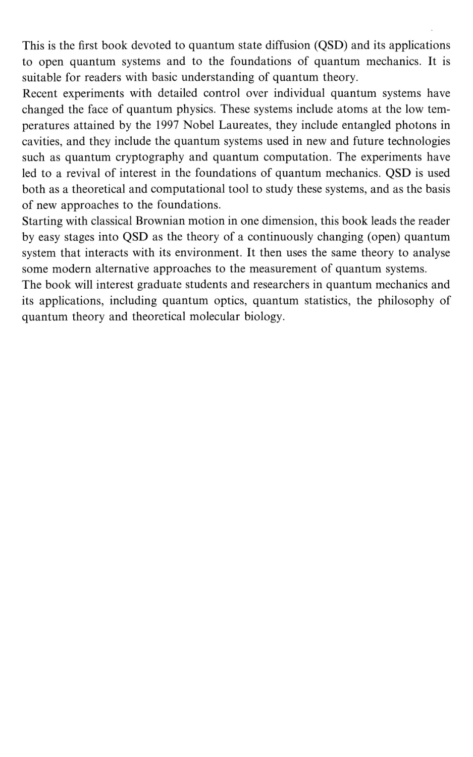
This is the first book devoted to quantum state diffusion (QSD) and its applications
to open quantum systems and to the foundations of quantum mechanics. It is
suitable for readers with basic understanding of quantum theory.
Recent experiments with detailed control over individual quantum systems have
changed the face of quantum physics. These systems include atoms at the low
temperatures attained by the 1997 Nobel Laureates, they include entangled photons in
cavities, and they include the quantum systems used in new and future technologies
such as quantum cryptography and quantum computation. The experiments have
led to a revival of interest in the foundations of quantum mechanics. QSD is used
both as a theoretical and computational tool to study these systems, and as the basis
of new approaches to the foundations.
Starting with classical Brownian motion in one dimension, this book leads the reader
by easy stages into QSD as the theory of a continuously changing (open) quantum
system that interacts with its environment. It then uses the same theory to analyse
some modern alternative approaches to the measurement of quantum systems.
The book will interest graduate students and researchers in quantum mechanics and
its applications, including quantum optics, quantum statistics, the philosophy of
quantum theory and theoretical molecular biology.

QUANTUM STATE DIFFUSION
Ian Percival
Queen Mary and Westfield College, London
CAMBRIDGE
UNIVERSITY PRESS

PUBLISHED BY THE PRESS SYNDICATE OF THE UNIVERSITY OF CAMBRIDGE
The Pitt Building, Trumpington Street, Cambridge CB2 IRP, United Kingdom
CAMBRIDGE UNIVERSITY PRESS
The Edinburgh Building, Cambridge CB2 2RU, UK http://www.cup.cam.ac.uk
40 West 20th Street, New York, NY 10011-4211, USA http://www.cup.org
10 Stamford Road, Oakleigh, Melbourne 3166, AustraHa
© Ian Percival 1998
This book is in copyright. Subject to statutory exception and the provisions of relevant collective licensing
agreements, no reproduction of any part may take place without the written permission of Cambridge
University Press.
First published 1998
Printed in the United Kingdom at the University Press, Cambridge
Typeset in Times Roman ll/14pt [KWS]
A catalogue record for this book is available from the British Library
Library of Congress Cataloguing in Publication data
Percival, Ian, 1931-
Quantum state diffusion / Ian Percival.
p. cm.
Includes bibliographical references and index.
ISBN 0 521 62007 4
1. Quantum theory. 2. Quantum theory-Industrial applications.
I. Title.
QC174.12.P416 1998
530.12-dc21 98-7168 CIP
ISBN 0 521 62007 4 hardback

To Jill

Contents
Acknowledgements xii
1. Introduction 1
1.1 Description 1
1.2 Summary 2
1.3 Literature on related fields 5
2. Brownian motion and Ito calculus 6
2.1 Brownian motion and QSD 6
2.2 Probabilities 11
2.3 Ito calculus 12
2.4 Using Ito calculus 14
2.5 Drift and the interval r 15
2.6 Correlation and ensemble covariance 17
2.7 Complex diffusion 19
2.8 Time scales and Markov processes 20
2.9 Many fluctuations 21
3. Open quantum systems 24
3.1 States of quantum systems 24
3.2 Ensembles of quantum systems 27
3.3 Entanglement 31
3.4 Open systems 35
3.5 Measurement and preparation 36
3.6 The boundary problem 40
3.7 Quantum expectation and quantum variance 41
4. Quantum state diffusion 44
4.1 Master equations 44
4.2 QSD equations from master equations 47
4.3 Examples 51
4.4 Projectors 61
4.5 Linear unravelling 62
4.6 Other fluctuations 63
4.7 QSD, jumps and Newtonian dynamics 64
4.8 The circuit analogy 65

X Contents
5. Localization 67
5.1 Measurement and classical motion 67
5.2 Quantum variance and co variance, ensemble localization 70
5.3 Quantum measurement 72
5.4 Dissipation 74
5.5 Channels and statistical properties 76
5.6 Localization theorems 77
5.7 Proof of dispersion entropy theorem 81
5.8 Discussion 82
6. Numerical methods and examples 85
6.1 Methods 85
6.2 Localization and the moving basis 88
6.3 Dissipative quantum chaos 89
6.4 Second-harmonic generation 93
6.5 Continuous Stern-Gerlach 94
6.6 Noise in quantum computers 95
6.7 How to write a QSD program 97
7. Quantum foundations 103
7.1 Introduction 103
7.2 Matter waves are real 105
7.3 Niels Bohr and Charles Darwin 106
7.4 Quantum theory and physical reaUty 107
7.5 Preparation of quantum states 109
7.6 Too many alternative theories 112
7.7 Gisin condition 115
8. Primary state diffusion - PSD 119
8.1 First approach - Schrodinger from diffusion 119
8.2 Decoherence 123
8.3 Feynman's lectures on gravitation 124
8.4 Second approach - spacetime PSD 125
8.5 Geometry of the fluctuations 129
8.6 Matter interferometers 129
8.7 Conclusions 132

Contents xi
9. Classical dynamics of quantum localization 134
9.1 Introduction 134
9.2 Classical systems and quantum densities 136
9.3 Quantum expectations and other properties of densities 139
9.4 Probability distributions and means 141
9.5 Elementary density diffusion 142
9.6 Generalization 144
9.7 Density entropy decreases 147
9.8 Localization for wide open systems 149
9.9 Localization of a particle in a medium 150
9.10 Discussion 154
10. Semiclassical theory and linear dynamics 155
10.1 Classical equations for open systems 155
10.2 Semiclassical theory of ensembles 156
10.3 Semiclassical theory of pure states 160
10.4 Localization regime 161
10.5 Liner phase space transformations and squeezed states 162
10.6 Linear dynamics and the linear approximation 166
10.7 Summary and discussion 169
References 170
Index 179

Acknowledgements
This book could not have been written without generous help from many
people and institutions.
I had help from my collaborators and my hosts, Gemot Alber, John
Briggs, Tod Brun, Carl Caves, Terry Clark, Predrag Cvitanovic, Lajos
Diosi, Barry Garraway, Jonathan Halliwell, Peter Knight, WilHam Power,
Peter Richter, Rtidger Schack, Tim Spiller, Walter Strunz and particularly
Nicolas Gisin, whose influence can be seen throughout. There were others
who wilHngly provided information or comments on early drafts, including
Bobby Acharya, John Charap, Dave Dunstan, Artur Ekert, Gian-Carlo
Ghirardi, Lucien Hardy, Frederick Karolyhazy, Philip Pearle, TulHo
Regge, Antonio Rimini, Steve Thomas, Graham Thompson, Dieter Zeh
and many more. Bob Jones, Jagjit Dhaliwal and Nelson Vanegas provided
indispensable help in overcoming problems with computers and Steve Adams
prepared the figures. Relevant financial support came from the Alexander
von Humboldt Foundation, the UK Engineering and Physical Sciences
Research Council and the Leverhulme Foundation.
I was lucky to have Simon Capehn, Jo Clegg, Mairi Sutherland and Ian
Sherratt of Cambridge University Press, and also Meg Dillon and Jill
Percival, to help with the editing and see the book through production,
and to have Simon's encouragement and advice.
Thanks to you all.
Ian Percival

1
Introduction
1.1 Description
Recent experiments have changed the face of quantum physics.
They include the detailed control over the states of individual quantum
systems such as atoms and photons, entanglement experiments such as tests
of Bell's inequalities and also technology based on entanglement, such as
quantum cryptography. They include laser cooling to picokelvin
temperatures and advances in matter interferometry, leading to measurements of
unprecedented precision.
These new experiments need new theories, in particular an analysis of those
individual quantum systems which have a significant interaction with their
environments, that is individual open quantum systems. The experiments
expose weaknesses in the usual interpretation of quantum mechanics, and
have revived interest in alternative quantum theories. They suggest precision
measurements to test alternative quantum theories experimentally and to
probe dynamics on Planck scales, such as times of about 10~'^^s.
This book is about the physics of open quantum systems and the
foundations of quantum mechanics. In 1984 Nicolas Gisin made a theoretical
connection between them [68, 67], which many authors have developed since
then. Quantum state diffusion, or QSD, is a mathematical theory that appHes
to both.
Questions concerning the theoretical and numerical solution of specific
practical problems, Hke the cooHng of atoms to very low temperatures, or
the effects of noise on a quantum computer, or the motion of a large
molecule Hke a protein in water, are commonly separated from questions on the
foundations of quantum mechanics, like the nature of quantum
measurement, or the reality of matter waves in more than three dimensions. In
QSD they are closely connected. To many physicists this looks bizarre.

2 Introduction
Nevertheless QSD can be applied to both. AppHcations and foundations
have helped one another. Numerical solutions of QSD equations for open
systems have provided insight into alternative quantum theories by showing
in detail how quantum states can localize during a measurement. And the
localization property of QSD, which arose from the study of quantum
measurement, is crucial to the efficient numerical solution of some problems of
open quantum systems. Experimental tests of alternative quantum theories
are difficult because of noise from the environment, which can be analysed
using the theory of open quantum systems and the practical application of
QSD.
There is a related convergence of two trends in physics previously quite
distinct: the quantum measurement problem considered by physicists
concerned with quantum foundations, and the quantum measurement process as
considered pragmatically by experimenters and their theoretical colleagues
looking for intuitive pictures and methods of computation.
The following chapters concentrate on two themes, with little divergence
from them: the application of quantum state diffusion to open systems and to
the foundations of quantum mechanics. Readers who are interested in related
fields will find a guide to the literature at the end of this introduction.
Most physicists working in quantum optics or condensed matter or
molecular science naturally do not want to be involved with the foundations.
Neither do most physicists or philosophers of science who work on the
foundations want to bother too much about numerical and computational
methods. The book takes account of this. Also, some of the more
mathematical derivations could easily be skipped by readers who are prepared to take
the results on trust. The connections between foundations and appHcations
are emphasized here in the introduction, but not in the remaining chapters.
1.2 Summary
Chapters 2 and 3 provide an introduction to the elementary theories of
stochastic processes and open quantum systems. The next two chapters on
general QSD theory and localization are for all readers. Open systems and
quantum measurement are used as examples. Chapter 6 is on QSD as a
numerical method for solving open system problems, and provides an
introduction to a standard QSD computer program that is available on the World
Wide Web. Chapters 7 and 8 are on the foundations of quantum theory.
Chapters 9 and 10 contain more specialized theory topics, including classical
and semiclassical QSD and the theory of open systems with Hnear dynamics.
The theory in the book is illustrated by many examples.

7.2 Summary 3
The dependence of chapters on one another suggests reading sequences
given by
1^2^3^4^5^6
5^ 7^ 8
4^9^ 10,
but much of the introductory and less mathematical parts can be read
independently, particularly in chapters 7 and 8 on quantum foundations.
Chapter 2 introduces open systems, the Ito calculus and the Ito form of
Langevin stochastic differential equations from scratch, using Brownian
motion as an example. Brownian motion is also used to illustrate the
importance of time scales in Markov processes, and to introduce variance and
covariance for ensembles. It assumes a nodding acquaintance with
elementary probabiHty theory.
Chapter 3 brings in the relevant quantum theory and notation, with the
emphasis on open systems, for which interaction with the environment is
significant and can be represented using ensembles with probabiHties. It
requires a background of elementary quantum mechanics in Dirac notation,
including the picture of a quantum state as a vector in Hilbert space. Some
properties of the density operator are illustrated for two-state systems by
motion on and inside the Bloch sphere. The usual definition of a quantum
measurement is generalized. Quantum variance and covariance for pure
states of individual quantum systems appear.
Chapter 4 uses the methods introduced in the previous two chapters to
derive the Langevin-Ito quantum state diffusion (QSD) equations for the
quantum states of an individual open system from the master equation for
the density operator of an ensemble. Alternative forms of the equations and
the connection with quantum jumps are discussed. A gallery of graphs
illustrates some solutions for simple examples.
Chapter 5 is on localization. This is the property of QSD that makes the
link between classical and quantum mechanics, which provides a dynamics
for the process of quantum measurement. It also helps practical
computations. LocaHzation is described in terms of variances and entropies which
decrease in the mean, and much of the chapter is devoted to showing this.
Some readers may want to skip the derivations and just look at the results.
Chapter 6 contains a description of numerical methods for the solution of
QSD equations, especially the moving basis, which uses the localization
property of QSD. It contains a user's guide to a program library, available

4 Introduction
on the World Wide Web. The methods are illustrated by some examples,
including the Duffing oscillator, second harmonic generation, particles in
traps, and quantum computers. The chapter assumes some knowledge of
numerical methods and computer modelling, but not the details of the
C + + language used for the standard computer library. The results of the
computations may be of wider interest.
Chapters 7 and 8 are on the foundations of quantum theory. They present
some of the merits and problems of Bohr's Copenhagen interpretation and of
those alternative quantum theories that are related to QSD. Some of the
material in these chapters assumes an understanding of the physical
implications of special and general relativity, but not the detailed theory. The part on
experimental tests is written with experimenters in mind.
Chapter 7 gives three reasons for the current interest in alternative theories,
one theoretical and two experimental. The difficulties of quantum theory are
compared with those of early atomic physics and of the origin of biological
species. Bell's conditions for a good quantum theory are stated, and it is
shown that neither the Copenhagen interpretation, nor the environmental
QSD of the earlier chapters satisfies them. There is a brief account of the
development of some good quantum theories that are related to QSD, and a
demonstration that some modifications of Schrodinger's equation are
difficult to detect, so that there is a great variety of possible good theories, despite
an important constraint.
Chapter 8 shows how to restrict the possibiHties by appeal to general
principles and other fields of physics. Primary state diffusion is derived
independently from two very different sets of principles. Firstly it is assumed that
state diffusion is primary and the ordinary deterministic Schrodinger
evolution is derived from it. This results in energy localization, whose merits and
faults are discussed. The second derivation depends on assumed spacetime
fluctuations on a Planck scale, due to quantum gravity. Special relativity is
appHed to the fluctuations, and is needed to produce position localization,
but the dynamics of the system remains nonrelativistic. Atom interferometry
experiments on spacetime fluctuations and the physics of the
classical-quantum boundary are discussed, together with a brief account of the theoretical
and experimental problems and prospects.
Chapters 9 and 10 provide a phase space picture of the evolution of
individual open quantum systems. Most of it needs a deeper understanding of
classical dynamics in phase space than the rest of the book. Those who Hke to
think classically vv^ill find a helpful alternative picture of QSD in these
chapters. They explain the classical dynamical theory of quantum localization, the

13 Literature on related fields 5
semiclassical limit of QSD, and the theory of localized systems with hnear
dynamics.
1.3 Literature on related fields
This book is about the application of quantum state diffusion to the theory
of open quantum systems and to the foundations of quantum theory. It deals
either briefly or not at all with many important related fields, for which this
section provides a brief guide.
The treatment of quantum measurement in ordinary quantum theory
textbooks does not deal adequately with continuous, repeated or incomplete
measurements, such as continuous monitoring of quantum systems by
photon counting in quantum optics, or nondestructive quantum
measurements designed to detect gravitational waves. These continuous
measurements can be handled adequately within the framework of ordinary
quantum theory, as shown by Davies and Srinivas [26, 142, 141] and
Mensky [94]. This provides a basis for the theory of quantum jumps [22,
121] and for the many practical appHcations of quantum trajectory methods
using jumps, which were developed independently, with references given in
section 4.7. Continuous measurement theory for gravitational waves is
described in [19].
The mathematical theory of the stochastic evolution of quantum states has
been developed by Hudson and Parthasarathy [85, 102], Belavkin [9],
BarchielH [4] and their collaborators.
John Bell's book [10] provides a stimulating introduction to the
foundations of quantum theory. Wheeler and Zurek's collection of classic papers
[154] is invaluable. The pilot wave theory of de BrogHe and Bohm is treated
in two recent books [18, 84]. In his book Bell points to similarities between
this theory and the theory of Everett [49, 153]. Bohm discussed the role of
causaHty and probabiHty in quantum mechanics in [16], whereas [93] provides
a non-mathematical introduction to the problems of quantum-nonlocahty
and relativity.
The problems of quantum theory and gravity are mostly well above the
level of this book, but the expositions in [108] are clearer than most.

2
Brownian motion and Ito calculus
2.1 Brownian motion and QSD
2.2 Probabilities
2.3 Ito calculus
2.4 Using Ito calculus
2.5 Drift and the interval r
2.6 Correlation and ensemble covariance
2.7 Complex diffusion
2.8 Time scales and Markov processes
2.9 Many fluctuations
A Brownian particle is an open classical system, and quantum state diffusion
(QSD) is a theory of open quantum systems, so there is a parallel between the
physics and mathematics of classical Brownian motion and the physics and
mathematics of quantum state diffusion. But Brownian motion is much
simpler, so it is used to introduce the properties of open systems, the Ito calculus
and the use of diffusion to probe small scales. All of these are important for
QSD.
2.1 Brownian motion and QSD
The interaction of an open system like a Brownian particle with its
environment significantly affects its dynamics. The motion is stochastic, so the future
state of the system is not uniquely determined by its present state. The
probability of a given future state is uniquely determined. General open
systems are defined in section 3.4.
Brownian motion is stochastic motion of an individual open classical
system, in contrast to the determinism of Hamiltonian dynamics. Quantum state
diffusion is stochastic motion of an individual open quantum system, in
contrast to the determinism of Schrodinger dynamics. In QSD the quantum
states diffuse in Hilbert space Hke Brownian particles diffusing in ordinary
position space. For example, the system may be an atom in a radiation field,
a radiation field in the presence of atoms, a molecule in a Hquid, or a
quantum computer in the presence of noise. It may be a quantum system which is
being measured. In QSD this diffusion is the source of quantum fluctuations
and the indeterminism of quantum physics.

2.1 Brownian motion and QSD 1
Brown did not discover Brownian motion. Anyone looking at water
through a microscope is likely to see little things wiggUng around, and
according to Brown they were seen by Leeuwenhoek, who lived from 1632
to 1723. In 1828 Brown estabhshed Brownian motion as an important
phenomenon, demonstrated that it was present in inorganic matter and refuted
by experiment various spurious mechanical explanations.
In the late nineteenth century there were good scientists Hke Ostwald and
Mach who did not beheve in the reaHty of atoms. For them, atomic theory
was just a convenient picture or model which could be used in physics and
chemistry to explain the properties of observable macro systems, and those
who beheved in the reaHty of atoms were misguided.
Einstein's 1905-1908 theory and the later experiments of Perrin estabhshed
the reality of atoms without question. Brownian motion is a diffusion
process, and because of this, macro scale experiments on Brownian motion could
be used to probe the atomic scale, even though the details of atomic dynamics
were not known at the time. These experiments are much easier than the
more direct methods Hke X-ray diffraction, scattering experiments and ultra-
microscopes. Brown's systematic studies were completed long before such
methods were possible. QSD is also a diffusion process. It is suggested in
chapter 8 that quantum state diffusion might be used to determine quantities
on the Planck scales of length and time, which are smaller than atomic scales
by more than twenty orders of magnitude. The role of QSD in quantum
theory today parallels the role of Brownian motion in the atomic theory of
a century ago.
The books of Einstein and Nelson give good accounts of the early work on
Brownian motion [46, 99].
There is a parallel between the theory of Brownian motion and the theory
of quantum state diffusion. A Brownian particle moves along a crooked path
r{t) in position space. This crooked path is a solution of a stochastic
differential equation, the Langevin equation. Langevin introduced differential
equations with stochastic forces, which will be treated more consistently in
section 2.3 using Ito's stochastic calculus. The state of an ensemble of
Brownian particles is represented by a density p(r, t) that is the solution of
a Hnear deterministic partial differential equation, caHed the Fokker-Planck
equation.
According to QSD, a single open quantum system moves along a crooked
path or trajectory \^{i)) in the state space, that is a solution of a stochastic
differential equation, the QSD equation. The evolution of an ensemble of
quantum systems is represented by a density operator p{t) that is a solution of

8 Brownian motion and ltd calculus
a Hnear deterministic equation, called the master equation, which may be a
matrix differential equation or a partial differential equation.
There is also a parallel in the computational methods that are used today.
For complicated Brownian processes, such as the motion of charged
Brownian particles in an electric field that varies in space and in time, it is
often easier to solve the Langevin equation numerically for a sample of
particles than to solve the Fokker-Planck equation for the density. The
first method is a Monte Carlo method. The Monte Carlo method is less
accurate, but it can be used where the Fokker-Planck equation is insoluble
in practice. Similarly, for open quantum systems that require many basis
states, it is often possible in practice to solve the QSD equation numerically
for a sample, when it is impossible to solve the master equation for the
density operator, as shown in chapter 6.
These parallels are well estabUshed. There are others which are less well
estabUshed.
For example, the theory of Brownian motion clarified the foundations of
kinetic theory, whereas QSD clarifies the foundations of quantum mechanics.
Theory and experiments on Brownian motion provided access to the physics
of atomic scales, whereas the primary state diffusion theory and matter
interferometer experiments of chapter 8 might provide access to the physics
of the Planck scales.
So Brownian motion and its theory provide a good introduction and
background to the physics and mathematics of QSD, despite the important
differences between them. For simpHcity, consider only the vertical motion of a
Brownian particle.
First suppose that the density of the particle is the same as the fluid around
it. Then there is no drift due to gravity. The displacement of the particle
fluctuates due to colHsions of the Brownian particle with molecules. This
process takes place on the atomic scale, producing random upward and
downward displacements, resulting in a diffusion away from its initial height.
The mean vertical displacement x{t) of the particle from its initial height is
zero,
Mx@ = 0, B.1)
where M will always be used to represent the mean over stochastic
fluctuations. 'Expectation' will not be used for such fluctuations, as it is needed for
quantum expectations. As in statistical mechanics, a mean is a property of a
large ensemble of individual systems. For our example, the mean vertical

2.1 Brownian motion and QSD 9
displacement is a property of an ensemble of Brownian particles that start
from the same height.
The mean square displacement from the initial position is proportional to
the time,
Mx^it) = a^t, B.2)
where by convention a is a positive constant. The value of a depends on the
mass of the particle, the viscosity of its fluid environment and the
temperature, but this does not concern us here. A typical displacement due to the
diffusion is proportional to the square root of the time, and this can be
expressed in terms of the root mean square (RMS) deviation.
Ax(t) = ^M x\t) = aVt^ B.3)
When the density of the Brownian particle is greater than the density of the
fluid through which it moves, there is an additional drift due to gravity. Its
vertical displacement is then made up of two parts, drift and stochastic
fluctuations,
vertical displacement = drift + stochastic fluctuations. B.4)
Here and throughout the book 3. fluctuation will always be a stochastic
variable with zero mean. It is only then that there is a unique decomposition of
the motion into separate drift and fluctuation components. Here a fluctuation
is a displacement and not a velocity.
The drift, due to the force of the Earth's gravitational field, is uniformly
downwards. In a short time interval 8t, the mean square displacement
M (Sxf' due to the diffusion is proportional to 8t, so a typical displacement
is proportional to the square root of the time interval. The drift is
proportional to the time interval 8t itself. The absence of the expected acceleration
term is explained in section 2.8.
Figure 2.1 illustrates simulated Brownian motion with drift. Figure 2.1(a)
gives the height. Over very short periods of time it is difficult to see the drift
because it is masked by the fluctuations, whereas over longer periods the drift
becomes relatively more important. Over very long periods it may be difficult
or impossible to distinguish the fluctuations at all. Figure 2.1(b) shows the
root mean square displacement ^JM (x^) from the initial height at r = 0 for a
sample of 100 Brownian particles. This is not a deviation from the mean. For

10
Brownian motion and ltd calculus
O.Ot
I.Ot
2.0t
3.0t
Figure 2.1a The height of a Brownian particle as a function of time.
(b)
o
D"
en
C
o
E
"o
o
3.0
2.0
1.0
0.0
-
-
-
1
—CiVT y^
1
1 1
{==C2 0^X
T
1 1
1 /
-
-
-
A
1 1
O.Ot
I.Ot
2.0t
3.0t
Figure 2.1b The RMS deviation from the initial height for a sample of 100 particles
r is defined in the text.

2.2 Probabilities 11
small times it looks roughly parabolic, typical of the square root dependence
of the fluctuations without the drift. For longer times it looks Hnear, typical
of drift without fluctuations.
The figure also shows the time interval r that marks the approximate
boundary between the smaller time intervals for which the diffusion
dominates and the larger time intervals for which the drift dominates. The
measured value of r provides valuable information about atomic scales.
For times T much longer than r, the fluctuations are typically about
(r/r)^^^ of the displacement due to the drift. This is t\iQ fluctuation factor,
which is defined for all processes in which there are both fluctuations and
drift. It is important for the experimental tests of spacetime fluctuations
proposed in chapter 8.
2.2 Probabilities
A Brownian particle is a special case of a system interacting with its
environment. The state of the environment cannot be represented exactly, but, as
usual in statistical mechanics, the probabiHty of a given state can be
represented. Consequently, interaction between system and environment produces
indeterminate stochastic evolution of the system, represented by an ensemble
with a probabiHty distribution in space for the Brownian trajectories.
The notation used here for probabiHties is easily extended to quantum
systems. Let Pr(x) be a probability distribution for a discrete or continuous
variable x. Then the total probabiHty for any value of x must be 1, so
Y^ Pr(x) = 1 or I dx' Pr(x) = 1,
B.5)
where the sum or integral is taken over aH possible values of x. Such sums
and integrals are so common that it is convenient to use a general notation
for both which is consistent with the corresponding quantum notation. The
trace Tr is the sum or integral over all possible values of a variable x and so
TrPr(x) = 1. B.6)
The variable x can represent a dynamical variable of some classical system,
like the height of a Brownian particle. If/(x) is some property of the system.

12 Brownian motion and ltd calculus
like the vertical distance of the particle from some point, then the mean of/
for the probabiHty distribution Pr(x) is
M/ = TrPr(x)/(x). B.7)
The ensemble variance or mean square deviation of/ is
^\f) = M (/ - Mff = M (/) - (M/)l B.8)
This is always positive or zero and its square root A/ is the standard
deviation. All the variances of this chapter are classical ensemble variances. In
chapter 3 we will meet the corresponding quantum variances.
The probability distribution for y =f(x) is
PrCy) = Tr, Pr(x) S{f{x) - y), B.9)
where the 8 function is the Dirac or Kronecker 5, depending on whether x is
continuous or discrete.
2.3 Ito calculus
Ito and Stratonovich have done for stochastic dynamics what Newton and
Leibniz did for ordinary dynamics, by treating the small displacements as
differentials. This results in a very elegant theory and differential calculus for
continuous stochastic processes that satisfy Langevin equations, sometimes
known as Wiener processes. This and other stochastic methods are described
for physicists in the books of Gardiner [55, 56]. Remarkably, Ito calculus is a
differential calculus of nondifferentiable functions.
When a Brownian particle with vertical displacement x diffuses with no
drift, the mean of the vertical distance traversed is zero and the mean square
or variance is proportional to the time. So for small displacements dx,
M dx(t) = 0, M [dx(t)f = a^dt, B.10)
where M represents a mean over all possible displacements dx(t) and a is a
positive constant. The small displacements are treated as differentials by Ito,
and their higher powers are neglected, as in the ordinary Leibniz differential
calculus, but the rules are different. For more complicated stochastic pro-

2.3 ltd calculus 13
cesses, it is convenient to introduce a standard normaHzed stochastic
differential dw, with zero mean and variance equal to the time, so that
Mdw = 0, M{dwf^dt. B.11)
For these differential fluctuations, only these means are significant. It does
not matter whether the ensemble of stochastic differentials is made up of
steps of fixed length with equal probabiHty of going to the left or to the
right, or of steps with a Gaussian distribution, or a rectangular distribution.
They all have the same effect, provided that they satisfy B.11).
It is implicitly assumed that fluctuations at different times are independent
of one another. This is the Markov assumption, discussed in more detail in
section 2.8. Brownian motion with no drift is then given by the solution of the
simplest Langevin-Ito differential equation
dx{t) = adw{t). B.12)
In this equation, and in general for Ito stochastic differential equations, it
is assumed that, at time t, the trajectory x(s) with 0 < ^ < ris already
determined, so that only the new fluctuation dw(t) need be considered. All the
particles of the ensemble are at the initial point x{t) at time t, but they are
usually at different points at time t + dt. So for a single step of the equation
the mean M refers to the ensemble of the current fluctuations dw(t) only.
Functions of t and x(t) have a fixed value, and so may be taken outside the
mean.
The properties of more general ensembles, formed from all the fluctuations
over finite time intervals, can be derived from the properties of these
elementary ensembles, in which the initial ensemble consists of systems in the same
state. That is why most of the Ito equations in this book have no mean M
on the right hand side. There is no need for it when all the initial states
are identical, and general equations can be obtained from the elementary
ensembles.
In ordinary differential calculus the whole theory can be based on first-
order differentials, higher orders being neglected by comparison with the first
order. The Ito differential calculus is also based on lower-order differentials,
but they are not just of first order. Stochastic differentials are of order (dr)^^^,
so the squares of stochastic differentials Hke dw cannot be neglected.
Squares of ordinary differentials like dt can be neglected as usual, and so
can products of the form dtdw, which are of order (dt)^^^. The contributions
of drift and diffusion terms can be considered independently, because cross

14 Brownian motion and ltd calculus
terms are neghgible, which simplifies the analysis of the diffusion equations
considerably. A stochastic differential of order dr whose mean is zero has
variance of order (dr)^ and therefore this is also neghgible. In the Ito calculus
all such neghgible differentials are set to zero. The variance of
(M {dwf) — {dwf is of order {dtf, which can be neglected, so if we want
to save notation, we can write
(dw)^ = dr, B.13)
without the mean that appears in equation B.11).
Following the rules of the Ito calculus, the differential of a function/ of a
stochastic variable x and a product of two functions / and g are
d/ = dx./+i(dx)^r, d(/g)=/dg + d/.g + d/.dg. B.14)
The ordering of the terms has been retained on the right side of the second
equation, because QSD sometimes has noncommuting fluctuations.
2.4 Using Ito calculus
The increase with time of the variance of the height of a Brownian particle
without drift is a simple example of the Ito calculus. Suppose for simphcity
that at r = 0 the displacement is x = 0. Then the variance at some later time is
E^(x) = M x^. The change in the variance after time dt is
dEV) = dMx^
= M d(x^) (change of the mean is mean of the change). B.15)
Using equation B.14) for the differential of a product,
dE^(x) = M 2xdx + M {dxf, B.16)
The initial displacement x is independent of the following fluctuation, so x
can be taken outside the mean, and
M xdx = X M dx = XC M dw = 0, 1
J 7 9 B.17)
dE^(x) = M {adwf = a^dt, J

2.5 Drift and the interval t 15
where the important term is the square of a stochastic differential, which
cannot be neglected in the I to calculus.
The averaged picture of Fokker and Planck does not represent the motion
of the individual particles directly, but uses the probabiHty distribution p(x, t)
of an ensemble of particles. If there is no drift, its differential equation
follows from the stochastic differential equation B.12), using the Ito calculus.
For a particular fluctuation dw, the distribution at time t + &t is given by
shifting p(x, t) by dx, giving
p(x, r + dr) = p{x — dx, t) = p(x — adw, t)
I 1 II 2 B-18)
= p(x, 0 - ap (x, r)dw + \a p (x, 0(dw) ,
where the prime means differentiation with respect to x. For the whole
ensemble we take the mean over all possible fluctuations. Now M dw = 0,
M {Awf = dt and
p(x, t + dt) = M p(x + dx, 0
= p(x, 0 + iC^/(x, t)dt, B.19)
so dp = ^c?f)'{x, t)dt (Fokker-Planck).
The solution of B.19) is the set of Gaussians illustrated in figure 2.2.
These two derivations are typical of many that appear in QSD. Because the
ordinary differential calculus is used so much, most people find it difficult to
avoid neglecting some of, the squared differentials at first. This problem is
overcome in the alternative but equivalent Stratonovich calculus [54], at the
price of a sHghtly more difficult interpretation of the results, but the Ito form
is used here.
2.5 Drift and the interval t
When the density of the particles is greater than their fluid environment, the
Earth's gravitational field adds a drift velocity v to the vertical diffusion,
giving the stochastic differential equation
dx = vdt + adw, B.20)
where the coefficient of dt gives the drift velocity and the coefficient of dw the
magnitude of the diffusion. If x is replaced by x - M x, equation B.20)

16
Brownian motion and ltd calculus
pM
1.0
0.8 h
0.6
0.4
0.2
0.0
-
-
-
-
-
....., . .. -t
1
/''/
/ /"^"\J^
/'''' ^-"T-^
//
1
1
---— f=0
—- t=l
-^^^^ t=2
4— t=3
\ '^ ~~-
1
-
-
-
H
H
H
-4-2024
X
Figure 2.2 Gaussian solutions of the Fokker-Planck equation for Brownian motion
without drift.
reduces to equation B.12), so the variance of the displacement x is unaffected
by the drift.
Also for more general differential stochastic processes, in which x
represents the state of some dynamical system, the drift is the term containing dt
and the diffusion terms contain fluctuations like dw. For sufficiently small
times, the diffusion, which is proportional to (dr)^^^, dominates the drift,
which is proportional to dt. The approximate boundary between the smaller
time intervals dominated by the diffusion and the longer time intervals
dominated by drift is obtained by supposing that equation B.20) remains vahd for
finite time intervals, and equating the increments due to fluctuation and drift,
giving
vT = ar^^'^, T = {a/vf (boundary interval). B.21)
This is the boundary interval illustrated in figure 2.1 on page 10.

2.6 Correlation and ensemble covariance 17
2.6 Correlation and ensemble covariance
This section follows from section 2.2 on probabilities. In any ensemble of
systems, two dynamical variables / and g may or may not be correlated. If
they are uncorrelated then their joint distribution is the product
Pr(/,g) = Pr(/)Pr(g) B.22)
and a knowledge of the value of/ then gives no information about the value
ofg.
The ensemble covariance off and g,
E(/, g) = Mif-Mf)(g-Mg) = M ifg) - (M/) (M g) B.23)
is defined in terms of the deviation of/ and g from their means. It is a bihnear
measure of the correlation between/ and g. It is zero if/ and g are
uncorrelated. If it is nonzero then they are correlated. But/ and g can be correlated
nonhnearly, in which case the covariance may be zero, despite the
correlation. An example of this is when the variables x and y are distributed
uniformly on a circle in the (x, j)-plane, represented by
x = cos0, y = sme, B.24)
where 9 is distributed uniformly between -n and n. The variables x and y are
then strongly correlated, but their covariance is zero. However, if the
covariance of every function of/ and every function of g is zero, then/ and g are
uncorrelated.
The covariance of/ with itself is just the variance of/.
i:(/,/) = S V). B.25)
We often need to deal with the statistical properties of complex variables/, g.
There is a natural definition of the variance, which is
E(/,/) = !:'(/) = M (/*/) - (M/)*(M/) = M |/|2 - |M/|2
= sVr) + 2Vi), B.26)
where zr and zi are the real and imaginary components of a complex
quantity z.
For general probabiHty distributions in complex/ and g, the properties of
the covariance are not so simple, but we will not be concerned with general

18 Brownian motion and ltd calculus
distributions, only with those distributions where multipHcation of the
important variables by a phase factor u leaves all probabiHties, including
joint probabilities, unchanged, so that
Pr(^/,^g) = Pr(/,g) (|^|' = 1). B.27)
In that case there is a natural generahzation of the definition of ensemble
variance to ensemble covariance, given by
E(/, g) = M (/*g) - (M/)*(M g) = S(/r, gR) + S(/i, gi), B.28)
which has the same basic properties as the ensemble covariance of real
variables. Correlation between systems is particularly important. If A and B are
two systems, and AB is the combined system, then A and B are uncorrelated
in an ensemble if the state x of A is uncorrelated with the state y of B, so
PrAB(^, y) = PrA(x)PrB(j). B.29)
It follows that if the covariance of every function of the state of A with
every function of the state of B is zero, the systems are uncorrelated, and
conversely.
Classical probabiHties, correlations, variances and covariances are
properties of classical ensembles, not of individual systems, even when the ensemble
is not mentioned explicitly. We will see in later chapters that this is not true of
quantum variances and covariances.
Two systems that have not interacted either directly or indirectly are
always uncorrelated. When they do interact, they almost always become
correlated. We often want to study the behaviour of one of the systems on
its own, even when it is continually interacting with another system. For
example, an open system is continuaHy interacting with its environment,
and the environment is usuaHy so big and compHcated that it cannot be
studied in detail. Brownian motion is an example. In such cases we are
only interested in the reduced probabiHty distribution for the system itself.
Let A be the system and B the environment. Write Tr^ for the integral over
aH the states y of the environment. Then the reduced distribution for A is
PrA(x) = TrBPrAB(^,j). B.30)
If we know something about the distribution of B, for example that it is in
thermal equilibrium at a fixed temperature, and we know the dynamics of the

2 J Complex diffusion
19
interaction between A and B, then we can often derive stochastic equations of
motion for A, and deterministic evolution equations for the probabiHty
distribution VxpJ^x),
The dynamics of quantum mechanical amplitudes for pure quantum states
has some features in common with the dynamics of classical probabiHties for
ensembles of classical systems. Similarly quantum entanglement, described in
section 3.3, resembles classical correlation in some respects. Despite these
common features, quantum ampHtudes and entanglement have some special
properties of their own.
2.7 Complex diffusion
For appHcations to quantum mechanics, isotropic diffusion in two real
dimensions is best considered as one-dimensional complex diffusion in the
complex z-plane illustrated in figure 2.3. The standard normalized complex
stochastic differential is
d^ = d^R + Zd^I,
where the real and imaginary parts satisfy
B.31)
Figure 2.3 Isotropic diffusion in the complex z-plane.

20 Brownian motion and ltd calculus
M d^i = M d^R = 0 (zero mean),
M d^id^R = 0 (zero covariance),
M d^l = M d^i = dt/2 (normalized).
The equivalent complex form of the conditions is more convenient:
M d^ = 0 (zero mean),
(d^)^ = S(df, d^) = 0 (zero covariance), B.33)
|d^|^ = S^(d^) = dt (normalized),
where because of the isotropy the statistics of the motion is unaffected if d^ is
multiplied by a phase factor of unit magnitude.
The equations B.14) for the differential of a product and of a function
apply to complex fluctuations as they do to real ones, but there is an
important simpHfication for complex fluctuations, because the square of a complex
differential fluctuation is zero, so the second term in the expression for d/
vanishes. This leads to a simpler quantum state diffusion theory when
complex fluctuations are used.
The Langevin-Ito equation of a particle with drift and diffusion at position
z{t) in the complex plane is
dz = v&t + ad^. B.34)
Both V and a can be complex, but the physics is unaffected by the (gauge)
transformation for which a is multiplied by a phase factor.
This completes the classical theory needed for an understanding of
elementary quantum state diffusion for open systems. Quantum state diffusion is a
diffusion of quantum states represented by normalized state vectors in a
complex Hilbert space, which is not so simple. But many of the methods
and notation introduced in this chapter are used.
2.8 Time scales and Markov processes
The Ito equations for Brownian motion are not vaHd on all time scales. For
example, if the environment of the Brownian particle is a gas, a molecule of
the gas takes a finite time to collide with the particle. For classical colHsions
we could take the time interval T^^x to be the minimum time for the collision
to produce half the total momentum transfer. During such time intervals the

2.9 Many fluctuations 21
motion looks smooth and cannot be represented by an Ito equation Hke
B.12) or B.20). There are correlations between the fluctuations over time
intervals comparable to T^oi and smaller, so that on this scale the Markov
assumption that there are no correlations is wrong. But for time scales that
are long by comparison, the correlations are neghgible and the Ito equations
can be used. Typically T^oi is smaller than the boundary time r by many
orders of magnitude, and cannot be detected experimentally.
In the theory of Brownian motion, a uniform drift has been assumed,
mhich seems incompatible with Newton's second law of motion. A heavy
body in air, Hke a skydiver's, first accelerates. The resistance of the air
then reduces her acceleration towards zero, so that she approaches a terminal
drift velocity. Her Brownian fluctuations are neghgible. For Brownian
particles the period of acceleration is normally so short that it can be neglected.
Only the terminal drift velocity and the fluctuations can be seen.
For dense gases and liquids the time between colHsions is very short
compared with the colHsion time. However, for diffusion in gases of very low
density, it may be very much longer, and when the mean free path is
macroscopic, the Markov assumption and Ito equations may not be vahd on any
scale. The quantum mechanics of the colHsions compHcates things further. It
was Einstein's achievement to recognize that the relevant theory was usually
independent of such complications. That is how he produced his theory more
than two decades before any proper understanding of the elementary
colHsions which cause the fluctuations.
Similar considerations apply to quantum state diffusion. The Markovian
Ito theory of quantum state diffusion is vahd on time scales that are long
compared with the basic time scale for interaction with the environment, but
sometimes the correlations between successive fluctuations cannot be
ignored, the evolution of the quantum system is non-Markovian, and QSD
cannot be used.
2.9 Many fluctuations
This section is a Httle bit more difficult than the rest of the chapter. It includes
the classical theory needed for all but the simplest appHcations of QSD, and
can be skipped at first reading. Definitions for single fluctuations are
generalized to many fluctuations, which introduces some mathematical
complications.
Suppose there are K real fluctuations dw^ with zero mean. We cannot
always rule out the possibiHty that the fluctuations dw^ are correlated, or
even Hnearly dependent. Since powers of dw^ higher than squares are negh-

22 Brownian motion and ltd calculus
gible, the means and variances and covariances provide all the statistical
information about them, so
M dw'k — 0 (zero mean), 1
f B 35)
S(dw^, dw^O = M dwk • dwk> = X^k' dr (general), J
thus defining X^j^j^.
The variance of a fluctuation is treated as a norm, and the covariance of
two fluctuations as a scalar product. By taking Hnear combinations of the
fluctuations we can transform them to a standard form, in which they are all
normalized to dt and orthogonal. This makes an orthonormal set of
fluctuations. Normalization is no problem, because fluctuations are always used
with coefficients, and unwanted constant factors can be absorbed into the
coefficients. Orthogonahty is the problem.
The symmetric matrix X^j^j^' can be diagonaHzed by an orthogonal
transformation:
Xjy = Y,OjkX'kMr, B.36)
kk'
giving a new set of fluctuations that are Hnear combinations of the old ones:
k
For the new fluctuations, the off-diagonal covariances are zero and, if some
of the old fluctuations dw^ are Hnearly dependent, some of the new variances
dwj are zero too. The latter may be ignored, as they do not contribute to the
diffusion. Suppose there are / remaining. Generally they are not normalized,
but they can be normaUzed so that each variance is dt, giving a set of ortho-
normal fluctuations:
M dwj = 0 (zero mean),
^ B.38)
S(dwy, dwj') = M dwj • dwj' = Sjj'dt (orthonormality).
This is the standard normalization, in which the norm of the vector
fluctuation {dWj} is Jdt.
There is a direct generalization to diffusion in a complex vector space,
which is needed for QSD. A general diffusion has correlated fluctuations
d^^ and nonzero off-diagonal covariances, using the definition of complex

2.9 Many fluctuations 23
covariance of section 2.6 in equation B.28). The Hermitian matrix Z^^/ can
be diagonahzed by a unitary change of basis. For the new fluctuations d^l,
the off-diagonal covariances are zero and, if some of the fluctuations d^^ are
linearly dependent, some of the diagonal variances of d^j are zero too, and
there are only J < K independent fluctuations. These can be normalized.
The new complex fluctuations have the standard form
M d^f = 0 (zero mean),
w B 39)
S(d^y, d^yO = M d^j • d^j^ = Sjj^dt (orthonormality).
The standard forms are not unique. Orthogonal transformations of {dwj} and
unitary transformations of {d^^} leave their properties are unchanged. These
may be considered as different fluctuations or as a different representation of
the same vector fluctuation in the Hnear fluctuation space.
A general Ito equation for a real variable x with many independent real
fluctuations is
dx = vdt + ^ ajdwj. B.40)
Let/(x, t) be a differentiable function of x and of t. Because it is differenti-
able with respect to t it does not depend exphcitly on the fluctuations. The
change in/(x, t) in a time dt is
d/(x, 0 = (df/dx)dx = (df/dx)vdt + Y^(df/dx)ajdwj. B.41)
Consequently the contributions to d/ from the drift term and each of the
fluctuation terms proportional to dwj are additive. This is the additivity rule,
which is also true for complex x with complex fluctuations, when x is a
vector, or even when it is a quantum state vector, as for QSD. The additivity
rule is used extensively in QSD to obtain the theory of compHcated systems
from the theory of elementary systems.

3
Open quantum systems
3.1 States of quantum systems
3.2 Ensembles of quantum systems
3.3 Entanglement
3.4 Open systems
3.5 Measurement and preparation
3.6 The boundary problem
3.7 Quantum expectation and quantum variance
An individual open quantum system can be represented by a pure state, and
the statistical properties of an ensemble of open systems by a probabihty
distribution over pure states. The density operator which can be obtained
from this distribution is more compact, but does not represent the dynamics
of the individual systems of the ensemble. A density operator is also used to
represent an open quantum system that is entangled with its environment as
the result of interaction. Measurement and preparation are given general
definitions in terms of the interaction of a quantum system with its
environment. The boundary between system and environment is ambiguous. For a
pure state there are quantum expectations, quantum variances and quantum
CO variances.
3.1 States of quantum systems
A pure state of a quantum system with a state vector 11//) that satisfies the
Schrodinger equation is a very useful fiction.
Even if the system is isolated, every system we know has interacted with
other systems in the past, and so has become entangled with them, as
described in section 3.3. Strictly speaking, no system is independent, and
so no system can be properly represented by a state vector \\l/). All systems
are open, with the exception of the whole universe. However, quantum
systems are commonly represented by state vectors, theories based on this
representation are very successful, and we use this representation too.
The representation of the same pure state by a projection operator or
projector
p = p^ = mm C.1)

3.1 States of quantum systems 25
is equivalent to state vector representation, except for a physically irrelevant
external phase factor. We use both.
The Schrodinger time evolution of a pure quantum state |V^) with
Hamiltonian H is given by the differential equations
\f{t)) = -(z7^)H|V^@) and P = -(z7^)[H, P], C.2)
from which it follows that the evolution over finite times is given by
\^lf(t)) = Qxp{-iHt/h)\i/{0)) and P@ = exp(-zHr/^)P@) exp(zHr/^).
C.3)
This evolution is Hnear. It is also deterministic, meaning that the present
state determines future states uniquely. The norm (V^|V^) of the state vector
and the corresponding trace TrP of the projector are preserved. Linear
norm-preserving transformations are unitary. Quantum state diffusion
preserves the norm and the trace, but it is neither Hnear nor deterministic. It is
nonhnear and stochastic.
An open quantum system continually interacts with its environment. An
ensemble of these systems is sometimes called a 'mixed state' of the system
and is represented by a density operator which is defined in the next section,
3.2. But in QSD we usually use the representation of a single state of the
ensemble by a pure state |V^). For open quantum systems, just like isolated
ones, this is a very useful fiction. We also use the density operator, but it
plays a secondary role.
The properties of systems with many orthogonal states are easier to
understand when there are only two, as in the example of a spin one-half system.
This chapter uses these 'two-state' systems to illustrate mathematically and
pictorially the properties of the more general systems that are needed for
QSD.
By convention, the states |+) and |-) with 'up' and 'down' spins in the +z
and -z direction are used as the base vectors A, 0) and @, 1) respectively.
These are the eigenvectors of the PauH matrix a^. The eigenvectors of a^
represent the spins in the ±x direction and of ay represent the spins in the
±y directions. The matrix representations of the operators and eigenvectors
can be found in most quantum mechanics texts.
The states and ensembles of 'two-state' systems are best visualized in the
three-dimensional linear space spanned by the projectors, which is not the
same as the Hilbert space of the states themselves. The projectors are points

26
Open quantum systems
on the surface of the Bloch or Poincare sphere, illustrated in figure 3.1. The
projectors P can be represented by 2 x 2 matrices. In the space of the
projectors, the centre of the sphere, which is the origin of the coordinates, is at
half the unit matrix, p. The vector representing the projector P is
r = (x, J, z) = TrPff,
where
^ = i^X^ <^V' ^z)
and the projector corresponding to the vector r is
P = i(I + r-J).
C.4)
C.5)
The projectors of the two eigenstates of a general spin-half matrix a are at
i(I ± a), which are on opposite sides of the sphere. A point on the surface of
the sphere indicates the direction of the spin in three-dimensional position
space. The up and down spins are at the north and south poles.
Besides spin-half systems, other examples of two-state systems are
polarization states of photons, the two states of an atom that resonate strongly
with laser Hght of a single fixed frequency, and the two occupation states for
a fermion. For photons, the up and down spins correspond to vertical and
+z
+x
Figure 3.1 Projectors as points on the surface of the Bloch sphere.

3.2 Ensembles of quantum systems 27
horizontal polarizations of the photon, the eigenstates of a^ to linear
polarization at 45° and the eigenstates oioy to circular polarizations. For two-state
atoms, the up and down spins correspond to the excited and ground states of
the atom and the other spins to coherent combinations of the two atomic
states.
Two-state quantum systems, Hke two-state classical systems, can be used to
represent binary numbers. The corresponding bits are called qubits, spoken as
'kewbits'. Quantum systems of many qubits behave very differently from
classical systems with many classical bits. For example, simultaneous parallel
operations can be performed on qubits that are impossible with classical bits.
This is the basis of modern quantum technology, including quantum
communication, quantum cryptography and possible future quantum computers.
QSD has been appHed to quantum computers, which are discussed further in
chapter 6.
All two-state Hamiltonians have the form hwa, where co is an angular
frequency and (t is a spin operator in an arbitrary direction. The
Schrodinger evolution of a pure quantum state is then given by uniform
rotation on the surface of the Bloch sphere with angular velocity co about
an axis through the eigenstates of a. For H = coa^, a state moves uniformly
around a Hne of latitude.
The book by Allen and Eberly [2] has a useful introduction to the Bloch
sphere.
3.2 Ensembles of quantum systems
Classical dynamics and Schrodinger dynamics are both deterministic, but
there is an unavoidable stochastic behaviour where they interact. Because
of this, probabiHty is more important for quantum theory than it is for
classical theories.
A single system whose state is not perfectly known, or whose evolution is
stochastic, is represented by an ensemble of systems with a probabiHty
distribution over pure states. One example is an open quantum system, Hke a
molecule in a fluid. Another is a coHection of many quantum systems, Hke
many runs of an experiment.
Depending on the type of ensemble, the probabiHties can be represented by
a continuous probabiHty distribution Pr(V^) in the very large space of aH
quantum states |V^) with projectors P^^, or a discrete distribution, which
consists of a set of probabiHties Pr(/) for states I7) with projectors Fj. The
states need not be orthogonal in either case. For simpHcity, the theory is
developed here for discrete distributions, which can be generalized without

28 Open quantum systems
difficulty to continuous distributions, replacing sums by integrals where
appropriate. Continuous distributions are discussed in [6].
For quantum state diffusion theory, the probabiHty distribution is the most
important representation of an ensemble of quantum systems. But it is not a
common representation, because the measurable properties are all given by a
simpler representation using density operators.
The density operator and the corresponding vector for an ensemble of
quantum systems are
p = 5^ Pr(/-)P,-, r = Trpa C.6)
and the point r is in the interior of the Bloch sphere unless the members of the
ensemble are identical.
Remarkably, ensembles with the same density operator cannot be
distinguished from one another by measurements, however they may be
performed, so that for many purposes such ensembles are equivalent. This
equivalence is a major theme of this book. However, a density operator
does not normally represent the individual systems of the ensemble. An
exception is the very special type of ensemble which consists of identical
pure states, for which the ensemble is represented by the pure state projector
for that state.
The probabiHty of the system being found by a measurement in the state
IV^) is
Tr pV^={f\p\ylf). C.7)
This property is sometimes used to define the density operator. The
probabilities must be positive or zero, and their sum for a complete set of ortho-
normal states is unity. In other words, the diagonal elements of any matrix
representation of p must be non-negative and sum to unity. These two
conditions are the positivity and trace conditions on the density operator.
An ensemble of quantum systems may start as an ensemble of identical
pure states and then evolve into an ensemble of differing pure states, just as
an ensemble of Brownian particles starting at one place evolves into an
ensemble at different places. Examples are quantum Brownian motion,
radioactive decay, optical transitions in atoms and nuclei, and quantum
measurements. All these processes can be treated using the theory of open
quantum systems.

3.2 Ensembles of quantum systems
29
An ensemble of different pure states of a two-state system can be
represented by a probability distribution on the surface of the Bloch sphere, or by
a point in its interior representing the density operator. The point
representing the density operator is a Hnear combination of the points on the surface,
with weights given by their probabiHties, like a centre of mass. If there are
only two pure states in the ensemble, then the density operator Hes on the line
joining their projectors. The inverse process of unravelling a density operator
into its component pure states is not unique, because the same density
operator can be formed from many different combinations of pure states, as
illustrated in figure 3.2, unless the ensemble consists of many copies of a single
pure state.
The Schrodinger dynamics of a probabiHty distribution Pr(V^) over pure
states is given directly by the evolution of the individual pure states of the
ensemble. For two-state systems, the distribution on the surface of the sphere
is rotated about the axis determined by the Hamiltonian, as illustrated in
figure 3.3.
-X
+x
Figure 3.2 Two unravellings of a density operator into pure state projectors. The
density operator p on the axis joining the north and south poles is a linear
combination of the pure state projectors at the end of the same straight line.

30
Open quantum systems
+Z
+x
Figure 3.3 The Schrodinger trajectory of a pure state on the Bloch sphere.
The Schrodinger dynamics of density operators is obtained directly from
the definition C.6) and the evolution of the projectors given by C.2) and
C.3). The equations are
p = -(z-MH,p]
C.8^)
and
p{t) = exp(-zHr/ %@) exp(zHr/ h).
CM)
For two-state systems, a density operator moves in a circle in the interior of
the Bloch sphere, around the axis through the eigenstates of the Hamiltonian,
illustrated in figure 3.4. The Schrodinger evolution is deterministic.
The stochastic evolution of quantum systems is more complicated. The
pure states perform a kind of Brownian motion in the space of pure state
projectors, which for two-state systems is the surface of the Bloch sphere.
This is quantum state diffusion. The resulting evolution of the density
operator, hke the classical probabiHty density of the previous chapter, is deter-

3.3 Entanglement
+Z
31
+X
Figure 3.4 The Schrodinger trajectory of a density operator in the interior of the
Bloch sphere.
ministic, and satisfies a hnear differential equation known as the master
equation. These processes are the subject of the following chapters.
3.3 Entanglement
Entanglement is one of the most puzzhng properties of quantum systems.
The concept was introduced by Schrodinger in 1935 [131, 132, 133, 154]. His
briefest definition of entanglement was 'the whole is in a definite state whereas
the parts are not'. In modern work on Bell inequahties the word is sometimes
used^in a narrower sense, but the original broad sense will be used here. For
open systems, the system together with its environment is in a definite pure
quantum state, but the system alone is not.
Einstein himself had difficulty with entanglement, perhaps to the point of
disbehef [47, 154]. But it is important to understand it, because it hes behind
the quantum theory of open systems and also many of the most fascinating
recent quantum experiments, including tests of the Bell inequalities, quantum
cryptography, quantum teleportation and proposals for quantum computers.

32 Open quantum systems
In an ensemble, the joint probabiHty distribution Pfab of a combined
classical system AB is not usually given by the separate distributions Pfa
of A and Pfb of B, because the states of A and B may be correlated as a result
of a past direct or indirect interaction. Correlation is a property of ensembles
of systems, not of individual systems. But if two individual classical systems
A and B are combined to make a system AB, the state of AB is given
completely by the state of A together with the state of B. Remarkably this
is not true in quantum mechanics. An individual combined quantum system
AB has properties that A and B alone do not. When this happens the two
systems A and B are entangled. Systems become entangled as a result of their
past direct or indirect interaction. Systems that have not interacted, either
directly, or indirectly through other systems, cannot be entangled.
If a quantum system AB is in an entangled pure state with projector Fab?
then neither A nor B behaves like a pure state. Separately, when A or B
interacts with another system C, or when it is measured, it behaves Hke an
ensemble of pure states, represented by a probabiHty distribution over pure
states, or by a density operator. These density operators are called reduced
density operators of the combined system AB. Let TrA represent the trace
over the space of the states of A, and similarly for TrB- Then the reduced
density operators for A and for B are
Pa = TrB Pab and p^ = TrA Pab- C-9)
One of the simplest examples of entanglement is for a spin-zero system that
decays into two spin-half systems A and B, which then move apart. The spin
states of A and B are then entangled, with pure spin state
Ixab) - A/V2)(|A+)|B-) - |A-)|B+)). C.10)
If we consider A as the system and B as the environment, the density operator
of A is given by
Pa = Tr^PAB = Tr^lXAB>(XABl = iU, C.11)
where Ia is the identity in the spin-space of A. The density operator ^Ia is at
the centre of the Bloch sphere, representing the spherically symmetric spin
distribution. A measurement of the spin of system A or system B alone gives
this boring result. But simultaneous measurements of the spins of A and B in
different directions tell us about the Bohm form of the Einstein-Podolsky-
Rosen thought experiment, the Bell inequahties, and subsequent laboratory

3.3 Entanglement
33
experiments. This is an example of entanglement between particles. The
measurements show a type of correlation of the spins that cannot be
produced by classical means. Entanglement in a pure state is not an actual
correlation, but measurement of entangled pure states produces a correlated
ensemble, so entanglement is potential correlation of a special type.
Systems are not always defined with fixed numbers of particles. Even in
classical statistical mechanics the number of particles is sometimes allowed to
vary, and this is essential for any quantum field theory. A system can be
defined as the state of a region of space, in which there may be a varying
number of particles.
An example of entanglement of systems defined in this way is quantum
interference, as illustrated by the two sHts experiment for individual photons
shown in figure 3.5. We suppose a photon is emitted in a short pulse. The
systems A and B are the contents of the regions illustrated when the pulse has
just gone through the sHts. At this time the system A behaves just Hke an
ensemble with probabiHty ^ of containing one photon, and probability i of
containing zero photons. The same appHes to B. A measurement of the
photon number in A and in B is a measurement of the state of the combined
system AB. Of the four possible number states of AB, only the two with one
photon are seen, so that the measurement shows a correlation between A and
B. Before the measurement, this is a potential correlation of the systems A
and B, so A and B are entangled. Later on, AB shows the well-known
interference properties, which are not obtained by combining the density opera-
Figure 3.5 A two slits experiment with individual photons.

34
Open quantum systems
Detector
^^ Ji ^^sf^ Laser beam
Laser beam
^^ Jr-^P™ Laser beam
Atom beam
Figure 3.6 A sketch of a Mach-Zehnder atom interferometer.
tors for A and B separately. It will not show these properties if the number of
photons in A or B is measured, even if the result of the measurement is that
no photon is seen. The measurement destroys the entanglement. The same
behaviour is seen in the Mach-Zehnder atom interferometer illustrated in
figure 3.6. Readers are warned that some physicists who work on Bell
inequahties do not use 'entanglement' for this case. Section 8.6 has more
on atom interferometers.
This illustrates the general properties of entanglement, which only appear
in correlations between the results of measurements on A and B, or when A
and B are brought together again, as in an interference experiment. Even then
the entanglement is often difficult to detect, if meanwhile either A or B has
interacted with its environment. Entanglement is extremely sensitive to such
interactions, which are studied using the theory of open quantum systems,
including quantum state diffusion. So although entanglement is a universal
property of quantum systems, it can be difficult to study experimentally or to
use in technology, as for the proposed quantum computers.
In general if A and B are entangled, and then stop interacting, the
entanglement remains, and it often happens that A and B stay separated, in which
case the subsequent separate evolution of A or of B depends on the sum of
their Hamiltonian operators. The trace over B of equation C.8a) or C.8Z?) for
Pab then shows that the evolution of A is given by equations C.8) with
H = Ha and p — pj^. So its reduced density operator evolves exactly Hke
an isolated ensemble of identical systems with the same density operator
Pa? and experiments on A alone cannot distinguish the two. The same appHes

3.4 Open systems 35
to B. But simultaneous measurements on A and B can give results that are
completely different from measurements on the two isolated and unentangled
ensembles. This is the key to quantum nonlocaUty properties in general and
experiments on Bell's inequaUties in particular.
3.4 Open systems
An open classical system is a system that interacts with its environment, thus
producing correlation between them. An open quantum system A is defined
here as a system that interacts with its environment B, producing
entanglement of A and B. But the theory of open systems is mainly concerned with
the properties of the system A. These depend on past interactions with the
environment, which produce entanglement, but entanglement as such is not
usually a major concern of the theory. Typically the environment is much
more compHcated than the system, and it is impractical to treat the combined
system AB. An example is an atom in a gas or in a radiation field, Hke an
atom near the surface of a star. Another is the radiation field of a gas laser,
whose environment is a gas of atoms with inverted populations. Another is a
resistor in a quantum circuit, in which the environment consists of the
internal freedoms of the resistor. Another is a protein in the messy environment of
a bacterium. Only in some of these systems is the environment B spatially
separated from the system A.
In some cases the environment remains in approximate thermal equih-
brium at a constant temperature, when it is often called a heat bath. In
other cases, as for example the interaction of atoms with a radiation field,
the combined system AB may be divided in different ways into system and
environment. The internal states of an atom may be the system, and the
radiation field may be the environment, as in matter interferometry. Or a
few modes of the radiation field may be the system and the internal states of
the atoms may be the environment, as for a gas laser. The system may be an
atom, and the environment may be some measuring apparatus, as when a
state of the atom is measured.
Let A be a system and B its environment. The outer boundary of B can be
chosen so large that, as far as A is concerned, the interaction of AB with its
environment can be neglected. Then AB can be taken to evolve by
Schrodinger evolution, and the evolution of the density operator p^ is
obtained by taking the trace:
Pa@ = TrB exp(-zHr/ ^)pab@ exp(zHr/ h). C.12)

36 Open quantum systems
Use 1 and 2 to label two ensembles of the combined system AB, with density
operators p^Bi ^^^ Pab2- ^^ time r = 0 a new ensemble of systems AB is
made of a sample from ensemble 1 with probabiHty Pr(l) and a sample from
ensemble 2 with probabiHty PrB). Then its density operator is
Pab(O) - Pr(l)/.>ABi@) + PrB)pAB2@)- C.13)
By the Hnearity of Schrodinger evolution, the same linear combination then
appHes for all times t. By taking the trace over B, we have that
when pa@) = Pr(l)PAi@) + PrB)pA2@),
then Pa@ — Pr(l)PAi@ + PrB)PA2@ (linear evolution).
C.14)
So, for this case, the evolution of the density operator of A is also linear, even
though it does not evolve according to Schrodinger.
Almost always, in practice, the environment is so big and complicated that
we cannot solve for AB in order to get the evolution of A, and so we have to
approximate. As would be expected, every one of these approximations gives
a linear evolution for the density operator p^.
In section 7.7 we see that the linearity of density operator evolution is
universal and fundamental; it does not depend on any special assumptions
or approximations. By contrast, the next chapter on quantum state diffusion
shows that the evolution of a state vector for an open system is usually
nonUnear.
3.5 Measurement and preparation
We start with a theory of quantum measurement which is not very far from
the usual one, and later develop it in stages into something very different.
Measurement is a physical process by which the state of a quantum system
influences the value of a classical variable. The meaning of quantum
measurement is here extended to any such process, including laboratory
measurements, but also other, very different, processes.
Laboratory measurements include the usual particle states that produce the
bubbles and sparks of experimental high-energy physics, photon states that
produce silver grains in photographic emulsions, and excited states of atoms
that produce small currents in soHd-state detectors.
Other measurements include the photons that send impulses through the
optic nerves of owls, the cosmic rays that produced small but permanent

3.5 Measurement and preparation 37
dislocations in mineral crystals during the Jurassic era, and the quantum
fluctuations in the early universe that are beheved to have caused today's
anisotropics in the universal background radiation and in galactic clusters. It
includes those quantum fluctuations that are amplified by chaotic dynamics
to produce significant changes in classical dynamical variables. For such
measurements there is no measuring apparatus in the usual sense.
In all cases, the system that does the measuring is called the measurer.
A measurement takes time, because a quantum system takes time to
influence a classical variable, but in the elementary quantum theory of
measurement this time is ignored. If it is treated as a physical process at all,
measurement is supposed to be instantaneous. Measurement that lasts a finite
time appears in the next chapter. In this chapter we take it to be instantaneous.
A measurement on an ensemble of identical pure states of a quantum
system typically produces a probabihty distribution over both the quantum
states of the system and the classical states of the measurer. This distribution
is conditional on the measurement being made, and so the probabiHties are
conditional or potential probabiHties. Considering them as actual
probabilities before any measurement is made leads to confusion, because in quantum
mechanics there are incompatible measurements.
A measurement is an interaction between the quantum system A that is
being measured and the measurer B, which can be considered as the
environment of A. Other parts of the environment may interact with the system
during the measurement, which experimenters try to avoid in laboratory
measurements. We can assume here that these interactions are neghgible.
In measurement theory, as in any theory of open quantum systems, there
is always a problem as to where to put the boundary between the system and
its environment. This problem is discussed in section 3.6. Here the system is
what is being measured and the environment is the measurer.
Let IV^) be an arbitrary state of a quantum system in an ensemble of
identical states with density operator p = P^. Let G be the Hermitian
operator for one of its dynamical variables, where for simplicity the spectrum of G
is discrete and nondegenerate with eigenvalues g, eigenstates \g) and
projectors Pg = \g){g\. Unless IV^) is itself an eigenstate of G, a measurement of g
produces an ensemble of different eigenstates of the quantum system, with
corresponding values of some classical variable of the measuring system. The
probabihty of making the transition to a particular state \g) is
Pr(g) = l(glV^)l' = TrP^P^. C.15)

38 Open quantum systems
During a measurement, an individual system evolves stochastically. It
jumps to state \g) with probabiHty Pr(g). The new state and projector are
W)^\g)-{g\W''Pg\f). C.16^)
P; - P^ = Pr(g)-ip^P^P^. C.16Z^)
Because of the normalization factors {g\if)~^ and Pr(g)~^, this is nonlinear in
IV^) and nonUnear in P^^, so it cannot be represented by any kind of
Schrodinger equation, stochastic or otherwise. This jump process is a short
time limit of the quantum state diffusion representation of measurement, as
illustrated in the next chapter and demonstrated for a special case in section
5.3.
On the other hand, the new density operator obtained as a result of the
measurement of the ensemble of identical pure states |V^) with initial density
operator p = P^^ is
p' = ^Prfe)P, = J]P,pP,, C.17)
which is a Hnear function of the original density operator p. The final state p
of the density operator is obtained by taking a mean over the final projectors
of C.16), with weights given by the probabiHties. The nonlinearities cancel on
taking the mean. This sudden transition from p to p is the short-time limit of
a Hnear master equation which represents the interaction of the measured
system with the measurer.
Equation C.16a) for a state and C.16Z?) for the corresponding projector
represent what happens in a single measurement. The density operator
equation C.17) represents what happens in the ensemble of all measurements. The
contrast between the nonlinear evolution of individual states represented by
the state vector |V^) or the projector P^ and the linear evolution of the
ensemble represented by the density operator p was emphasized by Gisin
[68], and is treated in more detail in chapter 7.
Although the final density operator can be obtained uniquely from the final
states and their probabiHties, the final states and probabiHties cannot be
obtained uniquely from the final density operator. Although the final density
operator p for the system is diagonal in g, its unravelHng into pure states is
not unique, and need not consist of eigenstates of G. For a a^ measurement
on a two-state system, a possible p and a single state and two possible
unravelhngs are shown in figure 3.2. In a measurement, the final states of

3.5 Measurement and preparation 39
the ensemble are all eigenstates of G. But one of the unravellings of figure 3.2
is not into eigenstates. The correct unravelling is not given by the density
operator alone, but needs further conditions. Thus in a measurement, the
final density operator does not give full information about individual states
of the ensemble.
Quantum state diffusion for pure states and the master equation for
density operators have similar properties, but their evolution is continuous and
takes a finite time.
Suppose that an initial ensemble of systems is made up of a mixture of pure
states li/j) with probabiHties Pr(/). Then the initial density operator is
p = J2^r(j)\ifj){ifj\ - J2^r(j^^r C-18)
The probabiHty that a G measurement will give the result g is then
Pr(g) = X;PrG)TrP,.P, = Tr [(^ PrG)P,)P,] = Tr[pP,] C.19)
J J
and the density operator after the measurement is
p' = J2 Prfe)Pg = E Tr \-P^g]^i' C-20)
g g
which is diagonal in G-representation.
Both Pr(g) and p depend Hnearly on the initial density operator p, but do
not depend on the way that the density operator is unravelled into pure states
with their associated probabiHties PrG). Ensembles with the same density
operator give the same results for all measurements. The measurements may
be delayed, by allowing the ensemble to evolve for a time before making a
measurement, either with or without interaction with another system. All
such evolutions are Hnear, with the same result: different ensembles with
the same density operator cannot be distinguished by a measurement. That
is why this representation is so often used instead of the probabiHty
distribution PrG). However, if a system A is entangled with another system B, then
measurements on the combined system AB can distinguish between different
ensembles of A with the same density operator.
The preparation of a quantum system is a physical process by which a
classical variable influences a quantum state. The definition is used for any
such physical process, whether it occurs in the laboratory or not. In a sense, it

40 Open quantum systems
is the inverse of the measurement process. Section 7.5 shows that there are
severe constraints on preparation, due to limitations on the number of
distinguishable states of physical systems that are usually treated as classical.
3.6 The boundary problem
The systems of celestial dynamics are usually treated as if they were isolated.
When Newton wanted to understand the dynamics of the motion of the
Earth (or Earth arid Moon) around the Sun, he first ignored the other
planets, but recognized that this was an approximation, which was improved
much later by including them. The 'system' then took in more than just the
Earth and the Sun. The boundary between system and environment was
moved outwards to include more of the environment, to improve the
approximation.
The same holds for open quantum systems. The system of interest may be
the state of excitation of an atom. When the atom is in a cavity, the atom can
be treated as the system and the radiation field of the cavity as the
environment, leading to exponential radiative decay of excited states. But when the
atom is in a highly excited Rydberg state and the cavity is of very high
quaUty, some atomic states may resonate with a mode of the field in the
cavity, and the original model is no longer good enough. Modes of the
radiation field in the cavity have to be included as part of the system, and
the walls of the cavity become the most important part of the environment.
The choice of boundary between system and environment is the boundary
problem. The atom in a cavity is a practical example. For open quantum
systems, entanglement between system and environment makes the boundary
problem more subtle and more difficult than for isolated quantum systems or
open classical systems.
This is particularly true for the application of quantum state diffusion to
measurement, for which the measurer is part of the environment of the
system. Where should we put the boundary between the system and the
measurer? In the quantum state diffusion theory of measurement this affects
our picture of the measurement process. Suppose it is a laboratory
measurement of the state of an atom, using emitted photons which are detected using
a photomultipHer and counter. The system could be the atom, or it could
include part of the photomultipHer, starting with the surface which emits a
photoelectron and the electrons which are emitted. When it is just the atom,
the measurement is seen as a diffusion process of the state of the atom on the
time scale of the decay. But as soon as a part of the photomultipHer is

5.7 Quantum expectation and quantum variance 41
included, the diffusion begins to look Hke a sudden jump on a far shorter
time-scale, as illustrated by various models in the following chapters.
In the practical problems of chapter 6, the ambiguity in the boundary
between system and environment can be turned to advantage by a careful
choice which includes just enough of the environment to provide the
precision required and no more. The boundary problem reappears in the
foundations of quantum mechanics as discussed in detail in chapter 7.
3.7 Quantum expectation and quantum variance
The mean value of a dynamical variable g, in the ensemble formed by
measuring g in an ensemble of identical pure states | V^), is the quantum
expectation or expectation
{G) = {G)^^{f\G\f), C.21)
where G is the corresponding operator. The expectation is defined in terms of
the operator and initial state before measurement, and is therefore a property
of the original pure state. In QSD, both actual means over ensembles,
denoted by M, and quantum expectations (.) for pure states, which are
potential means over ensembles, are important.
Suppose that the current pure state of the system is |V^) and that G is an
operator. The quantum expectation of G for the state |V^) is defined by C.21).
This definition will be used even when G is not Hermitian, as in the case of
creation and annihilation operators.
The corresponding shifted operator, which depends on the current state | V^)
and has zero expectation for the current state, is used a lot in QSD theory. It
is
Ga-G-(V^|G|iA) = G-(G). C.22)
Commutators of shifted and unshifted operators are the same:
[G,F] = [Ga,F]. C.23)
A general operator G may be separated into its real and imaginary (strictly
Hermitian and anti-Hermitian) parts Gr and zGi, given by
Gr = i(G + G^) zGi = i(G - G^). C.24)

42 Open quantum systems
For the usual annihilation operator a of an oscillator, these parts are given by
x/B^M, iy/{2h)K C.25)
where x and y are conjugate dynamical variables and a, a^ x and y satisfy the
standard commutation relations,
[a,at] = l, [x,y] = z^. C.26)
Other useful properties of operators and pure states are the quantum
variance, which measures the potential variabiHty of an operator G for a pure
state IV^), and the quantum covariance, which is a bihnear measure of the
entanglement, or potential ensemble covariance of two operators F and G.
This is the quantum analogue of the classical covariance, which is a bihnear
measure of correlation, and has the same advantages and disadvantages. The
quantum variance and covariance are defined in terms of expectations by
analogy with the definitions of classical variance and covariance. They can be
defined for both Hermitian and non-Hermitian operators.
For an Hermitian operator G the quantum variance g^{G) for pure state |V^)
is the classical variance of the variable g in the ensemble obtained by
measuring G and G^. It is
a^(G) = (G^) - (G)^ - (Ag)^ (Hermitian), C.27)
where Ag is the corresponding standard deviation.
The quantum covariance of Hermitian F and G is
a(F, G) = (FG) - (F) (G) (Hermitian). C.28)
If F and G do not commute, then in general a(F, G) ^ a(G, F). The quantum
covariance of G with itself is just the quantum variance of G. In chapter 5 the
definitions of quantum variance and covariance are extended to non-
Hermitian operators.
Quantum expectation, variance and covariance are potential statistical
properties of a pure quantum state, not actual statistical properties. This is
an important distinction, particularly when interpreting experiments where
systems are entangled. In QSD, ensemble means and variances for ensembles
of quantum systems have to be distinguished from the quantum expectations
and quantum variances of the individual states.

5.7 Quantum expectation and quantum variance 43
An open quantum system continually interacts with its environment. Its
'mixed state' is traditionally represented by a density operator p. In QSD, an
individual quantum system is always considered as a pure state represented
by a state vector |V^), whether it is isolated or open, whether it is interacting
with its environment or not. The density operator is used, but plays a
secondary role.

4
Quantum state diffusion
4.1 Master equations
4.2 QSD equations from master equations
4.3 Examples
4.4 Projectors
4.5 Linear unravelling
4.6 Other fluctuations
4.7 QSD, jumps and Newtonian dynamics
4.8 The circuit analogy
Chapter 2 showed how Brownian motion, hke the dynamics of all open
classical systems, can be represented either as the solution of a stochastic
equation for an individual system of the ensemble, or in terms of a
probability distribution that satisfies a hnear deterministic equation. Chapter 3
introduced open quantum systems from the viewpoint of probabihty
distributions and the density operator. This chapter presents the dynamics of open
quantum systems, starting in the first section with the hnear deterministic
master equation for the density operator, and then using it to derive the
stochastic quantum state diffusion equations for an individual system of
the ensemble. These QSD equations for state vectors are D.19), D.20) and
D.21). Measurement and dissipation in two-state systems illustrate the theory
by example. Sections 4.4-4.7 present QSD equations for projectors and also
alternative stochastic equations that do not satisfy the conditions of QSD.
Much of this chapter and the next follows the papers of Gisin and Percival
[72, 73, 74, 111].
4.1 Master equations
Interaction of an open quantum system with the environment produces
stochastic changes that can be represented by an ensemble of changing pure
states IV^(O) with probabihty distribution Pr(V^(r)), or by a changing density
operator p(t).
The density operator satisfies a linear master equation. Lindblad [91]
showed that if any physical density operator p(t) satisfies a hnear differential
equation, then this equation can always be put into the Lindblad form

4.1 Master equations 45
■p = --^[n,p\ + ^(l,y>L; - \-L]-Ljp - ipLJL;) (Lindblad), D.1)
J
where the Lindblad operators or Lindblads L^ may or may not be Hermitian.
Master equations have been obtained for a wide variety of open systems,
thereby defining Lindblads for these systems. Only the Hamiltonian and
Lindblads are needed to formulate QSD for a particular system, and so
the experience gained in formulating master equations for open systems
can be applied directly to QSD. Measurement is a special case, which is
treated in detail later.
Just as the Hamiltonian operator H determines the contribution of the
internal deterministic dynamics to the change of p, so the Lindblad operators
\jj determine the contribution of the stochastic dynamics due to interaction
with the environment. Later we will see, for example, that an Hermitian
Lindblad operator can be used to represent the effect of a measurement,
and that a non-Hermitian annihilation Lindblad operator represents a
dissipation.
In the isolation limit, when the effect of the environment is neghgible, the
Lindblads may be neglected, the Hamiltonian remains, and each system of
the ensemble evolves by Schrodinger's equation. In the opposite limit, when
the effect of the Hamiltonian is neghgible and the effect of the environment
dominates, the systems are wide open, and their evolution is determined by
the Lindblad terms. The theory of wide open systems is relatively simple and
has many applications. The same theory can often be apphed to systems in
which the Hamiltonian is important, by using a form of interaction
representation to remove the Hamiltonian from the equations.
The simplest type of wide open system is the elementary open system with
only one Lindblad and with master equation
Pit) = Lpit)V - iL+LKO - ^KOL^L. D.2)
There are many types of interaction with the environment. We illustrate the
properties of master equations and QSD equations using elementary open
systems with simple Lindblads representing measurement and dissipation.
In this chapter we take account of the fact that measurement takes a finite
time. The measurement of a dynamical variable with Hermitian operator G is
represented by the Lindblad L — cG, where c is a constant that determines
the rate of measurement. Using |g)-representation, the solution of the master
equation for pg'g(t) with initial values Pg'g(O) is

46
Quantum state diffusion
p^g{t) = exp[-c\g' - gft]pg,g@).
D.3)
The off-diagonal elements are suppressed exponentially in time at a rate
which increases with the difference between the eigenvalues. When c is
large, the measurement takes place rapidly, and tends to become a sudden
jump as described in the previous chapter. For a two-state system, the Bloch
vector r(t) for a (t^ measurement with an initial state given by r@) is
r(t) = iQxpi-ct)x@), exp(-c^Oj@), ^@)).
D.4)
The measurement produces an exponential drift along a straight hne directly
towards the axis joining |+) and |—) states at the north and south poles of the
Bloch sphere.
A typical dissipative process is the radiative decay of the excited state of a
two-state atom. The excited state is \e) = |+), the ground state is \g) = |—).
The decay process is represented by the operator
y%_ = iy2(a^ - ia) = Y-
0 0
1 0
D.5)
whose Hermitian conjugate is y^^+- Y is the rate of decay. Also aj^a_ = P+,
the projector onto the excited state. The elementary Lindblad master
equation is
p = yG_p G+ - iy(P+p + pP+).
D.6)
The general initial condition is a hnear combination of the ground and
excited states, with Bloch vector r@). The time dependence of the density
matrix is
lp_+i<s)e-y"^ p__{Q){\ -e-y')
D.7)
The Bloch vector is given by
r@ = (x@).
-Yt/2
,X0)e->"/^B@)+l)e
-Yt
1
D.8)
and moves along a parabolic path to the south pole, which represents the
ground state.

4.2 QSD equations from master equations 41
The master equation for an elementary system is invariant under
multiplication of L by a complex phase factor u of unit modulus. The same effect is
produced by L and by uL, even when L is Hermitian and uL is not. For
elementary systems, one Lindblad equation uniquely represents the evolution
of the ensemble.
The Lindblad equation for a general system is similarly invariant for
multiplication of the vector L of Lindblads hj by a unitary matrix u/^j. The new
equation, obtained by replacing the Lj by L^ = ^ u/^jLj is also of Lindblad
form. It may be considered as a different but equivalent equation, but it is
preferable to consider it as the same equation with a different representation
for the Lindblad vector in a Hnear space. The QSD equations also have this
unitary invariance property, which is not shared by all stochastic diffusion
equations for quantum states.
The ambiguity in the choice of Lindblads is a nuisance, so it is helpful to
adopt a convention which reduces the choice. The convention is that where
possible Hermitian Lindblads are used in preference to others, giving a
standard form for this case.
4.2 QSD equations from master equations
An ensemble of quantum systems, whose state vectors satisfy a stochastic
differential equation, has a density operator that satisfies a unique
deterministic differential master equation. By contrast a master equation
corresponds to many different stochastic equations for its component states.
These are known as different unravellings of the master equation. QSD is
one such unravelHng.
This section shows how the quantum state diffusion equation is derived
from the master equation D.1) for an elementary system.
A density operator p for an evolving quantum system can be expressed in
many ways as a mean M over a distribution of normaUzed pure state
projection operators. We seek differential equations for \\l/(t)) such that the density
operator given by the ensemble mean over the projectors
p(t) = M\if{t)){xlr(t)\ D.9)
satisfies the Lindblad master equation D.1).
In time dt the variation |dV^) in |V^) is then given by the Ito equation
\dif) - |drift)dr + |fluct)d^ = \v)dt + [f)d^. D.10)

48 Quantum state diffusion
The evolution of the state vector is continuous. The differential stochastic
fluctuation d^ has equal and independent fluctuations in its real and
imaginary parts (chapter 2):
Md^-0, M(d^)^ = 0, M|d^|^ = dr. D.11)
Fluctuations at different times are assumed to be statistically independent, so
the stochastic differential equation represents a Markov process. The state
vector remains normaUzed. These four conditions lead to a unique
unravelling into states whose trajectories in Hilbert space satisfy the QSD equations.
The other unravelHngs described in sections 4.5 and 4.6 fail to satisfy at least
one of these conditions.
First we derive the dominant fluctuation terms, and then the drift. To
preserve normalization, keeping the state vector on the unit sphere, the
differential change in the state vector due to the fluctuation must be orthogonal
to the state vector itself, because the fluctuations are of higher order than the
drift. So
(V^l/>=0. D.12)
Taking means over \d'\jf) and |dV^)(dV^| in equation D.10),
M \df) = \v)dt 1
M|dV^)(diA| = l/)(/|dr
so the change in the density operator is given by
D.13)
dp - M (|iA)(diAI + \dxlf){ir\ + |di/f)(dV^|)
or i> = {\ir){v\ + \v){rlr\ + \f){f\). D.14)
The stochastic terms are determined by the component of p in the space
orthogonal to |i/^), so, using the master equation D.1),
\f)(f\ = (/ - w)mp{i - wm ^i.1- w)m'LpL^ (/ - w){-^\)
= {i-\^ir)mMif)mi^\i-w)m
= |(L - (L))V^)((L - (L))iAI = \L^f)(L^f\, D.15)
where (L) and L^ are defined by C.21) and C.22). So

4.2 QSD equations from master equations 49
l/)-^(L-(L))|V^), D.16)
where w is a phase factor for the operator L. However in the QSD equation
D.10) the distribution of the fluctuations d^ given by D.11) is invariant under
multiplication by a phase factor, so that u makes no difference to the
stochastic equations and can be omitted.
The drift is given by
pW)^W){vW) + \v)^ D.17)
from which it follows on premultiplying by {'\j/\ that
so that \v) — f)\il/) — \{if\p\if)\if) + iri{t)\'\lf)
^ ((L^)L - iL^L - i(L^)(L) + ir^{t)) \f)^ D.18)
where the last line follows from the master equation D.1) with p — |V^)(V^|.
The pure imaginary function of time ir]{t) changes only the phase factor of
the state vector, and so is nonphysical. It is chosen by convention to be zero,
so that the phase change agrees with the Schrodinger equation in the absence
of interaction with the environment.
So the elementary QSD equation is
\&f) = ({V)L - iVL - i{V){L))\if)dt + (L - (L))|V^)d^ 1
; ; D.19)
= ((L^)L-iL^L-i(L^)(L)j|V^)dr + LAlV^)d^. J
For Hermitian L this becomes
\dif) = -iLl\if)dt + L^\if)d^, D.20)
where L^ = L — (L) is the shifted L-operator whose expectation for the
current state |V^) is zero. This QSD equation represents the measurement of
a dynamical variable whose operator is proportional to L. It can be shown
that the mean of the expectation M (L) remains constant, as would be
expected from a measurement.
For general systems, the derivation of the QSD equation follows the same
Hues, with a unitary transformation of the Lj instead of the phase factor u in

50 Quantum state diffusion
D.16). Given the Lindblad master equation D.1) for the density operator p,
the stochastic differential equation for the state vector |V^) is
\dylf) = -^H|V^)dr + 5^((LX--iL;L,--i(L^^
^ D.21)
The general equation follows from Schrodinger's equation and the equation
D.19) for an elementary system on using the additivity rule of section 2.9.
Because of the rule, this book concentrates throughout on elementary
systems with no Hamiltonian and only one Lindblad.
The first sum in D.21) represents the drift of the state vector and the second
sum the independent random fluctuations due to the different interactions of
the system with its environment. (L^) = (V^|Ly|V^) is the expectation of L^- for
state IV^), and the density operator is given by the mean over the projectors
onto the quantum states of the ensemble:
p = M\if){if\, D.22)
where M represents a mean over the ensemble.
The d^j are independent normaUzed complex differential random variables,
satisfying the complex relations from B.33), which are
Md^y = 0, D.23a)
M (d^jd^j^) = 0, M (d^/d^yO = Sjj^dt. D.23b)
Unlike the master equation, the QSD equation D.21) is nonlinear, because the
scalars (L^) depend quadratically on |V^). If the time dependence of the scalars
is known, then the state can be obtained by solving a linear stochastic
differential equation, suggesting a possible iterative solution.
The QSD equations are also usually nonlocal, which means that the
solutions depend on distant influences. This can be seen for the case of the
elementary open system whose state is represented by a wave function
il/(x,t). Suppose the Lindblad in the QSD equation D.19) is the position
operator L = x. The value of ^/(x, t + dt) for a particular point x depends
on the expectation (x) = Jdx • \\j/(x)\^x, which depends on all the non-zero

(a)
43 Examples
+Z
51
-X
+x
Figure 4.1a A single trajectory on the Bloch sphere for H = 0, L = ca^,
values of V^(x, 0, however far from x the point x may be. This nonlocahty
causes problems for relativistic QSD, as discussed in section 8.7.
The solution of a QSD equation is a nondifferentiable function of time. Its
Fourier transform is Hke the Fourier transform of white noise, whose amph-
tudes are significant up to arbitrarily high frequencies. Bohr's relation
E = tko imphes correspondingly high energies, but there are no such energies,
so the usual Fourier relation between energy and time breaks down in non-
relativistic QSD. But the Fourier relation between momentum and position is
retained, introducing a fundamental asymmetry that is incompatible with
special relativity.
4.3 Examples
Consider the examples of two-state measurement and dissipation. In each
case the QSD projector diffuses on the surface of the Bloch sphere. For a a^
measurement, the diffusion is illustrated in figure 4.1a. Figure 4.1b illustrates
the time dependence of {a^) for the same trajectory.

Quantum state diffusion
Figure 4.1b The time dependence of {a^
The projector diffuses around the surface of the sphere to either the north
or south pole, corresponding to the |+) or |—) state of the system. The
probabihty of diffusion to each of these states from an initial state |V^@)) is
given by initial expectations of the corresponding projectors. This is an
illustration of the expectations for states becoming probabihties for the ensemble
after the measurement. This is shown for a small sample in figure 4.2.
Notice that for QSD there is no ambiguity in the unravelling. The ensemble
of trajectories is defined uniquely. The equations not only give the correct
evolution of the density operator, which was an input into their derivation,
but they also give the unravelHng of the density operator into evolving pure
states, all of which approach the eigenstates |+) and |—). This long-term
behaviour of individual systems was not put in as a condition at any stage.
Of course it is not possible to predict which of the trajectories of the ensemble
will be seen in a given experiment. That depends on the fluctuation, which is
unknown.
It may seem surprising that diffusing states concentrate at two points on
the sphere. It is as if the sphere becomes more and more sticky as the state

4.3 Examples
53
{?,) 0.5
Figure 4.2 The time dependence of (Pi) for seven trajectories with the same initial
condition |V^@)) ^ A/V2)(H-) + |-)), but different fluctuations.
approaches an eigenstate, so that the states of the system find it more difficult
to diffuse away than to diffuse towards the eigenstates.
Figures 4.3a and 4.3b illustrate the radiative decay of a two-state atom
from the excited state. The diffusion typically takes a time comparable to the
decay time, with a significant proportion of this time in intermediate states
between the excited and ground states.
This is not seen in the laboratory, where the emitted photons can be
counted, and sudden quantum jumps are seen. Such jumps are also seen in
QSD as a result of simultaneous measurement and radiative decay, which is
the correct QSD representation of the decay process as seen in the
laboratory. The QSD equation is no longer elementary, but has two Lindblad
operators.
Li = y (T_
(decay),
\jo — c a^
(measurement). D.24)
The time dependence of (Pi) is illustrated in figures 4.4a-c for y^O.3,
c = 0.15, 0.3 and 8. As the measurement Lindblad increases, the continuous

54
Quantum state diffusion
(a)
+X
Figure 4.3a Radiative decay: a trajectory on the Bloch sphere.
(b) 1.0
<P,> 0.5
Figure 4.3b The time dependence of the expectation of the projector
(Pj) = i(l -f (<T_)), which is +1 for the excited state, and 0 for the ground state.

4.3 Examples
55
(a) 1.0
<P,>
(b)
<P,>
Figure 4.4 For caption see next page.

56
(C)
Quantum state diffusion
(P,>
I.U
0.8
0.6
0.4
0.2
n n
y.-v-iy
-
-
1
1 1 1 1 1 1
-
-
-\
A
1 1 1 1 ' ' 1
10
20
f
30
40
Figure 4.4 The time dependence of the expectation of the projector onto an excited
state during radiative decay for the same decay constant y = 0.3. The measurement
constant is c = 0.15, 0.3 and 8.0 for (a), (b) and (c) respectively.
diffusion becomes more and more hke a jump. These are not instantaneous
jumps, but their sharpness depends on the nature of the interaction of the
system with its environment, through Lj. Their mean rate is determined by
Lj alone.
A comparison of this example with [155], which also uses the Bloch sphere
for illustration, highhghts the differences between QSD, in which the jumps
appear as a limit of continuous diffusion, and the quantum jump approach in
which state diffusion appears as a special limit of quantum jumps. This is
discussed in more detail in section 4.7.
Figures 4.5a-d illustrate a forced and damped hnear oscillator in
interaction representation, for which the Hamiltonian and Lindblad operators are
H = 2//x(a^ - a),
L = y a
D.25)
and the initial state is |V^o) = |5), where |5) is a Fock number state
representing the fifth excited state. For figures 4.5a,b, there is zero forcing, /x = 0.

4.3 Examples
57
(a) 2.0
1.0
(P)
0.0
-1.0
1 "'"I 1
r t. "'■ -'-."".'■. ■-' ' -
I
L r:
' • ^
1 —1 J
1 r" 1
r":^ .-■-■.
■■^- ',_
'*■■
V
:> ^-^^ J
w^-/'
10.0
Figure 4.5 For caption see next page.

58
Quantum state diffusion
(C)
1.0
0.0
(p)
-1.0
-2.0
I" . " "■-■*-". J
I ' -'I
I ' '-I
[■■■■■■■■■jr h;
■ - I
L -' "^ J
I ' -~ "I
- I -f
L '" "J
: c /
-1.0
0.0
(q)
1.0
2.0
(d)
<n> 4 y
Figure 4.5 Phase space plots and expectation of the photon number or energy for a
forced, damped Hnear oscillator.

43 Examples 59
The figures illustrate state diffusion towards a coherent state, which moves
like a classical particle and has no stochastic fluctuations. This is an example
in the quantum domain of localization in phase space, which is characteristic
of our everyday experience in the classical domain. We use localization in the
sense of the state of an individual system of an ensemble being confined to the
neighbourhood of a single state or group of states. We use it for a quantum
state being localized in the neighbourhood of a point in phase space, as for a
confined wave packet. We also use it to describe the processes that lead to
these localized states, sometimes called reduction in the traditional theory of
quantum measurement.
The next example is a quantum cascade for an oscillator with emission and
measurement, also in interaction representation. The operator Lj represents
the interaction required to measure the system in a given state, whereas L2
represents the damping due to photon emission. The operators are
H = 0, Li=6a^a, L2 = 0.1a. D.26)
Figure 4.6 shows that the continuous state diffusion approximates to a
succession of sudden jumps.
Our final example, illustrated in figure 4.7, shows how a Hamiltonian can
turn momentum localization into phase space localization, with a resultant
position localization. This is a very simple example of a general phenomenon
for systems of many freedoms, in which the dynamics of the Hamiltonian can
produce phase space localization from a few simple Hermitian Lindblads,
even just one. The operators are
H-i(q^ + P^). L = 0.3p. D.27)
The initial condition is the Fock number state |5) and the graph shows (q)
and (p) as a function of time, with quantum standard deviations, the square
root of the variance, for each. The Hamiltonian causes a rotation in phase
space, which turns a wave packet that is localized in momentum into a wave
packet locaUzed in position, with the result that both of them localize, though
not quite to a minimum indeterminacy wave packet for these conjugate
variables.

60
Quantum state diffusion
<n> 2.0
0.6 0.8 1.0 1.2 1.4 1.6
Figure 4.6 Sudden jumps approximated by continuous state diffusion.
Figure 4.7 Momentum localization for an oscillator. The vertical bars are A^ and
A/>. The graph of (p) is distinguished by the continuous line at the centre of the bars.

4.4 Projectors 61
Other examples are given in the papers Usted at the end of the chapter
summary, including symmetry breaking by localization and a QSD picture of
measurement by the formation of a photographic latent image. Spiller and
his collaborators have studied thermal equiUbrium and the behaviour of
quantum capacitors [139, 137]. Further examples are given in more detail
in chapter 6.
4.4 Projectors
Quantum state diffusion has a particularly elegant representation in terms of
projection operators, or projectors [34]. It follows directly from the
fluctuation term L^|V^)d^ in the elementary QSD equation D.19) that the equation
of change for the pure state projector has the form
dp^ = dmm = xdt+L^p^d^+p^4dr D.28)
and it follows from the master equation D.1) for the ensemble with initial
density operator P^^ that
Xdt = M dP^ = dp
= LP^L^d? - i(L^LP^ + P^L^L)d?,
D.29)
givmg
dP^ = LP^L^d? - KL^LP^ + P^L^L)d?
+ L^P^d^ + P^L^d^* (elementary). D.30)
The generalization from the elementary equations for one Lindblad and no
Hamiltonian to the general equations with a Hamiltonian and any number of
Lindblads is obvious.
In this representation the connection between the QSD equation for the
state vector and the master equation for the density operator is particularly
clear.

62 Quantum state diffusion
4.5 Linear unravelling
If we just omit the nonUnear terms from the QSD equations we get the much
simpler Unear equations
|d0) = -iL^L|0)d? + L|0)d^ D.31)
The linear form of the projector equations is exactly the same as above D.30),
with L in place of L^, and it is obvious that the mean gives the usual master
equations. So why isn't the linear form always used? It is because the norm of
the individual state wave functions is not preserved. The change in the norm
is given by
d(|0|') = TrdP^ = @|L|0)d^ + @|Lt|0)dr I
=.2@|LR|0)d^R-2@|Li|0)d^i. J
For Unear unravelUng the ensemble is not a normal ensemble in which each
member of the ensemble has equal weight, but a weighted ensemble, in which
the weight is given by the changing norm. Linear unravelling has many
advantages, because the analysis is much simpler. In particular the path
integral formulation is relatively straightforward for Unear unravelUng.
But it also has a major disadvantage. The \(j){t)) of Unear unravelUng does
not represent an individual physical system. Even if each solution of the
stochastic equations is normalized, giving
10^@)-I0(O)/I0(OK D.33)
the normalized states are not solutions of the ordinary QSD equations, their
mean does not give the master equation and they do not represent the
evolution of an individual system. Thus a solution of the Unear equations cannot
be used to represent the evolution of an individual system, such as a single
run of a laboratory experiment.
A consequence of this is that when the solutions of the Unear stochastic
equations are used in a Monte Carlo numerical method, the sample tends to
be dominated by the single member with the greatest norm, so that the
statistics are very bad when the runs last a significant period of time. The
statistics can be improved by simulating biological reproduction of the
members with large norm, but this compUcates the programming, and is still
inferior to the usual nonlinear numerical Monte Carlo method described in

4.6 Other fluctuations 63
chapter 6. Another consequence is that the Unear stochastic equations do not
satisfy Bell's conditions for a good quantum theory in chapter 7.
Hudson and Parthasarathy have developed the mathematics of linear
unravelling [85, 102], whereas Goetsch and Graham treat the physics [79].
4.6 Other fluctuations
We now return to the nonUnear theory. The unitary condition described after
equation D.8) is a consequence of having complex fluctuations satisfying the
conditions D.11) or D.23). We now relax these conditions, allowing other
types of fluctuation. Since these conditions are needed to obtain a unique
QSD equation from a master equation, there is then a large choice of possible
quantum state diffusion equations consistent with a given master equation.
The two most important can be expressed in terms of real fluctuations dw
defined in section 2.9. They can be illustrated for a two-state system with the
Hermitian Lindblad L = G^ on the Bloch sphere of figure 3.1. First suppose
that d^ is replaced by dw in the fluctuation term. Then the state diffuses along
a line of longitude to either the north or south pole of the Bloch sphere. Like
QSD, this state diffusion process localizes, and represents a measurement of
the z-component of the spin. Such state diffusion equations can be used to
represent measurement. They have been used extensively by researchers on
continuous spontaneous localization, discussed in more detail in chapter 7.
Secondly suppose that d^ is replaced by —/dw, so that the fluctuations are
pure imaginary. Then, for the two-state system with Lindblad L = a^, the
state diffuses along a Hne of latitude. There is no localization, and the theory
cannot be used to represent a measurement. This form of state diffusion
represents a system with a fluctuating Hamiltonian, for example a charged
particle or atom in a classical electromagnetic field. Ordinary QSD with
complex fluctuations is used to represent interactions between system and
environment, which produces entanglement between them. The pure
imaginary fluctuations represent the action of a stochastic environment on the
system, represented by a fluctuating Hamiltonian, which does not produce
entanglement.
The general form of the state diffusion equations with real and pure
imaginary fluctuations is the same as for the QSD equations, with d^ replaced by
dw or by /dw. The measurement and the fluctuation result in the same master
equation and the same evolution of the density operator. So the two
processes cannot be distinguished from each other or from QSD by looking at
the density operator. However, they represent different evolutions for the
individual systems. For both real and imaginary fluctuations, it must be

64 Quantum state diffusion
remembered that the theory is no longer invariant under unitary
transformations in the space of the fluctuations, nor in the space of the Lindblad
operators. Consequently, phase factors in these operators now make a difference to
the evolution of the individual states of the ensemble.
4.7 QSD, jumps and Newtonian dynamics
So far we have assumed that the quantum states satisfy a stochastic
differential equation with continuous solutions. Not all unravellings have this
property. There is also the possibility that the stochastic process consists of
a sequence of discrete quantum jumps. Such unravellings are very commonly
used for the solution of practical problems in quantum optics, and they have
also been used as the foundation of an alternative quantum theory.
In comparing QSD and jumps it is useful to consider an analogy. For the
Newtonian dynamics of the Earth and the Moon, momentum is continuously
transferred between them. But in the impulsive dynamics of bilUards,
snooker, pool or Newton's balls, momentum is supposed to be transferred
instantaneously. A continuous change of momentum can be interpreted as a
sequence of small sudden changes or impulses, and this picture is often
appropriate for calculations and theory. Conversely, an impulse can be
considered as the short-time Umit of a continuous transfer of momentum, with
the magnitude of the impulse held constant. Either approach is legitimate,
but in classical dynamics the continuous theory is usually treated as
fundamental and the sudden changes or impulses are considered to be secondary.
Similarly in the unravelling of master equations, either a continuous
stochastic equation Uke a QSD equation, or a sequence of sudden jumps, can be
considered as fundamental, and the other derived from it. In this book we
show how the jumps can be derived as a limit of QSD. In quantum optics the
interaction between an electromagnetic field and a photon counter is
continuous. But the response of a photon counter to absorption of a photon is very
rapid. It can be considered as instantaneous, and it therefore makes sense to
model these measurements of quantum optics by jumps, and that is what is
usually done in practice. By contrast, where the response of the environment
is naturally considered as continuous, for example in the interaction of an
organic molecule with its Uquid environment, and in the examples given in
chapter 6, QSD is more appropriate. States can be localized both with QSD
and with jumps [83]. Localization appears to be more natural for QSD.
Localization is a physical process, but its details are not accessible to
experiment. We have no way of deciding from experiment whether it is a
continuous diffusion process or a series of stochastic jumps. Localization can

4.8 The circuit analogy 65
be based on continuous stochastic changes or on quantum jumps as
fundamental. Either is legitimate, but here, by analogy with Newtonian dynamics,
the continuous theory is treated as fundamental, and the jumps as secondary.
It should be remembered, as in the case of hard colUsions between soUd
bodies in Newtonian dynamics, that where sudden changes are more
important, as in photon counting, jumps are often simpler in theory and in practice.
This is important when deciding whether to use QSD in the computer
program described in chapter 6.
The appUcation of quantum jump methods to quantum optics was
stimulated by Dehmelt's three-level scheme for observing them in single trapped
atoms [29, 30]. The method has an extensive literature, including [22, 121,
148, 24, 160, 45, 96, 25, 155, 156].
Garraway and Knight have made comparisons between QSD and quantum
jump simulations for dissipative systems in quantum optics [57, 59, 58]. They
showed that QSD often localizes where jump simulations do not. With
Steinbach they introduced a Monte Carlo method which provides a fourth-
order simulation of the master equation [147]. Holland, Marksteiner, Marte
and Zoller have shown how to produce localization with jumps by simulating
fictional measurements [83].
The time correlation functions and spectra of open quantum systems [90]
can be evaluated using quantum jump methods [22, 54] and QSD [128], but it
is not simple to find a correlation function for a single QSD trajectory with
the correct ensemble mean. This problem has been addressed by Gisin using
the Heisenberg picture [71], and by Brun and Gisin who introduce a
supplementary state vector trajectory that depends on the original trajectory
through an additional QSD equation [20].
4.8 The circuit analogy
The representation of measurement by an Hermitian Lindblad is formal. One
of the aims of QSD is to show that this formal treatment of measurement
follows from a more detailed treatment of the interaction between the system
and the apparatus as its environment, but this depends on the details of the
physics of the measuring apparatus, and the choice of boundary. It has not
yet been worked out in sufficient detail.
There is an analogy between the state diffusion theory of quantum
mechanics and classical circuit theory. An electric circuit includes
Hamiltonian elements, with capacitance and inductance, and also non-
Hamiltonian elements, such as resistors, which represent the interaction of
the circuit with its 'environment', consisting of the internal electronic

66 Quantum state diffusion
freedoms of the resistor. This interaction produces stochastic fluctuations in
the form of thermal noise, which can be represented by an Ito equation. The
resistors are normally treated on the same basis as the Hamiltonian parts of
the system.
It is not considered necessary to analyse the detailed physics of every
resistor before attempting to solve a problem in circuit theory. But it is
important that such an analysis should be possible, for without it there can
be no understanding of the physics of the process. A simple example is the
aerial treated as a resistor. A more compUcated example is the detailed
dynamics of electrons in a solid state resistor. This is obviously much more
difficult than the representation of a Unear resistor by a real impedance in
circuit theory.
The simple representation is the analogue of the representation of a
quantum measurement by an Hermitian Lindblad, the electron dynamics is the
analogue of the treatment of measuring apparatus as the environment of the
quantum system and working out the interactions between them in detail.
For example, this would require an analysis of the physics of amplifiers and
electron multipliers. It has not yet been done in general, but a special case
appears in section 6.5.

5
Localization
5.1 Measurement and classical motion
5.2 Quantum variance and covariance, ensemble localization
5.3 Quantum measurement
5.4 Dissipation
5.5 Channels and statistical properties
5.6 Localization theorems
5.7 Proof of dispersion entropy theorem
5.8 Discussion
The localization properties of QSD are important for practical numerical
computations and essential for its appUcation to quantum foundations.
When a physical variable represented by an Hermitian operator is measured,
the state locaUzes tow^ards a single value of that variable. For more general
interactions of the system w^ith its environment, the states of the system tend
to localize to w^ave packets that are confined to small regions of phase space.
These properties have been confirmed numerically for a w^ide variety of
simple systems. General properties for w^ide open systems are derived in this
chapter from the QSD equations themselves. Localization produced by
QSD is so important that the theory is explained in detail in this chapter,
w^hich is more mathematical than the other chapters. If you are only
interested in the main results, you can find them in the first and last sections.
5.1 Measurement and classical motion
Stern and Gerlach passed a beam of silver atoms through a magnetic field
and detected them w^ith photographic emulsion. The beam w^as split into tw^o,
corresponding to the components of spin in the direction of the magnetic
field, as illustrated in figure 5.1.
In a Stern-Gerlach experiment, w^hen the spin of an atom in the initial
beam is aUgned in a direction perpendicular to the field, the de BrogUe
w^ave of the atomic motion is a Hnear combination of weaves of equal ampU-
tude in each beam. The probabiUties are equal too, but a single atom is only
seen in one of them. The process of detection, w^hich produces a microscopic
permanent image of each atom on a photographic plate, appears to localize
the atom in one beam or the other. This is sometimes called reduction. The

68
Localization
t P+ ^-^ Atomic
beam
Emulsion
\!
Figure 5.1 Stern-Gerlach apparatus and localization of silver atoms by a
photographic emulsion.
Stern-Gerlach experiment is typical of many quantum measurements in the
laboratory.
When a gamma ray is emitted by a nucleus, its wave is spread around the
nucleus in all directions, but when it is detected by absorption in a fluorescent
screen, its effect is seen as a localized flash of light. This is the old problem of
wave-particle duaUty, seen in figure 5.2.
These experiments and others Uke them cannot be explained by using only
Schrodinger's quantum dynamics. For Bohr and von Neumann and almost
Figure 5.2 Localization of a gamma ray emitted by a nucleus.

5.7 Measurement and classical motion
69
Figure 5.3 The track of a classical Brownian particle and a sketch of the
corresponding outgoing de Broglie wave.
all practising quantum physicists since then, the theory of the experiments
requires an interpretation, which is additional to the dynamics.
As shown by Ehrenfest, classical motion of free particles can be simulated
for short periods of time by localized wave packets that are solutions of
Schrodinger's equation. Later, according to the equation, these wave packets
disperse more or less rapidly into larger and larger regions of space. Yet even
small systems Uke Brownian particles insist on behaving classically for
arbitrarily long periods of time, as if there were some process that keeps them
locaUzed, as shown in figure 5.3. All classical dynamical variables behave as if
there were a process that keeps them localized.
According to QSD there is a process that keeps all classical dynamical
variables localized, and which also produces the localization in quantum
measurements. It is quantum state diffusion. This was the reason for
introducing QSD in the first place. When the diffusion takes place as a result of an
interaction of the system with its environment, it is immaterial whether that
environment happens to include measuring apparatus, or some more general
environment. Almost any interaction with an environment produces
localization, with different environments producing different kinds of localization.
Measurement is nothing special. The strengths and weaknesses of QSD and

70 Localization
the usual interpretation of quantum measurements are discussed in more
detail in chapter 7.
Localization is also the key to computing the evolution of open quantum
systems. The computation requires a set of basis states. The number of these
needed for a localized wave packet is often many orders of magnitude less
than the number needed for an unlocalized wave, making computations
possible for systems whose evolution is otherwise uncomputable.
Localization can even make the evolution of an open quantum system easier
to compute than when the system is isolated. Chapter 6 has a detailed
account of the use of localization in QSD computations.
In section 5.2, the definitions of variance and covariance in section 3.7 are
extended to non-Hermitian operators. Sections 5.3 and 5.4 present simple
examples, of localization for one dynamical variable, and of localization in
phase space. The rest of the chapter describes in more detail the physics of
localization, particularly in position space. General properties are
summarized in four principles and two theorems.
The principles are:
Pril. Interactions with independent parts of the environment lead to statistically
independent quantum state diffusions.
Pri2. Amplitudes fluctuate where probabilities are conserved: where there are
independent environmental interactions in subspaces, ensemble probabilities are
conserved, but amplitudes for the individual systems of the ensemble
fluctuate, unless the effective rate of interaction of the system with its environment
is zero.
Pri3. The above probability conservation and fluctuation together imply
localization (with special exceptions).
Pri4. Position localization of states in position space follows from locality of
interactions. The rest frame of the localization is determined by the environment.
The theorems are the dispersion entropy theorem and the general
localization theorem. These appeared in [111].
A classical theory of localization is presented in chapter 9, which deals with
the locaUzation of systems with high quantum number, whereas a theory of
the localized states is given in section 10.6.
5.2 Quantum variance and covariance, ensemble localization
The definitions of section 3.7 for Hermitian operators are here extended to
arbitrary operators. They are natural generalizations of the classical covar-

5.2 Quantum variance and covariance, ensemble localization 71
iance of complex variables in section 2.6, and many of the results of that
section carry over to this one.
The quantum covariance of two operators for a system in the state |V^) is
or(F, G) = (FIg^) = (F^G) ^ (FtG^)
= (F^G)-(F)*(G). E.1)
The quantum covariance of F with itself is just the quantum variance of F:
a(F, F) = (F^F) - (F)*(F) = a^(F). E.2)
For Hermitian F, o-^(F) = (A/)^, where A/ is the standard deviation of the
measured dynamical variable /.
When F is non-Hermitian and it does not commute with F^, the variance
o-^(F) is not the same as that of its conjugate F^, but their average is the sum
of the variances o-^(Fr) and o-^(Fi). This convention is helpful to the later
analysis, but differs from an earlier convention of Caves [23]. In particular,
for annihilation and creation operators,
or2(a) + i = or2(a^) - . = -L(or2(x) + o'iy)). E.3)
2h'
If o-^(a) = 0, then
a\x) + a'{y)=h, E.4)
the value for the ground state of an oscillator, or for the more general
coherent states, which are minimum indeterminacy wave packets.
The ensemble localization A(F) of an Hermitian or non-Hermitian operator
F is defined as the inverse of the ensemble mean of the quantum variance:
A(F) = (Mor^(F))"\ E.5)
According to this definition, the localization of the annihilation operator a is
infinite for a minimum indeterminacy coherent state.
With these definitions there are strict lower bounds on the rates of locaUza-
tion for wide open systems.

72 Localization
5.3 Quantum measurement
In a Stern-Gerlach experiment, for simpUcity on a single silver atom with its
spin perpendicular to the field, Schrodinger's equation can be applied to the
combined system of atom and photographic plate. The result is a quantum
state that is a coherent linear combination of the quantum states of the two
possible latent images of the atom on the plate. What is seen is quite
different: an image in one place or the other. This is a simple example of the
paradox of Schrodinger's cat [133, 132, 154]. It is an example of destructive
measurement.
In the case of nondestructive measurement, Schrodinger's equation
produces an entanglement between the measured system and the measurer, with
non-zero ampUtudes for all the possible values of the relevant classical
variables of the measurer. Again this is not seen. The classical variable has a
more-or-less definite value, the entanglement for an individual run of an
experiment is destroyed, but reappears as a correlation between measurer
and measured system in an ensemble of many runs.
A quantum measurement is an interaction between a quantum system and
its environment in which the state of the quantum system significantly
influences a classical dynamical variable of the environment. A laboratory
measurement is just one example, but there are many others, described in section
3.5. The interaction is not instantaneous, but takes a finite time. Because of
the interaction, the system is open, and we can apply QSD. The interaction is
always complicated, but for the measurement of a single dynamical variable
with operator F, the main effect of the interaction on the system can be
represented by a single Lindblad operator L = cF, where c is a positive
constant that determines the rate of the measurement.
At first we suppose that the effect of the Hamiltonian evolution of the
system can be neglected during the course of the measurement, as in a
well-prepared Stern-Gerlach experiment. The system is then wide open.
Because L is an Hermitian operator, the QSD equation is
|diA) = -iLi|iA)d? + L^|iA)d^, E.6)
where L^ is the shifted operator defined by C.22).
For any Hermitian operator G that commutes with L, the change in the
expectation (G) of G due to the diffusion of |V^) in time &t is

5.3 Quantum measurement 73
d(G) = {if\Gm) + m\G\^lf) + {df\G\d^lf)
= 2Re(iA|G|dV^) + (dV^lGldiA)
= -(GLi)d? + (LAGLA)d? + 2Re((GL^)d^) E.7)
= 2Re(a(G, L)d^)
= 2or(G, L)d§R,
since o-(G, L) is real. We always use 2Re to represent the addition of the
complex conjugate or the Hermitian conjugate to the expression that follows
it, sometimes denoted +cc or +HC on the right of the expression in the
quantum optics literature.
For
L = cG, we have d(G) = 2ca^(G)d^R. E.8)
Taking the mean, we get zero, M d(G) = 0. The ensemble mean of the change
in expectation is zero, so that the measurement of a dynamical variable does
not change the mean of any dynamical variable that commutes with it. In
particular it does not change its own mean, which is just as well, as the result
would be wrong if it did.
Equation E.7) is used to obtain the changes in (G) and (G^) that are
needed for the change of the localization A(G), which is the inverse of the
ensemble mean of the variance of G. The change in M o-^(G) is
M da^(G) = M (d(G^) - 2(G)d(G) - (d(G))^)
= -2[a(G, -Lifdt. E.9)
When L = cG, this simplifies to
M (da^(G)/dO = -2c\a^{G)f. E.10)
To go further, look at the whole ensemble over a finite time. This requires
an ensemble mean of both sides, giving
-^Ma^(G) = -2c^M (a^(G))^ < -2c^(M a^(G))^ E.11)
at
where the inequality follows from the positivity of the ensemble variance of
o-^(G) defined by equation B.8):

74 Localization
E^(a^(G)) = M (a^(G))^-(M a^{G)f> 0. E.12)
So a bound on the change of the ensemble localization of G
-1
A(G) = (m a^(G)) E.13)
is given by
i(A-') < -2c^A-,
dA o o
so that -- > Ic^ and A@ > A@) + 2&-t. E.14)
at
In practice, the value of c is very large when the system becomes entangled
with macroscopic variables, as it does during a measurement. Localization
then appears to be instantaneous. This is the quantum jump limit of a
measurement, giving a physical picture which is consistent with the Copenhagen
interpretation.
The above treatment of measurement makes no reference to the physics of
the measuring apparatus. It is formal, and one of the aims of QSD is to show
that such formal treatments follow from a more detailed theory of the
interaction between the measured quantum system and the measuring apparatus
as the environment of the system, as discussed in section 4.8. The theory
depends on where the division between system and environment is made,
and on the detailed physics of the measuring apparatus, including dissipation
in amplifiers and resistors. Section 6.5 contains a brief description of such a
theory, as appUed to the continuous Stern-Gerlach effect by Alber and
Steimle.
Quantum measurement is an untypical interaction between system and
environment, which produces localization in only one dynamical variable
of the system. For most systems, phase space localization is the norm. This
has been demonstrated extensively by numerical experiments, and is analysed
in the next section and in chapters 9 and 10.
5.4 Dissipation
The simplest types of dissipation are represented by the a_ spin operator and
the annihilation operator a, which is used to illustrate phase space
localization here. These are non-Hermitian operators, and they do not commute with

5.4 Dissipation 75
their conjugates. The theory is not quite so simple as for measurement, and
we take the opportunity to derive the expression for the change in the
variance o-^(G) of an arbitrary operator G for a wide open system with any
number of arbitrary Ly.
From the QSD equation D.21) with H = 0, after much cancellation, the
change in (F) for arbitrary F and many Lindblads is
d(F) = (lAIFIdiA) + (diAIFIV^) + (dV^IFIdiA)
= ^{(lJfL; - ilJi^F - iFL;Ly)d^
' +or(F,L,)d^,- + or(L)\F)d^;} E-15)
^;^{i(L;[F,L,] + [L,;F]L,)d^ + or(F,L,)d^y+or(L;,F)d^;}.
./■
Putting F = G and F =: G'^G we find that
M da^(G) = M d(G"^'G) - 2M Re(G^)d(G) - M d(G"^)d(G)
= i M (LJ[G^G, Ly] + [lJ, G^G]L^)d? (commutation)
- M Re((F^) (lJ[G, L^] + [LJ, G]L^))d? (commutation)
- M (|a(G, Ly)|^ + |or(Lj, G)\^)dt (covariance).
E.16)
The commutation terms can have either sign, but the covariance term must
always be negative. So a Lindblad L localizes an operator G for which the
commutators vanish, unless the covariances are both zero. But if the
operators do not commute, then the commutators can produce delocalization. This
is what happens for conjugate variables, so that they satisfy Heisenberg
indeterminacy despite the localization. However, in the classical theory of
chapters 9 and 10, the commutation terms are negUgible, and even conjugate
variables are localized.
Now apply the general result E.16) to localization due to dissipation, when
there is a single Lindblad proportional to the annihilation operator:
L = y^a, G = a, E.17)
where y is a rate. The commutation relation [a, a^] = 1 gives
M da^(a) = -yM p(a) + (a^(a))%|a(a^ a)|^ld^ E.18)

76 Localization
which is always negative unless both o-^(a) and o-(a^ a) are zero. Using the
inequality E.12), dropping the last term in E.18) above, and putting
A = l/Mo-^(a) gives
d(l/A) < -Kl/A + \/h^)dt or dA > y(A + 1). E.19)
To get the boundary of the inequality over a finite time, we replace it by an
equality and integrate, to get
A@>(A@) + 1)^^'-1. E.20)
The localization increases exponentially at a rate given by y, which is also the
rate of dissipation. In the mean, the quantum wave localizes exponentially at
this rate to a coherent state, which is a minimum indeterminacy wave packet.
5.5 Channels and statistical properties
Channels help us to understand the physics of measurement, and to analyse
the statistical properties of quantum states.
The space of states |V^) of a quantum system may be divided or partitioned
into orthogonal subspaces or channels. The channels are labelled by the
complete set of projectors Py^ that project onto them, where
P^P, = P,P^ = 3,,P„ E^^ = I- E.21)
k
The partitions are often spatially separated. In that case the projectors
project onto mutually exclusive regions of position space, and the channels can
be thought of as regions of ordinary position space. For the Stern-Gerlach
experiment, position space is divided into two parts, each containing a beam
of atoms with a + or — spin. More generally, channels correspond to the
eigenspaces of Hermitian operators. When these operators represent
dynamical variables, then the channels label values or ranges of those variables. A
channel may contain one state, an infinite continuum of states, or anything in
between. We can ignore transitions between the internal states of each
channel, and consider only the transitions between the channels, which are
represented by relatively simple operators.
A complicated interaction that produces localization in eigenspaces of a
dynamical variable with Hermitian operator G can be represented by an
Hermitian Lindblad cG. If the operators are chosen well, then the compli-

5.6 Localization theorems
11
cated physics of more general interactions can be represented adequately,
though approximately, by simple models with a few Lindblads, not
necessarily Hermitian.
One simplification is that each channel, consisting of any number of states,
can be represented by a one-state channel. The transitions between channels
are then represented by relatively simple operators. For example annihilation
and downward transition operators can represent dissipation by the
environment, and a compUcated interaction that produces localization in eigenspaces
of a dynamical variable can be represented by an Hermitian environment
operator cG, If the operators are chosen well, then localization of quite
compUcated systems can be represented adequately, though approximately,
by these simple models.
5.6 Localization theorems
This section states two theorems about localization in different channels: the
dispersion entropy theorem and the general localization theorem. The latter
is proved here, and the former in the next section. Other properties of
localization are derived in chapters 9 and 10 on classical and semiclassical theory.
Suppose there are two or more channels defined by a complete set of
independent projectors Py^.
A block diagonal operator has no nonzero off-diagonal matrix elements
coupling the channels, so the nonzero elements He in square blocks along
the diagonal, each block representing a channel, as in figure 5.4. For the
Figure 5.4 The matrix of a block diagonal operator. Unshaded areas are zero.

78
Localization
Figure 5.5 The matrix of a local operator. Unshaded areas are zero.
dispersion entropy theorem, we assume that the Hamiltonian interaction
between channels is negUgible compared with the localization rate.
Consequently the Hamiltonian is block diagonal and for every channel
projector Py^, we have [H, P^^] == 0.
The local operator shown in figure 5.5 consists of only one diagonal block,
with nonzero elements in one channel only. Because of principle Pril of
section 5.1, the fluctuations in different regions of position space are
independent. So for this case the Lindblads are local. This is the other condition
for the theorem, from which it follows that every Lindblad belongs to a
channel with projector Vj^. Let the Lindblads belonging to a particular V^
be labelled Ly^y withy == 1,2,. Since they are local, each one of them satisfies
the condition
P/Lyr./P// — E//.E//^L
l^kj'^i'
'ik^l'k^kj
(all £, e).
E.22)
Neither the Hamiltonian H nor the Lindblads couple the channels. So the
channels are separable, since each channel and its environment operate
independently. Because of the separabiUty, the ensemble mean M(P)t) is
conserved. Later we shall see that, for the individual systems of the ensemble.

5.6 Localization theorems 79
the weight Wj^, which is the conditional probability (P^) for being in channel
k, is not conserved. This is the nonlocal property of the localization process:
despite the lack of interaction between the channels, which are often
separated in space, the weights change.
A normalized state vector |V^) can be represented as a linear combination of
normalized channel state vectors
IV^) = J]^^IV^^) ((V^^IV^/c) = 1), E.23)
where
\ak\^ - {^k) = Wj, E.24)
is the weight of the state |V^) in the channel Py^. The expectations of the
Lindblads are
(L,;) ^ {^lr\L,j\t) = {ifk\^kj\ifk). E.25)
where Ly^^ is the /th Lindblad belonging to channel Py^^. The effective
interaction rate in channel k is then defined as
^^-^KVl', E.26)
j
which has the dimensions of inverse time.
The dispersion or delocalization for state |V^) and partition P^^ is measured
by the quantum dispersion entropy Q\
Q = Qm,Pk) = -J2Wk\n W,. E.27)
k
Evidently, the smaller the entropy, the greater the localization among the
channels.
The dispersion entropy theorem states that the mean rate of decrease of
quantum dispersion entropy for the partition is minus a weighted sum over
effective interaction rates:

80 Localization
- E ^-^A - Wk)(Rk/wl) < 0, E.28)
where Rj^/Wl are nonsingular. For only two complementary channels,
d^^ ^^ V W, W2 J E.29)
= -Wi WjiRi/Wf + R2/WI) < 0.
The mean quantum dispersion entropy always decreases, so the localization
always increases, unless the effective interaction rate is zero, or the
localization is complete. Section 5.8 discusses this result. The proof is given in section
5.7.
The second theorem of this section is the general localization theorem, for
which the conditions are weaker. The Hamiltonian can couple the channels
and the Lindblads Ly are block diagonal in the channel subspaces, so that, for
all P^ and Ly,
P,Ly = LyPfc = P,LyP,. E.30)
The general localization theorem for an initial pure state then says that for
each projector Py^ the change in the ensemble mean of the variance is
dMa\Vk) = M(l -2(P^))(-/r^[H,P^])d^
- M (|or(P^, L,-)|' + lorCLj, P^)|^)d^. E.31)
The Hamiltonian term follows from C.2) and P^ = Py^. The remaining terms
follow from equation E.16) with G = P^^, where all sums but the last are zero
because Py^ commutes with L^. If the Hamiltonian, like the Lindblads, is
block diagonal in the subspaces of Py^, then the first term is zero, and the
system localizes in the space of each Py^:
^Ma2(Pfc)<0, E.32)
with equality when
(P,Ly> - (P,>(Ly) = or(Pfe, Ly) = 0 (for all kj), E.33)

5.7 Proof of the dispersion entropy theorem 81
which is a very special case.
When the Hamiltonian is block diagonal, the expectation of each projector
tends to zero or one, and the system can only localize into one of the
channels.
When a de Broglie wave enters a medium such as a solid, liquid or a dense
gas, the Hamiltonian then represents the diffusion of the particle within the
medium. The change in position as a result of the diffusion is on a
microscopic scale during the localization, so even when the Hamiltonian is not
zero, its effects are negligible, and a particle which interacts with material in a
number of regions of space localizes into just one of them. An example is the
localization of a silver atom by the photographic emulsion in the Stern-
Gerlach experiment.
5.7 Proof of the dispersion entropy theorem
For the change in the dispersion entropy E.27) we need to evaluate d(xlnx)
to second order in dx, which is
d(xInx) := A + Inx)dx + (dx)VBx). E.34)
Since M dW^y^ = 0, only the quadratic term contributes to the change in the
entropy
Md(W^^ln W^,) = M(dW^;,)VBW^;,) E.35)
and so
M dg ::= - ;^ M {m^fl{lW^\ E.36)
k
Now use equation E.15) for the change in (Py^). Since the Lindblads are local,
they are also block diagonal, and the commutators are zero. The quantum
covariances are
or(P,, L,,.) = A - fr,)(L,,-) = a{\.\.^ P,)*,
or(P,, L,.) = - Wk{Lj,j) ^ orD., P,)* (k^ / k)
so

82 Localization
{dWuf = (d(P,))' = 2A - W,f 5;] |(L,,->|'dr + 2Wi J2 E l<L/^7)l'd?
= 2(l-2W,)R,,dt + 2W^J2^k'dt.
E.38)
Therefore, since Xl/t '^/t — 1»
k ^ k k' j,k'
k
W,
which proves the dispersion entropy theorem.
5.8 Discussion
First consider the four principles of section 5.1.
Independent parts of the environment of a system usually act
independently, and so are represented by different sets of environment Lindblads
Ly, and statistically independent fluctuations d^y. This is the principle Pril,
which can be applied to the diffusion of a particle by a gas, or the absorption
of a particle by a screen.
Localization needs interaction between system and environment, producing
entanglement between them. One-way action of system on environment is not
enough (section 4.6). Consequently the scattering of a particle by a fixed
scattering centre has zero effective interaction rate, since there is zero recoil,
and if the scatterer is very heavy relative to the system, the effective
interaction rate and resultant entanglement are very small. These are examples of
action of the environment on the system, and not of interaction between
environment and system. They can be represented exactly or approximately
by an additional fluctuating Hamiltonian, not by Lindblad environment
operators, and they do not produce localization. The same goes for the
focussing and diffraction of photons by nonabsorptive optical apparatus,
or the electrons in an electron microscope, where the recoil of the apparatus
is negligible.
The principle Pri2 follows directly from the state diffusion equation D.21).
Amplitude fluctuations always occur unless |V^) is a simultaneous eigenstate
of all the Lindblads, which happens when

5.8 Discussion 83
Ljlif) = {Lj)\if) (ally) E.40)
and which is clearly exceptional.
If the Hamiltonian H and the Lindblads Ly are block diagonal, so that they
do not couple the channels significantly, the ensemble probability of being in
any of the channels is conserved. But for the state \\l/) of an individual system
of the ensemble, the magnitude and phase of the channel components P^^IV^)
all fluctuate, unless E.40) is satisfied. There is more detail in the rest of this
chapter.
Pri3 is a consequence of the localization theorems.
Pri4 is about the special case of position localization. In that case the
projectors Py^ project onto mutually exclusive regions of position space,
and, provided that these regions are not too small, the Hamiltonian coupling
between the different parts of the environment in the different regions can be
neglected. Further, it is a consequence of the approximate locality of
interactions that the environment of the region Py^ has no effect on the system
when the system is in a different region Py^^, and so the conditions of the
dispersion entropy theorem are easily and very generally satisfied for the
position variable.
The permanence of position localization depends on the standard of rest,
or rest frame. In any frame that moves significantly with respect to the
physical environment, localization is not permanent, because the system
will necessarily move from one region to another, spoiling the position
localization. So the environment provides the reference frame for position
localization.
We have shown how the quantum state diffusion equations of an open
system represent explicitly the process of localization in a subspace or
channel of the state space. The localization due to the environment increases when
the ensemble mean of the quantum variance or the quantum dispersion
entropy of the channel projectors decreases, and the two theorems
demonstrate that this always happens unless the change is zero. Explicit formulae
for the rates of change are obtained in terms of effective interaction rates.
Localization is characteristic of the interaction of a system with its
environment, whether or not that environment contains measuring apparatus or an
observer.
It may seem remarkable that the mean quantum dispersion entropy should
behave contrarily to every other physical entropy under the conditions given
here. But this is just a consequence of the remarkable properties of quantum
mechanics, in which wave properties of a system, which require it to be
extended, are followed by particle properties, in which it is localized, as for

84 Localization
example in the two-slits experiment. The dispersion entropy theorem is a
mathematical expression of these properties. The reduction of mean
dispersion entropy is consistent with the increase of thermodynamic entropy
because ensemble entropies increase as a result of the diffusion of pure
quantum states, and this more than compensates for the decrease in the
mean over the quantum dispersion entropies of the individual pure states
of the ensemble.
The Hamiltonian term can increase the mean quantum dispersion entropy,
and often does, so in general this entropy can either increase or decrease. This
contrasts with the entropy theorem of the classical theory in chapter 9.
In the QSD picture the localization process appears explicitly, whereas in
the usual picture the density operator gives an average over the localized
states. The reduction of its off-diagonal elements due to the environment
has been associated with the localization process before, as described in detail
by Zeh and his collaborators, and also by Omnes. This view is further
discussed in chapter 7.
Depending on the nature of the system and its interaction with the
environment, there may be localization in many different dynamical variables, but
localization in position is particularly important because interactions are
localized in position space, but not in momentum or other dynamical
variables.
For compound systems with many particles, the interaction is not localized
in the configuration space of the system, but the interaction of each
distinguishable particle with the environment is localized in position space, and the
overall effect is to localize each particle in position space, which is equivalent
to localizing the whole system in configuration space.

6
Numerical methods and examples
6.1 Methods
6.2 Localization and the moving basis
6.3 Dissipative quantum chaos
6.4 Second-harmonic generation
6.5 Continuous Stern-Gerlach
6.6 Noise in quantum computers
6.7 How to write a QSD program
MtQV a brief summary of the methods that can be used to study open
quantum systems, the formulation and numerical methods of QSD are described,
with particular emphasis on the moving basis. This is followed by summaries
of various applications which illustrate the use of the program and show
something of the variety of problems that can be tackled using QSD. The
final section explains how to obtain and use a general-purpose QSD
computer program, using the computations needed to prepare some of the figures in
chapter 4 as examples. Key references are [127, 130].
6.1 Methods
The problems are to simulate the evolution of an open quantum system, and
to compute the properties of an ensemble of open quantum systems.
Numerical solutions are needed for all but the simplest systems, because
analytic solutions cannot be found. All the methods described here depend
for their formulation on the Lindblads. Fortunately, past research on master
equations has produced a large stock of Lindblads for a variety of processes
and systems, which can now be used for QSD. The same past experience is
very valuable for the choice of boundary between system and environment,
described in section 3.6.
There are several numerical methods (NM) for solving these problems,
including quantum state diffusion:
NMl. Master equation. Direct stepwise integration for the ensemble. This is
expensive in computer resources, but provides the most accurate results when it is
possible to use it. It does not simulate the evolution of individual systems.

86 Numerical methods and examples
The remaining methods are based on the unravelling of the master
equation in different ways into an ensemble of pure states. They are sometimes
known as quantum trajectory or Monte Carlo simulation methods.
NM2. Quantum jump methods. These involve continuous integration of the drift
term, including the Schrodinger term, interrupted by discrete quantum
jumps representing the stochastic part of the interaction with the
environment, usually considered as a measurement process. These have been the
most widely used in quantum optics, where they were developed. They are at
their best when the main environmental effect is a measurement involving
particle counting, normally photon counting, or a process which is easy to
simulate in this way.
NM3. Quantum state diffusion, QSD. This is often preferable when the
environment changes continuously instead of by discrete jumps, and when its
influence on the system is well represented by a known master equation. QSD is
particularly efficient when there is strong localization.
NM4. The moving basis. This is also known as mixed classical-quantum
representation. It is not really a different method, but a supplement to the quantum
trajectory methods, in which the basis states are made to change with time.
It makes a big improvement in the efficiency of these methods when there is
significant localization in phase space and is very effective as the motion
approaches the classical limit. It is of little help for the master equation.
Quantum jump methods now have an extensive hterature, some of it
referenced in the introduction and in section 4.7, so this chapter concentrates on
QSD, using an easily available computer library prepared by Schack and
Brun [130], which we will call the QSD hbrary. The QSD library can also
be used for jump methods and for mixtures of diffusion and jumps, where
appropriate.
The solution of a time-dependent Schrodinger equation for an isolated
system, or a QSD equation for a single open system of an ensemble, is the
trajectory of a pure quantum state in Hilbert space. The computer
representation of the state |V^@) at a given time t requires a finite basis of (usually)
orthonormal states |t/„) such that
"X
\il/) = Y^\u^){u^\i/)
«x «x
'^' F.1)
77—1 77—1
The number of basis states n^ may be the dimension of the state space, for
example when the system consists of a finite number of spins. But usually it is

6.1 Methods 87
chosen as an approximation to a state space of infinite dimension, for
example when the Hamiltonian and Lindblads include positions, momenta, or
field amplitudes with infinite spectra. The representation of the state is
then approximate too. The state is represented in the computer by the 2n^
real numbers c^r, c^j.
The evolution of the system over a time 8t is simulated by matrix
multiplications of state vectors, where the matrices represent the Hamiltonian and
Lindblad operators. In general they are n^ x n^ matrices, but whenever
possible the representation is chosen so that the matrices are sparse, so that the
number of non-zero or significant elements is proportional to n^. This reduces
the time of computation by a factor of order n^, but puts a severe constraint
on the choice of representation.
Computations are limited both in space (computer store or memory) and in
time. Despite enormous advances in computer technology, these Umitations
are still important. For a single trajectory, only a few operations are
performed on each number c^{t) for a given time t. The time of computation for
a single quantum trajectory depends roughly linearly on the space used in the
computer store, and so we only need consider the space. Even when the
Hamiltonian and Lindblad operators are represented by sparse matrices,
the density operator rarely is. The store for a state vector needs to hold
about 2n^ real numbers, but the store for a density operator needs to hold
ni real numbers. So the solution of the master equation almost always needs
much more space and time than a single run for a trajectory.
In practice we find that even a few runs of the QSD equations can tell us a
lot about an open system, just Uke a few runs of a laboratory experiment.
This analogy still holds when the system is far away from any laboratory, as
for an atom in the atmosphere of a star. In fact, running QSD on a computer
is very similar to running a laboratory experiment. In such situations QSD
equations gain over master equations by a factor of order n^ in computer
space and in time. In practice it is usually found that the space limitation is
more severe.
However, for many purposes, ensemble means are the significant
quantities, in which case QSD requires many runs with different fluctuations in
order to build up statistics. In this mode QSD is a Monte Carlo method,
with all its advantages and disadvantages. It is Uke a computer model of a
laboratory experiment in which the number of runs is sufficient to build up
'good statistics'. A computer experiment, Uke a laboratory experiment, needs
careful design and planning, and the runs take a lot of time. Under these
circumstances numerical solution of the master equation is always more
accurate and sometimes quicker, provided it is possible to use it. But very

88 Numerical methods and examples
often it is not possible, because there is not enough space in the computer.
Simulation methods Uke QSD or quantum jumps are then the only ones
available.
6.2 Localization and the moving basis
For systems with field modes or moving particles, localization often gives us a
method of further improving the efficiency of computation by a large factor.
Suppose the system has operators with corresponding dynamical variables of
d freedoms and a IJ-dimensional phase space with vector coordinate and
momentum {q,p).
The volume of a region of phase space has dimensions of (action)^, which
can be measured in Planck units of {InPif, the volume of a phase space
Planck cell. This measures the number of well-chosen basis states needed
to represent a state vector which is confined within the region [109]. We
need a measure of the approximate effective volume V of phase space
occupied by a pure state | ^). This is provided by taking the overlap with standard
shifted wave packets, coherent states Uq^p^, for which the expectations of their
J-dimensional coordinate and momentum are (qo^Po)- The effective volume
V is defined as the volume for which the overlap is greater than some
prescribed small value €\ as illustrated in figure 6.1. The circles of area Inh in
the figure represent coherent states \a) with overlap \{if\a)\ = 6^ . See section
10.5 for more about coherent states and their representation.
For typical Hamiltonians and Lindblads, an approximate position
representation, or alternatively the number states of a harmonic oscillator, give
suitable bases, in which the operators representing dynamical variables are
Figure 6.1 The effective volume V in phase space.

6.3 Dissipative quantum chaos 89
represented by sparse matrices. Since most appUcations have been in
quantum optics, where the field modes are oscillators, and nonlinearities are
usually small, the oscillator basis is used here and in the computer Ubrary
of section 6.7.
The minimum number of states required to represent |i/r) to a given
precision is then given approximately by the number of Planck cells in V. As the
state of a system localizes in phase space, fewer basis states are needed. If the
localization is sufficiently strong, V may be reduced to a few Planck volumes,
with a corresponding small number of basis states. This small volume moves
around in the phase space along an approximately classical trajectory, so, to
take advantage of the localization, the basis must follow the trajectory. The
detailed theory is given in chapter 10. This is the moving basis [146, 127]. The
volume of phase space occupied by the ensemble is almost always much
bigger than the volume occupied by the pure states, and so localization rarely
works for the master equation. This is shown particularly clearly in the
example of the chaotic motion of the Duffing oscillator in the next section.
In practice, the current values of the expectations (q), (p), which define the
centroid of the wave packet, are used as the ceii^e of an oscillator basis, with
Fock states \n) obtained by shifting from a standard oscillator basis centred
at the conventional origin of the phase space. States are included up to some
maximum value n^. With an appropriate choice of conjugate coordinates and
momenta, these cover a circular or 2 J-dimensional hyperspherical volume of
phase space up to some precision which is determined by the program. To
maintain precision, the hypersphere must include the volume K, as illustrated
in figure 6.2.
6.3 Dissipative quantum chaos
Now for specific applications, using QSD with a moving basis.
Classical chaos in dissipative and Hamiltonian systems has been widely
studied by numerical integration of the equations of motion for a sample
of trajectories. The quantum chaos of Hamiltonian systems has also been
well studied, mainly by analysing spectra. The nature of the classical limit for
Hamiltonian systems is a subtle one.
By comparison, quantum dissipative systems have been neglected. This is
partly because the density operator does not represent individual systems.
Quantum trajectories represent the evolution of individual systems. They are
the quantum analogue of classical trajectories, and localization makes the
classical limit of QSD relatively straightforward in principle. In practice it is a
numerical challenge, because, as the ratios of the classical actions to Planck's

90
Numerical methods and examples
Figure 6.2 Shifted oscillator eigenstates and the volume V.
constant increase, so does the effective size of any fixed basis used to
represent the quantum states. The moving basis is ideal for this situation. It
becomes relatively more and more efficient as the classical Umit is
approached.
Spiller and Ralph [140] were the first to study the emergence of chaos in
open quantum systems, in a dissipative quantum map. Here we discuss the
work of Brun and his collaborators [21, 77], who used the QSD program
Ubrary of section 6.7 to look at the classical limit of the quantum Duffing
oscillator.
The classical Duffing oscillator is a damped, driven, one-freedom system
with the double well potential
F.2)
a driving force of the form gcos@ and a damping —2Tx proportional to the
velocity. The classical equations of motion are
d^x
Ax
—y + 2r-—+ x"
df dt
X = gcos@.
F.3)
Because of the time dependence, the solutions lie in a phase space of three
dimensions, and the evolution is conveniently represented by the intersection
of the trajectories with a Poincare surface of section. It has a chaotic regime
with a strange attractor.

6.3 Dissipative quantum chaos 91
For the master equation and for QSD, the Hamiltonian is
"'"^ + ^~|" + |'''''^^^'* + ^^'*P + P'*^
F.4)
and there is one Lindblad, which is
L = 2^/f a = V2r(q + /p), F.5)
where a is the annihilation operator. We put h—\.
The constant yS is a scaling factor, which increases the scale of the classical
actions as yS ^ 0, whilst keeping h constant, so this corresponds to the
classical limit.
The intersections of the QSD phase space trajectory (q@), (p@) with the
surface of section are illustrated in figure 6.3, for T = 0.125, g — 0.3 and with
four different values of yS. The quantum system with yS = 1 can be represented
by 10 basis states. So it can easily be solved using any method, including the
master equation. The chaotic behaviour is entirely masked by quantum
fluctuations of the centroid. QSD with a moving basis was used to investigate the
transition from this quantum regime to the classical limit, which is a far more
demanding computational problem. For yS = 0.01 the quantum surface of
section is indistinguishable in form from the classical plot, and the
intermediate values of P clearly show the transition from quantum to classical
dynamics.
The final effective value for h for (d) was scaled down by a factor of 10000
compared with its initial value for (a). The density operator would have
needed more than 10^ real numbers, and a fixed basis about 50000 real
numbers. For this near approach to the classical limit, QSD with a moving
basis needed about 15 basis states.
The same system has been studied in the adiabatic or rotating wave
approximation by Rigo, Alber, Mota-Furtado and O'Mahony [124]. They
use QSD to show that an individual quantum system can exhibit bistabiUty,
going over smoothly to the classical limit, with a mean transition time for the
switching between the two equiUbrium points due to quantum fluctuations.
This resolves a controversy concerning this limit.

<P> oh-
-10
(b)
2 h
<P> 0
h
1
^ 0
0 00<>0-0<
0^'^Sj
«'*"^^
0
1 1 1 « 1
*o * 4o *
eO 0* *: o o«
^"aSrS^Sfcito^TOW^^^^^ ^
**o *
0
1 1
o
o *
o
1
1
o
o 1
^
■Kfi^^^
S|fe.-5.....
^«^o
oo^ o ' o
0 o
o o
-
o
<p>
(d) 0.8
0.4
<P>
-0.4
-1
0 12 -10
(X) (x>
Figure 6.3 The Poincare surface of section for a single QSD trajectory of a forced damped Duffing oscillator in the chaotic regime
with r = 0.125, g = 0.3 and four scalings: (a) ^ = 1.0, (b) ^ = 0.25, (c) ^ = 0.1 and (d) fi = 0.01.

6.4 Second-harmonic generation 93
6.4 Second-harmonic generation
For d freedoms and N basis states per freedom, the total number of basis
states required is of order N^, so two freedoms are much more of a challenge
than one.
Second-harmonic generation or frequency doubling is a standard process
of quantum optics which produces squeezed light (see section 10.5). It is a
system of two freedoms, which are optical modes or oscillators, with angular
frequencies coi, coi, approximately in 2 to 1 resonance. They interact through
a nonUnear coupling in a cavity driven by a coherent classical external field of
angular frequency cof, which is in near resonance with ^dj. The cavity modes
are sUghtly damped and detuned, with detuning parameters
bi — (jO\ ~ CDf, 82 = 0J — 2(jOf. F.6)
Thus the cavity drives the first oscillator, which then drives the second
through the coupling. From the the interaction representation master
equation formulation of Drummond and his collaborators [43, 44], the
Hamiltonian is given by
F.7)
where the a^ are annihilation operators. The damping is represented by the
Lindblad operators
/h=
- Eia|ai +82^2^2
+ k4 - ai)
+ ^x(ara2-a?a|)
(oscillators)
(driving force)
(coupling),
Ly := j2Kjaj, F.8)
A direct numerical solution of the master equation for this problem is
difficult, because in the usual Fock basis the number of basis states needed is
equal to the product of the highest significant photon numbers Uj in each
mode, and this can become very large. The QSD method with a fixed Fock
basis was used by Gisin and Percival [72] and by Goetsch and Graham [78].
Zheng and Savage appUed the quantum jump method without a moving basis
to the chaotic regime of this system with typical photon numbers (oscillator
levels) of 200 in each mode [159]. About 500 basis states per mode were used:
roughly 250000 basis states in all. This was a tour-de-force which required
hundreds of hours on a 32-processor supercomputer.

94
Numerical methods and examples
1200
1000
CD
n
E
800
600
400
200
2 4 6 8 10 i:
Scaled time in dimensionless units
First oscillator
Second ocillator
Figure 6.4 The expectation of the photon number versus dimensionless scaled time
for a single second-harmonic generation trajectory. Full curve: fundamental mode
(ni). Broken curve: second harmonic mode @2). The values of the parameters are
given in [128].
The same problem was studied using QSD with a moving basis by Schack
and his collaborators [127], where more references to earher treatments may
be found. However, the mean photon number was chosen to be about six
times larger in each mode, making it even more difficult to solve. The total
number of basis states depended on the precision required, but was typically
about 200. It took a few hours per trajectory on a PC, and the calculated
variation in mean photon number of each oscillator as a function of time is
shown in figure 6.4. The big reduction in the number of basis states was due
to the use of the moving basis.
In [128], QSD was used on the same problem to compute optical spectra.
6.5 Continuous Stern-Gerlach
In one of the most detailed QSD computations of a laboratory measurement,
Steimle and Alber have analysed the continuous Stern-Gerlach effect using
QSD with a moving basis [145]. This study is particularly interesting because
it makes a connection between the finite measurement times of QSD and the
finite measurement times proposed by Dehmelt [27, 28] in his interpretation
of experiments on continuous nondestructive measurements of the z-motion
and spin of a single electron in a Penning trap. It takes account of
environmental effects that are due to the measurement, and others that are not.

6.6 Noise in quantum computers 95
In contrast to the original Stern-Gerlach experiment described in section
5.1, the detection process does not absorb the electron, so its dynamics can be
monitored continuously, and has been used in experiments to determine
fundamental physical constants. The apparatus consists of a Penning trap
containing a single electron which undergoes cyclotron, magnetron and z-
oscillations of very different frequencies, and an ^D^-shift spectrometer. This
has a near-resonant sinusoidal drive which forces the z-motion of the electron
into a state of high mean quantum number. This motion is coupled to an
external circuit which has a resistor. The dissipation due to the resistor
localizes the z-motion into an approximately coherent state whose phase is
measured by a phase-sensitive detector. The cyclotron motion is coupled to
the electron spin through weak inhomogeneous magnetic fields. The non-
dissipative dynamics is represented by a compUcated Hamiltonian, which
is simplified by using the adiabatic approximation on the hierarchy of
frequencies.
The Lindblads represent the effect of the surrounding thermal radiation
field on the cyclotron motion, the dissipative effect of the resistor on the
electronic z-motion and the continuous measurement of the out-of-phase
quadrature component of the current induced in the resistor.
Alber and Steimle's computations used parameters similar to those of the
experiments. They showed that it was practicable to vary the effective
measurement time, as defined by Dehmelt, over a wide range of values,
corresponding to 'complete' and 'incomplete' measurements. They also showed
numerically that, in the stationary Umit, the ensemble mean of a quantum
variance using the QSD wave functions remained essentially unchanged for
two different choices of the boundary between system and environment.
This example demonstrates by a tour-de-force calculation how questions of
interpretation are related to the practical analysis of real laboratory
measurements.
6.6 Noise in quantum computers
Quantum computers are computers that depend on quantum mechanics for
their operation [11, 12, 51, 52, 1, 31, 13, 138]. They are very promising [135],
but they have not yet been built. The noise produced by interactions with the
environment is a major problem. A program based on the QSD Ubrary has
been used to simulate the effects of noise in quantum computers.
Qubits are introduced in section 3.1. A quantum computer operates on
qubits as a classical computer operates on classical bits. An individual qubit
is represented in the computer by the state of a single two-state system, such

96 Numerical methods and examples
as a spin-half system. The binary numbers blOllO and bllOll, representing
the decimal numbers d22 and d27, are stored as the product states
|d22) = |1)|0)|1)|1)|0) |d27) ^ |1)|1)|0)|1)|1). F.9)
The two numbers are stored together by the same five spin systems as the
Unear combination
A/V^)(|d22) + |d27)), F.10)
which is an entangled state of the qubits. More numbers can be stored in
more elaborate entangled states up to the 32 dimensions of the Hilbert space
of the five spins. Numerical processes on these states are parallel operations
on all the numbers. So quantum computers are strongly parallel computers
that take full advantage of the dimensionality of the Hilbert space of
quantum states. The Hilbert entropy, defined later in section 7.5, measures the
information capacity of the binary elements of a quantum computer.
Extracting information from a quantum computer is not so simple as
extracting it from a classical computer, but it has been proved that if the noise
problem can be solved, quantum computers would be far more powerful
than classical computers for some problems, like factorization of integers
into products of large primes [135]. Quantum error correction methods
[136, 143, 144] can be used to reduce the problem, but the correction devices
can themselves act as sources of noise.
A multiple spin version of QSD was used by Barenco and his collaborators
to support an analytic estimate of the effects of different kinds of noise,
which showed that error correction can remain beneficial in the presence of
sufficiently weak noise [5]. Their method of error correction for a single qubit
over a given lapse time was this. First entangle it, using a coupling
Hamiltonian, with four other qubits, then wait for a while with no
Hamiltonian, and then disentangle the qubits using another coupling
Hamiltonian to produce the wanted output qubit, so that the total time
was equal to the lapse time. The noise present during the entire lapse time
was represented by Lindblads operating on each of the qubits.
The output state |V^^) was compared with the input state |V^) using the
'mismatch' M = 1 — |(V^IV^^)|^ and the result used to check an analytic
estimate, which was found to work well for reasonable values of the parameters.
The difficulty of simulating the quantum computer on a classical machine
was itself evidence of the power of quantum computers. In this case it was
possible to solve the master equation for 5 qubits, and the comparison with

6.7 How to write a QSD program 97
QSD showed that the latter only had statistical errors, and these were of the
order of 1-2%.
As the number n^ of qubits increases, the computer space and time taken
by QSD increases approximately Unearly with Wq, but for the master equation
integration they increase at least quadratically, and soon swamp the space
available.
6.7 How to write a QSD program
The QSD program library written by Schack and Brun [130] is available on
the World Wide Web. It can be obtained by downloading it from the site
http://www.ma.rhbnc.ac.uk/applied/QSD.html F.11)
It is written in the C++ language, but for many purposes only the elements
of C++ presented here are needed. The Hbrary was used to produce many of
the figures of this book. The following description and the program 6.1 show
in detail how that was done for figure 4.1a, as an example of how to write
QSD programs using the QSD Hbrary.
There is no single program. The details of the numerical methods are
written in the Hbrary, and can be caHed when needed. For many purposes
only a sketchy knowledge of C++ is needed to write programs using the
library of main program templates. In C++ new types of variable can be
defined, and the usual arithmetic operations Hke addition and multiplication
can be defined for these new types, so programming more closely resembles
the usual mathematical notation, and the use of the program Hbrary has some
resemblance to the use of Maple or Mathematica.
The Hbrary comes with a number of main programs which can be used as
templates to write a wide variety of user programs. They are
simple.cc, template.cc, onespin.cc,
spins.cc, moving.cc, sums.cc.
The foHowing shows how to use onespin. cc as a template to produce the
graph of a Bloch sphere trajectory like that in figure 4.1a.
Figure 4.1a illustrates the evolution of a two-state system, and the natural
choice of template is onespin.cc, which solves QSD equations for such
systems. The user programs are first stored for safety in a separate directory.
Then onespin.cc is retrieved into the main directory qsdl.3.2 (or later
edition) for use as a template. This template is presented as program 6.1.

// onespm.cc
// One spin, one trajectory.
#include <math.h>
#include <stdio.h>
#include <iostream.h>
#include <fstream.h>
#include "ACG.h"
#include "Traject.h"
#include "State.h"
#include "Operator.h"
#include "SpinOp.h"
#include "Complex.h"
main()
{
// Basic operators
IdentityOperator id;
NullOperator null;
SigmaX sx;
SigmaY sy;
SigmaZ sz;
SigmaPlus sp;
Operator sm - sp.he(); // sp.hcO is the Hermitian conjugate of sp.
// The Hamiltonian
double omega=0.5;
double epsilon=0.1;
Operator H = omega*sz + epsilon*sx;
// The Lindblad operators
const int nOfLindblads = 1;
double gamma-0.1;
Operator LI - gamma*sm;
Operator L[nOfLindblads] = {Ll};
// The initial state
State psiOB,SPIN); // ground state ("spin down")
psiO *= sp; // excited state ("spin up")
// The random niomber generator
int seed =74298; // change seed for independent runs
ACG gen(seed,55); // don't change the value 55
ComplexNormal randl (Scgen) ;
// Stepsize and integration time
double dt=0.01; // basic time step
int numdts=10; // time interval between outputs - numdts*dt
int numsteps = 20; // total integration time = numsteps*nuindts*dt
double accuracy = 0.000001;
AdaptiveStep theStepper(psiO,H,nOfLindblads,L,accuracy);
// deterministic part: adaptive stepsize 4th/5th order Runge Kutta
// stochastic part: fixed stepsize Euler
// AdaptiveStochStep theStepper(psiO,H,nOfLindblads,L, accuracy) ;
// deterministic part: adaptive stepsize 4th/5th order Runge Kutta
// stochastic part: Euler, same (variable) stepsize as deterministic part
// Output
const int nOfOut = 2;
Operator outlist[nOfOut] = {sz,sx}; // Operators to output
char *flist[nOfOut] = {"sz.out","sx.out"}; // Output files
// While the program is running, in addition to the data written in the
// output files, 7 columns are written to standard output:
// the time 't' in column 1;
// 4 values determined by the array 'pipe' (see below) in columns 2-5;
// the effective dimension of Hilbert space in column 6;
// the number of adaptive steps taken in column 7.
int pipe[4] = {1,3,5,7};
// The 4 numbers in 'pipe' refer to a list formed by the real
// and imaginary parts of the expectations and variances of the operators
// in 'outlist'.
// Example: For outlist={sz,sx} as above, pipe={1,3,5,7} refers to
// the 1st, 3rd, 5th and 7th entries in the list
// { Re(<sz>) , Im(<sz>) ,Re (<sz^2>-<sz>^2 ) , Im(<sz^2>-<sz>'^2) ,
// Re (<sx>) ,Im(<sx>) ,Re(<sx^2>-<sx>^2) , Im(<sx''2>-<sx>^2) },
// i.e. to the values I
// Re(<sz>), Re(<sz'^2>-<sz>'^2) , Re(<sx>), Re (<sx^2>-<sx>^2) .

// Integrate 'nTraj' trajectories, all starting from the same
// initial state ^psiO'.
int nTraj = 1;
for( int i=0; i<nTraj; i++ ) {
Trajectory theTraject(psiO,dt,theStepper,&randl);
theTraject.plotExp(nOfOut,outlist,flist,pipe,numdts,numsteps);
cout << endl;
}
// onespin.cc, edited to produce trajectory like the
// one in figure 4.1a.
// One spin, one trajectory.
#include <math.h>
#include <stdio.h>
#include <iostream.h>
#include <fstream.h>
#include "ACG.h"
#include "Traject.h"
#include "State.h"
#include "Operator,h"
#include "SpinOp.h"
#include "Complex.h"
main()
{
// Basic operators
IdentityOperator id;
NullOperator null;
Sigmax sx;
SigmaY sy;
SigmaZ sz;
SigmaPlus sp;
Operator sm = sp.hc();
// sp.hc() is the Hermitian conjugate of sp.
// The Hamiltonian
Operator H = null;
// The Lindblad operators
const int nOfLindblads = 1;
double garnma=0 .1;
Operator LI ^ gaiTiraa*sz;
Operator L[nOfLindblads] = {LI};
// The initial state
double TWOPI=2*3.14159; // required constant
Complex I=@.,1.); // required constant
State psiOB,SPIN); // ground state ("spin down")
psiO = cos(TWOPI/6)*psiO+(I*sin(TWOPI/6))*sp*psiO;
// In N hemisphere, latitude 3 0deg
// sp*psiO is "spin up". Scalars multiplied first.
// The random niomber generator
int seed = 74298; // change seed for independent runs
ACG gen(seed,55); // don't change the value 55
ComplexNormal randl(&gen);
// Stepsize and integration time
double dt=0.01; // basic time step
int nuindts=2; // time interval between outputs = numdts*dt
int numsteps=4000; // total integration time = numsteps*n\imdts*dt
double accuracy = 0.000001;
AdaptiveStep theStepper(psiO,H,nOfLindblads,L,accuracy);
// Output
const int nOfOut = 2;
Operator outlist[nOfOut] = {sy,sz};
char *flist[nOfOut] = {"sy.out","sz.out"};
int pipe[4] = {1,5,1,5};
// Operators to output
// Output files
int nTraj = 1;
for( int i=0; i<nTraj; i++ ) {
Trajectory theTraject(psiO,dt,theStepper,&randl);
theTraject.plotExp(nOfOut,outlist,flist,pipe,numdts,numsteps);
cout << endl;
}

100 Numerical methods and examples
The final edited form is shown as program 6.2. The output columns of the
standard output, sent to a file (using standard output redirection) were used
as coordinates for the graph of the trajectory on the Bloch sphere, without
the sphere and lines of latitude and longitude.
In figure 4.1a, the Hamiltonian was zero, so it is redefined as
H = null;
The number of Lindblads is 1, so it is kept as
const int nOf Lindblads = 1;
The value of the coefficient of the Lindblad is 0.135, so the variable gamma is
redefined as
double gamma = 0.135;
To measure the z-spin, the Lindblad is
Operator LI = gamma*sz;
When editing the main program, declare every new constant or variable. It
must be one of the types already defined in one of the classes, for example a
state, a basic operator or an operator. The main programs of the Ubrary are a
good guide.
Two constants, one real and one complex, are needed to define the initial
state:
double TW0PI=2*3.14159; // required constant
Complex I = @. , 1. ) ; // required constant.
The initial state is closer to the north pole than the south pole, and is given by
State psiOB,SPIN) ; // ground state (' 'spin down^ O
psiO = cos(TW0PI/6)*psi0+(I*sin(TW0PI/6))*sp*psi0;
// In N hemisphere, latitude SOdeg
// sp*psiO is ' 'spin up^ ^ . Scalars multiplied first.
The random number generator can be left as it is for one trajectory, but a
new seed can be chosen for other trajectories. The basic time interval is
sufficiently small to illustrate a trajectory, but for a continuous Une output

6 J How to write a QSD program 101
it is advisable to have a shorter time interval between outputs. To illustrate
localization, a longer total integration time is advisable. So this section of the
program becomes
// Stepsize and integration time
double dt=0.01; // basic time step
int numdts=2; // time interval between outputs = numdts*dt
int numsteps=4000;
// total integration time = numsteps*numdts*dt (99)
The output variables, which give the coordinates on the projected Bloch
sphere are sz, sx, and so the output becomes
// Output
const int nOfOut = 2;
Operator outlist [nOf Out] = {sy,sz} // Operators to output.
This gives the standard output, which is used for the graph. For
consistency, the output files should also be redefined as
char *f list [nOf Out] = ' 'sy.out^ ^ ' 'sz.out^ '; // Output files
There are two types of output. For each output operator G there is an output
operator data file with five columns. The first column, labelled 0, is the time t.
The rest are Re(G), Im(G), Re[(G^) - (G)^], Im[(G^) - (G)^]. The columns
are treated as if labelled from 0 to 4. This is individual labelling. In all the
output operator data files there are 1 + 4*nOfOut independent columns,
labelled from 0 to 4*nOfOut, with column 0 representing the time, and the
remainder being the other columns of the output data files, taken in the order
of appearance in the 'outUst' of the program. This is standard output
labelling, and is described in the comments which come with the program. The
standard output contains a selection from these 1 + 4*nOfOut columns. The
first column labelled 0 is the time. The next four are a selection from the
output operator data files, which are numbered according to the standard
output labelling, as arguments in {,,,} in the 'int pipe[4] ^ program fine.
This part of the standard output can be sent to a file for graphing. Column 6
is ' dim^ the current effective dimension of Hilbert space, that is the number
of basis states used at the current time. Column 7 is ' steps ^ the current

102 Numerical methods and examples
number of adaptive steps taken, which can be used to estimate the number of
steps required by the program for a given physical time.
For our standard output, the value in the third column, labelled 2 and
representing {a^) is plotted against the value in the second column, labelled 1
and representing {Cy).
Further details of the program are given in [130]. More sophisticated
changes, like introducing new classes, or programming the classical theory,
cannot be made by editing the template main programs, and need a greater
understanding of C++.

103
7
Quantum foundations
7.1 Introduction
7.2 Matter waves are real
7.3 Niels Bohr and Charles Darwin
7.4 Quantum theory and physical reality
7.5 Preparation of quantum states
7.6 Too many alternative theories
7.7 Gisin condition
This chapter and the next apply the methods of quantum state diffusion to
the foundations of quantum mechanics. Problems with the foundations are
first introduced and then compared with similar problems in other fields.
Quantum state diffusion has developed in parallel with its apphcation to
quantum foundations. The relation between them is presented through a
selective history of alternative quantum theories that add stochastic terms
to the Schrodinger equation. The reasons for introducing these theories, their
scope and the constraints that apply to them are discussed.
7.1 Introduction
The foundations of a field of science are not hke the foundations of a
building, for the first can survive reasonably well without proper foundations, but
the second cannot. Nevertheless, the foundations of a field of science can be
important, and they are particularly important when the field is being
extended into completely new areas. This was true of quantum theory in
the 1920s and 1930s and it is true of quantum theory today.
The book by Wheeler and Zurek [154] contains an excellent collection of
historical articles on the foundations of quantum mechanics. The quantum
theory books by David Bohm [15], by Peres [119] and by Rae [123] use
ordinary quantum theory and take particular care with the foundations.
Much that is presented in this chapter follows Bell [10].
The quantum dynamics of atoms is very different from the classical
dynamics of planets or the dynamics of the classical variables of laboratory
apparatus. Seeing this difference in the 1920s, Niels Bohr and his colleagues
in Copenhagen and Gottingen divided the universe into the classical and

104 Quantum foundations
quantum domains, with different physical laws in each. This was an essential
feature of Bohr's Copenhagen interpretation of quantum theory.
In Bohr's time, and for most physicists since then, the precise location of
the boundary between these domains was of no importance. Atoms,
molecules, baryons and leptons are quantum systems, whereas stars, planets,
spectroscopes and accelerators are classical. The instruments are around
10^^ times more massive than the systems they are used to study. The
experimenters of the time had no possibility of locating the classical-quantum
boundary, so its location was irrelevant in practice.
The Copenhagen interpretation was a glorious and successful compromise,
and a powerful theoretical tool for almost all quantum physics since.
Classical and quantum systems obey different deterministic dynamics, but
there is an essential indeterminacy where they interact. In 1935, those Uke
Einstein and Schrodinger who were dissatisfied with this division of the
universe found themselves working at the margins of physics, because their
objections made no contact with experiment or observation [47, 131].
Throughout most of the nineteenth century there was doubt abouLtie
reaUty of atoms. According to Ostwald and Mach in 1895, atomic theory
was just a convenient model that could be used to answer questions about
experiments in chemistry and physics, but those who believed in the reaUty of
atoms were misguided [120]. By the end of the century most scientists had
been convinced of their reaUty, but there were stiU many who disagreed.
Chapter 2 of this book describes how Einstein and Perrin finally resolved
the controversy with theory and experiments on Brownian motion. Atoms
are real.
Throughout most of the twentieth century there has been doubt about the
reaUty of matter waves, particularly those in more than three dimensions.
According to the quantum theory of many textbooks, they are just a
convenient model that can be used to answer questions about experiments in
physics and chemistry, but those who believe in the reaUty of these waves are
misguided. This view is embedded in the language of those textbooks that teU
us about quantum wave functions but not about quantum waves.
But there are now many alternative theories in which all matter consists of
quantum waves in three or more dimensions, with very different dynamical
behaviour in the classical and quantum limits for large and very small
systems. Since matter is real, so are the waves. In some of these theories, there is
a diffusion, resembUng a Brownian motion, of quantum states. There is
today no experimental evidence Uke Brownian motion for the reaUty of
matter waves, because we still have not been able to experiment at the

7.2 Matter waves are real 105
classical-quantum boundary. However, there is other experimental evidence,
as we shall see.
Physical reality was important for both Einstein and Schrodinger.
Einstein, Podolsky and Rosen wrote the famous EPR paper on elements of
physical reality in 1935 [47]. EPR also argued strongly for the locality of
physical influences. John Bell showed that locality and quantum theory were
incompatible. Quantum nonlocaUty predicts distant correlations that are
classically impossible, and so could be tested experimentally. Subsequent
experiments, notably by Freedman and Clauser in 1972 [53] and by
Aspect, Dalibard and Roger in 1982 [3], have provided evidence for quantum
nonlocality in the laboratory. Details of these and related experiments are
given in [119]. In these situations, physical systems behave nonlocally. So any
alternative theory in which quantum systems Uke atoms and classical systems
like measuring apparatus have the same dynamics has to be a nonlocal
theory.
Schrodinger was happy with his picture of an electron in a hydrogen atom
as a wave in three-dimensional physical space, but not with the two electrons
of a helium atom as a wave in a six-dimensional configuration space. He
could not accept the reality of the higher-dimensional waves. So in 1935
neither Einstein nor Schrodinger could develop an alternative realistic
quantum theory of all matter because of their other unshakeable beliefs.
Dirac wrote in 1963 that these problems with quantum foundations were
real, but were not then ripe for solution, and so should be left for later [41].
Now modern instruments control individual atoms beyond Bohr's wildest
dreams. New experiments are beginning to probe near possible boundaries
between the quantum and the classical domains. New theories unite these
domains, and some might be tested experimentally. So the problems of
quantum foundations may now be ripe.
7.2 Matter waves are real
Today's quantum nonlocaUty experiments make distant correlations that are
classically impossible. Quantum cryptography keeps secrets in nonclassical
ways. Section 6.6 explains how quantum computers, if they can be made, will
also use higher-dimensional waves. For a long time we have known from
Heisenberg's uncertainty principle that we can sometimes do less with a
quantum system than expected from classical theory, but now we can
sometimes do more. If higher-dimensional quantum waves were not real, how
could we use them to do things that can't be done classically?
Higher-dimensional matter waves must be real.

106 Quantum foundations
Modern physics demands universal theories. Since quantum waves are real
and classical systems are real, we need a unified dynamics for both. Without
it, there is a gap in our physics, which cannot be filled till we understand the
physics at the quantum-classical boundary and which will not be complete
without experiments that explore the boundary. Atom traps and
interferometers now provide experimenters with remarkable control over individual
atoms. The classical-quantum boundary might be in their sights within a
few years, so theory is needed to guide the experimenters.
The 'measurement hypothesis' of the usual theory is not enough. We need
an alternative theory which describes the dynamics of classical and quantum
systems as solutions of the same equations. The distinction between classical
dynamics and quantum dynamics must come from limiting properties of the
solutions of these equations and not from an evasive interpretation of the
theory. Schrodinger's equation and its sophisticated field and string theory
extensions have to be modified if they are to represent localized particles that
obey classical dynamics. Several alternative quantum theories do this for the
Schrodinger equation. For them localization is a dynamical process derived
from a modified equation.
We need unified theories of classical and quantum mechanics to guide the
experimenters: where should they look for the elusive boundary between
classical and quantum systems, and what should they look for?
7.3 Niels Bohr and Charles Darwin
Probability, stochastic processes, and their problems are at least as important
in biology as in physics. They are compared in [75]. In the theory of the
evolution of species, stochastic processes come in universally as the source
of new variation. They also represent the mixing of genes in sexual
reproduction, but that does not concern us here.
In Darwin's 1859 theory of evolution, the process of natural selection acts
on whatever variabiUty between individuals there is, to produce new varieties
and species, but he was not clear on what caused the variabiUty in the first
place. The mechanism became clearer with Mendel's 1865 rules of heredity,
through what we now call genes, which gradually became accepted after
1900. The genetic theory was successfully incorporated into a general
mathematical theory of evolution by natural selection in the 1940s. The new
variation is produced by random mutation of genes, which has to be very
small over a few generations. What are the genes? It was not until the DNA
double heUx containing the genes was discovered in 1953, that the physical
basis of genetic variation could be understood.

7A Quantum theory and physical reality 107
Compare this with quantum theories of measurement.
Although the mathematical laws of probabiUty in the Copenhagen theory
are clear, it is no more clear about the mechanism and the physical basis of
the indeterminacy of quantum measurements than Darwin was about the
mechanism and physical basis of variation in species. Both the biological
and physical theories were effective and convincing for the purposes for
which they were introduced, and both came to dominate their fields. Both
of them were incomplete.
Alternative theories of quantum mechanics with stochastic dynamics are
analogous to the mathematical biological theories of the 1940s. In each case
the mechanism is clear, but the physical basis of the stochastic fluctuations is
not. Just as genetic mutation must be slow on the time scale of generations,
so the stochastic dynamics of quantum states is slow on the time scales of the
Schrodinger equation. The processes are much more difficult to detect
directly than the effects that they produce. As natural selection has led to
the development of the beautiful variety of modern species from the simplest
beginnings, so the diffusion of quantum states might produce the classical
world from the very different quantum world.
The quantum theory equivalent of the DNA double helix would be the
experimental detection of quantum fluctuations on an atomic scale, that is,
the detection of the quantum-classical boundary. This will be discussed in the
next chapter.
7.4 Quantum theory and physical reality
In a letter of 27 May 1926 to Schrodinger on his recently proposed wave
equation, H. A. Lorentz pointed out that a wave packet, which when moving
with the group velocity should represent a particle, 'can never stay together
and remain confined to a small volume in the long run. The sUghtest
dispersion in the medium will pull it apart in the direction of propagation, and even
without that dispersion it will always spread more and more in the transverse
direction. Because of this unavoidable blurring a wave packet does not seem
to be very suitable for representing things that we want to ascribe a rather
permanent existence.' This shows the difficulty of using Schrodinger wave
packets to represent classical free particles. The dispersion is even stronger
when there are particle interactions. This difficulty is overcome by some of
the alternative theories.
There are two opposing trends in modern quantum theory.
One is pragmatic, and says that it is enough for a theory to answer well-
posed questions about experiments and observations. A theory should be

108 Quantum foundations
useful, and no more is required. The other says that we should demand more
of our theories, and this was the position of Einstein and of Bell, who wanted
a complete description of physical reaUty [47, 10].
John Bell remained to the end of his Ufe a demanding physicist, who said
that quantum mechanics was about beables, and not about observables. He
gave support to complete theories, in particular the pilot wave theory of de
Broglie and Bohm [18, 84] and the theory of Ghirardi, Rimini and Weber [63,
62]. From Bell's viewpoint these are good quantum theories (GQ) because
they are complete and because they satisfy four further conditions [10]:
GQl. The theory can provide a complete and unambiguous description of physical
reality.
GQ2. The state and evolution of an individual system are explicitly and
unambiguously represented.
GQ3. There is no ambiguous division between the quantum and classical domains.
GQ4. There is no ambiguous division between system and environment.
These conditions are all worth stating, but they are not independent. A
theory that satisfies GQl must also satisfy the rest, and a theory which
satisfies GQ2 must also satisfy GQ3 and GQ4.
Ordinary quantum theory does not satisfy these conditions. It does not
satisfy GQ3, and so it does not satisfy GQl and GQ2. In the quantum theory
of measurement, the system evolves according to quantum mechanics, but
the apparatus must obey classical laws if it is to provide a record of the
measurement. The division between them is ambiguous. Nevertheless, it is
our most successful theory.
Quantum state diffusion for open systems satisfies GQ3, but not GQ4,
because the division between system and environment is ambiguous. As it
stands, it is not a good quantum theory in the sense of Bell. Thus QSD
provides a different representation of a system for different locations of
the boundary between system and environment. That is a practical
advantage, because the boundary can be adjusted to represent the behaviour of
ensembles of open systems by the simplest theory or computation. The
predictions are approximate, as for all theories when they are appUed to specific
problems outside cosmology, because it is not possible to include the whole
universe, and anything which doesn't is approximate.
But the ambiguity rules out QSD for open systems as a good quantum
theory in the sense of Bell. For the example of a quantum measurement, a
boundary that is too close to the system does not represent its evolution
accurately. A boundary suitable for the computations of chapter 6 gives a
good representation of the system, but not necessarily of the measurer. A

7.5 Preparation of quantum states 109
boundary that includes the important 'classical' variables of the measurer,
but not its microscopic variables, provides a good representation of both
quantum system and measurer, because the microscopic variables of the
apparatus localize the macroscopic variables. But suppose we take the
surface of a sphere s light-years away from the quantum system and measurer as
the boundary. There is nothing in principle against this, but the quantum
state of the system and the classical variables of the environment then remain
entangled until the entanglement can be destroyed by interaction with the
environment at least s/2 years later. Until that time the classical variables
remain unlocaUzed, until then there are unphysical 'Schrodinger cat' states.
There is a wide range of choices of boundary between the extremes that
gives a reasonable picture of the system and measurer, but the formulation of
di fundamental theory should be independent of any such boundary. This is
not just a weakness of QSD for open systems, but also of other theories, like
those of Zeh [157, 86, 158], and also of Omnes form of consistent histories.
The decoherent or consistent histories theory [80, 101, 60, 42, 61] satisfies
GQ3 but not GQ2. Omnes' version does not satisfy GQ4. Nevertheless there
are some interesting connections between QSD and the consistent histories
approach [40, 81].
If quantum state diffusion is to become a fundamental theory, then the
dependence on the boundary must be removed. There must be an intrinsic or
spontaneous diffusion of quantum states. It must be weak in systems which
Schrodinger's equation describes well, and strong for classical systems. It
must be universal and independent of any environment. Schrodinger's
equation must break down somewhere for all physical systems. What contrary
evidence do we have that this equation, or its modern extensions to fields and
strings, appUes universally?
If the Schrodinger equation is to be modified, we need to know how well it
has been checked experimentally. How would we check that there are no
additional stochastic terms for an arbitrary state of four hydrogen molecules
in a 1 cm^ box, with a maximum energy less than the mean energy at room
temperature? We could only do so by detecting the coherence properties of
the state. The next section shows that this is not just difficult, it is impossible,
because such an arbitrary state cannot be sufficiently well prepared.
7.5 Preparation of quantum states
A system can never be prepared in an exact quantum state. For example,
these days the angle of a polarization plate controls the polarization angle of
a photon to no better than about 10 radians. A good measure of the

110 Quantum foundations
Sphere of
normalized states
Figure 7.1 Preparation error cone in Hilbert space.
accuracy of preparation is the Hilbert space angle a between the prepared
state IV^) and the target state |1):
|(V^|1)|^ <cos^a, G.1)
defining a cone around |1) in the Hilbert space, as illustrated in figure 7.1.
The polarization plate is an example of a practical limit to the preparation
of a quantum state. There is also a fundamental Umit, given by the
preparation principle.
Preparation principle. If a 'classical' system C is used to prepare a state of a
quantum system Q, then the number of unambiguous preparation states of Q
is no greater than the number of distinguishable quantum states of C.
Thus the quantum properties of the 'classical' apparatus put a limit on the
precision of preparation of a quantum system. The example of the
polarization plate makes this clear. If the angular momentum of the plate is
sufficiently well defined, then the precision of the angle of orientation is limited by
quantum indeterminacy. This is clearly a fundamental limit on the use of the
plate for controlUng the angle of polarization of photons. The limit becomes
much more severe as the number of possible quantum states increases.
For general systems, if a ^ 7r/4 the prepared state is useless for testing the
interference properties of Schrodinger's equation, since the uncertainty in the
initial state is too great to test them. Suppose the number N of orthogonal
quantum states of the system is large. Then the numerical factors in the

7.5 Preparation of quantum states 111
following can be neglected. Use a logarithmic measure of the number of cells
of a partition. This is an entropy in dimensionless units.
Measurement Preparation
Boltzmann entropy S^ Hilbert entropy 5'h
Partition phase space into cells Partition sphere of
(Boltzmann: arbitrary size) normed states into cells
(Modern: Planck cells)
Number of cells = N Number of cells ^ a~^^
(distinct measurement states) (distinct preparation states)
Putting these relations together we find that the Hilbert entropy for the
preparation of a system is approximately equal to the exponential of its
Boltzmann entropy:
5'b = In A^, 5'h ^ -2N\na ^ 2| lna|^^^ G.2)
We now use the preparation principle, which can be expressed in terms of
entropies of the quantum system Q and the classical system C that is used to
prepare it as
^h(Q) < ^b(C),
5'b(Q) < ^^S^(C) (preparation principle).
G.3)
The observable universe is an upper bound on the size of the system C used
to prepare Q. Its Boltzmann entropy is 5'b(universe) ^ 10^^, so if this is used
to prepare a quantum system Q, then
5B(Q)<881nl0^200. G.4)
Figure 7.2 illustrates four hydrogen molecules in a box. The wave number
of an H2 molecule with the mean kinetic energy for a temperature of 300 K is
about 3.5 X lO^^m"^ giving a quantum number of about n = 10^ for transla-
tional motion within a centimetre in one direction. This is illustrated in figure
7.2. So for all three directions there are roughly rP ^ 10^"^ states below this
energy, and a resultant Boltzmann entropy of translational motion S^ = 55
in the dimensionless units used in this section. Consequently four molecules
have a greater Boltzmann entropy than 200, and it is impossible to prepare an

112
Quantum foundations
Figure 7.2 States of H2 molecules in a 1 cm box.
arbitrary state of this system sufficiently well to test its interference properties
[110, 129].
Suppose that quantum state diffusion were an intrinsic property of isolated
quantum systems, and that it was significant for most quantum states of these
hydrogen molecules. For most states we have no way to detect the effect of
the diffusion on the molecules. We could detect it for some unentangled
systems, but there are relatively few of these, and it could be absent for
them. The experimental evidence for an unmodified Schrodinger equation
is very weak, even for small systems Uke a few atoms, let alone systems
that are normally considered to be classical. There is plenty of room to
modify it. The problem is to detect whatever modification there might be.
7.6 Too many alternative theories
Here is a brief account of the early development of the alternative theories
that are most closely related to quantum state diffusion. It is not an account
of all alternative theories, which would occupy more than the whole book. It

7.6 Too many alternative theories 113
does not include theories based on gravity or on spacetime fluctuations,
which appear in the next chapter.
In 1966 Bohm and Bub [17] proposed a theory with a space of ordinary
state ket vectors |V^), which represent the state of quantum systems, and
satisfy Schrodinger's equation. There is also a dual space of bra vectors
which is different from the state vector space and has different dynamics.
The components of the bra vectors are to introduce the stochasticity into the
physics, but the details of the dynamics are unspecified. Bohm and Bub
pointed out that measuring apparatus was just another kind of environment
for a quantum system, and should be treated like other environments.
In the same year Nelson put forward his 'stochastic quantum mechanics' in
which quantum indeterminacy comes from a sort of Brownian motion of
particles in position space on the scale of the usual wave packets [98, 99].
He used the Ito calculus.
In 1976 Pearle [103] introduced nonUnear terms into the Schrodinger
equation for an individual quantum system, in which apparently random
variations are produced by small changes in the phase factor of the state. In a
measurement there is a resulting diffusion towards the eigenstates. In 1979
[104] he wrote an article with the title Towards explaining why events occur',
which very clearly stated the need for reality of the waves of quantum
dynamics, and introduced an explicit stochastic equation for these waves.
In 1984, Gisin [68, 67] considered the measurement of a two-state system,
represented by the projector P, and contrasted the von Neumann postulate
for the density operator
p^PpP + (I-P)p(I-P), G.5)
which is a Unear relation, with the Liiders postulate for the state vector
1^) _^ |PV.)/||PV^|| with probability (iA|P|iA) 1
liA) ^ |(I-P)V^)/||(I-P)V^|| with probability (lAII-PIV^), J
which is nonlinear. He showed that Liiders transition follows from the long
time limit of the solution of a nonUnear stochastic Ito equation of QSD form,
but without the complex fluctuations, demonstrating localization to an eigen-
state. He derived the von Neumann postulate as a limit of the linear master
equation for the density operator obtained from the fluctuating pure states.
These letters demonstrated the importance of a consistent evolution of the
master equation, which he analysed in more detail in 1989 [69], as described

114 Quantum foundations
in section 7.7. In 1986 Diosi [32] showed how to unravel a dissipative master
equation using quantum jumps.
Also in 1986, Ghirardi, Rimini and Weber [63] produced the first complete
theory, with a universal stochastic localization of position. They
demonstrated how the localization could be undetectable for small quantum
systems, yet dominant for large classical ones. The rates were specified by two
undetermined parameters. However, the theory was based on equations for
density operators, not pure states, and on jumps. Bell [10] presented the
theory in terms of stochastic equations for the states, and it was later
reformulated in terms of diffusing quantum states by Diosi [34], Gisin [69], Pearle
[107] and Ghirardi, Pearle and Rimini [64], who gave it the name of
continuous spontaneous localization.
In 1988 Diosi extended Gisin's state diffusion theory to include position
locaUzation. He showed that a free particle locaUzes to a Gaussian wave
packet that behaves like a Brownian particle [34, 35]. He also generalized
the theory for wide open systems in terms of the probability distribution
Pr(V^) of section 3.2, with an alternative representation in terms of orthogonal
quantum jumps [36].
These theories all suppose some intrinsic, spontaneous diffusion or jumps,
and satisfy Bell's conditions. They all have real fluctuations in the sense of
section 4.6, not the complex unitary invariant fluctuations of QSD
introduced in [72] and used in chapter 4 to obtain the QSD equation from the
master equation.
The theories which follow the early work of Ghirardi, Rimini and Weber
are based on Lindblads which depend on the position. However, there is
strong numerical and other evidence from QSD that phase space localization
to wave packets is a property of all systems with both a Hamiltonian and a
sufficiently strong Hermitian Lindblad or Lindblads, except for very simple
or special cases. The Lindblad produces localization in only one direction in
the 2(i-dimensional phase space, but the Hamiltonian then mixes this
direction with the others, so that the quantum wave localizes in all directions in
the phase space. This process is very clearly demonstrated for the example in
section 4.3 of a mechanical oscillator whose Lindblad is proportional to the
momentum. It localizes in both momentum and position, producing an
oscillating wave packet with near minimum indeterminacy product. A set of
mechanical oscillators Uke atoms in a solid, with momentum locaUzation,
will localize in phase space, and therefore in position. Collisions between
particles have the same effect, so atoms in gases with a variety of
Hermitian Lindblads will also localize in phase space. Phase space
localization includes position localization, so, for real systems with Hamiltonians

7.7 Gisin condition 115
that include interaction, position localization does not need Lindblads that
depend on position.
The energy localization of the next chapter is very special. For nonrelati-
vistic fluctuations, it does not localize in position.
Intrinsic state diffusion could occur for entangled systems as simple as four
hydrogen molecules at 300 K without violating any possible experiments, let
alone actual experiments. Conseqently there is an enormous range of
Lindblads and parameters for intrinsic QSD that are consistent with
experience and satisfy Bell's conditions.
The problem is not to find an alternative theory, but to choose among this
variety of possible theories. How then can we guide experimenters to possible
violations of Schrodinger's equation so that they can detect the quantum-
classical boundary? The next section describes an important constraint on
possible theories, but the variety remains. The next chapter suggests an
answer.
7.7 Gisin condition
Shimony [134] uses 'peaceful coexistence' to describe the resolution of the
difficult problems of compatibiUty of the nonlocaUty of quantum mechanics
and special relativity. In the next chapter we show that not all of them have
been resolved.
A condition on compatibiUty of reaUstic nonUnear evolution equations and
special relativity was put forward by Gisin [68] as part of a lively exchange of
comments with Pearle [105], who subsequently gave a detailed treatment of
the special case of matrix diagonalization [106]. This section mainly follows
Gisin's 1989 paper [69], whose methods he [70] and Polchinski [122] used in a
critique of Weinberg's nonlinear quantum theory [151, 152].
In chapters 3 and 4 we accepted the experimental evidence that the
evolution of an ensemble of quantum systems depends on the density operator p
and not on its unravelUng into pure states. We now show that this
fundamental property is a consequence of special relativity, that signals cannot be
transmitted faster than the velocity of light, and also an additional
assumption about preparation of entangled systems. It follows from these
conditions, and from the Unearity of the evolution of density operators, that any
deterministic evolution of the state vectors must also be Unear.
Suppose the density operator p@) of a system A at time t — 0 has two
unravelUngs into pure states |/) with projectors P/@) and into states \j) with
projectors P/@), where there are m different values of / and n <m different
values of 7

116 Quantum foundations
p@) = Y. P^(OP/@) = E P^(/')P/0) (P^@ 7^ 0^ Pr(/') 7^ 0)- G.7)
The states with projectors P/@) need not be orthogonal, and the same is true
of the P/O). None of the probabiUties Pr(/), Pr(/) is zero.
Since the sets of states |/) and \j) make the same density operator they must
span the same state space, and since none of the probabilities is zero, we can
find real ampHtudes Cf, Cj and a matrix Vy such that
c? = Pr@, cj^-PriJl
c,|0 = ;Ef^-9I7).
G.8)
Substituting into the equations G.7) for the density operator then gives
Y.'jVij\j)U'\V*.,c/= Y,cj\j){j\, so E^*'-^^ = Vy G.9)
W J i
For m — n the matrix Vy is unitary, and in general it is a rectangular
generalization of a unitary matrix.
Suppose that there is a distant physical system B with a set of m ortho-
normal states \Ui) and another set of w states
i
whose orthonormaUty follows from the generalized unitary property G.9) of
Vij. Then the entangled state
i J
of the combined system AB has a reduced density operator
PA@) = TrBlx)(x|. G.12)
If \Ui) and \Vj) are nondegenerate eigenstates of two operators Y and N for the
system B, then a Y measurement of B unravels the system A in one way and
an N measurement unravels it the other way.
Now suppose, contrary to what we want to prove, that the evolution of
pure states is deterministic and nonUnear, and that the evolution of the two

7.7 Gisin condition 111
unravelUngs can lead to different density operators at a later time t. Denote
the deterministic evolution by the possibly nonUnear (super)operator T(t) on
the projectors P such that
T(OP@) = P@. G.13)
Suppose that the two ensembles corresponding to the two unravellings evolve
after time t into ensembles with different density operators
Pi(o = ;^T(OP.(o) 7^ P2(o - ;^T(OPy(o). (i,u)
Suppose the entangled system |x) can be prepared with A and B further
apart than ct where c is the velocity of Ught. Suppose an experimenter
Barbara at B wants to transmit a binary message to an experimenter
Arthur at A faster than the velocity of Ught: 'y^s, I wiU', or 'no, I won't'.
Then she has to measure Y for yes or N for no at time 0. The result is that the
system A goes into one or other of the unravelled ensembles. Arthur patiently
waits for a time t, and then measures the expectation of an operator G for
which
TrGpi@ 7^TrGp2@. G.15)
The probability of a given g depends on the unraveUing, and so it depends on
Barbara's message. This changes the probabiUty of 'yes' and of 'no', but
doesn't give a definite answer. The probabiUty of an unfortunate
misunderstanding can be reduced to an arbitrarily small value by carrying out many
copies of the experiment in paraUel.
Physics prevents even the most passionate messages being sent faster than
the velocity of Ught, and so z/the state x can be prepared, it follows that the
evolution of the density operators cannot depend on the unraveUing. As a
direct result of this it foUows that the operator T{t) of G.13) applies also to
the density operators, whose evolution is Unear. Consequently the evolution
of the projectors must be Unear, and that means that the evolution of the
states is also Unear.
We conclude with Gisin that if signals cannot be sent faster than the
velocity of light, and if entangled states of the type |x) can be prepared,
then deterministic nonlinear evolution of state vectors is impossible.
We have seen in section 7.5 that there are strong Umitations on the
preparation of entangled states for all but the simplest systems, so we can only

118 Quantum foundations
conclude that the deterministic nonhnear evolution contradicts special
relativity for these. But it would be difficult to construct a theory with strictly
Unear evolution for simple systems and nonhnear evolution for more
complicated systems, so, whilst deterministic nonhnear evolution of state vectors
is not entirely ruled out, it is unhkely.
Gisin and Rigo have taken this argument further, by showing how to add
precise noise terms to the deterministic nonhnear evolution equation which
give solutions closest to the solutions of the master equation [76].

119
8
Primary state diffusion - PSD
8.1 First approach - Schrodinger from diffusion
8.2 Decoherence
8.3 Feynman's lectures on gravitation
8.4 Second approach - spacetime PSD
8.5 Geometry of the fluctuations
8.6 Matter interferometers
8.7 Conclusions
Primary state diffusion, or PSD, is obtained twice, from different principles.
First comes a nonrelativistic formulation that follows from the need to derive
the long-time behaviour of a physical system from its short-time behaviour
[112, 113]. The second formulation relates PSD to spacetime fluctuations,
and follows a long tradition that relates alternative quantum theories to
gravity [114, 115]. The second formulation has no free parameters, but it is
not unique, because of different possible geometries of fluctuations in space-
time. Experimental tests are proposed, which might also serve as tests of
quantum gravity theories. The chapter concludes with the implications for
quantum measurement and a discussion of the many remaining unsolved
problems. Some of these issues are discussed in [116, 115].
8.1 First approach - Schrodinger from diffusion
The first form of primary state diffusion is derived in this section as the
simplest formulation of a nonrelativistic theory in which quantum state
diffusion is a fundamental property of all physical systems [112]. This theory
leads to energy localization, a good approximation for systems that remain
sufficiently localized in space, but the nonrelativistic theory is incomplete
because there is no space locaUzation of extended systems.
In science, the evolution of a system over a long time period can be
obtained by combining the effects over shorter time periods. If diffusion
and drift are both present, then for short periods the diffusion dominates
the drift. If they are sufficiently short, the drift is negUgible compared with
the diffusion. This leads to a reversal of the usual roles of diffusion and
Schrodinger dynamics, whereby the long-time Schrodinger dynamics is
derived from the short-term diffusion dynamics. The diffusion is fundamen-

120 Primary state diffusion - PSD
tal and universal, and we derive the drift from the diffusion, not the other
way round.
Primary state diffusion means that the quantum state diffusion is primary
and the drift, including ordinary quantum mechanics, is secondary. In the
first version, the principles of primary state diffusion (PSD) are:
PSDl. State vector. The state of a system at any time t is represented by a
normalized state vector |V^@)- This applies to classical systems like the solar system,
pointers, data records and Brownian particles as well as to quantum systems
like electrons and photons.
PSD2. Operator. The dynamics of the system is determined by a system diffusion
operator K, which is linear.
PSD3. State diffusion. The change of state obeys an elementary QSD equation, with
Lindblad K. There is no Schrodinger term.
IdV^) = (K)*K-iKtK-i(K)*(K))|V^)d^
+ K^IV^)d^
The operator K is not Hermitian and K^ = K — (K), as in equation C.22).
The quantum fluctuations of PSD3 are independent of spatial coordinates in
the nonrelativistic theory, but are space-dependent in any relativistic theory.
The operator K determines the Schrodinger dynamics along with the state
diffusion.
The choice of K is severely constrained by the following conditions.
CI. Schrodinger evolution. Over longer periods, when state diffusion is negligible,
the Schrodinger evolution is given by the anti-Hermitian part of the drift
operator in the QSD equation, so the quantum state diffusion equation
must be of the form
|dV^) = -(i/ h)n\if)dt + R\if)dt + K^\if)d^, (8.2)
where the first term represents the regular Schrodinger evolution and the
second term is the residual drift.
C2. Limited disruption. The diffusion is not so fast that it disrupts the regular
Schrodinger evolution to a degree that violates experimental or observational
evidence.
C3. Fast diffusion. The rate of diffusion is sufficiently fast to localize classical
dynamical variables.

8.1 First approach - Schrodinger from diffusion 121
The last condition is based on the assumption that there are dynamical
variables that behave classically, and that this classical behaviour does not
normally depend on acts of observation or measurement.
For systems described by classical variables, the state vectors must be so
localized in configuration and phase space that they cannot be distinguished
from classical points which move according to the classical equations of
motion. In particular the motion of the centre of mass of a planet, stone
or Brownian particle is classical.
Notice that conditions C2 and C3 are opposing restrictions on PSD theory,
one ensuring that the state diffusion is not too fast, and the other that it is not
too slow.
By equating corresponding terms in the state diffusion equation of PSD3
and equation (8.2) of CI, we find that for all |V^),
(8.3)
(iA|Kr|iA)Ki - (iA|Ki|iA)Kr = c{f)l - H//z
= c{^|f)l-{^|f\l\^|f)Yi/K
R(iA) = -1 4(iA)K^(iA), (8.4)
where I is the unit operator, c{\j/) is a real constant corresponding to an
arbitrary phase factor, and Kr, Ki are Hermitian. So c(V^) must have the
form
c{f) = {xlf\C\xlf) (8.5)
for some operator C. Since the equation is valid for all IV^), it can be written
as an equation for outer products of operators, as
C B) I - I (8) H/ ^ = Kr (8) Ki - Ki (8) Kr. (8.6)
Since the right side is antisymmetric, so is the left side, and
(H/ ^) (8) I - I (8) (H/ ^) = Kr (8) Ki - Ki (8) Kr . (8.7)
K must be a Hnear combination of the Hamiltonian and the unit operator I,
and since the dynamics is independent of a phase factor of unit modulus
multiplying K, the coefficient ai of H can be taken as positive.
Substitution shows that the real part of the coefficient of I has no effect on
the dynamics, so

122 Primary state diffusion - PSD
K = aiH + ia2l, (8.8)
where ai is positive and ^2 is real, so that by (8.7)
K = aiH + -^I. (8.9)
When this is substituted into the original QSD equation it leads to a
transformed QSD equation
|dv^) = (-i/h)n^dt - ajni\xi/)dt
+ aiH^\\l/)d^ (transformed). (8.10)
Note that as ai -> 0, the diffusion becomes neghgible and the transformed
QSD is the Schrodinger equation, apart from a nonphysical phase factor.
This equation of nonrelativistic PSD has the same form as the state diffusion
equation for the measurement of energy. So the principles PSD1-PSD3 and
the condition CI lead to a universal intrinsic energy localization. This was
first proposed by Bedford and Wang [7, 8], tentatively suggested as an
intrinsic state diffusion process by Gisin [69], and appeared as an approximation to
a density operator decoherence theory in the work of Milburn [95] and
Moya-Cessa et al. [97].
In the extreme case of a single Hamiltonian for the whole universe, the
fluctuation d^ acts simultaneously over all space at a given time. This satisfies
GaHlean relativity, but is an obvious violation of special relativity, for which
there is no absolute simultaneity. Nevertheless the nonrelativistic theory gives
a good picture of what happens to a system of nonzero rest mass in a Hmited
region of space time.
In PSD, as in Brownian motion, there is a time constant Tq that marks the
boundary between the time intervals for which diffusion dominates and those
for which the drift dominates. This is given by
ro=ajh^, ax=xy''/h. (8.11)
The time constant Tq is universal for PSD, and more useful than ai.

8.2 Decoherence 123
8.2 Decoherence
Ramsey devised a method of putting an atom into a coherent Hnear
combination of two different energy states with energy difference A^' = ko. Since
PSD produces energy locaHzation, these combinations have a fundamental
characteristic Hfetime, after which the diffusion reduces the standard
deviation in energy to less than A^', so that the system tends to go into one or
other of the energy states.
Using the general theory of localization, this gives a 'primary decoherence
rate' Tp,
rp = a?ro, (8.12)
whose inverse is a primary coherence decay time. The decay time increases as
the square of the energy difference. If a Ramsey experiment does not show
decoherence, this puts an upper bound on Tq. This leads to a theory of
decoherence rates.
Primary state diffusion is not the only possible reason for decoherence. It
can be dissipated earher by decay, Hke the radiative decay of an atom, or the
radioactive decay of a nucleus, or by interaction with matter in the
environment, as in Hne broadening, after which the coherence is no longer
observable. Normal environments are sufficiently big for this secondary decoherence
by dissipation to mask the primary decoherence, and the rate for this will be
denoted Fs, the secondary coherence decay rate.
Experiments are not normally designed to measure decoherence rates, but
nevertheless many do so, because unwanted decoherence interferes with the
purpose of the experiments. Because all relevant experiments to date have
been found consistent with ordinary quantum theory,
Ts > Tp (8.13)
and
^o<^ = r,, (8.14)
where r^ is a characteristic time for the secondary decoherence, which is
different for each experiment, and puts a bound on the universal time
constant Tq. Specific bounds are given in [112].

124 Primary state diffusion - PSD
8.3 Feynman's lectures on gravitation
In his lectures on gravitation A961-2) [50], Richard Feynman said
The extreme weakness of quantum gravitational effects now poses some
philosophical problems; maybe nature is trying to tell us something here, maybe we should not
try to quantize gravity. ... It is still possible that quantum theory does not absolutely
guarantee that gravity has to be quantized. ... In this spirit I would like to suggest
that it is possible that quantum mechanics fails at large distances and for large
objects. Now, mind you, I do not say that I think that quantum mechanics does
fail at large distances, I only say that it is not inconsistent with what we know. If this
failure is connected with gravity, we might speculatively expect this to happen for
masses such that GM^/ he = 1, or M near 10"^ g.
This is the Planck mass, which is given below in (8.15).
He continues later:
If there was some mechanism by which the phase evolution had a little bit of
smearing in it, so it was not absolutely precise, then our ampHtudes would become
probabiHties for very complex objects. But surely, if the phases did have this built in
smearing, there might be some consequences to be associated with this smearing. If
one such consequence were to be the existence of gravitation itself, then there would
be no quantum theory of gravitation, which would be a terrifying idea for the rest of
these lectures.
This theme was taken up by Karolyhazy in 1966 [88, 87], who connected
stochastic reduction of the wave function with gravity through an
imprecision in the spacetime structure, but the imprecision comes from the presence
of large masses, and the resultant decoherence is very weak.
There the matter rested for many years.
In 1993 Diosi and Lukacs [39, 38] showed that the Fourier expansion of the
small scale fluctuations in Karolyhazy's theory leads to unacceptably large
fluctuations in energy density. The same objection appHes to spacetime PSD,
the theory introduced in this section. However, the objection is based on the
Fourier relation between spacetime and energy-momentum. Section 4.2
shows that in QSD these Fourier relations are incompatible with special
relativity, and so must break down for PSD and related theories. Thus the
objection cannot be sustained.
Nevertheless this result of Diosi and Lukacs shows how important it is to
find a replacement for these Fourier relations.
Hawking [82] made a connection between entropy loss in black holes and
quantum decoherence, which was used as the basis of Penrose's picture of an
alternative quantum theory [108]. A wave function that is sufficiently spread
out in space, and gets coupled to a larger system which produces significant

8.4 Second approach - space time PSD 125
Weyl curvature, represents a significant rise in the gravitational entropy, and
then reduction takes place.
During 1987-9, Diosi introduced explicit stochastic gravitational
theories of localization [33, 37], emphasizing that both gravity and quantum
mechanics must be changed because neither is vahd on all scales. He based
his theory on a classical fluctuating Newtonian gravitational field. Ghirardi,
Grassi and Rimini [66] showed that this theory requires a further
fundamental length, which they provided in a modified theory.
ElHs, Mohanty and Nanopoulos modified the ordinary Schrodinger
evolution, with non-unitarity coming from wormhole interactions [48].
Again, as in the previous chapter, there is a wide range of possible theories,
in some of which there are free parameters. Some of them have parameters
whose values can be so extreme that there is no accessible critical experiment
that is guaranteed to distinguish them from ordinary quantum theory, which
is frustrating for those who might want to test them experimentally. For
example, any theory requiring a test of the interference properties of particles
with mass close to the Planck mass is inaccessible to experiment [116].
8.4 Second approach ~ spacetime PSD
Planck introduced his fundamental time, length and mass shortly before his
first paper on quantum theory. In their modern form, using h for the Planck
constant, they are
7^pianck = (^G/c^)^^5.39xlO-'S,
i^pianck = (hG/c')'^ ^ 1.62 X 10-^'m,
Mpianck = (fic/Cy^ ^ 2.18 X 10-'kg,
(8.15)
where G is Newton's gravitational constant.
In spacetime PSD, primary state diffusion is derived from different
foundations [114]. Although the Schrodinger equation is primary and the
fluctuations are secondary, the name is retained because the theory is the same. The
quantum fluctuations are obtained from stochastic fluctuations of spacetime
on and below the scale of the Planck length and time. This fixes the scale of
the time constant Tq. On these scales the transformation from a flat
Minkowski universe to our universe resembles the transformation from the
time variable to the space variable of Brownian motion. This transformation
is not differentiable and requires the Ito differential calculus to replace ordin-

126 Primary state diffusion - PSD
ary differential calculus. There is a close parallel with the application of the
Ito calculus to Brownian motion in chapter 2.
Although special and general relativity are used for the properties of space-
time, the spacetime PSD equation itself is nonrelativistic. It is proposed as the
nonrelativistic limit of some unknown relativistic theory, discussed in the
concluding section of this chapter. The principal experimental test of PSD
is in atom interferometry, for which the atoms move at speeds of metres per
second, and the usual relativistic corrections are utterly neghgible.
In the original PSD equation given above, the fluctuations d^ are coupled
to the quantum system through the Hamiltonian; that is, relativistically, they
are coupled to matter through the mass. But the gravitational field is also
coupled to matter through the mass. This suggests that quantum fluctuations
and gravity might be different manifestations of the same field. In general
relativity, gravity comes from the large-scale structure of spacetime, so we
should expect the quantum fluctuations to come from the small-scale
structure of spacetime.
This results in a semiclassical theory in which matter is treated quantally,
and spacetime is represented classically. The probabiHstic quantum
properties of matter follow from the stochastic spacetime fluctuations, which drive
the quantum state through the resultant diffusion term which is added to the
Schrodinger equation. With this hypothesis, the only important constants to
appear are the velocity of Hght, the gravitational constant G and the Planck
constant h for quantum mechanics. In effect, there are no free parameters.
According to the equivalence principle of general relativity, around every
spacetime point of our universe there is a sufficiently small region with a
smooth transformation relating it to a flat Minkowski universe. If spacetime
has quantum fluctuations on the Planck scale, and they are independent
along timeUke paths, then the transformation from a flat Minkowski space-
time to our spacetime resembles Brownian motion on larger scales, and the
transformation is not differentiable. So there are no locally inertial Lorentz
frames in our universe, and no small region around any point with a smooth
transformation relating it to a Minkowski universe. The equivalence principle
does not hold. As we go down in scale towards the Planck domain, spacetime
become less flat, not more so. Spacetime PSD is based on a stochastic
differential structure and a fluctuating spacetime metric whose quantum
fluctuations are expressed in terms of nondifferentiable relations between classical
spacetimes. The usual quantum fluctuations of QSD are consequences of
these spacetime fluctuations.
Spacetime PSD theory is therefore made of two parts: a Minkowski
universe and its Lorentz frames, and the properties of our universe that

8.4 Second approach - spacetime PSD 111
are obtained by local nondifferentiable spacetime transformations between
the Minkowski universe and ours.
In a Lorentz frame of the Minkowski universe with time 7, nonrelativistic
quantum systems are represented by states that satisfy the Schrodinger
equation,
h\df) = -Mdl\f) (8.16)
to a good approximation. Quantized fields satisfy the flat spacetime laws of
quantum field theory. There is no classical dynamics because there is no
quantum state diffusion and no locaHzation. In PSD, as in other theories
that satisfy Bell's conditions for a good quantum theory, there is only one
world, which includes both quantum and classical dynamics, but for PSD the
existence of the latter depends on the locaHzation in phase space produced by
quantum state diffusion.
As for Brownian motion, the physics depends on the scale. On sub-Planck
scales, the transformation from flat Minkowski spacetime to the spacetime of
our universe is dominated by the fluctuation term. On far super-Planck scales
it is dominated by the smooth differentiable transformations of general
relativity, which for simpHcity are replaced by the identity transformation. On
intermediate scales a proper time interval A^ for a timehke segment of space-
time is represented by
A^ = A^+rJA^(jc), (8.17C)
where rj is a universal time constant and the fluctuation depends on space-
time points, not just on the time. This is a conformal transformation, in
which the Minkowski metric is multipHed by a scalar factor, as considered
by Sanchez-Gomez [126]. The spacetime transformations and the new metric
are both complex. An imaginary component is needed to produce classical
dynamics from quantum dynamics, but it makes no other discernible change
on macro scales.
For nonrelativistic systems, the differential time-time component of the
fluctuating transformation is then given to a good approximation by
d7^d/ + rjd^. {%.\lb)
The simplest assumption is that r^ is the Planck time Tpianck? but a small
numerical factor C of order unity, Hke lit, cannot be excluded, so

128 Primary state diffusion - PSD
Xl = CTVlanck- (8.18)
Apart from the constant C, spacetime PSD is a rigid theory with no free
parameters. Near the Planck scales, the transformation between the
Minkowski universe and our universe is complex. It is this which produces
the Hnear fluctuation term of the QSD equation. The nonhnear terms of the
QSD equation are needed to preserve the norm and produce the localization.
These are the principles of spacetime PSD:
STPl. The state vector |V^) satisfies a nonlinear QSD equation, where the right side
is an operator on \\l/).
STP2. On far sub-Planck scales the operator is given by the transformation from
the flat Minkowski universe, except for an additional scalar times the unit
operator, which is needed to preserve normalization.
STP3. On far super-Planck scales the anti-Hermitian part of the operator is given
by the transformation from the Minkowski universe. This is the Schrodinger
operator.
STP4. The norm of |V^> is preserved.
These principles lead to the following consequences.
Using the Schrodinger equation in Minkowski space and STPl-3, the state
vector satisfies an equation of the form
h\df) = {-iHdt + Vi{f)dt + r^^Hd^ - ^(iA)Id^)|V^), (8.19)
where R(V^) is an Hermitian operator.
It follows from STP4 that
0 = d{f\f) = 2Re(V^| - zH + R(V^)|V^)d/
+ 2Re((V^|ry^H-^I|V^)d^)
+ (lAKry^H - sl)\r\^^n - sl)\f)dt (8.20)
and since d^ can vary, its coefficient must be zero, so ^ = r}^^(V^|H|V^) and
R(V^) = -iriHi. (8.21)
So the state vector in the uniformly fluctuating universe satisfies the primary
state diffusion equation
h\dxlf) = {-iU^dt - KoHid/ + rlH^d^)\xlf), (8.22)

8.6 Matter interferometers 129
with
^0 = '^l = CTpianck. (8.23)
as required.
8.5 Geometry of the fluctuations
For Brownian motion the diffusion constant was enough to specify the
motion uniquely for scales large compared with atomic scales.
Unfortunately the specification of the time constant Tq is not enough to specify
the fluctuating spacetime transformation of PSD uniquely. The problem is
that we do not know the geometry of the fluctuations, that is the form that
the fluctuations take as a function of space and time. There are many possible
Lorentz-invariant geometries. Any of the main theories of quantum gravity,
such as superstring theory, or the noncommutative geometry of Connes,
might be used to obtain the statistical properties of the fluctuations in space-
time. But they have not yet been derived. Here we choose three possible
simple geometries that appear to be reasonable [117].
Gl. Independent fluctuations in spacetime Planck cells of four-volume T'pianck^^^?
not to be confused with the more usual Planck cells in phase space.
G2. Fluctuations propagating with the velocity of light, with commutative
geometry.
G3. As G2, but with /7(9/7-commutative geometry.
We choose the simplest example of each. The main purpose is to find out if
the fluctuations might be seen in the laboratory.
8.6 Matter interferometers
Einstein's theories of spacetime and relativity depend on the comparison of
proper times for two clocks that follow different paths between two space-
time points. The clocks start together, move apart, and then come together
again. This is the kind of experiment that is needed to detect spacetime
fluctuations, but it is not nearly accurate enough.
Nowadays we can do much better. An atom is a quantum clock, with a
very high frequency, proportional to its mass. (This way of using an atom as
a clock is quite different from its use for frequency standards.) In an atom
interferometer the same atom foUows the two different paths, 'here' and
'there', with a state given by the coherent Hnear combination

130 Primary state diffusion - PSD
—P Iclock here, vacuum there) + —p |vacuum here, clock there). (8.24)
V 2 V 2
This increases the accuracy so much that atom interferometry seems to offer
the best chances of detecting spacetime fluctuations in the laboratory. The
reason is that the energy difference in the decoherence rate F given by (8.12)
is the rest mass energy mc of the atom, so
r = (mc^/hf To, r,,pianck = 1.08 X 10's-\ (8.25)
where F,, pianck? the decay rate for an atomic mass unit u when Tq = Tpianck? is
experimentally accessible. The phase change of each wave packet is
proportional to the proper time along its path, resulting in constructive or
destructive interference where they recombine. A phase change of n in either path
interchanges constructive and destructive interference. So the interference
pattern tells us something about the time difference between the paths.
In the absence of fluctuations, the phase change over a proper time interval
T is r]{T) = AQ^T, where Qj^ is the frequency for the atomic mass unit and A
is the atomic number of the atom. The intrinsic spacetime fluctuations add an
additional fluctuating phase, whose value is obtained by multiplying ^G") by
the fluctuation factor given in section 2.1:
8rj(T) = (ro/Tf'rj(T) = AQ,(roTy^\ (8.26)
If the fluctuations were to produce phase shifts of about 1 radian, they would
reduce the contrast of the interference pattern. In practice the effect can be
detected with a phase shift ten or a hundred times smaller.
In matter interferometry it is difficult to avoid interactions with the
environment which also reduce the contrast. The challenge is to detect the space-
time fluctuations unambiguously. From the formulae for 8r]{T) it follows that
the best experiments are those with relatively large atomic number A and
large atomic drift time T.
For example, in the interferometer built by Kasevich and Chu [89], the
centres of the wave packets for individual sodium atoms {A = 23) were kept
about 6mm apart for 0.2s. Using the formula, ^G") ^7 x 10^"^ radians. A
detectable phase change in ^G") of 0.1 radians represents a precision of about
1 part in 10^^ for the proper times in this experiment. This extraordinary
precision has already been achieved, and offers the possibility of detecting
fluctuations in spacetime through the reduction in the contrast of the
interference pattern.

8.6 Matter interferometers 131
When the phase shift r]{T) is scaled by the fluctuation factor (tq/tY^^, with
To equal to the Planck time, the size of the fluctuations is approximately 3000
radians. This is much greater than the detectable 0.1 radians, so independent
Planck scale spacetime fluctuations in the two paths would easily destroy the
interference pattern.
The experimental bound on the time constant Tq for the three geometries
above has been obtained [117] for an atom of atomic number A, a drift time
T and a spacetime area cA between the paths (thus A is in units of time^).
When the relatively small kinetic energy terms were neglected, the results for
the three geometries were as follows.
Gl. Independent:
10-49 2
^'^~2A^ (^l-8xlO-^^s). (8.27)
G2. Propagating, commuting:
none. (8.28)
G3. Propagating, noncommuting (spin-half):
10-49 2
^o<^^ i^\.Sx\0~''s). (8.29)
The approximate numerical values are for the experiment of Kasevich and
Chu.
But the experimenters did observe interference. There was a reduction in
contrast, but this could be explained as the result of interactions with the
environment, giving bounds on the time constants for the first and third cases
which are actually less than the Planck time. The main weakness of this
argument is that the model of the interferometer is fairly crude. No account
has been taken of the finite size of the atomic wave packets in the
experiments. Nevertheless it demonstrates that the small numerical value of the
Planck time does not alone prevent experimental access to Planck-scale
phenomena. The small value of the Planck time is not an impassable barrier
to the precision of modern matter interferometers.
This experiment (and several others) give evidence against some types of
spacetime fluctuation. It would be much better to see positive evidence of
spacetime fluctuations through suppression of interference, which could be
tried by increasing the atomic number A, the atomic drift time T and possibly

132 Primary state diffusion - PSD
the separation of the wave packets. It would also be necessary to remove the
effects of environmental interactions as far as possible.
8.7 Conclusions
Given a geometry of spacetime fluctuations, primary state diffusion defines
the physics of the classical-quantum boundary unambiguously. If we assume
that the time constant Tq for the fluctuations is within a few orders of
magnitude of the Planck time, then, for the relatively simple geometries chosen,
either there is no localization, or it is so fast that it should already have been
observed as a reduction in the contrast of the interference pattern in matter
interferometry experiments. There is still no unambiguous evidence for this
reduction of contrast. It is too early to conclude that the experiments rule out
the theory, because the spacetime fluctuations used were not derived from
any theory of quantum gravity, and the model of the interferometer was
fairly crude. Other geometries that are derived from quantum gravity theories
might give a weaker localization that is compatible with experiment.
So far, the predicted rate of localization easily satisfies the other bound,
since it is certainly fast enough to localize macroscopic systems and Brownian
particles.
Special relativistic invariance poses severe problems for realistic
localization theories. Experiments on Bell inequahties show a form of nonlocahty
that is reproduced in nonrelativistic primary state diffusion through the
nonlinear terms in the equations. To my knowledge no one has succeeded in
finding a realistic Lorentz invariant theory of this type. Conversely, despite
the obvious difficulties with nonlocality, no one appears to have shown
conclusively that such a theory is impossible. The linear unravelling of section 4.5
is compatible with special relativity [65], but it provides no explicit and
unambiguous representation of the evolution of an individual system, so it
does not satisfy Bell's condition GQ3 for a good quantum theory. We know
that in any good Lorentz invariant quantum theory based on QSD the usual
Fourier relations between conjugate variables like position and momentum
must break down, but there is still no such theory.
It has been known for a long time that quantum gravity implies spacetime
fluctuations. Fluctuations in the early universe may have produced the
observed inhomogeneities in the distribution of galaxies and in the universal
background radiation today. But there is still no final theory which unites
gravity and the other forces of nature, despite the enormous theoretical effort
that has been put into producing one. There is not even a universally
accepted theory of quantum gravity.

SJ Conclusions 133
So, although numerical evidence suggests that spacetime fluctuations could
become accessible to experiment using matter interferometers, there is no
guarantee. It depends on the nature of the fluctuations, and this depends
on quantum gravity, which is not fully understood. The preliminary estimates
presented here indicate that some types of spacetime fluctuations are ruled
out by experiment. This suggests that feasible experiments might distinguish
between different fundamental theories, such as various versions of super-
string theory, or noncommuting geometries of spacetime. This would be a
significant advance in a field which needs more experimental checks, if it can
be done. It may rule out some theories, but we don't know with certainty
what effects, if any, that they predict, so we can't yet tell.
Despite the arguments presented here, it is not certain that the problem of
the classical-quantum boundary in reahstic quantum theories is related to
spacetime fluctuations, but so far they appear to be the only way of limiting
the enormous variety of localization processes discussed in section 7.6 to a
manageable choice. There is supporting evidence in this chapter that two
completely distinct lines of development lead to the same theory. The first,
in which the quantum state diffusion is primary, and Schrodinger evolution is
derived from it, has one free parameter. The parameter is determined by the
second, which depends on spacetime fluctuations.
This suggests that the classical-quantum boundary and spacetime
fluctuations are different aspects of the same thing, that the detection of one would
also be the detection of the other, that the problems of quantum foundations
and quantum gravity are linked, and the solution of one could bring with it
the solution of the other. If this is so, then both theories would have to
change. We have discussed at length how quantum theory has to change if
the evolution of individual systems is to be represented explicitly. We have
presented evidence that the basic equations for quantum amplitudes are
nonlinear, nonlocal, and preserve the norm. Because they are nonlinear they are
non-unitary. Unitarity is a cornerstone of theories like superstring theory,
even when many other familiar properties of everyday theoretical physics are
abandoned. This is an indication of how much these theories would have to
change.

134
9
Classical dynamics of quantum localization
9.1 Introduction
9.2 Classical systems and quantum densities
9.3 Quantum expectations and other properties of densities
9.4 Probability distributions and means
9.5 Elementary density diffusion
9.6 Generalization
9.7 Density entropy decreases
9.8 Localization for wide open systems
9.9 Localization of a particle in a medium
9.10 Discussion
In the laboratory, on scales large compared with Planck's constant,
localization is well represented by a nonlinear stochastic dynamics of quantum
densities in classical phase space. This is quantum density diffusion dynamics. As
in Hamiltonian dynamics, which is a more familiar large-scale limit of
Schrodinger dynamics, the wave properties of quantum systems are not
represented. The action takes place in phase space as a generalization of
the Liouville dynamics of phase space distributions. This chapter introduces
the dynamics of quantum densities descriptively through the conditions that
it must satisfy. Its derivation as a classical limit of QSD is given in the next
chapter. Localization properties of the dynamics are derived. The phase
space density diffusion theory presented here corresponds to the quantum
theory of localization by Hermitian Lindblads in QSD given in chapter 5, but
it is simpler, and the theory is taken further.
9.1 Introduction
Quantum state diffusion provides a dynamics for the localization or
reduction of a quantum mechanical wave packet during a measurement or similar
physical process. The essence of this localization dynamics is captured in the
classical theory presented here, which applies to the common situation where
the localization takes place over macroscopic distances and the wave
properties of the system are no longer relevant. It provides a picture of the
localization process in classical phase space. In this chapter the theory is developed
from classical Hamiltonian dynamics in phase space and the known proper-

9.1 Introduction 135
ties of localization. It is derived as part of the semiclassical limit of QSD in
the next chapter. Localization theorems are proved, and the theory is used to
show that absorption by a screen leads to quantum jumps.
In a Stern-Gerlach experiment, the detection process produces localization
over macroscopic distances. This is typical of quantum measurements,
whether they are laboratory measurements, or the more general type of
measurement defined in section 3.5, and suggests a classical localization
theory.
Hamiltonian dynamics can be derived as a limit of Schrodinger dynamics,
but it can also be treated as an independent theory in its own right. Here we
show that the essence of localization of quantum states in phase space can be
treated similarly. It can be captured in a classical picture, which is formulated
as the localization of densities in classical phase space. Physical processes are
easier to visualize in phase space than in Hilbert space. The properties of
density localization are obtained from the known properties of localization
dynamics in QSD. From these properties we obtain the basic density
diffusion equations, which the next chapter shows to be the classical limit of QSD.
In many situations, and particularly for measurement processes, this
classical model of localization describes the essential physics. It has also proved
useful both for practical applications of QSD, and for an understanding of
the role of localization in measurement theory. In the numerical applications
of chapter 6, localization is used to make large reductions in the number of
basis states. This reduction relies on the phase space picture, which is much
easier to analyse by using density diffusion theory than using QSD itself. In
measurement theory, the density diffusion provides a simpler picture of
localization by measurement, in the common situations where the wave
properties of the quantum states are no longer relevant. This is illustrated by the
simplified example of absorption by a screen presented in section 9.9.
Quantum state diffusion is obviously very different from classical
Hamiltonian dynamics. There are two features in particular that distinguish
them. One is that in QSD matter has wave properties, such as interference
and diffraction, and the other is the property of localization. The Schrodinger
equation captures the first, but not the second. The density localization
theory introduced here captures the second, but not the first. The relations
between the theories are illustrated in figure 9.1.
For simplicity the density diffusion theory of this chapter is restricted to
nonrelativistic systems whose interactions with the environment are
represented by Hermitian Lindblad operators in QSD. These include interactions
with measurement apparatus and similar interactions.

136
Classical dynamics of quantum localization
No wave j
properties X
Density
Diffusion
No N^^^
localization
Quantum State
Diffusion
No
^ localization
Schrodinger
Dynamics
y
Classical
Dynamics
r No wave
properties
Figure 9.1 Relations between theories.
Sections 9.2 and 9.3 introduce the basic properties of the phase space
densities of individual quantum systems, whilst section 9.4 deals with
ensembles. A density diffusion equation for simple systems is obtained in section
9.5, and it is generalized in section 9.6. The next two sections provide
measures of localization: entropy in section 9.7 and variance in section 9.8.
Section 9.9 applies the theory to localization of a particle in a beam that
strikes a solid surface, providing a paradigm for quantum measurement, and
showing how quantum jumps can be derived from this classical version of
quantum state diffusion. Section 9.10 discusses density diffusion as a physical
process and as a new type of classical dynamics.
This chapter is based on [118].
9.2 Classical systems and quantum densities
A quantum particle, unlike a classical particle, can be in more than one place
at a time. It is nonlocal.
The state of a single classical system with d freedoms is represented by a
point {q,p) in phase space, where q and;? are (i-dimensional vectors
representing the coordinate and conjugate momentum. A single quantum system
without its wave properties, Hke interference and diffraction, is represented
here by a quantum density D{q,p) in classical phase space, which is never
negative. Because it does not represent the wave properties of a quantum
system, the quantum density should not be used where the wave properties
dominate. The quantum density represents the nonlocality.

9.2 Classical systems and quantum densities 137
There is an analogy in ordinary ray optics, where on large scales the light
intensity is given by tracing the rays of light, but this does not give the wave
properties, like interference and diffraction. The density D is analogous to the
light intensity, which is a coarse-grained electromagnetic energy density.
Ordinary ray optics does not need a theory of localization, but for
individual photons it does. When a partially absorbent lens focuses a very weak
broad-band photon source of finite size onto an absorbent screen, the lens
and screen both localize the photons. A photon then has a quantum density
D which is a function of its position and momentum. The energy density in
phase space is proportional to the mean over the quantum densities for the
individual photons, and the density diffusion theory of this chapter applies.
The quantum density D is not the same as the Wigner distribution W,
which retains the wave properties, and shows structure down to the scale
of Planck cells of volume {Infif. The next chapter treats the relation between
their equations of motion. The quantum density D has none of the
characteristic wave properties like interference and diffraction, and shows structure
only on larger scales. The phase space dynamics of phase space densities
represents quantum localization on scales much larger than the Planck
constant h, which is where the classical dynamics of phase space points is used to
represent Schrodinger dynamics. Indeed, in the limit when localization of the
phase space densities has taken place, density diffusion dynamics is the same
as classical dynamics.
The dynamics of a classical system is represented by a phase space
trajectory {q{t),p{t)). For Hamiltonian dynamics with Hamiltonian H{q,p, t), the
trajectory is determined by Hamilton's equation
{qJ) = {dH/dp,-dH/dql (9.1)
where the partial derivatives represent gradients in momentum and
coordinate space. The probability of a state of an ensemble in classical statistical
mechanics is represented by an ensemble of points in phase space whose
probability distribution is p(q,p). When the system is isolated, so that
there is no interaction with the environment, the value of p{q{t),p{t)) remains
constant as the state moves along the Hamiltonian trajectory. We say that the
phase point is carried by the Hamiltonian flow in the phase space. The time
dependence of the distribution p{q, p) as a function of fixed points {q, p) is
given by the Hnear Liouville equation

138 Classical dynamics of quantum localization
where {p, H] is a Poisson bracket.
Quantum systems are different. Matter interferometers show that a single
electron, neutron or atom can be in two or more places at once. A quantum
system cannot therefore be represented by a point in phase space. However, a
single quantum system in a pure state without its wave properties can be
represented by a non-negative normalized density D{q, p) such that
f D(q,pj)=l (9.3)
where /^ represents an integral over all phase space. Its value at (q,p) is
proportional to the conditional probability that the system will be found
by a measurement in a region of phase space around (q,p). The region
must be large on the scale of Planck's constant, but can be small on macro
scales.
For quantum particles we have to work with both densities D and
distributions p in phase space, and keep the distinction between them. The density is
a large-scale smoothed approximation to the phase space distribution of a
pure quantum state. Dynamical variables have density expectations,
variances and covariances, which are approximations to quantum expectations,
variances and covariances. These have the same form as the corresponding
quantities for the distributions, but must not be confused with them. A
density and a density expectation are quantum properties of the system,
even though their representation is classical.
The density /) is a conditional probability distribution, like those of section
3.5. It is not a probability distribution like p, although when there is no
localization it has the same dynamics. Quantum wave properties, like
interference and diffraction, are not represented, and so a quantum interference
pattern is averaged over many neighbouring maxima and minima.
Localization properties are represented.
The loss of the wave properties provides a classical picture of the physics of
quantum locaHzation and also makes the analysis simpler than for QSD,
because many drift terms disappear. A particle in a beam can be represented
by a density D that is spread throughout some volume of the beam, which is
often of macroscopic dimensions. It is also spread in momentum. A free
electron in a soHd at room temperature is represented by a density D
distributed within the solid. An electron in a beam which strikes the surface of

9.3 Quantum expectations and other properties of densities 139
the soHd may be represented by a density that is partly in the beam, and
partly in the soHd, an important case for us, which is treated in section 9.9.
The point density
D(q,p) = 8(q - q^,p - po) = 8(q - qo)8(p -po) (9.4)
represents a quantum state confined to a region around the phase space point
{qo,Po), which is neghgibly small on macro scales. It represents a wave packet
that is confined in phase space on a macro scale, although it may still extend
over regions that are large on the scale of powers of a Planck cell.
Without localization, the density D{q,p,t) satisfies the same classical
Liouville equation as the distribution p(q,p,t) of phase space points.
Localization introduces additional terms. Point densities are already
localized, so the locaHzation has no effect on them, and they follow
Hamiltonian trajectories in phase space. The classical picture of quantum
locaHzation has the same strengths and weaknesses as ordinary classical
dynamics. It no longer works on scales determined by Planck's constant,
and does not represent the wave properties of material particles, such as
interference and diffraction.
Since localization is a stochastic process, the density D(q,p, t) satisfies a
stochastic equation in time. The probabiHty distribution Pr(Z)) of densities D
represents an ensemble of densities. This probabiHty is a function of points in
the space of densities, which is a large space, like the Hilbert space of
quantum mechanics. Fortunately it is not used very much.
9.3 Quantum expectations and other properties of densities
The density D represents the quantum state of a single system of an ensemble.
The integrated value of D over a region of phase space is a quantum weight,
representing a conditional probability, not a probabiHty, although it is
related to a probability through the stochastic dynamics of localization.
More detail is given in section 3.5. Dynamical variables have quantum
expectations, given by weighted averages over the whole phase space Q.
The simplest example is the norm N{D) of Z), which is the expectation of
unity,
N{D)^ f D{q,p)^L (9.5)
The norm must always be equal to 1.

140 Classical dynamics of quantum localization
Quantum expectations, quantum variances and quantum covariances are
defined in terms of these densities, just Hke the corresponding means,
variances and covariances of classical probabiHty distributions. The quantum
density expectation of a dynamical variable G is
{G)
^{G)j,= f D{q,p)G{q,py (9.6)
The square of the variation of G around the expectation (G) is the quantum
density variance
a\G) = a(G, G) = ((G - {G)f) = (G^) - (G)l (9.7)
The ensemble localization A(G) of G is defined to be the inverse of the
mean over the ensemble of the quantum density variance of G:
A(G)= l/Ma^(G). (9.8)
The quantum density covariance of two dynamical variables G and F is
a(G, F) = ((G - {G)){F - {F))) - {GF) - {G){F). (9.9)
For ordinary classical probabiHty distributions, the covariance is a measure
of the correlation of G and F, but for these densities it is a measure of the
quantum entanglement of G and F. Because of localization, the properties of
entanglement are essentiaHy different from the properties of correlation. In
fact it is primarily entanglement that makes quantum systems behave so
strangely. Our use of 'entanglement' here is a generalization of its normal
use in quantum mechanics, as in section 3.3.
The density dispersion entropy Sj^ of a density D is minus the expectation
of the logarithm of the density:
Sj, = -{lnD)^- f D{q,p)lnD{q,pl (9.10)
Jn
It is a useful logarithmic measure of the dispersion of the density D in phase
space. The more the density is dispersed throughout the space, the larger the
entropy, the faster the density localizes in phase space, the faster the entropy
decreases. UnHke the quantum dispersion entropy of section 5.6, the density

9.4 Probability distributions and means 141
lispersion entropy does not depend on any choice of partition of the state
5pace into channels.
9.4 Probability distributions and means
Like phase space points for open classical systems and the state vectors of
quantum systems in QSD, phase space densities for open quantum systems
obey statistical laws. A quantum system that interacts with a measurer is
open, and it is this type of interaction which concerns us.
Given a single initial density Z), the future densities cannot be predicted
exactly, but they have a probabiHty distribution Pr(Z)), so there is a stochastic
dynamics of quantum densities. In density dynamics, the distribution p{q,p)
is defined in terms of the probabiHties Pr(Z)). If there is only one density
D(q,p) in the ensemble, then p(q,p) — D{q,p). When there are more, p is an
ensemble mean M over densities:
p{q^ p)^ j d{D) Fr{D)D{q, p)^M D(q, p\ (9.11)
where the integral is over the whole Z)-space. If the probabiHty distribution
p is derived from the probabiHty distribution of densities Pr(Z)), then the
ensemble mean of the expectation for a dynamical variable G is
M G = M (G) - jd{D)Fr{D){G) = jd(D) j D(q,p)G{q,py (9.12)
This will be called the ensemble mean, or even just 'the mean' of G. Unlike
the expectation, it is a property of ensembles. In the special case when aH the
D are point densities, p is the usual phase space distribution of phase points
for the particles, and the ensemble mean is the usual ensemble mean of
classical statistical mechanics. We wiH show that the dynamics of localization
tends to make systems approach this special case.
The mean (9.12) is linear in D. However we wiH be particularly interested in
the means of variances, like M a~(G), because they can be used to measure
the locaHzation for an ensemble of densities. These are quadratic in D.
Quadratics in D also appear in the localization dynamics of densities,
which is therefore nonlinear, unlike the Liouville equation (9.2).
For quantum particles we have to work with both quantum densities and
distributions in phase space, and keep the distinction between them. The
quantum density expectations, variances and covariances must not be con-

142 Classical dynamics of quantum localization
fused with the corresponding quantities for the distributions. The quantum
expectation and variance, Hke the density itself, are quantum properties of
the system, even though their representation is classical.
9.5 Elementary density diffusion
At first, suppose that the system is simple, so that the Hamiltonian is
negligible and the diffusion depends on a single dynamical variable L — cF,
corresponding to an Hermitian Lindblad operator in QSD. This represents the
locaHzation of i^ as a result of density diffusion, where c is a nonzero
constant that determines the rate of localization. The measurement of F is an
example of such an interaction. The fundamental quantum density diffusion
equations which localize the densities need to satisfy a number of reasonable
conditions. The simplest possible Hnear equation satisfies all the conditions
except the normaHzation condition, which can easily be restored by
introducing a quadratic normalization term. A number of important results follow.
The first two conditions apply to the density D itself. They are
Col. The norm N{D) of D is conserved.
Co2. The non-negativity of D is preserved.
The rest are conditions on the mean and localization of dynamical
variables.
Co3. The ensemble mean of any G remains constant.
Co4. The dynamical variable L localizes.
The only condition that may be surprising is Co3, which is not true for
QSD. However, equation E.16) shows that the variation of M(G) is zero if
the commutators are zero, which they are in the classical limit.
To obtain the density diffusion equations, first assume for simplicity an
initial ensemble at time t with only one density D{t). At later times the
ensemble will have many densities. Because of Co2, D{t) is real for all
times and the fluctuations must be real. Real fluctuations are denoted
dw = dw(/), where
M dw@ = 0, M {dw{t)f = d/ (9.13)
and the fluctuations at different times are statistically independent, the
Markov condition of QSD.

9.5 Elementary density diffusion 143
Let M be the mean over these fluctuations, as usual. The simplest non-
rivial diffusion equation for a density D which includes the Lindblad
lynamical variable L and the fluctuation dw is
dD = LDdw (trial equation). (9.14)
This equation is linear in D, but it cannot be right, because the norm is not
conserved:
dN{D) = {L)dw (trial). (9.15)
This can be rectified by subtracting the expectation of (L) from L, giving
dZ) = (L - {L))Ddw (density diffusion). (9.16)
This is the simplest density diffusion equation. The right side of the
evolution equation is quadratic in Z), and, because it is nonlinear, the density
D{q,p) cannot be a probabihty distribution. The expectation (L) depends
on the value of D{q,p) in all regions of phase space for which it is not
zero. So the change in D depends on its value in all these regions. This usually
means that the evolution is nonlocal, as quantum localization is known to be.
So this density diffusion equation is nonhnear in D and nonlocal.
We now demonstrate that the solution of (9.16) satisfies all the conditions
Col-Co4.
For the normalization condition Col,
dN= f dD= I {L- {L))Ddw
Jn Jn (9.17)
= ((L) - (L))d>r = 0.
For Co2, if the value of D(q,p) at any point (q,p) is zero, then it remains
unchanged, and so by continuity D cannot pass the value zero.
For Co 3, the change in the expectation of an arbitrary dynamical variable
Gis
d(G) = f GdD
Jq
G{L - {L))Dd\v = {G(L - (L)))dw ^^'^^^
a{G, L)dw,
/

144 Classical dynamics of quantum localization
so, for arbitrary G,
Md(G) =0, (9.19)
which confirms Co 3.
For Co4, we need particular cases of (9.18) and (9.19) for G — L and
G = L^. These are
d(L) = a\L)dw, M d(L^) = 0. (9.20)
Using the Ito differential of a product B.14), the ensemble mean of the
change in the variance of L is
M da^L) = M d(L^) - M d{Lf
= -M {d{L)f = -M {a\L)fdt.
(9.21)
From the inequahty E.12) it follows that
dA/dt > 1, A@ > A@) +1. (9.22)
The mean of the quantum variance of L decreases, unless it is already zero.
The factor of 2 between the rates for density diffusion and QSD can be traced
to the different normaHzation conventions for real and complex fluctuations.
We will now show that any dynamical variable G is locaHzed unless the
covariance a(G, L) is zero, and so L deserves the name of localizer. From
equations (9.18) and (9.19), we have for arbitrary G that
M da^(G) = -M (d(G))^ = -(a(G, L)fdt, (9.23)
from which the result follows.
An important consequence is that a localizer proportional to a coordinate
q localizes a conjugate momentum p unless their covariance is zero. Only
when the locaHzation approaches the Heisenberg limit does the quantum
commutator become significant, so that the indeterminacy principle is not
violated. Before that time the covariance term dominates.
9.6 Generalization
A general density diffusion equation has a Hamiltonian H and many
localizers Lj with their corresponding fluctuations dwf

9.6 Generalization 145
dD = {D, H}dt + Y^{Lj - {Lj))Ddwj, (9.24)
J
where {D, H] is the usual Poisson bracket for the Hamiltonian evolution, and
the fluctuations dwj are independent and normalized to d/, so that
M dWj = 0, M dwjdwk = Sjkdt, (9.25)
as in section 2.9. These orthonormal fluctuations dWj are not unique. Any
orthogonal transformation gives an equivalent set dw^ of orthonormal
fluctuations dWj — ^y Oj]^dw']^. The localizers Ly may also be considered as a
vector, in the space of dynamical variables. The orthogonal transformation
Ly = ^y^L^O"^)^. gives a new set of localizers, and it follows that the
equation
dD = {D, H]dt + Y^k - {L'k))Ddw'^ (9.26)
k
is the same equation as (9.24) in a different representation. To preserve the
density diffusion equations, an orthogonal transformation of the fluctuations
must be complemented by an inverse orthogonal transformation of the
localizers Lj. Since dw^ is just a set of orthonormalized differential fluctuations,
they could be replaced by the original dwy^, which shows that the density
diffusion equations are independent of the representation of the localizers
in L-space. The transformation theory of locaHzers is similar to the
corresponding transformation theory for the master equation in section 4.1, which
also applies to QSD.
The QSD theory of localization in position space presented in chapter 5
can be taken over into density diffusion theory. In the laboratory, the density
of a particle such as an electron may be partly in a vacuum and partly
absorbed in one of a number of solid objects. We can suppose that the
vacuum and the objects divide position space into regions k. Frequently
the form of the density within each region is of no importance and we are
only interested in the probabiHty that the particle will be found in region k,
given by integrating the position space density over the whole region. For
simplicity we can then assume that the localizers are constant within each
region, and can be represented by Hnear combinations of projectors onto the
regions.
Such a locaHzation process takes place in position space, but the phase
space theory is just as simple and more general, and so we derive the diffusion

146 Classical dynamics of quantum localization
equations for a discrete set of quantum weights, each given by an integral of
the phase space density over the region k.
Wk = / PkD, (9.27)
= / PkD,
Jn
where Pj^ is the characteristic function or projector which is 1 inside and 0
outside the region k. The notation highHghts the parallel with the
corresponding theory for projectors and channels in QSD, which is treated in
chapter 5. The expectation of the projector is
{Pk) = f DP,= W,. (9.28)
Jn
Start with a simple wide open system with a single localizer given by a
linear combination of projectors with constant coefficients Ij^:
L = Y,lkPk^ (9.29)
k
whose expectation is
{L) = Y,^kWk, (9.30)
k
with the density diffusion equation
dZ) = (L - {L))Ddw = Y. ^^^^k - Wk)Ddw. (9.31)
k
The change of the weight d Wj^ is then
dW,= I P,dD = I P,(L - {L))Ddw =Uk-T 4' Wk) IV.dw
Jq Jn ^ V ^ (9.32)
= {Ik - {^)Wkdw,
where by definition
(£) = (L) = ^4'W"fc'. (9.33)

9.7 Dens ity en tropy decreases \A1
The equations generalize directly to the case of many locaHzers Lj as
^Wk = Y.{kj - {^j))Wkdwj, (9.34)
j
which is the stochastic diffusion equation for the weights.
The special case of one localizer for each region applies, for example, to the
case of position space localization. In that case we can label the localizers
with k. They are
Lk^tkPk so hj = hjh (9.35)
and the density diffusion equations become
dl^, = Ddw, - Y,{lk')dwk) Wk. (9.36)
k'
Notice that the Hamiltonian evolution has not been included in this
generalization. A particular case with Hamiltonian evolution included is given in
section 9.9.
9.7 Density entropy decreases
Entropy is a natural measure for the spread of a probability distribution p of
classical systems in phase space, and is also used to measure the spread of the
quantum density D. The theory is simpler than the theory of quantum
dispersion entropy of sections 5.6 and 5.7.
The density dispersion entropy S^ of a density D is defined by (9.10) as
Sd = - [ DlnD. (9.37)
To obtain changes in S^ with time, we need changes in the integrand, which
requires the expansion of In Z) up to second order in D. From E.34) it is given
by
d{D In D) = (\+ In D)dD + {dD)^/{2D). (9.38)
Using M dD = 0 and the orthonormality of the fluctuations, it follows that

148 Classical dynamics of quantum localization
MdSo = - lidDf/ilD) = -U T{Lj - {Lj)fDdt
(9.39)
= --J^a\Lj)dt=--a\L)dt,
J
where o^{L) is the variance of the vector localizer L — {Lj}.
The Hamiltonian evolution does not change the density along the classical
paths, making no contribution to the change in the entropy of the density, in
contrast to QSD. So unless the variances are all zero, and the density is
confined to a subspace of the phase space in which all the Lj are constant,
the entropy of the density always decreases. This is the density entropy
theorem.
Since localization tends to concentrate the density in the phase space, it is
not surprising that the entropy always decreases as a result of the
localization. This is contrary to the usual idea as to how an entropy should behave. It
is one of the remarkable properties of the observed localization of matter in a
quantum measurement. Since the probability distribution p remains constant
along the Hamiltonian trajectories, the fine-grained distribution entropy
= - f plnp (9.40)
Jn
remains constant, so, as discussed in more detail in section 5.9, we cannot use
the decrease in entropy to gain useful work, because the loss of entropy of the
densities for each member of the ensemble is cancelled by the increase in the
distribution entropy which results from the fluctuations. The net result is a
constant distribution entropy S. The second law of thermodynamics is about
p and not about D.
If there is dissipative interaction with the environment, which we do not
consider here, the distribution entropy does not remain constant. It normally
increases, but can decrease if the environment is at a lower temperature.
For a system with a Hamiltonian, with chaotic regions of phase space and
with weak localization, the entropy density theorem can be deceptive.
According to the theorem, the regions of phase space in which the density
is large decrease in volume, but according to chaos theory, they become
stretched, folded and squeezed. As a result, the regions of high density
may be small, but they are dispersed over much of the chaotic region.
Consequently, a coarse-grained density may remain unlocalized.

9.8 Localization for wide open systems 149
It is for this reason that the localization theorem of the next section is for
wide open systems, in which the effect of the Hamiltonian is negligible.
9.8 Localization for wide open systems
Suppose there are many L^, and let G, F be arbitrary dynamical variables, not
necessarily connected with the Lj in any way. By using the same methods as
in section 9.5, it is easy to show that conditions Col-Co3 are satisfied for
wide open systems when there are many localizers.
For Co4 it is more complicated. For an arbitrary G,
d{G) = f GdD = Tf G(Lj - {Lj))dwj = Tcr(G, Lj)dwj. (9.41)
JQ j JQ j
The mean change in the covariance a(G, F) is
M da(G, F) = -M d{G)d{F) = -M ^<t(G, Lj)dWjaiG, Lk)dwk
-M 'Y^o{G,Lj)a{F,Lj)dt.
(9.42)
J
Notice that the mean is retained in the last expression, since it is not assumed
here that the initial ensemble has only one state.
Two special cases of this result are particularly useful. When G = F,
M da\G) = -M ^(a(G, Lj)fdt, (9.43)
which is minus a sum of squares. Any dynamical variable therefore localizes,
unless its covariance with all the localizers is zero. Specializing further,
suppose L' is a localizer, and G = F = L'. In a basis in which L' ~ Li, we
have
M da^{L') = -M ^ a{L\ Ljfdt < -(M a\L')fdt. (9.44)
The ensemble variance £^((J^(L0) is never negative, so
d(M a\L')) = M da^(L') < -M {a^(L')fdt < -(M a\L')fdt, (9.45)

150 Classical dynamics of quantum localization
The change in the localization A = A{L') of L' is
dA'Vd/ < -A^ and dA/dt > 1, (9.46)
so
A@ > A@) + /. (9.47)
There is a similar result for any localizer L' = J^j CjLj with Y^j Icjf = I.
When the localization increases, the variance decreases. For a system that
is open but not wide open, the variance of a dynamical variable can be
increased as a result of the Hamiltonian evolution, unhke the entropy of
the density. For example, a density Z) of a free particle with a spread of
momentum and no localizer has a position variance that increases linearly
with time. Chaotic Hamiltonians can increase variances exponentially.
So for systems with nonzero Hamiltonians and localizers there is often a
competition between them. When the locaHzation is sufficiently strong, the
density locaHzes to a small region around a phase point which then moves in
phase space like the phase point of the simple Hamiltonian system. When the
localization is very weak, the result depends on the Hamiltonian. Except for
special cases, for example when there is a single localizer, which is conserved
by the Hamiltonian, integrable systems slowly localize. Chaotic systems were
discussed above in section 9.7.
9.9 Localization of a particle in a medium
A particle with an extended wave packet strikes an absorbent solid surface.
We know from experiment that in an ensemble of identical wave packets,
different wave packets are absorbed at different times. This section uses
density diffusion theory to analyse this simple example.
The medium can be a soHd, liquid, gas or vacuum. The particle is the
system and the medium is the environment, which is treated as uniform, so
the rate of localization is independent of the position of the particle within it.
For the vacuum it is supposed to be zero. For many different media, each
medium occupies a volume labelled k, which includes the whole of the
momentum space and a restricted part of position space. The theory of
section 9.6 can be used, in which the localization into different regions is
expressed in terms of weights W/^. The localization rate can depend on the
momentum of the particle, but for simpHcity we will neglect this dependence,
so the momentum dependence of the distribution plays no role. We can use

9.9 Localization of a particle in a medium 151
(b)
Particle beam Solid
Figure 9.2 A truncated one-particle beam striking a solid surface. The hatched
regions sketch the distribution p: (a) before, (b) during, and (c) after entry.
densities D(x, j, z), regions k, and the corresponding weights W}^ that depend
on position alone.
Suppose that a single system of the ensemble is a wave packet in the form
of a truncated uniform beam of length L and velocity v, containing a single
particle. Suppose that the velocity is in the x direction. The beam strikes a
sohd surface perpendicular to its motion at time / = 0, which absorbs and
locahzes it in a finite time T. The distribution p for the ensemble is sketched
in figure 9.2.
We want to find the properties of the quantum weights Wf^. Suppose that
initially, before it strikes the surface, the density D of each particle of the
ensemble occupies the whole beam uniformly, so it is then the same as the
distribution p. Label the regions of position space by k = 0 for the vacuum
and k = I for the sohd.
The y and z coordinates play no role, and we consider only the dynamics in
the X direction. Denoting space integrals by /dx, the ensemble probabilities
Pr(A:) and the individual particle weights Wi^ are
Pr@) = f dx'p, Wq= f dx'D,
./beam J beam
Pr(l) = / dx-p, W^= i dx-D,
Jsolid Jsolid
(9.48)
with the normalization properties

152 Classical dynamics of quantum localization
MW,^ Vx{k\ E ^^ = E P^(^) = 1 • (9.49)
k k
During stage (a) of the figure there is no absorption by the soHd, and during
stage (c) absorption is complete for the entire ensemble. The interesting stage
is (b), when the beam is being absorbed. During this period, Pr(l) increases at
a rate R = l/T, and so dPr(l) = Rdt and Pr(l) = Rt. The weight W^ for the
absorbed part of the density may be greater or less than Pr(l), but the density
is uniform, so that the rate of increase of Wi due to the Hamiltonian
dynamics without density diffusion or locaHzation is given by
dWi = W^Rdt (Hamiltonian). (9.50)
Wq decreases at the same rate.
We will show that the weights are nearly always close to 0 and 1, and
change suddenly from one to the other. That is, the weights jump. The
dispersion of the weights Wq and Wi is conveniently measured by the
quantum variances of the projectors Pq, P\, which are the same, and are
given by
cr\Pk) = {Pi) - {Pkf =^Wi- W\ = W, Wo. (9.51)
This is small for strong localization, when the weights are close to 0 or 1,
larger otherwise. Before t = 0 and after t = T the quantum variance cP'iPk) is
zero. We now show that the ensemble mean of this variance is very small at
all times, so the weight W^ jumps suddenly from near 1 to near 0, and
conversely for W\.
Since the density diffusion is uniform in the soHd, it can be represented by
Ux) = L (soHd),
^ ^ ^ ^ ^ (9.52)
L{x) = 0 (beam),
where l\ is a rate which is determined by interactions of the particle within
the soHd, and is therefore very fast by comparison with the rate R.
From equation (9.52) and the density diffusion equation (9.11), the change
in the weights due to density diffusion in the soHd is therefore
dWi = (£i - {i))Widw = £i()^i - Wf)dw (diffusion). (9.53)
Adding the Hamiltonian and diffusion contributions we get

9.9 Localization of a particle in a medium 153
diWx = W^Mt + l^(W^-Wl)dw (total), (9.54)
which is the equation of change for the weights. Because of the normalization
condition in (9.49) there is no need for a separate equation for W^.
The change in the mean of the quantum variance is
M dG^(Pk) = M (dW^i - 2PF,dfFi - (dW^f)
= Mt - 2M W^Mt - t\M {a\Pk)fdt
< Rdt - £]M (a\Pk)fdt
<[R-i\(Ma\P,)f]dt,
(9.55)
where the ensemble variance is used in the last inequahty, as usual. The
Hamiltonian term tends to increase the mean variance, and the density
diffusion term tends to decrease it. Replacing the inequahty by an equahty
gives the boundary, which is obtained analytically, giving
~2k't
Ma'< (i?/£f)if__- (k^ = i,Ri)
\ +e ^^^ (9.56)
< {R/i\f = {i\Ty\
Since l\ is a rate determined by the interactions of the particles within the
soHd, which is much faster than the rate at which the beam enters the soHd,
M(j^ is always much less than unity. So by equation (9.51), Wi is nearly
always very close to 0, its value at / = 0, or to 1, its value dX t = T. Thus
it must change very quickly from 0 to 1, a good approximation to an
instantaneous jump.
For a single system of the ensemble, the particle remains in the beam and
then jumps suddenly into the solid. This is what happens when a quantum
particle with an extended matter wave strikes a solid surface, which is
justified by a verbal argument in the usual interpretation of quantum mechanics.
Here it is derived from the dynamics of density diffusion, as an
approximation to quantum state diffusion.
This theory applies generally to systems in which the interaction of the
particle with a medium or measuring apparatus is fast, for example in a
measurement of a state of a quantum system. Since localization in laboratory
quantum measurements is on a macroscopic scale, this shows by a simple
example how the quantum jumps which appear in quantum measurements
can be derived from quantum state diffusion. It is also an example of

154 Classical dynamics of quantum localization
localization for which the wave properties of the quantum system are
unimportant.
9.10 Discussion
Quantum systems appear to spread out Hke waves and then become locaHzed
like particles. In quantum state diffusion this locaHzation is a stochastic
physical process in which the states of individual quantum systems obey a
nonlinear QSD equation and the state of an ensemble of quantum systems
obeys a Hnear master equation. The quantum systems of QSD have both
wave and localization properties.
Density diffusion theory is an approximation to QSD in which the wave
properties are neglected. It is a good approximation when the localization is
on a macro scale, and when the quantum system is interacting so strongly
with its environment that its coherence no longer has any significant effect
and its wave properties are almost completely lost. Such strong interactions
occur when signals from quantum systems are amplified and when they are
recorded, as in the formation of a photographic latent image [74]. They may
also result from interaction of a quantum system with a heat bath, but this is
represented by the classical theory of non-Hermitian Lindblads, which has
not been treated here.
The state of a quantum system is represented by a density in phase space,
with a nontrivial combination of Hamiltonian and locaHzation processes.
This is a new kind of nonlinear classical dynamics, which is different for
regular and chaotic classical systems, and whose properties are not yet
fully worked out. When momentum dependence is relatively unimportant,
the process of locaHzation in ordinary position space can be visualized and
analysed, as in the example of a particle in a beam striking a solid surface
presented in section 9.9.
Density diffusion theory provides a theoretical tool for the study of the
macro scale dynamics of locaHzation in quantum systems, and its relative
simpHcity opens up the possibiHty of studying more compHcated or more
subtle locaHzation processes.

10
Semiclassical theory and linear dynamics
10.1 Classical equations for open systems
10.2 Semiclassical theory of ensembles
10.3 Semiclassical theory of pure states
10.4 Localization regime
10.5 Linear phase space transformations and squeezed states
10.6 Linear dynamics and the linear approximation
10.7 Summary and discussion
The semiclassical limit of QSD is subtle, since it depends on the phase space
dispersion of the wave packet. There are two regimes, for if it is large then
localization dominates, and if it is small then the localized wave packet
follows an approximately classical path in the phase space. The first section
describes the relevant classical theory of open systems, and the next two
reformulate quantum state diffusion as a semiclassical expansion of the
evolution of the Wigner phase space function. The general semiclassical theory
of localization in section 10.4 includes a derivation of the localization theory
of the previous chapter. Sections 10.5 and 10.6 develop the theory for systems
with hnear dynamics in terms of localized Gaussian wave packets, or shifted
squeezed states. This provides a basis for a more general theory of the wave
packet regime, but a completely general theory is not given.
10.1 Classical equations for open systems
The classical theory is needed for comparison. For a system with d freedoms
this is a generalization of the theory of Brownian motion of chapter 2, in
which the classical trajectories are in phase space. It is convenient to use 2d-
dimensional phase space vectors
^ = {q^p) = C^^i. • • - -^^2^) = {q\.'". qd^Pi^ -".Pd) (lo.i)
with gradient vectors and partial derivatives

156 Semiclassical theory and linear dynamics
/ d d d ^ \_(^ 1\
Vaqi""'9qd'apr""9pd^ ~ v9?'9p^
9 a - ^ '
9]^'---'a^)=^^"---'^^'^^-
At first reading it is helpful to think of the simplest example with (i = 1, so
that the phase space has only two dimensions, and the indices r, s that label
phase space coordinates have only two values, representing a single
coordinate and its conjugate momentum.
Following equation B.20) for Brownian motion in position space, the
general Ito equation in phase space is
dxy — Vydt + ^^^bys^Ws {r,s = 1,..., 2d), A0.3)
s
where v^. are the drift terms, b^s is the phase space diffusion matrix and dw^
are the real orthonormal fluctuations introduced in section 2.9. The resultant
classical Fokker-Planck equation for the phase space probabiHty distribution
p(Xy, f) is
P = - E ^^^"^P^ + 5 E ^Uibb'Xp), A0.4)
r rs
where Z?^^ is the transposed matrix [125, 55].
10.2 Semiclassical theory of ensembles
The semiclassical theory of this chapter is largely based on [149]. As usual,
the limit as ^ -> 0 depends on what is held constant, and this depends on the
physics. Here it is supposed that the effect of the environment is held
constant, whilst a semiclassical limit is taken for the system. This is not the same
as taking the semiclassical limit for system and environment, and only then
dividing the system from the environment.
Another subtlety concerns measurement. Quantum measurement, unHke
classical measurement, almost always affects the system. Physically, the
classical Hmit of a master equation for quantum measurement can produce no
effect on the system, and we will show that this follows from the theory.
However, when wave packets are spread out over macro distances or
momenta, things are very different for the classical limit of the QSD
equation. The solutions of the equation must show locaHzation of phase space

10.2 Semiclassical theory of ensembles 157
densities, both for measurement, as in the previous chapter, and dissipative
processes. This chapter shows that there are two different semiclassical limits,
depending on the dispersion of the wave in phase space. The limit for the
localization regime, when the dispersion is much larger than Planck cells of
volume {Infif, is different from the limit for the wave packet regime, when
the dispersion is comparable to a Planck cell. It does not treat the subtle
intermediate regime for which the dispersion for different pairs of conjugate
variables is in different regimes.
The general semiclassical theory follows from the theory of elementary
wide open systems with zero Hamiltonian and one Lindblad given here.
The classical Hmit depends on the relation between commutators and
Poisson brackets, which is clarified by rewriting the master equation D.2) as
p = LpL^-iL^Lp-ipL^L
= i ([Lp, L^] - [pL^ L]) (general L) A0.5)
= \ [[L, p], L] (Hermitian L only).
In order to obtain a finite classical limit, there must be an expHcit
^-dependence of the Lindblad in equation A0.5). Given that {-i/ h)\F, G] ^ [F, G},
the new equations with this dependence are
P = ;^ ([Lp, L^] - [P^\ L]) (L -> L/ h^) (general L),
2^^ ^ ^ A0.6)
p = —r[[L, p], L] (L -> L/ h^) (Hermitian L).
2/z
For general Lindblads the change in the density operator p for the
ensemble has a nonzero classical limit, but for Hermitian Lindblads it does
not, so a semiclassical expansion is needed to obtain the first nonzero term.
An Hermitian Lindblad has a negligible effect on the change of the density
operator in the classical limit. Later we will see that for the individual states
of the ensemble this is not true, and the Hermitian Lindblads may even be
more important than the Hamiltonian.
The Hnk between quantum and classical is achieved by expressing the
quantum master and QSD equations in terms of Wigner functions in phase
space. The Wigner-Moyal transform of the density operator p is the quantum
phase space function

158 Semiclassical theory and linear dynamics
pAq.p) = {2/7ThY'^ jdW {q - 4\p\q + 4)k4\lp). A0.7)
which is real because p is Hermitian. By convention this is written as the
Wigner function
W=W{q^p)^p^{q^p\ A0.8)
From this point we will be expanding W up to first order in h and
expressing it in terms of the zeroth order in the expansion of the Wigner-Moyal
Lindblad L-^, which is just the phase space function L = L(q,p), and so the
suffix h can be dropped. The expansion depends on whether or not the
operator L is Hermitian.
The master equation for the density operator can be transformed into a
master equation for the Wigner function. The expansion of the resulting
change in W up to first order in h is
W ={i({LW, L*} - {L*PF, L}) (drift)
- |({L, {W, L*}} + {L*, [W, L}}) (general L, first order in h),
W ={h{L,[W, L]] (Hermitian L, first order in h),
A0.9)
where {F, G] is the Poisson bracket. For Hermitian L, the zeroth-order drift
is identically zero.
When L is not Hermitian, L(q,p) can be separated into its real and
imaginary parts as
L(q,p) = L^(q,p) + iLiiq^p). A0.10)
Comparison of A0.9) for the zeroth-order term in the change of the Wigner
phase space function W with A0.4) for the change in the phase space
distribution p gives the classical drift term
V = {LjdL^/dp - L^dLi/dp, L^dLi/dq - LydL^/dq), A0.11)
where the first part represents the drift in the coordinates, and the second
part the drift in the conjugate momenta. The change in the distribution for a
phase point moving with this drift velocity is given by the divergence of the
velocity, proportional to a Poisson bracket:

10.2 Semiclassical theory of ensembles 159
div^ = V • ^ = -2{Lr, Li}. A0.12)
If this is zero, as for Hermitian L and some other cases too, Liouville's
theorem is satisfied and the phase space flow is incompressible. Otherwise,
for a typical dissipative process, the bracket is positive, and the phase space
distribution tends to localize in phase space.
An example for d =-\ is dissipation due to the annihilation operator of
section 5.4, for which
L = y^(q + ip) and {Lr, Lj} = y. A0.13)
Obviously this type of localization of distributions is very different from the
phase space localization of densities due to quantum measurement, the
subject of the last chapter. In the example, it is classical cooHng due to a zero-
temperature environment.
According to the classical theory, the density goes on localizing
indefinitely, so that eventually it occupies a region smaller than a Planck cell,
which is unphysical. The classical theory breaks down before this stage is
reached. The localization due to the drift is cancelled by the diffusion, which
is given by the next term in the semiclassical expansion A0.9). This is an
example where terms which appear at first sight to be of different order in
Planck's constant have the same order of magnitude, because the density
approaches the wave packet regime, and can no longer be considered as
independent of Planck's constant.
The 2d x 2d semiclassical diffusion matrix bj.^ is expressed in terms of two
vectors, each with d identical elements:
^R — (^R' ^R' ^R' • •' ^R' ^r)' Li = (Li, Lj. Li, ..., Li, Li). A0.14)
It is
b,, = /Wd{-d/dp. d/dqf {Li, Lf), A0.15)
which gives a quantum diffusion proportional to h. Notice that the
Hermitian and anti-Hermitian parts of the Lindblad have a classical
interpretation. The example represents zero-temperature dissipation, which must
be accompanied by fluctuations, because of the quantum
fluctuation-dissipation theorem. In this case the fluctuations only become significant when the
phase space dispersion approaches the size of a Planck cell.

160 Semiclassical theory and linear dynamics
For Hermitian L, the zeroth-order drift is zero, and the phase space density
is preserved for the drift, so Liouville's theorem is satisfied. The dissipation is
of order h, and of course all imaginary parts Lj are zero.
As usual, the general theory can be obtained by adding in a Hamiltonian
and summing over many Lindblads. The result is
W ={H, W} + {i J^(mW, L*} - {L* W, A})
-^J2'<^Li,{W,m + {Ll{W,L^}}) (general), j^ A0.16)
W ={H, W] -\h^[Li, {W, Li}} (all L,- Hermitian), J
for the semiclassical limits of the master equations 10.6.
10.3 Semiclassical theory of pure states
This follows from the semiclassical limit of the QSD equation. The projector
form D.30) of the QSD equation is closest to the ensemble analysis of the
previous section, so it is used here. The pure state equivalent of the ensemble
master equation A0.1) is the equation for the change in the projector P = P^^,
which is
dP = (LPL"^ - iL^LP - iPL^L)d/ + 2ReLAP^d^,
so dP = i ([LP, L^] - [PL^ L])d/ + 2ReLAP^d^ (general L),
and dP = i [[L, P], L]d/ + 2ReLAPv.d^ (Hermitian L),
A0.17)
where 2Re represents the sum of the operator and its Hermitian conjugate
and operates on all factors to its right.
Since the drift of the projector QSD equation D.30) is the same as for the
Fokker-Planck equation, we only have to look in detail at the contribution of
the fluctuation terms. Let dfi represent a change due to the fluctuations alone,
omitting the drift terms which are proportional to dt.
For consistency, the same factors of powers of h must be used for the
fluctuations as for the drift, and, with the definitions of L in A0.6),
dflP = rhReL^P^d^ (all L). A0.18)

10.4 Localization regime 161
Using P — Pfi(q,p) for the Wigner phase space representation of the pure
state projector P^,, the contribution of the fluctuation to the variation of P is
dflP = 2Re(r^/^LAPd^ + {i/2)h^^^{L, P}d^) A0.19)
to order h^, where
L^(q,p) = L(q,p) - f L(q,p)P(q,p). A0.20)
From A0.16) and A0.19), the equations for dP with a Hamiltonian and any
number of Lindblads are
dP = {H, P}dt +1 / J2({L,P, L*} - {L*P, L,})dt
i
-jY.{m,{p,m + {Li{p,L,}})dt
i
+ 2Re ^( r^'^Lii^Pd^i + (//2) h^'^m, P}d^i) (general),
A0.21fl)
dP = [H, P}dt - i^X^{L„ {P, Li}}dt
i
+ 2Re Yy. h'^'^Li^Pd^i + {i/2) h^'^{Lu P}d^,) (all L,- Hermitian).
A0.21/))
The striking thing about these equations is that the classical limit is
singular, with a singularity of order fT^^^, even for Hemiitian L, when the
classical effect on the density operator is zero. The physical impHcations of
this are discussed in the next section.
10.4 Localization regime
In the localization regime the dispersion is much larger than a Planck cell.
For an elementary system with a single Hermitian L, A0.21Z?) becomes
dP = {//, P}dt + 2r^/^LAPd^R - ^^/^{L, P}d^i (order h^), A0.22)

162 Semiclassical theory and linear dynamics
where d^R, d^j are the real and imaginary parts of d^, which are both
normalized to \dt. When L^ is of order f?, so that the variance L is of classical size,
the second term dominates. It is the density diffusion equation (9.16) with
D = P and a different definition of L. The system is effectively wide open
because the effect of the Hamiltonian is of lower order than the effect of the
Lindblad. For this regime the density diffusion theory of the previous chapter
can be taken over in its entirety, for a single Lindblad or many Lindblads.
Dynamical variables proportional to L{q, p) localize. As a result
M da^(L) = M d{{L^f) < 0 A0.23)
and the magnitude of L^ tends to decrease. As L localizes, the singular term
becomes relatively less important, and the other terms become more
significant. At first the Hamiltonian starts to have an effect, so the projector tends
to follow the Hamiltonian flow in phase space. The term in h^ is also Hke a
Hamiltonian flow, but it is proportional to the fluctuation d^i and not to dt.
Consequently the motion is dominated by this fluctuation term for
sufficiently small time intervals, and by the usual Hamiltonian term for longer
time intervals.
The localization regime of a system with a general L is similar. Both the
real and imaginary parts of the Lindblad tend to localize, as we saw for the
simple example of the annihilation operator in section 5.4. However, for
general L the term
{LP,L^}-{L''P,L} A0.24)
is significant. When [Lr, Lj] ^ 0, then {Lr, Lj} ^ 0 and this term prevents the
wave packet from localizing into a region of phase space for which
Heisenberg indeterminacy would be violated.
The localization proceeds until the size of the wave packet is affected by
these additional terms, which is the wave packet regime of the next two
sections.
10.5 Linear phase space transformations and squeezed states
This section and the next apply QSD to systems whose dynamics is linear, in
particular systems whose Hamiltonian is quadratic and whose Lindblads are
linear in coordinates and momenta. It has no special connection with the
linear QSD of section 4.5. It has close connections with the moving basis of
chapter 6, and is needed for the theory of the wave packet regime. A related

10.5 Linear phase space transformations and squeezed states 163
study of squeezed states is in [150], of semiclassical mechanics is in [92] and of
Bogolubov transformations is in [14].
We start with a completely localized elementary system of one freedom for
which the initial state of the system |V^@)) at time / = 0 is a minimum
indeterminacy wave packet, which is a Gaussian. For these states and others
like them, Planck's constant h is the natural unit of action, and it is put equal
to unity here, so that a Planck cell has area In. For the initial state, the
coordinate frame (q, p) in phase space can be shifted and scaled by a
canonical transformation to a frame (qo,Po) so that IV^@)) is the null eigenstate of
the annihilation operator ao = (l/A/2)(qQ + z'Pq), giving
aolV^(O)) = 0, IV^(O)) = |0. + zO.) (initial state), A0.25)
where the eigenvalue 0. + zO. of the annihilation operator is used to label
the state. This state is also the ground state |0) of the Hamiltonian
H = ^(q^ +P^), one of the Fock number states \n) labelled by an integer.
Of course, the expectation value of ag for this state is
(lA(O)laoliA(O)) = (ao) = 0. + zO., A0.26)
so the real and imaginary parts, which are the expectation values of the
position and momentum operators, are zero too.
This section treats shifting and scaling in detail.
The definition of the annihilation operator depends on the choice of
canonical coordinates for the phase space. For new coordinates (q\p),
there will be a new annihilation operator a' and a new null eigenstate of
that annihilation operator. The null eigenstate for a given {q\p) will be
called the standard wave packet for that coordinate system.
For complex a = a^ + zaj, a coherent state \a), centred at the phase point
(q,p) = A/2(aR, Q^i) is produced by shifting the wave packet from the origin,
producing a new eigenstate of the annihilation operator:
ao|a) = a\a) (coherent state). A0.27)
Obviously \a) is the null eigenstate of a shifted annihilation operator
a^ = ao-aI, A0.28)

164 Semiclassical theory and linear dynamics
which can be considered as the annihilation operator associated with a
shifted origin in the phase space. Its null eigenstate is the standard wave
packet for the coordinates with the shifted origin.
A shift in phase space is a special example of a general Hnear canonical
transformation. To each of these general transformations there corresponds a
transformed annihilation operator whose null eigenstate is a general squeezed
state or Gaussian wave packet in the original representation.
In quantum theory, linear changes of coordinate frame are special changes
of representation, and here the classical frame changes will be called by the
same name. Linear transformations of coordinates and momenta look just
the same whether they are transformations of quantum operators (q, p) or
classical phase space variables {q,p). Both of them are simpler in terms of the
quantum annihilation operator
a = (l/A/2)(q + zp) (annihilation, h=\) A0.29)
or its classical equivalent, which is the classical complex ampHtude or
amplitude
a = (l/V2)(q + ip) (amplitude, h = 1). A0.30)
Notice that the quantum unit of action is used for both.
We need to represent canonical transformations in terms of ampHtudes a.
For one freedom, though not for more, a canonical transformation from
{q,p) to (qp) is defined by the condition that the area is preserved by the
transformation, so that the Jacobian of the transformation is unity:
(dq/dq){dp/dp) - {dq/dp){dp/dq') = 1 (area preservation). A0.31)
This condition appHed to the complex variables a and za* shows that they are
canonical conjugates, which is to be expected, since the corresponding
operators obey the standard quantum commutation relations for canonically
conjugate operators. A general linear canonical transformation can be defined in
terms of a general ampHtude a that is a Hnear function of the initial ampHtude
^0 of A0.25) and its conjugate a^:
a= —a-\- yS^o + y*^0' A0.32)

10.5 Linear phase space transformations and squeezed states 165
where a, ^ and y are all complex numbers. The a here is a shift, just as it was
above, and the sign is chosen for consistency with A0.28). The inverse of this
transformation has coefficients a_, y6_, y_ given by
a_ = a*/ - ^a, ^_ = ^6, y_ = -y, A0.33)
The complex conjugate of A0.32) shows that
id" = -za* + iya^ + i^^'al A0.34)
and the condition that a and id" must satisfy the area-preserving condition
A0.31) gives
|^|2 = 1 + |y|2 (canonical), A0.35)
so, for a canonical transformation, |y6| > 1. The null eigenstate of the
operator
a =-al + ^ao +/aS A0.36)
corresponding to A0.32) defines a Gaussian wave packet or squeezed state,
giving a correspondence
transformation -> ampHtude a -> operator a -> wave packet
between canonical transformations and Gaussian wave packets. There is a
unique standard wave packet for every a, ^6, y defining a canonical
transformation. In the old representation the wave packet is a shifted squeezed state,
but in the new representation it is the standard wave packet.
There is not a unique transformation for a given Gaussian wave packet. A
null eigenstate of an annihilation operator a is also an eigenstate of wa where
w is a complex phase factor of unit modulus, corresponding to a rotation
about the origin of the complex plane or the phase space, and to the
substitutions
a -> ua, y6 -> Wy6, y -> dy. A0.37)
So we can always choose a phase so that ^ is positive. This condition makes
the transformation unique, and also defines ^ uniquely in terms of y, using
A0.35):

166 Semiclassical theory and linear dynamics
An arbitrary Gaussian wave packet or squeezed state is defined uniquely as
the standard wave packet of a coordinate frame defined by (a, y). It is the
null eigenstate |a, y) of the transformed annihilation operator a(a, y):
a(a, y)\a, y) = 0,
so (-al + ^ao + /aj)|a, y) = 0. A0.39)
Note that a(a, 0. + zO.) annihilates a coherent state shifted by a/^q^r in
the ^-direction and v^aj in the /^-direction.
It is helpful to have a geometric picture of the wave packets. If the standard
wave packet |0. + zO., 0. + zO.) is represented by a circle of area In at the
origin, then |a, y) is represented by an ellipse of the same area, centred at
a/2 (ofR, Qfj), with the ratio of its axes determined by the magnitude of y and
the direction of its major axis given by the phase of y.
We will show in the next section that the QSD equation for an elementary
linear system turns Gaussian wave packets into Gaussian wave packets. They
are preserved. Consequently the solution can be expressed as an evolving
state \a{t), y{i)) which can be pictured as an ellipse of area In, whose centre
follows a classical trajectory in the phase space determined by a{t) and whose
shape is determined by y{i). Typically the ellipse changes its eccentricity and
orientation with time.
This classical picture of completely localized states complements the
classical picture of localization presented in the previous chapter. The next
section obtains the stochastic equations for \a{i), y{t)).
10.6 Linear dynamics and the linear approximation
Linear systems are simpler to analyse than others, and were used as examples
by the early researchers on QSD. This section does not contain a full
treatment of QSD for Hnear systems, and can be supplemented by looking at the
papers of Halliwell and Zoupas [81, 161] and the numerical example in [21].
Consider first a simple wide open system with an initial Gaussian wave
packet at / = 0 and a Lindblad Hnear in q and p. Choose the initial
representation {qo,Po) so that the initial wave packet is a standard wave packet:
|V.@)) = |0) = |0. + zO., 0. + zO.), A0.40)

10.6 Linear dynamics and the linear approximation 167
where an integer labels a Fock state. Let Eq be the annihilation operator for
this representation, which is used as the standard representation to which
others are related. Since the initial Lindblad Lq is linear, it can be written as
Lo = Z>ao + c*aj, A0.41)
where b is real and c is complex, and terms proportional to the unit operator
are ignored because they have the same effect as a Hamiltonian.
Consequently @|Lo|0) = 0 and so from D.20) the state at time dt is
W) = |iA@)) -iLjLolV^@))dr + Lo|TA@))d^
= |0) -i(cao + 6aJ)c*aJ|0)d/ + c*aJ|0)d§
= |0)-i|c|^|0)d/-(l/V2Nc*|2)d/ + c*|l)d§. A0.42)
For the solution |V^') take a trial Gaussian wave packet
|iA') = |a',y') = |da,dK), A0.43)
which is the null eigenstate of the annihilation operator a(dQ!, dy), so that
from A0.39), in the original representation
0 = a(da,d)/)|iA')
= [-daI + (l+d^)ao + d/aJ]
X [|0) - i |chO)d/ - bc*{\/^)\2)dt + c*|l)d§]
= (-da + A + d^)cM§)|0)
+ {-c*dadH-bc*dt + dY*)\\)
+ (c*V2d)/*d§)|2), A0.44)
where negligible products of differentials have been ignored. This
complicated equation has the simple solution
da = c*d^. dy = bcdt. A0.45)
So the state at time dt is the Gaussian wave packet
IVr(dO) = \c*d^, bcdt) A0.46)

168 Semiclassical theory and linear dynamics
and Hnear dynamics preserves Gaussian wave packets. The centroid of the
wave-packet has a Brownian motion in the phase space. Over short times the
shape of the wave packet drifts. Over longer periods it is affected by the
fluctuations. So for an ensemble of identical Gaussian wave packets, the
individual states diffuse apart in the phase space, like Brownian particles
moving in two dimensions, but at first they change their shape together.
Now suppose the equations have been integrated up to time /, with a
known state vector \a{i), y{i)), which is annihilated by a(a(/), y@), and
known values a_{i), ]/_(/) for the inverse transformation.
The Lindblad can be time-dependent, with original representation
Lo@ = KOao + ^*(OaJ. A0.47)
The transformation defined by a{t), y{i) can be used to transform Lo@ to the
current representation. The equations can then be integrated for time dt as
above, getting the new state in the current representation, which can then be
transformed back to the original representation using a_{t), y-{t).
For a Hamiltonian and two Lindblads, the changes da, dy over a time dt,
produced by the Hamiltonian and by each Lindblad separately, can be added
together, by the additivity rule. Any more linear Lindblads are Hnearly
dependent, so they are equivalent to two. The generalization to many
freedoms is more compHcated, and is not treated here.
The linear approximation is the appHcation of the Hnear theory to nonhnear
systems. It requires the time-dependent operators corresponding to the phase
functions obtained by expanding
dH{q,p)/dq, dH{q,p)/dp and Lj{q,p) A0.48)
about the current centroid of the wave packet given by
{q{tlp{t)) = ^{a^{t\a,{t)) A0.49)
and then using the Hnear theory to integrate forward by a time 8t. The
approximation ignores any deviations from Gaussian wave packets, and
can be used when localization is nearly complete and the higher powers of
the expansion of A0.48) are relatively smaH over the region occupied by the
wave packets.
The Hnear approximation provides a good picture of the localization
regime for the semiclassical theory, with approximate Gaussian wave packets
whose position and shape in phase space change with time. The general

10.7 Summary and discussion 169
theory of the classical limit in the localization regime and its connection with
the usual theory of open classical systems is subtle. It is treated using
coordinates and momenta in [149].
10.7 Summary and discussion
The two regimes of the semiclassical theory have very different properties.
For a sufficiently small ratio of Planck's constant to the relevant classical
variables with the dimensions of action, localization dominates in the
localization regime. As the relative value of h increases, the effects of the
Hamiltonian begin to appear, and then the fluctuations of Hamiltonian
form. As expected, the classical theory appears in the limit ^ -> 0, but the
details of this limit are not simple. Care is needed when drawing physical
conclusions from these limits for intrinsic fluctuations Hke primary state
diffusion, because these depend on the magnitude of the Lindblads, which
can be very small compared with the other operators.
When the semiclassical theory is applicable, then localization continues
until the Hamiltonian and Lindblad phase functions look Hnear on the
scale of the wave packet. The linear theory is then a good approximation,
the states are represented by Gaussians in either position or momentum
representation, and the evolution of a single system can be expressed in
terms of an evolving stochastic change in a Hnear canonical representation.
The wave packet can be pictured in phase space as an ellipsoid with the
volume of a Planck cell whose position fluctuates and whose shape also
changes, Hke squeezed states of arbitrary orientation in quantum optics.
The motion of the centroid of the wave packet can be considered as a
classical property, but the shape of the wave packet is a quantum property.
Nevertheless, the theory and computation of the evolution of the wave
packet depend only on the classical mechanics of the Hnear system. As an
approximation to a nonlinear system, the theory depends only on the
behaviour of phase space functions in the neighbourhood of the trajectory of the
centroid of the wave packet.

References
D.Z. Albert. On quantum mechanical automata. Phys. Lett. A, 98:249-
252, 1983.
L. Allen and J. Eberly. Optical Resonance and Two-level Atoms. Dover,
New York, 1st edition, 1987.
A. Aspect, J. Dalibard and G. Roger. Experimental test of Bell inequalities
using time-varying analysers. Phys. Rev. Lett., 49:1804-1807, 1982.
A. BarchielU and V.P. Belavkin. Measurements continuous in time and a-
posteriori states in quantum mechanics. /. Phys. A, 24:1495-1514, 1991.
A. Barenco, T.A. Brun, R. Schack and T.P. Spiller. Effects of noise on
quantum error correction algorithms. Phys. Rev. A, 56:1177-1188, 1997.
H.-P. Bauer and F. Petruccione. Stochastic dynamics of reduced wave
functions and continuous measurement in quantum optics. Fortschr. Phys.,
45:39-78, 1997.
D. Bedford and D. Wang. Towards an objective interpretation of quantum
mechanics. Nuo. Cim., B26:313-315, 1975.
D. Bedford and D. Wang. A criterion for state vector reduction. Nuo.
Cim., B37:55-62, 1977.
V.P. Belavkin, O. Hirota and R.L. Hudson, eds. Quantum Communications
and Measurement, Plenum, New York, 1995.
J.S. Bell. Speakable and Unspeakable in Quantum Mechanics. Cambridge
University Press, 1987.
P. Benioff. The computer as a physical system. /. Stat. Phys., 22:563-591,
1980.
P. Benioff. Quantum mechanical models of Turing machines that dissipate
no energy. Phys. Rev. Lett., 48:1581, 1982.
P. Benioff. Quantum mechanical Hamiltonian models of computers. In
D.M. Greenberger, ed.. New Techniques and Ideas in Quantum
Measurement Theory, New York Academy of Sciences, New York, 1986.
J-P. Blaizot and G. Ripka. Quantum Theory of Finite Systems. MIT Press,
Cambridge, Mass. 1986.
D. Bohm. Quantum Theory. Prentice-Hall, New York, 1951.
D. Bohm. Causality and Chance in Modern Physics. Routledge and Kegan
Paul, London, 1984.
D. Bohm and J. Bub. Rev. Mod. Phys., 38:453-469, 1966.
D. Bohm and B.J. Hiley. The Undivided Universe. Routledge, London,
1993.
V.B. Braginsky and F.Ya. KhaliH. Quantum Measurement. Cambridge
University Press, 1992.
T.A. Brun and N. Gisin. Quantum state diffusion and time correlation
functions. /. Mod. Opt., 43:2289-2300, 1996.
T.A. Brun, I.C. Percival and R. Schack. Quantum chaos in open systems:
a quantum state diffusion analysis. /. Phys. A, 29:2077-2090, 1996.
H.J. Carmichael. An Open Systems Approach to Quantum Optics. Springer,
Berlin, 1993.
170

References 111
CM. Caves. Quantum limits on noise in Hnear amplifiers. Phys. Rev. Z),
26:1817, 1982.
C. Cohen-Tannoudji and J. DaHbard. Single-atom laser spectroscopy -
looking for dark periods in flourescent light. Europhys. Lett., 1:441, 1986.
C. Cohen-Tannoudji, B. Zambon and E. Arimondo. Quantum-jump
approach to dissipative processes: application to amplification without
inversion. /. Opt. Soc. Am. B, 10:2107-2120, 1993.
E.B. Davies. Quantum Theory of Open Systems. Academic, London, 1976.
H. Dehmelt. Continuous Stern-Gerlach effect - principle and idealized
apparatus. Proc. Nat. Acad. ScL USA, 83:2291, 1986.
H. Dehmelt. Continuous Stern-Gerlach effect - noise and the measurement
process. Proc. Nat. Acad. Sci. USA, 83:3074, 1986.
H.G. Dehmelt. Bull. Am. Phys. Soc, 20:60, 1975.
H.G. Dehmelt. mono-ion oscilator as potential laser frequency standard.
IEEE Trans. Instrum. Meas., 31:83, 1982.
D. Deutsch. Quantum theory, the Church-Turing principle and the
universal quantum computer. Proc. R. Soc. Lond. A, 400:97-117, 1985.
L. Diosi. Stochastic pure state representation for open quantum systems.
Phys. Lett. A, 114:451-454, 1986.
L. Diosi. A universal master equation for the gravitational violation of
quantum mechanics. Phys. Lett., 120:377-381, 1987.
L. Diosi. Continuous quantum measurement and Ito formahsm. Phys.
Lett. A, 129:419-423, 1988.
L. Diosi. Localized solution of a simple nonlinear quantum Langevin
equation. Phys. Lett. A, 132:233-236, 1988.
L. . Quantum stochastic processes as models for state vector reduction. /.
Phys. y4, 21:2885-2898, 1988.
L. Diosi Models for universal reduction of macroscopic quantum
fluctuations. Phys. Rev. A, 40:1165-1174, 1989.
L. Diosi and B. Lukacs. Calculation of X-ray signals from Karolyhazy
hazy spacetime. Nuo. Cim., 108B: 1419-1421, 1993.
L. Diosi and B. Lukacs. Karolyhazy's quantum spacetime generates
neutron star density in vacuum. Nuo. Cim., 108B:1419-1421, 1993.
L. Diosi, N. Gisin, J. Halliwell and LC. Percival. Decoherent histories and
quantum state diffusion. Phys. Rev. Lett.. 74:203-207, 1995.
P.A.M. Dirac. Evolution of the physicist's picture of nature. Sci.
American, 208:45, 1963.
H.F. Dowker and J.J. Halliwell. The quantum mechanics of history: the
decoherence functional in quantum mechanics. Phys. Rev. D, 46:1580-
1609, 1992.
P.D. Drummond, K.J. McNeil and D.F. Walls. Nonequihbrium transitions
in second harmonic generation i. semiclassical theory. Optica Acta, 27:321,
1980.
P.D. Drummond, K.J. McNeil and D.F. Walls. Nonequihbrium transitions
in second harmonic generation ii. quantum theory. Optica Acta, 28:211,
1981.
R. Dum, P. Zoller and H. Ritsch. Monte Carlo simulation of the atomic
master equation for spontaneous emission. Phys. Rev. A, 45:4879-4887,
1992.

172 References
A. Einstein. Investigations on the Theory of the Brownian Movement.
Dover, New York, 1956.
A. Einstein, B. Podolsky and N. Rosen Can quantum-mechanical
description of reality be considered complete? Phys. Rev., 47:777-780,
1935.
J. Ellis, S. Mohanty and D.V. Nanopoulos. Quantum gravity and the
collapse of the wave function. Phys. Lett., 221B:113-119, 1989.
H. Everett. Relative state formulation of quantum mechanics. Rev. Mod.
Phys., 29:454, 1957.
R.P. Feynman, F.B. Moringo and W.G. Wagner. Lectures on Gravitation.
California Institute of Technology, 1973.
R.P. Feynman. Simulating physics with computers. Int. J. Theor. Phys.,
21:467, 1982.
R.P. Feynman. Quantum mechanical computers. Found. Phys., 16:507-531,
1986.
S. J. Freeman J.F. Clauser. Phys. Rev. Lett., 28:938, 1972.
C.W. Gardiner, A.S. Parkins and P. Zoller. Wave-function quantum
stochastic differential equations and quantum-jump simulation methods.
Phys. Rev. A, 46:4363-4381, 1992.
C.W. Gardiner. Handbook of Stochastic Methods. Springer, BerHn, 2nd
edition, 1985.
C.W. Gardiner. Quantum Noise. Springer, Berlin, 1st edition, 1991.
B.M. Garraway and P.L. Knight. Evolution of quantum superpositions in
open environments: Quantum trajectories, jumps and localization in phase
space. Phys. Rev. A, 50:2548-2563, 1994.
B.M. Garraway, P.L. Knight, and J. Steinbach. Dissipation of quantum
superpositions - localization and jumps. Appl. Phys. B, 60:63-68, 1995.
B.M. Garraway and P.L. Knight. Comparison of quantum-state diffusion
and quantum-jump simulations of two-photon processes in a dissipative
environment. Phys. Rev. A, 49:1266-1274, 1994.
M. Gell-Mann and J.B. Hartle. Quantum mechanics in the Hght of
quantum cosmology. In W.H. Zurek, ed.. Complexity, Entropy and the
Physics of Information, Addison Wesley, Redwood City, CA, 1990.
M. Gell-Mann and J.B. Hartle. Classical equations for quantum systems.
Phys. Rev. D, 47:3345-3382, 1993.
G.-C. Ghirardi, A. Rimini and T. Weber. Disentanglement of quantum
wave functions: Answer to comment on 'unified dynamics for microscopic
and macroscopic systems'. Phys. Rev. D, 36:3287-3289, 1986.
G.-C. Ghirardi, A. Rimini and T. Weber. Unified dynamics for
microscopic and macroscopic systems. Phys. Rev. D, 34:470-491, 1986.
G.-C. Ghirardi, P. Pearle and A. Rimini. Markov processes in Hilbert
space and continuous spontaneous locaHzation of systems of identical
particles. Phys. Rev. A, 42:78-89, 1990.
G.-C. Ghirardi, R. Grassi and P. Pearle. Relativistic dynamical reduction
models: General framework and examples. Foundations of Physics,
20:1271-1316, 1990.
G.-C. Ghirardi, R. Grassi and A. Rimini. A continuous spontaneous
reduction model involving gravity. Phys. Rev. A, 42:1057-1064, 1990.
N. Gisin. Comment on 'quantum measurements and stochastic processes'.
Phys. Rev. Lett., 53:1775-1776, 1984.

References 173
N. Gisin. Quantum measurements and stochastic processes. Phys. Rev.
Lett., 52:1657, 1984.
N. Gisin. Stochastic quantum dynamics and relativity. Helvetica Physica
Acta, 62:363-371, 1989.
N. Gisin. Weinberg's nonlinear quantum mechanics and supraluminal
communications. Phys. Lett. A, 143:1-2, 1990.
N. Gisin. Time correlations and Heisenberg picture in the quantum state
diffusion model of open systems. /. Mod. Opt., 40:2313-2319, 1993.
N. Gisin and I.C. Percival. The quantum state diffusion model applied to
open systems. /. Phys. A, 25:5677-5691, 1992.
N. Gisin and I.C. Percival. Quantum state diffusion, locaHsation and
quantum dispersion entropy. /. Phys. A, 26:2233-2243, 1993.
N. Gisin and I.C. Percival. The quantum state diffusion picture of physical
processes. /. Phys. A, 26:2245-2260, 1993.
N. Gisin and I.C. Percival. Quantum state diffusion, from foundations to
applications. In R.S. Cohen, ed.. Experimental Metaphysics. Kluwer,
Dordrecht, 1997.
N. Gisin and M. Rigo. Relevant and irrelevant Schrodinger equations. /.
Phys. A, 28:7375-7390, 1995.
N. Gisin, T.A. Brun and M. Rigo. From quantum to classical: the
quantum state diffusion model. In M. Ferrero and A. van der Merwe, eds.
New Developments on Fundamental Problems in Quantum Physics, pages
141-149, Kluwer, Dordrecht, 1997.
P. Goetsch and R. Graham. Quantum trajectories for nonlinear optical
processes. Ann. Physik, 2:706-719, 1993.
P. Goetsch and R. Graham. Linear stochastic wave equations for
continuously measured quantum systems. Phys. Rev. A, 50:5242-5255,
1994.
R. Griffiths. Consistent histories and the interpretation of quantum
mechanics. /. Statist. Phys., 36:219-272, 1984.
J.J. Halliwell and A. Zoupas. Quantum state diffusion, density matrix
diagonalization and decoherent histories: A model. Phys. Rev. D, 52:7294,
1995.
S. Hawking. Unpredictability of quantum gravity. Comm. Math. Phys.,
87:395^15, 1982.
M. Holland, S. Marksteiner, P. Marte, and P. Zoller. Measurement-
induced localization from spontaneous decay. Phys. Rev. Lett., 76:3683-
3686, 1996.
P.R. Holland. The Quantum Theory of Motion. Cambridge University
Press, 1993.
R.L. Hudson and K.R. Parthasarathy. Quantum Ito's formula and
stochastic evolution. Comm. Math. Phys., 93:301-323, 1984.
E. Joos and H.D. Zeh. The emergence of classical properties through
interaction with the environment. Z. Phys. B, 59:223-243, 1985.
A. Karolyhazy, F. Frenkel and B. Lukacs. On the possible role of gravity
in the reduction of the wave function. In R. Penrose and C.J. Isham, eds.
Quantum Concepts in Space and Time, pp 109-128. Clarendon, Oxford,
1986.
[88] F. Karolyhazy. Gravitation and quantum mechanics of macroscopic
objects. Nuo. Cim., A 42:390^02, 1996.

174 References
M. Kasevich and S. Chu. Atomic interferometry using stimulated Raman
transitions. Phys. Rev. Lett., 67:181-184, 1991.
M. Lax. Quantum noise x: Density-matrix treatment of field and
population-difference fluctuations. Phys. Rev., 157:213, 1967.
G. Lindblad. On the generators of quantum dynamical semigroups. Comm.
Math. Phys., 48:119-130, 1976.
R.G. Littlejohn. The semiclassical evolution of wave packets. Phys.
Reports, 138:193-291, 1986.
T. Maudlin. Quantum Non-locality and Relativity. Blackwell, Oxford, 1994.
M.B. Mensky. Continuous Quantum Measurements and Path Integrals.
Institute of Physics, Bristol, 1993.
G.J. Milburn. Intrinsic decoherence in quantum mechanics. Phys. Rev. A,
44:5401-5406, 1991.
K. Molmer, Y. Castin and J. Dalibard. Monte-Carlo wave function
method in quantum optics. /. Opt. Soc. Am. B, 10:524-538, 1993.
H. Moya-Cessa, V. Buzek, M.S. Kim and P.L. Knight. Intrinsic
decoherence in the atom-field interaction. Phys. Rev. A, 48:3900-3905,
1993.
E. Nelson. Derivation of the Schrodinger equation from Newtonian
mechanics. Phys. Rev., 150:1079-1085, 1966.
E. Nelson. Dynamical Theories of Brownian Motion. Princeton University
Press, Princeton, 1967.
R. Omnes. Consistent interpretations of quantum mechanics. Rev. Mod.
Phys., 64:339-382, 1992.
R. Omnes. The Interpretation of Quantum Mechanics. Princeton University
Press, Princeton, 1994.
K.R. Parthasarathy. An Introduction to Quantum Stochastic Calculus.
Birkhauser, Basel, 1992.
P. Pearle. Reduction of the state vector by a nonlinear Schrodinger
equation. Phys. Rev. D, 13:857-868, 1976.
P. Pearle. Towards explaining why events occur. Int. J. Theor. Phys.,
18:489-518, 1979.
P. Pearle. Comment on 'quantum measurements and stochastic processes'.
Phys. Rev. Lett., 53:1775, 1984.
P. Pearle. Stochastic dynamical reduction theories and superluminal
communication. Phys. Rev. D, 33:2240-2252, 1986.
P. Pearle. Combining stochastic dynamical state vector reduction with
spontaneous localization. Phys. Rev. A, 39:2277-2289, 1989.
R. Penrose and C.J. Isham, eds. Quantum Concepts in Space and Time.
Clarendon, Oxford, 1986.
I.e. Percival. Atomic scattering computations. In P.G. Burke and B.L.
Moiseiwitsch, eds. Atomic Processes and Applications, pages 321-329,
North-Holland, Amsterdam, Holland, 1976..
I.e. Percival. Quantum records. In P. Cvitanovic, I. Percival and
A. Wirzba, eds. Quantum Chaos, Quantum Measurement, pages 199-204,
Kluwer, Dordrecht, Holland, 1992.
I.e. Percival. Localization of wide-open quantum systems. /. Phys. A,
27:1003-1020, 1994.
I.e. Percival. Primary state diffusion. Proc. R. Soc. Lond. A, 447:189-209,
1994.

References 175
[113] I.C. Percival. Environmental and primary state diffusion. In V.P. Belavkin,
ed., Quantum Communication and Measurement, pages 265-280. Plenum,
New York, 1995.
[114] I.C. Percival. Quantum spacetime fluctuations and primary state diffusion.
Proc. R. Soc. Lond. A, 451:503-513, 1995.
[115] I.C. Percival and W.T. Strunz. Atom interferometry for quantum gravity?
In M. Ferrero and A. van der Merwe, eds. New Developments on
Fundamental Problems in Quantum Physics, pages 291-300, Kluwer,
Dordrecht, 1997.
[116] I.C. Percival. Atom interferometry, spacetime and reality. Physics World,
10C):43-48, March 1997.
[117] I.C. Percival and W.T. Strunz. Detection of spacetime fluctuations by a
model matter interferometer. Proc. R. Soc. Lond. A, 453:431^46, 1997.
[118] I.C. Percival and W.T. Strunz. Classical dyanamics of quantum
localization. /. Phys. A, 31:1815-1830, 1998.
[119] A. Peres. Quantum Theory: Concepts and Methods. Kluwer, Dordrecht,
1995.
[120] B. Pippard. Physics in 1900. In A. Brown, L.M. Pais and B. Pippard, eds.
Twentieth Century Physics, volume 1, pages 1-41. Institute of Physics,
Bristol, 1995.
[121] M.B. Plenio and P.L. Knight. The quantum jump approach to dissipative
dynamics in quantum optics. Rev. Mod. Phys., 70:101-144, 1998.
[122] J. Polchinski. Weinberg's nonlinear quantum mechanics and the Einstein-
Podolsky-Rosen paradox. Phys. Rev. Lett., 66:397, 1991.
[123] A.I.M Rae. Quantum Mechanics. Institute of Physics, Bristol, 1992.
[124] M. Rigo, F. Mota-Furtado, G. Alber and P.P. O'Mahony. Quantum state
diffusion model and the damped driven nonlinear oscillator. Phys. Rev. A,
55:1165-1673, 1997.
[125] H. Risken. The Fokker-Planck Equation. Springer, Berlin, 1989.
[126] J.L. Sanchez-Gomez. Decoherence through stochastic fluctuations in the
gravitational field. In L. Diosi and B. Lucacs, eds, Stochastic evolution of
quantum states in open sytems and in measurement processes, pages 88-93,
World Scientific, Singapore. 1994.
[127] R. Schack, T.A. Brun and LC. Percival. Quantum state diffusion,
localization and computation. /. Phys. A, 28:5401-5413, 1995.
[128] R. Schack, T.A. Brun and I.C. Percival. Quantum state diffusion with a
moving basis: computing quantum-optical spectra. Phys. Rev. A, 53:2694,
1996.
[129] R. Schack, G.M. D'Ariano and CM. Caves. Hypersensitivity to
perturbation in the quantum kicked top. Phys. Rev. E, 50:972-987, 1994.
[130] R. Schack and T.A. Brun. A C-h-h library using quantum trajectories to
solve quantum master equations. Comp. Phys. Comm., 102:210-228, 1997.
[131] E. Schrodinger. The present situation in quantum mechanics.
Naturwissenschaften, 23:807-812,823-828,844-849, 1935.
[132] E. Schrodinger. The present situation in quantum mechanics. Proc. Camb.
Phil. Soc. , 31:555, 1935.
[133] E.^ Schrodinger. The present situation in quantum mechanics. Proc. Camb.
Phil. Soc, 32:446, 1936.

176 References
[134] A. Shimony. Controllable and uncontrollable nonlocality. In S. Kamefuchi,
ed., Foundations of quantum mechanics in the Light of New Technology,
pages 225-230, Physical Society of Japan, Tokyo, 1984.
[135] P.W. Shor. In S. Goldwasser, ed.. Proceedings of the 35th Annual
Symposium on the Theory of Computer Science, page 124. IEEE Computer
Society Press, Los Alamitos, California, 1994.
[136] P.W. Shor. Scheme for reducing decoherence in quantum computer
memory. Phys. Rev. A, 52:R2493-R2496, 1995.
[137] T.P. Spiller, J.F. Prance, T.D. Clark, R.J. Prance and H. Prance.
Behaviour of individual ultra-small capacitance of quantum devices. Int. J.
Mod. Phys. B, 11:779-803, 1997.
[138] T.P. Spiller. Quantum information processing: cryptography, computation
and teleportation. Proc. IEEE, 84:1719-1746, 1996.
[139] T.P. Spiller, B.M. Garraway and I.C. Percival. Thermal-equilibrium in the
quantum state diffusion picture. Phys. Lett. A, 179:63-66, 1993.
[140] T.P. Spiller and J.F. Ralph. The emergence of chaos in an open quantum
system. Phys. Lett. A, 194:235-240, 1994.
[141] M.D. Srinivas. Quantum theory of continuous measurements and its
applications to quantum optics. Pramana, 47:1-23, 1996.
[142] M.D. Srinivas and E.B. Davies. Photon counting probabilities in quantum
optics. Optica Acta, 28:981, 1981.
[143] A.M. Steane. Error-correcting codes in quantum theory. Phys. Rev. Lett. ,
77:793, 1996.
[144] A.M. Steane. Multiple-particle interference and quantum error correction.
Proc. R. Soc. Lond. A, 452:2551, 1996.
[145] T. Steimle and G. Alber. The continuous Stern-Gerlach effect and the
quantum state diffusion model of state reduction. Phys. Rev. A, 53:1282-
1291, 1996.
[146] T. Steimle, G. Alber and I.C. Percival. Mixed classical-quantal
representation for open quantum systems. /. Phys. A, 28:L491-L496, 1995.
[147] J. Steinbach, B.M. Garraway and P.L. Knight. High-order unraveling of
master-equations for dissipative evolution. Phys. Rev. A, 51:3302-3308,
1995.
[148] S. Stenholm and M. Wilkens. Jumps in quantum theory. Contemporary
Physics, 38:257-268, 1997.
[149] W.T. Strunz and I.C. Percival. The semiclassical limit of quantum state
diffusion - a phase space approach. /. Phys. A, 31:1801-1813, 1998.
[150] D.F. Walls and G.J. Milburn. Quantum Optics. Springer, Berlin, 1994.
[151] S. Weinberg. Testing quantum mechanics. Ann. Phys. (N.Y.), 194:336,
1989.
[152] S. Weinberg. Precision tests of quantum mechanics. Phys. Rev. Lett.,
62:485, 1989.
[153] J.A. Wheeler. Everett's 'relative state' formulation of quantum theory. Rev.
Mod. Phys., 29:463, 1957.
[154] J.A. Wheeler and W.H. Zurek, eds. Quantum Theory and Measurement.
Princeton University Press, Princeton, 1983.
[155] H.M. Wiseman and G.J. Milburn. Interpretation of quantum jump and
diffusion processes illustrated on the Bloch sphere. Phys. Rev. A, 47:1652-
1666, 1993.

References 111
[156] H.M. Wiseman and G.J. Milburn. Quantum theory of field quadrature
measurements. Phys. Rev. A, 47:642-662, 1993.
[157] H.D. Zeh. On the interpretation of measurement in quantum theory.
Found. Phys., 1:69, 1970.
[158] H.D. Zeh. There are no quantum jumps, nor are there particles. Phys.
Lett. A, 172:189-192, 1993.
[159] X.P. Zheng and CM. Savage. Quantum trajectories and classical
attractors in 2nd-harmonic generation. Phys. Rev. A, 51:792-797, 1995.
[160] M. Zoller, P. Marte and D.F. Walls. Quantum jumps in atomic systems.
Phys. Rev. A, 35:198, 1987.
[161] A. Zoupas. Phase-space localization and approach to thermal equilibrium
for class of open systems. Phys. Lett. A, 219:162, 1996.

INDEX
Page numbers in italic indicate where definitions appear
absorption, by solid, 150
action and interaction, 63
additivity rule, 23, 50
amplifiers, 66
amplitudes, fluctuation, 70
angle
Hilbert space, 110
orientation, 110
polarization, 109
annihilation, 42, 163, 164
annihilation operator, shifted, 163
applications
numerical, 135
of QSD see QSD examples
area preservation, 164
atom, 35, 40, 129
reality of, 7
atom interferometer, 34, 126, 129-32
beables, 108
beam, 138, 151
Bedford and Wang, 122
Bell, 105, 108, 114
Bell inequalities, 1, 31, 35. 132
Bell's conditions, 108, 115
Bloch sphere, 26, 27, 28-31. 51. 97
Bloch vector, 26, 46
Bohm, 108
and Bub, 113
Bohr, 68, 103, 106
boundary,
classical-quantum, 104, 106. 107. 115. 132. 133
system-environment, 37, 65, 74. 85. 108
boundary problem, 40, 40-1
Brownian motion, 6-16, 20-1, 104. 114. 125,
129, 156
in phase space, 168
quantum, 28
C++ computer language, 97
canonical transformation, linear. 164
capacitor
classical. 65
quantum. 61
cascade, quantum. 59
cavity, atom in. 40
centroid. wave packet, 89
channels. 76, 76-82. 141
chaos. 37. 148. 150
dissipative quantum, 89
in open quantum systems, 90
circuit analogy, 65
classical limit 86, 89
singular. 161
classical picture, 138
classical-quantum boundary, see boundary
clock. 129
quantum, 129
coherence decay time, primary, 123
communication, quantum, 27
commutation terms, 75
commutator, 142, 157
compound systems, 84
computation, 8, 85, 97
methods, 2
computer, quantum, 27, 31, 95-7, 105
computer space, 87
computer time, 87
computer store see computer space
condensed matter, 2
conformal transformation, 127
Connes, 129
correlation, 17, 18, 32, 72
cosmic rays, 36
counting,
particle, 86
photon, 86
course-graining, 137
179

180
Index
covariance, 75
complex variables, 18
density, 138
ensemble, 17
quantum, 42, 10, 71, 140
quantum density 140
cryptography, quantum, 1, 27, 31, 105
de Broglie, 108
decay
radiative, 46, 53
rate of, 46
decay time, 53
decoherence, 123
decoherence rate
primary, 123
secondary, 123
Dehmelt, 65, 94-5
delocalization, 75
densities
classical phase space, 135
stochastic dynamics of, 141
density
coarse-grained, 148
point, 139
quantum, 134, 136, 137
density diffusion, 142-7, 152, 154, 162
equations, 135, 147
density operator, 28, 32, 117, 122
final, 38
initial, 38
linear evolution, 115-18
unravelling, 29
destruction, see annihilation, 164
detectors, 36
deterministic, 25
deviation, mean square, 12
differential structure, stochastic, 126
diffraction, 135, 139
diffusion,
complex, 19-20
fast, 120
intrinsic, 109
spontaneous, 109, 114
Dirac, 105
dispersion, 107, 152, 157
dispersion entropy theorem, 77, 79, 81, 83
disruption, limited, 120
dissipation, 45, 46, 51, 65, 74^6, 123, 148, 157,
159
distribution
phase space, 138
Wigner, 137
Diosi, 114, 124
domain
classical, 103
quantum, 104
drift 8, 12, 13,47, 119
duality, wave-particle, 68
Duffing oscillator, 90-2
dynamics
celestial, 40
classical, 127, 134, 139
deterministic, 104
Hamiltonian, 134, 137
linear, 162-9
Liouville, 134
localization, 134
phase space, 137
quantum density, 134
quantum, 25, 103
Schrodinger, 25, 134
unified, 106
effective interaction rate, 79
Ehrenfest, 69
Einstein, 104, 105, 108
Einstein, Podolsky and Rosen, 105
elementary open system see open system
ensemble
elementary, 13
quantum 27, 28
semiclassical, 156
weighted, 62
entanglement, 19, 31, 31-6, 42, 72, 140
entropy
Boltzmann, 111
density, 147-9
density dispersion 140, 147
density theorem, 148
Hilbert, 96, 111
physical, 83
quantum dispersion, 79, 83
environment, 9, 11, 18, 35, 66
effects, 94
zero-temperature, 159
equilibrium, thermal, 35, 61
error correction, quantum, 96
evolution
analogy with quantum theory, 106-7
Hamiltonian, 148
Schrodinger, 120
expectation
quantum, 41, 139, 140
quantum density, 138, 140
experiment, 115, 123, 133
many runs, 27
tests of primary state diffusion, 119, 129-132
factorization of integer, 96
fermion, 26
Feynman, lectures on gravitation, 124
field amplitudes, 87
field modes, 89
field theory, quantum, 33, 106
flow, Hamiltonian, 137
fluctuation factor, //, 131
fluctuation geometries, 119
fluctuation-dissipation, quantum, 159

Index
181
fluctuations, 8, 9, 47, 147
complex, 19-20, 114
in energy density, 124
independent, 48, 82
many, 21-3
orthonormal, 22-3
pure imaginary, 63
quantum, 6, 120
real, 114, 142, 63
space, 23
spacetime geometry, 129
spacetime, 119, 131-3
Fock state, see state, number
Fokker-Planck equation, 7, 8
classical, 156
formulation, nonrelativistic, 119
foundations, quantum 5, 8, 64, 103-18, 133
Fourier relation, 51, 124, 132
general localization theorem, 77, 80, 83
genes, 106
geometry of fluctuations, 129, 131, 132
noncommutative, 129, 131
Ghirardi, Rimini and Weber, 108, 114
Gisin, 113, 114, 122
Gisin condition, 115-18
good statistics, 87
gravitational field, 126
gravity
quantum, 5, 119, 124, 129, 132, 133
wave detection, 5
group velocity, 107
harmonic motion, simple, see linear oscillator
Hawking, 124
heat bath, 35, 154
Heisenberg picture, 65
Heisenberg uncertainty, see under indeterminacy
high-energy physics, 36
Hilbert entropy, see under entropy,
history, consistent, 109
indeterminacy, 104, 105, 107. 110
Heisenberg, 162
product, 114
quantum, 6, 76
inductance, 65
interaction, 32
with measurer, 135
system and environment, 82
interaction representation, 45, 56
interference, 33, 110, 130, 131, 135, 139
interferometer, matter, 1, 8, 129, 138
interpretation
Copenhagen, 74, 103, 107
quantum theory, 69
interval, boundary, 16, 122
isolation limit, 45
Ito calculus, 12-15, 19-20, 21-3
jump, 5, 38, 53, 114, 135
limit, 74
orthogonal, 114
spontaneous, 114
in weights, 152
jump methods, 86
Kasevich and Chu, 130-1
Karolyhazy, 124
Langevin equation, 7, 8, 12
Langevin-Ito equation, 13
complex, 20
laser, gas, 35
laser cooling, 1
library, computer, 89, 90
light intensity, 137
limits, semiclassical, 157
Lindblad, 45, 114
annihilation, 45
dissipation, 45
equation, general, 47
Hermitian, 135
measurement. 45
operator, see Lindblad
linear approximation. 168
linear oscillator, forced and damped, 56-9
linearity. 36
Liouville equation. 138, 139
Liouville's theorem, 159
locality. 105
localization, 59, 64, 65, 67-84, 70, 106, 135, 137,
153
classical dynamics of 134-54
classical theory, 135
classical variables, 69
continuous spontaneous, 72, 114
energy, 115, 122
ensemble, 71, 140
gravitational, 125
jumps and QSD, 64
momentum, 59-60
moving basis, 88
of phase space densities, 156
phase space, 59-60, 74, 86, 114
position, 59-60, 70, 83
position space, 145
realistic theory, 133
strong, 86, 152
localization regime, 157, 161-2
localization theorems, 77-84, 135, 142-50
to wave packets, 114
localizer, 144
many, 147
Lorentz frame, 126
Lorentz, 107
Lukacs, 124
Ltiders postulate, 113
Mach, 7, 104
Mach-Zehnder, 34, 134
Markov process, 13, 20-1, 48, 142
master equation, 31, 39, 44-7, 157
elementary, 46
for Wigner function, 158

182
Index
36, 40, 45, 49, 51, 53, 59,
matrix, sparse, 87
mean
of densities, 141
ensemble, 8, 42, 87
and expectation, 8
of expectation, 49
of variance, 141
measurement, 107, 134, 138, 156, 157
apparatus, 35
complete, 95
continuous nondestructive, 94
density representation, 142
destructive, 72
general, 135
Hermitean Lindblad, 65
hypothesis, 106
incompatible, 37
laboratory, 36, 135, 153
localization in, 69
nondestructive, 72
quantum 28, 35-9,
72
time, 94
measurer 37, 66, 105, 108, 113, 141
methods
jumps, 86
master equation, 85
Monte Carlo, 8, 86, 87
moving basis, 86, 88-9
numerical, 85-9
QSD, 86
quantum trajectory, 86, 97
metric
complex, 127
fluctuating spacetime, 126
Milburn, 122
mixed classical-quantum representation see
moving basis
mixed state see state
molecule. 111
momentum, conjugate, 144
Monte Carlo, see methods
moving basis, see methods
Moya-Cessa, 122
multipliers, electron, 66
Nelson, 113
noise, 1, 2
quantum computers, 95-7
non-negativity, 142
nonlinearity, 25, 38, 113, 141, 143
nonlocality, 35, 115, 136, 143
norm of quantum density, 139
norm-preserving, 25
number state, 163
numerical solutions, 1, 8, 85-102
observables, 108
Omnes, 84
open quantum system, see system
operator
density, see density operator
Hermitian, 42
local 78
non-Hermitian, 42
shifted, 41, 49
system diffusion, 120
oscillator, 42, 88, 89
linear, see linear oscillator
Ostwald, 7, 104
output variables, 101
parameters, free, 126
particle
localization in a medium, 150
localized, 106
scattering, 82
quantum, 136
particle counting, 86
partition, 76
of state space, 141
peaceful coexistence, 115
Pearle, 113, 114, 115
Penrose, 124
Perrin, 7, 104
phase space, 134, 136
energy density, 137
linear transformations, 162-6
philosophy of science, 2
photography, 36, 61, 67, 81, 154
pilot wave, 5, 108
Planck cell, 88, 139, 157, 159, 163
Planck length, 125
Planck mass, 124, 125
Planck scales, 8
Planck time, 125
Poincare sphere, see Bloch sphere
Poisson bracket, 138
polarization, 26, 109
position space, 76
positivity condition, 28
pragmatism, 107
preparation, 39, 109, 110
of a quantum system, 39
preparation principle, 110, 111
primary state diffusion, 8, 119-133
spacetime, 125-9
principle, equivalence, 126
principles,
localization, 70
spacetime primary state diffusion, ]
probability distribution
conditional, 37, 138-9
reduced, 18
probability
conservation, 70
potential, 37
probability distributions, of densities,
projection operator, see projector
projector, 24, 28
equations for QSD, 61
properties, potential, 42
PSD, see primary state diffusion
28
141

Index
183
pure state, 24—5, 30
identical, 28
semiclassical, 160-1
QSD 6, 38, 39, 44-66
and Brownian motion, 6
computer library, 86
examples, 89-97
isolated systems, 112
library, 97
localization, 69, 83
from master equations, 47-51
mathematical theory, 5
open systems, 108
QSD equation
elementary, 49, 120
general, 49-50
iterative solution, 50
nonlinearity, 50
nonlocality, 50
number of runs, 87
transformed, 122
QSD methods, see methods
QSD program
how to write, 97-102
template, 98
quantum foundations, see foundations
quantum mechanics
interpretation, 1
stochastic, 113
see also quantum theory
quantum optics, 2, 5, 64, 65, 86, 89
quantum state, exact, 109
quantum state diffusion, see QSD
quantum teleportation, 31
quantum theory
alternative, 1, 2, 104, 112
ambiguous, 108
approximate, 108
fundamental, 109
good,108
realistic, 105
Weinberg's nonlinear, 115
quantum trajectory, see methods
quantum weights, 146
qubit, 27, 95
radiation, universal background, 132
radiation field, 35
radiative decay, 40
radioactive decay, 28
Ramsey, 123
ray optics, 137
reality
of atoms, 104
physical, 105, 107, 108
reduced, 32
reduction see localization,
relativity, 5
general, 126
special, 51, 115, 117, 122, 126, 132
resistance, 65
resonance, 26
rest frame, 83
Rydberg state, 40
Sanchez-Gomez, 127
scale
macro, 154
sub-Planck, 127
super-Planck, 127
Schrodinger, 68, 105, 107
Schrodinger cat, 72, 109
Schrodinger dynamics, probability 29
Schrodinger equation, 135, 150^
from diffusion, 119
screen, absorption by, 135
second-harmonic generation, 93^
semiclassical limit, 135
semiclassical theory, 155-162
semiclassical, summary, 169
separable, 78
shifted operator see operator
Shimony, 115
signals, 117
solid, free electron in, 138
spacetime.
large-scale structure, 126
nondifferentiable. 127
small-scale structure. 126
species. 106
spectra. 65. 94
spin one-half, 25-7
spin state. 32
squeezed light, 93
squeezed state. 164, 162-6
basis, 89
coherent. 59, 88, 163
mixed- 25, 43
number, 88, 89
pure see pure state
statistical mechanics, 11
classical, 137
Stern-Gerlach 67, 72, 76, 81, 135
continuous, 74, 94-5
stochastic, 25, 107, 139
stochastic evolution, quantum systems, 30
stochastic processes, continuous, 12
Stratonovich calculus, 12, 15
superstrings, 106, 129, 133
symmetry breaking, by localization, 61
system
elementary open, 45, 49
open, 18, 35-6
open classical, 35, 155
open quantum, 1, 2, 24, 25, 27, 35,
35^1, 70, 85
technology, quantum, 27
theory
complete, 108
good, 108
unified, 106
universal, 106

184
Index
time
drift, 131
Planck, 125, 127, 131
time correlation functions, 65
time scales, 20-1
trace, 11
trace condition, 28
trajectory
classical, 89
phase space, 137
transformation theory, see methods
densities, 145
fluctuations, 21-3
transition, 28, 37, 38
trap. Penning, 94
two-slits experiment, 33, 84
two-state, 25-7, 97
uncertainty, quantum see indeterminacy
unitarity, 133
universe
early, 37, 132
Minkowski, 125
observable. 111
unravelling, 30, 47, 64, 115-17
linear, 62, 63
not unique, 38
uniqueness for QSD, 52
variability, 106
variables, classical, 72
variance, 72, 14, 17
complex variables, 17
density, 140
ensemble, 42
mean density, 153
quantum, 42, 70, 77, 140, 152
quantum density, 140
vector space, complex, 22
volume, effective, 88
von Neumann, 68
postulate, 113
wave
higher dimensional, 105
matter 104, 105
quantum, 105
wave functions, 104
wave packet, 59, 107, 134
centroid, 168
confined, 139
finite size, 131
Gaussian, 114, 164
geometric picture, 166
localized, 69
regime, 157, 162
standard, 164, 166
wave properties, 135, 138
weight, 79
quantum, 139, 150
wide open, 45, 146
density localization, 149-50
Wiener processes, 12
Wigner function, 157
Wigner-Moyal transform, 157, 158
World Wide Web, 97
wormholes, 125
Zeh, 84