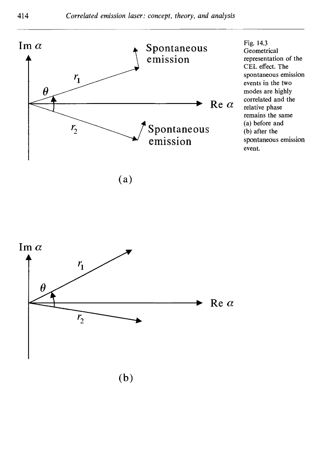
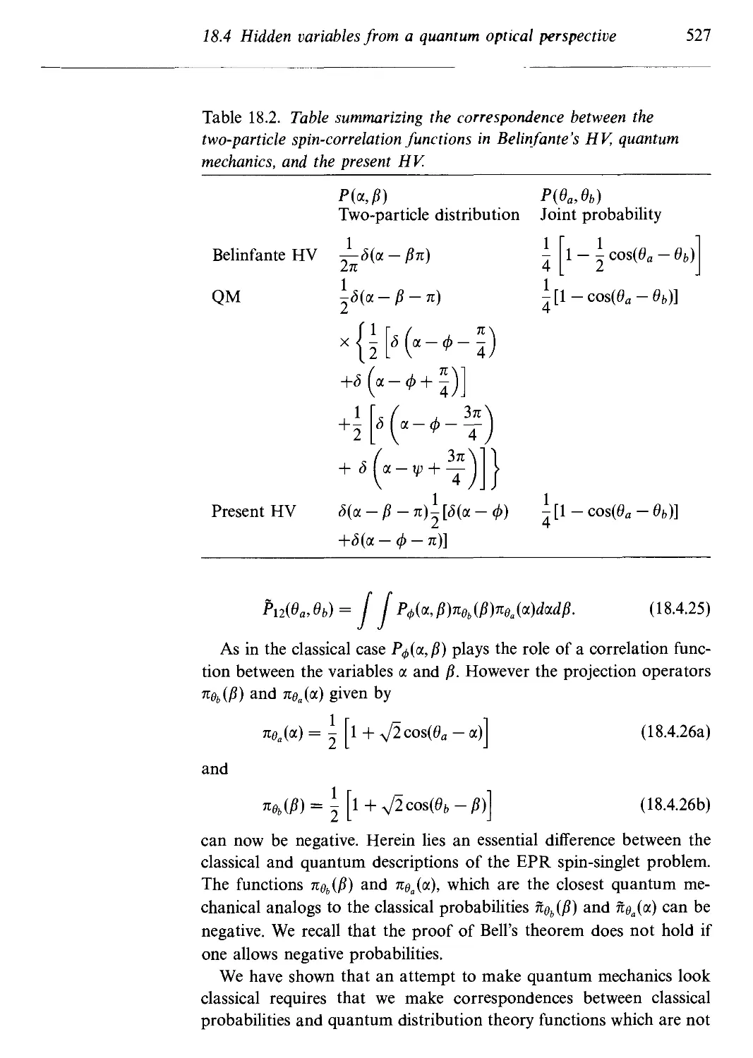
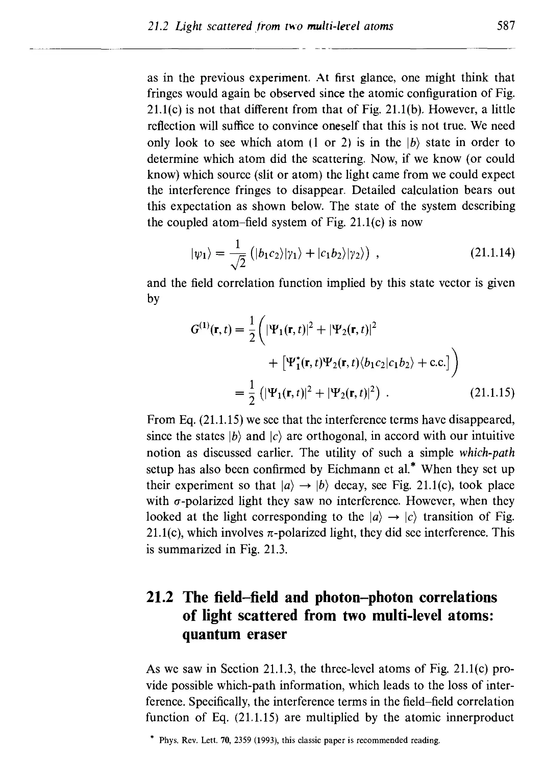
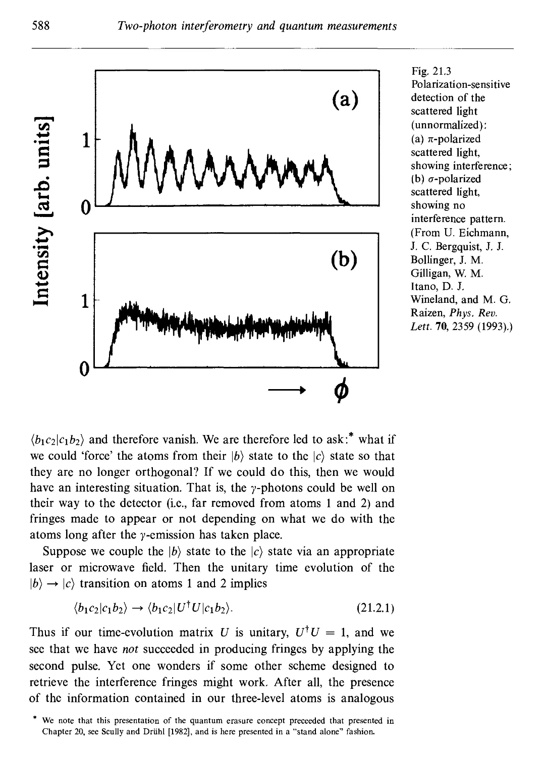
/


Author: Scully M.O. Zubairy M.S.
Tags: physics quantum optics quantum physics
ISBN: 0-521-43458-0
Year: 1997


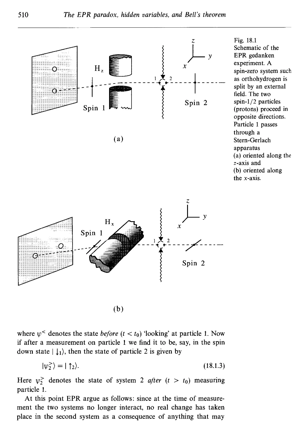
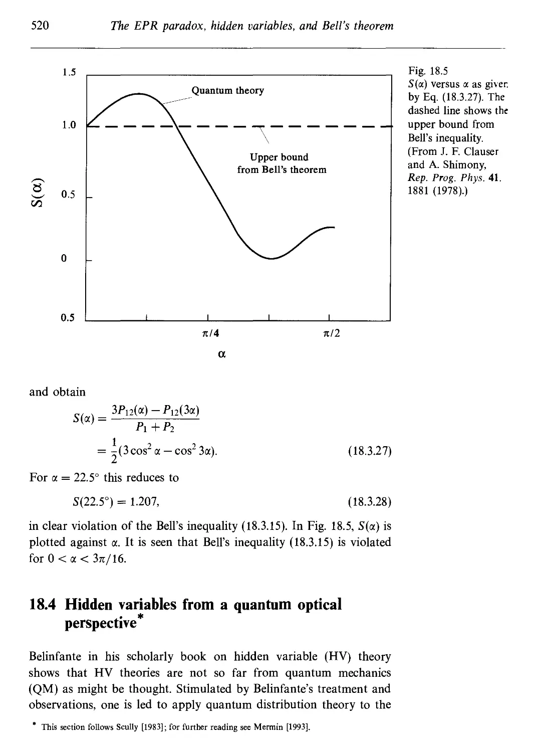
Text
QUANTUM
~ OPTICS
MARLAN O. SCULLY AND M. SUHAIL ZUBAIRY
The field of quantum optics has witnessed significant developments in recent
years, from the laboratory realization of counter-intuitive concepts such as
lasing without inversion and micromasers, to the investigation of fundamental
issues in quantum mechanics, such as complementarity and hidden variables.
This book provides an in-depth and wide-ranging introduction to the subject
of quantum optics, emphasizing throughout the basic principles and their
applications.
The book begins by developing the basic tools of quantum optics, and goes on
to show the application of these tools in a variety of quantum optical systems,
including resonance fluorescence, lasers, micromasers, squeezed states, and
atom optics. The final four chapters are devoted to a discussion of quantum
optical tests of the foundations of quantum mechanics, and particular aspects
of measurement theory.
Assuming only a background of standard quantum mechanics and electro-
electromagnetic theory, and containing many problems and references, this book will
be invaluable to graduate students of quantum optics, as well as to established
researchers in this field.
Marian O. Scully has received numerous honors as a result of his many
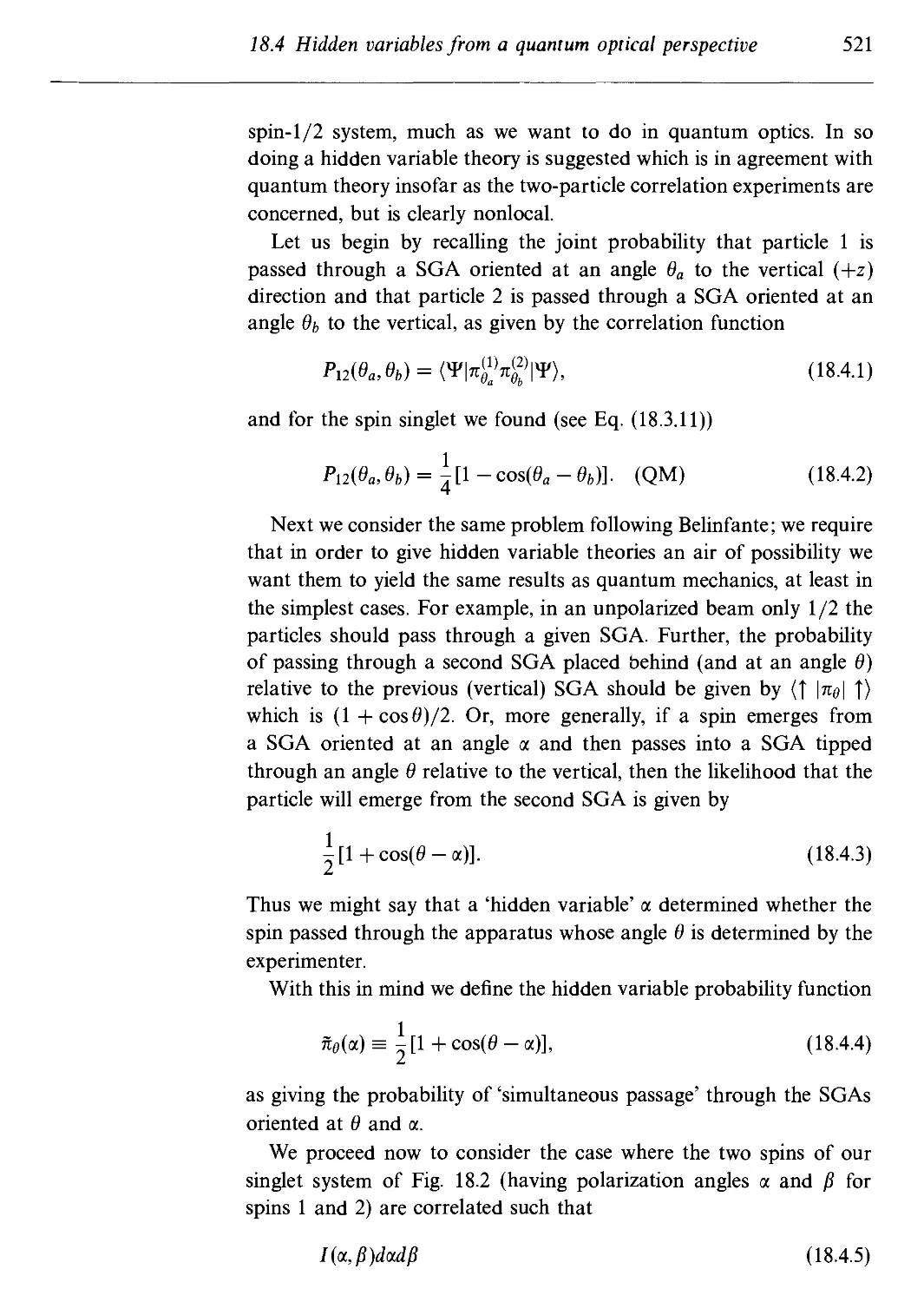
pioneering contributions as a researcher and educator on both sides of the
Atlantic. These include: the Adolph Lomb Medal of the Optical Society of
America, the Elliot Cresson Medal of the Franklin Society, Guggenheim Fel-
Fellowship, and the Alexander von Humboldt Award. He is an elected member
of the Max-Planck Society and a Fellow of the American Physical Society, the
Optical Society of America, and the American Association of the Advance-
Advancement of Science. He has held the faculty positions at Yale, MIT, University
of Arizona, University of New Mexico and is currently Burgess Distinguished
Professor of Physics, Director of the Center for Theoretical Physics at Texas
A&M University, Co-Director of the Texas Laser Lab., and Auswrtiges Wis-
senschaftliches Mitglied at the Max-Planck Institut fur Quantenoptik.
M. Suhail Zubairy received his PhD degree from the University of Rochester
in 1978. He held research and faculty positions at the University of Rochester,
University of Arizona, and the University of New Mexico before joining the
Quaid-i-Azam University, Islamabad in 1984 where he is presently a Professor
and founding Chairman of the Department of Electronics. He has held visiting
appointments at the Max-Planck Institut fur Quantenoptik, Universitat Ulm,
University of New Mexico, and the University of Campinas. He has been an
Associate Member of the International Centre for Theoretical Physics, Trieste.
He was awarded the Order of Sitara-e-Imtiaz by the President of Pakistan in
1993. He has received the Salam Prize for Physics and a Gold Medal from
the Pakistan Academy of Sciences. He is a Fellow of the Pakistan Academy
of Sciences and the Optical Society of America.
Quantum
optics
Marian O. Scully
Texas A&M University and Max-Planck-Institut fur Quantenoptik
M. Suhail Zubairy
Quaid-i-Azam University
Cambridge
UNIVERSITY PRESS
PUBLISHED BY THE PRESS SYNDICATE OF THE UNIVERSITY OF CAMBRIDGE
The Pitt Building, Trumpington Street, Cambridge, United Kingdom
CAMBRIDGE UNIVERSITY PRESS
The Edinburgh Building, Cambridge CB2 2RU, UK
40 West 20th Street, New York, NY 10011-4211, USA
10 Stamford Road, Oakleigh, VIC 3166, Australia
Ruiz de Alarcon 13, 28014 Madrid, Spain
Dock House, The Waterfront, Cape Town 8001, South Africa
http: //www.cambridge.org
© Cambridge University Press 1997
This book is in copyright. Subject to statutory exception
and to the provisions of relevant collective licensing agreements,
no reproduction of any part may take place without
the written permission of Cambridge University Press.
First published 1997
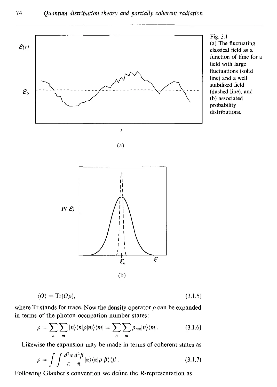
Reprinted 1999, 2001
Printed in the United Kingdom at the University Press, Cambridge
Typeface Times 10/13pt System MfcX [UPH]
A catalogue record for this book is available from the British Library
Library of Congress Cataloguing in Publication data
Scully, Marian O. (Marian Orvil), 1939-
Quantum optics / Marian O. Scully and M. Suhail Zubairy.
p. cm.
Includes bibliographical references and index.
ISBN 0 521 43458 0. - ISBN 0 521 43595 1 (pbk.)
1. Quantum optics. I. Zubairy, Muhammad Suhail, 1952- .
II. Title.
QC446.2.S4 1996
535-dc20 94-42949 CIP
ISBN 0 521 43458 0 hardback
ISBN 0 521 43595 1 paperback
Contents
Preface xix
1 Quantum theory of radiation 1
1.1 Quantization of the free electromagnetic field 2
1.1.1 Mode expansion of the field 3
1.1.2 Quantization 4
1.1.3 Commutation relations between electric and magnetic
field components 7
1.2 Fock or number states 9
1.3 Lamb shift 13
1.4 Quantum beats 16
1.5 What is light? - The photon concept 20
1.5.1 Vacuum fluctuations and the photon concept 20
1.5.2 Vacuum fluctuations 22
1.5.3 Quantum beats, the quantum eraser, Bell's theorem,
and more 24
1.5.4 'Wave function for photons' 24
l.A Equivalence between a many-particle Bose gas and a
set of quantized harmonic oscillators 35
Problems 40
References and bibliography 43
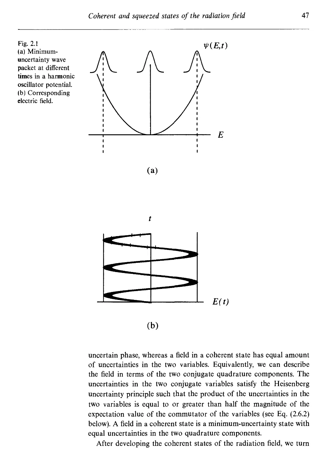
2 Coherent and squeezed states of the radiation field 46
2.1 Radiation from a classical current 48
2.2 The coherent state as an eigenstate of the annihilation
operator and as a displaced harmonic oscillator state 50
2.3 What is so coherent about coherent states? 51
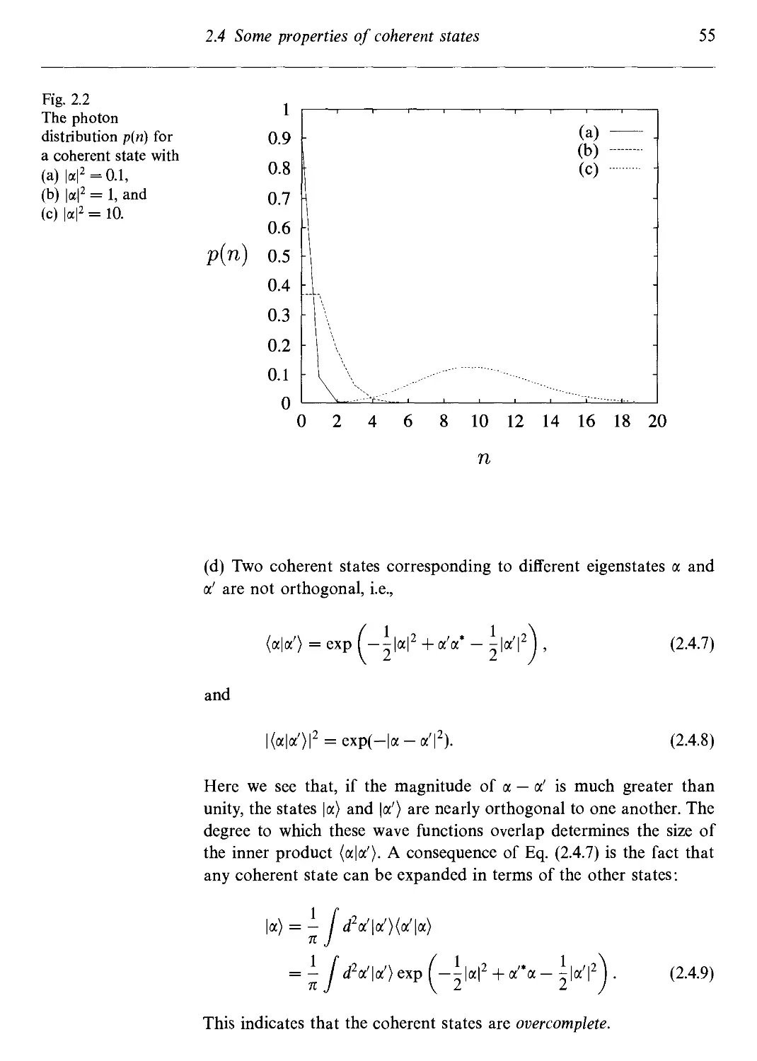
2.4 Some properties of coherent states 54
2.5 Squeezed state physics 56
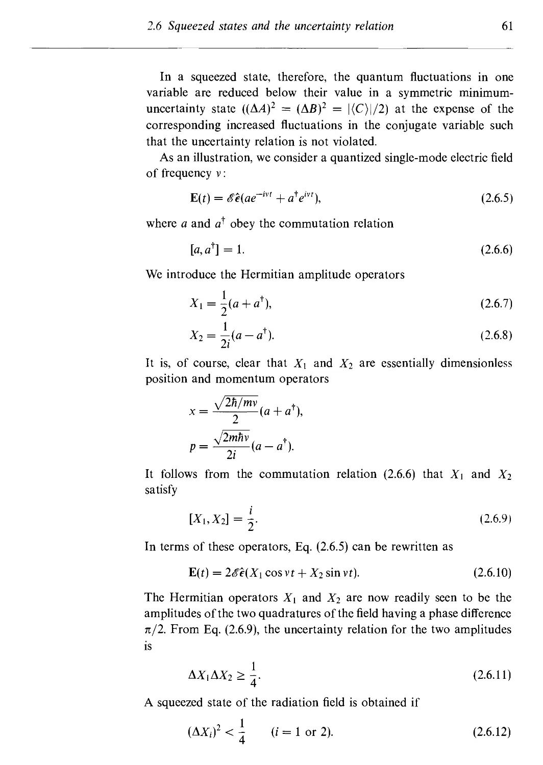
viii Contents
2.6 Squeezed states and the uncertainty relation 60
2.7 The squeeze operator and the squeezed coherent states 63
2.7.1 Quadrature variance 65
2.8 Multi-mode squeezing 66
Problems 67
References and bibliography 70
Quantum distribution theory and partially coherent radiation 72
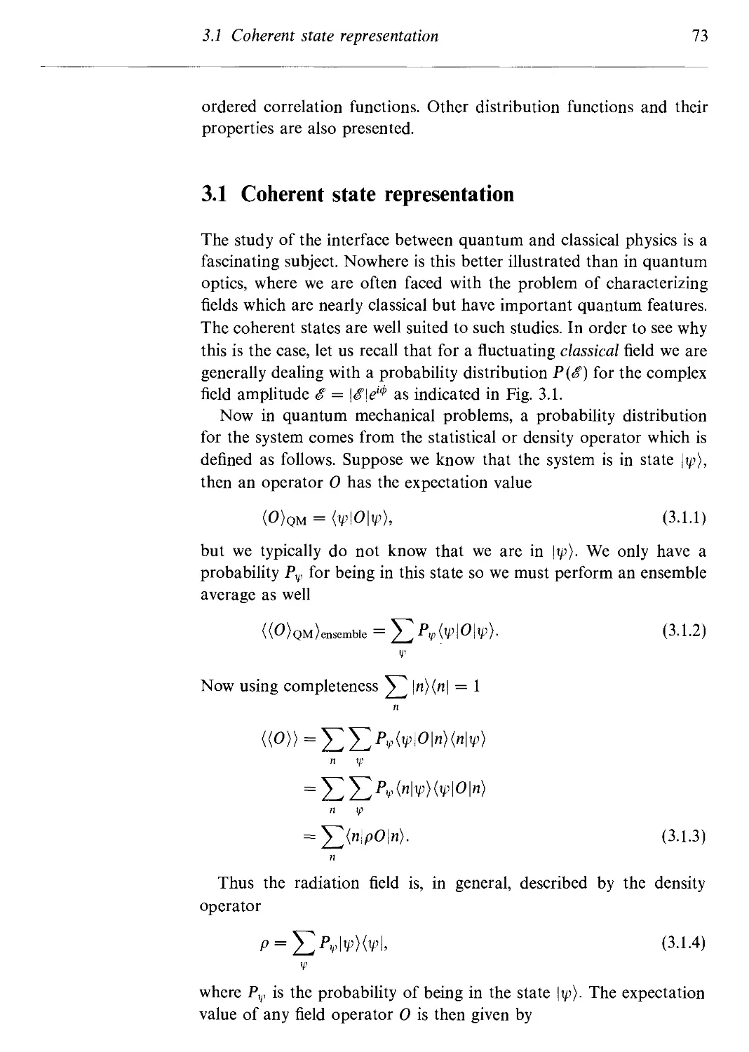
3.1 Coherent state representation 73
3.1.1 Definition of the coherent state representation 75
3.1.2 Examples of the coherent state representation 77
3.2 g-representation 79
3.3 The Wigner-Weyl distribution 81
3.4 Generalized representation of the density operator and
connection between the P-, Q-, and W-distributions 83
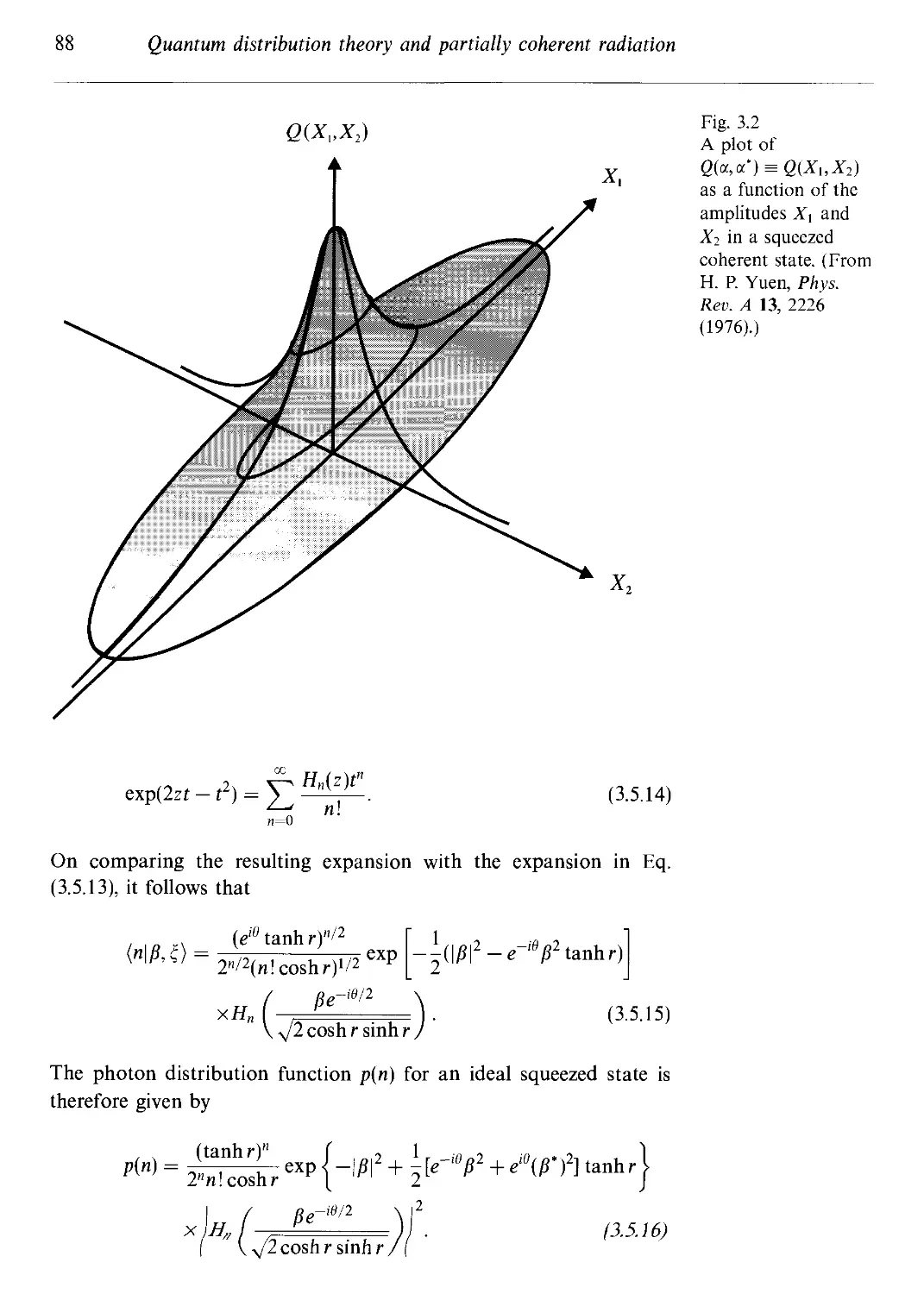
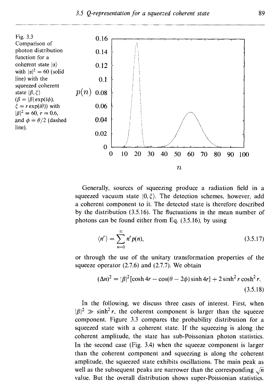
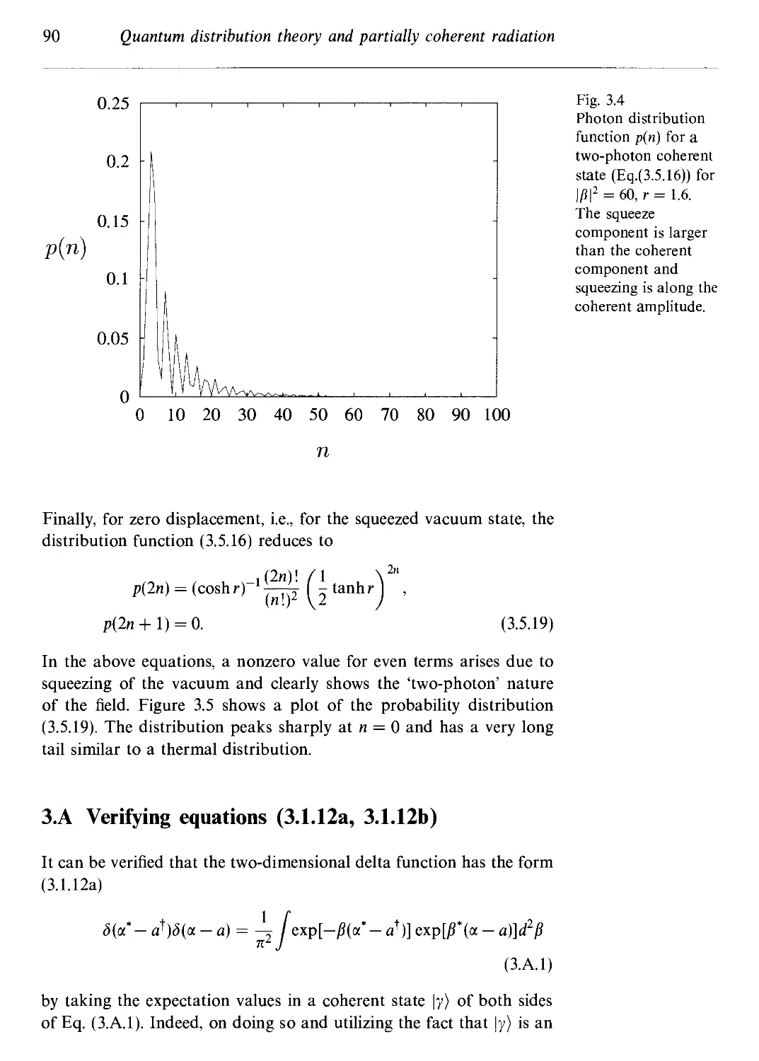
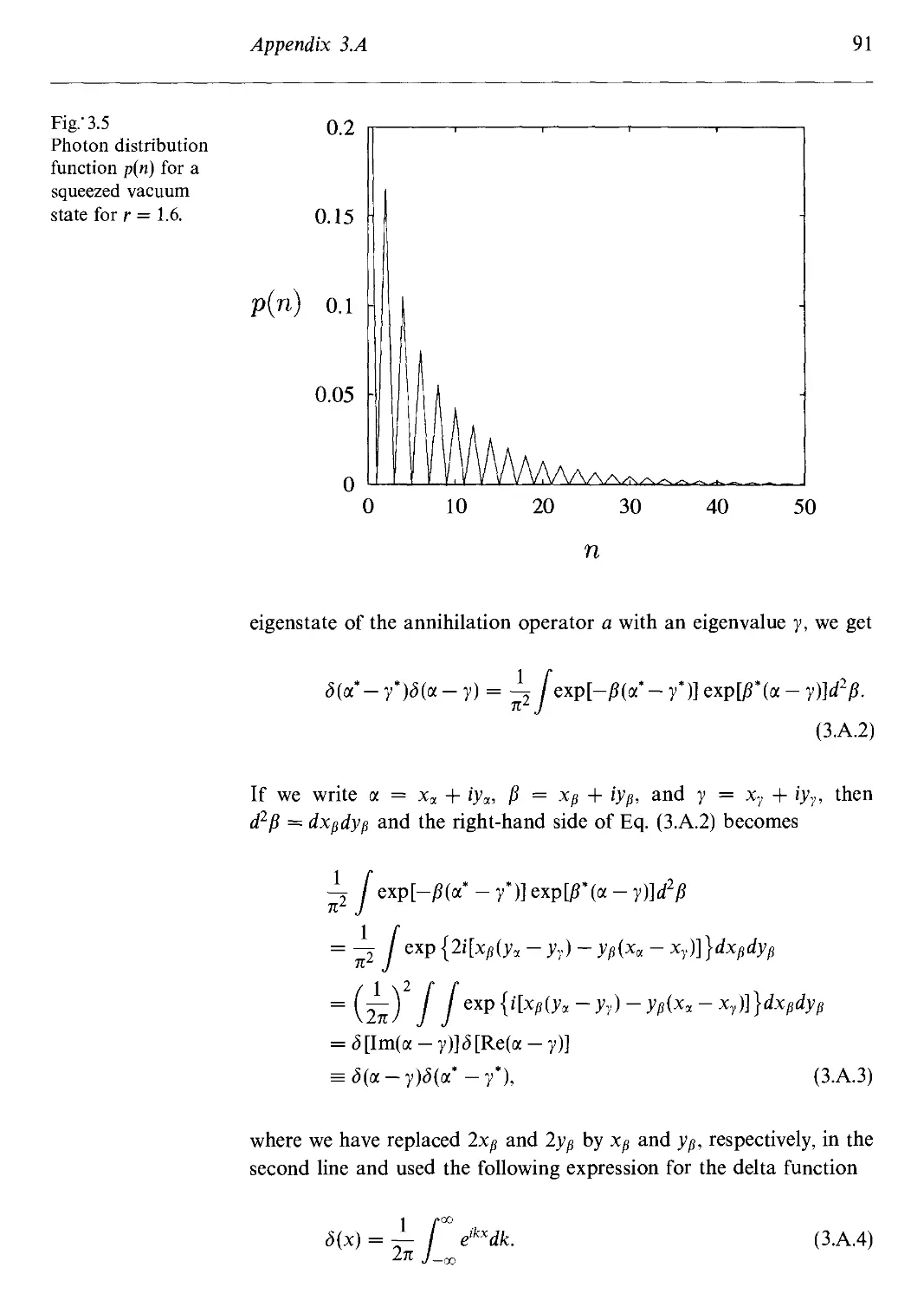
3.5 g-representation for a squeezed coherent state 86
3.A Verifying equations C.1.12a, 3.1.12b) 90
3.B c-number function correspondence for the Wigner-
Weyl distribution 92
Problems 94
References and bibliography 96
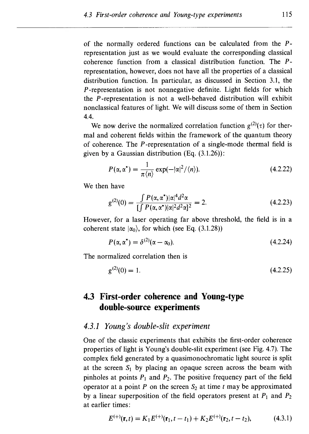
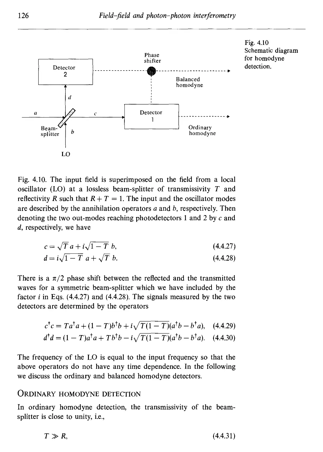
Field-field and photon-photon interferometry 97
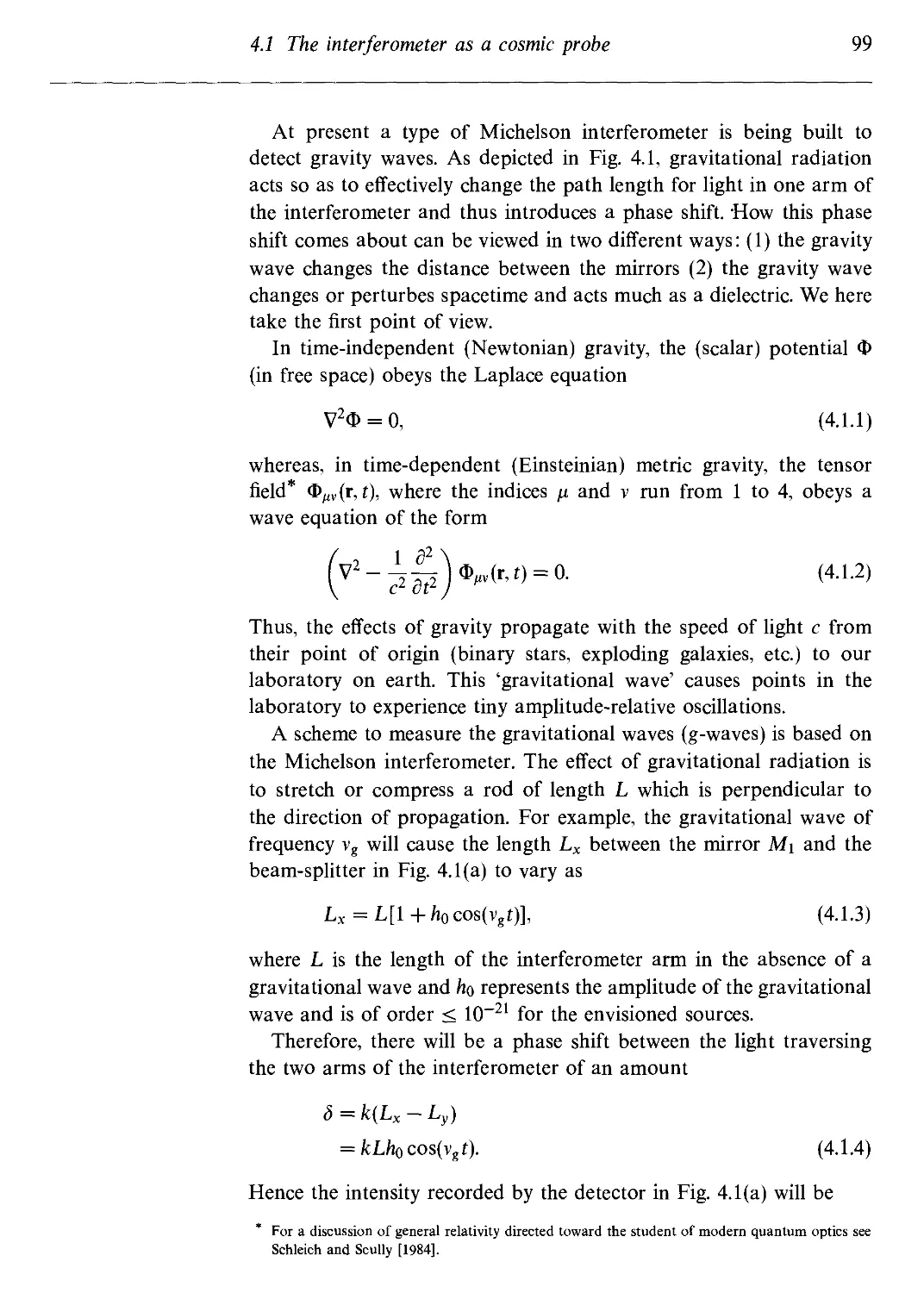
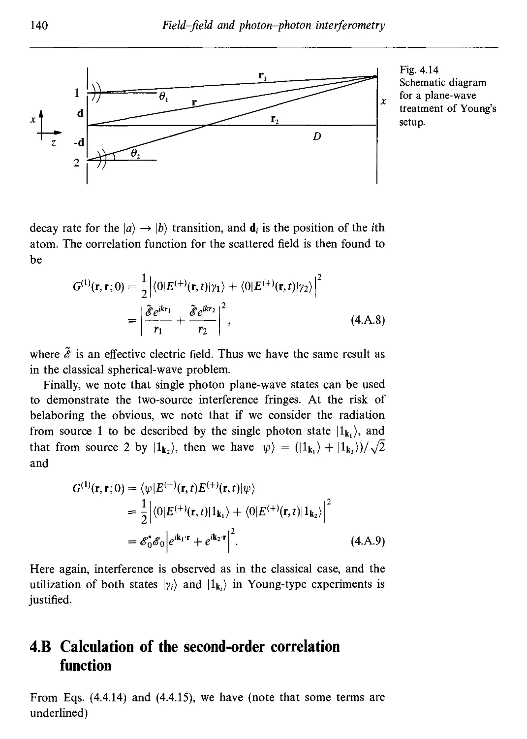
4.1 The interferometer as a cosmic probe 98
4.1.1 Michelson interferometer and general relativity 98
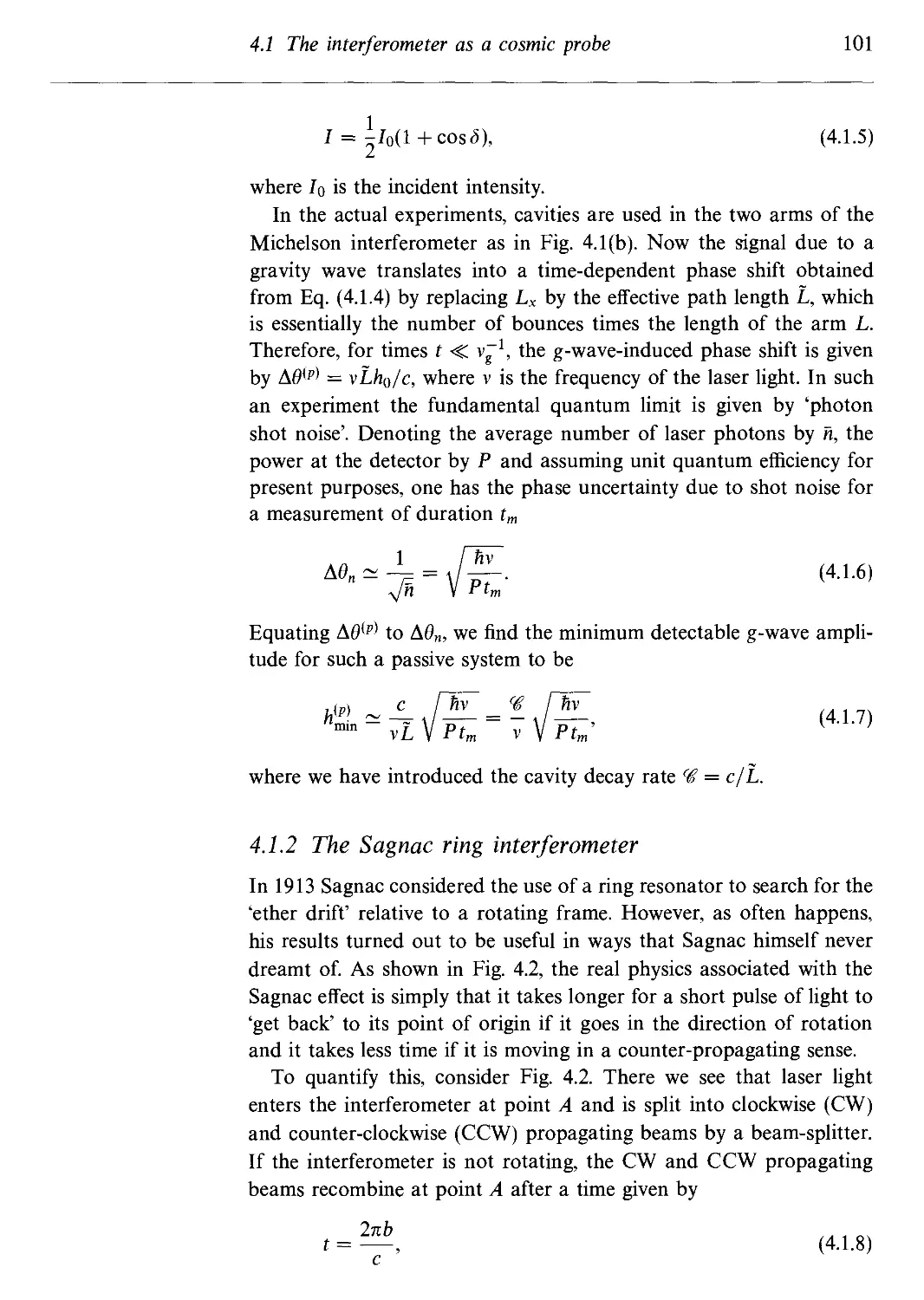
4.1.2 The Sagnac ring interferometer 101
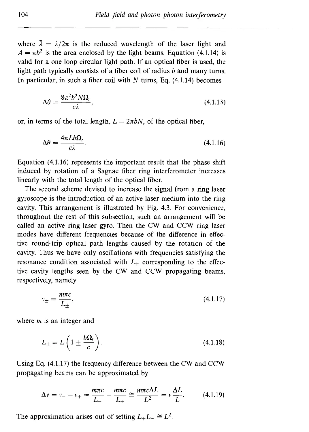
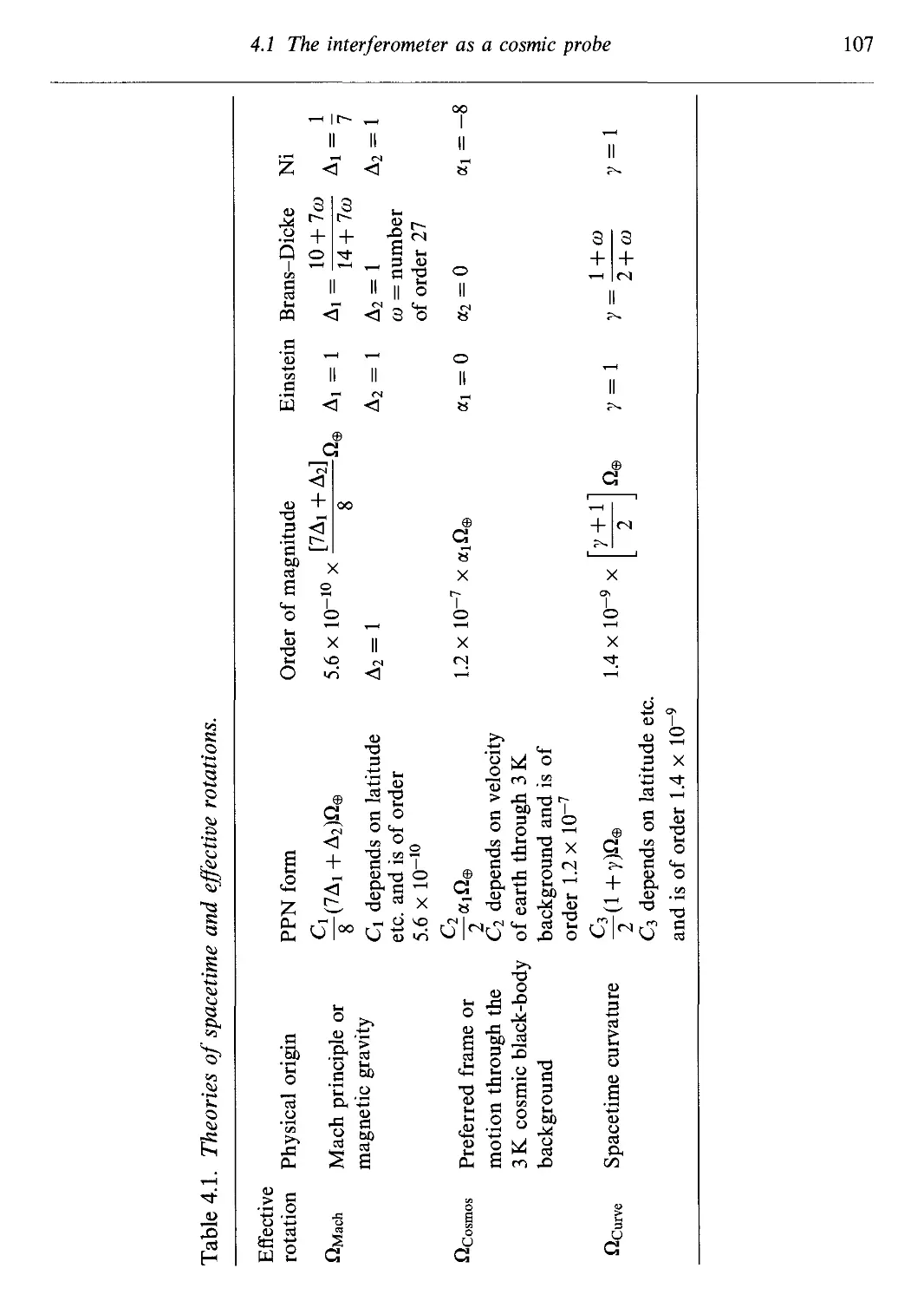
4.1.3 Proposed ring laser test of metric gravitation theories 106
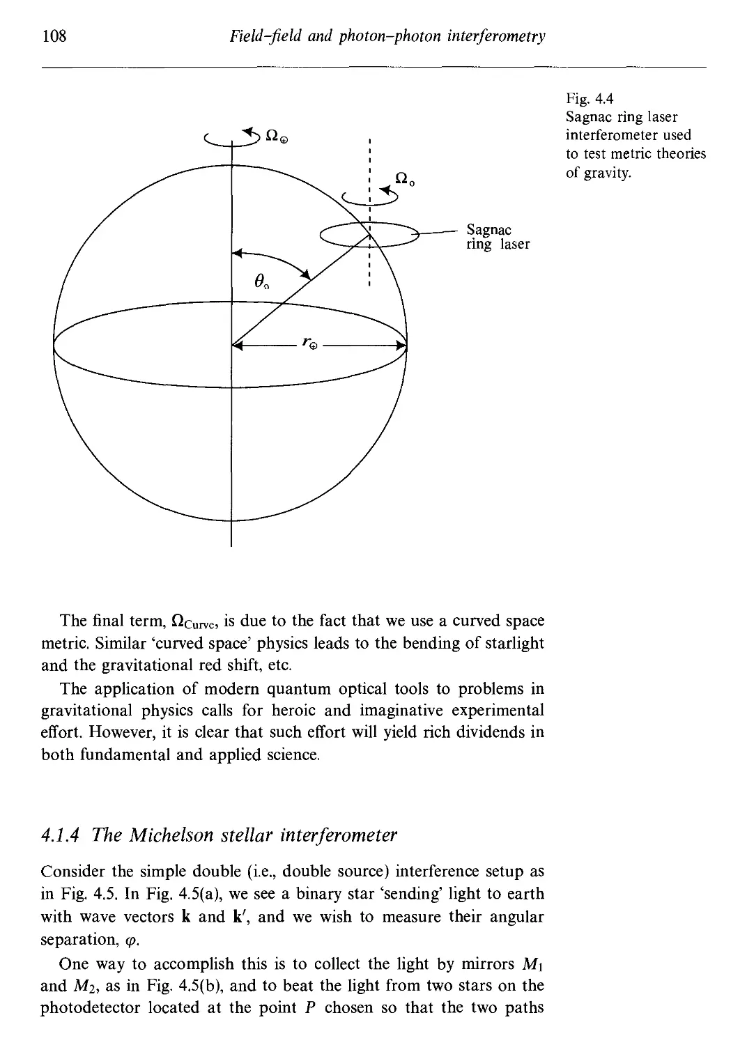
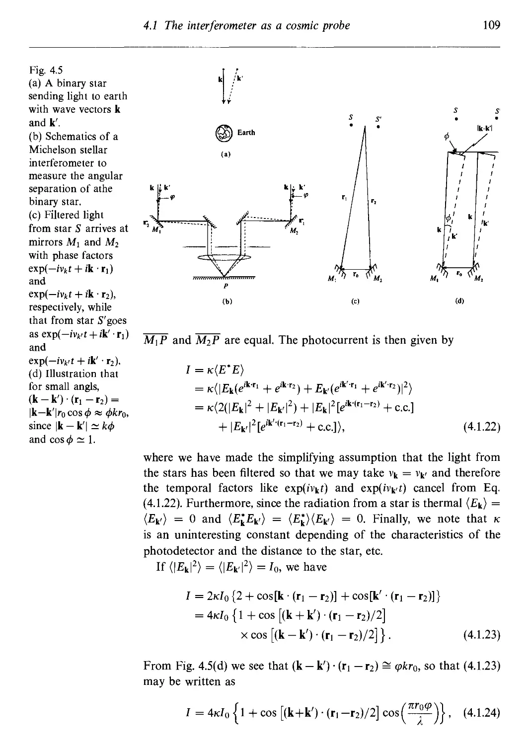
4.1.4 The Michelson stellar interferometer 108
4.1.5 Hanbury-Brown-Twiss interferometer 110
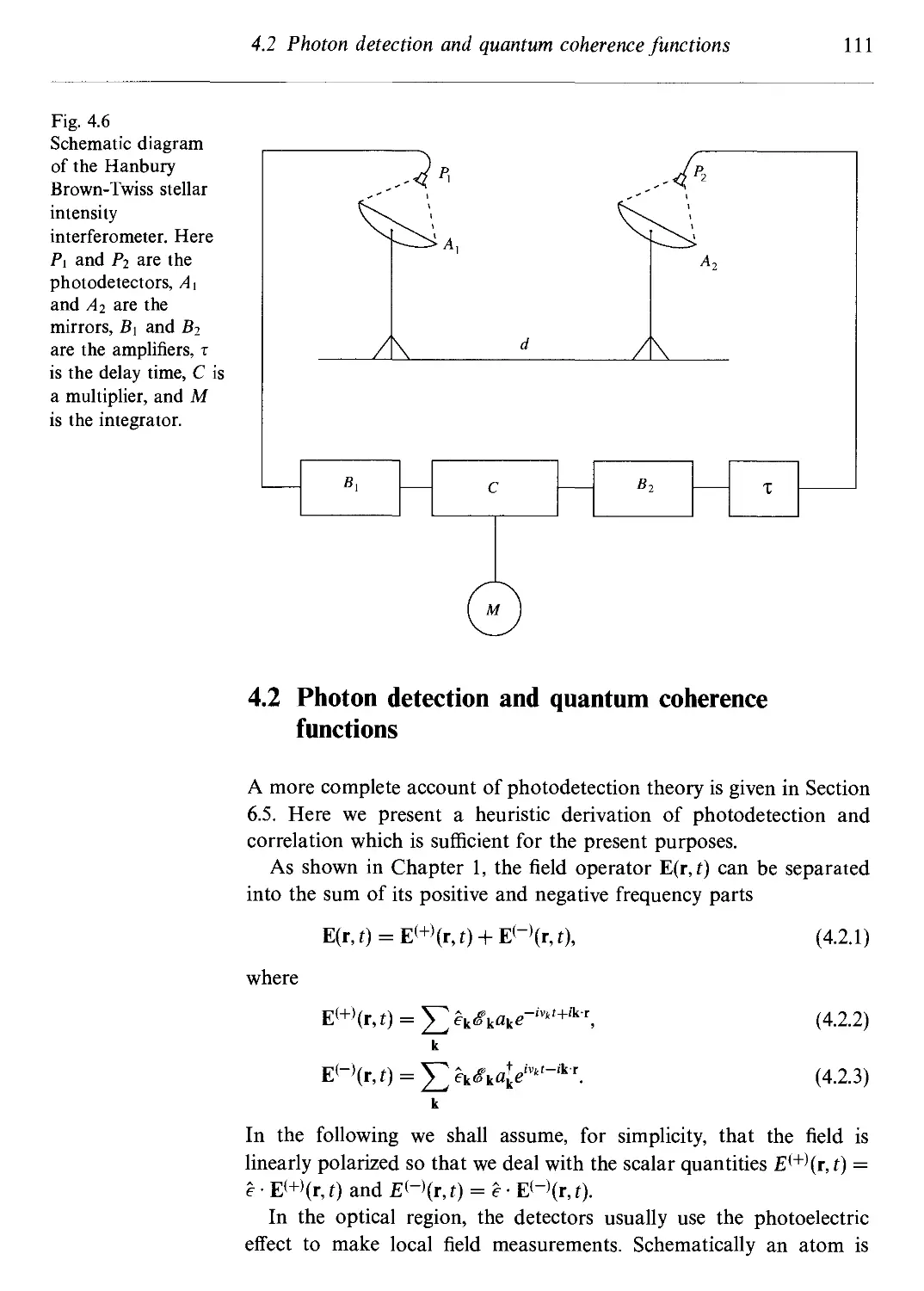
4.2 Photon detection and quantum coherence functions 111
4.3 First-order coherence and Young-type double-source
experiments 115
4.3.1 Young's double-slit experiment 115
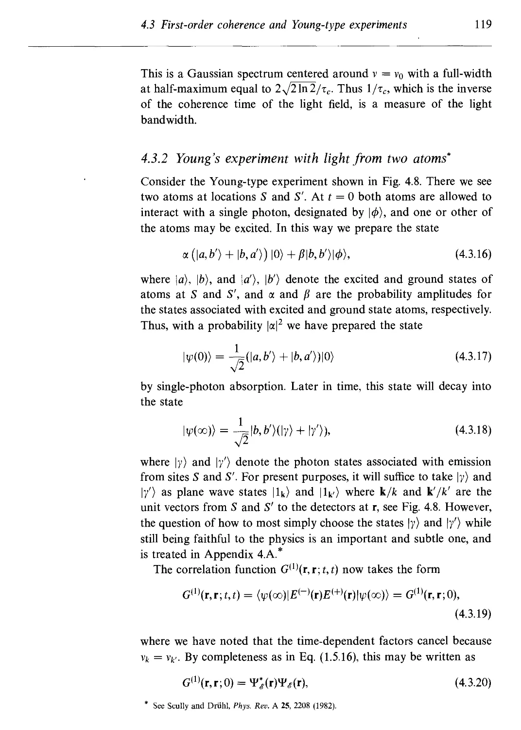
4.3.2 Young's experiment with light from two atoms 119
4.4 Second-order coherence 120
4.4.1 The physics behind the Hanbury-Brown-Twiss effect 121
4.4.2 Detection and measurement of squeezed states via
homodyne detection 125
4.4.3 Interference of two photons 131
4.4.4 Photon antibunching, Poissonian, and sub-Poissonian
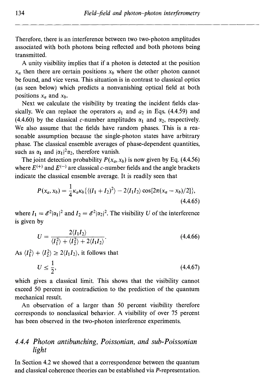
light 134
4.5 Photon counting and photon statistics 137
Contents ix
4.A Classical and quantum descriptions of two-source
interference 139
4.B Calculation of the second-order correlation function 140
Problems 141
References and bibliography 143
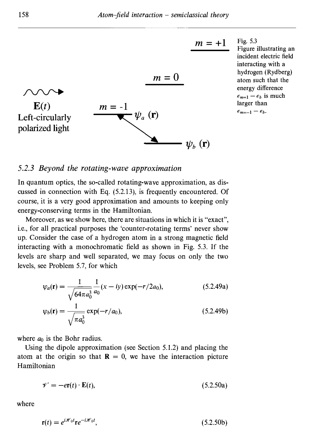
Atom-field interaction - semiclassical theory 145
5.1 Atom-field interaction Hamiltonian 146
5.1.1 Local gauge (phase) in variance and minimal-coupling
Hamiltonian 146
5.1.2 Dipole approximation and r ■ E Hamiltonian 148
5.1.3 p ■ A Hamiltonian 149
5.2 Interaction of a single two-level atom with a single-
mode field 151
5.2.1 Probability amplitude method 151
5.2.2 Interaction picture 155
5.2.3 Beyond the rotating-wave approximation 158
5.3 Density matrix for a two-level atom 160
5.3.1 Equation of motion for the density matrix 161
5.3.2 Two-level atom 162
5.3.3 Inclusion of elastic collisions between atoms 163
5.4 Maxwell-Schrodinger equations 164
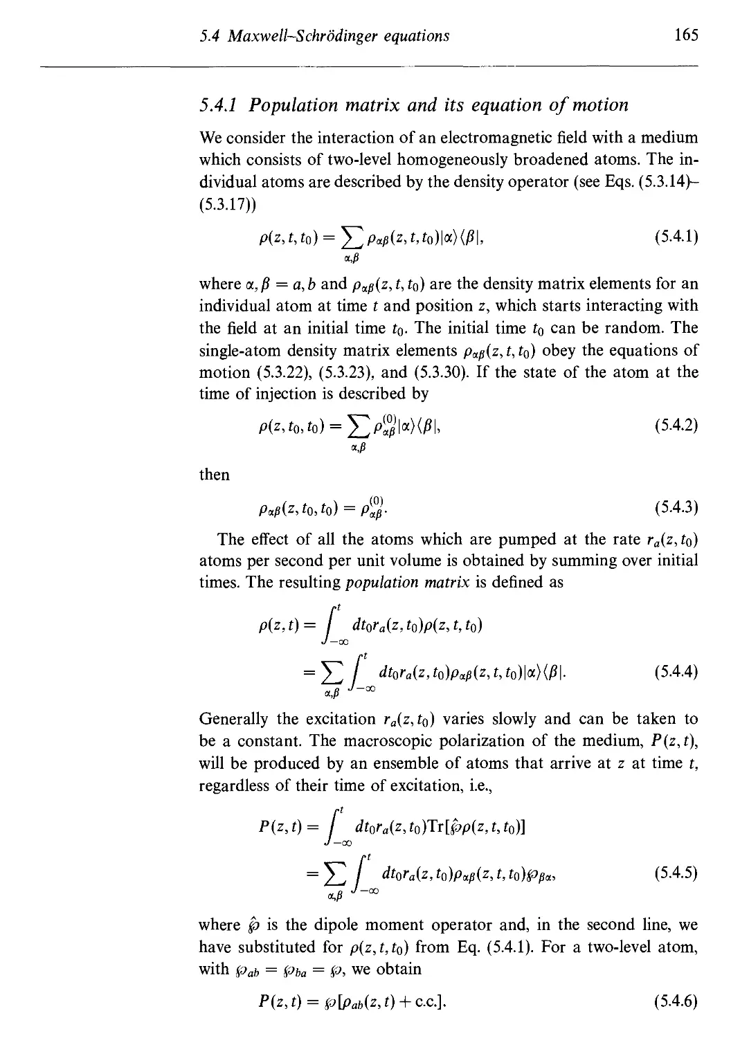
5.4.1 Population matrix and its equation of motion 165
5.4.2 Maxwell's equations for slowly varying field functions 166
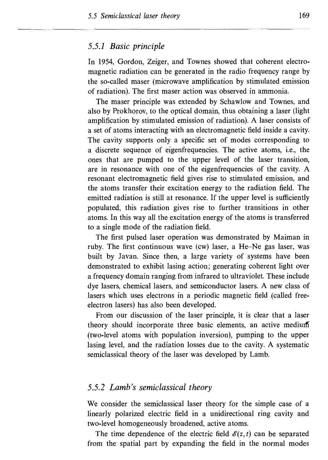
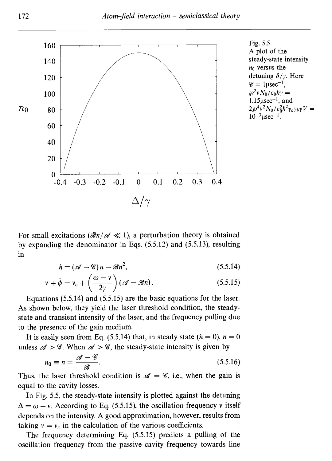
5.5 Semiclassical laser theory 168
5.5.1 Basic principle 169
5.5.2 Lamb's semiclassical theory 169
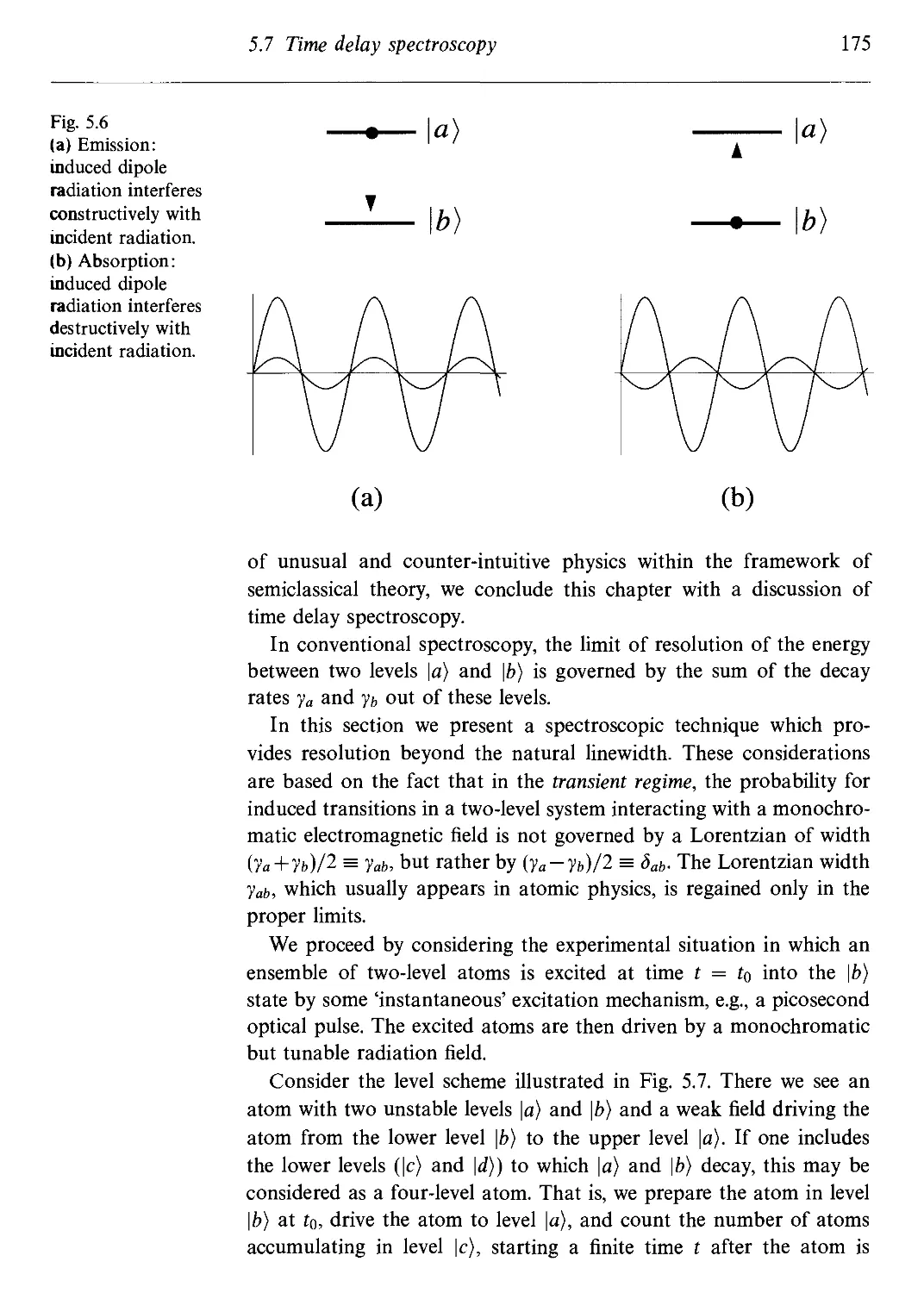
5.6 A physical picture of stimulated emission and
absorption 173
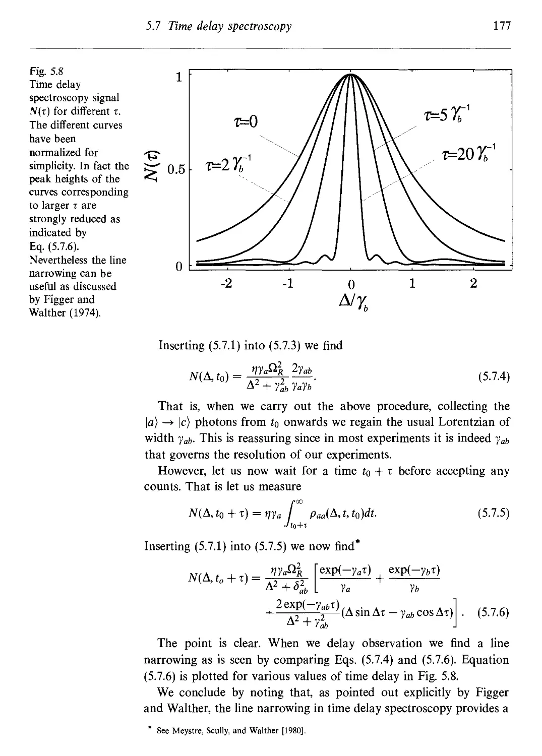
5.7 Time delay spectroscopy 174
5.A Equivalence of the r • E and the p ■ A interaction
Hamiltonians 178
5.A.I Form-invariant physical quantities 178
5.A.2 Transition probabilities in a two-level atom 180
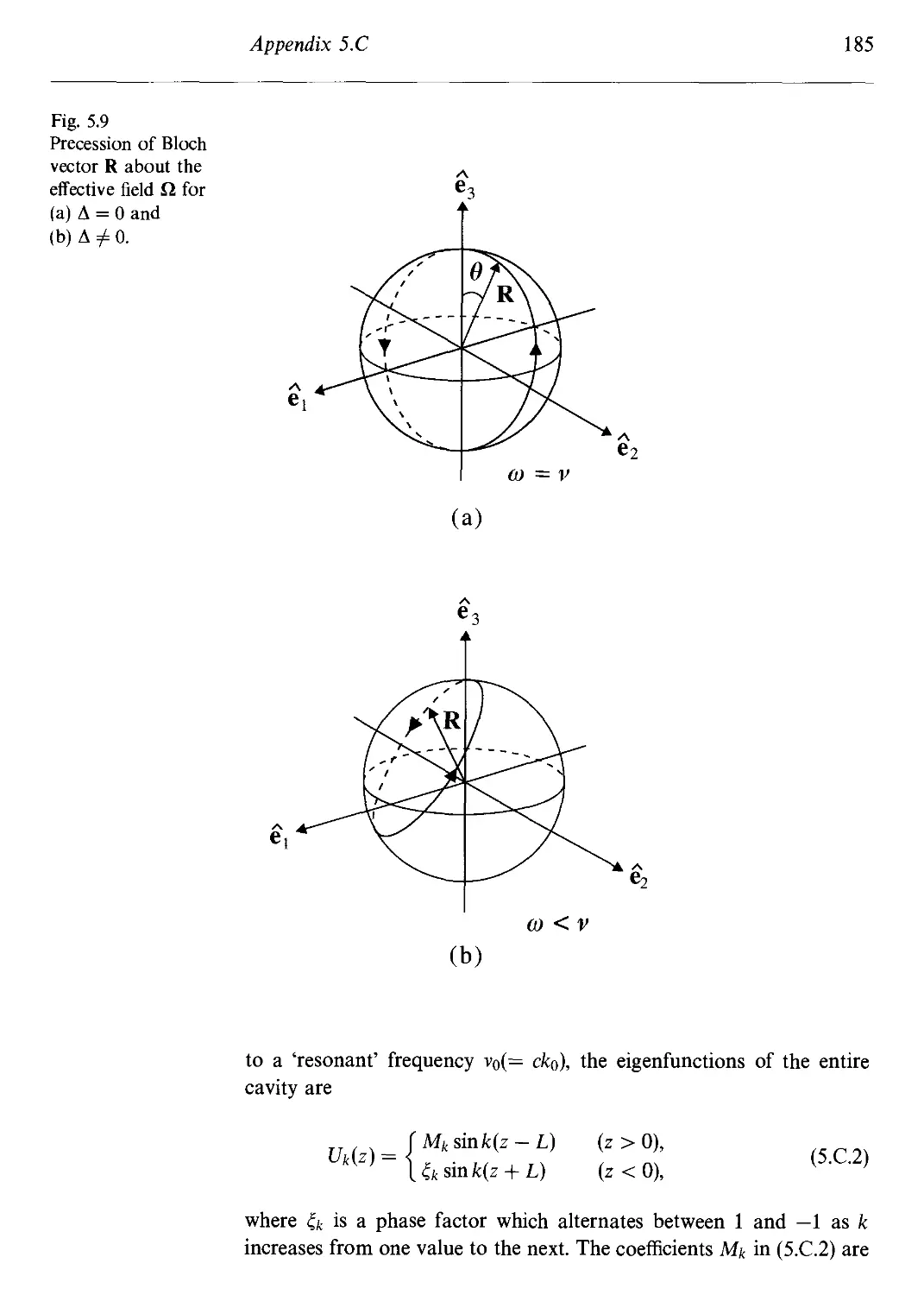
5.B Vector model of the density matrix 183
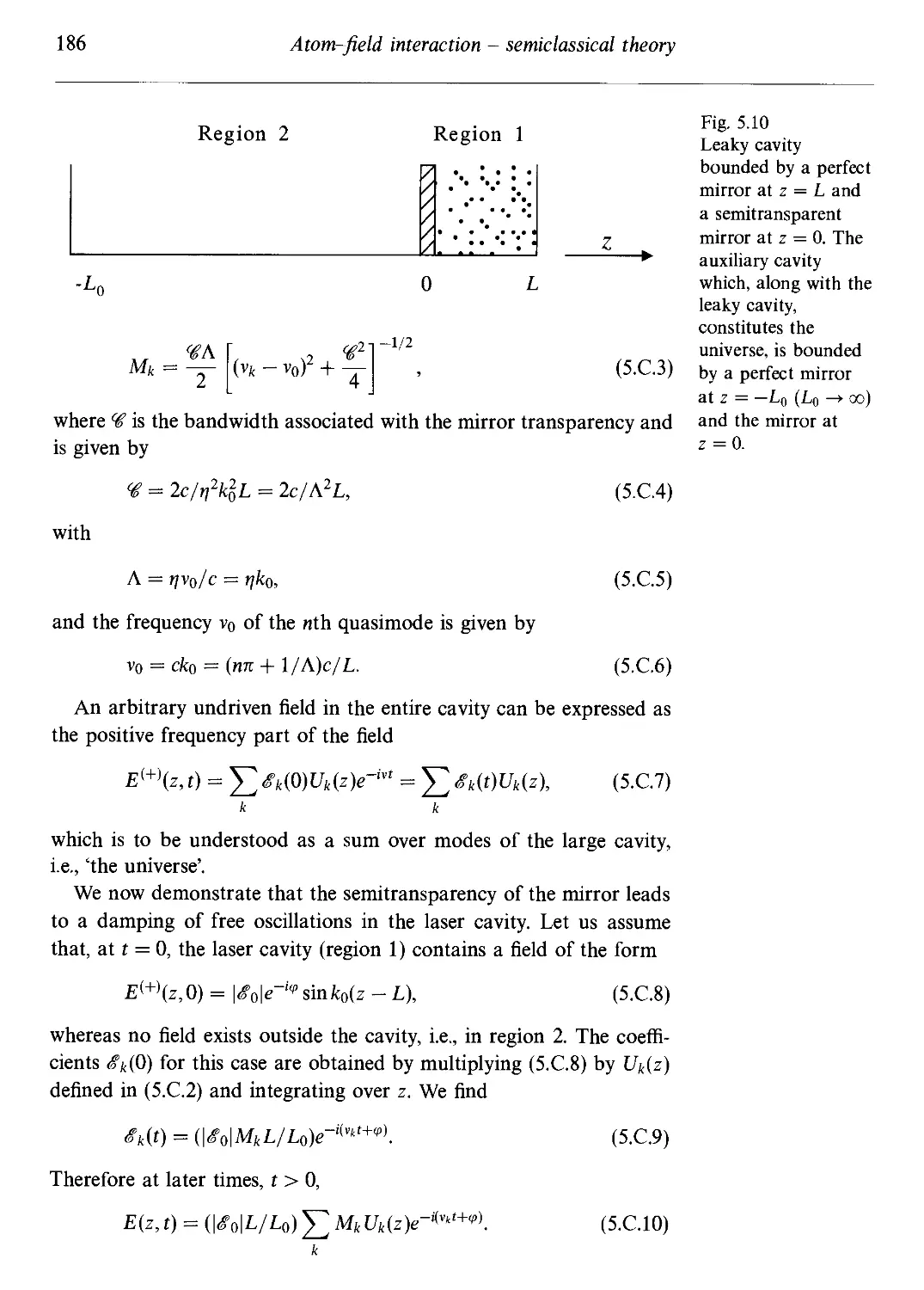
5.C Quasimode laser physics based on the modes of the
universe 185
Problems 187
References and bibliography 190
Atom-field interaction - quantum theory 193
6.1 Atom-field interaction Hamiltonian 194
Contents
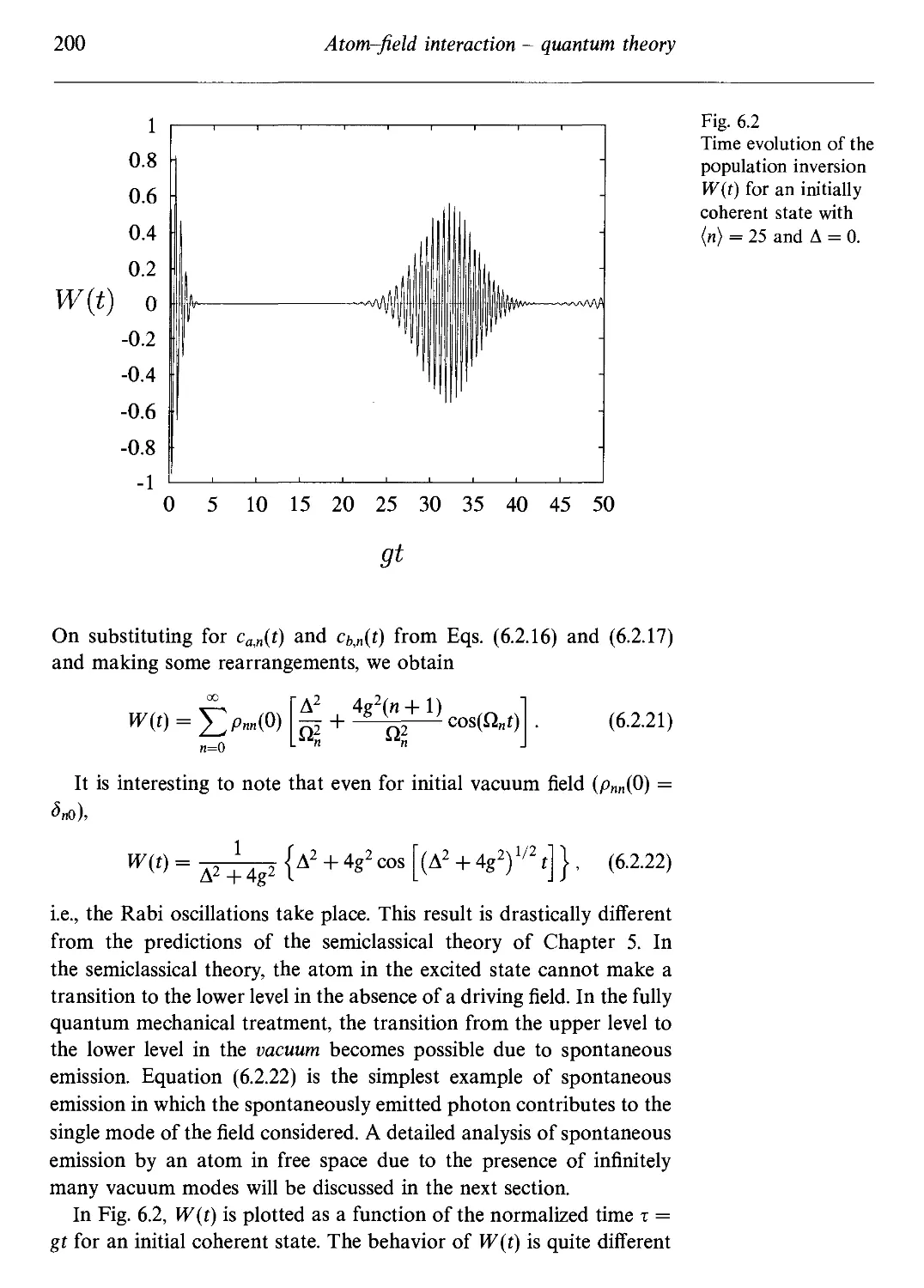
6.2 Interaction of a single two-level atom with a single-
mode field 196
6.2.1 Probability amplitude method 197
6.2.2 Heisenberg operator method 202
6.2.3 Unitary time-evolution operator method 204
6.3 Weisskopf-Wigner theory of spontaneous emission
between two atomic levels 206
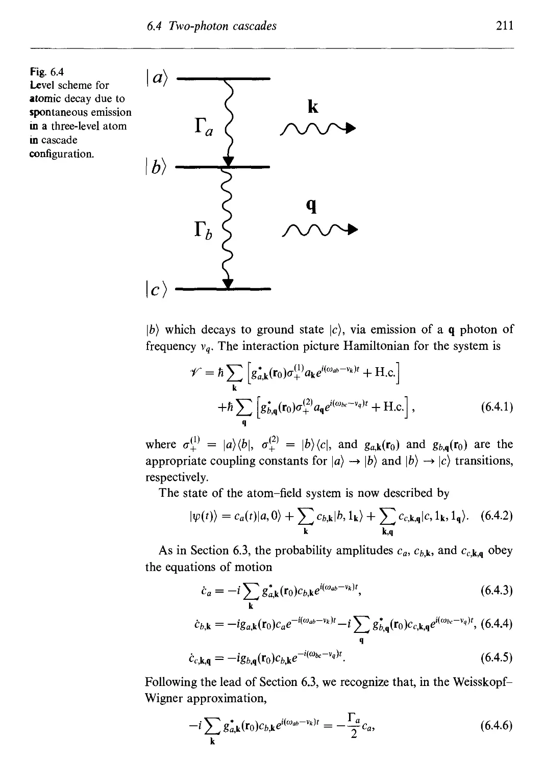
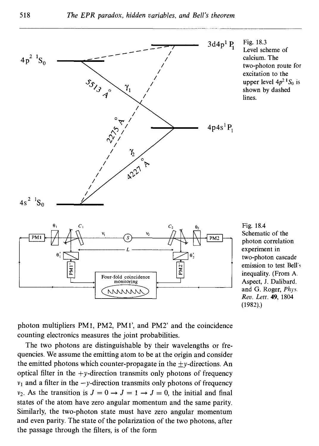
6.4 Two-photon cascades 210
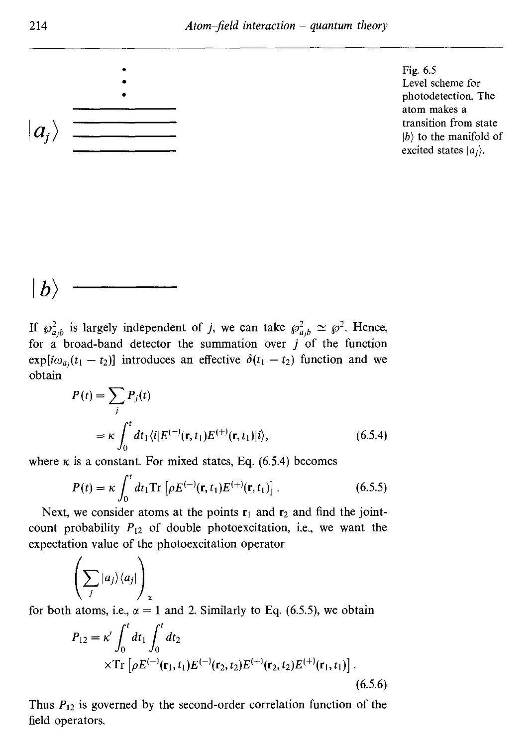
6.5 Excitation probabilities for single and double photo-
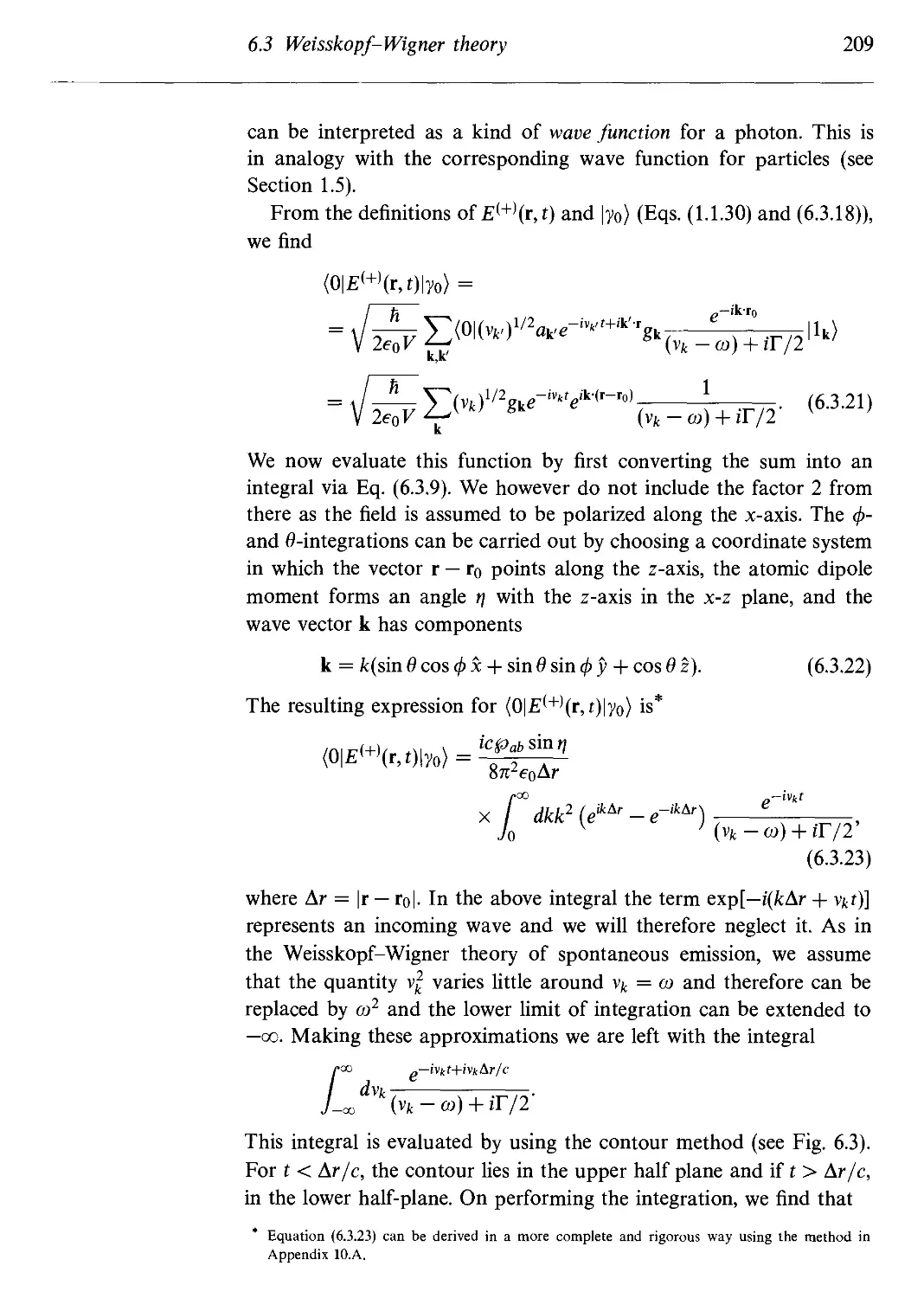
excitation events 213
Problems 215
References and bibliography 217
7 basing without inversion and other effects of atomic
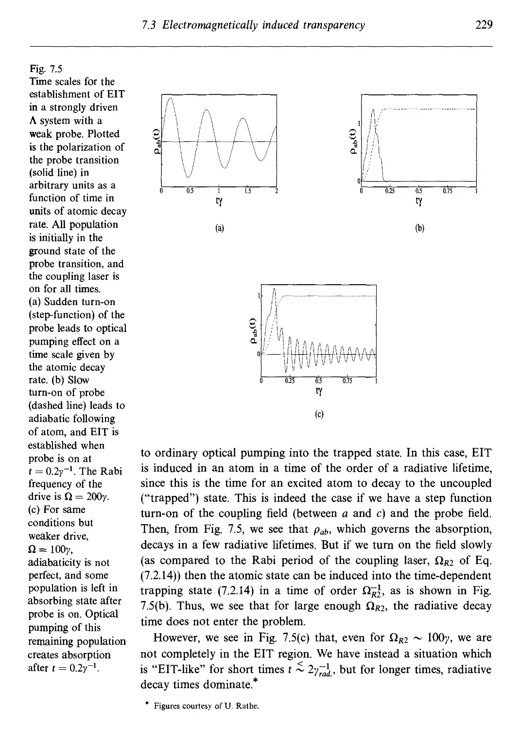
coherence and interference 220
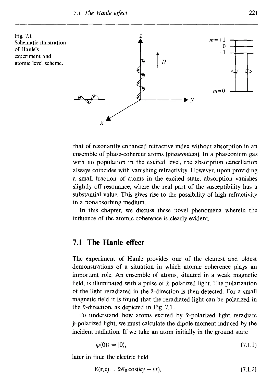
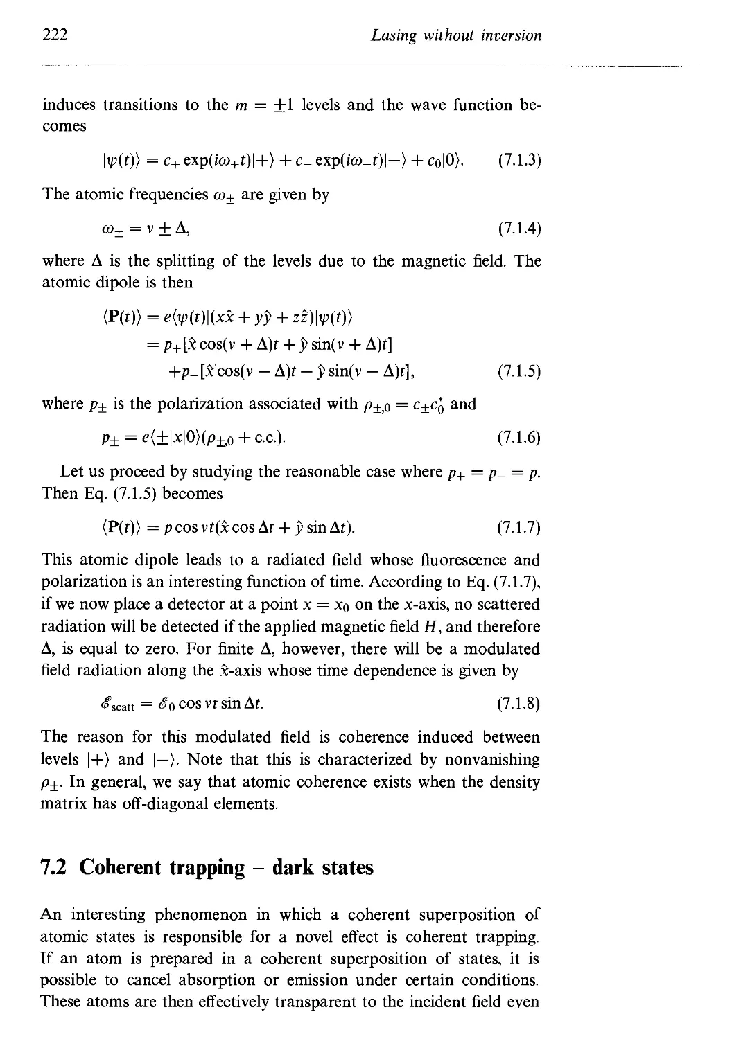
7.1 The Hanle effect 221
7.2 Coherent trapping - dark states 222
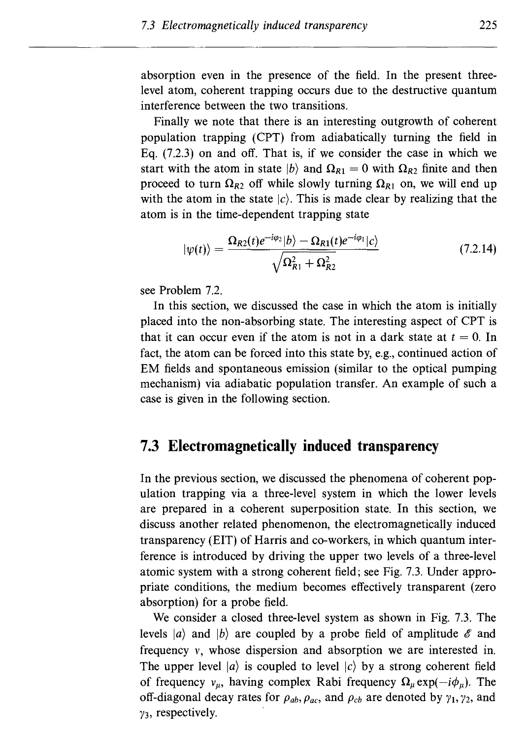
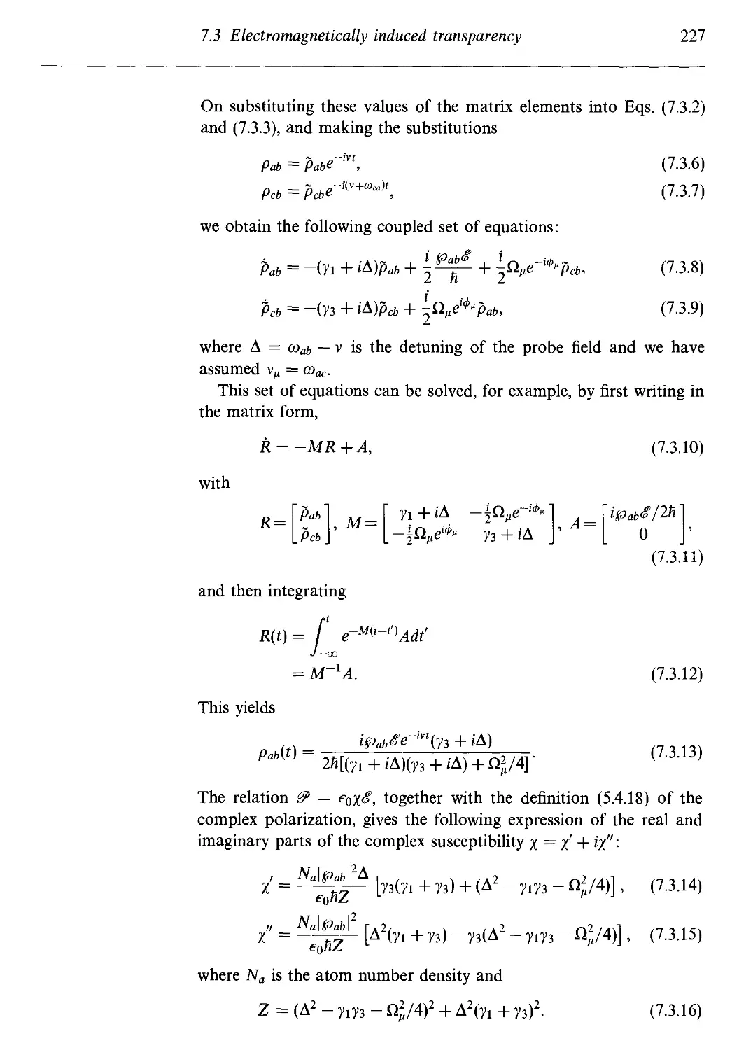
7.3 Electromagnetically induced transparency 225
7.4 basing without inversion 230
7.4.1 The LWI concept 230
7.4.2 The laser physics approach to LWI: simple treatment 232
7.4.3 LWI analysis 233
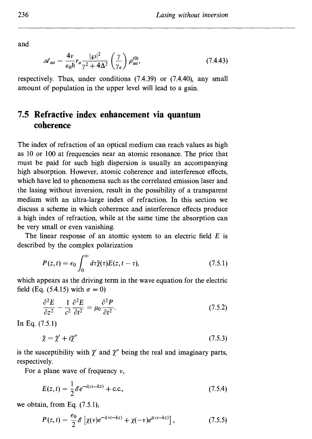
7.5 Refractive index enhancement via quantum coherence 236
7.6 Coherent trapping, lasing without inversion, and
electromagnetically induced transparency via an exact
solution to a simple model 241
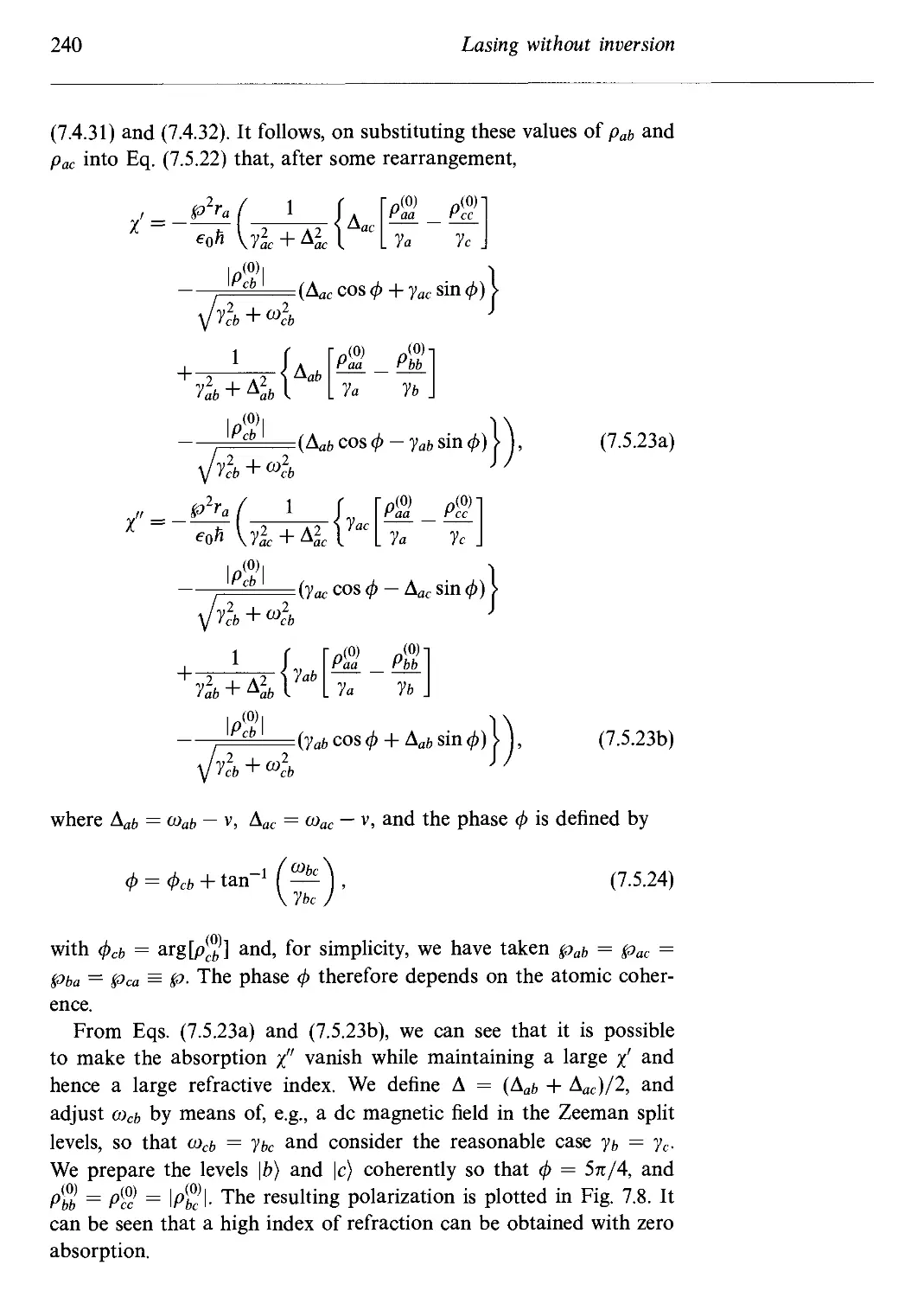
Problems 244
References and bibliography 245
8 Quantum theory of damping - density operator and wave
function approach 248
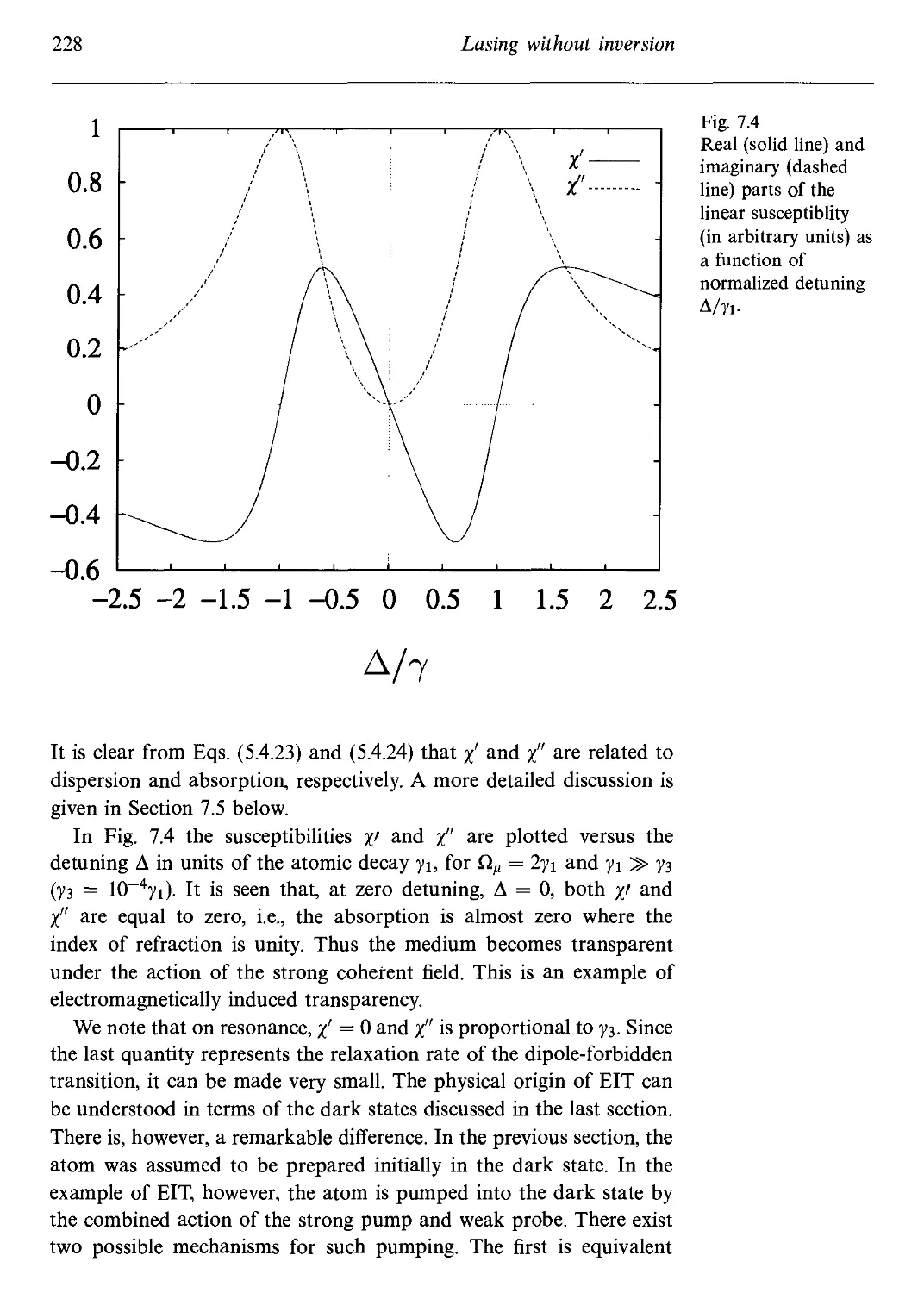
8.1 General reservoir theory 249
8.2 Atomic decay by thermal and squeezed vacuum
reservoirs 250
8.2.1 Thermal reservoir 251
8.2.2 Squeezed vacuum reservoir 253
8.3 Field damping 255
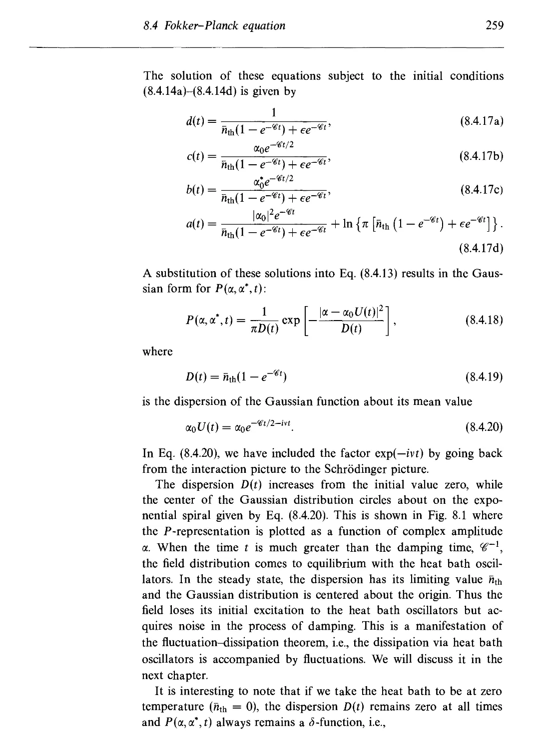
8.4 Fokker-Planck equation 256
8.5 The 'quantum jump' approach to damping 260
8.5.1 Conditional density matrices and the null measurement 261
8.5.2 The wave function Monte Carlo approach to damping 263
Contents xi
Problems 267
References and bibliography 269
9 Quantum theory of damping - Heisenberg-Langevin approach 271
9.1 Simple treatment of damping via oscillator reservoir:
Markovian white noise 272
9.2 Extended treatment of damping via atom and oscillator
reservoirs: non-Markovian colored noise 276
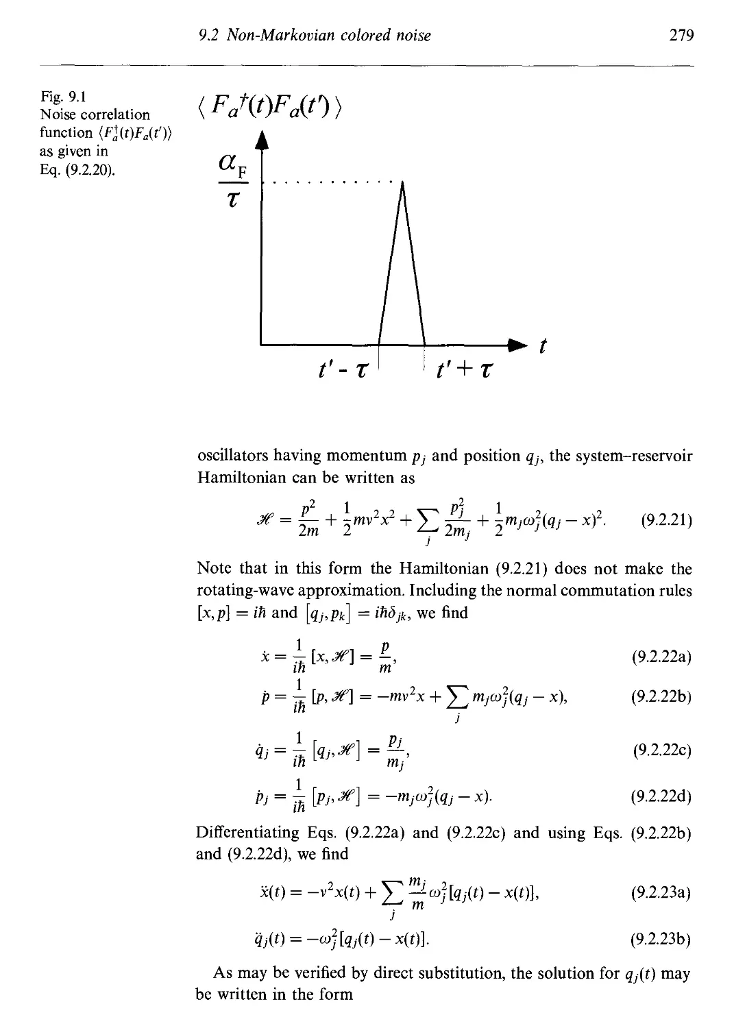
9.2.1 An atomic reservoir approach 276
9.2.2 A generalized treatment of the oscillator reservoir
problem 278
9.3 Equations of motion for the field correlation functions 281
9.4 Fluctuation-dissipation theorem and the Einstein
relation 283
9.5 Atom in a damped cavity 284
Problems 289
References and bibliography 290
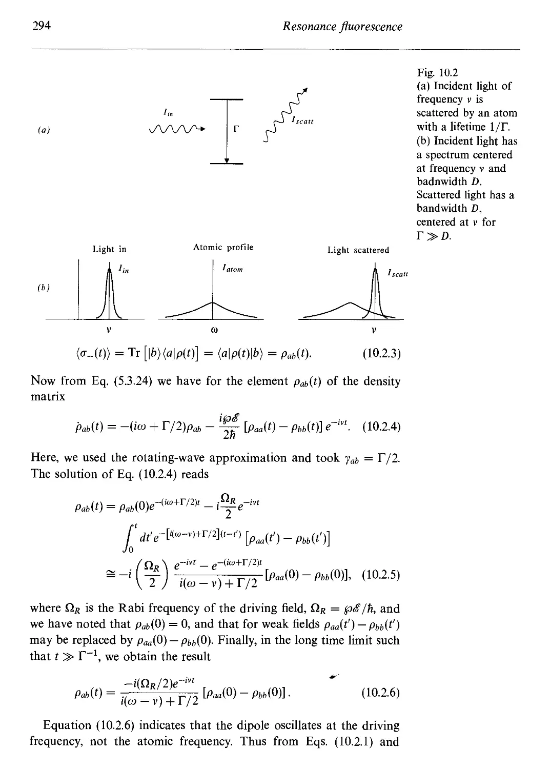
10 Resonance fluorescence 291
10.1 Electric field operator for spontaneous emission
from a single atom 292
10.2 An introduction to the resonance fluorescence
spectrum 293
10.2.1 Weak driving field limit 293
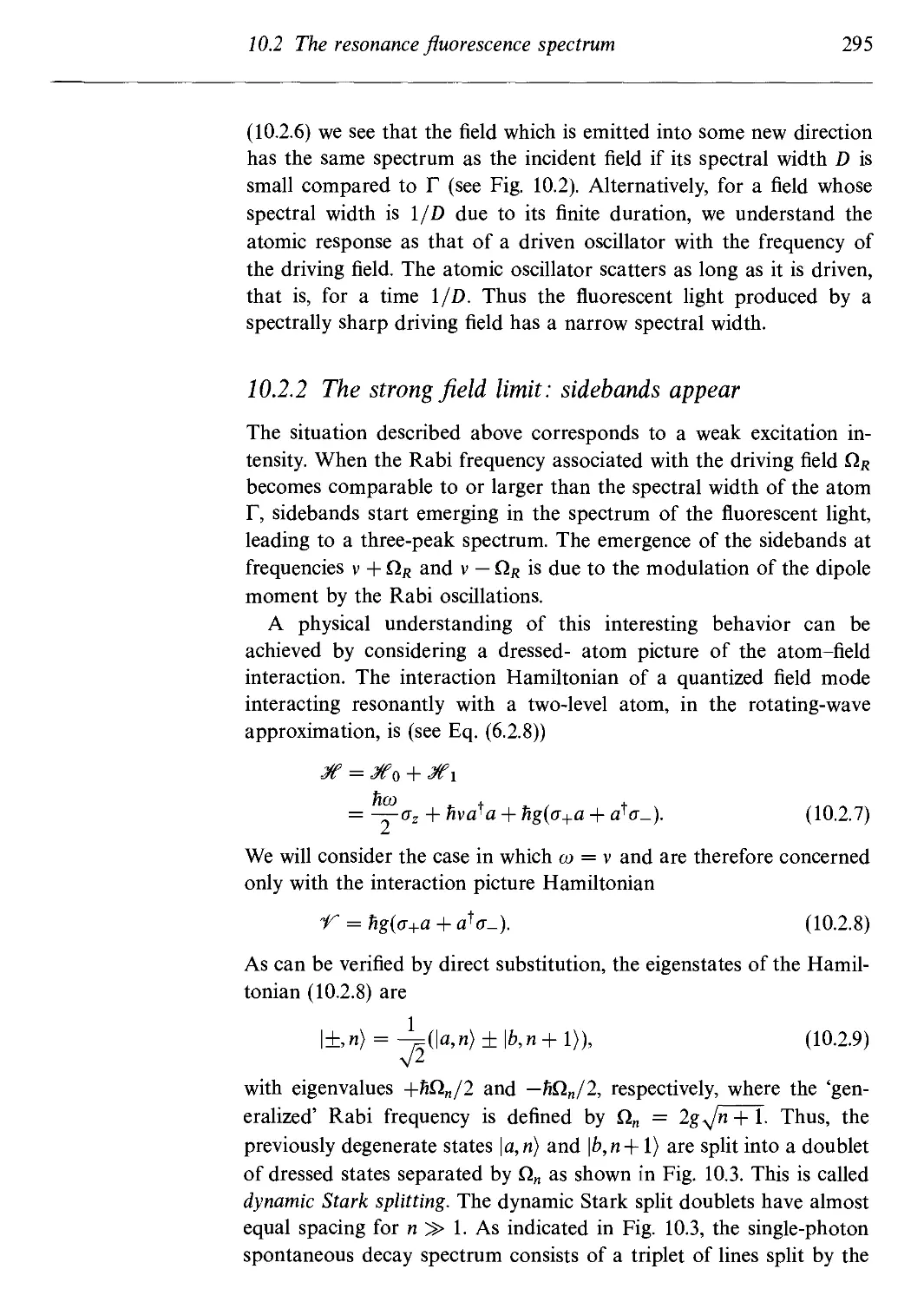
10.2.2 The strong field limit: sidebands appear 295
10.2.3 The widths of the three peaks in the very strong
field limit 296
10.3 Theory of a spectrum analyzer 298
10.4 From single-time to two-time averages: the Onsager-
Lax regression theorem 300
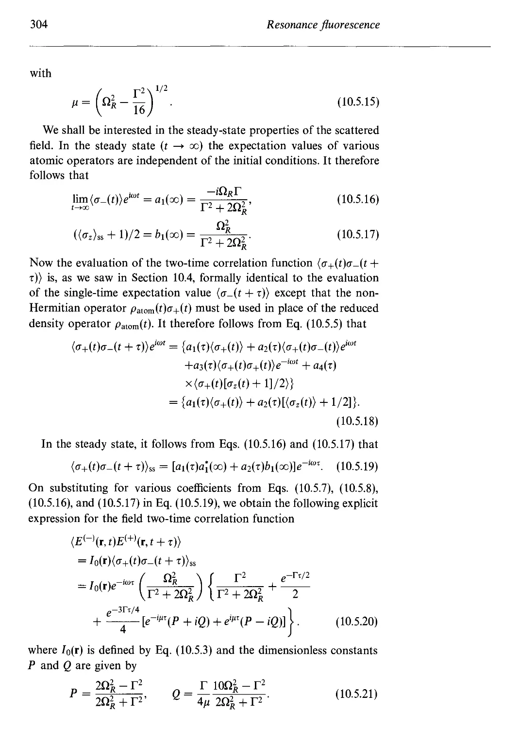
10.5 The complete resonance fluorescence spectrum 302
10.5.1 Weak field limit 305
10.5.2 Strong field limit 305
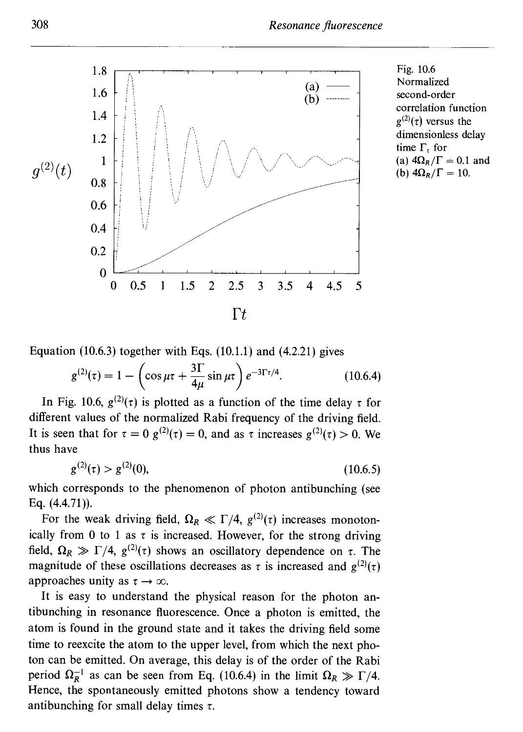
10.6 Photon antibunching 307
10.7 Resonance fluorescence from a driven V system 309
10.A Electric field operator in the far-zone approximation 311
10.B The equations of motion for and exact solution of the
density matrix in a dressed-state basis 316
10.B.1 Deriving the equation of motion in the dressed-state
basis 316
10.B.2 Solving the equations of motion 317
xii Contents
10.C The equations of motion for and exact solution of the
density matrix in the bare-state basis 320
10.D Power spectrum in the stationary regime 321
10.E Derivation of Eq. A0.7.5) 322
Problems 323
References and bibliography 325
11 Quantum theory of the laser - density operator approach 327
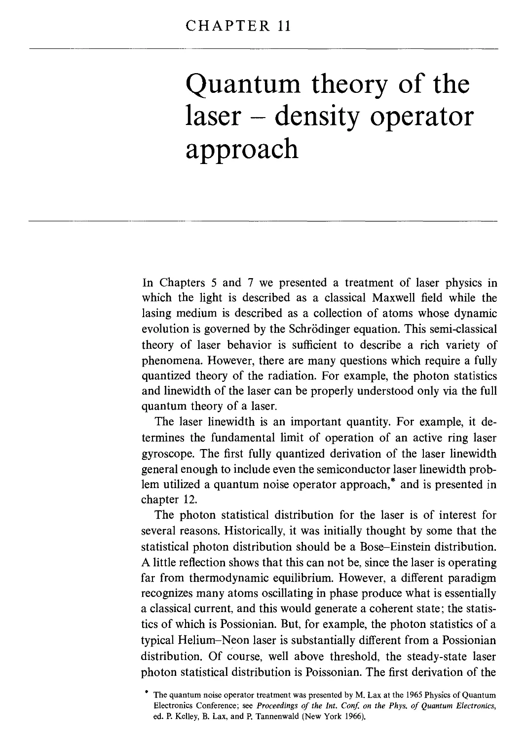
11.1 Equation of motion for the density matrix 328
11.2 Laser photon statistics 336
11.2.1 Linear approximation {$6 = 0) 337
11.2.2 Far above threshold (si > <€) 338
11.2.3 Exact solution 338
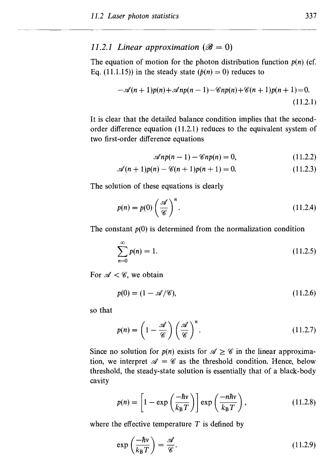
11.3 P-representation of the laser 340
11.4 Natural linewidth 341
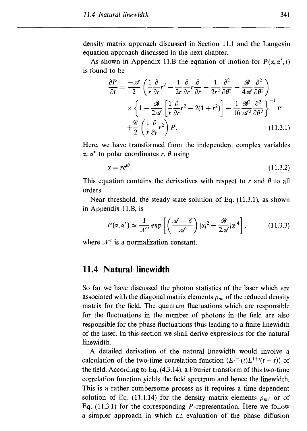
11.4.1 Phase diffusion model 342
11.4.2 Fokker-Planck equation and laser linewidth 345
11.5 Off-diagonal elements and laser linewidth 346
11.6 Analogy between the laser threshold and a second-
order phase transition 349
11.A Solution of the equations for the density matrix
elements 352
ll.B An exact solution for the P-representation of the laser 354
Problems 358
References and bibliography 360
12 Quantum theory of the laser - Heisenberg-Langevin approach 362
12.1 A simple Langevin treatment of the laser linewidth
including atomic memory effects 362
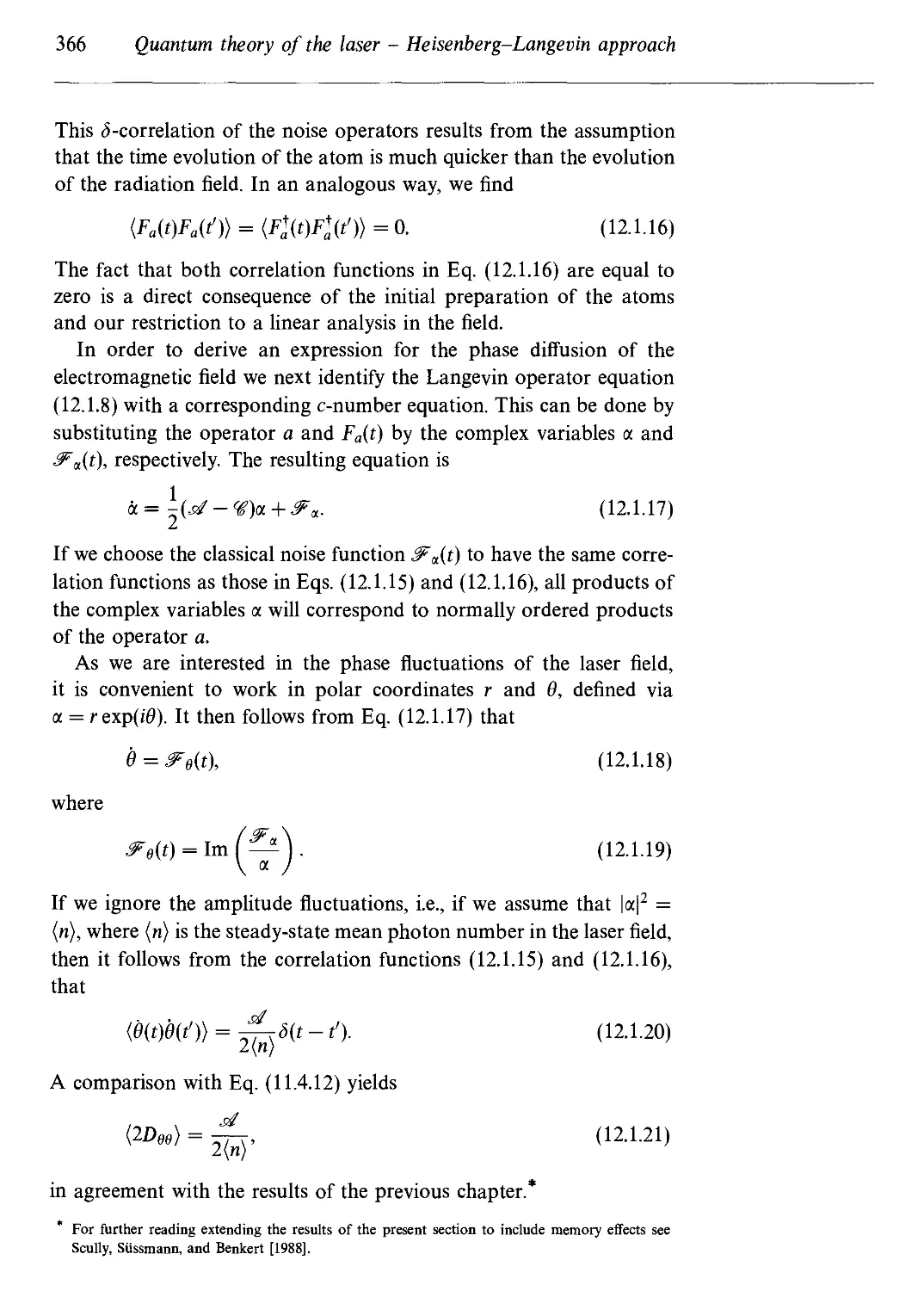
12.2 Quantum Langevin equations 367
12.3 c-number Langevin equations 373
12.4 Photon statistics and laser linewidth 376
Problems 380
References and bibliography 381
13 Theory of the micromaser 383
13.1 Equation of motion for the field density matrix 384
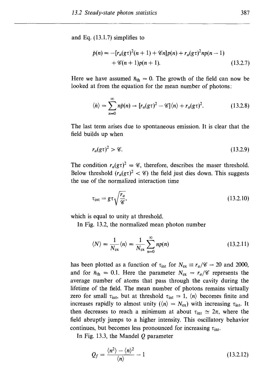
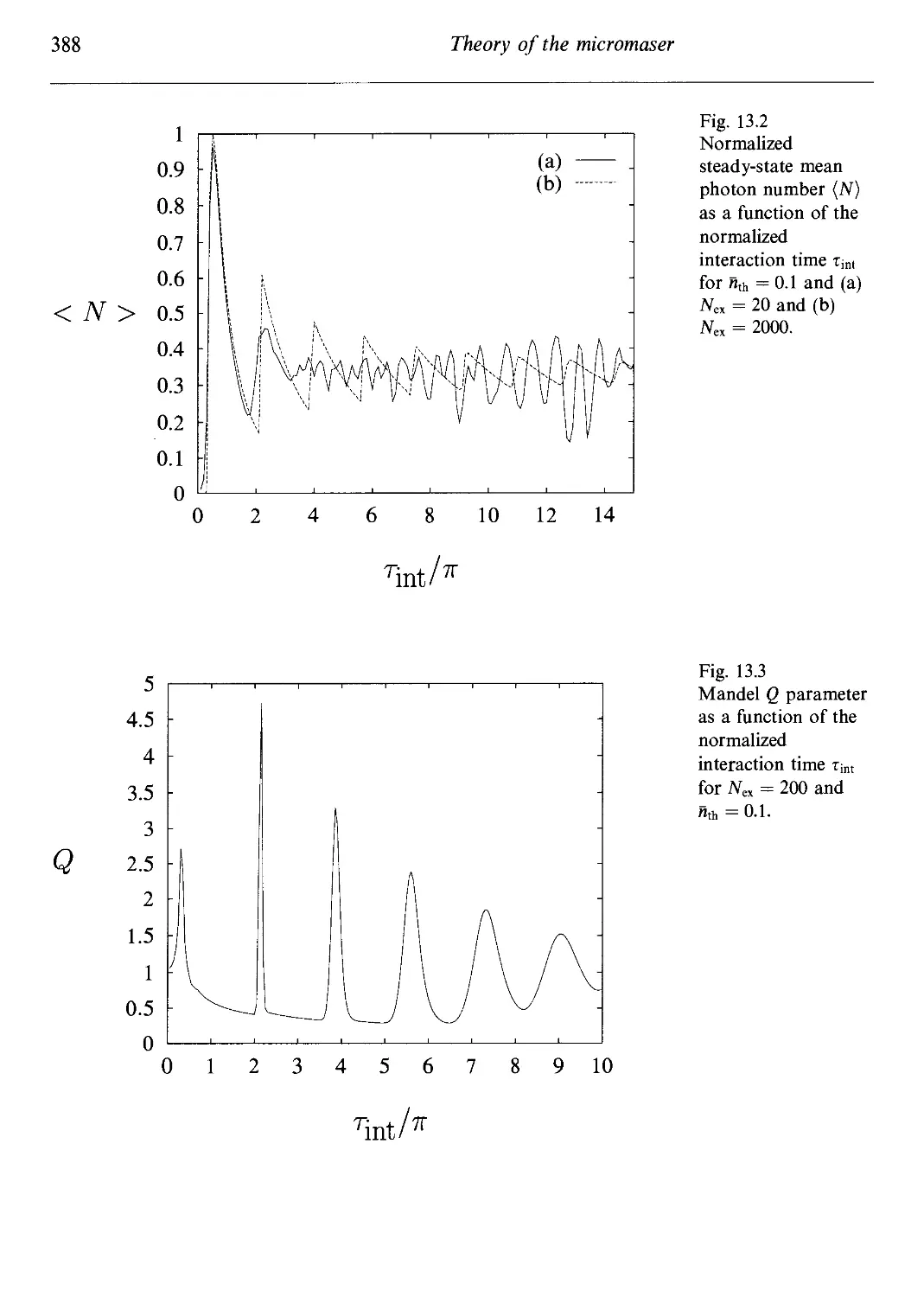
13.2 Steady-state photon statistics 386
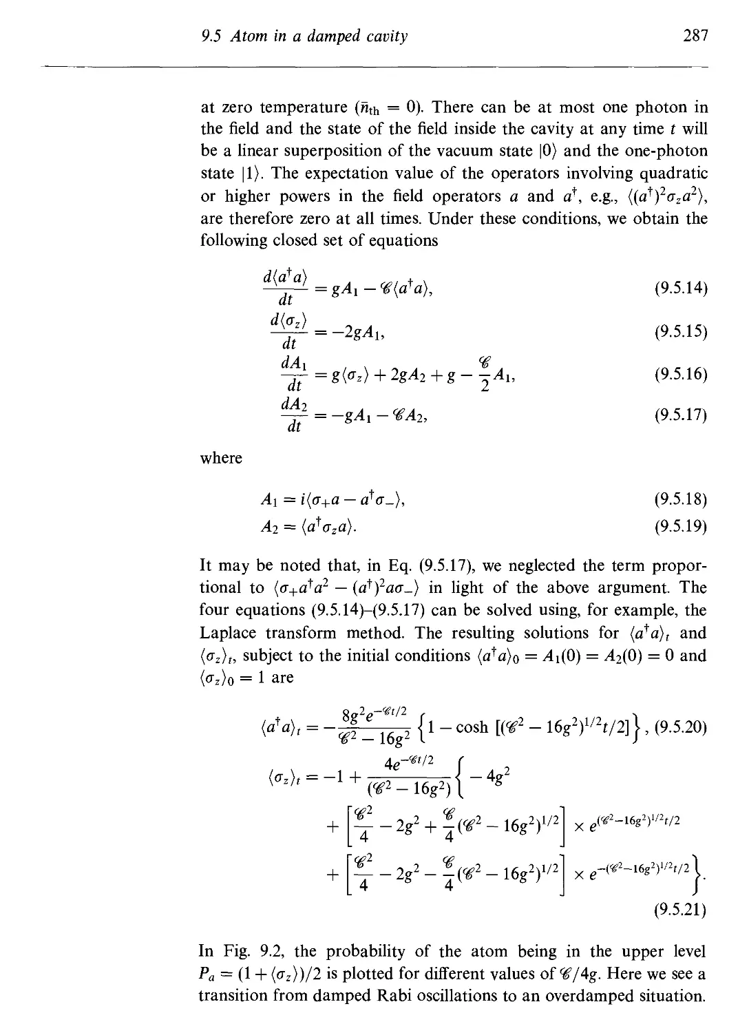
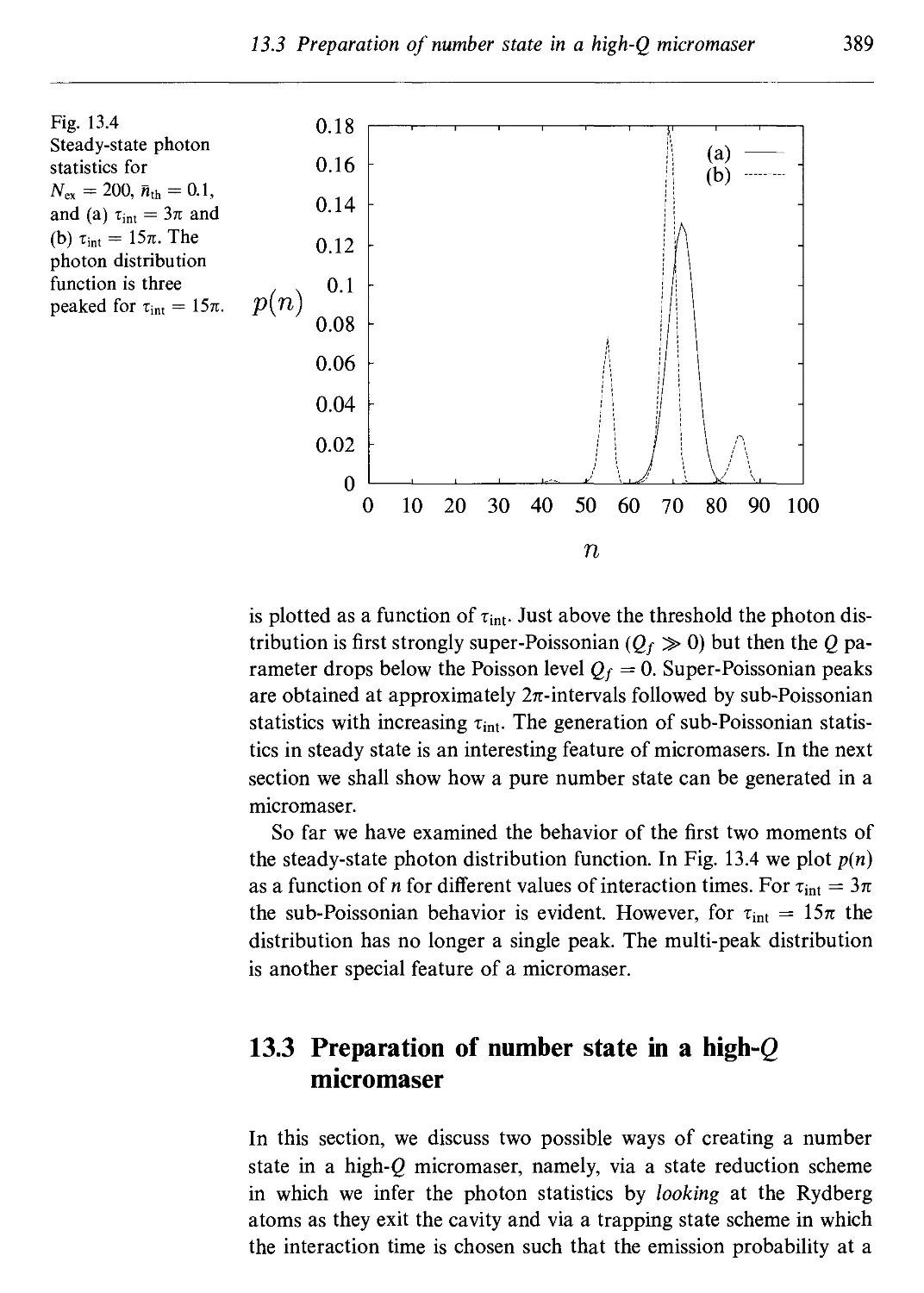
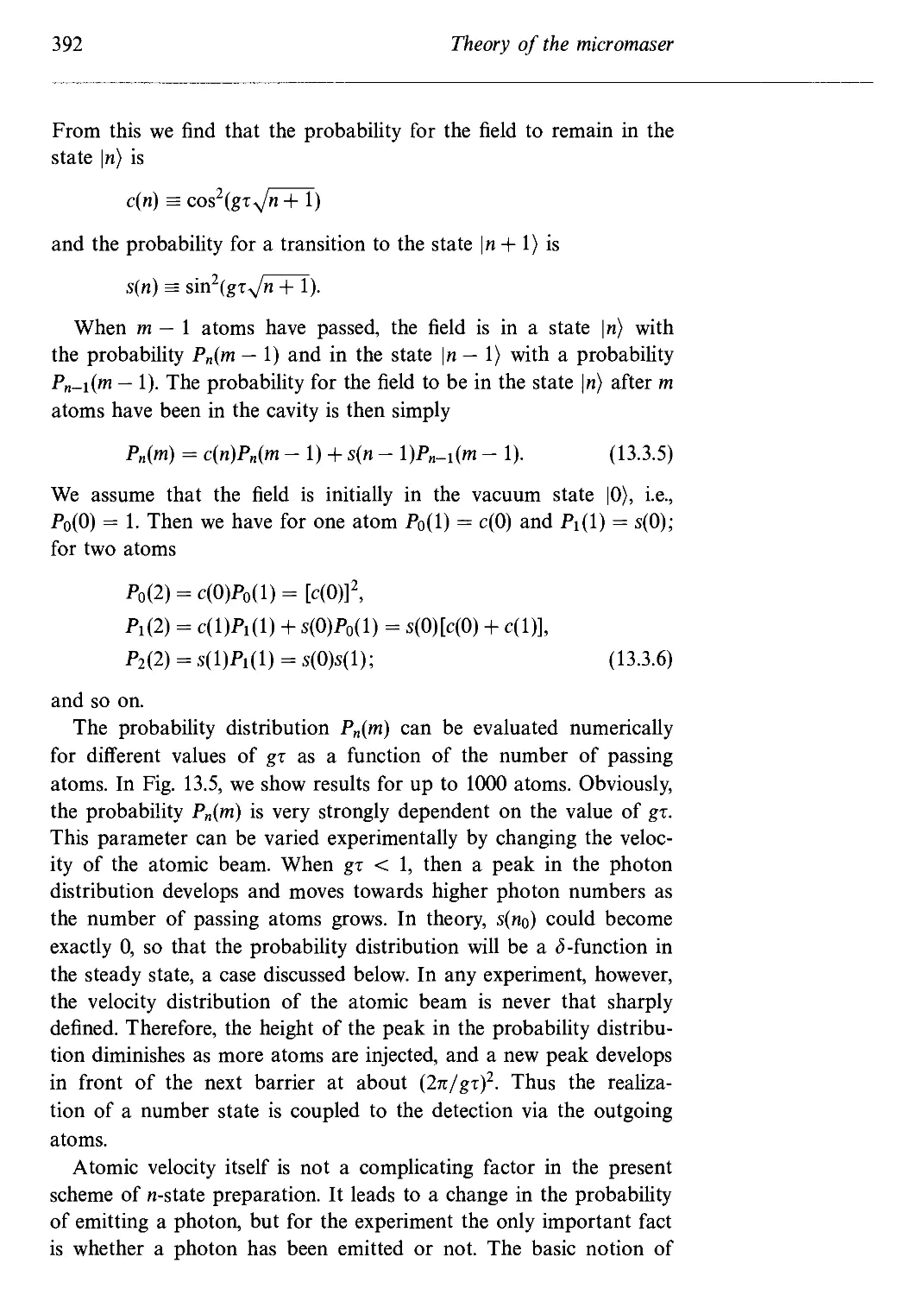
13.3 Preparation of number state in a high-Q micromaser 389
13.3.1 State reduction 390
13.3.2 Trapping states 393
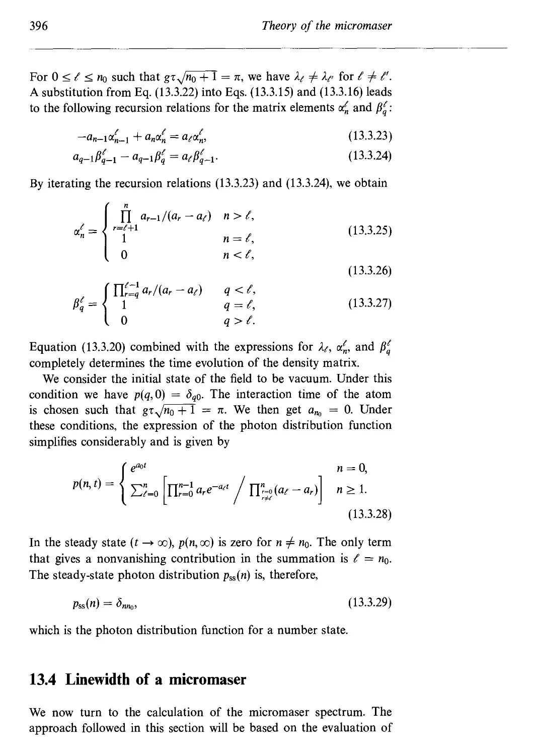
13.4 Linewidth of a micromaser 396
Contents xiii
Problems 398
References and bibliography 400
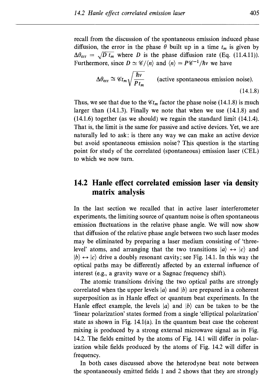
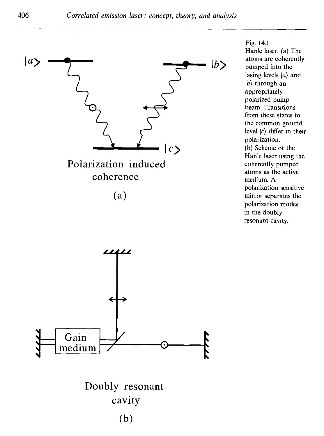
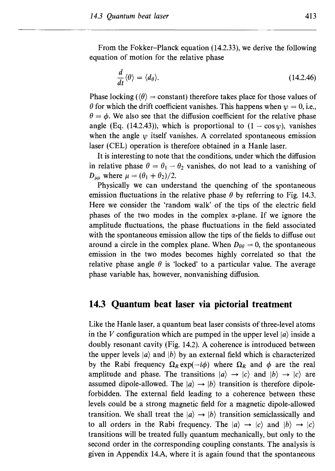
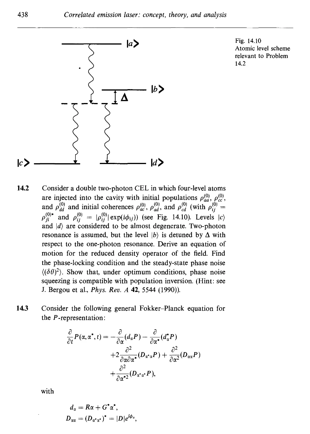
14 Correlated emission laser: concept, theory, and analysis 402
14.1 Correlated spontaneous emission laser concept 403
14.2 Hanle effect correlated emission laser via density
matrix analysis 405
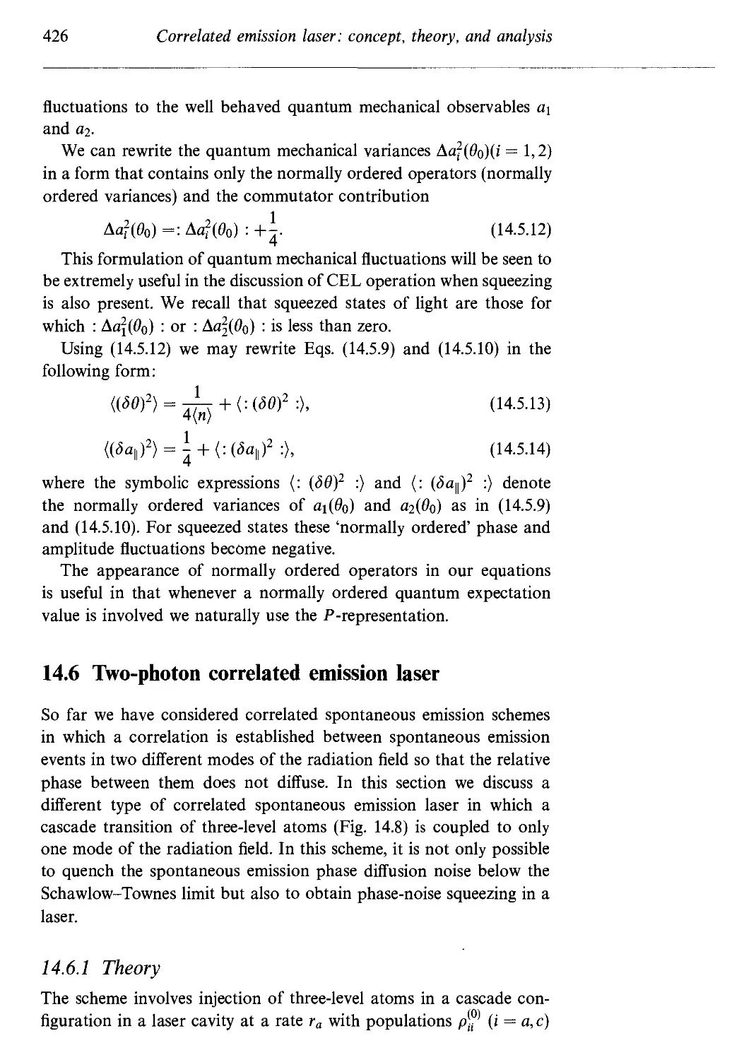
14.3 Quantum beat laser via pictorial treatment 413
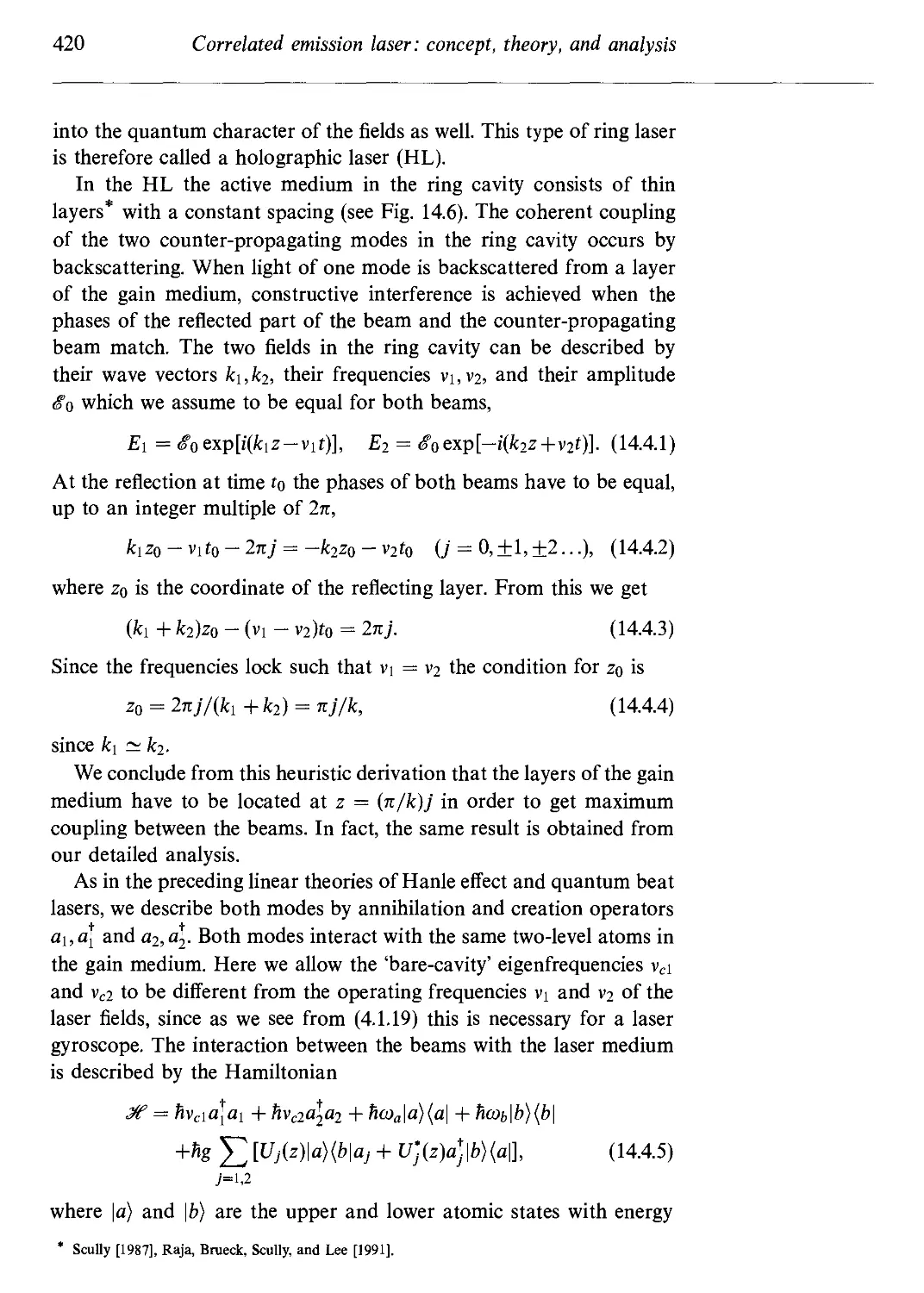
14.4 Holographic laser 418
14.5 Quantum phase and amplitude fluctuations 423
14.6 Two-photon correlated emission laser 426
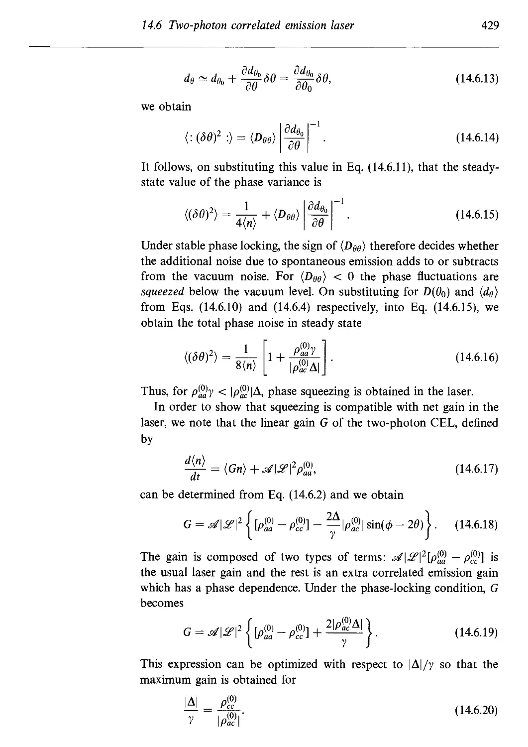
14.6.1 Theory 426
14.6.2 Heuristic account of a two-photon CEL 430
14.A Spontaneous emission noise in the quantum beat laser 433
Problems 437
References and bibliography 440
15 Phase sensitivity in quantum optical systems: applications 442
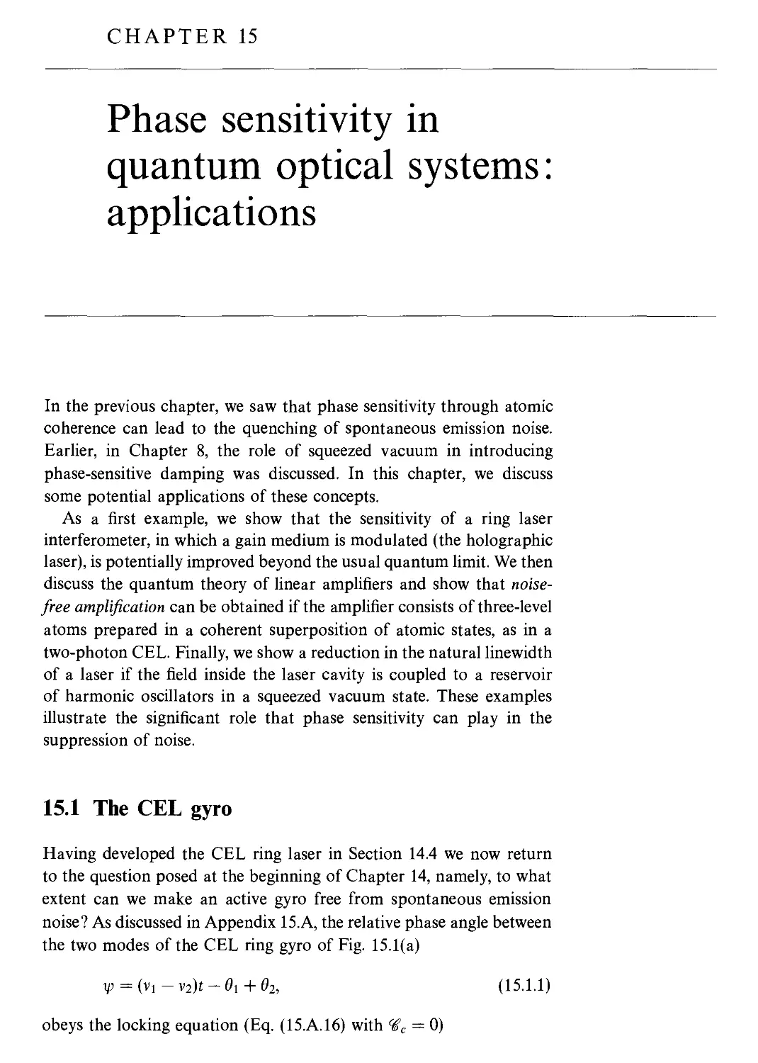
15.1 The CEL gyro 442
15.2 Linear amplification process: general description 446
15.3 Phase-insensitive amplification in a two-level system 448
15.4 Phase-sensitive amplification via the two-photon
CEL: noise-free amplification 450
15.5 Laser with an injected squeezed vacuum 452
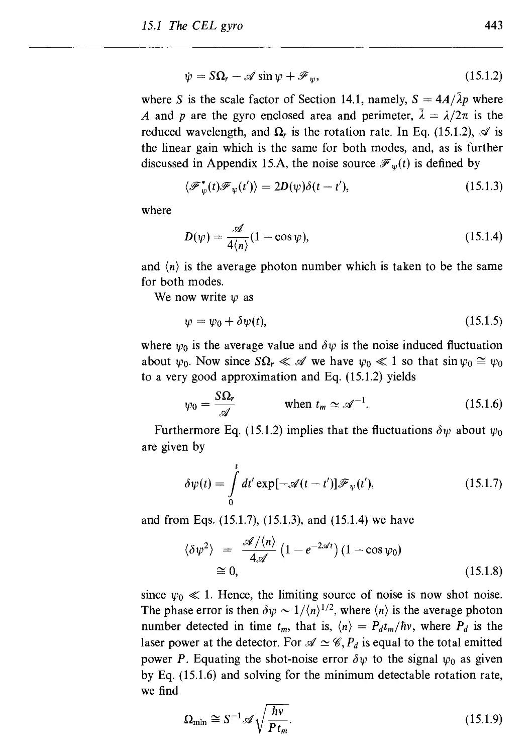
15.A Analysis of the CEL gyro with reinjection 454
Problems 457
References and bibliography 458
16 Squeezing via nonlinear optical processes 460
16.1 Degenerate parametric amplification 460
16.2 Squeezing in an optical parametric oscillator 463
16.3 Squeezing in the output of a cavity field 467
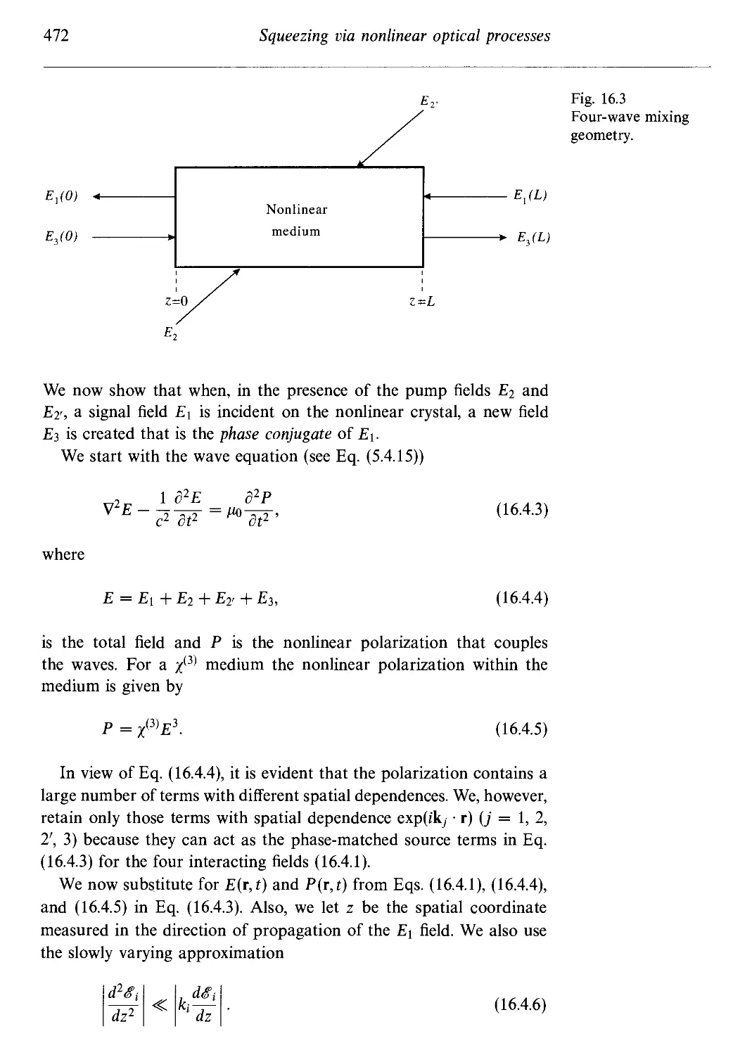
16.4 Four-wave mixing 471
16.4.1 Amplification and oscillation in four-wave mixing 471
16.4.2 Squeezing in four-wave mixing 475
16.A Effect of pump phase fluctuations on squeezing in
degenerate parametric amplification 476
16.B Quantized field treatment of input-output formalism
leading to Eq. A6.3.4) 480
Problems 482
References and bibliography 484
xiv Contents
17 Atom optics 487
17.1 Mechanical effects of light 488
17.1.1 Atomic deflection 488
17.1.2 Laser cooling 489
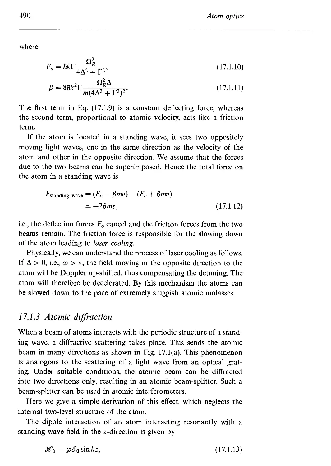
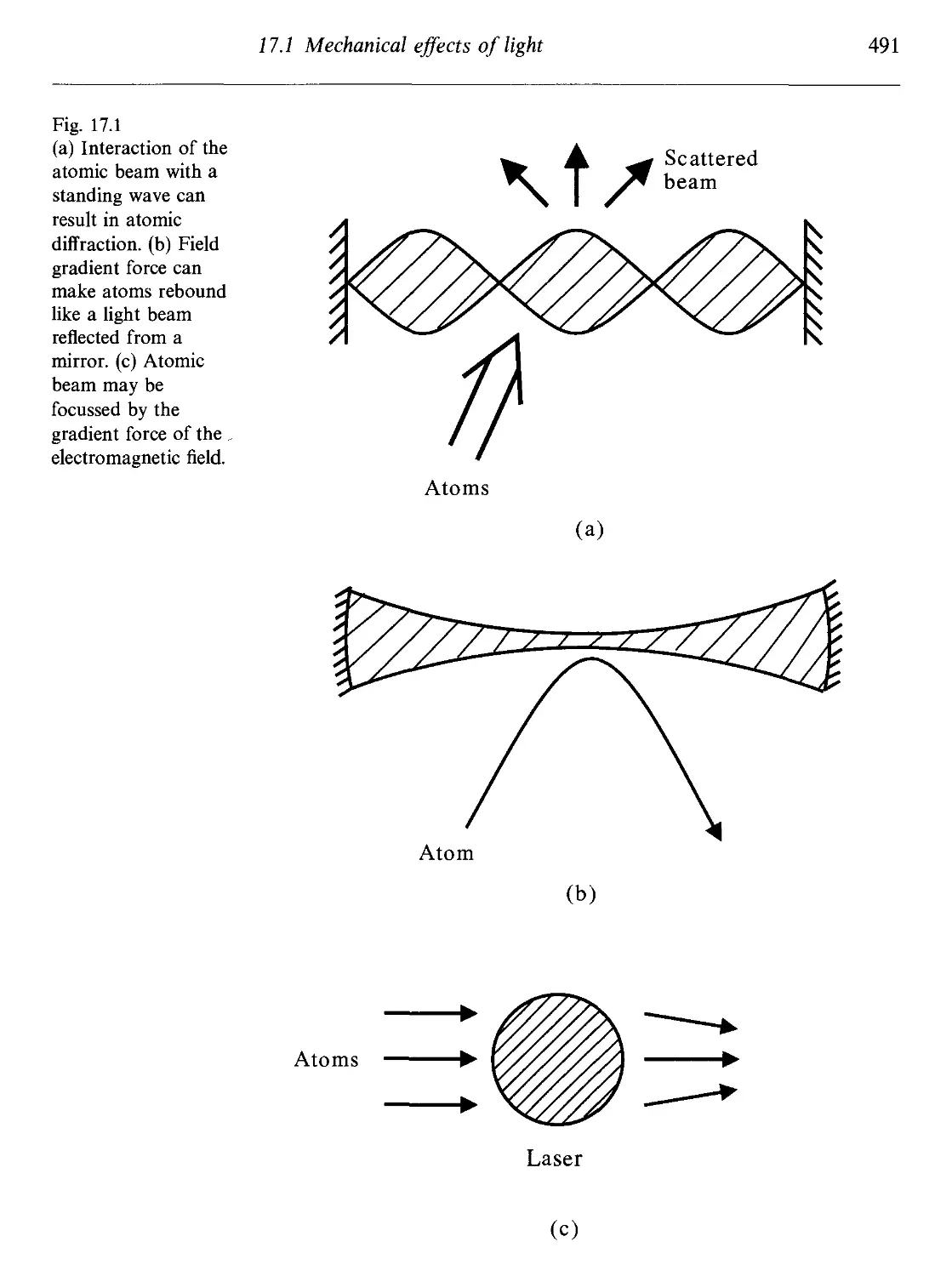
17.1.3 Atomic diffraction 490
17.1.4 Semiclassical gradient force 493
17.2 Atomic interferometry 494
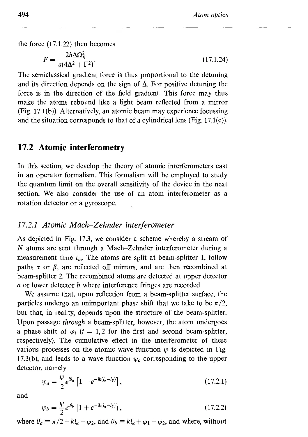
17.2.1 Atomic Mach-Zehnder interferometer 494
17.2.2 Atomic gyroscope 496
17.3 Quantum noise in an atomic interferometer 498
17.4 Limits to laser cooling 499
17.4.1 Recoil limit 499
17.4.2 Velocity selective coherent population trapping 501
Problems 503
References and bibliography 504
18 The EPR paradox, hidden variables, and Bell's theorem 507
18.1 The EPR 'paradox' 508
18.2 Bell's inequality 513
18.3 Quantum calculation of the correlations in Bell's
theorem 515
18.4 Hidden variables from a quantum optical perspective 520
18.5 Bell's theorem without inequalities: Greenberger-
Horne-Zeilinger (GHZ) equality 529
18.6 Quantum cryptography 531
18.6.1 Bennett-Brassard protocol 531
18.6.2 Quantum cryptography based on Bell's theorem 532
18.A Quantum distribution function for a single spin-up
particle 533
18.B Quantum distribution function for two particles 534
Problems 536
References and bibliography 539
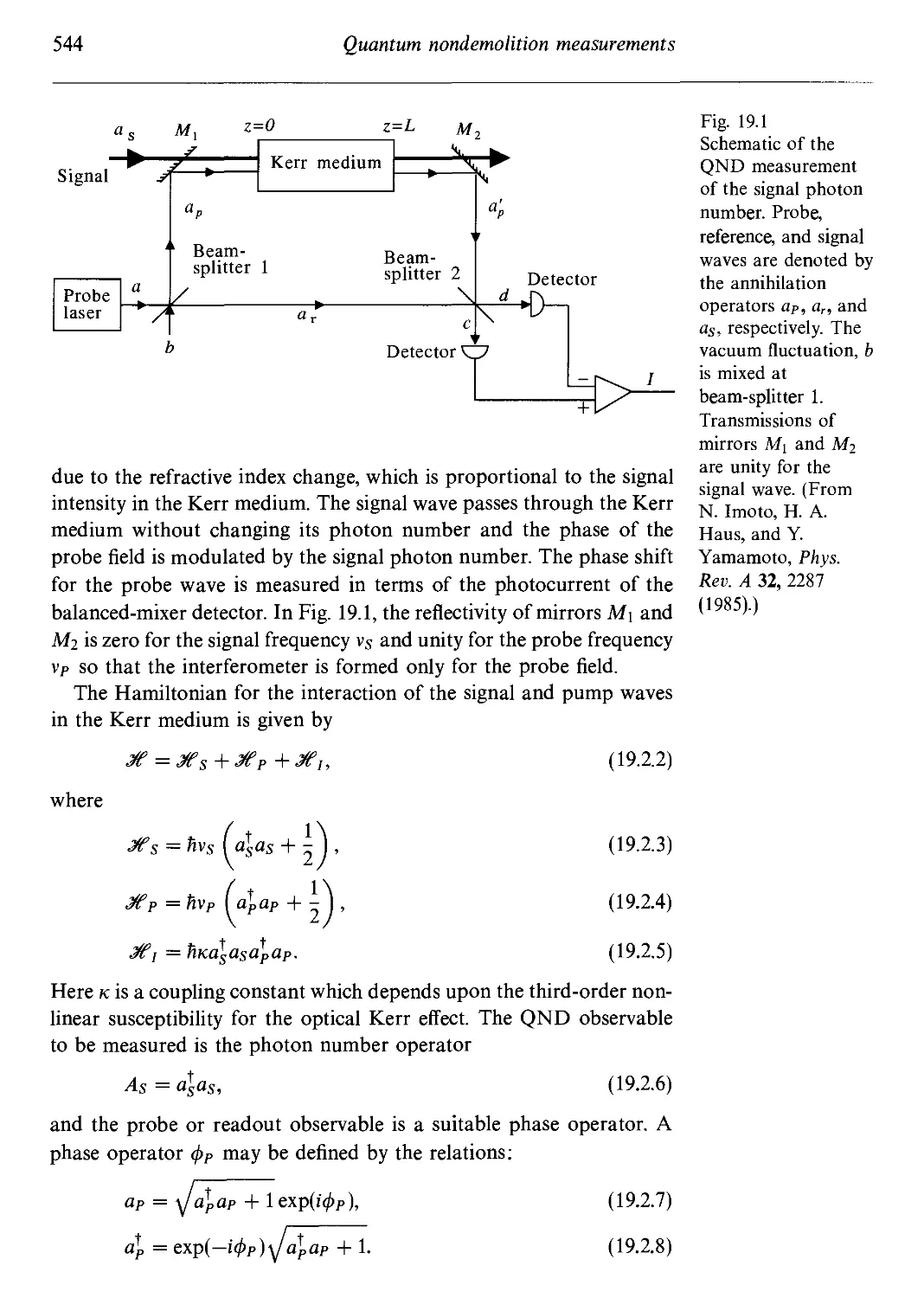
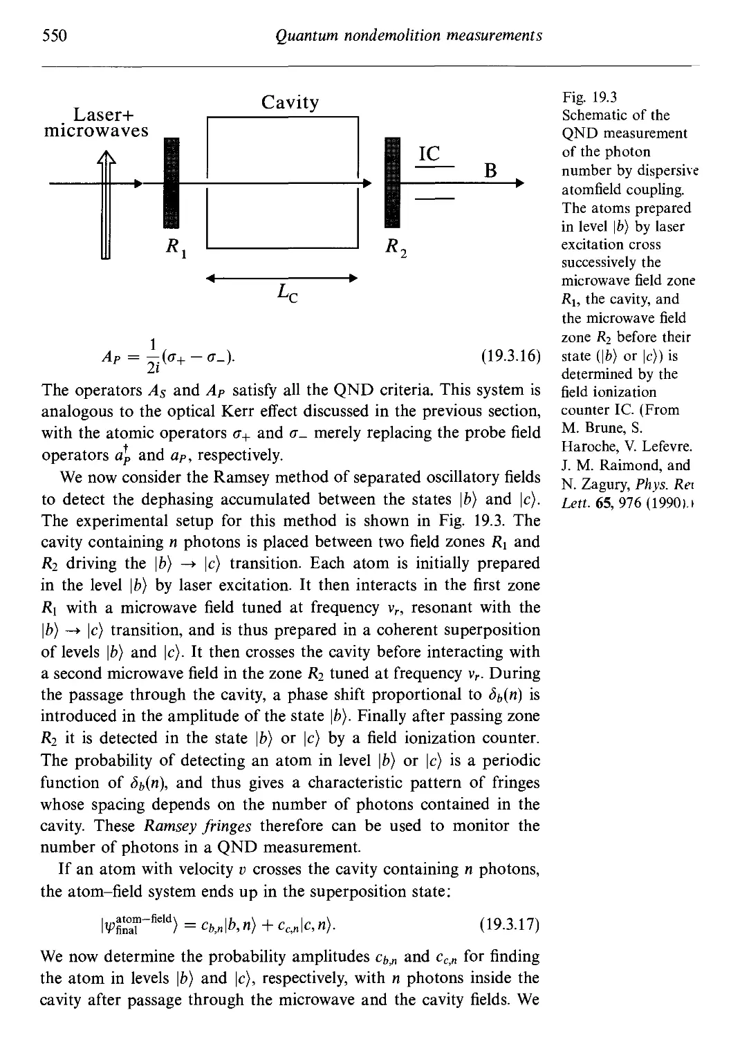
19 Quantum nondemolition measurements 541
19.1 Conditions for QND measurements 542
19.2 QND measurement of the photon number via the
optical Kerr effect 543
19.3 QND measurement of the photon number by
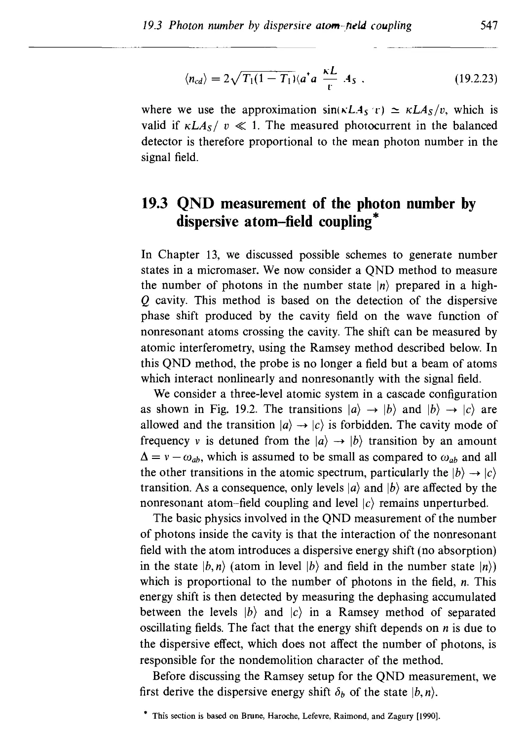
dispersive atom-field coupling 547
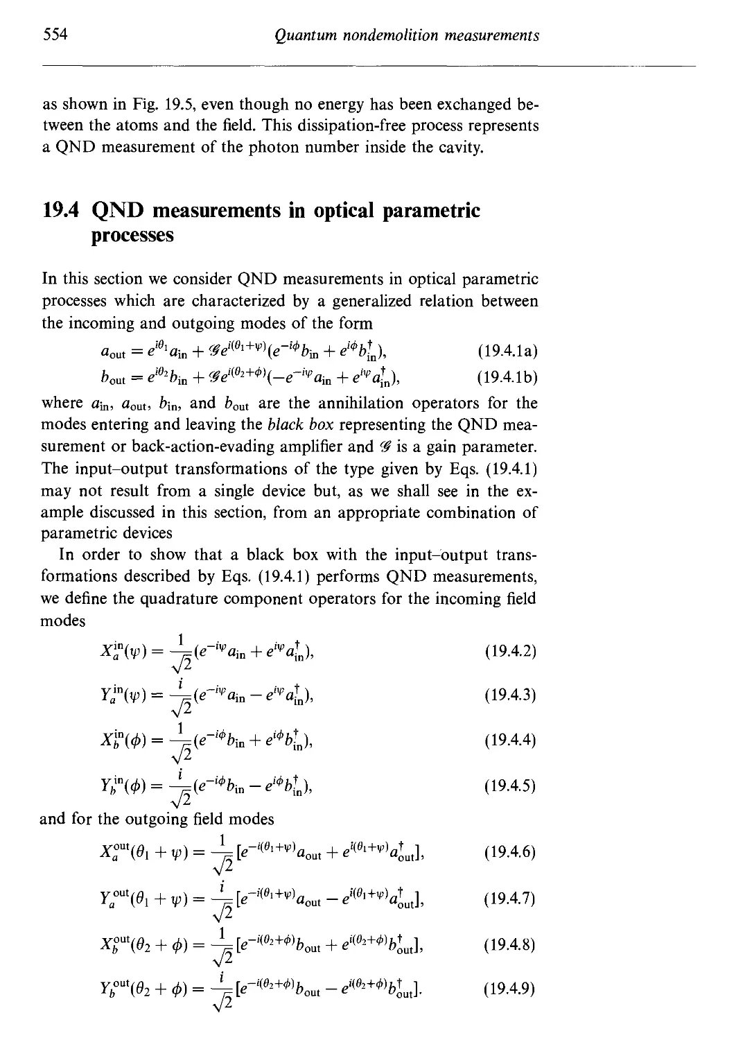
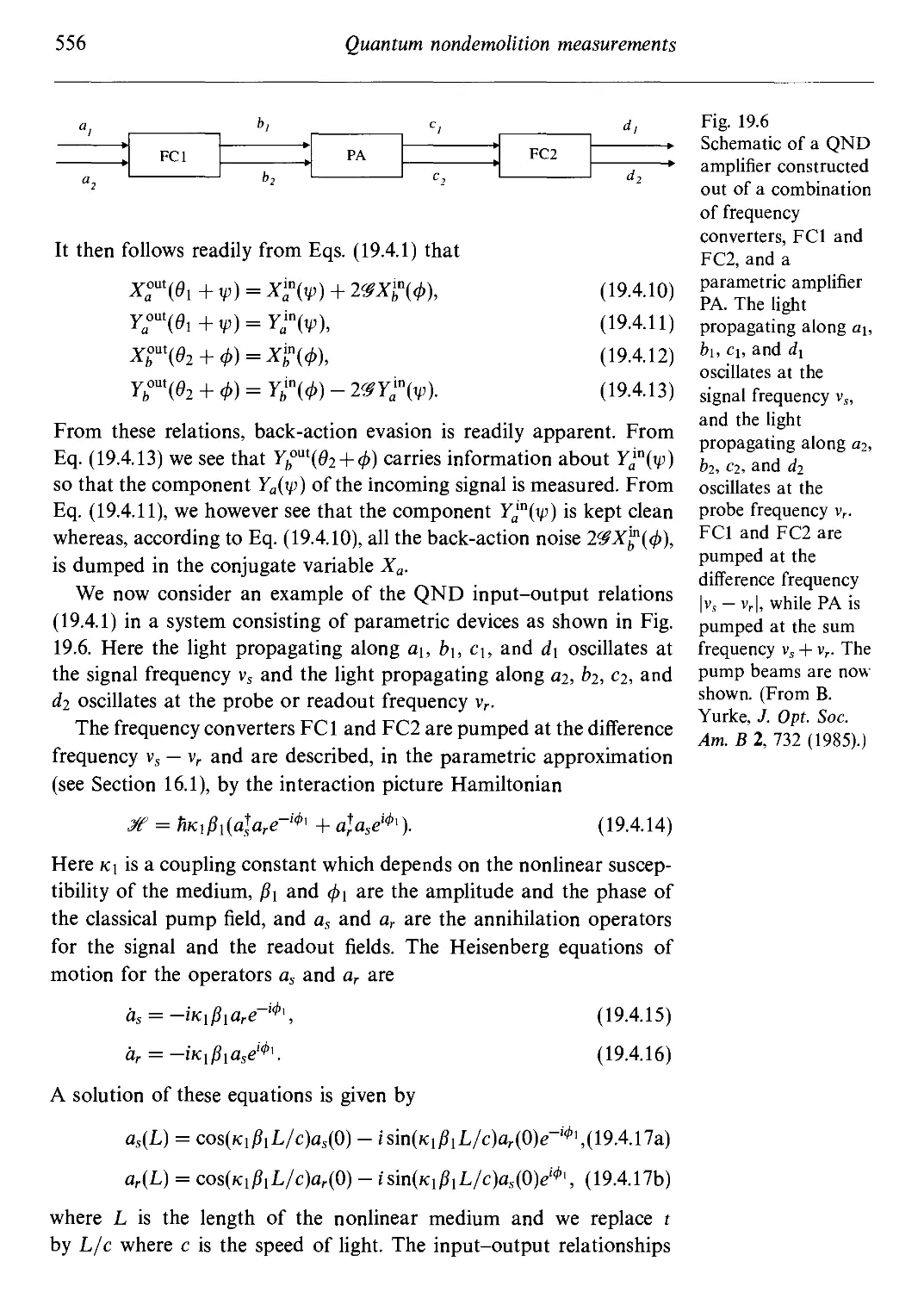
19.4 QND measurements in optical parametric processes 554
Problems 558
References and bibliography 560
Contents xv
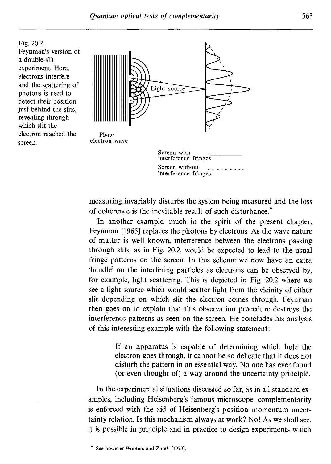
20 Quantum optical tests of complementarity 561
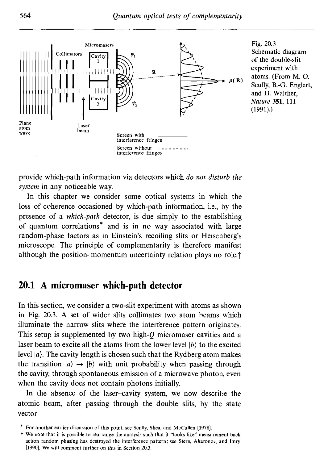
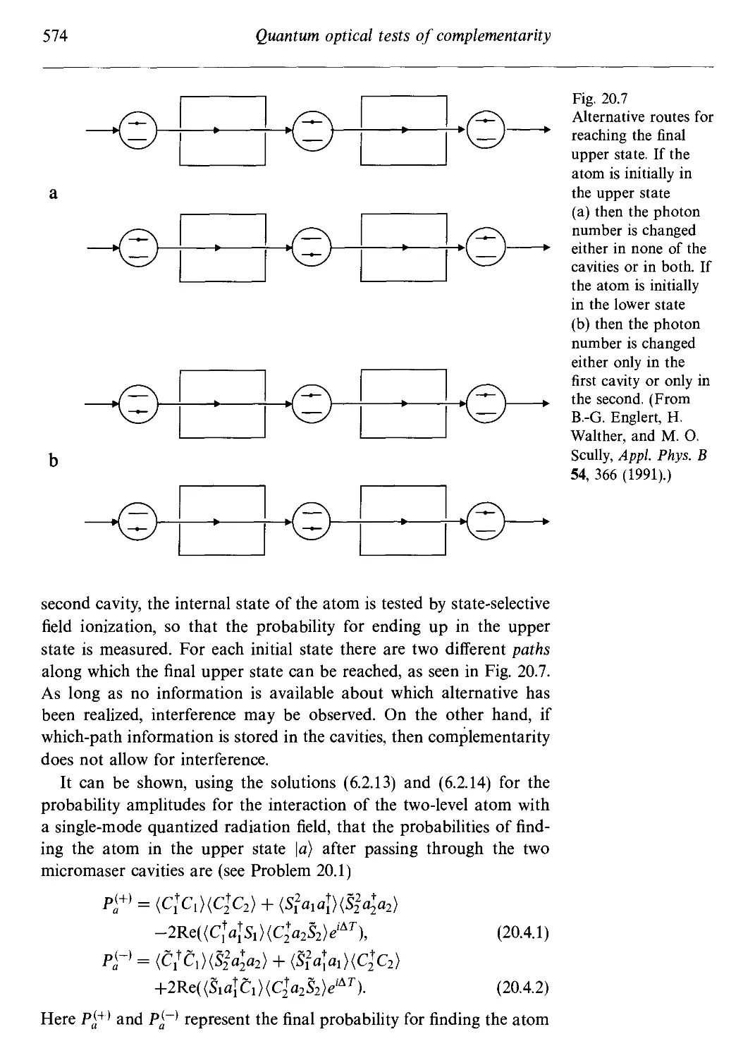
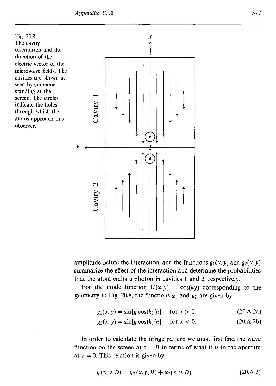
20.1 A micromaser which-path detector 564
20.2 The resonant interaction of atoms with a microwave
field and its effect on atomic center-of-mass motion 566
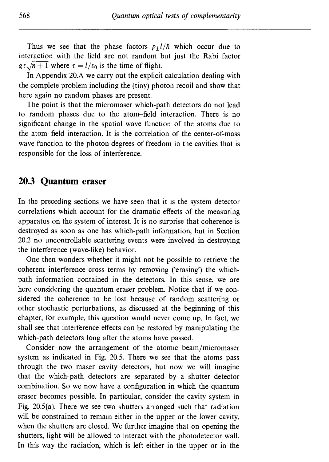
20.3 Quantum eraser 568
20.4 Quantum optical Ramsey fringes 573
20.A Effect of recoil in a micromaser which-path detector 576
Problems 579
References and bibliography 580
21 Two-photon interferometry, the quantum measurement
problem, and more 582
21.1 The field-field correlation function of light scattered
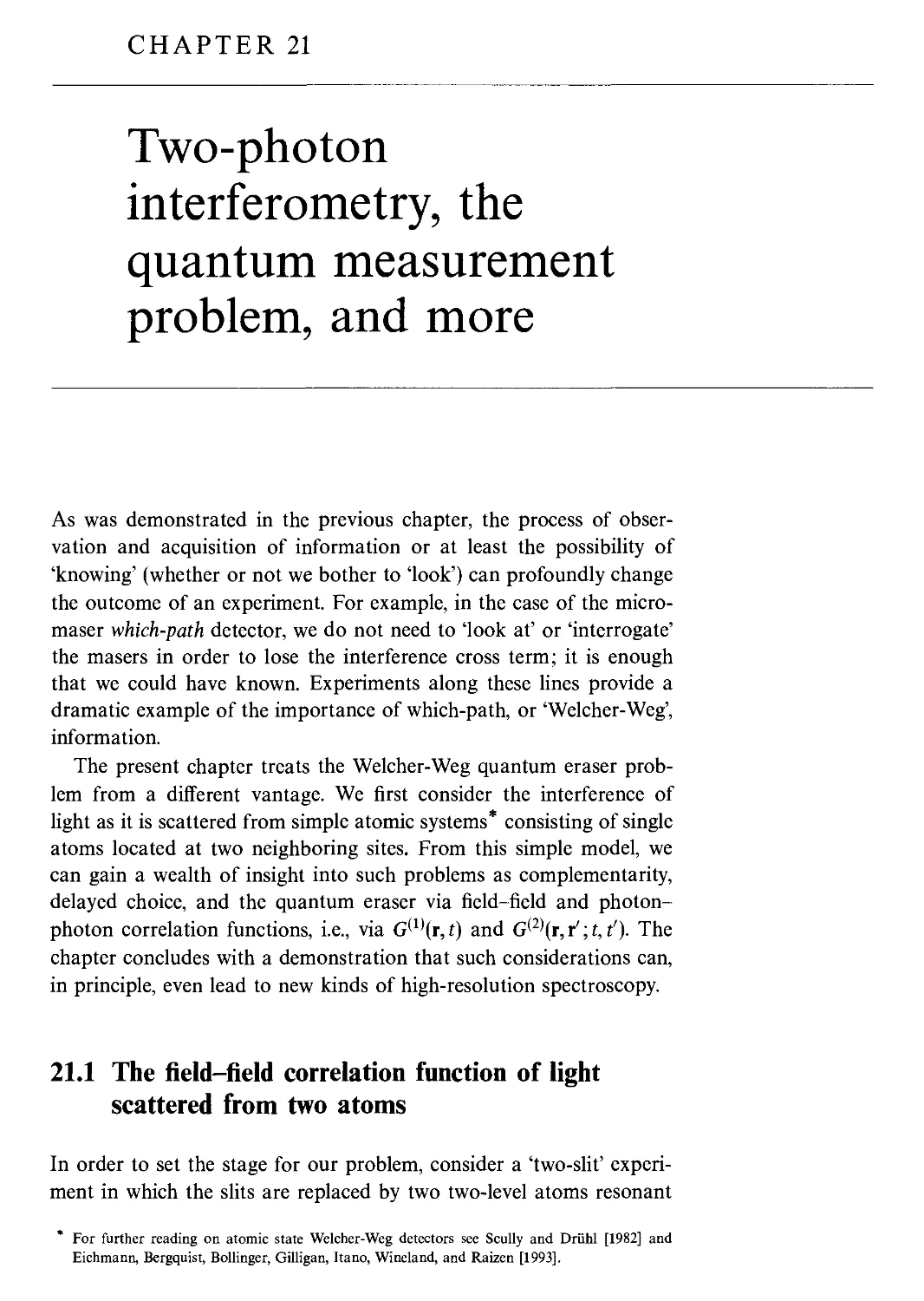
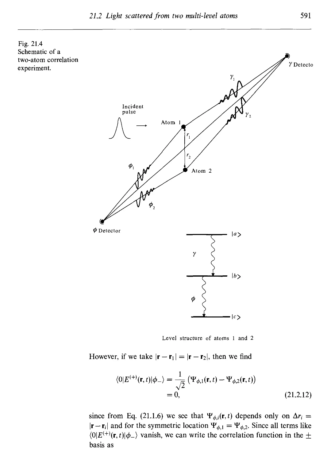
from two atoms 582
21.1.1 Correlation function GA)(r, t) generated by scatter-
scattering from two excited atoms 585
21.1.2 Excitation by laser light 585
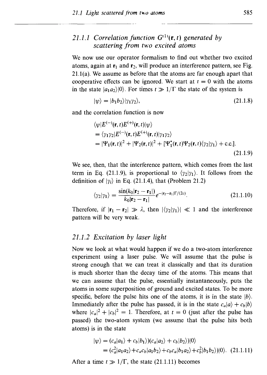
21.1.3 Using three atomic levels as a which-path flag 586
21.2 The field-field and photon-photon correlations of
light scattered from two multi-level atoms: quantum
eraser 587
21.2.1 Alternative photon basis 590
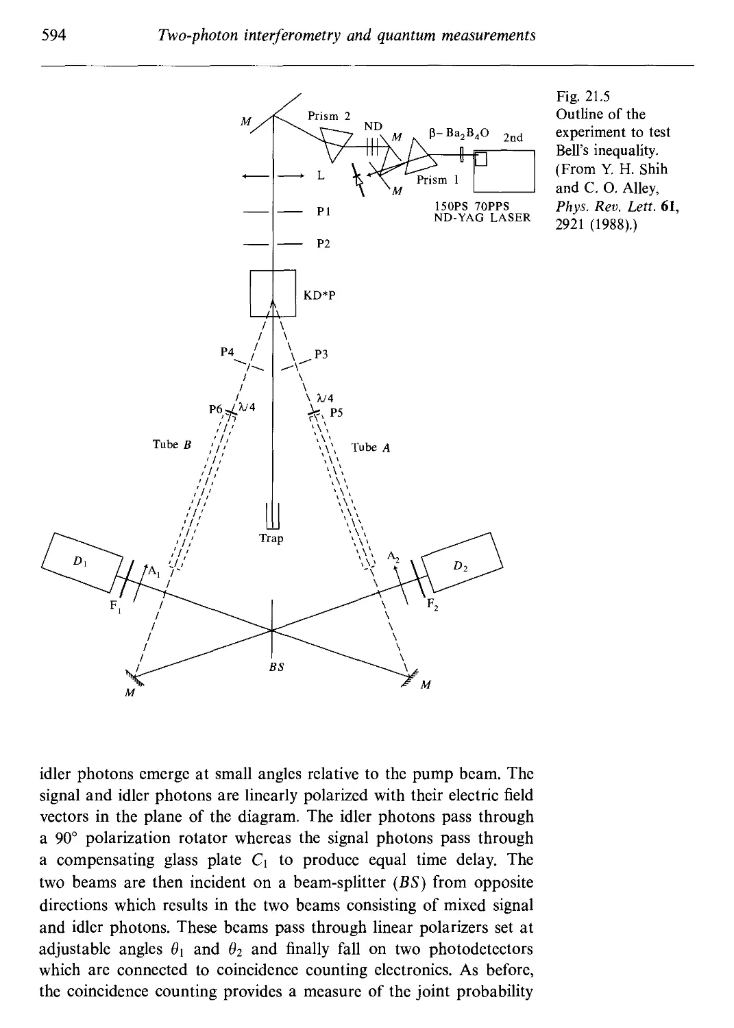
21.3 Bell's inequality experiments via two-photon
correlations 592
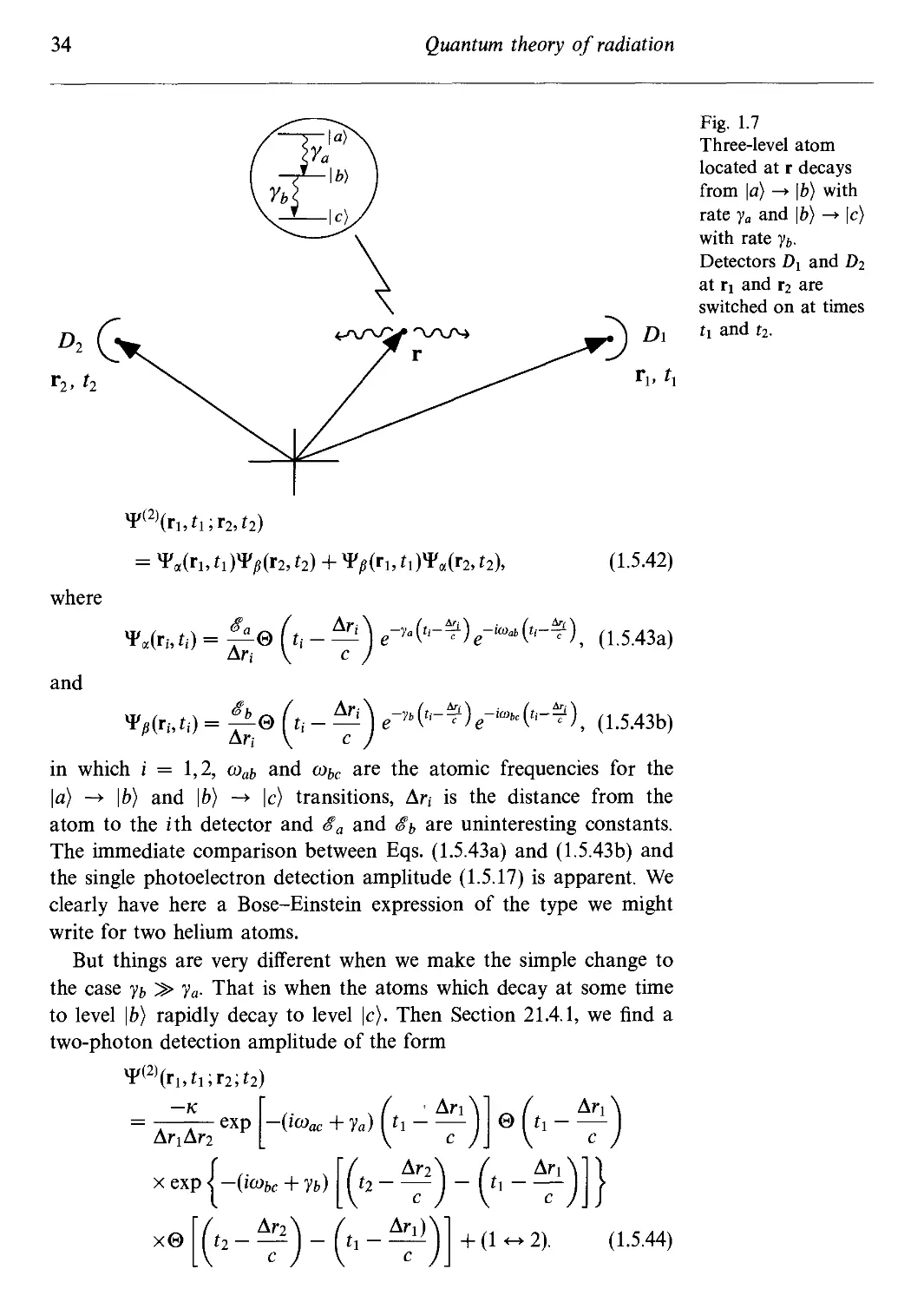
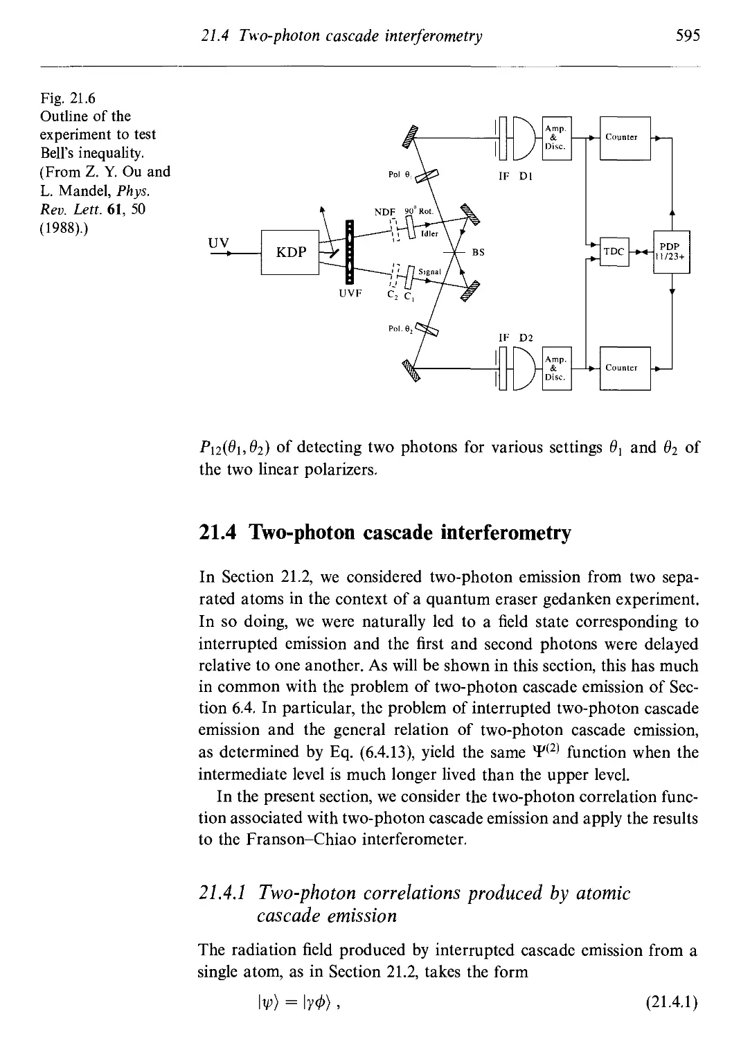
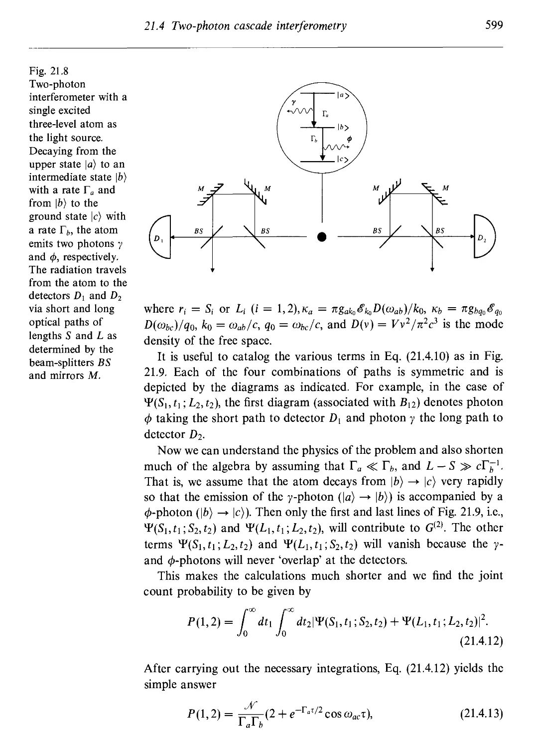
21.4 Two-photon cascade interferometry 595
21.4.1 Two-photon correlations produced by atomic
cascade emission 595
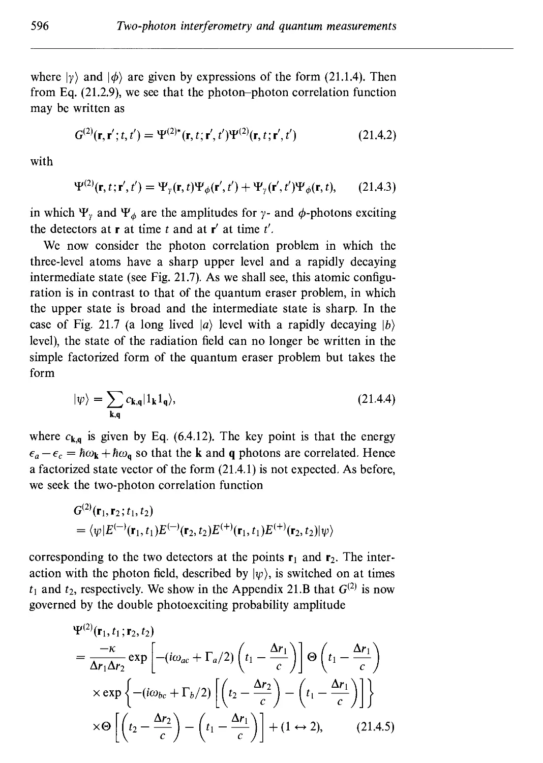
21.4.2 Franson-Chiao interferometry 597
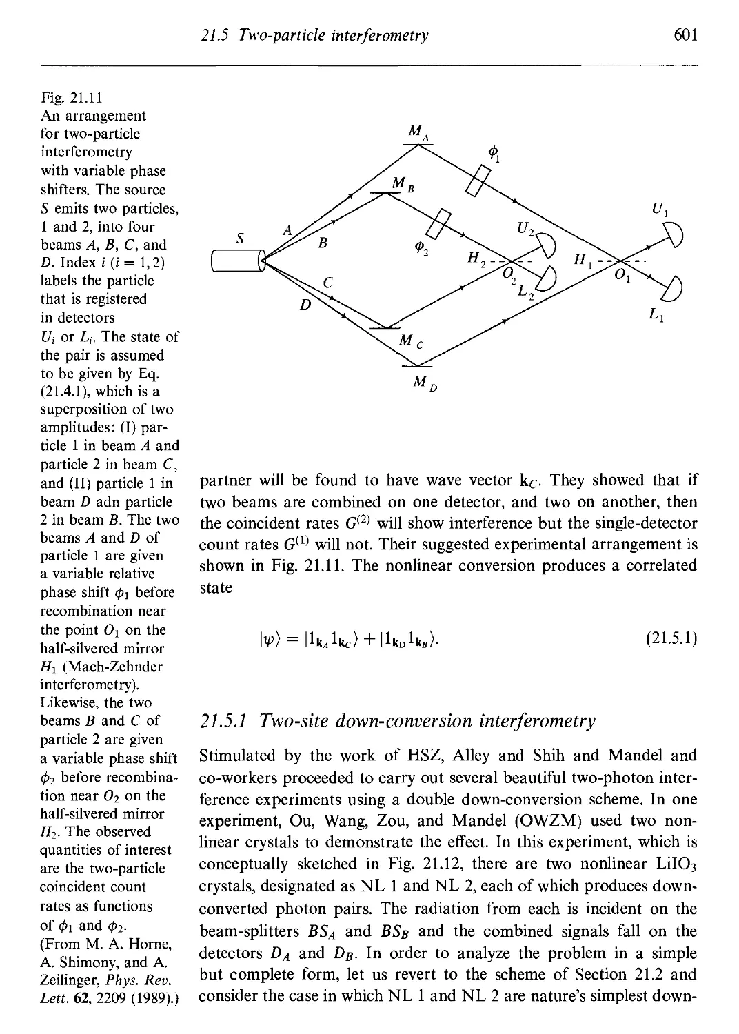
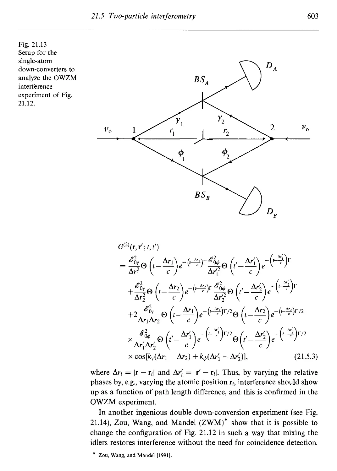
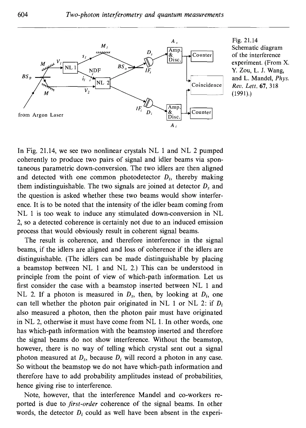
21.5 Two-particle interferometry via nonlinear down-
conversion and momentum selected photon pairs 600
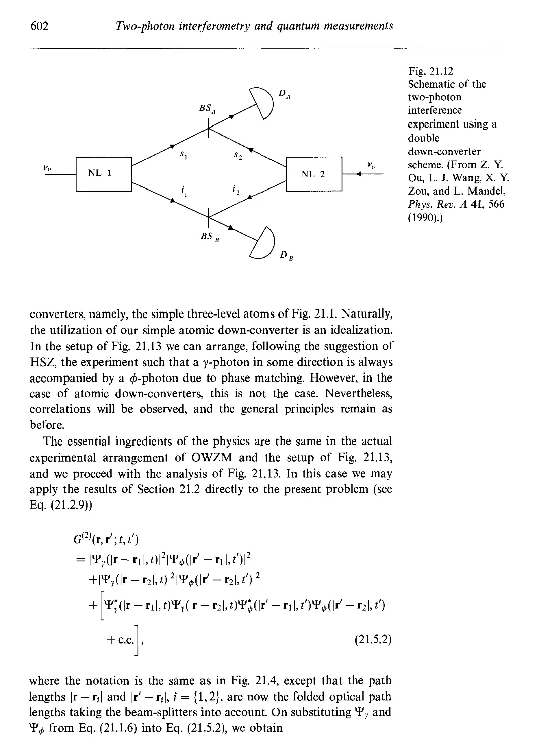
21.5.1 Two-site down-conversion interferometry 601
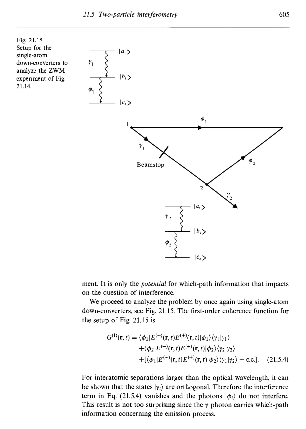
21.6 A vacuum-fluctuation picture of the ZWM
experiment 607
21.7 High-resolution spectroscopy via two-photon cascade
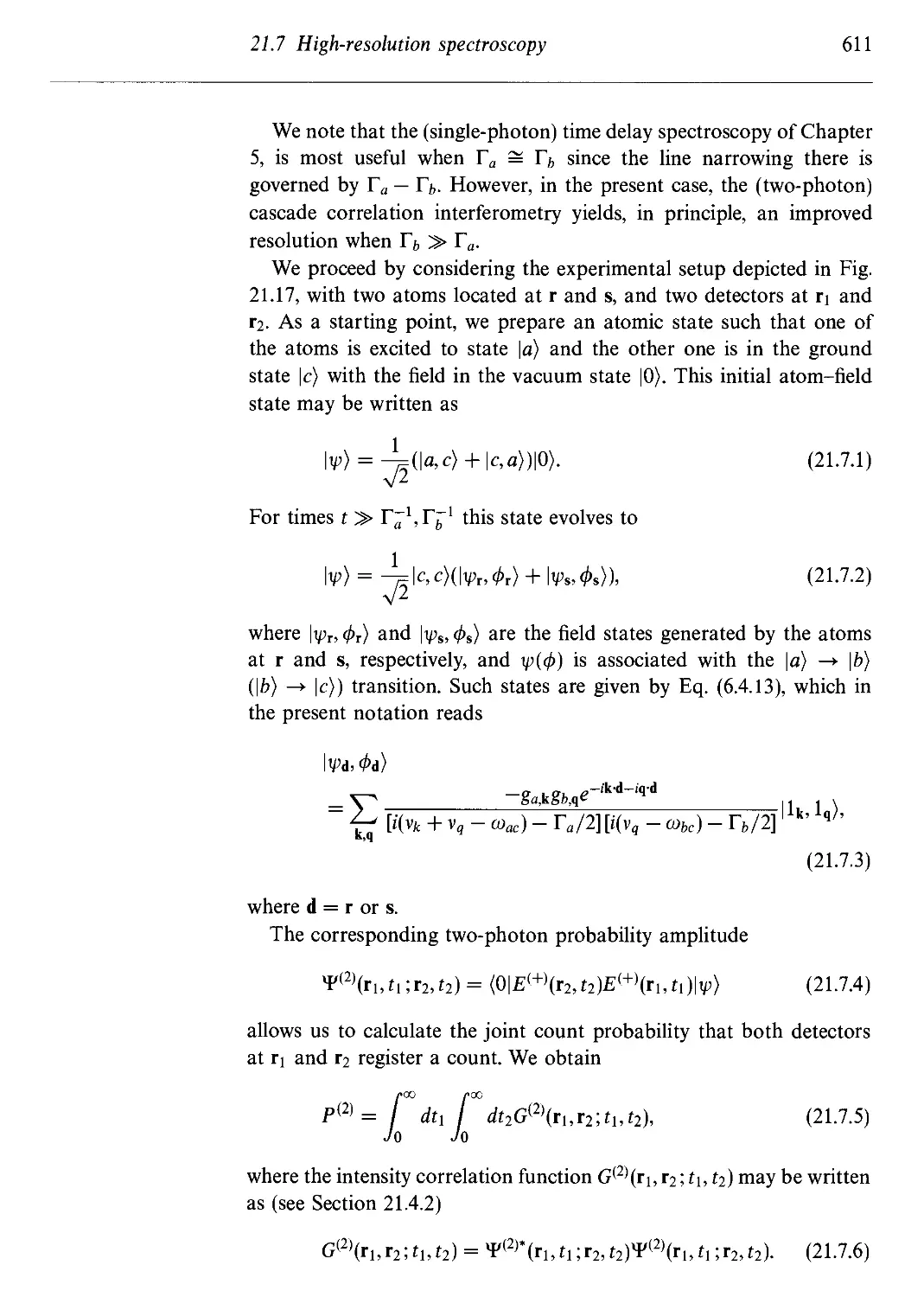
interferometry 610
21.A Scattering from two atoms via an operator approach 614
81.В Calculation of the two-photon correlation function in
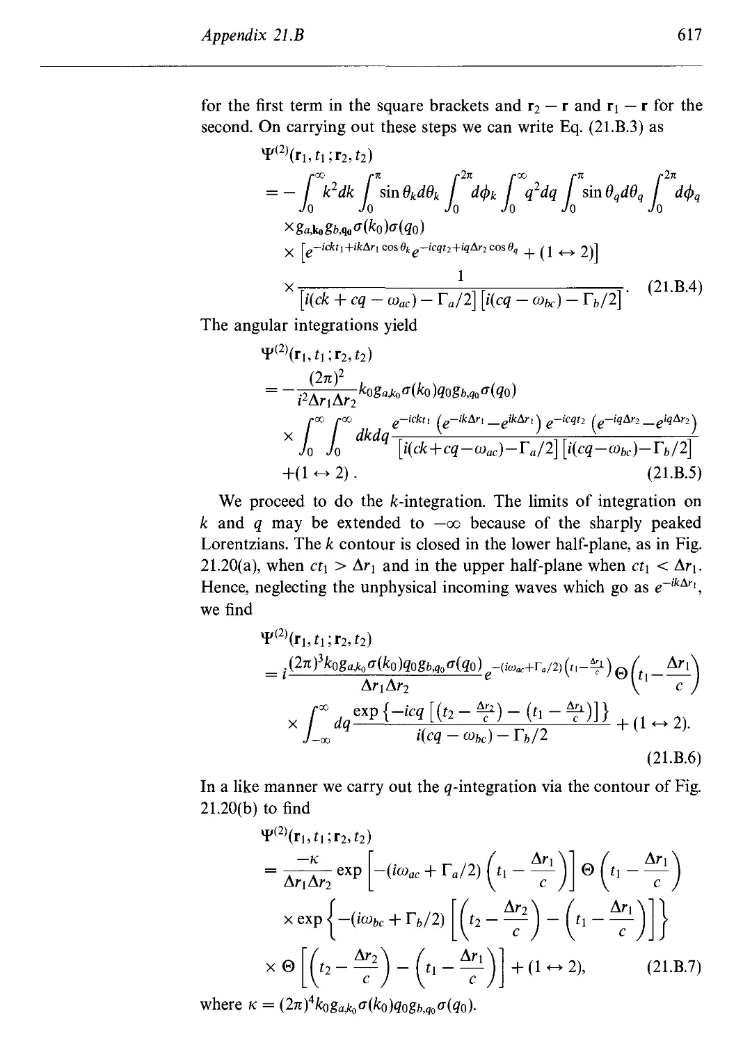
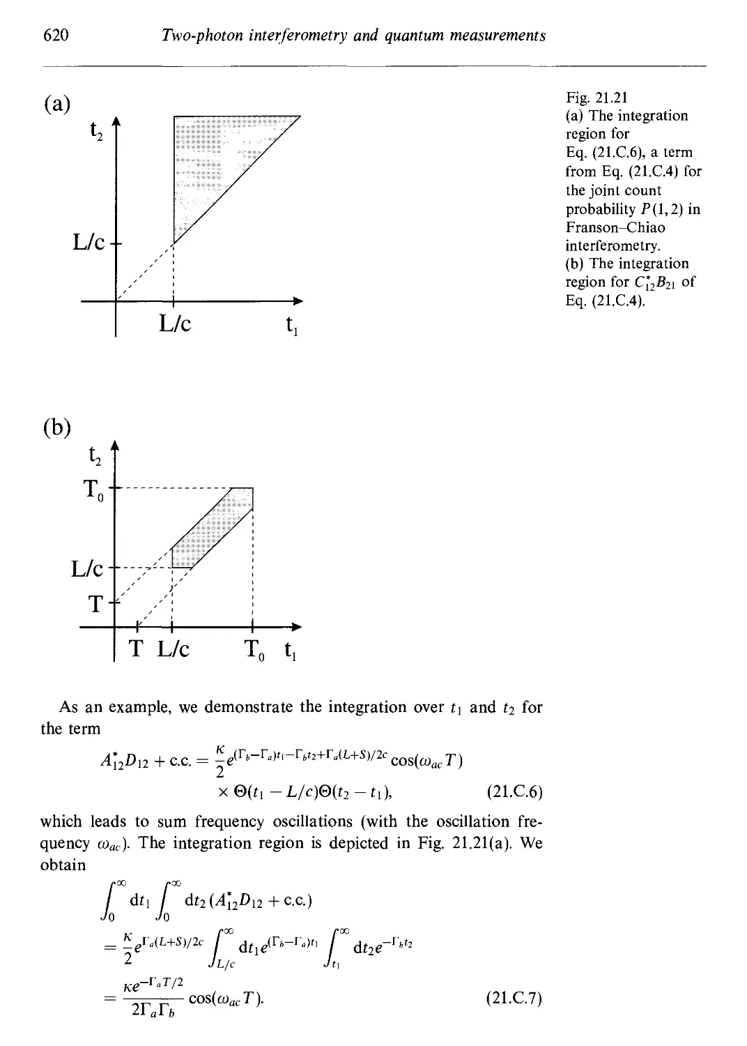
atomic cascade emission 616
21.C Calculation of the joint count probability in Franson-
Chiao interferometry 618
xvi Contents
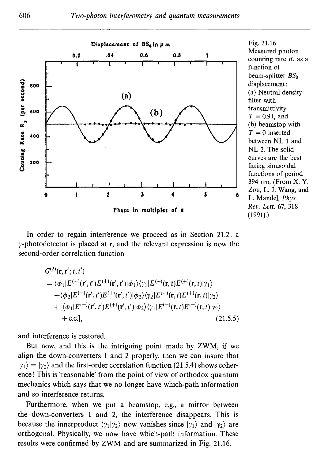
Problems 621
References and bibliography 622
Index 624
To
Thelma Т. Scully and Naseem Fatima Zubairy
and to the memory of
Orvil O. Scully and Muhibul Islam Zubairy
Preface
Quantum optics, the union of quantum field theory and physical
optics, is undergoing a time of revolutionary change. The subject has
evolved from early studies on the coherence properties of radiation
like, for example, quantum statistical theories of the laser in the
sixties to modern areas of study involving, for example, the role
of squeezed states of the radiation field and atomic coherence in
quenching quantum noise in interferometry and optical amplifiers.
On the one hand, counter intuitive concepts such as lasing without
inversion and single atom (micro) masers and lasers are now laboratory
realities. Many of these techniques hold promise for new devices whose
sensitivity goes well beyond the standard quantum limits. On the other
hand, quantum optics provides a powerful new probe for addressing
fundamental issues of quantum mechanics such as complementarity,
hidden variables, and other aspects central to the foundations of
quantum physics and philosophy.
The intent of this book is to present these and many other exciting
developments in the field of quantum optics to students and scientists,
with an emphasis on fundamental concepts and their applications,
so as to enable the students to perform independent research in this
field. The book (which has developed from our lectures on the subject
at various universities, research institutes, and summer schools) may
be used as a textbook for beginning graduate students with some
background in standard quantum mechanics and electromagnetic the-
theory. Each chapter is supplemented by problems and general references.
Some of the problems rely heavily on the treatment given in a research
paper, leading students directly to the scientific literature. The role of
the references is to identify original papers, and to refer the reader to
xx Preface
review articles and related papers for in-depth study. No attempt is
made to give an exhaustive list of references.
The book is divided roughly into three parts. In the first six chapters,
we develop the 'tools' of quantum optics. In the next eleven chapters,
these 'tools' are applied to various quantum optical systems. In the
last four chapters, we consider the application of modern quantum
optical physics to testing the foundations of quantum mechanics.
The book opens with the presentation of the quantization of the
radiation field by associating each mode of the field with a quantized
harmonic oscillator. The strong motivation to quantize the radiation
field in many quantum optical systems comes from phenomena such
as quantum beats, two-photon interferometry, and the generation of
nonclassical states of the radiation field, e.g., Fock states. Some of
these phenomena shed new light on our understanding of the elusive
concept of the photon. In the first part of the book, we discuss the
various states of the radiation field, e.g., coherent and squeezed states,
and introduce the distribution functions of the field which form a
correspondence between the quantum and the classical theories of
radiation. We then develop a quantum theory of coherence in terms of
the correlation functions of the field, which provides a framework for
discussing the outcome of interferometric experiments. We proceed to
develop the semiclassical and quantum theories of the interaction of
the radiation field with matter, with an emphasis on formulating a
theoretical framework directed toward understanding the many faceted
problems of modern quantum optics.
In the second part, we use this theoretical framework to develop
theories of atomic and field damping, resonance fluorescence, laser and
micromaser operation, and the study of the quantum noise properties
of such nonlinear optical processes as parametric amplification and
four-wave mixing. Atomic coherence effects in many novel systems
are discussed in detail. For example, the role of atomic coherence in
suppressing absorption leads to interesting effects such as lasing with-
without inversion and electromagnetically induced transparency. Atomic
coherence can also play a role in quenching Schawlow-Townes spon-
spontaneous emission noise in lasers, as in the correlated emission laser
(CEL). Such CEL systems have potential applications in, e.g., laser
gyro physics and 'noise-free' amplification.
In the third part, we move on to the application of modern quan-
quantum optical physics to fundamental questions related to the founda-
foundation of quantum mechanics. These include Bell's theorem, quantum
nondemolition measurements, 'which-path' detectors, and two-photon
interferometry.
Preface xxi
We have benefited greatly from our interaction with many of our
colleagues, friends, and students in the preparation of this book. They
are too numerous to be individually acknowledged and we are able to
express our gratitude to only a few of them here.
We would especially like to thank Stephen Harris, Willis Lamb,
Julian Schwinger, and Herbert Walther, who have strongly influenced
our thinking through their profound contributions to physics in gen-
general and many fruitful collaborations in particular. Their imprint on
this book is evident: but for them, entire chapters would be missing.
We are grateful to Peter Knight for providing the encouragement for
writing this book. Critical comments from and helpful discussions
with him and with Girish Agarwal, Richard Arnowitt, Chris Bednar,
Janos Bergou, Leon Cohen, Jonathan Dowling, Joe Eberly, Michael
Fleischhauer, Edward Fry, Julio Gea-Banacloche, Roy Glauber, Trung-
Dung Ho, Hwang Lee, Lorenzo Narducci, Robert O'Connell, Norman
Ramsey, Ulrich Rathe, Wolfgang Schleich, Krzysztof Wodkiewicz,
Bernand Yurke, and Shi-Yao Zhu provided invaluable assistance con-
concerning many subtle points. One of us (MSZ) would like to express his
gratitude to the Pakistan Atomic Energy Commission for the financial
support over the years, and particularly its Chairman, Ishfaq Ahmad,
for his deep interest and commitment that played a vital role in the
completion of this project. MOS would like to acknowledge the sup-
support of the Office of Naval Research, and particularly Herschel Pilloff,
whose wisdom and dedication to scientific excellence have resulted
in many successful joint projects and conferences which have had a
marked impact on this book. The support of the Houston Advanced
Research Center (HARC), and the Welch Foundation is also deeply
appreciated. We thank Jeanne Williams for the careful typing in TgX,
and Jim and Andrey Bailey for the hospitality of the Bailey ranch,
where the manuscript was completed.
Finally, we are grateful to our family members, Judith, James,
Debra, Robert, Steven, and Jacquelyn, and Parveen, Sarah, Sahar, and
Raheel, for their support, and understanding, especially during the
extended absences in the course of the last decade, when this book
was contemplated, planned, and written.
Marian O. Scully
M. Suhail Zubairy
CHAPTER 1
Quantum theory of
radiation
Light occupies a special position in our attempts to understand nature
both classically and quantum mechanically. We recall that Newton,
who made so many fundamental contributions to optics, championed a
particle description of light and was not favorably disposed to the wave
picture of light. However, the beautiful unification of electricity and
magnetism achieved by Maxwell clearly showed that light was properly
understood as the wave-like undulations of electric and magnetic fields
propagating through space.
The central role of light in marking the frontiers of physics con-
continues on into the twentieth century with the ultraviolet catastrophe
associated with black-body radiation on the one hand and the pho-
photoelectric effect on the other. Indeed, it was here that the era of
quantum mechanics was initiated with Planck's introduction of the
quantum of action that was necessary to explain the black-body ra-
radiation spectrum. The extension of these ideas led Einstein to explain
the photoelectric effect, and to introduce the photon concept.
It was, however, left to Dirac* to combine the wave- and particle-
like aspects of light so that the radiation field is capable of explaining
all interference phenomena and yet shows the excitation of a specific
atom located along a wave front absorbing one photon of energy. In
this chapter, following Dirac, we associate each mode of the radiation
field with a quantized simple harmonic oscillator, this is the essence
of the quantum theory of radiation. An interesting consequence of the
quantization of radiation is the fluctuations associated with the zero-
The pioneering papers on the quantum theory of radiation by Dirac [1927] and Fermi [1932]
should be read by every student of the subject. Excellent modern treatments are to be found in
the textbooks by: Loudon, The Quantum Theory of Light [1973], Cohen-Tannoudji, Dupont-Roc,
and Grynberg, Atom-Photon Interactions [1992], Weinberg, Theory of Quantum Fields [1995], and
Pike and Sarkar, Quantum Theory of Radiation [1995].
Quantum theory of radiation
point energy or the so-called vacuum fluctuations. These fluctuations
have no classical analog and are responsible for many interesting
phenomena in quantum optics. As is discussed at length in Chapters
5 and 7, a semiclassical theory of atom-field interaction in which only
the atom is quantized and the field is treated classically, can explain
many of the phenomena which we observe in modern optics. The
quantization of the radiation field is, however, needed to explain effects
such as spontaneous emission, the Lamb shift, the laser linewidth, the
Casimir effect, and the full photon statistics of the laser. In fact,
each of these physical effects can be understood from the point of
view of vacuum fluctuations perturbing the atoms, e.g., spontaneous
emission is often said to be the result of 'stimulating' the atom by
vacuum fluctuations. However, as compelling as these reasons are
for quantizing the radiation field, there are other strong reasons and
logical arguments for quantizing the radiation field.
For example, the problem of quantum beat phenomena provides
us with a simple example in which the results of self-consistent fully
quantized calculation differ qualitatively from those obtained via a
semiclassical theory with or without vacuum fluctuations. Another
experiment wherein a quantized theory of radiation is required for
the proper interpretation of the observed results is two-photon in-
terferometry and the production of entangled states associated with
such a configuration. This is discussed in detail in Chapter 21. Fur-
Further support that the electromagnetic field is quantized is provided by
the experimental observations of nonclassical states of the radiation
field, e.g., squeezed states, sub-Poissonian photon statistics, and photon
antibunching.
Following this brief motivation for the quantum theory of radiation,
we now turn to the quantization of the free electromagnetic field.
1.1 Quantization of the free electromagnetic field
With the objective of quantizing the electromagnetic field in free
space, it is convenient to begin with the classical description of the
field based on Maxwell's equations. These equations relate the electric
and magnetic field vectors E and H, respectively, together with the
displacement and inductive vectors D and B, respectively, and have
the form (in mks units):
VxH=^, A.1.1a)
1.1 Quantization of the free electromagnetic field
VxE=-^, A.1.1b)
V-B = O, A.1.1c)
V-D = O, A.1.Id)
with the constitutive relations
В = /юН, A.1.2)
D = e0E- A.1.3)
Here eo and цо are the free space permittivity and permeability,
respectively, and /io^o = c~2 where с is the speed of light in vacuum.
It follows, on taking the curl of Eq. A.1.1b) and using Eqs. A.1.1a),
A.1.Id), A.1.2), and A.1.3), that E(r,t) satisfies the wave equation
^O. „Л.4,
In deriving Eq. A.1.4) we also used V x (V x E) = V(V • E) - V2E.
1.1.1 Mode expansion of the field
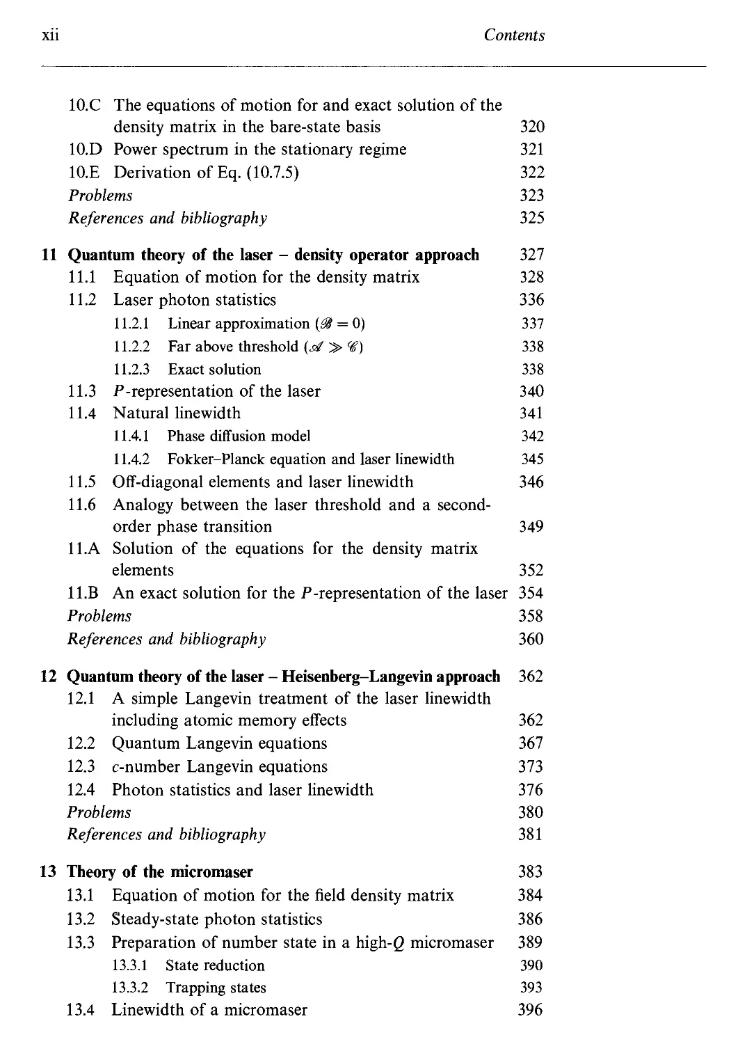
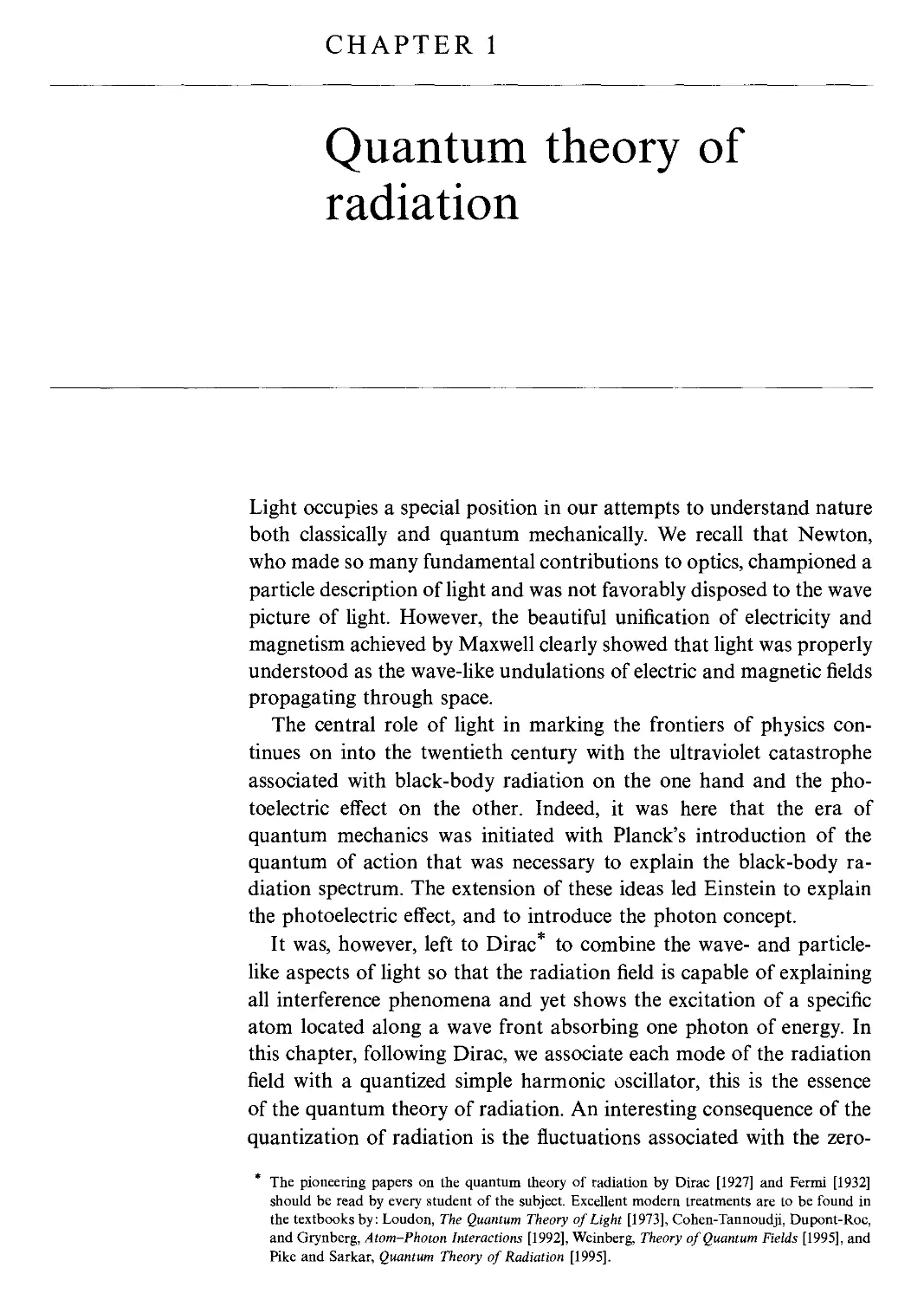
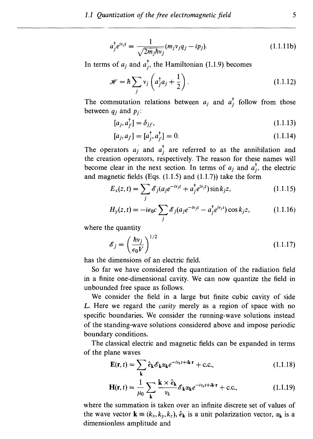
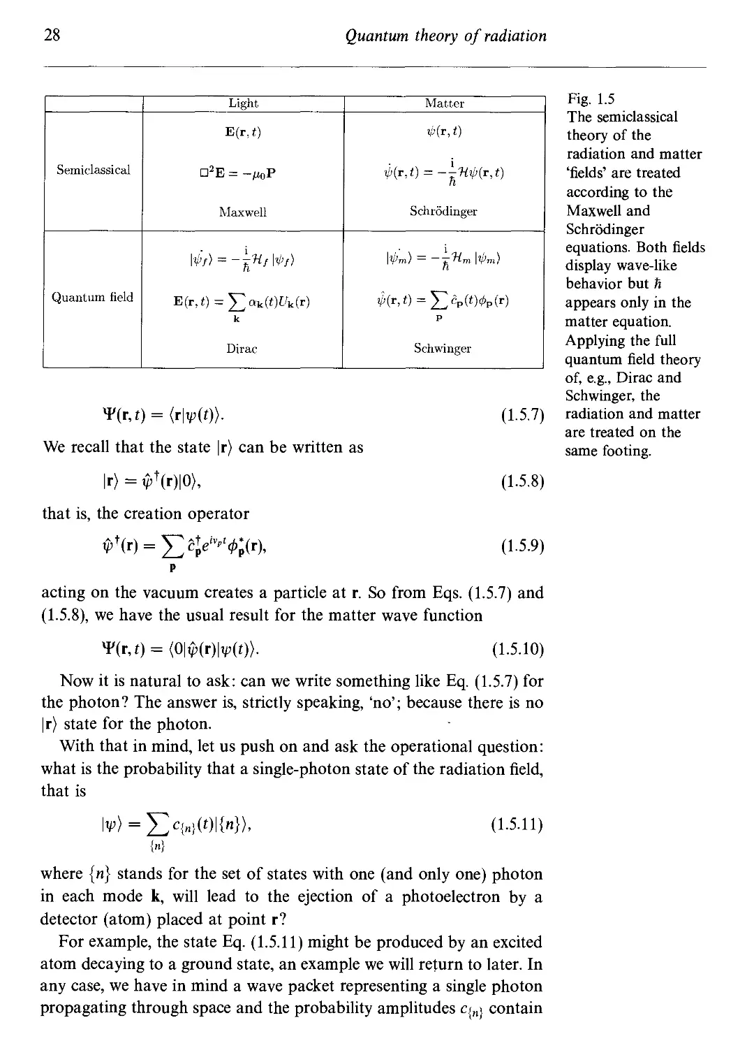
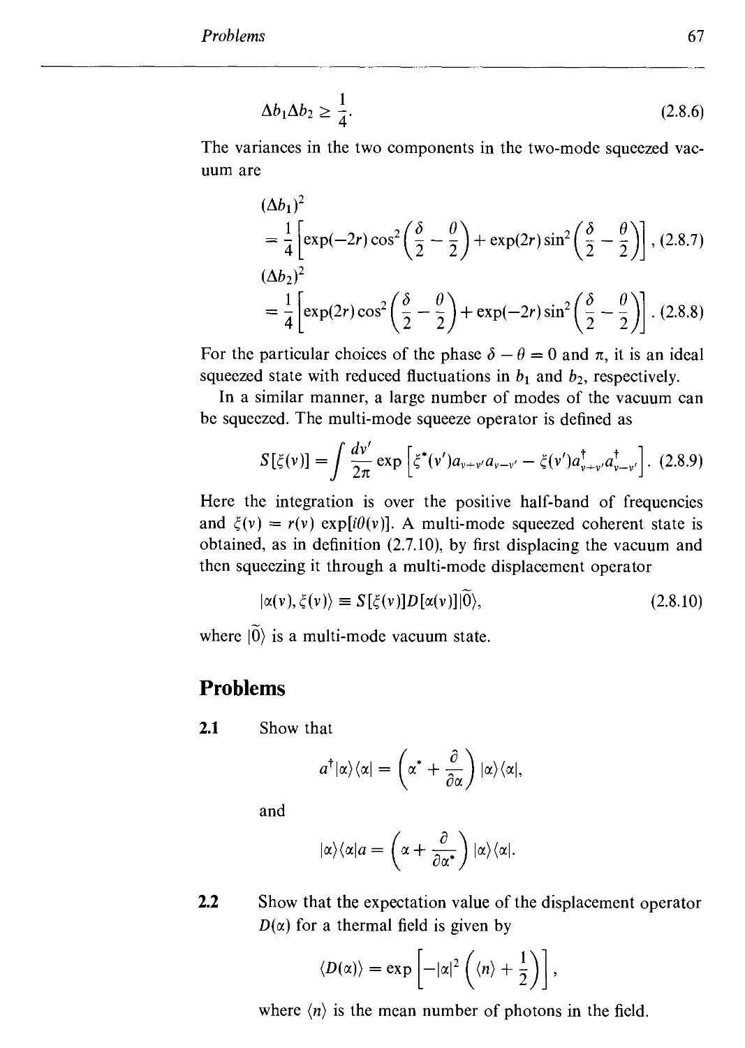
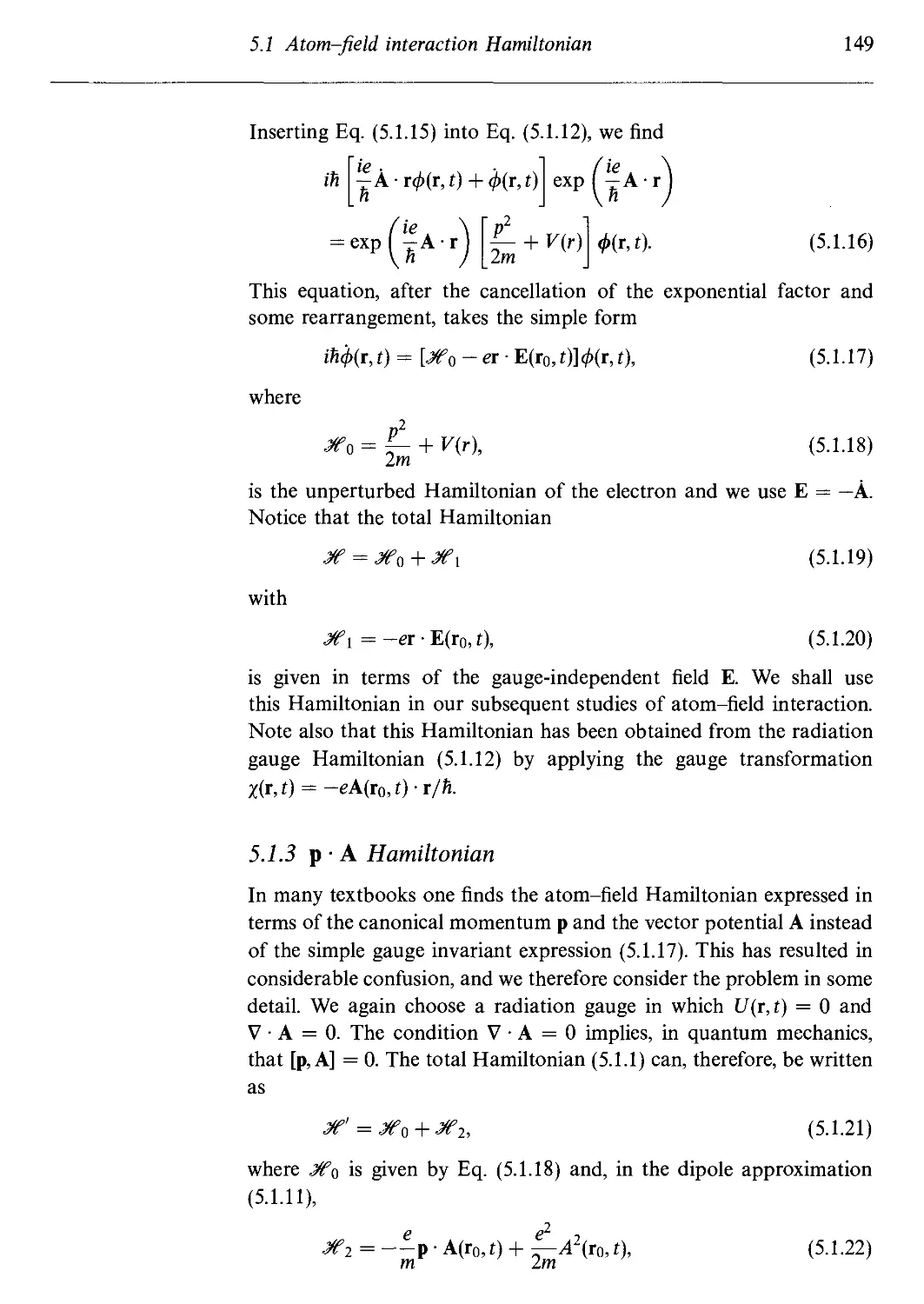
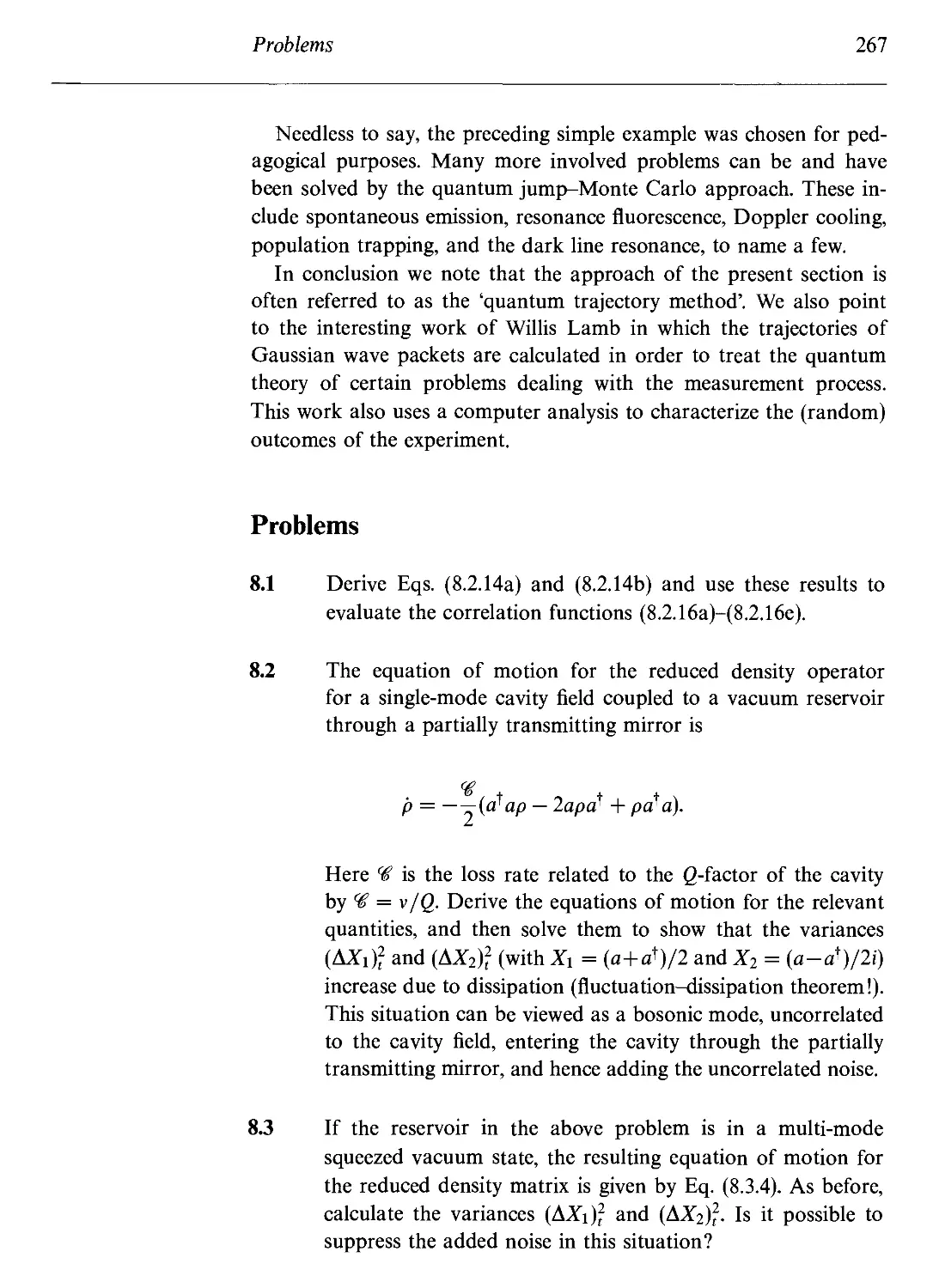
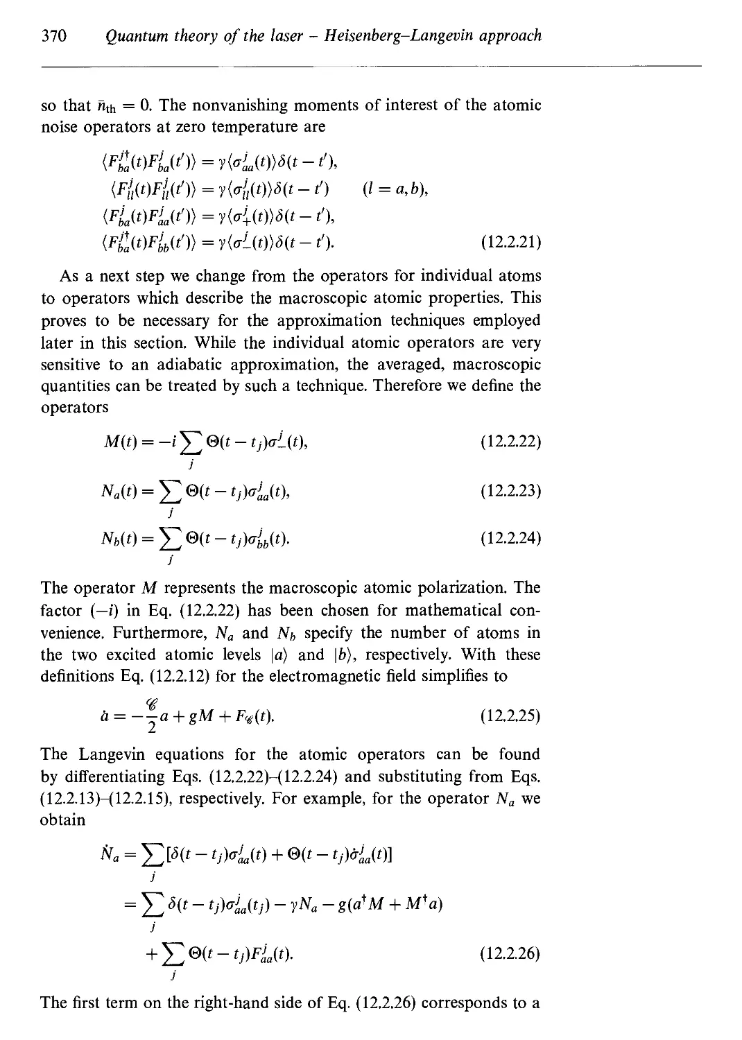
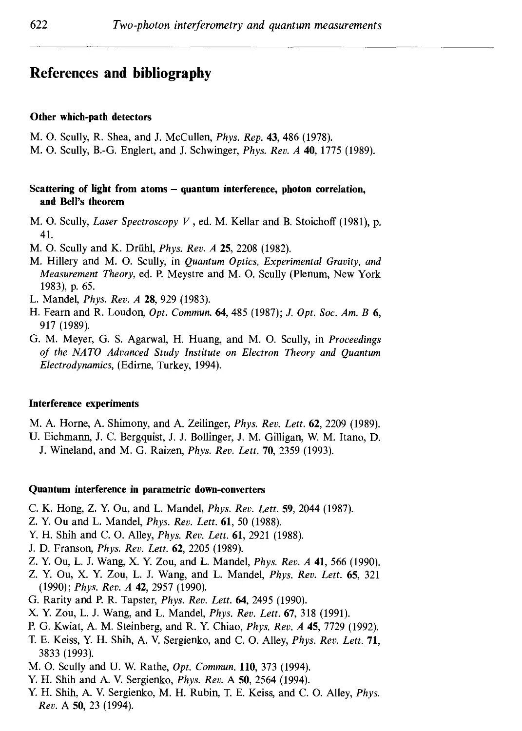
We first consider the electric field to have the spatial dependence
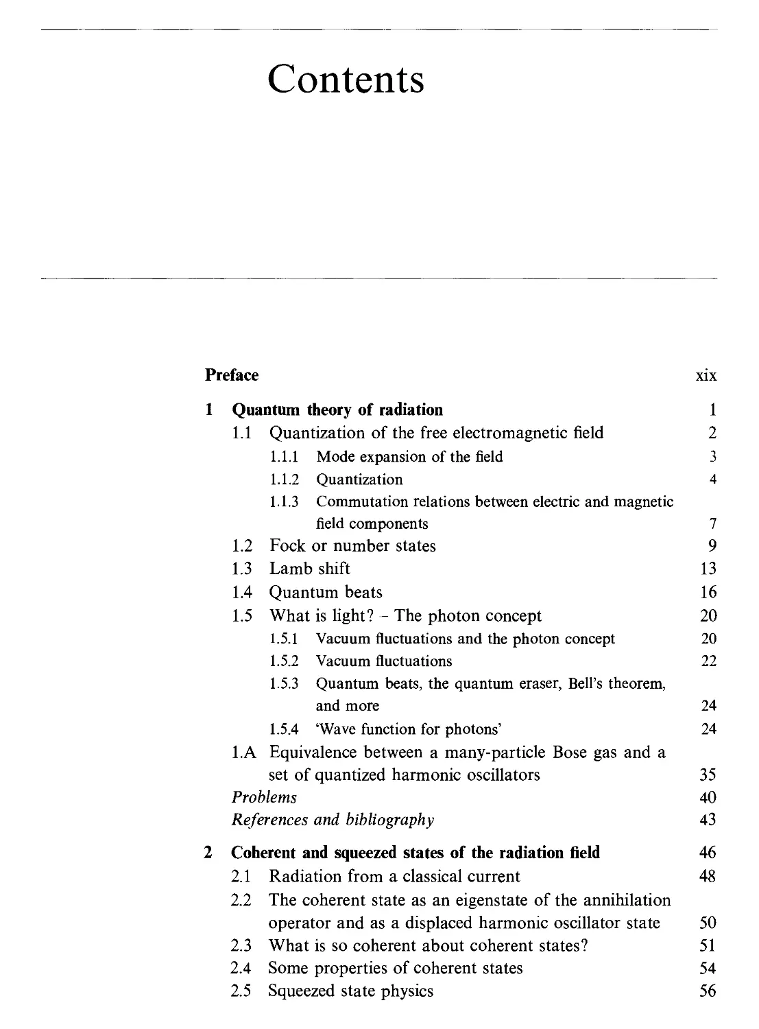
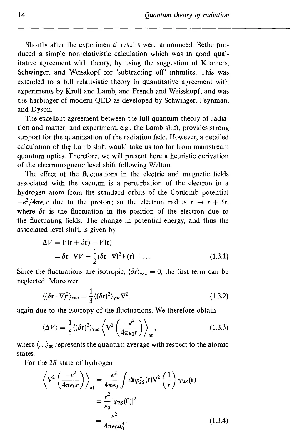
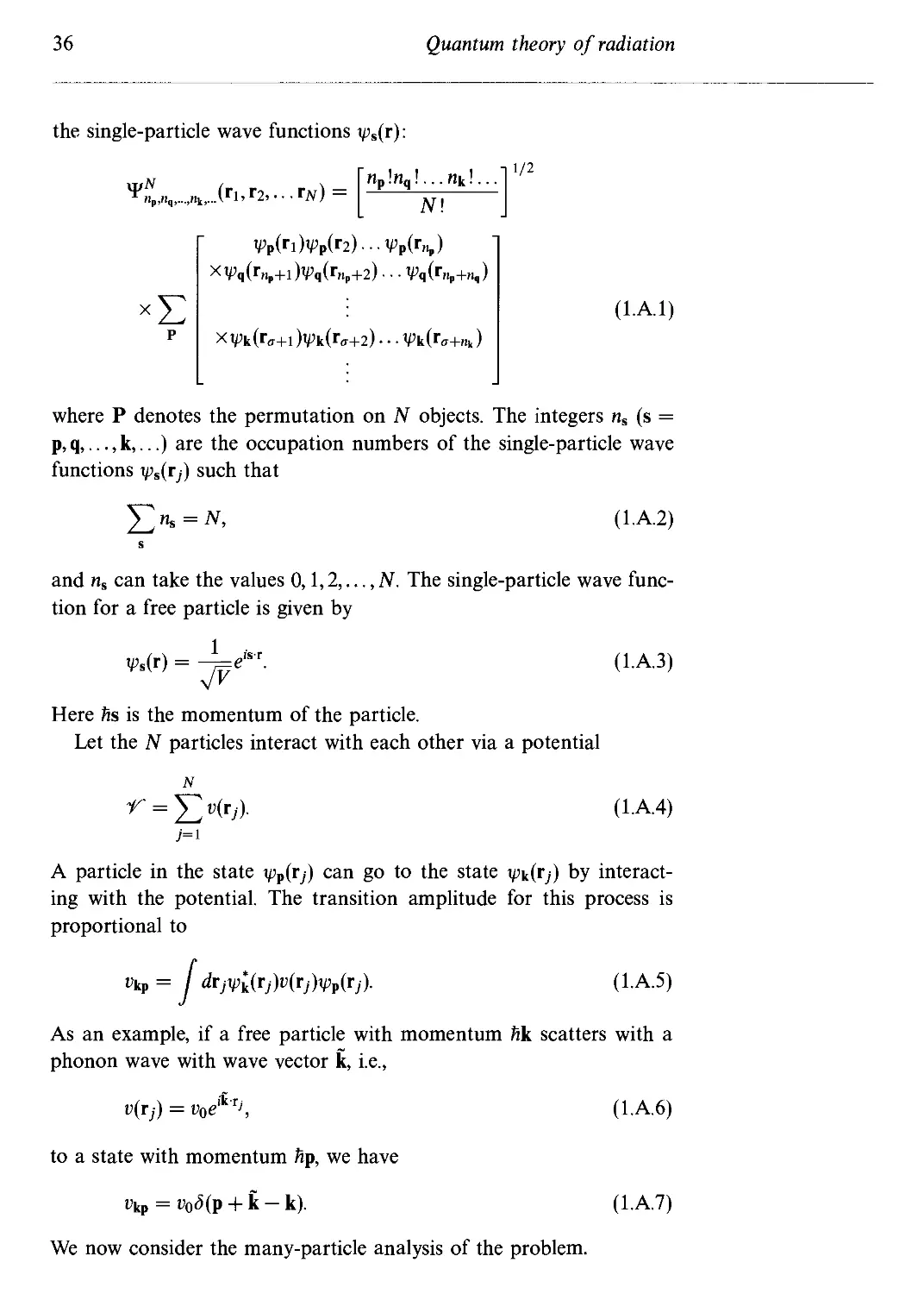
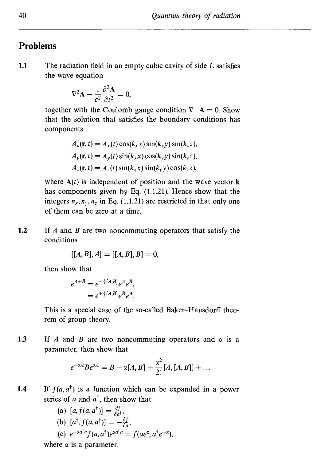
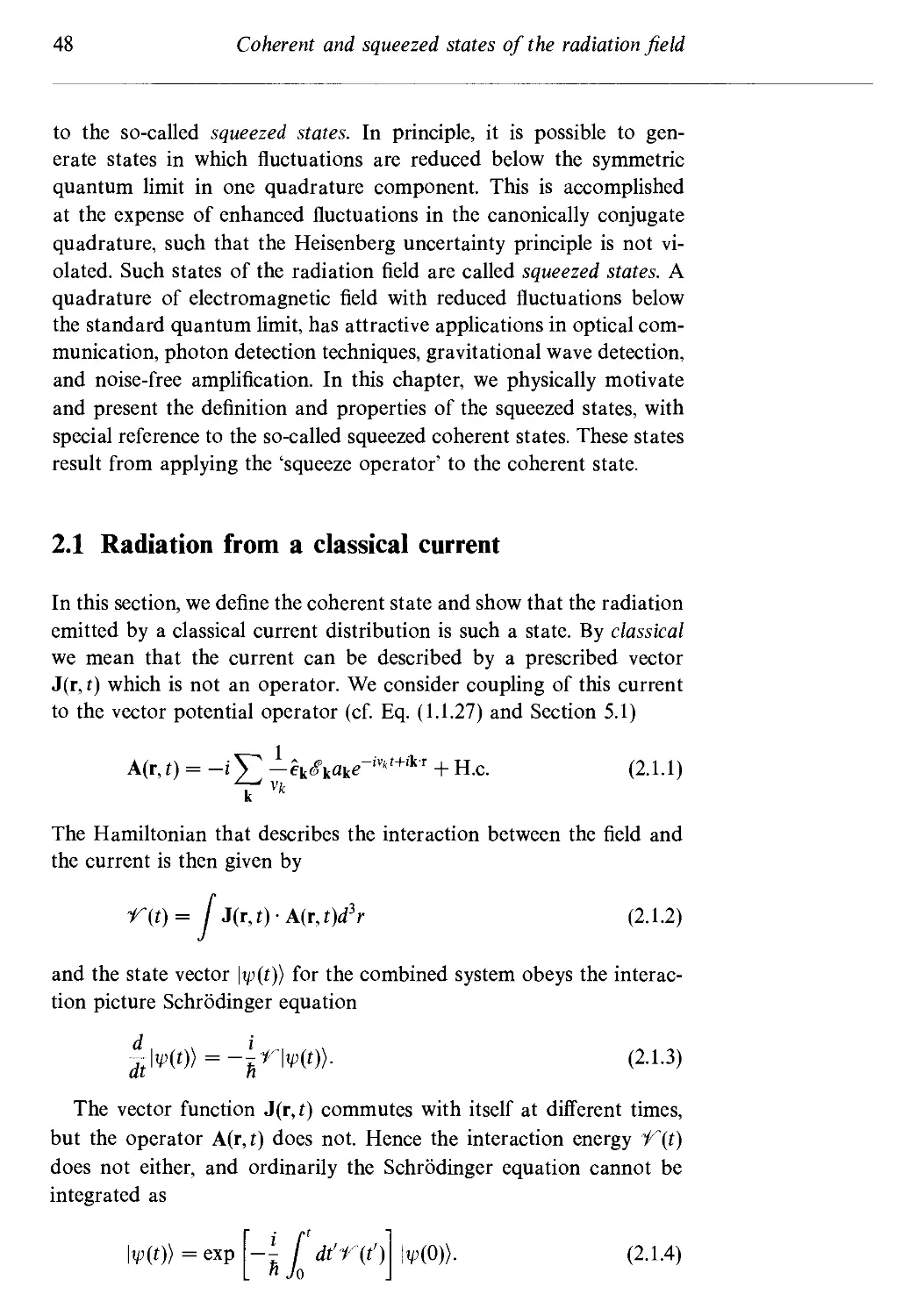
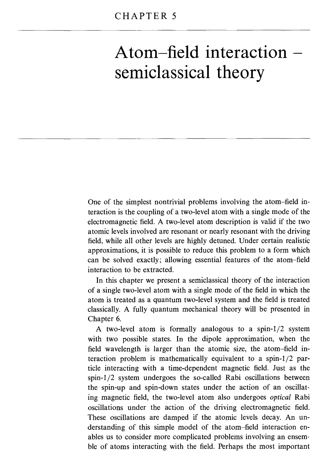
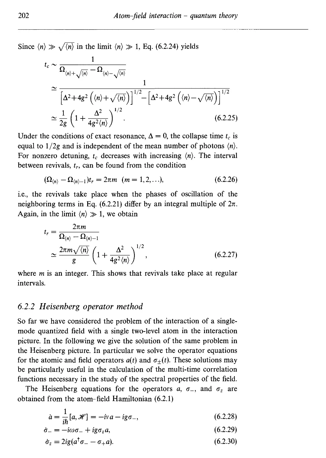
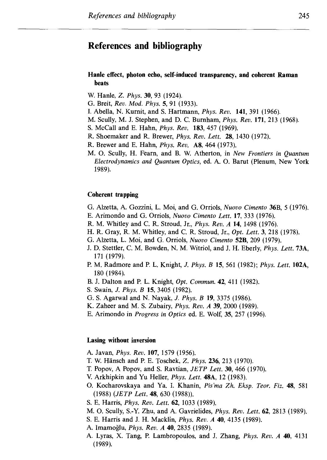
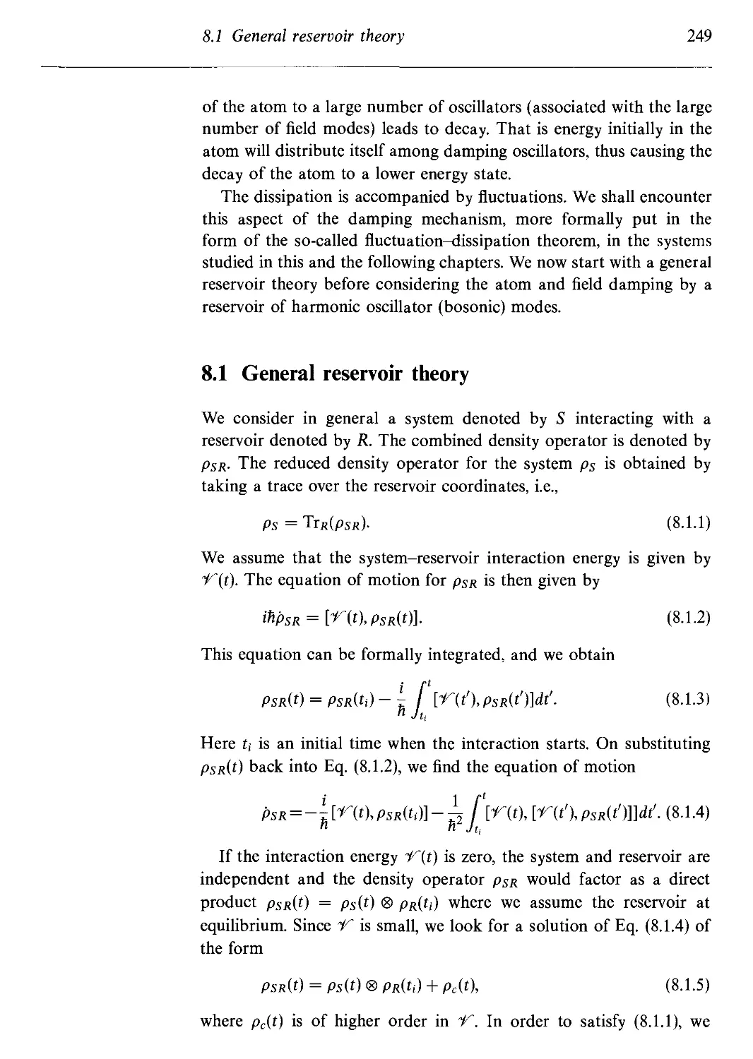
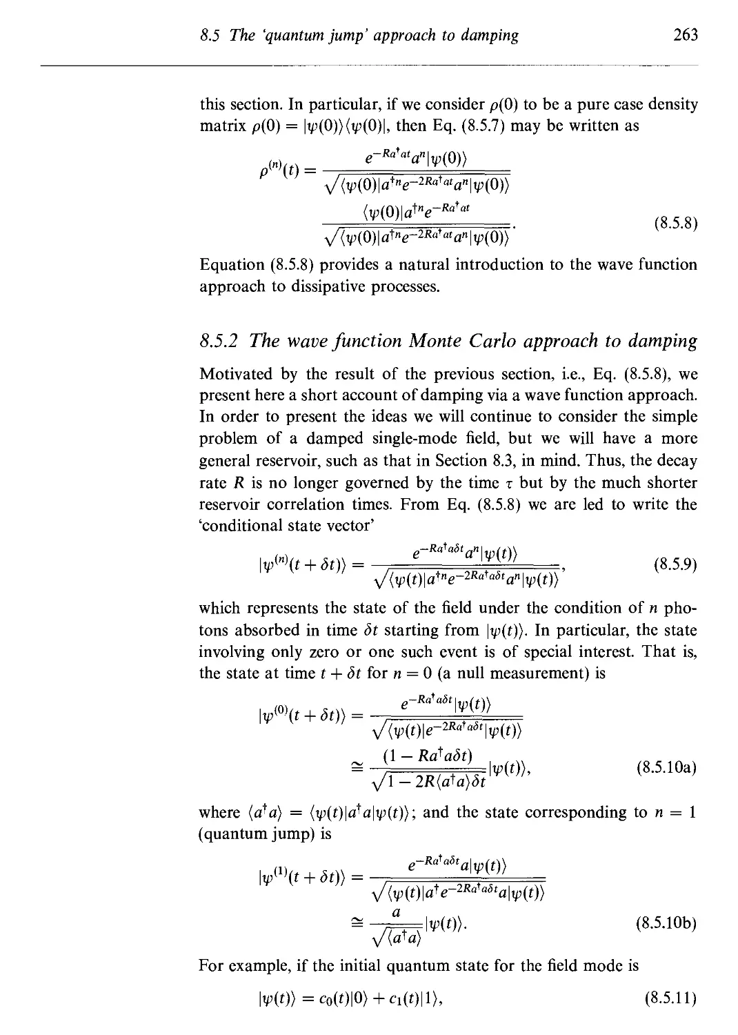
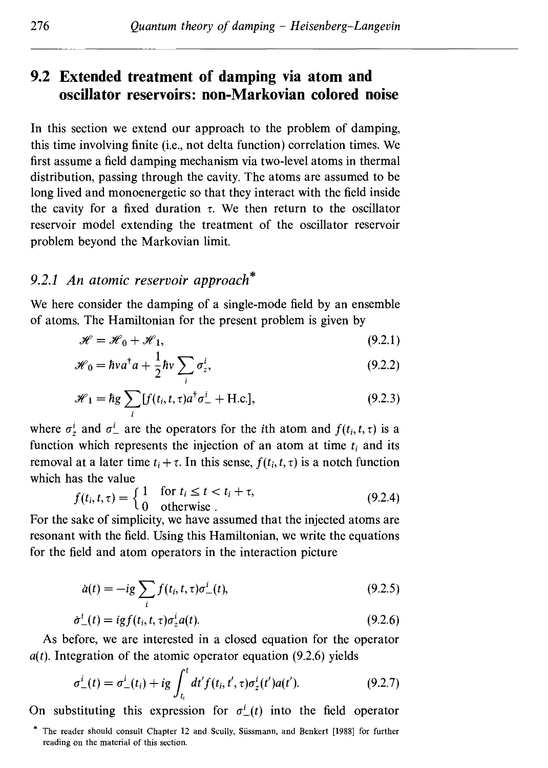
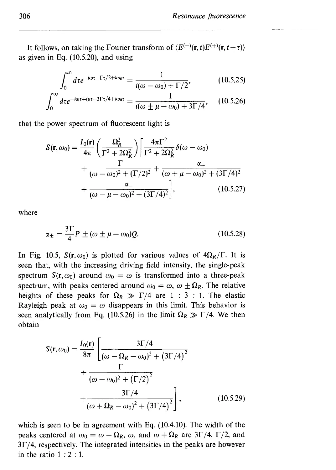
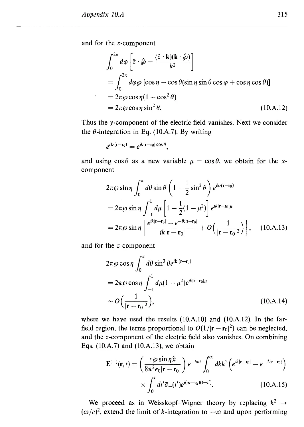
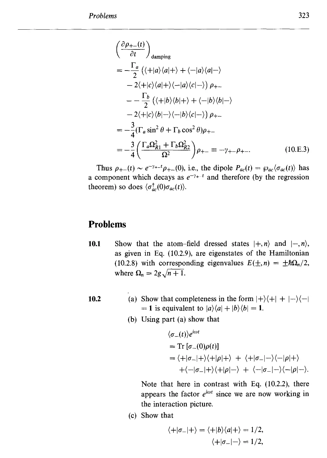
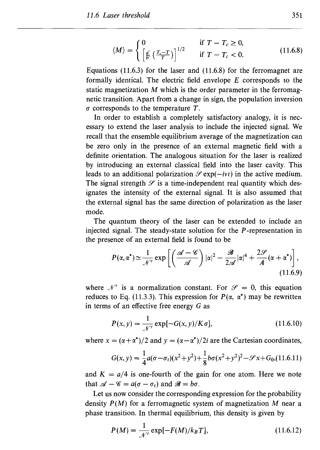
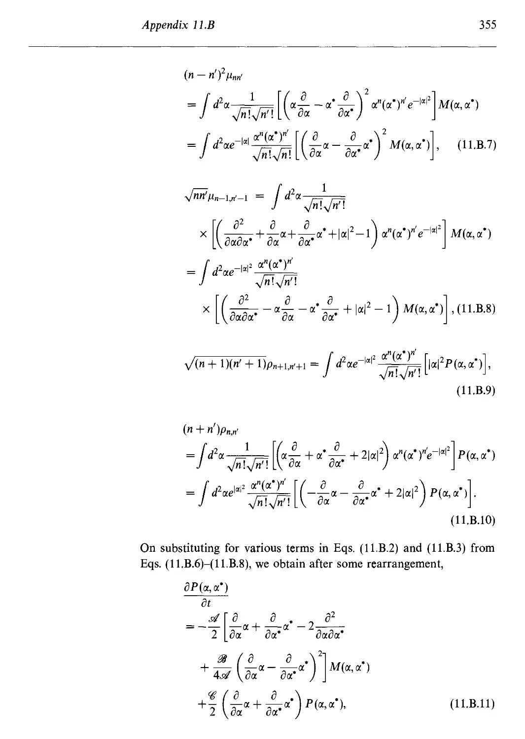
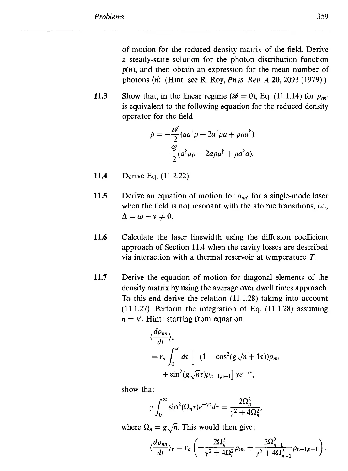
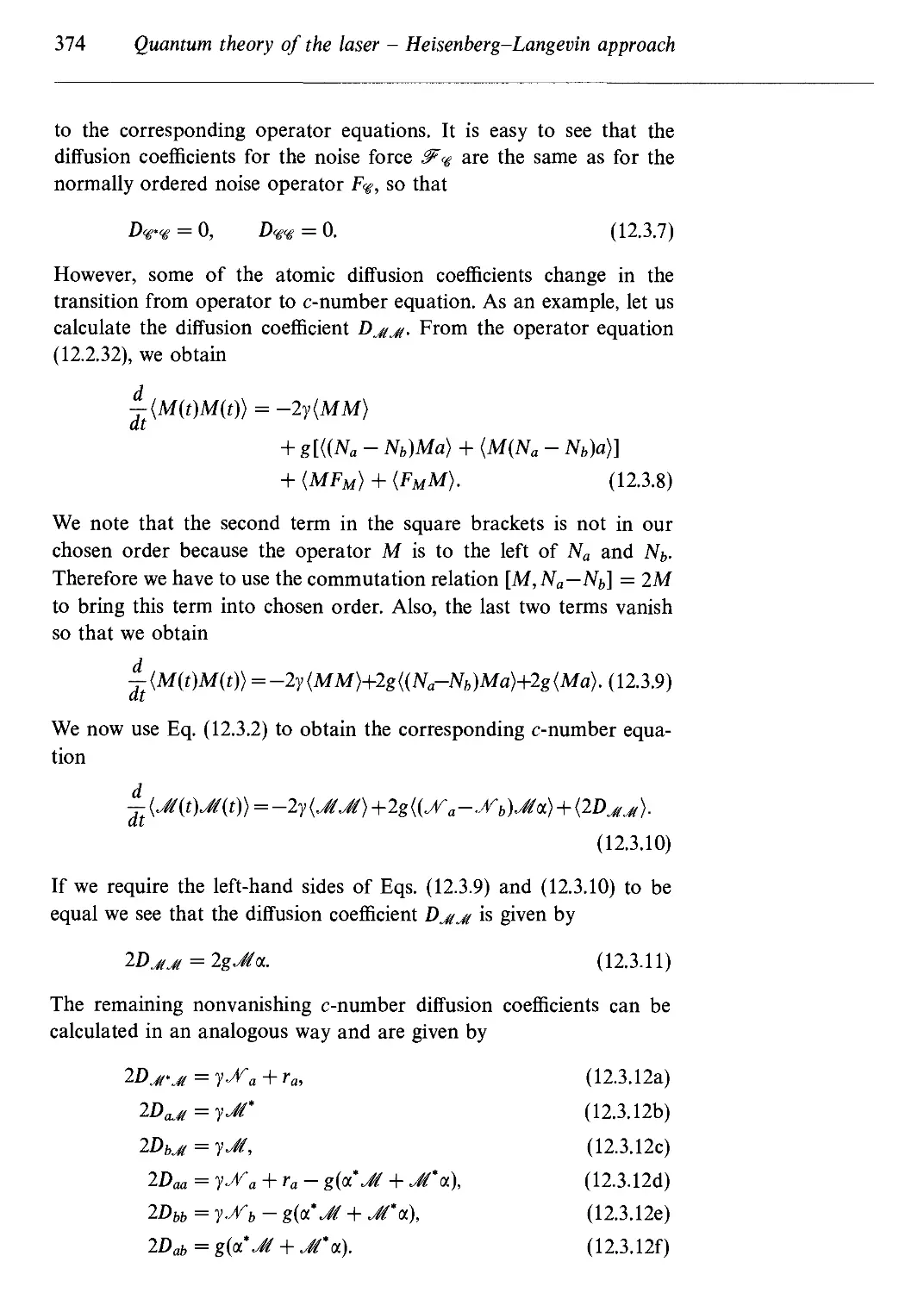
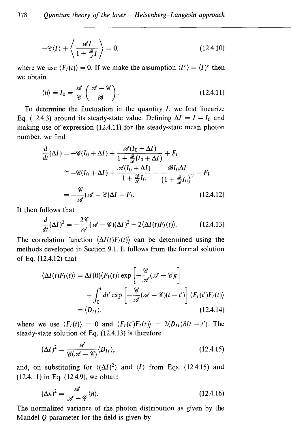
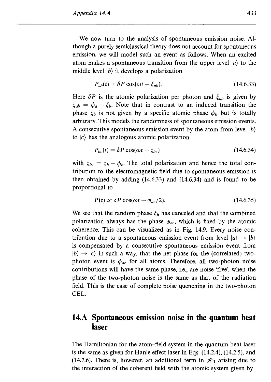
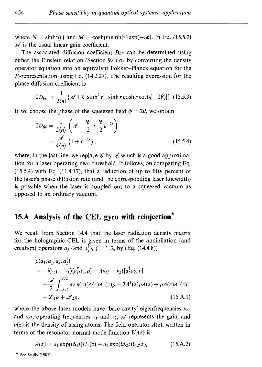
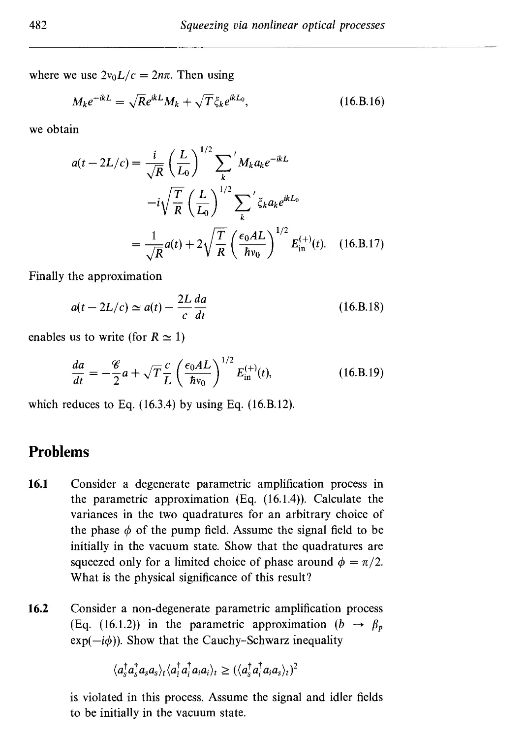
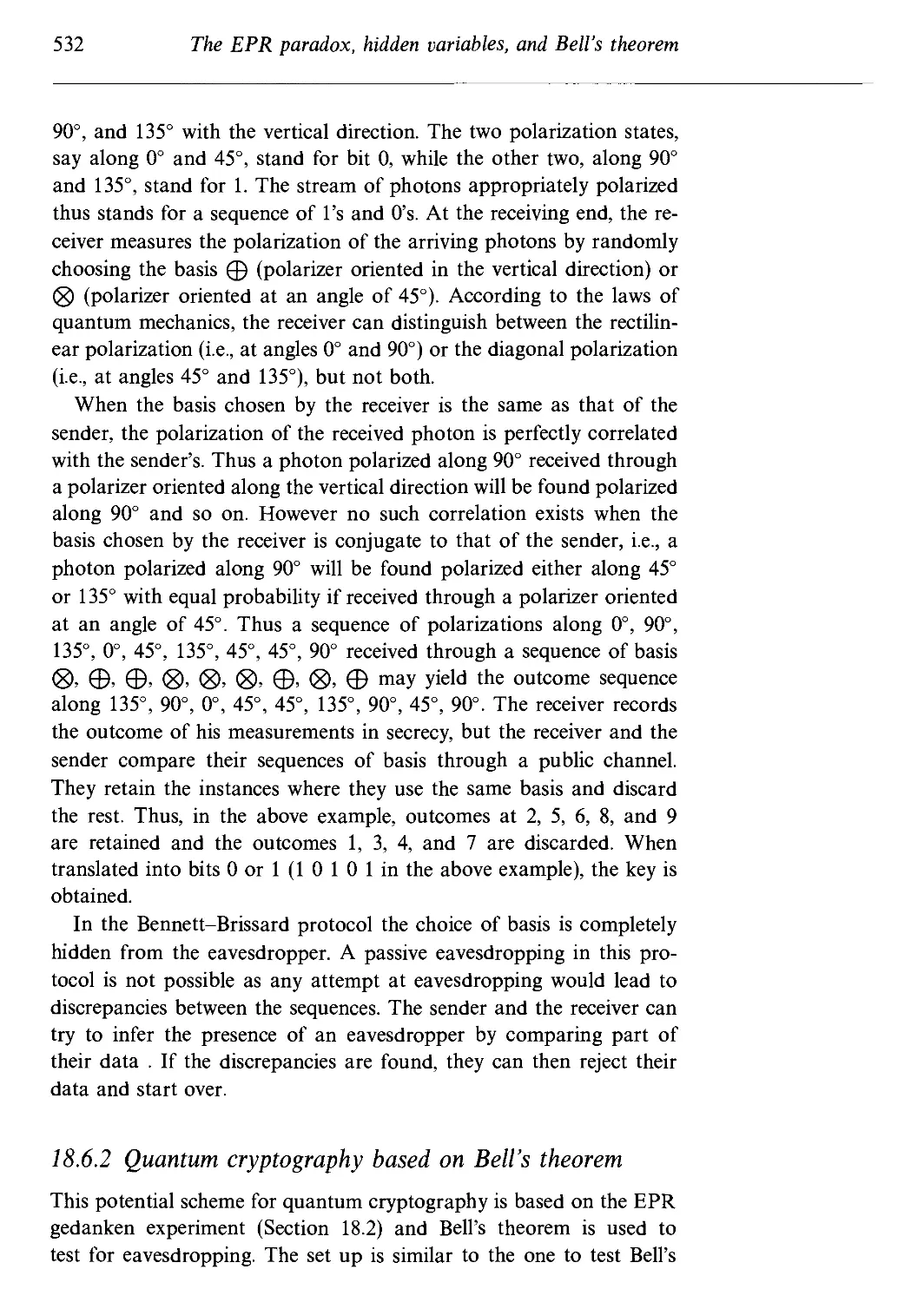
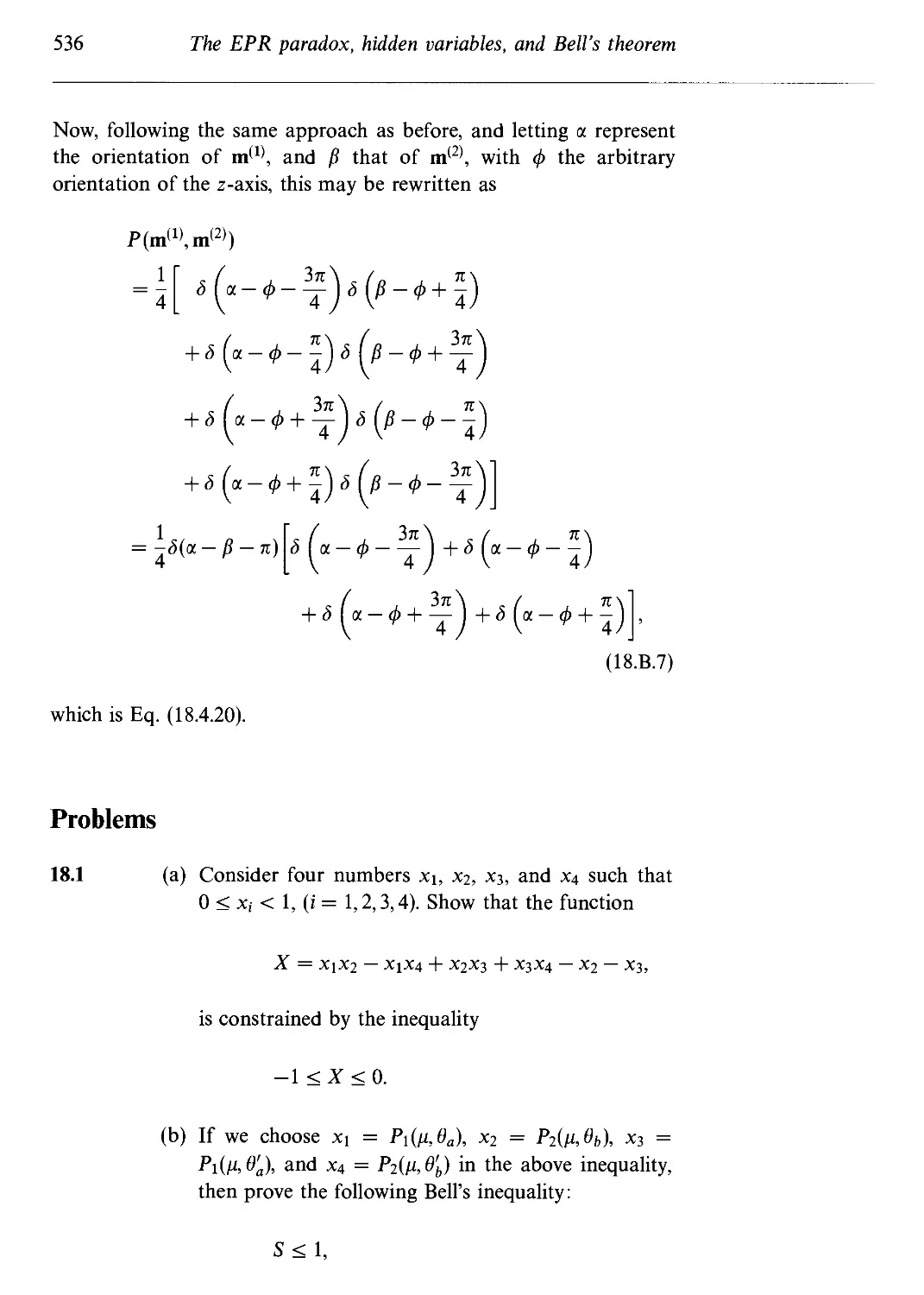
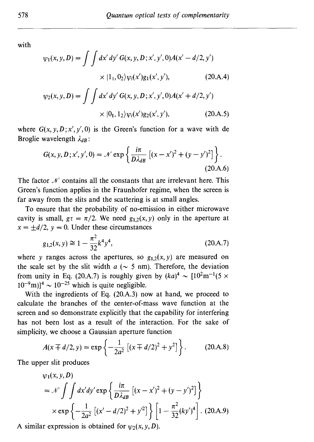
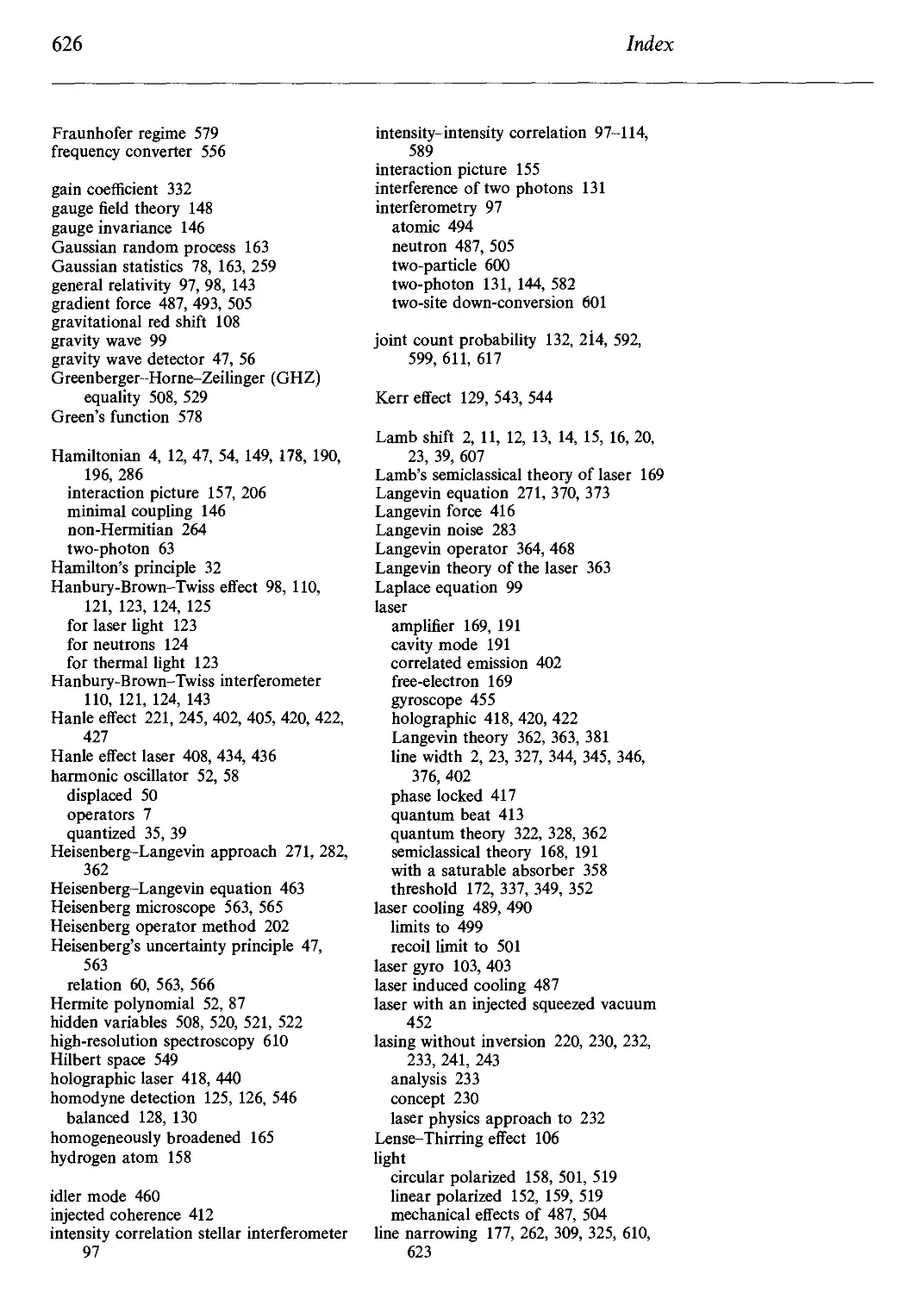
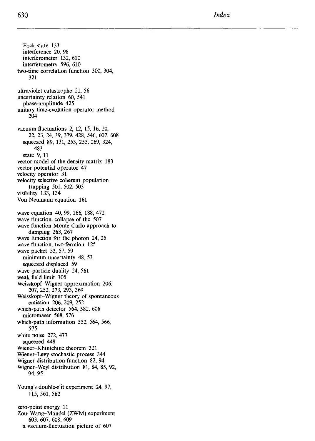
appropriate for a cavity resonator of length L (Fig. 1.1). We take the
electric field to be linearly polarized in the x-direction and expand in
the normal modes of the cavity
Ex{z, t) = Y,Aj4j(t) *in(kjz), A.1.5)
J
where qj is the normal mode amplitude with the dimension of a length,
kj = jn/L, with j = 1,2,3,..., and
'/2
with Vj = jnc/L being the cavity eigenfrequency, V = LA (A is the
transverse area of the optical resonator) is the volume of the resonator
and nij is a constant with the dimension of mass. The constant nij has
been included only to establish the analogy between the dynamical
problem of a single mode of the electromagnetic field and that of
the simple harmonic oscillator. The equivalent mechanical oscillator
will have a mass nij, and a Cartesian coordinate qj. The nonvanishing
component of the magnetic field Hy in the cavity* is obtained from
Eq. A.1.5):
In the present treatment of field quantization in vacuum we are focussing on the electric E(r, t)
and magnetic H(r, t) fields. In a material medium it is preferable to work with D(r, t) and В(г,г);
see Bialynicki-Birula and Bialynicka-Birula [1976].
Quantum theory of radiation
Л Л Л
\7 ХГЛУ Xj
Fig. 1.1
Electromagnetic field
of frequency v inside
a cavity. The field is
assumed to be
transverse with the
electric field
polarized in the
x-direction.
A.1.7)
The classical Hamiltonian for the field is
dt(e0E2x
A.1.8)
where the integration is over the volume of the cavity. It follows, on
substituting from Eqs. A.1.5) and A.1.7) for Ex and Hy, respectively,
in Eq. A.1.8), that
A.1.9)
where pj = nij-qj is the canonical momentum of the jih mode. Equation
A.1.9) expresses the Hamiltonian of the radiation field as a sum of
independent oscillator energies. Each mode of the field is therefore
dynamically equivalent to a mechanical harmonic oscillator.
1.1.2 Quantization
The present dynamical problem can be quantized by identifying qj
and pj as operators which obey the commutation relations
[qj,Pj>] = ihdjf, A.1.10a)
[qj, qj>] = [pj,pj>] = 0. A.1.10b)
It is convenient to make a canonical transformation to operators aj
and a\:
A.1.11a)
1.1 Quantization of the free electromagnetic field
A.1.11b)
In terms of a,- and aj, the Hamiltonian A.1.9) becomes
A.1.12)
The commutation relations between aj and a] follow from those
between qj and pj:
[aj,a],]=dJf, A.1.13)
[aj,af] = [a),a),]=0. A.1.14)
The operators ay and aj are referred to as the annihilation and
the creation operators, respectively. The reason for these names will
become clear in the next section. In terms of aj and a], the electric
and magnetic fields (Eqs. A.1.5) and A.1.7)) take the form
Ex(z, t) = Y^ £j(aje-ivjt + a)eiv>1) sinkjz, A.1.15)
j
Hy(z,t) = -ieocY,<?j(aje~ivjt ~ а)е1^) cos kjz, A.1.16)
where the quantity
has the dimensions of an electric field.
So far we have considered the quantization of the radiation field
in a finite one-dimensional cavity. We can now quantize the field in
unbounded free space as follows.
We consider the field in a large but finite cubic cavity of side
L. Here we regard the cavity merely as a region of space with no
specific boundaries. We consider the running-wave solutions instead
of the standing-wave solutions considered above and impose periodic
boundary conditions.
The classical electric and magnetic fields can be expanded in terms
of the plane waves
E(r, t) = Y, ek£k<*ke~ivtt+ikt + c.c, A.1.18)
к
1 1 A
H(r, t) = - У iiii!i^kake-1Vt'+;kr + c.c, A.1.19)
rt) Y П
where the summation is taken over an infinite discrete set of values of
the wave vector к = (kx,ky,kz), ek is a unit polarization vector, ак is a
dimensionless amplitude and
Quantum theory of radiation
- A.1.20,
In Eqs. A.1.18) and A.1.19) c.c. stands for complex conjugate. The
periodic boundary conditions require that
_ 2nnx _2nny _2nnz
where nx, ny, nz are integers @, +1, +2,...). A set of numbers (nx, ny, nz)
defines a mode of the electromagnetic field. Equation A.1.Id) requires
that
к ■ ek = 0, A.1.22)
i.e., the fields are purely transverse. There are, therefore, two indepen-
independent polarization directions of e^ for each k.
The change from a discrete distribution of modes to a continuous
distribution can be made by replacing the sum in Eqs. A.1.18) and
A.1.19) by an integral:
where the factor 2 accounts for two possible states of polarization.
In many problems, we shall be interested in the density of modes
between the frequencies v and v + dv. This can be obtained by trans-
transforming from the rectangular components (kx, ky, kz) to the polar
coordinates (k sin в cos ф, к sin в sin ф, к cos в), so that the volume ele-
element in к space is
* -> v2
d3k = k2dk sin вйвйф = -.dv sin вdвdф. A.1.24)
The total number of modes in volume L3 in the range between v and
v + dv is given by
/ L\3 v2dv Г f2n L3v2
dJf = 2 — —5— / ddsmd / dф = _ , dv. A.1.25)
\2nJ c3 Jo Jo r tc2c3
Therefore the number of modes with frequencies in the range v to
v + dv is
L3v2
D(v)dv = -~dv, A.1.26)
where D(v) is called the mode density.
1.1 Quantization of the free electromagnetic field
As before, the radiation field is quantized by identifying otk and <xk
with the harmonic oscillator operators ay and a\, respectively, which
satisfy the commutation relation [ak,a£] = 1. The quantized electric
and magnetic fields take the form
E(r, t) = Y^ h^kake-iVkt+ikt + H.c, A.1.27)
к
1 1 A
H(r, t) = — V ^-^<?kake-ivt'+*-r + H.c, A.1.28)
where H.c. stands for Hermitian conjugate. Usually the positive and
negative frequency parts of these field operators are written separately.
For example, the electric field operator E(r, t) is written as
E(r, t) = E(+)(r, t) + E(-»(r, t), A.1.29)
where
r, t) = ^ ек£каке~ы+1к'\ A.1.30)
к
Here E(+)(r, t) contains only the annihilation operators and its adjoint
E(-)(r, t) contains only the creation operators.
1.1.3 Commutation relations between electric and magnetic
field components
An important consequence of imposing the quantum conditions A.1.13)
and A.1.14) is that as the electric and magnetic field strengths do not
commute they are thus not measurable simultaneously. In order to
show this we rewrite the quantized mode expansions A.1.27) and
A.1.28) for E(r,t) and H(r, t), respectively by including explicitly the
two states of polarization denoted by the symbol X:
E(r, t) = Y, ^кам^Жкг + H.c, A.1.32)
M
H(r, t) = - Y ^^~SkakAe-^t+ikt + H.c. A.1.33)
The corresponding commutation relations between the operators
and aj^ are
A.1.34)
Quantum theory of radiation
It then follows that the equal time commutator between the field
components is given by
M
where ek;;' (i = x,y,z) is the ith component of екл). We proceed by
using the operator identity of Problem 1.9 to write
aA)aA) , aB)aB) , KK < /л 1 i£\
ek ek ' ek ek ' IT = ' A.1.JO)
where e^'e^1', ek2)ek2), and kk denote dyadic products. One can verify
that taking the inner product of A.1.36) with the Cartesian unit vector
ej from the left and e, from the right yields
JDJD , .B) B) _ с kkj
eki ekj + eki ekj ~ d'J ~ "p-- A.1.37)
The summation over the polarization states in Eq. A.1.35) can
now be carried out using A.1.37). The resulting expression for the
commutator is
[Ex(r,t),Hy(r',t)] = %Y,k* [еМГ'Г1 -e-lMr-f)] ■ A.1.38)
к
We now replace the summation by an integral via
The factor of 2 has not been included as was done in Eq. A.1.23)
because, in the present case, we have summed over two polarization
states explicitly. We obtain
8_
a?
In general
[Ex(r,t),Hy(r',t)] = -ihc2-d^(r-r'). A.1.40)
[Ej(r,t),Hj(r',t)]=O (j = x,y,z), A.1.41)
[Ej(r, t),Hk(r', t)] = -ihc2^3{3\r - r'), A.1.42)
where j, к, and / form a cyclic permutation of x, y, and z.
We, therefore, conclude that the parallel components of E and H
may be measured simultaneously whereas the perpendicular compo-
components cannot.
1.2 Fock or number states
1.2 Fock or number states
In this section we first restrict ourselves to a single mode of the field
of frequency v having creation and annihilation operators cfi and a,
respectively. Let \n) be the energy eigenstate corresponding to the
energy eigenvalue £„, i.e.,
Ж\п) = hv Ua + Л \n) = En\n). A.2.1)
If we apply the operator a from the left, we obtain after using the
commutation relation [а, аЦ = 1 and some rearrangement
Жа\п) = (£„ - hv)a\n). A.2.2)
This means that the state
\n-l) = — \n), A.2.3)
(Xn
is also an energy eigenstate but with the reduced eigenvalue
£B_i = £„ - hv. A.2.4)
In Eq. A.2.3), <х„ is a constant which will be determined from the
normalization condition
<n-l|n-l) = l. A.2.5)
If we repeat this procedure n times we move down the energy ladder
in steps of hv until we obtain
ЖаЩ = (Eo - hv)a\0). A.2.6)
Here Eq is the ground state energy such that (Eo—hv) would correspond
to an energy eigenvalue smaller than Eq. Since we do not allow energies
lower than Eo for the oscillator, we must conclude
a|0) = 0. A.2.7)
The state |0) is referred to as the vacuum state. Using this relation we
can find the value of Eo from the eigenvalue equation
A-2.8)
This gives
Eo = i»v. A.2.9)
It then follows from Eq. A.2.4) that
10
Quantum theory of radiation
En=(n+ ±) hv.
From Eq. A.2.1), we obtain
a*a\n) = n\n),
A.2.10)
A.2.11)
i.e., the energy eigenstate \n) is also an eigenstate of the 'number'
operator
n = aU.
A.2.12)
The normalization constant а„ in Eq. A.2.3) can now be determined.
<n - l|n - 1> =
{n\aU\n) =
= 1. A.2.13)
If we take the phase of the normalization constant а„ to be zero then
а„ = ^Jn. Equation A.2.3) then becomes
a\n) = ф\п-\).
A.2.14)
We can proceed along the same lines with the operator eft. The resulting
equation is
ft
cft\n) =
A repeated use of this equation gives
ratyi
I") = ^
A.2.15)
A.2.16)
It is useful to interpret the energy eigenvalues A.2.10) as corre-
corresponding to the presence of n quanta or photons of energy hv. The
eigenstates \n) are called Fock states or photon number states. They
form a complete set of states, i.e.,
A.2.17)
The energy eigenvalues are discrete, in contrast to classical electromag-
electromagnetic theory where energy can have any value. The energy expectation
value can however take on any value, for the state vector is, in general,
an arbitrary superposition of energy eigenstates, i.e.,
A.2.18)
1.2 Fock or number states
11
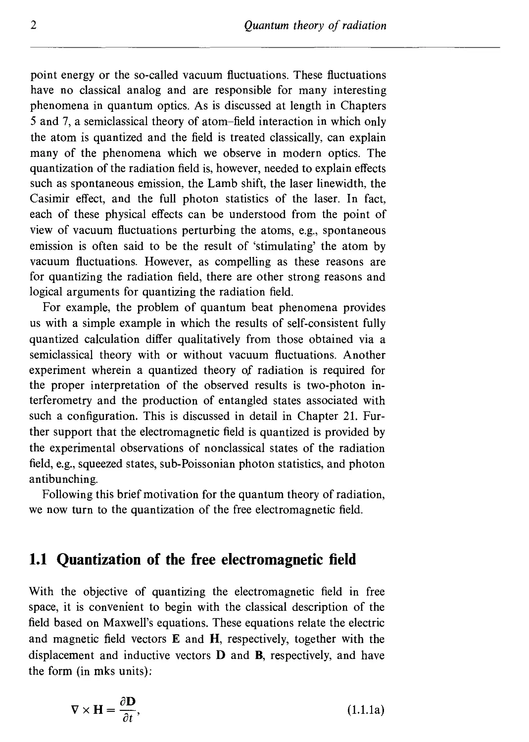
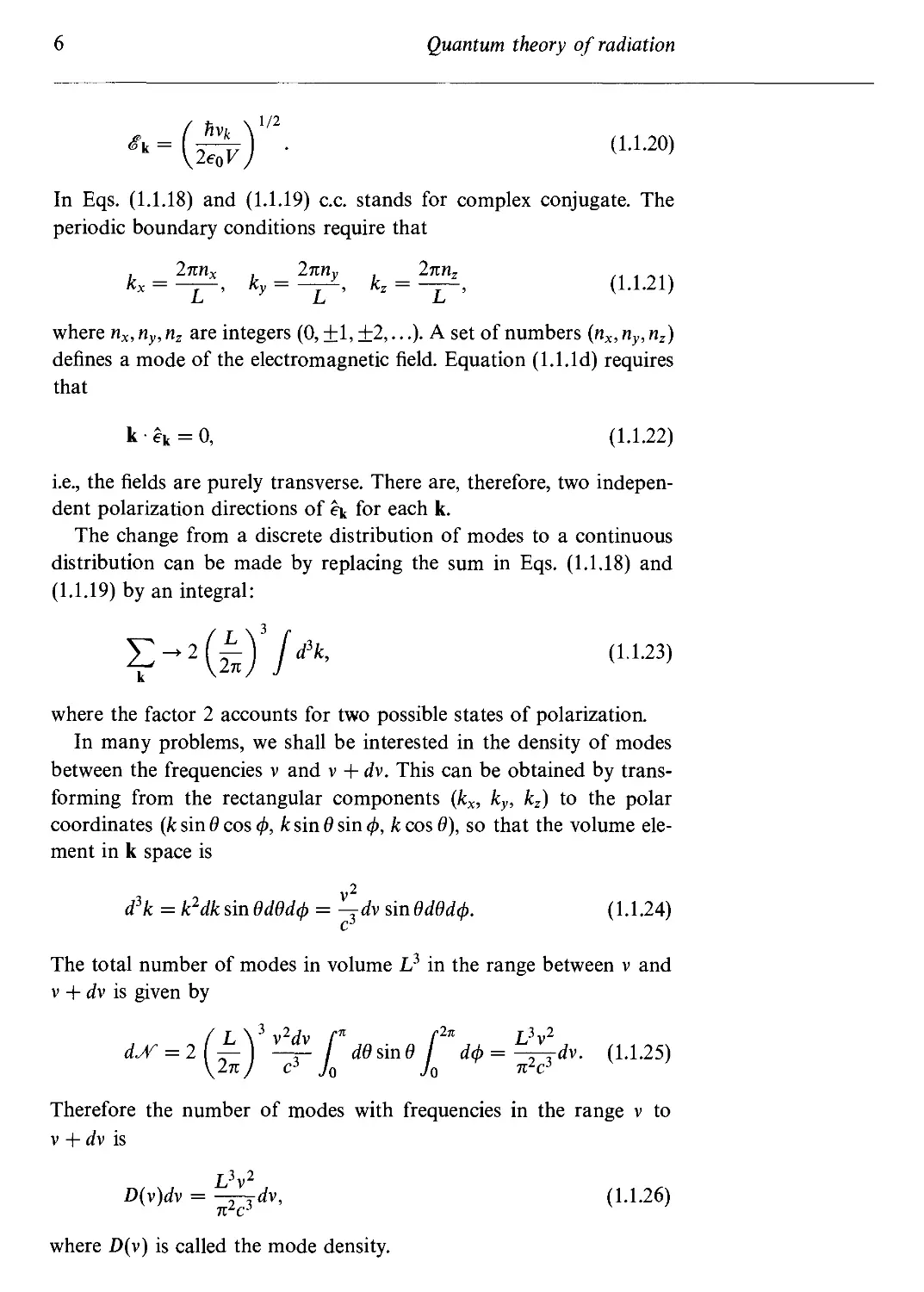
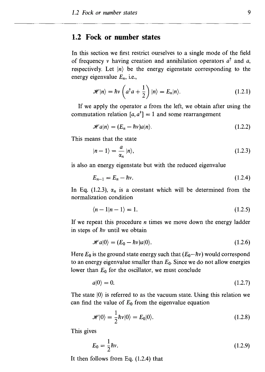
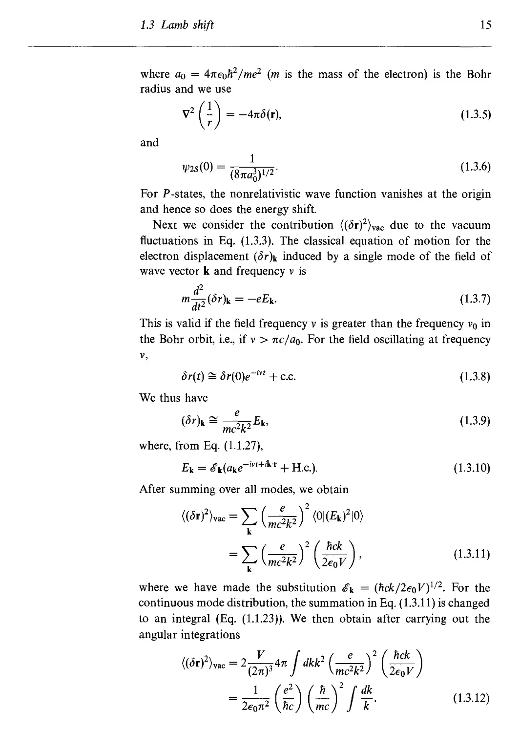
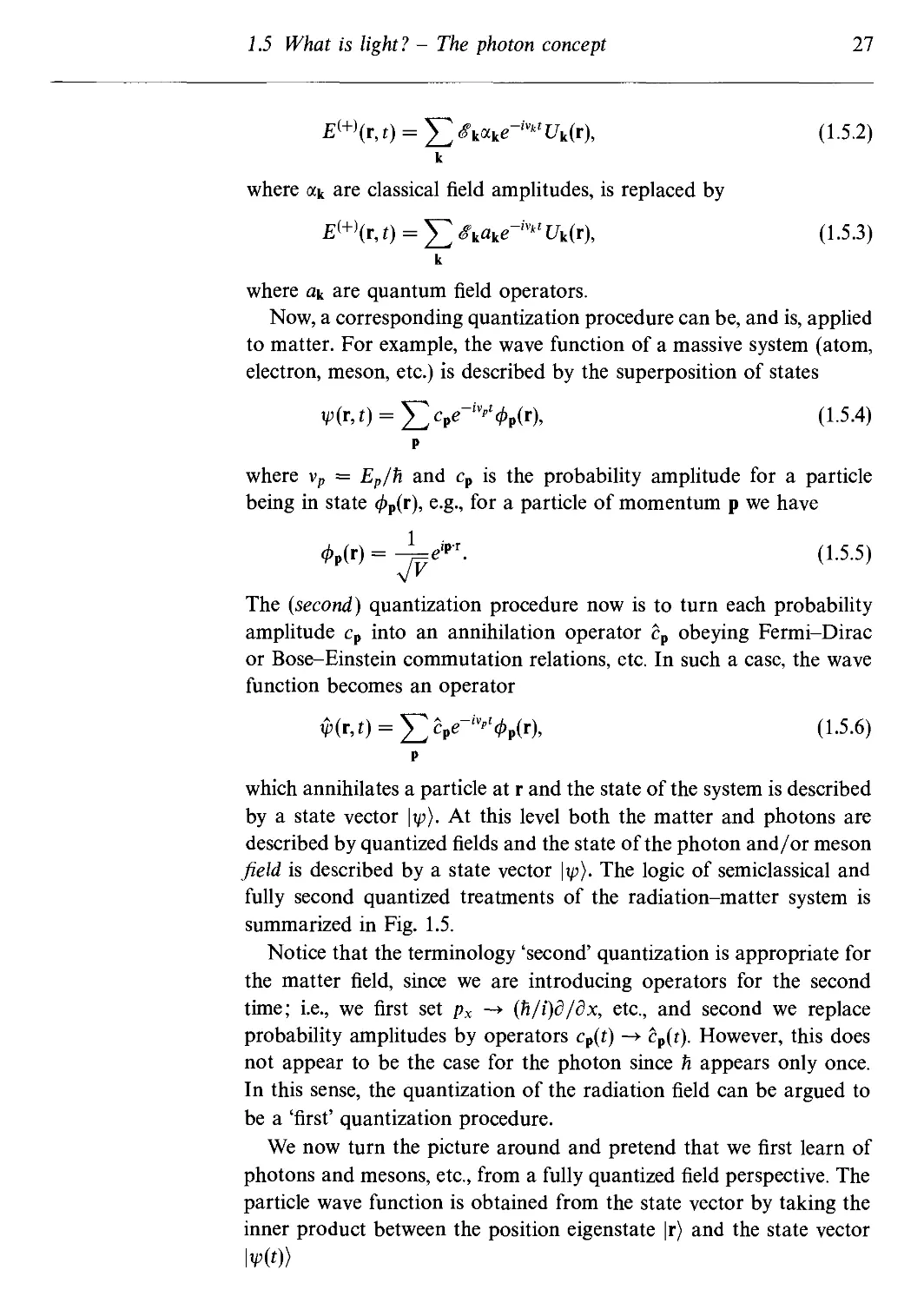
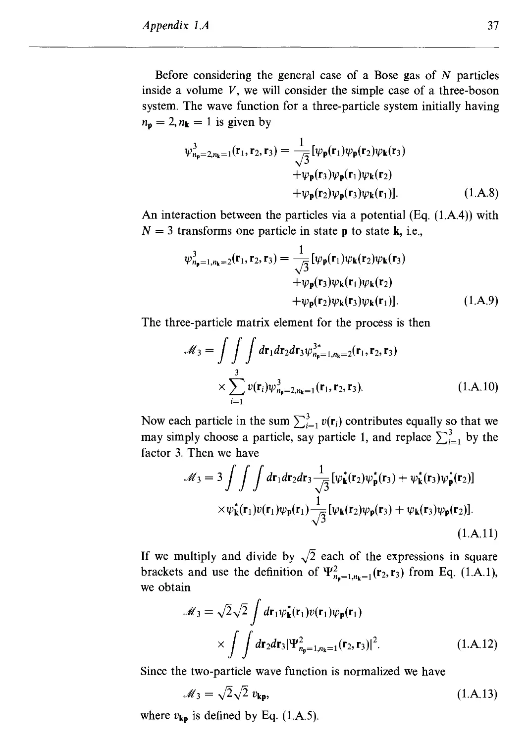
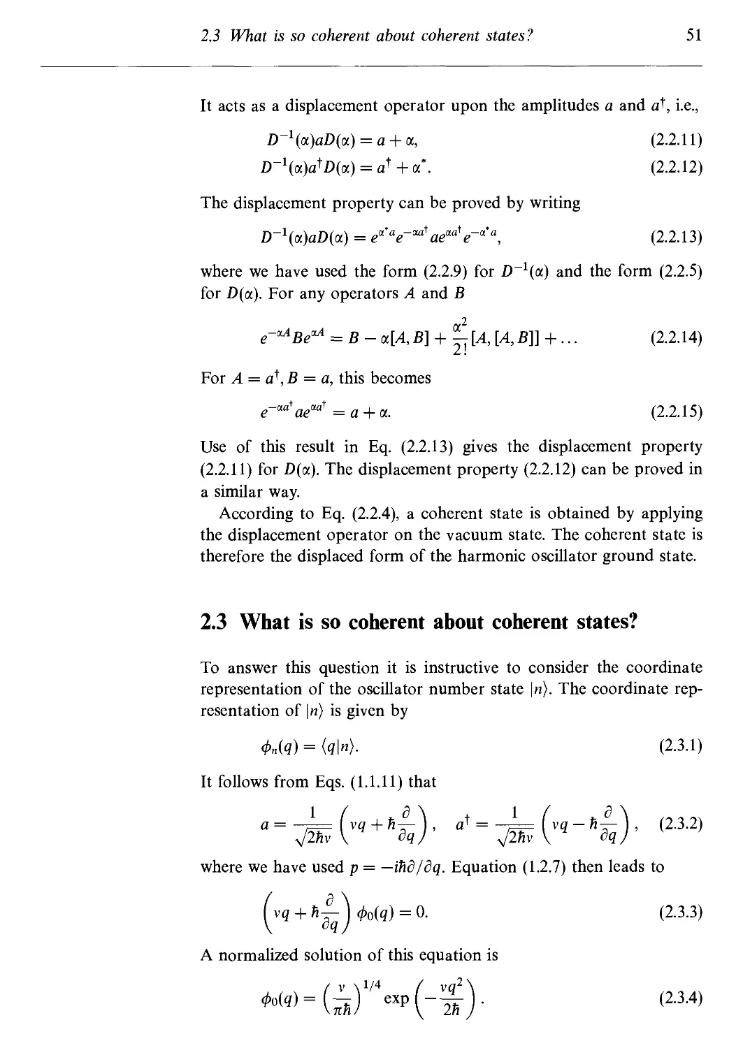
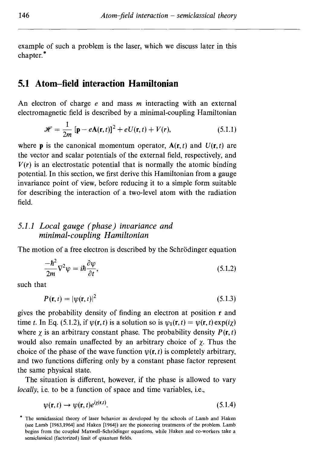
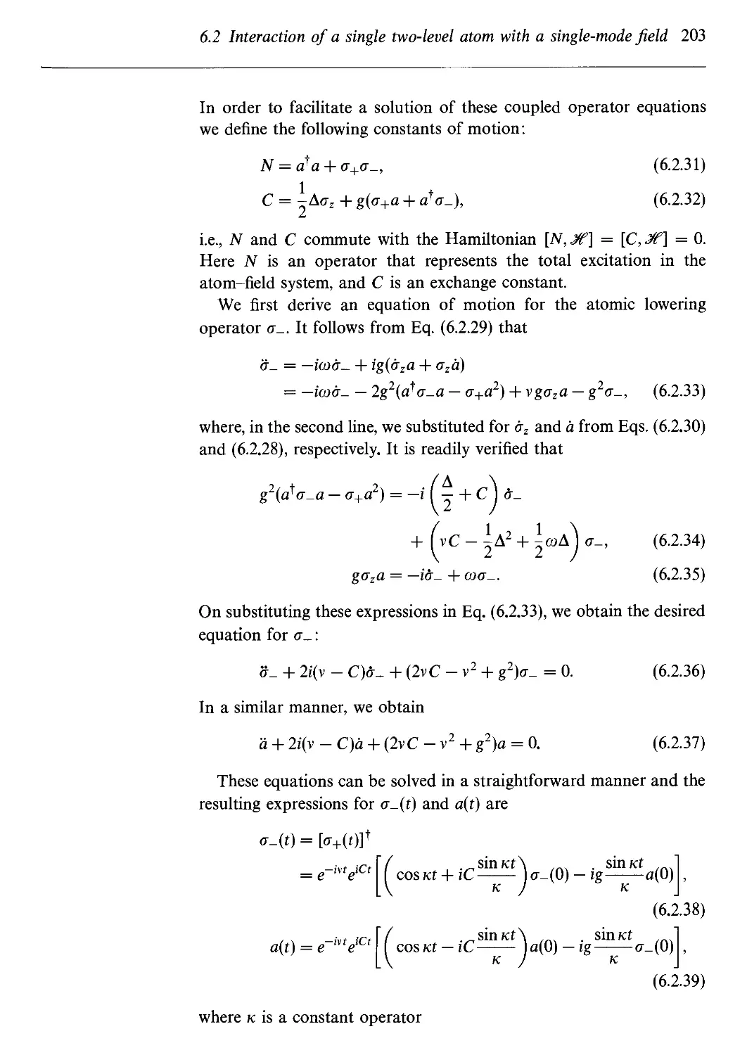
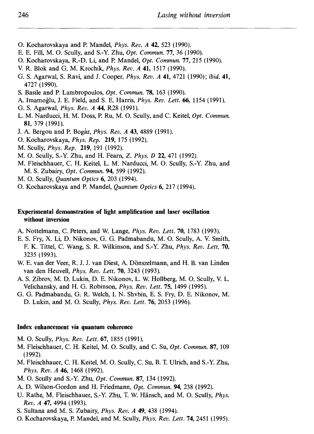
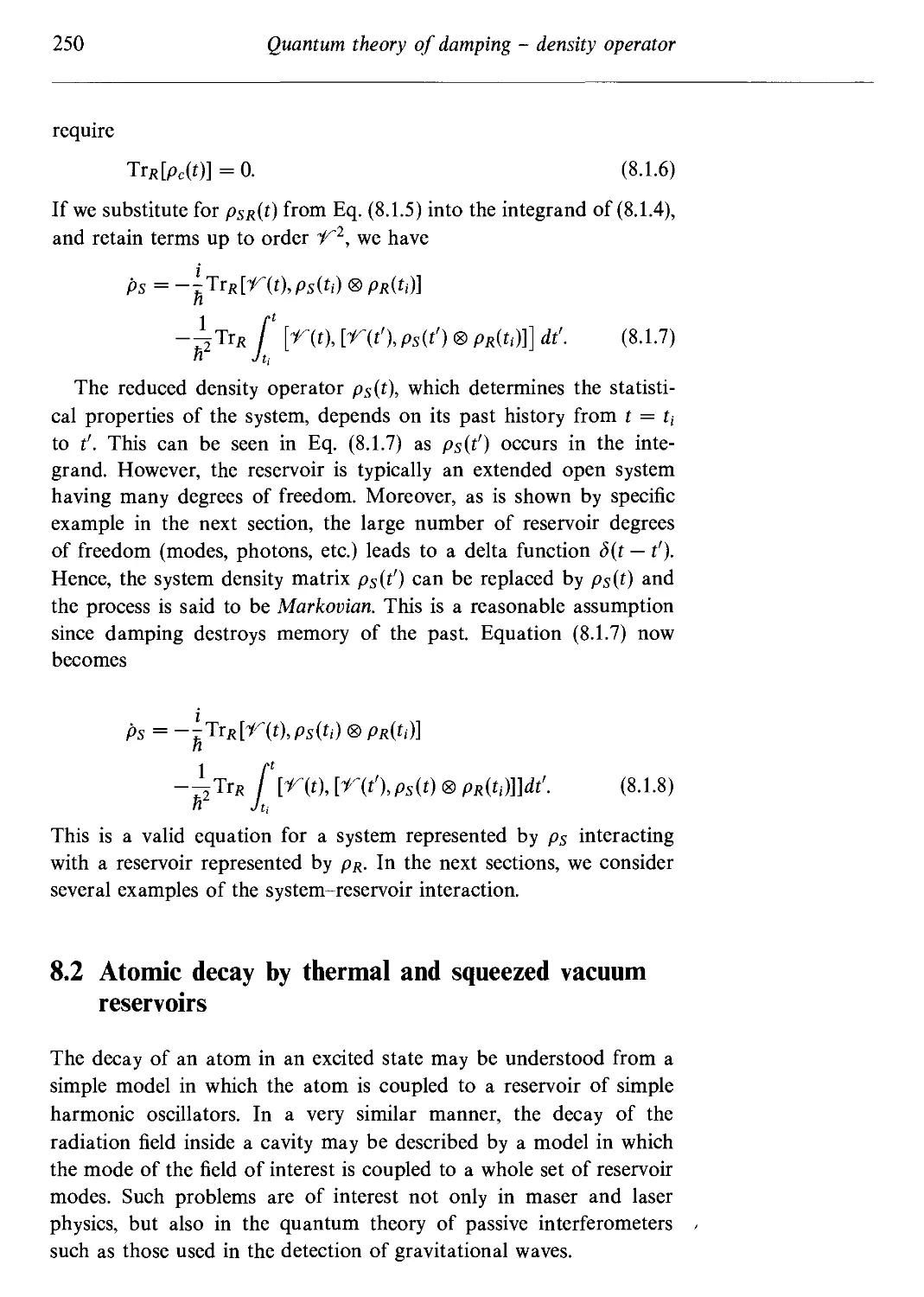
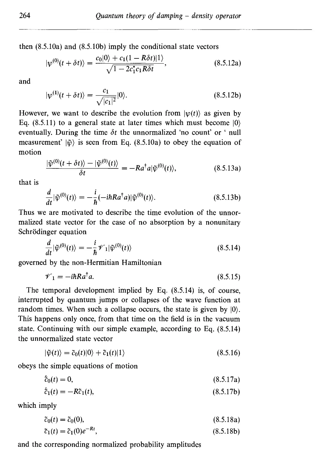
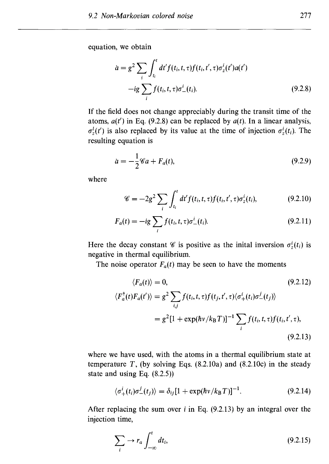
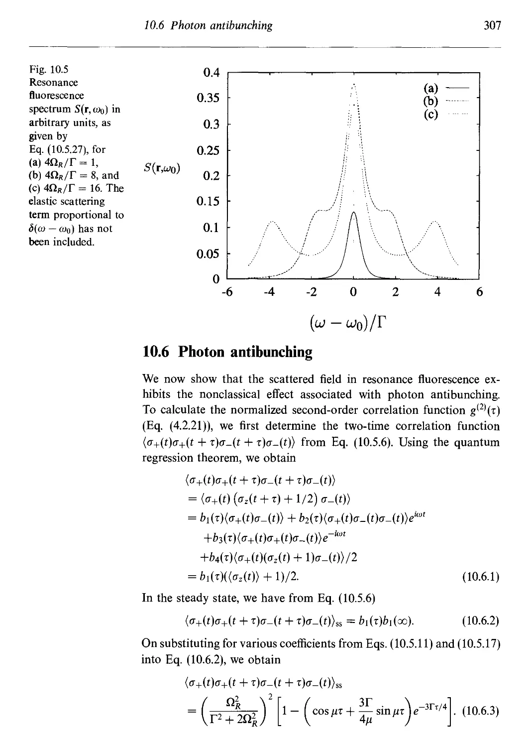
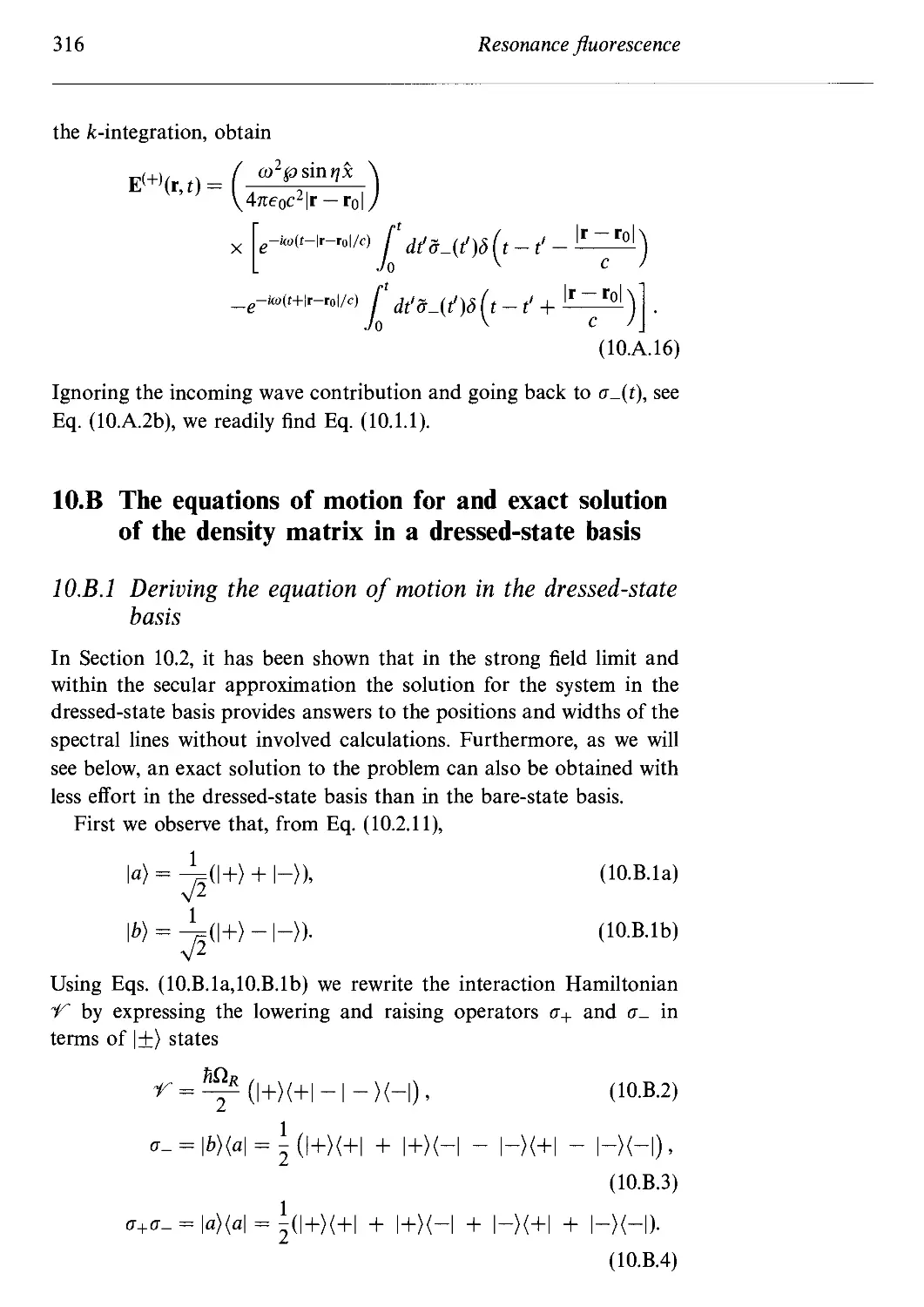
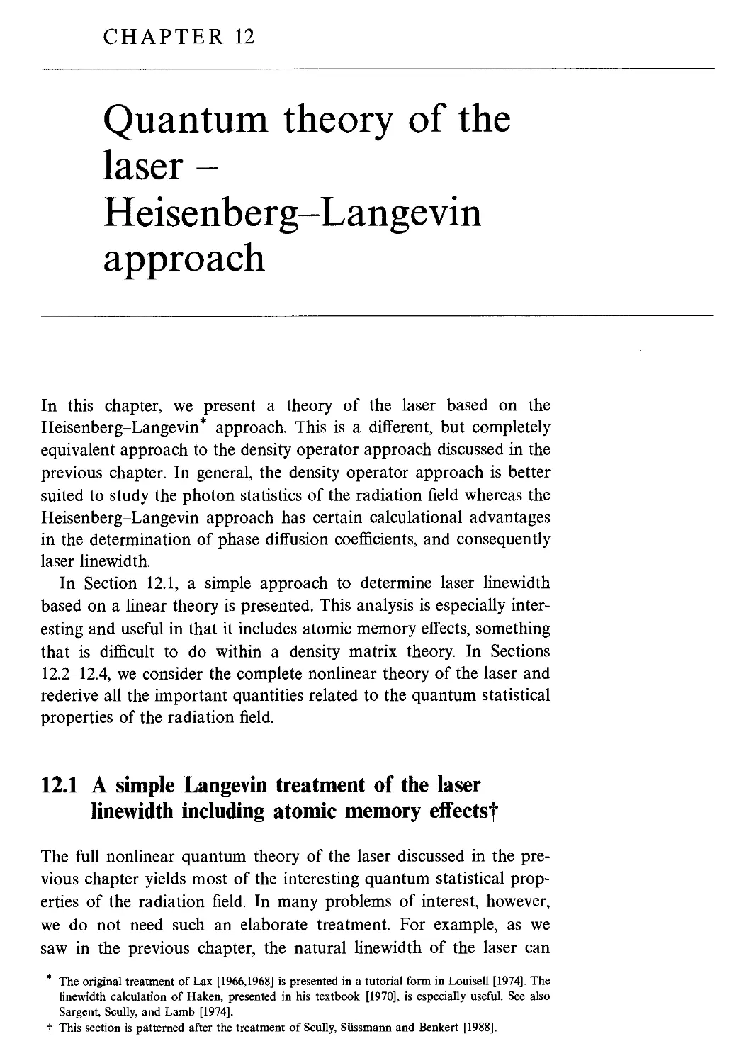
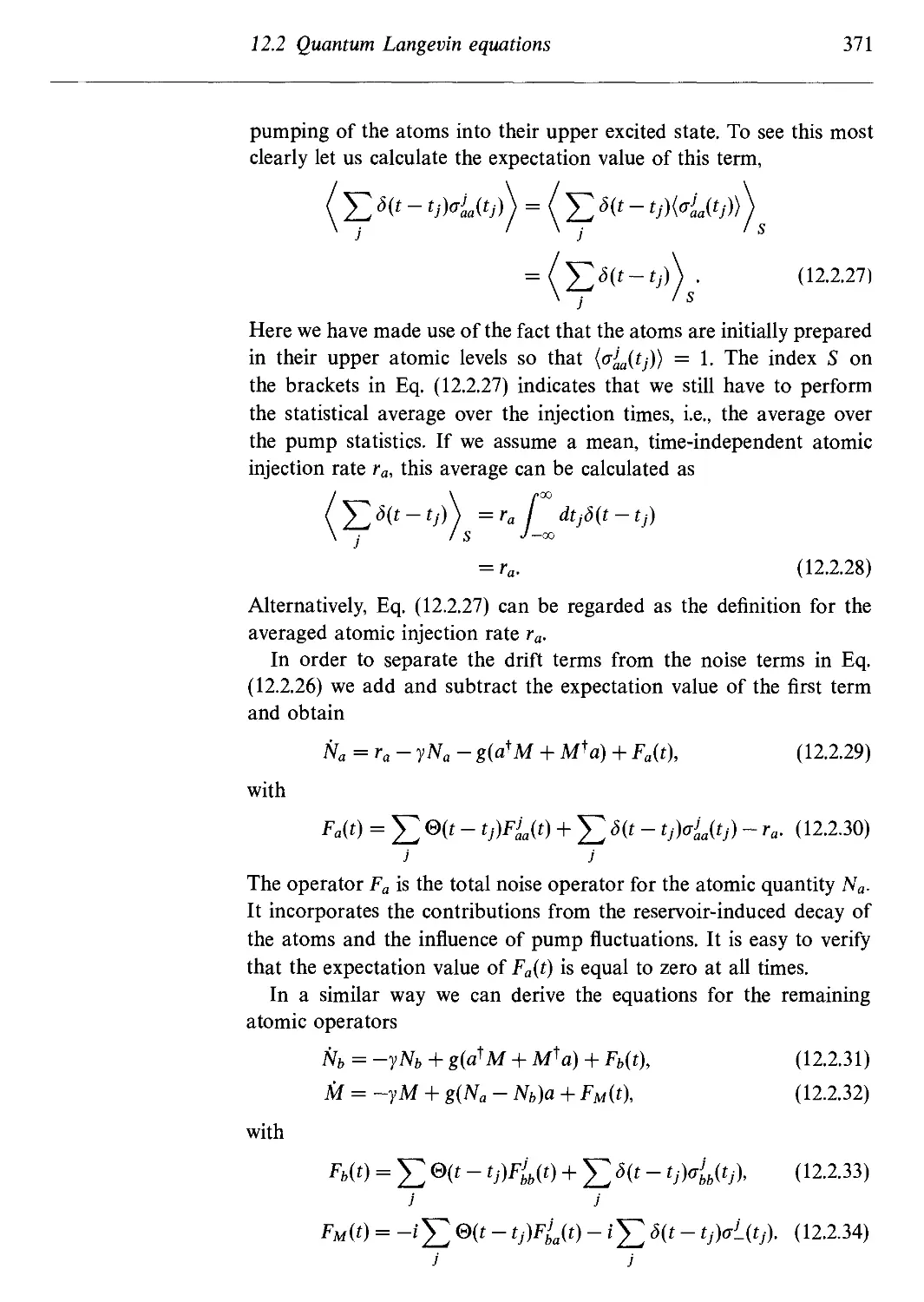
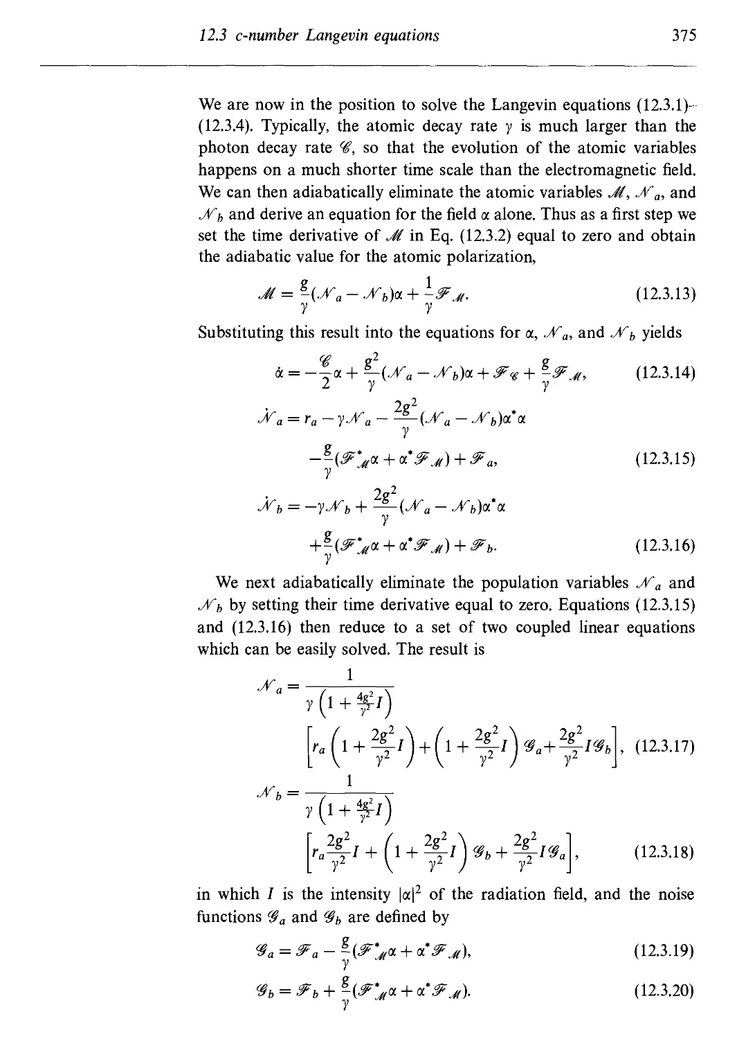
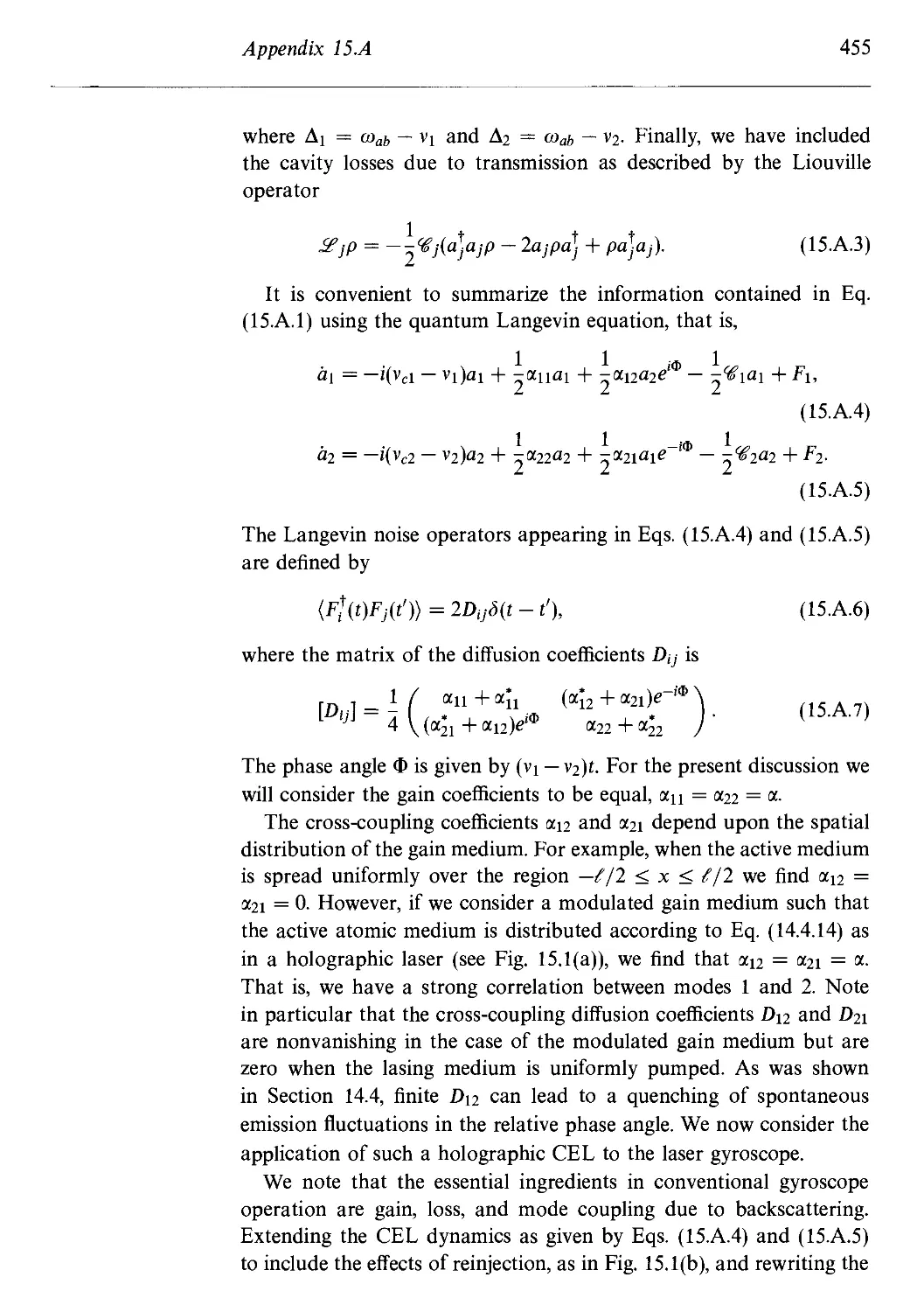
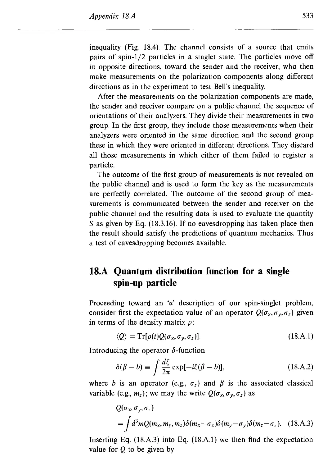
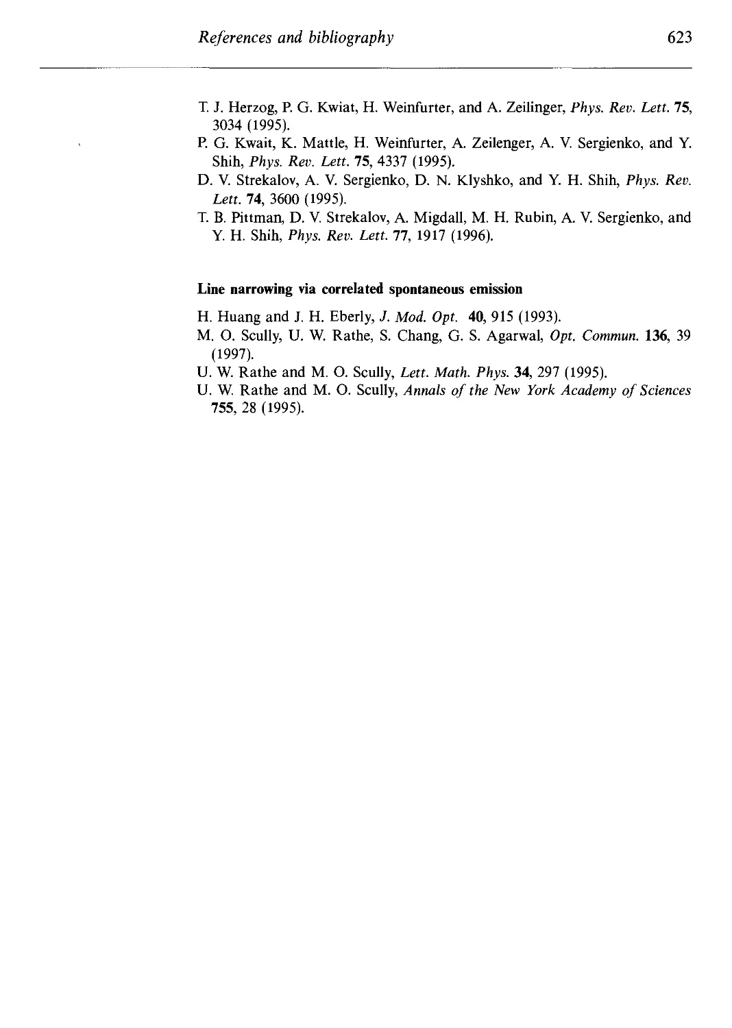
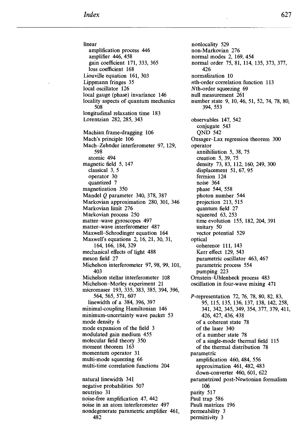
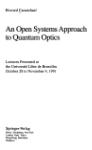
Fig. 1.2
Energy levels for the
quantum mechanical
harmonic oscillators
associated with the
electromagnetic field.
The creation
operator a* adds a
quantum of energy
hv, whereas the
destruction operator
a subtracts the same
amount of energy.
En+1 = {n
En =(n
3/2)/u/
1/2) hv
E2 = 5/2 hv
Ег = 3/2 hv
Eo = 1/2 hv
where cn are complex coefficients. The residual energy ftv/2 corre-
corresponding to Eo is called the zero-point energy. In Fig. 1.2, the energy
levels for the quantum mechanical oscillations associated with the
electromagnetic field are given.
An important property of the number state \n) is that the corre-
corresponding expectation value of the single-mode linearly polarized field
operator
E(t,t) =
—ivt+ik-r
H.c.
vanishes, i.e.,
(n\E\n) = 0.
A.2.19)
A.2.20)
However, the expectation value of the intensity operator E2 is given
by
(n\E2\n) =
.4..
A.2.21)
i.e., there are fluctuations in the field about its zero ensemble average.
It is interesting to note that there are nonzero fluctuations even for a
vacuum state |0). These vacuum fluctuations are responsible for many
interesting phenomena in quantum optics as discussed earlier. For
example, it may be considered that they stimulate an excited atom to
emit spontaneously. They also account for the Lamb shift of 2P1/2 —>
2Si/2 energy levels of atomic hydrogen. In particular in Section 1.3,
12 Quantum theory of radiation
we shall see how the vacuum fluctuations of the electromagnetic field
are responsible for the Lamb shift.
The operators a and af annihilate and create photons, respectively,
for, as seen in Eqs. A.2.14) and A.2.15), they change a state with n
photons into one with n — 1 or n + 1 photons. The operators a and af
are therefore referred to as annihilation (or destruction) and creation
operators, respectively. These operators are not themselves Hermitian
(а Ф a^) and do not represent observable quantities such as the electric
and magnetic field amplitudes. However, some combinations of the
operators are Hermitian such as a\ = {a + at)/2 and a2 = {a — <rf)/2i.
So far we have considered a single-mode field and have found that,
in general, the wave function can be written as a linear superposition
of photon number states \n). We now extend this formalism to deal
with multi-mode fields.
We can rewrite the Hamiltonian Ж in Eq. A.1.12) as
where
My = hvk (а[ак + Л . A.2.23)
The energy eigenstate \nk) of Ж k is defined in a manner similar to the
single-mode field via the energy eigenvalue equation
= hvk (nk + i J |ик>. A.2.24) ■
The general eigenstate of Ж can therefore have nkl photons in the
first mode, nkl in the second, n\^ in the /th and so forth, and can be
written as \nkl)\nkl)... |"кЛ ■•■ or more conveniently
K,nk2,...,"k,,..-) = IW)- A.2.25)
The annihilation and creation operators akl and a\ lower and raise
the /th entry alone, i.e.,
Як,К,"к2,■ ■ •,"к,,■ ■ ■} = д/йкТК,"к2,■ • ■,"к, - 1,■ ■ ■>, A.2.26)
akj"ki."k2,...,nk,,...> = V4, + 1|Пк1,Пк2,...,Ик, +1,...}.
A.2.27)
The general state vector for the field is a linear superposition of these
eigenstates:
IV> = X] X] • • • X] ■ • • cnk1,nk2,.-^,-l"ki. "k2, ■ ■ ■, Пкг,...)
1.3 Lamb shift 13
This is a more general superposition than
., A-2.29)
where \\p^) are state vectors for individual modes. Equation A.2.28)
includes state vectors of the type A.2.29) as well as more general
states having correlations between the field modes which can result
from interaction of the various field modes with a common system.
1.3 Lamb shift
The precision observation of the Lamb shift, between the 2S\/2 and
2P\/2 levels in hydrogen, was in a real sense the stimulus for mod-
modern quantum electrodynamics (QED). According to Dirac theory, the
2S\/2 and 2P\/2 levels should have equal energies. However, radiative
corrections due to the interaction between the atomic electron and the
vacuum, shift the 2S\/2 level higher in energy by around 1057 MHz
relative to the 2P1/2 level.
Early attempts to calculate such 'vacuum induced' radiative correc-
corrections were frustrated in that they predicted infinite level shifts. How-
However, the beautiful measurement of Lamb and Retherford provided
the stimulus for renormalization theory which has been so successful
in handling these divergences.
On the occasion of Lamb's sixty-fifth birthday, Freeman Dyson*
wrote:
Your work on the hydrogen fine structure led directly to the
wave of progress in quantum electrodynamics on which I
took a ride to fame and fortune. You did the hard, tedious,
exploratory work. Once you had started the wave rolling,jthe
ride for us theorists was easy. And after we had zoomed
ashore with our fine, fancy formalisms, you still stayed with
your stubborn experiment. For many years thereafter you
were at work, carefully coaxing the hydrogen atom to give us
the accurate numbers which provided the solid foundations
for all our speculations...
Those years, when the Lamb shift was the central theme
of physics, were golden years for all the physicists of my
generation. You were the first to see that that tiny shift, so
elusive and hard to measure, would clarify in a fundamental
way our thinking about particles and fields.
* Dyson [1978].
14 Quantum theory of radiation
Shortly after the experimental results were announced, Bethe pro-
produced a simple nonrelativistic calculation which was in good qual-
qualitative agreement with theory, by using the suggestion of Kramers,
Schwinger, and Weisskopf for 'subtracting off' infinities. This was
extended to a full relativistic theory in quantitative agreement with
experiments by Kroll and Lamb, and French and Weisskopf; and was
the harbinger of modern QED as developed by Schwinger, Feynman,
and Dyson.
The excellent agreement between the full quantum theory of radia-
radiation and matter, and experiment, e.g., the Lamb shift, provides strong
support for the quantization of the radiation field. However, a detailed
calculation of th^ Lamb shift would take us too far from mainstream
quantum optics. Therefore, we will present here a heuristic derivation
of the electromagnetic level shift following Welton.
The effect of the fluctuations in the electric and magnetic fields
associated with the vacuum is a perturbation of the electron in a
hydrogen atom from the standard orbits of the Coulomb potential
—e2/4neor due to the proton; so the electron radius r —> r + dr,
where dr is the fluctuation in the position of the electron due to
the fluctuating fields. The change in potential energy, and thus the
associated level shift, is given by
AV = V(r + dr) - V(r)
= Er-VF + i(Er-VJF(r) + ... A.3.1)
Since the fluctuations are isotropic, (<5r)vac = 0, the first term can be
neglected. Moreover,
<(<5r ■ VJ)vac = j((<5rJ)vacV2, A.3.2)
again due to the isotropy of the fluctuations. We therefore obtain
, A.3.3)
U(dr))v
6
where (.. .}at represents the quantum average with respect to the atomic
states.
For the 2S state of hydrogen
V2
4ne0
/drV2
J
e2
A.3.4)
1.3 Lamb shift 15
where a0 = 4neoh2/me2 (m is the mass of the electron) is the Bohr
radius and we use
V2 (i J = -4nd(r), A.3.5)
and
For P-states, the nonrelativistic wave function vanishes at the origin
and hence so does the energy shift.
Next we consider the contribution ((drJ)vac due to the vacuum
fluctuations in Eq. A.3.3). The classical equation of motion for the
electron displacement {Sr)k induced by a single mode of the field of
wave vector к and frequency v is
m^Fr)k = -eEk. A.3.7)
atz
This is valid if the field frequency v is greater than the frequency vq in
the Bohr orbit, i.e., if v > nc/a0. For the field oscillating at frequency
v,
6r(t) s er@)e-in + c.c. A.3.8)
We thus have
mczkz
where, from Eq. A.1.27),
£k = <?к(аке~"жкт + H.c.). A.3.10)
After summing over all modes, we obtain
where we have made the substitution ik = (frck/2eoV)l/2. For the
continuous mode distribution, the summation in Eq. A.3.11) is changed
to an integral (Eq. A.1.23)). We then obtain after carrying out the
angular integrations
he
\2e0Vj
me J J к
16 Quantum theory of radiation
This gives a divergent result. However as noted before, the present
method is only valid for v > nc/ao, or equivalently к > n/a0. It is
also valid only for wavelengths longer than the Compton wavelength,
i.e., к < mc/fr, because of magnetic effects on the motion which begin
when v/c = p/mc = frk/mc ;S 1. The present method is invalid if the
electron is relativistic. We can therefore choose the lower and upper
limits for the integral in Eq. A.3.12) to be n/ao and mc/h, respectively.
We then obtain
On substituting Eqs. A.3.4) and A.3.13) into Eq. A.3.3), we obtain
the following expression for the Lamb shift
3 4ne0 4ne0hc \mc J Snal \ e2 )
This shift is about 1 GHz in good agreement with the observed shift,
considering the crude approximations made in the calculation.
Finally, we note the exciting developments in Lamb shift physics
made possible by modern quantum optical techniques, namely the
measurement of the radiation shift of the IS state via precise mea-
measurements of the two-photon 1S-2S transition first performed by
Hansch and co-workers.
1.4 Quantum beats
Over the past decades several alternative theories to quantum elec-
electrodynamics (QED) have been proposed. One such theory is based
on stochastic electrodynamics. In this theory, matter is treated quan-
quantum mechanically while radiation is described according to Maxwell's
equations, to which one adds vacuum fluctuations. In this picture, it
would seem that almost all quantum phenomena, such as spontaneous
emission, Lamb shift, and the laser linewidth, can be understood in a
semiquantitative fashion.
Quantum beat* phenomena however provide us with a simple ex-
example of a case in which the results of a self-consistent fully quantized
calculation differ substantially from those obtained via a semiclassical
theory (SCT) even when augmented by the notion of vacuum fluctua-
fluctuations. This is a good example of a problem which cannot be explained,
let alone calculated, by semiclassical-type arguments.
* Svanberg [1991].
1.4 Quantum beats 17
In later chapters, we shall present elaborate theories of atom-field
interaction based on semiclassical and fully quantum mechanical treat-
treatments. In this section, however, we discuss quantum beats via QED
and SCT in three-level atomic systems using simple arguments. We
consider two different types of three-level atoms in the so-called V
and Л type configurations which are prepared in a coherent superpo-
superposition of all three states. Both systems are first treated semiclassically
and then by QED methods in order to compare the results of both
approaches.
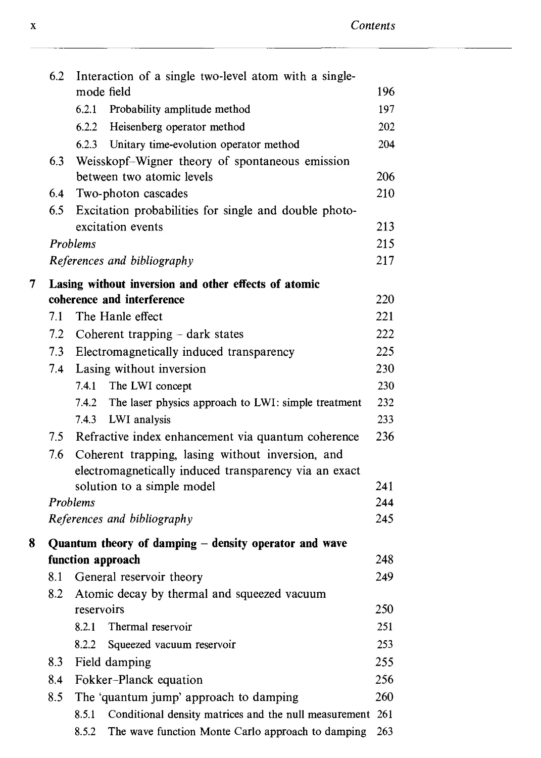
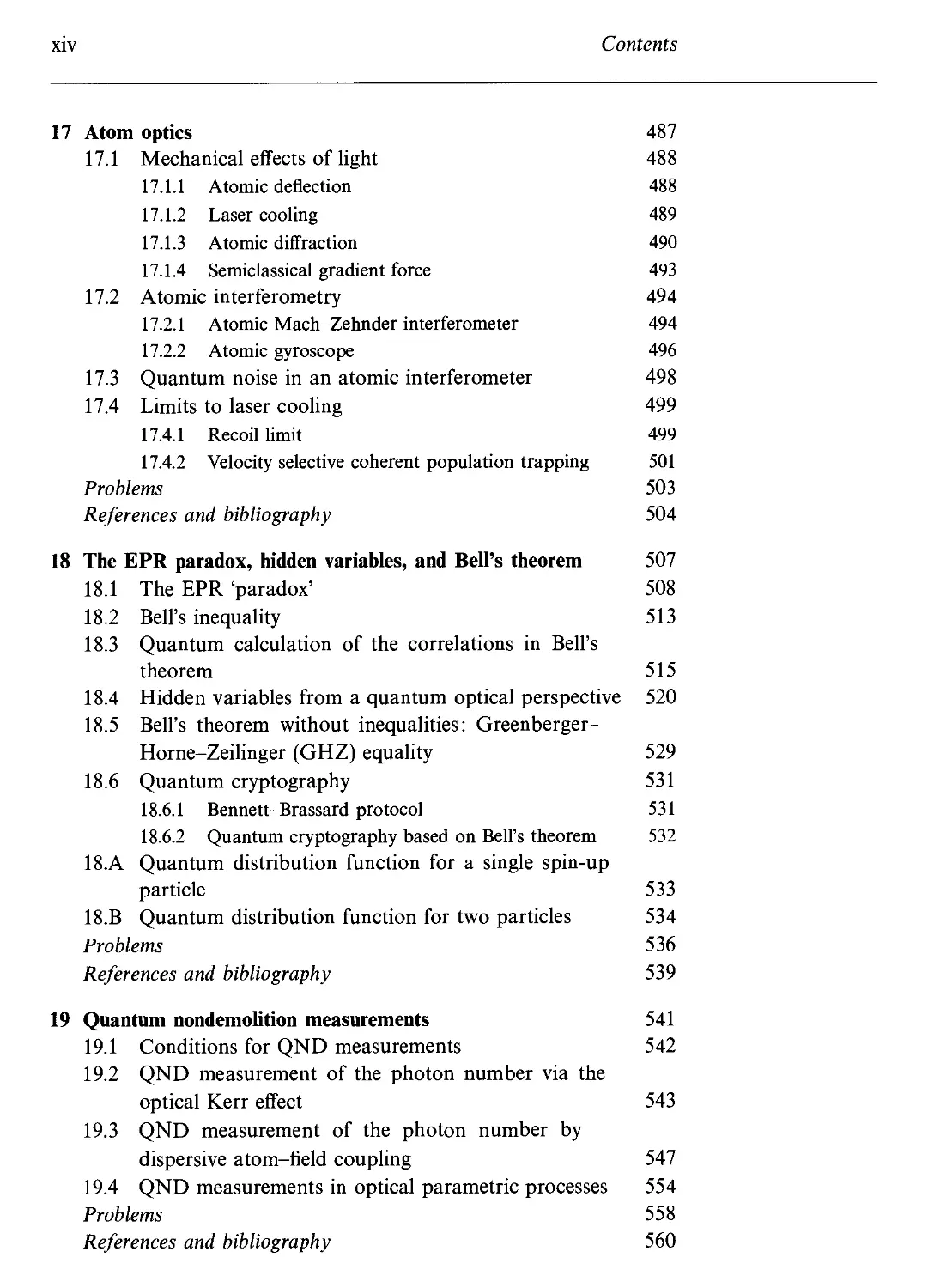
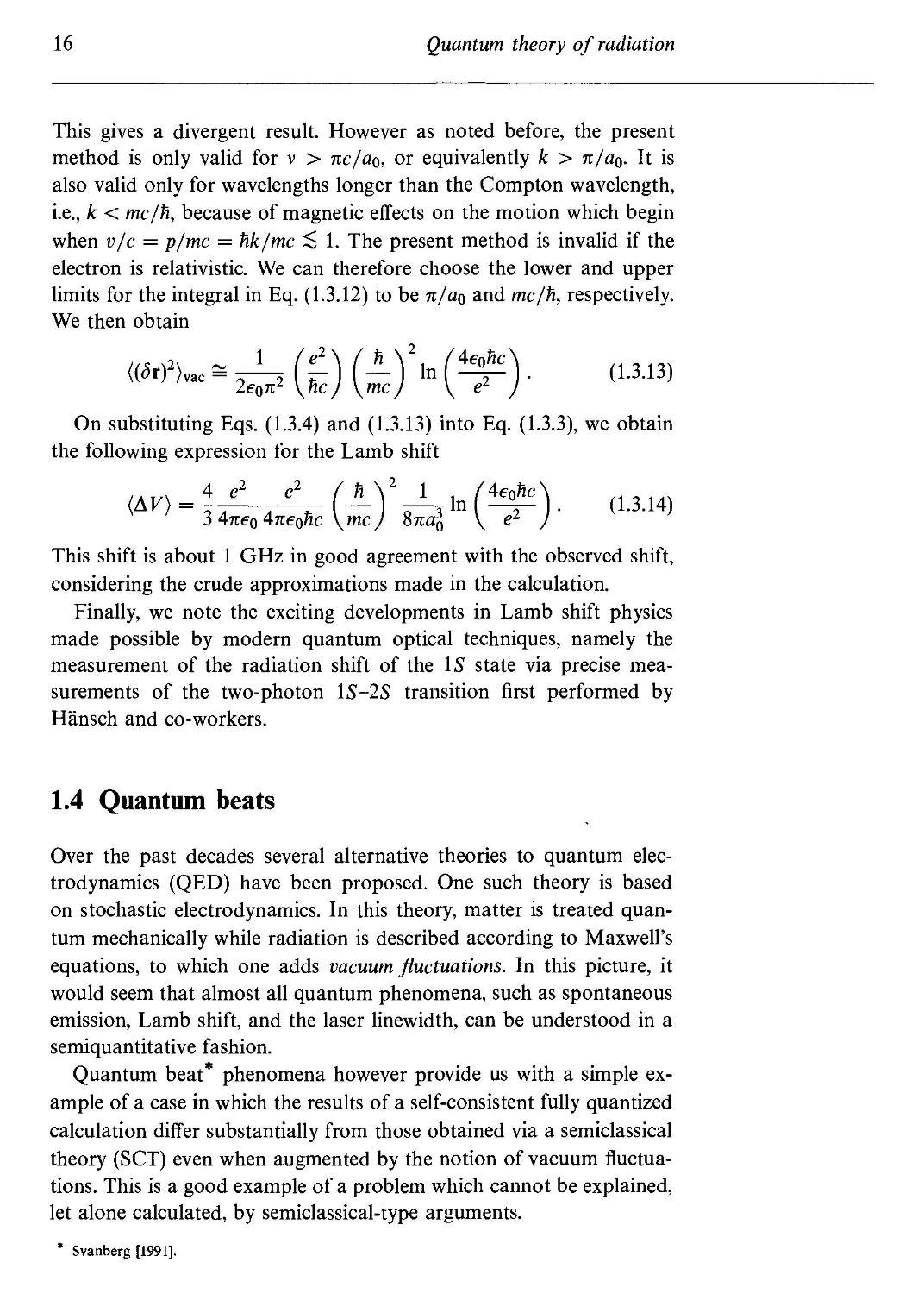
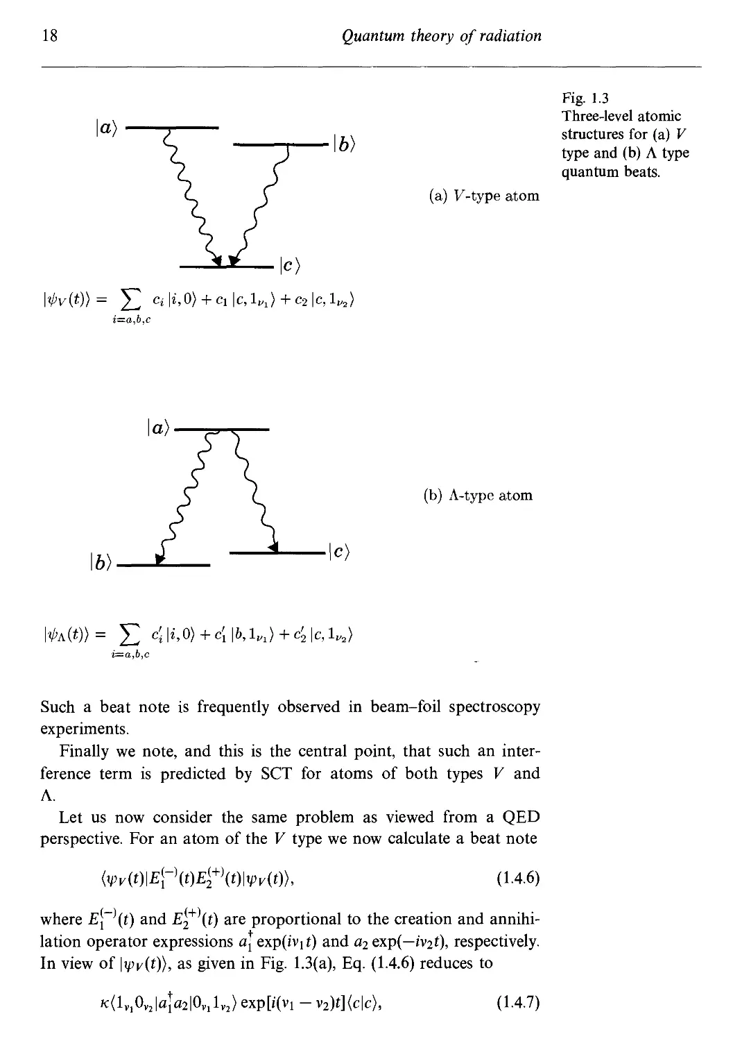
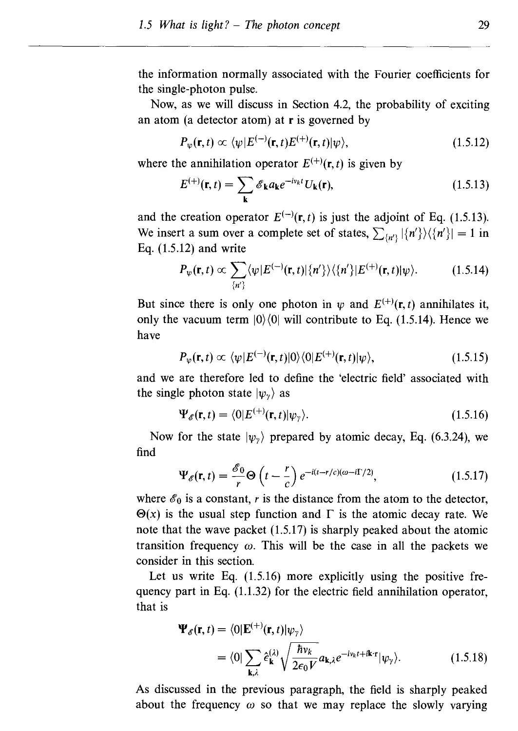
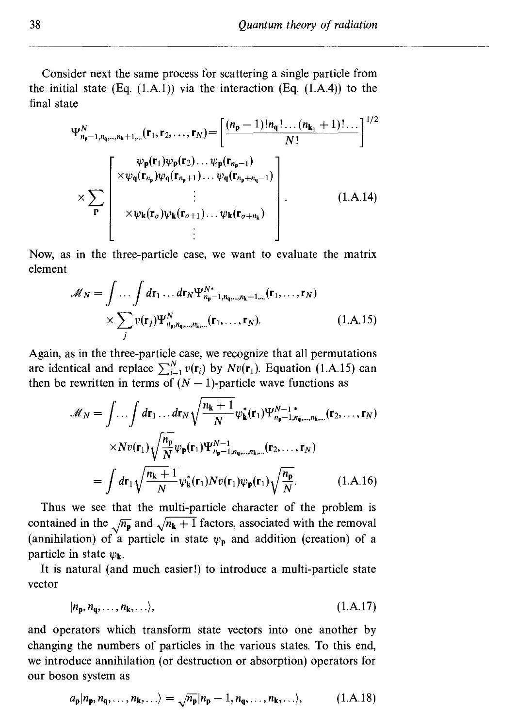
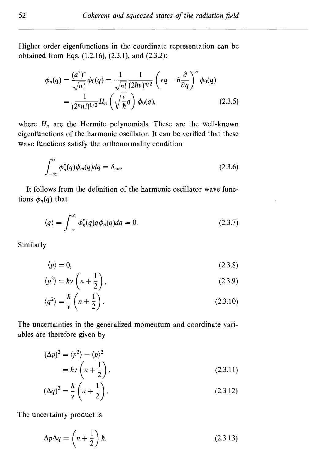
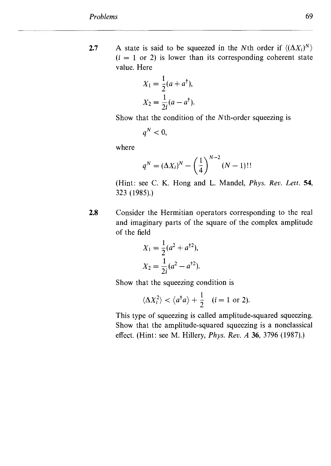
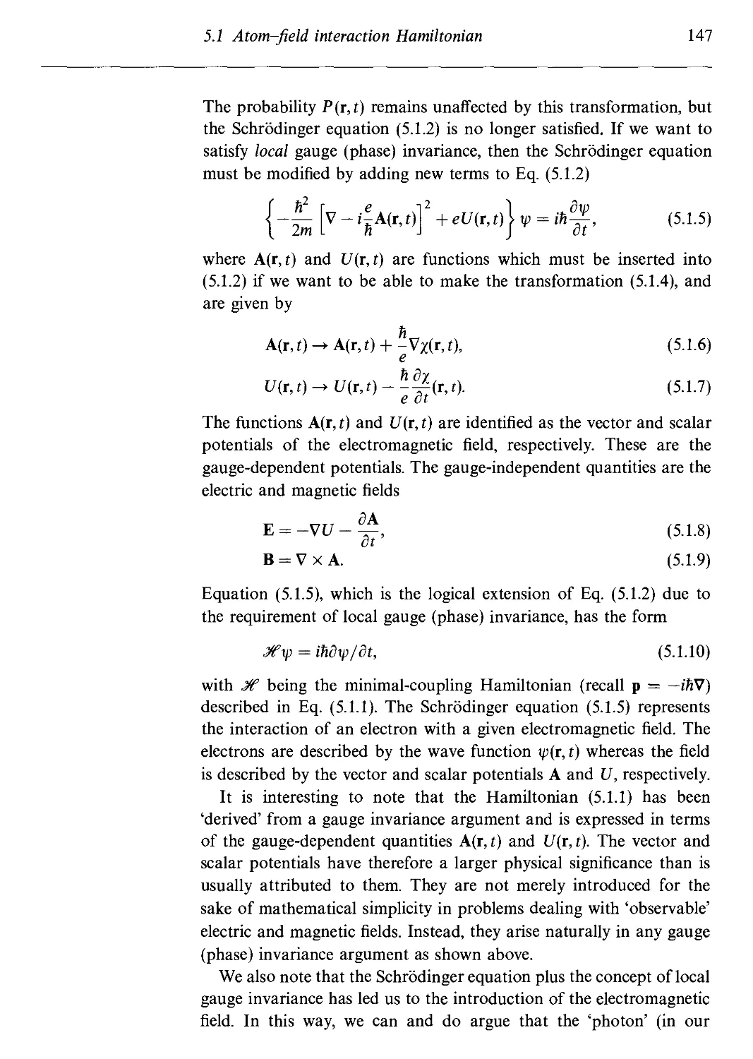
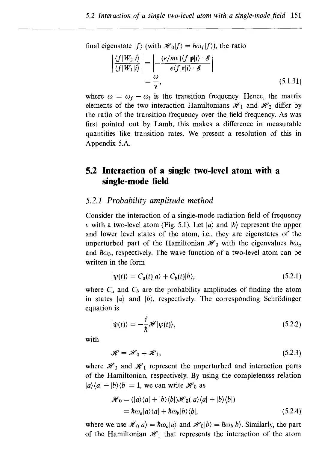
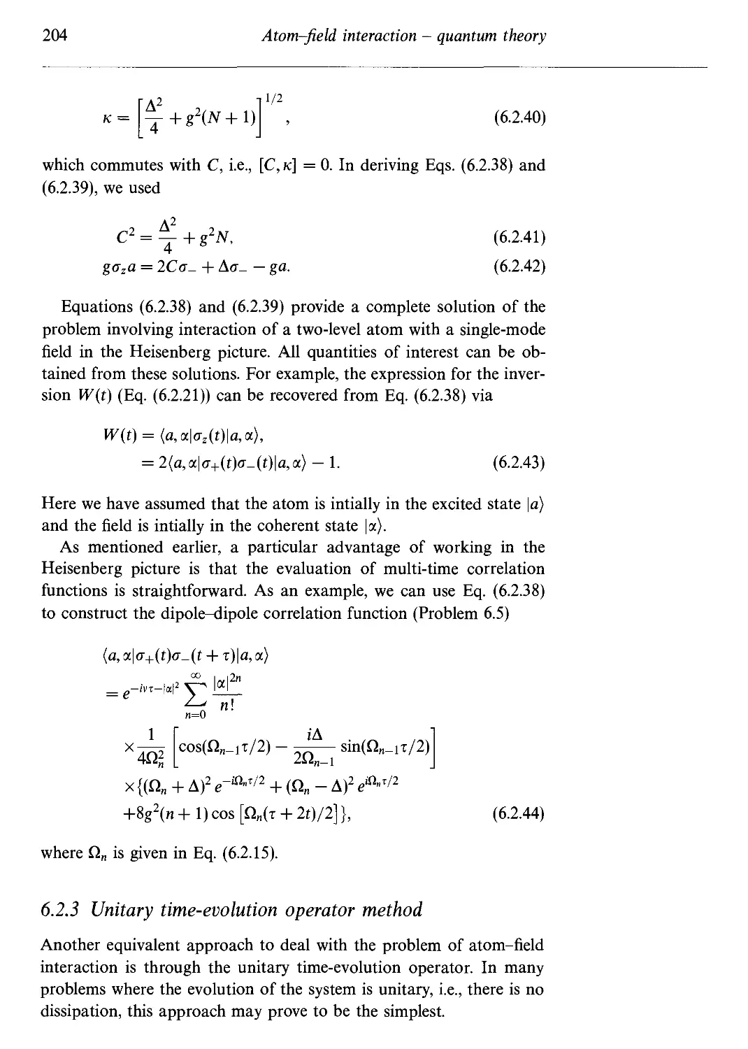
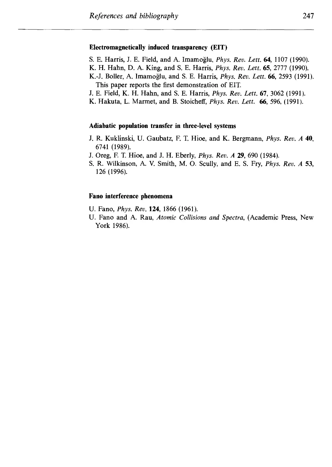
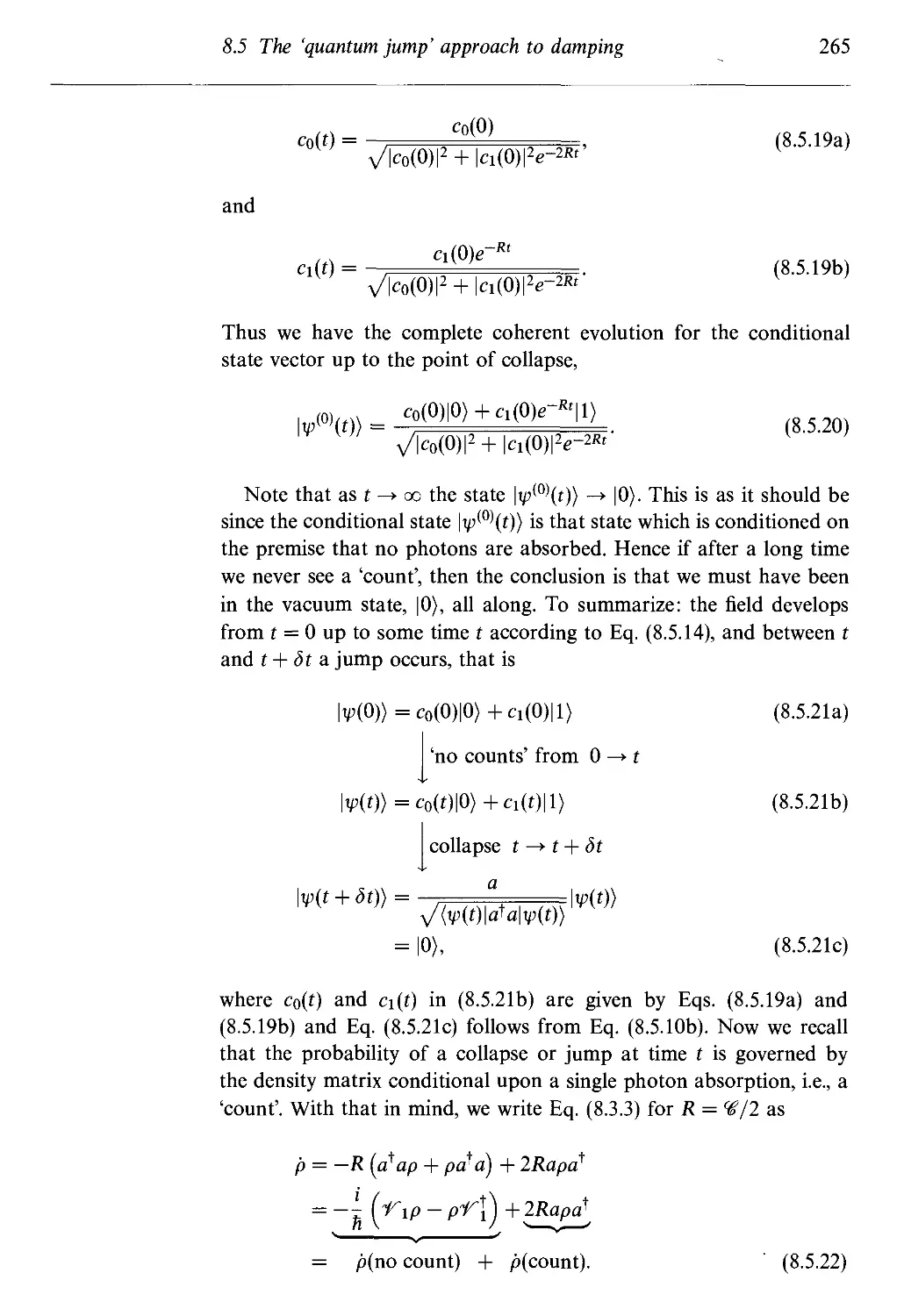
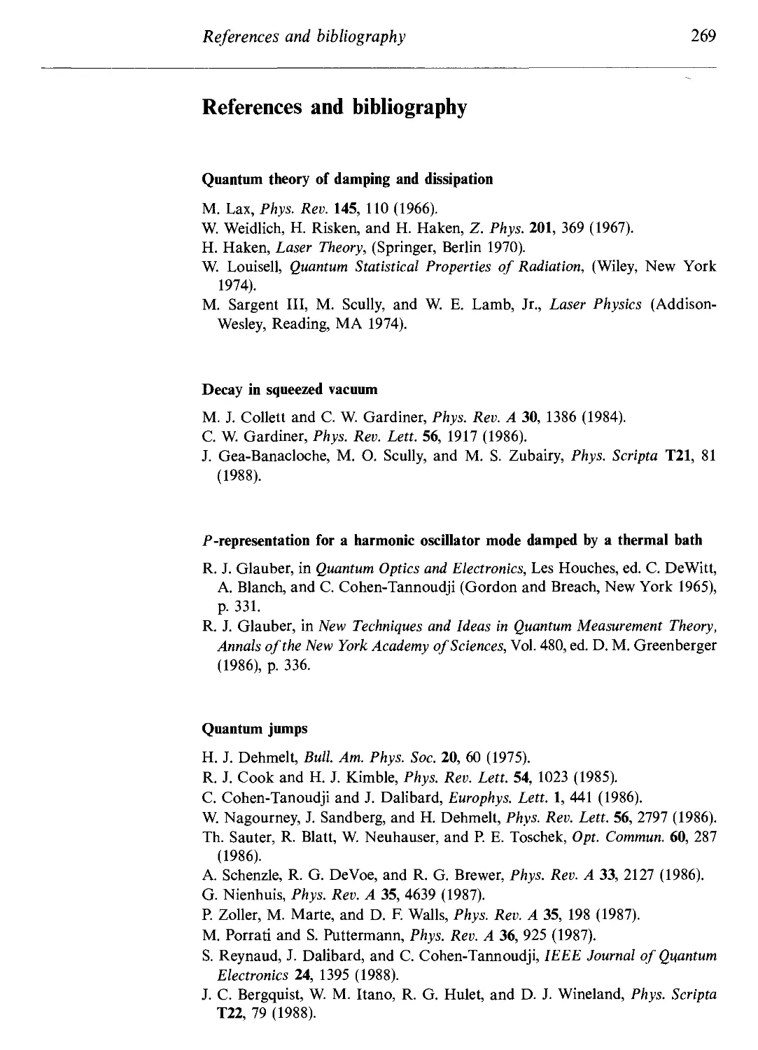
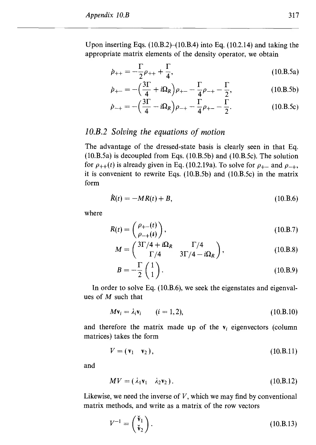
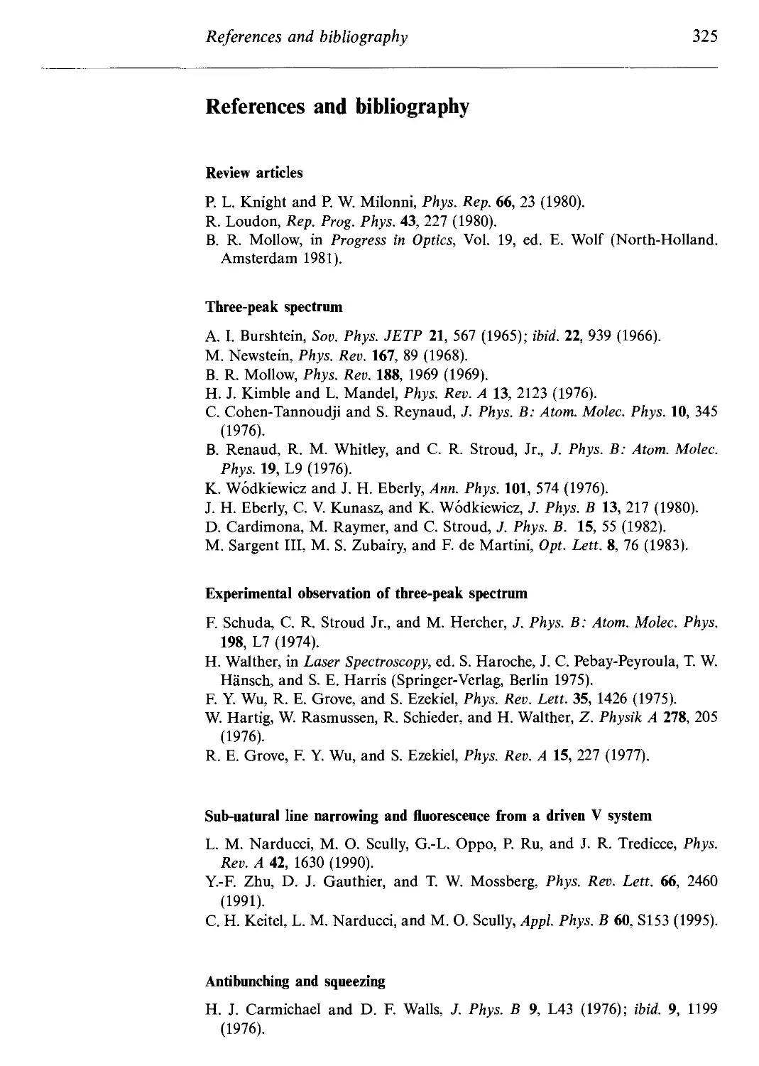
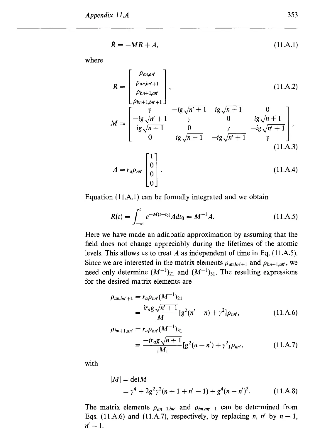
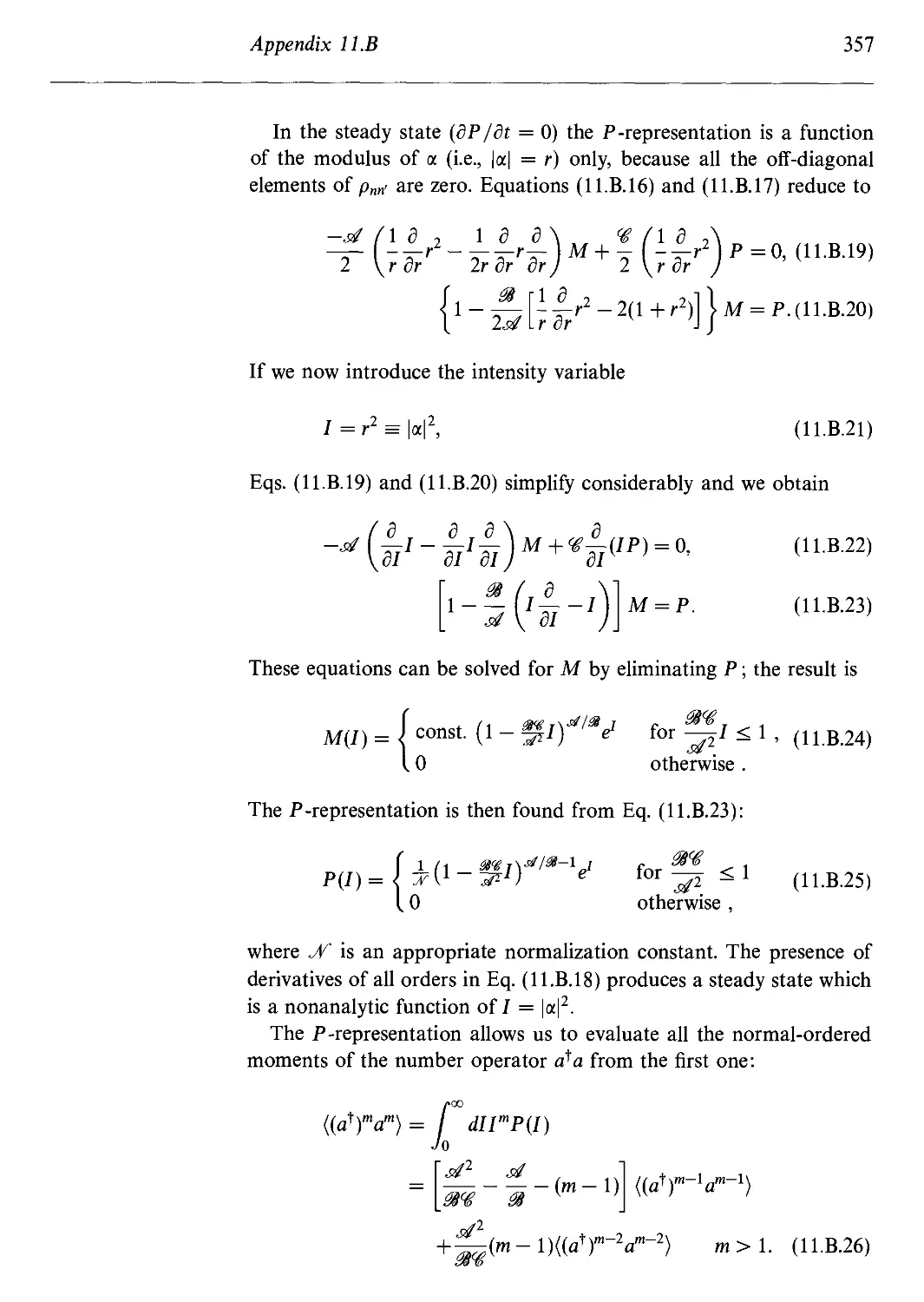
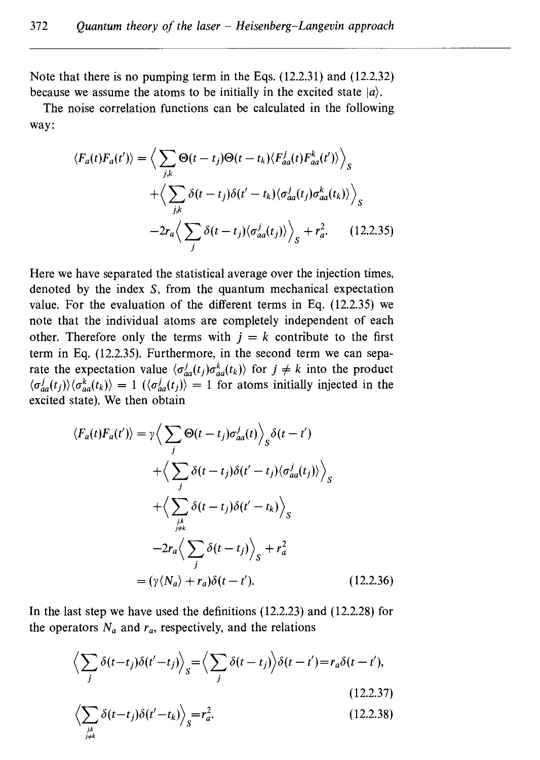
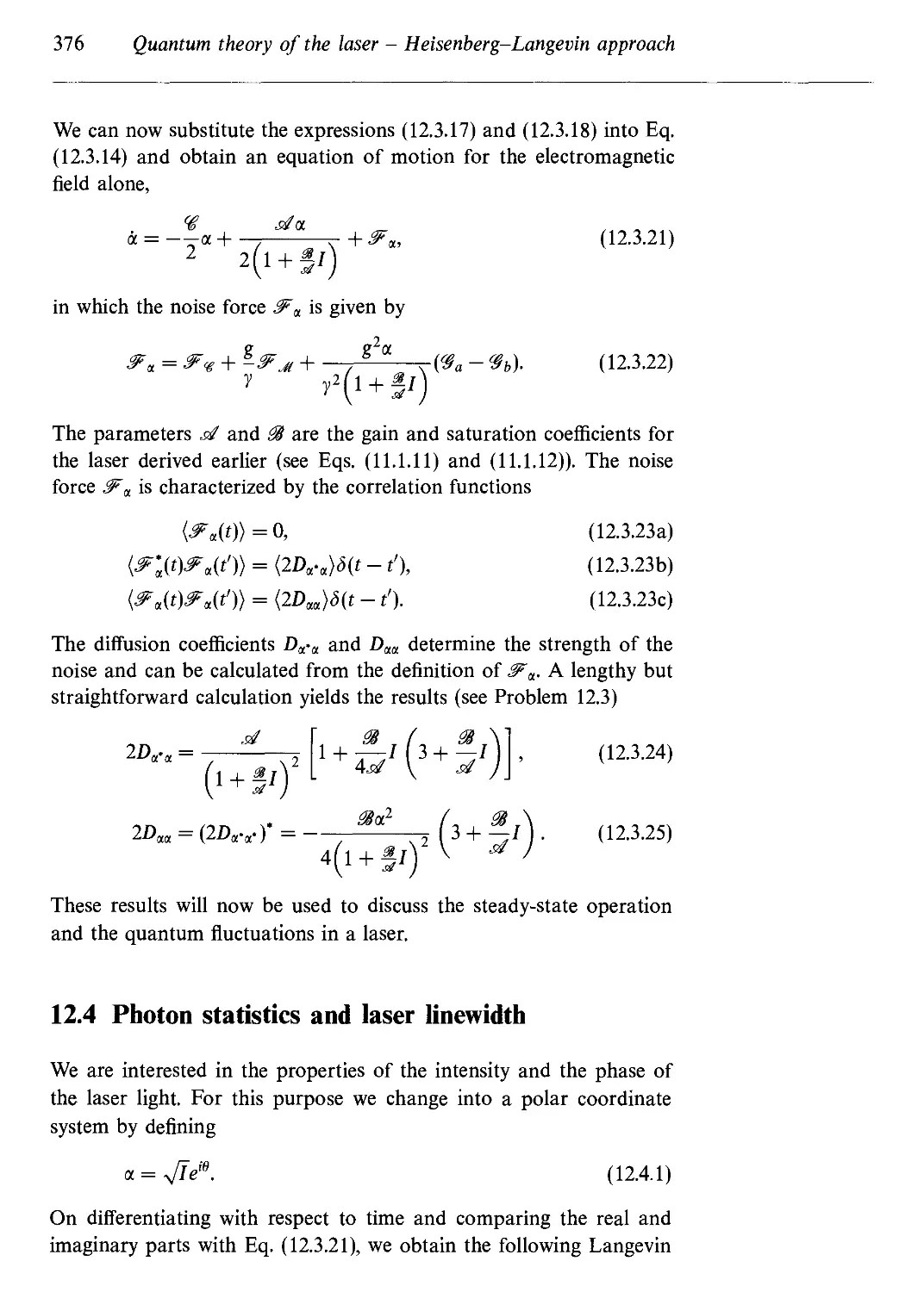
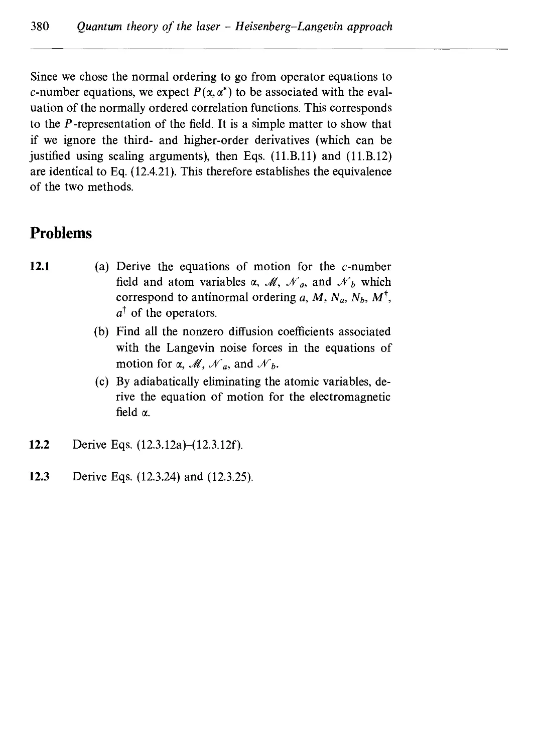
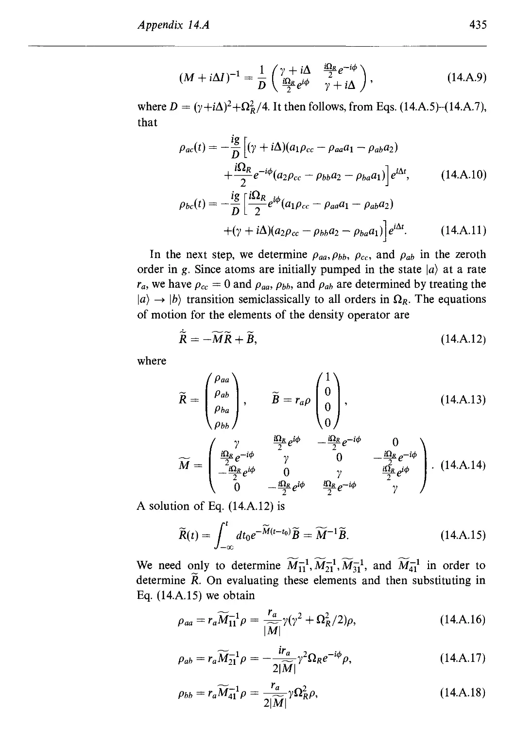
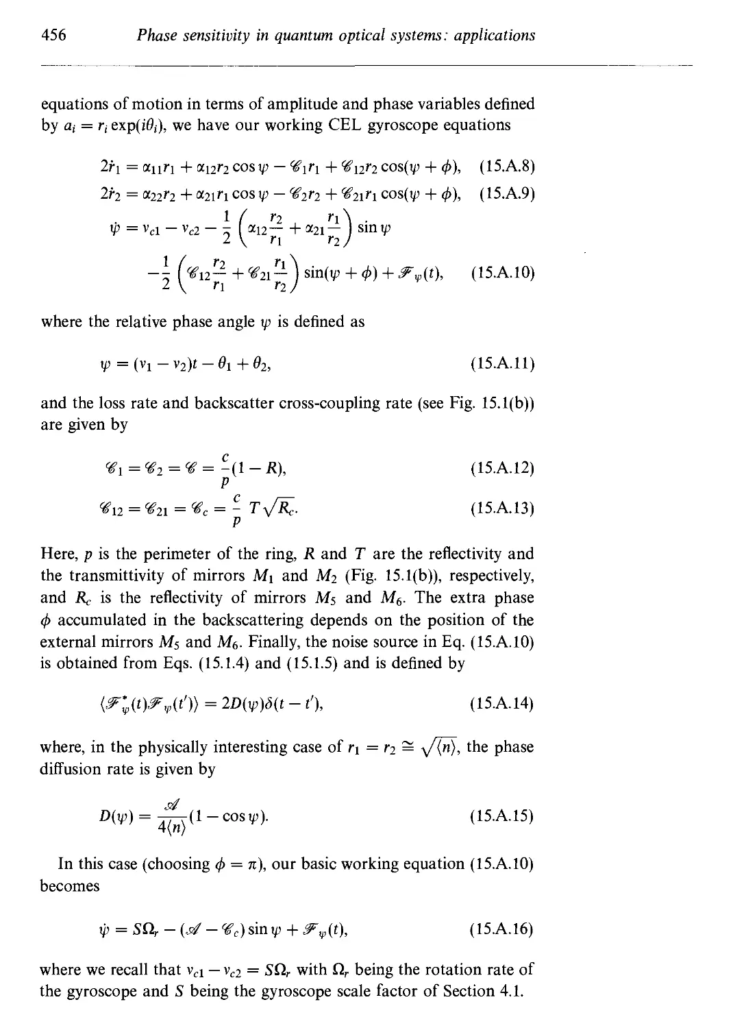
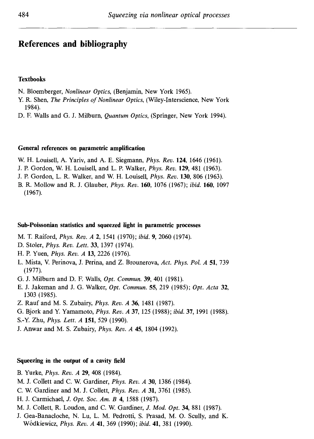
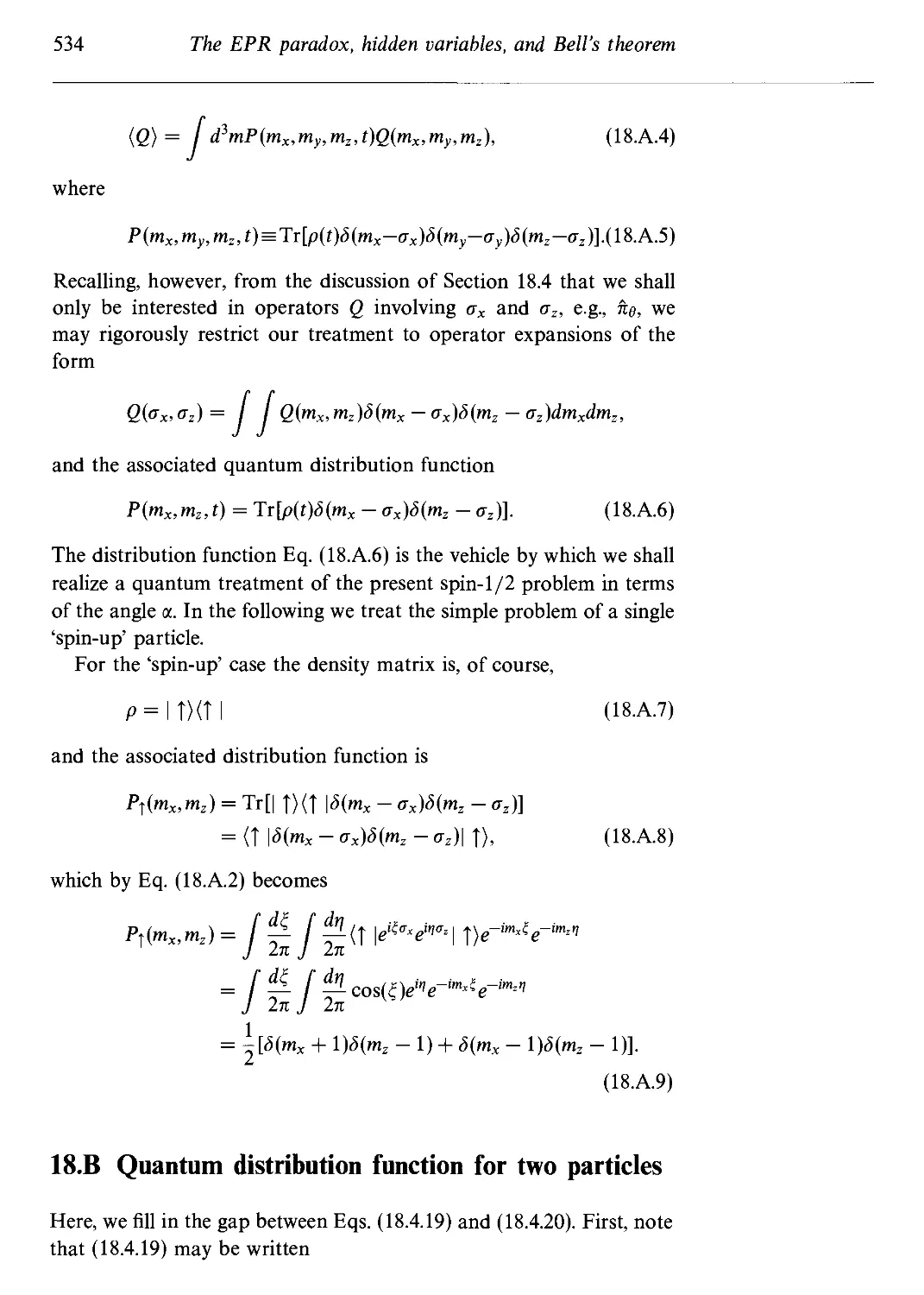
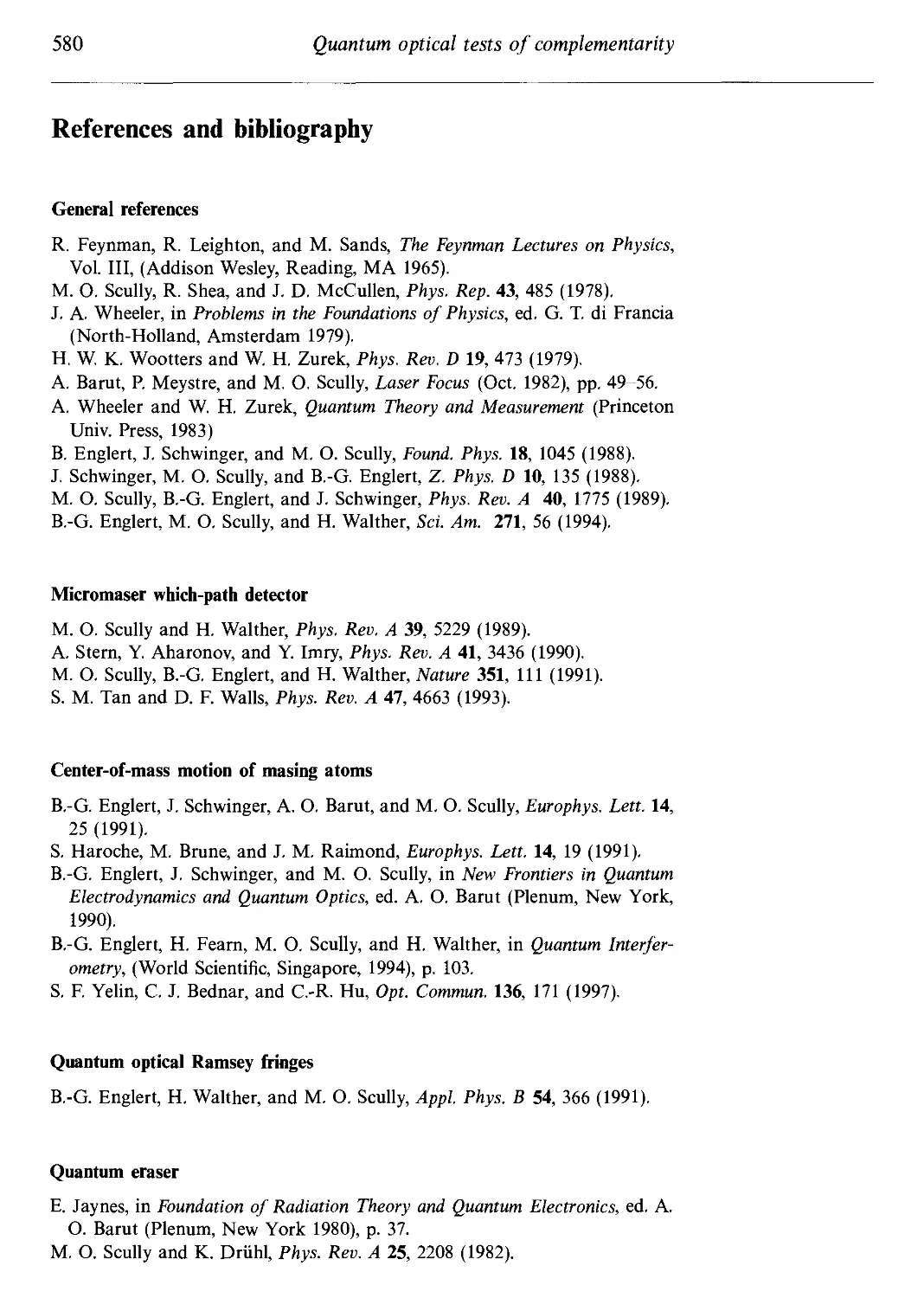
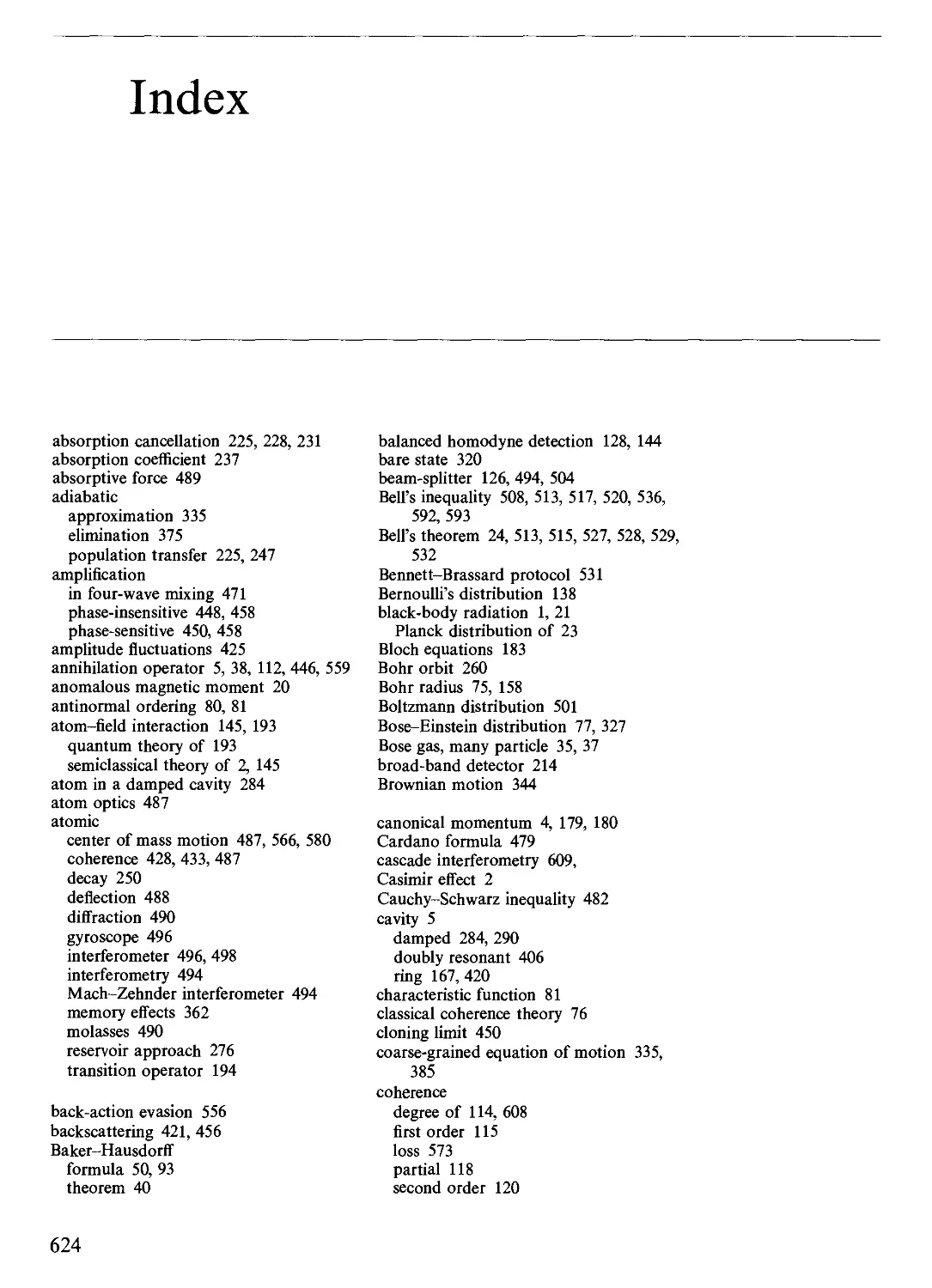
As depicted in Fig. 1.3, an ensemble of atoms prepared in a coherent
superposition of states is described by a state vector,
| xp(t)) = ca exp(-icoat)\a) + cb exp(-icobt)\b)
+ccexp{-i(oct)\c), A.4.1)
where ca, сь, and cc are probability amplitudes for the atom to be in
levels |a), \b), and \c), respectively. Furthermore, if the nonvanishing
dipole matrix elements are denoted by
V type atoms Л type atoms
A.4.2)
ac = e(a\r
be = e(b\r
c) &>ac = e(a\r\c)
c) SPab=e(a\r\b),
where the designations V and Л are explained in Fig. 1.3, then the
state A.4.1) implies that each atom contains two microscopic oscillating
dipoles, that is,
V type atoms Л type atoms
A.4.3)
с(с*ьсс) exp(jv2t) + 0>аь(с"ась) exp(iv2t)
+C.C. +C.C,
where vi = coa — coc, V2 = <*>ь — &>c for V type atoms and vi = coa — а>ь,
V2 = <*>a — <Uc for Л type atoms. From a semiclassical perspective, the
field radiated will then be a sum of two terms
E{+) = <f! exp(-ivit) + 8г exp(-iv2t), A.4.4)
in an obvious notation. Hence it is clear that a square law detector
contains an interference or beat note term
= \ёх\2 + \S2\2 + {S\g2 exp[i(vi - v2)t] + cc.}. A.4.5)
18
Quantum theory of radiation
Fig. 1.3
Three-level atomic
structures for (a) V
type and (b) Л type
quantum beats.
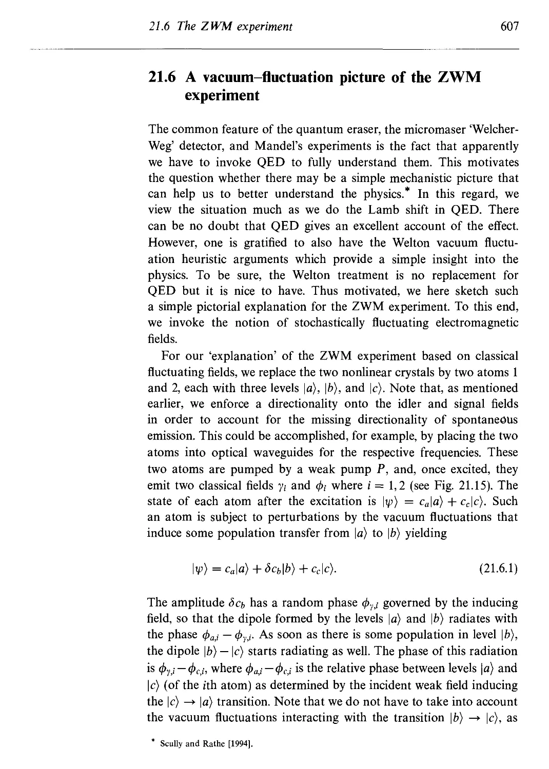
(a) F-type atom
cl\c,lVl)+c2\c,lVa)
i=a,b,c
(b) Л-type atom
i—a,b,c
Such a beat note is frequently observed in beam-foil spectroscopy
experiments.
Finally we note, and this is the central point, that such an inter-
interference term is predicted by SCT for atoms of both types V and
Л.
Let us now consider the same problem as viewed from a QED
perspective. For an atom of the V type we now calculate a beat note
(yv(t)\E[ \t)EF\t)\y)v{t)),
A.4.6)
where e\ \t) and E^\t) are proportional to the creation and annihi-
annihilation operator expressions a[exp(ivit) and a2 exp(—ivit), respectively.
In view of \xpv(t)), as given in Fig. 1.3(a), Eq. A.4.6) reduces to
K(lVl0V2|afa2|0VllV2)exp[i(vi -v2)t](c\c),
A.4.7)
1.4 Quantum beats 19
where к is a constant. Hence, the beat note calculated via QED is
given by
Kexp[i(vi-v2)t](c|c>. A.4.8)
=i
On the other hand for Л type atoms we have
<VA(t)|£(rVL+V)l<M@), A-4.9)
and taking \y)\{t)) from Fig. 1.3(b) this becomes
K'(lVl0V2|a}a2|0VllV2)exp[i(vi -v2)t](c\b)
= к' exp[i(vi - v2)t] (c\b). A.4.10)
=o
Summarizing these QED considerations,
V type atoms :{rpv(t)\E[~\t)E{+\t)\rpv(t)) = »cexp[i(vi - v2)t],
Л type atoms : (xpK{t)\E^\t)E(+\t)\VA(t)> = 0 A.4.11)
whereas in the SCT calculations one finds the beat note amplitude to
be nonvanishing for both V type and Л type atoms.
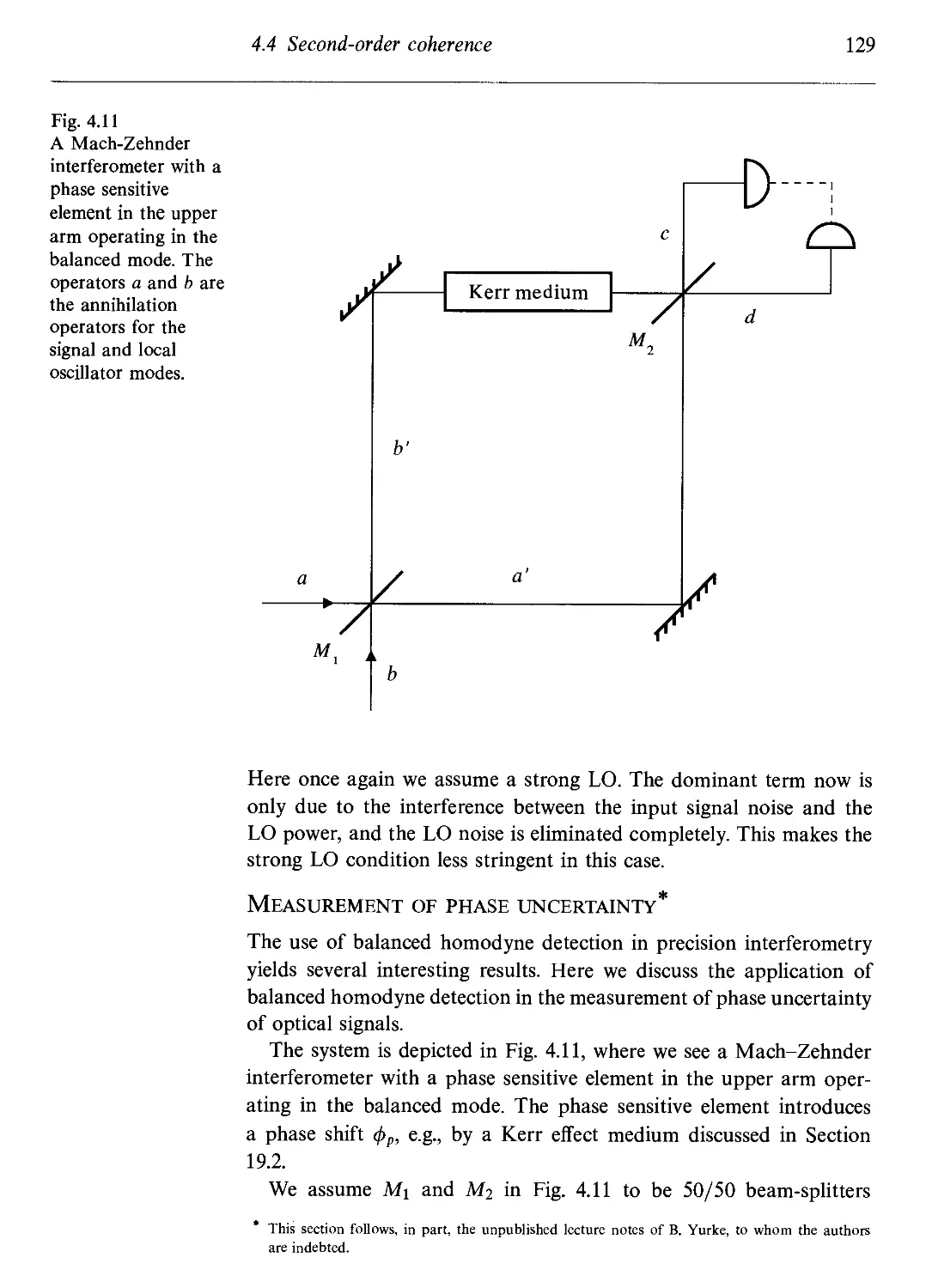
The following argument based on the quantum theory of measure-
measurement provides some physical insight concerning the missing beats. A
V type atom when coherently excited will decay via the emission of
a photon with frequency vi or v2. Since both transitions lead to the
same final atomic state, one cannot determine along which path, vi
or v2, the atom decayed. Analogous to Young's double-slit problem,
this uncertainty in atomic trajectory leads to an interference between
photons with frequencies vi and v2, giving rise to quantum beats. The
complementary nature of which-path information and the appearance
of quantum beats will be discussed in detail in Chapter 19. A coher-
coherently excited Л type atom will also decay via the emission of a photon
with frequency vi or v2. However, after the emission is long past, an
observation of the atom would now tell us which decay channel A or
2) was taken (atom in \c) or \b)). Consequently, we expect no beats in
this case.
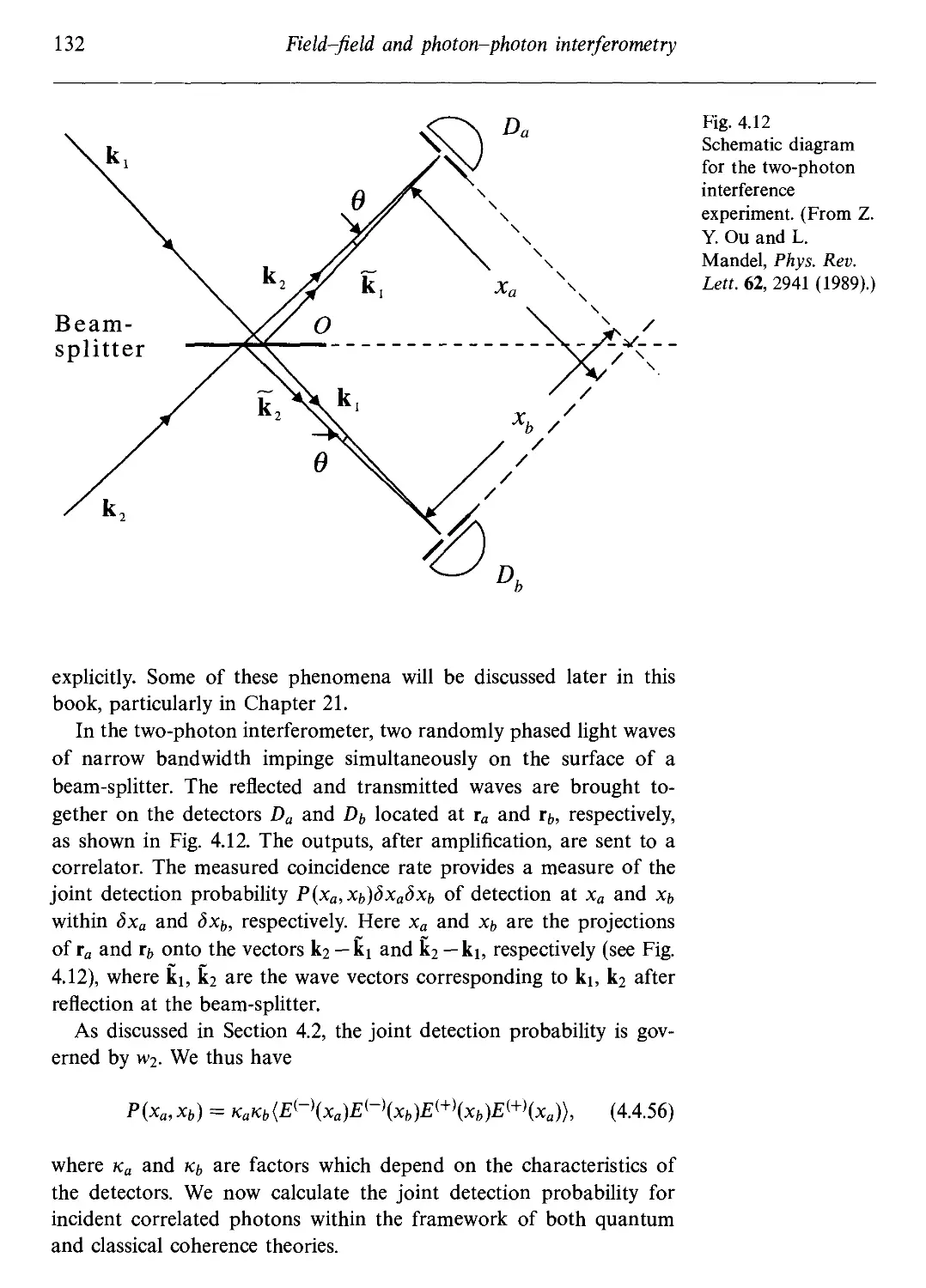
The clear conclusion is that a QED calculation is consistent with
our most fundamental notions of quantum theory, while SCT applied
to this problem is not.
20 Quantum theory of radiation
1.5 What is light? - The photon concept
The quantum theory of radiation provides a complete description of
radiation-matter interactions (when supplemented by certain renor-
malization presumptions). It is however tempting to argue that the
conceptual underpinnings of the quantum theory of radiation and the
concept of a photon can be best thought of as involving a classical
electromagnetic field plus the fluctuations associated with vacuum.
However, advances in quantum optics have brought forward new
arguments for quantizing the electromagnetic field, and with them,
deeper insight into the conceptual nature of photons. With such ex-
examples as quantum beat phenomena, the quantum eraser, and certain
two-photon interference phenomena, as discussed later in this book,
it becomes necessary to think of the photon as a quantum mechanical
entity whose basic physics is much deeper than the semiclassical the-
theory plus vacuum fluctuation logic. We also note that there are deep
questions associated with the question of metric in a quantized field
theory, and that, in one of his last papers, Feynman* makes inter-
interesting comments connecting the possibility of a deeper understanding
of renormalization theory by combining negative probability concepts
with indefinite-metric physics. Some of these ideas and the extensions
of our conceptual understanding of the photon are the subject of this
concluding section of this chapter.
1.5.1 Vacuum fluctuations and the photon concept
While the formal quantum theory of radiation and quantum elec-
electrodynamics has had amazing success in explaining the interaction
of electromagnetic radiation with matter, there are certain conceptual
problems. For example, the various infinities associated with the calcu-
calculations of quantities, such as the Lamb shift, the anomalous magnetic
moment.
On the other hand, as we shall see in later chapters of this book,
there are many processes associated with the radiation-matter inter-
interaction which can be well explained by a semiclassical theory in which
the field is treated classically and the matter is treated quantum me-
mechanically. Examples of physical phenomena which can be explained
either totally or largely by semiclassical theory include the photoelec-
photoelectric effect which was first explained semiclassically by Wentzel in 1927.
Stimulated emission, resonance fluorescence, and many other effects
In: Negative Probabilities in Quantum Mechanics, ed. B. Hiley and F. Peat (Routledge, London,
1978).
1.5 What is light? - The photon concept 21
do not require the full machinery of the quantum theory of radiation
for their explanation; they can rather be explained by a semiclassical
analysis.
In the same spirit, it is interesting to note that the two clouds
on the horizon of physics at the beginning of the twentieth century
both involved electromagnetic radiation. As the reader will no doubt
recall, it was stated that the only two issues that were not com-
completely understood in physics at that time were the null result of the
Michelson-Morley experiment and the Rayleigh-Jeans catastrophe
associated with black-body radiation. The Michelson-Morley experi-
experiment, of course, led to special relativity, which was the logical capstone
of classical mechanics and electrodynamics, and the Planck solution
to the Rayleigh-Jeans catastrophe was the beginning of quantum
mechanics.
It is, however, interesting and important to realize that neither
of these phenomena involved the concept of a photon. In the first
instance, Einstein was thinking essentially of transformations involving
Maxwell's equations and in the second instance, Planck was thinking
in terms of quantizing the energies of the oscillators in the walls of
his cavity, not quantizing the radiation field. Up to this point, neither
the quantum theory of radiation nor the ideal concept of the photon
had been conceived.
The first introduction of the photon concept was Einstein's utiliza-
utilization of the idea to explain the photoelectric effect. It is again interesting
to note, as we alluded to earlier, that most of the photoelectric ef-
effect can be understood semiclassically. We recall for the reader that
there are three issues associated with the photoelectric effect that any
theory needs to explain. First, when light of frequency v falls on a
photoemissive surface, the energy of the ejected electrons Te obeys the
expression
Пу = Ф+Те, A.5.1)
where Ф is a work function and is a parameter characterizing the par-
particular material under discussion. Second, the rate of electron ejection
is proportional to the square of the electric field of the incident light.
Third, there is no time delay between the time in which the field begins
falling on the photoactive surface and the instance of photoelectron
emission. The first two of these phenomena can, in contrast to what
we read in most textbooks, be explained fully by simply quantizing
the atoms associated with the photodetector. However, the third point,
namely, the lack of a delay is a bit more subtle. It may be reasonably
argued that quantum mechanics teaches us that the rate of ejection is
22 Quantum theory of radiation
finite even for small times, i.e., times involving a few optical cycles of
the radiation field. Nevertheless, one may argue that the concept of the
photon is really explicit here in the sense that conservation of energy
is at stake. That is, if we have only a short period of time т elapsing
between the instants that the radiation field begins to interact with
the photoemitting atoms and the emission of the photoelectron, the
amount of energy which has fallen on the surface would be governed
by €qE2At, where A is the cross-section of the incident beam. For
sufficiently short times, the energy which has fallen on the photode-
tector may not exceed Ф. This clearly shows that we are not able to
conserve energy if we take a semiclassical point of view. However, the
photon concept in which the ejection of the photoelectron implies that
a photon is annihilated gets around this problem completely. This is
one of the triumphs of the quantum field theory.
In any case, it is a tribute to Einstein's deep understanding of
physics that he was able to introduce the photon concept from such
limited, and in some ways, misleading information. Having listed some
of the virtues of the semiclassical theory, we now turn to the question
of where it breaks down. In many arguments of this type, one hears
the statement that it is the lack of the back-action of the field on the
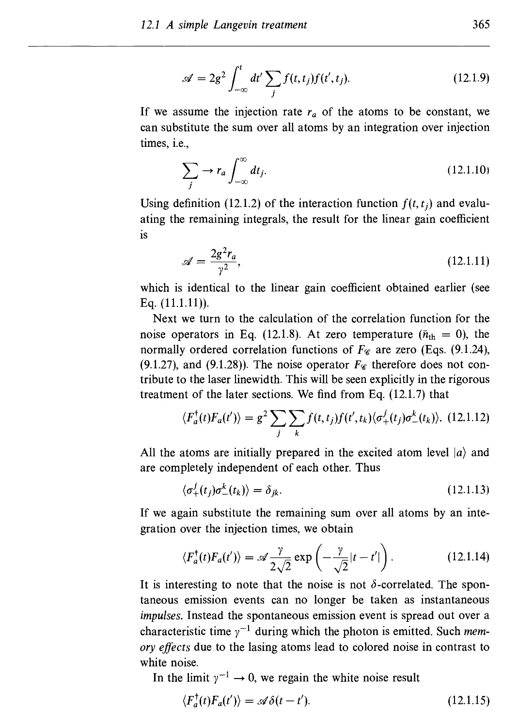
atom that is missing in semiclassical theory. This is, of course, not
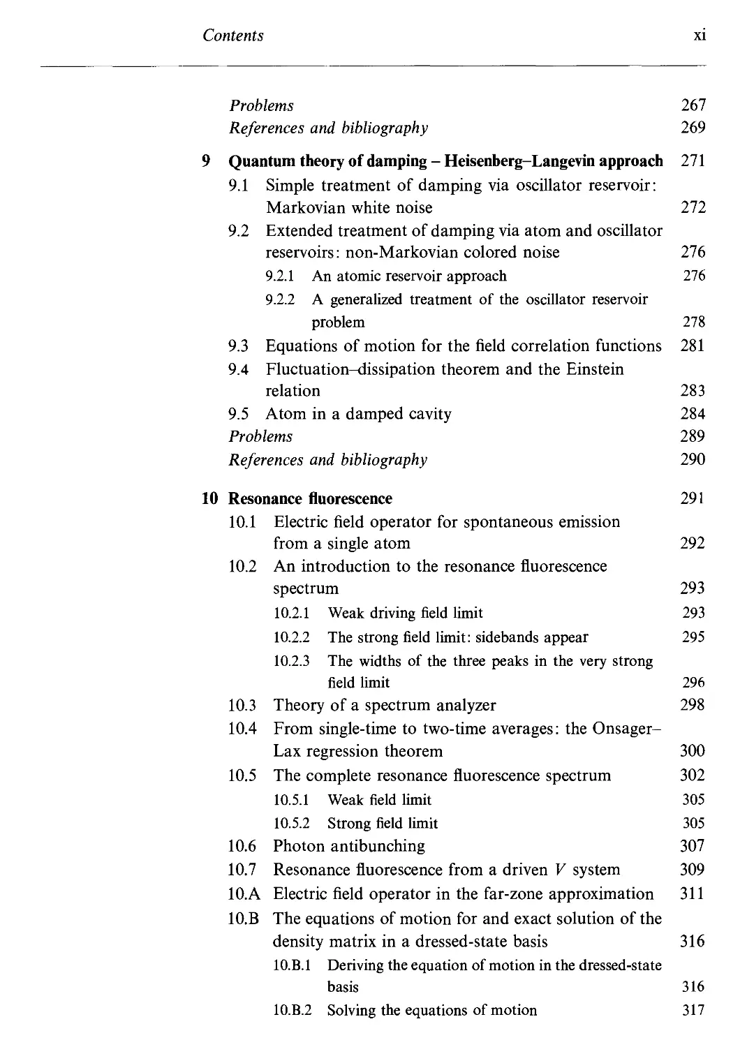
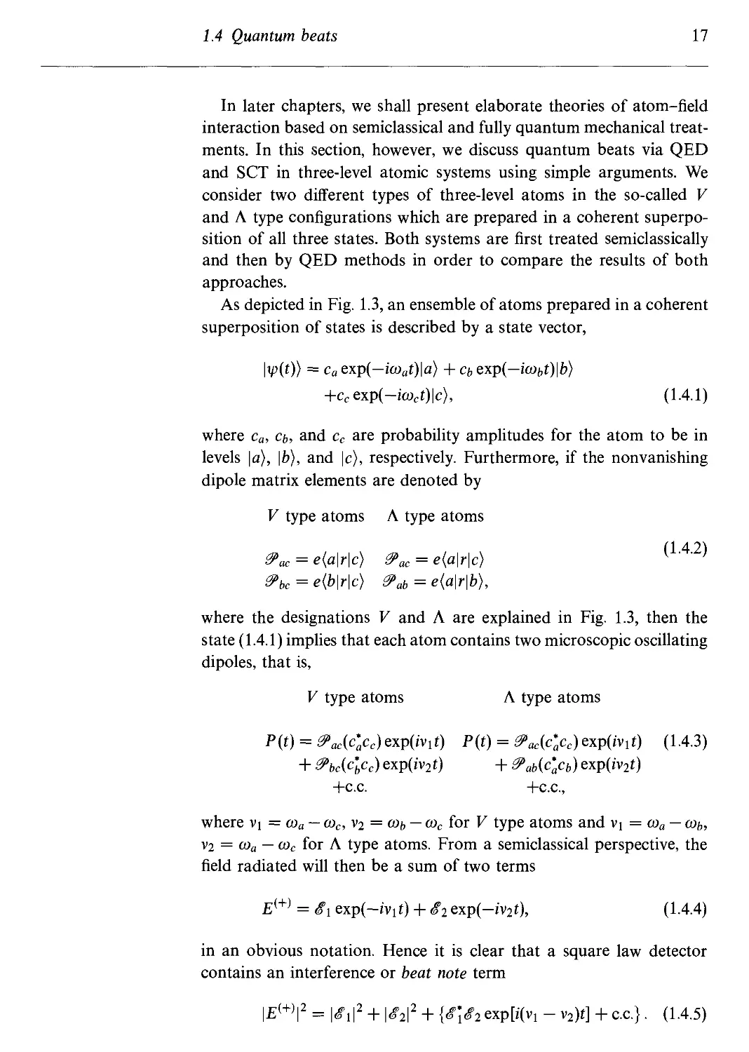
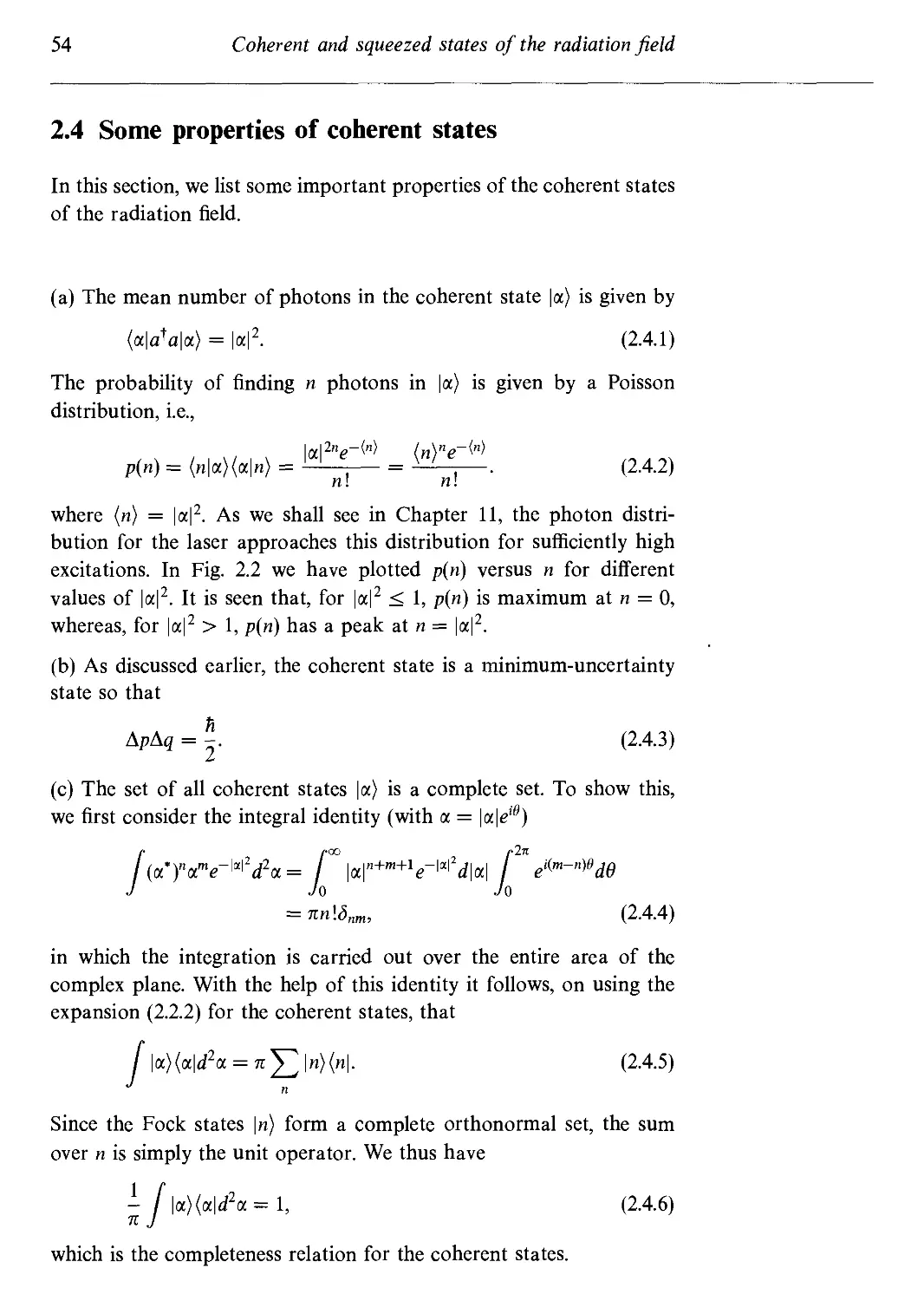
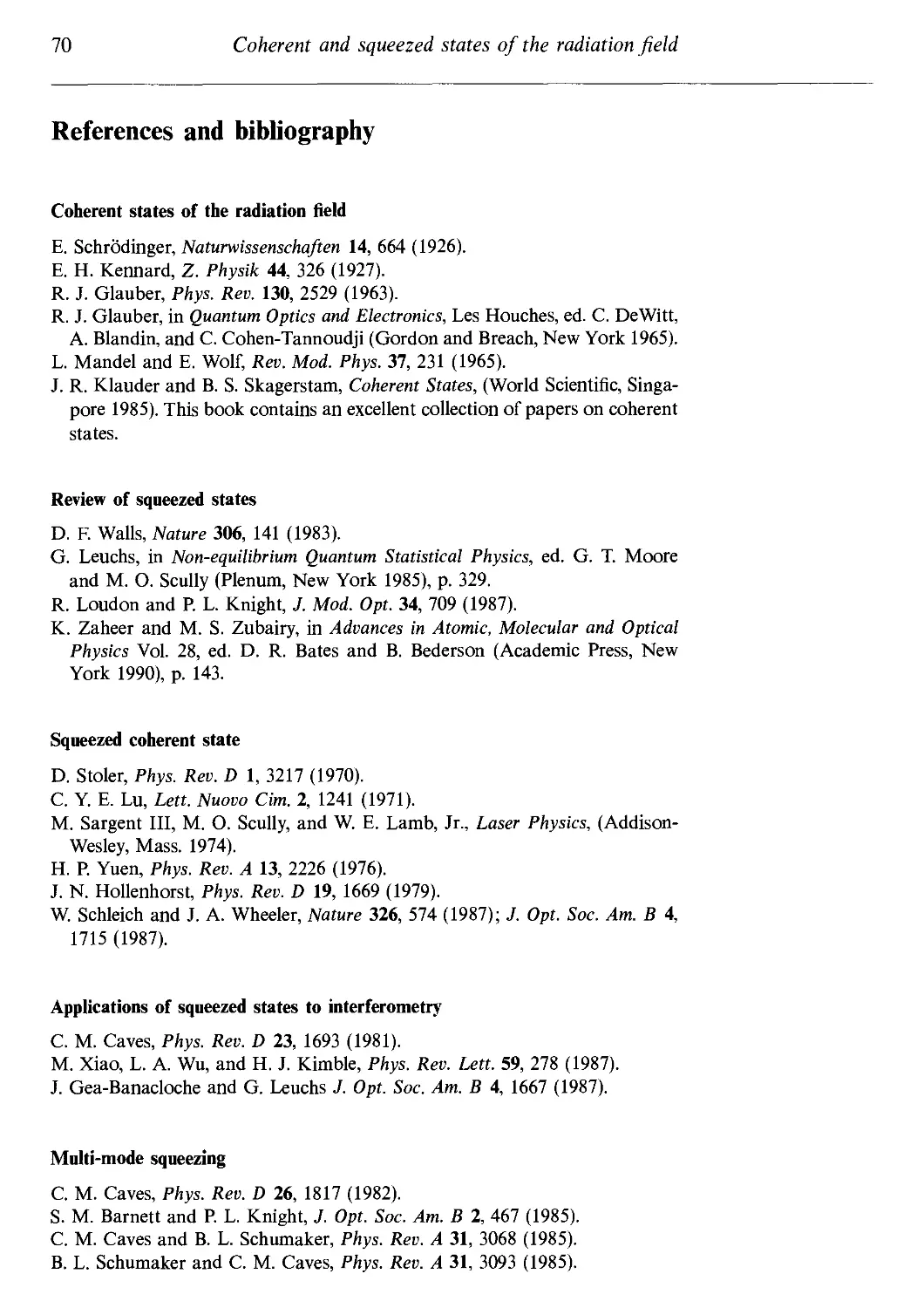
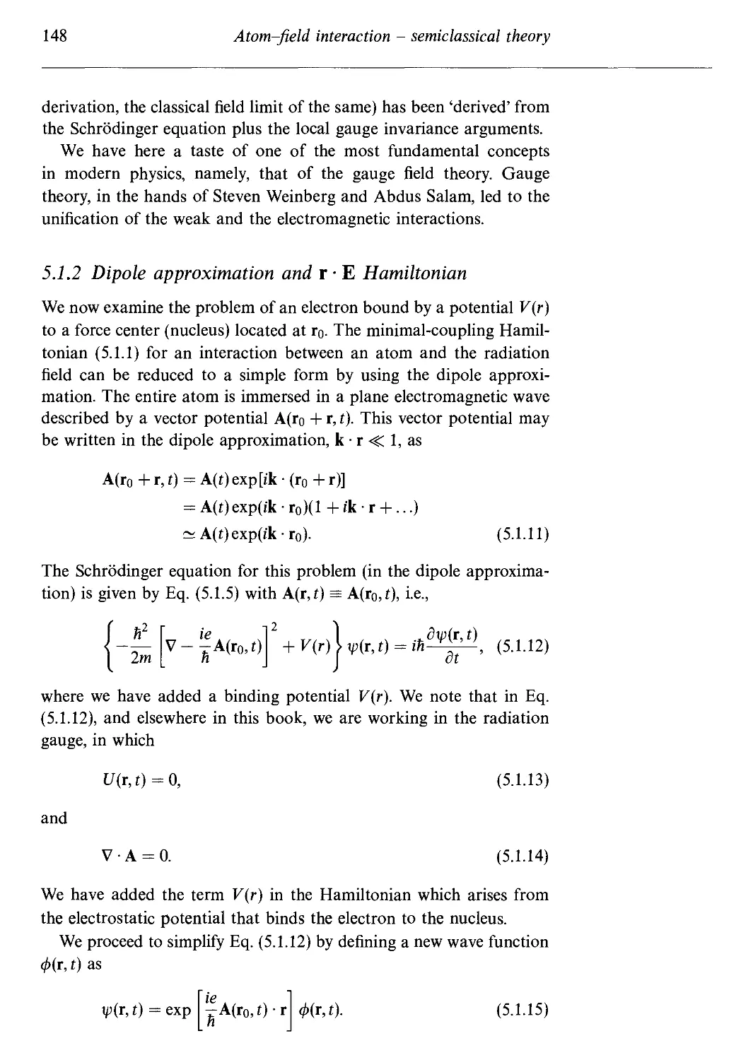
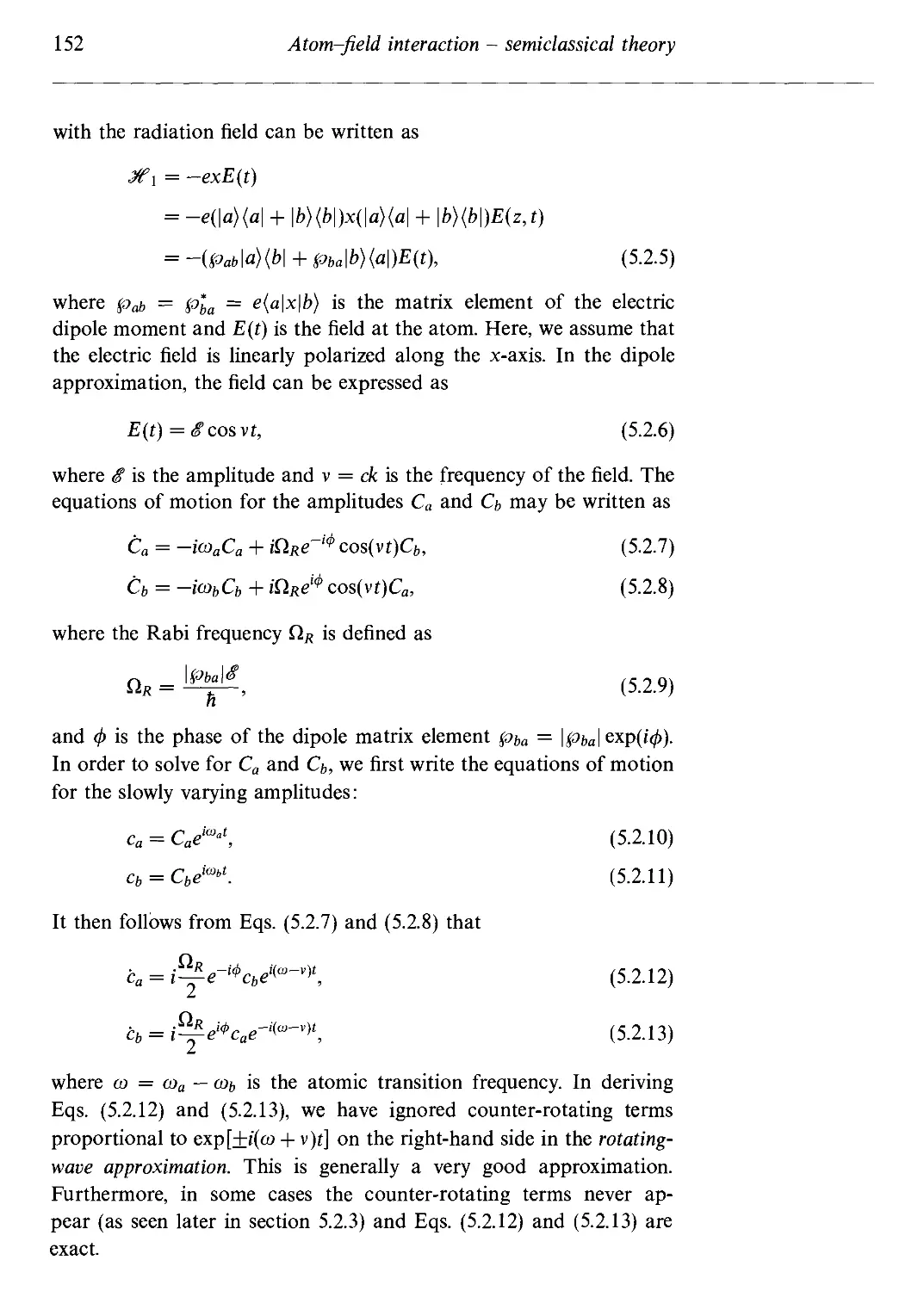
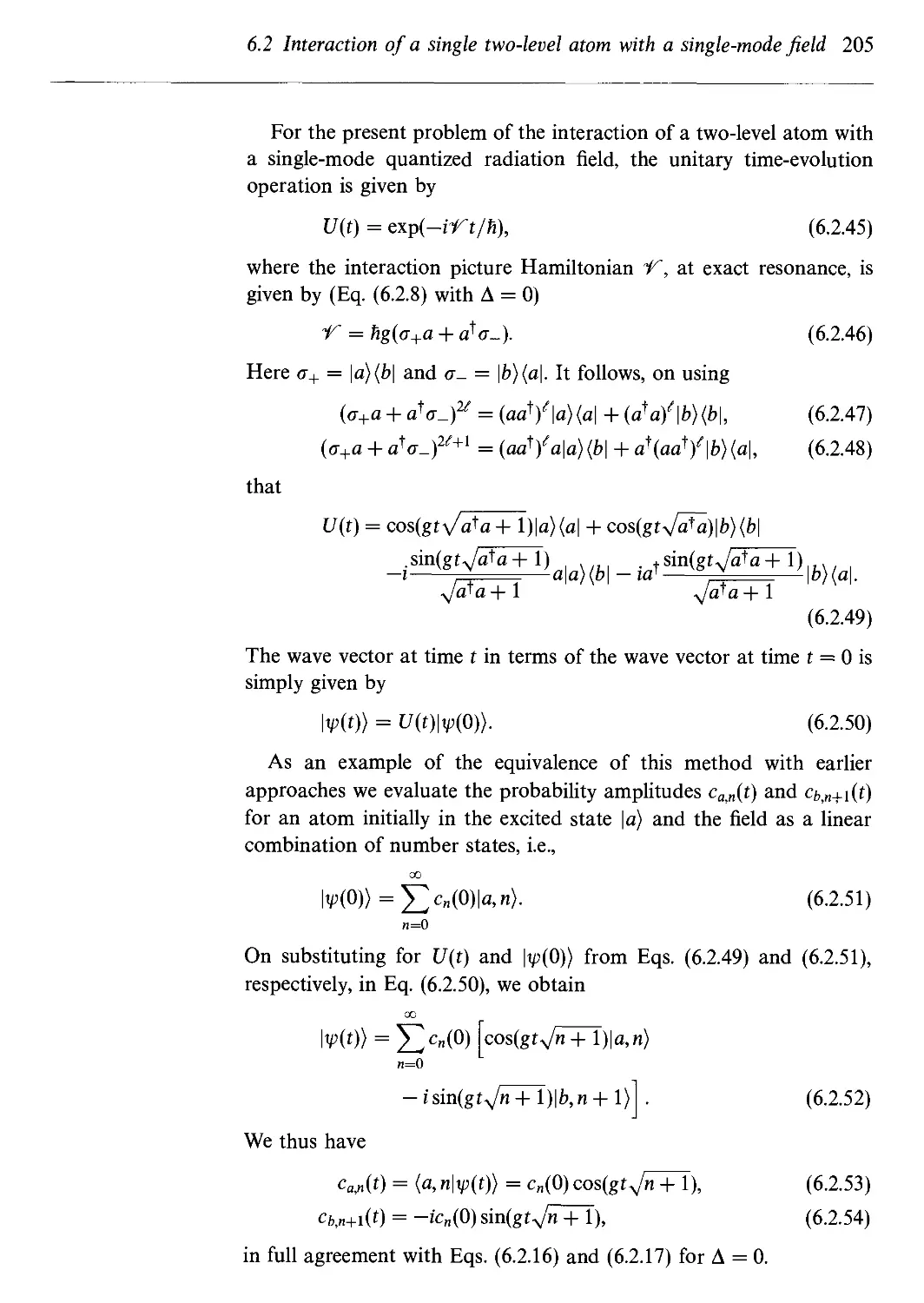
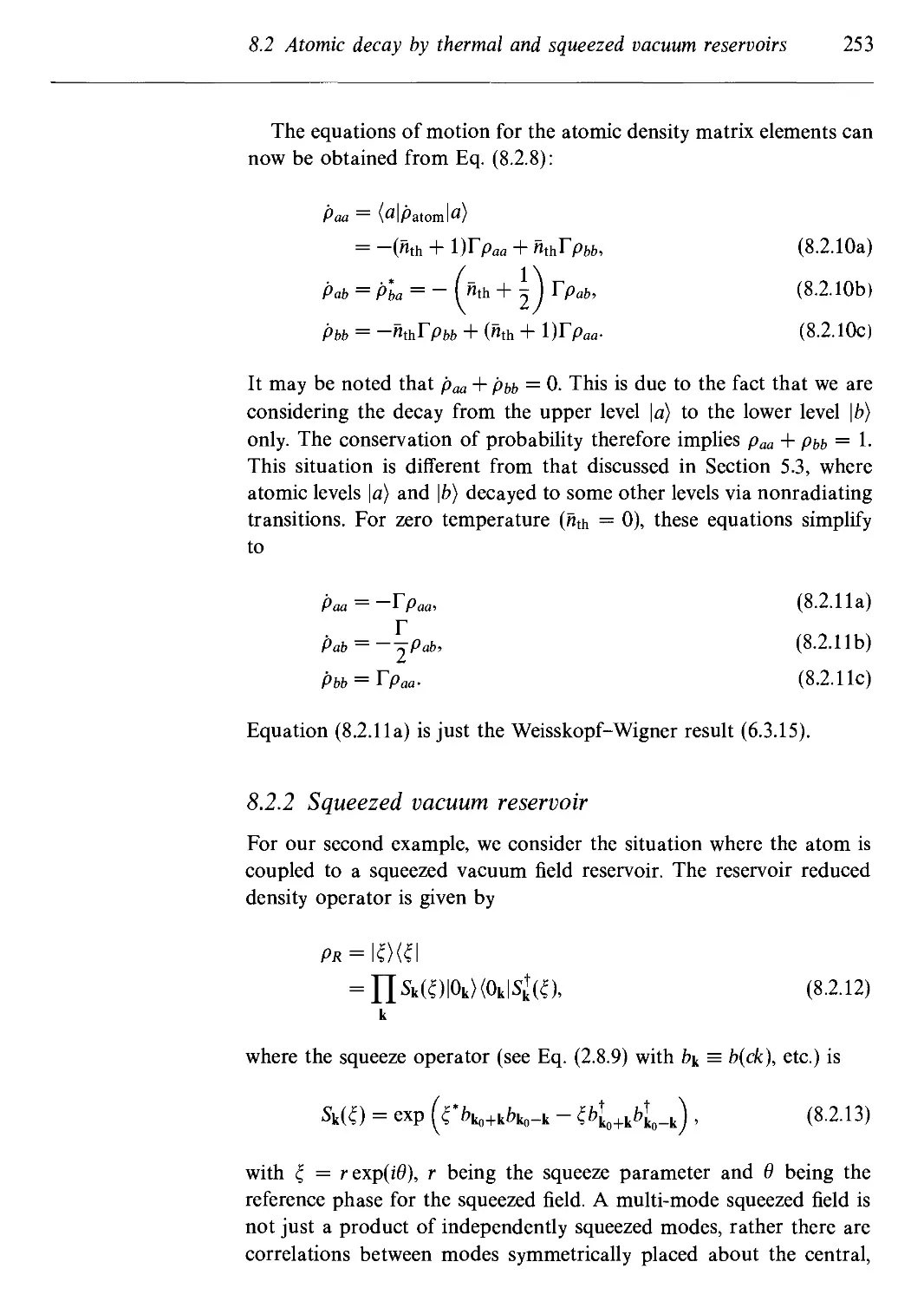
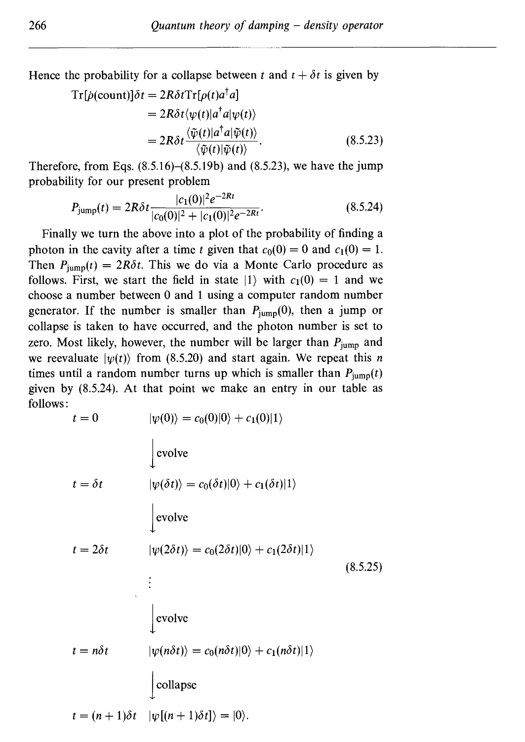
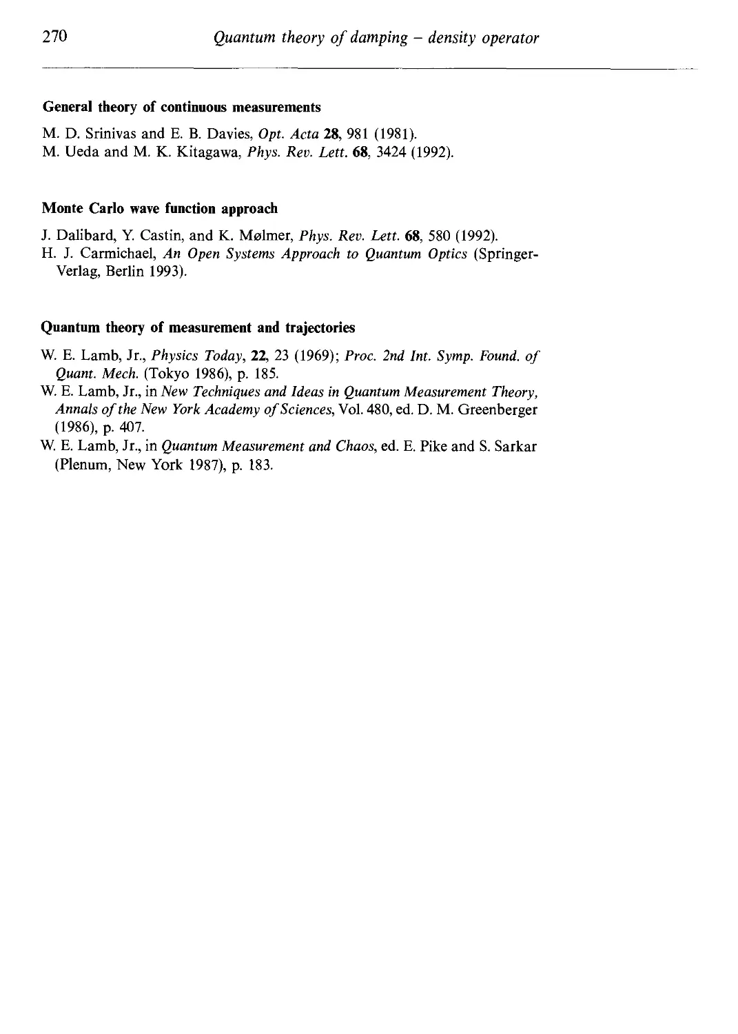
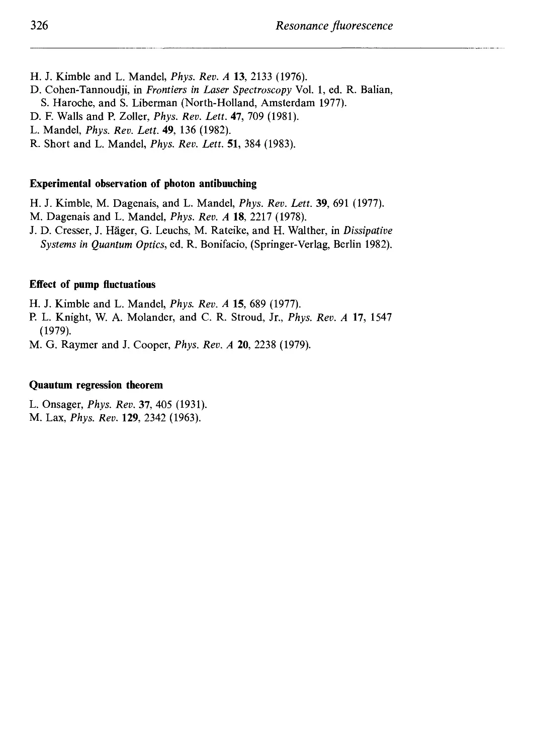
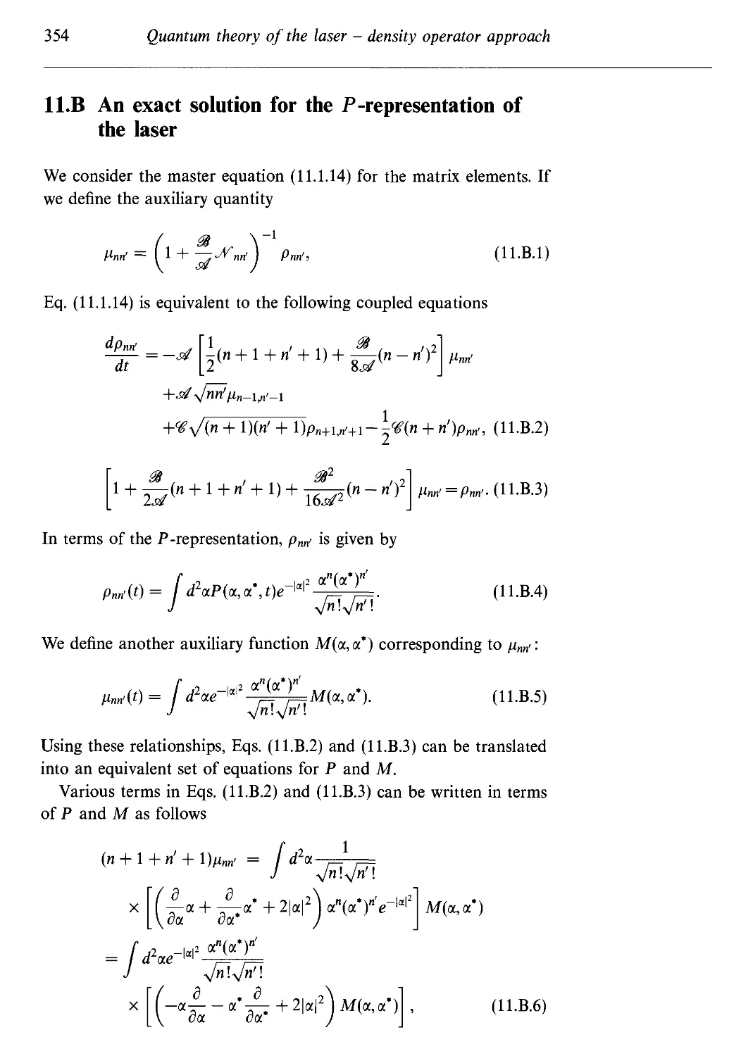
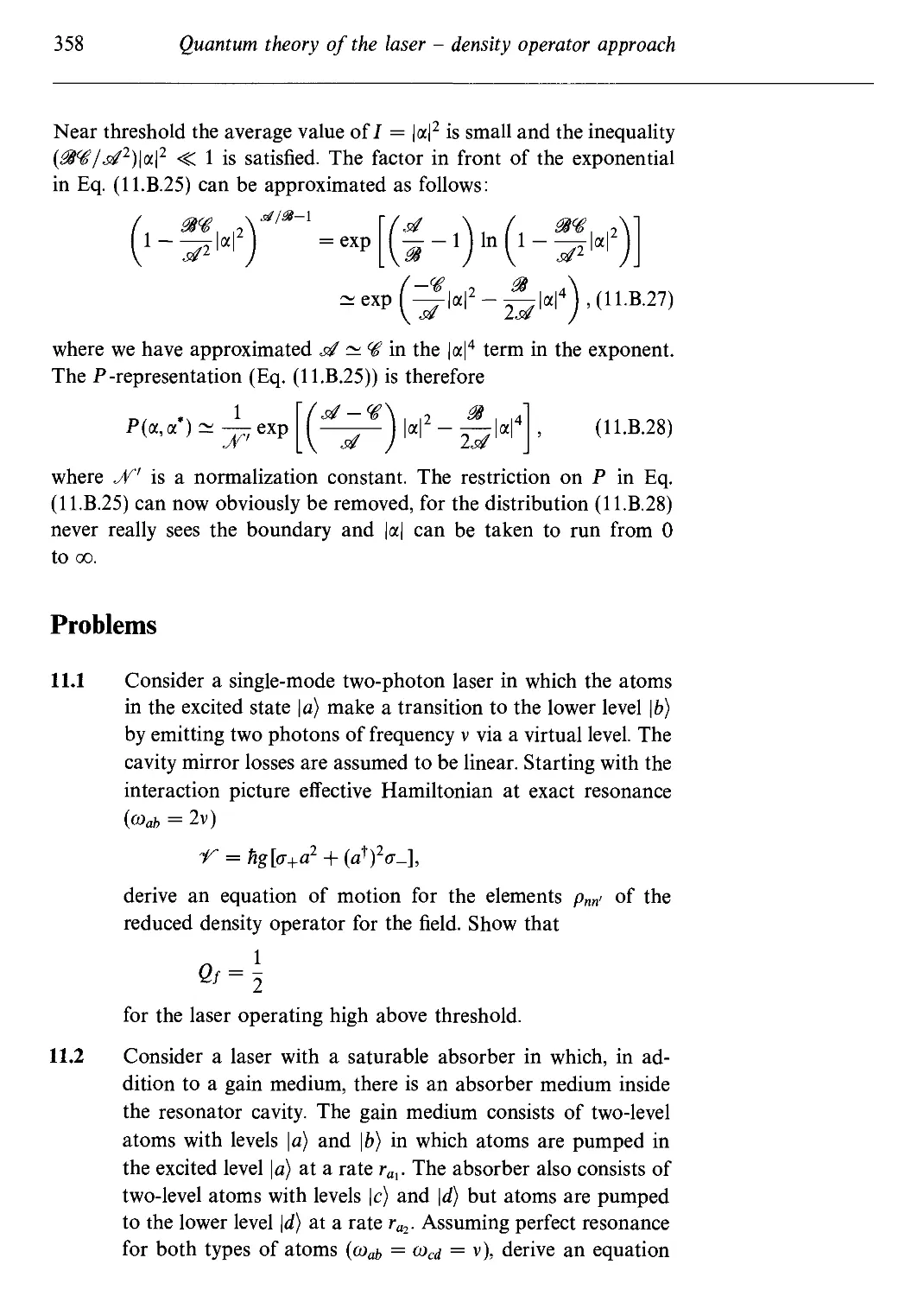
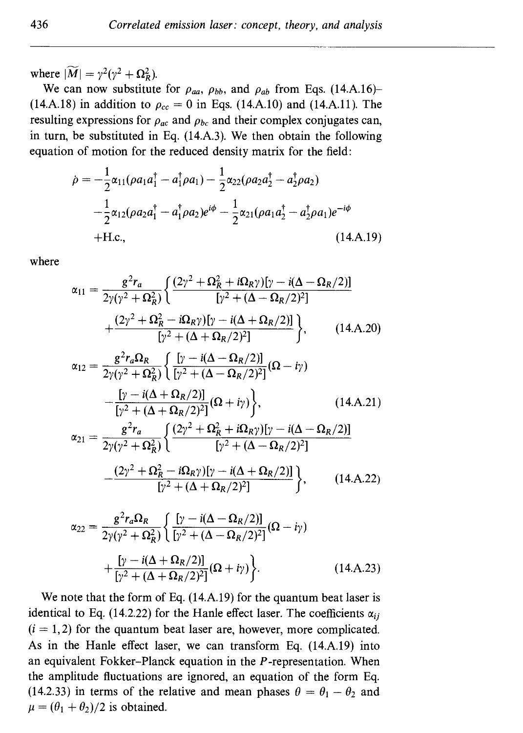
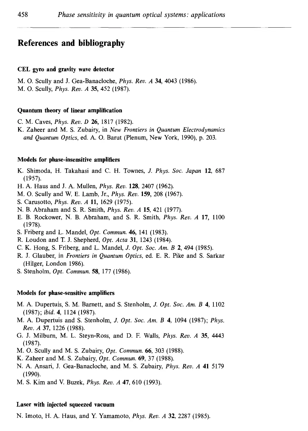
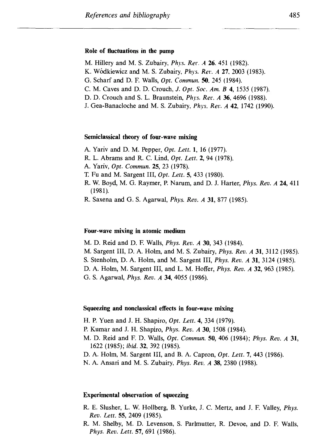
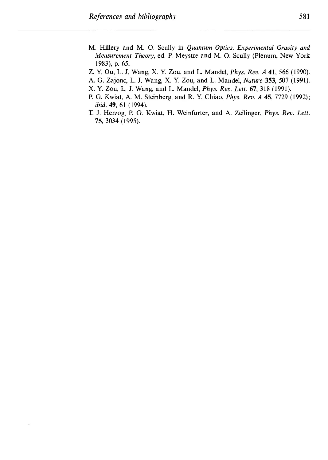
the case, as this back-action is contained by forcing the theory to be
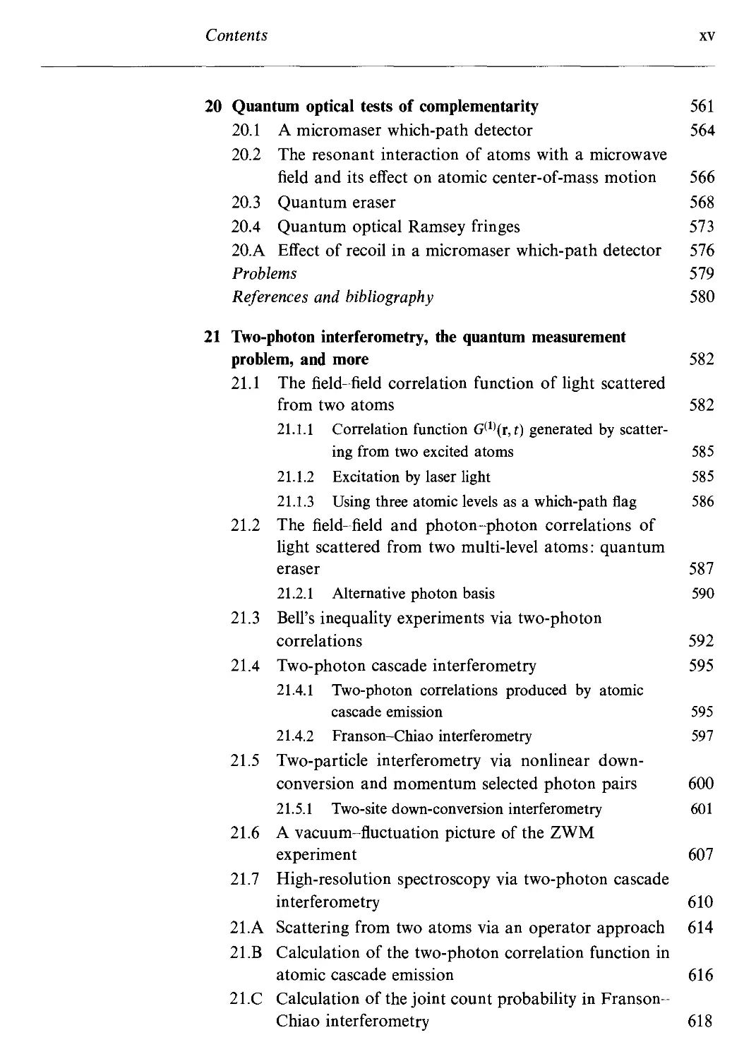
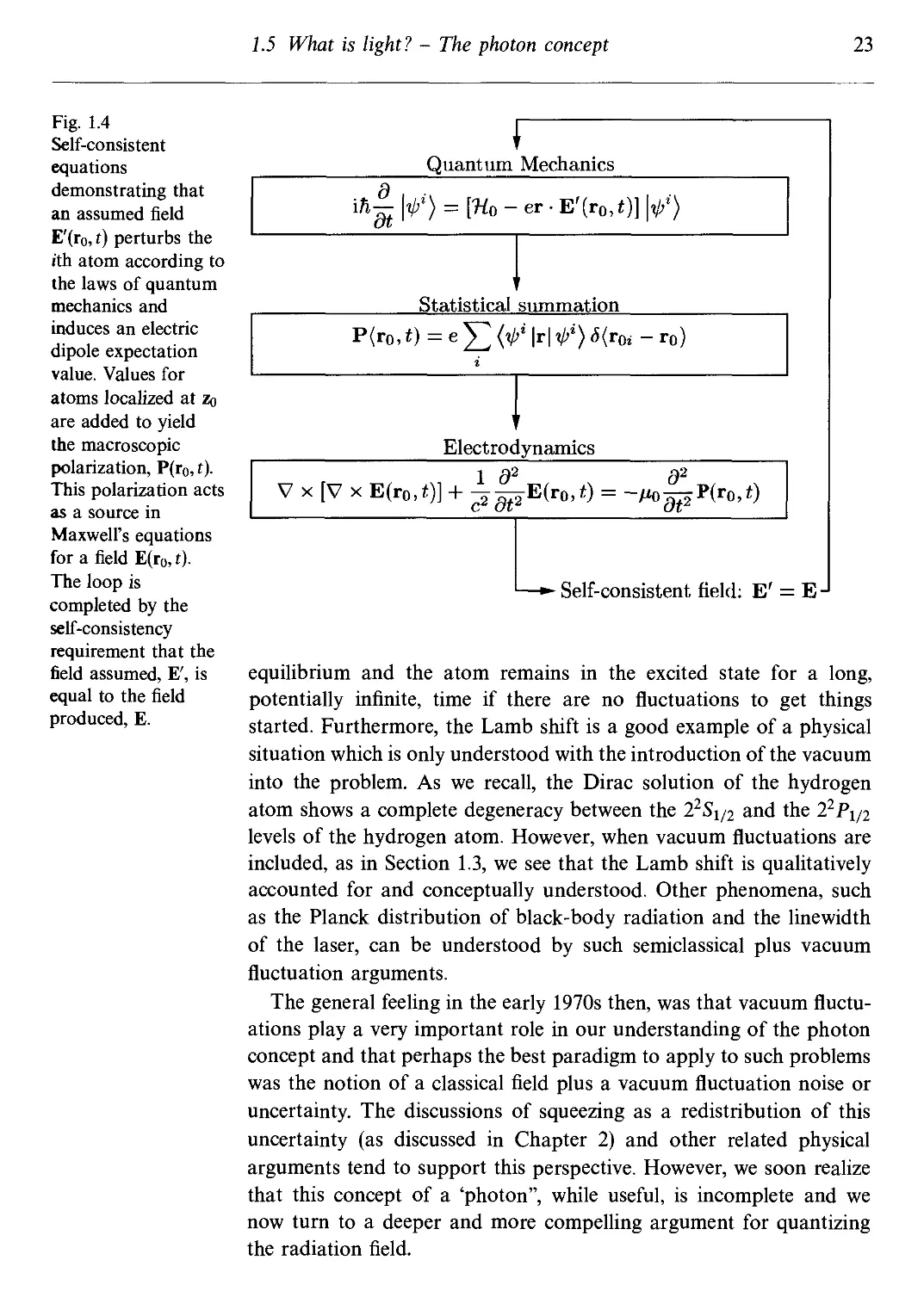
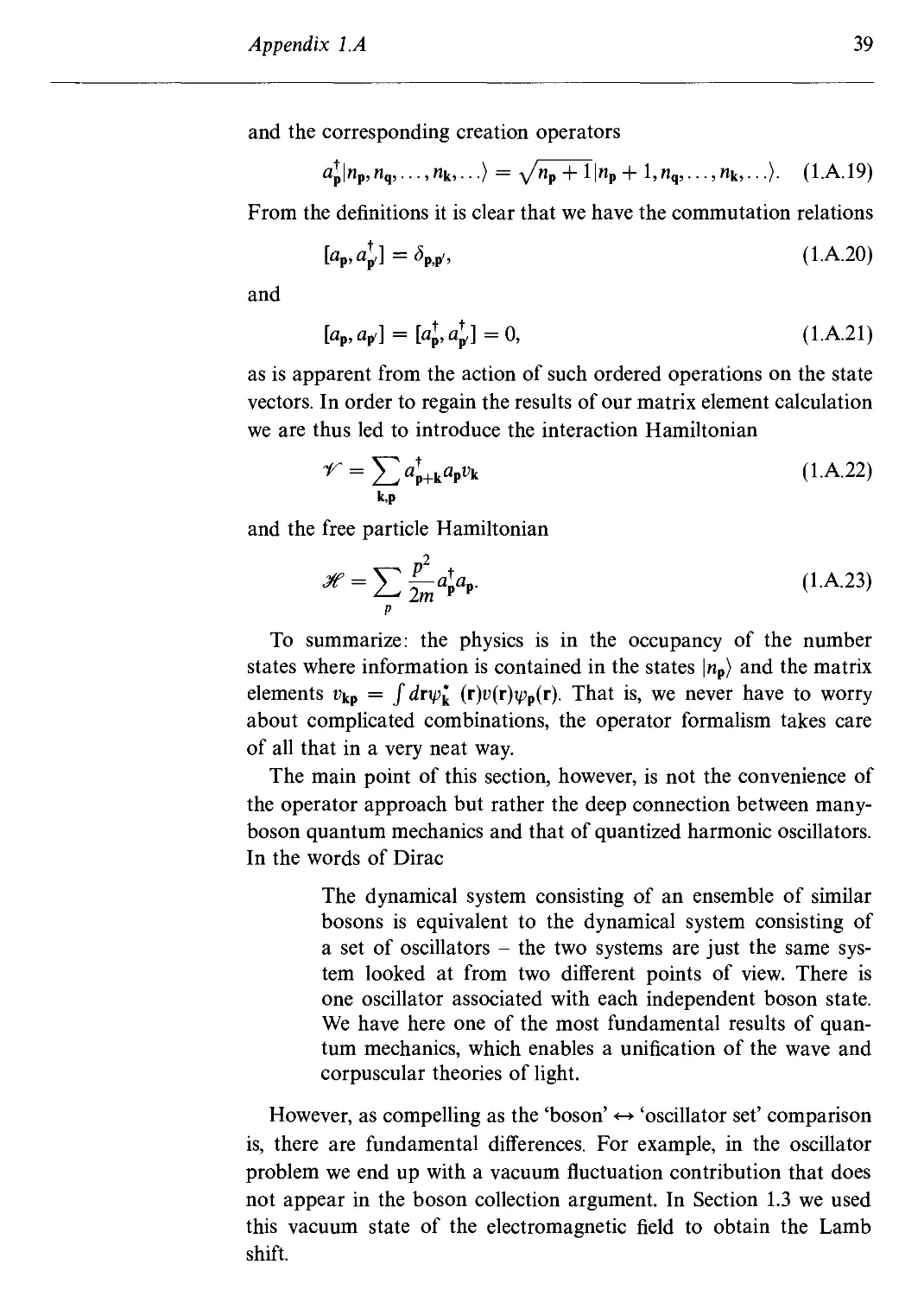
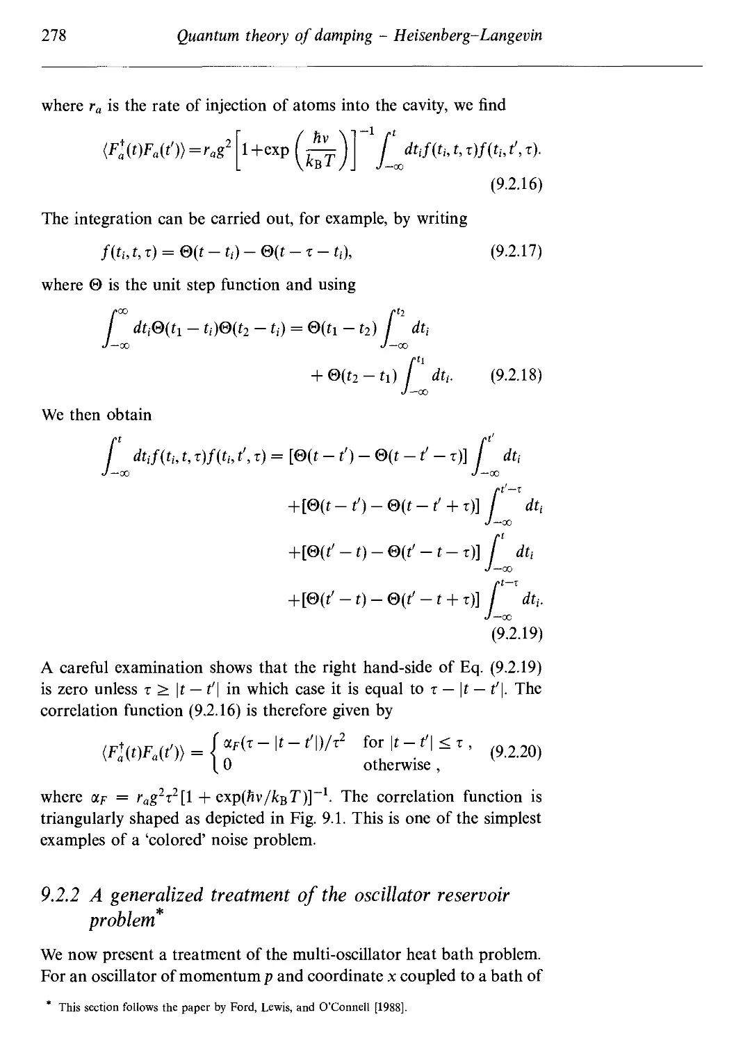
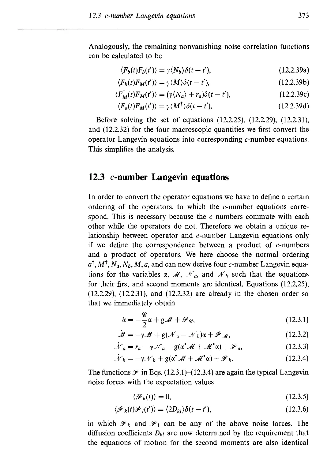
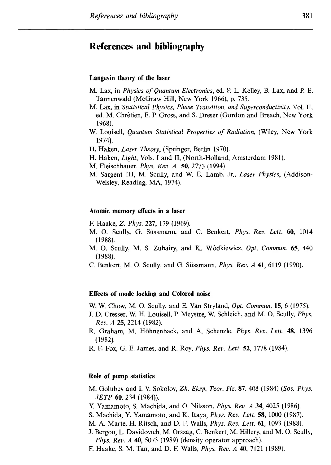
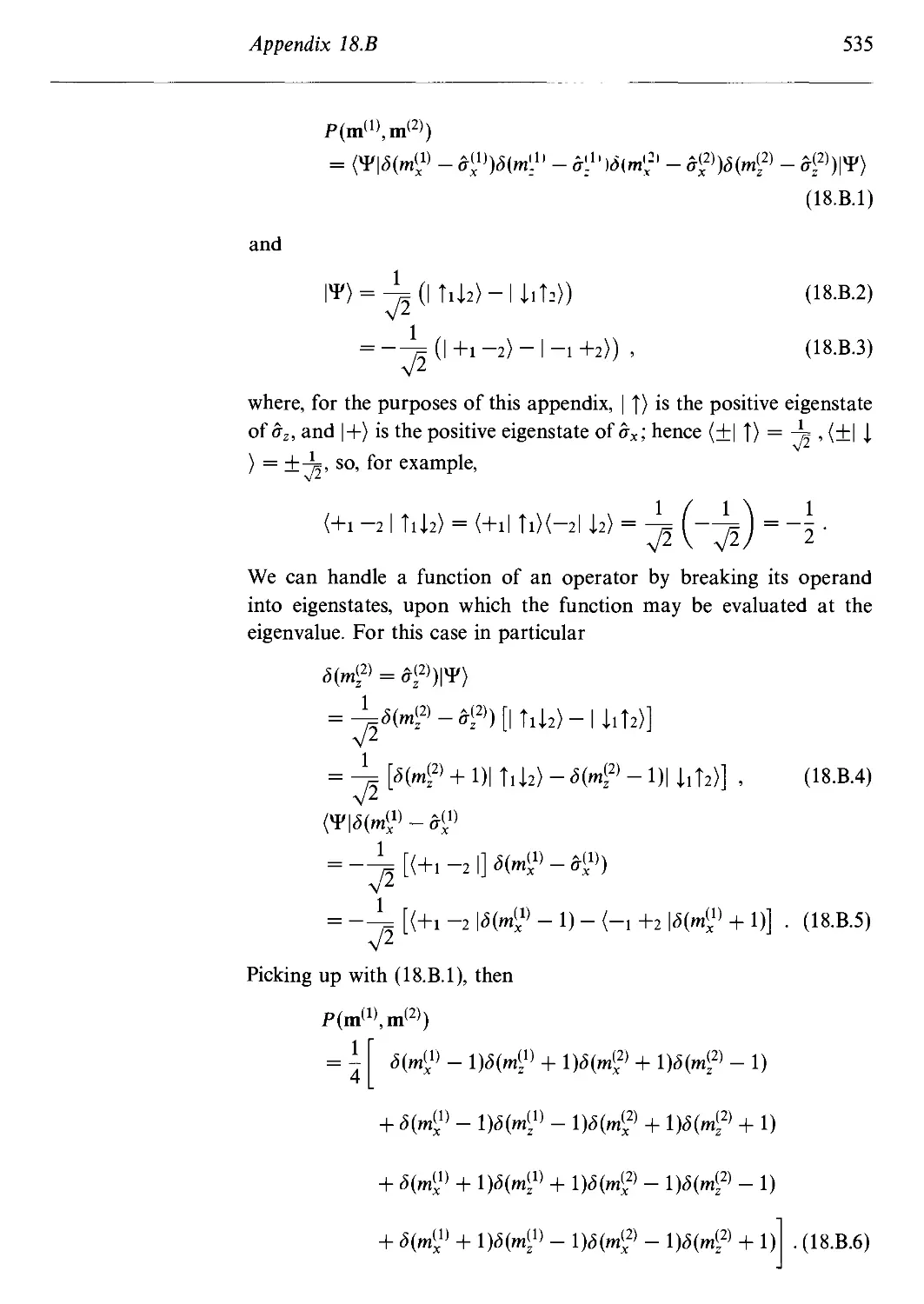
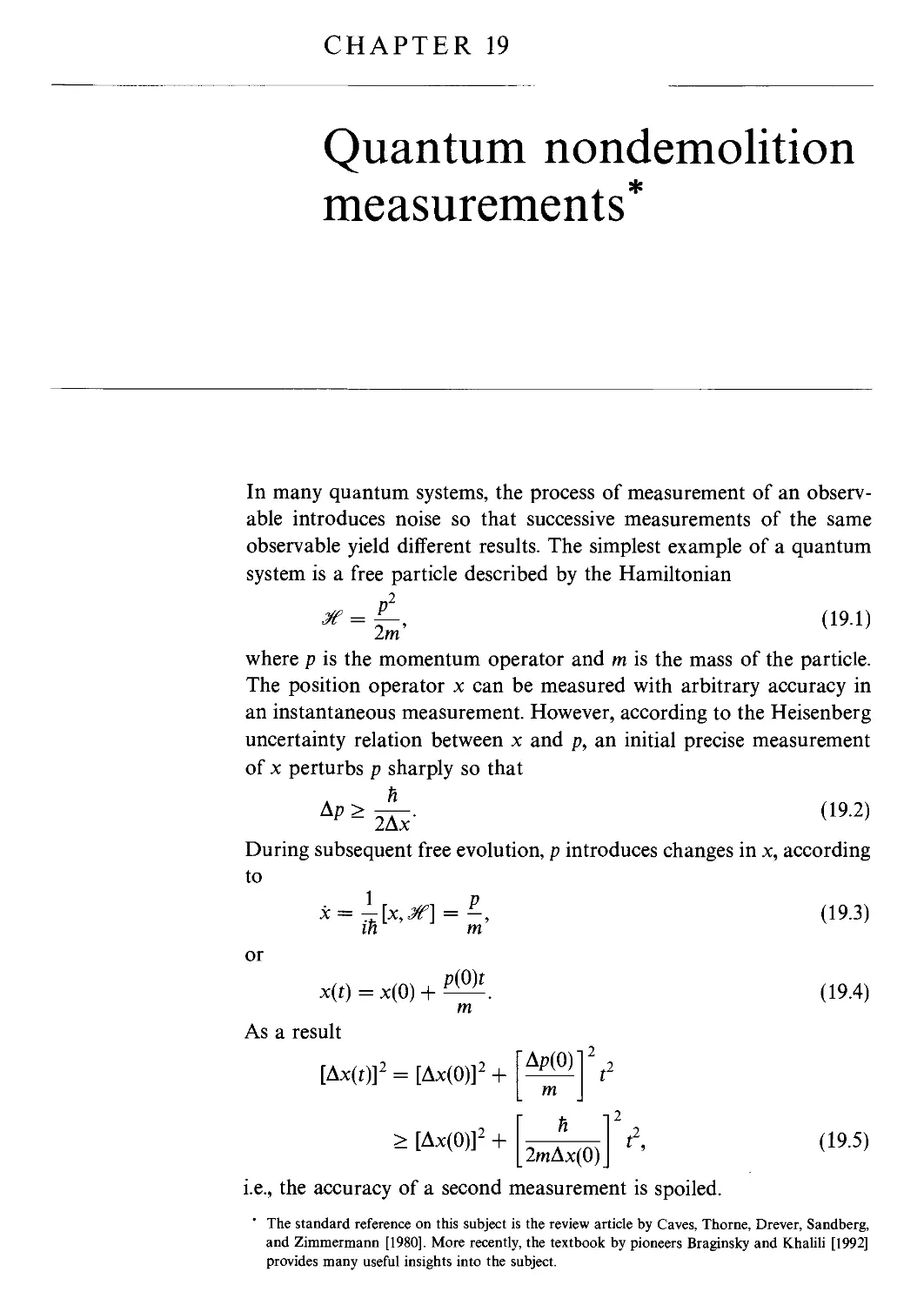
self-consistent as shown in Fig. 1.4. There we see that the existence
of a field enters into the Schrodinger equation in such a way as
to induce a dipole in an otherwise unperturbed atom. This dipole
then radiates and is the source of absorption, stimulated emission,
resonance fluorescence, etc. Now, the radiation which is emitted by
the dipole is itself a source of perturbation of the atomic.wave function
(i.e., back-action) in a self-consistent analysis, as indicated in Fig. 1.4.
However, the success of the semiclassical theory can only go so far
and we now turn to the problems in which it breaks down and indicate
how these examples can be understood by supplementing semiclassical
theory with fluctuations due to the vacuum.
1.5.2 Vacuum fluctuations
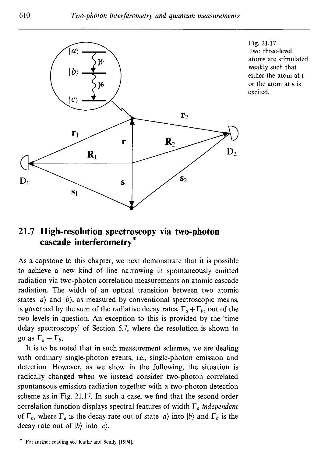
Perhaps the most important example of a situation which is not
covered by the semiclassical theory of Fig. 1.4 is the spontaneous
emission of light. We note that an atom, which is initially in the
excited state, will remain in the excited state since there is no dipole
associated with an atom in any pure quantum state and therefore
the atom never starts radiating. The situation is that of unstable
1.5 What is light? - The photon concept
23
Fig. 1.4
Self-consistent
equations
demonstrating that
an assumed field
E'(r0, t) perturbs the
ith atom according to
the laws of quantum
mechanics and
induces an electric
dipole expectation
value. Values for
atoms localized at Zo
are added to yield
the macroscopic
polarization, P(r0, t).
This polarization acts
as a source in
Maxwell's equations
for a field E(r0, t).
The loop is
completed by the
self-consistency
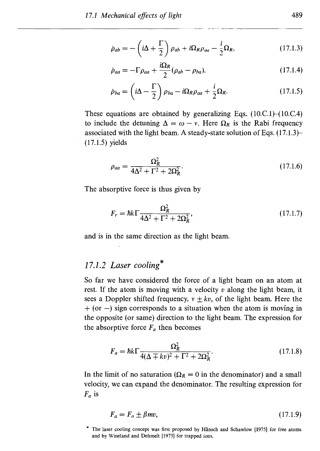
requirement that the
field assumed, E', is
equal to the field
produced, E.
\ 7
Quantum Mechanics
Statistical summation
i
Electrodynamics
V x [V x E(ro,t)] + ^^-
Self-consistent field: E' = EJ
equilibrium and the atom remains in the excited state for a long,
potentially infinite, time if there are no fluctuations to get things
started. Furthermore, the Lamb shift is a good example of a physical
situation which is only understood with the introduction of the vacuum
into the problem. As we recall, the Dirac solution of the hydrogen
atom shows a complete degeneracy between the 22Si/2 and the 22P1/2
levels of the hydrogen atom. However, when vacuum fluctuations are
included, as in Section 1.3, we see that the Lamb shift is qualitatively
accounted for and conceptually understood. Other phenomena, such
as the Planck distribution of black-body radiation and the linewidth
of the laser, can be understood by such semiclassical plus vacuum
fluctuation arguments.
The general feeling in the early 1970s then, was that vacuum fluctu-
fluctuations play a very important role in our understanding of the photon
concept and that perhaps the best paradigm to apply to such problems
was the notion of a classical field plus a vacuum fluctuation noise or
uncertainty. The discussions of squeezing as a redistribution of this
uncertainty (as discussed in Chapter 2) and other related physical
arguments tend to support this perspective. However, we soon realize
that this concept of a 'photon", while useful, is incomplete and we
now turn to a deeper and more compelling argument for quantizing
the radiation field.
24 Quantum theory of radiation
1.5.3 Quantum beats, the quantum eraser, Bell's theorem,
and more
As we discussed in Section 1.4, the existence of quantum beats in an
upper-state V type doublet ensemble in contrast to the absence of
quantum beats associated with a lower-doublet in а Л type atomic
configuration forms the basis for an alternative argument for quan-
quantizing the radiation field which has nothing to do with the previous
vacuum fluctuations. The quantum beat argument provides an exam-
example of the insufficiency of semiclassical theory plus vacuum fluctuations
to understand the physics of the phenomenon. From this early exam-
example sprang concepts such as the quantum eraser and the two-photon
correlation interference phenomena. This eventually showed that the
early arguments and statements to the effect 'photons interfere only
with themselves' were to be understood only within the context of
Young's double-slit type experiments, and should not be pushed be-
beyond that limit. We here have a great example of the importance of
photon entangled states. Such entangled states are used in optical tests
of Bell's inequalities and it could therefore be argued that they pro-
provide a deeper insight into the photon concept and indeed all quantum
mechanics. As discussed in the last chapter of this book, we have a
deeper appreciation of the nature of the quantum theory of light as a
result of recent quantum optical studies.
1.5.4 'Wave function for photons'
The heading of this section is put in quotes for two reasons. First, it
is the heading of a section in Power's classic book on QED. Second,
the quotes serve to alert the reader to the fact that there is, strictly
speaking, no such a thing as a 'photon wave function'.
For example, Power and also Kramers make the point that one may
not think of the 'photon' in the same sense as a massive (nonrelativis-
tic) particle. On the other hand, some physicists argue that a single
photon in free space is analogous to the meson if we let the meson
mass go to zero. It is therefore interesting to consider the evidence and
arguments for and against the concept of a 'photon wave function'.
The 'wave-particle duality' of light was the philosophical notion
which led De Broglie to suggest that electrons might display wave-
like behavior. However from the perspective of modern quantum
optics, the wave mechanical, Maxwell-Schrodinger, treatment makes
a clear distinction between light and matter waves. The interference
* See also Bialynicki-Birula [1994].
1.5 What is light? - The photon concept 25
and diffraction of matter waves are the essence of quantum mechanics.
However the corresponding behavior in light is described by the
classical Maxwell equations.
But the question naturally rises: can we think of the electric field
of light as a kind of 'wave function for the photon'? Specifically in
his book on quantum mechanics Kramers asks in the section entitled
'The Photon Wave Function: Motivation and Definition',
How far and how exactly can one consistently compare the
radiation field with an ensemble of independent particles?
When in 1924 De Broglie suggested that material particles
should show wave phenomena ... such a comparison was of
great heuristic importance. Now that wave mechanics has
become a consistent formalism one could ask whether it is
possible to consider the Maxwell equations to be a kind of
Schrodinger equation for light particles, instead of considering
them, as we have done up to now, to be classical equations of
motion which formally look like a wave equation, and which
are quantized only later on; or are both ideas equivalent?
At the end of the section Kramers answers the question as follows:
The answer to the question put at the beginning of this section
is thus that one can not speak of particles in a radiation field in
the same sense as in the (non-relativistic) quantum mechanics
of systems of point particles.
Kramers' reason for this conclusion is the same as that clearly
stated by Power who says (in Section 5.1 entitled 'Wave Function For
Photons')
Thus it is natural to ask what are the 0's for photons? Strictly
speaking there are no such wave functions! One may not
speak of particles in a radiation field in the same sense as in
the elementary quantum mechanics of systems of particles as
used in the last chapter. The reason is that the wave equation
... solutions of Schrodinger's time-dependent wave function
corresponding to an energy Ex have a circular frequency
cox = +Ex/K while the monochromatic solutions of the wave
equation have both +cox- The E and В fields satisfying the
Maxwell equations in free space, and therefore satisfying the
wave equation too, are real and are not eigenfunctions of
ifrd/dt. A Schrodinger wave of given energy must be complex.
That is, the real electric wave (Eq. A.1.27)) has both exp(—ivkt) and
exp(ivkt) parts while the matter wave has only exp(—ivpt) type terms.
We shall return to this point later, but let us first recall the arguments
26 Quantum theory of radiation
of Bohm in his classic Quantum Theory book on the subject. On page
98 he notes that
The probability that an electron can be found with position
between x and x + dx is
P(x) = \p* (x)\p(x)dx.
He then compares this with the situation for light and goes on to say:
There is, strictly speaking, no function that represents the
probability of finding a light quantum at a given point. If we
choose a region large compared with a wavelength, we obtain
approximately
^ Пх) + Ж\х)
K) ~ 8nhv(x) '
but if this region is denned too well, v(x) has no meaning.
Later on Bohm makes the statement that for matter
There is a probability current
S = —A//Д1/; - xpAxp')
which satisfies the relation
at
but he notes that
There is no corresponding quantity for light.
We agree with the conclusion of Kramers and Bohm, namely that
the concept of a photon wave function must be used with care and
can be very misleading. However as we shall see, each- of the above
objections to the concept can be overcome.
We begin by noting that, from the perspective of a semiclassical
theory, we are dealing with a wave description of the (classical) ra-
radiation, and (quantum) matter systems. Only when we proceed to
quantize the radiation field are the radiation-matter equations treated
on the same footing. In this fully quantized theory, it is instructive to
consider matter from a second quantized vantage. Recall the quan-
quantization procedure of Section 1.1 in which we replaced the Fourier
amplitudes of the field by operators. Consider the classical complex
field £(r, t) for polarized light. Since the light is polarized, we can
ignore the vector character of the field. In passing from the classical
to the quantum description of the field we replace the coefficients of
the field eigenfunctions, t/k(r), by operators, i.e.,
1.5 What is light ? - The photon concept 27
> A.5.2)
к
where a^ are classical field amplitudes, is replaced by
A.5.3)
where at are quantum field operators.
Now, a corresponding quantization procedure can be, and is, applied
to matter. For example, the wave function of a massive system (atom,
electron, meson, etc.) is described by the superposition of states
e-iv>>p(r)) A.5.4)
where vp = Ep/h and cp is the probability amplitude for a particle
being in state фр(г), e.g., for a particle of momentum p we have
фр(т) = -j=e^. A.5.5)
The (second) quantization procedure now is to turn each probability
amplitude cp into an annihilation operator cp obeying Fermi-Dirac
or Bose-Einstein commutation relations, etc. In such a case, the wave
function becomes an operator
p
which annihilates a particle at r and the state of the system is described
by a state vector \xp). At this level both the matter and photons are
described by quantized fields and the state of the photon and/or meson
field is described by a state vector \xp). The logic of semiclassical and
fully second quantized treatments of the radiation-matter system is
summarized in Fig. 1.5.
Notice that the terminology 'second' quantization is appropriate for
the matter field, since we are introducing operators for the second
time; i.e., we first set px -» (fr/i)d/dx, etc., and second we replace
probability amplitudes by operators cp(t) —*■ cp(t). However, this does
not appear to be the case for the photon since Й appears only once.
In this sense, the quantization of the radiation field can be argued to
be a 'first' quantization procedure.
We now turn the picture around and pretend that we first learn of
photons and mesons, etc., from a fully quantized field perspective. The
particle wave function is obtained from the state vector by taking the
inner product between the position eigenstate |r) and the state vector
28
Quantum theory of radiation
Semiclassical
Quantum field
Light
E(r,t)
Maxwell
к
Dirac
Matter
■ i
\j){r,t) = ——'Hip(r,t)
h
Schrodinger
I'/'m) = ~^^m I'/'m)
P
Schwinger
A.5.7)
A.5.8)
A.5.9)
acting on the vacuum creates a particle at r. So from Eqs. A.5.7) and
A.5.8), we have the usual result for the matter wave function
4>(r,t) = (r\xp(t)).
We recall that the state |r) can be written as
|r) = vf(r)|0),
that is, the creation operator
= (O\xp(r)\xp(t)).
A.5.10)
Now it is natural to ask: can we write something like Eq. A.5.7) for
the photon? The answer is, strictly speaking, 'no'; because there is no
r) state for the photon.
With that in mind, let us push on and ask the operational question:
what is the probability that a single-photon state of the radiation field,
that is
1>>. A-5.11)
where {n} stands for the set of states with one (and only one) photon
in each mode k, will lead to the ejection of a photoelectron by a
detector (atom) placed at point r?
For example, the state Eq. A.5.11) might be produced by an excited
atom decaying to a ground state, an example we will return to later. In
any case, we have in mind a wave packet representing a single photon
propagating through space and the probability amplitudes c^ contain
Fig. 1.5
The semiclassical
theory of the
radiation and matter
'fields' are treated
according to the
Maxwell and
Schrodinger
equations. Both fields
display wave-like
behavior but Й
appears only in the
matter equation.
Applying the full
quantum field theory
of, e.g., Dirac and
Schwinger, the
radiation and matter
are treated on the
same footing.
1.5 What is light? - The photon concept 29
the information normally associated with the Fourier coefficients for
the single-photon pulse.
Now, as we will discuss in Section 4.2, the probability of exciting
an atom (a detector atom) at r is governed by
Pv(r,t) oc (W\E^(r,t)E^(r,t)\xp), A.5.12)
where the annihilation operator £(+)(r, t) is given by
£(+)(r,t) = J>kake-ivt't/k(r), A.5.13)
к
and the creation operator E^~\r,t) is just the adjoint of Eq. A.5.13).
We insert a sum over a complete set of states, YIm) I{"'})({"'}I = 1 in
Eq. A.5.12) and write
Pv(r,t) oc ^{V|£(-)(r,t)|{n'}){{n'}|£(+)(r,t)lv). A.5.14)
But since there is only one photon in \p and £(+)(r, t) annihilates it,
only the vacuum term |0}@| will contribute to Eq. A.5.14). Hence we
have
Pv(r,t)oc Ы£Н(м)|0}<0|£(+>(г,0Ы, A.5.15)
and we are therefore led to define the 'electric field' associated with
the single photon state \xpy) as
- A-5.16)
Now for the state \xpy) prepared by atomic decay, Eq. F.3.24), we
find
, 0 = у © (f -
where Sq is a constant, r is the distance from the atom to the detector,
®(x) is the usual step function and Г is the atomic decay rate. We
note that the wave packet A.5.17) is sharply peaked about the atomic
transition frequency со. This will be the case in all the packets we
consider in this section.
Let us write Eq. A.5.16) more explicitly using the positive fre-
frequency part in Eq. A.1.32) for the electric field annihilation operator,
that is
(L5-18)
As discussed in the previous paragraph, the field is sharply peaked
about the frequency со so that we may replace the slowly varying
30 Quantum theory of radiation
frequency vk as it appears in the square-root factor by со and write
r, 0 = а/^П? <°l E tiX)WMT\Vy}- A-5.19)
l E
M
Comparing A.5.19) with the wave function A.5.4) we are led to define
the photodetection probability amplitude as
_. ,,, p-ivtt+ikT
<Ру(т, t) = ^е(кХ)@\ак/—1=^\гру}, A.5.20)
м vy
which is to say
/|%(r,0. A.5.21)
We may write an equation of motion for q>y(r, t) by using Maxwell's
equations, which couple together the electric field A.5.16) with the
magnetic field
4Ar,t) = {W(+)(r,t)\Vy), A-5.22)
where H'+)(r>0 is the positive frequency part of the magnetic field
operator A.1.33), which we here write in the form
(L5-23)
Using Eqs. A.5.22) and A.5.23) and proceeding as in the case of
4V(r, t) we find
f.y
(r,t). A.5.24)
Now we may write Maxwell's equations A.1.1) in terms of <py (Eq.
A.5.21)) and xy (Eq. A.5.24)) as
VxZ7 = I^, A.5.25a)
V ■ Xy = 0, A.5.25c)
V • (py = 0. A.5.25d)
We proceed to express Eqs. A.5.25a-1.5.25d) in an aesthetically pleasing
1.5 What is light? ~ The photon concept
31
matrix form by writing <p and i as 1 x 3 column matrices
(Px
(Py
(Pz .
; xy =
Xx
Xy
.Xz.
A.5.26)
in terms of which, see Problem 1.7, Maxwell's equations A.5.25a-
1.5.25d) may be written as
4 hi = [ ° T
dt у„ \cs ■ p 0
•'][:]•
and
A.5.27a)
A.5.27b)
where sx> sy> and sz are the 3 x 3 matrices given in Problem 1.7, and
p is the usual momentum operator (ft/i)V.
It is interesting to compare Maxwell's equations in the form A.5.27a,
1.5.27b) to the Dirac equations* for the neutrino
4
dt
0 c«7-p
ff-P 0
A.5.28)
where the two-component spinors <р^ and in make up the Dirac wave
function for the neutrino
A.5.29)
With equations of motion A.5.27a,1.5.27b) in hand we easily derive
the equation of continuity
5f
A.5.30)
where
A.5.31)
and the current density j is found, see Problem 1.8, to be
j = I'Jvi', A.5.32)
The correspondence between the Maxwell and Dirac equations is well known. See, for example,
Bialynicki-Birula, [1994].
32
Quantum theory of radiation
Quantum
field theory
"Wave"
mechanics
Classical limit:
Eikonal physics
Photon
\4>i) = -£«7 \b)
7~ ft [cs-p 0 j 7
L^-~—J n(r)
Ray optics
* fnds = 0
Fermat's principle
Neutrino
Фт}
ф i Г 0 -<»-р]ф
*" fi[c<T-p 0 J *"
L^--—J V(r)
Classical mechanics
6 f Ldt = 0
Hamilton's principle
with the 'velocity' operator given by
Г0 -s"
V = С
0
A.5.33)
The comparison between Чу and 4% is summarized in Fig. 1.6.
While it is amusing to note the similarities between the photon
and the neutrino equations of motion, important and basic differences
must be noted. For example, if we consider the electronic cousin to
A.5.28) in the nonrelativistic limit we have, for example, a plane wave
relation of the form
<Pelectron(r, t) = -L
A.5.34)
where kz = pz/h and а>к = p^/lmh. Now to give the electron a
momentum kick in the x-direction we need only apply the boost
operation exp(i/cxx) where now x = д/дкх. Thus the new momentum
is given by
к = ёх/сх +ez/cz.
A.5.35)
But now consider the same sort of operation applied to A.5.20).
That is if we initially write q>(r, t) for a plane wave propagating in the
z-direction with polarization in the x-direction, that is
J(kzz-wkt)
<p(r, t) =
A.5.36)
Fig. 1.6
A symmetric
description for a
photon and a
neutrino. In the
classical limit (Last
row), light is
described by ray
optics whereas
matter is described
by the analogous
classical Hamilton's
principle. The
quantum field
theoretical
description of a
photon and a
neutrino in the first
row is also quite
symmetric. The
'wave' mechanics row
indicates the
equations of motion
for%(r,t)and
and we then apply a boost operation as before, we might think we
1.5 What is light? - The photon concept 33
could write the new function
J{kzz+k%x~<at)
q>(r,t) = ex — . A.5.37)
But now the Maxwell equation A.5.27b) is no longer satisfied
10. A.5.38)
This is just one example of how the photon 'wave function' is different
from that of a nonrelativistic massive particle, and a 'photon-as-a-
particle' picture can be misleading.
As another, even more dramatic example, we turn to the question of
two-photon events. Specifically we have in mind two photon emission
and detection as in Fig. 1.7. As discussed in detail in Chapter 4, the
probability of two photoelectrons being counted at detectors D\ and
D2 is governed by the two-photon correlation function. To that end,
we calculate the two-photon correlation function
GB)(ri,ti;r2,t2)
(r2, t2)£(+)(r2, t2)£(+)(n, ti)lv>, A-5-39)
corresponding to two detectors at points ri and r2 and where the
interaction with the photon field, described by \xp), is switched on at
times t\ and t2, respectively as in Fig. 1.7.
We note that for the radiation from a single atom only two photons
are involved so that
and therefore it is the two-photon detection amplitude
A-5.41)
which we must now consider.
First consider the case in which the atomic decay rates from level
|a) to level \b), ya, and from level \b) to level \c), уь, are such that
У а ~> Уь, that is the atom decays very quickly to level \b) and then
after some time decays to level \c). In such a case we find, see Section
21.4.1, that
34
Quantum theory of radiation
Di
^) + 'F/,(rbt1L'e(r2,t2),
where
and
A.5.42)
A.5.43a)
A.5.43b)
in which i = 1,2, ша^ and ш^с are the atomic frequencies for the
|a) -» |b) and \b) -» |c) transitions, An is the distance from the
atom to the ith detector and <?a and #ь are uninteresting constants.
The immediate comparison between Eqs. A.5.43a) and A.5.43b) and
the single photoelectron detection amplitude A.5.17) is apparent. We
clearly have here a Bose-Einstein expression of the type we might
write for two helium atoms.
But things are very different when we make the simple change to
the case уь ~> ya- That is when the atoms which decay at some time
to level \b) rapidly decay to level \c). Then Section 21.4.1, we find a
two-photon detection amplitude of the form
-к
exp -
x exp -j -{icobc + yb)
X0 t2 I — t, —
с yj V с
+ A «■ 2).
A.5.44)
Fig. 1.7
Three-level atom
located at г decays
from \a) —* \b) with
rate ya and \b) —> \c)
with rate уъ.
Detectors Dx and D2
at ri and Г2 are
switched on at times
ti and t2.
Appendix LA 35
The message is clear. When ya » уъ we have essentially independent
photons emitted. But when ya <C уь the two events are strongly
correlated and the 'photon-as-a-particle' picture is very misleading.
In conclusion, we can say that while we have perhaps overcome
the main objection of Kramers (the probability amplitude @\Е\гр) ~
е-ш on]y) an(j partially overcome that of Bohm (photodetection
events are indeed localized* to distances smaller than the wavelength),
naively visualizing q>(r, t) as a literal particle-like wave function can be
misleading. "Photon" physics is very different from that of Schrodinger
particles.
The proper operational "photon" philosophy is well summarized
by Willis Lamb who says:
What do we do next? We can, and should, use the Quantum
Theory of Radiation. Fermi showed how to do this for the
case of Lippmann fringes. The idea is simple, but the details
are somewhat messy. A good notation and lots of practice
makes it easier. Begin by deciding how much of the universe
needs to be brought into the discussion. Decide what normal
modes are needed for an adequate treatment. Decide how to
model the light sources and work out how they drive the
system.
This is what we will be doing in the next 20 chapters.
l.A Equivalence between a many-particle Bose gas
and a set of quantized harmonic oscillators
In Section 1.1 we quantized the radiation field by associating each
mode of the field with a quantized simple harmonic oscillator. This
procedure led to the introduction of the Fock or number state of
the field containing, for each oscillator, n photons and the associated
operators a and cfl which annihilate and create photons, respectively. In
this section, we argue that a set of harmonic oscillators is dynamically
equivalent to a many-particle Bose gas.
Consider a Bose gas of N particles inside a volume V. The N-
particle wave function can be written by symmetrizing the product of
We note however that the localization of the photon (as opposed to the localizability of the
photon-detection probability amplitude) is qualitatively different from the localization of a
massive particle e.g., an electron. For an electron it is possible to 'fit' the electron into a small box
greater than or equal to the Compton wavelength. For the photon, however, it is not possible
to 'fit' or 'force' the photon into a box smaller than its wavelength. See Deutsch and Garrison
[1991].
36
Quantum theory of radiation
the single-particle wave functions xps(r):
N Гпр!п,!...Пк!.
^nr,n, Ик,.(гь Г2,.. . Г„) = ^ J^
xi/;q(rnp+1)i/;q(rnp+2).
A.A.1)
where P denotes the permutation on N objects. The integers ns (s =
p,q,...,k,...) are the occupation numbers of the single-particle wave
functions xps(rj) such that
A.A.2)
and ns can take the values 0,1,2,..., N. The single-particle wave func-
function for a free particle is given by
A.A.3)
Here fts is the momentum of the particle.
Let the N particles interact with each other via a potential
A.A.4)
7=1
A particle in the state ipp(r7) can go to the state i/>k(r/) by interact-
interacting with the potential. The transition amplitude for this process is
proportional to
= /
A.A.5)
As an example, if a free particle with momentum Йк scatters with a
phonon wave with wave vector k, i.e.,
v(tj) = voe&T',
to a state with momentum Йр, we have
We now consider the many-particle analysis of the problem.
Appendix LA 37
Before considering the general case of a Bose gas of N particles
inside a volume V, we will consider the simple case of a three-boson
system. The wave function for a three-particle system initially having
np = 2, Mk = 1 is given by
1Л) [
An interaction between the particles via a potential (Eq. A.A.4)) with
N = 3 transforms one particle in state p to state k, i.e.,
4()
-Н/>р(ГзI/>к(Г1I/>к(Г2)
The three-particle matrix element for the process is then
*^з = / / / аг1аг2аг31й„ =1 „.=2(rbr2, r3)
J J J '
з
X 53»(Г{^=2Л=1(Г1,Г2,Г3). A.A.10)
Now each particle in the sum ^3=1 v(rt) contributes equally so that we
may simply choose a pa
factor 3. Then we have
м i f f f
^3 = 3/ / / <
J J J
may simply choose a particle, say particle 1, and replace Yl1=i ^У tne
i
A.A.11)
If we multiply and divide by yjl each of the expressions in square
brackets and use the definition of ^ =1„к=1(г2,г3) from Eq. (l.A.l),
we obtain
x I j Л2Лз|^=11Вк=1(г2,г3)|2. A.А12)
Since the two-particle wave function is normalized we have
where t?kp is denned by Eq. A.A.5).
38
Quantum theory of radiation
Consider next the same process for scattering a single particle from
the initial state (Eq. A.A.1)) via the interaction (Eq. A.A.4)) to the
final state
wN r(np
Тйр-1,п,,...,«к+1,...(ГЫ2, ■ ■ ■, tN)= ^
X1/>k(rff)i/>k(rff+l) ■ ■ ■ Ук(Га+пк)
A.A.14)
Now, as in the three-particle case, we want to evaluate the matrix
element
= J'...
»;_hn4 „k+1>...(rb...,
Again, as in the three-particle case, we recognize that all permutations
are identical and replace Y^tLi v(Tt) by Nv(ri). Equation A.A.15) can
then be rewritten in terms of (N — l)-particle wave functions as
A.A.16)
Thus we see that the multi-particle character of the problem is
contained in the /n^ and yjn^ + 1 factors, associated with the removal
(annihilation) of a particle in state xpp and addition (creation) of a
particle in state щ.
It is natural (and much easier!) to introduce a multi-particle state
vector
|np, nq, ...,
A.A.17)
and operators which transform state vectors into one another by
changing the numbers of particles in the various states. To this end,
we introduce annihilation (or destruction or absorption) operators for
our boson system as
ap\np, nq,..., nk,...} = ^Jp|np - 1, nq,..., nk
A.A.18)
Appendix LA 39
and the corresponding creation operators
aj|np,nq,...,nk,...) = у/пр + 1\пр + 1,пч,...,пк,...). A.А.19)
From the definitions it is clear that we have the commutation relations
K,aP,]=<W> AA.20)
and
as is apparent from the action of such ordered operations on the state
vectors. In order to regain the results of our matrix element calculation
we are thus led to introduce the interaction Hamiltonian
k,p
and the free particle Hamiltonian
To summarize: the physics is in the occupancy of the number
states where information is contained in the states |np) and the matrix
elements юкр = J drip^ (r)v(r)xpp(r). That is, we never have to worry
about complicated combinations, the operator formalism takes care
of all that in a very neat way.
The main point of this section, however, is not the convenience of
the operator approach but rather the deep connection between many-
boson quantum mechanics and that of quantized harmonic oscillators.
In the words of Dirac
The dynamical system consisting of an ensemble of similar
bosons is equivalent to the dynamical system consisting of
a set of oscillators - the two systems are just the same sys-
system looked at from two different points of view. There is
one oscillator associated with each independent boson state.
We have here one of the most fundamental results of quan-
quantum mechanics, which enables a unification of the wave and
corpuscular theories of light.
However, as compelling as the 'boson'«-»'oscillator set' comparison
is, there are fundamental differences. For example, in the oscillator
problem we end up with a vacuum fluctuation contribution that does
not appear in the boson collection argument. In Section 1.3 we used
this vacuum state of the electromagnetic field to obtain the Lamb
shift.
40 Quantum theory of radiation
Problems
1.1 The radiation field in an empty cubic cavity of side L satisfies
the wave equation
together with the Coulomb gauge condition V ■ A = 0. Show
that the solution that satisfies the boundary conditions has
components
Ax(t, t) = Ax(t) cos(kxx) sin(kyy) sin(/czz),
Ay(t, t) = Ay(t) sin(kxx) cos(kyy) sin(/czz),
Az(t, t) = Az(t) sin(kxx) sin(kyy) cos(/czz),
where A(t) is independent of position and the wave vector к
has components given by Eq. A.1.21). Hence show that the
integers nx,ny,nz in Eq. A.1.21) are restricted in that only one
of them can be zero at a time.
1.2 If A and В are two noncommuting operators that satisfy the
conditions
[[A,B],A] = [[A,B],B]=0,
then show that
eA+B =e~li[A'B]eAeB,
This is a special case of the so-called Baker-Hausdorff theo-
theorem of group theory.
1.3 If A and В are two noncommuting operators and a is a
parameter, then show that
e-«ABe«A =B_a[A^B] + °L[Af [AfB]]+...
1.4 If f(a, af) is a function which can be expanded in a power
series of a and a', then show that
(a) [a,f(a,J)} = ^,
(b) [at,/(a,at)]=-|X,
(c) e-aaUf(a,af)exa'a=f(aex,af;e-x),
where a is a parameter.
Problems
41
1.5 Show that
ate-»ete
-"eV
1.6
1.7
[flT,e-"e'e]=(e"-l)e-"eV,
where a is a parameter.
Show that the free-field Hamiltonian
Ж = hv (a<a+ -
can be written in terms of the number states as
and hence
Show that Maxwell's equations in free space may be written
in the form of Eqs. A.5.27a) and A.5.27b) by first showing
that
If=VxH,
с dt
-—=VxE,
where Ё = Jeo E and Й =
s • VV = V x V,
sx =
Sz =
0
0
0
0
1
0
0
0
1
-1
0
0
0 "
-1
0 .
0"
0
0
, Sy =
V • E = 0,
V ■ Й = 0,
H. Then prove that
0 0 1
0 0 0
-10 0
where s and V on the left-hand side are regarded as 1 x 3
column vectors. Use this identity to obtain Eqs. A.5.27a) and
A.5.27b).
42 Quantum theory of radiation
1.8 Derive the current density A.5.32) by writing the equations of
motion for <py and Xy in the form
<py = cs ■ Vxy,
Xy = —cs ■ V<py, q>\ = cVxl' st>
x] = -cV<p] ■ s\
and noting that sf = —s.
1.9 Verify that Yji*& = 1 by taking the dot product with any
vector v. Thus if ei = e^\ ёг = e^\ and ёз = к/к we have
equation A.1.36). It is also possible to prove A.1.37) by letting
к, в, ф be the polar coordinates of the wave vector k, so that
к = /c(sin в cos ф, sin в sin ф, cos в).
The two transverse polarization vectors can then be repre-
represented by
e(k' = (cos в cos ф, cos в sin ф, — sin в),
and it can be verified that
J1U1) , -B)_B) _ с kikJ
eki ekj + ekt ekj - °ij ~ -gr>
where i,j represent the Cartesian components. Demonstrate
this by direct substitution.
References and bibliography 43
References and bibliography
Quantization of the radiation field
P. A. M. Dirac, Proc. Roy. Soc. A 114, 243 A927).
E. Fermi Rev. Mod. Phys. 4, 87 A932).
Some useful books dealing with the quantum theory of radiation and quantum
optics
W. Heitler, The Quantum Theory of Radiation, (Oxford University Press, New
York 1954).
H. A. Kramers, Quantum Mechanics, (North-Holland, Amsterdam 1958).
E. A. Power, Introductory Quantum Electrodynamics, (Longman, London 1964).
J. R. Klauder and E. C. G. Sudarshan, Fundamentals of Quantum Optics, (W
A. Benjamin, New York 1970).
J. Perina, Coherence of Light, (Van Nostrand, London 1972).
F. Haake, Statistical Treatment of Open Systems by Generalised Master Equa-
Equations, (Springer Tracts in Modern Physics, Vol. 66), (Springer-Verlag, Berlin
1973).
R. Loudon, The Quantum Theory of Light, (Oxford University Press, New
York 1973).
W. H. Louisell, Quantum Statistical Properties of Radiation, (John Wiley, New
York 1973).
G. S. Agarwal, Quantum Statistical Theories of Spontaneous Emission, (Springer
Tracts in Modern Physics, Vol. 70), (Springer-Verlag, Berlin 1974).
H. M. Nussenzveig, Introduction to Quantum Optics, (Gordon and Breach,
New York 1974).
L. Allen and J. H. Eberly, Optical Resonance and Two-Level Atoms, (John
Wiley, New York 1975).
I. Bialynicki-Birula and Z. Bialynicka-Birula, Quantum Electrodynamics, (Perg-
amon Press, Oxford 1976).
M. Sargent III, M. O. Scully, and W E. Lamb, Jr., Laser Physics, (Addison-
Wesley, Mass. 1974).
С Itzykson and J. B. Zuber, Quantum Field Theory, (McGraw Hill, New York
1980).
H. Haken, Light, Vols. I and II, (North-Holland, Amsterdam 1981).
P. L. Knight and L. Allen, Concepts of Quantum Optics, (Pergamon Press,
Oxford 1983).
J. Perina, Quantum Statistics of Linear and Nonlinear Optical Phenomena, (D.
Reidel, Dordrecht 1984).
С Cohen-Tannoudji, J. Dupont-Roc, and G. Grynberg, Photons and Atoms,
Introduction to Quantum Electrodynamics, (Wiley, New York 1989).
P. Meystre and M. Sargent III, Elements of Quantum Optics, (Springer-Verlag,
Berlin 1990).
B. W. Shore, The Theory of Coherent Atomic Excitation, Vols. 1 and 2, (John
Wiley, New York 1990).
С W. Gardiner, Quantum Noise, (Springer-Verlag, Berlin 1991).
44 Quantum theory of radiation
С Cohen-Tannoudji, J. Dupont-Roc, and G. Grynberg, Atom-Photon Interac-
Interactions, (Wiley, New York 1992).
H. Carmichael, An Open Systems Approach to Quantum Optics, (Springer-
Verlag, Berlin 1993).
P. W. Milonni, The Quantum Vacuum: An Introduction to Quantum Electrody-
Electrodynamics, (Academic, New York 1994).
W. Vogel and D.-G. Welsch, Lectures on Quantum Optics, (Akademie Verlag,
Berlin 1994).
J. Perina, Z. Hradil, and B. Jurco, Quantum Optics and Fundamentals of Physics,
(Kluwer, Dordrecht 1994).
D. F. Walls and G. J. Milburn, Quantum Optics, (Springer-Verlag, Berlin 1994).
L. Mandel and E. Wolf, Optical Coherence and Quantum Optics, (Cambridge,
London 1995).
S. Weinberg, Theory of Quantum Fields, (Cambridge, London 1995).
E. R. Pike and S. Sarkar, Quantum Theory of Radiation, (Cambridge, London
1995).
U. Leonhardt, Measuring the Quantum State of Light, (Cambridge, London
1997).
Lamb shift
W E. Lamb, Jr. and R. С Retherford, Phys. Rev. 72, 241 A947).
H. Bethe, Phys. Rev. 72, 339 A947).
T. A. Wei ton, Phys. Rev. 74, 1157 A948). We have followed the simple, though
not rigorous, approach of this paper to calculate the Lamb shift.
N. H. Kroll and W E. Lamb, Jr., Phys. Rev. 75, 388 A949).
J. B. French and V. F. Weisskopf, Phys. Rev. 75, 1240 A949).
F. Dyson's letter, in W. E. Lamb, Jr., A Festschrift on the Occasion of his 65th
Birthday, ed. D. ter Haar and M. O. Scully (North-Holland, Amsterdam
1978), p. XXXVI.
E. A. Hildum, U. Boest, D. H. Mclntyre, R. G. Beausoleil, and T. W Hansch,
Phys. Rev. Lett. 56, 576 A986). This paper reports the first precise measure-
measurement of the 1S-2S energy interval in atomic hydrogen.
Quantum beats
A. Corney and G. W Series, Proc. Phys. Soc. 83, 207 A964).
W W Chow, M. O. Scully, and J. O. Stoner, Jr., Phys. Rev. A 11, 1380 A975).
R. M. Herman, H. Groth, R. Kornblith, and J. H. Eberly, Phys. Rev. A 11,
1389 A975).
I. C. Khoo and J. H. Eberly, Phys. Rev. A 14, 2174 A976).
E. T. Jaynes, in Foundations of Radiation Theory and Quantum Electrodynamics,
ed. A. O. Barut (Plenum, New York 1980).
M. O. Scully, in Foundations of Radiation Theory and Quantum Electrodynam-
Electrodynamics, ed. A. O. Barut (Plenum, New York 1980).
S. Svanberg, Atomic and Molecular Spectroscopy, (Springer-Verlag, Berlin,
1991).
References and bibliography 45
Localizability of photons and electrons and the photon wave function
T. D. Newton and E. P. Wigner, Rev. Mod. Phys. 21, 400 A949).
L. Mandel, Phys. Rev. 144, 1071 A961).
J. M. Jauch and С Piron, Helv. Phys. Acta 40, 559 A967).
W. O. Amrein, Helv. Phys. Acta 42, 149 A969).
R. J. Cook, Phys. Rev. A 25, 2164 A982); ibid 26, 2754 A982).
E. R. Pike and S. Sarkar, Phys. Rev. A 35, 926 A987).
I. H. Deutsch and J. С Garrison Phys. Rev. 43, 2498 A991).
I. Bialynicki-Birula, Acta Phys. Polonica A 86, 97 A994).
W. E. Lamb, Jr., Appl. Phys. В 60, 77 A995).
CHAPTER 2
Coherent and squeezed
states of the radiation
field
Following the development of the quantum theory of radiation and
with the advent of the laser, the states of the field that most nearly
describe a classical electromagnetic field were widely studied. In order
to realize such 'classical' states, we will consider the field generated by a
classical monochromatic current, and find that the quantum state thus
generated has many interesting properties and deserves to be called a
coherent state* An important consequence of the quantization of the
radiation field is the associated uncertainty relation for the conjugate
field variables. It therefore appears reasonable to propose that the
wave function which corresponds most closely to the classical field
must have minimum uncertainty for all times subject to the appropriate
simple harmonic potential.
In this chapter we show that a displaced simple harmonic oscillator
ground state wave function satisfies this property and the wave packet
oscillates sinusoidally in the oscillator potential without changing
shape as shown in Fig. 2.1. This coherent wave packet always has
minimum uncertainty, and resembles the classical field as nearly as
quantum mechanics permits. The corresponding state vector is the
coherent state |a), which is the eigenstate of the positive frequency
part of the electric field operator, or, equivalently, the eigenstate of
the destruction operator of the field.
Classically an electromagnetic field consists of waves with well-
defined amplitude and phase. Such is not the case when we treat the
field quantum mechanically. There are fluctuations associated with
both the amplitude and phase of the field. An electromagnetic field
in a number state |n) has a well-defined amplitude but completely
The coherent state concept was introduced by Schrodinger [1926]. For an excellent treatment of
the subject see the Les Houches lectures of Glauber [1965].
Coherent and squeezed states of the radiation field
47
Fig. 2.1
(a) Minimum-
uncertainty wave
packet at different
times in a harmonic
oscillator potential.
|b) Corresponding
electric field.
V>(E,t)
(a)
E(t)
(b)
uncertain phase, whereas a field in a coherent state has equal amount
of uncertainties in the two variables. Equivalently, we can describe
the field in terms of the two conjugate quadrature components. The
uncertainties in the two conjugate variables satisfy the Heisenberg
uncertainty principle such that the product of the uncertainties in the
two variables is equal to or greater than half the magnitude of the
expectation value of the commutator of the variables (see Eq. B.6.2)
below). A field in a coherent state is a minimum-uncertainty state with
equal uncertainties in the two quadrature components.
After developing the coherent states of the radiation field, we turn
48 Coherent and squeezed states of the radiation field
to the so-called squeezed states. In principle, it is possible to gen-
generate states in which fluctuations are reduced below the symmetric
quantum limit in one quadrature component. This is accomplished
at the expense of enhanced fluctuations in the canonically conjugate
quadrature, such that the Heisenberg uncertainty principle is not vi-
violated. Such states of the radiation field are called squeezed states. A
quadrature of electromagnetic field with reduced fluctuations below
the standard quantum limit, has attractive applications in optical com-
communication, photon detection techniques, gravitational wave detection,
and noise-free amplification. In this chapter, we physically motivate
and present the definition and properties of the squeezed states, with
special reference to the so-called squeezed coherent states. These states
result from applying the 'squeeze operator' to the coherent state.
2.1 Radiation from a classical current
In this section, we define the coherent state and show that the radiation
emitted by a classical current distribution is such a state. By classical
we mean that the current can be described by a prescribed vector
J(r, t) which is not an operator. We consider coupling of this current
to the vector potential operator (cf. Eq. A.1.27) and Section 5.1)
A(r,t) = -iY -hS\ave~iVkt+iVr + H.c. B.1.1)
The Hamiltonian that describes the interaction between the field and
the current is then given by
■T(t) = / J(r, t) ■ A(r, t)d3r B.1.2)
and the state vector \ip(t)} for the combined system obeys the interac-
interaction picture Schrodinger equation
~Mt)) = -Ln^Mt)}. B.1.3)
The vector function J(r, t) commutes with itself at different times,
but the operator A(r,t) does not. Hence the interaction energy тГ(г)
does not either, and ordinarily the Schrodinger equation cannot be
integrated as
M0> = exp [-j. jf dt'r(t')^ MO)}. B.1.4)
2.1 Radiation from a classical current 49
However, the various commutators introduced in obtaining the correct
integration yield B.1.4) multiplied by an overall phase factor which
we discard. With B.1.1) and B.1.2), the exponential in B.1.4) becomes
exp
\-1- f dt'nt')] = П exP(«k4 - «квк
. " Jo J k
B.1.5)
where the complex time-dependent amplitude ak is
ak = —gv f dt! [drek ■ Jv(r,t)eiV((t'"*r. B.1.6)
nvk Jo J
In Eq. B.1.6) the dipole current Jv(r, t) is given the subscript v
to denote the fact that it is a monochromatic dipole oscillating at
frequency v = ck. We choose the initial state \ip@)} to be the vacuum
|0), and the state vector B.1.4) then becomes
IV@> = П exP(ak4 - «kak)|0)k. B.1.7)
к
This state of the radiation field is called a coherent state and is
denoted as |{ak}}. It is apparent that the multi-mode coherent state
in Eq. B.1.7) can be expressed as a product of single-mode coherent
states |ock):
li^kj/ = I I l^k/> B.1.8)
к
where
ak) = exp(akak — a^ak) |0)t- B.1-9)
In the remainder of this chapter, we shall be mostly concerned with
a single-mode coherent state. We shall therefore remove the index к
from our definition in Eq. B.1.9) and write
|a) = exp(aa+ - a'a) |0). B.1.10)
In the following, we present alternative approaches to the coherent
state.
50 Coherent and squeezed states of the radiation field
2.2 The coherent state as an eigenstate of the
annihilation operator and as a displaced harmonic
oscillator state
Expression B.1.10) was obtained by defining the coherent state of
the radiation field |a) as a state of the field which is generated by
a classically oscillating current distribution. The same expression for
a) can be obtained by defining it as an eigenstate of the annihilation
operator a with an eigenvalue a, i.e.,
a\<x) = ф). B.2.1)
An expression of |a) in terms of the number state \n) is given by
'^> B.2.2)
and since \n) = [(at)"/->Jn\]\0) this can be written as
|a) = eaat|0}e4a|2/2. B.2.3)
Next we note that since exp(—a*a)|0) = |0), Eq. B.2.3) can be rewritten
as
|a> = D(a)|0>, B.2.4)
where
D(u) = <r|a|2/VaVa'a. B.2.5)
Now, in view of the Вакег-Hausdorff formula, if A and В are any two
operators such that
[[A,B],A] = [[A,B],B] = 0, B.2.6)
then
ел+в = е-]Ля\,геА(рш B2J)
If we write A = aaf,B = —a* a, it follows that
D(a) = e^-«'a, B.2.8)
in agreement with Eq. B.1.10). Another equivalent antinormal form
of D(a) is
D(a) = e|a|2/VaVat. B.2.9)
The operator D(a) is a unitary operator, i.e.,
Z)t(a) = Щ-а) = [D(a)]-\ B.2.10)
2.3 What is so coherent about coherent states? 51
It acts as a displacement operator upon the amplitudes a and at, i.e.,
\ a + a, B.2.11)
Z)-1(a)atD(a) = af + a*. B.2.12)
The displacement property can be proved by writing
ie~a'a, B.2.13)
where we have used the form B.2.9) for D~l(a) and the form B.2.5)
for D(a). For any operators A and В
For A = at, В = a, this becomes
e'^ae^ =a + a. B.2.15)
Use of this result in Eq. B.2.13) gives the displacement property
B.2.11) for D(a). The displacement property B.2.12) can be proved in
a similar way.
According to Eq. B.2.4), a coherent state is obtained by applying
the displacement operator on the vacuum state. The coherent state is
therefore the displaced form of the harmonic oscillator ground state.
2.3 What is so coherent about coherent states?
To answer this question it is instructive to consider the coordinate
representation of the oscillator number state |n). The coordinate rep-
representation of |n) is given by
ФМ = (q\n). B.3.1)
It follows from Eqs. A.1.11) that
l-h~), B.3.2)
where we have used p = —ihd/dq. Equation A.2.7) then leads to
' д \
vq + n— (j>o(q) = 0. B.3.3)
A normalized solution of this equation is
B.3.4)
52 Coherent and squeezed states of the radiation field
Higher order eigenfunctions in the coordinate representation can be
obtained from Eqs. A.2.16), B.3.1), and B.3.2):
+)" . 1 1 / . д V
B.3.5)
- Bпи 1I/2"»
where Hn are the Hermite polynomials. These are the well-known
eigenfunctions of the harmonic oscillator. It can be verified that these
wave functions satisfy the orthonormality condition
f ф'МФтШя = дт. B.3.6)
J — GO
It follows from the definition of the harmonic oscillator wave func-
functions фп(({) that
/•GO
(q) = / <t>'n(q)q<t>n(q)dq = 0. B.3.7)
Similarly
(p) = 0, B.3.8)
B.3.9)
B.3.10)
The uncertainties in the generalized momentum and coordinate vari-
variables are therefore given by
(ApJ = (p2) - (pJ
\ B.3.11)
B.3.12)
The uncertainty product is
APAq=(n+l-\h. B.3.13)
23 What is so coherent about coherent states? 53
This has minimum possible value of Й/2 for the ground state wave
function <j>o(q)-
It is of special interest to find a wave packet which maintains the
same variance Aq while undergoing simple harmonic motion. Such a
wave function would correspond most closely to a classical field. In
order to investigate this possibility we assume that, at time t = 0, the
wave function ip(q, t) is of the form B.3.4) of the minimum-uncertainty
wave packet except that it is displaced in the positive q direction by
an amount <jo- We then have
[i2} B-ЗЛ4)
The time evolution of this wave packet is derived in Problem 2.3,
where it is shown that the initial packet given by Eq. B.3.14) implies
that the probability density later in time is
] B.3.15)
We note that the wave packet B.3.14) oscillates back and forth in a
simple harmonic oscillator potential without changing its shape, i.e.,
it sticks together or coheres. This is to be contrasted with the wave
packet which is a delta function at t = 0, goes to a plane wave at
vt = я/2, and is again a delta function at vt = л, see Section 2.5 for
more details. Although the delta function packet returns to its original
shape at the end of a period, it has a variance which is a strong
function of time, i.e., it does not cohere.
The packet ip has the minimum-uncertainty product allowed by
quantum mechanics, namely ApAq = Й/2. These states therefore pro-
provide the closest quantum mechanical analog to a free classical single-
mode field.
The minimum-uncertainty wave packet B.3.14) which coheres in a
simple harmonic oscillator potential is given by (Problem 2.4)
B.3.16)
with a = (у/2ЙI/2<2о, where we use (j)(q) = (q\n). The state |a) as-
associated with ip(q,O) therefore has an expansion in number states
identical to that for a coherent state, as given by Eq. B.2.2). The
minimum-uncertainty wave packet ip(q, 0) is therefore the coordinate
representation of the coherent state.
54 Coherent and squeezed states of the radiation field
2.4 Some properties of coherent states
In this section, we list some important properties of the coherent states
of the radiation field.
(a) The mean number of photons in the coherent state |a) is given by
(a|afa|a) = |a|2. B.4.1)
The probability of finding n photons in |a) is given by a Poisson
distribution, i.e.,
\2пе-(п) (п)"е~(")
p(n) = (n\a)(a\n) =
where (n) = |a|2. As we shall see in Chapter 11, the photon distri-
distribution for the laser approaches this distribution for sufficiently high
excitations. In Fig. 2.2 we have plotted p(n) versus n for different
values of |a|2. It is seen that, for \a\2 < 1, p(n) is maximum at n = 0,
whereas, for |a|2 > 1, p(n) has a peak at n = |a|2.
(b) As discussed earlier, the coherent state is a minimum-uncertainty
state so that
ApAq = *. B.4.3)
(c) The set of all coherent states |a) is a complete set. To show this,
we first consider the integral identity (with a = \a\e'°)
f(a)name-M2d2a= f |ar+m+V|a|2rf|a| / " ei{m-n)ed6
J Jo Jo
= nn\Snm, B.4.4)
in which the integration is carried out over the entire area of the
complex plane. With the help of this identity it follows, on using the
expansion B.2.2) for the coherent states, that
B.4.5)
Since the Fock states \n) form a complete orthonormal set, the sum
over n is simply the unit operator. We thus have
- [\a){a\d2a = l, B.4.6)
л J
which is the completeness relation for the coherent states.
2.4 Some properties of coherent states
55
Fig. 2.2
The photon
distribution p(n) for
a coherent state with
(a) |a|2 = 0.1,
(b) |a|2 = 1, and
(c) |a|2 = 10.
p{n)
(a)
(b)
(C)
.■------"г'——
8 10 12 14 16 18 20
П
(d) Two coherent states corresponding to different eigenstates a and
a' are not orthogonal, i.e.,
ф') = exp (-^
and
= exp(-|a-af)
B.4.7)
B.4.8)
Here we see that, if the magnitude of a — a' is much greater than
unity, the states |a) and |a') are nearly orthogonal to one another. The
degree to which these wave functions overlap determines the size of
the inner product (a|a'}. A consequence of Eq. B.4.7) is the fact that
any coherent state can be expanded in terms of the other states:
B.4.9)
a') exp (~|a|2 + a"a - ±|af) .
This indicates that the coherent states are overcomplete.
56 Coherent and squeezed states of the radiation field
2.5 Squeezed state physics
Natural philosophy, the union of experimental and theoretical science,
abounds with wonderful examples of the fruitful interplay between
experimental and theoretical thought. The 'ultraviolet catastrophe' ob-
observed in black-body radiation led Planck to introduce the notion of
the quantum. These considerations led Einstein to the concept of 'stim-
'stimulated emission' which was the key to understanding the differences
between the radiation distributions of Planck and Wien. Stimulated
emission is, of course, the basis for the laser which ushered in the
modern era of quantum optics.
Squeezed states of the radiation field provide another, near term,
example of the rich interplay between experiment and theory. By itself,
the squeezing of states of the field is of limited interest. For example,
the number state consisting of n photons clearly exists, but how to
make it and who cares if we do?
One answer to the 'who cares?' question comes from the search
for gravitational radiation. As is further discussed in Chapter 4, the
acceleration of distant matter, e.g., the explosion of a supernova, leads
to tiny forces on laboratory instruments. For example, an oscillating
gravity wave can drive a mechanical oscillator which thus serves as a
gravity wave detector.
But the amplitudes of oscillation generated by many sources of
gravitational radiation are anticipated to be much smaller than the
width of the ground state wave function. This prompted people to
think about squeezing the ground state wave function (zero-point
noise) of quantum mechanical oscillators.
That such 'squeezing' is possible in principle is made clear by
considering the elementary quantum mechanics of the simple harmonic
oscillator (SHO). As is depicted in Fig. 2.3, a wave packet which is
sharply peaked (i.e., squeezed) initially will spread out and return to
its initial state periodically. A little review of the SHO time evolution
makes this clear.* Recall that the wave function at time t is related to
that at t = 0 by the expression
ip(x,t) = Jdx'G(x,x',t)ip(x',O), B.5.1)
where the well known SHO propagator, as given in quantum mechanics
texts, is
G(x,x',t)
mv |exp(-^[(x2+x;2)cosvt-2xx/]}, B.5.2)
2ттЙ| sinvt| \2fcsinvt ; J/
See, for example, Sargent, Scully, and Lamb, Laser Physics [1974] Appendix H.
2.5 Squeezed state physics
57
Fig. 2.3
Evolution of a
squeezed state of a
simple harmonic
oscillator.
with m and v being the mass and frequency of the oscillator.
Now if we begin at t = 0 with a S -function wave packet \p(x',0) =
S(x' — xo) then at a time t = n/2v later the wave function will be a
plane wave; that is, our squeezed state evolves as
= 0) = d(x-x0),
, . ,~ s I mv г /mvxo
„(x,t = 7r/2v)=^—ехр[г(—
\p(x,t = я/v) = <5(x + x0).
(
B.5.3a)
B.5.3b)
B.5.3c)
Thus, from Fig. 2.3 and Eqs. B.5.3), we see that if we start with
a sharp or squeezed state we will return to a sharp state every half
period. In this sense we have the possibility of a kind of 'stroboscopic'
measurement, in which we look at our oscillator at t = 0, n/v, 2n/v,...,
so that we are not limited by the width of the ground state wave
function.
Having motivated and illustrated squeezed states, let us proceed
to a better understanding of these states by considering a gedanken
experiment illustrating how we might prepare such states. To this
end, let us return briefly to the question of how we might prepare a
coherent state.
In classical mechanics we can excite a SHO into motion by, e.g.,
stretching the spring of Fig. 2.4 to a new equilibrium position and
releasing it to produce oscillation. In quantum mechanics a similar
procedure can be followed but we must be more specific about how
58
Coherent and squeezed states of the radiation field
/ Xq
x
m,e
we prepare the initial state of the SHO. Let us envision a SHO
characterized by mass m and charge e in a field £0, as in Fig. 2.4; then
the Hamiltonian is
B.5.4a)
Fig. 2.4
Dashed potential
applies for a
spring-type SHO and
causes a particle of
mass m and charge e
to oscillate about
x = 0. Applying a dc
electric field stretches
the spring to a new
equilibrium position
xq about which the
point charge particle
now oscillates.
which we may write as
B.5.4b)
We have in B.5.4b) the well-known fact that applying a linear
potential to a SHO just shifts its equilibrium point. Clearly the same
solutions obtain. We have thus prepared a displaced ground state as
in Fig. 2.4. And upon turning off the dc field, i.e., setting £0 = 0, we
will have a coherent state |a) which oscillates without changing its
shape.
It is to be noted that applying the dc field to the SHO is mathe-
mathematically equivalent to applying the displacement operator B.2.8) to
the state |0). This is summarized in Fig. 2.4.
2.5 Squeezed state physics
59
Fig. 2.5
(a) The SHO
potential is first
displaced by a dc
elecric field and then
'skewed' by barriers
which limit the
charge oscillation to
a finite region.
(b) The SHO
potential is displaced
and 'narrowed' by a
quadratic
displacement
potential.
(a)
Barrier
Displaced 'skewed' N
SHO potential
Displaced 'narrowed'
SHO potential
V= -eE0(ax-bxi)
(b)
Next, let us consider how we might prepare a squeezed state. Sup-
Suppose we again apply a dc field but this time with a 'wall' which limits
the SHO to a finite region as in Fig. 2.5(a).
In such a case, it would be expected that the wave packet would be
deformed or 'squeezed' when it is pushed against the barrier. Similarly
the quadratic displacement potential of Fig. 2.5(b) would be expected
to produce a squeezed wave packet. To see that this is indeed the case,
consider the Hamiltonian for the SHO in the presence of the quadratic
potential
= y- + -kx2 - eE0(ax - bx2),
B.5.5a)
where the ax term will displace the oscillator and the bx2 is added in
order to give us a barrier to 'squeeze the packet against'. We rewrite
B.5.5a) as
= i— + -(fc + 2ebE0)x2 - eaEox.
2m 2
B.5.5b)
From Eq. B.5.5b) it is clear that we again have a displaced ground
state, but this time with the larger effective spring constant k! =
к + 2ebE0. This, of course, means that we have a squeezed displaced
wave packet as depicted in Fig. 2.6. This is the desired result.
In conclusion we note that, just as it is the creation operator part of
the linear displacement potential which is most important in preparing
a coherent state; we shall find that it is the two-photon at2 and a2
contributions, contained within the bx2 term in Eqs. B.5.5), that are
most important in preparing a squeezed coherent state.
60
Coherent and squeezed states of the radiation field
Original ground state
Squeezed ground state
Fig. 2.6
The displaced
'narrowed' SHO
potential squeezes
the wave packet.
2.6 Squeezed states and the uncertainty relation
Having motivated the study and nature of squeezed states, let us
consider what other properties we might expect from them. Consider
two Hermitian operators A and В which satisfy the commutation
relation
[A,B] = iC.
B.6.1)
According to the Heisenberg uncertainty relation, the product of the
uncertainties in determining the expectation values of two variables A
and В is given by
AAAB> r
B.6.2)
A state of the system is called a squeezed state if the uncertainty in
one of the observables (say A) satisfies the relation
(AAJ
B.6.3)
If, in addition to the condition B.6.3), the variances satisfy the
minimum-uncertainty relation, i.e.,
AAAB = -\(C)\,
then the state is called an ideal squeezed state.
B.6.4)
2.6 Squeezed states and the uncertainty relation 61
In a squeezed state, therefore, the quantum fluctuations in one
variable are reduced below their value in a symmetric minimum-
uncertainty state ((AAJ = (ABJ = \{C)\/2) at the expense of the
corresponding increased fluctuations in the conjugate variable such
that the uncertainty relation is not violated.
As an illustration, we consider a quantized single-mode electric field
of frequency v:
E(t) = Se{ae'ivt + aVvr), B.6.5)
where a and a' obey the commutation relation
[a,a+] = l. B.6.6)
We introduce the Hermitian amplitude operators
B.6.7)
X2=Ua-J). B.6.8)
2x
It is, of course, clear that X\ and Хг are essentially dimensionless
position and momentum operators
/2h/mv
P= —j.— (a-a1).
It follows from the commutation relation B.6.6) that Xi and Хг
satisfy
[XuX2] = \- B.6.9)
In terms of these operators, Eq. B.6.5) can be rewritten as
E(t) = 2ёе{Хх cos v t + X2 sinvt). B.6.10)
The Hermitian operators X\ and Хг are now readily seen to be the
amplitudes of the two quadratures of the field having a phase difference
л/2. From Eq. B.6.9), the uncertainty relation for the two amplitudes
is
^. B.6.11)
A squeezed state of the radiation field is obtained if
if < ^ (i = 1 or 2). B.6.12)
62 Coherent and squeezed states of the radiation field
An ideal squeezed state is obtained if in addition to Eq. B.6.12), the
relation
AX1AX2 = - B.6.13)
4
also holds.
In the next section we will consider the two-photon coherent state
which is an example of an ideal squeezed state. Here we mention that
the coherent state |a) and the Fock state \n) are not squeezed states.
It follows from Eq. B.6.7) that, in a coherent state,
(AX1J = (u\X2\u)-((a\X1\u)J
= -(a|[a2 + aa' + a'a + (a+J]|a) — -[(a|(a + a^)\a.}]2
= l-. B.6.14)
Similarly
(AX2J = \- B.6.15)
In a similar manner, in a Fock state,
= <n|*2|n)-«n|*i|n»2, B.6.16)
= -ABn + \). B.6.17)
In Fig. 2.7 error contours of the uncertainties in Xi and X2, along
with the corresponding graphs of the electric field versus time are
shown for a coherent state, a squeezed state with reduced noise in
X\, and a squeezed state with reduced noise in Хг- Each point in the
error contour for various states corresponds to a wave with a certain
amplitude and a certain phase. A summation of all such waves in
the error contours thus leads to the uncertainties of the electric field
represented by the shaded region. A coherent state (Fig. 2.7(a)), having
identical uncertainties in both X\ and X2, has a constant value for
the variance of the electric field. A squeezed state with reduced noise
in Xi (Fig. 2.7(b)) has reduced uncertainty in the amplitude at the
expense of large uncertainty in the phase of the electric field whereas
the situation is reversed for a squeezed state with reduced noise in X2
(Fig. 2.7(c)).
2.7 The squeeze operator and the squeezed coherent states
63
Fig. 2.7
Error contours and
the corresponding
graphs of electric
field versus time for
(a) a coherent state,
(b) a squeezed state
with reduced nosie in
Xu and (с) а
squeezed state with
reduced noise in Xj.
(From C. Caves,
Phys. Rev. D 23, 1693
A981).)
Eft)
(a)
-o-
Eft)
(b)
Eft)
(c)
2.7 The squeeze operator and the squeezed coherent
states
In Section 2.5 we found that quadratic terms in x, i.e., terms of the
form (a + a^J, were important in the preparation of squeezed states.
With that thought in mind, we are naturally motivated to consider
degenerate parametric processes in connection with the generation
of such states of the radiation field. In fact, much of squeezed state
physics is nicely illustrated by the degenerate parametric process, as
discussed in Chapter 16. The associated two-photon Hamihonian can
be written as
B.7.1)
64 Coherent and squeezed states of the radiation field
where g is a coupling constant. Hence the state of the field generated
by this expression is
\xp(t)) = e(gans'a2> |0) B.7.2)
and this leads us to define the unitary squeeze operator
B.7.3)
where £ = rexp(i6) is an arbitrary complex number. It is easy to see
that
S+(£) = S~l(Z) = S(-a B.7.4)
A straightforward application of the formula
eABe~A = В + [A,B] + j[A, [A,B]] + ..., B.7.5)
leads to the following useful unitary transformation properties of the
squeeze operator
= a cosh r - aV sinh r, B.7.6)
= a+ cosh r - ae'i0 sinh r. B.7.7)
If we define a rotated complex amplitude at an angle в/2
Yi + iY2 = (Xi + iX2)e-w/2, B.7.8)
it follows from Eq. B.7.6) that
iY2)S(£) = Yie-r + iY2er. B.7.9)
A squeezed coherent state |a, E) is obtained by first acting with the
displacement operator D(a) on the vacuum followed by the squeeze
operator S(£), i.e.,
|a,f) = S(f)D(a)|0), B.7.10)
with a = |a| exp(iq>). As discussed earlier, whereas a coherent state is
generated by linear terms in a and af in the exponent, the squeezed
coherent state requires quadratic terms.
In the following we discuss some properties of the squeezed coherent
state since it is a canonical example of a squeezed state.
2.7 The squeeze operator and the squeezed coherent states 65
2.7.1 Quadrature variance
The operator expectation values of the state |a, £) can be determined
from the definition B.7.10) by making use of the transformation
properties of the displacement and squeezing operators (Eq. B.7.3)).
It then follows that
= (a|(acoshr — aVe sinhr)|a)
= acoshr-aYflsinhr, B.7.11)
(a2) = ((а*J)'
= a2cosh2r + (a*Je2iflsinh2r — 2|a|V0sinhrcoshr
-eiflcoshrsinhr, B.7.12)
(afa) = |a|2(cosh2r + sinh2r)-(a*)Vflsinhrcoshr
-а2е-ю sinhrcoshr + sinh2r. B.7.13)
The variances of the rotated amplitudes Yt and Y2 can be determined
from these expectation values. On substituting for Xi and Xi from
Eqs. B.6.7) and B.6.8) into Eq. B.7.8) we obtain
yi + iT2 = flexp(-i0/2), B.7.14)
so that
2 = G12)-G1J
~((ае-">'2 + aVfl/2)J = -e*, B.7.15)
(A72J = \e2r, B.7.16)
A7iAy2=i. B.7.17)
A squeezed coherent state is therefore an ideal squeezed state. As
shown in Fig. 2.8, in the complex amplitude plane the coherent state
error circle is squeezed into an error ellipse of the same area. The
principal axes of the ellipse lie along Y\ and Y2 rotated at an angle в/2
from Xi and Xi, respectively. The degree of squeezing is determined
by r = \£\ which is therefore called the squeeze parameter.
66
Coherent and squeezed states of the radiation field
АУ,
Fig. 2.8
Error contour for a
squeezed coherent
state.
2.8 Multi-mode squeezing
The single-mode two-photon coherent state can be generalized to a
multi-mode squeezed state by using a generator which incorporates
the product of annihilation (and creation) operators for correlated
pairs of modes symmetrically placed around a mode of frequency, say,
v. First, we discuss the simple case of two-mode squeezing and then
generalize it to the multi-mode case. The two-mode squeezed state is
obtained by the action of the unitary operator
S(£) = eVa'+''a>-''-ia^-«', B.8.1)
on the two-mode vacuum.
To show that the operators spanning the two modes exhibit squeez-
squeezing, we define collective creation and destruction operators
Fy [ v+v' > e "v-v'J '
V2
b = —щ [av+v> + e~liav-v>] .
The in-phase and in-quadrature components are given by
B.8.2)
B.8.3)
B.8.4)
B.8.5)
The corresponding uncertainty relation is
Problems 67
AbiAb2 > 7. B.8.6)
The variances in the two components in the two-mode squeezed vac-
vacuum are
(AbiJ
-2r) cos2 ( ~ - "- ) + expBr) sin2 ( ^ - "- ) \ , B.8.7)
(Ab2)
2
И ^ л(Ь в\ , __t ^^2/S
= - expBr) cos21 - - - \ + exp(-2r) sin21 - - - I . B.8.8)
For the particular choices of the phase <5 — 0 = 0 and n, it is an ideal
squeezed state with reduced fluctuations in bx and b2, respectively.
In a similar manner, a large number of modes of the vacuum can
be squeezed. The multi-mode squeeze operator is defined as
(v)] = / ~ exp \C(v')av+v,av-v, - £(v>* a*J . B.8.9)
I In i J
Here the integration is over the positive half-band of frequencies
and £(v) = r(v) exp[i0(v)]. A multi-mode squeezed coherent state is
obtained, as in definition B.7.10), by first displacing the vacuum and
then squeezing it through a multi-mode displacement operator
B.8.10)
where |0) is a multi-mode vacuum state.
Problems
2.1 Show that
and
2.2 Show that the expectation value of the displacement operator
D(u) for a thermal field is given by
(£>(«)) = exp [-|a|
where (n) is the mean number of photons in the field.
68 Coherent and squeezed states of the radiation field
2.3 The time evolution of the wave packet B.3.14) is determined
by the Schrodinger equation for the harmonic oscillator
h2 d2 v2
A general solution of this equation can be given in terms of
the stationary wave functions
00
и=0
where En = (n + l/2)hv and an are arbitrary coefficients. Using
the orthonormality conditions on the wave functions фп(я),
find an and hence prove Eq. B.3.15).
2.4 Derive Eq. B.3.16).
2.5 An alternate definition of a squeezed coherent state is
where £ = r expO'0). Show that the variances in the quadrature
components Yi and Y2, such that
Yi + iY2 = ае-ю/2,
are given by
(AY1J = -e'2r,
4
(A72J = \e2r.
2.6 Consider a two-mode squeezed state defined by
where
A(a,) = exp(a,-at - а.'щ) (i =1,2),
is the coherent displacement operator for the two modes
described by destruction and creation operators a* and a],
respectively,
Suit) = exp(f'flifl2 + ЫА)
is the two-mode squeeze operator, and |0) is the two-mode
vacuum state. Show that there is no squeezing in the two
individual modes. (Hint: see S. M. Barnett and P. L. Knight,
J. Opt. Soc. Am. В 2, 467 A985).)
Problems 69
2.7 A state is said to be squeezed in the JVth order if ((AXt)N)
(i = 1 or 2) is lower than its corresponding coherent state
value. Here
- l< fl
l j
_ 1 f
Show that the condition of the iVth-order squeezing is
qN<0,
where
(Hint: see С. К. Hong and L. Mandel, Phys. Rev. Lett. 54,
323 A985).)
2.8 Consider the Hermitian operators corresponding to the real
and imaginary parts of the square of the complex amplitude
of the field
X2 = (a-a).
Show that the squeezing condition is
(AX?) < (rfa) + i (i = 1 or 2).
This type of squeezing is called amplitude-squared squeezing.
Show that the amplitude-squared squeezing is a nonclassical
effect. (Hint: see M. Hillery, Phys. Rev. A 36, 3796 A987).)
70 Coherent and squeezed states of the radiation field
References and bibliography
Coherent states of the radiation field
E. Schrodinger, Naturwissenschaften 14, 664 A926).
E. H. Kennard, Z. Physik 44, 326 A927).
R. J. Glauber, Phys. Rev. 130, 2529 A963).
R. J. Glauber, in Quantum Optics and Electronics, Les Houches, ed. C. DeWitt,
A. Blandin, and C. Cohen-Tannoudji (Gordon and Breach, New York 1965).
L. Mandel and E. Wolf, Rev. Mod. Phys. 37, 231 A965).
J. R. Klauder and B. S. Skagerstam, Coherent States, (World Scientific, Singa-
Singapore 1985). This book contains an excellent collection of papers on coherent
states.
Review of squeezed states
D. F. Walls, Nature 306, 141 A983).
G. Leuchs, in Non-equilibrium Quantum Statistical Physics, ed. G. T. Moore
and M. O. Scully (Plenum, New York 1985), p. 329.
R. Loudon and P. L. Knight, J. Mod. Opt. 34, 709 A987).
K. Zaheer and M. S. Zubairy, in Advances in Atomic, Molecular and Optical
Physics Vol. 28, ed. D. R. Bates and B. Bederson (Academic Press, New
York 1990), p. 143.
Squeezed coherent state
D. Stoler, Phys. Rev. D 1, 3217 A970).
С Y. E. Lu, Lett. Nuovo Cim. 2, 1241 A971).
M. Sargent III, M. O. Scully, and W E. Lamb, Jr., Laser Physics, (Addison-
Wesley, Mass. 1974).
H. P. Yuen, Phys. Rev. A 13, 2226 A976).
J. N. Hollenhorst, Phys. Rev. D 19, 1669 A979).
W Schleich and J. A. Wheeler, Nature 326, 574 A987); J. Opt. Soc. Am. В 4,
1715 A987).
Applications of squeezed states to interferometry
С. М. Caves, Phys. Rev. D 23, 1693 A981).
M. Xiao, L. A. Wu, and H. J. Kimble, Phys. Rev. Lett. 59, 278 A987).
J. Gea-Banacloche and G. Leuchs J. Opt. Soc. Am. В 4, 1667 A987).
Multi-mode squeezing
С. М. Caves, Phys. Rev. D 26, 1817 A982).
S. M. Barnett and P. L. Knight, J. Opt. Soc. Am. В 2, 467 A985).
С. M. Caves and В. L. Schumaker, Phys. Rev. A 31, 3068 A985).
B. L. Schumaker and С. М. Caves, Phys. Rev. A 31, 3093 A985).
References and bibliography 71
Higher order squeezing
R. A. Fisher, M. M. Nieto, and V. D. Sandberg, Phys. Rev. D 29, 1107 A984).
M. Hillery, M. S. Zubairy, and K. Wodkiewicz, Phys. Lett. 103A, 259 A984).
G. D'Ariano, M. Rasetti, and N. Vadacchino, Phys. Rev. D 32, 1034 A985).
С. К. Hong and L. Mandel, Phys. Rev. Lett. 54, 323 A985).
S. L. Braunstein and R. I. McLachlam, Phys. Rev. A 35, 1659 A987).
M. Hillery, Phys. Rev. A 36, 3796 A987); Opt. Commun. 62, 135 A987).
CHAPTER 3
Quantum distribution
theory and partially
coherent radiation
As we have seen in the previous chapters, there are quantum fluc-
fluctuations associated with the states corresponding to classically well-
defined electromagnetic fields. The general description of fluctuation
phenomena requires the density operator. However, it is possible to
give an alternative but equivalent description in terms of distribution
functions. In the present chapter, we extend our treatment of quan-
quantum statistical phenomena by developing the theory of quasi-classical
distributions. This is of interest for several reasons.
First of all, the extension of the quantum theory of radiation to
involve nonquantum stochastic effects such as thermal fluctuations
is needed. This is an important ingredient in the theory of partial
coherence. Furthermore, the interface between classical and quantum
physics is elucidated by the use of such distributions. The arch type
example being the Wigner distribution.*
In this chapter, we introduce various distribution functions. These
include the coherent state representation or the Glauber-Sudarshan P-
representation. The P-representation is used to evaluate the normally
ordered correlation functions of the field operators. As we shall see in
the next chapter, the P -representation forms a correspondence between
the quantum and the classical coherence theory. This distribution
function does not have all of the properties of the classical distribution
functions for certain states of the field, e.g., it can be negative. We also
discuss the so-called Q-representation associated with the antinormally
The first quasiclassical distribution, Wigner [1932], was written from a wave function perspective.
The later work of Moyal [1949] introduced the characteristic function approach to obtaining the
Wigner distribution. For reviews of the subject see Hillery, O'Connell, Scully, and Wigner [1984],
and Reichl, chapter 7 [1980]. The very readable textbooks by Louisell [1974], Walls and Milburn
[1994], and Cohen [1995] extend the quasiclassical distribution concept and are recommended
reading.
3.1 Coherent state representation 73
ordered correlation functions. Other distribution functions and their
properties are also presented.
3.1 Coherent state representation
The study of the interface between quantum and classical physics is a
fascinating subject. Nowhere is this better illustrated than in quantum
optics, where we are often faced with the problem of characterizing
fields which are nearly classical but have important quantum features.
The coherent states are well suited to such studies. In order to see why
this is the case, let us recall that for a fluctuating classical field we are
generally dealing with a probability distribution P(<$) for the complex
field amplitude S = \6°\е'ф as indicated in Fig. 3.1.
Now in quantum mechanical problems, a probability distribution
for the system comes from the statistical or density operator which is
defined as follows. Suppose we know that the system is in state \ip),
then an operator 0 has the expectation value
@>qm = (v\O\xp), C.1.1)
but we typically do not know that we are in \xp). We only have a
probability Pv for being in this state so we must perform an ensemble
average as well
«O)QM)ensemble = ^^(v|O|v). C.1.2)
Now using completeness ^ \n)(n\ = 1
n \p
n ip
C.1.3)
Thus the radiation field is, in general, described by the density
operator
2> C.1.4)
where Pv is the probability of being in the state \\p). The expectation
value of any field operator 0 is then given by
74
Quantum distribution theory and partially coherent radiation
£(t)
e0
t
(a)
Fig. 3.1
(a) The fluctuating
classical field as a
function of time for a
field with large
fluctuations (solid
line) and a well
stabilized field
(dashed line), and
(b) associated
probability
distributions.
P(£)
(О) = Tr(Op), C.1.5)
where Tr stands for trace. Now the density operator p can be expanded
in terms of the photon occupation number states:
= У^У^Рпт|п)(т|.
C.1.6)
Likewise the expansion may be made in terms of coherent states as
C.1.7)
Following Glauber's convention we define the R-representation as
3.1 Coherent state representation 75
(|a|2+l/i|2), C.1.8)
so that the density matrix may be written as
We thus have used two indices n and m or a and /? in order to specify
the density matrix.
We next make contact with P(S), as discussed earlier, by developing
a diagonal coherent state representation. That is, we express the density
operator p in terms of the diagonal pair |a)(a| in the following.
3.1.1 Definition of the coherent state representation
Consider an operator 0N(a,d<), which is a function of a and a* in the
normal order (all the creation operators a* on the left-hand side and
all the annihilation operators a on the right-hand side), i.e.,
ON(a, af) =
It may be noted that any operator involving a and a* can be con-
converted into a normal ordered form by using the commutation relation
[a,af] = 1. For example a2ai = a1 a2 + 2a. The expectation value of
the operator Ом(а,а^) can then be written as
As discussed in Appendix 3.A, we define the operator
<5(a* - ar)e(a - a)
= ^ f exp[-j8(a* - af)] exP[j3> - a)]d2p, C.1.12a)
or, in an equivalent form
<5(a* - af)<5(a - a)
= Л / exp[-ij3(a* - af)] exp[-ij8'(a - a)]d2p. C.1.12b)
We will use C.1.12a) and C.1.12b) interchangeably in the text. Equa-
Equation C.1.11) can then be rewritten as
(ON(a,J)) = J ^а^2^2сптТт[рЗ(а - <t)d(a- a)](a')"am
= / d2uP(u,u)ON(a,u), C.1.13)
where
76 Quantum distribution theory and partially coherent radiation
P(a, a*) = Tr[p<5(a* - a+)<5(a - a)]. C.1.14)
It is seen from Eq. C.1.13) that the function P(u,a") can be used to
evaluate the expectation values of any normal ordered function of a
and a* using the methods of classical statistical mechanics. Due to the
Hermiticity of the density operator p, the distribution function P(a, a*)
is real. Moreover, since Tr(p) = 1, P(a,a*) is normalized to unity, i.e.,
P(a,a)d2a= 1. C.1.15)
The function P(u,a") is referred to as the P-representation or the
coherent state representation. The name coherent state representation
is due to the following representation of the density operator p by
means of a diagonal representation in terms of the coherent states:
p= I Р(а,а*)|а)(а|^2а. C.1.16)
The equivalence of the definitions of P(a, a*) as given by Eqs. C.1.14)
and C.1.16) can be seen simply by substituting for p from Eq. C.1.16)
into Eq. C.1.14). As we shall see in the next chapter, P(a,a*) forms а
connection between the classical and quantum coherence theory.
Before considering some examples of the P-representation, we give
a simple procedure to find P(a,a*) from a knowledge of p. Let |/?)
and |—)S) be the coherent states with /? and — /? being the eigenvalues
of a, respectively. Then, using Eq. B.4.7),
{~P\p\P) = J P(<x,a){-P\a){a\P)d2a
= e~ml /[P(a,a>Ha|Va'~/)'ad2a- C.1.17)
At this point we note that if a = xx + iyx and /? = x$ + iyp, then
d2a = dxxdyx and /?a* — /Га = 2i(ypxa — xpyx), and Eq. C.1.17)
becomes
C.1.18)
Thus, (—P\p\P)e^ is the two-dimensional Fourier transform of
P(a, a*)e~~|a|\ This shows the utility of considering the matrix element
(—P\p\P), since the inverse Fourier transform readily gives P(a,a*) in
3.1 Coherent state representation 11
terms of the density operator p. On taking the Fourier inverse of Eq.
C.1.17), we obtain
P(a,O = e-~^ I j {-
= Cr [{-Р\р\Р)ет2е-^'+1ГЧ2р. C.1.19)
nl J
This is the required expression.
3.1.2 Examples of the coherent state representation
As a first example, we calculate P(a,a*) for the thermal field. A
field emitted by a source in thermal equilibrium at temperature Г is
described by a canonical ensemble
P Тг[ехр(-«ГДВТ)Г
where къ is the Boltzmann constant and Ж is the free-field Hamil-
tonian, Ж = hv(afa + 1/2). For simplicity, we restrict ourselves to
a single mode of the field. On substituting this form of Ж into Eq.
C.1.20) we obtain
Correspondingly
(n) = Tr(afap) = [exp (J?A - lj . C.1.22)
Equation C.1.21) can therefore be rewritten in terms of (n) as
This leads to the well-known result that the photon distribution in a
thermal field is described by the Bose-Einstein distribution, i.e.,
Pnn = (n\p\n)
(ЗЛ'24)
78 Quantum distribution theory and partially coherent radiation
Next we substitute for p from Eq. C.1.23) into Eq. C.1.19). We note
that
п!
'lj8|2/A + 7^)l' C-1.25)
so that
1 е-М2/<»>, C.1.26)
я(п
i.e., the P -representation of the thermal distribution is given by a
Gaussian distribution.
As another example, we consider the P -representation of a coherent
state |ao). Here p = |ao)(ao| so that
aol2 - l/?|2 - «o/T + j8«o)- C-1.27)
It then follows from Eq. C.1.19) that
P(a,a')= -Ll«l2-I«»l2 f е-№-<$*Р(*-*>)#р
nl J
= bB\a-a0), C.1.28)
i.e., the P -representation of a coherent state is a two-dimensional delta
function.
Even though the P -representation allows us to evaluate the normally
ordered correlation functions of the field operators a and a\ it is not
nonnegative definite and as such cannot be described as a distribution
function for certain field states. This can be readily seen by evaluating
the P-representation of a number state \n), for which p = \n)(n\ and
HW> = <-№><>#}
= ехр(-|/?|У > Pl . C.1.29)
n\
3.2 Q-representation 79
The corresponding P -representation is, therefore, given by
(_nneW2 r
n2n\ J
e^2 d2n f . .
~ nhil да.пда*п J e
C.1.30)
п! дапда.
For n > 0, this is clearly not a nonnegative definite function and, there-
therefore, a number state does not have a well-defined P -representation.
As we will discuss in the next chapter, whenever the photon distri-
distribution pm is narrower than the Poisson distribution, as in the case of
number state \n), P(a,a*) becomes badly behaved. This is the price we
pay for forcing quantum physics into a classical format, i.e., for using
P(u,u") instead of say, R(a,/T).
3.2 Q-representation
Just as the P -representation is associated with the evaluation of nor-
normally ordered correlation functions of the field operators a and a\ we
may define other distribution functions which may be associated with
different orderings of a and at The distribution function which helps
in determining the antinormally ordered correlation functions is the
so-called Q-representation. It is defined as
Q(u, a) = Tr[p<5(a - a)d(a - d)]. C.2.1)
It follows, on inserting the representation B.4.6) for unity between
<5(<x - a) and <5(a* - af) and using B.2.1) that
Q(a,a*)= -Tr f d2a'[pS(« - a)|a')(a'|<5(a* - af)]
^ J
= ^Tr J d2x'{pd(a-
= -<ф|а>, C.2.2)
n
i.e., Q(u, a*) is proportional to the diagonal element of the density
operator in the coherent state representation. It follows from the
completeness of the coherent states |a) (Eq. B.4.6)) and the condition
Tr(p) = 1 that Q(a, a*) is normalized to unity, i.e.,
80 Quantum distribution theory and partially coherent radiation
I Q(a,a)d2a= 1. C.2.3)
In order to see how the antinormally ordered correlation functions
of a and eft are evaluated using the Q-representation, we first define a
function 0A(a, eft) in antinormal order, i.e.,
0A(a, af) = ^ E <*"»flV)" C-2-4)
л m
It then follows that
= E E d™\ [ «>T(«\p\*)d2u
n m
(«,«'^(«,«'А C.2.5)
where, in the third line, we inserted
- [\u)(u\d2u=l. C.2.6)
Unlike the P-representation, Q(u, a*) is nonnegative definite and
bounded. This can be seen by substituting for p from Eq. C.1.4) into
Eq. C.2.2). We then obtain
^]PvKi/>|a)|2. C.2.7)
v
Since |(v|a)|2 < 1, we have
Q(a,a)<-. C.2.8)
n
The Q-representation may be related to the P-representation by
taking the coherent state diagonal element of p in Eq. C.1.16). The
resulting equation is
Q(u,a) = - !P(a',a")e-|"-"'|2dV. C.2.9)
As an example, Q(a, a*) for a number state \n) is given by
C.2.10)
nnl
which is a well-behaved function. The Q-representation of a squeezed
state is given in Section 3.5.
3.3 The Wigner-Weyl distribution 81
3.3 The Wigner-Weyl distribution
So far we have discussed various distribution functions, namely P-
and Q-representations associated with the normal and the antinormal
orderings, respectively, of the operators a and eft. We can similarly
derive distribution functions associated with other orderings.
To summarize, we have introduced
P(a, a*) = Tr[<5(a* - af)<5(a - a)p], C.3.1a)
g(a, a*) = Tr[<5(a - a)8(a - eft)p], C.3.1b)
which we can write in terms of the so-called characteristic functions.
For example, inserting C.1.12b) into C.3.1a) we have
P(a, a) = ~ J #Ре-#''-*''СЫ(Р, П, 0-3.2)
where the characteristic function C(n\fS,fi*) is defined as
') = Tr (V^V^'v) • C-3.3)
Likewise, we may write C.3.1b) as
Q(a,a) = ~ [d2Pe-il>''-ill''CW(P,n, C.3.4)
nl J
with the characteristic function
C(a\p,p*) = Tr (V7**V^V) • C.3.5)
Another useful distribution, due to Wigner and Weyl, is defined as
pe-'^-^'C^iPJ'), C.3.6)
where the characteristic function C(s)(/?,/T) is given by
C(s)(jS, p*) = Tr (e^+^'y) . C.3.7)
This distribution function W(a, a*) is associated with symmetric order-
ordering. It can be used to evaluate expectation values of any symmetrically
ordered functions of a and af in a classical fashion. For example,
i <aaf + eft a) = / W(a.,a)a.ad2a.. C.3.8)
In Appendix 3.B, we give a procedure to find the c-number func-
function 0s(a, a*) corresponding to the symmetrically ordered form of an
operator 0(a,aft).
Historically, the W(a,a.*) distribution was introduced in terms of
the position q and momentum p operators in a form equivalent to
82 Quantum distribution theory and partially coherent radiation
W(p, q) = -^2 I da I dxei(xp+aq)Tr [e'^+^p]. C.3.9)
To cast this into the form first introduced by Wigner we use the
operator identity
gA+B =
which holds when the commutator [A, B] commutes with A and B, to
write C.3.9) as
W(p,q)
= 7^-vy I'da [ dxei(xp+aq)Tr (e-hpe-ia'qe-ihaz/2p), C.3.10)
Bл ) J J ^ >
which by cyclic invariance under the trace may be written as
I'dxei(xp+aq)TT (e-hp/2e-iaqpe-"p/2^ е~т<п/2. C.3.11)
Writing the trace in the coordinate representation this becomes
f dq' {q'\e-ixp'2e-iaq pe-ixpl2\q')e-maxl2, C.3.12)
and noting that exp(—ixp/2)\q') = \q' — Йт/2) etc., we find
d4eia(q~q'\c( + hx/2\p\q' - hx/2)eixp. C.3.13)
Finally, we carry out the cr-integration to obtain a delta function <5(<jf —
q'), which allows us to carry out the ^'-integration, and introducing
the notation у — —Йт/2, we write W(p, q) in the usual form
W(p, q)=^J dye-i2^n(q - y\p\q + y). C.3.14)
The Wigner function in the form C.3.14) has been widely used in a
host of problems; and we further elaborate on its connection with the
P- and Q-distributions in the next section.
3.4 Generalized representation of the density operator 83
3.4 Generalized representation of the density operator
and connection between the P-, Q-, and
W-distributions
In the following, we present a generalized representation of the density
operator originally due to Cohen and applied to quantum optics by
Agarwal and Wolf. The P-, Q-, and ^-representations can be derived
as special cases of this generalized representation.
A generalized representation F(n)(a,a*) of the density operator is
given by
p = n j F(n)(a,a*)A(n)(a - a, a - J)d2u., C.4.1)
where
Here Q(P,j]*) (such that 0@,0) = 0) is a function which characterizes
different orderings. For example, when O(/?,/T) = — \P\2/2 we have
F(n>(a,a') = P(a,a*) and when fi(j8,j8*) = |j3|2/2 we have F<n)(a,a*) =
To see these results explicitly, we first consider
П(|8,/Г) = -^-. C-4.3)
It follows from Eqs. B.2.6) and B.2.7) that
exp f-l£L + /fat _ pa\ = exp(-iS'a)exp(iSat), C.4.4)
and we obtain
A@)(a -a,a-a^) = \
= -|a)(a|. C.4.5)
On substituting this expression for A(n)(a — a, a* — a^) into Eq. C.4.1)
we recover the definition of the P-representation (Eq. C.1.16)) with
84 Quantum distribution theory and partially coherent radiation
On the other hand, if we choose п(Р,Р*) = \P\2/2,
A(nV - a, a' - flt) = _L Г e-W-a^giri'-aWp. CA6)
It follows from Eq. C.4.1) that
i(a'|p|a')= f F{n\a,a)(a'\Ain\a-a,a -ar)\a')d2a. C.4.7)
л J
However, from Eq. C.4.6),
(a'|A(n)(a-a,a' -at)|a') = ^ AaV^^-^^'^V)^
= — / e-/J(a"-«'*)+/?*(«-«')^2 n
П2 J
= <5B)(a - a'). C.4.8)
On carrying out the a-integration in Eq. C.4.7) we recover Eq. C.2.2)
withg(a,a')sF(">(a,a*).
Another distribution, the Wigner-Weyl distribution, is recovered for
the proper choice of Q, namely, Q(a, a*) = 0. To that end, we invert
Eq. C.4.1) by using the function
A<°>(« - a, a' - flt) = -L / exP[-O(j8, /J')]
x exp[i?(a* - af) - i?*(a - a)]d2iS. C.4.9)
Now, it can be shown that (see Problem 3.3)
Tr [A(n)(a - a, a - а^)А{П)(а' - a, a" - a^)]
= -<5B)(a - a'). C.4.10)
ж
It then follows from Eq. C.4.1) that
F{n\a,a) = Tr [pA{n)(a - a,a - af)]. C.4.11)
From Eqs. C.4.9) and C.4.11), we obtain
W(a,a)
= \ I Тф exp(-)8at + P'a)] exp(jSa* - P*a)d2p, C.4.12)
which, as expected, is the same as Eq. C.3.6) with P replaced by — ip
and p* by ip*. Equations C.1.14) for the P-representation and C.2.2)
for the Q-representation can be recovered from expression C.4.11) for
Q(P,P') = -\P\2/2 and Q(PJ') = \P\2/2, respectively.
In the following we derive an explicit expression for the Wigner-
Weyl distribution W(a,a*). First we mention that W(cc,cc*) is the
Fourier transform of the function Tr[pexp(—Pa^ + P*a)]/n2. We also
note that exp(—2|a|2) is the Fourier transform of exp(—\P\2/2)/2n, i.e.,
3.4 Generalized representation of the density operator 85
exp(-2|a|2) = 2^
It then follows from the convolution theorem that
W(a,a')exp(-2|a|2) = /"c(j8,j8')exp(j8a' ~P'a)d2p, C.4.14)
where C(j5,li*) is the convolution product
,P') = -^ f Tr{pexp[-(i5 - PiW + (/Г - fl)a]}
C.4.15)
An explicit expression for C(ji,fi*) can be obtained by using the
identity B.2.7) and inserting the resolution of the identity in terms of
coherent states (Eq. B.4.6)) as follows:
exp[-()8 - jSOflt]
хехр[(/Г-ДИ1/»з)</»з1}
x™p(-\\P-Pi\2-\\P
2Pi. C.4.16)
On carrying out the integrations over /?i, Eq. C.4.16) reduces to
^2 C.4.17)
Finally, on substituting for C(j8,j8") from Eq. C.4.17) into Eq. C.4.14)
and changing the variables of integration from fi,p* to —2/?, —2/Г, we
obtain
W(a,a)
= A expB|a|2) J{-P\p\P) ехр[-2(^а' - ^*a)]rf2j9. C.4.18)
This expression, which is very similar to the corresponding expression
for P-representation (Eq. C.1.19)), can be used to evaluate the Wigner-
Weyl distribution for the given density operator of the field.
86 Quantum distribution theory and partially coherent radiation
3.5 Q-representation for a squeezed coherent state
In this section, we derive the Q-representation for the squeezed coher-
coherent state |/?,£). According to Eq. C.2.2)
e(a,a')=-(a|p|a} = -Ka|/U)|2. C.5.1)
Now
C.5.2)
We therefore need to calculate the function (<x|S(<j;)|j8).
It follows, on using the properties of the coherent state and the
transformation property B.7.7) of S(<j;) that
af cosh r - «Г® sinh r)|j8>
^')-«"'"/»sinhr] («
C.5.3)
The function (<x|S(<j;)|j8) therefore satisfies the following differential
equation
^ - pe~w sinhr + (If coshr - a^|(a|SE)|j8) = 0.
C.5.4)
The solution of this equation is
= Kcxp(-hp\2 + a'iSsech r + ^e-^tanhrj. C.5.5)
The form of K, which may depend upon a,a*,fi*,r, and 9, can be
determined using the unitarity of S(<j;). It follows from
= (P\S4t)\*) =
3.5 Q-representation for a squeezed coherent state 87
that
\Р\ + ^е(Р
= K(p,p*,a ,г,в + n)exp (~\a\2 - ^е~юа2tanhr) . C.5.7)
The form of К is therefore
K(a,aJ\r,6)
= (sech rI/2exp [-—И2 - ^ei()(a*Jtanhrj . C.5.8)
The coefficient (sech rI/2 is chosen so that the normalization condition
- [\Ш£)\Р)\2<Р<* = 1 C.5.9)
я J
is satisfied.
On substituting this expression for К in Eq. C.5.5) we obtain
(u\S(W) = (sech rI/2 exp j - ^(|a|2 + |j3|2) + a>ech r
~\ [e'VJ ~ е~юр2] tanhrj. C.5.10)
The Q-representation for the state |/?,0 is therefore
6(o, a') = exp <^ - (|a|2 + |jS|2) + (a*jS + £'a)sech r
-^ [ei()(a'2 - iS*2) + e~ie(a2 - p2)] tanhrj. C.5.11)
In Fig. 3.2, 6(a,a') = Q(XhX2) № = (a+a')/2, Z2 = (a-a*)/2i) is
plotted as a function of the amplitudes X\,Xi of the two quadratures.
We clearly see the unequal variances in X\ and X2 in the state |<x, £). We
can employ expression C.5.10) for (<x|S(<j;)|j8) to calculate the photon
distribution function of a squeezed coherent state.
The photon distribution function p(n) for the field in state \p, <jj) is
given by
\(n\p,0\2. C.5.12)
The quantity (n|/?, <jj) can be determined by writing
„=o „=o
and expanding the right-hand side of Eq. C.5.10) in powers of a* by
means of the generating function for the Hermite polynomials Hn(z):
Quantum distribution theory and partially coherent radiation
Q(x{,x2)
Fig. 3.2
A plot of
as a function of the
amplitudes Xx and
X2 in a squeezed
coherent state. (From
H. P. Yuen, Phys.
Rev. A 13, 2226
A976).)
expBzt -12) =
n=0
Hn(z)f
n!
C.5.14)
On comparing the resulting expansion with the expansion in Eq.
C.5.13), it follows that
(e'°tanhr)
хЯ„
и/2
1
ч
cosh r sinh r )
C.5.15)
The photon distribution function p(n) for an ideal squeezed state is
therefore given by
«"> "
-m2 + \[
2
х)Н„
V y/2 cosh r sinh r
C.5.16)
3.5 Q-representation for a squeezed coherent state
89
Fig. 3.3
Comparison of
photon distribution
function for a
coherent state |<x)
with \a\2 = 60 (solid
line) with the
squeezed coherent
state \Р,£)
£ =rехр(гб)) with
|jS|2 = 60, r = 0.6,
and ф = 9/2 (dashed
line).
0.16
0.14
0.12
0.1
p(n) 0.08
0.06
0.04
0.02
10 20 30 40 50 60 70 80 90 100
n
Generally, sources of squeezing produce a radiation field in a
squeezed vacuum state |0, £). The detection schemes, however, add
a coherent component to it. The detected state is therefore described
by the distribution C.5.16). The fluctuations in the mean number of
photons can be found either from Eq. C.5.16), by using
C.5.17)
n=0
or through the use of the unitary transformation properties of the
squeeze operator B.7.6) and B.7.7). We obtain
(AnJ = \/}\2 [cosh Ar - cos{9 - 2ф) sinh Ar] + 2 sinh2 r cosh2 r.
C.5.18)
In the following, we discuss three cases of interest. First, when
|/?|2 » sinh2r, the coherent component is larger than the squeeze
component. Figure 3.3 compares the probability distribution for a
squeezed state with a coherent state. If the squeezing is along the
coherent amplitude, the state has sub-Poissonian photon statistics.
In the second case (Fig. 3.4) when the squeeze component is larger
than the coherent component and squeezing is along the coherent
amplitude, the squeezed state exhibits oscillations. The main peak as
well as the subsequent peaks are narrower than the corresponding ^Jn
value. But the overall distribution shows super-Poissonian statistics.
90
Quantum distribution theory and partially coherent radiation
0.25
0.2
0.15
p(n)
0.1
0.05
0 10 20 30 40 50 60 70 80 90 100
П
Finally, for zero displacement, i.e., for the squeezed vacuum state, the
distribution function C.5.16) reduces to
pBn) = (cosh г) '
(и!J
1 ,_ \2П
- tanh г ,
pBn
C.5.19)
In the above equations, a nonzero value for even terms arises due to
squeezing of the vacuum and clearly shows the 'two-photon' nature
of the field. Figure 3.5 shows a plot of the probability distribution
C.5.19). The distribution peaks sharply at n = 0 and has a very long
tail similar to a thermal distribution.
Fig. 3.4
Photon distribution
function p(n) for a
two-photon coherent
state (Eq.C.5.16)) for
\p\2 = 60, r = 1.6.
The squeeze
component is larger
than the coherent
component and
squeezing is along the
coherent amplitude.
3.A Verifying equations C.1.12a, 3.1.12b)
It can be verified that the two-dimensional delta function has the form
C.1.12a)
1 f
<5(a*- a!)8{a. - a) = — / exp[-jS(a* - a!)] exp[jg*(a - a)]d2fi
nzj
C.A.1)
by taking the expectation values in a coherent state \y) of both sides
of Eq. C.A.1). Indeed, on doing so and utilizing the fact that \y) is an
Appendix З.А
91
Fig/ 3.5
Photon distribution
function p(n) for a
squeezed vacuum
state for r = 1.6.
0.15
p{n) o.i -
0.05 -
П
eigenstate of the annihilation operator a with an eigenvalue y, we get
S(a-y')S(a -y) = -^
C.A.2)
If we write a = xa + iya, fi = xp + iyp, and у = xy + iyy, then
= dxpdyp and the right-hand side of Eq. C.A.2) becomes
^ / exp {2
гп) / /
- yy) -
-y'
C.A.3)
where we have replaced 2x$ and 2yp by Xp and _y^, respectively, in the
second line and used the following expression for the delta function
S(x) = ~ / eikxdk.
C.A.4)
92 Quantum distribution theory and partially coherent radiation
Equation C.1.12b)
8(a - a^)8(a - a)
= -1 / exp[-i]3(a* - a+)] exp[-i/T (a - a)]d2^ C.A.5)
can be obtained from C.A.1) simply by changing the variables /? —> i/?
and j8* ->• -ij8*.
Another formula for the antinormally ordered two-dimensional
delta function, namely,
S(a-a)S(a -a^)
= \ [exp[p*(a- a)]exp[-p(a - J)]d2p, C.A.6)
which has been used to define the Q-representation (Eq. C.2.1)), can
be proven by inserting
[ = l, C.A.7)
as follows:
^ f exp[j3> - a)] expH3(a* -
= ^ f J e^
= }.[ />>
= ^Js(a-y)\y)(y\S(a-f)d2
= 8(a - a)8(a - a!). C.A.8)
3.B c-number function correspondence for the
Wigner-Weyl distribution
Given an operator 0(a, cfl) and the Wigner-Weyl distribution W(a, a*),
we calculate the c-number function Os(a,a*) such that
{O(a,ar)) = Tr(Op) = /d2a0s(a,a*)^(a,a*). (З.В.1)
Recall that the Wigner-Weyl distribution is defined as (Eqs. C.3.6)
and C.3.7))
Appendix 3.B
93
If • t
n2 J
with the characteristic function
?,/?•)= feils'a+ilSa'W(a,a)d2a
V)
C.B.2)
= Tr(ei/Ja eI/J ae~l/J| /2p). C.B.3)
where, in the last line, we use the Baker-Hausdorff formula B.2.7).
Now for any normally ordered operator 0(a, cfl), one can write
It can be easily found that
and
Then we have
3'=й=0
й=0
C.B.4)
2i
f 2
~J a
x I d + -1 e'7i'a+'/ia"
x [dan 2i I e
/s-=is=o
= [ d2a0s(a,a*)W{a,a*),
which yields
Os(a,a*)
C.B.5)
n,m
2i
r __ I ^
2i
M'a+ifia'
3'=й=0
.C.B.6)
Equation C.B.6) is our desired result. Consider some examples:
94 Quantum distribution theory and partially coherent radiation
(a) 0(a,
/S'=/i=O
(b)
= a
Os(a,a*)
д
:w
d(ifS
= a a —
1
2i.
2i
\
(a
д
ip
1
/ J
ft \
2i)e
C.B.7)
0s(a,a*)
2,-
/i-=/i=O
= a*2a-a*.
C.B.8)
The operator corresponding to the Wigner distribution func-
function in the coordinate-momentum representation is given by
Cohen A986).
Problems
3.1 Show that
i(aot+ato)= f W{a,a')\a\2d2a,
where W(a, a*) is the Wigner-Weyl distribution.
Problems 95
3.2 ' Show that
Tr[D(a)] = nd{2)(a),
Tr[D(a)D^(a')] = nSi2)(a - a'),
where D(a) is the displacement operator. Using these results,
show that
Tr[A<">(a - a, a* - flt)A<°y - a, a" - a+)]
The operators A(n' and A'n) are defined in Eqs. C.4.2) and
C.4.9), respectively.
3.3 Show that the Wigner-Weyl distribution W(a, a*) can be ex-
expressed in terms of the P-representation P(a, a*) via the rela-
relation
3.4 Determine Q(a, a*) and W(a,a*) for a coherent state and a
thermal state.
96 Quantum distribution theory and partially coherent radiation
References and bibliography
P -representation
R. J. Glauber, Phys. Rev. 131, 2766 A963).
E. С G. Sudarshan, Phys. Rev. Lett. 10, 277 A963).
D. F. Walls and G. J. Milburn, Quantum Optics, (Springer-Verlag, Berlin 1994).
Q-, Wigner-Weyl and other distributions
E. Wigner, Phys. Rev. 40, 749 A932).
J. Moyal, Proc. Cambridge Phil. Soc. 45, 99 A949).
Y. Kano, J. Math. Phys. 6, 1913 A965).
J. R. Klauder, J. McKenna, and D. G. Currie, J. Math. Phys. 6, 734 A965).
С L. Mehta and E. С G. Sudarshan, Phys. Rev. 138, B274 A965).
L. Cohen, J. Math. Phys. 7, 781 A966).
M. Lax, 1968 Brandis Lectures on Fluctuation and Coherence Phenomena (Gor-
(Gordon and Breach, New York 1968).
K. E. Cahill and R. J. Glauber, Phys. Rev. Ill, 1857 A969).
G. S. Agarwal and E. Wolf, Phys. Rev. D 2, 2161, 2187, 2206 A970).
W Louisell, Quantum Statistical Properties of Radiation, (Wiley, New York
1974).
P. Carruthers and F. Zachariaser, Phys. Rev. D 13, 950 A976).
L. A. Reichl, A Modern Course in Statistcal Physics, (University of Texas Press
1980).
M. Hillery, R. F. O'Connell, M. O. Scully, and E. P. Wigner, Physics Reports,
106, 123 A984).
L. Cohen, in Frontiers of Nonequilibrium Statistical Physics, ed. G. T. Moore
and M. O. Scully (Plenum, New York 1986), p. 97.
L. Cohen, Time Frequency Analysis, (Prentice Hall, New York 1995).
W. Vogel and D.-G. Welsch, Lectures on Quantum Optics, (Akademe Verlag,
Berlin 1994).
CHAPTER 4
Field-field and
photon-photon
interferometry
Optical interferometry was at the heart of the revolution which ushered
in the new era of twentieth century physics. For example, the Michelson
interferometer was used to show that there is no detectable motion
relative to the 'ether'; a key experiment in support of special relativity.
It is a wonderful tribute to Michelson that the same interferometer
concept is central to the gravity-wave detectors which promise to
provide new insights into general relativity and astrophysics in the
twenty-first century. Similar tales can be told about the Sagnac and
Mach-Zehnder interferometers as discussed in this chapter. We further
note that the intensity correlation stellar interferometer of Hanbury-
Brown and Twiss* was a driving force in ushering in the modern era
of quantum optics.
We are thus motivated to develop the theory of field (amplitude)
and photon (intensity) correlation interferometry. In doing so we will
find that the subject provides us with an exquisite probe of the micro
and macrocosmos, i.e., quantum mechanics and general relativity.
With these thoughts in mind we here develop a framework to
study the quantum statistical correlations of light. We will motivate
the quantum correlation functions of the field operators from the
standpoint of photodetection theory. Many experimentally observed
quantities, such as photoelectron statistics and the spectral distribu-
distribution of the field, can be related to the appropriate field correlation
functions. These correlation functions are essential in the description
of Young's double-slit experiment and the notion of the power spec-
spectrum of light. The intensity correlation functions are usually associated
with the intensity-intensity correlation measurements as required in
See the pioneering work of Hanbury-Brown and Twiss [1954, 1956]. Excellent pedagogical
treatments of the problem are given by Fano [1961], Glauber [1965], and Baym [1969]. For a
review of the subject see Hanbury-Brown [1974].
98 Field-field and photon-photon interferometry
the descriptions of the famous Hanbury-Brown-Twiss effect and other
two-photon interference experiments which we discuss in this chapter.
Quantum coherence theory also allows us to examine field states
which exhibit certain nonclassical features, i.e., states which cannot be
described by a classical statistical theory. Such states can arise when
the quantum nature of light is explicitly exhibited. Examples are the
number and squeezed states of the radiation field.
In the next two sections we discuss the application of interferometry
to astrophysics and general relativity and then turn to a general
discussion of photon optics.
4.1 The interferometer as a cosmic probe
The foundations of physics are anchored in the bedrock of curved
spacetime. 'Spacetime' in the sense of Minkowski who showed us
that physical events (e.g., the emission of a photon) are best viewed
as occurring in a (flat) four-dimensional geometry having one time
and three spatial coordinates. The adjective 'curved' enters the picture
when gravitation is included in the problem. That is, according to
Einstein's theory of general relativity, we view gravity as arising from
(or described by) the curvature of this four-dimensional space. This
curvature itself is produced by the presence of massive bodies in the
universe, the earth, sun, Crab Nebula, etc.
Many theorists regard the general theory of relativity to be the
most beautiful of all physical theories. However, due to the smallness
of the gravitational coupling constant,
G = 6.67 x 10~8 cm3/g s2,
experimental tests of this theory are very scarce. This fact is under-
underscored by Misner, Thorne, and Wheeler, who observed that: 'For the
first half century of its life, general relativity was a theorist's paradise
but an experimentalist's hell! However, thanks in large part to advances
in modern laser optics, new tests of metric gravity (general relativity)
have been, and will continue to be, carried out. The optical interfer-
interferometer is the main tool in these astrophysical and general relativistic
studies.
4.1.1 Michelson interferometer and general relativity
As mentioned earlier, the Michelson interferometer was used to search
for motion through the ether and was one of the key experiments in
formulating special relativity and modern physics.
4.1 The interferometer as a cosmic probe 99
At present a type of Michelson interferometer is being built to
detect gravity waves. As depicted in Fig. 4.1, gravitational radiation
acts so as to effectively change the path length for light in one arm of
the interferometer and thus introduces a phase shift. -How this phase
shift comes about can be viewed in two different ways: A) the gravity
wave changes the distance between the mirrors B) the gravity wave
changes or perturbes spacetime and acts much as a dielectric. We here
take the first point of view.
In time-independent (Newtonian) gravity, the (scalar) potential Ф
(in free space) obeys the Laplace equation
У2Ф = О, D.1.1)
whereas, in time-dependent (Einsteinian) metric gravity, the tensor
field* Ф^(г, t), where the indices /л and v run from 1 to 4, obeys a
wave equation of the form
Thus, the effects of gravity propagate with the speed of light с from
their point of origin (binary stars, exploding galaxies, etc.) to our
laboratory on earth. This 'gravitational wave' causes points in the
laboratory to experience tiny amplitude-relative oscillations.
A scheme to measure the gravitational waves (g-waves) is based on
the Michelson interferometer. The effect of gravitational radiation is
to stretch or compress a rod of length L which is perpendicular to
the direction of propagation. For example, the gravitational wave of
frequency vg will cause the length Lx between the mirror M\ and the
beam-splitter in Fig. 4.1 (a) to vary as
Lx = L[l+h0cos(vgt)l D.1.3)
where L is the length of the interferometer arm in the absence of a
gravitational wave and ho represents the amplitude of the gravitational
wave and is of order < 10~21 for the envisioned sources.
Therefore, there will be a phase shift between the light traversing
the two arms of the interferometer of an amount
8 = k{Lx - Ly)
= kLh0cos(vgt). D.1.4)
Hence the intensity recorded by the detector in Fig. 4.1 (a) will be
For a discussion of general relativity directed toward the student of modern quantum optics see
Schleich and Scully [1984].
100
Field-field and photon-photon interferometry
M,
Laser
Beam- /
splitter ,,
M,
Detector
Fig. 4.1
(a) An external laser
drives a Michelson
interferometer which
is indluenced by an
incident gravity wave
denoted by h^.. (b) A
Michelson
interferometer with
cavities in both arms,
'folds' the light many
times, thus
lengthening the
effective optical path
lengths in each arm.
(a)
Laser ►-
(b)
4.1 The interferometer as a cosmic probe 101
I = b0(i+Cos<5), D.1.5)
where To is the incident intensity.
In the actual experiments, cavities are used in the two arms of the
Michelson interferometer as in Fig. 4.1(b). Now the signal due to a
gravity wave translates into a time-dependent phase shift obtained
from Eq. D.1.4) by replacing Lx by the effective path length L, which
is essentially the number of bounces times the length of the arm L.
Therefore, for times t < v, the g-wave-induced phase shift is given
by A0'p) = vLho/c, where v is the frequency of the laser light. In such
an experiment the fundamental quantum limit is given by 'photon
shot noise'. Denoting the average number of laser photons by n, the
power at the detector by P and assuming unit quantum efficiency for
present purposes, one has the phase uncertainty due to shot noise for
a measurement of duration tm
D.1.6)
Equating A0'p) to Авп, we find the minimum detectable g-wave ampli-
amplitude for such a passive system to be
where we have introduced the cavity decay rate # = c/L.
4.1.2 The Sagnac ring interferometer
In 1913 Sagnac considered the use of a ring resonator to search for the
'ether drift' relative to a rotating frame. However, as often happens,
his results turned out to be useful in ways that Sagnac himself never
dreamt of. As shown in Fig. 4.2, the real physics associated with the
Sagnac effect is simply that it takes longer for a short pulse of light to
'get back' to its point of origin if it goes in the direction of rotation
and it takes less time if it is moving in a counter-propagating sense.
To quantify this, consider Fig. 4.2. There we see that laser light
enters the interferometer at point A and is split into clockwise (CW)
and counter-clockwise (CCW) propagating beams by a beam-splitter.
If the interferometer is not rotating, the CW and CCW propagating
beams recombine at point A after a time given by
D.1.8)
102
Field-field and photon-photon interferometry
Fig. 4.2
Schematics of a
Sagnac ring
interferometer.
where b is the radius of the circular beam path. However, if the inter-
interferometer is rotating, with angular velocity Clr, about an axis through
the center and perpendicular to the plane of the interferometer, then
the beams reencounter the beam-splitter at different times because
the CW (co-directional with Qr) propagating beam must traverse a
path length of slightly more than 2nb in order to complete one round
trip, since the interferometer rotates through a small angle during the
round-trip transit time. Similarly, the CCW propagating beam tra-
traverses a path length slightly less than 2nb during one round trip. If
we denote the round-trip transit time of the CW beam by t+ and that
of the CCW beam by t~, then t+ is given by
t+ =
2nb
с
1-
bur
-l
D.1.9a)
where, in the first line, b£lrt+ is the arc length the interferometer
rotates through before the CW beam arrives back at the beam-splitter.
4.1 The interferometer as a cosmic probe 103
Similarly,
__ lnb-ЬпгГ
The difference between t+ and t~ is given by
For reasonable values of b and Qr, (bdrJ < c2, so that
A^4^, D.1.11)
the round-trip optical path difference, AL, is given by
AL = cAt=4-^. D.1.12)
с
From Eq. D.1.12) we see the round-trip optical path difference, ac-
according to this analysis, is directly proportional to the rotation rate
of the interferometer. A more general approach valid for an arbitrary
interferometer shape leads to the result
AL=1^, D.1.13)
с
where A is the area enclosed by the light path and z is a unit vector
normal to the surface of the interferometer.
The effectiveness of the Sagnac interferometer is limited by the fact
that the optical path difference given by Eq. D.1.12) is much less than
a wavelength. (For instance, if b = 1 m and Qr = 10 deg/h, then
AL = 4.1 x 10~12 m.) At first glance this would seem to make the
use of ring laser gyros impractical as rotation sensing devices, since
sensitivities of 10~3 deg/h or less are desirable. However, there are
two different schemes used to greatly increase the sensitivity of ring
laser gyros.
The first of these is to increase the total round-trip path length of the
light by the use of a kilometer-long optical fiber as the interferometer
cavity. To see why this increases the sensitivity of the gyroscope, we
shall recast Eq. D.1.12) into a more general form. From Eq. D.1.12)
we see that the phase difference, АО, between the counter-propagating
beams after one round trip is given by
2nAL = 8^ = 44^
A CA cA
104 Field-field and photon-photon interferometry
where X = X/2n is the reduced wavelength of the laser light and
A = nb2 is the area enclosed by the light beams. Equation D.1.14) is
valid for a one loop circular light path. If an optical fiber is used, the
light path typically consists of a fiber coil of radius b and many turns.
In particular, in such a fiber coil with N turns, Eq. D.1.14) becomes
or, in terms of the total length, L = 2nbN, of the optical fiber,
^ D.1.16)
CA
Equation D.1.16) represents the important result that the phase shift
induced by rotation of a Sagnac fiber ring interferometer increases
linearly with the total length of the optical fiber.
The second scheme devised to increase the signal from a ring laser
gyroscope is the introduction of an active laser medium into the ring
cavity. This arrangement is illustrated by Fig. 4.3. For convenience,
throughout the rest of this subsection, such an arrangement will be
called an active ring laser gyro. Then the CW and CCW ring laser
modes have different frequencies because of the difference in effec-
effective round-trip optical path lengths caused by the rotation of the
cavity. Thus we have only oscillations with frequencies satisfying the
resonance condition associated with L+ corresponding to the effec-
effective cavity lengths seen by the CW and CCW propagating beams,
respectively, namely
mnc
v+ = -j—, D.1.17)
where m is an integer and
Y D.1.18)
Using Eq. D.1.17) the frequency difference between the CW and CCW
propagating beams can be approximated by
mnc mnc mncAL AL , . ,n,
Av=v_-v+ = — -— ^-^-=у— D.1.19)
The approximation arises out of setting L+L- = L2.
4.1 The interferometer as a cosmic probe
105
Fig. 4.3
Schematics of an
active ring laser
gyroscope.
Now, a couple of important points need to be made. The first
of these is that when using an active ring laser gyro it is the fre-
frequency difference (not the optical path difference) between the counter-
propagating beams which is measured. This frequency difference is
generally measured by heterodyning the two output beams. Also note
that the frequency difference given by Eq. D.1.19) is a factor of v/L
larger than the optical path length difference given by Eq. D.1.12).
This increased scale factor together with the relative experimental
ease associated with small frequency difference measurements makes
the active ring laser gyro the most common and, currently, the most
sensitive interferometer rotation sensor.
Inserting Eq. D.1.12) into Eq. D.1.19) gives (for a circular ring)
2vbur 2bur
Av =
D.1.20)
с к
Note that Av does not depend on the total length of the cavity so an
increased scale factor is not achieved by using long fiber optic coils in
active ring laser gyros. For an arbitrary cavity geometry, Eq. D.1.20)
becomes
AAUr
Av =
pi '
D.1.21)
where A is the area enclosed by the light path and p is the perimeter
of the light path. The constant of proportionality, AA/'Xp, between Av
106 Field-field and photon-photon interferometry
and Qr is often called the scale factor, which we will later represent
by the symbol S.
4.1.3 Proposed ring laser test of metric gravitation theories
Recent progress in research using ring laser gyroscopic devices indi-
indicates that rotation rates as slow as 10~10 £2e, where Qe is the earth's
rotation rate, are potentially measurable. With this in mind, exper-
experiments sensitive to Machian frame-dragging (Lense-Thirring effect),
the presence of a preferred frame in the universe (preferred frame cos-
cosmology), and the curvature of local spacetime can now be envisioned.
Since Einstein formulated the general theory of relativity, there
have been many other alternative theories of gravitation, e.g., due to
Brans-Dicke and Ni. These theories, which have been motivated by
different considerations, lead to different predictions for the effects
discussed above. The theoretical framework of the parametrized post-
Newtonian (PPN) formalism, which provides a means for studying
a very wide class of metric theories of gravitation in the weak-field
and slow-motion setting of the solar system, has been developed to
systematically compare the various theories with experiment.
When an ultrasensitive ring laser is placed on the rotating earth,
we expect to have several 'effective rotations' depending on the par-
particular theory of metric gravity and spacetime we choose. These are
summarized in Fig. 4.4 and Table 4.1. There, we see that in addition
to the rotation of the ring at Qo and the earth's rotation Qe, we have
three other contributions corresponding to ^мась, ^cosmos, and Qcurve>
respectively.
The first of these effective rotations, ОмасЬ is regarded as a "weak"
verification of Mach's principle. That is, our gyro experiences an
effective rotation even if it is fixed relative to the fixed stars (i.e., if
we step off the earth so that the Qo and Qe do not directly affect
our ring laser). This effective rotation rate is due solely to the fact
that we are near another massive rotating body - the earth. Another
way to interpret this is as a kind of magnetic gravity analogous to the
magnetic moment associated with a spinning electron.
The second contribution, ^cosmos, arises from the presence of a
preferred (rest) coordinate system. This 'preferred frame' might be
thought to be that implied by the 3 К black-body background. Ein-
Einstein's theory of general relativity involves no preferred coordinate
frame, while in the theory of Ni the universe is at rest in a preferred
frame. This effect is especially interesting since it is one of the least
well established in gravitation physics.
Table 4.1. Theories of spacetime and effective rotations.
Effective
rotation
PPN form
si
Physical origin
Mach principle or
magnetic gravity ^ depends Qn
etc. and is of order
5.6 x 100
C2 _
Preferred frame or -^-«l"®
motion through the C2 depends on velocity
3 К cosmic black-body of earth through 3 К
background background and is of
order 1.2 x 10
C3
Spacetime curvature —A +y)£l®
Сз depends on latitude etc.
and is of order 1.4 x 10~9
Order of magnitude
5.6 x 10-- x [VAi+
О
A2 = l
1.2 x 10 x aifie
1.4 x 10"9 x
Einstein Brans-Dicke Ni
A2 =
7 =
Al 14 + 7w
A2 = l
со = number
of order 27
= 0 a2 = 0
7 =
1+co
2 + w
A2 =
7 = 1
108
Field-field and photon-photon interferometry
Sagnac
ring laser
Fig. 4.4
Sagnac ring laser
interferometer used
to test metric theories
of gravity.
The final term, Qcurve, is due to the fact that we use a curved space
metric. Similar 'curved space' physics leads to the bending of starlight
and the gravitational red shift, etc.
The application of modern quantum optical tools to problems in
gravitational physics calls for heroic and imaginative experimental
effort. However, it is clear that such effort will yield rich dividends in
both fundamental and applied science.
4.1.4 The Michelson stellar interferometer
Consider the simple double (i.e., double source) interference setup as
in Fig. 4.5. In Fig. 4.5(a), we see a binary star 'sending' light to earth
with wave vectors к and k', and we wish to measure their angular
separation, (p.
One way to accomplish this is to collect the light by mirrors M\
and Mi, as in Fig. 4.5(b), and to beat the light from two stars on the
photodetector located at the point P chosen so that the two paths
4.1 The interferometer as a cosmic probe
109
Fig. 4.5
(a) A binary star
sending light to earth
with wave vectors к
and k'.
(b) Schematics of a
Michelson stellar
interferometer to
measure the angular
separation of athe
binary star.
(c) Filtered light
from star S arrives at
mirrors Mi and M2
with phase factors
and
exp(-iv*t + гк • r2),
respectively, while
that from star S'goes
as exp(—hk't + ik ■ ri)
and
exp(—ivk't + г'к' • r2).
(d) Illustration that
for small angls,
(к-к')-(Г!-Г2) =
к—k'|roCOs</>« фкгд,
since |k —k'| ~ кф
and cos</> ~ 1.
Ik'
Earth
(a)
1 m.
p
(b)
Ik-k'l
i к'
'к'
(d)
M\P and MiP are equal. The photocurrent is then given by
I = k(E'E)
= к(\Ек(е1к-" + e^) + Ek,(eik'r> + eik'^)\2)
= кB(\Ек\2 + \Ek,\2) + \Ek\2[eik-(ri-^ + ex.]
+ |ЕИ Vk '(Г1"Г2) + c.c.]), D.1.22)
where we have made the simplifying assumption that the light from
the stars has been filtered so that we may take vk = vkr and therefore
the temporal factors like exp(i'vkt) and exp(/vk't) cancel from Eq.
D.1.22). Furthermore, since the radiation from a star is thermal (£k) =
(£k,) = 0 and (Е^Еи) = (E^)(Ek') = 0. Finally, we note that к
is an uninteresting constant depending of the characteristics of the
photodetector and the distance to the star, etc.
If(|£k|2) = (|£k.|2)=/o, we have
I = 2k1q {2 + cos[k • (n - r2)] + cos[k' • (n - r2)]}
= 4kI0 {1 + cos [(k + k') • (n - r2)/2]
xcos[(k-k')-(ri-r2)/2]}.
D.1.23)
From Fig. 4.5(d) we see that (k - k') • (ri - r2) = <pkr0, so that D.1.23)
may be written as
= 4kI0 {l + cos [(k+k') ■ (г!-г2)/2]
, D.1.24)
110 Field-field and photon—photon interferometry
where we have noted |k| = |k'| = 2n/L Thus, we see that the pho-
tocurrent will contain an interference term which is modulated as we
vary r0 and would serve to determine q> varying ro until пгО(р/Х = л,
etc.
This clever scheme has been applied to several nearby binaries. Un-
Unfortunately, atmospheric and instrumental fluctuations enter strongly
into the term cos [(k + k') • (n -r2)/2] in Eq. D.1.24) and limit the
utility of the approach. This is where Hanbury-Brown and Twiss make
their dramatic entrance.
4.1.5 Hanbury-Brown-Twiss interferometer
The essence of the Hanbury-Brown-Twiss (HB-T) stellar interferom-
interferometer is to recognize that if we consider two photodetectors at points
A\ and A2 with position vectors ri and r2, respectively, as in Fig. 4.6,
then we have the photocurrents
I(tt,t) = K {\Ek\2 + \Ek,\2 + [£k£*,^k-k'>r' + c.c] } (i= 1,2),
D.1.25)
and there is phase information in the exp[i(k — k') • r,] terms.
What if we multiply the currents from two detectors (at A\ and A2
in Fig. 4.6)? From Eq. D.1.25) this will yield
<7(rbrH(r2,r)>
= K2({\Ek\2 + \Ek,\2 + [EkEk,e«k-k'>" + c.c]}
{|£k|2
Ek,|2 + [ЕкЕ'к,е«к-к'^ + c.c
+(|£k|2)(|£k,|2) [e^-^')-(r,-rJ) + cx_j у DL26)
where we have used the fact that (\Ek\2E^Ekt) = 0, etc. Thus we
see that the desired low frequency interference term is present; but
atmospherically sensitive terms like cos[(k+k')-(ri —r2)/2] are absent.
This is the key insight of Hanbury Brown and Twiss.
It is fair to say, however, that the Hanbury-Brown-Twiss effect
created quite a stir when it was first announced. Many questions
were voiced, e.g., how can we get phase information by beating pho-
photocurrents? Does this not somehow violate quantum mechanics? And
what about Dirac's statement that photons only interfere with them-
themselves? The confusion is resolved by considering the quantum theory
of photon detection and correlation to which we now turn.
4.2 Photon detection and quantum coherence functions
111
Fig. 4.6
Schematic diagram
of the Hanbury
Brown-Twiss stellar
intensity
interferometer. Here
Pi and Рг are the
photodetectors, A\
and A2 are the
mirrors, B\ and B2
are the amplifiers, т
is the delay time, С is
a multiplier, and M
is the integrator.
4.2 Photon detection and quantum coherence
functions
A more complete account of photodetection theory is given in Section
6.5. Here we present a heuristic derivation of photodetection and
correlation which is sufficient for the present purposes.
As shown in Chapter 1, the field operator E(r, t) can be separated
into the sum of its positive and negative frequency parts
where
D.2.1)
D.2.2)
D.2.3)
In the following we shall assume, for simplicity, that the field is
linearly polarized so that we deal with the scalar quantities £'+)(r, t) =
e■ E<+>(r,t) and E<->(r,t) = e- E<->(r,t).
In the optical region, the detectors usually use the photoelectric
effect to make local field measurements. Schematically an atom is
112 Field-field and photon-photon interferometry
placed in the radiation field at position r in its ground state. The
photoelectrons produced by photoionization are then observed. In
such absorptive detectors, the measurements are destructive as the
photons responsible for producing photoelectrons disappear. In this
case, therefore, only the annihilation operator £*+' contributes. The
transition probability of the detector atom for absorbing a photon
from the field at position r between times t and t + dt is proportional
to w\ (r, t)dt, with
w1(r,t) = |(/|£(+)(r,t)|i)l2. D.2.4)
where |i) is the initial state of the field before the detection process
and |/) is the final state in which the field could be found after the
process. The final state of the field is never measured. We can therefore
sum over all the final states
t)|i>, D-2.5)
where in the last line we use the completeness relation
D.2.6)
The photon counting rate wi is therefore proportional to the expecta-
expectation value of the positive definite Hermitian operator £'~'(r, t)E^+\r, t)
taken in the initial state of the field |i). In practice, however, we almost
never know precisely the state \i). Since the precise knowledge of the
field does not usually exist, we resort to a statistical description by
averaging over all the possible realizations of the initial field
wi(r, t) = J2 Pi(i\E{-\r, r)£(+)(r, r)|i>. D.2.7)
i
If we introduce the density operator for the field
>WI> D-2.8)
>
we can rewrite Eq. D.2.7) as
Wl(r, t) = Tr[p£<-)(r, t)£(+)(r, t)]. D.2.9)
4.2 Photon detection and quantum coherence functions 113
We define the first-order correlation function of the field
GA)(rbr2;tbt2) = Tr[p£<->(rbti)£(+)(r2,t2)]
= (£(-)(rbti)£(+)(r2,t2)). D.2.10)
Usually we deal with statistically stationary fields in optics, i.e., the
correlation functions of the field are invariant under displacements
of the time variable. The correlation function GA)(ri>r2;£b£2) then
depends on t\ and t2 only through the time difference т = t2 — t\,
2;T). D.2.11)
In terms of GA), the counting rate w\ is given by
W! =GA)(r,r;0). D.2.12)
We now consider the joint counting rate at two photodetectors at
ri and Гг. The joint probability of observing one photoionization at
point Г2 between t2 and t2 + dt2 and another one at point ri between
t\ and t\ + dt\ with t\ < t2 is proportional to w2(ri,ti;r2,t2)dt\dt2,
where
w2(rbti;r2,t2) = |(/|E<+>(r2,t2)£(+)(rbfi)|i)l2- D.2.13)
It follows, on summing over all the final states and averaging over all
the possible realizations of the initial field as before, that
()
= Jr[pE^(r1,t1)E^(T2,t2)E^(T2,t2)E{+\Tut1)]. D.2.14)
The joint probability of photodetection is thus governed by the second-
order quantum mechanical correlation function
GB)(r1,r2,r3,r4;t1,t2,t3,t4) =
г4,Й)). D.2.15)
In general, we can define the nth-order correlation function
G("'(n. • ■ •, г«> г«+ь ■ ■ ■ ,г2и; tu..., tn, tn+u. ■ ■, tin)
■ ■ ■ E{+)(r2n, t2n)]
D.2.16)
In this definition of the nth-order correlation function we have included
114 Field-field and photon-photon interferometry
equal numbers of creation and destruction operators because such
correlation functions are measured in typical multi-photon counting
experiments.
It is apparent from the above discussion that the correlation func-
functions of the field operators which are encountered in any photon
detection experiment based on the photoelectric effect are in normal
order (that is, with all the destruction operators on the right and all
the creation operators on the left). For example, the average light
intensity at point r at time t is
G(r,t)> = {E^-\T,t)E{+)(T,t)), D.2.17)
and the measured intensity-intensity correlation function is equal
to (E(-\r,t)El--\r,t)El+\r,t)E(+\r,t)), which is different from (I(r,t)
I(r,t)).
We can define the quantum mechanical first- and second-order
degrees of coherence at the position r as
, D.2.18)
D.2.19)
(r, t)) <£(-)(r, t + т)£(+)(г, t + т))
gB)(r,T)
(£<~>(r, t)E(~\r, t + т)£<+>(г, t + т)£<+>(г, t))
, t)) <£H(r, t
where we have assumed the field to be statistically stationary. In the
definition of g*2)(r,T), we have chosen not only the normal ordering
of the field operators in the numerator but a certain time ordering.
This time ordering is a consequence of the way the photoelectron rate
is calculated above (note that ti > t\ in Eq. D.2.14)). Considerably
simpler forms for these quantities are obtained in the special case when
the radiation field consists of only a single mode. Then most factors
cancel when the mode expansions for £'+' and £'"' are substituted
from Eqs. D.2.2) and D.2.3) into Eqs. D.2.18) and D.2.19), leaving
I>>' D120)
{a'a)z
Since only the normally ordered correlation functions are involved
in the photodetection processes, the P-representation P(a, a*) forms
a correspondence between classical and quantum coherence theory.
This happens because the quantum mechanical expectation values
4.3 First-order coherence and Young-type experiments 115
of the normally ordered functions can be calculated from the P-
representation just as we would evaluate the corresponding classical
coherence function from a classical distribution function. The P-
representation, however, does not have all the properties of a classical
distribution function. In particular, as discussed in Section 3.1, the
P-representation is not nonnegative definite. Light fields for which
the P-representation is not a well-behaved distribution will exhibit
nonclassical features of light. We will discuss some of them in Section
4.4.
We now derive the normalized correlation function gB)(r) for ther-
thermal and coherent fields within the framework of the quantum theory
of coherence. The P-representation of a single-mode thermal field is
given by a Gaussian distribution (Eq. C.1.26)):
P(a,a*) = щ exp(-|a|2/(n)). D.2.22)
We then have
gB)@) =
However, for a laser operating far above threshold, the field is in a
coherent state |a0), for which (see Eq. C.1.28))
P(a,a*) = <5B)(« - oo). D.2.24)
The normalized correlation then is
gB)@) = 1. D.2.25)
4.3 First-order coherence and Young-type
double-source experiments
4.3.1 Young's double-slit experiment
One of the classic experiments that exhibits the first-order coherence
properties of light is Young's double-slit experiment (see Fig. 4.7). The
complex field generated by a quasimonochromatic light source is split
at the screen Si by placing an opaque screen across the beam with
pinholes at points Pi and P2. The positive frequency part of the field
operator at a point P on the screen S2 at time t may be approximated
by a linear superposition of the field operators present at Pi and P2
at earlier times:
E(+)(r, t) = KiE(+>(ri, t - ti) + K2E{+\r2, t - t2), D.3.1)
116
Field-field and photon-photon interferometry
Fig. 4.7
Schematic diagram
of an idealized
Young's double-slit
experiment.
where t* = st/c (i = 1,2) is the time needed for the light to travel from
the pinhole Pt to the point P and ri and r2 are the position vectors
at the pinholes Pi and P2, respectively. The coefficients K\ and K2
depend on the size and geometry of the pinholes. From diffraction
theory it follows that K\ and K2 are purely imaginary numbers.
A photodetector placed at the point P measures the intensity
G(r,t))=Tr[p£<-)(r,t)£(+)(r,t)]
= \Ki |2Tr[p£<-)(rb t - ti)£(+)(rb t - ti)]
- t2)E(+\r2,t-t2)]
->(rb t-ti)£(+)(r2, t-t2)]}.D.3.2)
We can rewrite this equation in terms of the first-order correlation
function
Gt-1\r\,T2',t\,t2) in the following way:
+\K2\2G^(r2,r2;t-t2,t-t2)
+2Re[K'1K2G{1)(r1,r2 ;t-tut-12)]. D.3.3)
For statistically stationary fields, expression D.3.3) for the average
intensity at the point P becomes
+2Re[K1*K2G<1)(r1,r2;T)], D.3.4)
4.3 First-order coherence and Young-type experiments 117
where x = t\ —12. The average intensity G(r, t)) is therefore independent
of the time t.
The first two terms in Eq. D.3.4) represent the average intensities at
the point P due to the light field at the pinholes Pi and P2, respectively.
The last term, however, gives a contribution due to fields at both the
pinholes and is responsible for the interference. In order to see this
clearly we set
G(i)(r)) = |K,|2GA)(rfor>;0) (»= 1,2). D.3.5)
We next define the normalized first-order correlation function
==. D.3.6)
In terms of gA)(ri,r2;r), Eq. D.3.4) can be rewritten as
l)(rur2;x)]. D.3.7)
Next we set
gA)(rbr2;T) = |gA)(ri.r2;T)|efa(r"s:t)-'w, D.3.8)
where а(г1,гг;т) = arg[gA)(ri>r2;i0] +vot and v0 is the field frequency.
We then obtain
<7(r,r)> = (lV(t))
x |gA)(rbr2;T)| со8[а(гьг2;т) - vot]. D.3.9)
For a quasimonochromatic source of light, GA)(r)), G*2)(r)),
|gA)(ri,r2;T)|, and а(гьг2;т) vary slowly with respect to position on
the screen. However, the cosine term varies rapidly due to the term
vot = vo(si — si)/c and will lead to sinusoidal variation of intensity on
the screen.
The physical meaning of gA)(ri,r2;T) can be understood if we
consider the visibility of the interference fringes on the screen. The
visibility, which is a measure of the sharpness of the interference
fringes, is defined as
TJ _ (J(r))max - G(r))min u-iw\
</(r)>max + G(r))min' ^-Ш)
where G(r))max and G(г))тщ represent the maximum and minimum
average intensity, respectively, in the neighborhood of the point P. To
a good approximation for cos[a(ri,r2;T) — vot] they are equal to +1
and -1 in Eq. D.3.9). We then obtain
118 Field-field and photon-photon interferometry
2[(/(r))(f(r))]
U ~ G(D(r)) + GB)(r)) lg
i.e., the visibility of the fringes is proportional to the magnitude of
gAHrbr2;T)> which is called the complex degree of coherence. In
particular, when the averaged intensities of the two beams are equal,
G(D(r)) = G<2>(r)), the visibility U is equal to |gA)(ri,r2;T)|. Thus
when gAVi,r2;r) = 0» no interference fringes are formed in the region
around P and it would be implied that the two light beams reaching
the point P are mutually incoherent. A maximum visibility of the
fringes is obtained around P when |gAVi»r2;T)l = 1 and the two light
beams reaching P are mutually completely coherent. This happens
when
(£<->(rb t)£(+)(r2, t + t)> = <T(rb tKfa, t + t). D.3.12)
The intermediate cases 0 < |gA)(ri,r2;i:)| < 1 characterize partial
coherence.
As an example, the emission from a Doppler-broadened spectral
light source, such as that from a thermal lamp, is described by
GA)(n,r2;t) = ^exp(-iv0T-T2/2T2), D.3.13)
where xc is a constant. It is therefore clear that as the path difference
ex becomes much larger than стс, |^A)(гх,Г2;т)| = ехр(—т2/2т2) goes
to zero and the interference fringes disappear. The constant zc, which
will be related to the light bandwidth (shown below), is thus a measure
of the coherence time of the light.
An important property of the first-order correlation function
is that it forms a Fourier transform pair with the power spectrum
S(r,v) of the statistically stationary field at the position r, i.e.,
S(r,v) = -Re/ dxG{l\r,r;x)ein. D.3.14)
я Jo
We therefore need the first-order correlation function at positive x to
compute the power spectrum.
We consider the example of the Doppler-broadened spectral light
source whose first-order correlation function is given by Eq. D.3.13).
The power spectrum for the light source, as computed from Eq. D.3.14)
is therefore equal to
S(r, v) = % exp[-(v - voJT2/2]. D.3.15)
4.3 First-order coherence and Young-type experiments 119
This is a Gaussian spectrum centered around v = v0 with a full-width
at half-maximum equal to 2N/21n2/rc. Thus 1/тс, which is the inverse
of the coherence time of the light field, is a measure of the light
bandwidth.
4.3.2 Young's experiment with light from two atoms*
Consider the Young-type experiment shown in Fig. 4.8. There we see
two atoms at locations S and S'. At t = 0 both atoms are allowed to
interact with a single photon, designated by \ф), and one or other of
the atoms may be excited. In this way we prepare the state
а{\а,Ь') + \Ь,а'))\О)+р\Ь,Ь')\ф), D.3.16)
where \d), \b), and \d), \b') denote the excited and ground states of
atoms at S and S', and a and ft are the probability amplitudes for
the states associated with excited and ground state atoms, respectively.
Thus, with a probability \a\2 we have prepared the state
M0)) = -U|a,b') + IM'))|0) D.3.17)
\J2.
by single-photon absorption. Later in time, this state will decay into
the state
4=M>(|y> + |/», D-3.18)
where \y) and \y') denote the photon states associated with emission
from sites S and S'. For present purposes, it will suffice to take |л/) and
|/) as plane wave states |lt) and |lk-) where k/k and k'/k' are the
unit vectors from S and S' to the detectors at r, see Fig. 4.8. However,
the question of how to most simply choose the states \y) and \y') while
still being faithful to the physics is an important and subtle one, and
is treated in Appendix 4.A.*
The correlation function GA)(r, r;t, t) now takes the form
D.3.19)
where we have noted that the time-dependent factors cancel because
vk = vk>. By completeness as in Eq. A.5.16), this may be written as
D.3.20)
* See Scully and Druhl, Phys. Rev. A 25, 2208 A982).
120
Field-field and photon-photon interferometry
Fig. 4.8
Schematic diagram
of an Young-type
experiment via light
from two atoms.
S'
= @\E<+\r)\ip(oo))
where
D.3.21)
Thus we see that an interference pattern is obtained which is gov-
governed by
GA)(r,r;0) = g\{\ + cos[(k - k') ■ r]}, D.3.22)
and as is discussed in Appendix 4.A, this can be written as
D.3.23)
= S\ [1 + cosBkxd/D)],
which is the usual result.
4.4 Second-order coherence
In the previous section we considered the first-order correlation func-
functions and their properties. For fields with identical spectral properties,
it is not possible to distinguish the nature of the light source from
only the first-order correlation function. For example, a laser beam
and the light generated by a conventional thermal source can both
have the same first-order coherence properties. The same, however, is
not true when we consider the second- and higher-order coherence
properties of the light sources. We therefore turn to the applications
of the second-order correlation functions of the field.
4.4 Second-order coherence 121
4.4.1 The physics behind the Hanbury-Brown-Twiss effect
Armed with a theory of photoelectron correlations, we now return to
the Hanbury-Brown-Twiss effect. Let us begin by considering the state
\xp) = |lkj ik,)s i.e., the case of two independent photons one having
momentum к and one having momentum k'. Now it is clear that the
second-order correlation function may be written as
GB)(rbr2;t,t)
= (lk, lv\E^(TUt)E^(T2,t)E^(T2,t)E{+\Ti,t)\lk, h'), D.4.1)
and using J2{n) I {"})({"} I = 1 tms becomes
G<2'(ri,r2;t,t) = ^2(h,lv\E^(ri,t)E^(T2,t)\{n})
{«}
x ({n}|£(+)(r2,t)£(+W)|lk,lk'). D.4.2)
As |1кДк') is a two-photon state which is annihilated by £(+)(r2,f)
E{+)(ri,t), only the |0)@| term survives.
In view of the above, we see that for the case of two single photons
we may write
GB)(rb r2 \t,t) = УB>*(гь r2; t, t)^2)(ri, t; r2, t), D.4.3)
where
¥2)(rbt;r2,t) = (O|£(+)(r2,t)£(+)(rbt)|lk,lk')- D.4.4)
From
£(+)(гьt) = ik (ake-in+ikl- + ak,e-in+ik'r^ (i = 1,2), D.4.5)
these become
= ё\е~1ы (е*Г1+к'Г2 + е'к'г'+кгЛ , D.4.6)
and
GB)(rbr2;t,t) = 2^{l +cos[(k-k') ■ (n -r2)]}. D.4.7)
122 Field-field and photon-photon interferometry
Fig. 4.9
1 Pictorial
representation of
terms in Eq. D.4.6).
Photon-correlation interferometry from two atoms
Consider next the case of two atoms at S and S' as in Fig. 4.9 in which
both atoms are initially excited, that is,
\W@)) = \a,a')\0). D.4.8)
Then after many decay times this goes into
\ip(oo)) = \b,b')\7,y'), D.4.9)
where, as in the previous section, we may take \y) = |lk), \y') = 11 f >.
The two-photon correlation function is then identical with that given
by Eqs. D.4.1) and D.4.7).
Next we turn to incoherent atom excitation in order to display
the real power of the HB-T effect. Specifically, suppose we excite the
atoms at S and S' by electron impact. Then at some instant, call it
t = 0, we will have a state of the form
MO)) = [\ф1<р\а,а') + \p\ (eie\a,b')+eie'\b,a')^
|0>, D.4.10)
which, see Appendix 4.A for a discussion of the spherical-versus plane-
wave description of interference physics, evolves into
Мое)) = [|«И1к, h>) + \P\
®\b,b'), D.4.11)
where <p, в, and в' are random phases due, for example, to random
excitation times of the atoms.
In such a case, the interference terms in the first-order correlation
function will be multiplied by a random phase factor, which we must
average over, that is
f f
interference cross terms
)г. D.4.12)
4.4 Second-order coherence 123
This vanishes due to the random nature of в and в'. Thus one might
conclude that atoms described by Eq. D.4.11) would never yield spatial
interference. This is not the case. If we use Eq. D.4.11) to calculate
G<2'(rbr2;t,t), we find
GBW2;t,t)
= |a|2(lk, lk-|£<-)(r1)£H(r2)£(+)(r2)£(+)(ri)|lk; lk,)
= 2|а|2<{1 + cos[(k - k') • (n - r2)]}. D.4.13)
Here we see again that the random phases which destroy first-order
coherence do not affect second-order HB-T type coherences.
The Hanbury-Brown-Twiss effect for thermal and
laser light
We now turn to the case of many-photon states associated with
thermal and laser light and calculate the HB-T correlations for two
such sources at S and S'.
As before, we look for the rate of coincidences in the photocount
rates of detectors at ri and r2 governed by the second-order correlation
function
G<2)(rbr2;t,t) = (E^(TUt)E^(T)
D.4.14)
and consider the case in which the essential terms in the electric field
operators £(r,-, t) (i = 1,2) are given by
»t) = Sv (ake-'vt+1'k-r' + ak-e-''v'+'k'ri) , D.4.15)
where к and k' are the wave vectors of light from the two sources S and
S'. Furthermore, as before, we are considering only equal frequency
intervals such that v = c|k| = c|k'|. Noting that only 'pairwise' operator
orderings remain for thermal light, phase-diffused laser light, and light
from two atoms (see Appendix 4.B), we have
GB)(rbr2;t,t)
a{a{
+a{,a{ak.ak [l + ^-k'Hr.-r^ ^. D.4.16)
124 Field-field and photon-photon interferometry
If we assume (ик) = (nk.) = (и) and likewise (n2.) = (n2.,) = (n2), we
may write Eq. D.4.16) as
GB)(rbr2;t,t)
= 2K((n2) - {n) + (nJ{l+cos [(k-k') • (n-rj)] }). D.4.17)
Next we calculate (n2) for the two different cases in question: stars
and phase-diffused laser light.
(a) Stars: the light from stars is thermal, therefore
{n2) = 2{nJ + {n), (n) = [ехр(ЙУ/ВД - I],
and Eq. D.4.17) yields
GB)(rbr2;t,t)
= 2£{B(nJ + (nJ{l +cos [(k-k') • (n -r2)] }).
D.4.18)
The last term in Eq. D.4.18) is the Hanbury-Brown-Twiss
term which allows us to measure the angle between к and k'
as in the discussion following Eq. D.1.24).
(b) Lasers: far above threshold, the photon statistics for the lasers
are Poissonian, therefore, (n2) = (nJ + (n), and we have
GB)(rbr2;t,t)
= 24((nJ + (nJ{l +cos [(k - k') ■ (n - r2)] }).
D.4.19)
So, in both cases, we can measure the angular separation without
the troublesome cos [(k + k') • (ri — r2)/2] -type terms which plague the
Michelson stellar interferometer.
The Hanbury-Brown-Twiss spatial interference
effect for neutrons
By now, it is clear (contrary to what one frequently hears and reads)
that the HB-T interference pattern, i.e., the interference cross terms in
GBVi>r2)> has nothing to do with the boson nature of the photons.
That is, the HB-T interference cross terms are present for radiation
emitted by two independent atoms or lasers as shown in the previous
two sections. In both of these cases, 'boson clumping' is absent.
Furthermore, it is clear from Eq. D.4.4) and Fig. 4.9 that the effect
carries over for neutrons as well. In such a case, the photon annihilation
operators such as that given by Eq. D.4.5) are replaced by a fermion
operator of the form
4.4 Second-order coherence 125
V>(rb t) = cke-in+ikri + ck,e-in+ik'ri, D.4.20)
where the relevant fermion annihilation operators ck and Ck< now obey
the anticommutation relations
Ck4< + 4ck = ^.ks D.4.21)
44- + 44 = °> D.4.22)
Ckck' + CfCk = 0. D.4.23)
Now Eq. D.4.4) is replaced by the two-fermion wave function
i,t;t2,t) = @\xp(t2,t)y)(ti,t)\xp)
ck'elk'r2cke'kri|lk,lk'), D.4.24)
= e-lin(
and because
= -@|ck4|0)@|Ck'4|0)
= -1, D.4.25)
while an equivalent operator algebra for the second term in D.4.24)
yields +1, the fermion-fermion correlation function takes the form
G<2Vi, r2; t, t) = 2{ 1 - cos[(k - k') ■ (n - r2)]}. D.4.26)
Thus we see that the Hanbury-Brown-Twiss effect works as well
for two radiative point sources, S and S' of Fig. 4.9, emitting neutrons
or p particles, as it does for у rays or a. particles. The only difference
is the sign of the interference term.
4.4.2 Detection and measurement of squeezed states via
homodyne detection
As seen earlier, direct photon count experiments, in which light of
photon number distribution p(n) falls directly on a photodetector,
provide information about the mean photon number and higher-order
moments only. Such intensity measurements, therefore, are not partic-
particularly sensitive to squeezing but to antibunching and sub- or super-
Poissonian statistics, which can also occur for nonsqueezed fields.
Detection of squeezed states, on the other hand, requires a phase-
sensitive scheme that measures the variance of a quadrature of the
field. In this section, we consider the problem of detection of squeezed
states of radiation via homodyne detection.
The schematic arrangement for homodyne detection is shown in
126
Field-field and photon-photon interferometry
Detector
2
a
Bearn-*^
splitter
d
/?
b
с
Phase
shifter
I Balanced
\ homodyne
Detector
1
Ordinary
homodyne
Fig. 4.10
Schematic diagram
for homodyne
detection.
LO
Fig. 4.10. The input field is superimposed on the field from a local
oscillator (LO) at a lossless beam-splitter of transmissivity T and
reflectivity R such that R + T = 1. The input and the oscillator modes
are described by the annihilation operators a and b, respectively. Then
denoting the two out-modes reaching photodetectors 1 and 2 by с and
d, respectively, we have
D.4.27)
D.4.28)
There is а я/2 phase shift between the reflected and the transmitted
waves for a symmetric beam-splitter which we have included by the
factor i in Eqs. D.4.27) and D.4.28). The signals measured by the two
detectors are determined by the operators
d=iyJl-T a+yff b.
Jc = To*a + A - T)rfb + iy/T{\ - T)(a4 - rfa), D.4.29)
dU = A - T)aU + Ttfb - iVr(l - T)(a4 - bU). D.4.30)
The frequency of the LO is equal to the input frequency so that the
above operators do not have any time dependence. In the following
we discuss the ordinary and balanced homodyne detectors.
Ordinary homodyne detection
In ordinary homodyne detection, the transmissivity of the beam-
beamsplitter is close to unity, i.e.,
T> R,
D.4.31)
4.4 Second-order coherence 127
and only the photocurrent from detector 1 is measured. The LO mode
is excited into a large amplitude coherent state |/J/) with phase ф{.
From Eq. D.4.29) the signal reaching detector 1 is obtained as
D.4.32)
where
Х(ф) = ХФ = \{ае-1ф + а*е1ф). D.4.33)
2
We see that the signal contains the transmitted part of the input
photons, reflected LO field, and most importantly, an interference term
between the input field and the LO field. It is precisely this interference
term that contains a quadrature of the input field depending upon the
phase of the LO. In this detection scheme, a strong LO is used so that
(l-r)|/»,|2»7Vfl). D.4.34)
The inequalities D.4.31) and D.4.34) together imply that almost all the
input field reaches the photodetector but the fraction of the LO field
reaching the detector is still dominant. We can, therefore, neglect the
first term in Eq. D.4.32) and the mean number of photons in mode с
is
(nc) = A - T)\p{\2 - 2л/ТA-Т)\р,\(Х(ф, + n/2)). D.4.35)
The first term constitutes a known constant value which can be
subtracted from the signal and the remaining signal contains the
quadrature of the input only.
The input and the LO modes are independent, i.e., (ab) = (a)(b).
The photon number fluctuations can then be calculated in a straight-
straightforward manner using Eqs. D.4.29) and D.4.30)
(AncJ = A - T)\p{\2{(\ -T) + 4Т[АХ(ф1 + n/2)]2}. D.4.36)
In obtaining Eq. D.4.36), we have used the inequality D.4.34) and
retained terms of second order in |/J(|. The signal noise is now seen
to contain reflected LO noise (first term) and the transmitted input
quadrature noise (second term). When the input is incoherent (or
vacuum), [АХ(ф1 + n/2)]2 = 1/4, and the remaining term represents
the LO shot noise. The squeezing condition for the input is
[АХ(ф, + n/2)]2 < 1/4 D.4.37)
128 Field-field and photon-photon interferometry
for certain values of the LO phase <f>i for which either quadrature X\
or X2 is squeezed.
In practice, the input is first blocked to determine the shot-noise
level. The input is then allowed to reach the beam-splitter and the
variance is determined with reference to the shot-noise level. Squeezing
therefore manifests itself in sub-Poissonian statistics in homodyne
detection.
Note, however, that intensity measurements in homodyne detection
are quite different from those in direct detection, i.e., (a) intensity fluc-
fluctuations in this case directly measure the fluctuations in a quadrature
of the input, and (b) the signal and its variance depend upon the local
oscillator phase angle, which is an external parameter.
Balanced homodyne detection
In the discussion following Eq. D.4.35), we assumed a perfectly coher-
coherent LO field and the oscillator excess noise has been neglected. The LO
shot noise and the excess noise that enter through the reflectivity of the
beam-splitter cannot be suppressed in ordinary homodyne detection
because T, in principle, can never be 1. The LO noise can therefore
limit ordinary homodyne detection. In particular, the detection is not
quantum limited if the transmitted input noise is smaller than the
reflected oscillator noise, as may be the case when the input noise is
too small.
An alternative scheme is based on two-port homodyne detection
which balances the output from the two ports of the beam-splitter.
The fact that the noninterference terms at the two ports have the
same sign and the interference terms appear with opposite signs (see
Eqs. D.4.29) and D.4.30)) can be exploited to completely eliminate the
noninterference terms. In this scheme, a 50/50 beam-splitter is used
and the difference of two photodetector measurements is obtained.
The output signal is determined by the operator
ncd = ctc _ dU = -i(afb - rfa). D.4.38)
The measured signal then is
(ncd) = -2\р,\(Х(ф, + n/2)). D.4.39)
We see that the LO contribution to the signal has been eliminated
and only the interference between the LO mean field and the input
quadrature survives. The variance of the output signal can be found
to be
(AncdJ = Щ\2[АХ(ф, + n/2)]2. D.4.40)
4.4 Second-order coherence
129
Fig. 4.11
A Mach-Zehnder
interferometer with a
phase sensitive
element in the upper
arm operating in the
balanced mode. The
operators a and b are
the annihilation
operators for the
signal and local
oscillator modes.
a
/
b'
/
' b
Kerr medium
a'
с
/
/
[>■-
d
Here once again we assume a strong LO. The dominant term now is
only due to the interference between the input signal noise and the
LO power, and the LO noise is eliminated completely. This makes the
strong LO condition less stringent in this case.
Measurement of phase uncertainty*
The use of balanced homodyne detection in precision interferometry
yields several interesting results. Here we discuss the application of
balanced homodyne detection in the measurement of phase uncertainty
of optical signals.
The system is depicted in Fig. 4.11, where we see a Mach-Zehnder
interferometer with a phase sensitive element in the upper arm oper-
operating in the balanced mode. The phase sensitive element introduces
a phase shift фр, e.g., by a Kerr effect medium discussed in Section
19.2.
We assume Mi and Mi in Fig. 4.11 to be 50/50 beam-splitters
This section follows, in part, the unpublished lecture notes of B. Yurke, to whom the authors
are indebted.
130 Field-field and photon-photon interferometry
and assume the two path lengths between them to be equal. The
annihilation operators of the various modes in Fig. 4.11 are related to
each other via
*/ = -L(
and
D.4.41)
D.4.42)
-v/2
= \ [A - е1ф") a + i A + е1ф") b], D.4.43)
= ![,■(!+ еЧ>г )а-A-е1ф>)Ь]. D.4.44)
Here, as before, we assume a n/2 phase shift for the reflected field.
The output signal in the balanced homodyne detector is given by
the operator
ncd = c^c — d^d
= (tfb - a<a)cos фр - {аЧ + tfa) sinфр. D.4.45)
If the local oscillator mode is in a large amplitude coherent state |/J/)
and the signal mode is in a vacuum state |0), the signal is
(ncd) = щ cos фр, D.4.46)
where щ = |Д;|2.
It is interesting to note that, for фр = n/2,
ncd = -{аЧ + btfl)> D.4.47)
i.e., nCd does not depend on the photon number operators and the
system in Fig. 4.11 is essentially equivalent to a balanced homodyne
detector of Fig. 4.10.
Now, for the signal mode in a vacuum state, the difference operator
D.4.47) has a variance
(AncdJ = \fr\2 = щ. D.4.48)
This can be related to the phase error by noting that, from Eq. D.4.46),
we have
^ D.4.49)
4.4 Second-order coherence 131
and, since on balance (фр = я/2),
д{пы) = «,. D.4.50)
Hence the phase error is given by
* - A"cd
\д(пы)/дфр\ гц
1 D.4.51)
/n,
If we now take the signal to be a squeezed vacuum state, |0, £) with
£ = rexp(i0),
(ncd) = (и; + sinh2 r) cos 0P
^ щ cos 0P. D.4.52)
On balance, фр = я/2, |d(ncrf)/50p| = hi, and
(AnaI = ni [cosh 2r - cos@ - 2ф,) sinh 2r] + sinh2 r, D.4.5 3)
where we have used Eqs. B.7.11)—B.7.13). If we take в = 2ф\, Eq.
D.4.53) becomes
(AncdJ = nie~2r + sinh2 r, D.4.54)
and, for щ > 1, we may neglect the sinh2r term in Eq. D.4.54) to
yield the reduced phase noise
Л A kncd
\д(пы)/дфр
D.4.55)
4.4.3 Interference of two photons
We now describe an experiment in which the joint probability for the
detection of two photons at two points is measured as a function
of the separation between the points. This two-photon interference
experiment is an example of the intensity correlation experiment where
the predictions of the quantum theoretical analysis are quite different
from the corresponding predictions of the classical coherence theory.
The experimental results agree with the predictions of the quantum
coherence theory for the choice of parameters where the classical and
quantum theories yield different results. The existence of nonclassical
effects in two-photon interference is just one example of a large number
of related phenomena where the quantum nature of light is exhibited
132
Field-field and photon-photon interferometry
Fig. 4.12
Schematic diagram
for the two-photon
interference
experiment. (From Z.
Y. Ou and L.
Mandel, Phys. Rev.
Lett. 62, 2941 A989).)
explicitly. Some of these phenomena will be discussed later in this
book, particularly in Chapter 21.
In the two-photon interferometer, two randomly phased light waves
of narrow bandwidth impinge simultaneously on the surface of a
beam-splitter. The reflected and transmitted waves are brought to-
together on the detectors Da and £>(, located at ra and rj,, respectively,
as shown in Fig. 4.12. The outputs, after amplification, are sent to a
correlator. The measured coincidence rate provides a measure of the
joint detection probability Р(ха,хь)дхаёхь of detection at xa and хь
within Sxa and дхь, respectively. Here xa and хь are the projections
of ra and 17, onto the vectors кг — ki and £2 — ki, respectively (see Fig.
4.12), where ki, £2 are the wave vectors corresponding to ki, k2 after
reflection at the beam-splitter.
As discussed in Section 4.2, the joint detection probability is gov-
governed by w2. We thus have
P(xa,xb) = ка
D.4.56)
where ка and кь are factors which depend on the characteristics of
the detectors. We now calculate the joint detection probability for
incident correlated photons within the framework of both quantum
and classical coherence theories.
4.4 Second-order coherence 133
If we treat О (see Fig. 4.12) as the origin, we can express the positive
frequency part of the fields £(+)(xa) and £(+)(x(,) in the form
D.4.57)
= g {jTaieiVvtb + iV^e*2**) , D.4.58)
where R and T are the reflectivity and the transmittivity of the beam-
beamsplitter, ai and a2 are the destruction operators for the input fields at
the beam-splitter, and g = (hv/2e0VI/2. If the beam-splitter is 50/50,
then R = T = 1/2. Equations D.4.57) and D.4.58) then simplify and
are given in the form
E{+)(xa) = -^(iflie*1'"' + fl2e*2'r<), D.4.59)
гь). D.4.60)
The initial state of the field for single photons is the two-photon
Fock state |li, 12). Such a state can be prepared in the process of
degenerate parametric amplification in a nonlinear medium (Chapter
16). The joint detection probability density, Eq. D.4.56), is therefore
given by
= KaKfc(ii,:
l
{1 - cos[(k2 - ki) • ra - (k2 - ki) ■ rfc]} D.4.61)
where we have substituted for £*+)(xa) and £(+)(хь) and their Hermi-
tian conjugates from Eqs. D.4.59) and D.4.60). If the angles в between
ki and k2 and between k2 and ki are very small, then the associated
interference pattern has a fringe spacing given by
In In In ,,, ^„4
L D.4.62)
|k!-k2| Itj-kxl k6'
where к = |ki| = |k2|, and we obtain
P(xa, xb) = \какь^{\ - cos[2n(xa - xb)/L]}. D.4.63)
Thus the joint detection probability exhibits a cosine modulation in
xa — хъ with visibility
U = Pmax ~ Pmin = 1. D.4.64)
134 Field-field and photon-photon interferometry
Therefore, there is an interference between two two-photon amplitudes
associated with both photons being reflected and both photons being
transmitted.
A unity visibility implies that if a photon is detected at the position
xa then there are certain positions хь where the other photon cannot
be found, and vice versa. This situation is in contrast to classical optics
(as seen below) which predicts a nonvanishing optical field at both
positions xa and хь.
Next we calculate the visibility by treating the incident fields clas-
classically. We can replace the operators a\ and a2 in Eqs. D.4.59) and
D.4.60) by the classical c-number amplitudes a.\ and a2, respectively.
We also assume that the fields have random phases. This is a rea-
reasonable assumption because the single-photon states have arbitrary
phase. The classical ensemble averages of phase-dependent quantities,
such as c<i and |ai|2a2, therefore vanish.
The joint detection probability P(xa, хь) is now given by Eq. D.4.56)
where £(+) and £'"' are classical c-number fields and the angle brackets
indicate the classical ensemble average. It is readily seen that
W + hf)
P(xa, xb) = -jKaKbWi + hf) - 2{hh) cos[2n(xa -
D.4.65)
where h = <$2\u-i\2 and I2 = <$2\а2\2. The visibility U of the interference
is given by
As (ф + (ф ;> 2(hl2), it follows that
U < \, D.4.67)
which gives a classical limit. This shows that the visibility cannot
exceed 50 percent in contradiction to the prediction of the quantum
mechanical result.
An observation of a larger than 50 percent visibility therefore
corresponds to nonclassical behavior. A visibility of over 75 percent
has been observed in the two-photon interference experiments.
4.4.4 Photon antibunching, Poissonian, and sub-Poissonian
light
In Section 4.2 we showed that a correspondence between the quantum
and classical coherence theories can be established via P-representation.
4.4 Second-order coherence 135
However, as we discussed, the P -representation does not have all the
properties of a classical distribution function. Thus it is possible that
certain inequalities for the correlation functions which implicitly as-
assume a well-defined probability distribution may not be satisfied. A
violation of these inequalities for certain radiation fields would there-
therefore provide explicit evidence for the quantum nature of light. In this
section we consider some examples of such fields.
In the classical coherence theory, the field operators are replaced by
c-number fields. For such classical fields, it follows from the Schwarz
inequality, |(a*ft)|2 < (N2)(|ft|2) (with a = I(r,t) and b = I(r,t + т)),
that
|(/(r,t)/(r,t + T))|2 < (I2(r,t))(I2(r,t + T)). D.4.68)
The corresponding inequality in the quantum coherence theory is ob-
obtained by replacing the product of intensities within the angle brackets
by the corresponding normally ordered operators, i.e.,
|(:/(r,t)/(r,t + T) :)|2<(:/2(r,t) :)(:/2(r,t + т) :), D.4.69)
where : : represents normal ordering, i.e., the creation operators to
the left and the annihilation operators to the right. This inequality is
satisfied for fields with a well-defined P-representation. It follows from
the definition of gB)(t) (Eq. D.2.21)), that, for statistically stationary
fields, this inequality can be recast in the following simple form
gB)(t) < gB)@). D.4.70)
This inequality was seen to be satisfied by thermal and coherent light.
We recall from the definition of gB)(t) that it is a measure of the
photon correlations between some time t and a later time t + x. When
the field satisfies the inequality gB)(r) < gB)@) for т < хс, the photons
exhibit excess correlations for times less than the correlation time
xc. This is called photon bunching as the photons tend to distribute
themselves preferentially in bunches rather than at random. When
such a light beam falls on a photodetector, more photon pairs are
detected close together than further apart (Fig. 4.13(a)). The thermal
field is an example of photon bunching.
In certain quantum optical systems, the inequality D.4.70) may be
violated with the result
gB)(T) > gB)@). D.4.71)
This would correspond to the phenomenon of photon antibunching.
This is the opposite effect, in which fewer photon pairs are detected
136
Field-field and photon-photon interferometry
(a)
(b)
(c)
Fig. 4.13
Photon counts as
functions of time for
light beams which
are (a) bunched, (b)
random, and (c)
antibunched.
close together than further apart (Fig. 4.13(c)). Photon antibunching
will be discussed in the process of resonance fluorescence from an
atom in Section 10.6.
Another nonclassical inequality is given by
gB)@)
D.4.72)
This nonclassical inequality is satisfied by fields whose P-representation
is not nonnegative definite. To see this explicitly, we first rewrite this
inequality, after some rearrangement, in the form (see Eq. D.2.21))
((aVaa) - (aUJ) < 0,
or, in terms of the P-representation,
P(a,a*)(|a|2-
0.
D.4.73)
D.4.74)
Since (|a|2 — (a^a)J is positive definite for all values of a, the only
way this inequality may be satisfied is if P(a,a*) is negative for at
4.5 Photon counting and photon statistics 137
least some values of a. Thus P(a, a*) does not satisfy the properties of
a classical distribution function. The inequality D.4.72) is satisfied by
fields whose photon distribution function is narrower than the Poisson
distribution. Such fields are referred to as sub-Poissonian. Fields for
which g'2'@) = 1 and g'2'@) > 1 are similarly referred to as Poissonian
and super-Poissonian, respectively. For example, a thermal field for
which gB)@) = 2 is super-Poissonian, a field in a coherent state |ao)
for which gB)@) = 1 is Poissonian, and the field in a number state |no)
for which gB)@) = 1 — I/no is sub-Poissonian.
It is evident from the above discussion that many other field states
can be constructed for which the P-representation will not be well-
behaved. One such state is the squeezed state of the radiation field. To
show this, we express (AX,-J (i = 1,2) as an average with respect to
the P-representation:
_ 1 2
--+(:AX,:)
D.4.75)
The condition for squeezing (AX,J < 1/4 (i = 1 or 2) requires that
P(a, a*) is negative for at least some values of a, i.e., it is not "non-
negative definite". A squeezed state of the radiation field, therefore, is
a nonclassical state.
4.5 Photon counting and photon statistics
In this section we determine the photoelectron counting statistics pro-
produced by a fully quantum mechanical field. The problem of obtaining
the photocount distribution from the photon statistics can be solved
in a completely quantum mechanical fashion. Here we give a simple
derivation of this relationship based on a simple probabilistic argu-
argument.
Let the probability of having a photoelectron ejected from a detector
interacting with a field having just one photon |1) for a certain time
be given by t\. The quantum efficiency ц depends on the characteristics
of the detector atoms and the interaction time. Now, if the state of the
radiation field is \n), the probability of observing m photoelectrons,
Pj£\ is proportional to t\m which is to be multiplied by the probability
that (n — m) quanta were not absorbed, i.e., A — t\f~m. This gives
pMaciHl-i/)"-. D.5.1)
138 Field-field and photon-photon interferometry
However, we do not know which m photons of the original number n
were absorbed, so we must include a combinatorial factor:
This is Bernoulli's distribution for m successful events (counts) and
n — m failures, each event having a probability t\. Since we have a
distribution of n values given by the photon distribution function pnn,
we must multiply Eq. D.5.2) by pnn and sum over n:
m]Pnn, D.5.3)
which yields the following expression for the photoelectron counting
distribution:
D5-4)
This expression is valid for all t\ @ < t\ < 1). Clearly, if we wish
to obtain the photon statistics by counting photoelectrons, we must
require ц — 1. In that case, we obtain from Eq. D.5.4)
Pm = Pmm. D.5.5)
In all other cases, ц < 1, and the measured photoelectron statistics
can be very different from the photon statistics.
Alternatively, we can write Pm in terms of the P-representation,
P(a,a*), of the field by noting that
^e-M\ D.5.6)
so that Eq. D.5.4) becomes
Pm = />«£ (Л P{a^)^e-^nm{\-nf-m. D.5.7)
By changing n to / + m and summing over /, we obtain
к. = /Ар(*.-)*^
D.5.8)
It may be pointed out that this equation can be inverted, i.e., it is
possible to derive the P-representation of the field from the knowledge
of Pm, given that p is diagonal in the n representation.
Appendix 4.A 139
4.A Classical and quantum descriptions of two-source
interference
Classically, the radiation from the two slits in Young's experiment is
correctly described by two spherical waves. In the notation of Fig.
4.14, the intensity at the screen then goes as
ikr2 2
D.A.1)
П r2
and the interference cross term is given by
Noting that rU2 = \/D2 + (x + dJ =s D + d2/BD) + xd/D, where the
'—' goes with source 1 and the '+' with source 2, we have
However, some texts give a plane-wave treatment of Young's setup,
in which it is argued that the radiation at the detector site r consists
of two plane waves. In such a case, we have
| \2, D.A.4)
and the interference cross term is
i(kk) c.c. D.A.5)
Hence if, in the notation of Fig. 4.14, we write к* = k(z cos 0, + x sin 0,),
then kj r = k(D cos et + xsinfl,-) = k(D + xd/D), where the '+' signs
go with 1 and 2, and we find
/12(r) £ ro£Qe-2ikxdlD + c.c, D.A.6)
in agreement with the spherical-wave treatment.
The quantum field theoretic description of Young's experiment is
well illustrated by replacing the two slits by two atoms as in Section
4.3.2 and Section 21.1. There the state vector for the photon emitted
by the ith atom is given by
where gk is a constant depending on the strength of atom-field cou-
coupling, со is the atomic frequency between levels \a) and \b), Г is the
140
Field-field and photon-photon interferometry
Fig. 4.14
Schematic diagram
for a plane-wave
treatment of Young's
setup.
decay rate for the \a) —► \b) transition, and d, is the position of the ith
atom. The correlation function for the scattered field is then found to
be
2
<0|E<+>(r,t)|y2>
D.A.8)
where & is an effective electric field. Thus we have the same result as
in the classical spherical-wave problem.
Finally, we note that single photon plane-wave states can be used
to demonstrate the two-source interference fringes. At the risk of
belaboring the obvious, we note that if we consider the radiation
from source 1 to be described by the single photon state Щ), and
that from source 2 by |lk2), then we have |i/j) = (|lk,) + |lk2))/>/2
and
_|_ gi
D.A.9)
Here again, interference is observed as in the classical case, and the
utilization of both states \yt) and | Ik,> in Young-type experiments is
justified.
4.B Calculation of the second-order correlation
function
From Eqs. D.4.14) and D.4.15), we have (note that some terms are
underlined)
Problems 141
GB)(rbr2;t,t)
= «[4A) + a{,(l)][a{B) + 4B)][flkB) + at B)]
«4ALB)^B)^A)
+ [4(lLB)flkB)flk'(l)
+al(l)al,B)akB)ak(l) + 4(lLB)afc,B)flb(l)
+ [4(lLB)flfcB)flfc(l) + 4ALB)^B)^A)
+4ALB)^B^A) + 4ALB)^B^A)
+ [4(lLB)flkB)flk(l) + 4A)
+4ALB)^B^A)
where
4@ = 4 e"*'".
4@ = 4 e~lVr'- D-B-2)
Note that all the termsin square brackets for the final equation van-
vanish when averaged for stars, phase-diffused lasers, thermal light, and
atoms. Therefore, keeping only the underlined terms, we find
GB)(rbr2;f,f) = <?kD4flkflk + 44'akflk
+44flkflk'[l + e-''(k-k'Hr'-r2>]
44 + /к-к>(г'-Г2)]). D.В.З)
Problems
4.1 Show that the radiation field state which is a linear superpo-
superposition of the vacuum state and a single photon state, i.e.,
\xp)=ao\O)+a1\l),
where ao and a\ are complex coefficients, is a nonclassical
state.
4.2 Let mn — (a^"an) be the nth-order moment of the intensity
variable. Consider the matrix defined by
142
Field-field and photon-photon interferometry
4.3
4.4
1 mi
Ш4
Show that for a classical P-representation det^ must be
positive definite. (Hint: see G. S. Agarwal and К. Тага, Phys.
Rev. A 46, 485 A992).)
Consider a state described by the density operator
p =
where Jf is a normalization constant and к = hv/k^T.
(a) Show that it goes over to a Fock state if к —* go and
to a thermal state if к —► 0.
(b) Find gB>@) and show that the photon statistics are
sub-Poissonian if
n <
where Я = [ехр(к) — I]
Find the photoelectron distribution function Pm for the co-
coherent state |a), the number state \n), and the single-mode
thermal field at temperature T.
References and bibliography 143
References and bibliography
Review articles on optical coherence theory
R. J. Glauber, in Quantum Optics and Electronics, Les Houches, ed. С DeWitt,
A. Blandin, and С Cohen-Tannoudji (Gordon and Breach, New York 1965).
L. Mandel and E. Wolf, Rev. Mod. Phys. 37, 231 A965).
L. Mandel and E. Wolf, editors, Selected Papers on Coherence and Fluctuations
of Light, Vols. 1 and 2 (Dover, New York 1970). These volumes contain an
excellent collection of papers on optical coherence theory until 1966.
R. J. Glauber, in Quantum Optics, ed. S. Kay and A. Maitland (Academic,
New York 1970).
L. Mandel, in Progress in Optics, Vol. 13, ed. E. Wolf (North-Holland, Ams-
Amsterdam 1976).
R. Loudon, Rep. Prog. Phys. 43, 913 A980).
H. Paul, Rev. Mod. Phys. 54, 1061 A982).
Sagnac interferometry and ring laser gyroscope
G. Sagnac, С R. Acad. Sci. 157, 708 A913).
F. Aronowitz, in Laser Applications, ed. M. Ross (Academic, New York 1971),
p. 113.
W. W Chow, J. Gea-Banacloche, L. M. Pedrotti, V. E. Sanders, W Schleich,
and M. O. Scully, Rev. Mod. Phys. 57, 61 A985).
Applications of ring laser gyroscopes to general relativity
M. O. Scully, M. S. Zubairy, and M. P. Haugan, Phys. Rev. A 24, 2009 A981).
W. Schleich and M. O. Scully, 'General Relativity and Modern Optics' in
Modern Trends in Atomic and Molecular Physics, Proceedings of Les Houches
Summer School, Session XXXVIII, ed. R. Stora and G. Grynberg (North-
Holland, Amsterdam 1984).
Hanbury-Brown-Twiss experiment
H. Hanbury-Brown and R. Q. Twiss, Phil. Mag. 45, 663 A954); Nature 178,
1046 A956); Proc. Roy. Soc. A242, 300 A957).
A. Forrester, R. Gudmundsen, and P. Johnson, Phys. Rev. 99, 1691 A955).
E. M. Purcell, Nature 178, 1449 A956).
U. Fano, Am J. Phys. 29, 539 A961).
G. Baym, Lectures on Quantum Mechanics, (Benjamin Pub., New York 1969),
p. 431.
R. Hanbury-Brown, The Intensity Interferometer (Taylor and Frances, London
1974).
144 Field-field and photon-photon interferometry
Two-photon correlation experiment
L. Mandel, Phys. Rev. A 28, 929 A983).
R. Ghosh and L. Mandel, Phys. Rev. Lett. 59, 1903 A987).
Z. Y. Ou and L. Mandel, Phys. Rev. Lett. 62, 2941 A989).
Photon counting and photon statistics
L. Mandel, Proc. Phys. Soc. 72, 1037 A958).
L. Mandel, in Progress in Optics, Vol. 2, ed. E. Wolf (North-Holland, Amster-
Amsterdam 1963), p. 181.
P. L. Kelley and W. H. Kleiner, Phys. Rev. 136, A316 A964).
M. O. Scully and W. E. Lamb, Jr., Phys. Rev. 179, 368 A969).
Power spectrum
J. H. Eberly and K. Wodkiewicz, J. Opt. Soc. Am. 67, 1252 A977). This paper
discusses the power spectrum for nonstationary fields.
J. H. Eberly, С V. Kunasz, and K. Wodkiewicz, J. Phys. В 13, 217 A980).
J. D. Cresser, Phys. Rep. 94, 47 A983). This paper gives an exhaustive review
of the subject.
Balanced homodyne detection
H. P. Yuen and V. W. S. Chan, Opt. Lett. 8, 177 A983).
N. G. Walker and J. E. Carrol, Opt. Quantum Electron. 18, 355 A986).
CHAPTER 5
Atom-field interaction
semiclassical theory
One of the simplest nontrivial problems involving the atom-field in-
interaction is the coupling of a two-level atom with a single mode of the
electromagnetic field. A two-level atom description is valid if the two
atomic levels involved are resonant or nearly resonant with the driving
field, while all other levels are highly detuned. Under certain realistic
approximations, it is possible to reduce this problem to a form which
can be solved exactly; allowing essential features of the atom-field
interaction to be extracted.
In this chapter we present a semiclassical theory of the interaction
of a single two-level atom with a single mode of the field in which the
atom is treated as a quantum two-level system and the field is treated
classically. A fully quantum mechanical theory will be presented in
Chapter 6.
A two-level atom is formally analogous to a spin-1/2 system
with two possible states. In the dipole approximation, when the
field wavelength is larger than the atomic size, the atom-field in-
interaction problem is mathematically equivalent to a spin-1/2 par-
particle interacting with a time-dependent magnetic field. Just as the
spin-1/2 system undergoes the so-called Rabi oscillations between
the spin-up and spin-down states under the action of an oscillat-
oscillating magnetic field, the two-level atom also undergoes optical Rabi
oscillations under the action of the driving electromagnetic field.
These oscillations are damped if the atomic levels decay. An un-
understanding of this simple model of the atom-field interaction en-
enables us to consider more complicated problems involving an ensem-
ensemble of atoms interacting with the field. Perhaps the most important
146 Atom-field interaction - semiclassical theory
example of such a problem is the laser, which we discuss later in this
chapter.*
5.1 Atom-field interaction Hamiltonian
An electron of charge e and mass m interacting with an external
electromagnetic field is described by a minimal-coupling Hamiltonian
* = i[p ~eA(r> t)]2+eU{T't]+V{r)' EЛЛ)
where p is the canonical momentum operator, A(r, t) and [7(r, t) are
the vector and scalar potentials of the external field, respectively, and
V(r) is an electrostatic potential that is normally the atomic binding
potential. In this section, we first derive this Hamiltonian from a gauge
invariance point of view, before reducing it to a simple form suitable
for describing the interaction of a two-level atom with the radiation
field.
5.1.1 Local gauge (phase) invariance and
minimal-coupling Hamiltonian
The motion of a free electron is described by the Schrodinger equation
V2xp = ih-jr, E.1.2)
such that
> = ММI2 E.1.3)
gives the probability density of finding an electron at position r and
time t. In Eq. E.1.2), if xp(r, t) is a solution so is щ(г, t) = i/>(r, t) exp(i^)
where % is an arbitrary constant phase. The probability density P(r, t)
would also remain unaffected by an arbitrary choice of x- Thus the
choice of the phase of the wave function xp(r, t) is completely arbitrary,
and two functions differing only by a constant phase factor represent
the same physical state.
The situation is different, however, if the phase is allowed to vary
locally, i.e. to be a function of space and time variables, i.e.,
W(T,t)^W(T,t)eix{t't}. E.1.4)
* The semiclassical theory of laser behavior as developed by the schools of Lamb and Haken
(see Lamb [1963,1964] and Haken [1964]) are the pioneering treatments of the problem. Lamb
begins from the coupled Maxwell-Schrodinger equations, while Haken and co-workers take a
semiclassical (factorized) limit of quantum fields.
5.1 Atom-field interaction Hamiltonian 147
The probability P(r, t) remains unaffected by this transformation, but
the Schrodinger equation E.1.2) is no longer satisfied. If we want to
satisfy local gauge (phase) invariance, then the Schrodinger equation
must be modified by adding new terms to Eq. E.1.2)
where A(r, t) and U(t, t) are functions which must be inserted into
E.1.2) if we want to be able to make the transformation E.1.4), and
are given by
A(r,f)->A(r,f)+*VZ(r,f), E.1.6)
l/(r,0->l/(r,0-^(r,0- E.1.7)
The functions A(r, t) and [7(r, t) are identified as the vector and scalar
potentials of the electromagnetic field, respectively. These are the
gauge-dependent potentials. The gauge-independent quantities are the
electric and magnetic fields
E = -V[/-—, E.1.8)
B = VxA. E.1.9)
Equation E.1.5), which is the logical extension of Eq. E.1.2) due to
the requirement of local gauge (phase) invariance, has the form
Жц> = ihdxp I'dt, E.1.10)
with Ж being the minimal-coupling Hamiltonian (recall p = — ih
described in Eq. E.1.1). The Schrodinger equation E.1.5) represents
the interaction of an electron with a given electromagnetic field. The
electrons are described by the wave function хр(т, t) whereas the field
is described by the vector and scalar potentials A and U, respectively.
It is interesting to note that the Hamiltonian E.1.1) has been
'derived' from a gauge invariance argument and is expressed in terms
of the gauge-dependent quantities A(r, t) and U(t, t). The vector and
scalar potentials have therefore a larger physical significance than is
usually attributed to them. They are not merely introduced for the
sake of mathematical simplicity in problems dealing with 'observable'
electric and magnetic fields. Instead, they arise naturally in any gauge
(phase) invariance argument as shown above.
We also note that the Schrodinger equation plus the concept of local
gauge invariance has led us to the introduction of the electromagnetic
field. In this way, we can and do argue that the 'photon' (in our
148 Atom-field interaction - semiclassical theory
derivation, the classical field limit of the same) has been 'derived' from
the Schrodinger equation plus the local gauge invariance arguments.
We have here a taste of one of the most fundamental concepts
in modern physics, namely, that of the gauge field theory. Gauge
theory, in the hands of Steven Weinberg and Abdus Salam, led to the
unification of the weak and the electromagnetic interactions.
5.1.2 Dipole approximation and r • E Hamiltonian
We now examine the problem of an electron bound by a potential V(r)
to a force center (nucleus) located at ro. The minimal-coupling Hamil-
Hamiltonian E.1.1) for an interaction between an atom and the radiation
field can be reduced to a simple form by using the dipole approxi-
approximation. The entire atom is immersed in a plane electromagnetic wave
described by a vector potential A(ro + r, t). This vector potential may
be written in the dipole approximation, к • r -C 1, as
A(r0 +r,t) = A(t) exp[ik • (r0 + r)]
= A(t) exp(ik • ro)(l + ik • r + ...)
~A(t)exp(ikT0). E.1.11)
The Schrodinger equation for this problem (in the dipole approxima-
approximation) is given by Eq. E.1.5) with A(r,t) з= A(ro,t), i-e->
, E.1.12)
where we have added a binding potential V(r). We note that in Eq.
E.1.12), and elsewhere in this book, we are working in the radiation
gauge, in which
[7(r,t) = O, E.1.13)
and
V-A = 0. E.1.14)
We have added the term V(r) in the Hamiltonian which arises from
the electrostatic potential that binds the electron to the nucleus.
We proceed to simplify Eq. E.1.12) by defining a new wave function
ф(т, t) as
V(r, t) = exp I| A(r0, t) ■ г] ф(т, t). E.1.15)
5.1 Atom-field interaction Hamiltonian 149
Inserting Eq. E.1.15) into Eq. E.1.12), we find
[16 • ~\ A6
-A • тф(т, t) + ф(т, t) exp - A • r
П J Vй
= exp № A ■ r) [|- + V{r)] ф(т, t). E.1.16)
This equation, after the cancellation of the exponential factor and
some rearrangement, takes the simple form
Шф(т, t) = [Жо - ex ■ E(r0,1)]ф(т, t), E.1.17)
where
Жа = f- + K(r), E.1.18)
is the unperturbed Hamiltonian of the electron and we use E = —A.
Notice that the total Hamiltonian
Ж = Жа + Ж^ E.1.19)
with
Jfi = -er-E(ro,t), E.1.20)
is given in terms of the gauge-independent field E. We shall use
this Hamiltonian in our subsequent studies of atom-field interaction.
Note also that this Hamiltonian has been obtained from the radiation
gauge Hamiltonian E.1.12) by applying the gauge transformation
5.1.3 p • A Hamiltonian
In many textbooks one finds the atom-field Hamiltonian expressed in
terms of the canonical momentum p and the vector potential A instead
of the simple gauge invariant expression E.1.17). This has resulted in
considerable confusion, and we therefore consider the problem in some
detail. We again choose a radiation gauge in which U(r, t) = 0 and
V • A = 0. The condition V • A = 0 implies, in quantum mechanics,
that [p, A] = 0. The total Hamiltonian E.1.1) can, therefore, be written
as
Ж' = Ж0 + Ж2, E.1.21)
where Ж о is given by Eq. E.1.18) and, in the dipole approximation
E.1.11),
e e2 ,
Ж2 = --p • A(r0, t) + 2^A2(r0, t), E.1.22)
150 Atom-field interaction - semiclassical theory
and the Schrodinger equation reads
2 -i л
'o--p- A(ro,t)+^-42(ro,f) y)(T,t) = ih—i/>(r,t). E.1.23)
m 2m J ot
The Л2 term in Eq. E.1.23) is ususally small and can be ignored. The
wave function xp(r, t) then obeys the equation of motion
ih—Щт, t) = \Жо — — p • A(r0, t) 1 \p(r, t), E.1.24)
corresponding to a Hamiltonian
Ж' = Жа - -p ■ A(r0, t), E.1.25)
m
and
e
2 m
E-1-26)
The two different Hamiltonians Ж\ and J^2 given in Eqs. E.1.20)
and E.1.26), respectively, seem to give different physical results since
the matrix elements of these Hamiltonians, calculated between the
eigenstates of the unperturbed Hamiltonian Жо, given by Eq. E.1.18),
are not the same. In order to show this explicitly, we consider a linearly
polarized monochromatic plane-wave field interacting with an atom
placed at r0 = 0. The electric field then takes the form
E@,t) = ^cosvt, E.1.27)
and the corresponding vector potential in the radiation gauge is
A@,t) = --^sinvt. E.1.28)
Consider now the time-independent amplitudes associated with Ж\_
and Жг,
= -ex-S, E.1.29a)
= — ?■£.
mv
We may relate W\ and W2 by noting that
W2 = — ?■£. E.1.29b)
mv
E.1.30)
We then find for the matrix elements of W\ and Wj, calculated
between an initial eigenstate |i) of Жц (with Жо\1) = ha>i\i)) and a
5.2 Interaction of a single two-level atom with a single-mode field 151
final eigenstate |/) (with Jto\f) = hcof\f)), the ratio
(f\W2i)
(/l^ilO
=
(e/mv)(f\p\i) ■ 8
e(/|r i) ■ S
-?. E.1.31,
where a = (Of — &>,- is the transition frequency. Hence, the matrix
elements of the two interaction Hamiltonians Ж\ and Ж г differ by
the ratio of the transition frequency over the field frequency. As was
first pointed out by Lamb, this makes a difference in measurable
quantities like transition rates. We present a resolution of this in
Appendix 5.A.
5.2 Interaction of a single two-level atom with a
single-mode field
5.2.1 Probability amplitude method
Consider the interaction of a single-mode radiation field of frequency
v with a two-level atom (Fig. 5.1). Let \a) and \b) represent the upper
and lower level states of the atom, i.e., they are eigenstates of the
unperturbed part of the Hamiltonian Жо with the eigenvalues hcoa
and ha>b, respectively. The wave function of a two-level atom can be
written in the form
\rp(t)) = Ca(t)\a) + Cb(t)\b), E.2.1)
where Ca and Q, are the probability amplitudes of finding the atom
in states |я) and \b), respectively. The corresponding Schrodinger
equation is
\ip(t)) = -1-ЖШ), E.2.2)
with
Ж = Жо + Ж и E.2.3)
where Жа and Ж\_ represent the unperturbed and interaction parts
of the Hamiltonian, respectively. By using the completeness relation
a)(a\ + \b)(b\ = 1, we can write Жо as
Жо = (\а)(а\ + \Ь)(Ь\)Жо(\а)(а\
= h(oa\a)(a\+hcob\b){b\, E.2.4)
where we use Ж0\а) = fr(oa\a) and Жо\Ь) = Ьа>ъ\Ь). Similarly, the part
of the Hamiltonian Ж\_ that represents the interaction of the atom
152 Atom-field interaction - semiclassical theory
with the radiation field can be written as
Ж i = -exE(t)
= -e(\a)(a\ + \b) (b\)x(\a) (a\ + \b)(b\)E(z,t)
= -(pab\a){b\ + pba\b){a\)E{t), E.2.5)
where раь = p*ba = e(a\x\b) is the matrix element of the electric
dipole moment and E(t) is the field at the atom. Here, we assume that
the electric field is linearly polarized along the x-axis. In the dipole
approximation, the field can be expressed as
E(t) = £cosvt, E.2.6)
where S is the amplitude and v = ck is the frequency of the field. The
equations of motion for the amplitudes Ca and Сь may be written as
Ca = -icoaCa + 1пке~'ф cos(vt)Cb, E.2.7)
Cb = -icobCb + И1яе1ф cos(vt)Ca, E.2.8)
where the Rabi frequency QR is defined as
E.2.9)
and ф is the phase of the dipole matrix element pba = \ръа\
In order to solve for Ca and Сь, we first write the equations of motion
for the slowly varying amplitudes:
Ca = <V4 E.2.10)
cb = Cbeiabt. E.2.11)
It then follows from Eqs. E.2.7) and E.2.8) that
ca = ^ечфсье^'-^, E.2.12)
cb = i^e^Cae'1^^, E.2.13)
where a> = a>a — а>ь is the atomic transition frequency. In deriving
Eqs. E.2.12) and E.2.13), we have ignored counter-rotating terms
proportional to ехр[+г(а> + v)t] on the right-hand side in the rotating-
wave approximation. This is generally a very good approximation.
Furthermore, in some cases the counter-rotating terms never ap-
appear (as seen later in section 5.2.3) and Eqs. E.2.12) and E.2.13) are
exact.
5.2 Interaction of a single two-level atom with a single-mode field 153
Fig. 5.1
Interaction of a
two-level atom with a
single-mode field.
V
\a)
\b)
The solutions for ca and сь can be written as
ca(t) = (а1ет/2 + a2e-intl2) eiAt/2, E.2.14)
cb{t) = (bieint/2 + Ь2е~т/2^ е~ш/2, E.2.15)
where A = со — v,
^ + (fi>-vJ, E.2.16)
and a\, a2, b\, and b2 are constants of integration which are determined
from the initial conditions:
а] = Ш [(Q ~ Л)Са@)
02 = i [(Q + Л)Са@) ~
~ A)Cb{0) ~
We then have
/A .
— sin
2
-iAt/2
It is not difficult to verify that
|Ca(f)|2 + \Cb(t)\2 = 1,
E.2.17)
E.2.18)
E.2.19)
E.2.20)
E.2.21)
E.2.22)
E.2.23)
154 Atom-field interaction - semiclassical theory
which is a simple statement of the conservation of probability since
the atom is in state |a) or \b).
If we assume that the atom is initially in the state |a) then ca@) =
1,C(,(O) = 0. The probabilities of the atom being in states |a) and \b)
at time t are then given by |ca(t)|2 and |о,(Г)|2. The inversion is given
by
W{t) = \ca(t)\2 - \cb(t)\2
ut\ . 2/ut
Q2 ;sin4yj+cos4yj. E.2.24)
Under the action of the incident field, a dipole moment is induced
between the two atomic levels. This induced dipole moment is given
by the expectation value of the dipole moment operator
P(t) = e{xp(t)\r\xp(t)) = C'aCbPab + cc. = сасьраЬеш + c.c.
E.2.25)
On substituting Eqs. E.2.21) and E.2.22) into Eq. E.2.25), we obtain,
for an atom initially in the upper level,
P(t)
E.2.26)
The dipole moment therefore oscillates with the frequency of the
incident field.
In the special case when the atom is at resonance with the incident
field (A = 0), we get Q = QR and
W(t) = cos(QRt). E.2.27)
The inversion oscillates between —1 and 1 at a frequency QR (see Fig.
5.2).
In 1937, Rabi considered the problem of a spin-1/2 magnetic dipole
undergoing precessions in a magnetic field and obtained an expression
for the probability that a spin-1/2 atom incident on a Stern-Gerlach
apparatus would be flipped from the (g) or (J) state to the (J) or (J)
state, respectively, by an applied radio-frequency magnetic field. In the
present problem, the atom undergoes a Rabi 'flopping' between the
upper and lower levels under the action of the electromagnetic Geld in
complete analogy with the spin-1/2 system.
5.2 Interaction of a single two-level atom with a single-mode field 155
Fig. 5.2
Oscillations of the
population inversion
W(t) as a function of
time.
10 12 14 16 18 20
tiRt
5.2.2 Interaction picture
Consider the Schrodinger equation
This equation can be integrated formally to give
\rp(t)) = U(t)\rp(O)),
where the unitary time-evolution operator is defined by
U(t) = ~JfTU(t),
E-2.28)
E.2.29)
E.2.30)
and [7@) = 1.
A useful approach to the atom-field interaction problem exists in
the interaction picture in which we assign to the state vector the time
dependence due only to the interaction energy. This is accomplished
by defining the state vector \щ) in the interaction picture via
\Wl(t)) = Ul(t)\tp(t)),
where
U0(t) = exp ( --
E.2.31)
E.2.32)
It then follows that
156 Atom-field interaction - semiclassical theory
ft\Wi(t)) = [f tfoC)] IV(O> + Ul(t)j-t\w(t)), E.2.33)
and hence, from Eqs. E.2.28), E.2.31), and E.2.32), we obtain
\(t))
jt r{t)\tpi(t)). E.2.34)
Here
fr(t) = Ut(t)jrlU0(t), E.2.35)
is the interaction picture Hamiltonian. An operator О in the
Schrodinger picture will accordingly transform as
O,(t)=ul(t)OU0(t). E.2.36)
This can be seen from the expectation value
@) = (W(t)\O\W(t))
= (W,(t)\Ut(t)OU0(t)\Wl(t))
E-2-37)
A formal solution of Eq. E.2.34) is
\ipi(t)) = U,(t)\Wl(O)), E.2.38)
where
U,(t) = ^exp I-- j^ Г№\ E.2.39)
is the time-evolution operator in the interaction picture, and &~ is the
time-ordering operator, which is a shorthand notation for
= 1-1
E.2.40)
In order to demonstrate the usefulness of the above formalism, we
consider the interaction of a two-level atom with a monochromatic
field of frequency v. The Hamiltonian for this problem is given by
Eqs. E.2.3), E.2.4), and E.2.5). It follows, on using
Жп0 = (ha>a)n\a)(a\ + (п(оь)п\Ь)(Ь\, E.2.41)
5.2 Interaction of a single two-level atom with a single-mode field 157
that
U0(t) = exp (~
= exp(-mV)|a)(a| + exp(-icobt)\b)(b\. E.2.42)
For an atom at z = 0, the interaction picture Hamiltonian is, therefore,
given by
e-i(«+v)^ E.2.43)
where A = со — v. The terms proportional to exp[+i(ct> + v)t] vary
very rapidly and their average over a time scale larger than 1/v
is zero. These terms can therefore be neglected in the rotating-wave
approximation. The simplified interaction picture Hamiltonian is
E.2.44)
where we assume resonance, A = 0. The time-evolution operator in
the interaction picture Ui(t) can be obtained simply from Eq. E.2.39)
by using
\\a)(a\ + \b)(b\r,
2n+l
(е-1ф\а)(Ь\+е'ф\Ь)(а\). E.2.45)
The resulting expression for Ui(t) is
U,(t) = cos (^j (\a)(a\ + \b)(b\) + ism i^j {е~'ф\а)(Ь\
+ е1ф\Ъ)(а\). E.2.46)
If the atom is initially in the excited state (|ip@)) = \a)\
= U,(t)\a)
= cos (Щ*) \а) + /sin (Щ*\ е'ф\Ь), E.2.47)
and we obtain the probability amplitudes
ca{t) = (a\xp) = cos №■} , E.2.48a)
cb(t) = (b\y) = i sin №\ ёф, E.2.48b)
in agreement with Eqs. E.2.21) and E.2.22).
158
Atom-field interaction - semiclassical theory
m = +1
m
= 0
E@
Left-circularly
polarized light
m = -1
а (Г)
Fig. 5.3
Figure illustrating an
incident electric field
interacting with a
hydrogen (Rydberg)
atom such that the
energy difference
em=\ — €ъ is much
larger than
em=_l - eb.
5.2.3 Beyond the rotating-wave approximation
In quantum optics, the so-called rotating-wave approximation, as dis-
discussed in connection with Eq. E.2.13), is frequently encountered. Of
course, it is a very good approximation and amounts to keeping only
energy-conserving terms in the Hamiltonian.
Moreover, as we show here, there are situations in which it is "exact",
i.e., for all practical purposes the 'counter-rotating terms' never show
up. Consider the case of a hydrogen atom in a strong magnetic field
interacting with a monochromatic field as shown in Fig. 5.3. If the
levels are sharp and well separated, we may focus on only the two
levels, see Problem 5.7, for which
Wa(r) = , — (x - iy) exp(-r/2a0),
\ръ(т) = —;= exp(-r/ao),
E.2.49a)
E.2.49b)
where ao is the Bohr radius.
Using the dipole approximation (see Section 5.1.2) and placing the
atom at the origin so that R = 0, we have the interaction picture
Hamiltonian
= -er(t) ■ E(t),
E.2.50a)
where
r(t) =
E.2.50b)
5.2 Interaction of a single two-level atom with a single-mode field 159
and therefore
rab{t) = -erab(t) ■ E(f) = -etab ■ E(t)ei<ot, E.2.51a)
-Tbait) = -etba(t) ■ E(f) = -etba ■ E(t)e-i<ot, E.2.51b)
where со is the atomic frequency.
Now, for the case of linear polarization in which
E(t) = xScosvt, E.2.52)
Eqs. E.2.51a, 5.2.51b) and E.2.52) imply
V~ab{t) = -exabg cos vtem
= -exab^e-i{v~^, E.2.53)
and likewise
^ba(t) = -exbaScosvte-i0>t
-e^-^1. E.2.54)
Thus we make the rotating-wave approximation in neglecting counter
terms that go like exp[+/(ct> + v)t].
Now consider the case of left-circular polarization (LCP), which
connects ц>а(г) and xpb(r), as given by Eqs. E.2.49). The electric field is
given by
E(t) = Mcosvt-y£smvt. E.2.55)
Equations E.2.53) and E.2.54) now take the form
V~ab(t) = -eS{xab cos vt + yabsmvt)ei<ot E.2.56a)
-Vba{t) = -eS{xba cos vt + yba sin vt)e~iwt E.2.56b)
where, in view of Eqs. E.2.49a) and E.2.49b), we can write
exab = / \p*a{t)x\pb(t)dr = p, E.2.57a)
eyab = / y'a(r)y\pb(r)dr = -ip, E.2.57b)
and similarly, exba = p and eyba = ip. Therefore Eqs. E.2.56a) and
E.2.56b) take the simple form
■T^t) = -pS(cosvt - ismvt)ei<ot = -pSe~^~<o')t E.2.58a)
rba{t) = -pg(cosvt + ismvt)e-i<ot = ~pSei(v~a)t, E.2.58b)
and the counter-rotating terms never appear.
160 Atom-field interaction - semiclassical theory
Finally, we note that although there are no counter terms of the form
ei{v+a>)t associated with the LCP light inducing Am = — 1 transitions,
there are counter terms associated with LCP and transitions to a state
n = 2,1 = l,nii = +1, i.e., Am = +1. Such transitions are usually said
to vanish due to angular momentum selection rules. Here they are
seen to 'vanish' since they go as counter rotating terms. That is, they
are allowed in the sense of an atom making a transition to an excited
state with the emission of a photon. Such terms can be much smaller
than the usual counter-rotating terms; see Problem 5.7.
5.3 Density matrix for a two-level atom*
For a given physical system, there exists a state vector \y>) which
contains all possible information about the system. If we want to
extract a piece of the system's information, we must calculate the
expectation value of the corresponding operator 0,
(O)QM = (v\O\y). E.3.1)
In many situations we may not know \xp); we may only know the
probability Pv that the system is in the state \xp). For such a situation,
we not only need to take the quantum mechanical average but also the
ensemble average over many identical systems that have been similarly
prepared. Instead of Eq. E.3.1), we now have (see Section 3.1)
«0)QM)ensemble = Tr(Op), E.3.2)
where the density operator p is denned by
P = J2PV\W)(W\. E.3.3)
v
It can be seen that
Tr(Op) = Tr(pO). E.3.4)
In the particular case where all Pv are zero except the one for a state
\щ), then
Р = ЫЫ, E.3.5)
and the state is called a pure state. It follows from the conservation
of probability that Tr(p) = 1. Also, for a pure state,
Tr(p2) = 1. E.3.6)
The more complete picture of stimulated emission as developed by Lamb and Scully [1971] is
found in Chapter HI of Sargent, Scully and Lamb [1974].
5.3 Density matrix for a two-level atom 161
5.3.1 Equation of motion for the density matrix
We can obtain the equation of motion for the density matrix from the
Schrodinger equation,
\ E.3.7)
Taking the time derivative of p (Eq. E.3.3)) we have
E.3.8)
where Pv is time independent. Using Eq. E.3.7) to replace \ф) and (ip\
in Eq. E.3.8) we get
р = -^[Ж,р]. E.3.9)
Equation E.3.9) is often called the Liouville or Von Neumann equa-
equation of motion for the density matrix. It is more general than the
Schrodinger equation since it uses the density operator instead of
a specific state vector and can therefore give statistical as well as
quantum mechanical information.
In Eq. E.3.9), we have not included the decay of the atomic levels
due to spontaneous emission. The excited atomic levels can also decay
because of collisions and other phenomena. The finite lifetime of the
atomic levels can be described very well by adding phenomenological
decay terms to the density operator equation E.3.9) (see also Problem
5.2).
The decay rates can be incorporated in Eq. E.3.9) by a relaxation
matrix Г, which is denned by the equation
(п|Г|ш) = упдпт. E.3.10)
With this addition, the density matrix equation of motion becomes
p = _I[jfsp]_ {Г,р}, E.3.11)
where {Г, p] = Tp + pT. In general, the relaxation processes are more
complicated.
The ijth matrix element of Eq. E.3.11) is
,• i
This formula is useful in the treatment of many-level systems.
162 Atom-field interaction - semiclassical theory
5.3.2 Two-level atom
We now consider the two-level atomic system again where the state
of the system is a linear combination of states \a) and \b), i.e., \xp) =
Ca\a) + Сь\Ь). Then the density matrix operator can be written as
P = IvXvl = [Ca(t)\a) + Cb(t)\b)] [C'a(t)(a\ + C'b(t)(b\]
= \Ca\2\a)(a\ + Cac;\a)(b\ + CbC'a\b)(a\ + \СЬ\2\Ь)(ЬЦ5.3АЗ)
Taking the matrix elements, we get
Paa = (a\p\a) = \Ca{t)\\ E.3.14)
Pab = (a\p\b) = Ca(t)C;(t), E.3.15)
РЪа=РаЪ, E.3.16)
Рьъ = (b\p\b) = \Cb(t)\2. E.3.17)
The matrix form of the density operator is
p=(Paa Pab). E.3.18)
\Pba Pbb)
It is obvious that paa and ръъ are the probabilities of being in
the upper and lower states, respectively. For the meaning of the off-
diagonal elements we need to remember that the atomic polarization,
see Eq. E.2.25), of the two-level atom (at z) is
P(z, t) = CaClpba + cc. = pab(z, t)pba + c.c. E.3.19)
So we see that the off-diagonal elements determine the atomic polar-
polarization.
We could have found this form for p more directly from Eq. E.3.5)
by remembering that in spinor notation
IV>=(cl); <V>I = (C; Q'). E.3.20)
Then by matrix multiplication
a I (C C\ — I ' a a b
(
CbJ \СьСа \Cb\l)
We can derive the equations of motion for the density matrix
elements from Eq. E.3.12) with the Hamiltonian given by Eqs. E.2.4)
5.3 Density matrix for a two-level atom 163
and E.2.5). The resulting equations are
Paa = -УаРаа + j: [pabEpba ~ C.C.], E.3.22)
Pbb = -УЬРЬЬ - T [pabEpba ~ C.C.], E.3.23)
Pab = -{Uu + Уаь)РаЬ ~ ^PabE(paa ~ Pbb), E.3.24)
where уаь = (уа + Уь)/2 with ya and уь denned by Eq. E.3.10) and E(t)
is given by Eq. E.2.6). In the rotating-wave approximation, cos(vt) is
replaced by exp(-ivt)/2 in Eqs. E.3.22)-E.3.24).
5.3.3 Inclusion of elastic collisions between atoms
The physical interpretation of the elements of the density matrix
allows us to include in these equations terms associated with certain
processes. One such process is the elastic collision between atoms in a
gas.
In particular, during an atom-atom collision the energy levels ex-
experience random Stark shifts without a change of state and the decay
rate for p^ is increased without much change in ya and уъ- The change
in the decay rate of раъ may be computed in a simple way as follows.
We assume that the random Stark shifts are included in Eq. E.3.24)
by adding a random shift 5(o(t) to the energy difference a. Ignoring
the atom-field interactions for simplicity, we can write the equation of
motion for the density matrix element раь as
Pab = ~ [iOi + iS@(t) + УаЛРаЬ- E.3.25)
Integrating Eq. E.3.25) formally, we have
yab)t - i j
Pab(i) = exp ~(ia + yab)t - i I dt'dwtf) pai,@). E.3.26)
We now perform an ensemble average of E.3.26) over the random
variations in d(o(t). This average affects only the dco(t) factor, so that
we find (expl-ij'dt'dcoit')]).
The function dco is as often positive as negative. Hence the ensemble
average (da>(t)) is zero. Furthermore, as the variations in dco(t) are
usually rapid compared to other changes which occur in times like
l/Уай, we take
{3@AN@@) = 2yphd(t-П E.3.27)
where уръ is a constant. We also assume that d(o(t) is described by a
Gaussian random process, so that the well-known moment theorem
164 Atom-field interaction - semiclassical theory
of Gaussian processes is valid. Under these conditions we obtain
/exp \~i f dt'Scoit')] \ = exp(-ypht), E.3.28)
which gives for the average of E.3.26)
Pab(t) = exp[-(icu + yab + yph)t]pab{0). E.3.29)
It follows, on differentiating this equation and including the interaction
term, that we have the modified equation of motion for раь '■
Pab = -№ + У)РаЬ ~ ^pabE(z, t) (рш - pbb) , E.3.30)
where у = yab + yph is the new decay rate. Equation E.3.30) is an
average equation with respect to collisions.
5.4 Maxwell-Schrodinger equations
The interaction of a single atom with the single-mode field, which was
discussed in the previous sections, represents a simple, idealized system.
In many problems of interest in quantum optics, one is interested in
the interaction of the radiation field with a large number of atoms. The
prime example of such a system is a single-mode laser where atoms
pumped into the excited level interact with the electromagnetic field
inside a cavity . Other examples include coherent pulse propagation
and optical bistability.
In this section, we develop a mathematical framework to treat such
problems based on a self-consistent set of equations for the matter
and the field. This set of equations and its extensions enable us to
deal with many semiclassical problems where the atoms are treated
quantum mechanically and the field is treated classically.
In the present semiclassical atom-field interaction, the classical field
induces electric dipole moments in the medium according to the laws
of quantum mechanics. The density matrix is used to facilitate the sta-
statistical summations involved in obtaining the macroscopic polarization
of the medium for the individual dipole moments. The semiclassical
approach, though remarkably good for many problems of interest in
the study of a given system, is however inadequate to provide infor-
information about the quantum statistical features of light. These aspects
will be presented in later chapters where the radiation field will be
treated quantum mechanically.
5.4 Maxwell-Schrodinger equations 165
5.4.1 Population matrix and its equation of motion
We consider the interaction of an electromagnetic field with a medium
which consists of two-level homogeneously broadened atoms. The in-
individual atoms are described by the density operator (see Eqs. E.3.14)-
E.3.17))
p(z,t,t0) = 5>a/i(z,t,to)|a}(/?|, E-4.1)
where a,f} = a,b and pap(z, t, to) are the density matrix elements for an
individual atom at time t and position z, which starts interacting with
the field at an initial time to- The initial time to can be random. The
single-atom density matrix elements pap(z,t,to) obey the equations of
motion E.3.22), E.3.23), and E.3.30). If the state of the atom at the
time of injection is described by
]» E.4.2)
then
P«p(z,to,to) = Pl$- E-4.3)
The effect of all the atoms which are pumped at the rate ra(z, to)
atoms per second per unit volume is obtained by summing over initial
times. The resulting population matrix is defined as
p{z,t)= I dtora(z,to)p(z,t,to)
J—CO
= J2[ dtora(z,to)pafi(z,t,to)\«)(P\. E.4.4)
a,/) •/-Q0
Generally the excitation ra(z,t0) varies slowly and can be taken to
be a constant. The macroscopic polarization of the medium, P{z,t),
will be produced by an ensemble of atoms that arrive at z at time t,
regardless of their time of excitation, i.e.,
P(z, t)= f dtora(z, to)Tr[pp(z, t, t0)]
J — CO
rt
/ dtora(z,to)pap(z,t,to)ppa, E.4.5)
where p is the dipole moment operator and, in the second line, we
have substituted for p(z, t, to) from Eq. E.4.1). For a two-level atom,
with pab = pba = p, we obtain
E.4.6)
166 Atom-field interaction - semiclassical theory
Thus the off-diagonal elements of the population matrix determine
the macroscopic polarization.
The equations of motion for the elements of the population matrix
p(z, t) can be obtained by taking the time derivative of Eq. E.4.4) and
using Eqs. E.3.22), E.3.23), and E.3.30). For example, if the atoms
are incoherently excited to levels \a) and \b) at a constant rate ra
(P(al =P{£ = 0),w obtain
Paa = h ~ УаРаа + j: (pEpba ~ C.C.), E.4.7)
рьь = fa — УьРьь ~ T(pEpba - c.c.), E.4.8)
n
Pab = ~(i(o + l)Pab - ^pE{paa - ръъ\ E.4.9)
where ka = rap^ and кь = rapf^. These equations for the two-level
atomic medium are coupled to the field E. The condition of self-
consistency requires that the equation of motion for the field E is
driven by the atomic population matrix elements. In the following
section, we derive such an equation for a single-mode running wave.
5.4.2 Maxwell's equations for slowly varying field functions
The electromagnetic field radiation is described by Maxwell's equa-
equations :
V-D = 0, VxE = -^, E.4.10)
at
V-B = 0, VxH = J + ^ E.4.11)
at
where
J = <7E. E.4.12)
Here P is the macroscopic polarization of the medium. In order to
avoid a complicated boundary-value problem, we assume the presence
of a medium with conductivity a. This conductivity is intended to
take into account phenomenologically the linear losses due to any
absorbing background medium, and also those losses due to diffraction
and mirror transmission. Combining the curl equations, taking the
appropriate time derivatives, and using Eq. E.4.12), we get the wave
equation
V x (V x E) + №G— +
5.4 Maxwell-Schrodinger equations
167
Fig. 5.4
Schematic diagram
of a laser in a
unidirectional ring
configuration.
i-7: •! Gaihlmedium . f^
The polarization P(r, t) thus acts as a source term in the equation for
the radiation field. We have in mind a situation in which the radiation
field interacts with two-level atoms inside a unidirectional ring cavity
as shown in Fig. 5.4. Usually both running waves exist inside the
cavity. The unidirectional situation is achieved by the insertion of a
device with high loss for one running wave. The variations in the
field intensity transverse to the laser axis are typically slowly varying
on the scale of the optical wavelength. Hence, we neglect the x- and
y-dependence of E, i.e.,
E(r, t) = E(z, t)x.
Equation E.4.13) then reduces to
d2E BE 1 82E
82P
The field of frequency v is represented as a running wave
E{z,t) = l-S{z,t)e~i[n-kz+<t>(zM +C.C,
E.4.14)
E.4.15)
E.4.16)
where S(z, t) and ф(г, t) are slowly varying functions of position and
time with к = v/c. For the problem of laser oscillation, к = vc/c where
vc is the cavity frequency. In general, S(z,t) is a complex function;
however, in the present and in the next section, we assume it to be
real.
If the field is written as in Eq. E.4.16) then the response of the
medium, neglecting higher harmonics, is given by the polarization
P(z, t) = ^(z, t)e-<-[vt-fe+4>(z,t)] + cc^ E.4.17)
where ^(z, t) is a slowly varying function of position and time.
168 Atom-field interaction - semiclassical theory
The slowly varying complex polarization 0*{z, t) is given in terms of
the population matrix by identification of the positive frequency parts
in Eqs. E.4.6) and E.4.17):
0>{z, t) = 2ppabei[vt-kz+4>{z't)]. E.4.18)
The expressions for E(z, t) and P(z, t) are substituted from Eqs. E.4.16)
and E.4.17) in Eq. E.4.15), and the following approximations are made
£«"• £«"• "«•■ £«•• <5-419»
— < v0>, — < k&. E.4.20)
at dz
These slowly varying amplitude and phase approximations are justified
when S, ф, and & do not change appreciably in an optical frequency
period. By noting that Eq. E.4.15) can be rewritten as
д i д\ ( д 1 д\г be
U ей) Г& + с JtЕ
and
~ + -%-)E^-2ikE, E.4.22)
dz cdtj
we obtain
^ + I^=_^_J_Hm^ E.4.23)
dz с dt 2e0
dA+lJA=k_l_ 1 w-W, E.4.24)
dz с dt с 2е0
where к = a/2eoc is the linear loss coefficient.
Equations E.4.7)-E.4.9), E.4.23), and E.4.24) form a self-consistent
set of equations. This set of equations is the starting point of the study
of many systems involving the interaction of the radiation field with
an ensemble of atoms. The generalization of this set of equations to a
multi-level atomic system and a multi-mode field is straightforward.
As an important example of the applications of this set of equations,
we present the semiclassical theory of the laser in the next section.
5.5 Semiclassical laser theory
In this section, we first outline the basic principle of laser operation
and then present a theory of the laser as developed principally by
Lamb and co-workers. The threshold condition for a laser and the
evolution equation of the electromagnetic field is also derived.
5.5 Semiclassical laser theory 169
5.5.1 Basic principle
In 1954, Gordon, Zeiger, and Townes showed that coherent electro-
electromagnetic radiation can be generated in the radio frequency range by
the so-called maser (microwave amplification by stimulated emission
of radiation). The first maser action was observed in ammonia.
The maser principle was extended by Schawlow and Townes, and
also by Prokhorov, to the optical domain, thus obtaining a laser (light
amplification by stimulated emission of radiation). A laser consists of
a set of atoms interacting with an electromagnetic field inside a cavity.
The cavity supports only a specific set of modes corresponding to
a discrete sequence of eigenfrequencies. The active atoms, i.e., the
ones that are pumped to the upper level of the laser transition,
are in resonance with one of the eigenfrequencies of the cavity. A
resonant electromagnetic field gives rise to stimulated emission, and
the atoms transfer their excitation energy to the radiation field. The
emitted radiation is still at resonance. If the upper level is sufficiently
populated, this radiation gives rise to further transitions in other
atoms. In this way all the excitation energy of the atoms is transferred
to a single mode of the radiation field.
The first pulsed laser operation was demonstrated by Maiman in
ruby. The first continuous wave (cw) laser, a He-Ne gas laser, was
built by Javan. Since then, a large variety of systems have been
demonstrated to exhibit lasing action; generating coherent light over
a frequency domain ranging from infrared to ultraviolet. These include
dye lasers, chemical lasers, and semiconductor lasers. A new class of
lasers which uses electrons in a periodic magnetic field (called free-
electron lasers) has also been developed.
From our discussion of the laser principle, it is clear that a laser
theory should incorporate three basic elements, an active medium"
(two-level atoms with population inversion), pumping to the upper
lasing level, and the radiation losses due to the cavity. A systematic
semiclassical theory of the laser was developed by Lamb.
5.5.2 Lamb's semiclassical theory
We consider the semiclassical laser theory for the simple case of a
linearly polarized electric field in a unidirectional ring cavity and
two-level homogeneously broadened, active atoms.
The time dependence of the electric field S(z, t) can be separated
from the spatial part by expanding the field in the normal modes
170 Atom-field interaction - semiclassical theory
of the cavity. In a ring cavity only certain discrete modes achieve
appreciable magnitude, namely, those with the frequencies
mnc ,„.,
vm= — =kmc, E.5.1)
where S is the circumference of the ring, m is a large integer (typically
of the order 106), and km is the corresponding wave number. Here,
we consider a single mode with unidirectional (running-wave) mode
functions U(z) = exp(i/cz) (Fig. 5.4).
The equations of motion for the field amplitude E.4.23) and phase
E.4.24) for the present problem reduce to
W(W, E.5.2a)
dt 2 2\e0) ' y
^ = (vc - v) - \ (j-^j «^Re^, E.5.2b)
where vc is the cavity frequency and у = (ya + уь)/2. In Eq. E.5.2a),
к has been replaced by %>/2c where # = vc/Q (where Q is the quality
factor of the cavity) to account for the field losses through the mirrors
of the cavity. The driving polarization 0> (Eq. E.4.18)) is determined
by Eq. E.4.9) which yields
• 2 rt
z, t) = ^f- / exp[-7(t - t') - i(a> - v)(t - 0]
x£(f)[pm(t')-Pbb(t')]dt'. E.5.3)
The integral E.5.3) can be simply performed, provided the amplitude
S(t') and the population difference раа—ръъ do not change appreciably
in the time 1/y, for then these terms can be factored outside the inte-
integral. This solution leads to rate equations for the atomic populations.
These approximations are exact in steady state (^ = 0). This gives
5-5 4b»
On substituting Eqs. E.5.4) into the equations of motion for paa and
рьь (E.4.7) and E.4.8)), we obtain the rate equations
Paa = K— УаРаа ~ R(Paa ~ Pbb), E.5.5a)
РЬЬ =h~ УЬРЬЬ + R(Paa ~ Pbb), E.5.5b)
where the rate constant is
5.5 Semiclassical laser theory 111
It is evident that the rate constant R, which determines the rate at
which the population difference varies in time, depends primarily on
the rate at which the total field intensity varies. Hence, the rate-
equation approximation consists of the assumption that the electric
field envelope varies slowly in atomic lifetimes. We can determine
the population difference in the steady state from Eqs. E.5.5). This
difference can be substituted in turn back into the equations for lm0>
and Re^, thus determining the polarization components.
In the steady state (paa = ръъ = 0), Eqs. E.5.5) yield
р--рьь=ттт- E-5-7)
where No = А-аУп1 —h%1 an(^ ^ = УаУь/2у. The population difference
is therefore given by No, which appears in the absence of the field,
divided by a factor which increases as the intensity of the electric field
increases.
Combining Eq. E.5.7) with Eqs. E.5.4) and E.5.2) we obtain the
amplitude and frequency determining equations
E5'9)
E.5.10a)
where V is the volume of the cavity and
V No
E.5.10b)
П2 ) \УаУъ) y2 + (co-vJ \2e0V
Here s/ is the linear gain parameter and & is the saturation parameter.
We now define a dimensionless intensity
n- 2hv , E.5.11)
which corresponds to the 'number of photons' in the laser. (Here,
6qS2V/2 is the total energy in the laser beam and hv is the energy
associated with a single photon.) This statement will be sharpened
when we study the quantum theory of the laser in Chapter 11. It
follows from Eqs. E.5.8) and E.5.9) that
' E-5Л2)
-
172
Atom-field interaction - setniclassical theory
-0.4 -0.3 -0.2 -0.1 0 0.1 0.2 0.3 0.4
Fig. 5.5
A plot of the
steady-state intensity
no versus the
detuning 5/y. Here
<g = lusecT1,
p2vN0/e0hy =
lASpsec1, and
2p4v2N0/e20h2yaybyV --
A/7
For small excitations {@n/j/ < 1), a perturbation theory is obtained
by expanding the denominator in Eqs. E.5.12) and E.5.13), resulting
in
co —
(st-
E.5.14)
E.5.15)
Equations E.5.14) and E.5.15) are the basic equations for the laser.
As shown below, they yield the laser threshold condition, the steady-
state and transient intensity of the laser, and the frequency pulling due
to the presence of the gain medium.
It is easily seen from Eq. E.5.14) that, in steady state (n = 0), n = 0
unless л/ > (€. When л/ > c€, the steady-state intensity is given by
no = n =
E.5.16)
i.e., when the gain is
Thus, the laser threshold condition is л/ =
equal to the cavity losses.
In Fig. 5.5, the steady-state intensity is plotted against the detuning
A = со — v. According to Eq. E.5.15), the oscillation frequency v itself
depends on the intensity. A good approximation, however, results from
taking v = vc in the calculation of the various coefficients.
The frequency determining Eq. E.5.15) predicts a pulling of the
oscillation frequency from the passive cavity frequency towards line
5.6 A physical picture of stimulated emission and absorption 173
center. Specifically, in steady state (ф = 0)
v = V~Y^> E-5-17)
where the stabilization factor
9>=я1-Япй = V
2y 2y
Equation E.5.17) can be interpreted as a center-of-mass equation in
which the oscillation frequency v assumes the average value of vc and
со with weights 1 and SS, respectively. In the typical case, # < 2y and
therefore v = vc, but v is pulled closer to the atomic frequency со. This
is called mode pulling.
5.6 A physical picture of stimulated emission and
absorption
In order to better appreciate the physics behind stimulated emission
and absorption, let us consider an atom at the point z = 0 interacting
with the field E(z,t) = S(z,t)cos(vt — kz). As before, the amplitudes
Ca and Сь are determined by Eqs. E.2.7) and E.2.8), and the slowly
varying amplitudes ca = CaeicOat and cb = Cbei(Obt are determined by
Eqs. E.2.12) and E.2.13), respectively. For simplicity, we assume exact
resonance A = со — v = 0. Then the solution E.2.21)—E.2.22) becomes
Ca(t) =
cb(t) =
ca@) cos ( — I + icb@) sin. 2 .
cft@)cos _2_ +ica@)sin
E.6.1a)
E.6.1b)
where we have assumed a real dipole matrix element раь = рьа = P-
Now, to the lowest order, we may trivially calculate раъ = cacbe~im
for the cases of atom in the excited state and the ground state.
For the first case (stimulated emission), in which ca@) = 1 and
сь@) = 0, we find to lowest order for an atom which passes through
the laser cavity in a time т
са(т) s 1, E.6.2a)
cb^) = f~, E.6.2b)
and the polarization is then (see Eq. E.4.18))
& = 2рраЬе1"
s -ipQRT. E.6.3)
174 Atom-field interaction - semiclassical theory
For the case of absorption, initially ca@) = 0, с;,@) = 1, to the
lowest order one gets
E.6.4a)
са(т) = i,
cb(x) = 1, E.6.4b)
and
. E.6.5)
Now, using Eq. E.4.23), for the atom initially in the excited state we
have
1J4 = « (
where we have neglected the cavity loss. It follows from Eq. E.6.6)
that the change in the electric field during the time x is
д«^-£_ Ц-Sx1, E.6.7)
2e0 П
i.e., the incident field experiences gain.
Likewise for the atom initially in the ground state, we have
= — ix, E.6.8)
and therefore
A<g^-—^-Sx\ E.6.9)
i.e., the incident field experiences loss. Thus the atom acts essentially
as a tiny oscillating electronic current induced by the incident light
field. Attenuation of an incident field is then the result of the radiation
from this current interfering destructively with the incident light (see
Fig. 5.6). This simple physical picture of stimulated emission and
absorption can be expanded to explain more complicated phenomena,
e.g., lasing without inversion, as we shall see in Section 7.3.1.
5.7 Time delay spectroscopy
In the previous section, we saw how simple and intuitively pleasing
the concepts of stimulated emission and absorption are when treated
within the framework of semiclassical radiation theory. As an example
5.7 Time delay spectroscopy
175
Fig. 5.6
(a) Emission:
induced dipole
radiation interferes
constructively with
incident radiation.
(b) Absorption:
induced dipole
radiation interferes
destructively with
incident radiation.
■♦— И
У
\b)
a
(a)
(b)
of unusual and counter-intuitive physics within the framework of
semiclassical theory, we conclude this chapter with a discussion of
time delay spectroscopy.
In conventional spectroscopy, the limit of resolution of the energy
between two levels \a) and \b) is governed by the sum of the decay
rates уa and уь out of these levels.
In this section we present a spectroscopic technique which pro-
provides resolution beyond the natural linewidth. These considerations
are based on the fact that in the transient regime, the probability for
induced transitions in a two-level system interacting with a monochro-
monochromatic electromagnetic field is not governed by a Lorentzian of width
Ga+7b)/2 = yab, but rather by (ya — уь)/2 = 5ab. The Lorentzian width
yab, which usually appears in atomic physics, is regained only in the
proper limits.
We proceed by considering the experimental situation in which an
ensemble of two-level atoms is excited at time t = to into the \b)
state by some 'instantaneous' excitation mechanism, e.g., a picosecond
optical pulse. The excited atoms are then driven by a monochromatic
but tunable radiation field.
Consider the level scheme illustrated in Fig. 5.7. There we see an
atom with two unstable levels \a) and \b) and a weak field driving the
atom from the lower level \b) to the upper level \a). If one includes
the lower levels (\c) and \d)) to which \a) and \b) decay, this may be
considered as a four-level atom. That is, we prepare the atom in level
\b) at to, drive the atom to level \a), and count the number of atoms
accumulating in level \c), starting a finite time t after the atom is
176
Atom-field interaction - semiclassical theory
c)
Fig. 5.7
Level diagram
indicating excitation
of atom from ground
state to \b),
subsequent
interaction with
resonant radiation
promoting atom
from \b) to \a) with
atendant decays to
states \d) and \c) at
rates yb and ya,
respectively.
prepared. The counting rate is measured as a function of the detuning
between the laser and atomic frequencies.
We proceed by solving the density matrix equations of motion
E.3.22)-E.3.24) for paa(t) to lowest nonvanishing order. This yields
Paa(t)
е~Уъ(г-Ч) _ 2е-УаЪ«-Ч
E.7.1)
where даь = {ya — Уь)/2, Qr is the Rabi frequency of the driven
transition and A is the detuning between the laser and (оаь- The key
point is that the Lorentzian factor in E.7.1) goes as уа — уь not ya +уь-
Now suppose we count the number of photons emitted when the
excited atom makes the \a) —»■ \c) transition. This will be equal to the
total number of atoms accumulated in level \c) which is determined
by the simple rate equation
Pcc(t,to) =yPaa(t,to),
E.7.2)
where the notation reminds us that the atoms are initially excited at
time to. Then the total number of spontaneously emitted photons from
time to to a time long after the initial excitation to level \b) is given by
N(A, t0) = ЦУа \ Paa(A, t, tO)dt, E.7.3)
Jta
where ц is a constant determined by the efficiency of photon detection.
5.7 Time delay spectroscopy
111
Fig. 5.8
Time delay
spectroscopy signal
N(x) for different т.
The different curves
have been
normalized for
simplicity. In fact the
peak heights of the
curves corresponding
to larger т are
strongly reduced as
indicated by
Eq. E.7.6).
Nevertheless the line
narrowing can be
useful as discussed
by Figger and
Walther A974).
Inserting E.7.1) into E.7.3) we find
N(A,to)=
E.7.4)
That is, when we carry out the above procedure, collecting the
) —*■ \c) photons from to onwards we regain the usual Lorentzian of
width у ж. This is reassuring since in most experiments it is indeed уаь
that governs the resolution of our experiments.
However, let us now wait for a time to + т before accepting any
counts. That is let us measure
/■00
= r,ya
Ло+т
\,t,to)dt.
E.7.5)
Inserting E.7.1) into E.7.5) we now find*
S+KbV У а
2ехр(-уайт)
,
Уь
(A sin At — уab cos At) . E.7.6)
**~ 1" УаЬ J
The point is clear. When we delay observation we find a line
narrowing as is seen by comparing Eqs. E.7.4) and E.7.6). Equation
E.7.6) is plotted for various values of time delay in Fig. 5.8.
We conclude by noting that, as pointed out explicitly by Figger
and Walther, the line narrowing in time delay spectroscopy provides a
See Meystre, Scully, and Walther [1980].
178 Atom-field interaction - semiclassical theory
high spectral resolution in the sense that we can separate closely spaced
lines. However, this higher resolution does not always lead to a higher
experimental accuracy in the final result for the atomic transition
frequencies шаъ. The reason for this is the exponential damping of the
signal with the time delay т by means of the prefactors exp(—yax) and
exp(—7(,t) in Eq. E.7.6) which decrease the signal. We will return to
the question of enhancing spectroscopic resolution in later chapters,
e.g., in Section 21.7.
5.A Equivalence of the r E and the p A interaction
Hamiltonians
In Section 5.1 we noted that in the radiation gauge (K-gauge) and in
the dipole approximation (A(r, t), U(r, t)) = (A(t),0), the gauge trans-
transformation
м" Й
yields the gauge @, — E(t) • r). We observe that the gauge @, —E(t) • r)
leads to the electric-dipole interaction Ж (Eq. E.1.19)), and thus we
call it the electric field gauge (£-gauge). The two Hamiltonians Ж
(Eq. E.1.19)) and Ж' (Eq. E.1.21)) are therefore related via the gauge
transformation E.A.1). A gauge transformation requires a transforma-
transformation of the potentials according to Eqs. E.1.6) and E.1.7) and of the
wave functions according to Eq. E.1.4). Nonidentical, wrong results
are obtained for physically measurable quantities in different gauges if
only one of these two transformations is carried out. We will discuss
how we have to handle the wave functions in the two different gauges
in order to obtain gauge-invariant physical predictions. Before this,
however, let us briefly discuss some examples of physical quantities.
5.A.1 Form-invariant physical quantities
A form-invariant physical quantity is defined as a quantity whose
corresponding operator Gx = G(AX, Ux) is form invariant under a
unitary transformation T(r, t) = exp[i^(r, t)], i.e.,
Gt = TGXT\ E.A.2)
where the wave function in the gauge x is transformed to the gauge
X' by the unitary transformation
грх>(т, t) = T(r, t)\px(x, t). E.A.3)
Appendix 5.A 179
The difference between physical and nonphysical quantities lies in the
gauge invariance of the eigenvalues. The eigenvalues of a physical
quantity are identical in all gauges, whereas the eigenvalues of non-
physical quantities depend on the chosen gauge. In order to show this,
we denote the eigenvalues and eigenstates of the operator Gx by gn
and \£x/t), respectively:
Gx\^n) = gn\Zx,n). EA.4)
Only for physical quantities are the eigenvalues gn gauge invariant,
= gn\Z*,n). EA.5)
Hence, nonphysical quantities can only be used as calculational tools.
We next consider some examples of physical and nonphysical quan-
quantities. The starting point for these considerations is the fact that the
operators r and p (p = — ifiV), associated with the position and the
canonical momentum of the particle, are the same in all gauges, by
which we mean that p is represented by —ifiV in all gauges. This
ensures that, in any gauge, the commutation relation [r^, p^] = ihdjk is
satisfied. With this rule the operator for the mechanical momentum,
nx = f- еАх(т, t), E.A.6)
is a physical, measurable quantity since
= p-eAx-
= P - eAt
= nx>. E.A.7)
Similarly, the instantaneous energy operator of the system, consisting
of the kinetic energy and the static potential (normally the atomic
binding potential)
*г = -*-\9- еА*(г>f)]2 + V(r), E.A.8)
Zm
represents a physical quantity as well as any other operator which is
only a function of other physical quantities like nx.
On the other hand, the canonical momentum p is not a physical
quantity since
p. E.A.9)
180 Atom-field interaction - semiclassical theory
In a similar way, the operator Жо = p2/2m (which does not depend
on potentials) is not a physical quantity because
t й Й2 ,
7Жо7 = Жо- — [p-Vx+(Vx)-p] + — (Vx) ^ ^o-E.A.lO)
2m 2m
In general, any operator which is a function of nonphysical quantities
alone, like the canonical momentum p or the vector or the scalar
potentials A^ or Ux, represents a nonphysical quantity. The total
Hamiltonian
1 ,
Жу = —Гр — eAy(r, t)l +eUy(r,t) + V(r) E.A.11)
* 2mlv x ' x ' У ' v ;
is also a nonphysical quantity, since it depends on the scalar potential
Ux.
We therefore conclude that the time evolution of a physical system
is determined by Hamiltonians such as Жх or Ж о, which in general are
not observable quantities. The physical quantities are, for example, the
mechanical momentum and the instantaneous energy of the system.
5.A.2 Transition probabilities in a two-level atom
In this subsection we restrict the discussion to the large-wavelength
dipole approximation (LWA) in which A may be considered to be
independent of r, i.e., A(r, t) = A(t). Since the energy operator Sx (as
given by Eq. E.A.8)) is time dependent, its eigenstates \a.x(t)), where
a = a,b, and its eigenvalues Ea = h(ox are also time dependent in
general, namely
Sx\ax(t)) = Ea\*x{t)). E.A.12)
However, in the LWA the eigenvalues of Sx are time independent.
This can be seen with the help of the gauge transformation E.A.1). In
the LWA
exp | _^^ | [p _ eA(t)]2 exp | -J^LJl | = p\ E.A13)
so that
ieA{t)
ieA(t) ■ r
= Жо. E.А.14)
The eigenstate \ax) is then related to the eigenstate |a(t)) of Жо by
[^#Г1 E-А.15)
Appendix 5.A 181
and the eigenvalues Ea of Sx coincide with the time-independent
eigenvalues Ex of Жо since the eigenvalues of physical quantities are
gauge independent.
In the £-gauge the unperturbed energy operator &e is equal to
the unperturbed Hamiltonian Ж о. Hence the eigenstates of Ж§ are
also the eigenstates of Se- Therefore, only in the £-gauge is the wave
function expanded in terms of energy eigenstates, and the coefficients
ca(r), where a = a, b, in Eqs. E.2.10) and E.2.11) are interpreted as
probability amplitudes for finding the system in an eigenstate of the
observable energy. In any other gauge, Жо is a nonphysical quantity
and its eigenstates are not the energy eigenstates of the system. The
expansion coefficients ca(r) in Eqs. E.2.10) and E.2.11) are then the
probability amplitudes for finding the system in an eigenstate of Ж о.
However, if Ж§ is a nonphysical quantity, this probability is gauge
dependent and has to be distinguished from the measurable, gauge-
invariant probability of finding the system in an energy eigenstate.
It is, therefore, useful to expand the wave function of the system in
terms of eigenstates of the energy operator ix
\y,x(t)} = daWe-^'la,} + db(t)e-i(Obt\bx). E.A.16)
The expansion coefficients da and db then coincide with the probability
amplitudes for transitions of the system to the eigenstates \ax) and
\bx), respectively of the energy operator Sx with energies hcoa and hcob:
da(t) = (ax\y,x(t))ei(°°t, E.A.17)
db(t) = (bx\y,x(t))ei(Okt. E.A.18)
We will now show explicitly that these amplitudes are gauge in-
invariant.
In the £-gauge, the probability amplitude da(t) is given by
dEa(t) = (alUoWWme™"' E.A.19)
and, in the K-gauge, by
~X(t) ■ r] t/0(t)t/j2)(t)exp f^A(O) • г] \Ъ)е[ю'\
= (a\ exp ] ^ ]
E.A.20)
where U0(t) = exp(-i\#V/fi) and
Uf (t) = ЗГехр \~ JldTUl{TWi{T)Ub{T)\ . E.A.21)
182
Atom-field interaction - semiclassical theory
Here, we assume that the atom is initially in the ground state \b).
Similar expressions exist for the amplitudes df(t) and d£(t). In the
first order of perturbation theory, the time-evolution operator t/j1'
becomes
ui1) = 1~i f
n Jo
E.A.22)
and the probability amplitude of the excited state in the £-gauge takes
the form
d*(t) = -Ua\ f dxUl
n Jo
e
in
eiAt-l
E.A.23)
This result is now compared to the corresponding result in the R-
gauge. In first-order perturbation theory,
Uo(t) 1 - г
x)Jf2Uo(x)
\b) exp(ia>at).
E.A.24)
Using E.1.26) and E.2.32) and A(t) = \^e~ivt, to lowest order in si,
yields
From E.1.30) we have pai = +imcorab and defining <f = ivsi yields
e
Yn"
E.A.25)
Thus, the amplitudes d^(t) and d^(t) are seen to be identical. This
resolves* the apparent contradiction pointed out at the end of Section
5.1.
The present treatment is oversimplified in that the effects of atomic decay are not included. For
the more general case, see Lamb, Schlicher and Scully [1987].
Appendix 5.В 183
5.B Vector model of the density matrix
A physical picture of the density matrix is provided by reducing Eqs.
E.3.22), E.3.23), and E.3.30) into a form equivalent to the Bloch
equations appearing in nuclear magnetic resonance. The present prob-
problem of a two-level atom interacting with an electromagnetic field is
similar to that of a spin-1/2 magnetic dipole undergoing precession
in a magnetic field. This formal similarity has led to the prediction,
observation, and physical understanding of a number of phenomena
associated with coherent pulse propagation in a system of two-level
atoms.
We introduce the real quantities
Ri = pabeivt + c.c, E.B.1)
R2 = ipabeivt+c.c., E.B.2)
Ri=paa-Pbb. E.B.3)
These quantities are components of the vector R, given by
R = R& + R2e2 + Riei. E.B.4)
where ёь ёг, and ёз form a set of mutually perpendicular unit vectors.
Here, Ri and R2 represent the atom's dipole moment, and Ri is the
population difference between the levels \d) and \b).
It follows from Eqs. E.3.22), E.3.23), and E.3.30) that, in the
rotating-wave approximation, (with ф = 0)
Ri = -AR2 - ±-Rb E.B.5)
R2 = ARi ~ ^rR2 + CIrRi, E.B.6)
T2
R^-^Ri-UrR^ E3.1)
n
where we have assumed ya = yb = 1/Ti and у = l/T2. The quantities
Ti and T2 are called the longitudinal and the transverse relaxation
times, respectively, in analogy with the corresponding quantities in
the Bloch equations. Equations E.B.5)-E.B.7) are referred to as the
optical Bloch equations.
When Ti = T2, these equations can be written in the following
compact form
R = —R + Rxfl, E.B.8)
where the effective field is given by
184 Atom-field interaction - semiclassical theory
D. = QRei - Аё3. E.В.9)
The time dependence of R, as given by Eq. E.B.8), is well known
from classical mechanics. The vector R precesses clockwise about
the effective field ft with diminishing amplitude. The precessions for
resonance and slightly off resonance are depicted in Fig. 5.9. Physically
R pointing along e3 (R3 = 1, Ri = R2 = 0) represents a system in
its upper level, paa = 1, ръъ = 0. Similarly, R pointing along —ёз
represents a system in its lower level.
5.C Quasimode laser physics based on the modes of
the universe*
Most laser theories, e.g., that of Section 5.5, describe the electromag-
electromagnetic field in terms of a discrete set of quasimodes of the laser cavity,
each of which has a finite quality factor Q. In the present section,
this theory is generalized for a laser with a cavity modeled by a semi-
transparent wall as one of the mirrors so that there are now many
modes of the 'universe' corresponding to each quasimode. Here we
show that the normal modes of the universe associated with a single
'mode' may, under proper conditions, lock together and the д -function
laser lineshape may be regained.
We consider the normal modes for a combined system of a laser
cavity coupled to the outside world. We represent the 'universe' by
a much larger cavity having perfectly reflecting walls. A simple one-
dimensional model which carries the essential features of such a com-
combined system is illustrated in Fig. 5.10. The mirrors at z = L and —Lo
are completely reflective, while the one at z = 0 is semitransparent.
Region 1 corresponds to a laser cavity and region 2 to the rest of the
universe.
We represent a semitransparent mirror by a very thin plate with a
very large dielectric constant. As an idealization of such a mirror we
choose the dielectric constant around z = 0 to be
where ц is a parameter with the dimension of length which determines
the transparency of this plate.
The normal mode functions of this system can be obtained by
solving Maxwell's equations with the proper boundary conditions (see
Problem 5.6). For those normal modes having frequency vk(= ck) close
* For further reading, see Lang, Scully and Lamb [1973].
Appendix 5.C
185
Fig. 5.9
Precession of Bloch
vector R about the
effective field il for
(a) A = 0 and
(b) А ф 0.
0) = V
(a)
0) < V
(b)
to a 'resonant' frequency vo(= ck0), the eigenfunctions of the entire
cavity are
Uk(z) =
Mk sin/c(z — L)
^ sin /c(z + L)
(z > 0),
(z < 0),
E.C.2)
where 4 is a phase factor which alternates between 1 and — 1 as к
increases from one value to the next. The coefficients Mk in E.C.2) are
186
Atom-field interaction - semiclassical theory
Re8ion 2
-Lo
1//2
E.C.3)
where # is the bandwidth associated with the mirror transparency and
is given by
<€ = 2c/ri2k%L = 2c/A2L,
Fig. 5.10
Leaky cavity
bounded by a perfect
mirror at z = L and
a semitransparent
mirror at z = 0. The
auxiliary cavity
which, along with the
leaky cavity,
constitutes the
universe, is bounded
by a perfect mirror
at z = -Lo (Lo -> со)
and the mirror at
z=0.
with
Л = rjvo/c = т]ко,
and the frequency v0 of the nth quasimode is given by
v0 = ck0 = (nn + l/A)c/L.
E.C.4)
E.С.5)
E.C.6)
An arbitrary undriven field in the entire cavity can be expressed as
the positive frequency part of the field
£(+)(z, t) = Y, M0)Uk(z)e-ivt = Y, *kWk(z),
к к
E.С.7)
which is to be understood as a sum over modes of the large cavity,
i.e., 'the universe'.
We now demonstrate that the semitransparency of the mirror leads
to a damping of free oscillations in the laser cavity. Let us assume
that, at t = 0, the laser cavity (region 1) contains a field of the form
- L),
E.C.8)
whereas no field exists outside the cavity, i.e., in region 2. The coeffi-
coefficients A@) for this case are obtained by multiplying E.C.8) by Uk(z)
defined in E.C.2) and integrating over z. We find
Sk{t) = (\So\MkL/Lo)e-i{vkt+v).
Therefore at later times, t > 0,
E(z, t) = (\4O\L/Lo) Y
E.C.9)
E.C.10)
Problems 187
The summation can be approximated by an integral if the frequency
separation between the normal modes is small compared to (€. Carry-
Carrying out the integration over к in E.C.10), the explicit form of E(z,t)
in the maser cavity turns out to be
£(+)(z,0) = Kol sinko(z - L)e-iivtt+<o)-'*t/2. E.C.11)
Equation E.C.11) indicates that the field localized in the maser cavity
decays exponentially owing to leakage through the mirror at a rate
Problems
5.1 Show that the Schrodinger equation E.1.5) is invariant under
local gauge transformations E.1.4), E.1.6), and E.1.7).
5.2 The finite lifetime of the atomic levels can be described by
adding phenomenological decay terms to the probability am-
amplitude equations E.2.12) and E.2.13):
where у is the decay constant and со = v. For an atom initially
in the state \a), show that the inversion at time t is
W(t) = e-ytcos(QRt).
5.3 Find the solution of Eq. E.B.8) (with Tt -> oo):
R = R xil
for R@) = 0. Give a physical interpretation of this solution.
5.4 Show that, in general,
Tr(p2) < 1,
where the equality is valid only for a pure state.
188 Atom-field interaction - semiclassical theory
5.5 Consider a three-level atom interacting with a classical field
of frequency v. The transitions \a) —► \b) and \b) —► \c) are
allowed whereas the transition \a) —► \c) is forbidden. It is
also assumed that coa — соь = cob — coc = v. Assuming the
atom to be initially in level |c), find the probabilities for the
atom to be in levels \a) and \c) after making the rota ting-wave
approximation.
5.6 The electromagnetic field in the entire cavity (region 1 and
region 2 in Fig. 5.10) is governed by the Maxwell wave equa-
equation
—
where E can be written as
E = Uk(z)e~iw.
(a) Find Uk(z) in the form E.C.2) and prove that
Ml _ tan2 kL
-lJ'
(Atan/cL-l)
where Л is given by Eq. E.C.5). Derive Eq. E.C.3).
(b) Show that
rL
-n>? dz
J-La
zUk(z)Uk,(z)e(z) = 0,
U>
where e(z) = eo[l + rjS(z)]. (Hint: see R. Lang, M.
O. Scully, and W. E. Lamb, Jr., Phys. Rev. A 7, 1788
A973).)
5.7 The m = +1 level of Fig. 5.3 is weakly coupled to the щ(г)
level by the left-circular polarized light of Eq. E.2.55) via
counter rotating terms. Note that in such a case (m = 0 to
m = +1) we normally rule out such coupling on the grounds
that right-circularly polarized light is needed for the m = 0 to
m = +1 transition.
Problems 189
(a) Show that if we define
WM = Vn=2,l=l,m,=+l(r)
= r,(x + iy)e-r/2ao,
where ц is the uninteresting constant
then
= — eg dry)*a(r)r ■ (xcosvt — ysinvr)
(b) Show, by specific example, that the counter terms
associated with the \b) -► \a!) transitions, which go
like [coa'b + v]~l can be much smaller than the usual
counter terms [coab + v]~l. Hint: consider a Rydberg
atom in which coab = coaib = 109Hz. If we now apply
a field of around 104 Gauss, we could arrange for the
Zeeman shifted о)аЬ ~ 103Hz while соа<ь ~ 1010Hz.
190 Atom-field interaction - semiclassical theory
References and bibliography
Textbooks
B. E. A. Saleh and M. С Teich, Fundamentals of Photonics, (Wiley-Interscience,
New York 1991).
Atom-field interaction Hamiltonian
M. Goppert-Mayer, Ann. Phys. (Leipzig) 9, 273 A931).
E. A. Power and S. Zienau, Philos. Tran. Roy. Soc. London 251, 427 A959).
С Cohen-Tannoudji, J. Dupont-Roc, and G. Grynberg, Atom-Photon Interac-
Interactions, (Wiley, New York 1992).
Interaction of a two-level atom with a single-mode field
H. A. Bethe, in Quantentheorie, Vol. 24/1 of Handbuch der Physik, 2nd ed.
(Springer, Berlin 1933), p. 273.
W. E. Lamb and R. С Retherford, Phys. Rev. 72, 339 A947).
R. P. Feynman, F. L. Vernon, and R. W. Hellworth, J. Appl. Phys. 28, 49
A957).
E. T. Jaynes and F. W. Cummings, Proc. IEEE 51, 89 A963).
L Allen and J. Eberly, Optical Resonance and Two Level Atom, (Wiley, New
York 1975).
S. Stenholm, Foundations of Laser Spectroscopy, (Wiley, New York 1984).
Experimental realization of a two-level atom
J. A. Abate, Opt. Commun. 10, 269 A974).
R. E. Grove, F. Y. Wu, and S. Ezekiel, Phys. Rev. A 15, 227 A977).
D. Meschede, H. Walther, and G. Mtiller, Phys. Rev. Lett. 54, 551 A985).
Comparison of p A and r - E Hamiltonians
W E. Lamb, Jr., Proc. Scuola Internazionale di Fisica Course XXXI, Academic
Press 1963.
H. Haken, Z. Phys. 181, 96 A964).
W E. Lamb, Jr., Phys. Rev. 85, 259 A952).
К. Н. Yang, Ann. Phys. (NY) 101, 62 A976).
D. H. Kobe and A. L. Smirl, Am. J. Phys. 46, 624 A978).
R. R. Schlicher, W. Becker, J. Bergou, and M. O. Scully, in Quantum Electro-
Electrodynamics and Quantum Optics, ed. A. O. Barut (Plenum, New York 1984),
p. 405.
W Becker, Opt. Commun. 56, 107 A985).
W E. Lamb, Jr., R. R. Schlicher, and M. O. Scully, Phys. Rev. A 36, 2763
A987).
References and bibliography 191
Maser operation
J. P. Gordon, H. J. Zeiger, and С. Н. Townes, Phys. Rev. 95, 282 A954); ibid.
99, 1264 A955).
Laser operation
Т. Н. Maiman, Nature 187, 493 A960).
A. Javan, W. R. Bennet, Jr., and D. R. Herriot, Phys. Rev. Lett. 6, 106
A961).
Semiclassical laser theory
A. M. Prokhorov, Sov. Phys. JETP 34, 1658 A958).
A. L. Schawlow and С. Н. Townes, Phys. Rev. 112, 1940 A958).
H. Haken and H. Sauermann, Z. Phys. 173, 261 A963); ibid. 176, 47
A963).
Proc. Enrico Fermi School of Physics Course XXXI, p78 A963)
W. E. Lamb, Jr., Phys. Rev. 134, A1429 A964).
M. Sargent III, W. E. Lamb, Jr., and R. L. Fork, Phys. Rev. 164, 450
A967).
S. Stenholm and W. E. Lamb, Jr., Phys. Rev. 181, 618 A969).
H. Haken, Laser Theory, (Springer, Berlin 1970).
W. Lamb and M. Scully, OSA Spring 1971, p. 66.
M. Sargent III, M. Scully, and W. E. Lamb, Jr., Laser Physics (Addison-
Wesley, Reading, MA 1974).
A. E. Siegman, Lasers (Univ. Sci. Books, Mill Valley, CA 1986).
P. Milonni and J. Eberly, Lasers (Wiley, New York 1988).
Laser amplifier
F. T. Arecchi and R. Bonifacio, IEEE J. Quan. Elect. QE-1, 169 A965).
F. A. Hopf and M. O. Scully, Phys. Rev, 179, 399 A969).
Laser cavity modes
A. G. Fox and T. Li, Bell System Tech. J. 40, 453 A961).
G. D. Boyd and J. P. Gordon, Bell System Tech. J. 40, 489 A961).
M. B. Spencer and W. E. Lamb, Jr., Phys. Rev. A 5, 884 A972).
R. Lang, M. O. Scully, and W. E. Lamb, Jr., Phys. Rev. A 1, 1788 A973).
R. Lang and M. O. Scully, Opt. Commun. 9, 331 A973).
K. Ujihara, Phys. Rev. A 12, 148 A975); ibid. 16, 652 A977).
192 Atom-field interaction - semiclassical theory
Time delay spectroscopy
H. Figger and H. Walther, Z. Phys. 267, 1 A974).
P. Meystre, M. Scully, and H. Walther, Opt. Commun. 33, 153 A980).
W. Demtroder, Laser Spectroscopy, (Springer, Berlin 1995).
CHAPTER 6
Atom-field interaction
quantum theory
In the preceding chapters concerning the interaction of a radiation field
with matter, we assumed the field to be classical. In many situations
this assumption is valid. There are, however, many instances where
a classical field fails to explain experimentally observed results and a
quantized description of the field is required. This is, for example, true
of spontaneous emission in an atomic system which was described
phenomenologically in Chapter 5. For a rigorous treatment of the
atomic level decay in free space, we need to consider the interaction
of the atom with the vacuum modes of the universe. Even in the
simplest system involving the interaction of a single-mode radiation
field with a single two-level atom, the predictions for the dynamics of
the atom are quite different in the semiclassical theory and the fully
quantum theory. In the absence of the decay process, the semiclassical
theory predicts Rabi oscillations for the atomic inversion whereas the
quantum theory predicts certain collapse and revival phenomena due
to the quantum aspects of the field. These interesting quantum field
theoretical predictions have been experimentally verified.
In this chapter we discuss the interaction of the quantized radiation
field with the two-level atomic system described by a Hamiltonian in
the dipole and the rotating-wave approximations. For a single-mode
field it reduces to a particularly simple form. This is a very interest-
interesting Hamiltonian in quantum optics for several reasons. First, it can
be solved exactly for arbitrary coupling constants and exhibits some
true quantum dynamical effects such as collapse followed by periodic
revivals of the atomic inversion. Second, it provides the simplest il-
illustration of spontaneous emission and thus explains the effects of
various kinds of quantum statistics of the field in more complicated
systems such as a micromaser and a laser, which we shall study in
194 Atom-field interaction - quantum theory
later chapters. Third, and perhaps most importantly,* it has become
possible to realize it experimentally through the spectacular advances
in the development of high-Q microwave cavities.
The spontaneous decay of an atomic level is treated by considering
the interaction of the two-level atom with the modes of the universe in
the vacuum state. We examine the state of the field that is generated
in the process of emission of a quantum of energy equal to the energy
difference between the atomic levels. Such a state may be regarded as
a single-photon state.
6.1 Atom-field interaction Hamiltonian
The interaction of a radiation field E with a single-electron atom can be
described by the following Hamiltonian in the dipole approximation:
Ж = ЖА + ЖF - ex ■ E. F.1.1)
Here Ж a and Ж p are the energies of the atom and the radiation field,
respectively, in the absence of the interaction, and r is the position
vector of the electron. In the dipole approximation, the field is assumed
to be uniform over the whole atom.
The energy of the free field Жp is given in terms of the creation
and destruction operators by
y F.1.2)
We can express Ж a and ex in terms of the atom transition operators
F.1.3)
i =
As before {\i)} represents a complete set of atomic energy eigenstates,
i.e., Y2i lO(i| — 1- It then follows from the eigenvalue equation ЖА
Ei\i) that
Also
ex = Y, e\i) (i\r\j) (j\ = £ Pyffy, F.1.5)
У У
Especially the micromaser of H. Walther and coworkers as discussed in Chapter 13. See also
the Physics Today article by Haroche and Kleppner [1989] which presents the physics of cavity
QED very nicely.
6.1 Atom-field interaction Hamiltonian 195
where (рц = e(i\r\j) is the electric-dipole transition matrix element.
The electric field operator is evaluated in the dipole approximation at
the position of the point atom. It follows from Eq. A.1.27) that, for
the atom at the origin, we have
' FЛ-6)
where Sk = (hvk/2e0VI/2. Here, for simplicity, we have taken a linear
polarization basis and the polarization unit vectors to be real.
It now follows, on substituting for Ж p, Ж a, ex, and E from Eqs.
F.1.2), F.1.4), F.1.5), and F.1.6) into Eq. F.1.1), that
= J2 nvka{ak + J2 E'a" + nJ2J2 &4-(<*k + 4), F.1.7)
к i ij к
where
In Eq. F.1.7), we have omitted the zero-point energy from the first
term. For the sake of simplicity, we will assume рц to be real through-
throughout this chapter.
We now proceed to the case of a two-level atom. For раь = pba, we
write
gk = g? = gbka- F-1.9)
The following form of the Hamiltonian is obtained
Ж =
. F.1.10)
к
The second term in Eq. F.1.10) can be rewritten as
EaGaa + Eb(Tbb = - Ho)(aaa ~ <Jbb) + x(£a + Eb), F.1.11)
where we use (Ea — Eb) = Hco and ааа + <*ъъ = 1- The constant energy
term (Ea + Eb)/2 can be ignored. If we use the notation
F.1.12)
F.1.13)
F.1.14)
the Hamiltonian F.1.10) takes the form
196 Atom-field interaction - quantum theory
J2 J2 ai). F.1.15)
к 1 к
It follows from the identity
Wij,Gkl] = Glldjk —Gkfiih F.1.16)
that g+,(T-, and <rz satisfy the spin-1/2 algebra of the Pauli matrices,
i.e.,
[<t_,<t+]=-<tz, F.1.17)
[<t_,<tz]=2<t_. F.1.18)
In the matrix notation, g-,g+, and <rz are given by
-a- -p. Чо1-")- <«••»
The <r_ operator takes an atom in the upper state into the lower state
whereas o+ takes an atom in the lower state into the upper state.
The interaction energy in Eq. F.1.15) consists of four terms. The
term c4<t_ describes the process in which the atom is taken from the
upper state into the lower state and a photon of mode к is created.
The term a]La+ describes the opposite process. The energy is conserved
in both the processes. The term a^G- describes the process in which
the atom makes a transition from the upper to the lower level and a
photon is annihilated, resulting in the loss of approximately 2%co in
energy. Similarly a^<r+ results in the gain of 2Hco. Dropping the energy
nonconserving terms corresponds to the rotating-wave approximation.
The resulting simplified Hamiltonian is
This form of the Hamiltonian describing the interaction of a single
two-level atom with a multi-mode field is the starting point of many
calculations in the field of quantum optics.
6.2 Interaction of a single two-level atom with a
single-mode field
It follows from Eq. F.1.20) that the interaction of a single-mode
quantized field of frequency v with a single two-level atom is described
6.2 Interaction of a single two-level atom with a single-mode field 197
by the Hamiltonian
Ж = Ж0 + Жи F.2.1)
where
Жо = hva^a + X H(oaz, F.2.2)
Ж i = Hg(a+a + aV.). F.2.3)
Here we have removed the subscript from the coupling constant g.
The Hamiltonian, given by Eqs. F.2.1)—F.2.3), describes the atom-field
interaction in the dipole and rotating-wave approximations. As we
show below, this important Hamiltonian of quantum optics provides
us with an exactly solvable example of the field-matter interaction.
It is convenient to work in the interaction picture. The Hamiltonian,
in the interaction picture, is given by
Using
it can be readily seen that
Combining Eqs. F.2.1)-F.2.3), F.2.4), F.2.6), and F.2.7), we have
Г = hg{a+aem + oV-e^), F.2.8)
where A = со — v.
In this section, we present three different but equivalent methods
to solve for the evolution of the atom-field system described by the
Hamiltonian F.2.1)—F.2.3) based on the solutions of the probability
amplitudes, the Heisenberg field and atomic operators, and the unitary
time-evolution operator.
6.2.1 Probability amplitude method
We first proceed to solve the equation of motion for |ip), i.e.,
F.2.9)
£[A, [A,B]] + ..., F.2.5)
At any time t, the state vector \y>(t)) is a linear combination of the
states \a,n) and \b,n). Here \a,n) is the state in which the atom is in
198 Atom-field interaction - quantum theory
the excited state \a) and the field has n photons. A similar description
exists for the state \b,n). As we are using the interaction picture, we
use the slowly varying probability amplitudes c^n and cbfl. The state
vector is therefore
Mr)) = J2Kn(t)\a, n) + cb,n(t)\b, и)]. F.2.10)
The interaction energy F.2.8) can only cause transitions between the
states \a,n) and \b,n + \). We therefore consider the evolution of the
amplitudes c^n and cb>n+i. The equations of motion for the probability
amplitudes c^n and cb,n+i are obtained by first substituting for \\p(t))
and -V from Eqs. F.2.10) and F.2.8) in Eq. F.2.9) and then projecting
the resulting equations onto (a,n\ and (b,n+ 1|, respectively. We then
obtain
F.2.11)
е~шса>п. F.2.12)
This coupled set of equations is very similar to that obtained in the
semiclassical treatment (cf. Eqs. E.2.12) and E.2.13)). These equations
can be solved exactly subject to certain initial conditions. A general
solution for the probability amplitudes is
Ca,n{t) = {^„@) [cOS (^ ) - ^ Sin
F.2.13)
Cb,n+l(t) =
")in /и -L 1 /О Л1 . -
F.2.14)
where
Q2n = A2 + 4g2(n+l). F.2.15)
If initially the atom is in the excited state \a) then cajn@) = c@) and
Ci,n+i@) = 0. Here cn@) is the probability amplitude for the field alone.
We then obtain
Са,пA) = C«(°) COS ( "У" ) ~ ?T Sil1 ( ~T ) e'At/2' F-2-16)
sin №) е-ш'2. F.2.17)
6.2 Interaction of a single two-level atom with a single-mode field 199
Fig. 6.1
Behavior of p(n), as
given by Eq. F.2.18),
for an initially
coherent state. The
value of the various
parameters are
д = 0, (и) = 25, and
gf=l.
0.08
0.07
0.06
0.05
p(n) 0.04
0.03
0.02
0.01
0
0 10 20 30 40 50 60 70 80 90 100
П
These equations give us a complete solution of the problem. All the
physically relevant quantities relating to the quantized field and the
atom can be obtained from them.
The expressions |ca,n(r)|2 and \cb>n(t)\2 represent the probabilities
that, at time t, the field has n photons present and the atom is in levels
a) and \b), respectively. The probability p(n) that there are n photons
in the field at time t is therefore obtained by taking the trace over the
atomic states, i.e.,
p(n) = |ca,n(r)|2
F.2.18)
where pm@) = |cn@)|2 is the probability that there are n photons
present in the field at time t = 0. In Fig. 6.1, we plot p(n) for an initial
coherent state
pnn@) =
n\
F.2.19)
Another important quantity is the inversion W(t) which is related
to the probability amplitudes ca,n(t) and c^n{t) by the expression
F.2.20)
200
Atom-field interaction - quantum theory
10 15 20 25 30 35 40 45 50
gt
Fig. 6.2
Time evolution of the
population inversion
W(t) for an initially
coherent state with
(n) = 25 and A = 0.
On substituting for ca,n(t) and Cb,n(i) from Eqs. F.2.16) and F.2.17)
and making some rearrangements, we obtain
W(t) =
n=0
n
cos(£V)| •
J
F.2.21)
It is interesting to note that even for initial vacuum field (pnn@) =
W(t) = A2^4g2 {A2 + 4g2 cos [(A2 + 4g2)V21] } , F.2.22)
i.e., the Rabi oscillations take place. This result is drastically different
from the predictions of the semiclassical theory of Chapter 5. In
the semiclassical theory, the atom in the excited state cannot make a
transition to the lower level in the absence of a driving field. In the fully
quantum mechanical treatment, the transition from the upper level to
the lower level in the vacuum becomes possible due to spontaneous
emission. Equation F.2.22) is the simplest example of spontaneous
emission in which the spontaneously emitted photon contributes to the
single mode of the field considered. A detailed analysis of spontaneous
emission by an atom in free space due to the presence of infinitely
many vacuum modes will be discussed in the next section.
In Fig. 6.2, W(t) is plotted as a function of the normalized time т =
gt for an initial coherent state. The behavior of W(t) is quite different
6.2 Interaction of a single two-level atom with a single-mode field 201
from the corresponding curve (Fig. 5.2) in the semiclassical theory.
In the present case the envelope of the sinusoidal Rabi oscillations
'collapses' to zero. However as time increases we encounter a 'revival'
of the collapsed inversion. This behavior of collapse and revival of
inversion is repeated with increasing time, with the amplitude of
Rabi oscillations decreasing and the time duration in which revival
takes place increasing and ultimately overlapping with the earlier
revival.
The phenomena of collapse and revival can be physically under-
understood from Eq. F.2.21). Each term in the summation represents
Rabi oscillations for a definite value of n. The photon distribu-
distribution function pnn(Q) determines the relative weight for each value
of n. At the initial time, t = 0, the atom is prepared in a defi-
definite state and therefore all the terms in the summation are corre-
correlated. As time increases the Rabi oscillations associated with dif-
different excitations have different frequencies and therefore become
uncorrelated leading to a collapse of inversion. As time is further
increased, the correlation is restored and revival occurs. This behav-
behavior continues and an infinite sequence of revivals is obtained. The
important thing is that revivals occur only because of the granular
structure of the photon distribution. Revival is thus a pure quan-
quantum phenomenon. A continuous photon distribution (without zeros)
would give a collapse, as would a classical random field, but no
revivals.
Simple expressions for the times tR, tc, and tr associated with the
sinusoidal Rabi oscillations, the collapse of these oscillations and their
revival, respectively, can be determined from Eq. F.2.21) in the limit
(n) > 1. The time period tR of the Rabi oscillations is given by the
inverse of the Rabi frequency Qn at n = (n), i.e.,
F-23)
As mentioned earlier, these Rabi oscillations continue until a collapse
time tc, when the oscillations associated with different values of n
become uncorrelated. Now, for the Poisson distribution F.2.19) for
the initial coherent field, the root-mean-square deviation in the photon
number An is equal to \Дп). An estimate of tc can therefore be
obtained from the condition
F-224)
202 Atom-field interaction - quantum theory
Since (n) > л/(й) in the limit (n) > 1, Eq. F.2.24) yields
1
t
[A2+4g2
1 / A2 \1/2
2g V 4g2(n);
Under the conditions of exact resonance, A = 0, the collapse time tc is
equal to l/2g and is independent of the mean number of photons (и).
For nonzero detuning, tc decreases with increasing (и). The interval
between revivals, tr, can be found from the condition
{u{n)-u{n)_l)tr=2nm (m= 1,2,...), F.2.26)
i.e., the revivals take place when the phases of oscillation of the
neighboring terms in Eq. F.2.21) differ by an integral multiple of 2л.
Again, in the limit (n) > 1, we obtain
_ 2nm
^r = 7л 7\
g
where m is an integer. This shows that revivals take place at regular
intervals.
6.2.2 Heisenberg operator method
So far we have considered the problem of the interaction of a single-
mode quantized field with a single two-level atom in the interaction
picture. In the following we give the solution of the same problem in
the Heisenberg picture. In particular we solve the operator equations
for the atomic and field operators a(t) and a+(t). These solutions may
be particularly useful in the calculation of the multi-time correlation
functions necessary in the study of the spectral properties of the field.
The Heisenberg equations for the operators a, <r_, and <rz are
obtained from the atom-field Hamiltonian F.2.1)
а=-[а,Ж] = -iva - ig<r_, F.2.28)
<t_ = —i(o<j- + igaza, F.2.29)
az = 2ig(af<T_ - a+a). F.2.30)
6.2 Interaction of a single two-level atom with a single-mode field 203
In order to facilitate a solution of these coupled operator equations
we define the following constants of motion:
N = afa + <t+<t-, F.2.31)
С = ~ Aaz + g(a+a + aV_), F.2.32)
i.e., N and С commute with the Hamiltonian [N, Ж] = [С, Ж] = 0.
Here N is an operator that represents the total excitation in the
atom-field system, and С is an exchange constant.
We first derive an equation of motion for the atomic lowering
operator <r_. It follows from Eq. F.2.29) that
<j_ = —icod- + ig(&za + <jza)
= —ico(j- — 2g2(aV_a — a+a1) + vgaza — g2ff-, F.2.33)
where, in the second line, we substituted for &z and a from Eqs. F.2.30)
and F.2.28), respectively. It is readily verified that
g (a' <r_a — a+a ) = —11 — + С
vC - ~A2 + ^coA ) <r_, F.2.34)
gaza = —i&- + (o<j-. F.2.35)
On substituting these expressions in Eq. F.2.33), we obtain the desired
equation for cr_:
a- + 2i(v - C)*_ + BvC - v2 + g2)<r_ = 0. F.2.36)
In a similar manner, we obtain
a + 2i(v - C)a + BvC -v2 + g2)a = 0. F.2.37)
These equations can be solved in a straightforward manner and the
resulting expressions for cr_(t) and a(t) are
cosKt + iC^a_@) - ig^«@)],
F.2.38)
a(t) = e-V [(cos* - i
F.2.39)
where к is a constant operator
204 Atom-field interaction - quantum theory
ГД2
*=[T+g2(N+l)J , F.2.40)
which commutes with C, i.e., [С, к] = О. In deriving Eqs. F.2.38) and
F.2.39), we used
C2 = ^ + g2N, F.2.41)
gaza = 2Ca- + A<r_ - ga. F.2.42)
Equations F.2.38) and F.2.39) provide a complete solution of the
problem involving interaction of a two-level atom with a single-mode
field in the Heisenberg picture. All quantities of interest can be ob-
obtained from these solutions. For example, the expression for the inver-
inversion W(t) (Eq. F.2.21)) can be recovered from Eq. F.2.38) via
W(t) = (a,oi\<Tz(t)\a,a.),
= 2<a,a|a+(t)<T_(t)|a,a)-l. F.2.43)
Here we have assumed that the atom is intially in the excited state \a)
and the field is intially in the coherent state |<x).
As mentioned earlier, a particular advantage of working in the
Heisenberg picture is that the evaluation of multi-time correlation
functions is straightforward. As an example, we can use Eq. F.2.38)
to construct the dipole-dipole correlation function (Problem 6.5)
1 Г ,„ ,_, гА
x {(Qn + AJ e-ia"r/2 + (Qn - AJ e
+8g2(n + 1) cos [Qn(i + 2t)/2]}, F.2.44)
where Qn is given in Eq. F.2.15).
6.2.3 Unitary time-evolution operator method
Another equivalent approach to deal with the problem of atom-field
interaction is through the unitary time-evolution operator. In many
problems where the evolution of the system is unitary, i.e., there is no
dissipation, this approach may prove to be the simplest.
6.2 Interaction of a single two-level atom with a single-mode field 205
For the present problem of the interaction of a two-level atom with
a single-mode quantized radiation field, the unitary time-evolution
operation is given by
[7@ = ехр(-г^/й), F.2.45)
where the interaction picture Hamiltonian Y, at exact resonance, is
given by (Eq. F.2.8) with A = 0)
"V = Hg(a+a + aV-).
Here <r+ = \a)(b\ and <r_ = \b)(a\. It follows, on using
(a+a + atajf = {act)(\a){a\+ {ct of \b) {b\,
(a+a + tta-f+l = (aa^Ya\a)(b\ + a\aet?\b)(a\,
that
U(t) = cos(gty/aU+l)\a)(a\ + cos(gtjala)\b) (b\
F.2.46)
F.2.47)
F.2.48)
g|)(| ^
yjaJa + 1 yja^a + 1
F.2.49)
The wave vector at time t in terms of the wave vector at time t = 0 is
simply given by
\xp(t)) = U(t)\xp@)). F.2.50)
As an example of the equivalence of this method with earlier
approaches we evaluate the probability amplitudes ca,n(t) and c^n+i(t)
for an atom initially in the excited state \a) and the field as a linear
combination of number states, i.e.,
\xp@))=J2cn@)\a,n).
F.2.51)
n=0
On substituting for U(t) and \\p@)) from Eqs. F.2.49) and F.2.51),
respectively, in Eq. F.2.50), we obtain
= ^2cn@) [cos(gtVn+l)|o,n>
0
n=0
— isin(gtV" + l)|b,n + 1>1 . F.2.52)
We thus have
СаА*) = (a, n\y(t)) = cB@) cos(gt> + 1), F.2.53)
Cb,n+i(t) = -icn@) sin(gtVi + 1), F.2.54)
in full agreement with Eqs. F.2.16) and F.2.17) for A = 0.
206 Atom-field interaction - quantum theory
6.3 Weisskopf-Wigner theory of spontaneous
emission between two atomic levels
In the previous section, we showed that an atom in the upper level
can make transitions back and forth to the lower state in time even
in the absence of an applied field. However, it is seen experimentally
that an atom in an excited state decays to the ground state with a
characteristic lifetime but it does not make back and forth transitions.
The atomic decay has been added into the atomic density matrix
equations (see Problem 5.2) phenomenologically. In our model of
spontaneous emission discussed in the previous section, the decay is
not included because we have considered only one mode of the field.
For a proper account of the atomic decay a continuum of modes,
corresponding to a quantization cavity which is infinite in extent,
needs to be included.
The interaction picture Hamiltonian, in the rotating-wave approxi-
approximation, for this system is
Г = h E ЫЫе+аье*10-^' + H.c], F.3.1)
к
where gk(ro) = gk exp(—гк • r0), i.e., we have included the spatial depen-
dependence explicitly. Here, r0 is the location of the atom. The interaction
picture Hamiltonian is obtained following the same method as out-
outlined in the beginning of Section 6.2. We assume that at time t = 0 the
atom is in the excited state \a) and the field modes are in the vacuum
state |0). The state vector is therefore
\xp(t)) = ca(t)\a, 0) + Y, cb,v\b, Ik), F.3.2)
к
with
ca@) = l, cb>k@) = 0. F.3.3)
We want to determine the state of the atom and the state of the
radiation field at some later time when the atom begins to emit
photons and we do so in the Weisskopf-Wigner approximation.
From the Schrodinger equation
^ F.3.4)
we get the equations of motion for the probability amplitudes ca and
Cb,k'-
Ш = -i Y, gk>oy(ft)-vtLk(t), F-3.5)
к
KVk)tca(t). F.3.6)
6.3 Weisskopf-Wigner theory 207
In order to get an equation that involves ca only, we first integrate
Eq. F.3.6),
= -igk(ro) f dt'e-^-^Cait'). F.3.7)
Jo
On substituting this expression of c^kit) into Eq. F.3.5), we obtain
Ш = - У] lgk(rO)|2 f dt'e^-^-^Ut'). F.3.8)
ь JO
This is still an exact equation. We have replaced two linear differential
equations by one linear differential-integral equation. Next we make
some approximations.
Assuming that the modes of the field are closely spaced in frequency,
we can replace the summation over к by an integral:
Aф Гddsine Пdkк2, F.3.9)
Jo Jo
^ Jo
where V is the quantization volume. It follows from Eq. F.1.8) that
F.3.10)
where в is the angle between the atomic dipole moment раь and the
electric field polarization vector e^. Equation F.3.8) therefore becomes
Г dvkvl [ dfe^'-^'-^Caif), F.3.11)
Jo Jo
ау' BтгJ6Йеос3
where integrations over в and ф have been carried out and we have
used к = Vk/c. In the emission spectrum, the intensity of light asso-
associated with the emitted radiation is going to be centered about the
atomic transition frequency со. The quantity v% varies little around
Vk = со for which the time integral in Eq. F.3.11) is not negligible. We
can therefore replace v£ by со3 and the lower limit in the Vk integration
by —oo. The integral
f
J — с
dvke*01-^-^ = 2nS(t - t'), F.3.12)
/—CO
yields the following equation for ca(t), in the Weisskopf-Wigner ap-
approximation :
Ca(t) - ~Ca(t), F.3.13)
where the decay constant
J^. F.3.14)
208 Atom-field interaction - quantum theory
A solution of Eq. F.3.13) gives
Paa = \Ca(t)\2 = ехр(-П), F.3.15)
i.e., an atom in the excited state \a) in vacuum decays exponentially
in time with the lifetime т = 1/Г.
During the process of spontaneous emission, the atom emits a
quantum of energy equal to Ea— Eb = hv. We now calculate the state
of the field emitted during the spontaneous emission process.
We first calculate the coefficient Cb,k(t). Substituting the solution for
ca(t) into Eq. F.3.7) we find
f dt>e-*
Jo
— p-i((o-vk)t-r
so that
\xp(t)) = e-rt/2\a,0)
Upon introducing the field state
e~tkI°
Ik), F.3.18)
for times long compared to the radiative decay t > Г we have \xp) —>
|b)|}>o). Here the index '0' in |}>o) reminds us that this state corresponds
to an atom located at position ro. This is a linear superposition of the
single-photon states with different wave vectors associated with them.
The first-order correlation function GA)(r,r;t,t) for large times is
given by
A)r, r; t, t) = <у|£(->(г, t)EM(t, t)\xp)
r, t)\y0). F.3.19)
Here a complete set of states is inserted and since only the vacuum
state survives while the other states lead to zero, we keep the vacuum
state only. We have also assumed, that the field is linearly polar-
polarized, say along the x-axis. As discussed in Section 4.2, GA)(r,r;t, t) is
proportional to the probability of registering a photon at time t by
a photodetector located at the position r. According to Eq. F.3.19),
GA)(r,r;t,t) = |(O|£(+)(r,t)|yo)l2. Thus the function
F.3.20)
6.3 Weisskopf-Wigner theory 209
can be interpreted as a kind of wave function for a photon. This is
in analogy with the corresponding wave function for particles (see
Section 1.5).
From the definitions of £<+)(r,t) and \y0) (Eqs. A.1.30) and F.3.18)),
we find
. F.3.21)
We now evaluate this function by first converting the sum into an
integral via Eq. F.3.9). We however do not include the factor 2 from
there as the field is assumed to be polarized along the x-axis. The ф-
and ^-integrations can be carried out by choosing a coordinate system
in which the vector г — Го points along the z-axis, the atomic dipole
moment forms an angle n with the z-axis in the x-z plane, and the
wave vector к has components
к = /c(sin в cos ф x + sin в sin ф у + cos в z). F.3.22)
The resulting expression for @|£(+)(r, t)\y0) is*
icpab sin ц
Jo
dkk2 (ейАг - е~1Ш)
(vk-co) + iT/2'
F.3.23)
where Ar = |r — ro|. In the above integral the term exp[—i(kAr + vtt)]
represents an incoming wave and we will therefore neglect it. As in
the Weisskopf-Wigner theory of spontaneous emission, we assume
that the quantity \\ varies little around vk = со and therefore can be
replaced by со2 and the lower limit of integration can be extended to
—oo. Making these approximations we are left with the integral
/» e-ivkt+in&r/c
dvk-. . .
(vfc -оз) + iT/2
This integral is evaluated by using the contour method (see Fig. 6.3).
For t < Ar/c, the contour lies in the upper half plane and if t > Ar/c,
in the lower half-plane. On performing the integration, we find that
Equation F.3.23) can be derived in a more complete and rigorous way using the method in
Appendix 10.A.
210
Atom-field interaction - quantum theory
Re к
, t)\y0) =
t -
where 0 is a unit step function and
CO2 pgb Sin П
4neoc2Ar
F.3.24)
F.3.25)
We then find that
GA)(r,r;t,t) =
|r —rol2
Q t-
r-i
Here the step function is a manifestation of the fact that the signal
cannot move faster than the speed of light.
Fig. 6.3
Contours used for
evaluating the
integral in
Eq. F.3.23) :Cj if
t < Ar/c and C2 if
t > Ar/c.
6.4 Two-photon cascades
In this section we consider the spontaneous emission in a three-level
atom in cascade configuration, as shown in Fig. 6.4. The atom in
upper state \a) emits а к photon of frequency vu and decays to state
6.4 Two-photon cascades
211
Fig. 6.4
Level scheme for
atomic decay due to
spontaneous emission
in a three-level atom
in cascade
configuration.
\b)
a
q
/\/\/n>
\c)
\b) which decays to ground state \c), via emission of a q photon of
frequency vq. The interaction picture Hamiltonian for the system is
F.4.1)
H.c
.c] ,
where <r^ = \a)(b\, af = \b)(c\, and ga,k(r0) and gb>q(r0) are the
appropriate coupling constants for \a) —>■ \b) and \b) —> \c) transitions,
respectively.
The state of the atom-field system is now described by
х\Ь, Ik)
\xp(t)) = ca(t)\a,
As in Section 6.3, the probability amplitudes ca, cbtk, and cc>k>q obey
the equations of motion
F.4.3)
b>q(ro)cc,k,4el(ft"'c~v'!)', F.4.4)
F.4.5)
Following the lead of Section 6.3, we recognize that, in the Weisskopf-
Wigner approximation,
~ ~ca, F.4.6)
212 Atom-field interaction - quantum theory
where Га is the atomic decay rate from state \a) to state \b). Further-
Furthermore, it is clear that the second term in Eq. F.4.4) represents decay
from \b) to \c) and we may write
F.4.7)
where Tb is the decay rate from state \b) to state \c). Upon inserting
Eqs. F.4.6) and F.4.7) into F.4.3)-F.4.5), we obtain the useful final
form for the atom-field equations of motion
Са = -у COJ F.4.8)
h,k = -igadroK'^-4*-^ - ycb,k, F.4.9)
cc,k,4 = -Wrojcbke-40*-^, F-4-10)
where we have substituted exp(—Tat/2) for ca(t) in the first term of
Eq. F.4.9).
We are most interested in the state of the field for times t > Г
and Г^1, i.e., we want to know cCik,q(oo) as ca(oo) and c^oo) tend to
zero.
It follows, on carrying out the simple integration implied by Eq.
F.4.9), that
CbM(t) = -igaM(r0) f
Jo
_ p-rbt/2
- F.4.11)
lD - COab) ~ ЦТа ~ ГЬ)
This expression for Cb^(t) can now be substituted into Eq. F.4.10), and
the resulting equation can be integrated to yield the following long
time limit of cc>k>q(t):
[i(vk+vq-(oac)-\ra][i(vq-(obc)-±rb]
As in the long time limit, both ca(t) and Cb,k(t) are zero, we insert
Cc,k,q(°o), as given by Eq. F.4.12), into Eq. F.4.2) and find that the
6.5 Excitation probabilities for photoexcitation 213
state of the radiation field is given by
\у> Ф) = z_^ 7^—; ? l'^irv ч—u^l Ilk' ^ч)'
F.4.13)
where |}>,</>) represents the two-photon state.
We shall make detailed use of this result in Chapter 21 when we
utilize two-photon correlation functions in order to gain insight into
the foundations of quantum mechanics.
6.5 Excitation probabilities for single and double
photoexcitation events
In Section 4.2 we presented heuristic arguments to show that the
photodetection probability is governed by the normally ordered field
correlation functions. Here we derive the excitation probability for
single and double photoelectron events using the atom-field interaction
formalism developed in this chapter.*
Consider the interaction of linearly polarized light, described by the
field operators £(+)(r> t) and £(~'(r> t), with an atomic system consisting
of a lower level \b) and a set of excited levels |a,-) (Fig. 6.5). We assume
that the atom is initially in state \b) and the field is in state \i). The
interaction picture Hamiltonian, in the rotating-wave approximation,
is
r = ~Yl fPajb<ra,bEl+)(t, t) exp(i(oajt) + H.c. F.5.1)
j
The state of the atom-field system at time t is given by
10- F-5.2)
The probability of exciting the atom to level |a,) is found by
calculating the expectation value of the projection operator \aj)(aj\, i.e.,
PJ{t) = (xp(t)\aj)(aJ\ip(t))
f i -t2)] (»|£H(r, t2)£(+)(r,
Я JoJo
F.5.3)
where we substitute for \xp(t)) from Eq. F.5.2). If we want only the
probability of excitation, we should sum over all excited levels |a7).
For an excellent treatment see the Les Houches lectures of Glauber [1965].
214
Atom-field interaction - quantum theory
Fig. 6.5
Level scheme for
photodetection. The
atom makes a
transition from state
\b) to the manifold of
excited states |a;-).
b)
If p2a.b is largely independent of j, we can take p2ab ~ p2. Hence,
for a broad-band detector the summation over j of the function
exp[icoaj(ti — t2Jl introduces an effective d(t\ — t2) function and we
obtain
]ti(i\F\~'(r filF'+Vr fill/) F 5 4Л
where к is a constant. For mixed states, Eq. F.5.4) becomes
P(t) = K dtiTr[pE{~](r,ti)EM(r,ti)] . F.5.5)
Jo
Next, we consider atoms at the points ri and Г2 and find the joint-
count probability P12 of double photoexcitation, i.e., we want the
expectation value of the photoexcitation operator
for both atoms, i.e., a = 1 and 2. Similarly to Eq. F.5.5), we obtain
Pu = *' [ dti f dt2
Jo Jo
xTr [p£H(ri,ti)£H(r2>t2)£(+)(r2jt2)£(+)(ri>tl)] .
F.5.6)
Thus Pa is governed by the second-order correlation function of the
field operators.
Problems
215
Fig. 6.6
Radiative decay of
two closely lying
levels \a) and \a') to
a common level \b).
a)
\a
Problems
6.1
6.2
6.3
A model sometimes considered to study the atom-field
coupling in a lossless cavity is represented by the Hamiltonian
Ж = HvcJa + hcoaz + hg
+ (а+аI/2а+а_],
in the usual notation. Note that the coupling is intensity
dependent. Calculate the atomic inversion and discuss its
evolution in terms of the various time scales, i.e., Rabi flopping
time, the collapse time, and the revival time, for (a) an initial
coherent state of the field and (b) an initial thermal state of
the field. Note that the infinite series in the expression for
inversion can be summed exactly in this case.
Calculate the population inversion for a two-level atom in-
interacting with a single-mode quantized radiation field in the
dipole and rotating-wave approximations for arbitrary time t
when, at t = 0, the field is in a coherent state |a), and the
atomic state is |y)atom = (|а> + е~'ф\Ь))/^/2 (\а) and \b) are
the upper and lower levels, respectively). Discuss the condi-
conditions under which the populations in the two levels remain
'trapped'.
Consider the atomic system shown in Fig. 6.6 with two closely
spaced upper levels \a) and \d) and a lower level \b). The
selection rules and the energy spacing of levels \a) and \d)
is such that they interact with the same vacuum modes. The
interaction of this system with a multi-mode vacuum field is
216 Atom-field interaction - quantum theory
described by the interaction picture Hamiltonian,
Г =
+ Н.с.
Here a£ is the creation operator for the mode with wave
vector k, and <лаь = coa — а>ь, соа'ь = ftV — а>ъ. Derive the
amplitude equations of motion for the three levels and show
that quantum interference effects arise due to the sharing of
common vacuum modes by the upper two levels.
Hint: see Zhu, Narducci, and Scully, Phys. Rev. A 52, 6
A995).
6.4 If С = \Aaz + g((T+a + a^aJ) and N = a?a + o+o-, show that
6.5 Prove Eq. F.2.44).
References and bibliography 217
References and bibliography
Review articles and textbooks on the two-level systems interacting with
single-mode quantized field
S. Stenholm, Phys. Rep. 6, 1 A973).
M. Sargent III, M. Scully, and W. E. Lamb, Jr., Laser Physics, (Addison-
Wesley, Reading, MA, 1974).
L. Allen and J. H. Eberly, Optical Resonance and Two-Level Atoms, (John
Wiley, New York, 1975).
P. L. Knight and P. W. Milonni, Phys. Rep. 66, 21 A980).
S. Stenholm, Foundations of Laser Spectroscopy, (Wiley, New York, 1984).
С Cohen-Tannoudji, J. Dupont-Roc, and G. Grynberg, Photons and Atoms,
Introduction to Quantum Electrodynamics, (Wiley, New York 1989).
S. Haroche and D. Kleppner, Physics Today 42, Jan. 24 A989).
С Cohen-Tannoudji, J. Dupont-Roc, and G. Grynberg, Atom-Photon Interac-
Interactions, (Wiley, New York 1992).
B. W Shore and P. L. Knight, J. Mod. Opt. 40, 1195 A993).
P. Berman ed., Cavity Quantum Electrodynamics (Acad. Press, New York 1994).
D. F. Walls and G. J. Milburn, Quantum Optics, (Springer-Verlag, Berlin 1994).
General references
E. T. Jaynes and F. W Cummings, Proc. IEEE 51, 89 A963).
R. J. Glauber, in Quantum Optics and Electronics, Les Houches, ed. С DeWitt,
A. Blandin, and С Cohen-Tannoudji (Gordon and Breach, New York 1965).
M. 0. Scully and W E. Lamb, Jr., Phys. Rev. 159, 208 A967).
M. Та vis and F. W Cummings, Phys. Rev. 188, 692 A969).
P. Meystre, A. Quattropani, and H. P. Baltes, Phys. Lett. 49A, 85 A974).
T. von Foerster, J. Phys. A 8, 95 A975).
J. R. Ackerhalt and K. Rzazewski, Phys. Rev. A 12, 2549 A975).
N. B. Narozhny, J. J. Sanchez-Mondragon, and J. H. Eberly, Phys. Rev. A 23.
236 A981).
P. L. Knight and P. M. Radmore, Phys. Rev. A 26, 676 A982).
K. Zaheer and M. S. Zubairy, Phys. Rev. A 37, 1628 A988).
J. Eiselt and H. Risken, Opt. Commun. 72, 351 A989); Phys. Rev. A 43, 346
A991).
T. Quang, P. L. Knight, and V. Buzek, Phys. Rev. A 44, 6092 A991).
Generalized models for quantized atom-field interactions
R. J. Cook and B. W Shore, Phys. Rev. A 20, 539 A979).
S. Kumar and С L. Mehta, Phys. Rev. A 21, 1573 A980).
B. Buck and С V. Sukumar, Phys. Lett. A 81, 132 A981).
S. Singh, Phys. Rev. A 25, 3206 A982).
N. N. Bogolubov, Jr., F. Le Kien, and A. S. Shumovsky, Phys. Lett. A 101,
201 A984); ibid. 107, 456 A985).
Z. Deng, Opt. Commun. 54, 222 A985).
218 Atom-field interaction - quantum theory
J. Seke, J. Opt. Soc. Am. В 2, 968 A985).
A. M. Abdel-Hafez, A. S. F. Obada, and M. M. A. Ahmad, Phys. Rev. A 35,
1634 A987).
P. Alsing and M. S. Zubairy, J. Opt. Soc. Am. В 4, 177 A987).
M. S. Iqbal, S. Mahmood, M. S. K. Razmi, and M. S. Zubairy, J. Opt. Soc.
Am. В 5, 1312 A988).
R. R. Puri and R. K. Bullough, J. Opt. Soc. Am. В 5, 2021 A988).
V. Buzek and I. Jex, J. Mod. Opt. 36, 1427 A989).
M. P. Sharma, D. A. Cardimona, and A. Gavrielides, J. Opt. Soc. Am. В 6,
1942 A989).
V. Buzek, Phys. Rev. A 39, 3196 A989); J. Mod. Opt. 37, 1033 A990).
G. Adam, J. Seke, and 0. Hittmair, Phys. Rev. A 42, 5522 A990).
A. Joshi and R. R. Puri, Phys. Rev. A 42, 4336 A990).
A. H. Toor and M. S. Zubairy, Phys. Rev. A 45, 4951 A992).
Collapse and revival phenomena
J. H. Eberly, N. B. Narozhny, and J. J. Sanchez-Mondragon, Phys. Rev. Lett.
44, 1323 A980).
G. Rempe and H. Walther, Phys. Rev. Lett. 58, 353 A987).
M. Fleischhauer and W. Schleich, Phys. Rev. A 47, 4258 A993).
Squeezing and photon antibunching in atom-field interactions
P. Meystre and M. S. Zubairy, Phys. Lett. A 89, 390 A982).
P. L. Knight, Phys. Scripta 33 (T12), 51 A986).
N. N. Bogolubov, Jr., F. Le Kien, and A. S. Shumovsky, Europhys. Lett. 4, 281
A987).
P. K. Aravind and G. Hu, Physica С 150, 427 A988).
С. С. Gerry, Phys. Rev. A 37, 2683 A988).
J. R. Kuklinski and J. L. Madajczyk, Phys. Rev. A 37, 3175 A988).
M. S. Kim, F. A. M. De Oliveira, and P. L. Knight, J. Mod. Optics 37, 659
A990).
M. H. Mahran, Phys. Rev. A 42, 4199 A990).
M. A. Mir and M. S. K. Razmi, Phys. Rev. A 44, 6071 A991).
Coherent superposition in atom-field interactions
S. J. D. Phoenix and P. L. Knight, Ann. Phys. (NY) 186, 381 A988).
K. Zaheer and M. S. Zubairy, Phys. Rev. A 39, 2000 A989).
J. Gea-Banacloche, Phys. Rev. Lett. 65, 3385 A990).
B. Sherman and G. Kurizki, Phys. Rev. A 45, 7674 A992).
Weisskopf-Wigner approximation
V. Weisskopf and E. Wigner, Z. Phys. 63, 54 A930).
M. Sargent III, M. Scully, and W. E. Lamb, Jr., Laser Physics, (Addison-
Wesley, Reading, MA 1974) p. 236.
References and bibliography 219
W. Louisell, Quantum Statistical Properties of Radiation, (Wiley, New York
1974).
H. J. Kimble, A. Mezzacappa, and P. W. Milonni, Phys. Rev. A 31, 3686
A985).
Two-photon effects and cascade emission
H. Holt, Phys. Rev. Lett. 19, 1275 A967).
L. M. Narducci, M. O. Scully, G.-L. Oppo, P. Ru, and J. R. Tredicce, Phys.
Rev. A 42, 1630 A990).
Y.-F. Zhu, D. J. Gauthier, and T. W. Mossberg, Phys. Rev. Lett. 66, 2460
A991).
H. Huang and J. H. Eberly, J. Mod. Opt. 40, 915 A993).
CHAPTER 7
basing without inversion
and other effects of
atomic coherence and
interference
Quantum coherence and correlations in atomic and radiation physics
have led to many interesting and unexpected consequences. For ex-
example, an atomic ensemble prepared in a coherent superposition of
states yields the Hanle effect, quantum beats, photon echo, self-induced
transparency, and coherent Raman beats.* In fact, in Section 1.4, we
saw that the quantum beat effect provides one of the most compelling
reasons for quantizing the radiation field.
A further interesting consequence of preparing an atomic system
in a coherent superposition of states is that, under certain conditions,
it is possible for atomic coherence to cancel absorption. Such atomic
states are called trapping states.^ The observation of nonabsorbing
resonances via atomic coherence and interference impacts on the con-
concepts of lasing without inversion (LWIL enhancement of the index
of refraction accompanied by vanishing absorption, and electromag-
netically induced transparency.
In lasing without inversion, the essential idea is the absorption
cancellation by atomic coherence and interference. This phenomenon
is also the essence of electromagnetically induced transparency. Usually
this is accomplished in three-level atomic systems in which there are
two coherent routes for absorption that can destructively interfere,
thus leading to the cancellation of absorption. A small population in
the excited state can thus lead to net gain. A related phenomenon is
The original treatments of self-induced transparency, McCall and Hahn [1969] and coherent
transient phenomena such as coherent Raman beats, Brewer and Hahn [1973] are in the spirit
of the present chapter and are recommended reading.
t For an excellent review of coherent population trapping, see Arimondo [1996].
% Although the LWI possibility was noted many years ago, Hansch and Toschek [1970], Popov,
Popov, and Ravtian [1970], and Arkhpkin and Heller [1983]; it has only recently been seri-
seriously pursued, see e.g. Kocharovskaya and Khanin [1988], Harris [1989],and Scully, Zhu, and
Gavrielides [1989]. Proof of principle experiments now exist which clearly demonstrate the
validity of the idea.
7.1 The Hanle effect
221
Fig. 7.1
Schematic illustration
of Hanle's
experiment and
atomic level scheme.
m=+l
0
-1
H
that of resonantly enhanced refractive index without absorption in an
ensemble of phase-coherent atoms (phaseonium). In a phaseonium gas
with no population in the excited level, the absorption cancellation
always coincides with vanishing refractivity. However, upon providing
a small fraction of atoms in the excited state, absorption vanishes
slightly off resonance, where the real part of the susceptibility has a
substantial value. This gives rise to the possibility of high refractivity
in a nonabsorbing medium.
In this chapter, we discuss these novel phenomena wherein the
influence of the atomic coherence is clearly evident.
7.1 The Hanle effect
The experiment of Hanle provides one of the clearest and oldest
demonstrations of a situation in which atomic coherence plays an
important role. An ensemble of atoms, situated in a weak magnetic
field, is illuminated with a pulse of x-polarized light. The polarization
of the light reradiated in the z-direction is then detected. For a small
magnetic field it is found that the reradiated light can be polarized in
the y-direction, as depicted in Fig. 7.1.
To understand how atoms excited by x-polarized light reradiate
y-polarized light, we must calculate the dipole moment induced by the
incident radiation. If we take an atom initially in the ground state
MO)} = Ю),
later in time the electric field
G.1.1)
E(r, t) = x<f0 cos(ky - vt),
G.1.2)
222 basing without inversion
induces transitions to the m = +1 levels and the wave function be-
becomes
\ip(t)} = c+ exp(ico+t)|+) + c_ exp(ico_t)|-> + co|O). G.1.3)
The atomic frequencies co+ are given by
co+ = v±A, G.1.4)
where A is the splitting of the levels due to the magnetic field. The
atomic dipole is then
= e(xp(t)\(xx + yy + zz)\xp(t))
= p+ [x cos(v + A)t + у sin( v + A)t]
+p-[xcos(v - A)t - у sin(v - A)t], G.1.5)
where p+ is the polarization associated with p+o = c+Cq and
p+= e(±\x\0)(P±fi + c.c). G.1.6)
Let us proceed by studying the reasonable case where p+ = p_ = p.
Then Eq. G.1.5) becomes
(P(t)) =pcosvt(xcosAt + ysinAt). G.1.7)
This atomic dipole leads to a radiated field whose fluorescence and
polarization is an interesting function of time. According to Eq. G.1.7),
if we now place a detector at a point x = xo on the x-axis, no scattered
radiation will be detected if the applied magnetic field Я, and therefore
A, is equal to zero. For finite A, however, there will be a modulated
field radiation along the ic-axis whose time dependence is given by
^scatt = A cos vt sin At. G.1.8)
The reason for this modulated field is coherence induced between
levels |+) and |—). Note that this is characterized by nonvanishing
p±. In general, we say that atomic coherence exists when the density
matrix has off-diagonal elements.
7.2 Coherent trapping - dark states
An interesting phenomenon in which a coherent superposition of
atomic states is responsible for a novel effect is coherent trapping.
If an atom is prepared in a coherent superposition of states, it is
possible to cancel absorption or emission under certain conditions.
These atoms are then effectively transparent to the incident field even
7.2 Coherent trapping - dark states
223
Fig. 7.2
Three-level atom in
ihe Л configuration
interacting with two
fields of frequencies
>i and vi-
viva, the presence of resonant transitions. In this section, we discuss the
effect of coherent trapping in three-level atomic systems.
Coherent superpositions of atomic states in three-level atoms have
many interesting applications. These include lasing without inversion
and refractive index enhancement in a nonabsorbing medium as dis-
discussed later in this chapter. Further applications include quantum
beats (see Section 1.4) and the correlated spontaneous emission laser
(Chapter 14).
We consider coherent trapping in a three-level atom interacting with
two fields of frequencies vi and V2 as shown in Fig. 7.2. We assume
the atom to be in the so-called Л configuration in which two lower
levels \b) and \c) are coupled to a single upper level \d). Other possible
three-level schemes include V and cascade configurations.
The Hamiltonian for the system, in the rotating-wave approxima-
approximation, is obtained by a suitable generalization of the Hamiltonian for
a two-level atom interacting with a single-mode field (Eqs. E.2.3)-
E.2.5)) to the present problem of a three-level atom interacting with
a two-mode field:
— ji о
where
: hcoa\a)(a\ + ha>h\b){b\ + hcoc\c){c\,
G.2.1)
G.2.2)
■(c|) + H.c.
G.2.3)
Here Qri exp(—1ф\) and Q«2 exp(—1ф2) are the complex Rabi frequen-
frequencies associated with the coupling of the field modes of frequencies vi
and V2 to the atomic transitions \a) —* \b) and \a) —* \c), respectively.
We have assumed that only \a)
dipole allowed.
\b) and \a) —► \c) transitions are
224 basing without inversion
The atomic wave function can be written in the form
\xp(t)) = са(ф-^\а) + cb(t)e-i0)bt\b) + с&у^с). G.2.4)
The equations of motion for the probability amplitudes ca(t), Cb(t),
and cc(t) can be derived from the Schrodinger equation ih\xp) = Ж\хр)
to be
ta = ^(URie-^Cb + Пк2е-'ф2сс), G.2.5)
■сь = ^Rie^ca, G.2.6)
^^са, G.2.7)
where we have assumed the fields to be resonant with the \a) —► \b)
and the \a) —► \c) transitions respectively, i.e., соаь = v\ and coac = v2-
We now assume the initial atomic state to be a superposition of the
two lower levels \b) and \c)
|V(O)) = cos@/2)|6) + sin@/2)e-'*) \c). G.2.8)
A solution of Eqs. G.2.5)-G.2.7) subject to the initial condition G.2.8)
is given by
ca(t) = isini£t/2) [QRie-* cosF/2) + Пте-^+^ sm@/2)],
G.2.9)
cb(t) = ^{[n2R2 + "li cos(flt/2)] cosF/2)
-МиПие11*1-*2-»' sin2(Qt/4) sin@/2)}, G.2.10)
cc(t) = ^{-2aR1aR2e-^l-*i) sin2(nt/4)cos(e/2)
+[Q2R1 + Q2R2 cos(nt/2)]e~i'p sinF/2)} G.2.11)
with Q, = (Q2R1 + ClR2I/2- It is evident that coherent trapping occurs
for
в = п/2, 4>i-<t>2-ip = ±n. G.2.12)
Under these conditions
ca(t) = O, G.2.13a)
cb(t) = -^, G.2.13b)
v2
cc(t) = -j^e-*», G.2.13c)
i.e., the population is trapped in the lower states and there is no
7.3 Electromagnetically induced transparency 225
absorption even in the presence of the field. In the present three-
level atom, coherent trapping occurs due to the destructive quantum
interference between the two transitions.
Finally we note that there is an interesting outgrowth of coherent
population trapping (CPT) from adiabatically turning the field in
Eq. G.2.3) on and off. That is, if we consider the case in which we
start with the atom in state \b) and Qri = 0 with fi«2 finite and then
proceed to turn Qr2 off while slowly turning QR\ on, we will end up
with the atom in the state \c). This is made clear by realizing that the
atom is in the time-dependent trapping state
Mt))= / 2 2 ■ •
у Rl ' R2
see Problem 7.2.
In this section, we discussed the case in which the atom is initially
placed into the non-absorbing state. The interesting aspect of CPT is
that it can occur even if the atom is not in a dark state at t = 0. In
fact, the atom can be forced into this state by, e.g., continued action of
EM fields and spontaneous emission (similar to the optical pumping
mechanism) via adiabatic population transfer. An example of such a
case is given in the following section.
7.3 Electromagnetically induced transparency
In the previous section, we discussed the phenomena of coherent pop-
population trapping via a three-level system in which the lower levels
are prepared in a coherent superposition state. In this section, we
discuss another related phenomenon, the electromagnetically induced
transparency (EIT) of Harris and co-workers, in which quantum inter-
interference is introduced by driving the upper two levels of a three-level
atomic system with a strong coherent field; see Fig. 7.3. Under appro-
appropriate conditions, the medium becomes effectively transparent (zero
absorption) for a probe field.
We consider a closed three-level system as shown in Fig. 7.3. The
levels |a) and \b) are coupled by a probe field of amplitude ё and
frequency v, whose dispersion and absorption we are interested in.
The upper level \a) is coupled to level \c) by a strong coherent field
of frequency v^, having complex Rabi frequency Ц, ехр(—1фц). The
off-diagonal decay rates for раь, рас, and рсь are denoted by 71,72, and
73, respectively.
226
basing without inversion
Fig. 7.3
Three-level atomic
system for
electromagnetically
induced
transparency.
The interaction Hamiltonian for the atom and the two fields is
again given by Eqs. G.2.1)—G.2.3), but with the substitutions
G.3.1)
The equations of motion for the density matrix elements раъ and рсь
are given by
Pab = -(i(Oab + У\)РаЬ ~ ^ ~J~e "'(Paa ~ Pbb)
+ ^„e
Pcb =
Рас = -(i(Oac + Уг)Рас ~ ^
~ Pec)
+ 2 h
G.3.2)
G.3.3)
G.3.4)
As seen earlier, the dispersion and absorption are determined by pa^,
i.e., we only need to calculate the polarization to lowest order in ё.
However, the coherent field coupling the levels \a) and \c) is large
and we must treat this part of the problem exactly, keeping Q^ to all
orders.
As the atoms are initially in the ground level \b),
JO) _ 1 @) _ @) _ @) _
Pbb — 1> Paa — Pec ~ Pea ~
G.3.5)
7.3 Electromagnetically induced transparency 227
On substituting these values of the matrix elements into Eqs. G.3.2)
and G.3.3), and making the substitutions
Pab = Раье-"\ G.3.6)
Pcb = pche-i(vM, G.3.7)
we obtain the following coupled set of equations:
Pab = "Gi + iA)Pab + \ ^jf + -^e'^Pcb, G.3.8)
Pcb = —G3 + i&)Pcb + x^V' Pab, G.3.9)
where A = соаь — v is the detuning of the probe field and we have
assumed v^ = coac.
This set of equations can be solved, for example, by first writing in
the matrix form,
R = -MR + A, G.3.10)
with
]
0 J'
G.3.11)
and then integrating
R(t) = f e
f
= M~lA. G.3.12)
This yields
м iPab£e-in(yi + iA)
The relation 0> = e^i, together with the definition E.4.18) of the
complex polarization, gives the following expression of the real and
imaginary parts of the complex susceptibility x ~ l' + ч" •
Ьз(У1 + 73) + (A2 - 7173 - <#4)], G.3.14)
X = ?^f [A2Gi + 73) - 73(A2 - 7173 - пЦА)}, G.3.15)
where Na is the atom number density and
Z = (A2 - 7i73 - П2/4J + A2Gl + узJ. G.3.16)
228
basing without inversion
-2.5 -2 -1.5 -1 -0.5 0 0.5 1 1.5 2 2.5
Fig. 7.4
Real (solid line) and
imaginary (dashed
line) parts of the
linear susceptiblity
(in arbitrary units) as
a function of
normalized detuning
A/yi-
A/7
It is clear from Eqs. E.4.23) and E.4.24) that / and /' are related to
dispersion and absorption, respectively. A more detailed discussion is
given in Section 7.5 below.
In Fig. 7.4 the susceptibilities %i and /' are plotted versus the
detuning A in units of the atomic decay 71, for Q,^ = 2y\ and 71 > 73
G3 = 10~47i). It is seen that, at zero detuning, A = 0, both ji and
/' are equal to zero, i.e., the absorption is almost zero where the
index of refraction is unity. Thus the medium becomes transparent
under the action of the strong coherent field. This is an example of
electromagnetically induced transparency.
We note that on resonance, / = 0 and /' is proportional to 73. Since
the last quantity represents the relaxation rate of the dipole-forbidden
transition, it can be made very small. The physical origin of EIT can
be understood in terms of the dark states discussed in the last section.
There is, however, a remarkable difference. In the previous section, the
atom was assumed to be prepared initially in the dark state. In the
example of EIT, however, the atom is pumped into the dark state by
the combined action of the strong pump and weak probe. There exist
two possible mechanisms for such pumping. The first is equivalent
7.3 Electromagnetically induced transparency
229
Fig. 7.5
Time scales for the
establishment of EIT
in a strongly driven
Л system with a
weak probe. Plotted
is the polarization of
the probe transition
(solid line) in
arbitrary units as a
function of time in
units of atomic decay
rate. All population
is initially in the
ground state of the
probe transition, and
the coupling laser is
on for all times,
(a) Sudden turn-on
(step-function) of the
probe leads to optical
pumping effect on a
time scale given by
the atomic decay
rate, (b) Slow
turn-on of probe
(dashed line) leads to
adiabatic following
of atom, and EIT is
established when
probe is on at
t = Q2y~l. The Rabi
frequency of the
drive is Q = 200y.
(c) For same
conditions but
weaker drive,
П = 100?,
adiabaticity is not
perfect, and some
population is left in
absorbing state after
probe is on. Optical
pumping of this
remaining population
creates absorption
after t = 0.2У.
(a)
(b)
к
№
АЛЛЛЛЛЛЛлл
025 0.5 0.75
(с)
to ordinary optical pumping into the trapped state. In this case, EIT
is induced in an atom in a time of the order of a radiative lifetime,
since this is the time for an excited atom to decay to the uncoupled
("trapped") state. This is indeed the case if we have a step function
turn-on of the coupling field (between a and c) and the probe field.
Then, from Fig. 7.5, we see that раь, which governs the absorption,
decays in a few radiative lifetimes. But if we turn on the field slowly
(as compared to the Rabi period of the coupling laser, fi«2 of Eq.
G.2.14)) then the atomic state can be induced into the time-dependent
trapping state G.2.14) in a time of order £1^], as is shown in Fig.
7.5(b). Thus, we see that for large enough QR2, the radiative decay
time does not enter the problem.
However, we see in Fig. 7.5(c) that, even for QK2 ~ ЮОу, we are
not completely in the EIT region. We have instead a situation which
is "EIT-like" for short times t ~ 2y~Jj, but for longer times, radiative
decay times dominate.*
* Figures courtesy of U. Rathe.
230
Lasing without inversion
a
v
Fig. 7.6
Three-level atomic
system interacting
with a field of
frequency v.
b)
c)
A
A
7.4 Lasing without inversion
Having seen that a coherent superposition of a ground state doublet
can cancel absorption, one is led to ask whether it might be possible
to achieve lasing even when there are more atoms in the ground state
doublet than in the excited \a) state. That is, it is generally the case
(as seen in Section 5.5) that a laser requires population inversion in
order to overcome the absorption from the lower level. But what if
we can arrange things (i.e., 'phase' atoms) such that the absorption is
canceled? Can we then lase without inversion? The answer is 'Yes'.
In this section, we present the analysis of such problems in which
lasing without inversion can be achieved using a coherently prepared
three-level atomic system (see Fig. 7.6). To that end, we proceed by
first presenting a very simple discussion of the physics behind lasing
without inversion (LWI), and then proceed toward a more rigorous
treatment of the problem.
7.4.1 The LWI concept
Let us consider again the Л-system as shown in Fig. 7.2, where an
upper level \a) is coupled to the lower levels \b) and \c) via two fields
of frequencies vi and V2. Only the atomic transitions \a) —► \b) and
|a) —► \c) are dipole allowed and we assume, for simplicity, resonance
conditions coab = vi and coac = vi- The Hamiltonian for the system
is given by Eqs. G.2.1)—G.2.3) and the equations of motion for the
probability amplitudes are given by Eqs. G.2.5)-G.2.7).
Consider first the case in which the population is initially equally
distributed with a fixed phase between the two lower states \b) and \c)
Ca@) = 0,
1
i.
G.4.1)
7.4 basing without inversion 231
This is a particular case of the initial condition G.2.8) with
в = n/2. G.4.2)
Hence, from the solution G.2.9)—G.2.11) it follows, to the lowest order,
that
ca(t) - i~ [QR1e~^ + QR2e-^+^}. G.4.3)
2y2
When
nR1 = QR2 = nR, G.4.4)
Eq. G.4.3) becomes
t2n2
\ca(t)\2 = -^[l+ cos(</>i - 02 - 4>)] • GA5)
This means the absorption is canceled (|ca(t)|2 = 0) if
Ф\ ~ Фг ~ Ч> = ±n, G.4.6)
i.e., we recovered the conditions G.2.12) for coherent trapping.
In the case of an initially excited atom
ca@) = 1, сь@) = cc@) = 0, G.4.7)
the solution of Eqs. G.2.5)-G.2.7) reads
ca(t) = cos №\ , G.4.8)
= i-=i sin I — j , G.4.9)
Cc(t) = ^sin(|). G.4.10)
For fit < 1, one gets approximately
cb(t) = i—^-, G.4.11a)
Cc(t)^i^-. G.4.11b)
The emission probability is then
\cb(t)\2 + \cc(t)\2 = ^-, G.4.12)
which is independent of the phases and is always positive. Thus if one
can arrange the system such that the conditions G.4.2), G.4.4), and
G.4.6) for absorption cancelation are fulfilled, there will be net gain
even in the absence of population inversion.
232 basing without inversion
7.4.2 The laser physics approach to LWI: simple treatment
Consider a system of three-level atoms interacting with a laser field
in a cavity. The simple model we will focus upon is that of Fig. 7.6.
The atoms have one upper level \a) and two lower levels \b) and
\c) with energies hcoa, hcob, and hcoc and decay rates ya, уь, and yc,
respectively. The transitions \a) —> \b) and \a) —► \c) are now induced
by one classical light field of frequency v. The transition \b) —► \c) is
dipole forbidden. The atoms are pumped at a rate ra in a coherent
superposition of states
Pitt) =
G.4.13)
Here p£) (a = a,b,c) are the level populations and p*®, (а ф a') are
the atomic coherences.
Before presenting a detailed theory, we first give a simple argument
to show how cancelation of absorption can lead to lasing without
inversion in this scheme.
As the levels \b) and \c) are independent, the probability of emission
is given by
'emission = "b ~\~ Pc
= (\Ka^b\2S2 + Ik^iV2)^, G.4.14)
where ка_>ь and ка^с are constants which depend on the matrix
element between the relevant levels and the coupling of the atom with
the field. On the other hand, the absorption probability is given by
absorption = ЩСЬ ~Ь Cc\ S
G.4.15)
Therefore, the rate of growth of the laser field amplitude, under
appropriate conditions, becomes
* = f \P2 ~ № ~ № - P% - PSV. G.4.16)
Here si is a constant. Thus, if the terms pf^ and pfj cancel pf^ and
р<£), we have
and we can have lasing even if only a small fraction of atoms is in the
excited state \a), i.e., even if paa < (рьь + рСс)-
7.4 Lasing without inversion 233
Physically, the lack of absorption in the three-level system con-
considered above is a manifestation of quantum coherence phenomena.
When an atom makes a transition from the upper level to the two
lower levels, the total transition probability is the sum of \a) —► \b) and
|a) —► \c) probabilities. However, the transition probability from the
two lower levels to the single upper level is obtained by squaring the
sum of the two probability amplitudes. When there is coherence be-
between the two lower levels, this can lead to interference terms yielding a
null in the transition probability corresponding to photon absorption.
7.4.3 LWI analysis
In order to show the role of the atomic coherence in lasing without
inversion in a more rigorous manner, we now present a semiclassical
theory in which the field is treated classically and restrict ourselves to
a linear analysis of the problem keeping terms up to the second order
in the atom-field coupling constant. The equation of motion for the
field amplitude for the present problem is (see Section 5.4)
= -^Im {ein[pcaPac(t) + pbaPab(t)]} . G.4.18)
The equations for the various elements of the population matrix can
be obtained by generalizing the method developed in Section 5.5.
In the present situation, we have, however, a 3 x 3 population matrix
p(z, t) =
where the summations over a and fi include the atomic levels \a), \b),
and \c) and the atoms are pumped at a constant rate ra in the coherent
superposition of states G.4.13). For the present problem of a single-
mode field of frequency v and complex amplitude <g(t) interacting with
a three-level atomic system, the atom-field intraction Hamiltonian is
given by Eqs. G.2.1)—G.2.3) with the substitutions
ПЛ1ее фе; ПиГе У.
Й Й
G.4.20)
The equations of motion for the elements of the population matrix
are thus given by
Pab = -{idiab + УаЬ)РаЬ ~ Г ~^Z e~lVt(paa - pbb)
GА21)
234 basing without inversion
Рае
Paa
Pbb
Pee
Pbc
dm 1 d Ь i £>ac<^t' n~in(n n 1
— \}VJac 1 Уас)Рас j t L \Paa Pec)
! i PabS{t)c_-m
2 Й
= raPaa ~ УаРаа,
= raPbb ~ УЬРЬЬ,
= Гар{ее] ~ УсРее,
= Гар{ь°с} - (iCObc + УЬс)РЬс-
G.4.22)
G.4.23)
G.4.24)
G.4.25)
G.4.26)
Here we have not included the interaction terms in the equations for
Paa, Рьь, Pec, and pbc because we are interested only in the linear theory.
The zeroth-order solutions of these equations, namely,
ft у
n / J* o—Ja{t—to)r n@) 'a @) A A~)l\
Paa — / «H)e raPaa ~ —Paa, A.4.LI)
J—гю Уа
Pbb = -pZ G.4.28)
7fe
Pec = -Pe°J, G.4.29)
Ус
Г" п(°)
^ = ( 4. V, /^' GA3O)
can be substituted into Eqs. G.4.21) and G.4.22) for раь and pac- The
resulting equations can then be integrated and we obtain
pab(t) = ~ i dt0e-{iia^+yMt-to)S(to)e-ino
<<#<!*—-—- Рас-,—-^.—г
[ [7a 7b J Gbc - ICObc)
ira S(t)e~in
2Й yab + i(C0ab ~ v)
X < pab
Уа УЬ
JO)
P
^- \, G.4.31)
2й yac + j(coac - v)
. G.4.32)
7a Ус J 7bc ■
In deriving these equations, we assume S(t) to be a slowly varying
function of t during the atomic lifetime and therefore replace <f(to) by
<g(t). On substituting back these expressions for раь and pac into Eq.
G.4.18) we obtain
7.4 basing without inversion
235
<f(t) = -x(daa-dbb-.
where
V
e0H
lab
^\РЛР:
УаЬ
_ _V_ Уае^
л<0)
-\Р ь\2 —
' 7ь '
Ли 2^-
ЛРае ,
si be = —rralm
(A
@)
(A - iyab)(icobc + УЬс)
G.4.33)
у , G.4.34)
G.4.35)
G.4.36)
, G.4.37)
, G.4.38)
with A = v — a>ab = a>ac — v = co/,c/2.
In Eq. G.4.33), the term л/аа which is proportional to pa^ is the
gain term. It has two parts corresponding to the emission processes
from level \a) to levels \b) and \c). The terms л/ьь and s/cc which
are proportional to pf^ and pfj, respectively, are the loss terms corre-
corresponding to absorption from levels \b) and \c) to the level \a). These
are the usual terms for a semiclassical theory which will require popu-
population inversion for a net gain. However, due to atomic coherence, we
now have phase-dependent terms s/bc and s/cb which are proportional
to pfc and pfh, respectively. It, therefore, appears possible that, for
certain choices of parameters, the absorption terms л^ьь and s/cc will
cancel the coherence terms stfbc and dcb leading to lasing without
inversion. This happens, for example, in the two cases
Уа=УЬ=Ус = У, Рас = Pab =
7»«bc, pTe=\Pc>h
and
7a < 7Ь Ус = УЪ = У, Рае = Pab = Р,
у = соаь, pfc=\p^\e^\
with 2\рьс\ = рьь + Pec- We then obtain
with
2v
= —гГ
\P\2
е0Й'а72 + А2
p@)
G.4.39)
G.4.40)
G.4.41)
G.4.42)
236 basing without inversion
and
■^aa = ~\ra }P Ak, ( — 1 p(%, G.4.43)
еф у1 + 4AZ \yaj
respectively. Thus, under conditions G.4.39) or G.4.40), any small
amount of population in the upper level will lead to a gain.
7.5 Refractive index enhancement via quantum
coherence
The index of refraction of an optical medium can reach values as high
as 10 or 100 at frequencies near an atomic resonance. The price that
must be paid for such high dispersion is usually an accompanying
high absorption. However, atomic coherence and interference effects,
which have led to phenomena such as the correlated emission laser and
the lasing without inversion, result in the possibility of a transparent
medium with an ultra-large index of refraction. In this section we
discuss a scheme in which coherence and interference effects produce
a high index of refraction, while at the same time the absorption can
be very small or even vanishing.
The linear response of an atomic system to an electric field E is
described by the complex polarization
P(z,t) = e0 dTl(i)E(z,t-T), G.5.1)
Jo
which appears as the driving term in the wave equation for the electric
field (Eq. E.4.15) with a = 0)
d2E 1 82E _ 82P
~z—j~ — ~j—j~ — /*o д "- y/.j.zj
In Eq. G.5.1)
X = ~x' + i~x" G.5.3)
is the susceptibility with f and f being the real and imaginary parts,
respectively.
For a plane wave of frequency v,
E(z, t) = -ge-i{n-kz) + c.c, G.5.4)
we obtain, from Eq. G.5.1),
P(z, t) = %& \X(v)e-i(n-kz) + x(-v)e^-k^], G.5.5)
7.5 Refractive index enhancement 237
where x(v) is the Fourier transform of f(t). A comparison with Eq.
E.4.17) (with 0 = 0) yields
G.5.6)
Thus, with x = i + if,
Re# = e<>£x', G.5.7)
and
G-5.8)
It follows, on substituting these expressions of Re# and Im# into
Eqs. E.4.23) and E.4.24), that / and x" represent the dispersion and
loss per unit wavelength, respectively.
Next, we relate the real and imaginary parts of the susceptibility to
the refractive index and the absorption coefficient of the medium.
On substituting for E and P from Eqs. G.5.4) and G.5.5), respec-
respectively, into Eq. G.5.2), we obtain the dispersion relation
k2 - %n2 = 0, G.5.9)
where
(v) = l + *(v). G.5.10)
As usual, we set к = vn/c. If и' and n" represent the real and imaginary
parts of n, i.e.,
n = n' + in", G.5.11)
then n' is the refractive index of the medium and n" is the associated
absorption coefficient. It is clear from the definition of n" that the
medium has absorption for n" > 0 and gain for n" < 0. It follows, on
combining Eqs. G.5.10) and G.5.11), that
= [A + Z'J + /2]1/4exp[isgn(z"H/2], G.5.12)
where в = tan~1[|/|/(l + /)]. We then obtain
G513)
„„
238 basing without inversion
It may be noted that, for / > 0 and / > \f\, we have
n'~(l + x')V2, G.5.15)
n"~0, G.5.16)
i.e., a large refractive index with little absorption. We first show that
these conditions are not satisfied in the usual two-level system before
discussing the large index of refraction with vanishing absorption via
quantum coherence.
For a two-level medium, the real and imaginary parts of the sus-
susceptibility can be determined by substituting for Re# and Im# from
Eqs. E.5.4) into Eqs. G.5.7) and G.5.8). We then obtain
p2ra А @)
lPaa ~
@) _ @I
аа Pbb\'
where A = со — v and we have used the linear approximation
Paa = "A G.5.18a)
la
Pbb = rffi. G.5.18b)
Here у = (уа+Уь)/2 and we will take ya = уъ- For a closed system of Na
atoms per unit volume, ra/ya and га/уь in Eqs. G.5.18a) and G.5.18b)
are replaced by Na so that Eqs. G.5.17a) and G.5.17b) become
, _ p2Na А г @) @)-|
1 -~^H-fTA~> iPaa ~Pbb\' G'5Л9а)
G'5Л9Ь)
These equalities are plotted in Fig. 7.7. The conditions x' > 1 with
/ > |/'| are not satisfied for any value of detuning. For example, in
the case of the \b) -» \a) transition (p^ = 0,p($ = 1), i = f when
A = 7 and we obtain
l' = x" = ^Na, G.5.20)
for у = yr where
^ G'5-21)
is the radiative decay rate between levels \a) and \b). Thus for a
7.5 Refractive index enhancement
239
Fig. 7.7
Real (solid line) and
imaginary (dashed
line) parts of the
linear susceptibility
(in arbitrary units) as
a function of
normalized detuning
A/y of a gas of
two-level atoms. Here
1
0.8
0.6
0.4
0.2
0
-0.2
-0.4
-0.6
'_,--"'''
/^v^^.
-2.5 -2 -1.5 -1 -0.5 0 0.5 1 1.5 2 2.5
A/7
wavelength of 1 цт and a gas at one atmosphere such that Na ~
1016 atoms/cm3, we have %' ~ 104, i.e., large index of refraction.
However, we also have /' ~ 104 where /' is essentially the loss
per unit wavelength. The light would therefore be totally absorbed
in a small fraction of a wavelength. Thus a high refractive index is
accompanied by large absorption.
The situation is completely different, however, for three-level
schemes of the type considered in the previous section, in which atomic
coherence is established and quantum interference effects occur.
We consider the case of a three-level structure with a pair of
closely lying lower levels, in which coherence is established between
the doublet states by some external means as discussed in Section 7.3.
Assuming dipole allowed transitions between the single level \a) and
the two closely spaced lower levels \b) and |c), the linear susceptibility
of the system is
= 2
G.5.22)
where the population matrix elements раь and pac are given by Eqs.
240
basing without inversion
G.4.31) and G.4.32). It follows, on substituting these values of раь and
Рас into Eq. G.5.22) that, after some rearrangement,
1
i
о
p(O) p(O)
Уа Ус
= (Дас COS </> + Уас SU1 </>)
2—т
УаЬ + K
b
-.(Aab cos ф-yab sin ф)} ),
G.5.23а)
1 60Й {у1 +
^
-.(уас COS ф — Аас Sill ф)
,
фсЬ +
2 ^,.,2
= Gab COS ф + АаЪ sin </>)>),
G.5.23b)
where Ааь = соаь — v, Дас = (оас — v, and the phase </> is defined by
G.5.24)
with фсъ = arg[p'b'] and, for simplicity, we have taken раь = Рас =
pba — рш = P- The phase ф therefore depends on the atomic coher-
coherence.
From Eqs. G.5.23a) and G.5.23b), we can see that it is possible
to make the absorption /' vanish while maintaining a large / and
hence a large refractive index. We define A = (Ааь + АЯс)/2, and
adjust oicb by means of, e.g., a dc magnetic field in the Zeeman split
levels, so that сось = Уы and consider the reasonable case уь = yc-
We prepare the levels \b) and \c) coherently so that ф = 5п/4, and
p<® = pf) = |pW|. The resulting polarization is plotted in Fig. 7.8. It
can be seen that a high index of refraction can be obtained with zero
absorption.
7.6 An exact solution to a simple model
241
Fig. 7.8
Real (solid line) and
imaginary (dashed
line) parts of the
linear susceptibility
as a function of the
normalized detuning
A/y for the case of
injected coherence.
Values of the
parameters are
ya = 0.1, уь=Ус = 2,
С = °-01'
pl = p?! = 0.495.
2 3 4 5
7.6 Coherent trapping, lasing without inversion, and
electromagnetically induced transparency via an
exact solution to a simple model
We have seen in the previous sections that population trapping, lasing
without inversion, and electromagnetically induced transparency are
consequences of quantum coherence and interference. In order to
provide a unified treatment for these phenomena in a single system, we
consider a system consisting of three-level atoms in the Л configuration
in which all levels decay at a rate у (Fig. 7.9).
If we prepare our atoms in the initial state
\V@))=ca@)\a)+cb@)\b)+cc@)\c),
G.6.1)
then the atomic state at time t is given by (Problem 7.2)
\xp(t))=A(t)\a)+B(t)\b)
G.6.2a)
242
basing without inversion
Fig. 7.9
Atomic configuration
for a unified
treatment of
coherent trapping,
lasing without
inversion, and
electromagnetically
induced
transparency.
where
A(t) = L@)cos(nr/2) -
~ sin(Qt/2)
B(t) = |-fce@)^ sin(Qt/2)
C(t) = -iCa
cb@)
cc@)
G.6.2b)
%?-cos(Qt/2)
G.6.2d)
and QR2 are the Rabi frequencies associated with the resonant
fields driving the \a) —> \b) and \a) —> \c) transitions, respectively, and
G.6.3)
7.6 An exact solution to a simple model 243
This general solution for the three-level problem can be employed to
obtain results relating to population trapping, lasing without inversion,
and electromagnetically induced transparency under appropriate initial
conditions.
(a) When atoms are prepared in a coherent superposition of lower
states, i.e.,
M0)> = ^f|b>-^|c>, G.6.4)
we obtain a trapped state for у = 0. This can be verified by substituting
ca@) = 0, cfe@) = Qri/Q, and cc@) = -Ori/O into Eqs. G.6.2).
(b) Next, we consider lasing without inversion. As we discussed earlier,
the gain per unit length in a laser is proportional to the imaginary
part of the polarization, i.e., Im#. Now if we inject the atoms in the
\a) state at the rate ra, we find
= yra I dtoca(t, to)cl(t,
J — 00
= yraj dto
s
20
1 "и
= 7~'*я—z г. (/.O.J)
2 О -(- 7
Here ca(t,t0) = cos[Q(t — to)/2] and cb(t,t0) = —i&Ri sin[Q(t—to)/2]/Q
are the probability amplitudes for the atom to be in states \a) and \b),
respectively, subject to the initial condition that the atoms are injected
in state \a) at time to. We can thus have lasing with inversion. If we also
simultaneously inject atoms in the trapping state (йкг|Ь) — &ri\c))/Q
we can have lasing without inversion since the trapped atoms will not
affect the gain.
(c) Lastly we consider decay-free Л electromagnetically induced trans-
transparency. Setting 7 = 0 and taking the atoms to be injected in the \b)
state, we have
°"' sin(Qt/2)|a> + fe + ^ cos(Qt/2)| \b)
'- cos(Qt/2)| \c). G.6.6)
Now the probability of absorbing a probe laser photon (i.e., exciting
the atom to state \a)) is given by
244
basing without inversion
which vanishes in the limit
cally induced transparency.
G.6.7)
. We then have electromagneti-
Problems
7.1
7.2
Consider a three-level atom in the Л configuration as shown
in Fig. 7.9. The atom-field Hamiltonian in the interaction
picture and on resonance is
LR2
where O^i and Qr:
the field driving \a
tively.
A) Show that
fl>(c|+H.c
are the Rabi frequencies associated with
—> \b) and |a) —> \c) transitions, respec-
i
«Rl
i
п
c),
i , \ --iu
B)
with Q = л/0^! + ii2R2 are the eigenstates of the
Hamiltonian. Find the corresponding eigenvalues.
By including the equal decay constants у for the
three levels, show that the solution of the Schrodinger
equation subject to the initial condition in Eq. G.6.1)
is given by Eqs. G.6.2a-7.6.2d). (See M. O. Scully,
Quantum Optics 6, 203 A994).)
Using adiabatic perturbation theory show that an atom in
state G.2.14) stays in that state. (Hint: see, J. R. Kuklinsky et
al., Phys. Rev. A 40, 6741 A989).)
References and bibliography 245
References and bibliography
Hanle effect, photon echo, self-induced transparency, and coherent Raman
beats
W. Hanle, Z. Phys. 30, 93 A924).
G. Breit, Rev. Mod. Phys. 5, 91 A933).
I. Abella, N. Kurnit, and S. Hartmann, Phys. Rev. 141, 391 A966).
M. Scully, M. J. Stephen, and D. C. Burnham, Phys. Rev. 171, 213 A968).
S. McCall and E. Hahn, Phys. Rev. 183, 457 A969).
R. Shoemaker and R. Brewer, Phys. Rev. Lett. 28, 1430 A972).
R. Brewer and E. Hahn, Phys. Rev. A8, 464 A973).
M. O. Scully, H. Fearn, and B. W. Atherton, in New Frontiers in Quantum
Electrodynamics and Quantum Optics, ed. A. O. Barut (Plenum, New York
1989).
Coherent trapping
G. Alzetta, A. Gozzini, L. Moi, and G. Orriols, Nuovo Cimento 36B, 5 A976).
E. Arimondo and G. Orriols, Nuovo Cimento Lett. 17, 333 A976).
R. M. Whitley and С R. Stroud, Jr., Phys. Rev. A 14, 1498 A976).
H. R. Gray, R. M. Whitley, and С R. Stroud, Jr., Opt. Lett. 3, 218 A978).
G. Alzetta, L. Moi, and G. Orriols, Nuovo Cimento 52B, 209 A979).
J. D. Stettler, C. M. Bowden, N. M. Witriol, and J. H. Eberly, Phys. Lett. 73A,
171 A979).
P. M. Radmore and P. L. Knight, J. Phys. В 15, 561 A982); Phys. Lett. 102A,
180 A984).
B. J. Dalton and P. L. Knight, Opt. Commun. 42, 411 A982).
S. Swain, J. Phys. В 15, 3405 A982).
G. S. Agarwal and N. Nayak, J. Phys. В 19, 3375 A986).
К. Zaheer and M. S. Zubairy, Phys. Rev. A 39, 2000 A989).
E. Arimondo in Progress in Optics ed. E. Wolf, 35, 257 A996).
basing without inversion
A. Javan, Phys. Rev. 107, 1579 A956).
T. W Hansch and P. E. Toschek, Z. Phys. 236, 213 A970).
T. Popov, A Popov, and S. Ravtian, JETP Lett. 30, 466 A970).
V. Arkhipkin and Yu Heller, Phys. Lett. 48A, 12 A983).
O. Kocharovskaya and Ya. I. Khanin, Pis'ma Zh. Eksp. Teor. Fiz. 48, 581
A988) (JETP Lett. 48, 630 A988)).
S. E. Harris, Phys. Rev. Lett. 62, 1033 A989).
M. O. Scully, S.-Y. Zhu, and A. Gavrielides, Phys. Rev. Lett. 62, 2813 A989).
S. E. Harris and J. H. Macklin, Phys. Rev. A 40, 4135 A989).
A. Imamoglu, Phys. Rev. A 40, 2835 A989).
A. Lyras, X. Tang, P. Lambropoulos, and J. Zhang, Phys. Rev. A 40, 4131
A989).
246 basing without inversion
O. Kocharovskaya and P. Mandel, Phys. Rev. A 42, 523 A990).
E. E. Fill, M. O. Scully, and S.-Y. Zhu, Opt. Commun. 77, 36 A990).
O. Kocharovskaya, R.-D. Li, and P. Mandel, Opt. Commun. 77, 215 A990).
V. R. Blok and G. M. Krochik, Phys. Rev. A 41, 1517 A990).
G. S. Agarwal, S. Ravi, and J. Cooper, Phys. Rev. A 41, 4721 A990); ibid. 41,
4727 A990).
S. Basile and P. Lambropoulos, Opt. Commun. 78, 163 A990).
A. Imamoglu, J. E. Field, and S. E. Harris, Phys. Rev. Lett. 66, 1154 A991).
G. S. Agarwal, Phys. Rev. A 44, R28 A991).
L. M. Narducci, H. M. Doss, P. Ru, M. O. Scully, and С Keitel, Opt. Commun.
81, 379 A991).
J. A. Bergou and P. Bogar, Phys. Rev. A 43, 4889 A991).
O. Kocharovskaya, Phys. Rep. 219, 175 A992).
M. Scully, Phys. Rep. 219, 191 A992).
M. O. Scully, S.-Y. Zhu, and H. Fearn, Z. Phys. D 22, 471 A992).
M. Fleischhauer, С H. Keitel, L. M. Narducci, M. O. Scully, S.-Y. Zhu, and
M. S. Zubairy, Opt. Commun. 94, 599 A992).
M. O. Scully, Quantum Optics 6, 203 A994).
O. Kocharovskaya and P. Mandel, Quantum Optics 6, 217 A994).
Experimental demonstration of light amplification and laser oscillation
without inversion
A. Nottelmann, С Peters, and W. Lange, Phys. Rev. Lett. 70, 1783 A993).
E. S. Fry, X. Li, D. Nikonov, G. G. Padmabandu, M. O. Scully, A. V. Smith,
F. K. Tittel, С Wang, S. R. Wilkinson, and S.-Y. Zhu, Phys. Rev. Lett. 70,
3235 A993).
W E. van der Veer, R. J. J. van Diest, A. Donszelmann, and H. B. van Linden
van den Heuvell, Phys. Rev. Lett. 70, 3243 A993).
A. S. Zibrov, M. D. Lukin, D. E. Nikonov, L. W Hollberg, M. O. Scully, V. L.
Velichansky, and H. G. Robinson, Phys. Rev. Lett. 75, 1499 A995).
G. G. Padmabandu, G. R. Welch, I. N. Shvbin, E. S. Fry, D. E. Nikonov, M.
D. Lukin, and M. O. Scully, Phys. Rev. Lett. 76, 2053 A996).
Index enhancement via quantum coherence
M. O. Scully, Phys. Rev. Lett. 67, 1855 A991).
M. Fleischhauer, С H. Keitel, M. O. Scully, and С Su, Opt. Commun. 87, 109
A992).
M. Fleischhauer, С H. Keitel, M. O. Scully, С Su, В. Т. Ulrich, and S.-Y. Zhu,
Phys. Rev. A 46, 1468 A992).
M. O. Scully and S.-Y. Zhu, Opt. Commun. 87, 134 A992).
A. D. Wilson-Gordon and H. Friedmann, Opt. Commun. 94, 238 A992).
U. Rathe, M. Fleischhauer, S.-Y. Zhu, T. W Hansch, and M. O. Scully, Phys.
Rev. A 47, 4994 A993).
S. Sultana and M. S. Zubairy, Phys. Rev. A 49, 438 A994).
O. Kocharovskaya, P. Mandel, and M. Scully, Phys. Rev. Lett. 74, 2451 A995).
References and bibliography 247
Electromagnetically induced transparency (EIT)
S. E. Harris, J. E. Field, and A. Imamoglu, Phys. Rev. Lett. 64, 1107 A990).
K. H. Hahn, D. A. King, and S. E. Harris, Phys. Rev. Lett. 65, 2777 A990).
K.-J. Boiler, A. Imamoglu, and S. E. Harris, Phys. Rev. Lett. 66, 2593 A991).
This paper reports the first demonstration of EIT.
J. E. Field, K. H. Hahn, and S. E. Harris, Phys. Rev. Lett. 67, 3062 A991).
K. Hakuta, L. Marmet, and B. Stoicheff, Phys. Rev. Lett. 66, 596, A991).
Adiabatic population transfer in three-level systems
J. R. Kuklinski, U. Gaubatz, F. T. Hioe, and K. Bergmann, Phys. Rev. A 40,
6741 A989).
J. Oreg, F. T. Hioe, and J. H. Eberly, Phys. Rev. A 29, 690 A984).
S. R. Wilkinson, A. V. Smith, M. O. Scully, and E. S. Fry, Phys. Rev. A 53,
126 A996).
Fano interference phenomena
U. Fano, Phys. Rev. 124, 1866 A961).
U. Fano and A. Rau, Atomic Collisions and Spectra, (Academic Press, New
York 1986).
CHAPTER 8
Quantum theory of
damping - density
operator and wave
function approach
In many problems in quantum optics, damping plays an important
role. These include, for example, the decay of an atom in an excited
state to a lower state and the decay of the radiation field inside a cavity
with partially transparent mirrors. In general, damping of a system is
described by its interaction with a reservoir with a large number of
degrees of freedom. We are interested, however, in the evolution of the
variables associated with the system only. This requires us to obtain
the equations of motion for the system of interest only after tracing
over the reservoir variables. There are several different approaches to
deal with this problem.
In this chapter, we present a theory of damping based on the
density operator in which the reservoir variables are eliminated by
using the reduced density operator for the system in the Schrodinger
(or interaction) picture. We also present a 'quantum jump' approach
to damping. In the next chapter, the damping of the system will be
considered using the noise operator method in the Heisenberg picture.
An insight into the damping mechanism is obtained by considering
the decay of an atom in an excited state inside a cavity. The atom may
be considered as a single system coupled to the radiation field inside
the cavity. Even in the absence of photons in the cavity, there are
quantum fluctuations associated with the vacuum state. As discussed
in Chapter 1, the field may be visualized as a large number of harmonic
oscillators, one for each mode of the cavity. As the size of the cavity
increases, the mode density increases, and, in free space, we get a
continuum of modes. There is therefore a "cavity mode" which is
resonant with the atomic transition.
We can also visualize the atom as an oscillator, with the excited
atom corresponding to an oscillator in the excited state. The coupling
8.1 General reservoir theory 249
of the atom to a large number of oscillators (associated with the large
number of field modes) leads to decay. That is energy initially in the
atom will distribute itself among damping oscillators, thus causing the
decay of the atom to a lower energy state.
The dissipation is accompanied by fluctuations. We shall encounter
this aspect of the damping mechanism, more formally put in the
form of the so-called fluctuation-dissipation theorem, in the systems
studied in this and the following chapters. We now start with a general
reservoir theory before considering the atom and field damping by a
reservoir of harmonic oscillator (bosonic) modes.
8.1 General reservoir theory
We consider in general a system denoted by S interacting with a
reservoir denoted by R. The combined density operator is denoted by
Psr. The reduced density operator for the system ps is obtained by
taking a trace over the reservoir coordinates, i.e.,
Ps = ТЫрзя). (8.1.1)
We assume that the system-reservoir interaction energy is given by
y(t). The equation of motion for pSR is then given by
l (8.1.2)
This equation can be formally integrated, and we obtain
PsR(t) = PsR(ti) - j:J [nt'),PsR(t')]dtr. (8.1.3)
Here U is an initial time when the interaction starts. On substituting
PsR(t) back into Eq. (8.1.2), we find the equation of motion
, [nt'),PsR(t')]]dt'. (8.1.4)
If the interaction energy -f(t) is zero, the system and reservoir are
independent and the density operator pSR would factor as a direct
product psR{t) = ps{t) <8> pr{U) where we assume the reservoir at
equilibrium. Since У is small, we look for a solution of Eq. (8.1.4) of
the form
PsR(t) = Ps(t) ® pR(U) + pc(t), (8.1.5)
where pc(t) is of higher order in V. In order to satisfy (8.1.1), we
250 Quantum theory of damping - density operator
require
TTR[pc{t)] = 0. (8.1.6)
If we substitute for psR(t) from Eq. (8.1.5) into the integrand of (8.1.4),
and retain terms up to order f, we have
Ps = ~TTR[r(t),ps(ti)9pR(ti)]
-ATr* f И')> [^')> Ps(f) ® Pr(U)]] dt'. (8.1.7)
The reduced density operator ps{t), which determines the statisti-
statistical properties of the system, depends on its past history from t = tt
to t'. This can be seen in Eq. (8.1.7) as Ps(t') occurs in the inte-
integrand. However, the reservoir is typically an extended open system
having many degrees of freedom. Moreover, as is shown by specific
example in the next section, the large number of reservoir degrees
of freedom (modes, photons, etc.) leads to a delta function 3(t — t').
Hence, the system density matrix ps{t') can be replaced by ps{t) and
the process is said to be Markovian. This is a reasonable assumption
since damping destroys memory of the past. Equation (8.1.7) now
becomes
Ps = — tTr^[^(O>Ps(fj) ® Pr(U)]
)pR(t,)]W. (8.1.8)
This is a valid equation for a system represented by ps interacting
with a reservoir represented by pR. In the next sections, we consider
several examples of the system-reservoir interaction.
8.2 Atomic decay by thermal and squeezed vacuum
reservoirs
The decay of an atom in an excited state may be understood from a
simple model in which the atom is coupled to a reservoir of simple
harmonic oscillators. In a very similar manner, the decay of the
radiation field inside a cavity may be described by a model in which
the mode of the field of interest is coupled to a whole set of reservoir
modes. Such problems are of interest not only in maser and laser
physics, but also in the quantum theory of passive interferometers
such as those used in the detection of gravitational waves.
8.2 Atomic decay by thermal and squeezed vacuum reservoirs 251
We first consider the radiative decay of a two-level atom damped
by a reservoir of simple harmonic oscillators described by annihi-
annihilation (and creation) operators by (and bk) and density distributed
frequencies v^ = cfc. In the interaction picture and the rotating-wave
approximation, the Hamiltonian is simply
V{t) = П ]T gk [ь£<г-е-;(а)-у*)! + <7+foke;(a)-v'>!] , (8.2.1)
к
where c- = \b}(a\ and a+ = \a}(b\ in terms of the excited (\a)) and
ground (\b)) states. The system now corresponds to the two-level atom
{Ps = Patom). On inserting the interaction energy У (Eq. (8.2.1)) into
the equation of motion (8.1.7) for ps = patom, we obtain
Patom = -i
к
Jt> k,k'
t') - G+patom(t')G-]
t'} _ a_patom(t')a+]
where the expectation values refer to the initial state of the reservoir.
At this point we choose a particular model for the state of the
reservoir.
8.2.1 Thermal reservoir
As a first example, we assume that the reservoir variables are dis-
distributed in the uncorrelated thermal equilibrium mixture of states.
The reservoir reduced density operator is the multi-mode extension of
the thermal operator, namely,
where k% is the Boltzmann constant and Г is the temperature. It can
be shown easily that
(h) = (Ь[) = 0, (8.2.4a)
<bJA'> = Mkk', (8.2.4b)
(bkbl) = (nk + l).5kk-, (8.2.4c)
(bkbk) = (blbl) = 0, (8.2.4d)
252 Quantum theory of damping - density operator
where the thermal average boson number
nk = ^-Ц . (8.2.5)
O) -1
On substituting for the various expectation values from Eqs. (8.2.4
into Eq. (8.2.2), we obtain
Patom
= - / dt' V gj[ {[<7_<7+patom@ ~ <T+Patom(* V-l
Jt, k
+ [<7+O-_patom(t') - 0-_patom(t'H-+]("k + \)el(c>~n){t~
(8.2.6)
We now carry out the same procedure as was used in the Weisskopf-
Wigner theory of spontaneous emission.
The sum over к may be replaced by an integral through the standard
prescription (Eq. F.3.9))
^гг [*йф Г d6 sin в Г dk к2, (8.2.7)
^ n) Jo Jo Jo
where V is the quantization volume. The integrations in Eq. (8.2.6) can
be carried out in the Weisskopf-Wigner approximation as discussed
in Section 6.3. In this way, we encounter integrals of the form F.3.12).
We thus find for the reduced density operator patom
Г
Patom@ = — nthy[0'-0+Patom(O ~ 0+Patom(O<7-]
г
-("th + l)^ [o+O'-PatomW - ff-Patom@<T+] + H.C,
(8.2.8)
where nth = n^ (fe0 = co/c) and
J^ (8.2.9)
is the atomic decay rate which is identical to the decay constant
(Eq. F.3.14)) derived in the Weisskopf-Wigner theory of spontaneous
emission. In deriving Eq. (8.2.8) we substituted the value of gk from
Eq. F.1.8).
8.2 Atomic decay by thermal and squeezed vacuum reservoirs 253
The equations of motion for the atomic density matrix elements can
now be obtained from Eq. (8.2.8):
Paa = (a|Patom|a)
= —(nth + 1)Граа + ЩъГръъ, (8.2.10a)
Pab = Pba = - ( ПЛ + ~ ) ГраЬ, (8.2.10b)
Pbb = -ЩъГрЬЬ + (nth + 1)Г>аа- (8.2.10с)
It may be noted that paa + pbb = 0. This is due to the fact that we are
considering the decay from the upper level \a) to the lower level \b)
only. The conservation of probability therefore implies paa + pbb = 1.
This situation is different from that discussed in Section 5.3, where
atomic levels \a) and \b) decayed to some other levels via nonradiating
transitions. For zero temperature (nth = 0), these equations simplify
to
Раа = -ГРаа, (8.2.11a)
Г
Pab = -^Pab, (8.2.11b)
Equation (8.2.11a) is just the Weisskopf-Wigner result F.3.15).
8.2.2 Squeezed vacuum reservoir
For our second example, we consider the situation where the atom is
coupled to a squeezed vacuum field reservoir. The reservoir reduced
density operator is given by
), (8.2.12)
к
where the squeeze operator (see Eq. B.8.9) with bk = b(ck), etc.) is
= exp
with ^ = гехр(гб), г being the squeeze parameter and в being the
reference phase for the squeezed field. A multi-mode squeezed field is
not just a product of independently squeezed modes, rather there are
correlations between modes symmetrically placed about the central,
254 Quantum theory of damping - density operator
resonant frequency v = cfeo of the squeezing device. Following the
method used to derive Eqs. B.7.6) and B.7.7), we obtain
^к-ко^к^к-ко = ^k COSh(r) — ^ко-к6^ sinn(r)> (8.2.14a)
Sk-kXSk-ko = b[ cosh(r) - Ь2ко-ке~Ш sinh(r). (8.2.14b)
Similar expressions exist for S'||o_kfok5ko--k and ■S'|[o_kfoJS'ko_k. The cal-
calculation of the expectation values, such as (bjbf), may therefore be
simplified by writing
' ctl* С 1Л \ /О О 1 C\
It follows that
(bk) = (bl)=O, (8.2.16a)
(blbv) = sinh2(r)«5kk', (8.2.16b)
(fokbk->=cosh2(r)<5kks (8.2.16c)
(bkbk>) = -ew sinh(r)cosh(r)<5k<>2ko_k, (8.2.16d)
(blbl) = -e~ie sinh(r) cosMrJ^'^ko-k- (8.2.16e)
On substituting Eqs. (8.2.16a-8.2.16e) into Eq. (8.2.2) and proceeding
as in the derivation of Eq. (8.2.8), we obtain
Patom = — у cosh2(r)@+<7_Patom ~ 2<7_patom0+ + Pa
p
— — Sinh (r)(<7_<7+patom —
—Ге~'в sinh(r) cosh(r)(
-Tew sinh(r) cosh(r)<7+patom0+. (8.2.17)
In deriving Eq. (8.2.17) we used <7_<7_ = a+a+ = 0.
From Eq. (8.2.17), equations of motion for the expectation value of
the operators ax= (<7_ + <7+)/2, ay=(a- — a+)/2i, and cz = B<7+<7_— 1)
are
(&x) = -^e2r(ax), (8.2.18a)
(&y) = ~e-2r(ay), (8.2.18b)
(&z) = -r[2sinh2(r) + 1](GZ) - Г - -Tz(az) - Г, (8.2.18c)
where Гг = F[2sinh2(r) + 1] and we have chosen the phase 0=0.
It is therefore clear that a squeezed vacuum reservoir leads to a
phase sensitive decay of the atom. The in-phase and in-quadrature
components, (ax) and (<ry), of the atomic dipole moment decay at
different rates depending on its initial phase relative to the phase в of
the squeezed vacuum.
8.3 Field damping 255
8.3 Field damping
We may apply the method developed in the last section to the decay
of a mode of the electromagnetic field of frequency v inside a cavity.
Instead of Eq. (8.2.1), we now use an interaction Hamiltonian of the
form
у = n^2gk[blae-^-v^ + Jbke'(v-Vk)t], (8.3.1)
where a (and cfl) are the destruction (and creation) operators of the
mode of interest. The operators bk and b\ represent modes of the
reservoir which damp the field. For transmission losses they actually
represent the field outside the cavity.
The equation of motion for the reduced density operator for the
field can now easily be obtained, since the calculation exactly parallels
the one for the atomic system discussed in the last section. This is done
by replacing <7_ and a+ by the field operators a and a\ respectively.
When the modes by are initially in the thermal equilibrium mixture
of states (8.2.3), the result is
p = --ynthfaaV - id pa + pad)
-|(nth + V(afap - lapd + pcta), (8.3.2)
where, as before, <£ is the decay constant and щь = Пк0 is the mean
number of quanta (at frequency v) in the thermal reservoir. Here p
denotes the reduced density operator for the field. In particular, at
zero temperature (nth = 0),
p = ~(dap-2apd+pda). (8.3.3)
If all the losses are transmission losses, 41 may be related to the quality
factor Q of the cavity by # = v/Q.
When the modes b\, are initially in a squeezed vacuum (Eq. (8.2.12)),
the resulting equation of motion for the reduced density matrix p is
p = -y(N + l)(dap - lapa^ + pa]a)
——N(aa^p — 2a ^ pa + paa^)
+ — M(aap — 2apa + pad)
(8.3.4)
256 Quantum theory of damping - density operator
where N = sinh2(r) and M = cosh(r) sinh(r) exp(—id). This equation
describes, for instance, the evolution of the field in a cavity coupled
through a partially transmitting mirror to an outside field which is
in a squeezed vacuum state. The equation of motion for the thermal
reservoir (Eq. (8.3.2)) can be recovered from Eq. (8.3.4) by the substitu-
substitutions N —> nth, M —у 0. The parameters N and M are however related
to each other via the equation \M\ = [N(N + 1)]1/2 for a squeezed
vacuum reservoir.
8.4 Fokker-Planck equation
A particularly interesting representation into which the density op-
operator equation of motion can be transformed is the coherent state
representation or P -representation discussed in Chapter 3. In this
section, we derive an equation of motion for the P -representation
corresponding to Eq. (8.3.2) for the density operator for a harmonic
oscillator mode damped by a thermal bath full of harmonic oscilla-
oscillators. The resulting equation will have the form of a Fokker-Planck
equation. The solution of this equation will reveal some interesting
features about the temporal evolution of the field distribution.
We substitute the P-representation, see Eq. C.1.16),
p= f P(a,a,t)\a)(a\d2a (8.4.1)
into Eq. (8.3.2) and the resulting equation is
[p(a,a,t)\a)(a\d2a = -^n
+\a)(a\aa^d2a
J P(*,*,t)((ta\a}{a
-2a|a)(a|at + |a)(a|afa)d2a. (8.4.2)
It follows from
(8.4.3a)
a|a)(a|=a|a)(a|, (8.4.3b)
'=a»(a|, (8.4.3c)
(8.4.3d)
8.4 Fokker-Planck equation
257
that
ааЦа){а\ — 2а*\а)(а\а + \а)(а\аа
i 8 j. •
= - a—+a
сада
а) (а
(8.4.4)
and
а?а\а)(а\ — 2а|а)(а|а* + \а)(а\а^а
a) (a
= a— +a
да
,8
(8.4.5)
We now substitute Eqs. (8.4.4) and (8.4.5) into Eq. (8.4.2) and integrate
the result by parts. In doing so we encounter the integral
J
d2a
= aP{a,a",t)\a)(a
da
aP{a,a",t) |a)(a|d2a. (8.4.6)
Since the distribution vanishes at the infinite limits, Eq. (8.4.6) becomes
p(a,a',t) (a^|a}(a|) d2a = -J\^aP(a,a\t)] \a)(a\d2a.
J
Similarly
д2
(8.4.7)
-Р(а,а',0||а)(а|^2а.
(8.4.8)
Then we have from Eq. (8.4.2)
2./ \\da da?
xP(a,a',t)l|a)(a|d2a.
dada* /
(8.4.9)
It follows on identifying the coefficients of |а)(а| in the integrands that
the equation of motion for P(a, a", t) is
258 Quantum theory of damping - density operator
Ц+Р + ш^. (8A10)
2 \да да ) дада*
This is the Fokker-Planck equation for the P -representation.
Next we find a solution of the Fokker-Planck equation. We assume
that the field is initially in a coherent state |ao), i.e.,
P(a,a',O) = <5B)(a-ao). (8.4.11)
In the Gaussian representation of the <5-function,
1 /I |2 \
f(a,at,0) = lim —exp( ~|a~a°' ). (8.4.12)
f->o ne \ e /
We therefore seek a solution of Eq. (8.4.10) in the form
P(a, a*, t) = exp[-a(t) + b(t)a + c{t)a - d(r)aa*], (8.4.13)
subject to the initial conditions
a@) = — + 1п(тге), (8.4.14a)
b@) = °^, (8.4.14b)
c@) = -, (8.4.14c)
d@) = -. (8.4.14d)
On substituting expression (8.4.13) for P(a, a*,t) into Eq. (8.4.10) and
carrying out the necessary t and a differentiations, we obtain
-a + ba + ca - d\a\2 = % 1 + пфс - d) + (- - ntbbd\a
(8.4.15)
A comparison of the terms proportional to |a|2, a*, a, and unity lead
to the following set of differential equations:
d = <€{d - ntbd2), (8.4.16a)
fc = ЧР (| - Илей) , (8.4.16b)
(8.4.16c)
a = -<e\\ + пфс - d)]. (8.4.16d)
8.4 Fokker-Planck equation 259
The solution of these equations subject to the initial conditions
(8.4.14a)-(8.4.14d) is given by
d(t) = ., „ __L , Tg_yt. (8A17a)
^=%. (8.4.17b)
—&, (8.4.17c)
(8.4.17d)
A substitution of these solutions into Eq. (8.4.13) results in the Gaus-
Gaussian form for P(a, a*,t):
where
^ (8.4.19)
is the dispersion of the Gaussian function about its mean value
<xoU(t) = <ъе-ш/1-ы. (8.4.20)
In Eq. (8.4.20), we have included the factor exp(—ivt) by going back
from the interaction picture to the Schrodinger picture.
The dispersion D{t) increases from the initial value zero, while
the center of the Gaussian distribution circles about on the expo-
exponential spiral given by Eq. (8.4.20). This is shown in Fig. 8.1 where
the P -representation is plotted as a function of complex amplitude
a. When the time t is much greater than the damping time, (€~l,
the field distribution comes to equilibrium with the heat bath oscil-
oscillators. In the steady state, the dispersion has its limiting value nth
and the Gaussian distribution is centered about the origin. Thus the
field loses its initial excitation to the heat bath oscillators but ac-
acquires noise in the process of damping. This is a manifestation of
the fluctuation-dissipation theorem, i.e., the dissipation via heat bath
oscillators is accompanied by fluctuations. We will discuss it in the
next chapter.
It is interesting to note that if we take the heat bath to be at zero
temperature (щь = О), the dispersion D(t) remains zero at all times
and P(a,a*,t) always remains a S-function, i.e.,
260
Quantum theory of damping - density operator
Re a
P(a,a* ,
without damping
with damping
exponential spiral
P(a,a*,t=0)
Im a
Fig. 8.1
The P-representation
for the complex
amplitude of a
harmonic oscillator
mode damped by a
thermal bath. The
harmonic oscillator
mode starts at t = 0
in a pure coherent
sate |oc) and the mean
value of the
amplitude moves on
an exponential spiral
decreasing steadily in
modulus, while its
dispersion increases.
(8.4.21)
The state of the field remains at all times in a pure coherent state.
This form of dissipation is completely noise free.
8.5 The 'quantum jump' approach to damping
Historically, the notions of quantum jumps and instantaneous collapse
of the wave function go back to the early days in which Einstein wor-
worried about outgoing spherical waves 'collapsing' when a photoelectron
is detected; and the notion of Bohr concerning the emission of light
when an atom 'jumped' between Bohr orbits.
However, with the coming of wave mechanics the whole question
of quantum jumps took on a new perspective. Atomic transitions were
'induced' and one often encountered statements that 'there were no
such a thing as quantum jumps'.
Recently, the work of Dehmelt and others clearly shows that sud-
sudden jumps are evident in many aspects of quantum optics, e.g., the
spectacular work involving single ions in a Paul trap.
More recently a new 'quantum jump' approach to dissipation has
developed, one can find names and concepts like: Monte Carlo simu-
simulation, quantum trajectories, collapse or reduction of the state vector,
8.5 The 'quantum jump' approach to damping
261
Fig. 8.2
Two-level atoms in
their ground state \b)
passing through a
resonant cavity.
a)
\b)
no count or 'null' measurement, and conditional density matrices. We
will here give a short account of this interesting idea as it applies to
damping or dissipation in quantum optics.
8.5.1 Conditional density matrices and the null
measurement
In the previous sections of this chapter we have developed the theory
of damping or dissipation in quantum mechanics from a density matrix
perspective. The result is typically an expression of the form of (8.3.3)
which describes the decay of a single mode of a resonant cavity at
temperature T = 0. There we took the model of a large number of
bath oscillators, e.g., phonons coupling energy out of the cavity mode.
However the result, Eq. (8.3.3), is not specific to the model and we will
here investigate the problem again using another model which will
lead us naturally to a different point of view concerning dissipation
processes.
Consider the model of Fig. 8.2 in which we are passing ground
state atoms through a cavity which is resonant with the atoms, i.e., the
Hamiltonian in the interaction picture is
= Hg(<f \Ь)(а\ + \а)(Ь\а).
(8.5.1)
Consider the density matrix for the field at time t + т, p(t + т),
resulting from a ground state atom injected at time t, i.e.,
pit + т) = Trato
|еы(Г + т)|Ь). (8.5.2)
It is natural to identify the two terms in (8.5.2) as 'conditional'
density matrices, i.e.,
Pa{t + t)
= conditional density matrix for field, atom excited
= (a\e-ir%lbp{t) <g> \b){b\eirx/h\a), (8.5.3a)
262 Quantum theory of damping - density operator
Pb(t + t)
= conditional density matrix for field, atom not excited
> \b){b\eirx/b\b). (8.5.3b)
We may regard pa and рь as conditional density matrices correspond-
corresponding to our having observed a count (excited atom) or no count (ground
state atom) in our atomic beam. That is, the atomic beam serves two
functions: it is a dissipation mechanism and it is also a kind of probe,
or photodetector, of the field.
We proceed by noting that for small times т, we may expand the
ехр(+1'тГт/Й) factors and find
Pa(t + t) = g4ap{t)a\ (8.5.4a)
pb(t + т) = p{t) - -gV [fltflp(t) + p{t)Ja)
s e-RxaUp{t)e-RwU, (8.5.4b)
where R = g2t/2.
Now we make the key step. We let the time т —> 0 and make the
ansatz that Eq. (8.5.4a) is to be associated with a 'quantum jump' of
photoabsorption at time t. Then if we consider a process in which
n counts are observed at times t\, tj,..., tn with no counts in between
these times, we have the conditional density matrix
/Tr, (8.5.5)
where S = Rala and the trace factor in the denominator is the
normalization factor. This may be simplified by taking account of the
fact that, e.g.,
-Rt>a, (8.5.6)
which may be used repeatedly to reduce Eq. (8.5.5) to the simple form
eaV@)ate«W
P [> Tr[p@)at»e-2^*a«] ' [ '
where the various factors of exp(—Rti) are canceled by the normal-
normalization. Equation (8.5.7) (and its generalizations) is the main result of
8.5 The 'quantum jump' approach to damping 263
this section. In particular, if we consider p@) to be a pure case density
matrix p@) = \гр(О))(гр(О)\, then Eq. (8.5.7) may be written as
Py (*) =
(8.5.8)
Equation (8.5.8) provides a natural introduction to the wave function
approach to dissipative processes.
8.5.2 The wave function Monte Carlo approach to damping
Motivated by the result of the previous section, i.e., Eq. (8.5.8), we
present here a short account of damping via a wave function approach.
In order to present the ideas we will continue to consider the simple
problem of a damped single-mode field, but we will have a more
general reservoir, such as that in Section 8.3, in mind. Thus, the decay
rate R is no longer governed by the time т but by the much shorter
reservoir correlation times. From Eq. (8.5.8) we are led to write the
'conditional state vector'
(8.5.9)
which represents the state of the field under the condition of n pho-
photons absorbed in time 3t starting from \rp(t)). In particular, the state
involving only zero or one such event is of special interest. That is,
the state at time t + 3t for n = 0 (a null measurement) is
A-"АЛ) :W<». (8.5.10a)
where (a^a) = (xp(t)\a^a\rp(t)); and the state corresponding to n = 1
(quantum jump) is
s-JL=|v(t)>. (8.5.10b)
For example, if the initial quantum state for the field mode is
(8.5.11)
264 Quantum theory of damping - density operator
then (8.5.10a) and (8.5.10b) imply the conditional state vectors
lv'°'(t + St)} = —, (8.5.12a)
y'l — 2c\c\Rdt
and
(8.5.12b)
lcil
However, we want to describe the evolution from |y@) as given by
Eq. (8.5.11) to a general state at later times which must become |0)
eventually. During the time 3t the unnormalized 'no count' or ' null
measurement' \ip) is seen from Eq. (8.5.10a) to obey the equation of
motion
ot
that is
jt\4>@\t)) = -i(-i«lfltfl)|vj<°)(t)>. (8.5.13b)
Thus we are motivated to describe the time evolution of the unnor-
unnormalized state vector for the case of no absorption by a nonunitary
Schrodinger equation
rl\4>yt)) (8.5.14)
governed by the non-Hermitian Hamiltonian
r1 = -iHRaU. (8.5.15)
The temporal development implied by Eq. (8.5.14) is, of course,
interrupted by quantum jumps or collapses of the wave function at
random times. When such a collapse occurs, the state is given by |0).
This happens only once, from that time on the field is in the vacuum
state. Continuing with our simple example, according to Eq. (8.5.14)
the unnormalized state vector
(8.5.16)
obeys the simple equations of motion
co(t) = 0, (8.5.17a)
ci(t) = -Rci(t), (8.5.17b)
which imply
co(t) = co(O), (8.5.18a)
ci(t) = ci@)e-*r, (8.5.18b)
and the corresponding normalized probability amplitudes
8.5 The 'quantum jump' approach to damping 265
co(t) = , " , (8.5.19a)
and
Thus we have the complete coherent evolution for the conditional
state vector up to the point of collapse,
= С0@)|0) + С1@)^|1)
VM0)P + \@)\2™ У
Note that as t -> oo the state |tp@)(r)) -> |0). This is as it should be
since the conditional state |tp@)(t)) is that state which is conditioned on
the premise that no photons are absorbed. Hence if after a long time
we never see a 'count', then the conclusion is that we must have been
in the vacuum state, |0), all along. To summarize: the field develops
from t = 0 up to some time t according to Eq. (8.5.14), and between t
and t + 5t a jump occurs, that is
co(O)|O)+ci(O)|l> (8.5.21a)
'no counts' from 0 —> t
co(t)|O)+Cl(t)|l) (8.5.21b)
collapse t —> t + 5t
=lv@>
= |0>, (8.5.21c)
where co(t) and ci(t) in (8.5.21b) are given by Eqs. (8.5.19a) and
(8.5.19b) and Eq. (8.5.21c) follows from Eq. (8.5.10b). Now we recall
that the probability of a collapse or jump at time t is governed by
the density matrix conditional upon a single photon absorption, i.e., a
'count'. With that in mind, we write Eq. (8.3.3) for R = '$/2 as
p = -R (Jap + pa1 a) + 2Rapaf
= />(no count) + p(count). ■ (8.5.22)
266 Quantum theory of damping - density operator
Hence the probability for a collapse between t and t + 3t is given by
Tr[p(count)]<5t = 2R5fIv[p{t)d a]
= 2Rdt{xp{t)Wa\xp{t))
. (8.5.23)
Therefore, from Eqs. (8.5.16)-(8.5.19b) and (8.5.23), we have the jump
probability for our present problem
\2e~2Rt
* (8.5.24)
Finally we turn the above into a plot of the probability of finding a
photon in the cavity after a time t given that co(O) = 0 and ci@) = 1.
Then Pjump@ = 2RSt. This we do via a Monte Carlo procedure as
follows. First, we start the field in state |1) with ci@) = 1 and we
choose a number between 0 and 1 using a computer random number
generator. If the number is smaller than Pjump(O)> then a jump or
collapse is taken to have occurred, and the photon number is set to
zero. Most likely, however, the number will be larger than Pjump and
we reevaluate |tp(t)) from (8.5.20) and start again. We repeat this n
times until a random number turns up which is smaller than PjUmp(f)
given by (8.5.24). At that point we make an entry in our table as
follows:
t = 0
evolve
t = 5t \wEt)) = coEt)\0) ■
evolve
t = 25t M2dt)) = coB<5t)|O) + dB5t)\l)
evolve
t = ndt \v(ndt)) = co(ndt)\O) + ci(ndt)\ 1)
(8.5.25)
collapse
lMt
Problems 267
Needless to say, the preceding simple example was chosen for ped-
pedagogical purposes. Many more involved problems can be and have
been solved by the quantum jump-Monte Carlo approach. These in-
include spontaneous emission, resonance fluorescence, Doppler cooling,
population trapping, and the dark line resonance, to name a few.
In conclusion we note that the approach of the present section is
often referred to as the 'quantum trajectory method'. We also point
to the interesting work of Willis Lamb in which the trajectories of
Gaussian wave packets are calculated in order to treat the quantum
theory of certain problems dealing with the measurement process.
This work also uses a computer analysis to characterize the (random)
outcomes of the experiment.
Problems
8.1 Derive Eqs. (8.2.14a) and (8.2.14b) and use these results to
evaluate the correlation functions (8.2.16a)-(8.2.16e).
8.2 The equation of motion for the reduced density operator
for a single-mode cavity field coupled to a vacuum reservoir
through a partially transmitting mirror is
o> j. j. j.
p = — — (a'ap — lapcv + pa'a).
Here <€ is the loss rate related to the g-factor of the cavity
by <€ = v/Q. Derive the equations of motion for the relevant
quantities, and then solve them to show that the variances
(AXi)? and (AX2)? (with Xi = {a+d)/2 and X2 = (a-ct)/2i)
increase due to dissipation (fluctuation-dissipation theorem!).
This situation can be viewed as a bosonic mode, uncorrelated
to the cavity field, entering the cavity through the partially
transmitting mirror, and hence adding the uncorrelated noise.
8.3 If the reservoir in the above problem is in a multi-mode
squeezed vacuum state, the resulting equation of motion for
the reduced density matrix is given by Eq. (8.3.4). As before,
calculate the variances (A.Xi)? and (AX2)j. Is it possible to
suppress the added noise in this situation?
268 Quantum theory of damping - density operator
8.4 For a thermal reservoir
p = - -(nth + l)(dap - lapd + pa'a)
--щь{аа]р - 2a*pa + pad),
where nth is the mean number of photons in the reservoir.
Derive the corresponding equation for the ^-representation
and solve it.
8.5 Derive Eqs. (8.2.18a)-(8.2.18c).
References and bibliography 269
References and bibliography
Quantum theory of damping and dissipation
M. Lax, Phys. Rev. 145, 110 A966).
W. Weidlich, H. Risken, and H. Haken, Z. Phys. 201, 369 A967).
H. Haken, Laser Theory, (Springer, Berlin 1970).
W. Louisell, Quantum Statistical Properties of Radiation, (Wiley, New York
1974).
M. Sargent III, M. Scully, and W. E. Lamb, Jr., Laser Physics (Addison-
Wesley, Reading, MA 1974).
Decay in squeezed vacuum
M. J. Collett and С W. Gardiner, Phys. Rev. A 30, 1386 A984).
С W. Gardiner, Phys. Rev. Lett. 56, 1917 A986).
J. Gea-Banacloche, M. O. Scully, and M. S. Zubairy, Phys. Scripta T21, 81
A988).
P-representation for a harmonic oscillator mode damped by a thermal bath
R. J. Glauber, in Quantum Optics and Electronics, Les Houches, ed. С DeWitt,
A. Blanch, and С Cohen-Tannoudji (Gordon and Breach, New York 1965),
p. 331.
R. J. Glauber, in New Techniques and Ideas in Quantum Measurement Theory,
Annals of the New York Academy of Sciences, Vol. 480, ed. D. M. Greenberger
A986), p. 336.
Quantum jumps
H. J. Dehmelt, Bull. Am. Phys. Soc. 20, 60 A975).
R. J. Cook and H. J. Kimble, Phys. Rev. Lett. 54, 1023 A985).
С Cohen-Tanoudji and J. Dalibard, Europhys. Lett. 1, 441 A986).
W. Nagourney, J. Sandberg, and H. Dehmelt, Phys. Rev. Lett. 56, 2797 A986).
Th. Sauter, R. Blatt, W. Neuhauser, and P. E. Toschek, Opt. Commun. 60, 287
A986).
A. Schenzle, R. G. DeVoe, and R. G. Brewer, Phys. Rev. A 33, 2127 A986).
G. Nienhuis, Phys. Rev. A 35, 4639 A987).
P. Zoller, M. Marte, and D. F. Walls, Phys. Rev. A 35, 198 A987).
M. Porrati and S. Puttermann, Phys. Rev. A 36, 925 A987).
S. Reynaud, J. Dalibard, and С Cohen-Tannoudji, IEEE Journal of Quantum
Electronics 24, 1395 A988).
J. С Bergquist, W M. Itano, R. G. Hulet, and D. J. Wineland, Phys. Scripta
Til, 79 A988).
270 Quantum theory of damping - density operator
General theory of continuous measurements
M. D. Srinivas and E. B. Davies, Opt. Ada 28, 981 A981).
M. Ueda and M. K. Kitagawa, Phys. Rev. Lett. 68, 3424 A992).
Monte Carlo wave function approach
J. Dalibard, Y. Castin, and K. NMmer, Phys. Rev. Lett. 68, 580 A992).
H. J. Carmichael, An Open Systems Approach to Quantum Optics (Springer-
Verlag, Berlin 1993).
Quantum theory of measurement and trajectories
W. E. Lamb, Jr., Physics Today, 22, 23 A969); Proc. 2nd Int. Symp. Found, of
Quant. Mech. (Tokyo 1986), p. 185.
W. E. Lamb, Jr., in New Techniques and Ideas in Quantum Measurement Theory,
Annals of the New York Academy of Sciences, Vol. 480, ed. D. M. Greenberger
A986), p. 407.
W. E. Lamb, Jr., in Quantum Measurement and Chaos, ed. E. Pike and S. Sarkar
(Plenum, New York 1987), p. 183.
CHAPTER 9
Quantum theory of
damping -
Heisenberg-Langevin
approach
In the previous chapter, we developed the equation of motion for a
system as it evolved under the influence of an unobserved (reservoir)
system. We used the density matrix approach and worked in the
interaction picture. In this chapter, we consider the same problem of
the system-reservoir interaction using a quantum operator approach.
We again eliminate the reservoir variables. The resulting equations for
the system operators include, in addition to the damping terms, the
noise operators which produce fluctuations. These equations have the
form of classical Langevin equations, which describe, for example, the
Brownian motion of a particle suspended in a liquid. The Heisenberg-
Langevin approach discussed in this chapter is particularly suitable
for the calculation of two-time correlation functions of the system
operator as is, for example, required for the determination of the
natural linewidth of a laser.
We first consider the damping of the harmonic oscillator by an
interaction with a reservoir consisting of many other simple harmonic
oscillators. This system describes, for example, the damping of a
single-mode field inside a cavity with lossy mirrors. The reservoir, in
this case, consists of a large number of phonon-like modes in the
mirrors. We also consider the decay of the field due to its interaction
with an atomic reservoir. An interesting application of the theory of
the system-reservoir interaction is the evolution of an atom inside a
damped cavity. It is shown that the spontaneous transition rate of the
atom can be substantially enhanced if it is placed in a resonant cavity.
272 Quantum theory of damping - Heisenberg-Langevin
9.1 Simple treatment of damping via oscillator
reservoir: Markovian white noise
We consider a system consisting of a single-mode field of frequency
v and annihilation operator a(t) interacting with a reservoir. The
reservoir may be taken as any large collection of systems with many
degrees of freedom. We assume that the reservoir consists of many
oscillators (e.g., phonons, other photon modes, etc) with closely spaced
frequencies v& and annihilation (and creation) operators bk (and fc£).
This system therefore describes the damping of a harmonic oscillator
by an interaction with a reservoir consisting of many other simple
harmonic oscillators. The field-reservoir system evolves in time under
the influence of the total Hamiltonian
(9.1.1)
= hva'a + J2 hvkb[bk, (9.1.2)
к
+ afbk). (9.1.3)
к
As before, Jfo consists of the energy of the free field and the reservoir
modes, and Ж\ is the interaction energy. The field operators commute
with the reservoir operators at a given time. We note that in Eq. (9.1.3)
we have here made the usual rotating wave approximation.
The Heisenberg equations of motion for the operators are
a = 1-[Ж,а] = -iva(t) - i J^MO, (9.1.4)
к = -ivkbk(t) - igka(t). (9.1.5)
We are interested in a closed equation for the harmonic oscillator
operator a(t). The equation for the reservoir operator bk(t) can be
formally integrated to yield
-iVkt - igk f dt'a^
Jo
MO = h@)e-iVkt - igk f dt'a^e-'^-'l (9.1.6)
Jo
Here the first term represents the free evolution of the reservoir modes,
whereas the second term arises from their interaction with the har-
harmonic oscillator. The reservoir operators bk(t) can be eliminated by
substituting the formal solution of bk(t) into Eq. (9.1.4). We find
a = -iva -J2d f dt'a^e-^1-^ + fa(t), (9.1.7)
fa(t) = -iJ2skbk@)e-iVkt. (9.1.8)
9.1 Markovian white noise 273
In Eq. (9.1.7), fa{t) is a noise operator because it depends upon the
reservoir operators fck(O). The evolution of the expectation values
involving the harmonic oscillator operator will therefore depend upon
the fluctuations in the reservoir. The noise operator varies rapidly due
to the presence of all the reservoir frequencies. The fast frequency
dependence of a{t) can be removed by transforming to the slowly
varying annihilation operator
a(t) = a(t)ein. (9.1.9)
We see that
and Eq. (9.1.7) reduces to
dt'a(t')e'i{Vk~v){t-t"> + F-a(t), (9.1.11)
Fn{t) = einfa(t) = -i J>fok@)<r;(vt-v)t. (9.1.12)
к
The time integration in Eq. (9.1.11) is similar to that encountered
in the Weisskopf-Wigner theory discussed in Section 6.3. As in the
Weisskopf-Wigner approximation, the summation in Eq. (9.1.11) yields
a 3(t — t') function and the integration can then be carried out. We
obtain
^ ~ \ЧЩ), (9.1.13)
Y gl f dt'a^e-^
к ^°
where the damping constant
<g = 2n[g(v)]2D{v). (9.1.14)
Here, g(v) = gv/c is the coupling constant evaluated at к = v/c and
D(v) = Vv21%2(? (with V being the quantization volume) is the density
of states (see Eq. A.1.26)). We can therefore replace Eq. (9.1.11) by
the Langevin equation
^a + Fa(t), (9.1.15)
where F~a{t) is the noise operator which depends on the reservoir
variables.
It is interesting to note that the presence of the noise operator in
Eq. (9.1.15) is necessary to preserve the commutation relation (9.1.10)
at all times. In the absence of the noise term (Fa(t) = 0), Eq. (9.1.15)
can be solved and we get
274 Quantum theory of damping - Heisenberg-Langevin
a{t) = а{0)е~^/2. (9.1.16)
If the operator a satisfies the commutation relation (9.1.10) at t = 0,
then
[a(t),at(t)]=e-*t, (9.1.17)
representing a violation of the commutation relation. The noise op-
operator with appropriate correlation properties helps to maintain the
commutation relation (9.1.10) at all times. The presence of the noise
term along with the damping term in Eq. (9.1.15) is a manifestation
of the fluctuation-dissipation theorem of statistical mechanics, i.e.,
dissipation is always accompanied by fluctuations.
We suppose that the reservoir is in thermal equilibrium, so that
<Ы0)}к = (bl@))R = 0, (9.1.18)
(bl(O)bk,(O))R = dkknk, (9.1.19)
(bk(O)bl,(O))R = (nk + 1)V. (9.1.20)
(bk(O)bk,(O))R = (bl(O)bl(O))R = 0. (9.1.21)
Using these relations with the noise operator value (9.1.12), we can
evaluate various first- and second-order correlation functions involving
Fa(t) as follows:
(a) It follows trivially from Eq. (9.1.18) that the reservoir averages of
Fa(t) and its adjoint f|(t) vanish, i.e.,
(F~a(t))R = (Fl(t))R = 0. (9.1.22)
(b) On using Eq. (9.1.19) we obtain
= Г
Jo
к к'
2 2k"k exp[i(vt - v)(t - t')]
к
Г' В(хкЫп)]2Цук)е1(^)(м'Чхк. (9.1.23)
Jo
In the last line, we have gone from a discrete representation to a
continuous representation in the usual way. We can now pull out the
slowly varying terms D(vk), g(vk), and n(vk) at vk = v and replace the
integral by a 5 -function. This gives
(Fat(t)Fa(t')>л = ^n,h<5(t - f), (9.1.24)
where <€ is given by Eq. (9.1.14) and nth = n(vk). In analogy with the
9.1 Markovian white noise 275
classical Langevin theory, we define the diffusion coefficient Data for
a^a through the equation
(Fl(t)F~a(t'))R = 2(Dm)Rd(t -1'). (9.1.25)
Hence, from Eq. (9.1.24), the diffusion coefficient is given by
2(Dm)R = 4fn,h. (9.1.26)
In a similar manner, we can show that
(Fa(t)Fl(i?)}R = ЩП& + l)d(t ~ f), (9.1.27)
(Fa(tW)}R = (Fl(t)Fl(t')}R = 0, (9.1.28)
so that
)R = V{nth + l), (9.1.29)
(Daa}R = (DaW}R = 0. (9.1.30)
(c)We now determine (Fl(t)a(t))R. This quantity will be needed below
in the derivation of the equation of motion for (<tfa)R. It follows, on
solving Eq. (9.1.15), that
= a@)exp(--t
We then obtain
(Fl(t)~a(t))R =
dt' exp \~(t- t') (Fl(t)Fu(t'))R. (9.1.32)
Here, we assumed that Fa(t) and 3@) are statistically independent.
From Eqs. (9.1.22) and (9.1.24), it follows that
(Fl(t)~a(t))R = |nth = (Data)*. (9.1.33)
Similarly, we can show that
(u\t)Fa{t))R = |n,h. (9.1.34)
These correlation functions will be employed to derive equations of
motion for the field correlation functions in Section 9.3. We next
consider the damping of a single-mode field via an atomic reservoir and
also extend and strengthen the present oscillator reservoir treatment.
The main result of these consideration is a correlation function for the
noise operator which is not a delta function, thus corresponding to
'colored' noise as opposed to the white noise presented in this section.
276 Quantum theory of damping - Heisenberg-Langevin
9.2 Extended treatment of damping via atom and
oscillator reservoirs: non-Markovian colored noise
In this section we extend our approach to the problem of damping,
this time involving finite (i.e., not delta function) correlation times. We
first assume a field damping mechanism via two-level atoms in thermal
distribution, passing through the cavity. The atoms are assumed to be
long lived and monoenergetic so that they interact with the field inside
the cavity for a fixed duration т. We then return to the oscillator
reservoir model extending the treatment of the oscillator reservoir
problem beyond the Markovian limit.
9.2.1 An atomic reservoir approach
We here consider the damping of a single-mode field by an ensemble
of atoms. The Hamiltonian for the present problem is given by
Жи (9.2.1)
i
*i = % YlUiU, U T)flVi. + H.c], (9.2.3)
i
where alz and a'_ are the operators for the ith atom and f(th t, т) is a
function which represents the injection of an atom at time t, and its
removal at a later time tt + x. In this sense, /(t,-, t, т) is a notch function
which has the value
f(tht,x)={1 fort,<t<t, + t, 924
I 0 otherwise .
For the sake of simplicity, we have assumed that the injected atoms are
resonant with the field. Using this Hamiltonian, we write the equations
for the field and atom operators in the interaction picture
ig X)/(ti, t, T)«r!_(t), (9.2.5)
(9.2.6)
As before, we are interested in a closed equation for the operator
a(t). Integration of the atomic operator equation (9.2.6) yields
ffL(t) = ffL(ti) + ig I dt'f(tu if, TK(t>(t')- (9.2.7)
On substituting this expression for a'_(t) into the field operator
* The reader should consult Chapter 12 and Scully, Siissmann, and Benkert [1988] for further
reading on the material of this section.
9.2 Non-Markovian colored noise 277
equation, we obtain
a = g2yJC dt'f(ti, t, z)f(th t', TK(t>(t')
(tbt,T)crL(ti). (9.2.8)
If the field does not change appreciably during the transit time of the
atoms, a{t') in Eq. (9.2.8) can be replaced by a{t). In a linear analysis,
a'z{t') is also replaced by its value at the time of injection alz(tt). The
resulting equation is
a = -\<$a + Fa{t), (9.2.9)
where
* = -2g2 V f dt'f{U, t, z)f(th t', z)a[{U), (9.2.10)
, Jt,
Fa(t) = -ig^/(t,,t,T)crL(ti). (9.2.11)
i
Here the decay constant <€ is positive as the inital inversion a'z{ti) is
negative in thermal equilibrium.
The noise operator Fa(t) may be seen to have the moments
(Fa(t)) = 0, (9.2.12)
(Fl(t)Fa(t'))=g2'
= g2[l+exp(Sv//cBr)]-1J]/(t,,t,T)/(t,,t',T),
i
(9.2.13)
where we have used, with the atoms in a thermal equilibrium state at
temperature Г, (by solving Eqs. (8.2.10a) and (8.2.10c) in the steady
state and using Eq. (8.2.5))
(<j'+(ti)aL(tj)) = dij[l + ехр^уДвГ)]. (9.2.14)
After replacing the sum over i in Eq. (9.2.13) by an integral over the
injection time,
+ ra f dtu (9.2.15)
J — CO
278 Quantum theory of damping - Heisenberg-Langevin
where ra is the rate of injection of atoms into the cavity, we find
(Fl(t)Fa(t')}=rag2\i+Qxp(^-)} f dt,f(tht,z)f(ti,if,T).
I \KBl /J J-cc
(9.2.16)
The integration can be carried out, for example, by writing
f(U, t, t) = ®(t - U) - ®(t - x - u), (9.2.17)
where © is the unit step function and using
I dti@(ti - ti)&(t2 - U) = ®(ti - t2) I dU
J—cc J—cc
ft,
+ ®(t2-h) / dtt. (9.2.18)
J—00
We then obtain
/ dtif(ti, t, T)f(ti, t', T) = [®(t - t') - &(t -t'- T)] f dti
J~cc J—cc
+[S{t - t') - &{t - t1 + t)] / dU
J—CC
+[®(t'-t)-®(t'-t-T)] I dU
J—cc
M-x
+[®(t'-t)-®(t'-t + T)] / dtt.
J—cc
(9.2.19)
A careful examination shows that the right hand-side of Eq. (9.2.19)
is zero unless т > \t — t'\ in which case it is equal to т — \t — t'\. The
correlation function (9.2.16) is therefore given by
for|f-f'|<r,
0 otherwise,
where a^ = rag2r2[l + ехр(Йу//свГ)]~1. The correlation function is
triangularly shaped as depicted in Fig. 9.1. This is one of the simplest
examples of a 'colored' noise problem.
9.2.2 A generalized treatment of the oscillator reservoir
problem*
We now present a treatment of the multi-oscillator heat bath problem.
For an oscillator of momentum p and coordinate x coupled to a bath of
* This section follows the paper by Ford, Lewis, and O'Connell [1988].
9.2 Non-Markovian colored noise
279
Noise correlation \ ^ aT\4^ aV ) )
function (Ft(t)Fa(f))
as given in „
Eq. (9.2.20). ^F
t'-T
t'+T
-► t
oscillators having momentum pj and position qj, the system-reservoir
Hamiltonian can be written as
Note that in this form the Hamiltonian (9.2.21) does not make the
rotating-wave approximation. Including the normal commutation rules
[x,p] = itr and [qj,pk] = '?%, we find
. _ J_
_ 1
1
Pj = li
= -mv2x
- x),
= ~mjtf(<lj ~ X).
(9.2.22a)
(9.2.22b)
(9.2.22c)
(9.2.22d)
Differentiating Eqs. (9.2.22a) and (9.2.22c) and using Eqs. (9.2.22b)
and (9.2.22d), we find
x(t) = -v2x(t)
m
qj(t) = -coj[qj(t)-x(t)}.
(9.2.23a)
(9.2.23b)
As may be verified by direct substitution, the solution for qj(t) may
be written in the form
280 Quantum theory of damping - Heisenberg-Langevin
qj(t) - x(t) = q%t) - f di! cos [coj(t - t')} x(f), (9.2.24)
J—00
where q^(t) is the solution to the problem in the absence of coupling
q)(t) = q.coscQjt+p, '-, (9.2.25)
mjcoj
in which qj and pj are the usual time-independent position and mo-
momentum operators.
Substituting (9.2.24) into (9.2.23a) we find
mx(t) + I dt'n(t - t')x(t') + mv2x(t) = F(t), (9.2.26)
J—00
where the damping function is given by
li(t -t') = ^2 mia>2j cos [°>№ - l')] > (9.2.27a)
j
and the noise operator takes the form
F(t) = Y^mj<x>fa<j(t)- (9.2.27b)
j
As it stands, Eq. (9.2.26) is closely related to Eq. (9.1.11). However,
the problem can be extended to include memory effects by writing the
following general expression for a damped oscillator
tx(t)+ I dt'fi(t-t')x(t') + mv2x = F(t), (9.2.28)
J—00
where
mx
= - dcoRe \Шт + i'0+)l Псо coth ( —^- ) cos \co(t - t')] ,
i Jo \2квТ;
(9.2.29)
with p. being the Fourier transform
Now for the case of constant damping, which is the one of most
interest to us, Re [p,(co + Ю+)] = Г and the correlation function takes
the form
Г /-00
я Jo
dcohco coth I — I cos \m(t — t')l
\ 2/cb T J l j
,9.2.30)
We note that Eq. (9.2.30), while going to 5{t - t') in the limit, in
general goes beyond the Markovian approximation, i.e., it implies
colored noise.
9.3 The field correlation functions 281
9.3 Equations of motion for the field correlation
functions
We can now derive the mean motion of a(t) and of the number
operator a*a. Since (Fa(t)}R = О, it follows from Eq. (9.1.15), that
jt(a(t))R = -^(a(t))R. (9.3.1)
Here, we see that the mean value of the system operator goes to
zero in time. Note that Eq. (9.3.1) is only averaged over the reservoir
coordinates It remains an operator in the field coordinates.
The mean time development of the field number operator is
+ (Fl(t)a(t))R + (aHt)Fu(t))R
+ Vntb. (9.3.2)
Thus, the steady-state value of the number operator (a?(t)a(t))R is
пй (times the field identity operator); this is nonzero in contrast to
(&(t))R and (a(t))R, which decay to zero in time according to Eq.
(9.3.1).
In a similar manner, it can be shown that
jt {a{t)~a\t))R = -<etftt)a\t))R + Щщъ + 1). (9.3.3)
On combining Eqs. (9.3.2) and (9.3.3), we see that the commutator
[a(t), a^(t)] retains its unity reservoir average in time instead of decay-
decaying to zero.
Using the same arguments as given for the derivation for the equa-
equations of motion for (a(t))R and (tf(t)a(t))R, Eqs. (9.3.1) and (9.3.2), we
can show that for arbitrary products of the creation and annihilation
operators,
(9.3.4)
In terms of the operators a and af (Eq. (9.1.9)) this equation reads
jt ПаТ)к = \iv(m - n) - |(m + J ((J)ma")R
+'g)mnn,h((a+)m-1a"-1)K. (9.3.5)
This equation, in a general way, describes the effect of the reservoir.
282 Quantum theory of damping - Heisenberg-Langevin
As mentioned earlier, the present Heisenberg-Langevin approach
to the quantum theory of damping is particularly suited for the cal-
calculation of multi-time correlation functions. This can be appreciated
by considering the simple example of the damping of the field of fre-
frequency v inside the cavity at the rate <€ = v/Q. Here Q is the quality
factor of the cavity.
The field operator a(t) = a(t)exp(ivt) obeys the equation
~a = -^a + F~a{t), (9.3.6)
which can be solved to yield (with т > 0)
a(tt + т) = a(tt) exp I -—t
+ f^ At' exp [-^(t; + т - t')] fa(f')- (9.3.7)
It follows, on using (a\ti)F~a(t'))R = {a%))R(Fa(t!))R = 0, that
(tf(ti)a{ti + t))r = (aT(t,)a(t,))« exp -—-т , (9.3.8)
i.e., the field correlation function decays exponentially with time. The
field spectrum can be obtained by taking the Fourier transform of the
correlation function
(а\и)а{и + т)>д = (а^-)а(Г,- + x))Re'in
ivT-^tV (9.3.9)
(9.3.10)
where (n) is the mean number of photons at the initial time t,. We
then obtain (see Eq. D.3.14))
S(to)=-Re/ (af(t)a(t + x))Reia4x
n Jo
lM(93 11)
n («-vJ +
This is a Lorentzian distribution centered at со = v with half-width
v/2Q.
An approximate expression of the mode density of the empty cavity,
Dc(co), is obtained by dividing S(co) by (n), i.e.,
The density of states inside the cavity is therefore significantly different
from its value in free space (see Eq. A.1.26)).
9.4 Fluctuation-dissipation theorem 283
9.4 Fluctuation-dissipation theorem and the Einstein
relation
We now make a connection between the present quantum Langevin
approach and the classical approach. In Section 9.1 we derived the
second-order correlation function of the Langevin noise Fa(t)
(Fl(t)Fa(t'))R = Vn&d(t - t'). (9.4.1)
On integrating both sides, we obtain
V=J- Г(Fl(t)F~a(t')}Rdt'. (9.4.2)
"th ./-00
This states that the system damping ^ is determined from the fluc-
fluctuating forces of the reservoir. Thus the fluctuations induced by the
reservoir give rise to dissipation in the system. This is one formulation
of the fluctuation-dissipation theorem.
Next we make use of Eqs. (9.1.15) and (9.1.26) to rewrite Eq. (9.3.2)
as follows
2(Dm)R = jt{a\t)~a{t))R - ^ Щ -
This is the Einstein relation to determine the diffusion constant. We
have derived this relation for the damped harmonic oscillator problem.
It can, however, be shown that this relation is valid for many general
system-reservoir problems. It can be similarly shown that
R - (a(t) \^ - fj] ^
~ ( [ti ~ F'a{t)] at(t)) " (9A4)
The Einstein relation relates the drift terms [da/dt—Fa(t)] and [da^/dt—
f|(t)] to the diffusion coefficients. In many problems of interest, this
relation provides an extremely simple way to calculate the diffusion
constant.
The Einstein relation can be employed to determine the diffusion
coefficients from the density matrix equations in a straightforward
manner. In order to indicate the procedure, we consider the simple
284 Quantum theory of damping - Heisenberg-Langevin
example of Eq. (8.3.2) which governs the damping of the field by an
interaction with a thermal reservoir. It follows from this equation that
= -f(fl>. (9-4-5)
(9.4.6)
j (a*a) = -<S?({a1 a) - nth), (9.4.7)
where, in deriving these equations, we used the cyclic property of the
trace (i.e., Tr(ABC) = Tr(CAB), etc) and the commutation relation
[a,af] = 1. Now the quantities [da/dt-Fa(t)] and [da*/dt — F],(t)] can
be obtained from Eqs. (9.4.5) and (9.4.6), respectively, by removing the
expectation value sign on the right-hand side. We then obtain
= -\a, (9.4.8)
= ~a\ (9.4.9)
On substituting Eqs. (9.4.7)-(9.4.9) into Eq. (9.4.3), we get
2(DaU) = «"пи,, (9.4.10)
in agreement with Eq. (9.1.26).
9.5 Atom in a damped cavity
A very simple application of the mathematical framework developed
in this chapter is the study of the evolution of a single two-level atom
initially prepared in the upper level \a) of the transition resonant
with the cavity mode. In particular, it is seen that the spontaneous
emission rate of the atom inside a resonant cavity is substantially
enhanced over its free-space value. The enhancement factor can be
derived rigorously from a quantum mechanical analysis where the
cavity damping is considered via interaction of the single-mode field
with a reservoir consisting of a large number of simple harmonic
oscillators. First, we present an heuristic argument to understand this
interesting phenomenon.
We recall that, in Section 6.3, we considered the spontaneous emis-
emission of an atom in free space, so that the atom interacts with a
continuum of modes of the electromagnetic field. The decay rate Г, as
given by Eq. F.3.14) can be rewritten as
9.5 Atom in a damped cavity 285
Г = 27r(|g(a;)|2)D(a;), (9.5.1)
where angle brackets represent an angular average, g(co) is the vac-
vacuum Rabi frequency, and D(a>) = Vco2/к2съ is the density of states
at the atomic transition frequency a>. The spontaneous decay rate
is therefore proportional to the density of states. The mode struc-
structure of the vacuum field is dramatically altered in a cavity whose
size is comparable to the wavelength. In a cavity of quality factor
Q, the mode density Dc(co) can be approximated by the Lorentzian
(Eq. (9.3.12))
Dc(co) = - V/W (9.5.2)
n (to — vJ + (v/2QY
The spontaneous decay rate of the atom inside the cavity is therefore
obtained by replacing D(a>) by Dc(co) in Eq. (9.5.1)
Гс = 2n(\g(co)\2)Dc((o). (9.5.3)
For a cavity tuned near the atomic resonance frequency, we have
Dc(co) ~ 2Q/nco and
Г -^
1 c ~ 3
((
3 \2heov) \nco) )
Thus, apart from the geometrical factor of order unity (for the
lowest cavity mode w = кс/L, where L is the length of the side
of the cavity, this factor is equal to 2/n2), the spontaneous decay
rate inside the cavity is enhanced by a factor Q over its free-space
value.
Another simple interpretation of the spontaneous emission en-
enhancement can be given in terms of the image charges. We can
simulate the effect of the cavity mirrors on the evolution of the
atom by replacing them by the Q images of the atoms in these mir-
mirrors. As the cavity is resonant with the atomic transition, all the
dipoles of these images are in phase with the atomic dipole. They
therefore act as Q aligned antenna in phase. A given antenna in
this array radiates Q times faster than an isolated antenna. The
atomic energy is therefore dissipated Q times faster than in free
space.
We now turn to a rigorous derivation of the atomic decay in a
damped cavity. We consider a system of a two-level atom interacting
with a single-mode electromagnetic field inside a cavity. The cavity is
286 Quantum theory of damping - Heisenberg-Langevin
coupled to a thermal reservoir through the walls of the cavity. The
atom-field reservoir Hamiltonian is therefore
Ж = Жр + ЖА + ЖАр + ЖК + Ж¥к, (9.5.5)
Ж¥ = hvafa, (9.5.6)
Ж А = ^hvaz, (9.5.7)
ЖАР = hg(a+a + afa-), (9.5.8)
(9.5.9)
(9.5.10)
Неге Жр and Ж a are the free field and atom Hamiltonians, respec-
respectively, Жaf represents the interaction of the single-mode cavity field
with the atom, ЖR is the energy of the reservoir modes and ЖfR rep-
represents the interaction of the field with the reservoir. For transmission
losses, the reservoir modes correspond to the vacuum modes that enter
the cavity through partially transmitting mirrors. We shall assume the
reservoir modes to be in thermal equilibrium at temperature T.
The quantities of interest in the system are the energy of the field
(ata) and the atomic inversion (az). The equation of motion for any
operator of the form (at)ma/b (where О a is an atomic operator, e.g.,
o+,o-,Oz) is given by
jt [(af)man0A] = -\ [(af)man0A, ЖР+ЖА + Ж Af\
Оа, (9.5.11)
where (d[(a?)man]/dt)R is given by Eq. (9.3.5). Using this equation, we
can derive the following equations of motion for (cfia) and (az):
d-^- = ig(a+a - flV_> - <€^a) + %ntb, (9.5.12)
^ 1 (9.5.13)
The angle brackets denote the reservoir as well as the quantum me-
mechanical average. These equations involve the average of the Hermitian
operator (a+a — cr_at) whose equation of motion in turn involves the
quantity (a^aza) and so on. In general, we get an infinite set of equa-
equations which may not be analytically solvable. However, the situation
is considerably simpler if initially the atom is in the excited state \a),
the field inside the cavity is in the vacuum state |0), and the cavity is
9.5 Atom in a damped cavity
287
at zero temperature (щъ = О). There can be at most one photon in
the field and the state of the field inside the cavity at any time t will
be a linear superposition of the vacuum state |0) and the one-photon
state |1). The expectation value of the operators involving quadratic
or higher powers in the field operators a and af, e.g., ((afJaza2),
are therefore zero at all times. Under these conditions, we obtain the
following closed set of equations
dja^a)
dt
d(cz)
dt
dAx
~dT
dA2
dt
= -2gAu
■2gA2+g--j
= -gAx -
where
= i(a+a —
afaza).
A2 = (af
(9.5.14)
(9.5.15)
(9.5.16)
(9.5.17)
(9.5.18)
(9.5.19)
It may be noted that, in Eq. (9.5.17), we neglected the term propor-
proportional to (a+a^a2 — (atJacr_) in light of the above argument. The
four equations (9.5.14)-(9.5.17) can be solved using, for example, the
Laplace transform method. The resulting solutions for (a^a)t and
(az)t, subject to the initial conditions (afa)o = 4i@) = A2@) = 0 and
(crz)o = 1 are
{a'a)t = -,gr %2 {l - cosh [(^2 - l6g2f2t/2]}, (9.5.20)
(az)t = -1 + ■
: - 16g2)
■2g +^
-.1/2
x e
:2I/2f/2\
(9.5.21)
In Fig. 9.2, the probability of the atom being in the upper level
Pa = A + (cz))/2 is plotted for different values of ^/4g. Here we see a
transition from damped Rabi oscillations to an overdamped situation.
288
Quantum theory of damping - Heisenberg-Langevin
2 3 4 5 6 7
9 10
Fig. 9.2
A plot of Pa versus
dimensionless time gr
for(a)#/4g = 0.1
and (b) #/4g = 10.
This different behavior can be seen easily by considering two limit-
limiting cases of Eq. (9.5.21). When <€ <C 4g, the atomic inversion (oz(t))
and the probability Pa take the simple forms
e-Vt/2
(9.5.22)
(9.5.23)
These damped Rabi oscillations are at the frequency 2g. In the oppo-
opposite limit <€ > 4g, we obtain
(az(t)) = -1
(9.5.24)
and
Pa(t) = e-{4g tm, (9.5.25)
i.e., the atom decays exponentially with a damping constant
1 4vVA/v^6^L
Apart from a trivial factor of 3, this expression is identical to Eq.
(9.5.4), which was obtained using a heuristic argument based on the
density of states. The factor of 3 disappears if, in Eq. (9.5.26), we
replace g2 by its average value over different orientations.
Problems 289
Problems
9.1 A single mode of frequency v interacts with a thermal reser-
reservoir. The evolution of the field-reservoir system is described
by the Langevin equation
where a(t) = a(t)ent; a is the destruction operator for the field
mode. Calculate the variance (AX^2 (with Xx = (a + at)/2)
at a time t in terms of the variance at the initial time t = 0.
9.2 Find the correlation function (Fl(t)Fa(t')) in Eq. (9.2.13) for
. 0 otherwise.
9.3 Calculate the second-order correlation functions
{Fl(t)F-a{t'))R , (Fa(t)Fl(t'))R ,
(Fa(t)F-a(t'))R, and (Fj
*
of the Langevin operator for a multi-mode squeezed vacuum
reservoir.
9.4 Derive the equation of motion for arbitrary products of cre-
creation and destruction operators ((a^)man) for (a) a thermal
reservoir and (b) a squeezed reservoir.
9.5 Consider the reservoir in a squeezed vacuum state. Use the
equation of motion for the density matrix for the field mode
and the Einstein relation to calculate the diffusion coefficient
Daat. Verify your results from Langevin theory.
290 Quantum theory of damping - Heisenberg-Langevin
References and bibliography
Operator treatment of quantum theory of damping and related problems
M. Lax, Phys. Rev. 145, 110 A966).
G. W. Ford, J. T. Lewis, and R. F. O'Connell, Phys. Rev. A 37, 4419 A988).
M. O. Scully, G. Sussmann, and С Benkert, Phys. Rev. Lett. 60, 1014 A988).
Atom in a damped cavity
E. M. Purcell, Phys. Rev. 69, 681 A946).
R. J. Cook and P. W. Milonni, Phys. Rev. A35, 5081 A987).
S. Haroche, in High Resolution Laser Spectroscopy, ed. K. Shimoda (Springer-
Verlag, Berlin 1976).
D. Kleppner, Phys. Rev. Lett. 47, 233 A981).
S. Sachdev, Phys. Rev. A 29, 2627 A984).
S. Haroche and J. M. Raimond, in Advances in Atomic and Molecular Physics,
Vol. 20, ed. D. Bates and B. Bederson (Academic Press, New York 1985),
p. 347.
J. A. Gallas, G. Leuchs, H. Walther, and H. Figger, in Advances in Atomic and
Molecular Physics, Vol. 20, ed. D. Bates and B. Bederson (Academic Press,
New York 1985), p. 413.
Experiments on enhanced or inhibited spontaneous emission in a cavity
P. Goy, J. M. Raimond, M. Gross, and S. Haroche, Phys. Rev. Lett. 50, 1903
A983).
G. Gabrielse, R. Van Dyck, Jr., P. Schwinberg, and H. Dehmelt, Bull. Am.
Phys. Soc. 29, 926 A984).
CHAPTER 10
Resonance fluorescence
The phenomenon of resonance fluorescence provides an interesting
manifestation of the quantum theory of light and is a "real world"
application of the material of the Chapters 8 and 9. In this process,
a two-level atom is typically driven by a resonant continuous-wave
laser field and the spectral and quantum statistical properties of the
fluorescent light emitted by the atom are measured. Experimentally
this can be achieved by scattering a laser off a collimated atomic beam
such that the directions of the laser beam, atomic beam, and detector
axis are mutually perpendicular as shown in Fig. 10.1.
If the driving field is monochromatic, then at low excitation intensity
the atom absorbs a photon at the excitation frequency and reemits
it at the same frequency as a consequence of conservation of energy.
The spectral width of the fluorescent light is therefore very narrow.
The situation, however, is considerably more complicated when the
excitation intensity increases and the Rabi frequency associated with
the driving field becomes comparable to, or larger than, the atomic
linewidth. At such intensity levels, the Rabi oscillations show up as
a modulation of the quantum dipole moment and sidebands start
emerging in the spectrum* of the emitted radiation. This so-called
dynamic Stark splitting is an interesting feature of the atom-field
interaction. In addition to that, the fluorescent light exhibits certain
nonclassical properties including photon antibunching and squeezing.
In this chapter, we develop a theory of resonance fluorescence to
explain these phenomena. We shall begin by relating the field operators
required to determine the characteristics of the scattered light to the
atomic dipole operators at an appropriately earlier time. The dipole
* The complete calculation of the spectrum was first given by Mollow [1969], and the beautiful
dressed-state explanation of the physics was later given by C. Cohen-Tannoudji and co-workers,
see e.g., Cohen-Tannoudji and Reynaud [1976].
292
Resonance fluorescence
Atomic beam
Laser beam
Detector
correlation functions will then be evaluated in a semiclassical treatment
in which the strong driving field is treated classically. The problem of
resonance fluorescence from a driven V type system is also presented.
In such a case, an interesting 'line narrowing' is observed. We here
give a simplified treatment of the problem which contains the essential
physics.
Fig. 10.1
Schematic setup of a
resonance
fluorescence
experiment. The
directions of the
atomic beam, the
laser beam, and the
detector axis are
mutually
perpendicular.
10.1 Electric field operator for spontaneous emission
from a single atom
We begin by considering a two-level atom located at a point r0 which
is driven by a strong continuous-wave laser field. This interaction can
be treated semiclassically as in Chapter 5. The driven atom is excited
to the higher energy state and then radiates spontaneously in a# di-
directions, see Chapter 6. The field operator at a point r, associated with
this fluorescent radiation field is related to the appropriate atomic op-
operator at a retarded time in order to allow the field to propagate from
the position ro to r. In Appendix 10.A, we determine this relationship,
10.2 The resonance fluorescence spectrum 293
which will allow us to study the spectral properties of the fluores-
fluorescent light by simply calculating the appropriate correlation functions
involving atomic operators of the driven atom.
As is shown in Appendix 10.A, upon making essentially the
Weisskopf-Wigner approximation, we find that the field operator E(+'
at the observation point г is given by
i?(+)/ t\ co2psinri л / |r — ro|\ nmi\
li, (r, t)=- ; x<J- I t A0.1.1)
4леос г — го V c J
with a similar expression for E(~~'(r, t). Equation A0.1.1) indicates that
the positive frequency part of the field operator is proportional to the
atomic lowering operator at a retarded time.
In Eq. A0.1.1), which is valid only in the far field, the dipole is
assumed to be in the x-z plane and r\ is the angle the dipole makes
with the z-axis, со is the atomic transition frequency, and p is the
dipole matrix element between the two levels. It can be seen that,
in the far-zone approximation, the scattered field is polarized in the
x-direction.
10.2 An introduction to the resonance fluorescence
spectrum
10.2.1 Weak driving field limit
Before embarking on the detailed calculations, we will employ simple
arguments to understand the spectral properties of fluorescent light.
As depicted in Fig. 10.2, a field of spectral width D and central
frequency v is incident on an atom with spectral width Г and cen-
central frequency со. The field induces a dipole moment in the atom
which governs the emitted or scattered light according to Eq. A0.1.1).
Specifically, if we take the expectation value of A0.1.1), we find
(+) } = cousin, , (t-JLzM)\ (Ю.2.1)
4пес2\т r| \ V с /I
4пеос2\т — ro|
The expectation value {o~{t)) may be calculated by noting that
<*_(')> = Tr [l/t(Off_(O)l/(f)p(O)]
= Tr[ff_@)p(f)], (Ю.2.2)
where U(t) is the time-evolution operator for the atom driven by
an intense classical field. Since the lowering operator is given by
ст_(О) = \b)(a\, it follows from Eq. A0.2.2) that
294
Resonance fluorescence
(a)
Fig. 10.2
(a) Incident light of
frequency v is
scattered by an atom
with a lifetime 1/Г.
(b) Incident light has
a spectrum centered
at frequency v and
badnwidth D.
Scattered light has a
bandwidth D,
centered at v for
Atomic profile
Light scattered
= Tr [\b)(a\p(t)] = (a\p(t)\b) = pab(t).
v
A0.2.3)
Now from Eq. E.3.24) we have for the element pab(t) of the density
matrix
Pab(t) = -(m + T/2)pab - l^L [Paa(t) - Pbb(t)] e-M. A0.2.4)
Here, we used the rotating-wave approximation and took yab = Г/2.
The solution of Eq. A0.2.4) reads
/о
= —i
i(w-v) + T/2
[Paa(O)-pbb(O)], A0.2.5)
where QR is the Rabi frequency of the driving field, £Ir = pS/%, and
we have noted that Pab@) = 0, and that for weak fields paa(t') — pbb(t')
may be replaced by pm@) — pbb@). Finally, in the long time limit such
that t > Г, we obtain the result
A0.2.6)
Equation A0.2.6) indicates that the dipole oscillates at the driving
frequency, not the atomic frequency. Thus from Eqs. A0.2.1) and
10.2 The resonance fluorescence spectrum 295
A0.2.6) we see that the field which is emitted into some new direction
has the same spectrum as the incident field if its spectral width D is
small compared to Г (see Fig. 10.2). Alternatively, for a field whose
spectral width is 1/D due to its finite duration, we understand the
atomic response as that of a driven oscillator with the frequency of
the driving field. The atomic oscillator scatters as long as it is driven,
that is, for a time 1/D. Thus the fluorescent light produced by a
spectrally sharp driving field has a narrow spectral width.
10.2.2 The strong field limit: sidebands appear
The situation described above corresponds to a weak excitation in-
intensity. When the Rabi frequency associated with the driving field Qr
becomes comparable to or larger than the spectral width of the atom
Г, sidebands start emerging in the spectrum of the fluorescent light,
leading to a three-peak spectrum. The emergence of the sidebands at
frequencies v +QR and v — QR is due to the modulation of the dipole
moment by the Rabi oscillations.
A physical understanding of this interesting behavior can be
achieved by considering a dressed- atom picture of the atom-field
interaction. The interaction Hamiltonian of a quantized field mode
interacting resonantly with a two-level atom, in the rotating-wave
approximation, is (see Eq. F.2.8))
&i i
= -^-az + hva^a + %g(a+a + aV-). A0.2.7)
We will consider the case in which m = v and are therefore concerned
only with the interaction picture Hamiltonian
Г = hg(c+a + fltff_). A0.2.8)
As can be verified by direct substitution, the eigenstates of the Hamil-
Hamiltonian A0.2.8) are
|±,n> = -U|a,n>±|M + l», A0.2.9)
with eigenvalues +Ш„/2 and —Ш„/2, respectively, where the 'gen-
'generalized' Rabi frequency is denned by Qn = 2gN/n + 1. Thus, the
previously degenerate states \a,n) and \b,n + l) are split into a doublet
of dressed states separated by Qn as shown in Fig. 10.3. This is called
dynamic Stark splitting. The dynamic Stark split doublets have almost
equal spacing for n » 1. As indicated in Fig. 10.3, the single-photon
spontaneous decay spectrum consists of a triplet of lines split by the
296
Resonance fluorescence
(О
Q
1
(o-Q
T
Q
1
@
f Л
n+\ quanta
n quanta
Fig. 10.3
Splitting of the
atomic states by the
dynamic Stark effect.
Rabi frequency Qn, with the central component being made of two
equal contributions.
10.2.3 The widths of the three peaks in the very strong
field limit
From Sections 10.2.1 and 10.2.2 we see that the gross spectral fea-
features, namely the delta function spectrum in the weak field limit and
the appearance of three peaks in the strong field limit, are readily
understood. What cannot be understood so easily is the widths of the
peaks. As will be seen, the central peak has a width of Г/2 and the
'sidebands' have widths of ЗГ/4. Why are they not the same?
The usual derivation of the three peaks is quite involved (see Section
10.5 and Appendix 10.B). We proceed to give a simple derivation in
the limit where the Rabi frequency is much larger than the atomic
decay rate. In order to get a simple derivation of the linewidths, we
first assume that the field photon distribution has a sharp peak around
the mean photon number n so that we may write
s cih = aR
A0.2.10)
In such a case, we may ignore the photon index in the eigenstates
A0.2.9) to write *
1+) = -L(
\b)y
A0.2.11)
10.2 The resonance fluorescence spectrum 297
These are eigenstates of the semiclassical interaction Hamiltonian (Eq.
E.2.54) with ф = n)
r-=^.(\a)(b\ + \b)(a\), A0.2.12)
such that
тИ±) = ±-4р|±). A0.2.13)
With these definitions and assumptions at hand, we proceed to solve
for the density matrix of the driven and damped atom. The atomic
density matrix obeys the equation of motion (in the interaction picture)
p = ~[ir,p]+ &p, A0.2.14)
where the damping term is found from Eq. (8.2.8) (in the limit nth = 0)
to be
Г
Z£p = ——(a+G-p — 2g-pg+ + pa+o-). A0.2.15)
To begin with, we seek the average (cr_(t)} which in the dressed-state
basis is given by (see Problem 10.2)
(a-(t))eiu>t = l- [p++(t) - p_(f) - p+_(t) + p_+(f)]. A0.2.16)
In view of the fact that p = 1 — p++ and p-+ = p+_ we need
to find only p++(t) and p+-(t) to determine (o-{t)). Thus we write
the equations of motion for p++ and p+- using Eqs. A0.2.14) and
A0.2.15) as (see Appendix 10.B)
p++ = ~p++(t) + j, A0.2.17a)
^)+_ - ^p_+ - I. A0.2.17b)
Furthermore, in the secular approximation which holds for strong
fields such that QR > Г, we may neglect the last two terms in Eq.
A0.2.17b) (because they will lead to rapidly oscillating terms) and
write
A0.2.18)
298 Resonance fluorescence
Solving A0.2.17a) and A0.2.18) we find
p++(t) = p++<0)e'^ + -A - e'^), A0.2.19a)
2
p+_(t) = р+-@)е~~ш~~%1. A0.2.19b)
Finally, we may insert Eqs. A0.2.19a,10.2.19b) into A0.2.16) to obtain
A0.2.20)
Equation A0.2.20) taken together with A0.2.1) suggests and leads
to several interesting points.
First of all, there is a central component which goes as exp(—Ft/2)
and thus implies a width Г/2 of the central peak together with the
two sidebands at +C1r having width ЗГ/4. This is pleasing in that we
have a simple way to calculate the linewidths.
However, as can be seen from Eq. A0.2.19a), the steady-state value
of p++@) is 1/2 and therefore the first term in A0.2.20) vanishes.
Likewise, in the limit QR > Г, the steady-state value of p+_@) tends
to 0 and our dipole hence seems to have vanished. The problem is that
we must think harder about what it means to calculate (and measure!)
the spectrum of the scattered light. We turn to this problem in the
next section.
10.3 Theory of a spectrum analyzer
In order to deal with the problem that was encountered in the last
section, we reconsider and sharpen our treatment of the measurement
of the spectrum of the scattered radiation. To that end, consider the
model of a spectrum analyzer as illustrated in Fig. 10.4. There we see a
detector atom having 'sharp' levels |a) and |/?) separated by an energy
hcoa. When we open the shutter at time to, scattered light illuminates
the atom until we close the shutter at time to + T.
We require that the time T be much greater than the reciprocal of
the spectral width 1/Г of the scattered light. The detector atom is now
excited to the upper level with a probability P(coa). Finally we 'look'
to see if the atom is excited, record the result, reset the detector atom
to the ground state |/?) and repeat the measurement many times.
Next we 'tune the detector atom' by changing coa (e.g., by varying
an external magnetic field) and repeat the measurement sequence of
the previous paragraph. Finally we plot the probability P(a>a) as a
10.3 Theory of a spectrum analyzer
299
Fig. 10.4
Schematic setup for a
"gedanken spectrum
analyzer'.
V
Driving field
Scattering
atom
Spectrum
analyzer
Detector
atom
Shutter
function of the frequency coa to obtain the spectrum of scattered
light.
The above 'gedanken spectrum analyzer' provides us with an oper-
operational definition of the spectral profile. It is now a simple matter to
calculate P(coa), see Eq. F.5.3), which yields in the present notation
a2 rT
'a, T) = —j- I
я Jto
Jto
dh
A0.3.1)
Here рар is the usual dipole matrix element, and the (• • •) average
over the creation and annihilation operators of the field stands for
Ti [pf •••], where pf is the field density matrix. More to the point,
the spectrum as defined by Eq. A0.3.1) can be written in terms of the
correlation function GA)(r, r; tb t2) (Eq. D.2.10)). In that notation, Eq.
A0.3.1) may be written as
P(coa, T)=^ fdh Г
, A0.3.2)
where GA>(r,r;ti,t2) = Tr [£<-)(r,ti)£<+)(r,t2)Pf]- As discussed in Ap-
Appendix 10.D, this probability is proportional to the power spectrum of
the scattered light and is equal to (for stationary fields)
) = к /^TGA)(iM-;0,T)eico»T + C.C.;
A0.3.3)
where к is a constant depending on the efficiency of the detector,
etc.
300 Resonance fluorescence
For the present resonance fluorescence problem we may use Eq.
A0.1.1) to write A0.3.3) as
A0.3.4)
where r = |r — ro|, and p is the atomic density matrix.
But how do we calculate the two-time average A0.3.4)? In Section
10.2 we were always dealing with single-time expectation values
(ff_(f)>=Tr[ff_(O)p(f)]. (Ю.3.5)
The question now is: can we use the knowledge of A0.3.5) to calculate
two-time expectation values as in Eq. A0.3.4)? The next section shows
how to accomplish this.
10.4 From single-time to two-time averages: the
Onsager-Lax regression theorem
The two-time correlation functions which will be used in our study of
the spectral density and photon antibunching properties of the fluo-
fluorescent light are (a+(t)a-(t + т)) and (a+(t)a+(t + x)a-(t + T)a-(t)). In
general, a solution of the density matrix is not sufficient to calculate
the two-time correlation functions; we need to determine the transition
probability distribution. However under certain conditions the quan-
quantum regression theorem allows us to calculate a two-time correlation
function from a single-time correlation function.
The total density operator at a time т with т > 0 is given in terms
of the density operator at an earlier time t = 0 by the expression
р(т) = 1/(т)р@IЛ(т), A0.4.1)
where U(x) is the unitary time-evolution operator for the total system.
Here p(t) is the density matrix for the total system of atom plus reser-
reservoir. It is assumed that the reservoir density matrix Pr@) is uncoupled
from the atomic density matrix patom@) at the initial (earlier) time
t = 0, i.e.,
p@) = pu@) <g> patOm@). (Ю.4.2)
The reduced density operator for the atom at time т is thus obtained
by taking the trace over reservoir variables, i.e.,
Patomto = TrR[U(T)pR($» <g> р.ют@I^(т)]. A0.4.3)
10.4 From single-time to two-time averages 301
The expectation value of о\-(т) is then given by
(<T_(t)) = TratomTrR[cT_@)/OR(T) <g> Pato
= Tratom{cT_@)TrR[U(t)Pr@) <
A0.4.4)
while the two-time correlation function
(ct+(O)ct_(t))
= TratomTrR[cT+@)cT_(T)/oR@) <g> patom@)]
= Tratom{cr+@)TrR[[/t(T)cT_@)[/(T)/OR@) (8) patom@)]}
= Tratom (СТ_(О)ТГЛ{[/(Т)М(О) ® [рМот@)«Т+@)] 1/*(т)}) .
A0.4.5)
Comparing Eq. A0.4.5) with A0.4.4) we can simply calculate
(ct+(O)ct_(t)) by employing /Oatom@)cr+@) instead of patom@) in Eq.
A0.4.4). It is clear that the two-time correlation function can be de-
determined from a knowledge of single-time expectation values. The
crucial assumption is Eq. A0.4.2) which is usually referred to as the
Markovian approximation.
A more general statement of the quantum regression theorem is that
if, for some operator O,
J>-(T)<6;@>, (Ю.4.6)
then
(O,(t)d(t + TNt(t)> = Yl aj(T)(di(t)d](t)dk(t)). A0.4.7)
With these premilinary steps in hand, we now go back to the
problem of Section 10.2.2. Using Eqs. A0.B.28) and A0.B.29), we can
write Eq. A0.2.20) in the bare-state representation as
- I{2Tr[|fl>(fl|p@)] - 1 -Тг[|Ь)(ф@)] +Tr[|fl>(b|p@)]}
+ 1{2Тг[|а>(а|р@)] - 1 + Tr[|b>(fl|p@)] - Tr[|fl)(b|p@)]}
e-TV"Rt, A0.4.8)
where we have also used the relation Py@) = Tr(|j)(i|p@)). If now we
302 Resonance fluorescence
use p@)a+@) instead of p@), as suggested above, we obtain
-\{-Tr[\a)(b\p@)] -
+ i{-Tr[|a>(b|p@)] +Tr[|a)(a|/O@)]}e-TV^. A0.4.9)
For the steady state, paa = рьь = 1/2, раь = Pba = 0, and we have the
final form of the two-time correlation function as
<M0)Mt)> = \
A0.4.10)
This result demonstrates the basic physics of the three-peak resonance
fluorescence spectrum including the 'widths' of the peaks. The present
(strong field limit) result A0.4.10) is extended to a general field strength
in Section 10.5.
10.5 The complete resonance fluorescence spectrum
In this section, we evaluate the complete power spectrum of the
radiation scattered by a two-level atom driven by an incident field
of arbitrary strength. The atom is assumed to be isolated and fixed
in position. We look for the field emitted along the x-axis. The field
operator in Eq. A0.1.1) can therefore be treated as scalar. The power
spectrum S(r,coo) of the fluorescent light at some suitably chosen point
г in the far field is obtained by taking the Fourier transform of the
normally ordered correlation function of the field (E^"\r, £)£(+'(r, t +
t)) with respect to т (see Appendix 10.D)
1 /"°
= -Re /
л Jo
A0.5.1)
Here we have assumed that the field, in the steady state, is statistically
stationary, i.e., the field correlation function is independent of the ori-
origin of time so the correlation function (£(~~'(r, 0£(+'(r> t + г)} depends
only on the time difference т.
It follows from Eq. A0.1.1) that
(£(-)(r, t)£(+)(r, t + т)> = /o(r)(ff+(Off-(t + т)>, A0.5.2)
10.5 Complete resonance fluorescence spectrum 303
where
m "Q1"" . A0.5.3)
The two-time correlation function (o+(£)<x_(t + т)) can be calculated
by using the quantum regression theorem if we know the appro-
appropriate single-time correlation functions. We are thus interested in
the expectation values of the interaction picture dipole operators
(<r+(t)) = pba(t)exp{icot), (a-(t)) = pab{t) exp(—icot), and the inver-
inversion operator (az(t)) = [paa(t) — Рьь(*)]- All higher-order correlation
functions can be determined from them. For example
(ff±@ff±@> = 0, A0.5.4a)
(ff+@M0> = «MO) + 1)A A0.5.4b)
As is shown in Appendix 10.B (see also Appendix 10.C), an exact
solution to the Liouville equation A0.2.14) yields
а2(т)(а-(фш
(Ю.5.5)
= Ьф)
+Ь4(т)(((тг@> + 1)/2, (Ю.5.6)
where
-iaRr ( _ЗГт/4Г [4u2R-r2\ .
A0.5.7)
е-ЗГт/4
-g— [rsin(/iT) + 4/icos(/it)] , A0.5.8)
е-ЗГт/4
A0.5.9)
> A0.5.10)
p2 "*д2 [l- (cos/^t + ^ sin/it) e1^4] , A0.5.11)
^ A0.5.12)
A0.5.13)
A0.5.14)
304 Resonance fluorescence
with
We shall be interested in the steady-state properties of the scattered
field. In the steady state (t —> oo) the expectation values of various
atomic operators are independent of the initial conditions. It therefore
follows that
= fll(oo) = r7^2» A0.5.16)
((cxz)ss + l)/2 = bi(oo) = p2 ^R2Q2. A0.5.17)
Now the evaluation of the two-time correlation function (o+{t)o-{t +
t)) is, as we saw in Section 10.4, formally identical to the evaluation
of the single-time expectation value (o-(t + т)) except that the non-
Hermitian operator patom(t)a+(i) must be used in place of the reduced
density operator patom@- It therefore follows from Eq. A0.5.5) that
+a,{z)(a+{t)a+{t))e-im +а,{т)
x{a+(t)[az(t)+U/2)}
= {fll(T)(ff+@> + a2(t)[(az(t)) + 1/2]}.
A0.5.18)
In the steady state, it follows from Eqs. A0.5.16) and A0.5.17) that
{a+{t)a-{t + т))„ = [fli(T)aI(oo) + fl2(T)bi(oo)]e-tot. A0.5.19)
On substituting for various coefficients from Eqs. A0.5.7), A0.5.8),
A0.5.16), and A0.5.17) in Eq. A0.5.19), we obtain the following explicit
expression for the field two-time correlation function
Т)>
-ЗГт/4
+ —j— [е-*\Р + iQ) + е^(Р - iQ)] J-. A0.5.20)
where /o(r) is defined by Eq. A0.5.3) and the dimensionless constants
P and Q are given by
n
10.5 Complete resonance fluorescence spectrum 305
A formula for the power spectrum can be derived by taking the
Fourier transform of (£(->(M)£(+)(M + т)> (see Eq. A0.5.1)). As we
have already seen in Sections 10.2 and 10.4, the spectrum shows
remarkably different behavior in the weak and strong field limits. We
therefore treat them separately.
10.5.1 Weak field limit
Equation A0.5.20) simplifies considerably in the weak field limit, i.e.,
when
UR < £. A0.5.22)
The Rabi frequency of the driving field is then much smaller than
the rate of emission of spontaneously radiated photons. The atom
therefore behaves as an overdamped quantum harmonic oscillator.
It follows from the definition of ц, Eq. A0.5.15), that in this limit
ц ^ iT/4. The first term in the curly bracket in Eq. A0.5.20) is then of
the order of unity, the second and third terms cancel each other, and
the fourth term is zero. We obtain
<£<->(r, 0£(+)(r, * + *)>= /o(r) (jty е~ш. A0.5.23)
The power spectrum of the emitted field is therefore
d(co-co0), A0.5.24)
i.e., the spectrum is given by а д -function. The result is not surprising
because, for a monochromatic resonant driving field, the atom absorbs
a photon at the excitation frequency, and energy conservation requires
that the emitted photon has the same frequency, as predicted for elastic
Rayleigh scattering. In this way, we regain the results of Section 10.2.1.
10.5.2 Strong field limit
The situation is more complex when the Rabi frequency of the driving
field is comparable to or greater than the atomic decay rate. Under
such circumstances the atom can coherently interact many times with
the field before spontaneously radiating a photon.
306 Resonance fluorescence
It follows, on taking the Fourier transform of (£( >(r, t)E^(r, t + x))
as given in Eq. A0.5.20), and using
/
Jo
= \^rn, (Ю.5.25)
o i(co - co0) + Г/2
00 — 1
dxe~i(OZ+if'z~3rz^+iu">z = A0 5 26)
1(со + ц-соо) + ЗГ/4' UU-3'/0J
that the power spectrum of fluorescent light is
+ E +
/ Л2 i /Г /Tl2 '
(«в - co0J + (Г/2J (<в + Ai - шоJ + (ЗГ/4)
where
A0.5.28)
In Fig. 10.5, S(r,a>o) is plotted for various values of 4QR/T. It is
seen that, with the increasing driving field intensity, the single-peak
spectrum S(r,a>o) around co0 = со is transformed into a three-peak
spectrum, with peaks centered around coo = со, со + ilR. The relative
heights of these peaks for QR > Г/4 are 1 : 3 : 1. The elastic
Rayleigh peak at coo = со disappears in this limit. This behavior is
seen analytically from Eq. A0.5.26) in the limit UR > Г/4. We then
obtain
S(T,co0) =
/o(r)
8тг
ЗГ/4
(со-Пк-сооJ + (ЗГ/4у
Г
+ Ъ-Щ г ' (Ю.5.29)
(со + UR- cooJ + (ЗГ/4) J
which is seen to be in agreement with Eq. A0.4.10). The width of the
peaks centered at coo = со — Qr, со, and со + Qr are ЗГ/4, Г/2, and
ЗГ/4, respectively. The integrated intensities in the peaks are however
in the ratio 1:2:1.
10.6 Photon antibunching
307
Fig. 10.5
Resonance
fluorescence
spectrum S(r, a>o) in
arbitrary units, as
given by
Eq. A0.5.27), for
(a) 4fiR/r = 1, s(
(b) 4fiR/r = 8, and v
(c) 4fiR/r = 16. The
elastic scattering
term proportional to
ё(а> — «о) has not
been included.
0.4
0.35
0.3
0.25
' 0) 0.2
0.15
0.1
0.05
0
10.6 Photon antibunching
We now show that the scattered field in resonance fluorescence ex-
exhibits the nonclassical effect associated with photon antibunching.
To calculate the normalized second-order correlation function gB)(r)
(Eq. D.2.21)), we first determine the two-time correlation function
(a+(t)a+(t + T)o-{t + x)a-(t)) from Eq. A0.5.6). Using the quantum
regression theorem, we obtain
In the steady state, we have from Eq. A0.5.6)
(a+{t)a+{t + T)ff-(t + T)ff_(t)>M = bi(T)bi(oo). A0.6.2)
On substituting for various coefficients from Eqs. A0.5.11) and A0.5.17)
into Eq. A0.6.2), we obtain
(a+(t)a+(t + x)a-(t + t)<t_@}ss
^щ) [l-(^cos^ + ^sin^je-3r*/4|. A0.6.3)
308
Resonance fluorescence
Fig. 10.6
Normalized
second-order
correlation function
gB'(-r) versus the
dimensionless delay
time Г\ for
(a) 4fiR/r = 0.1 and
(b) 4П„/Г = 10.
Equation A0.6.3) together with Eqs. A0.1.1) and D.2.21) gives
= 1—1 cos fix + — sin цт ) е~ЗГт/4.
A0.6.4)
In Fig. 10.6, gB)(?) is plotted as a function of the time delay т for
different values of the normalized Rabi frequency of the driving field.
It is seen that for т = 0 g'2'(r) = 0, and as т increases gB)(r) > 0. We
thus have
gB)(T) > gB)@), A0.6.5)
which corresponds to the phenomenon of photon antibunching (see
Eq. D.4.71)).
For the weak driving field, QR <C Г/4, gB)(r) increases monoton-
ically from 0 to 1 as т is increased. However, for the strong driving
field, Qr > Г/4, gB)(?) shows an oscillatory dependence on т. The
magnitude of these oscillations decreases as т is increased and gB)(?)
approaches unity as т —> oo.
It is easy to understand the physical reason for the photon an-
antibunching in resonance fluorescence. Once a photon is emitted, the
atom is found in the ground state and it takes the driving field some
time to reexcite the atom to the upper level, from which the next pho-
photon can be emitted. On average, this delay is of the order of the Rabi
period Qr1 as can be seen from Eq. A0.6.4) in the limit Qr > Г/4.
Hence, the spontaneously emitted photons show a tendency toward
antibunching for small delay times т.
10.7 Resonance fluorescence from a driven V system
309
Fig. 10.7
Schematic
representation of the
V model; Vi and V2
are the carrier
frequencies of the
driving fields.
\b)
10.7 Resonance fluorescence from a driven V system
We conclude this chapter with a discussion of the fluorescence from
a three-level atom* driven by two coherent fields, see Fig. 10.7. The
major difference between this problem and the driven two-level atom
problem is the addition of a second driving field to the traditional ar-
arrangement of resonance fluorescence. This not only causes qualitative
changes in the shape of the emission and absorption spectra but also
modifies the linewidth in a way that depends on the atomic parameters
and the relative strength of the fields. In particular, the spectral com-
components can acquire very different widths and peak heights relative to
the case of the standard resonance fluorescence in which a two-level
system is driven by a single near-resonant field, see Fig. 10.8.
The excited states in Fig. 10.7, \a) and \b), decay to level \c) at rates
Ta and Ть, and we assume Ta > Гь . Furthermore, we assume the
driving Rabi frequencies coupling \a) and \c) (Qri) and \b) and \c)
(Qr2) are such that Qr2 » Qri- In this case, a spectral narrowing is
seen in Fig. 10.8. In the next few paragraphs we provide a heuristic
treatment of the problem.
We approach this problem by expanding the atomic dipole operator
in the most natural set of states, the dressed states of the atom-driving
field system, and derive the relaxation rates of the dressed coherences
which govern the linewidths of the resonance fluorescence spectrum in
the strong driving field approximation. We derive an explicit expression
for the damping rate that sets the width of one of the outer sidebands
and identify the contributions made by the two excited atomic states to
this dressed coherence decay. It turns out that the vacuum fluctuations
at frequencies close to one of the two allowed atomic transitions may
be dominated by those that affect the other transition because of the
* For a simple physical treatment see Keitel, Narducci, and Scully [1995]; the experimental paper
of Zhu, Gauthier, and Mossberg [1991] is a classic.
310
Resonance fluorescence
S (too) 0.1
mutual coupling that the dressed states of the entire system impose
between the bare excited atomic states.
The dressed states are eigenstates of the atom-driving field Hamil-
tonian
Г = hgl(\c)(a\a\ + |fl>(c|fli) + hg2{\c)(b\a\ + \b)(c\a2) A0.7.1)
where ai and a2 are the annihilation operators for the field modes
whose number states we denote by \n) and \m), respectively. Then the
eigenstates are as given in Fig. 10.9 and the transition matrix elements
between dressed states associated with the spontaneous emission of
a photon are given in Fig. 10.10. As is depicted in Fig. 10.10, there
are now five lines on both the \a) —* \c) and the \b) —* \c) transitions,
though only three lines of each are depicted in Fig. 10.10.
The linewidths of the spectral components are assigned by the
time evolution of the corresponding dressed coherences. As an explicit
example, we consider the component of the dipole operator (see Eq.
A0.2.16))
A0.7.2)
A0.7.3)
If the external driving fields are sufficiently strong, or more precisely if
the effective Rabi frequency Q is much larger than both spontaneous
decay rates of the upper atomic states, we can apply the secular
approximation and find that, see Appendix 10.E,
that oscillates with the frequency а>ж + 2Q, where
Fig. 10.8
Spectrum of
spontaneous emission
for the |a) —> \c)
transition, for
resonant driving
fields: (a) Standard
spectrum with
coherent field
coupling \a) and \c),
(b) same with strong
\b) —> \c) driving
field. (From L. M.
Narducci, M. O.
Scully, G.-L. Oppo,
P. Ru, and J. R.
Tredicce, Phys. Rev.
A 42, 1630 A990).
Appendix 10. A
311
TVansitions
at uja,
, n,m — 1)]
\+,n,m) = 4-[|c,n,m) +sin9\a,n —
n,m) = cos0\a,n — l,m) — sin#|b, n,m —
—,n,m) = 4-[|c,n,m) — sm9\a,n — l,m) — cos#|ft,n,m — 1)]
= -4j[|c,n - l,m) + sin0|a,n- 2,m) + cos0|b,n - l,m - 1)]
= cos#|a,n - 2, m) — sin#|ft, n — l,m —
= -^-[|c,n — l,m) — sin#|a,n - 2,m) —
— l,m — 1)]
sin б = ■
Fig. 10.9 Eigenstates corresponding to n photons in the first driving field and m photons in the second
decaying to states with n — 1 and m photons, respectively. Relevant portion of states associated with
transitions at a>ac are underscored with wavy lines.
P+- = -2iilp+- - У+-Р+-,
where
A0.7.4)
A0.7.5)
It is clear that when Ta > Тъ but ilR2 > ilRu the width of the line
at a>ac + 2fi goes as Г;,.
Thus we may say that the vacuum interaction associated with
the \b) —>■ \c) transition determines the width of the \a) —> \c) peak
at a>ac + 2Q. This effect has been experimentally observed, by Zhu,
Gauthier and Mossberg [1991].
10.A Electric field operator in the far-zone
approximation
We start by considering the interaction of the two-level atom with
the radiation field, which is described by the following rotating-wave
312
Resonance fluorescence
\ \ \ |0,«- Urn)
Fig. 10.10
Decay of states with
n and m photons in
driving fields to
states having n — 1, m
and n, m — 1 photons,
respectively. Five
peaks will be
observed around
both frequencies wac
and a>bc of which
only three each are
shown.
±,n, |r|±,n - 1 ,m>|2 = - sm'e\{a,n - l,m|r|c, n- 1 ,m)|!
, n ,m\r\-,n- l,m>|2 = J- sin2» |(a,n- l,m|r]c,n- l,m)|2
0, n,m I rl-,n- 1 ,т>Г = - cos2S \{д, n - \,m |r|c, n - 1 ,m)|2
approximation Hamiltonian (see Eq. F.1.20))
к,Я
м
Here we have included the interaction between the atom and all the
field modes characterized by wave vector к and polarization X. We
proceed by introducing the slowly varying operators a^x and <jf_ such
that
ам@ = au@e~'vtt, A0.A.2a)
<r_@ = o_{t)e-iwt. A0.A.2b)
The Heisenberg equations of motion for these are
A0.A.3a)
_ A0.A.3b)
M
Appendix 10. A 313
These equations can be formally integrated to yield
MO = MO) - igMe~/(co~Vt)t~'tro f dt'o-it'y^-^-^,
Jo
A0.A.4a)
д.®=»_(o)+j] *-gky(c°-vt№o
u
x / ^(tOM^e"*"""^'". A0.A.4b)
Jo
The first terms in these equations represent the free evolution of
the field and atomic operators in the absence of interaction. In the
following sections, we shall focus on the contribution to the field due
to its interaction with the atom.
It follows from Eq. A.1.30), that the positive frequency part of the
electric field operator is
^. (Ю.А.5)
where S\ = {hvk/2e0VI/2. On substituting for a^x{i) from Eqs.
A0.A.2a) and A0.A.4a), we obtain
/ Л'вЦОе*
Jo
A0.А.6)
where we have recalled the definition of gk from Eq. F.1.8) and
replaced the sum by an integral via
Recalling from Eq. A.1.36), that
X
we have the vector field operator in a useful form
x / A'oL(ty(co~Vt)(t~t'). A0.A.7)
Jo
Next we assume that the line joining the atom to the observation is
314
Resonance fluorescence
► У
along the z-axis, which is parallel to г — го, and the electric dipole is in
the x-z plane making an angle n with the z-axis, see Fig. 10.11. Then
the vectors к and p are defined in polar coordinates by
к = k(x sin в cos cp + у sin в sin q> + z cos в),
p = p(x sin n + z cos ц).
A0.A.8)
A0.A.9)
Consider first the angular integrations in Eq. A0.A.7). The cp-
integration yields for the x-component
f2n
= / dcpp [sinn—sin6cos(p(sinri sin6coscp + cosncos6)]
Jo
= 27tpsin»j(l sin20), AО.А.1О)
2
for the ^-component
f2n , Га - (у ■ Ю(к ■ рУ\
j dcp \y ■ p rj
Jo L fe J
rln
= I dcpp [0 — sin в sin cp(sin n sin в cos cp + cos ^ cos в)]
Jo
Fig. 10.11
The atomic dipole
and the k-vector of
the electric field in
polar coordinates.
= 0,
A0.A.11)
Appendix 10. A
315
and for the z-component
f2n
/ dcpp [cos ц — cos 0(sin r\ sin в cos q> + cos r\ cos 0)]
io
— cos20)
= 2np cos ц sin2
A0.A.12)
Thus the ^-component of the electric field vanishes. Next we consider
the ^-integration in Eq. A0.A.7). By writing
e!k-(i—ro) _ eft|r-
and using cos0 as a new variable \i = cos0, we obtain for the x-
component
sin n I d6 sin в (l - - sin2
sin n f dn |l (
[Jk\i-io\ _ _-йс|г-го| . I v I
+0(- r) , A0.A.13)
ifc|r-ro| V|r-ro|2/J
and for the z-component
2npcosri [ d9sin30e/k(r-ro)
io
/ d/i(l - ^2)е*1г-го1"
A0.А.14)
where we have used the results A0.A.10) and A0.A.12). In the far-
field region, the terms proportional to 0(l/|r — ro|2) can be neglected,
and the z-component of the electric field also vanishes. On combining
Eqs. A0.A.7) and A0.A.13), we obtain
Jo
A0.A.15)
We proceed as in Weisskopf-Wigner theory by replacing k2 —>
(co/cJ, extend the limit of к -integration to —oo and upon performing
316
Resonance fluorescence
the к -integration, obtain
r-rol/o I"
_ t> _
_e-to(t+|r-r0|/c)
A0.A.16)
Ignoring the incoming wave contribution and going back to d-{t), see
Eq. A0.A.2b), we readily find Eq. A0.1.1).
10.B The equations of motion for and exact solution
of the density matrix in a dressed-state basis
10.B.I Deriving the equation of motion in the dressed-state
basis
In Section 10.2, it has been shown that in the strong field limit and
within the secular approximation the solution for the system in the
dressed-state basis provides answers to the positions and widths of the
spectral lines without involved calculations. Furthermore, as we will
see below, an exact solution to the problem can also be obtained with
less effort in the dressed-state basis than in the bare-state basis.
First we observe that, from Eq. A0.2.11),
(lO.B.la)
(lO.B.lb)
Using Eqs. A0.B.la,10.B.lb) we rewrite the interaction Hamiltonian
У by expressing the lowering and raising operators a+ and cr_ in
terms of |+) states
|->H), (Ю.В.2)
=Л (I+X+I + i+x-i - i-x+i - i-x-i),
A0.B.3)
A0.B.4)
Appendix 10.B 317
Upon inserting Eqs. A0.B.2)-A0.B.4) into Eq. A0.2.14) and taking the
appropriate matrix elements of the density operator, we obtain
-p++ + 4, A0.B.5a)
+- - £p-+ - y. A0.B.5b)
10.B.2 Solving the equations of motion
The advantage of the dressed-state basis is clearly seen in that Eq.
A0.B.5a) is decoupled from Eqs. A0.B.5b) and A0.B.5c). The solution
for p++(t) is already given in Eq. A0.2.19a). To solve for p+_ and p-+,
it is convenient to rewrite Eqs. A0.B.5b) and A0.B.5c) in the matrix
form
R(t) = -MR(t) + В, A0.В.6)
where
(^W) ,10117)
(Ю.В.9)
In order to solve Eq. A0.B.6), we seek the eigenstates and eigenval-
eigenvalues of M such that
and therefore the matrix made up of the v, eigenvectors (column
matrices) takes the form
7 = (vi v2), A0.B.11)
and
A2v2). A0.B.12)
Likewise, we need the inverse of V, which we may find by conventional
matrix methods, and write as a matrix of the row vectors
l
318 Resonance fluorescence
It may help the student of modern quantum mechanics (who knows
Dirac notation better than matrix mathematics!) to note that
v, <—> (Я A0.В.14)
Now by construction, (i.e., this is how we define V~l)
VV~l = 1, A0.B.15)
which in terms of our eigenvectors and reciprocal eigenvectors can be
written as
V2 ) I 1 1 = viVi + V2V2 = 1, A0.B.16)
(again note that this is like |1)A| + |2)B| = 1).
Using A0.B.15) we may write A0.B.6) as
A(t) = -FF~1MFFK(O + B, A0.B.17)
or
j- [V^Rit)] = -{V-lMV)[V-lR{t)] + V'lB. A0.B.18)
at
Since
V~lMV = (]l ? ) = А A0.В.19)
we have
^-[V~lR(t)] = -DlV^Rit)] + V~XB, A0.B.20)
at
which has the solution
V^Rit) = e-DtV-lR(Q) + f dt'e~m~f)V~xB. A0.B.21)
Jo
It follows readily from Eq. A0.B.21) that
R(t) = (Ve-DtV-l)R@) + VD~\\ - e-m)V~xB. A0.B.22)
In view of the fact that D is diagonal, e~Dt is simply equal to
A0.B.23)
Now we can see that once the eigenvalues and eigenvectors are
known, p+-(t) and p~+(t) can be derived from Eq. A0.B.22) by
straightforward matrix multiplications.
Appendix 10.B 319
For our problem, the eigenvalues of M are
Ai,2 = ^ + *Л A* = Jfi| - (£) > (Ю.В.24)
with corresponding eigenstates
(cos9\ /—sin0\ ,,„„„,
V! = . a ) , v2 = fl , A0.B.25)
\ sin в ) \ cos в )
where tan0 = -Di/r)(fiR -/i). With these, F, F, and D can
be constructed and after some algebra, we arrive at the following
expression for p+-(t)
p+- = —
Г(Г/2~*Ч A0.В.26)
On substituting for p++(t) from Eq. A0.2.19a) and p+~(t) from Eq.
A0.B.26) into
o- = Pab = /o++ - iIm(p+_) - -, A0.B.27)
and noting that
р++ = ^A + р(л + Рьв), A0.В.28)
p+- = -Bpaa-\-pab + pba), A0.B.29)
we obtain (<т_(г+т)> and (az{t+x)) in the form A0.5.5)-A0.5.14), which
are needed for evaluating the power spectrum. For a comparison, we
sketch the solution to the same problem in the 'conventional' bare-state
basis in Appendix 10.C, using a slightly different technique.
320 Resonance fluorescence
10.C The equations of motion for and exact solution
of the density matrix in the bare-state basis
It is instructive to solve the resonance fluorescence problem in the bare-
state basis if only to show how much easier it is in the dressed-state
basis. The equations of motion for the various density matrix elements
can be obtained from Eqs. A0.2.14) and A0.2.15) by substituting for
У from Eq. A0.2.12) and then taking the appropriate elements of the
density operator. The resulting equations can be written in a compact
matrix form as
R(t) = -MR(t) + B, A0.C.1)
where (with рьь = \- paa)
/Pab\
R=\paa), (Ю.С.2)
\PbaJ
( Г/2 -iuR 0 \
M = I -XIr/2 Г iuR/2 ] , A0.C.3)
A0.C.4)
The striking difference between Eqs. A0.B.5a-10.B.5c) (or A0.B.6))
and Eq. A0.C.1) above is that in the set of equations A0.B.5a -10.B.5c),
A0.B.5a) is decoupled from the others, whereas in A0.C.1), all three
equations for раь, раа, and рьа are entangled. This means that in the
bare-state basis, we have to deal with 3x3 matrices while in the
dressed-state basis, we have only 2x2 matrices.
Equation A0.C.1) can be solved by first finding the eigenvalues of
the matrix M, which read
Ai = y, h = ^- + in, h = ^ - W, A0.C.5)
where as before ц = \/HR — Г2/16. By denoting again the eigenvectors
and reciprocal eigenvectors by v/ and v/ (/ = 1,2,3), respectively, we
have similarly to Eq. A0.B.16)
v, = 1. A0.C.6)
Using Eq. A0.C.6), it can be shown that
Appendix 10.D 321
3
„-Mt
e-Mt0 = ^(^ojv/e-*4, A0.C.7)
/=i
where 0 is a 3 x 1 column matrix. A solution can now be found as
follows:
/t+x
- e~Mt)M-lB
M~lB. A0.C.8)
After finding the inverse matrix M~l and substituting various quan-
quantities into equation A0.C.8), one can find Eqs. A0.5.5)-A0.5.14) for
(<r_(* + t)) and (az(t + т)) (Problem 10.3).
10.D Power spectrum in the stationary regime
According to the Wiener-Khintchine theorem, the power spectrum
S(«o) is given in terms of the two-time correlation function of the
radiation field by
-- — lim — / dt <
1П Г^со I JQ JQ
A0.D.1)
Under the stationary condition, the correlation function (£(~'(f)
£(+)(t')) depends only on the time difference т = t — t' and Eq.
A0.D.1) becomes
S(«o) = ~ lim ~ f dtl [ dS+ [ dt')
lit Г^со T Jo \J0 Jt J
= ~ lim ~ f dt\ f
A0.D.2)
Provided that the field operators are correlated only over a short
period of time, we can extend the upper limit of the т-integrations to
322 Resonance fluorescence
infinity with no significant change. Since we have
(£<-»W£(+)@)) = (£H@)£(+)(t))', A0.D.3)
it follows from Eq. A0.D.2) that
S(wo) = -Re Г Л(£Н(О)£(+)(т)УЮо1. A0.D.4)
л Jo
10.E Derivation of Eq. A0.7.5)
We note that (in an obvious notation) the damping operator in the
dressed-state picture goes as
V ^ / damping
= -y (+1 (\a){a\p + p\a)(a\ - 2\c)(a\p\a)(c\)
-p\b)(b\-2\c)(b\p\b)(c\)\-),
A0.E.1)
and upon inserting a complete set of states
fdp+-(t)\
V V* / damping
2 v.
A0.E.2)
In the strong field limit we keep only terms which go as p+_ and
this yields
Problems 323
(8p+-{t)\
V Ot J damping
-(Гя sin2 в + Ть cos2 0)p+-
(ЮЕЗ)
Thus p+-(t) ~ е~у+-ер+_@), i.e., the dipole Pac(t) = £>ac(<rac(t)) has
a component which decays as e~y*-f and therefore (by the regression
theorem) so does (o-Jc@)o-ac(t)).
Problems
10.1 Show that the atom-field dressed states \+,n) and \—,n),
as given in Eq. A0.2.9), are eigenstates of the Hamiltonian
A0.2.8) with corresponding eigenvalues E(+,n) = +Ш„/2,
where Qn = 2g4/n + 1.
10.2 (a) Show that completeness in the form |+)(+| + |—)(—I
= 1 is equivalent to \a)(a\ + \b)(b\ = 1.
(b) Using part (a) show that
= Tr [ff_@)/)@]
= {+\a_\+){+\p\+) + (+|ff_|-><
+(-\a_\+)(+\p\-) + (-i^i-)^^!-).
Note that here in contrast with Eq. A0.2.2), there
appears the factor emt since we are now working in
the interaction picture,
(c) Show that
<+|ff_|+> = (+\b)(a\+) = 1/2,
324 Resonance fluorescence
and
(d) Collecting the above, prove Eq. A0.2.16).
10.3 Derive Eqs. A0.5.5)-A0.5.14) following the method presented
in Appendix 10.C.
10.4 Consider the resonance fluorescence from a two-level atom
which is damped by a multi-mode squeezed vacuum. In this
case, the equation of motion for the atomic density operator
is given by (see Eq. (8.2.17))
P
= —r VV,p\-—cosh2(r)(a+(r^p
——sinh2(r)(o-_o-+p — 2<y+p<7-
—Ге~'в sinh(r)cosh(r)(r-p(T-
—reiesinh(r)cosh(r)<7+p<7+,
where r is the squeeze parameter, в is the reference phase for
the squeezed field, and У is the interaction picture Hamilto-
nian A0.2.12). Derive an expression for the resonance fluo-
fluorescence spectrum for a strong coherent driving field. Show
that the width of the central peak in the three-peak spectrum
can be made narrower than the corresponding width for the
atomic decay in vacuum by an appropriate choice of в. (Hint:
see H. J. Carmichael, A. S. Lane, and D. F. Walls, Phys. Rev.
Lett. 58, 2539 A987).)
References and bibliography 325
References and bibliography
Review articles
P. L. Knight and P. W. Milonni, Phys. Rep. 66, 23 A980).
R. Loudon, Rep. Prog. Phys. 43, 227 A980).
B. R. Mollow, in Progress in Optics, Vol. 19, ed. E. Wolf (North-Holland.
Amsterdam 1981).
Three-peak spectrum
A. I. Burshtein, Sov. Phys. JETP 21, 567 A965); ibid. 22, 939 A966).
M. Newstein, Phys. Rev. 167, 89 A968).
B. R. Mollow, Phys. Rev. 188, 1969 A969).
H. J. Kimble and L. Mandel, Phys. Rev. A 13, 2123 A976).
С Cohen-Tannoudji and S. Reynaud, J. Phys. B: Atom. Molec. Phys. 10, 345
A976).
B. Renaud, R. M. Whitley, and С R. Stroud, Jr., J. Phys. B: Atom. Molec.
Phys. 19, L9 A976).
K. Wodkiewicz and J. H. Eberly, Ann. Phys. 101, 574 A976).
J. H. Eberly, С V. Kunasz, and K. Wodkiewicz, J. Phys. В 13, 217 A980).
D. Cardimona, M. Raymer, and С Stroud, J. Phys. B. 15, 55 A982).
M. Sargent III, M. S. Zubairy, and F. de Martini, Opt. Lett. 8, 76 A983).
Experimental observation of three-peak spectrum
F. Schuda, С R. Stroud Jr., and M. Hercher, J. Phys. B: Atom. Molec. Phys.
198, L7 A974).
H. Walther, in Laser Spectroscopy, ed. S. Haroche, J. С Pebay-Peyroula, T. W
Hansch, and S. E. Harris (Springer-Verlag, Berlin 1975).
F. Y. Wu, R. E. Grove, and S. Ezekiel, Phys. Rev. Lett. 35, 1426 A975).
W Hartig, W Rasmussen, R. Schieder, and H. Walther, Z. Physik A 278, 205
A976).
R. E. Grove, F. Y. Wu, and S. Ezekiel, Phys. Rev. A 15, 227 A977).
Sub-uatural line narrowing and fluoresceuce from a driven V system
L. M. Narducci, M. O. Scully, G.-L. Oppo, P. Ru, and J. R. Tredicce, Phys.
Rev. A 42, 1630 A990).
Y.-F. Zhu, D. J. Gauthier, and T. W. Mossberg, Phys. Rev. Lett. 66, 2460
A991).
С H. Keitel, L. M. Narducci, and M. O. Scully, Appl. Phys. В 60, S153 A995).
Antibunching and squeezing
H. J. Carmichael and D. F. Walls, J. Phys. В 9, L43 A976); ibid. 9, 1199
A976).
326 Resonance fluorescence
H. J. Kimble and L. Mandel, Phys. Rev. A 13, 2133 A976).
D. Cohen-Tannoudji, in Frontiers in Laser Spectroscopy Vol. 1, ed. R. Balian,
S. Haroche, and S. Liberman (North-Holland, Amsterdam 1977).
D. F. Walls and P. Zoller, Phys. Rev. Lett. 47, 709 A981).
L. Mandel, Phys. Rev. Lett. 49, 136 A982).
R. Short and L. Mandel, Phys. Rev. Lett. 51, 384 A983).
Experimental observation of photon antibuuching
H. J. Kimble, M. Dagenais, and L. Mandel, Phys. Rev. Lett. 39, 691 A977).
M. Dagenais and L. Mandel, Phys. Rev. A 18, 2217 A978).
J. D. Cresser, J. Hager, G. Leuchs, M. Rateike, and H. Walther, in Dissipative
Systems in Quantum Optics, ed. R. Bonifacio, (Springer-Verlag, Berlin 1982).
Effect of pump fluctuations
H. J. Kimble and L. Mandel, Phys. Rev. A 15, 689 A977).
P. L. Knight, W. A. Molander, and С R. Stroud, Jr., Phys. Rev. A 17, 1547
A979).
M. G. Raymer and J. Cooper, Phys. Rev. A 20, 2238 A979).
Quautum regression theorem
L. Onsager, Phys. Rev. 37, 405 A931).
M. Lax, Phys. Rev. 129, 2342 A963).
CHAPTER 11
Quantum theory of the
laser - density operator
approach
In Chapters 5 and 7 we presented a treatment of laser physics in
which the light is described as a classical Maxwell field while the
lasing medium is described as a collection of atoms whose dynamic
evolution is governed by the Schrodinger equation. This semi-classical
theory of laser behavior is sufficient to describe a rich variety of
phenomena. However, there are many questions which require a fully
quantized theory of the radiation. For example, the photon statistics
and linewidth of the laser can be properly understood only via the full
quantum theory of a laser.
The laser linewidth is an important quantity. For example, it de-
determines the fundamental limit of operation of an active ring laser
gyroscope. The first fully quantized derivation of the laser linewidth
general enough to include even the semiconductor laser linewidth prob-
problem utilized a quantum noise operator approach,* and is presented in
chapter 12.
The photon statistical distribution for the laser is of interest for
several reasons. Historically, it was initially thought by some that the
statistical photon distribution should be a Bose-Einstein distribution.
A little reflection shows that this can not be, since the laser is operating
far from thermodynamic equilibrium. However, a different paradigm
recognizes many atoms oscillating in phase produce what is essentially
a classical current, and this would generate a coherent state; the statis-
statistics of which is Possionian. But, for example, the photon statistics of a
typical Helium-Neon laser is substantially different from a Possionian
distribution. Of course, well above threshold, the steady-state laser
photon statistical distribution is Poissonian. The first derivation of the
* The quantum noise operator treatment was presented by M. Lax at the 1965 Physics of Quantum
Electronics Conference; see Proceedings of the Int. Conf. on the Phys. of Quantum Electronics,
ed. P. Kelley, B. Lax, and P. Tannenwald (New York 1966).
328 Quantum theory of the laser - density operator approach
photon statistics for the laser used a density matrix* formalism and is
the subject of the present chapter.
There is a deep sense in which laser threshold behavior is analogous
to a second-order phase transition.! This is properly understood within
the context of a fully quantized theory of the laser as is discussed in
this chapter. Finally we note that the micromaser is, in a real sense,
the archetype device requiring a quantum theory of the laser for its
proper understanding. This is presented in chapter 13.
11.1 Equation of motion for the density matrix
Having treated the semiclassical theory in Chapter 5, and having
treated the damping of quantum systems in Chapters 8 and 9, we now
proceed toward a 'photon' description of laser operation. The quantum
theory of laser radiation is basically a problem in nonequilibrium
quantum statistical mechanics. We seek a coarse-grained equation of
motion for the laser radiation-density matrix as it evolves due to the
addition (and subsequent removal) of many excited atoms. We will
derive such an equation in two ways.
Method I
We consider a system of atoms inside a cavity, with the atomic level
structure shown in Fig. 11.1. To describe laser oscillation, the theory
must include pumping and damping mechanisms. To obtain laser
pumping action, we assume that the atoms of the gain medium are
pumped into their upper state \a) from a low lying level |g) at random
times to at a rate Xa. The lasing levels \a) and |ft) can decay to levels
c) and \d), respectively, at rates ya and уь, which in turn decay to level
|g) at decay rates yc and yd, respectively, as shown in the Fig. 11.1.
The decay rate from level \a) to level |g) is denoted by yg. For the
sake of simplicity, we assume ya = уь = у and consider the laser to be
tuned to atomic resonance. The details of the dissipation mechanism
for the field inside the cavity are not very important for the theory
of laser. In the semiclassical theory the damping was represented by
Ohmic currents (Section 5.5), here we may assume that there are only
The density matrix treatment as developed by Scully, Lamb, and Stephen was also presented at
the 1965 Physics of Quantum Electronics Conf., ibid p. 75. Very clear treatments of the subject
are to be found in Loudon [1973] and Pike and Sarkar [1995].
f Graham and Haken [1970] and DiGiorgio and Scully [1970]. For an excellent account of the
subject, see Haken [1975].
11.1 Equation of motion for the density matrix
329
Fig. 11.1
Laser action takes
place between the
two excited energy
levels |a) and \b)
separated by a
frequency со. The
level | a) is excited at
a rate ra, while levels
\a) and \b) decay to
levels \c) and \d),
respectively, at rates
ya and уь- Levels \a),
c), and \d) decay to
level |g) at rates yg,
yc, and yd,
respectively.
\c)
transmission losses which can be accounted for by the interaction
of the radiation field inside the cavity with a reservoir of vacuum
modes representing the outside world (modes of the universe*) as seen
through the partially transmitting mirrors.
In this approach we first seek the quantum mechanical analogue to
Maxwell's equations for the field, and an expression corresponding to
the atomic driving polarization. We will outline Method I emphasizing
the relation with the semiclassical theory.
The Hamiltonian for the interaction of the active atoms, which are
resonant with the single-mode laser field, in the interaction picture
and the rotating-wave approximation (Eq. F.2.8)) is
* See R. Lang, M. O. Scully, and W. E. Lamb, Jr., Phys. Rev. A 7, 1788 A973) and R. Lang and
M. O. Scully, Opt. Commun. 9, 331 A973).
330 Quantum theory of the laser - density operator approach
where a'+ = (\a)(b\)\ al_ = (\b)(a\)' are the raising and lowering
operators for the ith atom. Here we have included only the interaction
of the lasing levels \a) and |ft) with the field, the pumping from level
|g) to |a) and the various level decays will enter phenomenologically
as they did in the semiclassical laser theory.
The equation of motion for the laser field density matrix due to the
interaction with the active lasing medium and the damping mechanism
is
Pnn> = -^Tratoms[r,p]nn, + (^р)пЖ , A1.1.1)
where from Eq. (8.3.3) we take
The lasing term of A1.1.1) written in more detail is
4Tra.oms[^,p]n,n' =
gain П П {a
A1.1.3a)
where {a} = ai,a2,..., ajv denotes the state of all N lasing atoms with
a,- = a or b and this may be further simplified as
\ Vkn;a,, n' , A1.1.3b)
where the projection of the atom-field density matrix onto the space
of the ith atom and the field is
{}{aVU) (ll.ljc)
{a'}
with {a'} = ai ••• a,_i,ai+i ••• aN. Using A1.1.3b,ll. 1.3c), we write
the lasing driving contribution to pnn> in Eq. A1.1.3a) as
ЗРП'"' ' =-zlratoms[T,pjnin,
gain
= _ I v \r
+"*/~Ьп,ап-1Рап-1,Ьп' ~ РЬпдп'-^аг'-ш]'
A1.1.3d)
where
11.1 Equation of motion for the density matrix 331
At this point we note that terms like J2t Рап,Ьп+1A> b) (witri f' being
the injection time of the ith atom) are the fully quantized analog of
the population matrix E.4.4).
Thus we are motivated to introduce the generalized population
matrix with elements such as
Jt) =roi ,, .л
Equation A1.1.3d) can be rewritten in terms of the elements of the
population matrix as
= T\^an,bn+\Pbn+l,an />an,bn'+l' bri-l,ari
gain "
-i-T^-um). A1.1.4)
We proceed by assuming that the atom-field population matrix for
the ith atom may be treated as if the effect of other atoms is felt only
through their contributions to pnn'(t)', just as in the semiclassical case
the collective field E(t) accounted for the influence of other atoms on
the ith atom. In this spirit we write the equations of motion for the
population matrix pm^ = (cc,n\patom-ueid\p,nr) as
Рап,ап' = ^aPgn,gnf УРап,ап' 1%Рап,ап'
— т('УГап,Ьп+1рЬп+1,ап'—рап,Ьп'+1'УГЬп'+1,ап'), (П. 1.5а)
Pan,bri+l = ~7Pan,bn'+l
— т('У/~ап,Ьп+1рЬп+1,Ьп'+1~~Рап,ап''У/~ап',Ьп>+1)> (П-1-5Ь)
Pbn+Uan1 = —УРЬп+1,ап>
— Т^Ьп+иапРащап'—рЬп+иЬп'+^Ьп'+ип'), (П.1.5с)
Pbn+l,bn'+l = —УРЬп+1,Ьп>+1
Рсп,сп> = УРап,ап' ~ УсРсп,Ы, A1.1.5е)
Pdn,dn> = УРЬпМ ~ ydPdn,dn>, A1.1.5f)
/>gn,gn' = -kapg»,g»> +У&рт,ап' +УсРсп,сп> +ydpdn,dri, (H-1.5g)
where the term Aapgnjgn< in Eq. A1.1.5a) represents pumping only into
the excited state \a) from level |g). It may be noted that Eq. A1.1.5g)
is quite general and is valid for more complicated schemes, e.g., when
atoms in levels \a) and |ft) can decay to many other levels and the
pumping to levels \a) and |ft) takes place from any arbitrary level.
As shown below, only Eqs. A1.1.5a)—A1.1.5d) and Eq. A1.1.4) are
332 Quantum theory of the laser - density operator approach
required to derive the equation of motion for the field density matrix.
Thus an effective two-level picture is valid.
Next we determine the components of the atom-field population
matrix elements pbn+ian', Pan,bn'+u Pan-ubn', and рЬп,ап>-ь First, we as-
assume that the decay rate from level \a) to level |g) is small, so that we
can ignore the terms proportional to yg in Eqs. A1.1.5a) and A1.1.5g).
It then follows from Eqs. A1.1.5e)-A1.1.5g) that, in steady state,
У
Pgn,gn' = Y (Paw* + Pbn,bn' )• A1.1.6)
We next assume yc, y& >• у, so that pcn,cn' = рлп,ы — О in steady state.
This condition ensures that as soon as the atoms have decayed from
lasing levels \a) and |ft) to levels \c) and \d), respectively, they decay
quickly to level |g) from which they are excited to level \a) by the
pumping process. Thus, from the fact that
Pnn' = Pan,an' + Pbn,bri + Pcn,cri + PdnAri + Pgn,gn' , A1.1.7a)
we then have
Pan,an> + Pbn,bn' — Pnn' ~ Pgn.gn' , A1.1.7b)
and Eq. A1.1.6) yields
Pgn,gn' ^ —hrPnn'- A1.1.8)
Equation A1.1.5a) can now be rewritten as
Pan,ari — raPnri УРап,ап'
т(^ап,Ьп+1РЬп+1,ап' Panjbn>+l^bn'+l,an'\ A1.1.9)
where ra = yXa/{y + Aa) is the effective pumping rate. Thus Eq. A1.1.9)
together with Eqs. A1.1.5b)-A1.1.5d) form a closed set of equations
for the matrix elements corresponding to the lasing levels \a) and
|ft). We solve the above equations of motion for pan,bn+i{t), etc, in
Appendix 11. A.
On substituting the various components of the atom-field popula-
population matrix in Eq. A1.1.4), from Appendix 11.A, we find the equation
of motion for pmi due to the gain medium:
(
v st ;gain
L/^J P^n'-u AU.10)
j
where we introduce the linear gain coefficient
11.1 Equation of motion for the density matrix 333
s/ = 2^, A1.1.11)
the self-saturation coefficient
®=\s/, A1.1.12)
У2
and the dimensionless factors
Л"'пп> = \(n + 1 + ri + 1) + {П~П'} ®, A1.1.13a)
/^|(n+l + n4l)+(6^. A1.1.13b)
The gain and saturation coefficients л/ and ^ are seen to correspond
to the coefficients in Eqs. E.5.10) of the semiclassical laser theory in
the case of upper level pumping and zero detuning. A connection
between the present quantum treatment and the semiclassical results
will be made at the end of this section.
It follows, on adding (n\^p\ri) from A1.1.2), that
( Л'пп>^ \
Pnn1 — — I YaTJ? fri л I Pnri
+
1 + •#■„-!,„'-
- ^Щп+п')рпп,+Щп+1)(п'+1)]1/2рп+ип,+1. A1.1.14)
This equation constitutes our basic result. In particular, the diagonal
elements pnn = p(n), which represent the probability of n photons in
the field, have the equation of motion
+ 1). A1.1.15)
It is important to note that the diagonal elements are coupled only to
diagonal elements and that, more generally, only off-diagonal elements
with the same difference (n — n') are coupled.
A simple physical meaning can be given to Eq. A1.1.15) for the
photon distribution function in terms of a probability flow diagram
(Fig. 11.2) by expanding the terms in the denominator of Eq. A1.1.15).
There we see the 'flow' of probability in and out of the \n) state
from and to the neighboring \n + 1) and |n — 1) states. For example,
the s/(n + l)p(n) term represents the flow of probability from the \n)
state to the \n + 1) state due to the emission of photons by lasing
atoms initially in the upper states. Here л/п is the rate of stimulated
334 Quantum theory of the laser - density operator approach
n + 1
n- 1
C(n + l)p(n + 1)
A(n + l)p(n)
Fig. 11.2
B(n + lJp(n) ... Probability flow
Cnp(n)
Anp(n - 1)
Bn2p(n -
emission, s/ is the spontaneous emission rate and these rates are
multiplied by p(ri) to yield the total probability flow rate. Since the
probability flows out of p(ri), this term is negative. The first term
in the expansion of the square-bracketed term in A1.1.15), namely
&(n + lJp(n) = st?(n+l)(&/s/)(n + l)p(n), corresponds to the process
in which photons are emitted and then reabsorbed, the reabsorption
rate being (&/s/)(n + l). Similar explanations exist for the other terms
including the loss terms.
Method II
As we have emphasized earlier, each atom in a gas laser contributes
its energy to the field independently, except in so far as the other
atoms have prepared an electromagnetic field with which it interacts.
With this in mind we consider the change in the radiation field-density
matrix due to the injection at time to of a single pumping atom in
the upper of the two atomic states \a) and |ft). Working in the n
representation, this change is given by
Spnn> = pnn'(to + t) - pm>(t0), A1.1.16)
where т is a time which is long compared with an atomic lifetime, but
short compared to the time characterizing the growth or decay of the
laser radiation. The macroscopic change in the density matrix Apnn>,
due to N atoms acting on the field in a time At will then be
A/W = NSpm> = raAt3pm,, A1.1.17)
where ra is the rate of atomic injection.
We now turn to the determination of Spm> as it appears in Eq.
A1.1.16). To obtain /w(to + t) we must follow the time development
of the combined atom-laser field system to time to + т and then form
the trace of its density matrix over the atomic states
x,n;a,n'(f0 + T) (« = О, Ъ). A1.1.18)
diagram for a laser.
11.1 Equation of motion for the density matrix 335
A coarse-grained derivative for the laser radiation-density matrix,
Ар/At = radp, is obtained by combining Eqs. A1.1.16)—A1.1.18):
dpm'
dt /gam
-рап^Ш A1.1.19)
In the adiabatic approximation, we replace to in this equation by
t. As the atoms are pumped to level \a) in the present treatment,
The quantities pan>an'(t + т), pbnjbAt + т), and pmflAi) can be de-
determined easily by solving the equations for the probability ampli-
amplitudes can and cbn+i (Eqs. F.2.11) and F.2.12)). For the resonant case,
A = w — v = 0, these solutions are
can(t
Cbn+l(t
yielding
Pan,an'\t
Pbn,bn'(t
+ T)
+ T)
+ T)
+ T)
Pan,an'{t)
— Can\t) COS(gT-^H
= —ican{t) sin(gTA
= pnn'(t)cos(gTV
= рп-1,„'_1 (t)sin(
= pnnit),
+1)'
Jn + T),
n + l)cos(gTVn' + l),
gx^sinigx^fn1),
A1.1.20)
A1.1.21)
A1.1.22)
A1.1.23)
A1.1.24)
since at time т = 0
= kan(t)l2- A1.1.25)
The resulting equation for the reduced density matrix of the field is
then
dpm>
+ra smigtyjn) sin(gTv/n7)pn-i,n'-i. A1.1.26)
dt 'gam
Notice that this equation has been obtained for a system in which two-
level atoms are injected in their upper level \a) at random times at a
rate ra and they interact with the radiation field for a time т before they
are removed. This model, and consequently Eq. A1.1.26), is directly
relevant to the study of the quantum statistics of a micromaser which
we consider in Chapter 13.
It is possible to use Eq.(l 1.1.26) to obtain A1.1.10). To this end
we consider an atom which is injected into the \a) state at time zero
and decays from \a) and |ft) to \c) and \d), as in Fig. 1.1, with a rate
У = Уа = Уь- The probability that the atom will "live" in states \a) and
| ft) to a time т is then
336 Quantum theory of the laser - density operator approach
A1.1.27)
We therefore take an average of Eq. A1.1.26) over this distribution to
get the density coarse-grained matrix equation for the laser radiation
'dpnn>
dt / gam
= —ra /
Jo
/■C
/
Jo
_
dxye yt[l —
+ra / dTye-'ltsin(gT^i)sm(gTv/n7)pn-i,n'-i. A1.1.28)
Jo
On carrying out the necessary integrations, we recover Eq. A1.1.10).
Details of the calculation are to be found in Problem 11.7.
In order to make a connection between the present quantum theory
of the laser and the semiclassical theory of Section 5.5, we derive an
equation for the mean number of photons (n) from Eq. A1.1.15). For
operation near threshold, &(п)/л/ <C 1, we obtain (after expanding
the denominators in the first two terms on the right-hand side)
j/ \ °°
din)
n=0
= (j/-^)(n)-^((n + lJ)+j/. A1.1.29)
This equation reduces to Eq. E.5.16) in the limits (n) ^> 1 and
(n2) = (nJ. Thus the semiclassical treatment is valid for large photon
numbers and in situations where the decorrelation approximation
(n2) = (nJ A1.1.30)
is valid.
The term s/ in Eq. A1.1.29), which is absent in the semiclassical
equation, gives the spontaneous emission into the laser field mode. We
see that, for n = 0 initially, the semiclassical field remains zero for all
times. In contrast, the quantum equation A1.1.29) can build up from
zero because of the spontaneous emission term stf.
11.2 Laser photon statistics
As we saw in the last section, the probability pnn(t) = p(n) of an n-
photon laser field changes in time due to gain produced by stimulated
emission and cavity losses. In this section, we consider the steady-state
solutions of the equation of motion A1.1.15) for pnn and obtain the
photon number statistics for steady-state operation.
Before discussing the general solution of Eq. A1.1.15), we consider
two limiting cases of laser operation.
11.2 Laser photon statistics 337
11.2.1 Linear approximation (& — 0)
The equation of motion for the photon distribution function p(n) (cf.
Eq. A1.1.15)) in the steady state (p(ri) = 0) reduces to
l)p(n)+s/np(n - 1)-<£пр(п)+Щп + Y)p(n + l)=0.
A1.2.1)
It is clear that the detailed balance condition implies that the second-
order difference equation A1.2.1) reduces to the equivalent system of
two first-order difference equations
- 1) - <$np(n) = 0, A1.2.2)
si(n + l)p(n) - <€(n + l)p(n + 1) = 0. A1.2.3)
The solution of these equations is clearly
A1.2.4)
The constant p@) is determined from the normalization condition
00
$> A1.2.5)
n=0
For s/ < c€, we obtain
p@) = A - sf/V), A1.2.6)
so that
Since no solution for p(ri) exists for stf > 4! in the linear approxima-
approximation, we interpret л/ = # as the threshold condition. Hence, below
threshold, the steady-state solution is essentially that of a black-body
cavity
where the effective temperature T is denned by
338 Quantum theory of the laser - density operator approach
11.2.2 Far above threshold (s/ > <&)
In this situation, the saturation is so large that the quantity e§(n)/sf ~>
1. We can then ignore the term unity in comparison with the term
&n/st in the denominators on the right-hand side of Eq. A1.1.15).
The resulting steady-state equation of motion for p(n) is
This equation is solved again by invoking the detailed balance condi-
condition which implies
^ 0. A1.2.11)
The normalized solution of these equations is
()Щ A1.2.12)
Щ
n!
with
Thus the photon statistics of the laser far above threshold are given
by a Poisson distribution which is a characteristic of a coherent state.
11.2.3 Exact solution
After discussing the two limiting cases, we give the general steady-state
solution of Eq. A1.1.15). It follows again from the detailed balance
condition that
0. A1.2.14)
1 + fn
The solution of this equation is clearly
(im5)
where p@) is determined from the normalization condition
= 1. The quantity p(n) is the product of n factors of the form
*. For
"* (ШЛ6)
these factors are each greater than unity, while for к > пр, these
factors are less than unity. Hence p(ri) increases for n up to np and
goes monotonically to zero for n > np. Thus the distribution peaks at
11.2 Laser photon statistics
339
Fig. 11.3
Steady-state photon
distribution function
for coherent (....) and
laser (—) radiation.
The laser is taken to
be 20 percent above
threshold, with the
parameter Я chosen
to give (n) = 200.
p(n)
0.035
0.03
0.025 ■
50 100 150 200 250 300 350 400
П
A1.2.17)
We may write Eq. A1.2.15) in a more convenient form as
A1.2.18)
The normalization constant p@) may be expressed in terms of conflu-
confluent hypergeometric functions
p@) =
£
,n=0
A1.2.19)
In Fig. 11.3, the photon distribution p(n) (Eq. A1.2.18)) is shown for
a laser operating 20 percent above threshold.
Calculating the average value of n, we find
„=o
340 Quantum theory of the laser - density operator approach
n=0
~/)+^Р@). (П-2.20)
For a laser appreciably above threshold, the last term in Eq. A1.2.20)
is clearly insignificant because p@) <C 1. We then obtain
= np. A1.2.21)
A similar calculation for (n2) yields
2 2 ^ (H-2.22)
Far above threshold, (n) is given by Eq. A1.2.21). The normalized
variance of the photon distribution is given by the so-called Mandel
Q parameter for the field. For the laser it is given by
Since Qf > 0 above threshold (s/ > c€), the field is super-Poissonian.
However, very far above threshold (л/ > <ё), Qf approaches zero
which is a characteristic of the Poisson distribution and this agrees
with our earlier analysis.
11.3 P -representation of the laser
In Chapter 3, we saw that the P -representation forms a correspondence
between the classical and quantum coherence theory. It is, therefore,
interesting to find the P -representation of the laser. All the normally
ordered correlation functions of the field operators can be evaluated
from it in a simple manner. There are, however, some other advantages
of using P -representation. As we shall see in the next section, a
calculation of the natural linewidth of the laser is highly facilitated
by the equation of motion for the P -representation. This problem is
relatively more complicated if the density matrix approach is followed.
The P -representation also helps to make a correspondence between the
11.4 Natural linewidth 341
density matrix approach discussed in Section 11.1 and the Langevin
equation approach discussed in the next chapter.
As shown in Appendix ll.B the equation of motion for P(a,a*,t)
is found to be
dt ~ 2 \~r~dr~r 2rdr'dr b^W 4s/ дв2
Here, we have transformed from the independent complex variables
a, a* to polar coordinates г, в using
a = rew. A1.3.2)
This equation contains the derivatives with respect to r and в to all
orders.
Near threshold, the steady-state solution of Eq. A1.3.1), as shown
in Appendix ll.B, is
[(^)А] A1.3.3)
where Jf' is a normalization constant.
11.4 Natural linewidth
So far we have discussed the photon statistics of the laser which are
associated with the diagonal matrix elements pnn of the reduced density
matrix for the field. The quantum fluctuations which are responsible
for the fluctuations in the number of photons in the field are also
responsible for the phase fluctuations thus leading to a finite linewidth
of the laser. In this section we shall derive expressions for the natural
linewidth.
A detailed derivation of the natural linewidth would involve a
calculation of the two-time correlation function {E{~\t)E{+)(t + %)) of
the field. According to Eq. D.3.14), a Fourier transform of this two-time
correlation function yields the field spectrum and hence the linewidth.
This is a rather cumbersome process as it requires a time-dependent
solution of Eq. A1.1.14) for the density matrix elements pnn> or of
Eq. A1.3.1) for the corresponding P -representation. Here we follow
a simpler approach in which an evaluation of the phase diffusion
342
Quantum theory of the laser - density operator approach
Im a
• •
.'Ж'
.y.v.
.v-v./
••••••• •
•
:'• >•":'• •:•" *
••• •
• •• •
»
•
Rea
Fig. 11.4
Electromagnetic field
as a complex vector.
The phase diffuses
due to spontaneous
emission events.
coefficient in the Fokker-Planck equation for the P -representation
gives the desired result. However, in order to motivate this approach,
we first present the phase diffusion model for the laser linewidth.
11.4.1 Phase diffusion model
In order to study the phase fluctuations of the laser field, we describe
the electromagnetic field as a complex vector (see Fig. 11.4) which
experiences small changes in its phase due to spontaneous emission
events. As these small changes are totally random, the phase gradually
diffuses and becomes equally distributed over In. We assume that the
small phase change due to a single spontaneous emission event takes
place on a far shorter time scale than the overall evolution of the field.
We consider a situation in which the laser is operating sufficiently
far above threshold that the amplitude fluctuations can be ignored.
The field £<+)(t) can then be written as
E{+\t) = л/(п) exp[i6(t) — ivot], A1.4.1)
where (и) is the mean number of photons of frequency vo in the field
in steady state. The spontaneous emission rate is equal to s/. Due to
11.4 Natural linewidth 343
the random spontaneous emission events the electric field phasor will
execute a random walk. Since the amplitude fluctuations are ignored,
it will be a one-dimensional random walk along the angular direction.
From the theory of random walk we find that the probability that a
distance £ is travelled after s/t steps is given by
In terms of the angular displacement в, we obtain
\nsttj
where we use t = у/Щд (see Fig. 11.4). It is easily shown that Р(в)
obeys the phase diffusion equation
where
Thus we see that the simple model in which the spontaneous emission
events give rise to a random walk for the tip of the electric field phasor
leads to a phase diffusion equation for PF).
Next we look at the second-order correlation function {E^~\t)E^
(t + t)) for the field. We assume that the field is statistically stationary
so that we need only to determine {Е^~\0)Е^+\т)). It is clear from
Fig. 11.4 that
(E{-\t)E{+)(t + x)) = {Е{-\0)Ет(т)) = (n)e-ivor(eie). A1.4.6)
It follows from Eq. A1.4.3) that
(cos0) = f Р(в)е>в<Ю = e~D\ A1.4.7)
so that
{E{-\t)E{+\t + t)) = {n)e-"u%-Dt. A1.4.8)
The power spectrum is then obtained by taking the Fourier transform
of the second-order correlation function (Eq. D.3.14)), i.e.,
S(v) = -Re / {E(-\t)E{+\t + %))eivtd%
71 Jo
= M 5 и
к (v -voJ+D2'
This is a Lorentzian distribution centered at v = v0 with a linewidth
344
Quantum theory of the laser - density operator approach
S(v)
S(v0)
-3 -2
-1 0 1
(v - vq)/D
Fig. 11.5
Normalized
frequency spectrum
S(v)/S(v0) given by
Eq. A1.4.9).
(full width at half maximum) of
2D =
2(n)
A1.4.10)
as depicted in Fig. 11.5.
This simple derivation of the laser linewidth based on a phase
diffusion model indicates that the diffusion coefficient in the equation
for the probability distribution gives the linewidth. In the next section
we shall take advantage of this insight in the derivation of the laser
linewidth based on the Fokker-Planck equation derived in the previous
section.
The phase diffusion model discussed above motivates an extremely
simple approach to many problems of interest. A field E(t) with a finite
linewidth ID can be described by Eq. A1.4.1) where it is assumed that
0(t) is the random phase with Gaussian statistics which performs a
Brownian motion described by the so-called Wiener-Levy stochastic
process
<0(O)=O,
@(tH(t')> = D(t + t'-\t- t'\). A1.4.11)
The derivative of this diffusion process is a white noise
@(tH(t')> = 2D5(t -11). A1.4.12)
11.4 Natural linewidth 345
It then follows from the moment theorem for a Gaussian distribution
that
= {n)e-haTe-D\ A1.4.13)
which is the same as Eq. A1.4.8). This model for a Lorentzian lineshape
will be employed in Chapter 16 when we study the effect of the finite
linewidth of the pump field in the parametric amplification process.
11.4.2 Fokker-Planck equation and laser linewidth
Following the classical approach to laser linewidth discussed above, we
now turn back to the fully quantum mechanical equations of motion
for the laser derived in previous sections. As we discussed in Chapter 4,
the quantum-classical correspondence in quantum optics is made via
P -representation. It is, therefore, reasonable to identify the diffusion
coefficient with the laser linewidth if the equation of motion for the
P -representation of the laser can be reduced to the form of A1.4.4).
As before we assume that, for steady-state operation sufficiently
far above threshold, the changes in P(a,a*) along the radial (field
amplitude) coordinate r are restricted by the steady-state operating
condition. These changes can, therefore, be neglected compared to
those along the в coordinate and Eq. A1.3.1) becomes
where
In deriving this equation we replaced r2 by (и) and assumed (и) >
1 > Я/st. It follows from Eq. A1.2.21) for (и) that
Near threshold when sf ~Ш,
2D~^-. A1.4.17)
346 Quantum theory of the laser ~ density operator approach
This expression for the diffusion coefficient, and hence the linewidth, is
identical to that obtained using heuristic arguments based on a phase
diffusion model.
It is interesting to note that Eq. A1.4.17) for the laser linewidth
near threshold could be derived from the laser equation in the linear
approximation (^ = 0) (see Eq. A1.4.15)). Furthermore, the loss
term proportional to <# does not directly enter the diffusion coefficient.
Thus, for operation near threshold (but sufficiently far above threshold
such that changes in P along the radial coordinate can be restricted
by its steady-state value), the laser linewidth can simply be derived
in the linear approximation without the loss term (as long as the
cavity losses are described via interaction with a thermal reservoir at
zero temperature). The mean number of photons (и) would, however,
depend on the saturation and loss parameters. This simplicity will be
exploited when we calculate the laser linewidth in more complicated
laser systems such as those discussed in Chapter 14.
11.5 Off-diagonal elements and laser linewidth
As we discussed earlier, a rigorous derivation of laser linewidth requires
a calculation of the two-time correlation function (E{~](t)E{+\t + т))
of the field. Due to the apparent difficulty in calculating this quantity
we followed a simple approach based on a phase diffusion model
in the previous section. Here we present an alternative approach to
calculating the laser linewidth based on the evaluation of the off-
diagonal elements of the reduced density matrix for the field.
We recall from Section 10.4 that, in the Markovian approximation
(which is satisfied in the present problem of the laser), the quantum
regression theorem is satisfied, i.e., the time dependence of the two-time
correlation function is identical to the time dependence of the mean
value of the field (£("'(t)>- Thus the determination of (£("'(t)> would
yield the laser linewidth. Now (£(~'(t)) is related to the off-diagonal
matrix element of the reduced density operator of the field by the
expansion
CO
(E{~\t)) ~ £ V^TT/v+Kt)- A1.5.1)
n=0
Hence the rate of decay of the off-diagonal matrix element pn,n+i(t)
implies a simultaneous decay of the field, thus producing the laser
linewidth. In this section we present a simple method to evaluate
Pn,n+i@ and recover the results for the laser linewidth.
11.5 Off-diagonal elements and laser linewidth
347
We begin with the equation of motion A1.1.14) for the density
matrix pn,n+k = pf1
and rewrite it by adding and subtracting the appropriate terms:
Pn-l
l+JT,
Щ(п
+Щп(п
Cn-lPn-l
A1.5.2)
where
together with
r(k) — 'N
L
Г к
Vn(n+/c).
(n+l)(n + k + l)J j/
, 1
\/n(n +k) ,
+ l).s/
A1.5.3)
A1.5.4)
A1.5.5)
Here the dimensionless factors jVnn> and jV'm, are given by Eqs.
A1.1.13a) and A1.1.13b). The equation of motion for p<f», Eq. A1.5.2),
couples only the nearest neighbors of pjf', i.e., it couples pjf' to pflr
and p^\, but does not introduce a coupling in the к -index. We, there-
therefore, face a three-term differential recurrence relation of complicated
348
Quantum theory of the laser - density operator approach
but time-independent coefficients. In the following we present an ap-
approximate but analytical approach to derive the lowest eigenvalue
from a detailed balance condition.
The detailed balance condition cjf'pjf' = d^p^ (and hence
suggests the ansatz
cj,-iPi,-i = 4
pf\t) = e-
n M
7=1 j
=1
A1.5.6)
It thus follows from Eq. A1.5.2) that
A1.5.7)
Thus far the analysis is exact. We now expand the exponents and find
to lowest order
A1.5.8)
Here we have assumed that
IDW-D^
~ hu(k)_
dt
t«l,
A1.5.9)
and analogously for ID^ — D^\. This condition is satisfied when ffl
is a slowly varying function of n. Equations A1.5.6) and A1.5.8) then
yield
i/^
A1.5.10)
where, in the last step, we have replaced n in /41' by the average
number of photons (и). The relation A1.5.10) reduces Eq. A1.5.1) to
(E{~\t))
A1.5.11)
n=0
With the help of Eq. A1.5.3), the linewidth 2D of the laser is, in the
limit (и) » 1,
11.6 Laser threshold 349
The second term in Eq. A1.5.12) is however negligible as compared to
the first term for all values of &{n)/sf. We thus obtain
in full agreement with Eq. A1.4.16).
11.6 Analogy between the laser threshold and a
second-order phase transition
In this section, we consider the possibility of useful analogies between
the laser theory and other problems in nonequilibrium statistical me-
mechanics. In fact, an interesting comparison may be made between
second-order phase transitions of ferromagnetic and superconducting
materials and the laser near threshold. The purpose of the present sec-
section is to demonstrate that the laser threshold behavior is analogous
to a second-order phase transition.
The basis of this similarity becomes evident when it is recalled
that the usual treatment of laser behavior is a self-consistent field
theory. In the laser analysis each atom develops a radiating dipole in
an electromagnetic field due to (i.e., emitted by) all the other atoms.
The radiation field produced by an ensemble of radiating atoms is
then calculated in a self-consistent fashion. In this way, the physics of
the laser problem is similar to that of a ferromagnet in which each
spin sees a mean magnetic field due to all other spins and aligns
itself accordingly, thus contributing to the average magnetic field.
The formal similarity between the macroscopic equations describing
the properties of the laser and those describing the ferromagnet is
striking, and suggests the identification of the laser electric field as the
variable corresponding to the ferromagnetic order parameter and the
atomic population inversion as that corresponding to the temperature.
Following this point of view, we show that the laser theory can be
discussed using the language of second-order phase transitions.
The steady-state solution for the P-representation, P(a, a*), is given
by Eq. A1.3.3). The expectation value (E) of the dimensionless electric
field operator E = (a + a*)/2 accordingly satisfies the equation of state
(я?-%)(Е)-<%(Е3) =0. A1.6.1)
If the laser is not too close to the threshold, we can replace (£3) by
(£K in the semiclassical limit, and obtain
(я?-%)(Е)-<%(ЕK =0. A1.6.2)
350 Quantum theory of the laser - density operator approach
The threshold condition is given in Section 11.2 as sf = c£. Upon
putting s/ = aa, Я = ba, and <& = aat, the steady-state solution of
Eq. A1.6.2) is
JO if a - at < 0 (below threshold),
= I [f (^T1)]V2 if o- - o-t > 0 (above threshold).
A1.6.3)
We now consider the molecular field theory for a ferromagnet. The
system contains JV magnetic atoms per unit volume, and we assume
that each atom has a magnetic moment /i. The average magnetization
(M) will be a function of the absolute temperature T of the system
and the external magnetic field Я.
In the case of noninteracting spins, (M) is given by
(M) = Nn tanh((iH/kB T), A1.6.4)
where kB is the Boltzmann constant. The case of interacting spins is,
of course, much more complicated and no exact solution is given for a
three-dimensional system. The simplest approximate solution has been
proposed by Weiss and is usually called the molecular field theory. In
this model, the effect of interactions between the spins is taken into
account simply by adding to the external field an internal magnetic
field H, which can be computed self-consistently and is proportional
to (M), through a constant 1 The equation of state of a ferromagnet
can be derived from Eq. A1.6.4) by substituting for Я the sum H+kM
and performing a series expansion in powers of (M). We then have
(M) = Nn tanh[u(H + X{M))/kB T]
з
1 (Я + Я(М>K
3 \kBT)
A1.6.5)
yielding
= а (Г — TC)\M) Н j—г( ~*~ Л\М))
В
~а\Т -ТС){М) + Ъ'Т{М)\ A1.6.6)
where
' — kfi г — ^^ ti — ^в (\\ Ы\
Nfi2' c kB ' 3iV3/i4'
Here we have substituted H = a'(T — TC)(M) in the cubic term in the
first line of Eq. A1.6.6).
From Eq. A1.6.6), we obtain the following relation between M and
Г for Я = 0:
11.6 Laser threshold 351
if T - Tc > 0,
Equations A1.6.3) for the laser and A1.6.8) for the ferromagnet are
formally identical. The electric field envelope E corresponds to the
static magnetization M which is the order parameter in the ferromag-
ferromagnetic transition. Apart from a change in sign, the population inversion
a corresponds to the temperature T.
In order to establish a completely satisfactory analogy, it is nec-
necessary to extend the laser analysis to include the injected signal. We
recall that the ensemble equilibrium average of the magnetization can
be zero only in the presence of an external magnetic field with a
definite orientation. The analogous situation for the laser is realized
by introducing an external classical field into the laser cavity. This
leads to an additional polarization Уехр(—ivt) in the active medium.
The signal strength У is a time-independent real quantity which des-
designates the intensity of the external signal. It is also assumed that
the external signal has the same direction of polarization as the laser
mode.
The quantum theory of the laser can be extended to include an
injected signal. The steady-state solution for the P -representation in
the presence of an external field is found to be
A1.6.9)
where Jf' is a normalization constant. For У = 0, this equation
reduces to Eq. A1.3.3). This expression for P(a, a*) may be rewritten
in terms of an effective free energy G as
P(x,y) = -^jexV[-G(x,y)/Ka], A1.6.10)
where x = (a+a*)/2 and у = (a—a*)/2i are the Cartesian coordinates,
G(x,y) = ^a(a-
and К = a/4 is one-fourth of the gain for one atom. Here we note
that s! — <€ = a{p — at) and & = ba.
Let us now consider the corresponding expression for the probability
density P(M) for a ferromagnetic system of magnetization M near a
phase transition. In thermal equilibrium, this density is given by
^T], A1.6.12)
352 Quantum theory of the laser - density operator approach
where
F(M) = ~a'(T - TC)M2 + h'TM3 - HM + Fo, A1.6.13)
with Fo being dependent on T and H. The similarity between the
fluctuation probability density A1.6.12) for P(M) and the expression
A1.6.10) for P(x,y) is apparent, and suggests the interpretation of
G(x,y) as a type of thermodynamic energy function. The fact that the
probability distribution for the laser field A1.6.10) and the correspond-
corresponding thermodynamical result A1.6.12) are in such close correspondence
is a strong argument in support of the analogy between the laser
threshold region and a second-order phase transition.
The close analogy between laser threshold behavior and a second-
order phase transition clearly shows that cooperative phenomena can
develop even far from thermal equilibrium. Other examples include
soft modes in ferroelectrics, chemical reactions, and turbulance. Ap-
Application of these ideas had led to new insights in fundamental and
applied science from laser physics to computer science and even sociol-
sociology. The notion of second order-disorder transitions far from thermal
equilibrium has led to many interesting innovations. We conclude this
chapter with a few examples.
In laser physics the study of symmetry breaking via an injected
signal leads to the suggestion of a phase locked array of N low
power lasers as a means of achieving high focal power (going as N2)
by overcoming Schawlow-Townes phase randomization. We also note
that the order-disorder transition encounted in optical bistability is
closely related laser threshold behavior in the presence of an injected
signal. Furthermore the multiple bifurcation road to chaos was a
natural extention of the laser phase-transition analogy. Finally we
point to the recent beautiful research in hydrodynamics via the study of
analogous behavior involving the transverse mode structure of a laser.
The analogy between driven parametric systems and the dynamics
of soft modes in a ferroelectric has led Landauer to new insights in
computer science. Similarly the order-disorder transitions occuring in
chemical reactions and even socialogy have been fruitfully investigated
from vantage of phase-transition physics far from thermodynamic
equilibrium.
11.A Solution of the equations for the density matrix
elements
A solution of the set of coupled equations A1.1.9) and A1.1.5b)-
A1.1.5d) is facilitated by rewriting it in the following matrix form
Appendix 11. A
353
R = -MR + A,
(НАЛ)
where
R =
M =
A1A.2)
A1A.4)
Pan,ari
pan,bn'+l
Pbn+l,ari
. pbn+lj>n'+l J
У -igy/n' + 1 ig^Jn + 1 0
fnT+l у 0 igVnTT
^П о у -igyfiTFi
О ig^Jn + 1 —igy/ri + 1 у
(ПАЗ)
"Г
О
О
О.
Equation (ПАЛ) can be formally integrated and we obtain
R(t)=
Here we have made an adiabatic approximation by assuming that the
field does not change appreciably during the lifetimes of the atomic
levels. This allows us to treat A as independent of time in Eq. A1.A.5).
Since we are interested in the matrix elements pan,bn'+i and Pbn+Uan1, we
need only determine (M^ and (М~1)ц. The resulting expressions
for the desired matrix elements are
with
Pan,bn'+l =ГаРпп'
\M\
Pbn+l,an' = ГаРпп'
A1.A.6)
A1.A.7)
\M\ = detM
= У4 + 2g2y2(n + 1 + n' + 1) + g\n - rif.
A1.A.8)
The matrix elements рап-\,Ъп' ап^ Pbn,an'-i can be determined from
Eqs. A1.A.6) and ALA.7), respectively, by replacing n, n' by и — 1,
n'-l.
354 Quantum theory of the laser - density operator approach
ll.B An exact solution for the P-representation of
the laser
We consider the master equation A1.1.14) for the matrix elements. If
we define the auxiliary quantity
AW = ( 1 + -^^nw ) Pnn>,
Eq. A1.1.14) is equivalent to the following coupled equations
,П'+1~1:ЩП + П')рпп4 A1.В.2)
In terms of the P -representation, pnn> is given by
pnn,(t)=
^[п~\фГ\
We define another auxiliary function M(a,a*) corresponding to
inn'(t)= I'
J
Using these relationships, Eqs. A1.B.2) and A1.B.3) can be translated
into an equivalent set of equations for P and M.
Various terms in Eqs. A1.B.2) and A1.B.3) can be written in terms
of P and M as follows
(n + l+n4l)/w = fd2a *
J yjnlyjril
Ч|2| М(а,а*)
x ^-а^-
Appendix 11.В
355
(и - и')
,'\2,
у Vn!vn!
fae-M2 а"(а*)П'
V)"'^|21 M(a,a')
aJl [|a|2P(a, аФ)],
A1.B.9)
(И
A1.В.10)
On substituting for various terms in Eqs. A1.B.2) and A1.B.3) from
Eqs. A1.B.6)-A1.B.8), we obtain after some rearrangement,
ЗР(а,а')
8t
2 [йа а*а
д
r(a'a)
(ll.B.ll)
356 Quantum theory of the laser - density operator approach
A1.B.12)
A convenient form of Eqs. (ll.B.ll) and A1.B.12) is obtained if we
transform from the independent complex variables a, a* to polar
coordinates г, в using
а = гею. A1.В.13)
It then follows that
' — Г 1
The transformed Eqs. (ll.B.ll) and A1.B.12) are therefore
8P(r,6)
dt
2 V r dr 2r dr dr
A1-ВЛ6)
A1.B.17)
An equation for P can be obtained by substituting for M from Eq.
(ll.B.17)intoEq. A1.B.16):
dP _ -st A д 2 1 д д_ Id2 <% д2
-l
1 8
This equation contains the derivatives with respect to r and в to all
orders.
Appendix 11.В 357
In the steady state (дР/dt = 0) the P -representation is a function
of the modulus of a (i.e., |a| = r) only, because all the off-diagonal
elements of р„„< are zero. Equations A1.B.16) and A1.B.17) reduce to
If we now introduce the intensity variable
I=r2 = \a\2,
Eqs. A1.B.19) and A1.B.20) simplify considerably and we obtain
= 0, A1.B.22)
['-^'s-'jj"-1"- <"**>
These equations can be solved for M by eliminating P; the result is
M(/) = | const. A - %lYlae for ^/ < 1 , A1.b.24)
I 0 otherwise .
The P -representation is then found from Eq. A1.B.23):
±A-"$I) e1 for-^ <1 (Ц.В.25)
0 otherwise ,
where jV is an appropriate normalization constant. The presence of
derivatives of all orders in Eq. A1.B.18) produces a steady state which
is a nonanalytic function of/ = |a|2.
The P -representation allows us to evaluate all the normal-ordered
moments of the number operator а'а from the first one:
/•CO
rmi
(J)mam) = Г dIImP(I)
Jo
/2
m>\.
358 Quantum theory of the laser - density operator approach
Near threshold the average value of/ = |a|2 is small and the inequality
(W/,s/2)|a|2 < 1 is satisfied. The factor in front of the exponential
in Eq. A1.B.25) can be approximated as follows:
~ exp
where we have approximated sf ~ <# in the |a|4 term in the exponent.
The P-representation (Eq. A1.B.25)) is therefore
1
A1.B.28)
where Jf' is a normalization constant. The restriction on P in Eq.
A1.B.25) can now obviously be removed, for the distribution A1.B.28)
never really sees the boundary and |a| can be taken to run from 0
to oo.
Problems
11.1 Consider a single-mode two-photon laser in which the atoms
in the excited state \a) make a transition to the lower level \b)
by emitting two photons of frequency v via a virtual level. The
cavity mirror losses are assumed to be linear. Starting with the
interaction picture effective Hamiltonian at exact resonance
{dab = 2v)
derive an equation of motion for the elements pnn< of the
reduced density operator for the field. Show that
for the laser operating high above threshold.
11.2 Consider a laser with a saturable absorber in which, in ad-
addition to a gain medium, there is an absorber medium inside
the resonator cavity. The gain medium consists of two-level
atoms with levels \a) and \b) in which atoms are pumped in
the excited level \a) at a rate rar The absorber also consists of
two-level atoms with levels \c) and \d) but atoms are pumped
to the lower level \d) at a rate гаг. Assuming perfect resonance
for both types of atoms (соаь = cocd = v), derive an equation
Problems 359
of motion for the reduced density matrix of the field. Derive
a steady-state solution for the photon distribution function
p(n), and then obtain an expression for the mean number of
photons (и). (Hint: see R. Roy, Phys. Rev. A 20, 2093 A979).)
11.3 Show that, in the linear regime @» = 0), Eq. A1.1.14) for pm,
is equivalent to the following equation for the reduced density
operator for the field
p = ——(aa'p — 2a* pa + pad>)
eg
——(d'ap — lapd* + pa* a).
11.4 Derive Eq. A1.2.22).
11.5 Derive an equation of motion for pnn> for a single-mode laser
when the field is not resonant with the atomic transitions, i.e.,
Д = со - v ф 0.
11.6 Calculate the laser linewidth using the diffusion coefficient
approach of Section 11.4 when the cavity losses are described
via interaction with a thermal reservoir at temperature T.
11.7 Derive the equation of motion for diagonal elements of the
density matrix by using the average over dwell times approach.
To this end derive the relation A1.1.28) taking into account
A1.1.27). Perform the integration of Eq. A1.1.28) assuming
n = n'. Hint: starting from equation
/-00 г
= ra I dx -A - cosz(gVi + b))p™
Jo L
+ sin2(gyfnx)pn-Un-l] ye~y\
show that
2ul
where Qn = g^Jn. This would then give:
,dpm. __
(
dt h ~ Га V ?ТЩ
Рпп
360 Quantum theory of the laser - density operator approach
References and bibliography
Laser theory - density operator approach
M. O. Scully, W. E. Lamb, Jr. and M. J. Stephen, Proceedings of the Interna-
International Conference on the Physics of Quantum Electronics, Puerto Rico, 1965,
ed. P. Kelley, B. Lax, and P. Tannanwald (New York, 1966), p. 75.
J. Fleck, Jr., Phys. Rev. 149, 309 A966).
M. O. Scully and W. E. Lamb, Jr., Phys. Rev. 159, 208 A967); ibid. 179, 368
A969).
E. R. Pine, Riv. Nuovo Cimento, Numero Speciale 1, 277 A969).
M. Scully, Proceedings of the International School of Physics "Enrico Fermi"
Course XLII ed. R. Glauber (Academic Press, New York 1969).
M. Sargent III, M. O. Scully, and W. E. Lamb, Jr., Appl. Opt. 9, 2423 A970).
M. O. Scully, D. M. Kim, and W. E. Lamb, Jr., Phys. Rev. A 2, 2529 A970);
ibid. 2, 2534 A970).
Y. R. Wang and W. E. Lamb, Jr., Phys. Rev. A 8, 866 A973).
S. Stenholm, Phys. Rep. 6C, 1 A973).
R. Loudon, The Quantum Theory of Light, (Oxford University Press, New
York 1973). 2nd ed.
L. A. Lugiato, Physics 81 A, 565 A976).
E. R. Pike and S. Sarkar, Quantum Theory of Radiation, (Cambridge, London
1996).
Laser theory - Fokker-Planck approach
H. Risken, Z. Phys. 191, 186 A965); in Progress in Optics, Vol. 8, ed. E. Wolf
(North-Holland, Amsterdam 1970).
R. D. Hemstead and M. Lax, Phys. Rev. 161, 350 A967).
H. Risken and H. D. Vollmer, Z. Phys. 201, 323 A967).
H. Haken, Z. Phys. 219, 246 A969).
S. Grossmann and P. H. Richter, Z. Phys. 249, 43 A971).
R. Graham and W A. Smith, Opt. Commun. 7, 289 A973).
P. Mandel, Physica (Utr.) 77, 174 A974).
F. Casagrande and L. A. Lugiato, Phys. Rev. A 14, 778 A976).
F T. Arecchi and A. M. Ricca, Phys. Rev. A 15, 308 A977).
M. M. Tehrani and L. Mandel, Phys. Rev. A 17, 677 A978); ibid. 17, 694
A978).
Laser-phase transition analogy and related works
V. DiGiorgio and M. O. Scully, Phys. Rev. A 2, 1170 A970).
R. Graham and H. Haken, Z. Phys. 237, 31 A970).
R. Landauer, IBM Journal of Res. and Dev. 14, 152 A970).
R. Landauer, Ferroelectrics 2, 47 A971).
P. Glandsdorff and I. Prigogine, Thermodynamic Theory of Structure, Stability,
and Fluctuations (Wiley, New York 1971).
References and bibliography 361
H. Haken, Rev. Mod. Phys. 47, 67 A975).
J. F. Scott, M. Sargent III, and С Cantrell, Opt. Commun. 15, 13 A975).
W. W. Chow, M. O. Scully, and E. W. van Stryland, Opt. Commun. 15, 6 A975).
W. Weidlich, Concepts and Models of a Quantitative Sociology: the Dynamics
of Interacting Population, (Springer, Berlin 1983).
A. Gatti and L. A. Lugiato, Phys. Rev. A 52, 1675 A995).
CHAPTER 12
Quantum theory of the
laser -
Heisenberg-Langevin
approach
In this chapter, we present a theory of the laser based on the
Heisenberg-Langevin* approach. This is a different, but completely
equivalent approach to the density operator approach discussed in the
previous chapter. In general, the density operator approach is better
suited to study the photon statistics of the radiation field whereas the
Heisenberg-Langevin approach has certain calculational advantages
in the determination of phase diffusion coefficients, and consequently
laser linewidth.
In Section 12.1, a simple approach to determine laser linewidth
based on a linear theory is presented. This analysis is especially inter-
interesting and useful in that it includes atomic memory effects, something
that is difficult to do within a density matrix theory. In Sections
12.2-12.4, we consider the complete nonlinear theory of the laser and
rederive all the important quantities related to the quantum statistical
properties of the radiation field.
12.1 A simple Langevin treatment of the laser
linewidth including atomic memory effects!
The full nonlinear quantum theory of the laser discussed in the pre-
previous chapter yields most of the interesting quantum statistical prop-
properties of the radiation field. In many problems of interest, however,
we do not need such an elaborate treatment. For example, as we
saw in the previous chapter, the natural linewidth of the laser can
The original treatment of Lax [1966,1968] is presented in a tutorial form in Louisell [1974]. The
linewidth calculation of Haken, presented in his textbook [1970], is especially useful. See also
Sargent, Scully, and Lamb [1974].
f This section is patterned after the treatment of Scully, Siissmann and Benkert [1988].
12.1 A simple Langevin treatment
363
Fig. 12.1
Interaction function
f(t, tj) which
determines the
interaction of the jth
atom and the
electromagnetic field.
f(t,tj)
be determined from a linearized theory of the laser. That is, the full
nonlinear theory serves to determine the amplitude of the field but the
phase fluctuations about this operating point are described by a linear
theory. In this section we present a simple linear Langevin theory
of the laser in which the atomic lifetime is included in an effective
Hamiltonian. The advantage of this simple approach is that it can be
easily extended to include interesting atomic memory effects as shown
below and to calculate the natural line width in other quantum optical
systems.
The effective Hamiltonian for a system of two-level atoms inter-
interacting with the single-mode field at exact resonance is given, in the
interaction picture, by
\-oLa). A2.1.1)
Here we have introduced a function f(t, tj) that determines the inter-
interaction between the jth atom which is injected at time tj in the upper
level and the radiation field. To be more specific, we define f(t, tj) as
f{t, tj) = 0(t - tj) exp[-y(t -
A2.1.2)
where @(t) is the usual step function. The function f(t, tj) is depicted
in Fig. 12.1. Here the exponential exp[—y(t — tj)/^/2] models the decay
364 Quantum theory of the laser - Heisenberg-Langevin approach
of the lasing atoms. The atomic decay has thus been incorporated in
the effective Hamiltonian.
The Heisenberg equations of motion for the radiation field and
atomic dipole operators are
a = -i^?a- Jg]T/(t,t>i + iv(t), A2.1.3)
j
&L = igf(t,tj)aia. A2.1.4)
In Eq. A2.1.3), we have included the effects of cavity losses through the
cavity damping rate # and its corresponding Langevin noise operator
F<g. At zero temperature (nth = 0), all the normally ordered correlation
functions of Fq are zero.
Formal integration of Eq. A2.1.4) then yields
ai = aL(tj) + ig f dt'f(t', tj)ai(t')a(t'). A2.1.5)
Jtj
We note that the definition of the function f(t', tj) allows us to extend
the lower integration index in Eq. A2.1.5) to —oo. Substituting this
equation into Eq. A2.1.3) for the radiation field results in
a = -hga + g2 f dt'J^fit, 4W, tj)ai(t')a(f)
Fa(t), A2.1.6)
where the noise introduced into the field due to the coupling to the
lasing atoms is given by
Fa(t) = -igJ2f(^ tjW-itj)- A2.1.7)
i
Equation A2.1.6) for the field operator a can be simplified if we
assume the linear gain to be mainly determined by the instantaneous
value of the radiation field. Such an approximation holds if the electric
field operator a(i) changes slowly during the atomic lifetime y. This
condition is met if у > (€. We can then approximate a(t') in the
integral of Eq. A2.1.6) by a(t) and take it out of the integration. We
also restrict our analysis to linear order in the field operator. We
can then approximate the population difference operator <j{(t') by its
expectation value at the initial time, i.e., we take (a[{tj)) = 1. The
resulting equation for a(i) is
^ Fa(t), A2.1.8)
in which the linear gain coefficient si is defined as
12.1 A simple Langevin treatment 365
J—oc
J2f(t,tj)f(t',tj). A2.1.9)
If we assume the injection rate ra of the atoms to be constant, we
can substitute the sum over all atoms by an integration over injection
times, i.e.,
J2^ra f dtj. A2.1.101
J—oo
Using definition A2.1.2) of the interaction function f(t,tj) and evalu-
evaluating the remaining integrals, the result for the linear gain coefficient
is
£4=1Ц±, A2.1.11)
which is identical to the linear gain coefficient obtained earlier (see
Eq. A1.1.11)).
Next we turn to the calculation of the correlation function for the
noise operators in Eq. A2.1.8). At zero temperature (nth = 0), the
normally ordered correlation functions of F<# are zero (Eqs. (9.1.24),
(9.1.27), and (9.1.28)). The noise operator F<g therefore does not con-
contribute to the laser linewidth. This will be seen explicitly in the rigorous
treatment of the later sections. We find from Eq. A2.1.7) that
(Fl(t)Fa(t>)) = g2^^f(tjj)f(t\tk)D(tj)<Tk_(tk)). A2.1.12)
j к
All the atoms are initially prepared in the excited atom level \a) and
are completely independent of each other. Thus
{ai(tj)ak_(tk)) = Sjk. A2.1.13)
If we again substitute the remaining sum over all atoms by an inte-
integration over the injection times, we obtain
(Fl(t)Fa(t')) = s/ Aexp (-^Ut-A . A2.1.14)
It is interesting to note that the noise is not S -correlated. The spon-
spontaneous emission events can no longer be taken as instantaneous
impulses. Instead the spontaneous emission event is spread out over a
characteristic time y during which the photon is emitted. Such mem-
memory effects due to the lasing atoms lead to colored noise in contrast to
white noise.
In the limit y —> 0, we regain the white noise result
tr). A2.1.15)
366 Quantum theory of the laser - Heisenberg-Langevin approach
This «5-correlation of the noise operators results from the assumption
that the time evolution of the atom is much quicker than the evolution
of the radiation field. In an analogous way, we find
(Fa(t)Fa(t')) = (Fl(t)Fl(t')) = 0. A2.1.16)
The fact that both correlation functions in Eq. A2.1.16) are equal to
zero is a direct consequence of the initial preparation of the atoms
and our restriction to a linear analysis in the field.
In order to derive an expression for the phase diffusion of the
electromagnetic field we next identify the Langevin operator equation
A2.1.8) with a corresponding c-number equation. This can be done by
substituting the operator a and Fa(t) by the complex variables a and
^a(t), respectively. The resulting equation is
(^<f)a + Jv A2.1.17)
If we choose the classical noise function J%(t) to have the same corre-
correlation functions as those in Eqs. A2.1.15) and A2.1.16), all products of
the complex variables a will correspond to normally ordered products
of the operator a.
As we are interested in the phase fluctuations of the laser field,
it is convenient to work in polar coordinates r and в, defined via
a = rexp(id). It then follows from Eq. A2.1.17) that
b = ?e(t), A2.1.18)
where
= Im — . A2.1.19)
V a /
If we ignore the amplitude fluctuations, i.e., if we assume that |a|2 =
(n), where (n) is the steady-state mean photon number in the laser field,
then it follows from the correlation functions A2.1.15) and A2.1.16),
that
-~S(t-t'). A2.1.20)
A comparison with Eq. A1.4.12) yields
BDee) = щ, A2.1.21)
*
in agreement with the results of the previous chapter.
For further reading extending the results of the present section to include memory effects see
Scully, Siissmann, and Benkert [1988].
12.2 Quantum Langevin equations
367
Fig. 12.2
Physical model of the
laser: atoms
(represented by dots)
proceed through the
laser cavity.
12.2 Quantum Langevin equations
In this section, we derive quantum Heisenberg-Langevin equations
for the field and atomic variables with all the nonlinear saturation
effects included. The photon statistics and the laser linewidth can be
determined from this set of equations.
Our physical model of the laser is depicted in Fig. 12.2. A set
of three-level atoms interacts with a single mode of the radiation
field inside a laser cavity. The atoms are initially prepared in level
\a) and the upper two atomic levels \a) and \b) constitute the lasing
transition. The lowest atomic level \c), which is far from resonance,
i.e., coac, cobc » coab, is an inert ground state to which atoms decay with
a decay rate y. The Hamiltonian of such a system in the interaction
picture and in the rotating-wave approximation, is given by
Ж =
A2.2.1)
where Ж Ат is the atom-field interaction Hamiltonian and Ж^р and
Жr2a represent the interaction of the field and the atomic system, with
reservoirs of harmonic oscillators of closely spaced frequencies vq and
Vk and annihilation operators cq and bt, respectively:
368 Quantum theory of the laser - Heisenberg-Langevin approach
L + aJ+a), A2.2.2)
4ч H(v - vq)t] + H.c, A2.2.3)
ч
= ft X] £ Ы2ЧЛ exp[i(cuac - vt)t]
У к
2) H.c, A2.2.4)
where @(t) is the unit step function, oL = \b)jj{a\ and <rJ+ = \a)jj(b\
are the lowering and raising operators, respectively, for the jth atom.
We assume g, g,1', and g[2', the appropriate coupling constants, to be
real, and
<JL = \n)jj{m\ (n,m = a,b,c). A2.2.5)
We have assumed, for simplicity, that the lasing transition \a) —> \b) is
resonant with the field, i.e., a>ab = v. Here we have included the effect
of all the atoms in ЖАР and the step function accounts for the fact
that the _/th atom starts the interaction with the field at its injection
time tj. This approach is somewhat different from the density operator
method where the effect of a large number of atoms is accounted for
by introducing the population matrix.
The Heisenberg equations of motion for the various field, atomic,
and reservoir variables are given by
a = -ig ]T 0(t - tj)ai - i ]T gq1)cqe'(v-v")t, A2.2.6)
j ч
&L = ig@(t - tj)(<ria - <rJbb)a
<e~i'(")t, A2-2.8)
к
b[b = -igQ(t - tj\JoL - cj+a)
A2.2.9)
12.2 Quantum Langevin equations 369
cq = -ig^ae-^-^', A2.2.10)
k = -t 53 gk2' [^e-^*1' + oLe-i»--*»] . A2.2.11)
On fonnally integrating Eqs. A2.2.10) and A2.2.11) and substituting
for cq and bk in Eqs. A2.2.6)-A2.2.9) (see Section 9.1), we find the
following quantum Langevin equations for the field and the atomic
operators.
a = ~a - ig ]T @(t - tj)<jl + Fv(t), A2.2.12)
ы
°Jaa
Нь
= —yaL
= -?<а
]
+ ig@(t-tj)(
+ ig@(t - tj)(
- ig@(t - tj)(
vL ~ a{b)a +
;aV> - a{a)
aVi - aJ+a)
+ Hait),
A2.2.13)
A2.2.14)
A2.2.15)
where # is the usual cavity decay rate and у is the atomic decay rate
which, for simplicity, we have taken to be the same for both upper
levels. We have made the usual Weisskopf-Wigner approximation (see
Section 6.3) to obtain these decay constants.
The operators F on the right-hand side of Eqs. A2.2.12)—A2.2.15)
are the Langevin noise operators which arise through the interaction
with the heat bath and are given by
Fv(t) = -iY,S4)c4(°ViV~Vq)t> (П.2.Щ
FLU)
FLU
к
-Kit)
= ~i<(t)]
=-4.it)]
к
к
к
ei(wbc-vk)t + Яс
A2.2.17)
A2.2.18)
A2.2.19)
The normally ordered correlation functions of F<$ are
(F«(t)> = 0,
0> = °- A2.2.20)
For simplicity we assume that the heat reservoir is at zero temperature
370 Quantum theory of the laser - Heisenberg-Langevin approach
so that nth = 0. The nonvanishing moments of interest of the atomic
noise operators at zero temperature are
{FJu(t)FJutf)) = y(aJu(t))8(t - t') (I = a,b),
(Fil(t)FJbb(t')) = y(oL(t))8(t - f). A2.2.21)
As a next step we change from the operators for individual atoms
to operators which describe the macroscopic atomic properties. This
proves to be necessary for the approximation techniques employed
later in this section. While the individual atomic operators are very
sensitive to an adiabatic approximation, the averaged, macroscopic
quantities can be treated by such a technique. Therefore we define the
operators
M(t) = -i^2&(t - tj)ol{i), A2.2.22)
j
Na(t) = ]T 0(t - tjWjt), A2.2.23)
J
4t). A2.2.24)
The operator M represents the macroscopic atomic polarization. The
factor (—i) in Eq. A2.2.22) has been chosen for mathematical con-
convenience. Furthermore, Na and Nb specify the number of atoms in
the two excited atomic levels \a) and \b), respectively. With these
definitions Eq. A2.2.12) for the electromagnetic field simplifies to
a = ~a + gM + Fv(t). A2.2.25)
The Langevin equations for the atomic operators can be found
by differentiating Eqs. A2.2.22H12.2.24) and substituting from Eqs.
A2.2.13)—A2.2.15), respectively. For example, for the operator Na we
obtain
(t-t;)Fia(t). A2.2.26)
j
The first term on the right-hand side of Eq. A2.2.26) corresponds to a
12.2 Quantum Langevin equations 371
pumping of the atoms into their upper excited state. To see this most
clearly let us calculate the expectation value of this term,
s(t - tMtj)) = ( y, Ht - tMvUtj)
I S
A2.2.27)
j s
Here we have made use of the fact that the atoms are initially prepared
in their upper atomic levels so that (<JJaa(tj)) = 1. The index S on
the brackets in Eq. A2.2.27) indicates that we still have to perform
the statistical average over the injection times, i.e., the average over
the pump statistics. If we assume a mean, time-independent atomic
injection rate ra, this average can be calculated as
=ra Г dtjS(t-tj)
S
J
= ra. A2.2.28)
Alternatively, Eq. A2.2.27) can be regarded as the definition for the
averaged atomic injection rate ra.
In order to separate the drift terms from the noise terms in Eq.
A2.2.26) we add and subtract the expectation value of the first term
and obtain
Na = ra - yNa - g(atM + Mta) + Fa(t), A2.2.29)
with
Fa(t) = ]T 0(t - tj)Fla(t) + ]T 8(t - tj)aia(tj) - ra. A2.2.30)
i j
The operator Fa is the total noise operator for the atomic quantity Na.
It incorporates the contributions from the reservoir-induced decay of
the atoms and the influence of pump fluctuations. It is easy to verify
that the expectation value of Fa(t) is equal to zero at all times.
In a similar way we can derive the equations for the remaining
atomic operators
Nb = ~yNb + g(a*M + M^a) + Fb(t), A2.2.31)
M = -yM + g(Na - Nb)a + FM(t), A2.2.32)
with
Fb(t) = ]T ®(t - tj)F}bb(t) + ]T S(t - tj)<Tib(tjl A2.2.33)
j J
FM(t) = -i^0(t - tj)Fla(t) - i^d(t- tj)aL(tj). A2.2.34)
372 Quantum theory of the laser - Heisenberg-Langevin approach
Note that there is no pumping term in the Eqs. A2.2.31) and A2.2.32)
because we assume the atoms to be initially in the excited state \a).
The noise correlation functions can be calculated in the following
way:
(Fa(t)Fa(t')) = (Y,&(t- tj)Q(t - hWUtWlV)))
] S(t - tj)S(t' - tyc)(o-L@)o-L(^)
+ r2a. A2.2.35)
Here we have separated the statistical average over the injection times,
denoted by the index S, from the quantum mechanical expectation
value. For the evaluation of the different terms in Eq. A2.2.35) we
note that the individual atoms are completely independent of each
other. Therefore only the terms with j = к contribute to the first
term in Eq. A2.2.35). Furthermore, in the second term we can sepa-
separate the expectation value ((^(t/Vaafe)) f°r j Ф к into the product
(<Jaa@))(<Jaa(t'i)) = 1 ((°aa@)) = 1 f°r atoms initially injected in the
excited state). We then obtain
(Fa(t)Fa(tf)) = У ( E ®(l ~ ЪШ*)) Ht ~ 0
= (y(Na)+ra)8(t-t'). A2.2.36)
In the last step we have used the definitions A2.2.23) and A2.2.28) for
the operators Na and ra, respectively, and the relations
[t - t') = ra8(t - t'),
A2.2.37)
A2.2.38)
12.3 c-number Langevin equations 373
Analogously, the remaining nonvanishing noise correlation functions
can be calculated to be
(Fb(t)Fb(t')) = y(Nb)S(t - t'), A2.2.39a)
(Fb(t)FM(t')) = y(M)d(t - 0, A2.2.39b)
(Fl(t)FM(t')) = (y{Na) + ra)d(t - f), A2.2.39c)
(Fa(t)FM(t')) = y(M^)8(t - t'). A2.2.39d)
Before solving the set of equations A2.2.25), A2.2.29), A2.2.31),
and A2.2.32) for the four macroscopic quantities we first convert the
operator Langevin equations into corresponding c-number equations.
This simplifies the analysis.
12.3 c-number Langevin equations
In order to convert the operator equations we have to define a certain
ordering of the operators, to which the c-number equations corre-
correspond. This is necessary because the с numbers commute with each
other while the operators do not. Therefore we obtain a unique re-
relationship between operator and c-number Langevin equations only
if we define the correspondence between a product of c-numbers
and a product of operators. We here choose the normal ordering
a\ M\ Na, Nb, M, a, and can now derive four c-number Langevin equa-
equations for the variables a, Ji, Jf a, and Jfb such that the equations
for their first and second moments are identical. Equations A2.2.25),
A2.2.29), A2.2.31), and A2.2.32) are already in the chosen order so
that we immediately obtain
A2.3.1)
, A2.3.2)
JTa = ra- yJTa - g{a'Jt + Ж a) + & a, A2.3.3)
jfb = -yjfb + g(<x'.J{ + Ж a) + J%. A2.3.4)
The functions J^ in Eqs. A2.3.1)—A2.3.4) are again the typical Langevin
noise forces with the expectation values
{&k(t))=O, A2.3.5)
)) = {2Dkl)S(t - П A2.3.6)
in which J*/c and 3F\ can be any of the above noise forces. The
diffusion coefficients Dki are now determined by the requirement that
the equations of motion for the second moments are also identical
374 Quantum theory of the laser - Heisenberg-Langevin approach
to the corresponding operator equations. It is easy to see that the
diffusion coefficients for the noise force J*^ are the same as for the
normally ordered noise operator F<g, so that
2V« = 0, Dw = 0. A2.3.7)
However, some of the atomic diffusion coefficients change in the
transition from operator to c-number equation. As an example, let us
calculate the diffusion coefficient Djut- From the operator equation
A2.2.32), we obtain
■f-(M(t)M(t)) = -2y(MM)
at
+ g[((Na - Nb)Ma) + {M(Na - Nb)a)]
+ (MFM) + (FMM). A2.3.8)
We note that the second term in the square brackets is not in our
chosen order because the operator M is to the left of Na and Nb.
Therefore we have to use the commutation relation [M,Na—Nb] = 2M
to bring this term into chosen order. Also, the last two terms vanish
so that we obtain
jt(M(t)M(t))=-2y(MM)+2g((Na-Nb)Ma)+2g(Ma). A2.3.9)
We now use Eq. A2.3.2) to obtain the corresponding c-number equa-
equation
d
A2.3.10)
If we require the left-hand sides of Eqs. A2.3.9) and A2.3.10) to be
equal we see that the diffusion coefficient Djiji is given by
IDjtjt = 2gJta.. A2.3.11)
The remaining nonvanishing c-number diffusion coefficients can be
calculated in an analogous way and are given by
+ ra, A2.3.12a)
A2.3.12b)
21>ъм = yJt, A2.3.12c)
2Daa = yJfa + ra- g{*Jt + Jf'a), A2.3.12d)
2Dbb = yjfb - g{a'Ji + JTa), A2.3.12e)
l + Jt*ct). A2.3.12f)
12.3 c-number Langevin equations 375
We are now in the position to solve the Langevin equations A2.3.1)-
A2.3.4). Typically, the atomic decay rate у is much larger than the
photon decay rate <ё, so that the evolution of the atomic variables
happens on a much shorter time scale than the electromagnetic field.
We can then adiabatically eliminate the atomic variables M, Jfa, and
Jfb and derive an equation for the field a alone. Thus as a first step we
set the time derivative of Jt in Eq. A2.3.2) equal to zero and obtain
the adiabatic value for the atomic polarization,
h & A2.3.13)
Substituting this result into the equations for a, Jfa, and Jfb yields
4 = -|a + ^-(JTa - ЛЪУ + &%+ -Рл, A2.3.14)
2g2
Jfa = ra— yJfa (Jfa —
A2.3.15)
a — jVb)a."a.
У
+~(&r\a + a*^'j?) + &'b. A2.3.16)
у
We next adiabatically eliminate the population variables Jfa and
by setting their time derivative equal to zero. Equations A2.3.15)
and A2.3.16) then reduce to a set of two coupled linear equations
which can be easily solved. The result is
1
A2.3.18)
T J T J
in which / is the intensity |a|2 of the radiation field, and the noise
functions ^a and % are defined by
<$a= j^a-?(jr\, a + a'j^,), A2.3.19)
У
A2.3.20)
376 Quantum theory of the laser - Heisenberg-Langevin approach
We can now substitute the expressions A2.3.17) and A2.3.18) into Eq.
A2.3.14) and obtain an equation of motion for the electromagnetic
field alone,
A2.3.21)
in which the noise force J% is given by
/a A2.3.22)
The parameters s/ and 36 are the gain and saturation coefficients for
the laser derived earlier (see Eqs. A1.1.11) and A1.1.12)). The noise
force J% is characterized by the correlation functions
(J%(t))=O, A2.3.23a)
t')} = B2WS(t - t'), A2.3.23b)
f')} = {2DmM(t - if). A2.3.23c)
The diffusion coefficients Da-a and Dm determine the strength of the
noise and can be calculated from the definition of &л. A lengthy but
straightforward calculation yields the results (see Problem 12.3)
2Dm = BZW)' = - n2 3 + У . A2.3.25)
( Jv ^)
These results will now be used to discuss the steady-state operation
and the quantum fluctuations in a laser.
12.4 Photon statistics and laser linewidth
We are interested in the properties of the intensity and the phase of
the laser light. For this purpose we change into a polar coordinate
system by defining
a = -Jleie. A2.4.1)
On differentiating with respect to time and comparing the real and
imaginary parts with Eq. A2.3.21), we obtain the following Langevin
12.4 Photon statistics and laser linewidth 377
equations for the variables / and в:
6 = Fe, A2.4.2)
i F A2A3)
where
A2.4.4)
F7 = 2/Re (^\ . A2.4.5)
In Eq. A2.4.5), we have neglected the noise-induced drift terms which
are much smaller than any of the remaining contributions. The dif-
diffusion coefficients for the noise operators Fg and Fi are found to
be
Wee = —( Щ l + —*l ' A2A6)
2/ll + ^J
2Du = lsdl 2. A2.4.7)
( )
Before we start our discussion of the photon statistics and the natural
linewidth, it is interesting to note that the diffusion coefficient Dee is
identical to the diffusion coefficient as given in Eq. A1.4.15), if / is
replaced by the steady-state expectation value (n). We shall establish a
direct relationship between the density matrix and the corresponding
P -representation approach discussed in the earlier sections with the
present Langevin approach later in this section.
In order to establish a relationship between the quantity / and the
photon statistics of the laser, we recall that we chose normal ordering
in the process of going from the operator equations A2.2.25), A2.2.29),
A2.2.31), and A2.2.32) to the c-number equations A2.3.1)-A2.3.4). The
intensity / therefore corresponds to the normally ordered products of
the operators of the field. The mean photon number (n) and the
photon number variance are then given by
(„} = (fltfl) = (/}, A2.4.8)
(AnJ = (aWa) - (a^J
= (a^a^aa) + {rfa) - (aUJ
= (/2} + (/}-(/}2
= (A/J + (/). A2.4.9)
It follows from Eq. A2.4.3) that, in steady state ((/} = 0),
378 Quantum theory of the laser - Heisenberg-Langevin approach
where we use (Fj(t)) = 0. If we make the assumption (Г) = (I)r then
we obtain
To determine the fluctuation in the quantity /, we first linearize
Eq. A2.4.3) around its steady-state value. Defining AI = I — Io and
making use of expression A2.4.11) for the steady-state mean photon
number, we find
A2.4.12)
It then follows that
jt + 2{AI(t)F,(t)). A2.4.13)
The correlation function (AI(t)Fj(t)) can be determined using the
methods developed in Section 9.1. It follows from the formal solution
of Eq. A2.4.12) that
dt' exp \-~Ы ~ m ~ t'
= (Dn), A2.4.14)
where we use (F7(t)} = 0 and (F7(t')f/@> = 2(D/7)<5(t - t'). The
steady-state solution of Eq. A2.4.13) is therefore
f ™Ф„), A2.4.15)
and, on substituting for ((AIJ) and (/} from Eqs. A2.4.15) and
A2.4.11) in Eq. A2.4.9), we obtain
The normalized variance of the photon distribution as given by the
Mandel Q parameter for the field is given by
12.4 Photon statistics and laser linewidth 379
Equations A2.4.11) and A2.4.17) are identical to the corresponding
results A1.2.21) and A1.2.23) obtained in Section 11.2 using the density
matrix approach.
Next we look at the phase rate of diffusion which is calculated with
the help of Eq. A2.4.2). On integrating Eq. A2.4.2), we get
6(t)= fdt'Fe(t'), A2.4.18)
Jo
so that
Ue2) = ^t f dt' f dt"(Fe(t')Fe(t"))
dt dt Jo Jo
= BDee). A2.4.19)
On substituting for (Wee) from Eq. A2.4.6) into Eq. A2.4.19) and
using expression A2.4.11) for the steady-state mean photon number,
we find, after time integration
W-^ + T&r'- A14'20)
The integration constant l/4(n) in Eq. A2.4.20) is due to the con-
contribution of vacuum fluctuations, and will be discussed in detail in
Section 14.5. The second term in Eq. A2.4.20) states that the phase
diffuses linearly in time and the rate of diffusion (»я/ + ^)/4(n) gives
the natural linewidth of the laser.
A connection between the density matrix and the quantum Langevin
approaches can be established via the equation for the probability dis-
distribution for the field. In Appendix 11.В we derived an equation of
motion for the P-representation (Eqs. (ll.B.ll) and A1.B.12)) which is
equivalent to the corresponding density matrix equation A1.1.14) for
the laser. Now according to a theorem of stochastic processes, if the
random complex variable a satisfies the Langevin equation A2.3.21)
with the correlation functions of the form A2.3.23aH12.3.23c), then
the probability distribution P(a,a*) satisfies the Fokker-Planck equa-
equation
2a
380 Quantum theory of the laser - Heisenberg-Langevin approach
Since we chose the normal ordering to go from operator equations to
c-number equations, we expect P(a, a*) to be associated with the eval-
evaluation of the normally ordered correlation functions. This corresponds
to the P -representation of the field. It is a simple matter to show that
if we ignore the third- and higher-order derivatives (which can be
justified using scaling arguments), then Eqs. (ll.B.ll) and A1.B.12)
are identical to Eq. A2.4.21). This therefore establishes the equivalence
of the two methods.
Problems
12.1 (a) Derive the equations of motion for the c-number
field and atom variables a, JK, Jfa, and Jfb which
correspond to antinormal ordering a, M, Na, Nb, M\
a^ of the operators.
(b) Find all the nonzero diffusion coefficients associated
with the Langevin noise forces in the equations of
motion for a, M, Jfa, and Jfh-
(c) By adiabatically eliminating the atomic variables, de-
derive the equation of motion for the electromagnetic
field a.
12.2 Derive Eqs. A2.3.12a)-A2.3.12f).
12.3 Derive Eqs. A2.3.24) and A2.3.25).
References and bibliography 381
References and bibliography
Langevin theory of the laser
M. Lax, in Physics of Quantum Electronics, ed. P. L. Kelley, B. Lax, and P. E.
Tannenwald (McGraw Hill, New York 1966), p. 735.
M. Lax, in Statistical Physics, Phase Transition, and Superconductivity, Vol. II,
ed. M. Chretien, E. P. Gross, and S. Dreser (Gordon and Breach, New York
1968).
W. Louisell, Quantum Statistical Properties of Radiation, (Wiley, New York
1974).
H. Haken, Laser Theory, (Springer, Berlin 1970).
H. Haken, Light, Vols. I and II, (North-Holland, Amsterdam 1981).
M. Fleischhauer, Phys. Rev. A 50, 2773 A994).
M. Sargent III, M. Scully, and W. E. Lamb, Jr., Laser Physics, (Addison-
Welsley, Reading, MA, 1974).
Atomic memory effects in a laser
F. Haake, Z. Phys. 227, 179 A969).
M. O. Scully, G. Sussmann, and С Benkert, Phys. Rev. Lett. 60, 1014
A988).
M. O. Scully, M. S. Zubairy, and K. Wodkiewicz, Opt. Commun. 65, 440
A988).
С Benkert, M. O. Scully, and G. Sussmann, Phys. Rev. A 41, 6119 A990).
Effects of mode locking and Colored noise
W. W. Chow, M. O. Scully, and E. Van Stryland, Opt. Commun. 15, 6 A975).
J. D. Cresser, W. H. Louisell, P. Meystre, W. Schleich, and M. O. Scully, Phys.
Rev. A 25, 2214 A982).
R. Graham, M. Hohnenback, and A. Schenzle, Phys. Rev. Lett. 48, 1396
A982).
R. F. Fox, G. E. James, and R. Roy, Phys. Rev. Lett. 52, 1778 A984).
Role of pump statistics
M. Golubev and I. V. Sokolov, Zh. Eksp. Teor. Fiz. 87, 408 A984) (Sov. Phys.
JETP 60, 234 A984)).
Y. Yamamoto, S. Machida, and O. Nilsson, Phys. Rev. A 34, 4025 A986).
S. Machida, Y. Yamamoto, and K. Itaya, Phys. Rev. Lett. 58, 1000 A987).
M. A. Marte, H. Ritsch, and D. F. Walls, Phys. Rev. Lett. 61, 1093 A988).
J. Bergou, L. Davidovich, M. Orszag, С Benkert, M. Hillery, and M. O. Scully,
Phys. Rev. A 40, 5073 A989) (density operator approach).
F. Haake, S. M. Tan, and D. F. Walls, Phys. Rev. A 40, 7121 A989).
382 Quantum theory of the laser - Heisenberg-Langevin approach
C. Benkert, M. O. Scully, J. Bergou, L. Davidovich, M. Hillery, and M. Orszag,
Phys. Rev. A 41, 2756 A990) (quantum Langevin approach).
H.-J. Briegel, B.-G. Englert, С Ginzel, and A. Schenzle, Phys. Rev. A 49, 5019
A994).
M. T. Fontenelle and L. Davidovich, Phys. Rev. A 51, 2560 A995).
CHAPTER 13
Theory of the
micromaser
The development of a single-atom maser or a micromaser* allows a
detailed study of the atom-field interaction. The situation realized is
very close to the ideal case of a single two-level atom interacting with a
single-mode quantized field as treated in Section 6.2. In a micromaser
a stream of two-level atoms is injected into a superconducting cavity
with a high quality factor. The injection rate can be such that only
one atom is present inside the resonator at any time. Due to the high
quality factor of the cavity, the radiation decay time is much larger
than the characteristic time of the atom-field interaction, which is
given by the inverse of the single-photon Rabi frequency. Therefore,
a field is built up inside the cavity when the mean time between the
atoms injected into the cavity is shorter than the cavity decay time. A
micromaser, therefore, allows sustained oscillations with less than one
atom on the average in the cavity.
The realization of a single-atom maser or a micromaser has been
made possible due to the enormous progress in the construction of
superconducting cavities together with the laser preparation of highly
excited atoms called Rydberg atoms. The quality factor of the su-
superconducting cavities is high enough for periodic energy exchanges
between atom and cavity field to be observed. The interesting prop-
properties of the Rydberg atoms make them ideal for micromasers. In
Rydberg atoms the probability of induced transitions between adja-
adjacent states becomes very large and scales as n4, where n denotes the
principle quantum number. Consequently, a few photons are enough
to saturate the transition between adjacent levels. In addition, the
lifetime for spontaneous transition is very large.
The first micromaser was realized by Meschede, Walther, and Miiller [1985]. For a review of key
earlier work leading up to the micromaser, see Haroche and Raimond [1985].
384
Theory of the micromaser
Rydberg atoms Micromaser Ionizing field
pumped to cavity for upper state
upper state
Ionizing field
for lower state
Fig. 13.1
Experimental setup
of a micromaser.
(From G. Rempe, F.
Schmidt-Kaler, and
H. Walther, Phys.
Rev. Lett. 64, 2783
A990).)
A sketch of the beautiful micromaser experiment at the Max-
Planck Institut fur Quantenoptik in Garching is shown in Fig. 13.1.
A highly collimated beam of rubidium atoms passes through a Fizeau
velocity selector. Before entering the cavity, the atoms are excited into
the upper maser level 63p3/2. The superconducting niobium cavity is
cooled down to a temperature of 0.5 К by means of a 3He cryostat. At
such a low temperature the number of thermal photons is reduced to
about 0.15 at a frequency of 21.5 GHz. The quality factor of the cavity
is 3 x 10¹⁰ corresponding to a photon lifetime of about 0.2 seconds.
The maser transitions from the 63рз/2 level to the 6W3/2 level at 21.5
GHz are studied. The average transit time of Rydberg atoms through
the cavity is 50 us and the atomic flux is as small as 1750 atoms/s.
After passing through the cavity, the Rydberg atoms in the upper and
lower levels are detected in two separate field ionization detectors. The
field strength is adjusted so as to ensure that in the first detector the
atoms in the upper level are ionized, but not those in the lower level.
The photon statistics of a micromaser exhibit many interesting
effects including sub-Poissonian statistics. Even a number state can be
generated using a cavity with a high enough quality factor. If there
are no thermal photons in the cavity, a condition which is achieved
by cooling the cavity to an extremely low temperature, interesting
features such as trapping states occur.
In this chapter, we study these interesting features of the photon
statistics as well as the linewidth of the micromaser. The application of
micromasers to the quantum measurement problem will be described
in Chapters 19 and 20.
13.1 Equation of motion for the field density matrix
We consider a single-mode resonator into which excited two-level
atoms are injected at a rate low enough that at most one atom at
13.1 Equation of motion for the field density matrix 385
a time is present inside the resonator cavity. The cavity damping is
considered so weak as to be negligible during the interaction time.
The lifetimes of all the levels are also assumed to be much larger
than the interaction time of the atom with the field in a maser cavity.
The spontaneous decay processes, to other levels or other modes, can
therefore be neglected, which means that the joint evolution of the
single-mode field and the atom is unitary.
The contribution of all the atoms which enter the cavity at random
times at a rate ra and interact for a fixed time т with the radiation
field inside the cavity before leaving the cavity have to be added to
obtain the coarse-grained equation of motion for the reduced density
matrix for the field, as is done in Method II, Section 11.1. The resulting
equation is (Eq. A1.1.26))
= —ra[l — cosigTy/n + l)cos(gz^/n' + l)]/w
gain
+ra sin(gz^i) sinigTy/riflpn-w-u A3.1.1)
to which we add the contribution due to the cavity losses (Eq. (8.3.2))
Z£p = — -r-(nth + l)(a?ap — lapa* + pa* a)
ел
——nth(aaV - 2a*pa + pact). A3.1.2)
This leads to the following equation of motion of the density matrix in
the photon number representation (with pnri = (n\p\ri); n, n' = 0,1,...):
Pnri = аП,п'Рт' + Ьи-1,и'-1Ри-1,и'-1 + Cn+l,n'+lPn+l,n'+b A3.1.3)
where
an,n> = -ra[\ -cos(gT^n + l)cos(gT^n' + 1)]
~ [2nth(n + ri + 1) + (n + и')], A3.1.4)
Ь„,„> = r a sin(gz V"~
1/2 A3.1.5)
A3.1.6)
This master equation forms the basis of most studies on the quantum
statistical properties of radiation in a micromaser. The diagonal ele-
elements p(n) = pnn, which represent the probability of n photons in the
field, satisfy the equation of motion
Pin) = anjlpin) + bn-in-ipin - 1) + cn+ln+1p(n + 1), A3.1.7)
386 Theory of the micromaser
with
а„,„ = -ra sin2(gTV^TT) - ЩщьBп + 1) + и], A3.1.8)
Ь„,„ = ra sin2(gT>TT) + <$nih{n + 1), A3.1.9)
Сп,п = ЩЩъ + 1)п. A3.1.10)
It may be noted that
<V + b«,« + с„,„ = О. A3.1.11)
13.2 Steady-state photon statistics
The steady-state photon number distribution can be obtained from
Eq. A3.1.7) by taking p(n) = 0 just as in Chapter 11. The resulting
equation
-{ra sin2(gzVn + 1) + %[nthBn + 1) + n]}p(n)
+ [ra sin2(gz7n) + <$htbn]p(n - 1)
+ МПл + 1)(и + 1)]Р(« + 1) = 0 A3.2.1)
leads to the following equivalent recursion relations:
[ra sin2(gz^yn) + %nthn]p(n - 1)
+ l)np(n), A3.2.2)
(n + 1),
A3.2.3)
and we obtain
p 1 ^ ^" *
where p@) is determined from the normalization relation
f>(«) = l. A3-2.5)
Equation A3.2.4) is the central result of this section as all the features
of the photon statistics for the micromaser can be extracted from it.
Before discussing the behavior of the steady-state photon distribu-
distribution function p(ri), we find a threshold condition for a micromaser. A
linear analysis is adequate for this purpose. In this approximation,
sm2(gxJn) ~ (gzJn, A3.2.6)
13.2 Steady-state photon statistics 387
and Eq. A3.1.7) simplifies to
Pin) = -MgTJ(n + 1) + Vn]p(n) + ra{gxfnp(n - 1)
+ Щп+\)р(п+1). A3.2.7)
Here we have assumed nth = 0. The growth of the field can now be
looked at from the equation for the mean number of photons:
(n) = YlnP№ = Mg*J - Щ{п) + ra(gTJ. A3.2.8)
The last term arises due to spontaneous emission. It is clear that the
field builds up when
ra(giJ > V. A3.2.9)
The condition ra(gxJ = <€, therefore, describes the maser threshold.
Below threshold (ra(gzJ < ^) the field just dies down. This suggests
the use of the normalized interaction time
which is equal to unity at threshold.
In Fig. 13.2, the normalized mean photon number
A3.2.11)
has been plotted as a function of Tjnt for Nex = Га/^ = 20 and 2000,
and for nth =0.1. Here the parameter Nex = га/^ represents the
average number of atoms that pass through the cavity during the
lifetime of the field. The mean number of photons remains virtually
zero for small Tint, but at threshold Tint = 1, (n) becomes finite and
increases rapidly to almost unity ((n) = Nex) with increasing Tint. It
then decreases to reach a minimum at about Tjnt ~ 2n, where the
field abruptly jumps to a higher intensity. This oscillatory behavior
continues, but becomes less pronounced for increasing т;т.
In Fig. 13.3, the Mandel Q parameter
Qf = Щ^ - 1 A3.2.12)
388
Theory of the micromaser
Fig. 13.2
Normalized
steady-state mean
photon number (N)
as a function of the
normalized
interaction time T;nt
for nth =0.1 and (a)
Nex = 20 and (b)
Nex = 2000.
10 12
14
Q
0 12 3 4 5 6 7
9 10
Fig. 13.3
Mandel Q parameter
as a function of the
normalized
interaction time т;т
for ЛГет = 200 and
nth = 0.1.
13.3 Preparation of number state in a high-Q micromaser
389
Fig. 13.4
Steady-state photon
statistics for
Na = 200, Ял = 0.1,
and (a) T;nt = Зя and
(b) ты = 15я. The
photon distribution
function is three
peaked for Tjnt = 15л;.
p(n)
1 !
, (a)
| (b) —- "
0.18
0.16
0.14
0.12
0.1
0.08
0.06
0.04
0.02
0
0 10 20 30 40 50 60 70 80 90 100
n
is plotted as a function of Tint. Just above the threshold the photon dis-
distribution is first strongly super-Poissonian (Q/ > 0) but then the Q pa-
parameter drops below the Poisson level Q/ = 0. Super-Poissonian peaks
are obtained at approximately 27r-intervals followed by sub-Poissonian
statistics with increasing Tint- The generation of sub-Poissonian statis-
statistics in steady state is an interesting feature of micromasers. In the next
section we shall show how a pure number state can be generated in a
micromaser.
So far we have examined the behavior of the first two moments of
the steady-state photon distribution function. In Fig. 13.4 we plot p(n)
as a function of n for different values of interaction times. For Tint = Зтг
the sub-Poissonian behavior is evident. However, for Tjnt = 15tt the
distribution has no longer a single peak. The multi-peak distribution
is another special feature of a micromaser.
13.3 Preparation of number state in a high-Q
micromaser
In this section, we discuss two possible ways of creating a number
state in a high-g micromaser, namely, via a state reduction scheme
in which we infer the photon statistics by looking at the Rydberg
atoms as they exit the cavity and via a trapping state scheme in which
the interaction time is chosen such that the emission probability at a
390 Theory of the micromaser
particular photon number becomes small and the field is truncated at
that photon number.
To experimentally achieve a state of the field where the number
of photons is exactly known, two conditions have to be fulfilled. The
first condition concerns the temperature. Thermal photons have to be
suppressed because they induce decay and influence the statistics so
that a superposition of number states is obtained. We can eliminate
thermal photons by cooling the cavity to a low enough temperature.
The mean number of thermal photons for a frequency of about 20
GHz is 3 x 10~5 at T = 0.1 K. As a second condition, we must not
lose photons stored in the cavity for the duration of the experiment,
i.e., we need a cavity in which losses can be neglected for this time. The
photon lifetime is determined by a decay rate # = v/Q. The quality
factor Q of the cavity can reach values of up to 1011, and with a
microwave frequency of about 20 GHz this results in photon lifetimes
of several seconds.
13.3.1 State reduction
We consider an experimental setup as shown in Fig. 13.1. Atoms in
their excited state are injected into an empty cavity, i.e., the field is
initially in the vacuum state |0). After they leave the cavity, they are
probed by a static electric field which ionizes all atoms in the upper
level. All the atoms that are not ionized have emitted a photon in
the cavity. When these atoms are counted (via electron detection as
in Fig. 13.1), the total number of photons in the maser field can be
inferred. It may be noted that state reduction and the connected ideas
of measurement theory are essential to this logic. By the determination
of the state of the outgoing atoms, the photon number in the field is
exactly known, i.e., the state of the field is reduced to a pure number
state. Since there is initally no radiation in the cavity, the field is
always in a number state when an atom enters the cavity. By the
interaction of the atom with the field, which is in a state \n), the field
state will be changed to a superposition of states \n) and \n + 1). Due
to the measurement of the atomic state afterwards, this superposition
is reduced to one of the states \n) or \n + 1), depending on the result
of the measurement.
Now, with zero cavity losses, we will maintain a number state since
no radiation will be lost from the cavity in the present experiment.
However, we will have only a priori probabilities as to which number
state we actually generate in the present state reduction scheme. These
a priori probabilities should not be confused with photon statistical
13.3 Preparation of number state in a high-Q micromaser 391
distributions. For example, if one considers a coherent state of the
radiation field, then every laser or every system being considered would
be in an indefinite superposition of number states. Whereas in the
present case, every system is in a specific number state; however, we do
not know prior to the experiment which state that will be. Therefore,
we have to perform the experiment repeatedly with a constant total
number of atoms, thus generating a large number of different number
states. The distribution of the photon numbers will be given by the
a priori probability distribution, which we are going to calculate. It
should be emphasized that the number of atoms leaving the cavity in
the lower state is equal to the number of photons in the cavity only
for a lossless cavity.
We now turn to the calculation of the probability Pn(m) of having
n photons in the field after m atoms have passed the cavity. To obtain
this probability, we derive a recursion relation. The time-evolution
operator U(x) for the interaction of one two-level atom with the field
is given by Eq. F.2.49), i.e.,
U(x) =
—i
\b)(a\.
A3.3.1)
We assume that initially the atom is in the upper level \a) and the field
is in the number state \n). The combined atom-field density operator
is therefore \a,n)(a,n\. After the interaction time т we have
l)\a,n)(a,n
l)\b, n
—i sin(gTyJn + 1) cos(gTyJn + 1)
x[\b,n+ \)(a,n\ - \a,n)(b,n+
A3.3.2)
The state of the radiation field is now determined via state reduction.
That is, if we determine that the atom is in the upper state \a), then
the density matrix A3.3.2) is reduced to the state
p(x) =
A3.3.3)
and if the atom is found to be in the state \b), the system density
matrix is given by
p(x) = si
A3.3.4)
392 Theory of the micromaser
From this we find that the probability for the field to remain in the
state \n) is
c(n) = cos2 (gz^/n + 1)
and the probability for a transition to the state \n + 1) is
s(n) = sm2(gTy/n + 1).
When m — 1 atoms have passed, the field is in a state \n) with
the probability Pn(m — 1) and in the state \n — 1) with a probability
Pn-i(m — 1). The probability for the field to be in the state \n) after m
atoms have been in the cavity is then simply
Pn(m) = c(n)Pn(m - 1) + s(n - l)P,_i(m - 1). A3.3.5)
We assume that the field is initially in the vacuum state |0), i.e.,
P0@) = 1. Then we have for one atom P0(l) = c@) and Pi(l) = s@);
for two atoms
P0B) = c@)P0(l) = [c@)]2,
Pi B) = c(l)Pi(l) + s@)P0(l) = s@)[c@) + c(l)],
P2B) = s(l)P1(l) = s@)s(l); A3.3.6)
and so on.
The probability distribution Pn(m) can be evaluated numerically
for different values of gx as a function of the number of passing
atoms. In Fig. 13.5, we show results for up to 1000 atoms. Obviously,
the probability Pn(m) is very strongly dependent on the value of gx.
This parameter can be varied experimentally by changing the veloc-
velocity of the atomic beam. When gx < 1, then a peak in the photon
distribution develops and moves towards higher photon numbers as
the number of passing atoms grows. In theory, s(no) could become
exactly 0, so that the probability distribution will be a <5-function in
the steady state, a case discussed below. In any experiment, however,
the velocity distribution of the atomic beam is never that sharply
defined. Therefore, the height of the peak in the probability distribu-
distribution diminishes as more atoms are injected, and a new peak develops
in front of the next barrier at about B;r/gTJ. Thus the realiza-
realization of a number state is coupled to the detection via the outgoing
atoms.
Atomic velocity itself is not a complicating factor in the present
scheme of n-state preparation. It leads to a change in the probability
of emitting a photon, but for the experiment the only important fact
is whether a photon has been emitted or not. The basic notion of
13.3 Preparation of number state in a high-Q micromaser
393
Fig. 13.5
Probability of
obtaining n photons
in the cavity after m
atoms have passed
for gr = 0.4. (From J.
Krause, M. O. Scully,
and H. Walther,
Phys. Rev. A 36, 4547
A987).)
Pn(m)
0.45
0.4
0.35
0.3
0.25
10 20
30 40 50 60 70
П
atomic observation leading to field information is in force regardless
of complicating influences such as atomic motion. If the experiment is
performed repeatedly, however, the statistics of the obtained photon
numbers in the number states will be influenced.
13.3.2 Trapping states
In general a steady state is reached in a micromaser due to the presence
of cavity losses as shown in Section 13.2. In such a situation, the field
statistics essentially depend on the duration of interaction x. Generally,
a steady state does not exist for a lossless cavity because atoms in
excited states are constantly being pumped inside the cavity. However,
a steady state can be obtained in a lossless cavity by choosing the
interaction time for which the emission probability at a particular
photon number becomes small, so that the field is truncated at that
photon number. Such a state is known as a trapping state. In this
section we discuss a scheme based on the manipulation of interaction
times to generate a pure number state.
We consider a setup in which atoms in their excited state are injected
into an empty cavity. If the interaction time of the atoms is chosen
such that, for nq photons inside the cavity,
gx^/n^T\ = qn (q = l,2,3,...), A3.3.7)
an excited atom will undergo q Rabi oscillations and will leave the
394
Theory of the micromaser
cavity in an excited state. The maser is said to be in an upward trapping
state since no probability flows from state \nq) to state \nq + 1) with
the injection of inverted atoms, the maser field evolves to a number
state \nq).
On the other hand, if
gx JTq=qn (q = l,2,3,...), A3.3.8)
an atom entering the cavity in its ground state will undergo complete
q Rabi oscillations to leave the cavity in the same state. The maser
is said to be in a downward trapping state. Clearly, the number
state immediately following a downward trapping state is an upward
trapping state. In both cases, the atoms entering the cavity see the
field as a 2qn pulse, and a steady state is achieved even in the absence
of losses, so that
= t,+r-
A3.3.9)
Equation A3.3.9) represents the conventional steady-state criterion
for a micromaser despite the fact that the field changes during the
interaction time т.
We now show how a number state results from an exact solution
of the master equation A3.1.1) for the micromaser.
In matrix notation, Eq. A3.1.1) (without the loss terms) for the
photon distribution function can be rewritten as
A3.3.10)
where
A3.3.11)
M =
—a0
0
—a/ •
A3.3.12)
with p(S,t) = (S\pF(tW) and ae = -ra sin2(gT^TT).
We define the eigenvalue X/ of the matrix M, corresponding to the
right eigenstate
13.3 Preparation of number state in a high-Q micromaser 395
A3.3.13)
and the left eigenstate
В, = \&р(...] A3.3.14)
by the following relations
A3.3.15)
= X(B(. A3.3.16)
If we multiply Eq. A3.3.15) by Be, from the left and Eq. A3.3.16) for
f by A( from the right and subtract the two equations, we obtain an
orthogonality relation:
Be At = 5ee, A3.3.17)
provided X( ф X(> or A/, X{< nondegenerate.
In view of Eq. A3.3.15), the solution of Eq. A3.3.10) is given by
Ч A3.3.18)
/=o
In cases where the eigenvalues are nondegenerate, the coefficient Q
can be determined using the orthogonality condition A3.3.17), and we
obtain
С, = В,Щ0). A3.3.19)
It follows from Eqs. A3.3.18) and A3.3.19) that
00 00
p(n, t) = Y, E Pq°ie-^p{q, 0). A3.3.20)
A determination of the eigenvalues Xe and the elements of the right and
the left eigenstates Ae and B( of the matrix will completely determine
the photon distribution function.
The eigenvalues Xe of M, which satisfy the equation
det(M - АД) = О A3.3.21)
(/ being the unit matrix), are given by
Xe = a{ = -ra sin2(gTV7TT). A3.3.22)
396 Theory of the micromaser
For 0 < t < no such that gT^/n0 + 1 = n, we have kg =fc kg< for t =fc ?.
A substitution from Eq. A3.3.22) into Eqs. A3.3.15) and A3.3.16) leads
to the following recursion relations for the matrix elements a?n and fi{q:
-an_i v.{_x + ajn = a(u?n, A3.3.23)
b {v A3.3.24)
By iterating the recursion relations A3.3.23) and A3.3.24), we obtain
A3.3.25)
A3.3.26)
Г" " ' q = {, A3.3.27)
0 q>{.
Equation A3.3.20) combined with the expressions for kg, v.en, and fieq
completely determines the time evolution of the density matrix.
We consider the initial state of the field to be vacuum. Under this
condition we have p(q,0) = dqo. The interaction time of the atom
is chosen such that gTs/n0~+l = n. We then get пщ = О. Under
these conditions, the expression of the photon distribution function
simplifies considerably and is given by
n = 0,
p(n, t) =
A3.3.28)
In the steady state (t —»со), р(п, со) is zero for n ф n0. The only term
that gives a nonvanishing contribution in the summation is t — n0.
The steady-state photon distribution p&&(n) is, therefore,
= <W A3.3.29)
which is the photon distribution function for a number state.
13.4 Linewidth of a micromaser
We now turn to the calculation of the micromaser spectrum. The
approach followed in this section will be based on the evaluation of
13.4 Linewidth of a micromaser 397
the off-diagonal elements of field density matrix elements, as was done
in Section 11.5 for the laser case.
The equation of motion for the density matrix pn,n+k = P^ (Eq.
A3.1.3)) can be rewritten in the form of Eq. A1.5.2), but with
Г к
+Щп1Ъ + 1) n + - - y/n(n + к)
- - y/(n+l)(n+k + 1) , A3.4.1)
= r a sm(gT.sJn + 1) sin(gz jn~Tk) + Ш^л/^п + к),
A3.4.2)
A3.4.3)
Following the same procedure as in Section 11.5, we obtain the fol-
following expression for the micromaser linewidth
where we expand the square roots in Eq. A3.4.1) in the limit (n) > 1.
In Fig. 13.6, we depict the detailed behavior of this approximate
phase diffusion constant D as a function of the normalized interaction
time Tint = gT^/га/^ for ra/%> = 50 atoms and ntn = Ю thermal
photons. The sharp resonances in the monotonic increase of D are
reminiscent of the trapping states. We note that the phase diffusion
is especially large when the maser is locked to a trapping state,
that is, when (n) is caught in one of the sharp minima. Equation
A3.4.4) reveals this behavior in the limit of short interaction times or
large photon numbers, i.e., when gT/4(nI/2 < 1. We expand the sine
function and arrive at the Schawlow-Townes linewidth, Eq. A1.5.13),
ID = f^H^L+l), A3.4.5)
4(n>
where
л/ = regV. A3.4.6)
The complicated pattern of the micromaser linewidth results from
the complicated dependence of (n) on the pump parameter which
enters in the denominator. The sine function in Eq. A3.4.4) suggests
in the limit of large Tint an oscillatory behavior of the linewidth. This
is confirmed by the exact numerical results shown in the inset of
Fig. 13.6.
398
Theory of the micromaser
D/C
0 0.5 1 1.5 2 2.5 3 3.5 4 4.5 5
Fig. 13.6
The relative
linewidth D/% based
on Eq. A3.4.4) as a
function of the
interaction time T;nt
for ra/<g = 50 and
йй, = 10. The inset
shows the exact
linewidth D/<g based
on the numerical
solution of the
density matrix
Eq. A3.1.3) for large
interaction times т;п,
for ra/<# = 20 and
n,h = 1.
Problems
13.1 Show that, in the semiclassical approximation
(nr) = (n)r (n) > 1,
the normalized mean number of photons, (N) = (n)/Nex, in
a micromaser is governed by
sin2(Tintv/(N)) = (AT).
Hence show that, for increasing values of Tint, there can be
more than one steady-state value of (N).
13.2 Show that the probability Pn(m) that there are n photons in
the micromaser cavity after m excited two-level atoms have
passed through an initially empty cavity is given by the general
expression
n-1
!=0
m—1
Problems
399
where we define
n m—1
E
1
lo
jm-2 И1—1
... ^2 П c(ij) for m > n, n > 0,
i»-i=o i=n
for m = n, n > 0,
for m < n or n < 0,
with Д = 1- (Hint: See J. Krause, M. O. Scully, T. Walther,
and R. Walther, Phys. Rev. A 39, 1915 A989).)
400 Theory of the micromaser
References and bibliography
Experiment
D. Meschede, H. Walther, and G. Mttller, Phys. Rev. Lett. 54, 551 A985).
S. Haroche and J. M. Raimond, in Advances in Atomic and Molecular Physics,
Vol. 20, ed. D. R. Bates and B. Bederson (Academic, New York 1985), p.
350.
G. A. C. Gallas, G. Leuchs, H. Walther, and H. Figger, in Advances in Atomic
and Molecular Physics, Vol. 20, ed. D. R. Bates and B. Bederson (Academic,
New York 1985), p. 414.
G. Rempe, H. Walther, and N. Klein, Phys. Rev. Lett. 58, 353 A987).
Theory
P. Filipowicz, J. Javanainen, and P. Meystre, Phys. Rev. A 34, 3077 A986).
L. A. Lugiato, M. O. Scully, and H. Walther, Phys. Rev. A 36, 740 A987).
Photon statistics via statistics of atomic detection
W Vogel, D.-G. Welsch, and L. Leine, J. Opt. Soc. Am. B. 4, 1633 A987).
G. Rempe and H. Walther, Phys. Rev. A 42, 1650 A990).
H. Paul and Th. Richter, Opt. Commun. 85, 508 A991).
H.-J. Briegel, B.-G. Englert, N. Sterpi, and H. Walther, Phys. Rev. A 49, 2962
A994).
С Wagner, A. Schenzle, and H. Walther, Opt. Commun. 107, 318 A994).
P. J. Bardroff, E. Mayr, and W Schleich, Phys. Rev. A 51, 4369 A995).
P. J. Bardroff, E. Mayr, W P. Schleich, P. Domokos, M. Brune, J.M. Raimond,
and S. Haroche, Phys. Rev. A 53 2736 A996).
Two-photon micromaser
M. Brune, J. M. Raimond, and S. Haroche, Phys. Rev. A 35, 154 A987).
L. Davidovich, J. M. Raimond, M. Brune, and S. Haroche, Phys. Rev. A 36,
3771 A987).
I. Ashraf, J. Gea-Banacloche, and M. S. Zubairy, Phys. Rev. A 42, 6704 A990).
I. Ashraf and M. S. Zubairy, Opt. Commun. 77, 85 A990).
Generation of number states and trapping states
P. Filipowicz, J. Javanainen, and P. Meystre, J. Opt. Soc. Am. В 3, 906 A986).
J. Krause, M. O. Scully, and H. Walther, Phys. Rev. A 36, 4547 A987).
J. Krause, M. O. Scully, T. Walther, and H. Walther, Phys. Rev. A 39, 1915
A989).
J. J. Slosser, P. Meystre, and S. L. Braunstein, Phys. Rev. Lett. 63, 934 A989).
S. Qamar, K. Zaheer, and M. S. Zubairy, Opt. Commun. 78, 341 A990).
References and bibliography 401
Micromaser spectrum
S. Qamar and M. S. Zubairy, Phys. Rev. A 44, 7804 A991).
M. O. Scully, H. Walther, G. S. Agarwal, T. Quang, and W. Schleich, Phys.
Rev. A 44, 5992 A991).
N. Lu, Phys. Rev. Lett. 70, 912 A993); Phys. Rev. A 47, 1347 A993).
T. Quang, G. S. Agarwal, J. Bergou, M. O. Scully, H. Walther, K. Vogel, and
W. Schleich, Phys. Rev. A 48, 803 A993).
Microlaser
K. An, J. J. Childs, R. R. Desari, and M. S. Feld, Phys. Rev. Lett. 73, 3375
A994).
K. An and M. S. Feld, Phys. Rev. A 52, 1691 A995).
CHAPTER 14
Correlated emission
laser: concept, theory,
and analysis
As discussed in the last three chapters, the fundamental source of noise
in a laser is spontaneous emission. A simple pictorial model for the
origin of the laser linewidth envisions it as being due to the random
phase diffusion process arising from the addition of spontaneously
emitted photons with random phases to the laser field. In this chapter
we show that the quantum noise leading to the laser linewidth can
be suppressed below the standard, i.e., Schawlow-Townes limit by
preparing the atomic systems in a coherent superposition of states as
in the Hanle effect and quantum beat experiments discussed in Chapter
7. In such coherently prepared atoms the spontaneous emission is said
to be correlated. Lasers operating via such a phase coherent atomic
ensemble are known as correlated spontaneous emission lasers (CEL).*
An interesting aspect of the CEL is that it is possible to eliminate
the spontaneous emission quantum noise in the relative linewidths by
correlating the two spontaneous emission noise events.
A number of schemes exist in which quantum noise quenching
below the standard limit can be achieved. In two-mode schemes a
correlation between the spontaneous emisson events in two different
modes of the radiation field is established via atomic coherence so
that the relative phase between them does not diffuse or fluctuate. In
a Hanle laser and a quantum beat laser this is achieved by pumping
the atoms coherently such that every spontaneously emitting atom
contributes equally to the two modes of the radiation, leading to a
reduction and even vanishing of the noise in the phase difference. In
a two-photon CEL, a cascade transition involving three-level atoms
is coupled to only one mode of the radiation field. A well-defined
* The simplest CEL treatment is via the quantum Langevin approach, Scully [1985]. We have
presented a density matrix Fokker-Planck analysis, Scully and Zubairy [1987], since it is more
readily extended to include, for example, nonlinear effects Krause and Scully [1987].
14.1 Correlated spontaneous emission laser concept 403
coherence between the upper and lower levels leads to a correlation
between the light emitted by an |a) —> \b) and a subsequent \b) —> \c)
transition, see Fig. 14.8.
In this chapter, we present the microscopic theories of these cor-
correlated spontaneous emission laser schemes and derive the conditions
under which the CEL quantum noise quenching takes place. CEL
operation leads to a vanishing diffusion constant in the relative phase
for the Hanle and quantum beat lasers and also to phase squeezing in
the two-photon CEL.
For the sake of simplicity, we restrict our analysis to the linear
theory. In our discussion on the natural linewidth of a single-mode
laser (see Section 11.4) we have already seen that a linear analysis
is sufficient for the linewidth calculations in above-threshold regions.
This brings out the physics most directly, and the fully nonlinear
analysis of Krause and Scully [1987] verifies this approach.
14.1 Correlated spontaneous emission laser concept
There is a good deal of interest in high precision laser interferometric
measurements in many areas of modern science. For example, the
heart of today's efforts to see gravitational radiation is the Michelson
interferometer, while the laser gyro using a Sagnac ring interferome-
interferometer often operates at the standard quantum "limit". As discussed in
Section 4.1, a Sagnac ring interferometer is used to measure rotation
rates. Here, in order to set the stage for the correlated spontaneous
emission laser, we discuss the quantum limits of passive and active
laser gyros.
We recall from Section 4.1.2, that in an optical ring of radius b
rotating at a rate Qr, the phase difference Ав between the counter-
propagating laser beams after one round trip is given by (Eq. D.1.14))
^ ,14....,
cX
where I = X/2n is the reduced wavelength.
However, since we are operating in a high quality optical cavity
characterized by a cavity decay rate <€, the light will make N circuits
around the ring where N = c^ /2nb, and the actual phase shift
between the со- and counter-propagating waves is given by
A0sig = NA6 = Б%-1Пг (passive), A4.1.2)
where S = 2b/I.
404 Correlated emission laser: concept, theory, and analysis
We recall that the quantum noise (for unit quantum efficiency), on
the other hand, is such that Аве„ ~ l/^/n where n, the measured
photon (photoelectron) number, is given by Ptm/hv where P is the
laser power and tm is the measurement time. So that
/ fiv
Mm*iJ-£- (passive), A4.1.3)
V "tm
and by equating A4.1.2) to A4.1.3) we find the usual quantum limit
for the laser gyro
Qmin ^ S-1* J — (passive). A4.1.4)
Now comes an interesting point. An active laser gyro operates on
the change of frequency associated with со- and counter-propagating
light. If the round-trip transit time of the clockwise (CW) and counter-
counterclockwise (CCW) propagating beams are denoted by t+ and t~, re-
respectively, then the frequencies v+ and v_ associated with the CW and
CCW beams are given by the resonance conditions ct*- = mnc/v+,
where m is an even integer. It follows, on substituting for t+ and t~
from Eqs. D.1.9), that to lowest order in bQr/c we have
v+ = v(l+bQr/c), A4.1.5)
where v = mnc/2nb. Then the frequency difference Av = 2vbQr/c
yields the active signal phase
A0sig = Avtm = Stm£lr (active). A4.1.6)
Comparing A4.1.2) and A4.1.6) we see that the phase signal in an
active gyro is many orders of magnitude larger than that of a passive
one since, for example, we could have tm ~ 1 sec but (в~х ~ 10~4
to 10~6 sec. It is for this reason that commercial laser gyros are
commonly active devices.
But what is the signal-to-noise ratio for an active gyro? One might
be tempted to argue (and many people have fallen into this type of
trap) that we should take the shot-noise error A4.1.3) together with
the signal A4.1.6) to find
Qmin = S"— J (active gyro shot noise limit). A4.1.7)
tm V Ptm
The good news is that expression A4.1.7) is much superior to the
passive gyro limit A4.1.4), the bad news is that it is wrong. As we
14.2 Hanle effect correlated emission laser 405
recall from the discussion of the spontaneous emission induced phase
diffusion, the error in the phase в built up in a time tm is given by
A0err = y/D tm where D is the phase diffusion rate (Eq. A1.4.11)).
Furthermore, since D ~ 4>/(п} and (n) = P^ /hv we have
[W
Д0егг = <$tm \ —— (active spontaneous emission noise).
V "tm
A4.1.8)
Thus, we see that due to the ^tm factor the phase noise A4.1.8) is much
larger than A4.1.3). Finally we note that when we use A4.1.8) and
A4.1.6) together (as we should) we regain the standard limit A4.1.4).
That is, the limit is the same for passive and active devices. Yet, we are
naturally led to ask: is there any way we can make an active device
but avoid spontaneous emission noise? This question is the starting
point for study of the correlated (spontaneous) emission laser (CEL)
to which we now turn.
14.2 Hanle effect correlated emission laser via density
matrix analysis
In the last section we recalled that in active laser interferometer
experiments, the limiting source of quantum noise is often spontaneous
emission fluctuations in the relative phase angle. We will now show
that diffusion of the relative phase angle between two such laser modes
may be eliminated by preparing a laser medium consisting of 'three-
level' atoms, and arranging that the two transitions |a) <-> \c) and
|ft) <-> \c) drive a doubly resonant cavity; see Fig. 14.1. In this way the
optical paths may be differently affected by an external influence of
interest (e.g., a gravity wave or a Sagnac frequency shift).
The atomic transitions driving the two optical paths are strongly
correlated when the upper levels |a) and |ft) are prepared in a coherent
superposition as in Hanle effect or quantum beat experiments. In the
Hanle effect example, the levels |a) and |ft) can be taken to be the
'linear polarization' states formed from a single 'elliptical polarization'
state as shown in Fig. 14.1 (a). In the quantum beat case the coherent
mixing is produced by a strong external microwave signal as in Fig.
14.2. The fields emitted by the atoms of Fig. 14.1 will differ in polar-
polarization while fields produced by the atoms of Fig. 14.2 will differ in
frequency.
In both cases discussed above the heterodyne beat note between
the spontaneously emitted fields 1 and 2 shows that they are strongly
406
Correlated emission laser: concept, theory, and analysis
\b>
Polarization induced
coherence
(a)
Fig. 14.1
Hanle laser, (a) The
atoms are coherently
pumped into the
lasing levels \a) and
\b) through an
appropriately
polarized pump
beam. Transitions
from these states to
the common ground
level \c) differ in their
polarization,
(b) Scheme of the
Hanle laser using the
coherently pumped
atoms as the active
medium. A
polarization sensitive
mirror separates the
polarization modes
in the doubly
resonant cavity.
Gain
medium
Doubly resonant
cavity
(b)
14.2 Hanle effect correlated emission laser
407
Fig. 14.2
Quantum beat laser.
(a) The atoms are
prepared in a
coherent
superposition of
upper levels \a) and
\b) by an external
field with an effective
Rabi frequency ClR.
The two laser
transitions at
frequencies vi and v2
share a common
lower level \c).
(b) Scheme of the
quantum beat laser
with doubly resonant
cavity.
\c>
Microwave field
induced coherence
(a)
Gain
medium
Doubly resonant
cavity
(b)
408 Correlated emission laser: concept, theory, and analysis
correlated. To see this, consider the atoms of Fig. 14.2 interacting with
a quantized field. The state vector is given by
I*) = ае-'ф°\а,0и02) + ре-1фк\Ь,0и02) + yi\c, 1ь02>
+ У2|с,0ь12>, A4.2.1)
where |1;) is the state a]\0i), i = 1,2, and a] (and щ) is the creation
(and annihilation) operators for photons having frequency v,-. Now the
expectation value for the electric field operator £J+),
£<+)(r, t) = S ia1e((klT-Vlt), A4.2.2)
calculated using Eq. A4.2.1) is easily seen to vanish since the states
a), \b), and \c) are orthogonal. Similar arguments show that (Ej )
likewise vanishes. However, the cross term does not vanish:
Wj-^I'F) = S\S2y[y2{c\c) exp[-i(ki - k2) ■ г
+ i(vi-v2)t]. A4.2.3)
That is, the spontaneously emitted photons at vi and v2 are correlated.
Motivated by the preceding arguments we are led to investigate
diffusion in the relative phase angle of the doubly resonant cavities in
Fig.'s 14.1b and 14.2b.
In the Hanle laser, we have an active medium of three-level atoms
such that the upper levels |a) and \b) are prepared in a coherent
superposition and decay to the state \c) via emission of radiation of
different polarization states (Fig. 14.1). In a doubly resonant cavity,
the two waves interact with the active medium with the help of a
polarization sensitive mirror.
The Hamiltonian for the atom-field system, in the rotating-wave
approximation, is given by
Jf = Jfo +-^l, A4.2.4)
where
Жо= ^2 fo>>i\i)(i\ + Hvia\ai + %v2a\a2, A4.2.5)
i=a,b,c
Жх = ftgifli|fl>(c| +hg2a2\b){c\ +H.c. A4.2.6)
Here gi and g2 are coupling constants for the transitions |a) —> \c) and
\b) —> \c), respectively. If the upper levels |a) and \b) are the Zeeman
sublevels of a degenerate upper state then, in the absence of an applied
magnetic field, coa ~ <х>ъ, and thus the fields emitted by the atoms in
the |a) —> \c) and \b) -*■ \c) transitions will differ in polarization, but
their frequencies will be essentially the same (vi = v2 = v). If we now
transform the Hamiltonian A4.2.4) into an interaction picture with
respect to Ж о, we obtain
14.2 Hanle effect correlated emission laser 409
Г = hgiaieiAt\a}(c\ + ng2a2eiAt\b)(c\ + H.c, A4.2.7)
where A = coa — coc — v = cob — coc — v is the detuning which we have
taken to be identical for the two transitions.
We assume that the atoms have initially been prepared in a coherent
superposition of the two upper states. The atomic density operator is
therefore given by
Patom(O) = (J+ca\a) + сь\Ь)){е-'фса(а\ + cb(b\)
{M%2^ A4.2.8)
Here ф is some fixed relative phase between the upper states and
Pal, = lp!*lexP(i0) is tne initial coherence.
An equation for the reduced density operator of the field p is
obtained by taking a trace over atoms,* which leads to
P = — rTratom[/f~, Patom-field]
= - \ ( [Гас, Pea] + [Гьс, Pcb] + [Гса, Pac] + [Гcb, Pbc] ), A4.2.9)
where patom-fieid denotes the full atom-field density operator and
^m = %i^i exp(;At), Уы = %2«2 exp(;At). The atomic matrix el-
elements рас and рьс can be evaluated to the first order in the coupling
constants g,- by solving the equations for the corresponding theory.
The equations of motion for pac and pbc are
Рас = -УРас - -jifacPcc - Paa^ac - Pab^bc), A4.2.10)
Pbc = -УРЬс - jifbcPcc - Pbb^bc - Pba^ac)- A4.2.11)
Here у is the atomic decay constant which, for simplicity, we have
taken to be the same for all levels. The zeroth-order equations of
motion for pcc,Paa,Pbb, and pab are
Pec = -ypec, A4.2.12)
Paa = ГаР{ааР - УРаа, A4.2.13)
f A4.2.14)
A4.2.15)
From this point on, p without indices refers to the reduced density matrix p^id = TratOmPatom-fieid-
With indices, such as р„ = (а\рмот-йеы\с}, it refers to the element of the full density matrix
between atomic states.
410 Correlated emission laser: concept, theory, and analysis
where ra is the rate of injection of atoms in the coherent superposition
A4.2.8). A steady-state solution of these equations yields
Pcc=0, A4.2.16)
Paa = -pV>P, A4.2.17)
Рьь = -p$p, A4.2.18)
Pab = yp£V A4.2.19)
It follows, on substituting these expressions for the zeroth-order matrix
elements in Eqs. A4.2.10) and A4.2.11) and then integrating, that
У J—ao
^%% A4.2.20)
Pbc{t) = yffTiA) №b]S2pa2e^ + pf^pa^']. A4.2.21)
The other matrix elements in Eq. A4.2.9) can be determined using
Pea = pic and pcb = plc.
On substituting for рда and pbc from Eqs. A4.2.20) and A4.2.21)
into Eq. A4.2.9), the following master equation for the field-density
operator p is obtained
P = --a.n{paia\ - a[pai)- -a.22{pa2a\ - a\pa2)
(l \)'ф ( ?)ё~1ф
+Н.с. A4.2.22)
with
_ 2ragl m
«и = ^rk,PZ A4-2.23)
A4.2.24)
y(y + iA)ir<
P?a\> A4-2.25)
»ib- A4-2.26)
In this equation, the terms proportional to an and a22 are the gain
14.2 Hanle effect correlated emission laser 411
terms for the two modes which would yield the usual linewidth ex-
expressions discussed in Section 11.4. The terms proportional to ац and
1*21 are, however, phase sensitive as they arise due to the coherent
preparation of the upper levels \a) and \b). In Eq. A4.2.22), we have
not included the cavity decay terms as they do not contribute to the
phase diffusion coefficients in the following calculations.
In order to study the phase noise, we convert Eq. A4.2.22) into an
equivalent Fokker-Planck equation for the P-representation F(ai,aj,
o<2, aj) by the following substitutions
^~(а*-£>р' р4~а;л
щ) р> A42-27)
with i = 1,2. The resulting Fokker-Planck equation then reads
i<t>(k~j)+c.c. A4.2.28)
d0Cj
ccjdcck
Next we define the polar coordinates rj, 6j (j = 1,2) via the relation a,
= rj exp(i6j). We also define the difference and mean angle variables
в = 0! - 02 and ц = @! + 02)/2. We then have
A4.2.30,
ir2d02.
-q- = 1— + —> A4.2.31)
Я0~ = ~~~~4г A4.2.32)
Above threshold the amplitude fluctuations are small and can be
neglected. This amounts to the assumption that P is independent of
r\ and r2 and it only depends on 0 and /i. The variables r\ and Г2
can be replaced by their mean values у/{щ) and y/(n2) in the steady
state. The exact expressions for (n\) and (n2) can be determined by a
nonlinear analysis. Under these conditions Eq. A4.2.28) reduces to
дР д 8 д2
■ iUnt ) ~T \L)QQr)
ojx 30
?)+^(DnnP), A4.2.33)
412
Correlated emission laser: concept, theory, and analysis
where
Dftft - 32
A4.2.38)
+C.C,
with xp = в — ф.
The physical meaning of the terms in Eq. A4.2.33) is the following.
The coefficients de and d^ are the drift coefficients with respect to the
variables в = 0i — 02 and ц = @i + #г)/2 and Dee and Dm are the
corresponding diffusion coefficients. The key feature of the diffusion
and the drift coefficients is that they are explicitly phase dependent
and these phase dependences arise due to the injected coherence. A
much simpler set of coefficients is obtained when
„@) _ „@) _ I JO) | _ | @), _ 1
Paa — Pbb — \Pab I ~~ \Pba I ~ 9'
gi = g2 = g and (ni) = (n2) = (n). Under these conditions
A4.2.39)
and
= ai2 = a2i = a22 = —
У(
de = —^-sint/j,
A +costp),
. —cost/;),
dli =
2Dee =
r
2Deit = 0,
m 8(n)v
where s/ = 2rag2/(y2 + A2) is the linear gain coefficient.
A4.2.40)
A4.2.41)
A4.2.42)
A4.2.43)
A4.2.44)
A4.2.45)
14.3 Quantum beat laser 413
From the Fokker-Planck equation A4.2.33), we derive the following
equation of motion for the relative phase
jt@) = (de). A4.2.46)
Phase locking ({6} = constant) therefore takes place for those values of
в for which the drift coefficient vanishes. This happens when xp = 0, i.e.,
в = ф. We also see that the diffusion coefficient for the relative phase
angle (Eq. A4.2.43)), which is proportional to A — cost/;), vanishes
when the angle xp itself vanishes. A correlated spontaneous emission
laser (CEL) operation is therefore obtained in a Hanle laser.
It is interesting to note that the conditions, under which the diffusion
in relative phase в = в{ — 02 vanishes, do not lead to a vanishing of
Dm where ц = @i + 02)/2.
Physically we can understand the quenching of the spontaneous
emission fluctuations in the relative phase в by referring to Fig. 14.3.
Here we consider the 'random walk' of the tips of the electric field
phases of the two modes in the complex a-plane. If we ignore the
amplitude fluctuations, the phase fluctuations in the field associated
with the spontaneous emission allow the tips of the fields to diffuse out
around a circle in the complex plane. When Dee = 0, the spontaneous
emission in the two modes becomes highly correlated so that the
relative phase angle в is 'locked' to a particular value. The average
phase variable has, however, nonvanishing diffusion.
14.3 Quantum beat laser via pictorial treatment
Like the Hanle laser, a quantum beat laser consists of three-level atoms
in the V configuration which are pumped in the upper level |a) inside a
doubly resonant cavity (Fig. 14.2). A coherence is introduced between
the upper levels |a) and \b) by an external field which is characterized
by the Rabi frequency Олехр(—1ф) where QR and ф are the real
amplitude and phase. The transitions |a) -> \c) and \b) -> \c) are
assumed dipole-allowed. The |a) —> \b) transition is therefore dipole-
forbidden. The external field leading to a coherence between these
levels could be a strong magnetic field for a magnetic dipole-allowed
transition. We shall treat the |a) —> \b) transition semiclassically and
to all orders in the Rabi frequency. The |a) -> \c) and \b) -> \c)
transitions will be treated fully quantum mechanically, but only to the
second order in the corresponding coupling constants. The analysis is
given in Appendix 14.A, where it is again found that the spontaneous
414
Correlated emission laser: concept, theory, and analysis
Im a
в
Spontaneous
emission
Re a
Spontaneous
emission
Fig. 14.3
Geometrical
representation of the
С EL effect. The
spontaneous emission
events in the two
modes are highly
correlated and the
relative phase
remains the same
(a) before and
(b) after the
spontaneous emission
event.
(a)
Im a
в
Re a
(b)
14.3 Quantum beat laser 415
emission quantum noise in the relative phase angle can be made
to vanish. We will here present a simple pictorial* treatment of the
problem yielding this result in an intuitively appealing fashion.
In the quantum beat CEL configuration two electric fields <?i =
ri exp(;0!) and $2 = Г2ехр(г02) with slowly varying amplitudes r/ and
phases 6j (J =1,2) are locked to a constant relative phase angle 6q.
This phase locking is described in its simplest form by the following
Adler equation for the phase difference (see Problem 14.3)
0 = a-ftsin0, A4.3.1)
where a = vi — v2 denotes the difference between the eigenfrequencies
Vj of the two cavities and ft is proportional to the gain coefficient.
We choose a rotating coordinate system in which the fields <?i and
&2 are slowly varying having a relative phase angle 0O = sin (a/ft)
given by Eq. A4.3.1) such that Sx = •v/(n>exp(-i0o/2) and S2 =
\/~{n) exp(;0o/2). Here we have assumed a symmetric configuration
such that n = Г2 = л/Jn) and (n) denotes the mean number of
photons in steady state.
Due to spontaneous emission, the electric fields ё -} (j= 1,2) fluctuate,
8Sj = Fj(t) A4.3.2)
with Gaussian noise sources Fj such that
(Fj) = (Fj(t)Fk(t')) = 0 (/, * = 1,2), A4.3.3)
(F'(t)Fk(t')} = 2Djk6(t - t') {j, к = 1,2). A4.3.4)
Note that the spontaneous emission events from two coherently excited
states are strongly correlated as demonstrated in the Hanle effect laser.
As a result the cross-correlation diffusion coefficient D12 can be made
nonvanishing.
We now consider the effect of fluctuating forces Fi and F2 on
the relative phase difference в shown in Fig. 14.4. The phase shift
36'i is caused by a spontaneous emission event дёь and is given for
7=[Im(^<f1)cos@/2) + Re(<5<?i)sin@/2)]. A4.3.5)
* For further reading see Schleich and Scully [1988].
416 Correlated emission laser: concept, theory, and analysis
Similarly we arrive at
sin(<5</>2)cos@/2) - \8£2\ cos(<5</>2)sin@/2)]
^=[bn(a*2)cos@/2) - Re(<5<?2)sin@/2)]. A4.3.6)
Hence the total fluctuation SO = S6i —дв2 in the phase difference в is
дв = —=[cos@/2)Im(<5<?i - Ьё2) + sm@/2)Re(8gi + 8S2)]
A4.3.7)
and in view of Eq. A4.3.2),
^0 ^[c
Vw
A4.3.8)
Denning SO/St = (dO/dt)\uwt we thus find
[cos@/2)Im(Fi - F2) + sin@/2)Re(Fi + F2)].
A4.3.9)
Adding this to the deterministic equation A4.3.1) we arrive at the
geometrically motivated equation of motion
в = a - b sin в + cos@/2)F_ + sin@/2)F+. A4.3.10)
In the last step we have introduced the Gaussian Langevin forces
F_ = Im(Fi-F2)/^/W and F+ = Re(Fi +F2)/y/(n) wnich according
to Eqs. A4.3.3) and A4.3.4) have the properties
(F_) = (F+) = 0, A4.3.11a)
and
= i.pn +D22-2Re(D12)]^(t-t'), A4.3.11b)
(n)
= JL[Dn +D22 + 2Re(D12)]^(t-t'), A4.3.11c)
= ~1m(Dl2M(t - t'). A4.3.1Ы)
Here we have used the fact that D12 = D*2i (which follows from Eq.
A4.3.4)). According to Eqs. A4.3.11b) and A4.3.11c) a correlation of
14.3 Quantum beat laser
All
Fig. 14.4
Phase diagram of
spontaneous emission
in a phase-locked
laser. The electric
fields 8\ and 82 are
locked to a phase
angle в. A fluctuation
bSj (j = 1,2) causes
a phase change ddj
given by Eqs. A4.3.5)
and A4.3.6).
l«J£,lsin(«iffl,+4
2 ' 2
the noise sources f\ and F2, that is, D12 7^ 0, leads to a reduction
of noise strength of F_ and to a corresponding increase in F+. Thus
the Langevin forces F_ and F+ are correlated as expressed by Eq.
A4.3.1 Id). Depending on the amount of correlation between Fi and
F2 either the cosine or the sine contribution in the equation of motion
for в (Eq. A4.3.10)) gains more weight.
In the absence of correlation, that is, Z>i2 = 0, the two noise forces
F_ and F+ have equal weight and Eq. A4.3.7) can be simplified by
introducing the Gaussian noise F = cos@/2)F_ + smF/2)F+ which
according to Eqs. A4.3.1 la)—A4.3.1 Id) has the properties
(F) = 0, A4.3.12)
(F(t)F(t')) = 23S(t - t'), A4.3.13)
where 3 = D/(n). Here and in the remainder of the section we have
set Dn = D22 s D. The equation of motion for в (Eq. A4.3.10)) thus
reduces to an equation for the so-called phase-locked laser (PLL)
0 = a — b sin в + F(t). A4.3.14)
We now turn to the case of maximum correlation, that is, Dn +D22 =
2ReZ>i2, and thus (F-(t)f-(t')) = 0- For the sake of simplicity we
assume ImDu = 0 and therefore (F-F+) = 0. Since (F_) = 0 and F-
is Gaussian all higher correlation functions are zero as well; therefore,
F_ = 0. As a result, Eq. A4.3.10) simplifies to the equation of motion
418 Correlated emission laser: concept, theory, and analysis
for the phase difference in the correlated spontaneous emission laser
(CEL)
в = a - b sin в + smF/2)F+(t), A4.3.15)
where according to Eq. A4.3.11c)
(F+(t)F+(t')) = 2(WM(t - t'). A4.3.16)
Comparing Eq. A4.3.16) with Eq. A4.3.13) we note that due to the
noise correlation, the noise strength is twice that associated with F.
Moreover, we emphasize that the two equations of motion for в,
Eqs. A4.3.14) and A4.3.15), are distinctly different. In Eq. A4.3.15)
the noise F+ is multiplied by a nonlinear function of the stochastic
variable в. In particular we note that ((двJ) = 4(D/(n))sin2@/2)<5t =
2(D/{n))(l — cos0)<5t which is the desired result.
14.4 Holographic laser
In previous sections, we discussed Hanle effect and quantum beat
lasers in which three-level atoms sustain the two laser modes which
correspond to transitions from two coherently prepared upper levels
to a common ground level. Here we discuss a holographic laser, in
which the active medium consists of two-level atoms in a ring cavity.
The CEL operation can be achieved in the two oppositely directed
running waves via a spatial modulation of the active medium. The
noise due to spontaneous emission is then suppressed just as in the
three-level lasers discussed earlier.
The motivation for the present CEL device derives from the realm
of coherent Fourier optics and holography. In particular, we recall
that in the process of preparing a hologram, one radiates a film with
two beams of light as indicated in Fig. 14.5(a). These two beams of
light (the reference beam and the incident beam) interfere to produce
a holographic grading or modulation in the film. We then read out
the information stored in this film by probing with the original light
beam which is now scattered from the striated layers of developed
film to produce our new signal (Fig. 14.5(b)). In this way we note that
the read beam scatters from the striated medium to produce the new
signal of interest.
In a similar way we anticipate that a striated gain medium will
produce a strong coupling between the two counter-propagating modes
of the ring laser. This correlation will be such that the two modes are
strongly correlated and this correlation is anticipated to carry over
14.4 Holographic laser
419
Fig. 14.5
(a) To create a
hologram, an object
beam and a reference
(write) beam
interfere. The
interference pattern
is recorded on the
file, (b) After
development the
reference (now read)
beam is scattered
from the atomic
layers in the
hologram. From the
scattered light a
virtual image of the
object is obtained.
Write beam
Object
Film
(a)
Read beam
Virtual image
Film
Scattered light
(b)
420 Correlated emission laser: concept, theory, and analysis
into the quantum character of the fields as well. This type of ring laser
is therefore called a holographic laser (HL).
In the HL the active medium in the ring cavity consists of thin
layers* with a constant spacing (see Fig. 14.6). The coherent coupling
of the two counter-propagating modes in the ring cavity occurs by
backscattering. When light of one mode is backscattered from a layer
of the gain medium, constructive interference is achieved when the
phases of the reflected part of the beam and the counter-propagating
beam match. The two fields in the ring cavity can be described by
their wave vectors fci,fc2, their frequencies vi,V2, and their amplitude
ёо which we assume to be equal for both beams,
Ei = <foexp[/(fciz-vit)], E2 = <foexp[-f(fc2z+v2t)]- A4.4.1)
At the reflection at time to the phases of both beams have to be equal,
up to an integer multiple of 2тг,
(j = 0,+l,+2...), A4.4.2)
where z0 is the coordinate of the reflecting layer. From this we get
(fci + k2)z0 - (vi - v2)to = 2nj. A4.4.3)
Since the frequencies lock such that vi = v2 the condition for zq is
z0 = Inj/ih + k2) = nj/k, A4.4.4)
since k\ ~ fc2.
We conclude from this heuristic derivation that the layers of the gain
medium have to be located at z = {n/k)j in order to get maximum
coupling between the beams. In fact, the same result is obtained from
our detailed analysis.
As in the preceding linear theories of Hanle effect and quantum beat
lasers, we describe both modes by annihilation and creation operators
ai,a\ and a2, a\. Both modes interact with the same two-level atoms in
the gain medium. Here we allow the 'bare-cavity' eigenfrequencies vci
and vc2 to be different from the operating frequencies vi and v2 of the
laser fields, since as we see from D.1.19) this is necessary for a laser
gyroscope. The interaction between the beams with the laser medium
is described by the Hamiltonian
Ж = hvcia\ai + h\c2a\ai + Ha>a\a)(a\ + Ha>b\b)(b\
+h Yl [Uj(z)\a)(b\aj + U'j(z)a)\b)(a\], A4.4.5)
./=1,2
where |a) and \b) are the upper and lower atomic states with energy
* Scully [1987], Raja, Brueck, Scully, and Lee [1991].
14.4 Holographic laser
421
Fig. 14.6
Holographic laser. A
stratified medium is
inside a ring cavity.
The two travelling
modes are partially
reflected in the
various atomic
layers. The reflected
light can interfere
constructively with
the
counter-propagating
mode, quenching the
phase noise. (From J.
Krause and M. O.
Scully, Phys. Rev. A
36. 1771 A987).)
Layers of
active atoms
Gain medium
\
separation со = соа—соъ and Uj(z) (j = 1,2) are normal mode functions.
In the interaction picture, this reduces to
У = /i(vci — vi)a[ai + /i(vC2 — v2)a\a2
+ hg[\a)(b\A(z, t) + A\z, t)\b)(a\], A4.4.6)
where the combined operator A(z, t) is given by
A(z, t) = a\ exp(iA\t)U\(z) + a2 exp(iA2t)U2(z), A4.4.7)
with Ai = со—vi and Д2 = co—v2. The coordinate z is defined parallel to
the beams so that the gain medium extends from z = —//2 to z = //2,
and we assume that the extension of the medium perpendicular to the
beam direction is independent of z.
422
Correlated emission laser: concept, theory, and analysis
Following the method outlined in Section 14.2 for the Hanle effect
laser, we can derive the following equation of motion for the reduced
density operator for the field:
P - -»(vci - vi)[ajai,p] - i(vc2 - v2)[a\a2,p]
-— / dzn(z)[A(z)A\z)p-2A\z)PA{z) + PA(z)A\z)],
2 J-f/2
A4.4.8)
where s/ = 2rag2/y2 is the usual gain parameter, and the summation
over all atoms inside the cavity has been carried out by a spatial
integration over the density n(z) of the gain atoms. For the sake of
simplicity, we assume vi = v2 = vci = vc2 = <x> in the following.
For travelling waves the normal mode functions U\(z) and U2(z)
are given by
Ui(z) = eikz,
U2(z) = e~ikz.
A4.4.9a)
A4.4.9b)
Then Eq. A4.4.8) reduces to the form A4.2.22) with
coefficients ay for the holographic laser are given by
= 0. The
- Г
- f
n(z)\Uj(z)\2dz
n(z)dz
A4.4.10)
J-e/2
n(z)XJx(z)XJ\(z)dz
n(z)e2lkzdz.
A4.4.11)
-е/2
As shown for the Hanle effect laser, the diffusion coefficient Dee for
the relative phase 6\ — 62 is given by (Eq. A4.2.36))
2Dee =
«22 -
A4.4.12)
where we assume (m) = (n2) = (и).
If the gain medium is not spatially modulated, i.e., n(z) = no, ai2
and a2i are of the order ац/fc which is very small at optical frequencies
as compared to an and can be neglected in Eq. A4.4.12). In this case
we no longer obtain noise quenching in the relative angle, and from
Eq. A4.4.12) we have
14.5 Quantum phase and amplitude fluctuations 423
2Dee = °щ- A4.4.13)
From Eqs. A4.4.10) and A4.4.11) we conclude that a modulation for
which the gain coefficients are equal must have the density of atoms
mainly at points where ellkz ~ 1, at z = nj/k where j is an integer. In
principle we would like to have E-functions there but in reality there
will be peaks in the density with a width Д. When we assume that
these peaks are of Gaussian* type, the density function n(z) between
z = -//2 and //2 looks as follows:
1/2 1
A4.4.14)
with jo = /k/2n and no = constant.
With this equation we obtain for the integrals of Eqs. A4.4.10) and
A4.4.11),
/ n(z)dz = n0, A4.4.15a)
J-m
1 / Д2р\
n(z)e2ikzdz = n0 exp -=4r • A4.4.15b)
2 V ln2/
We see that all integrals are approximately equal if the width Д is much
smaller than 1/fc. This result (Eqs. A4.4.15)) is still valid when only
every nth peak in Eq. A4.4.14) is nonzero (n is a positive integer). From
Eqs. A4.4.10) and A4.4.11) we see immediately that all coefficients for
gain are equal (an = агг = ац = a2i), which is required to obtain a
vanishing diffusion coefficient D(d).
14.5 Quantum phase and amplitude fluctuations
As seen in Chapter 2, squeezed quantum fluctuations of the radia-
radiation field are associated with the decomposition of the electric field
amplitude into its 'cos cot' and 'sin cot' phases. This suggests that the
electric field annihilation operator be written as: a = a\ + iai, where
fli and a2 are the Hermitian amplitudes of the two quadrature phases.
The quantum mechanical properties of these amplitudes imply the
uncertainty relation:
AaxAa2 > К A4.5.1)
* See Krause and Scully [1987].
424 Correlated emission laser: concept, theory, and analysis
Squeezed states of light are those for which
(AaiJ < l- or (Aa2J < 1. A4.5.2)
These are the standard definitions of squeezing.
In laser physics amplitude and phase fluctuations are fundamental
quantities of interest. As shown in Chapter 11, far above threshold, the
amplitude fluctuations are quite small, and occur around a constant
value which, in a semiclassical approximation, is given by л/Щ where
(и) is the steady-state number of emitted photons. In the following we
will relate the laser phase and amplitude fluctuations to the Hermitian
operators a\ and a2. We present the arguments using first a simple
semiclassical picture of the laser radiation.
From Fig. 14.7 it is clear that the fluctuation 8щ is associated with
pure amplitude fluctuations of a. Simple trigonometry leads to the
following relations:
Sap~w° 4- EflVe°
<Ц = \Sa\ cos@ - во) = — , A4.5.3)
2
Sae~Wo — Sa'eWo
<5ax = \Sa\ sin@ - 0o) = — 2- , A4.5.4)
where da = \Sa\ew. In these formulas во is the instantaneous phase
of the semiclassical electric field amplitude and в is the phase of the
fluctuating displacement da. The terms 8щ and 8a± are related to the
following 0o-dependent amplitudes:
... ае-шо + а'еШо ,.,„,
fli@o) = 2 ' A4.5.5)
ае~Шо — a'ew°
аг(во) = 2. ■ A4.5.6)
We recognize in these amplitudes the standard a\ and a2 quadratures
but rotated by an angle во towards the direction fixed by the electric
amplitude a. For fluctuations leading to a small change of the phase
бв and amplitude dr, we have
8щ = 5ai@o) = Sr, A4.5.7)
да± = да2(в0) = a tan 8в ~ у/Щдв. A4.5.8)
Here in the last step we have replaced a by the semiclassical expression
л/(п) since in the rotated frame its phase is zero, and have approxi-
approximated the tangent by the arc. These relations allow us to approximately
identify amplitude and phase fluctuations with the fluctuations of the
phase-dependent quantities а\(во) and а2(во).
14.5 Quantum phase and amplitude fluctuations
425
Fig. 14.7
Amplitude дщ and
phase fluctuation дв
of the complex
amplitude a.
Im a
-*■ Re a
Up to this point our arguments have been semiclassical. We now
extend our conclusions to the quantum case. To this end we replace, in
Eqs. A4.5.5) and A4.5.6), the classical amplitudes a and a* by boson
annihilation and creation operators a and d< and associate the phase во
with a rotation of Hermitian observables. Such a unitary transforma-
transformation leaves the commutation relation intact, i.e., [ai@o),a2@o)] = »'/2
and the uncertainty relation A4.5.1) is seen to be invariant under ar-
arbitrary rotations by the angle во- This means that by generalizing the
semiclassical amplitude and phase fluctuations we obtain the following
quantum mechanical expressions:
((«ЦJ} = (Да2@о)>,
A4.5.9)
A4.5.10)
where now the right-hand sides of Eqs. A4.5.9) and A4.5.10) are the
quantum mechanical variances of the а\(во) and the a2@o) operators.
From these definitions and the relation A4.5.1) we obtain the following
phase-amplitude uncertainty relation:
1
((ёвJ)((ёа{1J) >
16(n)
A4.5.11)
Note that this definition is free from problems associated with at-
attempts to construct a quantum phase operator. It has a clear physical
interpretation and relates in a simple way the phase and the amplitude
426 Correlated emission laser: concept, theory, and analysis
fluctuations to the well behaved quantum mechanical observables a\
and u2.
We can rewrite the quantum mechanical variances Aa2Fo)(i = 1,2)
in a form that contains only the normally ordered operators (normally
ordered variances) and the commutator contribution
Aa2F0) =: Aa2F0) : +\. A4.5.12)
This formulation of quantum mechanical fluctuations will be seen to
be extremely useful in the discussion of CEL operation when squeezing
is also present. We recall that squeezed states of light are those for
which : Аа2(в0) : or : Аа\(во) : is less than zero.
Using A4.5.12) we may rewrite Eqs. A4.5.9) and A4.5.10) in the
following form:
№J) = щ + <: №2 ■), A4.5.13)
4 , x.v-ц, :>, A4.5.14)
where the symbolic expressions (: (SOJ :} and (: (<5ацJ :} denote
the normally ordered variances of а\(во) and 02F0) as in A4.5.9)
and A4.5.10). For squeezed states these 'normally ordered' phase and
amplitude fluctuations become negative.
The appearance of normally ordered operators in our equations
is useful in that whenever a normally ordered quantum expectation
value is involved we naturally use the P-representation.
14.6 Two-photon correlated emission laser
So far we have considered correlated spontaneous emission schemes
in which a correlation is established between spontaneous emission
events in two different modes of the radiation field so that the relative
phase between them does not diffuse. In this section we discuss a
different type of correlated spontaneous emission laser in which a
cascade transition of three-level atoms (Fig. 14.8) is coupled to only
one mode of the radiation field. In this scheme, it is not only possible
to quench the spontaneous emission phase diffusion noise below the
Schawlow-Townes limit but also to obtain phase-noise squeezing in a
laser.
14.6.1 Theory
The scheme involves injection of three-level atoms in a cascade con-
configuration in a laser cavity at a rate ra with populations pti' (i = a, c)
14.6 Two-photon correlated emission laser
427
Fig. 14.8
Scheme of the
two-photon
correlated emission
laser. State
preparation (first
cavity) is separated
from the laser
operation (second
cavity). Atoms in the
first cavity are
prepared in a
coherent
superposition by, e.g.,
passing through a foil
or near a knife edge
or optical pumping,
and are injected into
the second cavity
where laser operation
takes place. The two
transitions \a) -> \b)
and \b) -> \c) are
coupled to the same
mode of the
radiation field.
\b> —
\c> —
Г
_1
~J
State
preparation
Г
1
J
Two-photon CEL
and initial coherence p^ = IpS'I exp(j(/>). I* is assumed that the inter-
intermediate level | ft) is detuned with respect to the laser frequency v by
an amount Д, i.e., Д = <х>ъс — v and coac = 2v. The interaction picture
Hamiltonian is given by
■V = h(vc-v)aU + Hg(ae-iAt\a)(b\+aeiAt\b)(c\+U.c.) A4.6.1)
where vc is the bare cavity eigenfrequency.
Following the method used in the derivation of the master equation
for the reduced density matrix for the field p in a Hanle effect laser,
we obtain the following equation for the present scheme.
P = { - ^
- ара)} + H
.c.j
A4.6.2)
-»(vc-v)[fl4/'].
where <£ = 7/G — ;Д) and j/ = 2rag2/y2.
In order to study the phase noise, we convert Eq. A4.6.2) into an
equivalent Fokker-Planck equation for the P-representation P(a,a').
As in the Hanle effect laser we assume that the amplitude fluc-
fluctuations can be neglected. The corresponding Fokker-Planck equa-
equation in the phase variable в may be obtained with the substitution
a ~ \/{njexp(id), (и) being the mean photon number in the field. The
resulting equation is (Problem 14.4)
дР д ,, _ д2
A4.6.3)
where
de =
A4.6.4)
A4.6.5)
428 Correlated emission laser: concept, theory, and analysis
A phase-locking condition can be obtained from the following
equation for the phase
{e) {d)
^ s(</> - 26))] + v - ve.
A4.6.6)
From Eq. A4.6.6) we get both a frequency pulling equation
A4.6.7)
and a phase-locking equation
{6)
A4.6.8)
Phase locking occurs for
в = в0 = | + ^sgn(A). A4.6.9)
This choice of в ensures that d(de)/dt < 0 for в = 0O-
Under the phase-locking condition A4.6.9) the diffusion coefficient
becomes
[2 ^] • A4-6.10)
It is clear that the contribution from the atomic coherence is affected
by the detuning differently from that of the population. A CEL action
is obtained when p») = \pfjA\/y. For pfj < \pfjA\/y, D@O) < 0 and
phase squeezing may be obtained as shown below.
As discussed before, the total phase uncertainty in the steady state
is
((<50J} = щ + (:(<50J:}, A4.6.11)
where the first term represents the shot noise due to vacuum fluctu-
fluctuations and the second term is due to spontaneous emission noise. In
order to connect the phase-diffusion coefficient to noise in the phase
variable of a laser, we obtain the equation of motion for (: (двJ :}
from the Fokker-Planck equation as
jt(: (S6J ■) = 2(: dgSO :} + 2(Dee), A4.6.12)
where SO = в — (в). In the steady state, the phase locks to the mean
value в = во for which de0 = 0. This value is stable if ddeJdO < 0.
Expanding d$ around во up to first order in Eq. A4.6.12), i.e.,
14.6 Two-photon correlated emission laser
429
we obtain
(: (SOJ :} = (D
дв
A4.6.13)
A4.6.14)
It follows, on substituting this value in Eq. A4.6.11), that the steady-
state value of the phase variance is
дв "■ A4A15)
1
Under stable phase locking, the sign of (Dee) therefore decides whether
the additional noise due to spontaneous emission adds to or subtracts
from the vacuum noise. For (Dee) < 0 the phase fluctuations are
squeezed below the vacuum level. On substituting for DFo) and (de)
from Eqs. A4.6.10) and A4.6.4) respectively, into Eq. A4.6.15), we
obtain the total phase noise in steady state
l
8<и)
1 +
A4.6.16)
Thus, for p^y < \pfJ\A, phase squeezing is obtained in the laser.
In order to show that squeezing is compatible with net gain in the
laser, we note that the linear gain G of the two-photon CEL, defined
by
A4.6.17)
can be determined from Eq. A4.6.2) and we obtain
G = .rf|j2f | \p$> - pfj] - j\pfj\ sin(</> - 20) j . A4.6.18)
The gain is composed of two types of terms: st\£?\2\p<® — pfj] is
the usual laser gain and the rest is an extra correlated emission gain
which has a phase dependence. Under the phase-locking condition, G
becomes
G =
- pfj] +
A4.6.19)
This expression can be optimized with respect to \A\/y so that the
maximum gain is obtained for
A4.6.20)
430 Correlated emission laser: concept, theory, and analysis
In deriving this condition, we recall that |j*f|2 depends on \A\/y and
we choose Ip^l2 = р<£>р{£> with p<°> + pfj = 1. When this condition is
satisfied
G = stp®, A4.6.21)
and
These expressions for gain and phase noise are remarkably sim-
simple. The gain depends only on the population of the upper level and
it does not depend on the initial population density of the lower
level \c). It is, therefore, possible to have net stimulated emission
gain and, hence, lasing even in the noninversion regime. This result
has its physical origin in the quantum interference which is brought
about by the initial preparation of the atomic system in a coher-
coherent superposition of levels. This interference eliminates the absorp-
absorption of radiation by the atoms while still allowing emission. A look
at the expression for the phase noise A4.6.22) indicates that phase
squeezing takes place for 0 < p$ < 0.5 with a maximum 50 per-
percent squeezing taking place for pfj ~ 0. The squeezing is, therefore
compatible with a net gain, leading to a bright source of squeezed
light.
14.6.2 Heuristic account of a two-photon CEL
As described above, the two-photon CEL consists of coherently pre-
prepared three-level atoms which are coupled to one mode of the cavity
field. For example, the atoms may be injected into the cavity after be-
being prepared in a coherent superposition of atomic levels (Fig. 14.8).
This atomic coherence leads to 'correlated emission' on the successive
transitions \a) -»■ |ft) and |ft) -»■ \c). When summing the contributions
of the |a) -»• |ft) and |ft) -»■ \c) transitions, we find that the phase of the
total radiated electric field is independent of the phase of level \b) and
the (spontaneously) emitted field is solely determined by the coherence
between upper and lower levels. In a spontaneous emission event, the
atom undergoes a spontaneous transition from, e.g., the upper level \a)
to |ft). Because of the randomness of such a transition, the acquired
phase of the level |ft) is not determined by the atomic coherence but
is totally arbitrary. However, in the subsequent transition of the atom
from level |ft) to level \c), the atom 'remembers' the arbitrary phase
of level | ft) and, in a CEL, total phase coherence in the two-photon
14.6 Two-photon correlated emission laser
431
Fig. 14.9
In the two-photon
CEL, if we represent
the electric field
contributions of two
correlated
spontaneous emission
events by <5<?i and
<5<?2 in the complex
<?-plane, then the
phase of the final
electric field remains
unchanged. Thus no
phase noise is added.
Re£
transition is preserved. In other words, the noise which is created by
a spontaneous transition from level \a) to level \b) is compensated
by a subsequent transition from level \b) to \c) in such a way that
the combined electric field always has the same phase (see Fig. 14.9).
This phase is completely determined by the atomic coherence between
the upper and lower levels. Therefore the 'noise' created by sponta-
spontaneous emission events in the CEL is quenched, and we understand the
origin of phase-noise reduction in a two-photon correlated emission
laser.
In an attempt to make these considerations more concrete we next
explain, using simple arguments, how atomic coherence can lead to a
significant reduction of phase noise in the two-photon correlated emis-
emission laser and derive equations which support our pictorial, physically
intuitive arguments.
We start with a three-level atom as in Fig. 14.8, in which the atomic
transitions from level \a) to \b) and from \b) to \c) are resonantly
coupled to one mode of the radiation field. We assume that we have
created a coherence between the three levels prior to the interaction
with the radiation field such that the atomic state vector can be written
as
\xp(t)) = сае1ф"е-ш\а)+сьёфье-1<аь1\Ь)+ссе1фсе-ш\с) A4.6.23)
with ca, сь, and cc being real numbers. The polarization for the
transition between levels \a) and \b) is then given by (see Eq. E.4.6))
A4.6.24)
= 2fp\Pab\cos(cot-(t>ab)
432
Correlated emission laser: concept, theory, and analysis
with
P = erba.
A4.6.25)
In the last step of Eq. A4.6.24) we have assumed the matrix element
гьа to be real. Furthermore, we have used the notations фаЬ = фа — фь
and со = coa — cob. Analogously we find for the transition between the
levels \b) and \c)
Pbc(t) = 2p\pbc\ cos(cot - фЬс).
A4.6.26)
For simplicity we analyze the resonant case in which the energy
differences between the lasing levels \a) —► \b) and \b) —► \c) are equal
to the energy of a photon in the radiation field. Additionally, we have
set rba — гсь. The total polarization per atom, is then given by the sum
of Pab(t) and Pbc(t):
P(t) = 2p[\pab\ COS((Ot - фаЬ) + \pbc\ COs(cOt - фЬс)]
— 2p/cos(cot — фо)
with
<? = \f\Pab\2 + \Pbc\2 + 2\Pab\\Pbc
The phase фо of the polarization is given by
COS фо = (|pab| COS фаь + \pbc\ COS фьс)/*,
ътфо - (\раь sin фаь + \Pbc sin фьс)/£.
- фЬс).
A4.6.27)
A4.6.28)
A4.6.29)
A4.6.30)
In the special case that \pab\ is equal to |рьс|, Eqs. A4.6.28) and
A4.6.30) can be further simplified:
A4.6.31)
Using the trigonometric identities cos a+cos /? = 2 cos[(a+/?)/2] cos[(a—
j8)/2] and sin a + sin j8 = 2 sin[(a + j8)/2] cos[(a - j8)/2], we find
1, ,
A4.6.32)
We thus see that the phase of the atomic polarization is completely
independent of the phase фь. This result will become important when
we discuss the influence of spontaneous emission events on the system.
Since the emitted electromagnetic field is proportional to the atomic
polarization, we can conclude that in a two-photon CEL the electric
field vector is governed by the phase фо given by Eq. A4.6.30). This is
depicted in Fig. 14.9.
Appendix 14.A 433
We now turn to the analysis of spontaneous emission noise. Al-
Although a purely semiclassical theory does not account for spontaneous
emission, we will model such an event as follows. When an excited
atom makes a spontaneous transition from the upper level \a) to the
middle level \b) it develops a polarization
Pab(t) = SP cos((ot - Ul A4.6.33)
Here dP is the atomic polarization per photon and £аь is given by
£ab — Фа — &>• Note that in contrast to an induced transition the
phase i*b is not given by a specific atomic phase фь but is totally
arbitrary. This models the randomness of spontaneous emission events.
A consecutive spontaneous emission event by the atom from level \b)
to \c) has the analogous atomic polarization
Pbc(t) = SP cos(cot - &с) A4.6.34)
with £bc — £б ~ Фс- The total polarization and hence the total con-
contribution to the electromagnetic field due to spontaneous emission is
then obtained by adding A4.6.33) and A4.6.34) and is found to be
proportional to
P(t) ос ёР cos((ot - фас/2). A4.6.35)
We see that the random phase £b has canceled and that the combined
polarization always has the phase фас, which is fixed by the atomic
coherence. This can be visualized as in Fig. 14.9. Every noise con-
contribution due to a spontaneous emission event from level \a) —► \b)
is compensated by a consecutive spontaneous emission event from
\b) —* \c) in such a way, that the net phase for the (correlated) two-
photon event is фас for all atoms. Therefore, all two-photon noise
contributions will have the same phase, i.e., are noise 'free', when the
phase of the two-photon noise is the same as that of the radiation
field. This is the case of complete noise quenching in the two-photon
CEL.
14.A Spontaneous emission noise in the quantum beat
laser
The Hamiltonian for the atom-field system in the quantum beat laser
is the same as given for Hanle effect laser in Eqs. A4.2.4), A4.2.5), and
A4.2.6). There is, however, an additional term in Ж\ arising due to
the interaction of the coherent field with the atomic system given by
434 Correlated emission laser: concept, theory, and analysis
where QR is the Rabi frequency and ф is the phase of the dipole
matrix element. The major difference between the present scheme and
that of the Hanle effect laser is that atoms, pumped incoherently in
the excited state \a), are driven into a coherent superposition of upper
levels by an external field whereas, in the Hanle effect laser, atoms are
already in a coherent superposition of states before their interaction
with the laser field starts. The Hamiltonian, in the interaction picture,
is given by
Г = hg(aieiAt\a)(c\ + a2eiAt\b)(c\) - *|*е-'*|а><&|
+ H.c. A4.A.2)
where Д = <x>a — coc — vi = соь — a>c — vi is the atomic detuning with
respect to the field and, for simplicity, we have assumed vi — v2 = V3 =
(oab- An equation for the reduced density operator of the field can be
obtained, as before, by taking a trace over atoms, i.e.,
P = ~([Гас,Рса] + [1ГЪс,рсьЫ1Гса,рас] + [ГсЬ,РЬс]).A4-&-3)
The matrix elements of the density operator pac and рьс can be
obtained by solving the following matrix equation
R = -MR - igAem, A4.A.4)
where
/ n \
A4.A.5)
Pbc
~" ' A4.A.6)
A = 1FCC Faa ' Ka0 z . A4.A.7)
\ ^2Pcc ~ Pbba2 ~ Pbaa\ )
It is clear that here, unlike the Hanle effect laser, the elements pac and
Pbc are coupled even in the zeroth order in the coupling constant g
by the external field QRexp(i(j>). A solution of Eq. A4.A.4) which is
linear in the coupling constant g is given by
R(t) = -ig f dtoe-m-to)AeiAto
J-ao
= -ig(M + iM)~xAeiht, A4.A.8)
where / is the unit matrix. Here
Appendix 14. A
435
BV^e» y + iA)> <14Л"9>
where D = (y+iAJ+Q2R/4. It then follows, from Eqs. A4.A.5M14.A.7),
that
Pac(t) = ~
em
eiAt
рььа2 -
Pbc(t) = -^ [-Z-
iA)(a2pcc - pbba2 -
In the next step, we determine Раа,Ръъ, Pec, and раъ in the zeroth
order in g. Since atoms are initially pumped in the state \a) at a rate
ra, we have pcc — 0 and paa, рьь, and раь are determined by treating the
a) —»• \b) transition semiclassically to all orders in QR. The equations
of motion for the elements of the density operator are
where
R = -MR + B,
/Paa\
Pab
Pba I
\pbb)
У
0
0
Vo/
О \
7
О
0
У
0
A solution of Eq. A4.A.12) is
R(t) =
A4.A.12)
A4.A.13)
A4.A.14)
A4.A.15)
We need only to determine M111,M211,M311, and М41Х in order to
determine R. On evaluating these elements and then substituting in
Eq. A4.A.15) we obtain
Paa - IV.
A4.A.16)
Pbb = Га
2\M\
2\M\
A4.A.17)
A4.A.18)
436 Correlated emission laser: concept, theory, and analysis
where \M\ = y2(y2 + Q2R).
We can now substitute for paa, pbb, and pab from Eqs. A4.A.16)-
A4.A.18) in addition to pcc = 0 in Eqs. A4.A.10) and A4.A.11). The
resulting expressions for pac and pbc and their complex conjugates can,
in turn, be substituted in Eq. A4.A.3). We then obtain the following
equation of motion for the reduced density matrix for the field:
p = —2( )
— -a.u(pd2a\ — а\рп2)е1ф — -и.2\(,ра\а\ — а\ра\)е 1ф
2 2
+Н.с, A4.А.19)
where
g2ra {By2 + П| + iuRy)[y - i(A - Or/2)]
11 2y(y2+Q2R)\ [y2 + (A-QR/2J]
A4.A.20)
g2rauR ( [y - i(A -K/ -,., .
a12 = л , , , ^7ч S г 7 , ,A FT^^rri" ~ г^
21
[у-»(А-Пд/2)]
We note that the form of Eq. A4.A.19) for the quantum beat laser is
identical to Eq. A4.2.22) for the Hanle effect laser. The coefficients a!;
(i — 1,2) for the quantum beat laser are, however, more complicated.
As in the Hanle effect laser, we can transform Eq. A4.A.19) into
an equivalent Fokker-Planck equation in the P -representation. When
the amplitude fluctuations are ignored, an equation of the form Eq.
A4.2.33) in terms of the relative and mean phases в — Q\ — 02 and
ц = @i + 62)/2 is obtained.
Problems 437
A CEL action is obtained in a quantum beat laser when the fol-
following conditions are satisfied:
A = ^p "« > У, A4.А.24)
i.e., the field detuning from the corresponding atomic lines is equal to
half the Rabi frequency of the driving field that coherently mixes the
levels |a) and \b), and they are much larger than the atomic decay
constant. Under these conditions
g2r
Rean = Rea22 ~ 2-f, A4.A.25)
2y2
i^ A4.A.26)
yZ
We then obtain from Eq. A4.236) (for (щ) = (n2) = (и))
"* A-cosip), A4.A.27)
8 (и)
where si — 2g2ra/y2 is the usual gain coefficient and гр = в — ф. When
xp — 0, the diffusion coefficient vanishes.
Problems
14.1 Consider a two-photon CEL in which atoms are injected into
the cavity with initial populations p®>, pf^, and pf} and initial
coherences
JO) = JO)' =
where \a), \b), and \c) refer to the top, middle, and bottom
levels, respectively of a three-level atomic system in a cascade
configuration. Assume the detunings соаь — v and а>ьс — v to
be zero. Find the phase-locking condition and the steady-
state phase noise ((SOJ) at the locked phase. Determine the
conditions under which CEL action and phase squeezing are
obtained. (Hint: see M. O. Scully et al., Phys. Rev. Lett. 60,
1832 A988).)
438
Correlated emission laser: concept, theory, and analysis
\a>
Fig. 14.10
Atomic level scheme
relevant to Problem
14.2
\b>
\c>
\d>
14.2 Consider a double two-photon CEL in which four-level atoms
are injected into the cavity with initial populations p<$, p<£),
and pf] and initial coherences pfj, p^, and pf] (with pf) —
pf and pf = \р{?]\ехрAфц)) (see Fig. 14.10). Levels \c)
and \d) are considered to be almost degenerate. Two-photon
resonance is assumed, but the level \b) is detuned by Д with
respect to the one-photon resonance. Derive an equation of
motion for the reduced density operator of the field. Find
the phase-locking condition and the steady-state phase noise
((SOJ). Show that, under optimum conditions, phase noise
squeezing is compatible with population inversion. (Hint: see
J. Bergou et al., Phys. Rev. A 42, 5544 A990)).
14.3 Consider the following general Fokker-Planck equation for
the P-representation:
d2
with
4 = Ra + GV,
Problems 439
where R and G are completely arbitrary complex parameters.
In polar coordinates, this equation reduces to
ot r o
Find dr, dg, Drr, Dgg, and Drg in terms of R, G, \D\, and (/>a.
Find the condition for phase locking and then a condition
for complete quenching of the phase noise. Ignore amplitude
fluctuations, i.e., replace r by л/Щ.
14.4 Derive the diffusion coefficients Dm, Da-a, and Da-a- corre-
corresponding to the field density operator equation A4.6.2) using
Einstein's relations as well as a Fokker-Planck equation for
P(a,a'). Use these results to derive Dgg.
14.5 (a) Show that, in a quantum beat laser described by the
field density operator equation A4.A.19) with ф — 0,
2
(b) Use these equations to derive an equation for the
relative phase в - в\ - в2 of the form A4.3.1) by
writing
(a2) = у/Ще1вг-™*.
Also assume all ay (i,j — 1,2) to be equal.
440 Correlated emission laser: concept, theory, and analysis
References and bibliography
Quantum beat laser
M. O. Scully, Phys. Rev. Lett. 55, 2802 A985).
M. O. Scully and M. S. Zubairy, Phys. Rev. A 35, 752 A987).
J. Bergou, M. Orszag, and M. O. Scully, Phys. Rev. A 38, 754 A988).
K. Zaheer and M. S. Zubairy, Phys. Rev. A 38, 5227 A988).
S. Swain, J. Mod. Opt. 35, 1 A988).
N. A. Ansari and M. S. Zubairy, Phys. Rev. A 40, 5690 A989).
U. W. Rathe and M. O. Scully, Phys. Rev. A 52, 3193 A995).
Hanle laser
J. Bergou, M. Orszag, and M. O. Scully, Phys. Rev. A 38, 768 A988).
B. J. Dalton in New Frontiers in Quantum Electrodynamics and Quantum Optics,
ed. A. O. Barut (Plenum Press, New York 1990), p. 167.
Holographic laser
J. Krause and M. O. Scully, Phys. Rev. A 36, 1771 A987).
M. O. Scully, Phys. Rev. A 35, 452 A987).
S. R. J. Brueck, M. Y. A. Raja, M. Orsinki, С F. Schaus, M. Mahbodzadeh,
and K. J. Dahlhaus, SPIE 1043, 111 A988).
M. Y A. Raja, S. R. J. Brueck, M. O. Scully, and С Lee, Phys. Rev. A 44,
4599 A991).
Two-photon CEL
M. O. Scully, K. Wodkiewicz, M. S. Zubairy, J. Bergou, N. Lu, and J. Meyer
ter Vehn, Phys. Rev. Lett. 60, 1832 A988).
N. Lu and S. Y Zhu, Phys. Rev. A 40, 5735 A989); ibid. 41, 2865 A990).
N. A. Ansari, J. Gea-Banacloche, and M. S. Zubairy, Phys. Rev. A 41, 5179
A990).
J. Bergou, С Benkert, L. Davidovich, M. O. Scully, S.-Y Zhu, and M. S.
Zubairy, Phys. Rev. A 42, 5544 A990).
Geometrical picture for CEL
W. Schleich and M. O. Scully, Phys. Rev. A 37, 1261 A988).
W. Schleich, M. O. Scully, and H.-G. von Garssen, Phys. Rev. A 37, 3010
A988).
References and bibliography 441
Phase squeezing
J. Bergou, M. Orszag, M. O. Scully, and K. Wodkiewicz, Phys. Rev. A 39,
5136 A989).
CEL experimental papers
M. Ohtsu and K.-Y. Liou, Appl. Phys. Lett. 52, 10 A988).
M. P. Winters, J. L. Hall, and P. E. Toschek, Phys. Rev. Lett. 65, 3116 A990).
I. Steiner, L. Schanz, and P. E. Toschek, in Proceedings of the Twelfth Interna-
International Conference on Laser Spectroscopy, Island of Capri, Italy (June 11-16,
1995).
CHAPTER 15
Phase sensitivity in
quantum optical systems:
applications
In the previous chapter, we saw that phase sensitivity through atomic
coherence can lead to the quenching of spontaneous emission noise.
Earlier, in Chapter 8, the role of squeezed vacuum in introducing
phase-sensitive damping was discussed. In this chapter, we discuss
some potential applications of these concepts.
As a first example, we show that the sensitivity of a ring laser
interferometer, in which a gain medium is modulated (the holographic
laser), is potentially improved beyond the usual quantum limit. We then
discuss the quantum theory of linear amplifiers and show that noise-
free amplification can be obtained if the amplifier consists of three-level
atoms prepared in a coherent superposition of atomic states, as in a
two-photon CEL. Finally, we show a reduction in the natural linewidth
of a laser if the field inside the laser cavity is coupled to a reservoir
of harmonic oscillators in a squeezed vacuum state. These examples
illustrate the significant role that phase sensitivity can play in the
suppression of noise.
15.1 The CEL gyro
Having developed the CEL ring laser in Section 14.4 we now return
to the question posed at the beginning of Chapter 14, namely, to what
extent can we make an active gyro free from spontaneous emission
noise? As discussed in Appendix 15.A, the relative phase angle between
the two modes of the CEL ring gyro of Fig. 15.1(a)
V = (vi - v2)t - 0i + 02, A5.1.1)
obeys the locking equation (Eq. A5.A.16) with <^c — 0)
15.1 The CEL gyro 443
A5.1.2)
where S is the scale factor of Section 14.1, namely, S — 4A/lp where
A and p are the gyro enclosed area and perimeter, 1 = k/2n is the
reduced wavelength, and fir is the rotation rate. In Eq. A5.1.2), j/ is
the linear gain which is the same for both modes, and, as is further
discussed in Appendix 15.A, the noise source &w(t) is denned by
(.F;(t)^v(O} = 2D(xp)S(t - t'\ A5.1.3)
where
^ A5.1.4)
and (и) is the average photon number which is taken to be the same
for both modes.
We now write xp as
xp = xpo + Sxp(t), A5.1.5)
where i^o is the average value and Sxp is the noise induced fluctuation
about щ. Now since SQr <C^we have i^o < 1 so that sin i^o = Ш
to a very good approximation and Eq. A5.1.2) yields
en
щ = -£ when tm ~ rf-\ A5.1.6)
Furthermore Eq. A5.1.2) implies that the fluctuations Sxp about i^o
are given by
t
Stp(t) = f dt1 expt-^U - 0]^w@> A5-17)
о
and from Eqs. A5.1.7), A5.1.3), and A5.1.4) we have
SO, A5.1.8)
since щ < 1. Hence, the limiting source of noise is now shot noise.
The phase error is then Sxp ~ l/(n}1/2, where (n) is the average photon
number detected in time tm, that is, (л) = Pdtm/hv, where Pd is the
laser power at the detector. For л/ ~ #, Pd is equal to the total emitted
power P. Equating the shot-noise error Sxp to the signal i^o as given
by Eq. A5.1.6) and solving for the minimum detectable rotation rate,
we find
/ ti,,
A5.1.9)
444
Phase sensitivity in quantum optical systems: applications
E,
Modulated
medium
(a)
Mt
\
Modulated
medium
\
\
\
\
/
\
Detector
Fig. 15.1
(a) CEL ring laser in
which correlation is
produced by a
striated or modulated
gain medium.
(b) CEL laser
gyroscope in which
light is extracted by
mirrors Mi and M2
and reinjected by
mirrors Ms and M6.
This leads to an
enhanced gyroscope
sensitivity. (From M.
O. Scully, Phys. Rev.
A 35, 452 A987).)
(b)
Evidently the CEL gyro limit A5.1.9) is the usual quantum limit
given by Eqs. A4.1.4) or A4.1.8) since s/ « 4>. However, we note that
the measurement time tm as it appears in A5.1.9) is of order л/,
while in the usual quantum limit tm is not constrained. Thus it might
look as if the CEL gyro has an inferior sensitivity. But this is not the
case because we could arrange for the gyro to attain its value i^o in a
time = л/, record the value of щ, unlock the gyro by, e.g., dithering
or other means and then 'turn off' the dither and allow the gyro to
again return to its locked value i^o- This we could do N times in a
time т > л/ where N « t/j/ = j/t. So that if we rewrite A5.1.9)
for tm ^ я/-1
15.1 The CEL gyro
445
A5.1.10)
we can improve on this by a factor of 1/yfN = 1/^/j/t to obtain
"min —
= S-VA^
A5.1.11)
Hence, we see that the 'many measurement' CEL gyro limit A5.1.11)
is not restricted to short times and the result is the same as the usual
quantum limit.
However, we note that we can improve on the CEL sensitivity
A5.1.9) if we extend the problem to include controlled backscatter as
in Fig. 15.1(b). As shown in Appendix 15.A, the equation for xp now
becomes
where
A5.1.12)
A5.1.13)
In the above, p is the perimeter of the ring, T is the transmittance of
mirrors Mi and Мг in Fig. 15.1(b), and Re is the reflectivity of mirrors
Ms and Мб- We now find a larger signal
Щ =
en
and therefore
(шля
Finally, we note that the power Рц is not the total emitted power
P but only (Ъл/ЩР (with <gd s j/ - <вс) since the detector port M3
extracts only a fraction ^/^ of the total emitted power. Furthermore,
the prefactor (j/ - <gc)/<& in Eq. A5.1.15) is just <<?,*/<<?, which taken
together with the fact that Pd = №/<<?)?, leads to
A5.1.16)
446 Phase sensitivity in quantum optical systems: applications
where e — l/^/Wt^, and where we have noted that tml ~ (j/—<<fc) = ^.
Thus, for our idealized model, gyroscope sensitivity is improved by
the factor e. We emphasize that the present calculation ignores mirror
losses due to absorption <&a. When such losses are included in the
simplest models, the factor e is governed by <&a/(<&a+<&)- In conclusion,
we see that: A) the CEL gyroscope has, in principle, a sensitivity
superseding the conventional quantum limit,* and B) this device is
not hampered by the usual 'dead-band' locking problem associated
with low rotation rates.
15.2 Linear amplification process: general description
A linear amplifier is an amplifier whose output is linearly related to its
input. This broad definition requiring only the linearity of operation
enables one to give a unified account of the quantum limits for such
devices without going into the details of their internal working.
Amplifiers are important in the measurement process as they bridge
the gap between the quantum and classical worlds. Apart from this,
there are numerous other applications. In communication systems, for
example, it may be advantageous to replace a repeater unit in an
optical fiber link by a direct amplification unit or an amplifier unit
could be used in a predetection capacity at the receiver.
A related question of interest is whether photon cloning by an am-
amplifier is possible. Such precise duplication of photons would present
opportunities for overcoming the limitations imposed by the uncer-
uncertainty principle in interference and photon correlation experiments.
Since amplification is achieved through an emissive process in optical
amplifiers, it is invariably influenced by spontaneous emission. This
imposes fundamental quantum limits on the signal-to-noise ratio at
the output.
The following operator transformation equation relating the annihi-
annihilation operators a;n and aout in the input and the output, respectively,
describes a linear amplification process:
A5.2.1)
where G is the amplification factor and the second term is required
for consistency so that the commutation relation at the output is
A similar type of reinjection scheme applied to a CEL gravity wave detection also improves
sensitivity, see Scully and Gea-Banacloche [1986].
15.2 Linear amplification process: general description 447
satisfied. Here Ff is an operator obeying a boson commutation rela-
relation, [F, ft] = 1, which commutes with a-m. We now define the two
Hermitian quadratures Хц and Xe+n/2 for the bosonic signals
Xe = hae-ie+a^eie). A5.2.2)
The variances in the two quadratures are
(AX£utJ = G{AXff + (G - l)(AFeJ, A5.2.3)
(AX^n/2J = G(AX$+n/2J + (G - l)(AFe+n/2J, A5.2.4)
where
Fe—7.(.Fe +F'e ). A5.2.5)
The first term in the preceding equations represents the amplified
input noise and the second term represents the additive noise due to
amplification. Such a gain-dependent noise is a manifestation of the
fluctuation-dissipation theorem discussed in Section 9.4.
In this connection, two questions arise. First, can the output of a
linear amplifier still display nonclassical features if these are imposed
at the input? Second, can an amplifier generate a squeezed output?
Answers to these questions divide the study of amplifiers into two
general classes, namely, the phase-insensitive and the phase-sensitive
amplifiers. In a phase-insensitive amplifier, the two quadratures are
treated equally, i.e., the quadratures are amplified by the same factor
and equal (phase-insensitive) noise is added to the two quadratures.
In such an amplifier, there is no preferred phase and a phase shift at
the input results in an equal phase shift at the output. In contrast, a
phase-sensitive amplifier treats the two quadratures differently in the
form of unequal added noise. For example, the added noise in one
quadrature can be reduced at the expense of a larger added noise in
the conjugate quadrature.
In order to amplify a signal, one needs a reservoir of energy that
can be supplied to the signal. However, a reservoir at high temperature
would simply feed thermal noise into the signal. The model involves
the interaction of a boson mode with a bath of inverted harmonic
oscillators. Such a reservoir has no ground state but the states of the
inverted harmonic oscillators have an upper bound. This amplifier still
adds thermal noise to the system since the state of the reservoir resem-
resembles a canonical distribution with negative temperature. A practical
implementation of this model consists of a group of inverted two-level
atoms. In this case, the linearity of operation means that only the one-
photon processes are taking place. This situation could correspond
448 Phase sensitivity in quantum optical systems: applications
to a laser with the end mirrors removed, being perturbed by a weak
external field. In the next section, we will discuss the characteristics of
this system and show explicitly that it adds a phase-insensitive noise
to the signal.
A phase-sensitive amplifier can be constructed by rigging* or by
modifying the reservoir by preparing it in a squeezed vacuum centered
around the frequency of the mode that is to be amplified. The boson
modes of the bath obey correlation functions (8.2.16). The master
equation for the amplifier whose reservoir consists of 'squeezed white
noise' is of the form
p — ——N(a!ap — 2apa* + pa* a)
-y (N + \){aa*p - 2a*pa + pad*)
+—M*(aap — 2a pa + paa)
+ ^-M(afa^p - 2a*pa* + paV), A5.2.6)
where j/ is an amplification constant. The terms proportional to M
and M* are responsible for the phase sensitivity of the amplifier. An
example of a physical implemenation of a phase-sensitive amplifier is
provided by a two-photon CEL. This system is discussed in Section
15.4.
15.3 Phase-insensitive amplification in a two-level
systemf
The interaction Hamiltonian for any given atom in the interaction
picture, at exact resonance and in the rotating-wave approximation, is
Г = Sgfatff- + a+a). A5.3.1)
The atoms are being injected into the cavity at a rate ra in an incoherent
superposition of upper and lower levels \a) and \b), i.e., at an initial
time tj,
Patom(ti) = р™\а)(а\ + р$\Ъ)(Ъ\, A5.3.2)
where p®} and pjj are the excitation probabilities to levels \a) and
\b) respectively. Following the methods developed in Chapter 11, we
* Stenholm [1986].
f See e.g., Caves [1982].
15.3 Phase-insensitive amplification 449
obtain the usual equation of motion for the reduced density operator
of the field, from the quantum theory of the laser:
p = ~ [p^(aa^p-2afpa+paaf)+p{^(afap-2apaf +pata)\,
A5.3.3)
where j/ = 2rag2/y2 is the gain coefficient with ra being the rate of
injection of atoms in the state A5.3.2) and у being the atomic decay
rate. In the above equation, the terms proportional to p<® and pf^
correspond to gain (due to emission) and loss (due to absorption),
respectively. As will be seen in the following, net amplification is
achieved when p^J > pfb\
Equation A5.3.3) can be solved for arbitrary times. For the present
purpose however, we can use it to obtain equations of motion for
various moments of the field operators a and a\
| fi°C A5.3.4)
, A5.3.5)
A5.3.6)
The set of linear equations A5.3.4)—A5.3.6) can be solved exactly to
obtain
(a)t = VG(aH, A5.3.7)
(ata)t = G(ataH + (G-l) Paa A5.3.8)
Paa — Pbb
{a2)t = G(a2}0, A5.3.9)
where
^^ A5.3.10)
is the gain factor. Equations A5.3.7)—A5.3.10) can be viewed as input-
output equations for the amplifier; the expectation value at time t
being the output from the amplifier in terms of the input (expectation
value at time t — 0). It is clear that amplification takes place (G > 1)
when p®} > pfi} and the system acts as an attenuator (G < 1) if
pS < pZ
We now define the two quadratures Xg and Xe+n/2, similar to the
definitions A5.2.3) and A5.2.4), through the relation
Xe - Ua4e + ае~ю). A5.3.11)
450 Phase sensitivity in quantum optical systems: applications
Here the multiplication by the exponential factors merely means an ar-
arbitrary rotation in the complex X-plane and it leaves the commutation
relations unaltered. It follows from Eqs. A5.3.7)—A5.3.9) that
(Xe)t = jG(Xe)o, A5.3.12)
(AXl)t = G(AXlH + (G - 1)Ж, A5.3.13)
where
We see that the two quadrature components Xg and Xe+n/2 experience
equal gains (G\ — G2 — G) and that the added noise in the two
quadratures is equal and independent of the phase angle в, i.e., A^f =
b^F\ — (G — \)jV. The amplifier under consideration is therefore a
phase-preserving, phase-insensitive amplifier. From Eq. A5.3.13), we
also see that the maximum gain preserving any squeezing at the output
is
Gmax = ltl'
which for a highly squeezed input, (AX^)o = 0, and for pfj — 1
give Gmax — 2. This is usually referred to as the cloning limit. Any
squeezing imposed at the input therefore, disappears during the process
of amplification due to the phase-insensitive added noise.
15.4 Phase-sensitive amplification via the two-photon
CEL: noise-free amplification*
In this section, we discuss a two-photon linear amplifier in which phase
sensitivity is introduced by preparing the gain medium, i.e., the atoms,
in a coherent superposition of states.
The system consists of three-level atoms in cascade configurations
with levels \a), \b), and \c). The boson mode of frequency v is assumed
to be in resonance with the two atomic transitions. The interaction
Hamiltonian in the interaction representation and in the rotating-wave
approximation is
Г = ng[a\\b)(a\ + \c)(b\) + (\a)(b\ + \b){c\)a]. A5.4.1)
* This section follows Scully and Zubairy [1988].
15.4 Phase-sensitive amplification 451
We consider a situation in which the atoms are injected at a rate ra, in
a coherent superposition of the states \a) and \c). The atomic density
operator at the initial time is
Patom(ti) = P<®\a)(a\ +pi°c)|a)(c| +pfj\c)(a\ + ^|c)(c|.A5.4.2)
Here p^ — pfj' is the initial coherence between the levels \a) and \c)
and p^J and pf^ are the corresponding populations for the two levels.
Following the same procedure as discussed in Section 11.1, the
equation of motion for the reduced density operator is obtained as
P = -уР(а1(а^Р - 2a^pa + paaf)
— 2apa + paa)
—pf^a'ap - 2apa! + pa^a). A5.4.3)
Similarly to Eq. A5.3.3), the terms proportional to p®> and pf,) cor-
correspond to the usual gain and absorption. But now, the anomalous
terms proportional to p^J and р<$ are also present and are responsible
for the phase-sensitive operation of the amplifier.
It follows from Eq. A5.4.3) that
(d/dt){a)t = \j*tf® - p$}](a)t, A5.4.4)
1
{d/dt){a\)t =
(d/dt)(a2)t = ^|p(°) - pW](a2)t - ^l A5.4.6)
These equations can be solved exactly and we obtain
(a)t - VG(a}0, A5.4.7)
(Ja)t = G(ataH + @)^ @)(G - 1), A5.4.8)
Paa ~ Pec
„@)
(a2)t = G(a2H - @Pac (O)(G-1), A5-4.9)
Paa ~ Pec
with G = exp{j/[p^' - pg']t} as the gain factor.
The evolution of the quadrature components defined in Eq. A5.3.11)
can now be obtained. It follows from Eq. A5.4.7) and its complex
conjugate that
(Xg)t = sfG(Xe)o. A5.4.10)
The noise in the quadrature Xg is
452 Phase sensitivity in quantum optical systems: applications
(AX2e)t = G(AX2eH + (G - 1)Жв, A5.4.11)
where
j— —, A5.4.12)
with
Pic' = lpi°clexp(i<£). A5.4.13)
Equation A5.4.11) is similar in form, to Eq. A5.3.13), but now the
added noise, i.e., the second term, depends upon the phase angle в.
Defining a parameter e such that
!BM) A5415)
It follows that the signal (Xe) can be amplified (G > 1) without
introducing added noise (Же < 1) under the following limits:
Bв~ф) = 0; <?-►(); j/t -► oo; j/te = finite. A5.4.16)
Under these conditions, ^+l/2 —► oo, i.e., the added noise in one
quadrature is reduced at the expense of increased added noise in the
second quadrature such that (J/~q + ^e+n/i) — l/2f > 1/2.
15.5 Laser with an injected squeezed vacuum
In Chapter 11, we saw that, in the absence of all sources of noise
(such as thermal and mechanical), the laser linewidth is limited by
spontaneous emission. A simple pictorial model in this regard (see
Section 11.4) envisions it as being due to a random phase diffusion
process arising due to the addition of spontaneously emitted photons
with random phases to the laser field. In an ordinary laser, vacuum is
entering the cavity through the out-coupling mirror and some of the
spontaneously emitted photons result from amplifying the fluctuations
of this vacuum. If the vacuum is replaced by a squeezed vacuum, the
phases of the spontaneously emitted photons will be biased resulting
in reduced phase diffusion and, consequently a reduced laser linewidth.
Here we consider a ring laser with one running-wave mode (Fig.
15.2) operating above threshold. An external field is coupled to the
intracavity field through an end mirror. The state of the external field
is assumed to be squeezed vacuum centered around the operating
frequency of the laser v = cko, and is given by (see Eqs. (8.2.12) and
(8.2.13))
15.5 Laser with an injected squeezed vacuum
453
Fig. 15.2
Ring laser
arrangement to
couple squeezed
vacuum (dashed line)
to the intracavity
field.
Squeezed
vacuum
\tp) =
A5.5.1)
where £ =r exp(i^). The radiation loss through the transmitting mirror
is therefore obtained by coupling the radiation inside the cavity to a
reservoir of harmonic oscillator modes in squeezed vacuum states.
This is done in Eq. (8.3.4).
The efFect of a squeezed vacuum is thus incorporated in the master
equation of the laser by replacing the cavity loss term (8.3.3) by (8.3.4).
In the linear approximation, we obtain*
p = ——(aa^p — 2a^pa + paa?)
--(JV + l)(a?ap - 2apa? + pa!a)
——N(aa^p — 2a? pa + paa?)
+—M(aap — lapa + paa)
+ -M\a!a!p - 2afpaf + pa?a?),
A5.5.2)
This interesting result was first obtained by Gea-Banacloche [1987]. It is important to note,
however, that this only leads to a 50% reduction of the ordinary laser linewidth. However, when
a squeezed vacuum is injected into a CEL, the system can yield for example, a bright source of
squeezed light; see, e.g., Bergou, Lu, and Scully [1989].
454 Phase sensitivity in quantum optical systems: applications
where N — sinh2(r) and M — cosh(r) sinh(r) exp(—i<j>). In Eq. A5.5.2)
л/ is the usual linear gain coefficient.
The associated diffusion coefficient Dee can be determined using
either the Einstein relation (Section 9.4) or by converting the density
operator equation into an equivalent Fokker-Planck equation for the
P -representation using Eq. A4.2.27). The resulting expression for the
phase diffusion coefficient is
2Dee = -p-{stf+<<g[s.xnh2 r-sinhrcoshrcos((£-20)]}. A5.5.3)
If we choose the phase of the squeezed field ф — 20, we obtain
where, in the last line, we replace ^ by s/ which is a good approxima-
approximation for a laser operating near threshold. It follows, on comparing Eq.
A5.5.4) with Eq. A1.4.17), that a reduction of up to fifty percent of
the laser's phase diffusion rate (and the corresponding laser linewidth)
is possible when the laser is coupled out to a squeezed vacuum as
opposed to an ordinary vacuum.
15.A Analysis of the CEL gyro with reinjection*
We recall from Section 14.4 that the laser radiation density matrix
for the holographic CEL is given in terms of the annihilation (and
creation) operators a,- (and a^), j — 1,2, by (Eq. A4.4.8))
p(aua\,a2,a\)
= -»'(vci - vi)[a\aup] - i(vc2 - v2)[a\a2,p\
-— / dzn{Z)[A{Z)A\Z)p-2A\z)PA(z)
1 J-(/2
where the above laser models have 'bare-cavity' eigenfrequencies vci
and vC2, operating frequencies vi and v2, jtf represents the gain, and
n(z) is the density of lasing atoms. The field operator A(z), written in
terms of the resonator normal-mode function Uj(z) is
A(z) = ai exp(iAit)Ui(z) + a2 exp(iA2t)U2(z), A5.A.2)
* See Scully [1987].
Appendix 15.A 455
where A! = coab — vi and A2 = соаь — v2. Finally, we have included
the cavity losses due to transmission as described by the Liouville
operator
P = —^€}(a)a}p - 2ajPa] + pa]a}).
A5.A.3)
It is convenient to summarize the information contained in Eq.
A5.A.1) using the quantum Langevin equation, that is,
= -»(vci - vi)ai + -anai + -xi2a2el<!> - -<$iai + Fu
A5.A.4)
a2 = -i(vc2 - v2)a2 + -a22a2 + -oc21a1e~m - -%2а2 + F2.
A5.A.5)
The Langevin noise operators appearing in Eqs. A5.A.4) and A5.A.5)
are denned by
(Fj(t)Fj(t')} = 2Du8{t - t'), A5.A.6)
where the matrix of the diffusion coefficients Dij is
a22+a22
The phase angle Ф is given by (vi — v2)t. For the present discussion we
will consider the gain coefficients to be equal, an = a22 = a.
The cross-coupling coefficients ai2 and a2i depend upon the spatial
distribution of the gain medium. For example, when the active medium
is spread uniformly over the region —//2 < x < //2 we find a12 =
a2i = 0. However, if we consider a modulated gain medium such that
the active atomic medium is distributed according to Eq. A4.4.14) as
in a holographic laser (see Fig. 15.1(a)), we find that ai2 = a2i = a.
That is, we have a strong correlation between modes 1 and 2. Note
in particular that the cross-coupling diffusion coefficients D\2 and D2\
are nonvanishing in the case of the modulated gain medium but are
zero when the lasing medium is uniformly pumped. As was shown
in Section 14.4, finite D\2 can lead to a quenching of spontaneous
emission fluctuations in the relative phase angle. We now consider the
application of such a holographic CEL to the laser gyroscope.
We note that the essential ingredients in conventional gyroscope
operation are gain, loss, and mode coupling due to backscattering.
Extending the CEL dynamics as given by Eqs. A5.A.4) and A5.A.5)
to include the effects of reinjection, as in Fig. 15.1(b), and rewriting the
456 Phase sensitivity in quantum optical systems: applications
equations of motion in terms of amplitude and phase variables defined
by a; = Yi exp(i0j), we have our working CEL gyroscope equations
2r\ = осип +ai2r2cosy> — ^iH + ШиГг cos(y> + ф), A5.А.8)
2Г2 = ОС22Г2 + &2\?\ COSXf — ^2Г2 + ^21 ^1 COS(\p + ф), A5.А.9)
Ф = vci - vc2 - -z ( ai2— + И21—
2 \ n r2
7; *i2 +*2i
2 V П '"г
where the relative phase angle xp is defined as
and the loss rate and backscatter cross-coupling rate (see Fig. 15.1(b))
are given by
(
V
Here, p is the perimeter of the ring, R and T are the reflectivity and
the transmittivity of mirrors Mi and M2 (Fig. 15.1(b)), respectively,
and Re is the reflectivity of mirrors Ms and M6. The extra phase
ф accumulated in the backscattering depends on the position of the
external mirrors Ms and Мб. Finally, the noise source in Eq. A5.A.10)
is obtained from Eqs. A5.1.4) and A5.1.5) and is defined by
(^,@^@) = 2D(rp)S(t - t'), A5.A.14)
where, in the physically interesting case of r\ = r2 = у/^й), the phase
diffusion rate is given by
In this case (choosing ф = л), our basic working equation A5.A.10)
becomes
V> = SQr - (я? - %c)sm\p + ^v{t), A5.A.16)
where we recall that vci — vc2 = SQr with Qr being the rotation rate of
the gyroscope and S being the gyroscope scale factor of Section 4.1.
Problems 457
Problems
15.1 Consider a two-photon linear amplifier in which a coher-
coherence between the upper level \a) and the lower level \c) is
introduced by a driving classical field of Rabi frequency fi.
The Hamiltonian for the atom-field system, in the interaction
picture, is
Г = hg[a\\b){a\ + \c)(b\) + (\a)(b\ + \b)(c\)a]
-i™(\a)(c\-\c)(a\),
where we have set the phase of the driving field ф = —я/2.
We assume equal decay rates у for all three levels.
(a) Derive an equation of motion for the reduced density
matrix of the field p.
(b) If we define the quadratures as X\ = (a + cfl)/2 and
X2 = (a — cfl)/2i, then show that
+ ^x{Gx - 1),
Jt = G2(AX2J0 + J^2(G2 - 1).
Determine G\, G2, Jf\, and Л~г.
(с) Show that when у > Q, we have a phase-insensitive
amplifier. (Hint: see N. A. Ansari, J. Gea-Banacloche,
and M. S. Zubairy, Phys. Rev. A 41, 5179 A990).)
15.2 Consider a phase-insensitive amplifier corresponding to the
model discussed in Section 15.3. If the input field is thermal
then show that the output field is also thermal.
15.3 Calculate the normally ordered photon number fluctuations
in the phase-sensitive amplifier discussed in Section 15.4. Show
that the additive noise depends not only on the initial atomic
parameters but also on the state of the input field. Can the
additive noise become negative? If so, derive the conditions
on the input field and the parameters of the amplifiers.
458 Phase sensitivity in quantum optical systems: applications
References and bibliography
CEL gyro and gravity wave detector
M. O. Scully and J. Gea-Banacloche, Phys. Rev. A 34, 4043 A986).
M. O. Scully, Phys. Rev. A 35, 452 A987).
Quantum theory of linear amplification
С. М. Caves, Phys. Rev. D 26, 1817 A982).
K. Zaheer and M. S. Zubairy, in New Frontiers in Quantum Electrodynamics
and Quantum Optics, ed. A. O. Barat (Plenum, New York, 1990), p. 203.
Models for phase-insensitive amplifiers
K. Shimoda, H. Takahasi and C. H. Townes, J. Phys. Soc. Japan 12, 687
A957).
H. A. Haus and J. A. Mullen, Phys. Rev. 128, 2407 A962).
M. O. Scully and W. E. Lamb, Jr., Phys. Rev. 159, 208 A967).
S. Carusotto, Phys. Rev. A 11, 1629 A975).
N. B. Abraham and S. R. Smith, Phys. Rev. A 15, 421 A977).
E. B. Rockower, N. B. Abraham, and S. R. Smith, Phys. Rev. A 17, 1100
A978).
S. Friberg and L. Mandel, Opt. Commun. 46, 141 A983).
R. Loudon and T. J. Shepherd, Opt. Acta 31, 1243 A984).
С. К. Hong, S. Friberg, and L. Mandel, J. Opt. Soc. Am. В 2, 494 A985).
R. J. Glauber, in Frontiers in Quantum Optics, ed. E. R. Pike and S. Sarkar
(Hilger, London 1986).
S. Stenholm, Opt. Commun. 58, 177 A986).
Models for phase-sensitive amplifiers
M. A. Dupertuis, S. M. Barnett, and S. Stenholm, J. Opt. Soc. Am. В 4, 1102
A987); ibid. 4, 1124 A987).
M. A. Dupertuis and S. Stenholm, J. Opt. Soc. Am. В 4, 1094 A987); Phys.
Rev. A 37, 1226 A988).
G. J. Milburn, M. L. Steyn-Ross, and D. F. Walls, Phys. Rev. A 35, 4443
A987).
M. O. Scully and M. S. Zubairy, Opt. Commun. 66, 303 A988).
K. Zaheer and M. S. Zubairy, Opt. Commun. 69, 37 A988).
N. A. Ansari, J. Gea-Banacloche, and M. S. Zubairy, Phys. Rev. A 41 5179
A990).
M. S. Kim and V. Buzek, Phys. Rev. A 47, 610 A993).
Laser with injected squeezed vacuum
N. Imoto, H. A. Haus, and Y. Yamamoto, Phys. Rev. A 32, 2287 A985).
References and bibliography 459
S. Stenholm, Phys. Scripta T12, 56 A986)
J. Gea-Banacloche, Phys. Rev. Lett. 59, 543 A987).
M. A. M. Marte and D. F. Walls, Phys. Rev. A 37, 1235 A988).
M. A. M. Marte, H. Ritsch, and D. F. Walls, Phys. Rev. A 38, 3577 A988).
J. Bergou, N. Lu, and M. Scully Opt. Commun. 73, 57 A989).
С Ginzel, R. Schack, and A. Schenzle, J. Opt. Soc. Am. В 8, 1704 A991).
CHAPTER 16
Squeezing via nonlinear
optical processes
When light beams interact inside a nonlinear medium, new harmonics
can be generated. Such is the case in the optical parametric and
four-wave mixing processes. In a parametric amplifier, a pump beam
generates signal and idler beams by interacting with a /2) nonlinearity,
whereas, in a four-wave mixing process, two beams interact with a
signal beam in a #C) nonlinearity and give rise to a conjugate beam.
These processes have long been considered as important sources of
the squeezed state of the radiation field, results that have been verified
experimentally.
In this chapter, we present the quantum statistical properties of
radiation in these nonlinear optical processes with special reference to
squeezing.*
16.1 Degenerate parametric amplification
A parametric amplifier or a parametric down-converter essentially
consists of two modes, usually called the signal and idler modes at
frequencies vs and vb respectively, coupled through a nonlinearity in,
e.g., a nonlinear crystal having a #B) coefficient by a pump mode at
frequency vp such that
vp=vs + vt. A6.1.1)
The pump is usually assumed to be in a large amplitude coherent state
and hence to produce a classically modulated interaction between the
signal and the idler modes. If the signal and the idler frequencies are
equal, the amplifier is said to operate in a degenerate mode. The fully
An excellent treatment of the subject matter is to be found in the textbook of Walls and Milburn
[1994].
16.1 Degenerate parametric amplification
461
Fig. 16.1
Parametric amplifier
geometry.
2v
Nonlinear
medium
quantum mechanical interaction picture Hamiltonian for the nonde-
generate parametric amplifier in the rotating-wave approximation is
Г = %к(а\а\Ъ
A6.1.2)
Here b and as(ai) are the annihilation operators for the pump and
signal (idler) modes, respectively, and к is a coupling constant which
depends upon the second-order susceptibility tensor that mediates the
interaction.
Due to the underlying two-photon nature of the interaction, the
parametric process has long been envisaged as a source of squeezed
light, and this has experimentally been found to be the case. In
nondegenerate operation, the field produced is a two-mode squeezed
state, whereas a degenerate parametric amplifier (DPA) in which vp =
2v and vs = Vj = v (see Fig. 16.1) produces a single-mode squeezed
state.
In this section, we consider degenerate parametric amplification
and discuss the characteristics of and limitations on the generation of
squeezed states.
The Hamiltonian for degenerate parametric amplification, in the
interaction picture, is
= Пк{апЬ + a2
A6.1.3)
In the parametric approximation, the pump field is treated classically
and pump depletion is neglected. The Hamiltonian in Eq. A6.1.3)
becomes
Г =
а2е1ф),
A6.1.4)
where /?p and ф are the real amplitude and phase of the coherent
pump field. This approximation is valid in the limits
Kt
0, /?p -у со, Kfipt = constant.
A6.1.5)
462 Squeezing via nonlinear optical processes
The Heisenberg equations of motion for the signal mode are
a = -inpaV*, A6.1.6)
af = Прае'ф. A6.1.7)
Here Qp = 2/c/?p is the effective Rabi frequency. Solution of Eqs.
A6.1.6) and A6.1.7) gives the following equations for operator expec-
expectation values:
a{t) = a0 cosh(Qpt) - iaj sinh(Qpt)e"^, A6.1.8)
af(t) = aj cosh(Qpt) + ia0 sinh(Qpt)e''*, A6.1.9)
where ao = a@). Note that for ф = n/2, the above equations are
the same as the transformation equations B.7.6) and B.7.7). For the
signal initially in a vacuum state, the variances in the two quadratures
X\ = (a + at)/2 and X2 = (a — at)/2i are therefore given by (see Eqs.
B.7.15) and B.7.16))
(AXi)? = \e~2\ A6.1.10)
(AX2J=\e2u, A6.1.11)
where и = Q.pt is the effective squeeze parameter. Equations A6.1.10)
and A6.1.11) show that the output from a DPA can be squeezed to 100
percent and is in an ideal squeezed state. This makes it a particularly
important source of squeezed radiation.
In the above analysis, we have assumed a perfectly coherent,
monochromatic pump with a stabilized intensity. This is an ideal
situation and in practice the quantum (as well as classical) noise in the
laser pump leads to fluctuations in amplitude and phase. In Appendix
16.A we consider the effect of pump phase fluctuations associated
with a finite linewidth on the squeezing properties of the signal mode.
For the pump linewidth D, the variances in the two quadratures are
given by Eqs. A6.A.19) and A6.A.20). In Fig. 16.2, we have plotted
(AXiJ versus Qpt for various values of D/Qp. The fluctuations in the
amplitude X\ increase due to the phase fluctuations in the pump field
and (AZiJ exhibits a minimum which decreases with increasing D/Qp.
Equations A6.A.19) and A6.A.20) simplify considerably in the limit
D < Г1 < Qp. We then obtain
A6.1.12)
A6.1.13)
16.2 Squeezing in an optical parametric oscillator
463
Fig. 16.2
((ДХ1J) versus Qpt
for (a) D/£lp = 0,
(b) D/Qp = 0.01,
(c) D/Qp = 0.05.
0.2 0.4 0.6 0.8 1 1.2 1.4 1.6 1
U UftL
8 2
It is clear from Eq. A6.1.12) that if the pump phase is off by ф, then
the large uncertainty expBu)/4 in the amplified quadrature {A.X2)} is
mixed into the uncertainty of the squeezed quadrature (AXi)? with
the phase angle ф; Dt is, roughly speaking, the amount by which ф
random walks in the time t.
16.2 Squeezing in an optical parametric oscillator
So far we have considered the open-ended model of the amplifier.
When the nonlinear medium is placed within an optical cavity, oscil-
oscillations build up inside and we have an optical parametric oscillator
(OPO). This is the preferred method to generate squeezing, since the
interaction is typically very weak and confining the light in a cavity
helps to obtain a sizable effect by increasing considerably the inter-
interaction time. Discussion of the signal field should now include the
losses from one or two end mirrors. For simplicity, we consider in the
following one of the end mirrors to be partially transmitting.
Using the methods developed in Chapter 9, we can derive the
following Heisenberg-Langevin equation for the field operators a and
A6.2.1)
464 Squeezing via nonlinear optical processes
af = -пра - |af + Ff@- A6.2.2)
Here <€ represents the cavity decay and F(t) is the associated noise
operator (cf. Eq. (9.1.15)) and we have chosen the phase of the pump
field ф = n/2. The expectation value of the noise operator is zero, i.e.,
(F(t)) = 0. A6.2.3)
Also
(F(t)F(t')) = (F\t)F(t')) = (FHt)F4t')) = 0, A6.2.4)
and
(F{t)F^(t')) = <£S{t - t'). A6.2.5)
In order to study the squeezing properties of the signal mode in
the steady state we evaluate (a), (a2), and (a?a). It follows from Eqs.
A6.2.1) and A6.2.2) that the expectation values (a) and (a1') satisfy
the following set of coupled equations:
d + <g
-{a) =-0,0)--{a), A6.2.6)
U . 4., л / \ ^ / +\
where we have used (F(t)) = (F^(t)) = 0. A solution of these equations
is given by
(a), = [(oo) cosh(Qpt) - (afH smh(upt)]e~^t/2, A6.2.8)
(a1), = [<flj> cosh(Qpt) - <flH sinh(Qpt)]e"%/2. A6.2.9)
It is clear from the above equations that, for an OPO operating below
threshold ("Sf/2 > Qp), in the steady state we have
<fl)M = (af)ss = 0. A6.2.10)
Next we look at the bilinear quantities (a2), (a^2), and (a^a). It
follows from Eqs. A6.2.3) and A6.2.4) that the quantities
A1 = (a2), A6.2.11)
A2 = {(aa[ + a'a)), A6.2.12)
Аз = <at2), A6.2.13)
satisfy the following set of equations
Ax = -UPA2 - <€Ax + ((aF + Fa)), A6.2.14)
A« — /\J Л i /Cr A i fyn А л I ((/7 f * I pT/i I /j T 17 I /7/7 I ^\
A6.2.15)
Аъ = -UPA2 - <€Аз + ((atFt + Ffaf)). A6.2.16)
16.2 Squeezing in an optical parametric oscillator
465
lip 2
A formal solution of Eq. A6.2.17) is given by
In order to determine the quantities involving the noise operators
F and F\ we first rewrite Eqs. A6.2.1) and A6.2.2) in the matrix form
A6.2.17)
A6.2.19)
A6.2.20)
A6.2.21)
On multiplying Eq. A6.2.21) by ^(t) from the left and using Eqs.
A6.2.3)—A6.2.5) along with the assumption that the field operators at
initial time t = 0 are statistically independent of the fluctuations, i.e.,
(a(O)F(t)) = 0 etc., we obtain
{FaA
J
A6.2.22)
<$ @ 0
2~l 0 1
In a similar manner
2 0 1 Г
This means that all the correlation functions involving the noise oper-
operators in Eqs. A6.2.14)-A6.2.16) are zero except (Fa*) =(aff) = ^/2.
Equations A6.2.14)—A6.2.16) can therefore be simplified and we obtain
A6.2.24)
A6.2.25)
A6.2.26)
M = -прА2 -
A2 = -2upAi + -2upAi -
Аъ = -ПРА2 -
These are three linear differential equations with three unknowns
466 Squeezing via nonlinear optical processes
which can be solved exactly. We are interested here only in the steady
state. Simple algebra leads to
A2 = ({aa* + afa))№ = -y^T Д' A6.2.28)
A6.2.29)
^T
To see the squeezing, the field is expressed in terms of the Hermitian
operators
^ A6.2.30)
X-ie/2
A6.2.31)
The variances of these operators in the steady state are
(AX2)ss = ^((ac
A6.2.33)
where we have taken в = 0. It is clear that the best squeezing in an
OPO is achieved on the oscillation threshold (Qp = #/2) giving
(A*i& = ^ A6.2.34)
This however represents only 50 percent squeezing below the vac-
vacuum level. The reason for this moderate squeezing can be attributed
to the vacuum fluctuations that enter the cavity through the partially
transmitting mirror. Alternatively, one may think of the OPO as pro-
producing pairs of correlated (signal + idler) photons and the cavity
mirror as letting some single photons escape from each pair, so that
some of the quantum correlation (and with it the squeezing) is lost.
A theoretical limit of 50 percent squeezing is not only unattractive,
it does not reflect the true experimental situation, which is concerned
with the field outside the cavity, whose degree of squeezing may
actually be quite different from the inside. We address this problem in
the next section.
16.3 Squeezing in the output of a cavity field 467
16.3 Squeezing in the output of a cavity field
A theoretical limit of 50 percent on intracavity squeezing in an optical
parametric oscillator (OPO) is somewhat disappointing. In this section
we show that the field emitted from the OPO is however almost
perfectly squeezed.* To begin with, we show that the relationship
between the cavity field and the field outside is not trivial especially
when one is interested in the antinormally ordered expectation values
involved in squeezing. A partially reflecting out-coupling mirror in
a cavity, not only lets the cavity field out, it allows the field from
outside (vacuum) to leak into the cavity. The cavity field and the input
field eventually become correlated over time. This correlation makes it
possible for the residual fluctuations in the spectrum of the transmitted
cavity field to cancel out with the corresponding fluctuations in the
reflected input field and lead to almost perfect multi-mode, or spectral
squeezing at an appropriate frequency.
The relationship between the fields outside and inside the cavity
may be understood as follows. Consider first a field of amplitude
£in(£) leaking into an empty cavity, of length L, through a single
semitransparent mirror of reflectivity R and transmittivity T. The
buildup of the cavity field amplitude £cav is, at resonance, described
by the following equation,
£cav@ = V«£cav(t - 2L/c) + y/f E^t), A6.3.1)
where 2L/c is the cavity round-trip time and it has been assumed
that there are no other losses than those due to the semitransparent
mirror. Here, we have used the fact that there is а л: phase shift when
the reflection takes place from low to high index of refraction, and
no phase shift for the opposite sequence. If the amplitudes in Eq.
A6.3.1) are slowly varying (£cav(* - 2L/c) ~ £cav@ - BL/c)dEcaw/dt),
and the reflectivity of the mirror is high (R ~ 1), this equation may
be approximated by
~dt~ = ~ ~2 ~1~L A6.3.2)
where <€ ~ cT/2L. Equation A6.3.2) is the basic working equation for
the so-called 'inside-outside' problem. A rigorous calculation of this
important result in terms of the 'modes of the universe' method of
Appendix 5.C is given in Appendix 16.B.
The resemblance between this equation and A6.2.1) suggests imme-
immediately that, in the quantized-field case, the Langevin force operator
* This important point was first made by Yurke [1984].
468 Squeezing via nonlinear optical processes
F(t) may be identified with the vacuum field outside as it leaks into
the cavity. Indeed, writing for the positive-frequency part of the input
field Ein(t)
where the foin(v) are operators for a multi-mode field in the vacuum
state, it is easy to verify that E^\t) does indeed have the proper-
properties A6.2.3)-A6.2.5) of the Langevin operator F. In Eq. A6.3.3), the
normalization adopted is appropriate for a one-dimensional travelling
field, with a transverse quantization area A; the creation and annihila-
annihilation operators obey the commutation relations [b(v'),tf(v)] = 8(v—v').
The assumption has been made that all the integrals over frequency
need only extend over an interval large compared to the cavity band-
bandwidth, but small compared to the actual central frequency vo; hence
^Jvo has been factored out of the integral.
When Eq. A6.3.3) is substituted in Eq. A6.3.2) and the positive-
frequency part of the cavity field is written as E^ = (Hvo/4eoAL)l^2a,
we obtain
da " ' " ' bin(v)e-^-^dv, A6.3.4)
where we have used the approximation <€ ~ cT/2L (implying large
mirror reflectivity). This agrees with A6.2.1)(with Qp = 0, i.e., for an
empty cavity) if
F(t) =\I2^KJ Ъф)е-^-^Чх, A6.3.5)
which, as mentioned above, yields the right correlation properties for
F(t) if the input field, on which the operators fom(v) act, is assumed to
be in the vacuum state.
To understand the far-reaching consequences of this identification
of the Langevin operator F{t) with the incoming vacuum field, we
observe that the output field is a combination of the reflected input
field and the transmitted cavity field, i.e.,
£out@ = -y/REnit) + у/ТЕаМ A6.3.6)
The possibility of observing greater squeezing outside the cavity than
inside arises because the two fields to be added on the right-hand side
of Eq. A6.3.6) are in fact correlated by virtue of Eq. A6.3.1). Equations
A6.2.22) and A6.2.23) display the correlations between the Langevin
operator F, proportional to E\n, and the intracavity field mode oper-
operator a(t) (proportional to £Cav@) m the case when the cavity contains
16.3 Squeezing in the output of a cavity field
469
a parametric amplifier medium. The squeezing in the output field
results from a partial cancelation of the fluctuations in the spectral
components of £;„ with the (already partly squeezed) fluctuations in
a(t).
Writing the equivalent of Eq. A6.3.6) for the positive-frequency
parts of the field, and taking the Fourier transform, yields
, A6.3.7)
A6.3.8)
bout(v) = —>
where a(t) has been written as
a(t)= fa{v)e-i(v-vo)tdv
The explicit form of the Fourier components a{v) of the intracavity
field is easily obtained from the exact solution A6.2.21). First, assume
operation in steady state, so that the first term, proportional to the
initial field inside the cavity, is gone. Then Eq. A6.2.21), with the
identification A6.3.5), explicitly shows that the field inside the cavity
grows over time from the input vacuum field. We obtain
F(t')dt'
a(t) = l- f
2 Jo
_I f
2 Jo
A6.3.9)
Substituting Eq. A6.3.5) and carrying out the integration over time,
a{t)=l4 2n
I
dv
e-i(v-vo)t _
*_П ;(v-vo)
+ •
e-i(v-v0)t _ e-(|+fip)t
- пр — i(v — Vo)
g'(v-vo)t _e-(
A6.3.10)
In the steady-state limit, i.e., the long time limit, the decaying
exponentials in A6.3.10) may be neglected. We can also change the
variable of integration in the second integral, from v to the reflected
frequency 2vq — v, with the result
a(t) =
' [f - i(y -
^H e-^'dv.
A6.3.11)
470 Squeezing via nonlinear optical processes
From Eqs. A6.3.11) and A6.3.8) we can find a(v) and substitute it
in Eq. A6.3.7). The result is
bout(v) = -у
[f-i(v-vo)]Mv) fl^v)
[|_f(v_Vo)]2_Q2
In what follows, consistently with the earlier approximations, we as-
assume that the reflectivity is so large that R in the first term may be set
equal to 1. Equation A6.3.12) exhibits the possibility of the cancela-
tions of the fluctuations in the spectral components of the intracavity
field (last term) with those of the reflected input field (first term).
The resultant squeezing may be much greater than the intracavity
one.
Taking the Hermitian conjugate of A6.3.12), evaluated at the re-
reflected frequency 2vo — v, and adding it to A6.3.12) we obtain
bout(v) + bLBvo - v)
^__^____1 [у») + ^-»)], A6.3.13)
-j — l(V — Vo) + lip
from which the degree of squeezing at any particular frequency of the
output field follows immediately from that of the input. Note that this
equation is quite general, in that it holds even if the input field is not
in the vacuum state.
Next, we define the quadrature variables
^() [fo
Xiin(vo) = \ [bin(vo) + bl(v0)], A6.3.14)
at the central frequency v = vo- It follows from Eq. A6.3.13), that the
ratio of the variances in the output and the input quadratures Xiout
and Xiin is given by
[AXlout(v0)]2 _ («/2-ap\2
[AXlin(v0)P \V/2 + np) ' U j
For the OPO near threshold, Qp ~ <if/2, and Eq. A6.3.15) shows that
essentially perfect squeezing is obtained in this particular quadrature.
(Note that this holds regardless of the input.) The noise reduction for
other frequencies, i.e., the spectrum of squeezing, is derived from Eq.
A6.3.13):
^1 = 1 2-^l . A6.3.16)
Sn (|+QpJ+(v_VoJ
This is an inverted Lorentzian whose width is of the order of the
cavity linewidth (since, below threshold, Q.p < #/2).
16.4 Four-wave mixing All
16.4 Four-wave mixing
Four-wave mixing is a nonlinear process in which two planar counter-
propagating pump waves interact in a nonlinear medium with a probe
field entering at an arbitrary angle to the pump waves and yield a
fourth (output) wave. The nature of the nonlinear medium in four-
wave mixing enters through the nonlinear susceptibility ^'3'. The two
pump waves and the probe wave couple through #C) to produce the
fourth wave, which is proportional to the spatial complex conjugate
of the probe wave.
A significant interest in the four-wave mixing process stems from
the possibility of generating phase conjugate waves with applications
in adaptive optics. The phenomenon of phase conjugation involves
a generation of the wave which contains the complex conjugate of
only the spatial part of the incident wave, leaving the temporal part
unchanged, i.e., a probe wave £(r, t) = Re{<f(r)exp[j(k ■ г — vt)]} is
converted into a phase conjugate wave Ерс(т, t) = Re{<f*(r)exp[—j(k ■
г + vt)]}. Equivalently, the spatial part of E(r,t) remains unchanged
and the sign of t is reversed; phase conjugation is thus equivalent to
time reversal. This property of phase conjugate mirrors can be used
to restore severely aberrated waves to their original state on passing
through the distorting medium twice.
Four-wave mixing is also an important source of squeezed light.
The first ever generation of a squeezed state was in this system.
In this section, we present a theory of four-wave mixing in a ;^3)
medium and discuss the generation of a squeezed state.
16.4.1 Amplification and oscillation in four-wave mixing
Consider the geometry shown in Fig. 16.3. Two intense pump waves £2
and Ex travelling in opposite directions interact with two weak fields
E\ and £3, all of the same frequency v, inside a nonlinear medium
characterized by a third-order nonlinear susceptibility ;^3'. The fields
£1 and £3 also travel in opposite directions, but different from those
of £2 and Ex- The fields £, (j = 1, 2, 2', 3) are assumed to be linearly
polarized and are given by
Ej(r, t) = i^/(iy<k''r-v'> + c.c, A6.4.1)
where ёj(t) are slowly varying quantities which are in general complex.
The wave directions imply that
ki + k3 = 0, k2 + k7 = 0. A6.4.2)
472
Squeezing via nonlinear optical processes
£,,
E3@)
Nonlinear
medium
EJL)
Z=L
Fig. 16.3
Four-wave mixing
geometry.
We now show that when, in the presence of the pump fields E2 and
£2', a signal field E\ is incident on the nonlinear crystal, a new field
£3 is created that is the phase conjugate of E\.
We start with the wave equation (see Eq. E.4.15))
d2E B2P
where
A6.4.3)
£ = £1 + £2 + £y + £3,
A6.4.4)
is the total field and P is the nonlinear polarization that couples
the waves. For a #C) medium the nonlinear polarization within the
medium is given by
P = /C)£3.
A6.4.5)
In view of Eq. A6.4.4), it is evident that the polarization contains a
large number of terms with different spatial dependences. We, however,
retain only those terms with spatial dependence exp(/k, ■ r) (j = 1, 2,
2', 3) because they can act as the phase-matched source terms in Eq.
A6.4.3) for the four interacting fields A6.4.1).
We now substitute for E(t,t) and P{t,t) from Eqs. A6.4.1), A6.4.4),
and A6.4.5) in Eq. A6.4.3). Also, we let z be the spatial coordinate
measured in the direction of propagation of the E\ field. We also use
the slowly varying approximation
dz2
h
dz
A6.4.6)
16.4 Four-wave mixing 473
Under these conditions, the signal and conjugate fields obey the fol-
following coupled-amplitude equations:
dz
where
dz \oj
(±)h A6.4.8)
+ 2SiS2'S'2, + 2S2g2,g\\ A6.4.9)
3v<3) ,
ГТ, = —-—F3E3 +Z<53<51<3l +Z<53<52<52
О
D. A6.4.10)
Since the signal and conjugate fields S\ and Si, respectively, are
assumed much weaker than the pump fields S2 and S2<, we can neglect
the first two terms in Eqs. A6.4.9) and A6.4.10). We also assume that
the pump fields are not depleted. We can then write Eqs. A6.4.7) and
A6.4.8) as
Ыхё^хкё\, A6.4.11)
dz
where
1,rvC)
A6.4.13)
3vyC)
к = -±—ё2ё2.. A6.4.14)
4e0c
This is a coupled set of linear equations which can be solved exactly
subject to the boundary conditions.
We can however reduce this set of equations to a simpler form by
a change of variables
«f! = g ie-iK'z, A6.4.15)
<f3 = sieiKlz. A6.4.16)
Equations A6.4.11) and A6.4.12) then reduce to
~ = ik£\, A6.4.17)
dz
, - -\кв\. A6.4.18)
dz
474 Squeezing via nonlinear optical processes
The generated field <f 3 is driven only by the complex conjugate of the
signal field amplitude, thus leading to phase conjugation.
If the fields are specified at the ends of the nonlinear crystal, z = 0
and z = L, then the solution of the set of equations A6.4.17) and
A6.4.18) is
= _1Ы^ШНь) + cos[|k|(z - L)]
kcos(|k:|L) cos(|k:|L)
Гт A6.4.20)
v ' cos(|k|L) v ' |k|cos(|k|L) 1V '
A particularly interesting case is that of a single input J'i(O) at
z = 0 with &i(L) = 0. The output field amplitudes are then given by
A6A21)
tic
£3@) = — tan(|K|LK;@). A6.4.22)
It is interesting to note that, for я/4 < \k\L < Ък/А,
> |*i@)|, A6.4.23)
i.e., the reflected wave amplitude is larger than that of the input.
Thus the device acts as a reflection amplifier. It also follows from Eq.
A6.4.21) that
\h{L)\ > |*i@)|, A6.4.24)
i.e., the transmitted signal wave is always more intense than the
incident wave. The amplifications of the reflected phase conjugate
wave and the transmitted signal wave take place because the medium
is actively pumped by externally applied waves, which can supply
energy. In the photon picture, we can describe the process of four-wave
mixing as a process in which one photon is annihilated from each of
the two pump waves and one photon is added to each of the signal
and phase conjugate field.
When \k\L = тг/2
A6.4.25)
which corresponds to oscillation. This however requires a careful
consideration as the assumption relating to the no-pump-depletion
ceases to apply as \k\L = к/2.
16.4 Four-wave mixing 475
16.4.2 Squeezing in four-wave mixing
We can extend the present classical analysis to a phenomenological
quantum treatment. This can be done if we replace the field variables
S\ and Si in Eqs. A6.4.17) and A6.4.18) by the operators a{ and a3.
We then obtain
^ = iKal A6.4.26)
dz
d-^=-i™\. A6.4.27)
For simplicity, we assume к = \к\. The solution of these operator
equations can be obtained from the classical solutions A6.4.19) and
A6.4.20):
ai(L) = itan(KL)al(L) + secfcL^O), A6.4.28)
a3@) = sec(KL)a3(L) + i tan{KL)a\{0). A6.4.29)
These solutions are analogous to the corresponding solutions for
the field operators in the parametric amplification process discussed
in Section 16.1. We are therefore tempted to study the squeezing
properties of the radiation field in the four-wave mixing process.
We define the quadrature components of the signal and the conju-
conjugate fields:
ajl = ±{aj+a)), A6.4.30)
aj2=j.(aj-a]), A6.4.31)
where j = 1,3. We assume the input fields ai@) and ai{L) to be in the
coherent state. For the fluctuations in the quadrature components for
the output fields, we get
Aab(L) = Aa?,@)
= -[1+Иап2{кЦ], A6.4.32)
4
where i = 1,2. Equation A6.4.32) shows that the fluctuations in the
output field are increased in the process of four-wave mixing. This is
not surprising because the output fields are amplified and we have
already learned that, in general, amplification adds noise.
If, instead, we consider the modes d\ and d-x, which are formed by a
linear combination of the input modes:
d=-^=(al+ai)ew, A6.4.33)
then the canonically conjugate Hermitian amplitude operators are
given by
476 Squeezing via nonlinear optical processes
di = ^{d + dt), A6.4.34)
d2 = j.{d-df). A6.4.35)
The squared variance of the operator di in terms of the correlation
functions of the field operators ai{L) and аз@) is
(fli(L)fl3@)> + (a
+(a\{L)ai{L)) + <aJ@)a3@)> + (a\{L)a3(O))
+ C.C. A6.4.36)
A similar expression can be written for {Ad2J. It follows, on substitut-
substituting for ai{L) and a3@) from Eqs. A6.4.28) and A6.4.29), respectively,
in Eq. A6.4.36) that, when в = n/A and the input fields are in coherent
states,
{AdiJ = i[sec(KL) - tan(KL)]2. A6.4.37)
4
Similarly
{Ad2f = - [sec(KL) + tan(*L)]2. A6.4.38)
As kL grows, the fluctuations in di are reduced below 1/4, and
eventually vanish as kL —> n/2. The amplitude di therefore is squeezed.
From Eqs. A6.4.37) and A6.4.38), we obtain
AdiAd2 = ^, A6.4.39)
i.e., the squeezed state is an ideal squeezed state.
16.A Effect of pump phase fluctuations on squeezing
in degenerate parametric amplification*
In Section 16.1, we pointed out that, in degenerate parametric ampli-
amplification, the assumption of a perfectly coherent monochromatic pump
with a stabilized intensity is an idealized situation. In practice, the
laser pump has a finite bandwidth which arises due to the phase
* This section follows Wodkiewicz and Zubairy [1983].
Appendix 16.A All
fluctuations of the field. In this appendix we consider the effect of
phase fluctuations of the laser pump in a parametric amplifier on the
quadrature variances, especially its effect on the squeezing of the signal
field.
The phase diffusion can be represented by
where фо is a fixed phase which in the present case we take to be
equal to n/2 and 8ф(£) is the random phase with zero mean, i.e.,
{8ф({)) = 0. We assume that 8ф@) = 0. As discussed in Section 11.4, a
Lorentzian lineshape of the pump field with phase-induced bandwidth
D is obtained if the derivative of the random phase дф(г) is white
noise, i.e.,
{5ф{гMф{1')) = 2DS{t -1'). A6.A.2)
We first determine the expectation value of the operator as aa'+a^a.
From the Heisenberg equations of motion A6.1.6) and A6.1.7) we
obtain the following stochastic multiplicative equation:
ф = [Mo + гдф^М^Ф, A6.А.З)
with
Ф = I a2eiS^ I , A6.A.4)
and
Mo= I -пр О О I , A6.A.5)
0
-Q
-n
0
0
0
p
p
0
1
0
-Щ
0
0
°\
0 .
-1/
-2QP
0
0
Mi = 0 1 0 . A6.A.6)
\0 0 -1/
Note that the operator a1 a + aa? is not coupled directly to a2 and
(a1'J. In order to calculate the stochastic expectation value ofa^a+aa^
we need to evaluate two auxiliary quantities (aV'5*) and ((at2)e~!E*).
For the fluctuating random phase &4>(t) given by the Wiener-Levy
stochastic process it can be shown that the following exact equation is
satisfied:
(Ф) = (Mo - 1>М2)(Ф) A6.А.7)
for arbitrary form of the time-independent matrices Mo and Mi.
This matrix equation specified for Ф, Mo, and Mi given by Eqs.
478
Squeezing via nonlinear optical processes
A6.A.4)-A6.A.6) can be solved exactly using, for example, the Laplace-
transform techniques. For the vacuum initial state of the signal mode,
we obtain
(a'a + aa
■>-/£-
Jc 2nx z
dz ezt(z + D)
+ ZD-4Q2-
A6.A.8)
Computing the roots of the algebraic equation in the denominator in
Eq. A6.A.8) and choosing properly the contour of integration С we
find the explicit time evolution as follows:
1
a* a + aa!)t = — sinh(^t) + cosh(^t)
where
1/2
A6.A.9)
A6.A.10)
Finally, the last operator required for squeezing amplitudes is the
stochastic average of (a2). Again from the Heisenberg equations of
motion with fluctuating phase we generate a multiplicative stochastic
equation of the form given by Eq. A6.A.3) with
a2 \
Ф =
\
A6.A.11)
and different forms of Mo and Mi,
Mo =
Mi =
0
1
-2Ц,
0
0
0
0
1
0
-1
0
-np
0
-ap
°\
0
-2
0
-2Ц,
0
I-
A6.A.12)
A6.A.13)
As in the previous case the stochastic expectation value of (Ф) satisfies
an exact differential equation A6.A.7) with matrices Mo and M\ given
now by expressions A6.A.12) and A6.A.13). With our specific ini-
initial condition, the Laplace-transform solution has the following exact
form:
dz_ ezti~lp{z + AD)
ic 2ni [z3 + 5Dz2 + {AD2 - 4Q2)z - 1
A6.A.14)
Jc 2ni
The exact time dependence, accordingly, has the form
Appendix 16. A 479
where A,- are the roots of the following cubic equation:
A3 + 5DA2 + 4(D2 - Q2)A - 8Q2D = 0. A6.A.16)
These roots can be obtained exactly using the Cardano formula. We
can, however, get a reasonable understanding of the physics by solving
this cubic equation in the realistic limit of small phase fluctuations (as
compared with the driving Rabi frequency, i.e., D <C Ц,). In this limit,
~-2D,
I'
A2 ^ 2QP - -
h * -2QP - -D, A6.A.17)
and accordingly
(a2)^,
4BQP + D/2)
From Eqs. A6.A.9) and A6.A.18) we obtain the following formu-
formulas for the variance of the Hermitian amplitudes with laser phase
fluctuations (with approximated roots A;):
(АХЛ2~ 1
1 1Jt~4
, -Bп„+ю/2)Л^р5Р/2)
2BQp-D/2)+
+ e-Df/2coshBQp£)|,
<Aу )> ~ -i [г-2дг 2Дар _ B
( 2jf~ 4[e BQ2_ZJ/8)
, -Bfip+3D/2)t BQP — 5Д/2)
2BQp-D/2)
These are the required expressions for the variance of the Hermitian
amplitudes in the presence of the pump fluctuations of the pump field.
480 Squeezing via nonlinear optical processes
16.B Quantized field treatment of input-output
formalism leading to Eq. A6.3.4)*
Consider a one-sided cavity that is bounded by a perfectly reflecting
mirror at z = L and by a partially transmitting mirror at z = 0.
Let the latter mirror be characterized by reflection and transmission
coefficients —л/R and -JT for fields normally incident on it from the
left and by y/R and -JT for fields normally incident on it from the
right. Because T Ф 0, normal modes entirely confined to the interior
of the cavity cannot, strictly speaking, be defined. A way to retain the
usefulness of the concept of normal modes for the present problem is
to introduce an auxiliary perfect mirror at z = — Lq < 0 and to take
Lo —> oo in the end, as in Appendix 5.C (see Fig. 5.8). The positive
frequency part of the quantized field can now be defined as (see Eq.
A.1.15))
£(+)(z, 0 = S gk0k(t)Uk{z), A6.В.1)
к
where Sk is given by
V/2 A6.B.2)
and the mode functions Vk(z) are (Eq. E.C.2))
Uk{z)=\MkSmk(z-L)
We note that Eq. A6.B.1) defines the quantized field so that it is
an easy matter to identify the incoming, outgoing, and intracavity
field operators. The rightward and leftward travelling parts of A6.B.1)
in the region z < 0, say at z = 0~, are the input field and the
output field, respectively, while the field in the region z > 0 (say
its rightward travelling part at z = 0+), is the intracavity field. The
positive-frequency parts of these fields are
The material of this section follows Gea-Banacloche et al. [1990].
Appendix 16.B 481
and
A6-B.7)
It is customary, as in Appendix 5.C, to define an intracavity annihi-
annihilation operator a at a quasimode frequency vo such that over the full
quasimode a behaves as a single-mode annihilation operator in the
sense that [a, a^] = 1. If we restrict the quasicontinuous sum over к in
A6.B.6) to a single quasimode,
v0 - cn/2L < vk < vo + сл/2Ь, A6.В.8)
then we may write that restricted sum, denoted by a prime superscript,
as
eL (fco = vo/c), A6.B.9)
in which
\fi\2 = '^
In the limit Lq —> oo, this becomes (with evk = Vk —
1/11 =y^VkW
where we substitute for Mk from Eq. E.C.3). In other words, we may
write £cav^ (t) (up to an arbitrary phase factor) as
From A6.B.6), this enables us to write the expression for a(t) directly
in terms of the annihilation operators ak of the modes of the whole
space,
1/2 ,
V Mkak(t)e~ikL. A6.B.13)
к
Now we may derive the operator equation for the decay of the
intracavity field when the cavity is empty. In that case we can write
ak(t) = ak{0)e~iVkt, A6.B.14)
and thus
/L\l/2 ,
a(t - 2L/c) = i [ — ) } MkakelkL, A6.B.15)
\LoJ V
482 Squeezing via nonlinear optical processes
where we use 2vqL/c = 2пл. Then using
Mke~ikL =
we obtain
Finally the approximation
a{t-2L/c)~a{t)-—^ A6.B.18)
с at
enables us to write (for R ~ 1)
1/2
which reduces to Eq. A6.3.4) by using Eq. A6.B.12).
Problems
16.1 Consider a degenerate parametric amplification process in
the parametric approximation (Eq. A6.1.4)). Calculate the
variances in the two quadratures for an arbitrary choice of
the phase ф of the pump field. Assume the signal field to be
initially in the vacuum state. Show that the quadratures are
squeezed only for a limited choice of phase around ф = n/2.
What is the physical significance of this result?
16.2 Consider a non-degenerate parametric amplification process
(Eq. A6.1.2)) in the parametric approximation (b —> fip
exp(—/0)). Show that the Cauchy-Schwarz inequality
is violated in this process. Assume the signal and idler fields
to be initially in the vacuum state.
Problems 483
16.3 Consider a degenerate parametric oscillator such that one end
mirror of the optical cavity is partially transmitting, through
which, instead of an ordinary vacuum, a multi-mode squeezed
vacuum centered around the signal frequency vs couples to
the field inside the cavity. Write down the equations of motion
for (a), (a2), and (afa). Show that the steady-state intracavity
squeezing at the pump threshold can be larger than 50 percent.
16.4 In the density operator approach, the equation of motion for
the density operator p for the signal field for the degenerate
parametric oscillator is given by
р = —т[Г,р] — -zicJap - lapd + pat a),
n 1
where ~f is the interaction Hamiltonian A6.1.4).
(a) Derive the equations of motion for (a), (a2), and
(a^a) when the phase of the pump field is chosen to be
7t/2. Compare these equations with the corresponding
equations derived in Section 16.2 using a Heisenberg-
Langevin approach.
(b) By solving these equations, show that
(AXiJ = 6^X^1 + ^A-61),
2 2 + N2A-G2).
Find G\, G2, N\, and N2.
16.5 Consider a degenerate parametric amplification process in the
parametric approximation (Eq. A6.1.4)). It is assumed that
the pump field has no phase fluctuations ф = фо, but it has
amplitude fluctuations /Jp = /?o+/MO- The random amplitude
Pi{t), with zero mean, {fii(t)) = 0, is described by the so-called
Ornstein-Uhlenbeck process,
{№)№)) = re-r(t-f\
Find {a)t, (a2)t, and (a?a)t and show that squeezing decreases
with increasing Г.
484 Squeezing via nonlinear optical processes
References and bibliography
Textbooks
N. Bloemberger, Nonlinear Optics, (Benjamin, New York 1965).
Y. R. Shen, The Principles of Nonlinear Optics, (Wiley-Interscience, New York
1984).
D. F. Walls and G. J. Milburn, Quantum Optics, (Springer, New York 1994).
General references on parametric amplification
W. H. Louisell, A. Yariv, and A. E. Siegmann, Phys. Rev. 124, 1646 A961).
J. P. Gordon, W. H. Louisell, and L. P. Walker, Phys. Rev. 129, 481 A963).
J. P. Gordon, L. R. Walker, and W H. Louisell, Phys. Rev. 130, 806 A963).
B. R. Mollow and R. J. Glauber, Phys. Rev. 160, 1076 A967); ibid. 160, 1097
A967).
Sub-Poissonian statistics and squeezed light in parametric processes
M. T. Raiford, Phys. Rev. A 2, 1541 A970); ibid. 9, 2060 A974).
D. Stoler, Phys. Rev. Lett. 33, 1397 A974).
H. P. Yuen, Phys. Rev. A 13, 2226 A976).
L. Mista, V. Perinova, J. Perina, and Z. Brounerova, Act. Phys. Pol. A 51, 739
A977).
G. J. Milburn and D. F. Walls, Opt. Commun. 39, 401 A981).
E. J. Jakeman and J. G. Walker, Opt. Commun. 55, 219 A985); Opt. Ada 32,
1303 A985).
Z. Rauf and M. S. Zubairy, Phys. Rev. A 36, 1481 A987).
G. Bjork and Y. Yamamoto, Phys. Rev. A 37, 125 A988); ibid. 37,1991 A988).
S.-Y Zhu, Phys. Lett. A 151, 529 A990).
J. Anwar and M. S. Zubairy, Phys. Rev. A 45, 1804 A992).
Squeezing in the output of a cavity field
B. Yurke, Phys. Rev. A 29, 408 A984).
M. J. Collett and С W Gardiner, Phys. Rev. A 30, 1386 A984).
С W Gardiner and M. J. Collett, Phys. Rev. A 31, 3761 A985).
H. J. Carmichael, J. Opt. Soc. Am. В 4, 1588 A987).
M. J. Collett, R. Loudon, and С W Gardiner, J. Mod. Opt. 34, 881 A987).
J. Gea-Banacloche, N. Lu, L. M. Pedrotti, S. Prasad, M. O. Scully, and K.
Wodkiewicz, Phys. Rev. A 41, 369 A990); ibid. 41, 381 A990).
References and bibliography 485
Role of fluctuations in the pump
M. Hillery and M. S. Zubairy, Phys. Rev. A 26. 451 A982).
K. Wodkiewicz and M. S. Zubairy, Phys. Rev. A 27. 2003 A983).
G. Scharf and D. F. Walls, Opt. Commun. 50. 245 A984).
С M. Caves and D. D. Crouch, J. Opt. Soc. Am. В 4, 1535 A987).
D. D. Crouch and S. L. Braunstein, Phys. Rev. A 36, 4696 A988).
J. Gea-Banacloche and M. S. Zubairy, Phys. Rev. A 42, 1742 A990).
Semiclassical theory of four-wave mixing
A. Yariv and D. M. Pepper, Opt. Lett. 1, 16 A977).
R. L. Abrams and R. С Lind, Opt. Lett. 2, 94 A978).
A. Yariv, Opt. Commun. 25, 23 A978).
T. Fu and M. Sargent III, Opt. Lett. 5, 433 A980).
R. W. Boyd, M. G. Raymer, P. Narum, and D. J. Harter, Phys. Rev. A 24, 411
A981).
R. Saxena and G. S. Agarwal, Phys. Rev. A 31, 877 A985).
Four-wave mixing in atomic medium
M. D. Reid and D. F. Walls, Phys. Rev. A 30, 343 A984).
M. Sargent III, D. A. Holm, and M. S. Zubairy, Phys. Rev. A 31, 3112 A985).
S. Stenholm, D. A. Holm, and M. Sargent III, Phys. Rev. A 31, 3124 A985).
D. A. Holm, M. Sargent III, and L. M. Hoffer, Phys. Rev. A 32, 963 A985).
G. S. Agarwal, Phys. Rev. A 34, 4055 A986).
Squeezing and nondassical effects in four-wave mixing
H. P. Yuen and J. H. Shapiro, Opt. Lett. 4, 334 A979).
P. Kumar and J. H. Shapiro, Phys. Rev. A 30, 1508 A984).
M. D. Reid and F. D. Walls, Opt. Commun. 50, 406 A984); Phys. Rev. A 31,
1622 A985); ibid. 32, 392 A985).
D. A. Holm, M. Sargent HI, and B. A. Capron, Opt. Lett. 7, 443 A986).
N. A. Ansari and M. S. Zubairy, Phys. Rev. A 38, 2380 A988).
Experimental observation of squeezing
R. E. Slusher, L. W Hollberg, B. Yurke, J. С Mertz, and J. F. Valley, Phys.
Rev. Lett. 55, 2409 A985).
R. M. Shelby, M. D. Levenson, S. Parlmutter, R. Devoe, and D. F. Walls,
Phys. Rev. Lett. 57, 691 A986).
486 Squeezing via nonlinear optical processes
R. E. Slusher, B. Yurke, P. Grangier, A. LaPorta, D. F. Walls, and M. D. Reid,
J. Opt. Soc. Am. В 4, 1453 A987).
L. A. Wu, M. Xiao, and H. J. Kimble, J. Opt. Soc. Am. В 4, 1465 A987).
L. A. Orozco, M. G. Raizen, M. Xiao, R. J. Brecha, and H. J. Kimble, J. Opt.
Soc. Am. В 4, 1490 A987).
CHAPTER 17
Atom optics
Matter-wave interferometry dates from the inception of quantum me-
mechanics, i.e., the early electron diffraction experiments. More recent
neutron interferometry experiments have yielded new insights into
many fundamental aspects of quantum mechanics. Presently, atom
interferometry has been demonstrated and holds promise as a new
field of optics - matter-wave optics. This field is particularly interest-
interesting since the potential sensitivity of matter-wave interferometers far
exceeds that of their light-wave or 'photon' antecedents.
In this chapter we consider the physics of light-induced forces on
the center-of-mass motion of atoms and their application to atom
optics (Fig. 17.1). The most obvious being the recoil associated with
the emission and absorption of light. This 'radiation pressure' is the
basis for laser induced cooling.*
Another very important mechanical effect is the gradient force
due to, e.g., transverse variation in the laser beam. These, essentially
semiclassical, forces are useful in guiding and trapping neutral atoms.
After considering the basic forces which allow us to cool, guide, and
trap atoms, we turn to the optics of atomic center-of-mass de Broglie
waves, i.e., atom optics. In keeping with the spirit of the present text,
we will focus on the quantum limits to matter-wave interferometry.
An analysis of a matter-wave gyro in an obvious extension of the
laser gyro and the similarity and relative merits of the two will be
compared and contrasted.
Finally we derive the "recoil limit" to laser cooling; and show that
it is possible to supersede this limit via atomic coherence effects.
Phillips, and Stramia A992).
488 Atom optics
17.1 Mechanical effects of light
As a consequence of the conservation of energy and momentum,
atoms can experience light-induced forces during their interaction
with a radiation field. In this section, we discuss the application of
these forces in causing the deflection, cooling, and diffraction of the
atomic beams. We also discuss the gradient force due to transverse
variation of the laser field.
17.1.1 Atomic deflection
When an atom absorbs or emits a photon of frequency v from a
light beam, a transfer of recoil momentum Ap = hk = hv/c takes
place between the atom and the field. If absorption is followed by
stimulated emission, no net momentum is transferred to the atom
as the momentum transferred in the process of absorption is can-
canceled by an equal but opposite transfer of momentum in the process
of stimulated emission. If, however, absorption is followed by spon-
spontaneous emission, there is a net momentum transfer to the atom
as the spontaneous emission in arbitrary directions gives no av-
average contribution to the momentum. If this process (absorption
followed by spontaneous emission) takes place a large number of
times, a substantial transfer of momentum can occur, from the light
beam to the atom, leading to atomic deflection. In the following,
we derive an expression for the deflection or recoil force on the
atoms.
As discussed above, an atom experiences a momentum recoil of
Ap = hk upon each radiative event. Hence the absorptive force of the
atom Fa is given by
Fa = rhk, A7.1.1)
where r is the rate of radiation decay or the net fluorescence rate.
For a two-level atom at rest, with a transition frequency со, the
rate r is proportional to the upper level occupancy p^, of the atom,
r = TPaa, A7.1.2)
where Г is the spontaneous emission rate from the excited state \a) to
the ground state \b).
The interaction of a two-level atom with a radiation field of fre-
frequency v is described by the following set of equations for the density
matrix elements:
17.1 Mechanical effects of light 489
/A + - J Pab + t^Rpaa ~ ^R, A7.1.3)
Paa = -Граа + —у~{РаЬ ~ Pbal A7.1.4)
iA--) Pba-i£lRPaa +^R- A7.1.5)
These equations are obtained by generalizing Eqs. A0.C.l)-A0.C.4)
to include the detuning A = со — v. Here QR is the Rabi frequency
associated with the light beam. A steady-state solution of Eqs. A7.1.3)—
A7.1.5) yields
A7L6)
The absorptive force is thus given by
A7-L7)
and is in the same direction as the light beam.
17.1.2 Laser cooling*
So far we have considered the force of a light beam on an atom at
rest. If the atom is moving with a velocity v along the light beam, it
sees a Doppler shifted frequency, v + kv, of the light beam. Here the
+ (or —) sign corresponds to a situation when the atom is moving in
the opposite (or same) direction to the light beam. The expression for
the absorptive force Fa then becomes
In the limit of no saturation (Qr = 0 in the denominator) and a small
velocity, we can expand the denominator. The resulting expression for
Fa is
Fa = F0±pmv, A7.1.9)
* The laser cooling concept was first proposed by Hansch and Schawlow [1975] for free atoms
and by Wineland and Dehmelt [1975] for trapped ions.
490 Atom optics
where
F0 = hkTA^R^, A7.1.10)
A7.1.11)
The first term in Eq. A7.1.9) is a constant deflecting force, whereas
the second term, proportional to atomic velocity, acts like a friction
term.
If the atom is located in a standing wave, it sees two oppositely
moving light waves, one in the same direction as the velocity of the
atom and other in the opposite direction. We assume that the forces
due to the two beams can be superimposed. Hence the total force on
the atom in a standing wave is
Fstanding wave = (Fo ~ fimv) - (Fo + fimv)
= -2$mv, A7.1.12)
i.e., the deflection forces Fo cancel and the friction forces from the two
beams remain. The friction force is responsible for the slowing down
of the atom leading to laser cooling.
Physically, we can understand the process of laser cooling as follows.
If A > 0, i.e., со > v, the field moving in the opposite direction to the
atom will be Doppler up-shifted, thus compensating the detuning. The
atom will therefore be decelerated. By this mechanism the atoms can
be slowed down to the pace of extremely sluggish atomic molasses.
17.1.3 Atomic diffraction
When a beam of atoms interacts with the periodic structure of a stand-
standing wave, a diffractive scattering takes place. This sends the atomic
beam in many directions as shown in Fig. 17.1 (a). This phenomenon
is analogous to the scattering of a light wave from an optical grat-
grating. Under suitable conditions, the atomic beam can be diffracted
into two directions only, resulting in an atomic beam-splitter. Such a
beam-splitter can be used in atomic interferometers.
Here we give a simple derivation of this effect, which neglects the
internal two-level structure of the atom.
The dipole interaction of an atom interacting resonantly with a
standing-wave field in the z-direction is given by
jfj = p<fosin/cz, A7.1.13)
17.1 Mechanical effects of light
491
Fig. 17.1
(a) Interaction of the
atomic beam with a
standing wave can
result in atomic
diffraction, (b) Field
gradient force can
make atoms rebound
like a light beam
reflected from a
mirror, (c) Atomic
beam may be
focussed by the
gradient force of the ,
electromagnetic field.
Scattered
beam
Atoms
(a)
Atom
(b)
Atoms
Laser
(c)
492
Atom optics
nhk
Fig. 17.2
An atomic beam of
wave vector k0 can
acquire a momenturr
nhk during passage
through a standing
wave resulting in
atomic diffraction.
Laser beam
where p is the atomic dipole moment. If the atom is initially in a
momentum eigenstate with momentum Й/со, i-e., tp(z,O) = exp(j/coz), we
find the time-dependent wave function
xp{z,t) = exp l--
tp{z,O)
= zxp(—iQRt sin/cz) exp(ikoz)
A7.1.14)
where QR = pS^/h is the Rabi frequency and Jn is the nth order
Bessel function. The momentum representation of xp(z, t), i.e., xp(p, t),
is obtained by taking the Fourier transformation of Eq. A7.1.14):
ф(р, t) =
lRtM [p - H{ko + nk)].
A7.1.15)
This represents the diffractive scattering into many momentum com-
components spaced by the photon momenta hk. This diffractive scattering
is due to the fact that the atom, during its passage through the stand-
standing wave, can exchange an integral number of photons of momenta
hk in the + or —z-direction (see Fig. 17.2).
17.1 Mechanical effects of light 493
17.1.4 Semiclassical gradient force
We now consider the force of an atom which enters the cavity in a
field region having a strong transverse variation. This is, for example,
the situation in a highly focussed Gaussian laser beam. We calculate
the magnitude of this gradient force.
The interaction Hamiltonian for an atom interacting with the field
can be written in the dipole approximation as
Л A7.1.16)
where, for a light beam propagating in the z-direction,
E(r,t) = ^o(x,y)e-i(n-kz)+c.c. A7.1.17)
In the semiclassical approximation, we can replace the dipole moment
operator p in Eq. A7.1.16) by its expectation value
Ф) = PabPabei(vt-kz) + c.c. A7.1.18)
In the rotating-wave approximation, the interaction energy is thus
equal to
^ A7.1.19)
where QR = pab$o/h is the Rabi frequency, which we assume to be
real.
A steady-state solution of Eqs. A7.1.3)—A7.1.5) yields
-2QR(A + iT/2)
Pab = 4A* + I* + 2fl|' A7Л-20)
which gives
Now the atom entering the field region will experience a force (for
2ПА W±Q2R(x,y), A7.1.22)
4A2 + Г2
where W± is the transverse gradient. For a plane wave, QR is indepen-
independent of transverse coordinates, and this force vanishes. However for a
focussed beam of width a
| ~ ^, A7.1.23)
494 A torn optics
the force A7.1.22) then becomes
F =
The semiclassical gradient force is thus proportional to the detuning
and its direction depends on the sign of A. For positive detuning the
force is in the direction of the field gradient. This force may thus
make the atoms rebound like a light beam reflected from a mirror
(Fig. 17.1(b)). Alternatively, an atomic beam may experience focussing
and the situation corresponds to that of a cylindrical lens (Fig. 17.1(c)).
17.2 Atomic interferometry
In this section, we develop the theory of atomic interferometers cast
in an operator formalism. This formalism will be employed to study
the quantum limit on the overall sensitivity of the device in the next
section. We also consider the use of an atom interferometer as a
rotation detector or a gyroscope.
17.2.1 Atomic Mach-Zehnder interferometer
As depicted in Fig. 17.3, we consider a scheme whereby a stream of
N atoms are sent through a Mach-Zehnder interferometer during a
measurement time tm. The atoms are split at beam-splitter 1, follow
paths a or /J, are reflected off mirrors, and are then recombined at
beam-splitter 2. The recombined atoms are detected at upper detector
a or lower detector b where interference fringes are recorded.
We assume that, upon reflection from a beam-splitter surface, the
particles undergo an unimportant phase shift that we take to be л:/2,
but that, in reality, depends upon the structure of the beam-splitter.
Upon passage through a beam-splitter, however, the atom undergoes
a phase shift of <p, (i =1,2 for the first and second beam-splitter,
respectively). The cumulative effect in the interferometer of these
various processes on the atomic wave function ц> is depicted in Fig.
17.3(b), and leads to a wave function xpa corresponding to the upper
detector, namely
Va = |^[l-e-<*(<«-W], A7.2.1)
and
Vb = pfc[l+e-ftfl.-W], A7.2.2)
where ва = n/2+klx + q>2, and вь = klx + q>i+ q>2, and where, without
17.2 Atomic interferometry
495
Fig. 17.3
(a) Schematic of the
atomic
Mach-Zehnder
interferometer.
(b) Phase changes by
the beam-splitters
and mirrors account
for accumulated
phase shifts in the
upper or lower
branches. (From M.
O. Scully and J. P.
Dowling, Phys. Rev.
A 48, 3186 A993).)
Detector a
Detector^
(b)
loss of generality, we let q>\ = q>2 = n. Here, к is the atomic wave num-
number and la and Ц are the path lengths through the upper and the lower
branches, respectively. We imagine now that the beam is recombined
by the second beam-splitter and the detectors a and b shown in Fig.
17.3(a) count the number of atoms as they arrive in the recombined
upper beam or lower beam, respectively. If we label N atoms with the
index i = 1, ..., N, as those sent through the interferometer during the
measurement time tm, then the appropriate state vector \<р)( for the ith
atom in the interferometer, after recombination, is given by
\<P)i= -^- A -<
A7.2.3)
where here <pap = k(lx — Ц). We see that this state is an appropriate
superposition of the number states |1а,0ь) and |0а, 1&) corresponding
to an atom incident on the upper or lower detector, respectively. The
state vector |Ф)дг for the N-atom state is then constructed via a direct
product of the individual atomic states, namely
496
Atom optics
\<b)N = Y[\q>)t. A7.2.4)
i=l
Let с\г and cai, where с = a,b, be the creation and annihilation
operators, respectively, for the number states \па,пь)и where, corre-
corresponding to number operators nGyi = c\jCaj, the eigenvalues na and nb
are 0 or 1. Then the number operator Na for the number of upper or
lower atoms is determined by
JV
No = J2n°J (° = a,b), A7.2.5)
and the operator с obeys the commutation relations
A7.2.6)
where the plus or minus sign indicates Bose or Fermi statistics, re-
respectively. The statistical nature of the atoms will be important in
circumstances where the density of particles in the interferometer is
so large that there is more than one atom at a time within a single
coherence length, or if the atoms are injected in a correlated manner
into the input port. The expectation values {Na)N of these number
operators, Eq. A7.2.5), are given by
A7.2.7)
1 +
i@a,h\nb,i\0a,h)i- A7.2.8)
This yields the expressions for the mean number of atoms in the a
and /J branches as
(iVa)jv = N sin2 Vap/2, {Nb)N = N cos2 Vt
These expectations constitute the signal.
A7.2.9)
17.2.2 Atomic gyroscope
We now consider an idealized atomic interferometer used as a rotation
sensor or gyroscope. The atom interferometer consists of semicircular
arms as depicted in Fig. 17.4. If the loop rotates with an angular
17.2 Atomic interferometry
497
Fig. 17.4
Schematic of an
atomic interferometer
with semicircular
arms to be used as a
rotation sensor or
gyroscope.
5l=bQ.rnd/v
frequency Qr about an axis through its center and normal to the
loop plane, the path difference between counter-propagating and co-
propagating beams can be seen to be (see Eq. D.1.12))
2кЬ2Пг
AL =
A7.2.10)
where b is the radius of the beam path and v is the atomic velocity.
This path difference translates into a Sagnac phase difference of
2лЬ2Пг 2AQr
Ав= i i -
vA vA
where A is the area enclosed by the arms and
h
A =
mv
A7.2.11)
A7.2.12)
is the atomic de Broglie wavelength. The phase difference is then given
by
2Amur
Ав =
A7.2.13)
This expression holds for both atom and light interferometers, if, in
the photon case, we define an effective photon mass my implicitly by
щс2 = hv. A7.2.14)
Now, since the 'mass' of a photon is governed by optical energies of
a few electron volts whereas atomic masses are of the order 103 Mev,
we see that the matter-wave gyroscopes potentially have a signal that
is enhanced by many orders of magnitude, compared to the laser gy-
gyroscopes. However, in order to determine the minimum rotation rate,
we have to consider the noise in an atom interferometer, to which we
turn in the next section.
498 Atom optics
17.3 Quantum noise in an atomic interferometer
We compute the quantum noise fluctuations using the second quan-
quantized formalism developed earlier. Recalling the definitions for the
number operator Na, Eq. A7.2.5), and the state vector |Ф)#, Eq.
A7.2.4), and using the commutation relations, Eq. A7.2.6), we may
write,
(AN2a) = N(<b\Nl\<b)N - (м(Ф\Ма\Ф)мJ
N N 2
A7.3.1)
where, as before, the upper and lower terms correspond to a = a or b,
respectively, and the + sign refers to the statistics of the particles: a
plus sign for bosons and a minus sign for fermions. We note that the
last, statistics-dependent term of Eq. A7.3.1) is the sum of nonnegative
matrix elements and so itself is nonnegative or nonpositive, according
to the plus sign or negative sign, respectively. A quantitative analysis
of the contribution of this statistics-dependent term requires a specific
model of the coherences between atoms in a dense beam. However,
one can qualitatively state that for sufficiently high densities the use
of fermionic atoms will tend to lower the quantum noise limit. This is
because the last term will be negative. Bosons will have the opposite
effect. In many experiments of interest, the beam intensity is so low
that there is only one atom at a time within a single coherence length.
In this case, the statistics-dependent term in the last line of Eq. A7.3.1)
is zero, and we are left with the result
(AN,) = ^- sin срф A7.3.2)
We notice that this result depends on the total number of atoms N.
Now, the signal in either branch Na is given by Eq. A7.2.9).
17.4 Limits to laser cooling 499
The quantum fluctuations in phase Аф1е in the measured phase
difference cpap may be determined by (see Eq. D.4.51))
-Jj,. (П.З.З)
a result that is independent of q>ap. This independence might appear
surprising at first, but it is a direct result of the fact that the quantum
number state noise (ANa) is proportional to the slope of the signal
(Na) for the upper and lower number states considered here.
We conclude by applying this result to the gyroscope problem. Let
us note that the atom number N is given by jtm, where j is the
atom flux (in atoms per second) hitting the detector. We have from
Eq. A7.3.3) the minimum detectable phase shift, <рт;п = l/y/ji^, and
equating this to the signal derived earlier, <рявпа1 = 4AmQr/h, we find
the minimum detectable rotation rate fi™n is given by
Q™n^(matter). A7.3.4)
r 2Am y/Jtin
This should be compared to the same result obtained using an optical
interferometer in which the flux j is given by the power P divided by
the photon energy hv, in other words
min ~ H П"~
r ~А~т~у\1~рТт
where my is the effective photon mass, denned by my = hv/c2. As
mentioned before, we note that the typical photon effective mass gives
an increase in sensitivity of 1010. This mass factor, however, is offset
by the low particle flux available for atoms. This fact increases the
laser gyroscope sensitivity over that of matter-wave devices by a
factor of around 102. In addition, the atoms make about one 'round
trip' through an interferometer, whereas in a ring laser gyroscope the
photons make many (« 104) circuits around the ring and yield an
additional sensitivity factor of 104 in favor of the laser system. This
still leaves the matter-wave device 104 times more sensitive.
17.4 Limits to laser cooling
17.4.1 Recoil limit
We turn now to the question of velocity spread i.e., fluctuations in the
momentum distribution associated with laser cooling. The z compo-
500 A torn optics
nent of the atomic momentum after absorption of n photons is given
by
hk cosdj {ПАЛ)
7=1
where hk cos 6j is the projection, onto the z axis, of the jih sponta-
spontaneously emitted photon.
Note that both the number of absorption events, n, and the emission
directions of the emitted photons are random variables. We next give
a heuristic derivation of the fluctuations in radiation pressure due to
these two random processes.
Considering the fluctuations due to spontaneous emission (SE), we
note that the number of SE events per second is given by
~ = ГРех A7.4.2)
where Г is the spontaneous emission rate and Pex is the probability
that the laser-driven atom is in the excited state. The diffusion in
momentum in a time At is then characterized by
AP2 = (P2) ~ (PJ A7-4.3)
and since (p) vanishes due to a large number of SE events we have
~At
at
= h2k2^-At A7.4.4)
where in the last line we have noted that dN/dt = Г/2 since Pex => 1/2
for a damped, driven, two-level atom.
Recalling that the diffusion coefficient is 2DSe = Ap2/At we have
DSE = \*2к2Г, A7.4.5)
which is the momentum diffusion coefficient due to spontaneous emis-
emission.
Likewise, there are fluctuations in radiation pressure due to fluctua-
fluctuations in the number of absorption events leading to atomic excitation.
It turns out that this source of noise is essentially equal to that due to
SE fluctuations. Hence the fluctuations due to emission and absorption
are characterized by a diffusion in velocity given by
D = Н2к2Г/т2 . A7.4.6)
17.4 Limits to laser cooling 501
Thus may we write the Fokker-Planck equation for the velocity space
probability density P(v, t) :
t]> A7Л7)
where the drift (damping) coefficient d governs the cooling process
and the diffusion (fluctuation) coefficient D governs the effective tem-
temperature of the cold gas.
From Eq A7.4.7) we see that, at steady state,
P(») = P@)exp|- I d{v')/D{v')dv'\ , A7.4.8)
and using the fact that maximum damping occurs when A and Or in
Eq. A7.1.11) are of order Г, we have d « hk2v/mg, and taking D(v)
from Eq. A7.4.6), the velocity distribution A7.4.8) becomes
P{v) = P{0)exp{-mv2/hT) . A7.4.9)
Comparing A7.4.9) to the usual Boltzmann distribution
f(v) = /@) exp(-mv2/2kB T), A7.4.10)
we have the effective temperature for a laser cooled gas
Teff as ЙГ/2/св. A7.4.11)
Eq. A7.4.11) is called the multi-photon recoil ("Doppler") limit to laser
cooling, and is in the ballpark of a few hundred micro-Kelvin. Such low
temperatures are interesting in many applications, but things get even
better when we add the physics of atomic coherence, i.e., population
trapping, to the laser cooling problem, as we see in the next section.
17.4.2 Velocity selective coherent population trapping*
In the previous section we found that for two-level atoms the recoil
limit to laser cooling is given by Eq. 17.4.11. But if we extend our
considerations to multi-level atoms, and in particular atoms having
two lower levels, then it is possible to cool beyond the single photon
recoil limit, kBT = h2k2/2m.
In order to see this, consider the situation as depicted in Fig. 17.5.
There we see an atom of momentum pz = p driven by two fields of
polarization <r+ and a~. Now velocity selective coherent population
For a good account of this ingenious idea see A, Aspect, E, Arimondo, R. Kaiser. N,
Vantseenkiste, and С Cohen-Tannoudji, J. Opt. Soc. Am. B6, 2112 A989); for another clever
'subrecoil cooling' scheme see M. Kasevich and S. Chu, Phys. Rev, Lett. 69, 1741 A992). Please
note that by "subrecoil" we mean below the single photon limit; which is, naturally, below the
multi-photon recoil limit.
502
Atom optics
\a,p)
v,o~
\b., p - Ш)
\b+,p+bk)
Fig. 17.5
Atom moving in
z-direction with
momentum p while
driven from lower
level (J = 1, m = -1)
state \bJ) to upper
level (J = 1, m = 0)
state | a) via a+
radiation, and (J = 1,
m = +1) state \b) to
\a) state via <r~
radiation.
Momentum of atom
in states b+ coupling
to excited state
having momentum p,
is p + hk.
trapping (VSCPT) occurs when the atom, after being excited, falls into
the state
X
\Ь-,р - hk)
We take the interaction with the laser field to be
A7.4.12)
■h.c.
A7.4.13)
where we have chosen the matrix elements such that pa,b- and
differ by a sign. From A7.4.12) and A7.4.13) we see that
(a,p\V\4>NC(P))=0.
A7.4.14)
When an atom is excited to state \a,p), it can spontaneously emit
a photon in any direction, and the atomic momentum can change by
any amount, q, from Ш to — hk. But when it happens to fall into a
noncoupled state it will cease to absorb laser photons.
In order to see clearly what is happening in VSCPT consider the
situations wherein a spontaneously emitted photon has left the atom
in a superposition of the two states
= -4 (\b+,
hk) + \b., q-hk}
= -jg (\b+,q + hk) - \b.,q - hk
A7.4.15a)
A7.4.15b)
Problems 503
However, these states are, in general, coupled by the kinetic energy
operator, that is
ФсШ |44W9)> = — • A7.4.16)
2m m
Hence an atom which falls into the state |*FjvcD)) will evolve into
a superposition of |4'nc(^)) and |4'c(q)) due to the nonvanishing
matrix element A7.4.16) of the kinetic energy operator coupling these
states. However, in the case of q = 0, these states are uncoupled, and
I^jvc(O)) is seen to be a 'perfect' trapping state.
To summarize: a multi-level atom, of the type shown in Fig. 17.5,
can be cooled below the single photon limit of some micro-Kelvin
via VSCPT. Atoms are trapped in the zero-velocity non-coupled state
I'Pjvc(O))- At present, VSCPT has been used to yield temperatures in
the nano-Kelvin domain.
Problems
17.1 As seen in Eq. A7.1.15), an atom experiences a diffractive
scattering in a standing wave with momentum components
spaced by the photon momenta Ш. Show that the momentum
width is given by
(Ap2) = \hWRt\
504 Atom optics
References and bibliography
Review articles and books on mechanical effects of light
P. E. Toschek, in New Trends in Atomic Physics, Vol. 1, Les Houches 1982, Ses-
Session XXXVIII, ed. G. Grynberg and R. Stora (North-Holland, Amsterdam
1984).
S. Stenholm, Rev. Mod. Phys. 58, 699 A986).
V. G. Minogin and V. S. Letokhov, Laser Light Pressure on Atoms, (Gordon
and Breach, New York 1987).
A. P. Kazantsev, G. J. Surdutovich, and V. P. Yakovlev, Mechanical Action of
Light on Atoms, (World Scientific, Singapore 1990).
Articles in Laser Manipulation of Atoms and Ions, Proceedings of the Interna-
International School of Physics Enrico Fermi, Course CXIII, ed. E. Arimondo, W.
D. Phillips, and F. Strumia (North-Holland, Amsterdam 1992).
Laser cooling and radiation pressure
V. S. Letokhov, JETP Lett. 7, 272 A968).
T. W. Hansch and A. L. Schawlow, Opt. Commun. 13, 68 A975).
D. Wineland and H. Dehmelt, Bull. Am. Phys. Soc. 20, 637 A975).
A. Ashkin, Phys. Rev. Lett. 40, 729 A978).
J. Javanainen and S. Stenholm, Appl. Phys. 21, 283 A980); ibid. 24, 71 A981);
ibid. 24, 151 A981).
S. Chu, L. Hallberg, J. E. Bjorkholm, A. Cable, and A. Ashkin, Phys. Rev.
Lett. 55, 48 A985).
S. Chu, J. E. Bjorkholm, A. Ashkin, and A. Cable, Phys. Rev. Lett. 57, 314
A986).
P. D. Lett, R. N. Watts, С I. Westbrook, W D. Phillips, P. L. Gould, and H.
J. Metcalf, Phys. Rev. Lett. 62, 1118 A988).
F. Diedrich, J. С Bergquist, W M. Itano, and D. J. Wineland, Phys. Rev. Lett.
62, 403 A989).
J. Dalibard and С Cohen-Tannoudji, J. Opt. Soc. Am. В 6, 2023 A989).
Y. Castin, H. Wallis, and J. Dalibard, J. Opt. Soc. Am. В 6, 2046 A989).
P. J. Ungar, D. S. Weiss, E. Riis, and S. Chu, J. Opt. Am. Soc. В 6, 2058 A989).
Y. Shevy, Phys. Rev. Lett. 64, 2905 A990).
С Salomon, J. Dalibard, A. Aspect, A. Metcalf, and С Cohen-Tannoudji,
Phys. Rev. Lett. 65, 559 A990).
E. P. Storey, M. J. Collett, and D. F. Walls, Phys. Rev. Lett. 68, 472 A992).
Atomic diffraction and atomic beam-splitter
P. E. Moskowitz, P. L. Gould, S. R. Atlas, and D. E. Pritchard, Phys. Rev.
Lett. 51, 370 A983).
С Tangvy, S. Reynaud, and С Cohen-Tannoudji, J. Phys. В 17, 4623 A984).
P. L. Gould, G. A. Ruff, and D. E. Pritchard, Phys. Rev. Lett. 56, 827A986).
References and bibliography 505
P. J. Martin, P. L. Gould, B. G. Oldaker, A. H. Miklich, and D. E. Pritchard,
Phys. Rev. A 36, 2495 A987).
P. J. Martin, B. G. Oldaker, A. H. Miklich, and D. E. Pritchard, Phys. Rev. A
60, 515 A988).
P. Meystre, E. Schumacher, and S. Stenholm, Opt. Commun. 73, 443 A989).
E. M. Wright and P. Meystre, Opt. Commun. 75, 388 A990).
P. L. Gould, P. G. Martin, G. A. Ruff, R. E. Stoner, J.-L. Picque, and D. E.
Pritchard, Phys. Rev. A 43, 585 A991).
V. M. Akulin, F. L. Kien, and W. P. Schleich, Phys. Rev. A 44, 1462 A991).
B. W. Shore, P. Meystre, and S. Stenholm, J. Opt. Soc. Am. В 8, 903 A991).
S. M. Tan and D. F. Walls, Phys. Rev. A 44, R2779 A991).
M. Wilkens, E. Schumacher, and P. Meystre, Opt. Comun. 86, 34 A991).
Atomic mirror and lens - gradient force
D. B. Pearson, Phys. Rev. Lett. 41, 1361 A978); Opt. Lett. 5, 111 A980).
R. Cook and R. Hill, Opt. Commun. 43, 258 A982).
V. I. Balykin, V. S. Letokhov, V. G. Minogin, and T. Z. Zueva, Appl. Phys. В
35, 149 A984).
V. I. Balykin, V. S. Letokhov, Yu. B. Ovchinnikov, and A. I. Sidorov, Phys.
Rev. Lett. 60, 2137 A988).
Neutron interferometry
R. Collela, A. W Overhauser, and S. A. Werner, Phys. Rev. Lett. 34, 1472
A975).
A. Zeilinger, Z. Phys. В 25, 97 A976).
H. Rauch, W Treimer, and U. Bonse, Phys. Lett. A 47, 369 A977).
S. A. Werner, J.-L. Staudemann, and R. Collela, Phys. Rev. Lett. 42, 1103
A979).
G. Badurek, H. Rauch, J. Summhammer, U. Kischko, and A. Zeilinger, Physics
В 151, 82 A988).
Noise in atom interferometry
B. Yurke, Phys. Rev. Lett. 56, 1515 A986).
O. Carnal and J. Mlynek, Phys. Rev. Lett. 66, 2689 A991).
D. W Keith, С R. Ekstrom, Q. A. Turchette, and D. E. Pritchard, Phys. Rev.
Lett. 66, 2693 A991).
F. Riehle, T. Kisters, A. Witte, J. Helmeche, and D. E. Borde, Phys. Rev. Lett.
67, 177 A991).
M. Kasevich and S. Chu, Phys. Rev. Lett. 67, 181 A991).
M. O. Scully and J. P. Dowling, Phys. Rev. A 48, 3186 A993).
506 Atom optics
Limits to laser cooling
A. P. Kazantsev, G. I. Surdovich, and V. P. Yakovlev, Mechanical Action of
Light on Atoms (World Scientific, Singapore 1990).
S. Stenholm, in Laser Manipulation of Atoms and Ions (Proc. International
School of Physics) ed. E. Arimondo, W. D. Phillips, and F Strumina
(North-Holland, Amsterdam 1992), p. 53.
A. Aspect, O. Emile, С Gerz, R. Kaiser, N. Vansteenkiste, H. Wallis, and С
Cohen-Tannoudji, ibid., p. 401.
CHAPTER 18
The EPR paradox,
hidden variables, and
Bell's theorem
Quantum mechanics is an immensely successful theory, occupying
a unique position in the history of science. It has solved mysteries
ranging from macroscopic superconductivity to the microscopic theory
of elementary particles and has provided deep insights into the nature
of vacuum on the one hand and the description of the nucleon on
the other. Whole new fields such as quantum optics and quantum
electronics owe their very existence to this body of knowledge.
However, despite the stunning successes of quantum mechanics,
there is no general agreement on the conceptual foundations and
interpretation of the subject. The theory provides unambiguous in-
information about the outcome of a measurement of a physical object.
However, many feel that it does not provide a satisfactory answer to
the nature of the "reality" we should attribute to the physical objects
between the acts of measurement.
The conceptual difficulty comes about because the wave function \xp)
is usually given by a coherent superposition of various distinguishable
experimental outcomes. If we denote the collection of states that
represent the possible outcomes of an experiment by \xpj), then \y)
= J2jcj\Wj) where c, = (ipj\ip). The probability of the outcome \xpj) is
Pj = \cj\2. In the process of measurement, the so called collapse of the
wave function takes place and a single, definite state \xpt) of the physical
object is chosen. The difficulty comes about in the interpretation of
the mechanism by which this definite state is chosen from amongst all
the possible outcomes.
An important consequence of the quantum mechanical formalism
is that it does not seem to allow a local description of events in the
sense discussed below. Alternatively, a local theory can be achieved
but with the additional difficulties of negative probabilities.
508 The EPR paradox, hidden variables, and Bell's theorem
This counter-intuitive nonlocal aspect of quantum mechanics has
been a subject of debate since the early days. In particular, Einstein,
Podolsky, and Rosen (EPR) conjectured, on the basis o'f a gedanken
experiment, that quantum mechanics is an incomplete theory. In the
absence of a concrete experimental situation to test the reality and
locality aspects of quantum mechanics, the debate concerning the
foundations of quantum mechanics continued to be essentially philo-
philosophical in nature for many years.
The situation however changed dramatically when, in 1964, J. S. Bell
formulated certain inequalities, known as Bell's inequalities,* which
should always be true for any theory that satisfies the intuitively
reasonable notions of reality and locality. One of the most interesting
results of modern physics is that quantum mechanics violates Bell's
inequalities in certain situations, and that experimental results agree
with the quantum mechanical predictions.
In this chapter, we present the EPR arguments concerning the
incompleteness of quantum mechanics. We then discuss Bell's inequality
and the quantum mechanical results violating it. The disagreement
between Bell's inequality and the quantum mechanical predictions
is further sharpened by the study of various alternative theories to
quantum mechanics, hidden variable (HV) theories being prominent
among these. In order to better understand the problem, we show
that a 'nonlocal' hidden variable theory can be developed which is in
agreement with quantum theory. Finally, we show that a new kind of
equality, the so-called Greenberger-Horne-Zeilinger (GHZ) equality,
is violated by quantum mechanics.
The present chapter, and the next two chapters as well, deal with
interpretational problems of quantum mechanics. In all such studies,
we follow the lead of Lamb [1969]; namely, develop the analysis
around the theory for an apparatus which is designed to make the
appropriate measurements. This sharpens the arguments and keeps
the goal in focus.
18.1 The EPR 'paradox'
In 1935, Einstein, Podolsky, and Rosen (EPR) presented an argument
to show that there are situations in which the general probabilistic
scheme of quantum theory seems to be incomplete. Here we present a
variation of this argument due to Bohm.
For a beautiful account of the subject, see Mermin [1990a,b].
18.1 The EPR 'paradox' 509
Let us consider a two-component system consisting of two spin-
1/2 particles (e.g., the Hg2 molecule). Up to some time t = 0, these
particles are taken to be in a bound state of zero angular momentum.
We designate the corresponding state vector as | Ч' i,2) - At time t = 0
we 'turn off' the binding potential (e.g.. we photo-disintegrate the
molecule) but introduce no angular momentum into the system and
do not disturb the spins in any way. The separate parts of the system
are now free to move off to opposite sides of the laboratory (or the
universe for that matter). We now consider two kinds of experimental
arrangements as shown in Figs. 18.1 (a) and 18.1(b).
First we consider the case where we measure the z-component of
spin 1 as indicated in Fig. 18.1 (a). Before making the measurement on
spin 1 the state vector for the system is
AТЬ>ЦТ» A8.1.1)
where | ТьЪ) labels the state of particle 1 with spin projection +1/2,
and the state of the second particle with spin projection —1/2 with
respect to the z-axis, etc.
Now one version of the EPR argument runs as follows:
A) Pick an arbitrary direction, which we can take to be the z-axis,
and pass one Hg atom (say atom 1) through a Stern-Gerlach
apparatus (SGA) oriented along the z-axis. The particle will
now be deflected in either the + or —z direction, say +z. Thus
we know the value of cz of that state is +1.
B) Knowing that the spin of particle 1 is up, we now know the
spin of particle 2 is down. But if we then pass atom 2 through
a SGA oriented along the x-axis we will find that particle 2
has a definite spin along the x-direction (either +x or —x),
i.e., we now know the value of cx.
C) Therefore, as the argument goes, we know both the z and x
components of spin 2, which is a violation of complementarity.
It is worthwhile to restate the above version of the EPR paradox,
which focused on an apparent violation of complementarity (we have
"found" both ax and <xz), in terms of a state vector picture.
Let us consider first the case where we measure the z-component
of spin 1 as indicated in Fig. 18.1 (a). Before making the measurement
(at some time to) on spin 1 the state vector for the system is
l<2> =-дA Tbh) - Hi, T2», . A8.1.2)
510
The EPR paradox, hidden variables, and Bell's theorem
О
О-""
Spin 1
1 Д 2
Spin 2
(a)
Fig. 18.1
Schematic of the
EPR gedanken
experiment. A
spin-zero system such
as orthohydrogen is
split by an external
field. The two
spin-1/2 particles
(protons) proceed in
opposite directions.
Particle 1 passes
through a
Stern-Gerlach
apparatus
(a) oriented along the
z-axis and
(b) oriented along
the x-axis.
О
О—
H
Spin 1
(b)
where \p< denotes the state before (t < to) 'looking' at particle 1. Now
if after a measurement on particle 1 we find it to be, say, in the spin
down state | J,i), then the state of particle 2 is given by
lvr> = I T2>-
A8.1.3)
Here y>2 denotes the state of system 2 after (t > to) measuring
particle 1.
At this point EPR argue as follows: since at the time of measure-
measurement the two systems no longer interact, no real change has taken
place in the second system as a consequence of anything that may
18.1 The EPR 'paradox' 511
happen to the first system. That is, there exists no interaction between
the two systems. Furthermore, EPR argue, since we have not affected
particle 2 by looking at 1, the state of particle 2 must be the same
before and after the measurement. That is,
\Wi) = \Wi) = I T2>, A8-1.4)
where \ip£) and \ipf) denote the 'before' and 'after' states.
But we could have just as well decided to measure the x-component
of particle 1 as in Fig. 18.1(b). Therefore, we naturally describe our
spins in terms of | + x) states
I ± x) = \±) = -U| |) ± | |», A8.1.5)
and our spin singlet state before the measurment is
№U> = "j|(l +1 ~2> - I -1 +2». A8"l-6)
Now after finding spin 1 to be in, say, the state |—i), we have
\Фг) = l+2>, A8.1.7)
which, following the EPR argument as before, implies
1^) = l+2>, A8-1.8)
a very unsatisfactory state of affairs! For in the words of EPR: 'Thus,
it is possible to assign two different state vectors [in our notation | |2)
and I+2)] to the same reality.''
One way out of this problem is to argue that when we are looking
at a subsystem (e.g., particle 2 only), then we should be using a density
matrix formulation. In general, when we are considering a composite
system consisting of two subsystems, A and B, and if we are only
interested in expectation values of operators Qa which refer to system
A alone, i.e.,
Q = Qa® 1b, A8.1.9)
then we are led to introduce the reduced density matrix pA. That is,
expressed in terms of the total density matrix p^g we have
(б) =
ah
= ][>! 52Ф\РАВ1в\Ъ)йл\а) = Tta(PaQa), A8.1.10)
a b
where reduced density matrix for system A is
512 The EPR paradox, hidden variables, and Bell's theorem
Pa = 5>1^в1В|Ь> = Ттв(рав). A8.1.11)
ь
Hence we should properly be considering the density matrix for system
2 (before looking at 1). In the first experiment, this is given by
2 i л, i • A8-1-12)
Likewise, the density matrix corresponding to the second experiment
is
= |(|—2><—2l + l+2><+2l), A8.1.13)
which in terms of | T2) and | J,i) spinors becomes
= \[(\ h) -1 b»«T21 - (b I) + (I ?2> +1 b»
«T21 + (b I)]
^^) A8-1.14)
Hence we now have
A8.1.15)
which equality demonstrates the internal consistency of quantum the-
theory. That is, we do not have two different descriptions of the same
particle if we use the proper density matrix approach.
But even though the internal workings of quantum mechanics can
be made self-consistent,* quantum mechanics seems strange. Further-
Furthermore, it is just this clever use of 'entangled' (e.g., spin singlet) states
as introduced by EPR and expanded by Bell that teaches us just how
strange the quantum world really is.
The inability of quantum mechanics to make definite predictions
for the outcome of certain measurements led EPR to postulate the
existence of 'hidden' variables which are not known and perhaps not
measurable. It was hoped that an inclusion of these hidden variables
would restore the completeness and determinism to the quantum the-
theory. Bell's inequalities, to which we turn next, provide a basis for a
* See also the treatment of Griffiths and of Gell-Mann and Hartle on a consistent interpretation
of quantum mechanics via quantum trajectories as discussed in Phys. Rev. Lett. 70, 2201 A993)
and references therein.
18.2 Bell's inequality 513
quantitative test of the hidden variable approach. It is shown that, by
performing correlation experiments of the type considered in EPR's
argument, one can distinguish between the predictions of certain hid-
hidden variable theories and quantum mechanics.
18.2 Bell's inequality
We consider the EPR gedanken experiment illustrated in Fig. 18.2.
A spin-zero system 'splits' into two spin-1/2 particles which then
have anticorrelated values of spin projection along any given axis.
For the purpose of proving Bell's theorem we are interested in the
probability that particle 1 will pass through a Stern-Gerlach apparatus
(SGAi) in Fig. 18.2 which is oriented at an angle ва with the vertical
(+z) direction and that particle 2 will pass through a Stern-Gerlach
apparatus (SGA2) which is oriented at an angle 9b to the vertical. We
denote this joint passage probability by Р(ва,вь) = Pab. To proceed
with the proof, we first establish our notation by considering the
expression,
particle 1 particle 2
Pab = P(+ ~ О I - + O). A8.2.1)
a b с a b с
Here, the left side of the partition in the expanded notation refers to
particle 1 and the right side to particle 2. As shown in Eq. A8.2.1)
there are three 'slots' on each side of the partition in which we have
put either a plus sign, a minus sign, or a circle. The first, second, and
third slots are reserved for information concerning passage through
an SGA oriented at the angles ва, вь, and вс, respectively. A plus sign
refers to passage and a minus sign to blockage. A circle means that the
particular joint probability in question does not contain information
about passage at that angle. So for example in Eq. A8.2.1) the first +
means that particle 1 passes the SGA oriented at ва but then particle
2 would not pass through a SGA oriented at ва and this we denote
by a —. Likewise if particle 2 passes through a SGA at 9b we put a +
in the record slot to the right of the vertical bar and therefore a — in
the record slot associated with particle 1.
Now that we have explained the notation in general, let us return
to Eq. A8.2.1). Recall that Pab denotes the probability that particle
1 passes SGAi oriented at the angle 6a to the z-axis and particle 2
passes SGA2 oriented at the angle 6b to the vertical. Likewise we write,
Pbc = P(O + - I O - +), A8.2.2)
514
The EPR paradox, hidden variables, and Bell's theorem
and
Рас = P(+ О - | - О +)■ A8.2.3)
The usefulness of this notation becomes apparent when we take
the next step. Although the joint probability Раъ says nothing about
passage at 6C we do know that for any given particle the probability
that it will pass an SGA oriented at 9C to the vertical plus the
probability that it will not pass such an apparatus must be equal to
unity. Using this fact and the anticorrelation of the spin projections
we write,
Pub = P{+ ~ О I - + O)
A8.2.4)
Similarly,
Рьс = P(O + - I О - +)
= P(+ H I \-) + P{ 1 I H h), A8.2.5)
Рас = Р(+ О - I - О +)
= P(+ H I l-) + P(H I 1- +). A8.2.6)
Given Eqs. A8.2.4)-( 18.2.6), the proof of Bell's theorem easily fol-
follows. We add Раь and P(,c to get,
Pab + Pbc =
A8.2.7)
We note that, using Eq. A8.2.6), Eq. A8.2.7) can be written as,
Pab + Pbc = Pac+P(+ ~ +1 - + -)
+ P(- + - | + -+). A8.2.8)
Classically, probabilities must be positive so that this implies,
Fig. 18.2
Schematic of the
EPR gedanken
experiment. A
spin-zero system such
as orthohydrogen is
split by an external
field. The two
spin-1/2 particles
(protons) proceed in
the opposite
directions where the>
pass through the
Stern-Gerlach
apparati oriented at
an angle Ba with the
vertical (+z)
direction in the case
of particle 1 and at
an angle Bh in the
case of particle 2. For
example the spin-up
particle as indicated
will 'pass' through
the lower hole.
18.3 Quantum calculation of the correlations in Bell's theorem 515
Pab + Pbc>Pac- A8.2.9)
This completes our proof of Bell's theorem.
18.3 Quantum calculation of the correlations in Bell's
theorem
The quantum calculation for the probability of a spin-1/2 particle
described by a state vector I1?) passing through a SGA oriented at
angle в is given by
Рч(в) = \(в\Ч>)\2, A8.3.1)
where the state |0) is formed by rotating a 'spin up' state about the
_y-axis
|0) = e-«4/2| |). A8.3.2)
Here we recall that
t)-(i). !«-(!)•
and
It)-(i).
We may rewrite A8.3.1) as
A8.3.5)
Now the projection operator \в)(в\ is a useful quantity which we
define as
A8.3.6)
From Eq. A8.3.2) this may be written as
щ = e-«4/2| |)(| \eiecy/2^ A8.3.7)
and using the fact that
A8.3.8)
we find that Eq. A8.3.7) becomes
щ = -(l + <Tzcos0 + <rxsin0). A8.3.9)
516 The EPR paradox, hidden variables, and Bell's theorem
Now from the previous discussion we see that the probability of
simultaneous passage through SGAs at ва and вь by the particles
described by the spin singlet state Eq. A8.1.1) is
Pab = <¥у|я£)я£)|Ч'у), A8.3.10)
where the projection operators n^ and nfj correspond to particles 1
and 2. After a little algebra, see Problem 18.3, we find
Pab = ^[1 - COS@a - 6b)] = \ Sin2 (^4^\ • A8.3.11)
Now in our derivation of Bell's inequality A8.2.9) we considered
only three angles. Hence, we may use our quantum mechanical result
A8.3.12)
to check whether Bell's theorem is 'obeyed' by quantum mechanics.
That is, is the 'quantum version' of Bell's inequality obeyed?
A8.3.13)
To answer this we need only consider the angles 9a = 0, вь = л/4, and
вс = тг/2, so that Eq. A8.3.13) implies
2sin - > sin -,
or
0.15 > 0.25, A8.3.14)
which is false and therefore quantum mechanics violates the Bell's
inequality!
Thus we have a clear situation in which the predictions of quan-
quantum mechanics and hidden variable theory are at variance. Many
experiments have been, and continue to be, carried out and all of
the experiments to date favor quantum mechanics, as seen below.
There are still a few 'loopholes' which leave the question open but
most workers now believe that the ultimate experiment* will support
quantum mechanics.
What is it that went wrong in our derivation of Bell's theorem?
How could such simple arguments be wrong? Perhaps the best way
to answer such question is through the study of the simple examples
that are considered in the next section.
* Kwiat, Eberhard, Steinberg, and Chiao [1994] and Fry, Walther, and Li [1995].
18.3 Quantum calculation of the correlations in Bell's theorem 517
It may be noted that there are a number of other Bell inequalities.
One useful form of the Bell inequalities (which is usually tested in
experiments) is due to Clauser and Home, and is given by (see Problem
18.1)
S<1, A8.3.15)
where
~ Pl2Fg, 6b)-Pl2Fa, в'Ь) + Ри(в'а, вЬ) + Ри(в'а, в'ь)
S= РЮ (ШЛ6)
with P\{Q'a) and Pii^b) being the passage probabilities for particles 1
and 2 to pass through the respective Stern-Gerlach apparati at angles
в'а and вь, respectively.
In many experiments to test the Bell's inequalities, certain sym-
symmetries help to simplify the inequality A8.3.15). In these experiments
Р\{в'а) and Piih) are independent of the angles в'а and 6b respectively,
i.e., P\{Q'a) = P\ and Pi{eb) = Pi- In addition the joint probabilities
Pi2(ea, вь) depend only on the magnitude of the difference of the an-
angles ва and 6b, i.e., Ри{ва,вь) = Pu{\®a — h\)- Suppose that we chose
ва, вь, в'ь, and в'а in A8.3.16) so that
Я ~ 0b\ = К - вь\ = Wa -вь\ = \ Я ~ в'ь\ = «■ A8.3.17)
We then have
Most experiments have been a variation of an experiment in which
one measures the polarization correlations of the photons emitted
successively in an atomic cascade. In such experiments, a three-level
atom proceeds from, for example, a J = 0 level to a J = 1 level, and
terminates in a J = 0 level which is the atomic ground state. Typically
the atomic level scheme in calcium is employed where the 4p2 1So
level is populated by laser radiation via two-photon excitation. It then
decays to the 4s2 1So state via the ApAs1 Pi level emitting two photons
of wavelengths 5513 A and 4227 A (see Fig. 18.3). Due to parity and
angular momentum conservation, there is a strong correlation in the
polarization of the emitted photons.
The schematics of the experiment are shown in Fig. 18.4. The pair
of correlated visible photons are emitted in the atomic cascade in a
well-stabilized high-efficiency source S. These photons pass through
the switching devices Ci and C2, followed by two polarizers in two
different orientations: ва and в'а on side 1, and вь and 9'b on side 2. The
518
The EPR paradox, hidden variables, and Bell's theorem
4p2
4s Sr
P F« 18-3
Level scheme of
calcium. The
two-photon route for
excitation to the
upper level 4p2 'So is
shown by dashed
lines.
4p4s'P,
Four-fold coincidence
monitoring
JL
Fig. 18.4
Schematic of the
photon correlation
experiment in
two-photon cascade
emission to test Bell-
inequality. (From A.
Aspect, J. Dalibard.
and G. Roger, Phys.
Rev. Lett. 49, 1804
A982).)
photon multipliers PM1, PM2, РМГ, and PM2' and the coincidence
counting electronics measures the joint probabilities.
The two photons are distinguishable by their wavelengths or fre-
frequencies. We assume the emitting atom to be at the origin and consider
the emitted photons which counter-propagate in the +_y-directions. An
optical filter in the +_y-direction transmits only photons of frequency
V! and a filter in the — _y-direction transmits only photons of frequency
v2. As the transition is J = 0 -»• J = 1 -»• J = 0, the initial and final
states of the atom have zero angular momentum and the same parity.
Similarly, the two-photon state must have zero angular momentum
and even parity. The state of the polarization of the two photons, after
the passage through the filters, is of the form
18.3 Quantum calculation of the correlations in Bell's theorem 519
\Via) = -L(\Ri)\R2) + |L,> L: ). A8.3.19)
V2
where R and L refer to the photon polarizations being right and
left circular and the subscripts 1 and 2 refer to the photons having
frequencies vi and v2, respectively. A change of basis to linear polar-
polarization states |x), \z) allows the state vector A8.3.19) to be rewritten
as
A8.3.20)
The joint linear polarization measurement made by polarizers at angles
ва and вь to the z-axis projects the state of Eq. A8.3.20) onto the two
polarization states
|0e) =cos0e|zi) +sin0e|xi), A8.3.21)
\вь) = cos eb\z2) + sin вь\х2). A8.3.22)
The quantum mechanical probability for passage through the two
polarization analyzers is therefore given by
= ^cos2(ea-eb). A8.3.23)
Next we calculate Pi(9) and Р2{в)- If the incident photon of frequency
vi is polarized along the x-axis, then the probability of passing the
polarizer oriented at an angle в with the x-axis, with
|*Fi) = cos в\х) + sin d\z), A8.3.24)
is cos20. However, as the incident beam is unpolarized, we average
over all values of в, i.e.,
P1(fl) = J- / cos2 Odd
*л Jo
A8.3.25)
2
Similarly
JM0) = ^. A8.3.26)
We now substitute the values of Ри(ва,вь), Pi(9), and Р2(в) from
Eqs. A8.3.23), A8.3.25), and A8.3.26), respectively, in Eq. A8.3.18),
520
The EPR paradox, hidden variables, and Bell's theorem
1.5
1.0
c/3
0.5 _
0
0.5
Quantum
i i
theory
~T
Upper bound
from Bell's theorem
v_x
1 1
я/4
nil
a
and obtain
3P12(g)-P12Ca)
Pi + Pi
= -Ccos2a — cos2 3a).
For a = 22.5° this reduces to
5B2.5°) = 1.207,
A8.3.27)
A8.3.28)
in clear violation of the Bell's inequality A8.3.15). In Fig. 18.5, S(a) is
plotted against a. It is seen that Bell's inequality A8.3.15) is violated
for 0 < a < Зтг/16.
Fig. 18.5
S(a) versus a as giver,
by Eq. A8.3.27). The
dashed line shows the
upper bound from
Bell's inequality.
(From J. F. Clauser
and A. Shimony,
Rep. Prog. Phys. 41.
1881 A978).)
18.4 Hidden variables from a quantum optical
perspective*
Belinfante in his scholarly book on hidden variable (HV) theory
shows that HV theories are not so far from quantum mechanics
(QM) as might be thought. Stimulated by Belinfante's treatment and
observations, one is led to apply quantum distribution theory to the
* This section follows Scully [1983]; for further reading see Mermin [1993].
18.4 Hidden variables from a quantum optical perspective 521
spin-1/2 system, much as we want to do in quantum optics. In so
doing a hidden variable theory is suggested which is in agreement with
quantum theory insofar as the two-particle correlation experiments are
concerned, but is clearly nonlocal.
Let us begin by recalling the joint probability that particle 1 is
passed through a SGA oriented at an angle ва to the vertical (+z)
direction and that particle 2 is passed through a SGA oriented at an
angle вь to the vertical, as given by the correlation function
Ри(ва,вь) = CVln^n^W), A8.4.1)
and for the spin singlet we found (see Eq. A8.3.11))
Pn@a,0b) = ^[l-cos@a-0b)]. (QM) A8.4.2)
Next we consider the same problem following Belinfante; we require
that in order to give hidden variable theories an air of possibility we
want them to yield the same results as quantum mechanics, at least in
the simplest cases. For example, in an unpolarized beam only 1/2 the
particles should pass through a given SGA. Further, the probability
of passing through a second SGA placed behind (and at an angle в)
relative to the previous (vertical) SGA should be given by (| \n$\ |)
which is A +cos0)/2. Or, more generally, if a spin emerges from
a SGA oriented at an angle a and then passes into a SGA tipped
through an angle в relative to the vertical, then the likelihood that the
particle will emerge from the second SGA is given by
^[l+cos@-a)]. A8.4.3)
Thus we might say that a 'hidden variable' a determined whether the
spin passed through the apparatus whose angle 9 is determined by the
experimenter.
With this in mind we define the hidden variable probability function
fte(a)=^[l+cos@-a)], A8.4.4)
as giving the probability of 'simultaneous passage' through the SGAs
oriented at в and a.
We proceed now to consider the case where the two spins of our
singlet system of Fig. 18.2 (having polarization angles a and /J for
spins 1 and 2) are correlated such that
I(a,p)dadp A8.4.5)
522 The EPR paradox, hidden variables, and Bell's theorem
is the probability that the spins carry polarizations a and /J, while all
other hidden variables can be randomly distributed. For maximum
polarization correlation, Belinfante then makes the reasonable ansatz
I(a,p) = S(a-p-n)~. A8.4.6)
In
Let us next ask: what is the probability of simultaneous passage of
spins 1 and 2 through the double SGA system of Fig. 18.2? That is,
what is Рп(ва, вь) in the hidden variable theory? Following the above
discussion and in view of Eqs. A8.4.4) and A8.4.5) we reasonably
answer
V(p)n£(a). A8.4.7)
And from Eqs. A8.4.6) and A8.4.4) this implies
Ыва, вь) = JJ dadpe(a ~ P ~ n)
^|^[l+cos@b-/»)]^[l+cos@e-a)]|. A8.4.8)
Carrying out the simple integrations in Eq. A8.4.8) we find
, вь) = Ml - \ cos@a - 6b)} .(HV) A8.4.9)
It is precisely the difference between the quantum correlation A8.4.2)
and the hidden variable result A8.4.9) which concerns us here.
What then should we think of the hidden variable prediction Eq.
A8.4.9)? It is not all that different from the quantum prediction. Might
there not be a germ of 'truth' hidden in Eq. A8.4.9) and, more to the
point, the arguments leading to it? In this context we quote Belinfante
[1973]:
"The polarization (spin) hidden-variable here introduced is, of
course, a quantity which does not exist in quantum theory ... in
quantum theory no such thing as a even exists."
In the following we shall argue that a rigorous quantum mechanical
treatment of the present problem can in fact be couched in terms of
the angular variable a. In so doing we shall be led to reconsider the
correlation function (Eq. A8.4.7)) and by a simple extension of Eq.
A8.4.6) regain the quantum result (Eq. A8.4.2)) via a 'hidden variable'
theory made to be a 'look-alike' to the quantum theory.
Proceeding toward a quantum mechanical description of spin-1/2
correlation we first calculate the two-dimensional spin distribution
function
18.4 Hidden variables from a quantum optical perspective
523
Fig. 18.6
Description of a
spin-up particle in
quantum distribution
theory.
Spin up
Pl(mz,mx) = Tr[p5(mx - axM(mz - az)],
A8.4.10)
for the case in which p = | |)(| |, i.e., a spin-up particle. As shown in
Appendix 18.A, this is given by
Consulting Fig. 18.6 we see that the quantum distribution function for
the state | j) corresponds to equal admixtures of'probability' at +n/4.
We may rewrite A8.4.11) in terms of an angle a as in Fig. 18.6 such
that mx = m sin a and mz = m cos a, we find
PT(a, m) = ^ [S (a - ^) + 8 (a + ^)] S(m - ф.). A8.4.12а)
Similarly we obtain, for spin-down,
)=\ U (a-^j+S (a + ^)| S(m-y/2). A8.4.12b)
Next we rewrite the operator щ of Eq. A8.3.7) in its associated
c-number representation, i.e.,
524 The EPR paradox, hidden variables, and Bell's theorem
щ = -(l+mzcos0+mxsin0), A8.4.13)
which may be written in terms of m and a as becomes
7t0 = -[l+mcos@-a)]. A8.4.14)
The vector length m in A8.4.14) can be determined by requiring that
(T |tco| T) be unity, i.e.,
1=
= - [
2 L
l+mcos-1 . A8.4.15)
4J
This fixes the value of m to be y/2.
In conclusion we note that the probability density calculated for the
state corresponding to an arbitrary angle ф is given by
Р+ф(а) = ^[б (a- ф-^j + S {а- ф + ^jj . A8.4.16)
To make a connection with the hidden variable theory of Belinfante
we note that the probability/projection functions in hidden variable
and quantum theory, i.e., щ{а) from Eq. A8.4.4) and щ(а) as given
by Eq. A8.4.14) are quite similar. Indeed the quantum probability
densities given by Eq. A8.4.16) suggest that we introduce similar
probability densities into our hidden variable considerations as
Р+ф(л) = 8(л-ф). A8.4.17)
This is summarized in Table 18.1.
Now we want to extend the results of Table 18.1 to a two-particle
spin-1/2 singlet with an eye toward the corresponding HV theory
which such studies suggest. Corresponding to the anticorrelated (sin-
(singlet) state for a pair of spin-1/2 particles
(| +! 2) I ! +2» A8.4.18)
we have the associated probability distribution
S{mf] - of>)}. A8.4.19)
In Eq. A8.4.19) p = |»P)(*P| with \4>) given by Eq. A8.4.18), of and
of' are the usual Pauli operators for the ith particle (i = 1,2), and m^
and m^ are the associated quasiclassical variables.
18.4 Hidden variables from a quantum optical perspective
525
Table 18.1. Tabulation emphasizing the close similarity between the
single-particle description in quantum mechanics and in the present HV
theory.
Quantum mechanics
'probability' m = ф.
1
Distribution Pt(a)=-x
Present HV
Passage щ(а) = -[1 +mcos@ — a)] rte(oc) = - [1 + cos@ — a)]
Pt(a) = <5(a)
Expectation <2"t = /рт(а)тг0(а)Ла
of passing _ i
/
= /рт(а)й0(а)Ла
We must now carry out a calculation for P(mA),mB)) similar to the
calculation of P(m) given above. After some algebra, we find
A8.4.20)
where a and /J are the angular variables corresponding to particles
1 and 2. The physical meaning of the various terms in Eq. A8.4.20)
is indicated in Fig. 18.7 for the case ф = 0. We note immediately
that the 'spin anticorrelation' factor occurring in Eq. A8.4.20), i.e., the
8{a — f5 — ri) term, is identical with that contained in Belinfante's /(a, /J)
given by Eq. A8.4.5). The difference, of course, is that the present
result follows directly from quantum theory. Furthermore the curly
bracketed factor corresponds to the sum of single-particle probability
density functions for spin along +ф and —ф.
In view of Eqs. A8.4.6), A8.4.16), A8.4.17), and A8.4.20), we are
motivated to consider the 'hidden variable' probability function
= 6{a-p- 7z;)i [6 (а -
6(л-ф- я)]. A8.4.21)
The joint count probabilities such as Eq. A8.4.9) can now be easily
calculated via the general expression
526
The EPR paradox, hidden variables, and Bell's theorem
Po«x,p)= \
\ [5(g—*
\ [
Anticorrelation
of spins
up
down
interpretation of the
joint probability
density for the
spin-spin correlation
function.
A8.4.22)
The present hidden variable 'theory' involves inserting Eqs. A8.4.4)
and A8.4.21) into Eq. A8.4.22) to obtain
Рп{ва, вь)= I f S(a-B- n)-[S(a -ф) + ё(а-ф- л)]
J J 2
x i [1 + cos@fc - /»)] 1 [1 + cos@a - a)]dadp
A8.4.23)
and, upon carrying out a couple of simple integrations, this yields
Рп{ва,вь) = ^[1 -cos@a -0ь)] A8.4.24)
for ф = ва. The present HV result A8.4.24) agrees with the quantum
mechanical prediction (Eq. A8.4.2)). The results of the various theories
are summarized in Table 18.2.
In conclusion we must address the question: what is the difference
between the present HV theory, which agrees with QM, and the Bell
treatment (as embodied in the Bell inequality), which differs from QM ?
The answer is: the present HV theory involves negative probability in
the first instance and furthermore the theory is nonlocal.
Concerning the negative probability aspect of the quantum mechan-
mechanical description, we recall the general form of the classical description
of Ра@аЛ) as given by Eq. A8.4.22).
In Eq. A8.4.22) ща(а) and щь(Р) represent the probabilities that
particle 2 with the 'hidden' variable a would pass through a SGAi
oriented at an angle ва to the vertical and particle 1 with the 'hidden'
variable /J would pass through SGAi oriented at an angle вь to the
vertical. Classically these probabilities are, of course, positive. The
function Рф(а,Р) represents the correlation between the variables a
and P and so integration over these leads to the joint probability of
passage, Ри{ва,вь). The general form for Ри{ва,вь) from quantum
distribution theory closely resembles the classical form (Eq. A8.4.22))
and is given by
18.4 Hidden variables from a quantum optical perspective 527
Table 18.2. Table summarizing the correspondence between the
two-particle spin-correlation functions in Belinfante's HV, quantum
mechanics, and the present HV.
') Р{ваЛ)
Two-particle distribution Joint probability
Belinfante HV ^-S(a -fin) \ [l - \ cos@a - 06)l
In 4 [ 2 J
QM \б{а.-Р-п) \[\-
Present HV 5(a-P- n)-[S(a - ф)
+5(a -ф-п)]
Pu(Ba,Qb) = J J Рф(а,Р)щ(Р)щ.(<*)<1ш1р. A8.4.25)
As in the classical case Рф(а,Р) plays the role of a correlation func-
function between the variables a and /?. However the projection operators
щь(Р) and 7Г0а(а) given by
яв» = ^ I1 + V2cos@a - a)] A8.4.26a)
and
^ I V ] A8.4.26b)
can now be negative. Herein lies an essential difference between the
classical and quantum descriptions of the EPR spin-singlet problem.
The functions neb{f5) and ща{а), which are the closest quantum me-
mechanical analogs to the classical probabilities n$b(f}) and ща(а) can be
negative. We recall that the proof of Bell's theorem does not hold if
one allows negative probabilities.
We have shown that an attempt to make quantum mechanics look
classical requires that we make correspondences between classical
probabilities and quantum distribution theory functions which are not
528 The EPR paradox, hidden variables, and Bell's theorem
positive semidefinite. Thus we see (in this example) how it is that we
have a quantum mechanical violation of Bell's theorem.
We now turn to a somewhat subtle but important point. Upon
calculating P12@a,0b) via PQ(a,P) from Eq. A8.4.20) with ф = 0
we find
x - [1 + m cos@fc - P)] - [1 + m cos{6a - a)]dadp
= ^[l-cos(ea-eb)], A8.4.27)
which is the same result as that obtained when Рф(а,Р) from Eq.
A8.4.20) is used. This is as would be expected since use of either
spherically symmetric state
|¥> = -j=[\ T1I2) - I I1T2)] -► Po(a,P) A8.4.28a)
or
W) = -^[| +1 -2) - I -1 +2)] - Рф(а,р) A8.4.28b)
should give the same results.
However, if, within the present HV theory, we carry out the cal-
calculation of Рп(ва,вь), using P0(a,P) as given in Fig. 18.7, we would
have
x [1 + cos@fc - /J)] I [1 + cos@a - a)]dadp
A8.4.29)
which yields
1 Г 1 1 1
- - cos@a + вь) - - cos@a -6b)\. A8.4.30)
This result is in clear agreement with the quantum prediction only if
вь = 0.
The physical content and interpretation of passage (projection)
functions, e.g., 7te(a) and the conditional probability distribution
Рф{а.,Р) in quantum theory and the present HV theory differ, and
18.5 GHZ equality 529
the roles of state preparation and experimental parameterization enter
into the theories in different ways.
In the quantum theory, state preparation involves choosing \гр), i.e.,
Рф(а,Р) and then the experiment in question tells us what operator,
e.g., 7to, we should calculate. However, if we change from Рф{а.,Р)
to Po(a, /J) the calculation should remain unchanged since we are
considering a spherically symmetric state.
In the present HV theory, on the other hand, the choice of P0(a,P),
for the present spherically symmetric problem, must 'match' the
choice of щ{а) as the calculations of Eqs. A8.4.29), A8.4.30), and
A8.4.26a,18.4.26b) indicate. Both Рф(а,Р) and щ(а) involve state
preparation and experimental specification. Thus while the present
HV theory reproduces the quantum spin-spin correlation function, it
differs from quantum theory in this important aspect. Thus we see
that the present HV theory is nonlocal.
18.5 Bell's theorem without inequalities:
Greenberger-Horne-Zeilinger (GHZ) equality
The results of Section 18.3 tell us that quantum theory, and not
the hidden variable theories, are supported by experiments, but the
hidden variable results are only ruled out in some regions of angle a.
Furthermore, as in Section 18.4, we see that (nonlocal) hidden variable
theories can even be derived that agree with quantum mechanics.
It would therefore be very interesting to find a situation in which
hidden variables and quantum mechanical correlations are completely
at variance. It is to this end that we now turn.
Greenberger, Home, and Zeilinger (GHZ) have shown, by consid-
considering certain three-particle correlation experiments, that the results of
the hidden variable theories and quantum mechanics are in complete
contradiction. There are no inequalities involved in the GHZ work
and the predictions of the hidden variable theories and quantum me-
mechanics are simply different. This provides a stronger refutation of the
hidden variable theories.
We consider the three-particle state
|Ч'>з = -^AЫ2Тз>-||1Ыз», A8.5.1)
instead of the earlier two-particle state
rF>2 = J=(IM2>-||iT2». A8.5.2)
530 The EPR paradox, hidden variables, and Bell's theorem
The state |*PK is an eigenstate of the operators o^o^
and o^o^o^K This can be checked by recalling that
A8.5.3)
so that, for example,
П) B) C) /i f f f \
— Ox Ov Ov —j=(\ 11 I 2 I 3/
A8.5.4)
So |*Р)з is an eigenstate of the operators o^of^o^ with eigenvalue
+1. In a similar manner, we can show that |*Р)з is also an eigenstate
of the operators o^o^o^ and o^o^o^ with eigenvalue +1.
Therefore we have a new kind of EPR correlation such that if we
find the measured values of o[}"> and oi2) to both be +1 then oi3) must
У У л
also be +1. However, if o^ and oj,2) are found to be +1 and —1,
respectively, then o^ will be —1. So we now have a new kind of EPR
'action at a distance'.
Next we proceed to note that
41L2L3)W3 = -W3 A8.5.5)
since
44PL? = 44443)n4M43)]K42L3)] ue.5.6)
(recall that a®of = -of of (i = 1,2,3)) and the operators of each
of the three bracketed expressions on |*PK yields +|*Р)з- Hence the
measurement of o£\ o@\ and o^ will always result in a situation
where the product of the three outcomes will be —1.
Next we consider the predictions of the outcome in the hidden
variable theories. To each operator of and of, we assign the corre-
corresponding classical quantities mf and mf where mf and mf can be
+1 or -1. It follows from Eq. A8.5.4) that
A8.5.7)
A8.5.8)
A8.5.9)
and also
<
mf
Therefore
mf
mf
mf
mf =
mf =
mf =
+1,
+1,
+1.
18.6 Quantum cryptography 531
Pm^}mf][m\um\2>m{x3i] = +1, A8.5.10)
or
*мA)*мB)*мC) |"*mA)"i2 Г*мB)т2 г*м(Зи2 j_1 /-i о ^ 1 1 Л
Г'(у irlv г/1„ I'*'ii I I fit,, I I fit.. I — "T~ A • IJ.O.J.AJ.I
Since [my^]2 = +1 etc., we see that
mx mx tnx = +1, (lo.j.i/j
in contradiction with the quantum prediction, Eq. A8.5.5), according
to which this quantity should be equal to —1.
18.6 Quantum cryptography
An interesting application of the quantum correlations between the
single photons in an EPR type setup discussed in Section 18.1 is in
the field of quantum cryptography. As we have discussed before, the
measurement of a quantum system in general causes a disturbance
and provides only incomplete information of the system before the
measurement. In quantum cryptography, this aspect of quantum me-
mechanics is used to allow two parties, the sender and the receiver, to
communicate in absolute secrecy, even in the presence of an eaves-
eavesdropper.
In any exchange of secret information, the data (usually a sequence
of bits 1 and 0) is combined with a random sequence of bits, called
the key, and is sent through a communication channel. The key is
known only to the sender and the receiver. The randomness of the key
ensures that the transmitted data is also random and is inaccessible
to a potential eavesdropper who does not have the key. The safety of
the channel therefore depends on the secrecy of the key. A problem
with a classical channel is that, in principle, eavesdropping can take
place without the sender or the receiver knowing. This is not true of
quantum cryptography, in which (as seen below) eavesdropping will
disturb the measured sequence in a detectable way. In the following,
we present different quantum cryptographic systems.
18.6.1 Bennett-Brassard protocol
In this scheme, the quantum cryptography apparatus consists of a
transmitter and a receiver. At the transmitter end, the sender trans-
transmits photons in one of the four polarization states, at angles 0°, 45°,
532 The EPR paradox, hidden variables, and Bell's theorem
90°, and 135° with the vertical direction. The two polarization states,
say along 0° and 45°, stand for bit 0, while the other two, along 90°
and 135°, stand for 1. The stream of photons appropriately polarized
thus stands for a sequence of l's and 0's. At the receiving end, the re-
receiver measures the polarization of the arriving photons by randomly
choosing the basis 0 (polarizer oriented in the vertical direction) or
0 (polarizer oriented at an angle of 45°). According to the laws of
quantum mechanics, the receiver can distinguish between the rectilin-
rectilinear polarization (i.e., at angles 0° and 90°) or the diagonal polarization
(i.e., at angles 45° and 135°), but not both.
When the basis chosen by the receiver is the same as that of the
sender, the polarization of the received photon is perfectly correlated
with the sender's. Thus a photon polarized along 90° received through
a polarizer oriented along the vertical direction will be found polarized
along 90° and so on. However no such correlation exists when the
basis chosen by the receiver is conjugate to that of the sender, i.e., a
photon polarized along 90° will be found polarized either along 45°
or 135° with equal probability if received through a polarizer oriented
at an angle of 45°. Thus a sequence of polarizations along 0°, 90°,
135°, 0°, 45°, 135°, 45°, 45°, 90° received through a sequence of basis
<8>> ®> ®> <8>> <8>> <8>> ©> <8>> © таУ yield the outcome sequence
along 135°, 90°, 0°, 45°, 45°, 135°, 90°, 45°, 90°. The receiver records
the outcome of his measurements in secrecy, but the receiver and the
sender compare their sequences of basis through a public channel.
They retain the instances where they use the same basis and discard
the rest. Thus, in the above example, outcomes at 2, 5, 6, 8, and 9
are retained and the outcomes 1, 3, 4, and 7 are discarded. When
translated into bits 0 or 1 A 0 1 0 1 in the above example), the key is
obtained.
In the Bennett-Brissard protocol the choice of basis is completely
hidden from the eavesdropper. A passive eavesdropping in this pro-
protocol is not possible as any attempt at eavesdropping would lead to
discrepancies between the sequences. The sender and the receiver can
try to infer the presence of an eavesdropper by comparing part of
their data . If the discrepancies are found, they can then reject their
data and start over.
18.6.2 Quantum cryptography based on Bell's theorem
This potential scheme for quantum cryptography is based on the EPR
gedanken experiment (Section 18.2) and Bell's theorem is used to
test for eavesdropping. The set up is similar to the one to test Bell's
Appendix 18.A 533
inequality (Fig. 18.4). The channel consists of a source that emits
pairs of spin-1/2 particles in a singlet state. The particles move off
in opposite directions, toward the sender and the receiver, who then
make measurements on the polarization components along different
directions as in the experiment to test Bell's inequality.
After the measurements on the polarization components are made,
the sender and receiver compare on a public channel the sequence of
orientations of their analyzers. They divide their measurements in two
group. In the first group, they include those measurements when their
analyzers were oriented in the same direction and the second group
these in which they were oriented in different directions. They discard
all those measurements in which either of them failed to register a
particle.
The outcome of the first group of measurements is not revealed on
the public channel and is used to form the key as the measurements
are perfectly correlated. The outcome of the second group of mea-
measurements is communicated between the sender and receiver on the
public channel and the resulting data is used to evaluate the quantity
S as given by Eq. A8.3.16). If no eavesdropping has taken place then
the result should satisfy the predictions of quantum mechanics. Thus
a test of eavesdropping becomes available.
18.A Quantum distribution function for a single
spin-up particle
Proceeding toward an 'a' description of our spin-singlet problem,
consider first the expectation value of an operator Q(ax,ay,az) given
in terms of the density matrix p:
{Q) =Tr[p(t)Q{ax,ay,az)l A8.A.1)
Introducing the operator ^-function
m-b)], A8.A.2)
where b is an operator (e.g., <jz) and /J is the associated classical
variable (e.g., mz); we may the write Q(ox, ay, az) as
Q{ax,ay,az)
= d3mQ{mx,my,mzM(mx—(rxM(my—(jy)S(mz—(jz). A8.A.3)
Inserting Eq. A8.A.3) into Eq. A8.A.1) we then find the expectation
value for Q to be given by
534 The EPR paradox, hidden variables, and Bell's theorem
(Q)= Id3mP(mx,my,mz,t)Q(mx,my,mz), A8.A.4)
where
P{mx,my,mz,t) = Tv[p(t)8(mx—<jxM(my—<jyM(mz— <7Z)].A8.A.5)
Recalling, however, from the discussion of Section 18.4 that we shall
only be interested in operators Q involving ax and oz, e.g., щ, we
may rigorously restrict our treatment to operator expansions of the
form
= / /
Q(mx,mz)S(mx - ax)S(mz - az)dmxdmz,
and the associated quantum distribution function
P{mx,mz,t) = Tx[p{t)8{mx - ox)8{mz - az)]. A8.A.6)
The distribution function Eq. A8.A.6) is the vehicle by which we shall
realize a quantum treatment of the present spin-1/2 problem in terms
of the angle a. In the following we treat the simple problem of a single
'spin-up' particle.
For the 'spin-up' case the density matrix is, of course,
P = I TXT I A8A.7)
and the associated distribution function is
,mz) = Tr[| TXT \Hmx - cx)b{mz - az)]
= (T \S(mx - axM(mz - az)\ |), A8.A.8)
which by Eq. A8.A.2) becomes
Pi(mx,mz) = J^-J^L(
= уЩтх + l)<5(mz - 1) + ё(тх - \)8{mz - 1)].
A8.А.9)
18.В Quantum distribution function for two particles
Here, we fill in the gap between Eqs. A8.4.19) and A8.4.20). First, note
that A8.4.19) may be written
Appendix 18.В
535
and
1
V5
-2) "I -I+2)) ,
A8.B.1)
A8.B.2)
A8.B.3)
where, for the purposes of this appendix, | |) is the positive eigenstate
of oz, and |+) is the positive eigenstate of ax; hence (+| |) = \ , (±1 I
) = ±-75, so, for example,
(+1 -21 lib) =
T1X-2I b) = -*= (-
We can handle a function of an operator by breaking its operand
into eigenstates, upon which the function may be evaluated at the
eigenvalue. For this case in particular
T1I2) -
A8.B.4)
= ~ [(+1 -2 \8(m
Picking up with A8.B.1), then
- 1) - (-1 +2
1)] . A8.B.5)
1I . A8.B.6)
536 The EPR paradox, hidden variables, and Bell's theorem
Now, following the same approach as before, and letting a represent
the orientation of mA), and /J that of mB), with ф the arbitrary
orientation of the z-axis, this may be rewritten as
A8.В.7)
which is Eq. A8.4.20).
Problems
18.1 (a) Consider four numbers x\, x2, хз, and x4 such that
0 < x,- < 1, (r = 1,2,3,4). Show that the function
X = X\X2 — X1X4 + X2X3 + X3X4 — X2 — X3,
is constrained by the inequality
-1 < X < 0.
(b) If we choose x\ = Р\{ц,ва), х2 = P2(ii,eb), x3 =
Pi(li, 0'a), and x4 = Р2{ц,в'ь) in the above inequality,
then prove the following Bell's inequality:
S< 1,
Problems 537
where
S =
with
= J
Р2(вь) = JdAP2(fi,eb),
а, вь) = J dAPidi, еа)Р2(ц, вь).
Here Р\(ц,ва) and Р2(ц,вь) are the probabilities of
detecting particles 1 and 2 with the orientation of
Stern-Gerlach apparati in Fig. 18.2 at angles 9a and
вь, respectively, where ц are the hidden variables
that describe 'completely' the emission process in
the source, and dA is a measure of the variables /л.
Now Pi{Q'a) and Ргфь) are the passage probabilities
for particles 1 and 2 to pass through the respective
Stern-Gerlach apparati oriented at angles в'а and вь,
respectively, and Рп(ва,вь) is the joint probability
that particles 1 and 2 will pass through their respec-
respective Stern-Gerlach apparati oriented at angles ва and
вь, respectively. (Hint: See J. F. Clauser and M. A.
Home, Phys. Rev. D 10, 526 A974).)
18.2 (a) Show that
(a \
I in sin
~j I ~l(Ty Sln
(b) Use this result to show that
= -A
18.3 For a spin singlet state
show that
538 The EPR paradox, hidden variables, and Bell's theorem
where
4f = \ [i + fff cos eb + 42) sin eb].
Here o-W and <j^ are the Pauli matrices for the ith spin.
18.4 Show that
1^>з = -д(| TiT2t3> - I libJ-з»
is an eigenstate of the operators a^a^a^ and a^a^a^.
References and bibliography 539
References and bibliography
The theory of measurement
W. E. Lamb, Jr., Physics Today, 22, 23 A969).
R. Griffiths, J. Stat. Phys. 36, 219 A984).
R. Griffiths, Phys. Rev. Lett. 70, 2201 A993).
M. Gell-Mann and J. B. Hartle, in Complexity, Entropy, and the Physics of
Information, edited by W. Zurek (Addison-Wesley, Reading, 1990).
EPR 'paradox'
A. Einstein, B. Podolsky, and N. Rosen, Phys. Rev. 47, 777 A935).
N. Bohr, Phys. Rev. 48, 696 A935). Bohr's reply to EPR has come down to
us as the so-called Copenhagen interpretation of quantum mechanics.
D. Bohm, Quantum Theory, (Prentice Hall, Englewood Cliffs, NJ 1951).
F. Belinfante, A Survey of Hidden Variable Theories, (Pergamon, New York
1973).
С D. Cantrell and M. O. Scully, Phys. Rep. С 43, 499 A978).
Bell's inequality
J. S. Bell, Physics 1, 195 A965); Rev. Mod. Phys. 38, 447 A966).
E. P. Wigner, Am. J. Phys. 38, 1005 A970).
J. F. Clauser and M. A. Home, Phys. Rev. D 10, 526 A974).
J. F. Clauser and A. Shimony, Rep. Prog. Phys. 41, 1881 A978). This is an
excellent review of the subject.
F. M. Pipkin, in Advances in Atomic and Molecular Physics, Vol. 14, ed. D. R.
Bates and B. Bederson (Academic, New York 1978), p. 281.
B. de' Espagnat, Set Am. 241, 158 (Nov. 1979). This paper gives a popular
account of Bell's inequality.
L. M. Pedrotti and M. O. Scully, in Quantum Electrodynamics and Quantum
Optics, ed. A. O. Barut (Plenum, New York 1984).
N. D. Mermin, Rev. Mod. Phys. 65, 803 A993).
Optical tests of Bell's inequality
S. J. Freedman and J. F. Clauser, Phys. Rev. Lett. 28, 938 A972).
E. S. Fry and R. С Thompson, Phys. Rev. Lett. 37, 465 A976).
A. Aspect, P. Grangier, and G. Roger, Phys. Rev. Lett. 49, 91 A982).
A. Aspect, J. Dalibard, and G. Roger, Phys. Rev. Lett. 49, 1804 A982).
Z. Y Ou and L. Mandel, Phys. Rev. Lett. 61, 50 A988).
Y H. Shih and С. О. Alley, Phys. Rev. Lett. 61, 2921 A988).
P. G. Kwiat, P. H. Eberhard, A. M. Steinberg, and R. Y Chiao, Phys. Rev. A
49, 3209 A994).
E. S. Fry, T. Walther, and S. Li, Phys. Rev. A 52, 4381 A995).
540 The EPR paradox, hidden variables, and Bell's theorem
Greenberger, Home, and Zeilinger (GHZ) equality
D. M. Greenberger, M. Home, and A. Zeilinger, in Bell's Theorem, Quantum
Theory, and Conceptions of the Universe, ed. M. Kafatos (Kluwer, Dordrecht
1989), p. 73.
N. D. Mermin, Am. J. Phys. 58, 731 A990a); Physics Today 43 F), 9 A990b).
D. M. Greenberger, M. A. Home, A. Shimony, and A. Zeilinger, Am. J. Phys.
58, 1131 A990).
Distribution functions for spin-1/2
R. L. Stratnovich, Sov. Phys. JETP 4, 891 A957).
Arecchi, E. Courtens, R. Gilmore, and H. Thomas, Phys. Rev. A 6, 2211 A972).
M. O. Scully, Phys. Rev. D 28, 2477 A983).
L. Cohen and M. O. Scully, Found. Phys. 16, 295 A986).
С Chandler, L. Cohen, С Lee, M. O. Scully, and K. Wodkiewicz, Found. Phys.
22, 867 A992).
J. P. Dowling, G. S. Agarwal, and W. P. Schleich, Phys. Rev. A 49, 4101 A994).
M. O. Scully and K. Wodkiewicz, Found. Phys. 24, 85 A994).
Quantum cryptography
С. Н. Bennett and G. Brassard, in Proceedings of IEEE International Confer-
Conference on Computers, Systems, and Signal Processing, Banglore, India (IEEE,
New York, 1984), p. 175. This paper presents the Bennett-Brassard protocol.
A. K. Ekert, Phys. Rev. Lett. 67, 661 A991). This paper presents quantum
cryptography based on Bell's theorem.
С. Н. Bennett, Phys. Rev. Lett. 68, 3121 A992).
С. Н. Bennett, G. Brassard, and N. D. Mermin, Phys. Rev. Lett. 68, 557 A992).
P. D. Townsend, J. G. Rarity, and P. R. Tapster, Electron. Lett. 29, 634 A993).
B. Huttner, N. Imoto, N. Gisin, and Т. Мог, Phys. Rev. A 51, 1863 A995).
CHAPTER 19
Quantum nondemolition
measurements*
In many quantum systems, the process of measurement of an observ-
observable introduces noise so that successive measurements of the same
observable yield different results. The simplest example of a quantum
system is a free particle described by the Hamiltonian
* = £, A9.1)
2m
where p is the momentum operator and m is the mass of the particle.
The position operator x can be measured with arbitrary accuracy in
an instantaneous measurement. However, according to the Heisenberg
uncertainty relation between x and p, an initial precise measurement
of x perturbs p sharply so that
During subsequent free evolution, p introduces changes in x, according
to
х=]-[х,Ж] = -, A9.3)
1Й m
or
x(t) = x@) + —. A9.4)
As a result
[Ax(r)]2 = [Ax@)]2 + -Щ t2
i2
i.e., the accuracy of a second measurement is spoiled.
' The standard reference on this subject is the review article by Caves, Thorne, Drever, Sandberg,
and Zimmermann [1980]. More recently, the textbook by pioneers Braginsky and Khalili [1992]
provides many useful insights into the subject.
542 Quantum nondemolition measurements
In quantum optical systems, the detection of the field variables is
usually done by photocounting techniques which are field destructive.
As a consequence successive measurements of the field variables yield
different results. It is desirable to consider schemes to avoid back action
of the measurement on the detected observable due to the measuring
process. Such a measurement in which one monitors an observable that
can be measured repeatedly with the result of each measurement being
completely determined by the result of an initial, precise measurement
is called a quantum nondemolition (QND) measurement.
In this chapter we first give conditions for QND measurements in
a general quantum system and then discuss QND schemes for the
measurement of the number of photons in certain quantum optical
systems
19.1 Conditions for QND measurements
In a general QND measurement, a signal observable As of a quantum
system S is measured by detecting a change in an observable AP of
the probe system P coupled to S during the measurement time T,
without perturbing the subsequent evolution of As. We can therefore
have a sequence of precise measurements of As such that the result
of each measurement is completely predictable from the result of the
preceding measurement. Such an observable is called QND observable.
The total Hamiltonian for the S-P system is expressed as
Ж = Ж$+Жр+Жи A9.1.1)
where Ж$, ЖР, and Ж\ are the Hamiltonians of system, probe,
and their interaction, respectively. The equations of motion for the
operators As and AP are
ША$ = [А$,Ж$ + Ж,] A9.1.2a)
iHAp = [АР,Жр + Ж{\. A9.1.2b)
We now consider the conditions that define a QND measurement
process. A measurement is the QND type if the observable As to be
measured, the probe or readout observable AP, and the interaction
Hamiltonian Ж{ satisfy the following conditions:
(a) Since As is to be measured, Ж\ must be a function of As, i.e.,
ТГ**- A9L3)
oA
19.2 Photon number via the optical Kerr effect 543
(b) As the probe P is being used to measure As, it cannot be a
constant of motion Ар Ф 0. The commutator of Ap and Ж\
must therefore be different from zero, i.e.,
[АР,Ж,]ф0. A9.1.4)
(c) The observable As should not be affected by its coupling to
AP during measurement, so that
[А$,Ж,]=0. A9.1.5)
(d) The unperturbed Hamiltonian Ж$ is not a function of Acs,
the conjugate observable of As, i.e.,
This requirement ensures that the motion of As does not
become unpredictable due to the uncertainty imposed on the
conjugate variable Acs by the measurement of As, and the
measurement of As does not affect As itself.
Conditions A9.1.3)—A9.1.6) define a QND measurement process.
We now consider QND measurement schemes in which the photon
number of the signal photons are measured.
19.2 QND measurement of the photon number via
the optical Kerr effect
The refractive index of many materials can be described by the relation
2 A9.2.1)
where no represents the usual, weak field refractive index and m is a
constant which gives the rate of change of the refractive index with
changing optical intensity. If a strong signal wave is incident on such
a nonlinear material, it causes a change in the refractive index and a
weak probe wave therefore experiences a phase shift in propagating
through the material which is proportional to the intensity of the
signal wave. The change in refractive index described by Eq. A9.2.1)
is called the optical Kerr effect. In this section we describe a QND
measurement scheme in which the photon number of the signal wave
is measured via the phase of the probe wave using the optical Kerr
effect.
The configuration for the QND measurement of the signal photon
number is given in Fig. 19.1. The probe wave undergoes a phase shift
544
Quantum nondemolition measurements
z=L
Signal
Probe
laser | " /:
b
Kerr medium
Beam-
Beamsplitter 1
Beam-
Beamsplitter 2
ar
Detector
Detector
\
due to the refractive index change, which is proportional to the signal
intensity in the Kerr medium. The signal wave passes through the Kerr
medium without changing its photon number and the phase of the
probe field is modulated by the signal photon number. The phase shift
for the probe wave is measured in terms of the photocurrent of the
balanced-mixer detector. In Fig. 19.1, the reflectivity of mirrors M\ and
Mi is zero for the signal frequency vs and unity for the probe frequency
vP so that the interferometer is formed only for the probe field.
The Hamiltonian for the interaction of the signal and pump waves
in the Kerr medium is given by
where
— Ji> 5 -f- Ji> p ~\~ л f
=hvP (aPaP + -
Ж i = Ыа\а$арар.
A9.2.2)
A9.2.3)
A9.2.4)
A9.2.5)
Here к is a coupling constant which depends upon the third-order non-
nonlinear susceptibility for the optical Kerr effect. The QND observable
to be measured is the photon number operator
As = alas, A9.2.6)
and the probe or readout observable is a suitable phase operator. A
phase operator фР may be defined by the relations:
aPap
aP = у i
aP =ехр(-1фр)у/аРар
A9.2.7)
A9.2.8)
Fig. 19.1
Schematic of the
QND measurement
of the signal photon
number. Probe,
reference, and signal
waves are denoted by
the annihilation
operators aP, ar, and
as, respectively. The
vacuum fluctuation, b
is mixed at
beam-splitter 1.
Transmissions of
mirrors Mi and M2
are unity for the
signal wave. (From
N. Imoto, H. A.
Haus, and Y.
Yamamoto, Phys.
Rev. A 32, 2287
A985).)
19.2 Photon number via the optical Kerr effect 545
It can be verified that exp(i</>P) and ехрн-кДр) are not Hermitian
operators, and they cannot therefore represent observable properties
of the field. They can, however, be combined to produce
cos фР = - [exp(i</>P) + exp(-i</>p)], A9.2.9a)
sin</>P = — [exp(i</>p) - exp(-i</>p)], A9.2.9b)
which are Hermitian operators. These operators can be regarded as
the quantum mechanical operators that represent the observable phase
properties of the electromagnetic field. We can thus choose
AP = sin фР. A9.2.10)
It follows from Eqs. A9.2.7), A9.2.8), and A9.2.10) that, in terms of
ap and ap
The conditions A9.1.3)—A9.1.6) can be checked for the operators As
and Ap (see Problem 19.2), which indicates that the present scheme
provides a QND measurement of the signal photon number As = alas.
In particular it is seen that As is a constant of motion.
The Heisenberg equation of motion for the probe operator aP inside
the Kerr medium is
aP = -iKAsaP. A9.2.12)
This time-evolution equation may be rewritten as a spatial-evolution
equation for the present travelling-wave problem by replacing t by
—z/v for propagation toward +z-direction with a velocity v, i.e.,
j-zaP(z) = jAsaP(z). A9.2.13)
Integrating Eq. A9.2.13) from z = 0 to L, we obtain
aP(L) = exp (*ASL) aP@), A9.2.14)
where we use the fact that As is a constant of motion. The operator
kAsL/v in Eq. A9.2.14) corresponds to the phase shift in aP. The
546
Quantum nondemolition measurements
operator AP for the probe field at z = L is then given by
1
/ Ik
=aP@)exp( —
I V
-exp ( — ASL J 4@)
. A9.2.15)
This phase shift in the probe field, and hence the signal photon number,
can be measured in the balanced-mixer detector.
We consider the output of the balanced-mixer detector in Fig. 19.1
where the annihilation operator for each part of the interferometer is
specified. As discussed in Section 4.4, the output signal in a two-port
homodyne detection scheme is determined by the operator
ncd = d4-Jc. A9.2.16)
We relate the field operators с and d to the input field operators a and
b for the probe laser output and the vacuum fluctuations, respectively.
The probe field aP and the reference field ar are related to a and b via
aP = iV 1 - Tia + у/т\Ь,
A9.2.17)
ar = y/T\a +
A9.2.18)
where T\ is the transmission coefficient of beam-splitter 1, and we have
assumed a я/2 phase shift in the reflected mode. The Kerr medium
shifts the phase of the probe wave according to Eq. A9.2.14):
a'P = exp [i
+
MO),
A9.2.19)
where the phase shift я/2 is added by adjusting the interferometer
configuration. With the value Г2 for the transmission coefficient of
beam-splitter 2, the fields с and d are written as
с = y/Y2ctp + iy/l - T2ar, A9.2.20)
d = iy/l - T2a'P + y/T~2ar. A9.2.21)
It follows from Eqs. A9.2.16)-A9.2.21) that, for T2 = 0.5,
ncd =
sin
—
—i—As I +btaexp( i
As the field b is in the vacuum mode,
• A9.2.22)
19.3 Photon number by dispersive atom Held coupling 547
(ncd) = 2V"Ti(l - ТО(а*а — A5 . A9.2.23)
г
where we use the approximation sin(\L.4s i) ~ kLAs/v, which is
valid if kLAs/ v < 1. The measured photocurrent in the balanced
detector is therefore proportional to the mean photon number in the
signal field.
19.3 QND measurement of the photon number by
dispersive atom-field coupling*
In Chapter 13, we discussed possible schemes to generate number
states in a micromaser. We now consider a QND method to measure
the number of photons in the number state \n) prepared in a high-
Q cavity. This method is based on the detection of the dispersive
phase shift produced by the cavity field on the wave function of
nonresonant atoms crossing the cavity. The shift can be measured by
atomic interferometry, using the Ramsey method described below. In
this QND method, the probe is no longer a field but a beam of atoms
which interact nonlinearly and nonresonantly with the signal field.
We consider a three-level atomic system in a cascade configuration
as shown in Fig. 19.2. The transitions \a) -> \b) and \b) -> \c) are
allowed and the transition \a) -> \c) is forbidden. The cavity mode of
frequency v is detuned from the \a) -> \b) transition by an amount
A = v — a>ab, which is assumed to be small as compared to a>a(, and all
the other transitions in the atomic spectrum, particularly the \b) -> \c)
transition. As a consequence, only levels \a) and \b) are affected by the
nonresonant atom-field coupling and level \c) remains unperturbed.
The basic physics involved in the QND measurement of the number
of photons inside the cavity is that the interaction of the nonresonant
field with the atom introduces a dispersive energy shift (no absorption)
in the state \b,n) (atom in level \b) and field in the number state \n))
which is proportional to the number of photons in the field, n. This
energy shift is then detected by measuring the dephasing accumulated
between the levels \b) and \c) in a Ramsey method of separated
oscillating fields. The fact that the energy shift depends on и is due to
the dispersive effect, which does not affect the number of photons, is
responsible for the nondemolition character of the method.
Before discussing the Ramsey setup for the QND measurement, we
first derive the dispersive energy shift 8ъ of the state \b,n).
* This section is based on Brune, Haroche, Lefevre, Raimond, and Zagury [1990].
548
Quantum nondemolition measurements
\b>
Fig. 19.2
Three-level atomic
system for the QND
measurement of the
photon number by
dispersive atom-field
coupling.
The interaction of the atom with the field is described by the
Hamiltonian (Eqs. F.2.1)-F.2.3))
- \b)(b\)
Hg(\a)(b\a
A9.3.1)
where we have considered the interaction of the field of frequency v
with the atomic levels \a) and \b) only and neglected the far detuned
level \c). The Hamiltonian Ж can be diagonalized to obtain atom-field
dressed states
|+) =cos6n\a,n — 1) — sin6n\b,n)
|—) = sin0n|a, и — 1) +cosdn\b,n)
with the corresponding eigenvalues
E+n = h \(n - l
^o)J - ^(
- А),
- -a>ab
-(£2n - A),
where
sin 6n =
COS вп =
-A
A9.3.2a)
A9.3.2b)
A9.3.3a)
A9.3.3b)
A9.3.4)
A9.3.5)
A9.3.6)
A9.3.7)
19.3 Photon number by dispersive atom field coupling 549
Let us assume that A is large compared to 2g N и so that
%^ < 1. A9.3.8)
A simple analysis shows that, if condition A9.3.8) is valid, cos0n ~ 1
and sin в„ ~ 0 so that
\+)~\a,n-l), A9.3.9a)
I—) ~ |b, n>, A9.3.9b)
with the corresponding eigenvalues
E+n = n\(n- l)v + ia,J - ^, A9.3.10a)
_„ = h (nv - ±wa
£_„ = h (nv - ±wab) + ^. A9.3.10b)
The net effect is that there is no change in the photon numbers but
the state \b,n), whose unperturbed energy is H(nv —ыаь/2), experiences
the energy shift
n^. A9.3.11)
The energy shift per photon, Hg2/A, can be large in Rydberg atom
systems. In the Rydberg levels of alkali atoms, a shift per photon of
105 sec is possible for appropriate detunings. The important point
of this analysis is that the energy shift is proportional to the number
of signal photons and it is dispersive, i.e., the shift is not accompanied
by the absorption of photons.
We now restrict our discussion to the atomic Hilbert space spanned
by the states \b) and \c) only. The effective Hamiltonian for the atom-
field interaction is
,, A9.3.12)
where
Жа = П-^а2, A9.3.13)
Ж{ = hva\as, A9.3.14)
j< A9.3.15)
with cz = (|b)(b| - \c)(c\), a+ = \b)(c\, and ст_ = \c)(b\. This effective
Hamiltonian can be seen to introduce a phase shift proportional to
<5(,(n) in level \b) and leave the level \c) unpertubed. Notice that и is
the eigenvalue of the signal operator As = alas. The probe observable
AP is chosen to be the atomic dipole operator
550
Quantum nondemolition measurements
Laser+
microwaves
Cavity
I
R,
\
1С
В
Ap = — (ff+-ff_)
A9.3.16)
The operators As and AP satisfy all the QND criteria. This system is
analogous to the optical Kerr effect discussed in the previous section,
with the atomic operators a+ and ст_ merely replacing the probe field
operators aP and aP, respectively.
We now consider the Ramsey method of separated oscillatory fields
to detect the dephasing accumulated between the states \b) and \c).
The experimental setup for this method is shown in Fig. 19.3. The
cavity containing и photons is placed between two field zones Rx and
R2 driving the \b) -> \c) transition. Each atom is initially prepared
in the level \b) by laser excitation. It then interacts in the first zone
R\ with a microwave field tuned at frequency vr, resonant with the
\b) -> \c) transition, and is thus prepared in a coherent superposition
of levels \b) and \c). It then crosses the cavity before interacting with
a second microwave field in the zone R2 tuned at frequency vr. During
the passage through the cavity, a phase shift proportional to <5(,(n) is
introduced in the amplitude of the state \b). Finally after passing zone
R2 it is detected in the state \b) or \c) by a field ionization counter.
The probability of detecting an atom in level \b) or \c) is a periodic
function of 8ь{п), and thus gives a characteristic pattern of fringes
whose spacing depends on the number of photons contained in the
cavity. These Ramsey fringes therefore can be used to monitor the
number of photons in a QND measurement.
If an atom with velocity v crosses the cavity containing и photons,
the atom-field system ends up in the superposition state:
lvCaTfield) = ciy.|M) + сс,„|с,п). A9.3.17)
We now determine the probability amplitudes сь,п and cc<n for finding
the atom in levels \b) and \c), respectively, with и photons inside the
cavity after passage through the microwave and the cavity fields. We
Fig. 19.3
Schematic of the
QND measurement
of the photon
number by dispersive
atomfield coupling.
The atoms prepared
in level \b) by laser
excitation cross
successively the
microwave field zone
Rb the cavity, and
the microwave field
zone Ri before their
state (\b) or \c)) is
determined by the
field ionization
counter 1С. (From
M. Brune, S.
Haroche, V. Lefevre.
J. M. Raimond, and
N. Zagury, Phys. Rei
Lett. 65, 976A9901.1
19.3 Photon number by dispersive atom-field coupling 551
assume, for the sake of simplicity, that the microwave fields in the
zones Ri and R2 are resonant with the b' -* \c) transition and they
are uniform in R\ and R2 with a Rabi frequency £lR, which is taken
to be real. The initial conditions for the probability amplitudes, before
the atom enters zone R{, are
cb,n = 1, cc,n = 0. A9.3.18)
The evolution of these amplitudes during the interaction of the atom
with the microwave field in the region R\ for a time т = L/v (where L
is the length of the zones R\ and R2 and v is the velocity of the atom)
is given by (see Eqs. E.2.12) and E.2.13))
см = i-^сс», A9.3.19a)
cc,n = 1^сь,п- A9.3.19b)
The solution of these equations, subject to the boundary conditions
A9.3.18), at time т is (see Eqs. E.2.12) and E.2.13))
cb,n = cos №f\ > A9.3.20a)
A9.3.20b)
After passage through the cavity containing и photons, сь,п is phase
shifted by an amount 6ь(п)хс = g2mc/A (where xc = Lc/v is the time
spent by the atom inside the cavity) while cc>n remains unchanged, so
that the atomic amplitudes before the atom enters zone R2 are
A9.3.21)
A9.3.22)
In zone R2, the amplitudes evolve again according to Eqs. A9.3.19a)
and A9.3.19b) which can be solved subject to the initial conditions
A9.3.21) and A9.3.22). The atomic amplitudes after passing through
zone R2 are then given by (see Eqs. E.2.21) and E.2.22))
ckn = cos> (^) exp (-^) - atf (^) , A9.3.23)
cc>n = -2 sin(£V) [exp (-«^) + l| • A9.3.24)
These expressions simplify considerably if the Rabi frequency £lR of
the microwave fields and the interaction time т are chosen such that
552
Quantum nondemolition measurements
qrt = л/2, and we obtain the following probabilities for finding the
atom in levels \b) and \c)
Pb = \Cb,n\2 = \
P - r I2 - -
г с — cc,n\ — ~
1 —COS
1 +COS
A9.3.25a)
A9.3.25b)
These are periodic functions of и exhibiting a characteristic pattern of
fringes whose spacing depends on n. Thus, by monitoring the atoms in
level \b) or \c), the number of photons in the cavity can be measured.
Physically we can understand the oscillatory nature of the prob-
probabilities Рь and Pc in terms of an atomic interference process. The
probability amplitude сСг„ of finding the atom in level \c) when it is
initially prepared in level \b) consists of two terms, as given by Eq.
A9.3.24). The term unity in the bracket corresponds to the process in
which the atom is transferred from \b) to \c) in zone R\ so that it does
not experience a phase shift due to the field inside the cavity and, in
zone R2 it stays in level \c). The term exp(—ig2xcn/A) corresponds to
the process in which the atom does not make a transition to level \c)
and experience a phase shift inside the cavity. The probability Pc is the
squared sum of partial amplitudes corresponding to these processes,
leading to the fringe pattern exhibited in Eq. A9.3.25b). In other
words, the atom is prepared in zone R{ in a coherent superposition
of two states, one that is affected by the cavity field and another that
is not. When the atom is detected in level \b) or \c), it is not possible
to tell through which path the system has evolved and the resulting
detection probability reveals the corresponding quantum coherence in
the form of a Ramsey fringe pattern. We shall examine, in detail, the
role of which-path information in quantum interference experiments in
the next chapter.
We now consider a more complicated but more realistic situation
where the initial field inside the cavity is not in a number state, but
rather in a superposition of number states, i.e., the field is described
by
A9.3.26)
An example of such a state of the field is a coherent state |a), for
which (see Eq. B.2.2))
bn =
и!
A9.3.27)
19.3 Photon number by dispersive atom-Held coupling
553
Fig. 19.4
The transformation
of an initial Poisson
distribution with
(n) = |a|2 = 10 by а
single atom detection
event. The initial
distribution \bn\2
(displayed in (a)) is
multiplied by the
oscillating fringe
function |c,(n)|2
(i = b or c)
(displayed in (b)). In
the resulting
distributions (c),
photon numbers
closest to dark
fringes are decimated.
The patterns
obtained after
detection of the atom
in levels \b) and \c)
are complementary.
(From M. Brune, S.
Haroche, J. M.
Raimond, L.
Davidovich, and N.
Zagury, Phys. Rev. A
45, 5193 A992).)
Atom detected in i
(a)
After interaction with an atom with velocity v, the state of the atom-
field system is obtained by a superposition state of the type:
|tpatom-field) =
d) =
9 3_2
The atom-field system is obviously in an entangled state which can-
cannot be expressed as a product of atom and field contributions, thus
presenting strong correlations between the atom and field parts.
A detection of the atom in, say, level \b) projects the state A9.3.28)
into
\bn\2\Cb,n
1/2
A9.3.29)
resulting in system disentanglement. The field state is now a superposi-
superposition of photon number states with probability amplitudes given within
a normalization factor by Ьпсь,п- The photon number distribution is
essentially multiplied by an oscillating function of n,
19.4, we see how the photon number distribution
\bn\
■\Ci,
(i = b or c),
cbfl\2. In Fig.
A9.3.30)
initially in a coherent state (bn given by Eq. A9.3.27)), is transformed
after detection of the atom in level \b) or \c). The photon numbers,
for which the fringe function |c,,n|2 is zero are efficiently decimated.
If a large number of atoms with random velocities v (random xc in
Eqs. A9.3.23) and A9.3.24)) pass through the Ramsey setup and are
found to be in the levels \b) or \c), other photon numbers are sup-
suppressed. The decimation goes on until we are left with only one photon
number. A photon number state is finally obtained inside the cavity,
554 Quantum nondemolition measurements
as shown in Fig. 19.5, even though no energy has been exchanged be-
between the atoms and the field. This dissipation-free process represents
a QND measurement of the photon number inside the cavity.
19.4 QND measurements in optical parametric
processes
In this section we consider QND measurements in optical parametric
processes which are characterized by a generalized relation between
the incoming and outgoing modes of the form
aom = e^a-m + 9<№^Xe*K + ЛЦ A9.4.1a)
bom = el4iD + ^е^+ф\-е-^аш + e'^ajj, A9.4.1b)
where a-m, aout, bm, and bout are the annihilation operators for the
modes entering and leaving the black box representing the QND mea-
measurement or back-action-evading amplifier and ^ is a gain parameter.
The input-output transformations of the type given by Eqs. A9.4.1)
may not result from a single device but, as we shall see in the ex-
example discussed in this section, from an appropriate combination of
parametric devices
In order to show that a black box with the input-output trans-
transformations described by Eqs. A9.4.1) performs QND measurements,
we define the quadrature component operators for the incoming field
modes
Xf() (~* + 'Ч)
Х?(ф) = -Ц^ь + e4\D), A9.4.4)
У?(ф) = ~д(е-'*Ьш - e*>bl), A9.4.5)
and for the outgoing field modes
*Г@1 + V) = Л [e-i{ei+v]aoat + e^+^alt], A9.4.6)
CVi + V) = -4 [e-m+v]aoat - e^+^alat], A9.4.7)
V2
ХГ@г + Ф) = -д [е-Кв2+ф]Ьоаг + e*b+»bU, A9.4.8)
А . A9.4.9)
19.4 QND measurements in optical parametric processes
555
Fig. 19.5
Evolution of the
photon number
distribution in a
QND sequence. The
initial photon
distribution is (a)
Poisson with
(n) = |a|2 = 5. Traces
(b)-(f) correspond to
the detection of 1, 3,
6, 10, and 15 atoms,
respectively. The field
finally collapses to
n = 3 Fock state.
(From M. Brune, S.
Haroche, J. M.
Raimond, L.
Davidovich, and N.
Zagury, Phys. Rev. A
45, 5193 A992).)
(f)
(e)
u
X)
a
s
e
e
о
о
■
F
(a)
F *"(HLiiii
10
20
556
Quantum nondemolition measurements
FCl
PA
FC2
It then follows readily from Eqs. A9.4.1) that
*Г@1 +W)= *i»
ф) = ¥1а(ф) -
A9.4.10)
A9.4.11)
A9.4.12)
A9.4.13)
From these relations, back-action evasion is readily apparent. From
Eq. A9.4.13) we see that Уьом{в2 + ф) carries information about Yain(y>)
so that the component Ya(w) of the incoming signal is measured. From
Eq. A9.4.11), we however see that the component Yain(v) is kept clean
whereas, according to Eq. A9.4.10), all the back-action noise 2&Х'™(ф),
is dumped in the conjugate variable Xa.
We now consider an example of the QND input-output relations
A9.4.1) in a system consisting of parametric devices as shown in Fig.
19.6. Here the light propagating along a\, b\, c\, and d\ oscillates at
the signal frequency vs and the light propagating along a2, b2, c2, and
d2 oscillates at the probe or readout frequency vr.
The frequency converters FCl and FC2 are pumped at the difference
frequency vs — vr and are described, in the parametric approximation
(see Section 16.1), by the interaction picture Hamiltonian
' re~^ + a}ase^).
Ж =
A9.4.14)
Here к\ is a coupling constant which depends on the nonlinear suscep-
susceptibility of the medium, ji\ and ф\ are the amplitude and the phase of
the classical pump field, and as and ar are the annihilation operators
for the signal and the readout fields. The Heisenberg equations of
motion for the operators as and ar are
A solution of these equations is given by
A9.4.15)
A9.4.16)
as(L) = cos(KjiL/c)as@) - ism{KXpxL/c)ar{<d)e-^\A9.4.17a)
ar(L) = cos{KjiL/c)ar@) - ism(KlplL/c)as{O)ei<t>\ A9.4.17b)
where L is the length of the nonlinear medium and we replace t
by L/c where с is the speed of light. The input-output relationships
Fig. 19.6
Schematic of a QND
amplifier constructed
out of a combination
of frequency
converters, FCl and
FC2, and a
parametric amplifier
PA. The light
propagating along аъ
Ь\, С\, and &\
oscillates at the
signal frequency vs,
and the light
propagating along аг,
Ьг, С2, and di
oscillates at the
probe frequency vr.
FCl and FC2 are
pumped at the
difference frequency
vs — vr|, while PA is
pumped at the sum
frequency vs + vr. The
pump beams are now
shown. (From B.
Yurke, J. Opt. Soc.
Am. В 2, 732 A985).)
19.4 QND measurements in optical parametric processes 557
for the frequency converters FC1 and FC2 in Fig. 19.6 are there-
therefore obtained by replacing fls@), ar@). as{L). and ar(L) by а\ a2, b\,
and i>2, respectively, for FC1 and by c\. c;. d\. and d2, respectively,
for FC2 in Eqs. A9.4.17a) and A9.4.17b). The resulting equations
are
bx = Kxax - i(l - К2I/2<Г'*'а2, A9.4.18)
b2 = -i(l -K\)xllei4nax + Kxa2, A9.4.19)
di = Kxcx - i(l - К\)и1е-^с2, A9.4.20)
d2 = -i(l -K^e'^ci +Kic2, A9.4.21)
where Kx = cos(K\fi\L/c).
The parametric amplifier PA in Fig. 19.6 is pumped at the sum
frequency vs + vr and is described, in the parametric approximation,
by the interaction picture Hamiltonian (see Eq. A6.1.2))
Ж = Пк2р2{а1а1е~гф1 + а5аге*ф2). A9.4.22)
The corresponding Heisenberg equations of motion for the operators
as and aj
as = -iK2p2a}e-i<t>2, A9.4.23a)
a} = iK2p2asei<t>2, A9.4.23b)
can be solved to yield
as(L) = as{0)cosh(K2p2L/c) - iaJ@)sinhGc2J?2Vc)e-^2,
A9.4.24)
ar(L) = ar@)cosh(K2p2L/c) - ial{0)smh{K2p2L/c)e-i<t>2.
A9.4.25)
The relationship between the field operators b\, b2, c\, and c2 in
Fig. 19.6 is then obtained by replacing as@), ar@), as(L), and ar(L)
in Eqs. A9.4.24) and A9.4.25) by bu b2, cu and c2, respectively. We
obtain
cx = K2bx - i{K22 - \)х12е-1ф2Ъ\, A9.4.26)
c2 = -i(K\ - l)l/2e-i<t>2b\ + K2b2, A9.4.27)
where K2 = cosh(K2p2L/c).
We are interested in relating the output operators d\ and d2 in
terms of the input operators a^ and a2. Equations A9.4.18)—A9.4.21),
558
Quantum nondemolition measurements
A9.4.26), and A9.4.27) can be solved to yield
h = K2BK2 - l)ai - 2ЩК2A - К\)х12е-^а2
-i{K2 - 1I/2е-'ф2а1, A9.4.28)
d2 = K2BK2 - \)a2 - 2iKxK2(\ -К2I/2егф1а{
-i{K2 - 1I/2е-!ф2а\. A9.4.29)
If K\ and K2 are adjusted (by adjusting the pump amplitudes) such
that
2K2
1/2
then Eqs. A9.4.28) and A9.4.29) reduce to
di=ai- i(K22 - I)l/2(e-^a2 + e^a^),
d2 = a2- i(K2 - I)l/2(e^ai + е-1фга\).
These equations are of the same form as Eqs. A9.4.1) for
ф1=ф-гр- я/2,
ф2 = -(ф + гр)- я/2.
A9.4.30)
A9.4.31)
A9.4.32)
A9.4.33)
A9.4.34)
This shows that the chain of the parametric devices in Fig. 19.6 is
capable of making QND measurements on the field variables provided
that the pump amplitudes and phases for the frequency converters and
the parametric amplifier are adjusted properly.
Problems
19.1 Prove the following properties of the phase operators cos ф
and sin</> as introduced in Eqs. A9.2.9a) and A9.2.9b).
(и
| cos</>|n) = (и| cosф\п — 1) = -,
(и—
= — (и| si
— 1) = —,
[a^a, cos ф] = —i sin ф,
[a* a, sin ф] = i cos ф.
Problems 559
19.2 For the Hamiltonian A9.2.2H 19.2.5). show that As and AP as
given by Eqs. A9.2.6) and A9.2.11) satisfy all the conditions
for QND measurement.
19.3 Show that Eq. A9.4.1b) is uniquely determined from Eq.
A9.4.1a) by the requirement that bout depends linearly on
the operators bjn, a^, and am, and that the creation and
annihilation operators satisfy the commutation relations
with all other independent commutation relations among in-
incoming creation and annihilation operators being zero, and
[aOut, aim] = 1,
[bout, boat] = 1,
with all other independent commutation relations among out-
outgoing creation and annihilation operators being zero.
560 Quantum nondemolition measurements
References and bibliography
Quantum nondemolition measurement (QND) concept
V. B. Braginsky, Y. I. Vorontsov, and F. I. Khalili, Zh. Eksp. Teor. Fiz. 73,
1340 A977) (Sov. Phys. JETP 46, 705 A977)).
V. B. Braginsky, Y. I. Vorontsov, and F. Y. Khalili, Zh. Exsp. Teor. Fiz. 73,
1340 A977) (Sov. Phys. JETP 46, 705 A977)).
W. G. Unruh, Phys. Rev. D 18, 1764 A978).
С M. Caves, K. S. Thorne, R. W. D. Drever, V. D. Sandberg, and M.
Zimmerman, Rev. Mod. Phys. 52, 341 A980).
V. B. Braginsky and F. Y. Khalili, Quantum Measurement, (Cambridge Univ.
Press, 1992).
QND schemes
G. J. Milburn and D. F. Walls, Phys. Rev. A 28, 2065 A983).
M. Hillery and M. O. Scully in Quantum Optics, Experimental Gravity and
Measurement Theory, ed. P. Meystre and M. O. Scully (Plenum, New York
1983), p. 661.
B. Yurke and L. R. Corruccini, Phys. Rev. A 30, 895 A984).
N. Imoto, H. A. Haus, and Y. Yamamoto, Phys. Rev. A 32, 2287 A985).
B. Yurke, J. Opt. Soc. Am. В 2, 732 A985).
M. Brune, S. Haroche, V. Lefevre, J. M. Raimond, and N. Zagury, Phys. Rev.
Lett. 65, 976 A990).
M. D. Levenson, Phys. Rev. A 42, 2935 A990).
M. J. Holland, D. F. Walls, and P. Zoller, Phys. Rev. Lett. 67, 1716 A991).
A. Shimizu, Phys. Rev. A 43, 3819 A991).
M. Brune, S. Haroche, J. M. Raimond, L. Davidovich, and N. Zagury, Phys.
Rev. A 45, 5193 A992).
S. Haroche, M. Brune, and J. M. Raimond, Appl. Phys. В 54, 355 A992); J.
Phys. II France 2, 659 A992).
Experimental demonstration of the QND schemes
M. D. Levenson, R. M. Shelby, M. Reid, and D. F. Walls, Phys. Rev. Lett. 57,
2473 A986).
N. Imoto, S. Watkins, and Y. Sasaki, Opt. Commun. 61, 159 A987).
A. LaPorta, R. E. Slusher, and B. Yurke, Phys. Rev. Lett. 62, 28 A989).
P. Grangier, J. F. Roch, and G. Roger, Phys. Rev. Lett. 66, 1418 A991).
Ramsey separated-oscillatory-field method
N. F. Ramsey, Molecular Beams, (Oxford University Press, New York 1985).
CHAPTER 20
Quantum optical tests of
complementarity*
Complementarity, e.g., the wave-particle duality of nature, lies at the
heart of quantum mechanics. It distinguishes the world of quantum
phenomena from the reality of classical physics. In the 1920s, quantum
theory as we know it today was still new, and examples used to
illustrate complementarity emphasized the position (particle-like) and
momentum (wave-like) attributes of a quantum mechanical object, be
it a photon or a massive particle. This is the historical reason why
complementarity is often superficially identified with the so-called
wave-particle duality of matter.
Complementarity, however, is a more general concept. We say that
two observables are complementary if precise knowledge of one of
them implies that all possible outcomes of measuring the other one
are equally probable. We may illustrate this by two extreme examples.
The first example consists of the position and momentum (along
one direction) of a particle: if, say, the position is predetermined
then the result of a momentum measurement cannot be predicted,
all momentum values are equally probable (in a large range). The
second extreme involves two orthogonal spin components of a spin-
1/2 particle: if, say, the vertical spin component has a definite value
(up or down) then upon measuring a horizontal component both values
(left or right, for instance) are found, each with a probability of 50%.
Thus, in the microcosmos complete knowledge in the sense of classical
physics is not available. The classic example of the merger of wave
and particle behavior is provided by Young's double-slit experiment.
There we find that it is impossible to tell which slit light went through
and still observe an interference pattern. In other words, any attempt
' The material in this chapter draws from Scully, Englert, and Schwinger [1989]; and Scully,
Englert, and Walther [1991].
562
Quantum optical tests of complementarity
Recoil Ap
Plane
atom wave
Screen with
interference fringes
Screen without
interference fringes
Ax
Fig. 20.1
Schematic diagram
of the double-slit
experiment. In this
gedanken experimeni
the slits can recoil
and reveal through
which slit the photon
reached the screen.
to gain which-path information will disturb the light so as to wash
out the interference fringes. This point is made especially clear in the
Einstein-Bohr dialogues, whose arguments we recall in the following
paragraphs.
Einstein invites us to consider a Young's double-slit experiment in
which the slits can recoil, as indicated in Fig. 20.1. The interference
pattern is constructed by, for example, measuring the output of a
photodetector array due to light passing through the slits. Now if the
mass of the optical baffle (double-slit assembly) is small enough, it will
recoil when the light is emitted by a given slit, then by conservation of
momentum, we could tell which wave vector ki or кг, the photon has
(see Fig. 20.1). That is, we would then have which-path information.
However, Bohr points out that we must also treat the recoiling plate
by the rules of quantum mechanics. Specifically, Bohr argues that the
physical position of the recoiling plate is only known to within Ax
due to the uncertainty principle. This error will contribute a random
phase shift Аф to our light beams which will destroy the interference
pattern.
Such random-phase arguments, showing how which-path informa-
information destroys the coherent wave-like interference aspects of a given
experimental setup, are appealing. This is in the spirit of Heisenberg's
y-ray microscope. In all such arguments, one notes that the act of
Quantum optical tests of complementarity
563
Fig. 20.2
Feynman's version of
a double-slit
experiment. Here,
electrons interfere
and the scattering of
photons is used to
detect their position
just behind the slits,
revealing through
which slit the
electron reached the
screen.
Plane
electron wave
Screen with
interference fringes
Screen without
interference fringes
measuring invariably disturbs the system being measured and the loss
of coherence is the inevitable result of such disturbance.*
In another example, much in the spirit of the present chapter,
Feynman [1965] replaces the photons by electrons. As the wave nature
of matter is well known, interference between the electrons passing
through slits, as in Fig. 20.2, would be expected to lead to the usual
fringe patterns on the screen. In this scheme we now have an extra
'handle' on the interfering particles as electrons can be observed by,
for example, light scattering. This is depicted in Fig. 20.2 where we
see a light source which would scatter light from the vicinity of either
slit depending on which slit the electron comes through. Feynman
then goes on to explain that this observation procedure destroys the
interference patterns as seen on the screen. He concludes his analysis
of this interesting example with the following statement:
If an apparatus is capable of determining which hole the
electron goes through, it cannot be so delicate that it does not
disturb the pattern in an essential way. No one has ever found
(or even thought of) a way around the uncertainty principle.
In the experimental situations discussed so far, as in all standard ex-
examples, including Heisenberg's famous microscope, complementarity
is enforced with the aid of Heisenberg's position-momentum uncer-
uncertainty relation. Is this mechanism always at work? No! As we shall see,
it is possible in principle and in practice to design experiments which
* See however Wooters and Zurek [1979].
564
Quantum optical tests of complementarity
interference fringes
Screen without
interference fringes
♦ />(R)
Fig. 20.3
Schematic diagram
of the double-slit
experiment with
atoms. (From M. 0.
Scully, B.-G. Englert,
and H. Walther,
Nature 351, 111
A991).)
provide which-path information via detectors which do not disturb the
system in any noticeable way.
In this chapter we consider some optical systems in which the
loss of coherence occasioned by which-path information, i.e., by the
presence of a which-path detector, is due simply to the establishing
of quantum correlations* and is in no way associated with large
random-phase factors as in Einstein's recoiling slits or Heisenberg's
microscope. The principle of complementarity is therefore manifest
although the position-momentum uncertainty relation plays no role.f
20.1 A micromaser which-path detector
In this section, we consider a two-slit experiment with atoms as shown
in Fig. 20.3. A set of wider slits collimates two atom beams which
illuminate the narrow slits where the interference pattern originates.
This setup is supplemented by two high-Q micromaser cavities and a
laser beam to excite all the atoms from the lower level \b) to the excited
level \a). The cavity length is chosen such that the Rydberg atom makes
the transition \a) —> \b) with unit probability when passing through
the cavity, through spontaneous emission of a microwave photon, even
when the cavity does not contain photons initially.
In the absence of the laser-cavity system, we now describe the
atomic beam, after passing through the double slits, by the state
vector
For another earlier discussion of this point, see Scully, Shea, and McCullen [1978].
t We note that it is possible to rearrange the analysis such that it "looks like" measurement back
action random phasing has destroyed the interference pattern; see Stern, Aharonov, and Imry
[1990]. We will comment further on this in Section 20.3.
20.1 A micromaser which-path detector 565
V(r) = i[vi(r) + V:(rl] i. B0.1.1)
where г is the center-of-mass coordinate and i denotes the internal
state of the atom. Hence the probability density for particles on the
screen at г = R is given by the squared modulus of *P(R),
P(K) = \[(\Vi\2 + \V2\2) + ivW2 + v'2Vi)]{i\i), B0.1.2)
We note that the usual interference behavior is represented by the
cross-term гр\ц>2 + viVi-
Next we consider the situation with the laser turned on and the
ultracold (vacuum) micromaser cavities put into the two paths, as in
Fig. 20.3. Before entering the cavities, the laser beam excites the atoms
to the long-lived Rydberg state \a). After passing through the cavities
and making the transition |a) —> \b), say, by spontaneous emission of
a photon, the state of the correlated atomic beam and maser cavity
system is given by
V>(r) = -^[vi(r)|liO2) + тр2(г)|0,12>]|Ь>, B0.1.3)
where, for example, II1O2) denotes the state in which there is one
photon in cavity 1 and none in cavity 2. Note that unlike Eq. B0.1.1)
this ip(r) is not a product of two factors, one referring to the atomic
and the other to the photonic degrees of freedom. The system and the
detector have become entangled by their interaction. In contrast to
Eq. B0.1.2), the probability density at the screen is now given by
\ (VW2<llQ2|0,l2>
B0.1.4)
But because (I1O2IO1I2) vanishes, the interference terms disappear
here, so that
^(R) = ^(IVil2 + IV2|2), B0.1.5)
does not show fringes.
The micromasers will serve as which-path detectors only if the
one extra photon left by the atom changes the photon field in a
detectable manner. Thus whether which-path information is available
or not depends on the photon states initially prepared in the cavities.
One extreme situation has just been discussed: no photons initially,
one photon in one of the detectors finally. Clearly, here one can
tell through which cavity, and therefore through which slit, the atom
came to the screen. The situation is quite different when the cavities
566 Quantum optical tests of complementarity
contain classical microwave radiation with large (average) numbers of
photons, m and m, which have spreads given by their square roots.
For instance, the change in photon number in cavity 1 is now from
ii + Jn\ to Hi + 1 + Jh~\. This change cannot be detected, because
Jn{ Э- 1, so that there is no which-path information available.
In the latter situation (classical radiation in the micromaser cavities),
we cannot tell through which slit the atom reached the screen and the
interference pattern is just the same as in the absence of the micromaser
cavities. In contrast, cavities containing no photons initially store
which-path information and therefore the interference pattern is lost. It
is changed to the incoherent superposition B0.1.5) of one-slit patterns.
Thus we have shown that the interference cross term, which goes
as
V>r(r)v>2(r)<li02|0,l2> B0.1.6)
vanishes because (I1O2IO1I2) = 0. But how do we know that the
'uncertainty principle' does not cause the \p\\p\ term to vanish as
well? In such a case we could argue that it is the introduction of
random phase factors, due to the interaction with the field, which are
responsible for the loss of interference. We next show that that is not
the case.
20.2 The resonant interaction of atoms with a
microwave field and its effect on atomic
center-of-mass motion*
The resonant atom-field Hamiltonian for our problem is
Ж = |- + -^- az + Поза1 a + % U{z)JT B0.2.1)
with
jr = o+a + cto-. B0.2.2)
Here we have added the term p2/2m associated with the center-of-
mass motion of the atom to the usual interaction Hamiltonian for a
two-level atom interacting with a single-mode field (Eq. F.2.8)). In Eq.
B0.2.1), p is the operator of the center-of-mass momentum of the atom
with mass m, and the function U(z) describes the spatial dependence
of the coupling between the atomic transition and the maser photons
- ideally it is a mesa function as sketched in Fig. 20.4.
For further reading on this subject, see Englert, Schwinger, and Scully [1990].
20.2 Interaction of atoms with microwave fields1
567
Fig. 20.4
The mesa function
U(z).
■> Z
0
Now the eigenstates of the operator Л' are given by
B0.2.3)
corresponding to the eigenvalues +yjn + 1 (see Section 10.2.2). The
(constant) energy eigenvalues of the system take the form
z <0
0<z</
E = £t + fig,
E = t-
B0.2.4a)
B0.2.4b)
B0.2.4c)
B0.2.5)
B0.2.6)
As the center-of-mass energy is much larger than the interaction
energy
and therefore
2w 2m
which implies
P± = (P2 :
n + 1.
B0.2.7)
Consider now the case in which the atom enters into the cavity
having и photons in its upper state \a), that is
xp{z = 0) = |o, п) = ~щ (|+, n) + I-, n)),
and at the cavity exit z = / we have
B0.2.8)
W(z = 0=4
— | a, n) cos
+i|b, n+ 1) sin
B0.2.9)
where i;q =
568 Quantum optical tests of complementarity
Thus we see that the phase factors p+l/h which occur due to
interaction with the field are not random but just the Rabi factor
giyjn + 1 where i = 1/vq is the time of flight.
In Appendix 20.A we carry out the explicit calculation dealing with
the complete problem including the (tiny) photon recoil and show that
here again no random phases are present.
The point is that the micromaser which-path detectors do not lead
to random phases due to the atom-field interaction. There is no
significant change in the spatial wave function of the atoms due to
the atom-field interaction. It is the correlation of the center-of-mass
wave function to the photon degrees of freedom in the cavities that is
responsible for the loss of interference.
20.3 Quantum eraser
In the preceding sections we have seen that it is the system detector
correlations which account for the dramatic effects of the measuring
apparatus on the system of interest. It is no surprise that coherence is
destroyed as soon as one has which-path information, but in Section
20.2 no uncontrollable scattering events were involved in destroying
the interference (wave-like) behavior.
One then wonders whether it might not be possible to retrieve the
coherent interference cross terms by removing ('erasing') the which-
path information contained in the detectors. In this sense, we are
here considering the quantum eraser problem. Notice that if we con-
considered the coherence to be lost because of random scattering or
other stochastic perturbations, as discussed at the beginning of this
chapter, for example, this question would never come up. In fact, we
shall see that interference effects can be restored by manipulating the
which-path detectors long after the atoms have passed.
Consider now the arrangement of the atomic beam/micromaser
system as indicated in Fig. 20.5. There we see that the atoms pass
through the two maser cavity detectors, but now we will imagine
that the which-path detectors are separated by a shutter-detector
combination. So we now have a configuration in which the quantum
eraser becomes possible. In particular, consider the cavity system in
Fig. 20.5(a). There we see two shutters arranged such that radiation
will be constrained to remain either in the upper or the lower cavity,
when the shutters are closed. We further imagine that on opening the
shutters, light will be allowed to interact with the photodetector wall.
In this way the radiation, which is left either in the upper or in the
20.3 Quantum eraser
569
Fig. 20.5
(a) Quantum eraser
configuration in
which electrooptic
shutters separate
microwave photons
in two cavities from
the detector wall
which absorbs
microwave photons
and acts as a
photodetector. (b)
Density of the
particles on the
screen depending
upon whether a
photocount is
observed in the
detector wall ('yes')
or not ('no')
demonstrating that
correlations between
the event on the
screen and the eraser
photocount are
necessary to retrieve
the interference
pattern. (From M. O.
Scully, B.-G. Englert,
and H. Walther,
Nature 351, 111
A991).)
micromasers
collimators
Plane
atom
wave
Screen with
interference fringes
Screen without
interference fringes"
yes
no
lower cavity, depending upon whether the atom travelled along the
upper or lower path, will now be absorbed and the memory of passage
(the which-path information) could be said to be erased.
Do we now (after erasure) regain interference fringes? The answer
is yes, but how can that be? The atom is now far removed from the
micromaser cavities and so there can be no thought of any physical
influence on the atom's center-of-mass wave function. The fact that
this situation is seemingly paradoxical has been noted by Jaynes*
(whom we paraphrase):
We have, then, the full EPR [Einstein-Podolsky-Rosen] para-
paradox - and more. By applying or not applying the eraser
mechanism before measuring the state of the microwave cavi-
cavities we can, at will, for the atomic beam into either : A) a state
with a known path, and no possibility of interference effects in
any subsequent measurement; B) a state with both \p\ and грг
present with a known relative phase. Interference effects are
then not only observable, but predictable. And we can decide
which to do after the interaction is over and the atom is far
from the cavities, so there can be no thought of any physical
influence on the atom's centre-of-mass wavefunction!
From this, it is pretty clear that present quantum theory
not only does not use - it does not even dare to mention
- the notion of a 'real physical situation'. Defenders of the
theory say that this notion is philosophically naive, a throw-
throwback to outmoded ways of thinking, and that recognition of
this constitutes deep new wisdom about the nature of human
Jaynes [1980]. The quantum eraser was first proposed independently by Scully and Driihl [1982],
and the connection between that work and the Jaynes paradox was first made by Scully, Englert,
and Walther [1992].
570 Quantum optical tests of complementarity
knowledge. I say that it constitutes a violent irrationality, that
somewhere in this theory the distinction between reality and
our knowledge of reality has become lost, and the result has
more the character of medieval necromancy than of science.
It has been my hope that quantum optics, with its vast new
technological capability, might be able to provide the experi-
experimental clue that will show us to resolve these contradictions.
We proceed to resolve the "Jaynes paradox" by extending the
mathematical description to include the detector, which is initially in
its ground state \d), we have
B0.3.1)
which replaces Eq. B0.1.3). After absorbing a photon, the detector
would be found in the excited state \e).
It is now convenient to introduce symmetric, xp+, and antisymmetric,
xp-, atomic states denned as
V±(r) = -^[Vi(r)±V2(r)]. B0.3.2)
Likewise, we introduce symmetric, |+), and antisymmetric, |—), states
of the radiation fields contained in the which-path cavities,
=(|l102) + |01l2)). B0.3.3)
V2
In terms of Eqs. B0.3.2) and B0.3.3), the state B0.3.1) of the atom-
beam/micromaser cavity/detector system appears as
B0.3.4)
We now consider the interaction between the radiation field existing
in the cavity and the detector. As mentioned earlier, we envisage the
detector to consist of an atom with a lower state \d) and an excited state
e). The interaction Hamiltonian between field and detector depends
on symmetric combinations of the field variables, so that only the
symmetric state |+) will couple to the fields.
We then find that the action of the detector (eraser) system produces
the state
[v+(r)|0,02>|e> + V_(r)|>|d>]|fc>, B0.3.5)
20.3 Quantum eraser 571
that is, the symmetric interaction couples only to the symmetric radi-
radiation state |+); the antisymmetric state — remains unchanged.
Now, the atomic probability density for B0.3.4) at the screen goes
as
B0.3.6)
and does not show any interference fringes as long as the final state
of the detector is unknown. But if one asks what is the probability
density Pe(R) for finding both the detector excited and the atom at R
on the screen, the answer is
Pe(R) =
^2 + IV2(R)|2] + ReK(R)v>2(R)L B0.3.7)
which exhibits the same fringes as Eq. B0.1.2), indicated as a solid line
in Fig. 20.5(b). In contrast, the probability density P^(R) for finding
both the detector deexcited and the atom at R on the screen is
Pd(R) = |V_(
i2 2 B0.3.8)
giving rise to the antifringes indicated by the broken line in Fig. 20.5(b).
If the eraser photon signal is disregarded, we obtain the superposition
(Eq. B0.3.6)), equal to half the sum of Pe and Pd, which is fringeless,
and, of course, identical with Eq. B0.1.5), see Fig. 20.3.
Here is the physical interpretation of this calculation. After an atom
has travelled from the oven to the screen, passing through the micro-
masers and leaving its tell-tale photon, we record an event somewhere
on the screen. Then we return to the which-path micromasers, open
the shutters and allow the absorption of the microwave photon. When
we observe a photocount in the detector we know that erasure has
been completed. In this event the atom is counted as a yes-atom.
Then we wait for another atom to pass through the system from
oven to screen. Again we record an event on the screen and then turn
to the micromaser cavities. This time suppose that, upon opening the
shutter, we observe no photocount in the quantum eraser detector.
This will be the case half of the time, as explained above. Now we
count the atom as a no-atom.
We repeat the above sequence many times. Eventually, the yes-
atoms will build up the solid-line fringes in Fig. 20.5, and the no-atoms
572
Quantum optical tests of complementarity
Screen with
interference fringes
Screen without
interference fringes
Fig. 20.6
Asymmetric setup in
which cavity 1
induces the transition
—> \b) and cavity
2 induces
■\c).
Which-path
information is erased
by the radio
frequency in the coil
where \b) —> \c)
happens. (From M.
O. Scully, B.-G.
Englert, and H.
Walther, Nature 351
111 A991).)
produce the broken-line antifringes. Finally we note that the fringes
and antifringes will cancel if we do not correlate them to the state of
the eraser detector.
Having presented the physics of quantum erasure we now turn to
an experimentally more realizable scheme which has much in common
with the quantum eraser idea. We consider as in Fig. 20.6, the asym-
asymmetric situation in which cavity 1 is tuned to the transition \a) -* \b),
and cavity 2 is tuned to the transition \a) -* \c).
Even if the cavities contain classical microwave radiation, as we
shall assume in the sequel, and therefore do not store which-path
information, the screen will not show interference fringes because
the internal atomic states \b) and \c) are orthogonal. This is analo-
analogous to the disappearance of the interference terms in Eq. B0.1.4),
except that now the atoms themselves carry the which-path informa-
information.
The latter circumstance again invites the question: could one induce
the transitions \b) —> \c) in the atoms that traversed cavity 1, so that the
which-path information is erased, and thereby make the interference
pattern reappear? The answer is affirmative. The actual experimental
realization, however, is a delicate matter, because one must exert
careful control on the phases of the various classical radiation fields.
To appreciate what is involved, suppose that between cavity 1 and the
slit plate there is a coil that can be fed with radio frequency of ~
50 MHz with the right strength to ensure the transition \b) —> \c), as
depicted in Fig. 20.6. In the interference region the state of the atom
is essentially
20.4 Quantum optical Ramsey fringes 573
e"V:iri]i- B0.3.9)
where the relative phase angle fi is determined by the phases of the
microwave fields in the two maser cavities and the radio-wave field in
the coil. As these fields have different frequencies, /? really refers to a
certain instant, the moment, say, when the atom is excited to state \a)
by the laser beam. The probability density at the screen
P(R) = MR)|2 = ^Ш1 + lv:|-) + Re(v>;e*V2), B0.3.10)
now exhibits an interference term that depends on fi very sensitively.
If, therefore, the value of ft varies from atom to atom, the interference
pattern will not build up. This illustrates quite well the omnipresent
phenomenon of coherence loss caused by random phases. Conse-
Consequently, we must ensure that the phase angle /? is the same for all
atoms to make the interference fringes reappear. In the setup of Fig.
20.6 this can be achieved by adjusting the phase of the radio frequency
radiation in the coil to the phases that the microwave fields in the
cavities have at the moment when the laser excites the atom. An addi-
additional bonus is the possibility of varying the chosen value of /?, which
enables us to shift the interference pattern on the screen. In summary,
the control* over the phase angle /? represents a switch with which the
experimenter can turn the interference fringes on and off, or relocate
them.
20.4 Quantum optical Ramsey fringes
Another interesting example allowing us to probe the way in which
a measurement process (the presence of a detector) influences the
investigated system is provided by a possible quantum optical Ramsey
fringes experiment. Such a possibility exists due to the fact that number
states of the radiation field can be generated in a micromaser as
discussed in Section 13.3. The present scheme is close to being realized
as opposed to the double-slit experiment supplemented by micromaser
cavities discussed in the previous section.
We consider an interferometer in which a two-level atom traverses
two identical high-Q micromaser cavities in succession as shown in
Fig. 20.7. Before entering the first cavity, the atoms are prepared in
either the upper state \a) or the lower state \b). After leaving the
Here the 'system-detector-correlation destroys interference' point of view (as opposed to random
phasing) receives strong support. If we focus on the "back-action-random-phase" point of view,
we are apt to miss this point.
574
Quantum optical tests of complementarity
Fig. 20.7
Alternative routes for
reaching the final
upper state. If the
atom is initially in
the upper state
(a) then the photon
number is changed
either in none of the
cavities or in both. If
the atom is initially
in the lower state
(b) then the photon
number is changed
either only in the
first cavity or only in
the second. (From
B.-G. Englert, H.
Walther, and M. O.
Scully, Appl. Phys. В
54, 366 A991).)
second cavity, the internal state of the atom is tested by state-selective
field ionization, so that the probability for ending up in the upper
state is measured. For each initial state there are two different paths
along which the final upper state can be reached, as seen in Fig. 20.7.
As long as no information is available about which alternative has
been realized, interference may be observed. On the other hand, if
which-path information is stored in the cavities, then complementarity
does not allow for interference.
It can be shown, using the solutions F.2.13) and F.2.14) for the
probability amplitudes for the interaction of the two-level atom with
a single-mode quantized radiation field, that the probabilities of find-
finding the atom in the upper state \a) after passing through the two
micromaser cavities are (see Problem 20.1)
B0.4.1)
+2Re((Sla\C1)(Cla2S2)e'AT). B0.4.2)
Here Pa(+) and Pa(~* represent the final probability for finding the atom
20.4 Quantum optical Ramsey fringes 575
in the upper state if the atom is initially in the upper and lower states,
respectively, Д = соаь — v is the atom-field detuning, Г is the time the
atom needs to cover the distance between the two cavities, and
2g sin( ,/A2+ 4g- a jo, r/2)
Sj = ) B0.4.3)
/A2 + 4g2ajaj
Cj = cos(v/A2+4g2aya] т/2) + i£-S}, B0.4.4)
where a, and a] (j = 1,2) are the destruction and creation operators of
the field in the two cavities, g is the atom-field coupling constant, т is
the duration of the interaction between the atom and either one of the
cavity fields, and Sj and C, are obtained upon replacing o,at by a^aj.
The expectation values in Eqs. B0.4.1) and B0.4.2) refer to an instant
prior to the atom entering the first cavity, so they are expectation
values of the photon fields as they are initially prepared. In deriving
Eqs. B0.4.1) and B0.4.2) the cavity damping and spontaneous decay
of the atom are neglected.
We now consider two different situations. In the first case we assume
that the initial field states inside the micromaser cavities are classical
states (coherent states with a large amplitude). We further assume,
for simplicity, that the mean photon numbers in these field states are
equal ((a\ai) = (a\a2) = n) and large (n > l,(A/2gJ), and are such
that
= -=. B0.4.5)
Under these conditions, Eqs. B0.4.1) and B0.4.2) simplify considerably.
If ф is the relative phase between the fields in the two cavities, then
the probability of finding the atom in the upper state finally is
ptt) = I [1 + cos(AT + ф)]. B0.4.6)
It is evident that, upon varying Г - for example, by changing the
distance between the cavities - the Ramsey fringes are observed. These
Ramsey fringes signify the presence of a coherent superposition of the
two atomic states in the region between the cavities. The which-path
information is not stored and, therefore, interferences are permitted.
In the other extreme situation, number states are prepared in both
cavities. The alternatives of Fig. 20.7 then correspond to these changes
in the photon states:
(a) |n, n) -> |n, n) or \n + 1, и - 1), B0.4.7a)
(b) |n,n) ->|и-1,и) or |n,n-l). B0.4.7b)
576 Quantum optical tests of complementarity
Consequently, the final numbers of photons in the cavities indicate
which path has actually been realized, so that no interferences are
possible. This is readily seen from Eqs. B0.4.1) and B0.4.2) where
the interference terms vanish for initial number states. When the
conditions discussed above are satisfied
Pe(±) = \, B0.4.8)
i.e., the probabilities for finding the atom finally in the upper state do
not display the Ramsey fringes.
Thus, by preparing number states or classical states (equal to co-
coherent states with a large amplitude) in the micromaser cavities, the
experimenter can either obtain which-path information or Ramsey
fringes. Both at the same time are not possible. It is interesting to
note that the loss of the capability of interfering brought about by
the number states has nothing to do with random phases, nor with a
variant of Heisenberg's uncertainty relations. It is the orthogonality,
or in physical terms the distinguishability of the two final states in
Eqs. B0.4.7), that causes this loss.
In summary, the atom interferometer can be employed to demon-
demonstrate how complementarity is enforced by a mechanism different from
random phases or bounds on uncertainty products. Ramsey fringes
must always disappear as soon as the micromaser cavities contain
information about which alternative has been realized. Although it
may be rather difficult to retrieve this information, it is there whether
we look at it or not. The mere fact that we could in principle have
which-path information is enough to rub out the fringes.
20.A Effect of recoil in a micromaser which-path
detector*
We write the wave function for the atoms at the slits, z = 0, in the
form of an entagled state
\w(x,y,0)}=A(x-d/2,y)\U,02}wi(x)gi(x,y)
2,y)\0u h)xpi(x)g2(x,y), B0.A.1)
where A(x + d/2,y) are the aperture functions which are nonzero
only in the vicinity of x = +d/2, у = 0, щ(х) is the probability
* This section follows from Englert et al. [1994] and Yelin et al. [1996].
Appendix 20.A
577
Fig. 20.8
The cavity
orientation and the
direction of the
electric vector of the
microwave fields. The
cavities are shown as
seen by someone
standing at the
screen. The circles
indicate the holes
through which the
atoms approach this
observer.
У
Cavity 1
Cavity 2
I,
Г
( <
( <
с
»j
-
I
1
amplitude before the interaction, and the functions gi(x,y) and g2(x,y)
summarize the effect of the interaction and determine the probabilities
that the atom emits a photon in cavities 1 and 2, respectively.
For the mode function U(x,y) = cos(ky) corresponding to the
geometry in Fig. 20.8, the functions gi and g2 are given by
gi(x,y) = sin\g cos(ky)z] for x > 0,
gi{x, y) = sin[g cos(fcj')T] for x < 0.
BO.A.2a)
BO.A.2b)
In order to calculate the fringe pattern we must first find the wave
function on the screen at z = D in terms of what it is in the aperture
at z = 0. This relation is given by
tp{x,y,D) =
B0.A.3)
578 Quantum optical tests of complementarity
with
щ(х,y,D) = J f dx'dy' G(x,y,D;x',y',O)A(x' - d/2,y')
x\h,02)wi(x')gi(x',y'), BО.А.4)
гр2(х, y,D) = J J dx' dy' G(x, y, D; x', y', O)A(x' + d/2, y')
x\0i,hMx')g2(x',y'), BО.А.5)
where G(x, y, D; x', y', 0) is the Green's function for a wave with de
Broglie wavelength Хцв '■
G(x, y, D; x', y', 0) = Л exp j -^- [(x - x'J + (y- у'J] }.
B0.A.6)
The factor Jf contains all the constants that are irrelevant here. This
Green's function applies in the Fraunhofer regime, when the screen is
far away from the slits and the scattering is at small angles.
To ensure that the probability of no-emission in either microwave
cavity is small, gi = n/2. We need g\j.{x,y) only in the aperture at
x = +d/2, у = 0. Under these circumstances
gi,2(*,H = l-^y, B0.A.7)
where у ranges across the apertures, so gi,2(x, y) are measured on
the scale set by the slit width a (~ 5 nm). Therefore, the deviation
from unity in Eq. B0.A.7) is roughly given by {kdf ~ [102m~1E x
l(T9m)]4 ~ 1(T25 which is quite negligible.
With the ingredients of Eq. B0.A.3) now at hand, we proceed to
calculate the branches of the center-of-mass wave function at the
screen and so demonstrate explicitly that the capability for interfering
has not been lost as a result of the interaction. For the sake of
simplicity, we choose a Gaussian aperture function
A(x + d/2,y) = exp |~ [(x + d/2J + y2] j . B0.A.8)
The upper slit produces
Vi(x,y,D)
dx'dy' exp | JjL [(x - x'J + (y- y'J] }
exp j-JL [(y _ d/2f + y'2} | [l - g(/c/L] . B0.A.9)
x
A similar expression is obtained for \pi(x,y,D).
Problems 579
The two-slit interference pattern is produced by
Re [у)'2(х,у,О)щ{х,у,О)] = Re [y)[(-x,y,D)y)i(x,y,D)].
B0.A.10)
Without the atom-photon interaction it is given by
where b = ^BD/2na. This expression identifies the fringe spacing
2nab/d = XdBD/d. Thus the interference pattern is not rubbed out by
transverse recoil effects.
Problems
20.1 Derive Eqs. B0.4.1) and B0.4.2).
20.2 Discuss whether or not the which-path information will be
stored in the atom interferometer discussed in Section 20.4 if
the radiation field inside the micromaser cavities is (a) a single
mode thermal field at temperature T, (b) a squeezed vacuum
state |£,0), or (c) a state described by the density operator
n=0
580 Quantum optical tests of complementarity
References and bibliography
General references
R. Feynman, R. Leighton, and M. Sands, The Feynman Lectures on Physics,
Vol. Ill, (Addison Wesley, Reading, MA 1965).
M. O. Scully, R. Shea, and J. D. McCullen, Phys. Rep. 43, 485 A978).
J. A. Wheeler, in Problems in the Foundations of Physics, ed. G. T. di Francia
(North-Holland, Amsterdam 1979).
H. W K. Wootters and W H. Zurek, Phys. Rev. D 19, 473 A979).
A. Barut, P. Meystre, and M. O. Scully, Laser Focus (Oct. 1982), pp. 49-56.
A. Wheeler and W. H. Zurek, Quantum Theory and Measurement (Princeton
Univ. Press, 1983)
B. Englert, J. Schwinger, and M. O. Scully, Found. Phys. 18, 1045 A988).
J. Schwinger, M. O. Scully, and B.-G. Englert, Z. Phys. D 10, 135 A988).
M. O. Scully, B.-G. Englert, and J. Schwinger, Phys. Rev. A 40, 1775 A989).
B.-G. Englert, M. O. Scully, and H. Walther, Sci. Am. Ill, 56 A994).
Micromaser which-path detector
M. O. Scully and H. Walther, Phys. Rev. A 39, 5229 A989).
A. Stern, Y. Aharonov, and Y. Imry, Phys. Rev. A 41, 3436 A990).
M. O. Scully, B.-G. Englert, and H. Walther, Nature 351, 111 A991).
S. M. Tan and D. F. Walls, Phys. Rev. A 47, 4663 A993).
Center-of-mass motion of masing atoms
B.-G. Englert, J. Schwinger, A. O. Barut, and M. O. Scully, Europhys. Lett. 14,
25 A991).
S. Haroche, M. Brune, and J. M. Raimond, Europhys. Lett. 14, 19 A991).
B.-G. Englert, J. Schwinger, and M. O. Scully, in New Frontiers in Quantum
Electrodynamics and Quantum Optics, ed. A. O. Barut (Plenum, New York,
1990).
B.-G. Englert, H. Fearn, M. O. Scully, and H. Walther, in Quantum Interfer-
ometry, (World Scientific, Singapore, 1994), p. 103.
S. F. Yelin, С J. Bednar, and C.-R. Hu, Opt. Commun. 136, 171 A997).
Quantum optical Ramsey fringes
B.-G. Englert, H. Walther, and M. O. Scully, Appl. Phys. В 54, 366 A991).
Quantum eraser
E. Jaynes, in Foundation of Radiation Theory and Quantum Electronics, ed. A.
O. Barut (Plenum, New York 1980), p. 37.
M. O. Scully and K. Druhl, Phys. Rev. A 25, 2208 A982).
References and bibliography 581
M. Hillery and M. O. Scully in Quantum Optics, Experimental Gravity and
Measurement Theory, ed. P. Meystre and M. O. Scully (Plenum, New York
1983), p. 65.
Z. Y. Ou, L. J. Wang, X. Y Zou, and L. Mandel, Phys. Rev. A 41, 566 A990).
A. G. Zajonc, L. J. Wang, X. Y Zou, and L. Mandel, Nature 353, 507 A991).
X. Y Zou, L. J. Wang, and L. Mandel, Phys. Rev. Lett. 67, 318 A991).
P. G. Kwiat, A. M. Steinberg, and R. Y Chiao, Phys. Rev. A 45, 7729 A992);
ibid. 49, 61 A994).
T. J. Herzog, P. G. Kwiat, H. Weinfurter, and A. Zeilinger, Phys. Rev. Lett.
75, 3034 A995).
CHAPTER 21
Two-photon
interferometry, the
quantum measurement
problem, and more
As was demonstrated in the previous chapter, the process of obser-
observation and acquisition of information or at least the possibility of
'knowing' (whether or not we bother to 'look') can profoundly change
the outcome of an experiment. For example, in the case of the micro-
maser which-path detector, we do not need to 'look at' or 'interrogate'
the masers in order to lose the interference cross term; it is enough
that we could have known. Experiments along these lines provide a
dramatic example of the importance of which-path, or 'Welcher-Weg',
information.
The present chapter treats the Welcher-Weg quantum eraser prob-
problem from a different vantage. We first consider the interference of
light as it is scattered from simple atomic systems* consisting of single
atoms located at two neighboring sites. From this simple model, we
can gain a wealth of insight into such problems as complementarity,
delayed choice, and the quantum eraser via field-field and photon-
photon correlation functions, i.e., via G^\r,t) and G^^r'jt, t'). The
chapter concludes with a demonstration that such considerations can,
in principle, even lead to new kinds of high-resolution spectroscopy.
21.1 The field-field correlation function of light
scattered from two atoms
In order to set the stage for our problem, consider a 'two-slit' experi-
experiment in which the slits are replaced by two two-level atoms resonant
For further reading on atomic state Welcher-Weg detectors see Scully and Druhl [1982] and
Eichmann, Bergquist, Bollinger, Gilligan, Itano, Wineland, and Raizen [1993].
21.1 Light scattered from two atoms
583
Fig. 21Л
(a) Figure depicting
light impinging from
the left on atoms at
sites 1 and 2.
Scattered photons 71
and 72 produce an
interference pattern
on the screen.
(b) Two-level atoms
are excited by a laser
pulse /1, and emit
7-photons in the
I a) —> \b) transition.
(c) Three-level atoms
excited by a pulse k
from |e) -> \a)
followed by emission
of 7-photons in the
I a) —> \b) transition.
(d) As (c) but a
second pulse /2 takes
atoms from
\b) -> \b'). Decay
from \b') -> \c)
results in emission of
</>-photons. (From
M. O. Scully and K.
Driihl, Phys. A 25,
2208 A982).)
(b)
(c)
(d)
with the incident pulse l\, as in Fig. 21.1(a). The field correlation
function
B1.1.1)
describes the interference pattern associated with the scattered light.
Here the positive frequency part of the field £(+)(r, t) is given by
the usual Fourier sum involving the annihilation operators a^ as (Eq.
A.1.30))
T-Vkt)
B1.1.2)
with a corresponding expression for the negative frequency part
£(~'(r, t). The relevant portion of our atom-scattered field system
is now described by a state vector of the form
B1.1.3)
584 Two-photon interferometry and quantum measurements
The state vector for the photon scattered from the ith atom is given
by Eq. F.3.18) as
BLL4)
where gk is a constant depending on the strength of the atom-field
coupling, со is the atomic frequency between levels |a) and \b), Г is the
decay rate for the |a) —>• \b) transition, and г( is the atomic position of
the ith atom. From Eqs. B1.1.1)—B1.1.4) the correlation function for
the scattered field is found to be
^ )l2, B1.1.5)
and from Eq. F.3.24) we have
where Ar; = |r — rj| is the distance from the ith atom to the detector.
Thus we have the interference cross term
Ч^г + c.c. = -^i-0(t - An/c)&(t - Ar2/c)
AriAr2
xeAt-An/c)r/2e-(,-Ar2/c)r/2 cos[ko{An _
B1.1.7)
with ко = со/с.
Equation B1.1.7) is just the interference pattern associated with a
Young's double-slit experiment generalized to the present scattering
problem. Note that when the 71 and 72 photons arrive at the detector
at the 'same time', interference fringes are present. If there is no
'overlap', i.e., if the coherence time of the scattered light is too short,
then there will be no interference. This is the temporal version of the
frequency domain statement to the effect that incoherent light does
not produce an interference pattern. This is clearly not the easiest way
to get this elementary result but it is amusing none the less. Finally,
we note that an operator approach to the present problem is given
in the Appendix 21.A. The operator approach is useful when dealing
with more complicated problems.
21.1 Light scattered from two atoms 585
21.1.1 Correlation function G'"(r, f) generated by
scattering from two excited atoms
We now use our operator formalism to find out whether two excited
atoms, again at Г! and r2, will produce an interference pattern, see Fig.
21.1 (a). We assume as before that the atoms are far enough apart that
cooperative effects can be ignored. We start at t = 0 with the atoms
in the state |aia2)|0). For times r > 1/Г the state of the system is
B1.1.8)
and the correlation function is now
B1.1.9)
We see, then, that the interference pattern, which comes from the last
term in Eq. B1.1.9), is proportional to (y2|yi). It follows from the
definition of \yt) in Eq. B1.1.4), that (Problem 21.2)
fco|r2-ri|
Therefore, if |ri — г2| > Я, then |(y2|yi)| < 1 and the interference
pattern will be very weak.
21.1.2 Excitation by laser light
Now we look at what would happen if we do a two-atom interference
experiment using a laser pulse. We will assume that the pulse is
strong enough that we can treat it classically and that its duration
is much shorter than the decay time of the atoms. This means that
we can assume that the pulse, essentially instantaneously, puts the
atoms in some superposition of ground and excited states. To be more
specific, before the pulse hits one of the atoms, it is in the state \b).
Immediately after the pulse has passed, it is in the state ca\a) + сь\Ъ)
where |ca|2 + \съ\2 = 1. Therefore, at t = 0 (just after the pulse has
passed) the two-atom system (we assume that the pulse hits both
atoms) is in the state
cb\h))(ca\a2) + cb\b2))\0)
= (^|fllfl2>+CeCb|flib2>+CbCe|bifl2>+c2|bib2»|0>. B1.1.11)
After a time t > 1/Г, the state B1.1.11) becomes
586
Two-photon interferometry and quantum measurements
194 nm
light beam
\W) =
cbca\y2) + c2b\0)).
B1.1.12)
We now want to compute the correlation function. If we assume that
the atoms are far enough apart that G2I71) = 0, we have
2|caCfc|2Re
B1.1.13)
The last term in Eq. B1.1.13) is the interference term and is a result
of the terms in Eq. B1.1.11) in which only one of the two atoms is
excited. If we want to maximize the size of the interference pattern
how should we choose the incoming pulse? The interference term is
proportional to \сась\2 = |ca|2(l — |ca|2). This expression is maximal
when |ca|2 = 1/2 so that we should choose a pulse which will produce
an atomic state in which \ca\ = |с;,|. A pulse which will do this is known
as a Gi/2)-pulse. Note that a n-pulse, which would invert both atoms,
would lead to no interference pattern at all. In recent experiments such
two-atom interference has been observed. In these experiments, two
198 Hg+ ions were localized in a Paul trap and irradiated by resonant
laser light at 194 nm tuned to the 6s2S!/2 —> 6p2Pi/2 transition, see
Fig. 21.2. The scattered light showed the interference pattern predicted
by Eq. B1.1.13).
Fig. 21.2
Schematic diagram
of the experiment.
Scattered light from
two ions (represented
by small circles near
the center of the
trap) is imaged onto
detector ZJ via the
collecting lens L,
aperture A, and an
optional polarizer P.
Detector Z)j serves as
a monitor of ion
number. (From U.
Eichmann, J. С
Bergquist, J. J.
Bollinger, J. M.
Gilligan, W. M.
Itano, D. J.
Wineland, and M. G.
Raizen, Phys. Rev.
Lett. 70, 2359 A993).)
21.1.3 Using three atomic levels as a which-path flag
Next let us alter our 'experiment' so as to replace the two-level atoms in
Fig. 21.1(b) by atoms having three levels as in Fig. 21.1(c). Our atoms
are now excited to \a) by the incident laser pulse h, and then decay
to \b) or \c) via y-photon emission. Let us now arrange our detection
system so that it is sensitive only to radiation emitted in the \a) -* \b)
transition, i.e., we ignore radiation from the \a) —> \c) transition. We
wish to again consider the scattered field correlation function just
21.2 Light scattered from гно multi-level atoms 587
as in the previous experiment. At first glance, one might think that
fringes would again be observed since the atomic configuration of Fig.
21.1(c) is not that different from that of Fig. 21.1(b). However, a little
reflection will suffice to convince oneself that this is not true. We need
only look to see which atom A or 2) is in the \b) state in order to
determine which atom did the scattering. Now, if we know (or could
know) which source (slit or atom) the light came from we could expect
the interference fringes to disappear. Detailed calculation bears out
this expectation as shown below. The state of the system describing
the coupled atom-field system of Fig. 21.1(c) is now
Ы = -j= (|bic2>|yi> + |cib2>l72» , B1.1.14)
and the field correlation function implied by this state vector is given
by
t)\2) • B1.1.15)
From Eq. B1.1.15) we see that the interference terms have disappeared,
since the states \b) and \c) are orthogonal, in accord with our intuitive
notion as discussed earlier. The utility of such a simple which-path
setup has also been confirmed by Eichmann et al.* When they set up
their experiment so that \a) —>• \b) decay, see Fig. 21.1(c), took place
with (т-polarized light they saw no interference. However, when they
looked at the light corresponding to the \a) —* \c) transition of Fig.
21.1(c), which involves тг-polarized light, they did see interference. This
is summarized in Fig. 21.3.
21.2 The field-field and photon-photon correlations
of light scattered from two multi-level atoms:
quantum eraser
As we saw in Section 21.1.3, the three-level atoms of Fig. 21.1(c) pro-
provide possible which-path information, which leads to the loss of inter-
interference. Specifically, the interference terms in the field-field correlation
function of Eq. B1.1.15) are multiplied by the atomic innerproduct
Phys. Rev. Lett. 70, 2359 A993), this classic paper is recommended reading.
588
Two-photon interferometry and quantum measurements
c/3
С
с
■4-*
с
Fig. 21.3
Polarization-sensitive
detection of the
scattered light
(unnormalized):
(a) 7t-polarized
scattered light,
showing interference;
(b) ст-polarized
scattered light,
showing no
interference pattern.
(From U. Eichmann,
J. С Bergquist, J. J.
Bollinger, J. M.
Gilligan, W. M.
Itano, D. J.
Wineland, and M. G.
Raizen, Phys. Rev.
Lett. 70, 2359 A993).)
(ftiC2|cift2) and therefore vanish. We are therefore led to ask:* what if
we could 'force' the atoms from their \b) state to the \c) state so that
they are no longer orthogonal? If we could do this, then we would
have an interesting situation. That is, the y-photons could be well on
their way to the detector (i.e., far removed from atoms 1 and 2) and
fringes made to appear or not depending on what we do with the
atoms long after the 7-emission has taken place.
Suppose we couple the \b) state to the \c) state via an appropriate
laser or microwave field. Then the unitary time evolution of the
\b) -* \c) transition on atoms 1 and 2 implies
Ъ2). B1.2.1)
Thus if our time-evolution matrix U is unitary, U^U = 1, and we
see that we have not succeeded in producing fringes by applying the
second pulse. Yet one wonders if some other scheme designed to
retrieve the interference fringes might work. After all, the presence
of the information contained in our three-level atoms is analogous
We note that this presentation of the quantum erasure concept proceeded that presented in
Chapter 20, see Scully and Driihl [1982], and is here presented in a "stand alone" fashion.
21.2 Light scattered from two multi-level atoms 589
to having information stored in the form of an observation, and we
know that the process of observation changes the state vector in a
nonunitary fashion. More pictorially, the question may well be asked:
can we erase the information (memory) locked in our atoms and thus
recover fringes? Motivated by these considerations, let us consider the
following information eraser: allow our atoms 1 and 2 to take on a
slightly more involved level structure involving four relevant levels as
depicted in Fig. 21.1(d). The second laser pulse h is tuned so as to
be resonant with the \b) —* \b') transition and tailored such that it
transfers 100 percent of the population from \b) to \b'). That is, we
let the second laser pulse be a n-pulse. Such a pulse is denned by the
requirement that the integrated amplitude of the laser pulse envelope
be such that
Ръу
П
/ dt'S{t') = n B1.2.2)
J—00
where ръу is the dipole matrix element connecting the \b) and \b')
states. Such a тг-pulse will take every atom it encounters in \b) to \b').
Hence, the state of the system after interacting with the li pulse is
\xp2) = -L (|bic2>|yi> + ki^)|72» . B1.2.3)
However, as indicated in Fig. 21.1(d), \b') is strongly coupled to \c),
so that after a short time we may be sure that the ith atom has decayed
to the \c) state via the emission of a photon which we designate as
|</>,). The state \ф) is the same as that of the |y)-photon state, with the
obvious changes in wave vector, decay rate, etc. The state vector after
(^-emission now reads
\Vi) = -i= (|cic2>(№m> + 1Ф2У2))) ■ B1.2.4)
Consider next an experimental arrangement which, in effect, allows
us to 'reduce' the photon states \ф\) and \ф2) to the vacuum with
the excitation of a common photodetector. This is shown in Fig. 21.4.
The photodetection of a </>-photon (at r', t') followed by detection of
y-radiation (at r, t) is described by the intensity correlation function
GB)(r, r'; t, t') = (xp\E(-}(r, t)E{-\r', t')E(+\r', t')Ei+\r, t)\xp),
B1.2.5)
where \tp) is given by Eq. B1.2.4). Let us simplify matters at this point
by considering our atoms to be of the type given in Fig. 21.1(d) and
we assume that a cascade of \a) —* \b) takes place with the emis-
emission of a y-photon and \b) -* \c) with the emission of a </>-photon.
590 Two-photon interferometry and quantum measurements
That is, we can think of the coupling to level \b') as being always
'on' and the state we are calling \b) is really \b') or we can think
of the initial \c) -* \a) excitation as being driven by a two-photon
excitation in which case both \a) -* \b) and \b) -* \c) are allowed tran-
transitions. We proceed to calculate GB)(r, r'; t, t') by denning the </>-photon
states
as in the case of the y-photons. We now have the </>-photon probability
amplitude
<0|£(+>(м)|<Ы=^(М), B1.2.7)
where here, and hence forth, we attach the subscript ф or у to denote
which photon and the subscript i to tell us which atom. The y-photon
counterpart to B1.2.7) reads
B1.2.8)
We therefore find the two-photon correlation function B1.2.5) to be
\ «7l0l| + <У202|) E{->E*-W+W+> (|71<M + |7202»
, t')l2-BL2.9)
Here again the cross terms produce an interference pattern. We would
not have the interference effect if we only measured the y-photon. The
measurement of the </>-photon is necessary to erase the information
about the path of the y-photon (i.e., whether it is scattered from atom
1 or atom 2).
21.2.1 Alternative photon basis
A significant simplification can be achieved by going to a different
basis. To this end, we rewrite our state B1.2.3) in terms of symmetric
and antisymmetric combinations. That is, if we define the photon
states
IZ±> = J=(IZi> ± IZ2», B1.2.10)
where % is either ф or y, then Eq. B1.2.4) may be written as
|V> = -J= [\с1С2){\ф+у+) + \Ф-У-))] . B1.2.11)
\/2
21.2 Light scattered from two multi-level atoms
591
Fig. 21.4
Schematic of a
two-atom correlation
experiment.
Incident
pulse
Ф Detector
Atom 2
У Detecto
Level structure of atoms 1 and 2
However, if we take |r — \\ \ = |r — r2|, then we find
, t)|0_> = ~ DVi(r, t) - Yw(r, 0)
= 0,
B1.2.12)
since from Eq. B1.1.6) we see that ^^(r, t) depends only on Ar, =
г — г,-1 and for the symmetric location Ч^д = Ч^д. Since all terms like
@|£(+)(r, t)\<f>-) vanish, we can write the correlation function in the +
basis as
592 Two-photon interferometry and quantum measurements
GB)(r,r';t,t')
= \{(у+ф+
B1.2.13)
We see that only the \ф+) states contribute. This means that, in
a given ensemble of scattering events, the |</>+)-half of the scattering
events are expected to lead to a count, while the |</>_)-half will lead
to no count. By keeping only those events which lead to a </>-photon
count, interference fringes are found in the statistical distribution of
y-photon counts on the observation screen. If on the other hand,
we choose not to read our </>-photon counter and keep all scattering
events, no interference pattern will be found in the complete ensemble
of all y-photon counts. Hence in our experiment the total ensemble
of scattering events is decomposed into two subensembles showing
interference fringes and 'antifringes'.
21.3 Bell's inequality experiments via two-photon
correlations
A two-atom correlation experiment of the type shown in Fig. 21.4 has
the basic ingredients necessary for testing Bell's inequality. We recall
that the correlated state resulting from two-photon emission by atoms
at the sites 1 and 2 is
Л ) , B1.3.1)
and the resulting joint count probability Руф for detection of a photon
in both the y- and ^-counters can be calculated via the second-order
correlation function.
That the present configuration could provide an experimental test
of Bell's theorem* is most easily established by making contact with
* A simple discussion of Bell's theorem and two-photon correlations in this context is given by
Scully [1981].
21.3 Bell's inequality experiments 593
the polarization correlation experiments discussed in Section 18.3. In
these photon cascade experiments, a 'polarization correlated photon
state' such as
IV> = -4 (\УхФх) + \УуФУ)) , B1.3.2)
is generated, see Fig. 18.4. The joint count distribution РУф as a function
of the angle between the analyzers 1 and 2 is then measured. It is clear
that there is a direct correspondence between the two problems and
that the analysis of the atomic cascade experiment would apply, with
obvious changes, to the present problem involving two atoms. Thus,
correlations involving the two-photon state given by Eq. B1.3.1) could
provide a new test of hidden variable theories via Bell's theorem.
The two-photon states are generated in a parametric down-
conversion process. We recall from the discussion in Chapter 16 that,
in a nondegenerate parametric amplification process, the interaction
of a pump wave of frequency vp with a nonlinear /2) crystal generates
signal and idler waves of frequencies vs and vf, respectively, such that
vp = vs + Vj. In the experiments to test Bell's inequality, the correlation
measurements of mixed signal and idler photons are performed as a
function of the two linear polarizer settings.
Shih and Alley* carried out an experiment based on the produc-
production of a correlated two-photon state produced by down-conversion
in a nonlinear crystal. In this experiment, 266 nm radiation was sent
through a deutrated potassium dihydrogen phosphate (KD*P) non-
nonlinear optical crystal to produce correlated photon pairs as in Fig.
21.5. Each photon was converted into a definite polarization eigen-
state by inserting quarter wave A/4) plates into the paths A and В
to transform the linear-polarization states into circular-polarization
states. The photons were superposed when they met at the beam-
beamsplitter (BS). In this way, using coincidence detection, polarizations of
the EPR type were observed and Bell's inequality was shown to be
violated.
In a similar experiment, Ou and Mandelf showed a clear violation
of Bell's inequality, and showed that the classical probability relations
for waves are violated as well. As shown in Fig. 21.6, uv pump
light falls on a nonlinear crystal of potassium dihydrogen phosphate
(KDP) and the signal and the idler photons are produced in the
down-conversion process. When the phase matching condition for the
degenerate parametric process (vs = vf) is satisfied, the signal and
* Shih and Alley [1988]; see also Franson [1989].
f Ou and Mandel [1988].
594
Two-photon interferometry and quantum measurements
м
Fig. 21.5
Outline of the
experiment to test
Bell's inequality.
(From Y. H. Shih
and С. О. Alley,
Phys. Rev. Lett. 61,
2921 A988).)
idler photons emerge at small angles relative to the pump beam. The
signal and idler photons are linearly polarized with their electric field
vectors in the plane of the diagram. The idler photons pass through
a 90° polarization rotator whereas the signal photons pass through
a compensating glass plate C\ to produce equal time delay. The
two beams are then incident on a beam-splitter (BS) from opposite
directions which results in the two beams consisting of mixed signal
and idler photons. These beams pass through linear polarizers set at
adjustable angles в\ and 02 and finally fall on two photodetectors
which are connected to coincidence counting electronics. As before,
the coincidence counting provides a measure of the joint probability
21.4 Two-photon cascade interferometry
595
Fig. 21.6
Outline of the
experiment to test
Bell's inequality.
(From Z. Y. Ou and
L. Mandel, Phys.
Rev. Lett. 61, 50
A988).)
UV
2) of detecting two photons for various settings в{ and в2 of
the two linear polarizers.
21.4 Two-photon cascade interferometry
In Section 21.2, we considered two-photon emission from two sepa-
separated atoms in the context of a quantum eraser gedanken experiment.
In so doing, we were naturally led to a field state corresponding to
interrupted emission and the first and second photons were delayed
relative to one another. As will be shown in this section, this has much
in common with the problem of two-photon cascade emission of Sec-
Section 6.4. In particular, the problem of interrupted two-photon cascade
emission and the general relation of two-photon cascade emission,
as determined by Eq. F.4.13), yield the same *РB) function when the
intermediate level is much longer lived than the upper level.
In the present section, we consider the two-photon correlation func-
function associated with two-photon cascade emission and apply the results
to the Franson-Chiao interferometer.
21.4.1 Two-photon correlations produced by atomic
cascade emission
The radiation field produced by interrupted cascade emission from a
single atom, as in Section 21.2, takes the form
IV> = \УФ) , B1.4.1)
596 Two-photon interferometry and quantum measurements
where \y) and \ф) are given by expressions of the form B1.1.4). Then
from Eq. B1.2.9), we see that the photon-photon correlation function
may be written as
GB)(r,r';t,t') = 4'<2>>>t;i',t'L'B)(M;i/,O B1.4.2)
with
r, t;r', t') = 4>y(r, 0^(г', t') + 4>', t'^r, t), B1.4.3)
in which Ч'у and *¥ф are the amplitudes for 7- and </>-photons exciting
the detectors at г at time t and at r' at time t'.
We now consider the photon correlation problem in which the
three-level atoms have a sharp upper level and a rapidly decaying
intermediate state (see Fig. 21.7). As we shall see, this atomic configu-
configuration is in contrast to that of the quantum eraser problem, in which
the upper state is broad and the intermediate state is sharp. In the
case of Fig. 21.7 (a long lived \a) level with a rapidly decaying \b)
level), the state of the radiation field can no longer be written in the
simple factorized form of the quantum eraser problem but takes the
form
B1.4.4)
k,q
where суА is given by Eq. F.4.12). The key point is that the energy
€a — €c = %a>k + Йсоч so that the к and q photons are correlated. Hence
a factorized state vector of the form B1.4.1) is not expected. As before,
we seek the two-photon correlation function
GB)(rbr2;tbt2)
, t!)£(+)(r2,
corresponding to the two detectors at the points ri and r2. The inter-
interaction with the photon field, described by \tp), is switched on at times
t\ and t2, respectively. We show in the Appendix 21.В that GB) is now
governed by the double photoexciting probability amplitude
x exp I -(icobc + Tb/2
-A-^ 2), B1.4.5)
21.4 Two-photon cascade interferometry
597
Fig. 21.7
The radiative
broadening of the
upper and
intermediate levels of
a three-level atom in
the cascade
configuration,
depicted
schematically for the
case Гь > Ya.
\b>
where к is an uninteresting constant at Art = |r, — r|. We emphasize
again that *РB) is not of the simple factorized form of Eq. B1.4.3). We
also note that Eq. B1.4.5) is generally valid for all values of Га and Гь-
Since ^2\ri,r2',ti,t2) is nonzero only for times t{ = Ar^/c + О(Г~'),
we can write Eq. B1.4.5) as (with Га > Гь)
—к
+(!<-2)
—к _,,,
Ar\Ar2
хе
_
•2),
B1.4.6)
i.e., in the limit Га > Гь, Eq. B1.4.5) reduces to a factorized form.
This is intuitively reasonable since the interrupted cascade problem is
essentially one in which the \b) state is 'long lived' and therefore we
are pleased to see that VPB) as given by Eq. B1.4.6) is of the form of
Eq. B1.4.3).
21.4.2 Franson-Chiao interferometry
We now turn to an intriguing example of two-photon correlation
interferometry first suggested by Franson* and realized by Chiaof
* Franson [1989].
t Kwiat, Steinberg, and Chiao [1992].
598 Two-photon interferometry and quantum measurements
and co-workers. The setup is depicted in Fig. 21.8. There we see
a two-photon interferometer with a single excited three-level atom
as the light source. Upon decaying from the upper state \a) to an
intermediate level \b) with a rate Га and from \b) to the ground state
\c) with a rate Гь, the atom emits two photons у and ф, respectively.
The radiation travels from the atom to the detectors D\ and D2 via
short and long optical paths of lengths S and L as determined by the
beamsplitters BS and mirrors M. Now the coherence length of the
emitted light is much less than the difference in path lengths in the
two arms of the Mach-Zehnder interferometer (BS-M-M-BS and
BS-BS in Fig. 21.8). One might therefore expect that there would be
no interference fringes observed, which is indeed the case if we look
at either detector alone. That is, there is no GA) coherence. However,
if we look at the correlation of photon counts in detectors D\ and D2,
i.e., if we look at GB), then we do find interference. We proceed to
analyze this problem by modeling the action of the beamsplitters and
mirrors via a Heisenberg treatment of the operators
[£($, U) + E\Lh ti)], B1.4.7)
where the short and long paths are described by Si and Lh respectively.
Using the two-photon state |*Р) given by Eq. F.4.13), we may write
GB) in terms of the pair probability amplitude
GB)(l, 2) = x¥'(l, 2)^A,2), B1.4.8)
where
B1-4-9)
For simplicity, we focus on the situation in which the detectors are
located at Г) = —r2. Then we have
, 2) = 1 @| [£<+>(S2, t2) + £(+)(L2, t2)]
t1;L2,t2), B1.4.10)
with
4/V2
+(!<-> 2), B1.4.11)
21.4 Two-photon cascade interferometry
599
Fig. 21.8
Two-photon
interferometer with a
single excited
three-level atom as
the light source.
Decaying from the
upper state \a) to an
intermediate state \b)
with a rate Ta and
from \b) to the
ground state \c) with
a rate Tb, the atom
emits two photons у
and ф, respectively.
The radiation travels
from the atom to the
detectors Di and D2
via short and long
optical paths of
lengths S and L as
determined by the
beam-splitters BS
and mirrors M.
where r,- = St or Ц (i = l,2),/ca = nga^
D(cobc)/q0, ко = coab/c, <?o = a>bc/c, and D(v) = Vv2/n2c3 is the mode
density of the free space.
It is useful to catalog the various terms in Eq. B1.4.10) as in Fig.
21.9. Each of the four combinations of paths is symmetric and is
depicted by the diagrams as indicated. For example, in the case of
Ч(Би t\; L2, ti), the first diagram (associated with B12) denotes photon
ф taking the short path to detector D{ and photon у the long path to
detector D2.
Now we can understand the physics of the problem and also shorten
much of the algebra by assuming that Га <C Tb, and L — S > сГ^1.
That is, we assume that the atom decays from \b) —* \c) very rapidly
so that the emission of the y-photon (|a) —> \b)) is accompanied by a
</>-photon (\b) —>■ \c)). Then only the first and last lines of Fig. 21.9, i.e.,
4>(Suti;S2,t2) and yV{Lutl;L2,t2), will contribute to GB). The other
terms 4>(Sl,tl;L2,t2) and ^(Luh^S^h) will vanish because the y-
and </>-photons will never 'overlap' at the detectors.
This makes the calculations much shorter and we find the joint
count probability to be given by
/•
/
Jo
= / dh / dtimsutuSi.ti)-
h;L2,t2)\2.
B1.4.12)
After carrying out the necessary integrations, Eq. B1.4.12) yields the
simple answer
P(l,2) =
\ + e r'x/2 cos соаст),
B1.4.13)
600
Two-photon interferometry and quantum measurements
t 7 #
2
7
2
t 7
2
7
Ф r
i
1
-TV +
1
Ф
J_
1
Ф
1
1
. yr
2
2
r
2
Fig. 21.9
Illustration of the
various terms in Eq.
B1.4.10), e.g., Bu can
be interpreted as the
contribution arising
from photon у taking
the long path to
detector D2 and
photon ф taking the
short path to D\.
where jf = (KaKb/2SLJ, coac = (oab + а>ьс, and т = (L — S)/c, and we
have taken Si = S2 = S and L\ = L2 = L.
21.5 Two-particle interferometry via nonlinear
down-conversion and momentum selected photon
pairs
In a pioneering paper Home, Shimony, and Zeilinger (HSZ)* studied
the problem of two-particle interferometry and suggested an arrange-
arrangement in which four beams are selected from the output of a nonlinear
crystal as in Fig. 21.10. Here they are taking specific advantage of the
fact that phase matching requires that
kA + kc = kB + kD = k,
where к is the wave vector of the driving laser. If a photon is found
to have a wave vector, say kA, then its correlated down-conversion
* Home, Shimony, and Zeilinger [1989].
Fig. 21.10
A three-dimensional
arrangement of four
beams selected from
the output of a
down-converting
crystal S. The
diaphragm
downstream from S
is normal to the
incident beam
direction /. The
pinholes from which
the beams A and D
emerge lie on a circle
centered about I, and
the pinholes from
which В and С
emerge lie on another
circle centered about
/. The plane AC
intersects the plane
BD along /. Beams A
and D and beams В
and С are to be
recombined. (From
M. A. Home, A.
Shimony, and A.
Zeilinger, Phys. Rev.
Lett. 62, 2209 A989).)
21.5 Two-particle interferometry
601
Fig. 21.11
An arrangement
for two-particle
interferometry
with variable phase
shifters. The source
S emits two particles,
1 and 2, into four
beams А, В, С, and
D. Indexi (i = l,2)
labels the particle
that is registered
in detectors
Ui or Li, The state of
the pair is assumed
to be given by Eq.
B1.4.1), which is a
superposition of two
amplitudes: (I) par-
particle 1 in beam A and
particle 2 in beam C,
and (II) particle 1 in
beam D adn particle
2 in beam B. The two
beams A and D of
particle 1 are given
a variable relative
phase shift ф\ before
recombination near
the point O\ on the
half-silvered mirror
H\ (Mach-Zehnder
interferometry).
Likewise, the two
beams В and С of
particle 2 are given
a variable phase shift
<j>2 before recombina-
recombination near Ог on the
half-silvered mirror
H2. The observed
quantities of interest
are the two-particle
coincident count
rates as functions
of ф\ and <j>2-
(From M. A. Home,
A. Shimony, and A.
Zeilinger, Phys. Rev.
Lett. 62, 2209 A989).)
partner will be found to have wave vector kc- They showed that if
two beams are combined on one detector, and two on another, then
the coincident rates GB) will show interference but the single-detector
count rates GA) will not. Their suggested experimental arrangement is
shown in Fig. 21.11. The nonlinear conversion produces a correlated
state
B1.5.1)
21.5.1 Two-site down-conversion interferometry
Stimulated by the work of HSZ, Alley and Shih and Mandel and
co-workers proceeded to carry out several beautiful two-photon inter-
interference experiments using a double down-conversion scheme. In one
experiment, Ou, Wang, Zou, and Mandel (OWZM) used two non-
nonlinear crystals to demonstrate the effect. In this experiment, which is
conceptually sketched in Fig. 21.12, there are two nonlinear ШО3
crystals, designated as NL 1 and NL 2, each of which produces down-
converted photon pairs. The radiation from each is incident on the
beam-splitters BSA and BSb and the combined signals fall on the
detectors DA and Dg. In order to analyze the problem in a simple
but complete form, let us revert to the scheme of Section 21.2 and
consider the case in which NL 1 and NL 2 are nature's simplest down-
602
Two-photon interferometry and quantum measurements
Fig. 21.12
Schematic of the
two-photon
interference
experiment using a
double
down-converter
scheme. (From Z. Y.
Ou, L. J. Wang, X. Y.
Zou, and L. Mandel,
Phys. Rev. A 41, 566
A990).)
converters, namely, the simple three-level atoms of Fig. 21.1. Naturally,
the utilization of our simple atomic down-converter is an idealization.
In the setup of Fig. 21.13 we can arrange, following the suggestion of
HSZ, the experiment such that a y-photon in some direction is always
accompanied by a ф-photon due to phase matching. However, in the
case of atomic down-converters, this is not the case. Nevertheless,
correlations will be observed, and the general principles remain as
before.
The essential ingredients of the physics are the same in the actual
experimental arrangement of OWZM and the setup of Fig. 21.13,
and we proceed with the analysis of Fig. 21.13. In this case we may
apply the results of Section 21.2 directly to the present problem (see
Eq. B1.2.9))
GB)(r,r';t,f')
+ cc. ,
B1.5.2)
where the notation is the same as in Fig. 21.4, except that the path
lengths |r — Ti\ and |r' — r;|, i = {1,2}, are now the folded optical path
lengths taking the beam-splitters into account. On substituting *РУ and
4V from Eq. B1.1.6) into Eq. B1.5.2), we obtain
21.5 Two-particle interferometry
603
Fig. 21.13
Setup for the
single-atom
down-converters to
analyze the OWZM
interference
experiment of Fig.
21.12.
BS
D,
GB)(r,r';t,t')
АпАг2
x cos[ky(Ar\ — Аг2) + кф(Аг[ — Ar'2)],
B1.5.3)
where Ar,- = |r — r
and Ar- = |r' — r,-|. Thus, by varying the relative
phases by, e.g., varying the atomic position r;, interference should show
up as a function of path length difference, and this is confirmed in the
OWZM experiment.
In another ingenious double down-conversion experiment (see Fig.
21.14), Zou, Wang, and Mandel (ZWM)* show that it is possible to
change the configuration of Fig. 21.12 in such a way that mixing the
idlers restores interference without the need for coincidence detection.
Zou, Wang, and Mandel [1991].
604
Two-photon interferometry and quantum measurements
м
from Argon Laser
Fig. 21.14
Schematic diagram
of the interference
experiment. (From X.
Y. Zou, L. J. Wang,
and L. Mandel, Phys.
Rev. Lett. 67, 318
, A991).)
In Fig. 21.14, we see two nonlinear crystals NL 1 and NL 2 pumped
coherently to produce two pairs of signal and idler beams via spon-
spontaneous parametric down-conversion. The two idlers are then aligned
and detected with one common photodetector Dh thereby making
them indistinguishable. The two signals are joined at detector Ds and
the question is asked whether these two beams would show interfer-
interference. It is to be noted that the intensity of the idler beam coming from
NL 1 is too weak to induce any stimulated down-conversion in NL
2, so a detected coherence is certainly not due to an induced emission
process that would obviously result in coherent signal beams.
The result is coherence, and therefore interference in the signal
beams, if the idlers are aligned and loss of coherence if the idlers are
distinguishable. (The idlers can be made distinguishable by placing
a beamstop between NL 1 and NL 2.) This can be understood in
principle from the point of view of which-path information. Let us
first consider the case with a beamstop inserted between NL 1 and
NL 2. If a photon is measured in Ds, then, by looking at Dt, one
can tell whether the photon pair originated in NL 1 or NL 2: if D,
also measured a photon, then the photon pair must have originated
in NL 2, otherwise it must have come from NL 1. In other words, one
has which-path information with the beamstop inserted and therefore
the signal beams do not show interference. Without the beamstop,
however, there is no way of telling which crystal sent out a signal
photon measured at Ds, because Dt will record a photon in any case.
So without the beamstop we do not have which-path information and
therefore have to add probability amplitudes instead of probabilities,
hence giving rise to interference.
Note, however, that the interference Mandel and co-workers re-
reported is due to first-order coherence of the signal beams. In other
words, the detector Dt could as well have been absent in the experi-
21.5 Two-particle interferometry
605
Fig. 21.15
Setup for the
single-atom
down-converters to
analyze the ZWM
experiment of Fig.
21.14.
ment. It is only the potential for which-path information that impacts
on the question of interference.
We proceed to analyze the problem by once again using single-atom
down-converters, see Fig. 21.15. The first-order coherence function for
the setup of Fig. 21.15 is
c.c]
B1.5.4)
For interatomic separations larger than the optical wavelength, it can
be shown that the states |у() are orthogonal. Therefore the interference
term in Eq. B1.5.4) vanishes and the photons |ф;} do not interfere.
This result is not too surprising since the у photon carries which-path
information concerning the emission process.
606
Two-photon interferometry and quantum measurements
Diiplicemcnt of BS, io|im
0.2 .04 0.6 0.8 1
e
о
о
о
800 —
5. 600 -.
2 400
ее
200 —
0 12 3 4 5 6
Phtse in multiples of я
In order to regain interference we proceed as in Section 21.2: a
y-photodetector is placed at r, and the relevant expression is now the
second-order correlation function
GB)(r,r';t,t')
r, t)\yi)
', t')E(+\r', 1')\ф2) <yi |£(-
+ c.c],
B1.5.5)
and interference is restored.
But now, and this is the intriguing point made by ZWM, if we
align the down-converters 1 and 2 properly, then we can insure that
IVi) = \У2) and the first-order correlation function B1.5.4) shows coher-
coherence ! This is 'reasonable' from the point of view of orthodox quantum
mechanics which says that we no longer have which-path information
and so interference returns.
Furthermore, when we put a beamstop, e.g., a mirror between
the down-converters 1 and 2, the interference disappears. This is
because the innerproduct (yiI72) now vanishes since \y\) and |-y2) are
orthogonal. Physically, we now have which-path information. These
results were confirmed by ZWM and are summarized in Fig. 21.16.
Fig. 21.16
Measured photon
counting rate Rs as a
function of
beam-splitter BSq
displacement:
(a) Neutral density
filter with
transmittivity
T =0.91, and
(b) beamstop with
Г = 0 inserted
between NL 1 and
NL 2. The solid
curves are the best
fitting sinusoidal
functions of period
394 nm. (From X. Y.
Zou, L. J. Wang, and
L. Mandel, Phys.
Rev. Lett. 67, 318
A991).)
21.6 The ZWM experiment 607
21.6 A vacuum-fluctuation picture of the ZWM
experiment
The common feature of the quantum eraser, the micromaser 'Welcher-
Weg' detector, and Mandel's experiments is the fact that apparently
we have to invoke QED to fully understand them. This motivates
the question whether there may be a simple mechanistic picture that
can help us to better understand the physics.* In this regard, we
view the situation much as we do the Lamb shift in QED. There
can be no doubt that QED gives an excellent account of the effect.
However, one is gratified to also have the Welton vacuum fluctu-
fluctuation heuristic arguments which provide a simple insight into the
physics. To be sure, the Welton treatment is no replacement for
QED but it is nice to have. Thus motivated, we here sketch such
a simple pictorial explanation for the ZWM experiment. To this end,
we invoke the notion of stochastically fluctuating electromagnetic
fields.
For our 'explanation' of the ZWM experiment based on classical
fluctuating fields, we replace the two nonlinear crystals by two atoms 1
and 2, each with three levels \a), \b), and |c). Note that, as mentioned
earlier, we enforce a directionality onto the idler and signal fields
in order to account for the missing directionality of spontaneous
emission. This could be accomplished, for example, by placing the two
atoms into optical waveguides for the respective frequencies. These
two atoms are pumped by a weak pump P, and, once excited, they
emit two classical fields yt and ф,- where i= 1,2 (see Fig. 21.15). The
state of each atom after the excitation is \xp) = ca\a) + cc\c). Such
an atom is subject to perturbations by the vacuum fluctuations that
induce some population transfer from \a) to \b) yielding
\W) = ca\a) + 3cb\b) + cc\c). B1.6.1)
The amplitude 8сь has a random phase фу<! governed by the inducing
field, so that the dipole formed by the levels \a) and \b) radiates with
the phase фа>,- — фу>;. As soon as there is some population in level \b),
the dipole \b) — \c) starts radiating as well. The phase of this radiation
is фуг1 — фф where фа,{ — фс,1 is the relative phase between levels \a) and
\c) (of the ith atom) as determined by the incident weak field inducing
the \c) —*■ \a) transition. Note that we do not have to take into account
the vacuum fluctuations interacting with the transition \b) —*■ \c), as
* Scully and Rathe [1994].
608 Two-photon interferometry and quantum measurements
they are second order in the field. The total dipole moments are thus
Pi = Pab\ca\\SCb\exp [—iCOabt + i@a,i ~ Фу,О]
+ higher orders . B1.6.2)
These dipole moments radiate fields
£.(r Л рУ1г Л 4- F^lr Л О\ f\ W
.11, M — fip 11, i I ^^ Lj • II, t L Ia1>U>JI
where the two contributions with different frequencies are given by
£/(r, t) = \*](Г)\ exp [-КОЛ + 1(Фа,1 - Фу,д + *y,i ' (' ~ 'i)] .
B1.6.4)
Ef (r, t) = \Sf (r)| exp [-гшЬс + #„• - фс,,) + il^,,- • (r - r,)] •
B1.6.5)
To obtain the degree of coherence these fields exhibit, we evaluate
the classical counterpart of the Glauber coherence function
GA)(r, t) = (£*(r, t)E(r, t)). B1.6.6)
The key term in the expansion of this expression according to Eq.
B1.6.3) determining the degree of coherence is the two-atom cross
term Ef(T,t)E$(r,t)
j [-Щл - фь2)])
x exp [г"(фсд -фсл)-1кФЛ " (r-ri)+ik^,2 " (г - гг)]
+ ... B1.6.7)
In the present case, the average over the statiscally independent vac-
vacuum phases фу>, yields zero. Vacuum fluctuation physics therefore
predicts the absence of interference, as does QED.
We next recall the relevant arguments for the treatment of the
ZWM problem from the point of view of QED. The interaction of
the atoms with the pump and subsequent decay leads to interference
as discussed in Section 21.5. The key term in the first-order coherence
function expression, determining whether interference fringes will be
detected, is
2) + ... B1.6.8)
21.6 The ZWM experiment 609
If the beamstop keeps the idler photon \y{) from overlapping with
photon \y2), then \yi) and 172} are states of two different modes and
are orthogonal, that is
QED argument, beamstop in: (yi|y2)=0=>no interference.
B1.6.9)
If, however, the beamstop is absent, then the two photons correspond
to states of the same mode
QED argument, beamstop out : (y\y) = 1 => interference.
B1.6.10)
Turning now to the vacuum fluctuation (VF) logic, we note that the
relevant first-order coherence function, as given by Eq. B1.6.7), is
G^(r,t) = {E'(T,t)E(r,t)) = к(ехр [-[{фуЛ - фуЛ)]}+...,
B1.6.11)
where we have written only the key term. With the beamstop in, the
two vacuum phases are statistically independent and the averaging
process will lead to a zero,
VF argument, beamstop in :
(exp [—i((t>y,i — ФУа)]) = 0 => no interference. B1.6.12)
If the beamstop is removed, then the vacuum field stimulating the
emission in atom 1 will travel to atom 2 and therefore impart the
same phase to both atoms. Hence the average in this case will produce
unity (since фуд = фуд)
VF argument, beamstop out :
(exp [-г"(Фуд - Фул)]) = 1 => interference. B1.6.13)
In summary, our vacuum fluctuation logic yields the same result as
QED, in accord with the 'pseudo-ZWM' experiment.
In general, we often find stochastic electrodynamics useful in pro-
providing insight. We stress, however, that the present heuristic approach
is no substitute for a full QED analysis. In fact, stochastic electro-
electrodynamics provides answers contradicting QED for certain problems.
A case in point is the analysis of quantum beats in Л type systems
presented in Chapter 1. We also run into trouble here if we push the
vacuum fluctuation logic too far.
610
Two-photon interferometry and quantum measurements
21.7 High-resolution spectroscopy via two-photon
cascade interferometry*
As a capstone to this chapter, we next demonstrate that it is possible
to achieve a new kind of line narrowing in spontaneously emitted
radiation via two-photon correlation measurements on atomic cascade
radiation. The width of an optical transition between two atomic
states \a) and \b), as measured by conventional spectroscopic means,
is governed by the sum of the radiative decay rates, Та + Тъ, out of the
two levels in question. An exception to this is provided by the 'time
delay spectroscopy' of Section 5.7, where the resolution is shown to
go as Га - Tb.
It is to be noted that in such measurement schemes, we are dealing
with ordinary single-photon events, i.e., single-photon emission and
detection. However, as we show in the following, the situation is
radically changed when we instead consider two-photon correlated
spontaneous emission radiation together with a two-photon detection
scheme as in Fig. 21.17. In such a case, we find that the second-order
correlation function displays spectral features of width Га independent
of Ть, where Га is the decay rate out of state \a) into \b) and Г/, is the
decay rate out of \b) into \c).
Fig. 21.17
Two three-level
atoms are stimulated
weakly such that
either the atom at r
or the atom at s is
excited.
For further reading see Rathe and Scully [1994].
21.7 High-resolution spectroscopy
611
We note that the (single-photon) time delay spectroscopy of Chapter
5, is most useful when Га = Г;, since the line narrowing there is
governed by Га — Г;,. However, in the present case, the (two-photon)
cascade correlation interferometry yields, in principle, an improved
resolution when Гь > Га.
We proceed by considering the experimental setup depicted in Fig.
21.17, with two atoms located at r and s, and two detectors at ri and
r2. As a starting point, we prepare an atomic state such that one of
the atoms is excited to state \a) and the other one is in the ground
state \c) with the field in the vacuum state |0). This initial atom-field
state may be written as
B1.7.1)
For times t >
this state evolves to
c, с)(\щ, фт)
B1.7.2)
where \\рт, фт) and \\ps, ф8) are the field states generated by the atoms
at r and s, respectively, and хр{ф) is associated with the \a) —> \b)
(\b) -*■ \c)) transition. Such states are given by Eq. F.4.13), which in
the present notation reads
k,q
-O)ac)- Гa/2] [i(vq -
where d = r or s.
The corresponding two-photon probability amplitude
ид,),
B1.7.3)
B1.7.4)
allows us to calculate the joint count probability that both detectors
at ri and r2 register a count. We obtain
PB)
/•00 (-0
=/ dti
Jo Jo
B1.7.5)
where the intensity correlation function GB)(rb r2; t\, t2) may be written
as (see Section 21.4.2)
B1.7.6)
612 Two-photon interferometry and quantum measurements
Inserting the state |y>) given by B1.7.2) into B1.7.4) yields
ь ti ;r2, t2) = -)= [@|£(+»(rb
y/2
= -L [ч*2>(гь ti; r2, t2) + 4f>(rb h; r2, t2)],
B1.7.7)
with ^2)(rbr2 -tuti) = <0|£<+)(ri,ti)£(+)(r2,t2)lv*.fo> (d = r or s).
Using Eq. B1.7.3) we find, as in Appendix 21.B
= кехр [-(icoab + Гв/2) (ti - 7)] ® (*i - 7)
x exp {-(гшЬс + rb/2) [(tj - -) - (*2 - -
+A «-> 2), B1.7.8)
B1.7.9)
In Eqs. B1.7.8) and B1.7.9), r,- = |r,- - r| and s, = |r,- - s| (i = 1, 2),
к is an uninteresting constant, and &(x) is the usual step function.
The notation A <-» 2) in Eq. B1.7.8) indicates that the ay, photon
now goes to detector D2 and the а>ьс photon to detector D\. Finally,
we note that identical physics applies to the atom located at s, and
the corresponding two-photon probability amplitude 4^2)(ri,£i;r2, t2)
is defined by Eq. B1.7.9).
In order to simplify the calculation, we consider the geometry of
Fig. 21.17, in which s2 > r2 and s\ = r\. With this case in mind, we
insert Eqs. B1.7.8) and B1.7.9) into Eq. B1.7.6) and carry out the
integrations of Eq. B1.7.5). After a somewhat lengthy calculation, we
find
B1.7.10)
with
/(т,Д) = cos соьсТ + e~r"x cos ау,т, B1.7.11)
g(-r, A) = cos«bcT — — sin«bcT
A a
— e~T"T I COS COabT — — Sin COabX ) . B1.7.12)
21.7 High-resolution spectroscopy
613
Fig. 21.18
Correlated emission
spectroscopy signal
part
in the joint count
probability for
different т. The
different curves have
been normalized for
simplicity.
т=6Га-1
■-ЙГ-1
In Eq. B1.7.10), A = coab — соЬс, т = (s2 — r2)/c, and с is the speed of
light. It is the presence of the sharp Lorentzian, of width Га, which
interests us here since one normally (i.e., in uncorrelated spontaneous
emission) expects a width Га + Г/,. In Fig. 21.18, we plot the signal
g(r, A)/(A2 + Г2) for different т to demonstrate the line narrowing. For
example, the dashed curve corresponding to т = 6Г shows a width
of approximately Га, independent of Г/,.
The term proportional to (A2 + Г2) in Eq. B1.7.10) enables us
to envision a high-resolution measurement of the atomic transition
frequencies «„/, and соьс in the following way. As indicated in Fig.
21.19, the intermediate level \b) of the atomic cascade may be taken to
be a magnetic sublevel with m = — 1 so that we can vary A = соаь—еоьс
around A = 0 by applying a magnetic field. In this way we could
map out the sharp Lorentzian (A2 + Г2) and thus provide a good
measurement of the magnetic field strength Bo for which A = 0. With
this knowledge of Bo, we are able to determine the difference of the
energy spacing of the unshifted transition frequencies between \a) and
I bo), | bo) being the intermediate state with m = 0, and between \bo) and
\c). This procedure thus enables us, in principle, to measure соаь0—а>ьаС
limited only by the line width of the atomic level \a). An additional
measurement for «аь0 + «ьоС = соас could be performed, also limited
by Га. So that we are finally in a position to determine соаьа and соь0с
to a precision governed only by Га.
Note at this point, however, that g(r,A) varies with A as well as
the Lorentzian denominator. This functional dependence is such that
614
Two-photon interferometry and quantum measurements
Fig. 21.19
Cascade radiation is
'tuned' by an external
magnetic field such
that
(Oab_ = (Ob-c = (Ой-
Then
A = (Oab- —(оь_с can
be varied around
zero. (The level \b.)
plays the role of \b)
in the calculation.)
for small т < Г the signal g(x, A)/(A2 + Г2) goes to a constant
independent of A. Therefore, the time delay т has to be of order Г.
This, however, leads to an exponential decrease of the signal amplitude
by means of the prefactor exp(—Г/,т) in Eq. B1.7.10), and eventually
to an oscillatory behavior of the signal by means of the sine and cosine
functions in Eq. B1.7.10). Both effects are well known from time delay
spectroscopy, see Section 5.7.
The devoted reader may well ask: what is the physics behind this
'two-photon line narrowing'? For the answer to this well taken ques-
question, we refer the reader to the literature.* It is perhaps appropriate
that we leave some questions open; the blossoming field of Quantum
Optics is itself very open ended.
21.A Scattering from two atoms via an operator
approach
It is useful to introduce an operator formalism for treating the problem
of Section 21.1 and also for the more complicated problems in Chapter
21. To that end, we introduce the operator y\ which we define as
(vk-co) + ir/2 k
which, in view of Eq. B1.1.4), implies
* See, e.g., Rathe and Scully [1994].
B1.A.1)
Appendix 2 LA 615
I7i> = yf Ю>. B1.А.2)
This can be used to rewrite the correlation function as
fol^-V.O^r.Olyi) = (O\yiE{~\T,t)Ei+)(T,tyy\\O). B1.A.3)
Now the operator product E(+)(r, t)y\ may be written as
£<+>(r, t)y\ = yj£<+>(r, t) + [£<+)(r, t), y\], B1.A.4)
where [E(+)(r, t), yj] is the usual commutator expression.
This is useful because yj£(+)(r,t)|O) = 0 and therefore from Eqs.
B1.A.3) and B1.A.4) we have
, B1.A.5)
and this can be simply evaluated since (Problem 21.1)
). B1.A.6)
We now apply this approach to the previous two-atom problem. As
before, suppose that we have two atoms at ri and r2 and that at t = 0
they are in the state (\ / ф.){\аф2) + |bia2})|0), i.e., one atom excited
and the other not. For times t » l/y the state of the system will be (if
the atoms are far enough apart so that the probability that one atom
absorbs the photon emitted by the other is negligible, i.e., |ri — i
|V> = -U|yi> + \У2))\Ьф2) = -4(yJ + У1)\О)\ЬФ2). B1-А.7)
V2 V2
The correlation function is now
t)(y\ + yl)\0)
= ^ |Ч> (Arb t) + xi>y(Ar2, t)\2 . B1.A.8)
2
The cross term in Eq. B1.A.8) is responsible for interference effects
and describes the fringes that would be produced on a screen which
caught the light emitted by the atoms. We can see this by actually
calculating the cross term and finding that if |r| » |ri| and |r2|, then
= =^0(t - r/c)e-(t-r/c)rcos[ko(r2 - ri) • r/|r|]. B1.A.9)
616 Two-photon interferometry and quantum measurements
The cosine factor describes the interference pattern. For example, if
ri = (a/2)z and r2 = —(a/2)z and we have a screen perpendicular to
the x-axis at a distance R from the origin then the spacing between
interference fringes will be just XR/a where к is the wavelength of the
light.
21.B Calculation of the two-photon correlation
function in atomic cascade emission
We note that for the radiation from a single atom, only two photons
are involved so that
and therefore it is the two-photon 'wave function' which is of interest
Using the fact that
£(r,-, U) = Y, ake-vtti+lkr< (i = 1,2), B1.B.2)
к
and taking \\p) from Eq. F.4.13) we have
k,q
Х-
i(Vk + Vq~ Mac) ~ Га/2] [i(vq - (Obc) ~ ГЬ/2]
/g-iViti+itT, -iv,t2+iqT2 , e-i4h+i^2e~if
x ggakgbq ^^^
[i(vfc + vq - a>ac) ~ Га/2] [i(va - шЬс) - Гь/2]
In order to evaluate VPB), we change the sums on к and q into
integrals, evaluate all coupling constants and density of state factors
at the atomic resonances ck0 = соаъ and cqo = а>ьс, and choose the
z-axis for the к and q integrations as Ari = п — r and Ar2 = r2 — r
Appendix 21.B 617
for the first term in the square brackets and r2 — r and n — r for the
second. On carrying out these steps we can write Eq. B1.B.3) as
= - k2dk / sin0kd0k / &<$>k \ q2dq / sin0qd0q / &
Jo Jo Jo Jo Jo Jo
x-r —f т
[i(ck + cq- coac) - Ta/2] [i(cq - cobc) - Гь/2]
The angular integrations yield
. B1.В.4)
Jo Jo
dkdq^
-ickti /e-ikArt _eikArt\ e-icqt2 /e-iq&r2 _ещ
[i(ck+cq-(oac)-ra/2][i(cq-cobc)-rb/2\
+A «-> 2). B1.B.5)
We proceed to do the /c-integration. The limits of integration on
к and q may be extended to —oo because of the sharply peaked
Lorentzians. The к contour is closed in the lower half-plane, as in Fig.
21.20(a), when ct\ > An and in the upper half-plane when ct\ < Arj.
Hence, neglecting the unphysical incoming waves which go as e~lkAri,
we find
= i -— '- e \ ''W (i ■
Ar\Ar2 V c
x / dq — — Ц- c + A <-> 2).
7-oo 1(Щ — Mbc) — Гь/2
B1.B.6)
In a like manner we carry out the ^-integration via the contour of Fig.
21.20(b) to find
ArjAr2 r L V c /J V c
с / V с
B1.B.7)
L\ c / V <-' /J
where к =
618
Two-photon interferometry and quantum measurements
Imk
Re к
X
(a)
Imq
Reg
X
(b)
Fig. 21.20
(a) Figure illustrating
pole at k0 =
(a>ac - ira/2)/c - q
and contour for
cti > Ari. Integral in
Eq. B1.B.5) vanishes
when ct\ < Arl. (b)
Pole at
<2o = (озьс - »
and contour for
(t2 - Ar2/c) >
21.C Calculation of the joint count probability in
Franson-Chiao interferometry
According to Eq. F.4.13), the two-photon state produced by cascade
emission from a single excited three-level atom at the origin is given
by the entangled state
[i(vk+vq-ojac)-ra/2][i(vq-ojbc)-rb/2]
B1.C.1)
The state I1?} allows us to calculate the joint count probability that
both detectors in the experimental configuration of Fig. 21.8 are excited
(within an infinite coincidence window), which is proportional to the
time integral
P(l,2)= f°dti Г&t2G{2\\,2)
Jo Jo
B1.C.2)
Appendix 21.C 619
over the Glauber second-order correlation function
) = VP*A,2L'A,2) B1.C.3)
with the "probability amplitude for a photo-electron pair" *РA,2) as
in Eq. B1.4.10).
Using Eq. B1.4.10) and the notation of Fig. 21.9, we find after
a somewhat lengthy calculation for S\ = S2 = S « L\ = L2 = L,
T = (L- S)/c, and S/c > Г + Г^1
/00 /*00
dti / dt2
Jo
+ |Si2l2 + |C12|2 + |ZI2|2) + A^2)]]
(A'i2D12 + c.c.) + (l«->2)]2
(A'12B12 + Cl2Di2 + c.c.) + A«->2)]з
\(A\2Cn + B\2Dn + c.c.)
[{B\2Cn + c.c.) + (l«->2
[л;2в21+с;2л21+c;2b2i+c;2zJi +dj2b21+&&] 1
B1.C.4)
2k 1 \ке~т°т/2 1 Г2ке-Г"г/2 1
=-р— cos(a»acT) + — cos(«bcT)
=-= cos(AT)
I alb J5
ГьГ/2 Г
+ r2 <
2Д
cos(cobcT) - — sm((obcT)
- —- sm(coabT)
16
B1.C.5)
where к = (какь/2БЬJ, соас = coab + cobc, A = coab — cobc. The square
bracket expressions in B1.C.4), enumerated by subscripts, are the
origin of the corresponding terms in B1.C.5).*
The various terms are discussed by Meyer, Agarwal, Huang, and Scully [1994].
620
Two-photon interferometry and quantum measurements
(a)
V
L/c-
/
L/c
/
t,
Fig. 21.21
(a) The integration
region for
Eq. B1.C.6), a term
from Eq. B1.C.4) for
the joint count
probability P(l,2) in
Franson-Chiao
interferometry.
(b) The integration
region for CI2B21 of
Eq. B1.C.4).
As an example, we demonstrate the integration over t\ and ti for
the term
Л* Г),-. j_ п п JXb~La)t\— rfct2+ra(L+S)/2c / гг>\
12 12 ~г t/.t/. — ~с СОэ^ШЙС 1 J
х 0(ti - L/c)®(t2 - h), B1.C.6)
which leads to sum frequency oscillations (with the oscillation fre-
frequency coac)- The integration region is depicted in Fig. 21.21(a). We
obtain
/•00 /*00
/•00 /*0
/ dti /
Jo Jo
JO JO
= 1pra(L+S)/2c
/
/c
р-Г„Т/2
cos(a»acT).
B1.C.7)
Problems
621
The integration regions for some of the other terms are slightly more
complicated, especially if we choose to have a finite coincidence win-
window. For example, Figure 21.21(b) shows the integration region for
the term Cj2i*2i with a coincidence window of time 7q.
Problems
21.1 Using the results of Section 6.3, show that
where
- _£2_ft ft -
An V с
t _ ^ gkexp(-ik-n)
V У - ;—:—
- со) + i
21.2 Show that
where \yt) (i = 1,2) are the single-photon states given in Eq.
B1.1.4).
622 Two-photon interferometry and quantum measurements
References and bibliography
Other whieh-path detectors
M. 0. Scully, R. Shea, and J. McCullen, Phys. Rep. 43, 486 A978).
M. O. Scully, B.-G. Englert, and J. Schwinger, Phys. Rev. A 40, 1775 A989).
Scattering of light from atoms - quantum interference, photon correlation,
and Bell's theorem
M. O. Scully, Laser Spectroscopy V, ed. M. Kellar and B. Stoichoff A981), p.
41.
M. O. Scully and K. Driihl, Phys. Rev. A 25, 2208 A982).
M. Hillery and M. O. Scully, in Quantum Optics, Experimental Gravity, and
Measurement Theory, ed. P. Meystre and M. O. Scully (Plenum, New York
1983), p. 65.
L. Mandel, Phys. Rev. A 28, 929 A983).
H. Fearn and R. Loudon, Opt. Commun. 64, 485 A987); J. Opt. Soc. Am. В 6,
917 A989).
G. M. Meyer, G. S. Agarwal, H. Huang, and M. O. Scully, in Proceedings
of the NATO Advanced Study Institute on Electron Theory and Quantum
Electrodynamics, (Edirne, Turkey, 1994).
Interference experiments
M. A. Home, A. Shimony, and A. Zeilinger, Phys. Rev. Lett. 62, 2209 A989).
U. Eichmann, J. С Bergquist, J. J. Bollinger, J. M. Gilligan, W. M. Itano, D.
J. Wineland, and M. G. Raizen, Phys. Rev. Lett. 70, 2359 A993).
Quantum interference in parametric down-converters
С. К. Hong, Z. Y. Ou, and L. Mandel, Phys. Rev. Lett. 59, 2044 A987).
Z. Y. Ou and L. Mandel, Phys. Rev. Lett. 61, 50 A988).
Y. H. Shih and С. О. Alley, Phys. Rev. Lett. 61, 2921 A988).
J. D. Franson, Phys. Rev. Lett. 62, 2205 A989).
Z. Y. Ou, L. J. Wang, X. Y. Zou, and L. Mandel, Phys. Rev. A 41, 566 A990).
Z. Y. Ou, X. Y. Zou, L. J. Wang, and L. Mandel, Phys. Rev. Lett. 65, 321
A990); Phys. Rev. A 42, 2957 A990).
G. Rarity and P. R. Tapster, Phys. Rev. Lett. 64, 2495 A990).
X. Y. Zou, L. J. Wang, and L. Mandel, Phys. Rev. Lett. 67, 318 A991).
P. G. Kwiat, A. M. Steinberg, and R. Y. Chiao, Phys. Rev. A 45, 7729 A992).
T. E. Keiss, Y. H. Shih, A. V. Sergienko, and С. О. Alley, Phys. Rev. Lett. 71,
3833 A993).
M. O. Scully and U. W Rathe, Opt. Commun. 110, 373 A994).
Y. H. Shih and A. V. Sergienko, Phys. Rev. A 50, 2564 A994).
Y. H. Shih, A. V. Sergienko, M. H. Rubin, Т. Е. Keiss, and С. О. Alley, Phys.
Rev. A 50, 23 A994).
References and bibliography 623
T. J. Herzog, P. G. Kwiat, H. Weinfurter, and A. Zeilinger, Phys. Rev. Lett. 75,
3034 A995).
P. G. Kwait, K. Mattle, H. Weinfurter, A. Zeilenger, A. V. Sergienko, and Y.
Shih, Phys. Rev. Lett. 75, 4337 A995).
D. V. Strekalov, A. V. Sergienko, D. N. Klyshko, and Y. H. Shih, Phys. Rev.
Lett. 74, 3600 A995).
T. B. Pittman, D. V. Strekalov, A. Migdall, M. H. Rubin, A. V. Sergienko, and
Y. H. Shih, Phys. Rev. Lett. 77, 1917 A996).
Line narrowing via correlated spontaneous emission
H. Huang and J. H. Eberly, J. Mod. Opt. 40, 915 A993).
M. O. Scully, U. W. Rathe, S. Chang, G. S. Agarwal, Opt. Commun. 136, 39
A997).
U. W. Rathe and M. O. Scully, Lett. Math. Phys. 34, 297 A995).
U. W. Rathe and M. O. Scully, Annals of the New York Academy of Sciences
755, 28 A995).
Index
absorption cancellation 225, 228, 231
absorption coefficient 237
absorptive force 489
adiabatic
approximation 335
elimination 375
population transfer 225, 247
amplification
in four-wave mixing 471
phase-insensitive 448, 458
phase-sensitive 450, 458
amplitude fluctuations 425
annihilation operator 5, 38, 112, 446, 559
anomalous magnetic moment 20
antinormal ordering 80, 81
atom-field interaction 145, 193
quantum theory of 193
semiclassical theory of 2, 145
atom in a damped cavity 284
atom optics 487
atomic
center of mass motion 487, 566, 580
coherence 428, 433, 487
decay 250
deflection 488
diffraction 490
gyroscope 496
interferometer 496, 498
interferometry 494
Mach-Zehnder interferometer 494
memory effects 362
molasses 490
reservoir approach 276
transition operator 194
back-action evasion 556
backscattering 421, 456
Baker-Hausdorff
formula 50, 93
theorem 40
balanced homodyne detection 128, 144
bare state 320
beam-splitter 126, 494, 504
Bell's inequality 508, 513, 517, 520, 536,
592, 593
Bell's theorem 24, 513, 515, 527, 528, 529,
532
Bennett-Brassard protocol 531
Bernoulli's distribution 138
black-body radiation 1, 21
Planck distribution of 23
Bloch equations 183
Bohr orbit 260
Bohr radius 75, 158
Boltzmann distribution 501
Bose-Einstein distribution 77, 327
Bose gas, many particle 35, 37
broad-band detector 214
Brownian motion 344
canonical momentum 4, 179, 180
Cardano formula 479
cascade interferometry 609,
Casimir effect 2
Cauchy-Schwarz inequality 482
cavity 5
damped 284, 290
doubly resonant 406
ring 167,420
characteristic function 81
classical coherence theory 76
cloning limit 450
coarse-grained equation of motion 335,
385
coherence
degree of 114, 608
first order 115
loss 573
partial 118
second order 120
624
Index
625
coherent
population trapping 221, 245, 501
superposition 17, 218, 243, 408, 550
velocity selective 501
coherent Raman beats 220
coherent state 46, 47, 49, 50, 51, 53, 54,
55, 62, 69, 74, 86, 95, 552, 553
representation 73, 75, 76, 77
squeezed 65, 68, 86
coherent trapping 222, 223, 224, 231, 241
collapse and revival phenomena 193,
201, 218
collisions 163
colored noise 276, 280, 365, 381
commutation relations 5, 7, 9, 179
between electric and magnetic fields 7
Bose-Einstein 27
Fermi-Dirac 27
complementarity 509, 561, 563
completeness 54, 73
Compton wavelength 16, 35
conductivity 166
continuity equation 31
correlated emission laser 402, 403, 405,
418, 440
gyro 442, 444, 445, 446, 454, 456
Hanle effect 405
two-photon 426, 429, 430, 431, 437,
438, 442, 450
correlated spontaneous emission 402,
609, 623
correlation function 113
field 583
first-order 113, 116, 118
intensity 589
second-order 113, 140, 214
two-photon 33, 590, 596, 616
Coulomb gauge 40
Crab Nebula 98
creation operator 9, 39, 559
current
classical 47
density 31, 42
damping 248, 269, 271, 290, 297
damping rate 273, 364
dark state 221
de Broglie wavelength 497
degenerate parametric amplification 63,
460, 461, 476, 482, 483
degree of coherence
first-order of 114
second-order of 114, 120
delta function 91, 258
two-dimensional 78, 90
density matrix 160, 183
conditional 261
equation of motion 161
for a two-level atom 160
reduced 249, 511
vector model of 183
density of states inside the cavity 282
detailed balance condition 337, 338, 348
diffusion coefficient 275, 345, 366, 374,
377, 412, 413, 415, 422, 455, 500
dimensionless intensity 171
dipole approximation 148, 149, 178, 194,
493
dipole matrix element 195
dipole moment 152, 165, 607
Dirac equation 31
dispersion 228, 237
dispersive energy shift 547
displacement operator 51, 67, 95
Doppler-broadened spectral light 118
down-conversion interferometry, two-side
602
dressed atom picture 295
dressed state 310, 316, 323, 548
dressed-state basis 316
drift coefficient 412, 413, 501
driven V type system 292
dynamic Stark splitting 291, 295
£-gauge 178
effective field 183
effective rotation 106
Einstein relation 276, 283, 454
elastic collisions 163
electric field 5, 147
classical 3, 5
far-zone approximation 311
gauge 178
operator 7, 29, 111,292
per photon 5, 6, 195
quantized 7
electromagnetic field 2, 146, 166
electromagnetically induced transparency
220, 225, 228, 241, 243, 244
elementary particles 507
EPR paradox 508, 509, 569
Fano interference 247
Fermat's principle 32
Fermi statistics 496
ferromagnet 349
field-field
correlation 582
interferometry 97
fluctuation-dissipation theorem 249, 274,
283, 447
Fock state 9, 10, 62, 142
Fokker-Planck equation 256, 258, 342,
345, 411, 413, 427, 428, 436, 454, 501
form invariance 178
four-wave mixing 460, 471, 485
squeezing in 475
Franson-Chiao interferometry 595, 597,
618
626
Index
Fraunhofer regime 579
frequency converter 556
gain coefficient 332
gauge field theory 148
gauge in variance 146
Gaussian random process 163
Gaussian statistics 78, 163, 259
general relativity 97, 98, 143
gradient force 487, 493, 505
gravitational red shift 108
gravity wave 99
gravity wave detector 47, 56
Greenberger-Horne-Zeilinger (GHZ)
equality 508, 529
Green's function 578
Hamiltonian 4, 12, 47, 54, 149, 178, 190,
196, 286
interaction picture 157, 206
minimal coupling 146
non-Hermitian 264
two-photon 63
Hamilton's principle 32
Hanbury-Brown-Twiss effect 98, 110,
121, 123, 124, 125
for laser light 123
for neutrons 124
for thermal light 123
Hanbury-Brown-Twiss interferometer
110, 121, 124, 143
Hanle effect 221, 245, 402, 405, 420, 422,
427
Hanle effect laser 408, 434, 436
harmonic oscillator 52, 58
displaced 50
operators 7
quantized 35, 39
Heisenberg-Langevin approach 271, 282,
362
Heisenberg-Langevin equation 463
Heisenberg microscope 563, 565
Heisenberg operator method 202
Heisenberg's uncertainty principle 47,
563
relation 60, 563, 566
Hermite polynomial 52, 87
hidden variables 508, 520, 521, 522
high-resolution spectroscopy 610
Hilbert space 549
holographic laser 418, 440
homodyne detection 125, 126, 546
balanced 128, 130
homogeneously broadened 165
hydrogen atom 158
idler mode 460
injected coherence 412
intensity correlation stellar interferometer
97
intensity-intensity correlation 97-114,
589
interaction picture 155
interference of two photons 131
interferometry 97
atomic 494
neutron 487, 505
two-particle 600
two-photon 131, 144, 582
two-site down-conversion 601
joint count probability 132, 2i4, 592,
599,611, 617
Kerr effect 129, 543, 544
Lamb shift 2, 11, 12, 13, 14, 15, 16, 20,
23, 39, 607
Lamb's semiclassical theory of laser 169
Langevin equation 271, 370, 373
Langevin force 416
Langevin noise 283
Langevin operator 364, 468
Langevin theory of the laser 363
Laplace equation 99
laser
amplifier 169, 191
cavity mode 191
correlated emission 402
free-electron 169
gyroscope 455
holographic 418, 420, 422
Langevin theory 362, 363, 381
line width 2, 23, 327, 344, 345, 346,
376, 402
phase locked 417
quantum beat 413
quantum theory 322, 328, 362
semiclassical theory 168, 191
with a saturable absorber 358
threshold 172, 337, 349, 352
laser cooling 489, 490
limits to 499
recoil limit to 501
laser gyro 103, 403
laser induced cooling 487
laser with an injected squeezed vacuum
452
lasing without inversion 220, 230, 232,
233, 241, 243
analysis 233
concept 230
laser physics approach to 232
Lense-Thirring effect 106
light
circular polarized 158, 501, 519
linear polarized 152, 159, 519
mechanical effects of 487, 504
line narrowing 177, 262, 309, 325, 610,
623
Index
627
linear
amplification process 446
amplifier 446, 458
gain coefficient 171, 333, 365
loss coefficient 168
Liouville equation 161, 303
Lippmann fringes 35
local oscillator 126
local gauge (phase) invariance 146
locality aspects of quantum mechanics
508
longitudinal relaxation time 183
Lorentzian 282, 285, 343
Machian frame-dragging 106
Mach's principle 106
Mach-Zehnder interferometer 97, 129,
598
atomic 494
magnetic field 5, 147
classical 3, 5
operator 30
quantized 7
magnetization 350
Mandel Q parameter 340, 378, 387
Markovian approximation 280, 301, 346
Markovian limit 276
Markovian process 250
matter-wave gyroscopes 497
matter-wave interferometer 487
Maxwell-Schrodinger equation 164
Maxwell's equations 2, 16, 21, 30, 31,
164, 166, 184, 329
mechanical effects of light 488
meson field 27
Michelson interferometer 97, 98, 99, 101,
403
Michelson stellar interferometer 108
Michelson-Morley experiment 21
micromaser 193, 335, 383, 385, 394, 396,
564, 565, 571, 607
linewidth of a 384, 396, 397
minimal-coupling Hamiltonian 146
minimum-uncertainty wave packet 53
mode density 6
mode expansion of the field 3
modulated gain medium 455
molecular field theory 350
moment theorem 163
momentum operator 31
multi-mode squeezing 66
multi-time correlation functions 204
natural linewidth 341
negative probabilities 507
neutrino 31
noise-free amplification 47, 442
noise in an atom interferometer 497
nondegenerate parametric amplifier 461,
482
nonlocality 529
non-Markovian 276
normal modes 2, 169, 454
normal order 75, 81, 114, 135, 373, 377,
426
normalization 10
nth-order correlation function 113
JVth-order squeezing 69
null measurement 261
number state 9, 10, 46, 51, 52, 74, 78, 80,
394, 553
observables 147, 542
conjugate 543
QND 542
Onsager-Lax regression theorem 300
operator
annihiliation 5, 38, 75
creation 5, 39, 75
density 73, 83, 112, 160, 249, 300
displacement 51, 67, 95
fermion 124
noise 364
phase 544, 558
photon number 544
projection 213, 515
quantum field 27
squeezed 63, 253
time evolution 155, 182, 204, 391
unitary 50
vector potential 529
optical
coherence 111, 143
Kerr effect 129, 543
parametric oscillator 463, 467
parametric process 554
pumping 223
Ornstein-Uhlenbeck process 483
oscillation in four-wave mixing 471
P-representation 72, 76, 78, 80, 82, 83,
95, 115, 135, 136, 137, 138, 142, 258,
341, 342, 345, 349, 354, 377, 379, 411,
426, 427, 436, 438
of a coherent state 78
of the laser 340
of a number state 78
of a single-mode thermal field 115
of the thermal distribution 78
parametric
amplification 460, 484, 556
approximation 461, 482, 483
down-converter 460, 601, 622
parametrized post-Newtonian formalism
106
parity 517
Paul trap 586
Pauli matrices 196
permeability 3
permittivity 3
628
Index
phase conjugation 471
phase diffused lasers 141
phase diffused thermal light 141
phase diffusion model 342, 344
phase fluctuations 425
phase-insensitive added noise 450
phase-insensitive amplifier 447, 450, 457
phase-locked laser 416
phase-noise squeezing 426
phase operator 544, 558
phase-sensitive amplifier 447, 448, 450
phase squeezing 441
phase transition, second order 328, 349,
352
phase uncertainty 129
phaseonium 221
photocurrent 109
photodetection theory 97
photodetector 126
photoelectric effect 1, 20, 21, 111
photoexcitation operator 214
photon antibunching 2, 134, 135, 136,
307, 308
photon bunching 135
photon cloning 446
photon concept 20
photon-correlation interferometry 122
photon counting 137
photon detection 111
photon distribution function 359, 396
of an ideal squeezed state 88
photon echo 220
photon effective mass 497
photon field 27
photon localization 35, 45
photon-photon correlations 587, 588
photon-photon interferometry 131
photon shot noise 101
photon statistical distribution for the
laser 327
photon statistics 137, 376, 377, 386
of the laser 2, 336
of a micromaser 384
sub-Foissonian 2
photon wave function 24, 25
Planck's distribution 23
Poisson distribution 54, 201, 327, 338
polarization 5, 162, 501
population inversion 155, 200
population matrix 165, 330, 331
position eigenstate 27
power spectrum 305, 321, 343
preferred frame cosmology 106
preparation of number state in a high-Q
micromaser 389
probability flow diagram 333
pump phase fluctuation 462, 476, 485
pump statistics 371, 381
QND observables 542
g-representation 72, 79, 80, 82, 83, 92
for a number state 80
for a squeezed coherent state 86
quadrature variance 65
quantization of the radiation field 2, 5
quantum approach to damping 260
quantum beat 2, 16, 17, 19, 20, 24
laser 402, 413, 420, 433, 436, 437
quantum coherence 111,236
quantum coherent theory 76
quantum cryptography 531, 532
quantum distribution 72, 533
quantum efficiency 137
quantum electrodynamics 16
quantum eraser 20, 24, 568, 587, 596
quantum fluctuation 341, 423, 475, 498
quantum harmonic oscillator 9, 35, 305
quantum interference 216, 225, 622
quantum jump 248
quantum Langevin approach 283, 379
quantum Langevin equation 367, 369,
455
quantum nondemolition measurement
542, 543, 545, 547, 550, 554, 558
quantum phase and amplitude
fluctuations 423
quantum phase operator 425
quantum regression theorem 301, 344
quantum theory of measurement 19
quantum theory of radiation 1, 2, 43, 72
quantum trajectories 267, 270, 512
quarter-wave plate 593
quasiclassical distribution 72
quasimode laser physics 184
R-representation 74
Rabi flopping 154, 215
Rabi frequency 223, 285, 305, 308, 383,
413, 434, 457, 479, 492, 493, 551
Rabi oscillations 145, 193, 200, 201, 394
damped 287
radiation from a classical current 47
radiation gauge 178
radiation pressure 487, 504
Ramsey fringes 550, 573, 575, 576
Ramsey method of separated oscillatory
fields 547, 550
random phase 122, 433, 477, 607
rate equation 170
Rayleigh-Jeans catastrophe 21
Rayleigh peak 306
Rayleigh scattering 305
reality 508
refractive index enhancement 236
resonance fluorescence 20, 136, 291, 292,
308, 320, 324
from a driven V system 309
spectrum 293, 302
ring laser 420
ring laser gyro 103, 104, 143, 403
Index
629
rotating-wave approximation 152, 157,
159, 188, 193, 196, 450, 461
beyond 158
running wave solution 5
Rydberg atoms 383, 384
Rydberg state 566
Sagnac interferometer 101, 143
Sagnac phase difference 497
Sagnac ring interferometer 101, 103, 104,
403
saturation parameter 171
scale factor 106, 443
Schawlow-Townes limit 402, 426
Schawlow-Townes linewidth 349, 397
Schawlow-Townes phase randomization
352
Schrodinger equation 22, 47, 48, 146,
147, 151, 155, 161, 164
Schwartz inequality 135
second-order coherence 120
second-order correlation function 113,
140, 308, 343
second-order phase transition 349
second quantization 26, 27
secular approximation 297
self-consistency equation 23, 168
self-induced transparency 220, 245
self-saturation coefficient 333
semiclassical laser theory 168, 191
semiclassical theory 17, 28
shot noise 428
signal mode 460
simple harmonic oscillator 3, 46, 53, 56
propagator 56
quantized 1
single-photon state 208
slowly varying
amplitude 152, 166
approximation 168, 472
spectrum analyzer, theory of 298
spherical wave 139
spin 1/2 system 145, 154
spin anticorrelation 525
spin correlation function 527
spin singlet state 509, 513, 524, 537
spontaneous emission 200, 402, 428, 430,
431, 432, 433, 446, 500
enhancement 285, 290
noise 402, 405, 428, 433
squeeze operator 47, 63, 64
squeeze parameter 65, 462
squeezed coherent states 47, 63, 64, 65,
66, 68, 87
multi-mode 67
Q-representation for a 86
squeezed quantum fluctuation 423
squeezed state 2, 47, 57, 61, 62, 88, 89,
125, 137, 426, 460
detection and measurement of 125
generation 461, 463
ideal 462, 476
two-mode 66, 68, 461
squeezed vacuum 131, 289, 448, 453, 454
laser with an injected 450
multi-mode 324, 483
squeezed vacuum reservoir 250, 254, 289
squeezing 469
amplitude-squared 69
higher order 69, 71
multi-mode 66, 70, 467
in an optical parametric oscillator 463
in the output of a cavity field 467
spectrum of 470
stablization factor 173
standing-wave solution 5
Stark shift 163
state preparation 529
state reduction 390
state vector
conditional 263
for photon 139, 208, 584, 611
multi-particle 38
reduction of 260
stationary field 113,321
Stern-Gerlach apparatus 509, 513, 517,
537
stimulated emission 20, 56, 173
physical picture of 173
strong field limit 305
sub-Poissonian statistics 384
superconductivity 507
super-Poissonian statistics 89, 389
susceptibility 236, 238, 239
symmetrically ordered functions 81
system-reservoir interaction 249
thermal field 67, 77
thermal reservoir 250, 251
thermal state 95
three-level atom 223, 309, 368, 406, 517,
547, 587, 610
three-particle state 529
three-peak spectrum 295, 307, 325
time delay spectroscopy 174
time ordering 114, 156
time reversal 472
transition amplitude 36
transition probability 112
transverse relaxation time 183
trapping state 220, 225, 393, 394
two-atom correlation 591
two-level atom 145, 151, 162, 190, 196,
217
two-mode squeezed state 68
two-photon
cascade 210
correlation function 33, 590, 592, 595,
596, 616
detection amplitude 34
630 Index
Fock state 133
interference 20, 98
interferometer 132, 610
interferometry 596, 610
two-time correlation function 300, 304,
321
ultraviolet catastrophe 21, 56
uncertainty relation 60, 541
phase-amplitude 425
unitary time-evolution operator method
204
vacuum fluctuations 2, 12, 15, 16, 20,
22, 23, 24, 39, 379, 428, 546, 607, 608
squeezed 89, 131, 253, 255, 269, 324,
483
state 9, 11
vector model of the density matrix 183
vector potential operator 47
velocity operator 31
velocity selective coherent population
trapping 501, 502, 503
visibility 133, 134
Von Neumann equation 161
wave equation 40, 99, 166, 188, 472
wave function, collapse of the 507
wave function Monte Carlo approach to
damping 263, 267
wave function for the photon 24, 25
wave function, two-fermion 125
wave packet 53, 57, 59
minimum uncertainty 48, 53
squeezed displaced 59
wave-particle duality 24, 561
weak field limit 305
Weisskopf-Wigner approximation 206,
207, 252, 273, 293, 369
Weisskopf-Wigner theory of spontaneous
emission 206, 209, 252
which-path detector 564, 582, 606
micromaser 568, 576
which-path information 552, 564, 566,
575
white noise 272, 477
squeezed 448
Wiener-Khintchine theorem 321
Wiener-Levy stochastic process 344
Wigner distribution function 82, 94
Wigner-Weyl distribution 81, 84, 85, 92,
94,95
Young's double-slit experiment 24, 97,
115, 561, 562
zero-point energy 11
Zou-Wang-Mandel (ZWM) experiment
603, 607, 608, 609
a vacuum-fluctuation picture of 607
u.jf LiiiLiinnn md hiddrn wruhk-, TIu-, i,.w>l рг-.мЛ-чп
iM*tb u id м\1^-гш^1Т1_;]11Г1гn.iii'-iiihi r< tiic --ubi^H г ^t Liu intuit!.
l- t-inph.imiijjtiinui^iiuiulii bis ^ puriLiplc- indthi-ir
zed-t.R-. iml in nmplu- The hn.il Ьч.г ^kiprei-, utilfM-r
uii-.ut-.4i lu.tqu.ntiim iptn_ d te-ts . t d4 t-Hiiuiui.n^.^
t,,,^,,r l> ,l,1Lkj,i .und.)t-,tmJ nd 44,mum irinhmu-.
l.Ltn.ini^iutu iliL.,r\ itidL.>ntiiiiiiij,uiimpi.iblcm, md
ит ,ri],, i- «-11 i- t" cMibli-litd test ir.htr. in tin- tid.i
Cambridge
UNIVERSITY PRESS