/


Author: Beiglböck W. Ehlers J. Hepp K. Weidenmüller H.
Tags: physics mathematical physics quantum mechanics quantum gravity quantum cosmology
ISBN: 0075-8450


Text
Lecture Notes in Physics
Volume 863
Founding Editors
W. Beiglböck
J. Ehlers
K. Hepp
H. Weidenmüller
Editorial Board
B.-G. Englert, Singapore, Singapore
U. Frisch, Nice, France
P. Hänggi, Augsburg, Germany
W. Hillebrandt, Garching, Germany
M. Hjort-Jensen, Oslo, Norway
R. A. L. Jones, Sheffield, UK
H. von Löhneysen, Karlsruhe, Germany
M. S. Longair, Cambridge, UK
M. L. Mangano, Geneva, Switzerland
J.-F. Pinton, Lyon, France
J.-M. Raimond, Paris, France
A. Rubio, Donostia, San Sebastian, Spain
M. Salmhofer, Heidelberg, Germany
D. Sornette, Zurich, Switzerland
S. Theisen, Potsdam, Germany
D. Vollhardt, Augsburg, Germany
W. Weise, Garching, Germany
For further volumes:
www.springer.com/series/5304
The Lecture Notes in Physics
The series Lecture Notes in Physics (LNP), founded in 1969, reports new developments in physics research and teaching—quickly and informally, but with a high
quality and the explicit aim to summarize and communicate current knowledge in
an accessible way. Books published in this series are conceived as bridging material between advanced graduate textbooks and the forefront of research and to serve
three purposes:
• to be a compact and modern up-to-date source of reference on a well-defined
topic
• to serve as an accessible introduction to the field to postgraduate students and
nonspecialist researchers from related areas
• to be a source of advanced teaching material for specialized seminars, courses
and schools
Both monographs and multi-author volumes will be considered for publication.
Edited volumes should, however, consist of a very limited number of contributions
only. Proceedings will not be considered for LNP.
Volumes published in LNP are disseminated both in print and in electronic formats, the electronic archive being available at springerlink.com. The series content
is indexed, abstracted and referenced by many abstracting and information services,
bibliographic networks, subscription agencies, library networks, and consortia.
Proposals should be sent to a member of the Editorial Board, or directly to the
managing editor at Springer:
Christian Caron
Springer Heidelberg
Physics Editorial Department I
Tiergartenstrasse 17
69121 Heidelberg/Germany
christian.caron@springer.com
Gianluca Calcagni r Lefteris Papantonopoulos
George Siopsis r Nikos Tsamis
Editors
Quantum Gravity
and Quantum
Cosmology
r
Editors
Gianluca Calcagni
Instituto de Estructura de la Materia
CSIC
Madrid, Spain
George Siopsis
Department of Physics and Astronomy
The University of Tennessee
Knoxville, TN, USA
Lefteris Papantonopoulos
Department of Physics
National Technical University of Athens
Athens, Greece
Nikos Tsamis
Crete Center for Theoretical Physics
Department of Physics
University of Crete
Heraklion, Greece
ISSN 0075-8450
ISSN 1616-6361 (electronic)
Lecture Notes in Physics
ISBN 978-3-642-33035-3
ISBN 978-3-642-33036-0 (eBook)
DOI 10.1007/978-3-642-33036-0
Springer Heidelberg New York Dordrecht London
Library of Congress Control Number: 2012952147
© Springer-Verlag Berlin Heidelberg 2013
This work is subject to copyright. All rights are reserved by the Publisher, whether the whole or part of
the material is concerned, specifically the rights of translation, reprinting, reuse of illustrations, recitation,
broadcasting, reproduction on microfilms or in any other physical way, and transmission or information
storage and retrieval, electronic adaptation, computer software, or by similar or dissimilar methodology
now known or hereafter developed. Exempted from this legal reservation are brief excerpts in connection
with reviews or scholarly analysis or material supplied specifically for the purpose of being entered
and executed on a computer system, for exclusive use by the purchaser of the work. Duplication of
this publication or parts thereof is permitted only under the provisions of the Copyright Law of the
Publisher’s location, in its current version, and permission for use must always be obtained from Springer.
Permissions for use may be obtained through RightsLink at the Copyright Clearance Center. Violations
are liable to prosecution under the respective Copyright Law.
The use of general descriptive names, registered names, trademarks, service marks, etc. in this publication
does not imply, even in the absence of a specific statement, that such names are exempt from the relevant
protective laws and regulations and therefore free for general use.
While the advice and information in this book are believed to be true and accurate at the date of publication, neither the authors nor the editors nor the publisher can accept any legal responsibility for any
errors or omissions that may be made. The publisher makes no warranty, express or implied, with respect
to the material contained herein.
Printed on acid-free paper
Springer is part of Springer Science+Business Media (www.springer.com)
Preface
This book is an edited version of the review talks given in the Sixth Aegean School
on Quantum Gravity and Quantum Cosmology, held in Chora on Naxos Island,
Greece, from 12th to 17th of September 2011. The aim is to present an advanced
multiauthored textbook meeting the needs of both postgraduate students and young
researchers, in the fields of gravity, relativity, cosmology and quantum field theory.
Quantum gravity in a broad sense is a fast-growing subject in physics and its
study is expected to give answers on the short-distance behaviour of the gravitational
interaction. Probing the high-energy and high-curvature regimes of gravitating systems can shed some light on the ways to achieve an ultraviolet complete quantum
theory of gravity, giving us information about fundamental problems of classical
gravity such as the initial big-bang singularity, the cosmological constant problem
and the physics at and beyond the Planck scale. On the other hand, it can give vital
information on the early-time inflationary evolution of our Universe.
The selected contributions to this volume discuss quantum gravity theories in
connection with cosmological models and observations, and explore what type of
signature modern and mathematically rigorous frameworks can be detected by experiments.
In the first part of the book, the idea of quantum gravity is introduced and approached from different angles. In the article by Kelly Stelle, an overview is given
of the way in which the unification program of particle physics has evolved into the
proposal of superstring theory as a prime candidate for unifying gravity with the
other forces and particles of nature. A key concern with quantum gravity has been
the problem of ultraviolet divergences, which is naturally solved in string theory
by replacing particles with spatially extended states as the fundamental excitations.
Next, Abhay Ashtekar is presenting a broad perspective on loop quantum gravity
and cosmology, while the article by Carlo Rovelli summarizes the present state of
the covariant formulation of the loop quantum gravity dynamics. A lattice spinor
gravity is formulated in the next article by Christof Wetterich, explaining why the
key ingredient for lattice regularized quantum gravity is diffeomorphism symmetry.
Andrzei Görlich describes the method of causal dynamical triangulations, a nonperturbative and background independent approach to quantum theory of gravity.
v
vi
Preface
The first part of the book ends with the article by E. Bergshoeff, M. Kovacevic,
J. Rosseel and Y. Yin who review the recent developments in massive gravity.
The second part of the book deals with quantum cosmology. Martin Bojoward
presents loop quantum cosmology as an attempt to understand the dynamics of loop
quantum gravity by realizing crucial effects in simpler, usually symmetric settings.
The next article by Martin Reuter and Frank Saueressig, after introducing the basic
ideas of the asymptotic safety approach to quantum Einstein gravity, discusses the
implications of asymptotic safety for the cosmology of the early Universe. The last
article is by Paul McFadden, about the recent developments in holographic cosmology which enables four-dimensional inflationary universes to be described in terms
of three-dimensional dual quantum field theories.
In the third part of the book, the observational status of dark matter (the article
by Joe Silk) and the observational status of dark energy (overviewed by Shinji Tsujikawa) are presented. The contribution by Robert Brandenberger describes two alternatives to the current cosmological scenario, the matter bounce and the string gas
cosmology scenarios. The last article, by M. Romania, N. Tsamis and R. Woodard,
presents a class of non-local, gravitational models obtained in quantum gravity in
an accelerating cosmological background.
The Sixth Aegean School and the present book became possible with the kind
support of many people and organizations. The School was organized and sponsored by the Albert Einstein Institute in Potsdam, the Physics Department of the
University of Crete, the Physics Department of the University of Tennessee and the
Physics Department of National Technical University of Athens, and it was cosponsored by the Municipality of Naxos and the General Secretariat of Aegean and Island
Policy. We specially thank the Municipality of Naxos for making available to us all
the excellent facilities of the Cultural Center in the former Ursuline School and all
the staff of the center for helping us to run smoothly the school. We also thank Katerina Chiou-Lahanas for her valuable help in organizing the school in Naxos. The
administrative support of the Sixth Aegean School was taken up with great care by
Fani Siatra and Katerina Papantonopoulou. We acknowledge the help of Vassilis
Zamarias who designed and maintained the webside of the School. We also thank
Petros Skamagoulis for helping us in editing this book.
Last, but not least, we are grateful to the staff of Springer-Verlag, responsible
for the Lecture Notes in Physics, whose abilities and help contributed greatly to the
appearance of this book.
Gianluca Calcagni
Lefteris Papantonopoulos
George Siopsis
Nikos Tsamis
Contents
Part I
1
2
Quantum Gravity
String Theory, Unification and Quantum Gravity . . . . .
K.S. Stelle
1.1 Introduction: The Ultraviolet Problems of Gravity . . .
1.2 String Theory Basics . . . . . . . . . . . . . . . . . . .
1.2.1 Reparametrization Invariance . . . . . . . . . .
1.2.2 The String Action . . . . . . . . . . . . . . . .
1.3 Effective Field Equations . . . . . . . . . . . . . . . .
1.4 Dimensional Reduction and T-Duality . . . . . . . . .
1.4.1 Dimensional Reduction of Strings and T-Duality
1.5 M-Theory and the Web of Dualities . . . . . . . . . . .
1.6 Branes and Duality . . . . . . . . . . . . . . . . . . . .
1.7 The Onset of Supergravity Divergences . . . . . . . . .
1.7.1 Supergravity Counterterm Analysis . . . . . . .
1.7.2 Supergravity Divergences from Superstrings . .
1.8 Other Aspects of String Theory . . . . . . . . . . . . .
1.8.1 The String Scale . . . . . . . . . . . . . . . . .
1.8.2 Boundaries of Moduli Space . . . . . . . . . .
1.8.3 String and Gravity Thermodynamics . . . . . .
1.9 Conclusion . . . . . . . . . . . . . . . . . . . . . . . .
References . . . . . . . . . . . . . . . . . . . . . . . . . . .
. . . . . .
.
.
.
.
.
.
.
.
.
.
.
.
.
.
.
.
.
.
.
.
.
.
.
.
.
.
.
.
.
.
.
.
.
.
.
.
.
.
.
.
.
.
.
.
.
.
.
.
.
.
.
.
.
.
Introduction to Loop Quantum Gravity and Cosmology . . . .
Abhay Ashtekar
2.1 Introduction . . . . . . . . . . . . . . . . . . . . . . . . . .
2.1.1 Development of Quantum Gravity: A Bird’s Eye View
2.1.2 Physical Questions of Quantum Gravity . . . . . . .
2.2 Loop Quantum Gravity and Cosmology . . . . . . . . . . . .
2.2.1 Viewpoint . . . . . . . . . . . . . . . . . . . . . . .
2.2.2 Advances . . . . . . . . . . . . . . . . . . . . . . . .
.
.
.
.
.
.
.
.
.
.
.
.
.
.
.
.
.
.
.
.
.
.
.
.
.
.
.
.
.
.
.
.
.
.
.
.
3
.
.
.
.
.
.
.
.
.
.
.
.
.
.
.
.
.
.
3
5
6
7
10
12
13
15
17
20
22
25
26
26
27
28
28
29
. . .
31
.
.
.
.
.
.
31
31
36
38
38
40
.
.
.
.
.
.
.
.
.
.
.
.
vii
viii
3
4
5
Contents
2.2.3 Challenges and Opportunities . . . . . . . . . . . . . . . .
References . . . . . . . . . . . . . . . . . . . . . . . . . . . . . . . . .
47
55
Covariant Loop Gravity . . . . . . . . . . . . . . . .
Carlo Rovelli
3.1 The Definition of the Theory . . . . . . . . . . .
3.2 Properties . . . . . . . . . . . . . . . . . . . . .
3.3 The Discretization of Parametrized Systems . . .
3.4 The Discretization of Classical General Relativity
3.5 Conclusion . . . . . . . . . . . . . . . . . . . . .
References . . . . . . . . . . . . . . . . . . . . . . . .
. . . . . . . . .
57
.
.
.
.
.
.
.
.
.
.
.
.
57
58
59
62
64
65
. .
67
.
.
.
.
.
.
.
.
.
.
.
.
.
.
.
.
.
.
.
.
.
.
.
.
.
.
.
.
.
.
.
.
67
68
71
72
74
75
77
78
79
81
83
86
87
89
90
92
. . . . . . . . . .
93
.
.
.
.
.
.
.
.
.
.
.
.
.
.
.
.
.
.
.
.
.
.
.
.
.
.
.
.
.
.
.
.
.
.
.
.
Spinor Gravity and Diffeomorphism Invariance on the Lattice . .
C. Wetterich
4.1 Introduction . . . . . . . . . . . . . . . . . . . . . . . . . . .
4.2 Spinors as Fundamental Degrees of Freedom . . . . . . . . . .
4.3 Action and Functional Integral . . . . . . . . . . . . . . . . .
4.4 Generalized Lorentz Transformations . . . . . . . . . . . . . .
4.5 Lorentz Invariant Spinor Bilinears . . . . . . . . . . . . . . . .
4.6 Action with Local Lorentz Symmetry . . . . . . . . . . . . . .
4.7 Gauge and Discrete Symmetries . . . . . . . . . . . . . . . . .
4.8 Discretization . . . . . . . . . . . . . . . . . . . . . . . . . .
4.9 Lattice Action . . . . . . . . . . . . . . . . . . . . . . . . . .
4.10 Lattice Diffeomorphism Invariance . . . . . . . . . . . . . . .
4.11 Lattice Diffeomorphism Invariance in Two Dimensions . . . .
4.12 Effective Action . . . . . . . . . . . . . . . . . . . . . . . . .
4.13 Metric . . . . . . . . . . . . . . . . . . . . . . . . . . . . . .
4.14 Effective Action for Gravity and Gravitational Field Equations
4.15 Conclusions and Discussion . . . . . . . . . . . . . . . . . . .
References . . . . . . . . . . . . . . . . . . . . . . . . . . . . . . .
Introduction to Causal Dynamical Triangulations .
Andrzej Görlich
5.1 Introduction . . . . . . . . . . . . . . . . . . .
5.1.1 Causal Triangulations . . . . . . . . . .
5.1.2 The Regge Action and the Wick Rotation
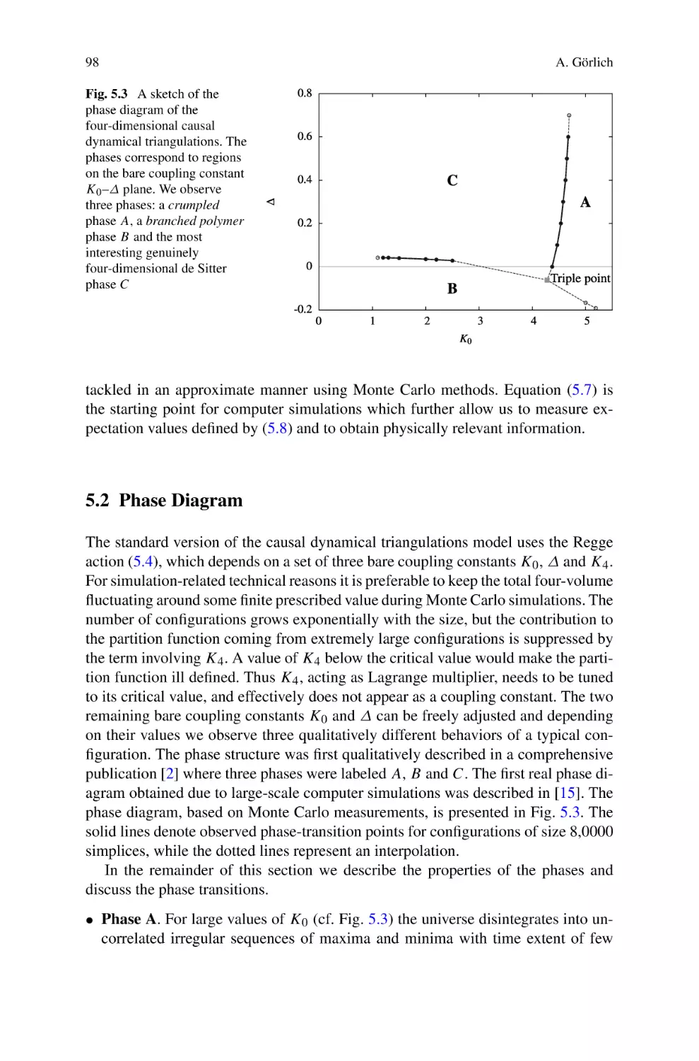
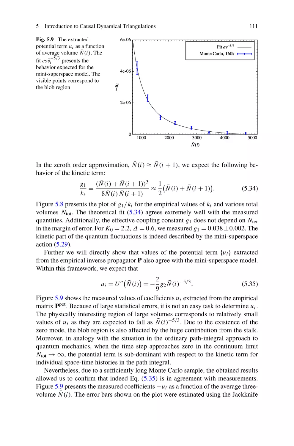
5.2 Phase Diagram . . . . . . . . . . . . . . . . . .
5.3 The Macroscopic de Sitter Universe . . . . . . .
5.3.1 The Spatial Volume . . . . . . . . . . .
5.3.2 The Mini-superspace Model . . . . . . .
5.3.3 The Four-Dimensional Space-Time . . .
5.4 Quantum Fluctuations . . . . . . . . . . . . . .
5.4.1 The Effective Action . . . . . . . . . . .
5.4.2 Flow of the Gravitational Constant . . .
5.5 The Geometry of Spatial Slices . . . . . . . . .
5.5.1 The Hausdorff Dimension . . . . . . . .
.
.
.
.
.
.
.
.
.
.
.
.
.
.
.
.
.
.
.
.
.
.
.
.
.
.
.
.
.
.
.
.
.
.
.
.
.
.
.
.
.
.
.
.
.
.
.
.
.
.
.
.
.
.
.
.
.
.
.
.
.
.
.
.
.
.
.
.
.
.
.
.
.
.
.
.
.
.
.
.
.
.
.
.
.
.
.
.
.
.
.
.
.
.
.
.
.
.
.
.
.
.
.
.
.
.
.
.
.
.
.
.
.
.
.
.
.
.
.
.
.
.
.
.
.
.
.
.
.
.
.
.
.
.
.
.
93
94
96
98
100
100
102
103
107
109
112
113
113
Contents
ix
5.5.2 Spectral Dimension . . . . . . . . . . . . . . . . . . . . . 115
5.6 Conclusions . . . . . . . . . . . . . . . . . . . . . . . . . . . . . 116
References . . . . . . . . . . . . . . . . . . . . . . . . . . . . . . . . . 116
6
Massive Gravity: A Primer . . . . . . . . . . . . .
E.A. Bergshoeff, M. Kovacevic, J. Rosseel, and Y. Yin
6.1 Introduction . . . . . . . . . . . . . . . . . . .
6.2 General Spin . . . . . . . . . . . . . . . . . . .
6.2.1 “Boosting up the Derivatives” . . . . . .
6.2.2 “Taking the Square Root” . . . . . . . .
6.3 Spin 1 . . . . . . . . . . . . . . . . . . . . . .
6.4 Spin 2 . . . . . . . . . . . . . . . . . . . . . .
6.4.1 3D New Massive Gravity . . . . . . . .
6.4.2 3D Topological Massive Gravity . . . .
6.4.3 Extensions . . . . . . . . . . . . . . . .
6.5 Conclusions . . . . . . . . . . . . . . . . . . .
Appendix Exercises . . . . . . . . . . . . . . . . .
References . . . . . . . . . . . . . . . . . . . . . . .
.
.
.
.
.
.
.
.
.
.
.
.
119
121
121
125
126
131
131
136
138
139
139
144
Loop Quantum Cosmology, Space-Time Structure, and Falsifiability
Martin Bojowald
7.1 Introduction . . . . . . . . . . . . . . . . . . . . . . . . . . . . .
7.2 Canonical Gravity . . . . . . . . . . . . . . . . . . . . . . . . . .
7.2.1 Cosmic Subtleties . . . . . . . . . . . . . . . . . . . . . .
7.2.2 Deformations of Space . . . . . . . . . . . . . . . . . . .
7.2.3 Gauge Theory . . . . . . . . . . . . . . . . . . . . . . . .
7.2.4 Quantum Corrections . . . . . . . . . . . . . . . . . . . .
7.3 Loop Quantum Gravity . . . . . . . . . . . . . . . . . . . . . . .
7.3.1 Corrections from Loop Quantum Gravity . . . . . . . . . .
7.3.2 Construction of Inverse-Triad Corrections . . . . . . . . .
7.3.3 Anomaly-Freedom . . . . . . . . . . . . . . . . . . . . . .
7.3.4 Falsifiability . . . . . . . . . . . . . . . . . . . . . . . . .
7.3.5 Anomaly-Free Holonomy Corrections . . . . . . . . . . .
7.4 Effective Theories . . . . . . . . . . . . . . . . . . . . . . . . . .
7.4.1 Effective Canonical Dynamics . . . . . . . . . . . . . . .
7.4.2 Moment Dynamics . . . . . . . . . . . . . . . . . . . . . .
7.4.3 Effective Constraints . . . . . . . . . . . . . . . . . . . . .
7.4.4 Isotropic Cosmology . . . . . . . . . . . . . . . . . . . . .
7.4.5 Beginning . . . . . . . . . . . . . . . . . . . . . . . . . .
7.5 Conclusions . . . . . . . . . . . . . . . . . . . . . . . . . . . . .
References . . . . . . . . . . . . . . . . . . . . . . . . . . . . . . . . .
149
Part II
7
8
. . . . . . . . . . 119
.
.
.
.
.
.
.
.
.
.
.
.
.
.
.
.
.
.
.
.
.
.
.
.
.
.
.
.
.
.
.
.
.
.
.
.
.
.
.
.
.
.
.
.
.
.
.
.
.
.
.
.
.
.
.
.
.
.
.
.
.
.
.
.
.
.
.
.
.
.
.
.
.
.
.
.
.
.
.
.
.
.
.
.
.
.
.
.
.
.
.
.
.
.
.
.
.
.
.
.
.
.
.
.
.
.
.
.
Quantum Cosmology
149
153
154
156
157
159
160
162
163
164
166
167
168
170
172
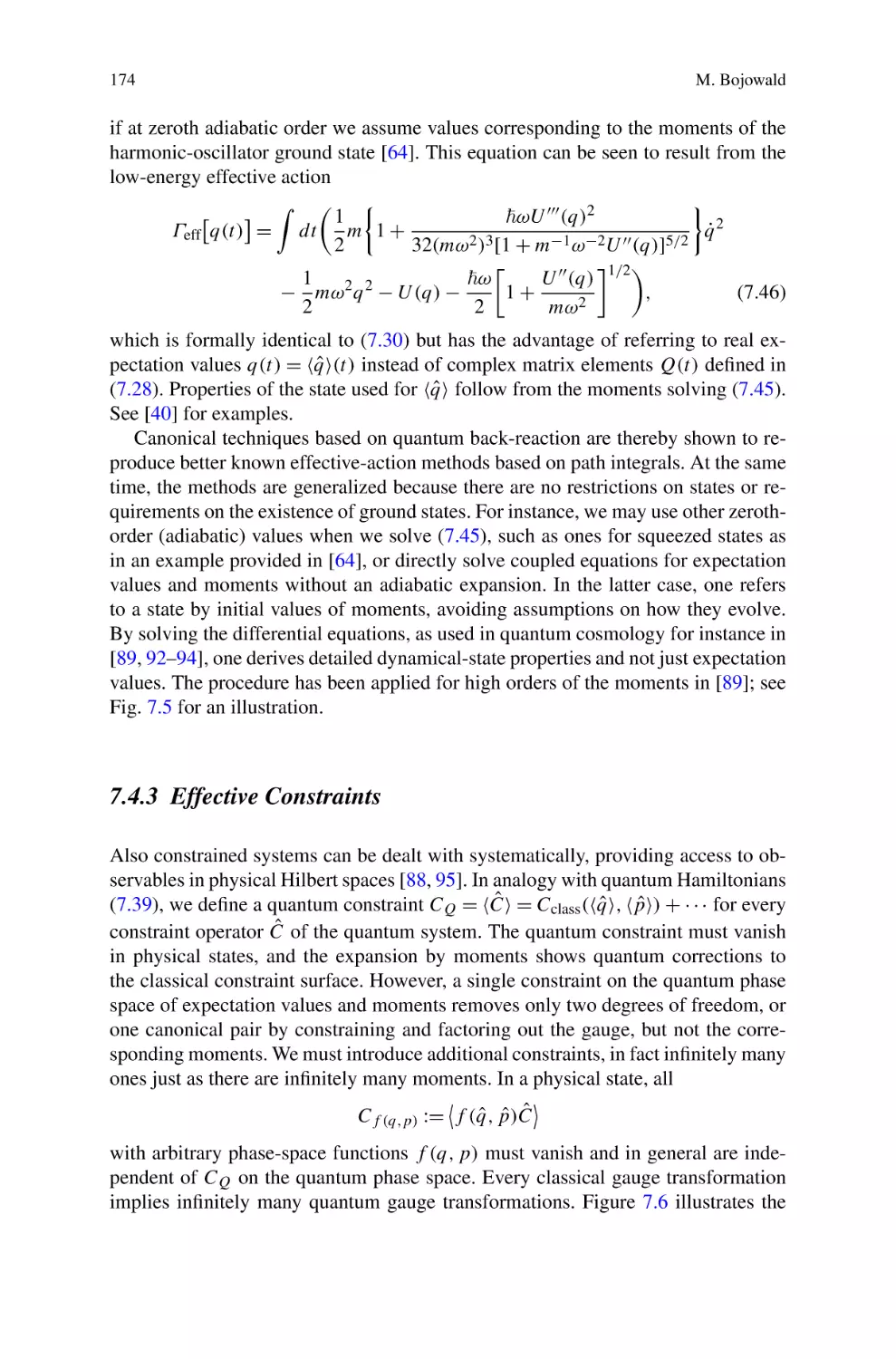
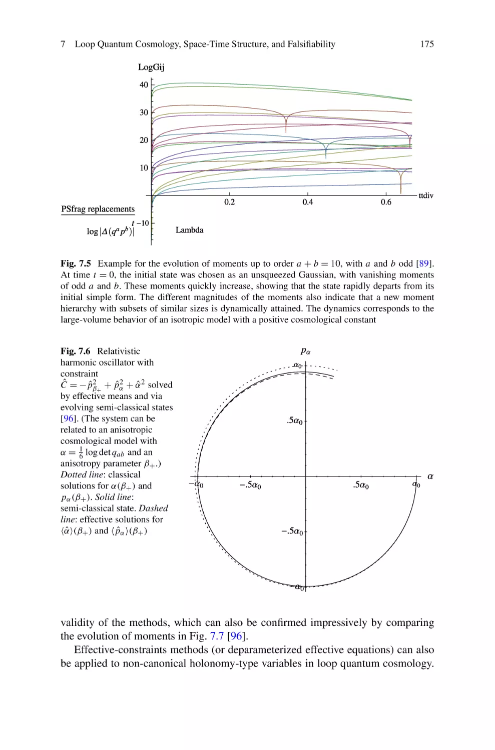
174
177
179
181
181
Asymptotic Safety, Fractals, and Cosmology . . . . . . . . . . . . . . 185
Martin Reuter and Frank Saueressig
8.1 Introduction . . . . . . . . . . . . . . . . . . . . . . . . . . . . . 185
x
Contents
8.2
8.3
8.4
8.5
8.6
8.7
9
Theory Space and Its Truncation . . . . . . . . . . . . . . . . .
The Effective Average Action for Gravity . . . . . . . . . . . . .
The Einstein–Hilbert Truncation . . . . . . . . . . . . . . . . .
The Multi-fractal Properties of QEG Space-Times . . . . . . . .
Spectral, Walk, and Hausdorff Dimension . . . . . . . . . . . . .
Fractal Dimensions Within QEG . . . . . . . . . . . . . . . . .
8.7.1 Diffusion Processes on QEG Space-Times . . . . . . . .
8.7.2 The Spectral Dimension in QEG . . . . . . . . . . . . .
8.7.3 The Walk Dimension in QEG . . . . . . . . . . . . . . .
8.7.4 The Hausdorff Dimension in QEG . . . . . . . . . . . .
8.7.5 Relations Between Dimensions . . . . . . . . . . . . . .
8.8 The RG Running of Ds and Dw . . . . . . . . . . . . . . . . . .
8.9 Matching the Spectral Dimensions of QEG and CDT . . . . . . .
8.10 Asymptotic Safety in Cosmology . . . . . . . . . . . . . . . . .
8.10.1 RG Improved Einstein Equations . . . . . . . . . . . . .
8.10.2 Solving the RG Improved Einstein Equations . . . . . . .
8.10.3 Inflation in the Fixed-Point Regime . . . . . . . . . . . .
8.10.4 Entropy and the Renormalization Group . . . . . . . . .
8.10.5 Primordial Entropy Generation . . . . . . . . . . . . . .
8.10.6 Entropy Production for RG Trajectory Realized by Nature
8.11 Conclusions . . . . . . . . . . . . . . . . . . . . . . . . . . . .
References . . . . . . . . . . . . . . . . . . . . . . . . . . . . . . . .
.
.
.
.
.
.
.
.
.
.
.
.
.
.
.
.
.
.
.
.
.
.
Holography for Inflationary Cosmology . . . . . . . . .
Paul McFadden
9.1 Introduction . . . . . . . . . . . . . . . . . . . . . .
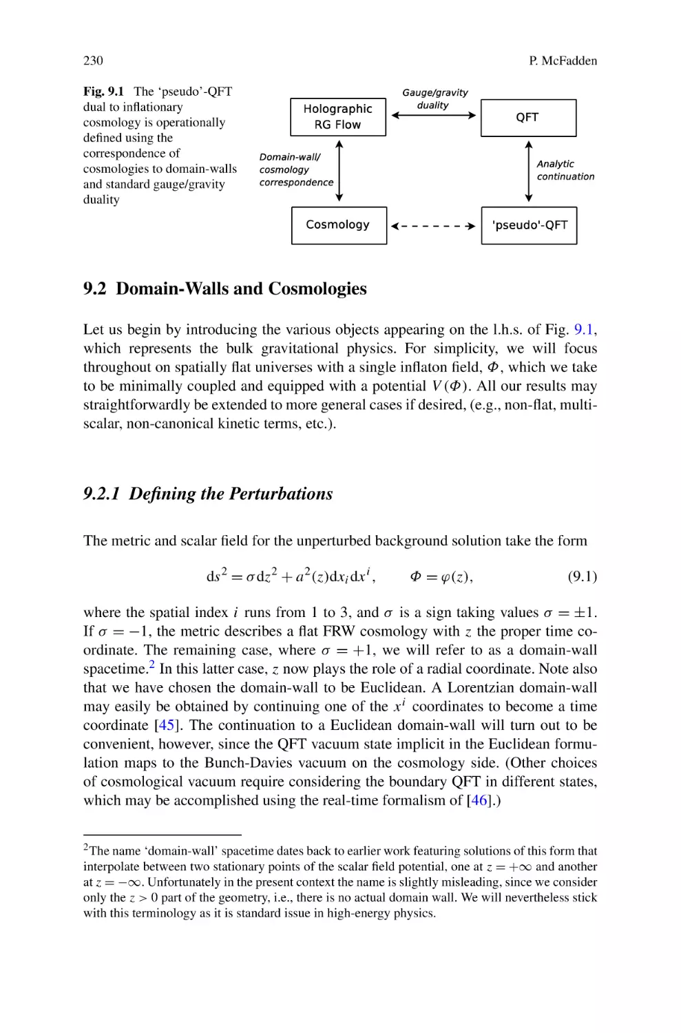
9.2 Domain-Walls and Cosmologies . . . . . . . . . . . .
9.2.1 Defining the Perturbations . . . . . . . . . . .
9.2.2 Dynamics . . . . . . . . . . . . . . . . . . .
9.2.3 The Domain-Wall/Cosmology Correspondence
9.2.4 Cosmological Power Spectra . . . . . . . . .
9.3 Holography for Cosmology . . . . . . . . . . . . . .
9.3.1 Background Solutions . . . . . . . . . . . . .
9.3.2 Basics of Holography . . . . . . . . . . . . .
9.3.3 Hamiltonian Holographic Renormalisation . .
9.3.4 The Stress Tensor 2-Point Function . . . . . .
9.3.5 Holographic Analysis . . . . . . . . . . . . .
9.3.6 Holographic Formulae for the Power Spectra .
9.4 Holographic Phenomenology for Cosmology . . . . .
9.4.1 A Prototype Dual QFT . . . . . . . . . . . . .
9.4.2 Calculating the Holographic Power Spectra . .
9.5 Confronting Observations . . . . . . . . . . . . . . .
9.6 Conclusion . . . . . . . . . . . . . . . . . . . . . . .
References . . . . . . . . . . . . . . . . . . . . . . . . . .
.
.
.
.
.
.
.
.
.
.
.
.
.
.
.
.
.
.
.
188
192
194
197
200
202
202
204
206
206
207
207
210
213
214
214
215
217
219
221
223
223
. . . . . . . 227
.
.
.
.
.
.
.
.
.
.
.
.
.
.
.
.
.
.
.
.
.
.
.
.
.
.
.
.
.
.
.
.
.
.
.
.
.
.
.
.
.
.
.
.
.
.
.
.
.
.
.
.
.
.
.
.
.
.
.
.
.
.
.
.
.
.
.
.
.
.
.
.
.
.
.
.
.
.
.
.
.
.
.
.
.
.
.
.
.
.
.
.
.
.
.
.
.
.
.
.
.
.
.
.
.
.
.
.
.
.
.
.
.
.
227
230
230
232
234
236
237
238
238
240
243
244
249
250
251
252
257
263
265
Contents
xi
Part III Observational Status
10
11
Observational Status of Dark Matter . . . . .
Joseph Silk
10.1 Introduction . . . . . . . . . . . . . . . .
10.2 The Observational Case . . . . . . . . . .
10.3 From Galaxies to Clusters . . . . . . . .
10.3.1 Galaxy Rotation Curves . . . . .
10.4 Large-Scale Structure . . . . . . . . . . .
10.4.1 Redshift Space Distortions . . .
10.4.2 Baryon Acoustic Oscillations . .
10.4.3 Cosmic Microwave Background
10.5 Future Prospects in Observation . . . . .
10.6 Future Prospects in Astrophysical Theory
10.7 Direct Detection . . . . . . . . . . . . . .
10.8 Indirect Detection . . . . . . . . . . . . .
10.8.1 Helioseismology . . . . . . . . .
10.8.2 High Energy Cosmic Rays . . .
10.8.3 Gamma Rays . . . . . . . . . .
10.8.4 The WMAP Microwave Haze . .
10.8.5 Decaying Dark Matter . . . . . .
10.9 The Future . . . . . . . . . . . . . . . . .
10.9.1 The Sun . . . . . . . . . . . . .
10.9.2 Direct Detection . . . . . . . . .
10.9.3 Air Cerenkov Telescopes . . . .
10.9.4 Strange Stars . . . . . . . . . . .
10.9.5 The Galactic Centre . . . . . . .
10.9.6 LHC . . . . . . . . . . . . . . .
10.10 Summary . . . . . . . . . . . . . . . . .
References . . . . . . . . . . . . . . . . . . . .
. . . . . . . . . . . . 271
.
.
.
.
.
.
.
.
.
.
.
.
.
.
.
.
.
.
.
.
.
.
.
.
.
.
.
.
.
.
.
.
.
.
.
.
.
.
.
.
.
.
.
.
.
.
.
.
.
.
.
.
.
.
.
.
.
.
.
.
.
.
.
.
.
.
.
.
.
.
.
.
.
.
.
.
.
.
.
.
.
.
.
.
.
.
.
.
.
.
.
.
.
.
.
.
.
.
.
.
.
.
.
.
.
.
.
.
.
.
.
.
.
.
.
.
.
.
.
.
.
.
.
.
.
.
.
.
.
.
.
.
.
.
.
.
.
.
.
.
.
.
.
.
.
.
.
.
.
.
.
.
.
.
.
.
.
.
.
.
.
.
.
.
.
.
.
.
.
.
.
.
.
.
.
.
.
.
.
.
.
.
.
.
.
.
.
.
.
.
.
.
.
.
.
.
.
.
.
.
.
.
.
.
.
.
.
.
.
.
.
.
.
.
.
.
.
.
.
.
.
.
.
.
.
.
.
.
.
.
.
.
.
.
Dark Energy: Observational Status and Theoretical Models .
Shinji Tsujikawa
11.1 Introduction . . . . . . . . . . . . . . . . . . . . . . . . .
11.2 Observational Constraints on Dark Energy . . . . . . . . .
11.2.1 Supernovæ Ia Observations . . . . . . . . . . . .
11.2.2 CMB . . . . . . . . . . . . . . . . . . . . . . . .
11.2.3 BAO . . . . . . . . . . . . . . . . . . . . . . . .
11.3 Cosmological Constant . . . . . . . . . . . . . . . . . . .
11.4 Modified Matter Models . . . . . . . . . . . . . . . . . .
11.4.1 Quintessence . . . . . . . . . . . . . . . . . . . .
11.4.2 k-Essence . . . . . . . . . . . . . . . . . . . . .
11.4.3 Coupled Dark Energy . . . . . . . . . . . . . . .
11.4.4 Unified Models of Dark Energy and Dark Matter .
11.5 Modified Gravity Models . . . . . . . . . . . . . . . . . .
11.5.1 f (R) Gravity . . . . . . . . . . . . . . . . . . .
.
.
.
.
.
.
.
.
.
.
.
.
.
.
.
.
.
.
.
.
.
.
.
.
.
.
.
.
.
.
.
.
.
.
.
.
.
.
.
.
.
.
.
.
.
.
.
.
.
.
.
.
.
.
.
.
.
.
.
.
.
.
.
.
.
.
.
.
.
.
.
.
.
.
.
.
.
.
271
272
272
272
274
274
275
275
275
276
279
279
280
280
281
281
282
282
282
283
283
283
284
284
284
285
. . . 289
.
.
.
.
.
.
.
.
.
.
.
.
.
.
.
.
.
.
.
.
.
.
.
.
.
.
.
.
.
.
.
.
.
.
.
.
.
.
.
289
291
291
294
296
298
300
301
304
307
311
313
313
xii
Contents
11.5.2 Scalar-Tensor Theories
11.5.3 DGP Model . . . . . .
11.6 Conclusions . . . . . . . . . . .
References . . . . . . . . . . . . . . .
12
13
.
.
.
.
.
.
.
.
.
.
.
.
.
.
.
.
.
.
.
.
.
.
.
.
.
.
.
.
.
.
.
.
.
.
.
.
.
.
.
.
.
.
.
.
.
.
.
.
.
.
.
.
.
.
.
.
.
.
.
.
Unconventional Cosmology . . . . . . . . . . . . . . . . . . . .
Robert H. Brandenberger
12.1 Introduction . . . . . . . . . . . . . . . . . . . . . . . . .
12.1.1 Overview . . . . . . . . . . . . . . . . . . . . .
12.1.2 Review of Inflationary Cosmology . . . . . . . .
12.1.3 Conceptual Problems of Inflationary Cosmology .
12.2 Matter Bounce . . . . . . . . . . . . . . . . . . . . . . .
12.2.1 The Idea . . . . . . . . . . . . . . . . . . . . . .
12.2.2 Realizing a Matter Bounce with Modified Matter .
12.2.3 Realizing a Matter Bounce with Modified Gravity
12.3 Emergent Universe . . . . . . . . . . . . . . . . . . . . .
12.3.1 The Idea . . . . . . . . . . . . . . . . . . . . . .
12.3.2 String Gas Cosmology . . . . . . . . . . . . . .
12.4 Cosmological Perturbations . . . . . . . . . . . . . . . . .
12.4.1 Overview . . . . . . . . . . . . . . . . . . . . .
12.5 Fluctuations in Inflationary Cosmology . . . . . . . . . .
12.6 Matter Bounce and Structure Formation . . . . . . . . . .
12.6.1 Basics . . . . . . . . . . . . . . . . . . . . . . .
12.6.2 Specific Predictions . . . . . . . . . . . . . . . .
12.7 String Gas Cosmology and Structure Formation . . . . . .
12.7.1 Overview . . . . . . . . . . . . . . . . . . . . .
12.7.2 Spectrum of Cosmological Fluctuations . . . . .
12.7.3 Key Prediction of String Gas Cosmology . . . . .
12.7.4 Comments . . . . . . . . . . . . . . . . . . . . .
12.8 Conclusions . . . . . . . . . . . . . . . . . . . . . . . . .
References . . . . . . . . . . . . . . . . . . . . . . . . . . . . .
.
.
.
.
.
.
.
.
.
.
.
.
.
.
.
.
.
.
.
.
.
.
.
.
Quantum Gravity and Inflation . . . . . . . .
M.G. Romania, N.C. Tsamis, and R.P. Woodard
13.1 Introduction . . . . . . . . . . . . . . . .
13.2 Model Building . . . . . . . . . . . . . .
13.3 Post-Inflationary Evolution . . . . . . . .
13.4 Conclusions . . . . . . . . . . . . . . . .
References . . . . . . . . . . . . . . . . . . . .
.
.
.
.
.
.
.
.
.
.
.
.
.
319
323
325
326
. . . 333
.
.
.
.
.
.
.
.
.
.
.
.
.
.
.
.
.
.
.
.
.
.
.
.
.
.
.
.
.
.
.
.
.
.
.
.
.
.
.
.
.
.
.
.
.
.
.
.
333
333
335
337
339
339
342
344
345
345
347
351
351
355
356
357
359
361
361
363
365
367
367
368
. . . . . . . . . . . . 375
.
.
.
.
.
.
.
.
.
.
.
.
.
.
.
.
.
.
.
.
.
.
.
.
.
.
.
.
.
.
.
.
.
.
.
.
.
.
.
.
.
.
.
.
.
.
.
.
.
.
.
.
.
.
.
375
381
391
393
394
Index . . . . . . . . . . . . . . . . . . . . . . . . . . . . . . . . . . . . . . 397
Part I
Quantum Gravity
Chapter 1
String Theory, Unification and Quantum
Gravity
K.S. Stelle
Abstract An overview is given of the way in which the unification program of
particle physics has evolved into the proposal of superstring theory as a prime candidate for unifying quantum gravity with the other forces and particles of nature. A
key concern with quantum gravity has been the problem of ultraviolet divergences,
which is naturally solved in string theory by replacing particles with spatially extended states as the fundamental excitations. String theory turns out, however, to
contain many more extended-object states than just strings. Combining all this into
an integrated picture, called M-theory, requires recognition of the rôle played by a
web of nonperturbative duality symmetries suggested by the nonlinear structures of
the field-theoretic supergravity limits of string theory.
1.1 Introduction: The Ultraviolet Problems of Gravity
Our currently agreed picture of fundamental physics involves four principal forces:
strong, weak, electromagnetic; and gravitational. The first three are well described
by the Standard Model, based on the nonabelian gauge group SU(3)strong ×
(SU(2) × U (1))electroweak . In the process of unifying these forces, one necessarily
had to postulate new physical phenomena going beyond the specifically desired unification. Thus, in order to make the SU(2) × U (1) electroweak unification work, one
had also to accept also the neutral Z 0 field in addition to the desired charged W ±
intermediate vector fields (needed to resolve the interactions of the nonrenormalizable 4-fermion Fermi theory). The experimental discovery of the corresponding Z 0
particle was a great triumph of the Standard Model.
Another key ingredient of our current perspective is the notion of spontaneous
symmetry breaking: symmetries of the field equations may be broken by the vacuum, thus becoming non-linearly realized and at the same time allowing for the
generation of masses for gauge fields—known as the Higgs effect. The Standard
Model is moreover renormalizable: although ultraviolet infinities exist, they can be
K.S. Stelle (B)
Imperial College London, London SW7 2AZ, UK
e-mail: k.stelle@imperial.ac.uk
G. Calcagni et al. (eds.), Quantum Gravity and Quantum Cosmology,
Lecture Notes in Physics 863, DOI 10.1007/978-3-642-33036-0_1,
© Springer-Verlag Berlin Heidelberg 2013
3
4
K.S. Stelle
corralled into renormalizations of a finite set of parameters, thus allowing for consistent perturbative analysis of the rest of the theory. And most importantly, the
Standard Model is now confirmed to very high precision by experiments at CERN,
Fermilab and other laboratories.
Einstein’s General Theory of Relativity, on the other hand, is nonrenormalizable,
causing it to break down when interpreted as a quantum theory. One immediate indication
√ of this is the dimensional character of the gravitational coupling constant
κ = 8πG, which has dimensions of length (in units where = c = 1). Einstein
gravity’s uncontrolled divergences go on to corrupt otherwise well-behaved “matter” theories.
Consider, for example, a radiative correction to the Higgs mass caused by a
gauge-particle emission and reabsorption:
In the Standard Model, with gauge coupling constant g, incoming momentum p
and loop momentum k, the corresponding integral with a cutoff Λ has the form
g
2
Λ
d 4k
k2
k 2 ((p + k)2 + m2 )
(1.1)
which has logarithmic divergences ∼ g 2 ln Λ p 2 , requiring a counterterm (∂φ)2 and
also another ∼ g 2 ln Λ m2 , requiring a counterterm m2 φ 2 . Since both of these counterterm operators are present in the Standard Model Lagrangian from the start, they
can be accounted for by standard wavefunction and mass renormalizations.
When the system is coupled to gravity, however, the ultraviolet divergent integrals get much worse:
κ2
Λ
d 4k
k4
k 2 ((p + k)2
+ m2 )
(1.2)
producing now logarithmic divergences ∼ κ 2 ln Λ(p 4 , m2 p 2 , m4 ) in addition to the
flat-space SM divergences. The p 4 divergence would require a counterterm (∂ 2 φ)2 ,
which is an operator not present in the original theory. Moreover, this bad ultraviolet
behavior gets worse and worse as the loop-order increases. At two loops, one encounters divergences ∼ κ 4 ln Λp 6 + · · · , requiring a counterterm like (∂ 3 φ)2 . Each
new loop adds 2 to the divergence count. Thus, Einstein gravity is not only uncontrolled in its own divergence structure; it also renders otherwise well-behaved matter
theories such as the Standard Model uncontrollable when coupled to gravity.
Pure General Relativity has a naïve degree of divergence at L loops in spacetime dimension D given by Δ = (D − 2)L + 2. When confronting the ultraviolet
problem of quantum gravity, one wants to focus on the most serious divergent structures, whose elimination would require the introduction of genuinely new operators
not present in the classical Lagrangian. For this purpose, candidate counterterms
1 String Theory, Unification and Quantum Gravity
5
that vanish subject to the classical field equations can be handled by a more standard procedure, by making field-redefinition renormalizations, which generalize the
wavefunction renormalizations of renormalizable theories. Leaving these more easily handled divergence structures to one side, one searches for counterterm structures that do not vanish subject to the classical equations of motion.
Using dimensional regularization to ensure a manifestly generally-coordinateinvariant quantization, one captures only the logarithmic divergences of a straight
momentum-cutoff procedure. To balance engineering dimensions, this requires
a number of factors of external momentum to be present on the external lines
of a divergent diagram, in order to pick out just the logarithmically divergent
part. Accordingly, at L = 2 loops in D = 4 dimensions,
one expects Δ = 6,
4 x √−g(R
ρσ λτ R μν ) or
which
could
be
achieved
by
counterterms
like
d
μνρσ R
λτ
4 √
d x −g(Rμνρσ R ρσ μν ) where = g μν ∇μ ∇ν is a covariant d’Alembertian.
However, use of the Bianchi identities shows that the second of these types vanishes subject to the classical equations of motion, so it may be dealt with by fieldredefinition renormalizations. Only the first is a truly dangerous type. And indeed, in
pure GR, such a (curvature)3 counterterm does occur at the 2-loop order in D = 4.
[1, 2].
In supergravity theories, local supersymmetry places additional constraints on
counterterms. This has the consequence that the 2-loop divergence of pure GR is
absent. In pure supergravities, the first counterterm that does not vanish subject to
the classical equations of motion (“on-shell” in the jargon) then occurs at the 3-loop
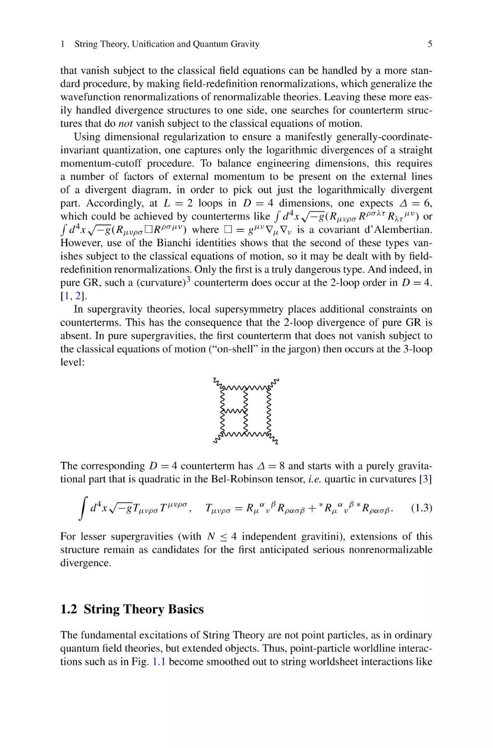
level:
The corresponding D = 4 counterterm has Δ = 8 and starts with a purely gravitational part that is quadratic in the Bel-Robinson tensor, i.e. quartic in curvatures [3]
√
(1.3)
d 4 x −gTμνρσ T μνρσ , Tμνρσ = Rμ α ν β Rρασβ + ∗ Rμ α ν β ∗ Rρασβ .
For lesser supergravities (with N ≤ 4 independent gravitini), extensions of this
structure remain as candidates for the first anticipated serious nonrenormalizable
divergence.
1.2 String Theory Basics
The fundamental excitations of String Theory are not point particles, as in ordinary
quantum field theories, but extended objects. Thus, point-particle worldline interactions such as in Fig. 1.1 become smoothed out to string worldsheet interactions like
6
K.S. Stelle
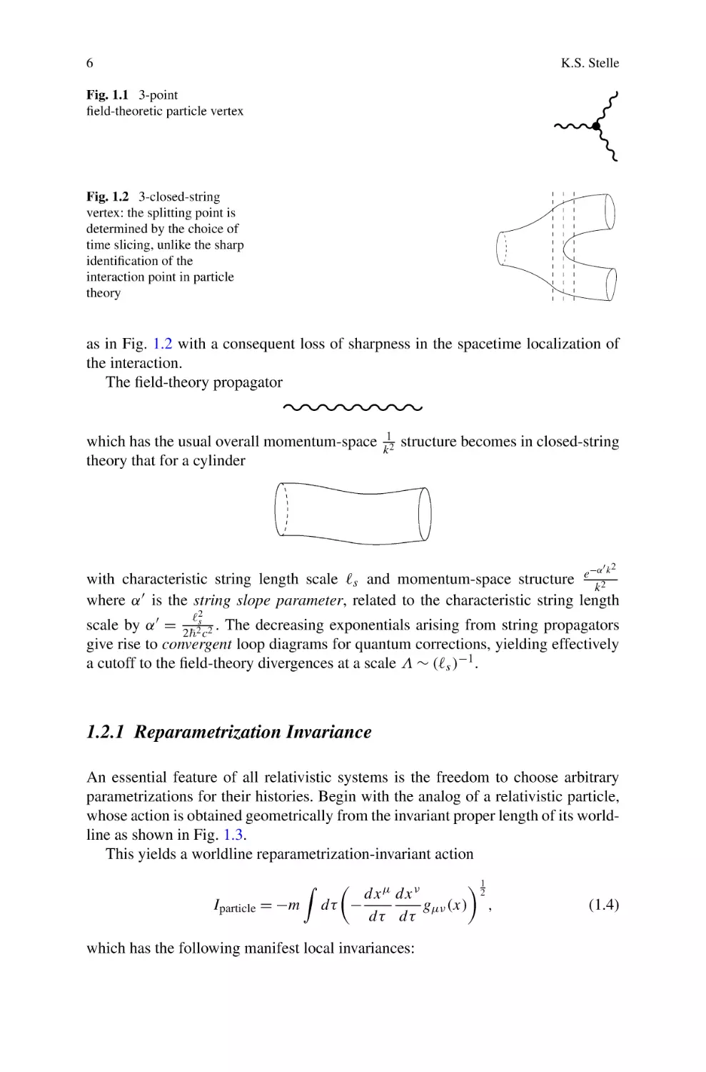
Fig. 1.1 3-point
field-theoretic particle vertex
Fig. 1.2 3-closed-string
vertex: the splitting point is
determined by the choice of
time slicing, unlike the sharp
identification of the
interaction point in particle
theory
as in Fig. 1.2 with a consequent loss of sharpness in the spacetime localization of
the interaction.
The field-theory propagator
which has the usual overall momentum-space
theory that for a cylinder
1
k2
structure becomes in closed-string
−α k 2
with characteristic string length scale s and momentum-space structure e k 2
where α is the string slope parameter, related to the characteristic string length
2
scale by α = 22sc2 . The decreasing exponentials arising from string propagators
give rise to convergent loop diagrams for quantum corrections, yielding effectively
a cutoff to the field-theory divergences at a scale Λ ∼ (s )−1 .
1.2.1 Reparametrization Invariance
An essential feature of all relativistic systems is the freedom to choose arbitrary
parametrizations for their histories. Begin with the analog of a relativistic particle,
whose action is obtained geometrically from the invariant proper length of its worldline as shown in Fig. 1.3.
This yields a worldline reparametrization-invariant action
Iparticle = −m
1
2
dx μ dx ν
gμν (x) ,
dτ −
dτ dτ
which has the following manifest local invariances:
(1.4)
1 String Theory, Unification and Quantum Gravity
7
Fig. 1.3 Particle worldline
1. Spacetime general covariance:
x μ → x μ (x)
∂x ρ ∂x σ
x = μ ν gρσ (x)
gμν
∂x ∂x
2. Worldline reparametrization invariance:
x μ τ = x μ (τ )
τ → τ dx μ
dx μ dx μ dτ
→
=
dτ
dτ
dτ dτ
(1.5)
(worldline scalar)
(1.6)
(worldline vector)
The worldline reparametrization invariance is physically important because it
removes a negative-energy mode: for a metric gμν of Minkowski signature (− +
+ + · · · ), the x 0 (τ ) “scalar field” along the d = 1 worldline has the wrong sign of
kinetic energy. However, this potential ghost mode is precisely removed from the
theory by the worldline reparametrization invariance.
As is generally the case for gauge theories, the worldline reparametrization invariance gives rise, in the Hamiltonian formalism, to a constraint on the conjugate
momenta:
∂L
pμ pν g μν (x) = −m2 , where pμ = ∂x μ .
(1.7)
∂( ∂τ )
Thus, for a particle in D dimensional spacetime, (D − 1) degrees of freedom remain
after taking into account the worldline reparametrization invariance and the corresponding Hamiltonian constraint. The constraint (1.7) is recognized as the massshell condition for the relativistic particle.
1.2.2 The String Action
Now generalize the relativistic particle action to that of a relativistic extended object
with intrinsic spatial dimensionality p = 1. Instead of a worldline, one now has a
8
K.S. Stelle
Fig. 1.4 Open string
worldsheet
2-dimensional worldsheet as illustrated in Fig. 1.4 for an open string; for a closed
string, one needs to identify σ = 0 and σ = π .
The string worldsheet action is then the reparametrization-invariant area of the
worldsheet W
1
d 2 ξ −det ∂i x μ (ξ )∂j x ν (ξ )gμν x(ξ ) 2 .
(1.8)
Istring = −T
W
As in the particle case, one has a number of local worldsheet invariances:
1. Spacetime general covariance x μ (τ, σ ) → x μ (τ, σ ).
2. d = 2 worldsheet reparametrization invariance x μ (τ , σ ) = x μ (τ, σ ).
3. Exceptionally for the d = 2 ↔ p = 1 case among the general class of “pbranes”, one has an additional local worldsheet invariance: Weyl invariance.
Weyl invariance is crucial to the ability to carry out quantization of the string.
Jealously preserving it leads to the notion of a critical dimension for string theory.
To see the Weyl invariance, reformulate the string action with an independent
worldsheet metric γij (ξ ) [4–6]:
1
Istring DZBdVHP = − T
2
d 2 ξ − det γ γ ij (ξ )Mij
(1.9)
where Mij = ∂i x μ ∂j x ν gμν (x) is the induced metric on the worldsheet and γ ij is
the matrix inverse of γj k . Varying γij (ξ ) as an independent field, obtain its field
equation (γ ik γ j l − 12 γ ij γ kl )Mkl = 0. Note that for d = 2 worldsheet dimensions,
the trace of this equation vanishes identically: γ kl Mkl − 12 γ ij γij γ kl Mkl ≡ 0.
This weakening of the set of algebraic equations for γij corresponds to the local
Weyl invariance of the DZBdVHP action:
γij → Ω(ξ )γij
ξi → ξi
(1.10)
(1.11)
1 String Theory, Unification and Quantum Gravity
9
where Ω(ξ ) is an arbitrary positive local scale factor. Varying the string action,
one obtains the algebraic equation determining γij (ξ ) = Ω(ξ )Mij , with Ω(ξ ) left
undetermined, and the d = 2 covariant wave equation for x μ (ξ ):
i
μ
∇(γ
,g) ∂i x = 0.
(1.12)
For closed bosonic strings, the wave equation (1.12), plus periodicity in the spatial worldsheet coordinate σ (conventionally taken to identify σ = 0 with σ = π ),
give the full classical dynamical system of closed-string equations.
For open strings, the σ coordinate is conventionally considered to take its values
in the closed interval σ ∈ [0, π]. Then, considering also the surface term arising
in the variation of IDZBdVHP upon integration by parts, one finds in addition the
following Neumann boundary conditions:
M0i ik ∂k x μ = 0
at σ = 0, π.
(1.13)
Considering strings in a flat spacetime background, gμν = ημν , and picking conformal gauge for the worldsheet reparametrization symmetries, γij =
Ω(ξ ) diag(−1, 1), the x μ (ξ ) wave equation and open-string boundary conditions
become
x μ = 0
∂ μ
x =0
∂σ
where = ηij ∂i ∂j is the flat-space d = 2 d’Alembertian (1.14)
at σ = 0, π.
(1.15)
These may be interpreted classically as requiring waves to travel back and forth
along the string at speed c = 1, while the boundary conditions imply that the endpoints of the open string travel through the embedding spacetime at speed c = 1.
For closed strings, there are periodicity conditions instead of reflective boundary conditions. In that case, there can be independent left- and right-moving waves
travelling around the string at speed c = 1.
A simple solution to the open-string equations of motion and boundary conditions is
1 + A2
1 + A2
0
3
x =
x =
(1.16)
p + + τ
p − + τ
2
p
2
p
x 1 = A cos σ cos τ
x 2 = A cos σ sin τ.
(1.17)
2
Boosting to a Minkowski reference frame where x 3 = 0, find p + = pA+ = ±A; in
this frame, the center-of-mass of the open string at σ = π/2 remains stationary
while the string profile at any time τ describes a straight line of length 2A rotating
with period 2πA (with respect to the background Minkowski time t = x 0 = Aτ ).
The total string energy for this solution is E = π2 T , where = 2A is the string
length. Thus, the parameter T should be interpreted as the string tension.
E2
The angular momentum for this solution is J 3 = π8 2 T = 2πT
. This linear rela2
tionship between angular momentum and (energy) is known as Regge behavior.
10
K.S. Stelle
Fig. 1.5 Linear Regge
trajectories relating spin and
(mass)2 of particle states
One can now make a rough Bohr-Sommerfeld estimate of the quantum spectrum,
requiring |J | = n, n ∈ Z and considering the excitations in their rest frames where
1
E = M. Then n = |J| = α M 2 where α = 2πcT
is the string slope parameter. The
quantized states lie on linear Regge trajectories making an angle α in a J / versus
M 2 plot (see Fig. 1.5).
Of course, finding such Regge trajectories in the physical particle spectrum
would be a spectacular confirmation of string theory.
The above semiclassical analysis makes the lowest-lying string state a massless
scalar. However, a more careful quantum analysis reveals a feature missed by the
Bohr-Sommerfeld analysis: the intercept at n = 0 is shifted down: α E 2 = n − 1 ↔
M 2 = n−1
. Thus, the n = 0 lowest-lying state of the bosonic string becomes a negα c4
2
ative M tachyon, while the n = 1 first excited state with |J | = becomes massless. Accordingly, the open-string quantum spectrum contains massless spin 1 gauge
fields.
The closed string dispenses with the reflective open-string boundary conditions
and accordingly has twice as many modes: independent left- and right-moving excitations. It turns out that the closed-string spectrum is a tensor product of open-string
spectra in the R & L sectors, together with a level-matching condition: the R and L
level numbers must be equal. The closed-string (nL , nR ) = (1, 1) states thus contain the tensor product of (spin 1)L × (spin 1)R states: the closed-string spectrum
contains massless spin 2.
1.3 Effective Field Equations
The spin 2 mode identified in the closed-string spectrum is not merely a hint that
closed-string theory has something to do with gravity. The full Einstein action also
emerges when one considers string theory from an effective-field-theory point of
view. The key to understanding this is the requirement that anomalies in the local
Weyl symmetry cancel.
1 String Theory, Unification and Quantum Gravity
11
Analysis of the spectrum of any string theory shows the presence of at least three
types of massless field: the graviton gμν (x), a 2-form antisymmetric tensor gauge
field Bμν (x) and a “dilatonic” scalar φ(x). In supersymmetric theories, the infamous tachyon of bosonic string theory is absent. In non-supersymmetric contexts,
the tachyon is interpreted as indicating that the presumed “vacuum” around which
one is trying to quantize is unstable and so one should shift instead to a stable vacuum background. This shift is made explicit in string field theory.
To begin with, consider just the massless backgrounds (gμν (x), Bμν (x), φ(x)).
The string action on this effective-field background is then
Igen. back.
=−
1
4πα
√
d 2 ξ −γ γ ij gμν (x) − ij Bμν (x) ∂i x μ ∂j x ν + α R(γ )φ(x) .
(1.18)
Note that the 2-form background gauge field Bμν (x) has rank needed to pull
back using ∂i x μ to a 2-form on the worldsheet, precisely as needed to contract with
the d = 2 Levi-Civita tensor ij . Note also that the coupling to the dilaton φ(x)
involves the worldsheet Ricci scalar R(γ ) and enters with an additional factor of α ,
as is appropriate if gμν , Bμν , φ and γij are all taken to be dimensionless.
The worldsheet Weyl symmetry γij (ξ ) → Ω(ξ )γij (ξ ) is respected by the Bμν
√
ij = ij
coupling (since −γ tensor
density is γij independent), but it is violated by the dilaton coupling φR(γ ). This is intentional: the dilaton coupling is introduced precisely
to complete the cancellation of Weyl-symmetry anomalies arising in the perturbative
α expansion.
Igen. back. is manifestly invariant under spacetime general coordinate transfor
mations x μ → x μ provided gμν and Bμν transform as tensors and the dilaton
φ is a scalar. It is also invariant under the Bμν gauge transformation Bμν →
Bμν + ∂μ ζν − ∂ν ζμ , which causes the integrand of Igen. back. to vary by a total derivative.
The general-coordinate and 2-form gauge invariances are precisely what are
needed to give agreement with the expected degree-of-freedom counts for these
( 1 D(D − 3), 12 (D − 2)(D − 3))
.
massless backgrounds: 2
metric
2-form
Imposing on this background-coupled string system the requirement that the
Weyl symmetry anomalies cancel gives differential-equation restrictions on the
background fields (gμν , Bμν , φ); these may be viewed as effective field equations
for these massless modes.
The system of effective field equations for (gμν , Bμν , φ) is, remarkably, derivable
from an effective action for the D dimensional massless modes [7].
√
3
Ieff = d D x −ge−2φ (D − 26) − α R + 4∇ 2 φ − 4(∇φ)2
2
−
2
1
Fμνρ F μνρ + O α .
12
(1.19)
12
K.S. Stelle
Note the appearance of a critical dimension: the “cosmological term” vanishes
only for D = 26, showing that, for a flat background, the Weyl anomalies can be
cancelled in this way only in 26 dimensional spacetime.
In superstring theories, there are additional anomaly contributions from the
fermionic modes which change the critical dimension to 10. Moreover, in supergravity theories, the tachyon is absent, so D = 10 flat space becomes a stable background of the massless modes. Aside from the change of the critical dimension to
10, however, the above effective action remains valid for a subset of the bosonic
background of the theory, known as the Neveu-Schwarz sector.
Now specialize to D = 10 for the superstring and accordingly drop the cosmological term. Moreover, the unfamiliar e−2φ factor in front of the Ricci scalar
R may be eliminated together with the 4e−2φ ∇ 2 φ term by redefining the metric:
(e)
(s)
gμν = e−φ/2 gμν where g (s) is the previous string-frame metric and g (e) is the new
Einstein-frame metric.
In the Einstein frame, the Neveu-Schwarz sector effective action then becomes
IEinstein =
1
1
d 10 x −g (e) R g (e) − ∇μ φ∇ μ φ − e−φ Fμνρ F μνρ .
2
12
(1.20)
Including effective-action contributions for the other (Ramond sector) bosonic
backgrounds and also for fermionic backgrounds, one obtains thus a correspondence between superstring theories and related supergravity theories: a supergravity
theory describes the massless field-theory sector of the corresponding superstring
theory. One obtains in this way effective supergravity theories for the following
superstring theory variants: type IIA, type IIB, type I with gauge group SO(32),
heterotic SO(32) and heterotic E8 × E8 .
1.4 Dimensional Reduction and T-Duality
In order to extract a more realistic physical scenario from the higher-dimensional
contexts native to string theory, one needs to reduce the effective theory down to
D = 4 one way or another. The most straightforward way to do this is by a traditional
Kaluza-Klein reduction.
The basic idea can be explained in terms of a massless scalar field in D = 5 on a
spacetime with the 5th direction periodically identified: y ∼ y + 2πR. Periodicity
requirements on the de Broglie waves eipy/R then require the momenta in the y
μ
direction to be quantized, pn = n
R . Thus, expand the D = 5 field φ(x , y), μ =
0, 1, 2, 3, using a complete set of eigenfunctions of the Laplace operator on a circle,
i.e. in terms of plane waves with quantized momenta:
μ iny/R
φ xμ, y =
φn x e
.
n∈Z
(1.21)
1 String Theory, Unification and Quantum Gravity
13
Inserting this expansion into the D = 5 Klein-Gordon field equation gives an
infinite number of D = 4 equations for the independent modes φn (x μ ):
1 ∂ 2 φn
n2
2
−
∇
φ
+
φn = 0.
n
c2 ∂t 2
R2
(1.22)
n
.
Thus, the n = 0 modes φn are massive, with masses mn = R
The basic physical picture is that at energies low compared to cR , the massive
modes φn>0 are frozen out, so the theory effectively reduces to just φ0 . Dimensional reduction of the supergravity theories associated to the various D = 10 string
theories produces the family of supergravity theories existing in lower spacetime
dimensions, including the maximally extended N = 8 supergravity in D = 4.
1.4.1 Dimensional Reduction of Strings and T-Duality
Consider now string theory in a background spacetime with a compactified direction, x M → (x μ , y), μ = 0, . . . , (D − 2). The Regge towers of string states can
be individually treated as particle fields; massless string states give rise to massless states in the (D − 1) lower dimensions plus Kaluza-Klein towers of states with
n
masses R
, just like in Kaluza-Klein field theory.
Strings, however, can do something different from particles in that they can wrap
around the compactified dimension. Consider a closed-string mode expansion
x M (τ, σ ) = q M (τ ) + p M 2 τ + 2ñRσ δyM
i αkM −2ik(τ −σ ) α̃kM −2ik(τ +σ )
e
e
+
+
2
k
k
(1.23)
k =0
where n, ñ ∈ Z and 2 = 2α , the (string length)2 .
As expected, the momentum in the compactified direction is quantized, p y =
n
R . However, owing to the fact that the string can wind around the compactified y
dimension a number ñ times (Fig. 1.6), the energy (i.e. mass) formula for the string
spectrum considered from the viewpoint of the dimensionally reduced theory has a
generalized form:
2 n 2
ñ2 R 2
M2 = 2
+ contributions from ordinary oscillator modes. (1.24)
+
c R2
α2
This mass formula suggests a striking symmetry of string theory that is not
present for particle theories: interchanging n ↔ ñ and simultaneously inverting the
compactification radius, R → α /R leaves the spectrum invariant.
This symmetry is T-duality: a string propagating on a compact direction of radius R with momentum mode n and winding mode ñ is equivalent to a string propagating on a compact direction of radius α /R with interchanged mode numbers:
momentum ñ and winding n.
14
K.S. Stelle
Fig. 1.6 Winding modes
with various ñ values
Because string and background configurations related by a T-duality transformation are identified, this symmetry, although discrete, extends the notion of local
symmetry in string theory beyond the ordinary context of general coordinate and
gauge invariances.
T-duality has a dramatic effect on curved background geometries. Start from a
simplified closed-string action without the dilaton:
Ig,B
1
=−
2
√
d 2 ξ −γ γ ij ∂i x M ∂j x N gMN − ij ∂i x M ∂j x N BMN .
(1.25)
Now suppose that there is an isometry in the y direction, i.e. that gMN and BMN
don’t depend on y. Of course, y(τ, σ ) is still a string variable—the string is not prevented from moving in the y direction of spacetime. But the background functional
dependence on y is trivial owing to the isometry. Accordingly, the string variable
y(τ, σ ) appears only through its derivative ∂i y.
vector. Enforce
Now replace ∂i y everywhere in the action by vi , a worldsheet
√
the curl-free nature of vi by a Lagrange multiplier term d 2 ξ −γ ij ∂i zvj . Then
eliminate vi by its algebraic equation of motion. The result is the T-dualized version
of the string action written in terms of x̃ M̃ (τ, σ ) = (x μ (τ, σ ), z(τ, σ )).
The net effect of a T-duality transformation may be seen by reassembling the results into an action Ig̃,B̃ of the same general form as Ig,B but now for string variables
x̃ M̃ (τ, σ ) and with dualized backgrounds g̃M̃ Ñ (x̃), B̃M̃ Ñ (x̃) given by [8]
−1
g̃μν = gμν + gyy
(Bμy Bνy − gμy gνy )
−1
Bμy
g̃μz = gyy
−1
g̃zz = gyy
−1
(gμy Bνy − gνy Bμy )
B̃μν = Bμν + gyy
−1
gμy .
B̃μz = gyy
Careful attention to the effect of T-duality transformations reveals that they can
map not only between different solutions of a given string theory, but they can even
map between solutions of different string theories. In particular, paying careful attention to the effect on spinor backgrounds shows [9–11] that T-duality maps between
type IIA and type IIB closed-string theories:
T
Type IIA on S 1 of radius R ←→ Type IIB on S 1 of radius α /R
1 String Theory, Unification and Quantum Gravity
15
1.5 M-Theory and the Web of Dualities
Another essential duality symmetry of string theory is strong-weak coupling duality,
or S-duality. The dilaton field plays a crucial rôle in this, as its expectation value
serves as the coupling constant for string interactions. String theory has no other à
priori determined parameters (except for the scale-setting slope parameter α ).
All the essential coupling constants are determined by vacuum expectation values
of scalar fields present in the theory, with coupling constants typically given by the
VEVs of exponentials like eφ . Since, in a dimensional-reduction context, massless
scalar fields derive from the moduli of the reduction manifold (e.g. torus circumferences, twist parameters, etc.), scalar fields with undetermined vacuum expectation
values are generically called moduli fields.
The most accessible illustration of the geometry of such moduli and the symmetries acting upon them is to be found in the massless sector of Type IIB theory,
whose effective action is Type IIB supergravity. The bosonic part of the action for
Type IIB supergravity is
1
1
IIB
T
M H[3]
I10 = d 10 x eR + e tr ∇μ M −1 ∇ μ M − eH[3]
4
12
−
1
1
(j )
(i)
2
eH[5]
− √ ij ∗ B[4] ∧ dA[2] ∧ dA[2] ,
240
2 2
(1.26)
subject to the further constraint of self-duality for the 5-form field strength
1
dB[2]
conHμ1 ...μ5 = 5!1 μ1 ...μ5 μ6 ...μ10 H μ1 ...μ10 . The 3-form field strengths H[3] =
2
tract into the 2 × 2 matrix built from the scalars φ and χ
−φ
e + χ 2 eφ χeφ
.
M=
χeφ
eφ
Multiplying out the scalar kinetic terms, one finds a more familiar form:
√
1
−
d 10 x −g ∂μ φ∂ν φg μν + e2φ ∂μ χ∂ν χg μν .
2
dB[2]
(1.27)
(1.28)
From the above form of the IIB action, one can see that it has an SL(2,
R) symmetry M → ΛM ΛT , H[3] → (ΛT )−1 H[3] , H[5] → H[5] where Λ = ac db with
det Λ = 1 is an SL(2, R) matrix. While the action of SL(2, R) on M is linear, the
action on (φ, χ) is nonlinear: these fields form an SL(2, R)/U (1) nonlinear sigma
model. The action of SL(2, R) on the scalars may be reformulated in terms of its
action on the modular field τ = χ + ie−φ , which transforms in a fractional linear
+b
fashion as τ → aτ
cτ +d .
At the nonperturbative quantum level, the SL(2, R) symmetry gets reduced to its
discrete subgroup SL(2, Z). This is necessary in order for the Gauss’s law charges
i to obey a Dirac quantization condition; SL(2, Z) is the subgroup
associated to H[3]
that preserves the resulting charge lattice. The surviving SL(2, Z) may be consid-
16
K.S. Stelle
ered to be generated by two elementary transformations, τ → τ + 1 and τ → − τ1 .
For χ = 0, the second of these inverts the v.e.v. of eφ , hence the string coupling
constant gs . So this is called S-duality because it exchanges strong and weak string
coupling.
Given that apparently different string theories can be related by T-duality transformations and that different coupling-constant regimes can be related by S-duality
transformations, one naturally searches for the full interrelated set of theories and
coupling regimes related by duality transformations, known as the “web of dualities”.
A key link in this web of dualities concerns the strong-coupling limit of type IIA
theory. There is no known duality that gives this limit purely within the type IIA
theory, but the relation between string-theory dualities and supergravity dualities
does suggest what the strong-coupling regime of type IIA string theory might become. There is one more maximal supergravity theory which had not yet been integrated into the general picture of string & supergravity theories: supergravity in 11dimensional spacetime. This theory has as bosonic fields just the metric gMN and a
α (α = 1, . . . , 32).
3-form gauge field CMN P , and as fermionic field the gravitino ψM
Overall there are 128 bosonic and 128 fermionic physical degrees of freedom per
spacetime point.
D = 11 supergravity contains no scalar fields, but when it is dimensionally reduced to D = 10 on a circle S 1 , straightforward Kaluza-Klein reduction generates
one scalar, basically from the g11 11 component of the D = 11 metric. The reduced
theory precisely reproduces D = 10 type IIA theory at the classical level, with the
Kaluza-Klein scalar φ becoming the dilaton of the type IIA theory and gs = eφ
being the supergravity realization of the type IIA string coupling constant. Since
g11 11 gives the metric on the reduction circle S 1 , the modulus field φ controls the
circumference of that circle. Thus, strong coupling, gs → ∞, corresponds to the
limit where the S 1 reduction circle circumference tends to infinity.
Now consider just compactification of D = 11 supergravity instead of dimensional reduction down to D = 10, i.e. define the theory on a circle S 1 but don’t
discard the Kaluza-Klein towers of massive states. Taking the limit gs → ∞ now
corresponds to returning the theory to uncompactified D = 11 supergravity.
If there is to be a D = 11 picture of D = 10 Type IIA theory, where can the
Kaluza-Klein towers of states come from? Well, the dimensional reduction of massless D = 11 states produces massive states that also carry a U (1) charge corresponding to the Kaluza-Klein vector, derived from g11,μ : they are 12 BPS states originating
in the Ramond sector of the theory. And, in fact, Type IIA theory does have just such
states: the tower of 12 BPS black hole states, carrying charges under the vector gauge
field Aμ of the Type IIA theory [12, 13].
For increasing gs = eφ , the spacing between the BPS mass levels decreases,
approaching a continuum as one approaches the decompactification limit of infinite
S 1 circumference, where the full D = 11 nature of the theory becomes more and
more manifest. Accordingly, the strong gs coupling limit of Type IIA string theory
is hypothesized to be described by a phase whose full quantum properties remain
incompletely known, but which has D = 11 supergravity as a field-theory limit. This
phase of the overall picture has been called M-Theory (Fig. 1.7).
1 String Theory, Unification and Quantum Gravity
17
Fig. 1.7 “Not to take this web of dualities as a sign that we are on the right track would be a bit
like believing that God had put fossils into the rocks in order to mislead Darwin about the evolution
of life.” Steven Hawking
1.6 Branes and Duality
Consider a T-duality transformation on the worldsheet variable y(τ, σ ) now in a bit
more detail, specializing to a flat background
in which g yy = k. The rel 2 √ spacetime
k
ij
evant part of the string action is − 2 d ξ −γ γ ∂i y∂j y. Now replace ∂i y → vi
and include as before
a Lagrange
√ multiplier z(τ, σ ) in order to enforce the vanishing of ∂i vj − ∂j vi : d 2 ξ(− k2 −γ γ ij vi vj + ij vi ∂j z). For v i , find the algebraic
equation v i = k1 ij ∂j z. Substituting back into the action then gives the T-dualized
2 √
1
d ξ −γ γ ij ∂i z∂j z.
result − 2k
Now consider, however, the effect of the above procedure on the usual openstring Neumann boundary condition ∂σ y = 0 at the endpoints (endpoint worldline
normal derivative vanishes). After T-dualization, this becomes ∂τ z = 0 at the endpoints (endpoint worldline tangential derivative vanishes). Thus, for the T-dualized
coordinate z(τ, σ ), one obtains a Dirichlet boundary condition z = constant at the
endpoints (Fig. 1.8):
T
Neumann b.c. ←→ Dirichlet b.c.
The surfaces on which Dirichlet boundary conditions are imposed obviously
would break Lorentz invariance if they were considered to be imposed externally
to the theory. However, considering them to be dynamical objects similar to solitons
in the theory restores Lorentz symmetry.
Analysis of the open-string modes in which p background spatial dimensions
are treated with Dirichlet and the remaining (10 − (p + 1)) spatial dimensions with
Neumann boundary conditions reveals modes associated to the (p + 1) dimensional
“worldvolume” of the Dirichlet surface (p spatial dimensions plus time). These are
a massless U (1) gauge field Ai together with (9 − p) massless scalar modes.
18
K.S. Stelle
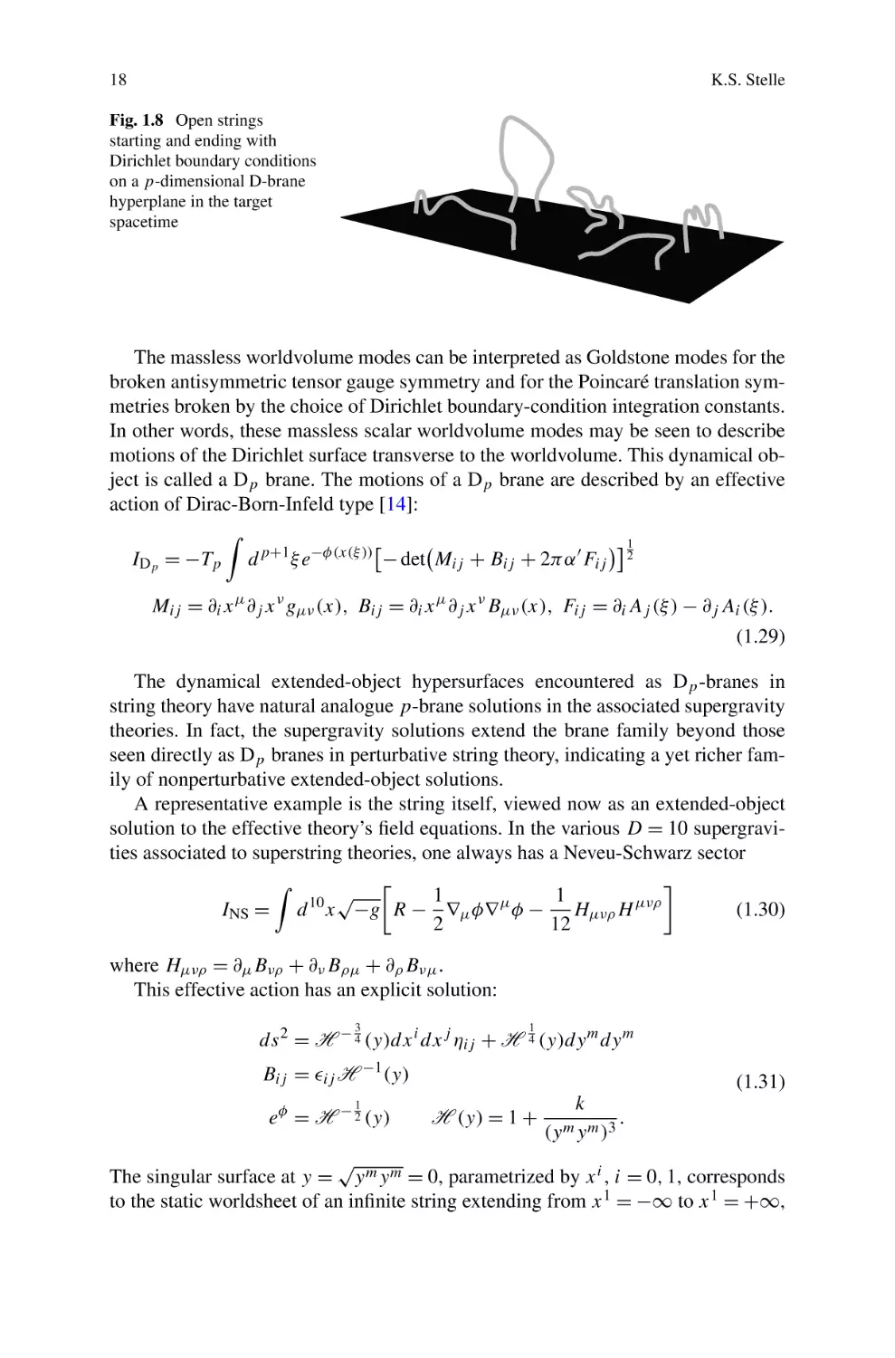
Fig. 1.8 Open strings
starting and ending with
Dirichlet boundary conditions
on a p-dimensional D-brane
hyperplane in the target
spacetime
The massless worldvolume modes can be interpreted as Goldstone modes for the
broken antisymmetric tensor gauge symmetry and for the Poincaré translation symmetries broken by the choice of Dirichlet boundary-condition integration constants.
In other words, these massless scalar worldvolume modes may be seen to describe
motions of the Dirichlet surface transverse to the worldvolume. This dynamical object is called a Dp brane. The motions of a Dp brane are described by an effective
action of Dirac-Born-Infeld type [14]:
1
IDp = −Tp d p+1 ξ e−φ(x(ξ )) − det Mij + Bij + 2πα Fij 2
Mij = ∂i x μ ∂j x ν gμν (x), Bij = ∂i x μ ∂j x ν Bμν (x), Fij = ∂i Aj (ξ ) − ∂j Ai (ξ ).
(1.29)
The dynamical extended-object hypersurfaces encountered as Dp -branes in
string theory have natural analogue p-brane solutions in the associated supergravity
theories. In fact, the supergravity solutions extend the brane family beyond those
seen directly as Dp branes in perturbative string theory, indicating a yet richer family of nonperturbative extended-object solutions.
A representative example is the string itself, viewed now as an extended-object
solution to the effective theory’s field equations. In the various D = 10 supergravities associated to superstring theories, one always has a Neveu-Schwarz sector
√
1
1
(1.30)
INS = d 10 x −g R − ∇μ φ∇ μ φ − Hμνρ H μνρ
2
12
where Hμνρ = ∂μ Bνρ + ∂ν Bρμ + ∂ρ Bνμ .
This effective action has an explicit solution:
3
1
ds 2 = H − 4 (y)dx i dx j ηij + H 4 (y)dy m dy m
Bij = ij H −1 (y)
e =H
φ
− 12
(y)
(1.31)
k
H (y) = 1 + m m 3 .
(y y )
√
The singular surface at y = y m y m = 0, parametrized by x i , i = 0, 1, corresponds
to the static worldsheet of an infinite string extending from x 1 = −∞ to x 1 = +∞,
1 String Theory, Unification and Quantum Gravity
19
Fig. 1.9 “Brane-scan” of supergravity p-brane solutions, linked by worldvolume (diagonal) and
transverse-space (vertical) dimensional reductions
with an 8-dimensional transverse space M8 within which the solution is spherically
symmetric.
The solution has a charge as well, given by Gauss’s law: U = ∂ M8 d 7 Σ m Hm01 =
6kΩ7 , where Ω7 is the volume of the unit 7-sphere corresponding to the infinite
boundary of M8 . This charge is equal to the ADM tension (energy/unit x 1 length)
of the solution, so this string solution is an analogue of the extremal ReissnerNordstrom solution of Einstein-Maxwell theory.
There is a great variety of p-brane solutions in supergravity theories, of diverse
worldvolume and transverse dimensionalities, as shown in Fig. 1.9. The supersymmetric p-brane spectrum naturally generalizes the extremal black holes of EinsteinMaxwell theory, which may be viewed as 0-branes. In a given dimension of spacetime, the brane spectrum also naturally carries a representation of the corresponding
supergravity duality group.
20
Table 1.1 Supergravity
E11−D(11−D) (R) duality
symmetries, KD maximal
compact subgroups and the
superstring E11−D(11−D) (Z)
discretizations
K.S. Stelle
D
E11−D(11−D) (R)
KD
E11−D(11−D) (Z)
10A
R+
1
1
10B
Sl(2, R)
SO(2)
Sl(2, Z)
9
Sl(2, R) × R+
SO(2)
Sl(2, Z)
8
Sl(3, R) × Sl(2, R)
SO(3) × SO(2)
Sl(3, Z) × Sl(2, Z)
7
Sl(5, R)
SO(5)
Sl(5, Z)
6
SO(5, 5, R)
SO(5) × SO(5)
SO(5, 5, Z)
5
E6(6) (R)
U Sp(8)
E6(6) (Z)
4
E7(7) (R)
SU(8)/Z2
E7(7) (Z)
3
E8(8) (R)
SO(16)
E8(8) (Z)
Dimensional reduction of the maximal theory down from D = 11 automatically
generates a GL(11 − D, R) nonlinearly realized symmetry of the D dimensional
reduced supergravity. However, special features of supergravity theories lead to an
enhancement of this anticipated duality group. These features include the combination of vectors and scalars coming from the D = 11 metric and the D = 11 3-form
gauge field, and also the dualization of higher-rank form fields to lower-rank fields
by Hodge dualization of the corresponding field strengths.
The resulting duality groups for maximal supergravity are shown in Table 1.1, where E11−D(11−D) is the nonlinearly realized duality symmetry in spacetime dimension D, KD is its linearly realized maximal compact subgroup and
E11−D(11−D) (Z) is the discretized “U-duality” [12, 13] form consistent with the
Dirac quantization condition, which is conjectured to survive in superstring theory.
1.7 The Onset of Supergravity Divergences
Now we shall return to the initial question of field-theoretic gravity theories and
their quantum problems. We have seen that there is a rich tapestry of supergravity
limits, with surprizing additional duality symmetries, which emerge as “zero-slope”
α → 0 limits of superstring/M-theory. The question remains whether links to theories based upon extended objects as the fundamental excitations have a bearing
on the original ultraviolet problems of field-theoretic gravity and supergravity theories. The dimensional character of Newton’s constant and the related nonlinearity
of the Einstein-Hilbert action leads to a general expectation of nonrenormalizability
in gravity and supergravity theories. Resolving the ultraviolet problem of quantum
gravity has consequently been one of the main aims of superstring theory. However,
it is important to understand precisely how the quantum properties of superstring
theories differ from those of the corresponding supergravities when the latter are
subject to standard field-theoretic quantization.
In order to understand this relation, the precise order of onset of nonrenormalizable divergences in supergravity theories has remained an intensely studied ques-
1 String Theory, Unification and Quantum Gravity
21
tion. Local supersymmetry brings about at least significant delays in the onset of
ultraviolet divergences, but the full reach of the corresponding nonrenormalization
theorems is still not fully clear. What is clear, however, is that links to superstring
and M-theory have led to some genuinely surprizing ultraviolet cancellations.
Explicit calculations of ultraviolet divergence coefficients have been carried out
using traditional Feynman diagram techniques up to the 2-loop level [1, 2]. Continuing on this way to higher loop orders, however, quickly becomes prohibitive: for the
important 3-loop level at which the first dangerous counterterms occur, an estimate
of the number of terms in a standard Feynman diagram calculation is of the order of
1020 , owing to the complexity of the vertices and propagators.
Nonetheless, important progress using new techniques developed since 1998 has
been made in the calculation of loop-diagram divergences in maximal supergravity and maximal super Yang-Mills theories. These new methods use heavily the
unitarity properties of Feynman diagrams, which generalize the optical theorem
Im T = T ∗ T of ordinary quantum mechanics [15–17].
Normally, one might think that one can only learn about the imaginary parts of
quantum amplitudes using unitarity. However when the unitarity diagram cutting
rules are combined with an expanded use of dimensional regularization, much more
can be learned. In dimensional regularization, one analytically continues the dimension of spacetime
in Feynman integrals
away from the dimension of interest, e.g.
replacing d 4 k loop integrals by d 4+ k.
The ordinary use of dimensional regularization focuses simply on the 1 poles
in quantum amplitudes, corresponding to logarithmic divergences in a straightforward high momentum cutoff regularization. However, one gets useful information
by retaining the full (4 + ) dimensional amplitude. In such an analytically continued integral, an integrand f (s) (where, e.g., s is a Mandelstam momentum invariant, quadratic in loop momenta) will become deformed to f (s)s −/2 in order to balance dimensions. Then, since s −/2 = 1 − (/2) ln s + · · · and since
ln(s) = ln(|s|) + iπθ (s), one can learn about the real parts of an amplitude by retaining imaginary terms at order .
The unitarity-based techniques allow for large classes of diagrams to become
cut constructible, and allow for the eventual reduction of a higher-loop amplitude
to integrals over products of tree amplitudes. At that point, other recent progress
in the understanding of tree amplitudes comes into play. Although the individual
Feynman diagrams at tree level are very complicated, sums of diagrams representing complete amplitudes can have striking simplicity, and in particular can satisfy
powerful recursion relations [18].
To date, these techniques have allowed the explicit calculation of maximal supergravity divergences to proceed up to the 4-loop level (Fig. 1.10), something that
would have been unthinkable using traditional Feynman diagram techniques [19].
The current status of the first possible maximal supergravity ultraviolet divergences is summarized in Table 1.2, with the currently known divergences shown
in gray. The BPS degree represents the degree of supersymmetry invariance of the
integrand prior to superspace integration. The surprizing feature of these results is
the tardiness of maximal supergravity in getting around to revealing its ultraviolet
22
K.S. Stelle
Fig. 1.10 Four out of the 50
diagrams arising in the
calculation of the 4-loop
divergences in maximal
supergravity
Table 1.2 Maximal supergravity first possible divergences & BPS degree from unitarity-based
calculations. Known divergences are shown in gray
Dimension D
11
10
8
7
6
5
4
Loop order L
2
2
1
2
3
6?
5?
BPS degree
0
0
1
2
1
4
1
8
0
1
4
Gen. form
∂ 12 R 4
∂ 10 R 4
R4
∂ 6 R4
∂ 6 R4
∂ 12 R 4
∂ 4 R4
divergences. At D = 8 dimensions and L = 1, one does indeed encounter the expected R 4 counterterm, but in lower spacetime dimensions this 12 BPS divergence
does not occur, leaving it to significantly less constrained counterterms to be the first
UV divergence candidates.
We will next see that careful analysis of the available counterterms reveals the
reasons for the unanticipated divergence cancellations, and will push the anticipated
first divergences even farther out than the calculational front shown in Table 1.2.
1.7.1 Supergravity Counterterm Analysis
The surprizing resilience of maximal N = 8 supergravity to the threat of anticipated
ultraviolet divergences has led to some speculation that perhaps superstring theory
isn’t actually necessary after all. Certainly, it has led to more than a decade of discussion between the unitarity-based calculators and supersymmetry practitioners in
trying to understand what is going on. The current state of affairs reflects a significant deepening in understanding of the consequences of local supersymmetry and
also of the rôle of duality symmetries of the maximal theory.
In the 1980’s, the understanding was that allowable counterterms would be those
subject to nonrenormalization theorems based upon linearly realized supersymmetry, generalizing the famous nonrenormalization theorem that disallows
as coun
terterms chiral superspace integrals (also called “F terms”) like d 4 x d 2 θ W (φ) in
N = 1, D = 4 supersymmetry, where W (φ) is a holomorphic function and φ is a
chiral superfield satisfying D̄φ = 0. Although such terms are fully allowed in a theory’s classical action (and, indeed, play a critical rôle in supersymmetric
extensions
of the Standard Model), only full superspace integrals like d 4 x d 2 θ d 2 θ̄ K(φ, φ̄)
are allowed to occur as counterterms.
It was known by the mid 1980’s that maximal supergravity and maximal super
Yang-Mills theory could be quantized with at least half of their full supersymmetry
1 String Theory, Unification and Quantum Gravity
23
Fig. 1.11 Half-BPS candidate counterterms for maximal super Yang-Mills and maximal supergravity theories
manifestly linearly realized—in a so-called “off-shell” formalism. This was explicitly constructed for the full maximal N = 4 super Yang-Mills theory, but only for the
linearized theory in the case of maximal N = 8 supergravity.
The resulting expectation was that the first allowed counterterms would have a d 8 θ superspace integral
structure in the case of maximal super Yang-Mills and a d 16 θ structure in the case
of maximal supergravity—i.e. full-superspace integrals for the linearly-realizable
half supersymmetry.
Accordingly, the first allowed counterterms in maximal super Yang-Mills and
maximal supergravity were considered to be [20, 21] of the structures shown in
Fig. 1.11.
Since d 16 θ integration has dimension 16/2 = 8, one finds terms with 8 derivatives among the many terms produced by superspace integration in the maximal supergravity
counterterm; general covariance requires these to be of the general form
4
R . So the above understanding would just allow the dangerous 3-loop anticipated
counterterm for the first D = 4 divergence.
This expectation of L = 3 loop first divergences has clearly been upset by the
unitarity-based calculations. This has led to a more detailed investigation of the
nonrenormalization theorems, and in particular to use of the Ward identities for
the full supersymmetry using a Batalin-Vilkovisky version of the BRST quantum
formalism—even though the transformations for the maximal theories are highly
nonlinear and close to form an expected supersymmetry algebra only subject to the
classical equations of motion.
To do this requires adding source fields for a whole range of additional operators
as needed to formulate the Ward identities. The resulting identities then take the
form of a cohomology problem for a generalized exterior derivative, acting on triples
of forms of adjacent rank. In addition, instead of computing beta functions for the
coefficients of the expected counterterms, it is advantageous to consider operator
insertions of the classical Lagrangian and its corresponding cocycle into its own
quantum amplitudes, and then to calculate gamma functions for the allowed operator
mixings of the Lagrangian cocycle with candidate counterterms and their cocycles,
the latter being required to be consistent in structure with that of the Lagrangian
cocycle [22, 23].
In the case of maximal super Yang-Mills, such considerations are sufficient to
explain all of the previously unanticipated single-trace operator cancellations. In
the case of maximal supergravity, similar arguments show why the R 4 counterterm
is in the end ruled out. But the unanticipated maximal supergravity cancellations
found by the unitarity methods go much further than that: D = 5, L = 2 & 4 and
D = 4, L = 3 & 4 divergences have all failed to occur.
24
K.S. Stelle
Table 1.3 Maximal supergravity current first divergence expectations & BPS degree. Known divergences are shown in gray and the first anticipated D = 4 and D = 5 divergences are shown in
black
Dimension D
11
10
8
7
6
5
4
Loop order L
2
2
1
2
3
6
7
BPS degree
0
0
1
2
1
4
1
8
0
1
8
Gen. form
∂ 12 R 4
∂ 10 R 4
R4
∂ 6 R4
∂ 6 R4
∂ 12 R 4
∂ 8 R4
In order to understand these further divergence cancellations, one needs to turn
an apparent bug of the supergravity Ward identities into a feature. Their analysis
is complicated by the density character of integrands in a locally supersymmetric
theory. Counterterm cocycle component forms need to be pulled back to a bosonic,
or “body” coordinate frame, and in local supersymmetry this involves not only the
gravitational vielbeins, but also the fermionic gravitino fields.
To turn this density character to our advantage, one needs to combine it with
the requirements of maximal supergravity’s continuous duality invariance: E7(7) (R)
in the D = 4 case. For this purpose, one needs to know how to quantize while
maintaining manifest duality symmetry, and this can be done in the case of the
maximal N = 8, D = 4 theory by sacrificing manifest Lorentz invariance so as to
i field strengths of the 28 vector fields can form an
handle the fact that only the Fμν
E7(7) (R) representation, separating them into self-dual and anti-self-dual parts in
order to form a 56 of E7(7) (R). Sacrificing manifest Lorentz symmetry in this way,
one can double the number of spacelike components of the vector fields, but reduce
the number by a factor of 1/2 by a duality constraint. In this formalism, one needs to
check for the absence of anomalies in the now non-manifest Lorentz symmetry and
also check the SU(8) divisor subgroup of the duality group. Happily, these anomaly
checks succeed, and as a result one may require that the perturbative field-theory
counterterms preserve the continuous duality symmetry [24].
Combining the requirements of the full local supersymmetry Ward identities with
the requirement of continuous duality symmetry, all of the outstanding divergence
cancellations currently found by the unitarity methods have been explained, and
new cancellations are now predicted at D = 4, L = 5 & 6. The resulting pattern of
anticipated1 first divergences is shown in Table 1.3.
D = 4, L = 7 situation requires special care [25]. At the linearized level, it would seem
that the ∂ 8 R 4 candidate could be the first full-superspace non-BPS counterterm in D = 4. The
A ) would seem to be the obvious candidate. However,
volume of superspace, d 4 xd 32 θ det(EM
rather surprisingly, it turns out that this superspace volume vanishes subject to the classical field
equations, so there is no need for such a counterterm in the renormalized action. Instead, what
looks like a non-BPS ∂ 8 R 4 counterterm at the linearized level turns into a 18 -BPS counterterm
at the full nonlinear level. This illustrates the important rôle that nonlinear structure can play in
quantum gravity divergence analysis.
1 The
1 String Theory, Unification and Quantum Gravity
25
1.7.2 Supergravity Divergences from Superstrings
A satisfying aspect of the current understanding of the relation between superstring
theory and maximal supergravity is that one now obtains exactly the above predictions for the onset of supergravity divergences from a superstring perspective as
well. In this regard, one may view superstring theory as a rather elaborate “regulator” of the supergravity quantum amplitudes.
In the critical dimension D = 10 for superstrings, the R 4 correction to the effective field-theory Lagrangian occurs with a coefficient α 3 , as can be seen on dimensional grounds, since α has dimensions of (length)2 , so α 3 R 4 has the same
dimensions as R. How then can there be divergences in the effective field theory,
which is obtained by taking the limit α → 0?
Recall that in order to compare D = 4 maximal supergravity to the string-theory
effective action, one must dimensionally reduce on a torus T 6 . Start from the string
frame, in which the gravitational Lagrangian e−2φ R has a scalar prefactor whose
v.e.v. gs−2 gives a D = 10 Newton’s constant G10 ∼ gs2 8s , where s is the string
2
scale, needed on dimensional grounds and related to α by α ∼ 22sc2 ; gs is the
string coupling constant. If the typical scale of one of the compact toroidal dimensions is R, then reduction of the effective action on T 6 produces an extra prefactor
g 2 8
of R 6 in the D = 4 effective action, giving a D = 4 Newton’s constant G4 ∼ Rs 6s .
1
Thus, the D = 4 Plank length 4 ∼ (G4 ) 2 is related to the string coupling constant
3
by gs ∼ R4 4 .
s
In order to compare the dimensionally reduced string effective action to quantized D = 4 maximal supergravity, one needs to ensure that the D = 4 Newton’s constant remains finite, while the towers of excited string states and also the
Kaluza-Klein excitations from the dimensional reduction all have masses that are
infinitely large compared to the D = 4 Planck scale 4 . This is achieved by taking
1 1
R
1
R , s & 2 4 , which is compatible with holding gs and 4 fixed while taking
3
s
1
s ∼ R 4 ( g4s ) 4 → 0.
This analysis would seem to indicate that the effective field theory could be ultraviolet finite. However, this string analysis can be misleading because string nonperturbative effects can conspire to swamp what one might otherwise want to identify
as the field-theoretic supergravity contribution [26]. Analysis of this “decoupling”
problem in the above supergravity limit shows that decoupling can be carried out
for loop orders L ≤ 6, but that beyond that order the decoupling issues prevent conclusions about field-theoretic finiteness from being made [27]. Moreover, analysis
of the superstring effective action contributions also shows they can be continuously
E7(7) (R) invariant to the same order [28, 29].
26
K.S. Stelle
1.8 Other Aspects of String Theory
1.8.1 The String Scale
Let us now consider the physically relevant energy or inverse-length scales characterizing the higher dimensions inherent in string theory. The analysis will be similar
to that of Sect. 1.7.2, except that instead of looking at the field-theory limit s → 0,
we now consider the finite values of s that are compatible with perturbatively realistic particle physics. First consider thecontext of a traditional Kaluza-Klein reducd 10 x e−2φ (R + 2s F 2 ), where F represents
tion, starting in D = 10 with I10 = −8
s
the Yang-Mills field strength. Next, dimensionally reduce down to D = 4 on a manifold of volume V6 while replacing φ by φ0 = φ. The D = 4 reduced action then
becomes
V6 −2φ0
I4 = 8 e
d 4 x R + 2s F 2
s
so in D = 4 we can identify
1
MPl =
V62
s
e−φ0
4
and gYM =
eφ0 3s
1
.
V62
Now, to avoid strong coupling in the D = 10 string theory, one requires eφ0 < 1
2 ∼ 1 . Hence V −6 = e2φ0 g −2 ≤ 30 and so for V ∼ R 6 ,
while in D = 4, gYM
6 s
6
YM
30
one finds s ∼ R. Moreover, substituting for e−φ0 in terms of gYM , one finds
MPl = (s gYM )−1 , requiring s ∼ M10Pl . This is as one might expect: in the standard dimensional reduction scenario, intrinsic string-theory effects cannot occur too
far below the Planck scale.
Consider now how the analysis changes when one switches from the standard
Kaluza-Klein reduction to a braneworld scenario. In a braneworld scenario, one
proposes that the observable lower-dimensional universe is concentrated on a subsurface of the higher-dimensional spacetime, instead of being smeared evenly over
the extra dimensions, i.e. instead of assuming there is no dependence on the extra
coordinates.
To see how the string-scale analysis changes, consider a Dp -brane with p > 3 and
with gauge fields defined only on the d = p + 1 dimensional D-brane worldvolume.
Of the p spatial D-brane dimensions, p − 3 are compactified and the remaining 3
coincide with the spatial directions of the reduced D = 4 spacetime. The starting
10 −2φ
3−p p+1
d xe
d
R + s
ξ e−φ F 2 . As before, one has MPl =
action is now −8
s
1
1
1
φ0 2
−φ0 but now g
V62 −4
YM = e 2 s
s e
(p−3)
−1
2
Vp−3
.
3−p
Limiting again the string coupling to perturbative values eφ0 ≤ 1, find Vp−3 s
−2
≤ gYM
∼ 30. Now, however, for V6 = Vp−3 V9−p one can have independent p =
1
1
p−3
9−p
2 = −2 (V
and R = V9−p
. One may write MPl
Vp−3
p−3 s
s
3−p
p−9
)(V9−p s
)e−2φ0 .
1 String Theory, Unification and Quantum Gravity
27
Fig. 1.12 Topology change
at a boundary of moduli space
3−p
−
1
Then from Vp−3 s ≤ 30, one learns s ∼ p (30) p−3 , while if R p (giving a
p−9
−2
highly asymmetric V6 ), one has V9−p s 1. Thus 2s Mpl
is now possible,
i.e. one can have a string mass scale significantly below the Planck scale [30].
Such brane-world considerations lie at the base of current experimental protocols searching for string or gravitational phenomena at the Large Hadron Collider
at CERN. A low string mass scale corresponds also to a low scale for inherently
quantum-gravitational effects such as the threshold production of black holes. These
would immediately then decay by Hawking radiation, but the resulting resonance
could have a striking new experimental signature.
1.8.2 Boundaries of Moduli Space
The infinities of perturbative field theory are tamed by string theory. But the story of
infinities does not end there. In string theory, the most important singularities occur
at the boundaries of moduli space, e.g. in amplitudes where moduli are about to
pinch off so that topology change can take place in a Riemann surface (Fig. 1.12).
These boundary configurations are the places where one really has to check
whether string theory is free of infinities. And often, when divergences seem apparent, one realizes that the singularities should be “blown up”, with new modes
particular to the singularity structure of the Riemann surface appearing. These can
contribute to blown-up singularity sectors with new gauge fields and other massless
modes in the effective field theory, so such special points in moduli space can also
give rise to important physical effects at the same time as posing a challenge to the
analysis of divergences.
The calculation of higher-loop string amplitudes requires detailed control of the
Riemann surface moduli in the quantum path integral. This has been comprehensively done up through the two-loop order [31, 33, 34]. This has enabled proofs of
the finiteness of string theory up to this level to be given [35, 36]. More recent developments have employed a pure-spinor approach to the string worldsheet [37, 38]
are expected to lead to an all-orders resolution of this key question.
28
K.S. Stelle
Fig. 1.13 “Fuzzball” effective geometry from an average over nonsingular geometries
1.8.3 String and Gravity Thermodynamics
One of the most famous results of string theory has been the derivation of the
A
for the entropy of a black hole in terms of the
Bekenstein-Hawking formula S = 4G
area A of the horizon. This derivation employed nearly supersymmetric (i.e. nearly
BPS) configurations in order to enable a detailed microstate counting agreeing with
the Bekenstein-Hawking entropy formula [39]. Current work includes study of the
deviation from a blackbody to a “greybody” spectrum in the emitted Hawking radiation.
Related work is aimed at understanding whether string theory evades Hawking’s
prediction that black holes lead to a loss of quantum information. This has led to
“fuzzball” formulations of macroscopic blackholes (Fig. 1.13) in terms of an average over BPS coherent states describing individual nonsingular geometries, in order
to give an account of the thermodynamics of non-supersymmetric black holes.
1.9 Conclusion
With the expansion of string theory to the M-theory picture of a web of perturbatively-defined theories (plus D = 11 supergravity) linked by duality symmetries, a
breathtaking unification vista has opened. And yet, this unification remains largely
an aspiration: despite many striking confirmations of duality relations, a proper definition of the fundamental states of M-theory and a corresponding derivation of
the duality symmetries acting on them remain to be given. Considering the history
of nonperturbative relations in field theory, this should not be so surprizing. Many
of the currently most important theoretical constructions (Yang-Mills theory, supersymmetry, even φ 4 theory) are not rigorously formulated outside perturbation
theory. Perhaps M-theory will upend this situation and in the end become better
formally grounded than phenomenological field theory currently is.
The theme of duality, meanwhile, continues to make further surprizing connections between previously distinct subjects. The picture of stacks of (3 + 1)dimensional D-branes in type IIB theory, with braneworld Goldstone modes constituting vector supermultiplets and interactions via open superstrings linking the
D-brane stacks to form nonabelian gauge theories, forms a “holomorphic” construction of supersymmetric Yang-Mills theory on the boundary of a (4 + 1)-dimensional
1 String Theory, Unification and Quantum Gravity
29
spacetime. This “gauge-gravity duality” provides powerful nonperturbative relations on both the “gravity” (or superstring) and “gauge” sides of the correspondence
(for a review, see [40]).
The gauge-gravity correspondence has evolved to cover many situations where
nonperturbative gauge-theory phenomena on boundaries are important. Key applications currently include the dynamics of quark-gluon plasmas, Navier-Stokes fluid
hydrodynamics, and applications in high-temperature superconductivity. The gaugegravity duality constructions can provide information about phases where the usual
field-theoretic partition function is neither convergent not Borel-summable: in other
words, in deeply nonperturbative regions of phase space.
Historically, string theory was born out of the study of resonances in stronginteraction physics. With some of the recent developments, it may in a sense be
returning to its birth context. But it also remains the strongest current approach
towards solving the key remaining problem of theoretical physics, which is the formulation of a quantum theory of gravity.
References
1. M.H. Goroff, A. Sagnotti, The ultraviolet behavior of Einstein gravity. Nucl. Phys. B 266, 709
(1986)
2. A.E.M. van de Ven, Two loop quantum gravity. Nucl. Phys. B 378, 309 (1992)
3. S. Deser, J.H. Kay, K.S. Stelle, Renormalizability properties of supergravity. Phys. Rev. Lett.
38, 527 (1977)
4. S. Deser, B. Zumino, A complete action for the spinning string. Phys. Lett. B 65, 369 (1976)
5. L. Brink, P. Di Vecchia, P.S. Howe, A locally supersymmetric and reparametrization invariant
action for the spinning string. Phys. Lett. B 65, 471 (1976)
6. A.M. Polyakov, Quantum geometry of bosonic strings. Phys. Lett. B 103, 207 (1981)
7. C.G. Callan Jr., E.J. Martinec, M.J. Perry, D. Friedan, Strings in background fields. Nucl.
Phys. B 262, 593 (1985)
8. T.H. Buscher, A symmetry of the string background field equations. Phys. Lett. B 194, 59
(1987)
9. J. Dai, R.G. Leigh, J. Polchinski, New connections between string theories. Mod. Phys. Lett.
A 4, 2073 (1989)
10. M. Dine, P.Y. Huet, N. Seiberg, Large and small radius in string theory. Nucl. Phys. B 322,
301 (1989)
11. M. Cvetic, H. Lu, C.N. Pope, K.S. Stelle, T duality in the Green-Schwarz formalism, and the
massless / massive IIA duality map. Nucl. Phys. B 573, 149 (2000). hep-th/9907202
12. C.M. Hull, P.K. Townsend, Unity of superstring dualities. Nucl. Phys. B 438, 109 (1995).
hep-th/9410167
13. E. Witten, String theory dynamics in various dimensions. Nucl. Phys. B 443, 85 (1995).
hep-th/9503124
14. E.S. Fradkin, A.A. Tseytlin, Quantum string theory effective action. Nucl. Phys. B 261, 1
(1985)
15. Z. Bern, L.J. Dixon, D.C. Dunbar, M. Perelstein, J.S. Rozowsky, On the relationship between
Yang-Mills theory and gravity and its implication for ultraviolet divergences. Nucl. Phys. B
530, 401 (1998). hep-th/9802162
16. Z. Bern, J.J.M. Carrasco, H. Johansson, Perturbative quantum gravity as a double copy of
gauge theory. Phys. Rev. Lett. 105, 061602 (2010). arXiv:1004.0476 [hep-th]
30
K.S. Stelle
17. Z. Bern, J.J.M. Carrasco, L.J. Dixon, H. Johansson, R. Roiban, Simplifying multiloop integrands and ultraviolet divergences of gauge theory and gravity amplitudes. arXiv:1201.5366
[hep-th]
18. R. Britto, F. Cachazo, B. Feng, E. Witten, Direct proof of tree-level recursion relation in YangMills theory. Phys. Rev. Lett. 94, 181602 (2005). hep-th/0501052
19. Z. Bern, J.J. Carrasco, L.J. Dixon, H. Johansson, R. Roiban, The ultraviolet behavior of N = 8
supergravity at four loops. Phys. Rev. Lett. 103, 081301 (2009). arXiv:0905.2326 [hep-th]
20. P.S. Howe, K.S. Stelle, P.K. Townsend, Superactions. Nucl. Phys. B 191, 445 (1981)
21. R.E. Kallosh, Counterterms in extended supergravities. Phys. Lett. B 99, 122 (1981)
22. G. Bossard, P.S. Howe, K.S. Stelle, The ultra-violet question in maximally supersymmetric
field theories. Gen. Relativ. Gravit. 41, 919 (2009). arXiv:0901.4661 [hep-th]
23. G. Bossard, P.S. Howe, K.S. Stelle, A note on the UV behaviour of maximally supersymmetric
Yang-Mills theories. Phys. Lett. B 682, 137 (2009). arXiv:0908.3883 [hep-th]
24. G. Bossard, C. Hillmann, H. Nicolai, E7(7) symmetry in perturbatively quantised N = 8 supergravity. J. High Energy Phys. 1012, 052 (2010). arXiv:1007.5472 [hep-th]
25. G. Bossard, P.S. Howe, K.S. Stelle, P. Vanhove, The vanishing volume of D = 4 superspace.
Class. Quantum Gravity 28, 215005 (2011). arXiv:1105.6087 [hep-th]
26. M.B. Green, H. Ooguri, J.H. Schwarz, Nondecoupling of maximal supergravity from the superstring. Phys. Rev. Lett. 99, 041601 (2007). arXiv:0704.0777 [hep-th]
27. M.B. Green, J.G. Russo, P. Vanhove, String theory dualities and supergravity divergences. J.
High Energy Phys. 1006, 075 (2010). arXiv:1002.3805 [hep-th]
28. H. Elvang, M. Kiermaier, Stringy KLT relations, global symmetries, and E7(7) violation. J.
High Energy Phys. 1010, 108 (2010). arXiv:1007.4813 [hep-th]
29. N. Beisert, H. Elvang, D.Z. Freedman, M. Kiermaier, A. Morales, S. Stieberger, E7(7) constraints on counterterms in N = 8 supergravity. Phys. Lett. B 694, 265 (2010). arXiv:1009.
1643 [hep-th]
30. I. Antoniadis, N. Arkani-Hamed, S. Dimopoulos, G.R. Dvali, New dimensions at a millimeter
to a Fermi and superstrings at a TeV. Phys. Lett. B 436, 257 (1998). hep-ph/9804398
31. E. D’Hoker, D.H. Phong, Two loop superstrings. 1. Main formulas. Phys. Lett. B 529, 241
(2002). hep-th/0110247
32. E. D’Hoker, D.H. Phong, Two loop superstrings. 2. The chiral measure on moduli space. Nucl.
Phys. B 636, 3 (2002). hep-th/0110283
33. E. D’Hoker, D.H. Phong, Two loop superstrings. 3. Slice independence and absence of ambiguities. Nucl. Phys. B 636, 61 (2002). hep-th/0111016
34. E. D’Hoker, D.H. Phong, Two loop superstrings 4: the cosmological constant and modular
forms. Nucl. Phys. B 639, 129 (2002). hep-th/0111040
35. S. Mandelstam, The n loop string amplitude: explicit formulas, finiteness and absence of ambiguities. Phys. Lett. B 277, 82 (1992)
36. N. Berkovits, Finiteness and unitarity of Lorentz covariant Green-Schwarz superstring amplitudes. Nucl. Phys. B 408, 43 (1993). hep-th/9303122
37. N. Berkovits, Covariant quantization of the Green-Schwarz superstring in a Calabi-Yau background. Nucl. Phys. B 431, 258 (1994). hep-th/9404162
38. N. Berkovits, Quantization of the superstring with manifest U(5) superPoincare invariance.
Phys. Lett. B 457, 94 (1999). hep-th/9902099
39. A. Strominger, C. Vafa, Microscopic origin of the Bekenstein-Hawking entropy. Phys. Lett. B
379, 99 (1996). hep-th/9601029
40. O. Aharony, S.S. Gubser, J.M. Maldacena, H. Ooguri, Y. Oz, Large N field theories, string
theory and gravity. Phys. Rep. 323, 183 (2000). hep-th/9905111
Chapter 2
Introduction to Loop Quantum Gravity
and Cosmology
Abhay Ashtekar
Abstract The goal of the lecture is to present a broad perspective on loop quantum
gravity and cosmology for young researchers which would serve as an introduction
to lectures by Rovelli and Bojowald. The first part is addressed to beginning students
and the second to young researchers who are already working in quantum gravity.
2.1 Introduction
This section, addressed to beginning researchers, is divided into two parts. The first
provides a historical perspective and the second illustrates key physical and conceptual problems of quantum gravity. Researchers who are already quite familiar
with quantum gravity can/should go directly to Sect. 2.2; there will be no loss of
continuity.
2.1.1 Development of Quantum Gravity: A Bird’s Eye View
The necessity of a quantum theory of gravity was pointed out by Einstein already in
a 1916 paper in the Sitzungsberichte der Preussischen Akademie. He wrote:
Nevertheless, due to the inneratomic movement of electrons, atoms would have to radiate
not only electromagnetic but also gravitational energy, if only in tiny amounts. As this
is hardly true in Nature, it appears that quantum theory would have to modify not only
Maxwellian electrodynamics but also the new theory of gravitation.
These words appeared nearly a hundred years ago. While there have been notable advances in the field especially over the past 25 years, we do not yet have a
fully satisfactory quantum theory of gravity. Why is the problem so hard? While
there are many difficulties, I believe that the central ones arise from the fact that in
A. Ashtekar (B)
Physics Department, Institute for Gravitational Physics and Geometry, 104 Davey, Penn State,
University Park, PA 16802, USA
e-mail: ashtekar@gravity.psu.edu
G. Calcagni et al. (eds.), Quantum Gravity and Quantum Cosmology,
Lecture Notes in Physics 863, DOI 10.1007/978-3-642-33036-0_2,
© Springer-Verlag Berlin Heidelberg 2013
31
32
A. Ashtekar
general relativity gravity is encoded in the very geometry of space-time. Therefore,
in a quantum theory of gravity, space-time geometry itself must be described by
quantum physics, with all its fuzziness. How do we do physics if there is no sharply
defined space-time in the background, serving as a grand arena for all dynamics?
To appreciate this point, let us begin with field theories in Minkowski space-time,
say Maxwell’s theory to be specific. Here, the basic dynamical field is represented
by a tensor field Fμν on Minkowski space. The space-time geometry provides the
kinematical arena on which the field propagates. The background, Minkowskian
metric provides light cones and the notion of causality. We can foliate this spacetime by a one-parameter family of space-like three-planes, and analyze how the
values of electric and magnetic fields on one of these surfaces determine those on
any other surface. The isometries of the Minkowski metric let us construct physical
quantities such as fluxes of energy, momentum, and angular momentum carried by
electromagnetic waves.
In general relativity, by contrast, there is no background geometry. The spacetime metric itself is the fundamental dynamical variable. On the one hand it is analogous to the Minkowski metric in Maxwell’s theory; it determines space-time geometry, provides light cones, defines causality, and dictates the propagation of all
physical fields (including itself). On the other hand it is the analog of the Newtonian
gravitational potential and therefore the basic dynamical entity of the theory, similar
in this respect to the Fμν of the Maxwell theory. This dual role of the metric is in
effect a precise statement of the equivalence principle that is at the heart of general
relativity. It is this feature that is largely responsible for the powerful conceptual
economy of general relativity, its elegance and its aesthetic beauty, its strangeness
in proportion. However, this feature also brings with it a host of problems. We see
already in the classical theory several manifestations of these difficulties. It is because there is no background geometry, for example, that it is so difficult to analyze
singularities of the theory and to define the energy and momentum carried by gravitational waves. Since there is no a priori space-time, to introduce notions as basic as
causality, time, and evolution, one must first solve the dynamical equations and construct a space-time. As an extreme example, consider black holes, whose traditional
definition requires the knowledge of the causal structure of the entire space-time. To
find if the given initial conditions lead to the formation of a black hole, one must
first obtain their maximal evolution and, using the causal structure determined by
that solution, ask if the causal past J − (I + ) of its future infinity I + is the entire space-time. If not, space-time contains a black hole and the future boundary
of J − (I + ) within that space-time is its event horizon. Thus, because there is no
longer a clean separation between the kinematical arena and dynamics, in the classical theory substantial care and effort is needed even in the formulation of basic
physical questions.
In quantum theory the problems become significantly more serious. To see this,
recall first that, because of the uncertainty principle, already in non-relativistic quantum mechanics, particles do not have well-defined trajectories; time-evolution only
produces a probability amplitude, Ψ (x, t), rather than a specific trajectory, x(t).
Similarly, in quantum gravity, even after evolving an initial state, one would not be
2 Introduction to Loop Quantum Gravity and Cosmology
33
left with a specific space-time. In the absence of a space-time geometry, how is one
to introduce even habitual physical notions such as causality, time, scattering states,
and black holes?
Loop quantum gravity provides a background approach to address such deep conceptual problems. In its initial formulation it was based on the canonical approach.
Therefore, let us begin with a summary of ideas underlying canonical gravity. Here
one notices that, in spite of the absence of a background space-time geometry, the
Hamiltonian formulation of general relativity is well-defined and attempts to use it
as a stepping stone to quantization. The fundamental canonical commutation relations are to lead us to the basic uncertainty principle. The motion generated by the
Hamiltonian is to be thought of as time evolution. The fact that certain operators on
the fixed (‘spatial’) three-manifold commute is supposed to capture the appropriate notion of causality. The emphasis is on preserving the geometrical character of
general relativity, on retaining the compelling fusion of gravity and geometry that
Einstein created. In the first stage of the program, completed in the early 1960s, the
Hamiltonian formulation of the classical theory was worked out in detail by Dirac,
Bergmann, Arnowitt, Deser and Misner and others [1–5].1 The basic canonical variable was the 3-metric on a spatial slice. The ten Einstein’s equations naturally decompose into two sets: four constraints on the metric and its conjugate momentum
(analogous to the equation DivE = 0 of electrodynamics) and six evolution equations. Thus, in the Hamiltonian formulation, general relativity could be interpreted
as the dynamical theory of 3-geometries. Wheeler therefore baptized it geometrodynamics [6, 7].
In the second stage, this framework was used as a point of departure for quantum theory by Bergmann, Komar, Wheeler, DeWitt and others. The basic equations
of the quantum theory were written down and several important questions were
addressed [5, 7]. Wheeler also launched an ambitious program in which the internal quantum numbers of elementary particles were to arise from non-trivial, microscopic topological configurations and particle physics was to be recast as ‘chemistry
of geometry’. However, most of the work in quantum geometrodynamics continued
to remain formal; indeed, even today the field theoretic difficulties associated with
the presence of an infinite number of degrees of freedom in the Wheeler–DeWitt
equation remain unresolved. Furthermore, even at the formal level, is has been difficult to solve the quantum Einstein’s equations. Therefore, after an initial burst
of activity, the quantum geometrodynamics program became stagnant. Interesting
results have been obtained by Misner, Wheeler, DeWitt and others in the limited
context of quantum cosmology where one freezes all but a finite number of degrees
of freedom. However, even in this special case, the initial singularity could not be resolved without additional ‘external’ inputs into the theory, such as the use of matter
violating energy conditions.
1 Since this introduction is addressed to non-experts, I will generally refer to books and review
articles which summarize the state of the art at various stages of development of quantum gravity.
References to original papers can be found in these reviews.
34
A. Ashtekar
The third stage in the canonical approach began with the following observation:
the geometrodynamics program laid out by Dirac, Bergmann, Wheeler and others
simplifies significantly if we regard a spatial connection (rather than the 3-metric) as
the basic object. In fact we now know that, among others, Einstein and Schrödinger
had recast general relativity as a theory of connections already in the fifties. (For
a brief account of this fascinating history, see [8].) However, they used the ‘LeviCivita connection’ that features in the parallel transport of vectors and found that
the theory becomes rather complicated. This episode had been forgotten and connections were re-introduced afresh in the mid 1980s [9].2 However, now these are
‘spin-connections’ required to parallel propagate spinors, and they turn out to simplify Einstein’s equations considerably. For example, the dynamical evolution dictated by Einstein’s equations can now be visualized simply as a geodesic motion
on the space of spin-connections (with respect to a natural metric extracted from the
constraint equations). Since general relativity is now regarded as a dynamical theory
of connections, this reincarnation of the canonical approach is called ‘connectiondynamics’.
Perhaps the most important advantage of the passage from metrics to connections
is that the phase-space of general relativity is now the same as that of gauge theories [9, 10]. The ‘wedge between general relativity and the theory of elementary
particles’ that Steve Weinberg famously referred to in his monograph on general
relativity largely disappears without having to sacrifice the geometrical essence of
the theory. One could now import into general relativity techniques that have been
highly successful in the quantization of gauge theories. At the kinematic level, then,
there is a unified framework to describe all four fundamental interactions. The dynamics, of course, depends on the interaction. In particular, while there is a background space-time geometry in electroweak and strong interactions, there is none in
general relativity. Therefore, qualitatively new features arise. These were exploited
in the late eighties and early nineties to solve simpler models—general relativity in
2 + 1 dimensions [9, 11, 12], linearized gravity clothed as a gauge theory [9], and
certain cosmological models. To explore the physical, 3 + 1 dimensional theory, a
‘loop representation’ was introduced by Rovelli and Smolin. Here, quantum states
2 This reformulation used (anti-)self-dual connections which are complex. These have a direct interpretation in terms space-time geometry and also render the constraint equations polynomial in
the basic variables. This simplicity was initially regarded as crucial for passage to quantum theory.
However, one is then faced with the task of imposing appropriate quantum ‘reality conditions’ to
ensure that the classical limit is real general relativity. Barbero introduced real connection variables
by replacing the ±i in the expression of the (anti-)self-dual connections with a real parameter β.
However, now the connection does not have a natural space-time interpretation and the constraints
are no longer polynomial in the basic variables. But the strategy became viable after Thiemann
introduced novel ideas to handle quantization of the specific non-polynomial terms that now feature in the constraints. Since then, this strategy has become crucial because the rigorous functional
calculus on the space of connections has so far been developed only for real connections. Immirzi
suggested that the value of β could be chosen so that the leading term in black hole entropy is
precisely (area/42Pl ). That is why β (which is often denoted by γ in later papers) is referred to as
the Barbero–Immirzi parameter.
2 Introduction to Loop Quantum Gravity and Cosmology
35
were taken to be suitable functions of loops on the 3-manifold.3 This led to a number
of interesting and intriguing results, particularly by Gambini, Pullin and their collaborators, relating knot theory and quantum gravity [13]. Thus, there was rapid and
unanticipated progress in a number of directions which rejuvenated the canonical
quantization program. Since the canonical approach does not require the introduction of a background geometry or use of perturbation theory, and because one now
has access to fresh, non-perturbative techniques from gauge theories, in relativity
circles there is a hope that this approach may lead to well-defined, non-perturbative
quantum general relativity, or its supersymmetric version, supergravity.
However, a number of these considerations remained rather formal until midnineties. Passage to the loop representation required an integration over the infinitedimensional space of connections and the formal methods were insensitive to possible infinities lurking in the procedure. Indeed, such integrals are notoriously difficult
to perform in interacting field theories. To pay due respect to the general covariance
of Einstein’s theory, one needed diffeomorphism invariant measures and there were
folk-theorems to the effect that such measures did not exist!
Fortunately, the folk-theorems turned out to be incorrect. To construct a welldefined theory capable of handling field theoretic issues, a quantum theory of Riemannian geometry was systematically constructed in the mid-nineties [14]. This
launched the fourth stage in the canonical approach. Just as differential geometry
provides the basic mathematical framework to formulate modern gravitational theories in the classical domain, quantum geometry provides the necessary concepts and
techniques in the quantum domain. It is a rigorous mathematical theory which enables one to perform integration on the space of connections for constructing Hilbert
spaces of states and to define geometric operators corresponding, e.g., to areas of
surfaces and volumes of regions, even though the classical expressions of these
quantities involve non-polynomial functions of the Riemannian metric. There are no
infinities. One finds that, at the Planck scale, geometry has a definite discrete structure. Its fundamental excitations are one-dimensional, rather like polymers, and the
space-time continuum arises only as a coarse-grained approximation. The fact that
the structure of space-time at Planck scale is qualitatively different from Minkowski
background used in perturbative treatments reinforced the idea that quantum general
relativity (or supergravity) may well be non-perturbatively finite (see, e.g., [14–16]).
Over the last six years, another frontier has advanced in loop quantum gravity:
spin foams (and the associated development of group field theory) which provide
a sum-over-histories formulation [15, 17, 18]. The new element here is that the
histories that enter the sum are quantum geometries of a specific type; they can
be regarded as the ‘time evolution’ of the polymer-like quantum 3 geometries that
emerged in the canonical approach. So far the sum has not been systematically derived starting from the classical theory as one generally does in, say, gauge theories.
3 This is the origin of the name ‘loop quantum gravity’. The loop representation played an important
role in the initial stages. Although this is no longer the case in the current, fourth phase, the name
is still used to distinguish this approach from others.
36
A. Ashtekar
Rather, one uses semi-heuristic considerations to arrive at a definition of the ‘transition amplitudes’ and then explores physical properties of the resulting quantum
theory. There are detailed arguments to the effect that one recovers the Einstein–
Hilbert action in an appropriate limit. Furthermore, although the underlying theory
is diffeomorphism invariant, given a suitable ‘boundary state’, there is a conceptual
framework to calculate n-point functions normally used in perturbative treatments.
Information about the background space-time on which these n-point functions live
is encoded in the chosen ‘boundary state’. However, a number of important problems still remain. The status is described in some detail in the lectures by Rovelli at
this school.
As of now, neither the Hamiltonian theory nor the spin foam program is complete. Therefore we do not have a complete quantum gravity theory incorporating
full quantum dynamics. Nonetheless, by using suitable truncations of the theory,
very significant progress has occurred over the last decade. These truncations have
enabled researchers to obtain a number of results of direct physical interest. I will
conclude with three main illustrations. By restricting oneself to the sector of general relativity consisting of space-times that admit an isolated horizon [19] as the
inner boundary, the very large entropy of black holes has been accounted for, using
microstates of the quantum horizon geometry. By restricting oneself to truncations
generally used in cosmology, it has been possible to show that quantum geometry
effects naturally lead to the resolution of the big-bang and big-crunch singularities that had eluded the Wheeler–DeWitt theory. Similarly, by restricting oneself to
a truncation that captures small fluctuations around Minkowski space-time, it has
been possible to derive the standard spin-2 graviton propagator starting with quantum space-time geometries that feature in spin-foams. In the next section, I will
discuss these and other advances further. Some of them are also discussed in the
contributions by Bojowald and Rovelli in this volume.
Finally, various researchers have also built bridges between loop quantum gravity and other approaches which also focus on problems of quantum gravity in its
own right, without tying it to the issue of unification of all interactions. These include the Euclidean path integral approach [20], Regge calculus [21], asymptotic
safety scenarios [22] (see the contribution by Reuter and Saueressig to the present
volume), discrete approaches [23], causal dynamical triangulations [24, 25], twistor
theory [26–28] and the theory of H-spaces [29], asymptotic quantization [30], noncommutative geometry [31], causal sets [32, 33] and Topos theory [34, 35].
2.1.2 Physical Questions of Quantum Gravity
Approaches to quantum gravity face two types of issues: Problems that are ‘internal’ to individual programs and physical and conceptual questions that underlie the
whole subject. Examples of the former are: Incorporation of physical (rather than
half flat) gravitational fields in the twistor program, mechanisms for breaking of supersymmetry and dimensional reduction in string theory, and issues of space-time
2 Introduction to Loop Quantum Gravity and Cosmology
37
covariance in the canonical approach. In this sub-section, I will focus on the second
type of issues by recalling some of the long-standing issues that any satisfactory
quantum theory of gravity should address.
• The big bang and other singularities: It is widely believed that the prediction of
a singularity, such as the big bang of classical general relativity, is primarily a signal
that the physical theory has been pushed beyond the domain of its validity. A key
question to any quantum gravity theory, then, is: What replaces the big bang? Are
the classical geometry and the continuum picture only approximations, analogous to
the ‘mean (magnetization) field’ of ferro-magnets? If so, what are the microscopic
constituents? What is the space-time analog of a Heisenberg quantum model of a
ferro-magnet? When formulated in terms of these fundamental constituents, is the
evolution of the quantum state of the universe free of singularities? General relativity predicts that the space-time curvature must grow unboundedly as we approach
the big bang or the big crunch but we expect the quantum effects, ignored by general relativity, to intervene, making quantum gravity indispensable before infinite
curvatures are reached. If so, what is the upper bound on curvature? How close to
the singularity can we ‘trust’ classical general relativity? What can we say about
the ‘initial conditions’, i.e., the quantum state of geometry and matter that correctly
describes the big bang? If they have to be imposed externally, is there a physical
guiding principle?
• Black holes. In the early seventies, using imaginative thought experiments,
Bekenstein argued that black holes must carry an entropy proportional to their area
[19, 20, 36]. About the same time, Bardeen, Carter and Hawking (BCH) showed
that black holes in equilibrium obey two basic laws, which have the same form as
the zeroth and the first laws of thermodynamics, provided one equates the black
hole surface gravity κ to some multiple of the temperature T in thermodynamics
and the horizon area ahor to a corresponding multiple of the entropy S [19, 20, 36].
However, at first this similarity was thought to be only a formal analogy because the
BCH analysis was based on classical general relativity and simple dimensional considerations show that the proportionality factors must involve Planck’s constant .
Two years later, using quantum field theory on a black hole background space-time,
Hawking showed that black holes in fact radiate quantum mechanically as though
they were black bodies at temperature T = κ/2π [20, 37]. Using the analogy with
the first law, one can then conclude that the black hole entropy should be given by
SBH = ahor /4G. This conclusion is striking and deep because it brings together the
three pillars of fundamental physics—general relativity, quantum theory and statistical mechanics. However, the argument itself is a rather hodge-podge mixture of
classical and semi-classical ideas, reminiscent of the Bohr theory of atom. A natural
question then is: what is the analog of the more fundamental, Pauli–Schrödinger
theory of the hydrogen atom? More precisely, what is the statistical mechanical origin of black hole entropy? What is the nature of a quantum black hole and what is
the interplay between the quantum degrees of freedom responsible for entropy and
the exterior curved geometry? Can one derive the Hawking effect from first principles of quantum gravity? Is there an imprint of the classical singularity on the final
quantum description, e.g., through ‘information loss’?
38
A. Ashtekar
• Planck scale physics and the low-energy world. In general relativity, there is no
background metric, no inert stage on which dynamics unfolds. Geometry itself is dynamical. Therefore, as indicated above, one expects that a fully satisfactory quantum
gravity theory would also be free of a background space-time geometry. However,
of necessity, a background-independent description must use physical concepts and
mathematical tools that are quite different from those of the familiar, low-energy
physics. A major challenge then is to show that this low-energy description does
arise from the pristine, Planckian world in an appropriate sense, bridging the vast
gap of some 16 orders of magnitude in the energy scale. In this ‘top-down’ approach, does the fundamental theory admit a ‘sufficient number’ of semi-classical
states? Do these semi-classical sectors provide enough of a background geometry to
anchor low-energy physics? Can one recover the familiar description? If the answers
to these questions are in the affirmative, can one pin point why the standard ‘bottomup’ perturbative approach fails? That is, what is the essential feature which makes
the fundamental description mathematically coherent but is absent in the standard
perturbative quantum gravity?
There are of course many more challenges: adequacy of standard quantum mechanics, the issue of time, of measurement theory and the associated questions of
interpretation of the quantum framework, the issue of diffeomorphism invariant observables and practical methods of computing their properties, convenient ways of
computing time evolution and S-matrices, exploration of the role of topology and
topology change, and so on. In loop quantum gravity described in the rest of this
chapter, one adopts the view that the three issues discussed in detail are more basic
from a physical viewpoint because they are rooted in general conceptual questions
that are largely independent of the specific approach being pursued. Indeed they
have been with us longer than any of the current leading approaches.
2.2 Loop Quantum Gravity and Cosmology
In this section, I will summarize the overall viewpoint, achievements, challenges
and opportunities underlying loop quantum gravity. The emphasis is on structural
and conceptual issues. For details, see [14–16, 38] and references therein. The development of the subject can be seen by following older monographs [9, 10, 13].
For a treatment at a more elementary (i.e., advanced undergraduate) level, see [39].
2.2.1 Viewpoint
In loop quantum gravity, one takes the central lesson of general relativity seriously:
gravity is geometry whence, in a fundamental quantum gravity theory, there should
be no background metric. Geometry and matter should both be ‘born quantum mechanically’. Thus, in contrast to approaches developed by particle physicists, one
2 Introduction to Loop Quantum Gravity and Cosmology
39
does not begin with quantum matter on a background geometry and use perturbation theory to incorporate quantum effects of gravity. There is a manifold but no
metric, or indeed any other physical fields, in the background.4
In classical gravity, Riemannian geometry provides the appropriate mathematical
language to formulate the physical, kinematical notions as well as the final dynamical equations. This role is now taken by quantum Riemannian geometry. In the
classical domain, general relativity stands out as the best available theory of gravity,
some of whose predictions have been tested to an amazing degree of accuracy, surpassing even the legendary tests of quantum electrodynamics. Therefore, it is natural
to ask: Does quantum general relativity, coupled to suitable matter (or supergravity,
its supersymmetric generalization), exist as consistent theories non-perturbatively?
There is no implication that such a theory would be the final, complete description
of Nature. Nonetheless, this is a fascinating and important open question in its own
right.
As explained in Sect. 2.1.1, in particle-physics circles the answer is often assumed to be in the negative, not because there is concrete evidence against nonperturbative quantum gravity, but because of the analogy to the theory of weak
interactions. There, one first had a 4-point interaction model due to Fermi which
works quite well at low energies but which fails to be renormalizable. Progress occurred not by looking for non-perturbative formulations of the Fermi model but
by replacing the model by the Glashow–Salam–Weinberg renormalizable theory of
electro-weak interactions, in which the 4-point interaction is replaced by W ± and Z
propagators. Therefore, it is often assumed that perturbative non-renormalizability
of quantum general relativity points in a similar direction. However, this argument
overlooks the crucial fact that, in the case of general relativity, there is a qualitatively new element. Perturbative treatments pre-suppose that the space-time can be
assumed to be a continuum at all scales of interest to physics under consideration.
This assumption is safe for weak interactions. In the gravitational case, on the other
hand, the scale of interest is the Planck length Pl and there is no physical basis
to pre-suppose that the continuum picture should be valid down to that scale. The
failure of the standard perturbative treatments may largely be due to this grossly
incorrect assumption and a non-perturbative treatment which correctly incorporates
the physical micro-structure of geometry may well be free of these inconsistencies.
Are there any situations, outside loop quantum gravity, where such physical expectations are borne out in detail mathematically? The answer is in the affirmative.
There exist quantum field theories (such as the Gross–Neveu model in three dimensions) in which the standard perturbation expansion is not renormalizable although
the theory is exactly soluble! Failure of the standard perturbation expansion can occur because one insists on perturbing around the trivial, Gaussian point rather than
4 In 2 + 1 dimensions, although one begins in a completely analogous fashion, in the final picture
one can get rid of the background manifold as well. Thus, the fundamental theory can be formulated
combinatorially [9, 11]. While some steps have been taken to achieve this in 3 + 1 dimensions, by
considering ‘abstract’ spin networks in the canonical approach and 2-complexes in spin foams, one
still needs a more complete handle on the underlying mathematics.
40
A. Ashtekar
the more physical, non-trivial fixed point of the renormalization group flow. Interestingly, thanks to recent work by Reuter, Lauscher, Percacci, Perini and others there
is now non-trivial and growing evidence that situation may be similar in Euclidean
quantum gravity. Impressive calculations have shown that pure Einstein theory may
also admit a non-trivial fixed point [22, 40, 41]. Furthermore, the requirement that
the fixed point should continue to exist in presence of matter constrains the couplings in non-trivial and interesting ways [42].
However, as indicated in the Introduction, even if quantum general relativity did
exist as a mathematically consistent theory, there is no a priori reason to assume
that it would be the ‘final’ theory of all known physics. In particular, as is the case
with classical general relativity, while requirements of background independence
and general covariance do restrict the form of interactions between gravity and matter fields and among matter fields themselves, the theory would not have a built-in
principle which determines these interactions. Put differently, such a theory would
not be a satisfactory candidate for unification of all known forces. However, just
as general relativity has had powerful implications in spite of this limitation in the
classical domain, quantum general relativity should have qualitatively new predictions, pushing further the existing frontiers of physics. Indeed, unification does not
appear to be an essential criterion for usefulness of a theory even in other interactions. QCD, for example, is a powerful theory even though it does not unify strong
interactions with electro-weak ones. Furthermore, the fact that we do not yet have a
viable candidate for the grand unified theory does not make QCD any less useful.
2.2.2 Advances
From the historical and conceptual perspectives of Sect. 2.1, loop quantum gravity has had several successes. Thanks to the systematic development of quantum
geometry, several of the roadblocks encountered by quantum geometrodynamics
were removed. Functional analytic issues related to the presence of an infinite number of degrees of freedom are now faced squarely. Integrals on infinite-dimensional
spaces are rigorously defined and the required operators have been systematically
constructed. Thanks to this high level of mathematical precision, the Hamiltonian
and the spin foam programs in loop quantum gravity have leaped past the ‘formal’
stage of development. More importantly, although key issues related to quantum
dynamics still remain, it has been possible to use the parts of the program that are
already well established to extract useful and highly non-trivial physical predictions. In particular, some of the long standing issues about the nature of the big
bang, physics of the very early universe, properties of quantum black holes, giving meaning to the n-point functions in a background independent framework have
been resolved. In this sub-section, I will further clarify some conceptual issues and
discuss some recent advances.
• Quantum geometry. The specific quantum Riemannian geometry underlying
loop quantum gravity predicts that eigenvalues of geometric operators (such as ar-
2 Introduction to Loop Quantum Gravity and Cosmology
41
eas of 2-surfaces and volumes of 3-dimensional regions) are discrete. Thus, continuum underlying general relativity is only a coarse-grained approximation. What
is the direct physical significance of this specific discreteness? Recall first that, in
the classical theory, differential geometry simply provides us with formulas to compute areas of surfaces and volumes of regions in a Riemannian manifold. To turn
these quantities into physical observables of general relativity, one has to define the
surfaces and regions operationally, e.g., by focusing on surfaces of black holes or regions in which matter fields are non-zero. Once this is done, one can simply use the
formulas supplied by differential geometry to calculate values of these observable.
The situation is rather similar in loop quantum gravity. For instance, the area of the
isolated horizon is a Dirac observable in the classical theory and the application of
the quantum geometry area formula to this surface leads to physical results. In 2 + 1
dimensions, Freidel, Noui and Perez have introduced point particles coupled to gravity. The physical distance between these particles is again a Dirac observable. When
used in this context, the spectrum of the length operator has direct physical meaning.
In all these situations, the operators and their eigenvalues correspond to the ‘proper’
lengths, areas and volumes of physical objects, measured in the rest frames. Finally,
sometimes questions are raised about compatibility between discreteness of these
eigenvalues and Lorentz invariance. As was emphasized by Rovelli and Speziale,
there is no tension whatsoever: it suffices to recall that discreteness of eigenvalues of the angular momentum operator Jˆz of non-relativistic quantum mechanics is
perfectly compatible with the rotational invariance of that theory.
• Quantum cosmology. In Friedmann–Lemaître–Robertson–Walker (FLRW)
models, loop quantum gravity has resolved the long-standing physical problem of
the fate of the big bang in quantum gravity [38]. Work by Bojowald, Ashtekar,
Pawłowski, Singh and others has shown that non-perturbative effects originating
in quantum geometry create an effective repulsive force which is negligible when
the curvature falls significantly below the Planck scale but rises very quickly and
dramatically in the deep Planck regime to overcome the classical gravitational attraction, thereby replacing the big bang by a quantum bounce. The same is true
with the big-crunch singularity in the closed models. More generally, using effective equations, Singh has shown that these quantum geometry effects also resolve
all strong curvature singularities in homogeneous isotropic models where matter
sources have an equation of state of the type p = p(ρ), including the exotic singularities such as the big rip. (These can occur with non-standard matter, still described
by an equation of state p = p(ρ).)
A proper treatment of anisotropies (i.e., Bianchi models) has long been a highly
non-trivial issue in general bouncing scenarios because the anisotropic shears dominate in Einstein’s equations in the contracting phase before the bounce, diverging
(as 1/a 6 which is) faster than, say, the dust or radiation matter density. Therefore, if
anisotropies are added even as a perturbation to a FLRW model, they tend to grow
unboundedly. What is the situation in loop quantum cosmology? The issue turned
out to be quite subtle and there were some oversights at first. But a careful examination by Ashtekar, Wilson-Ewing and others has shown that the singularity is again
resolved: any time a shear scalar (a potential for the Weyl curvature) or matter density approaches the Planck regime, the repulsive force of quantum geometry grows
42
A. Ashtekar
to dilute it. As in the isotropic case, effective equations can again be used to gain
physical insights. In particular, they show that the matter density is again bounded
above. Singularity resolution in these Bianchi models is also important from a more
general consideration. There is a conjecture due to Belinskii, Khalatnikov and Lifshitz (BKL) that says that as one approaches a space-like singularity in classical
general relativity, ‘the terms containing time derivatives dominate over those containing spatial derivatives, so that the dynamics of the gravitational field at any one
spatial point are better and better approximated by the dynamics of Bianchi models’.
By now considerable evidence has accumulated in support of the BKL conjecture
and it is widely believed to be essentially correct. One might therefore hope that the
singularity resolution in the Bianchi models in loop quantum cosmology has opened
a door to showing that all strong curvature, space-like singularities are resolved by
the quantum geometry effects underlying loop quantum gravity.
Finally, the simplest type of (non-linear) inhomogeneous models (the 1-polarization Gowdy space-times) have also been analyzed in detail. These models were studied extensively in the early quantum gravity literature, prior to the advent of loop
quantum cosmology (LQC). In all cases the singularity had persisted. A systematic
study in the context of loop quantum cosmology was initiated by Mena, MartínBenito, Pawłowski and others by making an astute use of the fact that the homogeneous modes of the model correspond to a Bianchi I space-time. Once again, the
underlying quantum geometry resolves the big-bang singularity.
I will conclude with the discussion of a conceptual point. In general relativity,
non-singular bouncing models can be and have been constructed by using matter
fields that violate energy conditions. In loop quantum cosmology, by contrast, matter fields satisfy all energy conditions. How can the theory then evade singularity
theorems of Penrose, Hawking and others? It does so because the quantum geometry effects modify the geometric, left-hand side of Einstein’s equations, whence
these theorems are inapplicable. However, there are more recent singularity theorems due to Borde, Guth and Vilenkin which do not refer to field equations at all.
How are these evaded? These theorems were motivated by the inflationary scenario
and therefore assume that the universe has been eternally undergoing an expansion.
In loop quantum cosmology, even with an inflationary potential, the pre-bounce
branch is contracting. Thus again the singularity is avoided because the solutions
violate a key assumption of these theorems as well.
• Quantum horizons. Loop quantum cosmology illuminates dynamical ramifications of quantum geometry but within the context of mini- and midi-superspaces
where an infinite number of degrees of freedom are frozen. The application to the
black hole entropy problem is complementary in that one considers the full theory
but probes consequences of quantum geometry which are not sensitive to full quantum dynamics. I will discuss this topic in a little more detail because it was not
covered in any of the main lectures at this school.
As explained in the Introduction, since mid-seventies, a key question in the
subject has been: What is the statistical mechanical origin of the entropy SBH =
(ahor /42Pl ) of large black holes? What are the microscopic degrees of freedom that
account for this entropy? This relation implies that a solar-mass black hole must
2 Introduction to Loop Quantum Gravity and Cosmology
43
have exp 1077 quantum states, a number that is huge even by the standards of statistical mechanics. Where do all these states reside? To answer these questions, in the
early 1990s Wheeler had suggested the following heuristic picture, which he christened ‘It from Bit’. Divide the black hole horizon into elementary cells, each with
one Planck unit of area, 2Pl and assign to each cell two microstates, or one ‘Bit’.
Then the total number of states N is given by N = 2n where n = (ahor /2Pl ) is the
number of elementary cells, whence entropy is given by S = ln N ∼ ahor . Thus,
apart from a numerical coefficient, the entropy (‘It’) is accounted for by assigning
two states (‘Bit’) to each elementary cell. This qualitative picture is simple and attractive. But can these heuristic ideas be supported by a systematic analysis from
first principles?
Ashtekar, Baez, Corichi and Krasnov used quantum geometry to provide such an
analysis. The first step was to analyze the structure of ‘isolated horizons’ in general
relativity [19] and use it in conjunction to quantum geometry to define an isolated
quantum horizon. To probe its properties, one has to combine the isolated horizon boundary conditions from classical general relativity and quantum Riemannian
geometry of loop quantum gravity with the Chern–Simons theory on a punctured
sphere, the theory of a non-commutative torus and subtle considerations involving
mapping class groups. This detailed analysis showed that, while qualitative features
of Wheeler’s picture are borne out, geometry of a quantum horizon is much more
subtle. First, while Wheeler’s ideas hold for any 2-surface, the loop quantum gravity
calculation requires a quantum horizon. Second, basic features of both of Wheeler’s
arguments undergo a change: (i) the elementary cells
√ do not have Planck area; values of their area are dictated by the spectrum, ∼ j (j + 1), of the area operator
in loop quantum gravity, where j is a half integer; (ii) individual cells carry much
more than just one ‘bit’ of information; the number of states associated with any
one cell is 2j + 1.
Nonetheless, a careful counting of states by Lewandowski, Domagała, Meissner and others has shown that the number of microstates is again proportional to
the area of the isolated horizon. To get the exact numerical factor of 1/4, one has
to fix the Barbero–Immirzi parameter of loop quantum gravity to a specific value.
One can use a specific type of isolated horizon for this—e.g., the spherically symmetric one with zero charge, or the cosmological one in the de Sitter space-time.
Once the value of the parameter is fixed, one gets the correct numerical coefficient
in the leading order contribution for isolated horizons with arbitrary mass and angular momentum moments, charge, and so on. (One also obtains a precise logarithmic
sub-leading correction, whose coefficient does not depend on the Barbero–Immirzi
parameter.) The final result has two significant differences with respect to the string
theory calculations: (i) one does not require near-extremality; one can handle ordinary 4-dimensional black holes of direct astrophysical interest which may be distorted and/or rotating; and, (ii) one can simultaneously incorporate cosmological
horizons for which thermodynamics considerations also apply [20].
Why does this value of the Barbero–Immirzi parameter not depend on nongravitational charges? This important property can be traced back to a key consequence of the isolated horizon boundary conditions: detailed calculations show
44
A. Ashtekar
that only the gravitational part of the symplectic structure has a surface term at the
horizon; the matter symplectic structures have only volume terms. (Furthermore, the
gravitational surface term is insensitive to the value of the cosmological constant.)
Consequently, there are no independent surface quantum states associated with matter. This provides a natural explanation of the fact that the Hawking–Bekenstein entropy depends only on the horizon area and is independent of electro-magnetic (or
other) charges. (For more detailed accounts of these results, see [14, 19].)
Over the last three years there has been a resurgence of interest in the subject,
thanks to the impressive use of number theory techniques by Barbero, Villasenor,
Agullo, Borja, Díaz-Polo and to sharpen and very significantly extend the counting
of horizon states. These techniques have opened new avenues to further explore
the microstates of the quantum horizon geometry through contributions by Perez,
Engle, Noui, Pranzetti, Ghosh, Mitra, Kaul, Majumdar and others.
To summarize, as in other approaches to black hole entropy, concrete progress
could be made in loop quantum gravity because: (i) the analysis does not require
detailed knowledge of how quantum dynamics is implemented in full theory, and,
(ii) restriction to large black holes implies that the Hawking radiation is negligible,
whence the black hole surface can be modeled by an isolated horizon [19]. The
states responsible for entropy have a direct interpretation in space-time terms: they
refer to the geometry of the quantum, isolated horizon.
• Quantum Einstein’s equations in the canonical framework. The challenge of
quantum dynamics in the full theory is to find solutions to the quantum constraint
equations and endow these physical states with the structure of an appropriate
Hilbert space. The general consensus in the loop quantum gravity community is
that while the situation is well-understood for the Gauss and diffeomorphism constraints, it is far from being definitive for the Hamiltonian constraint. Non-trivial
development due to Thiemann is that well-defined candidate operators representing the Hamiltonian constraint exist on the space of solutions to the Gauss and
diffeomorphism constraints [16]. However there are several ambiguities [14] and,
unfortunately, we do not understand the physical meaning of choices made to resolve them. Detailed analysis in the limited context of loop quantum cosmology has
shown that choices which appear to be mathematically natural can nonetheless lead
to unacceptable physical consequences such as departures from general relativity in
completely tame situations with low curvature [38]. Therefore, much more work is
needed in the full theory.
The current status can be summarized as follows. Four main avenues have been
pursued to construct and solve the quantum Hamiltonian constraint. The first is the
‘Master Constraint program’ introduced by Thiemann [16]. The idea
here is to avoid
using an infinite number of Hamiltonian constraints S (N ) = N (x)S (x)d 3 x,
each smeared by a so-called ‘lapse function’ N . Instead, one squares the integrand
S (x) itself in an appropriate sense and then integrates it on the 3-manifold M. In
simple examples, this procedure leads to physically viable quantum theories. However, in loop quantum gravity the procedure does not remove any of the ambiguities
in the definition of the Hamiltonian constraint. Rather, if the ambiguities are resolved, the principal strength of the strategy lies in its potential to complete the
2 Introduction to Loop Quantum Gravity and Cosmology
45
last step in quantum dynamics: finding the physically appropriate scalar product on
physical states. The general philosophy is similar to that advocated by John Klauder
over the years in his approach to quantum gravity based on coherent states [43].
A second strategy to solve the quantum Hamiltonian constraint is due to Gambini,
Pullin and their collaborators. It builds on their extensive work on the interplay
between quantum gravity and knot theory [13]. The more recent of these developments use the relatively new invariants of intersecting knots discovered by Vassiliev.
This is a novel approach which furthermore has a potential of enhancing the relation between topological field theories and quantum gravity. As our knowledge of
invariants of intersecting knots deepens, this approach could provide increasingly
significant insights. In particular, it has the potential of leading to a formulation of
quantum gravity which does not refer even to a background manifold.
The third approach comes from spin-foam models [17, 44] which, as discussed
below, provide a path integral approach to quantum gravity. Over the last four years,
there has been extensive work in this area, discussed in articles by Rovelli, Speziale,
Baratin, Perini, Fairbairn, Bianchi, and Kaminski. Transition amplitudes from path
integrals can be used to restrict the choice of the Hamiltonian constraint operator
in the canonical theory. This is a very promising direction and Freidel, Noui, Perez,
Rovelli and others have analyzed this issue especially in 2 + 1 dimensions. The
idea in the fourth approach, due to Varadarajan, Laddha, Henderson, Tomlin and
others, is to use insights gained from the analysis of parameterized field theories.
Now the emphasis is on drastically reducing the large freedom in the choice of the
definition of the Hamiltonian constraint by requiring that the quantum constraint algebra closes, so that one is assured that there is no obstruction to obtaining a large
number of simultaneous solutions to all constraints. Because the Poisson bracket
between two Hamiltonian constraints is a diffeomorphism constraint, one has to
find a viable expression of the operator generating infinitesimal diffeomorphisms.
(Until this work, the focus was on the action only of finite diffeomorphisms in the
kinematical setup.) Very recently, this program has witnessed promising advances.
The Hamiltonian constraint one is led to define shares qualitative features of ‘improved dynamics’ of loop quantum cosmology that lies at the foundation of the most
significant advances in that area.
In this discussion I have focused primarily on pure gravity. In the mid 1990s
Brown, Kuchař and Romano had introduced frameworks in which matter fields
can be used as ‘rods and clocks’ thereby providing a natural ‘de-parametrization’
of the constraints in the classical theory. Giesel, Thiemann, Tambornino, Domagała, Kaminski, Lewandowski, Husain and Pawłowski have used these considerations as the point of departure to construct loop quantum gravity theories for these
systems. Deparametrization greatly facilitates the task of finding Dirac observables
and makes it easier to interpret the quantum theory. However, as in the Master Constraint program, issues associated with quantization ambiguities still remain and the
domain on which matter fields serve as good clocks and rods still needs to be clarified.
• Spin foams. Four different avenues to quantum gravity have been used to arrive
at spin-foam models (SFMs). The fact that ideas from seemingly unrelated directions converge to the same type of structures and models has provided a strong
46
A. Ashtekar
impetus to the spin foam program. Indeed, currently this is the most active area on
the mathematical physics side of loop quantum gravity [44].
The first avenue is the Hamiltonian approach to loop quantum gravity [14–16].
By mimicking the procedure that led Feynman [45] to a sum-over-histories formulation of quantum mechanics, Rovelli and Reisenberger proposed a space-time
formulation of this theory. This work launched the spin-foam program. The second
route stems from the fact that the starting point in canonical loop quantum gravity is
a rewriting of classical general relativity that emphasizes connections over metrics
[14]. Therefore in the passage to quantum theory it is natural to begin with the path
integral formulation of appropriate gauge theories. A particularly natural candidate
is the topological BF theory because in three space-time dimensions it is equivalent
to Einstein gravity, and in higher dimensions general relativity can be regarded as a
constrained BF theory [17, 46]. The well-controlled path integral formulation of the
BF theory provided the second avenue and led to the SFM of Barrett and Crane.
The third route comes from the Ponzano–Regge model of 3-dimensional gravity
that inspired Regge calculus in higher dimensions. Here one begins with a simplicial
decomposition of the space-time manifold, describes its discrete Riemannian geometry using edge lengths and deficit angles and constructs a path integral in terms of
them. If one uses holonomies and discrete areas of loop quantum gravity in place
of edge lengths, one is again led to a spin foam. These three routes are inspired
by various aspects of general relativity. The fourth avenue starts from approaches
to quantum gravity in which gravity is to emerge from a more fundamental theory
based on abstract structures that, to begin with, have nothing to do with space-time
geometry. Examples are matrix models for 2-dimensional gravity and their extension to 3-dimensions (the Boulatov model) where the basic object is a field on a
group manifold rather than a matrix. The Boulatov model was further generalized
to a group field theory tailored to 4-dimensional gravity [15, 18]. The perturbative
expansion of this group field theory turned out be very closely related to ‘vertex expansions’ in SFMs. Thus the SFMs lie at a junction where four apparently distinct
paths to quantum gravity meet. Through contributions of many researchers it has
now become an active research area (see, e.g., [15, 17]).
Four years ago, two groups, Engle–Livine–Pereira–Rovelli (EPRL), and Freidel–
Krasnov (FK), put forward precise proposals for the sum over quantum geometries
that could provide detailed dynamics in loop quantum gravity. The motivations were
different but for the physically interesting values of the Barbero–Immirzi parameter
(selected, e.g., by the black hole entropy considerations), the two proposals agree.
This is an improvement over the earlier Barrett–Crane model which cured some of
the problems faced by that model. Perhaps more importantly, thanks to the generalizations by Kaminski, Kisielowski and Lewandowski, the canonical and path
integral approaches have been brought closer to one another: they use the same
kinematics. However, there does not yet exist a systematic ‘derivation’ leading to
this proposal starting from classical general relativity, say, along the lines used in
textbooks to arrive at the path integral formulation of gauge theories. Nonetheless
the program has attracted a large number of researchers because: (i) there do exist semi-heuristic considerations motivating the passage; (ii) as I indicated above, it
2 Introduction to Loop Quantum Gravity and Cosmology
47
can be arrived at from four different avenues; and (iii) detailed asymptotic analysis by Barrett, Hellmann, Dowdall, Fairbairn, Pereira and others strongly indicates
that these models have the correct classical limit; and, (iv) because of the use of
quantum geometry (more precisely, because there is a non-zero area gap) this sum
over quantum geometries has no ultraviolet divergences. More recently, Fairbairn,
Meusberger, Han and others have extended these considerations to include a cosmological constant by a natural use of quantum groups. It is then argued that, for a
given 2-simplex, the sum is also infrared finite.
However, the issue of whether to sum over distinct 2-complexes or to take an
appropriate ‘continuum limit’ is still debated and it is not known whether the final
result would be finite in either case.5 In the cosmological mini-superspaces, the situation is well-controlled: under a single assumption that a sum and an integral can be
interchanged, the analog of the sum over 2-complexes (called the vertex expansion
in the spin foam literature) has been shown to converge, and furthermore, converge
to the ‘correct’ result that is already known from a well-established Hamiltonian
theory [38].
A much more detailed discussion of spin foams can be found in [17, 44]
2.2.3 Challenges and Opportunities
Developments summarized so far should suffice to provide a sense of the extent
to which advances in loop quantum gravity already provide an avenue to a nonperturbative and background independent formulation of quantum gravity. I will
conclude by providing an illustrative list of the open issues. Some of these are currently driving the field while others provide challenges and opportunities for further
work. This discussion assumes that the reader is familiar with basic ideas behind
current research in loop quantum gravity.
2.2.3.1 Foundations
• Hamiltonian theory. In Sect. 2.2.2 I outlined four strategies that are being used to
extract quantum dynamics. I will now sketch another avenue, inspired in part by the
success of loop quantum cosmology, that has been proposed by Domagała, Giesel,
Kaminski and Lewandowski. In loop quantum cosmology, a massless scalar field
often serves as an ‘internal clock’ with respect to which observables of physical
interest evolve [38]. The idea is to take over this strategy to full quantum gravity by focusing on general relativity coupled with a massless scalar field. This is a
particularly interesting system because, already in the 1990s, Kuchař and Romano
showed that one can rearrange the constraints of this system so that they form a
5 Mathematically, this situation is somewhat reminiscent to perturbative super-string theory, where
there is evidence that each term in the expansion is finite but the sum is not controlled.
48
A. Ashtekar
true Lie algebra, where the Hamiltonian constraints Poisson commute with each
other on the entire phase space. Interestingly, under seemingly mild assumptions
one can show that solutions of this system admit space-like foliations on which
φ is constant. Consequently, even though the system has infinitely many degrees
of freedom, as in LQC one can use φ as a relational time variable. With T3 spatial topology for definiteness, one can decompose all fields into homogeneous and
purely inhomogeneous modes. If one were to truncate the system by setting the inhomogeneous modes to zero, the resulting quantum theory would be precisely the
loop quantum cosmology of Bianchi I models that has been analyzed in detail by
Ashtekar and Wilson-Ewing. One might imagine incorporating the inhomogeneous
modes using the ‘hybrid’ quantization scheme that has been successfully used in
the Gowdy models by Mena, Martín-Benito, Pawłowski and others, although it will
have to be non-trivially generalized to handle the fact that there are no Killing fields.
As in the Gowdy models, this will likely involve some gauge fixing of the diffeomorphism and Gauss constraints. Even if these gauge fixing strategies do not work
globally on the full phase space, one should still obtain a quantum theory tailored
to a ‘non-linear neighborhood’ of FLRW or Bianchi I space-times. Finally, effective
equations for this system would also provide valuable insights into the singularity resolution (which we expect to persist in an appropriate, well-defined sense). In
particular, one would be able to compare and contrast their prediction with the simple BKL behavior near the general relativistic singularity, found by Andersson and
Rendall for this system. More generally, this analysis will enable one to place loop
quantum cosmology in the setting of full loop quantum gravity.
A second important open issue is to find restrictions on matter fields and their
couplings to gravity for which this non-perturbative quantization can be carried out
to a satisfactory conclusion. Supersymmetry, for example, is known to allow only
very specific matter content. Recent work by Bodendorfer, Thiemann and Thurn
has opened a fresh window for this analysis. A second possibility is suggested by
the analysis of the closure of the constraint algebra in quantum theory. When it is
extended to allow for matter couplings, the recent work by Varadarajan, Laddha,
and Tomlin referred to in Sect. 2.2.2 could provide a promising approach to explore
this issue in detail. Finally, as mentioned in Sect. 2.1.1, the renormalization group
approach has provided interesting hints. Specifically, Reuter et al. have presented
significant evidence for a non-trivial fixed point for vacuum general relativity in 4
dimensions [22]. When matter sources are included, it continues to exist only when
the matter content and couplings are suitably restricted. For scalar fields, in particular, Percacci and Perini have found that polynomial couplings (beyond the quadratic
term in the action) are ruled out, an intriguing result that may ‘explain’ the triviality of such theories in Minkowski space-times [42]. Are there similar constraints
coming from loop quantum gravity?
• Spin foams. As discussed in Sect. 2.2.2, the spin foam program has made significant advances over the last four years. Results on the classical limit and finiteness of
the sum over histories for a fixed 2-complex are especially encouraging. Therefore
it is now appropriate to invest time and effort on key foundational issues.
First, we need a better understanding of the physical meaning of the ‘vertex expansion’ that results when one sums over arbitrary 2-complexes. In particular, is
2 Introduction to Loop Quantum Gravity and Cosmology
49
there a systematic physical approximation that lets us terminate the sum after a finite number of terms? In group field theory each term is multiplied by a power of
the coupling constant [15, 18] but the physical meaning of this coupling constant
in space-time terms is not known. Analysis by Ashtekar, Campiglia and Henderson
in the cosmological context bears out an early suggestion of Oriti that the coupling
constant is related to the cosmological constant. In the full theory, Fairbairn, Meusberger, Han and others have shown that the cosmological constant can be incorporated using quantum groups (which also makes the spin foam sum infrared finite for
a fixed 2-complex). It is then natural to ask if there is a precise sense in interpreting
the vertex expansion as a perturbation series in a parameter physically related to the
cosmological constant also in the full theory.
Second, as I mentioned in Sect. 2.2.2, the issue of whether one should actually
sum over various 2-complexes (i.e., add up all terms in the vertex expansion), or take
an appropriately defined continuum limit is still open. Rovelli and Smerlak have
argued that there is a precise sense in which the two procedures coincide. But so far
there is no control over the sum and experts in rigorous field theory have expressed
the concern that, unless a new principle is invoked, the number of terms may grow
uncontrollably as one increases the number of vertices. Recent work on group field
theory by Oriti, Rivasseau, Gurau, Krajewski and others may help streamline this
analysis and provide the necessary mathematical control.
Finally, because the EPRL and FK models are motivated from the BF theory, they
inherit certain (‘Plebanski’) sectors which classically do not correspond to general
relativity. In addition, analysis of cosmological spin foams re-enforces an early idea
due to Oriti that one should only sum over ‘time oriented’ quantum geometries.
Some of these issues are now being analyzed in detail by Engle and others. But
more work is needed on these basic conceptual issues.
• Low-energy physics. In low-energy physics one uses quantum field theory on
given background space-times. Therefore one is naturally led to ask if this theory can
be arrived at by starting from loop quantum gravity and making systematic approximations. Here, a number of interesting challenges appear to be within reach. Fock
states have been isolated in the polymer framework [14] and elements of quantum
field theory on quantum geometry have been introduced [16]. These developments
lead to concrete questions. For example, in quantum field theory in flat space-times,
the Hamiltonian and other operators are regularized through normal ordering. For
quantum field theory on quantum geometry, on the other hand, the Hamiltonians are
expected to be manifestly finite [14, 16]. Can one then show that, in a suitable approximation, normal ordered operators in the Minkowski continuum arise naturally
from these finite operators? Can one ‘explain’ why the so-called Hadamard states of
quantum field theory in curved space-times are special? These considerations could
also provide valuable hints for the construction of viable semi-classical states of
quantum geometry.
Since quantum field theory in FLRW space-times plays such an important role
in the physics of the early universe, it is especially important to know if it can be
systematically derived from loop quantum gravity. A number of obstacles immediately come to mind. In the standard treatment of quantum fields on cosmological
50
A. Ashtekar
space-times, one typically works with conformal or proper time, makes a heavy use
of the causal structure made available by the fixed background space-time, and discusses dynamics as an unitary evolution in the chosen time variable. In quantum
geometry state of loop quantum cosmology, none of these structures are available.
Even in the ‘deparameterized picture’ it is a scalar field that plays the role of internal time; proper and conformal times are at best operators. Even when the quantum
state is sharply peaked on an effective solution, we have only a probability distribution for various space-time geometries; we do not have a single, well-defined,
classical causal structure. Finally, in loop quantum gravity, dynamics is teased out of
the constraint while in quantum field theory in curved space-times it is dictated by
a Hamiltonian. These obstacles seem formidable at first; Ashtekar, Kaminski and
Lewandowski have shown that they can be overcome if one works with spatially
compact topology and focuses just on a finite number of modes of the test field.
The first assumption frees one from infrared issues which can be faced later, while
the second restriction was motivated by the fact that, in the inflationary scenario,
only a finite number of modes of perturbations are relevant to observations. It is
important to remove these restrictions and use the resulting framework to analyze
the questions on the quantum gravity origin of Hadamard states and of the adiabatic
regularization procedure routinely used in cosmology.
2.2.3.2 Applications
• The very early universe. Because the initial motivations for inflation are not as
strong as they are often portrayed to be, several prominent relativists were put off
by the idea. As a consequence, recent developments in the inflationary paradigm
have not drawn due attention in general relativity circles. In my view, there is a
compelling case to take the paradigm seriously: it predicted the main features of
inhomogeneities in the cosmic microwave background (CMB) which were subsequently observed and which serve as seeds for structure formation.
Let me first explain this point in some detail. Note first that one analyzes CMB
inhomogeneities in terms of their Fourier modes and observationally relevant wave
numbers are in a finite range, say k. Using this fact, we can write down the four
assumptions on which the inflationary scenario is based:
1. Some time in its very early history, the universe underwent a phase of accelerated
expansion during which the Hubble parameter H was nearly constant.
2. During this phase the universe is well-described by a FLRW background spacetime together with linear perturbations.
3. A few e-foldings before the longest wavelength mode in the family k under
consideration exited the Hubble radius, these Fourier modes of quantum fields
describing perturbations were in the Bunch–Davis vacuum.
4. Soon after a mode exited the Hubble radius, its quantum fluctuation can be regarded as a classical perturbation and evolved via linearized Einstein’s equations.
2 Introduction to Loop Quantum Gravity and Cosmology
51
Then quantum field theory on FLRW space-times and classical general relativity
imply the existence of tiny inhomogeneities in CMB which have been seen by the
7-year WMAP data. Numerical simulations show that these seeds grow to yield the
large-scale structure that is observed today. Although the assumptions are by no
means compelling, the overall economy of thought is nonetheless impressive. In
particular, in this paradigm, the origin of the large-scale structure of the universe
lies just in vacuum fluctuations! Therefore, it is of considerable interest to attempt
to provide a quantum gravity completion of this paradigm.
The issues that are left open by this standard paradigm are of two types: Particle
Physics issues and Quantum Gravity issues. Let me focus on the second for now:
1. Initial singularity: The paradigm assumes classical general relativity and theorems due to Borde, Guth and Vilenkin then imply that space-time had an initial
big bang singularity. For reasons discussed in Sect. 2.1, this is an artifact of using general relativity in domains where it is not applicable. Therefore, one needs
a viable treatment of the Planck regime and the corresponding extension of the
inflationary paradigm.
2. Probability of inflation: In loop quantum cosmology, the big bang is replaced by
a quantum bounce. So it is natural to introduce initial conditions there. Will a
generic homogeneous, isotropic initial state for the background, when evolved,
encounter a phase of slow roll inflation compatible with the 7-year WMAP data?
3. Trans-Planckian issues: In classical general relativity, if we evolve the Fourier
modes of interest back in time, they become trans-Planckian. We need a quantum
field theory on quantum cosmological space-times to adequately handle them.
4. Observations: The question then is whether the initial quantum state at the
bounce, when evolved forward in time agrees sufficiently with the Bunch–Davis
vacuum at the onset of inflation so as not to contradict the observations. More
importantly, are there small deviations which could be observed in future missions?
Recent work by Ashtekar, Sloan, Agullo, Nelson and Barreau, Cailleteau, Grain and
Mielczarek has made notable advances in facing these questions [38] but there are
ample opportunities for other research that will provide both a viable quantum gravity completion of the inflationary paradigm and potentially observable predictions.
Finally, even if loop quantum gravity does offer a viable quantum gravity completion of the inflationary paradigm, open issues related to particle physics will still
remain. In particular: What is the physical origin of the inflaton field? Of the potential one must use to get a sufficiently long slow roll? Is there only one inflaton or
many? If many, what are their interactions? What are the couplings that produce the
known particles as the inflaton oscillates around the minimum of the potential at the
end of inflation (the so-called ‘reheating’)? Therefore, it would be healthy to look
also for alternatives to inflation. Indeed, the alternatives that have been advocated by
Brandenberger and others involve bouncing models and therefore have similarities
with the general loop quantum cosmology paradigm. Because the expansion of the
universe from the bounce to the surface of last scattering in the post-bounce branch
is much smaller than that in the inflationary scenario, at the bounce, modes of direct interest to the CMB observations now have physical frequencies much below
52
A. Ashtekar
the Planck scale. Therefore, the trans-Planckian issue is avoided and quantum field
theory in curved space-times should be viable for these modes. This fact, coupled
with the absence of singularity, enables one to calculate a transfer matrix relating
modes in the pre-bounce epoch to those in the post-bounce epoch. Under suitable
assumptions, Brandenberger and others have shown that this relation gives rise to a
nearly scale invariant spectrum of scalar and tensor modes in the post-bounce phase.
But the underlying premise in these calculations is that perturbations originate in the
distant past of the contracting branch where the geometry is nearly flat and quantum
fields representing perturbations are taken to be in their vacuum state. This idea that
the entire evolution from the distant past in the contracting phase to the bounce is
well described by a homogeneous model with small perturbations is not at all realistic. But since the general paradigm has several attractive features, it would be of
considerable interest to investigate whether loop quantum cosmology bounces allow
similar alternatives to inflation without having to assume that non-linearities can be
neglected throughout the pre-bounce phase.
• Black hole evaporation: The issue of the final state. Black hole thermodynamics was initially developed in the context of stationary black holes. Indeed, until
relatively recently, there were very few analytical results on dynamical black holes
in classical general relativity. This changed with the advent of dynamical horizons
which provide the necessary analytical tools to extract physics from numerical simulations of black hole formation and evaporation. It also led to some new insights
on the fundamental side. In particular, it was also shown that the first law can be
extended to these time-dependent situations and the leading term in the expression
of the entropy is again given by ahor /42Pl [19]. Hawking radiation will cause the
horizon of a large black hole to shrink very slowly, whence it is reasonable to expect
that the description of the quantum horizon geometry can be extended from isolated
to dynamical horizons in this phase of the evaporation. The natural question then is:
Can one describe in detail the black hole evaporation process and shed light on the
issue of information loss?
The space-time diagram of the evaporating black hole, conjectured by Hawking, is shown in the left-hand drawing in Fig. 2.1. It is based on two ingredients:
(i) Hawking’s original calculation of black hole radiance, in the framework of quantum field theory on a fixed background space-time; and (ii) heuristics of backreaction effects which suggest that the radius of the event horizon must shrink to
zero. It is generally argued that the semi-classical process depicted in this figure
should be reliable until the very late stages of evaporation when the black hole has
shrunk to Planck size and quantum gravity effects become important. Since it takes
a very long time for a large black hole to shrink to this size, one then argues that the
quantum gravity effects during the last stages of evaporation will not be sufficient
to restore the correlations that have been lost due to thermal radiation over such a
long period. Thus there is loss of information. Intuitively, the lost information is
‘absorbed’ by the ‘left-over piece’ of the final singularity which serves as a new
boundary to space-time.
However, loop quantum gravity considerations suggest that this argument is incorrect in two respects. First, the semi-classical picture breaks down not just at the
2 Introduction to Loop Quantum Gravity and Cosmology
53
Fig. 2.1 Conjectured space-time diagrams of evaporating black holes in full quantum theory.
(a) Left figure: Standard paradigm, originally proposed by Hawking. Information is lost because
part of the incoming state on I − falls into the part of the future singularity that is assumed to persist in the full quantum gravity theory. (b) Right figure: New paradigm motivated by the singularity
resolution in LQC. What forms and evaporates is a dynamical horizon H . Quantum space-time
is larger and the incoming information on the full I − is adequately recovered on the I − of this
larger space-time
end point of evaporation but in fact all along what is depicted as the final singularity.
Using ideas from quantum cosmology, the interior of the Schwarzschild horizon was
analyzed in the context of loop quantum gravity by Ashtekar, Bojowald, Modesto,
Vandersloot and others. This analysis is not as complete or refined as that in the
cosmological context. But the qualitative conclusion that the singularity is resolved
due to quantum geometry effects is likely to be robust. If so, the space-time does not
have a singularity as its final boundary. The second limitation of this semi-classical
picture is its depiction of the event horizon. The notion of an event horizon is teleological and refers to the global structure of space-time. Resolution of the singularity
introduces a domain in which there is no classical space-time, whence the notion
ceases to be meaningful; it is simply ‘transcended’ in quantum theory. Using these
considerations Ashtekar and Bojowald introduced a new paradigm for black hole
evaporation in loop quantum gravity, depicted in the right hand drawing of Fig. 2.1:
Now, it is the dynamical horizon that evaporates with emission of quantum radiation, and the initial pure state evolves to a final pure state on the future null infinity
of the extended space-time. Thus, there is no information loss. In this paradigm, the
semi-classical considerations would not be simply dismissed; they would be valid in
certain space-time regions and under certain approximations. But for fundamental
conceptual issues, they would not be inadequate.
However, this is still only a paradigm and the main challenge is to develop it
into a detailed theory. Just as Wheeler’s ‘It from Bit’ ideas were transformed into
a detailed theory of quantum horizon geometry, it should be possible to construct
a detailed theory of black hole evaporation based on this paradigm. More recently,
this paradigm was put on a firm footing by Ashtekar, Taveras and Varadarajan in the
case of 2-dimensional black holes first introduced by Callen, Giddings, Harvey and
Strominger. The model is interesting especially because its action and equations of
54
A. Ashtekar
motion closely mimic those governing 4-dimensional, spherically symmetric black
holes formed by the gravitational collapse of a scalar field. Ashtekar, Pretorius and
Ramazanoglu have used a combination of analytical and numerical methods to analyze the mean field approximation in complete detail. It explicitly shows that some
of the common assumptions regarding effects of including back reaction, discussed
in the last paragraph, are incorrect. This analysis further reinforces the paradigm of
the figure on the right. It is therefore of considerable interest to extend all this analysis to four dimensions in the loop quantum gravity setting. The very considerable
work on spherically symmetric midi-superspaces by Gambini, Pullin, Bojowald and
others will serve as a point of departure for this analysis.
• Contact with low-energy physics. Spin foam models provide a convenient arena
to discuss issues such as the graviton propagator, n-point functions and scattering, that lie at the heart of perturbative treatments. At first, it seems impossible to
have non-trivial n-point functions in a diffeomorphism invariant theory. Indeed, how
could one say that the 2-point function falls off as 1/r n when the distance r between
the two points has no diffeomorphism invariant meaning? Thanks to a careful conceptual set-up by Oeckl, Colosi, Rovelli and others, this issue has been satisfactorily
resolved. To speak of n-point functions, one needs to introduce a boundary state
(in which the expectation values are taken) and the notion of distance r descends
from the boundary state. Interestingly, a detailed calculation of the 2-point function
brought out some limitations of the Barrett–Crane model and provided new impetus
for the EPRL and FK models. These calculations by Bianchi, Ding, Magliaro and
Perini strongly indicate that, to the leading order, a graviton propagator with the
correct functional form and tensorial structure will arise from these models.
However, these calculations can be improved in a number of respects and their
full implications have yet to be properly digested. In particular, one needs a better
handle on contributions from 2-complexes with large numbers of vertices and the
physics of the sub-leading terms. These terms seem to be sensitive to the choice of
the boundary state and there is not a canonical one representing Minkowski space.
Therefore, comparison with the standard perturbation theory in Minkowski space
is difficult. This is a fertile and important area for further research. Indeed the key
challenge in this area is to ‘explain’ why perturbative quantum general relativity fails
if the theory exists non-perturbatively. As mentioned in Sect. 2.1, heuristically the
failure can be traced back to the insistence that the continuum space-time geometry
is a good approximation even below the Planck scale. But a more detailed answer
is needed. For example, is it because, as developments in the asymptotically safe
scenarios indicate [22, 40, 41], the renormalization group has a non-Gaussian fixed
point?
• Unification. Finally, there is the issue of unification. At a kinematical level,
there is already an unification because the quantum configuration space of general
relativity is the same as in gauge theories which govern the strong and electroweak interactions. But the non-trivial issue is that of dynamics. To conclude, let
us consider a speculation. One possibility is to use the ‘emergent phenomena’ scenario where new degrees of freedom or particles, which were not present in the
initial Lagrangian, emerge when one considers excitations of a non-trivial vacuum.
2 Introduction to Loop Quantum Gravity and Cosmology
55
For example, one can begin with solids and arrive at phonons; start with superfluids and find rotons; consider superconductors and discover Cooper pairs. In loop
quantum gravity, the micro-state representing Minkowski space-time will have a
highly non-trivial Planck-scale structure. The basic entities will be 1-dimensional
and polymer-like. One can argue that, even in absence of a detailed theory, the fluctuations of these 1-dimensional entities should correspond not only to gravitons but
also to other particles, including a spin-1 particle, a scalar and an anti-symmetric
tensor. These ‘emergent states’ are likely to play an important role in Minkowskian
physics derived from loop quantum gravity. A detailed study of these excitations
may well lead to interesting dynamics that includes not only gravity but also a selected family of non-gravitational fields. It may also serve as a bridge between loop
quantum gravity and string theory. For, string theory has two a priori elements:
unexcited strings which carry no quantum numbers and a background space-time.
Loop quantum gravity suggests that both could arise from the quantum state of
geometry, peaked at Minkowski (or, de Sitter) space. The polymer-like quantum
threads which must be woven to create the classical ground state geometries could
be interpreted as unexcited strings. Excitations of these strings, in turn, may provide
interesting matter couplings for loop quantum gravity.
Acknowledgements My understanding of classical and quantum gravity has deepened through
discussions with a large number of colleagues. Much of this overview is taken from the somewhat
more detailed review article in the Proceedings of the Third School on Quantum Geometry and
Quantum Gravity, Pos/QGQG2011-001. I would like to thank Miguel Campiglia, Kristina Giesel,
Alok Laddha and especially Carlo Rovelli for their comments on the manuscript. This work was
supported in part by the European Science Foundation through its network Quantum Geometry and
Quantum Gravity, NSF grant PHY 1205388 and the Eberly research funds of The Pennsylvania
State University.
References
1. R. Arnowitt, S. Deser, C.W. Misner, in Gravitation: An Introduction to Current Research, ed.
by L. Witten (Wiley, New York, 1962), pp. 227–265. gr-qc/0405109
2. A. Komar, in Relativity, ed. by M. Carmeli, S.I. Fickler, L. Witten (Plenum Press, New York,
1970), pp. 19–29
3. P.G. Bergmann, A. Komar, in General Relativity and Gravitation, vol. 1, ed. by A. Held
(Plenum Press, New York, 1980), pp. 227–254
4. A. Ashtekar, R. Geroch, Rep. Prog. Phys. 37, 1211 (1974)
5. K. Kuchař, in Quantum Gravity 2, a Second Oxford Symposium, ed. by C.J. Isham, R. Penrose,
D.W. Sciama (Clarendon Press, Oxford, 1981), pp. 329–374
6. J.A. Wheeler, Geometrodynamics (Academic Press, New York, 1962)
7. J.A. Wheeler, in Relativity, Groups and Topology, ed. by C.M. DeWitt, B.S. DeWitt (Gordon
and Breach, New York, 1964), pp. 467–500
8. A. Ashtekar, in The Universe: Visions and Perspectives, ed. by N. Dadhich, A. Kembhavi
(Kluwer, Dordrecht, 2000), pp. 13–34. gr-qc/9901023
9. A. Ashtekar, Lectures on Non-perturbative Canonical Gravity (World Scientific, Singapore,
1991)
10. J. Baez, J.P. Muniain, Gauge Fields, Knots and Gravity (World Scientific, Singapore, 1994)
11. A. Ashtekar, in Gravitation and Quantizations: Proceedings of the 1992 Les Houches Summer School, ed. by B. Julia, J. Zinn-Justin (Elsevier, Amsterdam, 1995), pp. 181–284.
gr-qc/9302024
56
A. Ashtekar
12. S. Carlip, Quantum Gravity in 2 + 1 Dimensions (Cambridge University Press, Cambridge,
1998)
13. R. Gambini, G. Pullin, Loops, Knots, Gauge Theories and Quantum Gravity (Cambridge University Press, Cambridge, 1996)
14. A. Ashtekar, J. Lewandowski, Class. Quantum Gravity 21, R53 (2004). gr-qc/0404018
15. C. Rovelli, Quantum Gravity (Cambridge University Press, Cambridge, 2004)
16. T. Thiemann, Introduction to Modern Canonical Quantum General Relativity (Cambridge
University Press, Cambridge, 2005)
17. A. Perez, Class. Quantum Gravity 20, R43 (2003). gr-qc/0301113
18. D. Oriti, in Approaches to Quantum Gravity (Cambridge University Press, Cambridge, 2009),
pp. 310–331. gr-qc/0607032
19. A. Ashtekar, B. Krishnan, Living Rev. Relativ. 7, 10 (2004). http://www.livingreviews.org/
lrr-2004-10. gr-qc/0407042
20. W. Israel, S.W. Hawking (eds.), General Relativity, an Einstein Centenary Survey (Cambridge
University Press, Cambridge, 1980)
21. R.W. Williams, P.M. Tuckey, Class. Quantum Gravity 9, 1409 (1992)
22. M. Niedermaier, M. Reuter, Living Rev. Relativ. 7, 9 (2006). http://www.livingreviews.org/
lrr-2006-5
23. R. Gambini, J. Pullin, in Approaches to Quantum Gravity (Cambridge University Press, Cambridge, 2009), pp. 378–392. gr-qc/0512065
24. R. Loll, Living Rev. Relativ. 1, 13 (1998). http://www.livingreviews.org/lrr-1998-13. gr-qc/
9805049
25. J. Ambjørn, J. Jurkiewicz, R. Loll, Phys. Rev. Lett. 93, 131301 (2004). hep-th/0404156
26. R. Penrose, in Quantum Gravity, an Oxford Symposium, ed. by C.J. Isham, R. Penrose D. W.
Sciama (Clarendon Press, Oxford, 1975), pp. 268–407
27. R. Penrose, W. Rindler, Spinors and Space-Times, vol. 2 (Cambridge University Press, Cambridge, 1988)
28. R. Penrose, in 100 Years of Relativity, ed. by A. Ashtekar (World Scientific, Singapore, 2005),
pp. 465–505
29. M. Ko, M. Ludvigsen, E.T. Newman, P. Tod, Phys. Rep. 71, 51 (1981)
30. A. Ashtekar, Asymptotic Quantization (Bibliopolis, Naples, 1984)
31. A. Connes, Non-commutative Geometry (Academic Press, New York, 1994)
32. R. Sorkin, in Lectures on Quantum Gravity, ed. by A. Gomberoff, D. Marolf (Plenum Press,
New York, 2005), pp. 305–327. gr-qc/0309009
33. F. Dowker, in 100 Years of Relativity, ed. by A. Ashtekar (World Scientific, Singapore, 2005),
pp. 445–464. gr-qc/0508109
34. C.J. Isham, in Deep Beauty, ed. by H. Halvorson (Cambridge University Press, Cambridge,
2011), pp. 187–205. arXiv:1004.3564
35. T. Dahlen, arXiv:1111.5685
36. R.M. Wald, Living Rev. Relativ. 4, 6 (2001). http://www.livingreviews.org/lrr-2001-6. gr-qc/
9912119
37. R.M. Wald, Quantum Field Theory in Curved Spacetime and Black Hole Thermodynamics
(Chicago University Press, Chicago, 1994)
38. A. Ashtekar, P. Singh, Class. Quantum Gravity 28, 213001 (2011). arXiv:1108.0893
39. R. Gambini, J. Pullin, A First Course in Loop Quantum Gravity (Oxford University Press,
Oxford, 2011)
40. J.M. Daum, M. Reuter, arXiv:1012.4280
41. J.M. Daum, M. Reuter, arXiv:1111.1000
42. D. Perini, Ph.D. Dissertation, SISSA, 2004
43. J. Klauder, Int. J. Mod. Phys. D 12, 1769 (2003)
44. C. Rovelli, arXiv:1102.3660
45. R.P. Feynman, Rev. Mod. Phys. 20, 367 (1948)
46. J.C. Baez, Lect. Notes Phys. 543, 25 (2000). gr-qc/9905087
Chapter 3
Covariant Loop Gravity
Carlo Rovelli
Abstract I summarize and illustrate the present state of the covariant formulation
of the loop quantum gravity dynamics.
3.1 The Definition of the Theory
A quantum theory of gravity is defined by the family of transition amplitudes [1–5].
WC (hl ) =
dhvf
δ(hf )
A(hvf ),
(3.1)
SU (2)
f
v
where the vertex amplitude is given by
A(hab ) =
dga
tr jab hab Yγ† ga gb−1 Yγ .
jab
SL(2C)
(3.2)
ab
C is a two-complex with faces f , edges e and vertices v, bounded by a graph Γ =
∂C with links l and nodes n, and Yγ is the linear map
(3.3)
Yγ : |j ; m → γ (j + 1), j ; j, m
from the SU(2) spin-j representation space Hj to the unitary SL(2, C) representation space Hp,k with quantum numbers p = γ (j + 1) and k = j . See [2] for the
full details on the notation. These transition amplitudes are ultraviolet finite and admits a q-deformed version [6–8] where they are finite. The theory can be coupled to
fermions and Yang–Mills fields [9].
The transition amplitude depends on L SU(2) elements hl associated with the
L links l of the graph that bounds C and is therefore an element W of the boundary Hilbert space H∂ C [2]. Semi-classical states ψ in H∂ C describe discretized 3d
geometries qψ formed by glued polyhedra [10, 11]. In particular, Regge geometries.
Evidence has piled up [12–15] that (3.1) converges to the Hamilton function
SΔ [q] of a Regge discretization of gravity in the classical limit, if C is the twoskeleton of the dual of the triangulation Δ. The structure of the theory is therefore
C. Rovelli (B)
Centre de Physique Théorique, Case 907, Luminy, 13288 Marseille, France
e-mail: rovelli@cpt.univ-mrs.fr
G. Calcagni et al. (eds.), Quantum Gravity and Quantum Cosmology,
Lecture Notes in Physics 863, DOI 10.1007/978-3-642-33036-0_3,
© Springer-Verlag Berlin Heidelberg 2013
57
58
C. Rovelli
Thus, the LQG transition amplitudes on a two-complex define a family of approximations to the full theory, and the classical limit of each of these (for C the
two-skeleton of Δ∗ ) is given by Regge gravity on Δ.
In the rest of this article, I illustrate properties and various aspects of these transition amplitudes. This article does not cover the quantum geometry defined by the
boundary states of the theory, which is amply discussed in many reviews. (See for
instance [2].)
3.2 Properties
The structure described above can be compared with that of lattice QCD, where C
corresponds to a given lattice. Here Eqs. (3.1) and (3.2) can be shown to provide a
discretization of the formal “sum over 4-geometries” of the exponential of the GR
action [16]
√ 4
i
Z ∼ Dg e R g d x ,
(3.4)
on a manifold with boundaries with fixed geometry. There is a crucial difference,
however. In QCD, the continuous limit requires the refinement of the lattice as well
as the tuning of a coupling constant to a critical value. In gravity, instead, there
is no parameter to be tuned. The difference can be traced directly to the general
covariance of the continuous theory. As shown in detail in [17], a general covariant
system can always be discretized without introducing a lattice spacing, and therefore
a scale. This difference is important and is the source of confusion.
A second important difference is that the three-metric q cannot be fully diagonalized in H∂ C . A maximal set of commuting operators in H∂ C is formed by areas
and volumes of the polyhedra, but these quantities do not suffice to determine the
geometry of the glued polyhedra. From this perspective the metric is like angular
momentum: the full set of data that determine the geometry is formed by operators that do not commute. Therefore, classical 3-metrics can only be associated with
semi-classical states in H∂ C . To have semi-classical states (where fluctuations are
3 Covariant Loop Gravity
59
small with respect to expectation values) we need large quantum numbers. In particular, we need large spins, and therefore large distances compared to the Planck
scale. Physically, this means that at small scale the geometry of space cannot be
Riemannian: it is a quantized geometry, and there is a Heisenberg uncertainty preventing the full 3-geometry to be sharp. In other words, the → 0 limit of the theory
is also necessarily a large-distance limit. At short scale, quantum gravity does not
have a proper continuous limit taking it to classical general relativity (GR). This was
of course expected on physical grounds.
Individual amplitudes (3.1)–(3.2) can be obtained as Feynman amplitudes of a
proper quantum field theory (QFT), using the group-field-theory formalism [18].
By separating the terms with vanishing spins and reinterpreting them as defined
on sub-two-complexes, it can be possible to re-express the limit as a series [19].
This observation, and the analogy with the standard Feynman expansion provide a
second interpretation to the expansion in C , as a perturbative expansion. States in
HΓ can be viewed as formed by N quanta, where N is the number of nodes of the
graph. Each node of the graph is like a particle in QED, namely a quantum of electromagnetic field. Here, each node represents a quantum of gravitational field. But
there is a key difference. QED Fock quanta carry quantum numbers coding where
they are located in the background space-manifold. Here, since in general relativity
the gravitational field is also physical space, individual quanta of gravity are also
quanta of space. Therefore they do not carry information about their localization in
space, but only information about the relative location with respect to one another.
This information is coded by the graph structure. Thus, the quanta of gravity form
themselves the texture of physical space. Therefore the graph can also be seen as a
generalization of the lattices of lattice QCD.
This convergence between the perturbative-QED picture and the lattice-QCD picture follows directly from the key physics of general relativity: the fact that the
gravitational field is physical space itself. Indeed, the lattice sites of lattice QCD are
small regions of space; according to general relativity, these are excitations of the
gravitational field, therefore they are themselves quanta of a (generally covariant)
quantum field theory. An N -quanta state of gravity has therefore the same structure as a Yang–Mills state on a lattice with N sites. This convergence between the
perturbative-QED and the lattice-QCD pictures is a beautiful feature of loop gravity.
3.3 The Discretization of Parametrized Systems
To understand the particular features of the transition amplitudes of loop quantum
gravity, it is useful to compare them with the following definition of the amplitudes
of a finite-dimensional ‘general covariant’ system. Consider a dynamical system
with configuration variable q ∈ C , and Lagrangian L(q, q̇). Given an initial configuration q at time t and a final configuration q at time t , let qq,t,q ,t : R → C be a
solution of the equations of motion such that qq,t,q ,t (t) = q and qq,t,q ,t (t ) = q .
60
C. Rovelli
Assume for the moment this exists and is unique. The Hamilton function is the
function on (C × R)2 defined by
t
S q, t, q , t =
dt L(qq,t,q ,t , q̇q,t,q ,t ),
(3.5)
t
namely, the value of the action on the solution of the equation of motion determined
by given initial and final data. This function, introduced by Hamilton in 1834 [20]
codes the solution of the dynamics of the system, has remarkable properties and is
a powerful tool that remains meaningful in background-independent physics. Let H
be the quantum Hamiltonian operator of the system and |q the eigenstates of its q
observables. The transition amplitude
i
W q, t, q , t = q e− H (t −t) |q
(3.6)
codes all the quantum dynamics. Now, consider a parametrized formulation of this
same system. That is, consider a new action which depends on n + 1 variables x =
(q, t) ∈ C × R ≡ Cex evolving in τ
˙
˙
I [q] = dt L(q, q̇) → dτ t L(q, q̇/t ) = dτ L (x, ẋ) ≡ I [x],
(3.7)
where on the left-hand side of the arrow the dot indicates a derivative with respect
to t, while on the right-hand side of the arrow (and from now on) it indicates a
derivative with respect to τ . For instance, a single-particle Lagrangian L = mq̇ 2 /2 −
V (q) gives L = mq̇ 2 /(2t˙) − t˙V (q). This ‘parametrized’ system describes the same
physics as the original one, but in a different logic. The physical time variable t is
now treated on the same footing as the other dynamical variables1 and the system
has a local gauge invariance under reparametrizations of τ . As was recognized in
the early days of the canonical analysis of general relativity [24], this is precisely the
structure of general relativity. The general relativistic coordinates x μ play the same
role as τ above and reparametrization invariance is the invariance under general
coordinate transformations. Above, the ‘parametrized’ form of the dynamics has
been derived from an original ‘un-parametrized’ form, while GR is directly written
in the parametrized form, with a local gauge-invariance. ‘De-parametrizing’ GR is
possible in principle, but spoils many of its formal properties, making the formalism
far more cumbersome and intractable. In GR we better live with reparametrization
invariance and, in fact, take advantage of it.
What is the Hamilton function of the parametrized system? From the definition,
τ
S x, τ, x , τ =
dτ L (xx,x , ẋx,x ),
(3.8)
τ
where xx,x (τ ) is a solution of the equations of motion such that xx,x (τ ) = x and
xx,x (τ ) = x . But a moment of reflection will convince the reader that
S x, τ, x , τ = S x, x ,
(3.9)
1 That
is, dynamics is not anymore interpreted as the description of the evolution in t of the n
configuration variables q, but rather as a description of the possible relations between the n + 1
variables x = (q, t) (see Sect. 3.2.4 in [21] and [22, 23]).
3 Covariant Loop Gravity
61
namely the Hamilton function of a parametrized system is independent from τ
and τ .2 Second, because of the gauge there are many solutions of the classical
equations with the same boundary data, but S(x, x ) is independent from the one
chosen, that is, it is gauge invariant. Both facts are immediate consequence of the
invariance of the action under reparametrizations of τ . Furthermore, since the new
action is just the old one in new variables, S(x, x ) is precisely nothing else than
(3.5).
That is, remarkably, the Hamilton function of the parametrized system is the
same object as the Hamilton function of the original system. In fact, notice that the
original Hamilton function was already a function of (two copies of) the extended
configuration space Cex = C × R. The Hamilton function was already born as if it
knew it had to work in a parametrized language.
Let me know give a definition of the path integral that defines the transitions
amplitudes of this system, as a limit of multiple integrals, as in the original Feyman’s
derivation of path integral, or as in lattice QCD. This can be defines as
dqn dtn i N (tn −tn−1 )L(qn ,qn−1 ,tn ,tn−1 )
e n=1
.
(3.11)
WN x, x =
μ(qn , tn )
The essential point is that the discretization of the parametrized action does not
involve a lattice spacing. This can be seen explicitly, for instance, by noticing that
the discretized form of the general-covariant action of a one-dimensional system
with kinetic and potential energy
N
m
a
SN [qn , tn ] =
2
n=1
=
(qn+1 −qn )2
a2
tn+1 −tn
a
tn+1 − tn
V (qn )
−
a
N
m (qn+1 − qn )2
n=1
2
tn+1 − tn
− (tn+1 − tn )V (qn )
cancels exactly! Notice that the ‘lattice spacing’ a is replaced by the variable quantity (tn − tn−1 ) [17].
We can therefore recover the structure illustrated in the diagram in Sect. 3.1. The
discretized quantum transition amplitude (3.11) yields the full quantum transition
amplitude in the N → ∞ limit and the Hamilton function of a discretization of the
classical parametrized theory in the → 0 limit. A concrete example is illustrated
in detail in [17].
2S
is a solution of the Hamilton–Jacobi equation
∂S/∂τ = H (x, ∂S/∂x).
(3.10)
But the canonical Hamiltonian H (x, px ) vanishes because of the gauge invariance and therefore
∂S/∂τ = 0.
62
C. Rovelli
3.4 The Discretization of Classical General Relativity
Consider a finite 4d region B surrounded by a 3d surface Σ.3 For simplicity, I begin
with metric variables—later on I will use other variables to describe the gravitational
field. We can fix pure gravity boundary data on Σ by giving the three-metric q of Σ.
Let gq be a 4d metric on B which satisfies the Einstein’s equations and induces the
3-metric q on Σ . The possibility that such gq might be non-existent or non-unique
does not concern us here, as discussed in the previous section. Consider the action
of GR, including the boundary term
1
√
√
d 4 x gR[g] +
d 3 x qk,
(3.12)
I [g] =
2 B
Σ
where k = k ab qab is the trace of the extrinsic curvature k ab on the boundary and q
is the induced 3-metric. If g is a solution of the equations of motion, the first term
vanishes. Thus, the Hamilton function of q is the action of gq , that is
√
S[q] = I [gq ] =
d 3 x qk ab [q](x)qab (x).
(3.13)
Σ
The non-trivial part of this expression is the dependence of the extrinsic curvature
k ab [q](x) on the 3-metric. This dependence is non-local: in general the extrinsic
curvature in a point x depends on the value of the metric on the entire surface Σ.4
Now, consider a discretization of GR. As a warm-up, consider the best-known
discretization, which is Regge calculus. Fix a triangulation Δ of B and consider
Regge geometries on B. A Regge geometry is a geometry which is everywhere flat
except on the triangles t of Δ, where the curvature is distributional and fully determined by the deficit angle θt at the triangle, determined by the sum of the dihedral
angles of the flat 4-simplices meeting at t. This geometry is uniquely determined
by giving the lengths li of the segments i of Δ, which determine the deficit angles
θt = θt (li ) and the areas At = At (li ) of these triangles. The Regge action is a local
function of these lengths and reads
IΔ [li ] =
θt (li )At (li ) +
θt (lib )At (lib ).
(3.14)
t∈Δ
t∈∂Δ
The triangulation of B indices a boundary triangulation ∂Δ on the boundary surface Σ. The boundary 3-metric is fully determined by the lengths of the boundary
3 In
the applications, we are particularly interested in the cases where B is a ball or a segment of
a cylinder, and therefore Σ has the topology of S3 , or S3 × S3 , which are respectively relevant to
discuss scattering and cosmology.
4 For a simple example of this dependence consider the Euclidean theory, and say that the metric
q is that of a metric 3-sphere with radius a. Such a sphere can be imbedded in many curved
4d manifolds, and the extrinsic curvature of the imbedding is not determined by q. But if the
4d Riemannian manifold is a solution of the Euclidean Einstein equations, then this freedom is
drastically reduced. A solution of the Einstein equations is flat space. A metric 3-sphere can be
imbedded in a flat 4d space as the surface of the ball with radius a and this fixes the extrinsic
curvature to be k ab = a −1 q ab , so that H [q(a)] = 6π 2 a 2 .
3 Covariant Loop Gravity
63
links ib , which I denote as q = {lib }. The Hamilton function of the Regge theory is
the discrete analog of (3.13):
SΔ [q] =
θt [lib ]At (lib ),
(3.15)
t∈∂Δ
where the sum is here over the triangles in the boundary and θt is the discrete extrinsic curvature at the boundary triangles, namely, the angle between the 4-normals of
the two boundary tetrahedra separated by the triangle t. While the area of a boundary triangle depends only on the length of its three sides, the extrinsic curvature
θt [lib ] is a non-trivial function of all the boundary lengths, determined by solving
the bulk Regge equations of motion. (I have used the square-brackets notation to
emphasize this non-local character of the dependence.)
Regge theory approximates GR in the following sense. First, say that a sequence
of Regge geometries gn converges to a Riemannian geometry g if there is map
f from one to the other such that for any two points x and y, |dg (f (x), f (y)) −
dgn (x, y)| < , where dg (x, y) is the distance between x and y in the geometry g.
Then consider a sequence Δn of refinements of a triangulations. Let a Regge geometry qn be on the boundary of Δn , such that the sequence qn converges to q.
A discretization is good if
lim SΔn [qn ] = S[q].
n→∞
(3.16)
The truncated transition amplitudes given at the opening of this article gave therefore two relevant limits. The → 0 limit gives the Regge Hamilton function.
lim (−i) log WΔ [q] = SΔ [q].
→0
(3.17)
If we restore physical units, we must add the Newton constant 1/8πG in front of
the action and (3.17) reads
(3.18)
lim −i8πlP2 log WΔ [qi ] = SΔ [q∂Δ ],
√
lP →0
where lP = G is the Planck length. Then, taking (3.16) into account, it is reasonable to define the quantum gravity transition amplitudes
W [q] = lim WΔn [qn ]
n→∞
(3.19)
if limn→∞ qn = q. (The choice of a particular sequence Δn can be avoided by defining a stricter limit, for Δ → ∞ in the sense of nets [19].) The limit itself, however,
is not of great significance from the perspective of a physicist, since the quantum
theory is already defined by its family of approximations (3.1).
It is reasonable to expect these approximation to be good in the regime where the
corresponding classical approximations are good, namely where (3.16) converges
fast. This is the regime where the bulk deficit angles are small, namely the regime
around flat space.5
5 The expansion in n should not be confused with the standard perturbative expansion used in QFT.
The latter is an expansion in the amplitude of the field, keeping all its modes. The former is an
expansion in the number of modes.
64
C. Rovelli
But should we expect the limit (3.19) to actually converge, and converge fast?
A rigorous answer to this equation is missing, but there are circumstantial arguments
that indicate that this could be the case in some regimes. The Regge approximation
becomes exact on flat space. That is, the Regge action and the continuous Einstein–
Hilbert action are equal for a flat geometry. It follows that if the geometry is flat,
the Regge discretization is ‘topological’ in the sense that it is invariant under a refinement of the triangulation. This very peculiar property was called Ditt-invariance
in [17] from Bianca Dittrich, who has emphasized it in her work with Benjamin
Bahr [25–27]. When the boundary data are near flatness, in the sense mentioned, a
refinement of the triangulation becomes therefore irrelevant. More precisely, let qn
be a sequence of boundary Regge metrics converging to a 3-geometry q such that
gq is close to a flat geometry. Then one may expect that in this regime WΔn [qn ]
converges fast, and therefore a small n is sufficient to give a good approximation to
the physical amplitudes.
3.5 Conclusion
Quantum gravity is often confusing. Field operator insertions in the path integral,
which are the main tool for analyzing conventional QFT, are uninteresting in quantum gravity, due to diff-invariance. The discretization used to define boundary amplitudes is often confused with the quantum discreteness of space. The general structure of a background-independent quantum theory is different from a conventional
QFT. What are good observables in quantum gravity, and how do we describe evolution? See for example [23, 28–41] and [42] for an overview.
I have given a tentative overall picture of the structure of the theory, the observables, and the form of the continuous and classical limits. The truncated boundary
transition amplitudes (3.1)–(3.2) are the tool for extracting physics from the theory.
From these quantities one can derive standard observables, for instance for analyzing cosmological evolution [43], or particle scattering [44], where the old idea
that the gravitons live on the non-perturbative quantum states (e.g., [45]) is realized
concretely by having the quantum excitations on the nodes of the boundary state.
These quantities admit two distinct limits. In the classical limit where quantum
effects are disregarded, they converge to the Hamilton function of a truncation of
GR. In the continuum limit, we expect them to converge to the transition amplitudes
of the full theory. If the present indications are confirmed, there should be a regime
in q where the convergence is rapid and therefore the truncation can work as an
effective expansion. The expansion parameter is gq ’s deviation from flatness.
The truncation introduced by C (or Δ) should not be confused with the physical
quantum discreteness of the geometry. The quantum discreteness of the geometry is
the fact that the geometrical size of the cells of the complex takes discrete values. It
disappears in the semi-classical limit, where the theory is studied at distances large
with respect to the Planck scale, while it persists in the continuum limit, with an
arbitrary large two-complex. In other words, no refinement of the cellular complex
3 Covariant Loop Gravity
65
can make the size of the cells go smoothly to zero, because geometry is physically
discrete at the Planck scale. This is the most characteristic aspect of quantum gravity.
Finally, not much is known about the effect of the radiative corrections on this
structure (for partial results, see [18, 46–48]). These are finite in the deformed version of (3.1) [6, 7] but this does not make them irrelevant. The main open problem in
quantum gravity, I think, is to study their effect on the convergence of the continuous
limit.
References
1.
2.
3.
4.
5.
6.
7.
8.
9.
10.
11.
12.
13.
14.
15.
16.
17.
18.
19.
20.
21.
22.
23.
24.
25.
26.
27.
28.
29.
30.
31.
32.
33.
34.
35.
C. Rovelli, arXiv:1004.1780
C. Rovelli, arXiv:1102.3660
J. Engle, E. Livine, R. Pereira, C. Rovelli, Nucl. Phys. B 799, 136 (2008). arXiv:0711.0146
L. Freidel, K. Krasnov, Class. Quantum Gravity 25, 125018 (2008). arXiv:0708.1595
W. Kaminski, M. Kisielowski, J. Lewandowski, Class. Quantum Gravity 27, 095006 (2010).
arXiv:0909.0939
M. Han, J. Math. Phys. 52, 072501 (2011). arXiv:1012.4216
W.J. Fairbairn, C. Meusburger, J. Math. Phys. 53, 022501 (2012). arXiv:1012.4784
M. Han, Phys. Rev. D 84, 064010 (2011). arXiv:1105.2212
E. Bianchi, M. Han, E. Magliaro, C. Perini, W. Wieland, arXiv:1012.4719
L. Freidel, S. Speziale, Phys. Rev. D 82, 084040 (2010). arXiv:1001.2748
E. Bianchi, P. Donà, S. Speziale, Phys. Rev. D 83, 044035 (2011). arXiv:1009.3402
F. Conrady, L. Freidel, Class. Quantum Gravity 25, 245010 (2008). arXiv:0806.4640
J.W. Barrett, R.J. Dowdall, W.J. Fairbairn, F. Hellmann, R. Pereira, Class. Quantum Gravity
27, 165009 (2010). arXiv:0907.2440
J.W. Barrett, R.J. Dowdall, W.J. Fairbairn, H. Gomes, F. Hellmann, J. Math. Phys. 50, 112504
(2009). arXiv:0902.1170
E. Magliaro, C. Perini, arXiv:1105.0216
C.W. Misner, Rev. Mod. Phys. 29, 497 (1957)
C. Rovelli, arXiv:1107.2310
J. Ben Geloun, R. Gurau, V. Rivasseau, Europhys. Lett. 92, 60008 (2010). arXiv:1008.0354
C. Rovelli, M. Smerlak, Class. Quantum Gravity 29, 055004 (2012). arXiv:1010.5437
W. Hamilton, British Association Report, 1834, 513
C. Rovelli, Quantum Gravity (Cambridge University Press, Cambridge, 2004)
C. Rovelli, Found. Phys. 41, 1475 (2011). arXiv:0903.3832
C. Rovelli, Phys. Rev. D 65, 124013 (2002). arXiv:gr-qc/0110035
S. Deser, R. Arnowitt, C. Misner, Nuovo Cimento 19, 668 (1961)
B. Dittrich, Adv. Sci. Lett. 2, 151 (2009). arXiv:0810.3594
B. Bahr, B. Dittrich, S. Steinhaus, Phys. Rev. D 83, 105026 (2011). arXiv:1101.4775
B. Bahr, B. Dittrich, Phys. Rev. D 80, 124030 (2009). arXiv:0907.4323
S.B. Giddings, D. Marolf, J.B. Hartle, Phys. Rev. D 74, 064018 (2006). hep-th/0512200
N. Tsamis, R. Woodard, Ann. Phys. 215, 96 (1992)
J.B. Hartle, in Gravitation and Quantizations: Proceedings of the 1992 Les Houches Summer School, ed. by B. Julia, J. Zinn-Justin (Elsevier, Amsterdam, 1995), pp. 285–480. gr-qc/
9304006
E. Witten, hep-th/0106109
C.E. Dolby, gr-qc/0406034
T. Banks, W. Fischler, S. Paban, J. High Energy Phys. 0212, 062 (2002). hep-th/0210160
C. Rovelli, Class. Quantum Gravity 8, 297 (1991)
H.W. Hamber, Phys. Rev. D 50, 3932 (1994). hep-th/9311024
66
C. Rovelli
36.
37.
38.
39.
40.
41.
42.
43.
44.
A. Ashtekar, R. Tate, C. Uggla, Int. J. Mod. Phys. D 2, 15 (1993). gr-qc/9302027
D.N. Page, W.K. Wootters, Phys. Rev. D 27, 2885 (1983)
A. Strominger, J. High Energy Phys. 0110, 034 (2001). hep-th/0106113
D. Marolf, Class. Quantum Gravity 12, 2469 (1995). gr-qc/9412016
R.M. Wald, Phys. Rev. D 48, 2377 (1993). gr-qc/9305024
K. Kuchař, Int. J. Mod. Phys. Proc. Suppl. D 20, 3 (2011)
E. Anderson, arXiv:1009.2157
E. Bianchi, C. Rovelli, F. Vidotto, Phys. Rev. D 82, 084035 (2010). arXiv:1003.3483
E. Bianchi, L. Modesto, C. Rovelli, S. Speziale, Class. Quantum Gravity 23, 6989 (2006).
gr-qc/0604044
J. Iwasaki, C. Rovelli, Int. J. Mod. Phys. D 1, 533 (1993)
C. Perini, C. Rovelli, S. Speziale, Phys. Lett. B 682, 78 (2009). arXiv:0810.1714
T. Krajewski, J. Magnen, V. Rivasseau, A. Tanasa, P. Vitale, Phys. Rev. D 82, 124069 (2010).
arXiv:1007.3150
V. Bonzom, M. Smerlak, Ann. Henri Poincaré 13, 185 (2012). arXiv:1103.3961
45.
46.
47.
48.
Chapter 4
Spinor Gravity and Diffeomorphism Invariance
on the Lattice
C. Wetterich
Abstract The key ingredient for lattice regularized quantum gravity is diffeomorphism symmetry. We formulate a lattice functional integral for quantum gravity in
terms of fermions. This allows for a diffeomorphism invariant functional measure
and avoids problems of boundedness of the action. We discuss the concept of lattice diffeomorphism invariance. This is realized if the action does not depend on the
positioning of abstract lattice points on a continuous manifold. Our formulation of
lattice spinor gravity also realizes local Lorentz symmetry. Furthermore, the Lorentz
transformations are generalized such that the functional integral describes simultaneously euclidean and Minkowski signature. The difference between space and time
arises as a dynamical effect due to the expectation value of a collective metric field.
The quantum effective action for the metric is diffeomorphism invariant. Realistic
gravity can be obtained if this effective action admits a derivative expansion for long
wavelengths.
4.1 Introduction
The conceptual unification of general relativity and quantum theory is one of the
central goals of theoretical physics. The aim of the present work is an approach to a
consistent and mathematically well defined formulation of quantum gravity within
the general framework of quantum field theory. It is based on the formulation of a
functional integral which is regularized on a lattice of space-time points. As long
as the number of space-time points remains finite we deal with a finite number of
degrees of freedom. Then all operations for the functional integral are well defined.
The continuum limit of infinite volume or vanishing lattice distance is taken at the
end.
The central ingredient for general relativity is diffeomorphism symmetry which
accounts for the invariance of the formulation under general coordinate transformations. In the presence of fermions this has to be supplemented by local Lorentz symC. Wetterich (B)
Institut für Theoretische Physik, Universität Heidelberg, Philosophenweg 16, 69120 Heidelberg,
Germany
e-mail: c.wetterich@thphys.uni-heidelberg.de
G. Calcagni et al. (eds.), Quantum Gravity and Quantum Cosmology,
Lecture Notes in Physics 863, DOI 10.1007/978-3-642-33036-0_4,
© Springer-Verlag Berlin Heidelberg 2013
67
68
C. Wetterich
metry, with Lorentz transformations acting on spinors and the vierbein. In our view
the implementation of these symmetries is crucial, much more basic than the choice
of particular degrees of freedom as the metric, the vierbein, spinors, or geometrical
objects. In a diffeomorphism invariant quantum field theory a metric will be induced
as a collective degree of freedom even if it is not present as a fundamental degree
of freedom in the formulation of the functional integral. If the quantum effective
action for the metric admits a derivative expansion for long wavelengths only a few
terms matter for the long distance physics. The possible terms are strongly restricted
by diffeomorphism symmetry. The first two are a cosmological constant term with
zero derivatives and an Einstein-Hilbert term involving the curvature scalar R with
two derivatives. For a small enough value of the cosmological constant this yields a
realistic theory for gravity. This holds even if the strict derivative expansion breaks
down in higher orders, for example by terms involving R 2 ln R.
We require the following six criteria for a quantum field theory for quantum
gravity:
(1) For a finite number of lattice points the functional integral is well defined.
(2) The lattice action and functional measure are invariant under lattice diffeomorphisms.
(3) A continuum limit exists where lattice diffeomorphism invariance turns into the
continuous diffeomorphism symmetry.
(4) The lattice theory is invariant under local Lorentz transformations. This symmetry is then preserved in the continuum limit.
(5) The continuum limit describes some massless (or very light) degrees of freedom. It comprises gravitational interactions.
(6) A derivative expansion gives a reasonable approximation for the gravitational
degrees of freedom at long wavelengths.
A model obeying these criteria realizes a consistent quantum gravity. It describes realistic gravitational interactions if the cosmological constant is small enough, and if
there are no additional massless gravitational degrees of freedom beyond the metric
or vierbein which induce observable effects like torsion.
4.2 Spinors as Fundamental Degrees of Freedom
For the formulation of a functional integral we first have to decide for the “fundamental degrees of freedom” which appear in the action and the functional measure.
There are various proposals for lattice formulations, based on spinors [1–3], nonlinear σ -models [2], vierbein and spin connection, the length of edges of simplices
in Regge gravity [4] or other objects of lattice geometry [5, 6].
The metric is a central object for general relativity. It would therefore seem natural to use directly the metric field variables for the formulation of the functional
integral. Such an approach encounters, however, two major difficulties. The first is
the difficulty to find a functional measure on the lattice that respects diffeomorphism
4 Spinor Gravity and Diffeomorphism Invariance on the Lattice
69
invariance. The second is the problem of boundedness of the action. Depending
on the metric configuration the curvature scalar can be positive or negative. Also
the determinant of the metric has no definite sign unless one imposes a non-linear
signature-constraint. These problems carry over to a formulation with the vierbein
as fundamental degree of freedom. Now it is the determinant e of the vierbein that
is not positive definite. This determinant appears as a multiplicative factor in the Lagrange density L , as required by the
of L as a scalar density under
transformation
diffeomorphisms. With action S = x L = x eL and L a diffeomorphism invariant
one can construct configurations of the vierbein with arbitrarily large positive or
negative values of S.
In Regge gravity the metric as basic degree of freedom is replaced by the lengths
of edges of simplices from which a metric can be computed. One can formulate
an invariant lattice functional measure. Despite some remarkable achievements it
remains unclear at the present stage if the problem of “boundedness of the action”
can be overcome such that a satisfactory continuum limit is reached.
Spinors as basic degrees of freedom avoid both problems. They transform as
scalars under general coordinate transformations and the formulation of an invariant functional measure therefore poses no problem. Since spinors are Grassmann
variables the functional integral becomes a Grassmann functional integral. Grassmann integrals are always well defined for a finite number of Grassmann variables
such that the problem of boundedness of the action is completely absent. Scalar
fields with a non-linear constraint (non-linear σ -models) are also a possibility. The
functional measure is trivially diffeomorphism invariant, and the action can become
bounded since the constraint forbids arbitrarily large values of the fields.
In this work we concentrate on spinors as basic degrees of freedom. We will discuss a lattice formulation which is close in spirit to spinor gravity as formulated in
Refs. [7–9]. The metric and the vierbein arise then as collective fields involving an
even number of spinors. First observations that a diffeomorphism invariant action
for fermions can be formulated without the use of a metric, and the conjecture that
the metric is a composite field, have been made long ago [10–13]. (The actual implementation in these early approaches is not always fully consistent—for example
the inverse of products of Grassmann variables does not exist.) We build on these
ideas, but we propose a different action that implements local Lorentz symmetry.
For continuous spacetime the action of spinor gravity has to be diffeomorphism
invariant. A loop expansion for a simple model [7, 8] has indeed shown that the
quantum effective action for the metric can indeed contain Einstein’s curvature
scalar. Early formulations of spinor gravity as in [7, 8] exhibit, however, only global
and not local Lorentz symmetry.
A simple geometrical quantity that can be constructed from two spinors is the
vierbein bilinear [10, 11],
Ẽμm = i ψ̄γ m ∂μ ψ,
(4.1)
with γ m the Dirac matrices. The spinors ψ are scalars with respect to diffeomorphisms, such that Ẽμm is a vector. With respect to global Lorentz transformations the
vierbein bilinear also transforms as a vector. We may consider Ẽμm as a matrix with
70
C. Wetterich
first index μ and second index m. Then the determinant Ẽ = det(Ẽμm ) transforms
as a scalar density under general coordinate transformations and is invariant under
global Lorentz transformations. An action
(4.2)
S = ∼ d 4 x Ẽ
is diffeomorphism symmetric and invariant under global Lorentz transformations.
One may try to identify the expectation value of Ẽμm with the vierbein. Doing so, one
encounters the problem that the action (4.2) is invariant under global but not under
local Lorentz transformations [7, 8]. The lack of local Lorentz symmetry leads to
additional massless degrees of freedom that are contained in the vierbein, beyond the
ones corresponding to the metric. (In case of local Lorentz symmetry these would be
gauge degrees of freedom.) The resulting torsion terms in the effective action have
been discussed in detail in Ref. [8]. It was found that one of the torsion invariants—
the only one generated at one loop order—is actually compatible with all present
observations, while a second possible invariant is excluded by the tests of general
relativity. In the present work we avoid this difficulty by formulating a model with
local Lorentz symmetry, with analogies to the higher dimensional model in Ref. [9].
The formulation of a basic theory only involving fermions can be viewed as a
possible path towards a unified theory of all interactions. In this case all bosons arise
as collective fields—in distinction to supersymmetry where fermions and bosons are
on equal footing. Gravitons, photons, gluons, W - and Z-bosons and the Higgs scalar
are all composite. Only at length scales large compared to the Planck length they
look fundamental, similar to the bosonic hydrogen atom at length scales large compared to Bohr radius. Realizing massless bosonic bound states in a purely fermionic
theory is quite common in other physical systems. For example, a Nambu-JonaLasinio model [14] with spontaneous symmetry breaking of the global chiral symmetry leads to massless pions if the chiral symmetry is exact. Many “massless”
bosonic excitations are known in condensed matter physics, as spin waves for an antiferromagnet in case of spontaneous breaking of the continuous spin-rotation symmetry. Usually, there is some physical reason for the presence of massless bosons,
as the Goldstone theorem for spontaneously broken continuous symmetries. In our
case a massless graviton is related to the spontaneous breaking of diffeomorphism
symmetry by the selection of a particular metric for the “ground state” or cosmological solution.
In the present work we concentrate on gravitational degrees of freedom for the
composite bosons. Gauge bosons or scalars as the Higgs-doublet can arise either
directly in a four-dimensional formulation as suitable fermion bilinears, or by dimensional reduction of a higher-dimensional theory of gravity. In our present formulation we find indeed additional symmetries. For two flavors of fermions the
continuum limit exhibits an SU(2)L × SU(2)R gauge symmetry.
Most important, the local Lorentz-transformations of the group SO(1, 3) are extended to complex transformation parameters realizing the group SO(4, C), which
also includes the euclidean rotation symmetry SO(4). No signature for space and
time are singled out in the basic formulation—both appear on completely equal
4 Spinor Gravity and Diffeomorphism Invariance on the Lattice
71
footing. The difference in signature between space and time arises as a dynamical
effect through expectation values of composite fields [9].
In the first part of this work we will discuss the continuum action for our model
of spinor gravity. It exhibits diffeomorphism symmetry and local Lorentz symmetry. We proceed to the lattice formulation in the second part. The third part investigates the issue of lattice diffeomorphism invariance. The fourth part addresses the
emergence of geometry from lattice spinor gravity. We describe the diffeomorphism
invariant quantum effective action for the collective metric field. Our treatment will
be largely based on Refs. [1, 2].
4.3 Action and Functional Integral
Let us explore a setting with 16 Grassmann variables ψγa at every spacetime point
x, γ = 1 . . . 8, a = 1, 2. Here γ denotes the eight real variables of a complex fourcomponent Dirac spinor and a is a flavor index for two species of Dirac fermions.
The coordinates x parametrize four real numbers, i.e. x μ = (x 0 , x 1 , x 2 , x 3 ). In the
lattice formulation these numbers are discrete. We will later associate t = x 0 with
a time coordinate, and x k , k = 1, 2, 3, with space coordinates. There is, however,
a priori no difference between time and space coordinates. The partition function Z
is defined as
Z = Dψgf exp(−S)gin ,
Dψ =
2
dψ1a (x) . . .
dψ8a (x)
.
(4.3)
x a=1
For discrete spacetime points on a lattice the Grassmann functional integral (4.3) is
well defined mathematically. We assume that the time coordinate x 0 = t obeys tin ≤
t ≤ tf . The boundary term gin is a Grassmann element constructed from ψγa (tin , x),
while gf involves terms with powers of ψγa (tf , x), were x = (x 1 , x 2 , x 3 ). If S as
well as gin and gf are elements of a real Grassmann algebra the partition function
is real. We may restrict the range of the space coordinates or use a torus T 3 instead
of R3 . For a discrete spacetime lattice the number of Grassmann variables is then
finite.
Observables A will be represented as Grassmann elements constructed from
ψγa (x). We will consider only bosonic observables that involve an even number of
Grassmann variables. Their expectation value is defined as
A = Z −1 Dψgf A exp(−S)gin .
(4.4)
“Real observables” are elements of a real Grassmann algebra, i.e. they are sums of
powers of ψγa (x) with real coefficients. For real S, gin and gf all real observables
72
C. Wetterich
have real expectation values. We will take the continuum limit of vanishing lattice
distance at the end. Physical observables are those that have a finite continuum limit.
For the formulation of the action we will first investigate the continuum limit
with x ∈ R4 . For this purpose we will work with complex Grassmann variables
ϕαa , α = 1 . . . 4,
a
(x),
ϕαa (x) = ψαa (x) + iψα+4
(4.5)
with α the “Dirac index” and a the “flavor index”. We propose an action which
involves twelve Grassmann variables and realizes diffeomorphism symmetry and
local SO(4, C) symmetry
S = α d 4 xϕαa11 . . . ϕαa88 ε μ1 μ2 μ3 μ4
a ...a b ...b
b
× Jα11...α88β11 ...β44 ∂μ1 ϕβb11 ∂μ2 ϕβb22 ∂μ3 ϕβ33 ∂μ4 ϕβb44 + c.c.,
(4.6)
where we sum over repeated indices. The choice of J is dictated by the requirement of Lorentz symmetry and will be discussed in the following chapters.
The complex conjugation c.c. replaces α → α ∗ , J → J ∗ and ϕα (x) → ϕα∗ (x) =
ψα (x) − iψα+4 (x), such that S ∗ = S. In terms of the Grassmann variables ψγa (x)
the action S as well as exp(−S) are elements of a real Grassmann algebra.
Invariance of the action under general coordinate transformations follows from
the use of the totally antisymmetric product of four derivatives ∂μ = ∂/∂x μ . Indeed, with respect to diffeomorphisms ϕ(x) transforms as a scalar, and ∂μ ϕ(x) as a
vector. The particular contraction with the totally antisymmetric tensor ε μ1 μ2 μ3 μ4 ,
ε 0123 = 1, allows for a realization of diffeomorphism symmetry without the use of
a metric.
4.4 Generalized Lorentz Transformations
We want to construct an action that is invariant under local generalized Lorentz
a ...a b ...b
transformations. Thus the tensor Jα11...α88β11 ...β44 must be invariant under global
SO(4, C) transformations. We will often use double indices ε = (α, a) or η = (β, b),
ε, η = 1 . . . 8. The tensor Jε1 ...ε8 η1 ...η4 is totally antisymmetric in the first eight indices ε1 . . . ε8 , and totally symmetric in the last four indices η1 . . . η4 . This follows
from the anticommuting properties of the Grassmann variables ϕε ϕη = −ϕη ϕε . We
will see that for any J invariant under global SO(4, C) transformations the action
(4.6) is also invariant under local SO(4, C) transformations.
Local SO(4, C) transformations act infinitesimally as
1
δϕαa (x) = − εmn (x) ΣEmn αβ ϕβa (x),
2
(4.7)
with arbitrary complex parameters εmn (x) = −εnm (x), m = 0, 1, 2, 3. The complex
4 × 4 matrices ΣEmn are associated to the generators of SO(4) in the (reducible) fourcomponent spinor representation. They can be obtained from the euclidean Dirac
4 Spinor Gravity and Diffeomorphism Invariance on the Lattice
73
matrices
ΣEmn = −
1 m n
γ ,γ ,
4 E E
γEm , γEn = 2δ mn .
(4.8)
Subgroups of SO(4, C) with different signatures obtain by appropriate choices
of εmn . Real parameters εmn correspond to euclidean rotations SO(4). Taking εkl ,
(M)
(M)
k, l = 1, 2, 3 real, and ε0k = −iε0k with real ε0k , realizes the Lorentz transformations SO(1, 3). The Lorentz transformations can be written equivalently with six
(M) (M)
mn and
real transformation parameters εmn , εkl = εkl , using Lorentz-generators ΣM
mn
signature η = diag(−1, 1, 1, 1),
1 (M) mn
δϕ = − εmn
ΣM ϕ,
2
(4.9)
with
mn
ΣM
=−
1 m n
γ ,γ ,
4 M M
m
n
γM
= ηmn .
, γM
(4.10)
0 = −iγ 0 , γ k = γ k .
The euclidean and Minkowski Dirac matrices are related by γM
E M
E
The transformation of a derivative involves an inhomogeneous part
1
1
δ∂μ ϕβ = − εmn Σ mn ∂μ ϕ β − ∂μ εmn Σ mn ϕ β ,
2
2
(4.11)
with Σ mn = ΣEmn , γ m = γEm . The first “homogeneous term” ∼ ∂μ ϕ transforms
as ϕβ . Thus an invariant tensor J guarantees an invariant action if the second term in
Eq. (4.11) does not contribute to δS. Contributions of the second “inhomogeneous
term” to the variation of the action δS involve at least nine spinors at the same posia
tion x, i.e. (Σ mn ϕ)bβ (x)ϕαa11 (x) . . . ϕα88 (x). Therefore this inhomogeneous contribution to δS vanishes due to the identity ϕα (x)ϕα (x) = 0 (no sum here)—at most eight
different complex spinors can be placed on a given position x. The invariance of S
under global SO(4, C) transformations entails the invariance under local SO(4, C)
transformations. We have constructed in Ref. [9] a model for sixteen dimensional
spinor gravity with local SO(16, C) symmetry. The present four-dimensional model
shows analogies to this.
It is important that all invariants appearing in the action (4.6) involve either only
factors of ϕα = ψα + iψα+4 or only factors of ϕα∗ = ψα − iψα+4 . It is possible to
construct SO(1, 3) invariants which involve both ϕ and ϕ ∗ . Those will not be invariant under SO(4, C), however. We can also construct invariants involving ϕ and
ϕ ∗ which are invariant under euclidean SO(4) rotations. They will not be invariant
under SO(1, 3). The only terms which are invariant under both SO(4) and SO(1, 3),
and more generally SO(4, C), are those constructed from ϕ alone or ϕ ∗ alone, or
products of such invariants. (Invariants involving both ϕ and ϕ ∗ can be constructed
as products of invariants involving only ϕ with invariants involving only ϕ ∗ .) We
conclude that for a suitable SO(4, C)-invariant tensor J the action has the symmetries required for a realistic theory of gravity for fermions, namely diffeomorphism
74
C. Wetterich
symmetry and local SO(1, 3) Lorentz symmetry. No signature and no metric are
introduced at this stage, such that there is no difference between time and space [9].
4.5 Lorentz Invariant Spinor Bilinears
We next want to construct the SO(4, C) invariant tensor J in Eq. (4.6). We do this
in steps by discussing first simpler invariants, out of which we will compose J . Our
model with two flavors allows us to construct two symmetric invariants with two
Dirac indices
b b
(4.12)
Sη±1 η2 = S ± β1 β2 = ∓(C± )β1 β2 (τ2 )b1 b2 ,
1 2
where τk denotes the Pauli matrices. The invariant tensors C± are antisymmetric [15]
(C± )β2 β1 = −(C± )β1 β2 ,
(4.13)
such that S ± is symmetric under the exchange (β1 , b1 ) ↔ (β2 , b2 ), or, in terms of
the double index η = (β, b),
Sη±2 η1 = Sη±1 η2 .
(4.14)
The SO(4, C)-invariants C± can best be understood in terms of Weyl spinors.
The matrix
γ̄ = −γ 0 γ 1 γ 2 γ 3
(4.15)
commutes with Σ mn such that the two doublets
1
ϕ+ = (1 + γ̄ )ϕ,
2
1
ϕ− = (1 − γ̄ )ϕ
2
(4.16)
correspond to inequivalent two component complex spinor representations (Weyl
spinors). We employ here a representation of the Dirac matrices γ m where γ̄ =
diag(1, 1, −1, −1), namely
γ 0 = τ1 ⊗ 1,
γ k = τ2 ⊗ τk .
(4.17)
(The general structure is independent of this choice. Our representation corresponds
to the Weyl basis of Ref. [16] where details of conventions can be found.) In this
representation one has
1
1
τ 0
,
C+ = (C1 + C2 ) = C1 (1 + γ̄ ) = 2
0 0
2
2
(4.18)
1
1
0
0
C− = (C1 − C2 ) = C1 (1 − γ̄ ) =
0 −τ2
2
2
T C = ψT C = ψT C .
such that ψ±
1
±
± ±
4 Spinor Gravity and Diffeomorphism Invariance on the Lattice
75
It is straightforward to construct invariants only involving the two Weyl spinors
1 and ϕ 2 by combining C with an appropriate flavor matrix. For this purpose
ϕ+
+
+
we can restrict the index η to the values 1 . . . 4. The action of SO(4, C) on ϕ+ is
given by the subgroup of complexified SU(2, C)+ transformations. In our basis the
generators of SU(2, C)+ read
i
Σ 0k = − τk ,
2
Σ kl = ε klm Σ 0m ,
(4.19)
such that Σ kl is linearly dependent on Σ 0k . (For SU(2, C)− the generators Σ kl
are identical, while Σ 0k = 2i τk . The subgroup of special unitary transformations
SU(2) obtains for real transformation parameters, while we consider here arbitrary
complex transformation parameters.)
We observe that we can also consider a group SU(2, C)L acting on the flavor
indices of ϕ+ . With respect to SU(2, C)+ × SU(2, C)L the four component spinor
ϕ+,η (η = 1 . . . 4) transforms as the (2, 2) representation. Since the matrix (τ2 )ab
in Eq. (4.12) is invariant under SU(2, C)L , the invariant S + is invariant under the
group
SO(4, C)+ ≡ SU(2, C)+ × SU(2, C)L .
(4.20)
(Here SO(4, C)+ should be distinguished from the generalized Lorentz transformation since it acts both in the space of Dirac and flavor indices.) With respect to
SO(4, C)+ the two-flavored spinor ϕ+ transforms as a four component vector. The
classification of tensors, invariants and symmetries can be directly inferred from
the analysis of four-dimensional vectors. Invariants only involving ϕ− can be constructed in a similar way with SU(2, C)R acting on the flavor indices of ϕ− and
SO(4, C)− = SU(2, C)− × SU(2, C)R .
4.6 Action with Local Lorentz Symmetry
A totally symmetric invariant four index object can be constructed as
Lη 1 η 2 η 3 η 4 =
1 + −
S
S
+ Sη+1 η3 Sη−2 η4 + Sη+1 η4 Sη−2 η3
6 η1 η2 η3 η4
+ Sη+3 η4 Sη−1 η2 + Sη+2 η4 Sη−1 η3 + Sη+2 η3 Sη−1 η4 .
(4.21)
The global invariant with four derivatives
D = ε μ1 μ2 μ3 μ4 ∂μ1 ϕη1 ∂μ2 ϕη2 ∂μ3 ϕη3 ∂μ4 ϕη4 Lη1 η2 η3 η4
(4.22)
involves two Weyl spinors ϕ+ and two Weyl spinors ϕ− . Furthermore, an invariant
with eight factors of ϕ involves the totally antisymmetric tensor for the eight values
of the double-index ε
A(8) =
1
εε ε ...ε ϕε . . . ϕε8
8! 1 2 8 1
76
C. Wetterich
=
1
εα α α α ϕ 1 . . . ϕα14 εβ1 β2 β3 β4 ϕβ21 . . . ϕβ24
(24)2 1 2 3 4 α1
= ϕ11 ϕ21 ϕ31 ϕ41 ϕ12 ϕ22 ϕ32 ϕ42 .
An action with local SO(4, C) symmetry takes the form
S = α d 4 xA(8) D + c.c.
(4.23)
(4.24)
Indeed, the inhomogeneous contribution (4.11) to the variation of D(x) contains factors (Σ mn ϕ b )β (x). As discussed before, it vanishes when multiplied with
A(8) (x), since the Pauli principle (ϕαa (x))2 = 0 admits at most eight factors ϕ for a
given x. In consequence, the inhomogeneous variation of the action (4.24)
vanishes
and S is invariant under local SO(4, C) transformations. In contrast to d 4 xD(x)
the action S in Eq. (4.24) is not a total derivative. Besides local SO(4, C), it is
also invariant under local SO(4, C)F gauge transformations, with SO(4, C)F =
SU(2, C)L × SU(2, C)R .
The derivative-invariant D can be written in the form
D = ε μ1 μ2 μ3 μ4 Dμ+1 μ2 Dμ−3 μ4 ,
(4.25)
Dμ±1 μ2 = ∂μ1 ϕη1 Sη±1 η2 ∂μ2 ϕη2 .
(4.26)
with
Inserting Eq. (4.25) into Eq. (4.24) we recognize the contraction of four derivatives with the totally antisymmetric ε-tensor which explains the invariance of S
under diffeomorphisms. Equation (4.25) shows that D is invariant under the exchange ϕ+,η ↔ ϕ−,η . The transformation ϕ → γ 0 ϕ maps Sη+1 η2 ↔ Sη−1 η2 and therefore Dμ+1 μ2 ↔ Dμ−1 μ2 , such that again D is invariant. (For our choice γ 0 = τ1 ⊗ 1
the transformation ϕ → γ 0 ϕ actually corresponds to ϕ+,η ↔ ϕ−,η .) We can also
decompose
A(8) = A+ A− ,
(4.27)
1
1
2
2
A+ = ϕ+1
ϕ+2
ϕ+1
ϕ+2
,
(4.28)
with
and similarly for
A− .
The combinations
Fμ±1 μ2 = A± Dμ±1 μ2
(4.29)
are invariant under local SO(4, C) × SO(4, C)F transformations. They involve six
Weyl spinors ϕ+ or six Weyl spinors ϕ− , respectively. The action involves products
of F + and F − ,
S = α d 4 xε μ1 μ2 μ3 μ4 Fμ+1 μ2 Fμ−3 μ4 + c.c.
(4.30)
4 Spinor Gravity and Diffeomorphism Invariance on the Lattice
77
We define the Minkowski action by
S = −iSM ,
e−S = eiSM ,
(4.31)
which yields the usual “phase factor” for the functional integral written in terms
of SM . We can define the operation of a transposition as a total reordering of all
Grassmann variables. The result of transposition for a product of Grassmann variables depends only on the number of factors Nϕ . For Nϕ = 2, 3 mod 4 the transposition results in a minus sign, while for Nϕ = 4, 5 mod 4 the product is invariant.
In consequence, one finds that SM is symmetric. With respect to the complex conjugation c.c. used in Eq. (4.5) the Minkowski action is antihermitean. This complex
conjugation, which is defined for the Grassmann variables ψγ by the involution
a
a
→ −ψα+4
for α = 1 . . . 4, is, however, not unique. We may define a differψα+4
ent conjugation by an involution where the Grassmann variables changing sign are
ψ51 , ψ61 , ψ71 , ψ81 , ψ32 , ψ42 , ψ52 and ψ62 . In this case we use the same definition as before for ϕα1 and ϕ12 , ϕ22 , but we replace ϕ32 and ϕ42 by new complex Grassmann
variables
ξ32 = ψ72 − iψ32 ,
2 ∗
ξ3 = ψ72 + iψ32 ,
ξ42 = ψ82 − iψ42 ,
2 ∗
ξ4 = ψ82 + iψ42 .
(4.32)
The new complex conjugation can be interpreted as a multiplication of c.c. in
2 → −ϕ 2 . Expressing the euclidean action in
Eq. (4.5) with the transformation ϕ−
−
1 , ϕ 2 and ξ 2 it changes sign under the new complex conjugation. With
terms of ϕ±
+
−
respect to this conjugation the Minkowski action is real and symmetric and therefore hermitean. We can use the first complex conjugation in order to establish that
we work with a real Grassmann algebra, and the second one to define hermiticity of
SM which is related to a unitary time evolution.
4.7 Gauge and Discrete Symmetries
Besides the generalized Lorentz transformations SO(4, C) the action (4.24), (4.30)
is also invariant under continuous gauge transformations. By the same argument
as for local SO(4, C) symmetry, any global continuous symmetry of the action is
also a local symmetry due to the Pauli principle. We have already encountered the
symmetry SU(2, C)L which transforms
i
a
b
δϕ+α
(x) = α̃+k (x)(τk )ab ϕ+α
(x),
2
(4.33)
with three complex parameters α̃+k , and similar for SU(2, C)R acting on ϕ− . For
real α̃+k these are standard gauge transformations with compact gauge group SU(2).
Altogether, we have four SU(2, C) factors. With respect to G = SU(2, C)+ ×
SU(2, C)− × SU(2, C)L × SU(2, C)R the Weyl spinors ϕ+ and ϕ− transform as
(2, 1, 2, 1) and (1, 2, 1, 2), respectively, and the action is invariant.
78
C. Wetterich
Discrete symmetries are also a useful tool to characterize the properties of the
model. Simple symmetries of the action are Z12 phase-transformations or multiplications with γ̄ or γ 0 , e.g.
ϕ → exp(2πin/12)ϕ,
ϕ → γ̄ ϕ,
ϕ → γ 0 ϕ.
The reflection of the three space coordinates
ψγa (x) → ψγa (P x),
P x 0 , x 1 , x 2 , x 3 = x 0 , −x 1 , −x 2 , −x 3 ,
(4.34)
(4.35)
changes the sign of the action. If this transformation is accompanied by any other
discrete transformation which inverts the sign of S the combined transformation
amounts to a type of parity symmetry. As an example, we may consider
ϕ 1 (x) → γ 0 ϕ 1 (x),
ϕ 2 (x) → γ 0 γ̄ ϕ 2 (x).
(4.36)
Time reflection symmetry can be obtained in a similar way by combining ψγa (x) →
ψγa (−P x) with a suitable transformation that changes the sign of S, as for
Eq. (4.36). Reflections of an even number of coordinates, including the simultaneous space and time reflections, ψγa (x) → ψγa (−x), leave the action invariant.
4.8 Discretization
In the second part we formulate a regularized version of the functional integral
(4.3). For this purpose we will use a lattice of space-time points. We recall that
the action (4.24) is invariant under SO(4) and SO(1, 3) transformations and does
not involve any metric. The regularization will therefore be valid simultaneously for
a Minkowski and a euclidean theory.
Let us consider a four-dimensional hypercubic lattice with lattice distance Δ. We
distinguish between the “even sublattice” of points y μ = ỹ μ Δ, ỹ μ integer, Σμ ỹ μ
even, and the “odd sublattice” zμ = z̃μ Δ, z̃μ integer, Σμ z̃μ odd. The odd sublattice
is considered as the fundamental lattice, and we associate to each position zμ the 16
(“real”) Grassmann variables ψγa (z), or their complex counterpart ϕαa (z). (We use
here z instead of x in order to make the difference between lattice coordinates and
continuum coordinates more visible.) The functional measure (4.3) is invariant under local SO(4, C) transformations since it can be written as a product of invariants
of the type A+ , A− in Eq. (4.28) and their complex conjugate for every z. It is also
invariant under local SU(2, C)L × SU(2, C)R gauge transformations.
We write the action as a sum over local terms or Lagrangians L (y),
L (y) + c.c.
(4.37)
S = α̃
y
Here y μ denotes a position on the even sublattice or “dual lattice”. It has eight
nearest neighbors on the fundamental lattice, with distance Δ from y. To each point
4 Spinor Gravity and Diffeomorphism Invariance on the Lattice
79
y we associate a “cell” of those eight points x̃j whose z̃-coordinates are given by
z̃μ = ỹ μ ± (wν )μ ,
(4.38)
μ
with (wν )μ = δν . The Lagrangian L (y) is given by a sum of “hyperloops”. A hyperloop is a product of an even number of Grassmann variables located at positions x̃j (ỹ), j = 1 . . . 8, within the cell at ỹ. In accordance with Eq. (4.6) we will
consider hyperloops with twelve spinors. In a certain sense the hyperloops are a
four-dimensional generalization of the plaquettes in lattice gauge theories.
We want to preserve the local SO(4, C)-symmetry for the lattice regularization
of spinor gravity. We therefore employ hyperloops that are invariant under local
SO(4, C) transformations. Local SO(4, C) symmetry can be implemented by constructing the hyperloops as products of invariant bilinears involving two spinors
located at the same position z̃,
H˜±k (z̃) = ϕαa (z̃)(C± )αβ (τ2 τk )ab ϕβb (z̃).
(4.39)
Since the local SO(4, C) transformations (4.7) involve the same εmn (z̃) for both
spinors the six bilinears H˜±k are all invariant. The three matrices τ̃k = τ2 τk are symmetric, such that C± ⊗ τ2 τk is antisymmetric, as required by the Pauli principle. An
SO(4, C) invariant hyperloop can be written as a product of six factors H˜ (z̃), with
z̃ belonging to the hypercube ỹ and obeying Eq. (4.38). We will take all six positions
to be different. Furthermore, we will take three factors H˜+ and three factors H˜− in
order to realize the global symmetries of the continuum limit.
4.9 Lattice Action
The lattice action is a sum of local terms L (y) for all hypercubes ỹ, where each
L (y) is a combination of hyperloops. Using only the bilinears (4.39) the local
Lorentz symmetry is guaranteed. We need a lattice implementation of the contraction of four derivatives with ε μ1 μ2 μ3 μ4 in order to realize diffeomorphism symmetry
in the continuum limit. As basic building blocks we define
±
Fμν
(ỹ) =
1 klm ¯ ±
ε Hk (ỹ)
12
× Hl ± (ỹ + wμ ) − Hl ± (ỹ − wμ )
× Hm± (ỹ + wν ) − Hm± (ỹ − wν ) ,
(4.40)
with H¯ (ỹ) the cell average
1 ±
Hk (ỹ + wν ) + Hk± (ỹ − wν ) .
H¯k± (ỹ) =
8 ν
(4.41)
80
C. Wetterich
A lattice diffeomorphism invariant action in four dimensions can be written as
S=
α μνρσ + −
ε
Fμν Fρσ + c.c.
128
(4.42)
ỹ
We observe that the action is invariant under π/2-rotations in all six planes spanned
by pairs of two coordinates zμ . It is also odd under all four reflections of a single
coordinate, zμ → −zμ , as well as under diagonal reflections zμ ↔ zν or zμ →
−zν (μ = ν).
Finally, we note that the three components H˜+k in Eq. (4.39) transform as a threecomponent vector with respect to global SU(2, C)L gauge transformations. Thus
the contraction (4.40) with the invariant tensor ε klm yields a SU(2, C)L -singlet,
+ (ỹ) is invariant under global SU(2, C) transformations. The lattice acand Fμν
L
tion is invariant under global SU(2, C)L × SU(2, C)R gauge transformations. It is,
however, not invariant under local gauge transformations of this kind. Local gauge
transformations transform the factors H˜±k at different positions x̃j differently. If we
would like to realize local SU(2) gauge symmetry we would have to replace (τ̃k )ab
in Eq. (4.39) by the invariant τ̃0 = τ2 . This is not compatible with local Lorentz
symmetry. The 4 × 4 matrices C± ⊗ τ̃0 are symmetric, such that H˜ would vanish due to the Pauli principle. One could try to realize a local U (1)-symmetry by
employing a different structure where only H˜±3 appears. This is, however, not compatible with the required transformation properties of the lattice action with respect
to reflections.
We define the lattice derivatives by the four relations
μ
H (ỹ + wν ) − H (ỹ − wν ) = xν+ − xν− ∂ˆμ H (ỹ),
(4.43)
where xν± = xp (ỹ ± wν ). Here we extend our discussion to a general assignment of
points in a manifold xp (z̃) for any discrete label z̃ of the lattice points. Our special
case of a regular lattice corresponds to xp (z̃) = Δz̃. With Δν = (xν+ − xν− )/2 the
cell volume amounts to
μ
ρ
V (ỹ) = 2εμνρσ Δ0 Δν1 Δ2 Δσ3
=
1
μ
ρ
εμνρσ ε μ ν ρ σ Δμ Δνν Δρ Δσσ .
12
(4.44)
The volume depends on the particular choice of positions xp (z̃). (We only consider
V (ỹ) > 0.) Also the expressions for the lattice derivatives ∂ˆμ H , which follow from
solving Eq.
depend on this “positioning of the lattice points”.
(4.43),
Using d 4 x = ỹ V (ỹ) one finds that the action does not depend on the positioning of the lattice points, if it is expressed in terms of lattice derivatives and a
continuous integral d 4 x, i.e.
α
+ ˆ−
(4.45)
S=
Fρσ + c.c.,
d 4 x ε μνρσ Fˆμν
16
4 Spinor Gravity and Diffeomorphism Invariance on the Lattice
81
with
1
±
(ỹ) = ε klm H¯k± (ỹ)∂ˆμ Hl ± (ỹ)∂ˆν Hm± (ỹ).
(4.46)
Fˆμν
12
The positioning dependence of the derivatives is cancelled by the one of the volume.
This will be crucial for the lattice diffeomorphism symmetry discussed in the next
section.
The continuum limit H¯ → H , ∂ˆμ → ∂μ , is diffeomorphism invariant due to the
contraction of the partial derivatives with the ε-tensor. It obtains formally as Δ → 0
at fixed y μ —for details see Ref. [2]. We use Eq. (4.29) and find for the continuum
limit
±
±
→ ±4iFμν
.
Fˆμν
(4.47)
One recovers the diffeomorphism symmetric action (4.30).
4.10 Lattice Diffeomorphism Invariance
In the third part of this work we discuss the lattice equivalent of diffeomorphism
symmetry of the continuum action. This “lattice diffeomorphism invariance” should
be a special property of the lattice action that guarantees diffeomorphism symmetry
for the continuum limit and the quantum effective action. We have no fundamental
metric or vierbein at our disposal. Neither do we employ geometrical objects as simplices in order to perform a “functional integration over geometries.” Our concept of
lattice diffeomorphism invariance differs therefore substantially from the approach
in Regge gravity [17–20]. The lattice points are associated to points in a coordinate
manifold. The latter is simply a region in Rd and we have to formulate an invariance
principle for this type of setting.
In the continuum, the invariance of the action under general coordinate transformations states that it should not matter if fields are placed at a point x or some
neighboring point x + ξ , provided that all fields are transformed simultaneously according to suitable rules. In particular, scalar fields H (x) are simply replaced by
H (x + ξ ). After an infinitesimal transformation the new scalar field H (x) at a
given position x is related to the original scalar field H (x) by
H (x) = H (x − ξ ) = H (x) − ξ μ ∂μ H (x).
(4.48)
Diffeomorphism symmetry states that the action is the same for H (x) and H (x).
Implicitly the general coordinate transformations assume that the same rule for
forming derivatives is used before and after the transformation.
We want to implement a similar principle for a lattice formulation. For this purpose we associate the abstract lattice points z̃ = (z̃0 , z̃1 , z̃2 , z̃3 ), with integer z̃μ , with
points on a manifold. We consider here a piece of Rd with cartesian coordinates
x μ = (x 0 , x 1 , . . . , x d−1 ), but we do not specify any metric a priori, nor assume its
μ
existence. A map z̃ → xp (z̃) defines the positioning of lattice points in the manifold.
82
C. Wetterich
μ
We can now compare two different positionings, as a regular lattice xp (z̃) = z̃μ Δ,
μ
or some irregular one with different coordinates xp (z̃), for the same abstract lattice
points z̃. In particular, we can compare two positionings related to each other by an
μ
μ
μ
arbitrary infinitesimal shift xp = xp + ξp (x). The notion of an infinitesimal neighborhood requires a continuous manifold and cannot be formulated for the discrete
abstract lattice points z̃.
Positioning of the lattice points on a manifold is also required for the notion of
a lattice derivative. One can define the meaning of two neighboring lattice points
z̃1 and z̃2 in an abstract sense. A lattice derivative of a field will then be connected
to the difference between field values at neighboring sites, H (z̃1 ) − H (z̃2 ). For
the definition of a lattice derivative ∂ˆμ H we need, in addition, some quantity with
dimension of length. This is provided by the positioning on the manifold and follows
from solving Eq. (4.43) for ∂ˆμ H . Furthermore, the positioning of z̃ on a manifold
is a crucial ingredient for the formulation of a continuum limit, where one switches
from H (z̃) to H (x) and derivatives thereof.
If the lattice action is originally formulated in terms of H (z̃) only, its expression
in terms of lattice derivatives will in general depend on the positioning, since the
relation between H (z̃) and lattice derivatives (4.43) depends on the positioning. We
can now state the principle of “lattice diffeomorphism invariance”. A lattice action
is lattice diffeomorphism invariant if its expression in terms of lattice derivatives
and a continuous integral does not depend on the positioning of the lattice points.
For infinitesimally close positionings the lattice action is then independent of ξp .
The lattice action (4.45) exhibits this property of lattice diffeomorphism invariance.
The usual discussion of lattice theories considers implicitly a given fixed positioning, for example a regular lattice. We investigate here a much wider class of positionings. Only the comparison of different positionings allows the formulation of
lattice diffeomorphism invariance. One can show that the continuum limit of a lattice diffeomorphism invariant action exhibits diffeomorphism symmetry [2]. Also
the quantum effective action is invariant under general coordinate transformations.
This extends to the effective action for the metric which appears in our setting as the
expectation value of a suitable collective field. The gravitational field equations are
therefore covariant, with a similar general structure as in general relativity.
In order to show diffeomorphism symmetry of the continuum limit and the effective action a central ingredient is the observation that diffeomorphism transformations can be realized by repositionings of the lattice variables, without transforming
the lattice variables themselves. One employs the concept of interpolating functions
[2] and defines a version of partial derivatives of interpolating functions that takes
into account the lack of knowledge of details of the interpolation. At the positions
of lattice cells these derivatives equal the lattice derivatives. For smooth interpolating fields they coincide with the standard definition of partial derivatives. In this
view, the lattice does not reflect a basic discreteness of space and time. It rather expresses the fact that only a finite amount of information is available in practice, and
that arbitrarily accurate continuous functions are an idealization since they require
an infinite amount of information. In a sense, we treat continuous functions similar
to numerical simulations. In our formulation diffeomorphism transformations are
4 Spinor Gravity and Diffeomorphism Invariance on the Lattice
83
nothing else than moving the lattice points, where the information about the function is given, within a manifold. Diffeomorphism symmetry is realized if the action
in terms of fields and their derivatives does not notice this change in positions.
4.11 Lattice Diffeomorphism Invariance in Two Dimensions
Basic construction principles of a lattice diffeomorphism invariant action can be
understood in two dimensions. We label abstract lattice points by two integers
z̃ = (z̃0 , z̃1 ), with z̃0 + z̃1 odd. For the discussion of lattice diffeomorphism invariance only the transformation of Hk as a scalar matters. Our discussion therefore also applies for fundamental scalars Hk [2]. For lattice spinor gravity Hk
is again a fermion bilinear. We use for every lattice point two species, a = 1, 2,
of two-component complex Grassmann variables ϕαa (z̃), α = 1, 2, or equivalently
eight real Grassmann variables ψγa (z̃), γ = 1 . . . 4, with ϕ1a (z̃) = ψ1a (z̃) + iψ3a (z̃),
ϕ2a (z̃) = ψ2a (z̃) + iψ4a (z̃). The functional measure (4.3) is replaced by
dψγ1 (z̃)dψγ2 (z̃) .
(4.49)
Dψ =
z̃
γ
We introduce the bilinears Hk as in Eq. (4.39), with α, β = 1, 2, and define
the action as a sum over local cells located at ỹ = (ỹ 0 , ỹ 1 ), with ỹ μ integer and
ỹ 0 + ỹ 1 even, as in Eq. (4.37). Each cell consists of four lattice points that are
nearest neighbors of ỹ, denoted by x̃j (ỹ), j = 1 . . . 4. Their lattice coordinates
are z̃(x̃1 (ỹ)) = (ỹ 0 − 1, ỹ 1 ), z̃(x̃2 (ỹ)) = (ỹ 0 , ỹ 1 − 1), z̃(x̃3 (ỹ)) = (ỹ 0 , ỹ 1 + 1), and
z̃(x̃4 (ỹ)) = (ỹ 0 + 1, ỹ 1 ). The local term L (ỹ) involves lattice fields on the four sites
of the cell that we denote by Hk (x̃j ). We choose
L (ỹ) =
1 klm
ε
Hk (x̃1 ) + Hk (x̃2 ) + Hk (x̃3 ) + Hk (x̃4 )
48
× Hl (x̃4 ) − Hl (x̃1 ) Hm (x̃3 ) − Hm (x̃2 ) .
(4.50)
At this point no notion of a manifold is introduced. We specify only the connectivity
of the lattice by grouping lattice points z̃ into cells ỹ such that each cell has four
points and each point belongs to four cells. This defines neighboring cells as those
that have two common lattice points. Neighboring lattice points belong to at least
one common cell.
We now proceed to an (almost) arbitrary positioning of the lattice points on a
μ
piece of R2 by specifying positions xp (z̃). This associates to each cell a “volume”
V (ỹ),
μ
1
μ
V (ỹ) = εμν x4 − x1 x3ν − x2ν ,
(4.51)
2
μ
with ε01 = −ε10 = 1 and xj shorthands for the positions of the sites x̃j of the cell ỹ,
μ
μ
i.e. xj = xp (z̃(x̃j (ỹ))). The volume corresponds to the surface inclosed by straight
84
C. Wetterich
lines joining the four lattice points x̃j (ỹ) of the cell in the order x̃1 , x̃2 , x̃4 , x̃3 . For
μ
simplicity we restrict the discussion to “deformations” of the regular lattice, xp =
μ
z̃ Δ, where V (ỹ) remains always positive and the path of one point during the
deformation never touches another point or a straight line between two other points
at the boundary of the surface. We use the volume V (ỹ) for the definition of an
integral over the relevant region of the manifold
V (ỹ),
(4.52)
d 2x =
ỹ
where we define the region by the surface covered by the cells appearing in the sum.
We next express the action (4.37), (4.50) in terms of average fields in the cell
Hk (ỹ) =
1
Hk x̃j (ỹ)
4
(4.53)
j
and lattice derivatives associated to the cell
∂ˆ0 Hk (ỹ) =
1
1
x3 − x21 Hk (x̃4 ) − Hk (x̃1 )
2V (ỹ)
− x41 − x11 Hk (x̃3 ) − Hk (x̃2 ) ,
0
1
x4 − x10 Hk (x̃3 ) − Hk (x̃2 )
∂ˆ1 Hk (ỹ) =
2V (ỹ)
− x30 − x20 Hk (x̃4 ) − Hk (x̃1 ) .
(4.54)
For the pairs (x̃j1 , x̃j2 ) = (x̃4 , x̃1 ) and (x̃3 , x̃2 ) the lattice derivatives obey
μ
μ
Hk (x̃j1 ) − Hk (x̃j2 ) = xj1 − xj2 ∂ˆμ Hk (ỹ),
(4.55)
similar to Eq. (4.43). In terms of average and derivatives all quantities in L (ỹ) deμ
pend on the cell variable ỹ or the associated position of the cell xp (ỹ) that we take
somewhere inside the surface of the cell, the precise assignment being unimportant
at this stage. In this form we denote L (ỹ) by Lˆ (ỹ; xp ) or Lˆ (x; xp ), where Lˆ (x)
only depends on quantities with support on discrete points in the manifold corresponding to the cell positions. We indicate explicitly the dependence on the choice
of the positioning by the argument xp .
The action appears now in a form referring to the positions on the manifold
S(xp ) = α̃ d 2 x L¯ (ỹ; xp ) + c.c = α̃ d 2 x L¯ (x; xp ) + c.c.,
(4.56)
with
Lˆ (ỹ; xp )
L¯ (ỹ; xp ) = L¯ (x; xp ) =
.
V (ỹ; xp )
(4.57)
4 Spinor Gravity and Diffeomorphism Invariance on the Lattice
85
Lattice diffeomorphism invariance states that for fixed H (ỹ) and ∂ˆμ H (ỹ) the ratio
L¯ (ỹ; xp ) is independent of the positioning, or independent of ξp for infinitesimal
changes of positions xp = xp + ξp ,
L¯ (ỹ; xp + ξp ) = L¯ (ỹ; xp ),
S(xp + ξp ) = S(xp ).
(4.58)
The ξp -independence of L¯ (ỹ; xp ) means that the dependence of V (ỹ; xp )
and Lˆ (ỹ; xp ) on the positioning xp must cancel. Inserting Eqs. (4.53), (4.55) in
Eq. (4.50) yields
1
Lˆ (ỹ) = ε klm V (ỹ)Hk (ỹ)ε μν ∂ˆμ Hl (ỹ)∂ˆν Hm (ỹ),
12
(4.59)
and we find indeed that the factor V (ỹ) cancels in L¯ (ỹ) = Lˆ (ỹ)/V (ỹ). Thus the
action (4.37), (4.50) is lattice diffeomorphism invariant. This property is specific
for a certain class of actions—for example adding to ε klm a quantity s klm which is
symmetric in l ↔ m would destroy lattice diffeomorphism symmetry. For all typical lattice theories the formulation of L (ỹ) only in terms of next neighbors and
common cells (not using a distance) does not refer to any particular positioning.
However, once one proceeds to a positioning of the lattice points and introduces
the concept of lattice derivatives, the independence on the positioning of L¯ (ỹ; xp )
for fixed H (ỹ) and ∂ˆμ H (ỹ) is not shared by many known lattice theories. For
example, standard lattice gauge theories are not lattice diffeomorphism invariant.
Using the concept interpolating functions for fermion-bilinears [2] the continuum
limit obtains by replacing lattice derivatives by partial derivatives and all average
fields by local fields. This yields for the continuum action as a functional of the
interpolating fields
α̃
(4.60)
S=
d 2 xε klm ε μν Hk (x)∂μ Hl (x)∂ν Hm (x) + c.c.
12
The lattice derivatives for the Grassmann variables are defined similar to Eq. (4.55)
by the two relations
μ
μ
(4.61)
ϕαa (x̃j1 ) − ϕ̃αa (x̃j2 ) = xj1 − xj2 ∂ˆμ ϕαa (ỹ)
for (j1 , j2 ) = (4, 1) and (3, 2). With
Hk (x̃j1 ) − Hk (x̃j2 ) = ϕαa (x̃j1 ) + ϕαa (x̃j2 ) (τ2 )αβ
× (τ2 τk )ab ϕβb (x̃j1 ) − ϕβb (x̃j2 ) ,
(4.62)
and using reordering of the Grassmann variables, one obtains from Eq. (4.50)
L (y) = −8iαA(ỹ) ϕαa (x̃4 ) − ϕαa (x̃1 ) (τ2 )αβ (τ2 )ab
× ϕβb (x̃3 ) − ϕβb (x̃2 ) + · · · ,
(4.63)
86
C. Wetterich
with
A(ỹ) = ϕ̄11 (ỹ)ϕ̄21 (ỹ)ϕ̄12 (ỹ)ϕ̄22 (ỹ),
(4.64)
and ϕ̄αa (ỹ) the cell average. The dots indicate terms that do not contribute in the
continuum limit. In terms of lattice derivatives (4.61) one finds the action
L¯ (ỹ) = −8i α̃A(ỹ)ε μν ∂ˆμ ϕαa (ỹ)(τ2 )αβ (τ2 )ab ∂ˆν ϕβb (ỹ) + · · · .
(4.65)
For fixed spinor lattice derivatives (4.61) the leading term (4.65) is again lattice
diffeomorphism invariant.
The continuum limit (4.60) can be expressed in terms of spinors using ∂μ Hk (x) =
2ϕ(x)τ2 ⊗ τ2 τk ∂μ ϕ(x), where the first 2 × 2 matrix E in E ⊗ F acts on spinor indices α, the second F on flavor indices a. With
Fμν = −A∂μ ϕτ2 ⊗ τ2 ∂ν ϕ
one obtains
(4.66)
S = 4i α̃
d 2 xε μν Fμν + c.c.,
(4.67)
in accordance with Eq. (4.65). Two comments are in order: (i) For obtaining a diffeomorphism invariant continuum action it is sufficient that the lattice action is lattice
diffeomorphism invariant up to terms that vanish in the continuum limit. (ii) The
definition of lattice diffeomorphism invariance is not unique, differing, for example,
if we take fixed lattice derivatives (4.54) for spinor bilinears or the ones (4.61) for
spinors. It is sufficient that the action is lattice diffeomorphism invariant for one of
the possible definitions of lattice derivatives kept fixed.
We finally note that A and Fμν are invariant under SO(4, C) transformations.
This symmetry group rotates among the four complex spinors ϕαa , with complex infinitesimal rotation coefficients. For real coefficients, one has SO(4), whereas other
signatures as SO(1, 3) are realized if some coefficients are imaginary. The continuum action (4.67) or (4.60) exhibits a local SO(4, C) gauge symmetry. A subgroup
of SO(4, C) is the two-dimensional Lorentz group SO(1, 1). The action (4.50) is
therefore a realization of lattice spinor gravity [1] in two dimensions.
The extension of this discussion to four dimensions is straightforward. One verifies that the lattice action (4.42) is lattice diffeomorphism invariant. One can also
define the concept of lattice diffeomorphism transformations [2] which is directly
linked to the repositioning of lattice points within a continuous manifold.
4.12 Effective Action
The quantum effective action for fermions is introduced in the usual way by introducing Grassmann valued sources and making a Legendre transform of ln Z. We
can also introduce the effective action for bosonic collective fields. As an example,
we discuss here first the fermion bilinear Hk .
4 Spinor Gravity and Diffeomorphism Invariance on the Lattice
87
The generating functional for the connected Greens functions of collective lattice
variables Hk is defined in the usual way
∗
W J (ỹ) = ln DψH exp −S +
Hk (ỹ)Jk (ỹ) + c.c ,
(4.68)
ỹ
with
δW
= Hk (ỹ) = hk (ỹ).
δJk∗ (ỹ)
(4.69)
(We don not write explicitly the boundary
terms gf and gin in Eq. (4.3) for Z. They
may be incorporated formally into Dψ .) In the continuum limit the source term
becomes
Hk (ỹ)Jk∗ (ỹ) = Hk (ỹ)jk∗ (ỹ) = Hk (x)jk∗ (x),
(4.70)
ỹ
x
x
where the lattice source field j (ỹ) = J (ỹ)/V (ỹ) transforms as a scalar density under lattice diffeomorphisms. One also may define
Γ [h, J ] = −W [J ] +
hk (ỹ)Jk∗ (ỹ) + c.c. ,
(4.71)
ỹ
which becomes the usual quantum effective action Γ [h] (generating functional of
1PI-Greens functions) if we solve Eq. (4.69) for J ∗ (ỹ) as a functional of h(ỹ) and
insert this solution into Eq. (4.71).
We have shown in ref. [2] that the effective action Γ [h] is lattice diffeomorphism
invariant. Its continuum limit exhibits the usual diffeomorphism symmetry if h(x)
transforms as a scalar. The proof relies on the observation that if the action does
not “notice” the positioning of lattice points on the coordinate manifold, the same
holds true for the effective action. No information about a specific positioning is
introduced by the construction (4.68)–(4.71).
4.13 Metric
In the fourth part of this note we discuss the emergence of geometry from our formulation of lattice spinor gravity. So far we have used the coordinates x μ only for
the parametrization of a region of a continuous manifold. We have not used the
notion of a metric and the associated “physical distance”. (The physical distance
differs from the coordinate distance |x − y|, except for the metric gμν = δμν .) The
notion of a metric and the associated physical distance, topology and geometry can
be inferred from the behavior of suitable correlation functions [21]. Roughly speaking, for a euclidean setting the distance between two points x and y gets larger if
a suitable properly normalized connected two-point function G(x, y) gets smaller.
88
C. Wetterich
This is how one world “measure” distances intuitively. In our case we may consider
the two point function for collective fields G(x, y) = Hk (x)Hk (y).
We define the metric as
1
Gμν (x) + G∗μν (x) ,
2
∂μ Hk (x)∂ν Hk (x).
Gμν (x) = μ−2
0
gμν (x) =
(4.72)
k
Here Hk (x) stands for the continuum limit or for a suitable interpolating field. The
real normalization constant μ−1
0 has dimension of length such that Gμν and gμν
are dimensionless. In general, the elements Gμν (x) can be complex such that gμμ
can be positive or negative real numbers. The signature of the metric is not defined
a priori. Points where det(gμν (x)) = 0 indicate singularities—either true singularities or coordinate singularities. More generally, the geometry and topology (e.g.
singularities, identification of points etc.) of the space can be constructed from the
metric [21]. The metric is the central object in general relativity and appears in our
setting as the expectation value of a suitable collective field.
On the lattice we may use interpolating functions [2] for Hk (x). For x coinciding
with the position of one of the cells yn = xp (ỹn ) the derivative ∂μ Hk (x) is then
given by the lattice derivative ∂ˆμ Hk (ỹ). For these values of x the field Gμν (x) can
be expressed by lattice quantities
Gμν (x) = μ−2
0
∂ˆμ Hk (ỹ)∂ˆν Hk (ỹ)
k
μ̃
ν̃
= μ−2
0 aμ (x)aν (x)Gμ̃ν̃ ,
(L)
(4.73)
with “lattice metric”
(L)
Gμ̃ν̃ = pk,μ̃ pk,ν̃
(4.74)
pk,μ̃ = Hk (ỹ + vμ̃ ) − Hk (ỹ − vμ̃ ).
(4.75)
and
Similar to the lattice derivatives, the x-dependence of the metric arises only through
μ̃
the functions aμ (x) which reflect the positioning of the lattice points. These functions obey
∂ˆμ Hk (ỹ) = aμμ̃ (x)pk,μ̃ ,
(4.76)
and their explicit form can be extracted from Eq. (4.57). For interpolating functions
Hk (x) transforming as scalars under general coordinate transformations the metric (4.72) transforms as a covariant second rank symmetric tensor. This is matched
by the transformation properties of the expression (4.73) under lattice diffeomorphisms.
4 Spinor Gravity and Diffeomorphism Invariance on the Lattice
89
As a particular positioning we can use the regular lattice x μ (z̃) = Δz̃μ . This
corresponds to a fixed choice of coordinates in general relativity. With this choice
μ̃
μ̃
one has dμ = 2Δδμ , V (ỹ) = 2Δ2 and therefore
aμμ̃ (x) =
1 μ̃
δ .
2Δ μ
(4.77)
2
Choosing μ−2
0 = 4Δ , the collective field Gμν in Eq. (4.73) coincides with the lat(L)
tice metric Gμν in Eq. (4.74).
Properties of the metric can often be extracted from symmetries. If the expectation values preserve lattice translation symmetry the metric gμν (x) will be independent of x. Invariance under a parity reflection implies g0k = gk0 = 0. Symmetry
of the expectation values under lattice rotations would imply a flat euclidean metric gμν ∼ δμν . A Minkowski metric gμν = ημν requires that the expectation values
violate the euclidean rotation symmetry.
4.14 Effective Action for Gravity and Gravitational Field
Equations
The quantum effective action for the metric, Γ [gμν ], can be constructed in the usual
way by introducing sources for the collective field,
μν
(x)
T̃
(x)
,
W [T̃ ] = ln DH exp −S + GR
μν
x
GR
μν
1
= Gμν + G∗μν ,
2
δW [T̃ ]
δ T̃ μν (x)
(4.78)
= gμν (x).
Solving formally for T̃ μν as a functional of gμν , the quantum effective action for
the metric obtains by a Legendre transform
Γ [gμν ] = −W + gμν (x)T̃ μν (x).
(4.79)
x
The metric obeys the exact quantum field equation
δΓ
= T̃μν (x),
δgμν (x)
(4.80)
and we realize that T̃ μν can be associated to the energy momentum tensor T μν by
√
T̃ μν = gT μν , g = | det gμν |.
Under a general coordinate transformation Hk (x) transforms as a scalar
δHk (x) = −ξ ν ∂ν Hk (x).
(4.81)
90
C. Wetterich
This implies that ∂μ Hk and GR
μν transform as covariant vectors and second rank
symmetric tensors, respectively. In consequence, T̃ μν transforms asa contravariant
μν and
tensor density, with T μν a symmetric second rank tensor. Thus x GR
μν T̃
μν
are diffeomorphism invariant, and Γ [gμν ] is diffeomorphism invariant if
x gμν T̃
W [T̃ ] is diffeomorphism invariant. This is indeed the case for T̃μν transforming as
a tensor density [2]—the argument is similar as for the diffeomorphism symmetry
of Γ [h(x)].
The functional integral (4.78) is well defined and regularized for a finite number
of lattice points. Therefore also Γ [gμν (x)] is a well defined functional that is, in
principle, unambiguously calculable. (More precisely, this holds for all metrics for
which the third equation (4.78) is invertible.)
A key question concerns the general form of the effective action Γ [gμν ]. If Γ
is diffeomorphism invariant and sufficiently local in the sense that an expansion
in derivatives of gμν yields a good approximation for slowly varying metrics, then
only a limited number of invariants as a cosmological constant or Einstein’s curvature scalar R contribute at long distances. The signature of the metric is not fixed
a priori. For g = 0 the inverse metric g μν is well defined—this contrasts with the
μν
Grassmann element Gμν or GR
μν for which no inverse exists. The existence of g
opens the possibility that Γ [gμν ] also involves the inverse metric. Two dimensions
are special for gravity since the graviton does not propagate. Our construction generalizes, however, in a straightforward way to four dimensions.
4.15 Conclusions and Discussion
We have constructed a lattice regularized functional integral for fermions with local
Lorentz symmetry. The continuum limit of both the action and the quantum effective action exhibits invariance under general coordinate transformations. We thus
have realized the first four of the six criteria for realistic quantum gravity that we
have specified in the introduction. The remaining two criteria (4.5) and (4.6) depend
on the form of the quantum effective action for the metric. The diffeomorphism invariance of the effective action suggests that it can describe a massless graviton if
the cosmological constant vanishes. For a verification of this conjecture one needs,
however, an explicit computation of the long wavelength limit of the effective action.
The symmetry properties of our model suggest that it can be used as a promising starting point for realistic quantum gravity. We have only sketched the way to
geometry. Much remains to be done before the effective action for the composite
metric can be computed explicitly. For our regularized model this issue is, at least,
well defined. However, only an explicit calculation can settle the issue if diffeomorphism invariant terms involving explicit length scales, as a cosmological constant or Einstein’s curvature scalar multiplied by the Planck mass, can be generated
by fluctuations. The classical continuum action (4.24) is dilatation symmetric—
the only coupling α is dimensionless. If the effective action for the graviton preserves dilatation symmetry no dimensional couplings can be present. In this case
4 Spinor Gravity and Diffeomorphism Invariance on the Lattice
91
one would expect gravitational invariants involving two powers of the curvature
tensor, as Rμνρσ R μνρσ , Rμν R μν or R 2 . Also composite scalar fields may play a
role, such that terms ∼ ξ 2 R can induce an Einstein-Hilbert term in the effective
action by spontaneous dilatation symmetry breaking through an expectation value
of ξ [22–24]. As an alternative, an explicit mass scale could be generated by running
couplings, which constitute a dilatation anomaly through quantum fluctuations.
For a regularized functional integral realizing lattice diffeomorphism invariance
the lattice distance Δ does not introduce an explicit length scale. It neither appears
in the lattice action nor in the continuum limit of the action. The parameter Δ only
characterizes a particular regular positioning of the abstract lattice points on a manifold, and one can vary its value by repositioning. This absence of a length scale
suggests that the ultraviolet limit of quantum gravity is characterized by an ultraviolet fixed point. Such a fixed point would realize the “asymptotic safety” scenario for
non-perturbative renormalizable gravity [25]. Recent progress [26, 27] in computations of the flow of gravitational couplings, based on functional renormalization
of the effective average action or flowing action [28, 29], give many hints in this
direction.
Besides the metric, a consistent coupling of fermions to gravity also needs the
vierbein. In our formulation of lattice spinor gravity we have several candidates of
the type
m
Ẽμm = ϕ a CγM
∂μ ϕ b Vab ,
(4.82)
with C = C1 or C2 defined in Eq. (4.18) and Vab a suitable 2 × 2 matrix in flavor
space. All objects (4.82) transform as vectors under general coordinate transformations, and as vectors under global generalized SO(4, C)-Lorentz transformations.
(Further objects transforming as vectors under global SO(1, 3)-transformations can
be constructed by replacing ϕα by a suitable linear combination of ϕβ∗ .) From this
point of view the expectation value
m
eμ
= Ẽμm /μe ,
(4.83)
with μe a suitable mass scale, resembles in many aspects the vierbein.
There are, however, also new unfamiliar features. The bilinear Ẽμm does not transform as a vector under local Lorentz transformations, but rather acquires an inhom , which
mogeneous piece [7–9]. By construction the quantum effective action for eμ
is formulated similarly to the effective action for the collective metric (4.79) or the
scalar bilinear hk (4.71), is invariant under local Lorentz transformations. In view
of the inhomogeneous transformation property one may expect some differences to
Cartan’s formulation of gravity [30].
As another striking feature we observe that Ẽμm does not transform as a singlet with respect to the gauge transformations SU(2)L × SU(2)R which act in flavor
space. (Exceptions are particular subgroups for particular choices of Vab .) This hints
to a more intrinsic entanglement between gauge transformations and Lorentz transformations. It remains to be seen if this new form of “gauge-gravity unification”
could lead to observable effects.
92
C. Wetterich
References
1.
2.
3.
4.
5.
6.
7.
8.
9.
10.
11.
12.
13.
14.
15.
16.
17.
18.
19.
20.
21.
22.
23.
24.
25.
26.
27.
28.
29.
30.
C. Wetterich, Phys. Lett. B 704, 612 (2011)
C. Wetterich, arXiv:1110.1539
D. Diakonov, arXiv:1109.0091 [hep-th]
H.W. Hamber, arXiv:0901.0964 [gr-qc]
J. Ambjorn, J. Jurkiewicz, R. Loll, arXiv:1105.5582 [hep-lat]
C. Rovelli, arXiv:1102.3660 [gr-qc]
A. Hebecker, C. Wetterich, Phys. Lett. B 57, 269 (2003)
C. Wetterich, Phys. Rev. D 70, 105004 (2004)
C. Wetterich, Phys. Rev. Lett. 94, 011602 (2005)
K. Akama, Y. Chikashige, T. Matsuki, H. Terazawa, Prog. Theor. Phys. 60, 868 (1978)
K. Akama, Prog. Theor. Phys. 60, 1900 (1978)
D. Amati, G. Veneziano, Phys. Lett. B 105, 358 (1981)
G. Denardo, E. Spallucci, Class. Quantum Gravity, 89 (1987)
Y. Nambu, G. Jona-Lasinio, Phys. Rev. 122, 345 (1961)
C. Wetterich, Nucl. Phys. B 211, 177 (1983)
C. Wetterich, Nucl. Phys. B 852, 174 (2011)
C. Itzykson, Fields on a random lattice, in Progess in Gauge Field Theory, Cargèse (1983)
T.D. Lee, in Discrete Mechanics, 1983. Erice School of Subnuclear Physics, vol. 21 (Plenum
Press, New York, 1985)
J.B. Hartle, J. Math. Phys. 26, 804 (1985)
H.W. Hamber, R.M. Williams, Nucl. Phys. B 435, 361 (1995)
C. Wetterich, Nucl. Phys. B 397, 299 (1993)
C. Wetterich, Nucl. Phys. B 302, 645 (1988)
C. Wetterich, Nucl. Phys. B 302, 668 (1988)
Y. Fujii, Phys. Rev. D 26, 2580 (1982)
S. Weinberg, in General Relativity: An Einstein Centenary Survey, ed. by S.W. Hawking, W.
Israel (Cambridge University Press, Cambridge, 1979), p. 790
M. Reuter, Phys. Rev. D 57, 971 (1998)
A. Codello, R. Percacci, C. Rahmede, Ann. Phys. 324, 414 (2009)
C. Wetterich, Phys. Lett. B 301, 90 (1993)
M. Reuter, C. Wetterich, Nucl. Phys. B 417, 181 (1994)
E. Cartan, Ann. Sci. Ec. Norm. Super. 40, 325 (1923)
Chapter 5
Introduction to Causal Dynamical
Triangulations
Andrzej Görlich
Abstract The method of causal dynamical triangulations is a non-perturbative and
background-independent approach to quantum theory of gravity. In this review we
present recent results obtained within the four dimensional model of causal dynamical triangulations. We describe the phase structure of the model and demonstrate
how a macroscopic four-dimensional de Sitter universe emerges dynamically from
the full gravitational path integral. We show how to reconstruct the effective action
describing scale factor fluctuations from Monte Carlo data.
5.1 Introduction
The model of causal dynamical triangulations (CDT) was proposed some years ago
by J. Ambjørn, J. Jurkiewicz and R. Loll with the aim of defining a lattice formulation of quantum gravity from first principles [1–4]. The foundation of this model
is the formalism of path integrals applied to quantize a theory of gravitation. The
causal dynamical triangulations method is a natural generalization of discretization
procedure, introduced in the definition of quantum mechanical Feynman’s path integral, to higher dimensions. In the path integral formulation of quantum gravity, the
role of a particle trajectory is played by the geometry of four-dimensional spacetime.
CDT provide an explicit recipe for calculating the path integral and for specifying
the class of virtual geometries which should be superimposed in the path integral.
Let us emphasize that no ad hoc discreteness of space-time is assumed from the
outset, and the discretization appears only as a regularization, which is intended to
be removed in the continuum limit. The presented approach has the virtue that it
allows quantum gravity to be relatively easily represented and studied by computer
simulations.
Classical theory of gravitation, general relativity, in contrast with other known
interactions describes the dynamics of space-time geometry where the considered
degree of freedom is the geometry associated with the metric field gμν (x). The nonA. Görlich (B)
Niels Bohr Institute, University of Copenhagen, Blegdamsvej 17, 2100 Copenhagen, Denmark
e-mail: goerlich@nbi.dk
G. Calcagni et al. (eds.), Quantum Gravity and Quantum Cosmology,
Lecture Notes in Physics 863, DOI 10.1007/978-3-642-33036-0_5,
© Springer-Verlag Berlin Heidelberg 2013
93
94
A. Görlich
vanishing curvature of the underlying space-time geometry is interpreted as a gravitational field. The starting point for construction of the quantum theory of gravitation
is the classical Einstein–Hilbert action ({−, +, +, +} signature and sign convention
as in [5, 6])
1
d 4 x − det g(R − 2Λ),
(5.1)
SEH [gμν ] =
16πG M
where G and Λ are respectively the Newton’s gravitational constant and the cosmological constant, M is the space-time manifold equipped with a pseudo-Riemannian
metric gμν with Minkowskian signature {−, +, +, +} and R denotes the associated
Ricci scalar curvature [7, 8]. We used the natural Planck units c = = 1. For simplicity, we assume that the topology of M is S 1 × S 3 .
Path-integrals are one of the most important tools used for the quantization of
classical field theories. The path integral or partition function of quantum gravity is
defined as a formal integral over all space-time geometries, i.e., equivalence classes
of space-time metrics g with respect to the diffeomorphism group DiffM on M ,
also called histories,
(5.2)
Z = DM [g]eiSEH [g] .
5.1.1 Causal Triangulations
To make sense of the formal gravitational path integral (5.2), the causal dynamical triangulations model uses a standard method of regularization, and replaces the
path integral over geometries by a sum over a discrete set T of all causal triangulations T . In other words, CDT serve as a regularization of smooth space-time
histories present in the formal path integral (5.2) with piecewise linear manifolds.
The building blocks of four dimensional CDT are four-simplices. A simplex is
a generalization of a triangle, which itself is a two-dimensional simplex, to higher
dimensions. Each four-dimensional simplex is composed of five vertices connected
to each other and is taken to be a subset of a four-dimensional Minkowski spacetime together with its inherent light-cone structure. Thus the metric inside every
simplex is flat. Figure 5.1 presents a visualization of four-simplices together with a
light-cone sketch. A four-dimensional simplicial manifold, with a given topology,
is obtained by properly gluing pairwise four-simplices along common tetrahedral
faces. A simplicial manifold takes over a metric from simplices of which it is built.
In general, such n-dimensional complex cannot be embedded in Rn , which signifies
a non-vanishing curvature. The curvature is singular and localized on the triangles.
The underlying assumption of CDT is the causality condition. It has a significant impact on desirable properties of the theory. As a consequence of the original
Lorentzian signature of space-time, in a gravitational path integral one should sum
over causal geometries only. We will consider only globally hyperbolic pseudoRiemannian manifolds which allow introducing a global proper-time foliation. The
5 Introduction to Causal Dynamical Triangulations
95
Fig. 5.1 A visualization of
fundamental building blocks
of four-dimensional causal
dynamical triangulations:
four-simplices. The simplices
join two successive slices t
and t + 1, and are divided
into two types: {4, 1} and
{3, 2}. The simplices are
equipped with the flat
Minkowski metric imposing
the light-cone structure
leaves of the foliation are spatial three-dimensional Cauchy surfaces Σ and are
called slices. Because topology changes of the spatial slices are often associated
with causality violation, we forbid the topology of the leaves to alter in time. Figure 5.2 illustrates a triangulation with imposed a foliation violating the causality
condition. For simplicity, we choose the spatial slices to have a fixed topology
Σ = S 3 , that of a three-sphere, and establish periodic boundary conditions in the
time direction. Therefore, we assume space-time topology to be M = S 1 × S 3 ,
where S 1 corresponds to time and S 3 to space. The spatial slices are enumerated by
a discrete time coordinate i. At each integer proper-time step i, a spatial slice itself
forms a triangulation of S 3 , made up of equilateral tetrahedra with a side length
as > 0, with an induced metric which has a Euclidean signature. Each vertex lies in
one spatial slice and is assigned the corresponding discrete time coordinate i.
Two successive slices, given respectively by triangulations T (3) (t) and
(3)
T (t + 1), are connected with four-simplices. The simplices are joined in such
a way that they form a four-dimensional piecewise linear geometry. Such an object
takes the form of a four-dimensional slab with the topology of [0, 1] × S 3 and has
T (3) (t) and T (3) (t + 1) as the three-dimensional boundaries. A set of slabs glued
one after another builds the whole simplicial complex. Such connection of two
consecutive slices, by interpolating the space between them with properly glued
four-simplices, does not spoil the causal structure. The triangulation of the later
slice wholly lies in the future of the earlier one.
Because each simplex connects two consecutive spatial slices and contains vertices lying in both of them, there are four kinds of simplices, namely {1, 4}, {2, 3},
{3, 2} and {4, 1}. The first number denotes the number of vertices lying in slice
T (3) (t), and the second lying in slice T (3) (t + 1). Figure 5.1 illustrates foursimplices of type {4, 1} and {3, 2} connecting slices t and t + 1.
Similarly, due to the causal structure, we distinguish two types of edges. The
space-like links connecting two vertices in the same slice have length as > 0. The
time-like links connecting two vertices in adjacent slices have length at . In causal
dynamical triangulations, the lengths as and at are constant but not necessarily
equal. Let us denote the asymmetry factor between the two lengths by α:
at2 = α as2 .
(5.3)
96
A. Görlich
Fig. 5.2 A visualization of a
two-dimensional
triangulation with a
light-cone structure and a
branching point marked. In
causal dynamical
triangulations spatial slices
are not allowed to split, which
prevents singularities of the
time arrow
In the Lorentzian case α < 0. The volumes and angles of simplices are functions of
as and at and differ for the two types {4, 1} and {3, 2}. Because no coordinates are
introduced, the CDT model is manifestly diffeomorphism-invariant. Such a formulation involves only geometric invariants such as lengths and angles.
5.1.2 The Regge Action and the Wick Rotation
The Einstein–Hilbert action (5.1) has a natural realization on piecewise linear manifolds called the Regge action. Let N41 mean the number of simplices of type {1, 4}
or {4, 1}, and N32 the number of simplices of type {2, 3} or {3, 2}. They sum up
to the4 total
√ number of simplices, N4 = N41 + N32 . The total physical four-volume
T d x | det g| is given√by a linear combination of N41 and N32 . Similarly, the
global curvature T d 4 x | det g|R can be expressed using the angle deficits which
are localized at triangles, and is a linear function of total volumes N32 , N41 and
the total number of vertices N0 . The Regge action, i.e., action (5.1) calculated for a
causal triangulation T , can be written in a very simple form,
S[T ] ≡ −K0 N0 [T ] + K4 N4 [T ] + Δ N41 [T ] − 6N0 [T ] ,
(5.4)
where K0 , K4 and Δ are bare coupling constants, and are nonlinear functions of
parameters appearing in the continuous Einstein–Hilbert action, namely G and Λ,
and the asymmetry factor α = at2 /as2 which is a regularization parameter [3]. K4
plays a similar role as a cosmological constant, it controls the total volume. K0 may
be viewed as the inverse of the gravitational coupling constant G. Δ is related to the
asymmetry factor α between lengths time-like and spatial-like links. It is zero when
at = as and does not occur in the Euclidean dynamical triangulations [9]. Δ will
play an important role since a change in Δ will be associated with geometric phase
transitions which might determine the ultraviolet limit of the lattice theory.
Causal dynamical triangulations provide a regularization of histories appearing
in the formal gravitational path integral (5.2). The integral is now discretized by
5 Introduction to Causal Dynamical Triangulations
97
replacing it with a sum over the set of all causal triangulations T weighted with the
Regge action (5.4), providing a meaningful definition of the partition function,
1
Z≡
eiS[T ] .
(5.5)
CT
T ∈T
CT is the order of the automorphism group of a triangulation T , and might be
viewed as the remnant of the division by the volume of the diffeomorphism group
DiffM .
The advantage of the CDT approach is that for a fixed size of the triangulations,
understood as the number of simplices N4 , the number of combinations is finite,
which in general makes it possible to use numerical calculations. Nonetheless, this
number grows exponentially with the size. Because of the oscillatory behavior of
the integrand (5.5), we are still led into problems in defining the path integral, and
in addition the mentioned numerical techniques are not useful. We may evade this
problem by applying a trick called Wick rotation, which, roughly, is based on the
analytical continuation of the time coordinate to imaginary values, and results in the
change of the space-time signature from Lorentzian to Euclidean and a substitution
of the complex amplitudes by real probabilities,
eiS
Lor
→ e−S
Euc
.
(5.6)
Due to the global proper-time foliation, the Wick rotation is well defined. It can be
simply implemented by analytical continuation of the lengths of all time-like edges,
at → iat ,
at2 = α as2 ,
α > 0.
This procedure is possible, because we have a distinction between time-like and
space-like links. The Regge action rotated to the Euclidean sector, after the redefinition applied in (5.6), S Euc = −iS Lor , has exactly the same simple form as its original
Lorentzian version (5.4). An exact derivation of the Wick-rotated Regge action can
be found in [3].
As a consequence of the regularization procedure and Wick rotation to the Euclidean signature, the partition function (5.2) is finally written as a real sum over the
set of all causal triangulations T,
1
Z=
e−S[T ] .
(5.7)
CT
T ∈T
We should keep in mind that the Euclidean Regge action S[T ] and the partition
function Z depend on bare coupling constants K0 , K4 and Δ. With the partition
function (5.7) there is associated a probability distribution on the space of triangulations P [T ] which defines the quantum expectation value
1 1 −S[T ]
O ≡
O[T ]P [T ],
P [T ] ≡
e
,
(5.8)
Z CT
T ∈T
where O[T ] denotes some observable defined on T. The above partition function
defines a statistical mechanical problem which is free of oscillations and may be
98
A. Görlich
Fig. 5.3 A sketch of the
phase diagram of the
four-dimensional causal
dynamical triangulations. The
phases correspond to regions
on the bare coupling constant
K0 –Δ plane. We observe
three phases: a crumpled
phase A, a branched polymer
phase B and the most
interesting genuinely
four-dimensional de Sitter
phase C
tackled in an approximate manner using Monte Carlo methods. Equation (5.7) is
the starting point for computer simulations which further allow us to measure expectation values defined by (5.8) and to obtain physically relevant information.
5.2 Phase Diagram
The standard version of the causal dynamical triangulations model uses the Regge
action (5.4), which depends on a set of three bare coupling constants K0 , Δ and K4 .
For simulation-related technical reasons it is preferable to keep the total four-volume
fluctuating around some finite prescribed value during Monte Carlo simulations. The
number of configurations grows exponentially with the size, but the contribution to
the partition function coming from extremely large configurations is suppressed by
the term involving K4 . A value of K4 below the critical value would make the partition function ill defined. Thus K4 , acting as Lagrange multiplier, needs to be tuned
to its critical value, and effectively does not appear as a coupling constant. The two
remaining bare coupling constants K0 and Δ can be freely adjusted and depending
on their values we observe three qualitatively different behaviors of a typical configuration. The phase structure was first qualitatively described in a comprehensive
publication [2] where three phases were labeled A, B and C. The first real phase diagram obtained due to large-scale computer simulations was described in [15]. The
phase diagram, based on Monte Carlo measurements, is presented in Fig. 5.3. The
solid lines denote observed phase-transition points for configurations of size 8,0000
simplices, while the dotted lines represent an interpolation.
In the remainder of this section we describe the properties of the phases and
discuss the phase transitions.
• Phase A. For large values of K0 (cf. Fig. 5.3) the universe disintegrates into uncorrelated irregular sequences of maxima and minima with time extent of few
5 Introduction to Causal Dynamical Triangulations
99
Fig. 5.4 Snapshot of a spatial volume N(i) for a typical configuration of phase A, B and C.
A typical configuration in phase C is bell-shaped with well-defined spatial and time extent
steps. As an example of a configuration in this phase, the spatial volume distribution N (i), defined as the number of tetrahedra in a spatial slice labeled by a
discrete time index i, is shown in Fig. 5.4. When looking along the time direction,
we observe a number of small universes. The geometry appears to be oscillating in
the time direction. They can merge and split with the passing of the Monte Carlo
time. These universes are connected by necks not much larger than the smallest
possible spatial slice. In the computer algorithm we do not allow these necks to
vanish such that the configuration becomes disconnected. This phase is related
to so-called branched polymers phase present in Euclidean dynamical triangulations (EDT) [9]. No spatially- nor time-extended universe, like the universe we
see in reality, is observed and phase A is regarded as non-physical.
• Phase B. For small values of Δ nearly all simplices are localized on one spatial
slice. Although we have a large three-volume collected at one spatial hypersurface
of a topology of a three-sphere S 3 , the corresponding slice has almost no spatial
extent. The Hausdorff dimension is very high, if not infinite. In the case of infinite
Hausdorff dimension the universe has neither time extent nor spatial extent, there
is no geometry in a traditional sense. Phase B is also regarded as non-physical.
• Phase C. For larger values of Δ we observe the third, physically most interesting, phase. In this range of bare coupling constants, a typical configuration is
bell-shaped and behaves like a well-defined four-dimensional manifold (cf. Fig.
5.4). The measurements of the Hausdorff dimensions confirm that at large scales
the universe is genuinely four-dimensional [2]. Most results presented in this pa-
100
A. Görlich
per were obtained for a point that is firmly placed in the phase C (cf. Fig. 5.3).
A typical configuration has a finite time extent and spatial extent which scales
as expected for a four-dimensional object. The averaged distribution of a spatial
volume coincides with the distribution of Euclidean de Sitter space S 4 and thus
this phase is also called the de Sitter phase.
The transitions between phases have been studied in detail in [20]. So far, there
is a strong numerical evidence that the transition between phases A and C is of first
order, while between phases B and C there is a second-order transition.
For the A–C phase transition, the distribution of values taken by the order parameter N0 , conjugate to K0 , reveals a two-peak structure, which corresponds to
different types of geometry. The peaks become sharper with the increase of the system size, N4 → ∞. This confirms that configurations behave as if they were either
in phase C or phase A and suggests that the A–C transition is of first order.
A similar two-peak distribution of the order parameter conjugate to the coupling
constant Δ, namely N41 − 6N0 , is present for the B–C phase transition. But with
the increasing total volume N4 peaks become blurred and start to merge. Also, the
measured value of the shift exponent ν̃ = 2.51(3) [20] is far from ν̃ = 1 expected for
a first-order transition. The above arguments strongly suggest that the B–C phase
transition is of second order.
5.3 The Macroscopic de Sitter Universe
We start the quantitative description of the Universe emerging in causal dynamical
triangulations by passing over local degrees of freedom of the quantum geometry,
and reducing the considerations to volumes of spatial slices. The causality condition
is ensured by imposing on configurations a global proper-time foliation and keeping
the topology of leaves fixed. Due to the discrete structure, successive spatial slices,
i.e., hypersurfaces of constant time, are labeled by a discrete time parameter i. The
index i ranges from 1 to T . By construction, they are glued in the way to form a
simplicial manifold with the topology of a three-sphere S 3 .
5.3.1 The Spatial Volume
The spatial three-volume N (i) is defined as the number of tetrahedra constituting a
spatial slice i = 1, . . . , T . Because each spatial tetrahedron is a base of one simplex
of the type {1, 4} and one
of the type {4, 1}, the three-volumes N (i) sums up to
the total volume Ntot ≡ Ti=1 N (i) = N41 /2. The spatial volume N (i) is an example of the simplest observable providing information about the large-scale shape of
the universe appearing in CDT path integral. An individual space-time history contributing to the partition function is not an observable, precisely in the same way as a
trajectory of a particle in the quantum-mechanical path integral is not an observable
5 Introduction to Causal Dynamical Triangulations
101
either. However, it is perfectly legitimate to talk about the expectation value N (i)
as well as about the fluctuations around the mean.
The lattice regularization present in CDT allows to adapt powerful Monte Carlo
techniques to calculate expectation values, defined by Eq. (5.8). Though in two dimensions we have analytical tools, in four dimensions it is currently the only way to
extract non-perturbative information about fluctuating geometries. Numerical simulations consist in generating a sequence of space-time geometries, more precisely
causal triangulations T , according to the probability distribution (5.8). Configurations are then used to calculate the average. A significant feature of the CDT approach, as shown in [11], is a dynamically emerging and physically realistic background geometry, described by the average N (i).
Let us focus on one particular point of the phase diagram firmly placed in
phase C, and given by the following values of bare coupling constants: K0 = 2.2,
Δ = 0.6, volume N41 = 160,000 and time-period T = 80. In this phase, the plot of
N(i) for an individual configuration is bell-shaped with a well-outlined blob. Figure 5.5 shows the volume profile N (i) of a typical configuration. For the range of
discrete volumes N4 under study, the Universe does not extend over the entire axis,
but rather is localized in a region much shorter than T = 80 time slices.
The Einstein–Hilbert action (5.1), and consequently the Regge action (5.4), is
invariant under time translations t → t + δ. Because configurations are periodic in
time, a straightforward average N (i) is meaningless, as it would give a uniform
distribution. From Fig. 5.5 it is clear that in phase C the time translation symmetry
is spontaneously broken. To perform a meaningful average of the spatial volume
N(i), we thus fix the position of the center of mass of the volume distribution
to be at t = 0. We apply this procedure to each configuration contributing to the
expectation value.
The expectation value N (i) is measured using Monte Carlo techniques,
K
1 (k)
N (i) ≈
N (i),
K
(5.9)
k=1
where the brackets . . . mean averaging over the whole ensemble of causal triangulations weighted with the Regge action (5.4) and the expectation value is approximated be a sum over K statistically independent Monte Carlo configurations.
Figure 5.5 shows the average spatial volume N (i) (black thick line) measured at
a point in the phase C, K0 = 2.2 and Δ = 0.6. The heights of the boxes visible
in the plot
indicate the amplitude of spatial volume fluctuations for each i given
by σi = N (i)2 − N (i)2 . Results obtained by simulations show that the average geometry, in the blob and tail region, is extremely well approximated by the
formula
N̄ (i) ≡ N (i) = H · cos3 (i/W ),
(5.10)
where W is proportional to the time extent of the Universe and H denotes its maximal spatial volume. The fit H · cos3 (i/W ) is also plotted in Fig. 5.5 with a dashed
gray line, but it is indistinguishable from the empirical curve. The background geometry given by the solution (5.10) is consistent with the geometry of a four-sphere
102
A. Görlich
Fig. 5.5 Spatial volume N(i)
of a randomly chosen typical
configuration (gray line) and
background geometry N(i)
(black line): Monte Carlo
measurements for fixed
N41 = 160, 000, K0 = 2.2,
Δ = 0.6. The best fit (5.10)
yields indistinguishable
curves at given plot
resolution. The bars height
indicate the average size of
quantum fluctuations
S 4 and corresponds to Euclidean de Sitter space, the maximally symmetric solution
of classical Einstein equations with a positive cosmological constant [12, 13].
This is one of the most important results obtained within the CDT framework [11]. While no background was put by hand, the measurements present a direct evidence that the background geometry of a four-sphere emerges dynamically.
Moreover, neglecting the stalk, which by construction has a non-zero volume, we
spontaneously end up with the S 4 topology, although we started with M = S 1 × S 3 .
5.3.2 The Mini-superspace Model
The shape of the three-volume N̄ (i) = H ·cos3 (i/W ) emerges as a classical solution
of the mini-superspace model. This model appears for example in quantum cosmological theories developed by Hartle and Hawking in their semi-classical evaluation
of the wave function of the Universe [17]. This model assumes a spatially homogeneous and isotropic metric on a Euclidean space-time with S 1 × S 3 topology,
ds 2 = dτ 2 + a 2 (τ )dΩ32 ,
(5.11)
dΩ32
denotes the
where a(τ ) is the scale factor depending on the proper time τ and
line element on S 3 . This means that all degrees of freedom except the three-volume
(scale factor) are frozen. In CDT model we have the opposite situation, no degrees
of freedom are excluded, instead we integrate out all of them but the scale factor.
Nevertheless, in both cases results demonstrate high
The physical volume
similarity.
of a spatial slice for a given time τ equals v(τ ) = dΩ3 det g|S 3 = 2π 2 a(τ )3 . The
Euclidean version of the Einstein–Hilbert action (5.1) [5, 6] calculated for the metric
(5.11) up to boundary terms is given by
2π 2
S[a] =
(5.12)
dτ −6a ȧ 2 − 6a + 2Λa 3 ,
16πG
and is called the mini-superspace action.
5 Introduction to Causal Dynamical Triangulations
103
Although it is formally easy to perform the Wick rotation of the Einstein–Hilbert
action (5.1), the corresponding Euclidean action suffers from the unboundedness
of the conformal mode. This is caused by the wrong sign of the kinetic term, as
is reflected in the standard mini-superspace action (5.12). Consequently, the Regge
action (5.4) is also unbounded from below. Some triangulations may have very large
negative values of the Regge action, but the action is always bounded from below
due to the UV lattice regularization. The problem of infinities is revived when taking the continuum limit. Fortunately, in the non-perturbative approaches, like CDT,
the partition function emerges as a subtle interplay of the entropic nature of triangulations and the bare action. The entropy factor may suppress the unbounded contributions coming from the conformal factor. There is a strong evidence [21] that,
after integrating out all degrees of freedom except the scale factor, which means taking into account the non-perturbative measure, one obtains a positive kinetic term
in (5.12). This is exactly what happens in four-dimensional causal dynamical triangulations: the effective action for N (i) is equal to the mini-superspace action (5.12),
but with an opposite sign, and is thus bounded from below. Together with a convergence of the coupling constants to their critical values, if such a point exists, the
entropic and action terms should be balanced, and one hopes to obtain the proper
continuum behavior.
Turning back to the spatial volume variable, the mini-superspace action (5.12)
can be rewritten as
2/3
v̇ 2
1
+ βv 1/3 − 3Λv , β = 9 2π 2
.
(5.13)
dτ
S[v] = −
24πG
v
The overall sign of the action does not affect the classical solution of equations of
motion. The classical trajectory, solving the Euler–Lagrange equation, is given by
v̄(τ ) = 2π 2 R 3 cos3
τ
,
R
R=
Λ
3
−1/2
.
(5.14)
The physical volume v̄(τ ) describes the maximally symmetric space for a positive
cosmological constant, namely the Euclidean de Sitter Universe or a geometry of a
four-sphere S 4 with radius R. This result is in agreement with the relation (5.10) for
N̄(i) found in numerical simulations. The de Sitter space emerges dynamically as a
background geometry in the CDT model.
5.3.3 The Four-Dimensional Space-Time
The scaling properties and the measured spectral dimension of the ensemble of triangulations show that the Universe coming out in the CDT model is genuinely fourdimensional. Up to now, we have presented results for only one value of the total
volume Ntot . Keeping the coupling constants K0 and Δ fixed, which naïvely means
that the geometry of simplices is not changed, we measure the expectation value
N̄(i) for different total volumes Ntot .
104
A. Görlich
Fig. 5.6 Average scaled
spatial volume n̄(t) for a
variety of total volumes Ntot
calculated for the scaling
dimension dH = 4. Measured
in Monte Carlo simulations
for K0 = 2.2 and Δ = 0.6.
We omit the error bars not to
obscure the picture. The
dashed line plots the fit
3
n̄(t) = 4B
cos3 (t/B), where
B = 0.69
1/d
If the scaling dimension is dH time intervals should scale as Ntot H , which implies that the volume-independent time coordinate t scales as a function of a discrete
time i as
t ≡ Δt · i,
− d1
Δt ≡ Ntot
H
.
(5.15)
To compare the spatial volume distributions N (i) for geometries with different
volumes Ntot , we introduce the scaled three-volume n(t),
−1+ d1
n(t) ≡ Ntot
H
n̄(t) = n(t) .
N (i),
(5.16)
For very large Ntot , the time interval Δt is close to zero and in the continuum limit
the sum over discrete time steps can be replaced by an integral,
dt . . . ↔
Δt . . . .
(5.17)
i
−1
The normalization condition reads n(t)dt = Ntot
i N (i) = 1.
Now it is possible to directly compare n(t) for various total volumes and check
for which value of the scaling dimension dH the overlap is the best [2]. The estimated value of dH = 3.98 ± 0.10 minimizes the error function defined as a spread of
scaled spatial volumes n(t). The error of determination of dH was estimated using
the Jackknife method [18]. The expected value dH = 4 is very close to the measured result, and is well within the margin of error. Figure 5.6 shows the scaled
three-volumes n(t) using dH = 4.0 for several values of total volumes Ntot .
Since n̄(t) is normalized and is obtained by the scaling of N̄ (i) which is given
by Eq. (5.10), it is expressed by the formula
n̄(t) =
3
t
,
cos3
4B
B
(5.18)
where B depends only on the coupling constants K0 and Δ, but not on Ntot . For
K0 = 2.2 and Δ = 0.6, the measured values is B ≈ 0.69. The curve (5.18) with
adjusted B is drawn with a dashed line in Fig. 5.6, and the fit is remarkably good.
5 Introduction to Causal Dynamical Triangulations
105
From Eqs. (5.16) and (5.18) and the scaling dimension dH = 4 we obtain the
following expression for the three-volume N̄ (i):
3/4
N̄ (i) =
i
3 Ntot
cos3
.
1/4
4 B
BNtot
(5.19)
As expected for a four-dimensional space-time, the time extent Tuniv of the blob,
1/4
measured in units of time steps, scales as Tuniv ∼ πB · Ntot . The expression (5.19)
specifies expression (5.10) and is only valid in the extended part of the Universe
where the spatial three-volumes are larger than the minimal cut-off size.
Let us relate the discrete spatial volume N (i) with the physical volume v(τ )
of hypersurfaces of constant time. The classical solution v̄(τ ) is given by formula (5.14), while the average discrete volume N̄ (i) is given by formula (5.19).
Up to some factors they are expressed by the same function. Henceforth, we make
the key assumption that the average configuration described by N̄ (i) in fact has a
geometry of a four-sphere S 4 given by v̄(τ ). The physical total four-volume of a
four-sphere with a radius R equals
πR
2
8π 2 4
V4 =
R = C4 a 4 Ntot ,
v̄(τ )dτ =
(5.20)
3
− π2 R
where
C4 = 2 Vol{4,1} +
N32
Vol{3,2} ,
N41
which is interpreted as the average four-volume shared by one spatial tetrahedron.
Here, a = as is the cut-off length, i.e., the lattice constant. The continuum time t
defined by (5.15) and the discrete time i are proportional to the proper time τ (cf.
(5.11)),
√
√
−1/4
τ = gtt t = gtt Δti, Δt = Ntot .
(5.21)
A slab between slices i and i + 1 has a proper-time extent Δτ and a four-volume
√
3/4
(5.22)
v(τ )Δτ = v(τ ) gtt Δt = C4 a 4 N (i) = Ntot C4 a 4 n(t).
The above equation is consistent with formula (5.20) which determines the total
four-volume of the emerging de Sitter space with a radius R. The proper-time extent
of the de Sitter Universe is πR, while in terms of the time t it is equal to πB, hence
R
τ
√
gtt = = ,
t
B
R=
3C4 Ntot
8π 2
1/4
a.
(5.23)
Assuming such scaling relations between physical and discrete volume (cf. (5.22)),
and between proper and discrete times (cf. (5.21)), we ensure that the empirically
derived formulas (5.18) or (5.19) describe a Euclidean de Sitter Universe for all Ntot .
Another quantity revealing information about the geometry is related to the diffusion phenomena, namely the so-called spectral dimension dS . On a d-dimensional
Riemannian manifold with a metric gμν (x), let ρ(x, x0 ; σ ) be the probability density of finding a diffusing particle at position x after some fictitious diffusion time σ ,
106
A. Görlich
Fig. 5.7 The spectral
dimension dS of the Universe
as a function of diffusion
time σ , measured for
K0 = 2.2, Δ = 0.6 and
N4 ≈ 368k. The thick curve
plots the average measured
spectral dimension, while the
highlighted area represents
the error bars. The best fit
120
dS (σ ) = 4.02 − 58+σ
is
drawn with a dashed line
with an initial position at σ = 0 fixed at x0 . The evolution of ρ(x, x0 ; σ ) is controlled
by the diffusion equation
∂σ ρ(x, x0 ; σ ) =
g ρ(x, x0 ; σ ),
1
ρ(x, x0 ; σ = 0) = √
δ(x − x0 ),
det g(x)
(5.24)
where g is the Laplace operator corresponding to gμν (x). The return probability describes the probability of finding a particle at the initial point after diffusion
time σ . The average return probability P (σ ), supplying a global information about
the geometries, is given by
1
d d x det g(x)ρ(x, x; σ ) ,
P (σ ) =
V4
d √
where V4 = d x det g(x) is the total space-time volume and the average is also
performed over the ensemble of geometries. For infinite flat manifolds the spectral
dimension dS can be extracted from the return probability due to its definition,
dS ≡ −2
d log P (σ )
.
d log σ
(5.25)
For the Euclidean flat manifold R d , the spectral and Hausdorff dimensions are equal
to the topological dimension, dS = dH = d. For the four-sphere S 4 , the spectral
dimension dS = 4 for short diffusion times, while for very large times, because of
the finite volume, the zero mode of the Laplacian will dominate and, with the above
definition, dS will tend to zero.
Definition (5.25) is particularly convenient because it is easy to perform numerical simulations which measure the return probability. In the CDT framework,
the space-time geometry is regularized by piecewise flat manifolds built of foursimplices. Let us recall that after the Wick rotation space-times appearing in the
model are Riemannian manifolds equipped with the positive-definite metric tensor.
The diffusion process can be carried out by implementing the discretized version of
5 Introduction to Causal Dynamical Triangulations
107
the diffusion equation (5.24), ρ(i, i0 ; σ + 1) − ρ(i, i0 ; σ ) = Δ j ↔i (ρ(j, i0 ; σ ) −
ρ(i, i0 ; σ )), where Δ denotes the time step and the sum is evaluated over all simplices j adjacent to i. Here variables i0 , i and j denote labels of simplices. The diffusion process is running on the dual lattice, i.e. the probability flows from a simplex
to its neighbors. Since each simplex has exactly five neighbors,
it is convenient to
set Δ = 1/5 and the diffusion equation reads ρ(i, i0 ; σ + 1) = 15 j ↔i ρ(j, i0 ; σ ).
To evaluate ρ(i, i0 ; σ ), we pick an initial four-simplex i0 lying in the central
slice iCV and impose the initial condition ρ(i, i0 ; σ = 0) = δi i0 . We iterate the
diffusion equation and calculate the probability density ρ(i, i0 ; σ ) for consecutive
diffusion steps σ [10]. Finally, we repeat the above operations for a number of
random starting
points i0 (K = 100) and calculate the average return probability
P (σ ) = K1 K
i0 =1 ρ(i0 , i0 ; σ ). In numerical simulations the return probability P (σ )
is averaged over a number of triangulations (∼1,000) and the spectral dimension dS
is calculated from the definition (5.25). Figure 5.7 shows the spectral dimension dS
as a function of the diffusion time steps σ , in the range 40 < σ < 500. For small values of σ (<30) lattice artifacts are very strong and the spectral dimension becomes
irregular. Because of the finite volumes of configurations, for very large σ ( 500),
the spectral dimension dS falls down to zero. In the presented range, the measured
spectral dimension dS is very well expressed by the formula
120
b
= 4.02 −
,
(5.26)
c+σ
58 + σ
where variables a, b and c were obtained from the best fit. As observed, the spectral
dimension depends on a diffusion time, and thus it is scale dependent. Small σ ,
means that the diffusion process probes only the nearest vicinity of the initial point.
Extrapolation of results gives the short-distance limit of the spectral dimension
dS (σ ) = a −
dS (σ → 0) = 1.95 ± 0.10.
In the long-distance limit the spectral dimension tends to
dS (σ → ∞) = 4.02 ± 0.05.
The short-range value of the spectral dimension dS = 2, much smaller than the scaling dimension dH , suggests a fractal nature of geometries appearing in the path
integral at short distances. At long distances dS = 4, and configurations resemble
a smooth manifold. Amazingly, such non-trivial scale dependence of the spectral
dimension of the quantum space-time, the same infrared (dS = 4) and ultraviolet
(dS = 2) behavior, is also present in Hořava–Lifshitz gravity [16] and in the renormalization group approach [19] (see the article by Reuter and Saueressig in this
volume).
5.4 Quantum Fluctuations
As we have seen, the dynamically emerging background geometry agrees strikingly
well with the solution of the mini-superspace model. By investigating properties of
108
A. Görlich
the semi-classical limit of the lattice approach, we will check if quantum fluctuations around the classical trajectory (5.14) are also correctly described by the effective mini-superspace action (5.13). Nevertheless, it should be clearly stated that
these considerations are truly non-perturbative, and take into account both a very
important influence of the entropy factor, which does not depend on bare coupling
constants, as well as the bare action (5.4). Based on numerical data obtained by
computer simulations, we construct, within the semi-classical approximation, the
effective action describing discrete spatial volume N (i) and compare it with the
mini-superspace action (5.13). The effective action comes into existence because of
a subtle interplay between the entropy and the bare action (5.4).
Let us denote the deviation of the three-volume N (i) from the expectation value
N̄(i) by
ηi = N (i) − N̄ (i).
Imitating the path integral approach to quantum mechanics, N (i) describes the position at discrete time i of a non-physical particle trajectory, giving a contribution
to the partition function. Likewise, ηi is a fluctuation from the classical trajectory
N̄(i). In the semi-classical approximation, the spatial volume fluctuations ηi are described by a quadratic form P, obtained by the quadratic expansion of the effective
action around the classical trajectory:
1
S[N = N̄ + η] ≈ S[N̄ ] +
(5.27)
ηi Pij ηj + O η3 ,
2
i,j
where the sum is performed over time slices i, j = 1, . . . , T .
The P matrix carries information about quantum fluctuations and may be extracted from numerical data. In analogy to N (i) (cf. (5.9)), we measure the covariance matrix C of volume fluctuations using Monte Carlo techniques,
Cij ≡ ηi ηj ≈
K
1 (k)
N (i) − N̄ (i) N (k) (j ) − N̄ (j ) .
K
(5.28)
k=1
If the quadratic approximation describes properly quantum fluctuations around the
average N̄ , the propagator C and the matrix P are directly related, Cij = P−1
ij .
For numerical convenience the measurements
were
performed
only
for
triangu
lations with a fixed total volume Ntot ≡ Ti=1 N (i). This constraint imposes on
the covariance matrix
√ C the existence of a zero mode, with corresponding constant
eigenvector ej0 = 1/ T , preventing the straightforward inversion of C. In order to
invert the matrix C we project it on the subspace orthogonal to the zero mode e0
and then perform the inversion. Details of this procedure are described in [12].
After measuring in Monte Carlo simulations the covariance matrix C, we get the
empirical Sturm–Liouville operator P which can be compared with the predictions
of the mini-superspace model. The empirical P matrix has an expected tridiagonal
structure with a high accuracy. The tridiagonal form suggests that the effective action describing fluctuations of N (i) is quasi-local in time. The action consists of
the kinetic part, which couples volumes of successive slices providing the non-zero
5 Introduction to Causal Dynamical Triangulations
109
subdiagonal elements of P, and the potential part, which contributes only to the
diagonal.
In [11] it was shown that the effective action corresponds to a discretization of
the mini-superspace action (5.13) up to an overall sign. Below we derive a discrete
version of the mini-superspace action with reversed sign,
v̇ 2
S[v] = dτ α + βv 1/3 − 2Λv ,
(5.29)
v
which later will be compared to the empirical action. We have incorporated the
factor 1/(24πG) into constants α, β and Λ. The discretization procedure is not
unique, but up to the order considered here, all discretizations are equivalent. We
substitute the physical volume v(τ ) with the discrete volume N (i) which may be
treated as a continuous variable inside the blob. The stalk region is governed by
very strong lattice artifacts, and therefore is not reliably treated in the semi-classical
approximation. The standard discretization of the time derivative is v̇ → N (i + 1)
− N(i), and the kinetic part is written as
α
v̇ 2
(N (i + 1) − N (i))2
→ g1
.
v
N (i + 1) + N (i)
Because both matrices C and P are symmetric, the discretized terms also must be
symmetric in i and i + 1. The potential part is discretized straightforwardly,
βv 1/3 − 2Λv → g2 N (i)1/3 − g3 N (i).
Therefore, a discretized, dimensionless version of action (5.29) is given by
S[N] =
i
g1
(N (i + 1) − N (i))2
+ g2 N (i)1/3 − g3 N (i).
N (i + 1) + N (i)
(5.30)
Further, we show that the discrete effective action (5.30) describes not only the
average N̄(i) (5.10), what follows from the classical trajectory of Eq. (5.29), but
indeed also the measured fluctuations η(i).
5.4.1 The Effective Action
The P operator can be decomposed into the kinetic part Pkin and the potential
part Ppot ,
P = Pkin + Ppot .
Only the kinetic part Pkin contributes to the sub-diagonal elements of the tridiagonal
matrix P. Because the square of the time derivative couples the preceding and following time steps, and because the covariance matrix is symmetric, Pkin should be
110
A. Görlich
Fig. 5.8 Kinetic term: The
directly measured expectation
values N̄ (i) (black line),
compared to gk1i (thick line)
extracted from the measured
covariance matrix C for
K0 = 2.2, Δ = 0.6 and
various total volumes Ntot
ranging from 20,000 to
160,000 simplices. The
theoretical prediction
g1
1
ki = 2 (N̄ (i) + N̄(i + 1)) is
realized with a very high
accuracy. The value of g1 is
constant for all volumes Ntot
a symmetric tridiagonal matrix, such that the sum of elements in a row or a column
is always zero. It can be decomposed into parts linearly dependent on ki :
Pkin =
T
ki X(i) ,
(i)
Xj k = δij δik + δ(i+1)j δ(i+1)k − δ(i+1)j δik − δij δ(i+1)k ,
i=1
(5.31)
where X(i) is a matrix corresponding to the discretization of the second time derivative ∂t2 at a time t = i.
Neglecting details of the zero mode removal, the potential part is diagonal,
T
Ppot = Diag {ui } =
ui Y(i) ,
(i)
Yj k = δij δik .
i=1
The decomposition of the empirical matrix P into a kinetic and potential part is
done using the least square method. We find such values of {ki } and {ui } for which
the matrix Pkin + Ppot is as close as possible to the empirical matrix P, i.e., we
minimize the residual sum of squares
2
RSS {ki }, {ui } ≡ Tr P − Pkin + Ppot .
(5.32)
We will omit details of the parameter fitting. Equation (5.32) is quadratic in {ki }
and {ui }, and the fitting boils down to calculating traces of products of matrices
X(i) and Y(j ) . We will show that the fitted values of the kinetic term {ki }, obtained
by minimizing residues (5.32), are indeed in agreement with the kinetic part of the
discrete mini-superspace action (5.30). The quadratic expansion (5.27) of the action
(5.30) gives
8N̄ (i)N̄ (i + 1)
∂ 2 S[N ]
ki = −Pii+1 = −
= g1
.
(5.33)
∂N (i)∂N (i + 1) N =N̄
(N̄ (i) + N̄ (i + 1))3
5 Introduction to Causal Dynamical Triangulations
111
Fig. 5.9 The extracted
potential term ui as a function
of average volume N̄ (i). The
−5/3
presents the
fit c2 v̄t
behavior expected for the
mini-superspace model. The
visible points correspond to
the blob region
In the zeroth order approximation, N̄ (i) ≈ N̄ (i + 1), we expect the following behavior of the kinetic term:
g1 (N̄ (i) + N̄ (i + 1))3 1
=
≈ N̄ (i) + N̄ (i + 1) .
ki
2
8N̄(i) N̄ (i + 1)
(5.34)
Figure 5.8 presents the plot of g1 /ki for the empirical values of ki and various total
volumes Ntot . The theoretical fit (5.34) agrees extremely well with the measured
quantities. Additionally, the effective coupling constant g1 does not depend on Ntot
in the margin of error. For K0 = 2.2, Δ = 0.6, we measured g1 = 0.038±0.002. The
kinetic part of the quantum fluctuations is indeed described by the mini-superspace
action (5.29).
Further we will directly show that values of the potential term {ui } extracted
from the empirical inverse propagator P also agree with the mini-superspace model.
Within this framework, we expect that
2
(5.35)
ui = U N̄ (i) = − g2 N̄ (i)−5/3 .
9
Figure 5.9 shows the measured values of coefficients ui extracted from the empirical
matrix Ppot . Because of large statistical errors, it is not an easy task to determine ui .
The physically interesting region of large volumes corresponds to relatively small
values of ui as they are expected to fall as N̄ (i)−5/3 . Due to the existence of the
zero mode, the blob region is also affected by the huge contribution from the stalk.
Moreover, in analogy with the situation in the ordinary path-integral approach to
quantum mechanics, when the time step approaches zero in the continuum limit
Ntot → ∞, the potential term is sub-dominant with respect to the kinetic term for
individual space-time histories in the path integral.
Nevertheless, due to a sufficiently long Monte Carlo sample, the obtained results
allowed us to confirm that indeed Eq. (5.35) is in agreement with measurements.
Figure 5.9 presents the measured coefficients −ui as a function of the average threevolume N̄(i). The error bars shown on the plot were estimated using the Jackknife
112
A. Görlich
Fig. 5.10 The measured
effective coupling constant g1
as a function of bare coupling
constant Δ for K0 = 2.2. The
B–C transition point is
located at about Δcrit = 0.05.
When approaching phase B
from phase C, the coupling
constant g1 diminishes and
the fluctuations grow, as
expected when reaching
phase transition point
method. Such a form allows us to directly compare the potential coefficients with
theoretical predictions −ui ∝ N̄ (i)−5/3 . The selected range of N̄ (i) corresponds to
the bulk. The best fit of the form f (x) = a x −c to the empirical values ui as a function of N̄(i) gives c = −1.658 ± 0.096. The measured exponent coefficient c is very
close to the theoretical value c = −5/3. The fit f (x) = a x −5/3 , corresponding to
the potential part of action (5.30), is presented in Fig. 5.9 with a thin line. The agreement with the data is good; the potential part of the effective action is indeed given
by U (x) = g2 x 1/3 − g3 x. Apart from obtaining the correct power ui ∝ N̄ −5/3 (i),
the coefficient in front of this term is also independent of Ntot .
5.4.2 Flow of the Gravitational Constant
The quantum fluctuations of the three-volume are very accurately described by the
discrete, dimensionless effective action
(N (i + 1) − N (i))2
+ g2 N 1/3 (i),
S N (i) =
g1
(5.36)
2N (i)
i
where we have omitted the cosmological constant term, since during the measurements the total volume Ntot was fixed. This action comes out as a discretization of
the mini-superspace action (5.13) with the opposite sign, which solves the problem
of unboundedness. Let us note that it is justified to use the semi-classical approximation as the distribution of spatial volumes N (i) in the bulk is given by Gaussian
fluctuations around the mean.
Using Eqs. (5.16), (5.17) and (5.21)–(5.23), we can rewrite the above discrete
action in terms of the physical volume v(τ ),
2
v̇
g1 gtt
1/3
.
(5.37)
+ g̃2 v
dτ
S v(τ ) = √
v
2 Ntot C4 a 4
5 Introduction to Causal Dynamical Triangulations
113
It is natural to identify the coupling constant G multiplying the effective action
(5.13) with Newton’s gravitational constant G. Using Eq. (5.23), we get the following relations between the gravitational constant G and the effective constant g1
[11, 12]:
√
√
2 Ntot C4 a 4 a 2 C4 B 2
G=
=
(5.38)
√ .
24πg1 gtt
g1 3 6
In
order to keep fixed the physical constant G, and thus the amplitude of fluctua−1/2 1/4
tions (δv(τ ))2 ∝ g1 Ntot a 2 , when taking the continuum limit a → 0 one has
to tune the effective coupling constant g1 ∝ a 2 . This means that in terms of the lattice volume N(i) fluctuations should diverge, and this happens when we approach
a second- or higher-order transition line. Therefore it is important to determine the
order of the transition. Figure 5.10 shows the measured effective coupling constant
g1 for various values of Δ. As mentioned before, the effective coupling constant g1
does not depend on Ntot when the bare coupling constants are fixed, and the same is
true for the classical trajectory v̄(t). Therefore, one also has to properly tune the bare
coupling constants so that the effective coupling constant satisfies g1 a −2 = const
while taking the limits Ntot → ∞ and a → 0. Indeed, when we approach the B–C
transition line g1 tends to zero.
Using relation (5.38) we can express the cut-off length a in terms of the Planck
length, and thus estimate the size of the Universe generated in computer simulations. Let us recall that in natural units G = 2Pl . For the bare coupling constants
K0 = 2.2, Δ = 0.6 we measured the quantities: K4crit = 0.922, ξ = N32 /N41 = 1.30,
α = 0.5858, C4 = 0.0317, g1 = 0.038, which results in a ≈ 1.9Pl and the linear
size πR of the universe built from 160,000 simplices is about 20Pl . The quantum
de Sitter universes studied here are therefore quite small, and quantum fluctuations
around their average shape are large (cf. (5.5)). Surprisingly, the semi-classical minisuperspace formulation gives an adequate description of the measured data, at least
for the volume profile.
5.5 The Geometry of Spatial Slices
Let us look deeper into the geometry of spatial slices. A spatial slice is a leaf of the
imposed global proper-time foliation and is labeled by a discrete time index i. Each
such hypersurface is a three-dimensional triangulation built of equilateral spatial
tetrahedra, more precisely, a piecewise linear manifold of topology S 3 . However,
it does not mean that the geometry of slices is close to the geometry of a threedimensional sphere.
5.5.1 The Hausdorff Dimension
Let us denote the number of tetrahedra building slice i by the discrete three-volume
n3 ≡ N (i). A basic observable defined on a slice is the number of tetrahedra n(r, i0 )
114
A. Görlich
Fig. 5.11 Scaled values of
−1/d
the radius n3 H r and shell
−1+1/dH
area n3
n(r) for
dH = 3. Data points for
various values of slice
volume n3 overlap. The gray
strip plots the scaled radial
volume averaged over all data
points. Measurements were
performed at K0 = 2.2 and
Δ = 0.6
at a three-dimensional distance r from some initial tetrahedron i0 . At distance r = 0
only the initial tetrahedron is counted and n(0, i0 ) = 1. For such definition, n(r, i0 )
corresponds to an area of the shell of radius r. Summing up the area over all shells
gives the discrete volume of a slice n3 . Let n(r) denotes the average of n(r, i0 ) over
all n3 initial tetrahedra i0 ,
n(r) =
n3
1
n(r, i0 ),
n3
i0 =1
n3 =
r
max
n(r, i0 ).
r=0
We will investigate scaling properties of n(r) with respect to the slice volume n3 .
The Hausdorff dimension of spatial slices may be measured by a comparison of the
scaled with volume n3 values of the radial volume n(r). First, for a large number
of Monte Carlo configurations, slices with the same volume n3 (more or less few
tetrahedra) are collected into groups. The average radial volume n(r) within a group
n3 is denoted as n(r)n3 .
For the Hausdorff dimension dH we expect that the radius r and the average
volume n(r)n3 scaled and normalized in the following way
−1/d
−1+1/dH
r, n(r) n → n3 H r, n3
n(r) n
(5.39)
3
3
overlap for all n3 . We define the error of the overlap of the scaled points and
find such value of dH which minimizes the dispersion. The best fit is obtained for
dH = 2.94 ± 0.05. Figure 5.11 presents the measured values of n(r)n3 scaled according to (5.39) with dH = 3 and for various values of n3 between 1,000 and 4,000
tetrahedra.
The measured value of dH is independent of the coupling constants K0 and Δ,
as long as we stay well inside the phase C. This results is true if we consider the
ensemble average of the slice geometry, but it does not mean that individual spatial
slices resemble a smooth three-dimensional geometry.
5 Introduction to Causal Dynamical Triangulations
115
Fig. 5.12 Spectral dimension
dS of spatial slices as a
function of diffusion time σ .
For short diffusion times, a
split for even (empty) and odd
(filled) values of σ is
observed arising from the
discrete structure. The
measured values of dS
converge to the thin line
corresponding to dS = 1.5
5.5.2 Spectral Dimension
We measure the spectral dimension of spatial slices in the same way as for the whole
simplicial manifolds. The probability of finding a diffusing particle in tetrahedron
i after a diffusion time σ and starting at tetrahedron i0 is given by the probability
density ρ(i, i0 ; σ ). The discrete diffusion equation, describing
the evolution of the
probability density, can be written as ρ(i, i0 ; σ + 1) = 14 j ↔i ρ(j, i0 ; σ ), where
the sum is over all tetrahedra j adjacent to i. For a starting tetrahedron i0 , chosen
at random, we set the initial condition ρ(i, i0 ; σ = 0) = δii0 . By iterating the diffusion equation, we calculate the return probability P (σ, i0 ) ≡ ρ(i0 , i0 ; σ ) for successive discrete diffusion steps σ . Further, we compute the average return probability
P (σ ) ≡ P (σ, i0 )i0 MC by averaging over initial points and configurations. For
each configuration we consider only the central slice. The spectral dimension dS is
obtained from the return probability using the definition (5.25). For a three-sphere
geometry, the spectral dimension dS is equal 3 for short diffusion times, and dS will
tend to zero for longer times. Figure 5.12 shows the values of the spectral dimension dS as a function of the diffusion time σ , determined by numerical simulation
using the definition (5.25) for a randomly chosen typical configurations in phase C.
Due to the discrete lattice structure, for small values of σ a split for even and odd
diffusion times is observed. Because of the finite volumes of the spatial slices, for
very large σ , dS falls down to zero. For the intermediate region, there is a plateau of
the spectral dimension at dS ≈ 1.5.
The significant difference between the measured Hausdorff dimension of spatial
slices, dH ≈ 3, and the measured spectral dimension, dS ≈ 1.5, is an indication of
the fractal nature of the slices. Indeed, this was proved in a direct way [14]. The
three-dimensional spatial slices reveal a large number of minimal necks. A minimal
neck consists of four triangles forming a tetrahedron, but where this tetrahedron
does not belong to the triangulation. They provide the three-dimensional triangulation with a tree-structure (for S 3 geometry). At many random places, a branch bifurcates into two or more branches. Most probably when the size of the slice grows
116
A. Görlich
to infinity, we would observe the fractal structure of branched polymers. A similar
structure is present in three-dimensional Euclidean dynamical triangulations, where
so-called baby Universes separated by minimal necks are observed [22].
5.6 Conclusions
The model of causal dynamical triangulations is a non-perturbative and backgroundindependent approach to quantum gravity. The foundations of this model are very
simple. It is a mundane lattice field theory with a piecewise linear manifold serving
as a regularization of general relativity. The introduction of Wick rotation allows
us to use very powerful Monte Carlo techniques and calculate quantum expectation
values of observables.
Based on the Monte Carlo measurements we predict the existence of three phases
within the CDT model. In the physically most interesting phase, so called de Sitter
phase, the time-translational symmetry is spontaneously broken and the scale factor
as a function of time behaves as a bell-shaped distribution. Recent results give a
strong evidence that the Universe which emerges dynamically in causal dynamical
triangulations is genuinely four-dimensional. Its geometry corresponds to de Siter
space, the maximally symmetric solution to the classical Einstein equations in the
presence of a positive cosmological constant. At large scales both the Hausdorff
and spectral dimensions are equal to 4. CDT presents a picture of the Universe with
superimposed finite quantum fluctuations around the classical trajectory, which are
well described semi-classically. The measurements of the covariance matrix allowed
us to reconstruct the discrete effective action describing quantum fluctuations of the
three-volume N(i). This action was identified with the discretization of the minisuperspace action. In the CDT model, however, no reduction of degrees of freedom
is introduced. Due to the identification, the effective coupling constant can be related
to the physical gravitational constant, giving a recipe of how to obtain a meaningful
continuum limit and expressing the lattice constant in terms of physical units.
The spatial slices of the imposed foliation reveal, however, a fractal structure
similar to branched polymers. Although the measurements show that the Hausdorff
dimension of the slices is equal to 3, the measured spectral dimension is only half of
this value. Indeed, the fractality was confirmed by a direct analysis of tree structures
defined in terms of so-called minimal necks.
Acknowledgements The author would like to thank Jerzy Jurkiewicz and Jan Ambjørn for introducing him into this fascinating topic and for a fruitful collaboration. The author acknowledges
support by The Danish Research Council via the grant “Quantum Gravity and the Role of Black
Holes”.
References
1. J. Ambjørn, J. Jurkiewicz, R. Loll, Phys. Rev. Lett. 85, 924 (2000). hep-th/0002050
5 Introduction to Causal Dynamical Triangulations
117
2. J. Ambjørn, J. Jurkiewicz, R. Loll, Phys. Rev. D 72, 064014 (2005). hep-th/0505154
3. J. Ambjørn, J. Jurkiewicz, R. Loll, Nucl. Phys. B 610, 347 (2001). hep-th/0105267
4. J. Ambjørn, J. Jurkiewicz, R. Loll, in Approaches to Quantum Gravity, ed. by D. Oriti (Cambridge University Press, Cambridge, 2009), pp. 341–359. hep-th/0604212
5. S.W. Hawking, in General Relativity: An Einstein Centenary Survey, ed. by S.W. Hawking,
W. Israel (Cambridge University Press, Cambridge, 1979), pp. 746–789
6. G.W. Gibbons, S.W. Hawking, Phys. Rev. D 15, 2752 (1977)
7. C.W. Misner, K.S. Thorne, J.A. Wheeler, Gravitation (Freeman, New York, 1973)
8. R.M. Wald, General Relativity (Chicago University Press, Chicago, 1984)
9. J. Ambjørn, S. Varsted, Nucl. Phys. B 373, 557 (1992)
10. J. Ambjørn, J. Jurkiewicz, R. Loll, Phys. Rev. Lett. 95, 171301 (2005). hep-th/0505113
11. J. Ambjørn, A. Görlich, J. Jurkiewicz, R. Loll, Phys. Rev. Lett. 100, 091304 (2008).
arXiv:0712.2485
12. J. Ambjørn, A. Görlich, J. Jurkiewicz, R. Loll, Phys. Rev. D 78, 063544 (2008).
arXiv:0807.4481
13. A. Görlich, Acta Phys. Pol. B 39, 3343 (2008)
14. J. Ambjørn, A. Görlich, J. Jurkiewicz, R. Loll, Phys. Lett. B 690, 420 (2010). arXiv:1001.4581
15. J. Ambjørn, A. Görlich, S. Jordan, J. Jurkiewicz, R. Loll, Phys. Lett. B 690, 413 (2010).
arXiv:1002.3298
16. P. Hořava, Phys. Rev. Lett. 102, 161301 (2009). arXiv:0902.3657
17. J.B. Hartle, S.W. Hawking, Phys. Rev. D 28, 2960 (1983)
18. B. Efron, Ann. Stat. 7, 1 (1979)
19. O. Lauscher, M. Reuter, J. High Energy Phys. 0510, 050 (2005). hep-th/0508202
20. J. Ambjørn, S. Jordan, J. Jurkiewicz, R. Loll, Phys. Rev. Lett. 107, 211303 (2011).
arXiv:1108.3932
21. A. Dasgupta, R. Loll, Nucl. Phys. B 606, 357 (2001). hep-th/0103186
22. J. Ambjørn, S. Jain, G. Thorleifsson, Phys. Lett. B 307, 34 (1993). hep-th/9303149
Chapter 6
Massive Gravity: A Primer
E.A. Bergshoeff, M. Kovacevic, J. Rosseel, and Y. Yin
Abstract We show that the recently constructed 3D higher-derivative “New Massive Gravity theory” is the result of a general procedure that allows one to construct,
in the free case, higher-derivative gauge theories for a wide class of “spins” in diverse dimensions. We specify the criterium that the “spin” and dimension need to
satisfy in order for the construction to apply. To clarify the general procedure we
present examples of higher-derivative gauge theories for the special cases of spin 1
in D = 3, 5 and 7 dimensions. We next apply the procedure to spin 2 in D = 3 dimensions and show how the New Massive Gravity and Topological Massive Gravity theories are constructed. Both theories allow interactions. We indicate how and
under which conditions the 3D New Massive Gravity theory can be extended to
D = 4 dimensions and the 3D Topological Massive Gravity theory can be extended
to D = 7 dimensions. We discuss the issue of interactions of these two theories.
6.1 Introduction
These lectures deal with higher-derivative theories of gravity. Consider first Einstein’s theory of gravity as a theory of interacting massless spin 2 particles around a
Minkowski space-time background. The dynamics of this theory is described by
the Einstein-Hilbert action which is second-order in the derivatives. As is wellknown, Einstein’s theory of gravity is perturbative non-renormalizable when expanded around a flat Minkowski spacetime. One way to try to cure this problem is
E.A. Bergshoeff (B) · M. Kovacevic · J. Rosseel · Y. Yin
Centre for Theoretical Physics, University of Groningen, Nijenborgh 4, 9747 AG Groningen,
The Netherlands
e-mail: E.A.Bergshoeff@rug.nl
M. Kovacevic
e-mail: maikovacevic@gmail.com
J. Rosseel
e-mail: J.Rosseel@rug.nl
Y. Yin
e-mail: Y.Yin@rug.nl
G. Calcagni et al. (eds.), Quantum Gravity and Quantum Cosmology,
Lecture Notes in Physics 863, DOI 10.1007/978-3-642-33036-0_6,
© Springer-Verlag Berlin Heidelberg 2013
119
120
E.A. Bergshoeff et al.
by adding higher-derivative terms to the Einstein-Hilbert action in order to obtain
better behaving propagators that could lead to a perturbative renormalizable theory.
Already in the seventies of the previous century a systematic investigation of
the effect of adding fourth-order derivative terms to the Einstein-Hilbert action was
undertaken by Stelle [1, 2]. He considered the most general such terms:
2
L ∼ R + a Rμν ab + b(Rμν )2 + cR 2 .
(6.1)
Here Rμν ab , Rμν , R are the Riemann tensor, Ricci tensor, Ricci scalar, respectively,
and a, b and c are generic coefficients with dimension of one over mass squared. The
outcome of his studies was that for generic coefficients the theory is renormalizable1
but not unitary. It is easy to understand why this is the case. In the above Lagrangian
the fourth order derivative terms act like the kinetic terms and the Einstein-Hilbert
term as the mass term. Since the kinetic terms are fourth-order in derivatives they
can generically be written as the product of two second-order operators. It turns
out that one operator corresponds to a massless graviton and the other one to a
massive graviton. Unfortunately, it turns out that the signs of the two kinetic terms
are opposite and that is why ghosts cannot be avoided.
The occurrence of a massive and massless graviton with opposite signs is a
generic feature of any dimension. For each dimension this would imply a breakdown of unitarity except for three dimensions since in three dimensions there is no
massless graviton! This implies that one is only left with the massive graviton only
whose kinetic term can always be given the correct sign by adjusting the over-all
sign of the Lagrangian. This is the reason that unitary higher-derivative theories of
gravity do exist in three dimensions. There is one more special situation that is less
obvious. It turns out that when expanding around an AdS vacuum solution instead
of a Minkowski space-time the coefficient in front of the linearized Einstein-Hilbert
term gets shifted with a term involving the cosmological term Λ. The value of Λ can
be chosen such that the coefficient in front of this term vanishes which has the effect
that there is no massive graviton! This special so-called “critical” point in parameter
space leads to the so-called “critical” gravity theories. Note that these critical gravity theories are not limited to three dimensions. They will be shortly discussed later
in these lectures.
It turns out that in three dimensions there are not one but two unitary higherderivate gravity theories. They are called Topological Massive Gravity (TMG) [3]
and New Massive Gravity (NMG) [4, 5]. An important difference between the two
theories is that only one of them (NMG) is parity-invariant. In these lectures we will
discuss the general procedure for constructing these TMG and NMG theories. This
also shows the way of how to extend these constructions, at least at the linearized
level, to higher than three dimensions.
1 This is not the case for special choices of the coefficients. In particular, scalar gravity, with a =
b = 0 and Weyl gravity, in which case a, b and c are chosen such that the Weyl tensor squared
combination is obtained, are not perturbative renormalizable.
6 Massive Gravity: A Primer
121
The organization of these lectures is as follows. In Sect. 6.2 we will discuss the
general procedure of constructing higher-derivative gauge theories mentioned above
for general dimensions and general spin. We will do this on hand of Young tableaux
thereby avoiding too many explicit (and complicated!) formulae. In Sect. 6.3 we
will elucidate this procedure by working out several examples corresponding to
“spin 1” fields. By this we mean fields that carry an index structure corresponding to a Young tableaux with one column. Subsequently, in Sect. 6.4 we will discuss
the “spin 2” case, i.e. we will discuss fields whose symmetry structure correspond
to Young tableaux with two columns. This will include the construction of the 3D
NMG and 3D TMG theories and a discussion of the higher-dimensional generalization (at the linearized level) of these theories. This will lead to the construction of
a new 4D NMG and 7D TMG theory which will be briefly discussed. In the conclusions we will address a few open issues. We have included an Appendix which
contains the four exercises that were mentioned during the lectures together with
their answers.
6.2 General Spin
In this section we will explain the general procedure of how to construct a higherderivative gauge theory for a massive field in a pictorial way using Young tableaux.
The precise formulae, corresponding to specific examples, will be presented in the
following sections. First, we will explain in Sect. 6.2.1 how to “boost up the derivatives” of a given massive theory. Next, in Sect. 6.2.2 we will explain how to “take
the square root” of a massive theory. The techniques of the first subsection may then
be applied to boost up the derivatives of this “square root” theory.
6.2.1 “Boosting up the Derivatives”
Following [6, 7],2 the starting point is a field S in D dimensions with indices corresponding to a GL(D, R) Young tableau with s columns. In order to elucidate the
general procedure, we consider as an example a 4D field with indices corresponding
to the following Young tableau with s = 2 columns:
S∼
(6.2)
For simplicity, we will restrict in the discussion below to the cases s = 1 and s = 2
only. Most of the discussion, however, is valid for any s. In order that the field S
2 For
a recent discussion, see also [8].
122
E.A. Bergshoeff et al.
describes a massless spin3 corresponding to the same Young tableau but with the
indices now referring to the SO(D − 2) little group4 the field S should transform
under a set of gauge transformations whose parameters λ correspond to GL(D, R)
Young tableaux that are obtained from the original tableau by deleting one box in
all possible ways such as to obtain an allowed Young tableau. For our example (6.2)
given above this leads to gauge parameters λ1 and λ2 corresponding to the following
two GL(D, R) Young tableaux
λ1 ∼
λ2 ∼
(6.3)
This corresponds to a generic 2-tensor gauge parameter λ = λ1 + λ2 . The transformation rule of the gauge field S is obtained by hitting the parameters λ1,2 with a
derivative and projecting to the original Young tableau:
δ
=
∂
+
∂
(6.4)
or, shortly, δS = ∂λ1 + ∂λ2 .
For a Young tableau with s columns a gauge-invariant curvature is obtained by
adding one box, representing a derivative, to each column. This leads to a curvature with s derivatives. Following the 4D spin 2 case we will call this curvature the
“generalized” Riemann tensor R(S) or, shortly, the Riemann tensor. For our example (6.2) we obtain
R(S) ∼
∂
(6.5)
∂
That this Riemann tensor is gauge-invariant can be seen from the fact that the substitution of the transformation rule (6.4) into the expression (6.5) always leads to
a column with two derivatives and hence a vanishing result since two derivatives
commute [8].
We now construct out of the Riemann tensor R(S) another tensor G(S) by taking
the dual of each column. Due to the Bianchi identities of the Riemann tensor this
new tensor is divergence-free in each of its indices. We now assume that the field
S and the tensor G(S) have indices corresponding to the same Young tableau. For
the example given in Eq. (6.2) this assumption is valid. Assuming this property we
can identify G(S) with the “generalized Einstein” tensor for S and write down the
following equations of motion for S:
G(S) = 0.
(6.6)
3D there is no concept of massless spin. In D = 3, 4 a Young tableau with s columns always
describes (massless or massive) degrees of freedom of spin s or less. For D > 4 the specification
of spin requires more than one number. For ease of notation we will call in these lectures any field
with indices corresponding to a GL(D, R) Young tableau with s columns a “spin-s” field.
3 In
obtain an irreducible SO(D − 2) representation from the field S one should first require that
all indices only take values in the (D − 2) transverse directions and, next, that all traces in any of
these transverse directions vanish.
4 To
6 Massive Gravity: A Primer
123
Table 6.1 This table lists, for s = 1, 2, all the GL(D, R) representations of S in 3 ≤ D ≤ 7 dimensions for which the massless representation describes zero physical degrees of freedom. The
star indicates that the equation of motion of the corresponding field S cannot be integrated to a
Lagrangian. The s = 2 Young tableaux with a † indicate the family of fields S that are all dual to a
symmetric tensor
D=3
D=4
D=6
D=7
s=1
s=2
D=5
†
†
†
†
†
Restricting to s = 1, 2, we find that for a single-column s = 1 Young tableau with
p boxes (p odd) and for any two-column s = 2 Young tableau these equations of
motion can be integrated to the following Lagrangian for S:5
L ∼ SG(S).
(6.7)
Making use of the property that the Einstein tensor G(S) is divergence-free in each
of its indices one can show that this Lagrangian is invariant under the gauge transformations (6.4). The corresponding Euler-Lagrange equations imply the equations
of motion (6.6). To derive these equations we use the fact that the Einstein tensor
G(S) defines a rank s self-adjoint differential operator. The special thing about the
cases described by the Lagrangian (6.7) is that the vanishing of the Einstein tensor
G(S) implies the vanishing of the Riemann tensor R(S) since, by construction, the
two are dual to each other. Since the Riemann tensor is zero, the original field S is a
pure gauge and, therefore, does not describe any massless physical degrees of freedom. The fact that there are no non-trivial solutions S of the equation G(S) = 0 is
the crucial property that underlies the construction of the higher-derivative massive
gauge theories we are going to describe below.
For a single-column s = 1 Young tableau with p boxes the fact that S and G(S)
correspond to the same Young tableau implies that the following relation between
p and D must hold:
1
p = (D − 1).
(6.8)
2
Similarly, for a Young tableau with s = 2 columns, of height p and q, we obtain the
condition
p + q = D − 1,
p, q = 0.
(6.9)
Consider now a field S corresponding to a given GL(D, R) Young tableaux. Following [6, 9] we may write down the massive “generalized” Fierz-Pauli (FP) equa5 For
s = 1 and p even this Lagrangian would be a total derivative.
124
E.A. Bergshoeff et al.
tions for this field as follows:
− m2 S = 0,
S tr = 0,
∂ · S = 0.
(6.10)
Here S tr indicates the trace of any of the two indices carried by S while ∂ · S denotes the divergence taken with respect to any of the indices of S. The effect of the
algebraic and differential subsidiary conditions given in Eq. (6.10) is that the massive physical degrees of freedom described by S transform according to a SO(D −1)
Young tableau that is equal to the original GL(D, R) Young tableau that corresponds
to S. We now assume that the massless representation corresponding to S describes
zero degrees of freedom. This requires imposing the restrictions (6.8) and (6.9), for
s = 1 and s = 2, respectively. For 3 ≤ D ≤ 7 this leads to the cases listed in Table 6.1. Note that for s = 2 we obtain in each dimension a mixed-symmetry tensor
that is the massive dual of a symmetric tensor [10]. This family of fields is indicated
with a dagger in Table 6.1. They play a special role in the construction of “New
Massive Gravity” theories beyond 3D, see Sect. 6.4.3 [11].
Assuming from now on that we restrict to the cases listed in Table 6.1 we know
that the Einstein tensor G(S) is in the same representation as S. We may now exploit
this fact and solve the divergence-free condition ∂ · S = 0 by making the following
replacement in the massive equations of motion (6.10):
S = G(T ),
(6.11)
for some other field T that is in the same GL(D, R) representation as S. Note that
after the replacement (6.11) one ends up with a gauge-theory for T although the
starting point (6.10) is not a gauge theory. The important thing is that the equation
G(T ) = 0 does not have any non-trivial solution which is not a pure gauge. Therefore, the replacement (6.11) represents all solutions of the equation ∂ · S = 0. This
implies that the degrees of freedom remain the same independent of whether they
are described in terms of S or T . The substitution (6.11) therefore leads us to an
equivalent higher-derivative gauge theory for the massive field T with the following
equations of motion:
G(T )tr = 0.
(6.12)
− m2 G(T ) = 0,
For s = 2 the above procedure was first applied to the case of a symmetric tensor in
3D in which case it leads to the (linearized) equations of motion of NMG [4, 5].
For Young tableaux with s = 1 or s = 2 columns one can write down actions
corresponding to the equations of motion (6.10) and the boosted up equations of
motion (6.12).6 However, it is not guaranteed that after boosting up the derivatives
the action will not contain ghosts. We consider first the s = 1 case. It turns out that
for a (2k − 1)-form T in D = 4k − 1 dimensions ghosts will occur. The reason for
this is that in these dimensions the “helicities” described by the (2k −1)-form T split
6 Starting
actions.
from s = 3 one needs to introduce an extra set of auxiliary fields to write down such
6 Massive Gravity: A Primer
125
into two groups which are not in the same induced representation of the Poincaré
group. They can only be mapped to each other by a parity transformation. Since
the replacement (6.11) breaks parity in these cases one does end up with a relative
minus sign between the kinetic terms of these two groups of helicities. Therefore,
one cannot adapt the overall sign of the action such as to avoid ghosts. On the other
hand, for a 2k-form in D = 4k + 1 dimensions the equations of motion cannot be
integrated to an action and the issue does not arise. It turns out that for s = 2 the
issue of ghosts does not arise since the replacement (6.11) never breaks parity for
s = 2. It has been conjectured that the same is true for any even s [12].
6.2.2 “Taking the Square Root”
The feature described at the end of the previous subsection, namely that the helicities
described by a field S, for given s, split into two groups which are only connected
by a parity transformation, manifests itself in a factorization of the Klein-Gordon
operator acting on that field. To be explicit, for D = 4k − 1 one can show that
the Klein-Gordon operator − m2 , when acting on a field S corresponding to a
Young tableaux with s columns of height 2k − 1 each, that satisfies the massive
FP equation (6.10), can be factorized in terms of two first-order matrix operators
D(±m)μ1 ···μ2k−1 ν1 ···ν2k−1 as follows:7
D(m)D(−m)S = 0,
S tr = 0,
∂ · S = 0,
(6.13)
where the full index structure of the operator D(m) is given by
D(m)μ1 ···μ2k−1 ν1 ···ν2k−1 =
1
ν ···ν
εμ ···μ αν1 ···ν2k−1 ∂α + mδμ11 ···μ2k−1
(6.14)
2k−1 .
(2k − 1)! 1 2k−1
It is understood that this operator acts on the first column of the Young tableaux
corresponding to S. It is an on-shell projector:
D 2 (m)S = D(m)S
if S satisfies (6.13).
(6.15)
One can show that the symmetry properties of D(m)D(−m)S are the same as that
of S itself as a consequence of the algebraic and differential subsidiary conditions.
One could try to write down a similar factorization in D = 4k + 1 dimensions for
a Klein-Gordon operator when acting on a Young tableau with s columns of height
2k each. However, in this case one finds that the Klein-Gordon operator with the
“wrong” sign of the mass term factorizes:
(6.16)
S tr = 0, ∂ · S = 0.
+ m2 S = −D(m)D(−m)S = 0,
7 We do not indicate indices. In later sections we will give the precise form of the equations in
specific examples, including the indices.
126
E.A. Bergshoeff et al.
The factorization (6.13) of the Klein-Gordon operator − m2 in D = 4k − 1
dimensions shows that one can take the “square root” of the generalized FP equations (6.10) and describe the dynamics of only half of the degrees of freedom by the
first-order differential equations
D(m)S = 0.
(6.17)
Note that this equation is not in the same representation as that of S. One can show
that it implies the algebraic conditions S tr = 0 and the differential subsidiary conditions ∂ · S = 0. The other half of the degrees of freedom are described by a similar
set of equations but with m replaced by −m. Under parity the two equations are
mapped into each other. For s = 1 these equations reduce to the massive self-duality
equations [13, 14]
R(S) = ±m S.
(6.18)
Such massive self-duality equations occur for instance in seven-dimensional gauged
supergravity theories where S is a 3-form and m plays the role of the gauge coupling
constant [13].
One can play the same trick of “boosting up the derivatives” not only on the
generalized FP equations (6.10) but also, in D = 4k − 1 dimensions, on the “square
root” of these equations, see Eq. (6.17). One thus arrives at the following higherorder derivative equations describing the same degrees of freedom:
D(m)G(T ) = 0.
(6.19)
The integration of these equations of motion to an action in this case does not lead
to ghosts since the degrees of freedom are always in the same irreducible induced
representation of the Poincaré group. In D = 3 dimensions this leads to Topological
Massive Electrodynamics (TME) for s = 1 [15, 16] and Topological Massive Gravity (TMG) for s = 2 [3]. The analogue of Eqs. (6.19) does not exist in D = 4k + 1
dimensions since the integration of these equations would lead to a Klein-Gordon
equation with the “wrong” sign in front of the mass term.
This ends our discussion of the general procedure of how to obtain out of a generalized massive FP theory for a massive field S, or its “square root”, a massive
higher-derivative gauge theory for a field T without ghosts. In the next sections we
will further explain the general expressions introduced in this section at the hand of
the one-column Young tableaux, i.e. s = 1.
6.3 Spin 1
In this section we consider the general case of a field S in D dimensions with indices
corresponding to a one-column s = 1 Young tableau. As explained in footnote 3 we
will generically denote this set of fields as “spin-1” fields. In these cases we are
dealing with a p-form gauge field Sμ1 ···μp (x) with gauge transformation
δSμ1 ···μp (x) = p∂[μ1 λμ2 ···μp ] (x).
(6.20)
6 Massive Gravity: A Primer
127
The gauge-invariant curvature or “Riemann tensor” of S is given by the curl of this
gauge field:
Rμ1 ···μp+1 (S) = (p + 1)∂[μ1 Sμ2 ···μp+1 ] .
(6.21)
In the following we discuss the cases p = 1, p = 2 and p = 3 in more detail.
p = 1 The simplest case that satisfies the condition (6.8) is a vector (p = 1) in
D = 3 dimensions. In that case the curvature or “Riemann tensor” R(S) and the
“Einstein tensor” G(S) are given by
Rμν (S) = 2∂[μ Sν] ,
1
Gμ (S) = εμ νρ Rνρ (S).
2
(6.22)
The massless Lagrangian (6.7) is now given by
1
L = ε μνρ Sμ Rνρ (S),
2
(6.23)
which indeed does not describe any massless spin 1 degree of freedom.
We next consider the massive Proca equation for a 3D massive vector field Sμ :
− m2 Sμ = 0,
∂ μ Sμ = 0.
(6.24)
These equations are derivable from the Proca Lagrangian
1
1
L = Gμ (S)Gμ (S) − m2 S μ Sμ .
2
2
(6.25)
This Lagrangian describes the unitary propagation of two states, one with helicity
+1 and one with helicity −1, see Exercise 1.8 The differential subsidiary condition
is solved by making the substitution:
Sμ = Gμ (T )
(6.26)
in terms of another vector field Tμ . Note that Tμ is a gauge field with gauge transformations δTμ = ∂μ λ. The substitution (6.26) leads to the following higher-derivative
so-called “extended Proca” equation for Tμ :
− m2 Gμ (T ) = 0,
(6.27)
which can be integrated to the following Lagrangian containing the “extended
Chern-Simons” term introduced in [17]:
1 μνρ
1
ε Gμ (T )∂ν Gρ (T ).
L = − T μ Gμ (T ) +
2
2m2
8 The
exercises, together with their solutions, are given in the Appendix.
(6.28)
128
E.A. Bergshoeff et al.
Table 6.2 This table lists all the s = 1 cases, with 3 ≤ D ≤ 7, where the “boosting up the derivatives” trick works without encountering ghosts. This leads to the 3D and 7D “Topological Massive
Electrodynamics” (TME) theories indicated in the table. The 5D “Extended Proca” (EP) theory,
indicated by a star in the table, is special in the sense that the equation of motion of this theory
cannot be integrated to a Lagrangian
D=3
D=4
D=5
D=6
D=7
EP
TME
A canonical analysis shows that this higher-derivative gauge theory contains ghosts
[12, 17]. For a proof of this statement, see Exercise 2.
To avoid ghosts one should first take the “square root” and consider the massive
self-duality equations
Rμν (S) = mεμν ρ Sρ .
(6.29)
Boosting up the derivatives and integrating the equations of motion leads to the
Lagrangian of 3D TME [15, 16], see Table 6.2
L =−
1
1 μν
R (T )Rμν (T ) + ε μνρ Tμ ∂ν Tρ .
4m
2
(6.30)
p = 2 We now move on and consider the next simplest case of a 2-form (p = 2)
in 5D. In this case we are dealing with gauge fields S, gauge parameters λ and
Riemann tensors R(S) corresponding to the following Young tableaux
S∼
λ∼
R(S) ∼
(6.31)
∂
These expressions correspond to the following formulae:
δSμν = 2∂[μ λν] ,
Rμνρ (S) = 3∂[μ Sνρ] ,
(6.32)
while the Einstein tensor Gμν (S) is given by
1
Gμν (S) = εμν ρσ τ Rρσ τ (S).
3
(6.33)
In this case the equation Gμν (S) = 0 cannot be integrated to a Lagrangian since the
candidate kinetic term S μν Gμν (S) is a total derivative, see Table 6.2. This is similar
to the self-dual 2-form in IIB string theory whose dynamics can be described by an
equation of motion without having a Lagrangian.
We next consider the equations of motion for a massive 5D two-form Sμν :
− m2 Sμν = 0,
∂ μ Sμν = 0.
(6.34)
6 Massive Gravity: A Primer
129
These equations are derivable from the following Lagrangian:
1
1
L = Gμν (S)Gμν (S) + m2 S μν Sμν .
8
2
(6.35)
The differential subsidiary condition given in (6.34) is solved by making the following substitution:
Sμν = Gμν (T )
(6.36)
in terms of another 2-form field Tμν . Note that Tμν is a gauge field with gauge transformations δTμν = 2∂[μ λν] . The substitution (6.36) leads to the following higherderivative equations of motion for T :
− m2 Gμν (T ) = 0.
(6.37)
Again, these equations cannot be integrated. Trying a Lagrangian of the form
L ∼ αT μν Gμν (T ) + βε μνρσ τ Gμν (T )∂ρ Gσ τ (T ) one finds that both terms are total
derivatives. The dynamics of this case can only be described by a set of equations
of motion without having a Lagrangian. Taking the “square root” is not an option
in this case since the integrability conditions of the massive self-duality equations
would lead to a Klein-Gordon equation with the wrong sign in front of the mass
term.
p = 3 Finally, we consider a 3-form (p = 3) in D = 7 dimensions. We are now
dealing with gauge fields S, gauge parameters λ and Riemann tensors R(S) given
by the following Young tableaux:
λ∼
S∼
R(S) ∼
(6.38)
∂
These expressions correspond to the following formulae:
δSμνρ = 3∂[μ λνρ] ,
Rμνρσ (S) = 4∂[μ Sνρσ ] ,
(6.39)
while the Einstein tensor Gμνρ (S) is given by
1
Gμνρ (S) = εμνρ αβγ δ Rαβγ δ (S).
4
(6.40)
This leads to the following massless Lagrangian
L = S μνρ (S)Gμνρ (S),
(6.41)
which does not describe any massless degrees of freedom.
We next consider the massive Proca equation for a 7D massive 3-form Sμνρ :
− m2 Sμνρ = 0,
∂ μ Sμνρ = 0.
(6.42)
130
E.A. Bergshoeff et al.
These equations are derivable from the Lagrangian
1
L = Gμνρ (S)Gμνρ (S) + m2 S μνρ Sμνρ .
2
(6.43)
The differential subsidiary condition is solved by making the substitution:
Sμνρ = Gμνρ (T )
(6.44)
in terms of another 3-form field Tμνρ . This substitution leads to the following higherderivative equations for Tμνρ :
(6.45)
− m2 Gμνρ (T ) = 0,
which can be integrated to the following Lagrangian
1
L = T μνρ − m2 Gμνρ (T ).
2
(6.46)
To see whether the Lagrangian (6.46) describes ghosts or not we perform a
canonical analysis. We first fix all gauge degrees of freedom by imposing the following gauge-fixing conditions on the 3-form T and the 2-form gauge parameters λ:
∂ i Tiμν = 0,
∂ i λiμ = 0,
i = 1, . . . , 6.
(6.47)
Using these conditions it follows that δ(∂ i Tiμν ) = ∇ 2 λμν , which shows that indeed
all gauge degrees of freedom in T are fixed.
Taking the gauge-fixing conditions (6.47) into account, we decompose T as follows:
T0ij = Tij ,
Tij k = εij k lmn ∂l Umn ,
(6.48)
where Tij = −Tj i , Uij = −Uj i , ∂ i Tij = 0 and ∂ i Uij = 0. Therefore, Tij and Uij
each describe 10 components.9
Using the decomposition (6.48) and dropping all terms with a spatial divergence
of T or U , the Lagrangian (6.46) can be rewritten as follows:
L = 36T ij − m2 ∇ 2 Uij .
The off-diagonal nature of this expression shows that this Lagrangian describes 20
massive degrees of freedom but that half of them are ghosts.
To avoid ghosts one should first take the “square root” and consider the massive
self-duality equations
Rμνρσ (S) =
9 It
1
mεμνρσ αβγ Sαβγ .
3!
(6.49)
is always understood that Tij and Uij are spatially divergenceless. This means that when we
apply the variational principle, we should not vary the “divergenceful degrees of freedom”.
6 Massive Gravity: A Primer
131
Table 6.3 This table lists all the s = 2 cases where the “boosting up the derivatives” trick works
without introducing ghosts. This leads to the different NMG and TMG theories indicated in the
table for 3 ≤ D ≤ 7. The cases with the sub-indices 1–3 are discussed in Sects. 6.4.1–6.4.3
D=3
NMG
1
TMG
2
D=4
D=5
D=6
D=7
3
3
Boosting up the derivatives and integrating the equations of motion leads to the 7D
higher-derivative TME Lagrangian, see Table 6.2
L =−
3 μνρσ
1
R
(T )Rμνρσ (T ) + ε μνρσ αβγ Tμνρ ∂σ Tαβγ .
4m
2
(6.50)
This finishes our discussion of the one-column Young tableaux.
6.4 Spin 2
We now consider fields corresponding to two-column Young tableaux, i.e. s = 2.
For 3 ≤ D ≤ 7 the cases where the “boosting up the derivatives” procedure does not
lead to ghosts are indicated in Table 6.3. In the first subsection we will discuss the
3D NMG theory [4, 5]. In the next subsection we will review the 3D TMG theory
[3]. In Sect. 6.4.3 we will briefly discuss the extensions of the 3D NMG and TMG
theories to higher dimensions. To keep in line with notational conventions we will
denote the two-column fields with the letter h instead of S since in specific cases h
can be viewed as the linearization of a metric tensor g.
6.4.1 3D New Massive Gravity
It is well-known that the pure Einstein-Hilbert term in three dimensions does not
describe any physical degrees of freedom: there are no gravitational waves in three
dimensions. For a proof of this, see Exercise 3. This is consistent with our analysis in
Sect. 6.2 where we concluded that setting the Einstein tensor corresponding to a 3D
symmetric tensor to zero implies that there are only gauge degrees of freedom left.
In this section we will show that adding a specific combination of higher-derivative
terms quadratic in the Riemann tensor has the effect that massive gravitons, with
helicities +2 and −2, start propagating unitarily. The corresponding model is called
NMG [4, 5]. The mass parameter is related to the dimension-full parameter in front
of the higher-derivative terms. Effectively, the higher-derivative term acts as the
kinetic term and the original Einstein-Hilbert term behaves like a mass term.
132
E.A. Bergshoeff et al.
It is surprising that NMG, given the fact that it contains higher derivatives, does
not contain ghosts. The same is not true for similar higher-derivative models in four
spacetime dimensions [1, 2]. In general our method of “boosting up the derivatives”
does not guarantee that this is the case. However, since in this case the theory is
parity-preserving, there are no ghosts to be expected. Below we will give a separate
proof that integrating the NMG equations of motion leads to a Lagrangian without
ghosts. But first we will describe how NMG is obtained by the boosting up procedure.
Our starting point are the Fierz-Pauli (FP) equations for a symmetric tensor h̃μν
in D dimensions:
ημν h̃μν = 0,
∂ μ h̃μν = 0.
(6.51)
− m2 h̃μν = 0,
The last two of these FP equations are algebraic and differential subsidiary conditions that have to the imposed in order to obtain the correct counting of degrees of
freedom. This counting is as follows:
1
5 for 4D,
D(D + 1) − 1 − D =
(6.52)
2 for 3D.
2
In 3D, the Lagrangian that gives these FP equations is given by
1
1 2 μν
2
LFP = h̃μν Glin
μν (h̃) − m h̃ h̃μν − h̃ ,
2
2
(6.53)
where we denote h̃ ≡ ημν h̃μν . The 3D linearized Einstein tensor Glin
μν (h̃) for any
symmetric tensor h̃μν is defined as
αβ γ δ
Glin
μν (h̃) ≡ εμ εν ∂α ∂γ h̃βδ .
(6.54)
We note that the trace h̃ plays the role of an auxiliary field: it is needed to write
down a Lagrangian but it does not describe a physical degree of freedom. Such
auxiliary fields become more and more abundant when one considers fields with
spin higher than two. It is instructive to see what goes wrong if one actually tries
to write down a FP Lagrangian in terms of a symmetric and traceless tensor Hμν
alone. The Klein-Gordon equation and the differential subsidiary condition for Hμν
would read:
∂ μ Hμν = 0.
(6.55)
− m2 Hμν = 0,
In analogy with the spin-1 case one could try to combine the above equations into
the following single equation of motion:
∂ ρ (∂ρ Hμν − ∂μ Hρν ) − m2 Hμν = 0.
(6.56)
The nice thing about this equation is that it implies the differential subsidiary condition. However, unlike the spin 1 case, this equation can never serve as the equation
6 Massive Gravity: A Primer
133
of motion for Hμν since, unlike Hμν itself, it is not symmetric in the free indices μ
and ν. One could next try to write down the most general symmetric and traceless
equation but it turns out that that does not work. The problem is that, in order to
derive the differential subsidiary condition ∂ μ Hμν = 0 one needs to make use of
the constraint ∂ ρ ∂ σ Hρσ = 0 first. In order to impose this constraint we must extend the field content and introduce an additional auxiliary scalar H . Making the
most general Ansatz in terms of Hμν and H one can indeed arrange things such that
the equations of motion imply both the constraint ∂ ρ ∂ σ Hρσ = 0 as well as H = 0.
Hence, the Lagrange multiplier H does not introduce a new physical degree of freedom. Having derived the Lagrangian in terms of Hμν and H one can go back to the
h̃-basis via the transformation
1
h̃μν ≡ Hμν + ημν H
3
(6.57)
and recover the FP Lagrangian (6.53).
We now apply our “boosting up the derivatives” procedure as explained in
Sect. 6.2.1. We take the standard FP equations in terms of a symmetric tensor h̃μν .
We next solve the differential subsidiary condition ∂ μ h̃μν = 0 by expressing h̃μν in
terms of the Einstein tensor of another symmetric field hμν :
h̃μν = Glin
μν (h),
(6.58)
with the linearized Einstein tensor Glin
μν (h) defined in (6.54). Substituting this solution of the constraint into the original FP equations (6.51) we obtain the following
equivalent higher-order equations of motion:
− m2 Glin
R lin (h) = 0,
(6.59)
μν (h) = 0,
where R lin (h) is the linearized Ricci scalar, i.e. the trace of the linearized Ricci
tensor
lin
Rμν
(h) = hμν − 2∂(μ ∂ ρ hν)ρ + ∂μ ∂ν h.
(6.60)
1
lin
lin
The linearized Einstein tensor can be written as Glin
μν (h) = Rμν (h) − 2 gμν R , so
R lin (h) = 0 is equivalent to ημν Glin
μν (h) = 0. The equations of motion (6.59) can be
integrated to a Lagrangian. At this point there are two surprises. First of all, as we
will show below, this Lagrangian does not contain ghosts. Secondly, it turns out that
the Lagrangian can be extended to a more general non-linear one with interactions.
More precisely, the quadratic (in hμν ) Lagrangian corresponding to (6.59) can be
viewed as the linearization of a non-linear quadratic curvature Lagrangian where the
metric gμν is expanded around a flat Minkowski spacetime metric ημν as follows:
gμν = ημν + hμν .
(6.61)
Upon making this substitution into this quadratic curvature Lagrangian and retaining
only the terms quadratic in hμν one obtains the quadratic Lagrangian that yields the
134
E.A. Bergshoeff et al.
equations of motion (6.59). It turns out that the quadratic curvature Lagrangian in
question is the NMG Lagrangian given by:
√
1
3 2
μν
R Rμν − R
.
(6.62)
L = −g −R −
8
2m2
A noteworthy feature of this NMG Lagrangian is that the Einstein Hilbert term has
the so-called “wrong” sign in the sense that it is not the sign it should have in four
spacetime dimensions. Note that this is possible due to the fact that the EinsteinHilbert term plays the role of a mass term and not of a kinetic term.
Before we prove that the NMG Lagrangian (6.62) describes unitarily the helicity
states +2 and −2 it is convenient to introduce the following generalization of this
Lagrangian:
√
1
3 2
μν
L = −g σ R + 4λm2 −
R
.
(6.63)
R
R
−
μν
8
2m2
We have introduced here two new parameters: a sign parameter σ = ± and a cosmological parameter λ. The Lagrangian (6.63) is sometimes referred to as “Cosmological New Massive Gravity” (CNMG). Note that the cosmological parameter λ
we have introduced is not necessarily equal to the cosmological constant Λ characterizing a maximally symmetric background. This is typical for higher-derivative
theories. Substituting the Ansatz
Gμν = 2Λgμν
(6.64)
into the NMG equations of motion leads to the following quadratic relationship
between λ and Λ:
(6.65)
4m4 λ = Λ Λ + 4m2 σ .
To analyze the modes propagated by the CNMG Lagrangian (6.63) it is convenient to first lower the number of derivatives by introducing a second auxiliary symmetric tensor field fμν . In terms of gμν and fμν one can write down the following
equivalent Lagrangian:
√
1 2 μν
2
μν
2
.
(6.66)
L = −g σ R + 4λm + f Gμν + m f fμν − f
2
The equation of motion of fμν may be used to solve for fμν in terms of Gμν (g).
Substituting this solution back into the Lagrangian (6.66) one obtains the CNMG
Lagrangian (6.63).
We now consider the linearization of (6.66) around a maximally symmetric background with metric ḡμν with cosmological constant Λ. We first expand the metric
gμν around this background as follows:
gμν = ḡμν + hμν .
(6.67)
6 Massive Gravity: A Primer
135
It turns out to be convenient to expand the auxiliary field fμν as
fμν =
1
Λ[ḡμν + hμν ] − kμν ,
m2
(6.68)
where kμν is an independent symmetric tensor fluctuation field. Substituting the
expansions (6.67) and (6.68) into the CNMG Lagrangian (6.63) one obtains (the
details can be found in [4, 5]) the following quadratic Lagrangian in terms of the
fluctuations hμν and kμν :
1
1
1 μν
lin
lin
k kμν − k 2 .
Lquadr ∼ − σ̄ hμν Gμν
(h) − 2 k μν Gμν
(h) +
2
2
m
2m
(6.69)
Here
σ̄ = σ −
Λ
2m2
(6.70)
lin (h) is the linearized Einstein tensor in the presence
is a shifted σ parameter and Gμν
of a cosmological constant:
1
lin
lin
lin
Gμν
(h) = Rμν
(h) − ḡμν ḡ ρσ Rρσ
(h) + 4Λhμν − 2Λḡμν h.
2
(6.71)
lin is given by
The linearized Ricci tensor Rμν
lin
(h) = hμν − ∇ ρ ∇μ hρν − ∇ ρ ∇ν hρμ + ∇μ ∇ν h.
Rμν
(6.72)
Some general properties of the generalized Einstein tensor (6.71) are given in Exercise 4.
One can show that, after an appropriate diagonalization, the Lagrangian (6.69)
can be written as the sum of a massless spin 2 Lagrangian and a massive spin 2
Lagrangian, with mass
M 2 = −m2 σ̄ .
(6.73)
This is related to the fact that the kinetic operator, which is of fourth-order in the
derivatives, can be written as the product of two second-order derivative operators.
One of these operators describes a massless graviton while the other factor describes
a massive graviton. In general the Lagrangian (6.69) contains a ghost because the
signs of the kinetic terms of the massless and massive graviton turn out to be of
opposite sign. There are now two special situations where this does not cause any
problem:
D = 3 In this case there is no massless graviton but only a massive graviton. This
implies that one can always adapt the overall sign of the Lagrangian such that the
kinetic term of the massive graviton has the correct sign. This case leads to the 3D
NMG theory of [4, 5].
136
E.A. Bergshoeff et al.
Fig. 6.1 This figure indicates
the unitary bulk region (the
boldface line) for the choice
σ = −1. The boundaries of
this unitary region occur for
λ = −1 and λ = 3 and are
discussed in the text
Λ = 2m2 σ For this special value of the cosmological constant the coefficient σ̄
in front of the linearized Einstein-Hilbert term vanishes and the massive graviton
becomes massless. This special point in the parameter space is more subtle in the
sense that it is a degenerate point in the spectrum where one mode, the massive
graviton, gets replaced by another, so-called logarithmic mode. This leads to a 3D
so-called “critical gravity” theory. The interesting thing about this critical point is
that it allows a natural generalization to D > 3 dimensions [18, 19].
Due to the fact that the sign parameter σ gets shifted to a σ̄ in a cosmological
background one can have unitary bulk models for both signs of σ depending on
the value of Λ. There are now several situations. As an example we have given the
unitary bulk region in Fig. 6.1 for the choice of σ = −1. Note that for each choice of
the cosmological parameter λ there may be two distinct values of the cosmological
constant Λ. The boundary points λ = −1 and λ = 3 are special. For λ = −1 there
is an enhanced gauge symmetry leading to a so-called “partial massless” graviton
[4, 5] while the λ = 3 case corresponds to the critical gravity case discussed above.
6.4.2 3D Topological Massive Gravity
In this section we consider the “square root”, as described in Sect. 6.2.2, of the 3D
massive FP equation and show how the procedure of “boosting up the derivatives”,
as described in Sect. 6.2.1, leads to 3D TMG. Our starting point is the massive spin
2 FP equations (6.51). Following the general procedure as described in Sect. 6.2.2
we write the 3D Klein-Gordon operator as the product of two first-order matrix
operators
O(±m)
ρ
μ
= εμ τρ ∂τ ± mδμρ .
(6.74)
Using such first-order operators, the Klein-Gordon operator acting on a symmetric,
traceless and divergenceless rank-2 tensor factorizes as follows:
(6.75)
− m2 h̃μν = O(m) μ σ O(−m) σ ρ h̃ρν .
6 Massive Gravity: A Primer
137
To show this factorization one must use that h̃μν satisfies the algebraic and differential subsidiary conditions of the FP equations.
√
We now take only one of the two first-order operators and consider the FP
equation [O(−m)]μ ρ h̃ρν = 0:
mh̃μν = εμ ρσ ∂ρ h̃σ ν .
(6.76)
One can easily prove from this equation that the symmetric tensor h̃μν satisfies the
FP subsidiary conditions of tracelessness and divergencefreeness. This equation can
be integrated to the following first-order action [20]
S=
1
2
d 3 x ε μνρ h̃μ σ ∂ν h̃ρσ − m h̃νμ h̃μν − h̃2 ,
(6.77)
which contains a non-symmetric tensor h̃μν = h̃νμ . The tensor h̃μν can be proven
to be symmetric after applying the variational principle and then manipulating its
equations of motion, but being a fundamental field in the action, it’s not symmetric.
Its anti-symmetric part behaves like the kind of auxiliary fields we discussed in the
case of NMG, see Sect. 6.4.1.
√
We now apply the “boosting up” procedure and consider the FP equations
(6.76) in terms of a symmetric tensor h̃μν . We next solve for the divergence-less
condition by expressing the tensor h̃μν in terms of a linearized second-order Einstein operator acting on another symmetric tensor hμν :
h̃μν = Glin
μν (h).
(6.78)
Substituting
this solution of the differential subsidiary condition into the original
√
FP equations (6.76) one obtains the following equivalent set of higher-order equations of motion:
lin
ρσ
mGlin
μν (h) = εμ ∂ρ Gσ ν (h).
(6.79)
These equations can be integrated to a Lagrangian that can be viewed as the linearization of the Lagrangian of TMG [3] around a Minkowski spacetime. Writing
gμν = ημν + hμν the TMG Lagrangian in terms of gμν is given by [3]
√
1
L = − −gR + LLCS ,
m
where the last term represents a Lorentz Chern Simons term:
2 α γ β
μνρ
α
β
LLCS = −ε
Γμβ ∂ν Γρα + Γμγ Γνβ Γρα .
3
(6.80)
(6.81)
Here Γ is the usual Levi-Civita connection for the spacetime metric g:
1
ρ
Γμν
= g ρσ (∂μ gνσ + ∂ν gμσ − ∂σ gμν ).
2
(6.82)
138
E.A. Bergshoeff et al.
The Riemann curvature tensor is determined, in 3D, by the Ricci tensor, which is
ρ λ
ρ
ρ
ρ
λ
.
(6.83)
− ∂μ Γρν
+ Γρλ Γμν
− Γμλ Γρν
Rμν ≡ Rρμ ρ ν = −2 ∂ρ Γμν
Note that, like in the NMG case, the Einstein-Hilbert term in the TMG Lagrangian
has the “wrong” sign.
6.4.3 Extensions
It turns out that, using our general procedure described in Sect. 6.2, both the 3D
NMG as well as the 3D TMG theories constructed in the previous two subsections
allow, at least at the linearized level, a natural extension to D > 3 dimensions. The
case of NMG has recently been discussed in [11]. Since this result was published
only after the Naxos lectures we will be rather brief here. The basic idea, needed to
extend NMG beyond three dimensions, is to use exotic representations to describe
the massive spin 2 states. Only in three dimensions the usual symmetric tensor description suffices. In D > 3 dimensions one should use, instead, a massive dual representation. These are the mixed-symmetry representations indicated by a dagger in
Table 6.1. A common feature of all these representations is that the corresponding
Einstein tensor does not describe any massless degrees of freedom. Starting from
the generalized FP equations of these fields one can therefore use our “boosting up
the derivatives” procedure and construct an equivalent higher-order in derivatives
Lagrangian that describes, unitarily, the same massive degrees of freedom as the
original massive spin 2 FP equation. The 4D NMG Lagrangian makes use of the
following exotic representation
h∼
4D NMG
(6.84)
For the actual construction of the 4D NMG Lagrangian and for more details we
refer to [11].
The 3D TMG theory can also be extended, at the linearized level, to D > 3 dimensions but it requires the use of different exotic representations of the massive
spin 2 states. Instead of using the massive dual of the symmetric tensor representation one should use a self-dual representation. Only in three dimensions these two
representations coincide and that is why both the 3D NMG and the 3D TMG theories can be formulated in terms of the symmetric tensor representation. Such massive self-dual representations exist in odd dimensions only and only in D = 4k − 1
dimensions, with k integer, do the integrability conditions that follow from the corresponding self-duality equations yield the desired Klein-Gordon operators with the
correct sign in front of the m2 term. The first dimensions beyond 3D where this
occurs is the 7D case. In that case the h field corresponds to the following self-dual
representation:
h∼
7D TMG
(6.85)
6 Massive Gravity: A Primer
139
The details of the construction of the corresponding (linearized) 7D TMG theory
will be discussed elsewhere [21].
6.5 Conclusions
In these lecture we have indicated the general procedure that can be applied to construct higher-derivative theories of gravity. The method is based on the assumption
that the field involved does not describe any degrees of freedom as a massless representation. This requires the property that setting its Einstein tensor to zero implies
that the field in question is a pure gauge. We derived the general criterium that
needs to be satisfied in order for this to be true. We exemplified our procedure by
first working out several cases involving “spin” 1 fields. Next, we applied the procedure to the “spin 2” case. We first reviewed the constructions of the 3D NMG
and the 3D TMG theories and, subsequently, showed how the procedure can also be
applied to construct higher-dimensional generalizations of these theories, at least at
the linearized level. The lowest-dimensional examples beyond 3D that we discussed
were the 4D NMG and the 7D TMG theories.
It is an open question whether interactions can be introduced for the D > 3 NMG
and TMG theories. An example of a 4D non-linear theory that makes use of an
exotic representation is the Eddington-Schrödinger theory which is equivalent to
general relativity with a cosmological constant, see [11]. This is some encouragement that it might be possible to introduce interactions for the case of 4D NMG.
It might necessitate that we need to consider an AdS background instead of a flat
Minkowski spacetime. It would be interesting to see whether the 7D TMG theory
can be reformulated as a Chern-Simons theory like the 3D case. This could facilitate the introduction of interactions in that case. Clearly, at the time of writing these
lectures the issue of interactions is unresolved and requires a further investigation.
Acknowledgements We would like to thank our collaborators Olaf Hohm and Paul Townsend,
with whom we wrote most of the papers upon which these lectures are based, for the many fruitful
interactions we had. These proceedings are based on two lectures given by one of us (E.B.). He
wishes to thank the organizers of the 6th Aegean Summer School for their kind invitation to deliver
these lectures and for the stimulating atmosphere provided by the School.
Appendix: Exercises
During the lectures several exercises were given. They are repeated here together
with their solutions.
Exercise 1 Show that the kinetic terms of the two degrees of freedom described by
the 3D Lagrangian (6.25) have the same sign. Hint: Use the following decomposition:
S0 = √
1
−∇ 2
(φ0 + λ̇),
Si = √
1
−∇ 2
ε ij ∂j φ1 + ∂i λ ,
i = 1, 2.
(6.86)
140
E.A. Bergshoeff et al.
Solution The 3D Lagrangian is given by:
1
1
L = Gμ (S)Gμ (S) − m2 S μ Sμ ,
2
2
(6.87)
where Gμ (S) = 12 εμ νρ Rνρ (S) and Rμν (S) = 2∂[μ Sν] . Now use the decomposition
(6.86) to calculate both terms in the Lagrangian (6.87). For the mass term we obtain
S μ Sμ = S 0 S0 + S i Si = −S0 S0 + Si Si
= (φ0 + λ̇)
(6.88)
1
1
(φ0 + λ̇) − (∂ˆi φ1 + ∂i λ) 2 (∂ˆi φ1 + ∂i λ),
∇2
∇
(6.89)
where ∂ˆi ≡ ε ij ∂j . This can be rewritten as follows:
S μ Sμ = φ0
1
1
1
φ0 + λ̇ 2 λ̇ + 2φ0 2 λ̇ + φ12 + λ2 .
2
∇
∇
∇
(6.90)
Similarly, the first term in (6.87) reduces to:
1
Gμ (S)Gμ (S) = − Rμν R μν = −2R0i R0i + Rij Rij = −2 φ1 φ1 + φ02 . (6.91)
2
Substituting the expressions
1
R0i = √
(∂ˆi φ˙1 − ∂i φ0 ),
−∇ 2
we obtain
1
Rij = √
(∂i ∂ˆj φ1 − ∂j ∂ˆi φ1 )
−∇ 2
Gμ (S)Gμ (S) = −2 φ1 φ1 + φ02 .
(6.92)
(6.93)
Putting everything together, the Lagrangian becomes:
1
1
1 2
1
φ0 − m2 φ0 2 φ0 − 2m2 φ0 2 λ̇ − m2 λ2 − m2 λ̇ 2 λ̇ + φ1 φ1 − m2 φ12 .
L =
2
∇
∇
∇
(6.94)
From this Lagrangian we obtain the EOM for the field φ0 :
φ0 −
m2
m2
φ
−
λ = 0 or
0
∇2
∇2
φ0 =
m2
λ̇.
∇ 2 − m2
(6.95)
Substituting this back into the Lagrangian and using that
φ02 = −λ̇2 + 2λ̇
1
1−
∇2
m2
1
1
1
φ0 = − 2 λ̇ + 2 φ0
∇2
∇
m
λ̇ = −λ̇2 − 2λ̇φ0 ,
(6.96)
(6.97)
6 Massive Gravity: A Primer
141
we obtain the following expression for the Lagrangian:
1
m2
2 2
.
φ1 φ1 − m2 φ12 − λ̇ 2
λ̇
−
m
L =
λ
2
∇ − m2
We next redefine λ in terms of a λ̃
λ=
−∇ 2 + m2 λ̃
(6.98)
(6.99)
to obtain the simpler expression
L =
1
φ1 φ1 − m2 φ12 − m2 λ̃∂0 ∂0 λ̃ + m2 λ̃∇ 2 λ̃ − m4 λ̃2 ,
2
(6.100)
which reduces to
1
1
L = φ1 − m2 φ1 + λ1 − m2 λ1
2
2
(6.101)
in terms of λ1 = m2 λ̃.
We deduce that the Lagrangian (6.101) describes two degrees of freedom, where
both of them have the same sign in front of the kinetic terms, and therefore, there
are no ghosts.
Exercise 2 We have seen that “boosting up the derivatives” in the 3D Lagrangian
(6.25) leads to the Lagrangian (6.28). Show that this Lagrangian describes two propagating degrees of freedom, one of which is a ghost. Hint: Work in the transverse
gauge ∂i Ti = 0 and use the following decomposition:
1
T0 = √
φ0 ,
−∇ 2
Ti = √
1
−∇ 2
ε ij ∂j φ1 .
(6.102)
Solution We consider the Lagrangian:
1
1 μνρ
L = − T μ Gμ (T ) +
ε Gμ (T )∂ν Gρ (T ),
2
2m2
(6.103)
where
1
Gμ (T ) = εμ νρ Rνρ (T ),
Rμν (T ) = 2∂[μ Tν] .
(6.104)
2
Using the decomposition (6.102) the first term in the Lagrangian becomes:
T μ Gμ (T ) = −ε0 j k T0 ∂j Tk + ε oij Tj ∂0 Ti + ε ij 0 Ti ∂j T0 + ε ij k Ti ∂j Tk
1 ˆ
1 ˆ
1 ˆi
1
=− √
φ0 ∂ˆ k √
∂k φ1 + √
∂i φ1
∂ φ0
√
−∇ 2
−∇ 2
−∇ 2
−∇ 2
= 2φ0 φ1 .
(6.105)
142
E.A. Bergshoeff et al.
Similarly, the second term in the Lagrangian (6.103) becomes
ε μνρ Gμ (T )∂ν Gρ (T ) = ε0 ij Tj ∂i T0 − εi 0j Tj ∂0 T i − εi j 0 T0 ∂j T i − εi j k Tk ∂j T i
= 2ε0 ij Tj ∂i T0 = 2Tj ∂ˆ j T0
1
1
j
j
ˆ
=2 √
∂ φ1 ∂ √
φ0 = 2φ1 φ0 .
−∇ 2
−∇ 2
(6.106)
Substituting the calculated terms into the original Lagrangian we obtain:
L =
1
φ1 − m2 φ0 .
2
m
(6.107)
Writing
φ0 = η − ψ,
φ1 = η + ψ
(6.108)
the Lagrangian reads
L =
1
η − m2 η − ψ − m2 ψ .
m2
(6.109)
The relative minus sign between the two kinetic terms shows that there are two
propagating degrees of freedom, one of which is a ghost.
Exercise 3 Consider the 3D linearized Einstein-Hilbert Lagrangian when linearized around a Minkowski spacetime:
1
L = S μν Gμν (S),
2
(6.110)
with the Einstein tensor Gμν (S) defined by
Gμν (S) = εμ αβ εν γ δ ∂α ∂γ Sβδ .
(6.111)
Show that this Lagrangian does not describe any physical degrees of freedom. Hint:
use the following decomposition:
S00 = −
1
φ0 ,
∇2
S0i = −
1 ˆ
∂i φ1 ,
∇2
Sij = −
1 ˆ ˆ
∂i ∂j φ2 ,
∇2
(6.112)
with ∂ˆi ≡ ε ij ∂j .
Solution We first rewrite the Lagrangian (6.110) as follows
L =
1
1 00
S G00 + 2S 0i G0i + S ij Gij = (S00 G00 − 2S0i G0i + Sij Gij ). (6.113)
2
2
6 Massive Gravity: A Primer
143
Using the definition (6.111) of the Einstein tensor and the decomposition (6.112) of
Sμν we obtain:
G00 (S) = ∂ˆi ∂ˆj Sij = −∇ 2 φ2 ,
G0i (S) = −∂i φ˙2 − ∂ˆi φ1 ,
Gij (S) = −
and hence
(6.114)
1 ˆ ˆ
(∂i ∂j φ0 + ∂ˆi ∂j φ˙1 + ∂i ∂ˆj φ˙1 + ∂i ∂j φ¨2 )
∇2
1
S00 G00 (S) = − 2 φ0 −∇ 2 φ2 = φ0 φ2 ,
∇
1
1
S0i G0i (S) = −φ1 2 ∂ˆi ∂i φ˙2 − φ1 2 ∂ˆi ∂ˆi φ1 = −φ12 ,
∇
∇
Sij Gij (S) = φ2
(6.115)
1 1 2 2
∇ ∇ φ0 = φ0 φ2 .
∇2 ∇2
Using all these expressions the Lagrangian as given in Eq. (6.113) reduces to
L =
1
2φ0 φ2 + 2φ12 = φ0 φ2 + φ12 .
2
(6.116)
This Lagrangian does not describe any propagating degrees of freedom.
lin (h) defined in
Exercise 4 Show that the linearized generalized Einstein tensor Gμν
(6.71) satisfies the Bianchi identities
lin
∇ μ Gμν
(h) = 0.
(6.117)
lin (h) is invariant under the linear diffeomorphisms
Show that the tensor Gμν
δhμν = ∇μ εν + ∇ν εμ .
(6.118)
[∇μ , ∇ν ]Vρ = Λ(ḡμρ Vν − ḡνρ Vμ ).
(6.119)
Hint: Use that
Solution Taking the divergence ∇ μ of the generalized Einstein tensor gives:
1
lin
lin
lin
(h) = ∇ μ Rμν
− ∇ν ḡ ρσ Rρσ
+ 4Λ∇ μ hμν − 2Λ∇ν h
∇ μ Gμν
2
= ∇ μ hμν − ∇ μ ∇ ρ ∇μ hρν − ∇ μ ∇ ρ ∇ν hρμ + ∇ν h
(6.120)
− ∇ν h − ∇ α ∇ σ hασ + 4Λ∇ μ hμν − 2Λ∇ν h.
Using the property [∇μ , ∇ν ]Vρ = Λ(ḡμρ Vν − ḡνρ Vμ ) together with
[∇μ , ∇ν ]Vρσ = 2Λ(ḡρ[μ Vν]σ + ḡσ [μ Vν]ρ ),
(6.121)
144
E.A. Bergshoeff et al.
the previous relation reduces to:
lin
∇ μ Gμν
(h) = −Λ∇ μ hμν + Λ∇ν h − ḡ μα ḡ ρβ [∇α , ∇β ]∇μ hρν
= −Λ∇ μ hμν + Λ∇ν h − Λ 3∇ ρ hρν − ∇ ρ hρν + ∇ν h
− Λ −∇ α hνα + ∇ ρ hρν − 3∇ α hαν
= −Λ∇ μ hμν + Λ∇ α hαν + Λ∇ν h − Λ∇ν h
= 0,
(6.122)
where we used:
[∇α , ∇β ]∇μ hρν = 2Λ(ḡμ[α ∇β] hρν + ḡν[α ∇|μ hρ|β] + ḡρ[α ∇|μ| hβ]ν ).
(6.123)
lin (h) under
We now calculate the variation of the generalized Einstein tensor Gμν
lin :
the linearized diffeomorphisms (6.118). We first calculate δRμν
lin
= δhμν − ∇ ρ ∇μ δhρν − ∇ ρ ∇ν δhρμ + ∇μ ∇ν ḡ αβ δhαβ
δRμν
= −4Λ∇μ εν − 4Λ∇ν εμ ,
(6.124)
where we used (6.118) and the following relation:
∇ ρ , ∇μ ∇ν ερ = 3Λ∇μ εν − Λḡμν ∇ ρ ερ .
(6.125)
It then follows that:
lin
δGμν
(h) = −4Λ(∇μ εν + ∇ν εμ ) + Λḡμν ḡ ρσ (2∇ρ εσ + 2∇σ ερ )
+ 4Λ(∇μ εν − 2∇ν εμ ) − 2Λḡμν ḡ ρσ (∇ρ εσ + ∇σ ερ )
= −4Λḡμν ∇ ρ ερ + 4Λḡμν ∇ ρ ερ = 0,
(6.126)
which is what we wanted to proof.
References
1. K.S. Stelle, Renormalization of higher derivative quantum gravity. Phys. Rev. D 16, 953
(1977)
2. K.S. Stelle, Classical gravity with higher derivatives. Gen. Relativ. Gravit. 9, 353 (1978)
3. S. Deser, R. Jackiw, S. Templeton, Topologically massive gauge theories. Ann. Phys. 140, 372
(1982) [Erratum-ibid. 185, 406 (1988), Ann. Phys. 281, 409 (2000)]
4. E.A. Bergshoeff, O. Hohm, P.K. Townsend, Massive gravity in three dimensions. Phys. Rev.
Lett. 102, 201301 (2009). arXiv:0901.1766 [hep-th]
5. E.A. Bergshoeff, O. Hohm, P.K. Townsend, More on massive 3D gravity. Phys. Rev. D 79,
124042 (2009). arXiv:0905.1259 [hep-th]
6. T. Curtright, Generalized gauge fields. Phys. Lett. B 165, 304 (1985)
6 Massive Gravity: A Primer
145
7. J.M.F. Labastida, Massless particles in arbitrary representations of the Lorentz group. Nucl.
Phys. B 322, 185 (1989)
8. M. Henneaux, A. Kleinschmidt, H. Nicolai, Higher spin gauge fields and extended KacMoody symmetries. arXiv:1110.4460 [hep-th]
9. T.L. Curtright, P.G.O. Freund, Massive dual fields. Nucl. Phys. B 172, 413 (1980)
10. B. Gonzalez, A. Khoudeir, R. Montemayor, L.F. Urrutia, Duality for massive spin two theories
in arbitrary dimensions. J. High Energy Phys. 0809, 058 (2008). arXiv:0806.3200 [hep-th]
11. E.A. Bergshoeff, J.J. Fernandez-Melgarejo, J. Rosseel, P.K. Townsend, On ‘new massive’ 4D
gravity. arXiv:1202.1501 [hep-th]
12. E.A. Bergshoeff, O. Hohm, P.K. Townsend, On higher derivatives in 3D gravity and higher
spin gauge theories. Ann. Phys. 325, 1118 (2010). arXiv:0911.3061 [hep-th]
13. P.K. Townsend, K. Pilch, P. van Nieuwenhuizen, Selfduality in odd dimensions. Phys. Lett. B
136, 38 (1984). Addendum-ibid. B 137, 443 (1984)
14. S. Deser, R. Jackiw, ‘Selfduality’ of topologically massive gauge theories. Phys. Lett. B 139,
371 (1984)
15. J.F. Schonfeld, A mass term for three-dimensional gauge fields. Nucl. Phys. B 185, 157 (1981)
16. S. Deser, R. Jackiw, S. Templeton, Three-dimensional massive gauge theories. Phys. Rev.
Lett. 48, 975 (1982)
17. S. Deser, R. Jackiw, Higher derivative Chern-Simons extensions. Phys. Lett. B 451, 73 (1999).
hep-th/9901125
18. H. Lu, C.N. Pope, Critical gravity in four dimensions. Phys. Rev. Lett. 106, 181302 (2011).
arXiv:1101.1971 [hep-th]
19. S. Deser, H. Liu, H. Lu, C.N. Pope, T.C. Şişman, B. Tekin, Critical points of D-dimensional
extended gravities. Phys. Rev. D 83, 061502 (2011). arXiv:1101.4009 [hep-th]
20. C. Aragone, A. Khoudeir, Selfdual massive gravity. Phys. Lett. B 173, 141 (1986)
21. E.A. Bergshoeff, M. Kovacevic, J. Rosseel, Y. Yin, On topologically massive spin-2 gauge
theories beyond three dimensions. J. High Energy Phys. 1210, 055 (2012). arXiv:1207.0192
[hep-th]
Part II
Quantum Cosmology
Chapter 7
Loop Quantum Cosmology, Space-Time
Structure, and Falsifiability
Martin Bojowald
Abstract Loop quantum cosmology attempts to understand the full dynamics of
loop quantum gravity by realizing crucial effects in simpler, usually symmetric settings. Several subtleties arise especially when cosmological questions are to be addressed, related to possible mini-superspace artefacts, consistent cosmological perturbation theory, and quantum space-time structure. Recent work on inhomogeneous
perturbations has highlighted some of the dangers of an over-reliance on simple
models, sometimes not just reduced by symmetry but also in the possible forms of
matter or quantum corrections. Only a consistent treatment of inhomogeneity, taking into account the full gauge structure related to general covariance, can show
what happens at high densities in quantum gravity. The relevant methods and results (especially effective equations, potential observational signatures, singularity
resolution and signature change) are surveyed in here.
7.1 Introduction
In order to understand quantum gravity and its implications for cosmology, the strategy of loop quantum cosmology [1–3] is to start with mini-superspace models of
high degrees of symmetry. In this way, one can probe quantum-geometry effects
suggested by the full theory of loop quantum gravity [4–6]. In a second set of (usually many and long) steps, one should then test what effects are reliable within the
full setting, how they may change qualitatively or quantitatively as more degrees of
freedom are taken into account, and eventually what the cosmological implications
of the full theory itself are.
There is justified skepticism: Classically, symmetric solutions are exact, if special, realizations of space-time according to general relativity. With any kind of
quantization, however, we necessarily violate uncertainty relations when we say
that one field, such as the spatial metric, and its canonically conjugate one, for instance extrinsic curvature, have exactly vanishing non-symmetric contributions. For
M. Bojowald (B)
The Pennsylvania State University, 104 Davey Lab, University Park, PA 16802, USA
e-mail: bojowald@gravity.psu.edu
G. Calcagni et al. (eds.), Quantum Gravity and Quantum Cosmology,
Lecture Notes in Physics 863, DOI 10.1007/978-3-642-33036-0_7,
© Springer-Verlag Berlin Heidelberg 2013
149
150
M. Bojowald
all symmetric solutions, at least some components of a canonical pair must both be
restricted to vanish, or else the solution would evolve away from a symmetric metric. In quantum gravity, symmetry reduction can be considered as an approximation
assuming that violations of the uncertainty relation do not matter much, but the
question of what kind of approximation exactly one is dealing with remains open.
It has been difficult to quantify what one is missing in a symmetry-reduced context, mainly owing to a lack of knowledge of and contact with a possible full theory
of quantum gravity. The main reason of doubt, for a long time, has been essentially a classical one: If one cannot impose exact symmetries, unstable dynamics
may quickly move non-symmetric solutions away from those of symmetric models,
and the latter’s implications would be too special and fine-tuned [7]. In other words,
classical instability can enlarge violations of the uncertainty relation committed by
mini-superspace models.
The situation has been improved by detailed developments in the full theory of
loop quantum gravity and its method of symmetry reduction at the quantum level
[8]. Although the full formulation as well as the connection with reduced models
remains tentative at a dynamical level and is still being developed, several general
aspects of quantum space-time structure have been uncovered. By now, we have
arrived at several statements telling us what can and what cannot be trusted about
mini-superspace models. The fact that mini-superspace models are always preliminary should not be forgotten, especially when it comes to high-density and presumably strongly quantum regimes such as the big bang. At present, no theory, including
loop quantum cosmology, is able to tell us what the actual quantum nature of the big
bang might be. Nevertheless, during more than a decade of following the strategy
of loop quantum cosmology, we have found several promising indications of new
effects that not only make the classical picture more consistent (removing singularities) but also have the potential of being tested observationally.
At a mathematical level, one quickly finds that loop quantum cosmology, as
motivated by full loop quantum gravity, is based on a quantum representation of
states and basic operators that is inequivalent [1, 9, 10] to what is used in traditional Wheeler–DeWitt quantizations [11, 12]. Based on new expressions of basic
operators [1, 9, 13], also the dynamics shows characteristic new features and effects
[14, 15]. However, more recently it has become clear that isotropic models on their
own cannot be reliable for cosmological predictions, for several reasons. They do
not capture all crucial aspects of spatial discreteness as implied by the full theory of
loop quantum gravity. Moreover, many aspects of the dynamics (at a quantum, effective, or semi-classical level) become so trivial in isotropic models that they simply
hide crucial full effects; oftentimes, the reduced nature especially of the dynamics
of isotropic models lulls us into believing in an oversimplified world.
It turned out that the isotropic lullaby is even more potent than symmetries would
suggest: Some popular models, with suitable matter contributions as discussed in detail in here, are harmonic. Implicitly, they eliminate many generic quantum features
just as the harmonic oscillator does compared with more general quantum systems.
In such models and closely related ones, the cosmological dynamics appears much
more regular than it is generally. One of the problems shown by recent work on loop
7 Loop Quantum Cosmology, Space-Time Structure, and Falsifiability
151
quantum cosmology is that a detailed analysis of specific models, as one was naturally driven to when mathematical questions of physical Hilbert spaces were being
addressed, turned out to be at odds with the generality required for a reliable picture
of quantum space-time.
Especially investigations in [16, 17], which applied methods of constructing
physical Hilbert spaces as laid out in [18], had to restrict models even beyond the
symmetry assumptions traditionally used in (loop) quantum cosmology. In [16] and
the rather large set of articles that followed, there are three levels of reduction:
1. symmetry reduction to isotropy or homogeneity, but also
2. a specific form of matter given by a free, massless scalar and
3. in many cases, a strict focus not only on one type of corrections (holonomy
corrections) but also a specific form of them chosen ad hoc.
The restriction on matter (2nd level) was necessary because a deparameterization
approach was chosen to construct physical Hilbert spaces, using evolution by one
of the phase-space degrees of freedom instead of coordinate time. A free, massless scalar ϕ has a constant momentum which never becomes zero; the scalar has a
strictly monotonic relationship with coordinate time and can directly be substituted
in equations of motion. The focus on one type of corrections and one specific realization of them (3rd level) was partially based on an incomplete understanding of
other corrections at that time, and partially on being misled by mini-superspace artefacts. Initially, the results, a smooth bounce replacing the classical singularity with
wavefunctions evolving nearly semi-classically without much apparent influence of
strong quantum behavior, seemed so promising that questions of how reliable all
the choices are were put on the back burner; or when necessary questions of robustness were addressed, they were done in such a restricted context that they could be
considered only as pro forma.
This approach has led to some valuable results regarding mathematical questions, for instance about self-adjointness properties of Hamiltonians [19, 20], possible ways to incorporate inhomogeneity in Gowdy models [21, 22], relationships
with path-integral quantization [23–26], and also for numerical techniques as applied in several examples to shed light on wavefunction evolution [27–29]. Unfortunately, however, although mathematics and physics often go hand in hand, the
specializations required for detailed mathematical results in isotropic loop quantum
cosmology turned out to be diametrically opposed to what is needed for reliable
physics. General methods of effective descriptions, which also allow one to address interesting mathematical and computational questions, have highlighted many
shortcomings, in particular:
• The matter choice of a free massless scalar was serendipitous in that it not only
trivializes the problem of time, it also eliminates quantum back-reaction and
makes the initial model analyzed in [16] harmonic. Although this property was
not realized initially but a little later, in [30] which was partially motivated by
152
M. Bojowald
numerical evolutions of states shown in [16], it is important for understanding
aspects of bounces properly. In these models, the Friedmann equation
2
ȧ
4πG pϕ2
8πG
ρfree
=
=
(7.1)
6
a
3 a
3
is written canonically as a constraint 12πG(pV V )2 − pϕ2 = 0, with V = a 3
(the volume of any region with coordinate volume one) and momentum pV =
H /4πG proportional to the Hubble parameter H = ȧ/a. If ϕ is used as
internal
time for deparameterization, evolution is generated by pϕ (V , pV ) =
√
12πG|pV V | as the Hamiltonian. Solving the constraint for pϕ in terms of V
and pV yields an expression quadratic in canonical variables, and quantum dynamics following the classical trajectories no matter what states we use (just as
it is realized for the harmonic oscillator in quantum mechanics). The harmonic
nature is preserved, although not obviously so, if one includes modifications motivated by quantum geometry in loop quantum gravity [30, 31]: holonomy corrections are implemented by replacing pV with sin(LpV )/L with some discreteness
parameter L, possibly of Planckian scale.
• Holonomy corrections, realized by the replacement of pV by sin(LpV )/L or in
resummed form eliminating pV via equations of motion by a modified Friedmann
equation [32, 33]
2
ȧ
8πG
ρfree
=
(7.2)
ρfree 1 −
a
3
ρQG
with the free scalar density ρfree and a quantum-gravity scale ρQG = 3/8πGL2
in terms of L, are not the main or dominant source of effects in loop quantum
gravity. They depend on the curvature scale pV ∝ H , just as higher-curvature
corrections do which are independent and have been ignored in work related to
[16] either by explicit choices or by considering only special classes of states.
Such corrections do not appear in harmonic models as realized by the free massless scalar in a spatially flat isotropic background with vanishing cosmological
constant, but they do show up when any one of these assumptions is violated.
With self-interacting matter, it is not clear what bounce behavior is realized, or if
there even is a bounce [34, 35].
• While deparameterization in the presence of a global clock variable can always
be used to describe phase-space trajectories, a proper discussion of evolution in
quantum gravity requires good knowledge of quantum space-time structure. Singularity avoidance in loop quantum cosmology [36], including bounce solutions
in restricted contexts, has the advantage of being independent of modified matter
sources violating energy conditions, as often used in other bounce models [37].
Rather, geometry is modified, for instance by replacing pV with sin(LpV )/L,
and therefore the Raychaudhuri equation for effective isotropic geometries takes
a different form compared to the classical one, sometimes allowing minima of the
scale factor. Quantum geometry, however, is a double-edged sword. It modifies
space-time structure in ways that cannot be seen when only homogeneous configurations are considered. Also wave equations for inhomogeneous modes should
7 Loop Quantum Cosmology, Space-Time Structure, and Falsifiability
153
be expected to change, and here finding the correct modifications is much more
difficult because there are strong consistency requirements from general covariance or anomaly freedom. When all this is taken into account, quantum gravity
significantly modifies the propagation of modes, and might even induce signature
change implying that no time (coordinate or internal) exists in certain regimes.
This consequence turned out to be realized in loop quantum cosmology, right in
the putative bounce phase of isotropic models [38, 39]. The universe does not
evolve through a bounce at high density; it rather emerges from Euclidean space.
Instead of using simple isotropic models as a stand-alone setting for cosmological model-building, their modern application is as a jumpboard, as a well-understood
basis for cosmological perturbation theory. In this context, a combination of results
using numerical methods following [16] and analytic approximations in the effective
context, following [30], has contributed to a detailed understanding of background
models originally proposed in loop quantum cosmology. The existing solvable and
harmonic models then play a role similar to the harmonic oscillator as a starting
point for quantum field theory. As in this more familiar case, interactions significantly change effects seen in free and harmonic models.
At the present stage, perturbation theory has not been fully worked out yet, but
several characteristic features have been found. Experience with loop quantum cosmology shows that one should always keep an open eye on the unexpected, rather
than merely developing and defending one’s favorite scenario. Low-energy implications of loop quantum cosmology, for instance during inflation, are rather wellunderstood (and promising), but the nature of strong quantum regimes such as the
big bang remains wide open even regarding qualitative scenarios.
As one recent highlight that illustrates the necessity of always keeping up a shield
of caution, it was seen that some models of loop quantum cosmology eliminate not
only the singularity at high density, but even time. Lorentzian space-time has a welldefined, non-singular beginning at which one may pose initial values. Although the
isotropic models used also have a collapse phase, it is not deterministically connected to expansion through a dynamical bounce. The correct interpretation can be
seen only when inhomogeneity is added to the model in a consistent way, a procedure in which one has to face the most daunting problems of full quantum gravity even if inhomogeneity is only perturbative. These issues and related aspects of
quantum space-time structure will be the main focus of this contribution. For other
up-to-date reviews, we refer to [2, 3, 40, 41].
7.2 Canonical Gravity
Loop quantum gravity follows a canonical quantization strategy, although its results
are sometimes combined with space-time summation and path-integral techniques
in order to shed additional light on dynamical aspects [4, 42, 43]. At its present
stage, the theory does not fully support the hope that canonical quantization could
154
M. Bojowald
lead to a fundamental theory of quantum gravity: It is beset by ambiguities in formulating quantum dynamics.
To test the theory further, beyond the question of how its dynamics may be constructed, we need to investigate its low-energy behavior for instance in a cosmological background. In such a situation, loop quantum gravity suggests several new
candidates for quantum-geometry corrections which, even if they cannot fully be
specified in the presence of ambiguities, make the theory and its general approach
promising for physics. But before such effects can be evaluated, the key issue of
consistency must be addressed: We must ensure that the theory, even at the quantum
level, obeys some notion of general covariance.
General covariance corresponds to gauge freedom of general relativity. If the theory is quantized, the same amount of gauge freedom must still be present, or else the
theory is anomalous and does not allow the right number and form of solutions. At
the quantum level, gauge transformations may not be exactly of the classical form
and there can be quantum effects even in them, not just in the dynamical equations.
But for every classical gauge transformation, there must be a quantum analog in
order to ensure that spurious degrees of freedom are still removed after the theory is
solved. The correct treatment of gauge and covariance is also necessary in cosmology for self-consistent perturbation equations, but it is not obvious in a canonical
setting in which one starts with different implementations of space and time derivatives.
7.2.1 Cosmic Subtleties
The classical scalar cosmological perturbation equations are
˙ c δϕ,
∂c (ψ̇ + H φ) = 4πGϕ̄∂
˙ ϕ̇ − ϕ̄˙ 2 φ + a 2 V (ϕ̄)δϕ ,
Δφ − 3H (ψ̇ + H φ) = 4πG ϕ̄δ
˙ ϕ̇ − a 2 V (ϕ̄)δϕ ,
ψ̈ + H (2ψ̇ + φ̇) + 2H˙ + H 2 φ = 4πG ϕ̄δ
(7.3)
(7.4)
(7.5)
˙ φ̇ + 3ψ̇) = 0, (7.6)
δ ϕ̈ + 2H δ ϕ̇ − Δδϕ + a V (ϕ̄)δϕ + 2a V (ϕ̄)φ − ϕ̄(
2
2
together with φ = ψ (in the absence of anisotropic stress) for the two metric perturbations φ of the time-time component and ψ of the space-space components,
assuming a scalar field ϕ = ϕ̄ + δϕ as the matter source. We have four equations for
two functions ψ and δϕ if we set φ = ψ, identified by the number of time derivatives
they contain as two constraints and two evolution equations. (The equation φ = ψ
follows from the off-diagonal spatial part of Einstein’s equation and is therefore part
of another evolution equation, not a constraint.)
Classically the system of equations is consistent: the constraints are automatically preserved by evolution (they have to be imposed just for initial values) and
evolution is gauge invariant and insensitive to coordinate changes. Also for the second aspect, the presence of preserved constraints is important, for they function as
the canonical generators of gauge transformations. If they were not preserved by
7 Loop Quantum Cosmology, Space-Time Structure, and Falsifiability
155
evolution, it would be impossible to express the equations by gauge-invariant variables without coupling to gauge artefacts.
But what happens if we try to bring in quantum corrections? It is easy to modify the background equations (in isotropy, the Friedmann equation and the Klein–
Gordon equation for a scalar field) by all kinds of effects, for instance those in (7.2).
There is a gauge transformation even in isotropic models, corresponding to time
reparameterizations. Indeed, the Friedmann equation contains only first-order time
derivatives and plays the role of a constraint. One can take another time derivative
of the equation and eliminate second-order time derivatives of the scalar so as to
obtain the Raychaudhuri equation, an equation of motion that automatically preserves the constraint presented by the Friedmann equation and respects the gauge
transformation.
Evolution is consistent if it is derived from a consistent set of constraints, as in the
example of the Raychaudhuri equation. If we bring in perturbative inhomogeneity,
however, the set of constraints and corresponding gauge transformations becomes
much larger than just a single one. Not only must the evolution equations respect
the constraints and their gauge transformations, the constraints must also respect
one another’s gauge transformations. If the constraints are consistent in this sense
(or first class), the evolution equations they generate are guaranteed to be consistent.
But in contrast to isotropic models, ensuring that the constraints themselves are consistent with one another is a highly non-trivial task. Quantum corrections then cannot be inserted at will, for instance by correcting just the background equations for
H and ϕ̄ in (7.3)–(7.6) and using the classical form of perturbation equations. Ensuring consistency and covariance becomes a highly restrictive condition, required
for cosmological perturbation theory or any analysis of inhomogeneous situations
to proceed.
There can be no shortcuts: Sometimes one uses gauge fixing in order to eliminate the gauge freedom before analyzing the equations. This procedure is valid
classically because we already know the gauge system and its consistency. But if
we use gauge fixing before we quantize the theory or insert quantum corrections in
the classical equations, there is no way to tell whether the results are consistent. We
use the classical gauge structure in order to fix the gauge, but then modify equations
and constraints by quantum corrections. The new gauge transformations generated
by modified constraints may or may not be consistent with the gauge structure used
to fix the gauge. There is no way of telling after the gauge has been fixed; one may
be lucky, but in many cases one is not. Many examples are known already in the
context of cosmological perturbation theory in which gauge-fixed models do not
agree with consistent treatments, sometimes crucially so. (Several examples will be
provided below.)
A milder form of fixing the structure related to covariance before quantization is
deparameterization, a process in which one chooses one of the degrees of freedom
as a measure for change instead of coordinate time. Equations can then be formulated in partially gauge-invariant terms, but there is still a remnant of the anomaly
problem. Equations will be invariant under changes of coordinates, but not under
changes of frame once the time degree of freedom has been chosen. If one can show
156
M. Bojowald
that physical results do not depend on the choice of internal time, one can confidently use the theory. But showing that is usually a highly non-trivial procedure;
at the quantum level, it is not even clear in all cases how to transform from one
internal time to another one. So far, semi-classical regimes can be treated in this
manner using effective techniques [44–46], but the question of insensitivity to the
choice of internal time is rarely addressed in deparameterized models. Also deparameterization does not avoid a detailed discussion of the anomaly problem and of
the insensitivity of physics to mathematical choices.
The form of gauge transformations, the way they arise in general relativity, and
the question of how they can be dealt with in quantum theory are thus important
issues for any physical evaluation of quantum gravity, including questions of cosmology. We will now focus on the structure of space-time in order to highlight the
relevant features.
7.2.2 Deformations of Space
Before entering general covariance, it is instructive to have a look at the space-time
structure of special relativity. The key notion to relate space and time is a Lorentz
boost of velocity v, mapping time t to another function
ct − vx/c
ct =
1 − v 2 /c2
(7.7)
of the original coordinates. In geometrical terms, we may interpret the algebraic
relation between ct and ct as a linear deformation of a spatial slice ct = const to
ct = const, so that ct = const + vx/c on a spatial slice after the deformation; see
Fig. 7.1. Completing this translation from algebraic transformations to geometrical
operators for all Poincaré transformations, one can confirm that all possible forms
of spatial deformations agree with generators Pμ and Mμν of the Poincaré algebra
[Pμ , Pν ] = 0,
[Mμν , Pρ ] = ημρ Pν − ηνρ Pμ ,
[Mμν , Mρσ ] = ημρ Mνσ − ημσ Mνρ − ηνρ Mμσ + ηνσ Mμρ .
(7.8)
(7.9)
(7.10)
With the geometrical reinterpretation, one can extend the setting easily to general covariance: we use non-linear deformations of spatial slices instead of just linear ones as illustrated in Fig. 7.2. We then have a much larger class of generators,
D[N a ] for tangential deformations along spatial vector fields N a (x) and H [N ] for
normal deformations by functions N (x). Geometry of hypersurface deformations
then provides the algebra
a a
= D LM a N a ,
(7.11)
D N ,D M
a
= H [LM a N ],
(7.12)
H [N ], D M
ab
H [N1 ], H [N2 ] = D q (N1 ∂b N2 − N2 ∂b N1 ) ,
(7.13)
7 Loop Quantum Cosmology, Space-Time Structure, and Falsifiability
157
Fig. 7.1 A Lorentz boost changes t to a new time coordinate t . Geometrically, the transformation
can be interpreted as a linear deformation of a spatial slice ct = const along its normal na by a
linear amount N(x) = const + vx/c
Fig. 7.2 Non-linear normal
deformations of spatial
hypersurfaces with lapse
functions N1 and N2 always
commute to a spatial
deformation with shift vector
N a = q ab (N1 ∂b N2 −N2 ∂b N2 )
using Lie derivatives and the induced metric qab on spatial slices. (See, e.g., [39]
for a recent explicit demonstration.) The metric appears because one refers to the
normal vector in order to identify H [N ] as normal deformations.
In order to confirm the hypersurface-deformation algebra as a generalization of
the Poincaré algebra, we can evaluate it for linear functions in some Cartesian coordinate patch (Fig. 7.3). With linear functions N = P0 + x a M̃a0 , Na = Pa + x b M̃ba
in a Minkowski background, we obtain the correct Poincaré algebra from the
hypersurface-deformation algebra.
7.2.3 Gauge Theory
The hypersurface-deformation algebra generalizes the Poincaré algebra, and necessarily makes it local with generators depending on the position. Any theory invariant
under hypersurface deformations must be a gauge theory. We may choose different
fields for the theory to be based on, but there is one distinguished candidate: The
induced metric qab changes under deformations of spatial slices, and appears in
structure functions of (7.13). When looking for a theory invariant under hypersurface deformations, it is then natural to take qab as a canonical field, combined with
a momentum field π ab . Hypersurface deformations will no longer be abstract generators of an algebra, but appear as constraint functions D[N a ] = 0 and H [N ] = 0
on phase space, that is as functionals of qab and π ab , such that
D N a , D M a = D LM a N a ,
(7.14)
a
= H [LM a N ],
(7.15)
H [N ], D M
ab
H [N1 ], H [N2 ] = D q (N1 ∂b N2 − N2 ∂b N1 ) ,
(7.16)
158
M. Bojowald
Fig. 7.3 Two linear normal
deformations with lapse
functions N1 (x) = vx/c and
N2 (x) = cΔt − vx/c
commute to a spatial
translation with shift
N a = −v a Δt : Boosting to
velocity v, waiting some time
Δt and then boosting back to
velocity zero makes all
objects appear to move a
distance vΔt
under Poisson brackets. Gauge transformations of phase-space functions then have
the general form δf = {f, H [N ] + D[N a ]}, interpreted as the generators of spacetime diffeomorphisms.
Local hypersurface-deformation invariance is equivalent to general covariance:
The requirement of (7.14)–(7.16) as a gauge algebra is the canonical analog of
having a space-time scalar action. (As argued by Dirac [47], the canonical notion is perhaps even more fundamental.) The hypersurface-deformation algebra is
a very strong kind of symmetry: it determines the dynamical structure of general
relativity. As shown in [48, 49], a gauge theory with local generators of hypersurface deformations and second-order equations of motion for the spatial metric qab
must be of Einstein–Hilbert form. To see this, one performs a Legendre transformation from (π ab , H ) to (Kab , L) with extrinsic curvature Kab = N −1 δH [N ]/δπ ab
and the Lagrangian density L = π ab Kab − H , uses the diffeomorphism constraint
D a = −2∇b π ab and writes (7.16) in unsmeared form as
δL(x)
Kab x δ x, x − x ↔ x
δqab (x )
δL
= −2
∇b β∇a δ x, x + β∇a ∇b δ x, x − x ↔ x .
δKab
This differential equation for L can be solved in an expansion by powers of Kab .
Only the values of Newton’s and the cosmological constant remain free.
With higher-derivative corrections there are new degrees of freedom, with some
of the time derivatives of qab canonically independent of πab . Functional derivatives and terms in the above equation will have to be changed accordingly, as well
as the expansion of L by powers of all the quantities related to time derivatives. The
quantum origin of new degrees of freedom that may give rise to higher-derivative
corrections will be explained in Sect. 7.4. If the condition on the order of derivatives
is dropped, there are many more action principles of higher-curvature form. Includ-
7 Loop Quantum Cosmology, Space-Time Structure, and Falsifiability
159
ing them, all classical actions of gravity have the same gauge algebra (7.14)–(7.16)
unless they explicitly break covariance.
7.2.4 Quantum Corrections
With these results, there are three options for corrections from quantum gravity.
7.2.4.1 Break Covariance
One may decide to dispense with gauge generators and covariance altogether.
However, since covariance is implemented by gauge transformations, the theory is
anomalous if the gauge is broken. For instance, we would have inconsistent cosmological perturbation equations: constraints D[N a ] = 0 and H [N ] = 0 still appear
but are not guaranteed to be preserved by evolution equations. Moreover, it will
remain unknown how to correctly combine degrees of freedom to physical ones.
Inconsistency can formally be avoided by choosing the gauge or frame before
quantization (usually referred to as gauge fixing in the former case, and deparameterization in the latter). Often, a hidden frame dependence results even if covariance
is not broken explicitly, for instance from deparameterization using a classical internal time ϕ so as to write the Hamiltonian constraint as C = pϕ + H (q, p). It is then
not guaranteed that physical results after quantization are insensitive to the choice
of internal time ϕ; if they are not, the theory is anomalous.
With broken covariance, the quantum “corrected” theory is not consistent unless
there is a classically distinguished frame.
7.2.4.2 Preserve Hypersurface-Deformation Algebra but Allow Equations of
Motion to Be of Higher Than Second Order
The action principle follows uniquely from the hypersurface-deformation algebra
only if equations of motion are restricted to be of second order in derivatives. Without this assumption, there is an infinite set of covariant action principles given by
higher-curvature theories.
Indeed, quantum corrections are most often thought of as terms that arise from a
low-energy effective action for the propagation of gravitons [50, 51]. The classical
form of covariance and the hypersurface-deformation algebra are then preserved,
but as always with effective actions one expects higher time derivatives. Combining
these two properties, we necessarily arrive at higher-curvature effective actions.
These theories are perfectly consistent from a gauge perspective. However, possible quantum corrections in nearly isotropic cosmology are of a tiny size, given
by ratios of the quantum-gravity scale (such as the Planck length) to the Hubble
distance. (See e.g. [52].)
This leaves us with only one interesting option in the cosmological context.
160
M. Bojowald
7.2.4.3 Non-trivial Consistent Deformation of the Hypersurface-Deformation
(and Poincaré) Algebra
If we consistently deform the hypersurface-deformation algebra, allowing quantum
corrections but respecting the number of gauge generators, we obtain a setting more
general even than the large class of higher-curvature effective actions. With a modified notion of hypersurface deformations and covariance, we have quantum corrections in the space-time structure, not just in the dynamics. Potentially, we may
obtain new, not extremely suppressed corrections.
The case of consistently deformed hypersurface-deformation algebras is not often found, but it is realized in loop quantum gravity: In all models consistently analyzed so far, starting with [53], two normal deformations obey the Poisson bracket
(7.17)
H(β) [N1 ], H(β) [N2 ] = D βq ab (N1 ∂b N2 − N2 ∂b N1 )
with a correction function β depending on the spatial metric or extrinsic curvature.
In order to see how such an algebra arises, we need to look at more details of loop
quantum gravity.
7.3 Loop Quantum Gravity
We start with the classical theory of general relativity in canonical variables Aia and
Ejb with Poisson brackets
Aia (x), Ejb (y) = 8πγ Gδab δji δ(x, y),
(7.18)
using the Barbero–Immirzi parameter γ [54, 55]. The parameter appears in the
Ashtekar–Barbero connection Aia = Γai + γ Kai , split into the spin connection Γai
and extrinsic curvature Kai [55, 56]. The spin connection is by definition compatible
(Γ )
with the densitized triad Eia : Da Eia = 0.
For a field theory, we cannot directly quantize the field values to well-defined
operators. Rather, we smear fields by spatial integrations so as to remove delta functions in their Poisson brackets. Smeared fields, or mode functions on a suitable background, become well-defined operators. When the metric is one of the fields to be
quantized, here related to the densitized triad Ejb with q ab det qcd = Eia Eib , we cannot do arbitrary integrations because there is no other metric to define integration
measures. Loop quantum gravity has solved this problem [57] by using holonomies
and fluxes
(f )
Aia τi t a dλ ,
FS (E) = na Eia f i d 2 y,
(7.19)
he (A) = P exp
e
S
with integrations over curves e of tangent vector t a and surfaces S of co-normal na
in space (and su(2)-generators τj = −iσj /2 in terms of Pauli matrices together with
su(2)-valued smearing functions f i on surfaces). The smeared objects are quantized
by using a representation of the holonomy-flux algebra obtained for their Poisson
brackets.
7 Loop Quantum Cosmology, Space-Time Structure, and Falsifiability
161
In this way, the theory provides operators ĥe for holonomies, but none directly
for Aia . Moreover, flux operators F̂S (understood as elementary areas) have discrete
spectra containing zero [58, 59]. First, one can use the (eigen)values Fn ∼ 4πγ Gn
of flux, with integers n, to set the quantum-gravity scale, with states forming (possibly irregular) lattices in space each of whose Plaquette areas has some value Fn .
The integer n appears as a quantum number, determining the excitation level of geometry. Depending on the state, the typical or average scale F̂ may differ from the
Planck scale 2P = G if quantum geometry is excited to n > 1.
Secondly, also depending on this scale, the form of basic operators available tells
us what corrections of the dynamics we can expect. For quantum dynamics, we write
classical expressions of the constraints and Hamiltonians in terms of holonomies
and fluxes. Classically, constraints and Hamiltonians are polynomial in Aia , but
holonomies are not. This mismatch of classical and quantum properties requires
regularizations or modifications of the classical theory by higher-order corrections,
motivated by background-independent quantum geometry.
Initially, however, the resulting dynamics is far from being unique. There are
many different ways to modify the classical Hamiltonian constraint so as to express
it in terms of holonomies rather than polynomials in connection components. There
are also factor-ordering choices, as always in canonical quantization. All the choices
involved constitute a large set of quantization ambiguities which may spell great
danger for the predictability of the theory.
On the other hand, strong consistency conditions are expected from the algebra of constraint operators, which generically does not remain anomaly-free after
the classical constraints in (7.16) are modified. One may therefore hope that successfully implemented consistency conditions significantly reduce the amount of
ambiguities—if one can find any consistent modification at all. At the present stage,
the issue remains insufficiently evaluated (but see [60] for an example, and recent
progress in [61]). Consistency conditions may be too strong to allow any modification of the classical theory, they may be too weak to reduce the level of ambiguity
significantly, or ideally they may just be strong enough to leave one unique theory,
or at least a highly constrained one.
Without a verdict on which outcome is realized, the arbitrariness of quantization
ambiguities so far is countered, depending on one’s viewpoint, by (i) the arbitrariness of ad hoc choices or (ii) the generality of phenomenological parameterizations.
Even in some isotropic cosmological models, in which the number of ambiguities is
smaller, articles suggesting to use ad hoc choices (usually implicitly) are plentiful.
For instance, a large part of the recent literature is based on several crucial but ad
hoc assumptions about the so-called area gap [16], corresponding to the step-size
in the flux spectrum Fn for a changing lattice. It enters isotropic equations via the
length scale L in ρQG of (7.2), and affects quantum dynamics. General phenomenological parameterizations, on the other hand, try to capture all expected ambiguities,
for instance by considering lattice refinement [62, 63]. The resulting freedom in predictions might, a priori, be expected to be too large to obtain any interesting results,
but several examples have been found in which loop quantum cosmology is predictive even in the presence of many fundamental ambiguities. While the theory may
not qualify as a fundamental one, it is phenomenologically falsifiable.
162
M. Bojowald
7.3.1 Corrections from Loop Quantum Gravity
With quantization and other modifications, we should expect corrections of different
types in the dynamics of loop quantum gravity:
• Using holonomies for connection components implies that there are higher-order
corrections of the connection when holonomies are expanded to regain the classical terms at leading order. In cosmology, such corrections are sensitive to the energy density, relative to a length scale used in holonomies. For instance, to arrive
at (7.2) we used sin2 (LpV )/L2 ∼ pV2 − 23 L2 pV4 + · · · with pV ∝ H . The sine is a
combination of holonomies evaluated in isotropic connections along straight lines
of length L/a in coordinates, or L measured in Friedmann geometry. This length
scale should be taken as the typical discreteness scale L = |F̂ | of the underlying theory, usually assumed of Planckian order. However, it is not completely
fixed by the theory itself because its size depends on the state and its excitation
level, in addition to specific choices for Hamiltonians. The discreteness scale L
is one of the most important parameters for phenomenological modelling (or the
main target of ad hoc choices, such as the area gap).
• Another type of corrections related to the energy density is more familiar: Quantum back-reaction of moments of the state on its expectation values provides
higher-derivative terms [64, 65]. It constitutes the canonical analog of the lowenergy effective action, resulting in higher-curvature corrections. These corrections are different from holonomy corrections because they include higher time
derivatives, but in nearly isotropic cosmology they are expected to be of the same,
usually tiny order.
• Finally, there is another type of quantum-geometry corrections, called inversetriad corrections, that results from quantizing
Ejb Ekc
Aia ,
| det E|d 3 x = 2πγ Gε ij k εabc √
.
(7.20)
| det E|
Inverses of the densitized triad as on the right-hand side are needed for the Hamiltonian constraint of gravity as well as matter Hamiltonians, but there is no direct
inverse of flux operators as the E-quantization: flux operators have discrete spectra containing zero. The left-hand side of the above equation, on the other hand,
is directly quantizable. It does not require an inverse of the densitized triad, the
connection can be expressed in terms of holonomies, and the Poisson bracket be
turned into a commutator divided by i [66].
Inverse-triad corrections, via
for Aia and elementary flux operators used
√ holonomies
3
to quantize the volume
| det E|d x depend, like holonomy corrections, on the
underlying discreteness scale L of a state. But they are not directly related to curvature, the Hubble parameter H , or the energy density, and therefore can more
easily be separated from the other two types. They could also be larger in subPlanckian curvature regimes. It is therefore of significant interest to derive their
phenomenological implications. This task, however, is not easy because inversetriad corrections are not implementable completely in mini-superspace models; one
7 Loop Quantum Cosmology, Space-Time Structure, and Falsifiability
163
must include at least perturbative inhomogeneity. (Holonomy corrections can more
easily be implemented in homogeneous models if L is simply related to the Planck
length, a choice which would make inverse-triad corrections unacceptably large
[67]. Avoiding the inconsistency of these two types of corrections with full reference
to the lattice scale and possible dynamical changes also requires an inhomogeneous
viewpoint.)
7.3.2 Construction of Inverse-Triad Corrections
Let us look at a lattice state with U (1)-holonomies ĥe and fluxes F̂e . (Fluxes are
normally associated with surfaces instead of curves e. However, for a regular lattice
one can pick a dual surface to each edge, and then assign flux operators to edges of
the lattice.) With a real parameter 0 < r < 1, we quantize the inverse-triad formula
(7.20) to
ĥ†e |F̂e |r ĥe − ĥ†e |F̂e |r ĥe
|F |r−1
sgn F e =
=: Iˆe ,
8πGrγ 2Pl
the numerator representing the classical Poisson bracket of holonomy and flux as a
commutator. Compared with (7.20), the formula here is more general by allowing a
range of powers 0 < r < 1 for quantization ambiguities. To evaluate these operators,
we use the relations [ĥe , F̂e ] = −4πγ 2Pl ĥe and ĥe ĥ†e = 1 of the holonomy-flux
algebra together with the unitarity of U (1)-holonomies, such that
r
r
ĥe |F̂e |r ĥ†e = F̂e − 4πγ 2Pl .
ĥ†e |F̂e |r ĥe = F̂e + 4πγ 2Pl ,
Effective Hamiltonians and constraints, obtained from expectation values of Hamiltonian operators, contain an expectation value
Iˆe =
|F̂e + 4πγ 2Pl |r − |F̂e − 4πγ 2Pl |r
8πGrγ 2Pl
+ moment terms
(7.21)
instead of the classical inverse, with ‘moment terms’ indicating the presence of additional fluctuations and moments that would contribute to quantum back-reaction
(see Sect. 7.4) but leave the main form of inverse-triad corrections with their characteristic dependence on F̂ unchanged. This derivation shows that inverse-triad
corrections depend crucially on the elementary (edge-wise) flux values in a given
state, relative to the Planckian flux 4πγ 2Pl [68].
For further analysis of effective constraints including inverse-triad corrections,
we refer to the quantum-gravity scale |F̂ | = L2 and define the correction function
α(L) :=
|Iˆ | |L2 + 4πγ 2Pl |r − |L2 − 4πγ 2Pl |r 2(1−r)
=
L
.
Iclass
8πγ r2Pl
(7.22)
One can easily evaluate these functions for different choices of r to see key properties. They approach the classical value 1 for large fluxes, and show significant
164
M. Bojowald
corrections for small fluxes. Somewhat counter-intuitively, inverse-triad corrections
are large if the discreteness scale L is nearly Planckian. One can understand this
consequence by considering inverse-triad corrections as a natural cut-off, implied
by the background-independent quantization used, of diverging inverses of Eia near
classical singularities. By referring to the discreteness scale L, they put constraints
also on holonomy corrections, which depend on the same value but are usually small
for Planckian L. The interplay of different corrections with disjoint regimes of dominance is important for restrictive phenomenology.
Intuitively, inverse-triad quantization eliminates classical divergences at degenerate Eia . Accordingly, the dynamics is most sensitive to these corrections when fluxes
are small, near classical singularities, but there are still effects at larger fluxes and in
more semi-classical regimes. The relation to the quantum-gravity scale L means that
the size of corrections cannot easily be estimated, unlike other corrections related to
the classical density. We must know properties of the underlying quantum-gravity
state to find a possible value for L, which in nearly classical regimes must be larger
than the Planck length for inverse-triad corrections to be sufficiently small. The same
is true for holonomy corrections for which L must be known as well. For holonomy
corrections treated in isolation, L is often (ad hoc) assumed to be Planckian, but this
value is not consistent with small inverse-triad corrections [67]. With observations
or other input to bound the size of corrections, properties such as the discreteness
scale L of an underlying quantum-gravity state can be discerned.
The interrelation of different corrections implies one crucial feature: the theory
imposes two-sided bounds on its parameters. Inverse-triad corrections are large for
small L, and holonomy as well as discretization effects become large for large L.
There is only a finite range for allowed values, not just an upper bound which could
always be evaded. The theory is falsifiable.
7.3.3 Anomaly-Freedom
Before using any corrections for cosmological phenomenology, we have to show
that they are dynamically consistent, in that they do not break the gauge algebra. To
that end, we first parameterize the more promising ones, inverse-triad corrections,
assuming that they are small, as α = 1 + δ(a) with δ(a) 1, written for a nearly
isotropic universe with scale factor a. With a power-law parameterization in suitable
phases of cosmological evolution, just two parameters δ0 and σ then determine the
effects of
δ(a) ∼ δ0 a σ .
(7.23)
Crucially for their applicability, inverse-triad corrections provide a non-trivial
consistent deformation of the hypersurface-deformation algebra, and accordingly
a new form of quantum space-time structure. This property allows us to develop
gauge-invariant and consistent cosmological perturbation equations in full detail.
As shown in [53], the Hamiltonian constraint
7 Loop Quantum Cosmology, Space-Time Structure, and Falsifiability
1
H(α 2 ) [N] =
16πγ G
3
d xN α
Eja Ekb
i
εij k Fab
√
| det E|
165
+ CL
(α 2 )
+ Hmatter [N] + ‘counterterms’,
corrected by inverse-triad corrections α and associated counterterms to close the
algebra, obeys the deformed constraint algebra
D N a , D M a = D LM a N a ,
(7.24)
H(α 2 ) [N ], D M a = H(α 2 ) [LM a N ],
2 ab
H(α 2 ) [N], H(α 2 ) [M] = D α q (N ∂b M − M∂b N ) ,
of the form (7.17) with β = α 2 , to second order in inhomogeneity in the constraints
(and therefore first order in equations of motion).
The existence of a consistent deformation implies that no gauge transformation
has been broken. The same number of gauge degrees of freedom and gauge transformations as in the classical theory is realized, but with the correction by α 2 , they
cannot correspond to ordinary hypersurface deformations or space-time diffeomor2 = q̃ dx a dx b because
phisms. In particular, there is no effective line element dseff
ab
a
coordinate differentials dx would still transform by classical coordinate changes,
not by the deformed gauge transformations changing q̃ab . Dynamically, the theory
cannot be purely of higher-curvature type, and it becomes more difficult (but not
impossible [39]) to derive effective actions. Instead of using an action principle, one
can work with equations of motion for observables invariant under gauge transformations generated by corrected constraints such as H(α 2 ) [N ].
After quantum-geometry corrections have been implemented consistently, the
gauge of the new constrained system may be fixed for further analysis. Gauge fixing
may therefore be used consistently, but this procedure is not equivalent to fixing
the gauge before quantization. (Classical gauge fixing assumes the classical gauge
structure, which is however deformed.) For instance, longitudinal gauge leads to
φ = ψ in the classical line element
ds 2 = −(1 − φ)dt 2 + a 2 (1 + ψ) dx 2 + dy 2 + dz2 ,
which is often assumed when the gauge is fixed before quantization. But φ =
(1 + h)ψ with h = 0 follows for inverse-triad corrections [53, 69], making results
with classical gauge fixing before quantization inconsistent. (This consequence of
inverse-triad corrections may be interpreted as an effective anisotropic stress, which
is missed by classically gauge-fixed treatments.)
The modified constraints generate equations of motion, automatically being
gauge invariant under local changes of hypersurfaces and preserving the constraints
for a consistently deformed system. As in the classical case, one can condense the
set of all equations to a single equation for the gauge-invariant scalar mode u, correcting the classical Mukhanov equation [70]:
z̃¨
−ü + s 2 Δu + u = 0,
z̃
(7.25)
166
M. Bojowald
ã¨
−ẅ + α 2 Δw + w = 0,
(7.26)
ã
combined with the second equation for tensor modes w [71, 72]. Here, we have
corrections s = α = 1 + δ, as well as corrected z̃(a), ã(a).
7.3.4 Falsifiability
The new Mukhanov equations imply different corrections for scalar and tensor
modes, and therefore corrections to the tensor-to-scalar ratio. Following the derivation, one can see that counterterms are responsible for the difference. If they were
zero, as always assumed in gauge-fixed treatments that do not take into account
the constraint algebra, another key form of quantum corrections would be missed.
We can also see from the corrections that the scalar and tensor propagation speeds
differ from the classical speed of light. However, general covariance is not broken but deformed, according to the consistent constraint algebra. Physically, while
gravitational waves travel at speeds different from the classical speed of light, electromagnetic waves are affected by the same type of corrections from inverse-triad
quantization in the Maxwell Hamiltonian. With a consistently deformed constraint
algebra, they move at the same corrected speed as gravitational waves [71]. The
speed of all massless modes therefore has the same value, and causality is preserved
[39].
Finally, for phenomenology we note that inverse-triad corrections according to
(7.22) are sensitive to L2 /2P , not directly to the energy density. They can therefore
be sizeable during inflation with its significantly sub-Planckian densities, more so
than holonomy corrections which are of the size L2 /2H . (If L ∼ P , inverse-triad
corrections are huge even at weak curvature. Therefore, the discreteness scale L of a
quantum-gravity state must be sufficiently larger than the Planck length, in contrast
to what is often assumed in ad hoc constructions.) A theoretical estimate, based
on the interplay of inverse-triad corrections with holonomy corrections, provides
δ = α − 1 > 10−8 [68]. With observational data, one complements the theoretical lower bound with an upper bound: 10−8 < δ = α − 1 < 10−4 [73]. There are
still several orders of magnitude allowed for the range of inverse-triad corrections,
but given the adverse circumstances of quantum gravity regarding observations, we
have a reasonably small number of orders of magnitude. Additional effects have
been analyzed in [74–82], although investigations have not always been restricted
to regimes of small α − 1 where perturbations are under control. With inverse-triad
corrections, the situation regarding observational tests is much more promising than
usually assumed in quantum gravity, when only curvature-related corrections are
considered.
We are still not certain whether loop quantum gravity can be fundamental, and
the deep quantum regime (for instance around the big bang) remains too ambiguous for reliable physics. But still, the theory can be tested thanks to inverse-triad
corrections, an unexpected but unavoidable quantum-geometry effect sensitive to
7 Loop Quantum Cosmology, Space-Time Structure, and Falsifiability
167
the microscopic quantum-gravity scale in relation to the Planck length, not to the
energy density. A complete and consistent implementation of these corrections requires an inhomogeneous model: in a mini-superspace setting, the only available
choices L ∼ P or (worse) a macroscopic scale are not consistent. A Planckian value
makes inverse-triad corrections too large even in semi-classical regimes; a macroscopic value makes them negligible but does not agree with the derivation leading
to (7.22). (Sometimes, inverse-triad corrections in non-compact spaces, but not in
compact ones, are claimed to depend on spurious averaging volumes for homogeneity, but this happens only if the choice of scale refers to it. Moreover, inverse-triad
corrections refer to elementary fluxes and cannot depend on global properties such
as the spatial topology. If this were the case, the theory would be unpredictive in realistic cosmology.) At the inhomogeneous level, on the other hand, we can (and must)
refer to the discreteness scale of an underlying state as the main quantum-gravity parameter. Here, a non-trivial consistent deformation of the hypersurface-deformation
algebra provides conceptual consistency as well as viable phenomenology thanks to
a small number of parameters in the resulting phenomenological description using
(7.23).
There are additional examples of consistent deformations in the literature on loop
quantum gravity. Inverse-triad corrections have been implemented consistently for
linear cosmological perturbations and in spherically symmetric models [83, 84]
without requiring linearization. There are also operator calculations in (2 + 1)dimensional models [61].
7.3.5 Anomaly-Free Holonomy Corrections
Holonomy corrections have been consistently implemented in spherically symmetric models [84], in 2 + 1 dimensions [85], and for cosmological perturbations [38].
In the latter case, Mukhanov-type equations are available [86]. While [85] uses
calculations at an operator level, including non-local holonomies integrated along
curves, spherically symmetric [84] and cosmological space-times [38] so far require
a local approximation of holonomy corrections. It remains unclear if the non-locality
of holonomy corrections can consistently be implemented as well, and whether the
local approximations are phenomenologically significant. Local correction functions are of the form sin(LpV )/L for pV as in isotropic models, except that pV (x)
may be allowed to depend on the spatial position.
In general, however, holonomy
corrections are non-local, with integrated sin{ e apV [e(λ)]dλ} as matrix elements.
One may use a derivative expansion for a local approximation to give rise to contributions from sin(LpV ), but there are also new terms L2 ∂a pV which in strongcurvature regimes, where holonomy corrections are important, cannot be expected
to be much smaller than L2 pV2 or even higher-order terms in an expansion of the
local modification.
Nevertheless, consistent deformations for local correction functions show interesting consequences for space-time structure. The general form of (7.17) for holonomy corrections has a correction function β(pV ) = cos(2LpV ), written for the case
168
M. Bojowald
of perturbations around isotropic models with curvature parameter pV related to
the Hubble parameter [38, 84]. An interesting difference with inverse-triad corrections is that β can now be negative, realized in high-density regimes where the replacement sin(LpV )/L of pV in the modified Friedmann equation reaches its maximum. A negative β in the deformed constraint algebra means (7.17) that we are now
dealing with Euclidean space rather than space-time [39]. Also the corresponding
Mukhanov-type equations, analogous to (7.25), show this clearly, with the analog of
s 2 or α 2 negative; an elliptic differential operator appears in the Mukhanov equation,
not a hyperbolic one as in a wave equation.
As this example shows, there can be extremely strong and unexpected modifications of space-time structure, which remain invisible at the level of homogeneous
background models or even with inhomogeneity if gauge-fixing or deparameterization is used. The form of signature change observed here means that the strongcurvature regime of loop quantum cosmology cannot directly be related to phenomenology: there is no evolution in Euclidean space, and no related notions of
bounces or structure formation.
In all these cases, it is a general theory of effective equations and constraints that
provides closer contact between quantum theory and phenomenology, formally analyzing quantum back-reaction of moments of states. In this way, higher-time derivatives and higher-curvature terms can be realized canonically. So far, calculations for
consistent constraint algebras have remained at the level of expectation values because quantum geometry already provides interesting corrections as in (7.22). We
now enter a discussion of details relevant for fluctuations and moments at higher
orders.
7.4 Effective Theories
Effective descriptions always provide useful procedures to extract physical information from quantum theories at low energies, taking into account state dynamics in
more intuitive terms. They allow one to derive corrections to classical equations and
observables instead of working with wavefunctions. For instance, for low-energy
effective actions we may start with the path integral
−1
4
Z[J ] = Dq exp −i
Sclass [q] + d xqJ ,
(7.27)
introduce W [J ] = i log Z[J ],
δW [J ]
Q(t) =
,
δJ J =0
(7.28)
and define the low-energy effective action as the Legendre transform
Γeff [q] = W J (q) −
d 4 xqJ.
(7.29)
7 Loop Quantum Cosmology, Space-Time Structure, and Falsifiability
169
In perturbative quantum gravity on Minkowski space-time, we obtain highercurvature effective actions in this way.
One can already see typical properties for systems with finitely many degrees of
freedom as in quantum mechanics. For an anharmonic oscillator, one starts with the
classical Hamiltonian H = p 2 /2m + mω2 q 2 /2 + U (q) and obtains
Γeff Q(t) =
1
ωU (Q)2
dt
Q̇2
m 1+
2
32(mω2 )3 [1 + m−1 ω−2 U (Q)]5/2
U (Q) 1/2
1
ω
,
(7.30)
1+
− mω2 Q2 − U (Q) −
2
2
mω2
to first order in and in a derivative expansion [87]. Although this effective action
looks classical to zeroth order in , on closer inspection this is not really the case:
Q(t) in (7.28) is
Dq q(t) exp(−i−1 Sclass [q])
Q(t) =
= fin|q̂|in ,
(7.31)
Dq exp(−i−1 Sclass [q])
an off-diagonal matrix element as the transition amplitude from an initial to a final
state. The variable Q for which the low-energy effective action is written, therefore,
is not guaranteed to be real-valued and the classical limit becomes problematic despite appearance. (One sometimes interprets complex variables in effective actions
as a sign of particle creation. However, in quantizations of single-particle systems
and especially in quantum-cosmological models this notion is somewhat obscure.)
A detailed look at the procedure reveals the following properties and problems:
The low-energy effective action assumes an expansion around the ground state of
the harmonic oscillator (or around the vacuum state of free field theory). Is there a
ground state of quantum gravity, and what could it look like? The classical contribution from gravity to the Hamiltonian constraint is unbounded from below, suggesting that there may be no ground state. More general states are possible by adapting
boundary conditions or the measure of path integrations. But the integrations will
no longer be Gaussian in general, and thus be more complicated. Also, such general
effective actions are no longer as unique-looking as the low-energy one: Their expansion coefficients depend on the state. In quantum field theory, an effective action
may not be manifestly Poincaré covariant if the non-vacuum state is not Poincaré
invariant (Minkowskian). In a Poincaré covariant quantum theory, the state and not
just effective fields would change by a transformation, mapping one effective action
to a new one. A single effective action on its own is Poincaré covariant only if it
is based on a Poincaré-invariant vacuum state to expand around, a situation too restrictive for quantum gravity. Finally, in generally covariant theories we must deal
with totally constrained systems. It is not clear how to deal with this situation for
the low-energy effective action.
All these properties show disadvantages when it comes to (canonical) quantum
gravity, for which path-integral techniques would have to be adapted, anyway.
170
M. Bojowald
7.4.1 Effective Canonical Dynamics
For loop quantum gravity, a canonical reformulation of effective-action techniques,
combined with a generalization to a more general class of states and to constrained
systems, is essential. Although especially field-theory aspects still have to be worked
out, much of the procedure is available and resolves the disadvantages seen with the
usual low-energy effective action. Even disregarding aspects of gravity, the canonical method has several advantages. It is more intuitive, for instance in that its effective equations of motion are written for the real expectation values q̂ (t) and p̂ (t)
instead of the potentially complex Q(t) in (7.28). It is also amenable to numerical
techniques for deriving and solving its equations [89], and it provides properties of
dynamical quantum states, not just corrections to the classical equations.
The basic idea is as follows: We aim to solve equations of motion
dq̂
[q̂, Ĥ ]
=
,
dt
i
dp̂
[p̂, Ĥ ]
=
dt
i
(7.32)
for expectation values without taking a detour of wavefunctions. The coupled dynamics of expectation values and, in general, moments of a state can be reformulated systematically as quantum-corrected equations of motion for q̂ (t) and p̂ (t)
of the classical type.
1 2
For the example of the harmonic oscillator, Ĥ = 2m
p̂ + 12 mω2 q̂ 2 , the equations,
for which we do not expect any quantum corrections, are straightforward to solve:
1
1
d
q̂ =
[q̂, Ĥ ] = p̂ ,
dt
i
m
d
1
p̂ =
[p̂, Ĥ ] = −mω2 q̂
dt
i
(7.33)
indeed has solutions q̂ (t) and p̂ (t) of the classical form, free of quantum corrections. The harmonic oscillator is easily solvable thanks to a linear dynamical
algebra [q̂, p̂] = i, [q̂, Ĥ ] = im−1 p̂, [p̂, Ĥ ] = −imω2 q̂. Therefore, only expectation values appear on the right-hand side of (7.33), no fluctuations or higher
moments.
Quantum states are not uniquely determined by expectation values of basic operators, but we can derive equations for fluctuations (ΔO)2 = Ô 2 − Ô 2 and the
covariance Cqp = 12 q̂ p̂ + p̂ q̂ − q̂ p̂ :
d
dq̂
2
[q̂ 2 , Ĥ ]
(Δq)2 =
− 2q̂
= Cqp ,
dt
i
dt
m
d
1
Cqp = −mω2 (Δq)2 + (Δp)2 ,
dt
m
d
2
2
(Δp) = −2mω Cqp ,
dt
and also subject them to the (generalized) uncertainty relation
2
(Δq)2 (Δp)2 − Cqp
≥
2
.
4
(7.34)
(7.35)
(7.36)
7 Loop Quantum Cosmology, Space-Time Structure, and Falsifiability
171
Fig. 7.4 Coherent states of
the harmonic oscillator,
shown by their moments: the
central line q̂ (t) oscillates
classically; the outer lines
q̂ (t) ± Δq(t) show the
spread. Solid lines: Δq
constant, unsqueezed state.
Dashed lines: Squeezed state
with covariance Cqp = 0
Looking for stationary states, these equations allow non-spreading solutions with
Cqp = 0 and
Δp = mωΔq.
(7.37)
√
They satisfy the uncertainty relation if Δq ≥ /2mω. At saturation, we obtain the
correct value for the ground state. More general coherent and squeezed states with
oscillating spread are obtained if Cqp = 0, illustrated in Fig. 7.4.
The equations and calculations are much more involved in general, for instance
for an anharmonic oscillator with Hamiltonian
Ĥ =
1 2
1 2 1
1
p̂ + V (q̂) =
p̂ + mω2 q̂ 2 + λq̂ 3 .
2m
2m
2
3
Now, equations of motion
1
d
q̂ = p̂ ,
dt
m
d
p̂ = −mω2 q̂ − λq̂
dt
2
− λ(Δq)2 = −V q̂ − λ(Δq)2
are not only non-linear, they also couple expectation values to the position fluctuation. The position fluctuation itself is dynamical and couples to the covariance,
while the covariance in
d
(Δq)2 =
dt
d
Cqp =
dt
2
Cqp ,
m
1
Cqp + mω2 (Δq)2 + 6λq̂ (Δq)2 + 3λG0,3
m
couples to a higher moment G0,3 (the skewness). Continuing the process of calculating evolution equations for all moments involved, we end up with an infinite
number of coupled moments [64, 65].
172
M. Bojowald
7.4.2 Moment Dynamics
For a systematic discussion, a useful set of coordinates is given by expectation values of basic operators, which we now denote as q = q̂ and p = p̂ for notational
simplicity, together with the moments
a
b
Δ q a p b := q̂ − q̂
p̂ − p̂
(7.38)
Weyl
defined with totally symmetric operator orderings, for all a + b ≥ 2 [64] (with the
notation of [88]). For semi-classical states, the moments can be arranged by orders
of magnitude according to the ierarchy Δ(q a p b ) ∼ (a+b)/2 , which can easily be
confirmed for Gaussian states. These orders are the main ingredient to specify semiclassical regimes for effective equations, allowing for states much more general than
Gaussians: A Gaussian form of the wavefunction would fix all infinitely many moments in terms of just one parameter (the variance Δq) for an unsqueezed state, or at
most two if the state is squeezed (the variance Δq and the covariance Δ(qp)). Moreover, the general semi-classicality condition for moments includes mixed states as
well as pure ones, an especially important fact in cosmological models which are
supposed to be obtained from the full theory by some kind of averaging procedure.
These variables define a phase space, with Poisson brackets following from commutators. We have
{q, p} = 1,
q, Δ q a p b = 0 = p, Δ q a p b ,
and {Δ(q a p b ), Δ(q c p d )} = · · · a more lengthy formula [89]. If we use the semiclassical ierarchy, we can determine and solve equations order by order in , making use of only finitely many variables and equations at each step. Restricting the
Poisson brackets to moments up to a finite order in in general leads to degenerate
Poisson manifolds which are not symplectic. (For instance, to order we include
the two expectation values and three second-order moments Δq 2 , Δ(qp) and Δp 2 .
With an odd number of dimensions, the Poisson manifold cannot be symplectic
and there is no symplectic form.) Therefore, effective equations, which necessarily
rely on a truncation of the infinitely many quantum degrees of freedom, cannot be
derived by symplectic methods. The usual canonical tools are available for degenerate Poisson manifolds as well, including constraint classifications and analysis; see,
e.g., [90, 91].
The dynamics of the moments is governed by the quantum Hamiltonian
HQ q, p, Δ(· · ·) = H (q̂, p̂) = H q + (q̂ − q), p + (p̂ − p)
(7.39)
1 ∂ a+b H (q, p)
= H (q, p) +
Δ q a p b , (7.40)
a
b
a!b! ∂q ∂p
a+b≥2
with coupling terms of expectation values and moments. With a general classical
Hamiltonian H = p 2 /2m + mω2 q 2 /2 + U (q), introducing dimensionless variables
Δ̃(q a p b ) = −(a+b)/2 (mω)(a−b)/2 Δ(q a p b ) for convenience, the quantum Hamiltonian becomes
7 Loop Quantum Cosmology, Space-Time Structure, and Falsifiability
HQ =
1 2 1
ω 2
p + mω2 q 2 + U (q) +
Δ̃q + Δ̃p 2
2m
2
2
1 a/2
U (a) (q)Δ̃ q a .
+
a! mω
173
(7.41)
(7.42)
a>2
We readily identify terms of the√zero-point energy 12 ω(Δ̃q 2 + Δ̃p 2 ): with Δq =
√
/2mω and Δp = mωΔq = mω/2 as derived for saturating stationary states
in (7.37), we have
Δ̃q 2 =
mωΔq 2 1
=
2
and Δ̃p 2 =
1
Δp 2
= ,
mω 2
such that the zero-point energy in (7.41) is E0 = ω/2. In the sum (7.42), we have
coupling terms U (a) (q)Δ̃(q a ) of expectation values and moments. The quantum
Hamiltonian HQ generates Hamiltonian equations of motion f˙ = {f, HQ },
q̇ =
p
,
m
ṗ = −mω2 q − U (q) −
(7.43)
1 a/2
U (a+1) (q)Δ̃ q a ,
a! mω
a
(7.44)
˙ q a p b = −bωΔ̃q a+1 p b−1 + aωΔ̃q a−1 p b+1 − b U (q) Δ̃q a+1 p b−1
Δ̃
mω
√
bU (q)
bU (q) a b−1 3
+
Δ̃ q a p b−1 Δ̃q 2 +
Δ̃ q p
Δ̃ q
3/2
2(mω)
3!(mω)2
√
U (q) a+2 b−1 U (q) a+3 b−1
b
+
+ ···,
−
p
p
Δ̃ q
Δ̃ q
2 (mω)3/2
3(mω)2
(7.45)
as infinitely many coupled equations for infinitely many variables.
While it is challenging to solve this whole system of equations exactly, the arrangement by moments makes it amenable to semi-classical approximations in direct terms. To first order in , only second-order moments and their dynamics contribute to (7.44), and only the top line (7.45) is needed for the moments. Combined with an adiabatic approximation that treats the evolution of moments as slow
compared to that of expectation values (as a systematic way of implementing the
derivative expansion of effective actions), we obtain to second order the equation of
motion
ωU (q)2
m 1+
q̈
32(mω2 )3 [1 + m−1 ω−2 U (q)]5/2
q̇ 2 {4mω2 U (q)U (q)[1 + m−1 ω−2 U (q)] − 5U (q)3 }
128m3 ω7 [1 + m−1 ω−2 U (q)]7/2
U (q)
+ mω2 q + U (q) +
= 0,
4mω[1 + m−1 ω−2 U (q)]1/2
+
174
M. Bojowald
if at zeroth adiabatic order we assume values corresponding to the moments of the
harmonic-oscillator ground state [64]. This equation can be seen to result from the
low-energy effective action
1
ωU (q)2
q̇ 2
Γeff q(t) = dt
m 1+
2
32(mω2 )3 [1 + m−1 ω−2 U (q)]5/2
U (q) 1/2
1
ω
,
(7.46)
1+
− mω2 q 2 − U (q) −
2
2
mω2
which is formally identical to (7.30) but has the advantage of referring to real expectation values q(t) = q̂ (t) instead of complex matrix elements Q(t) defined in
(7.28). Properties of the state used for q̂ follow from the moments solving (7.45).
See [40] for examples.
Canonical techniques based on quantum back-reaction are thereby shown to reproduce better known effective-action methods based on path integrals. At the same
time, the methods are generalized because there are no restrictions on states or requirements on the existence of ground states. For instance, we may use other zerothorder (adiabatic) values when we solve (7.45), such as ones for squeezed states as
in an example provided in [64], or directly solve coupled equations for expectation
values and moments without an adiabatic expansion. In the latter case, one refers
to a state by initial values of moments, avoiding assumptions on how they evolve.
By solving the differential equations, as used in quantum cosmology for instance in
[89, 92–94], one derives detailed dynamical-state properties and not just expectation
values. The procedure has been applied for high orders of the moments in [89]; see
Fig. 7.5 for an illustration.
7.4.3 Effective Constraints
Also constrained systems can be dealt with systematically, providing access to observables in physical Hilbert spaces [88, 95]. In analogy with quantum Hamiltonians
(7.39), we define a quantum constraint CQ = Ĉ = Cclass (q̂ , p̂ ) + · · · for every
constraint operator Ĉ of the quantum system. The quantum constraint must vanish
in physical states, and the expansion by moments shows quantum corrections to
the classical constraint surface. However, a single constraint on the quantum phase
space of expectation values and moments removes only two degrees of freedom, or
one canonical pair by constraining and factoring out the gauge, but not the corresponding moments. We must introduce additional constraints, in fact infinitely many
ones just as there are infinitely many moments. In a physical state, all
Cf (q,p) := f (q̂, p̂)Ĉ
with arbitrary phase-space functions f (q, p) must vanish and in general are independent of CQ on the quantum phase space. Every classical gauge transformation
implies infinitely many quantum gauge transformations. Figure 7.6 illustrates the
7 Loop Quantum Cosmology, Space-Time Structure, and Falsifiability
175
Fig. 7.5 Example for the evolution of moments up to order a + b = 10, with a and b odd [89].
At time t = 0, the initial state was chosen as an unsqueezed Gaussian, with vanishing moments
of odd a and b. These moments quickly increase, showing that the state rapidly departs from its
initial simple form. The different magnitudes of the moments also indicate that a new moment
hierarchy with subsets of similar sizes is dynamically attained. The dynamics corresponds to the
large-volume behavior of an isotropic model with a positive cosmological constant
Fig. 7.6 Relativistic
harmonic oscillator with
constraint
Ĉ = −p̂β2+ + p̂α2 + α̂ 2 solved
by effective means and via
evolving semi-classical states
[96]. (The system can be
related to an anisotropic
cosmological model with
α = 16 log det qab and an
anisotropy parameter β+ .)
Dotted line: classical
solutions for α(β+ ) and
pα (β+ ). Solid line:
semi-classical state. Dashed
line: effective solutions for
α̂ (β+ ) and p̂α (β+ )
validity of the methods, which can also be confirmed impressively by comparing
the evolution of moments in Fig. 7.7 [96].
Effective-constraints methods (or deparameterized effective equations) can also
be applied to non-canonical holonomy-type variables in loop quantum cosmology.
176
M. Bojowald
Fig. 7.7 Moments for the relativistic harmonic oscillator as in Fig. 7.6 [96]. Solid line: semi-classical state initially Gaussian. Dashed line: effective solution with the same initial values. Horizontal
lines indicate values of moments no longer considered small
The modified Friedmann equation (7.2) is then realized at zeroth order in : it reflects merely modifications from quantum geometry but ignores possible corrections
for quantum dynamics. In analogy with the system in Fig. 7.6, solutions to (7.2)
correspond to the dotted, not the dashed line. The modified Friedmann equation
therefore does not capture deviations of quantum-state evolution from the classical trajectory which always occur in anharmonic systems and are contained only in
quantum back-reaction. (Some numerical studies of state evolution have been done
for anharmonic cosmologies with holonomy-type variables; see, e.g., [27]. However, studies so far have not attempted an analysis of the generic behavior free of
bias toward the initial state.)
The effective procedure has several advantages compared with traditional techniques of solving quantum constrained systems: Physical states can be implemented
by reality conditions; no integral form of the physical inner product or a complete
physical Hilbert space are required. The procedure is then much more tractable
especially for non-deparameterizable systems [44–46], where alternatives for the
construction of Hilbert spaces [97–99] encounter difficulties in the evolution of observables, freezing at turning points of internal times [100]. Moreover, if there are
several constraints Ĉ i one can address the anomaly problem by computing Poisson
i and higher-order constraints. If quantum corrections in the conbrackets for CQ
straints are sufficiently parameterized, to take into account quantization ambiguities
and also properties of general semi-classical states in which to take expectation values, one can solve for parameter choices that make the system anomaly-free. (Pa-
7 Loop Quantum Cosmology, Space-Time Structure, and Falsifiability
177
rameterizations usually require counterterms [53] not seen directly in simple correction functions such as (7.22).) These calculations can be quite involved, but they
are still much easier than what would be required at an operator level.
7.4.4 Isotropic Cosmology
Methods of effective equations and constraints can be applied in quite some detail
to cosmology in isotropic ADM or Ashtekar–Barbero variables, not only illustrating
more general applications to inhomogeneity but also providing relevant information
on background evolution and coherent states. With spatial flatness, we have an ADM
canonical pair (a, 3a ȧ/4πG) with the scale factor a, transformed canonically (up
to a constant) to a pair c = γ ȧ, |p| = a 2 , with {c, p} = 8πγ G/3. These variables
are realized as the components of an isotropic connection Aia = cδai and densitized
triad Eia = pδia . (The triad component p can take both signs thanks to its orientation
freedom, and γ > 0 is the Barbero–Immirzi parameter as in Sect. 7.3.)
In these variables, we have the Hamiltonian constraint
√
c2 |p| 8πG
Hmatter = 0,
C := −
+
3
γ2
which when it vanishes is equivalent to the Friedmann equation. It generates the
Raychaudhuri equation in proper time by ṗ = {p, C}, ċ = {c, C}.
In loop quantum cosmology, we represent the constraint as a state equation
Ĉ|ψ = 0, but with exp(if0 |p|x c) used for c as a version of holonomies:
√
sin2 (f0 |p|x c) |p| 8πG
Hmatter = 0.
+
(7.47)
−
3
γ 2 f02 |p|2x
The two parameters f0 and x parameterize the dependence of the discreteness scale
L = f0 |p|x+1/2 /γ on the geometry due to lattice refinement [62, 63], for instance
with x = −1/2 as used in [17].
Writing the equation
for physical states in the triad representation, for coefficients ψμ of |ψ = μ ψμ (ϕ)|μ expanded in triad eigenstates |μ (with an extra
label ϕ for a possible matter fields) we obtain a difference equation [9, 15] for a
wavefunction of the universe:
C+ (μ)ψμ+1 (ϕ) − C0 (μ)ψμ (ϕ) + C− (μ)ψμ−1 (ϕ) = Ĥϕ (μ)ψμ (ϕ).
(7.48)
This is a recurrence relation for the wavefunction on mini-superspace, but we can
interpret it as an ‘evolution’ equation in ‘internal time’ μ, the quantized triad component. With or without an evolution picture, the dynamics is non-singular because
the wavefunction can be extended uniquely across the classical singularity at μ = 0
[36]. As a geometrical picture, one may view evolution as a bounce: For negative
μ, evolving forward in μ implies that the volume Vμ ∝ |μ|3/2 shrinks, turning into
expansion after crossing μ = 0 [101]. But in general, a simple geometrical picture
is not available in the strong quantum regime surrounding the classical singularity.
178
M. Bojowald
With effective equations, intuitive geometrical pictures may be derived more systematically. Calculations are tractable in harmonic systems in which the dynamics
of expectation values and moments decouples to finite sets. However, quantum cosmology is not close to the harmonic oscillator, the eponymous harmonic system.
More generally, for the absence of quantum back-reaction we need a linear dynamical algebra of basic variables with the Hamiltonian. Such a system can be arranged
by coupling spatially flat isotropic geometry to a free, massless scalar, so that the
loop-modified Hamiltonian constraint becomes
√
sin2 (f0 |p|x c) |p| 4πG pϕ2
+
= 0.
(7.49)
−
3 |p|3/2
γ 2 f02 |p|2x
Now choosing ϕ as internal time, evolution is generated by
pϕ ∝ H (c, p) = sin f0 |p|x c |p|1−x ,
again parameterizing lattice refinement by f0 and x.
After a canonical transformation to V = |p|1−x /f0 (1 − x) and P := −f0 |p|x c,
we realize the system as a harmonic one: We have a linear dynamical algebra of
) and Ĥ = |ImJˆ|:
sl(2, R)-type with operators V̂ , Jˆ = V exp(iP
[V̂ , Jˆ] = Ĥ ,
[V̂ , Ĥ ] = −Jˆ,
[Jˆ, Ĥ ] = V̂ .
(7.50)
(The absolute value in Ĥ might seem problematic at first, but is harmless [31, 95].)
Solving the resulting Hamiltonian equations of motion and imposing reality conditions to ensure that exp(iP ) is quantized to a unitary operator shows bouncing behavior, with V (ϕ) ∝ cosh(ϕ) (provided the evolving state is semi-classical at least
once) [30, 31].
For anharmonic cosmological systems, the effective dynamics is governed by
the quantum Hamiltonian Ĥ (· , Δ(·)) with moment couplings from interaction
terms. As an example for the low-curvature behavior ignoring
the holonomy modi√
fication, with a cosmological constant we have H = V P 2 − Λ classically and
dP̂
∝ − P̂
dϕ
dV̂
∝
dϕ
2
(ΔP )2
1
−Λ+ Λ
+ ···,
2 (P̂ 2 − Λ)3/2
V̂ P̂
P̂
2
−Λ
(7.51)
Δ(V P )
3 V̂ P̂ (ΔP )2
−Λ
+ · · · , (7.52)
+ Λ
2
5/2
2 (P̂ − Λ)
(P̂ 2 − Λ)3/2
with moments up to second order [89] but no appearance of ΔV since H is linear
in V . We can make ΔV large without affecting the dynamics much (until other moments coupled to ΔV increase). Large fluctuations of a certain kind therefore do not
necessarily imply strong quantum back-reaction, in contrast to the usual statistical
properties of fluctuations. The case of a positive cosmological constant is of interest
because here some moments can become large even in low-curvature regimes. The
evolution of states has been analyzed with different methods [89, 102].
Finally, the most general case of isotropic models with quantum back-reaction is
obtained for a general, possibly self-interacting scalar. The simple version is again
7 Loop Quantum Cosmology, Space-Time Structure, and Falsifiability
179
the free, massless scalar, or a stiff fluid with ρ = p, producing bouncing background
solutions. Initially, we have coupled equations such as (7.51) and (7.52) but with
holonomy modifications. One can eliminate P̂ in (7.52) or Jˆ for holonomy-type
variable, using the modified Friedmann constraint, then parameterize correlations
(even to higher orders) by one parameter η, define the quantum-gravity scale ρQG =
3/(8πGL2 ) + · · · with extra terms from fluctuations, and write the equation for
dV̂ /dϕ as one for
ȧ =
pϕ
da dϕ d(f0 (1 − x)V̂ )1/(2(1−x))
=
∝ 3 V̂
dτ
dτ
dϕ
2a
2x−1
2(1−x)
Evolution is then governed by the effective Friedmann equation
2
ȧ
ρ
8πG
ρ 1−
=
a
3
ρQG
1
ρ
(ρ − p)2 2
±
η
1−
η(ρ − p) +
2
ρQG
ρ +p
dV̂
.
dϕ
(7.53)
for the scale factor a via V̂ [34, 35]. If only the top line is present, as in the free
scalar model with ρ = p [32, 33], it follows immediately that a bounce is possible
when the density reaches the quantum-gravity scale ρQG = 3/(8πGL2 ). The second
line, however, makes it impossible, at the present stage, to tell what happens in
general without kinetic domination (with dynamics not close to a harmonic model).
Is there a bounce, or not? The question of whether the singularity is always avoided
remains open, even in isotropic models. Alternatively to a bounce, there could be an
asymptotic approach to smaller volume, or oscillations at a small level. (With a selfinteracting or massive scalar, we can no longer deparameterize. However, effective
equations can be applied even to constrained systems with local internal times, valid
only for a finite range [44–46].)
As discussed in Sects. 7.1 and 7.3.1, holonomy corrections are significant in
regimes where higher-curvature corrections are also strong. In canonical quantizations, higher-curvature terms and the higher time derivatives they contain follow
from quantum back-reaction. Therefore, the moment terms in (7.53) with their correlation parameter should, for anharmonic models, be as significant as holonomy
modifications that give rise to the ρ 2 /ρQG -term in the first line of (7.53). With
dynamical states, however, η is time dependent and difficult to predict in highcurvature and strong quantum regimes. No easy conclusions about bounces are possible.
7.4.5 Beginning
Further results show several crucial properties of relevance for general dynamical
aspects and the meaning but also indeterminism of ‘bounces’. The bounce in the
harmonic model is a consequence of modified classical dynamics, replacing P 2 by a
180
M. Bojowald
Fig. 7.8 Harmonic
cosmology displayed in
analogy with the harmonic
oscillator in Fig. 7.4: the
expectation value is in the
middle, and spreads
according to fluctuations. For
an unsqueezed Gaussian
state, the fluctuations are
symmetric. The squeezing
determines the asymmetry of
the state, but remains largely
unrestricted in quantum
cosmology, implying cosmic
forgetfulness
periodic function. The modification is motivated by quantum geometry, in particular
the use of holonomy operators in background-independent quantizations, but it does
not result from quantum dynamics. (See also [103] and [104].)
To shed light on state dependence, we may go back to the harmonic model and
find properties of solutions for state parameters. One general consequence is cosmic
forgetfulness: there are upper bounds
ΔV
Δpϕ
ΔV
≤
−
p̂
ϕ
V̂ ϕ→∞
V̂ ϕ→−∞
for the change of fluctuations in a dynamical coherent [105] or semi-classical state
[106], with ϕ → ±∞ at the two asymptotic ends of large volume, separated by the
bounce regime. (In the free, massless model, p̂ϕ and Δpϕ are constant.) Semiclassicality of the state is preserved, not altogether surprisingly in this harmonic
model, but the moments do vary, perhaps considerably so. Rewriting the inequality
as
1 − ΔVϕ→−∞ ≤ Δpϕ /p̂ϕ
(7.54)
ΔVϕ→∞ (ΔV /V̂ )ϕ→∞
shows that the change of volume fluctuations can be quite dramatic if matter is more
quantum than geometry at large volume: Δpϕ /p̂ϕ (ΔV /V̂ )|ϕ→∞ , a usual assumption in quantum field theory on curved space-time. (One may always find states
for which the values of fluctuations are more symmetric, for instance unsqueezed
Gaussian ones [31]. But this does not disprove cosmic forgetfulness as a statement
about general classes of states free of prejudice on their form.)
Harmonicity does not rule out significant changes of the quantum behavior
through the bounce. Cosmic forgetfulness [105, 107] shows that a strong sensitivity
to initial values of the moments makes it practically impossible to reconstruct the
pre-big bang state from knowledge of the state after the big bang, as illustrated in
Fig. 7.8. Also in the bounce regime, state parameters are largely unrestricted. We
cannot estimate well what value the correlation parameter η in (7.53) might be at
high density. With this limitation, resulting from a combination of quantum back-
7 Loop Quantum Cosmology, Space-Time Structure, and Falsifiability
181
reaction and cosmic forgetfulness, generic bounce statements are extremely difficult
to obtain.
Moreover, we have to keep in mind that non-singular solutions for expectation
values do not necessarily imply a classical space-time structure. We must embed the
model in a consistent deformation with holonomy corrections. Partial implementations are available [38], but the classicality of the pre-bounce space-time structure remains unclear until a complete picture for general holonomy corrections is
obtained. What has been seen already is that the bounce phase itself is not at all
dynamical, because holonomy corrections also make the space-time signature turn
Euclidean [39]; see Sect. 7.3.5. (An evolution picture is not required for cosmic forgetfulness and the inequality (7.54): we are just comparing values of variables along
gauge orbits of the Hamiltonian constraint.) The universe does not evolve through a
bounce; it emerges from Euclidean space.
All these results show that we cannot reconstruct the pre-bounce phase; instead,
a non-singular beginning is derived in loop quantum cosmology.
7.5 Conclusions
The evaluation of the dynamics of loop quantum gravity greatly benefits from a
general framework for effective equations. It allows us to expand around excited or
general semi-classical states, not just the ground state. General semi-classical states
beyond Gaussians (or even density states) are possible in terms of the moments, significantly going beyond other analyses in which a Gaussian form is often assumed.
One can deal with effective constraints, and perform an anomaly analysis. Technically, calculations are much more tractable and less redundant than working with
wavefunctions.
The deep quantum regime remains hard, but even here effective equations do
provide independent reliable information. In semi-classical regimes, we can address
long-standing issues such as the anomaly problem, or the problem of time. We learn
that quantum gravity may have drastic effects on the space-time structure, including
signature change at high densities. Perturbation theory derived from effective equations is crucial for semi-classical or low-energy aspects—just what is needed for
potentially observable cosmology. Thanks largely to the presence of inverse-triad
corrections, the theory becomes falsifiable in this systematic framework.
Acknowledgements
This work was supported in part by NSF grant PHY0748336.
References
1. M. Bojowald, Class. Quantum Gravity 17, 1489 (2000). gr-qc/9910103
2. M. Bojowald, Living Rev. Relativ. 11, 4 (2008). http://www.livingreviews.org/lrr-2008-4.
gr-qc/0601085
182
M. Bojowald
3. M. Bojowald, Quantum Cosmology: A Fundamental Theory of the Universe (Springer, New
York, 2011)
4. C. Rovelli, Quantum Gravity (Cambridge University Press, Cambridge, 2004)
5. T. Thiemann, Introduction to Modern Canonical Quantum General Relativity (Cambridge
University Press, Cambridge, 2007)
6. A. Ashtekar, J. Lewandowski, Class. Quantum Gravity 21, R53 (2004). gr-qc/0404018
7. K.V. Kuchař, M.P. Ryan, Phys. Rev. D 40, 3982 (1989)
8. M. Bojowald, H.A. Kastrup, Class. Quantum Gravity 17, 3009 (2000). hep-th/9907042
9. M. Bojowald, Class. Quantum Gravity 19, 2717 (2002). gr-qc/0202077
10. A. Ashtekar, M. Bojowald, J. Lewandowski, Adv. Theor. Math. Phys. 7, 233 (2003).
gr-qc/0304074
11. B.S. DeWitt, Phys. Rev. 160, 1113 (1967)
12. D.L. Wiltshire, in Cosmology: The Physics of the Universe, ed. by B. Robson, N. Visvanathan, W.S. Woolcock (World Scientific, Singapore, 1996), pp. 473–531. gr-qc/0101003
13. M. Bojowald, Class. Quantum Gravity 17, 1509 (2000). gr-qc/9910104
14. M. Bojowald, Class. Quantum Gravity 18, 1055 (2001). gr-qc/0008052
15. M. Bojowald, Class. Quantum Gravity 18, 1071 (2001). gr-qc/0008053
16. A. Ashtekar, T. Pawłowski, P. Singh, Phys. Rev. D 73, 124038 (2006). gr-qc/0604013
17. A. Ashtekar, T. Pawłowski, P. Singh, Phys. Rev. D 74, 084003 (2006). gr-qc/0607039
18. W.F. Blyth, C.J. Isham, Phys. Rev. D 11, 768 (1975)
19. W. Kaminski, J. Lewandowski, Class. Quantum Gravity 25, 035001 (2008).
arXiv:0709.3120
20. W. Kaminski, T. Pawłowski, Phys. Rev. D 81, 024014 (2010). arXiv:0912.0162
21. M. Martín-Benito, L.J. Garay, G.A. Mena Marugán, Phys. Rev. D 78, 083516 (2008).
arXiv:0804.1098
22. D. Brizuela, G.A. Mena Marugán, T. Pawłowski, Class. Quantum Gravity 27, 052001 (2010).
arXiv:0902.0697
23. A. Ashtekar, M. Campiglia, A. Henderson, Phys. Lett. B 681, 347 (2009). arXiv:0909.4221
24. A. Ashtekar, M. Campiglia, A. Henderson, Class. Quantum Gravity 27, 135020 (2010).
arXiv:1001.5147
25. C. Rovelli, F. Vidotto, Class. Quantum Gravity 27, 145005 (2010). arXiv:0911.3097
26. A. Henderson, C. Rovelli, F. Vidotto, E. Wilson-Ewing, Class. Quantum Gravity 28, 025003
(2011). arXiv:1010.0502
27. E. Bentivegna, T. Pawłowski, Phys. Rev. D 77, 124025 (2008). arXiv:0803.4446
28. M. Martín-Benito, G.A. Mena Marugán, T. Pawłowski, Phys. Rev. D 80, 084038 (2009).
arXiv:0906.3751
29. G.A. Mena Marugán, J. Olmedo, T. Pawłowski, Phys. Rev. D 84, 064012 (2011).
arXiv:1108.0829
30. M. Bojowald, Phys. Rev. D 75, 081301(R) (2007). gr-qc/0608100
31. M. Bojowald, Phys. Rev. D 75, 123512 (2007). gr-qc/0703144
32. K. Vandersloot, Phys. Rev. D 71, 103506 (2005). gr-qc/0502082
33. P. Singh, Phys. Rev. D 73, 063508 (2006). gr-qc/0603043
34. M. Bojowald, Phys. Rev. Lett. 100, 221301 (2008). arXiv:0805.1192
35. M. Bojowald, Gen. Relativ. Gravit. 40, 2659 (2008). arXiv:0801.4001
36. M. Bojowald, Phys. Rev. Lett. 86, 5227 (2001). gr-qc/0102069
37. M. Novello, S.E.P. Bergliaffa, Phys. Rep. 463, 127 (2008). arXiv:0802.1634
38. T. Cailleteau, J. Mielczarek, A. Barrau, J. Grain, arXiv:1111.3535
39. M. Bojowald, G.M. Paily, arXiv:1112.1899
40. M. Bojowald, in Foundations of Space and Time: Reflections on Quantum Gravity, ed. by
J. Murugan, A. Weltman, G.F.R. Ellis (Cambridge University Press, Cambridge, 2012).
arXiv:1101.5592
41. K. Banerjee, G. Calcagni, M. Martín-Benito, SIGMA 8, 016 (2012). arXiv:1109.6801
42. A. Perez, Class. Quantum Gravity 20, R43 (2003). gr-qc/0301113
43. D. Oriti, Approaches to Quantum Gravity (Cambridge University Press, Cambridge, 2009)
7 Loop Quantum Cosmology, Space-Time Structure, and Falsifiability
183
44. M. Bojowald, P.A. Höhn, A. Tsobanjan, Class. Quantum Gravity 28, 035006 (2011).
arXiv:1009.5953
45. M. Bojowald, P.A. Höhn, A. Tsobanjan, Phys. Rev. D 83, 125023 (2011). arXiv:1011.3040
46. P.A. Höhn, E. Kubalova, A. Tsobanjan, arXiv:1111.5193
47. P.A.M. Dirac, Proc. R. Soc. A 246, 333 (1958)
48. K.V. Kuchař, J. Math. Phys. 15, 708 (1974)
49. S.A. Hojman, K. Kuchař, C. Teitelboim, Ann. Phys. 96, 88 (1976)
50. J.F. Donoghue, Phys. Rev. D 50, 3874 (1994). gr-qc/9405057
51. C.P. Burgess, Living Rev. Relativ. 7, 5 (2004). http://www.livingreviews.org/lrr-2004-5.
gr-qc/0311082
52. N. Kaloper, M. Kleban, A. Lawrence, S. Shenker, Phys. Rev. D 66, 123510 (2002).
hep-th/0201158
53. M. Bojowald, G. Hossain, M. Kagan, S. Shankaranarayanan, Phys. Rev. D 78, 063547
(2008). arXiv:0806.3929
54. G. Immirzi, Class. Quantum Gravity 14, L177 (1997). gr-qc/9612030
55. J.F. Barbero, Phys. Rev. D 51, 5507 (1995). gr-qc/9410014
56. A. Ashtekar, Phys. Rev. D 36, 1587 (1987)
57. C. Rovelli, L. Smolin, Nucl. Phys. B 331, 80 (1990)
58. C. Rovelli, L. Smolin, Nucl. Phys. B 442, 593 (1995). Erratum: Nucl. Phys. B 456, 753
(1995). gr-qc/9411005
59. A. Ashtekar, J. Lewandowski, Class. Quantum Gravity 14, A55 (1997). gr-qc/9602046
60. A. Perez, Phys. Rev. D 73, 044007 (2006). gr-qc/0509118
61. A. Henderson, A. Laddha, C. Tomlin, arXiv:1204.0211 [gr-qc]
62. M. Bojowald, Gen. Relativ. Gravit. 38, 1771 (2006). gr-qc/0609034
63. M. Bojowald, Gen. Relativ. Gravit. 40, 639 (2008). arXiv:0705.4398
64. M. Bojowald, A. Skirzewski, Rev. Math. Phys. 18, 713 (2006). math-ph/0511043
65. M. Bojowald, A. Skirzewski, Int. J. Geom. Methods Mod. Phys. 4, 25 (2007).
hep-th/0606232
66. T. Thiemann, Class. Quantum Gravity 15, 1281 (1998). gr-qc/9705019
67. M. Bojowald, Class. Quantum Gravity 26, 075020 (2009). arXiv:0811.4129
68. M. Bojowald, G. Calcagni, S. Tsujikawa, Phys. Rev. Lett. 107, 211302 (2011).
arXiv:1101.5391
69. M. Bojowald, G. Hossain, M. Kagan, S. Shankaranarayanan, Phys. Rev. D 79, 043505
(2009). arXiv:0811.1572
70. M. Bojowald, G. Calcagni, J. Cosmol. Astropart. Phys. 1103, 032 (2011). arXiv:1011.2779
71. M. Bojowald, G. Hossain, Phys. Rev. D 77, 023508 (2008). arXiv:0709.2365
72. G. Calcagni, G. Hossain, Adv. Sci. Lett. 2, 184 (2009). arXiv:0810.4330
73. M. Bojowald, G. Calcagni, S. Tsujikawa, J. Cosmol. Astropart. Phys. 1111, 046 (2011).
arXiv:1107.1540
74. E.J. Copeland, D.J. Mulryne, N.J. Nunes, M. Shaeri, Phys. Rev. D 77, 023510 (2008).
arXiv:0708.1261
75. E.J. Copeland, D.J. Mulryne, N.J. Nunes, M. Shaeri, Phys. Rev. D 79, 023508 (2009).
arXiv:0810.0104
76. G. Calcagni, M.V. Cortês, Class. Quantum Gravity 24, 829 (2007). gr-qc/0607059
77. M. Shimano, T. Harada, Phys. Rev. D 80, 063538 (2009). arXiv:0909.0334
78. A. Barrau, J. Grain, Phys. Rev. Lett. 102, 081301 (2009). arXiv:0902.0145
79. J. Grain, A. Barrau, A. Gorecki, Phys. Rev. D 79, 084015 (2009). arXiv:0902.3605
80. J. Grain, T. Cailleteau, A. Barrau, A. Gorecki, Phys. Rev. D 81, 024040 (2010).
arXiv:0910.2892
81. J. Mielczarek, T. Cailleteau, J. Grain, A. Barrau, Phys. Rev. D 81, 104049 (2010).
arXiv:1003.4660
82. J. Mielczarek, M. Szydłowski, Phys. Lett. B 657, 20 (2007). arXiv:0705.4449
83. M. Bojowald, J.D. Reyes, R. Tibrewala, Phys. Rev. D 80, 084002 (2009). arXiv:0906.4767
84. J.D. Reyes, Ph.D. thesis, The Pennsylvania State University, 2009
184
M. Bojowald
85. A. Perez, D. Pranzetti, Class. Quantum Gravity 27, 145009 (2010). arXiv:1001.3292
86. T. Cailleteau, A. Barrau, arXiv:1111.7192
87. F. Cametti, G. Jona-Lasinio, C. Presilla, F. Toninelli, in Proceedings of the International
School of Physics ‘Enrico Fermi’, Course CXLIII (IOS Press, Amsterdam, 2000), pp. 431–
448. quant-ph/9910065
88. M. Bojowald, A. Tsobanjan, Phys. Rev. D 80, 125008 (2009). arXiv:0906.1772
89. M. Bojowald, D. Brizuela, H.H. Hernandez, M.J. Koop, H.A. Morales-Técotl, Phys. Rev. D
84, 043514 (2011). arXiv:1011.3022
90. M. Bojowald, T. Strobl, Rev. Math. Phys. 15, 663 (2003). hep-th/0112074
91. M. Bojowald, Canonical Gravity and Applications: Cosmology, Black Holes, and Quantum
Gravity (Cambridge University Press, Cambridge, 2010)
92. M. Bojowald, H. Hernández, A. Skirzewski, Phys. Rev. D 76, 063511 (2007).
arXiv:0706.1057
93. M. Bojowald, R. Tavakol, Phys. Rev. D 78, 023515 (2008). arXiv:0803.4484
94. M. Bojowald, D. Mulryne, W. Nelson, R. Tavakol, Phys. Rev. D 82, 124055 (2010).
arXiv:1004.3979
95. M. Bojowald, B. Sandhöfer, A. Skirzewski, A. Tsobanjan, Rev. Math. Phys. 21, 111 (2009).
arXiv:0804.3365
96. M. Bojowald, A. Tsobanjan, Class. Quantum Gravity 27, 145004 (2010). arXiv:0911.4950
97. R.M. Wald, Phys. Rev. D 48, 2377 (1993). gr-qc/9305024
98. T. Thiemann, Class. Quantum Gravity 23, 2211 (2006). gr-qc/0305080
99. B. Dittrich, T. Thiemann, Class. Quantum Gravity 23, 1025 (2006). gr-qc/0411138
100. A. Higuchi, R.M. Wald, Phys. Rev. D 51, 544 (1995). gr-qc/9407038
101. M. Bojowald, Gen. Relativ. Gravit. 35, 1877 (2003). gr-qc/0305069
102. J. Mielczarek, W. Piechocki, Phys. Rev. D 83, 104003 (2011). arXiv:1011.3418
103. R. Helling, arXiv:0912.3011
104. J. Haro, E. Elizalde, arXiv:0901.2861
105. M. Bojowald, Proc. R. Soc. A 464, 2135 (2008). arXiv:0710.4919
106. W. Kaminski, T. Pawłowski, Phys. Rev. D 81, 084027 (2010). arXiv:1001.2663
107. M. Bojowald, Nat. Phys. 3, 523 (2007)
Chapter 8
Asymptotic Safety, Fractals, and Cosmology
Martin Reuter and Frank Saueressig
Abstract These lecture notes introduce the basic ideas of the asymptotic safety
approach to quantum Einstein gravity (QEG). In particular they provide the background for recent work on the possibly multi-fractal structure of the QEG spacetimes. Implications of asymptotic safety for the cosmology of the early Universe are
also discussed.
8.1 Introduction
Finding a consistent and fundamental quantum theory for gravity is still one of the
most challenging open problems in theoretical high-energy physics to date. As is
well known, the perturbative quantization of the classical description for gravity,
general relativity, results in a non-renormalizable quantum theory [1–3]. One possible lesson drawn from this result may assert that gravity constitutes an effective
field theory valid at low energies, whose ultraviolet (UV) completion requires the
introduction of new degrees of freedom and symmetries. This is the path followed,
e.g., by string theory. In a less radical approach, one retains the fields and symmetries known from general relativity and conjectures that gravity constitutes a fundamental theory at the non-perturbative level. One proposal along this line is the
asymptotic safety scenario [4–6] initially put forward by Weinberg [7–10]. The key
ingredient in this scenario is a non-Gaussian fixed point (NGFP) of the gravitational
renormalization group (RG) flow, which controls the behavior of the theory at high
energies and renders physical quantities safe from unphysical divergences. Given
that the NGFP comes with a finite number of unstable (or relevant) directions, this
construction is as predictive as a ‘standard’ perturbatively renormalizable quantum
field theory.
M. Reuter (B) · F. Saueressig
Institute of Physics, University of Mainz, Staudingerweg 7, 55099 Mainz, Germany
e-mail: reuter@thep.physik.uni-mainz.de
F. Saueressig
e-mail: saueressig@thep.physik.uni-mainz.de
G. Calcagni et al. (eds.), Quantum Gravity and Quantum Cosmology,
Lecture Notes in Physics 863, DOI 10.1007/978-3-642-33036-0_8,
© Springer-Verlag Berlin Heidelberg 2013
185
186
M. Reuter and F. Saueressig
(1) The primary tool for investigating this scenario is the functional renormalization group equation (FRGE) for gravity [11], which constitutes the spring-board for
the detailed investigations of the non-perturbative renormalization group behavior
of quantum Einstein gravity [11–60]. The FRGE defines a Wilsonian RG flow on a
theory space which consists of all diffeomorphism-invariant functionals of the metric gμν , and turned out to be ideal for investigating the asymptotic safety conjecture
[4–8]. In fact, it yielded substantial evidence for the non-perturbative renormalizability of quantum Einstein gravity. The theory emerging from this construction
(henceforth denoted ‘QEG’) is not a quantization of classical general relativity. Instead, its bare action corresponds to a non-trivial fixed point of the RG flow and is a
prediction therefore.
The approach of [11] employs the effective average action Γk [61–72] which has
crucial advantages as compared to other continuum implementations of the Wilsonian RG flow [73–76]. The scale dependence of Γk is governed by the FRGE [61]
−1
δ 2 Γk
1
k∂k Γk [Φ, Φ̄] = STr
+ Rk
k∂k Rk .
2
δΦ A δΦ B
(8.1)
Here Φ A is the collection of all dynamical fields considered, Φ̄ A denotes their background counterparts and STr denotes a generalized functional trace carrying a minus
sign for fermionic fields and a factor 2 for complex fields. Moreover Rk is a matrixvalued infrared cutoff, which provides a k-dependent mass-term for fluctuations
with momenta p 2 k 2 , while vanishing for p 2 k 2 . Solutions of the flow equation give rise to families of effective field theories {Γk [gμν ], 0 ≤ k < ∞} labeled
by the coarse-graining scale k. The latter property opens the door to a rather direct
extraction of physical information from the RG flow, at least in single-scale cases: If
the physical process under consideration involves a single typical momentum scale
p0 only, it can be described by a tree-level evaluation of Γk [gμν ], with k = p0 .
(2) Already soon after the asymptotic safety program had taken its modern form,
various indications pointed in the direction that in QEG space-time should have
certain features in common with a fractal. In ref. [13] the four-dimensional graviton
propagator has been studied in the regime of asymptotically large momenta and it
has been found that near the Planck scale a kind of dynamical dimensional reduction
occurs. As a consequence of the NGFP controlling the UV behavior of the theory,
the four-dimensional graviton propagator essentially behaves as two-dimensional
on microscopic scales.
Subsequently, the “finger prints” of the NGFP on the fabric of the effective QEG
space-times have been discussed in [15], where it was shown that asymptotic safety
induces a characteristic self-similarity of space-time on length scales below the
Planck length Pl . The graviton propagator becomes scale-invariant in this regime
[13]. Based on this observation it was argued that, in a cosmological context, the geometry fluctuations it describes can give rise to a scale-free spectrum of primordial
density perturbations responsible for structure formation [77–81]. Thus the overall
picture of the space-time structure in asymptotically safe gravity as it emerged about
8 Asymptotic Safety, Fractals, and Cosmology
187
ten years ago comprises a smooth classical manifold on large distance scales, while
on small scales one encounters a low-dimensional effective fractal [13, 15].
The characteristic feature at the heart of these results is that the effective field
equations derived from the gravitational average action equip every given smooth
space-time manifold with, in principle, infinitely many different (pseudo-) Riemannian structures, one for each coarse-graining scale [82, 83]. Thus, very much like in
the famous example of the coast line of England [84], the proper length on a QEG
space-time depends on the ‘length of the yardstick’ used to measure it. Earlier on
similar fractal properties had already been found in other quantum gravity theories,
in particular near dimension 2 [85], in a non-asymptotically safe model [86] and by
analyzing the conformal anomaly [87].
Along a different line of investigations, the causal dynamical triangulation (CDT)
approach has been developed and first Monte-Carlo simulations were performed
[88–95]; see [96] for a recent review. In this framework one attempts to compute
quantum gravity partition functions by numerically constructing the continuum limit
of an appropriate statistical mechanics system. This limit amounts to a second-order
phase transition. If CDT and its counterpart QEG, formulated in the continuum by
means of the average action, belong to the same universality class, one may expect
that the phase transition of the former is described by the non-trivial fixed point
underlying the asymptotic safety of the latter.
Remarkably, ref. [90–92] reported results which indicated that the four-dimensional CDT space-times, too, undergo a dimensional reduction from four to two
dimensions as one ‘zooms’ in on short distances. In particular, it had been demonstrated that the spectral dimension ds measured in the CDT simulations has the very
same limiting behaviors, 4 → 2, as in QEG [97]. Therefore it was plausible to assume that both approaches indeed ‘see’ the same continuum physics.
This interpretation became problematic when ref. [94] carried out CDT simulations for d = 3 macroscopic dimensions, which favor a value near ds = 2 on the
shortest length-scale probed since, in this case, the QEG prediction for the fixed
point region is the value ds = 3/2 [97]. Furthermore, the authors of ref. [98] reported simulations within the Euclidean dynamical triangulation (EDT) approach
in d = 4, which favor a drop of the spectral dimension from 4 to about 1.5; this is
again in conflict with the QEG expectations if one interprets the latter dimension as
the value in the continuum limit.
Later on we will present several types of scale-dependent effective dimensions,
specifically the spectral dimension ds and the walk dimension dw for the effective
QEG space-times. We shall see that on length scales slightly larger than Pl there
exists a further regime which exhibits the phenomenon of dynamical dimensional
reduction. There the spectral dimension is even smaller than near the fixed point,
namely ds = 4/3 in the case of 4 dimensions classically. Moreover, we shall argue
that the (3-dimensional) results reported in [94] are in perfect accord with QEG, but
that the shortest possible length scale achieved in the simulations is not yet close
to the Planck length. Rather, the Monte Carlo data probe the transition between the
classical and the newly discovered ‘semi-classical’ regime [99].
For similar work on fractal features in different approaches we must refer to the
literature [100–122].
188
M. Reuter and F. Saueressig
(3) As for possible physics implications of the RG flow predicted by QEG, ideas
from particle physics, in particular the ‘RG improvement’, have been employed in
order to study the leading quantum gravity effects in black holes [123–126], cosmological space-times [77–81, 127–136] or possible observable signatures from
asymptotic safety at the LHC [137–140]. Among other results, it was found [123–
125] that the quantum effects tend to decrease the Hawking temperature of black
holes, and that their evaporation process presumably stops completely once the
black holes mass is of the order of the Planck mass. In cosmology it turned out
that inflation can occur without the need of an inflaton, and that the running of the
cosmological constant might be responsible for the observed entropy of the present
Universe [79–81].
These lectures are intended to provide the necessary background for these developments. They consist of three main parts, dealing with the basic ideas of asymptotic
safety, the fractal QEG space-times, and possible implications of asymptotic safety
for cosmology, respectively.
8.2 Theory Space and Its Truncation
We start by reviewing the basic ideas underlying asymptotic safety, referring to [4–
6] for a more detailed discussion. The arena in which the Wilsonian RG dynamics
takes place is ‘theory space’. Albeit a somewhat formal notion, it helps in visualizing
various concepts related to functional renormalization group equations; see Fig. 8.1.
To describe it, we shall consider an arbitrary set of fields Φ(x). Then the corresponding theory space consists of all (action) functionals A : Φ → A[Φ] depending
on this set, possibly subject to certain symmetry requirements (a Z2 -symmetry for a
single scalar, or diffeomorphism invariance if Φ denotes the space-time metric, for
instance). So the theory space {A[·]} is completely determined once the field content
and the symmetries are fixed. Let us assume we can find a set of ‘basis functionals’
{Pα [·]} so that every point of theory space has an expansion of the form
A[Φ, Φ̄] =
∞
ūα Pα [Φ, Φ̄].
(8.2)
α=1
The basis {Pα [·]} will include both local field monomials and non-local invariants
and we may use the ‘generalized couplings’ {ūα , α = 1, 2, . . .} as local coordinates.
More precisely, the theory space is coordinatized by the subset of ‘essential couplings’, i.e., those coordinates which cannot be absorbed by a field reparameterization.
Geometrically speaking the FRGE for the effective average action, Eq. (8.1),
defines a vector field β on theory space. The integral curves along this vector field
are the ‘RG trajectories’ k → Γk parameterized by the scale k. They start, for k →
∞, at the microscopic action S and terminate at the ordinary effective action at
8 Asymptotic Safety, Fractals, and Cosmology
189
Fig. 8.1 The points of theory
space are the action
functionals A[·]. The RG
equation defines a vector field
β on this space; its integral
curves are the RG trajectories
k → Γk . They emanate from
the fixed point action
Γ∗ ≡ Γ∞ , which might differ
from the bare action by a
simple explicitly known
functional, and end at the
standard effective action Γ
k = 0. The natural orientation of the trajectories is from higher to lower scales k, the
direction of increasing ‘coarse graining’. Expanding Γk as in (8.2),
Γk [Φ, Φ̄] =
∞
ūα (k)Pα [Φ, Φ̄],
(8.3)
α=1
the trajectory is described by infinitely many ‘running couplings’ ūα (k). Inserting
(8.3) into the FRGE we obtain a system of infinitely many coupled differential equations for the ūα ’s:
k∂k ūα (k) = β α (ū1 , ū2 , . . . ; k),
α = 1, 2, . . . .
(8.4)
Here the ‘beta functions’ β α arise by expanding
the trace on the right-hand side of
the FRGE in terms of {Pα [·]}, i.e., 12 Tr[· · · ] = ∞
α=1 β α (ū1 , ū2 , . . . ; k)Pα [Φ, Φ̄].
The expansion coefficients β α have the interpretation of beta functions similar to
those of perturbation theory, but not restricted to relevant couplings. In standard
field theory jargon one would refer to ūα (k = ∞) as the ‘bare’ parameters and to
ūα (k = 0) as the ‘renormalized’ or ‘dressed’ parameters.
The notation with the bar on ūα and β α is to indicate that we are still dealing
with dimensionful couplings. Usually the flow equation is reexpressed in terms of
the dimensionless couplings
uα ≡ k −dα ūα ,
(8.5)
where dα is the canonical mass dimension of ūα . Correspondingly, the essential uα ’s
are used as coordinates of theory space. The resulting RG equations
k∂k uα (k) = βα (u1 , u2 , . . .)
(8.6)
are a coupled system of autonomous differential equations. The βα ’s have no explicit
k-dependence and define a ‘time independent’ vector field on theory space.
In this language, the basic idea of renormalization can be understood as follows.
The boundary of theory space depicted in Fig. 8.1 is meant to separate points with
coordinates {uα , α = 1, 2, . . .} with all the essential couplings uα well defined, from
190
M. Reuter and F. Saueressig
points with undefined, divergent couplings. The basic task of renormalization theory
consists in constructing an ‘infinitely long’ RG trajectory which lies entirely within
this theory space, i.e., a trajectory which neither leaves theory space (that is, develops divergences) in the UV limit k → ∞ nor in the infrared (IR) limit k → 0. Every
such trajectory defines one possible quantum theory.
The consistent UV behavior can be ensured by performing the limit k → ∞ at
a fixed point {u∗α , α = 1, 2, . . .} ≡ u∗ of the RG flow. The fixed point is a zero of
the vector field β ≡ (βα ), i.e., βα (u∗ ) = 0 for all α = 1, 2, . . . . The RG trajectories,
solutions of k∂k uα (k) = βα [u(k)], have a low ‘velocity’ near a fixed point because
the βα ’s are small there and directly at the fixed point the running stops completely.
As a result, one can ‘use up’ an infinite amount of RG time near/at the fixed point
if one bases the quantum theory on a trajectory which runs into such a fixed point
for k → ∞. This construction ensures that in the UV limit the trajectory ends at
an ‘inner point’ of theory space giving rise to a well-behaved action functional.
Thus we can be sure that, for k → ∞, the trajectory does not develop pathological
properties such as divergent couplings. The resulting quantum theory is ‘safe’ from
unphysical divergences.
At this stage it is natural to distinguish two classes of fixed points. First, the
UV limit may be performed at a Gaussian fixed point (GFP) where u∗α = 0, ∀α =
1, 2, . . . . In this case, the fixed point functional does not contain interactions and the
theory becomes asymptotically free in the UV. This is the construction underlying
perturbatively renormalizable quantum field theories. More general, one can also
use a non-Gaussian fixed point (NGFP) for letting k → ∞, where, by definition, not
all of the coordinates u∗α vanish. In the context of gravity, Weinberg [7, 8] proposed
that the UV limit of the theory is provided by such a NGFP.
Note that at the NGFP it is the dimensionless essential couplings (8.5) which
assume constant values. Therefore, even directly at a NGFP where uα (k) ≡ u∗α , the
dimensionful couplings keep running according to a power law
ūα (k) = u∗α k dα .
(8.7)
Furthermore, non-essential dimensionless couplings are not required to attain fixed
point values.
Given a fixed point, an important concept is its UV critical hypersurface SUV , or
synonymously, its unstable manifold. By definition, it consists of all points of theory
space which are pulled into the fixed point by the inverse RG flow, i.e., for increasing
k. Its dimensionality dim(SUV ) ≡ ΔUV is given by the number of attractive (for
increasing cutoff k) directions in the space of couplings.
For the RG equations (8.6), the linearized flow near the fixed point is governed
by the Jacobi matrix B = (Bαγ ), Bαγ ≡ ∂γ βα (u∗ ):
k∂k uα (k) =
γ
Bαγ uγ (k) − u∗γ .
(8.8)
8 Asymptotic Safety, Fractals, and Cosmology
191
The general solution to this equation reads
uα (k) = u∗α
+
I
CI VαI
k0
k
θI
,
(8.9)
where the V I ’s are the right-eigenvectors of B with eigenvalues −θI , i.e.,
I
I
γ Bαγ Vγ = −θI Vα . Since B is not symmetric in general the θI ’s are not guaranteed to be real. We assume that the eigenvectors form a complete system though.
Furthermore, k0 is a fixed reference scale, and the CI ’s are constants of integration. The quantities θI are referred to as critical exponents since when the renormalization group is applied to critical phenomena (second-order phase transitions)
the traditionally defined critical exponents are related to the θI ’s in a simple way
[68, 69].
If uα (k) is to describe a trajectory in SUV , uα (k) must approach u∗α in the limit
k → ∞ and therefore we must set CI = 0 for all I with Re θI < 0. Hence the dimensionality ΔUV equals the number of B-eigenvalues with a negative real part, i.e.,
the number of θI ’s with Re θI > 0. The corresponding eigenvectors span the tangent
space to SUV at the NGFP. If we lower the cutoff for a generic trajectory with all
CI nonzero, only ΔUV ‘relevant’ parameters corresponding to the eigendirections
tangent to SUV grow (Re θI > 0), while the remaining ‘irrelevant’ couplings pertaining to the eigendirections normal to SUV decrease (Re θI < 0). Thus near the
NGFP a generic trajectory is attracted towards SUV .
Coming back to the asymptotic safety construction, let us now use this fixed
point in order to take the limit k → ∞. The trajectories which define an infinite cutoff limit are special in the sense that all irrelevant couplings are set to zero: CI = 0
if Re θI < 0. These conditions place the trajectory exactly on SUV . There is a ΔUV parameter family of such trajectories, and the experiment must decide which one
is realized in Nature. Therefore the predictive power of the theory increases with
decreasing dimensionality of SUV , i.e., number of UV attractive eigendirections of
the NGFP. If ΔUV < ∞, the quantum field theory thus constructed is comparable
to and as predictive as a perturbatively renormalizable model with ΔUV ‘renormalizable couplings’. Summarizing, we call a theory asymptotically safe if its UV behavior is controlled by a non-Gaussian fixed point with a finite number of relevant
directions. The former condition ensures that the theory is safe from unphysical UV
divergences while the latter requirement guarantees the predictivity of the construction.
Up to this point our discussion did not involve any approximation. A method
which gives rise to non-perturbative approximate solutions is to truncate the theory
space {A[·]}. The basic idea is to project the RG flow onto a finite-dimensional
subspace of theory space. The subspace should be chosen in such a way that the
projected flow encapsulates the essential physical features of the exact flow on the
full space.
Concretely, the projection onto a truncation subspace
is performed as fol
lows. One makes an ansatz of the form Γk [Φ, Φ̄] = N
ū
i=1 i (k)Pi [Φ, Φ̄], where
192
M. Reuter and F. Saueressig
the k-independent functionals {Pi [·], i = 1, . . . , N} form a ‘basis’ on the subspace selected. For a scalar field φ, say, examples include pure potential terms
d d xφ m (x), d d xφ n (x) ln φ 2 (x), . . . , a standard kinetic term d d x(∂φ)2 , higher
order derivative terms d d x φ(∂ 2 )n φ, d d x f (φ)(∂ 2 )n φ(∂ 2 )m φ, . . . , and nonlocal terms like d d x φ ln(−∂ 2 )φ, . . . . Even if Γ∞ is simple, a standard φ 4 action,
say, the evolution from k = ∞ downwards will generate such terms.
The projected RG flow is described by a set of ordinary (if N < ∞) differential
equations for the couplings ūi (k). They arise as follows. Let us assume we expand
the Φ-dependence of 12 Tr[· · · ] (with the ansatz for Γk [Φ, Φ̄] inserted) in a basis
{Pα [·]} of the full theory space which contains the Pi ’s spanning the truncated space
as a subset:
∞
1
Tr[· · · ] =
β α (ū1 , . . . , ūN ; k)Pα [Φ, Φ̄]
2
α=1
=
N
β i (ū1 , . . . , ūN ; k)Pi [Φ, Φ̄] + rest.
(8.10)
i=1
Here the ‘rest’ contains all terms outside the truncated theory space; the approximation consists in neglecting precisely
those terms. Thus, equating (8.10) to the LHS
of the flow equation, ∂t Γk = N
i=1 ∂t ūi (k)Pi , the linear independence of the Pi ’s
implies the coupled system of ordinary differential equations
∂t ūi (k) = β i (ū1 , . . . , ūN ; k),
i = 1, . . . , N.
(8.11)
Solving (8.11) one obtains an approximation to the exact RG trajectory projected
onto the chosen subspace. Note that this approximate trajectory does, in general,
not coincide with the projection of the exact trajectory, but if the subspace is well
chosen, it will not be very different from it.
8.3 The Effective Average Action for Gravity
The effective average action for gravity which has been introduced in ref. [11]
is a concrete implementation of the general ideas outlined above. The ultimate goal is to give meaning to an integral over ‘all’ metrics γμν of the form
Dγμν exp{−S[γμν ] + source terms} whose bare action S[γμν ] is invariant under
general coordinate transformations. The first step consists in splitting the quantum
metric according to
γμν = gμν + hμν
(8.12)
where gμν is a fixed, but unspecified, background metric and hμν are the quantum
fluctuations around this background which are not necessarily small. This allows
8 Asymptotic Safety, Fractals, and Cosmology
193
the formal construction of the gauge-fixed (Euclidean) gravitational path integral
DhDC μ D C̄μ exp −S[g+h]−S gf [h; g]−S ghost [h, C, C̄; g]−Δk S[h, C, C̄; g] .
(8.13)
Here S[g + h] is a generic action, which depends on γμν only, while the background
gauge fixing S gf [h; g] and ghost contribution S ghost [h, C, C̄; g] contain gμν and hμν
in such a way that they do not combine into a full γμν . We take S gf [h; g] to be a
gauge fixing ‘of the background type’ [141], i.e., it is invariant under diffeomorphisms acting on both hμν and ḡμν .
The key ingredient in the construction of the FRGE is the coarse graining term
Δk S[h, C, C̄; g]. It is quadratic in the fluctuation field,
μνρσ
−D̄ 2 hρσ ,
d d x ghμν Rk
μνρσ
plus a similar term for the ghosts. The kernel Rk
(p 2 ) provides a k-dependent
mass term which separates the fluctuations into high momentum modes p 2 k 2
and low momentum modes p 2 k 2 with respect to the scale set by the covariant
μνρσ
(p 2 ) ensures that the high
Laplacian of the background metric. The profile of Rk
momentum modes are integrated out unsuppressed while the contribution of the low
momentum modes to the path integral is suppressed by the k-dependent mass term.
Varying k then naturally realizes Wilson’s idea of coarse graining by integrating out
the quantum fluctuations shell by shell.
The k-derivative of Eq. (8.13) with hμν and the ghosts coupled to appropriate
sources, provides the starting point for the construction of the functional renormalization group equation for the effective average action Γk [61–67]. (See [68, 69] for
reviews.) For gravity this flow equation takes the form [11]
(2)
1
∂t Γk [h̄, ξ, ξ̄ ; g] = STr Γk + Rk
2
−1
∂t Rk .
(8.14)
Here t = log(k/k0 ), STr is a functional supertrace which includes a minus sign for
the ghosts ξ ≡ C , ξ̄ ≡ C̄ , Rk is the matrix-valued (in field space) IR cutoff intro(2)
duced above, and Γk is the second variation of Γk with respect to the fluctuation
fields. Notably, Γk [h̄, ξ, ξ̄ ; g] depends on two metrics, gμν and
gαβ ≡ γαβ = gαβ + h̄αβ ,
h̄αβ ≡ hαβ .
(8.15)
In this sense, Γk is of an intrinsically bimetric nature, and therefore we often write
Γk [g, g, ξ, ξ̄ ] ≡ Γk [h̄ = g −g, ξ, ξ̄ ; g]. This functional is invariant under background
gauge transformations acting on all four fields simultaneously. It is a k-dependent
generalization of the standard effective action Γ ≡ Γ0 to which it reduces in the limit
k → 0. It can also be shown that Γk in the limit k → ∞ is essentially equivalent to
the bare action S. (For further details about Γk for gravity we refer to [11].)
194
M. Reuter and F. Saueressig
8.4 The Einstein–Hilbert Truncation
Solving the FRGE (8.14) is equivalent to (and as difficult as) calculating the functional integral over γμν . It is therefore important to devise efficient approximation
methods. The truncation of theory space is the one which makes maximum use of
the FRGE reformulation of the quantum field theory problem at hand.
The first truncation for which the RG flow has been worked out [11] is the
√
‘Einstein–Hilbert truncation’ which retains in Γk only the terms d d x g and
√
d d x gR, already present in the in the classical action, with k-dependent coupling constants, as well as the classical gauge fixing and ghost terms:
Γk =
1
16πGk
√
d d x g{−R + 2λ̄k } + class. gf- and gh-terms.
(8.16)
In this case the truncation subspace is 2-dimensional. The ansatz (8.16) contains two
free functions of the scale, the running cosmological constant λ̄k and the running
Newton constant Gk .
Upon inserting the ansatz (8.16) into the flow equation (8.14) it boils down to a
system of two ordinary differential equations. We shall display them here in terms
of the dimensionless running cosmological constant and Newton constant, respectively:
λk ≡ k −2 λ̄k ,
gk ≡ k d−2 Gk .
(8.17)
Using λk and gk the RG equations become autonomous
k∂k λ(k) = βλ g(k), λ(k) ,
k∂k g(k) = βg g(k), λ(k) ,
with
βg (gk , λk ) = d − 2 + ηN (gk , λk ) gk .
√
(8.18)
(8.19)
Here ηN ≡ ∂t ln Gk is the anomalous dimension of the operator gR. The explicit
form of the beta functions βg and βλ for arbitrary cutoff Rk and dimension can be
found in ref. [11]. Here we only display the result for d = 4 and a sharp cutoff:
gk
5
∂t λk = −(2 − ηN )λk −
(8.20a)
5 ln(1 − 2λk ) − 2ζ (3) + ηN ,
π
2
∂t gk = (2 + ηN )gk ,
18
2gk
+ 5 ln(1 − 2λk ) − ζ (2) + 6 .
ηN = −
6π + 5gk 1 − 2λk
(8.20b)
(8.20c)
In [14] this system has been analyzed in detail, using both analytical and numerical methods. In particular all RG trajectories have been classified, and examples
have been computed numerically. The most important classes of trajectories in the
phase portrait on the g–λ-plane are shown in Fig. 8.2.
The RG flow is found to be dominated by two fixed points (g ∗ , λ∗ ): the GFP
at g ∗ = λ∗ = 0, and a NGFP with g ∗ > 0 and λ∗ > 0. There are three classes of
8 Asymptotic Safety, Fractals, and Cosmology
195
Fig. 8.2 RG flow in the g–λ-plane. The arrows point in the direction of increasing coarse graining,
i.e., of decreasing k. (From [14])
trajectories emanating from the NGFP: trajectories of Type Ia and IIIa run towards
negative and positive cosmological constants, respectively, and the single trajectory
of Type IIa (‘separatrix’) hits the GFP for k → 0. The high momentum properties of
QEG are governed by the NGFP; for k → ∞, in Fig. 8.2 all RG trajectories on the
half-plane g > 0 run into this point. The two critical exponents are a complex conjugate pair θ1,2 = θ ± iθ with θ > 0. The fact that at the NGFP the dimensionless
coupling constants gk , λk approach constant, non-zero values then implies that the
dimensionful quantities run according to
Gk = g ∗ k 2−d ,
λ̄k = λ∗ k 2 .
(8.21)
Hence for k → ∞ and d > 2 the dimensionful Newton constant vanishes while the
cosmological constant diverges.
So, the Einstein–Hilbert truncation does indeed predict the existence of a NGFP
with exactly the properties needed for the asymptotic safety construction. Clearly
the crucial question is whether the NGFP found is the projection of an exact fixed
point in the full theory or merely the artifact of an insufficient approximation. This
question has been analyzed during the past decade within truncations of ever increasing complexity. All investigations performed to date support the existence of a
NGFP in the exact theory, and without exception they predict a projected RG flow
on the g–λ-plane which is qualitatively similar to that of the Einstein–Hilbert truncation. In fact, the phase portrait in Fig. 8.2 has survived substantial generalizations
of the truncation ansatz for the average action. Furthermore, clear evidence for a
small, finite dimensionality of SUV was found, first in 2 + ε dimensions [15] and
then by an impressively complex calculation in d = 4 also [31, 32].
196
M. Reuter and F. Saueressig
Beside its successes in describing gravity at high energies, QEG also recovers
classical general relativity at low energies. Concretely, it was shown in [123–125]
that Fig. 8.2 contains Type IIIa trajectories which are in agreement with observational data. This analysis is fairly robust and clear-cut; it does not involve the NGFP.
All that is needed is the RG flow linearized about the GFP. In its vicinity one has
[11]
λ̄(k) = λ̄0 + ν Ḡk d + · · · ,
G(k) = Ḡ + · · · ,
(8.22)
i.e., λ̄ displays a running ∝ k d and G is approximately constant. Here ν is a positive
constant of order unity [11, 14]. These equations are valid if λ(k) 1 and g(k) 1.
They describe a 2-parameter family of RG trajectories labeled by the pair (λ̄0 , Ḡ). It
will prove convenient to use an alternative labeling (λT , kT ) with λT ≡ (4ν λ̄0 Ḡ)1/2
and kT ≡ (λ̄0 /ν Ḡ)1/4 . The old labels are expressed in terms of the new ones as
λ̄0 = 12 λT kT2 and Ḡ = λT /(2νkT2 ). It is furthermore convenient to introduce the abbreviation gT ≡ λT /(2ν). When parameterized by the pair (λT , kT ) the trajectories
assume the form
1
λ̄(k) = λT kT2 1 + (k/kT )4 ≡ λ̄0 1 + (k/kT )4 ,
2
λT
gT
G(k) =
≡ 2,
2νkT2
kT
(8.23)
or, in dimensionless form,
1
λ(k) = λT
2
kT
k
2
+
k
kT
2
,
g(k) = gT
k
kT
2
.
(8.24)
As for the interpretation of the new variables, it is clear that λT ≡ λ(k ≡ kT ) and
gT ≡ g(k = kT ), while kT is the scale at which βλ (but not βg ) vanishes according
to the linearized running: βλ (kT ) ≡ kdλ(k)/dk|k=kT = 0. Thus we see that (gT , λT )
are the coordinates of the turning point T of the Type IIIa trajectory considered, and
kT is the scale at which it is passed. The regimes k > kT (k < kT ) are conveniently
referred to as the ‘UV regime’ (‘IR regime’).
Let us now hypothesize that, within a certain range of k-values, the RG trajectory realized in Nature can be approximated by (8.24). In order to determine
its parameters (λ̄0 , Ḡ) or (λT , kT ) we must perform a measurement of G and λ̄.
19
If we interpret the observed values Gobserved = m−2
Pl , mPl ≈ 1.2 × 10 GeV, and
2
−120
λ̄observed ≈ 10
mPl as the running G(k) and λ̄(k) evaluated at a scale k kT ,
then we get from (8.23) that λ̄0 = λ̄observed and Ḡ = Gobserved . Using the definitions
of λT and kT along with ν = O(1) this leads to the order-of-magnitude estimates
gT ≈ λT ≈ 10−60 and kT ≈ 10−30 mPl ≈ (10−3 cm)−1 . Because of the tiny values of
gT and λT the turning point lies in the linear regime of the GFP. Going beyond the
linear regime, the k-dependence of G and λ̄ is plotted schematically in Fig. 8.3.
8 Asymptotic Safety, Fractals, and Cosmology
197
Fig. 8.3 The dimensionful Λ(k) ≡ λ̄(k) and G(k) for a Type IIIa trajectory with realistic parameters
8.5 The Multi-fractal Properties of QEG Space-Times
We now proceed by discussing an intriguing consequence arising from the scaledependence of the gravitational effective action, namely that the QEG space-time
at short distances develops fractal properties [13, 15, 97]. As we have seen, the
effective average action Γk [gμν ] defines an infinite set of effective field theories,
valid near a variable mass scale k. Intuitively speaking, the solution gμν k of the
scale dependent field equation
δΓk
g k =0
δgμν (x)
(8.25)
can be interpreted as the metric averaged over (Euclidean) space-time volumes of a
linear extension which typically is of the order of 1/k. Knowing the scale dependence of Γk , i.e., the renormalization group trajectory k → Γk , we can in principle
follow the solution gμν k from the ultraviolet (k → ∞) to the infrared (k → 0).
(1) Quantum space-times. It is an important feature of this approach that the infinitely many equations of (8.25), one for each scale k, are valid simultaneously.
They all refer to the same physical system, the ‘quantum space-time’, but describe
its effective metric structure on different scales. An observer using a ‘microscope’
with a resolving power ≈ k −1 will perceive the Universe to be a Riemannian manifold with metric gμν k .1 At every fixed k, gμν k is a smooth classical metric. But
since the quantum space-time is characterized by the infinity of Eqs. (8.25) with
k = 0, . . . , ∞ it can acquire very non-classical and in particular fractal features. In
1 The ‘resolving power’ of the microscope is in general a complicated function of k. It can be
found by an algorithm outlined in [97]. For the purposes of the present discussion it is sufficient to
think of this relationship as ≈ 1/k, like on flat space.
198
M. Reuter and F. Saueressig
particular, it was concluded in [13, 15] that the effective dimensionality of spacetime is scale dependent. It equals 4 at macroscopic distances ( Pl ) but, near
≈ Pl , it gets dynamically reduced to the value 2. For Pl space-time resembles a 2-dimensional fractal. In the following we review the arguments that led to
this conclusion.
(2) Self-similarity in the fixed point regime. For simplicity we use the Einstein–
Hilbert truncation to start with, and we consider space-times with classical dimensionality d = 4. The corresponding RG trajectories are shown in Fig. 8.2. The physically relevant ones, for k → ∞, all approach the NGFP at (g∗ , λ∗ ) so that the
dimensionful quantities run according to (8.21). This scaling behavior is realized in
the asymptotic scaling regime k mPl . Near k = mPl the trajectories cross over towards the GFP at g = λ = 0, and then run towards negative, vanishing, and positive
values of λ, respectively. For our present purpose, it suffices to consider the limiting
cases of very small and very large distances of a RG trajectory. We assume that Gk
and λ̄k behave as in (8.21) for k mPl , and that they are constant for k mPl . The
precise interpolation between the two regimes will not be needed here.
The argument of ref. [15] concerning the fractal nature of the QEG space-times
was as follows. Within the Einstein–Hilbert truncation of theory space, the effective
field equations (8.25) happen to coincide with the ordinary Einstein equation, but
with Gk and λ̄k replacing the classical constants. Without matter,
Rμν g
k
=
2
λ̄k gμν k .
2−d
(8.26)
Since in absence of dimensionful constants of integration λ̄k is the only quantity
in this equation which
sets a scale, every solution to (8.26) has a typical radius of
curvature rc (k) ∝ 1/ λ̄k . (For instance, the maximally symmetric S 4 -solution has
the radius rc = r = 3/λ̄k .) If we want to explore the space-time structure at a
fixed length scale we should use the action Γk [gμν ] at k = 1/ because with this
functional a tree level analysis is sufficient to describe the essential physics at this
scale, including the relevant quantum effects. Hence, when we observe the spacetime with a microscope of resolution , we will see an average radius of curvature
given by rc () ≡ rc (k = 1/). Once is smaller than the Planck length Pl ≡ m−1
Pl
we are in the fixed point regime where λ̄k ∝ k 2 so that rc (k) ∝ 1/k, or
rc () ∝ .
(8.27)
Thus, when we look at the structure of space-time with a microscope of resolution
Pl , the average radius of curvature which we measure is proportional to the
resolution itself. If we want to probe finer details and decrease we automatically
decrease rc and hence increase the average curvature. Space-time seems to be more
strongly curved at small distances than at larger ones. The scale-free relation (8.27)
suggests that at distances below the Planck length the QEG space-time is a special
kind of fractal with a self-similar structure. It has no intrinsic scale because in the
fractal regime, i.e., when the RG trajectory is still close to the NGFP, the parameters
8 Asymptotic Safety, Fractals, and Cosmology
199
which usually set the scales of the gravitational interaction, G and λ̄, are not yet
‘frozen out’. This happens only later on, somewhere half way between the nonGaussian and the Gaussian fixed point, at a scale of the order of mPl .
Below this scale, Gk and λ̄k stop running and, as a result, rc (k) becomes independent of k so that rc () = const for Pl . In this regime gμν k is k-independent,
indicating that the macroscopic space-time is describable by a single smooth, classical Riemannian manifold.
(3) Anomalous dimension and graviton propagator. An independent argument
supporting the assertion that the QEG space-time has an effective dimensionality
which is k-dependent and non-integer in general based upon the anomalous dimension ηN ≡ ∂t ln Gk has been put forward in ref. [13]. In a sense which we shall make
more precise in a moment, the effective dimensionality of space-time equals 4 + ηN .
The RG trajectories of the Einstein–Hilbert truncation (within its domain of validity) have ηN ≈ 0 for k → 0 and ηN ≈ −2 for k → ∞, the smooth change by two
units occurring near k ≈ mPl . As a consequence, the effective dimensionality is 4
for Pl and 2 for Pl .
In fact, the UV fixed point has an anomalous dimension η ≡ ηN (g∗ , λ∗ ) = −2.
We can use this information in order to determine the momentum dependence of
the dressed graviton propagator for momenta p 2 m2Pl . Expanding (8.16) about
flat space and omitting the standard tensor structures we find the inverse propagator
2
Gk (p)−1 ∝ G−1
k p . The conventional dressed propagator G (p) contained in Γ ≡
Γk=0 is obtained from the exact Gk in the limit k → 0. For p 2 > k 2 m2Pl the
2
actual cutoff scale is the physical
momentum p itself so that the k-evolution of
2
Gk (p) stops at the threshold k = p . Therefore,
2
√
G(p)−1 ∝ p 2 G−1
k k= p 2 ∝ p
1− η2
(8.28)
−η when η is (approximately) constant. In d flat dimensions, and
because G−1
k ∝k
for η = 2 − d, the Fourier transform of G(p) ∝ 1/(p 2 )1−η/2 yields the following
propagator in position space:
G (x; y) ∝
1
.
|x − y|d−2+η
(8.29)
This form of the propagator is well known from the theory of critical phenomena, for
instance. (In the latter case it applies to large distances.) Equation (8.29) is not valid
directly at the NGFP. For d = 4 and η = −2 the dressed propagator is G(p) = 1/p 4 ,
which has the following representation in position space:
G (x; y) = −
1
ln μ|x − y| .
2
8π
(8.30)
Here μ is an arbitrary constant with the dimension of a mass. Obviously (8.30) has
the same form as a 1/p 2 -propagator in 2 dimensions.
200
M. Reuter and F. Saueressig
Slightly away from the NGFP, before other physical scales intervene, the propagator is of the familiar type (8.29) which shows that the quantity ηN has the standard interpretation of an anomalous dimension in the sense that fluctuation effects
modify the decay properties of G so as to correspond to a space-time of effective
dimensionality 4 + ηN .
Thus the properties of the RG trajectories imply a remarkable dimensional reduction: Space-time, probed by a ‘graviton’ with p 2 m2Pl is 4-dimensional, but
it appears to be 2-dimensional for a graviton with p 2 m2Pl [13]. More generally,
in d classical dimensions, where the macroscopic space-time is d-dimensional, the
anomalous dimension at the fixed point is ηN = 2 − d. Therefore, for any d, the
dimensionality of the fractal as implied by ηN is d + ηN = 2 [13, 15].
8.6 Spectral, Walk, and Hausdorff Dimension
The fractal properties of the QEG space-time can be further quantified by investigating random walks and diffusion processes on fractals. In this course one is led to
introduce various notions of fractal dimensions, such as the spectral or walk dimension [142]. A priori they have no reason to equal the effective dimension deff = d + η
implied by the running Newton constant and the graviton propagator.
(1) The spectral dimension. Consider the diffusion process where a spinless test
particle performs a Brownian random walk on an ordinary Riemannian manifold
with a fixed classical metric gμν (x). It is described by the heat-kernel Kg (x, x ; T )
which gives the probability density for a transition of the particle from x to x during
the fictitious time T . It satisfies the heat equation
∂T Kg x, x ; T = −Δg Kg x, x ; T ,
(8.31)
where Δg = −D 2 denotes the Laplace operator. In flat space, this equation is easily
solved by
Kg x, x ; T =
d d p ip·(x−x ) −p2 T
e
e
.
(2π)d
(8.32)
In general, the heat-kernel is a matrix element of the operator exp(−T Δg ). In the
random walk picture its trace per unit volume,
Pg (T ) = V −1
d d x g(x)Kg (x, x; T ) ≡ V −1 Tr exp(−T Δg ),
(8.33)
√
has the interpretation of an average return probability. Here V ≡ d d x g(x) dean asymptotic early time
notes the total volume. It is well known that Pg possesses
∞
−d/2
n
expansion (for T → 0) of the form Pg (T ) = (4πT )
n=0 An T , with An denoting the Seeley–DeWitt coefficients. From this expansion one can motivate the
8 Asymptotic Safety, Fractals, and Cosmology
201
definition of the spectral dimension ds as the T -independent logarithmic derivative
d ln Pg (T )
.
(8.34)
ds ≡ −2
d ln T T =0
On smooth manifolds, where the early-time expansion of Pg (T ) is valid, the spectral
dimension agrees with the topological dimension d of the manifold.
Given Pg (T ), it is natural to define an, in general T -dependent, generalization of
the spectral dimension by
Ds (T ) ≡ −2
d ln Pg (T )
.
d ln T
(8.35)
According to (8.34), we recover the true spectral dimension of the space-time
by considering the shortest possible random walks, i.e., by taking the limit ds =
limT →0 Ds (T ). Note that in view of a possible comparison with other (discrete)
approaches to quantum gravity the generalized, scale-dependent version (8.35) will
play a central role later on.
(2) The walk dimension. Regular Brownian motion in flat space has the celebrated
property that the random walker’s average square displacement increases linearly
with time: r 2 ∝ T . Indeed, performing the integral (8.32) we obtain the familiar
probability density
1
|x − x |2
K x, x ; T =
exp −
.
(8.36)
4T
(4πT )d/2
Using (8.36) yields the expectation value r 2 ≡ x 2 = d d x x 2 K(x, 0; T ) ∝ T .
Many diffusion processes of physical interest (such as diffusion on fractals) are
anomalous in the sense that this linear relationship is generalized to a power law
r 2 ∝ T 2/dw with dw = 2. The interpretation of the so-called walk dimension dw is
as follows. The trail left by the random walker is a random object, which is interesting in its own right. It has the properties of a fractal, even in the ‘classical’ case
when the walk takes place on a regular manifold. The quantity dw is precisely the
fractal dimension of this trail. Diffusion processes are called regular if dw = 2, and
anomalous when dw = 2.
(3) The Hausdorff dimension. Finally, we introduce the Hausdorff dimension dH .
Instead of working with its mathematically rigorous definition in terms of the Hausdorff measure and all possible covers of the metric space under consideration, the
present, simplified definition may suffice for our present purposes. On a smooth set,
the scaling law for the volume V (r) of a d-dimensional ball of radius r takes the
form
V (r) ∝ r dH .
(8.37)
The Hausdorff dimension is then obtained in the limit of infinitely small radius,
ln V (r)
.
r→0 ln r
dH ≡ lim
(8.38)
202
M. Reuter and F. Saueressig
Contrary to the spectral or walk dimension whose definitions are linked to dynamical diffusion processes on space-time, no such dynamics is associated with dH .
8.7 Fractal Dimensions Within QEG
Upon introducing various concepts for fractal dimensions in the last section, we now
proceed with their evaluation for the QEG effective space-times, following refs. [97]
and [99]. Our discussion will mostly be based on the Einstein–Hilbert truncation.
As we shall see this restriction is actually unnecessary in the asymptotic scaling
regime, i.e., when the RG trajectory is close to the NGFP. In this case we can derive
exact results for the spectral and walk dimension by exploiting the scale invariance
of the theory at the fixed point.
8.7.1 Diffusion Processes on QEG Space-Times
Since in QEG one integrates over all metrics, the central idea is to replace Pg (T ) by
its expectation value
P (T ) ≡ Pγ (T ) ≡
Dγ DCD C̄Pγ (T ) exp −Sbare [γ , C, C̄] .
(8.39)
Here γμν denotes the microscopic metric and Sbare is the bare action related to
the UV fixed point, with the gauge-fixing and the pieces containing the ghosts C
and C̄ included. For the untraced heat-kernel, we define likewise K(x, x ; T ) ≡
Kγ (x, x ; T ) . These expectation values are most conveniently calculated from
the effective average action Γk , which equips the d-dimensional smooth manifolds underlying the QEG effective space-times with a family of metric structures
{ gμν k , 0 ≤ k < ∞}, one for each coarse-graining scale k [82, 97]. These metrics
are solutions to the effective field equations implied by Γk .
We shall again approximate the latter by the Einstein–Hilbert truncation (8.16).
The corresponding effective field equation is given by (8.26). Based on this equation, we can easily find the k-dependence of the corresponding solution gμν k by
2
rewriting (8.26) as [λ̄k0 /λ̄k ]R μ ν ( g k ) = 2−d
λ̄k0 δ μ ν for some fixed reference scale
k0 , and exploiting that R μ ν (cg) = c−1 R μ ν (g) for any constant c > 0. This shows
that the metric and its inverse scale according to, for any d,
λ̄k
gμν (x) k = 0 gμν (x) k ,
0
λ̄k
λ̄k μν
g (x) k .
g μν (x) k =
0
λ̄k0
Denoting the Laplace operators corresponding to the metrics gμν
Δ(k) and Δ(k0 ), respectively, these relations imply
Δ(k) =
λ̄k
Δ(k0 ).
λ̄k0
k
and gμν
(8.40)
k0
by
(8.41)
8 Asymptotic Safety, Fractals, and Cosmology
203
At this stage, the following remark is in order. In the asymptotic scaling regime
associated with the NGFP, the scale-dependence of the couplings is fixed by the
fixed-point condition (8.21). This implies in particular
gμν (x) k ∝ k −2 (k → ∞).
(8.42)
This asymptotic relation is actually an exact consequence of asymptotic safety,
which solely relies on the scale-independence of the theory at the fixed point.
We can evaluate the expectation value (8.39) by exploiting the effective field theory properties of the effective average action. Since Γk defines an effective field
theory at the scale k we know that O(γμν ) ≈ O( gμν k ) provided the observable O involves only momentum scales of the order of k. We apply this rule to the
RHS of the diffusion equation, O = −Δγ Kγ (x, x ; T ). The subtle issue here is the
correct identification of k. If the diffusion process involves (approximately) only
a small interval of scales near k over which λ̄k does not change much, the corresponding heat equation contains the operator Δ(k) for this specific, fixed value of k:
∂T K(x, x ; T ) = −Δ(k)K(x, x ; T ). Denoting the eigenvalues of Δ(k0 ) by En and
the corresponding eigenfunctions by φn , this equation is solved by
K x, x ; T =
φn (x)φn x exp −F k 2 En T .
(8.43)
n
Here we introduced the convenient notation F (k 2 ) ≡ λ̄k /λ̄k0 . Knowing the propagation kernel, we can time-evolve any initial probability distribution p(x; 0) according
to
p(x; T ) = d d x g0 x K x, x ; T p x ; 0 ,
(8.44)
with g0 the determinant of gμν
k0 . If the initial distribution has an eigenfunction
expansion of the form p(x; 0) = n Cn φn (x), we obtain
p(x; T ) =
Cn φn (x) exp −F k 2 En T .
(8.45)
n
If the Cn ’s are significantly different from zero only for a single eigenvalue EN ,
we are dealing with a single-scale problem and would identify k 2 = EN as the relevant scale at which the running couplings are to be evaluated. In general the Cn ’s
are different from zero over a wide range of eigenvalues. In this case we face a multiscale problem where different modes φn probe the space-time on different length
scales. If Δ(k0 ) corresponds to flat space, say, the eigenfunctions φn = φp are plane
waves with momentum p μ , and they resolve structures on a length scale of √
order
1/|p|. Hence, in terms of the eigenvalue En ≡ Ep = p 2 the resolution is ≈ 1/ En .
This suggests that when the manifold is √
probed by a mode with eigenvalue E√n it
‘sees’ the metric gμν k for the scale k = En . Actually, the identification k = En
is correct also for curved space since, in the construction of Γk , the parameter k is
introduced precisely as a cutoff in the spectrum of the covariant Laplacian.
204
M. Reuter and F. Saueressig
As a consequence, under the spectral sum of (8.45), we must use the scale k 2 =
En which depends explicitly on the resolving power of the corresponding mode.
Likewise, in Eq. (8.43), F (k 2 ) is to be interpreted as F (En ):
K x, x ; T =
φn (x)φn x exp −F (En )En T
n
=
φn (x) exp −F Δ(k0 ) Δ(k0 )T φn x .
(8.46)
n
As in [97], we choose k0 as a macroscopic scale in the classical regime, and we
assume that at k0 the cosmological constant is small, so that gμν k0 can be approximated by the flat metric on Rd . The eigenfunctions of Δ(k0 ) are plane waves then
and Eq. (8.46) becomes
K x, x ; T =
d d p ip·(x−x ) −p2 F (p2 )T
e
e
,
(2π)d
(8.47)
where the scalar products are performed with respect to the flat metric, gμν k0 =
δμν . The kernel (8.47) satisfies the relation K(x, x ; 0) = δ d (x − x ) and, provided
that limp→0 p 2 F (p 2 ) = 0, also d d xK(x, x ; T ) = 1.
Taking the trace of (8.47) within this ‘flat-space approximation’ yields [97]
d d p −p2 F (p2 )T
e
.
(2π)d
P (T ) =
(8.48)
Introducing z = p 2 , the final result for the average return probability reads
P (T ) =
∞
1
(4π)d/2 Γ (d/2)
dz zd/2−1 exp −zF (z)T ,
(8.49)
0
where F (z) ≡ λ̄(k 2 = z)/λ̄k0 . In the classical case, F (z) = 1, the relation (8.49) reproduces the familiar result P (T ) = 1/(4πT )d/2 , whence Ds (T ) = d independently
of T . We shall now discuss the spectral dimension for several other illustrative and
important examples.
8.7.2 The Spectral Dimension in QEG
(A) Let us evaluate the average return probability (8.49) for a simplified RG trajectory where the scale dependence of the cosmological constant is given by a power
law, with the same exponent δ for all values of k:
λ̄k ∝ k δ
=⇒
F (z) ∝ zδ/2 .
(8.50)
By rescaling the integration variable in (8.49) we see that in this case
P (T ) =
const
.
T d/(2+δ)
(8.51)
8 Asymptotic Safety, Fractals, and Cosmology
205
Hence (8.35) yields the important result
Ds (T ) =
2d
2+δ .
(8.52)
It happens to be T -independent, so that for T → 0 trivially ds = 2d/(2 + δ).
(B) Next, let us be slightly more general and assume that the power law (8.50) is
valid only for squared momenta in a certain interval, p 2 ∈ [z1 , z2 ], but λ̄k remains
unspecified otherwise. In this case we can obtain only partial information about
P (T ), namely for T in the interval [z2−1 , z1−1 ]. The reason is that for T ∈ [z2−1 , z1−1 ]
the integral in (8.49) is dominated by momenta for which approximately 1/p 2 ≈ T ,
i.e., z ∈ [z1 , z2 ]. This leads us again to the formula (8.52), which now, however,
is valid only for a restricted range of diffusion times T ; in particular the spectral
dimension of interest may not be given by extrapolating (8.52) to T → 0.
(C) Let us consider an arbitrary asymptotically safe RG trajectory so that its behavior for k → ∞ is controlled by the NGFP. In this case the running of the cosmological constant for k M, with M a characteristic mass scale of the order of the
Planck mass, is given by a quadratic scale-dependence λ̄k = λ∗ k 2 , independently of
d. This corresponds to a power law with δ = 2, which entails in the NGFP regime,
i.e., for T 1/M 2 ,
Ds (T ) =
d
2
(NGFP regime).
(8.53)
This dimension, again, is locally T -independent. It coincides with the T → 0 limit:
ds =
d
.
2
(8.54)
This is the result first derived in ref. [97]. As it was explained there, it is actually an
exact consequence of asymptotic safety which relies solely on the existence of the
NGFP and does not depend on the Einstein–Hilbert truncation.
(D) Returning to the Einstein–Hilbert truncation, let us consider the piece of the
Type IIIa RG trajectory depicted in Fig. 8.4 which lies inside the linear regime of
the GFP. Newton’s constant is approximately k-independent there and the cosmological constant evolves according to (8.22). When k is not too small, so that λ̄0
can be neglected relative to ν Ḡk d , we are in what we shall call the ‘k d regime’; it
is characterized by a pure power law λ̄k ≈ k δ with δ = d. The physics behind this
scale dependence is simple and well-known: It represents the vacuum energy density obtained by summing up the zero-point energies of all field modes integrated
out. For T in the range of scales pertaining to the k d regime we find
Ds (T ) =
2d
2+d
d
k regime .
(8.55)
206
M. Reuter and F. Saueressig
8.7.3 The Walk Dimension in QEG
In order to determine the walk dimension for the diffusion on the effective QEG
space-times, we return to Eq. (8.47) for the untraced heat-kernel. We restrict ourselves to a regime with a power-law running of λ̄k , whence F (p 2 ) = (Lp)δ with
some constant length-scale L.
Introducing qμ ≡ pμ T 1/(2+δ) and ξμ ≡ (xμ − xμ )/T 1/(2+δ) , we can rewrite
(8.47) in the form
1
|x − x |
(8.56)
K x, x ; T = d/(2+δ) Φ
T
T 1/(2+δ)
with the function
Φ |ξ | ≡
d d q iq·ξ −Lδ q 2+δ
e e
.
(2π)d
(8.57)
For δ = 0, this obviously reproduces (8.36). From the argument of Φ in (8.56) we
infer that r = |x − x | scales as T 1/(2+δ) so that the walk dimension can be read off
as
Dw (T ) = 2 + δ.
(8.58)
In analogy with the spectral dimension, we use the notation Dw (T ) rather than dw
to indicate that it might refer to an approximate scaling law which is valid for a finite
range of scales only.
For δ = 0, 2, and d we find, in particular, for any topological dimension d,
⎧
⎪
classical regime,
⎨2
NGFP regime,
Dw = 4
(8.59)
⎪
⎩ 2 + d k d regime.
Regimes with all three walk dimensions of (8.59) can be realized along a single RG
trajectory. Again, the result for the NGFP regime, Dw = 4, is exact in the sense that
it does not rely on the Einstein–Hilbert truncation.
8.7.4 The Hausdorff Dimension in QEG
The smooth manifold underlying QEG has per se no fractal properties whatsoever.
In particular, the volume of a d-ball B d covering a patch of the smooth manifold of
√
QEG space-time scales as V (B d ) = B d d d x gk ∝ (rk )d . Thus, by comparing to
Eq. (8.37), we read off that the Hausdorff dimension is strictly equal to the topological one:
dH = d.
(8.60)
8 Asymptotic Safety, Fractals, and Cosmology
207
8.7.5 Relations Between Dimensions
(1) The Alexander-Orbach relation. For standard fractals the quantities ds , dw ,
and dH are not independent but are related by [143]
ds
dH
.
=
2
dw
(8.61)
By combining Eqs. (8.52), (8.58), and (8.60) we see that the same relation holds true
for the effective QEG space-times, at least within the Einstein–Hilbert approximation and when the underlying RG trajectory is in a regime with power-law scaling
of λ̄k . For every value of the exponent δ we have
Ds (T )
dH
=
.
2
Dw (T )
(8.62)
(2) (Non-) Recurrence. The results dH = d, Dw = 2 + δ imply that, as soon as δ >
d − 2, we have Dw > dH and the random walk is recurrent then [142]. Classically
(δ = 0) this condition is met only in low dimensions d < 2, but in the case of the
QEG space-times it is always satisfied in the k d regime (δ = d), for example. So also
from this perspective the QEG space-times, due to the specific quantum gravitational
dynamics to which they owe their existence, appear to have a dimensionality smaller
than their topological one.
(3) Four dimensions are special. It is intriguing that, in the NGFP regime, Dw = 4
independently of d. Hence the walk is recurrent (Dw > dH ) for d < 4, non-recurrent
for d > 4, and the marginal case Dw = dH is realized if and only if d = 4, making
d = 4 a distinguished value.
Notably, there is another feature of the QEG space-times which singles out d = 4:
It is the only dimensionality for which Ds (NGFP regime) = d/2 coincides with the
effective dimension deff = d + η∗ = 2 obtained from the scale-dependent graviton
propagator (see Sect. 8.5.)
8.8 The RG Running of Ds and Dw
Let us consider an arbitrary RG trajectory k → (gk , λk ), where gk ≡ Gk k d−2 and
λk ≡ λ̄k k −2 are the dimensionless Newton constant and cosmological constant, respectively. Along such a RG trajectory there might be isolated intervals of k-values
where the cosmological constant evolves according to a power law, λ̄k ∝ k δ , for
some constant exponents δ which are not necessarily the same on different such
intervals. If the intervals are sufficiently long, it is meaningful to ascribe a spectral and walk dimension to them since δ = const implies k-independent values
Ds = 2d/(2 + δ) and Dw = 2 + δ.
In between the intervals of approximately constant Ds and Dw , where the kdependence of λ̄k is not a power law, the notion of a spectral or walk dimension
208
M. Reuter and F. Saueressig
might not be meaningful. The concept of a scale-dependent dimension Ds or Dw is
to some extent arbitrary with respect to the way it interpolates between the ‘plateaus’
on which δ = const for some extended period of RG time. While RG methods allow
the computation of the Ds and Dw values on the various plateaus, it is a matter
of convention how to combine them into continuous functions k → Ds (k), Dw (k)
which interpolate between the respective values.
(1) The exponent δ as a function on theory space. Next we describe a special proposal for a k-dependent Ds (k) and Dw (k) which is motivated by technical simplicity and the general insights it allows. We retain Eqs. (8.52) and (8.58), but promote
δ → δ(k) to a k-dependent quantity
δ(k) ≡ k∂k ln(λ̄k ).
(8.63)
When λ̄k satisfies a power law, λ̄k ∝ k δ , this relation reduces to the case of constant δ. If not, δ has its own scale dependence, but no direct physical interpretation should be attributed to it. The particular definition (8.63) has the special property that it actually can be evaluated without first solving for the RG trajectory.
The function δ(k) can be seen as arising from a certain scalar function on theory
space, δ = δ(g, λ), whose k-dependence results from inserting an RG trajectory:
δ(k) ≡ δ(gk , λk ). In fact, (8.63) implies δ(k) = k∂k ln(k 2 λk ) = 2 + λ−1
k k∂k λk so
−1
that δ(k) = 2 + λk βλ (gk , λk ) upon using the RG-equation k∂k λk = βλ (g, λ). Thus
when we consider δ as a function on theory space, coordinatized by g and λ, it reads
1
δ(g, λ) = 2 + βλ (g, λ).
λ
(8.64)
Substituting this relation into (8.52) and (8.58), the spectral and the walk dimensions
become functions on the g–λ-plane,
Ds (g, λ) =
2d
,
(8.65)
Dw (g, λ) = 4 + λ−1 βλ (g, λ).
(8.66)
4 + λ−1 βλ (g, λ)
and
As we discussed already, the scaling regime of a NGFP has the exponent δ = 2.
From Eq. (8.64) we learn that this value is realized at all points (g, λ) where βλ = 0.
The second condition for the NGFP, βg = 0, is not required here, so that we have
δ = 2 along the entire line in theory space:
B = (g, λ) | βλ (g, λ) = 0 .
(8.67)
For d = 4 the curve B is shown as the dashed line in Fig. 8.4. Both the GFP
(g, λ) = (0, 0) and the NGFP, (g, λ) = (g ∗ , λ∗ ), are located on this curve. Furthermore, the turning points T of all Type IIIa trajectories are also situated on B, and
the same holds for all the higher-order turning points which occur when the trajectory spirals around the NGFP. The line B divides the (g, λ)-plane in three domains:
8 Asymptotic Safety, Fractals, and Cosmology
209
Fig. 8.4 The (g, λ) theory space with the line of turning points, B , and a typical trajectory of Type
IIIa. The arrows point in the direction of decreasing k. The big black dot indicates the NGFP while
the smaller dots represent points at which the RG trajectory switches from increasing to decreasing
λ or vice versa. The point T is the lowest turning point, and C is a typical point within the classical
regime. For λ 0.4, the RG flow leaves the classical regime and is no longer reliably captured by
the Einstein–Hilbert truncation
(i) Above B: βλ > 0, δ > 2 ⇒ Ds < d/2, Dw > 4. (ii) Below B: βλ < 0, δ < 2 ⇒
Ds > d/2, Dw < 4. (iii) On B: βλ = 0, δ = 2 ⇒ Ds = d/2, Dw = 4. This observation leads us to an important conclusion: The values δ = 2 ⇐⇒ Ds = d/2, Dw = 4
which (without involving any truncation) are found in the NGFP regime, actually
also apply to all points (g, λ) ∈ B, provided the Einstein–Hilbert truncation is reliable and no matter is included.
(2) Running dimensions along a RG trajectory. We proceed by investigating how
the spectral and walk dimension of the effective QEG space-times changes along a
given RG trajectory. As discussed above, our interest is in scaling regimes where Ds
and Dw remain (approximately) constant for a long interval of k-values. For the remainder of this section, we will restrict ourselves to the Einstein–Hilbert truncation
in d = 4.
We start by numerically solving the coupled differential equations (8.18) with the
β-functions from [11] for a series of initial conditions keeping λinit = λ(k0 ) = 0.2
fixed and successively lowering ginit = g(k0 ). The result is a family of RG trajectories where the classical regime becomes more and more pronounced. Subsequently,
these solutions are substituted into (8.65) and (8.66), which give Ds (t; ginit , λinit )
and Dw (t; ginit , λinit ) in dependence of the RG-time t ≡ ln(k) and the RG trajectory. One can verify explicitly that substituting the RG trajectory into the return
probability (8.49) and computing the spectral dimension from (8.34) by carrying
out the resulting integrals numerically gives rise to the same picture.
Figure 8.5 shows the resulting spectral dimension and the localization of the
plateau-regimes on the RG trajectory. In the left diagram, ginit decreases by one
order of magnitude for each shown trajectory, starting with the highest value to the
very left. As a central result, Fig. 8.5 establishes that the RG flow gives rise to three
plateaus where Ds (t) and Dw (t) are approximately constant:
210
M. Reuter and F. Saueressig
Fig. 8.5 The t ≡ ln(k)-dependent spectral dimension along illustrative solutions of the RGequations (8.18) in d = 4. The trajectories develop three plateaus: the classical plateau with
Ds = 4, Dw = 2, the semi-classical plateau where Ds = 4/3, Dw = 6 and the NGFP plateau with
Ds = 2, Dw = 4. (Recall that Dw = 2d/Ds = 8/Ds .) The plateau values are indicated by the horizontal lines. The second figure shows the location of these plateaus on the RG trajectory: the
classical, k 4 , and NGFP regime appear between the points P1 and P2 , P3 and P4 , and above P5 ,
respectively
(i) For small values k, below t 1.8, say, one finds a classical plateau where
Ds = 4, Dw = 2 for a long range of k-values. Here δ = 0, indicating that the
cosmological constant is indeed constant.
(ii) Following the RG flow towards the UV (larger values of t) one next encounters
the semi-classical plateau where Ds = 4/3, Dw = 6. In this case δ(k) = 4 so
that λ̄k ∝ k 4 on the corresponding part of the RG trajectory.
(iii) Finally, the NGFP plateau is characterized by Ds = 2, Dw = 4, which results
from the scale-dependence of the cosmological constant at the NGFP λ̄k ∝
k 2 ⇐⇒ δ = 2.
The plateaus become more and more extended the closer the trajectory’s turning
point T gets to the GFP, i.e., the smaller the IR value of the cosmological constant.
8.9 Matching the Spectral Dimensions of QEG and CDT
The key advantage of the spectral dimension Ds (T ) is that it may be defined and
computed within various a priori unrelated approaches to quantum gravity. In particular, it is easily accessible in Monte Carlo simulations of the causal dynamical
triangulations (CDT) approach in d = 4 [90–92] and d = 3 [94] as well as in Euclidean dynamical triangulations (EDT) [98]. This feature allows a direct comparison between DsCDT (T ) and DsEDT (T ) obtained within the discrete approaches and
DsQEG (T ) capturing the fractal properties of the QEG effective space-times. In [99]
we carried out this analysis for d = 3, using the Monte Carlo data obtained in [94]
according to the following scheme:
(i) First, we numerically construct a RG trajectory gk (g0 , λ0 ), λk (g0 , λ0 ) depending on the initial conditions g0 , λ0 , by solving the flow equations (8.18).
8 Asymptotic Safety, Fractals, and Cosmology
211
Table 8.1 Initial conditions g0fit , λfit
0 for the RG trajectory providing the best fit to the Monte Carlo
data [94]. The fit-quality (ΔDs )2 , given by the sum of the squared residues, improves systematically when increasing the number of simplices in the triangulation
g0fit
λfit
0
(ΔDs )2
70k
0.7 × 10⁻⁵
7.5 × 10⁻⁵
0.680
100k
8.8 × 10⁻⁵
39.5 × 10⁻⁵
0.318
200k
13 × 10−5
61 × 10−5
0.257
(ii) We evaluate the resulting spectral dimension DsQEG (T ; g0 , λ0 ) of the corresponding effective QEG space-time. This is done by first finding the return
probability P (T ; g0 , λ0 ), Eq. (8.49), for the RG trajectory under consideration
and then substituting the resulting expression into (8.35). The spectral dimension constructed in this way depends not only on the length of the random walk
but also on the initial conditions of the RG trajectory.
(iii) We determine the RG trajectory underlying the CDT-simulations by fitting the
parameters g0 , λ0 to the Monte Carlo data. The corresponding best-fit values are obtained via an ordinary least-squares fit, minimizing the squared Euclidean distance
(ΔDs )2 ≡
500
QEG
2
CDT
Ds
T ; g0fit , λfit
(T ) ,
0 − Ds
(8.68)
T =20
between the (continuous) function DsQEG (T ; g0 , λ0 ) and the points DsCDT (T ).
We thereby restrict ourselves to the random walks with discrete, integer length
20 ≤ T ≤ 500, which constitute the ‘reliable’ part of the data.
The resulting best-fit values g0fit , λfit
0 for triangulations with N = 70,000, N =
100,000, and N = 200,000 simplices are collected in Table 8.1. Notably, the sum
over the squared residuals in the third column of the table improves systematically with an increasing number of simplices. By integrating the flow equation for
g(k), λ(k) for the best-fit initial conditions one furthermore observes that the points
g0fit , λfit
0 are actually located on different RG trajectories. Increasing the size of the
simulation N leads to a mild but systematic increase of the distance between the
turning point T and the GFP of the corresponding best-fit trajectories.
Figure 8.6 then shows the direct comparison between the spectral dimensions
obtained by the simulations (continuous curves) and the best-fit QEG trajectories
(dashed curves) for 70k, 100k and 200k in the upper left, upper right and lower left
panel, respectively. This data is complemented by the relative error
ε≡−
CDT (T )
DsQEG (T ; g0fit , λfit
0 ) − Ds
DsQEG (T ; g0fit , λfit
0)
(8.69)
for the three fits in the lower right panel. The 70k data still shows a systematic deviation from the classical value Ds (T ) = 3 for long random walks, which is not present
212
M. Reuter and F. Saueressig
Fig. 8.6 Comparison between the spectral dimension measured in 3-dimensional CDT space–
times build from 70k (upper left), 100k (upper right), and 200k simplices (lower left) obtained in
[94] (continuous curves) and the best fit values for DsQEG (T ; g0fit , λfit
0 ) (dashed curves). The relative errors for the fits to the CDT-datasets with N = 70,000 (circles), N = 100,000 (squares) and
N = 200,000 (triangles) simplices are shown in the lower right. The residuals growth for very
small and very large durations T of the random walk, consistent with discreteness effects at small
distances and the compactness of the simulation for large values of T , respectively. The quality
of the fit improves systematically for triangulations containing more simplices. For the N = 200k
data the relative error is ≈1 %
in the QEG results. This mismatch decreases systematically for larger triangulations
where the classical regime becomes more and more pronounced. Nevertheless and
most remarkably we find that for the 200k-triangulation ε 1 %, throughout.
We conclude this section by extending DsQEG (T ; g0fit , λfit
0 ) obtained from the
200k data to the region of very short random walks T < 20. The result is depicted
in Fig. 8.7 which displays DsCDT (T ) (continuous curve) and DsQEG (T ; g0fit , λfit
0 )
(dashed curve) as a function of log(T ). Similarly to the four-dimensional case discussed in Fig. 8.5, the function DsQEG (T ; g0fit , λfit
0 ) obtained for d = 3 develops three
plateaus where the spectral dimension is approximately constant over a long T interval. For successively decreasing duration of the random walks, these plateaus
correspond to the classical regime DsQEG (T ) = 3, the semi-classical regime where
DsQEG (T ) ≈ 1 and the NGFP regime where DsQEG (T ) = 3/2. The figure illustrates
that DsCDT (T ) probes the classical regime and part of the first crossover towards
the semi-classical regime only. This is in perfect agreement with the assertion [94]
that the present simulations do not yet probe structures below the Planck scale.
This assessment resolves the apparent contradiction between the extrapolation re-
8 Asymptotic Safety, Fractals, and Cosmology
213
Fig. 8.7 Comparison between the spectral dimensions obtained from the dynamical triangulation
with 200k simplices (continuous curve) and the corresponding DsQEG (T ; g0fit , λfit
0 ) predicted by
QEG (dashed curve). In the latter case, the scaling regime corresponding to the NGFP is reached
for log(T ) < −40, which is well below the distance scales probed by the Monte Carlo simulation
sult limT →0 DsCDT (T ) ≈ 2 and the QEG prediction limT →0 DsQEG (T ) = 3/2. Performing the extrapolation of limT →0 DsCDT (T ) based on the leading corrections to
the classical regime does not reliably identify the signature of a non-Gaussian fixed
point in Ds (T ).
A similar conclusion also holds true in four dimensions. Comparing the profiles
of DsQEG (T ) shown in Fig. 8.5 with the fitting functions used in the CDT [90–92] or
EDT [98] simulations shows that all the Monte Carlo data points obtained are positioned on the infrared side of the turning point of the RG trajectories underlying the
QEG effective space-times. They neither probe the semi-classical plateau nor the
scaling regime of the NGFP. Depending on where the data are cut off, one obtains
different tangents to the first crossover, which lead to widely different extrapolations
for the value ds = Ds (T )|T =0 . We believe that this is actually at the heart of the apparent mismatch in the spectral dimension for infinitesimal random walks reported
from the CDT and EDT computations.
8.10 Asymptotic Safety in Cosmology
At this point we switch to another field where QEG effects might be relevant, the
cosmology of the early Universe. As we discussed at the end of Sect. 8.4, the Type
IIIa trajectories displayed in Fig. 8.2 possess all the qualitative properties one would
expect from the RG trajectory describing gravitational phenomena in the real Universe. They can have a long classical regime and a small, positive cosmological constant in the infrared. Remarkably, along the RG trajectory realized by Nature [79–
214
M. Reuter and F. Saueressig
81, 133], the dimensionful running cosmological constant λ̄(k) changes by about
120 orders of magnitude between k-values of the order of the Planck mass and
macroscopic scales, while the dimensionful Newton constant G(k) has no strong
k-dependence in this regime. For k > mPl , the scale dependence of G(k) and λ̄(k)
is governed by the NGFP, implying that λ̄(k) diverges and G(k) approaches zero,
see Eq. (8.21). An immediate question is whether there is any experimental or observational evidence that would hint at this enormous scale dependence of the gravitational parameters. Clearly, the natural place to search for such phenomena is cosmology.
8.10.1 RG Improved Einstein Equations
The computational setting for investigating the signatures arising from the scaledependent couplings are the RG improved Einstein equations: By means of a
suitable cutoff identification k = k(t) we turn the scale dependence of G(k) and
λ̄(k) into a time dependence, and then substitute the resulting G(t) ≡ G[k(t)] and
λ̄(t) ≡ λ̄[k(t)] into the Einstein equations Gμν = −λ̄(t)gμν + 8πG(t)Tμν . We specialize gμν to describe a spatially flat (K = 0) Robertson–Walker (FRW) metric
with scale factor a(t), and we take Tμ ν = diag[−ρ, p, p, p] to be the energymomentum tensor of an ideal fluid with equation of state p = wρ, where w > −1
is constant. Then the improved Einstein equation boils down to the modified Friedmann equation and a continuity equation:
1
8π
G(t)ρ + λ̄(t),
3
3
λ̄˙ + 8πρ Ġ
.
ρ̇ + 3H (ρ + p) = −
8πG
H2 =
(8.70a)
(8.70b)
The modified continuity equation (8.70b) is the integrability condition for the improved Einstein equation implied by Bianchi identity, D μ [λ̄(t)gμν − 8πG(t)Tμν ] =
0. It describes the energy exchange between the matter and gravitational degrees of
freedom (geometry). For later use let us note that upon defining the critical density
ρcrit (t) ≡ 3H (t)2 /[8πG(t)], the relative density ΩM ≡ ρ/ρcrit and Ωλ̄ = ρλ̄ /ρcrit
the modified Friedmann equation (8.70a) can be written as ΩM (t) + Ωλ̄ (t) = 1.
8.10.2 Solving the RG Improved Einstein Equations
The general strategy for solving Eqs. (8.70a), (8.70b) is as follows. First we obtain
G(k) and λ̄(k) by solving the flow equation in the Einstein–Hilbert truncation before
constructing the cosmologies by numerically solving the RG improved evolution
equations. We shall employ the cutoff identification k(t) = ξ H (t), where ξ is a
8 Asymptotic Safety, Fractals, and Cosmology
215
fixed positive constant of order unity. This is a natural choice since in a Robertson–
Walker geometry the Hubble parameter measures the curvature of space-time; its
inverse H −1 defines the size of the ‘Einstein elevator’.
The very early part of the cosmology can be described analytically. For k → ∞
the trajectory approaches the NGFP so that G(k) = g ∗ /k 2 and λ̄(k) = λ∗ k 2 . In this
case the differential equation can be solved analytically, with the result
H (t) =
α
,
t
a(t) = At α ,
α=
1
(3 + 3w) 1 − Ωλ̄∗
2
−1
,
(8.71)
2 , λ̄(t) =
and
and ρ(t) = ρ
t −4 , G(t) = Gt
λ̄/t 2 . Here A, ρ
, G,
λ̄ are positive constants. They parametrically depend on the relative vacuum energy density in the
fixed point regime, Ωλ̄∗ , which assumes values in the interval (0, 1). If α > 1 the
deceleration parameter q = α −1 − 1 is negative and the Universe is in a phase of
power-law inflation. Furthermore, it has no particle horizon if α ≥ 1, but does have
a horizon of radius dH = t/(1 − α) if α < 1. In the case of w = 1/3 this means that
there is a horizon for Ωλ̄∗ < 1/2, but none if Ωλ̄∗ ≥ 1/2.
8.10.3 Inflation in the Fixed-Point Regime
Next we discuss in more detail the cosmologies originating from the epoch of
power-law inflation which is realized in the NGFP regime if Ωλ̄∗ > 1/2. Since
the transition from the fixed point to the classical FRW regime is rather sharp, it
will be sufficient to approximate the RG improved UV cosmologies by the following caricature: For 0 < t < ttr , the scale factor behaves as a(t) ∝ t α , α > 1. Here
α = (2 − 2Ωλ̄∗ )−1 since w = 1/3 will be assumed. Thereafter, for t > ttr , we have
a classical, entirely matter-driven expansion a(t) ∝ t 1/2 . Clearly this is a very attractive scenario: neither to trigger inflation nor to stop it one needs any ad hoc
ingredients such as an inflaton field or a special potential. It suffices to include
the leading quantum effects in the gravity + matter system. Following [79–81], the
RG improved cosmological evolution for the RG trajectory realized by Nature is
characterized as follows:
(A) The transition time ttr is dictated by the RG trajectory. It leaves the asymptotic
scaling regime near k ≈ mPl . Hence H (ttr ) ≈ mPl and since ξ = O(1) and H (t) =
α/t, we find the estimate
ttr = αtPl .
(8.72)
Here, as always, the Planck mass, time, and length are defined in terms of the value
1/2 = G1/2
of Newton’s constant in the classical regime: tPl = Pl = m−1
Pl = Ḡ
observed .
Let us now assume that Ωλ̄∗ is very close to 1 so that α is large: α 1. Then (8.72)
implies that the transition takes place at a cosmological time which is much later
than the Planck time. At the transition the Hubble parameter is of order mPl , but
216
M. Reuter and F. Saueressig
Fig. 8.8 The proper length L and the Hubble radius as a function of time. The NGFP and FRW
cosmologies are valid for t < ttr and t > ttr , respectively. The classical cosmology has an apparent
initial singularity at tas outside its domain of validity. Structures of size eN Pl at ttr cross the Hubble
radius at tN , a time which can be larger than the Planck time
the cosmological time is in general not of the order of tPl . Stated differently, the
‘Planck time’ is not the time at which H and the related physical quantities assume
Planckian values. The Planck time as defined above is well within the NGFP regime:
tPl = ttr /α ttr .
In the NGFP regime 0 < t < ttr the Hubble radius H (t) ≡ 1/H (t), i.e., H (t) =
t/α, increases linearly with time but, for α 1, with a very small slope. At the
transition, t = ttr , the NGFP solution is to be matched continuously with a FRW
cosmology√(with vanishing cosmological constant). We may use the classical formula a ∝ t for the scale factor, but we must shift the time axis on the classical side
such that a, H , and then as a result of (8.70a), also ρ are continuous at ttr . Therefore, a(t) ∝ (t − tas )1/2 and H (t) = 12 (t − tas )−1 for t > ttr . Equating this Hubble
parameter at t = ttr to H (t) = α/t, valid in the NGFP regime, we find that the shift
1
tas must be chosen as tas = (α − 12 )tPl = (1 − 2α
)ttr < ttr . Here the subscript ‘as’
stands for ‘apparent singularity’. This is to indicate that if one continues the classical cosmology to times t < ttr , it has an initial singularity (‘big bang’) at t = tas .
Since, however, the FRW solution is not valid there, nothing special happens at tas ;
the true initial singularity is located at t = 0 in the NGFP regime; see Fig. 8.8.
(B) We now consider some structure of comoving length Δx, a single wavelength
of a density perturbation, for instance. The corresponding physical, i.e., proper
length is L(t) = a(t)Δx then. In the NGFP regime it has the time dependence
L(t) = (t/ttr )α L(ttr ). The ratio of L(t) and the Hubble radius evolves according to
L(t)/H (t) = (t/ttr )α−1 L(ttr )/H (ttr ). For α > 1, i.e., Ωλ̄∗ > 1/2, the proper length
of any object grows faster than the Hubble radius. So objects which are of ‘subHubble’ size at early times can cross the Hubble radius and become ‘super-Hubble’
at later times; see Fig. 8.8.
Let us focus on a structure which, at t = ttr , is eN times larger than the Hubble
radius. Before the transition we have L(t)/H (t) = eN (t/ttr )α−1 . Assuming eN > 1,
there exists a time tN < ttr at which L(tN ) = H (tN ), so that the structure considered
8 Asymptotic Safety, Fractals, and Cosmology
‘crosses’ the Hubble radius at the time tN . It is given by
N
.
tN = ttr exp −
α−1
217
(8.73)
What is remarkable about this result is that, even with rather moderate values of α,
one can easily ‘inflate’ structures to a size which is by many e-folds larger than the
Hubble radius during a very short time interval at the end of the NGFP epoch.
The largest structures in the present Universe, evolved backward in time by the
classical equations to the point where H = mPl , have a size of about e60 Pl there. We
can use (8.73) with N = 60 to find the time t60 at which those structures crossed the
Hubble radius. With α = 25 the result is t60 = 2.05tPl = ttr /12.2. Remarkably, t60
is smaller than ttr by one order of magnitude only. As a consequence, the physical
conditions prevailing at the time of the crossing are not overly ‘exotic’ yet. The
Hubble parameter, for instance, is only one order of magnitude larger than at the
transition: H (t60 ) ≈ 12mPl . The same is true for the temperature; one can show that
T (t60 ) ≈ 12T (ttr ) where T (ttr ) is of the order of mPl . Note that t60 is larger than tPl .
(C) QEG offers a natural mechanism for generating primordial fluctuations during the NGFP epoch. The idea is that the NGFP amounts to a kind of ‘critical
phenomenon’ with characteristic fluctuations on all scales. They turn out to have
a scale-free spectrum with a spectral index close to n = 1. For a detailed discussion
of this mechanism the reader is referred to [15, 77–81]. Suffice it to say that the
quantum mechanical generation of the primordial fluctuations makes essential use
of the dimensionally reduced form of the graviton propagator; it happens on subHubble distance scales. However, thanks to the inflationary NGFP era the modes
relevant to cosmological structure formation were indeed smaller than the Hubble
radius at a sufficiently early time, for t < t60 , say. (See the L(t) curve in Fig. 8.8.)
8.10.4 Entropy and the Renormalization Group
In standard Friedmann–Robertson–Walker cosmology where the expansion is adiabatic, the entropy (within a comoving volume) is constant. It has always been somewhat puzzling therefore where the huge amount of entropy contained in the present
Universe comes from. Presumably it is dominated by the cosmic microwave background radiation (CMBR) photons which contribute an amount of about 1088 to the
entropy within the present Hubble sphere.
The observation that the value of the cosmological constant decreases during
the expansion of the universe hints at another mechanism at work within the RG
improved cosmologies: the dynamical creation of entropy. Following [79–81] we
shall argue that in principle the entire entropy of the massless fields in the present
Universe can be understood as arising from this effect. If energy can be exchanged
freely between the cosmological constant and the matter degrees of freedom, the
218
M. Reuter and F. Saueressig
entropy observed today is obtained precisely if the initial entropy at the big bang
vanishes. The assumption that the matter system must allow for an unhindered energy exchange with λ̄ is essential; see refs. [77–81].
To make the argument as transparent as possible, let us first consider a Universe
without matter, but with a positive λ̄. Assuming maximal symmetry, this is nothing
but de Sitter space, of course. In static coordinates its metric is given by ds 2 = −[1+
2ΦN (r)]dt 2 + [1 + 2ΦN (r)]−1 dr 2 + r 2 (dθ 2 + sin2 θ dφ 2 ) with ΦN (r) = − 16 λ̄r 2 . In
the weak field and slow motion limit ΦN (r) has the interpretation of a Newtonian
potential; for λ̄ > 0 it is an upside-down parabola. Point particles in this space-time
‘roll down the hill’ and are rapidly driven away from the origin r = 0 and from
any other particle. Now assume that the magnitude of |λ̄| is slowly (‘adiabatically’)
decreased. This will cause the potential ΦN (r) to move upward as a whole, its slope
decreases. So the change in λ̄ increases the particle’s potential energy. This is the
simplest way of understanding that a positive decreasing cosmological constant has
the effect of ‘pumping’ energy into the matter degrees of freedom.
We are thus led to suspect that, because of the decreasing cosmological constant,
there is a continuous inflow of energy into the cosmological fluid contained in an
expanding Universe. It will ‘heat up’ the fluid or, more exactly, lead to a slower decrease of the temperature than in standard cosmology. Furthermore, by elementary
thermodynamics, it will increase the entropy of the fluid. If during the time dt an
amount of heat dQ > 0 is transferred into a volume V at the temperature T the
entropy changes by an amount dS = dQ/T > 0. To be as conservative (i.e., close
to standard cosmology) as possible, we assume that this process is reversible. If not,
dS is even larger.
In order to quantify this argument, we model the matter in the early Universe
by a gas with nb bosonic and nf fermionic massless degrees of freedom, all at the
same temperature. In equilibrium its energy density, pressure, and entropy density
are given by the usual relations (here neff = nb + 78 nf )
ρ = 3p =
s=
π2
neff T 4 ,
30
2π 2
neff T 3 ,
45
(8.74a)
(8.74b)
so that in terms of U ≡ ρV and S ≡ sV ,
T dS = dU + p dV .
(8.74c)
In an out-of-equilibrium process of entropy generation the question arises how the
various thermodynamical quantities are related then. To be as conservative as possible, we make the assumption that the irreversible inflow of energy destroys thermal
equilibrium as little as possible in the sense that the equilibrium relations (8.74a)–
(8.74c) continue to be (approximately) valid. Such minimally non-adiabatic processes were termed ‘adiabatic’ (with the quotation marks) in ref. [144, 145].
8 Asymptotic Safety, Fractals, and Cosmology
219
8.10.5 Primordial Entropy Generation
Let us return to the modified continuity equation (8.70b). After multiplication by a 3
it reads
ρ̇ + 3H (ρ + p) a 3 = P(t),
(8.75)
where we defined
˙
≡ − λ̄ + 8πρ Ġ a 3 .
P
8πG
(8.76)
Without assuming any particular equation of state, Eq. (8.75) can be rewritten as
d 3
d 3
ρa + p
a = P(t).
dt
dt
(8.77)
The interpretation of this equation is as follows. Let us consider a unit coordinate, i.e., comoving volume in the Robertson–Walker space-time. Its corresponding
proper volume is V = a 3 and its energy contents is U = ρa 3 . The rate of change of
these quantities is subject to (8.77):
dV
dU
+p
= P(t).
dt
dt
(8.78)
≡ 0 this equation together with the standard therIn classical cosmology where P
modynamic relation dU + pdV = T dS is used to conclude that the expansion of the
Universe is adiabatic, i.e., the entropy inside a comoving volume does not change
as the Universe expands, dS/dt = 0.
is non-zero and we interpret (8.78) as
When λ̄ and G are time dependent, P
describing the process of energy (or ‘heat’) exchange between the scalar fields λ̄
and G and the ordinary matter. This interaction causes S to change,
T
d 3
dS
=T
sa = P(t),
dt
dt
(8.79)
where here and in the following we write S ≡ sa 3 for the entropy carried by the
matter inside a unit comoving volume and s for the corresponding proper entropy
density. The actual rate of change of the comoving entropy is
d 3
dS
=
sa = P(t),
dt
dt
(8.80)
. If T is known as a function of t we can integrate (8.79) to
where P ≡ P/T
obtain S = S(t). In the RG improved cosmologies the entropy production rate per
comoving volume
˙
λ̄ + 8πρ Ġ a 3
(8.81)
P(t) = −
8πG
T
220
M. Reuter and F. Saueressig
is non-zero because the gravitational ‘constants’ λ̄ and G have acquired a time dependence.
Clearly we can convert the heat exchanged, T dS, to an entropy change only
if the dependence of the temperature T on the other thermodynamical quantities,
in particular ρ and p is known. For this reason we shall now make the following
assumption about the matter system and its (non-equilibrium!) dynamics:
The matter system is assumed to consist of neff species of effectively massless
degrees of freedom which all have the same temperature T . The equation of state is
p = ρ/3, i.e., w = 1/3, and ρ depends on T as
ρ(T ) = κ 4 T 4 ,
κ≡
π2
neff
30
1/4
.
(8.82)
No assumption is made about the relation s = s(T ).
The first assumption, radiation dominance and equal temperature, is plausible
since we shall find that there is no significant entropy production any more once
H (t) has dropped substantially below mPl . The second assumption, Eq. (8.82),
amounts to the hypothesis formulated above, the approximate validity of the equilibrium relations among ρ, p, and T .
Note that while we used (8.74c) in relating P(t) to the entropy production and
also postulated Eq. (8.74a), we do not assume the validity of the formula for the entropy density, Eq. (8.74b), a priori. We shall see that the latter is an automatic consequence of the cosmological equations. To make the picture as clear as possible we
shall neglect in the following all ordinary dissipative processes in the cosmological
fluid.
Using p = ρ/3 and (8.82) the entropy production rate can be seen to be a total
time derivative, P(t) = d/dt[(4/3)κa 3 ρ 3/4 ]. Therefore we can immediately integrate (8.79) and obtain
4
S(t) = κa 3 ρ 3/4 + Sc ,
3
(8.83)
or, in terms of the proper entropy density, s(t) = (4/3)κρ(t)3/4 + Sc /a(t)3 . Here Sc
is a constant of integration. In terms of T , using (8.82) again,
s(t) =
2π 2
Sc
neff T (t)3 +
.
45
a(t)3
(8.84)
The final result (8.84) is very remarkable for at least two reasons. First, for Sc =
0, Eq. (8.84) has exactly the form (8.74b) which is valid for radiation in equilibrium.
Note that we did not postulate this relationship, only the ρ(T )-law was assumed.
The equilibrium formula s ∝ T 3 was derived from the cosmological equations, i.e.,
the modified conservation law. This result makes the hypothesis ‘non-adiabatic, but
as little as possible’ self-consistent. Second, if limt→0 a(t)ρ(t)1/4 = 0, which is
actually the case for the most interesting class of cosmologies we shall find, then
S(t → 0) = Sc by Eq. (8.83). As we mentioned in the introduction, the most plausible initial value of S is S = 0 which means a vanishing constant of integration
8 Asymptotic Safety, Fractals, and Cosmology
221
Sc here. But then, with Sc = 0, Eq. (8.83) tells us that the entire entropy carried
by the massless degrees of freedom today (CMBR photons) is due to the RG running.
8.10.6 Entropy Production for RG Trajectory Realized by Nature
Substituting the NGFP solution (8.71) for w = 1/3 the entropy production rate
(8.81) reads P(t) = 4κ(α − 1)A3 ρ
3/4 t 3α−4 . For the entropy per unit comoving
volume we find, if α = 1, S(t) = Sc + (4/3)κA3 ρ
3/4 t 3(α−1) , and the corresponding
3
3α
proper entropy density is s(t) = Sc /(A t ) + 4κ
ρ 3/4 /(3t 3 ). For the discussion of
the entropy we must distinguish three qualitatively different cases.
(i) The case α > 1, i.e., 1/2 < Ω ∗ < 1: Here P(t) > 0 so that the entropy and enλ̄
ergy content of the matter system increases with time. By Eq. (8.81), P > 0 implies
λ̄˙ + 8πρ Ġ < 0. Since λ̄˙ < 0 but Ġ > 0 in the NGFP regime, the energy exchange is
predominantly due to the decrease of λ̄ while the increase of G is subdominant in
this respect. The comoving entropy S(t) has a finite limit for t → 0, S(t → 0) = Sc ,
and S(t) grows monotonically for t > 0. If Sc = 0, which would be the most natural
value in view of the discussion above, all of the entropy carried by the matter fields
is due to the energy injection from λ̄.
(ii) The case α < 1, i.e., 0 < Ω ∗ < 1/2: Here P(t) < 0 so that the energy and
λ̄
entropy of matter decreases. Since P < 0 amounts to λ̄˙ + 8πρ Ġ > 0, the dominant
physical effect is the increase of G with time, the counteracting decrease of λ̄ is less
important. The comoving entropy starts out from an infinitely positive value at the
initial singularity, S(t → 0) → +∞. This case is unphysical probably.
(iii) The case α = 1, Ω ∗ = 1/2: Here P(t) ≡ 0, S(t) = const. The effect of a deλ̄
creasing λ̄ and increasing G cancels exactly.
At lower scales the RG trajectory leaves the NGFP and very rapidly ‘crosses
over’ to the GFP. This is most clearly seen in the behavior of the anomalous dimension ηN (k) ≡ k∂k ln G(k) which changes from its NGFP value η∗ = −2 to the classical ηN = 0. This transition happens near k ≈ mPl or, since k(t) ≈ H (t), near a cosmological ‘transition’ time ttr defined by the condition k(ttr ) = ξ H (ttr ) = mPl . (Recall that ξ = O(1).) The complete solution to the improved equations can be found
with numerical methods only. It proves convenient to use logarithmic variables normalized with respect to their respective values at the turning point. Beside the ‘RG
time’ τ ≡ ln(k/kT ), we use x ≡ ln(a/aT ), y ≡ ln(t/tT ), and U ≡ ln(H /HT ).
Summarizing the numerical results, one can say that for any value of Ωλ̄∗ the UV
cosmologies consist of two scaling regimes and a relatively sharp crossover region
near k, H ≈ mPl corresponding to x ≈ −34.5 which connects them. At higher kscales the fixed point approximation is valid, at lower scales one has a classical
FRW cosmology in which λ̄ can be neglected.
222
M. Reuter and F. Saueressig
Fig. 8.9 The crossover epoch of the cosmology for Ωλ̄∗ = 0.98. The plots (a), (b), (c) display the
logarithmic Hubble parameter U , as well as q, Ωλ̄ , g and λ as a function of the logarithmic scale
factor x. A crossover is observed near x ≈ −34.5. The diamond in plot (d) indicates the point on
the RG trajectory corresponding to this x-value. (The lower horizontal part of the trajectory is not
visible on this scale.) The plots (e) and (f) show the x-dependence of the anomalous dimension
and entropy production rate, respectively
As an example, Fig. 8.9 shows the crossover cosmology with Ωλ̄∗ = 0.98 and
w = 1/3. The entropy production rate P has a maximum at ttr and quickly goes to
zero for t > ttr ; it is non-zero for all t < ttr . By varying the Ωλ̄∗ -value one can check
that the early cosmology is indeed described by the NGFP solution (8.71). For the
logarithmic H vs. a plot, for instance, it predicts U = −2(1 − Ωλ̄∗ )x for x < −34.4.
The left part of the plot in Fig. 8.9a and its counterparts with different values of Ωλ̄∗
indeed comply with this relation. If Ωλ̄∗ ∈ (1/2, 1) we have α = (2 − 2Ωλ̄∗ )−1 > 1
and a(t) ∝ t α describes a phase of accelerated power-law inflation.
When Ωλ̄∗ 1 the slope of U (x) = −2(1 − Ωλ̄∗ )x decreases and finally vanishes
at Ωλ̄∗ = 1. This limiting case corresponds to a constant Hubble parameter, i.e., to
de Sitter space. For values of Ωλ̄∗ smaller than, but close to 1 this de Sitter limit is
approximated by an expansion a ∝ t α with a very large exponent α. The phase of
power-law inflation automatically comes to a halt once the RG running has reduced
λ̄ to a value where the resulting vacuum energy density no longer can overwhelm
the matter energy density.
8 Asymptotic Safety, Fractals, and Cosmology
223
8.11 Conclusions
In these lectures we reviewed the basic ideas of asymptotic safety and explained
why we believe that quantum Einstein gravity is likely to be renormalizable in the
modern non-perturbative sense. We argued that the scale-dependence of the gravitational couplings intrinsic to asymptotic safety gives rise to multi-fractal features of
the effective space-times and should also have an impact on the cosmological evolution of the Universe we live in. In the latter context, we proposed three possible
candidate signatures: a period of automatic, cosmological constant-driven inflation
that requires no ad hoc inflaton, the entropy carried by the radiation which fills the
Universe today, and the primordial density perturbations necessary for structure formation. If these perturbations are an imprint of the metric fluctuations in the NGFP
regime, the ‘critical phenomenon’ properties of the latter might be the origin of
the observed scale free spectrum of the former. It is indeed an exciting idea that
what we see when we look at the starry sky, during a clear summer night on the
Cycladic Islands, for instance, might actually be a snapshot of the geometry fluctuations governed by the short-distance limit of QEG, and tremendously magnified by
the cosmic expansion.
Acknowledgements M.R. would like to thank the organizers of the 6th Aegean Summer School
for the opportunity to present this material and their cordial hospitality at Naxos. We are also grateful to D. Benedetti and J. Henson for sharing their Monte Carlo data with us, and A. Nink for a
careful reading of the manuscript. The research of F.S. is supported by the Deutsche Forschungsgemeinschaft (DFG) within the Emmy-Noether program (Grant SA/1975 1-1).
References
1.
2.
3.
4.
5.
6.
7.
8.
9.
10.
11.
12.
13.
14.
15.
G. ’t Hooft, M.J.G. Veltman, Ann. Henri Poincaré Phys. Theor. A 20, 69 (1974)
M.H. Goroff, A. Sagnotti, Phys. Lett. B 160, 81 (1985)
A.E.M. van de Ven, Nucl. Phys. B 378, 309 (1992)
M. Niedermaier, M. Reuter, Living Rev. Relativ. 7, 9 (2006). http://www.livingreviews.org/
lrr-2006-5
M. Reuter, F. Saueressig, in Geometric and Topological Methods for Quantum Field Theory,
ed. by H. Ocampo, S. Paycha, A. Vargas (Cambridge University Press, Cambridge, 2010).
arXiv:0708.1317
R. Percacci, in Approaches to Quantum Gravity, ed. by D. Oriti (Cambridge University Press,
Cambridge, 2009). arXiv:0709.3851
S. Weinberg, in General Relativity, an Einstein Centenary Survey, ed. by S.W. Hawking, W.
Israel (Cambridge University Press, Cambridge, 1979)
S. Weinberg, in Conceptual Foundations of Quantum Field Theory, ed. by T.Y. Cao (Cambridge University Press, Cambridge, 1999), pp. 241–251. hep-th/9702027
S. Weinberg, arXiv:0903.0568
S. Weinberg, PoS CD 09, 001 (2009). arXiv:0908.1964
M. Reuter, Phys. Rev. D 57, 971 (1998). hep-th/9605030
D. Dou, R. Percacci, Class. Quantum Gravity 15, 3449 (1998). hep-th/9707239
O. Lauscher, M. Reuter, Phys. Rev. D 65, 025013 (2002). hep-th/0108040
M. Reuter, F. Saueressig, Phys. Rev. D 65, 065016 (2002). hep-th/0110054
O. Lauscher, M. Reuter, Phys. Rev. D 66, 025026 (2002). hep-th/0205062
224
M. Reuter and F. Saueressig
16.
17.
18.
19.
20.
21.
22.
23.
24.
25.
26.
27.
28.
29.
30.
31.
32.
33.
34.
35.
36.
37.
38.
O. Lauscher, M. Reuter, Class. Quantum Gravity 19, 483 (2002). hep-th/0110021
O. Lauscher, M. Reuter, Int. J. Mod. Phys. A 17, 993 (2002). hep-th/0112089
W. Souma, Prog. Theor. Phys. 102, 181 (1999). hep-th/9907027
M. Reuter, F. Saueressig, Phys. Rev. D 66, 125001 (2002). hep-th/0206145
M. Reuter, F. Saueressig, Fortschr. Phys. 52, 650 (2004). hep-th/0311056
A. Bonanno, M. Reuter, J. High Energy Phys. 0502, 035 (2005). hep-th/0410191
R. Percacci, D. Perini, Phys. Rev. D 67, 081503 (2003). hep-th/0207033
R. Percacci, D. Perini, Phys. Rev. D 68, 044018 (2003). hep-th/0304222
D. Perini, Nucl. Phys. Proc. Suppl. 127C, 185 (2004). hep-th/0305053
A. Codello, R. Percacci, Phys. Rev. Lett. 97, 221301 (2006). hep-th/0607128
D. Litim, Phys. Rev. Lett. 92, 201301 (2004). hep-th/0312114
P. Fischer, D. Litim, Phys. Lett. B 638, 497 (2006). hep-th/0602203
R. Percacci, D. Perini, Class. Quantum Gravity 21, 5035 (2004). hep-th/0401071
R. Percacci, J. Phys. A 40, 4895 (2007). hep-th/0409199
A. Codello, R. Percacci, C. Rahmede, Int. J. Mod. Phys. A 23, 143 (2008). arXiv:0705.1769
P.F. Machado, F. Saueressig, Phys. Rev. D 77, 124045 (2008). arXiv:0712.0445
A. Codello, R. Percacci, C. Rahmede, Ann. Phys. 324, 414 (2009). arXiv:0805.2909
M. Reuter, H. Weyer, Phys. Rev. D 79, 105005 (2009). arXiv:0801.3287
M. Reuter, H. Weyer, Gen. Relativ. Gravit. 41, 983 (2009). arXiv:0903.2971
M. Reuter, H. Weyer, Phys. Rev. D 80, 025001 (2009). arXiv:0804.1475
P.F. Machado, R. Percacci, Phys. Rev. D 80, 024020 (2009). arXiv:0904.2510
J.E. Daum, M. Reuter, Adv. Sci. Lett. 2, 255 (2009). arXiv:0806.3907
D. Benedetti, P.F. Machado, F. Saueressig, Mod. Phys. Lett. A 24, 2233 (2009). arXiv:0901.
2984
D. Benedetti, P.F. Machado, F. Saueressig, Nucl. Phys. B 824, 168 (2010). arXiv:0902.4630
D. Benedetti, P.F. Machado, F. Saueressig, arXiv:0909.3265
J.-E. Daum, U. Harst, M. Reuter, J. High Energy Phys. 1001, 084 (2010). arXiv:0910.4938
U. Harst, M. Reuter, J. High Energy Phys. 1105, 119 (2011). arXiv:1101.6007
A. Eichhorn, H. Gies, M.M. Scherer, Phys. Rev. D 80, 104003 (2009). arXiv:0907.1828
K. Groh, F. Saueressig, J. Phys. A 43, 365403 (2010). arXiv:1001.5032
A. Eichhorn, H. Gies, Phys. Rev. D 81, 104010 (2010). arXiv:1001.5033
E. Manrique, M. Reuter, Ann. Phys. 325, 785 (2010). arXiv:0907.2617
E. Manrique, M. Reuter, F. Saueressig, Ann. Phys. 326, 440 (2011). arXiv:1003.5129
E. Manrique, M. Reuter, F. Saueressig, Ann. Phys. 326, 463 (2011). arXiv:1006.0099
E. Manrique, M. Reuter, Phys. Rev. D 79, 025008 (2009). arXiv:0811.3888
E. Manrique, S. Rechenberger, F. Saueressig, Phys. Rev. Lett. 106, 251302 (2011). arXiv:
1102.5012
J.-E. Daum, M. Reuter, Phys. Lett. B 710, 215 (2012). arXiv:1012.4280
J.-E. Daum, M. Reuter, PoS CNCFG 2010, 003 (2010). arXiv:1111.1000
D. Benedetti, K. Groh, P.F. Machado, F. Saueressig, J. High Energy Phys. 1106, 079 (2011).
arXiv:1012.3081
M. Niedermaier, Phys. Rev. Lett. 103, 101303 (2009)
K. Groh, S. Rechenberger, F. Saueressig, O. Zanusso, PoS EPS -HEP2011, 124 (2011).
arXiv:1111.1743
D. Benedetti, New J. Phys. 14, 015005 (2012). arXiv:1107.3110
P. Forgács, M. Niedermaier, hep-th/0207028
M. Niedermaier, J. High Energy Phys. 0212, 066 (2002). hep-th/0207143
M. Niedermaier, Nucl. Phys. B 673, 131 (2003). hep-th/0304117
M. Niedermaier, Class. Quantum Gravity 24, R171 (2007). gr-qc/0610018
C. Wetterich, Phys. Lett. B 301, 90 (1993)
M. Reuter, C. Wetterich, Nucl. Phys. B 417, 181 (1994)
M. Reuter, C. Wetterich, Nucl. Phys. B 427, 291 (1994)
M. Reuter, C. Wetterich, Nucl. Phys. B 391, 147 (1993)
M. Reuter, C. Wetterich, Nucl. Phys. B 408, 91 (1993)
39.
40.
41.
42.
43.
44.
45.
46.
47.
48.
49.
50.
51.
52.
53.
54.
55.
56.
57.
58.
59.
60.
61.
62.
63.
64.
65.
8 Asymptotic Safety, Fractals, and Cosmology
66.
67.
68.
69.
70.
71.
72.
73.
74.
75.
76.
77.
78.
79.
80.
81.
82.
83.
84.
85.
86.
87.
88.
89.
90.
91.
92.
93.
94.
95.
96.
97.
98.
99.
100.
101.
102.
103.
104.
105.
106.
107.
108.
109.
110.
111.
112.
113.
114.
225
M. Reuter, Phys. Rev. D 53, 4430 (1996). hep-th/9511128
M. Reuter, Mod. Phys. Lett. A 12, 2777 (1997). hep-th/9604124
J. Berges, N. Tetradis, C. Wetterich, Phys. Rep. 363, 223 (2002). hep-ph/0005122
C. Wetterich, Int. J. Mod. Phys. A 16, 1951 (2001). hep-ph/0101178
M. Reuter, hep-th/9602012
J. Pawlowski, Ann. Phys. 322, 2831 (2007). hep-th/0512261
H. Gies, hep-ph/0611146
C. Bagnuls, C. Bervillier, Phys. Rep. 348, 91 (2001). hep-th/0002034
T.R. Morris, Prog. Theor. Phys. Suppl. 131, 395 (1998). hep-th/9802039
J. Polonyi, Cent. Eur. J. Phys. 1, 1 (2004)
O.J. Rosten, Phys. Rep. 511, 177 (2012). arXiv:1003.1366
A. Bonanno, M. Reuter, Phys. Rev. D 65, 043508 (2002). hep-th/0106133
M. Reuter, F. Saueressig, J. Cosmol. Astropart. Phys. 0509, 012 (2005). hep-th/0507167
A. Bonanno, M. Reuter, J. Phys. Conf. Ser. 140, 012008 (2008). arXiv:0803.2546
A. Bonanno, M. Reuter, J. Cosmol. Astropart. Phys. 0708, 024 (2007). arXiv:0706.0174
A. Bonanno, M. Reuter, Entropy 13, 274 (2011). arXiv:1011.2794
M. Reuter, J. Schwindt, J. High Energy Phys. 0601, 070 (2006). hep-th/0511021
M. Reuter, J. Schwindt, J. High Energy Phys. 0701, 049 (2007). hep-th/0611294
B. Mandelbrot, The Fractal Geometry of Nature (Freeman, New York, 1977)
H. Kawai, M. Ninomiya, Nucl. Phys. B 336, 115 (1990)
R. Floreanini, R. Percacci, Nucl. Phys. B 436, 141 (1995). hep-th/9305172
I. Antoniadis, P.O. Mazur, E. Mottola, Phys. Lett. B 444, 284 (1998). hep-th/9808070
J. Ambjørn, J. Jurkiewicz, R. Loll, Phys. Rev. Lett. 93, 131301 (2004). hep-th/0404156
J. Ambjørn, J. Jurkiewicz, R. Loll, Phys. Lett. B 607, 205 (2005). hep-th/0411152
J. Ambjørn, J. Jurkiewicz, R. Loll, Phys. Rev. Lett. 95, 171301 (2005). hep-th/0505113
J. Ambjørn, J. Jurkiewicz, R. Loll, Phys. Rev. D 72, 064014 (2005). hep-th/0505154
J. Ambjørn, J. Jurkiewicz, R. Loll, Contemp. Phys. 47, 103 (2006). hep-th/0509010
J. Ambjørn, S. Jordan, J. Jurkiewicz, R. Loll, Phys. Rev. Lett. 107, 211303 (2011). arXiv:
1108.3932
D. Benedetti, J. Henson, Phys. Rev. D 80, 124036 (2009). arXiv:0911.0401
R. Kommu, arXiv:1110.6875
J. Ambjørn, J. Jurkiewicz, R. Loll, Lect. Notes Phys. 807, 59 (2010). arXiv:0906.3947
O. Lauscher, M. Reuter, J. High Energy Phys. 0510, 050 (2005). hep-th/0508202
J. Laiho, D. Coumbe, Phys. Rev. Lett. 107, 161301 (2011). arXiv:1104.5505
M. Reuter, F. Saueressig, J. High Energy Phys. 1112, 012 (2011). arXiv:1110.5224
L. Modesto, Class. Quantum Gravity 26, 242002 (2009). arXiv:0812.2214
L. Modesto, arXiv:0905.1665
F. Caravelli, L. Modesto, arXiv:0905.2170
E. Magliaro, C. Perini, L. Modesto, arXiv:0911.0437
S. Carlip, AIP Conf. Proc. 1196, 72 (2009). arXiv:0909.3329
S. Carlip, in Foundations of Space and Time, ed. by G. Ellis, J. Murugan, A. Weltman (Cambridge University Press, Cambridge, 2012). arXiv:1009.1136
S. Carlip, D. Grumiller, Phys. Rev. D 84, 084029 (2011). arXiv:1108.4686
A. Connes, J. High Energy Phys. 0611, 081 (2006). hep-th/0608226
A.H. Chamseddine, A. Connes, M. Marcolli, Adv. Theor. Math. Phys. 11, 991 (2007). hep-th/
0610241
D. Guido, T. Isola, J. Funct. Anal. 203, 362 (2003). math.OA/0202108
D. Guido, T. Isola, in Advances in Operator Algebras and Mathematical Physics, ed. by F.
Boca, O. Bratteli, R. Longo, H. Siedentop (Theta, Bucharest, 2005). math.OA/0404295
C. Antonescu, E. Christensen, math.OA/0309044
D. Benedetti, Phys. Rev. Lett. 102, 111303 (2009). arXiv:0811.1396
T.P. Sotiriou, M. Visser, S. Weinfurtner, Phys. Rev. Lett. 107, 131303 (2011). arXiv:1105.
5646
G. Calcagni, Phys. Rev. Lett. 104, 251301 (2010). arXiv:0912.3142
226
M. Reuter and F. Saueressig
115. G. Calcagni, J. High Energy Phys. 1003, 120 (2010). arXiv:1001.0571
116. G. Calcagni, Phys. Lett. B 697, 251 (2011). arXiv:1012.1244
117. M. Arzano, G. Calcagni, D. Oriti, M. Scalisi, Phys. Rev. D 84, 125002 (2011). arXiv:1107.
5308
118. G. Calcagni Adv. Theor. Math. Phys. (to be published). arXiv:1106.5787
119. G. Calcagni, J. High Energy Phys. 1201, 065 (2012). arXiv:1107.5041
120. E. Akkermans, G.V. Dunne, A. Teplyaev, Phys. Rev. Lett. 105, 230407 (2010). arXiv:1010.
1148
121. E. Akkermans, G.V. Dunne, A. Teplyaev, Europhys. Lett. 88, 40007 (2009). arXiv:0903.
3681
122. C.T. Hill, Phys. Rev. D 67, 085004 (2003). hep-th/0210076
123. A. Bonanno, M. Reuter, Phys. Rev. D 62, 043008 (2000). hep-th/0002196
124. A. Bonanno, M. Reuter, Phys. Rev. D 73, 083005 (2006). hep-th/0602159
125. A. Bonanno, M. Reuter, Phys. Rev. D 60, 084011 (1999). gr-qc/9811026
126. M. Reuter, E. Tuiran, Phys. Rev. D 83, 044041 (2011). arXiv:1009.3528
127. A. Bonanno, M. Reuter, Phys. Lett. B 527, 9 (2002). astro-ph/0106468
128. A. Bonanno, M. Reuter, Int. J. Mod. Phys. D 13, 107 (2004). astro-ph/0210472
129. E. Bentivegna, A. Bonanno, M. Reuter, J. Cosmol. Astropart. Phys. 0401, 001 (2004).
astro-ph/0303150
130. S. Weinberg, Phys. Rev. D 81, 083535 (2010). arXiv:0911.3165
131. M. Reuter, H. Weyer, Phys. Rev. D 69, 104022 (2004). hep-th/0311196
132. M. Reuter, H. Weyer, Phys. Rev. D 70, 124028 (2004). hep-th/0410117
133. M. Reuter, H. Weyer, J. Cosmol. Astropart. Phys. 0412, 001 (2004). hep-th/0410119
134. B.F.L. Ward, Mod. Phys. Lett. A 23, 3299 (2008). arXiv:0808.3124
135. A. Bonanno, A. Contillo, R. Percacci, Class. Quantum Gravity 28, 145026 (2011). arXiv:
1006.0192
136. M. Hindmarsh, D. Litim, C. Rahmede, J. Cosmol. Astropart. Phys. 1107, 019 (2011). arXiv:
1101.5401
137. J. Hewett, T. Rizzo, J. High Energy Phys. 0712, 009 (2007). arXiv:0707.3182
138. D.F. Litim, T. Plehn, Phys. Rev. Lett. 100, 131301 (2008). arXiv:0707.3983
139. B. Koch, Phys. Lett. B 663, 334 (2008). arXiv:0707.4644
140. K. Falls, D.F. Litim, A. Raghuraman, Int. J. Mod. Phys. A 27, 1250019 (2012). arXiv:1002.
0260
141. B.S. DeWitt, The Global Approach to Quantum Field Theory (Clarendon Press, Oxford,
2003)
142. D. ben-Avraham, S. Havlin, Diffusion and Reactions in Fractals and Disordered Systems
(Cambridge University Press, Cambridge, 2004)
143. S. Alexander, R. Orbach, J. Phys. Lett. (Paris) 43, L625 (1982)
144. J.A.S. Lima, Phys. Rev. D 54, 2571 (1996). gr-qc/9605055
145. J.A.S. Lima, Gen. Relativ. Gravit. 29, 805 (1997). gr-qc/9605056
Chapter 9
Holography for Inflationary Cosmology
Paul McFadden
Abstract We review the construction of a holographic framework for cosmology
enabling four-dimensional inflationary universes to be described in terms of threedimensional dual quantum field theories. We show how cosmological observables
are encoded in the correlation functions of the dual QFT, and obtain precise holographic formulae for the primordial power spectra. Through perturbative QFT calculations, we compute holographically the observational signatures of a universe
emerging from a non-geometric phase in which the gravitational description is
strongly coupled at early times. A custom fit to WMAP7 and other astrophysical
data allows us to estimate the parameters of the holographic model and assess its
performance relative to standard power-law ΛCDM.
9.1 Introduction
The notion of holography first emerged from considerations of black hole physics.
In [49],’t Hooft observed that the onset of gravitational collapse imposes an upper
bound on the entropy of any given region of spacetime. Through simple scaling
arguments, he showed that the configuration with the maximum possible entropy
consists of a single black hole completely filling the region, whose entropy then
scales as the area of the region’s boundary in Planck units. Since entropy is a measure of the number of (Boolean) degrees of freedom, it follows that the number of
degrees of freedom in any gravitational theory scales as the area of the boundary. In
particular, the gravitational entropy scales in the same way as the ordinary extensive
entropy of a non-gravitational QFT living in one dimension less. Driving this argument to its ultimate conclusion [47, 49], one arrives at the holographic principle:
that any quantum gravitational system should admit an equivalent dual description
in terms of a non-gravitational QFT living in one dimension less.
Astonishingly, a concrete realisation of this conjecture—the AdS/CFT correspondence—was subsequently found in string theory [30], and a precise holographic
P. McFadden (B)
Perimeter Institute for Theoretical Physics, Waterloo, ON, Canada N2J 2Y5
e-mail: pmcfadden@perimeterinstitute.ca
G. Calcagni et al. (eds.), Quantum Gravity and Quantum Cosmology,
Lecture Notes in Physics 863, DOI 10.1007/978-3-642-33036-0_9,
© Springer-Verlag Berlin Heidelberg 2013
227
228
P. McFadden
dictionary linking bulk and boundary quantities was established soon thereafter
[16, 53]. In spite of the generality of ’t Hooft’s original argument, however, almost
all explicit realisations of holography to date necessarily involve spacetimes with a
negative cosmological constant. The extent to which holographic dualities may be
extended to encompass more general spacetimes is an unanswered question of the
greatest importance.
One promising strategy is to start with spacetimes closely related to those already
in possession of a well understood holographic description. Inflationary cosmologies provide just such an example, and of course are of great interest in their own
right. In a recent series of papers [7, 14, 33–37] we proposed how to set up a holographic framework for cosmology, enabling cosmological evolution to be described
through the physics of a dual three-dimensional non-gravitational QFT. While our
chief focus is the primordial inflationary epoch, the framework we propose may also
be applied to the late-time de Sitter epoch our universe is currently entering. In this
article, we will review this basic holographic framework and discuss the holographic
calculation of the cosmological power spectrum, expanding and updating our earlier
account1 [35].
Aside from the conceptual interest attached to a holographic description of inflationary cosmology, there are a number of more pragmatic reasons motivating such
a development. Firstly, uncovering the structure of three-dimensional QFT in cosmological observables brings in new intuition about their structure and may lead
to more efficient computational techniques, particularly for the calculation of nonGaussianities. Secondly, the standard inflationary scenario, despite its successes,
is still unsatisfactory in a number of ways: it generically requires fine tuning, and
there are trans-Planckian issues and questions about the initial conditions for inflation, see for instance [6, 50]. A key feature of known holographic dualities is
their strong/weak coupling nature, meaning that in the regime where the one description is weakly coupled the other is strongly coupled. A holographic framework
for cosmology thus provides a natural arena for constructing new models with intrinsic strong-coupling gravitational dynamics at early times—a holographic nongeometric phase—that have only a weakly coupled three-dimensional QFT description. Such models lie beyond the scope of the conventional inflationary paradigm,
and may potentially be free from the problems besetting conventional inflationary
models. Moreover, as we will see, models of this nature generically lead to qualitatively different predictions for cosmological observables that will be measured in
the near future.
Any holographic proposal for cosmology should specify what the dual QFT is
and how to use it to compute cosmological observables. The holographic description we propose uses the one-to-one correspondence between cosmologies and socalled ‘domain-wall’ spacetimes discussed in [9, 45], and assumes that standard
holographic dualities (also known as gauge/gravity dualities, since the dual QFT
1 The slides for the talk accompanying these proceedings may also be found online at http://www.
physics.ntua.gr/cosmo11/Naxos2011/MorningLectures/McFadden.pdf.
9 Holography for Inflationary Cosmology
229
is typically a large-N gauge theory) are valid. More precisely, the steps involved
are illustrated in Fig. 9.1. The first step is to map any given inflationary spacetime
to a domain-wall spacetime. For cosmologies that at late times approach either a de
Sitter spacetime or a power-law scaling solution, the corresponding domain-wall solutions describe holographic renormalisation group flows (i.e., spacetimes in which
the radial evolution of the bulk geometry holographically encodes RG flow in the
dual QFT). For these cases there is an operational gauge/gravity duality, meaning
one has a dual description in terms of a three-dimensional QFT. Crucially, the map
between cosmologies and domain-walls may equivalently be expressed entirely in
terms of QFT variables, and amounts to a certain analytic continuation of parameters and momenta. Applying this analytic continuation to the regular QFT dual to
the domain-wall spacetime, we obtain the QFT dual of the original cosmological
spacetime.
We call this latter theory a ‘pseudo’-QFT because we currently only have an operational definition for it, namely, we do the computations in the regular QFT dual
to the corresponding domain-wall spacetime and then apply the analytic continuation. From the standard holographic dictionary, to compute tree-level cosmological
correlators we need continue only the large-N correlators of the dual QFT, where N
is the rank of the gauge group of the dual QFT. (Loop corrections to cosmological
correlators then correspond to 1/N 2 corrections in the dual QFT.) In the large-N
limit, this analytic continuation is well defined and simply amounts to the insertion
of a few minus signs in specific formulae. Thus, from a strictly pragmatic point of
view, our operational definition of the pseudo-QFT is sufficient to compute all observable quantities of interest. Nonetheless, one might ultimately hope for a more
fundamental definition, in particular one that is valid beyond large-N perturbation
theory. Interesting progress along these lines (albeit for a very different bulk gravitational theory) was recently made in [1], where the pseudo-QFT dual to Vasiliev
higher spin gravity on de Sitter space was identified as a specific Sp(N ) gauge theory.
The remainder of this article is organised as follows. In Sect. 9.2, we discuss the
general features of domain-walls and cosmologies: the form of the background metric and perturbations, their dynamics, the domain-wall/cosmology correspondence,
and the primordial cosmological power spectrum. In Sect. 9.3, we discuss holography for cosmology: the background solutions of interest, the basics of holography
including the radial Hamiltonian formulation, properties of the stress tensor 2-point
function, and the analysis required to derive holographic formulae for the cosmological power spectra. In Sect. 9.4, we introduce holographic phenomenology for cosmology, and discuss the computation of the holographic power spectra up to 2-loop
order in perturbation theory. Finally, in Sect. 9.5, we discuss the observational compatibility of the predicted holographic power spectrum in the light of WMAP7 and
other astrophysical data.
230
P. McFadden
Fig. 9.1 The ‘pseudo’-QFT
dual to inflationary
cosmology is operationally
defined using the
correspondence of
cosmologies to domain-walls
and standard gauge/gravity
duality
9.2 Domain-Walls and Cosmologies
Let us begin by introducing the various objects appearing on the l.h.s. of Fig. 9.1,
which represents the bulk gravitational physics. For simplicity, we will focus
throughout on spatially flat universes with a single inflaton field, Φ, which we take
to be minimally coupled and equipped with a potential V (Φ). All our results may
straightforwardly be extended to more general cases if desired, (e.g., non-flat, multiscalar, non-canonical kinetic terms, etc.).
9.2.1 Defining the Perturbations
The metric and scalar field for the unperturbed background solution take the form
ds 2 = σ dz2 + a 2 (z)dxi dx i ,
Φ = ϕ(z),
(9.1)
where the spatial index i runs from 1 to 3, and σ is a sign taking values σ = ±1.
If σ = −1, the metric describes a flat FRW cosmology with z the proper time coordinate. The remaining case, where σ = +1, we will refer to as a domain-wall
spacetime.2 In this latter case, z now plays the role of a radial coordinate. Note also
that we have chosen the domain-wall to be Euclidean. A Lorentzian domain-wall
may easily be obtained by continuing one of the x i coordinates to become a time
coordinate [45]. The continuation to a Euclidean domain-wall will turn out to be
convenient, however, since the QFT vacuum state implicit in the Euclidean formulation maps to the Bunch-Davies vacuum on the cosmology side. (Other choices
of cosmological vacuum require considering the boundary QFT in different states,
which may be accomplished using the real-time formalism of [46].)
2 The name ‘domain-wall’ spacetime dates back to earlier work featuring solutions of this form that
interpolate between two stationary points of the scalar field potential, one at z = +∞ and another
at z = −∞. Unfortunately in the present context the name is slightly misleading, since we consider
only the z > 0 part of the geometry, i.e., there is no actual domain wall. We will nevertheless stick
with this terminology as it is standard issue in high-energy physics.
9 Holography for Inflationary Cosmology
231
Turning now to include perturbations, the inflaton may be decomposed into a
background piece ϕ and a perturbation δϕ,
Φ(z, x) = ϕ(z) + δϕ(z, x),
while the perturbed metric may be written in the ADM form
ds 2 = σ N 2 dz2 + gij dx i + N i dz dx j + N j dz ,
(9.2)
where the perturbed lapse and shift functions
N = 1 + δN (z, x),
Ni = gij N j = δNi (z, x),
gij = a 2 (z) δij + hij (z, x) .
We may then further decompose the perturbations into scalar, vector and tensor
pieces according to
δNi = a 2 (ν,i + νi ),
hij = −2ψδij + 2χ,ij + 2ω(i,j ) + γij ,
(9.3)
where the vector perturbations νi and ωi are transverse, νi,i = 0 and ωi,i = 0, while
the tensor perturbation γij is transverse traceless, γij,i = 0 and γii = 0. (Here, and
in the remainder of this article, we adopt the convention that repeated covariant
indices are summed using the Kronecker delta. In contrast, an index is raised or
lowered using the full metric.)
Gauge-invariant variables may be defined by relating the perturbations in a general gauge to those in some fully-fixed gauge. We will see shortly that the dynamics comprise only a single scalar degree of freedom, plus one tensor mode. To
parametrise this scalar degree of freedom, a particularly useful choice is the gaugeinvariant variable ζ (z, x) encoding the curvature perturbation on uniform energy
density slices. More precisely, ζ is defined so that in comoving gauge, where δϕ
vanishes, the spatial part of the perturbed metric reads
gij = a 2 e2ζ eγ̂ ij ,
where γ̂ij is transverse traceless and the exponential is to be expanded out (i.e.,
[eγ̂ ]ij = δij + γ̂ij + · · · ). This prescription fixes the gauge completely, thereby defining the gauge-invariant variables ζ and γ̂ij to all orders in perturbation theory. In our
forthcoming discussion of the holographic power spectrum, however, we will only
need to work to linear order in perturbation theory. In this case, upon transforming to
a general gauge, we find ζ and γ̂ij correspond to the gauge-invariant combinations
ζ = −ψ −
H
δϕ,
ϕ̇
γ̂ij = γij .
The corresponding expressions at quadratic order in perturbation theory, as required
for the treatment of non-Gaussianities, may be found in [36, 37]. (Note in particular
that γij is no longer gauge-invariant at quadratic order.)
232
P. McFadden
Finally, when working in momentum space, it is useful to decompose the transverse traceless tensors in a helicity basis according to
(s)
γ̂ (s) (z, q)εij (q),
(9.4)
γ̂ij (z, q) =
s=±
(s)
where q is the spatial 3-momentum and the helicity tensors εij (q) are normalised
so that
(s)
(s)
(s )
(s)
εij (q)εij (−q) = 2δ ss ,
εij (q)εkl (−q) = 2Πij kl ,
(9.5)
s=±
with the transverse traceless projector Πij kl and the transverse projector πij defined
by
1
Πij kl = (πik πj l + πil πj k − πij πkl ),
2
πij = δij −
qi qj
.
q2
(s)
(−q)γ̂ij (z, q).
Note that with these normalisation conventions, γ̂ (s) (z, q) = (1/2)εij
Explicit expressions for the helicity tensors may be found in [37, 51]. Under com(s)∗
(s)
(−s)
plex conjugation, εij (q) = εij (−q) = εij (q).
9.2.2 Dynamics
Having written the metric in the ADM form (9.2), we may now write the action for
both domain-walls and cosmologies in the combined form
2
1
√
S = 2 d4 xN g Kij K ij − K 2 + N −2 Φ̇ − N i Φ,i
2κ
+ σ −R + g ij Φ,i Φ,j + 2κ 2 V (Φ) .
(9.6)
Here, κ 2 = 8πG, R is the scalar curvature of the spatial metric gij and Kij =
[(1/2)ġij − ∇(i Nj ) ]/N is the extrinsic curvature of constant-z slices. While this
expression might seem unfamiliar, it is simply the action of gravity minimally coupled to a scalar field with a potential V (Φ) in disguise. Setting σ = −1 for example,
the action (9.6) is equivalent to the familiar inflationary action
1
SC = 2 d4 x g (4) R (4) − (∂Φ)2 − 2κ 2 V (Φ) .
2κ
Our reason for preferring the ADM form (9.6) is simply that it neatly encompasses
both Lorentzian cosmologies and Euclidean domain-walls: the spatial gradient and
potential terms on the second line appear with positive sign for Euclidean domainwalls and with negative sign for Lorentzian cosmologies, while the kinetic terms on
the first line take the same sign for both.
9 Holography for Inflationary Cosmology
233
In the following, we will restrict our consideration to background solutions in
which the evolution of the scalar field ϕ(z) is (piece-wise) monotonic in z, as appropriate for describing holographic RG flows. For such solutions, ϕ(z) can be inverted
to z(ϕ), allowing the Hubble rate H ≡ ȧ/a to be expressed as a function of ϕ, say as
H (z) = −(1/2)W (ϕ). The complete equations of motion for the background then
take the simple form
1
H = − W,
2
ϕ̇ = W,ϕ ,
3
2σ κ 2 V = (W,ϕ )2 − W 2 .
2
(9.7)
In cosmology, this first-order formalism dates back to the work of [42], where it
was obtained by application of the Hamilton-Jacobi method. For domain-walls, this
formalism has been discussed from variety of standpoints in [10, 12, 15, 44, 45].
An action for the perturbations may be obtained by solving the Hamiltonian and
momentum constraints for the comoving-gauge lapse and shift in terms of ζ and γ̂ij ,
then backsubstituting into (9.6). Keeping track of the sign σ , at quadratic order we
find
a3
σa
1
(9.8)
γ̂ij,k γ̂ij,k ,
S = 2 d4 x a 3 ε ζ̇ 2 + σ aε(∂ζ )2 + γ̂˙ij γ̇ij +
8
8
κ
where ε = −Ḣ /H 2 = φ̇ 2 /2H 2 = 2(W,ϕ /W )2 . (In standard inflation ε would be the
usual slow-roll parameter, however we have no need to assume slow roll here.) The
action at cubic order may be derived by the same method, albeit with more work;
the result may be found in [31] (or including the sign σ , in [36]).
In momentum space, the corresponding linear equations of motion are
0 = ζ̈ + (3H + ε̇/ε)ζ̇ − σ a −2 q 2 ζ,
0 = γ̂¨ (s) + 3H γ̂˙ (s) − σ a −2 q 2 γ̂ (s) . (9.9)
From the first of these equations one finds that ζ tends to a constant on superhorizon scales for which q aH . This property accounts for the utility of ζ in inflationary cosmology: perturbations exit the horizon during inflation, after which they
remain constant until their eventual re-entry in the subsequent radiation- or matterdominated eras.
Finally, in preparation for our holographic analysis to follow, it is useful to define
response functions relating the canonical momenta to the perturbations. From the
quadratic action (9.8), the canonical momenta (times an overall factor of κ 2 ) are
Π = κ2
∂L
= 2εa 3 ζ̇ ,
∂ ζ̇
Πij = κ 2
∂L
1
= a 3 γ̂˙ij .
˙
4
∂ γ̂ij
(9.10)
In momentum space, we may further decompose Πij in a helicity basis,
Πij (z, q) =
s=±
(s)
Π (s) (z, q)εij (q),
1
Π (s) (z, q) = a 3 γ̂˙ (s) (z, q).
4
The linear response functions Ω and E are then defined by
(9.11)
234
P. McFadden
Π(z, q) = Ω(z, q)ζ (z, q),
Π (s) (z, q) = E(z, q)γ̂ (s) (z, q).
(9.12)
Note that Ω and E are perfectly well-defined once a given solution of (9.9) has
been specified (the normalisation of the solution does not matter for this purpose).
From (9.9), the response functions satisfy
0 = Ω̇ +
1
Ω 2 − 2σ aεq 2 ,
2a 3 ε
0 = Ė +
4 2 σa 2
q .
E −
4
a3
(9.13)
To deal with holographic non-Gaussianities one must extend the above definition
of response functions to quadratic order in perturbation theory [36, 37]. The linear
response functions Ω and E are however sufficient to derive the holographic power
spectra, as is our goal here.
9.2.3 The Domain-Wall/Cosmology Correspondence
Defining the analytically continued variables κ̄ and q̄ according to
κ̄ 2 = −κ 2 ,
q̄ = −iq,
(9.14)
where q = + q 2 and q̄ = + q̄ 2 denote magnitudes of spatial 3-momenta, it is easy
to see that a perturbed cosmological solution written in terms of the variables κ and
q continues to a perturbed Euclidean domain-wall solution expressed in terms of the
variables κ̄ and q̄. The first continuation is equivalent to reversing the sign of the
potential in the background equation of motion (9.7). (We will see shortly, however,
that the continuation we have chosen has a clearer interpretation in terms of the
variables of the dual QFT.) The second of these analytic continuations generates the
necessary sign change q̄ 2 = −q 2 in the linear equations of motion (9.9). The choice
of branch cut we made (i.e., q̄ = −iq rather than q̄ = +iq) stems from the necessity
of mapping the cosmological Bunch-Davies vacuum behaviour at early times,
z
dz
→ −∞,
(9.15)
ζ, γ̂ (s) ∼ exp(−iqτ ) as τ =
a(z )
to the domain-wall solution that decays smoothly in the domain-wall interior,
ζ, γ̂ (s) ∼ exp(q̄τ )
as τ → −∞,
as required in the calculation of holographic correlation functions.
9 Holography for Inflationary Cosmology
235
Turning now to the linear response functions, if we choose Ω(z, q) and E(z, q) to
be cosmological response functions solving (9.13) with σ = −1 and Bunch-Davies
initial conditions, then the corresponding domain-wall response functions Ω̄(z, q̄)
and Ē(z, q̄) are given by the analytic continuation
Ω̄(z, −iq) = Ω(z, q),
Ē(z, −iq) = E(z, q).
(9.16)
(Note we have defined our response functions so that they are independent of κ 2 ;
this was in fact our motivation for introducing the extra factor of κ 2 in (9.10).)
We have thus established that the correspondence between cosmologies and
domain-walls holds, not only for the background solutions, but also for linear perturbations around them. This is the basis for the relation between power spectra and holographic 2-point functions, to be discussed shortly. The correspondence also holds at higher order in perturbation theory, allowing cosmological nonGaussianities to be related to holographic higher-point functions. This may be established in a straightforward fashion by working out the momentum-space Lagrangian
for ζ and γ̂ (s) at higher order in perturbation theory (for explicit results at cubic order, see [36, 37]). One finds that the sign σ is always associated with factors of
momenta such that the continuation (9.14) indeed maps perturbed cosmological solutions to perturbed domain-wall solutions.
Finally, let us note the analytic continuations (9.14) may equivalently be expressed in terms of dual QFT variables as
N̄ = −iN,
q̄ = −iq,
(9.17)
where N̄ is the rank of the gauge group of the QFT dual to the domain-wall spacetime, and N is the rank of the gauge group of the pseudo-QFT dual to the corresponding cosmology. These relations follow directly from (9.14) noting that in
the standard holographic dictionary κ̄ −2 ∝ N̄ 2 , working in units where the AdS
radius has been set to unity. (Indeed, in our later results, we will see explicitly
that holographic correlation functions calculated from the gravity side of the correspondence appear with an overall prefactor of κ̄ −2 . On the QFT side of the correspondence, this prefactor corresponds to the overall prefactor of N̄ 2 in correlators
arising from the trace over gauge indices.) Our choice of branch cut in the continuation of N̄ has been chosen so that the dimensionless effective QFT coupling,
2 = g 2 N̄/q̄ = g 2 N/q, does not change when we analytically continue from
geff
YM
YM
QFT to pseudo-QFT. As we will see later in Sect. 9.4.2, this will turn out to be im2 at
portant because the QFT correlators are in general non-analytic functions of geff
large N [2, 19].
236
P. McFadden
9.2.4 Cosmological Power Spectra
In the inflationary paradigm, cosmological perturbations originate on sub-horizon
scales as quantum fluctuations of the vacuum. Quantising the interaction picture
fields ζ and γ̂ij in standard fashion (see, e.g., [28]),
ζ (z, q) = a(q)ζq (z) + a † (−q)ζq∗ (z),
γ̂ (s) (z, q) = b(s) (q)γ̂q (z) + b(s)† (−q)γ̂q∗ (z),
(9.18)
(9.19)
where the creation and annihilation operators obey the usual commutation relations
(s)
a(q), a † q = (2π)3 δ q − q ,
b (q), b(s )† q = (2π)3 δ q − q δ ss ,
(9.20)
and the mode functions ζq (z) and γ̂q (z) are solutions of the linearised equations
of motion (9.9), with initial conditions corresponding to the Bunch-Davies vacuum
(9.15). The normalisation of the mode functions is fixed by imposing the canonical
commutation relations,3
ζ (z, q), κ −2 Π z, q = i(2π)3 δ q + q ,
(9.21)
γ̂ij (z, q), κ −2 Πkl z, q = i(2π)3 δ q + q Πij kl ,
(9.22)
where the latter, upon converting to the helicity basis using (9.5), reads
(s)
i
γ̂ (z, q), κ −2 Π (s ) z, q = (2π)3 δ q + q δ ss .
2
(9.23)
Using (9.10)–(9.11) and the mode decompositions (9.18)–(9.19), the canonical commutation relations are equivalent to the Wronskian relations
(9.24)
i = 2εa 3 κ −2 ζq (z)ζ̇q∗ (z) − ζ̇q (z)ζq∗ (z) ,
1
i
= a 3 κ −2 γ̂q (z)γ̂˙q∗ (z) − γ̂˙q (z)γ̂q∗ (z) .
2 4
(9.25)
As well as fixing the normalisation of the mode functions, these relations imply
2
ζq (z) =
−κ 2
,
2 Im[Ω(z, q)]
2
γ̂q (z) =
−κ 2
,
4 Im[E(z, q)]
(9.26)
where we have used the definition of the response functions Ω and E given in (9.12).
Computing now the 2-point functions, we find
2
ζ (z, q)ζ (z, −q) = ζq (z) ,
3 Recall
2
γ̂ (s) (z, q)γ̂ (s ) (z, −q) = γ̂q (z) δ ss ,
(9.27)
that κ −2 Π and κ −2 Π (s) , rather than Π and Π (s) , are the actual canonical momenta.
9 Holography for Inflationary Cosmology
237
where our double bracket notation indicates dropping the delta function associated
with momentum conservation, e.g.,
z(z, q)ζ z, q = (2π)3 δ q + q ζ (z, q)ζ (z, −q) .
(9.28)
According to convention, the late-time scalar and tensor power spectra are then defined as
q3
q3
ζ
(q)ζ
(−q)
=
|ζq(0) |2 ,
2π 2
2π 2
2q 3
q3
Δ2T (q) ≡
γ̂
(q)
γ̂
(−q)
= 2 |γ̂q(0) |2 ,
ij
ij
2π 2
π
Δ2S (q) ≡
(9.29)
(9.30)
where ζq(0) and γ̂q(0) are the constant late-time values of the cosmological mode
functions. Physically, the power spectra represent the contribution to the field variance in position space per logarithmic interval in wavenumbers, e.g.,
1
2
ζ (x)2 =
4πq
dq
ζ
(q)ζ
(−q)
=
Δ2S (q)d ln q.
(2π)3
Using (9.26), the cosmological power spectra may also be expressed in terms of
the late-time values Ω(0) and E(0) of the response functions:
Δ2S (q) = −
κ 2q 3
,
4π 2 Im[Ω(0) (q)]
Δ2T (q) = −
κ 2q 3
.
2π 2 Im[E(0) (q)]
(9.31)
We will see shortly that the holographic 2-point functions for the corresponding
domain-wall spacetime may similarly be expressed in terms of the domain-wall
linear response functions. Since the domain-wall response functions are related to
the cosmological response functions via (9.16), we will therefore be able to relate
the cosmological power spectra above to the holographic 2-point functions.
9.3 Holography for Cosmology
In the present section we turn our attention to the top half of Fig. 9.1, depicting standard gauge/gravity duality. We begin by enumerating the well understood classes of
holographic RG flows and discussing some basic features of holographic dualities.
We then review Hamiltonian holographic renormalisation and a useful decomposition of the stress tensor 2-point function. Proceeding with our main holographic
analysis, we obtain expressions for the stress tensor 2-point function in terms of
the domain-wall response functions. Ultimately, our purpose is to derive the holographic formulae for the cosmological power spectra given in (9.66). Readers not
238
P. McFadden
concerned with the more intricate aspects of holographic analysis may prefer to
begin with Sects. 9.3.1 and 9.3.2 then skip to Sect. 9.3.6.
9.3.1 Background Solutions
At present, there are two general classes of domain-wall solutions for which a well
understood holographic description exists. We list these classes below: it is for these
backgrounds that our holographic framework for cosmology is most readily applicable.
(i) Asymptotically AdS domain-walls. In this case the solution behaves asymptotically as
a(z) ∼ ez ,
ϕ∼0
as z → ∞.
The boundary theory has a UV fixed point which corresponds to the bulk AdS
critical point. Depending on the rate at which ϕ approaches zero as z → ∞,
the QFT is either a deformation of the conformal field theory (CFT), or else the
CFT in a state in which the dual scalar operator acquires a nonvanishing vacuum
expectation value (see [43] for details). Under the domain-wall/cosmology correspondence, these solutions are mapped to cosmologies that are asymptotically
de Sitter at late times.
(ii) Asymptotically power-law solutions. In this case the solution behaves asymptotically as
√
ϕ ∼ 2n log(z/z0 ) as z → ∞,
(9.32)
a(z) ∼ (z/z0 )n ,
where z0 = n−1. Examples of such dualities are provided by considering the
near-horizon limit of the non-conformal branes [5, 18]. In particular, for the
case n = 7, the asymptotic geometry corresponds to the near-horizon limit of a
stack of D2 brane solutions. The detailed holographic dictionary for these theories has been worked out only relatively recently [23, 24, 52]. These theories
are characterised by the fact that they have a ‘generalised conformal structure’
[20–22, 24] (see also Sect. 9.4.1). Under the domain-wall/cosmology correspondence, asymptotically power-law domain walls are mapped to cosmologies
that are asymptotically power-law at late times.
9.3.2 Basics of Holography
Gauge/gravity duality is an exact equivalence between a bulk gravitational theory
and a boundary QFT. Typically, the boundary QFT is a gauge theory that admits a
large-N expansion. The N here denotes the rank of the gauge group: an example of
such theory, with gauge group SU(N ), is discussed in Sect. 9.4.1. The large-N limit
9 Holography for Inflationary Cosmology
239
consists of taking N → ∞ while keeping the ’t Hooft coupling λ = gY2 M N fixed.
One can show that in this limit only planar diagrams survive [48]. On the bulk side,
taking the large-N limit means that one suppresses loop effects. The value of λ then
controls whether the supergravity approximation is valid or not.
Under the duality, bulk fields are related to local gauge-invariant operators of the
boundary QFT. In particular, the bulk metric is related to the boundary stress tensor,
Tij , while bulk scalar fields, such as the inflaton, correspond to boundary scalar
operators (e.g., tr Fij F ij where Fij is the gauge field strength and the trace runs
over the gauge group indices). More precisely, the map is specified as follows. First,
recall that in order to define a quantum theory we must specify the behaviour of the
fields at infinity. In a gravitational theory, this means in particular that the spacetime
asymptotics must be prescribed. In gauge/gravity duality, the fields that specify the
boundary conditions on the bulk side are identified with the sources of the boundary
QFT operators [16, 53]. Correlation functions for these gauge-invariant operators
may then be extracted from the asymptotics of bulk solutions. Conversely, given the
correlation functions of dual operators, one may reconstruct the bulk asymptotics.
Thus, to define the bulk theory, we need to specify appropriate boundary conditions. These boundary conditions must involve an arbitrary boundary metric, since
this will act as a source for the stress tensor. Such boundary conditions are supplied
by giving an asymptotically locally AdS metric, which in four dimensions takes the
form,
ds 2 = dr 2 + gij (r, x)dx i dx j ,
(9.33)
gij (r, x) = e2r g(0)ij (x) + e−2r g(2)ij (x) + · · · + e−2mr g(2m)ij (x) + · · · .
This encompasses the boundary conditions for the bulk metric, both for asymptotically AdS domain-walls and for asymptotically power-law solutions. In the former
case, the radial coordinate r may be identified with z, and 2m = 3. For asymptotically power-law solutions, one may perform a conformal√transformation to the
dual frame [5] defined by g̃ij = exp(−λΦ)gij , where λ = 2/n. The asymptotic
solution above then describes the most general asymptotics
for the dual frame metric g̃ij , where now 2m = (3n − 1)/(n − 1) > 3 and r = exp(−λΦ/2)dz (see [24]
for details). In general, much of the holographic analysis for spacetimes with powerlaw asymptotics may be obtained from that for asymptotically AdS2m+1 spacetimes,
which are related to power-law spacetimes via dimensional reduction on a T2m−3
torus followed by an analytic continuation in m [23].
In the asymptotic expansion (9.33), the leading coefficient g(0)ij (x) is an arbitrary (non-degenerate) three-dimensional metric on the conformal boundary of the
bulk spacetime. Since this is the metric on which the dual QFT lives, g(0)ij acts as
the source for the dual stress tensor Tij . The subleading coefficients g(2k)ij (x), with
k < m, are then locally determined in terms of g(0)ij via an asymptotic analysis of
the field equations. The coefficient g(2m)ij (x), however, is only partially constrained
by this asymptotic analysis. (On the QFT side, these constraints correspond to the
QFT Ward identities.) In fact, one finds that the coefficient g(2m)ij (x) is directly
240
P. McFadden
related to the expectation value of the boundary stress tensor [11, 24]:
Tij =
1
(2mg(2m)ij ).
2κ̄ 2
(9.34)
An analogous relation also exists for the expectation value of the dual scalar operator in terms of the asymptotic behaviour of the bulk scalar field (see [11, 24] for
details). We emphasize that this result only requires that Einstein equations hold
asymptotically.
Here, we focused our discussion on the stress tensor, but an analogous discussion holds for all operators provided we specify appropriate boundary conditions
for the corresponding bulk fields. If one includes such additional fields, then the
holographic formulae such as (9.34) will in general acquire additional terms [3, 4],
but the structure described above remains the same. More importantly for our purposes, since we are only interested in correlation functions of the stress tensor, we
only need to turn on a source for the stress tensor, in which case the formulae above
hold unchanged.4
The relation (9.34) may be read in two ways: (i) given a bulk gravitational solution we may read off the dual QFT data encoded by the solution; (ii) given QFT
data we may reconstruct the bulk asymptotic solution. We stress that this asymptotic reconstruction is possible even when gravity is strongly coupled in the interior
(corresponding to a weakly coupled boundary QFT). The coefficients up to g(2m)ij
simply encode the boundary conditions, i.e., the fact that we are considering asymptotically locally AdS configurations (in the dual frame for the power-law case). In
gauge/gravity duality, these terms encode the fact that we have turned on a source
for the dual operator (the stress tensor for the case at hand), and this is unrelated
to whether the dual QFT is at weak or strong coupling. The first term to depend
on the bulk dynamics is g(2m)ij . When gravity is weakly coupled, this coefficient is
determined by the behaviour of the gravitational solution deep in the interior. When
gravity is strongly coupled, this coefficient should be obtained by solving the full
stringy dynamics in the interior. Gauge/gravity duality requires that the value obtained this way must agree with the g(2m)ij determined via (9.34) from the weakly
coupled dual QFT.
9.3.3 Hamiltonian Holographic Renormalisation
In the following, rather than using (9.34) directly, we will instead employ the radial
Hamiltonian formulation of [38, 39]. Here, the radial direction plays a role equivalent to that of time in the usual Hamiltonian formalism. The radial Hamiltonian
formulation has a number of advantages for our present purposes; in particular, it
4 Modulo
contributions to (9.34) from condensates of low-dimension operators, cf. the discussion
of the Coulomb branch flow in [3, 4]. Such cases can be analysed along similar lines but we will
not discuss this here.
9 Holography for Inflationary Cosmology
241
leads to a universal formula for the 1-point function that is independent of any of the
issues (additional fields, etc.) discussed in the previous subsection. It further permits
us to work with an arbitrary potential for the scalar field, so long as this potential
admits background solutions of either the asymptotically AdS or the asymptotically
power-law form. (In contrast, the formula (9.34) must be established on a case by
case basis for different potentials, as in [3, 4, 11].)
A key feature of spacetimes of the form (9.33) is that, to leading order as r → ∞,
the radial derivative is equal to the dilatation operator δD , i.e.,
(9.35)
∂r = δD 1 + O e−2r ,
where the δD acts on the metric as δD gij (x, r) = 2gij (x, r). (In particular, this
means the scale factor a transforms as δD a = a.) The bulk scalar field also transforms with a specific conformal weight. Equation (9.35) is a sharp version of the
oft-quoted relation between the radial direction and the energy scale of the dual
QFT. This equivalence allows one to trade the asymptotic radial expansion (9.33)
for a covariant expansion in eigenfunctions of the dilatation operator. By definition,
an eigenfunction A(n) of weight n satisfies
δD A(n) = −nA(n) ,
hence, for example, the scale factor a has weight minus one. From (9.35), A(n) ∼
e−nr (1 + O(e−2r )), so the radial expansion and the expansion in eigenfunctions
of the dilatation operator are closely related. The latter expansion is manifestly covariant, however, whereas expanding in the bulk radial coordinate is not a covariant
operation.
In the radial Hamiltonian formalism then, the expectation value of the dual stress
tensor is given by
Tji =
−2
√ Πji
g
(9.36)
(3)
where Πji is the radial canonical momentum in Fefferman-Graham gauge where
Ni = 0 and N = 1, and the subscript indicates taking the piece with overall dilatation weight three.5 Indeed, one might have anticipated this on general grounds, since
in three dimensions the conformal dimension of the stress tensor is three. Equation (9.36) is the universal formula we mentioned above.6 To extract the piece with
5 In
odd bulk dimensions the transformation of this specific coefficient also has an additional
anomalous contribution due to the conformal anomaly [17]. In four bulk dimensions there is no
anomaly, however, and this coefficient is a true eigenfunction of δD .
speaking, while (9.36) holds universally, expressing Πji in terms of the coefficients in the
asymptotic expansion of the bulk fields depends on the details of theory under consideration (field
content, interactions, etc.). Fortunately, however, we will not need this information here.
6 Strictly
242
P. McFadden
dilatation weight three, Πji may first be decomposed in eigenfunctions of the dilatation operator. In general, the radial canonical momentum will contain pieces with
weight less than three: the process of holographic renormalisation then amounts to
determining these terms through the asymptotic analysis and subtracting them. In
[38, 39], it is shown that removing these pieces is equivalent to adding local boundary covariant counterterms to the on-shell action.
For asymptotically AdS domain-walls, the radial canonical momentum is
Πji =
1 √ i
g Kj − Kδji ,
2
2κ̄
(9.37)
where Kij = (1/2)∂z gij is the extrinsic curvature of constant-z slices. (Recall for
domain-walls, the z coordinate is a radial variable.) In the case of asymptotically
power-law domain-walls, the relevant radial canonical momentum is instead that of
the dual frame [24], namely
Π̃ji =
1
2κ̄ 2
g̃eλΦ K̃ji − (K̃ + λΦ,r )δji .
(9.38)
Here, all tilded quantities belong to the dual frame and ∂r = eλϕ/2 ∂z . (Note the
r.h.s. of (9.36) should also be evaluated in the dual frame.)
9.3.3.1 Constraint Equations
In our later analysis, we will need to make use of the Hamiltonian and momentum
constraint equations, and so it is convenient to first present these here. As mentioned
above, for asymptotically AdS domain-walls, the holographic analysis is performed
in Fefferman-Graham gauge with N = 1 and Ni = 0. In the case of asymptotically power-law domain-walls, the holographic analysis also requires the choice of
Fefferman-Graham gauge, but in the dual frame. The corresponding Einstein frame
metric gij = eλΦ g̃ij then has vanishing shift Ni but a nonzero lapse perturbation
δN = (λ/2)δϕ. In the following, to cover both cases, we will assume the shift has
been gauged to zero but allow for a nonzero lapse perturbation.
Differentiating the Lagrangian (9.6) with respect to N and Ni , we obtain the
domain-wall Hamiltonian and momentum constraints
0 = −R + K 2 − Kij K ij + 2κ̄ 2 V − N −2 Φ̇ 2 + g ij Φ,i Φ,j ,
j
j
0 = ∇j Ki − δi K − N −1 Φ̇Φ,i ,
(9.39)
(9.40)
where Kij = (1/2N )ġij . Expanding to linear order then yields
0 = −4a −2 ∂ 2 ψ + 2H ḣ + 4κ̄ 2 V δN − 2ϕ̇δ ϕ̇ + 2κ̄ 2 V δϕ,
(9.41)
1
1
0 = ḣij,j − ḣ,i + 2H δN,i − ϕ̇δϕ,i .
2
2
(9.42)
9 Holography for Inflationary Cosmology
243
Acting on the latter equation with ∂ −2 ∂i we may extract the scalar part
0 = 2ψ̇ − ϕ̇δϕ + 2H δN.
(9.43)
9.3.4 The Stress Tensor 2-Point Function
Prior to commencing our holographic calculation, let us briefly discuss the QFT
correlator that will be of interest to us, the stress tensor 2-point function. As we have
in mind some regular three-dimensional QFT dual to a domain-wall spacetime, we
will denote momenta using q̄ rather than q. The boundary metric on which the QFT
lives will moreover be flat in the absence of sources.
Quite generally, the diffeomorphism Ward identity implies that the stress tensor
2-point function is transverse, i.e.,
0 = q̄i Tij (q̄)Tkl (−q̄) .
Our double bracket notation here once again suppresses the delta function associated
with momentum conservation, as in (9.28). It is then a simple exercise to show
that only two transverse tensors with the correct symmetries can be built from the
momentum q̄i and the background metric δij . Through this argument, we find the
stress tensor 2-point function admits the general decomposition
Tij (q̄)Tkl (−q̄) = A(q̄)Πij kl + B(q̄)πij πkl .
(9.44)
Here, A(q̄) encodes the transverse traceless piece of the 2-point function while B(q̄)
encodes the trace piece, since
1
T (s) (q̄)T (s ) (−q̄) = A(q̄)δ ss ,
2
T (q̄)T (−q̄) = 4B(q̄),
(s)
where T (s) (q̄) = (1/2)εij (−q̄)Tij (q̄) in parallel with our earlier treatment of
γ̂ (s) (q̄).
At a more formal level, the 2-point function encodes the variation of the 1-point
function in the presence of sources, δ Tji s , under a linear variation of the appropriate source, in this case the metric g(0)ij on which the QFT lives. Setting
g(0)ij = δij + δg(0)ij , we therefore have
1
δ Tji (x) s = δ im δ Tmj (x) s = −
2
kl
x ,
dx δ im Tmj (x)Tkl x δg(0)
244
P. McFadden
where in the first equality we used the fact that the 1-point function Tij (x) vanishes
on a flat background (i.e., with the source set to zero). In momentum space, this
becomes
kl
1
(q̄).
δ Tji (q̄) = − δ im Tmj (q̄)Tkl (−q̄) δg(0)
2
In particular, inserting (9.44) and decomposing the metric variation as in (9.3), we
find
1
(s)
δ T (s) (q̄) s = A(q̄)γ(0) (q̄),
2
δ T (q̄) s = −4B(q̄)ψ(0) (q̄).
(9.45)
9.3.5 Holographic Analysis
Our goal is now to evaluate the stress tensor 2-point function in terms of the domainwall response functions. To do so, we will expand (9.36) to linear order in the
sources then compare with (9.45). We will deal first of all with the case of asymptotically AdS domain-walls before turning to the case of power-law asymptotics.
Working in Fefferman-Graham gauge where N = 1 and Ni = 0, expanding out
(9.37) in momentum space to linear order, we find
1
(s)
δ T (s) s = − κ̄ −2 γ̇(3) ,
2
δ T
s
= κ̄ −2 ḣ(3) .
(9.46)
Substituting for γ̇ (s) using (9.11)–(9.12), the first of these equations reads
δ T (s) s = −2κ̄ −2 a −3 Ē(q̄)γ (s) (3) .
As the factor a −3 has dilation weight three, the coefficient of the source γ(0) is
−2κ̄ −2 Ē(0) (q̄). Comparing with (9.45), we may then identify the transverse traceless piece of the 2-point function,
(s)
A(q̄) = −4κ̄ −2 Ē(0) (q̄).
(9.47)
In this formula, the zero subscript indicates taking the piece of the response function
that has zero weight under dilatations, i.e., the piece that is independent of r as
r → ∞. In general, Ē diverges as r → ∞, and so to extract Ē(0) correctly requires
first determining the terms with eigenvalue less than zero and subtracting these from
Ē, before taking the limit r → ∞ (see the example in the next subsection, and also
[39]). The issue here is that the subtraction of the infinite pieces may induce a change
in the finite part as well, which may happen if the local covariant counterterms
needed to cancel the infinities necessarily have a finite part as well.
9 Holography for Inflationary Cosmology
245
To identify the trace piece B(q̄) of the stress tensor 2-point function we need
to express ḣ in terms of ψ, which requires use of the constraint equations. Setting
δN = 0, the Hamiltonian and momentum constraints (9.41) and (9.43) take the form
ḣ = −
ϕ̇
2q̄ 2
ψ + δ ϕ̇ + (. . .)δϕ,
H
a2H
ψ̇ = (. . .)δϕ.
(9.48)
Here, and in the following, we will ignore terms proportional to δϕ since these do
not contribute to B(q̄). (Instead, since δφ(0) sources the dual scalar operator O, they
contribute to the correlator T O .) Now, on the one hand, we have
H
H
(9.49)
ζ̇ = −ψ − δ ϕ̇ = − δ ϕ̇ + (. . .)δϕ,
ϕ̇
ϕ̇
while on the other hand,
ζ̇ =
1
1
1
Π = 3 Ω̄(q̄)ζ = − 3 Ω̄(q̄)ψ + (. . .)δϕ.
2a 3 ε
2a ε
2a ε
(9.50)
Thus, at linear order,
H
δ ϕ̇ = 3 Ω̄(q̄)ψ + (. . .)δϕ,
a ϕ̇
ḣ =
Ω̄(q̄)
2q̄ 2
ψ + (. . .)δϕ.
− 2
a3
a H
(9.51)
From (9.46) and (9.45), we then identify
1
B(q̄) = − κ̄ −2 Ω̄(0) .
4
(9.52)
Note we have dropped the contribution to B(q̄) from the term in (9.51) proportional
to q̄ 2 : this contribution simply amounts to a scheme-dependent contact term which
may be removed through the addition of a finite local counterterm. In extracting the
zero-dilatation weight piece of the response function Ω̄(0) , similar considerations
apply as discussed above for the case of Ē(0) .
Having seen how the stress tensor 2-point function for asymptotically AdS
domain-walls is given by the zero-dilatation weight pieces of the appropriate response functions, let us now turn to the case of asymptotically power-law domainwalls. Fortunately the analysis is very closely related to that above. We start by
writing the perturbed dual frame metric in Fefferman-Graham gauge as
ds̃ 2 = e−λΦ ds 2 = dr 2 + ã 2 [δij + h̃ij ]dx i dx j ,
(9.53)
h̃ij = −2ψ̃δij + 2χ̃,ij + 2ω̃(i,j ) + γ̃ij ,
(9.54)
246
P. McFadden
where ã = ae−λϕ/2 and dr = e−λϕ/2 dz. These dual frame perturbations are then
related to their Einstein frame counterparts by
ψ̃ = ψ + (λ/2)δϕ,
ω̃i = ωi ,
χ̃ = χ,
γ̃ij = γij .
In addition, we have a nonzero Einstein frame lapse perturbation δN = (λ/2)δϕ as
noted previously.
The 1-point function in the presence of sources is given by (9.36), using the dual
frame canonical momentum (9.38). Expanding (9.38) to linear order and converting
dual frame perturbations to Einstein frame perturbations (as well as r-derivatives to
z-derivatives), we obtain
1
δ T (s) s = − κ̄ −2 e3λϕ/2 γ̇ (s) (3) ,
2
δ T
s
= κ̄ −2 e3λϕ/2 ḣ + (. . .)δϕ (3) .
One may now proceed as in the asymptotically AdS case, using the response functions to substitute for the radial derivatives of metric perturbations, the only difference being that there is now a nonzero lapse perturbation. Since the constraint equations (9.41) and (9.43) only involve δN and its spatial derivative δN,i , but never
its radial derivative δ Ṅ , the new terms involving the lapse perturbation can only
contribute to the (. . .)δϕ piece and never to the piece of interest proportional to ψ.
(If there were a piece proportional to δ Ṅ = (λ/2)δ ϕ̇, this would contribute a term
proportional to ψ via (9.51).) We may therefore recycle our analysis above giving
δ T (s) s = −2κ̄ −2 e3λϕ/2 a −3 Ē(q̄)γ (s) (3) ,
2q̄ 2
−2 −3λϕ/2 Ω̄(q̄)
e
ψ + (. . .)δϕ
− 2
δ T s = κ̄
a3
a H
(9.55)
.
(9.56)
(3)
Returning to the dual frame,
δ T (s) s = −2κ̄ −2 ã −3 Ē(q̄)γ̃ (s) (3) ,
Ω̄(q̄) 2q̄ 2 eλϕ/2
ψ̃ + (. . .)δϕ
−
δ T s = κ̄ −2
ã 3
ã 2 H
(9.57)
.
(9.58)
(3)
Since the dilatation weight of ã in the dual frame is minus one, examining the above
we in fact recover precisely our previous results (9.47) and (9.52). These results are
thus valid for both asymptotically AdS domain-walls as well as for asymptotically
power-law domain-walls. In the latter case, however, the subtraction of terms with
negative dilatation weight before sending r → ∞ should be performed in the dual
frame, as we will see in the following example.
9 Holography for Inflationary Cosmology
247
9.3.5.1 An Example: Exact Power-Law Inflation
To illustrate the above discussion, let us consider the domain-wall backgrounds exactly equal (rather than merely asymptotic) to (9.32), namely
√
ϕ = 2n ln(z/z0 ),
z0 = n − 1 > 0.
a = (z/z0 )n ,
Under the domain-wall/cosmology correspondence, these solutions are mapped to
cosmologies undergoing exact power-law inflation. While this particular model is
strongly constrained by the WMAP data [25], this need not concern us here since
our purpose is simply to illustrate the steps involved in the holographic computation. Furthermore, we will see in Sect. 9.4 that the strong coupling version of these
models (i.e., where gravity is strongly coupled at early times but the dual threedimensional QFT is weakly coupled) are compatible with observations.
Referring back to the background
equations of motion (9.7), we find the func√
tion W = −(2n/z0 ) exp(−ϕ/ 2n). It then follows that ε = 1/n and both mode
functions γ̂q and ζq obey the same equation of motion, which for the domain-wall
spacetime reads
0 = ζ̈q̄ + (3n/z)ζ̇q̄ − (z/z0 )−2n q̄ 2 ζq̄ .
(9.59)
Imposing regularity in the interior, the solution is
ζq̄ = Cq̄ ρ σ Kσ (ρ),
where Kσ is a modified Bessel function of the second kind of order σ = (3n −
1)/2(n − 1) > 3/2, the radial coordinate ρ = q̄(z/z0 )1−n , and Cq̄ is an arbitrary
function of q̄. The boundary z → ∞ corresponds to ρ = 0 while the domain-wall
interior corresponds to ρ → ∞. The corresponding radial canonical momentum
(times κ̄ 2 ) is equal to
Πq̄ =
2Cq̄
2ε
ζ̇q̄ = −
3
n
a
−2σ
ρ
ρ∂ρ ρ σ Kσ (ρ) .
q̄
Expanding about ρ = 0, we find
1
Γ (1 − σ ) 2σ
ζq̄ = Cq̄ 1 +
ρ2 + · · · − σ
ρ + ··· ,
4(1 − σ )
4 Γ (1 + σ )
1
2q̄ 2σ
2σ Γ (1 − σ )
ρ 2(1−σ ) + · · · − σ
+ ··· ,
Πq̄ = −Cq̄
n
2(1 − σ )
4 Γ (1 + σ )
(9.60)
(9.61)
and thus
Πq̄
2q̄ 2σ
Ω(q̄) =
=−
ζq̄
n
1
2σ Γ (1 − σ )
2(1−σ )
ρ
+ · · · . (9.62)
+ ··· − σ
2(1 − σ )
4 Γ (1 + σ )
248
P. McFadden
As expected, this diverges as ρ → 0. To compute the 2-point function we need to
identify the parts that have negative dilatation eigenvalue, subtract them from (9.62),
and then take ρ → 0.
√
To do this, we first transform to the dual frame via g̃ij = e− (2/n)ϕ gij and then
change radial variable, r = z0 ln(z/z0 ) = − ln(ρ/q̄). The metric is now that of AdS,
ds 2 = dr 2 + e2r dx2 ,
and the dilatation operator is exactly equal to the radial derivative,
δD = ∂r = −ρ∂ρ .
(This reflects the fact that the AdS isometry group is the same as the conformal
group in one dimension less.) It follows that any monomial in ρ is an eigenfunction
of δD ,
δD ρ n = −nρ n ,
and one can simply identify in (9.62) all terms with negative eigenvalue; for example, Ω̄(−2σ +2) = −q̄ 2σ ρ −2(σ −1) /(n(1−σ )). We then have
Ω̄(0) =
4σ Γ (1 − σ ) 2σ
q̄ .
n4σ Γ (1 + σ )
In this example, the identification of the terms with negative eigenvalues could
be accomplished by inspection. In more complicated examples, however, this is no
longer the case, so we briefly indicate here how one could compute them (see [39]
for a more complete discussion). Starting from (9.13) with σ = +1 and changing
the radial coordinate from z to r, one obtains
2
n
∂r Ω̄ + Ω̄ 2 e−2σ r − q̄ 2 e2(σ −1)r = 0.
2
n
(9.63)
This equation may now be solved asymptotically by expanding Ω in dilatation
eigenvalues,
Ω̄ =
Ω̄(−2σ +2k) ,
k≥1
making use7 of ∂r = δD and collecting all terms with the same weight. For example,
to leading order, at weight (−2σ +2), only the first and last term in (9.63) can have
this weight, and one obtains Ω̄(−2σ +2) = −(q̄ 2 /n(1−σ )) exp(2(σ −1)r) in agreement with our earlier result. Through iteration, one may obtain all coefficients with
negative eigenvalue.
7 In examples where the background solution is only asymptotically AdS, the relation between the
dilatation operator and the radial derivative contains subleading terms (see (9.35)) that must be
taken into account. For a full discussion, see [39].
9 Holography for Inflationary Cosmology
249
Having obtained Ω̄(0) , we finally compute B(q̄):
1
σ Γ (1 − σ ) −2 2σ
π
B(q̄) = − κ̄ −2 Ω̄(0) = − σ
κ̄ q̄ = − σ 2
κ̄ −2 q̄ 2σ .
4
n4 Γ (1 + σ )
4 Γ (σ )n sin πσ
A near-identical argument holds for the tensors γ̂ (s) yielding Ω̄(0) = (8/n)Ē(0) , and
hence A(q̄) = 2nB(q̄). Via the domain-wall/cosmology correspondence, applying
the continuations (9.14), the imaginary parts of the cosmological response functions
are
4π
κ −2 q 2σ .
(9.64)
Im Ω(0) = (8/n) Im E(0) = − σ 2
n4 Γ (σ )
From (9.31), we then recover the expected cosmological power spectra:
Δ2S (q) =
n 2
n4σ −2 Γ 2 (σ ) 2 3−2σ
ΔT (q) =
κ q
.
16
π3
(9.65)
Note that we could equally well have obtained (9.64) by applying the continuations (9.14) to the unrenormalised domain-wall response function (9.62), then taking the imaginary part followed by the limit z → ∞. This is because the divergent
terms one subtracts to obtain the renormalised response functions are all analytic
functions of q̄ 2 (as may be seen from (9.62), where the leading term is proportional
to q̄ 2 ) and hence under the continuation q̄ 2 = −q 2 , these terms remain real and do
not contribute to the imaginary part of the cosmological response functions. Only
the leading non-analytic piece of the domain-wall response functions contributes
to the late-time imaginary part of the cosmological response functions: this leading
non-analytic piece is finite and is simply Ω̄(0) . In fact, the late-time values of the
imaginary parts of the cosmological response functions have to be finite as a consequence of the Wronskian relations (9.24)–(9.25) and the fact that ζ and γ̂ij tend to
finite constants at late times.
9.3.6 Holographic Formulae for the Power Spectra
After the detailed arguments of the preceding subsections, let us summarise our
progress thus far. Firstly, in (9.31), we expressed the cosmological power spectra in
terms of the imaginary pieces of the cosmological response functions at late times.
Secondly, in (9.47) and (9.52), we saw how the stress tensor 2-point function of the
dual QFT is given by the zero-dilatation weight pieces of the corresponding domainwall response functions. To extract these zero-dilatation weight pieces, the domainwall response functions had first to be renormalised by subtracting counterterms
with negative dilatation weight, before sending z → ∞. As we saw in the previous
subsection, however, these counterterms are necessarily analytic functions of q̄ 2 ,
and so do not contribute to the imaginary part of the corresponding cosmological
response function at late times. The latter is therefore precisely given by analytically
250
P. McFadden
continuing the zero-dilatation weight piece of the domain-wall response function
according to (9.16) and taking the imaginary part. Putting all this together, we arrive
at our principal result: that the cosmological power spectra are directly related to the
stress tensor 2-point function of the dual QFT via the holographic formulae
Δ2S (q) =
−q 3
,
16π 2 Im B(−iq)
Δ2T (q) =
−2q 3
.
π 2 Im A(−iq)
(9.66)
In these formulae, as well as the analytic continuation of momentum indicated, one
must also continue N̄ = −iN . As one might expect, the scalar power spectrum is
related to the trace piece of the stress-tensor 2-point function, while the tensor power
spectrum is related to the transverse traceless piece of the 2-point function.
9.4 Holographic Phenomenology for Cosmology
As noted in the introduction, one of the most striking features of holographic dualities is that they are strong/weak coupling dualities, meaning that when one description is weakly coupled, the other is strongly coupled, and vice versa. In the
regime where the dual QFT is strongly coupled then, the gravitational description
is weakly coupled and our holographic formulae should (and indeed they do) reproduce the results of standard single-field inflation. In this situation, application of the
holographic framework offers a fresh perspective, and may lead to new insights, but
offers no new predictions.
In the regime in which the dual QFT is weakly coupled, however, the corresponding gravitational description is instead strongly coupled at very early times.
Let us emphasize that by ‘strongly coupled’ gravity we do not mean that the perturbative fluctuations around the background FRW spacetime are strongly coupled,
but rather, that the description in terms of metric fluctuations is itself not valid. This
is a non-geometric ‘stringy’ phase. A geometric description emerges only asymptotically, and at late times one recovers a specific accelerating FRW spacetime (to
be matched to conventional hot big bang cosmology), along with a specific set of
inhomogeneities. Crucially, these inhomogeneities are not linked with a perturbative quantisation around the FRW spacetime as in conventional inflation, but rather,
they originate from the dynamics of the dual weakly coupled QFT. Holography thus
suggests a natural generalisation of the inflationary mechanism to strongly coupled
gravity, in which the properties of cosmological perturbations may be determined
through three-dimensional perturbative QFT calculations. To follow these late-time
inhomogeneities through the reheating transition to the post-inflationary universe,
just as in conventional inflation, one then makes use of the conservation of ζ and γ̂ij
on superhorizon scales (or more generally, the ‘separate universes’ argument, see
e.g., [8, 42]).
9 Holography for Inflationary Cosmology
251
In order to compute the observational predictions of such a scenario, it is necessary to specify more precisely the nature of the dual QFT. Ideally, one would be able
to deduce this from first principles via some string/M-theoretic construction. In the
absence of such a construction, we will instead pursue a (holographic) phenomenological approach. As with other known holographic dualities, the dual QFT will in
general involve scalars, fermions and gauge fields, and it should admit a large N
limit. The question is then whether one can find a theory which is compatible with
current observations. A further guiding principle is to consider QFTs of the type
featured earlier in Sect. 9.3.1, for which the holographic dual is well understood.
One might thus consider either deformations of CFTs (dual to asymptotically de
Sitter cosmologies) or else QFTs with a generalised conformal structure (dual to
asymptotically power-law cosmologies). In the following we will focus on the latter
class of QFTs, leaving exploration of the former to future work.
9.4.1 A Prototype Dual QFT
Any QFT dual to an asymptotically power-law cosmology is required to satisfy quite
a restrictive set of properties [24]. Specifically, (i) it should admit a large-N limit,
(ii) all fields should be massless, (iii) it should have a dimensionful coupling constant, and (iv) all terms in the Lagrangian should have the same scaling dimension,
which should be different from three. The properties (ii)–(iv) imply that the theory
admits a generalised conformal structure [22], i.e., the theory would be conformal if
the coupling constant is promoted to a background field transforming non-trivially
under conformal transformations.
A simple class of models exhibiting these properties is given by three-dimensional
SU(N̄ ) Yang-Mills theory coupled to a number of massless scalars and fermions, all
transforming in the adjoint of SU(N̄ ), and with interactions consisting of Yukawa
and quartic scalar terms. (We write the rank of the QFT gauge group as N̄ here,
since we will first be performing calculations using the QFT dual to the domainwall spacetime before analytically continuing to the pseudo-QFT.) Theories of this
type are typical in holography where they appear as the worldvolume theories of
2
D-branes. In three dimensions, the Yang-Mills coupling gYM
has dimension one
and so the theory is super-renormalisable. Moreover, by rescaling the fields appropriately, one may arrange that the coupling appears only as an overall constant
multiplying the action. Assigning scaling dimension one to scalars and gauge fields,
and 3/2 to fermions, one finds that kinetic terms and the interactions all have dimension four. Allowing NA gauge fields AI (I = 1, . . . , NA ); Nφ minimal scalars
φ J (J = 1, . . . , Nφ ); Nχ conformal scalars χ K (K = 1, . . . , Nχ ) and Nψ fermions
ψ L (L = 1, . . . , Nψ ), the Lagrangian then takes the form
S=
1
2
gYM
d3 x tr
2
1 I I ij 1 J 2 1
Fij F + Dφ
+ Dχ K + ψ̄ L Dψ L
2
2
2
252
P. McFadden
αβ
+ λM1 M2 M3 M4 Φ M1 Φ M2 Φ M3 Φ M4 + μML1 L2 Φ M ψαL1 ψβL2 .
(9.67)
αβ
Here, the couplings λM1 M2 M3 M4 and μML1 L2 (where α and β are spinor indices) are
dimensionless, and we have grouped the scalars appearing in the interaction terms as
Φ M = ({φ J }, {χ K }). When we couple the theory to gravity, the conformal scalars
acquire an additional Rχ 2 coupling; on a flat background this means the conformal scalars have a different stress tensor to their minimally coupled counterparts.
Specifically, the stress tensor on a flat background is given by
Tij =
1
2
gYM
tr 2FikI FjI k + Di φ J Dj φ J + Di χ K Dj χ K
2 1
1
←
→
− Di Dj χ K + ψ̄ L γ(i D j ) ψ L
8
2
2 1 2
1 I I kl 1 J 2 1
Fkl F + Dφ
− δij
+ Dχ K − D 2 χ K
2
2
2
8
αβ
M1 M2 M3 M4
M L1 L2
.
+ λM1 M2 M3 M4 Φ Φ Φ Φ + μML1 L2 Φ ψα ψβ
(9.68)
9.4.2 Calculating the Holographic Power Spectra
To extract predictions, we need to compute the coefficients A(q̄) and B(q̄) appearing in the general decomposition (9.44) of the stress tensor 2-point function, analytically continue the results, and then insert them in the holographic formulae (9.66)
for the power spectra. This task is made somewhat simpler by the generalised conformal structure and large-N̄ counting, which together imply that the general form
of the 2-point function at large N̄ is
2
2
A(q̄) = q̄ 3 N̄ 2 fA geff
,
B(q̄) = q̄ 3 N̄ 2 fB geff
,
(9.69)
2 ) and f (g 2 ) are general functions8 of the dimensionless effective
where fA (geff
B eff
’t Hooft coupling
2
2
= gYM
geff
N̄ /q̄.
Under the QFT analytic continuations (9.17),
N̄ 2 q̄ 3 → −iN 2 q 3 ,
8 If
2
2
geff
→ geff
,
instead we had imposed only the generalised conformal structure and not the large-N̄ counting,
2 ) → f (N̄ 2 , g 2 ), where f (N̄ 2 , g 2 ) is a
then the r.h.s. of (9.69) would be modified as N̄ 2 f (geff
eff
eff
general function of two variables.
9 Holography for Inflationary Cosmology
253
Fig. 9.2 1-loop contribution
to the stress tensor 2-point
function. We sum over the
contributions from gauge
fields, scalars and fermions,
with each diagram yielding a
contribution of order ∼N̄ 2 q̄ 3
hence A(q̄) and B(q̄) continue very simply in theories with generalised conformal
2 was our original reason for coninvariance. (Recall here that the invariance of geff
2 is required
tinuing N̄ = −iN and not N̄ = +iN in (9.17). The invariance of geff
2
2
2 .) Inserting
since fA (geff ) and fB (geff ) are in general non-analytic functions of geff
(9.69) into the holographic formulae (9.66) then, the cosmological power spectra
are
Δ2S (q) =
1
1
,
2
2
2 )
16π N fA (geff
Δ2T (q) =
2
π 2N 2
1
.
2 )
fB (geff
(9.70)
In principle these formulae receive subleading 1/N 2 corrections, however, as we
shall see shortly, the observational data favour N ∼ 104 rendering such terms neg2 )
ligible in practice. In the following, we now turn to evaluate the functions fA (geff
2
2
and fB (geff ) in the perturbative limit where geff is small.
9.4.2.1 1-Loop Calculation
The leading contribution to the 2-point function of the stress tensor is at one loop
(see Fig. 9.2). Since the stress tensor has dimension three, and the only dimensionful
quantity that can appear to this order is q̄ (1-loop amplitudes are independent of
gY2 M ), it follows that
2
(0)
A(q̄) = fA N̄ 2 q̄ 3 + O geff
,
(0)
2
(0)
B(q̄) = fB N̄ 2 q̄ 3 + O geff
,
(9.71)
(0)
2 ) where f
i.e., fA/B = fA/B + O(geff
A/B are numerical coefficients whose value
depends only on the field content. Explicit calculation then reveals that
(0)
fA = (NA + Nφ + Nχ + 2Nψ )/256,
(0)
fB = (NA + Nφ )/256.
(9.72)
Inserting this into our holographic formulae, we find
Δ2S (q) =
1
(0)
16π 2 N 2 fB
2
,
+ O geff
Δ2T (q) =
2
(0)
π 2 N 2 fA
2
.
+ O geff
(9.73)
254
P. McFadden
From an observational perspective, the cosmological power spectra are known to be
well fitted by the empirical parametrisations
nS (q)−1
q
Δ2S (q) = Δ2S (q∗ )
,
q∗
nT (q)
q
Δ2T (q) = Δ2T (q∗ )
q∗
(9.74)
where Δ2S/T (q∗ ) is the scalar/tensor amplitude at some chosen pivot scale q∗ , and
nS/T (q) is the scalar/tensor spectral tilt. Comparing with (9.73), we see immediately
2 ),
that the power spectra are scale-invariant to leading order (i.e. nS = 1 + O(geff
2
nT = O(geff )), regardless of the precise field content of the model. To estimate the
value of N we may compare with the observed amplitude of the scalar power spectrum. From the WMAP data [25] we have Δ2S (q∗ ) ∼ O(10−9 ), hence N ∼ O(104 ),
justifying our use of the large N limit.
The observational data also serve to provide an upper bound on the ratio of tensor
to scalar power spectra. From (9.73), we find
2
(0) (0)
,
r = Δ2T /Δ2S = 32fB /fA + O geff
and hence an upper bound on r translates into a constraint on the field content of
the dual QFT through (9.72). A smaller upper bound on r requires increasing the
number of conformal scalars and massless fermions and/or decreasing the number
of gauge fields and minimal scalars.
9.4.2.2 2-Loop Corrections
Corrections to the stress tensor 2-point function at 2-loop order give rise to small
deviations from scale invariance. In the following we will focus on the case of the
scalar power spectrum, since this is the more tightly constrained by observational
data. (The behaviour of the tensor power spectrum is essentially identical, however,
with only the values of the coefficients being different.) At 2-loop order then, either by inspection or from direct calculation of some of the contributing diagrams
2 ) takes the form
depicted in Fig. 9.3, the function fB (geff
2
4
2
2
2
fB geff
= fB(0) 1 − fB(1) geff
,
ln geff
+ fB(2) geff
+ O geff
(1)
(2)
(9.75)
where fB and fB are numerical coefficients depending on the QFT field content,
as well as the Yukawa and the quartic couplings.
As is well known, in perturbation theory super-renormalisable theories with
massless fields display severe infrared divergences. Indeed, each of the 2-loop di2
multiplying an
agrams listed in Fig. 9.3 evaluates to an overall factor of N̄ 3 gYM
integral with superficial degree of (infrared) divergence two. Imposing an infrared
9 Holography for Inflationary Cosmology
255
Fig. 9.3 Diagram topologies contributing at 2-loop order
cut-off, q̄IR , one may evaluate the integrals to obtain ∼q̄ 2 ln(q̄/q̄IR ). Altogether, one
finds a 2-loop contribution to the stress tensor 2-point function of the order
2
2
2
2
2
ln(q̄/q̄IR ) = N̄ 2 q̄ 3 −geff
ln geff
+ geff
ln gYM
N̄ 2 q̄ 3 geff
N̄ /q̄IR .
(9.76)
Thus, fB(1) is determined by the full 2-loop calculation but fB(2) remains undetermined, since q̄IR is so far arbitrary. It was argued in [19], however, that this infrared
divergence is an artefact of perturbation theory and that instead the theory develops
a physical scale that acts as a cut-off. To compute this scale generally requires nonperturbative information. For a specific class of models, it was shown in [2] that a
2 N̄ . Similar behaviour
large-N̄ resummation leads to a finite answer with q̄IR ∼ gYM
is expected for the class of QFTs we consider here, but a precise determination of
(2)
the infrared scale q̄IR (and hence fB ) is not yet to hand.
Instead, we will simply assume that all the cosmological scales relevant to the
CMB lie far above the infrared scale q̄IR , allowing the effects of the latter to be
neglected. The validity of this assumption may then be cross-checked through comparison with the observational data. To this end, we rearrange (9.75) in the form
4
2
2
2
ln 1/ fB(3) geff
= fB(0) 1 + fB(1) geff
+ O geff
,
f geff
(3)
(2)
(9.77)
(1)
where fB = exp(−fB /fB ). Thus, as long as we probe the theory at momentum
(3)
scales far above q̄IR , the specific value of fB should only provide a small correction
(3)
(3)
(1)
2 | |ln f
since |ln geff
B |. We will thus write fB = β|fB | and take β = 1 in the
following. (For the effects of allowing the parameter β to vary, see [14].)
To simplify our notation, we set
(1)
2
fB gYM
N̄ = g q̄∗ ,
(9.78)
where q̄∗ is the pivot scale. Substituting back into (9.70), we obtain the following
2-loop approximation to the power spectrum9
9 Note
that in previous treatments [33–35] we chose to Taylor expand the result (9.79); here, we
retain the full form to provide better accuracy in the case that gq∗ /q is not so small.
256
P. McFadden
Fig. 9.4 Perturbative theoretical prediction for the power spectrum of the holographic model. The
lower curve corresponds to g > 0 while the upper corresponds to g < 0. The perturbative calcu2 ∼ gq /q 1, corresponding to large momenta q/gq 1 far from the
lation is reliable for geff
∗
∗
peak/trough feature at ln |q/gq∗ | = 1. At sufficiently high momenta, the power spectrum becomes
nearly scale invariant, with g > 0 corresponding to a blue tilt and g < 0 to a red tilt
Δ2S (q) = Δ2S (q∗ )
(0)
1
,
1 + (gq∗ /q) ln |q/gq∗ |
(9.79)
where Δ2S (q∗ ) = 1/(4π 2 N 2 fB ).
The power spectrum (9.79) is plotted in Fig. 9.4 for both positive and negative g.
At sufficiently large momenta the spectrum rapidly becomes nearly scale invariant,
with positive values of g resulting in a slight blue tilt and negative values of g
yielding a slight red tilt. This behaviour reflects the fact that the dual QFT becomes
asymptotically free at high momenta, with the free theory itself corresponding to an
exact Harrison-Zel’dovich spectrum.
At lower momenta, the existence of the non-perturbative infrared scale qIR becomes apparent, resulting in the peak/trough feature in the spectrum at q = egq∗ .
2 ) underpinning the power
Note, however, that the perturbative calculation of fB (geff
2
spectrum (9.79) breaks down when geff ∼ gq∗ /q becomes of order unity (recalling
(1)
that fB is a constant of order unity). This means that the perturbative result (9.79)
becomes unreliable at low momenta close to the peak/trough feature in Fig. 9.4.
Moreover, our approximation β = 1 is no longer justified in this regime and one
should retain β as an independent parameter. Since the smallest momentum scale
appearing in the CMB is of the order 10−4 Mpc−1 , if the power spectrum (9.79) is
to reliably fit the entire range of CMB scales, then we conclude that the maximum
value of g is restricted to be of the order |g|max ∼ 2 × 10⁻³ .
9 Holography for Inflationary Cosmology
257
9.5 Confronting Observations
Having obtained the 2-loop approximation (9.79) to the holographic power spectrum, in this section we discuss its compatibility with the current observational data
[14] (see also [13]). In addition to specifying the primordial power spectrum (9.79),
we need to specify the matter content of the post-inflationary universe: for simplicity
we will assume a six-parameter ‘holographic-ΛCDM’ model describing a flat universe with radiation, baryons, cold dark matter and a cosmological constant. Four
of the six parameters thus describe the composition and expansion of the universe,
namely the Hubble rate H0 = 100h km/s/Mpc, the physical baryon and dark matter
densities Ωb h2 and Ωc h2 , and the optical depth due to re-ionisation τ . (Given that
we do not need spatial curvature to fit the data, the current dark energy contribution
then follows from the requirement that the overall density of the universe is equal
to the critical value.) The remaining two parameters are those featuring in the holographic power spectrum (9.79), namely the amplitude Δ2S (q∗ ) and the holographic
coupling g. (The pivot scale is arbitrary and we will take it to be q̄∗ = 0.05 Mpc−1 .)
As a benchmark for the performance of the holographic model, we will also evaluate the performance the conventional power-law ΛCDM model. This latter model
may be obtained by replacing the holographic power spectrum (9.79) with a spectrum of the power-law form (9.74), with the spectral index ns assumed to be constant. (Such a power spectrum provides a good approximation to the predictions of
simple conventional inflationary models, for which the running αs = dns /d ln q is of
higher order in slow roll than the departure from scale invariance ns − 1 [27].) Both
ΛCDM and the holographic model thus have six parameters: in place of the holographic coupling g, ΛCDM has the spectral index ns , with the other five parameters
Ωb h2 , Ωc h2 , h, τ and Δ2s (q∗ ) being common to both models.
The best-fit values for the six parameters of the holographic-ΛCDM model
are summarised10 in Table 9.1, based on the analysis of [14]. Analogous results for power-law ΛCDM may be found in Table 9.2. The results are quoted
both for the seven-year WMAP data [26], as well as for the combined data sets
WMAP+BAO+H0 and WMAP+CMB also introduced in [26]. (The former is a
combination of WMAP7 with priors on the Hubble constant [41] and angular diameter distances [40], while the latter is a combination of WMAP7 with small-scale
CMB experiments.)
Comparing Tables 9.1 and 9.2, we see that the estimated values of those parameters common to both models are essentially overlapping, with only Ωb h2 differing
by about one standard deviation. The best-fit value of the holographic coupling g is
as expected small, indicating a nearly scale-invariant spectrum. The best-fit value of
g is not so small, however, that we can be fully comfortable with our approximation
10 Note
we have exchanged the dimensionless Hubble parameter h for the parameter θ denoting
the ratio between the sound horizon at the time of last scattering and the angular diameter distance
of the surface of last scattering. Physically, this ratio fixes the position of the acoustic peaks and is
tightly constrained by the data. Theoretically, θ is a function of Ωb h2 , Ωc h2 and h, hence given
Ωb h2 and Ωc h2 , θ may be expressed in terms of h (for more details see, e.g., Sect. 7.2 of [51]).
258
P. McFadden
Table 9.1 Parameters of holographic-ΛCDM and their uncertainties at the 68 % confidence level
WMAP7
WMAP+BAO+H0
WMAP+CMB
Ωb h2
0.02310 ± 0.00045
0.02312 ± 0.00043
0.02326 ± 0.00045
Ωc h2
0.1077 ± 0.0051
0.1120 ± 0.0036
0.1076 ± 0.0042
100θ
1.0407 ± 0.0026
1.0406 ± 0.0026
1.0423 ± 0.0022
τ
0.087 ± 0.015
0.084 ± 0.015
0.088 ± 0.016
Δ2S
(2.146 ± 0.088) × 10−9
(2.172 ± 0.086) × 10−9
(2.151 ± 0.084) × 10−9
g
−0.00127 ± 0.00093
−0.00136 ± 0.00094
−0.00114 ± 0.00088
Table 9.2 Parameters of power-law ΛCDM and their uncertainties at the 68 % confidence level
WMAP7
WMAP+BAO+H0
WMAP+CMB
Ωb h2
0.02252 ± 0.00056
0.02257 ± 0.00053
0.02265 ± 0.00051
Ωc h2
0.1116 ± 0.0054
0.1127 ± 0.0035
0.1124 ± 0.0048
100θ
1.0394 ± 0.0027
1.0400 ± 0.0026
1.0411 ± 0.0022
τ
0.088 ± 0.014
0.088 ± 0.014
0.088 ± 0.014
Δ2S (q∗ )
(2.183 ± 0.073) × 10−9
(2.191 ± 0.075) × 10−9
(2.190 ± 0.068) × 10−9
ns
0.969 ± 0.014
0.970 ± 0.012
0.969 ± 0.013
Table 9.3 Best-fit log likelihood values − ln L for both the holographic model and ΛCDM, as
well as the difference Δ ln L = ln LΛCDM − ln Lhol between them. The errors on the best-fit log
likelihoods are estimated to be around 0.1
Δ ln Lbest
Holographic Model
ΛCDM
WMAP7
3735.5
3734.3
1.2
WMAP+BAO+H0
3737.3
3735.7
1.6
WMAP+CMB
3815.0
3812.5
2.5
|g|q∗ /q 1 used to derive the holographic power spectrum. At the lower end of
the range of momentum scales contributing to the CMB, q ≈ 10−4 Mpc−1 , we find
|g|q∗ /q ≈ 0.65, indicating that the higher-order loop corrections and the effects of
the infrared scale are potentially becoming important. Understanding the magnitude
and significance of these effects is an important goal for future work.
The best-fit log likelihoods for both models are summarised in Table 9.3. The
likelihood function L (αM ) ≡ P (D|αM ) encodes the probability of obtaining the
data D, given the model M with some choice of parameters αM . Thus, from Table 9.3, the probability of obtaining the observed WMAP7 data is approximately
three times as likely given the power-law ΛCDM model with all parameters set to
their best-fit values as for the holographic model, also with its parameters set to their
best-fit values. Power-law ΛCDM is therefore slightly better at fitting the data, as
illustrated in Fig. 9.5.
9 Holography for Inflationary Cosmology
259
Fig. 9.5 Best-fit angular power spectra for power-law ΛCDM (lower curve, coloured red online)
and holographic model (upper curve, coloured green online), versus the WMAP7 data
In performing a comparison of two models, however, the relevant quantity is not
goodness of fit as measured by the best-fit log likelihood, but rather, the Bayesian
evidence (see, e.g., [29] for an extended discussion). Given two models M1 and M2 ,
we wish to evaluate which model is most probable given the data, i.e., the ratio
P (M1 |D) P (D|M1 ) P (M1 )
=
,
P (M2 |D) P (D|M2 ) P (M2 )
where from Bayes’ theorem
P (M1 |D) =
P (D|M1 )P (M1 )
P (D)
and similarly for M2 . (The unconditional probability for the data P (D) is a modelindependent constant and so drops out of the ratio P (M1 |D)/P (M2 |D).) Assuming
that each model is a priori equally as likely so P (M1 )/P (M2 ) is unity, the relevant
quantity to compute is then the evidence ratio E1 /E2 , where
E1 ≡ P (D|M1 ) = dαM1 P (αM1 )L (αM1 )
and similarly for M2 . The evidence thus naturally takes into account our uncertainty
regarding the parameters of the model by integrating the likelihood over the entire
parameter space, weighted by the prior probability P (αM ). (In contrast, the bestfit likelihood is simply the maximum value attained by the likelihood at any single
point in this parameter space.)
To compute the evidence then, we need to assign prior probability distributions
P (αM ) for the parameters of each model. If we assume flat priors, namely, a prior
260
P. McFadden
probability that is constant over some defined region and zero outside, the evidence
reduces to the integral
1
E=
(9.80)
dαM L (αM ),
VolM
where VolM is the volume of the region in parameter space over which the prior
probability distribution is non-zero. If the likelihood function is strongly peaked
with support over only a relatively small region inside VolM , changing the prior region can strongly affect the computed evidence. Provided the changes to the overall
volume of the parameter space do not add or exclude regions where L is large, the
integral will be unaffected while VolM can change substantially, with the computed
evidence being inversely proportion to VolM .
With the exception of ns and g, both models have the same parameters. By using
the same priors for the variables shared by the holographic and standard ΛCDM
scenarios the ambiguity in the evidence associated with VolM is minimised. The
situation with g and ns is however more problematic. For the holographic model,
we should restrict g to values where perturbative expansion used to derive (9.79)
is valid. As we estimated at the end of Sect. 9.4.2.2, this corresponds to restricting
|g| < |g|max ≈ 2 × 10⁻³ . (In fact the computed value of the evidence is only mildly
dependent on the value of |g|max , as we will see in Figs. 9.6 and 9.7, see also [14].)
The choice prior for ns is less straightforward since, unlike |g|max , the spectral index is a purely empirical parameter and we cannot restrict it by appealing to
the internal consistency of some underlying theory. Moreover, our best information
about ns is derived from the WMAP data we are using to compute the evidence, and
it would be inappropriately circular to set the prior on ns directly from a parameter estimate derived from the WMAP data itself! To illustrate the consequences of
this dilemma, we will consider two different choices of prior, 0.92 < ns < 1.0 and
0.9 < ns < 1.1. The first choice includes only the range over which the likelihood is
appreciably different from zero, maximising the evidence for ΛCDM at the risk of
being circular. The second choice is centered symmetrically on the scale-invariant
Harrison-Zel’dovich spectrum, and hence does not provide any information about
the sign of ns . (In this sense the second choice is fairer, since we do not provide the
holographic model with the sign of the tilt, corresponding to the sign of g, either.)
The result of the evidence calculation for the WMAP7 data set is presented in
Fig. 9.6, and the results including the other data sets are given in Fig. 9.7. (Details
of the numerical implementation of the computation and the choice of priors for the
parameters common to both models may be found in [14].) Examining the plots,
if we assume the narrow prior of 0.92 < n2 < 1, we find the difference in − ln E
is of order 1.2 to 1.6, which corresponds to weak evidence in favour of ΛCDM.
The difference in evidence is slightly more pronounced for the combined data sets
WMAP7+BAO+H0 and WMAP+CMB when compared to the pure WMAP7 data
set. On the other hand, for the wider prior of 0.9 < ns < 1.1, the difference in evidence is less than unity, and as such is not considered statistically significant. Regardless of which prior is used, we do not find any strong evidence in favour of
ΛCDM, where ‘strong’ evidence is generally taken to mean differences in − ln E
9 Holography for Inflationary Cosmology
261
Fig. 9.6 The Bayesian evidence for the WMAP7 data set. The ΛCDM model with the narrow
and broad priors corresponds to the lowermost solid line and the middle dashed line respectively (coloured orange online). The uppermost solid line (red) is the evidence for the pure Harrison-Zel’dovich spectrum with ns = 1. The data points represent evidence computed for the holographic model, as a function of |g|max , as indicated on the horizontal axis. As a guide to the eye,
the shading indicates differences in evidence Δ ln E of 1, 2.5 and 5 relative to ΛCDM with the
narrow prior (i.e., relative to the lowermost solid line)
of greater than 2.5. At this stage then, the only firm conclusion that can be drawn is
that better data is required. Fortunately, with the imminent release of data from the
Planck satellite we will not have long to wait.
An important clue to the theoretical issues at stake is provided by comparing the
evidence for the holographic model with that of the exactly scale-invariant HarrisonZel’dovich spectrum. From Figs. 9.6 and 9.7, we find that the computed evidence for
both models is roughly identical. With hindsight, this is perhaps not too surprising
since the holographic power spectrum coincides with the Harrison-Zel’dovich spectrum when the holographic coupling g = 0 (i.e., when the dual QFT is free). Moreover, to ensure the validity of the perturbative calculation underpinning the holographic power spectrum (9.79) across the entire range of CMB momentum scales,
we restricted the maximum value of the holographic coupling to |g| < |g|max . In effect, this restriction limits the amount of scale-dependence that may be obtained
from the holographic model, accounting for its similarity in performance to the
Harrison-Zel’dovich spectrum.
A number of potential approaches to this problem present themselves: the most
conservative would be to improve our determination of gmax by computing the un(1)
known coefficient fB at 2-loop order (the result will in general depend on the
Yukawa and quartic couplings, as well as the field content of the dual QFT). It may
be that the simple order-of-magnitude estimate of |g|max used here is too small,
meaning that our perturbative calculation in fact allows more scale-dependence than
262
P. McFadden
Fig. 9.7 The Bayesian evidence for the WMAP7+BAO+H0 and WMAP7+CMB data sets, displayed using the same conventions as in Fig. 9.6
we have permitted here. An improved understanding of the infrared scale is also required to determine how far we may push our perturbative calculation of the power
spectrum. A more radical approach would be to relax the assumption that the dual
QFT should be perturbative over the entire range of CMB momentum scales, and
2 to become large at the lower end of the CMB range. To pursue
instead permit geff
2 ), and hence the holographic
this connection, it would be interesting to see if fB (geff
power spectrum, could be computed numerically via lattice simulations.
9 Holography for Inflationary Cosmology
263
9.6 Conclusion
In this article, we presented a holographic framework for inflationary cosmology,
based on standard holography in combination with the domain-wall/cosmology correspondence. Cosmological observables are related by this framework to correlation
functions of a dual three-dimensional QFT. The correlation functions of this dual
QFT may be obtained by a straightforward analytic continuation of the correlators
of the regular QFT dual to the corresponding domain-wall spacetime, at least within
the context of large-N perturbation theory. Analysing the behaviour of linearised
fluctuations, we obtained precise holographic formulae relating the scalar and tensor cosmological power spectra to the 2-point function of the stress tensor of the
dual QFT.
When the dual QFT is strongly coupled, the gravitational description is weakly
coupled and we recover the predictions of conventional inflationary scenarios, albeit from a holographic perspective. When the dual QFT is weakly coupled, however, we obtain a scenario in which the gravitational description is strongly coupled
at early times, describing an early universe which is in a non-geometric phase. In
general, there are two classes of dual QFT for which the holographic description is
comparatively well understood. The first class comprises deformations of conformal field theories, and corresponds to universes which are asymptotically de Sitter
towards the end of the inflationary epoch. The properties and phenomenology of
these models is relatively unexplored and is a major direction for future research.
The second class, on which we focused here, describe QFTs with generalised conformal symmetry and correspond to universes whose geometry is asymptotically
power-law towards the end of the inflationary era. Dual QFTs of this form are superrenormalisable and are moreover free from infrared divergences, offering in principle a complete description of the corresponding cosmological evolution. For this
class of models, we saw how to compute the scalar and tensor cosmological power
spectra explicitly up to 2-loops in perturbation theory.
The overall amplitude of the power spectrum is proportional to 1/N 2 , implying
that N ∼ O(104 ) in accordance with the large-N limit. At leading 1-loop order, the
power spectrum is moreover scale-invariant on simple dimensional grounds, with
small deviations from scale invariance arising only from corrections at 2-loop order in perturbation theory. The validity of perturbation theory (or equivalently, the
assumed strong coupling of the gravitational description at early times) is therefore
directly linked to the near scale-invariance of the observed power spectrum. A custom fit of the predicted 2-loop holographic power spectrum to WMAP7 and other
astrophysical data sets confirms that these predictions are indeed fully compatible
with current observational data. Nevertheless, there are strong prospects for observationally distinguishing the holographic-ΛCDM model from conventional powerlaw ΛCDM following the release of data from the Planck satellite and other forthcoming observational probes. In particular, the holographic power spectrum rapidly
becomes scale invariant at high momenta, essentially as a consequence of asymptotic freedom in the dual QFT. This generates a relatively strong running of the
power spectrum, in which successive logarithmic derivatives dk ns (q)/d ln q k are of
264
P. McFadden
comparable order, in sharp contrast to conventional inflationary models for which
successive logarithmic derivatives are of higher order in slow roll.
Some theoretical issues concerning the holographic power spectrum nonetheless remain. One of the most pressing is the need to determine more accurately the
range of validity of the 2-loop approximation to the power spectrum, motivating a
full 2-loop calculation as well as a detailed investigation of the effects of the nonperturbative infrared scale. Needless to say, should the future observational data
definitively rule out a primordial power spectrum of the form we have considered
here, only the specific class of dual QFTs possessing generalised conformal symmetry would be ruled out, rather than the notion of holography for cosmology per se.
In this eventuality, one would then be able to focus exclusively on QFTs describing
deformations of conformal field theories.
Another important issue for models assuming a strongly coupled gravitational
description at early times is the exact nature of the post-inflationary transition to
a conventional weakly coupled hot big bang phase. It would be very interesting to
develop a detailed theory for this transition period, the analogue of the reheating
period in conventional scenarios. In order to exit the holographic period we would
need to modify the UV structure of the dual QFT (since the UV of the QFT corresponds to late times), which may be achieved by adding irrelevant operators to the
QFT. At momenta far below the momentum scale qU V set by the lowest dimension
irrelevant operator, the computation of the 2-point function (and therefore of the
power spectrum) is however well approximated by the computation we performed
here. Thus, as long as qU V is much larger that the largest momentum scale seen by
CMB (i.e., qU V 10−1 Mpc−1 ), the error incurred by omitting this exit period is
very small. In principle, though, one could compute corrections to the holographic
formulae due to such irrelevant operators and extract from the data the best-fit value
for qU V . We leave such a study for future work, but note that the ability to fit the
data well without these corrections suggests they are indeed small.
A final topic we have not discussed here is the predictions of holographic models
for primordial non-Gaussianity. Up to the level of the 3-point function, these predictions have been calculated in great detail in [7, 36, 37]. As one might expect, cosmological 3-point functions are related via holographic formulae to 3-point functions
of the stress tensor of the dual QFT. The analysis is of essentially the same character as that studied here for the holographic power spectrum, though the necessity
of working at quadratic order in perturbation theory leads to a somewhat greater
technical complexity. A consideration of special importance is the appearance of
‘semi-local’ contact terms in the holographic formulae: these terms contribute when
two of the three points in a 3-point function are coincident. From a purely QFT perspective one might be tempted to discard terms of this form, however when inserted
into the relevant holographic formulae they contribute to ‘local’-type cosmological
non-Gaussianity and so must be retained. Intriguingly, for model QFTs of the type
considered here, the cosmological scalar bispectrum is predicted [37] to be of exactly the equilateral template (to our knowledge, the only model known to do so),
with the nonlinearity parameter fNL = 5/36. Remarkably, this value for fNL is a
concrete prediction fully independent of the field content of the dual QFT. The analogous predictions for 3-point functions involving tensors were determined in [7]. In
9 Holography for Inflationary Cosmology
265
particular, for the case of three gravitons, one may recover the exact 3-point function
of conventional slow-roll inflation, extending the result recently reported in [32].
To conclude, let us remind ourselves of some of the many pressing questions
that remain. Can we use the holographic description to enhance our understanding
of inflationary fine tunings? Is there a holographic description for the late-time de
Sitter epoch we find ourselves entering, and if so, what are the consequences? Can
we understand the entropy of de Sitter space holographically?
Acknowledgements I am grateful to the organisers of the Sixth Aegean Summer School for a
stimulating conference and an exciting opportunity to present this work, as well as to my collaborators Adam Bzowski, Richard Easther, Raphael Flauger and Kostas Skenderis with whom this
work was developed. This research was funded through a VENI grant from NWO, the Netherlands
Organisation for Scientific Research.
References
1. D. Anninos, T. Hartman, A. Strominger, Higher spin realization of the DS/CFT correspondence (2011). arXiv:1108.5735
2. T. Appelquist, R.D. Pisarski, High-temperature Yang-Mills theories and three-dimensional
quantum chromodynamics. Phys. Rev. D 23, 2305 (1981). doi:10.1103/PhysRevD.23.2305
3. M. Bianchi, D.Z. Freedman, K. Skenderis, How to go with an RG flow. J. High Energy Phys.
0108, 041 (2001)
4. M. Bianchi, D.Z. Freedman, K. Skenderis, Holographic renormalization. Nucl. Phys. B 631,
159–194 (2002)
5. H.J. Boonstra, K. Skenderis, P.K. Townsend, The domain wall/QFT correspondence. J. High
Energy Phys. 01, 003 (1999)
6. R.H. Brandenberger, Inflationary cosmology: progress and problems (1999). hep-ph/9910410
7. A. Bzowski, P. McFadden, K. Skenderis, Holographic predictions for cosmological 3-point
functions (2011). arXiv:1112.1967
8. P. Creminelli, A. Nicolis, M. Zaldarriaga, Perturbations in bouncing cosmologies: dynamical attractor versus scale invariance. Phys. Rev. D 71, 063505 (2005).
doi:10.1103/PhysRevD.71.063505
9. M. Cvetic, H.H. Soleng, Naked singularities in dilatonic domain wall space times. Phys. Rev.
D 51, 5768–5784 (1995). doi:10.1103/PhysRevD.51.5768
10. J. de Boer, E.P. Verlinde, H.L. Verlinde, On the holographic renormalization group. J. High
Energy Phys. 08, 003 (2000)
11. S. de Haro, S.N. Solodukhin, K. Skenderis, Holographic reconstruction of spacetime and
renormalization in the AdS/CFT correspondence. Commun. Math. Phys. 217, 595–622
(2001). doi:10.1007/s002200100381
12. O. DeWolfe, D.Z. Freedman, S.S. Gubser, A. Karch, Modeling the fifth dimension with scalars
and gravity. Phys. Rev. D 62, 046008 (2000). doi:10.1103/PhysRevD.62.046008
13. M. Dias, Cosmology at the boundary of de Sitter using the dS/QFT correspondence. Phys.
Rev. D 84, 023512 (2011). doi:10.1103/PhysRevD.84.023512
14. R. Easther, R. Flauger, P. McFadden, K. Skenderis, Constraining holographic inflation with
WMAP. JCAP 1109(030) (2011). doi:10.1088/1475-7516/2011/09/030
15. D.Z. Freedman, C. Nunez, M. Schnabl, K. Skenderis, Fake supergravity and domain wall
stability. Phys. Rev. D 69, 104027 (2004). doi:10.1103/PhysRevD.69.104027
16. S. Gubser, I.R. Klebanov, A.M. Polyakov, Gauge theory correlators from noncritical string
theory. Phys. Lett. B 428, 105–114 (1998). doi:10.1016/S0370-2693(98)00377-3
266
P. McFadden
17. M. Henningson, K. Skenderis, The holographic Weyl anomaly. J. High Energy Phys. 9807,
023 (1998)
18. N. Itzhaki, J.M. Maldacena, J. Sonnenschein, S. Yankielowicz, Supergravity and the
large N limit of theories with sixteen supercharges. Phys. Rev. D 58, 046004 (1998).
doi:10.1103/PhysRevD.58.046004
19. R. Jackiw, S. Templeton, How superrenormalizable interactions cure their infrared divergences. Phys. Rev. D 23, 2291 (1981). doi:10.1103/PhysRevD.23.2291
20. A. Jevicki, T. Yoneya, Space-time uncertainty principle and conformal symmetry in D-particle
dynamics. Nucl. Phys. B 535, 335–348 (1998). doi:10.1016/S0550-3213(98)00578-1
21. A. Jevicki, Y. Kazama, T. Yoneya, Quantum metamorphosis of conformal transformation in D3-brane Yang-Mills theory. Phys. Rev. Lett. 81, 5072–5075 (1998).
doi:10.1103/PhysRevLett.81.5072
22. A. Jevicki, Y. Kazama, T. Yoneya, Generalized conformal symmetry in D-brane matrix models. Phys. Rev. D 59, 066001 (1999). doi:10.1103/PhysRevD.59.066001
23. I. Kanitscheider, K. Skenderis, Universal hydrodynamics of non-conformal branes. J. High
Energy Phys. 04, 062 (2009). doi:10.1088/1126-6708/2009/04/062
24. I. Kanitscheider, K. Skenderis, M. Taylor, Precision holography for non-conformal branes. J.
High Energy Phys. 09, 094 (2008). doi:10.1088/1126-6708/2008/09/094
25. E. Komatsu et al., Five-year Wilkinson Microwave Anisotropy Probe (WMAP) observations: cosmological interpretation. Astrophys. J. Suppl. 180, 330–376 (2009).
doi:10.1088/0067-0049/180/2/330
26. E. Komatsu et al., Seven-year Wilkinson Microwave Anisotropy Probe (WMAP)
observations: cosmological interpretation. Astrophys. J. Suppl. 192, 18 (2011).
doi:10.1088/0067-0049/192/2/18
27. A. Kosowsky, M.S. Turner, CBR anisotropy and the running of the scalar spectral index. Phys.
Rev. D 52, 1739–1743 (1995). doi:10.1103/PhysRevD.52.R1739
28. D. Langlois, Lectures on inflation and cosmological perturbations. Lect. Notes Phys. 800,
1–57 (2010). doi:10.1007/978-3-642-10598-21
29. D. MacKay, Information Theory, Inference, and Learning Algorithms (Cambridge University
Press, Cambridge, 2003). Available online at http://www.inference.phy.cam.ac.uk/mackay/
itila/book.html
30. J.M. Maldacena, The large N limit of superconformal field theories and supergravity. Adv.
Theor. Math. Phys. 2, 231–252 (1998). doi:10.1023/A:1026654312961
31. J.M. Maldacena, Non-Gaussian features of primordial fluctuations in single field inflationary
models. J. High Energy Phys. 05, 013 (2003)
32. J.M. Maldacena, G.L. Pimentel, On graviton non-Gaussianities during inflation. J. High Energy Phys. 1109, 045 (2011). doi:10.1007/JHEP09(2011)045
33. P. McFadden, K. Skenderis, Holography for cosmology. Phys. Rev. D 81, 021301 (2010).
doi:10.1103/PhysRevD.81.021301
34. P. McFadden, K. Skenderis, Observational signatures of holographic models of inflation, in
Proceedings of 12th Marcel Grossmann Meeting, (2010) arXiv:1010.0244
35. P. McFadden, K. Skenderis, The holographic Universe. J. Phys. Conf. Ser. 222, 012007 (2010)
36. P. McFadden, K. Skenderis, Cosmological 3-point correlators from holography. J. Cosmol.
Astropart. Phys. 1106, 030 (2011). doi:10.1088/1475-7516/2011/06/030
37. P. McFadden, K. Skenderis, Holographic non-Gaussianity. J. Cosmol. Astropart. Phys. 1105,
013 (2011). doi:10.1088/1475-7516/2011/05/013
38. I. Papadimitriou, K. Skenderis, AdS/CFT correspondence and geometry, in Proceedings of the
Strasburg Meeting on AdS/CFT (2004). hep-th/0404176
39. I. Papadimitriou, K. Skenderis, Correlation functions in holographic RG flows. J. High Energy
Phys. 10, 075 (2004). doi:10.1088/1126-6708/2004/10/075
40. B.A. Reid et al., Baryon acoustic oscillations in the Sloan digital sky survey
data release 7 galaxy sample. Mon. Not. R. Astron. Soc. 401, 2148–2168 (2010).
doi:10.1111/j.1365-2966.2009.15812.x
9 Holography for Inflationary Cosmology
267
41. A.G. Riess, L. Macri, S. Casertano, M. Sosey, H. Lampeitl et al., A redetermination of the
Hubble constant with the Hubble space telescope from a differential distance ladder. Astrophys. J. 699, 539–563 (2009). doi:10.1088/0004-637X/699/1/539
42. D.S. Salopek, J.R. Bond, Nonlinear evolution of long wavelength metric fluctuations in inflationary models. Phys. Rev. D 42, 3936–3962 (1990). doi:10.1103/PhysRevD.42.3936
43. K. Skenderis, Lecture notes on holographic renormalization. Class. Quantum Gravity 19,
5849–5876 (2002). doi:10.1088/0264-9381/19/22/306
44. K. Skenderis, P.K. Townsend, Gravitational stability and renormalization-group flow. Phys.
Lett. B 468, 46–51 (1999). doi:10.1016/S0370-2693(99)01212-5
45. K. Skenderis, P.K. Townsend, Hidden supersymmetry of domain walls and cosmologies. Phys.
Rev. Lett. 96, 191301 (2006). doi:10.1103/PhysRevLett.96.191301
46. K. Skenderis, B.C. van Rees, Real-time gauge/gravity duality. Phys. Rev. Lett. 101, 081,601
(2008). doi:10.1103/PhysRevLett.101.081601
47. L. Susskind, The World as a hologram. J. Math. Phys. 36, 6377–6396 (1995).
doi:10.1063/1.531249
48. G. ’t Hooft, A planar diagram theory for strong interactions. Nucl. Phys. B 72, 461 (1974).
doi:10.1016/0550-3213(74)90154-0
49. G. ’t Hooft, Dimensional reduction in quantum gravity (1993). gr-qc/9310026
50. N. Turok, A critical review of inflation. Class. Quantum Gravity 19, 3449–3467 (2002).
doi:10.1088/0264-9381/19/13/305
51. S. Weinberg, Cosmology (Oxford University Press, Oxford, 2008)
52. T. Wiseman, B. Withers, Holographic renormalization for coincident Dp-branes. J. High Energy Phys. 10, 037 (2008). doi:10.1088/1126-6708/2008/10/037
53. E. Witten, Anti-de Sitter space and holography. Adv. Theor. Math. Phys. 2, 253–291 (1998)
Part III
Observational Status
Chapter 10
Observational Status of Dark Matter
Joseph Silk
Abstract Identification of dark matter is one of the most urgent problems in cosmology. I describe the astrophysical case for dark matter, from both an observational
and a theoretical perspective. I also review the current status of direct and indirect
detection of dark matter, and review the prospects for future advances.
10.1 Introduction
Identification of dark matter is one of the most urgent problems in cosmology. It
is most likely a weakly interacting particle that is yet to be discovered. One cannot
eliminate exotic scalar fields as a model for dark matter or even alternative theories
of gravity that dispense with dark matter. However theory favours a weakly interacting particle, to the extent that models such as SUSY provide a plethora of potential
dark matter candidates. Moreover SUSY is highly motivated, so it behooves us to examine its predictions carefully. Of course should evidence for SUSY fail to emerge
in the near future from the LHC one would have to reconsider a much wider range
of dark matter models. These are not lacking. However because the SUSY LSP is
such an appealing candidate on theoretical grounds, almost all dark matter searches
are designed around the LSP. This overview will therefore focus on the observational motivations rather than the particle physics aspects of dark matter constraints
on SUSY dark matter candidates such as the LSP, or NLSP, or even on non-SUSY
candidates.
J. Silk
Institut d’Astrophysique de Paris, UMR 7095 CNRS, Université Pierre et Marie Curie,
98 bis Boulevard Arago, Paris 75014, France
J. Silk
Department of Physics and Astronomy, The Johns Hopkins University, 3701 San Martin Drive,
Baltimore, MD 21218, USA
J. Silk (B)
Beecroft Institute of Particle Astrophysics and Cosmology, University of Oxford, 1 Keble Road,
Oxford OX1 3RH, UK
e-mail: silk@astro.ox.ac.uk
G. Calcagni et al. (eds.), Quantum Gravity and Quantum Cosmology,
Lecture Notes in Physics 863, DOI 10.1007/978-3-642-33036-0_10,
© Springer-Verlag Berlin Heidelberg 2013
271
272
J. Silk
10.2 The Observational Case
The first evidence for dark matter emerged from studies of galaxy clusters in the
1930s [1], on megaparsec scales. There is now overwhelming evidence for dark
matter from kiloparsec scales to scales of hundreds of megaparsecs. Our best laboratories for dark matter are dwarf spheroidal galaxies. Most of these, a kiloparsec or
less across, are almost pure dark matter. The ratio of dark matter to baryonic matter
is an order of magnitude larger than the canonical value of 15 from the Big Bang. In
the Milky Way, within say the orbit of the sun 8 kpc from the galactic center, there
are approximately equal masses of ordinary matter and dark matter. Only on much
larger scales does the dark matter to ordinary matter ratio approach the canonical
value.
In fact this convergence to the primordial value is a function of the mass of the
system. The Milky Way in its entirety, halo included, is deficient in ordinary matter
by about a factor of 2. This is on a scale of 100 kpc. One has to go to galaxy groups
and clusters, on a scale of order a Mpc, before the asymptotic value is attained,
From here onto the horizon, the dark matter dominance amounts to a factor of 15.
I conclude that dark matter is ubiquitous.
In addition, large-scale structure simulations demonstrate unambiguously that
the dark matter is cold. Theory favours the idea that dark matter most likely is a
weakly interacting massive particle (WIMP), with a favoured candidate being the
LSP found in the theory of supersymmetry, in the mass range 0.001–10 TeV. The
motivation for a WIMP arises from the so-called WIMP miracle: the relic abundance
of dark matter arises naturally from production followed by thermal freeze-out of
generic Majorana particle candidates with generically weak-like interactions if
1 ∼< nσ v >∼ 3 × 10⁻²⁶ cm3 /s (Ωχ /0.3),
where σ is the self-annihilation cross-section. Of course there are numerous nonWIMP dark matter candidates ranging from very light particle such as axions (mass
∼10−6 eV) to GUT or even Planck-scale mass particles, as well as exotic scalar
fields. However physicists are far from identifying the specific particle.
In this review I will focus on the astrophysics. I will describe the observational
evidence for dark matter and illustrate how the field has evolved in recent years.
10.3 From Galaxies to Clusters
10.3.1 Galaxy Rotation Curves
Perhaps the best studied galaxy for dark matter is the Milky Way Galaxy. A new
rotation curve model leads to estimates of the local dark matter density near the Sun
at 8 kpc from the centre of the Galaxy of 0.235 ± 0.030 GeV cm−3 , and the total
mass inside the Galaxy at 385 kpc, halfway to M31, of (7.03±1.01)×1011 M . This
10
Observational Status of Dark Matter
273
leads to a stellar baryon fraction of 0.072 ± 0.018, or about half of the primordial
value [2].
Disk galaxies are generally dominated by dark matter. The dark matter problem
assumed a central position in cosmology for two reasons. New developments in optical and in radio astronomy allowed dynamical measurements in the outer regions
of individual spiral galaxies.
In the 1970s, Rubin and Roberts, among others, pioneered observations of extended flat rotation curves in the optical and 21 cm wave bands respectively. The
first discussion of the need for unseen matter seems to be by Roberts and Rots
(1973) [3] who argue that “The shapes of the rotation curves at large radii indicate
a significant amount of matter at these distances and imply that spiral galaxies are
larger than found from photometric measurements.” Indeed an important paper that
establishes the systematic flatness of rotation curves from optical data [4] builds on
the earlier study led by Rubin [5]. They state that “Roberts and his collaborators
deserve credit for first calling attention to flat rotation curves.”
However uncertainty remained about the interpretation because of possible gradients in the disk mass-to-light (M/L) ratios (reviewed in [6] who state that “By the
1970s, flat rotation curves were routinely detected (Rogstad and Shostak 1972) [7]
but worries about side bands still persisted, and a variation in M/L across the disk
was a possible explanation.”
At the same time there was new theoretical insight. This occurred in 1970. The
first convincing dark matter inference was made by Freeman, [8] who modelled
a self-gravitating exponential disk and demonstrated that the predicted decline of
the rotation curve requires addition of dark matter to match the flat rotation curves
known at the time. His transformational 1970 paper was the first indication from rotation curve analysis that the rotation curve is not determined by the mass distribution in the disk alone, but requires a contribution to its amplitude from an extended
distribution of dark matter. This insight led to the concept of individual galaxies
embedded in dark halos.
This was followed by a dynamical argument advanced by [9] that dark halos are
required by global stability arguments in order to avoid non-axisymmetric instabilities and bar formation, A similar argument was given independently by [10]. This
argument is now partly discounted because bulges stabilise and bars are virtually
universal. Global stability requires a halo containing 60 % of the disk mass at the
disk edge [11], but the presence of bulges may reduce this requirement. There does
remain the issue of bulgeless galaxies however. Some massive galaxies are bulgeless
and exceedingly flat [14], requiring a dark matter-dominated halo.
Freeman’s argument was further refined by the notion of maximum disks, introduced in 1985 [12] because of the unknown disk M/L value. Maximum disks
provide the maximum contribution of the disk mass to the rotation curve. Dark matter is required to account for 15 % of the rotation curve or 30 % of the mass within
the scale of maximum rotation velocity [13], and dominates further out where the
rotation curve flattens. Kinematical data demonstrates that most disks are indeed
sub-maximal. Dark matter is universally accepted as required in disk galaxy halos,
unless recourse is made to alternative theories of gravity such as MOND or TEVES,
cf. [15].
274
J. Silk
Dwarf spheroidal galaxies are dark matter laboratories, dominated by dark matter. However the numbers defy interpretation. Feedback is readily adjusted to reduce
the numbers of low mass dwarfs [16], but the most massive dwarfs predicted by
LCDM simulations should be observed: they are not. Unorthodox feedback (AGN)
may be a solution [17].
Most dwarfs have cores rather than cusps as predicted by CDM-only simulations.
Supernova feedback may turn cusps into cores by gas sloshing [18]. Baryon feedback reconciles data with simulations that include baryon feedback and associated
gas outflows [19].
The local dark matter density is poorly known. It is important for direct detection experiments. A disk component is predicted from dragging and disruption of
satellites [20]. For an isothermal population of old tracers (A and F stars) [21],
one find ρdm = 0.003 ± 0.008M /pc3 (90 per cent confidence level). However, the
vertical dispersion profile of these tracers is poorly known. For a non-isothermal
profile (similar to the blue disc stars from SDSS DR-7), the local density increases
to ρdm = 0.033 ± 0.008M /pc3 .
Galaxy clusters are a promising venue for testing dark matter predictions. The
central dark matter cusp, if it exists, can be constrained by combining measurements
of the stellar kinematics of the central galaxy with a strong lensing analysis of radial
and tangential arcs near the cluster center (e.g., [22]). Outside the cluster core, the
cluster mass profile can be measured through weak lensing (see [23]). The inferred
cluster concentrations probe the cluster formation epoch. There is no consensus
on whether the results are consistent with LCDM, or require additional large-scale
power such as might be provided by non-gaussianity or by dynamical dark energy.
X-ray studies of the hot intracluster medium (ICM) provide the gas pressure gradient. By assuming hydrostatic equilibrium, this yields the cluster mass (e.g., [24]).
One can avoid assumptions about hydrostatic equilibrium via weak lensing, and also
probe the ICM gas in a complementary fashion via the Sunyaev-Zeldovich effect on
the cosmic microwave background (see, e.g., [25]).
Cluster counts are sensitive to the universal dark matter value, and in particular to
the growth rate of density fluctuations. This is partially suppressed at recent epochs
as dark energy dominates, and hence number counts of clusters are reduced [26].
10.4 Large-Scale Structure
10.4.1 Redshift Space Distortions
Galaxy redshift surveys have historically been the main probe of dark matter on
large scales, those of clusters and of superclusters of galaxies. Redshift space distortions measure Ωm . On smaller scales, these provide virial estimators [27] and are
sensitive on quasilinear scales to the growth rate of density fluctuations. The new
surveys (2DF, SDSS, WiggleZ) are able to probe the power spectrum of galaxies
over 0.1 < z < 0.9. Redshift-space distortions are measured on large scales, to over
10
Observational Status of Dark Matter
275
k < 0.3h/Mpc. The growth rate is strongly dependent on Ωm which is found to be
0.27 to about 5 % and is well probed over this redshift range [28].
10.4.2 Baryon Acoustic Oscillations
The acoustic imprint of the matter-radiation plasma prior to decoupling leaves
baryon as well as radiation acoustic oscillations in the residual power spectra. The
acoustic wavelength is a geometrical probe of the curvature of the universe. The
baryon acoustic oscillations are especially powerful as a probe because one can
slice the universe by redshift. Assuming the dark energy is a cosmological constant and allowing the spatial curvature to vary, recent studies of large galaxy samples find that this geometrical measurement of the curvature of universe yields
Ωk = 0.0035 ± 0.0054 [29, 30].
10.4.3 Cosmic Microwave Background
The radiation power spectrum has a high significance detection of the acoustic
peaks. However projection onto the last scattering surface introduces additional degeneracies. These arise because the distance to last scatter (equivalently the age of
the universe) is degenerate with respect to curvature. The spectral index adds further
uncertainty. The situation has been improved with fine-scale measurements of the
CMB anisotropies that probe the damping tail. Both the ACT and SPT experiments
are able to measure the damping of the primordial primary CMB fluctuations and
reconstruct the BAOs. To make progress one has to remove degeneracies that limit
independent determinations of ΩDM , Ωb . For a Hubble constant prior (h = 0.74),
one obtains Ωb = 0.023 ± 0.0012, a more constraining result than obtained from
primordial nucleosynthesis Ωb = 0.022 ± 0.002 [31].
Other canonical parameters that have less than a few percent uncertainty are the
scalar spectral index ns = 0.965 and the normalisation to unit variance of galaxy
count to mass fluctuations, σ8 = 0.8, on mass scale 2.5 × 10¹⁴ h−1 M .
10.5 Future Prospects in Observation
Dark matter and dark energy surveys are complementary. The four leading methods
in dark energy measurements are supernovae, BAO, weak lensing, and counts of
clusters of galaxies. These measure various nearly orthogonal combinations of dark
matter and dark energy, and are primarily being developed to constrain theories of
cosmic acceleration. However improved dark matter diagnostics are an inevitable
corollary. These methods are reviewed in [32]. The conclusions are that:
276
J. Silk
(a) Type Ia supernovae provide immense precision for measuring distances relative to local calibrators (i.e., distances in h−1 Mpc) at z ∼ 0.5, with future surveys
designed to achieve statistical errors of 0.01 mag or less (or ∼0.5 % in distance).
However systematic uncertainties may be dominant, including imperfect photometric calibration, redshift evolution in the population of SNe, and the effects of dust
extinction.
(b) The BAO method augments the SN method by measuring absolute distances
(in Mpc), assuming a calibration of the sound horizon. Spectroscopic BAO measurements cover a greater comoving volume and measure H (z) directly in addition to the
distance-redshift relation. Cosmic variance-limited BAO surveys provide sensitivity
to dark energy over the range 1 < z < 3, independently of supernovae. However if
the universe were more inhomogeneous than usually assumed over 100 Mpc scales,
there would be considerable uncertainty in BAO approaches.
(c) Weak lensing measurements probe both the distance-redshift relation and the
linear growth rate of structure. One challenge is to obtain an accurate PSF which affects galaxy images and must be determined to very high accuracy (∼0.001). Other
major challenges are calibration of photometric redshift distributions to a similar
level of accuracy, and correction for the intrinsic alignment of galaxies.
(d) Cluster abundance measurements measure the growth rate of structure and
can thereby probe alternative gravity models. A major challenge is obtain the calibration of the cluster mass scale to better than 1 %. The combination of new x-ray
and SZ surveys should help refine cluster mass determinations.
10.6 Future Prospects in Astrophysical Theory
Theory lacks adequate resolution and physics. Of course these issues are intricately
connected. One needs to tackle baryon physics and the associated possibilities for
feedback. At this point in time, the leading simulations, such as the ERIS cosmological simulation of the MWG, provide at best 10 pc resolution in a state of the
art simulation with gas and star formation. The gas and star formation physics is
included in an ad hoc way, because of the resolution limitation. For example, a star
formation threshold in density is adopted. and varied to explore possible sensitivity
of the results. However in reality it is the unresolved subgrid physics that determines
the actual threshold, if one even exists. Mastery of the required subparsec-scale
physics will take time, but there is no obvious reason why with orders of magnitude
improvement in computing power we cannot achieve this goal.
For the moment, phenomenology drives all modelling. This is true especially
for local star formation. A serious consequence is that physics honed on local starforming regions, where one has high resolution probes of star-forming clouds and
of ongoing feedback, may not necessarily apply in the more extreme conditions of
the early universe.
One issue that arises frequently is whether the perceived challenges to LCDM
justify a new theory of gravity. From MOND onwards, there are any number of alternative theories that are designed to explain certain observations. However none
10
Observational Status of Dark Matter
277
can explain all observations, as is often said to be the case for LCDM. But to the
extent that any unexplained anomalies exist, these are invariably at no more than the
2-sigma level of significance. It seems to me that such “evidence” is not adequate
motivation for abandoning Einstein-Newton gravity. While it is overwhelmingly
clear that there are many potential discrepancies with LCDM, we have certainly
not developed the optimal LCDM theory of galaxy formation. Current theory does
not adequately include the baryons nor do we reliably understand star formation, let
alone feedback.
Here is a summary of some of the key reasons that LCDM does not provide a
robust explanation of the following observations: I list 10 examples.
• (a) Massive bulgeless galaxies with thin disks are reasonably common [14]. Simulations invariably make thick disks and bulges. Indeed the bulges are typically
overly massive relative to the disks for all galaxies other than S0s. Massive thin
disks are especially hard to simulate unless very fine-tuned feedback is applied.
A consensus is that the feedback prescriptions are far from unique. One appealing
solution involves supernova feedback. This drives a galactic fountain that feeds
the bulge. A wind is driven from the bulge where star formation is largely suppressed for sufficiently high feedback [33]. Another proposal includes radiation
pressure from massive stars as well as supernovae. The combined feedback helps
expand the halo expansion, thereby limiting dynamical friction and bulge formation [34].
• (b) Dark matter cores are generally inferred in dwarf spheroidal galaxies, whereas
LCDM theory predicts a cusp, the NFW profile. Strong supernova feedback can
eject enough baryons from the innermost region to create a core [35].
• (c) The excessive predicted numbers of dwarf galaxies are one of the most cited
problems with LCDM. The discrepancy amounts to orders of magnitude. The
issue of dwarf visibility is addressed by feedback that ejects most of the baryons
and thereby renders the dwarfs invisible, at least in the optical bands. There are
three commonly discussed mechanisms for dwarf feedback: reionization of the
universe at early epochs, supernovae and tidal stripping. AGN-driven outflows
via intermediate mass black holes provide another alternative to which relatively
little attention has been paid [36].
Reionization only works for the lowest mass dwarfs. The ultrafaint dwarfs in
the MWG may be fossils of these first galaxies [37]. It is argued that supernova
feedback solves the problem for the more massive dwarfs [38]. However this
conclusion is disputed by [17] for whom prediction in simulations of massive
dwarfs is a problem. These authors argue that the relatively massive dwarfs should
form stars, and we see no counterparts of these systems, apart possibly from rare
massive dwarfs such as the Magellanic Clouds.
One can also appeal to a lower star formation efficiency (SFE) in dwarfs, plausibly associated with low metallicities and hence low dust and H2 content. Models based on metallicity-regulated star formation can account for the numbers and
radial distribution of the dwarfs by a decreasing SFE [39]. This explanation is
disputed by [40], who infer a range in SFEs for the dwarfs of some two orders of
magnitude. A similar result appeals to the halo mass threshold below which star
278
•
•
•
•
•
•
J. Silk
formation must be suppressed to account for the dwarf luminosity function, with
the stellar masses of many observed dwarfs violating this condition [41]. Finally,
tidal stripping may provide a solution [42], at least for the inner dwarfs.
(d) Another long-standing problem relates to downsizing. Massive galaxies are
in place before lower mass galaxies as measured by stellar mass assembly, and
their star formation time-scales and chemical evolution time-scales at their formation/assembly epoch are shorter. It is possible to develop galaxy formation
models with suitable degrees and modes of feedback that address these issues.
However a major difficulty confronted by all semi-analytical models (SAMs) is
that the evolution of the galaxy luminosity function contradicts the data, either at
high or at low redshift. The SAMs that are normalised to low redshift and tuned
to account for the properties of local galaxies fail at high redshift by generating
too many red galaxies [43]. Too few blue galaxies are predicted at z = 0.3. This
problem has been addressed by including AGB stars in the stellar populations.
This fix results in a more rapid reddening time-scale by speeding up the evolution
of the rest-frame near-infrared galaxy luminosity function [44]. There is a price
to be paid however: now there are excess numbers of blue galaxies predicted at
z = 0.5.
(e) The luminosity function problem is most likely related to another unexplained
property of high redshift galaxies.The SSFR evolution at high z is very different
from that at low z. Essentially, it saturates. One finds an infrared main sequence
of galactic star formation rates: SF R versus M∗ [45].
(f) Much has been made of nearby rotation curve wiggles that trace similar dips in
the stellar surface density that seemingly reduce the significance of any dark matter contribution. Maximum disks optimise the contribution of stars to the rotation
curve, and these wiggles are most likely associated with spiral density waves.
A similar result may be true for low surface brightness gas-rich dwarf galaxies
[46]. High mass-to-light ratios are sometimes required, but these are easily accommodated if the IMF is somewhat bottom-heavy. The case for IMF variations
has been made for several data sets, primarily for early-type galaxies (e.g. [47]).
The LSB dwarfs are plausible relics of the building blocks expected in hierarchical formation theories.
(g) Spiral arms are seen in the HI distribution in the outer regions of some disks.
This tells us that significant angular momentum transfer is helping feed in the
optical inner disk. The baron self-gravity is large enough that one does not for
example need to appeal to a flattened halo, which might otherwise be problematic
for the DM model [48].
(h) The slope and normalisation of the baryon Tully-Fisher relation does not agree
with the simplest LCDM prediction. The observed slope is approximately 4, similar to what is found for MOND [49]. LCDM (without feedback) gives a slope
of 3 [50], but fails to account for the observed dispersion and possible curvature.
(i) The baryon fraction in galaxies is some 50 % of the primordial value predicted
by light element nucleosynthesis. These baryons are not in hot gaseous halos [51].
Convergence to the universal value on cluster scales is controversial: convergence
to the WMAP value is seen for x-ray clusters above a temperature of 5 keV [52],
10
Observational Status of Dark Matter
279
but could be as large as 30 % even for massive clusters [53, 54]. If the latter
discrepancy were to be confirmed, one would need significant bias of baryons
relative to dark matter, presumably due to feedback, on unprecedentedly large
scales.
• (j) Bulk flows are found over 100 Mpc scales that are up to several deviations
larger than expected in LCDM [55]. The technique primarily uses Tully-Fisher
and fundamental plane galaxy calibrators of the distance scale. An x-ray approach, calibrating via kSZ, claims the existence of a bulk flow out to 800 Mpc
[56]. However the discrepancies with LCDM are controversial because of possible systematics.
10.7 Direct Detection
Many weakly interacting massive elementary particles, if dark matter, must pass
through us every second, about 106 m−2 s−1 . Detection techniques involve large
masses of some suitable material that is studied for weak signals from the rare
WIMP interactions. The detectors are located deep underground or under mountains, to avoid spurious cosmic-ray induced events. The nuclear recoil signatures
include ionisation, phonons and scintillation, and ideally require all of these effects.
Event detections have been reported by several experiments. These include
CDMS2 (X kg germanium), CoGeNT and CRESST-II. However none of these have
sufficient significance to be attributed to dark matter. The one exception is the NaI
scintillation experiment, DAMA/LIBRA, now running for 14 years at Gran Sasso.
This experiment uses solar modulation to enhance the direct detection signal and
reports a 8.9 σ detection. The report of an almost 3 sigma detection of annual modulation in CoGeNT has produced considerable excitement, but tension remains with
the other experiments in both amplitude of the modulation and scattering crosssection. The competing experiments rule out most explanations, including incoherent spin-independent scatterings. However windows remaining are via coherent spin-dependent scatterings by light WIMPs on protons, or via spin-dependent
scatterings with isospin suppression of neutron scatterings. Alternatively, allowance
for streams in the local dark matter density adds sufficient uncertainty to reduce
these tensions [57]. The allowed WIMP mass range is 5–20 GeV. Discounting
DAMA/LIBRA, the allowed window for neutralinos extends up to several TeV.
10.8 Indirect Detection
Halo Majorana fermion WIMPs occasionally annihilate today into energetic particles: ν, γ , p̄, e+ . They are also trapped by the sun and other stars. All of these lead
to possible signals. Introduction of a primordial asymmetry reduces the annihilation signal relative to the direct detection signal, at the expense of increasing the
annihilation rate for the subdominant symmetric component [58].
280
J. Silk
10.8.1 Helioseismology
WIMP scattering on protons modifies the solar temperature profile. Low mass
(mχ 5 GeV) WIMPS are trapped and fill the solar core and modify T (r). This
leads to a detectable signal from solar physics-motivated experiments. Helioseismology has successfully studied p-modes from the outer regions of the sun. These
measurements are sensitive to the temperature profile. The predicted signal probes
solar structure. The revised solar opacities have thrown this field into disarray, since
the totality of solar data, including solar neutrinos and helioseismology, can no
longer be fit by the solar standard model. Addition of low mass WIMPs adds a
new degree of freedom, and affects the helioseismology signal because of the modified solar temperature profile. The effect is especially strong for 5 GeV WIMPs that
interact via spin-dependent scatterings. If their abundance is high enough, e.g. if annihilations are partially or totally suppressed, one can even eliminate them as a DM
candidate. Annihilation suppression in favour of a built-in asymmetry is reasonably
natural for WIMPs in the mass range 5–10 GeV. Asymmetric dark matter (aDM)
provides a compelling explanation for the observed baryon fraction ∼mp /mχ , admittedly at the price of losing the perhaps less “natural” SUSY LSP-motivated explanation for Ωχ . Collider constraints on the large annihilation cross-sections required for the Majorana component require a light mediator particle that allows
new annihilation channels that are weakly coupled to the standard model [59],
although these limits are only restrictive for 10 GeV WIMPs if elliptical galaxy
halo shapes are introduced as a constraint on the self-interaction dark matter crosssection.
10.8.2 High Energy Cosmic Rays
Rare particles in cosmic rays, most notably p̄ and e+ , are a unique signature of dark
matter annihilations. The search for high energy antiprotons has led to no surprises
so far, although in principle because secondary p̄ from cosmic ray spallations are
Lorentz-boosted, there is a potential signal to be sought below 1 GeV. However solar
modulation effects make this a difficult measurement.
Cosmic ray positrons have provided a far more productive target. Hints of a
signal came with the HEAT balloon-borne experiment that detected a rise in the
positron fraction e+ /(e+ + e− ) above ∼10 GeV. This result has been confirmed by
the PAMELA satellite to ∼100 GeV, and most recently by FERMI to ∼200 GeV
[60], and cannot easily be attributed to cosmic ray secondary production of e+ .
Additional sources are needed. The associated cosmic ray electron flux has been
measured by FERMI to ∼1 TeV , and to ∼3 TeV by HESS and most recently by
MAGIC, [61] The spectrum shows a drop at a few TeV.
Possible explanations include nearby astrophysical positron sources, dark matter
decays or dark matter annihilations. The most likely sources are nearby pair-wind
pulsars by Milagro at a median gamma ray energy of 20 TeV. More distant pulsars
10
Observational Status of Dark Matter
281
will also contribute, but the nearest sources dominate in typical cosmic ray diffusion
models. Supernova remnant acceleration models also present a viable option [62].
Such astrophysical solutions will be tested by the predicted anisotropy, which in the
pulsar explanation already is close to the FERMI one-year upper limit [63].
The dark matter explanation of the positron excess requires a TeV particle. In the
case of annihilations, considerable local substructure is required to give a boost to
the annihilation rate. A halo dark matter clumpiness factor as large as 103 is usually
invoked in order to boost the signal, since at a specified dark matter density (determined by the galactic rotation curve), the annihilation flux is inversely proportional
to the square of the neutralino mass.
Theory struggles to generate such large clumpiness factors. One solution is via a
Sommerfeld enhancement for ultracold dark matter. This might be expected for substructure in cold dense clumps (of order solar mass or below) in CDM. In this case,
one achieves a local annihilation cross-section as required of order 10−23 cm3 s−1 .
Production of excessive gamma rays from the inner galaxy is avoided if tidal destruction of substructure destroys most of the boost in the bulge region [64]. Extragalactic constraints are constraining but are unable to definitively eliminate the annihilation interpretation of the essentially local positron/electron fluxes. The strongest
constraints include the effects of prolonging the decoupling of the CMB as well as
diffuse gamma ray signals from dwarfs, but are insensitive for TeV WIMPs.
10.8.3 Gamma Rays
Recent data from the Fermi satellite has constrained dark matter models. The
FERMI energy range spans 0.02–300 GeV, with angular resolution of 5 degrees
to 5 arcmin, depending on the energy, and energy resolution of around 10 %. Theory of dark matter annihilations (and decays) predicts several gamma ray smoking
guns. These include a harder spectrum than expected via π 0 decay channels, spectral
bumps and lines, and inverse Compton gammas, as well as radio synchrotron photons from high energy electrons and positrons. The ideal laboratory for dark matter
detection via annihilations is to look at dark matter laboratories such as gamma rays
from nearby dark matter-dominated dwarf galaxies. Hitherto only upper limits have
been set on gamma ray emission, with Fermi setting stronger limits at lower particle
masses, and the ACT arrays at higher masses. For thermal decoupling, the neutralino
mass must exceed ∼30 GeV from Fermi dwarf [65] and CMB [66] constraints.
10.8.4 The WMAP Microwave Haze
Dark matter annihilations in the galactic bulge lead to a possible radio synchrotron
signal. The WMAP quasi-spherical haze residuals in the lowest frequency WMAP
channels has been interpreted as such a signal [67], and led to the prediction that the
282
J. Silk
same high energy electrons would lead to an inverse Compton gamma ray flux, produced by Compton scattering of e+e- on the interstellar radiation field. This leads
to an expected Fermi haze, once known templates were subtracted [68]. Analysis of
the diffuse gamma ray emission in the inner bulge, once known templates were subtracted, revealed the presence of enormous bubble-like features, north and south of
the Galactic Center [69]. These clearly are not due to dark matter injection but rather
arise from an immense explosion some tens of millions of years ago that requires
local reacceleration over tens of degrees (at least a kpc) in order to account for the
short electron lifetimes. The dark matter contribution has been recently revived. In
addition to this large-scale diffuse emission, there is an unexplained spectral distortion within the central degree where part of the Fermi haze is unexplained by
known sources or foregrounds. A second diffuse component seems to be required
in addition to cosmic ray-induced gammas in the lower energy channels. A reasonable spectral and morphological fit is attained with neutralinos in the mass range 7–
45 GeV for different annihilation channels with leptonic or hadronic final states [70].
The Fermi collaboration remains agnostic on these results, having produced significant unexplained residuals when all known sources are subtracted out in the GC
region [71]. The origin of the possibly associated WMAP haze, also confirmed as
a new CMB foreground component [72], still remains a mystery. Indeed the same
electron component postulated for the Fermi spectral excess generates a synchrotron
component that has been interpreted as contributing to the WMAP haze signal [73].
10.8.5 Decaying Dark Matter
Another dark matter option is via decays of massive neutralinos. The required decay
time is ∼1026 sec [74]. The morphological differences between annihilating and
decaying dark matter provides a distinguishable characteristic [75]. Decaying dark
matter in galaxy clusters turns out to be the best probe since the nearest clusters just
fill the Fermi beam and thereby give optimal sensitivity to a possible diffuse signal
from the cluster. FERMI constraints effectively eliminate decaying dark matter as
an option [76].
10.9 The Future
10.9.1 The Sun
As the sun orbits the galaxy, it traps massive neutralinos that scatter off protons.
These accumulate in the solar core where they annihilate, producing energetic neutrinos that may induce signals via muon production in experiments under ice such as
IceCube, or under water such as ANTARES. Future scaled-up experiments should
be capable of imaging the sun if neutralinos indeed annihilate at masses up to a TeV.
10
Observational Status of Dark Matter
283
If WIMPs do not self-annihilate, as would be the case for asymmetric WIMPs,
the numbers build up in the sun and lead to another signal. At low masses, WIMPs
fill the core of the sun and WIMP recoils redistribute the solar temperature profile.
This effect is optimised at the lowest masses that do not evaporate from the sun
(∼5 GeV) but still gives a helioseismological signal for WIMPs below ∼20 GeV.
This effect will be especially relevant once solar g-modes are detected [77]. There
is also a potentially detectable solar neutrino signal [78] if WIMPs are allowed to
accumulate and scatter via spin-dependent couplings where direct detection limits
are weak.
10.9.2 Direct Detection
How low do we need to go in direct detection in order to eliminate SUSY-motivated
WIMPs? Tonne-scale detectors are under construction [79] and should be able to go
well beyond the LHC benchmark models in terms of sensitivity to dark matter.
10.9.3 Air Cerenkov Telescopes
Another technique that allows sensitive determinations of gamma rays measures atmospheric Cerenkov radiation from muon-poor air showers. These are induced by
TeV gamma rays and have adequate resolution to resolve out identifiable discrete
sources. An ultimate Cerenkov telescope array with 10 km2 area can probe down to
10 GeV and achieve SUSY-model sensitivities comparable and complementary to
those of ton-scale direct detection experiments [80]. ACTs provide the most promising avenue for complementing direct detection.
10.9.4 Strange Stars
A neutron star is a dark matter collector. If neutron matter is metastable, the energy
from WIMP annihilations may trigger the conversion of a neutron star to a quark
star [81]. The rest mass energy of the neutron star is liberated in high energy particles, neutrinos and photons. One might be able to observe such an event, in a region
of high dark matter density, as a gamma ray burst of unusual characteristics. The
explosion is intrinsically off-centre because of the thermal distribution of WIMPS
that spans the inner part of the neutron star core. The resulting anisotropic ejection
can provide a momentum kick to the surviving quark star.
284
J. Silk
10.9.5 The Galactic Centre
There is a black hole of mass 4 × 10⁶ M identified with the radio source SagA∗
at the Galactic Centre. Theoretical arguments suggest that when it formed it may
have acquired a steep dark matter cusp that would yield an enhanced annihilation
signal in gamma rays. The characteristic features of this spectrum are an exponential
plus flat power-law, and no variability. HESS data confirms the exponential cut-off
above a few TeV and no detectable variability [82], but the power-law is too steep
for an annihilating particle with a unique mass. Addition of Fermi data confirms a
complex inflected spectrum [83]. There are two possible interpretations: an astrophysical source, with novel spectral characteristics, or dark matter annihilations of
a TeV particle together with a steep power-law contribution from an astrophysical
source (and/or a lower mass annihilating particle).
10.9.6 LHC
The LHC reach overlaps with indirect dark matter detection experiments. The SUSY
benchmark models for direct detection are accessible at the LHC and there is complementarity with indirect searches [84]. However the ultimate sensitivity to these
models will come from combining direct detection with ACT array telescopes.
10.10 Summary
The case for dark matter is powerful. Alternative theories of gravity are far more
complex than Einstein gravity. For example, both vector and tensor degrees of freedom are invoked in TEVES in addition to the usual scalar potential. And even with
this extra freedom, a vigorous debate rages as to whether there remain observations
that defy explanation. Motivation for exploring alternative gravity requires more
than the need to test Einstein’s theory, since there are a vast variety of alternatives
waiting in the wings. Indeed Einstein gravity awaits its first major confrontation with
the hopefully imminent detection of gravity waves. Rather, one needs a discrepancy
of significance comparable to the precession of Mercury’s perihelion advance that
motivated Einstein to go beyond Newtonian gravity. The astronomical data show no
such evidence. This is certainly true for galaxies and galaxy clusters. To reconcile
with LCDM, there is a price to pay, namely that of astrophysical complexity. But
this is hardly headline news. We do not invoke new physics to account for unusual
weather patterns.
On the largest scales, there are intriguing hints of possible anomalies. These
range from bulk flows to CMB features. However the data is too compromised by
possible systematics to reach any robust conclusions. The greatest weakness in the
dark matter saga is that we have not identified the nature of the dark matter itself.
10
Observational Status of Dark Matter
285
This is a serious issue. But patience is counselled. We live at a moment when the new
discipline of particle astrophysics is flourishing. Many experiments are underway or
being planned to search for direct and indirect traces of dark matter, generally on the
assumption that it is a weakly interacting elementary particle. The LHC is searching
for hints of particle candidates for dark matter, motivated by supersymmetry. These
arguments may be wrong. Theorists may be guilty of hubris. But as we finally approach the ability to probe large swathes of SUSY-motivated parameter space, the
tantalizing claims of “discoveries” of dark matter signatures, hitherto unconfirmed,
contribute to a feeling of growing excitement in the particle astrophysics community. We should revisit the situation in a decade. If by then we have not identified a
dark matter particle candidate, I certainly will be more enthusiastic about exploring
alternative gravity theories. Perhaps we will identify a theory that simultaneously
accounts for dark matter and dark energy.
References
1.
2.
3.
4.
5.
6.
7.
8.
9.
10.
11.
12.
13.
14.
15.
16.
17.
18.
19.
20.
21.
22.
23.
24.
25.
26.
27.
28.
29.
F. Zwicky, Helv. Phys. Acta 6, 110–127 (1933)
Y. Sofue, Publ. Astron. Soc. Jpn. 64(2) (2012)
M.S. Roberts, A.H. Rots, Astron. Astrophys. 26, 483 (1973)
V.C. Rubin, W.K. Ford, S.E. Thonnard, Astrophys. J. 225, L107 (1978)
V.C. Rubin, W.K. Ford, Astrophys. J. 159, 379 (1970)
Y. Sofu, V.C. Rubin, Annu. Rev. Astron. Astrophys. 39, 137 (2001)
D.H. Rogstad, G.S. Shostak, Astrophys. J. 176, 315 (1972)
K. Freeman, Astrophys. J. 160, 811 (1970)
J.P.E. Ostriker, P.J.E. Peebles, A. Yahil, Astrophys. J. Lett. 193, L1 (1974)
J. Einasto, A. Kaasik, E. Saar, Nature 250, 309 (1974)
J. Sellwood, arXiv:1006.4855 (2010)
C. Carignan, K. Freeman, Astrophys. J. 294, 494
P. Sackett, Astrophys. J. 483, 103 (1997)
J. Kormendy, N. Drory, R. Bender, M. Cornell, Astrophys. J. 723, 54 (2010)
J.D. Bekenstein, arXiv:1201.2759 (2012)
S.J.M. Koposov, J. Yoo, H.-W. Rix, D. Weinberg, A. Macciò, J. Escudé, Astrophys. J. 696,
2179 (2009)
M. Boylan-Kolchin, J.S. Bullock, M. Kaplinghat, Mon. Not. R. Astron. Soc. 415, L40 (2011)
S. Mashchenko, H.M.P. Couchman, J. Wadsley, Nature 442, 539 (2006)
S.-H. Oh, C. Brook, F. Governato, E. Brinks, L. Mayer, W.J.G. de Blok, A. Brooks, F. Walter,
Astron. J. 142, 24. arXiv:1011.2777
J.I. Read, L. Mayer, A.M. Brooks, F. Governato, G. Lake, Mon. Not. R. Astron. Soc. arXiv:
0902.0009
S. Garbari, J.I. Read, G. Lake, Mon. Not. R. Astron. Soc. arXiv:1105.6339
A. Zitrin, T. Broadhurst, D. Coe et al., Astrophys. J. 742, 117 (2011)
K. Umetsu, T. Broadhurst, A. Zitrin, E. Medezinski, D. Coe, M. Postman, Astrophys. J. 738,
41 (2011)
D.A. Buote, F. Gastaldello, P. Humphrey et al., Astrophys. J. 664, 123 (2007)
M.B. Gralla, K. Sharon, M.D. Gladders et al., Astrophys. J. 737, 74 (2011)
S.W. Allen, A.E. Evrard, A.B. Mantz, Annu. Rev. Astron. Astrophys. 49, 409–470 (2011)
N. Kaiser, Mon. Not. R. Astron. Soc. 227, 1–27 (1987)
C. Blake et al., Mon. Not. R. Astron. Soc. 415, 2892 (2011). arXiv:1104.2948
C. Blake et al., Mon. Not. R. Astron. Soc. 418 1707. arXiv:1108.2635
286
J. Silk
30. S. Ho et al., arXiv:1201.2137
31. R. Hlozek et al., Astrophys. J. arXiv:1105.4887
32. D.H. Weinberg, M.J. Mortonson, D.J. Eisenstein, C. Hirata, A.G. Riess, E. Rozo, Phys. Rep.
arXiv:1201.2434
33. C.B. Brook, G. Stinson, B.K. Gibson, R. Roškar, J. Wadsley, T. Quinn, Mon. Not. R. Astron.
Soc. 419, 771. arXiv:1105.2562
34. A.V. Maccio, Astrophys. J. Lett. 744, L9. arXiv:1111.5620
35. F. Governato et al., Nature 463, 203–206 (2010)
36. J. Silk, A. Nusser, Astrophys. J. 725, 556 (2011)
37. M.S. Bovill, M. Ricotti, Astrophys. J. 741, 18 (2011). arXiv:1010.2233
38. A.V. Maccio, X. Kang, F. Fontanot, R.S. Somerville, S.E. Koposov, P. Monaco, Mon. Not. R.
Astron. Soc. 402, 1995 (2010)
39. A.V. Kravtsov, Adv. Astron. 281913 (2010). arXiv:0906.3295
40. M. Boylan-Kolchin, J.S. Bullock, M. Kaplinghat, Mon. Not. R. Astron. Soc. arXiv:1111.2048
41. I. Ferrero, M.G. Abadi, J.F. Navarro, L.V. Sales, S. Gurovich, Mon. Not. R. Astron. Soc. 425,
2817 (2012). arXiv:1111.6609
42. S. Nickerson, G. Stinson, H.M.P. Couchman, J. Bailin, J. Wadsley, Mon. Not. R. Astron. Soc.
415, 257 (2011). arXiv:1103.3285
43. F. Fontanot, G. De Lucia, P. Monaco, R.S. Somerville, P. Santini, Mon. Not. R. Astron. Soc.
397, 1776 (2009)
44. B. Henriques et al., Mon. Not. R. Astron. Soc. 415, 3571 (2011). arXiv:1009.1392
45. D. Elbaz et al., Astron. Astrophys. 533, 119 (2011). arXiv:1105.2537
46. R.A. Swaters, R. Sancisi, T.S. van Albada, J.M. van der Hulst, Astrophys. J. 729, 118 (2011).
arXiv:1101.3120
47. P. van Dokkum, C. Conroy, Astrophys. J. 735, L13 (2011)
48. G. Bertin, N.C. Amorisco, Astron. Astrophys. arXiv:0912.3178
49. M. Milgrom, Astrophys. J. 270, 365 (1983)
50. S. McGaugh, Phys. Rev. Lett. 106, 121303. arXiv:1102.3913
51. M.E. Anderson, J.N. Bregman, Astrophys. J. 714, 320 (2010)
52. X. Dai, J.N. Bregman, C.S. Kochanek, E. Rasia, Astrophys. J. 719, 119–125 (2010)
53. S. Andreon, Mon. Not. R. Astron. Soc. 407, 263 (2010). arXiv:1004.2785
54. J.M. Shull, B.D. Smith, C.W. Danforth, Astrophys. J. arXiv:1112.2706
55. H.A. Feldman, R. Watkins, M.J. Hudson, Mon. Not. R. Astron. Soc. 407, 2328–2338 (2010)
56. A. Kashlinsky, F. Atrio-Barandela, H. Ebeling, A. Edge, D. Kocevski, Astrophys. J. 712, L81–
L85 (2010)
57. A. Natarajan, C. Savage, K. Freese, Phys. Rev. D. arXiv:1109.0014
58. H. Iminniyaz, M. Drees, X. Chen, J. Cosmol. Astropart. Phys. arXiv:1104.5548
59. T. Lin, H. Yu, K. Zurek, arXiv:1111.0293
60. M. Ackermann (The Fermi LAT Collaboration), arXiv:1109.0521
61. D. Borla Tridon, P. Colin, L. Cossio, M. Doro, V. Scalzotto, in 32nd ICRC (2011). arXiv:1110.
4008
62. D. Grasso, D. Gaggero, in Contribution to the 2011 Fermi Symposium—eConf Proceedings
C110509 (2011). arXiv:1110.2591
63. Astropart. Phys. 34, 528–538 (2011)
64. T.R. Slatyer, N. Toro, N. Weiner, Phys. Rev. D. arXiv:1107.3546
65. A. Geringer-Sameth, S.M. Koushiappas, arXiv:1108.2914
66. S. Galli, F. Iocco, G. Bertone, A. Melchiorri, Phys. Rev. D 84, 027302 (2011)
67. D. Hooper, D.P. Finkbeiner, G. Dobler, Phys. Rev. D 76, 083012 (2007)
68. D. Hooper, G. Zaharias, Phys. Rev. D 77, 043511 (2008)
69. M. Su, T.R. Slatyer, D.P. Finkbeiner, Astrophys. J. 724, 1044–1082 (2010)
70. D. Hooper, T. Linden, arXiv:1110.0006 (2011)
71. A. Morselli et al. (Fermi-LAT Collaboration), arXiv:1012.2292 [astro-ph.HE]
72. D. Pietrobon et al., Astrophys. J. arXiv:1110.5418
73. D. Hooper, T. Linden, Phys. Rev. D 83, 083517 (2011)
10
Observational Status of Dark Matter
74.
75.
76.
77.
A. Ibarra, D. Tran, C. Weniger, J. Cosmol. Astropart. Phys. 1, 9 (2010)
T. Delahaye, J. Silk, Phys. Rev. Lett. 105, 221301 (2010)
L. Dugger, T.E. Jeltema, S. Profumo, J. Cosmol. Astropart. Phys. 12, 15 (2010)
S. Turck-Chieze, R.A. Garcia, I. Lopes, J. Ballot, S. Couvidat, S. Mathur, D. Salabert, J. Silk,
Astrophys. J. Lett. 746, L12 (2012)
I. Lopes, J. Silk, Science 330, 462 (2010)
Y. Akrami et al., J. Cosmol. Astropart. Phys. 04, 012 (2011)
L. Bergstrom, T. Bringmann, J. Edsjo, Phys. Rev. D 83, 045024 (2010)
A. Perez-Garcia, J. Silk, J. Stone, Phys. Rev. Lett. 105, 1101 (2010)
F. Aharonian et al., Astron. Astrophys. 503, 817 (2009)
M. Chernyakova, D. Malyshev, F.A. Aharonian, R.M. Crocker, D.I. Jones, Astrophys. J. 726
(2011). arXiv:1009.2630
G. Bertone, D.G. Cerdeno, M. Fornasa, L. Pieri, R. Ruiz de Austri, R. Trotta, arXiv:1111.2607
78.
79.
80.
81.
82.
83.
84.
287
Chapter 11
Dark Energy: Observational Status
and Theoretical Models
Shinji Tsujikawa
Abstract About 70 % of the energy density of the Universe today consists of dark
energy responsible for cosmic acceleration. We present observational bounds on
dark energy constrained by the type Ia supernovæ, cosmic microwave background,
and baryon acoustic oscillations. We also review theoretical attempts to explain the
origin of dark energy. This includes the cosmological constant, modified matter
models (such as quintessence, k-essence, coupled dark energy, unified models of
dark energy and dark matter), and modified gravity models (such as f (R) gravity,
scalar-tensor theories, braneworlds).
11.1 Introduction
The observational discovery of the late-time cosmic acceleration reported in 1998
[1, 2] based on the type Ia supernovæ (SN Ia) opened up a new field of research in
cosmology.1 The source for this acceleration, dubbed dark energy [3], is unknown,
in spite of tremendous efforts to understand its origin over the last decade [4–9].
Dark energy is distinguished from ordinary matter in that it has a negative pressure
whose equation of state wDE is close to −1. Independent observational data such as
SN Ia [10–13], cosmic microwave background (CMB) [14, 15], and baryon acoustic
oscillations (BAO) [16–18] have continued to confirm that about 70 % of the energy
density of the present Universe consists of dark energy.
The simplest candidate for dark energy is the so-called cosmological constant Λ
whose equation of state is wDE = −1. If the cosmological constant originates from
a vacuum energy of particle physics, its energy scale is significantly larger than
(0)
the dark energy density today [19] (ρDE ≈ 10−47 GeV4 ). Hence we need to find a
mechanism to obtain the tiny value of Λ consistent with observations. A lot of efforts have been made in this direction under the framework of particle physics. For
1 Saul
Perlmutter, Adam Riess, and Brian Schmidt won the Nobel prize of physics in 2012.
S. Tsujikawa (B)
Department of Physics, Faculty of Science, Tokyo University of Science, 1–3 Kagurazaka,
Shinjuku-ku, Tokyo, 162-8601, Japan
e-mail: shinji@rs.kagu.tus.ac.jp
G. Calcagni et al. (eds.), Quantum Gravity and Quantum Cosmology,
Lecture Notes in Physics 863, DOI 10.1007/978-3-642-33036-0_11,
© Springer-Verlag Berlin Heidelberg 2013
289
290
S. Tsujikawa
example, the recent development of string theory shows that it is possible to construct de Sitter vacua by compactifying extra dimensions in the presence of fluxes
with an account of non-perturbative corrections [20].
The first step toward understanding the property of dark energy is to clarify
whether it is a simple cosmological constant or it originates from other sources that
dynamically change in time. Dynamical dark energy models can be distinguished
from the cosmological constant by studying the evolution of wDE . The scalar field
models of DE such as quintessence [21–30] and k-essence [31–33] predict a wide
variety of variations of wDE , but still the current observational data are not sufficient to provide some preference of such models over the Λ-Cold-Dark-Matter
(ΛCDM) model. Moreover, the field potentials need to be sufficiently flat such that
the field evolves slowly enough to drive the present cosmic acceleration. This demands that the field mass be extremely small (mφ ≈ 10−33 eV) relative to typical
mass scales appearing in particle physics [34, 35]. However it is not entirely hopeless to construct viable scalar-field dark energy models in the framework of particle
physics. We note that there is another class of modified matter models based on
perfect fluids—the so-called (generalized) Chaplygin gas model [36, 37]. If these
models are responsible for explaining the origin of dark matter as well as dark energy, then they are severely constrained from the matter power spectrum in galaxy
clustering [38].
There exists another class of dynamical dark energy models that modify general
relativity. The models that belong to this class are f (R) gravity [39–42] (f is a function of the Ricci scalar R), scalar-tensor theories [43–47], and the Dvali, Gabadadze
and Porrati (DGP) braneworld model [48]. The attractive feature of these models is
that the cosmic acceleration can be realized without recourse to a dark energy component. If we modify gravity from general relativity, however, there are stringent
constraints coming from local gravity tests as well as a number of observational
constraints such as large-scale structure (LSS) and CMB. Hence the restriction on
modified gravity models is in general very tight compared to modified matter models. We shall construct viable modified gravity models and discuss their observational and experimental signatures.
This review is organized as follows. In Sect. 11.2 we provide recent observational
constraints on dark energy obtained by SN Ia, CMB, and BAO data. In Sect. 11.3 we
review theoretical attempts to explain the origin of the cosmological constant consistent with the low-energy scale of dark energy. In Sect. 11.4 we discuss modified
gravity models of dark energy—including quintessence, k-essence, coupled dark
energy, and unified models of dark energy and dark matter. In Sect. 11.5 we review
modified gravity models and provide a number of ways to distinguish those models
observationally from the ΛCDM model. We conclude in Sect. 11.6.
We use units such that c = = 1, where c is the speed of light and is reduced
Planck’s constant. The gravitational constant G is related to the Planck mass mpl =
1.2211 × 10¹⁹ GeV via G = 1/m2pl and the reduced Planck mass Mpl = 2.4357 ×
2 , respectively. We write the Hubble constant today
1018 GeV via κ 2 ≡ 8πG = 1/Mpl
as H0 = 100h km s−1 Mpc−1 , where h describes the uncertainty on the value H0 .
We use the metric signature (−, +, +, +).
11
Dark Energy: Observational Status and Theoretical Models
291
11.2 Observational Constraints on Dark Energy
The late-time cosmic acceleration is supported by a number of independent
observations—such as (i) supernovæ observations, (ii) Cosmic Microwave Background (CMB), and (iii) Baryon acoustic oscillations (BAO). In this section we
discuss observational constraints on the property of dark energy.
11.2.1 Supernovæ Ia Observations
In 1998 Riess et al. [1] and Perlmutter et al. [2] independently reported the late-time
cosmic acceleration by observing distant supernovæ of type Ia (SN Ia). The lineelement describing a 4-dimensional homogeneous and isotropic Universe is given
by
2
dr 2
2
μ
ν
2
2
2
2
2
+ r dθ + sin θ dφ , (11.1)
ds = gμν dx dx = −dt + a (t)
1 − Kr 2
which is called the Friedmann–Lemaître–Robertson–Walker (FLRW) metric. Here
a(t) is the scale factor with cosmic time t, and K = +1, −1, 0 correspond to closed,
open and flat geometries, respectively. The redshift z is defined by z = a0 /a − 1,
where a0 = 1 is the scale factor today.
In order to discuss the cosmological evolution in the low-redshift regime (z <
O(1)), let us consider non-relativistic matter with energy density ρm and dark energy with energy density ρDE and pressure PDE , satisfying the continuity equations
ρ̇m + 3Hρm = 0,
(11.2)
ρ̇DE + 3H (ρDE + PDE ) = 0,
(11.3)
which correspond to the conservation of the energy-momentum tensor Tμν for each
component (∇μ T μν = 0, where ∇ represents a covariant derivative). Note that a dot
represents a derivative with respect to t. The cosmological dynamics is known by
solving the Einstein equations
Gμν = 8πGTμν ,
(11.4)
where Gμν is the Einstein tensor. For the metric (11.1) the 00 component of the
Einstein equations gives
H2 =
8πG
K
(ρm + ρDE ) − 2 ,
3
a
(11.5)
where H ≡ ȧ/a is the Hubble parameter. We define the density parameters
Ωm ≡
8πGρm
,
3H 2
ΩDE ≡
8πGρDE
,
3H 2
ΩK ≡ −
K
,
(aH )2
(11.6)
292
S. Tsujikawa
which satisfy the relation Ωm + ΩDE + ΩK = 1 from Eq. (11.5). Integrating
Eqs. (11.2) and (11.3), we obtain
z
3(1 + wDE )
(0)
(0)
ρm = ρm
d z̃ ,
(11.7)
(1 + z)3 ,
ρDE = ρDE exp
1 + z̃
0
where ‘0’ represents the values today and wDE = PDE /ρDE is the equation of state
of dark energy. Plugging these relations into Eq. (11.5), it follows that
z
3(1 + wDE )
(0)
(0)
2
2
(0)
3
2
d z̃ + ΩK (1 + z) .
H (z) = H0 Ωm (1 + z) + ΩDE exp
1 + z̃
0
(11.8)
The expansion rate H (z) can be known observationally by measuring the luminosity distance dL (z) of SN Ia. The luminosity distance is defined by dL2 ≡
Ls /(4πF ), where Ls is the absolute luminosity of a source and F is an observed
flux. It is a textbook exercise [8, 9] to derive dL (z) for the FLRW metric (11.1):
z
d z̃
1+z
(0)
dL (z) =
,
(11.9)
sinh
ΩK
E(z̃)
(0)
0
H0 ΩK
(0)
(0)
where E(z) ≡ H (z)/H0 . The function fK (χ) ≡ 1/ ΩK sinh( ΩK χ) can be understood as fK (χ) = sin χ (for K = +1), fK (χ) = χ (for K = 0), and fK (χ) =
sinh χ (for K = −1). For the flat case (K = 0), Eq. (11.9) reduces to dL (z) =
z
(1 + z) 0 d z̃/H (z̃), i.e.,
d dL (z) −1
H (z) =
.
(11.10)
dz 1 + z
Hence the measurement of the luminosity distance dL (z) of SN Ia allows us to find
the expansion history of the Universe for z < O(1).
The luminosity distance dL is expressed in terms of an apparent magnitude m
and an absolute magnitude M of an object, as
dL
.
(11.11)
10 pc
The absolute magnitude M at the peak of brightness is the same for any SN Ia
under the assumption of standard candles, which is around M ≈ −19 [1, 2]. The
luminosity distance dL (z) is known from Eq. (11.11) by observing the apparent
magnitude m. The redshift z of an object is known by measuring the wavelength
λ0 of light relative to its wavelength λ in the rest frame, i.e., z = λ0 /λ − 1. The
observations of many SN Ia provide the dependence of the luminosity distance dL
in terms of z.
Expanding the function (11.9) around z = 0, it follows that
3
1
E (0) 2
dL (z) =
z+ 1−
z +O z
H0
2
3
1
1
(0)
(0) 2
z + 1 − 3wDE ΩDE + ΩK z + O z ,
(11.12)
=
H0
4
m − M = 5 log10
11
Dark Energy: Observational Status and Theoretical Models
293
Fig. 11.1 68.3 %, 95.4 %,
and 99.7 % confidence level
(0)
contours on wDE and Ωm
(denoted as w and Ωm in the
figure) constrained by the
Union08 SN Ia datasets. The
equation of state wDE is
assumed to be constant. From
Ref. [13]
where a prime represents a derivative with respect to z. Note that, in the second line,
(0)
we have used Eq. (11.8). In the presence of dark energy (wDE < 0 and ΩDE > 0) the
luminosity distance gets larger than that in the flat Universe without dark energy. For
(0)
smaller (negative) wDE and for larger ΩDE this tendency becomes more significant.
The open Universe without dark energy can also give rise to a larger value of dL (z),
(0)
but the density parameter ΩK is constrained to be close to 0 from the WMAP data
(0)
(more precisely, −0.0133 < ΩK < 0.0084 [15]). Hence, in the low-redshift regime
(z < 1), the luminosity distance in the open Universe is not very different from that
in the flat Universe without dark energy.
As we see from Eq. (11.12), the observational data in the high-redshift regime
(z > 0.5) allows us to confirm the presence of dark energy. The SN Ia data released by Riess et al. [1] and Perlmutter et al. [2] in 1998 in the redshift regime
0.2 < z < 0.8 showed that the luminosity distances of observed SN Ia tend to be
larger than those predicted in the flat Universe without dark energy. Assuming a
flat Universe with a dark-energy equation of state wDE = −1 (i.e., the cosmological
constant), Perlmutter et al. [2] found that the cosmological constant is present at the
99 % confidence level. According to their analysis the density parameter of non(0)
relativistic matter today was constrained to be Ωm = 0.28+0.09
−0.08 (68 % confidence
level) in the flat universe with the cosmological constant.
Over the past decade, more SN Ia data have been collected by a number of highredshift surveys—such as SuperNova Legacy Survey (SNLS) [10], Hubble Space
Telescope (HST) [11], and ‘Equation of State: SupErNovæ trace Cosmic Expansion’
(ESSENCE) [12] survey. These data also confirmed that the Universe entered the
epoch of cosmic acceleration after the matter-dominated epoch. If we allow the case
in which dark energy is different from the cosmological constant (i.e., wDE = −1),
(0)
(0)
then observational constraints on wDE and ΩDE (or Ωm ) are not so stringent. In
(0)
Fig. 11.1 we show the observational contours on (wDE , Ωm ) for constant wDE obtained from the ‘Union08’ SN Ia data by Kowalski et al. [13]. Clearly the SN Ia data
alone are not yet sufficient to place tight bounds on wDE .
294
S. Tsujikawa
In the flat Universe dominated by dark energy with constant wDE , it follows from
(0)
Eq. (11.8) that H 2 ≈ H02 ΩDE (1 + z)3(1+wDE ) ∝ a −3(1+wDE ) . Integrating this equation, we find that the scale factor evolves as a ∝ t 2/[3(1+wDE )] for wDE > −1 and
a ∝ eH t for wDE = −1. The cosmic acceleration occurs for −1 ≤ wDE < −1/3. In
fact, Fig. 11.1 shows that wDE is constrained to be smaller than −1/3. If wDE < −1,
which is called phantom or ghost dark energy [49], the solution corresponding to the
expanding Universe is given by a ∝ (ts − t)2/[3(1+wDE )] , where ts is a constant. In
this case the Universe ends at t = ts with a so-called big rip singularity [50, 51]
at which the curvature grows toward infinity. The current observations allow the
possibility of the phantom equation of state. We note, however, that a dark-energy
equation-of-state index smaller than −1 does not necessarily imply the appearance
of the big rip singularity. In fact, in some modified gravity models such as f (R)
gravity it is possible to realize wDE < −1 without having a future big rip singularity [52].
11.2.2 CMB
The temperature anisotropies in CMB are affected by the presence of dark energy.
The position of the acoustic peaks in CMB anisotropies depends on the expansion
history from the decoupling epoch to the present. Hence the presence of dark energy
leads to a shift in the positions of acoustic peaks. There is also another effect called
the integrated Sachs–Wolfe (ISW) effect [53] induced by the variation of the gravitational potential during the epoch of the cosmic acceleration. Since the ISW effect
is limited to large-scale perturbations, the former effect is typically more important.
The cosmic inflation in the early Universe [54–57] predicts nearly scale-invariant
spectra of density perturbations through the quantum fluctuation of a scalar field.
This is consistent with the CMB temperature anisotropies observed by COBE [58]
and WMAP [14]. The perturbations are ‘frozen’ after the scale λ = (2π/k)a (k is a
comoving wavenumber) leaves the Hubble radius H −1 during inflation (λ > H −1 )
[59, 60]. After inflation, perturbations cross inside the Hubble radius again (λ <
H −1 ) and they start to oscillate as sound waves. This second horizon crossing occurs
earlier for larger k (i.e., for smaller-scale perturbations).
η
We define the sound horizon as rs (η) = 0 d η̃cs (η̃), where cs is the sound speed
and dη = a −1 dt. The squared sound speed is given by
cs2 =
1
,
3(1 + Rs )
Rs =
3ρb
,
4ργ
(11.13)
where ρb and ργ are the energy densities of baryons and photons, respectively. The
characteristic angle for the location of CMB acoustic peaks is [61]
θA ≡
rs (zdec )
(c)
dA (zdec )
,
(11.14)
11
Dark Energy: Observational Status and Theoretical Models
295
(c)
where dA is the comoving angular diameter distance related to the luminosity dis(c)
tance dL via the duality relation dA = dL /(1 + z) [9], and zdec ≈ 1090 is the redshift at the decoupling epoch. The CMB multipole A that corresponds to the angle
(11.14) is
(c)
A =
d (zdec )
π
.
=π A
θA
rs (zdec )
(11.15)
Using Eq. (11.9) and the background equation 3H 2 = 8πG(ρm +ρr ) for the redshift
z > zdec (where ρm and ρr are the energy density of non-relativistic matter and
radiation, respectively), we obtain [62, 63]
√
Rs (adec ) + Rs (aeq ) + 1 + Rs (adec ) −1
3π ωb
ln
A =
R, (11.16)
4 ωγ
1 + Rs (aeq )
(0)
(0)
where ωb ≡ Ωb h2 and ωγ ≡ Ωγ h2 , and R is the so-called CMB shift parameter
defined by [64]
(0)
zdec
Ωm
dz
(0)
.
(11.17)
ΩK
R ≡ (0) sinh
E(z)
0
ΩK
The quantity Rs = 3ρb /(4ργ ) can be expressed as
Rs (a) =
3ωb
a.
4ωγ
(11.18)
In Eq. (11.16), adec and aeq correspond to the scale factor at the decoupling epoch
and at the radiation-matter equality, respectively.
The change of cosmic expansion history from the decoupling epoch to the present
affects the CMB shift parameter, which gives rise to the shift for the multipole A .
The general relation for all peaks and troughs of observed CMB anisotropies is given
by [65]
m = A (m − φm ),
(11.19)
where m represents peak numbers (m = 1 for the first peak, m = 1.5 for the first
(0)
, the
trough, . . . ) and φm is the shift of multipoles. For a given cosmic curvature ΩK
(0)
quantity φm depends weakly on ωb and ωm ≡ Ωm h2 . The shift of the first peak can
be fitted as φ1 = 0.265 [65]. The WMAP 7-year bound on the CMB shift parameter
is given by [15]
R = 1.725 ± 0.018,
(11.20)
at the 68 % confidence level. Taking R = 1.72 together with other values ωb =
0.02265, ωm = 0.1369, and ωγ = 2.469 × 10⁻⁵ constrained by the WMAP 5year data, we obtain A ≈ 300 from Eq. (11.16). Using the relation (11.19) with
φ1 = 0.265 we find that the first acoustic peak corresponds to 1 ≈ 220, as observed
in CMB anisotropies.
296
S. Tsujikawa
(0)
Fig. 11.2 68.3 %, 95.4 % and 99.7 % confidence level contours on wDE and Ωm (denoted as
w and Ωm in the figure, respectively) for a flat Universe. The left panel illustrates the individual
constraints from SN Ia, CMB, and BAO, as well as the combined constraints (filled gray contours,
statistical errors only). The upper right panel shows the effect of including systematic errors. The
lower right panel illustrates the impact of the Supernova Cosmology Project (SCP) Nearby 1999
data. From Ref. [13]
In the flat Universe (K = 0) the CMB shift parameter is simply given by
(0)
z
(0)
(0)
R = Ωm 0 dec dz/E(z). For smaller Ωm (i.e., for larger ΩDE ), R tends to be
smaller. For the cosmological constant (wDE = −1) the normalized Hubble expan(0)
(0)
sion rate is given by E(z) = [Ωm (1 + z)3 + ΩDE ]1/2 . Under the bound (11.20) the
(0)
density parameter is constrained to be 0.72 < ΩDE < 0.77. This is consistent with
the bound coming from the SN Ia data. One can also show that, for increasing wDE ,
(0)
the observationally allowed values of Ωm gets larger. However, R depends weakly
on the wDE . Hence the CMB data alone do not provide a tight constraint on wDE .
(0)
In Fig. 11.2 we show the joint observational constraints on wDE and Ωm (for constant wDE ) obtained from the WMAP 5-year data and the Union08 SN Ia data [13].
The joint observational constraints provide much tighter bounds compared to the
individual constraint from CMB and SN Ia. For the flat Universe Kowalski et al.
(0)
+0.022+0.018
[13] obtained the bounds wDE = −0.955+0.060+0.059
−0.066−0.060 and Ωm = 0.265−0.021−0.016
(with statistical and systematic errors) from the combined data analysis of CMB
and SN Ia.
11.2.3 BAO
The detection of baryon acoustic oscillations first reported in 2005 by Eisenstein
et al. [16] in a spectroscopic sample of 46,748 luminous red galaxies observed by
11
Dark Energy: Observational Status and Theoretical Models
297
the Sloan Digital Sky Survey (SDSS) has provided another test for probing the property of dark energy. Since baryons are strongly coupled to photons prior to the decoupling epoch, the oscillation of sound waves is imprinted in baryon perturbations
as well as CMB anisotropies.
The sound horizon at which baryons were released from the Compton drag of
photons determines the location of baryon acoustic oscillations. This epoch, called
the drag epoch, occurs at the redshift zd . The sound horizon at z = zd is given by
η
rs (zd ) = 0 d dηcs (η), where cs is the sound speed. According to the fitting formula of zd by Eisenstein and Hu [66], zd and rs (zd ) are constrained to be around
zd ≈ 1020 and rs (zd ) ≈ 150 Mpc.
We observe the angular and redshift distributions of galaxies as a power spectrum
P (k⊥ , k ) in the redshift space, where k⊥ and k are the wavenumbers perpendicular
and parallel to the direction of light, respectively. In principle, we can measure the
following two ratios [67]
θs (z) =
rs (zd )
(c)
dA (z)
,
δzs (z) =
rs (zd )H (z)
,
c
(11.21)
(c)
where the speed of light c is recovered for clarity. In the first equation dA is the
comoving angular diameter distance related to the proper angular diameter distance
(c)
dA via the relation dA = dA /a = dA (1 + z). The quantity θs (z) characterizes the
angle orthogonal to the line of sight, whereas the quantity δzs corresponds to the
oscillations along the line of sight.
The current BAO observations are not sufficient to measure both θs (z) and δzs (z)
independently. From the spherically averaged spectrum one can find a combined
distance scale ratio given by [67]
1/3
θs (z)2 δzs (z)
≡
rs (zd )
,
[(1 + z)2 dA2 (z)c/H (z)]1/3
or, alternatively, the effective distance ratio [16]
1/3
DV (z) ≡ (1 + z)2 dA2 (z)cz/H (z)
.
(11.22)
(11.23)
In 2005 Eisenstein et al. [16] obtained the constraint DV (z) = 1370 ± 64 Mpc at the
redshift z = 0.35. In 2007 Percival et al. [17] measured the effective distance ratio
defined by
rBAO (z) ≡
rs (zd )
,
DV (z)
(11.24)
at the two redshifts: rBAO (z = 0.2) = 0.1980 ± 0.0058 and rBAO (z = 0.35) =
0.1094 ± 0.0033. This is based on the data from the 2-degree Field (2dF) Galaxy
Redshift Survey. These data provide the observational contour of BAO plotted in
Fig. 11.2. From the joint data analysis of SN Ia, WMAP 5-year, and BAO data,
+0.063
Kowalski et al. [13] placed the constraints wDE = −0.969+0.059
−0.063 (stat)−0.066 (sys)
+0.013
and Ωm = 0.274+0.016
−0.016 (stat)−0.012 (sys) for the constant equation of state of dark
energy.
(0)
298
S. Tsujikawa
The recent measurement of the 2dF as well as the SDSS data provided the effective distance ratio to be rBAO (z = 0.2) = 0.1905 ± 0.0061 and rBAO (z = 0.35) =
0.1097 ± 0.0036 [18]. Using these data together with the WMAP 7-year data [15]
and the Gaussian prior on the Hubble constant H0 = 74.2 ± 3.6 km s−1 Mpc−1 ,
Komatsu et al. [15] derived the constraint wDE = −1.10 ± 0.14 (68 % confidence
level) for the constant equation of state in the flat Universe. Adding the high-z SN
Ia in their analysis they found the most stringent bound: wDE = −0.980 ± 0.053
(68 % confidence level). Hence the ΛCDM model is well consistent with a number
of independent observational data.
Finally we should mention that there are other constraints coming from the cosmic age [68], large-scale clustering [69–71], gamma ray bursts [72], and weak lensing [73]. So far we have not found strong evidence for supporting dynamical dark
energy models over the ΛCDM model, but future high-precision observations may
break this degeneracy.
11.3 Cosmological Constant
The cosmological constant Λ is one of the simplest candidates of dark energy, and
as we have seen in the previous section, it is favored by a number of observations.
However, if the origin of the cosmological constant is a vacuum energy, it suffers
from a serious problem of its energy scale relative to the dark energy density today [19]. The zero-point energy of √
some field of mass m with momentum k and
frequency ω is given by E = ω/2 = k 2 + m2 /2. Summing over the zero-point energies of this field up to a cut-off scale kmax ( m), we obtain the vacuum energy
density
kmax 3
d k 1 2
k + m2 .
(11.25)
ρvac =
(2π)3 2
0
Since the integral is dominated by the mode with large k ( m), we find that
kmax
4
kmax
4πk 2 dk 1
k
=
ρvac ≈
.
(11.26)
(2π)3 2
16π 2
0
Taking the cut-off scale kmax to be the Planck mass mpl , the vacuum energy density
can be estimated as ρvac ≈ 1074 GeV4 . This is about 10121 times larger than the
(0)
observed value ρDE ≈ 10−47 GeV4 .
Before the observational discovery of dark energy in 1998, most people believed
that the cosmological constant is exactly zero and tried to explain why it is so.
The vanishing of a constant may imply the existence of some symmetry. In supersymmetric theories the bosonic degree of freedom has its Fermi counterpart which
contributes to the zero-point energy with an opposite sign.2 If supersymmetry is unbroken, an equal number of bosonic and fermionic degrees of freedom is present
2 The
readers who are not familiar with supersymmetric theories may consult the books [74, 75].
11
Dark Energy: Observational Status and Theoretical Models
299
such that the total vacuum energy vanishes. However, it is known that supersymmetry is broken at sufficient high energies (for the typical scale MSUSY ≈ 103 GeV).
Therefore, the vacuum energy is generally non-zero in the world of broken supersymmetry.
Even if supersymmetry is broken, there is a hope to obtain a vanishing Λ or a tiny
amount of Λ. In supergravity theory the effective cosmological constant is given by
an expectation value of the potential V for chiral scalar fields ϕ i [74]:
∗
2
(11.27)
V ϕ, ϕ ∗ = eκ K Di W K ij (Dj W )∗ − 3κ 2 |W |2 ,
where K and W are the so-called Kähler potential and the superpotential, respec∗
tively, which are functions of ϕ i and its complex conjugate ϕ i∗ . The quantity K ij
∗
is an inverse of the derivative Kij ∗ ≡ ∂ 2 K/∂ϕ i ∂ϕ j , whereas the derivative Di W is
defined by Di W ≡ ∂W/∂ϕ i + κ 2 W (∂K/∂ϕ i ).
The condition Di W = 0 corresponds to the breaking of supersymmetry. In this
case, it is possible to find scalar-field values leading to a vanishing potential (V = 0),
but this is not in general an equilibrium point of the potential V . Nevertheless, there
is a class of Kähler potentials and superpotentials giving a stationary scalar-field
configuration at V = 0. The gluino condensation model in E8 × E8 superstring theory proposed by Dine [76] belongs to this class. The reduction of the 10-dimensional
action to the 4-dimensional action gives rise to a so-called modulus field T . This
field characterizes the scale of the compactified 6-dimensional manifold. Generally one has another complex scalar field S corresponding to 4-dimensional dilaton/axion fields. The fields T and S are governed by the Kähler potential
1
3
(11.28)
K(T , S) = − 2 ln T + T ∗ − 2 ln S + S ∗ ,
κ
κ
where (T + T ∗ ) and (S + S ∗ ) are positive definite. The field S couples to the gauge
fields, while T does not. An effective superpotential for S can be obtained by integrating out the gauge fields under the use of the R-invariance [77]:
3S
3
,
(11.29)
W (S) = Mpl c1 + c2 exp −
2c3
where c1 , c2 , and c3 are constants.
Substituting Eqs. (11.28) and (11.29) into Eq. (11.27), we obtain the field potential
1
∗
(DS W )K SS (DS W )∗
V=
(T + T ∗ )3 (S + S ∗ )
4
Mpl
2
3
∗
c1 + c2 exp − 3S
1
+
=
S
+
S
, (11.30)
2c
2c
(T + T ∗ )3 (S + S ∗ )
3
3
∗
W )K T T (D
∗
2
2
where, in the first line, we have used the property (DT
T W ) = 3κ |W |
for the modulus term. This potential is positive because of the cancellation of the
last term in Eq. (11.27). The stationary field configuration with V = 0 is realized
under the condition DS W = ∂W/∂S − W/(S + S ∗ ) = 0. The derivative, DT W =
κ 2 W ∂K/∂T = −3W/(T + T ∗ ), does not necessarily vanish. When DT W = 0 the
300
S. Tsujikawa
supersymmetry is broken with a vanishing potential energy. Therefore it is possible to obtain a stationary field configuration with V = 0 even if supersymmetry is
broken.
The discussion above is based on the lowest-order perturbation theory. This picture is not necessarily valid to all finite orders of perturbation theory because the
non-supersymmetric field configuration is not protected by any symmetry. Moreover, some non-perturbative effect can provide a large contribution to the effective
cosmological constant [35]. The so-called flux compactification in type IIB string
theory allows us to realize a metastable de Sitter (dS) vacuum by taking into account
a non-perturbative correction to the superpotential (coming from brane instantons)
as well as a number of anti D3-branes in a warped geometry [20]. Hence it is not
hopeless to obtain a small value of Λ or a vanishing Λ even in the presence of some
non-perturbative corrections.
Kachru, Kallosh, Linde and Trivedi (KKLT) [20] constructed dS solutions in type
II string theory compactified on a Calabi–Yau manifold in the presence of flux. The
construction of the dS vacua in the KKLT scenario consists of two steps. The first
step is to freeze all moduli fields in the flux compactification at a supersymmetric
anti de Sitter (AdS) vacuum. Then a small number of anti D3-branes is added in
a warped geometry with a throat, so that the AdS minimum is uplifted to yield a
dS vacuum with broken supersymmetry. If we want to use the KKLT dS minimum
derived above for the present cosmic acceleration, we require that the potential energy VdS at the minimum is of the order of VdS ≈ 10−47 GeV4 . Depending on the
number of fluxes there is a wealth of dS vacua, which introduced the notion of string
landscape [78].
The question why the vacuum we live in has a very small energy density among
many possible vacua has been sometimes answered with the anthropic principle
[79, 80]. Using the anthropic arguments, Weinberg put the bound on the vacuum
energy density [81]
−10−123 m4pl ρΛ 3 × 10−121 m4pl .
(11.31)
The upper bound comes from the requirement that the vacuum energy does not dominate over the matter density for redshift z 1. Meanwhile, the lower bound comes
from the condition that ρΛ does not cancel the present cosmological density. Some
people have studied landscape statistics by considering the relative abundance of
long-lived low-energy vacua satisfying the bound (11.31) [82–85]. These statistical
approaches are still under study, but it will be interesting to pursue the possibility to
obtain high probabilities for the appearance of low-energy vacua.
11.4 Modified Matter Models
In this section we discuss ‘modified matter models’ in which the energy-momentum
tensor Tμν on the right-hand side of the Einstein equations contains an exotic
matter source with a negative pressure. The models that belong to this class are
quintessence, k-essence, coupled dark energy, and generalized Chaplygin gas.
11
Dark Energy: Observational Status and Theoretical Models
301
11.4.1 Quintessence
A canonical scalar field φ responsible for dark energy is dubbed quintessence
[28, 29] (see also Refs. [21–25] for earlier works). The action of quintessence is
described by
1
1 μν
4 √
S = d x −g
R − g ∂μ φ∂ν φ − V (φ) + SM ,
(11.32)
2
2κ 2
where R is a Ricci scalar and φ is a scalar field with a potential V (φ). As a matter
action SM , we consider perfect fluids of radiation (energy density ρr , equation of
state wr = 1/3) and non-relativistic matter (energy density ρm , equation of state
wm = 0).
In the flat FLRW background radiation and non-relativistic matter satisfy the
continuity equations ρ̇r + 4Hρr = 0 and ρ̇m + 3Hρm = 0, respectively. The energy
density ρφ and the pressure Pφ of the field are ρφ = φ̇ 2 /2 + V (φ) and Pφ = φ̇ 2 /2 −
V (φ), respectively. The continuity equation, ρ̇φ + 3H (ρφ + Pφ ) = 0, translates to
φ̈ + 3H φ̇ + V,φ = 0,
(11.33)
where V,φ ≡ dV /dφ. The field equation of state is given by
wφ ≡
Pφ
φ̇ 2 − 2V (φ)
= 2
.
ρφ
φ̇ + 2V (φ)
From the Einstein equations (11.4) we obtain the following equations:
κ2 1 2
2
φ̇ + V (φ) + ρm + ρr ,
H =
3 2
Ḣ = −
κ2 2
4
φ̇ + ρm + ρr .
2
3
(11.34)
(11.35)
(11.36)
Although {ρr , ρm } ρφ during radiation and matter eras, the field energy density needs to dominate at late times to be responsible for dark energy. The condition to realize the late-time cosmic acceleration corresponds to wφ < −1/3,
i.e., φ̇ 2 < V (φ) from Eq. (11.34). This means that the scalar potential needs to
be flat enough for the field to evolve slowly. If the dominant contribution to the
energy density of the Universe is the slowly rolling scalar field satisfying the
condition φ̇ 2 V (φ), we obtain the approximate relations 3H φ̇ + V,φ ≈ 0 and
3H 2 ≈ κ 2 V (φ) from Eqs. (11.33) and (11.35), respectively. Hence the field equation of state in Eq. (11.34) is approximately given by
2
wφ ≈ −1 + εs ,
3
(11.37)
where εs ≡ (V,φ /V )2 /(2κ 2 ) is the so-called slow-roll parameter [59]. During the
accelerated expansion of the Universe, εs is much smaller than 1 because the potential is sufficiently flat. Unlike the cosmological constant, the field equation of state
deviates from −1 (wφ > −1).
302
S. Tsujikawa
√
√
√
Introducing the√
dimensionless variables x1 ≡ κ φ̇/( 6H ), x2 ≡ κ V /( 3H ),
√
and x3 ≡ κ ρr /( 3H ), we obtain the following equations from Eqs. (11.33),
(11.35), and (11.36) [8, 27, 86, 87]:
√
6 2 1
(11.38)
x1 = −3x1 +
λx2 + x1 3 + 3x12 − 3x22 + x32 ,
2
2
√
6
1
x2 = −
λx1 x2 + x2 3 + 3x12 − 3x22 + x32 ,
(11.39)
2
2
1
x3 = −2x3 + x3 3 + 3x12 − 3x22 + x32 ,
(11.40)
2
where a prime represents a derivative with respect to N = ln a, and λ is defined by
λ ≡ −V,φ /(κV ). The density parameters of the field, radiation, and non-relativistic
matter are given by Ωφ = x12 + x22 , Ωr = x32 , and Ωm = 1 − x12 − x22 − x32 , respectively. One has constant λ for the exponential potential [27]
V (φ) = V0 e−κλφ ,
(11.41)
in which case the fixed points of the system (11.38)–(11.40) can be derived by setting xi = 0 (i = 1, 2, 3). The fixed point that can be used for dark energy is given
by
λ
λ2
λ2
wφ = −1 + ,
Ωφ = 1. (11.42)
(x1 , x2 , x3 ) = √ , 1 − , 0 ,
6
3
6
Cosmic acceleration can be realized for wφ < −1/3, i.e., λ2 < 2. One can show that,
in this case, the accelerated fixed point is a stable attractor [27]. Hence the solutions
finally approach the fixed point (11.42) after the matter era (characterized by the
fixed point (x1 , x2 , x3 ) = (0, 0, 0)).
If λ varies with time, we have the following relation
√
(11.43)
λ = − 6λ2 (Γ − 1)x1 ,
2 . For monotonically decreasing potentials one has λ > 0 and
where Γ ≡ V V,φφ /V,φ
x1 > 0 for V,φ < 0 and λ < 0 and x1 < 0 for V,φ > 0. If the condition
Γ =
V V,φφ
2
V,φ
> 1,
(11.44)
is satisfied, the absolute value of λ decreases toward 0 irrespective of the signs of
V,φ [30]. Then the solutions finally approach the accelerated ‘instantaneous’ fixed
point (11.42) even if λ2 is larger than 2 during radiation and matter eras [86, 87].
In this case the field equation of state gradually decreases to −1, so the models
showing this behavior are called ‘freezing’ models [88]. The condition (11.44) is
the so-called tracking condition under which the field density eventually catches up
that of the background fluid.
A representative potential of the freezing model is the inverse power-law potential V (φ) = M 4+n φ −n (n > 0) [24, 30], which can appear in the fermion condensate model as a dynamical supersymmetry breaking [89]. In this case one has
11
Dark Energy: Observational Status and Theoretical Models
303
Fig. 11.3 The allowed region
in the (wφ , wφ ) plane for
thawing and freezing models
of quintessence (wφ is
denoted as w in the figure).
The thawing models
correspond to the region
between the curves (a)
wφ = 3(1 + wφ ) and (b)
wφ = 1 + wφ , whereas the
freezing models are
characterized by the region
between the curves (c)
wφ = 0.2wφ (1 + wφ ) and (d)
wφ = 3wφ (1 + wφ ). The
dotted line shows the border
between the acceleration and
deceleration of the field
(φ̈ = 0), which corresponds to
wφ = 3(1 + wφ )2 . From
Ref. [88]
Γ = (n + 1)/n > 1 and hence the tracking condition is satisfied. Unlike the cosmological constant, even if the field energy density is not negligible relative to the
background fluid density around the beginning of the radiation era, the field eventually enters the tracking regime to lead to the late-time cosmic acceleration [30].
Another example of freezing models is V (φ) = M 4+n φ −n exp(αφ 2 /m2pl ), which has
a minimum with a positive energy density at which the field is eventually trapped.
This potential is motivated in the framework of supergravity [90].
There is another class of quintessence potentials called ‘thawing’ models [88]. In
thawing models the field with mass mφ has been frozen by the Hubble friction (i.e.,
the term H φ̇) until recently and then it begins to evolve after H drops below mφ . At
early times the equation of state of dark energy is wφ ≈ −1, but it begins to grow
for H < mφ . The representative potentials that belong to this class are (a) V (φ) =
V0 + M 4−n φ n (n > 0) and (b) V (φ) = M 4 cos2 (φ/f ). The potential (a) with n = 1
was originally proposed by Linde [91] to replace the cosmological constant by a
slowly evolving scalar field. In Ref. [92] this was revised to allow for negative values
of V (φ). The universe will collapse in the future if the system enters the region
with V (φ) < 0. The potential (b) is motivated by the pseudo-Nambu–Goldstone
boson (PNGB), which was introduced in Ref. [93] in response to the first tentative
suggestions for the existence of the cosmological constant. The small mass of the
PNGB model required for dark energy is protected against radiative corrections, so
this model is favored theoretically. In fact there are a number of interesting works to
explain the small energy scale M ≈ 10−3 eV required for the PNGB quintessence
in supersymmetric theories [94–97].
The freezing models and the thawing models are characterized by the conditions
wφ ≡ dwφ /dN < 0 and wφ > 0, respectively. More precisely, the allowed regions
for the freezing and thawing models are given by 3wφ (1 + wφ ) wφ 0.2wφ (1 +
304
S. Tsujikawa
wφ ) and 1 + wφ wφ 3(1 + wφ ), respectively [88] (see Ref. [98] for details).
These regions are illustrated in Fig. 11.3. While the observational data up to now
are not sufficient to distinguish freezing and thawing models by the variation of wφ ,
we may be able to do so with the next-decade high-precision observations.
11.4.2 k-Essence
Scalar fields with non-canonical kinetic terms often appear in particle physics. In
general, the action for such theories can be expressed as
1
4 √
S = d x −g
R + P (φ, X) + SM ,
(11.45)
2κ 2
where P (φ, X) is a function in terms of a scalar field φ and its kinetic energy X =
−(1/2)g μν ∂μ φ∂ν φ, and SM is a matter action. Even in the absence of the field
potential V (φ) it is possible to realize the cosmic acceleration due to the kinetic
energy X [99]. The application of these theories to dark energy was first carried
out by Chiba et al. [31]. In Ref. [32] this was extended to more general cases and
the models based on the action (11.45) were named ‘k-essence’. The action (11.45)
includes a wide variety of theories listed below.
• (A) Low-energy effective string theory.
The action of low-energy effective string theory in the presence of a higher-order
˜ 4 is given by [100, 101]
derivative term (∇φ)
1
˜ 4 + O α 2 ,
˜ 2 + α B(φ)(∇φ)
S = 2 d 4 x̃ −g̃ F (φ)R̃ + ω(φ)(∇φ)
2κ
(11.46)
which is derived by the expansion in terms of the Regge slope parameter
α
(this is related to the string mass scale Ms via the relation Ms = 2/α ). The
scalar field φ, dubbed dilaton field, is coupled to the Ricci scalar R with the
strength F (φ). This frame is called the Jordan frame, in which the tilde is used in
the action (11.46). Under a conformal transformation, gμν = F (φ)g̃μν , we obtain
the action in the Einstein frame [99]
√
1
2
SE = d 4 x −g
R
+
K(φ)X
+
L(φ)X
+
·
·
·
,
(11.47)
2κ 2
where K(φ) = 3(F,φ /F )2 − 2ω/F and L(φ) = 2α B(φ)/κ 2 .
• (B) Ghost condensate.
The theories with a negative kinetic energy −X generally suffers from a vacuum instability [102, 103], but the presence of the quadratic term X 2 can evade
this problem. The model constructed in this vein is the ghost condensate model
characterized by the Lagrangian [104]
P = −X +
X2
,
M4
(11.48)
11
Dark Energy: Observational Status and Theoretical Models
305
where M is a constant. A more general version of this model, called the dilatonic
ghost condensate [105], is
X2
,
(11.49)
M4
which is motivated by a dilatonic higher-order correction to the tree-level action
(as we have discussed in the case (A)).
• (C) Tachyon.
A tachyon field appears as an unstable mode of D-branes (non-Bogomol’nyi–
Prasad–Sommerfield, non-BPS, branes). The effective 4-dimensional Lagrangian
is given by [106–108]
√
P = −V (φ) 1 − 2X,
(11.50)
P = −X + eκλφ
where V (φ) is a potential of the tachyon field φ. While it is difficult for the
tachyon model to be compatible with inflation in the early Universe because of
the problem for ending inflation, one can use it for dark energy provided that the
potential is shallower than V (φ) = V0 φ −2 [109–113].
• (D) Dirac–Born–Infeld (DBI) theory.
In the so-called ‘D-cceleration’ mechanism in which a scalar field φ parametrizes
a direction on the approximate Coulomb branch of the system in N = 4 supersymmetric Yang–Mills theory, the field dynamics can be described by the DBI
action for a probe D3-brane moving in a radial direction of the anti de Sitter
space-time [114, 115]. The Lagrangian density with the field potential V (φ) is
given by
P = −f (φ)−1 1 − 2f (φ)X + f (φ)−1 − V (φ),
(11.51)
where f (φ) is a warped factor of the AdS throat. In this theory one can realize the
acceleration of the Universe even in the regime where 2f (φ)X is close to 1. The
application of this theory to dark energy has been carried out in Refs. [116, 117].
For the theories with the action (11.45), the pressure Pφ and the energy density
ρφ of the field are Pφ = P and ρφ = 2XP,X − P , respectively. The equation of state
of k-essence is given by
wφ =
Pφ
P
.
=
ρφ
2XP,X − P
(11.52)
As long as the condition |2XP,X | |P | is satisfied, wφ can be close to −1. In the
ghost condensate model (11.48) we have
wφ =
1 − X/M 4
,
1 − 3X/M 4
(11.53)
which gives −1 < wφ < −1/3 for 1/2 < X/M 4 < 2/3. In particular, the de Sitter
solution (wφ = −1) is realized at X/M 4 = 1/2. Since the field energy density is
ρφ = M 4 /4 at the de Sitter point, it is possible to explain the cosmic acceleration
today for M ≈ 10−3 eV.
306
S. Tsujikawa
In order to discuss stability conditions of k-essence in the ultraviolet (UV)
regime, we decompose the field into the homogenous and perturbed parts as
φ(t, x) = φ0 (t) + δφ(t, x) in the Minkowski background and derive the Lagrangian
and the Hamiltonian for perturbations. The resulting second-order Hamiltonian
reads [105]
(∇δφ)2
(δφ)2
(δ φ̇)2
+ P,X
− P,φφ
.
(11.54)
2
2
2
The term P,φφ is related to the effective mass of the field, which is unimportant in
the UV regime as long as the field is responsible for dark energy. The positivity of
the first two terms in Eq. (11.54) leads to the following stability conditions
δH = (P,X + 2XP,XX )
P,X + 2XP,XX ≥ 0,
P,X ≥ 0.
(11.55)
The phantom model with a negative kinetic energy −X with a potential V (φ),
i.e., P = −X − V (φ), do not satisfy the above conditions. Although the phantom
model with P = −X − V (φ) can lead to the background cosmological dynamics allowed by SN Ia observations (wφ < −1) [102, 118, 119], it suffers from a
catastrophic particle production of ghosts and normal fields because of the instability of the vacuum [102, 103]. This problem is overcome in the ghost condensate
model (11.48) in which the conditions (11.55) are satisfied for X/M 4 > 1/2. Thus,
successful k-essence models need to be constructed to be consistent with the conditions (11.55), while the field is responsible for dark energy under the condition
|2XP,X | |P |.
The propagation speed cs of the field is given by [120]
cs2 =
Pφ,X
P,X
=
,
ρφ,X
P,X + 2XP,XX
(11.56)
which is positive under the conditions (11.55). The speed cs remains subluminal
provided that
P,XX > 0.
(11.57)
This condition is ensured for the models (11.48), (11.49), (11.50), and (11.51).
There are some k-essence models proposed to solve the coincidence problem of
dark energy. One example is [32, 33]
P=
√
1
−2.01 + 2 1 + X + 3 · 10−17 X 3 − 10−24 X 4 .
2
φ
(11.58)
In these models the solutions can finally approach the accelerating phase even if they
start from relatively large values of the k-essence energy density Ωφ in the radiation
era. In such cases, there is a period in which the sound speed becomes superluminal
before reaching the accelerated attractor [121]. Moreover, it was shown that the
basins of attraction of a radiation scaling solution in such models are restricted to be
very small [122]. We stress that these properties arise only for the k-essence models
constructed to solve the coincidence problem.
11
Dark Energy: Observational Status and Theoretical Models
307
11.4.3 Coupled Dark Energy
Since the energy density of dark energy is of the same order as that of dark matter in
the present Universe, this implies that dark energy may have some relation with dark
matter. In this section we discuss the cosmological viability of coupled dark energy
models and related topics such as scaling solutions, the chameleon mechanism, and
varying α.
11.4.3.1 The Coupling Between Dark Energy and Dark Matter
In the flat FLRW cosmological background, a general coupling between dark energy
(with energy density ρDE and equation of state wDE ) and dark matter (with energy
density ρm ) may be described by the following equations
ρ̇DE + 3H (1 + wDE )ρDE = −β,
(11.59)
ρ̇m + 3Hρm = +β,
(11.60)
where β is the rate of the energy exchange in the dark sector.
There are several forms of couplings proposed so far. Two simple examples are
given by
(A)
β = κQρm φ̇,
(11.61)
(B)
β = αHρm ,
(11.62)
where Q and α are dimensionless constants. The coupling (A) arises in scalar-tensor
theories after the conformal transformation to the Einstein frame [123–126]. In general the coupling Q is field-dependent [127, 128], but Brans–Dicke theory [129]
(including f (R) gravity) gives rise to a constant coupling [130]. The coupling (B)
is more phenomenological, but this form is useful to place observational bounds
from the cosmic expansion history.
Let us consider the coupling (A) in the presence of a coupled quintessence field
with the exponential potential (11.41). We assume that the coupling Q is constant.
Taking into account radiation uncoupled to dark energy (ρr ∝ a −4 ), the Friedmann
2
equation is given by 3H 2 = κ 2 (ρDE + ρm + ρr ),√
where ρDE = φ̇
√V (φ). In√ /2 +
troducing the√dimensionless variables x1 = κ φ̇/( 6H ), x2 = κ V /( 3H ), and
√
x3 = κ ρr /( 3H ) as in Sect. 11.4.1, we obtain
√
√
6 2 1
6
2
2
2
λx2 + x1 3 + 3x1 − 3x2 + x3 −
Q 1 − x12 − x22 − x32 ,
x1 = −3x1 +
2
2
2
(11.63)
and the same differential equations for x2 and x3 as given in Eqs. (11.39) and
(11.40). For this dynamical system there is a scalar-field dominated fixed point given
in Eq. (11.42) as well as the radiation point (x1 , x2 , x3 ) = (0, 0, 1). In the presence
308
S. Tsujikawa
of the coupling Q, the standard matter era is replaced by a ‘φ-matter-dominated
epoch (φMDE)’ [125] characterized by
√
6
2
(x1 , x2 , x3 ) = −
Q, 0, 0 ,
Ωφ = Q2 ,
wφ = 1.
(11.64)
3
3
Defining the effective equation of state
2Ḣ
,
(11.65)
3H 2
one has weff = 2Q2 /3 for the φMDE, which is different from 0 in the uncoupled
case. Provided that 2Q2 /3 < 1, the φMDE is a saddle followed by the accelerated
point (11.42) [125].
2
The evolution of the scale factor during the φMDE is given by a ∝ t 2/(3+2Q ) ,
which is different from that in the uncoupled quintessence. This leads to a change to
the CMB shift parameter defined in Eq. (11.17). From the CMB likelihood analysis,
the strength of the coupling is constrained to be |Q| < 0.1 [125]. The evolution of
matter density perturbations is also subject to change by the effect of the coupling.
Under a quasi-static approximation on sub-horizon scales the matter perturbation
δm obeys the following equation [131, 132]
weff = −1 −
δ̈m + (2H + Qφ̇)δ̇m − 4πGeff ρm δm ≈ 0,
(11.66)
(1 + 2Q2 )G.
During
where the effective gravitational coupling is given by Geff =
2
the φMDE one can obtain the analytic solution to Eq. (11.66), as δm ∝ a 1+2Q .
Hence the presence of the coupling Q leads to a larger growth rate relative to the
uncoupled quintessence. We can parameterize the growth rate of matter perturbations, as [133]
f≡
δ̇m
= (Ωm )γ ,
H δm
(11.67)
where Ωm ≡ κ 2 ρm /(3H 2 ) is the density parameter of non-relativistic matter. In
the ΛCDM model the growth index γ can be approximately given by γ ≈ 0.55
[134, 135]. In the coupled quintessence the growth rate can be fitted to the numerical
solution by the formula f = (Ωm )γ (1 + cQ2 ), where c = 2.1 and γ = 0.56 are
the best-fit values [136]. Using the galaxy and Lyman-α power spectra, the growth
index γ and the coupling Q are constrained to be γ = 0.6+0.4
−0.3 and |Q| < 0.52 (95 %
confidence level), respectively. This is weaker than the bound coming from the CMB
constraint [136]. We also note that the equation for matter perturbations has been
derived for the coupled k-essence scenario with a field-dependent coupling Q(φ)
[137, 138]. In principle, it is possible to reconstruct the coupling from observations
if the evolution of matter perturbations is known accurately [139].
11.4.3.2 Chameleon Mechanism
If a scalar field φ is coupled to baryons as well as dark matter, this gives rise to a
fifth-force interaction that can be constrained experimentally. A large coupling of
11
Dark Energy: Observational Status and Theoretical Models
309
the order of unity arises in modified gravity theories as well as superstring theories.
In such cases, we need to suppress such a strong interaction with baryons for the
compatibility with local gravity experiments. There is a way to screen the fifth force
under the so-called chameleon mechanism [140, 141], in which the field mass is different depending on the matter density in the surrounding environment. If the field
is sufficiently heavy in the regions of high density, a spherically-symmetric body
can have a ‘thin-shell’ around its surface such that the effective coupling between
the field and matter is suppressed outside the body.
The action of a chameleon scalar field φ with a potential V (φ) is given by
(i) (i)
1
1 μν
4 √
R − g ∂μ φ∂ν φ − V (φ) + d 4 xLM gμν
, ΨM ,
S = d x −g
2
2
2κ
(11.68)
where g is the determinant of the metric gμν (in the Einstein frame) and LM is a
(i)
(i)
(i)
matter Lagrangian with matter fields ΨM coupled to a metric gμν . The metric gμν
(i)
is related to the Einstein frame metric gμν via gμν = e2κQi φ gμν , where Qi are the
strengths of the couplings for each matter component with the field φ. The typical
field potential is chosen to be of the runaway type (such as V (φ) = M 4+n φ −n ). We
also restrict the form of the potential such that |V,φ | → ∞ as φ → 0.
Varying the action (11.68) with respect to φ, we obtain the field equation
μν (i)
κQi e4κQi φ g(i) Tμν
,
(11.69)
φ − V,φ = −
i
where
(i)
Tμν
μν
= −(2/ −g (i) )δLM /δg(i) is the stress-energy tensor for the i-th form
μν
(i)
of matter. For non-relativistic matter we have g(i) Tμν = −ρ̃i , where ρ̃i is an energy
density. It is convenient to introduce the energy density ρi ≡ ρ̃i e3κQi φ , which is conserved in the Einstein frame. In the following, let us consider the case in which the
couplings Qi are the same for all species, i.e., Qi = Q. In a spherically symmetric
space-time under the weak gravitational background (i.e., neglecting the backreaction of gravitational potentials), Eq. (11.69) reads
d 2 φ 2 dφ dVeff
=
,
+
r dr
dφ
dr 2
(11.70)
where r is a distance from the center of symmetry, and Veff is the effective potential
given by
Veff (φ) = V (φ) + eκQφ ρ,
(11.71)
and ρ ≡ i ρi . For the runaway potential with V,φ < 0 the positive coupling Q
leads to a minimum
of the effective potential. In f (R) gravity the negative coupling
√
(Q = −1/ 6) gives rise to a minimum for the potential with V,φ > 0 (as we will
see in Sect. 11.5.1.3).
We assume that a spherically-symmetric body has a constant density ρ = ρA
inside the body (r < rc ) and that the energy density outside the body (r > rc ) is
ρ = ρB . The mass Mc of the body and the gravitational potential Φc at the radius rc
310
S. Tsujikawa
are given by Mc = (4π/3)rc3 ρA and Φc = GMc /rc , respectively. The effective po (φ ) = 0
tential Veff (φ) has two minima at the field values φA and φB satisfying Veff
A
and Veff (φB ) = 0, respectively. The former corresponds to the region with a high
(φ ), whereas the latter
density that gives rise to a heavy mass squared m2A ≡ Veff
A
(φ ). When we
to the lower density region with a lighter mass squared m2B ≡ Veff
B
consider the ‘dynamics’ of the field φ according to Eq. (11.70) we need to consider
the inverted effective potential (−Veff ) having two maxima at φ = φA and φ = φB .
The boundary conditions for the field are given by dφ
dr (r = 0) = 0 and
φ(r → ∞) = φB . The field φ is at rest at r = 0 and begins to roll down the potential when the matter-coupling term κQρA eκQφ becomes important at a radius r1
in Eq. (11.70). As long as r1 is close to rc so that Δrc ≡ rc − r1 rc , the body has
a thin-shell inside the body. Since the field acquires a sufficient kinetic energy in
the thin-shell regime (r1 < r < rc ), it climbs up the potential hill outside the body
(r > rc ). The field profile can be obtained by matching the solutions of Eq. (11.70) at
the radius r = r1 and r = rc . Neglecting the mass term mB , we obtain the thin-shell
field profile outside the body [140–142]
φ(r) ≈ φB −
2Qeff GMc
,
κ
r
(11.72)
where
κ(φB − φA )
.
(11.73)
6QΦc
Here εth is called the thin-shell parameter. Under the conditions Δrc /rc 1 and
1/(mA rc ) 1, the thin-shell parameter is approximately given by εth ≈ Δrc /rc +
1/(mA rc ) [142]. As long as εth 1, the amplitude of the effective coupling Qeff
can be much smaller than 1. Hence it is possible for the large coupling models
(|Q| = O(1)) to be consistent with local gravity experiments if the body has a thinshell.
Let us study the constraint on the thin-shell parameter from the possible violation
of the equivalence principle (EP). The tightest bound comes from the solar system
tests of weak EP using the free-fall acceleration of Moon (aMoon ) and Earth (a⊕ )
toward Sun [141]. The experimental bound on the difference of two accelerations is
given by [143, 144]
|aMoon − a⊕ |
< 10−13 .
(11.74)
(aMoon + a⊕ )/2
If Earth, Sun, and Moon have thin-shells, the field profiles outside the bodies are
given by Eq. (11.72) with the replacement of corresponding quantities. The acceleration induced by a fifth force with the field profile φ(r) and the effective coupling
Qeff is a fifth = |Qeff ∇φ(r)|. Using the thin-shell parameter εth,⊕ for Earth, the accelerations a⊕ and aMoon toward Sun (mass M ) are [141]
Φ⊕
GM
2 2
1
+
18Q
,
(11.75)
ε
a⊕ ≈
th,⊕
Φ
r2
2
Φ⊕
GM
2 2
aMoon ≈
1 + 18Q εth,⊕
,
(11.76)
Φ ΦMoon
r2
Qeff = 3Qεth ,
εth ≡
11
Dark Energy: Observational Status and Theoretical Models
311
where Φ ≈ 2.1 × 10⁻⁶ , Φ⊕ ≈ 7.0 × 10⁻¹⁰ , and ΦMoon ≈ 3.1 × 10⁻¹¹ are the
gravitational potentials of Sun, Earth and Moon, respectively. Hence the condition (11.74) translates into
εth,⊕ < 8.8 × 10⁻⁷ /|Q|.
(11.77)
Since the condition |φB | |φA | is satisfied for the field potentials under consideration, one has εth,⊕ ≈ κφB /(6QΦ⊕ ) from Eq. (11.73). Then the condition (11.77)
translates into
|κφB,⊕ | < 3.7 × 10⁻¹⁵ .
(11.78)
For example, let us consider the inverse power-law potential V (φ) = M 4+n φ −n .
4 /ρ )(M/M )n+4 ]1/(n+1) M , where we
In this case we have φB,⊕ = [(n/Q)(Mpl
B
pl
pl
recovered the reduced Planck mass Mpl = 1/κ. For n and Q of the order of unity,
the constraint (11.78) gives M < 10−(15n+130)/(n+4) Mpl . When n = 1, for example,
one has M < 10−2 eV. If the same potential is responsible for dark energy, the
mass M is constrained to be larger than this value [145]. For the potential V (φ) =
M 4 exp(M n /φ n ), however, we have that V (φ) ≈ M 4 + M 4+n φ −n for φ > M, which
is responsible for dark energy for M ≈ 10−3 eV. This can be compatible with the
mass scale M constrained by (11.78) [145].
11.4.4 Unified Models of Dark Energy and Dark Matter
There are a number of works to explain the origin of dark energy and dark matter
using a single fluid or a single scalar field. Let us first discuss the generalized Chaplygin gas (GCG) model as an example of a single fluid model [36, 37]. In this model
the pressure P of the perfect fluid is related to its energy density ρ via
P = −Aρ −α ,
(11.79)
where A is a positive constant. The original Chaplygin gas model corresponds to
α = 1 [36].
Plugging the relation (11.79) into the continuity equation ρ̇ + 3H (ρ + P ) = 0,
we obtain the integrated solution
1/(1+α)
B
ρ(t) = A + 3(1+α)
,
(11.80)
a
where B is an integration constant. In the early epoch (a 1) the energy density
evolves as ρ ∝ a −3 , which means that the fluid behaves as dark matter. In the late
epoch (a 1) the energy density approaches a constant value A1/(a+α) and hence
the fluid behaves as dark energy. A fluid with the generalized Chaplygin gas therefore interpolates between dark matter and dark energy.
Although this model is attractive to provide unified description of two dark components, it is severely constrained by the matter power spectrum in large-scale struc-
312
S. Tsujikawa
ture. The gauge-invariant matter perturbation δm with a comoving wavenumber k
obeys the following equation of motion [38]
3
cs k 2
δm = 0,
δ̈m + 2 + 3cs2 − 6w H δ̇m − H 2 1 − 6cs2 − 3w 2 + 8w −
2
a
(11.81)
where w = P /ρ is the fluid equation of state and cs is the sound speed given by
cs2 =
dP
= −αw.
dρ
(11.82)
Since w → 0 and cs2 → 0 in the limit z 1, the sound speed is much smaller than
unity in the deep matter era and starts to grow around the end of it. Since w is
negative, cs2 is positive for α > 0 and negative for α < 0.
From Eq. (11.81) the perturbations satisfying the following condition grow via
the gravitational instability
2 3 aH
c <
s
2 k
2
.
(11.83)
When |cs2 | > (3/2)(aH /k)2 , the perturbations exhibit either rapid growth or
damped oscillations depending on the sign of cs2 . The violation of the condition (11.83) mainly occurs around the present epoch in which |w| is of the order of unity and hence |cs2 | ∼ |α|. The smallest scale relevant to the galaxy matter power spectrum in the linear regime corresponds to a wavenumber around
k = 0.1h Mpc−1 . Then the constraint (11.83) gives the upper bound on the values of |α| [38]:
|α| 10−5 .
(11.84)
Hence the generalized Chaplygin gas model is hardly distinguishable from the
ΛCDM model. In particular the original Chaplygin gas model (α = 1) is excluded
from the observations of large-scale structure. Although non-linear clustering may
change the evolution of perturbations in this model [146, 147], it is unlikely that the
constraint (11.84) is relaxed significantly.
The above conclusion comes from the fact that in the Chaplygin gas model the
sound speed is too large to match with observations. There is a way to avoid this
problem by adding a non-adiabatic contribution to Eq. (11.81) to make cs vanish [148]. It is also possible to construct unified models of dark energy and dark
matter using a purely kinetic scalar field [149]. Let us consider k-essence models in
which the Lagrangian density P (X) has an extremum at some value X = X0 , e.g.
[149]
P = P0 + P2 (X − X0 )2 .
(11.85)
The pressure Pφ = P and the energy density ρφ = 2XP,X − P satisfy the continuity
equation ρ̇φ + 3H (ρφ + Pφ ) = 0, i.e.,
(P,X + 2XP,XX )Ẋ + 6H P,X X = 0.
(11.86)
11
Dark Energy: Observational Status and Theoretical Models
313
The solution around X = X0 can be derived by introducing a small parameter
ε = (X − X0 )/X0 . Plugging Eq. (11.85) into Eq. (11.86), we find that ε satisfies
the equation ε̇ = −3H ε at linear order. Hence we obtain the solution X = X0 [1 +
ε1 (a/a1 )−3 ], where ε1 and a1 are constants. The validity of the above approximation
demands that ε1 (a/a1 )−3 1. Since Pφ ≈ P0 and ρφ ≈ −P0 + 4P2 X02 ε1 (a/a1 )−3
in the regime where X is close to X0 , the field equation of state is given by
a −3 −1
4P2 2
wφ ≈ − 1 −
X0 ε1
.
(11.87)
P0
a1
Since wφ → −1 at late times it is possible to give rise to the cosmic acceleration.
One can also realize wφ ≈ 0 during the matter era, provided that the condition
1 is satisfied. The squared sound speed defined in Eq. (11.56) is
4P2 X02 /|P0 |
approximately given by
a
1
cs2 ≈ ε1
2
a1
−3
,
(11.88)
which is much smaller than unity. Hence the large sound speed problem can be
evaded in the model (11.85). In Ref. [150] it was shown that the above purely
k-essence model is equivalent to a fluid with a closed-form barotropic equation of
state plus a constant term that works as a cosmological constant to all orders in
structure formation.
11.5 Modified Gravity Models
There is another class of dark energy models in which gravity is modified from general relativity (GR). We review a number of cosmological and gravitational aspects
of f (R) gravity, Gauss–Bonnet gravity, scalar-tensor theories, and a braneworld
model. We also discuss observational signatures of those models to distinguish them
from other dark energy models.
11.5.1 f (R) Gravity
The simplest modification to GR is f (R) gravity with the action
√
1
S = 2 d 4 x −gf (R) + d 4 xLM (gμν , ΨM ),
2κ
(11.89)
where f is a function of the Ricci scalar R and LM is a matter Lagrangian for
perfect fluids. The Lagrangian LM depends on the metric gμν and the matter fields
ΨM . We do not consider a direct coupling between the Ricci scalar and matter.
314
S. Tsujikawa
11.5.1.1 Viable f (R) Dark Energy Models
In the standard variational approach called metric formalism, the affine connections
λ are related to the metric g . In this formalism the field equation can be derived
Γμν
μν
by varying the action (11.89) with respect to gμν :
1
F (R)Rμν (g) − f (R)gμν − ∇μ ∇ν F (R) + gμν F (R) = κ 2 Tμν ,
(11.90)
2
√
where F (R) ≡ ∂f/∂R, and Tμν = −(2/ −g )δLM /δg μν is the energy-momentum
tensor of matter. The trace of Eq. (11.90) is given by
3F (R) + F (R)R − 2f (R) = κ 2 T ,
(11.91)
where T = g μν Tμν = −ρM + 3PM . Here ρM and PM are the energy density and
the pressure of matter, respectively.
The de Sitter point corresponds to a vacuum solution at which the Ricci scalar is
constant. Since F (R) = 0 at this point, we obtain
F (R)R − 2f (R) = 0.
(11.92)
The model f (R) =
satisfies this condition and hence it gives rise to an exact de Sitter solution. In fact the first model of inflation proposed by Starobinsky
[54] corresponds to f (R) = R + αR 2 , in which the cosmic acceleration ends when
the term αR 2 becomes smaller than R. Dark energy models based on f (R) theories can be also constructed to realize the late-time de Sitter solution satisfying the
condition (11.92).
The possibility of the late-time cosmic acceleration in f (R) gravity was first
suggested by Capozziello [39] in 2002. An f (R) dark energy model of the form
f (R) = R − μ2(n+1) /R n (n > 0) was proposed in Refs. [40–42], but it became clear
that this model suffers from a number of problems such as the matter instability
[151], absence of the matter era [152, 153], and inability to satisfy local gravity
constraints [154–159]. This problem arises from the fact that f,RR < 0 in this model.
In order to see why the models with negative values of f,RR are excluded, let us
consider local fluctuations on a background characterized by a curvature R0 and a
density ρ0 . We expand Eq. (11.91) in powers of fluctuations under a weak-field approximation. We decompose the quantities F (R), gμν , and Tμν into the background
part and the perturbed part: R = R (0) +δR, F = F (0) (1+δF ), gμν = ημν +hμν , and
(0)
(0)
Tμν = Tμν + δTμν , where we have used the approximation that gμν corresponds the
metric ημν in the Minkowski space-time. Then the trace Eq. (11.91) reads [156, 157]
αR 2
∂2
κ2
2
2
δ
−
∇
+
M
δ
=
−
δT ,
F
F
∂t 2
3F (0)
where δT ≡ ημν δTμν , and
R (0)
1
1 f,R (R (0) )
2
(0)
=
−R
−1 .
M ≡
3 f,RR (R (0) )
3 m(R (0) )
(11.93)
(11.94)
11
Dark Energy: Observational Status and Theoretical Models
315
Here the quantity m = Rf,RR /f,R characterizes the deviation from the ΛCDM
model (f (R) = R − 2Λ). In the homogeneous and isotropic cosmological background (without a Hubble friction), δF is a function of the cosmic time t only and
Eq. (11.93) reduces to
κ2
ρ,
(11.95)
3F (0)
where ρ ≡ −δT . For the models where the deviation from the ΛCDM model
is small, we have m(R (0) ) 1 so that |M 2 | is much larger than R (0) . If
M 2 < 0, the perturbation δF exhibits a violent instability. Then the condition
M 2 ≈ f,R (R (0) )/[3f,RR (R (0) )] > 0 is needed for the stability of cosmological
perturbations. We also require that f,R (R (0) ) > 0 to avoid anti-gravity (i.e., to
avoid that the graviton becomes a ghost). Hence the condition f,RR (R (0) ) > 0
needs to hold for avoiding a tachyonic instability associated with the negative mass
squared [160–164].
For the consistency with local gravity constraints in solar system, the function
f (R) needs to be close to that in the ΛCDM model in the region of high density (in
the region where the Ricci scalar R is much larger than the cosmological Ricci scalar
R0 today). We also require the existence of a stable late-time de Sitter point given
in Eq. (11.92). From the stability analysis about the de Sitter point, one can show
that it is stable for 0 < m = Rf,RR /f,R < 1 [165–167]. Then we can summarize the
conditions for the viability of f (R) dark energy models:
δ̈F + M 2 δF =
•
•
•
•
(i) f,R > 0 for R ≥ R0 .
(ii) f,RR > 0 for R ≥ R0 .
(iii) f (R) → R − 2Λ for R R0 .
(iv) 0 < Rf,RR /f,R < 1 at the de Sitter point satisfying Rf,R = 2f .
The examples of viable models satisfying all these requirements are [168–170]
(B)
(R/Rc )2n
with n, μ, Rc > 0,
(11.96)
(R/Rc )2n + 1
−n
with n, μ, Rc > 0, (11.97)
f (R) = R − μRc 1 − 1 + R 2 /Rc2
(C)
f (R) = R − μRc tanh (R/Rc )
(A)
f (R) = R − μRc
with μ, Rc > 0,
(11.98)
where μ, Rc , and n are constants. Models similar to (C) were proposed in Refs. [171,
172]. Note that Rc is roughly of the order of the present cosmological Ricci scalar
Rc the models are close to the ΛCDM model (f (R) ≈ R − μRc ), so
R0 . If R
that GR is recovered in the region of high density. The models (A) and (B) have the
following asymptotic behavior
R −2n
(R Rc ),
f (R) ≈ R − μRc 1 −
(11.99)
Rc
which rapidly approaches the ΛCDM model for n 1. The model (C) shows
an even faster decrease of m in the region R
Rc . The model f (R) = R −
μRc (R/Rc )n (0 < n < 1) proposed in Refs. [167, 173] is also viable, but it does
316
S. Tsujikawa
not allow the rapid decrease of m in the region of high density required for the
consistency with local gravity tests.
For example, let us consider the model (B). The de Sitter point given by the
condition (11.92) satisfies
μ=
x1 (1 + x12 )n+1
,
2
2[(1 + x1 )n+1 − 1 − (n + 1)x12 ]
(11.100)
where x1 ≡ R1 /Rc and R1 is the Ricci scalar at the de Sitter point. The stability
condition (0 < m < 1) at this point gives [169]
n+2
> 1 + (n + 2)x12 + (n + 1)(2n + 1)x14 .
(11.101)
1 + x12
The condition
gives the lower bound on the parameter μ. When n = 1 one
√ (11.101) √
has x1 > 3 and μ > 8 3/9. Under Eq. (11.101) one can show that the conditions
f,R > 0 and f,RR > 0 are also satisfied for R ≥ R1 .
11.5.1.2 Observational Signatures of f (R) Dark Energy Models
In the flat FLRW space-time we obtain the following equations of motion from
Eqs. (11.90) and (11.91):
1
3F H 2 = κ 2 ρm + (F R − f ) − 3H Ḟ ,
2
2F Ḣ = −κ 2 ρm − F̈ + H Ḟ ,
(11.102)
(11.103)
where, for the perfect fluid, we have taken into account only the non-relativistic
matter with energy density ρm . In order to confront f (R) dark energy models with
SN Ia observations, we rewrite Eqs. (11.102) and (11.103) as follows:
3AH 2 = κ 2 (ρm + ρDE ),
(11.104)
−2AḢ = κ 2 (ρm + ρDE + PDE ),
(11.105)
where A is some constant and
1
(11.106)
κ 2 ρDE ≡ (F R − f ) − 3H Ḟ + 3H 2 (A − F ),
2
1
κ 2 PDE ≡ F̈ + 2H Ḟ − (F R − f ) − 3H 2 + 2Ḣ (A − F ). (11.107)
2
By defining ρDE and PDE in this way, one can easily show that the following continuity equation holds:
ρ̇DE + 3H (ρDE + PDE ) = 0.
(11.108)
We define the dark energy equation of state wDE ≡ PDE /ρDE , which is directly
related to the one used in SN Ia observations. From Eqs. (11.104) and (11.105), it is
given by [52, 174]
11
Dark Energy: Observational Status and Theoretical Models
wDE = −
2AḢ + 3AH 2
weff
=
,
3AH 2 − κ 2 ρm 1 − (F /A)Ω̃m
317
(11.109)
where Ω̃m ≡ κ 2 ρm /(3F H 2 ). Viable f (R) models approach the ΛCDM model in
the past, i.e., F → 1 as R → ∞. In order to reproduce the standard matter era in the
high-redshift regime we can choose A = 1 in Eqs. (11.104) and (11.105). Another
possible choice is A = F0 , where F0 is the present value of F . This choice is suitable
if the deviation of F0 from 1 is small (as in scalar-tensor theory with a massless
scalar field [175, 176]). In both cases the equation of state wDE can be smaller than
−1 before reaching the de Sitter attractor [52, 168, 170, 172, 177]. This originates
from the fact that the presence of non-relativistic matter makes the denominator in
Eq. (11.109) smaller than 1. Thus f (R) dark energy models give rise to a phantom
equation of state without violating stability conditions of the system. The models
(A) and (B) are allowed by the SN Ia observations provided that n is larger than the
order of unity [178, 179].
The modification of gravity manifests itself in the effective gravitational coupling that appears in the equation of cosmological perturbations. The full perturbation equations in f (R) gravity are presented in Refs. [180–182]. When we confront
f (R) models with the observations of large-scale structure, the wavenumbers k of
interest are sub-horizon modes with k/a
H . We can employ a so-called quasistatic approximation under which the dominant terms in perturbation equations correspond to those including k 2 /a 2 , δρm , and M 2 [8, 176, 183]. Then the matter density perturbation δm approximately satisfies the following equation [183, 184]:
δ̈m + 2H δ̇m − 4πGeff ρm δm ≈ 0,
(11.110)
where ρm is the energy density of non-relativistic matter, and
Geff =
G 1 + 4mk 2 /(a 2 R)
,
f,R 1 + 3mk 2 /(a 2 R)
(11.111)
where m ≡ Rf,RR /f,R . This approximation is accurate for viable f (R) dark energy models as long as an oscillating mode of the scalar-field degree of freedom is
suppressed relative to the matter-induced mode [169, 170, 185, 186].
In the regime where the deviation from the ΛCDM model is small such that
mk 2 /(a 2 R) 1, the effective gravitational coupling Geff is very close to the
gravitational constant G. Then the matter perturbation evolves as δm ∝ t 2/3 during the matter dominance. Meanwhile in the regime mk 2 /(a 2 R)
1 one has
Geff ≈ 4G/(3f
),
so
that
the
evolution
of
δ
during
the
matter
era
is
given by
,R
m
√
δm ∝ t ( 33−1)/6 [169, 170]. The transition from the former regime to the latter
regime occurs at the critical redshift [187]
(0)
2
2n(2n + 1) (2(1 − Ωm ))2n+1 1/(6n+4)
k
zk ≈
− 1,
(11.112)
(0)
a0 H0
μ2n
(Ωm )2(n+1)
where ‘0’ represents the values today. The time tk at the transition has a scaledependence tk ∝ k −3/(6n+4) , which means that the transition occurs earlier for
318
S. Tsujikawa
larger k. The matter power spectrum Pδm = |δm |2 at the onset of cosmic acceleration (at time tΛ ) shows a difference compared to the case of the ΛCDM model
[169]:
√
Pδm
PδΛCDM
m
=
tΛ
tk
2(
33−1 2
−3)
6
∝k
√
33−5
6n+4
.
(11.113)
(t0 ) is in general difThe ratio of the two power spectra today, i.e., Pδm (t0 )/PδΛCDM
m
ferent from Eq. (11.113), but the difference is small for n of the order of unity [170].
The modified evolution of perturbations for the redshift z < zk gives rise to the
integrated Sachs–Wolfe effect in CMB anisotropies [161, 173, 188, 189], but this is
limited to very large scales (low multipoles). Since the CMB spectrum on the scales
relevant to the large-scale structure (k 0.01h Mpc−1 ) is hardly affected by this
modification, there is a difference between
√the spectral indices of the CMB spectrum
and the galaxy power spectrum: Δns = ( 33 − 5)/(6n + 4). Observationally we do
not find any strong signature for the difference of slopes of the two spectra. If we
take the mild bound Δns < 0.05, we obtain the constraint n > 2.
11.5.1.3 Local Gravity Constraints
Let us discuss local gravity constraints on f (R) dark energy models. In the region of
high density where gravitational experiments are carried out, the linear expansion of
R in terms of the cosmological value R (0) and the perturbation δR is no longer valid
because of the violation of the condition δR R (0) . In such a non-linear regime,
the chameleon mechanism [140, 141] can be at work to suppress the effective coupling between dark energy and non-relativistic matter. In order to study how the
chameleon mechanism works in f (R) gravity, we transform the action (11.89) to
the Einstein frame action under the conformal transformation g̃μν = F gμν [190],
1
1 μν
4
SE = d x −g̃
R̃ − g̃ ∂μ φ∂ν φ − V (φ) + d 4 xLM (gμν , Ψm ),
2
2κ 2
(11.114)
√
2
2
where κφ ≡ 3/2 ln F , V (φ) = (RF − f )/(2κ F ), and a tilde represents quantities in the Einstein frame.
The action (11.114) is the same as (11.68) with the correspondence that gμν in the
(i)
Jordan frame is equivalent to gμν
√ in the action (11.68). Since the quantity F is given
by F = e−2κQφ with Q = −1/ 6 in metric f (R) gravity, the field φ is coupled to
non-relativistic
√ matter (including baryons and dark matter) with a universal coupling
Q = −1/ 6. Let us consider the models (11.96) and (11.97), which behave as
Eq. (11.99) in the region of high density (R Rc ). For the functional form (11.99)
the effective potential defined in Eq. (11.71) is
√
−κφ 2n/(2n+1)
μRc −4κφ/√6
1
−
(2n
+
1)
+ ρe−κφ/ 6 ,
Veff (φ) ≈
e
√
2
2κ
6nμ
(11.115)
11
Dark Energy: Observational Status and Theoretical Models
319
where
F = e2κφ/
√
6
= 1 − 2nμ
R
Rc
−(2n+1)
(11.116)
.
Inside and outside a spherically-symmetric body, the effective potential (11.115) has
the following minima given, respectively, by
√
κφA ≈ − 6nμ
Rc
κ 2 ρA
,
One has |φB | |φA | provided that ρA
The bound (11.78) translates into
nμ
x12n+1
√
κφB ≈ − 6nμ
2n+1
2n+1
. (11.117)
ρB .
2n+1
R1
ρB
Rc
κ 2 ρB
< 1.5 × 10⁻¹⁵ ,
(11.118)
where x1 = R1 /Rc and R1 is the Ricci scalar at the de Sitter point. Let us consider
the case in which the Lagrangian density is given by (11.99) for R ≥ R1 . In the original models of Hu and Sawicki [168] and Starobinsky [169] there are some modification to the estimation of R1 , but this change is not significant when we place
constraints on model parameters. The de Sitter point for the model (11.99) corresponds to μ = x12n+1 /[2(x12n − n − 1)]. Substituting this relation into Eq. (11.118),
we find
R1
2n
2(x1 − n − 1) ρB
n
2n+1
< 1.5 × 10⁻¹⁵ .
(11.119)
The stability of the de Sitter point requires that m(R1 ) < 1, which translates into
the condition x12n > 2n2 + 3n + 1. Then the term n/[2(x12n − n − 1)] is smaller
than 0.25 for n > 0. Using the approximation that R1 and ρB are of the orders of
the present cosmological density 10−29 g/cm3 and the baryonic/dark matter density
10−24 g/cm3 in our galaxy, respectively, we obtain the following constraint from
(11.119) [191]:
n > 0.9.
(11.120)
Thus n does not need to be much larger than unity. Under the condition (11.120),
the deviation from the ΛCDM becomes important as R decreases to the order of Rc .
11.5.2 Scalar-Tensor Theories
There is another class of modified gravity called scalar-tensor theories in which the
Ricci scalar R is coupled to a scalar field ϕ. One of the simplest examples is Brans–
Dicke (BD) theory [129] with the action
ωBD
1
4 √
2
(∇ϕ) − U (ϕ) + SM (gμν , ΨM ),
S = d x −g ϕR −
(11.121)
2
2ϕ
320
S. Tsujikawa
where ωBD is the BD parameter, U (ϕ) is the field potential, and SM is a matter
action that depends on the metric gμν and matter fields Ψm . The original BD theory
[129] does not have the field potential U (ϕ).
The general action for scalar-tensor theories can be written as
1
1
4 √
2
S = d x −g f (ϕ, R) − ω(ϕ)(∇ϕ) + SM (gμν , ΨM ),
(11.122)
2
2
where f is a general function of the scalar field ϕ and the Ricci scalar R, ω is a
function of ϕ. We choose the unit κ 2 = 1. We consider theories of the type
f (ϕ, R) = F (ϕ)R − 2U (ϕ).
(11.123)
Under the conformal transformation g̃μν = F gμν , the action in the Einstein frame
is given by [190]
1
1 ˜ 2
4
SE = d x −g̃ R̃ − (∇φ) − V (φ) + SM (gμν , ΨM ),
(11.124)
2
2
where V = U/F 2 . We have introduced a new scalar field φ in order to make the
field kinetic term canonical:
3 F,ϕ 2 ω
(11.125)
φ ≡ dϕ
+ .
2 F
F
We define the coupling between dark energy and non-relativistic matter, as
F,φ
F,ϕ 3 F,ϕ 2 ω −1/2
Q≡−
+
.
(11.126)
=−
2F
F 2 F
F
√
In f (R) gravity we have ω = 0 and hence
√ F = exp( 2/3φ) from Eq. (11.125).
Then the coupling is given by Q = −1/ 6 from Eq. (11.126). If Q is constant as
in f (R) gravity, the following relations hold from Eqs. (11.125) and (11.126):
F = e−2Qφ ,
dφ
ω = 1 − 6Q2 F
dϕ
2
.
(11.127)
In this case the action (11.122) in the Jordan frame reads [130]
1
1
4 √
2
2
S = d x −g F (φ)R − 1 − 6Q F (φ)(∇φ) − U (φ) + SM (gμν , Ψm ).
2
2
(11.128)
In the limit that Q → 0 the action (11.128) reduces to the one for a minimally
coupled scalar field φ with the potential U (φ). The transformation of the Jordan
frame action (11.128) under the conformal transformation g̃μν = e−2Qφ gμν gives
rise to the Einstein frame action (11.124) with a constant coupling Q.
One can compare (11.128) with the action (11.121) in BD theory. Setting ϕ =
F = e−2Qφ , one finds that the two actions are equivalent if the parameter ωBD is
related to Q via the relation [130, 141]
3 + 2ωBD =
1
.
2Q2
(11.129)
11
Dark Energy: Observational Status and Theoretical Models
321
Using this relation, we find that the general-relativistic limit
√ (ωBD → ∞) corresponds to the vanishing coupling (Q → 0). Since Q = −1/ 6 in f (R) gravity, this
corresponds to the Brans–Dicke parameter ωBD = 0 [154, 192, 193].
There are also other scalar-tensor theories that give rise to field-dependent couplings Q(φ). For a non-minimally coupled scalar field with F (ϕ) = 1 − ξ ϕ 2 and
ω(ϕ) = 1 in the action (11.122) with (11.123), the coupling is field-dependent,
i.e., Q(ϕ) = ξ ϕ/[1 − ξ ϕ 2 (1 − 6ξ )]1/2 . The cosmological dynamics of dark energy models based on such theories have been studied by a number of authors [44–
47, 124, 194, 195].
Let us consider BD theory with the action (11.128). In the absence of the potential U (φ) the BD parameter ωBD is constrained to be ωBD > 4.0 × 10⁴ from solarsystem experiments [144]. This bound also applies to the case of a nearly massless
field with the potential U (φ) in which the Yukawa correction e−Mr is close to unity
(where M is the scalar field mass and r is an interaction length). Using the bound
ωBD > 4.0 × 10⁴ in Eq. (11.129), we find
|Q| < 2.5 × 10⁻³ .
(11.130)
In this case the cosmological evolution for such theories is hardly distinguishable
from the Q = 0 case. Even for scalar-tensor theories with such small couplings, it
was shown that the phantom equation state of dark energy can be realized without
the appearance of a ghost state [196–199].
In the presence of the field potential it is possible for large coupling models
(|Q| = O(1)) to satisfy local gravity constraints under the chameleon mechanism,
provided that the mass M of the field φ √
is sufficiently large in the region of high density. In metric f (R) gravity (Q = −1/ 6) the
√ field potential U (φ) in Eq. (11.128)
corresponds to U = (F R − f )/2 with φ = 3/2 ln F . The viable f (R) dark energy models (11.96) and (11.97) have the asymptotic form (11.99), in which case
the field potential is given by
√
2n + 1
μRc
2φ/ 6 2n/(2n+1)
. (11.131)
1−
1−e
U (φ) =
2
(2nμ)2n/(2n+1)
For BD theories with the constant coupling Q, one can generalize the potential
(11.131) to the form
p
U (φ) = U0 1 − C 1 − e−2Qφ
(U0 > 0, C > 0, 0 < p < 1).
(11.132)
As φ → 0, the potential (11.132) approaches the finite value U0 with a divergence
of the field mass squared M 2 = U,φφ → ∞. This model has a curvature singularity
at φ = 0 as in the case of the f (R) models (11.96) and (11.97). The mass M decreases as the field evolves away from φ = 0. The late-time cosmic acceleration can
be realized by the potential (11.132) provided that U0 is of the order of H02 .
Since the action (11.124) in the Einstein frame is equivalent to the action (11.68),
the chameleon mechanism can be at work even for BD theories with large couplings (|Q| = O(1)). Considering a spherically symmetric body with homogenous
densities ρA and ρB inside and outside bodies respectively, the effective potential
322
S. Tsujikawa
Veff = V (φ) + eQφ ρ in the Einstein frame (where V (φ) = U (φ)/F 2 ) has two minima characterized by
φA ≈
1 2U0 pC
2Q
ρA
1/(1−p)
φB ≈
,
1 2U0 pC
2Q
ρB
1/(1−p)
.
(11.133)
Using the experimental bound (11.78) coming from the violation of equivalence
principle together with the condition for realizing the cosmic acceleration today, we
obtain the constraint [130]
5
.
(11.134)
p>1−
13.8 − log10 |Q|
When |Q| = 10−2 and |Q| = 10−1 we have p > 0.68 and p > 0.66, respectively.
In f (R) gravity the above bound corresponds to p > 0.65, which translates into
n > 0.9 for the model (11.99).
The evolution of cosmological perturbations in scalar-tensor theories has been
discussed in Refs. [130, 176, 183, 200, 201]. Under the quasi-static approximation
on sub-horizon scales, the matter perturbation δm for the theory (11.128) obeys the
following equation of motion [130, 201]:
δ̈m + 2H δ̇m − 4πGeff ρm δm ≈ 0,
(11.135)
where the effective (cosmological) gravitational coupling is
Geff =
G (k 2 /a 2 )(1 + 2Q2 )F + M 2
.
F
(k 2 /a 2 )F + M 2
(11.136)
Here M 2 ≡ U,φφ is the field mass squared. In the ‘general relativistic’ regime
characterized by M 2 /F
k 2 /a 2 , one has Geff ≈ G/F and δm ∝ t 2/3 . In the
‘scalar-tensor’ regime characterized
by M 2 /F k 2 /a 2 , it follows that Geff ≈
√
(1 + 2Q2 )G/F and δm ∝ t ( 25+48Q −1)/6 . If the transition from the former regime
to the latter regime occurs during the matter era, this gives rise to a difference between the spectral indices of the matter power spectrum and of the CMB spectrum
on the scales 0.01h Mpc−1 k 0.2h Mpc−1 [130]:
(1 − p)( 25 + 48Q2 − 5)
.
(11.137)
Δns =
4−p
2
Under the criterion Δns < 0.05, we obtain the bounds p > 0.957 for Q = 1 and
p > 0.855 for Q = 0.5. As long as p is close to 1, the model can be consistent with
both cosmological and local gravity constraints.
For the perturbed metric ds 2 = −(1 + 2Ψ )dt 2 + a 2 (t)(1 − 2Φ)δij dx i dx j , the
gravitational potentials obey the following equations under a quasi-static approximation on sub-horizon scales [130]
k2
4πG (k 2 /a 2 )(1 + 2Q2 )F + M 2
Ψ
≈
−
ρ m δm ,
F
a2
(k 2 /a 2 )F + M 2
k2
4πG (k 2 /a 2 )(1 − 2Q2 )F + M 2
Φ
≈
−
ρ m δm ,
F
a2
(k 2 /a 2 )F + M 2
(11.138)
(11.139)
11
Dark Energy: Observational Status and Theoretical Models
323
where we have recovered the gravitational constant G. The results
(11.138) and
√
(11.139) include those in f (R) gravity by setting Q = −1/ 6. In the regime
M 2 /F k 2 /a 2 , the evolution of Ψ and Φ is subject to change compared to that
in the GR regime characterized by M 2 /F
k 2 /a 2 . In general, the difference from
GR may be quantified by the parameters q and ζ [202]:
k2
Φ −Ψ
= ζ.
(11.140)
Φ = −4πGqρm δm ,
Φ
a2
In the regime M 2 /F k 2 /a 2 of scalar-tensor theory (11.128), it follows that q ≈
(1 − 2Q2 )/F and ζ ≈ −4Q2 /(1 − 2Q2 ).
In order to confront dark energy models with the observations of weak lensing,
it may be convenient to introduce the following quantity [202]:
1
(11.141)
Σ ≡q 1− ζ .
2
From the definition (11.140) we find that the weak lensing potential ψ = Φ + Ψ
can be expressed as
a2
ρm δm Σ.
(11.142)
k2
In scalar-tensor theory (11.128) one has Σ = 1/F . The effect of modified gravity
theories manifests itself in weak lensing observations in at least two ways. One is
the multiplication of the term Σ on the right-hand side of Eq. (11.142). Another is
the modification of the evolution of δm . The latter depends on two parameters q and
ζ , or equivalently, Σ and ζ . Thus two parameters (Σ, ζ ) will be useful to detect
signatures of modified gravity theories from future surveys of weak lensing.
ψ = −8πG
11.5.3 DGP Model
In the so-called Dvali–Gabadadze–Porrati (DGP) [48] braneworld it is possible
to realize a ‘self-accelerating Universe’ even in the absence of dark energy. In
braneworlds standard model particles are confined on a 3-dimensional (3D) brane
embedded in the 5-dimensional bulk space-time with large extra dimensions. In the
DGP braneworld model [48] the 3-brane is embedded in a Minkowski bulk spacetime with infinitely large extra dimensions. Newton gravity can be recovered by
adding a 4D Einstein–Hilbert action sourced by the brane curvature to the 5D action. Such a 4D term may be induced by quantum corrections coming from the
bulk gravity and its coupling with matter on the brane. In the DGP model the standard 4D gravity is recovered for small distances, whereas the effect from the 5D
gravity manifests itself for large distances. The late-time cosmic acceleration can be
realized without introducing a dark energy component [203, 204].
The action for the DGP model is given by
√
1
1
S= 2
d 5 X −g̃ R̃ + 2
d 4 X −gR − d 5 X −g̃LM , (11.143)
2κ(5)
2κ(4)
324
S. Tsujikawa
where g̃AB is the metric in the 5D bulk and gμν = ∂μ X A ∂ν X B g̃AB is the induced
metric on the brane with X A (x c ) being the coordinates of an event on the brane
2 and κ 2 , are
labelled by x c . The 5D and 4D (reduced) gravitational constants, κ(5)
(4)
2 = 1/M 3 and
related to the 5D and 4D Planck masses, M(5) and M(4) , via κ(5)
(5)
2 = 1/M 2 . The first and second terms in Eq. (11.143) correspond to Einstein–
κ(4)
(4)
Hilbert actions in the 5D bulk and on the brane, respectively. The matter action con√
sists of a brane-localized matter whose action is given by d 4 x −g(σ + LMbrane ),
where σ is the 3-brane tension and LMbrane is the Lagrangian density on the brane.
Since the tension is not related to the Ricci scalar R, it can be adjusted to be zero.
(5)
(5)
The Einstein equation in the 5D bulk is given by GAB = 0, where GAB is the
5D Einstein tensor. Imposing the Israel junction conditions on the brane with a Z2
symmetry, we obtain the 4D Einstein equation [205]
Gμν −
1
2
(Kμν − Kgμν ) = κ(4)
Tμν ,
rc
(11.144)
where Kμν is the extrinsic curvature on the brane and Tμν is the energy-momentum
2 /(2κ 2 ).
tensor of localized matter. The cross-over scale rc is defined by rc ≡ κ(5)
(4)
The Friedmann equation on the flat FLRW brane takes a simple form [203, 204]
H2 −
2
κ(4)
ε
H=
ρM ,
rc
3
(11.145)
where ε = ±1, and ρM is the energy density of matter on the brane (with pressure PM ) satisfying the continuity equation
ρ̇M + 3H (ρM + PM ) = 0.
(11.146)
If rc is much larger than the Hubble radius H −1 , the first term in Eq. (11.145)
dominates over the second one. In this case the standard Friedmann equation,
2 ρ /3, is recovered. Meanwhile, in the regime r < H −1 , the presence
H 2 = κ(4)
M
c
of the second term in Eq. (11.145) leads to a modification to the standard Friedmann equation. In the Universe dominated by non-relativistic matter (ρM ∝ a −3 ),
the Universe approaches a de Sitter solution for ε = +1: H → HdS = 1/rc . Hence it
is possible to realize the present cosmic acceleration provided that rc is of the order
of the present Hubble radius H0−1 .
Although the DGP braneworld is an attractive model allowing a self acceleration,
the joint constraints from SNLS, BAO, and CMB data shows that this model is
disfavored observationally [206–210]. Moreover the DGP model contains a ghost
mode for the branch of the self acceleration [211, 212].
In the DGP model, a brane bending mode φ in the bulk corresponds to a scalarfield degree of freedom. In general, such a field can mediate a long-range fifth force
incompatible with local gravity experiments, but the presence of a self-interaction
of φ allows the so-called Vainshtein mechanism [213] to work within a radius
r∗ = (rg rc2 )1/3 (rg is the Schwarzschild radius of a source). The DGP model can
be consistent with local gravity constraints under some range of conditions on the
energy-momentum tensor [214–216].
11
Dark Energy: Observational Status and Theoretical Models
325
The DGP model stimulated other approaches for constructing ghost-free theories
in the presence of non-linear self-interactions of a scalar field φ. It is important to
keep the field equations at second order in time derivatives to avoid that an extra
degree of freedom gives rise to a ghost state. In particular Nicolis et al. [217] imposed a constant gradient-shift symmetry (‘Galilean’ symmetry), ∂μ φ → ∂μ φ + bμ ,
to restrict the equations of motion at second order, while keeping a universal gravitational coupling with matter. In the 4-dimensional Minkowski space-time they
found five terms Li (i = 1, . . . 5) giving rise to equations of motion satisfying the
Galilean symmetry. The first three terms are given by L1 = φ, L2 = ∇μ φ∇ μ φ, and
L3 = φ∇μ φ∇ μ φ. The term L3 is the non-linear field derivative that appears in
the DGP model, which allows the possibility for the consistency with solar system
experiments through the Vainshtein mechanism. Deffayet et al. [218, 219] derived
the covariant expression of the terms Li (i = 1, . . . 5) by extending the analysis to
the curved space-time. The cosmology based on such a covariant Galileon was studied in Ref. [220]. For the covariant Galileon there is a tracker solution that finally
approaches a de Sitter fixed point responsible for cosmic acceleration today. Since
the equation of state of the tracker is wDE = −2 during the matter era, the solutions
approaching the tracker at late-times are favored observationally [221].
11.6 Conclusions
We summarize the results presented in this review.
• The cosmological constant (wDE = −1) is favored by a number of observations,
but theoretically it is still challenging to explain why its energy scale is very small.
• Quintessence leads to the variation of the field equation of state in the region
wφ > −1, but the current observations are not sufficient to distinguish between
quintessence potentials.
• In k-essence it is possible to realize the cosmic acceleration by a field kinetic
energy, while avoiding the instability problem associated with a phantom field.
The k-essence models that aim to solve the coincidence problem inevitably leads
to the superluminal propagation of the sound speed.
• In coupled dark energy models there is an upper bound on the strength of the
coupling from the observations of CMB, large-scale structure and SN Ia.
• The generalized Chaplygin gas model allows the unified description of dark energy and dark matter, but it needs to be very close to the ΛCDM model to explain
the observed matter power spectrum. There is a class of viable unified models of
dark energy and dark matter using a purely k-essence field.
• In f (R) gravity and scalar-tensor theories it is possible to construct viable models
that satisfy both cosmological and local gravity constraints. These models leave
several interesting observational signatures such as modifications to the matter
power spectrum and to the weak-lensing spectrum.
• The DGP model allows the self-acceleration of the Universe, but it is effectively
ruled out from observational constraints and the ghost problem. However, some of
326
S. Tsujikawa
the extension of works such as Galileon gravity allow the possibility for avoiding
the ghost problem, while satisfying cosmological and local gravity constraints.
We hope that future high-precision observations will allow us to approach the
origin of dark energy.
Acknowledgements The author thanks the organizers of the Sixth Aegean Summer School for
inviting him to give a lecture on dark energy. This work was supported by Grant-in-Aid for Scientific Research Fund of the JSPS (No. 30318802) and Grant-in-Aid for Scientific Research on
Innovative Areas (No. 21111006).
References
1. A.G. Riess et al. (Supernova Search Team Collaboration), Astron. J. 116, 1009 (1998).
astro-ph/9805201
2. S. Perlmutter et al. (Supernova Cosmology Project Collaboration), Astrophys. J. 517, 565
(1999). astro-ph/9812133
3. D. Huterer, M.S. Turner, Phys. Rev. D 60, 081301 (1999). astro-ph/9808133
4. V. Sahni, A.A. Starobinsky, Int. J. Mod. Phys. D 9, 373 (2000). astro-ph/9904398
5. S.M. Carroll, Living Rev. Relativ. 4, 1 (2001). http://www.livingreviews.org/lrr-2001-1.
astro-ph/0004075
6. P.J.E. Peebles, B. Ratra, Rev. Mod. Phys. 75, 559 (2003). astro-ph/0207347
7. T. Padmanabhan, Phys. Rep. 380, 235 (2003). hep-th/0212290
8. E.J. Copeland, M. Sami, S. Tsujikawa, Int. J. Mod. Phys. D 15, 1753 (2006). hep-th/0603057
9. L. Amendola, S. Tsujikawa, Dark Energy: Theory and Observations (Cambridge University
Press, Cambridge, 2010)
10. P. Astier et al. (The SNLS Collaboration), Astron. Astrophys. 447, 31 (2006). astro-ph/
0510447
11. A.G. Riess et al., Astrophys. J. 659, 98 (2007). astro-ph/0612666
12. W.M. Wood-Vasey et al. (ESSENCE Collaboration), Astrophys. J. 666, 694 (2007).
astro-ph/0701041
13. M. Kowalski et al. (Supernova Cosmology Project Collaboration), Astrophys. J. 686, 749
(2008). arXiv:0804.4142
14. D.N. Spergel et al. (WMAP Collaboration), Astrophys. J. Suppl. 148, 175 (2003). astro-ph/
0302209
15. E. Komatsu et al., Astrophys. J. Suppl. 192, 18 (2011). arXiv:1001.4538
16. D.J. Eisenstein et al. (SDSS Collaboration), Astrophys. J. 633, 560 (2005). astro-ph/0501171
17. W.J. Percival, S. Cole, D.J. Eisenstein, R.C. Nichol, J.A. Peacock, A.C. Pope, A.S. Szalay,
Mon. Not. R. Astron. Soc. 381, 1053 (2007). arXiv:0705.3323
18. W.J. Percival et al., Mon. Not. R. Astron. Soc. 401, 2148 (2010). arXiv:0907.1660
19. S. Weinberg, Rev. Mod. Phys. 61, 1 (1989)
20. S. Kachru, R. Kallosh, A.D. Linde, S.P. Trivedi, Phys. Rev. D 68, 046005 (2003). hep-th/
0301240
21. Y. Fujii, Phys. Rev. D 26, 2580 (1982)
22. L.H. Ford, Phys. Rev. D 35, 2339 (1987)
23. C. Wetterich, Nucl. Phys. B 302, 668 (1988)
24. B. Ratra, J. Peebles, Phys. Rev. D 37, 321 (1988)
25. T. Chiba, N. Sugiyama, T. Nakamura, Mon. Not. R. Astron. Soc. 289, L5 (1997).
astro-ph/9704199
26. P.G. Ferreira, M. Joyce, Phys. Rev. Lett. 79, 4740 (1997). astro-ph/9707286
27. E.J. Copeland, A.R. Liddle, D. Wands, Phys. Rev. D 57, 4686 (1998). gr-qc/9711068
11
28.
29.
30.
31.
32.
33.
34.
35.
36.
37.
38.
39.
40.
41.
42.
43.
44.
45.
46.
47.
48.
49.
50.
51.
52.
53.
54.
55.
56.
57.
58.
59.
60.
61.
62.
63.
64.
65.
66.
67.
68.
69.
70.
71.
Dark Energy: Observational Status and Theoretical Models
327
R.R. Caldwell, R. Dave, P.J. Steinhardt, Phys. Rev. Lett. 80, 1582 (1998). astro-ph/9708069
I. Zlatev, L.M. Wang, P.J. Steinhardt, Phys. Rev. Lett. 82, 896 (1999). astro-ph/9807002
P.J. Steinhardt, L.M. Wang, I. Zlatev, Phys. Rev. D 59, 123504 (1999). astro-ph/9812313
T. Chiba, T. Okabe, M. Yamaguchi, Phys. Rev. D 62, 023511 (2000). astro-ph/9912463
C. Armendariz-Picon, V.F. Mukhanov, P.J. Steinhardt, Phys. Rev. Lett. 85, 4438 (2000).
astro-ph/0004134
C. Armendariz-Picon, V.F. Mukhanov, P.J. Steinhardt, Phys. Rev. D 63, 103510 (2001).
astro-ph/0006373
S.M. Carroll, Phys. Rev. Lett. 81, 3067 (1998). astro-ph/9806099
C.F. Kolda, D.H. Lyth, Phys. Lett. B 458, 197 (1999). hep-ph/9811375
A.Yu. Kamenshchik, U. Moschella, V. Pasquier, Phys. Lett. B 511, 265 (2001). gr-qc/
0103004
M.C. Bento, O. Bertolami, A.A. Sen, Phys. Rev. D 66, 043507 (2002). gr-qc/0202064
H. Sandvik, M. Tegmark, M. Zaldarriaga, I. Waga, Phys. Rev. D 69, 123524 (2004). astro-ph/
0212114
S. Capozziello, Int. J. Mod. Phys. D 11, 483 (2002). gr-qc/0201033
S. Capozziello, S. Carloni, A. Troisi, Recent Res. Dev. Astron. Astrophys. 1, 625 (2003).
astro-ph/0303041
S. Capozziello, V.F. Cardone, S. Carloni, A. Troisi, Int. J. Mod. Phys. D 12, 1969 (2003).
astro-ph/0307018
S.M. Carroll, V. Duvvuri, M. Trodden, M.S. Turner, Phys. Rev. D 70, 043528 (2004).
astro-ph/0306438
L. Amendola, Phys. Rev. D 60, 043501 (1999). astro-ph/9904120
J.P. Uzan, Phys. Rev. D 59, 123510 (1999). gr-qc/9903004
T. Chiba, Phys. Rev. D 60, 083508 (1999). gr-qc/9903094
N. Bartolo, M. Pietroni, Phys. Rev. D 61, 023518 (2000). hep-ph/9908521
F. Perrotta, C. Baccigalupi, S. Matarrese, Phys. Rev. D 61, 023507 (2000). astro-ph/9906066
G.R. Dvali, G. Gabadadze, M. Porrati, Phys. Lett. B 485, 208 (2000). hep-th/0005016
R.R. Caldwell, Phys. Lett. B 545, 23 (2002). astro-ph/9908168
A.A. Starobinsky, Gravit. Cosmol. 6, 157 (2000). astro-ph/9912054
R.R. Caldwell, M. Kamionkowski, N.N. Weinberg, Phys. Rev. Lett. 91, 071301 (2003).
astro-ph/0302506
L. Amendola, S. Tsujikawa, Phys. Lett. B 660, 125 (2008). arXiv:0705.0396
R.K. Sachs, A.M. Wolfe, Astrophys. J. 147, 73 (1967)
A.A. Starobinsky, Phys. Lett. B 91, 99 (1980)
D. Kazanas, Astrophys. J. 241, L59 (1980)
K. Sato, Mon. Not. R. Astron. Soc. 195, 467 (1981)
A.H. Guth, Phys. Rev. D 23, 347 (1981)
G.F. Smoot et al., Astrophys. J. 396, L1 (1992)
A.R. Liddle, D.H. Lyth, Cosmological Inflation and Large-Scale Structure (Cambridge University Press, Cambridge, 2000)
B.A. Bassett, S. Tsujikawa, D. Wands, Rev. Mod. Phys. 78, 537 (2006). astro-ph/0507632
L. Page et al. (WMAP Collaboration), Astrophys. J. Suppl. 148, 233 (2003). astro-ph/
0302220
W. Hu, N. Sugiyama, Astrophys. J. 444, 489 (1995). astro-ph/9407093
W. Hu, N. Sugiyama, Astrophys. J. 471, 542 (1996). astro-ph/9510117
G. Efstathiou, J.R. Bond, Mon. Not. R. Astron. Soc. 304, 75 (1999). astro-ph/9807103
M. Doran, M. Lilley, Mon. Not. R. Astron. Soc. 330, 965 (2002). astro-ph/0104486
D.J. Eisenstein, W. Hu, Astrophys. J. 496, 605 (1998). astro-ph/9709112
M. Shoji, D. Jeong, E. Komatsu, Astrophys. J. 693, 1404 (2009). arXiv:0805.4238
B. Feng, X.L. Wang, X.M. Zhang, Phys. Lett. B 607, 35 (2005). astro-ph/0404224
M. Tegmark et al. (SDSS Collaboration), Phys. Rev. D 69, 103501 (2004). astro-ph/0310723
U. Seljak et al., Phys. Rev. D 71, 103515 (2005). astro-ph/0407372
M. Tegmark et al. (SDSS Collaboration), Phys. Rev. D 74, 123507 (2006). astro-ph/0608632
328
S. Tsujikawa
72. D. Hooper, S. Dodelson, Astropart. Phys. 27, 113 (2007). astro-ph/0512232
73. B. Jain, A. Taylor, Phys. Rev. Lett. 91, 141302 (2003). astro-ph/0306046
74. D. Bailin, A. Love, Supersymmetric Gauge Field Theory and String Theory (Institute of
Physics Publishing, Bristol, 1994)
75. M. Green, J.H. Schwarz, E. Witten, Superstring Theory (Cambridge University Press, Cambridge, 1987)
76. M. Dine, R. Rohm, N. Seiberg, E. Witten, Phys. Lett. B 156, 55 (1985)
77. I. Affleck, M. Dine, N. Seiberg, Nucl. Phys. B 256, 557 (1985)
78. L. Susskind, in Universe or Multiverse? ed. by B. Carr (Cambridge University Press, Cambridge, 2007), pp. 247–266. hep-th/0302219
79. B. Carter, in Confrontation of Cosmological Theories with Observational Data, ed. by M.S.
Longair (Kluwer, Dordrecht, 1974), pp. 291–298
80. J. Barrow, F. Tipler, The Cosmological Anthropic Principle (Oxford University Press, Oxford, 1988)
81. S. Weinberg, Phys. Rev. Lett. 59, 2607 (1987)
82. J. Garriga, A. Vilenkin, Phys. Rev. D 61, 083502 (2000). astro-ph/9908115
83. F. Denef, M.R. Douglas, J. High Energy Phys. 0405, 072 (2004). hep-th/0404116
84. J. Garriga, A.D. Linde, A. Vilenkin, Phys. Rev. D 69, 063521 (2004). hep-th/0310034
85. R. Blumenhagen, F. Gmeiner, G. Honecker, D. Lüst, T. Weigand, Nucl. Phys. B 713, 83
(2005). hep-th/0411173
86. A. de la Macorra, G. Piccinelli, Phys. Rev. D 61, 123503 (2000). hep-ph/9909459
87. S.C.C. Ng, N.J. Nunes, F. Rosati, Phys. Rev. D 64, 083510 (2001). astro-ph/0107321
88. R.R. Caldwell, E.V. Linder, Phys. Rev. Lett. 95, 141301 (2005). astro-ph/0505494
89. P. Binétruy, Phys. Rev. D 60, 063502 (1999). hep-ph/9810553
90. P. Brax, J. Martin, Phys. Lett. B 468, 40 (1999). astro-ph/9905040
91. A.D. Linde, in Three Hundred Years of Gravitation, ed. by S.W. Hawking, W. Israel (Cambridge University Press, Cambridge, 1987), pp. 604–630
92. R. Kallosh, J. Kratochvil, A. Linde, E.V. Linder, M. Shmakova, J. Cosmol. Astropart. Phys.
0310, 015 (2003). astro-ph/0307185
93. J.A. Frieman, C.T. Hill, A. Stebbins, I. Waga, Phys. Rev. Lett. 75, 2077 (1995). astro-ph/
9505060
94. Y. Nomura, T. Watari, T. Yanagida, Phys. Lett. B 484, 103 (2000). hep-ph/0004182
95. K. Choi, Phys. Rev. D 62, 043509 (2000). hep-ph/9902292
96. J.E. Kim, H.P. Nilles, Phys. Lett. B 553, 1 (2003). hep-ph/0210402
97. L.J. Hall, Y. Nomura, S.J. Oliver, Phys. Rev. Lett. 95, 141302 (2005). astro-ph/0503706
98. E.V. Linder, Phys. Rev. D 73, 063010 (2006). astro-ph/0601052
99. C. Armendariz-Picon, T. Damour, V.F. Mukhanov, Phys. Lett. B 458, 209 (1999). hep-th/
9904075
100. M. Gasperini, G. Veneziano, Astropart. Phys. 1, 317 (1993). hep-th/9211021
101. M. Gasperini, G. Veneziano, Phys. Rep. 373, 1 (2003). hep-th/0207130
102. S.M. Carroll, M. Hoffman, M. Trodden, Phys. Rev. D 68, 023509 (2003). astro-ph/0301273
103. J.M. Cline, S. Jeon, G.D. Moore, Phys. Rev. D 70, 043543 (2004). hep-ph/0311312
104. N. Arkani-Hamed, H.C. Cheng, M.A. Luty, S. Mukohyama, J. High Energy Phys. 0405, 074
(2004). hep-th/0312099
105. F. Piazza, S. Tsujikawa, J. Cosmol. Astropart. Phys. 0407, 004 (2004). hep-th/0405054
106. M.R. Garousi, Nucl. Phys. B 584, 284 (2000). hep-th/0003122
107. A. Sen, J. High Energy Phys. 0204, 048 (2002). hep-th/0203211
108. G.W. Gibbons, Phys. Lett. B 537, 1 (2002). hep-th/0204008
109. T. Padmanabhan, Phys. Rev. D 66, 021301 (2002). hep-th/0204150
110. L.R.W. Abramo, F. Finelli, Phys. Lett. B 575, 165 (2003). astro-ph/0307208
111. J.M. Aguirregabiria, R. Lazkoz, Phys. Rev. D 69, 123502 (2004). hep-th/0402190
112. M.R. Garousi, M. Sami, S. Tsujikawa, Phys. Rev. D 70, 043536 (2004). hep-th/0402075
113. E.J. Copeland, M.R. Garousi, M. Sami, S. Tsujikawa, Phys. Rev. D 71, 043003 (2005).
hep-th/0411192
11
114.
115.
116.
117.
118.
119.
120.
121.
122.
123.
124.
125.
126.
127.
128.
129.
130.
131.
132.
133.
134.
135.
136.
137.
138.
139.
140.
141.
142.
143.
144.
145.
146.
147.
148.
149.
150.
151.
152.
153.
154.
155.
156.
Dark Energy: Observational Status and Theoretical Models
329
E. Silverstein, D. Tong, Phys. Rev. D 70, 103505 (2004). hep-th/0310221
M. Alishahiha, E. Silverstein, D. Tong, Phys. Rev. D 70, 123505 (2004). hep-th/0404084
J. Martin, M. Yamaguchi, Phys. Rev. D 77, 123508 (2008). arXiv:0801.3375
Z.K. Guo, N. Ohta, J. Cosmol. Astropart. Phys. 0804, 035 (2008). arXiv:0803.1013
P. Singh, M. Sami, N. Dadhich, Phys. Rev. D 68, 023522 (2003). hep-th/0305110
M. Sami, A. Toporensky, Mod. Phys. Lett. A 19, 1509 (2004). gr-qc/0312009
J. Garriga, V.F. Mukhanov, Phys. Lett. B 458, 219 (1999). hep-th/9904176
C. Bonvin, C. Caprini, R. Durrer, Phys. Rev. Lett. 97, 081303 (2006). astro-ph/0606584
M. Malquarti, E.J. Copeland, A.R. Liddle, M. Trodden, Phys. Rev. D 67, 123503 (2003).
astro-ph/0302279
C. Wetterich, Astron. Astrophys. 301, 321 (1995). hep-th/9408025
L. Amendola, Phys. Rev. D 60, 043501 (1999). astro-ph/9904120
L. Amendola, Phys. Rev. D 62, 043511 (2000). astro-ph/9908023
D.J. Holden, D. Wands, Phys. Rev. D 61, 043506 (2000). gr-qc/9908026
G. Huey, B.D. Wandelt, Phys. Rev. D 74, 023519 (2006). astro-ph/0407196
S. Das, P.S. Corasaniti, J. Khoury, Phys. Rev. D 73, 083509 (2006). astro-ph/0510628
C. Brans, R.H. Dicke, Phys. Rev. 124, 925 (1961)
S. Tsujikawa, K. Uddin, S. Mizuno, R. Tavakol, J. Yokoyama, Phys. Rev. D 77, 103009
(2008). arXiv:0803.1106
L. Amendola, D. Tocchini-Valentini, Phys. Rev. D 66, 043528 (2002). astro-ph/0111535
L. Amendola, Phys. Rev. D 69, 103524 (2004). astro-ph/0311175
J. Peebles, The Large-Scale Structure of the Universe (Princeton University Press, Princeton,
1980)
L.M. Wang, P.J. Steinhardt, Astrophys. J. 508, 483 (1998). astro-ph/9804015
E.V. Linder, Phys. Rev. D 72, 043529 (2005). astro-ph/0507263
C. Di Porto, L. Amendola, Phys. Rev. D 77, 083508 (2008). arXiv:0707.2686
L. Amendola, Phys. Rev. Lett. 93, 181102 (2004). hep-th/0409224
L. Amendola, S. Tsujikawa, M. Sami, Phys. Lett. B 632, 155 (2006). astro-ph/0506222
S. Tsujikawa, Phys. Rev. D 72, 083512 (2005). astro-ph/0508542
J. Khoury, A. Weltman, Phys. Rev. Lett. 93, 171104 (2004). astro-ph/0309300
J. Khoury, A. Weltman, Phys. Rev. D 69, 044026 (2004). astro-ph/0309411
T. Tamaki, S. Tsujikawa, Phys. Rev. D 78, 084028 (2008). arXiv:0808.2284
C.M. Will, Living Rev. Relativ. 4, 4 (2001). http://www.livingreviews.org/lrr-2001-4.
gr-qc/0103036
C.M. Will, Living Rev. Relativ. 9, 3 (2005). http://www.livingreviews.org/lrr-2006-3. gr-qc/
0510072
P. Brax, C. van de Bruck, A.C. Davis, J. Khoury, A. Weltman, Phys. Rev. D 70, 123518
(2004). astro-ph/0408415
P.P. Avelino, L.M.G. Beca, J.P.M. de Carvalho, C.J.A. Martins, E.J. Copeland, Phys. Rev. D
69, 041301 (2004). astro-ph/0306493
L. Amendola, F. Finelli, C. Burigana, D. Carturan, J. Cosmol. Astropart. Phys. 0307, 005
(2003). astro-ph/0304325
L. Amendola, I. Waga, F. Finelli, J. Cosmol. Astropart. Phys. 0511, 009 (2005).
astro-ph/0509099
R.J. Scherrer, Phys. Rev. Lett. 93, 011301 (2004). astro-ph/0402316
D. Giannakis, W. Hu, Phys. Rev. D 72, 063502 (2005). astro-ph/0501423
A.D. Dolgov, M. Kawasaki, Phys. Lett. B 573, 1 (2003). astro-ph/0307285
L. Amendola, D. Polarski, S. Tsujikawa, Phys. Rev. Lett. 98, 131302 (2007). astro-ph/
0603703
L. Amendola, D. Polarski, S. Tsujikawa, Int. J. Mod. Phys. D 16, 1555 (2007). astro-ph/
0605384
T. Chiba, Phys. Lett. B 575, 1 (2003). astro-ph/0307338
G.J. Olmo, Phys. Rev. Lett. 95, 261102 (2005). gr-qc/0505101
G.J. Olmo, Phys. Rev. D 72, 083505 (2005). gr-qc/0505135
330
S. Tsujikawa
157. I. Navarro, K. Van Acoleyen, J. Cosmol. Astropart. Phys. 0702, 022 (2007). gr-qc/0611127
158. A.L. Erickcek, T.L. Smith, M. Kamionkowski, Phys. Rev. D 74, 121501 (2006). astro-ph/
0610483
159. T. Chiba, T.L. Smith, A.L. Erickcek, Phys. Rev. D 75, 124014 (2007). astro-ph/0611867
160. S.M. Carroll, I. Sawicki, A. Silvestri, M. Trodden, New J. Phys. 8, 323 (2006). astro-ph/
0607458
161. Y.S. Song, W. Hu, I. Sawicki, Phys. Rev. D 75, 044004 (2007). astro-ph/0610532
162. R. Bean, D. Bernat, L. Pogosian, A. Silvestri, M. Trodden, Phys. Rev. D 75, 064020 (2007).
astro-ph/0611321
163. T. Faulkner, M. Tegmark, E.F. Bunn, Y. Mao, Phys. Rev. D 76, 063505 (2007). astro-ph/
0612569
164. L. Pogosian, A. Silvestri, Phys. Rev. D 77, 023503 (2008). arXiv:0709.0296
165. V. Muller, H.J. Schmidt, A.A. Starobinsky, Phys. Lett. B 202, 198 (1988)
166. V. Faraoni, Phys. Rev. D 70, 044037 (2004). gr-qc/0407021
167. L. Amendola, R. Gannouji, D. Polarski, S. Tsujikawa, Phys. Rev. D 75, 083504 (2007).
gr-qc/0612180
168. W. Hu, I. Sawicki, Phys. Rev. D 76, 064004 (2007). arXiv:0705.1158
169. A.A. Starobinsky, JETP Lett. 86, 157 (2007). arXiv:0706.2041
170. S. Tsujikawa, Phys. Rev. D 77, 023507 (2008). arXiv:0709.1391
171. S.A. Appleby, R.A. Battye, Phys. Lett. B 654, 7 (2007). arXiv:0705.3199
172. E.V. Linder, Phys. Rev. D 80, 123528 (2009). arXiv:0905.2962
173. B. Li, J.D. Barrow, Phys. Rev. D 75, 084010 (2007). gr-qc/0701111
174. R. Gannouji, B. Moraes, D. Polarski, J. Cosmol. Astropart. Phys. 0902, 034 (2009).
arXiv:0809.3374
175. D.F. Torres, Phys. Rev. D 66, 043522 (2002). astro-ph/0204504
176. B. Boisseau, G. Esposito-Farese, D. Polarski, A.A. Starobinsky, Phys. Rev. Lett. 85, 2236
(2000). gr-qc/0001066
177. H. Motohashi, A.A. Starobinsky, J. Yokoyama, Prog. Theor. Phys. 123, 887 (2010). arXiv:
1002.1141
178. M. Martinelli, A. Melchiorri, L. Amendola, Phys. Rev. D 79, 123516 (2009). arXiv:0906.
2350
179. A. Ali, R. Gannouji, M. Sami, A.A. Sen, Phys. Rev. D 81, 104029 (2010). arXiv:1001.5384
180. J.c. Hwang, H.r. Noh, Phys. Rev. D 65, 023512 (2002). astro-ph/0102005
181. J.c. Hwang, H. Noh, Phys. Rev. D 71, 063536 (2005). gr-qc/0412126
182. A. De Felice, S. Tsujikawa, Living Rev. Relativ. 13, 3 (2010). http://www.livingreviews.
org/lrr-2010-3. arXiv:1002.4928
183. S. Tsujikawa, Phys. Rev. D 76, 023514 (2007). arXiv:0705.1032
184. S. Tsujikawa, K. Uddin, R. Tavakol, Phys. Rev. D 77, 043007 (2008). arXiv:0712.0082
185. S.A. Appleby, R.A. Battye, J. Cosmol. Astropart. Phys. 0805, 019 (2008). arXiv:0803.1081
186. H. Motohashi, A.A. Starobinsky, J. Yokoyama, Int. J. Mod. Phys. D 18, 1731 (2009). arXiv:
0905.0730
187. S. Tsujikawa, R. Gannouji, B. Moraes, D. Polarski, Phys. Rev. D 80, 084044 (2009). arXiv:
0908.2669
188. P. Zhang, Phys. Rev. D 73, 123504 (2006). astro-ph/0511218
189. Y.S. Song, H. Peiris, W. Hu, Phys. Rev. D 76, 063517 (2007). arXiv:0706.2399
190. K.i. Maeda, Phys. Rev. D 39, 3159 (1989)
191. S. Capozziello, S. Tsujikawa, Phys. Rev. D 77, 107501 (2008). arXiv:0712.2268
192. J. O’Hanlon, Phys. Rev. Lett. 29, 137 (1972)
193. P. Teyssandier, P. Tourrenc, J. Math. Phys. 24, 2793 (1983)
194. C. Baccigalupi, S. Matarrese, F. Perrotta, Phys. Rev. D 62, 123510 (2000). astro-ph/0005543
195. A. Riazuelo, J.P. Uzan, Phys. Rev. D 66, 023525 (2002). astro-ph/0107386
196. L. Perivolaropoulos, J. Cosmol. Astropart. Phys. 0510, 001 (2005). astro-ph/0504582
197. S. Nesseris, L. Perivolaropoulos, J. Cosmol. Astropart. Phys. 0701, 018 (2007). astro-ph/
0610092
11
Dark Energy: Observational Status and Theoretical Models
331
198. J. Martin, C. Schimd, J.P. Uzan, Phys. Rev. Lett. 96, 061303 (2006). astro-ph/0510208
199. R. Gannouji, D. Polarski, A. Ranquet, A.A. Starobinsky, J. Cosmol. Astropart. Phys. 0609,
016 (2006). astro-ph/0606287
200. V. Acquaviva, L. Verde, J. Cosmol. Astropart. Phys. 0712, 001 (2007). arXiv:0709.0082
201. Y.S. Song, L. Hollenstein, G. Caldera-Cabral, K. Koyama, J. Cosmol. Astropart. Phys. 1004,
018 (2010). arXiv:1001.0969
202. L. Amendola, M. Kunz, D. Sapone, J. Cosmol. Astropart. Phys. 0804, 013 (2008). arXiv:
0704.2421
203. C. Deffayet, Phys. Lett. B 502, 199 (2001). hep-th/0010186
204. C. Deffayet, G.R. Dvali, G. Gabadadze, Phys. Rev. D 65, 044023 (2002). astro-ph/0105068
205. K. Hinterbichler, A. Nicolis, M. Porrati, J. High Energy Phys. 0909, 089 (2009).
arXiv:0905.2359
206. I. Sawicki, S.M. Carroll, astro-ph/0510364
207. M. Fairbairn, A. Goobar, Phys. Lett. B 642, 432 (2006). astro-ph/0511029
208. R. Maartens, E. Majerotto, Phys. Rev. D 74, 023004 (2006). astro-ph/0603353
209. U. Alam, V. Sahni, Phys. Rev. D 73, 084024 (2006). astro-ph/0511473
210. Y.S. Song, I. Sawicki, W. Hu, Phys. Rev. D 75, 064003 (2007). astro-ph/0606286
211. A. Nicolis, R. Rattazzi, J. High Energy Phys. 0406, 059 (2004). hep-th/0404159
212. M.A. Luty, M. Porrati, R. Rattazzi, J. High Energy Phys. 0309, 029 (2003). hep-th/0303116
213. A.I. Vainshtein, Phys. Lett. B 39, 393 (1972)
214. C. Deffayet, G.R. Dvali, G. Gabadadze, A.I. Vainshtein, Phys. Rev. D 65, 044026 (2002).
hep-th/0106001
215. A. Gruzinov, New Astron. 10, 311 (2005). astro-ph/0112246
216. M. Porrati, Phys. Lett. B 534, 209 (2002). hep-th/0203014
217. A. Nicolis, R. Rattazzi, E. Trincherini, Phys. Rev. D 79, 064036 (2009). arXiv:0811.2197
218. C. Deffayet, G. Esposito-Farese, A. Vikman, Phys. Rev. D 79, 084003 (2009). arXiv:0901.
1314
219. C. Deffayet, S. Deser, G. Esposito-Farese, Phys. Rev. D 80, 064015 (2009). arXiv:0906.1967
220. A. De Felice, S. Tsujikawa, Phys. Rev. Lett. 105, 111301 (2010). arXiv:1007.2700
221. S. Nesseris, A. De Felice, S. Tsujikawa, Phys. Rev. D 82, 124054 (2010). arXiv:1010.0407
Chapter 12
Unconventional Cosmology
Robert H. Brandenberger
Abstract I review two cosmological paradigms which are alternative to the current
inflationary scenario. The first alternative is the “matter bounce”, a non-singular
bouncing cosmology with a matter-dominated phase of contraction. The second is
an “emergent” scenario, which can be implemented in the context of “string gas cosmology”. I will compare these scenarios with the inflationary one and demonstrate
that all three lead to an approximately scale-invariant spectrum of cosmological perturbations.
12.1 Introduction
12.1.1 Overview
“Unconventional cosmology” is the title which I was given for my lectures. Based
on my interpretation of this title my job is to lecture on alternatives to the current paradigm of early universe cosmology, the “conventional theory”. The fact that
almost all cosmologists agree that there is a current paradigm speaks to the remarkable progress of cosmology over the past three decades. At the time when the current paradigm of early universe cosmology, the inflationary scenario [1] (see also
[2–4]), was developed, we had very little observational information about the largescale structure of the universe. The success of inflationary cosmology at that point
in time is that it could explain some of the puzzles which the previous paradigm—
Standard Big Bang cosmology—could not address. It was very soon realized [5]
(see also [4, 6, 7])) that inflation was much more powerful than simply being able
to explain puzzles of Standard Big Bang cosmology such as the flatness and horizon problems. In fact, inflationary cosmology gave rise to the first explanation for
the origin of inhomogeneities in the universe based on causal physics: It yields a
mechanism for generating an approximately scale-invariant spectrum of primordial
density fluctuations, i.e. the kind of spectrum which had already been suggested as
R.H. Brandenberger (B)
Physics Department, McGill University, 3600 University Street, Montreal, QC H3A 2T8, Canada
e-mail: rhb@physics.mcgill.ca
G. Calcagni et al. (eds.), Quantum Gravity and Quantum Cosmology,
Lecture Notes in Physics 863, DOI 10.1007/978-3-642-33036-0_12,
© Springer-Verlag Berlin Heidelberg 2013
333
334
R.H. Brandenberger
a reasonable one to be consistent with the (at that time limited) information about
the distribution of galaxies [8, 9]. As already realized earlier, such a primordial
spectrum of density fluctuations leads to an angular power spectrum of anisotropies
in the cosmic microwave background (CMB) radiation which is scale-invariant on
large scales and characterized by acoustic oscillations on angular scales of a degree
and lower [10, 11]. This prediction has now been confirmed observationally [12]
with high accuracy. It is important, however, to keep in mind that any theory which
yields an approximately scale-invariant spectrum of primordial fluctuations—and
I will present a couple of such theories in these lectures—will agree with the recent high-precision observations of the large-scale structure and CMB anisotropies.
Thus, current observations cannot be interpreted as a proof that inflation took place.
In spite of its phenomenological success, inflationary cosmology suffers from
some important conceptual problems, which may imply that it is not so “conventional” after all. These problems motivate the search for alternative proposals for
the evolution of the early universe and for the generation of structure. These alternatives must be consistent with the current observations, and they must make
predictions with which they can be observationally distinguished from inflationary
cosmology.
There are indeed paradigms alternative to inflation which generate an almost
scale-invariant spectrum of primordial cosmological fluctuations. In these lectures
I will present two examples—first the string gas realization [13, 14] (see [15–
17] for reviews) of the emergent universe paradigm [18], and second the “matter
bounce scenario” [19, 20] (see [21] for reviews). I should emphasize, however, that
these are not the only alternatives to the inflationary scenario. The Pre-Big-Bang
scenario [22], the Ekpyrotic scenario [23], and the pseudo-conformal construction
[24, 25] are other promising models, and there are others.
The outline of this lecture series is as follows. The first lecture (Sects. 12.1–12.3)
focuses on background (homogeneous and isotropic) cosmologies. I begin with a
review of the inflationary scenario, the current paradigm of early universe cosmology. After discussing the phenomenological successes of the scenario, I will list a
number of conceptual problems which in part motivate the search for alternative
scenarios. In Sect. 12.2 I introduce the first alternative paradigm which will be discussed here, the “matter bounce” scenario. After presenting the basic idea of the
scenario, I will discuss various ways to realize it. In Sect. 12.3 I turn to the “emergent Universe” scenario. Once again, I begin by presenting the basic ideas before
turning to a discussion of “string gas cosmology”, the specific realization which has
provided some very interesting results.
The second lecture (Sects. 12.4–12.7) focuses on the question of how the inhomogeneities and anisotropies which are observed now in the distribution of galaxies
on large scales and in temperature maps of the CMB, respectively, are generated. I
will first (Sect. 12.4) briefly review the theory of cosmological perturbations. Then,
I will emphasize that all three scenarios (inflation, the matter bounce and string gas
cosmology), yield fluctuations in agreement with current data, but are distinguishable by future observations. Fluctuations in inflation are reviewed in Sect. 12.5,
those in the matter bounce in Sect. 12.6, and those in string gas cosmology in
12
Unconventional Cosmology
335
Fig. 12.1 A sketch showing the time line of inflationary cosmology. The period of accelerated
expansion begins at time ti and end at tR . The time evolution after tR corresponds to what happens
in Standard Cosmology
Sect. 12.7. The final section focuses on outstanding problems of the various scenarios, and contains some general discussion.
These lectures are a modified version of lectures given previously [21] at various
summer schools.
12.1.2 Review of Inflationary Cosmology
Inflationary cosmology [1] addresses several shortcomings of Standard Big Bang
cosmology (the previous paradigm of early universe cosmology). It explains why
the universe is to a good approximation homogeneous and isotropic on large scales
(the “horizon problem”), it explains why it is to an excellent accuracy spatially flat
(the “flatness problem”), and it can explain its large size and entropy from initial
conditions where the universe is of microscopic size.
The idea of inflationary cosmology is to add a period to the evolution of the very
early universe during which the scale factor undergoes accelerated expansion—most
often nearly exponential growth. To obtain exponential expansion of space in the
context of Einstein gravity, the energy density must be constant. Thus, during inflation the total energy and size of the universe both increase exponentially. In this way,
inflation can solve the size and entropy problems of Standard Cosmology. Since the
horizon expands exponentially during the period of inflation and all classical fluctuations redshift, inflation produces an approximately homogeneous and isotropic
space. In addition, the relative contribution of spatial curvature decreases during
the period of inflation. Thus, inflation can also address the “flatness problem” of
Standard Big Bang cosmology. Any “unconventional cosmology” which claims to
provide an alternative to inflation must also address the basic problems of Standard
Cosmology mentioned above.
The time line of inflationary cosmology is sketched in Fig. 12.1. The time ti is the
beginning of the inflationary period, and tR is its end (the meaning of the subscript
R will become clear later). Although inflation is usually associated with physics at
very high energy scales, e.g. E ∼ 1016 GeV, all that is required from the initial basic
considerations is that inflation ends before the time of nucleosynthesis.
During the period of inflation, the density of any pre-existing particles is diluted
exponentially. Hence, if inflation is to be viable, it must contain a mechanism to
336
R.H. Brandenberger
heat the universe at tR , a “reheating” mechanism—hence the subscript R on tR .
This mechanism must involve dramatic entropy generation. It is this non-adiabatic
evolution which leads to a solution of the flatness problem.
Inflationary cosmology, however, does more than simply solve some conceptual
problems of the previous paradigm. It for the first time provided a causal theory of
structure formation. Any proposed alternative to cosmological inflation must also
match this success. Here we review the basic idea of why inflationary cosmology
can provide a causal explanation of the observed inhomogeneities in the universe.
The calculations will be reviewed in the second lecture.
In order to understand why inflation provides a causal structure formation mechanism, we start with a space-time sketch of inflationary cosmology as presented in
Fig. 12.2. The vertical axis is time, the horizontal axis corresponds to physical distance. Three different distance scales are shown. The solid line labelled by k is the
physical length corresponding to a fixed comoving perturbation. The second solid
line (blue) is the Hubble radius
lH (t) ≡ H −1 (t).
(12.1)
As will be shown in Lecture 2, he Hubble radius separates scales where microphysics dominates over gravity (sub-Hubble scales) from ones on which the effects
of microphysics are negligible (super-Hubble scales). Hence, a necessary requirement for a causal theory of structure formation is that scales we observe today originate at sub-Hubble lengths in the early universe. The third length is the “horizon”,
the forward light cone of our position at the Big Bang. The horizon is the causality
limit. Note that because of the exponential expansion of space during inflation, the
horizon is exponentially larger than the Hubble radius. It is important not to confuse
these two scales. Hubble radius and horizon are the same in Standard Cosmology,
but in all three early universe scenarios which will be discussed in these lectures
they are completely different (in inflationary cosmology the horizon is exponentially larger, in the matter bounce scenario it is in fact infinite, and in the emergent
scenario it is infinite if the emergent phase extends to t = −∞). In fact, in any
structure formation scenario the two scales need to be different.
From Fig. 12.2 it is clear that provided the period of inflation is sufficiently long,
all scales which are currently observed originate as sub-Hubble scales at the beginning of the inflationary phase. Thus, in inflationary cosmology it is possible to have
a causal generation mechanism of fluctuations [4–6]. Since matter pre-existing at
ti is redshifted away, we are left with a matter vacuum. The inflationary universe
scenario of structure formation is based on the hypothesis that all current structure
originated as quantum vacuum fluctuations. From Fig. 12.2 it is also clear that the
horizon problem of standard cosmology can be solved provided that the period of
inflation lasts sufficiently long. For inflation to solve the horizon and flatness problem of Standard cosmology, the period of exponential expansion must be greater
than about 50H −1 (this number depends very slightly on the energy scale at which
inflation takes place).
In order to obtain exponential expansion of space in the context of Einstein gravity, matter with an equation of state p = −ρ is required, where p and ρ are pressure
12
Unconventional Cosmology
337
Fig. 12.2 Space-time sketch
of inflationary cosmology.
The vertical axis is time, the
horizontal axis corresponds
to physical distance. The
solid line labelled k is the
physical length of a fixed
comoving fluctuation scale.
The role of the Hubble radius
and the horizon are discussed
in the text
and energy density, respectively. In the context of renormalizable quantum field theory, a phase dominated by almost constant (both in space and time) potential energy
of a scalar matter field is required.
12.1.3 Conceptual Problems of Inflationary Cosmology
In spite of the phenomenological success of the inflationary paradigm, conventional
scalar field-driven inflation suffers from several important conceptual problems.
The first problem concern the nature of the inflaton, the scalar field which generates the inflationary expansion. No particle corresponding to the excitation of a
scalar field has yet been observed in nature, and the Higgs field which is introduced
to give elementary particles masses in the Standard Model of particle physics does
not have the required flatness of the potential to yield inflation, unless it is nonminimally coupled to gravity [26]. In particle physics theories beyond the Standard
Model there are often many scalar fields, but it is in general very hard to obtain the
required flatness properties on the potential
The second problem (the amplitude problem) relates to the amplitude of the spectrum of cosmological perturbations. In a wide class of inflationary models, obtaining
the correct amplitude requires the introduction of a hierarchy in scales, namely [27]
V (ϕ)
≤ 10−12 ,
Δϕ 4
(12.2)
where Δϕ is the change in the inflaton field during the minimal length of the inflationary period, and V (ϕ) is the potential energy during inflation.
338
R.H. Brandenberger
Fig. 12.3 Space-time diagram (sketch) of inflationary cosmology where we have added an extra length scale, namely the Planck length lpl (majenta vertical line). The symbols have the same
meaning as in Fig. 12.2. Note, specifically, that—as long as the period of inflation lasts a couple
of e-foldings longer than the minimal value required for inflation to address the problems of Standard Big Bang cosmology—all wavelengths of cosmological interest to us today start out at the
beginning of the period of inflation with a wavelength which is smaller than the Planck length
A more serious problem is the trans-Planckian problem [28]. Returning to the
space-time diagram of inflation (see Fig. 12.3), we can immediately deduce that,
provided that the period of inflation lasted sufficiently long (for GUT scale inflation
the number is about 70 e-foldings), then all scales inside the Hubble radius today
started out with a physical wavelength smaller than the Planck scale at the beginning
of inflation. Now, the theory of cosmological perturbations is based on Einstein’s
theory of General Relativity coupled to a simple semi-classical description of matter. It is clear that these building blocks of the theory are inapplicable on scales
comparable and smaller than the Planck scale. Thus, the key successful prediction
of inflation (the theory of the origin of fluctuations) is based on suspect calculations
since new physics must enter into a correct computation of the spectrum of cosmological perturbations. The key question is as to whether the predictions obtained
using the current theory are sensitive to the specifics of the unknown theory which
takes over on small scales. Simple toy models of new physics on super-Planck scales
based on modified dispersion relations were used in [29, 30] (see also [31–33]) to
show that the resulting spectrum of cosmological fluctuations indeed depends on
what is assumed about physics on trans-Planckian scales.
A fourth problem is the singularity problem. It was known for a long time that
Standard Big Bang cosmology cannot be the complete story of the early universe
because of the initial singularity, a singularity which is unavoidable when basing
12
Unconventional Cosmology
339
cosmology on Einstein’s field equations in the presence of a matter source obeying
the weak energy conditions (see e.g. [34] for a textbook discussion). The singularity
theorems have been generalized to apply to Einstein gravity coupled to scalar field
matter, i.e. to scalar field-driven inflationary cosmology [35]. It was shown that, in
this context, a past singularity at some point in space is unavoidable. Thus we know,
from the outset, that scalar field-driven inflation cannot be the ultimate theory of the
very early universe.
The Achilles heel of scalar field-driven inflationary cosmology may be the cosmological constant problem. We know from observations that the large quantum
vacuum energy of field theories does not gravitate today. However, to obtain a period of inflation one is using the part of the energy-momentum tensor of the scalar
field which looks like the vacuum energy. In the absence of a solution of the cosmological constant problem it is unclear whether scalar field-driven inflation is robust,
i.e. whether the mechanism which renders the quantum vacuum energy gravitationally inert today will not also prevent the vacuum energy from gravitating during the
period of slow-rolling of the inflaton field.
A final problem which we will mention here is the concern that the energy scale
at which inflation takes place is too high to justify an effective field theory analysis
based on Einstein gravity. In simple toy models of inflation, the energy scale during
the period of inflation is about 1016 GeV, very close to the string scale in many
string models, and not too far from the Planck scale. Thus, correction terms in the
effective action for matter and gravity may already be important at the energy scale
of inflation, and the cosmological dynamics may be rather different from what is
obtained when neglecting the correction terms.
In Fig. 12.4 we show once again the space-time sketch of inflationary cosmology.
In addition to the length scales which appear in the previous versions of this figure,
we have now shaded the “zones of ignorance”, zones where the Einstein gravity
effective action is sure to break down. As described above, fluctuations emerge from
the short distance zone of ignorance (except if the period of inflation is very short),
and the energy scale of inflation might put the period of inflation too close to the
high energy density zone of ignorance to trust the predictions based on using the
Einstein action.
The arguments in this subsection provide a motivation for considering alternative
scenarios of early universe cosmology. Below we will focus on two scenarios, the
matter bounce and string gas cosmology, a realization of the emergent universe
paradigm.
12.2 Matter Bounce
12.2.1 The Idea
The first alternative to cosmological inflation as a theory of structure formation is the
“matter bounce” , an alternative which is not yet well appreciated (for an overview
340
R.H. Brandenberger
Fig. 12.4 Space-time diagram (sketch) of inflationary cosmology including the two zones of ignorance—sub-Planckian wavelengths and trans-Planckian densities. The symbols have the same
meaning as in Fig. 12.2. Note, specifically, that—as long as the period of inflation lasts a couple
of e-foldings longer than the minimal value required for inflation to address the problems of Standard Big Bang cosmology—all wavelengths of cosmological interest to us today start out at the
beginning of the period of inflation with a wavelength which is in the zone of ignorance
the reader is referred to [21]). The scenario is based on a cosmological background
in which the scale factor a(t) bounces in a non-singular manner.
Figure 12.5 shows a space-time sketch of such a bouncing cosmology. Without
loss of generality we can adjust the time axis such that the bounce point (minimal
value of the scale factor) occurs at t = 0. There are three phases in such a nonsingular bounce: the initial contracting phase during which the Hubble radius is
decreasing linearly in |t|, a bounce phase during which a transition from contraction
to expansion takes place, and thirdly the usual expanding phase of Standard Cosmology. There is no prolonged inflationary phase after the bounce, nor is there a
time-symmetric deflationary contracting period before the bounce point. As is obvious from the Figure, scales which we observe today started out early in the contracting phase at sub-Hubble lengths. The matter bounce scenario assumes that the
contracting phase is matter-dominated at the times when scales we observe today
exit the Hubble radius. A model in which the contracting phase is the time reverse
of our current expanding phase would obey this condition. The assumption of an
initial matter-dominated phase will be seen later in Lecture 2 to be important if we
want to obtain a scale-invariant spectrum of cosmological perturbations from initial
vacuum fluctuations [19, 20].
12
Unconventional Cosmology
341
Fig. 12.5 Space-time sketch
in the matter bounce scenario.
The vertical axis is conformal
time η, the horizontal axis
denotes a co-moving space
coordinate. The vertical line
indicates the wavelength of a
fluctuation mode. Also, H −1
denotes the co-moving
Hubble radius
Let us make a first comparison with inflation. A non-deflationary contracting
phase replaces the accelerated expanding phase as a mechanism to bring fixed comoving scales within the Hubble radius as we go back in time, allowing us to consider the possibility of a causal generation mechanism of fluctuations. Starting with
vacuum fluctuations, a matter-dominated contracting phase is required in order to
obtain a scale-invariant spectrum. This corresponds to the requirement in inflationary cosmology that the accelerated expansion be nearly exponential.
How are the problems of Standard Big Bang cosmology addressed in the matter
bounce scenario? First of all, note that since the universe begins cold and large, the
size and entropy problems of Standard Cosmology do not arise. As is obvious from
Fig. 12.5, there is no horizon problem for the matter bounce scenario as long as
the contracting period is long (to be specific, of similar duration as the post-bounce
expanding phase until the present time). By the same argument, it is possible to
have a causal mechanism for generating the primordial cosmological perturbations
which evolve into the structures we observe today. Specifically, as will be discussed
in Sect. 12.6, if the fluctuations originate as vacuum perturbations on sub-Hubble
scales in the contracting phase, then the resulting spectrum at late times for scales
exiting the Hubble radius in the matter-dominated phase of contraction is scaleinvariant [19, 20].
The flatness problem is the one which is only partially addressed in the matter
bounce setup. The contribution of the spatial curvature decreases in the contracting phase at the same rate as it increases in the expanding phase. Thus, to explain
the observed spatial flatness, comparable spatial flatness at early times in the contracting phase is required. This is an improved situation compared to the situation
in Standard Big Bang cosmology where spatial flatness is overall an unstable fixed
point and hence extreme fine tuning of the initial conditions is required to explain
342
R.H. Brandenberger
the observed degree of flatness. But the situation is not as good as it is in a model
with a long period of inflation where spatial flatness is a local attractor in initial
condition space (it is not a global attractor, though!).
How does the matter bounce scenario address the conceptual problem of inflation? First of all, the length scale of fluctuations of interest for current observations
on cosmological scales is many orders of magnitude larger than the Planck length
throughout the evolution. If the energy scale at the bounce point is comparable to
the particle physics GUT scale, then typical wavelengths at the bounce point are
not too different from 1 mm. Hence, the fluctuations never get close to the small
wavelength zone of ignorance in Figs. 12.3 and 12.4, and thus a description of the
evolution of fluctuations using Einstein gravity should be well justified modulo possible difficulties at the bounce point which we will return to in Sect. 12.6. Thus,
there is no trans-Planckian problem for fluctuations in the matter bounce scenario.
As will be discussed below, new physics is required in order to provide a nonsingular bounce. Thus, the “solution” of the singularity problem is put in by hand
and cannot be counted as a success, except in realizations of the matter bounce
in the context of a string theory background in which the non-singular evolution
follows from general principles. Such a theory has recently been presented in [36,
37] (see [38] for an analysis of fluctuations in these models). Existing matter bounce
models do not address the cosmological constant problem. However, I would like
to emphasize that the mechanism which drives the evolution in the matter bounce
scenario is robust against our ignorance of what solves the cosmological constant
problem, an improvement of the situation compared to the situation in inflationary
cosmology.
With Einstein gravity and matter satisfying the usual energy conditions it is not
possible to obtain a non-singular bounce. Thus, new physics is required in order to
obtain a non-singular bouncing cosmology. Such new physics can arise by modifying the gravitational sector, or by modifying the matter sector. The study of bouncing
cosmologies has a long history (see [39] for an in-depth review of a lot of these past
approaches). We will now turn to a brief overview of some more recent work on
non-singular bouncing cosmology with the matter bounce in mind.
12.2.2 Realizing a Matter Bounce with Modified Matter
In order to obtain a cosmological bounce in the context of Einstein gravity, it is
necessary to introduce a new form of matter which violates the Null Energy Condition (NEC). A simple way to do this is by introducing quintom matter [40–43].
Resulting nonsingular quintom bouncing models have been discussed in [44, 45].
Quintom matter is a set of two matter fields, one of them regular matter (obeying
the NEC), the second a “phantom” field with opposite sign kinetic term which violates the NEC. Even though this model is plagued by ghost instabilities [46], we
will use it to illustrate the basic idea of how a bouncing cosmology can be obtained.
We [44, 45] model both matter components with scalar fields, the mass of the
regular one (ϕ) being m, and M being that of the field ϕ̃ with wrong sign kinetic
12
Unconventional Cosmology
343
term. We consider a contracting universe and assume that early on both fields are
oscillating, but that the amplitude A of ϕ greatly exceeds the corresponding amplitude A˜ of ϕ̃ such that the energy density is dominated by ϕ. During the initial
period of contraction, both amplitudes grow at the same rate. At some point, A
will become so large that the oscillations of ϕ freeze out.1 Then, A will grow only
slowly, whereas A˜ will continue to increase. Thus, the (negative) energy density
in ϕ̃ will grow in absolute value relative to that of ϕ. The total energy density will
decrease towards 0. At that point, H = 0 by the Friedmann equations. Since it is
only the phantom field which has large kinetic energy, it follows that Ḣ > 0 when
H = 0. Hence, a non-singular bounce occurs.
The Higgs sector of the Lee-Wick model [47] provides a concrete realization of
the quintom bounce model, as studied in [48]. Quintom models like all other models
with negative sign kinetic terms suffer from an instability problem [46] in the matter
sector and are hence problematic. In addition, they are unstable against the addition
of radiation (see e.g. [49, 50]) and anisotropic stress (the BKL instability [51]).
An improved way of obtaining a non-singular bouncing cosmology using modified matter is by using a ghost condensate field [52] (see also [53, 54] where ghost
condensates have been used to produce non-singular bounces in different contexts).
The ghost condensation mechanism is the analog of the Higgs mechanism in the
kinetic sector of the theory. In the Higgs mechanism we take a field φ whose mass
when evaluated at φ = 0 is tachyonic, add higher powers of φ 2 to the potential term
in the Lagrangian such that there is a stable fixed point φ = v = 0, and thus when
expanded about φ = v the mass term has the “safe” non-tachyonic sign. In the ghost
condensate construction we take a field φ whose kinetic term
X ≡ −g μν ∂μ φ∂ν φ
(12.3)
appears with the wrong sign in the Lagrangian. Then, we add higher powers of X
to the kinetic Lagrangian such that there is a stable fixed point X = c2 and such that
when expanded about X = c2 the fluctuations have the regular sign of the kinetic
term:
2
1
L = M 4 X − c2 − V (φ),
(12.4)
8
where V (φ) is a usual potential function, M is a characteristic mass scale and the
dimensions of φ are chosen such that X is dimensionless.
In the context of cosmology, the ghost condensate is
φ = ct
(12.5)
and breaks local Lorentz invariance. Now let us expand the homogeneous component of φ about the ghost condensate:
φ(t) = ct + π(t).
(12.6)
If π̇ < 0 then the gravitational energy density is negative, and a non-singular bounce
is possible. Thus, in [52] we constructed a model in which the ghost condensate field
1 This
corresponds to the time reverse of entering a region of large-field inflation.
344
R.H. Brandenberger
starts at negative values and the potential V (φ) is negligible. As φ approaches φ = 0
it encounters a positive potential which slows it down, leading to π̇ < 0 and hence
to negative gravitational energy density. Thus, a non-singular bounce can occur. We
take the potential to be of the form
V (φ) ∼ φ −α
(12.7)
for |φ| M, where M is the mass scale above which the higher derivative kinetic
terms are important. For sufficiently large values of α, namely
α ≥ 6,
(12.8)
the energy density in the ghost condensate increases faster than that of radiation
and anisotropic stress at the universe contracts. Hence, this bouncing cosmology is
locally stable against the addition of radiation and anisotropic stress (there is still an
instability to the development of anisotropic stress in the contracting phase prior to
the time when the ghost condensate starts to dominate).
Non-singular bouncing cosmologies can also be obtained making use of Galileon
models [55, 56]. However, these models also suffer from an instability against the
development of anisotropic stress.
The Ekpyrotic contracting universe (contracting phase with an equation of state
w 1 is stable against the growth of anisotropies, as shown in [57]). Thus, one way
of obtaining a matter bounce which is stable against the development of anisotropic
−
stress is to have a phase of Ekpyrotic contraction set in shortly after the time teq
of equal matter and radiation in the contracting phase. A model in which this is
realized and in which the non-singular bounce is generated by a ghost condensate
and Galileon construction has recently been worked out in [58].
12.2.3 Realizing a Matter Bounce with Modified Gravity
It is unreasonable to expect that Einstein gravity will provide a good description of
the physics at very high energy densities. In particular, all approaches to quantum
gravity lead to correction terms in the gravitational action (compared to the pure
Einstein term) which become dominant at the Planck scale. It is possible (and in
some approaches to quantum gravity such as string theory even likely) that the new
terms will tend to prevent cosmological singularities from appearing, and hence
might allow a bouncing cosmology even in the presence of matter which obeys the
NEC.
One early study is based on a higher derivative Lagrangian resulting from the
“nonsingular universe construction” of [59] which is based on a Lagrange multiplier
construction which forces all space-time curvature invariants to stay bounded as the
energy density increases. This Lagrangian admits bouncing solutions in the presence
of regular matter. Another model is the non-local higher derivative action of [60]
which is constructed to be ghost-free about Minkowski space-time and which admits
bouncing solutions. Mirage cosmology [61] (induced gravity on a brane which is
12
Unconventional Cosmology
345
moving into and out of a high-curvature throat of a higher-dimensional bulk spacetime also admits bouncing cosmologies [62].
A few years ago there was a lot of interest in Horava-Lifshitz gravity [63], an
approach to quantum gravity in four space-time dimensions which is based on a
gravitational Lagrangian which is power-counting renormalizable with respect to
the reduced symmetry group of spatial diffeomorphisms only (we drop the invariance requirement under space-dependent time reparametrizations), the lost symmetry is replaced by an anisotropic scaling symmetry between space and time. The
Lagrangian contains higher space derivative terms. As was realized in [64], in the
presence of spatial curvature these higher space derivative terms act as ghost radiation and ghost anisotropic stress and lead to the possibility of a non-singular
bouncing cosmology.
Loop quantum cosmology is an approach to quantum cosmology which also
leads to bouncing solutions (see e.g. [65, 66] for a review). What is responsible here
for singularity avoidance is the fundamental discreteness of the area which comes
from quantization. Other lecturers at this school have discussed loop quantum cosmology in depth.
Superstring theory as a quantum theory which includes gravity will likely also
resolve cosmological singularities. As will be discussed in detail in the section on
string gas cosmology, the new degrees of freedom which string theory admits compared to point particle theories lead to duality symmetries which relate large and
small spaces. Physical quantities such as the temperature remain bounded, and it
is hence likely to obtain bouncing cosmological solutions. Our understanding of
string cosmology is hampered by the lack of a fully non-perturbative formulation of
string theory in a cosmological space-time. Most analyses of string cosmology are
performed using string-motivated field theory. A specific theory in which the field
theory approximations are under good control is the Type II string cosmology of
[36, 37].
12.3 Emergent Universe
12.3.1 The Idea
The “emergent universe” scenario [18] is another non-singular cosmological scenario in which time runs from −∞ to +∞. The idea is that if we follow the evolution of our homogeneous and isotropic space-time into the past, the expansion rate
H ceases to increase as we approach a certain limiting scale (most likely related to
the Planck energy). Instead of further increasing, H decreases to zero, and the scale
factor approaches a constant value as we tend to past infinity. The time evolution of
the scale factor is sketched in Fig. 12.6.
In Fig. 12.7 we sketch the space-time diagram in emergent cosmology. Since
the early emergent phase is quasi-static, the Hubble radius is infinite. For the same
reason, the physical wavelength of fluctuations remains constant in this phase. At
346
R.H. Brandenberger
Fig. 12.6 The dynamics of
emergent universe
cosmology. The vertical axis
represents the scale factor of
the universe, the horizontal
axis is time
the end of the emergent phase, the Hubble radius decreases to a microscopic value
and makes a transition to its evolution in Standard Cosmology.
Once again, we see that fluctuations originate on sub-Hubble scales. In emergent
cosmology, it is the existence of a quasi-static phase which leads to this result. What
sources fluctuations depends on the realization of the emergent scenario. String gas
cosmology is the example which I will consider later on. In this case, the source
of perturbations is thermal: string thermodynamical fluctuations in a compact space
with stable winding modes, and this in fact leads to a scale-invariant spectrum [14].
How does emergent cosmology address the problems of Standard Cosmology?
As in the case of a bouncing cosmology, the horizon is infinite and hence there is no
horizon problem. Since there is likely thermal equilibrium in the emergent phase,
a mechanism to homogenize the universe exists, and hence spatial flatness is not
a mystery. As discussed in the previous paragraph, there is no causality obstacle
against producing cosmological fluctuations. The scenario is non-singular, but this
cannot in general be weighted as a success unless the emergent phase can be shown
to arise from some well controlled ultraviolet physics.
Like in the case of a bouncing cosmology, there is no trans-Planckian problem
for fluctuations—their wavelength never gets close to the Planck scale. And like in
the case of a bouncing cosmology, the physics driving the background dynamics
is robust against our ignorance of what solves the cosmological constant problem.
These are two advantages of the emergent scenario compared to inflation.
On the negative side, the origin of the large size and entropy of our universe
remains a mystery in emergent cosmology. Also, the physics yielding the emergent
phase is not well understood in terms of an effective field theory setting, in contrast
to the physics yielding inflation.
Whereas there are a lot of toy models for a bouncing cosmology, there are not
many models that realize an emergent universe. The “String Gas Cosmology” model
discussed below is a concrete proposal. Another recent proposal is in the context
of Galileon cosmology [67] (see [68] for a discussion of the termination of the
emergent phase in the context of the model of [67]). There is also a relationship with
the work of [24, 25]. The small number of concrete models, however, does not mean
12
Unconventional Cosmology
347
Fig. 12.7 Space-time diagram (sketch) showing the evolution of fixed co-moving scales in emergent cosmology. The vertical axis is time, the horizontal axis is physical distance. The solid curve
represents the Einstein frame Hubble radius H −1 which shrinks abruptly to a micro-physical scale
at tR and then increases linearly in time for t > tR . Fixed co-moving scales (the dotted lines labeled
by k1 and k2 ) which are currently probed in cosmological observations have wavelengths which
were smaller than the Hubble radius long before tR . They exit the Hubble radius at times ti (k) just
prior to tR , and propagate with a wavelength larger than the Hubble radius until they re-enter the
Hubble radius at times tf (k)
that this approach is not promising. I suspect that any non-perturbative approach to
quantum gravity which leads to an emergence of space after some phase transition
will lead to a convincing realization of emergent cosmology.
12.3.2 String Gas Cosmology
String gas cosmology [13] (see also [69], and see [15–17] for a review) is a realization of the emergent cosmology paradigm which results from coupling a gas of
fundamental strings to a background space-time metric. It is assumed that the spatial
sections are compact. For simplicity, we take all spatial directions to be toroidal and
denote the radius of the torus by R.
The guiding principle of string gas cosmology is to focus on symmetries and
degrees of freedom which are new to string theory (compared to point particle theories) and which will be part of any non-perturbative string theory, and to use them to
develop a new cosmology. The symmetry we make use of is T-duality, and the new
degrees of freedom are the string oscillatory modes (corresponding to fluctuations
348
R.H. Brandenberger
in the shape of a string) and the string winding modes (strings winding the background space). Strings also have momentum modes which correspond to the center
of mass motion of the strings. Point particles only have momentum modes.
The first key feature of string theory is that there is a limiting temperature for a
gas of strings in thermal equilibrium, the Hagedorn temperature [70] TH . This stems
from the fact that the number of string oscillatory states increases exponentially with
energy. Thus, if we take a box of strings and adiabatically decrease the box size, the
temperature will never diverge. This is the first indication that string theory has the
potential to resolve the cosmological singularity problem.
The second key feature of string theory upon which string gas cosmology is based
is T-duality. To introduce this symmetry, let us discuss the radius dependence of the
energy of the basic string states: The energy of an oscillatory mode is independent
of R, momentum mode energies are quantized in units of 1/R, i.e.
ls 2
,
(12.9)
R
where ls is the string length and μ is the mass per unit length of a string. The winding
mode energies are quantized in units of R, i.e.
En = nμ
Em = mμR,
(12.10)
where both n and m are integers. Thus, a new symmetry of the spectrum of string
states emerges: Under the change
R → 1/R
(12.11)
in the radius of the torus (in units of ls ) the energy spectrum of string states is
invariant if winding and momentum quantum numbers are interchanged
(n, m) → (m, n).
(12.12)
The above symmetry is the simplest element of a larger symmetry group, the
T-duality symmetry group which in general also mixes fluxes and geometry. The
string vertex operators are consistent with this symmetry, and thus T-duality is a
symmetry of perturbative string theory. Postulating that T-duality extends to nonperturbative string theory leads [71] to the need of adding D-branes to the list of
fundamental objects in string theory. With this addition, T-duality is expected to
be a symmetry of non-perturbative string theory. Specifically, T-duality will take a
spectrum of stable Type IIA branes and map it into a corresponding spectrum of
stable Type IIB branes with identical masses [72].
As discussed in [13], the above T-duality symmetry leads to an equivalence between small and large spaces, an equivalence elaborated on further in [73, 74].
Let us now turn to the background cosmology which emerges from string gas
cosmology. First consider the adiabatic evolution of a box of strings as the box radius R decreases. If the initial radius is much larger than the string length, then in
thermal equilibrium most of the energy is initially in the momentum modes since
they are the lightest ones. As R decreases, the temperature first rises as in standard
cosmology since the string states which are occupied (the momentum modes) get
12
Unconventional Cosmology
349
Fig. 12.8 The temperature (vertical axis) as a function of radius (horizontal axis) of a gas of
closed strings in thermal equilibrium. Note the absence of a temperature singularity. The range of
values of R for which the temperature is close to the Hagedorn temperature TH depends on the
total entropy of the universe. The upper of the two curves corresponds to a universe with larger
entropy
heavier. However, as the temperature approaches the Hagedorn temperature, the energy begins to flow into the oscillatory modes and the temperature levels off. As
the radius R decreases below the string scale, the temperature begins to decrease as
the energy begins to flow into the winding modes whose energy decreases as R decreases (see Fig. 12.8). Thus, as argued in [13], the temperature singularity of early
universe cosmology is resolved in string gas cosmology.
The equations that govern the background of string gas cosmology are not
known. The Einstein equations are not the correct equations since they do not obey
the T-duality symmetry of string theory. Many early studies of string gas cosmology
were based on using the dilaton gravity equations [75–77]. However, these equations
are not satisfactory, either. Firstly, we expect that string theory correction terms to
the low energy effective action of string theory become dominant in the Hagedorn
phase. Secondly, the dilaton gravity equations yield a rapidly changing dilaton during the Hagedorn phase (in the string frame). Once the dilaton becomes large, it
becomes inconsistent to focus on fundamental string states rather than brane states.
In other words, using dilaton gravity as a background for string gas cosmology does
not correctly reflect the S-duality symmetry of string theory. A background for string
gas cosmology including a rolling tachyon was proposed [78] which allows a background in the Hagedorn phase with constant scale factor and constant dilaton; but
this construction is rather ad hoc. Another study of this problem was given in [79].
Some conclusions about the time-temperature relation in string gas cosmology
can be derived based on thermodynamical considerations alone. One possibility is
that R starts out much smaller than the self-dual value and increases monotonically.
From Fig. 12.8 it then follows that the time-temperature curve will correspond to
that of a bouncing cosmology. A specific realization of this possibility in the context
of a string theory background in which the effective background equations of motion
are well justified is given in [36, 37].
Alternatively, it is possible that the universe starts out in a meta-stable state near
the Hagedorn temperature, the Hagedorn phase, and then smoothly evolves into an
350
R.H. Brandenberger
Fig. 12.9 The process by which string loops are produced via the intersection of winding strings.
The top and bottom lines are identified and the space between these lines represents space with one
toroidal dimension un-wrapped
expanding phase dominated by radiation like in Standard Cosmology. Note that we
are assuming that not only the scale factor but also the dilaton is constant in time.
This is the setup which is assumed in the string gas realization of the emergent
universe scenario.
Note that it is the annihilation (see Fig. 12.9) of winding strings into string loops
(which acts as stringy radiation) which leads to the transition from the early quasistatic phase to the radiation phase of Standard Cosmology.
The evolution of the scale factor in string gas cosmology is as in any general
emergent universe scenario (see Fig. 12.6). In this figure, along the horizontal axis,
the approximate equation of state for the string gas cosmology realization of the
emergent scenario is also indicated. During the Hagedorn phase the pressure is
negligible due to the cancellation between the positive pressure of the momentum
modes and the negative pressure of the winding modes, after time tR the equation
of state is that of a radiation-dominated universe.
As pointed out in [13], the annihilation process which allows for the expansion
of spatial radii is only possible in at most three large spatial dimensions. This is a
simple dimension counting argument: string world sheets have measure zero intersection probability in more than four large space-time dimensions. Hence, string gas
cosmology may provide a natural mechanism for explaining why there are exactly
three large spatial dimensions. This argument was supported by numerical studies
of string evolution in three and four spatial dimensions [80] (see also [81]). The flow
of energy from winding modes to string loops can be modelled by effective Boltzmann equations [82] analogous to those used to describe the flow of energy between
infinite cosmic strings and cosmic string loops (see e.g. [83–85] for reviews).
There is a caveat regarding the above mechanism. In the analysis of [82] it was
assumed that the string interaction rates were time-independent. If the dynamics of
the Hagedorn phase is modelled by dilaton gravity, the dilaton is rapidly changing
during the phase in which the string frame scale factor is static. As discussed in
[86, 87] (see also [88]), in this case the mechanism which tells us that exactly three
spatial dimensions become macroscopic does not work.
An important question which has to be addressed in any model of string cosmology is what stabilizes the moduli, in particular the sizes and shapes of the extra
spatial dimensions. In this respect string gas cosmology in the context of heterotic
12
Unconventional Cosmology
351
string theory has some major advantages over other approaches to string cosmology, at least in the context of toroidal compactifications, the ones which have been
studied to date. This issue is reviewed in detail in [89]. The basic idea [90] is that
winding modes about the extra spatial dimensions create an energy barrier against
expansion, whereas momentum modes cause an energy barrier against contraction.
There is hence an energetically favored value for the radius R of an extra spatial
dimension (which is typically the string length). This is the self-dual radius. This
mechanism is a special case of the general principle of moduli trapping at enhanced
symmetry states [91, 92].
In order to avoid a cosmological constant problem, it is important that the induced
potential energy of the four-dimensional effective field theory vanishes at the selfdual radius. This issue has been studied in detail [93, 94] in the case of heterotic
superstring theory, and it was shown that the special massless enhanced symmetry
states which appear at the self-dual radius and dominate the potential at that point
have vanishing potential energy. Thus, in heterotic string gas cosmology the radion
moduli are dynamically stabilized. By studying the off-diagonal Einstein equations
in the presence of a string gas with both momentum and winding modes it can also
be shown [95] that the shape moduli are stabilized at points of extra symmetry.
The only modulus which is not stabilized by string winding and momentum
modes is the dilaton. One can [96] introduce gaugino condensation, the same mechanism used in string inflation model building (see e.g. [97] for a recent review) and
show that this generates a stabilizing potential for the dilaton without interfering
with the radion stabilization force provided by the string winding and momentum
modes. Gaugino condensation also leads [98] to supersymmetry breaking (typically
at a high energy scale).
A final comment concerns the isotropy of the three large dimensions. In contrast to the situation in Standard cosmology, in string gas cosmology the anisotropy
decreases in the expanding phase [99]. Thus, there is a natural isotropization mechanism for the three large spatial dimensions.
12.4 Cosmological Perturbations
12.4.1 Overview
The topic of the second lecture is the theory of cosmological perturbations and its
applications to both inflationary cosmology and the “un-conventional” cosmological
alternatives discussed in the first lecture.
The theory of cosmological perturbations is the main tool of modern cosmology.
It allows us to follow the evolution of small inhomogeneities generated in the very
early universe and propagate their evolution to the present time, which then allows
us to work out predictions of models of the early universe. For an extensive overview
of the subject the reader is referred to [100], and to [101] for an overview.
352
R.H. Brandenberger
As we have seen in the first lecture, in many models of the very early Universe, in
particular in inflationary cosmology, in the emergent universe paradigm and in the
matter bounce scenario, primordial inhomogeneities are generated in an initial phase
on sub-Hubble scales. The wavelength is then stretched relative to the Hubble radius
H −1 (t), where H is the cosmological expansion rate, becomes larger than the Hubble radius at some time and then propagates on super-Hubble scales until re-entering
at late cosmological times. In a majority of the current structure formation scenarios
(string gas cosmology is an exception in this respect), fluctuations are assumed to
emerge as quantum vacuum perturbations. Hence, to describe the generation and
evolution of the inhomogeneities, both General Relativity and quantum mechanics
are required. What makes the theory of cosmological perturbations tractable is that
the amplitude of the fractional fluctuations is small today and hence (since gravity is
a purely attractive force) that it was even smaller in the early universe. This justifies
the linear analysis of the generation and evolution of fluctuations.
In the context of a Universe with an inflationary period, the quantum origin of
cosmological fluctuations was first discussed in [5] and also [4, 6] for earlier ideas.
In particular, Mukhanov [5] and Press [6] realized that in an exponentially expanding background, the curvature fluctuations would be scale-invariant, and Mukhanov
provided a quantitative calculation which also yielded the logarithmic deviation
from exact scale-invariance.
Here we give a very abbreviated overview of the quantum theory of cosmological
perturbations. The reader is referred to [101] for a description which is closer to
what was presented at the Naxos school.
The basic idea of the theory of cosmological perturbations is simple. In order
to obtain the action for linearized cosmological perturbations, we expand the action for gravity and matter to quadratic order in the fluctuating degrees of freedom.
The linear terms cancel because the background is taken to satisfy the background
equations of motion.
At first sight, it appears that there are ten degrees of freedom for the metric fluctuations, in addition to the matter perturbations. However, four of these degrees of
freedom are equivalent to space-time diffeomorphisms. To study the remaining six
degrees of freedom for metric fluctuations it proves very useful to classify them according to how they transform under spatial rotations. There are two scalar modes,
two vector modes and two tensor modes. At linear order in cosmological perturbation theory, scalar, vector and tensor modes decouple. For simple forms of matter
such as scalar fields or perfect fluids, the matter fluctuations couple only to the scalar
metric modes. These are the so-called “cosmological perturbations” which we study
below.
If matter has no anisotropic stress, then one of the scalar metric degrees of freedom disappears. In addition, one of the Einstein constraint equations couples the
remaining metric degree of freedom to matter. Thus, if there is only one matter
component (e.g. one scalar matter field), there is only one independent scalar cosmological fluctuation mode.
To obtain the action and equation of motion for this mode, we begin with the
Einstein-Hilbert action for gravity and the action for matter (which we take for sim-
12
Unconventional Cosmology
353
plicity to be a scalar field ϕ—for the more complicated case of general hydrodynamical fluctuations the reader is referred to [100])
√
1
1
R + ∂μ ϕ∂ μ ϕ − V (ϕ) ,
(12.13)
S = d 4 x −g −
16πG
2
where R is the Ricci curvature scalar.
The simplest way to proceed is to work in longitudinal gauge, in which the metric
and matter take the form (assuming no anisotropic stress)
ds 2 = a 2 (η) 1 + 2φ(η, x) dη2 − 1 − 2φ(t, x) dx2
ϕ(η, x) = ϕ0 (η) + δϕ(η, x),
(12.14)
where η in conformal time. The two fluctuation variables φ and δϕ must be linked by
the Einstein constraint equations since there cannot be matter fluctuations without
induced metric fluctuations.
The two nontrivial tasks of the lengthy [100] computation of the quadratic piece
of the action is to find out what combination of δϕ and φ gives the variable v in
terms of which the action has canonical kinetic term, and what the form of the
time-dependent mass is. This calculation involves inserting the ansatz (12.14) into
the action (12.13), expanding the result to second order in the fluctuating fields,
making use of the background and of the constraint equations, and dropping total
derivative terms from the action. In the context of scalar field matter, the quantum
theory of cosmological fluctuations was developed by Mukhanov [102, 103] and
Sasaki [104]. The result is the following contribution S (2) to the action quadratic in
the perturbations:
1
z 2
(2)
4
2
(12.15)
S =
d x v − v,i v,i + v ,
2
z
where the canonical variable v (the “Sasaki-Mukhanov variable” introduced in
[103]—see also [105]) is given by
ϕ0
v = a δϕ +
φ ,
(12.16)
H
with H = a /a, and where
aϕ0
.
H
As long as the equation of state does not change over time
z=
z(η) ∼ a(η).
(12.17)
(12.18)
Note that the variable v is related to the curvature perturbation R in comoving coordinates introduced in [108] and closely related to the variable ζ used in [106, 107]:
v = zR.
(12.19)
The equation of motion which follows from the action (12.15) is (in momentum
space)
vk + k 2 vk −
z
vk = 0,
z
(12.20)
354
R.H. Brandenberger
where vk is the k’th Fourier mode of v. The mass term in the above equation is in
general given by the Hubble scale (the scale whose wave-number will be denoted
kH ). Thus, it immediately follows that on small length scales, i.e. for k > kH , the
solutions for vk are constant amplitude oscillations. These oscillations freeze out
at Hubble radius crossing, i.e. when k = kH . On longer scales (k
kH ), there is
a mode of vk which scales as z. This mode is the dominant one in an expanding
universe, but not in a contracting one.
Given the action (12.15), the cosmological perturbations can be quantized by
canonical quantization (in the same way that a scalar matter field on a fixed cosmological background is quantized [109]).
The final step in the quantum theory of cosmological perturbations is to specify
an initial state. Since in inflationary cosmology all pre-existing classical fluctuations are red-shifted by the accelerated expansion of space, one usually assumes
that the field v starts out at the initial time ti mode by mode in its vacuum state. This
prescription, however, can be criticized in light of the trans-Planckian problem for
cosmological fluctuations. It assumes that ultraviolet modes which are continuously
crossing the Planck scale cutoff k = mpl are in their vacuum state, which is a strong
constraint on physics on trans-Planckian scales.
There are two other questions which immediately emerge: what is the initial
time ti , and which of the many possible vacuum states should be chosen. It is usually
assumed that since the fluctuations only oscillate on sub-Hubble scales, the choice
of the initial time is not important, as long as it is earlier than the time when scales of
cosmological interest today cross the Hubble radius during the inflationary phase.
The state is usually taken to be the Bunch-Davies vacuum (see e.g. [109]), since
this state is empty of particles at ti in the coordinate frame determined by the FRW
coordinates Thus, we choose the initial conditions
1
vk (ηi ) = √
2k
√
k
vk (ηi ) = √
2
(12.21)
where ηi is the conformal time corresponding to the physical time ti .
Returning to the case of an expanding universe, the scaling
vk ∼ z ∼ a
(12.22)
implies that the wave function of the quantum variable vk which performs quantum vacuum fluctuations on sub-Hubble scales, stops oscillating on super-Hubble
scales and instead is squeezed (the amplitude increases in configuration space but
decreases in momentum space). This squeezing corresponds to quantum particle
production. It is also one of the two conditions which are required for the classicalization of the fluctuations. The second condition is decoherence which is induced by
the non-linearities in the dynamical system which are inevitable since the Einstein
action leads to highly nonlinear equations (see [110] for an in-depth discussion of
this point, and [111] for related work).
12
Unconventional Cosmology
355
Note that the squeezing of cosmological fluctuations on super-Hubble scales occurs in all models, in particular in string gas cosmology and in the bouncing universe scenario since also in these scenarios perturbations propagate on super-Hubble
scales for a long period of time. In a contracting phase, the dominant mode of vk on
super-Hubble scales is not the one given in (12.22) (which in this case is a decaying
mode), but rather the second mode which scales as z−p with an exponent p which
is positive and whose exact value depends on the background equation of state.
Applications of this theory in inflationary cosmology, in the matter bounce scenario and in string gas cosmology will be considered in the following sections.
12.5 Fluctuations in Inflationary Cosmology
We will now use the quantum theory of cosmological perturbations developed in
the previous section to calculate the spectrum of curvature fluctuations in inflationary cosmology. The starting point are quantum vacuum initial conditions for the
canonical fluctuation variable vk :
1
vk (ηi ) = √
(12.23)
2k
for all k for which the wavelength is smaller than the Hubble radius at the initial
time ti .
The amplitude remains unchanged until the modes exit the Hubble radius at the
respective times tH (k) given by
(12.24)
a −1 tH (k) k = H.
We need to compute the power spectrum PR (k) of the curvature fluctuation R
defined in (12.19) at some late time t when the modes are super-Hubble. We first
relate the power spectrum via the growth rate (12.22) of v on super-Hubble scales
to the power spectrum at the time tH (k) and then use the constancy of the amplitude
of v on sub-Hubble scales to relate it to the initial conditions (12.23). Thus
PR (k, t) ≡ k 3 Rk2 (t) = k 3 z−2 (t) vk (t)
2
2
a(t)
vk tH (k)
a(tH (k))
2
3 −2
= k z tH (k) vk tH (k)
= k 3 z−2 (t)
∼ k3
a(t)
z(t)
2
2
a −2 tH (k) vk (ti ) ,
2
(12.25)
where in the final step we have used (12.18) and the constancy of the amplitude
of v on sub-Hubble scales. Making use of the condition (12.24) for Hubble radius
crossing, and of the initial conditions (12.23), we immediately see that
PR (k, t) ∼
a(t)
z(t)
2
k 3 k −2 k −1 H 2 ,
(12.26)
356
R.H. Brandenberger
and that thus a scale invariant power spectrum with amplitude proportional to H 2
results, in agreement with what was argued on heuristic grounds in the overview of
inflation in the first section. To obtain the precise amplitude, we need to make use
of the relation between z and a. We obtain
PR (k, t) ∼
H4
ϕ̇02
(12.27)
which for any given value of k is to be evaluated at the time tH (k) (before the end
of inflation). For a scalar field potential (see following subsection)
V (ϕ) = λϕ 4
(12.28)
the resulting amplitude in (12.27) is λ. Thus, in order to obtain the observed value
of the power spectrum of the order of 10−10 , the coupling constant λ must be tuned
to a very small value.
12.6 Matter Bounce and Structure Formation
As we already discussed in Sect. 12.2 of these notes, in a non-singular bouncing cosmology fluctuations on scales relevant to current cosmological observations have a
physical wavelength which at early times during the contracting phase was smaller
than the Hubble radius. Hence, a causal generation mechanism for fluctuations is
possible. In fact, in [19, 20] it was realized that fluctuations which originate on subHubble scales in their quantum vacuum state and exit the Hubble radius during a
matter-dominated contracting phase acquire a scale-invariant spectrum. As we review below, this is due to the particular growth rate of the dominant fluctuation mode
in the contracting phase which is exactly right to convert a vacuum spectrum into
a scale-invariant one. During any non-matter phase of contraction which might follow the initial matter-dominated phase the slope of the spectrum remains unchanged
on super-Hubble scales since all corresponding mode functions grow by the same
factor. Thus, the spectrum of fluctuations right before the bounce is scale-invariant.
Provided that the spectrum does not change its slope during the bounce phase, a
model falling into the matter bounce category will provide an alternative to inflation
for generating s scale-invariant spectrum of curvature perturbations.
The propagation of infrared (IR) fluctuations through the non-singular bounce
was analyzed in the case of the higher derivative gravity model of [60] in [112],
in mirage cosmology in [62], in the case of the quintom bounce in [44, 45, 48],
for a ghost condensate bounce in [52], for a Horava-Lifshitz bounce in [113, 114],
and more recently [38] in the string theory bounce model of [36, 37]. The result of
these studies is that the scale-invariance of the spectrum before the bounce persists
after the bounce as long as the time period of the bounce phase is short compared
to the wavelengths of the modes being considered. Note that if the fluctuations have
a thermal origin, then the condition on the background cosmology to yield scaleinvariance of the spectrum of fluctuations is different [115].
12
Unconventional Cosmology
357
12.6.1 Basics
First we will consider fluctuations in a matter bounce without extra degrees of freedom. In this case, we need only focus on the usual fluctuation variable v. The equation of motion its Fourier mode vk is
vk + k 2 −
z
z
vk = 0.
(12.29)
If the equation of state of the background is time-independent, then z ∼ a and hence
the negative square mass term in (12.29) is H 2 . Thus, on length scales smaller than
the Hubble radius, the solutions of (12.29) are oscillating, whereas on larger scales
they are frozen in, and their amplitude depends on the time evolution of z.
In the case of an expanding universe the dominant mode of v scales as z. However, in a contracting universe it is the second of the two modes which dominates.
If the contracting phase is matter-dominated, i.e. a(t) ∼ t 2/3 and η(t) ∼ t 1/3 the
dominant mode of v scales as η−1 and hence
vk (η) = c1 η2 + c2 η−1 ,
(12.30)
where c1 and c2 are constants. The c1 mode is the mode for which ζ is constant
on super-Hubble scales. However, in a contracting universe it is the c2 mode which
dominates and leads to a scale-invariant spectrum [19, 20]:
Pζ (k, η) ∼ k 3 vk (η) a −2 (η)
2
∼ k 3 vk ηH (k)
2
ηH (k)
η
∼ const,
2
∼ k 3−1−2
(12.31)
where we have made use of the scaling of the dominant mode of vk , the Hubble
radius crossing condition ηH (k) ∼ k −1 , and the assumption that we have a vacuum
spectrum at Hubble radius crossing.
At this point we have shown that the spectrum of fluctuations is scale-invariant
on super-Hubble scales before the bounce phase. The evolution during the bounce
depends in principle on the specific realization of the non-singular bounce. In any
concrete model, the equations of motion can be solved numerically without approximation during the bounce. Alternatively, we can solve them approximately
using analytical techniques. Key to the analytical analysis are the General Relativistic matching conditions for fluctuations across a phase transition in the background
[116, 117]. These conditions imply that both Φ and ζ̃ are conserved at the bounce,
where
ζ̃ = ζ +
1
k2Φ
.
3H 2−H
(12.32)
However, as stressed in [118], these matching conditions can only be used at a transition when the background metric obeys the matching conditions. This is not the
358
R.H. Brandenberger
case if we were to match directly between the contracting matter phase and the expanding matter phase, as was done in early studies [119–122] of fluctuations in the
Ekpyrotic scenario.
In the case of a non-singular bounce we have three phases: the initial contracting
phase with a fixed equation of state (e.g. w = 0), a bounce phase during which
the universe smoothly transits between contraction and expansion, and finally the
expanding phase with constant w. We need to apply the matching conditions twice:
first at the transition between the contracting phase and the bounce phase (on both
sides of the matching surface the universe is contracting), and then between the
bouncing phase and the expanding phase. The bottom line of the studies of [38, 44,
45, 48, 52, 62, 112–114] is that on length scales large compared to the time of the
bounce, the spectrum of curvature fluctuations is not changed during the bounce
phase. Since typically the bounce time is set by a microphysical scale whereas the
wavelength of fluctuations which we observe today is macroscopic (about 1 mm
if the bounce scale is set by the particle physics GUT scale), we conclude that for
scales relevant to current observations the spectrum is unchanged during the bounce.
This completes the demonstration that a non-singular matter bounce leads to a scaleinvariant spectrum of cosmological perturbations after the bounce provided that the
initial spectrum on sub-Hubble scales is vacuum.
The fact that fluctuations grow both in the contracting and expanding phase has
implications for cyclic cosmologies in four space-time dimensions: In the presence of fluctuations, no such cyclic models are possible—the growth of fluctuations
breaks this cyclicity. As we showed above, the spectral index of the power spectrum
of the fluctuations changes during the bounce. Hence, four space-time-dimensional
cyclic background cosmologies are not predictive—the index of the power spectrum
changes from cycle to cycle [123]. Note that the cyclic version of the Ekpyrotic scenario [124] avoids these problems because it is not cyclic in the above sense: it is
a higher space-time-dimensional model in which the radius of an extra dimensions
evolves cyclically, but the four-dimensional scale factor does not.
The above analysis is applicable only as long as no new degrees of freedom
become relevant at high energy densities, in particular during the bounce phase. In
non-singular bounce models obtained by modifying the matter sector, new degrees
of freedom arise from the extra matter fields. They can thus give entropy fluctuations
which may compete with the adiabatic mode studied above. In the quintom bounce
model this issue has recently been studied in [125]. It was found that fluctuations in
the ghost field which yields the bounce are unimportant on large scales since they
have a blue spectrum. However, entropy fluctuations due to extra low-mass fields
can be important. Their spectrum is also scale-invariant, and this yields the “matter
bounce curvaton” mechanism.
In non-singular bouncing models obtained by modifying the gravitational sector of the theory the identification of potential extra degrees of freedom is more
difficult. As an example, let us mention the situation in the case of the HoravaLifshitz bounce. The theory has the same number of geometric degrees of freedom
as General Relativity, but less symmetries. Thus, more of the degrees of freedom
are physical. Recall from the discussion of the theory of cosmological perturbations
12
Unconventional Cosmology
359
in Sect. 12.2 that there are ten total geometrical degrees of freedom for linear cosmological perturbations, four of them being scalar, four vector and two tensor. In
Einstein gravity the symmetry group of space-time diffeomorphisms is generated
at the level of linear fluctuations by four functions, leaving six of the ten geometrical variables as physical—two scalar, two vector and two tensor modes. In the
absence of anisotropic stress the number of scalar variables is reduced by one, and
the Hamiltonian constraint relates the remaining scalar metric fluctuation to matter.
In Horava-Lifshitz gravity one loses one scalar gauge degree of freedom, namely
that of space-dependent time reparametrizations. Thus, one expects an extra physical degree of freedom. It has been recently been shown [126] that in the projectable
version of the theory (in which the lapse function N (t) is constrainted to be a function of time only) the extra degree of scalar cosmological perturbations is either
ghost-like or tachyonic, depending on parameters in the Lagrangian. Thus, the theory appears to be ill-behaved in the context of cosmology. However, in the full nonprojectable version (in which the lapse N (t, x) is a function of both space and time,
the extra degree of freedom is well behaved. It is important on ultraviolet scales but
decouples in the infrared [127].
12.6.2 Specific Predictions
Canonical single field inflation models predict very small non-Gaussianities in the
spectrum of fluctuations. One way to characterize the non-Gaussianities is via the
three point function of the curvature fluctuation, also called the “bispectrum”. As
realized in [128], the bispectrum induced in the minimal matter bounce scenario (no
entropy modes considered) has an amplitude which is at the borderline of what the
Planck satellite experiment will be able to detect, and it has a special form. These
are specific predictions of the matter bounce scenario with which the matter bounce
scenario can be distinguished from those of standard inflationary models (see [129]
for a recent detailed review of non-Gaussianities in inflationary cosmology and a
list of references). In the following we give a very brief summary of the analysis of
non-Gaussianities in the matter bounce scenario.
Non-Gaussianities are induced in any cosmological model simply because the
Einstein equations are non-linear. In momentum space, the bispectrum contains amplitude and shape information. The bispectrum is a function of the three momenta.
Momentum conservation implies that the three momenta have to add up to zero.
However, this still leaves a rich shape information in the bispectrum in addition to
the information about the overall amplitude.
A formalism to compute the non-Gaussianities for the curvature fluctuation variable ζ was developed in [130]. Working in the interaction representation, the threepoint function of ζ is given to leading order by
ζ (t, k1 )ζ (t, k2 )ζ (t, k3 )
t
dt ζ (t, k1 )ζ (t, k2 )ζ (t, k3 ), Lint t ,
=i
ti
(12.33)
360
R.H. Brandenberger
where ti corresponds to the initial time before which there are any non-Gaussianities.
The square parentheses indicate the commutator, and Lint is the interaction Lagrangian
The interaction Lagrangian contains many terms. In particular, there are terms
containing the time derivative of ζ . Each term leads to a particular shape of the bispectrum. In an expanding universe such as in inflationary cosmology ζ̇ = 0. However, in a contracting phase the time derivative of ζ does not vanish since the dominant mode is growing in time. Hence, there are new contributions to the shape which
have a very different form from the shape of the terms which appear in inflationary
cosmology. The larger value of the amplitude of the bispectrum follows again from
the fact that there is a mode function which grows in time in the contracting phase.
The three-point function can be expressed in the following general form:
P2
ζ
ki 3
ki
× A (k1 , k2 , k3 ),
ζ (k1 )ζ (k2 )ζ (k3 ) = (2π)7 δ
(12.34)
where ki = |ki | and A is the shape function. In this expression we have factored
out the dependence on the power spectrum Pζ . In inflationary cosmology it has become usual to express the bispectrum in terms of a non-Gaussianity parameter fN L .
However, this is only useful if the shape of the three point function is known. As a
generalization, we here use [128]
|B|N L (k1 , k2 , k3 ) =
10 A (k1 , k2 , k3 )
.
3
3
i ki
(12.35)
The computation of the bispectrum is tedious. In the case of the matter bounce
(no entropy fluctuations) the result is
3
A =
ki9 +
ki7 kj2
2 3
256 ki
i=j
6 3
−9
ki kj + 5
ki5 kj4
i=j
− 66
i=j
ki5 kj2 kk2 + 9
i=j =k
ki4 kj3 kk2 .
(12.36)
i=j =k
This equation describes the shape which is predicted. Some of the terms (such as
the last two) are the same as those which occur in single field slow-roll inflation, but
the others are new. Note, in particular, that the new terms are not negligible.
If we project the resulting shape function A onto some popular shape masks we
35
,
(12.37)
8
for the local shape (k1
k2 = k3 ). This is negative and of order O(1). For the
equilateral form (k1 = k2 = k3 ) the result is
|B|local
NL = −
12
Unconventional Cosmology
361
255
,
64
and for the folded form (k1 = 2k2 = 2k3 ) one obtains the value
equil
|B|N L = −
(12.38)
9
(12.39)
|B|folded
NL = − .
4
These amplitudes are close to what the Planck CMB satellite experiment will be
able to detect.
The matter bounce scenario also predicts a change in the slope of the primordial
power spectrum on small scales [131]: scales which exit the Hubble radius in the
radiation phase retain a blue spectrum since the squeezing rate on scales larger than
the Hubble radius is insufficient to give longer wavelength modes a sufficient boost
relative to the shorter wavelength ones.
12.7 String Gas Cosmology and Structure Formation
In this section we discuss cosmological fluctuations in one particular realization of
the emergent universe scenario, namely string gas cosmology. In contrast to the case
of exponential inflation and the matter bounce, where a scale-invariant spectrum
emerges from initial quantum vacuum fluctuations independent of the specific realization of the background cosmology, in the case of the emergent universe scenario
a scale-invariant spectrum is generated only in the string gas cosmology realization, and in other realizations which share some general properties which will be
mentioned at the end of this section.
12.7.1 Overview
The analysis of cosmological perturbations in string gas cosmology (pioneered
in [14]) is based on the cosmological background of string gas cosmology represented in Fig. 12.6. In turn, this background yields the space-time diagram sketched
in Fig. 12.10. As in Fig. 12.2, the vertical axis is time and the horizontal axis denotes the physical distance. For times t < tR , we are in the static Hagedorn phase
and the Hubble radius is infinite. For t > tR , the Einstein frame Hubble radius is
expanding as in standard cosmology. The time tR is when the string winding modes
begin to decay into string loops, and the scale factor starts to increase, leading to the
transition to the radiation phase of standard cosmology.
Let us now compare the evolution of the physical wavelength corresponding to
a fixed co-moving scale with that of the Einstein frame Hubble radius H −1 (t). The
evolution of scales in string gas cosmology is identical to the evolution in standard
and in inflationary cosmology for t > tR . If we follow the physical wavelength of
the co-moving scale which corresponds to the current Hubble radius back to the
time tR , then—taking the Hagedorn temperature to be of the order 1016 GeV—we
362
R.H. Brandenberger
Fig. 12.10 Space-time diagram (sketch) showing the evolution of fixed co-moving scales in string
gas cosmology. The vertical axis is time, the horizontal axis is physical distance. The solid curve
represents the Einstein frame Hubble radius H −1 which shrinks abruptly to a micro-physical scale
at tR and then increases linearly in time for t > tR . Fixed co-moving scales (the dotted lines labeled
by k1 and k2 ) which are currently probed in cosmological observations have wavelengths which
are smaller than the Hubble radius long before tR . They exit the Hubble radius at times ti (k) just
prior to tR , and propagate with a wavelength larger than the Hubble radius until they re-enter the
Hubble radius at times tf (k)
obtain a length of about 1 mm. Compared to the string scale and the Planck scale,
this is in the far infrared.
The physical wavelength is constant in the Hagedorn phase since space is static.
But, as we enter the Hagedorn phase going back in time, the Hubble radius diverges
to infinity. Hence, as in the case of inflationary cosmology, fluctuation modes begin
sub-Hubble during the Hagedorn phase, and thus a causal generation mechanism for
fluctuations is possible.
However, the physics of the generation mechanism is very different. In the case
of inflationary cosmology, fluctuations are assumed to start as quantum vacuum
perturbations because classical inhomogeneities are red-shifting. In contrast, in the
Hagedorn phase of string gas cosmology there is no red-shifting of classical matter.
Hence, it is the fluctuations in the classical matter which dominate. Since classical
matter is a string gas, the dominant fluctuations are string thermodynamic fluctuations.
Our proposal for string gas structure formation is the following [14] (see [132]
for a more detailed description). For a fixed co-moving scale with wavenumber k we
compute the matter fluctuations while the scale in sub-Hubble (and therefore gravitational effects are sub-dominant). When the scale exits the Hubble radius at time
ti (k) we use the gravitational constraint equations to determine the induced metric
12
Unconventional Cosmology
363
fluctuations, which are then propagated to late times using the usual equations of
gravitational perturbation theory. Since the scales we are interested in are in the far
infrared, we use the Einstein constraint equations for fluctuations.
12.7.2 Spectrum of Cosmological Fluctuations
We write the metric including cosmological perturbations (scalar metric fluctuations) and gravitational waves in the following form (using conformal time η)
ds 2 = a 2 (η) (1 + 2Φ)dη2 − (1 − 2Φ)δij + hij dx i dx j .
(12.40)
As in previous sections, we are working in the longitudinal gauge for the scalar
metric perturbations and we have taken matter to be free of anisotropic stress. The
spatial tensor hij (x, t) is transverse and traceless and represents the gravitational
waves.
Note that in contrast to the case of slow-roll inflation, scalar metric fluctuations
and gravitational waves are generated by matter at the same order in cosmological perturbation theory. This could lead to the expectation that the amplitude of
gravitational waves in string gas cosmology should be generically larger than in inflationary cosmology. This expectation, however, is not realized [133] since there is
a different mechanism which suppresses the gravitational waves relative to the density perturbations (namely the fact that the gravitational wave amplitude is set by
the amplitude of the pressure, and the pressure is suppressed relative to the energy
density in the Hagedorn phase).
Assuming that the fluctuations are described by the perturbed Einstein equations
(they are not if the dilaton is not fixed [134, 135]), then the spectra of cosmological perturbations Φ and gravitational waves h are given by the energy-momentum
fluctuations in the following way [132]
Φ(k)
2
= 16π 2 G2 k −4 δT 0 0 (k)δT 0 0 (k) ,
(12.41)
where the pointed brackets indicate expectation values, and
h(k)
2
= 16π 2 G2 k −4 δT i j (k)δT i j (k) ,
(12.42)
where on the right hand side of (12.42) we mean the average over the correlation
functions with i = j , and h is the amplitude of the gravitational waves.2
Let us now use (12.41) to determine the spectrum of scalar metric fluctuations.
We first calculate the root mean square energy density fluctuations in a sphere of
radius R = k −1 . For a system in thermal equilibrium they are given by the specific
heat capacity CV via
δρ 2 =
2 The
T2
CV .
R6
(12.43)
gravitational wave tensor hij can be written as the amplitude h multiplied by a constant
polarization tensor.
364
R.H. Brandenberger
The specific heat of a gas of closed strings on a torus of radius R can be derived
from the partition function of a gas of closed strings. This computation was carried
out in [136] (see also [137]) with the result
CV ≈ 2
R 2 /3
.
T (1 − T /TH )
(12.44)
The specific heat capacity scales holographically with the size of the box. This result
follows rigorously from evaluating the string partition function in the Hagedorn
phase. The result, however, can also be understood heuristically: in the Hagedorn
phase the string winding modes are crucial. These modes look like point particles in
one less spatial dimension. Hence, we expect the specific heat capacity to scale like
in the case of point particles in one less dimension of space.3
With these results, the power spectrum P (k) of scalar metric fluctuations can be
evaluated as follows
PΦ (k) ≡
1 3
k Φ(k)
2π 2
2
= 8G2 k −1 δρ(k)
= 8G2 k 2 (δM)2
2 −4
= 8G k
= 8G2
2
R
2
(δρ)
R
T
1
,
3s 1 − T /TH
(12.45)
where in the first step we have used (12.41) to replace the expectation value of
|Φ(k)|2 in terms of the correlation function of the energy density, and in the second
step we have made the transition to position space.
The first conclusion from the result (12.45) is that the spectrum is approximately scale-invariant (P (k) is independent of k). It is the ‘holographic’ scaling
CV (R) ∼ R 2 which is responsible for the overall scale-invariance of the spectrum
of cosmological perturbations. However, there is a small k dependence which comes
from the fact that in the above equation for a scale k the temperature T is to be evaluated at the time ti (k). Thus, the factor (1 − T /TH ) in the denominator is responsible
for giving the spectrum a slight dependence on k. Since the temperature slightly decreases as time increases at the end of the Hagedorn phase, shorter wavelengths for
which ti (k) occurs later obtain a smaller amplitude. Thus, the spectrum has a slight
red tilt.
3 We
emphasize that it was important for us to have compact spatial dimensions in order to obtain the winding modes which are crucial to get the holographic scaling of the thermodynamic
quantities.
12
Unconventional Cosmology
365
12.7.3 Key Prediction of String Gas Cosmology
As discovered in [133], the spectrum of gravitational waves is also nearly scale
invariant. However, in the expression for the spectrum of gravitational waves the
factor (1 − T /TH ) appears in the numerator, thus leading to a slight blue tilt in
the spectrum. This is a prediction with which the cosmological effects of string
gas cosmology can be distinguished from those of inflationary cosmology, where
quite generically a slight red tilt for gravitational waves results. The physical reason
for the blue tilt in string gas cosmology is that large scales exit the Hubble radius
earlier when the pressure and hence also the off-diagonal spatial components of Tμν
are closer to zero.
Let us analyze this issue in a bit more detail and estimate the dimensionless
power spectrum of gravitational waves. First, we make some general comments. In
slow-roll inflation, to leading order in perturbation theory matter fluctuations do not
couple to tensor modes. This is due to the fact that the matter background field is
slowly evolving in time and the leading order gravitational fluctuations are linear in
the matter fluctuations. In our case, the background is not evolving (at least at the
level of our computations), and hence the dominant metric fluctuations are quadratic
in the matter field fluctuations. At this level, matter fluctuations induce both scalar
and tensor metric fluctuations. Based on this consideration we might expect that in
our string gas cosmology scenario, the ratio of tensor to scalar metric fluctuations
will be larger than in simple slow-roll inflationary models. However, since the amplitude h of the gravitational waves is proportional to the pressure, and the pressure
is suppressed in the Hagedorn phase, the amplitude of the gravitational waves will
also be small in string gas cosmology.
The method for calculating the spectrum of gravitational waves is similar to the
procedure outlined in the last section for scalar metric fluctuations. For a mode with
fixed co-moving wavenumber k, we compute the correlation function of the offdiagonal spatial elements of the string gas energy-momentum tensor at the time ti (k)
when the mode exits the Hubble radius and use (12.42) to infer the amplitude of the
power spectrum of gravitational waves at that time. We then follow the evolution of
the gravitational wave power spectrum on super-Hubble scales for t > ti (k) using
the equations of general relativistic perturbation theory.
The power spectrum of the tensor modes is given by (12.42):
Ph (k) = 16π 2 G2 k −4 k 3 δT i j (k)δT i j (k)
(12.46)
for i = j . Note that the k 3 factor multiplying the momentum space correlation function of T i j gives the position space correlation function C i j i j (R) , namely the root
mean square fluctuation of T i j in a region of radius R = k −1 . Thus,
Ph (k) = 16π 2 G2 k −4 C i j i j (R).
(12.47)
366
R.H. Brandenberger
The correlation function C i j i j on the right hand side of the above equation follows
from the thermal closed string partition function and was computed explicitly in
[137] (see also [132]). We obtain
1
2 2T
2
(1 − T /TH ) ,
(12.48)
Ph (k) ∼ 16π G 3 (1 − T /TH ) ln
ls
ls2 k 2
which, for temperatures close to the Hagedorn value reduces to
1
lP l 4
Ph (k) ∼
(1 − T /TH ) ln2 2 2 (1 − T /TH ) .
ls
ls k
(12.49)
This shows that the spectrum of tensor modes is—to a first approximation, namely
neglecting the logarithmic factor and neglecting the k-dependence of T (ti (k))—
scale-invariant.
On super-Hubble scales, the amplitude h of the gravitational waves is constant.
The wave oscillations freeze out when the wavelength of the mode crosses the Hubble radius. As in the case of scalar metric fluctuations, the waves are squeezed.
Whereas the wave amplitude remains constant, its time derivative decreases. Another way to see this squeezing is to change variables to
ψ(η, x) = a(η)h(η, x)
(12.50)
in terms of which the action has canonical kinetic term. The action in terms of ψ
becomes
1
a
2
S=
(12.51)
d 4 x ψ − ψ,i ψ,i + ψ 2
2
a
from which it immediately follows that on super-Hubble scales ψ ∼ a. This is the
squeezing of gravitational waves [138].
Since there is no k-dependence in the squeezing factor, the scale-invariance of
the spectrum at the end of the Hagedorn phase will lead to a scale-invariance of the
spectrum at late times.
Note that in the case of string gas cosmology, the squeezing factor z(η) for scalar
metric fluctuations does not differ substantially from the squeezing factor a(η) for
gravitational waves. In the case of inflationary cosmology, z(η) and a(η) differ
greatly during reheating, leading to a much larger squeezing for scalar metric fluctuations, and hence to a suppressed tensor to scalar ratio of fluctuations. In the case
of string gas cosmology, there is no difference in squeezing between the scalar and
the tensor modes.
Let us return to the discussion of the spectrum of gravitational waves. The result
for the power spectrum is given in (12.49), and we mentioned that to a first approximation this corresponds to a scale-invariant spectrum. As realized in [133], the logarithmic term and the k-dependence of T (ti (k)) both lead to a small blue-tilt of the
spectrum. This feature is characteristic of our scenario and cannot be reproduced in
inflationary models. In inflationary models, the amplitude of the gravitational waves
is set by the Hubble constant H . The Hubble constant cannot increase during inflation, and hence no blue tilt of the gravitational wave spectrum is possible.
12
Unconventional Cosmology
367
A heuristic way of understanding the origin of the slight blue tilt in the spectrum
of tensor modes is as follows. The closer we get to the Hagedorn temperature, the
more the thermal bath is dominated by long string states, and thus the smaller the
pressure will be compared to the pressure of a pure radiation bath. Since the pressure
terms (strictly speaking the anisotropic pressure terms) in the energy-momentum
tensor are responsible for the tensor modes, we conclude that the smaller the value
of the wavenumber k (and thus the higher the temperature T (ti (k)) when the mode
exits the Hubble radius, the lower the amplitude of the tensor modes. In contrast,
the scalar modes are determined by the energy density, which increases at T (ti (k))
as k decreases, leading to a slight red tilt.
The reader may ask about the predictions of string gas cosmology for nonGaussianities. The answer is [139] that the non-Gaussianities from the thermal string
gas perturbations are Poisson-suppressed on scales larger than the thermal wavelength in the Hagedorn phase. However, if the spatial sections are initially large,
then it is possible that a network of cosmic superstrings [140, 141] will be left behind. These strings—if stable—would achieve a scaling solution (constant number
of strings crossing each Hubble volume at each time [83–85]). Such strings give
rise to linear discontinuities in the CMB temperature maps [142], lines which can
be searched for using edge detection algorithms such as the Canny algorithm (see
[143–146] for recent feasibility studies).
12.7.4 Comments
At the outset of this section we mentioned that not all emergent universe scenarios
will produce a scale-invariant spectrum. For example, string gas cosmology in a
non-compact three-dimensional space will not have the holographic scaling of the
specific heat capacity and hence will not yield a scale-invariant spectrum.
Under which conditions does our above analysis generalize? Three conditions
appear to be necessary in order to obtain scale-invariant cosmological fluctuations
from an emergent background. Firstly, the background cosmology should have a
quasi-static early phase followed after a short transition period by the radiation
phase of Standard Big Bang cosmology. Secondly, the evolution of cosmological
fluctuations on the infrared scales relevant to current cosmological observations
should be describable in terms of perturbed Einstein gravity, i.e. using the formalism discussed in Sect. 12.4, even if the background cosmology cannot. Finally, the
specific heat capacity CV (R) in a region of radius R should scale holographically,
i.e.
CV (R) ∼ R 2 .
(12.52)
12.8 Conclusions
In these lectures I have given an overview of the matter bounce and emergent universe scenarios of primordial cosmology. Both yield causal mechanisms for the gen-
368
R.H. Brandenberger
eration of a scale-invariant spectrum of cosmological perturbations, the same kind
of spectrum which is predicted by inflationary cosmology. In all three scenarios,
the fluctuations are to a good approximation Gaussian. Thus, current cosmological
observations cannot tell these models apart.
I have discussed specific predictions for future observations with which the three
early universe can be teased apart observationally. The string gas cosmology realization of the emergent Universe predicts a small blue tilt in the spectrum of gravitational waves. Since inflationary models generically predict a red tilt, the tilt in
the gravitational wave spectrum is a very promising characteristic. The simplest
realization of the matter bounce scenario produces a distinguished shape of the cosmological bispectrum—and this appears to be an interesting distinctive signal to
explore.
Part of the motivation for looking for alternatives to inflation comes from the
realization that (at least current versions of) inflationary cosmology suffers from a
number of conceptual problems, in particular a trans-Planckian problem for the fluctuations, and the singularity problem for the background cosmology. As I hope to
have convinced the reader, these problems are resolved both in string gas cosmology
and in the matter bounce scenario (in the latter, the singularity problem is “solved”
by construction).
The matter bounce and emergent universe scenarios successfully address many
of the problems of Standard Big Bang cosmology which inflationary cosmology
addresses. In particular, neither scenario has a horizon problem. However, they do
not solve all of the problems. The biggest challenge for the matter bounce scenario
appears to be the instability to anisotropic stress. The biggest problem of string
gas cosmology is our lack of an effective field theory which is consistent with the
cosmological background evolution which is required. String gas cosmology also
does not explain the size and entropy of the universe.
I have focused on two alternative cosmological scenarios. As mentioned earlier,
there are more, e.g. the Ekpyrotic universe. A goal of future research should be
to find improved realizations of all three cosmological scenarios considered here,
and also to develop new paradigms which hopefully will have fewer conceptual
problems that current ones.
Acknowledgements I wish to thank the organizers of this school for inviting me to give these
lectures on the beautiful island of Naxos, and for their hospitality. I wish to thank all of my collaborators on whose work I have drawn. This work has been supported in part by funds from an NSERC
Discovery Grant and from the Canada Research Chair program. I also acknowledge support from
the Killam foundation for the period 9/09–8/11.
References
1. A.H. Guth, The inflationary universe: a possible solution to the horizon and flatness problems. Phys. Rev. D 23, 347 (1981)
2. R. Brout, F. Englert, E. Gunzig, The creation of the universe as a quantum phenomenon.
Ann. Phys. 115, 78 (1978)
12
Unconventional Cosmology
369
3. A.A. Starobinsky, A new type of isotropic cosmological models without singularity. Phys.
Lett. B 91, 99 (1980)
4. K. Sato, First order phase transition of a vacuum and expansion of the universe. Mon. Not.
R. Astron. Soc. 195, 467 (1981)
5. V. Mukhanov, G. Chibisov, Quantum fluctuation and nonsingular universe. JETP Lett. 33,
532 (1981) (In Russian) [Pisma Zh. Eksp. Teor. Fiz. 33, 549 (1981)]
6. W. Press, Spontaneous production of the Zel’dovich spectrum of cosmological fluctuations.
Phys. Scr. 21, 702 (1980)
7. A.A. Starobinsky, Spectrum of relict gravitational radiation and the early state of the universe. JETP Lett. 30, 682 (1979) [Pisma Zh. Eksp. Teor. Fiz. 30 719 (1979)]
8. Y.B. Zeldovich, A hypothesis, unifying the structure and the entropy of the universe. Mon.
Not. R. Astron. Soc. 160, 1P (1972)
9. E.R. Harrison, Fluctuations at the threshold of classical cosmology. Phys. Rev. D 1, 2726
(1970)
10. R.A. Sunyaev, Y.B. Zeldovich, Small scale fluctuations of relic radiation. Astrophys. Space
Sci. 7, 3–19 (1970)
11. P.J.E. Peebles, J.T. Yu, Primeval adiabatic perturbation in an expanding universe. Astrophys.
J. 162, 815–836 (1970)
12. C.L. Bennett et al., First year Wilkinson Microwave Anisotropy Probe (WMAP) observations: preliminary maps and basic results. Astrophys. J. Suppl. 148, 1 (2003). arXiv:astro-ph/
0302207
13. R.H. Brandenberger, C. Vafa, Superstrings in the early universe. Nucl. Phys. B 316, 391
(1989)
14. A. Nayeri, R.H. Brandenberger, C. Vafa, Producing a scale-invariant spectrum of perturbations in a Hagedorn phase of string cosmology. Phys. Rev. Lett. 97, 021302 (2006).
arXiv:hep-th/0511140
15. R.H. Brandenberger, String gas cosmology, in String Cosmology, ed. by J. Erdmenger (Wiley, New York, 2009). arXiv:0808.0746 [hep-th]
16. T. Battefeld, S. Watson, String gas cosmology. Rev. Mod. Phys. 78, 435 (2006). arXiv:hep-th/
0510022
17. R.H. Brandenberger, String gas cosmology: progress and problems. Class. Quantum Gravity
28, 204005 (2011). arXiv:1105.3247 [hep-th]
18. G.F.R. Ellis, R. Maartens, The emergent universe: inflationary cosmology with no singularity. Class. Quantum Gravity 21, 223 (2004). gr-qc/0211082
19. D. Wands, Duality invariance of cosmological perturbation spectra. Phys. Rev. D 60, 023507
(1999). arXiv:gr-qc/9809062
20. F. Finelli, R. Brandenberger, On the generation of a scale-invariant spectrum of adiabatic fluctuations in cosmological models with a contracting phase. Phys. Rev. D 65, 103522 (2002).
arXiv:hep-th/0112249
21. R.H. Brandenberger, Cosmology of the very early universe. AIP Conf. Proc. 1268, 3–70
(2010). arXiv:1003.1745 [hep-th]
22. M. Gasperini, G. Veneziano, Pre-big bang in string cosmology. Astropart. Phys. 1, 317
(1993). arXiv:hep-th/9211021
23. J. Khoury, B.A. Ovrut, P.J. Steinhardt, N. Turok, The ekpyrotic universe: colliding branes
and the origin of the hot big bang. Phys. Rev. D 64, 123522 (2001). arXiv:hep-th/0103239
24. V.A. Rubakov, Harrison-Zeldovich spectrum from conformal invariance. J. Cosmol. Astropart. Phys. 0909, 030 (2009). arXiv:0906.3693 [hep-th]
25. K. Hinterbichler, J. Khoury, The pseudo-conformal universe: scale invariance from spontaneous breaking of conformal symmetry. arXiv:1106.1428 [hep-th]
26. F.L. Bezrukov, M. Shaposhnikov, The standard model Higgs boson as the inflaton. Phys.
Lett. B 659, 703 (2008). arXiv:0710.3755 [hep-th]
27. F.C. Adams, K. Freese, A.H. Guth, Constraints on the scalar field potential in inflationary
models. Phys. Rev. D 43, 965 (1991)
28. R.H. Brandenberger, Inflationary cosmology: progress and problems. arXiv:hep-ph/9910410
370
R.H. Brandenberger
29. R.H. Brandenberger, J. Martin, The robustness of inflation to changes in superPlanck scale
physics. Mod. Phys. Lett. A 16, 999 (2001). arXiv:astro-ph/0005432
30. J. Martin, R.H. Brandenberger, The transPlanckian problem of inflationary cosmology. Phys.
Rev. D 63, 123501 (2001). arXiv:hep-th/0005209
31. J.C. Niemeyer, Inflation with a high frequency cutoff. Phys. Rev. D 63, 123502 (2001). arXiv:
astro-ph/0005533
32. J.C. Niemeyer, R. Parentani, Minimal modifications of the primordial power spectrum from
an adiabatic short distance cutoff. Phys. Rev. D 64, 101301 (2001). arXiv:astro-ph/0101451
33. S. Shankaranarayanan, Is there an imprint of Planck scale physics on inflationary cosmology?
Class. Quantum Gravity 20, 75 (2003). arXiv:gr-qc/0203060
34. S.W. Hawking, G.F.R. Ellis, The Large Scale Structure of Space-Time (Cambridge University
Press, Cambridge, 1973)
35. A. Borde, A. Vilenkin, Eternal inflation and the initial singularity. Phys. Rev. Lett. 72, 3305
(1994). arXiv:gr-qc/9312022
36. C. Kounnas, H. Partouche, N. Toumbas, Thermal duality and non-singular cosmology in
d-dimensional superstrings. Nucl. Phys. B 855, 280 (2012). arXiv:1106.0946 [hep-th]
37. C. Kounnas, H. Partouche, N. Toumbas, S-brane to thermal non-singular string cosmology.
arXiv:1111.5816 [hep-th]
38. R. Brandenberger, C. Kounnas, H. Partouche, S. Patil, N. Toumbas, Fluctuations in nonsingular bouncing cosmologies from Type II superstrings, to be submitted
39. M. Novello, S.E.P. Bergliaffa, Bouncing cosmologies. Phys. Rep. 463, 127 (2008).
arXiv:0802.1634 [astro-ph]
40. B. Feng, X.L. Wang, X.M. Zhang, Dark energy constraints from the cosmic age and supernova. Phys. Lett. B 607, 35 (2005). arXiv:astro-ph/0404224
41. B. Feng, M. Li, Y.S. Piao, X. Zhang, Oscillating quintom and the recurrent universe. Phys.
Lett. B 634, 101 (2006). arXiv:astro-ph/0407432
42. Y.F. Cai, T. Qiu, Y.S. Piao, M. Li, X. Zhang, Bouncing universe with quintom matter. J. High
Energy Phys. 0710, 071 (2007). arXiv:0704.1090 [gr-qc]
43. Y.F. Cai, T.T. Qiu, J.Q. Xia, X. Zhang, A model of inflationary cosmology without singularity. Phys. Rev. D 79, 021303 (2009). arXiv:0808.0819 [astro-ph]
44. Y.F. Cai, T. Qiu, R. Brandenberger, Y.S. Piao, X. Zhang, On perturbations of quintom bounce.
J. Cosmol. Astropart. Phys. 0803, 013 (2008). arXiv:0711.2187 [hep-th]
45. Y.F. Cai, X. Zhang, Evolution of metric perturbations in quintom bounce model. J. Cosmol.
Astropart. Phys. 0906, 003 (2009). arXiv:0808.2551 [astro-ph]
46. J.M. Cline, S. Jeon, G.D. Moore, The phantom menaced: constraints on low-energy effective
ghosts. Phys. Rev. D 70, 043543 (2004). arXiv:hep-ph/0311312
47. B. Grinstein, D. O’Connell, M.B. Wise, The Lee-Wick standard model. Phys. Rev. D 77,
025012 (2008). arXiv:0704.1845 [hep-ph]
48. Y.F. Cai, T. Qiu, R. Brandenberger, X. Zhang, A nonsingular cosmology with a scaleinvariant spectrum of cosmological perturbations from Lee-Wick theory. Phys. Rev. D 80,
023511 (2009). arXiv:0810.4677 [hep-th]
49. J. Karouby, R. Brandenberger, A radiation bounce from the Lee-Wick construction? Phys.
Rev. D 82, 063532 (2010). arXiv:1004.4947 [hep-th]
50. J. Karouby, T. Qiu, R. Brandenberger, On the instability of the Lee-Wick bounce. Phys.
Rev. D 84, 043505 (2011). arXiv:1104.3193 [hep-th]
51. V.A. Belinsky, I.M. Khalatnikov, E.M. Lifshitz, Oscillatory approach to a singular point in
the relativistic cosmology. Adv. Phys. 19, 525 (1970)
52. C. Lin, R.H. Brandenberger, L.P. Levasseur, A matter bounce by means of Ghost condensation. J. Cosmol. Astropart. Phys. 1104, 019 (2011). arXiv:1007.2654 [hep-th]
53. P. Creminelli, L. Senatore, A smooth bouncing cosmology with scale invariant spectrum. J.
Cosmol. Astropart. Phys. 0711, 010 (2007). arXiv:hep-th/0702165
54. E.I. Buchbinder, J. Khoury, B.A. Ovrut, New ekpyrotic cosmology. Phys. Rev. D 76, 123503
(2007). arXiv:hep-th/0702154
12
Unconventional Cosmology
371
55. T. Qiu, J. Evslin, Y.F. Cai, M. Li, X. Zhang, Bouncing Galileon cosmologies. J. Cosmol.
Astropart. Phys. 1110, 036 (2011). arXiv:1108.0593 [hep-th]
56. D.A. Easson, I. Sawicki, A. Vikman, G-bounce. J. Cosmol. Astropart. Phys. 1111, 021
(2011). arXiv:1109.1047 [hep-th]
57. J.K. Erickson, D.H. Wesley, P.J. Steinhardt, N. Turok, Kasner and mixmaster behavior in universes with equation of state w ≥ 1. Phys. Rev. D 69, 063514 (2004). arXiv:hep-th/0312009
58. Y. Cai, D. Easson, R. Brandenberger, Towards a nonsingular bouncing cosmology. J. Cosmol.
Astropart. Phys. 1208, 020 (2012). arXiv:1206.2382
59. R.H. Brandenberger, V.F. Mukhanov, A. Sornborger, A cosmological theory without singularities. Phys. Rev. D 48, 1629 (1993). arXiv:gr-qc/9303001
60. T. Biswas, A. Mazumdar, W. Siegel, Bouncing universes in string-inspired gravity. J. Cosmol. Astropart. Phys. 0603, 009 (2006). arXiv:hep-th/0508194
61. A. Kehagias, E. Kiritsis, Mirage cosmology. J. High Energy Phys. 9911, 022 (1999).
arXiv:hep-th/9910174
62. R. Brandenberger, H. Firouzjahi, O. Saremi, Cosmological perturbations on a bouncing
brane. J. Cosmol. Astropart. Phys. 0711, 028 (2007). arXiv:0707.4181 [hep-th]
63. P. Horava, Quantum gravity at a Lifshitz point. Phys. Rev. D 79, 084008 (2009). arXiv:
0901.3775 [hep-th]
64. R. Brandenberger, Matter bounce in Horava-Lifshitz cosmology. Phys. Rev. D 80, 043516
(2009). arXiv:0904.2835 [hep-th]
65. M. Bojowald, Quantum cosmology. Lect. Notes Phys. 835, 1 (2011)
66. A. Ashtekar, P. Singh, Loop quantum cosmology: a status report. Class. Quantum Gravity
28, 213001 (2011). arXiv:1108.0893 [gr-qc]
67. P. Creminelli, A. Nicolis, E. Trincherini, Galilean genesis: an alternative to inflation. J. Cosmol. Astropart. Phys. 1011, 021 (2010). arXiv:1007.0027 [hep-th]
68. L. Levasseur Perreault, R. Brandenberger, A.-C. Davis, Defrosting in an emergent Galileon
cosmology. Phys. Rev. D 84, 103512 (2011). arXiv:1105.5649 [astro-ph.CO]
69. J. Kripfganz, H. Perlt, Cosmological impact of winding strings. Class. Quantum Gravity 5,
453 (1988)
70. R. Hagedorn, Statistical thermodynamics of strong interactions at high-energies. Nuovo Cimento Suppl. 3, 147 (1965)
71. J. Polchinski, String Theory, vols. 1 and 2 (Cambridge Univ. Press, Cambridge, 1998)
72. T. Boehm, R. Brandenberger, On T-duality in brane gas cosmology. J. Cosmol. Astropart.
Phys. 0306, 008 (2003). arXiv:hep-th/0208188
73. K. Hotta, K. Kikkawa, H. Kunitomo, Correlation between momentum modes and winding modes in Brandenberger-Vafa’s string cosmological model. Prog. Theor. Phys. 98, 687
(1997). arXiv:hep-th/9705099
74. M.A.R. Osorio, M.A. Vazquez-Mozo, A cosmological interpretation of duality. Phys. Lett.
B 320, 259 (1994). arXiv:hep-th/9311080
75. A.A. Tseytlin, C. Vafa, Elements of string cosmology. Nucl. Phys. B 372, 443 (1992). arXiv:
hep-th/9109048
76. G. Veneziano, Scale factor duality for classical and quantum strings. Phys. Lett. B 265, 287
(1991)
77. A.A. Tseytlin, Dilaton, winding modes and cosmological solutions. Class. Quantum Gravity
9, 979 (1992). arXiv:hep-th/9112004
78. R.H. Brandenberger, A.R. Frey, S. Kanno, Towards a nonsingular tachyonic big crunch.
Phys. Rev. D 76, 063502 (2007). arXiv:0705.3265 [hep-th]
79. S. Arapoglu, A. Karakci, A. Kaya, S-duality in string gas cosmology. Phys. Lett. B 645, 255
(2007). arXiv:hep-th/0611193
80. M. Sakellariadou, Numerical experiments in string cosmology. Nucl. Phys. B 468, 319
(1996). arXiv:hep-th/9511075
81. G.B. Cleaver, P.J. Rosenthal, String cosmology and the dimension of space-time. Nucl. Phys.
B 457, 621 (1995). arXiv:hep-th/9402088
372
R.H. Brandenberger
82. R. Brandenberger, D.A. Easson, D. Kimberly, Loitering phase in brane gas cosmology. Nucl.
Phys. B 623, 421 (2002). arXiv:hep-th/0109165
83. A. Vilenkin, E.P.S. Shellard, Cosmic Strings and Other Topological Defects (Cambridge
Univ. Press, Cambridge, 1994)
84. M.B. Hindmarsh, T.W.B. Kibble, Cosmic strings. Rep. Prog. Phys. 58, 477 (1995). arXiv:
hep-ph/9411342
85. R.H. Brandenberger, Topological defects and structure formation. Int. J. Mod. Phys. A 9,
2117 (1994). arXiv:astro-ph/9310041
86. R. Easther, B.R. Greene, M.G. Jackson, D. Kabat, String windings in the early universe. J.
Cosmol. Astropart. Phys. 0502, 009 (2005). arXiv:hep-th/0409121
87. R. Danos, A.R. Frey, A. Mazumdar, Interaction rates in string gas cosmology. Phys. Rev. D
70, 106010 (2004). arXiv:hep-th/0409162
88. B. Greene, D. Kabat, S. Marnerides, Dynamical decompactification and three large dimensions. Phys. Rev. D 82, 043528 (2010). arXiv:0908.0955 [hep-th]
89. R.H. Brandenberger, Moduli stabilization in string gas cosmology. Prog. Theor. Phys. Suppl.
163, 358 (2006). arXiv:hep-th/0509159
90. S. Watson, R. Brandenberger, Stabilization of extra dimensions at tree level. J. Cosmol. Astropart. Phys. 0311, 008 (2003). arXiv:hep-th/0307044
91. L. Kofman, A. Linde, X. Liu, A. Maloney, L. McAllister, E. Silverstein, Beauty is attractive: moduli trapping at enhanced symmetry points. J. High Energy Phys. 0405, 030 (2004).
arXiv:hep-th/0403001
92. S. Watson, Moduli stabilization with the string Higgs effect. Phys. Rev. D 70, 066005 (2004).
arXiv:hep-th/0404177
93. S.P. Patil, R. Brandenberger, Radion stabilization by stringy effects in general relativity and
dilaton gravity. Phys. Rev. D 71, 103522 (2005). arXiv:hep-th/0401037
94. S.P. Patil, R.H. Brandenberger, The cosmology of massless string modes. J. Cosmol. Astropart. Phys. 0601, 005 (2006). arXiv:hep-th/0502069
95. R. Brandenberger, Y.K. Cheung, S. Watson, Moduli stabilization with string gases and fluxes.
J. High Energy Phys. 0605, 025 (2006). arXiv:hep-th/0501032
96. R.J. Danos, A.R. Frey, R.H. Brandenberger, Stabilizing moduli with thermal matter and nonperturbative effects. Phys. Rev. D 77, 126009 (2008). arXiv:0802.1557 [hep-th]
97. C.P. Burgess, L. McAllister, Challenges for string cosmology. Class. Quantum Gravity 28,
204002 (2011). arXiv:1108.2660 [hep-th]
98. S. Mishra, W. Xue, R. Brandenberger, U. Yajnik, Supersymmetry breaking and dilaton stabilization in string gas cosmology. arXiv:1103.1389 [hep-th]
99. S. Watson, R.H. Brandenberger, Isotropization in brane gas cosmology. Phys. Rev. D 67,
043510 (2003). arXiv:hep-th/0207168
100. V.F. Mukhanov, H.A. Feldman, R.H. Brandenberger, Theory of cosmological perturbations.
Part 1. Classical perturbations. Part 2. Quantum theory of perturbations. Part 3. Extensions.
Phys. Rep. 215, 203 (1992)
101. R.H. Brandenberger, Lectures on the theory of cosmological perturbations. Lect. Notes Phys.
646, 127 (2004). arXiv:hep-th/0306071
102. V.F. Mukhanov, Quantum theory of gauge invariant cosmological perturbations. Sov. Phys.
JETP 67(7), 1297 (1988) [Zh. Eksp. Teor. Fiz. 94, 1 (1988)]
103. V.F. Mukhanov, Gravitational instability of the universe filled with a scalar field. JETP Lett.
41, 493 (1985) [Pisma Zh. Eksp. Teor. Fiz. 41, 402 (1985)]
104. M. Sasaki, Large scale quantum fluctuations in the inflationary universe. Prog. Theor. Phys.
76, 1036 (1986)
105. V.N. Lukash, Production of phonons in an isotropic universe. Sov. Phys. JETP 52, 807 (1980)
[Zh. Eksp. Teor. Fiz. 79]
106. J.M. Bardeen, P.J. Steinhardt, M.S. Turner, Spontaneous creation of almost scale—free density perturbations in an inflationary universe. Phys. Rev. D 28, 679 (1983)
107. R.H. Brandenberger, R. Kahn, Cosmological perturbations in inflationary universe models.
Phys. Rev. D 29, 2172 (1984)
12
Unconventional Cosmology
373
108. D.H. Lyth, Large scale energy density perturbations and inflation. Phys. Rev. D 31, 1792
(1985)
109. N.D. Birrell, P.C.W. Davies, Quantum Fields in Curved Space (Cambridge University Press,
Cambridge, 1982), 340p
110. C. Kiefer, I. Lohmar, D. Polarski, A.A. Starobinsky, Pointer states for primordial fluctuations
in inflationary cosmology. Class. Quantum Gravity 24, 1699 (2007). arXiv:astro-ph/0610700
111. P. Martineau, On the decoherence of primordial fluctuations during inflation. Class. Quantum
Gravity 24, 5817 (2007). arXiv:astro-ph/0601134
112. S. Alexander, T. Biswas, R.H. Brandenberger, On the transfer of adiabatic fluctuations
through a nonsingular cosmological bounce. arXiv:0707.4679 [hep-th]
113. X. Gao, Y. Wang, W. Xue, R. Brandenberger, Fluctuations in a Hořava-Lifshitz bouncing
cosmology. J. Cosmol. Astropart. Phys. 1002, 020 (2010). arXiv:0911.3196 [hep-th]
114. X. Gao, Y. Wang, R. Brandenberger, A. Riotto, Cosmological perturbations in HořavaLifshitz gravity. Phys. Rev. D 81, 083508 (2010). arXiv:0905.3821 [hep-th]
115. Y.F. Cai, W. Xue, R. Brandenberger, X.m. Zhang, Thermal fluctuations and bouncing cosmologies. J. Cosmol. Astropart. Phys. 0906, 037 (2009). arXiv:0903.4938 [hep-th]
116. J.C. Hwang, E.T. Vishniac, Gauge-invariant joining conditions for cosmological perturbations. Astrophys. J. 382, 363 (1991)
117. N. Deruelle, V.F. Mukhanov, On matching conditions for cosmological perturbations. Phys.
Rev. D 52, 5549 (1995). arXiv:gr-qc/9503050
118. R. Durrer, F. Vernizzi, Adiabatic perturbations in pre big bang models: matching conditions
and scale invariance. Phys. Rev. D 66, 083503 (2002). arXiv:hep-ph/0203275
119. D.H. Lyth, The failure of cosmological perturbation theory in the new ekpyrotic scenario.
Phys. Lett. B 526, 173 (2002). hep-ph/0110007
120. D.H. Lyth, The primordial curvature perturbation in the ekpyrotic universe. Phys. Lett. B
524, 1 (2002). hep-ph/0106153
121. R. Brandenberger, F. Finelli, On the spectrum of fluctuations in an effective field theory of
the ekpyrotic universe. J. High Energy Phys. 0111, 056 (2001). hep-th/0109004
122. J. Khoury, B.A. Ovrut, P.J. Steinhardt, N. Turok, Density perturbations in the ekpyrotic scenario. Phys. Rev. D 66, 046005 (2002). hep-th/0109050
123. R.H. Brandenberger, Processing of cosmological perturbations in a cyclic cosmology. Phys.
Rev. D 80, 023535 (2009). arXiv:0905.1514 [hep-th]
124. P.J. Steinhardt, N. Turok, Cosmic evolution in a cyclic universe. Phys. Rev. D 65, 126003
(2002). hep-th/0111098
125. Y. Cai, R. Brandenberger, X. Zhang, The matter bounce curvaton scenario. J. Cosmol. Astropart. Phys. 1103, 003 (2011). arXiv:1101.0822 [hep-th]
126. A. Cerioni, R.H. Brandenberger, Cosmological perturbations in the projectable version of
Horava-Lifshitz gravity. J. Cosmol. Astropart. Phys. 1108, 015 (2011). arXiv:1007.1006
[hep-th]
127. A. Cerioni, R.H. Brandenberger, Cosmological perturbations in the “healthy extension” of
Horava-Lifshitz gravity. arXiv:1008.3589 [hep-th]
128. Y.F. Cai, W. Xue, R. Brandenberger, X. Zhang, Non-Gaussianity in a matter bounce. J. Cosmol. Astropart. Phys. 0905, 011 (2009). arXiv:0903.0631 [astro-ph.CO]
129. X. Chen, Primordial non-Gaussianities from inflation models. Adv. Astron. 2010, 638979
(2010). arXiv:1002.1416 [astro-ph.CO]
130. J.M. Maldacena, Non-Gaussian features of primordial fluctuations in single field inflationary
models. J. High Energy Phys. 0305, 013 (2003). arXiv:astro-ph/0210603
131. H. Li, J.Q. Xia, R. Brandenberger, X. Zhang, Constraints on models with a break in the
primordial power spectrum. Phys. Lett. B 690, 451 (2010). arXiv:0903.3725 [astro-ph.CO]
132. R.H. Brandenberger, A. Nayeri, S.P. Patil, C. Vafa, String gas cosmology and structure formation. Int. J. Mod. Phys. A 22, 3621 (2007). arXiv:hep-th/0608121
133. R.H. Brandenberger, A. Nayeri, S.P. Patil, C. Vafa, Tensor modes from a primordial Hagedorn phase of string cosmology. Phys. Rev. Lett. 98, 231302 (2007). arXiv:hep-th/0604126
374
R.H. Brandenberger
134. R.H. Brandenberger et al., More on the spectrum of perturbations in string gas cosmology. J.
Cosmol. Astropart. Phys. 0611, 009 (2006). arXiv:hep-th/0608186
135. N. Kaloper, L. Kofman, A. Linde, V. Mukhanov, On the new string theory inspired mechanism of generation of cosmological perturbations. J. Cosmol. Astropart. Phys. 0610, 006
(2006). arXiv:hep-th/0608200
136. N. Deo, S. Jain, O. Narayan, C.I. Tan, The effect of topology on the thermodynamic limit for
a string gas. Phys. Rev. D 45, 3641 (1992)
137. A. Nayeri, Inflation free, stringy generation of scale-invariant cosmological fluctuations in
D = 3 + 1 dimensions. arXiv:hep-th/0607073
138. L.P. Grishchuk, Amplification of gravitational waves in an isotropic universe. Sov. Phys.
JETP 40, 409 (1975) [Zh. Eksp. Teor. Fiz. 67, 825 (1974)]
139. B. Chen, Y. Wang, W. Xue, R. Brandenberger, String gas cosmology and non-Gaussianities.
arXiv:0712.2477 [hep-th]
140. E. Witten, Cosmic superstrings. Phys. Lett. B 153, 243 (1985)
141. E.J. Copeland, R.C. Myers, J. Polchinski, Cosmic F and D strings. J. High Energy Phys.
0406, 013 (2004). hep-th/0312067
142. N. Kaiser, A. Stebbins, Microwave anisotropy due to cosmic strings. Nature 310, 391 (1984)
143. S. Amsel, J. Berger, R.H. Brandenberger, Detecting cosmic strings in the CMB with the
Canny algorithm. J. Cosmol. Astropart. Phys. 0804, 015 (2008). arXiv:0709.0982 [astro-ph]
144. A. Stewart, R. Brandenberger, Edge detection, cosmic strings and the south pole telescope.
J. Cosmol. Astropart. Phys. 0902, 009 (2009). arXiv:0809.0865 [astro-ph]
145. R.J. Danos, R.H. Brandenberger, Canny algorithm, cosmic strings and the cosmic microwave
background. Int. J. Mod. Phys. D 19, 183 (2010). arXiv:0811.2004 [astro-ph]
146. R.J. Danos, R.H. Brandenberger, Searching for signatures of cosmic superstrings in the
CMB. J. Cosmol. Astropart. Phys. 1002, 033 (2010). arXiv:0910.5722 [astro-ph.CO]
Chapter 13
Quantum Gravity and Inflation
M.G. Romania, N.C. Tsamis, and R.P. Woodard
Abstract We review some perturbative results obtained in quantum gravity in an accelerating cosmological background. We then describe a class of non-local, purely
gravitational models which have the correct structure to reproduce the leading infrared logarithms of quantum gravitational back-reaction during the inflationary
regime. These models end inflation in a distinctive phase of oscillations with slight
and short violations of the weak energy condition and should, when coupled to matter, lead to rapid reheating. By elaborating this class of models we exhibit one that
has the same behaviour during inflation, goes quiescent until the onset of matter
domination, and induces a small, positive cosmological constant of about the right
size thereafter. We also briefly comment on the primordial density perturbations that
this class of models predict.
13.1 Introduction
FRW Cosmology and Inflation On scales larger than about 100 Mpc the universe is well described by the F RW geometry:
ds 2 = −dt 2 + a 2 (t)dx · dx.
(13.1)
The time variation of the scale factor a(t) gives the instantaneous values of the
Hubble parameter H (t) and the deceleration parameter q(t):
H (t) ≡
ȧ(t)
d
=
ln a(t),
a(t) dt
(13.2)
M.G. Romania (B) · N.C. Tsamis
Department of Physics, University of Crete, 710 03 Heraklion, Greece
e-mail: romania@physics.uoc.gr
N.C. Tsamis
e-mail: tsamis@physics.uoc.gr
R.P. Woodard
Department of Physics, University of Florida, Gainesville, FL 32611, USA
e-mail: woodard@phys.ufl.edu
G. Calcagni et al. (eds.), Quantum Gravity and Quantum Cosmology,
Lecture Notes in Physics 863, DOI 10.1007/978-3-642-33036-0_13,
© Springer-Verlag Berlin Heidelberg 2013
375
376
M.G. Romania et al.
q(t) ≡ −
Ḣ (t)
ȧ(t)ä(t)
= −1 − 2 ≡ −1 + ε(t).
ȧ 2 (t)
H (t)
(13.3)
Their current values are: Hnow (73.8 ± 2.4) km/sec Mpc 2.4 × 10⁻¹⁸ Hz [1]
and εnow 0.33 ± 0.13 [2, 3].
There is overwhelming evidence that the history of the universe included a period of accelerated expansion known as inflation and defined by H > 0 with ε < 1
[4, 5]. This expansion occurred very early—t ∼ 10−33 sec—and the latest data
[3, 6], plus the assumption of single scalar inflation imply: HI 1.7 × 1038 Hz
with εI 0.011 [7].
The Horizon Problem The strongest evidence in favor of primordial inflation
is the fact that we can detect epochs of cosmological history during which the observable universe was in thermal equilibrium. Without an early phase of primordial
acceleration there is no way such distant regions can even have exchanged a single
photon, much less interacted strongly enough to have equilibrated. To understand
why, let us use the fact that photons travel on paths with zero invariant interval to
calculate the size of our horizon:
dt
.
(13.4)
ds 2 = −dt 2 + a 2 (t)dr 2 = 0 ⇒ dr =
a(t)
Now consider some past time tpast , and compare the coordinate distance Rpast we
can observe at tnow with the coordinate radius of light which propagated from the
beginning of the universe at tinitial to tpast :
dt
, for tpast < t < tnow ,
Rpast =
(13.5)
a(t)
dt
, for tinitial < t < tpast .
Rfuture =
(13.6)
a(t)
For the universe at tpast to have reached thermal equilibrium by causal processes
requires:
Rpast 2
≤ 1.
(13.7)
Rfuture
Suppose the universe expanded with constant ε ≡ −Ḣ H −2 :
1
1
⇒ a ∼ t ε
(13.8)
H=
εt
1
dt
=
.
(13.9)
⇒
a(t) (ε − 1)H a
If the universe was decelerating throughout its existence the upper limit of (13.9)
dominates over the lower one:
⇒
constant ε
ε>1
⇒
⇒
⇒
1
H a ∼ t 1− ε falls
1
,
Rpast ∼
(ε − 1)H a now
Rfuture Rpast .
1
Rfuture ∼
(ε − 1)H a past
(13.10)
(13.11)
(13.12)
13
Quantum Gravity and Inflation
377
For instance, at recombination—when the universe is observed to be in thermal
equilibrium to one part in 105 !—and at nucleosynthesis, respectively:
Rpast 2
∼ 2000 and 109 .
(13.13)
Rfuture
Hence the observed equilibrium during these epochs could not have come about by
causal processes; it would have had to be an accidental feature of the way the universe began. No one knows how the universe began, but assuming it began in a very
high degree of thermal equilibrium seems problematic. This sort of unsatisfactory
conclusion can be avoided if we assume the universe went through a phase of acceleration before tpast . In that case the integral (13.9) is dominated by its lower limit
and we can make the past light-cone arbitrarily large by assuming tinitial is close to
zero:
ε<1
⇒
⇒
1
H a ∼ t 1− ε grows
(13.14)
1
Rfuture ∼
(ε − 1)H a
(13.15)
initial
⇒
for tinitial → 0 : Rfuture
Rpast .
(13.16)
Single-Scalar Inflation Although the evidence for a phase of primordial inflation
is very strong [8], there is no compelling mechanism for making it happen [9]. The
simplest model consists of gravity plus a minimally coupled scalar field (called the
inflaton) whose Lagrangian is [10]:
√
1 μν
R
.
(13.17)
L = −g − g ∂μ ϕ∂ν ϕ − V (ϕ) +
2
16πG
Note that this model is general enough to support any expansion history a(t), provided only that Ḣ (t) ≤ 0 throughout. To see this, note that the nontrivial Einstein
equations are:
2
1 dϕ
3H 2 = 8πG
+ V (ϕ) ,
2 dt
2
1 dϕ
−2Ḣ + 3H 2 = 8πG
− V (ϕ) .
2 dt
(13.18)
(13.19)
One would usually take the scalar potential V (ϕ) as given and use these equations
to determine the expansion history, but let us adopt the opposite perspective. That
is, we will assume a(t) is known and we then use the equations to reconstruct the
potential V (ϕ) which supports that geometry. By adding (13.19) to (13.18) we get
the inflaton as a function of time:
1
2
t
Ḣ (t ) 2
dϕ
−2Ḣ = 8πG
⇒ ϕ(t) = ϕI +
dt −
.
(13.20)
dt
4πG
378
M.G. Romania et al.
By inverting this relation we get the time as a function of the inflaton: t = t (ϕ). Now
subtract (13.19) from (13.18) to find the potential which gives the desired expansion
history:
3
H 2 t (ϕ) .
6H 2 = 16πGV (ϕ) ⇒ V (ϕ) =
(13.21)
8πG
This construction seems to have first appeared in [11], and independently in [12]
and [13].
Scalar Inflation Problems As we have seen, the potential energy of a minimally
coupled scalar field can cause inflation, but this mechanism involves assumptions
which seem unlikely and are sometimes contradictory:
• That the universe began with the scalar field approximately spatially homogeneous over more than a Hubble volume V (ϕ) > H −3 [14].
• That the scalar field potential must be flat enough make inflation last a long time
[9, 10].
• That the minimum of the scalar field potential has just the right value Vmin 0 to
leave the post-inflationary universe with only the small amount of vacuum energy
we detect today [15–18].
• That the scalar field couples enough to ordinary matter so that its kinetic energy
can create a hot, dense universe at the end of inflation, but not so much that
loop corrections from ordinary matter compromise the flatness of the inflaton
potential [19].
Gravity-Driven Inflation A more natural mechanism for inflation can be found
within gravitation—which, after all, plays the dominant role in shaping cosmological evolution—by supposing that the bare cosmological constant Λ is not unnaturally small but rather large and positive. Here “large” means a Λ induced by some
matter scale which might be as high as 1018 GeV. Then, the value of the dimensionless coupling constant would be GΛ ∼ 10−4 , rather than the putative value
of 10−122 [15–18].
Because Λ is constant in space, no special initial condition is needed to start
inflation. We also dispense with the need to employ a new, otherwise undetected
scalar field. However, Λ is constant in time as well, and classical physics can offer
no natural mechanism for stopping inflation once it has begun [20, 21]. Quantum
physics can: accelerated expansion continually rips virtual infrared gravitons out
of the vacuum [22, 23] and these gravitons attract one another, thereby slowing
inflation [24, 25]. This is a very weak effect for GΛ 1, but a cumulative one,
so inflation would last a long time for no other reason than that gravity is a weak
interaction [24, 25].
Graviton Physical Modes In terms of the full metric field gij (x), the fluctuating
graviton field hTijT (x) is defined as:
√
gij (t, x) = a 2 (t) δij + 32πGhTijT (t, x) .
(13.22)
13
Quantum Gravity and Inflation
379
The free field expansion of the graviton field is:
d 3k
u(t, k)eik·x εij (k, λ)α(k, λ) + (c.c.) ,
hTijT (t, x) =
(2π)3
(13.23)
λ
where (c.c.) denotes complex conjugation, εij (k, λ) are the same transverse and
traceless polarization tensors as in flat space, α(k, λ) is the annihilation operator,
and u(t, k) are the mode functions which obey:
ü(t, k) + 3H (t)u̇(t, k) +
k2
a 2 (t)
u(t, k) = 0.
(13.24)
The mechanism we have sketched is that inflation rips gravitons out of the vacuum, and then the self-gravitation of these particles slows inflation. Let us first estimate the energy E(t, k) which is present in a single polarization of a single wave
vector k at time t. Because the precise definition of energy is subtle for gravitons we
base this estimate on a massless, minimally coupled scalar field ϕ(x), whose mode
equation is the same as (13.24). The scalar field Lagrangian density is:
1√
1
1
L (x) = −
−gg μν ∂μ ϕ∂ν ϕ = a 3 (t)ϕ̇ 2 − ∇ϕ · ∇ϕ.
(13.25)
2
2
2
The Lagrangian diagonalizes in momentum space:
2
d 3 k 1 3
1
˙ (t, k)2 − a(t)k 2
ϕ
(t,
k)
(13.26)
a
(t)
ϕ
L(t) = d 3 xL (x) =
2
(2π)3 2
so that any mode with wavenumber k evolves independently as a harmonic oscillator q(t) with a time-dependent mass m(t) ∼ a 3 (t) and angular frequency
ω(t) ≡ ka −1 (t):
q(t) = u(t, k)A + u∗ (t, k)A† ,
(13.27)
A, A† = 1,
1
1
E(t, k) = a 3 (t)q̇ 2 (t) + a(t)k 2 q 2 (t).
(13.28)
2
2
For the special case of de Sitter the mode functions are given by:
ik
ik
H
1−
exp
.
(13.29)
u(t, k) = √
H a(t)
H a(t)
2k 3
Although our conclusions are quite generic, it will simplify the subsequent analysis
if we make this assumption of de Sitter.
At any instant t the minimum energy is Emin (t, k) = 12 ka −1 (t). However because
both the mass and angular frequency are time-dependent, the state with minimum
energy at one instant is not the minimum energy state at later times; there is particle
production. Bunch-Davies vacuum |Ω is the minimum energy state in the distant
past, and the expectation value of the energy operator (13.28) in this state is:
2 k 2 a(t)
a 3 (t)
u(t, k)2
u̇(t, k) +
2
2
1
H a(t) 2
k
+
.
=
a(t) 2
2k
Ω|E(t, k)|Ω =
(13.30)
(13.31)
380
M.G. Romania et al.
By setting this equal to ( 12 + N )ω, one can read off the instantaneous occupation
number N (t, k):
H a(t) 2
N (t, k) =
.
(13.32)
2k
We can consider N (t, k) to be the number of gravitons with one polarization and
wave vector k that have been created by time t.
At this point a short digression is useful on the significance of the co-moving
wave number k in an expanding universe. Because k = 2π/λ is the inverse of a
coordinate length, the physical wave number is ka −1 (t). This falls exponentially
during inflation. Horizon crossing is when the physical wave number equals the
Hubble parameter:
Horizon Crossing
⇒ kphys = ka −1 (t) = H.
(13.33)
It is natural to separate modes into “infrared” and “ultraviolet” depending upon
whether or not they have experienced horizon crossing:
Infrared
⇒
H < k < H a(t),
(13.34)
Ultraviolet
⇒
k > H a(t).
(13.35)
From (13.32) we see that there is negligible production of ultraviolet gravitons,
whereas the number of infrared gravitons in even a single wave vector grows exponentially. This is a crucial observation because it means that the physics of this
effect is controlled by the known, low energy theory of gravity, without regard to its
still unknown ultraviolet completion.
The energy density induced by both polarizations of these infrared gravitons
equals:
Ha 3
H4
d k
2
k
ρI R = 3
=
N
(t,
k)
.
(13.36)
a(t) 8π 2
a (t)
(2π)3
This is much less than the energy density of the cosmological constant:
ρΛ =
3H 2
8πG
⇒
ρI R
GH 2
10−11 .
=
ρΛ
3π
(13.37)
One may wonder if the gravitational self-interaction of ρI R can even screen itself,
much less ρΛ . To see that it can, note that even a small energy density can induce
significant screening if it interacts over a sufficiently large volume. A simple way to
see this is to consider the total energy density ρtot produced by a static energy density
ρbare distributed throughout a sphere of radius R. For simplicity, we follow ADM
[26] in using the Newtonian formula assuming it is the total mass 43 πρtot c−2 R 3 that
gravitates:
2 R2
4πGρtot
5c4
16πGρbare R 2
ρtot ≈ ρbare −
⇒
ρ
≈
1
+
−
1
.
tot
5c4
8πGR 2
5c4
(13.38)
13
Quantum Gravity and Inflation
381
As R goes to infinity the screening becomes total—i.e., ρtot goes to zero—
independent of how small ρbare is.
Equation (13.38) means the gravitational self-interaction of infrared gravitons
can screen ρI R , but what about the vastly larger energy density ρΛ of the cosmological constant? The key observation for realizing that even ρΛ can be screened is
that the gravitational self-interaction hasn’t had time to reach a static limit. Indeed,
most of the universe is not even now in causal contact, and never will be if the current phase of accelerated expansion persists. The lower bound of ρtot = 0 implicit
in the static result (13.38) arises because it is the instantaneous value of ρtot which
gravitates, so making it smaller by screening also cuts off the effect. But that cutoff disappears when one takes account of the causal nature of the interaction. The
source for the gravitational field at time t is not the instantaneous energy density
of infrared gravitons but rather its value far back in the past light-cone. That is not
reduced by the instantaneous energy density becoming small; indeed, the effect of
screening is to make the past light-cone open outwards, which exposes more of the
early times when the energy density of infrared gravitons was high.
This discussion does not prove the viability of gravity-driven inflation. Because
inflationary particle production is itself a 1-loop effect, the gravitational response to
it cannot occur at less than 2-loop order. Two-loop computations in quantum gravity are not simple around flat space background, and they are considerably tougher
around de Sitter. Then there is the delicate gauge issue of how to invariantly quantify
screening [27]. Good physicists on both sides of the question have debated whether
or not there is a significant screening effect from the mechanism we have described
[28, 29], or from any of the related relaxation mechanisms which have been proposed [30–50]. There is even disagreement about the basic formalism of perturbative quantum gravity on de Sitter background [51–58]. The aim of this introduction
has been merely to establish the plausibility of the mechanism. Having hopefully
done that, we will henceforth explore a simple class of effective field equations that
might describe it.
13.2 Model Building
Perturbative Results
Let use first review some perturbative results on de Sitter:
de Sitter Inflation ⇒
a(t) = eH t .
(13.39)
The gravitational Lagrangian is:
√
1
(R − 2Λ) −g.
(13.40)
16πG
It turns out that quantum corrections cannot grow faster than powers of ln(a) = H t
[59, 60]. We are interested in the regime of ln(a)
1, in which case one needs
only the leading logarithm contributions at any loop order L which contain the
most factors of ln(a). Explicit computations [24, 25, 61], and general counting rules
Lgr =
382
M.G. Romania et al.
[59, 60], give the following behaviour for the leading logarithm contributions to the
energy density induced by quantum gravitational effects:
ρ1 ∼ +Λ2 ,
ρ2 ∼ −GΛ ln a(t) ,
L−1
.
ρL ∼ −Λ2 GΛ ln a(t)
3
(13.41)
(13.42)
(13.43)
Because stress-energy is separately conserved at each loop order, the quantum gravitationally induced pressure must be that of negative vacuum energy, up to small
subleading logarithm corrections:
ρ̇L = −3H (ρL + pL )
⇒
pL (t) ∼ −ρL (t).
Hence the general form of the pressure is:
p(t) ∼ Λ2 f GΛ ln(a) .
(13.44)
(13.45)
Perturbation theory is valid only if the effective dimensionless coupling constant
GΛ ln(a) of the theory is small. Thus, perturbation theory breaks down after a large
number of e-foldings—N ≡ H t = ln(a) ∼ (GΛ)−1 . However, if we had the effective field equations, at least for a general F RW geometry, it would be possible to
evolve arbitrarily far in the future. So we shall try to guess these equations based on
some general principles, and on what we know from perturbation theory.
Guessing the Effective Field Equations
motion coming from (13.40) are:
The classical gravitational equations of
Gμν = −Λgμν .
(13.46)
The equations of motion in the presence of the quantum induced stress-energy tensor
Tμν [g] are:
Gμν = −Λgμν + 8πGTμν [g].
(13.47)
The full quantum induced stress-energy encodes all information about quantum
gravity. For example, variations of it about flat space—with Λ = 0—give all scattering amplitudes to all orders in perturbation theory. There is absolutely no chance
we can guess this, nor is there any need to do so. We require only the most cosmologically significant part of the full effective quantum gravitational equations; that
is, a functional of the F RW scale factor a(t).
A few basic principles can be used to guide us [62]:
(i) Correspondence: The form of Tμν [g] must of course reproduce the known
results from perturbation theory about de Sitter space.
(ii) Non-locality: It is easy to show that a purely local Tμν [g](x) can only lead to a
constant change in the cosmological constant. Note first that such a local Tμν [g](x)
must be composed of the Riemann tensor and its derivatives. Now consider the de
Sitter geometry for an arbitrary Hubble parameter H , not necessarily equal to the
one associated with Λ = 3H 2 . The Riemann tensor for this geometry reduces to
13
Quantum Gravity and Inflation
383
a constant times sums of products of the metric, and any covariant derivative of it
therefore vanishes:
Rρσ μν = H 2 [gρμ gσ ν − gρν gσ μ ] ⇒
Dα Rρσ μν = 0.
(13.48)
Hence any local stress-energy must reduce, for this geometry, to #H 4 gμν , and the
effective field equation would become:
2
8
2 H
2
4
2
− πGH gμν .(13.49)
Gμν = −3H gμν + #8πGH gμν = −3H
H2 3
This amounts to merely a renormalization of Λ:
9
32
Λ =
1 + πGΛ − 1 .
16πG
9
(13.50)
If one began in this geometry—which our actual renormalization condition would
require—then there would never be any deviation form it. We conclude that screening requires a non-local Tμν [g].
(iii) Causality: The quantum induced stress-energy must be both conserved and
causal, in the sense that Tμν [g](x) depends only upon metrics on or within the past
light-cone of the point x μ . We would normally ensure conservation by defining the
stress-energy from the variation of an invariant effective action:
δΓ [g]
2
· μν
Tμν [g](x) = − √
−g δg (x)
⇒
D ν Tμν = 0.
(13.51)
However, this procedure conflicts with causality for the sort of non-local contributions of greatest interest to us.
To understand the problem, consider the action of a point particle q(t). Suppose
the action contains a non-local term of the form q(s) × q(s − Δt). One might think
that its non-locality is safely confined to the past of q(s), but any variation must
also affect the term q(s − Δt). This gives rise to an equation which depends on the
future as well as the past:
Γ [q] = dsq(s)q(s − Δt) ⇒
(13.52)
δΓ
= ds δ(s − t)q(s − Δt) + q(s)δ(s − Δt − t)
(13.53)
δq(t)
= q(t − Δt) + q(t + Δt).
(13.54)
This same problem must afflict any variation such as (13.51) which is based on a
non-local effective action that contains only a single field.
The proper way to derive non-local effective field equations which are both
causal and conserved is by varying the Schwinger-Keldysh effective action [63–
± ; with the
70]. This avoids the single field conundrum by employing two fields gμν
+ sign corresponding to the background metric during forward evolution and the
− sign to backwards evolution. The stress-energy tensor of the Schwinger-Keldysh
384
M.G. Romania et al.
formalism is the variation with respect to either field, after which the two fields are
set equal:
δΓ [g + , g − ]
2
·
.
(13.55)
Tμν [g](x) = − √
+
−g
δgμν
(x) g ± =g
One can show that the + and − contributions from fields at any point x μ exactly
cancel unless x μ is on or within the past light-cone of x μ .
The Schwinger-Keldysh effective action is what one should use to derive the
correct effective field equations. However, deriving anything is tough in quantum
gravity. The point of this exercise was to try guessing the most cosmologically significant part of the effective field equations. Because it is those equations we seek,
not the effective action, we shall adopt the shortcut of simply making an appropriately non-local and causal ansatz for them, and then enforce conservation directly.
Perfect Fluid Ansatz The ansatz must apply to all F RW cosmologies. The
“perfect fluid” form of Tμν can represent any cosmology and in addition provides
enough free parameters to enforce conservation and correspondence with perturbative results:
Tμν [g] = (ρ + p)uμ uν + pgμν .
(13.56)
Our stress-energy is defined by specifying three things:
(i) the energy density ρ as a functional of the metric tensor ρ[g](x),
(ii) the pressure p as a functional of the metric tensor p[g](x), and
(iii) the 4-velocity field uμ as a functional of the metric tensor uμ [g](x), chosen to
be timelike and normalized:
g μν uμ uν = −1 ⇒ uμ uμ;ν = 0.
(13.57)
Because of the normalization (13.57), only three of the components of uμ are algebraically independent. Hence our ansatz consists of five independent functionals in
total. Stress-energy conservation:
D μ Tμν = 0,
(13.58)
provides four equations and allows us to determine any four of these functionals in
terms of the fifth. It turns out to be most convenient to specify the induced pressure
functional p[g] and then use conservation to obtain the form of the induced energy
density ρ[g] and the 4-velocity uμ [g], up to their initial value data.
Building p[g] We want the pressure p[g](x) to be a causal, non-local functional
of the metric which reduces to the form (13.45) in the de Sitter limit. A very simple
ansatz along these lines is:
p[g](x) = Λ2 f −GΛX[g](x) ,
(13.59)
13
Quantum Gravity and Inflation
385
where −X[g](x) is a dimensionless, non-local functional of the metric that grows
like ln(a) when the metric is de Sitter. A natural way of incorporating causal nonlocality is through the inverse of some differential operator. The simplest choice for
this operator is the covariant scalar d’Alembertian:
√
1
≡ √ ∂μ g μν −g∂ν .
(13.60)
−g
To make X[g](x) dimensionless, we need to act the inverse of on a curvature
scalar, the simplest choice for which is the Ricci scalar R. We are therefore led to
consider X[g] = −1 R, with the inverse defined using retarded boundary conditions.
To see that this simple ansatz has the right properties, we specialize and R to
a general F RW geometry:
= − ∂t2 + 3H ∂t ,
R(t) = 12H 2 (t) + 6Ḣ (t).
(13.61)
Hence the specialization of X[g](x) to F RW is:
t
t
1
−3
dt a
dt a 3 12H 2 + 6Ḣ .
X= R=−
0
0
(13.62)
For de Sitter spacetime—a(t) = eH t with constant H —we get the correct correspondence limit:
4
1
R = −4 ln(a) + 1 − e−3H t .
(13.63)
3
More generally, expression (13.62) implies that −X[g](x) will grow during the inflationary regime of large Ricci curvature, and then freeze in to a constant during the
radiation dominated era of R(t) = 0. As long as the function f (x) in (13.59) grows
monotonically and without bound, this ansatz for the pressure is bound to produce
enough screening to end inflation in roughly the right way.
Numerical Results There is no hope of deriving an analytic solution for a(t)
when the pressure is as complicated as (13.59) with (13.62), but this is a simple
problem to solve numerically. Figures 13.1, 13.2 give the evolution of the non-local
source X(t), Figs. 13.3, 13.4 present the Ricci scalar R(t), and Figs. 13.5, 13.6 show
the Hubble parameter H (t). These results were generated for the choice f (x) =
exp(x) − 1—the “exponential model”—although any function f (x) which grows
monotonically and without bound gives the same qualitative behaviour, including
even f (x) = x. To avoid a long preliminary evolution with negligible effect, we set
the unrealistically high value of GΛ = 1/200. Again, the behaviour is qualitatively
the same for any choice of GΛ.
The following basic features emerge from our numerical work [62]:
• During the era of inflation, the source −X(t) grows while the curvature scalar
R(t) and the Hubble parameter H (t) decrease.
• Inflationary evolution dominates roughly until we reach the critical point Xcr defined by:
1 − 8πGΛf [−GΛXcr ] ≡ 0.
(13.64)
386
M.G. Romania et al.
Fig. 13.1 The evolution of the source X(t) over the full range for the exponential model
Fig. 13.2 The evolution of the source X(t) during the oscillatory regime for the exponential model
• The epoch of inflation (q < 0) ends slightly before X(t) reaches Xcr . This is most
directly seen from the deceleration parameter because initially q(t = 0) = −1,
while at criticality q(t = tcr ) = + 12 .
• The source X(t) oscillates with constant period and decreasing amplitude.
• Oscillations in R(t) become significant as we approach the end of inflation; they
are centered around R = 0, their frequency is given by:
ω = GΛH0 72πfcr ,
(13.65)
and their amplitude decreases like the inverse of the number of oscillations.
• While there is net expansion during the era of oscillations, the Hubble parameter
H (t) attains small negative values for short time intervals. Of course negative
13
Quantum Gravity and Inflation
387
Fig. 13.3 The evolution of the curvature scalar R(t) over the full range for the exponential model
Fig. 13.4 The evolution of the curvature scalar R(t) during the oscillatory regime for the exponential model
H (t) corresponds to a compressing universe, which should lead to rapid reheating
when matter couplings are included.
Analytic Results Although one cannot obtain analytic results for the full evolution of a(t), it is possible to give an approximate treatment for the period of oscillations. We use the evolution equation:
2Ḣ + 3H 2 = Λ 1 − 8πGΛf [−GΛX] ,
X≡
1
R.
(13.66)
388
M.G. Romania et al.
Fig. 13.5 The evolution of the Hubble parameter H (t) over the full range for the exponential
model
Fig. 13.6 The evolution of the Hubble parameter H (t) during the oscillatory regime for the exponential model
Recall that we assume only that the function f (x) grows monotonically and without
bound. Hence there must exist a critical point Xcr such that:
1
1 −1
f
.
(13.67)
1 − 8πGΛf [−GΛXcr ] = 0 ⇒ Xcr = −
GΛ
8πGΛ
Inflationary evolution dominates roughly until we reach the critical point. Close to
the critical point the induced pressure p is nearly constant and, thus, it makes sense
to expand f around its critical point:
f fcr − GΛΔX(t)fcr ,
ΔX(t) ≡ X(t) − Xcr .
(13.68)
13
Quantum Gravity and Inflation
389
Now consider the linearized evolution equation:
2Ḣ + 3H 2 8π(GΛ)2 Λ(X − Xcr )f [−GΛXcr ].
(13.69)
Using (13.61) we can express the co-moving time derivative of the Hubble parameter as:
1
Ḣ = R − 2H 2 .
6
(13.70)
Because the amplitudes of both R(t) and H (t) fall like t −1 during the era of oscillations, the second term in (13.70) is irrelevant. Consequently, the evolution equation
(13.69) becomes:
−R + 3H 2 −24π(GΛ)2 Λ(X − Xcr )fcr ,
where we have defined:
fcr ≡ f [−GΛXcr ] ≡ −
1 d
f [−GΛX]
.
GΛ dX
X=Xcr
Action of the d’Alembertian operator (13.61) on (13.71) gives:
R̈ + 2H Ṙ + ω2 − Ḣ R + 3H 2 R − 36H 4 0,
(13.71)
(13.72)
(13.73)
where we define:
ω2 ≡ 24π(GΛ)2 Λfcr .
(13.74)
We can again neglect the various “small” terms in (13.73) to infer:
R̈ + 2H Ṙ + ω2 R 0 ⇒ R(t)
sin(ωt)
.
a(t)
(13.75)
This reveals the presence of oscillations. Note also that the frequency (13.74) agrees
with numerical results.
Generic Results It is also possible to derive approximate analytic results for the
period of inflation. If N is the number of e-foldings before criticality, the various
geometrical parameters are [71–73]:
a(t) = acr e−N ,
1
4
H (t) ω 4N + ,
3
3
2
ε(t)
.
4N + 43
(13.76)
(13.77)
(13.78)
During the oscillatory era it is best to describe these same parameters using the
time Δt ≡ t − tcr since criticality. The following approximate relations hold [71–
73]:
390
M.G. Romania et al.
√
a(t) = acr C2 C1 + ωΔt + 2 cos(ωΔt + φ) ,
√
ω[1 − 2 sin(ωΔt + φ)]
H (t) =
,
√
C1 + ωΔt + 2 cos(ωΔt + φ)
√
√
2 cos(ωΔt + φ)[C1 + ωΔt + 2 cos(ωΔt + φ)]
ε(t) = 1 +
.
√
[1 − 2 sin(ωΔt + φ)]2
(13.79)
(13.80)
(13.81)
The constants φ, C1 and C2 in relations (13.79)–(13.81) are chosen to match the
two epochs at criticality (N = 0 and Δt = 0):
√
√
π
2 − 2970
≈− ,
(13.82)
φ = arcsin
56
2
√
√
√
27
27
C1 =
(13.83)
−
sin φ − 2 cos φ ≈ 3,
2
2
1
1
C2 =
≈ .
(13.84)
√
C1 + 2 cos φ 6
Primordial Density Perturbations
(i) Scalar perturbations. Initially ultraviolet modes in scalar driven inflation oscillate and redshift, and then become approximately constant around the time of
horizon crossing [5]. The behaviour of scalar perturbations in this model differs in two significant ways. First, initially ultraviolet modes merely redshift,
they do not oscillate. Like scalar driven inflation, the modes of this model become approximately constant around the time of horizon crossing. However, all
super-horizon modes in this model begin oscillating with the same frequency ω
at the end of inflation [74]. Because there are so many of these super-horizon
modes after a long period of inflation, the fact that all of them start to oscillate at the end of inflation should lead to very rapid reheating, without the need
to invoke anything other than the usual gravitational couplings to matter. After the universe reaches radiation domination one can show that the oscillations
stop [24, 25], which is consistent with an approximately scale invariant power
spectrum. What we cannot do is to evaluate the normalization. That is fixed by
canonical quantization in scalar driven inflation, but we only have the effective
field equations for this model. Recall that the combination of causality and nonlocality means our effective field equations cannot derive from a conventional
action principle.
(ii) Tensor perturbations. The analysis of tensor perturbations in this class of models is much simpler than that of scalar perturbations [72, 73]. The reason is that
our perfect fluid stress-energy has no effect on the tensor perturbations hTijT .
Therefore the resulting power spectrum Δ2h has the usual form:
Δ2h (k)
16GH 2 (tk )
,
π
(13.85)
13
Quantum Gravity and Inflation
391
but with the expansion history peculiar to our model. There is nothing unconventional about our expansion history (13.76)–(13.78) during the epoch of inflation, so our prediction for the B mode of polarization in the cosmic microwave
background is not distinct from that of scalar driven inflation. The period for
which our model differs is the phase of oscillations (13.79)–(13.81), during
which the usual Hubble “friction” term actually changes sign. Because the end
of inflation comes about 50 e-foldings after the horizon crossing of the observable part of the cosmic microwave background, the corresponding enhancement
in the stochastic background of gravitational radiation will be at the uncomfortably high frequency of f ∼ 109 Hz [72, 73]. No current gravity wave detector
has sensitivity at this frequency but one has been proposed [75].
13.3 Post-Inflationary Evolution
We assume that energy flows from the gravitational to the matter sector, leading to
a radiation dominated universe at t = tr . Because our model is sourced by the Ricci
scalar, which vanishes during radiation domination, the quantum induced stressenergy simply cancels the bare cosmological constant. There is no deviation from
conventional cosmology until the onset of matter domination at t = tm . By that
time the scales are so much below those of primordial inflation that only very small
changes occur in X(t), and we can use first order perturbation theory to compute
the total pressure:
Λ
+ p[g](x)
8πG
Λ
=−
1 − 8πGΛf −GΛ(Xcr + ΔX)
8πG
Λ
− × (GΛ)2 fcr ΔX.
G
The simple source (13.59) grows according to the formula:
3
4
ΔX(t) ≡ X(t) − Xcr = − ln 1 + Hm (t − tm ) + O(1).
3
2
ptot ≡ −
(13.86)
(13.87)
(13.88)
(13.89)
These facts give rise to two fatal problems for the model:
• The Sign problem: Because f is monotonically increasing and unbounded:
ptot > 0
when X(t) < Xcr 0.
(13.90)
The observation of late time acceleration [15–18] implies the opposite.
• The Magnitude problem: The magnitude of the total pressure produced is unacceptably large:
GΛHI 2
ptot
fcr ΔX 1086 × fcr × ΔX,
(13.91)
pnow
Hnow
392
M.G. Romania et al.
where we have used:
3
H2 ,
pnow −
8πG now
HI ∼ 1013 GeV, Hnow ∼ 10−33 eV.
(13.92)
Improved Ansatz Both problems can be addressed by changing the source
(13.62). What we need to do is add an extra curvature S inside the inverse
d’Alembertian, divided by Λ to keep things dimensionless [76]:
(13.93)
p[g](x) = Λ2 f [−GΛX](x),
1
GΛ
S
1
R×
. (13.94)
−GΛX = −GΛ R −→ −G (R × S) = −
Λ
In this way the magnitude falls with cosmological evolution so that ΔX(t) experiences only an acceptably small change at the onset of matter domination. To keep
inflation ending successfully it is necessary to evaluate this curvature S far back in
the past of the Ricci scalar R. We obtained acceptable results with a factor of ten.
That suffices for the magnitude problem. To solve the sign problem we note
that the curvature scalar is positive during both inflation—R = +12H 2 —and matter
domination—R = +3H 2 . A simple choice for S that changes its sign is R00 which
equals −3H 2 during inflation and + 32 H 2 during matter domination [76]. Note that
we can invariantly select the 00 component of Rμν using the timelike 4-velocity field
μ
uμ , which is just δ0 for F RW . Hence the specialization of the improved ansatz to
F RW is:
p[g](x) = Λ2 f [−GΛY ](x),
1
1 1
t
≡ Xcr + ΔY.
Y [g](t) = −
R(t) × R00
Λ
10
Late Time Acceleration
ansatz [76]:
(13.95)
(13.96)
Finally, we compute the total pressure in the improved
ptot −GΛ3 fcr ΔY −200GΛ2 fcr Hm2 .
(13.97)
For the exponential model:
f (x) = ex − 1
⇒ fcr =
1
,
8πGΛ
(13.98)
the pressure ratio is:
t
tm
⇒
ptot
200
Hm 2
2
8π(GΛ) × fcr ×
pnow
3
Hnow
200
8π(GΛ)2 × fcr × 1010
3
2
× 1012 × GΛ.
3
(13.99)
(13.100)
(13.101)
It is evident that for physically reasonable values of GΛ = M 4 MP−4l we can achieve
the desired equality of ptot with pnow whose ratio is given by (13.101).
13
Quantum Gravity and Inflation
393
13.4 Conclusions
There is very strong evidence that the universe underwent a very early phase of
accelerated expansion known as primordial inflation. One can devise a scalar inflaton (13.17) to support this geometry but this entails positing a new and otherwise
undetected degree of freedom, as well as making some unrealistic and sometimes
contradictory assumptions about the inflaton’s potential and its initial condition.
On the other hand, there is no question that inflation results in the production of a
vast sea of infrared gravitons, nor is there any question that these gravitons attract
one another to some extent. Explicit results from perturbation theory indicate that
this attraction grows stronger with time, until perturbation theory eventually breaks
down.
Great controversy surrounds this final claim but, if it can be established, the phenomenological payoff is enormous. For then it becomes possible to dispense with
the scalar inflaton and to make a virtue out of what is usually regarded as a terrible
problem: namely, the fact that the observed cosmological constant is more than 120
orders of magnitude below its natural scale. We propose that the bare cosmological
constant is not unnaturally small but instead only a few orders of magnitude below the Planck scale. What is being measured today is not this bare cosmological
constant but rather the expansion rate, and we propose that the effect of the bare
cosmological constant on the current expansion rate is subject to almost perfect
screening by the self-gravitation of gravitons produced during a very long period of
Λ-driven inflation.
We believe it is possible to use perturbation theory to establish the reality of
quantum gravitational screening. We also feel one can resum the series of leading
infrared logarithms to derive what happens at late times. However, neither thing will
be easy, nor will they be quickly attained. In the meantime, we have devised a class
of non-local effective field equations which might describe the eventual result of
such a derivation. At this stage, one is free to dismiss our motivation from quantum
gravitational inflation and simply regard these effective field equations in the same
light as another classical model of inflation. They are at least no worse than scalar
inflaton models, and they do have some remarkable and quite generic features. Chief
of these are that inflation ends in a phase of oscillations which violate the weak energy condition, and for which there is participation from every super-horizon mode,
not just the zero mode. The former feature may have left an observable signature
in the stochastic background of gravitational radiation [72, 73]. And the last feature
should lead to almost instantaneous reheating using only the universal gravitational
coupling to matter [74].
Although the simplest of our models breaks down after the onset of matter domination, it can be easily fixed. Indeed, this can be done in such a way as to explain
the current phase of cosmic acceleration. It will be interesting to see if any of these
models can be derived from fundamental theory.
Acknowledgements We are grateful to L. Papantonopoulos for the invitation to deliver these
lectures and for his extraordinary patience while they were written up. This work was partially
394
M.G. Romania et al.
supported by European Union grant FP-7-REGPOT-2008-1-CreteHEPCosmo-228644, by EU program “Thalis” ESF/NSRF 2007-2013, by NSF grant PHY-0855021, and by the Institute for Fundamental Theory at the University of Florida.
References
1.
2.
3.
4.
5.
6.
7.
8.
9.
10.
11.
12.
13.
14.
15.
16.
17.
18.
19.
20.
21.
22.
23.
24.
25.
26.
27.
28.
29.
30.
31.
32.
33.
34.
35.
36.
37.
38.
39.
40.
41.
A.G. Riess et al., Astrophys. J. 730, 119 (2011). arXiv:1103.2976
M. Hicken et al., Astrophys. J. 700, 1097 (2009). arXiv:0901.4804
E. Komatsu et al., Astrophys. J. Suppl. 192, 18 (2011). arXiv:1001.4538
A. Linde, Particle Physics and Inflationary Cosmology (Harwood, Amsterdam, 1990)
V.F. Mukhanov, Physical Foundations of Comology (Cambridge University Press, Cambridge,
2005)
R. Keisler et al., Astrophys. J. 743, 28 (2011). arXiv:1105.3182
E.O. Kahya, V.K. Onemli, R.P. Woodard, Phys. Lett. B 694, 101 (2010). arXiv:1006.3999
A.H. Guth, Phys. Rev. D 23, 347 (1981)
A. Albrecht, P.J. Steinhardt, Phys. Rev. Lett. 48, 1220 (1982)
A. Linde, Phys. Lett. B 108, 389 (1982)
N.C. Tsamis, R.P. Woodard, Ann. Phys. 267, 145 (1998). arXiv:hep-th/9712331
T.D. Saini, S. Raychaudhury, V. Saini, A.A. Starobinsky, Phys. Rev. Lett. 85, 1162 (2000).
arXiv:astro-ph/9910231
S. Capozziello, S. Nojiri, S.D. Odintsov, Phys. Lett. B 634, 93 (2006). arXiv:hep-th/0512118
T. Vachaspati, M. Trodden, Phys. Rev. D 61, 023502 (1999). arXiv:gr-qc/9811037
A.G. Riess et al., Astron. J. 116, 1009–1038 (1998). arXiv:astro-ph/9805201
S. Perlmutter et al., Astrophys. J. 517, 565–586 (1999). arXiv:astro-ph/9812133
Y. Wang, P. Mukherjee, Astrophys. J. 650, 1 (2006). arXiv:astro-ph/0604051
U. Alam, V. Sahni, A.A. Starobinsky, J. Cosmol. Astropart. Phys. 0702, 011 (2007).
arXiv:astro-ph/0612381
R. Allahverdi, R. Brandenberger, F.Y. Cyr-Racine, A. Mazumdar, Annu. Rev. Nucl. Part. Sci.
60, 27 (2010). arXiv:1001.2600
L.F. Abbott, S. Deser, Nucl. Phys. B 195, 76 (1982)
P.H. Ginsparg, M.J. Perry, Nucl. Phys. B 222, 245 (1983)
L.P. Grishchuck, Sov. Phys. JETP 40, 409 (1975)
L.H. Ford, L. Parker, Phys. Rev. D 16, 1601 (1977)
N.C. Tsamis, R.P. Woodard, Nucl. Phys. B 474, 235 (1996). arXiv:hep-ph/9602315
N.C. Tsamis, R.P. Woodard, Ann. Phys. 253, 1 (1997). arXiv:hep-ph/9602316
R. Arnowitt, S. Deser, C.W. Misner, Phys. Rev. Lett. 4, 375 (1960)
N.C. Tsamis, R.P. Woodard, Class. Quantum Gravity 22, 4171 (2005). arXiv:gr-qc/0506089
J. Garriga, T. Tanaka, Phys. Rev. D 77, 024021 (2008). arXiv:0706.0295
N.C. Tsamis, R.P. Woodard, Phys. Rev. D 78, 028501 (2008). arXiv:0708.2004
A.M. Polyakov, Sov. Phys. Usp. 25, 187 (1982)
N.P. Myhrvold, Phys. Rev. D 28, 2439 (1983)
E. Mottola, Phys. Rev. D 31, 754 (1985)
E. Mottola, Phys. Rev. 33, 2136 (1986)
P.O. Mazur, E. Mottola, Nucl. Phys. B 278, 694 (1986)
I. Antoniadis, J. Iliopoulos, T.N. Tomaras, Phys. Rev. Lett. 56, 1319 (1986)
N.C. Tsamis, R.P. Woodard, Phys. Lett. B 301, 351 (1993)
A.D. Dolgov, M.B. Einhorn, V.I. Zakharov, Phys. Rev. D 52, 717 (1995). arXiv:gr-qc/9403056
A.M. Polyakov, Nucl. Phys. B 834, 316 (2010). arXiv:0912.5503
D. Krotov, A.M. Polyakov, Nucl. Phys. B 849, 410 (2011). arXiv:1012.2107
A. Higuchi, Class. Quantum Gravity 26, 072001 (2009). arXiv:0809.1255
E.T. Akhmedov, Mod. Phys. Lett. A 25, 2815 (2010). arXiv:0909.3722
13
Quantum Gravity and Inflation
42.
43.
44.
45.
46.
47.
48.
49.
E.T. Akhmedov, P. Burda, Phys. Lett. B 687, 267 (2010). arXiv:0912.3435
E.T. Akhmedov, A. Roura, A. Sadofyev, Phys. Rev. D 82, 044035 (2010). arXiv:1006.3274
D. Marolf, I.A. Morrison, Phys. Rev. D 82, 105032 (2010). arXiv:1006.0035
D. Marolf, I.A. Morrison, Phys. Rev. D 84, 044040 (2011). arXiv:1010.5327
D. Marolf, I.A. Morrison, Gen. Relativ. Gravit. 43, 3497 (2011). arXiv:1104.4343
H. Kitamoto, Y. Kitazawa, Nucl. Phys. B 839, 552 (2010). arXiv:1004.2451
A. Higuchi, D. Marolf, I.A. Morrison, Phys. Rev. D 83, 084029 (2011). arXiv:1012.3415
C.P. Burgess, R. Holman, L. Lelond, S. Shandera, J. Cosmol. Astropart. Phys. 1010, 017
(2010). arXiv:1005.3551
D. Boyanovsky, R. Holman, J. High Energy Phys. 1105, 047 (2011). arXiv:1103.4648
S.P. Miao, N.C. Tsamis, R.P. Woodard, J. Math. Phys. 50, 122502 (2009). arXiv:0907.4930
S.P. Miao, N.C. Tsamis, R.P. Woodard, J. Math. Phys. 51, 072503 (2010). arXiv:1002.4037
S.P. Miao, N.C. Tsamis, R.P. Woodard, J. Math. Phys. 52, 122301 (2011). arXiv:1106.0925
E.O. Kahya, S.P. Miao, R.P. Woodard, J. Math. Phys. 53, 022304 (2012). arXiv:1112.4420
A. Higuchi, D. Marolf, I.A. Morrison, Class. Quantum Gravity 28, 245012 (2011).
arXiv:1107.2712
S.P. Miao, N.C. Tsamis, R.P. Woodard, Class. Quantum Gravity 28, 245013 (2011).
arXiv:1107.4733
S.S. Kouros, Class. Quantum Gravity 18, 4961 (2001). arXiv:gr-qc/0107064
P.J. Mora, R.P. Woodard, arXiv:1202.0999
N.C. Tsamis, R.P. Woodard, Nucl. Phys. B 724, 295 (2005). arXiv:gr-qc/0505115
T. Prokopec, N.C. Tsamis, R.P. Woodard, Ann. Phys. 323, 1324 (2008). arXiv:0707.0847
N.C. Tsamis, R.P. Woodard, Ann. Phys. 321, 875 (2006). arXiv:gr-qc/0506056
N.C. Tsamis, R.P. Woodard, Phys. Rev. D 80, 083512 (2009). arXiv:0904.2368
J. Schwinger, J. Math. Phys. 2, 407 (1961)
K.T. Mahanthappa, Phys. Rev. 126, 329 (1962)
P.M. Bakshi, K.T. Mahanthappa, J. Math. Phys. 4, 1 (1963)
P.M. Bakshi, K.T. Mahanthappa, J. Math. Phys. 4, 12 (1963)
L.V. Keldysh, Sov. Phys. JETP 20, 1018 (1965)
K.C. Chou, Z.B. Su, B.L. Hao, L. Yu, Phys. Rep. 118, 1 (1985)
R.D. Jordan, Phys. Rev. D 33, 444 (1986)
E. Calzetta, B.L. Hu, Phys. Rev. D 35, 495 (1987)
N.C. Tsamis, R.P. Woodard, Phys. Rev. D 80, 083512 (2009). arXiv:0904.2368
M.G. Romania, N.C. Tsamis, R.P. Woodard, Class. Quantum Gravity 28, 075013 (2011).
arXiv:1006.5150
M.G. Romania, N.C. Tsamis, R.P. Woodard, arXiv:1108.1696
N.C. Tsamis, R.P. Woodard, Phys. Rev. D 82, 063502 (2010). arXiv:1006.4834
A. Nishizawa et al., Phys. Rev. D 77, 022002 (2008). arXiv:0710.1944
N.C. Tsamis, R.P. Woodard, Phys. Rev. D 81, 103509 (2010). arXiv:gr-qc/1001492
50.
51.
52.
53.
54.
55.
56.
57.
58.
59.
60.
61.
62.
63.
64.
65.
66.
67.
68.
69.
70.
71.
72.
73.
74.
75.
76.
395
Index
A
Alexander-Orbach relation, 207
Anomalous dimension, 194, 199, 221
Anomaly-freedom, 165
Asymptotic safety, 195
Asymptotically safe theory, 191
B
Background field, 186, 192
Background gauge transformations, 193
Background metric, 192
BAO, see baryon acoustic oscillations
Bare action, 188, 192
Baryon acoustic oscillations, 275, 296
Bayesian evidence, 259
Big bang, 37
Big rip, 294
BKL conjecture, 42
Black hole, 37
Bosonic string, 10
Bounce, 152, 179
Branched polymer, 98
Branes, 17
Braneworld, 26
Brans–Dicke theory, 319
C
Causal Dynamical Triangulations, see CDT
CDT, 93, 210, 212
comparison with QEG, 210
CMB, 217, 294
Comoving volume, 219
Consistent deformation, 160
Cosmic forgetfulness, 180
Cosmic microwave background, 275, 289, 334
Cosmological constant, 194, 195, 207, 213
dimensionless, 194
running, 194
Cosmological perturbations, 154, 351, 390
Cosmological power spectrum, 236
Cosmological time, 215
Covariance, 159
Cutoff (infrared), 186, 193, 194
D
Dark energy, 289
Dark matter, 272, 307
CDM, 274
decaying, 282
direct detection, 279
indirect detection, 279
LHC, 284
de Sitter universe in CDT, 100
Deparameterization, 152, 155
DGP model, 323
Diffeomorphism invariance, 68, 71
on lattice, 81
Diffusion equation, 106
Diffusion processes on QEG space-times, 202
Dilaton, 304
Dimensional reduction, 12
of strings, 13
Discretization, 78
Domain-wall spacetime, 230
Domain-wall/cosmology correspondence, 234
E
Early Universe, 213
Effective action, 188, 193
Effective average action, 186, 188
for gravity, 192
Effective constraints, 174
G. Calcagni et al. (eds.), Quantum Gravity and Quantum Cosmology,
Lecture Notes in Physics 863, DOI 10.1007/978-3-642-33036-0,
© Springer-Verlag Berlin Heidelberg 2013
397
398
Effective field equations, 197, 202
Effective Friedmann equation, 152, 179
Einstein–Hilbert action, 194
Einstein–Hilbert truncation, 194, 195
Ekpyrotic scenario, 334
Entropy, 217, 218
entropy production rate, 219
primordial entropy generation, 219
Entropy production, 221
Euclidean space, 153
F
f (R) gravity, 290, 313
Falsifiability, 166, 181
Fierz-Pauli equation, 132
First-class constraints, 155
Fixed point, 190, see also NGFP
Flow equation, 189, 193
Fractals, 197
FRGE, 188, 193
Friedmann–Robertson–Walker geometry, 214
FRW metric, 291
Functional renormalization group equation, see
FRGE
G
Galaxy rotation curves, 272
Gamma rays, 281
Gauge fixing, 155, 193
gauge fixing action, 193
Gaussian fixed point (GFP), 190, 194
Generalised conformal structure, 251
Geometrodynamics, 33
Ghost action, 193
Grassmann variables, 71
anticommuting, 72
Graviton propagator, 199
Gravity thermodynamics, 28
H
Hagedorn phase, 349
Hamiltonian holographic renormalisation, 240
Harmonic cosmology, 152, 178
Harmonic oscillator, 171
Hausdorff dimension, 201
in QEG, 206
Heat-kernel, 200, 202
Helioseismology, 280
High energy cosmic rays, 280
Higher-curvature action, 159
Holographic principle, 227
Holographic-ΛCDM model, 257
Holography, 238
Holonomy corrections, 167, 179
Index
Holonomy-flux algebra, 160
Horava-Lifshitz gravity, 359
Horizon problem, 376
Hubble parameter, 215
Hypersurface-deformation algebra, 156
I
Improved Einstein equations, 214
Inflation, 376
gravity-driven, 378
single-scalar, 377
Inflationary cosmology, 335
Inflationary NGFP era, 217
Inflaton, 215
Inverse-triad corrections, 163, 181
K
K-essence, 304
Kähler potential, 299
KKLT model, 300
L
Landscape, 300
Large-scale structure, 274
Late time acceleration, 392
Lattice refinement, 177
LCDM model, 277
Loop quantum gravity, 35
Low-energy effective action, 169
Luminosity distance, 292
M
M-Theory, 15
Matter bounce, 339
modified gravity, 344
structure formation, 356
Modified Friedmann equation, 214
Moments, 172
Mukhanov equation, 165
Multi-fractal space-time, see space-time
N
New massive gravity (NMG), 120
3-dimensional, 131
Newton’s constant, 194, 195, 207, 214
dimensionless, 194
running, 194
NGFP, 186, 190, 195, 198, 203, 215
Non-Gaussian fixed point, see NGFP
Non-Gaussianities, 359
P
Path integral, gravitational, 193
Phantom dark energy, 294
Index
Phase diagram in CDT, 98
Phase portrait (flow diagram)
of the Einstein–Hilbert truncation, 194
Planck scale, 186, 198, 205, 215
Poincaré algebra, 156
Primordial entropy generation, 219
Proca equation, 127
extended, 128
Q
QEG, 186, 197, 198
Quantum Einstein gravity, see QEG
Quantum Hamiltonian, 172
Quantum metric fluctuations, 192
Quintessence, 301
R
Random walk, 200, 201, 207
Redshift, 291
Regge action, 96
Regge trajectories, 10
Renormalization, 4
perturbative, 120
Renormalization group, see RG
Reparametrization invariance, 6
worldline, 7
worldsheet, 8
Resolving power of a microscope, 197
Return probability, 106
RG, 186, 188, 189
RG trajectory, 188, 190, 192
S
Scalar-tensor theories, 290, 319
Scale factor, 291
Schwinger-Keldysh action, 384
Self-similarity of space-time, 198
Signature change, 153, 181
Simplex, 94
Singularities, 152
Space-time
classical regime, 204, 206, 210
multi-fractal properties, 197, 198, 200, 202
NGFP regime, 206, 210
self-similarity, 198
semi-classical regime, 206, 210
399
Spectral dimension, 106, 115, 200, 209
in QEG, 204
running, 209
Spin foams, 35, 45, 48, 57
Spinors, 68
bilinears, 74
representation, 73
Weyl, 74
Stress tensor 2-point function, 243
String gas cosmology, 347
String scale, 26
String theory, 5
Supergravity, 15, 20, 126
counterterms, 22
divergences, 20
Superpotential, 299
Superstrings, 25, 345
Symmetry reduction, 151
T
T-duality, 13, 17
Theory space, 188
Topological massive gravity (TMG), 120
3-dimensional, 136
Trans-Planckian problem, 52
Transition amplitude in quantum gravity, 57
Truncation, 188, 191, 194
U
Ultraviolet divergences, 3
in gravity, 4
in supergravity, 21
Universality, 187
UV behavior, 186
W
Walk dimension, 201, 207
in QEG, 206
running, 207
Weyl symmetry, 8
worldsheet, 11
Y
Young tableaux, 121
one-column, 126
two-column, 131